Automated Data Collection With R Simon Munzert, Christian Rubba, Peter Meißner, Dominic Nyhuis
Simon%20Munzert%2C%20Christian%20Rubba%2C%20Peter%20Mei%C3%9Fner%2C%20Dominic%20Nyhuis-Automated%20Data%20Collection%20with%20R_
User Manual:
Open the PDF directly: View PDF ![]() .
.
Page Count: 477 [warning: Documents this large are best viewed by clicking the View PDF Link!]
- Automated Data Collection with R
- Contents
- Preface
- 1 Introduction
- Part One A Primer on Web and Data Technologies
- 2 HTML
- 2.1 Browser presentation and source code
- 2.2 Syntax rules
- 2.3 Tags and attributes
- 2.3.1 The anchor tag <a>
- 2.3.2 The metadata tag <meta>
- 2.3.3 The external reference tag <link>
- 2.3.4 Emphasizing tags <b>, <i>, <strong>
- 2.3.5 The paragraphs tag <p>
- 2.3.6 Heading tags <h1>, <h2>, <h3>,
- 2.3.7 Listing content with <ul>, <ol>, and <dl>
- 2.3.8 The organizational tags <div> and <span>
- 2.3.9 The <form> tag and its companions
- 2.3.10 The foreign script tag <script>
- 2.3.11 Table tags <table>, <tr>, <td>, and <th>
- 2.4 Parsing
- Summary
- Further reading
- Problems
- 3 XML and JSON
- 4 XPath
- 5 HTTP
- 6 AJAX
- 7 SQL and relational databases
- 8 Regular expressions and essential string functions
- 2 HTML
- Part Two A Practical Toolbox for Web Scraping and Text Mining
- 9 Scraping the Web
- 9.1 Retrieval scenarios
- 9.1.1 Downloading ready-made files
- 9.1.2 Downloading multiple files from an FTP index
- 9.1.3 Manipulating URLs to access multiple pages
- 9.1.4 Convenient functions to gather links, lists, and tables from HTML documents
- 9.1.5 Dealing with HTML forms
- 9.1.6 HTTP authentication
- 9.1.7 Connections via HTTPS
- 9.1.8 Using cookies
- 9.1.9 Scraping data from AJAX-enriched webpages with Selenium/Rwebdriver
- 9.1.10 Retrieving data from APIs
- 9.1.11 Authentication with OAuth
- 9.2 Extraction strategies
- 9.3 Web scraping: Good practice
- 9.4 Valuable sources of inspiration
- Summary
- Further reading
- Problems
- 9.1 Retrieval scenarios
- 10 Statistical text processing
- 11 Managing data projects
- 9 Scraping the Web
- Part Three A Bag of Case Studies
- 12 Collaboration networks in the US Senate
- 13 Parsing information from semistructured documents
- 14 Predicting the 2014 Academy Awards using Twitter
- 15 Mapping the geographic distribution of names
- 16 Gathering data on mobile phones
- 17 Analyzing sentiments of product reviews
- References
- General index
- Package index
- Function index
- EULA

A Practical Guide to
Web Scraping and Text Mining
Automated Data
Collection with R
Simon Munzert|Christian Rubba|Peter Meißner|Dominic Nyhuis
Automated Data Collection with R

Automated Data Collection with R
A Practical Guide to Web Scraping and
Text Mining
Simon Munzert
Department of Politics and Public Administration, University of Konstanz,
Germany
Christian Rubba
Department of Political Science, University of Zurich and National Center of
Competence in Research, Switzerland
Peter Meißner
Department of Politics and Public Administration, University of Konstanz,
Germany
Dominic Nyhuis
Department of Political Science, University of Mannheim, Germany
This edition rst published 2015
© 2015 John Wiley & Sons, Ltd
Registered ofce
John Wiley & Sons Ltd, The Atrium, Southern Gate, Chichester, West Sussex, PO19 8SQ, United Kingdom
For details of our global editorial ofces, for customer services and for information about how to apply for
permission to reuse the copyright material in this book please see our website at www.wiley.com.
The right of the author to be identied as the author of this work has been asserted in accordance with the
Copyright, Designs and Patents Act 1988.
All rights reserved. No part of this publication may be reproduced, stored in a retrieval system, or transmitted, in
any form or by any means, electronic, mechanical, photocopying, recording or otherwise, except as permitted by
the UK Copyright, Designs and Patents Act 1988, without the prior permission of the publisher.
Wiley also publishes its books in a variety of electronic formats. Some content that appears in print may not be
available in electronic books.
Designations used by companies to distinguish their products are often claimed as trademarks. All brand names and
product names used in this book are trade names, service marks, trademarks or registered trademarks of their
respective owners. The publisher is not associated with any product or vendor mentioned in this book.
Limit of Liability/Disclaimer of Warranty: While the publisher and author have used their best efforts in preparing
this book, they make no representations or warranties with respect to the accuracy or completeness of the contents
of this book and specically disclaim any implied warranties of merchantability or tness for a particular purpose.
It is sold on the understanding that the publisher is not engaged in rendering professional services and neither the
publisher nor the author shall be liable for damages arising herefrom. If professional advice or other expert
assistance is required, the services of a competent professional should be sought.
Library of Congress Cataloging-in-Publication Data
Munzert, Simon.
Automated data collection with R : a practical guide to web scraping and text mining / Simon Munzert, Christian
Rubba, Peter Meißner, Dominic Nyhuis.
pages cm
Summary: “This book provides a unied framework of web scraping and information extraction from text data
with R for the social sciences”– Provided by publisher.
Includes bibliographical references and index.
ISBN 978-1-118-83481-7 (hardback)
1. Data mining. 2. Automatic data collection systems. 3. Social sciences–Research–Data processing.
4. R (Computer program language) I. Title.
QA76.9.D343M865 2014
006.3′12–dc23
2014032266
A catalogue record for this book is available from the British Library.
ISBN: 9781118834817
Set in 10/12pt Times by Aptara Inc., New Delhi, India.
1 2015
To my parents, for their unending support. Also, to Stefanie.
—Simon
To my parents, for their love and encouragement.
—Christian
To Kristin, Buddy, and Paul for love, regular walks, and a nal deadline.
—Peter
Meiner Familie.
—Dominic
Contents
Preface xv
1 Introduction 1
1.1 Case study: World Heritage Sites in Danger 1
1.2 Some remarks on web data quality 7
1.3 Technologies for disseminating, extracting, and storing web data 9
1.3.1 Technologies for disseminating content on the Web 9
1.3.2 Technologies for information extraction from web documents 11
1.3.3 Technologies for data storage 12
1.4 Structure of the book 13
Part One A Primer on Web and Data Technologies 15
2HTML 17
2.1 Browser presentation and source code 18
2.2 Syntax rules 19
2.2.1 Tags, elements, and attributes 20
2.2.2 Tree structure 21
2.2.3 Comments 22
2.2.4 Reserved and special characters 22
2.2.5 Document type denition 23
2.2.6 Spaces and line breaks 23
2.3 Tags and attributes 24
2.3.1 The anchor tag <a>24
2.3.2 The metadata tag <meta>25
2.3.3 The external reference tag <link>26
2.3.4 Emphasizing tags <b>,<i>,<strong>26
2.3.5 The paragraphs tag <p>27
2.3.6 Heading tags <h1>,<h2>,<h3>,…27
2.3.7 Listing content with <ul>,<ol>, and <dl>27
2.3.8 The organizational tags <div>and <span>27
viii CONTENTS
2.3.9 The <form>tag and its companions 29
2.3.10 The foreign script tag <script>30
2.3.11 Table tags <table>,<tr>,<td>, and <th>32
2.4 Parsing 32
2.4.1 What is parsing? 33
2.4.2 Discarding nodes 35
2.4.3 Extracting information in the building process 37
Summary 38
Further reading 38
Problems 39
3 XML and JSON 41
3.1 A short example XML document 42
3.2 XML syntax rules 43
3.2.1 Elements and attributes 44
3.2.2 XML structure 46
3.2.3 Naming and special characters 48
3.2.4 Comments and character data 49
3.2.5 XML syntax summary 50
3.3 When is an XML document well formed or valid? 51
3.4 XML extensions and technologies 53
3.4.1 Namespaces 53
3.4.2 Extensions of XML 54
3.4.3 Example: Really Simple Syndication 55
3.4.4 Example: scalable vector graphics 58
3.5 XML and Rin practice 60
3.5.1 Parsing XML 60
3.5.2 Basic operations on XML documents 63
3.5.3 From XML to data frames or lists 65
3.5.4 Event-driven parsing 66
3.6 A short example JSON document 68
3.7 JSON syntax rules 69
3.8 JSON and Rin practice 71
Summary 76
Further reading 76
Problems 76
4XPath 79
4.1 XPath—a query language for web documents 80
4.2 Identifying node sets with XPath 81
4.2.1 Basic structure of an XPath query 81
4.2.2 Node relations 84
4.2.3 XPath predicates 86
4.3 Extracting node elements 93
4.3.1 Extending the fun argument 94
4.3.2 XML namespaces 96
4.3.3 Little XPath helper tools 97
CONTENTS ix
Summary 98
Further reading 99
Problems 99
5 HTTP 101
5.1 HTTP fundamentals 102
5.1.1 A short conversation with a web server 102
5.1.2 URL syntax 104
5.1.3 HTTP messages 106
5.1.4 Request methods 108
5.1.5 Status codes 108
5.1.6 Header elds 109
5.2 Advanced features of HTTP 116
5.2.1 Identication 116
5.2.2 Authentication 121
5.2.3 Proxies 123
5.3 Protocols beyond HTTP 124
5.3.1 HTTP Secure 124
5.3.2 FTP 126
5.4 HTTP in action 126
5.4.1 The libcurl library 127
5.4.2 Basic request methods 128
5.4.3 A low-level function of RCurl 131
5.4.4 Maintaining connections across multiple requests 132
5.4.5 Options 133
5.4.6 Debugging 139
5.4.7 Error handling 143
5.4.8 RCurl or httr—what to use? 144
Summary 144
Further reading 144
Problems 146
6 AJAX 149
6.1 JavaScript 150
6.1.1 How JavaScript is used 150
6.1.2 DOM manipulation 151
6.2 XHR 154
6.2.1 Loading external HTML/XML documents 155
6.2.2 Loading JSON 157
6.3 Exploring AJAX with Web Developer Tools 158
6.3.1 Getting started with Chrome’s Web Developer Tools 159
6.3.2 The Elements panel 159
6.3.3 The Network panel 160
Summary 161
Further reading 162
Problems 162
x CONTENTS
7 SQL and relational databases 164
7.1 Overview and terminology 165
7.2 Relational Databases 167
7.2.1 Storing data in tables 167
7.2.2 Normalization 170
7.2.3 Advanced features of relational databases and DBMS 174
7.3 SQL: a language to communicate with Databases 175
7.3.1 General remarks on SQL, syntax, and our running example 175
7.3.2 Data control language—DCL 177
7.3.3 Data denition language—DDL 178
7.3.4 Data manipulation language—DML 180
7.3.5 Clauses 184
7.3.6 Transaction control language—TCL 187
7.4 Databases in action 188
7.4.1 Rpackages to manage databases 188
7.4.2 Speaking R-SQL via DBI-based packages 189
7.4.3 Speaking R-SQL via RODBC 191
Summary 192
Further reading 193
Problems 193
8 Regular expressions and essential string functions 196
8.1 Regular expressions 198
8.1.1 Exact character matching 198
8.1.2 Generalizing regular expressions 200
8.1.3 The introductory example reconsidered 206
8.2 String processing 207
8.2.1 The stringr package 207
8.2.2 A couple more handy functions 211
8.3 A word on character encodings 214
Summary 216
Further reading 217
Problems 217
Part Two A Practical Toolbox for Web Scraping and Text Mining 219
9 Scraping the Web 221
9.1 Retrieval scenarios 222
9.1.1 Downloading ready-made les 223
9.1.2 Downloading multiple les from an FTP index 226
9.1.3 Manipulating URLs to access multiple pages 228
9.1.4 Convenient functions to gather links, lists, and tables from HTML
documents 232
9.1.5 Dealing with HTML forms 235
9.1.6 HTTP authentication 245
9.1.7 Connections via HTTPS 246
9.1.8 Using cookies 247
CONTENTS xi
9.1.9 Scraping data from AJAX-enriched webpages with
Selenium/Rwebdriver 251
9.1.10 Retrieving data from APIs 259
9.1.11 Authentication with OAuth 266
9.2 Extraction strategies 270
9.2.1 Regular expressions 270
9.2.2 XPath 273
9.2.3 Application Programming Interfaces 276
9.3 Web scraping: Good practice 278
9.3.1 Is web scraping legal? 278
9.3.2 What is robots.txt? 280
9.3.3 Be friendly! 284
9.4 Valuable sources of inspiration 290
Summary 291
Further reading 292
Problems 293
10 Statistical text processing 295
10.1 The running example: Classifying press releases of the British
government 296
10.2 Processing textual data 298
10.2.1 Large-scale text operations—The tm package 298
10.2.2 Building a term-document matrix 303
10.2.3 Data cleansing 304
10.2.4 Sparsity and n-grams 305
10.3 Supervised learning techniques 307
10.3.1 Support vector machines 309
10.3.2 Random Forest 309
10.3.3 Maximum entropy 309
10.3.4 The RTextTools package 309
10.3.5 Application: Government press releases 310
10.4 Unsupervised learning techniques 313
10.4.1 Latent Dirichlet Allocation and correlated topic models 314
10.4.2 Application: Government press releases 314
Summary 320
Further reading 320
11 Managing data projects 322
11.1 Interacting with the le system 322
11.2 Processing multiple documents/links 323
11.2.1 Using for-loops 324
11.2.2 Using while-loops and control structures 326
11.2.3 Using the plyr package 327
11.3 Organizing scraping procedures 328
11.3.1 Implementation of progress feedback: Messages and
progress bars 331
11.3.2 Error and exception handling 333
xii CONTENTS
11.4 Executing Rscripts on a regular basis 334
11.4.1 Scheduling tasks on Mac OS and Linux 335
11.4.2 Scheduling tasks on Windows platforms 337
Part Three A Bag of Case Studies 341
12 Collaboration networks in the US Senate 343
12.1 Information on the bills 344
12.2 Information on the senators 350
12.3 Analyzing the network structure 353
12.3.1 Descriptive statistics 354
12.3.2 Network analysis 356
12.4 Conclusion 358
13 Parsing information from semistructured documents 359
13.1 Downloading data from the FTP server 360
13.2 Parsing semistructured text data 361
13.3 Visualizing station and temperature data 368
14 Predicting the 2014 Academy Awards using Twitter 371
14.1 Twitter APIs: Overview 372
14.1.1 The REST API 372
14.1.2 The Streaming APIs 373
14.1.3 Collecting and preparing the data 373
14.2 Twitter-based forecast of the 2014 Academy Awards 374
14.2.1 Visualizing the data 374
14.2.2 Mining tweets for predictions 375
14.3 Conclusion 379
15 Mapping the geographic distribution of names 380
15.1 Developing a data collection strategy 381
15.2 Website inspection 382
15.3 Data retrieval and information extraction 384
15.4 Mapping names 387
15.5 Automating the process 389
Summary 395
16 Gathering data on mobile phones 396
16.1 Page exploration 396
16.1.1 Searching mobile phones of a specic brand 396
16.1.2 Extracting product information 400
16.2 Scraping procedure 404
16.2.1 Retrieving data on several producers 404
16.2.2 Data cleansing 405
16.3 Graphical analysis 406
CONTENTS xiii
16.4 Data storage 408
16.4.1 General considerations 408
16.4.2 Table denitions for storage 409
16.4.3 Table denitions for future storage 410
16.4.4 View denitions for convenient data access 411
16.4.5 Functions for storing data 413
16.4.6 Data storage and inspection 415
17 Analyzing sentiments of product reviews 416
17.1 Introduction 416
17.2 Collecting the data 417
17.2.1 Downloading the les 417
17.2.2 Information extraction 421
17.2.3 Database storage 424
17.3 Analyzing the data 426
17.3.1 Data preparation 426
17.3.2 Dictionary-based sentiment analysis 427
17.3.3 Mining the content of reviews 432
17.4 Conclusion 434
References 435
General index 442
Package index 448
Function index 449
Preface
The rapid growth of the World Wide Web over the past two decades tremendously changed
the way we share, collect, and publish data. Firms, public institutions, and private users
provide every imaginable type of information and new channels of communication generate
vast amounts of data on human behavior. What was once a fundamental problem for the
social sciences—the scarcity and inaccessibility of observations—is quickly turning into
an abundance of data. This turn of events does not come without problems. For example,
traditional techniques for collecting and analyzing data may no longer sufce to overcome
the tangled masses of data. One consequence of the need to make sense of such data has
been the inception of “data scientists,” who sift through data and are greatly sought after by
researchers and businesses alike.
Along with the triumphant entry of the World Wide Web, we have witnessed a second
trend, the increasing popularity and power of open-source software like R. For quantitative
social scientists, Ris among the most important statistical software. It is growing rapidly
due to an active community that constantly publishes new packages. Yet, Ris more than a
free statistics suite. It also incorporates interfaces to many other programming languages and
software solutions, thus greatly simplifying work with data from various sources.
On a personal note, we can say the following about our work with social scientic data:
rour nancial resources are sparse;
rwe have little time or desire to collect data by hand;
rwe are interested in working with up-to-date, high quality, and data-rich sources; and
rwe want to document our research from the beginning (data collection) to the end
(publication), so that it can be reproduced.
In the past, we frequently found ourselves being inconvenienced by the need to manually
assemble data from various sources, thereby hoping that the inevitable coding and copy-and-
paste errors are unsystematic. Eventually we grew weary of collecting research data in a
non-reproducible manner that is prone to errors, cumbersome, and subject to heightened risks
of death by boredom. Consequently, we have increasingly incorporated the data collection and
publication processes into our familiar software environment that already helps with statistical
analyses—R. The program offers a great infrastructure to expand the daily workow to steps
before and after the actual data analysis.
xvi PREFACE
Although Ris not about to collect survey data on its own or conduct experiments any
time soon, we do consider the techniques presented in this book as more than the “the poor
man’s substitute” for costly surveys, experiments, and student-assistant coders. We believe
that they are a powerful supplement to the portfolio of modern data analysts. We value the
collection of data from online resources not only as a more cost-sensitive solution compared
to traditional data acquisition methods, but increasingly think of it as the exclusive approach
to assemble datasets from new and developing sources. Moreover, we cherish program-based
solutions because they guarantee reliability, reproducibility, time-efciency, and assembly of
higher quality datasets. Beyond productivity, you might nd that you enjoy writing code and
drafting algorithmic solutions to otherwise tedious manual labor. In short, we are convinced
that if you are willing to make the investment and adopt the techniques proposed in this book,
you will benet from a lasting improvement in the ease and quality with which you conduct
your data analyses.
If you have identied online data as an appropriate resource for your project, is web
scraping or statistical text processing and therefore an automated or semi-automated data
collection procedure really necessary? While we cannot hope to offer any denitive guidelines,
here are some useful criteria. If you nd yourself answering several of these afrmatively, an
automated approach might be the right choice:
rDo you plan to repeat the task from time to time, for example, in order to update your
database?
rDo you want others to be able to replicate your data collection process?
rDo you deal with online sources of data frequently?
rIs the task non-trivial in terms of scope and complexity?
rIf the task can also be accomplished manually—do you lack the resources to let others
do the work?
rAre you willing to automate processes by means of programming?
Ideally, the techniques presented in this book enable you to create powerful collections of
existing, but unstructured or unsorted data no one has analyzed before at very reasonable cost.
In many cases, you will not get far without rethinking, rening, and combining the proposed
techniques due to your subjects’ specics. In any case, we hope you nd the topics of this
book inspiring and perhaps even eye opening: The streets of the Web are paved with data that
cannot wait to be collected.
What you won’t learn from reading this book
When you browse the table of contents, you get a rst impression of what you can expect to
learn from reading this book. As it is hard to identify parts that you might have hoped for but
that are in fact not covered in this book, we will name some aspects that you will not nd in
this volume.
What you will not get in this book is an introduction to the Renvironment. There are
plenty of excellent introductions—both printed and online—and this book won’t be just
another addition to the pile. In case you have not previously worked with R, there is no reason
PREFACE xvii
to set this book aside in disappointment. In the next section we’ll suggest some well-written
Rintroductions.
You should also not expect the denitive guide to web scraping or text mining. First, we
focus on a software environment that was not specically tailored to these purposes. There
might be applications where Ris not the ideal solution for your task and other software
solutions might be more suited. We will not bother you with alternative environments such
as PHP, Python, Ruby, or Perl. To nd out if this book is helpful for you, you should ask
yourself whether you are already using or planning to use Rfor your daily work. If the answer
to both questions is no, you should probably consider your alternatives. But if you already
use Ror intend to use it, you can spare yourself the effort to learn yet another language and
stay within a familiar environment.
This book is not strictly speaking about data science either. There are excellent intro-
ductions to the topic like the recently published books by O’Neil and Schutt (2013), Torgo
(2010), Zhao (2012), and Zumel and Mount (2014). What is occasionally missing in these
introductions is how data for data science applications are actually acquired. In this sense,
our book serves as a preparatory step for data analyses but also provides guidance on how to
manage available information and keep it up to date.
Finally, what you most certainly will not get is the perfect solution to your specic
problem. It is almost inherent in the data collection process that the elds where the data are
harvested are never exactly alike, and sometimes rapidly change shape. Our goal is to enable
you to adapt the pieces of code provided in the examples and case studies to create new pieces
of code to help you succeed in collecting the data you need.
Why R?
There are many reasons why we think that Ris a good solution for the problems that are
covered in this book. To us, the most important points are:
1. Ris freely and easily accessible. You can download, install, and use it wherever and
whenever you want. There are huge benets to not being a specialist in expensive
proprietary programs, as you do not depend on the willingness of employers to pay
licensing fees.
2. For a software environment with a primarily statistical focus, Rhas a large community
that continues to ourish. Ris used by various disciplines, such as social scientists,
medical scientists, psychologists, biologists, geographers, linguists, and also in busi-
ness. This range allows you to share code with many developers and prot from
well-documented applications in diverse settings.
3. Ris open source. This means that you can easily retrace how functions work and mod-
ify them with little effort. It also means that program modications are not controlled
by an exclusive team of programmers that takes care of the product. Even if you are
not interested in contributing to the development of R, you will still reap the benets
from having access to a wide variety of optional extensions—packages. The num-
ber of packages is continuously growing and many existing packages are frequently
updated. You can nd nice overviews of popular themes in Rusage on http://cran.r-
project.org/web/views/.
xviii PREFACE
Brain
Manually with MS
Excel
MS Excel
SPSS
MS Word, Endnote
Research question,
theory, design
Data collection
Data manipulation
Data analysis
Publication
Steps Tools
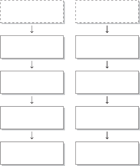
Figure 1 The research process not using R—stylized example
4. Ris reasonably fast in ordinary tasks. You will likely agree with this impression if you
have used other statistical software like SPSS or Stata and have gotten into the habit of
going on holiday when running more complex models—not to mention the pain that is
caused by the “one session, one data frame” logic. There are even extensions to speed
up R, for example, by making C code available from within R, like the Rcpp package.
5. Ris powerful in creating data visualizations. Although this not an obvious plus for data
collection, you would not want to miss R’s graphics facilities in your daily workow.
We will demonstrate how a visual inspection of collected data can and should be a
rst step in data validation, and how graphics provide an intuitive way of summarizing
large amounts of data.
6. Work in Ris mainly command line based. This might sound like a disadvantage to
Rrookies, but it is the only way to allow for the production of reproducible results
compared to point-and-click programs.
7. Ris not picky about operating systems. It can generally be run under Windows, Mac
OS, and Linux.
8. Finally, Ris the entire package from start to nish. If you read this book, you are
likely not a dedicated programmer, but hold a substantive interest in a topic or specic
PREFACE xix
Brain / R
R
R
R
L
ATE
X/ R
Research question,
theory, study
design
Data collection
Data manipulation
Data analysis
Publication
Steps Tools
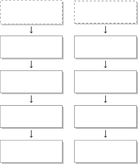
Figure 2 The research process using R—stylized example
data source that you want to work with. In that case, learning another language will
not pay off, but rather prevent you from working on your research. An example of a
common research process is displayed in Figure 1. It is characterized by a permanent
switching between programs. If you need to make corrections to the data collection
process, you have to climb back down the entire ladder. The research process using
R, as it is presented in this book, takes place within a single software environment
(Figure 2). In the context of web scraping and text processing, this means that you
do not have to learn another programming language for the task. What you will need
to learn are some basics in the markup languages HTML and XML and the logic of
regular expressions and XPath, but the operations are executed from within R.
Recommended reading to get started with R
There are many well-written books on the market that provide great introductions to R.
Among these, we nd the following especially helpful:
Crawley, Michael J. 2012. The R Book, 2nd edition. Hoboken, NJ: John Wiley & Sons.
xx PREFACE
Adler, Joseph. 2009. R in a Nutshell. A Desktop Quick Reference. Sebastopol, CA: O’Reilly.
Teetor, Paul. 2011. R Cookbook. Sebastopol, CA: O’Reilly.
Besides these commercial sources, there is also a lot of free information on the Web. A
truly amazing online tutorial for absolute beginners by the Code School is made available at
http://tryr.codeschool.com/. Additionally, Quick-R(http://www.statmethods.net/) is a good
reference site for many basic commands. Lastly, you can also nd a lot of free resources and
examples at http://www.ats.ucla.edu/stat/r/.
Ris an ever-growing software, and in order to keep track of the developments you might
periodically like to visit some of the following websites: Planet R(http://planetr.stderr.org/)
provides the history of existing packages and occasionally some interesting applications.
R-Bloggers (http://www.r-bloggers.com/) is a blog aggregator that collects entries from many
R-related blog sites in various elds. It offers a broad view on hundreds of Rapplications
from economics to biology to geography that is mostly accompanied by the necessary code to
replicate the posts. R-Bloggers even features some basic examples that deal with automated
data collection.
When running into problems, Rhelp les are sometimes not too helpful. It is often more
enlightening to look for help in online forums like Stack Overow (http://stackoverow.com)
or other sites from the Stack Exchange network. For complex problems, consider the
Rexperts on GitHub (http://github.com). Also note that there are many Special Interest
Group (SIG) mailing lists (http://www.r-project.org/mail.html) on a variety of topics and
even local R User Groups all around the world (http://blog.revolutionanalytics.com/local-
r-groups.html). Finally, a CRAN Task View has been set up, which gives a nice overview
over recent advances in web technologies and services in the Rframework: http://cran.r-
project.org/web/views/WebTechnologies.html
Typographic conventions
This is a practical book about coding, and we expect you to often have it sitting somewhere
next to the keyboard. We want to facilitate the orientation throughout the book with the
following conventions: There are three indices—one for general topics, one for Rpackages,
and one for Rfunctions. Within the text, variables and R(and other) code and functions
are set in typewriter typeface, as in summary(). Actual Rcode is also typewriter style and
indented. Note that code input is indicated with “R” and a prompt symbol (“R>”); Routput
is printed without the prompt sign, as in
R> hello <- "hello, world"
R> hello
[1] "hello, world"
The book’s website
The website that accompanies this book can be found at http://www.r-datacollection.com

PREFACE xxi
Among other things, the site provides code from examples and case studies. This means
that you do not have to manually copy the code from the book, but can directly access and
modify the corresponding Rles. You will also nd solutions to some of the exercises, as
well as a list of errata. If you nd any errors, please do not hesitate to let us know.
Disclaimer
This is not a book about spidering the Web. Spiders are programs that graze the Web for
information, rapidly jumping from one page to another, often grabbing the entire page content.
If you want to follow in Google’s Googlebot’s footsteps, you probably hold the wrong book
in your hand. The techniques we introduce in this book are meant to serve more specic and
more gentle purposes, that is, scraping specic information from specic websites. In the
end, you are responsible for what you do with what you learn. It is frequently not a big leap
from the code that is presented in this book to programs that might quickly annoy website
administrators. So here is some fundamental advice on how to behave as a practitioner of
web data collection:
1. Always keep in mind where your data comes from and, whenever possible, give credit
to those who originally collected and published it.1
2. Do not violate copyrights if you plan to republish data you found on the Web. If the
information was not collected by yourself, chances are that you need permission from
the owners to reproduce them.
3. Do not do anything illegal! To get an idea of what you can and cannot do in your data
collection, check out the Justia BlawgSearch (http://blawgsearch.justia.com/), which
is a search site for legal blogs. Looking for entries marked ‘web scraping’ might help
to keep up to date regarding legal developments and recent verdicts. The Electronic
Frontier Foundation (http://www.eff.org/) was founded as early as 1990 to defend the
digital rights of consumers and the public. We hope, however, that you will never have
to rely on their help.
We offer some more detailed recommendations on how to behave when scraping content
from the Web in Section 9.3.3.
Acknowledgments
Many people helped to make this project possible. We would like to take the opportunity to
express our gratitude to them. First of all, we would like to say thanks to Peter Selb to whom
we owe the idea of creating a course on alternative data collection. It is due to his impulse
that we started to assemble our somewhat haphazard experiences in a comprehensive volume.
We are also grateful to several people who have provided invaluable feedback on parts of the
book. Most importantly we thank Christian Breunig, Holger D¨
oring, Daniel Eckert, Johannes
1To lead by example, we owe some of the suggestions to Hemenway and Calishain (2003)’s Spidering Hacks
(Hack #6).
xxii PREFACE
Kleibl, Philip Leifeld, and Nils Weidmann, whose advice has greatly improved the material.
We also thank Kathryn Uhrig for proofreading the manuscript.
Early versions of the book were used in two courses on “Alternative data collection
methods” and “Data collection in the World Wide Web” that took place in the summer
terms of 2012 and 2013 at the University of Konstanz. We are grateful to students for their
comments—and their patience with the topic, with R, and outrageous regular expressions. We
would also like to thank the participants of the workshops on “Facilitating empirical research
on political reforms: Automating data collection in R” held in Mannheim in December 2012
and the workshop “Automating online data collection in R,” which took place in Zurich in
April 2013. We thank Bruno W¨
uest in particular for his assistance in making the Zurich
workshop possible, and Fabrizio Gilardi for his support.
It turns out that writing a volume on automating data collection is a surprisingly time-
consuming endeavor. We all embarked on this project during our doctoral studies and devoted
a lot of time to learning the intricacies of web scraping that could have been spent on the
tasks we signed up for. We would like to thank our supervisors Peter Selb, Daniel Bochsler,
Ulrich Sieberer, and Thomas Gschwend for their patience and support for our various detours.
Christian Rubba is grateful for generous funding by the Swiss National Science Foundation
(Grant Number 137805).
We would like to acknowledge that we are heavily indebted to the creators and maintainers
of the numerous packages that are applied throughout this volume. Their continuous efforts
have opened the door for new ways of scholarly research—and have provided access to
vast sources of data to individual researchers. While we cannot possibly hope to mention
all the package developers in these paragraphs, we would like to express our gratitude to
Duncan Temple Lang and Hadley Wickham for their exceptional work. We would also like
to acknowledge the work of Yihui Xie, whose package was crucial in typesetting this book.
We are grateful for the help that was extended from our publisher, particularly from
Heather Kay, Debbie Jupe, Jo Taylor, Richard Davies, Baljinder Kaur and others who were
responsible for proofreading and formatting and who provided support at various stages of
the writing process.
Finally, we happily acknowledge the great support we received from our friends and
families. We owe special and heartfelt thanks to: Karima Bousbah, Johanna Flock, Hans-
Holger Friedrich, Dirk Heinecke, Stefanie Klingler, Kristin Lindemann, Verena Mack, and
Alice Mohr.
Simon Munzert
Christian Rubba
Peter Meißner
Dominic Nyhuis

1
Introduction
Are you ready for your rst encounter with web scraping? Let us start with a small example
that you can recreate directly on your machine, provided you have Rinstalled. The case study
gives a rst impression of the book’s central themes.
1.1 Case study: World Heritage Sites in Danger
The United Nations Educational, Scientic and Cultural Organization (UNESCO) is an
organization of the United Nations which, among other things, ghts for the preservation
of the world’s natural and cultural heritage. As of today (November 2013), there are 981
heritage sites, most of which of are man-made like the Pyramids of Giza, but also natural
phenomena like the Great Barrier Reef are listed. Unfortunately, some of the awarded places
are threatened by human intervention. Which sites are threatened and where are they located?
Are there regions in the world where sites are more endangered than in others? What are the
reasons that put a site at risk? These are the questions that we want to examine in this rst
case study.
What do scientists always do rst when they want to get up to speed on a topic? They Wikipedia—
information
source of choice
look it up on Wikipedia! Checking out the page of the world heritage sites, we stumble across
a list of currently and previously endangered sites at http://en.wikipedia.org/wiki/List_of_
World_Heritage_in_Danger. You nd a table with the current sites listed when accessing the
link. It contains the name, location (city, country, and geographic coordinates), type of danger
that is facing the site, the year the site was added to the world heritage list, and the year it
was put on the list of endangered sites. Let us investigate how the sites are distributed around
the world.
While the table holds information on the places, it is not immediately clear where they
are located and whether they are regionally clustered. Rather than trying to eyeball the table,
it could be very useful to plot the locations of the places on a map. As humans deal well with
Automated Data Collection with R: A Practical Guide to Web Scraping and Text Mining, First Edition.
Simon Munzert, Christian Rubba, Peter Meißner and Dominic Nyhuis.
© 2015 John Wiley & Sons, Ltd. Published 2015 by John Wiley & Sons, Ltd.

2 AUTOMATED DATA COLLECTION WITH R
visual information, we will try to visualize results whenever possible throughout this book.
But how to get the information from the table to a map? This sounds like a difcult task, but
with the techniques that we are going to discuss extensively in the next pages, it is in fact
not. For now, we simply provide you with a rst impression of how to tackle such a task with
R. Detailed explanations of the commands in the code snippets are provided later and more
systematically throughout the book.
To start, we have to load a couple of packages. While Ronly comes with a set of
basic, mostly math- and statistics-related functions, it can easily be extended by user-written
packages. For this example, we load the following packages using the library() function:1
R> library(stringr)
R> library(XML)
R> library(maps)
In the next step, we load the data from the webpage into R. This can be done easily using
the readHTMLTable() function from the XML package:
R> heritage_parsed <- htmlParse("http://en.wikipedia.org/wiki/
List_of_World_Heritage_in_Danger",
encoding = "UTF-8")
R> tables <- readHTMLTable(heritage_parsed, stringsAsFactors = FALSE)
We are going to explain the mechanics of this step and all other major web scraping
techniques in more detail in Chapter 9. For now, all you need to know is that we are telling R
that the imported data come in the form of an HTML document. Ris capable of interpreting
HTML, that is, it knows how tables, headlines, or other objects are structured in this le format.
This works via a so-called parser, which is called with the function htmlParse(). In the next
step, we tell Rto extract all HTML tables it can nd in the parsed object heritage_parsed
and store them in a new object tables. If you are not already familiar with HTML, you will
learn that HTML tables are constructed from the same code components in Chapter 2. The
readHTMLTable() function helps in identifying and reading out these tables.
All the information we need is now contained in the tables object. This object is a list of
all the tables the function could nd in the HTML document. After eyeballing all the tables,
we identify and select the table we are interested in (the second one) and write it into a new
one, named danger_table. Some of the variables in our table are of no further interest,
so we select only those that contain information about the site’s name, location, criterion of
heritage (cultural or natural), year of inscription, and year of endangerment. The variables in
our table have been assigned unhandy names, so we relabel them. Finally, we have a look at
the names of the rst few sites:
R> danger_table <- danger_table <- tables[[2]]
R> names(danger_table)
[1] "NULL.Name" "NULL.Image" "NULL.Location"
[4] "NULL.Criteria" "NULL.Area.ha..acre." "NULL.Year..WHS."
1This assumes that the packages are already installed. If they are not, type the following into your console:
install.packages(c("stringr", "XML", "maps"))

INTRODUCTION 3
[7] "NULL.Endangered" "NULL.Reason" "NULL.Refs"
R> danger_table <- danger_table[, c(1, 3, 4, 6, 7)]
R> colnames(danger_table) <- c("name", "locn", "crit", "yins", "yend")
R> danger_table$name[1:3]
[1] "Abu Mena" "Air and T´
en´
er´
e Natural Reserves"
[3] "Ancient City of Aleppo"
This seems to have worked. Additionally, we perform some simple data cleaning, a step
often necessary when importing web-based content into R. The variable crit, which contains
the information whether the site is of cultural or natural character, is recoded, and the two
variables y_ins and y_end are turned into numeric ones.2Some of the entries in the y_end
variable are ambiguous as they contain several years. We select the last given year in the
cell. To do so, we specify a so-called regular expression, which goes [[:digit:]]4$—we
explain what this means in the next paragraph:
R> danger_table$crit <- ifelse(str_detect(danger_table$crit, "Natural") ==
TRUE, "nat", "cult")
R> danger_table$crit[1:3]
[1] "cult" "nat" "cult"
R> danger_table$yins <- as.numeric(danger_table$yins)
R> danger_table$yins[1:3]
[1] 1979 1991 1986
R> yend_clean <- unlist(str_extract_all(danger_table$yend, "[[:digit:]]4$"))
R> danger_table$yend <- as.numeric(yend_clean)
R> danger_table$yend[1:3]
2001 1992 2013
The locn variable is a bit of a mess, exemplied by three cases drawn from the data-set:
R> danger_table$locn[c(1, 3, 5)]
[1] "EgyAbusir, Egypt30◦50'30<U+2033>N 29◦39'50<U+2033>E<U+FEFF> /
<U+FEFF>30.84167◦N 29.66389◦E<U+FEFF> / 30.84167; 29.66389<U+FEFF>
(Abu Mena)"
[2] "Syria !Aleppo Governorate, Syria36◦14'0<U+2033>N 37◦10'0<U+2033
>E<U+FEFF> / <U+FEFF>36.23333◦N 37.16667◦E<U+FEFF> / 36.23333; 37.16667
<U+FEFF> (Ancient City of Aleppo)"
[3] "Syria !Damascus Governorate, Syria33◦30'41<U+2033>N 36◦18'23
<U+2033>E<U+FEFF> / <U+FEFF>33.51139◦N 36.30639◦E<U+FEFF> / 33.51139;
36.30639<U+FEFF> (Ancient City of Damascus)"
The variable contains the name of the site’s location, the country, and the geographic The rst
regular
expression
coordinates in several varieties. What we need for the map are the coordinates, given by the
latitude (e.g., 30.84167N) and longitude (e.g., 29.66389E) values. To extract this information,
we have to use some more advanced text manipulation tools called “regular expressions”,
2We assume that you are familiar with the basic object classes in R. If not, check out the recommended readings
in the Preface.
4 AUTOMATED DATA COLLECTION WITH R
which are discussed extensively in Chapter 8. In short, we have to give Ran exact description
of what the information we are interested in looks like, and then let Rsearch for and extract
it. To do so, we use functions from the stringr package, which we will also discuss in detail
in Chapter 8. In order to get the latitude and longitude values, we write the following:
R> reg_y <- "[/][ -]*[[:digit:]]*[.]*[[:digit:]]*[;]"
R> reg_x <- "[;][ -]*[[:digit:]]*[.]*[[:digit:]]*"
R> y_coords <- str_extract(danger_table$locn, reg_y)
R> y_coords <- as.numeric(str_sub(y_coords, 3, -2))
R> danger_table$y_coords <- y_coords
R> x_coords <- str_extract(danger_table$locn, reg_x)
R> x_coords <- as.numeric(str_sub(x_coords, 3, -1))
R> danger_table$x_coords <- x_coords
R> danger_table$locn <- NULL
Do not be confused by the rst two lines of code. What looks like the result of a monkey
typing on a keyboard is in fact a precise description of the coordinates in the locn variable.
The information is contained in the locn variable as decimal degrees as well as in degrees,
minutes, and seconds. As the decimal degrees are easier to describe with a regular expression,
we try to extract those. Writing regular expressions means nding a general pattern for
strings that we want to extract. We observe that latitudes and longitudes always appear
after a slash and are a sequence of several digits, separated by a dot. Some values start
with a minus sign. Both values are separated by a semicolon, which is cut off along with
the empty spaces and the slash. When we apply this pattern to the locn variable with the
str_extract() command and extract the numeric information with str_sub(), we get the
following:
R> round(danger_table$y_coords, 2)[1:3]
[1] 30.84 18.28 36.23
R> round(danger_table$x_coords, 2)[1:3]
[1] 29.66 8.00 37.17
This seems to have worked nicely. We have retrieved a set of 44 coordinates, corresponding
to 44 World Heritage Sites in Danger. Let us have a rst look at the data. dim() returns the
number of rows and columns of the data frame; head() returns the rst few observations:
R> dim(danger_table)
[1] 44 6
R> head(danger_table)
name crit yins yend y_coords x_coords
1 Abu Mena cult 1979 2001 30.84 29.66
2 Air and T´
en´
er´
e Natural Reserves nat 1991 1992 18.28 8.00
3 Ancient City of Aleppo cult 1986 2013 36.23 37.17
4 Ancient City of Bosra cult 1980 2013 32.52 36.48
5 Ancient City of Damascus cult 1979 2013 33.51 36.31
6 Ancient Villages of Northern Syria cult 2011 2013 36.33 36.84
INTRODUCTION 5
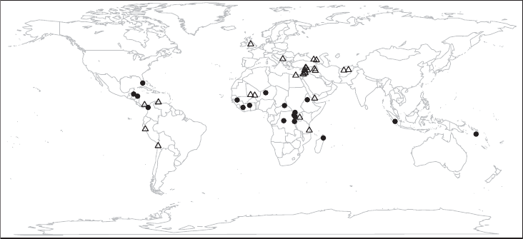
Figure 1.1 Location of UNESCO World Heritage Sites in danger (as of March 2014).
Cultural sites are marked with triangles, natural sites with dots
The data frame consists of 44 observations and 6 variables. The data are now set up in a A rst look at
the data
way that we can proceed with mapping the sites. To do so, we use another package named
“maps.” In it we nd a map of the world that we use to pinpoint the sites’ locations with
the extracted yand xcoordinates. The result is displayed in Figure 1.1. It was generated as
follows:
R> pch <- ifelse(danger_table$crit == "nat", 19, 2)
R> map("world", col = "darkgrey", lwd = 0.5, mar = c(0.1, 0.1, 0.1, 0.1))
R> points(danger_table$x_coords, danger_table$y_coords, pch = pch)
R> box()
We nd that many of the endangered sites are located in Africa, the Middle East, and
Southwest Asia, and a few others in South and Central America. The endangered cultural
heritage sites are visualized as the triangle. They tend to be clustered in the Middle East and
Southwest Asia. Conversely, the natural heritage sites in danger, here visualized as the dots,
are more prominent in Africa. We nd that there are more cultural than natural sites in danger.
R> table(danger_table$crit)
cult nat
26 18
We can speculate about the political, economic, or environmental conditions in the affected The UNESCO
behaves
politically
countries that may have led to the endangerment of the sites. While the information in the
table might be too sparse for rm inferences, we can at least consider some time trends
and potential motives of the UNESCO itself. For that purpose, we can make use of the two
variables y_ins and y_end, which contain the year a site was designated a world heritage
and the year it was put on the list of endangered World Heritage Sites. Consider Figure 1.2,
which displays the distribution of the second variable that we generated using the hist()
6 AUTOMATED DATA COLLECTION WITH R
Year when site was put on the list of endangered sites
Frequency
1980 1985 1990 1995 2000 2005 2010 2015
0246810 12 14
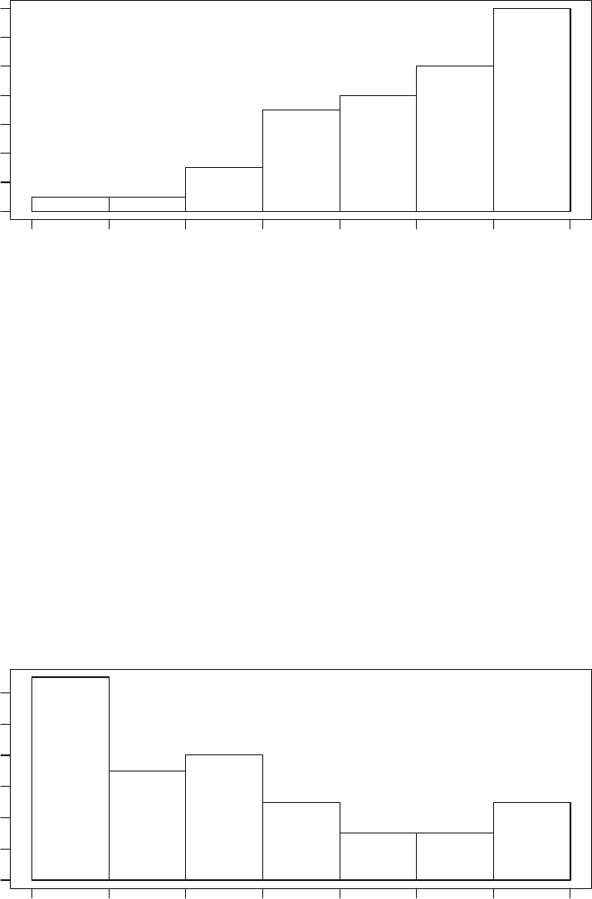
Figure 1.2 Distribution of years when World Heritage Sites were put on the list of endan-
gered sites
command. We nd that the frequency with which sites were put on the “red list” has risen in
recent decades—but so has the number of World Heritage Sites:
R> hist(danger_table$yend,
R> freq = TRUE,
R> xlab = "Year when site was put on the list of endangered sites",
R> main = "")
Even more interesting is the distribution of time spans between the year of inscription
and the year of endangerment, that is, the time it took until a site was put on the “red list”
after it had achieved World Heritage Site status. We calculate this value by subtracting the
endangerment year from the inscription year. The result is plotted in Figure 1.3.
Years it took to become an endangered site
Frequency
0 5 10 15 20 25 30 35
024681012
Figure 1.3 Distribution of time spans between year of inscription and year of endangerment
of World Heritage Sites in danger

INTRODUCTION 7
R> duration <- danger_table$yend - danger_table$yins
R> hist(duration,
R> freq = TRUE,
R> xlab = "Years it took to become an endangered site",
R> main = "")
Many of the sites were put on the red list only shortly after their designation as world
heritage. According to the ofcial selection criteria for becoming a cultural or natural heritage,
it is not a necessary condition to be endangered. In contrast, endangered sites run the risk
of losing their status as world heritage. So why do they become part of the List of World
Heritage Sites when it is likely that the site may soon run the risk of losing it again? One
could speculate that the committee may be well aware of these facts and might use the list as
a political means to enforce protection of the sites.
Now take a few minutes and experiment with the gathered data for yourself! Which is the
country with the most endangered sites? How effective is the List of World Heritage Sites in
Danger? There is another table on the Wikipedia page that has information about previously
listed sites. You might want to scrape these data as well and incorporate them into the map.
Using only few lines of code, we have enriched the data and gathered new insights, which
might not have been obvious from examining the table alone.3This is a variant of the more
general mantra, which will occur throughout the book: Data are abundant—retrieve them,
prepare them, use them.
1.2 Some remarks on web data quality
The introductory example has elegantly sidestepped some of the more serious questions that
are likely to arise when approaching a research problem. What type of data is most suited to
answer your question? Is the quality of the data sufciently high to answer your question?
Is the information systematically awed? Although this is not a book on research design or
advanced statistical methods to tackle noise in data, we want to emphasize these questions
before we start harvesting gigabytes of information.
When you look at online data, you have to keep its origins in mind. Information can be What is the
primary source
of secondary
data?
rsthand, like posts on Twitter or secondhand data that have been copied from an ofine
source, or even scraped from elsewhere. There may be situations where you are unable to
retrace the source of your data. If so, does it make sense to use data from the Web? We think
the answer is yes.
Regarding the transparency of the data generation, web data do not differ much from
other secondary sources. Consider Wikipedia as a popular example. It has often been debated
whether it is legitimate to quote the online encyclopedia for scientic and journalistic pur-
poses. The same concerns are equally valid if one cares to use data from Wikipedia tables or
texts for analysis. It has been shown that Wikipedia’s accuracy varies. While some studies
nd that Wikipedia is comparable to established encyclopedias (Chesney 2006; Giles 2005;
Reavley et al. 2012), others suggest that the quality might, at times, be inferior (Clauson
et al. 2008; Leithner et al. 2010; Rector 2008). But how do you know when relying on one
specic article? It is always recommended to nd a second source and to compare the content.
3The watchful eye has already noticed a link on the site that leads to a map visualizing the locations as we did
in Figure 1.1. We acknowledge the work, but want to be able to generate such output ourselves.
8 AUTOMATED DATA COLLECTION WITH R
If you are unsure whether the two sources share a common source, you should repeat the
process. Such cross-validations should be standard for the use of any secondary data source,
as reputation does not prevent random or systematic errors.
Besides, data quality is nothing that is stuck to the data like a badge, but rather depends
Data quality
depends on the
user’s purposes
on the application. A sample of tweets on a random day might be sufcient to analyze the
use of hash tags or gender-specic use of words, but is less useful for predicting electoral
outcomes when the sample happens to have been collected on the day of the Republican
National Convention. In the latter case, the data are likely to suffer from a bias due to the
collection day, that is, they lack quality in terms of “representativeness.” Therefore, the only
standard is the one you establish yourself. As a matter of fact, quality standards are more alike
when dealing with factual data—the African elephant population most likely has not tripled
in the past 6 months and Washington D.C., not New York, is the capital of the United States.
To be sure, while it is not the case that demands on data quality should be lower when
Why web data
can be of
higher quality
for the user
working with online data, the concerns might be different. Imagine you want to know what
people think about a new phone. There are several standard approaches to deal with this
problem in market research. For example, you could conduct a telephone survey and ask
hundreds of people if they could imagine buying a particular phone and the features in
which they are most interested. There are plenty of books that have been written about the
pitfalls of data quality that are likely to arise in such scenarios. For example, are the people
“representative” of the people I want to know something about? Are the questions that I pose
suited to solicit the answers to my problem?
Another way to answer this question with data could be to look for “proxies,” that is,
indicators that do not directly measure the product’s popularity itself, but which are strongly
related. If the meaning of popularity entails that people prefer one product over a competing
one, an indirect measurement of popularity could be the sales statistics on commercial
websites. These statistics usually contain rankings of all phones currently on sale. Again,
questions of representativeness arise—both with regard to the listed phones (are some phones
not on the list because the commercial website does not sell them?) and the customers (who
buy phones from the Web and from a particular site?). Nevertheless, the ranking does provide
a more comprehensive image of the phone market—possibly more comprehensive than any
reasonably priced customer survey could ever hope to be. The availability of entirely new
information is probably the most important argument for the use of online data, as it allows
us to answer new questions or to get a deeper understanding of existing questions. Certainly,
hand in hand with this added value arise new questions of data quality—can phones of
different generations be compared at all, and can we say anything about the stability of such
a ranking? In many situations, choosing a data source is a trade-off between advantages and
disadvantages, accuracy versus completeness, coverage versus validity, and so forth.
To sum up, deciding which data to collect for your application can be difcult. We propose
ve steps that might help to guide your data collection process:
1. Make sure you know exactly what kind of information you need. This can be
specic (“the gross domestic product of all OECD countries for the last 10 years”) or
vague (“peoples’ opinion on company X’s new phone,” “collaboration among members
of the US senate”).
2. Find out whether there are any data sources on the Web that might provide direct
or indirect information on your problem. If you are looking for hard facts, this is
probably easy. If you are interested in rather vague concepts, this is more difcult.
INTRODUCTION 9
A country’s embassy homepage might be a valuable source for foreign policy action
that is often hidden behind the curtain of diplomacy. Tweets might contain opinion
trends on pretty much everything, commercial platforms can inform about customers’
satisfaction with products, rental rates on property websites might hold information
on current attractiveness of city quarters....
3. Develop a theory of the data generation process when looking into potential
sources. When were the data generated, when were they uploaded to the Web, and by
whom? Are there any potential areas that are not covered, consistent or accurate, and
are you able to identify and correct them?
4. Balance advantages and disadvantages of potential data sources. Relevant aspects
might be availability (and legality!), costs of collection, compatibility of new sources
with existing research, but also very subjective factors like acceptance of the data
source by others. Also think about possible ways to validate the quality of your data.
Are there other, independent sources that provide similar information so that random
cross-checks are possible? In case of secondary data, can you identify the original
source and check for transfer errors?
5. Make a decision! Choose the data source that seems most suitable, document your
reasons for the decision, and start with the preparations for the collection. If it is
feasible, collect data from several sources to validate data sources. Many problems
and benets of various data collection strategies come to light only after the actual
collection.
1.3 Technologies for disseminating, extracting, and storing
web data
Collecting data from the Web is not always as easy as depicted in the introductory example.
Difculties arise when data are stored in more complex structures than HTML tables, when
web pages are dynamic or when information has to be retrieved from plain text. There are
some costs involved in automated data collection with R, which essentially means that you
have to gain basic knowledge of a set of web and web-related technologies. However, in
our introduction to these fundamental tools we stick to the necessary basics to perform web
scraping and text mining and leave out the less relevant details where possible. It is denitely
not necessary to become an expert in all web technologies in order to be able to write good
web scrapers.
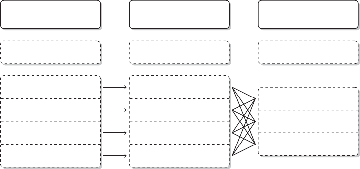
There are three areas that are important for data collection on the Web with R. Figure 1.4
provides an overview of the three areas. In the remainder of this section, we will motivate
each of the subelds and illustrate their various linkages. This might help you to stay on top
of things when you study the fundamentals in the rst part of the book before moving on to
the actual web scraping tasks in the book’s second part.
1.3.1 Technologies for disseminating content on the Web
In the rst pillar we encounter technologies that allow the distribution of content on the Web.
There are multiple ways of how data are disseminated, but the most relevant technologies in
this pillar are XML/HTML, AJAX, and JSON (left column of Figure 1.4).
10 AUTOMATED DATA COLLECTION WITH R
Technologies for
disseminating content
on the Web
HTTP
XML/HTML
JSON
AJAX
Plain text
Technologies for
information extraction
R
XPath
JSON parsers
Selenium
Regular expressions
Technologies for data
storage
R
SQL
Binary formats
Plain-text formats
Figure 1.4 Technologies for disseminating, extracting, and storing web data
For browsing the Web, there is a hidden standard behind the scenes that structures how
HTML
information is displayed—the Hypertext Markup Language or HTML. Whether we look for
information on Wikipedia, search for sites on Google, check our bank account, or become
social on Twitter, Facebook, or YouTube—using a browser means using HTML. Although
HTML is not a dedicated data storage format, it frequently contains the information that we
are interested in. We nd data in texts, tables, lists, links, or other structures. Unfortunately,
there is a difference between the way data are presented in a browser on the one side and how
they are stored within the HTML code on the other. In order to automatically collect data
from the Web and process them with R, a basic understanding of HTML and the way it stores
information is indispensable. We provide an introduction to HTML from a web scraper’s
perspective in Chapter 2.
The Extensible Markup Language or XML is one of the most popular formats for exchang-
XML
ing data over the Web. It is related to HTML in that both are markup languages. However,
while HTML is used to shape the display of information, the main purpose of XML is to store
data. Thus, HTML documents are interpreted and transformed into pretty-looking output by
browsers, whereas XML is “just” data wrapped in user-dened tags. The user-dened tags
make XML much more exible for storing data than HTML. In recent years, XML and its
derivatives—so-called schemes—have proliferated in various data exchanges between web
applications. It is therefore important to be familiar with the basics of XML when gathering
data from the Web (Chapter 3). Both HTML and XML-style documents offer natural, often
hierarchical, structures for data storage. In order to recognize and interpret such structures,
we need software that is able to “understand” these languages and handle them adequately.
The necessary tools—parsers—are introduced in Chapters 2 and 3.
Another standard data storage and exchange format that is frequently encountered on the
JSON
Web is the JavaScript Object Notation or JSON. Like XML, JSON is used by many web
applications to provide data for web developers. Imagine both XML and JSON as standards
that dene containers for plain text data. For example, if developers want to analyze trends
on Twitter, they can collect the necessary data from an interface that was set up by Twitter
INTRODUCTION 11
to distribute the information in the JSON format. The main reason why data are preferably
distributed in the XML or JSON formats is that both are compatible with many programming
languages and software, including R. As data providers cannot know the software that is
being used to postprocess the information, it is preferable for all parties involved to distribute
the data in formats with universally accepted standards. The logic of JSON is introduced in
the second part of Chapter 3.
AJAX is a group of technologies that is now rmly integrated into the toolkit of modern AJAX
web developing. AJAX plays a tremendously important role in enabling websites to request
data asynchronously in the background of the browser session and update its visual appearance
in a dynamic fashion. Although we owe much of the sophistication in modern web apps to
AJAX, these technologies constitute a nuisance for web scrapers and we quickly run into a
dead end with standard R tools. In Chapter 6 we focus on JavaScript and the XMLHttpRequest,
two key technologies, and illustrate how an AJAX-enriched website departs from the classical
HTML/HTTP logic. We also discuss a solution to this problem using browser-integrated Web
Developer Tools that provide deep access to the browser internals.
We frequently deal with plain text data when scraping information from the Web. In a Plain text
way, plain text is part of every HTML, XML, and JSON document. The crucial property we
want to stress is that plain text is unstructured data, at least for computer programs that simply
read a text le line by line. There is no introductory chapter to plain text data, but we offer a
guide on how to extract information from such data in Chapter 8.
To retrieve data from the Web, we have to enable our machine to communicate with HTTP
servers and web services. The lingua franca of communication on the Web is the Hypertext
Transfer Protocol (HTTP). It is the most common standard for communication between web
clients and servers. Virtually every HTML page we open, every image we view in the browser,
every video we watch is delivered by HTTP. Despite our continuous usage of the protocol
we are mostly unaware of it as HTTP exchanges are typically performed by our machines.
We will learn that for many of the basic web scraping applications we do not have to care
much about the particulars of HTTP, as Rcan take over most of the necessary tasks just ne.
In some instances, however, we have to dig deeper into the protocol and formulate advanced
requests in order to obtain the information we are looking for. Therefore, the basics of HTTP
are the subject of Chapter 5.
1.3.2 Technologies for information extraction from web documents
The second pillar of technologies for web data collection is needed to retrieve the information
from the les we gather. Depending on the technique that has been used to collect les,
there are specic tools that are suited to extract data from these sources (middle column of
Figure 1.4). This section provides a rst glance at the available tools. An advantage of using
Rfor information extraction is that we can use all of the technologies from within R,even
though some of them are not R-specic, but rather implementations via a set of packages.
The rst tool at our disposal is the XPath query language. It is used to select specic XPath
pieces of information from marked up documents such as HTML, XML or any variant of
it, for example SVG or RSS. In a typical data web scraping task, calling the webpages is an
important, but usually only intermediate step on the way toward well-structured and cleaned
datasets. In order to take full advantage of the Web as a nearly endless data source, we have
to perform a series of ltering and extraction steps once the relevant web documents have
been identied and downloaded. The main purpose of these steps is to recast information that
12 AUTOMATED DATA COLLECTION WITH R
is stored in marked up documents into formats that are suitable for further processing and
analysis with statistical software. This task consists of specifying the data we are interested
in and locating it in a specic document and then tailoring a query to the document that
extracts the desired information. XPath is introduced in Chatper 4 as one option to perform
these tasks.
In contrast to HTML or XML documents, JSON documents are more lightweight and
JSON parsers
easier to parse. To extract data from JSON, we do not draw upon a specic query language,
but rely on high-level Rfunctionality, which does a good job in decoding JSON data. We
explain how it is done in Chapter 3.
Extracting information from AJAX-enriched webpages is a more advanced and complex
Selenium
scenario. As a powerful alternative to initiating web requests from the Rconsole, we present
the Selenium framework as a hands-on approach to getting a grip on web data. Selenium
allows us to direct commands to a browser window, such as mouse clicks or keyboard inputs,
via R. By working directly in the browser, Selenium is capable of circumventing some of
the problems discussed with AJAX-enriched webpages. We introduce Selenium in one of
our scraping scenarios of Chapter 9 in Section 9.1.9. This section discusses the Selenium
framework as well as the RWebdriver package for Rby means of a practical application.
A central task in web scraping is to collect the relevant information for our research
Regular
expressions problem from heaps of textual data. We usually care for the systematic elements in textual
data—especially if we want to apply quantitative methods to the resulting data. Systematic
structures can be numbers or names like countries or addresses. One technique that we
can apply to extract the systematic components of the information are regular expressions.
Essentially, regular expressions are abstract sequences of strings that match concrete, recurring
patterns in text. Besides using them to extract content from plain text documents we can also
apply them to HTML and XML documents to identify and extract parts of the documents that
we are interested in. While it is often preferable to use XPath queries on markup documents,
regular expressions can be useful if the information is hidden within atomic values. Moreover,
if the relevant information is scattered across an HTML document, some of the approaches
that exploit the document’s structure and markup might be rendered useless. How regular
expressions work in Ris explained in detail in Chapter 8.
Besides extracting meaningful information from textual data in the form of numbers or
Text mining
names we have a second technique at our disposal—text mining. Applying procedures in this
class of techniques allows researchers to classify unstructured texts based on the similarity
of their word usages. To understand the concept of text mining it is useful to think about the
difference between manifest and latent information. While the former describes information
that is specically linked to individual terms, like an address or a temperature measurement,
the latter refers to text labels that are not explicitly contained in the text. For example, when
analyzing a selection of news reports, human readers are able to classify them as belonging
to particular topical categories, say politics, media, or sport. Text mining procedures provide
solutions for the automatic categorization of text. This is particularly useful when analyzing
web data, which frequently comes in the form of unlabeled and unstructured text. We elaborate
several of the available techniques in Chapter 10.
1.3.3 Technologies for data storage
Finally, the third pillar of technologies for the collection of web data deals with facilities for
data storage (right column of Figure 1.4). Ris mostly well suited for managing data storage
INTRODUCTION 13
technologies like databases. Generally speaking, the connection between technologies for
information extraction and those for data storage is less obvious. The best way to store data
does not necessarily depend on its origin.
Simple and everyday processes like online shopping, browsing through library catalogues, SQL
wiring money, or even buying a couple of sweets at the supermarket all involve databases. We
hardly ever realize that databases play such an important role because we do not interact with
them directly—databases like to work behind the scenes. Whenever data are key to a project,
web administrators will rely on databases because of their reliability, efciency, multiuser
access, virtually unlimited data size, and remote access capabilities. Regarding automated
data collection, databases are of interest for two reasons: One, we might occasionally be
granted access to a database directly and should be able to cope with it. Two, although, Rhas
a lot of data management facilities, it might be preferable to store data in a database rather
than in one of the native formats. For example, if you work on a project where data need to
be made available online or if you have various parties gathering specic parts of your data,
a database can provide the necessary infrastructure. Moreover, if the data you need to collect
are extensive and you have to frequently subset and manipulate the data, it also makes sense
to set up a database for the speed with which they can be queried. For the many advantages
of databases, we introduce databases in Chapter 7 and discuss SQL as the main language for
database access and communication.
Nevertheless, in many instances the ordinary data storage facilities of Rsufce, for
example, by importing and exporting data in binary or plain text formats. In Chapter 11, we
provide some details on the general workow of web scraping, including data management
tasks.
1.4 Structure of the book
We wrote this book with the needs of a diverse readership in mind. Depending on your
ambition and previous exposure to R, you may read this book from cover to cover or choose
a section that helps you accomplish your task.
rIf you have some basic knowledge of Rbut are not familiar with any of the scripting
languages frequently used on the Web, you may just follow the structure as is.
rIf you already have some text data and need to extract information from it, you might
start with Chapter 8 (Regular expressions and string functions) and continue with
Chapter 10 (Statistical text processing).
rIf you are primarily interested in web scraping techniques, but not necessarily in
scraping textual data, you might want to skip Chapter 10 altogether. We recommend
reading Chapter 8 in either case, as text manipulation basics are also a fundamental
technique for web scraping purposes.
rIf you are a teacher, you might want to use the book as basic or supplementary
literature. We provide a set of exercises after most of the chapters in Parts I and II for
this purpose. Solutions are available on the book’s website www.r-datacollection.com
for about half the exercises, so you can assign them as homework or use them for test
questions.
14 AUTOMATED DATA COLLECTION WITH R
For all others, we hope you will nd the structure useful as well. The following is a short
outline of the book’s three parts.
Part I: A primer on web and data technologies In the rst part, we introduce the fun-
damental technologies that underlie the communication, exchange, storage, and display of
information on the World Wide Web (HTTP, HTML, XML, JSON, AJAX, SQL), and provide
basic techniques to query web documents and datasets (XPath and regular expressions). These
fundamentals are especially useful for readers who are unfamiliar with the architecture of
the Web, but can also serve as a refresher if you have some prior knowledge. The rst part
of the book is explicitly focused on introducing the basic concepts for extracting the data
as performed in the rest of the book, and on providing an extensive set of exercises to get
accustomed quickly with the techniques.
Part II: A practical toolbox for web scraping and text mining The book’s second part
consists of three core chapters: The rst covers several scraping techniques, namely the use
of regular expressions, XPath, various forms of APIs, other data types and source-specic
techniques. We present a set of frequently occurring scenarios and apply popular Rpackages
for these tasks. We also address legal aspects of web scraping and give advice on how to
behave nicely on the Web. The second core chapter deals with techniques for statistical text
processing. Data are frequently available in the form of text that has to be further analyzed to
make it t for subsequent analyses. We present several techniques of the two major methods for
statistically processing text—supervised and unsupervised text classication—and show how
latent information can be extracted. In the third chapter, we provide insights into frequently
occurring topics in the management of data projects with R. We discuss how to work with the
le system, how to use loops for more efcient coding, how to organize scraping procedures,
and how to schedule scraping tasks that have to be executed on a regular basis.
Part III: A bag of case studies In the third part of the book, we provide a set of applications
that make use of the techniques introduced in the previous parts. Each of the case studies
starts out with a short motivation and the goal of the analysis. The case studies go into more
detail than the short examples in the technical chapters and address a wide range of problems.
Moreover, they provide a practical insight into the daily workow of data scraping and text
processing, the pitfalls of real-life data, and how to avoid them. Additionally, this part comes
with a tabular overview of the case studies’ contents’ with a view of the main techniques to
retrieve the data from the Web or from texts and the main packages and functions used for
these tasks.
Part One
A PRIMER ON WEB AND
DATA TECHNOLOGIES

2
HTML
There is a hidden standard behind almost everything that we see and do when surng the
web, the HyperText Markup Language, short: HTML. Whether we look for information on
Wikipedia, search for sites on Google, check our bank account, or become social on Twitter,
Facebook, and YouTube—when we use a browser—we use HTML.
HTML is a language for presenting content on the Web that was rst proposed by Tim
Berners-Lee (1989). The standard has continuously evolved since the initial introduction, the
most recent incarnation is HTML5 that is being developed by the World Wide Web Consor-
tium (W3C) and the Web Hypertext Application Technology Working Group (WHATWG).1
Although each revision of HTML has established new features and restructured old ones, the
basic grammar of HTML documents has not changed much over the years and is likely to
remain fairly stable in the foreseeable future, making it one of the most important standards
for working with and on the Web.
This chapter introduces the fundamentals of HTML from the perspective of a web data
collector. We will learn how to use browsers to display the source code of webpages and inspect
specic HTML elements (Section 2.1). Section 2.2 develops the logic of markup languages
in general and the syntax of HTML as a specic instance of a markup language. We go on to
present the most important vocabulary in HTML (Section 2.3). Finally, we consider parsing—
the process of reconstructing the structure and semantics of HTML documents—and how it
helps to retrieve information from web documents in Section 2.4.
1The W3C develops standards for web technologies. It was founded by Tim Berners-Lee and currently comprises
a staff of a couple dozen employees as well as hundreds of member organizations (see www.w3.org). In the course
of this book we will mainly get in touch with W3C because of their recommended techniques. For example, HTML,
XML, HTTP, and other technologies we are discussing in this volume are W3C recommendations. Endorsements
by the W3C are a strong signal to web developers that they can and should rely on these techniques.
Automated Data Collection with R: A Practical Guide to Web Scraping and Text Mining, First Edition.
Simon Munzert, Christian Rubba, Peter Meißner and Dominic Nyhuis.
© 2015 John Wiley & Sons, Ltd. Published 2015 by John Wiley & Sons, Ltd.
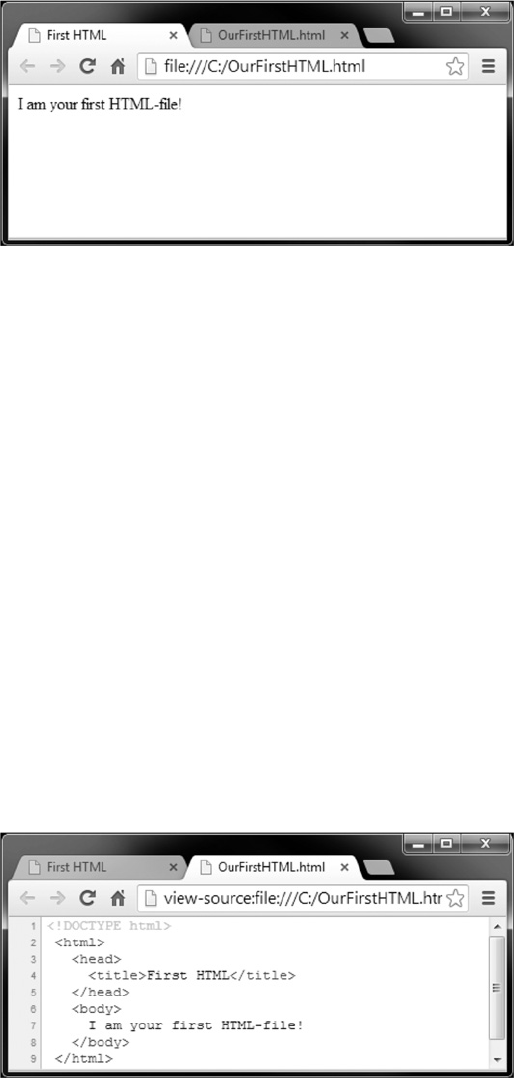
18 AUTOMATED DATA COLLECTION WITH R
Figure 2.1 Browser view of a simple HTML document
2.1 Browser presentation and source code
An HTML le is basically nothing but plain text—it can be opened and edited with any text
editor. What makes HTML so powerful is its marked up structure. HTML markup allows
dening the parts of a document that need to be displayed as headlines, the parts that contain
links, the parts that should be organized as tables, and numerous other forms. The markup
denitions rely on predened character sequences—the tags—that enclose parts of the text.
Markup tells browsers (more specically, parsers; see Section 2.4) how the document is
structured and the function of its various parts.
What you see in your browser is therefore not the HTML document itself but an interpre-
tation of it. Let us elaborate this idea with a small example. Figures 2.1 and 2.2 show the same
HTML document—OurFirstHTML.html. Figure 2.1 displays an interpreted version of the le
like we are used to; Figure 2.2 shows the source code of the document. Try it yourself. Use your
browser and go to http://www.r-datacollection.com/materials/html/OurFirstHTML.html.
Right-click on the window and select view source code from the context menu. Now check
out other websites and inspect their source code. Under ordinary circumstances there is little
reason to inspect the source code, but in online data collection it is often crucial. Inciden-
tally, as we introduce the specics of the HTML format over the course of this chapter
Figure 2.2 Source view of a simple HTML document
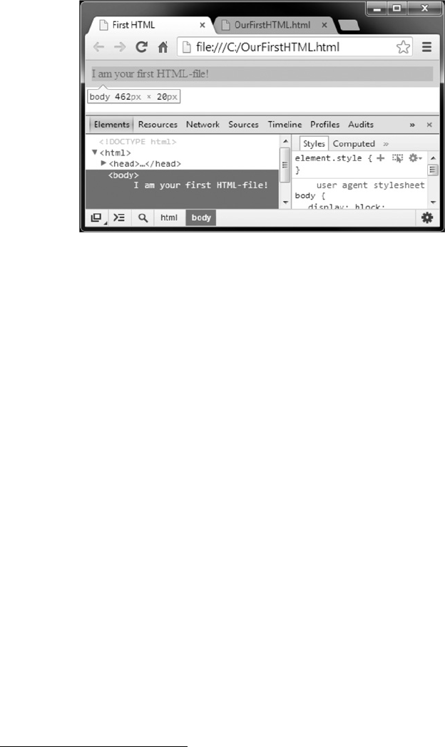
HTML 19
Figure 2.3 Inspect elements view of a simple HTML document
we will make reference to several supplementary les that are available at http://www.r-
datacollection.com/materials/html/.
It might seem that a lot of information from the source code gets lost in the interpretation Markup in
action
of the document. After all, there is considerably more text in the source code than just the
single sentence we see in Figure 2.1. In fact, the scale of structuring information and actual
content is clearly tipped in favor of the former. There is a fair amount of text in the source code
that contains instructions for the browser that is not printed to the screen. Nevertheless, part
of the information is in fact displayed, but in more subtle ways. Have a look at the browser
tab headings in Figure 2.1. The page title is First HTML, which was dened in the source
code: <title>First HTML</title>. This is HTML markup in action: First HTML was
marked up by <title> and </title> to dene it as the title of the document.
To identify which parts of the source code correspond to which elements in the browser
window and vice versa, we can use an element inspector, which is implemented in most
browsers. Again, try it yourself. Highlight the sentence in the browser window that we
opened above, right-click on the window, and select inspect element from the context menu.
The browser will display the part of the HTML document that is responsible for the selected
element (Figure 2.3). We can also reverse the process by clicking on parts of the source code
to highlight the corresponding parts in the interpreted version of the document. Try to do the
same with other websites and start inspecting elements.
2.2 Syntax rules
Now that we have checked out our rst HTML document and learned about the difference
between the interpreted version of a document and its source code, let us dive deeper into the
rules and concepts that underlie HTML.2
2Note that although there are several versions of HTML and you might encounter websites that adhere to older
standards, we present documents that follow HTML5 rules. Either way, for the purposes of data collection the
differences are negligible.
20 AUTOMATED DATA COLLECTION WITH R
2.2.1 Tags, elements, and attributes
Plain text is turned into an HTML document by tags that can be interpreted by a browser.Elements
They can be thought of as named braces that enclose content and dene its structural function.
For instance, the <title> tags in our introductory example designated the enclosed text as
title to be displayed in the head of the browser tab. The combination of start tag, content, and
end tag is called element,asin:
1<title>First HTML</title>
Start tags and end tags are also known as opening and closing tags. Tags are always
enclosed by <and >to distinguish them from the content. Start and end tags carry the same
name, but the end tag is preceded by a slash /. When referring to an element, it is common
to leave out the angle brackets and just use the name within the tags, as in body tag, title
tag and so on. We sometimes nd that elements and tags are actually used synonymously.
Throughout the book, we will refer to the start tag—for example, <name>—to address the
entire element.
Although it is recommended that each element has a start and an end tag, this is not
common practice for all types of elements. For example, the <br> tag indicates a line break
and is not closed by a </br> counterpart. Tags can also be closed within the start tag by
adding a slash at the end, as in <body/>. We call such elements empty because they do not
hold any content. Otherwise they would have to be written as <body></body>. It is possible
to write a tag as <tagname>,<TAGNAME>,<TagName> or any other combination of capital
and small letters, as standard HTML is not case sensitive. It is nevertheless recommended to
always use small letters as in <tagname>.
Another feature of tags are attributes. A widely used attribute is the following:
Attributes
1<a href="http://www.r-datacollection.com/">Link to Homepage</a>
The anchor tag <a> allows the association of text—here, ‘Link to Homepage’—
with a hyperlink—http://www.r-datacollection.com/—that points to another address. The
href="http://www.r-datacollection.com/"attribute species the anchor. Browsers
automatically format such elements by underlining the content and making it clickable. In
general, attributes enable the specication of options for how the content of a tag should be
handled. Which attributes are permitted depends on the specic tag.
Attributes are always placed within the start tag right after the tag name. A tag can hold
multiple attributes that are simply separated by a space character. Attributes are expressed
as name–value pairs, as in name="value". The value can either be enclosed by single or
double quotation marks. However, if the attribute value itself contains one type of quotation
mark, the other type has to be used to enclose the value:
1<example quote='He sat down and spoke: "What?", he said.'>
2<example quote="He sat down and spoke: 'What?', he said.">
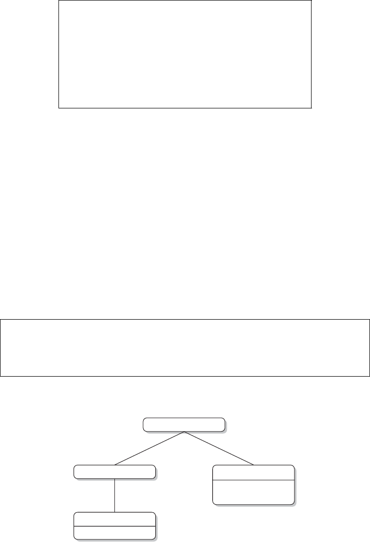
HTML 21
1<!DOCTYPE html>
2<html>
3<head>
4<title>First HTML</title>
5</head>
6<body>
7I am your first HTML file!
8</body>
9</html>
Figure 2.4 Source code of OurFirstHTML.html
2.2.2 Tree structure
Have another look at the source code of OurFirstHTML.html in Figure 2.4. Ignoring <!DOC-
TYPE html> for now, the rst element in the example is the <html> element. Between
the tags of this element, several tags are opened and closed again: <head>,<title>, and
<body>.The<head> and <body> tags are directly enclosed by the <html> element; the
<title> element is enclosed by the <head> tag. A good way to describe the multiple layers
of an HTML document is the tree analogy. Figure 2.5 illustrates the simple tree structure of
OurFirstHTML.html.The<html> element is the root element that splits into two branches,
<head> and <body>.<head> is followed by another branch called <title>.
Elements need to be strictly nested within each other in a well-formed and valid HTML
le. A pair of start and end tags has to be completely enclosed by another pair of tags. An
obvious violation of this rule would be:
1<head>
2<title>Do not
3</head>
4do this</title>
<html>
<body>
I am your first
HTML-file!
<head>
<title>
First HTML
Figure 2.5 A tree perspective on OurFirstHTML.html (see Figure 2.4)

22 AUTOMATED DATA COLLECTION WITH R
2.2.3 Comments
HTML offers the possibility to insert comments into the code that are not evaluated and
therefore not displayed in the browser. Comments are marked by <!-- at the beginning
and --> at the end. All text between these character sequences will be ignored. In practice, a
comment could look like this:
1<!-- Hi, I am a comment.
2I can span several lines and I am able to store additional
content that is not displayed by the browser. -->
Note that comments are still part of the document and can be read by anyone who inspects
the source code of a page.
2.2.4 Reserved and special characters
Reserved characters are used for control purposes in a language. We have learned that HTML
content is written in plain text, which is true both for the markup and the content part of the
document. As some characters are needed for the markup, they cannot be used literally in the
content. For example, we have learned that <and >are used to form tags in HTML. They are
markup characters. Imagine we want to display something like this in the browser: 5 <6but
7>3. It is impossible to include them plainly into an HTML le, like…
1<p>5<6but7>3</p>
…as the parser would interpret the <and >signs as enclosing a tag name. In order toCharacter
entities display the characters literally in a browser window, HTML relies on specic sequences of
characters called character entities or simply entities. All the entities start with an ampersand
&and end with a semicolon ;. Thus, <and >can be included in the content of a le with their
entity expressions < and >. When interpreting the HTML le, the browser will now
display the character that these entities represent. The above example therefore needs to be
rewritten as follows:
1<p>5 < 6 but 7 > 3 </p>
Since HTML documents can be written in numerous languages that often contain non-
simple latin characters like ¨
O,´
E,orØ, there is an extensive list of entities, all starting with an
ampersand (&) and ending with a semicolon (;). Table 2.1 provides a couple of examples of
characters and their entity representation—note that entities can be written either by number
or name.
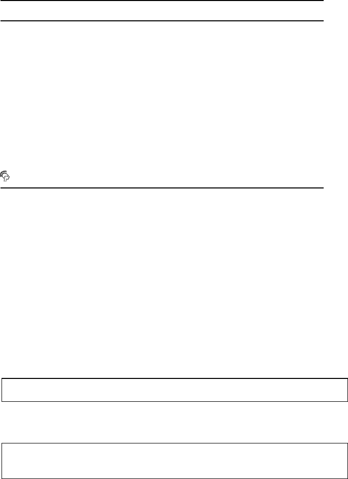
HTML 23
Table 2.1 HTML entities
Character Entity number Entity name Explanation
" " " quotation mark
' ' ' apostrophe
&& & ampersand
<< < less than
>> > greater than
  non-breaking space
§§ § section
´
AÀ À A with grave accent
´
EÈ È E with grave accent
´
aà à a with grave accent
´
eè è e with grave accent
♡♥ ♥ heart
𐇑 plumed head (Phaistos Disc)
Note: For a more comprehensive list of HTML entities, visit http://unicode-table.com
2.2.5 Document type denition
Recall the example from the beginning of the chapter? The rst line of the HTML read
<!DOCTYPE html>. It contains the so-called document type denition (DTD) that informs
the browser about the version of the HTML standard the document adheres to. HTML emerged
more than 20 years ago and has since seen some reformulation of the rules that might lead to
misinterpretations if the HTML version of the document was not made explicit. As the DTD
plays a more crucial role in XML, we postpone an extensive elaboration of the concept to
Section 3.3. For now, it sufces to know that DTDs are found—if included—in the rst line
of the HTML document. Below you nd a list of various DTDs.
rHTML5:
1<!DOCTYPE HTML>
rStrict HTML version 4.01:
1<!DOCTYPE HTML PUBLIC "-//W3C//DTD HTML 4.01//EN"
2"http://www.w3.org/TR/html4/strict.dtd">
2.2.6 Spaces and line breaks
Spaces and line breaks in HTML source code do not translate directly into spaces and line
breaks in the browser presentation. While line breaks are ignored altogether, any number
of consecutive spaces are presented as a single space. To force spaces into the interpreted
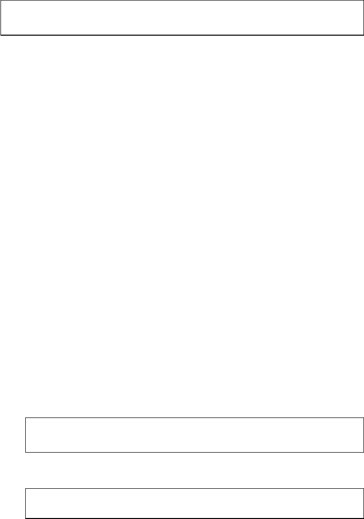
24 AUTOMATED DATA COLLECTION WITH R
version of the document, we use the non-breaking space entity and the line break tag
<br> for line breaks:
1<p>Writing<br> code<br>
2 is<br> poetry</p>
For a more extensive treatment of the subject, you may want to look into SpacesAndLin
eBreaks.html from the book’s materials.
2.3 Tags and attributes
HTML has plenty of legal tags and attributes, and it would go far beyond the scope of this book
to talk about each and every one. Instead, we will focus on a subset of tags that are of special
interest in the context of web data collection. Note that if not specied otherwise working
examples of the tags introduced in the following can be found in the TagExample.html from
the book’s materials.
2.3.1 The anchor tag <a>
The anchor tag <a> is what turns HTML from just a markup language into a hypertext markupThe H in
HTML language by enabling HTML documents to link to other documents. Much of the site-to-site
navigation in browsers works via anchor elements.
We often nd ourselves in situations where we want to extract information not from a
single page but from a whole series of pages. If we are lucky, the pages are listed on an index
page. More frequently, however, we have to collect links from one page that points to the next
page, which points to the next page, and so on. In both cases the information we are looking
for—the location of another page—is stored in an <a> element.
In fact, <a> elements are even more exible as they can not only link to other les, butThe exibility
of <a> and
href
also link to specic parts of a document. It is possible to link to anchors in a document to
make navigation on a site more convenient.
Have a look at TagExample.html. The parts of the HTML that are most interesting to us at
the moment are the blue underlined text snippets—the hyperlinks. There should be three links.
One refers to another webpage and two other point to the top and bottom, respectively, of the
current page. Have a look at the source code or the following list to see how this was achieved.
rLinking to another document:
1<a href="en.wikipedia.org/wiki/List_of_lists_of_lists">Link with
absolute path</a>
rSetting a reference point:
1<aid="top">Reference Point</a>
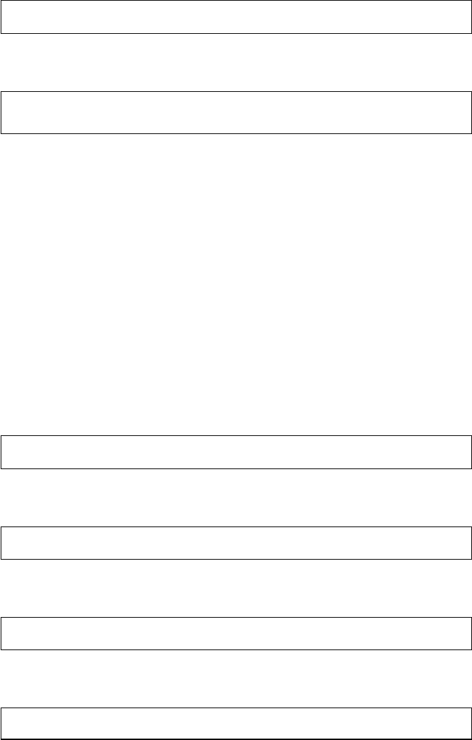
HTML 25
rLinking to a reference point:
1<a href="#top">Link to Reference Point</a>
rLinking to reference point in another document:
1<a href="http://en.wikipedia.org/wiki/List_of_pharaohs#New_Kingdom">
Link to Reference Point</a>
2.3.2 The metadata tag <meta>
The <meta> tag is an empty tag written in the head element of an HTML document. <meta>
elements do not have to be closed and thus differ from the general rule that empty elements
have to be closed with a dash /. As the name already suggests, <meta> provides meta
information on the HTML document and answers questions like: Who is the author of the
document? Which encoding scheme is used? Are there any keywords characterizing the page?
What is the language of the document?
In general, two attributes are specied in a meta element. The rst attribute can be either
name or http-equiv; the second is always content.<meta> elements with name as rst
attribute refer to information on the document while meta elements with http-equiv dene
how the document needs to be handled by HTTP (see Chapter 5). Below you nd several
examples showing the diverse usage of meta.Tosee<meta> in a real HTML document,
check out TagExample.html again. Some popular <meta> tags are used for:
rspecifying keywords:
1<meta name="keywords" content="Automation, Data, R">
rasking robots not to index the page or to follow its links (on robots see Section 9.3.2):
1<meta name="robots" content="noindex, nofollow">
rdeclaring character encodings (since HTML5):
1<meta charset="ISO-8859-1"/>
rdening character encodings (prior to HTML5):
1<meta http-equiv="content-type" content="text/html; charset=ISO-8859-1">
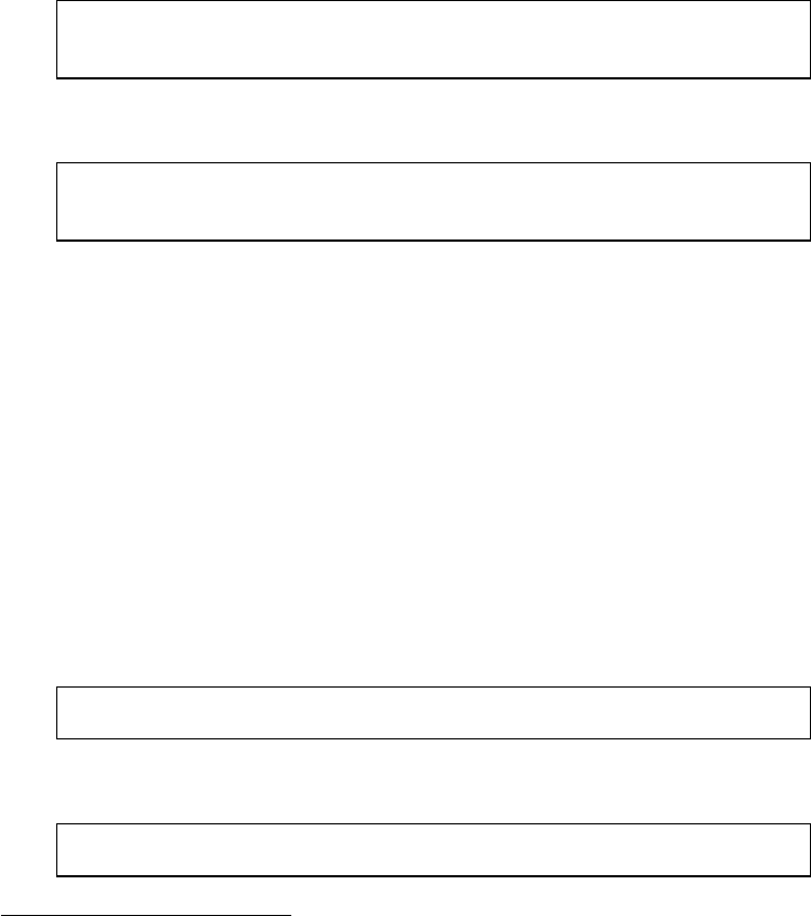
26 AUTOMATED DATA COLLECTION WITH R
2.3.3 The external reference tag <link>
The link tag is used to link to and include information and external les. External information
linked to the the HTML document might be license information for the website, a document
listing authors, a help page for the website, an icon that appears in the browser tab or one or
more style sheets that are used for layouts. The <link> element is empty and used within the
<head> element. All information is provided with attributes. Below you nd two examples
of the most common use.
rspecifying style sheets to use:
1<link rel="stylesheet" href="htmlresources/awesomestyle.css"
2type="text/css"/>
rspecifying the icon associated with the website:
1<link rel="shortcut icon" href="htmlresources/favicon.ico"
2type="image/x-icon"/>
Again, you might also like to check the source code of TagExample.html. Note that the
rel attribute describes the type of relationship between the current and the linked document.
The href attribute species the location of the external le. The type attribute describes the
le type according to the MIME scheme3.
2.3.4 Emphasizing tags <b>,<i>,<strong>
Tags like <b>,<i>,<strong> are layout tags that refer to bold, italics, and strong emphasis.
We can make use of the information in emphasis tags to locate content with a specic
layout. Imagine a document that contains a list of addresses where the name is set in italics.
Looking for the <i> tag makes it easy to identify the useful information. The examples below
exemplify the usage of these various layout tags. TagExample.html shows how they work in
a full-edged HTML document.
rText with bold type setting:
1<b>some text set in bold</b>
rText set in italics:
1<i>some text set in italics</i>
3The MIME scheme is a standardized two-part identier for le formats. For a more extensive discussion of the
subject, see Chapter 5.
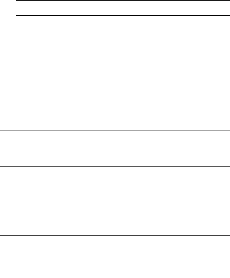
HTML 27
rText dened as important:
1<strong>some text so important to be emphasized</strong>
2.3.5 The paragraphs tag <p>
The <p> tag labels its content as being a paragraph and ensures that line breaks are inserted <p>
before and after its content:
1<p>This text is going to be a paragraph one day and separated from other
text by line breaks.</p>
2.3.6 Heading tags <h1>,<h2>,<h3>,…
In order to dene different levels of headlines—level 1 to level 6—HTML provides a series <h1>,<h2>,…
of tags <h1>,<h2>,…down to <h6>. See below for some examples:
1<h1>heading of level 1 -- this will be BIG</h1>
2<h2>heading of level 2 -- this will be big</h2>
3...
4<h6>heading of level 6 -- the smallest heading</h6>
2.3.7 Listing content with <ul>,<ol>,and<dl>
Several tags exist to list content. They are used depending on whether they wrap around an
ordered list (<ol>), an unordered list (ul), or a description list (<dl>). The former two tags
make use of nested <li> elements to dene list items, while the latter needs two further
elements: <dt> for keyword and <dd> for its description. An example for an unordered list
would be:
1<ul>
2<li>Dogs</li>
3<li>Cats</li>
4<li>Fish</li>
5</ul>
2.3.8 The organizational tags <div>and <span>
Another way of dening the appearance of parts of the HTML document are the <div>
and <span> tags. While <div> and <span> themselves do not change the appearance of
the content they enclose, these tags are used to group parts of the document—the former is
used to dene groups across lines, tags, and paragraphs, while the latter is used for in-line
grouping.
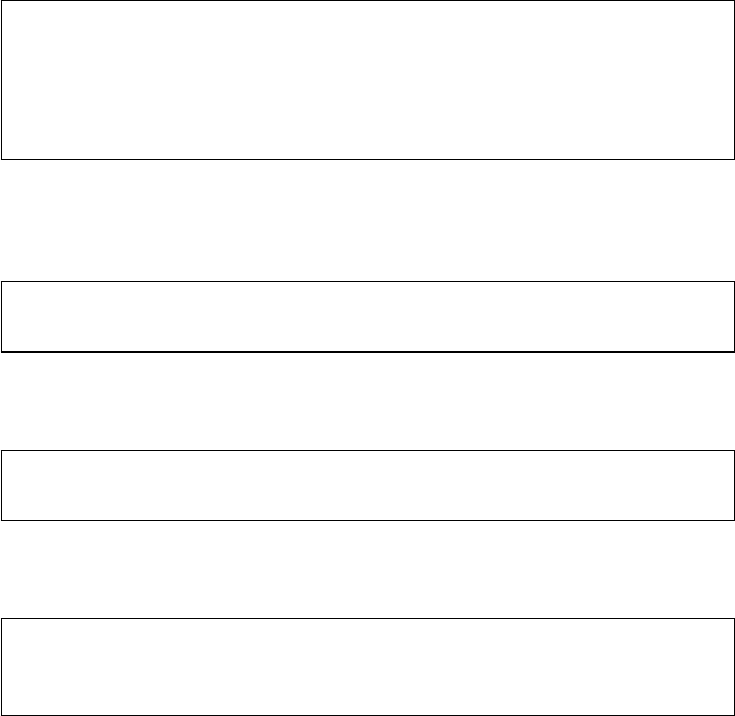
28 AUTOMATED DATA COLLECTION WITH R
Grouping parts of an HTML document is handy when combined with Cascading StyleCSS
Sheets (CSS), a language for describing the layout of HTML and other markup documents
like XML, SVG, and XHTML. Below you nd example denitions of two styles. The rst
style denition applies to all <div> elements of class happy, while the second does the same
for <span> elements:
1div.happy { color:pink;
2font-family:"Comic Sans MS";
3font-size:120% }
4span.happy { color:pink;
5font-family:"Comic Sans MS";
6font-size:120% }
Style denitions are commonly stored in separate CSS les, for example, awesomestyle
.css, and are later included via <link> tags in the header:
1<link href="htmlresources/awesomestyle.css"
2rel="stylesheet" type="text/css"/>
Later in the document they are passed to an element using an additional class attribute:
1<div class="happy"><p>I am a happy styled paragraph</p></div>
2non-happy text with <span class="happy">some happiness</span>
Alternatively, the style can be directly dened within the style attribute of an element:
1<div
2style="color:pink; font-family:"Comic Sans MS"; font-size:120%">
3<p>I am a happy styled paragraph</p></div>
The purpose of CSS is to separate content from layout to improve the document’s accessi-
bility. Dening styles outside of an HTML and assigning them via the class attribute enables
the web designer to reuse styles across elements and documents. This enables developers to
change a style in one single place—within the CSS le—with effects on all elements and
documents using this style.
So why should we care about style? First of all, one should always care about style.
But second, as CSS is so handy for developers, <div>,<span>, and class tags are used
frequently. They thus provide structure to the HTML document that we can make use of to
identify where our desired information is stored.

HTML 29
2.3.9 The <form>tag and its companions
An advanced feature of HTML are forms. HTML forms do more than just layout content.
They enable users to interact with servers by sending data to them instead of only receiving
data from them. Forms are introduced by the <form> tag and supported by other tags
like <fieldset>,<input>,<textarea>,<select>, and <option> and their respective
attributes. This two-way exchange of information between user and server allows for a more
dynamic browsing experience. Instances where we use forms on a daily basis are search
engines like Google. We type in a query in the text eld and a new site is called based on our
request. Let us proceed with an example to explain various concepts of HTML forms. The
code snippet below is part of FormExample.html from the book’s materials:
1<form name="submitPW" action="Passed.html" method="get">
2password:
3<input name="pw" type="text" value="">
4<input type="submit" value="SubmitButtonText">
5</form>
The form in the example consists of one <form> element and two <input> elements How HTML
forms work
nested within the former. The <form> tag has a name attribute, an action attribute, and
a specic method.Thename of the form serves as an internal identier. The action and
method attributes dene what the browser is supposed to do once the submit button is pressed.
action denes the location of the response.
The most common protocol for requesting and receiving resources on the Web is HTTP
(Hypertext Transfer Protocol). The method attribute refers to the HTTP method that is used
to send the information to the server. Most likely it will be POST or GET. For now it sufces
to say that when GET is used, the information that is sent to the server is appended to the
URL. Conversely, when POST is used the information is not transmitted via the requested
URL. For details on HTTP methods, see Chapter 5.
Regarding the <input> elements we can distinguish between several avors. There are
normal inputs, hidden inputs, reset inputs, and those that are used to dene the submit button.
Normal inputs collect the data to be sent to the server and come in various forms like text
elds, color selectors, check boxes, date selectors, and sliders. Hidden inputs dene data that
is sent to the server but the user has no option to manipulate the input. Reset inputs simply
reset all inputs and selections made so far. Inputs that form submit buttons result in sending
the supplied data. The input avor is dened by the value of the type attribute. For hidden
inputs the type is hidden, for reset inputs reset, and for submit buttons submit. The types
for normal inputs depend on the type of information that is collected, for example, text,
color,checkbox,date, and range.
Inputs require two attributes. First, the name attribute unambiguously associates the
information with a specic input; the type attribute is required to tell the browser how to
gather the information. An optional attribute, value, supplies a default value that is sent to
the server if no information is supplied by the user.
Three other tags can be used to gather information in a form—<textarea> and
<select> in combination with <option>.<textarea> elements are used to gather text
that spans multiple lines. To select one or multiple items from a list, HTML documents use

30 AUTOMATED DATA COLLECTION WITH R
<select>. While the <select> element serves to set attribute values, the nested option
elements dene the list of items the user can select from. Similar to the <input> elements,
a name attribute is needed for sending the data from <textarea> and <select> elements.
For an overview of the various types of inputs, check out InputTypes.html.
To see forms in action, go to: http://www.r-datacollection.com/materials/html/FormEx
ample.html. The page pretends to be a gate keeper and asks for a password. As we are about
halfway through the HTML chapter we trust that you are able to guess the password with
three tries at most. Go ahead and give it a try! In the example the action attribute is set to
Passed.html, meaning that the password gathered on the rst page gets submitted to this new
page. Try it out once more and select another password. Again, we get to the new document
and the page contains the information that we typed into the text eld. HTML forms turn
the static HTML dinosaur into a exible and mighty tool.4The takeaway point is that the
information gets sent and the response changes according to our inputs.
Let us consider the example form from above again. We notice that pw is the name of
the rst <input> element. We already know that the name attribute of <input> serves
as a label for transporting the information. If you inspect the URL of the response you
notice that the password has been appended to the URL, which now looks something like
.../Passed.html?pw=xxxxxxx. From this we conclude that the form uses a GET method
rather than a POST method—otherwise the pasword would not show up in the URL. The
part of the URL that contains our password is called query string. Query strings always
appear at the end of the URL and start with ?. The information in query strings is written as
parameter=value pairs—just like HTML tag attributes—and are separated by &if more
than one pair is specied.
Now that you know about HTML forms and query strings, take a moment and use your
browser to check out forms in actions. Find pages that use forms and look carefully if and
how they use query strings. You might also want to go back to Passed.html in your browser
and manipulate the pw value directly within the address bar to see what happens.
2.3.10 The foreign script tag <script>
HTML itself is not a programming language. HTML is a markup language that describes
content and denes its presentation. Once an HTML le is loaded in the browser, it remains
stable and does not change by events or user interaction. Nevertheless, we all know examples
of highly dynamic websites. Most of them probably make heavy use of the <script>
element.5
The <script> element is a container for scripts that enable HTML to include function-Arststabat
JavaScript ality from other programming languages. This other language will frequently be JavaScript.
JavaScript allows the browser to change the content and structure of the document after it has
been loaded from the server, enabling user interaction and event handling.
In FormExample.html and Passed.html we already made use of the <script> element.
There are two <script> elements in the Passed.html document. The rst is placed within
the header and denes the function that extracts the value of a specic parameter from the
URL. The second is placed directly within the body and executes the function that searches
4To be fair, Passed.html is not pure HTML but includes some JavaScript, which we will touch upon in Chapter 6.
5See Chapter 6 for a more elaborate discussion of the topic.
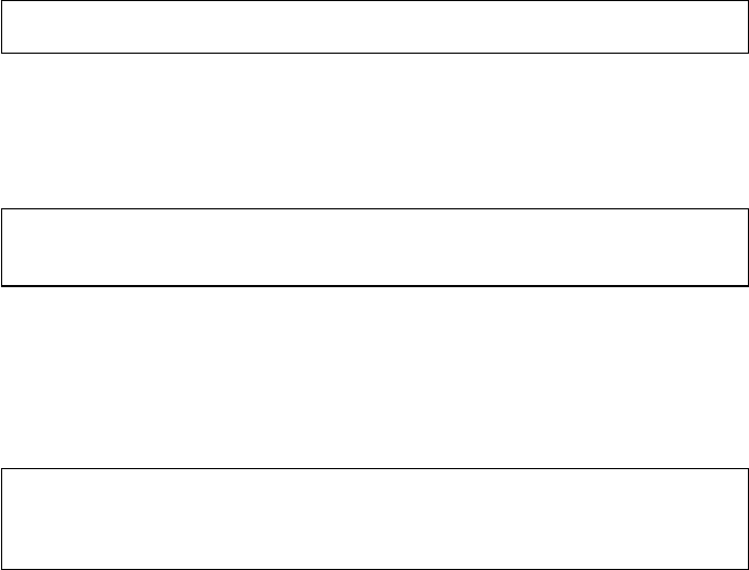
HTML 31
forthevalueofthepw parameter. After storing the value in a variable, it writes the value into
the HTML document.
Once again, go ahead and try it yourself: Open Passed.html and manipulate the URL so
it looks something like this: .../Passed.html?pw=xxxx. Save the page on your hard disk
(right click,save as) and reopen the saved page in your browser. Now check out the source
code of the page before and after saving. While the original page contained the original source
code, the second includes the changes your browser made after loading the page.
Let us get back to HTML and how we can recognize that JavaScript has been used.
JavaScript can appear broadly in three forms: explicitly in a <script> element, implicitly
by referring to an external JavaScript within a <script> element, and implicitly as an event
in an HTML element. Below you nd examples of all three types of JavaScript usage.
rExplicit JavaScript (printing the current time and date):
1<script> document.write( Date() ); </script>
This snippet adds the current date and time to the document.
rReference to an external JavaScript and using its functions within another script
element (printing the browser used to view the document):
1<script src="htmlresources/browserdetect.js"></script>
2<script> document.write(BrowserDetect.browser); </script>
This snippet loads an external JavaScript le (browserdetect.js) and uses the functions
it contains (BrowserDetect) to add information about the browser of the document.
rTriggering JavaScript with events (changing the style class when hovering over the
element)
1<p onmouseover="this.className='over'"
2onmouseout="this.className='out'">
3Hover Me!</p>
This snippet triggers two events, one when the mouse cursor hovers over the element
and one when the mouse cursor leaves the area of the element—onmouseover and
onmouseout—and assigns two JavaScript functions that are executed whenever the
events take place. The functions change the class of the element to over or out and the
styles associated with these two classes take effect.
Now open http://www.r-datacollection.com/materials/html/JavaScript.html in your
browser and have a look at the examples. The document displays the time you opened
the document, shows the current time, indicates which browser you are using (the version
number as well as the platform it is running on), changes colors from white to black as long

32 AUTOMATED DATA COLLECTION WITH R
Table 2.2 Nominal GDP per capita
Nominal GDP
Rank (per capita, USD) Name
1 170,373 Lichtenstein
2 167,021 Monaco
3 115,377 Luxembourg
4 98,565 Norway
5 92,682 Qatar
as you hover over the Hover Me! text, and adds text to the document when you ll out the
text eld and press enter.
Have a look at the source code and try to map which parts of the document are plain
HTML and which are the work of JavaScript.
2.3.11 Table tags <table>,<tr>,<td>,and<th>
The next group of elements enables HTML to display tables. Check out Table 2.2 and compare
it to its HTML code representation below. To begin a table we make use of <table>.We
start new lines with <tr>. Within <tr>, we can either use <td> for dening cells or <th>
for header cells.
Table 2.2 as HTML code—the full HTML document is HTMLTable.html from the book’s
materials:
<table>
<tr><th>Rank</th><th>Nominal GDP</th><th>Name</th></tr>
<tr><th></th><th>(per capita, USD)</th><th></th></tr>
<tr><td>1</td><td>170,373</td><td>Lichtenstein</td></tr>
<tr><td>2</td><td>167,021</td><td>Monaco</td></tr>
<tr><td>3</td><td>115,377</td><td>Luxembourg</td></tr>
<tr><td>4</td><td>98,565</td><td>Norway</td></tr>
<tr><td>5</td><td>92,682</td><td>Qatar</td></tr>
</table>
2.4 Parsing
After having learned the key features of HTML documents, we now turn to loading and
representing the contents of HTML/XML les in an Rsession.6This step is crucial if we care
to extract information from web documents in a principled and robust fashion from within R.7
6Although different in many respects, HTML and XML are similar regarding their grammar and thus, the
discussion on HTML parsing is very relevant for XML parsing, too. XML is subject of the next chapter (Chapter 3).
7See Chapter 4 on how to exploit the parsed representation of parsed documents for data extraction.
HTML 33
While performing web scraping, we usually get in touch with HTML in two steps: First,
we inspect content on the Web and examine whether it is attractive for further analyses.
Second, we import HTML les into Rand extract information from them. Parsing HTML
occurs at both steps—by the browser to display HTML content nicely, and also by parsers in
Rto construct useful representations of HTML documents in our programming environment.
In the remainder of this chapter we begin by motivating the use of parsers and then discuss
some of the problems inherent in the process as well as their solutions.
2.4.1 What is parsing?
Before showing the application of a parser, let us think about why we need to parse the
contents of marked up web documents such as HTML compared to merely reading them into
an Rsession. The difference between reading and parsing is not just a semantic one. Instead,
reading functions differ from parsing functions in that the former do not care to understand
the formal grammar that underlies HTML but merely recognize the sequence of symbols
included in the HTML le. To see that, let us employ base R’s readLines() function,
which loads the content of an HTML le. As a stylized, running example in this part, we
consider fortunes.html (see the chapter’s materials)—a simple HTML le that consists of
several nuggets of Rwisdoms. We apply readLines() on the document, store the output in
an object called fortunes, and print its content to the screen:
R> url <- "http://www.r-datacollection.com/materials/html/fortunes.html"
R> fortunes <- readLines(con = url)
R> fortunes
readLines() maps every line of the input le to a separate value in a character vector.
Although easy to use, readLines() creates a at representation of the document, which is
of limited use for extracting information from it. The main problem is that readLines() is
agnostic about the different tag elements (name, attribute, values, etc.) and produces results
that do not reect the document’s internal hierarchy as implied by the nested tags in any
sensible way.
To achieve a useful representation of HTML les, we need to employ a program that under- Document
Object Model
(DOM)
stands the special meaning of the markup structures and reconstructs the implied hierarchy
of an HTML le within some R-specic data structure. This representation is also referred to
as the Document Object Model (DOM). It is a queryable data object that we can build from
any HTML le and is useful for further processing of document parts. This transformation
from HTML code to the DOM is the task of a DOM-style parser. Parsers belong to a general
class of domain-specic programs that traverse over symbol sequences and reconstruct the
semantic structure of the document within a data object of the programming environment.
In the remainder of this book, we will use functionality from the XML package to parse web
documents (Temple Lang 2013c). XML provides an interface to libxml2, a powerful parsing
library written in C that is able to cope with many parsing-specic problems. To get started,
let us parse fortunes.html and store it in a new object called parsed_fortunes using XML’s
htmlParse() function:
R> library(XML)
R> parsed_fortunes <- htmlParse(file = url)
R> print(parsed_fortunes)
<!DOCTYPE HTML PUBLIC "-//IETF//DTD HTML//EN">
34 AUTOMATED DATA COLLECTION WITH R
<html>
<head><title>Collected R wisdoms</title></head>
<body>
<div id="R Inventor" lang="english" date="June/2003">
<h1>Robert Gentleman</h1>
<p><i>'What we have is nice, but we need something very different'</i></p>
<p><b>Source: </b>Statistical Computing 2003, Reisensburg</p>
</div>
<div lang="english" date="October/2011">
<h1>Rolf Turner</h1>
<p><i>'R is wonderful, but it cannot work magic'</i> <br><emph>answering
a request for automatic generation of 'data from a known mean and 95% CI'
</emph></p>
<p><b>Source: </b><a href="https://stat.ethz.ch/mailman/listinfo/r-help">
R-help</a></p>
</div>
<address>
<a href="http://www.r-datacollectionbook.com"><i>The book homepage</i></a>
<a></a>
</address>
</body>
</html>
Printing the object to the screen, we receive a visual feedback that we created a copy
of the le inside the Rsession. For conventional parsing tasks, htmlParse() will be all
that is necessary to create a properly parsed document object. At a minimum, the function
needs to be handed the le path via its file argument. This may either be an HTML le (or
compressed archive of HTML les) that already exists on the hard drive or an URL pointing
to a web document.
htmlParse() and other DOM-style parsers effectively conduct the following steps.DOM parsing:
A two-step
process 1. htmlParse() rst parses the entire target document and creates the DOM in a tree-like
data structure of the C language. In this data structure every element that occurs in the
HTML is now represented as its own entity, or as an individual node. All nodes taken
together are referred to as the node set. The parsing process also includes an automatic
validation step for malformation. From its source code (see object fortunes) we learn
that fortunes.html contains two structural errors. Not only have some of the attribute
values been left unquoted but also a closing tag for the second paragraph tag (<p>)
is missing. Yet, as we see from the parsed output, these two aws have both been
remedied. This is due to libxml2 which is capable to work on non-well-formed HTML
documents because it recognizes errors and corrects them in order to create a valid
DOM.
2. In the next step the C-level node structure is converted into an object of the Rlanguage.
This is necessary because further processing of the DOM, for example, modifying and
extracting information from it, is tremendously more convenient in a higher-level
language such as R. Internally, Ruses lists to reect the hierarchical order of nodes.
More specically, the transformation between C and Ris managed through so-called

HTML 35
handler functions. These handler functions regulate the translation of a C-level node
into an Rlist element and can be intercepted by the user to determine whether and how
a node should be reected in the Robject.
For most parsing tasks, you will nd that htmlParse()’s default options are sufciently
powerful to create the DOM. Nevertheless, some control over the parsing process can be
benecial in cases where the target document is of considerable size, carries unnecessary
information, or needs to be altered in some predened way. To deal with these situations,
the next section looks at ways to affect the building process of the DOM, for example, by
formulating rules that structure the mapping of specic elements into an Robject.
2.4.2 Discarding nodes
Discarding unnecessary parts of web documents in the parsing stage can help mitigate memory
issues and enhance extraction speed. Handlers provide a comfortable way to manipulate (i.e.,
delete, add, modify) nodes in the tree construction stage. As we have already noted, handler
functions regulate the conversion of the C-level node structure into the R-object. By default,
that is, when the handlers are left unchanged, all nodes will be mapped into the Rlist structure,
but we are free to manipulate this process.
We specify handlers as a list of named functions, where the name corresponds to a node Specifying
handler
functions
name and the function species what should happen with the node. The function is executed
on encountering a node with a specic name. To exemplify, consider the problem of deleting
the <body> node in our example HTML le. In the parsing stage, we can easily get rid of this
node including all of its children, that is, nodes that are nested deeper in the tree as follows:
R> h1 <- list("body" = function(x){NULL})
R> parsed_fortunes <- htmlTreeParse(url, handlers = h1, asTree = TRUE)
R> parsed_fortunes$children
$html
<html>
<head>
<title>Collected R wisdoms</title>
</head>
</html>
We rst create an object h1 containing a list of a function named after the node we want
to delete. We then pass this object to the htmlTreeParse() function via its handlers
argument. Printing parsed_doc to the screen shows that the <body> node is not part of the
DOM tree anymore. Internally, the handler has replaced all instances of the <body> node with
the NULL object, which is equivalent to deleting these nodes. When using handler functions,
one needs to set the asTree argument to TRUE to indicate that the DOM should be returned
and not the handler function itself.
Via the XML package we can pass generic handler functions to operate on specic XML Generic
handlers
elements such as the processing instructions, XML comments, CDATA, or the general node
set.8A complete overview over these generic handlers is presented in Table 2.3. To illustrate
8For an explanation of XML comments and CDATA see Chapter 3.
36 AUTOMATED DATA COLLECTION WITH R
Table 2.3 Generic handlers for DOM-style parsing
Function name Node type
startElement() XML element
text() Text node
comment() Comment node
cdata() <CDATA>node
processingInstruction() Processing instruction
namespace() XML namespace
entity() Entity reference
Source: Adapted from Nolan and Temple Lang (2014, p. 153).
their use, consider the problem of deleting all nodes with name div or title as well as
comments that appear in the document. We start again by creating a list of handler functions.
Inside this list, the rst handler element species a function for all XML nodes in the document
(startElement). Handlers of that name allow describing functions that are executed on all
nodes in the document. The function species a request for a node’s name (xmlName) and
implements a control structure that returns the NULL object if the node’s name is either div
or title (meaning we discard this node) or else includes the full node in the DOM tree. The
second handler element (comment) species a function for discarding any HTML comment:
R> h2 <- list(
startElement = function(node, ...){
name <- xmlName(node)
if(name %in% c("div", "title")){NULL}else{node}
},
comment = function(node){NULL}
)
Let us pass the handler function to htmlTreeParse():
R> parsed_fortunes <- htmlTreeParse(file = url, handlers = h2, asTree = TRUE)
If we print parsed_fortunes to the screen, we nd that we rid ourselves of the nodes
specied in the handlers:
R> parsed_fortunes$children
$html
<html>
<head/>
<body>
<address>
<a href="http://www.r-datacollectionbook.com">
<i>The book homepage</i>
</a>
<a/>
</address>
</body>
</html>
HTML 37
2.4.3 Extracting information in the building process
We motivated the parsing of HTML les as a necessary intermediate step to extracting
information from web documents. In this process, we usually want the parser to traverse the
entire C-level node set and then build the document tree in an Rdata structure from which
we extract a particular information. Conceptually, there is an alternative strategy where we
conduct the extraction directly during the parsing process. Under some circumstances, this
strategy can provide considerable advantages since multiple loadings of a document can be
avoided, although it is also a little bit more challenging compared to the DOM-style parsing
approach presented before. Once again, handler functions play a key role in this process. But
rather than using the handler to describe how a C-level node should be converted into an
element of the RDOM tree, we now want to specify the handlers to route specic nodes into
an Robject of our own choosing. Ultimately, this saves us an additional traversal step and thus
constitutes a more efcient way to pull out target information. Before we dive deeper into
this section, we would like to point out that the contents of this section are fairly advanced. If
you are not too familiar with Rscoping issues, you might like to skip ahead to the summary
of this chapter. You can continue with the book just ne without having read this part.
For an example, consider the problem of extracting the information from fortunes.html Scope issues
that is written in italics, that is, encapsulated with <i> tags. Underlying this task is a tricky
problem of functional scope that we need to address. Ultimately, we want to create a data object
containing the information in our current workspace or global environment. But functions
in R—and our handler functions are no different—operate on local variables and have no
writing access to the global environment, which is a necessary requirement for this problem.
The solution is to dene the handler function for the <i> nodes in the document as a Using closure
handler
functions
so-called closure—a function that is capable of referencing objects that are not local to it. A
closure function not only contains a function’s arguments and body, but also an environment.
Here, the environment is needed to dene container variables to which we route the handler’s
output, as well as a return function for the variables’ contents.
We start by dening a nesting function getItalics().i_container is our local
container variable that will hold all information set in italics. Next, we dene the handler
function for the <i> nodes. On the right side of the rst line of this function, we concatenate
the contents of the container variable with a new instance of the <i> node value. The resulting
vector then overwrites the existing container object by using the super assignment operator
<< −, which allows making an assignment to nonlocal variables. Lastly, we create a function
called returnI() with the purpose of returning the container object just created:
R> getItalics = function() {
i_container = character()
list(i = function(node, ...) {
i_container <<- c(i_container, xmlValue(node))
}, returnI = function() i_container)
}
Next, we execute getItalics() and route its return values into a new object h3.
Essentially, h3 now contains our handler function, but additionally, the function can access
i_container and returnI() as these two objects were created in the same environment
as the handler function:
R> h3 <- getItalics()
38 AUTOMATED DATA COLLECTION WITH R
Now we can pass this function to htmlTreeParse()’s handlers argument:
R> invisible(htmlTreeParse(url, handlers = h3))
For clarity, we employ the invisible() function to suppress printing of the DOM to the
screen. To take a look at the fetched information we can make a call to h3()’s returnI()
function to print all the occurrences of <i> nodes in the document to the screen:
R> h3$returnI()
[1] "'What we have is nice, but we need something very different'"
[2] "'R is wonderful, but it cannot work magic'"
[3] "The book homepage"
Summary
In this chapter we focused on getting a basic understanding of HTML. We learned that what
we get presented when surng the web is an interpreted version of the marked up source
code that holds the content. Tags form the core of the markup used in HTML and can be
used to dene structure, appearance, and content. Furthermore, elements not only contain
information but can also be used to transmit information from user to server or to incorporate
functionality from other computer languages, most notably JavaScript. We should be able at
this point to locate information we seek in the source code and to connect source code to
browser interpretation and vice versa. Along with knowledge about the structure of HTML
elements we are ready to learn how to exploit structure and layout of HTML les to collect
the information we need.
Parsing is an important step in processing information from web documents. The native
structure of HTML does not naturally map into Robjects. We can import HTML les as raw
text, but this deprives us of the most useful features of these documents. We have learned in
this chapter how to parse the tree structure of HTML documents, giving them a representation
in the Renvironment. We will learn powerful tools to locate and extract nodes within these
objects and the information they hold in Chapter 4. But rst we turn to XML, a more generic
counterpart to HTML and a frequently used format to exchange data on the Web.
Further reading
As HTML is a W3C standard, we recommend a look at the W3 pages and the accompanied
W3schools pages (http://www.w3schools.com) if you want to dive deeper into HTML and
JavaScript. As HTML is also a WHATWG standard, you might like to check out their web
pages for further information on HTML and related technologies (http://www.whatwg.org/).
For example, the history section explains why W3C and WHATWG develop HTML5 paral-
lelly. Further helpful web sources are the following.
rA complete list of tags with description and example:
http://www.w3schools.com/tags
rA long list of special characters, symbols, and their entity representation:
http://www.w3schools.com/charsets/ref_html_8859.asp
HTML 39
rA much much longer list of characters and their entity representation:
http://unicode-table.com
rAn HTML validator:
http://validator.w3.org
For those who like it short but also like to hold a real book in their hands there is Niederst
Robbins’s (2013) less than 200 pages HTML5 Pocket Reference. You can nd more thorough
treatments of the subjects in Castro and Hyslop (2014) for HTML and CSS and Flanagan
(2011) for JavaScript.
Problems
1. Why is it important that HTML is a web standard?
2. Write down the HTML tags for (a) the primary heading, (b) starting a new paragraph,
(c) inserting foreign code, (d) constructing ordered lists, (e) creating a hyperlink, and
(f) creating an email link!
3. HTML source code inspection.
(a) Open three webpages you frequently use in your browser.
(b) Have a look at the source code of all three.
(c) Inspect various elements with the Inspect Elements tool of your browser.
(d) Save each of them to your hard drive.
4. Building a basic HTML document, part I.
(a) Write a minimal HTML le.
(b) Add your name as a comment.
(c) Add a level one and a level two headline.
(d) Add some further content, for example, a sentence about the current weather.
(e) Add a paragraph with some further content, for example, a sentence about tomor-
row’s weather.
5. Building a basic HTML document, part II.
(a) Write a minimal HTML document.
(b) Include a paragraph that contains 10 special characters—only ve of them may be
mentioned in Table 2.1.
(c) Use http://www.r-datacollection.com/materials/html/simple.css as your default
style le.
(d) Check the validity of your document at http://validator.w3.org.
6. Building a basic HTML document, part III.
(a) Write a minimal HTML document.
(b) Include a table with two columns and three rows.
(c) The rst column should contain rst,second, and third. The second column should
contain links to your top three web pages.
(d) Have a look at the list of tags at http://www.w3schools.com/tags. Try to use some
of the tags you are not yet familiar with in your HTML document.
40 AUTOMATED DATA COLLECTION WITH R
7. The base Rfunction download.file() is a standard tool to gather data from the Web
with R. Investigate the function’s syntax and try to use it to save the front pages of your
three most favorite websites to your local disk.
8. The base Rfunctions readLines() and writeLines() can be used to import and
export character data to and from RTry to use them to import the webpages you have
gathered in the previous exercise and save them in different objects. Next, combine the
three objects into a list object. Finally, use writeLines() to store the pages again in
external les.
9. An encounter with JavaScript.
(a) Check out http://www.r-datacollection.com/materials/html/fortunes3.html in your
browser.
(b) View the page’s source code.
(c) Download both JavaScript les linked to the document using the download
.file() function.
10. Building a basic HTML document, part IV.
(a) Write a minimal HTML document.
(b) Include a form that has two inputs—name and age.
(c) Dene the form in a way that it sends data to http://www.r-datacollection.com/
materials/http/GETexample.php via the GET method.
(d) Make sure it works—the server should respond with Hello YourName! You are
YourAge years old.
(e) Try to send high age values. At what point does the response message change?

3
XML and JSON
XML, the eXtensible Markup Language, is one of the most popular formats for exchanging
data over the Web. But it is more than that. It is ubiquitous in our daily life. As Harold and
Means (2004, xiii) note:
XML has become the syntax of choice for newly designed document formats
across almost all computer applications. It’s used on Linux, Windows, Macintosh,
and many other computer platforms. Mainframes on Wall Street trade stocks with
one another by exchanging XML documents. Children playing games on their
home PCs save their documents in XML. Sports fans receive real-time game
scores on their cell phones in XML. XML is simply the most robust, reliable, and
exible document syntax ever invented.
XML looks familiar to someone with basic knowledge about HTML, as it shares the same
features of a markup language. Nevertheless, HTML and XML both serve their own specic
purposes. While HTML is used to shape the display of information, the main purpose of XML
is to store data. Therefore, the content of an XML document does not get much nicer when it
is opened with a browser—XML is data wrapped in user-dened tags. The user-dened tags
make XML much more exible for storing data than HTML. The main goal of this chapter
is not to turn you into an XML coding expert, but to get you used to the key components of
XML documents.
We start with a look at a running XML example (Section 3.1) and continue with an
inspection of the XML syntax (Section 3.2). There are several ways to limit the endless
exibility in XML markup. We cover technologies that allow extending XML as well as
dening new standards that simplify exchanging specic data on the Web efciently in
Sections 3.3 and 3.4. Section 3.5 shows how to handle XML data with R. If your web
scraping task does not specically involve XML data you might be ne to just scan this part
Automated Data Collection with R: A Practical Guide to Web Scraping and Text Mining, First Edition.
Simon Munzert, Christian Rubba, Peter Meißner and Dominic Nyhuis.
© 2015 John Wiley & Sons, Ltd. Published 2015 by John Wiley & Sons, Ltd.

42 AUTOMATED DATA COLLECTION WITH R
of the chapter as you are already familiar with the most important concepts of the XML
language from the previous chapter.
Another standard for data storage and interchange we frequently nd on the Web is the
JavaScript Object Notation, abbreviated JSON. JSON is an increasingly popular alternative
to XML for data exchange purposes that comes with some preferable features. The second
part of this chapter therefore turns to JSON. We introduce the format with a small example
(Section 3.6), talk about the syntax (Section 3.7), and learn how to import JSON content into
Rand process the information (Section 3.8).
3.1 A short example XML document
We start with a short example of an XML le. The XML code in Figure 3.1 provides a sample
of three James Bond movies, along with some basic information. Probably the most distinctive
feature of XML code is that human readers have no problem in interpreting the data. Values
and names are wrapped in meaningful tags. Each of the three movies is attributed with a
name, a year, two actors, the budget, and the box ofce results. Indentation further facilitates
reading but is not a necessary component of XML. It highlights the hierarchical structure
of the document. The document starts with the root element <bond_movies>, which also
closes the document. The elements are repeated for each movie entry—the content varies.
1<?xml version="1.0" encoding="ISO-8859-1"?>
2<bond_movies>
3<movie id="1">
4<name>Dr. No</name>
5<year>1962</year>
6<actors bond="Sean Connery" villain="Joseph Wiseman"/>
7<budget>1.1M</budget>
8<boxoffice>59.5M</boxoffice>
9</movie>
10 <movie id="2">
11 <name>Live and Let Die</name>
12 <year>1973</year>
13 <actors bond="Roger Moore" villain="Yaphet Kotto"/>
14 <budget>7M</budget>
15 <boxoffice>126.4M</boxoffice>
16 </movie>
17 <movie id="3">
18 <name>Skyfall</name>
19 <year>2012</year>
20 <actors bond="Daniel Craig" villain="Javier Bardem"/>
21 <budget>175M</budget>
22 <boxoffice>1108.6M</boxoffice>
23 </movie>
24 </bond_movies>
Figure 3.1 An XML code example: James Bond movies

XML AND JSON 43
Some elements are special. The element in the rst line (<?xml...>) is not repeated, and
this and the <actors> element hold some additional information between the <...> signs.
The XML language works quite intuitively. You should have no problems to expand and
rene the dataset before even knowing every rule of the syntax. In fact, why not try it? Copy
the le, go to Wikipedia, look for other details on the movies, and try to add them to the le!
You can check later if you have written correct XML code. This is because information is
stored as plain text and the tags that allow arranging the data in meaningful ways are entirely
user-dened and should be comprehensible. While the tags might not even be necessary to
interpret the data, they make XML a computer language and as such useful for communication
on and between computers.
The fact that XML is a plain text format is what makes it ultimately compatible. This Why XML is so
popular
means that whatever browser, operating system, or PC hardware we use, we can process it.
No further information or decoder is needed to interpret the data and their structure. The tags
are delivered along with the data and fully describe the document—this is commonly called
self-describing. Further, as tags can be nested within each other, XML documents can be used
to represent complex data structures (Murrell 2009, p. 116). We will discuss these structures in
the following section. To be sure, although XML is so exible, it possesses a clear set of rules
that denes the basic layout of a document. We can use simple tools to check if these rules are
obeyed.1There are also tools to further restrict structure and content in an XML document.
Many developers have used the syntax of XML to create new XML-based languages that
basically restrict XML to a xed set of elements, structure, and content, which we will look
deeper into in Sections 3.4.3 and 3.4.4. Still, these derived languages remain valid XML.
XML has gained a considerable amount of its popularity through these extensions.
The downside of storing information in XML les is a lack of efciency. Plain text XML
documents often hold a lot of redundant information. Note that in standard XML, the starting
and closing tags are repeated for every entry. This can consume more space in the document
than the actual data. Especially when we deal with large datasets or data that provide highly
hierarchical structure, it may take up a lot of memory to try to import and manipulate the data.
The preferred program to open XML les are programs that are capable of highlighting How to view
XML les
the syntax of the documents and automatically indent the elements according to their level
in the hierarchical structure. Current versions of all mainstream browsers are able to layout
XML les adequately, and it is quite likely that your favorite code editor is capable of XML
highlighting as well. Note, however, that XML les can be very large and contain millions of
lines of data, so it may take a while to open them.
In the following sections we will talk more about the syntax of XML. We will learn how
to import XML data into Rand how to transform it into other data formats that are more
convenient for analysis. We will also look at other XML “avors” that are used to store a
variety of data types. You might be surprised about the numerous applications that rely on
XML and how one can make use of this knowledge for data scraping purposes.
3.2 XML syntax rules
As any other computer language, XML has a set of syntax rules and key elements we have to
know in order to nd our way in any document. But fear not: XML rules are very simple.
1However, as mostly passive users of XML, this is rarely of interest to us.
44 AUTOMATED DATA COLLECTION WITH R
3.2.1 Elements and attributes
Take another look at Figure 3.1. It helps explain large parts of what we have to know aboutXML
declaration XML. An XML document always starts with a line that makes declarations for the XML
document:
1<?xml version="1.0" encoding="ISO-8859-1"?>
version="1.0" indicates the version of XML that is being used. There are currently
two versions: XML 1.0 and XML 1.1.2Additionally, the declaration can, but need not hold
the character encoding of the document, which in our case is encoding="ISO-8859-
1".3Another attribute the declaration can contain—but does not in our example—is the
standalone attribute, which take values of yes or no and indicates whether there are
external markup declarations that may affect the content of the document.4
An XML le must contain one and only one root element that embraces the wholeRoot element
document. In our case, it is:
1<bond_movies>
2...
3<\bond_movies>
Information is usually stored in elements. An XML element is dened by its start tag andElement syntax
the content. An element frequently has an end tag, but can also be closed in the start tag with
aslash/. It can contain
rother elements.
rattributes, bits of information that describe the element in more detail. Attributes,
like elements, are slots for information, but they cannot contain further elements or
attributes.
rdata of any form and length, for example, text, numbers or symbols.
ra mixture of everything, which sounds complicated but is a rather ordinary case when
elements contain other elements that contain data. For example, the <movie> elements
in Figure 3.1 all contain an attribute, other elements, and data within the children
elements.
rnothing, which means really nothing—no data, no other element, not even white
spaces.
2The differences between the two existing versions are marginal and relate to encoding issues that are usually of
no interest to us.
3To learn more about encodings, see Section 8.3.
4For more information, see the elucidations by W3C on http://www.w3.org/TR/xml/#sec-rmd

XML AND JSON 45
Consider the rst <title> element from above:
1<title>Dr. No</title>
Its constituent parts are
the element title title
the start tag <title>
the end tag </title>
the data value Dr. No
We are already familiar with the start tag–end tag logic from HTML. The benet of this
syntax is that we can easily locate data of a certain element in the document, regardless
of where, that is, on which line or hierarchical level it is located. The element <title>
occurs three times in the example. We could retrieve all of these elements by building a query
like “give me the content of all elements named <title>.” This is what we will learn in
Chapter 4 when we learn how to use the query language XPath. A more compact way of
writing elements is
1<actors bond="Sean Connery" villain="Joseph Wiseman"/>
This element contains
the element name actors
the start tag <actors.../>
rst attribute’s name bond
rst attribute’s value Sean Connery
second attribute’s name villain
second attribute’s value Joseph Wiseman
In this case there is no end tag but only a start tag. This is a so-called empty element Attributes
because the element contains no data. Empty elements are closed with a slash /. The element
in the example is of course not literally empty. Just like in HTML, XML elements can contain
attributes that provide further information. There is no limit to the number of attributes an
element can contain. The example element has two attributes. They are separated by a white
space. Attributes are always part of a start tag and hold their values in quotes after an equal
sign. The information stored in attributes is called attribute value. Attribute values always
have to be put in quotes, either using single quotes like bond='Sean Connery' or double
quotes like bond="Daniel Craig". However, if the attribute value itself contains quotes,
you should use the opposed pair of quotes for the attribute value:
1<actors henchman="Richard 'Jaws' Kiel"/>

46 AUTOMATED DATA COLLECTION WITH R
As the structure of an XML document is inherently exible, there are many ways to storeElements vs.
attributes the same content. Note how the actors were stored in the running example in Figure 3.1.
Another way would have been the following:
1<actors>
2<bond>Sean Connery</bond>
3<villain>Jospeh Wiseman</villain>
4</actors>
All information is retained, but the actors’ names are now stored in elements, not attributes.
Both ways are equally valid. The problem with attributes is that they do not allow fur-
ther branching—attributes cannot be expanded and can only contain one value. Besides,
we nd them more difcult to read and more inconvenient to extract compared to ele-
ments. They are, however, not altogether useless. Take a look at the code in Figure 3.1.
Attributes named id are used to make elements with the same name uniquely identiable.
This can be of help when we need to manipulate information in a particular element of the
XML tree.
3.2.2 XML structure
Each XML document can be represented as a hierarchical tree. The fact that data are stored
in a hierarchical manner is well suited for many data structures we are confronted with:
Survey participants are nested within countries. Survey participants’ responses are nested
within survey participants. Votes are nested within polling stations that are nested within
electoral districts that are nested within countries, and so on. Figure 3.2 gives a graphical
representation of the XML data from the XML code in Figure 3.1. At the very top stands
the root element <bond_movies>. All other elements have one and only one parent.In
fact, we can apply a family tree analogy to the entire document, describing each element as
anode:
rthe movie nodes are children of the root node bond_movies;
rthe movie nodes are siblings;
rthe bond_movie node is the parent of the movie nodes, which are parents of the
title,..., boxoffice nodes;
rthe title,..., boxoffice nodes are grandchildren of bond_movies.
Note that the attributes and their values are presented in the element value boxes in
Figure 3.2, even though they could be viewed as further leaves in the XML tree. However, as
attributes cannot be parents to other elements or attributes, they are rather element-describing
content than autonomous nodes. Nevertheless, they are strictly speaking attribute nodes.
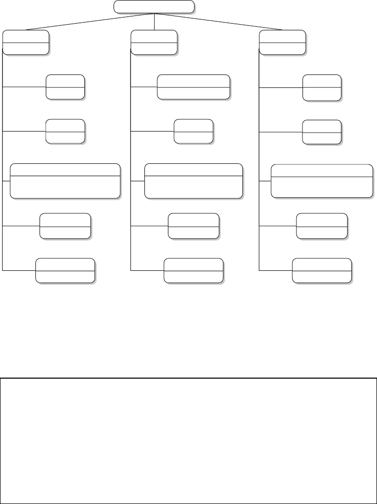
XML AND JSON 47
<bond_movies>
<movie>
id="1"
<movie>
id="2"
<movie>
id="3"
<title>
Dr. No
<year>
1962
<actors>
bond="Sean Connery"
villain="Joseph Wiseman"
<budget>
1.1M
<boxofce> <boxofce><boxofce>
59.9M
<title>
Live and Let Die
<year>
1973
<actors>
bond="Roger Moore"
villain="Yaphet Kotto"
<budget>
7M
126.4M
<title>
Skyfall
<year>
2012
<actors>
bond="Daniel Craig"
villain="Javier Bardem"
<budget>
175M
1108.6M
Figure 3.2 Tree perspective on an XML document
Elements must be strictly nested, which means that no cross-nesting is allowed. An illegal
document structure would be:
1<family>
2<father>Jack</father>
3<mother>Josephine</mother>
4<child>Jonathan
5<family>
6<mother>Julia</mother>
7<child>Jeff</child>
8</family>
9</family>
10 </child>
While it is theoretically sensible that the element <child> with the value Jonathan
opens a new <family> branch containing Jonathan’s wife Julia and their child Jeff,
Jonathan’s <child> element has to be closed before the <family> element.

48 AUTOMATED DATA COLLECTION WITH R
3.2.3 Naming and special characters
One of the strengths of XML is that we are basically free to chose the names of elements.Element names
However, there are some naming rules:
rElement names can be composed of letters, numbers, and other characters, like
in <name1> …</name1>. Special characters like ¨
a, ¨
o, ¨
u, ´
e, `
e, or `
a are allowed,
but not recommended—they might limit the compatibility of XML les across
systems.
rNames must not start with a number, like in <123name> …</123name>.
rNames must not start with a punctuation character, like in <.name> …</.name>.
rNames must not start with the letters xml (or XML, or Xml, etc.), like in
<xml.rootname> …</xml.rootname>.
rElement names and attribute names are case sensitive. <movie> is not the same as
<MOVIE> or <Movie>.
rNames must not contain spaces, like in <my family> …</my family>.
As in HTML, there are some characters that cannot be used literally in the content as they
are needed for markup. To represent these characters in the content, they have to be replaced
by escape sequences. These entities are listed in Table 3.1 and used as follows
1<actor protagonist="Scarlett O'Hara"/>
2<math_wisdom>pi>3</math_wisdom>
You do not always need to escape special characters. For example, apostrophes are
sometimes left unescaped, like in "Richard 'Jaws' Kiel" in the example above. In this
case, the apostrophes are unambiguous because the attribute value is enclosed by double
quotes. Using apostrophes in XML element values is usually no problem either, because
they have no special meaning in the value slot of the element, only inside tags as limiters to
attribute values.
Table 3.1 Predened entities in XML
Character Entity reference Description
< < Less than
> > Greater than
& & Ampersand
" " Double quotation mark
' ' Single quotation mark
XML AND JSON 49
3.2.4 Comments and character data
XML provides a way to comment content with the syntax Comments
1<!-- an arbitrary comment -->
Everything in between <!-- and --> is not treated as part of the XML code and therefore
ignored by parsers. Comments may be used between tags or within element content, but not
within element or attribute names.
The use of escape sequences can be cumbersome when the elements to be escaped are
common in the data values. For example, imagine the following character sequence needs to
be stored in an XML le
11 < 3 < pi < 9 <= sqrt(81) < 1'081 > -2 > -999
In XML code, this would translate to
11 < 3 < pi < 9 <= sqrt(81) < 1'081 > -2 > -999
To avoid this mess, XML provides an environment that prevents the content from being CDATA
interpreted. It is called CDATA andworksasfollows
1<![CDATA[
21 < 3 < pi < 9 <= sqrt(81) < 1'081 > -2 > -999
3]]>
All characters in the CDATA section are taken as is. The difference between comments
and a CDATA section is that a comment is not part of the document …
1<?xml version="1.0" encoding="ISO-8859-1"?>
2<bond_movies>
3<movie id="1">
4<title>Dr. No</title>
5<year>1962</year>
6<actors bond="Sean Connery" villain="Joseph Wiseman"/>
7<budget>1.1M</budget>
8<boxoffice>59.5M</boxoffice>
9</movie>
10 <!-- more movies & details to follow here! -->
11 </bond_movies>

50 AUTOMATED DATA COLLECTION WITH R
…whereas a CDATA section is:
1<?xml version="1.0" encoding="ISO-8859-1"?>
2<bond_movies>
3<movie id="1">
4<title>Dr. No</title>
5<year>1962</year>
6<actors bond="Sean Connery" villain="Joseph Wiseman"/>
7<budget>1.1M</budget>
8<boxoffice>59.5M</boxoffice>
9<deadpeople>
10 <![CDATA[
11 "John Strangways" & "Chauffeur" & "Prof R.J. Dent"
12 & "Quarrel" & "Dr. No"
13 ]]>
14 </deadpeople>
15 </movie>
16 </bond_movies>
If we write both snippets in an XML le and open it with a browser, the comments are not
displayed or explicitly highlighted as part of the XML tree. In contrast, the CDATA section
is displayed in the tree. If we delete the CDATA tags, this will produce an error because the
browser fails to interpret the ampersands and quotation marks.
You may want to try this out yourself. Save the last code snippet with your text editor as
an XML le and open it with your browser. Modify the content of the XML le, save it, and
reload the content with the browser. Experiment with allowed and disallowed changes. Try
special characters, cross-nested tags, and forbidden element names.
3.2.5 XML syntax summary
To sum up, the XML syntax comprises the following set of rules:
1. An XML document must have a root element.
2. All elements must have a start tag and be closed, except for the declaration, which is
not part of the actual XML document.
3. XML elements must be properly nested.
4. XML attribute values must be quoted.
5. Tags are named with characters and numbers, but may not start with a number or
“xml.”
6. Tag names may not contain spaces and are case sensitive.
7. Space characters are preserved.
8. Some characters are illegal and have to be replaced by meta characters.

XML AND JSON 51
9. Comments can be included as follows: <!-- comment -->.
10. Content can be excluded from parsing using: <![CDATA[...]]>.
3.3 When is an XML document well formed or valid?
In short, an XML document is well formed when it follows all of the syntax rules from the Well-formed
and valid XML
previous section. Techniques to extract information from XML documents rely on properly
written syntax. If we are in doubt that an XML document is well formed, there are ways
to check. For instance, the XML Validator on http://www.xmlvalidation.com/ checks for
mismatches between start and end tags, whether attribute values are quoted, whether illegal
characters have been used, in short: whether any of the rules are violated.
We can distinguish between well formed and valid XML. An XML document is valid The Document
Type Denition
(DTD)
when it
1. is well formed and
2. conforms to the rules of a Document Type Denition.
As we have seen, the structure of an XML document is arbitrary—tag names and levels
of hierarchy are dened by the user. However, there is a way to restrict this arbitrariness by
using Document Type Denitions, DTDs. A DTD is a set of declarations that denes the
XML structure, how elements are named, and what kind of data they should contain. A DTD
for our running example in Figure 3.1 could look like this
1<?xml version="1.0" encoding="ISO-8859-1"?>
2<!DOCTYPE bond_movies [
3<!ELEMENT bond_movies (movie)>
4<!ELEMENT movie (title,year,actors,budget,boxoffice)>
5<!ELEMENT title (#PCDATA)>
6<!ELEMENT year (#PCDATA)>
7<!ELEMENT actors (#PCDATA)>
8<!ELEMENT budget (#PCDATA)>
9<!ELEMENT boxoffice (#PCDATA)>
10 <!ATTLIST actors
11 bond CDATA #IMPLIED
12 villain CDATA #IMPLIED>
13 <!ATTLIST movie id CDATA #IMPLIED>
14 ]>
15 <bond_movies>
16 ...
17 <\bond_movies>
In this variant, the DTD is included in the XML document and wrapped in a DOCTYPE
denition, <!DOCTYPE bond_movies [...]>. This is called an internal DTD. For the
purpose of web scraping we normally do not need to be able to write DTDs, so we will
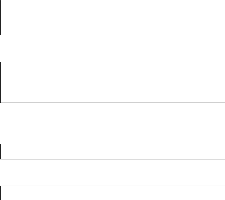
52 AUTOMATED DATA COLLECTION WITH R
not explain every detail of the declaration syntax but just provide some fundamentals on the
appearance of DTDs. Elements can be declared like
1<!ELEMENT element (#PCDATA)> <!-- element contains only parsed
character data -->
2<!ELEMENT element ANY> <!-- element contains any data that can be
parsed -->
Children of elements are declared as follows
1<!ELEMENT element (child1,child2,child3,...)>
2<!ELEMENT element (child1)> <!-- child occurs only once -->
3<!ELEMENT element (child1+)> <!-- child occurs 1 or more times -->
4<!ELEMENT element (child1*)> <!-- child occurs 0 or more times -->
5<!ELEMENT element (child1?)> <!-- child occurs at most once -->
It gets a bit more complicated with the declaration of mixed content. If, for example, an
element contains one or more occurrences of the <child1> to <child3> elements or simply
parsed character data, the declaration would look like
1<!ELEMENT element (child1|child2|child3|#PCDATA)+>
Declaring attributes can look as follows
1<!ATTLIST element attribute CDATA #IMPLIED>
The IMPLIED attribute value means that the corresponding attribute is optional; REQUIRED
would mean that the attribute is required. There are multiple online tools that allow validating
XML les against a DTD. Just type “dtd validation” into a search engine and pick one of the
rst results.
Why should we care whether an XML document is well formed or valid? Above all,
it is important to know that many les come with an internal DTD at the beginning of the
document. In general, DTDs serve several purposes. Data exchanges can be standardized as
senders and receivers know in advance what they are supposed to send and get. As a sender,
you can check if your own XML les are valid. As a receiver it is possible to check whether
the XML you retrieve is of the kind you or your program expects.
DTD itself is only one of several XML schema languages. Such languages help to describe
XML schemas
and constrain the structure and content of an XML document. Another schema language is
XML Schema (XSD), developed by W3C. It allows dening a schema in XML syntax and
has some merits that are of little interest for our purposes. One area where XML schemas
play an important role is XML extensions, which are the topic of the next section.
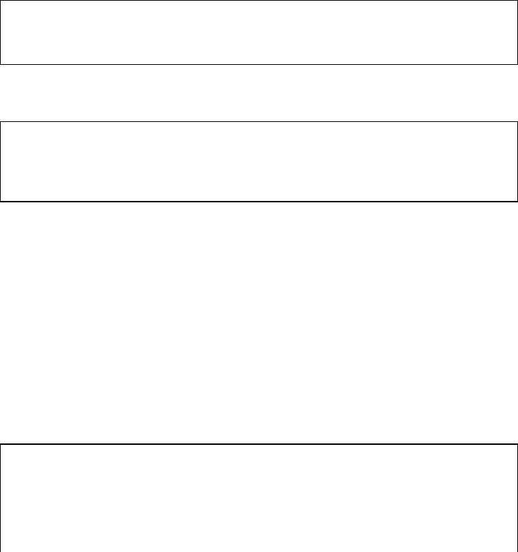
XML AND JSON 53
3.4 XML extensions and technologies
We have seen that XML has advantages compared to HTML for exchanging data on the
Web as it is extensible—and thus exible. However, exibility also carries the potential
for uncertainty or inconsistency, for example, when the same element names are used for
different content. Several extensions and technologies exist that improve the usability of
XML by suggesting standards or providing techniques to set such standards. Some of the
most important of these techniques are described in this section.
3.4.1 Namespaces
Consider the following two pieces of HTML and XML:
1<head>
2<title>Basic HTML Sample Page</title>
3</head>
1<book id="1">
2<author>Douglas Crockford</author>
3<title>JavaScript: The Good Parts</title>
4</book>
Both pieces store information in the element <title>. If the XML code were embedded
in HTML code, this might create confusion. As we will see, there are many XML extensions
to store specic data, for example, geographic, graphical, or nancial data. All of these
languages are basically XML with limited vocabulary. When several of these XML-based
languages are used in one document, element or attribute names can become ambiguous if
they are multiply assigned. XML namespaces are used to circumvent such problems. The
idea is very simple: Ambiguous elements become distinguishable if some unique identier is
added. Just like zip codes allow distinguishing between many different Springelds and area
codes make phone numbers unambiguous, namespaces help make elements and attributes
uniquely identiable.
The implementation of namespaces is straightforward:
1<root xmlns:h="http://www.w3.org/1999/xhtml"
2xmlns:t="http://funnybooknames.com/crockford">
4<h:head>
5<h:title>Basic HTML Sample Page</h:title>
6</h:head>

54 AUTOMATED DATA COLLECTION WITH R
8<t:book id="1">
9<t:author>Douglas Crockford</t:author>
10 <t:title>JavaScript: The Good Parts</t:title>
11 </t:book>
13 </root>
In this example, namespaces are declared in the root element using the xmlns attribute
and two prexes, hand t. The namespace name, that is, the namespace attribute value, usually
carries a Uniform Resource Identier (URI) that points to some Internet address. The URIs
in the example are two URLs that refer to an existing Internet resource on the W3C homepage
and the ctional domain funnybooknames.com. When dealing with namespaces, note the
following rules:
(i) Namespaces can be declared in the root element or in the start tag of any other
element. In the latter case, all children of this element are considered part of this
namespace.
(ii) The namespace name does not necessarily have to be a working URL. Parsers will
never try to follow the link, not even a URI. Any other string is ne. However, it is
common practice to use URIs for two reasons: First, as they are a long, unique string
of characters, duplicates are unlikely, and second, actual URLs can point the human
reader to pages where more information about the namespace is given.5
(iii) Prexes do not have to be explicitly stated, so the declaration can either be xmlns
or xmlns:prefix . If the prex is dropped, the xmlns is assumed to be the default
namespace and any element without a prex is considered to be in that namespace.
When prexes are used, it is bound to a namespace in the declaration. Attributes,
however, never belong to the default namespace.
3.4.2 Extensions of XML
Thus far, we have praised XML for its exibility and extensibility. However, standardization
also has its benets in data exchange scenarios. Recall how browsers deal with HTML. They
“know” what a table looks like, how headings should be formatted, and so on. In general,
many data exchange processes can be standardized because sender and recipient agree on the
content and structure of the data to be exchanged.
Following this logic, a multitude of extensions of the XML language has been developed
that combine the classical XML features of openness with the benets of standardization. In
that sense, XML has become an important metalanguage—it provides the general architecture
for other XML markup languages. Varieties of XML rely on XML schemas that specify
5When the same URL is used again and again—such as http://www.w3.org/1999/xhtml—this reduces the
usefulness of namespaces. Therefore, one should think of references to locations one has full control over, like an
owned web domain where a DTD or XML schema is stored.

XML AND JSON 55
Table 3.2 List of popular XML markup languages
Name Purpose Common lename extensions
Atom web feeds .atom
RSS web feeds .rss
EPUB open e-book .epub
SVG vector graphics .svg
KML geographic visualization .kml, .kmz
GPX GPS data (waypoint, tracks, routes) .gpx
Ofce Open XML Microsoft Ofce documents .docx, .pptx, .xlsx
OpenDocument Apache OpenOfce documents .odt, .odp, .ods, .odg
XHTML HTML extension and standardization .xhtml
For a more comprehensive list, see http://en.wikipedia.org/wiki/List_of_XML_markup_languages.
allowed structure, elements, attributes, and content. Table 3.2 lists some of the most popular
XML derivations. Among them are languages for geographic applications like KML or GPX
as well as for web feeds and widely used ofce document formats. You might be surprised
to nd that MS Word makes heavy use of XML. To gain basic insight into XML extensions
that are ubiquitous on the Web, we focus on two popular XML markup languages—RSS
and SVG.
3.4.3 Example: Really Simple Syndication
Web users commonly cultivate a list of bookmarks of their favorite webpages. It can be rather
tiresome to regularly check for new content on the sites. Really Simple Syndication (RSS)6
was built to solve this problem—both for the user and the content providers. The basic idea
is that news sites, blog owners, etc., convert their content into a standardized format that can
be syndicated to any user.
We illustrate the logic of RSS in Figure 3.3. Authors of a blog or news site set up an RSS The logic of
RSS
le that contains some information on the news provider, which is stored on a web server.
The le is updated whenever new content is published on the blog. Both are usually done
by an RSS creation program like RSS builder. The list of entries or notications is often
called RSS feed or RSS channel and might be located at http://www.example.net/feed.rss.Itis
written in XML that follows the rules of the RSS format. Common elements that are allowed
in this XML avor are listed in Table 3.3. There are elements that describe the channel and
others that describe single entries. Users collect channels by subscribing to an RSS reader
or aggregator like Feedly, which automatically locates the RSS feed on a given website and
lays out the content. These readers automatically update subscribed feeds and offer further
management functionalities. This way, users are able to assemble their own online news.
There are several versions of RSS, the current one being RSS 2.0. RSS syntax has remained
fairly simple, especially for users who are familiar with XML. The rules are strict, that is,
6Originally, RSS was an abbreviation of RDF Site Summary and was later redened as Rich Site Summary. In
2002, it was redubbed again to Really Simple Syndication.
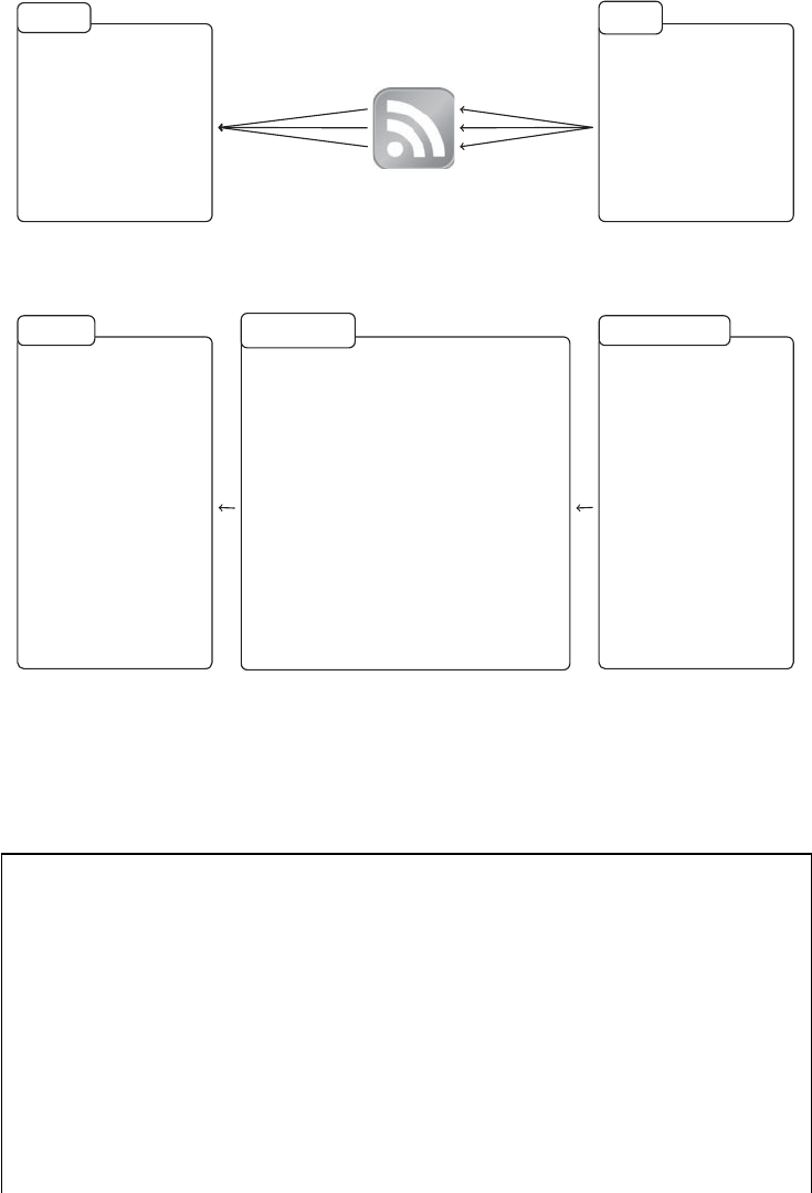
56 AUTOMATED DATA COLLECTION WITH R
Schema
• Subscription to feeds
• Use of browser, desktop
or mobile RSS readers
• RSS reader manages
subscriptions, parses
feeds, offers handsome
display of content
Demand
Syndication
Aggregation
RSS • Blogs, news media,
audio, video, . . .
• Stored on web server
• Standardization of
content in RSS channel
• Provides full or summa-
rized content, metadata
Supply
Example
The squirrels blog
A squirrel’s daily business
October 23, 2013
Today, I saw a squirrel in
the . . .
.
.
.
The ADCR blog
Scraping the NFL
October 23, 2013
Today’s finger exercise
will be to scrape historical
data from NFL games . . .
End user
<rss version="2.0">
<channel>
<title>The squirrels blog</title>
<link>http://www.cutesquirrels.com/</link>
<description>All about squirrels!
</description>
<item>
<title>A squirrel’s daily business</title>
<link>http://www.cutesquirrels.com/131023
</link>
<description>Today, I saw a squirrel in
the ... </description>
</item>
.
.
.
</channel>
</rss>
RSS/XML file
A squirrel’s daily business
October 23, 2013
Today, I saw a squirrel
in the neighbor’s garden
collecting food for the
winter.
Squirrelogy #127: breeding
October 26, 2013
This time in our popular
squirrelogy section, I want
to talk about the breeding
behavior of . . .
Website content
Figure 3.3 How RSS works
there is a very limited set of allowed elements and a clear document structure. Consider the
following example of a ctional RSS channel accompanying this book:
1<?xml version="1.0" encoding="UTF-8" ?>
2<rss version="2.0">
3<channel>
4<title>The ADCR blog</title>
5<description>Blog to the ADCR book; Wiley 2014</description>
6<link>http://www.r-datacollection.com/blog</link>
7<lastBuildDate>Tue, 22 Oct 2013 00:01:00 +0000 </lastBuildDate>
8<item>
9<title>Why R is useful for web scraping</title>
10 <description>R is becoming the most popular statistical
software and is growing fast due to an active community
publishing several additional packages every day. Yet,
R is more than [...]</description>
XML AND JSON 57
11 <link>http://www.r-datacollection.com/blog/why-r-is-useful</link>
12 <pubDate>Tue, 22 Oct 2013 00:01:00 +0000 </pubDate>
13 </item>
14 </channel>
15 </rss>
RSS documents start with an XML and RSS declaration in the rst two lines. The
<channel> element wraps around both meta information and the actual entries. The channel’s
meta block has three required elements—<title>,<description>, and <link>.Inthe
example, there is another optional element, <lastBuildDate>, that indicates the last time
content was changed on the channel. The content block consists of a set of <item> elements.
Whenever a new story, blog entry, etc., is published, a new <item> element is added to
the feed. <item> elements have three obligatory children—again, they are called <title>,
<description>, and <link>. The main content is usually stored in the <description>
element. Sometimes the whole entry is stored here, sometimes just the rst few lines or a
summary. In general, RSS syntax obeys the same set of rules as XML syntax.
Table 3.3 List of common RSS 2.0 elements and their meaning
Element name Meaning
root elements
rss The feed’s root element
channel A channel’s root element
channel elements
description* Short statement describing the feed
link* URL of the feed’s website
title* Name of the feed
item The core information element: each item contains an entry of the feed
item elements
link* URL of the item
title* Title of the item
description* Short description of the item
author Email address of the item’s author
category Classication of item’s content
enclosure Additional content, for example, audio
guid Unique identier of the item
image Display of image (with children <url>, <title>, and <link>)
language Language of the feed
pubDate Publishing date of item
source RSS source of the item
ttl “Time-to-live,” number of minutes until the feed is refreshed from the
RSS
Elements marked with “*” are mandatory. For more information on RSS 2.0 specication, see
http://www.rssboard.org/rss-specication

58 AUTOMATED DATA COLLECTION WITH R
1<?xml version="1.0" standalone="no"?>
2<!DOCTYPE svg PUBLIC "-//W3C//DTD SVG 1.1//EN"
3"http://www.w3.org/Graphics/SVG/1.1/DTD/svg11.dtd">
5<svg xmlns="http://www.w3.org/2000/svg" version="1.1">
6<ellipse cx="100" cy="70" rx="100" ry="70" style="fill:grey"/>
7<ellipse cx="110" cy="75" rx="80" ry="50" style="fill:white"/>
8<text x="65" y="160" fill="blue" style="font-size:160; font-stretch:
ultraexpanded;font-family:sans;font-weight:bold">R</text>
9</svg>
Figure 3.4 SVG code example: Rlogo
Take a moment to look at actual RSS feeds. They are all around the Web and indi-
cated with the RSS icon ( ). There are several popular news and blogging platforms
about R. For example, have a look at http://planetr.stderr.org/ where new Rpackages are
posted (via Dirk Eddelbuettel’s CRANberries blog http://dirk.eddelbuettel.com/cranberries/),
and at http://www.r-bloggers.com/, a meta-blogging platform that collects content from the
Rblogosphere.
RSS 2.0 is not the only content syndication format. Besides various predecessors, another
popular standard is Atom, which is also XML-based and has a very similar syntax. In order
to grab RSS feeds into R, we can use the same XML extraction tools that are presented in
Section 3.5.
3.4.4 Example: scalable vector graphics
A more peculiar but incredibly popular extension of XML is scalable vector graphics (SVG).
SVG is used to represent two-dimensional vector graphics. It has been developed at the W3C
since 1999 and was initially released in 2001 (Dailey 2010). The idea was to create a vector
graphic format that stores graphic information in lightweight, exible form for exchange over
the Web.
Vector graphic formats consist of basic geometric forms such as points, curves, circles,
Vector graphics
versus raster
graphics
lines, or polygons, all of which can be expressed mathematically. In contrast, raster graphic
formats store graphic information as a raster of pixels, that is, rectangular cells of a certain
color. In contrast to raster graphics, vector graphics can be resized without any loss of
quality and are usually smaller. As the SVG format is based on XML, SVG graphics can
be manipulated with an ordinary text editor. There are, however, SVG editors that simplify
this task. For example, Inkscape is an open-source graphics editor that implements SVG by
default and runs on all common operating systems.7In order to view SVG les, we can use
current versions of the common browsers.
To get a rst impression of how SVG works, Figure 3.4 provides code of a small SVG
An SVG
example le. This code generates a stylized representation of the Ricon just like the one displayed
in Figure 3.5. In fact, if we open an SVG le with the content of the sample code with our
browser, we see the graphic shown in Figure 3.5. The syntax does not only resemble XML, it
7See http://inkscape.org/ for further information and download.

XML AND JSON 59
Figure 3.5 The Rlogo as SVG image from code in Figure 3.4
is XML with a limited set of legal elements and attributes. An SVG le starts with the usual
XML declaration. The standalone attribute indicates that the document refers to an external
le, in this case an external DTD in lines 2 and 3. This DTD is stored at the www.w3.org
webpage and describes which elements and attributes are legal in the current SVG version 1.1
(as of March 2014). The actual SVG code that describes the graphic is enclosed in the <svg>
element. It contains a namespace and a version attribute.
SVG uses a predened set of elements and attributes to represent parts of a graphic SVG basics
(‘SVG shapes’). Among the basic shapes of SVG are lines (<line>), rectangles (<rect>),
circles (<circle>), ellipses (<ellipse>), polygons (<polygon>), (<text>), and, the most
general of all, paths (<path>). Each of these elements comes with a specic set of attributes
to tune the object’s properties, for example, the position of the corners, the size and radius
of a circle, and so on. Elements are placed on a virtual coordinate system, with the origin
(0,0) in the upper-left corner. Formatted text can also be placed into the graphic. The order
of elements is important. A later-listed element covers a previous element—elements can
therefore be thought of as layers. Further, there is a palette of special effects like blurs or
color gradients. Elements can even be animated. A complex SVG graphic is often generated
by quite complex SVG code. The complexity usually does not stem from a highly hierarchical
structure—most of the elements are often just children of the root element—but from the
mass of elements and their attributes. Our basic graphic in Figure 3.5 is composed of only
three elements—two ellipses and one text element. By default, elements come in the compact
form of XML element syntax: Elements are usually empty and contain no further information
than those given in the attributes.
Back to the example, the locations of the ellipses are dened by their attributes cx and
cy, their shape by the horizontal and vertical radius in rx and ry. Colors and other effects
can be passed via arguments in the style attribute. The white ellipse is plotted on the top
of the grey ellipse simply because it appears second in the code, creating the donut effect.
Finally, shape, color, font, and location of the “R” is dened in the <text> element.
Beyond the principle advantages of vector over raster graphics, SVG, in particular, has SVG and the
Web
some features that make it attractive as a graphic standard on the Web: It can be edited with
any text editor, opened with the common browsers, follows a familiar syntax as it is basically
just XML, and has been developed for a wide range of applications. We have learned that
XML is exible but because of the exibility cannot be interpreted further by a browser. This
is not true for XML extensions such as SVG. As the set of elements and attributes is clearly
dened, browsers can be programmed to display SVG content as meaningful graphic, not as

60 AUTOMATED DATA COLLECTION WITH R
code—just as they interpret and display HTML code. In HTML5, SVG graphics can even be
embedded as simply as this
1<html>
2<body>
3<svg><rect width="300" height="100"/> </svg>
4</body>
5</html>
Why could SVG be useful in the context of automated data collection? At rst glance, SVGSVG is useful
for data
gatherers
is a exible and widely used vector graphics format. From the data collection perspective,
however, it is more than that. The information in these graphs—and often more than just the
visible parts—are stored in text form and can therefore be searched, subsetted, etc. SVG is
becoming more and more popular on the Web and is used for increasingly complex tasks,
for example, to store geographic information, create interactive maps, or visualize massive
amounts of data.8
The takeaway message of these two examples is that XML is present in many different
areas, and many of these applications hold potentially useful information. And the neat thing
is: We will learn how easy it is to retrieve and process this information with R, regardless of
whether the information is stored in “pure” XML or any of its extensions.
3.5 XML and Rin practice
Let us now turn to practice. How can XML les be viewed, how can they be imported and
accessed in an Rsession, and how can we convert information from an XML document
into data structures that are more convenient for further graphical or statistical analysis, like
ordinary data frames, for example?
As we said before, XML les can be opened and viewed in all text editors and browsers.
However, while text editors usually take the XML le as is, modern web browsers automati-
cally parse the XML and try to represent its structure. This fails when the XML document is
not valid. In this case, the browser might tell you why it thinks the parsing failed, for example,
because of an opening and ending tag mismatch on a certain line. From this perspective, the
web browser is a decent tool to check if your XML is well formed. In standard web scraping
tasks, we usually do not view XML documents le by le but download them in a rst step
and import them into our Rworkspace in a second (see Chapter 9).
3.5.1 Parsing XML
We parse XML for the same reason that we parse HTML documents (see Section 2.4.1),
to create a structure-aware representation of XML les that allows a simple information
8To learn more about SVG check out Eisenberg (2002) and the elucidations on the W3C pages: http://www.w3
.org/Graphics/SVG/. For a quick access to the language, the SVG primer by Dailey (2010) should prove useful.

XML AND JSON 61
1<?xml version="1.0"?>
2<!DOCTYPE document SYSTEM "technologystocks.dtd">
3<document>
4<Apple>
5<date>2013/11/13</date>
6<close>520.634</close>
7<volume>7022001.0000</volume>
8<open>518</open>
9<high>522.25</high>
10 <low>516.96</low>
11 <company>Apple</company>
12 <year>2013</year>
13 </Apple>
14 <Apple>
15 <date>2013/11/12</date>
16 <close>520.01</close>
17 <volume>7295400.0000</volume>
18 <open>517.67</open>
19 <high>523.92</high>
20 <low>517</low>
21 <company>Apple</company>
22 <year>2013</year>
23 </Apple>
24 (...)
25 </document>
Figure 3.6 XML example document: stock data
extraction from these les. Similar to what was outlined in the HTML parsing section, the
process of parsing XML essentially includes two steps. First, the symbol sequence that
constitutes the XML le is read in and used to build a hierarchical tree-like data structure
from its elements in the C language, and second, this data structure is translated into an R
data structure via the use of handlers.
The package we use to import and parse XML documents is, appropriately enough, called
XML (Temple Lang 2013c). Using the XML package we can read, search, and create XML
documents—although we only care about the former two tasks. Let us see how to load XML
les into R. For DOM-style parsing of XML les one can use xmlParse(). The arguments
of the function coincide with those of htmlParse() for the most part. We illustrate the
process with the help of technology.xml, an XML le that holds stock information for three
technology companies. The rst few lines of the document are presented in Figure 3.6. As
we see, the le contains stock information like the closing value, lowest and highest value for
a day, and the traded volume. To obtain the XML tree with R, we pass the path of the le to
xmlParse()’s file argument:
R> library(XML)
R> parsed_stocks <- xmlParse(file = "stocks/technology.xml")

62 AUTOMATED DATA COLLECTION WITH R
1<!ELEMENT document (Apple,IBM,Google)>
2<!ELEMENT Apple (date,close,volume,open,high,low,company,year)>
3<!ELEMENT Google (date,close,volume,open,high,low,company,year)>
4<!ELEMENT IBM (date,close,volume,open,high,low,company,year)>
5<!ELEMENT close (#PCDATA)>
6<!ELEMENT company (#PCDATA)>
7<!ELEMENT date (#PCDATA)>
8<!ELEMENT high (#PCDATA)>
9<!ELEMENT low (#PCDATA)>
10 <!ELEMENT open (#PCDATA)>
11 <!ELEMENT volume (#PCDATA)>
12 <!ELEMENT year (#PCDATA)>
Figure 3.7 DTD of stock data XML le (see Figure 3.6)
The xmlParse() function is used to parse the XML document.9The parsing function
offer a set of options that can be ignored in most settings but are still worth knowing. It is
possible to treat the input as XML and not as a le name (option asText), to decide whether
both namespace URI and prex should be provided on each node or just the prex (option
fullNamespaceInfo), to determine whether an XML schema is parsed (option isSchema),
or to validate the XML against a DTD (option validate). Let us consider this last option in
more detail.
Although HTML and XML are very similar in most respects, a noteworthy difference
XML
validation exists in that XML is conned to much stricter specication rules. As we have seen in
Section 3.3, valid XML not only has to be well formed, that is, tags must be closed, attributes
names must be in quotes, etc., but also has to adhere to the specications in its DTD. To check
whether the document conforms to the specication, a validation step can be included after
the DOM has been created by setting the validate argument to TRUE. We try to validate
technology.xml with the corresponding external technologystocks.dtd (see Figure 3.7), which
is deposited in our folder and referred to in line 2 of the XML le (see Figure 3.6):
R> library(XML)
R> parsed_stocks <- xmlParse(file = "stocks/technology.xml", validate = TRUE)
There is no complaint; the validation has succeeded. To demonstrate what happens if an
XML does not conform to a given DTD, we manipulate the DTD such that the document node
is no longer dened. As a consequence, the XML le does not conform to the (corrupted)
DTD anymore and the function raises a complaint:
R> library(XML)
R> stocks <- xmlParse(file = "stocks/technology-manip.xml", validate = TRUE)
No declaration for element document
Error: XML document is invalid
9The XML package provides a set of other XML parsing functions, namely xmlTreeParse(),
xmlInternalTreeParse(),xmlNativeTreeParse(),andxmlEventParse(). As their names suggest, they
differ in the way how the XML tree is parsed. xmlInternalTreeParse() and xmlNativeTreeParse() are
equivalent to xmlParse(). Further, all are almost equivalent to xmlTreeParse(), except that the parser automat-
ically relies on the internal nodes (the useInternalNodes parameter is set TRUE).
XML AND JSON 63
In general, the rather bulky logic of XML validation with DTD, XSD, or other schemas
should not discourage you from making use of the full power of the XML DOM structure. In
most web scraping scenarios, there is no need to validate the les and we can simply process
them as they are.
3.5.2 Basic operations on XML documents
Once an XML document is parsed we can access its content using a set of functions in the
XML package. While we recommend using the more general and robust XPath for searching
and pulling out information from XML documents, here we present some basic operations
that might sufce for less complex XML documents. To see how they work, let us go back to
our running example: We start by parsing the bond.xml le:
R> bond <- xmlParse("bond.xml")
R> class(bond)
[1] "XMLInternalDocument" "XMLAbstractDocument"
When we type bond into our console, the output looks pretty much like the original XML
le. We know, however, that the object is anything but pure character data. For instance, we
can perform some basic operations on the root element. The top-level node is extracted with
the xmlRoot() function; xmlName() and xmlSize() return the root element’s name and
the number of children:
R> root <- xmlRoot(bond)
R> xmlName(root)
[1] "bond_movies"
R> xmlSize(root)
[1] 3
Within the node sets, basic navigation or subsetting works in analogy to indexing ordinary Navigation
lists in R. That is, we can use numerical or named indices to select certain nodes. This is not
possible with objects of class XMLInternalDocument that are generated by xmlParse().
We therefore work with the root object, which belongs to the class XMLInternalEle-
mentNode. Indexing with predicate “1” yields the rst child:
R> root[[1]]
<movie id="1">
<name>Dr. No</name>
<year>1962</year>
<actors bond="Sean Connery" villain="Joseph Wiseman"/>
<budget>1.1M</budget>
<boxoffice>59.5M</boxoffice>
</movie>
We have to use double brackets to access the internal node. By adding another index, we
can move further down the tree and extract the rst child of the rst child:
R> root[[1]][[1]]
<name>Dr. No</name>
64 AUTOMATED DATA COLLECTION WITH R
Element names can be used as predicates, too. Using double brackets yields the rst
element in the tree, single brackets return objects of class XMLInternalNodeList.Tosee
the difference, compare
R> root[["movie"]]
<movie id="1">
<name>Dr. No</name>
<year>1962</year>
<actors bond="Sean Connery" villain="Joseph Wiseman"/>
<budget>1.1M</budget>
<boxoffice>59.5M</boxoffice>
</movie>
with
R> root["movie"]
$movie
<movie id="1">
<name>Dr. No</name>
<year>1962</year>
<actors bond="Sean Connery" villain="Joseph Wiseman"/>
<budget>1.1M</budget>
<boxoffice>59.5M</boxoffice>
</movie>
$movie
<movie id="2">
<name>Live and Let Die</name>
<year>1973</year>
<actors bond="Roger Moore" villain="Yaphet Kotto"/>
<budget>7M</budget>
<boxoffice>126.4M</boxoffice>
</movie>
$movie
<movie id="3">
<name>Skyfall</name>
<year>2012</year>
<actors bond="Daniel Craig" villain="Javier Bardem"/>
<budget>175M</budget>
<boxoffice>1108.6M</boxoffice>
</movie>
attr(,"class")
[1] "XMLInternalNodeList" "XMLNodeList"
Names and numbers can also be combined. To return the atomic value of the rst <name>
element, we could write
R> root[["movie"]][[1]][[1]]
Dr. No
XML AND JSON 65
The structure of the object is retained and can be used to locate elements and values. How-
ever, content retrieval from XML les via ordinary predicates is quite complex, error prone,
and anything but convenient. Further, this method does not capitalize on node relations—a
core feature of parsed XML documents. For anybody who is seriously working with XML
data, there are good reasons to learn the very powerful query language XPath. We will show
how this is done in the next chapter.
In general, all methods and all those to follow are applicable to other XML-based lan- Accessing
documents of
the XML
family
guages as well. The parser does not care about naming and structure of documents as long as
the code is valid. Therefore, documents like the RSS sample code from above can be imported
just as easy as
R> xmlParse("rsscode.rss")
<?xml version="1.0" encoding="UTF-8"?>
<rss version="2.0">
<channel>
<title>The ADCR blog</title>
<description>Blog to the ADCR book; Wiley 2014</description>
<link>http://www.r-datacollection.com/blog</link>
<lastBuildDate>Tue, 22 Oct 2013 00:01:00 +0000 </lastBuildDate>
<item>
<title>Why R is useful for web scraping</title>
<description>R is becoming the most popular statistical software
and is growing fast due to an active community publishing several
additional packages every day. Yet, R is more than [...]</description>
<link>http://www.r-datacollection.com/blog/why-r-is-useful</link>
<pubDate>Tue, 22 Oct 2013 00:01:00 +0000 </pubDate>
</item>
</channel>
</rss>
3.5.3 From XML to data frames or lists
Sometimes it sufces to transform an entire XML object into common Rdata structures like
vectors, data frames, or lists. The XML package provides some appropriate functions that
make such operations straightforward if the original structure is not too complex.
Single vectors can be extracted with xmlSApply(), a wrapper function for lapply()
and sapply() that is built to deal with children of a given XML node. The function operates
on an XML node (provided as rst argument), applies any given function on its children
(given as the second argument), and commonly returns a vector. We can use the function in
combination with xmlValue() and xmlGetAttr() (and other functions; see Table 4.4) to
extract element or attribute values:
R> xmlSApply(root[[1]], xmlValue)
name year actors budget boxoffice
"Dr. No" "1962" "" "1.1M" "59.5M"
R> xmlSApply(root, xmlAttrs)
movie.id movie.id movie.id
"1" "2" "3"
R> xmlSApply(root, xmlGetAttr, "id")
movie movie movie
"1" "2" "3"
66 AUTOMATED DATA COLLECTION WITH R
As long as XML documents are at in the hierarchical sense, that is, the root node’s most
distant relatives are grandchildren or children, they can usually be transformed easily into a
data frame with xmlToDataFrame()
R> (movie.df <- xmlToDataFrame(root))
name year actors budget boxoffice
1 Dr. No 1962 1.1M 59.5M
2 Live and Let Die 1973 7M 126.4M
3 Skyfall 2012 175M 1108.6M
Note, however, that this function already runs into trouble with the <actor> element,
which is itself empty except for two attributes. The corresponding variable in the data.frame
object is left empty with a shrug.
Similarly, a conversion into a list is possible with xmlToList():
R> movie.list <- xmlToList(bond)
XML and other data exchange formats like JSON can store much more complicated data
structures. This is what makes them so powerful for data exchange over the Web. Forcing
such structures into one common data frame comes at a certain cost—complicated data
transformation tasks or the loss of information. xmlToDataFrame() is not an almighty
function to achieve the task for which it is named. Rather, we are typically forced to develop
and apply own extraction functions.
3.5.4 Event-driven parsing
While parsing the XML example les in Section 3.5.1 was processed quickly by R,les
of larger size can lead to overloaded working memory and concomitant data management
problems. As a format primarily designed for carrying data across services, XML les are
oftentimes of substantially greater size than HTML les. In many instances, le sizes can
exceed the memory capacity of ordinary desktop PCs and laptops. This problem is aggravated
when data streams are concerned, where XML data arrives iteratively. These applications
obstruct the DOM-based parsing approach we have been applying in this and the previous
chapter and demand for a more iterative parsing style.
The root of the problem stems from the way the DOM-style parsers process and store
Event-driven/
SAX parser information. The parser creates two copies of a given XML le—one as the C-level node set
and the second as the data structure in the Rlanguage. To detect certain elements in an XML
le, we can deal with this problem by employing a parsing technique called event-driven
parsing or SAX parsing (Simple API for XML). Event-driven parsing differs from DOM-
style parsing in that it skips the construction of the complete DOM at the C level. Instead,
event-driven parsers sequentially traverse over an XML le, and once they nd a specied
element of interest they prompt an instant, user-dened reaction to this event. This procedure
provides a huge advantage over DOM-style parsers because the machine’s memory never has
to hold the complete document.
Let us reconsider technology.xml and the problem of extracting information about the
Apple stock. Assume we are interested in obtaining Apple’s daily closing value along with
the date. Once again, we make use of a handler function to specify how to handle a node
of interest. Similar to the extraction problem considered in Section 2.4.3, we dene the
handler as a nested function to combine it with a reference environment and container

XML AND JSON 67
1branchFun <- function(){
2container_close <- numeric()
3container_date <- numeric()
5"Apple" = function(node,...) {
6date <- xmlValue(xmlChildren(node)[[c("date")]])
7container_date <<- c(container_date, date)
8close <- xmlValue(xmlChildren(node)[[c("close")]])
9container_close <<- c(container_close, close)
10 #print(c(close, date));Sys.sleep(0.5)
11 }
12 getContainer <- function() data.frame(date=container_date,
close=container_close)
13 list(Apple=Apple, getStore=getContainer)
14 }
Figure 3.8 Rcode for event-driven parsing
variables (see Figure 3.8). branchFun() denes two local variables container_close
and container_date, serving as the container variables. Since we are interested in Apple
stock information, we suggest the following approach: We start by dening a handler function
for the <Apple> nodes (lines 6 and 8). Conditional on these elements, we look for their
children called date and close and return their values (lines 7 and 9). A return function
getContainer() is dened (line 12) that assembles the container variable’s contents into a
data frame and returns this object.
To generate a usable instance of the handler function, we execute the function and pass
its return value into a new object called h5:
R> (h5 <- branchFun())
$Apple
function (node, ...)
{
date <- xmlValue(xmlChildren(node)[[c("date")]])
container_date <<- c(container_date, date)
close <- xmlValue(xmlChildren(node)[[c("close")]])
container_close <<- c(container_close, close)
}
<environment: 0x0000000008c4afa8>
$getStore
function ()
data.frame(date = container_date, close = container_close)
<environment: 0x0000000008c4afa8>
We are now ready to run the SAX parser over our technology.xml le using XML’s
xmlEventParse() function. Instead of the handlers argument we will pass the han-
dler function to the branches argument. The branches is a more general version of the
handlers argument, which allows to specify functions over the entire node content, includ-
ing its children. This is exactly what we need for this task since in our handler function h5
68 AUTOMATED DATA COLLECTION WITH R
we have been making use of the xmlChildren function for retrieving child information.
Additionally, for the handlers argument we need to pass an empty list:
R> invisible(xmlEventParse(file = "stocks/technology.xml",
branches = h5, handlers = list()))
To get an idea about the iterative traversal through the document, remove the commented
line in the handler and rerun the SAX parser. Finally, to fetch the information from the local
environment we employ the getStore() function and route the contents into a new object:
R> apple.stock <- h5$getStore()
To verify parsing success, we display the rst ve rows of the returned data frame:
R> head(apple.stock, 5)
R> # date close 1 2013/11/13 520.634 2 2013/11/12 520.01 3 2013/11/
11 519.048 4
R> # 2013/11/08 520.56 5 2013/11/07 512.492
As we have seen, the event-driving parsing works and returns the correct information.
Nonetheless, we do not recommend users to resort to this style of parsing as their preferred
means to obtain data from XML documents. Although event-style parsing exceeds the DOM-
style parsing approach with respect to speed and may, in case of really large XML les, be the
only practical method, it necessitates a lot of code overhead as well as background knowledge
on Rfunctions and environments. Therefore, for the small- to medium-sized documents that
we deal with in this book, in the coming chapters we will focus on the DOM-style parsing
and extraction methods provided through the XPath query language (Chapter 4).
3.6 A short example JSON document
In this section, we will become acquainted with the benets of the data exchange standard
JSON. The acronym (pronounced “Jason”) stands for JavaScript Object Notation. JSON was
designed for the same tasks that XML is often used for—the storage and exchange of human-
readable data. Many APIs by popular web applications provide data in the JSON format.
As its name suggests, JSON is a data format that has its origins in the JavaScript pro-
gramming language. However, JSON itself is language independent and can be parsed with
many existing programming languages, including R. JSON has turned into one of the most
popular formats for web data provision. It is therefore worth studying for our purposes. We
start again with a synthetic example and continue with a more systematic look at the syntax.
In the nal part of the chapter, we will learn the JSON syntax and how to access JSON data
with R.
The JSON code in Figure 3.9 holds some basic information on the rst three Indiana
Indiana Jones
and the rst
JSON example
Jones movies. We observe that JSON has a more slender appearance than XML. Data are
stored in key/value pairs, for example, "name" : "Raiders of the Lost Ark", which
obviates the need for end tags. Different types of brackets (curly and square ones) allow
describing hierarchical structures and to differentiate between unordered and ordered data.
Just as in XML, JSON data structures can become arbitrarily complex regarding nestedness.
Apart from differences in the syntax, JSON is as intuitive as XML, particularly when indented
like in the example code, although this is no necessary requirement for valid JSON data.

XML AND JSON 69
1{"indy movies" :[
2{
3"name" : "Raiders of the Lost Ark",
4"year" : 1981,
5"actors" : {
6"Indiana Jones": "Harrison Ford",
7"Dr. Ren´
e Belloq": "Paul Freeman"
8},
9"producers": ["Frank Marshall", "George Lucas", "Howard Kazanjian"],
10 "budget" : 18000000,
11 "academy_award_ve": true
12 },
13 {
14 "name" : "Indiana Jones and the Temple of Doom",
15 "year" : 1984,
16 "actors" : {
17 "Indiana Jones": "Harrison Ford",
18 "Mola Ram": "Amish Puri"
19 },
20 "producers": ["Robert Watts"],
21 "budget" : 28170000,
22 "academy_award_ve": true
23 },
24 {
25 "name" : "Indiana Jones and the Last Crusade",
26 "year" : 1989,
27 "actors" : {
28 "Indiana Jones": "Harrison Ford",
29 "Walter Donovan": "Julian Glover"
30 },
31 "producers": ["Robert Watts", "George Lucas"],
32 "budget" : 48000000,
33 "academy_award_ve": false
34 }]
35 }
Figure 3.9 JSON code example: Indiana Jones movies
3.7 JSON syntax rules
JSON syntax is easy to learn. We only have to know (a) how brackets are used to structure
the data, (b) how keys and values are identied and separated, and (c) which data types exist
and how they are used.
Brackets play a crucial role in structuring the document. As we see in the example data in
Figure 3.9, the whole document is enclosed in curly brackets. This is because indy movies
is the rst object that holds the three movie records in an array, that is, an ordered sequence.
Arrays are framed by square brackets. The movies, in turn, are also objects and therefore
enclosed by curly brackets. In general, brackets work as follows:
1. Curly brackets, “{” and “},” embrace objects. Objects work much like elements in
XML and can contain collections of key/value pairs, other objects, or arrays.
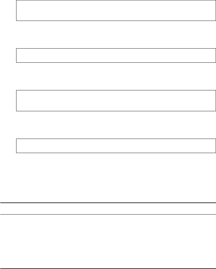
70 AUTOMATED DATA COLLECTION WITH R
2. Square brackets, “[” and “],” enclose arrays. An array is an ordered sequence of
objects or values.
Actual data are stored in key/value pairs. The rules for keys and values are
1. Keys are placed in double quotes, data are only placed in double quotes if they are
string data
1"name" : "Indiana Jones and the Temple of Doom"
2"year" : 1984
2. Keys and values are always separated by a colon
1"year" : 1981
3. Key/value pairs are separated by commas
1{"Indiana Jones": "Harrison Ford",
2"Dr. Rene Belloq": "Paul Freeman"}
4. Values in an array are separated by commas
1["Frank Marshall", "George Lucas", "Howard Kazanjian"]
JSON allows a set of different data types for the value part of key/value pairs. They are
listed in Table 3.4.
Table 3.4 Data types in JSON
Data type Meaning
Number integer, real, or oating point (e.g., 1.3E10)
String white space, zero, or more Unicode characters (except "or \;\introduces
some escape sequences)
Boolean true or false
Null null, an unknown value
Object content in curly brackets
Array ordered content in square brackets

XML AND JSON 71
And that is it.10 From the perspective of an XML user, note what is not possible in
JSON: We cannot add comments, we do not distinguish between missing values and null
values, there are no namespaces and no internal validation syntax like XML’s DTD. But this
does not make JSON inferior to XML in absolute terms. They are rather based on different
concepts. JSON is not a markup language and not even a document format. It is anticipated
to be versionless—there is no JSON 1.0—and no change in the grammar is expected. It is
just a data interchange standard that is so general that it can be parsed by many languages
without effort.
Although there is not much to highlight in JSON data, there are some tools that facil- JSON
pocketknife
tools
itate accessing JSON documents for human readers. The JSON Formatter & Validator at
http://jsonformatter.curiousconcept.com/ is just one of several tools on the Web that automat-
ically indent JSON input. This makes it much easier to read because JSON data frequently
come without indentation or line breaks. The tool also helps check for bugs in the data. If
you want to convert XML to JSON data, take a look at http://www.freeformatter.com/xml-
to-json-converter.html or similar tools. However, such conversions are never isomorphic and
rules have to be set to deal with, for example, attributes and namespaces.
Why is JSON so important for the Web even though XML already provides a popular data The importance
of JSON for the
Web
exchange format? First of all, there are some technical properties that make JSON preferable to
XML. Generally, it is more lightweight due to its less verbose syntax and only allows a limited
set of data types that are compatible with many if not most existing programming languages.
Regarding compatibility, JSON has another crucial feature: We cover only basics of JavaScript
in this book (see Chapter 6), but JavaScript is a major player on the Web to generate dynamic
content and user–browser interactions. JSON is ultimately compatible with JavaScript and
can be directly parsed into JavaScript objects. From a practical point of view, JSON seems to
become the most widely used data exchange format for web APIs; Twitter as well as YouTube
and many bigger and smaller web services have begun using JSON-only APIs.
3.8 JSON and Rin practice
While Rhas one standard set of tools to handle XML-type data—the XML package—there
are several packages that allow importing, exporting, and manipulating JSON data. The rst
published package was rjson (Couture-Beil 2013) and is still used in some R-based API
wrappers. The package that is currently more established, however, is RJSONIO (Temple
Lang 2013b), which we will use in this section. Finally, we also discuss the recently published
package jsonlite (Ooms and Temple Lang 2014), which builds on RJSONIO and improves
mapping between Robjects and JSON strings.
We begin the discussion with an inspection of the RJSONIO package. In its current version
(1.0.3), the package offers 24 functions, most of which we usually do not apply directly. We
now return to the running example, the data in the indy.json le. Using the isValidJSON()
function, we rst check whether the document consists of valid JSON data:
R> isValidJSON("indy.json")
[1] TRUE
10There are some encoding details we do not dwell on here—if you want to go a little bit more into details,
http://www.json.org/ provides further information.
72 AUTOMATED DATA COLLECTION WITH R
This seems to be the case. The two core functions are fromJSON() and toJSON().
fromJSON() reads content in JSON format and converts it to Robjects, toJSON() does the
opposite:
R> indy <- fromJSON(content = "indy.json")
content is the function’s main argument. In our case, indy.json is a le in the workingfromJSON()
directory, but it could also be a character string possibly from the Web via getURL()
or imported with readLines().ThefromJSON() function offers several other useful
arguments, and as the package is well maintained, the documentation—accessible with
?fromJSON—is worth a look. A very useful argument is simplify, controlling whether
the function tries to combine identical elements to vectors. Otherwise the individual elements
remain separate list elements. The nullValue argument allows specifying how to deal with
JSON nulls. In general, JSON data types (see Table 3.4) match Rdata types nicely (numeric,
integer, character, logical). The null value is a little more differentiated in R, however. There
is NULL for empty objects and NA for indicating a missing value. Therefore, the nullValue
argument helps to specify how to deal with these cases, like turning them into NAs. The
function maps the JSON data structure into an Rlist object:
R> class(indy)
[1] "list"
From this point on we can deal with the data the standard Rway, that is, decomposeThere is no
ultimate XML/
JSON-to-R
function
or subset the list or force (parts of) it into vectors, data frames, or other structures. We
have already observed that seemingly powerful functions like xmlToDataFrame() can
be of limited use when we face real data. Data frames are useful to represent a simple
“observations by variables” structure, but become very complex if they are used to represent
highly hierarchical data. In contrast, JSON and XML can represent far more complex data
structures. When loading JSON or XML data into R, one often has to decide which subsets
of information are necessary and need to be inserted into a data frame. Consequently, there
cannot be a global and universal function for JSON/XML to Rdata format conversion. We
have to build our own tools case by case. In our example, we might want to try to map the
list to a data frame, consisting of three observations and several variables. The problem is
that actors and producers have several values. One option is to extract the information
variable by variable and merge in the end. This could work as follows:
R> library(stringr)
R> indy.vec <- unlist(indy, recursive = TRUE, use.names = TRUE)
R> indy.vec[str_detect(names(indy.vec), "name")]
indy movies.name
"Raiders of the Lost Ark"
indy movies.name
"Indiana Jones and the Temple of Doom"
indy movies.name
"Indiana Jones and the Last Crusade"
This strategy rst attens the complex list structure into one vector. The recursive argu-
ment ensures that all components of the list are unlisted. Since the key names are retained in
the vector by setting use.names to TRUE, we can identify all original key/value pairs with
the name name using a simple regular expression and the str_detect() function from the
stringr package (see also Chapter 8). This strategy has its drawbacks. First, all list elements

XML AND JSON 73
are coerced to a common mode, resulting in character vectors in most cases. This is useful
for the names variable, but less appropriate for the years variable. Further, this step-by-step
approach is tedious when many variables have to be extracted. An only slightly more comfort-
able option uses sapply() and feeds it with the [[ operators and the variable name for ele-
ment subsetting, calling indy[[1]][[1]][['name']],indy[[1]][[2]][['name']],
and so on:
R> sapply(indy[[1]], "[[", "year")
[1] 1981 1984 1989
The benet of this approach over the rst is that data types are retained. Finally, to pull
all variables and directly assemble them into a data frame, we have to take into account that
some variables do not exist or vary in structure from observation to observation in the sample
data. For example, the number of producers varies. We do the conversion as follows:
R> library(plyr)
R> indy.unlist <- sapply(indy[[1]], unlist)
R> indy.df <- do.call("rbind.fill", lapply(lapply(indy.unlist, t),
data.frame, stringsAsFactors = FALSE))
We rst unlist the elements within the list. The second command is more complex. First,
we transpose each list element, turn them into data frames, and nally make use of the
rbind.fill() function of the plyr package to combine the data frames into one single data
frame, taking care of the fact that some variables do not exist in some data frames. The
result reveals that we would have to continue with some data cleansing—note for example
the split-up producer variables:
R> names(indy.df)
[1] "name" "year"
[3] "actors.Indiana.Jones" "actors.Dr..Ren´
e.Belloq"
[5] "producers1" "producers2"
[7] "producers3" "budget"
[9] "academy_award_ve" "actors.Mola.Ram"
[11] "producers" "actors.Walter.Donovan"
It is clear that importing JSON data, or working with lists in general, can be painful. Even
if data structures are simpler, we need to use apply functions. Consider this last example of a
JSON data import with a simple Peanuts dataset:
1[
2{
3"name":"van Pelt, Lucy",
4"sex":"female",
5"age":32
6},
7{
8"name":"Peppermint, Patty",
9"sex":"female",
10 "age":null
11 },

74 AUTOMATED DATA COLLECTION WITH R
12 {
13 "name":"Brown, Charlie",
14 "sex":"male",
15 "age":27
16 }
17 ]
We turn the data into an ordinary data frame with the following expression:
R> peanuts.json <- fromJSON("peanuts.json", nullValue = NA,
simplify = FALSE )
R> peanuts.df <- do.call("rbind", lapply(peanuts.json, data.frame,
stringsAsFactors = FALSE))
We parse the JSON snippet with the fromJSON function and tell the parser to set null
values to zero. We also set simplify to FALSE in order to retain the list structure in
all elements. Otherwise, the parser would convert the second entry to a character vector,
rendering the data.frame() apply function useless. We use the lapply() function to turn
the lists into data frames and keep strings as strings with the stringsAsFactors = FALSE
argument. Finally, we join the data frames with a do.call() on rbind(). The result looks
acceptable:
R> peanuts.df
name sex age
1 van Pelt, Lucy female 32
2 Peppermint, Patty female NA
3 Brown, Charlie male 27
To do the conversion the other way round, that is from Rto JSON data, the function wetoJSON()
need is toJSON():
R> peanuts.json <- toJSON(peanuts.df, pretty = TRUE)
R> file.output <- file("peanuts_out.json")
R> writeLines(peanuts.json, file.output)
R> close(file.output)
While transforming JSON data into appropriate Robjects cannot always be done withMore consistent
mapping with
jsonlite
preexisting functions, but require some postprocessing of the resulting objects, the recently
developed jsonlite package offers more consistency between both data structures. It builds
upon the parser of the RJSONIO package and provides the main functions fromJSON()
and toJSON as well, but implements a different mapping scheme (see Ooms 2013). A
set of rules ensures that data from an external source like an API are transformed in a
way that guarantees consistent transformations. Some important conventions for JSON-to-R
conversions for arrays are
rarrays are encoded as character data if at least one value is of type character;
rnull values are encoded as NA;
rtrue and false values are encoded as 1 and 0 in numerical vectors and TRUE and
FALSE in character and logical vectors.
XML AND JSON 75
There are more conventions for the transformation of vectors, matrices, lists, and data
frames. They are documented in Ooms (2013). For our purposes, the rules concerning JSON-
to-Rconversion are most important, as this is part of the regular scraping workow. Consider
the following set of transformations from JSON arrays into Robjects to see how the conven-
tions cited above work in practice:
R> library(jsonlite)
R> x <- '[1, 2, true, false]'
R> fromJSON(x)
[1]1210
R> x <- '["foo", true, false]'
R> fromJSON(x)
[1] "foo" "TRUE" "FALSE"
R> x <- '[1, "foo", null, false]'
R> fromJSON(x)
[1] "1" "foo" NA "FALSE"
The consistent mapping rules of jsonlite not only ensure that data are transformed ade-
quately on the vector level, but also make mapping of JSON data into Rdata frames a lot
easier. Reconsidering the Peanuts example with jsonlite, it turns out that the JSON data are
conveniently mapped into the desired Robject of type data.frame right away:
R> (peanuts.json <- fromJSON("peanuts.json"))
name sex age
1 van Pelt, Lucy female 32
2 Peppermint, Patty female NA
3 Brown, Charlie male 27
In the Indiana Jones example, the Indy JSON is also mapped into a list. However, the
only element in the list is a data frame of the desired content. We simply pull the data frame
from the list to access the variables
R> (indy <- fromJSON("indy.json"))
$'indy movies'
name year actors.Indiana Jones
1 Raiders of the Lost Ark 1981 Harrison Ford
2 Indiana Jones and the Temple of Doom 1984 Harrison Ford
3 Indiana Jones and the Last Crusade 1989 Harrison Ford
actors.Dr. Ren´
e Belloq actors.Mola Ram actors.Walter Donovan
1 Paul Freeman <NA> <NA>
2 <NA> Amish Puri <NA>
3 <NA> <NA> Julian Glover
producers budget academy_award_ve
1 Frank Marshall, George Lucas, Howard Kazanjian 18000000 TRUE
2 Robert Watts 28170000 TRUE
3 Robert Watts, George Lucas 48000000 FALSE
R> indy.df <- indy$'indy movies'
R> indy.df$name
[1] "Raiders of the Lost Ark"
[2] "Indiana Jones and the Temple of Doom"
[3] "Indiana Jones and the Last Crusade"
In short, whenever RJSONIO returns a list when you would expect a data frame, jsonlite
manages to generate tabular data from JSON data structures as long as it is appropriate,
76 AUTOMATED DATA COLLECTION WITH R
because the mapping scheme acknowledges the way in which tabular data are stored in R,
which is column based, and JSON—and many other formats, languages, or databases—which
is row based (see Ooms 2013).
To be sure, the functionality of jsonlite does not solve all problems of JSON-to-Rtransfer.
However, the choice of rules implemented in jsonlite makes the import of JSON data into R
more consistent. We therefore suggest to make this package the standard tool when working
with JSON data even though it is still in an early version.
Summary
Both XML and JSON are very important standards for data exchange on the Web, and as
such will occur several times in the course of this book (for example in Chapter 4 and the
case study on Twitter, Chapter 14). Knowing how to handle both data types is helpful in many
web data collection tasks.
We have seen that XML serves as a basic standard for many other formats, such as GPX,
KML, RSS, SVG, XHTML. Whenever we encounter such data on the Web we are able to
import and process them in Rtoo. JSON is an increasingly popular alternative to XML for the
exchange of data on the Web, especially when working with web services/web APIs. JSON
is derived from JavaScript and can be parsed in many languages, including R.
Further reading
There are many books that go far beyond this basic introduction to XML and JSON. If you
have acquired a taste for the languages of the Web and plan to go deeper into web developing,
you could have a look at XMLinaNutshellby Harold and Means (2004) or at Ray (2003). For
the web scraping tasks presented in this book, however, deeper knowledge of XML should
not be necessary.
If you want to dig deeper into JSON and JavaScript, the book JavaScript: The Good Parts
by JSON developer Douglas Crockford (2008) might be a good start. For a quick overview,
the excellent website http://www.json.org/ is highly recommended.
Problems
1. Describe the relationship between XML and HTML.
2. What are possible ways to import XML data into R? What are the advantages and
disadvantages of each approach?
3. What is the purpose of namespaces in XML-style documents?
4. What are the main elements of the JSON syntax?
5. Write the smallest well-formed XML document you can think of.
6. Why do we need an escape sequence for the ampersand in XML?
7. Take a look at the invalid XML code snippet in Section 3.2.2. How could the family
structure be represented in a valid XML document so that it is possible to identify
Jonathan both as a child and as a father?

XML AND JSON 77
8. Go to your vinyl record, CD, DVD, or Blu-ray Disc shelf and randomly pick three titles.
Create an XML document that holds useful information about your sample of discs.
9. Inform yourself about the Election Markup Language (EML).
(a) Find out the purpose of EML.
(b) Look for the current specication of the language and identify the key concepts.
(c) Search for a real EML document, load it into Rand turn parts of it into native
data structures.
10. Working with SVG les.
(a) Manipulate the ricon.svg le such that the icon is framed with a black box. Redene
the color, size, and font of the image.
(b) Rebuild the RSS icon as an SVG document.
11. Find the formatting errors in the following JSON piece.11
1{
2"text": "@slowpoketweeter @yaaawn123: Just saw a cat on
the road. Awesome! #YOLO",
3"truncated": false,
4"favorited": "true",
5"source": "<a href= \"http://twitter.com/ \" rel= \"
nofollow \">Twitter for iPhone</a>",
6"id_str": "61723550048377463",
7"user_mentions": ["slowpoketweeter" "yaaawn123"],
8"screen_name": "SlowpokeTweeter",
9"id",
10 "retweet_count": 4,
11 "geo": NULL,
12 "created_at": "Sun Apr 03 23:48:36 +0000 2011";
13 user: {
14 "statuses_count": 3,511,
15 "profile_background_color": "C0DEED",
16 "followers_count": "48",
17 "description": "watcha doin in my waters?",
18 "screen_name": "OldGREG85",
19 "time_zone": "Hawaii",
20 'lang': "en",
21 "friends_count": 81,
22 "geo_enabled": false,
23 }
12. Convert the James Bond XML example from Figure 3.1 into valid JSON.
13. Convert the Indiana Jones example from Figure 3.9 into valid XML.
14. Import the indy.json le into Rand extract the values of all budget keys.
11The example is a shortened fragment of the content that is being returned by the Twitter Streaming API.
78 AUTOMATED DATA COLLECTION WITH R
15. The XML le potus.xml (available in the book’s materials) contains biographical infor-
mation on US presidents.
(a) Use the DOM-style XML parser and parse the document into an Robject called
potus. Inspect the source code. The <occupation> nodes contain additional
white space at the end of the text string. Find the appropriate argument to remove
them in the parsing stage.
(b) The XML le contains <salary> nodes. Discard them while parsing the le.
Remove the additional white space in the <occupation> nodes by using a custom
handler function and a string manipulation function (see Section 8.2).
(c) Write a handler for extracting the <hometown> nodes’ value and pass it to the
DOM-style parser. Repeat the process with an event-driven parser. Inspect the
results.

4
XPath
In Chapters 2 and 3 we introduced and illustrated how HTML/XML documents use markup
to store information and create the visual appearance of the webpage when opened in the
browser. We also explained how to use a scripting language like Rto transform the source
code underlying web documents into modiable data objects called the DOM with the use
of dedicated parsing functions (Sections 2.4 and 3.5.1). In a typical data analysis workow,
these are important, but only intermediate steps in the process of assembling well-structured
and cleaned datasets from webpages. Before we can take full advantage of the Web as a nearly
endless data source, a series of ltering and extraction steps follow once the relevant web
documents have been identied and downloaded. The main purpose of these steps is to recast
information that is encoded in formats using markup language into formats that are suitable
for further processing and analysis with statistical software. Initially, this task comprises
asking what information we are interested in and identifying where the information is located
in a specic document. Once we know this, we can tailor a query to the document and obtain
the desired information. Additionally, some data reshaping and exception handling is often
necessary to cast the extracted values into a format that facilitates further analysis.
This chapter walks you through each of these steps and helps you to build an intuition for
querying tree-based data structures like HTML/XML documents. We will see that accessing
particular information from HTML/XML documents is straightforward using the concise,
yet powerful path statements provided by the XML Path language (short XPath), a very
popular web technology and W3C standard (W3C 1999). After introducing the basic logic
underlying XPath, we show how to leverage the full power of its vocabulary using predicates,
operators, and custom extractor functions in an application to real documents. We further
explore how to work with namespace properties (Section 4.3.2). The chapter concludes with
a pointer to helpful tools (Section 4.3.3) and a more high-level discussion about general
problems in constructing efcient and robust extraction code for HTML/XML documents
(Section 4.3.3).
Automated Data Collection with R: A Practical Guide to Web Scraping and Text Mining, First Edition.
Simon Munzert, Christian Rubba, Peter Meißner and Dominic Nyhuis.
© 2015 John Wiley & Sons, Ltd. Published 2015 by John Wiley & Sons, Ltd.
80 AUTOMATED DATA COLLECTION WITH R
4.1 XPath—a query language for web documents
XPath is a query language that is useful for addressing and extracting parts from HTML/XML
documents. XPath is best categorized as a domain-specic language, which indicates that its
eld of application is a rather narrow one—it is simply a very helpful tool for selecting
information from marked up documents such as HTML, XML, or any variant of it such as
SVG or RSS (see Sections 3.4.3 and 3.4.3). XPath is also a W3C standard, which means
that the language is subjected to constant maintenance and widely employed in modern web
applications. Among the two versions of XPath that are in current use, we apply XPath 1.0
as it provides sufciently powerful statements and is implemented in the XML package for R.
As a stylized, running example, we revisit fortunes.html—a simple HTML le that
First stop:
Parsing includes short quotes of Rwisdoms. A rst, necessary step prior to applying XPath is to
parse the document and make its content available in the workspace of the Rsession, since
XPath only works on the DOM representation of a document and cannot be applied on the
native code. We begin by loading the XML package and use htmlParse() to parse the le
into the object parsed_doc:
R> library(XML)
R> parsed_doc <- htmlParse(file = "fortunes.html")
The document is now available in the workspace and we can examine its content using
XML’s print() method on the object:
R> print(parsed_doc)
<!DOCTYPE HTML PUBLIC "-//IETF//DTD HTML//EN">
<html>
<head><title>Collected R wisdoms</title></head>
<body>
<div id="R Inventor" lang="english" date="June/2003">
<h1>Robert Gentleman</h1>
<p><i>'What we have is nice, but we need something very different'</i></p>
<p><b>Source: </b>Statistical Computing 2003, Reisensburg</p>
</div>
<div lang="english" date="October/2011">
<h1>Rolf Turner</h1>
<p><i>'R is wonderful, but it cannot work magic'</i> <br><emph>answering a
request for automatic generation of 'data from a known mean and 95% CI'
</emph></p>
<p><b>Source: </b><a href="https://stat.ethz.ch/mailman/listinfo/r-help">
R-help</a></p>
</div>
<address>
<a href="http://www.r-datacollection.com"><i>The book homepage</i>
</a><a></a>
</address>
</body>
</html>
Before proceeding, we would like to restate a crucial idea from Chapter 2 that will be
helpful in understanding the basic logic of XPath statements. HTML/XML documents use
tags to markup information and the nestedness of the tags describe a hierarchical order.
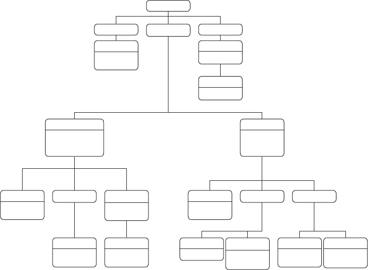
XPATH 81
<html>
<head> <body> <address>
<title>
value:
Collected ...
<a>
href: https ...
<i>
href: https ...
<div>
id: R-Inventor
lang: english
date: June/2003
<h1>
value:Robert
Gentleman
<p>
<i>
value:What
we ...
<p>
value:
Statistical ...
<b>
value:
Source ...
<div>
lang: english
date:
October/2011
<h1>
value:Robert
Turner
<p>
<i>
value:R is ...
<emph>
value:
answering ...
<p>
<b>
value:
Source ...
<a>
value:R-help
href: http ...
Figure 4.1 A tree perspective on parsed_doc
One way to depict this hierarchical order of tags is by means of a tree as it is portrayed in
Figure 4.1. In the tree, edges represent the nestedness of a lower-level node inside a higher-
level node. Throughout this chapter we will not only refer to this image but also adopt graph
language to describe the location of the tags in the document as well as their relations.
Therefore, if we refer to the <div> node, we mean the entire information that is encapsulated
within the div tags, that is, the value of the node, its set of attributes as well as their values, and
its children nodes. When we use the word node set, we refer to a selection of multiple nodes.
4.2 Identifying node sets with XPath
4.2.1 Basic structure of an XPath query
To get started, let us put ourselves to the task of extracting information from the <i> nodes, Hierarchical
addressing
mechanism
that is, text that is written in italics, which contain the actual quotes. A look at either HTML
code or the document tree in Figure 4.1 reveals that there are two nodes of interest and they
are both located at the lowest level of the document. In XPath, we can express this hierarchical
order by constructing a sequence of nodes separated by the /(forward slash). This is called a
hierarchical addressing mechanism and it is similar to a location path on a local le system.
The resemblance is not accidental but results from a similar hierarchical organization of the
underlying document/le system. Just like folders can be nested inside other folders on a

82 AUTOMATED DATA COLLECTION WITH R
local hard drive, the DOM treats an XML document as a tree of nodes, where the nestedness
of nodes within other nodes creates a node hierarchy.
For our HTML le we can describe the position of the <i> nodes by describ-Absolute paths
ing the sequence of nodes that lead to it. The XPath that represents this position is
“/html/body/div/p/i.” This statement reads from left to right: Start at the root node
<html>—the top node in a tree is also referred to as the root note—proceed to the <body>
node, the <div> node, the <p> node, and nally the <i> node. To apply this XPath we use
XML’s xpathSApply() function. Essentially, xpathSApply() allows us to conduct two
tasks in one step. First, the function returns the complete node set that matches the XPath
expression. Second, if intended, we can pass an extractor function to obtain a node’s value,
attribute, or attribute value.1In our case, we set xpathSApply()’s rst argument doc to the
parsed document and the second argument path to the XPath statement that we wish to apply:
R> xpathSApply(doc = parsed_doc, path = "/html/body/div/p/i")
[[1]]
<i>'What we have is nice, but we need something very different'</i>
[[2]]
<i>'R is wonderful, but it cannot work magic'</i>
In the present case, the specied path is valid for two <i> nodes. Thus, the XPath queryRelative paths
extracts more than one node at once if it describes a valid path for multiple nodes. The path
that we just applied is called an absolute path. The distinctive feature about absolute paths is
that they always emanate from the root node and describe a sequence of consecutive nodes to
the target node. As an alternative we can construct shorter, relative paths to the target node.
Relative paths tolerate “jumps” between nodes, which we can indicate with //. To exemplify,
consider the following path:
R> xpathSApply(parsed_doc, "//body//p/i")
[[1]]
<i>'What we have is nice, but we need something very different'</i>
[[2]]
<i>'R is wonderful, but it cannot work magic'</i>
This statement reads as follows: Find the <body> node at some level of the document’s
hierarchy—it does not have to be the root—then nd one or more levels lower in the hierarchy
a<p> node, immediately followed by an <i> node. We obtain the same set of <i> nodes as
previously. An even more concise path for the <i> nodes would be the following:
R> xpathSApply(parsed_doc, "//p/i")
[[1]]
<i>'What we have is nice, but we need something very different'</i>
[[2]]
<i>'R is wonderful, but it cannot work magic'</i>
1These two steps may be conducted separately from one another. You can use getNodeSet() to apply the XPath.
Using a looping structure or functionality from the apply() family, the received node set can be postprocessed and
the information recast.
XPATH 83
These three examples help to stress an important point in XPath’s design. There are Deciding
between
relative and
absolute paths
virtually always several ways to describe the same node set by means of different XPath
statements. So why do we construct a long absolute path if a valid relative path exists that
returns the same information? xpathSApply() traverses through the complete document
and resolves node jumps of any width and at any depth within the document tree. The
appeal of relative paths derives from their shortness, but there are reasons for favoring
absolute paths in some instances. Relative path statements result in complete traversals of
the document tree, which is rather expensive computationally and decreases the efciency
of the query. For the small HTML le we consider here, computational efciency is of
no concern. Nonetheless, the additional strain will become noticeable in the speed of code
execution when larger le sizes or extraction tasks for multiple documents are concerned.
Hence, if speed is an issue to your code execution, it is advisable to express node locations by
absolute paths.
Beyond pure path logic, XPath allows the incorporation of symbols with special meaning Wildcard
operator
in the expressions. One such symbol is the wildcard operator *. The wildcard operator
matches any (single) node with arbitrary name at its position. To return all <i> nodes from
the HTML le we can use the operator between the <div> and <i> node to match the
<p> nodes:
R> xpathSApply(parsed_doc, "/html/body/div/*/i")
[[1]]
<i>'What we have is nice, but we need something very different'</i>
[[2]]
<i>'R is wonderful, but it cannot work magic'</i>
Two further elements that we repeatedly make use of are the .and the .. operator. Selection
expressions
The .operator selects the current nodes (or self-axis) in a selected node set. This operation
is occasionally useful when using predicates. We postpone a detailed exploration of the .
operator to Section 4.2.3, where we discuss predicates. The .. operator selects the node one
level up the hierarchy from the current node. Thus, if we wish to select the <head> node we
could rst locate its child <title> and then go one level up the hierarchy:
R> xpathSApply(parsed_doc, "//title/..")
[[1]]
<head>
<title>Collected R wisdoms</title>
</head>
Lastly, we sometimes want to conduct multiple queries at once to extract elements that Multiple paths
lie at different paths. There are two principal methods to do this. The rst method is to use
the pipe operator ∣to indicate several paths, which are evaluated individually and returned
together. For example, to select the <address> and the <title> nodes, we can use the
following statement:
R> xpathSApply(parsed_doc, "//address | //title")
[[1]]
<title>Collected R wisdoms</title>
84 AUTOMATED DATA COLLECTION WITH R
[[2]]
<address>
<a href="http://www.r-datacollectionbook.com">
<i>The book homepage</i>
</a>
<a/>
</address>
Another option is to store the XPath queries in a vector and pass this vector to xpathSAp-
ply(). Here, we rst generate a named vector twoQueries where the elements represent
the distinct XPath queries. Passing twoQueries to xpathSApply() we get
R> twoQueries <- c(address = "//address", title = "//title")
R> xpathSApply(parsed_doc, twoQueries)
[[1]]
<title>Collected R wisdoms</title>
[[2]]
<address>
<a href="http://www.r-datacollectionbook.com">
<i>The book homepage</i>
</a>
<a/>
</address>
4.2.2 Node relations
The XPath syntax introduced so far is sufciently powerful to select some of the nodes in the
document, but it is of limited use when the extraction tasks become increasingly complex.
Connected node sequences simply lack expressiveness, which is required for singling out
specic nodes from smaller node subsets. This issue is nicely illustrated by the queries that
we used to identify the <i> nodes in the document. Assume we would like to identify the
<i> node that appears within the second section element <div>. With the syntax introduced
so far, no path can be constructed to return this single node since the node sequence to this
node is equally valid for the <i> nodes within the rst section of the document.
In this type of situation, we can make use of XPath’s capability to exploit other features
The family tree
analogy of the document tree. One such feature is the position of a node relative to other nodes
in the document tree. These relationships between nodes are apparent in Figure 4.1. Most
nodes have nodes that precede or follow their path, an information that is often unique and
thus differentiates between nodes. As is usual in describing tree-structured data formats, we
employ notation based on family relationships (child, parent, grandparent, …) to describe the
between-node relations. This feature allows analysts to extract information from a specic
target node with an unknown name solely based on the relationship to another node with a
known name. The construction of a proper XPath statement that employ this feature follows
the pattern node1/relation::node2, where node2 has a specic relation to node1.Let
us try to apply this technique on the problem discussed above, selecting the second <div>
node in the document. We learn from Figure 4.1 that only the second <div> node has an <a>

XPATH 85
node as one of its grandchildren. This constitutes a unique feature of the second <div> node
that we can extract as follows:
R> xpathSApply(parsed_doc, "//a/ancestor::div")
[[1]]
<div lang="english" date="October/2011">
<h1>Rolf Turner</h1>
<p><i>'R is wonderful, but it cannot work magic'</i> <br/><emph>answering a
request for automatic generation of 'data from a known mean and 95% CI'
</emph></p>
<p><b>Source: </b><a href="https://stat.ethz.ch/mailman/listinfo/r-help">
R-help</a></p>
</div>
Here, we rst select the <a> nodes in the document and then subselect among this set all
ancestor nodes with name div. Comparing the resulting node set to the results from above,
we nd that a smaller set is returned. If we were interested on extracting only the text in italics
from this node set, we can make a straightforward extension to this expression. To proceed
from the thus selected <div> node to all the <i> that come one or more levels lower in the
hierarchy, we add //i to the expression:
R> xpathSApply(parsed_doc, "//a/ancestor::div//i")
[[1]]
<i>'R is wonderful, but it cannot work magic'</i>
As a testament to XPath’s capability to reect complex relationships between nodes,
consider the following statement:
R> xpathSApply(parsed_doc, "//p/preceding-sibling::h1")
[[1]]
<h1>Robert Gentleman</h1>
[[2]]
<h1>Rolf Turner</h1>
Here, we rst select all the <p> nodes in the document and then all the <h1> siblings that
precede these nodes.2
Generally, XPath statements are limitless with respect to their length and the number of
special symbols used in it. To illustrate the combination of the wildcard operator with another
node relation, consider the following statement:
R> xpathSApply(parsed_doc, "//title/parent::*")
[[1]]
<head>
<title>Collected R wisdoms</title>
</head>
2When we apply XPath in real scraping scenarios, we usually cannot draw on visual representations of node
relations like the one in Figure 4.1. Such information must be read directly from the page’s source code. This often
is the most demanding part in information extraction tasks that use XPath.

86 AUTOMATED DATA COLLECTION WITH R
Table 4.1 XPath axes
Axis name Result
ancestor Selects all ancestors (parent, grandparent, etc.) of the
current node
ancestor-or-self Selects all ancestors (parent, grandparent, etc.) of the
current node and the current node itself
attribute Selects all attributes of the current node
child Selects all children of the current node
descendant Selects all descendants (children, grandchildren, etc.) of the
current node
descendant-or-self Selects all descendants (children, grandchildren, etc.) of the
current node and the current node itself
following Selects everything in the document after the closing tag of
the current node
following-sibling Selects all siblings after the current node
namespace Selects all namespace nodes of the current node
parent Selects the parent of the current node
preceding Selects all nodes that appear before the current node in the
document except ancestors, attribute nodes, and
namespace nodes
preceding-sibling Selects all siblings before the current node
self Selects the current node
Source: http://www.w3schools.com/xpath/xpath_axes.asp
The parent selects nodes in the tree that appear one level higher with respect to the
reference node <title. The wildcard operator is used to express indifference regarding the
node names. In combination, this statement returns every parent node for every <title>
node in the document. For a full list of available relations, take a look at Table 4.1. A visual
impression of all available node relationships is displayed in Figure 4.2.
4.2.3 XPath predicates
Beside exploiting relationship properties of the tree, we can use predicates to obtain and
process numerical and textual properties of the document. Applying these features in a
conditioning statement for the node selection adds another level of expressiveness to XPath
statements. Put simply, predicates are nothing but simple functions that are applied to a node’s
name, value, or attribute, and which evaluate whether a condition (or set of conditions) is
true or false. Internally, a predicate returns a logical response. Nodes where the response is
true are selected. Their general use is as follows: After a node (or node set) we specify the
predicate in square brackets, for example, node1[predicate]. We select all <node1> nodes
in the document that comply with the condition formulated by the predicate. As a complete
coverage of all predicates is neither possible nor helpful for this introduction, we restrict our
attention to the most frequent—and in our view most helpful—predicates in XPath. We have
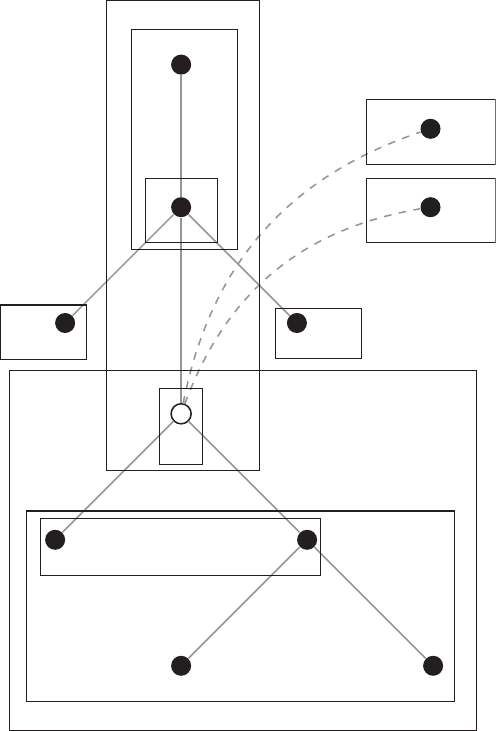
XPATH 87
Parent
Ancestor
Ancestor-or-self
Attribute
Preceding Following
Self
Child
Descendant
Descendant-or-self
Namespace
Figure 4.2 Visualizing node relations. Descriptions are presented in relation to the white
node
listed some of the available predicates in Table 4.2. Our goal is not to provide an exhaustive
examination of this topic, but to convey the inherent logic in applying predicates. We will see
that some predicates work in combination with so-called operators. A complete overview of
available operators is presented in Table 4.3.
4.2.3.1 Numerical predicates
XPath offers the possibility to take advantage of implied numerical properties of documents, Implicit
numerical
properties
such as counts or positions. There are several predicates that return numerical properties,
which can be used to create conditional statements. The position of a node is an important

Table 4.2 Overview of some important XPath functions
Function Description Example
name(<node>) Returns the name of <node> or the rst node
in a node set
//*[name()='title']; Returns: <title>
text(<node>) Returns the value of <node> or the rst node
in a node set
//*[text()='The book homepage']; Returns: <i> with value The
book homepage
@attribute Returns the value of a node’s attribute or of
the rst node in a node set
//div[@id='R Inventor']; Returns: <div> with attribute id value R
Inventor
string-length(str1) Returns the length of str1. If there is no
string argument, it returns the length of the
string value of the current node
//h1[string-length()>11]; Returns: <h1> with value Robert
Gentleman
translate(str1, str2,
str3)
Converts str1 by replacing the characters in
str2 with the characters in str3
//div[translate(./@date, '2003', '2005')='June/2005'];
Returns: rst <div> node with date attribute value June/2003
contains(str1,str2) Returns TRUE if str1 contains str2,
otherwise FALSE
//div[contains(@id, 'Inventor')]; Returns: rst <div> node
with id attribute value R Inventor
starts-with(str1,str2) Returns TRUE if str1 starts with str2,
otherwise FALSE
//i[starts-with(text(), 'The')]; Returns: <i> with value The
book homepage
substring-before
(str1,str2)
Returns the start of str1 before str2 occurs
in it
//div[substring-before(@date, '/')='June']; Returns:
<div> with date attribute value June/2003
substring-after
(str1,str2)
Returns the remainder of str1 after str2
occurs in it
//div[substring-after(@date, '/')=2003]; Returns: <div>
with date attribute value June/2003
not(arg) Returns TRUE if the boolean value is FALSE,
and FALSE if the boolean value is TRUE
//div[not(contains(@id, 'Inventor'))]; Returns: the <div>
node that does not contain the string Inventor in its id attribute value
local-name(<node>) Returns the name of the current <node> or the
rst node in a node set—without the
namespace prex
//*[local-name()='address']; Returns: <address>
count(<node>) Returns the count of a nodeset <node> //div[count(.//a)=0]; Result: The second <div> with one <a>
child
position(<node>) Returns the index position of <node> that is
currently being processed
//div/p[position()=1]; Result: The rst <p> node in each <div>
node
last() Returns the number of items in the processed
node list <node>
//div/p[last()]; Result: The last <p> node in each <div> node

XPATH 89
Table 4.3 XPath operators
Operators Description Example
∣Computes two node sets //i | //b
+Addition 5+3
-Subtraction 8-2
*Multiplication 8*5
div Division 8 div 5
=Equal count = 27
!= Not equal count != 27
<Less than count < 27
≤Less than or equal to count <= 27
>Greater than count > 27
≥Greater than or equal to count >= 27
or Or count = 27 or count = 28
and And count > 26 and count < 30
mod Modulo (division remainder) 7 mod 2
Source:Adapted from http://www.w3schools.com/xpath/xpath_operators.asp
numerical characteristic that we can easily implement. Let us collect the <p> nodes that
appear on rst position:
R> xpathSApply(parsed_doc, "//div/p[position()=1]")
[[1]]
<p>
<i>'What we have is nice, but we need something very different'</i>
</p>
[[2]]
<p><i>'R is wonderful, but it cannot work magic'</i> <br/><emph>answering a
request for automatic generation of 'data from a known mean and 95% CI'
</emph></p>
The predicate we use is position() in combination with the equal operator =.3The
statement returns two nodes. The position predicate does not evaluate which <p> node is on
rst position among all <p> nodes in the document but on rst position in each node subset
relative to its parent. If we wish to select the last element of a node set without knowing the
number of nodes in a subset in advance, we can use the last() operator:
R> xpathSApply(parsed_doc, "//div/p[last()]")
[[1]]
<p><b>Source: </b>Statistical Computing 2003, Reisensburg</p>
[[2]]
<p>
<b>Source: </b>
<a href="https://stat.ethz.ch/mailman/listinfo/r-help">R-help</a>
</p>
3Please note that an even more concise way of expressing the same query is //div/p[1].
90 AUTOMATED DATA COLLECTION WITH R
Output from numerical predicates may be further processed with mathematical operations.
To select the next to last <p> nodes, we extend the previous statement:
R> xpathSApply(parsed_doc, "//div/p[last()-1]")
[[1]]
<p>
<i>'What we have is nice, but we need something very different'</i>
</p>
[[2]]
<p><i>'R is wonderful, but it cannot work magic'</i> <br/><emph>answering a
request for automatic generation of 'data from a known mean and 95% CI'
</emph></p>
A count is another numerical property we can use as a condition for node selection. One
of the most frequent uses of counts is selecting nodes based on their number of children
nodes. An implementation of this logic is the following:
R> xpathSApply(parsed_doc, "//div[count(.//a)>0]")
[[1]]
<div lang="english" date="October/2011">
<h1>Rolf Turner</h1>
<p><i>'R is wonderful, but it cannot work magic'</i> <br/><emph>answering a
request for automatic generation of 'data from a known mean and 95% CI'
</emph></p>
<p><b>Source: </b><a href="https://stat.ethz.ch/mailman/listinfo/r-help">
R-help</a></p>
</div>
Piece by piece, the statement reads as follows. We start by selecting all the <div> nodes
in the document (//div). We rene the selection by using the count() predicate, which
takes as argument the thing we need to count. In this case we count the number of <a>
nodes that precede the selected <div> nodes (.//a). The .element is used to condition on
the previous selection. Internally, this results in another node set, which we then pass to the
count() function. Combining the operator with a value >0, we ask for those <div> nodes
in the document that have more than zero <a> nodes as children. Besides nodes, we can also
condition on the number of attributes in a node:
R> xpathSApply(parsed_doc, "//div[count(./@*)>2]")
[[1]]
<div id="R Inventor" lang="english" date="June/2003">
<h1>Robert Gentleman</h1>
<p><i>'What we have is nice, but we need something very different'</i></p>
<p><b>Source: </b>Statistical Computing 2003, Reisensburg</p>
</div>
The @element retrieves the attributes from a selected node. Here, the ./@* expression
returns all the attributes—regardless of their name—from the currently selected nodes. We
pass these attributes to the count function and evaluate whether the number of attributes is
greater than 2. Only the nodes returning TRUE for this function are selected.
The number of characters in the content of an element is another kind of count we can
obtain and use to condition node selection. This is particularly useful if all we know about
our extraction target is that the node contains some greater amount of text. It is implemented
as follows:
XPATH 91
R> xpathSApply(parsed_doc, "//*[string-length(text())>50]")
[[1]]
<i>'What we have is nice, but we need something very different'</i>
[[2]]
<emph>answering a request for automatic generation of 'data from a
known mean and 95% CI'</emph>
We rst obtain a node set of all the nodes in the document (//*). On this set, we impose
the condition that the content of these nodes (as returned by text()) must contain more than
50 characters.
It is sometimes useful to invert the node selection and return all nodes for which the Boolean
functions
predicate does not return TRUE. XPath includes a couple of functions that allow employing
Boolean logic in the query. To express an inversion of a node set, one can use the Boolean
not function to select all nodes that are not selected by the query. To select all <div> with
two or fewer attributes, we can write
R> xpathSApply(parsed_doc, "//div[not(count(./@*)>2)]")
[[1]]
<div lang="english" date="October/2011">
<h1>Rolf Turner</h1>
<p><i>'R is wonderful, but it cannot work magic'</i> <br/><emph>answering a
request for automatic generation of 'data from a known mean and 95% CI'
</emph></p>
<p><b>Source: </b><a href="https://stat.ethz.ch/mailman/listinfo/r-help">
R-help</a></p>
</div>
4.2.3.2 Textual predicates
Since HTML/XML les or any of their variants are plain text les, textual properties of the
document are useful predicates for node selection. This might come in handy if we need
to pick nodes on the basis of text in their names, content, attributes, or attributes’ values.
Besides exact matching, working with strings often requires tools for partial matching of
substrings. While XPath 1.0 is sufciently powerful in this respect, version 2.0 has seen huge
improvements with the implementation of a complete library of regular expression predicates
(for an introduction to string manipulation techniques see Chapter 8). Nonetheless, XPath 1.0
fares well enough in most situations, so that switching to other XPath implementations is not
necessary. To begin, let us explore methods to perform exact matches for strings. We already
introduced the =operator for equalizing numerical values, but it works just as well for exact
string matching. To select all <div> nodes in the document, which contain quotes written
in October 2011, that is, contain an attribute date with the value October/2011, we can
write
R> xpathSApply(parsed_doc, "//div[@date='October/2011']")
[[1]]
<div lang="english" date="October/2011">
<h1>Rolf Turner</h1>
<p><i>'R is wonderful, but it cannot work magic'</i> <br/><emph>answering a
request for automatic generation of 'data from a known mean and 95% CI'
</emph></p>
92 AUTOMATED DATA COLLECTION WITH R
<p><b>Source: </b><a href="https://stat.ethz.ch/mailman/listinfo/r-help">
R-help</a></p>
</div>
We rst select all the <div> nodes in the document and then subselect those that have
an attribute date with the value October/2011. In many instances, exact matching for
strings as implied by the equal sign is an exceedingly strict operation. One way to be more
liberal is to conduct partial matching for strings. The general use of these methods is as
follows: string_method(text1, 'text2'), where text1 refers to a text element in the
document and text2 to a string we want to match it to. To select all nodes in a document
that contain the word magic in their value, we can construct the following statement:
R> xpathSApply(parsed_doc, "//*[contains(text(), 'magic')]")
[[1]]
<i>'R is wonderful, but it cannot work magic'</i>
In this statement we rst select all the nodes in the document and condition this set
using the contains() function on whether the value contains the word magic as returned
by text(). Please note that all partial matching functions are case sensitive, so capitalized
versions of the term would not be matched. To match a pattern to the beginning of a string, the
starts_with() function can be used. The following code snippet illustrates the application
of this function by selecting all the <div> nodes with an attribute id, where the value starts
with the letter R:
R> xpathSApply(parsed_doc, "//div[starts-with(./@id, 'R')]")
[[1]]
<div id="R Inventor" lang="english" date="June/2003">
<h1>Robert Gentleman</h1>
<p><i>'What we have is nice, but we need something very different'</i></p>
<p><b>Source: </b>Statistical Computing 2003, Reisensburg</p>
</div>
ends_with() is used to match a string to the end of a string. It is frequently useful toPreprocessing
node strings preprocess node strings before conducting matching operations. The purpose of this step is to
normalize node values, attributes, and attribute values, for example, by removing capitaliza-
tion or replacing substrings. Let us try to extract only those quotes that have been published
in 2003. As we see in the source code, the <div> nodes contain a date attribute, which holds
information about the year of the quote. To condition our selection on this value, we can issue
the following expression:
R> xpathSApply(parsed_doc, "//div[substring-after(./@date, '/')='2003']//i")
[[1]]
<i>'What we have is nice, but we need something very different'</i>
Let us consider the statement piece by piece. We rst select all the <div> nodes in
the document (//div). The selection is further conditioned on the returned attribute value
from the predicate. In the predicate we rst obtain the date value for all the selected nodes
(./@date). This yields the following vector: June/2003, October/2011. The values are
passed to the substring-after() function where they are split according to the /, specied
as the second argument. Internally, the function outputs 2003, 2011. We then conduct exact
matching against the value 2003, which selects the <div> node we are looking for. Finally,
we move down to the <i> node by attaching //i to the expression.
XPATH 93
4.3 Extracting node elements
So far, we have used xpathSApply() to return nodes that match specied XPath statements.
We learned that the function returns a list object that contains the nodes’ name, value, and
attribute values (if specied). We usually do not care for the node in its entirety, but need to
extract a specic information from the node, for example, its value. Fortunately, this task is
fairly straightforward to implement. We simply pass an extractor function to the fun argument
in the function call. The XML package offers an extensive set of these functions to select the
pieces of information we are interested in. A complete overview of all extractor functions is
presented in Table 4.4. For example, in order to extract the value of the <title> node we
can simply write
R> xpathSApply(parsed_doc, "//title", fun = xmlValue)
[1] "Collected R wisdoms"
Instead of a list with complete node information, xpathSApply() now returns a vector Extractor
functions
object, which only contains the value of the node set that matches the XPath statement. For
nodes without value information, the functions would return an NA value. Beside the value, we
can also extract information from the attributes. Passing xmlAttrs() to the fun argument
will select all attributes that are in the selected nodes:
R> xpathSApply(parsed_doc, "//div", xmlAttrs)
[[1]]
id lang date
"R Inventor" "english" "June/2003"
[[2]]
lang date
"english" "October/2011"
In most applications we are interested in specic rather than all node attributes. To select
a specic attribute from a node, we use xmlGetAttr() and add the attribute name:
R> xpathSApply(parsed_doc, "//div", xmlGetAttr, "lang")
[1] "english" "english"
Table 4.4 XML extractor functions
Function Argument Return value
xmlName Node name
xmlValue Node value
xmlGetAttr name Node attribute
xmlAttrs (All) node attributes
xmlChildren Node children
xmlSize Node size

94 AUTOMATED DATA COLLECTION WITH R
4.3.1 Extending the fun argument
Processing returned node sets from XPath can easily extend beyond mere feature extraction
as introduced in the last section. Rather than extracting information from the node, we can
adapt the fun argument to perform any available numerical or textual operation on the node
element. We can build novel functions for particular purposes or modify existing extractor
functions for our specic needs and pass them to xpathSApply(). The goal of further
processing can either lie in cleansing the numeric or textual content of the node, or some kind
of exception handling in order to deal with extraction failures.
To illustrate the concept in a rst application, let us attempt to extract all quotes from the
Custom
functions for
xpathSApply()
document and convert the symbols to lowercase during the extraction process. We can use
base R’s tolower() function, which transforms strings to lowercase. We begin by writing a
function called lowerCaseFun(). In the function, we simply feed the information from the
node value to the tolower() function and return the transformed text:
R> lowerCaseFun <- function(x) {
x <- tolower(xmlValue(x))
x
}
Adding the function to xpathSApply()’s fun argument, yields:
R> xpathSApply(parsed_doc, "//div//i", fun = lowerCaseFun)
[1] "'what we have is nice, but we need something very different'"
[2] "'r is wonderful, but it cannot work magic'"
The returned vector now consists of all the transformed node values and spares us an
additional postprocessing step after the extraction. A second and a little more complex
postprocessing function might include some basic string operations that employ functionality
from the stringr package. Again, we begin by writing a function that loads the stringr package,
collects the date and extracts the year information4:
R> dateFun <- function(x) {
require(stringr)
date <- xmlGetAttr(node = x, name = "date")
year <- str_extract(date, "[0-9]{4}")
year
}
Passing this function to the fun argument in xpathSApply() yields:
R> xpathSApply(parsed_doc, "//div", dateFun)
[1] "2003" "2011"
We can also use the fun argument to cope with situations where an XPath statement
returns an empty node set. In XML’s DOM the NULL object is used to indicate a node that
4See Chapter 8 for an introduction to string manipulation. In particular, the function str_extract() in the
custom extractor function collects four consecutive digits using a so-called regular expression. The concept and
details of regular expressions will also be explained in Chapter 8.
XPATH 95
does not exist. We can employ a custom function that includes a test for the NULL object and
makes further processing dependent on positive or negative evaluation of this test:
R> idFun <- function(x) {
id <- xmlGetAttr(x, "id")
id <- ifelse(is.null(id), "not specified", id)
return(id)
}
The rst line in this custom function saves the node’s id value into a new object id.
Conditional on this value being NULL, we either return not specified or the id value in
the second line. To see the results, let us pass the function to xpathSApply():
R> xpathSApply(parsed_doc, "//div", idFun)
[1] "R Inventor" "not specified"
4.3.1.1 Using variables in XPath expressions
The previous examples were simple enough to allow querying all information with a single,
xed XPath expression. Occasionally, though, it becomes inevitable to treat XPath expressions
themselves as variable parts of the extraction program. Data analysts often nd that a specic
type of information is encoded heterogeneously across documents, and hence, constructing a
valid XPath expression for all documents may be impossible, especially when future versions
of a site are expected to change. To illustrate this, consider extracting information from the
XML le technology.xml, which we introduced in Section 3.5.1. Previously, we extracted
the Apple stock from this le, but now we tackle the problem of pulling out all companies’
stock information. The problem is that the target closing stock information (<close>)is
encapsulated in parent nodes with different names (Apple, Google, IBM). Instead of creating
separate query functions for each company, we can help ourselves by using the sprintf()
function to create exible XPath expressions. We start by parsing the document again and
building a character vector with the relevant company names:
R> parsed_stocks <- xmlParse(file = "technology.xml")
R> companies <- c("Apple", "IBM", "Google")
Next, we use sprintf() to create the queries. Inside the function, we set the basic
template of the XPath expression. The string %s is used to indicate the variable part, where
sstands for a string variable. The object companies indicates the elements we want to
substitute for %s:
R> (expQuery <- sprintf("//%s/close", companies))
[1] "//Apple/close" "//IBM/close" "//Google/close"
We can proceed as usual by rst laying out an extractor function…
R> getClose <- function(node) {
value <- xmlValue(node)
company <- xmlName(xmlParent(node))
mat <- c(company = company, value = value)
}
96 AUTOMATED DATA COLLECTION WITH R
…and then passing this extractor function to xpathSApply(). Here, we additionally
convert the output to a more convenient data frame format and change the vector type:
R> stocks <- as.data.frame(t(xpathSApply(parsed_stocks, expQuery, getClose)))
R> stocks$value <- as.numeric(as.character(stocks$value))
R> head(stocks, 3)
company value
1 Apple 520.6
2 Apple 520.0
3 Apple 519.0
4.3.2 XML namespaces
In our introduction to XML technologies in Chapter 3, we introduced namespaces as a feature
to create uniquely identied nodes in a web document. Namespaces become an indispensable
part of XML when different markup vocabularies are used inside a single document. Such
may be the result of merging two different XML les into a single document. When the
constituent XML les employ similar vocabulary, namespaces help to resolve ambiguities
and prevent name collisions.
Separate namespaces pose a problem to the kinds of XPath statements we have been
considering so far, since XPath ordinarily considers the default namespace. In this section
we learn how to specify the namespace under which a specic node set is dened and thus
extract the elements of interest. Let us return to the example we used in our introduction
to XML namespaces (Section 3.4). The le books.xml not only contains an HTML title but
also information on a book enclosed in XML nodes. We start by parsing the document with
xmlParse() and print its contents to the screen:
R> parsed_xml <- xmlParse("titles.xml")
R> parsed_xml
<?xml version="1.0" encoding="UTF-8"?>
<!DOCTYPE presidents SYSTEM "presidents.dtd">
<root xmlns:h="http://www.w3.org/1999/xhtml" xmlns:t="http://
funnybooknames.com/crockford">
<h:head>
<h:title>Basic HTML Sample Page</h:title>
</h:head>
<t:book id="1">
<t:author>Douglas Crockford</t:author>
<t:title>JavaScript: The Good Parts</t:title>
</t:book>
</root>
For the sake of the example, let us assume we are interested in extracting information
from the <title> node, which holds the text string JavaScript: The Good Parts.We
can start by issuing a call to all <title> nodes in the document and retrieve their values:
R> xpathSApply(parsed_xml, "//title", fun = xmlValue)
list()
Evidently, the call returns an empty list. The key problem is that neither of the twoBypassing
namespaces <title> nodes in the document has been dened under the default namespace on which
XPATH 97
standard XPath operates. The specic namespaces can be inspected in the xmlns statements
in the attributes of the <root> node. Here, two separate namespaces are declared, which are
referred to by the letters hand t. One way to bypass the unique namespaces is to make a
query directly to the local name of interest:
R> xpathSApply(parsed_xml, "//*[local-name()='title']", xmlValue)
[1] "Basic HTML Sample Page" "JavaScript: The Good Parts"
Here, we rst select all the nodes in the document and then subselect all the nodes with
local name title. To conduct namespace-aware XPath queries on the document, we can extend
the function and use the namespaces argument in the xpathSApply() function to refer
to the particular namespace under which the second <title> node has been dened. We
know that the namespace information appears in the <root> node. We can pass the second
namespace string to the namespaces argument of the xpathSApply() function:
R> xpathSApply(parsed_xml, "//x:title", namespaces = c(x = "http://
funnybooknames.com/crockford"),
fun = xmlValue)
[1] "JavaScript: The Good Parts"
Similarly, if we were interested in extracting information from the <title> node under
the rst namespace, we would simply change the URI:
R> xpathSApply(parsed_xml, "//x:title", namespaces = c(x = "http://
www.w3.org/1999/xhtml"),
fun = xmlValue)
[1] "Basic HTML Sample Page"
These methods require the namespaces under which the nodes of interest have been
declared to be known in advance. The literal specication of the URI can be circum-
vented if we know where in the document the namespace denition occurs. Namespaces are
always declared as attribute values of an XML element. For the sample le, the information
appears in the <root> node’s xmlns attribute. We capitalize on this knowledge by extracting
the namespace URI for the second namespace using the xmlNamespaceDefinitions()
function:
R> nsDefs <- xmlNamespaceDefinitions(parsed_xml)[[2]]
R> ns <- nsDefs$uri
R> ns
[1] "http://funnybooknames.com/crockford"
Having stored the information in a new object, the namespace URI can be passed to the
XPath query in order to extract information from the <title> node under that namespace:
R> xpathSApply(parsed_xml, "//x:title", namespaces = c(x = ns), xmlValue)
[1] "JavaScript: The Good Parts"
4.3.3 Little XPath helper tools
XPath’s versatility comes at the cost of a steep learning curve. Beginners and experienced
XPath users may nd the following tools helpful in verifying and constructing valid statements
for their extraction tasks:
98 AUTOMATED DATA COLLECTION WITH R
SelectorGadget SelectorGadget (http://selectorgadget.com) is an open-source bookmarklet
that simplies the generation of suitable XPath statements through a point-and-click approach.
To make use of its functionality, visit the SelectorGadget website and create a bookmark for
the page. On the website of interest, activate SelectorGadget by clicking on the bookmark.
Once a tool bar on the bottom left appears, SelectorGadget is activated and highlights the
page’s DOM elements when the cursor moves across the page. Clicking an element adds
it to the list of nodes to be scraped. From this selection, SelectorGadget creates a general-
ized statement that we can obtain by clicking on the XPath button. The XPath expression
can then be passed to xpathSApply()’s path argument. Please note that in order to use
the generated XPath expressions in xpathSApply(), you need to be aware that the type
of quotation mark that embrace the XPath expression may not be used inside the expres-
sion (e.g., for the attribute names). Replace them either with double (" ") or single (‘’)
quotation marks.
Web Developer Tools Many modern browsers contain a suite of developer tools to help
inspect elements in the webpage and create valid XPath statements that can be passed to
XML’s node retrieval functions. Beyond information on the current DOM, developer tools
also allow tracing changes to DOM elements in dynamic webpages. We will make use of
these tools in Section 6.3.
Summary
In this chapter we made a broad introduction to the XPath language for querying XML
documents. We hope to have shown that XPath constitutes an indispensable investment for
data analysts who want to work with data from webpages in a productive and efcient manner.
With the tools introduced at the end of this chapter, many extraction problems may even be
solved through simply clicking elements and pasting the returned expression. Despite their
helpfulness, these tools may fail for rather intricate extraction problems, and, thus, knowing
how to build expressions from scratch remains a necessary skill. We also would like to assert
that the construction of an applicable XPath statement is rarely a one-shot affair but requires
an iterative learning process. This process can be described as a cycle of three steps. In the
construction stage, we assemble an XPath statement that is believed to return the correct
information. In the testing stage, we apply the XPath, observe the returned node set or error
message, and nd that perhaps the returned node set is too broad or too narrow. The learning
stage is a necessary stage when the XPath query has failed. Learning from this failure, we
might infer a more suitable XPath expression, for example, by making it more strict or more
lax in order to obtain only the desired information. Going back to step number one, we apply
the rened XPath to check whether it now yields the correct set of nodes. For many extraction
problems we nd that multiple traverses through this cycle are necessary to build condence
in the robustness of the programmed extraction routine. We are going to elaborate on the
XPath scraping strategy again in Section 9.2.2.
The issue of XPath robustness is exacerbated when the code is to work on unseen instances
of a webpage, for example, when the extraction code is automatically executed daily (see
Section 11.2). Inevitably, websites undergo changes to their structure; elements are removed
or shifted, new features are implemented, visual appearances are modied, which ultimately
affect the page’s contents as well. This is especially true for popular websites. But we will
XPATH 99
see that certain dispositions can be made in the XPath statements and auxiliary code design
to increase robustness and warn the analyst when the extraction fails. One possibility is to
rely on textual predicates when textual information should be extracted from the document.
Adding information to the query on the substantive interest can add necessary robustness to
the code.
Further reading
A full exploration of XPath and the XML package is beyond the scope of this chapter. For
an extensive overview of the XML package, interested readers are referred to Nolan and
Temple Lang (2014). A more concise introduction to the package is provided by Temple
Lang (2013c). Tennison provides a comprehensive overview of XPath 1.0 (Tennison 2001).
Another helpful overview of XPath 1.0 and 2.0 methods can be found in Holzner (2003). For
an excellent online documentation on web technologies, including XPath, consult Mozilla
Developer Network (2013).
Problems
1. What makes XPath a domain-specic language?
2. XPath is the XML Path language, but it also works for HTML documents. Explain why.
3. Return to the fortunes1.html le and consider the following XPath expression:
//a[text()[contains(., 'R-help')]]§. Replace §to get the <h1> node with
value “Robert Gentleman.”
4. Construct a predicate with the appropriate string functions to test whether the month of
a quote is October.
5. Consider the following two XPath statements for extracting paragraph nodes from a
HTML le. 1. //div//p,2.//p. Decide which of the two statements makes a more
narrow request. Explain why.
6. Verify that for extracting the quotes from fortunes.html the XPath expression //i does
not return the correct results. Explain why not.
7. The XML le potus.xml contains biographical information on US presidents. Parse the
le into an object of the Rsession.
(a) Extract the names of all the presidents.
(b) Extract the names of all presidents, beginning with the 40th term.
(c) Extract the value of the <occupation> node for all Republican presidents.
(d) Extract the <occupation> node for all Republican presidents that are also Baptists.
(e) The <occupation> node contains a string with additional white space at the
beginning and the end of the string. Remove the white space by extending the
extractor function.
(f) Extract information from the <education> nodes. Replace all instances of “No
formal education” with NA.
(g) Extract the <name> node for all presidents whose terms started in or after the year
1960.
100 AUTOMATED DATA COLLECTION WITH R
8. The State of Delaware maintains a repository of datasets published by the Delaware
Government Information Center and other Delaware agencies. Take a look at Natural-
izations.xml (included in the chapter’s materials at http://www.r-datacollection.com).
The le contains information about naturalization records from the Superior Court.
Convert the data into an Rdata frame.
9. The Commonwealth War Graves Commission database contains geographical informa-
tion on burial plots and memorials across the globe for those who lost their lives as a
result of World War I. The data have been recast as a KML document, an XML-type
data structure. Take a look at cwgc-uk.kml (included in the chapter’s materials). Parse
the data and create a data frame from the information on name and coordinates. Plot
the distribution on a map.
10. Inspect the SelectorGadget (see Section 4.3.3). Go to http://planning.maryland.gov/
Redistricting/2010/legiDist.shtml and identify the XPath expression suited to extract
the links in the bottom right table named Maryland 2012 Legislative District Maps
(with Precincts) using SelectorGadget.

5
HTTP
To retrieve data from the Web, we have to enable our software to communicate with
servers and web services. The lingua franca of communication on the Web is HTTP, the
Hypertext Transfer Protocol. HTTP dates back to the late 1980s when it was invented by Tim
Berners-Lee, Roy Fielding and others at the CERN near Geneva, Switzerland (Berners-Lee
2000; Berners-Lee et al. 1996). It is the most common protocol for communication between
web clients (e.g., browsers) and servers, that is, computers that respond to requests from
the network. Virtually every HTML page we open, every image we view in a browser,
every video we watch is delivered by HTTP. When we type a URL into the address bar,
we usually do not even start with http:// anymore, but with the hostname directly (e.g.,
r-datacollection.com) as a request via HTTP is taken for granted and automatically processed
by the browser. HTTP’s current ofcial version 1.1 dates back to 1999 (Fielding et al. 1999),
a fact that nicely illustrates its reliability over the years—in the same time period, other web
standards such as HTML have changed a lot more often.
We hardly ever come into direct contact with HTTP. Constructing and sending HTTP
requests and processing servers’ HTTP responses are tasks that are automatically processed
by our browsers and email clients. Imagine how exhausting it would be if we had to formulate
requests like “Hand me a document called index.html from the host www.nytimes.com/ in
the directory pages/science/ using the HTTP protocol” every time we wanted to search for
articles. But have you ever tried to use Rfor that purpose? To maintain our heroic claim that R
is a convenient tool for gathering data from the Web, we need to prove that it is in fact suited
to mimic browser-to-web communication. As we will see, for many of the basic web scraping
tasks we still do not have to care much about the HTTP particulars in the background, as R
handles this for us by default. In some instances, however, we have to dig deeper into protocol
le transfers and formulate precise requests in order to get the information we want. This
chapter serves as an introduction to those parts of HTTP that are most important to us to
become successful web scrapers.
Automated Data Collection with R: A Practical Guide to Web Scraping and Text Mining, First Edition.
Simon Munzert, Christian Rubba, Peter Meißner and Dominic Nyhuis.
© 2015 John Wiley & Sons, Ltd. Published 2015 by John Wiley & Sons, Ltd.

102 AUTOMATED DATA COLLECTION WITH R
The chapter starts with an introduction to client–server conversation (Section 5.1.1).
Before we turn to the technical details of HTTP, we briey digress to talk about URLs,
standardized names of resources on the Internet (Section 5.1.2). Our presentation of HTTP is
then subdivided into a fundamental look at the logic of HTTP messages (Section 5.1.3), request
methods (Section 5.1.4), status codes (Section 5.1.5), and headers (Section 5.1.6). In the
second part, we inspect more advanced features of HTTP for identication and authentication
purposes (Sections 5.2.1 and 5.2.2) and talk about the use of proxies (Section 5.2.3). Although
HTTP is by far the most widespread protocol on the Web, we also take a look at HTTPS
and FTP (Section 5.3). We conclude with the practical implementation of HTTP-based
communication using R(Section 5.4). All in all, we have tried to keep this introduction
to HTTP as nontechnical as possible, while still enabling you to use Ras a web client in
situations that are not explicitly covered in this book.
5.1 HTTP fundamentals
5.1.1 A short conversation with a web server
To access content on the Web, we are used to typing URLs into our browser or to simply
clicking on links to get from one place to another, to check our mails, to read news, or
to download les. Behind this program layer that is designed for user interaction there are
several more layers—techniques, standards, and protocols—that make the whole thing work.
Together they are called the Internet Protocol Suite (IPS). Two of the most prominent players
of this Protocol Suite are TCP (Transmission Control Protocol) and IP (Internet Protocol).
They represent the Internet layer (IP) and the transportation layer (TCP). The inner workings
of these techniques are beyond the scope of this book, but fortunately there is no need to
manually manipulate contents of either of these protocols to conduct successful web scraping.
What is worth mentioning, however, is that TCP and IP take care of reliable data transfer
between computers in the network.1
On top of these transportation standards there are specialized message exchange protocols
like HTTP (Hyper Text Transfer Protocol), FTP (File Transfer Protocol), Post Ofce Protocol
(POP) for email retrieval, SMTP (Simple Mail Transfer Protocol) or IMAP (Internet Message
Access Protocol) for email storage and retrieval. All of these protocols dene standard
vocabulary and procedures for clients and servers to talk about specic tasks—retrieving
or storing documents, les, messages, and so forth. They are subsumed under the label
application layer.
Other than the name suggests, HTTP is not only a standard for hypertext document
retrieval. Although HTTP is quite simple, it is exible enough to ask for nearly any kind of
resource from a server and can also be used to send data to the server instead of retrieving it.
Figure 5.1 presents a stylized version of ordinary user–client interactions. Simply put,
Client-server
communication when we access a website like www.r-datacollection.com/index.html, our browser serves
as the HTTP client. The client rst asks a DNS server (Domain Name System) which IP
1If you care to learn more about the Transmission Control Protocol or the Internet Protocol, both Fall and Stevens
(2011) and Forouzan (2010) provide extensive introductions to the topic. For a more accessible introduction, check
out https://www.netbsd.org/docs/guide/en/chap-net-intro.html
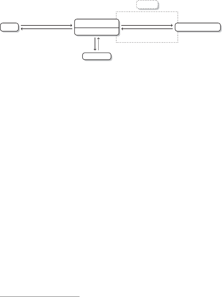
HTTP 103
User HTTP Client
Browser
DNS Server
HTTP Server
Text
images
files
video
sound
Mouse
keybord
HTTP response
HTTP request
URL IP
address
TCP/IP
Figure 5.1 User–server communication via HTTP
address is associated with the domain part of the URL we typed in.2In our example, the
domain part is www.r-datacollection.com.3After the browser has received the IP address as
response from the DNS server, it establishes a connection to the requested HTTP server via
TCP/IP. Once the connection is established, client and server can exchange information—in
our case by exchanging HTTP messages. The most basic HTTP conversation consists of one
client request and one server response. For example, our browser asks for a specic HTML
document, an image, or some other le, and the server responds by delivering the document
or giving back an error code if something went wrong. In our example, the browser would ask
for index.html and start parsing the content of the response to provide the representation of the
website. If the received document contains further linked resources like images, the browser
continues sending HTTP requests to the server until all necessary resources are transmitted.
In the early days of the Internet, one could literally observe how the browser loaded webpages
piece by piece. By now, it almost seems like webpages are received all at once due to the avail-
ability of higher bandwidths, keeping HTTP connections alive or posing numerous requests
in parallel.
There are two important facts about HTTP that should be kept in mind. First, HTTP is
not only a protocol to transport hypertext documents but is used for all kinds of resources.
Second, HTTP is a stateless protocol. This means that without further effort each pair of
request and response between client and server is handled by default as though the two
were talking to each other for the rst time no matter how often they previously exchanged
information.
Let us take a look at one of these standardized messages. For the sake of the example we HTTP
messages
establish a connection to www.r-datacollection.com and ask the server to send us index.html.
The HTTP client rst translates the host URL into an IP address and then establishes a
connection to the server on the default HTTP port (port 80). The port can be imagined as a
door at the server’s house where the HTTP client knocks. Consider the following summary
of the client-side of the conversation:4
2Note that we only scratch the surface of the technologies of client–server communication. If you want to learn
more about the technologies behind it, for example, how DNS servers are contacted, we point you to the “Further
reading” section of this chapter.
3We consider the structure of URLs in the next section.
4We will elaborate further below how to monitor the HTTP exchanges.
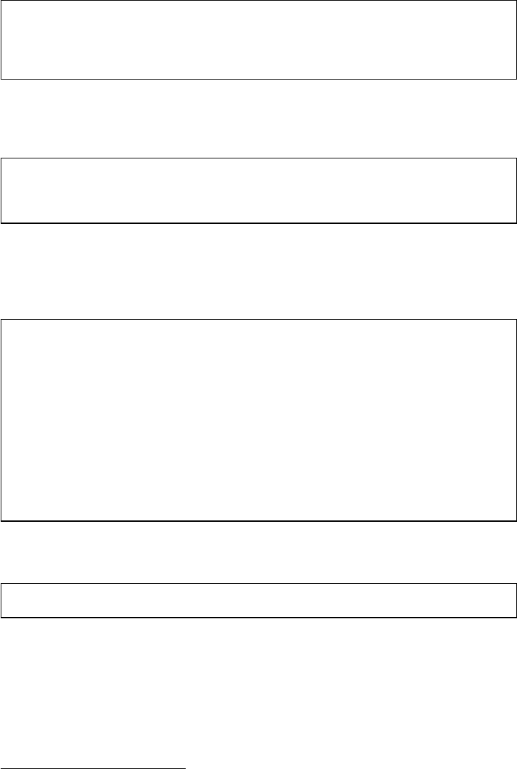
104 AUTOMATED DATA COLLECTION WITH R
1About to connect() to www.r-datacollection.com port 80 (#0)
2Trying 173.236.186.125... connected
3Connected to www.r-datacollection.com (173.236.186.125) port 80 (#0)
4Connection #0 to host www.r-datacollection.com left intact
After having established the connection the server expects a request and our client sends
the following HTTP request to the server:
1GET /index.html HTTP/1.1
2Host: www.r-datacollection.com
3Accept: */*
Now it is the client’s turn to expect a response from the server. The server responds with
some general information followed by the content of our requested document.5The HTTP
response reads as follows:
1HTTP/1.1 200 OK
2Date: Thu, 27 Feb 2014 09:40:35 GMT
3Server: Apache
4Vary: Accept-Encoding
5Content-Length: 131
6...
8<!DOCTYPE HTML PUBLIC "-//IETF//DTD HTML//EN">
9<html> <head>
10 <title></title>
11 </head>
12 ...
After having received all the data, the connection is closed again by the client …
1Closing connection #0
…and the transaction is completed.
5.1.2 URL syntax
The location of websites and other web content are identied by Uniform Resource
Locators (URLs). They are not part of HTTP but make communication via HTTP and
5Several lines of the server response have been omitted for purposes of presentation.

HTTP 105
other protocols straightforward for users.6The general URL format can be expressed as
follows:
scheme://hostname:port/path?querystring#fragment
A corresponding real-life example would be
http://www.w3.org:80/People/Berners-Lee/#Bio
Each URL starts with a scheme that denes the protocol that is used to communicate
between client/application and server. In the example, the scheme is http, separated by a
colon. There are other schemes like ftp (File Transfer Protocol) or mailto, which corre-
sponds to email addresses that rely on the SMTP (Simple Mail Transfer Protocol) standard.
Most enable communication in networks, but you will also nd the file scheme familiar,
which addresses les on local or network drives.
The hostname provides the name of the server where the resource of interest is stored.
It is a unique identier of a server. The hostname along with the port component tell the
client at which door it has to knock in order to get access to the requested resource. The
information is provided in the example as www.w3.org:80. Port 80 is the default port in the
Transmission Control Protocol (TCP). If the client is ne with using the default port, this part
of the URL can be dropped. Hostnames are usually human readable, but every hostname also
has a machine-readable IP address. In the example, www.w3.org belongs to the IP address
128.30.52.37, making the following an equivalent URL:7
http://128.30.52.37/People/Berners-Lee/#Bio
As we usually provide the human-friendly versions of URLs, the Domain Name System
(DNS) translates hostnames into numerical IP addresses. Therefore, the DNS is frequently
compared to a worldwide phone book that redirects users who provide hostnames to services
or devices.
The path determines the location of the requested resource on the server. It works like
paths on any conventional le system where les are nested in folders that may again be
nested in folders and so on. Path segments are separated by slashes (/).
In some cases, URLs provide supplementary information in the path that helps the server
to process the request correctly. The additional information is delivered in query strings that
hold one or more name=value pairs. The query string is separated from the rest of the URL
by a question mark. It encodes data using a ‘eld =value’ format and uses the ampersand
symbol (&) to separate multiple name–value pairs.
https://www.google.com/search?q=RCurl+filetype%3Apdf
A comparable URL is constructed when we search for “RCurl” documents on Google
that are of type PDF. The name–value pair q=RCurl+filetype%3Apdf is the transformed
6We will learn in Section 9.1.3 that one of the easiest ways to collect data from websites is often to inspect
and manipulate the URLs that refer to content of interest. Sometimes the URLs follow a simple logic, for example,
when they contain a running index. It is simple to generate a set of URLs, automatically access them, and store their
content.
7We can use services like the one at http://whatismyipaddress.com/ip-lookup to look up the corresponding IP
addresses of hostnames.

106 AUTOMATED DATA COLLECTION WITH R
actual request written in the search form as “RCurl letype:pdf,” a compact syntax to search
for PDF les that include the term “RCurl.” One could easily extend the request with further
search parameters such as tbs=qdr:y. This would limit the results to hits that are younger
than one year.8
Finally, fragments help point to a specic part of a document. This works well if the
requested resource is HTML and the fragment identier refers to a section, image, or similar.
In the example above, the fragment #Bio requests a direct jump to the biography section of
the document. Note that fragments are handled by the browser, that is, on the client side. After
the server has returned the whole document, the fragment is used to display the specied part.
There are some encoding rules for URLs. URLs are transmitted using the ASCII character
URL encoding
set, which is limited to a set of 128 characters. All characters not included in this set and most
special characters need to be escaped, that is, they are replaced by a standardized representa-
tion. Consider once again the example. The expression “RCurl letype:pdf” is converted to
q=RCurl+filetype%3Apdf. Both white space and the colon character seem to be “unsafe”
and have been replaced with a +sign and the URL encoding%3A, respectively. URL encodings
are also called percent-encoding because the percent character %initializes each of these
encodings. Note that the plus character is a special case of a URL escape sequence that is only
valid in the query part. In other parts, the valid URL encoding of space is %20. A complete
list of URL encodings can be found at http://www.w3schools.com/tags/ref_urlencode.asp.
We can encode or decode characters in URLs with the base functions URLencode()
and URLdecode() in R.Thereserved argument in the former function ensures that non-
alphanumeric characters are encoded with their percent-encoding representation:
R> t <- "I'm Eddie! How are you & you?1+1=2"
R> (url <- URLencode(t, reserve = TRUE))
[1] "I'm%20Eddie!%20How%20are%20you%20%26%20you%3f%201%20+%201%20%3d%202"
R> URLdecode(url)
[1] "I'm Eddie! How are you & you? 1+1=2"
These functions can be useful when we want to construct URLs manually, for example,
to specify a GET form (see below), without having to insert the percent-encodings by hand.
5.1.3 HTTP messages
HTTP messages, whether client requests or server response messages, consist of three parts:
start line,headers, and body—see Figures 5.2 and 5.3. While start lines differ for request
and response, the messages’ header and body sections are structured identically.
To separate start line from headers and headers from body, carriage return and line feed
characters (CRLF) are used.9Note that start line and headers are separated by one sequence of
CRLF while the last header before the body is followed by two CRLF. In R, these characters
are represented as escaped characters \rfor carriage return and \nfor new line feed.
The start line is the rst and indispensable line of each HTTP message. In requests,
the start line denes the method used for the request, followed by the path to the resource
8We can identify additional parameters by specifying advanced searches and observing the changes in the URL.
For a comprehensive overview, see http://jwebnet.net/advancedgooglesearch.html
9Carriage return and line feed are control characters that are inherited from typewriters. Using a typewriter,
starting a new line required returning the carriage to the left and moving the plate one line further down.
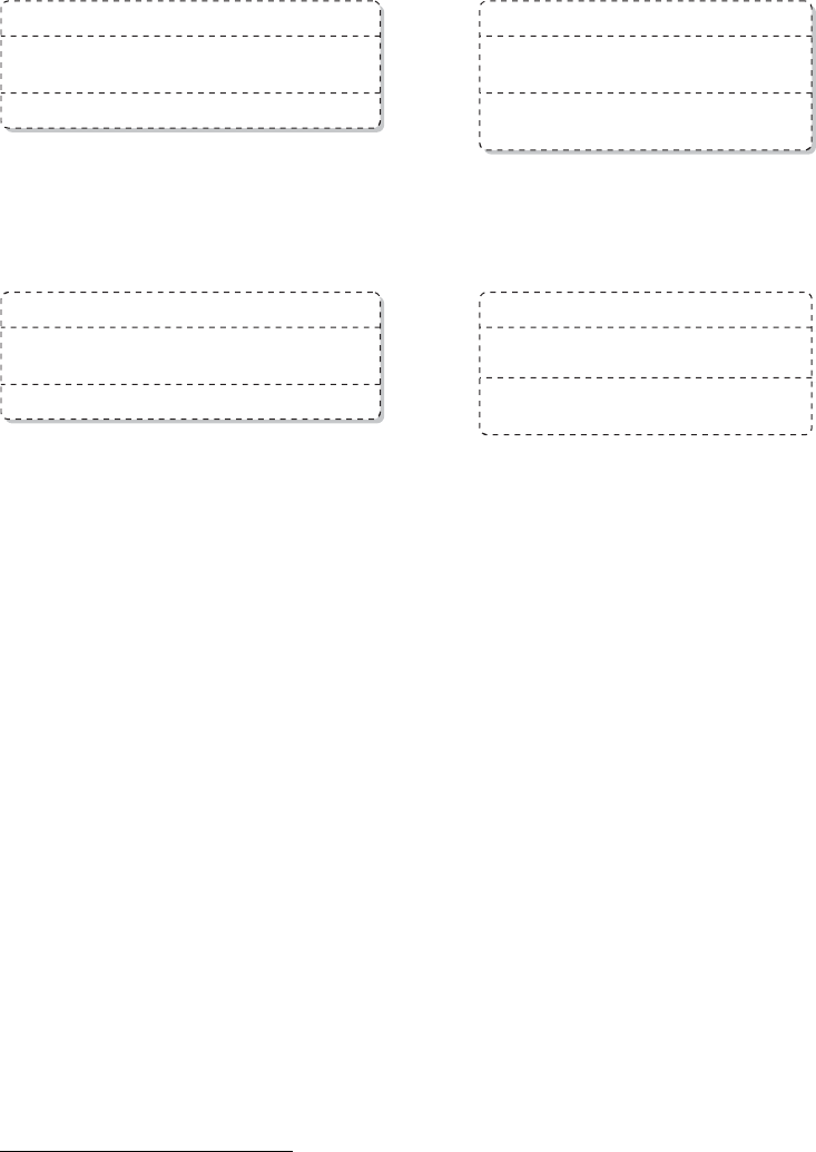
HTTP 107
[method] [path] [version] [CRLF]
[header name:] [header value] [CRLF]
[CRLF]
[body]
Start line
Header
Body
POST /greetings.html HTTP/1.1
Host: www.r-datacollection.com
Hi, there.
How are you?
Schema Example
Figure 5.2 HTTP request schema
[version] [status] [phrase] [CRLF]
[header name:] [header value] [CRLF]
[CRLF]
[body]
Start line
Header
Body
HTTP/1.1 200 OK
Content-type: text/plain
I am ne, thank you very much.
What else might I help you with?
Schema Example
Figure 5.3 HTTP response schema
requested, followed by the highest HTTP version the client can handle. In our example we use
the POST method requesting greetings.html and indicate that our client understands HTTP
up to version 1.1.
The server response start line begins with a statement on the highest HTTP version the
server can handle, followed by a status code, followed by a human-readable explanation of
the status. Here, www.r-datacollection.com tells us that it understands HTTP up to version
1.1, that everything went ne by returning 200 as status code, and that this status code means
something like OK.
The header section below the start line provides client and server with meta information
about the other sides’ preferences or the content sent along with the message. Headers contain
a set of header elds in the form of name–value pairs. Ordinarily, each header eld is placed
on a new line and header eld name and value are separated by colon. If a header line becomes
very long, it can be divided into several lines by beginning the additional line with an empty
space character to indicate that they belong to the previous header line.
The body of an HTTP message contains the data. This might be plain text or binary MIME types
data. Which type of data the body is composed of is specied in the content-type header,
following the MIME type specication (Multipurpose Internet Mail Extensions). MIME
types tell the client or server which type of data it should expect. They follow a scheme of
main-type/sub-type. Main types are, for example, application, audio, image, text, and video
with subtypes like application/pdf, audio/mpg, audio/ogg, image/gif, image/jpeg, image/png,
text/plain, text/html, text/xml, video/mp4, video/quicktime, and many more.10
10For the full set, see the list provided by IANA (Internet Assigned Numbers Authority) at http://www.iana.org/
assignments/media-types/media-types.xhtml.
108 AUTOMATED DATA COLLECTION WITH R
Table 5.1 Common HTTP request methods
Method Description
GET Retrieves resource from server
POST Retrieves resource from server using the message body to
send data or les to the server
HEAD Works like GET, but server responds only with start line
and header, no body
PUT Stores the body of the request message on the server
DELETE Deletes a resource from the server
TRACE Traces the route of the message along its way to the server
OPTIONS Returns list of supported HTTP methods
CONNECT Establishes a network connection
Source: Fielding et al. (1999).
5.1.4 Request methods
When initiating HTTP client requests, we can choose among several request methods—see
Table 5.1 for an overview. The two most important HTTP methods are GET and POST.Both
methods request a resource from the server, but differ in the usage of the body. Whereas
GET does not send anything in the body of the request, POST uses the body to send data. In
practice, simple requests for HTML documents and other les are usually executed with the
GET method. Conversely, POST is used to send data to the server, like a le or inputs from
an HTML form.
If we are not interested in content from the server we can use the HEAD method. HEAD
tells the server to only send the start line and the headers but not transfer the requested
resource, which might be convenient to test if our requests are accepted. Two more handy
methods for testing are OPTIONS, which asks the server to send back the methods it supports
and TRACE, which requests the list of proxy servers (see Section 5.2.3) the request message
has passed on its way to the server.
Last but not least there are two methods for uploading les to and deleting les from
aserver—PUT and DELETE—as well as CONNECT, a method for establishing an HTTP
connection that might be used, for example, for SSL tunneling (see Section 5.3.1).
We will elaborate the methods GET and POST, the two most important methods for web
scraping, when we discuss HTTP in action (see Section 5.4).
5.1.5 Status codes
When a server responds to a request, it will always send back a status code in the start line
of the response. The most famous response that nearly everybody knows from browsing the
Web is 404, stating that the server could not nd the requested document. Status codes can
range from 100 up to 599 and follow a specic scheme: the leading digit signies the status
category—1xx for informations, 2xx for success, 3xx for redirection, 4xx for client errors
and 5xx for server errors—see Table 5.2 for a list of common status codes.

HTTP 109
Table 5.2 Common HTTP status codes
Code Phrase Description
200 OK Everything is ne
202 Accepted The request was understood and accepted but no
further actions have yet taken place
204 No Content The request was understood and accepted but no
further data needs to be returned except for
potentially updated header information
300 Multiple Choices The request was understood and accepted but the
request applies to more than one resource
301 Moved Permanently The requested resource has moved, the new location is
included in the response header Location
302 Found Similar to Moved Permanently but temporarily
303 See Other Redirection to the location of the requested resource
304 Not Modied Response to a conditional request stating that the
requested resource has not been changed
305 Use Proxy To access the requested resource a specic proxy
server found in the Location header should be used
400 Bad Request The request has syntax errors
401 Unauthorized The client should authenticate itself before progressing
403 Forbidden The server refuses to provide the requested resource
and does not give any further reasons
404 Not Found The server could not nd the resource
405 Method Not Allowed The method in the request is not allowed for the
specic resource
406 Not Acceptable The server has found no resource that conforms to the
resources accepted by the client
500 Internal Server Error The server has encountered some internal error and
cannot provide the requested resource
501 Not Implemented The server does not support the request method
502 Bad Gateway The server acting as intermediate proxy or gateway got
a negative response forwarding the request
503 Service Unavailable The server can temporarily not fulll the request
504 Gateway Timeout The server acting as intermediate proxy or gateway got
no response to its forwarded request
505 HTTP Version Not
Supported
The server cannot or refuses to support the HTTP
version used in the request
Source: Fielding et al. (1999).
5.1.6 Header elds
Headers dene the actions to take upon reception of a request or response. Headers can
be general or belong to one specialized group: header elds for requests, header elds for
responses, and header elds regarding the body of the message. For example, request header

110 AUTOMATED DATA COLLECTION WITH R
elds can inform the server about the type of resources the client accepts as response,
like restricting the responses to plain HTML documents or give details on the technical
specication of the client, like the software that was used to request the document. They can
also describe the content of the message, which might be plain text or binary, an image or
audio le and might also have gone through encoding steps like compression. Header elds
always follow the same, simple syntax. The name comes rst and is separated with a colon
from the value. Some header elds contain multiple values that are separated by comma.
Let us go through a sample of common and important header elds to see what they can
do and how they are used. The paragraphs in the following overview provide the name of
the header in bold and the eld type in parentheses, that is, whether the header is used for
request, response, or body.
Accept (request)
1Accept: text/html,image/gif,image/*,*/*;q=0.8
Accept is a request header eld that tells the server about the type of resources the client
is willing to accept as response. If no resource ts the restrictions made in Accept, the server
should send a 406 status code. The specication of accepted content follows the MIME type
scheme. Types are separated by commas; semicolons are used to specify so-called accept
parameters type/subtype;acceptparameter=value,type/.... The asterisk (*) can
be used to specify ranges of type and subtypes. The rules of content-type preferences are
as follows: (1) more specic types are preferred over less specic ones and (2) types are
preferred in decreasing order of the qparameter while (3) all type specications have a
default preference of q =1 if not specied otherwise.
The above example can be read as follows: The client accepts HTML and GIF but if
neither is available will accept any other image type. If no other image type is available, the
client will also accept any other type of content.
Accept-Encoding (request)
1Accept-Encoding: gzip,deflate,sdch;q=0.9,identity;q=0.8;*;q=0
Accept-Encoding tells the server which encodings or compression methods are
accepted by the client. If the server cannot send the content in the specied encoding, it
should return a 406 status code.
The example reads as follows: The client accepts gzip and deflate for encoding. If
neither are available it also accepts sdch and otherwise content that was not encoded at all.
It will not accept any other encodings as the value of the acceptance parameter is 0, which
equals nonacceptance.
Allow (response; body)
1Allow: GET,PUT
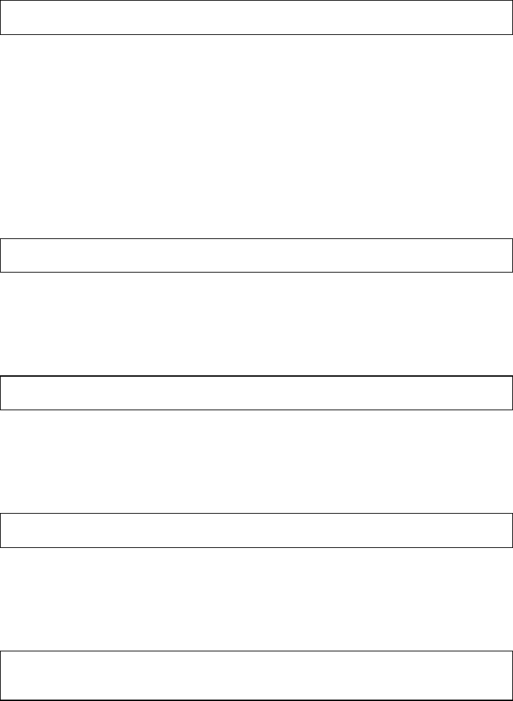
HTTP 111
Allow informs the client about the HTTP methods that are allowed for a particular
resource and will be part of responses with a status code of 405.
Authorization (request)
1Authorization: Basic cm9va2llOjEyM0lzTm90QVNlY3VyZVBX
Authorization is a simple way of passing username and password to the server.
Username and password are rst merged to username:password and encoded according
to the Base64 scheme. The result of this encoding can be seen in the header eld line above.
Note that the encoding procedure does not provide encryption, but simply ensures that all
characters are contained in the ASCII character set. We discuss HTTP authorization methods
in more detail in Section 5.2.2.
The Authorization header eld in the example indicates that the authorization method
is Basic and the Base64-encoded username–password combination is cm9va2...
Content-Encoding (response; body)
1Content-Encoding: gzip
Content-Encoding species the transformations, for example, compression methods,
that have been applied to the content—see Accept-Encoding for further details.
Content-Length (response; body)
1Content-Length: 108
Content-Length provides the receiver of the message with information on the size of
the content in decimal number of OCTETs (bytes).
Content-Type (response; body)
1Content-Type: text/plain; charset=UTF-8
Content-Type provides information on the type of content in the body. Content types
are described as MIME types—see Accept for further details.
Cookie (request)
1Cookie: sessionid=2783321; path=/; domain=r-datacollection.com;
expires=Mon, 31-Dec-2035 23:00:01 GMT
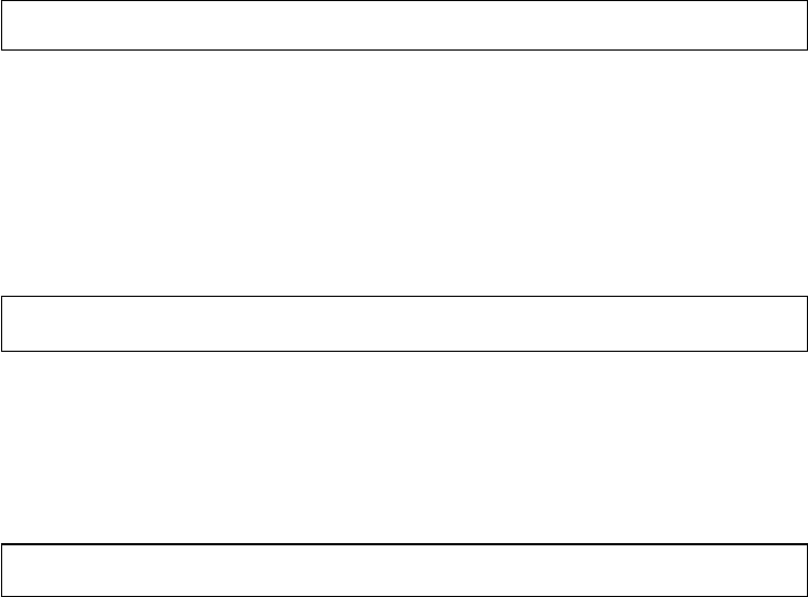
112 AUTOMATED DATA COLLECTION WITH R
Cookies are information sent from server to client with the Set-Cookie header eld.
They allow identifying clients—without cookies servers would not know that they have
had contact with a client before. The Cookie header eld returns the previously received
information. The syntax of the header eld is simple: Cookies consist of name=value pairs
that are separated from each other by semicolon. Names like expires,domain,path, and
secure are reserved parameters that dene how the cookie should be handled by the client.
expires denes a date after which the cookie is no longer valid. If no expiration date is
given the cookie is only valid for one session. domain and path specify for which resource
requests the cookie is needed. secure is used to indicate that the cookie should only be sent
over secured connections (SSL; see Section 5.3.1). We introduce cookies in greater detail in
Section 5.2.1.
The example reads as follows: The cookie sessionid=2783321 is valid until 31st of
December 2035 for the domain www.r-datacollection.com and all its subdirectories (declared
with /).
From (response)
1From: eddie@r-datacollection.com
From provides programmers of web crawlers or scraping programs with the option to send
their email address. This helps webmasters to contact those who are in control of automated
robots and web crawlers if they observe unauthorized behavior. This header eld is useful for
web scraping purposes, and we discuss it in Section 5.2.1.
Host (request)
1Host: www.r-datacollection.com:80
Host is a header eld required in HTTP/1.1 requests and helps servers to decide upon
ambiguous URLs when more than one host name redirects to the same IP address.
If-Modied-Since (request)
1If-Modified-Since: Thu, 27 Feb 2014 13:05:34 GMT
If-Modified-Since can be used to make requests conditional on the time stamp
associated with the requested resource. If the server nds that the resource has not been
modied since the date provided in the header eld, it should return a 304 (Not Modied)
status code. We can make use of this header to write more efcient and friendly web scrapers
(see Section 9.3.3).

HTTP 113
Connection (request, response)
1Connection: Keep-Alive
1Connection: Close
Connection is an ambiguous header eld in the sense that it has two completely different
purposes in HTTP/1.0 and HTTP/1.1. In HTTP/1.1, connections are persistent by default. This
means that client and server keep their connection alive after the request–response procedure
has nished. In contrast, it is standard in HTTP/1.0 to close connections after the client has
got its response. Since establishing connections for each request, the value Keep-Alive can
be specied in HTTP/1.0, while this is the default procedure in HTTP/1.1 and thus does not
have to be explicitly stated. Instead, the server or client can force the connection to be shut
down after the request–response exchange with the Close value.
Last-Modied (response; body)
1Last-Modified: Tue, 25 Mar 2014 19:24:50 GMT
Last-Modified provides the date and time stamp of the last modication of the
resource.
Location (response; body)
1Location: redirected.html
Location serves to redirect the receiver of a message to the location where the requested
resource can be found. This header is used in combination with status code 3xx when content
has moved to another place or in combination with status code 201 when content was created
as result of the request.
Proxy-Authorization (request)
1Proxy-Authentication: Basic bWFnaWNpYW5zYXlzOmFicmFrYWRhYnI=
ThesameasAuthorization, only for proxy servers. For more information on proxies,
see Section 5.2.3.
Proxy-Connection (request)
1Proxy-Connection: keep-alive
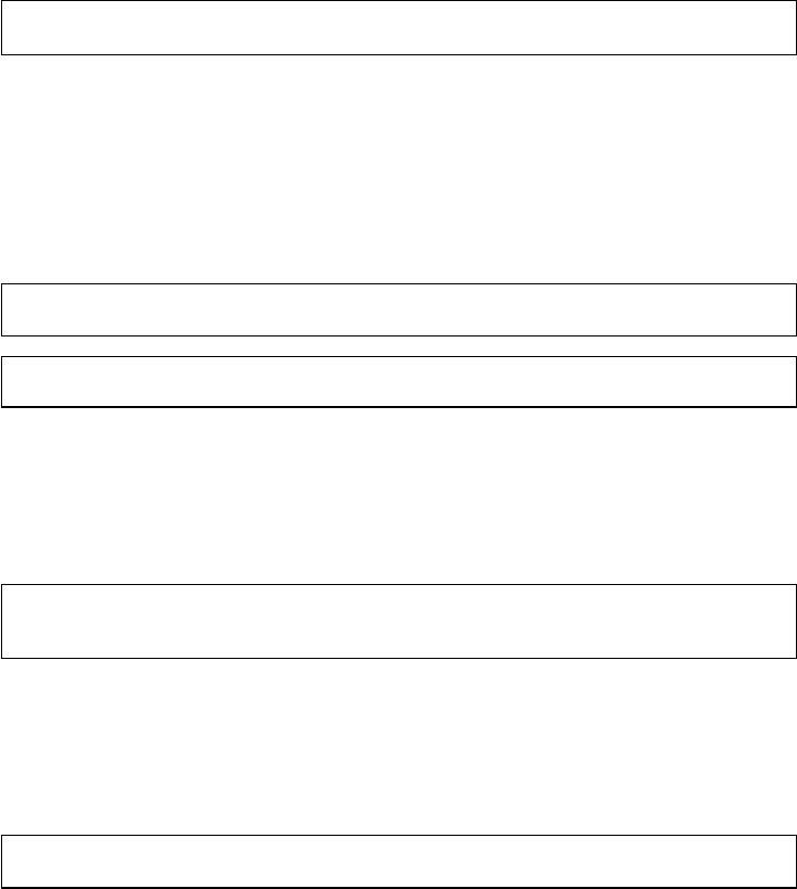
114 AUTOMATED DATA COLLECTION WITH R
The same as Connection, only for proxy servers. For more information on proxies, see
Section 5.2.3.
Referer (request)
1Referer: www.r-datacollection.com/index.html
Referer is a header eld that informs the server what referred to the requested resource.
In the example, www.r-datacollection.com/index.html might provide a link to a picture (e.g.,
/pictures/eddie.jpg). In a request for this picture the referer header eld can be added
to signal that the user has already been on the site and does not want to access the image from
elsewhere, like another website.
Server (response)
1Server: Apache/2.4.7 (Unix) mod_wsgi/3.4 Python/2.7.5 OpenSSL/1.0.1e
1Server: Microsoft-IIS/8.0
Server provides information about the server addressed in the request. The rst server
above is based on Apache software using a Unix platform (httpd.apache.org/), while the
second one is based on Microsoft’s Internet Information Service (www.microsoft.com/).
Set-Cookie (response)
1Set-Cookie: sessionid=2783321; path=/; domain=r-datacollection.com;
2expires=Mon, 31-Dec-2035 23:00:01 GMT
Set-Cookie asks the client to store the information contained in the Set-Cookie header
eld and send them along in subsequent requests as part of the Cookie header. See Cookie
and Section 5.2.1 for further explanation.
User-Agent (request)
1User-Agent: Mozilla/4.0 (compatible; MSIE 7.0; Windows NT 6.0)
The User-Agent header eld indicates the type of client that makes a request to the
server. These more or less cryptic descriptions can indicate the use of a certain browser
on a certain operating system. This information can be helpful for the server to adapt the
content of the response to the system of the client. Nevertheless, the User-Agent can contain
arbitrary user-dened information, such as User-Agent: My fabulous web crawler or
User-Agent: All your base are belong to us. Web scrapers can and should use
User-Agents responsibly. We discuss how this is done in Sections 5.2.1 and 9.3.3.

HTTP 115
Vary (response)
1Vary: User-Agent, Cookie, Accept-Encoding
1Vary: *
The server response sometimes depends on certain parameters, for example, on the
browser or device of the client (e.g., a desktop PC or a mobile phone), on whether the user
has previously visited a site and has received a cookie, and on the encoding format the client
accepts. Servers can indicate that content changes according to these parameters with the
Vary header eld.
The rst example above indicates that the content might vary with changes in User-
Agent,Cookie,orAccept-Encoding. The second example is rather unspecic. It states
that changes on an unspecied set of parameters lead to changes in the response. This header
eld is important for the behavior of browser caches that try to load only new content and
retrieve old and unchanged content from a local source.
Via (request, response)
1Via: 1.1 varnish
1Via: 1.1 www.spiegel.de, 1.0 lnxp-3960.srv.mediaways.net (squid/3.1.4)
Via is like Server but for proxy servers and gateways that HTTP messages pass on their
way to the server or client. Each proxy or gateway can add its ID to this header, which is
usually a protocol version and a platform type or a name.
WWW-Authenticate (response)
1WWW-Authenticate: Basic realm="r-datacollection"
1WWW-Authenticate: Digest realm="r-datacollection" qop="auth"
2nonce="ecf88f261853fe08d58e2e903220da14"
WWW-Authenticate asks the client to identify itself and is sent along a 401 Unauthorized
status code. It is the counterpart to the Authorization request header eld. The WWW-
Authenticate header eld describes the method of identication as well the “realm” this
identication is valid for, as well as further parameters needed for authorization. The rst
example requests basic authentication while the second asks for digest authentication, which
ensures that passwords cannot be read out by proxies. We explain both types of authentication
in Section 5.2.2.
116 AUTOMATED DATA COLLECTION WITH R
5.2 Advanced features of HTTP
What we have learned so far are just the basics of HTTP-based communication. There are
more complex tasks that go beyond the default conguration of standard HTTP methods.
Both web users and server maintainers may ask questions like the following:
rHow can servers identify revisiting users?
rHow can users avoid being identied?
rHow can communication between servers and clients be more than “stateless,” that is,
how can they memorize and rely on previous conversations?
rHow can users transfer and access condential content securely?
rHow can users check if content on the server has changed—without requesting the full
body of content?
Many of these tasks can be handled with means that are directly implemented in HTTP.
We will now highlight three areas that extend the basic functionality of HTTP. The rst
comprises issues of identication, which are useful to personalize web experiences. The
second area deals with different forms of authentication that serve to make server–client
exchanges more secure. The third area covers a certain type of web intermediaries, that is,
middlemen between clients and servers, namely proxy servers. These are implemented for
a variety of reasons like safety or efciency. As the availability of content may depend on
the use of such advanced features, basic knowledge about them is often useful for web data
collection tasks.
To showcase some advanced HTTP requests, we use the server at http://httpbin.org.This
Using
httpbin.org to
test HTTP
requests
server, set up by Kenneth Reitz, offers a testing environment for HTTP requests and returns
JSON-encoded content. It is a useful service to test HTTP calls before actually implementing
them in real-life scenarios. We use it to formulate calls to the server via RCurl commands and
evaluate the returned message within R.
Further, we will gently introduce the RCurl package to demonstrate some advanced HTTP
features by example. RCurl provides means to use Ras a web client software. The package is
introduced in greater detail in Section 5.4.
5.2.1 Identication
The communication between client and server via the HTTP protocol is an amnesic matter.
Connections are established and closed for each session; the server does not keep track of
earlier requests from the same user by default. It is sometimes desirable that server responses
are built upon results from previous conversations. For example, users might prefer that sites
are automatically displayed in their language or adapted to t a specic device or operating
system. Moreover, customers of an online shop want to place items into a virtual shopping
cart and continue browsing other products, while the website keeps track of these operations.
Apart from scenarios like these that enhance user experience, some basic knowledge about
clients is interesting for web administrators who want to know, for example, from which other
sites their pages are visited most frequently.

HTTP 117
HTTP offers a set of procedures that are used for such purposes. We discuss the most
popular and relevant ones in the context of web scraping—basic identication header elds
and cookies.
5.2.1.1 HTTP header elds for client identication
By default, modern web browsers deliver basic client identication in the HTTP header when
sending a request to a server. This information is usually not sufcient to uniquely identify
users but may improve surng experience. As we will see, it can also make sense to pass
these elds to servers when the request does not come from a browser but, for example, from
a program like Rthat processes a scraping script.
The User-Agent header eld contains information about the software that is used on the User-Agent
client side. Ordinary browsers deliver User-Agent header elds like the following:
1GET /headers HTTP/1.1
2Host: httpbin.org
3User-Agent: Mozilla/5.0 (Windows NT 6.3) AppleWebKit/537.36
(KHTML, like Gecko) Chrome/31.0.1650.57 Safari/537.36
What is hidden behind this cryptic string is that the request was performed by a Chrome
browser, version 31.0.1650.57. The browser is ‘Mozilla-compatible’ (this is of no further
interest), operates on a Windows system, and draws upon the web kit.11 This information
does not sufce to uniquely identify the user. But they still serve an important purpose: They
allow web designers to deliver content that is adapted to the clients’ software.
While an adequate layout is hardly relevant for web scraping purposes, we can deliver
information on the software we use for scraping in the User-Agent eld to keep our work as
transparent as possible. Technically, we could put any string in this header. A both useful and
convenient approach is to provide the current Rversion number along with the platform that
Ris run on. This way, the webmaster at the other end of the interaction is told what kind of
program puts a series of requests to the server. The following command returns the current R
version number and the corresponding platform:
R> R.version$version.string
[1] "R version 3.0.2 (2013-09-25)"
R> R.version$platform
[1] "x86_64-w64-mingw32"
We can use this string to congure a GET request that we conduct with the getURL()
function of the RCurl package:
R> cat(getURL("http://httpbin.org/headers",
useragent = str_c(R.version$platform,
R.version$version.string,
sep=", ")))
11If you care to see the User-Agent of your default browser, copy the string that is given back when you request
the site http://httpbin.org/user-agent and paste it into the ‘Analyze’ form at http://useragentstring.com.
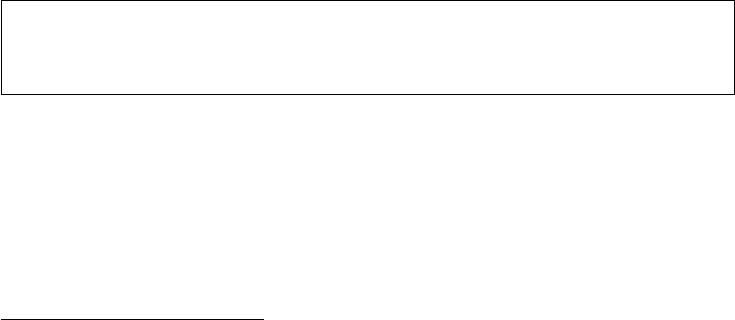
118 AUTOMATED DATA COLLECTION WITH R
{
"headers": {
"X-Request-Id": "0726a0cf-a26a-43b9-b5a4-9578d0be712b",
"User-Agent": "x86_64-w64-mingw32, R version 3.0.2 (2013-09-25)",
"Connection": "close",
"Accept": "*/*",
"Host": "httpbin.org"
}
}
cat() is used to concatenate and print the results over several lines. The useragent
argument allows specifying a User-Agent header eld string. RCurl takes care of writing
this string into a header eld and passes it to the server. http://httpbin.org/headers returns the
sent header information in JSON format.12 Beside the set of header elds that are used by
default, we nd that a User-Agent header eld has been added.13
We will later learn that the basis of the RCurl package is the C library libcurl.Many
of the options that libcurl offers can also be used in RCurl’s high-level functions (for more
details, see Section 5.4.1). We will return to the use of User-Agents in practical web scraping
in Section 9.3.3.
The second header eld that is informative about the client is the Referer.ItstorestheReferer
URL of the page that referred the user to the current page. Referrers can be used for trafc
evaluation to asses where visitors of a site come from. Another purpose is to be able to limit
access to specic server content like image les. A webmaster could modify the settings of
the server such that access to images is only possible from another resource on the server
in order to prevent other people from using images on their own webpage by referring to
the location on the original server. This causes unwanted trafc and is therefore unwelcome
behavior. The default browser setting is that the Referer header is delivered automatically.
This may look as follows:
1GET /headers HTTP/1.1
2Host: httpbin.org
3Referer: http://www.r-datacollection.com/
We can provide the Referer header eld with Rusing getURL()’s referer argument.
We test the request to http://httpbin.org/headers with:14
R> getURL("http://httpbin.org/headers", referer = "http://www.r-
datacollection.com/")
12Note that we use the cat() function to concatenate and print the returned JSON string.
13We do not have to care about the X-Request-Id and Heroku-Request-Id header elds, they are added by
the service at http://httpbin.org for debugging purposes.
14We do not print the JSON output from now on—you can easily see the returned content by loading RCurl and
pasting the command in your Rconsole.

HTTP 119
Note that adding information on the Referer from within Ris misleading when Rhas
not actually been referred from the site provided. We suggest that if it is necessary to provide
a valid referrer in order to get access to certain resources, stay identiable, for example, by
properly specifying the From header eld as described below, and contact the webmaster if
in doubt. Providing wrong information in the Referer header eld in order to disguise the
source of the access request is called referrer spoong. This may have its legitimacy for data
privacy purposes but is not encouraged by scraping etiquette (see Section 9.3.3).
The From header eld for client identication is not delivered by browsers but a convenient From
header for well-behaved web spiders and robots. It carries the user’s email address to make
her identiable for web administrators. In web scraping, it is good practice to specify the
From header eld with a valid email address, as in
1GET /headers HTTP/1.1
2Host: httpbin.org
3From: eddie@r-datacollection.com
Providing contact details signals good intentions and enables webmasters who note
unusual trafc patterns on their sites to get in touch. We thus reformulate our request:
R> getURL("http://httpbin.org/headers", httpheader = c(From =
"eddie@r-collection.com"))
Note that we have to use the httpheader option here to add the From header eld, as
from is not a valid option—in contrast to “referer,” for example. httpheader allows us
to specify additional other header elds.
5.2.1.2 Cookies
Cookies help to keep users identiable for a server. They are a tool to turn stateless HTTP
communication into a stateful conversation where future responses depend on past conver-
sations. Cookies work as follows: Web servers store a unique session ID in a cookie that is
placed on the client’s local drive, usually in a text le. The next time a browser sends an
HTTP request to the same web server, it looks for stored cookies that belong to the server
and—if successful—adds the cookie information to the request. The server then processes
this “we already met” information and adapts its response. Usually, further information on
the user has been stored on the server over the course of several conversations and can be
“reactivated” using cookies. In other words, cookies enable browsers and servers to continue
conversations from the past.
Cookies are shared via the HTTP header elds “Set-Cookie” (in the response header)
and “Cookie” (in the request header). A typical conversation via HTTP that results in a
cookie exchange looks as follows. First, the client makes a request to a web server:
1GET /headers HTTP/1.1
2Host: httpbin.org
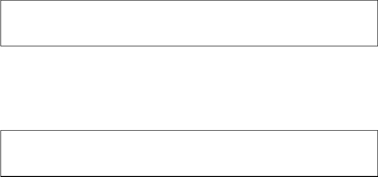
120 AUTOMATED DATA COLLECTION WITH R
If the request is successful, the server responds and passes the cookie with the Set-
Cookie response header eld. The eld provides a set of name–value pairs:
1HTTP/1.1 200 OK
2Set-cookie: id="12345"; domain="httpbin.org"
3...
The id attribute allows the server to identify the user in a subsequent request and the
domain attribute indicates which domain the cookie is associated with. The client stores the
cookie and attaches it in future requests to the same domain, using the Cookie request header
eld:
1GET /headers HTTP/1.1
2Host: httpbin.org
3Cookie: id="12345"
There are several types of cookies that differ in terms of persistence and range. SessionDifferent types
of cookies cookies are kept in memory only as long as the user visits a website and are deleted as soon
as the browser is closed. Persistent cookies, or tracking cookies, last longer—their lifetime
is dened by the value of the max-age attribute or the expires attribute (not shown in
the examples above). The browser delivers the cookie with every request during a cookie’s
lifetime, which makes the user traceable for the server across several sessions. Third-party
cookies are used to personalize content across different sites. They do not belong to the
domain the client visits but to another domain. If you have ever wondered how personalized
ads are placed on pages you visit—this is most likely done with third-party cookies that are
placed by advertising companies on domains you visit and which can be used by advertisers
to tailor ads to your interests. The use of cookies for such purposes surely has contributed to
the fact that cookies have a bad reputation regarding privacy. In general, however, cookies are
only sent to the server that created them. Further, the user can decide how to handle locally
stored cookies. And in the end, cookies are useful as they often enhance the web experience
considerably.
If cookies inuence the content a server returns in response to a request, they can be
relevant for web scraping purposes as well. Imagine we care to scrape data from our crammed
shopping cart in an online store. During our visit we have added several products to the cart.
In order to track our spending spree, the server has stored a session ID in a cookie that keeps
us identiable. If we want to request the webpage that lists the shopped items, we have to
deliver the cookie with our request.
In order to deliver existing cookies with R, we can draw upon the cookie argument:
R> getURL("http://httpbin.org/headers", cookie = "id=12345;domain=
httpbin.org")
It is usually not desirable to manage cookies manually, that is, retrieve them, store them,
and send them. This is why browsers automatically take care of such operations by default.
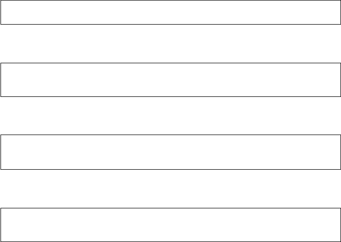
HTTP 121
In order to achieve similar convenience in R, we can rely on libcurl’s cookiefile and
cookiejar options that, if specied correctly, manage cookies for us. We show in detail how
this can be done in Section 9.1.8.
5.2.2 Authentication
While techniques for client identication are useful to personalize web content and enable
stateful communication, they are not suited to protect content that only the user should see.
A set of authentication techniques exist that allow qualied access to condential content.
Some of these techniques are part of the HTTP protocol. Others, like OpenID or OAuth (see
Section 9.1.11), have been developed more recently to extend authentication functionality on
the Web.
The simplest form of authentication via the HTTP protocol is basic authentication (Franks Basic
authentication
et al. 1999). If a client requests a resource that is protected by basic authentication, the server
sends back a response that includes the WWW-Authenticate header. The client has to repeat
its request with a username and password in order to be granted access to the requested
resource. Both are stored in the response’s Authorization header. If the server can verify
that the username/password combination is correct, it returns the requested resource in a
HTTP 200 message. Technically, basic authentication looks as follows.
1. The client requests a protected resource:
1GET /basic-auth/user/passwd HTTP/1.1
2. The server asks the client for a user name and password:
1HTTP/1.1 401 Authorization required
2WWW-Authenticate: Basic realm="Protected area"
3. The client/user provides the requested username and password in Base64 encoding:
1GET /basic-auth/user/passwd HTTP/1.1
2Authorization: Basic dXNlcm5hbWU6cGFzc3dvcmQ=
4. The server returns the requested resource:
1HTTP/1.1 200 OK
2...
Note that in the third step, the username/password combination has been automatically
“encrypted” into the string sequence “dXNlcm5hbWU6cGFzc3dvcmQ=.” This transformation
is done via Base64 encoding. Base64 encoding is not actually an encrypting technique but
follows a rather trivial and static scheme (see Gourley and Totty 2002, Appendix E). We can
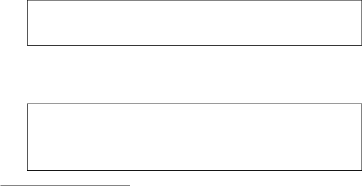
122 AUTOMATED DATA COLLECTION WITH R
perform Base64 encoding and decoding with R; the necessary functions are implemented in
the RCurl package:
R> (secret <- base64("This is a secret message"))
[1] "VGhpcyBpcyBhIHNlY3JldCBtZXNzYWdl"
attr(,"class")
[1] "base64"
R> base64Decode(secret)
[1] "This is a secret message"
The example reveals the insecurity of basic HTTP authentication: As long as it is done
via standard HTTP, the sensitive information is sent practically unencrypted across the net-
work. Therefore, basic authentication should only be used in combination with HTTPS (see
Section 5.3.1).
A more sophisticated authentication technique is digest authentication (Franks et al.
Digest
authentication 1999). The idea behind digest authentication is that passwords are never sent across the Web
in order to verify a user, but only a “digest” of it. The server attaches a little random string
sequence to its response, called nonce. The browser transforms username, password, and the
nonce into a hash code, following one of several algorithms that are known to both server and
browser. This hash code is then sent back, compared to the hash calculations of the server,
and if both match the server grants access to the client. The crucial point is that the hash alone
does not sufce to learn anything about the password; it is just a “digest” of it. This makes
digest authentication an improvement relative to basic authentication, as the encrypted client
message is incomprehensible for an eavesdropper.
Steps 2 and 3 in the authentication procedure sketched above are slightly different. The
server returns something like the following:15
2a. The server asks the client for a username and password and delivers a nonce, reports
a “quality of protection” value (qop) and describes the realm as Protected area:
1HTTP/1.1 401 Authorization required
2WWW-Authenticate: Digest realm="Protected area",
3qop="auth",nonce="f7hf4xu8n2kxuujnszrctx4fexqnahopjdrn4zbi"
3a. The client provides the encrypted username and password in the response attribute,
as well as the unencrypted username, the qop and nonce parameters and a client nonce
(cnonce):
1GET /basic-auth/user/passwd HTTP/1.1
2Authorization: Digest username="user", nonce="
f7hf4xu8n2kxuujnszrctx4fexqnahopjdrn4zbi", qop="auth",
cnonce="1g443t8b", response="
y1h5uafdsda8r2wsxdy1vxzhqnht5ngry2m5argc"
15Note that this is a simplied example. We have left out some intermediate steps, but the fundamental logic
remains the same.

HTTP 123
HTTP Client
Browser
Proxy HTTP Server
HTTP response
HTTP request
HTTP response
HTTP request
Figure 5.4 The principle of web proxies
In Section 9.1.6 we give a short demonstration of HTTP authentication in practice with
RCurl.
5.2.3 Proxies
Web proxy servers, or simply proxies, are servers that act as intermediaries between clients
and other servers. HTTP requests from clients are rst sent to a proxy, which evaluates the
request and passes it to the desired server. The server response takes the way back via the
proxy. In that sense, the proxy serves as a server to clients and as a client to other servers (see
Figure 5.4).
Proxies are useful for several purposes. They are deployed for performance, economic, The use of
proxies
and security reasons. For users, proxies can help to
rspeed up network use;
rstay anonymous on the Web;
rget access to sites that restrict access to IPs from certain locations;
rget access to sites that are normally blocked in the country from where the request
is put; or
rkeep on querying resources from a server that blocks requests from IPs we have
used before.
Especially when proxies are used for any of the last three reasons, web scrapers might get
into troubles with the law. Recent verdicts point in the direction that it is illegal to use proxy
servers in order to get access to public websites that one has been disallowed to visit (see
Kerr 2013). We therefore do not recommend the use of proxies for any of these purposes.
In order to establish connections via a proxy server, we have to know the proxy’s IP Types of
proxies
address and port. Some proxies require authentication as well, that is, a username and a
password. There are many services on the Web that provide large databases of open and free
proxies, including their location and specication. Open proxies can be used by anyone who
knows their IP address and port. Note that proxies vary in the degree to which they provide
anonymity to the user. Transparent proxies specify a Via header eld in their request to
the server, lling it with their IP. Further, they offer an X-Forwarded-For header eld
with your IP. Simple anonymous proxies replace both the Via and the X-Forwarded-For
header eld with their IP. As both elds are delivered only when a proxy is used, the server
knows that the requests comes from a server, but does not easily see the client’s IP address
behind it. Distorting proxies are similar but replace the value of the X-Forwarded-For
header eld with a random IP address. Finally, High anonymity proxies or elite proxies
behave like normal clients, that is, they neither provide the Via nor the X-Forwarded-For
header eld but only their IP and are not immediately identiable as proxy servers.
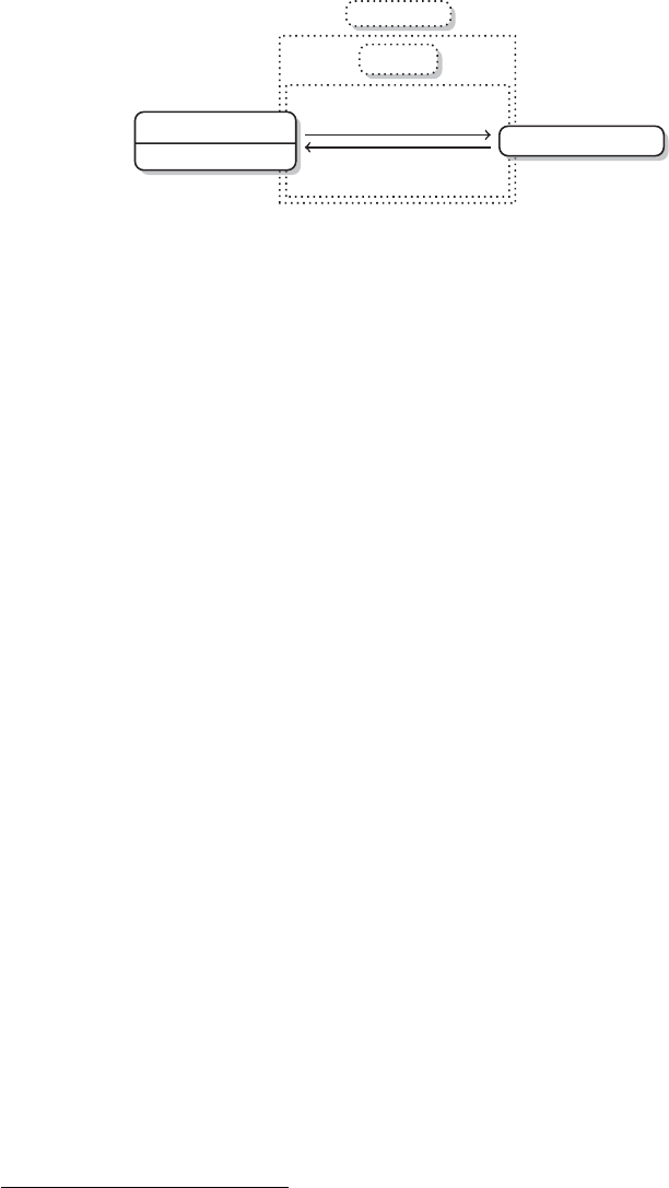
124 AUTOMATED DATA COLLECTION WITH R
HTTP Client
Browser HTTP Server
HTTP response
HTTP request
TCP/IP
TLS or SSL
Figure 5.5 The principle of HTTPS
To send a request to a server detouring via a proxy with R, we can add the proxy argument
to the request command. In the following, we choose a ctional proxy from Poland that has
the IP address 109.205.54.112 and is on call on port 8080:
R> getURL("http://httpbin.org/headers",
R> proxy = "109.205.54.112:8080",
R> followlocation = TRUE)
IP address and port of the proxy are specied in the proxy option. Further, we set
the followlocation argument to TRUE to ensure that we are redirected to the desired
resource.
5.3 Protocols beyond HTTP
HTTP is far from the only protocol for data transfer over the Internet. To get an overview of
the protocols that are currently supported by the RCurl package, we call
R> library(RCurl)
R> curlVersion()$protocols
[1] "tftp" "ftp" "telnet" "dict" "ldap" "ldaps" "http"
[8] "file" "https" "ftps" "scp" "sftp"
Not all of them are relevant for web scraping purposes. In the following, we will high-
light two protocols that we often encounter when browsing and scraping the Web: HTTPS
and FTP.
5.3.1 HTTP Secure
Strictly speaking, the Hypertext Transfer Protocol Secure (HTTPS) is not a protocol of
its own, but the result of a combination of HTTP with the SSL/TLS (Secure Sockets
Layer/Transport Security Layer) protocol. HTTPS is indispensable when it comes to the
transfer of sensitive data, as is the case in banking or online shopping. To transfer money or
credit card information we need to ensure that the information is inaccessible to third parties.
HTTPS encrypts all the client–server communication (see Figure 5.5). HTTPS URLs have
the scheme https and use the port 443 by default.16
16Recall that the default HTTP port is 80.
HTTP 125
HTTPS serves two purposes: First, it helps the client to ensure that the server it talks
to is trustworthy (server authentication). Second, it provides encryption of client–server
communication so that users can be reasonably sure that nobody else reads what is exchanged
during communication.
The SSL/TLS security layer runs as a sublayer of the application layer where HTTP SSL/TLS
operates. This means that HTTP messages are encrypted before they get transmitted. The
SSL protocol was rst dened in 1994 by Netscape (see Freier et al. 2011) and was updated
as TLS 1.0 in 1999 (see Dierks and Allen 1999). When using the term “SSL” in the following,
we refer to both SSL and TLS as their differences are of no importance to us.
A crucial feature of SSL that allows secure communication in an insecure network is
public key, or asymmetric, cryptography. As the name already indicates, encryption keys are
in fact not kept secret but publicly available to everyone. In order to encrypt a message for
a specic receiver, the receiver’s public key is used. In order to decrypt the message, both
the public and a private key is needed, and the private key is only known to the receiver. The
basic idea is that if a client wants to send a secret message to a server, it knows how to encrypt
it because the server’s public key is known. After encryption, however, nobody—not even
the sender—is able to decipher the message except for the receiver, who possesses both the
public and the private key.
We do not have to delve deeply into the details of public key encryption, how the secret SSL handshake
codes (ciphers) work, and why it is so hard to crack them in order to understand HTTPS’s
purpose. For the details of cryptography behind SSL, we refer to the excellent introductions
by Gourley and Totty (2002) and Garnkel (2002). If you want to get a more profound
understanding of digital cryptography, the books by Ferguson et al. (2010) and Paar and Pelzl
(2011) are a good choice. What is worth knowing though is how secure channels between
client and server are actually established and how we can achieve this from within R.Avery
simplied scheme of the “SSL handshake,” that is, the negotiation between client and server
about the establishment of an HTTPS connection before actually exchanging encrypted HTTP
messages, works as follows (see Gourley and Totty 2002, pp. 322–328).
1. The client establishes a TCP connection to the server via port 443 and sends information
about the SSL version and cipher settings.
2. The server sends back information about the SSL and cipher settings. The server also
proves his identity by sending a certicate. This certicate includes information about
the authority that issued the certicate, for whom it was issued and its period of validity.
As anybody can create his or her own certicates without much effort, the signature of
a trusted certicate authority (CA) is of great importance. There are many commercial
CAs, but some providers also issue certicates for free.
3. The client checks if it trusts the certicate. Browsers and operating systems are shipped
with lists of certicate authorities that are automatically trusted. If one of these author-
ities has signed the server’s certicate, the client trusts the server. If this is not the
case, the browser asks the user whether she nds the server trustworthy and wants to
continue, or if communication should be stopped.
4. By using the public key of the HTTPS server, the client generates a session key that
only the server can read, and sends it to the server.
5. The server decrypts the session key.

126 AUTOMATED DATA COLLECTION WITH R
6. Both client and server now possess a session key. Thus, knowledge about the key is not
asymmetric anymore but symmetric. This reduces computational costs that are needed
for encryption. Future data transfers from server to client and vice versa are encrypted
and decrypted through this symmetric SSL tunnel.
It is important to note that what is protected is the content of communication. This
includes HTTP headers, cookies, and the message body. What is not protected, however, are
IP addresses, that is, websites a client communicates with.
We will address how connections via HTTPS are established in Rand how much of the
technical details are hidden deeply in the respective functions in Section 9.1.7—using HTTPS
with Ris not difcult at all.
5.3.2 FTP
The File Transfer Protocol (FTP) was developed to transfer les from client to server (upload),FTP vs. HTTP
from server to client (download), and to manage directories. FTP was rst specied in 1971
by Abhay Bhushan (1971); its current specication (see Postel and Reynolds 1985) is almost
30 years old. In principle, HTTP has several advantages over FTP. It allows persistent, keep-
alive connections, that is, connections between client and server that are maintained for several
transfers. This is not possible with FTP, where the connection has to be reestablished after
each transfer. Further, FTP does not natively support proxies and pipelining, that is, several
simultaneous requests before receiving an answer. On the upside, FTP may be faster under
certain circumstances, as it does not come with a bunch of header elds like HTTP—just the
binary or ASCII les are transferred.
FTP uses two ports on each side, one for data exchange (“data port,” the default is port 20)
Active and
passive modes and one for command exchange (“control port,” the default is port 21). Just like HTTP, FTP
comes with a set of commands that specify which les to transfer, what directories to create,
and many other operations.17 FTP connections can be established in two different modes:
the active mode and the passive mode. In active FTP, the client connects with the server’s
command port and then requests a data transfer to another port. The problem with this mode
is that the actual data connection is established by the server. As the client’s rewall has not
been told that the client expects data to come in on a certain port, it usually blocks the server’s
attempt to deliver the data. This issue is tackled with the passive mode in which the client
initiates both the command and the data connection. We are going to demonstrate accessing
FTP servers with Rin Section 9.1.2.
5.4 HTTP in action
We now learn to use Ras an HTTP client. We will have a closer look at two available
packages: the powerful RCurl package (Temple Lang 2013a), and the more lightweight but
sometimes also more convenient httr package (Wickham 2012) that rests on the voluminous
RCurl package.
17For an overview over existing commands, see http://www.nsftools.com/tips/RawFTP.htm
HTTP 127
Base Ralready comes with basic functionality for downloading web resources. The
download.file() function handles many download procedures where we do not need
complex modications of the HTTP request. Further, there is a set of basic functions to set
up and manipulate connections. For an overview, type ?connections in R. However, using
these functions is anything but convenient. Regarding download.file(), there are two
major drawbacks for sophisticated web scraping. First, it is not very exible. We cannot use
it to connect with a server via HTTPS, for example, or to specify additional headers. Second,
it is difcult to adhere to our standards of friendly web scraping with download.file(),
as it lacks basic identication facilities. However, if we just want to download single les,
download.file() works perfectly ne. For more complex tasks, we can apply the func-
tionality of the RCurl and the httr package.
5.4.1 The libcurl library
Much of what we need to do with Ron the web is dramatically facilitated by libcurl (Stenberg
2013). libcurl is an external library programmed in C. Development began in 1996 by Daniel
Stenberg and the cURL project and has since been under continuous development. The
purpose of libcurl is to provide an easy interface to various Internet protocols for programs
on many platforms. Over time, the list of features has grown and now comprises a multitude
of possible actions and options to congure, among others, HTTP communication. We can
think of it as a tool that knows how to
rspecify HTTP headers;
rinterpret URL encoding;
rprocess incoming streams of data from web servers;
restablish SSL connections;
rconnect with proxies;
rhandle authentication;
and much more. In contrast, R’s url() and download.file() are precious little help
when it comes to complex tasks like lling forms, authentication, or establishing a stateful
conversation. Therefore, libcurl has been tapped to enable users to work with the libcurl
library in their ordinary programming environment. In his manifest of RCurl and libcurl’s
philosophy, Temple Lang points out the benets of libcurl: Being the most widely used
le transfer library, libcurl is extraordinarily well tested and exible (Temple Lang 2012a).
Further, being programmed in C makes it fast. To get a rst impression about the exibility of
libcurl, you might want to start by taking a look at the available options of libcurl’s interface at
http://curl.haxx.se/libcurl/c/curl_easy_setopt.html. Alternatively, you can type the following
into Rto get the comprehensive list of libcurl’s “easy” interface options that can be specied
with RCurl:
R> names(getCurlOptionsConstants())
Currently, there are 174 available options. Among them are some that we have already
relied on above, like useragent or proxy. We sometimes speak of curl options instead of

128 AUTOMATED DATA COLLECTION WITH R
libcurl options for reasons of convenience. curl is a command line tool also developed by the
cURL software project. With Rwe draw on the libcurl library.18
5.4.2 Basic request methods
5.4.2.1 The GET method
In order to perform a basic GET request to retrieve a resource from a web server, the
High-level
functions RCurl package provides some high-level functions—getURL(),getBinaryURL(), and
getURLContent(). The basic function is getURL();getBinaryURL() is convenient when
the expected content is binary, and getURLContent() tries to identify the type of content
in advance by inspecting the Content-Type eld in the response header and proceeding
adequately. While this seems preferable, the conguration of getURLContent() is some-
times more sophisticated, so we continue to use getURL() by default except when we expect
binary content.
The function automatically identies the host, port, and requested resource. If the call
succeeds, that is, if the server gives a 2XX response along with the body, the function
returns the content of the response. Note that if everything works ne, all of the negotia-
tion between R/libcurl and the server is hidden from us. We just have to pass the desired
URL to the high-level function. For example, if we try to fetch helloworld.html from
www.r-datacollection.com/materials/http, we type
R> getURL("http://www.r-datacollection.com/materials/http/helloworld.html")
[1] "<html>\n<head><title>Hello World</title></head>\n<body><h3>Hello World
</h3>\n</body>\n</html>"
The body is returned as character data. For binary content, we use getBinaryURL()
and get back raw content. For example, if we request the PNG image le sky.png from
www.r-datacollection.com/materials/http, we write
R> pngfile <- getBinaryURL("http://www.r-datacollection.com/materials/http/
sky.png")
It depends on the format how we can actually process it; in our case we use the
writeBin() function to locally store the le:
R> writeBin(pngfile, "sky.png")
Sometimes content is not embedded in a static HTML page but returned after we sub-GET forms
mit an HTML form. The little example at http://www.r-datacollection.com/materials/http/
GETexample.html lets you specify a name and age as input elds. The HTML source code
looks as follows:
1<!DOCTYPE HTML>
2<html>
3<head>
4<title>HTTP GET Example</title></head><body>
5<h3>HTTP GET Example</h3>
18See also http://daniel.haxx.se/docs/curl-vs-libcurl.html for the differences between cURL,curl,andlibcurl.

HTTP 129
6<form action="GETexample.php" method="get">
7Name: <input type="text" name="name" value="Anny Omous"><br>
8Age: <input type="number" name="age" value="23"><br><br>
9<input type="submit" value="Send Form and Evaluate"><br><br>
10 <input type="submit" value="Send Form and Return Request" name="return">
11 </form>
12 </body>
13 </html>
The <form> element indicates that data put into the form is sent to a le
called GETexample.php.19 After having received the data from the GET request, the
PHP script evaluates the input and returns “Hello <name>! You are <age> years
old.” In the browser, we see an URL of form http://www.rdatacollection.com/materials/
http/GETexample.php?name=<name>&age=<age>, which indicates that a PHP script has
generated the output.
How can we process this and similar requests from within R? There are several ways to
specify the arguments of an HTML form. The rst is to construct the URL manually using
paste() and to pass it to the getURL() function:
R> url <- "http://www.r-datacollection.com/materials/http/GETexample.php"
R> namepar <- "Eddie"
R> agepar <- "32"
R> url_get <- str_c(url, "?", "name=", namepar, "&", "age=", agepar)
R> cat(getURL(url_get))
Hello Eddie!
You are 32 years old.
An easier way than using getURL() and constructing the GET form request manually is
to use getForm(), which allows specifying the parameters as separate values in the function.
This is our preferred procedure as it simplies modifying the call and does not require manual
URL encoding (see Section 5.1.2). In order to get the same result as above, we write
R> url <- "http://www.r-datacollection.com/materials/http/GETexample.php"
R> cat(getForm(url, name = "Eddie", age = 32))
Hello Eddie!
You are 32 years old.
5.4.2.2 The POST method
When using HTML forms we often have to use the POST method instead of GET.In POST forms
general, POST allows more sophisticated requests, as the request parameters do not have do
be inserted into the URL, which may be limited in length. The POST method implies that
parameters and their values are sent in the request body, not in the URL itself. We replicate
the example from above, except that now a POST request is required. The form is located at
19PHP, Hypertext Preprocessor or previously Personal Home Page Tools is a scripting language which is
frequently implemented on the server side to create dynamic webpages. The ending .php indicates that the content
is generated by a PHP script.

130 AUTOMATED DATA COLLECTION WITH R
http://www.r-datacollection.com/materials/http/POSTexample.html. The HTML source code
reads as follows:
1<!DOCTYPE HTML>
2<html>
3<head>
4<title>HTTP POST Example</title></head>
5<body>
6<h3>HTTP POST Example</h3>
7<form action="POSTexample.php" method="post">
8Name: <input type="text" name="name" value="Anny Omous"><br>
9Age: <input type="number" name="age" value="23"><br><br>
10 <input type="submit" value="Send Form and Evaluate" name="send"><br><br>
11 <input type="submit" value="Send Form and Return Request" name="return">
12 </form>
13 </body>
14 </html>
We nd that the <form> element has remained almost identical, except for the required
method, which is now POST. When we submit the POST form in the browser we see that
the URL changes to ../POSTexample.php and no query parameters have been added as in the
GET query. In order to replicate the POST query with R, we do not have to construct the
request manually but can use the postForm() function:
R> url <- "http://www.r-datacollection.com/materials/http/POSTexample.php"
R> cat(postForm(url, name = "Eddie", age = 32, style = "post"))
Hello Eddie!
You are 32 years old.
postForm() automatically constructs the body and lls it with the pre-specied parame-
ter pairs. Unfortunately, there are several ways to format these pairs, and we sometimes have
to explicitly specify the one that is accepted in advance using the style argument (see Nolan
and Temple Lang 2014, p. 270–272 and http://www.w3.org/TR/html401/interact/forms.html
for details on the form content types). For the application/x-www-form-urlencoded
form content type, we have to specify style = "post" and for the multipart/form-
data form content type, style = "httppost". This formats the parameter pairs in the
body correctly and adds the request header "Content-Type" = "application/x-
www-form-urlencoded" or "Content-Type" = "multipart/form-data". To nd
the adequate POST format, we can look for an attribute named enctype in the <form>
element. If it is specied as enctype='application/x-www-form-urlencoded',we
use style = "post". If it is missing (as above), leaving out the style parameter should
also work.
5.4.2.3 Other methods
RCurl offers functions to deal with other HTTP methods as well. We can change meth-
ods in calls to getURL(),getBinaryURL(),getURLContent() by making use of the
customrequest option, for example,
HTTP 131
R> url <- "r-datacollection.com/materials/http/helloworld.html"
R> res <- getURL(url = url, customrequest = "HEAD", header = TRUE)
R> cat(str_split(res, "\r")[[1]])
HTTP/1.1 200 OK
Date: Wed, 26 Mar 2014 00:20:07 GMT
Server: Apache
Vary: Accept-Encoding
Content-Type: text/html
As we hardly encounter situations where we need these methods, we refrain from going
into more detail.
5.4.3 A low-level function of RCurl
RCurl builds on the powerful libcurl library, making it a mighty weapon in the hands of
the initiated and an unmanageable beast in the hands of others. The low-level function
curlPerform() is the workhorse of the package. The function gathers options specied
in Ron how to perform web requests—which protocol or methods to use, which headers to
set—and patches them through to libcurl to execute the request. Everything in this function
has to be specied explicitly so later on we will come back to more high-level functions.
Nevertheless, it is useful to demonstrate how the high-level functions work under the hood.
We start with a call to curlPerform() to request an HTML document:
R> url <- "www.r-datacollection.com/materials/http/helloworld.html"
R> (pres <- curlPerform(url = url))
OK
0
Instead of getting the content of the URL we only get the information that everything seems
to have worked as expected by the function. This is because we have to specify everything
explicitly when using curlPerform(). The function did retrieve the document but did not
know what to do with the content. We need to dene a handler for the content. Let us create
one ourselves. First, we create an object pres to store the document and a function that takes
the content as argument and writes it into pres. As the list of options can get extensive we
save them in a separate object performOptions and pass it to curlPerform():
R> pres <- NULL
R> performOptions <- curlOptions(url = url,
writefunc = function(con) pres <<- con )
R> curlPerform(.opts = performOptions)
OK
0
R> pres
[1] "<html>\n<head><title>Hello World</title></head>\n<body><h3>Hello
World</h3>\n</body>\n</html>"
That looks more like what we would have expected. In addition to the content handler, there
are other handlers that can be supplied to curlPerform(): a debug handler via debugfunc,
and a HTTP header handler via headerfunc. There are sophisticated functions in RCurl for
each of these types that spare us the need to specify our own handler functions. For content
132 AUTOMATED DATA COLLECTION WITH R
and headers, basicTextGatherer() turns an object into a list of functions that handles
updates, resets, and value retrieval. In the following example we make use of all three. Note
that in order for debugfunc to work we need to set the verbose option to TRUE:
R> content <- basicTextGatherer()
R> header <- basicTextGatherer()
R> debug <- debugGatherer()
R> performOptions <- curlOptions(url = url,
writefunc = content$update,
headerfunc = header$update,
debugfunc = debug$update,
verbose = T)
R> curlPerform(.opts=performOptions)
OK
0
Using the value() function of content we can extract the content that was sent from the
server.
R> str_sub(content$value(), 1, 100)
[1] "<html>\n<head><title>Hello World</title></head>\n<body><h3>Hello
World</h3>\n</body>\n</html>"
header$value() contains the headers sent back from the server:
R> header$value()
[1] "HTTP/1.1 200 OK\r\nDate: Wed, 26 Mar 2014 00:20:10 GMT\r\nServer:
Apache\r\nVary: Accept-Encoding\r\nContent-Length: 89\r\nContent-Type:
text/html\r\n\r\n"
debug$value() stores various pieces of information on the HTTP request. See Sec-
tion 5.4.6 for more information on this topic:
R> names(debug$value())
[1] "text" "headerIn" "headerOut" "dataIn" "dataOut"
[6] "sslDataIn" "sslDataOut"
R> debug$value()["headerOut"]
headerOut
"GET /materials/http/helloworld.html HTTP/1.1\r\nHost: www.r-datacollection.
com\r\nAccept: */*\r\n\r\n"
5.4.4 Maintaining connections across multiple requests
It is a common scenario to make multiple requests to a server, especially if we are interested
in accessing a set of resources like multiple HTML pages. The default setting in HTTP/1.0 is
to establish a new connection with each request, which is slow and inefcient. Connections
in HTTP/1.1 are persistent by default, meaning that we can use the same connection for
multiple requests. RCurl provides the functionality to reuse established connections, which
we can exploit to create faster scrapers.
HTTP 133
Reusing connections works with the so-called “curl handles.” They serve as containers Curl handles
for the connection itself and additional features/options. We establish a handle as follows:
R> handle <- getCurlHandle()
The handle in the handle object is of class CURLHandle and currently an empty container.
We can add useful curl options from the list listCurlOptions(), for example:
R> handle <- getCurlHandle(useragent = str_c(R.version$platform,
R> R.version$version.string,
R> sep=", "),
R> httpheader = c(from = "ed@datacollection.com"),
R> followlocation = TRUE,
R> cookiefile = "")
In the example, we specify a User-Agent header eld that contains the current Rversion
and a From header eld containing an email address, set the followlocation argument to
TRUE, and activate cookie management (see Section 5.4.5). The curl handle can now be used
for multiple requests using the curl argument. For instance, if we have a vector of URLs in
the object url, we can retrieve them with getURL() fed with the settings in the curl handle
from above.
R> lapply(urls, getURL, curl = handle)
Note that the curl handle container is not xed across multiple requests, but can Cloning
handles
be modied. As soon as we specify new options in a request, these are added—or old
ones overridden—in the curl handle, for example, with getURL(urls, curl = handle,
httpheader = c(from = "max@datacollection.com")). To retain the status of the
handle but use a modied handle for another request, we can duplicate it and use the “cloned”
version with dupCurlHandle():
R> handle2 <- dupCurlHandle(curlhandle,
R> httpheader = c(from = "ed@datacollection.com"))
Cloning handles can be especially useful if we want to reuse the settings specied in a
handle in requests to different servers. Not all settings may be useful for every request (e.g.,
protocol settings or referrer information), and some of the information should probably be
communicated only to one specic server, like authentication details.
When should we use curl handles? First, they are generally convenient for specifying and
using curl options across an entire session with RCurl, simplifying our code and making it
more reliable. Second, fetching a bunch of resources from the same server is faster when we
reuse the same connection.
5.4.5 Options
We have seen that we can use curl handles to specify options in RCurl function calls. However,
there are also other means. Generally, RCurl options can be divided into those that dene the
behavior of the underlying libcurl library and those that dene how information is handled
in R. The list of possible options is vast, so we selected the ones we frequently use and listed
them in Table 5.3. Some of these options were already introduced above, the others will be
explained below. Let us begin by showing the various ways to declare options.

Table 5.3 List of useful libcurl options that can be specied in RCurl functions
Option Description Example
HTTP
connecttimeout Set maximum number of seconds waiting to connect to server connecttimeout = 10
customrequest Dene HTTP method to use in RCurl’s high-level functions customrequest = "HEAD"
.encoding Species the encoding scheme we expect .encoding = "UTF-8"
followlocation Follow the redirection to another URL if suggested by the
server
followlocation = TRUE
header Retrieve response header information as well header = TRUE
httpheader Species additional HTTP request headers httpheader = c('Accept-Charset'
= "utf-8")
maxredirs Limit the number of redirections to avoid innite loop error
with followlocation = TRUE
maxredirs = 5L
range Retrieve a certain byte range from a le, that is, only parts of a
document (does not work with every server; see p. 264)
range = "1-250"
referer Convenience option to specify a Referer header eld referer = "www.example.com"
timeout Set maximum number of seconds waiting for curl request to
execute
timeout = 20
useragent Convenience option to specify a User-agent header eld useragent = "RCurl"

FTP (see Sections 5.3.2 and 9.1.2)
dirlistonly Set if only the le names and no further information should be
downloaded from FTP servers
dirlistonly = TRUE
ftp.use.epsv Set extended or regular passive mode when accessing FTP
servers
ftp.use.epsv = FALSE
Cookies (see Sections 5.2.1.1 and 9.1.8)
cookiefile Species a le that contains cookies to read from it or, if
argument remains empty, activates cookie management
cookiefile = ""
cookiejar Writes cookies that have been gathered over several requests
toale
cookiejar = "/files/cookies"
SSL (see Sections 5.3.1 and 9.1.7)
cainfo Specify le with digital signatures for SSL certicate
verication
cainfo = system.file("CurlSSL",
"cacert.pem", package =
"RCurl")
ssl.verifyhost Set validation of the certicate-host match true or false ssl.verifyhost = FALSE
ssl.verifypeer Set validation of server certicate true or false—useful if a
server lacks a certicate but is still trustworthy
ssl.verifypeer = FALSE

136 AUTOMATED DATA COLLECTION WITH R
We can declare options for single calls to the high-level functions (e.g., getURL,getURL-Options as
arguments Content, and getBinaryURL). In this case the options will only affect that single function
call. In the following example we add header = TRUE in order to not only retrieve the
content but also the response header:20
R> url <- "www.r-datacollection.com/materials/http/helloworld.html"
R> res <- getURL(url = url, header = TRUE)
R> cat(str_split(res, "\r")[[1]])
HTTP/1.1 200 OK
Date: Wed, 26 Mar 2014 00:20:11 GMT
Server: Apache
Vary: Accept-Encoding
Content-Length: 89
Content-Type: text/html
<html>
<head><title>Hello World</title></head>
<body><h3>Hello World</h3>
</body>
</html>
Another, more persistent way of specifying options is to bind them to a curl handle asOptions in
handles described in the previous section. Every function using this handle via the curl option will
use the same options. If a function uses the handle and redenes some options or adds others,
these changes will stick to the handle. In the following example we create a new handle and
specify that the HTTP method HEAD should be used for the request:
R> handle <- getCurlHandle(customrequest = "HEAD")
R> res <- getURL(url = url, curl = handle)
R> cat(str_split(res, "\r")[[1]])
The rst function call using the handle results in an empty vector because HEAD provides
no response body and the header option was not specied. In the second call we add the
header argument to retrieve header information:
R> res <- getURL(url = url, curl = handle, header = TRUE)
R> cat(str_split(res, "\r")[[1]])
HTTP/1.1 200 OK
Date: Wed, 26 Mar 2014 00:20:14 GMT
Server: Apache
Vary: Accept-Encoding
Content-Type: text/html
The added header specication has become part of the handle. When we reuse it, we do
not need to specify header = TRUE anymore:
R> res <- getURL(url = url, curl = handle)
R> cat(str_split(res, "\r")[[1]])
20Note that unfortunately not all options work the same way for each of the high-level functions. The header
argument, for example, does not expect Boolean input in getURLContent(). We will point to exceptions when we
come across them.
HTTP 137
HTTP/1.1 200 OK
Date: Wed, 26 Mar 2014 00:20:16 GMT
Server: Apache
Vary: Accept-Encoding
Content-Type: text/html
With dupCurlHandle() we can also copy the options set in one handle to another
handle:
R> handle2 <- dupCurlHandle(handle)
R> res <- getURL(url = url, curl = handle2)
Two more global approaches exist. First, we can dene a list of options, save it in an object, Global options
and pass it to .opts when initializing a handle or calling a function. The curlOptions()
function helps to expand and match option names:
R> curl_options <- curlOptions(header = TRUE, customrequest = "HEAD")
R> res <- getURL(url = url, .opts = curl_options)
To specify further curl options when using getForm() and postForm(),wehavetouse
the .opts argument. Otherwise the function cannot distinguish between form parameters and
curl options. Further, instead of specifying the parameters of POST directly after the URL,
they can also be processed in a list passed to the .params option:
R> cat(postForm(url, .params = c(name = "Eddie", age = "32"),
style = "post",
.opts = list(useragent = "Eddie's R scraper",
referer = "www.r-datacollection.com")))
<html>
<head><title>Hello World</title></head>
<body><h3>Hello World</h3>
</body>
</html>
Second, we can even use R’s global option system to specify standard values that will be
part of each curl handle or function call unless specied otherwise:
R> options(RCurlOptions = list(header = TRUE, customrequest = "HEAD"))
R> res <- getURL(url = url)
R> options(RCurlOptions = list())
Now that we know how to set options, we should inspect two options a little closer because
they can control HTTP methods and HTTP headers: customrequest and httpheader.
The customrequest option was already used throughout the examples above and tells
libcurl to use whatever method specied—for example, POST,HEAD,orPUT instead of
the default GET. For instance, we can transform getURL() into a function that posts form
information:
R> res <- getURL("www.r-datacollection.com/materials/http/POSTexample.php",
customrequest = "POST",
postfields = "name=Eddie&age=32")
R> cat(str_split(res, "\r")[[1]])
Hello Eddie!
You are 32 years old.

138 AUTOMATED DATA COLLECTION WITH R
Individual HTTP headers can be added using the httpheaders option. We add themAdding request
header elds as a list where names of the list items identify the header name and their values correspond
to header values. Let us specify some helpful standard headers and pass them to a call to
getURL(). To check which headers are sent along the HTTP request, we send our request
to a page that simply returns the HTTP request that was received. First we send a request
without any further specications:
R> url <- "r-datacollection.com/materials/http/ReturnHTTP.php"
R> res <- getURL(url = url)
R> cat(str_split(res, "\r")[[1]])
GET /materials/http/ReturnHTTP.php HTTP/1.1
Authorization:
Host: r-datacollection.com
Accept: */*
Connection: close
The results from above show that only few headers are sent along our HTTP request. Now
we want to add a from and user-agent header specication to the list:21
R> standardHeader <- list(
from = "eddie@r-datacollection.com",
'user-agent' = str_c(R.version$platform,
R.version$version.string,
sep=", "))
R> res <- getURL(url = url, httpheader = standardHeader)
R> cat(str_split(res, "\r")[[1]])
GET /materials/http/ReturnHTTP.php HTTP/1.1
Authorization:
Host: r-datacollection.com
Accept: */*
From: eddie@r-datacollection.com
User-Agent: x86_64-w64-mingw32, R version 3.0.2 (2013-09-25)
Connection: close
To conclude this section we provide an example of a list of default options. We recommendA set of default
options setting these options via options() directly at the start of a session after loading RCurl.
This way it is transparent which options are set as default values for all functions and
handles with the convenience of having to type the options only once. First, we include
the from and user-agent options from above to always identify ourselves. Next we set
followlocation to TRUE to tell libcurl to automatically follow redirections—maxredirs
restricts these redirections to avoid innite loops. Next, we specify a default connection
timeout as well as a completion timeout (connecttimeout and timeout). The former
tells libcurl to stop trying to connect to a server after 10 seconds while the latter timeout is
for the maximum time we give libcurl to complete a request altogether. The standard libcurl
connection timeout is 300 seconds. Setting the cookiefile option enables libcurl to receive,
21For a list of other conventional header elds, see Section 5.1.6 or the comprehensive list at
http://www.w3.org/Protocols/rfc2616/rfc2616-sec14.html
HTTP 139
save, and send back cookies. The last option species the location for les that contain digital
signatures for SSL certicate verication:
R> defaultOptions <- curlOptions(
httpheader = list(
from = "Eddie@r-datacollection.com",
'user-agent' = str_c(R.version$platform,
R.version$version.string,
sep=", ")),
followlocation = TRUE,
maxredirs = 10,
connecttimeout = 10,
timeout = 300,
cookiefile = "RCurlCookies.txt",
cainfo = system.file("CurlSSL","cacert.pem", package = "RCurl"))
R> options(RCurlOptions = defaultOptions)
The list of default options can be emptied using
R> options(RCurlOptions = list())
5.4.6 Debugging
What happens in case of an error in an HTTP call? We have documented in Section 5.1.5 that
many things can go wrong and the server communicates the presumed type of error. In the
simplest of cases, we might have gotten the URL wrong:
R> getURL("http://www.stata-datacollection.com")
Error: Could not resolve host: www.stata-datacollection.com; Host
not found
Some errors might be less obvious but still prevent us from receiving content from a
server. In this section we will show some tools that help identify reasons why things do not
work as expected. We know already that we can ask RCurl functions to capture the response
headers in addition to the content by setting the header option to TRUE. Often, however, we
want to have more information, for example the information that arrives at the server after
we put a request to it.
A generally useful tool for HTTP debugging is the service at http://httpbin.org, which
provides a set of endpoints for specic HTTP requests. To check whether a GET request is
specied correctly and what information arrives at the server, we write
R> url <- "httpbin.org/get"
R> res <- getURL(url = url)
R> cat(res)
{
"args": {},
"origin": "134.34.221.149",
"headers": {
"Accept": "*/*",
"X-Request-Id": "348467d6-6641-4863-abb3-a79a602f17e5",
140 AUTOMATED DATA COLLECTION WITH R
"Host": "httpbin.org",
"Connection": "close"
},
"url": "http://httpbin.org/get"
}
Moreover, RCurl provides its own way of checking HTTP calls by specifying a debugRCurl
debugging
functions
gatherer within the function call. The procedure is powerful and does not rely on exter-
nal resources. It works as follows. First, we create an object that contains three functions
(update(),value(),reset()) by calling the debugGatherer():
R> debugInfo <- debugGatherer()
R> names(debugInfo)
[1] "update" "value" "reset"
R> class(debugInfo[[1]])
[1] "function"
In a second step, we request a document using the ordinary getURL() function and
use the debugfunction option. With this option we specify a function that gathers debug
information as is supplied by libcurl—the update() function we stored in debugInfo.To
make the necessary debugging information available, we have to set the verbose option
to TRUE:
R> url <- "r-datacollection.com/materials/http/helloworld.html"
R> res <- getURL(url = url, debugfunction = debugInfo$update,
verbose = T)
In a third and last step, we access the debugging information gathered during the execution
of getURL() by calling the value() function stored in the debugInfo object. The value
function provides seven items:
R> names(debugInfo$value())
[1] "text" "headerIn" "headerOut" "dataIn" "dataOut"
[6] "sslDataIn" "sslDataOut"
The rst item of the resulting vector—text—captures information libcurl provides about
the procedure:
R> cat(debugInfo$value()["text"])
About to connect() to r-datacollection.com port 80 (#0)
Trying 173.236.186.125... connected
Connected to r-datacollection.com (173.236.186.125) port 80 (#0)
Connection #0 to host r-datacollection.com left intact
Closing connection #0
headerIn stores the HTTP response header:
R> cat(str_split(debugInfo$value()["headerIn"], "\r")[[1]])
HTTP/1.1 200 OK
Date: Wed, 26 Mar 2014 00:20:25 GMT
Server: Apache
HTTP 141
Vary: Accept-Encoding
Content-Length: 89
Content-Type: text/html
The HTTP request header is stored in headerOut:
R> cat(str_split(debugInfo$value()["headerOut"], "\r")[[1]])
GET /materials/http/helloworld.html HTTP/1.1
Host: r-datacollection.com
Accept: */*
The body of the response is contained in dataIn:
R> cat(str_split(debugInfo$value()["dataIn"], "\r")[[1]])
<html>
<head><title>Hello World</title></head>
<body><h3>Hello World</h3>
</body>
</html>
The body of the sent data—for example, if we use the POST method—is found in
dataOut:
R> cat(str_split(debugInfo$value()["dataOut"], "\r")[[1]])
In this example it is empty as we used the GET method, which, by denition, does not
send any data along with the request body.
The remaining two items sslDataIn and sslDataOut are analogous to dataIn and
dataOut but for encrypted connections. They are also empty in our request:
R> cat(str_split(debugInfo$value()["sslDataIn"], "\r")[[1]])
R> cat(str_split(debugInfo$value()["sslDataOut"], "\r")[[1]])
Another source of valuable information might be the getCurlInfo() function, which
provides additional information on the present state of a curl handle. To get the information
we rst specify a handle, use it in a function call, and then apply getCurlInfo() to the
handle:
R> handle <- getCurlHandle()
R> url <- "r-datacollection.com/materials/http/helloworld.html"
R> res <- getURL(url = url, curl = handle)
R> handleInfo <- getCurlInfo(handle)
The information provided is manifold:
R> names(handleInfo)
[1] "effective.url" "response.code"
[3] "total.time" "namelookup.time"
[5] "connect.time" "pretransfer.time"
[7] "size.upload" "size.download"
[9] "speed.download" "speed.upload"
[11] "header.size" "request.size"
[13] "ssl.verifyresult" "filetime"
142 AUTOMATED DATA COLLECTION WITH R
[15] "content.length.download" "content.length.upload"
[17] "starttransfer.time" "content.type"
[19] "redirect.time" "redirect.count"
[21] "private" "http.connectcode"
[23] "httpauth.avail" "proxyauth.avail"
[25] "os.errno" "num.connects"
[27] "ssl.engines" "cookielist"
[29] "lastsocket" "ftp.entry.path"
[31] "redirect.url" "primary.ip"
[33] "appconnect.time" "certinfo"
[35] "condition.unmet"
A useful operation might be to consider the total time it took to complete the request
and the time it took to do all the things necessary to start the transfer—that is, resolve the
host name, establish the connection to the host, and send the request—to get an idea where
possible bottlenecks occur:
R> handleInfo[c("total.time", "pretransfer.time")]
$total.time
[1] 0.219
$pretransfer.time
[1] 0.11
If the time before the actual download takes up a substantial part of the overall time it
takes to complete a request, we should—for multiple requests to the same server—ensure
that connections are reused. Let us gather the ratio of pre-transfer time to total time ten times
in succession with and without reusing the same handle:
R> preTransTimeNoReuse <- rep(NA, 10)
R> preTransTimeReuse <- rep(NA, 10)
R> url <- "r-datacollection.com/materials/http/helloworld.html"
R> # no reuse
R> for (i in 1:10) {
handle <- getCurlHandle()
res <- getURL(url = url, curl = handle)
handleInfo <- getCurlInfo(handle)
preTransTimeNoReuse[i] <- handleInfo$pretransfer.time
}
R> # reuse
R> handle <- getCurlHandle()
R> for (i in 1:10) {
res <- getURL(url = url, curl = handle)
handleInfo <- getCurlInfo(handle)
preTransTimeReuse[i] <- handleInfo$pretransfer.time
}
The gathered times show quite nicely how connection times can accumulate when estab-
lishing connections for each request and how this can be prevented by reusing curl handles
that establish a connection once and reuse this connection to send multiple requests:

HTTP 143
R> preTransTimeNoReuse
[1] 0.110 0.094 0.109 0.109 0.094 0.109 0.110 0.109 0.125 0.110
R> preTransTimeReuse
[1] 0.125 0.000 0.000 0.000 0.000 0.000 0.000 0.000 0.000 0.000
5.4.7 Error handling
After discussing tools for discovering why things might not work, this section presents an
RCurl specic way to handle errors. We can experience various types of errors—those that
we generated ourselves (e.g., by specifying a wrong host name or asking for a nonexisting
resource), those that are due to a broken connection, and those generated on the server side.
The set of functions provided by RCurl to retrieve content know a lot of different error types.
We get a list by calling the getCurlErrorClassNames() function. We selected a couple
of the most common ones:
R> getCurlErrorClassNames()[c(2:4, 7, 8, 10, 23, 29, 35, 64)]
[1] "UNSUPPORTED_PROTOCOL" "FAILED_INIT" "URL_MALFORMAT"
[4] "COULDNT_RESOLVE_HOST" "COULDNT_CONNECT" "REMOTE_ACCESS_DENIED"
[7] "HTTP_RETURNED_ERROR" "OPERATION_TIMEDOUT" "HTTP_POST_ERROR"
[10] "FILESIZE_EXCEEDED"
Using tryCatch()22 we can specify individual actions to react to different types of
errors. As an example we choose a user-generated error. We have a set of two URLs. We
begin by trying to collect the rst one. This operation fails because the host does not exist.
The second URL serves as a replacement in case the rst URL produces an error of class
COULDNT_RESOLVE_HOST:
R> url1 <- "wwww.r-datacollection.com/materials/http/helloworld.html"
R> res <- getURL(url1)
Error: Could not resolve host: wwww.r-datacollection.com; Host not
found
The call produces an error and res is not created. This can cause further errors in the
program if we try to process the res object.
Now let us try to react to the error. In the following snippet, the object res stores the
results from a call to tryCatch(). Within the function we rst state the default—retrieving
the URL. The next two statements are of the form errorType =errorFunction. For each error
tryCatch checks whether the class of the error matches one of the error names provided—in
our case COULDNT_RESOLVE_HOST and error—and executes the matching function. In
the example the default statement produces a resolve host error and the second URL will be
retrieved. Any other error would have produced an NA that would have been assigned to res
and the default error message would have been printed.
R> url2 <- "www.r-datacollection.com/materials/http/helloworld.html"
R> res <- tryCatch(
getURL(url = url1),
COULDNT_RESOLVE_HOST = function(error) {
getURL(url = url2)
},
22See Section 11.3.2 for a more general elaboration of this function.
144 AUTOMATED DATA COLLECTION WITH R
error = function(error) {
print(error$message)
NA
}
)
R> cat(str_split(res,"\r")[[1]])
<html>
<head><title>Hello World</title></head>
<body><h3>Hello World</h3>
</body>
</html>
5.4.8 RCurl or httr—what to use?
RCurl is a quite powerful package that helps to make the most sophisticated requests and to
receive and process the incoming response. At times, it is a bit bulky, however. Fortunately,
there is a package that offers a more slender interface: the httr package (Wickham 2012). It
builds upon RCurl by wrapping the functions we have discussed so far.
In Table 5.4 we contrast functions of both packages to perform selected HTTP and
authentication tasks. Some of the functions have quite a different syntax and do not always
provide the same functionality. Although we do not want to go into more details of the httr
package at this point, there is no reason to be dogmatic and work with only one of the two
packages. In fact, httr offers several features that considerably ease some data collection tasks,
for example, authentication via OAuth (see Section 9.1.11).
Summary
A basic knowledge of HTTP is fundamental to specify advanced requests to web servers
with R. In this chapter, we gave a brief overview of the basic concepts of HTTP and some
more intricate features that prove useful in web scraping. We also introduced RCurl, which
provides excellent facilities to use Ras an HTTP client and for other protocols.
There may be Rusers who have performed some rudimentary web scarping tasks with
download.file() and have thus largely disregarded most of the features of RCurl and
libcurl to specify advanced HTTP requests. We have argued that the RCurl toolbox offers a
number of handy features that should pay off even for basic scraping tasks. And after all, even
though the package is not too easily accessible for users who are not yet experienced with
HTTP, the fundamentals can be learned and implemented quickly. For those who are deterred
by the vast range of functions in the manual, the httr package offers convenient wrappers
for the most useful RCurl features and a couple more handy functions. In Section 9.1 we
will come back to some scenarios of HTTP communication with R. We will show, among
other things, how to efciently deal with forms, use HTTP authentication, and collect data
via HTTP Secure.
Further reading
Gourley and Totty (2002) offer an encyclopedic introduction to HTTP. The shorter—and a
little less useful—version is the “HTTP Pocket Reference” by Wong (2000). A very thorough
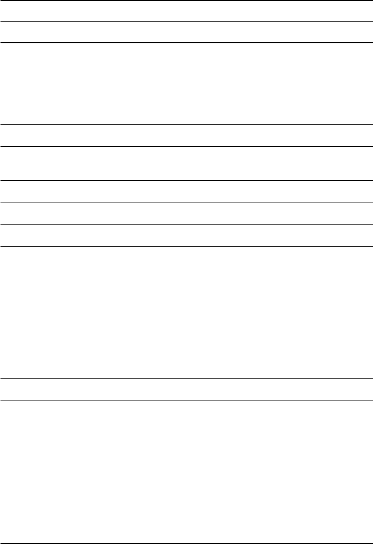
HTTP 145
Table 5.4 Selected HTTP and authentication tasks and how to realize them with RCurl or
httr
Task RCurl function/option httr function
HTTP methods (verbs)
Specify GET request getURL(),
getURLContent(),
getForm()
GET()
Specify POST request postForm() POST()
Specify HEAD request httpHEAD() HEAD()
Specify PUT request httpPUT() PUT()
Content extraction
Extract raw or character content
from response
content <-
getURLContent()
content()
Curl handle specication
Specify curl handle getCurlHandle(),curl handle()
Request conguration
Specify curl options .opts config()
Specify glocal curl options options(RCUrlOptions =
list()),.opts
set_config()
Execute code with curl options with_config()
Add headers to request httpheaders add_headers()
Authenticate via one type of
HTTP authentication
userpwd authenticate()
Specify proxy connection proxy use_proxy()
Specify User-Agent header eld useragent user_agent()
Specify cookies cookiefile set_cookies()
Error and exception handling
Display HTTP status code getCurlInfo(handle)
$response.code
http_status()
Display R error if request fails stop_for_status()
Display R warning if request fails warn_for_status()
Return TRUE if returned status
code is exactly 200
url_ok()
Return TRUE if returned status
code is in the 200s
url.exists() url_success()
Set maximum request time timeout timeout()
Provide more information about
client–server communication
verbose verbose()
(continued)

146 AUTOMATED DATA COLLECTION WITH R
Table 5.4 (Continued)
Task RCurl function/option httr function
URL modication
Parse URL into constituent
components
parse_url()
Replace components in parsed
URL
modify_url()
Build URL string from parsed
URL
build_url()
OAuth registration
Retrieve OAuth 1.0 access token oauth1.0_token()
Retrieve OAuth 2.0 access token oauth2.0_token()
Register OAuth application oauth_app()
Describe Oauth endpoint oauth_endpoint()
Sign Oauth 1.0 request sign_oauth1.0()
Sign Oauth 2.0 request sign_oauth2.0()
Functions are indicated as function(), arguments within RCurl high-level functions, as argument.
treatment of the subject can be found in “DNS and BIND” (Liu and Albitz 2006), although
we doubt that this will add much to your practical web scraping skills. While libcurl is
generally well documented on the Web at http://curl.haxx.se/libcurl/, RCurl and httr are less
so. Fortunately, the recently published “XML and Web Technologies for Data Sciences with
R” (Nolan and Temple Lang 2014) provides an extensive overview of RCurl’s functionality.
Problems
1. What are the common methods dened in HTTP/1.1? Describe what they are used for.
Which are most important for web scraping?
2. Describe the basic makeup of an HTTP message!
3. What are the ve basic status types a server can respond with?
4. What headers can be used for identication purposes?
5. Why can cookies be necessary or even useful when we scrape information from
websites?
6. Browse to http://curl.haxx.se/libcurl/c/curl_easy_setopt.html and read about the
autoreferer,followlocation, and customrequest options. Are these options
part of the RCurl package?
7. Create a handle called problemsH that denes options to identify yourself and provide
information about your software.
HTTP 147
8. Using the problemsH handle, download http://www.r-datacollection.com/materials/
http/simple.html with …
(a) …getURL() and save it as simple1.html.
(b) …getBinaryURL() and save it as simple2.html.
(c) …getURLContent() and save it as simple3.html.
(d) Add cookie management to the handler and download all verses from http://www
.r-datacollection.com/materials/http/SessionCookie.php
9. Create a debug gatherer object called info and a new handle called problemsD with
the following features:
(a) Cookie management is enabled.
(b) info is used as debugfunction.
(c) You should identify yourself and your software.
10. Using problemsD as handle, replicate the previous problem and save all request headers
(outgoing headers) in hout.txt and response headers (incoming headers) in hin.txt.
Inspect both les with a text editor and answer the following questions.
(a) How many times did the server ask for a specic cookie in subsequent requests?
(b) Which parameters did the server send in the request(s) for sending a specic cookie
in subsequent requests?
(c) How many times was the cookie sent to the server?
(d) Which parameters/values where sent to the server as cookies?
(e) Learn about the details of the last request executed by problemsD, specically:
response code, time it took to complete the request, download size, download speed,
list of cookies, number of times the request was redirected, and content type of the
response.
11. Declare the following options as default values for all RCurl functions:
(a) Server redirections should be followed.
(b) The maximum number of redirects should be 10.
(c) Identify yourself and your software.
(d) Enable cookie management.
Create a new handle called problemsG. Check whether your specications
work by downloading http://httpbin.org/cookies/set?myname=Eddie, http://httpbin.org/
redirect/20, and http://httpbin.org/headers using getURL() and problemsG.
12. Write a function called presentHTTP() that prints header and content information to
the screen in a readable format. Use str_split() and cat() to solve the problem.
13. Create a debug gatherer object info or reset the one you created in a previous problem.
Create a new handle called problemsM that uses info’s update function as debug
function parameter.
(a) Use readLines() to read http://www.r-datacollection.com/materials/http/
bunchofles.html into a vector called urls.
(b) Use the following functions to download the les and save them to disk: getURL(),
getURLContent(),download.file()—names should be of form: geturl1.html,
geturl2.html,…;geturlcontent1.html, geturlcontent2.html,…;downloadle1.html,
downloadle2.html.
(c) Which of the functions accept a vector of urls as argument?
148 AUTOMATED DATA COLLECTION WITH R
14. Use getForm() and postForm() to send ve query parameters to http://www.r-
datacollection.com/materials/http/return.php and capture the returned document in
objects getParameters and postParameters.
15. Replicate the following RCurl commands with httr functions:
(a) getURL("www.r-datacollection.com/index.html", useragent =
"R", httpheader = c(From = your@email.address))
(b) getForm("www.r-datacollection.com/materials/http/GETexample
.php", name = "Eddie", age = 32)
(c) postForm("www.r-datacollection.com/materials/http/POSTexample
.php", name = "Eddie", age = 32, style = "post")
(d) getCurlHandle(useragent ="R", httpheader = c(from
= "your@email.address"), followlocation = TRUE,
cookiefile = "")

6
AJAX
At this point in the book you are familiar with HTML’s versatile markup vocabulary for
structuring content (Chapter 2) and HTTP, the primary protocol for requesting information
from web servers (Chapter 5). In combination, these two technologies not only provide the
foundation for virtually all web services, but they also dene a reliable infrastructure for
disseminating information throughout the Web.
Despite their popularity, HTML/HTTP impose strict constraints on the way users access
information. If you abstract from the examples we have previously introduced, you nd that
the HTML/HTTP infrastructure implies a rather static display of content in a page layout,
which is retrieved through sequential, iterative requests initiated by the user. The inherent
inexibility of HTML/HTTP is most apparent in its inability to create more dynamic displays
of information, such as we are used to from standard desktop applications. After receiving an
HTML document from the server the visual appearance of the screen will not change since
HTTP provides no mechanism to update a page after it has been downloaded. What impedes
HTML/HTTP from providing content more dynamically is its lack of three critical elements:
1. a mechanism to register user behavior in the browser (and not just on the server);
2. a scripting engine to formulate responses to those events;
3. a more versatile data requesting mechanism for fetching information asynchronously.
Because HTML/HTTP is technically unable to provide any of the above features, a
series of additional web technologies have found their way into the toolkit of modern web
developers over the last 15 years. A prominent role in this transformation is assumed by a
group of technologies that are subsumed under the term AJAX, short for “Asynchronous
JavaScript and XML.” AJAX has become a staple web technology to which we owe much of
the sophistication of modern web applications such as Facebook, Twitter, the Google services,
or any kind of shopping platform.
Automated Data Collection with R: A Practical Guide to Web Scraping and Text Mining, First Edition.
Simon Munzert, Christian Rubba, Peter Meißner and Dominic Nyhuis.
© 2015 John Wiley & Sons, Ltd. Published 2015 by John Wiley & Sons, Ltd.
150 AUTOMATED DATA COLLECTION WITH R
Although AJAX-enriched websites provide tremendous advantages from a user perspec-
tive, they create difculties for our efforts to automatically gather web data. This is so because
AJAX-enriched webpages constitute a signicant departure from the static HTML/HTTP site
model in which a HTTP-requested webpage is displayed equally for all users and all infor-
mation that is displayed on screen is delivered upfront. This presents a serious obstacle to
analysts who care to collect web data since a simple HTTP GET request (see Section 5.1.4)
may not sufce if information is loaded iteratively only after the site has been requested. We
will see that the key to circumventing this problem is to understand at which point the data
of interest is loaded and apply this knowledge to trace the origin of the data.
The remainder of this chapter introduces AJAX technologies that turn static into dynamic
HTML. We will focus on the conceptual ideas behind AJAX that will inform solutions for data
retrieval. In Section 6.1 we start by introducing JavaScript, the most popular programming
language for web content and show how it turns HTML websites into dynamic documents
via DOM manipulation. In Section 6.2 we discuss the XMLHttpRequest, an Application
Programming Interface (API) for browser–server communication and important data retrieval
mechanism for dynamic web applications. Finally, to solve problems caused by AJAX,
Section 6.3 explicates how browser-implemented Developer Tools can be helpful for gathering
insight into a page’s underlying structure as well as tracing the source of dynamic data requests.
6.1 JavaScript
The JavaScript programming language has a prominent role in the group of AJAX technolo-
gies. Developed by Brendan Eich at Netscape in 1995, JavaScript is a complete, high-level
programming language (Crockford 2008). What sets JavaScript apart from other languages
is its seamless integration with other web technologies (e.g., HTML, CSS, DOM) as well as
its support by all modern browsers, which contain powerful engines to interpret JavaScript
code. Because JavaScript has become such an important part in the architecture of web
applications, the language has been raised to a W3C web standard. Similar to R’s packaging
system, extra functionality in JavaScript is incorporated through the use of libraries. In fact,
most web development tasks are not executed in native JavaScript code anymore, but are car-
ried out using special purpose JavaScript libraries. We follow this practice for the examples
in this chapter and use functionality from jQuery—the self-ascribed “write less, do more”
library—with a particular focus on easing DOM manipulation.
6.1.1 How JavaScript is used
To recognize JavaScript in the wild, it is important to know that there are three methods for
enhancing HTML with JavaScript functionality. A dedicated place for in-line code to appear is
between the HTML <script> tags (see also Section 2.3.10). These tags are typically located
before the <head> section of the document but they may as well be placed at any other
position of the document. Another way is to make reference to an externally stored JavaScript
code le via a path passed to the scr attribute of the <script> element. This method helps
to organize HTML and JavaScript at two separate locations and thus eases maintainability.
Lastly, JavaScript code can appear directly in an attribute of a specic HTML element in so-
called event handlers. Regardless of the method, a JavaScript-enhanced HTML le requires
the browser to not only parse the HTML content and construct the DOM, but also to read the

AJAX 151
JavaScript code and carry out its commands. Let us illustrate this process with JavaScript’s
DOM manipulation functionality.
6.1.2 DOM manipulation
A popular application for JavaScript code is to create some kind of alteration of the information
or appearance of the current browser display. These modications are called DOM manip-
ulations and they constitute the basic procedures for generating dynamic browser behavior.
The possible alterations allowed in JavaScript are manifold: HTML elements may either be
removed, added or shifted, attributes to any HTML element can be added or changed, or CSS
styles can be modied. To show how such scripts may be employed, consider fortunes1.html
for a lightly JavaScript-enriched webpage.
1<!DOCTYPE HTML PUBLIC "-//IETF//DTD HTML//EN">
2<html>
4<script type="text/javascript" src="jquery-1.8.0.min.js"></script>
5<script type="text/javascript" src="script1.js"></script>
7<head>
8<title>Collected R wisdoms</title>
9</head>
11 <body>
12 <div id="R Inventor" lang="english" date="June/2003">
13 <h1>Robert Gentleman</h1>
14 <p><i>'What we have is nice, but we need something very different'</i></p>
15 <p><b>Source: </b>Statistical Computing 2003, Reisensburg</p>
16 </div>
18 <div lang="english" date="October/2011">
19 <h1>Rolf Turner</h1>
20 <p><i>'R is wonderful, but it cannot work magic'</i><br><emph>answering a
request for automatic generation of 'data from a known mean and 95% CI’
</emph></p>
21 <p><b>Source: </b><a href="https://stat.ethz.ch/mailman/listinfo/r-help">R-
help</a></p>
22 </div>
24 <address><a href="http://www.r-datacollection.com"><i>The book homepage</i></a>
</address>
25 </body>
26 </html>
For the most part, the code is identical to the fortunes example we introduced in Sec-
tion 2.4.1. The only modication of the le concerns the extra code appearing in lines 4 and
5. The HTML <script> element offers a way to integrate HTML with functionality drawn
from other scripting languages. The type of scripting language to be used is set via the type
attribute. Since browsers expect that incorporated code is written in JavaScript by default, we
can leave this attribute unspecied. Here, we include JavaScript using the reference method

152 AUTOMATED DATA COLLECTION WITH R
as it helps emphasize the conceptual difference between the two documents and enhances
clarity. In line 4 we make a reference to the jQuery library for which there exists a copy in
the folder of the HTML document. By referencing the le jquery-1.8.0.min.js, jQuery can
be accessed throughout the program. The next line makes a reference to the le script1.js,
which includes the code responsible for the DOM alterations. To view the le’s content, you
can open the le in any text processor:
1$(document).ready(function() {
2$("p").hide();
3$("h1").click(function(){
4$(this).nextAll().slideToggle(300);
5});
6});
Before explaining the script, take the time to download the fortunes1.html le from the
materials section at http://www.r-datacollection.com and open it in a browser to discover
differences to the example le in Section 2.4.1. Opening the le you should see two named
headers and a hyperlink to the book’s homepage (see Figure 6.1, panel (a)). Apparently, some
information that is contained in the HTML code, such as the quotes and their contexts, has
been concealed in the browser display of the webpage. Assuming that JavaScript is enabled
in your browser, a click on one of the headers should initiate a rolling transition and further
content relating to the quote should become visible (see Figure 6.1, panel (b)). Another click
on the header results in the content being hidden again. The dynamic behavior just observed
is the result of the code in script1.js. To get an understanding of how these behaviors are
produced, let us parse this code line by line and discuss what it does.
The rst line starts with the $() operator, jQuery’s method for selecting elements in the
DOM. Inside the parentheses we write document to indicate that all elements that are dened
(a) initial state
(b) after a click on ‘Robert Gentleman
’
Figure 6.1 Javascript-enriched fortunes1.html (a) Initial state (b) After a click on “Robert
Gentleman”
AJAX 153
in the DOM are to be selected. The returned selection of the $() operator is passed to the
ready() method. Essentially, the document ready handler ready() instructs the script to
pause all JavaScript code execution until the entire DOM has been built inside the browser,
meaning that all the HTML elements are in existence. This is necessary for any reasonably
sized HTML le since the browser will take some time to build the DOM. Not instructing the
script to pause until all HTML information is loaded could lead to a situation where the script
acts on elements that do not yet exist in the DOM. The essential part starts in line 2, which
denes the dynamic behaviors. Once again we employ the $() operator but only to select all
the <p> nodes in the document. As you can see in fortunes1.html, these are the elements that
contain more information on the quote and its source. The selection of all paragraph nodes is
passed to the hide() method, which accounts for the behavior that in the initial state of the
page all paragraph elements are hidden. The third line initiates a selection of all <h1> header
nodes in the document, which are used to mark up the names of the quoted. We bind an
event handler to this selection for the “click” JavaScript event. The click() handler allows
recognizing whenever a mouse click on a <h1> element in the browser occurs and to trigger
an action. What we want the action to be is dened in the parentheses from lines 3 to 5. On line
4, we rst return the element on which the click has occurred via $(this).ThenextAll()
method selects all the nodes following after the node on which the click has occurred (see
Section 4.1 for the DOM relations) and binds the slideToggle() method to this selection,
which denes a rather slow (300 ms) toggle effect for fading the elements in and out again.
On a conceptual level, this example illustrates that the underlying HTML code and the Implications of
JavaScript for
scraping, 1
information displayed in the browser do not necessarily coincide in a JavaScript-enriched
website. This is due to the exibility of the DOM and JavaScript that allow HTML elements
to be manipulated, for example, by fading them in and out. But what are the implications of this
technology for scraping information from this page? Does DOM manipulation complicate
the scraping process with the tools introduced earlier? To address this question, we parse
fortunes1.html into an Robject and display its content:
R> library(XML)
R> (fortunes1 <- htmlParse("fortunes1.html"))
<!DOCTYPE HTML PUBLIC "-//IETF//DTD HTML//EN">
<html>
<head>
<script type="text/javascript" src="jquery-1.8.0.min.js"></script><script
type="text/javascript" src="script1.js"></script><title>Collected R wisdoms
</title>
</head>
<body>
<div id="R Inventor" lang="english" date="June/2003">
<h1>Robert Gentleman</h1>
<p><i>'What we have is nice, but we need something very different'</i></p>
<p><b>Source: </b>Statistical Computing 2003, Reisensburg</p>
</div>
<div lang="english" date="October/2011">
<h1>Rolf Turner</h1>
<p><i>'R is wonderful, but it cannot work magic'</i> <br><emph>answering a
request for automatic generation of 'data from a known mean and 95% CI'
</emph></p>
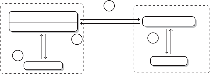
154 AUTOMATED DATA COLLECTION WITH R
<p><b>Source: </b><a href="https://stat.ethz.ch/mailman/listinfo/r-help">R-
help</a></p>
</div>
<address><a href="http://www.r-datacollection.com"><i>The book homepage</i></a>
</address>
</body>
</html>
Evidently, all the information is included in the HTML le and can be accessed via
the HTTP request, parsing, and extraction routines we previously presented. As we will see
further below, this is unfortunately not always the case.
6.2 XHR
A limitation of the HTTP protocol is that communication between client and server necessarily
follows a synchronous request–response pattern. Synchronous communication means that the
user’s interaction with the browser is being disabled while a request is received, processed,
and a new page is delivered by the web server.
A more exible data exchange mechanism is required to enable a continuous user expe-
rience that resembles the behavior of desktop applications. A popular method to allow for
a continuous exchange of information between the browser and the web server is the so-
called XMLHttpRequest (XHR), an interface that is implemented in nearly all modern web
browsers. It allows initiating HTTP or HTTPS requests to a web server in an asynchronous
fashion. XHR’s principal purpose is to allow the browser to fetch additional information in
the background without interfering with the user’s behavior on the page.
To illustrate this process, take a look at the graphical illustration of the XHR-enriched
User–server
communication
with XHR
communication model in Figure 6.2. As in the traditional HTTP communication process (see
Section 5.1.1), XHR provides a mechanism to exchange data between a client and a server.
A typical communication proceeds as follows.
1. Commonly, but not necessarily, the user of a webpage is also the initiator of the AJAX
request. The initiating event can be any kind of event that is recognizable by the
browser, for example, a click on a button. JavaScript then instantiates an XHR object
XMLHttpRequest
XHR callback function
User Interface
HTTP Server
Data Storage
1
2
3
4
HTTP response
HTTP request
HTML &
CSS data
JavaScript
Data
exchange
Figure 6.2 The user–server communication process using the XMLHttpRequest. Adapted
from Stepp et al. (2012)

AJAX 155
that serves as the object that makes the request and may also dene how the retrieved
data is used via a callback function.
2. The XHR object initiates a request to the server for a specied le. This request may
either be sent through HTTP or HTTPS. Due to JavaScript’s Same Origin Policy,
cross-domain requests are forbidden in native AJAX applications, meaning that the
le to be requested must be in the domain of the current webpage. While the request
is taking place in the background, the user is free to continue interacting with the site.
3. On the server side, the request is received, processed, and the response including data
is sent back to the browser client via the XHR object.
4. Back in the browser client, the data are received and an event is triggered that is caught
by an event handler. If the content of the le needs to be displayed on the page, the le
may be relayed through a previously dened callback event handler. Via this handler
the content can be manipulated to present it in the browser. Once the process handler
has processed the information, it can be fed back into the current DOM and displayed
on the screen.
To see XHR in action, we now discuss two applications.
6.2.1 Loading external HTML/XML documents
The simplest type of data to be fetched from the server via an XHR request is a document
containing HTML code. The task we illustrate here is to gather an HTML code and feed
it back into the current webpage. The proper method to carry out this task in jQuery is its
load() method. The load() method instantiates an XHR object that sends an HTTP GET
request to the server and retrieves the data. Consider the following empty HTML le named
fortunes2.html, which will serve as a placeholder document:
1<!DOCTYPE HTML PUBLIC "-//IETF//DTD HTML//EN">
2<html>
4<script type="text/javascript" src="jquery-1.8.0.min.js"></script>
5<script type="text/javascript" src="script2.js"></script>
7<head>
8<title>Collected R wisdoms</title>
9</head>
11 <body>
13 <address><a href="http://www.r-datacollection.com"><i>The book homepage</i></a>
</address>
14 </body>
15 </html>
The task is to insert substantially interesting information from another HTML document
into fortunes2.html. Key to this task is once again a JavaScript code to which we refer in line 5.

156 AUTOMATED DATA COLLECTION WITH R
1$(document).ready(function() {
2$("body").load("quotes/quotes.html", function() {
3alert("Quotes.html was fetched.");
4});
5});
Like the previous script, script2.js starts with the document ready handler ready() to
ensure the DOM is completely loaded before executing the script. In line 2 we initiate a
selection for the <body> node. The <body> node serves as an anchor to which we link
the data returned from the XHR data request. The essential part of the script uses jQuery’s
load() method to fetch information that is accessible in “quotes/quotes.html.” The load()
method creates the XHR object, which is not only responsible for requesting information
from the server but also for feeding it back into the HTML document. The le quotes.html
contains the marked up quotes.
1<div id="R Inventor" lang="english" date="June/2003">
2<h1>Robert Gentleman</h1>
3<p><i>'What we have is nice, but we need something very different'</i></p>
4<p><b>Source: </b>Statistical Computing 2003, Reisensburg</p>
5</div>
7<div lang="english" date="October/2011">
8<h1>Rolf Turner</h1>
9<p><i>'R is wonderful, but it cannot work magic'</i><br><emph>answering a
request for automatic generation of 'data from a known mean and 95% CI'
</emph></p>
10 <p><b>Source: </b><a href="https://stat.ethz.ch/mailman/listinfo/r-help">R-
help</a></p>
11 </div>
As part of the load() method, we also assign a callback function that is executed in case
the XHR request is successful. In line 3, we use JavaScript to open an alert box with the
text in quotation marks. This is purely for illustrative purpose and could be omitted without
causing any problems. To check the success of the method, open fortunes2.html in a browser
and compare the displayed information with the HTML code outlined above.
How does the XHR object interfere with attempts to obtain information from the quotes?
Implications of
JavaScript for
scraping, 2
Once again we compare the information displayed in the browser with what we get by parsing
the document in R:
R> library(XML)
R> (fortunes2 <- htmlParse("fortunes2.html"))
<!DOCTYPE HTML PUBLIC "-//IETF//DTD HTML//EN">
<html>
<head>
<script type="text/javascript" src="jquery-1.8.0.min.js"></script><script
type="text/javascript" src="script2.js"></script><title>Collected R wisdoms</title>
</head>
<body>
<address><a href="http://www.r-datacollection.com"><i>The book homepage</i></a>
</address>
</body>
</html>

AJAX 157
Unlike in the previous example, we observe that information shown in the browser is not
included in the parsed document. As you might have guessed, the reason for this is the XHR
object, which loads the quote information only after the placeholder HTML le has been
requested.
6.2.2 Loading JSON
Although the X in AJAX stands for the XML format, XHR requests are not limited to
retrieving data formatted this way. We have introduced the JSON format in Chapter 3, which
has become a viable alternative, preferred by many web developers for its brevity and wide
support. jQuery not only provides methods for retrieving JSON via XHR request but it also
includes parsing functions that facilitate further processing of JSON les. Compared to the
example before, we need to remind ourselves that JSON content is displayed unformatted
in the browser. In this example, we therefore show rst how to instruct jQuery to access a
JSON le and second, how to convert JSON information into HTML tags, to obtain a clearer
and more attractive display of the information. Take a look at fortunes3.html for our generic
placeholder HTML document.
1<!DOCTYPE HTML PUBLIC "-//IETF//DTD HTML//EN">
2<html><head>
3<title>Collected R wisdoms (JavaScript Extension)</title>
4</head>
5<body>
7<button id="quoteButton">Click for quotes!</button>
9</body>
11 <script type="text/javascript" src="jquery-1.8.0.min.js"></script>
12 <script type="text/javascript" src="script3.js"></script>
14 <address><a href="http://www.r-datacollection.com"><i>The book homepage</i></a>
</address>
15 </body></html>
The new element here is an HTML button element to which we assign the id quote
Button. Inside the HTML code there is a reference to script3.js.
1$("#quoteButton").click(function(){
2$.getJSON("quotes/all_quotes.json", function(data){
3$.each(data, function(key, value){
4$("body").prepend("<div date='"+value.date+"'><h1>"+value.author+"
</h1><p><i>'"+value.quote+"'</i></p><p><b>Source: </b>'"+value.
source+"'</p></div>");
5});
6});
7});
Once again, go ahead and open fortunes3.html to check out the behavior of the document.
What you should observe is that upon clicking on the button, new quote information appears
that is visually similar to what we have seen in fortunes.html.

158 AUTOMATED DATA COLLECTION WITH R
Let us dismantle the script into its constituent parts. In the top line, the scripts initiates a
query for a node with id quoteButton. This node is being bound to the click event handler.
The next lines detail the click’s functionality. If a click occurs a data request is sent via
jQuery’s getJSON() method. This method does two things. First, the request for the le is
initiated and the data fetched using a HTTP GET request. Second, the data are parsed by a
JSON parser, which disassembles the le’s key and value pairs into usable JavaScript objects.
The le to be requested is specied as all_quotes.json, which contains the complete set of R
wisdoms and is located in the folder named quotes. The rst couple of lines of this le are
printed below:
1[
2{
3"quote": "What we have is nice, but we need something very different.",
4"author": "Robert Gentleman",
5"context": null,
6"source": "Statistical Computing 2003, Reisensburg",
7"date": "June 2003"
8},
9{
10 "quote": "R is wonderful, but it cannot work magic.",
11 "author": "Rolf Turner",
12 "context": "answering a request for automatic generation of 'data from a
known mean and 95% CI'",
13 "source": "R-help",
14 "date": "October 2011"
15 },
Line 3 initiates a looping construct that iterates over the objects of the retrieved JSON le
and denes a function for the key and value variables. The function rst performs a selection
of the HTML document’s <body> node to which it prepends the expression in parentheses. As
you can see, this expression is a mixture of HTML markup and some sort of variable objects
(encapsulated by +signs) through we can inject JSON information. Effectively, this statement
produces familiar HTML code that includes data, author, quote, and source information from
each object of the JSON le.
6.3 Exploring AJAX with Web Developer Tools
When sites employ more sophisticated request methods, a cursory look at the source code
will usually not sufce to inform our Rscraping routine. To obtain a sufcient understanding
of the underlying structure and functionality we need to dig a little deeper. Despite our praise
for the Renvironment, using Rwould render this task unnecessarily cumbersome and, at least
for AJAX-enriched sites, it simply does not provide the necessary functionality. Instead, we
examine the page directly in the browser. The majority of browsers comes with functionality
that has turned them into powerful environments for developing web projects—and helpful
companions for web scrapers. These tools are not only helpful for on-the-y engagement with
a site’s DOM, but they may also be used for inspecting network performance and activities
that are triggered through JavaScript code. In this section, we make use of Google Chrome’s
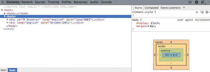
AJAX 159
suite of Web Developer Tools (WDT), but tools of comparable scope are available in all the
major browser clients.
6.3.1 Getting started with Chrome’s Web Developer Tools
We return to the previously introduced fortunes2.html le, which caused some headache due
to its application of XHR-based data retrieval. Open the le in Google Chrome to accustom
yourself once again with the site’s structure. By default, WDT are not visible. To bring them
to the forefront, you can right-click on any HTML element and select the Inspect Element
option. Chrome will split the screen horizontally, with the lower panel showing the WDT and
the upper panel the classical page view of fortunes2.html. IInside the WDT (Chrome version
33.0.1750.146), the top-aligned bar shows eight panels named Elements, Network, Sources,
Timeline, Proles, Resources, Audits, and Console and which correspond to the different
aspects of a site’s behavior that we can analyze. Not all of these panels will be important for
our purposes, so the next sections only discuss the Elements and the Network panels in the
context of investigating a site’s structure and creating an Rscraping routine.
6.3.2 The Elements panel
From the Elements panel, we can learn useful information about the HTML structure of the Perspective on
the DOM tree
page. It reveals the live DOM tree, that is, all the HTML elements that are displayed at any
given moment. Figure 6.3 illustrates the situation upon opening the WDT on fortunes2.html.
The Elements panel is particularly useful for learning about the links between specic HTML
code and its corresponding graphical representation in the page view. By hovering your cursor
over a node in the WDT, the respective element in the HTML page view is highlighted. To do
the reverse and identify the code piece that produces an element in the page view, click on the
magnifying glass symbol at the top right of the panel bar. Now, once you click on an element
in the page view, the WDT highlights the respective HTML element in the DOM tree. The
Elements panel is also helpful for generating an XPath expression that can be passed directly
to R’s extractor functions (see Chapter 4). Simply right-click on an element and choose “Copy
XPath” from the menu.
Figure 6.3 View on fortunes2.html from the Elements panel
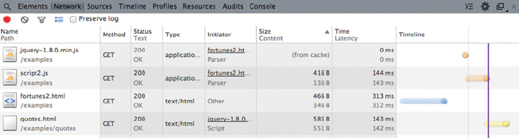
160 AUTOMATED DATA COLLECTION WITH R
Figure 6.4 View on fortunes2.html from the Network panel
6.3.3 The Network panel
The Network panel provides insights into resources that are requested and downloaded overTracing
resources the network in real time. It is thus an ideal tool to investigate resource requests that have
been initiated by JavaScript-triggered XHR objects. Make sure to open the Network panel tab
before loading a webpage, otherwise the request will not be captured. Figure 6.4 shows the
Network panel after loading fortunes2.html. The panel shows that altogether four resources
have been requested since the fortunes2.html has been opened. The rst column of the panel
displays the le names, that is, fortunes2.html,jquery-1.8.0.min.js,script2.js, and quotes.html.
The second column provides information on the HTTP request method that provided the le.
Here, all four les have been requested via HTTP GET. The next column displays the HTTP
status code that was returned from the server (see Section 5.1.5). This can be of interest when
an error occurs in the data request. The type column depicts the les’ type such as HTML
or JavaScript. From the initiator column we learn about the le that triggered the request.
Lastly, the size, time, and timeline columns provide auxiliary information on the requested
resources.
We are interested in collecting the quote information. Since the information is not
part of the source HTML, we can refrain from further inspecting fortunes2.html.From
the other three les, we can also ignore jquery-1.8.0.min.js as this is a library of meth-
ods. While script2.js could include the required quote information in principle, good web
development practice usually separates data from scripts. By the principle of exclusion, we
have thus identied quotes.html as the most likely candidate for containing the quotes. To
take a closer look, click on the le, like in Figure 6.5. From the Preview tab we observe
that quotes.html indeed contains the information. In the next step we need to identify
the request URL for this specic le so we can pass it to R. This information is easily
obtained from the Headers tab, which provides us with the header information that requested
quotes.html. For our purpose, we only need the URL next to the Request URL eld, which is
http://r-datacollection.com/materials/ajax/quotes/quotes.html. With this information, we can
return to our Rsession and pass the URL to RCurl’s getURL() command:
R> (fortunes_xhr <- getURL("r-datacollection.com/materials/ajax/quotes/
quotes.html"))
[1] "<div id=\"R Inventor\" lang=\"english\" date=\"June/2003\">\n <h1>
Robert Gentleman</h1>\n <p><i>'What we have is nice, but we need something
very different'</i></p>\n <p><b>Source: </b>Statistical Computing 2003,
Reisensburg</p>\n</div>\n\n<div lang=\"english\" date=\"October/2011\">\n
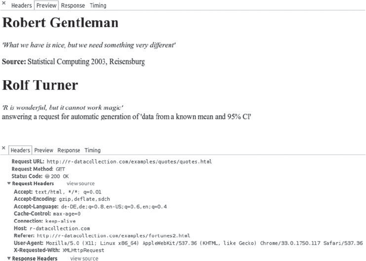
AJAX 161
(a) Preview
(b) Headers
Figure 6.5 Information on quotes.html from the Network panel (a) Preview (b) Headers
<h1>Rolf Turner</h1>\n <p><i>'R is wonderful, but it cannot work magic'</i>
<br><emph>answering a request for automatic generation of 'data from a known
mean and 95% CI'</emph></p>\n <p><b>Source: </b><a href=\"https://stat.
ethz.ch/mailman/listinfo/r-help\">R-help</a></p>\n</div>"
The results do in fact contain the target information, which we can now process with all
the functions that were previously introduced.
Summary
AJAX has made a lasting impact on the user friendliness of services provided on the Web.
This chapter gave a short introduction to the principles of AJAX and it sought to convey the
conceptual differences between AJAX and classical HTTP-transmitted contents. From the
perspective of a web scraper, AJAX constitutes a challenge since it encourages a separation
of the stylistic structure of the page (HTML, CSS) and the information that is displayed (e.g.,
XML, JSON). Therefore, to retrieve data from a page it might not sufce to download and
parse the front-end HTML code. Fortunately, this does not prevent our data scraping efforts.
As we have seen, the AJAX-requested information was located in a le on the domain of the
main page that is accessible to anyone who takes an interest in the data. With Web Developer
Tools such as provided in Chrome, we can trace the le’s origin and obtain a URL that
oftentimes leads us directly to the source of interest. We will come back to problems created
162 AUTOMATED DATA COLLECTION WITH R
by dynamically rendered pages when we discuss the Selenium/Webdriver framework as an
alternative solution to these kinds of scraping problems (see Section 9.1.9).
Further reading
To learn more about AJAX consult Holdener III (2008) or Stepp et al. (2012). A good way
to learn and discover useful features of the Chrome Web Developer Tools is on the tool’s
reference pages Google (2014) or for a book reference Zakas (2010).
Problems
1. Why are AJAX-enriched webpages often valuable for web users, but an obstacle to web
scrapers?
2. What are the three methods to embed JavaScript in HTML?
3. Why are Web Developer Tools particularly useful for web scraping when the goal is to
gather information from websites using dynamic HTML?
4. Return to fortunes3.html. Implement the JavaScript alert() function at two points of
the document. First, put the function in the <node> section of the document with text
“fortunes3.html successfully loaded!” Second, open script3.js and include the alert()
function here as well with text “quotes.html successfully loaded!” Watch the page’s
behavior in the browser.
5. Use the appropriate parsing function for fortunes3.html and verify that it does not
contain the quotes of interest.
6. Use the Web Developer Tools to identify the source of the quote information in for-
tunes3.html. Obtain the request URL for the le and create an Rroutine that parses it.
7. Write a script for fortunes2.html that extracts the source of the quote. Conduct the
following steps:
(a) Parse fortunes2.html into an Robject called fortunes2.
(b) Write an XPath statement to extract the names of the JavaScript les and create
a regular expression for extracting the name of the JavaScript script (and not the
library).
(c) Import the JavaScript code using readLines() and extract the le path of the
requested HTML document quotes.html.
(d) Parse quotes.html into an Robject called quotes and query the document for the
names.
8. Repeat exercise two for fortunes3.html. Extract the sources of the quotes.
9. The website http://www.parl.gc.ca/About/Parliament/FederalRidingsHistory/hfer.asp?
Language=E&Search=C provides information on candidates in Canadian federal elec-
tions via a request to a database.
(a) Request information for all candidates with the name “Smith.” Inspect the live
DOM tree with Web Developer Tools and nd out the HTML tags of the returned
information.
AJAX 163
(b) Which mechanism is used to request the information from the server? Can you
manipulate the request manually to obtain information for different candidates?
10. The city of Seattle maintains an open data platform, providing ample information
on city services. Take a look at the violations database at https://data.seattle.gov/
Community/Seattle-code-violations-database/8agr-hifc
(a) Use the Web Developer Tools to learn about how the database information is stored
in HTML code.
(b) Assess the data requesting mechanism. Can you access the underlying database
directly?

7
SQL and relational databases
Handling and analyzing data are key functions of R. It is capable of handling vectors, matrices,
arrays, lists, data frames as well as their import and export, aggregation, transformation,
subsetting, merging, appending, plotting, and, not least, analysis. If one of the standard data
formats does not sufce there is always the possibility of dening new ones and incorporating
them into the Rdata family. For example, the sp package denes a special purpose data object
to handle spatial data (see Bivand and Lewin-Koh 2013; Pebesma and Bivand 2005). So, why
should we care about databases and yet another language called SQL?
Simple and everyday processes like shopping online, browsing through library catalogs,
wiring money, or even buying sweets in the supermarket all involve databases. We hardly ever
realize that databases play an important role because we neither see nor interact with them
directly—databases like to work behind the scenes. Whenever data are key to a project, web
administrators will rely on databases because of their reliability, efciency, multiuser access,
virtually unlimited data size, and remote access capabilities.
Regarding automated data collection, databases are of interest for two reasons: First, we
When
databases
become useful
might occasionally get direct access to a database and should be able to cope with it. Second,
and more importantly, we can use databases as a tool for storing and managing data. Although
Rhas a lot of useful data management facilities, it is after all a tool designed to analyze data,
not to store it. Databases on the other hand are specically designed for data storage and
therefore offer some features that base Rcannot provide. Consider the following scenarios.
rYou work on a project where data needs to be presented or made accessible on a
website—using a database, you only need one tool to achieve this.
rIn a data collection project, you do not gather all the data yourself but have other
parties gathering specic parts of it—with a database you have a common, current,
always accessible, and reliable infrastructure at hand that several users can access at the
same time.
Automated Data Collection with R: A Practical Guide to Web Scraping and Text Mining, First Edition.
Simon Munzert, Christian Rubba, Peter Meißner and Dominic Nyhuis.
© 2015 John Wiley & Sons, Ltd. Published 2015 by John Wiley & Sons, Ltd.
SQL AND RELATIONAL DATABASES 165
rWhen several parties are involved, most databases allow for dening different users
with different rights—one party might only be able to read, others have access only
to parts of the data, and yet others are equipped with administrative rights but cannot
create new users.
rYou have loads of data that exceed the RAM available on your computer—databases
are only limited by the available disk size. In fact, databases can even be distributed
across multiple disks or several machines altogether.
rIf your data are complex it might be difcult to write into one data table—databases
are best at storing such kind of data. Not only do they allow storing but also retrieving
and subsetting data with complex data structures.
rYour data are large and you have to subset and manipulate them frequently—querying
databases is fast.
rYour data are complex and you use them for various purposes—for example, the
information is distributed across several tables but depending on the context you need
to combine information from specic tables in a task-specic way. Databases allow the
denition of virtual tables to have data always up to date, organized in a specic way
without using much disk space.
rYou care about data quality and have several rules when data are valid and when they
are not. Using databases you can dene specic rules for extending or updating your
database.
Section 7.1 provides a brief overview of how Rand databases are related to one another
and denes some of the vocabulary indispensable for talking about databases. Subsequently,
Section 7.2 dives into the conceptual basics of relational databases, followed by an introduc-
tion to SQL fundamentals, the language to handle relational databases in Section 7.3. In the
last part (Section 7.4) we learn how to deal with databases using R—establishing connections,
passing through SQL queries, and using convenient functions of the numerous Rpackages
that provide database connectivity.
7.1 Overview and terminology
For a start let us consider a schematic overview of how R, SQL, the database and the
database management system are related (see Figure 7.1). As you can see, we do not access
the database directly. Instead, Rprovides facilities to connect to the database management
system—DBMS—which then executes the user requests written as SQL queries. The tasks
are dened by the user, but how the tasks are achieved is up to the DBMS. SQL is the tool for
speaking to a whole range of DBMS. It is the workhorse of relational database management.
Let us dene some of the terms that we have used up to this point to have a common basis Some
denitions
to build upon throughout the remainder of the chapter.
Data are basically a collection of information such as numbers, logical values, text, or
some other format. Sometimes collections of information might be data for one purpose but
a useless bunch of bits and bytes for another. Imagine that we have collected names of people
that have participated in the Olympic Games. If we only care to know who has participated,
it might sufce if our data has the format of: "Carlo Pedersoli". If, however, we want to
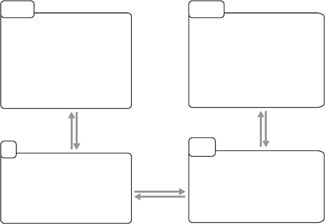
166 AUTOMATED DATA COLLECTION WITH R
•Defines structure of data
•Defines validity of data
•Inputs data
•Manipulates data
•Queries data
•Sets user rights
USER
•Connects to database
•Provides convenience functions
•Sends SQL-queries
•Recieves results
R
•Data control language
•Data definition language
•Data manipulation language
•Transaction control language
SQL
•Executes SQL-queries and sends
back results
•Manages user rights
•Manages users access
•Manages data structure
•Manages data
DBMS
Figure 7.1 How users, R, SQL, DBMS, and databases are related to each other
sort the data by last name, a format like "Pedersoli, Carlo" is more appropriate. To be
on the safe side, we might even consider splitting the names into rst name ("Carlo") and
last name ("Pedersoli"). Beingonthesafesideplays a crucial role in database design and
we will come back to it.
In general a database is simply a collection of data. Within most database systems and
relational database systems, the data are related to each other. Consider for example a table
that contains the bodyweights of various people. We have at least two types of data in the
table: bodyweights and names. What is more, not only does the table store the two variables,
but additionally it provides information on how these two pieces of information are related to
each other. The most basic rule is this: Every piece of information in a single row is related to
each other. We are familiar with handling tables that are structured in this way. In relational
databases, these relations between data can be far more complex and will typically be spread
across multiple tables.
Adatabase management system (DBMS) is an implementation of a specic database
concept bundled together with software. The software is responsible for managing the user
rights and access, the way data and meta information are stored physically, or how SQL
statements are interpreted and executed. DBMS are numerous and exist as open source as
well as commercial products for all kinds of purposes, operation systems, data sizes, and
hardware architectures.
Relational database management systems (RDBMS) are a specic type of DBMS
based on the relational model and the most common form of database management systems.
Relational databases have been around for a while. The concept goes back to the 1970s when
Edgar F. Codd proposed to store data in tables that would be related and the relations again
stored in tables (Codd 1970). Relational databases, although simple in their conceptual basics,

SQL AND RELATIONAL DATABASES 167
are general and exible enough to store all kinds of different data structures, while the specic
parts of the database remain easy to understand. Popular relational DBMS are Oracle, MySQL,
Microsoft SQL Server, PostgreSQL, DB2, Microsoft Access, Sybase, SQLite, Teradata, and
File-Maker.1In this book we exclusively talk about RDBMS and use DBMS and RDBMS
interchangeably.
SQL2is a language to communicate with relational database management systems. When
Codd proposed the relational model for databases in 1970, he also proposed to use a language
to communicate with database systems that should be general and work only on a meta level.
The idea was to be able to express exactly what a DBMS should do—the same statement
on different DBMS should always lead to the same result—but leave it completely up to
the DBMS how to achieve it computationally (Codd 1970). Such a language would be
user friendly and would allow using a common framework for different implementations
of the relational model. Based on these conceptual ideas, SQL was later developed by
Donald D. Chamberlin and Raymond F. Boyce (1974) and, although occasionally revised
throughout the decades, still lives on today as the one common language for relational
database communication.
Aquery is strictly speaking a request sent to a DBMS to retrieve data. In a broader
and more frequently used sense it refers to any request made to a DBMS. Such requests
might dene or manipulate the structure of the data, insert new data, or retrieve data from the
database.
7.2 Relational Databases
7.2.1 Storing data in tables
The main concept of relational databases is that any kind of information can be represented in Tables and
relations
a table. We already know that tables are devices to store data as well as relations—each piece
of information within the same row is related to the same entity. To achieve more complex
relations—for example, a persons’ weight is measured twice, or the weight is measured for
a persons’ children as well—we can relate data from one table to another.
Let us take a look at an example to make this point clear. Imagine that we have collected
data on some of our friends—Peter, Paul, and Mary. We collected information on their
birthdays, their telephone numbers, and their favorite foods—see Tables 7.1 and 7.2. We
had trouble putting the data into one table and ended up separating the data into two tables.
Because we do not like to duplicate information, we did not add the full names to the telephone
table(Table 7.2), but specied IDs referring to the names in a column called nameid.Now
how do we nd Peter’s telephone number? First, we look up Peter’s ID in the birthdays table
(Table 7.1) because we know that data on the same line is related—Peter’s ID is 1. Second,
we check which row in the telephone table has a 1on nameid—rows one and three. Third, we
look up the telephone numbers for these rows—001665443 and 001878345—and realize
1See also http://db-engines.com/en/ranking/relational+dbms
2There is an ongoing debate about whether or not SQL is an acronym and how to pronounce it correctly—well,
no and S-Q-L are the correct answers. SQL is the successor name of SEQUEL, which was the name of an airplane
and thus had to be changed (McJones et al. 1997, p. 22). SEQUEL (not SQL) was an acronym for: Structured English
QUery Language (McJones et al. 1997, p. 14). The pronunciation of SQL was ofcially declared as S-Q-L (Gillespie
2012).

168 AUTOMATED DATA COLLECTION WITH R
Table 7.1 Our friends’ birthdays and favorite foods
nameid name birthday favoritefood1 favoritefood2 favoritefood3
1 Peter Pascal 01/02/1991 spaghetti hamburger
2 Paul Panini 02/03/1992 fruit salad
3 Mary Meyer 03/04/1993 chocolate sh ngers hamburger
that Peter has two telephone numbers. We can also reverse the process and ask which name
of the birthdays table belongs to a specic telephone number or what number we need to call
to speak to a fruit salad or spaghetti lover.
The relation in our example is called 1:m or one-to-many, as one person can be related to
zero, one, or more telephone numbers. There are of course also 1:1,n:1, and n:m relations
(one-to-one,many-to-one,many-to-many), which work just the same way except that the
number of data that might show up on one or the other side of the relation differs.
This connection of tables to express relations between data is one of the most important
Keys
concepts in relational database models. But note that to make it work we had to include
identiers in both tables. These so-called keys ensure that we know which entity the data
belongs to and how to combine information from different tables.
Including keys makes some parts of the data redundant—the nameid column exists inRedundancy
and
exclusiveness
Table 7.1 and in Table 7.2—but it also reduces redundancy. Let us consider the example again
to make this point clear. Have another look at Table 7.1. There are three columns to store the
same type of data. We have to store the data somewhere and what can we do about the fact
that some of our friends did name more than one preference? Imagine what it would look
like if we recorded more than just these 3 preferences, maybe 5 or 7 or even 10. We would
have to add another column for each preference and if somebody only had one preference all
the other columns would remain empty. Clearly there has to be another way to cope with this
kind of data rather than adding column after column to store some more preferences. Indeed
there is.
We divide the data contained in the birthdays table into two separate tables that are related
to each other via a key. Have a look at Tables 7.3 and 7.4 for the result. Now we do not have
to care how many favorite foods somebody names, because we always have the option of
adding another row whenever necessary and still all preferences are unambiguously related
to one person.
Even though the data are stored in a cleaner way, we still have some redundancy in our
food preference table. Is it necessary to have hamburgers in the table twice? In our example
it does not change much, but if the example was just a little more complex, for example, with
Table 7.2 Our friends’ telephone numbers
telephoneid nameid telephonenumber
1 1 001665443
2 2 00255555
3 1 001878345
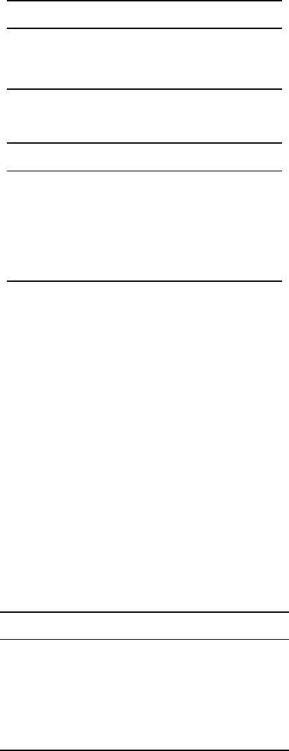
SQL AND RELATIONAL DATABASES 169
Table 7.3 Our friends’ birthdays—revised
name id rst name last name birthday
1 Peter Pascal 01/02/1991
2 Paul Panini 02/03/1992
3 Mary Meyer 03/04/1993
Table 7.4 Our friends’ food preferences
nameid foodname rank
1 spaghetti 1
1 hamburger 2
2 fruit salad 1
3 chocolate 1
3 sh ngers 2
3 hamburger 3
10 instead of 3 friends and 80% of them being fans of hamburgers, the table would grow
quickly. What if we would like to add further information on the food types? Do we store it in
the same table—repeating the information for hamburger over and over again? No, we would
do something similar to what we did when putting telephone numbers in a separate table
(Table 7.2). In the new food preference table (Table 7.5) all information on the preferences
itself remains untouched, because this will be the table on preferences. Furthermore, the key
relating it to the birthdays table (Table 7.3)—nameid—and the key relating it to the new
table on food (Table 7.6)—foodid—are kept.
After restructuring our data, we now have a decent database. Take a look at Figure 7.2
to see how the data are structured. In the schema each table is represented by a square. As
we can see, there are four tables. Let us call them birthdays,telephone,foodranking, and
foodtypes. The upper part of the square gives the name of the table, the column names are
listed in the lower part. The double-headed arrows show which tables are related by pointing
to the columns that serve as keys—the columns set in bold and the columns set in italics.
Table 7.5 Our friend’s food preferences—revised
rankid nameid foodid rank
1111
2122
3231
4341
5352
6323
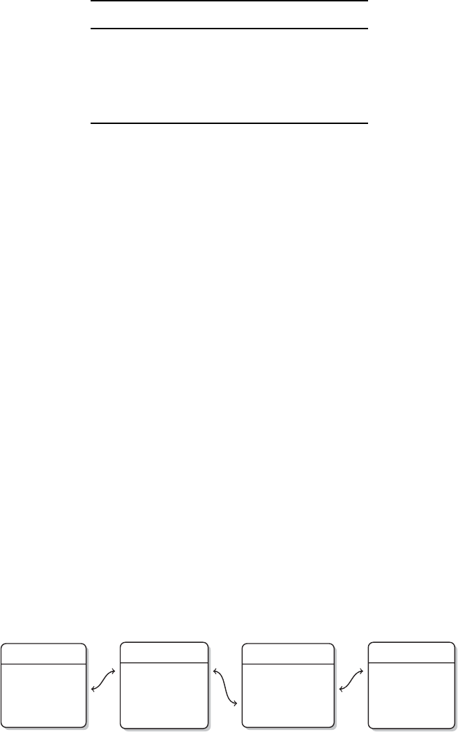
170 AUTOMATED DATA COLLECTION WITH R
Table 7.6 Food types
foodid food name healthy kcalp100g
1 spaghetti no 0.158
2 hamburger no 0.295
3 fruit salad yes 0.043
4 chocolate no 0.546
5 sh ngers no 0.290
The reason why some keys are set in bold and some are set in italics is because there arePrimary keys
and foreign
keys
two types of keys: primary keys and foreign keys. Primary keys are keys that unambiguously
identify each row in a table—nameid in our birthdays table (Table 7.3) is an example where
each person is associated with exactly one unique nameid.nameid is not a primary key in
our telephone table (Table 7.2), as subjects might well have more than one telephone number,
making the ID value non-unique. Thus, while nameid in the telephone table is still a key, it is
now called a foreign key. Foreign keys are keys that unambiguously identify rows in another
table. In other words, each nameid found in the telephone table refers to one and only one
row in the birthdays table. There cannot be a nameid in the telephone table that matches
more than one nameid in the birthdays table.
Note that it does not matter whether keys consist of one single value per row or a com-
Combined keys
bination of values. Nor does it matter whether the identier is a number, a string, something
else, or a combination of those. A key can span across several columns as long as the value
combinations fulll the requirements for primary or foreign keys. Primary keys in our exam-
ple are restricted to one single column and are always running integers, but they could look
different.
Let us consider an example of an alternative primary key to make this point clear. In our
food preference table (Table 7.5) neither nameid nor foodid are sufcient as primary keys,
because individuals appear multiple times depending on their stated preferences and the same
food might be preferred by several subjects. However, as no one prefers the same food twice,
the combination of name identier and food identier would be valid as primary key for the
food preference table.
7.2.2 Normalization
In the previous paragraphs we decomposed our data step by step. We did so because it saves
unnecessary work in the long run and keeps redundancy at bay. Normalization is the process
birthdays
nameid
firstname
lastname
birthday
foodranking
rankid
foodid
nameid
rank
telephone
telephoneid
nameid
telephone
foodtypes
foodid
foodname
healthy
kcalp100g
Figure 7.2 Database scheme
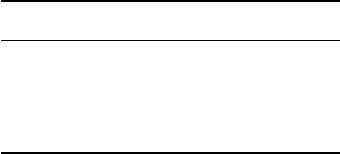
SQL AND RELATIONAL DATABASES 171
of getting rid of redundancies and possible inconsistencies. In the following section, we will
learn about this procedure, which is quite helpful to cope with complex data. If you do not
plan to use databases to store data—for example, you only want to store large amounts of
data that otherwise t nicely into a single table, or you only need it for its user management
capabilities—you can simply skip this section or come back to it later on.
Let us go through the formal rules for normalization to ensure we understand why
databases often look the way they do and how we might do it ourselves. While there are
numerous ways of decomposing data stored in tables—called normal forms—we will only
cover the rst three, as they are the most important and most common.
First normal form
1. One column shall refer to one thing and to one thing only and any column row
intersection should contain only one piece of data (the atomacy of data requirement).
This rule requires that different types of information are not mixed within one column.
One could argue that we violated this rule by storing both rst and last names in
the name column of our rst birthdays table (Table 7.1). We corrected this in the
updated birthdays table (Table 7.3), where rst name and last name were split up
into two columns. Furthermore, it requires that the same data are saved in only one
column.
This rule was violated in the rst version of our birthdays table, where we had three
columns to store a person’s favorite food. By exporting the information to the favorite
food table (Tables 7.4 and 7.5) and food type table (Table 7.6), this problem was taken
care of—a person’s favorite food is now stored in a single column. In addition it is not
allowed to store more than one piece of the same information in an intersection of row
and column. For example, it is not allowed to store two telephone numbers in a single
cell of a table. Take a look at Tables 7.7, 7.8, and 7.9 for three examples that violate
the rst normal form.
2. Each table shall have a primary key.
This rule is easy to understand as keys were covered at length in the previous section.
It ensures that data can be related across tables and that data in one row is related to
the same entity.
Table 7.7 First normal form error—1
zip code and city
789222 Big Blossom
43211 Little Hamstaedt
123456 Bloomington
…
This table fails the rst rule of the rst normal
form because two different types of information
are saved in one column—a city’s zip code and
a city’s name.

172 AUTOMATED DATA COLLECTION WITH R
Table 7.8 First normal form error—2
telephone
0897729344, 0666556322
123123454
675345334
…
This table fails the rst rule of the rst nor-
mal form because two telephone numbers
are saved within the rst row.
Table 7.9 First normal form error—3
telephone1 telephone2
0897729344 0666556322
123123454
675345334
…
This table fails the rst rule of the rst nor-
mal form because it uses two columns to
store the same kind of information.
Second normal Form
1. All requirements for the rst normal form shall be met.
2. Each column of a table shall relate to the complete primary key.
We have learned that a primary key can be a combination of the values of more than
one column. This rule requires that all data in a table describe one thing only: only
people, only telephone numbers, only food preferences or only food types. One can
think of this rule as a topical division of data among tables.
Consider Table 7.10 for a violation of this rule. The primary key of the table is a
combination of nameid and foodid. The problem is that firstname and birthday
relate to nameid only while favoritefood relates to foodid only. The only column
that depends on the whole primary key—the combination of nameid and foodid—is
rank, which stores the rank of a specic food in a specic person’s food preference
order.
A solution to this violation of the second normal form is to split the table into several
tables. One table to capture information on persons, one on food and yet another on
food preferences. Take a look at Tables 7.3, 7.5, and 7.6 from the previous section for
tables that are compliant with the second normal form.
Third normal form
1. All requirements for the second normal form shall be met.
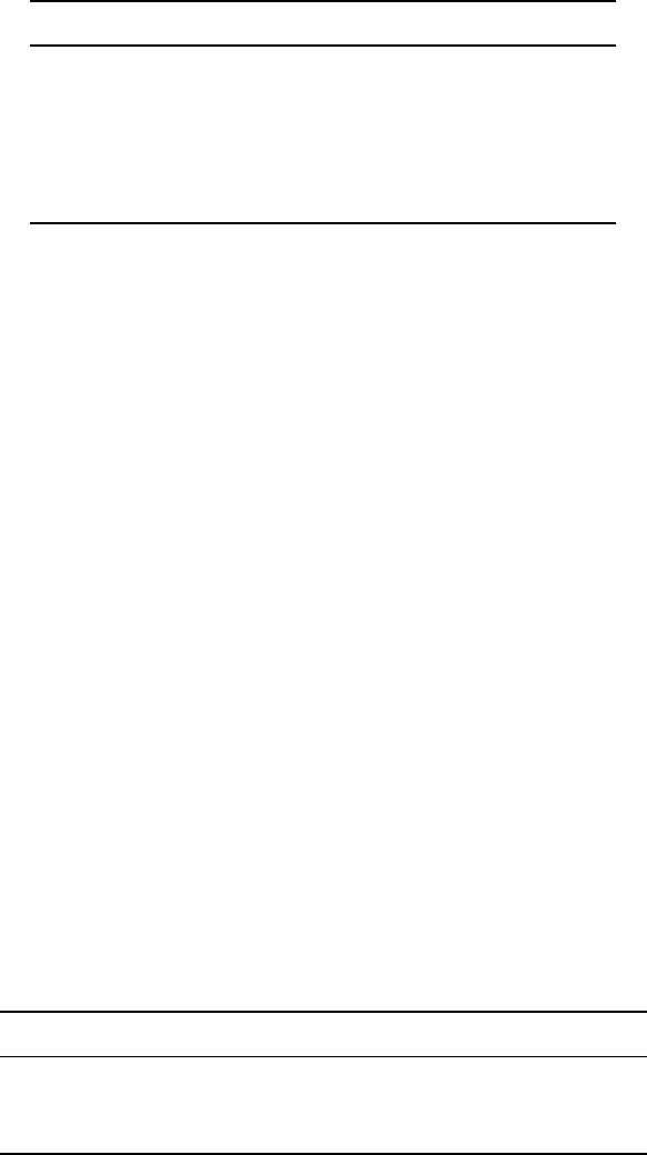
SQL AND RELATIONAL DATABASES 173
Table 7.10 A second normal form error
nameid rstname birthday favoritefood foodid rank
1 Peter 01/02/1991 spaghetti 1 1
1 Peter 01/02/1991 hamburger 2 2
2 Paul 02/03/1992 fruit salad 3 1
3 Mary 03/04/1993 chocolate 4 1
3 Mary 03/04/1993 sh ngers 5 2
3 Mary 03/04/1993 hamburger 1 3
This table does not comply to second normal form because all columns
except rank either relate to one part of the combined primary key (nameid
and foodid) or to other part but not to both.
2. Each column of a table shall relate only and directly to the primary key.
The third normal form is actually a more strict version of the second normal form.
Simply stated, it excludes that data on different things are kept in one table.
Consider Table 7.11. The table only contains three entries, so we could easily use
nameid as primary key. Because the primary key only consists of one column, every
piece of information depends on the whole primary key. But the table remains odd,
because it contains two kinds of information—information related to individuals and
information related to food. As the primary key is based on subjects, all information
on them relates directly to the primary key. Things look different for information that
relates to food. Food-specic information is only related to the primary key insofar as
subjects have food preferences. Therefore, including information on food in the table
violates the third normal form. Again, the information should be stored in separate
tables like in Tables 7.3, 7.5, and 7.6 from the previous subsection.
Keep in mind that there are several other normal forms, but for our purposes these three
should sufce. Recall that normalization is primarily done to ensure data consistency—
meaning that any given piece of information is stored only once in a database. If the same
piece of information is stored twice, changes would have to be made in multiple places and
might contradict each other if forgotten.
There are, however, no technical restrictions that prevent us from putting redundant or
inconsistent data structures into a database. Whether this benets our goal strongly depends on
questions like: What purpose does the database serve? What do we describe in our database?
How are the elements in our database related to each other? Will information be added
in the future? Will the database serve other purposes in the future? How much effort is it
Table 7.11 A third normal form error
nameid rstname birthday favoritefood healthy kcalp100g
1 Peter 01/02/1991 spaghetti no 0.158
2 Paul 02/03/1992 fruit salad yes 0.043
3 Mary 03/04/1993 chocolate no 0.546
This table does not comply to third normal form because favoritefood,
healthy and kcalp100g do not relate directly to persons which the primary
key (nameid) is based on.
174 AUTOMATED DATA COLLECTION WITH R
to completely normalize our database? The higher the complexity of the data, the higher
the number of different purposes a database might serve and the higher the probability that
information might be added in the future, the greater the effort that should be put into planning
and rigorously designing the database structure. Generally speaking, when you try to extract
data from an unknown database, you should always check the structure of the database to
make sure you get the right information.
7.2.3 Advanced features of relational databases and DBMS
Understanding how to store data in tables, how to decompose the data, and how relations
work in databases is enough for a basic understanding of the nature of databases. But often
DBMS have implemented further features like data type denitions, data constraints, virtual
tables or views, procedures, triggers, and events that make DBMS powerful tools but go far
beyond what can be captured in this short introduction. Nonetheless, we will briey describe
these concepts to provide an idea of what is possible when working with DBMS.
One aspect we usually have to take care of when building up a database is to specify each
Data types
column’s data type. The data type denition tells the DBMS how to handle and store the
data; it affects the required disk space and also impacts efciency. There are several broad
data types that are implemented in one way or another in every DBMS: boolean data, that is,
true and false values, numeric data (integer and oat), character or text data, data referring to
dates, times, and time spans as well as data types for les (so-called BLOBs—binary large
objects). Which types are available and how they are implemented depends on the specic
DBMS, so we will not go into details here. The manual section of each DBMS should list
and describe the supported data types, how they are implemented, and further features that
are associated with it. To get an idea, consider Table 7.11 once more. Column by column the
data types can be specied as: integer, character, date, character, boolean, and oat.
Beyond xing columns to specic types of data, some DBMS even implement the possibil-
Constraints
ity to constrain data. Constraining data enables the user to dene under which circumstances—
for which values and value ranges—data should be accepted and in which cases the DBMS
should reject to store the data. In general, there are two ways to constrain data validity:
Specifying columns as primary or foreign keys and explicitly specifying which values or
value ranges are valid and which are not. Setting a column as primary key results in the
rejection of duplicated values because primary keys must identify each row unambiguously.
Dening a column as foreign key will lead to the rejection of values that are not already part
of the primary key it relates to. Explicit constraining of data instead is user-dened and might
be as simple as forbidding negative values or more complex involving several clauses and
references to other tables. No matter which type of constraint is used the general behavior of
the DBMS is to reject values that do not fulll the constraint.
DBMS are designed for consistent handling of data. This entails that queries to the
Transactions
database should not break it, for example, if an invalid change is requested or a data import
suddenly breaks up—for example, when our system crashes. This is ensured by enforcing that
a manipulation is completely carried out or not at all. Furthermore, DBMS usually provide a
way to dene transactional blocks. This feature is useful whenever we have a manipulation
that takes several steps and we want all steps to take effect or none—that is, we do not want
the process to stop halfway through because one statement causes an error, leaving us with
data that is partially manipulated.
Nearly all DBMS provide a way to secure access to the database. The simplest possibility
User
management is to ask for a password before granting access to the whole database but more elaborate
SQL AND RELATIONAL DATABASES 175
frameworks are common like having several users with their own passwords. Furthermore,
each user account can be accompanied with different user rights. One user might only be
allowed to read a single table, while another can read all tables and even add new data. Yet
other users might be allowed to create new tables and grant user rights to other users.
DBMS can easily handle accesses of more than one user to the same database at the same Multi-user
access
time. That is, DBMS will always give you the present state of the database as response to a
query including changes made by other users but only those that were completely executed.
How a DBMS precisely solves problems of concurrent access is DBMS specic.
As the normalization of data and complex structures makes it more cumbersome to Views
assemble the data needed for a specic purpose, most DBMS have the possibility to dene
virtual tables called views. Imagine that we want to retrieve and compose data from different
data tables frequently. We can dene a query each time we need the specic combination of
data. Alternatively, we can dene the query once and save it in a separate table. The downside
of this operation is that it takes up additional disk space. Further, we have to recreate the table
each time to make sure it is up to date, which is identical to dening the query anew each
time we need the specic combination of data.
Another, more elegant solution is to store the query that provides the data we need as a
virtual table. This table is virtual because instead of the data only the query that provides the
data is stored. This virtual table behaves exactly as if the data was stored in the table, but
potentially saves a lot of rewriting and rethinking. Compared to executing the query once and
saving the results in the database, the data in the virtual table will always be up to date.
All DBMS provide functions for data manipulation and aggregation in addition to the Functions
simple data storage capacities. These functions might provide us with the current date, the
absolute value of a number, a substring, the mean for a set of values, and so on. Note that
while Rfunctions can return all kinds of data formats, database functions are restricted
to scalars. Which functions are provided and how they are named is DBMS dependent.
Furthermore, most DBMS allow user-dened functions as well but, again, the syntax for
function denition might vary.
Another DBMS-dependent feature is procedures and triggers. Procedures and triggers Procedures and
triggers
help extending the functionality of SQL. Imagine a database with a lot of tables, where
adding a new entry involves changes to many tables. Procedures are stored sequences of
queries that can be recalled whenever needed, thus making repeating tasks much easier.
While procedures are executed upon user request, triggers are procedures that are executed
automatically when certain events, like changes in a table, take place.
7.3 SQL: a language to communicate with Databases
7.3.1 General remarks on SQL, syntax, and our running example
Now that we have learned how databases and DBMS work and which features they provide, SQL, a
multi-purpose
language
we can turn our attention to SQL, the language to communicate with DBMS. SQL is a
multipurpose language that incorporates vocabulary and syntax for various tasks:
rDCL (data control language)
The DCL part of SQL helps us to dene who is allowed to do what and where in our
database and allows for ne-grained user rights denitions.
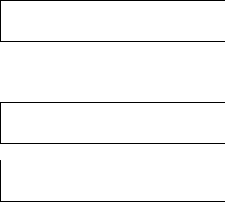
176 AUTOMATED DATA COLLECTION WITH R
rDDL (data denition language)
DDL is the part of SQL that denes the structure of the data and its relations. This
means that the vocabulary enables us to create tables and columns, dene data types,
primary keys and foreign keys, or to set constraints.
rDML (data manipulation language)
The DML part of SQL takes care of actually lling our database with data or retrieving
information from it.
rTCL (transaction control language)
The last part of SQL is TCL, which enables us to commit or rollback previous queries.
This is similar to save and undo buttons in ordinary desktop programs.
The syntax and vocabulary of SQL is rather simple. Let us rst consider the general syntax
General syntax
before moving on to specic vocabularies and syntaxes of the different language branches
of SQL.
SQL statements generally start with a command describing which action should be
executed—for example, CREATE,SELECT,UPDATE,orINSERT INTO—followed by the unit
on which it should be executed—for example, FROM table1—and one or more clauses—for
example, WHERE column1 = 1. Below you nd four SQL statement examples.
1>CREATE DATABASE database1 ;
2>SELECT column1 FROM table1 WHERE column2 = 1 ;
3>UPDATE table1 SET column1 = 1 WHERE column2 > 3 ;
4>INSERT INTO table1 (column1, column2)
VALUES ('rc11', 'rc12'), ('rc21', 'rc22') ;
Although it is customary to write all SQL statements in capital letters, SQL is actually
case insensitive towards its key words. Using capital or small case does not change the
interpretation of the statements. Note however, that depending on the DBMS, the DBMS
might be case sensitive to table and column names. For purposes of readability we will stick
to the capitalized key words and lower case table and column names.
Each SQL statement ends with a semicolon—therefore, SQL statements might span across
multiple lines.
1>CREATE TABLE table (
2> column1 INTEGER NOT NULL AUTO_INCREMENT ,
3> column2 VARCHAR(100) NOT NULL ,
4>PRIMARY KEY (column1)
5>);
Comments either start with -- or have to be put in between /* and */.
1>--One line comment.
2>/*
3>Comment spanning
4>several lines
5>*/
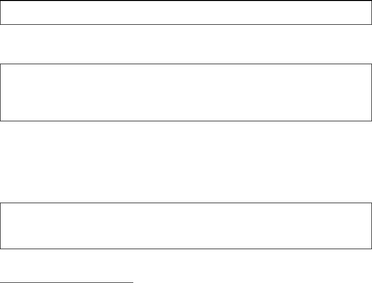
SQL AND RELATIONAL DATABASES 177
For the remainder of this section we will use the birthdays, foodranking, and foodtypes Running
example and
SQL execution
tables (Tables 7.3, 7.5, and 7.6) from the database that we built up in the previous sections.
As SQL is the common standard for a broad range of DBMS, the examples should work
with most DBMS that speak SQL. However, there might always be slight differences—for
example, SQLite does not support user management.
To access the database, you can either use Ras client—you will nd a description of
the possible ways in the next section—or install and use another client software. Before you
can access the database, you have to create your own server—except when using SQLite,
which works with the Rpackage RSQLite out of the box. We recommend using a MySQL
community server in combination with MySQL Workbench CE for a start. Both the MySQL
server and MySQL Workbench are easy to install, easy to use, and can be downloaded
free of charge. Furthermore, MySQL ODBC drivers are reliable, are available for a large
range of platforms, and it is easy to connect to the server from within Rby making use of
RODBC.3
7.3.2 Data control language—DCL
To control access and privileges to our database, we rst ask the DBMS to create a database
called db1:
1>CREATE DATABASE db1 ;
Next, we create and delete several users identifying themselves by password:
1>CREATE USER 'tester' IDENTIFIED BY '123456' ;
2>CREATE USER 'tester2' IDENTIFIED BY '123456' ;
3>CREATE USER 'tester3' IDENTIFIED BY '123456' ;
4>DROP USER 'tester3' ;
Now we can use two powerful SQL commands to dene what a user is allowed to
do. GRANT for granting privileges and REVOKE to remove privileges. A full SQL statement
granting user tester all privileges; all privileges for a certain database, and all privileges
for a certain table in a database looks as follows:
1>GRANT ALL ON *.* TO 'tester2' ;
2>GRANT ALL ON db1.* TO 'tester2' ;
3>GRANT ALL ON db1.table1 TO 'tester2' ;
3The examples were checked with MySQL 5.5.34 and MySQL Workbench CE 5.2.47 to establish the connection.
You can download the MySQL Community Server and MySQL Workbench from http://www.mysql.com.When
asked for an account login or sign up, look for the No thanks, just start my download button—or create an account
if you like.
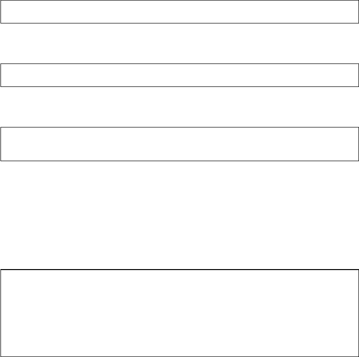
178 AUTOMATED DATA COLLECTION WITH R
We can also grant specic privileges only, for example, for selecting and inserting
information:
1>GRANT SELECT, INSERT ON *.* TO 'tester2' ;
We can add the right to grant privileges to other users as well:
1>GRANT SELECT, INSERT ON *.* TO 'tester2' WITH GRANT OPTION ;
To remove all privileges from our test user, we can use REVOKE or delete the user altogether.
1>REVOKE ALL ON *.* FROM 'tester2' ;
2>DROP USER 'tester2' ;
7.3.3 Data denition language—DDL
After having created a database and a user and having set up the user rights, we can turnCREATE TABLE
to those statements that dene the structure of our data. The commands for data denition
are CREATE TABLE for the denition of tables, ALTER TABLE for changing aspects of an
existing table, and DROP TABLE to delete a table from the database. Let us start by dening
Table 7.3, the revised birthdays table.
1>CREATE TABLE birthdays (
2> nameid INTEGER NOT NULL AUTO_INCREMENT ,
3> firstname VARCHAR(100) NOT NULL ,
4> lastname VARCHAR(100) NOT NULL ,
5> birthday DATE ,
6>PRIMARY KEY (nameid)
7>);
Let us go through this line by line. The rst line starts the statement by using CREATE
TABLE to indicate that we want to dene a new table and also species the name ‘birthdays’
for this new table. The details of the columns follow in parentheses. Each column denition
is separated by a colon and always starts with the name of the column. After the name we
specify the data type and may add further options. While the data types of nameid and
birthday—INTEGER and DATETIME—are self-explaining, the name variables were dened
as characters with a maximum length of 100 characters—VARCHAR(100).
Using the options NOT NULL and AUTO_INCREMENT we dene some basic constraints.
NOT NULL species that this column cannot be left empty—we demand that each person
included in birthdays has to have a name identier, a rst name and a last name. Should we
try to add an observation to the table without all of these pieces of information, the DBMS
will refuse to include it in birthdays.TheAUTO_INCREMENT parameter for the nameid

SQL AND RELATIONAL DATABASES 179
column adds the option that whenever no name identier is manually specied when inserting
data, the DBMS takes care of that by assigning a unique number. The last line before we
close the parentheses and terminate the statement with a semicolon adds a further constraint
to the table. With PRIMARY KEY (nameid) we dene that nameid should serve as primary
key. The DBMS will prevent the insertion of duplicated values into this column.
Let us add two more tables to our database to add some complexity and to showcase
some further concepts. We dene the structure of Tables 7.5 and 7.6, where we recorded food
preferences and food attributes.
1>CREATE TABLE foodtypes (
2> foodid INT NOT NULL AUTO_INCREMENT,
3> foodname VARCHAR(100) NOT NULL,
4> healthy INT,
5> kcalp100g float,
6>PRIMARY KEY (foodid)
7>);
1>CREATE TABLE foodranking (
2> rankid INT NOT NULL AUTO_INCREMENT ,
3> foodid INT ,
4> nameid INT ,
5> rank INT NULL ,
6>PRIMARY KEY (rankid) ,
7>FOREIGN KEY (foodid) REFERENCES foodtypes (foodid) ON UPDATE CASCADE,
8>FOREIGN KEY (nameid) REFERENCES birthdays (nameid) ON UPDATE CASCADE );
The creation of foodtypes is quite similar to that of birthdays. More interesting is
the creation of the food preference table, because it relates to data about subjects as well as to
information about food—captured in birthdays and foodtypes. Take a look at the lines
starting with FOREIGN KEY. First, we choose the column that serves as foreign key, then we
dene which primary key this column refers to, followed by further options. By specifying
ON UPDATE CASCADE we choose that whenever the primary key changes, this change is
cascaded down to our foreign key column that is changed accordingly.
To change the denition of a table later on, we can make use of the ALTER TABLE ALTER TABLE
command. Below you nd several examples for adding a column, changing the data type of
this column, and dropping it again.
1>ALTER TABLE foodtypes ADD COLUMN dummy INT ;
2>ALTER TABLE foodtypes MODIFY COLUMN dummy FLOAT ;
3>ALTER TABLE foodtypes DROP COLUMN dummy ;
To get rid of a table, we can use DROP TABLE.DROP TABLE
1>CREATE TABLE dummy (dcolumn INT);
2>DROP TABLE dummy ;
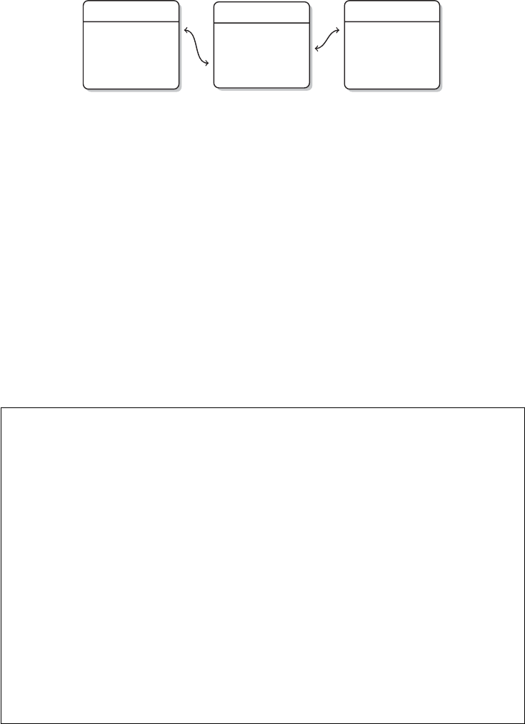
180 AUTOMATED DATA COLLECTION WITH R
birthdays
nameid
firstname
lastname
birthday
foodranking
rankid
foodid
nameid
rank
foodtypes
foodid
foodname
healthy
kcalp100g
Figure 7.3 SQL example database scheme
7.3.4 Data manipulation language—DML
Now that we have dened some tables in our database, we need to learn how to insert,
manipulate, and retrieve data from it. Figure 7.3 provides an overview of the structure of our
database—bold column names refer to primary keys while italics denote foreign keys; the
arrows show which foreign keys relate to which primary keys.
The following three SQL statements use the INSERT INTO command to ll our tablesINSERT INTO
with data. After selecting the name of the table to ll, we also specify column names—
enclosed in parentheses—to specify for which columns data are provided and in which order.
If we had not specifed column names, data for all columns would be provided in the same
order as in the denition of the table. As each table contains one column that is automatically
lled with identication numbers—nameid,foodid,rankid—we do not want to specify
this information manually but let the DBMS take care of it. Note that every non-numeric
value—text and dates—is enclosed in single quotes’.
1>INSERT INTO birthdays (firstname, lastname, birthday)
2>VALUES ('Peter', 'Pascal', '1991-02-01'),
3> ('Paul', 'Panini', '1992-03-02'),
4> ('Mary', 'Meyer', '1993-04-03') ;
5>
6>INSERT INTO foodtypes (foodname, healthy,kcalp100g)
7>VALUES ('spaghetti', 0, 0.158),
8> ('hamburger', 0, 0.295),
9> ('fruit salad', 1, 0.043),
10 > ('chocolate', 0, 0.546),
11 > ('fish fingers', 0, 0.290) ;
12 >
13 >INSERT INTO foodranking (nameid, foodid, rank)
14 >VALUES (1, 1, 1),
15 > (1, 2, 2),
16 > (2, 3, 1),
17 > (3, 4, 1),
18 > (3, 5, 2),
19 > (3, 2, 3) ;
To update and delete rows of data, we have to specify for which rows the update orUPDATE
deletion takes place. For this we can make use of the WHERE clause. Let us create a new
column that captures whether or not the energy of a food type is above 0.2 kcal per 100 g. To
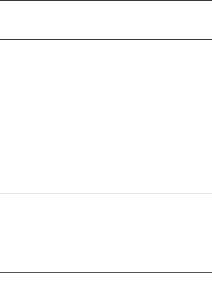
SQL AND RELATIONAL DATABASES 181
achieve this, we tell the DBMS to create a new column and to update the column.4In a last
step, we delete the column again:
1>SET SQL_SAFE_UPDATES = 0 ;
2>ALTER TABLE foodtypes ADD COLUMN highenergy INT ;
3>UPDATE foodtypes SET highenergy=1 WHERE kcalp100g > 0.2 ;
4>UPDATE foodtypes SET highenergy=0 WHERE kcalp100g <= 0.2 ;
5>ALTER TABLE foodtypes DROP COLUMN highenergy ;
Let us have another example of deleting data. We rst create a row with false data and DELETE
then drop the row:
1>INSERT INTO foodtypes (foodname, healthy, kcalp100g)
2>VALUES ("Dominic's incredible pancakes", NULL, NULL);
3>DELETE FROM foodtypes WHERE foodname = "Dominic's incredible pancakes" ;
Data retrieval works similar to insertion of data and is achieved using the SELECT com- SELECT
mand. After the SELECT command we specify the columns we want to retrieve, followed
by the keyword FROM and the name of the table from which we want to get the data. The
following query retrieves all columns of the birthday table:
1>SELECT * FROM birthdays ;
2+--------+-----------+----------+------------+
3| nameid | firstname | lastname | birthday |
4+--------+-----------+----------+------------+
5| 1 | Peter | Pascal | 1991-02-01 |
6| 2 | Paul | Panini | 1992-03-02 |
7| 3 | Mary | Meyer | 1993-04-03 |
8+--------+-----------+----------+------------+
This retrieves only the birthdays:
1>SELECT birthday FROM birthdays ;
2+------------+
3| birthday |
4+------------+
5| 1991-02-01 |
6| 1992-03-02 |
7| 1993-04-03 |
8+------------+
4The rst line is only relevant for MySQL. By default, MySQL prevents updates that have a WHERE clause not
referring to a primary key.
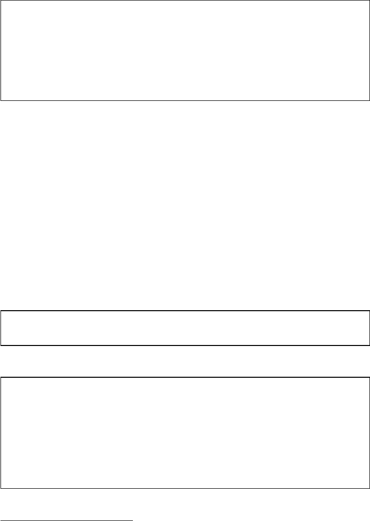
182 AUTOMATED DATA COLLECTION WITH R
Retrieving birthdays and rst names:
1>SELECT firstname, birthday FROM birthdays ;
2+-----------+------------+
3| firstname | birthday |
4+-----------+------------+
5| Peter | 1991-02-01 |
6| Paul | 1992-03-02 |
7| Mary | 1993-04-03 |
8+-----------+------------+
So far we only retrieved data from a single table but often we need to combine data fromJOIN
multiple tables. Combining data is done with the JOIN command—similar to the merge()
function in R. There are four possible joins:5
1. INNER JOIN will return a row whenever there is a match in both tables.
2. LEFT JOIN will return a row whenever there is a match in the rst table.
3. RIGHT JOIN will return a row whenever there is a match in the second table.
4. FULL JOIN will return a row whenever there is a match in one of the tables.
To show how joins work, let us consider three examples in which data from the birthdays
table and the foodranking table are combined. Both tables are related by nameid. We will
match rows on this identier, meaning that information from both tables is merged by identical
values on nameid.
To show the differences in the join statements, let us add a row to the birthdays table with
anameid value that is not included in the foodranking table:
1>INSERT INTO birthdays (nameid,firstname,lastname,birthday)
2>VALUES (10,"Donald","Docker","1934-06-09") ;
The birthdays table now has one additional row:
1>SELECT * FROM birthdays ;
2+--------+-----------+----------+------------+
3| nameid | firstname | lastname | birthday |
4+--------+-----------+----------+------------+
5| 1 | Peter | Pascal | 1991-02-01 |
6| 2 | Paul | Panini | 1992-03-02 |
7| 3 | Mary | Meyer | 1993-04-03 |
8| 10 | Donald | Docker | 1934-06-09 |
9+--------+-----------+----------+------------+
5Note that support of the different join commands is DBMS dependent. For example, SQLite only supports
INNER JOIN and LEFT JOIN while MySQL has no implementation of FULL JOIN.

SQL AND RELATIONAL DATABASES 183
Recall the food ranking table (Table 7.5). The rst JOIN command is an inner join, which
needs matching keys in both tables. Therefore, only information related to Peter, Paul, and
Mary should show up in the resulting table, because Donald does not have a nameid in both
tables:
1>SELECT birthdays.nameid, firstname, lastname, birthday, foodid, rank
2>FROM birthdays
3>INNER JOIN foodranking
4>ON birthdays.nameid=foodranking.nameid ;
5+--------+-----------+----------+------------+--------+------+
6| nameid | firstname | lastname | birthday | foodid | rank |
7+--------+-----------+----------+------------+--------+------+
8| 1 | Peter | Pascal | 1991-02-01 | 1 | 1 |
9| 1 | Peter | Pascal | 1991-02-01 | 2 | 2 |
10 | 2 | Paul | Panini | 1992-03-02 | 3 | 1 |
11 | 3 | Mary | Meyer | 1993-04-03 | 4 | 1 |
12 | 3 | Mary | Meyer | 1993-04-03 | 5 | 2 |
13 | 3 | Mary | Meyer | 1993-04-03 | 2 | 3 |
14 +--------+-----------+----------+------------+--------+------+
Joins are de facto extended SELECT statements. As in an ordinary SELECT statement we
rst specify the command followed by the names of the columns to be retrieved. Note that
the columns to be retrieved can be from both tables. If columns with the same name exist
in both tables they should be preceded by the table name to clarify which column we are
referring to—for example, birthdays.nameid refers to the name identication column in
the birthdays table. The column specication is followed by FROM and the name of the rst
table. In contrast to ordinary SELECT statements we now specify the join keywords—in this
case INNER JOIN—followed by the name of the second table. Using the keyword ON we
specify which columns serve as keys for the match.
As expected, Donald does not show up in the resulting table because his id is not included
in the foodranking table. Furthermore, the resulting table has a row for each food preference
so that information from the birthdays table like name and birthday is duplicated as needed.
1>SELECT birthdays.nameid, firstname, lastname, birthday, foodid, rank
2>FROM birthdays
3>LEFT JOIN foodranking
4>ON birthdays.nameid=foodranking.nameid ;
5+--------+-----------+----------+------------+--------+------+
6| nameid | firstname | lastname | birthday | foodid | rank |
7+--------+-----------+----------+------------+--------+------+
8| 1 | Peter | Pascal | 1991-02-01 | 1 | 1 |
9| 1 | Peter | Pascal | 1991-02-01 | 2 | 2 |
10 | 2 | Paul | Panini | 1992-03-02 | 3 | 1 |
11 | 3 | Mary | Meyer | 1993-04-03 | 4 | 1 |
12 | 3 | Mary | Meyer | 1993-04-03 | 5 | 2 |
13 | 3 | Mary | Meyer | 1993-04-03 | 2 | 3 |
14 | 10 | Donald | Docker | 1934-06-09 | NULL |NULL |
15 +--------+-----------+----------+------------+--------+------+
184 AUTOMATED DATA COLLECTION WITH R
Because LEFT JOIN only requires that a key appears in the rst—or left—table, Donald
Docker is now included in the resulting table, but there is no information on food preference—
both columns show NULL values for Donald Docker. If we had specied the join the other
way around with foodranking being the rst table and birthdays second, Donald would
not have been included as his id is not part of foodranking.
More than one table can be combined with join statements. To get the individuals’
preferences as well as the actual name of the food—we need columns from three tables. We
gather this information by extending the INNER JOIN of our previous example with another
join that species that tables foodranking and foodtypes are related via their foodid
columns and a request for the foodname column:
1>SELECT firstname, rank, foodname FROM birthdays
2>INNER JOIN foodranking
3>ON birthdays.nameid = foodranking.nameid
4>INNER JOIN foodtypes
5>ON foodranking.foodid = foodtypes.foodid ;
6+-----------+------+--------------+
7| firstname | rank | foodname |
8+-----------+------+--------------+
9| Peter | 1 | spaghetti |
10 | Peter | 2 | hamburger |
11 | Mary | 3 | hamburger |
12 | Paul | 1 | fruit salad |
13 | Mary | 1 | chocolate |
14 | Mary | 2 | fish fingers |
15 +-----------+------+--------------+
Let us clean up before moving to the next section by dropping the data on Donald from
the database:
1>DELETE FROM birthdays WHERE firstname = 'Donald' ;
7.3.5 Clauses
We have already used the WHERE clause in SQL statements to restrict data manipulations to
certain rows, but we have neither treated the clause thoroughly nor have we mentioned that
SQL also has other clauses.
Let us begin by extending our knowledge of the WHERE clause. We already know thatWHERE and
operators it restricts data manipulations and retrievals to specic rows. Restrictions are specied in
the form of column_name operator value, where operator denes the type of compar-
ison and value, the content of the comparison. Possible operators are =and != for equal-
ity/inequality, <,<=,>,>= for smaller (or equal) and greater (or equal) values, LIKE for basic
matching of text patterns and IN to specify a set of acceptable values.
We can also use AND and OR to build more complex restrictions and even nest restrictions
by using parentheses. Let us start with a composite WHERE clause with two conditions—see

SQL AND RELATIONAL DATABASES 185
the code snippet below. This statement retrieves data from all three tables but the resulting
set of rows is restricted by the WHERE clause to those lines that have a food preference rank
equal or larger than 2and where the firstname matches 'Mary'.
1>SELECT firstname, foodname, rank FROM birthdays
2>INNER JOIN foodranking ON birthdays.nameid = foodranking.nameid
3>INNER JOIN foodtypes ON foodranking.foodid = foodtypes.foodid
4>WHERE rank >= 2 AND firstname = 'Mary' ;
5+-----------+--------------+------+
6| firstname | foodname | rank |
7+-----------+--------------+------+
8| Mary | hamburger | 3 |
9| Mary | fish fingers | 2 |
10 +-----------+--------------+------+
The next statement has a nested composite WHERE clause and uses alphabetical sorting of
text (firstname < 'Peter'). While firstname should never match 'Mary', the other
part of the clause states that either healthy should equal to 1or firstname should be a
string that precedes Peter alphabetically.
1>SELECT firstname, foodname, healthy FROM birthdays
2>INNER JOIN foodranking ON birthdays.nameid = foodranking.nameid
3>INNER JOIN foodtypes ON foodranking.foodid = foodtypes.foodid
4>WHERE (healthy = 1 OR firstname < 'Peter') AND firstname != 'Mary' ;
5+-----------+-------------+---------+
6| firstname | foodname | healthy |
7+-----------+-------------+---------+
8| Paul | fruit salad | 1 |
9+-----------+-------------+---------+
The following statement is an example of using IN—the value of firstname should
match one of three names:
1>SELECT firstname, lastname FROM birthdays
2>WHERE firstname IN ('Peter','Paul','Karl') ;
3+-----------+----------+
4| firstname | lastname |
5+-----------+----------+
6| Peter | Pascal |
7| Paul | Panini |
8+-----------+----------+
The last statement showcases the usage of LIKE—%is a wildcard for any number of any
character and _is a wildcard for any one character. The statement requires that a row is part
of the resulting table if either firstname contains er at the end of the string preceded by
186 AUTOMATED DATA COLLECTION WITH R
any number of characters or that lastname contains an ethat is preceded by any number of
characters and followed by exactly one character.
1>SELECT firstname, lastname FROM birthdays
2>WHERE firstname LIKE '%er' OR lastname LIKE '%e_';
3+-----------+----------+
4| firstname | lastname |
5+-----------+----------+
6| Peter | Pascal |
7| Mary | Meyer |
8+-----------+----------+
A second clause is the ORDER BY clause, which enables us to order results by columnORDER BY
values. Below you nd several examples that order the results of a data retrieval. The standard
for sorting is to do it in ascending order.
1>SELECT firstname FROM birthdays ORDER BY firstname ;
2+-----------+
3| firstname |
4+-----------+
5| Mary |
6| Paul |
7| Peter |
8+-----------+
To revert this behavior, we can add the keyword DESC. We can also specify more than
one column to dene the sort order and choose for every column whether it should be used
in ascending or descending order.
1>SELECT firstname FROM birthdays
2>ORDER BY birthday DESC, firstname ASC ;
3+-----------+
4| firstname |
5+-----------+
6| Mary |
7| Paul |
8| Peter |
9+-----------+
The GROUP BY clause allows aggregating values. The type of aggregation depends on theGROUP BY
specic aggregation function that we use.6In the following example the use of GROUP
6Aggregation functions are, for example, averages (AVG), counts (COUNT), rst values (FIRST), maxima (MAX),
and sums (SUM).

SQL AND RELATIONAL DATABASES 187
BY is exemplied with the COUNT aggregation function, which returns a count of how
many food preferences each person has—the result is a table with a row for each unique
nameid from the birthdays table and a count of how many times a food preference was
recorded.
1>SELECT firstname, COUNT(rank) FROM birthdays
2>INNER JOIN foodranking ON birthdays.nameid = foodranking.nameid
3>INNER JOIN foodtypes ON foodranking.foodid = foodtypes.foodid
4>GROUP BY birthdays.nameid ;
5+-----------+-------------+
6| firstname | COUNT(rank) |
7+-----------+-------------+
8| Peter | 2 |
9| Paul | 1 |
10 | Mary | 3 |
11 +-----------+-------------+
To lter the aggregation table resulting from a GROUP BY clause, a special clause is HAVING
needed—a WHERE clause can be used in combination with GROUP BY, but this excludes
rows only before aggregation not after. Using HAVING we can lter the aggregation
results.
1>SELECT firstname, COUNT(rank) FROM birthdays
2>INNER JOIN foodranking ON birthdays.nameid = foodranking.nameid
3>INNER JOIN foodtypes ON foodranking.foodid = foodtypes.foodid
4>GROUP BY birthdays.nameid
5>HAVING COUNT(rank) > 1 ;
6+-----------+-------------+
7| firstname | COUNT(rank) |
8+-----------+-------------+
9| Peter | 2 |
10 | Mary | 3 |
11 +-----------+-------------+
7.3.6 Transaction control language—TCL
SQL statements are usually executed after a statement is sent to the DBMS and made START
TRANSACTION
and COMMIT
permanent unless some error occurs. This standard behavior can be modied by explicitly
starting a transacting with START TRANSACTION. Using this statement a save point is created.
Instead of executing each SQL statement immediately and making them permanent, each
statement is executed temporarily until it is explicitly committed by the user with the COMMIT
command. If an error occurs before COMMIT was specied all changes until the last save point
are reversed.

188 AUTOMATED DATA COLLECTION WITH R
We can achieve the same behavior by asking the DBMS to ROLLBACK until the last saveROLLBACK
point. Below you nd an example where some data are added and then the database is reversed
to the status when the save point was set.
1>START TRANSACTION ;
2>INSERT INTO birthdays (firstname, lastname)
3>VALUES ('Simon', 'Sorcerer') ;
4>SELECT firstname, lastname FROM birthdays ;
5+-----------+-----------+
6| firstname | lastname |
7+-----------+-----------+
8| Peter | Pascal |
9| Paul | Panini |
10 | Mary | Meyer |
11 | Simon | Sorcerer |
12 +-----------+-----------+
13 >ROLLBACK ;
14 >SELECT firstname, lastname FROM birthdays ;
15 +-----------+----------+
16 | firstname | lastname |
17 +-----------+----------+
18 | Peter | Pascal |
19 | Paul | Panini |
20 | Mary | Meyer |
21 +-----------+----------+
7.4 Databases in action
7.4.1 Rpackages to manage databases
Rhas several packages to connect to DBMS: One way is to use packages that rely on the DBI
package (R Special Interest Group on Databases 2013) like RMySQL (James and DebRoy
2013), ROracle (Denis Mukhin and Luciani 2013), RPostgreSQL (Conway et al. 2013) and
RSQLite (James and DebRoy 2013) to establish a “native” connection to a specic DBMS.
While the DBI package denes virtual functions, the database-specic packages implement
these functions in database-specic ways. The added value of this approach is that while
there is a common set of functions that are expected to work the same way, different package
authors can concentrate on developing and maintaining solutions for one type of database
only.
Another approach to work with DBMS via Ris to rely on RODBC (Ripley and Lapsley
2013). This package uses open database connectivity (ODBC) drivers as an indirect way to
connect to DBMS and requires that the user installs and congures the necessary driver before
using it in R. ODBC drivers are available across platforms and for a wide variety of DBMS.
They even exist for data storage formats that are no databases at all, like CSV or XLS/XLSX.
The package also delivers a general approach to manage different types of databases with the
same set of functions. On the downside, this approach depends on whether ODBC drivers are
available for the DBMS type to be used in combination with the platform Ris working on.
SQL AND RELATIONAL DATABASES 189
Which package to use is essentially a matter of taste and how difcult it is to get the
package or driver running—at the moment and to the authors’ best knowledge RSQLite is
the only package that works completely out of the box across multiple platforms. All other
packages need driver installation and/or package compilation.
7.4.2 Speaking R-SQL via DBI-based packages
As the DBI package denes a common framework for working with databases from within
R, all database packages that rely on this framework work the same way, regardless of which
particular DBMS we establish a connection to. To show how things work for DBI-based
packages, we will make use of RSQLite. Let us load the birthdays database, which has been
bundled as an SQLite le and execute a simple SELECT statement:
R> # loading package
R> library(RSQLite)
R> # establish connection
R> sqlite <- dbDriver("SQLite")
R> con <- dbConnect(sqlite, "birthdays.db")
R> # 'plain' SQL
R> sql <- "SELECT * FROM birthdays"
R> res <- dbGetQuery(con, sql)
R> res
nameid firstname lastname birthday
1 1 Peter Pascal 1991-02-01
2 2 Paul Panini 1992-03-02
3 3 Mary Meyer 1993-04-03
R> res <- dbSendQuery(con, sql)
R> fetch(res)
nameid firstname lastname birthday
1 1 Peter Pascal 1991-02-01
2 2 Paul Panini 1992-03-02
3 3 Mary Meyer 1993-04-03
Using these functions we are able to perform basic database operations from within R.
Let us go through the code line by line. First we load the RSQLite package so that Rknows
how to handle SQLite databases. Next, we build up a connection to the database by rst
dening the driver and then using the driver in the actual connection. Because our SQLite
database has no password, we do not have to specify much except the database driver and
the location of the database. Now we can query our database. We have two functions to do
so: dbGetQuery() and dbSendQuery(). Both functions ask the DBMS to execute a single
query, but differ in how they handle the results returned by the DBMS. The rst one fetches
all results and converts them to a data frame, while the second one will not fetch any results
unless we explicitly ask Rto do so with the fetch() function.
Because we can send any SQL query that is supported by the specic DBMS, these four
functions sufce to fully control databases from within R. Nonetheless, there are several other
functions provided by DBI-based packages. These functions do not add further features but
help to make communication between Rand DBMS more convenient. There are, for example,
190 AUTOMATED DATA COLLECTION WITH R
functions for getting an overview of the database properties—dbGetInfo()—and the tables
that are provided—dbListTables():
R> # general information
R> dbGetInfo(con)[2]
$serverVersion
[1] "3.7.17"
R> # listing tables
R> dbListTables(con)
[1] "birthdays" "foodranking" "foodtypes" "sqlite_sequence"
There are also functions for reading, writing, and removing tables, which are as convenient
as they are self-explanatory: dbReadTable(),dbWriteTable(),dbExistsTable(), and
dbRemoveTable().
R> # reading tables
R> res <- dbReadTable(con, "birthdays")
R> res
nameid firstname lastname birthday
1 1 Peter Pascal 1991-02-01
2 2 Paul Panini 1992-03-02
3 3 Mary Meyer 1993-04-03
R> # writing tables
R> dbWriteTable(con, "test", res)
[1] TRUE
R> # table exists?
R> dbExistsTable(con, "test")
[1] TRUE
R> # remove table
R> dbRemoveTable(con, "test")
[1] TRUE
To check the data type an Robject would be assigned if stored in a database, we use
dbDataType():
R> # checking data type
R> dbDataType(con, res$nameid)
[1] "INTEGER"
R> dbDataType(con, res$firstname)
[1] "TEXT"
R> dbDataType(con, res$birthday)
[1] "TEXT"
We can also start, revert, and commit transactions as well as close a connection to a
DBMS:
R> # transaction management
R> dbBeginTransaction(con)
[1] TRUE
R> dbRollback(con)

SQL AND RELATIONAL DATABASES 191
[1] TRUE
R> dbBeginTransaction(con)
[1] TRUE
R> dbCommit(con)
[1] TRUE
R> # closing connection
R> dbDisconnect(con)
[1] TRUE
7.4.3 Speaking R-SQL via RODBC
Communicating with databases by relying on the RODBC package is quite similar to the
DBI-based packages. There are functions that forward SQL statements to the DBMS and
convenience functions that do not require the user to specify SQL statements.7
Let us start by establishing a connection to our database and passing a simple SELECT *
statement to read all lines of the birthdays table:
R> # reading package
R> require(RODBC)
R> # establishing connection
R> con <- odbcConnect("db1")
R> # 'plain' SQL
R> sql <- "SELECT * FROM birthdays ;"
R> res <- sqlQuery(con, sql)
R> res
nameid firstname lastname birthday
1 1 Peter Pascal 1991-02-01
2 2 Paul Panini 1992-03-02
3 3 Mary Meyer 1993-04-03
The code to establish a connection and pass the SQL statement to the DBMS is quite
similar to what we have seen before. One difference is that we do not have to specify any
driver as the driver and all other connection information have already been specied in the
ODBC manager so that we only have to refer to the name we gave this particular connection
in the ODBC manager.
Besides the direct execution of SQL statements, there are numerous convenience functions
similar to those found in the DBI-based packages. To get general information on the connection
and the drivers used or to list all tables in the database, we can use odbcGetInfo() and
sqlTables():
R> # general information
R> odbcGetInfo(con)[3]
Driver_ODBC_Ver
"03.51"
7The example works with MySQL drivers. They are available at http://dev.mysql.com/downloads/
connector/odbc/. MySQL ODBC drivers are reliable and available for a whole range of platforms. If you have
followed the examples in the last section with your own MySQL database, you can now connect to it to follow the
example.
192 AUTOMATED DATA COLLECTION WITH R
R> # listing tables
R> sqlTables(con)[, 3:5]
TABLE_NAME TABLE_TYPE REMARKS
1 birthdays TABLE
2 foodranking TABLE
3 foodtypes TABLE
To get an overview of the ODBC driver connections that are currently specied in our
ODBC manager, we can use odbcDataSources(). The function reveals that db1 to which
we are connected is based on MySQL drivers version 5.2:
R> odbcDataSources()
db1
"MySQL ODBC 5.2 ANSI Driver"
We can also ask for whole tables without specifying the SQL statement by a simple call
to sqlFetch():
R> # 'plain' SQL
R> res <- sqlFetch(con, "birthdays")
R> res
nameid firstname lastname birthday
1 1 Peter Pascal 1991-02-01
2 2 Paul Panini 1992-03-02
3 3 Mary Meyer 1993-04-03
Similarly, we can write Rdata frames to SQL tables with convenience functions. We can
also empty tables or delete them altogether:
R> # writing tables
R> test <- data.frame(x = 1:3, y = letters[7:9])
R> sqlSave(con, test, "test")
R> sqlFetch(con, "test")
xy
11g
22h
33i
R> # empty table
R> sqlClear(con, "test")
R> sqlFetch(con, "test")
[1] x y
<0 rows> (or 0-length row.names)
R> # drop table
R> sqlDrop(con, "test")
Summary
In this chapter we learned about databases, SQL, and several Rpackages that enable us to
connect to databases and to access the data stored in them. Simply put, relational databases
SQL AND RELATIONAL DATABASES 193
are collections of tables that are related to one another by keys. Although Ris capable of
handling data, databases offer solutions to certain data management problems that are best
dealt with in a specic environment. SQL is the lingua franca for communication between
the user and a wide range of database management systems. While SQL allows us to dene
what should be done, it is in fact the DBMS that manages how this is achieved in a reliable
manner. As a multipurpose language we can use SQL to manage user rights, dene data
structures, import, manipulate, and retrieve data as well as to control transactions. We have
seen that Ris capable of communicating with a variety of databases and provides additional
convenience functions. As DBMS were designed for reliable and efcient handling of data
they might be solutions to limited RAM size, multipurpose usages of data, multiuser access
to data, complex data storage, and remote access to data.
Further reading
Relational databases and SQL are part of the web technology community and are therefore
treated in hundreds of forums, blogs, and manuals. Therefore, you can easily nd a solution
to most problems by typing your question into any ordinary search engine. To learn the
full spectrum of options for a specic DBMS, you might be better advised to turn to a
comprehensive treatment of the subject. For an introduction to MySQL we recommend
Beaulieu (2009). Those who like it a little bit more fundamental might nd the SQL Bible
(Kriegel and Trukhnov 2008) or Relational Database Design and Implementation (Harrington
2009) helpful sources. Last but not least the SQL Pocket Guide (Gennick 2011) is a gentle
pocket reference that ts in every bookshelf.
Problems
The following problems are built around two—more or less—real-life databases, one on
Pokemon characters, the other on data about elections, governments, and parties. The Poke-
mon data was gathered and provided by Francisco S. Velazquez. We extracted some of the
tables and provide them as CSV les along with supplementary material for this chapter. The
complete database is available at https://github.com/kikin81/pokemon-sqlite.TheParlGov
database is provided by D¨
oring (2013). It combines data on “elections, parties, and govern-
ments for all EU and most OECD members from 1945 until today” gathered from multiple
sources. More information is available at http://parlgov.org. Downloading the whole database
will be part of the exercise.
Pokemon problems
1. Load the RSQLite package and create a new RSQLite database called pokemon.sqlite.
2. Use read.csv2() to read pokemon.csv,pokemon_species.csv,pokemon_stats.csv,
pokemon_types.csv,stats.csv,type_efcacy.csv, and types.csv into Rand write the tables
to pokemon.sqlite. Have a look at PokemonReadme.txt to learn about the tables you
imported.
3. Use functions from DBI/RSQLite to read the tables that you stored in the database
back into Rand save them in objects named: pokemon,pokemon_species,
pokemon_stats,pokemon_types,stats,type_efficacy, and types.
194 AUTOMATED DATA COLLECTION WITH R
4. Build a query that SELECTs those pokemon from table pokemon that are heavier than
4000. Next, build a SELECT query that JOINs tables pokemon and pokemon_species.
5. Combining the previous SQL queries, build a query that JOINs both tables and restricts
the results to Pokemon that are heavier than 4000.
6. Build a query that SELECTs all Pokemon names from table pokemon_species that have
Nido as part of their name.
7. Fetching names.
(a) Build a query that SELECTs Pokemon names.
(b) Send the query to the database using dbSendQuery() and save the result in an
object.
(c) Use fetch() three times in a row, each time retrieving another set of ve names.
(d) Use dbClearResult() to clean up afterwards.
8. Creating views.
(a) Create a VIEW called pokeview …
(b) …that JOINs table pokemon with table pokemon_species,
(c) …and contains the following information: height and weight, species identier,
Pokemon id from which the Pokemon evolves, the id of the evolution chain, and
ids for Pokemon and species.
(d) Create a VIEW called typeview …
(e) …that JOINspokemon_types and types …
(f) …and contains the following information: slot of the type, identier of the type,
and ids for Pokemon, damage class, and type.
(g) Create a VIEW called statsview …
(h) …that JOINspokemon_stats and stats …
(i) …and contains the following information: identier of the statistic, base value of
the statistics, and ids for Pokemon, statistics, and damage class.
9. Using the views you created, which Pokemon are of type dragon? Which Pokemon has
most health points, which has the best attack, defense, and speed?
ParlGov problems
10. Use download.file() with mode="wb" to save the following resource http://parlgov
.org/stable/static/data/parlgov-stable.db as parlgov.sqlite and establish a connection.
11. Get a list of all tables in the database. According to info_data_source, which external
data sources were used for the database?
12. Figure out for which countries the database offers data.
13. Which time span is covered by the election table?
14. How many early elections were there in Spain, the United Kingdom, and Switzerland?
15. Creating views.
(a) CREATE aVIEW named edata …
(b) …that JOINs table election_result …
(c) …with tables election,country, and party …
SQL AND RELATIONAL DATABASES 195
(d) …so that the view contains the following information: country name, date of the
election, the abbreviated party name, party name in English, seats to be won in
total, seats won by party, vote share won by the party, as well as ids for country,
election, election results, and party.
(e) Make sure the VIEW is restricted to elections of type 13 (elections to parliament).
(f) Read the data of the view into Rand save it in an object.
(g) Add a variable storing the seat share.
(h) Plot vote shares versus seat shares. Use text() to add the name of the country if
vote share and seat share differ by more than 20 percentage points.
16. Find answers to the following questions in the database.
(a) Which country had a cabinet lead by Lojze Peterle?
(b) Which parties were part of that government?
(c) What were their vote shares in the election?
17. More SELECT queries.
(a) Build a query that SELECTs column tbl_name and type from table sqlite_master.
(b) Build a query that SELECTs column sql from table sqlite_master WHERE column
tbl_name equals edata. Save the result in an object and use cat() to display the
contents of the object.
(c) Do the same for tbl_name equal to view_election.

8
Regular expressions and essential
string functions
The Web consists predominantly of unstructured text. One of the central tasks in web scraping
is to collect the relevant information for our research problem from heaps of textual data.
Within the unstructured text we are often interested in systematic information—especially
when we want to analyze the data using quantitative methods. Systematic structures can be
numbers or recurrent names like countries or addresses. We usually proceed in three steps.
First we gather the unstructured text, second we determine the recurring patterns behind the
information we are looking for, and third we apply these patterns to the unstructured text
to extract the information. This chapter will focus on the last two steps. Consider HTML
documents from the previous chapters as an example. In principle, they are nothing but
collections of text. Our goal is always to identify and extract those parts of the document that
contain the relevant information. Ideally we can do so using XPath—but sometimes the crucial
information is hidden within atomic values. In some settings, relevant information might
be scattered across an HTML document, rendering approaches that exploit the document
structure useless. In this chapter we introduce a powerful tool that helps retrieve data in such
settings—regular expressions. Regular expressions provide us with a syntax for systematically
accessing patterns in text.
Consider the following short example. Imagine we have collected a string of names and
Ashort
example corresponding phone numbers from ctional characters of the “The Simpsons”TVseries.
Our task is to extract the names and numbers and to put them into a data frame.
R> raw.data <- "555-1239Moe Szyslak(636) 555-0113Burns, C. Montgomery555
-6542Rev. Timothy Lovejoy555 8904Ned Flanders636-555-3226Simpson,
Homer5553642Dr. Julius Hibbert"
Automated Data Collection with R: A Practical Guide to Web Scraping and Text Mining, First Edition.
Simon Munzert, Christian Rubba, Peter Meißner and Dominic Nyhuis.
© 2015 John Wiley & Sons, Ltd. Published 2015 by John Wiley & Sons, Ltd.
REGULAR EXPRESSIONS AND ESSENTIAL STRING FUNCTIONS 197
The rst thing we notice is how the names and numbers come in all sorts of formats. Some
numbers include area codes, some contain dashes, others even parentheses. Yet, despite these
differences we also notice the similarities between all the phone numbers and the names. Most
importantly, the numbers all contain digits while all the names contain alphabetic characters.
We can make use of this knowledge by writing two regular expressions that will extract only
the information that we are interested in. Do not worry about the details of the functions
at this point. They simply serve to illustrate the task that we tackle in this chapter. We will
learn the various elements the queries are made up of and also how they can be applied in
different contexts to extract information and get it into a structured format. We will return to
the example in Section 8.1.3.
R> library(stringr)
R> name <- unlist(str_extract_all(raw.data, "[[:alpha:]., ]{2,}"))
R> name
[1] "Moe Szyslak" "Burns, C. Montgomery" "Rev. Timothy Lovejoy"
[4] "Ned Flanders" "Simpson, Homer" "Dr. Julius Hibbert"
R> phone <- unlist(str_extract_all(raw.data, "\\(?(\\d{3})?\\)?
(-| )?\\d{3}(-| )?\\d{4}"))
R> phone
[1] "555-1239" "(636) 555-0113" "555-6542" "555 8904"
[5] "636-555-3226" "5553642"
We can input the results into a data frame:
R> data.frame(name = name, phone = phone)
name phone
1 Moe Szyslak 555-1239
2 Burns, C. Montgomery (636) 555-0113
3 Rev. Timothy Lovejoy 555-6542
4 Ned Flanders 555 8904
5 Simpson, Homer 636-555-3226
6 Dr. Julius Hibbert 5553642
Although Roffers the main functions necessary to accomplish such tasks, Rwas not
designed with a focus on string manipulation. Therefore, relevant functions sometimes lack
coherence. As the importance of text mining and natural language processing in particular has
increased in recent years, several packages have been developed to facilitate text manipulation
in R. In the following sections—and throughout the remainder of this volume—we rely
predominantly on the stringr package, as it provides most of the string manipulation capability
we require and it enforces a more consistent coding behavior (Wickham 2010).
The following section introduces regular expressions as implemented in R. Section 8.2
provides an overview on how string manipulation can be used in practice. This is done by
presenting commands that are available in the stringr package. If you have previously worked
with regular expressions, you can skip Section 8.1 without much loss. Section 8.3 concludes
with some aspects of character encodings—an important concept in web scraping.

198 AUTOMATED DATA COLLECTION WITH R
8.1 Regular expressions
Regular expressions are generalizable text patterns for searching and manipulating text data.
Strictly speaking, they are not so much a tool as they are a convention on how to query strings
across a wide range of functions. In this section, we will introduce the basic building blocks
of extended regular expressions as implemented in R. The following string will serve as a
running example:
R> example.obj <- "1. A small sentence. - 2. Another tiny sentence."
8.1.1 Exact character matching
At the most basic level characters match characters—even in regular expressions. Thus,
extracting a substring of a string will yield itself if present:
R> str_extract(example.obj, "small")
[1] "small"
Otherwise, the function would return a missing value:
R> str_extract(example.obj, "banana")
[1] NA
The function we use here and in the remainder of this section is str_extract() from
the stringr package, which we assume is loaded in all subsequent examples. It is dened as
str_extract(string, pattern) such that we rst input the string that is to be operated
upon and second the expression we are looking for. Note that this differs from most base
functions, like grep() or grepl(), where the regular expression is typically input rst.1The
function will return the rst instance of a match to the regular expression in a given string.
We can also ask Rto extract every match by calling the function str_extract_all():
R> unlist(str_extract_all(example.obj, "sentence"))
[1] "sentence" "sentence"
The stringr package offers both str_whatever() and str_whatever_all() in many
instances. The former addresses the rst instance of a matching string while the latter
accesses all instances. The syntax of all these functions is such that the character vector in
question is the rst element, the regular expression the second, and all possible additional
values come after that. The functions’ consistency is the main reason why we prefer to use
the stringr package by Hadley Wickham (2010). We introduce the package in more detail
in Section 8.2. See Table 8.5 for an overview of the counterparts of the stringr functions in
base R.
As str_extract_all() is ordinarily called on multiple strings, the results are returned
as a list, with each list element providing the results for one string. Our input string in the
call above is a character vector of length one; hence, the function returns a list of length
one, which we unlist() for convenience of exposition. Compare this to the behavior of the
function when we call it upon multiple strings at the same time. We create a vector containing
1See also Table 8.5 for a comparison between base Rand stringr string manipulation functions.

REGULAR EXPRESSIONS AND ESSENTIAL STRING FUNCTIONS 199
the strings text,manipulation, and basics. We use the function str_extract_all()
to extract all instances of the pattern a:
R> out <- str_extract_all(c("text", "manipulation", "basics"), "a")
R> out
[[1]]
character(0)
[[2]]
[1] "a" "a"
[[3]]
[1] "a"
The function returns a list of the same length as our input vector—three—where each
element in the list contains the result for one string. As there is no ain the rst string, the rst
element is an empty character vector. String two contains two as, string three one occurrence.
By default, character matching is case sensitive. Thus, capital letters in regular expressions
are different from lowercase letters.
R> str_extract(example.obj, "small")
[1] "small"
small is contained in the example string while SMALL is not.
R> str_extract(example.obj, "SMALL")
[1] NA
Consequently, the function extracts no matching value. We can change this behavior by
enclosing a string with ignore.case().2
R> str_extract(example.obj, ignore.case("SMALL"))
[1] "small"
We are not limited to using regular expressions on words. A string is simply a sequence
of characters. Hence, we can just as well match particles of words …
R> unlist(str_extract_all(example.obj, "en"))
[1] "en" "en" "en" "en"
…or mixtures of alphabetic characters and blank spaces.
R> str_extract(example.obj, "mall sent")
[1] "mall sent"
Searching for the pattern en in the example string returns every instance of the pattern, Matching
beginnings and
ends
that is, both occurrences in the word sentence, which is contained twice in the example
object. Sometimes we do not simply care about nding a match anywhere in a string but are
2This behavior is a property of the stringr package. For case-insensitive matching in base functions, set the
ignore.case argument to TRUE. Incidentally, if you have never worked with strings before, tolower() and
toupper() will convert your string to lower/upper case.

200 AUTOMATED DATA COLLECTION WITH R
concerned about the specic location within a string. There are two simple additions we can
make to our regular expression to specify locations. The caret symbol (ˆ) at the beginning
of a regular expression marks the beginning of a string—$at the end marks the end.3Thus,
extracting 2from our running example will return a 2.
R> str_extract(example.obj, "2")
[1] "2"
Extracting a 2from the beginning of the string, however, fails.
R> str_extract(example.obj, "ˆ2")
[1] NA
Similarly, the $sign signals the end of a string, such that …
R> unlist(str_extract_all(example.obj, "sentence$"))
character(0)
…returns no matches as our example string ends in a period character and not in theThe pipe
operator word sentence. Another powerful addition to our regular expressions toolkit is the pipe,
displayed as |. This character is treated as an OR operator such that the function returns all
matches to the expressions before and after the pipe.
R> unlist(str_extract_all(example.obj, "tiny|sentence"))
[1] "sentence" "tiny" "sentence"
8.1.2 Generalizing regular expressions
Up to this point, we have only matched xed expressions. But the power of regular expressions
stems from the possibility to write more exible, generalized search queries. The most general
among them is the period character. It matches any character.
R> str_extract(example.obj, "sm.ll")
[1] "small"
Another powerful generalization in regular expressions are character classes, which are
enclosed in brackets—[]. A character class means that any of the characters within the
brackets will be matched.
R> str_extract(example.obj, "sm[abc]ll")
[1] "small"
The above code extracts the word small as the character ais part of the character class
[abc]. A different way to specify the elements of a character class is to employ ranges of
characters, using a dash -.
R> str_extract(example.obj, "sm[a-p]ll")
[1] "small"
3Note that inside a character class a caret has a different meaning (see p. 202).

REGULAR EXPRESSIONS AND ESSENTIAL STRING FUNCTIONS 201
Table 8.1 Selected predened character classes in Rregular expressions
[:digit:] Digits:0123456789
[:lower:] Lowercase characters: a–z
[:upper:] Uppercase characters: A–Z
[:alpha:] Alphabetic characters: a–z and A–Z
[:alnum:] Digits and alphabetic characters
[:punct:] Punctuation characters: ., ; etc.
[:graph:] Graphical characters: [:alnum:] and [:punct:]
[:blank:] Blank characters: Space and tab
[:space:] Space characters: Space, tab, newline, and other space characters
[:print:] Printable characters: [:alnum:],[:punct:] and [:space:]
Source: Adapted from http://stat.ethz.ch/R-manual/R-patched/library/base/html/regex.html
In this case, any characters from ato pare valid matches. Apart from alphabetic characters
and digits, we can also include punctuation and spaces in regular expressions. Accordingly,
they can be part of a character class. For example, the character class [uvw. ] matches the
letters u,vand was well as a period and a blank space. Applying this to our running example
(Recall: "1. A small sentence. - 2. Another tiny sentence.") yields all of its
constituent periods and spaces but neither u,v,orwas there are none in the object. Note that
the period character in the character class loses its special meaning. Inside a character class,
a dot only matches a literal dot.
R> unlist(str_extract_all(example.obj, "[uvw. ]"))
[1]".""""""""."""""".""""""""."
So far, we have manually specied character classes. However, there are some typical Character
classes
collections of characters that we need to match in a body of text. For example, we are often
interested in nding all alphabetic characters in a given text. This can be accomplished with
the character class [a-zA-Z], that is, all letters from ato zas well as all letters from A
to Z. For convenience, a number of common character classes have been predened in R.
Table 8.1 provides an overview of selected predened classes.
In order to use the predened classes, we have to enclose them in brackets. Otherwise,
Rassumes that we are specifying a character class consisting of the constituent characters.
Say we are interested in extracting all the punctuation characters in our example. The correct
expression is
R> unlist(str_extract_all(example.obj, "[[:punct:]]"))
[1] "." "." "-" "." "."
Notice how this differs from
R> unlist(str_extract_all(example.obj, "[:punct:]"))
[1] "n" "t" "n" "c" "n" "t" "t" "n" "n" "t" "n" "c"
Not enclosing the character class returns all the :,p,u,n,c, and tin our running
example. Note that the duplicate :does not throw off R. A redundant inclusion of a character
in a character class will only match each instance once.
202 AUTOMATED DATA COLLECTION WITH R
R> unlist(str_extract_all(example.obj, "[AAAAAA]"))
[1] "A" "A"
Furthermore, while [A-Za-z] is almost identical to [:alpha:], the former disregards
special characters, such that …
R> str_extract("Franc¸ois Hollande", "Fran[a-z]ois")
[1] NA
…returns no matches, while …
R> str_extract("Franc¸ois Hollande", "Fran[[:alpha:]]ois")
[1] "Franc¸ois"
…does. The predened character classes will cover many requests we might like to make
but in case they do not, we can even extend a predened character class by adding elements
to it.
R> unlist(str_extract_all(example.obj, "[[:punct:]ABC]"))
[1] "." "A" "." "-" "." "A" "."
In this case, we extract all punctuation characters along with the capital letters A,B, and C.
Incidentally, making use of the range operator we introduced above, this extended character
class could be rewritten as [[:punct:]A-C]. Another nifty use of character classes is to
invert their meanings by adding a caret (ˆ) at the beginning of a character class. Doing so,
the function will match everything except the contents of the character class.
R> unlist(str_extract_all(example.obj, "[ˆ[:alnum:]]"))
[1] "." " " " " " " "." " " "-" " " "." " " " " " " "."
Accordingly, in our case every non-alphanumeric character yields every blank spaceQuantiers
and punctuation character. To recap, we have learned that every digit and character matches
itself in a regular expression, a period matches any character, and a character class will
match any of its constituent characters. However, we are still missing the option to use
quantication in our expressions. Say, we would like to extract a sequence starting with
an s, ending with a l, and any three alphabetic characters in between from our running
example. With the tools we have learned so far, our only option is to write an expression like
s[[:alpha:]][[:alpha:]][[:alpha:]]l. Recall that we cannot use the .character as
this would match any character, including blank spaces and punctuation.
R> str_extract(example.obj, "s[[:alpha:]][[:alpha:]][[:alpha:]]l")
[1] "small"
Writing our regular expressions in this manner not only quickly becomes difcult to read
and understand, but it is also inefcient to write and more prone to errors. To avoid this we
can add quantiers to characters. For example, a number in {} after a character signals a
xed number of repetitions of this character. Using this quantier, a sequence such as aaaa
could be shortened to read a{4}. In our case, we thus write …
R> str_extract(example.obj, "s[[:alpha:]]{3}l")
[1] "small"

REGULAR EXPRESSIONS AND ESSENTIAL STRING FUNCTIONS 203
Table 8.2 Quantiers in Rregular expressions
?The preceding item is optional and will be matched at most once
*The preceding item will be matched zero or more times
+The preceding item will be matched one or more times
{n} The preceding item is matched exactly ntimes
{n,} The preceding item is matched nor more times
{n,m} The preceding item is matched at least ntimes, but not more than mtimes
Source: Adapted from http://stat.ethz.ch/R-manual/R-patched/library/base/html/regex.html
…where [[:alpha:]]{3} matches any three alphabetic characters. Table 8.2 provides
an overview of the available quantiers in R. A common quantication operator is the +sign,
which signals that the preceding item has to be matched one or more times. Using the .as
any character we could thus write the following in order to extract a sequence that runs from
an Ato sentence with any number—greater than zero—of any characters in between.
R> str_extract(example.obj, "A.+sentence")
[1] "A small sentence. - 2. Another tiny sentence"
Rapplies greedy quantication. This means that the program tries to extract the greatest Greedy
quantication
and how to
avoid it
possible sequence of the preceding character. As the .matches any character, the function
returns the greatest possible sequence of any characters before a sequence of sentence.We
can change this behavior by adding a ?to the expression in order to signal that we are only
looking for the shortest possible sequence of any characters before a sequence of sentence.
The ?means that the preceding item is optional and will be matched at most once (see again
Table 8.2).
R> str_extract(example.obj, "A.+?sentence")
[1] "A small sentence"
We are not restricted to applying quantiers to single characters. In order to apply a
quantier to a group of characters, we enclose them in parentheses.
R> unlist(str_extract_all(example.obj, "(.en){1,5}"))
[1] "senten" "senten"
In this case, we are asking the function to return a sequence of characters where the rst
character can be any character and the second and third characters have to be an eand an n.
We are asking the function for all instances where this sequence appears at least once, but
at most ve times. The longest possible sequence that could conform to this request would
thus be 3 ×5=15 characters long, where every second and third character would be an e
and an n. In the next code snippet we drop the parentheses. The function will thus match all
sequences that run from any character over eto nwhere the nhas to appear at least once but
at most ve times. Consider how the previous result differs from the following:
R> unlist(str_extract_all(example.obj, ".en{1,5}"))
[1] "sen" "ten" "sen" "ten"

204 AUTOMATED DATA COLLECTION WITH R
Table 8.3 Selected symbols with special meaning
\wWord characters: [[:alnum:]_]
\WNo word characters: [ˆ[:alnum:]_]
\sSpace characters: [[:blank:]]
\SNo space characters: [ˆ[:blank:]]
\dDigits: [[:digit:]]
\DNo digits: [ˆ[:digit:]]
\bWord edge
\BNo word edge
\<Word beginning
\>Word end
So far, we have encountered a number of characters that have a special meaning in regularMetacharacters
expressions.4They are called metacharacters. In order to match them literally, we precede
them with two backslashes. In order to literally extract all period characters from our running
example, we write
R> unlist(str_extract_all(example.obj, "\\."))
[1] "." "." "." "."
The double backslash before the period character is interpreted as a single literal backslash.
Inputting a single backslash in a regular expression will be interpreted as introducing an escape
sequence. Several of these escape sequences are quite common in web scraping tasks and
should be familiar to you. The most common are \nand \twhich mean new line and tab.
For example, “a\n\n\na” is interpreted as a, three new lines, and another a. If we want the
entire regular expression to be interpreted literally, we have a better alternative than preceding
every metacharacter with a backslash. We can enclose the expression with fixed() in order
for metacharacters to be interpreted literally.
R> unlist(str_extract_all(example.obj, fixed(".")))
[1] "." "." "." "."
Most metacharacters lose their special meaning inside a character class. For example, a
period character inside a character class will only match a literal period character. The only
two exceptions to this rule are the caret (ˆ) and the -. Putting the former at the beginning
of a character class matches the inverse of the character class’ contents. The latter can be
applied to describe ranges inside a character class. This behavior can be altered by putting
the -at the beginning or the end of a character class. In this case it will be interpreted
literally.
One last aspect of regular expressions that we want to introduce here are a number of
Further
shortcuts shortcuts that have been assigned to several specic character classes. Table 8.3 provides an
overview of available shortcuts.
4We have encountered .,|,(,),[,],{,},ˆ,$,*,+,?and -.

REGULAR EXPRESSIONS AND ESSENTIAL STRING FUNCTIONS 205
Consider the \wcharacter. This symbol matches any word character in our running
example, such that …
R> unlist(str_extract_all(example.obj, "\\w+"))
[1] "1" "A" "small" "sentence" "2" "Another"
[7] "tiny" "sentence"
…extracts every word separated by blank spaces or punctuation. Note that \wis equivalent
to [[:alnum:]_] and thus the leading digits are interpreted as whole words. Consider further
the useful shortcuts for word edges \>,\<, and \b. Using them, we can be more specic in
the location of matches. Imagine we would like to extract all efrom our running example
that are at the end of a word. To do so, we could apply one of the following two expressions:
R> unlist(str_extract_all(example.obj, "e\\>"))
[1] "e" "e"
R> unlist(str_extract_all(example.obj, "e\\b"))
[1] "e" "e"
This query extracts the two efrom the edges of the word sentence. Finally, it is even Backreferencing
possible to match a sequence that has been previously matched in a regular expression. This
is called backreferencing. Say, we are looking for the rst letter in our running example
and—whatever it may be—want to match further instances of that particular letter. To do
so, we enclose the element in question in parentheses—for example, ([[:alpha:]]) and
reference it using \1.5
R> str_extract(example.obj, "([[:alpha:]]).+?\\1")
[1] "A small sentence. - 2. A"
In our example, the letter is an A. The function returns this match and the subsequent
characters up to the next instance of an A. To make matters a little more complicated, we now
look for a lowercase word without the letter aup to and including the second occurrence of
this word.
R> str_extract(example.obj, "(\\<[b-z]+\\>).+?\\1")
[1] "sentence. - 2. Another tiny sentence"
The expression we use is (\\<[b-z]+\\>).+?\\1. First, consider the [b-z]+ part.
The expression matches all sequences of lowercase letters of length one or more that do not
contain the letter a. In our running example, neither the 1nor the Afulll this requirement.
The rst substring that would match this expression is the double lin the word small. Recall
that the +quantier is greedy. Hence, it tries to capture the longest possible sequence which
would be ll instead of l. This is not what we want. Instead, we are looking for a whole word
of lowercase letters that do not contain the letter a. Thus, to exclude this nding we add the
\\<and \\>to the expression to signal a word’s beginning and end. This entire expression is
enclosed in parentheses in order to reference it further down in the expression. The rst part
of the string that this expression matches is the word sentence. Next, we are looking for
the subsequent occurrence of this substring in our string using the \\1—regardless of what
comes in between (.+?). Not so easy, is it?
5There can be up to nine backreferences, which would be labeled \1,\2, etc.
206 AUTOMATED DATA COLLECTION WITH R
8.1.3 The introductory example reconsidered
Now that we have encountered the main ingredients of regular expressions, we can come
back to our introductory example of sorting out the Simpsons phone directory. Take another
look at the raw data.
R> raw.data
[1] "555-1239Moe Szyslak(636) 555-0113Burns, C. Montgomery555-6542Rev.
Timothy Lovejoy555 8904Ned Flanders636-555-3226Simpson, Homer5553642Dr.
Julius Hibbert"
In order to extract the names, we used the regular expression [[:alpha:]., ]{2,}.Let
us have a look at it step by step. At its core, we used the character class [:alpha:], which
signals that we are looking for alphabetic characters. Apart from these characters, names can
also contain periods, commas and empty spaces, which we want to add to the character class to
read [[:alpha:]., ]. Finally, we add a quantier to impose the restriction that the contents
of the character class have to be matched at least twice to be considered a match. Failing to add
a quantier would extract every single character that matches the character class. Moreover,
we have to specify that we only want matches of at least length two; otherwise the expression
would return the empty spaces between some of the phone numbers.
R> name <- unlist(str_extract_all(raw.data, "[[:alpha:]., ]{2,}"))
R> name
[1] "Moe Szyslak" "Burns, C. Montgomery" "Rev. Timothy Lovejoy"
[4] "Ned Flanders" "Simpson, Homer" "Dr. Julius Hibbert"
We also wanted to extract all the phone numbers from the string. The regular expression
we used for the task was a little more complicated to conform to the different formats of the
phone numbers. Let us consider the elements that phone numbers consist of, mostly digits
(\\d). The primary source of difculty stems from the fact that the phone numbers were not
formatted identically. Instead, some contained empty spaces, dashes, parentheses, or did not
have an area code attached to them.
Applying our knowledge of regular expressions, we are now able to dismantle the regular
expression. In its entirety it reads \\(?(\\d{3})?\\)?(-| )?\\d{3}(-| )?\\d{4}.Let
us go through the expression. The rst part of the expression reads \\(?(\\d{3})?\\)?.In
the center we nd \\d{3}, which we use to collect the three-digit area code. As this is not
contained in every phone number we enclose the expression with two parentheses and add
a question mark, signaling that this part of the expression can be dropped. Before and after
this core element we add \\(and \\)to incorporate two literal parentheses surrounding the
three-digit area code. These too can be dropped, if the phone number does not contain them,
using the ?. Next, our regular expression contains the expression (-| )?. This means that
either a dash or an empty space will be matched, but again, we enclose the entire expression
with parentheses and add a question mark in order to signal that this part of the expression
might be missing. These elements are then simply repeated. Specically, we are looking for
three digits, another dash or empty space that might or might not be part of the phone number,
and four more digits. Applying this to our mock example yields
R> phone <- unlist(str_extract_all(raw.data, "\\(?(\\d{3})?\\)?(-| )?\\d
{3}(-| )?\\d{4}"))

REGULAR EXPRESSIONS AND ESSENTIAL STRING FUNCTIONS 207
R> phone
[1] "555-1239" "(636) 555-0113" "555-6542" "555 8904"
[5] "636-555-3226" "5553642"
Before moving on to discuss how regular expressions can be used in practice in the Regular
expression
avors
subsequent section, we would like to conclude this part with some general observations on
regular expressions. First, even though we have provided a fairly comprehensive picture on
how we can go about generalizing regular expressions to meet our string manipulation needs,
there are still several aspects that we have not covered in this section. In particular, there
are two avors of regular expressions implemented in R—extended basic and Perl regular
expressions. In the above example we have exclusively relied on the former. While Perl
regular expressions provide some additional features, most tasks can be accomplished by
relying on the default avor—the extended basic variant.6
Although there is no harm in learning Perl regular expressions we advise you to stick to
the default for several reasons. One, it is generally confusing to keep two avors in mind—
especially if this is your rst time approaching regular expressions. Two, most tasks can be
accomplished with the default implementation. Sometimes this means solving a task in two
steps rather than one but in many instances this behavior is even preferable. We believe that
it is poor practice to try and come up with a “golden expression” that accomplishes all your
string manipulation needs in just one line. For the sake of readability one should try to restrict
the number of steps that are taken in any given line of code. This simplies error detection
and furthermore helps grasp what is going on in your code when revisiting it at a later stage.
Keeping this rule in mind, the use of such intricate concepts as backreferences becomes
dubious. While there may be instances when they cannot be avoided, they also tend to make
code confusing. Splitting all the steps that are taken inside a backreference expression into
several smaller steps is often preferable.
Now we have the building blocks ready to take a look at what can be accomplished with
regular expressions in practice.
8.2 String processing
8.2.1 The stringr package
In this section we present some of the available functions that rely on regular expressions.
To do so we look at functions that are implemented in the stringr package. Two functions
we have used throughout the last section were str_extract() and str_extract_all().
They extract the rst/all instance/s of a match between the regular expression and the string.
To reiterate, str_extract() extracts the rst matching instance to a regular expression …
R> str_extract(example.obj, "tiny")
[1] "tiny"
…while str_extract_all() extracts all of the matches.
R> str_extract_all(example.obj, "[[:digit:]]")
[[1]]
[1] "1" "2"
6If you care to use Perl regular expressions, simply enclose the expression with perl(). This behavior is a
convention of the stringr package. For Perl regular expressions in base functions, set the perl switch to TRUE.For
information on additional functionality in Perl regular expressions, check out http://www.pcre.org/.

208 AUTOMATED DATA COLLECTION WITH R
Table 8.4 Functions of package stringr in this chapter
Function Description Output
Functions using regular expressions
str_extract() Extracts rst string that matches
pattern
Character vector
str_extract_all() Extracts all strings that match
pattern
List of character vectors
str_locate() Returns position of rst pattern
match
Matrix of start/end
positions
str_locate_all() Returns positions of all pattern
matches
List of matrices
str_replace() Replaces rst pattern match Character vector
str_replace_all() Replaces all pattern matches Character vector
str_split() Splits string at pattern List of character vectors
str_split_fixed() Splits string at pattern into xed
number of pieces
Matrix of character vectors
str_detect() Detects patterns in string Boolean vector
str_count() Counts number of pattern
occurrences in string
Numeric vector
Further functions
str_sub() Extracts strings by position Character vector
str_dup() Duplicates strings Character vector
str_length() Returns length of string Numeric vector
str_pad() Pads a string Character vector
str_trim() Discards string padding Character vector
str_c() Concatenates strings Character vector
We have pointed out that the function outputs differ. In the former case a character vector
is returned, while a list is returned in the latter case. Table 8.4 gives an overview of the
different functions that will be introduced in the present chapter. Column two presents a short
description of the function’s purpose, column three species the format of the return value. If
instead of extracting the result we are interested in the location of a match in a given string,
we use the functions str_locate() or str_locate_all().
R> str_locate(example.obj, "tiny")
start end
[1,] 35 38
The function outputs a matrix with the start and end position of the rst instance of aSubstring
extraction match, in this case the 35th to 38th characters in our example string. We can make use of
positional information in a string to extract a substring using the function str_sub().
R> str_sub(example.obj, start = 35, end = 38)
[1] "tiny"
REGULAR EXPRESSIONS AND ESSENTIAL STRING FUNCTIONS 209
Here we extract the 35th to 38th characters that we know to be the word tiny. Possibly,
a more common task is to replace a given substring. As usual, this can be done using the
assignment operator.
R> str_sub(example.obj, 35, 38) <- "huge"
R> example.obj
[1] "1. A small sentence. - 2. Another huge sentence."
str_replace() and str_replace_all() are used for replacements more generally.
R> str_replace(example.obj, pattern = "huge", replacement = "giant")
[1] "1. A small sentence. - 2. Another giant sentence."
We might care to split a string into several smaller strings. In the easiest of cases we simply String splitting
dene a split, say at each dash.
R> unlist(str_split(example.obj, "-"))
[1] "1. A small sentence. " " 2. Another huge sentence."
We can also x the number of particles we want the string to be split into. If we wanted
to split the string at each blank space, but did not want more than ve resulting strings, we
would write
R> as.character(str_split_fixed(example.obj, "[[:blank:]]", 5))
[1] "1." "A"
[3] "small" "sentence."
[5] "- 2. Another huge sentence."
So far, all the examples we looked at have assumed a single string object. Recall our little
running example that consists of two sentences—but only one string.
R> example.obj
[1] "1. A small sentence. - 2. Another huge sentence."
We can apply the functions to several strings at the same time. Consider a character vector
that consists of several strings as a second running example:
R> char.vec <- c("this", "and this", "and that")
The rst thing we can do is to check the occurrence of particular pattern inside a character String detection
vector. Assume we are interested in knowing whether the pattern this appears in the elements
of a given vector. The function we use to do this is str_detect().
R> str_detect(char.vec, "this")
[1] TRUE TRUE FALSE
Moreover, we could be interested in how often this particular word appears in the elements String counting
of a given vector …
R> str_count(char.vec, "this")
[1] 1 1 0
210 AUTOMATED DATA COLLECTION WITH R
…or how many words there are in total in each of the different elements.
R> str_count(char.vec, "\\w+")
[1] 1 2 2
We can duplicate strings …String
duplication R> dup.obj <- str_dup(char.vec, 3)
R> dup.obj
[1] "thisthisthis" "and thisand thisand this"
[3] "and thatand thatand that"
…or count the number of characters in a given string.
R> length.char.vec <- str_length(char.vec)
R> length.char.vec
[1] 4 8 8
Two important functions in web data manipulation are str_pad() and str_trim().String padding
They are used to add characters to the edges of strings or trim blank spaces.
R> char.vec <- str_pad(char.vec, width = max(length.char.vec),
side = "both", pad = " ")
R> char.vec
[1] " this " "and this" "and that"
In this case we add white spaces to the shorter string equally on both sides such that eachString
trimming string has the same length. The opposite operation is performed using str_trim(), which
strips excess white spaces from the edges of strings.
R> char.vec <- str_trim(char.vec)
R> char.vec
[1] "this" "and this" "and that"
Finally, we can join strings using the str_c() function.String joining
R> cat(str_c(char.vec, collapse = "\n"))
this
and this
and that
Here, we join the three strings of our character vector into a single string. We add a new
line character (\n) and produce the result using the cat() function, which interprets the
new line character as a new line. Beyond joining the contents of one vector, we can use the
function to join two different vectors.
R> str_c("text", "manipulation", sep = " ")
[1] "text manipulation"
If the length of one vector is the multiple of the other, the function automatically recycles
the shorter one.
R> str_c("text", c("manipulation", "basics"), sep = " ")
[1] "text manipulation" "text basics"

REGULAR EXPRESSIONS AND ESSENTIAL STRING FUNCTIONS 211
Table 8.5 Equivalents of the functions in the stringr
package in base R
stringr function Base function
Functions using regular expressions
str_extract() regmatches()
str_extract_all() regmatches()
str_locate() regexpr()
str_locate_all() gregexpr()
str_replace() sub()
str_replace_all() gsub()
str_split() strsplit()
str_split_fixed() –
str_detect() grepl()
str_count() –
Further functions
str_sub() regmatches()
str_dup() –
str_length() nchar()
str_pad() –
str_trim() –
str_c() paste(),paste0()
Throughout this book we frequently rely on the stringr package for strings processing.
However, base Rprovides string processing functionality as well. We nd the base functions
less consistent and thus more difcult to learn. If you still want to learn them or want to
switch from base Rfunctionality to the stringr package, have a look at Table 8.5. It provides
an overview of the analogue functions from the stringr package as implemented in base R.
8.2.2 A couple more handy functions
Many string manipulation tasks can be accomplished using the stringr package we introduced Approximate
matching
in the previous section. However, there are a couple of additional functions in base Rwe would
like to introduce in this section. Text data, especially data scraped from web sources, is often
messy. Data that should be matched come in different formats, names are spelled differently—
problems come from all sorts of places. Throughout this volume we stress the need to cleanse
data after it is collected. One way to deal with messy text data is the agrep() function,
which provides approximate matching via the Levenshtein distance. Without going into too
much detail, the function calculates the number of insertions, deletions, and substitutions
necessary to transform one string into another. Specifying a cutoff, we can provide a criterion
on whether a pattern should be considered as present in a string.
R> agrep("Barack Obama", "Barack H. Obama", max.distance = list(all = 3))
[1] 1

212 AUTOMATED DATA COLLECTION WITH R
In this case, we are looking for the pattern Barack Obama in the string Barack H.
Obama and we allow three alterations in the string.7See how this compares to a search for
the pattern in the string Michelle Obama.
R> agrep("Barack Obama", "Michelle Obama", max.distance = list(all = 3))
integer(0)
Too many changes are needed in order to nd the pattern in the string; hence there is no
result. You can change the maximum distance between pattern and string by adjusting both
the max.distance and the costs parameter. The higher the max.distance parameter
(default =0.1), the more approximate matches it will nd. Using the costs parameter you
can adjust the costs for the different operations necessary to liken to strings.
Another handy function is pmatch(). The function returns the positions of the strings inDetecting
positions the rst vector in the second vector. Consider the character vector from above, c("this",
"and this", "and that").
R> pmatch(c("and this", "and that", "and these", "and those"), char.vec)
[1] 2 3 NA NA
We are looking for the positions of the elements in the rst vector (c("and this",
"and that", "and these", "and those") in the character vector. The output signals
that the rst element is at the second position, the second at the third. The third and fourth
elements in the rst vector are not contained in the character vector. A nal useful function
is make.unique(). Using this function you can transform a collection of nonunique strings
by adding digits where necessary.
R> make.unique(c("a", "b", "a", "c", "b", "a"))
[1] "a" "b" "a.1" "c" "b.1" "a.2"
Although there are a lot of handy functions already available, there will always beExtending base
functionality problems and situations when the one special function desperately needed is missing. One of
those problems might be the following. Imagine we have to check for more than one pattern
within a character vector and want to get a logical vector indicating compliant rows or an
index listing all the compliant row numbers. For checking patterns, we know that grep(),
grepl(),orstr_detect() might be good candidates. Because grep() offers a switch
for returning the matched text or a row index vector, we try to build a solution starting with
grep(). We begin by downloading a test dataset of Simpsons episodes and store it in the
local le episodes.Rdata.
R> library(XML)
R> # download file
R> if(!file.exists("listOfSimpsonsEpisodes.html")){
link <- "http://en.wikipedia.org/wiki/List_of_The_Simpsons_episodes"
download.file(link, "listOfSimpsonsEpisodes.html", mode="wb")
}
R> # getting the table
7An alternative way to specify the maximum distance between two strings is to input a fraction of changes over
the entire length of a string.
REGULAR EXPRESSIONS AND ESSENTIAL STRING FUNCTIONS 213
R> tables <- readHTMLTable("listOfSimpsonsEpisodes.html",
header=T, stringsAsFactors=F)
R> tmpcols <- names(tables[[3]])
R> for(i in 3:20){
tmpcols <- intersect(tmpcols, names(tables[[i]]))
}
R> episodes <- NULL
R> for(i in 3:20){
episodes <- rbind(episodes[,tmpcols],tables[[i]][,tmpcols])
}
R> for(i in 1:dim(episodes)[2]){
Encoding(episodes[,i]) <- "UTF-8"
}
R> names(episodes) <- c("pnr", "nr", "title", "directedby",
"Writtenby", "airdate", "productioncode")
R> save(episodes,file="episodes.Rdata")
Let us load the table containing all the Simpsons episodes.
R> load("episodes.Rdata")
As you can see below, it is easy to switch between different answers to the same
question—which episodes mention Homer in the title—using grep(),grepl() and using the
value = TRUE option. The easy switch makes these functions particularly valuable when
we start developing regular expressions, as we might need an index or logical vector at the
end, but we can use the value option to check if the used pattern actually works.
R> grep("Homer",episodes$title[1:10], value=T)
[1] "Homer's Odyssey" "Homer's Night Out"
R> grepl("Homer",episodes$title[1:10])
[1] FALSE FALSE TRUE FALSE FALSE FALSE FALSE FALSE FALSE TRUE
What is missing, however, is the option to ask for a whole bunch of patterns to be matched
at the same time. Imagine we would like to know whether there are episodes where Homer
and Lisa are mentioned in the title. The standard solution would be to make a logical vector
for each separate pattern to be matched and later combine them to a logical vector that equals
TRUE when all patterns are found.
R> iffer1 <- grepl("Homer",episodes$title)
R> iffer2 <- grepl("Lisa",episodes$title)
R> iffer <- iffer1 & iffer2
R> episodes$title[iffer]
[1] "Homer vs. Lisa and the 8th Commandment"
Although this solution might seem acceptable in the case of two patterns, it becomes more
and more inconvenient if the number of patterns grows or if the task has to be repeated. We
will therefore create a new function built upon grep().
R> grepall <- function(pattern, x,
ignore.case = FALSE, perl = FALSE,
fixed = FALSE, useBytes = FALSE,
value=FALSE, logic=FALSE){
214 AUTOMATED DATA COLLECTION WITH R
# error and exception handling
if(length(pattern)==0 | length(x)==0){
warning("Length of pattern or data equals zero.")
return(NULL)
}
# apply grepl() and all()
indicies <- sapply(pattern, grepl, x,
ignore.case, perl, fixed, useBytes)
index <- apply(indicies, 1, all)
# indexation and return of results
if(logic==T) return(index)
if(value==F) return((1:length(x))[index])
if(value==T) return(x[index])
}
R> grepall(c("Lisa","Homer"), episodes$title)
[1] 26
R> grepall(c("Lisa","Homer"), episodes$title, value=T)
[1] "Homer vs. Lisa and the 8th Commandment"
The idea of the grepall() function is that we need to repeat the pattern search for a series
of patterns—as we did in the previous code snippet when doing two separate pattern searches.
Going through a series of things can be done by using a loop or more efciently by using apply
functions. Therefore, we rst apply the grepl() function to get the logical vectors indicating
which patterns were found in which row. We use sapply() because we have a vector as
input and would like to have a matrix like object as output. What we get is a matrix with
columns referring to the different search patterns and rows referring to the individual strings.
To make sure all patterns were found in a certain row we use a second apply—this time we use
apply() because we have a matrix as input—where the all() function returns TRUE when
all values in a row are true and FALSE if any one value in a row is false. Depending on whether
or not we want to return a vector containing the row numbers or a vector containing the text
for which all the patterns were found the value option switches between two different uses
of the internal logical vector to return row numbers or text accordingly. To get the full logical
vector we can use the logic option. Besides providing functionality that works like grep()
and grepl() for multiple search terms, all other options like ignore.case,perl,fixed,
or useBytes are forwarded to the rst apply step, so that this functionality is also part of the
new function.
8.3 A word on character encodings
When working with web-based text data—particularly non-English data—one quickly runs
into encoding issues. While there are no simple rules to deal with these problems, it is
important to keep the difculties that arise from them in mind. Generally speaking, character
encodings refer to how the digital binary signals are translated into human-readable characters,
for example, making a “d” from “01100100.” As there are many languages around the world,
there are also many special characters, like ¨
a, ø, c¸, and so forth. The issues arise since there
are different translation tables such that without knowing which particular table is used to
encode a binary signal it is difcult to draw inferences on the correct content of a signal. If

REGULAR EXPRESSIONS AND ESSENTIAL STRING FUNCTIONS 215
you have not changed the defaults, Rworks with the system encoding scheme to present the
output. You can query this standard with the following function:
R> Sys.getlocale()
[1] "LC_COLLATE=German_Germany.1252;LC_CTYPE=German_Germany.1252;
LC_MONETARY=German_Germany.1252;LC_NUMERIC=C;LC_TIME=German_Germany.1252"
If you have not gured it out already from the names on the cover, this book was written
by four guys from Germany on a computer with a German operating system. The name of
the character encoding, hidden behind the number 1252,isWindows-1252 and it is the
default character encoding on systems that run Microsoft Windows in English and some
other languages. Your output is likely to be a different one. For example, if you are working
on a Windows PC and are located in the United States, Rwill give you a feedback like
English_United States.1252. If you are operating on a Mac, the encoding standard is
UTF-8.8Let us input a string with some special characters. Consider this fragment from a
popular Swedish song, called “small frogs” (sm˚
a grodorna):
R> small.frogs <- "Sm˚
a grodorna, sm˚
a grodorna ¨
ar lustiga att se."
R> small.frogs
[1] "Sm˚
a grodorna, sm˚
a grodorna ¨
ar lustiga att se."
There are several special characters in this fragment. By default, our inputs and outputs Convert
encodings
are assumed to be of Windows-1252 standard; thus the output is correct. Using the function
iconv(), we can translate a string from one encoding scheme to another:
R> small.frogs.utf8 <- iconv(small.frogs, from = "windows-1252",
to = "UTF-8")
R> Encoding(small.frogs.utf8)
[1] "UTF-8"
R> small.frogs.utf8
[1] "Sm˚
a grodorna, sm˚
a grodorna ¨
ar lustiga att se."
In this case, the function applies a translation table from the Windows-1252 encoding to Declare
encodings
the UTF-8 standard. Thus, the binary sequence is recast as a UTF-8-encoded string. Consider
how this behavior differs from the one we encounter when applying the Encoding() function
to the string.
R> Encoding(small.frogs.utf8) <- "windows-1252"
R> small.frogs.utf8
[1] "Sm˜
A¥ grodorna, sm˜
A¥ grodorna ˜
A¤r lustiga att se."
Doing so, we force the system to treat the UTF-8-encoded binary sequence as though it
were generated by a different encoding scheme (our system default Windows-1252), resulting
in the well-known garbled output we get, for example, when visiting a website with malspeci-
ed encodings. There are currently 350 conversion schemes available, which can be accessed
using the iconvlist() function.
8This is quite convenient for working with data from the Web, as UTF-8 is probably the most popular scheme
and therefore used on many websites.
216 AUTOMATED DATA COLLECTION WITH R
R> sample(iconvlist(), 10)
[1] "PT154" "latin7" "UTF-16BE" "CP51932"
[5] "IBM860" "CP50221" "IBM424" "CP1257"
[9] "WINDOWS-50221" "IBM864"
Having established the importance of keeping track of the encodings of text and web-
based text, in particular, we now turn to the question of how to gure out the encoding of an
unknown text. Luckily, in many instances a website gives a pointer in its header. Consider the
<meta> tag with the http-equiv attribute from the website of the Science Journal, which
is located at http://www.sciencemag.org/.
R> library(RCurl)
R> enc.test <- getURL("http://www.sciencemag.org/")
R> unlist(str_extract_all(enc.test, "<meta.+?>"))
[1] "<meta http-equiv=\"Content-Type\" content=\"text/html;
charset=UTF-8\" />"
[2] "<meta name=\"googlebot\" content=\"NOODP\" />"
[3] "<meta name=\"HW.ad-path\" content=\"/\" />"
The rst tag provides some structured information on the type of content we can expectTestin g fo r
encodings on the site as well as how the characters are encoded—in this case UTF-8. But what if such a
tag is not available? While it is difcult to guess the encoding of a particular text, a couple of
handy functions toward this end have been implemented in the tau package. There are three
functions available to test the encoding of a particular string, is.ascii(),is.locale(),
and is.utf8(). What these functions do is to test whether the binary sequences are “legal”
in a particular encoding scheme. Recall that the letter “˚
a” is stored as a particular binary
sequence in the local encoding scheme. This binary sequence is not valid in the ASCII
scheme—hence, the string cannot have been encoded in ASCII. And in fact, this is what we
nd:
R> library(tau)
R> is.locale(small.frogs)
[1] TRUE
R> is.ascii(small.frogs)
[1] FALSE
Summary
Many aspects of automated data collection deal with textual data. Every step of a typical
web scraping exercise might involve some form of string manipulation. Be it that you need
to format a URL request according to your needs, collect information from an HTML page,
(re-)arrange results that come in the form of strings, or general data cleansing. All of these
tasks could require some form of string manipulation. This chapter has introduced the most
important tool for any of these tasks—regular expressions. These expressions allow you to
search for information using highly exible queries.
The chapter has also outlined the main elements of string manipulation. First, we consid-
ered the ingredients of regular expressions as implemented in R. Starting with the simplest of

REGULAR EXPRESSIONS AND ESSENTIAL STRING FUNCTIONS 217
all cases where a character represents itself in a regular expression, we subsequently treated
more elaborate concepts to generalize searches, such as quantiers and character classes. In
the second step, we considered how regular expressions and string manipulation is generally
performed. To do so, we principally looked at the function range that is provided by the
stringr package and several functions that go beyond the package. The chapter concluded
with a discussion on how to deal with character encodings.
Further reading
In this chapter, we introduced extended basic regular expressions as implemented in R. Check
out http://stat.ethz.ch/R-manual/R-patched/library/base/html/regex.html for an overview of
the available concepts. We restricted our exposition to extended regular expressions, as
these sufce to accomplish most common tasks in string manipulation. There is, however,
a second avor of regular expressions that is implemented in R—Perl regular expressions.
These introduce several aspects that allow string manipulations that were not discussed in
this chapter.9Should you be interested in nding out more about Perl regular expressions,
check out http://www.pcre.org/.
Problems
1. Describe regular expressions and why they can be used for web scraping purposes.
2. Find a regular expression that matches any text.
3. Copy the introductory example. The vector name stores the extracted names.
R> name
[1] "Moe Szyslak" "Burns, C. Montgomery" "Rev. Timothy Lovejoy"
[4] "Ned Flanders" "Simpson, Homer" "Dr. Julius Hibbert"
(a) Use the tools of this chapter to rearrange the vector so that all elements conform to
the standard first_name last_name.
(b) Construct a logical vector indicating whether a character has a title (i.e., Rev. and
Dr.).
(c) Construct a logical vector indicating whether a character has a second name.
4. Describe the types of strings that conform to the following regular expressions and
construct an example that is matched by the regular expression.
(a) [0-9]+\\$
(b) \\b[a-z]{1,4}\\b
(c) .*?\\.txt$
(d) \\d{2}/\\d{2}/\\d{4}
(e) <(.+?)>.+?</\\1>
9In almost all cases, however, one can break up search queries into several smaller queries that can easily be
handled by the extended regular expressions.
218 AUTOMATED DATA COLLECTION WITH R
5. Rewrite the expression [0-9]+\\$in a way that all elements are altered but the
expression performs the same task.
6. Consider the mail address chunkylover53[at]aol[dot]com.
(a) Transform the string to a standard mail format using regular expressions.
(b) Imagine we are trying to extract the digits in the mail address. To do so we write
the expression [:digit:]. Explain why this fails and correct the expression.
(c) Instead of using the predened character classes, we would like to use the predened
symbols to extract the digits in the mail address. To do so we write the expression
\\D. Explain why this fails and correct the expression.
7. Consider the string <title>+++BREAKING NEWS+++</title>.Wewouldliketo
extract the rst HTML tag. To do so we write the regular expression <.+>. Explain why
this fails and correct the expression.
8. Consider the string (5-3)ˆ2=5ˆ2-2*5*3+3ˆ2 conforms to the binomial
theorem. We would like to extract the formula in the string. To do so we write the
regular expression [ˆ0-9=+*()]+. Explain why this fails and correct the expression.
9. The following code hides a secret message. Crack it with Rand regular expressions.
Hint: Some of the characters are more revealing than others! The code snippet is also
available in the materials at www.r-datacollection.com.
clcopCow1zmstc0d87wnkig7OvdicpNuggvhryn92Gjuwczi8hqrfpRxs5Aj5dwpn0Tanwo
Uwisdij7Lj8kpf03AT5Idr3coc0bt7yczjatOaootj55t3Nj3ne6c4Sfek.r1w1YwwojigO
d6vrfUrbz2.2bkAnbhzgv4R9i05zEcrop.wAgnb.SqoU65fPa1otfb7wEm24k6t3sR9zqe5
fy89n6Nd5t9kc4fE905gmc4Rgxo5nhDk!gr
10. Why it is important to be familiar with character encodings when working with string
data?
Part Two
A PRACTICAL TOOLBOX
FOR WEB SCRAPING AND
TEXT MINING

9
Scraping the Web
Having learned much about the basics of the architecture of the Web, we now turn to data
collection in practice. In this chapter, we address three main aspects of web scraping with
R. The rst is how to retrieve data from the Web in different scenarios (Section 9.1). Recall
Figure 1.4. The rst part of the chapter looks at the stage where we try to get resources from
servers into R. The principal technology to deal with in this step is HTTP. We offer a set
of real-life scenarios that demonstrate how to use libcurl to gather data in various settings.
In addition to examples based on HTTP or FTP communication, we introduce the use of
web services (web application programming interfaces [APIs]) and a related authentication
standard, OAuth. We also offer a solution for the problem of scraping dynamic content that
we described in Chapter 6. Section 9.1.9 provides an introduction to Selenium, a browser
automation tool that can be used to gather content from JavaScript-enriched pages.
The second part of the chapter turns to strategies for extracting information from gathered
resources (Section 9.2). We are already familiar with the necessary technologies: regular
expressions (Chapter 8) and XPath (Chapter 4). From a technology-based perspective, this
corresponds to the second column of Figure 1.4. In this part we shed light on these techniques
from a more practical perspective, providing a stylized sketch of the strategies and discuss
their advantages and disadvantages. We also consider APIs once more. They are an ideal
case of automated web data collection as they offer a seamless integration of the retrieval and
extracting stages.
Whatever the level of difculty for scraping information from the web, the circle of On the art of
web scraping
scraping remains almost always identical. The followings tasks are part of most scraping
exercises:
1. Information identication
2. Choice of strategy
3. Data retrieval
Automated Data Collection with R: A Practical Guide to Web Scraping and Text Mining, First Edition.
Simon Munzert, Christian Rubba, Peter Meißner and Dominic Nyhuis.
© 2015 John Wiley & Sons, Ltd. Published 2015 by John Wiley & Sons, Ltd.
222 AUTOMATED DATA COLLECTION WITH R
4. Information extraction
5. Data preparation
6. Data validation
7. Debugging and maintenance
8. Generalization
The art of scraping lies in cleverly combining and redening these tasks, and we can only
sketch out some basic principles, either theoretically (as in Section 9.2) or by examples in
the set of retrieval scenarios and case studies. In the end, questions such as “Is automation
efcient?,” “Is Rthe right tool for my web data collection work?,” and “Is my data source of
choice reliable in the long run?” are project-specic and lack a generally helpful answer.
The third part of this chapter addresses an important, but sometimes disregarded aspect of
web scraping. It deals with the question of how to behave nicely on the Web as a web scraper.
We are convinced that the abundance of online data is something positive and opens up
new ways for understanding human interactions. Whether collecting these data is inherently
positive depends in no small part on (a) the behavior of data gatherers and (b) on the purpose
for which data are collected. The latter point is entirely up to you. For the former point, we
offer some basic advice in Section 9.3. We discuss legal implications of web scraping, show
how to take robots.txt, an informal standard for web crawler behavior, into account, and offer
a practical guideline for friendly web-scraping practice.
We conclude the chapter with a glimpse of ongoing efforts for giving Rmore interfaces
with web data and on lighthouses of web scraping more generally (Section 9.4).
A nal remark before we get started: This chapter is mostly about how to build special-
Spiders versus
scrapers purpose web scrapers. In our denition scrapers are programs that grab specic content from
web pages. Such information could be telephone data (see Chapter 15), data on products (see
Chapter 16), or political behavior (see Chapter 12). Spiders (or crawlers or web robots), in
contrast, are programs that grab and index entire pages and move around the Web following
every link they can nd. Most scraping work involves a spidering component. In order to
extract content from webpages, we usually rst download them as a whole and then continue
with the extraction part. In general, however, we disregard scenarios in which the goal is to
wander through the Web without a specic data collection target.
9.1 Retrieval scenarios
For the following scenarios of web data retrieval, we rely on the following set of Rpackages
which were introduced in the rst part of the book. We assume that you have loaded them for
the exercises. We will indicate throughout the chapter whenever we make use of additional
packages.
R> library(RCurl)
R> library(XML)
R> library(stringr)
SCRAPING THE WEB 223
9.1.1 Downloading ready-made les
The rst way to get data from the Web is almost too banal to be considered here and actually
not a case of web scraping in the narrower sense. In some situations, you will nd data
of interest ready for download in TXT, CSV, or any other plain-text/spreadsheet or binary
format like PDF, XLS, or JPEG. Rcan still prove useful for such simple tasks, as (a) the
data acquisition process remains reproducible in principle and (b) it may save a considerable
amount of time. We picked two common examples to illustrate the benets of using Rin
scenarios like these.
9.1.1.1 CSV election results data
The Maryland State Board of Elections at http://www.elections.state.md.us/ provides a rich
data resource on past elections. We identied a set of comma-separated value spreadsheets that
comprise information on state-, county-, and precinct-level election results for the 2012 Pres-
idential election in Maryland in one of the page’s subdirectories at http://www.elections.
state.md.us/elections/2012/election_data/index.html. The targeted les are accessible via
“General” hyperlinks. Suppose we want to download these les for analyses.
The links to the CSV les are scattered across several tables on the page. We are only
interested in some of the documents, namely those that contain the raw election results for
the general election. The page provides data on the primaries and on ballot questions, too. In
order to retrieve the desired les, we want to proceed in three steps.
1. We identify the links to the desired les.
2. We construct a download function.
3. We execute the downloads.
The XML package provides a neat function to identify links in an HTML document—
getHTMLLinks(). We introduce this and other convenience functions from the package in
greater detail in Section 9.1.4.
We use getHTMLLinks() to extract all the URLs and external le names in the HTML Identifying
locations
document that we rst assign to the object url. The list of links in links comprises more
entries than we are interested in, so we apply the regular expression _General.csv to retrieve
the subset of external le names that point to the general election result CSVs. Finally, we
store the le names in a list to be able to apply a download function to this list in the next step.
R> url <- "http://www.elections.state.md.us/elections/2012/election_
data/index.html"
R> links <- getHTMLLinks(url)
R> filenames <- links[str_detect(links, "_General.csv")]
R> filenames_list <- as.list(filenames)
R> filenames_list[1:3]
[[1]]
224 AUTOMATED DATA COLLECTION WITH R
[1] "http://www.elections.state.md.us/elections/2012/election_data/
State_Legislative_Districts_2012_General.csv"
[[2]]
[1] "http://www.elections.state.md.us/elections/2012/election_data/
Allegany_County_2012_General.csv"
[[3]]
[1] "http://www.elections.state.md.us/elections/2012/election_data/
Allegany_By_Precinct_2012_General.csv"
Next, we set up a function to download all the les and call the function downloadCSV().Constructing a
download
function
The function wraps around the base Rfunction download.file(), which is perfectly
sufcient to download URLs or other les in standard scenarios. Our function has three
arguments. filename refers to each of the entries in the filenames_list object. baseurl
species the source path of the les to be downloaded. Along with the le names, we can
thus construct the full URL of each le. We do this using str_c() and feed the result to
the download.file() function. The second argument of the function is the destination on
our local drive. We determine a folder where we want to store the CSV les and add the
le name parameter. We tweak the download by adding (1) a condition which ensures that
the le download is only performed if the le does not already exist in the folder using the
file.exists() function and (2) a pause of 1 second between each le download. We will
motivate these tweaks later in Section 9.3.3.
R> downloadCSV <- function(filename, baseurl, folder) {
R> dir.create(folder, showWarnings = FALSE)
R> fileurl <- str_c(baseurl, filename)
R> if (!file.exists(str_c(folder, "/", filename))) {
R> download.file(fileurl,
R> destfile = str_c(folder, "/", filename))
R> Sys.sleep(1)
R> }
R> }
We apply the function to the list of CSV le names filenames_list using l_ply()Executing the
download from the plyr package. The function takes a list as main argument and passes each list element
as argument to the specied function, in our case downloadCSV(). We can pass further
arguments to the function. For baseurl we identify the path where all CSVs are located.
With folder we select the local folder where want to store the les.
R> library(plyr)
R> l_ply(filenames_list, downloadCSV,
R> baseurl = "www.elections.state.md.us/elections/2012/election_data/",
R> folder = "elec12_maryland")
To check the results, we consider the number of downloaded les and the rst couple of
entries.
R> length(list.files("./elec12_maryland"))
[1] 68

SCRAPING THE WEB 225
R> list.files("./elec12_maryland")[1:3]
[1] "Allegany_By_Precinct_2012_General.csv"
[2] "Allegany_County_2012_General.csv"
[3] "Anne_Arundel_By_Precinct_2012_General.csv"
Sixty-eight CSV les have been added to the folder. We could now proceed with an
analysis by importing the les into Rusing read.csv(). The web scraping task is thus
completed and could easily be replicated with data on other elections stored on the website.
9.1.1.2 PDF legislative district maps
download.file() frequently does not provide the functionality we need to download
les from certain sites. In particular, download.file() does not support data retrieval via
HTTPS by default and is not capable of dealing with cookies or many other advanced features
of HTTP. In such situations, we can switch to RCurl’s high-level functions which can easily
handle problems like these—and offer further useful options.
As a showcase we try to retrieve PDF les of the 2012 Maryland legislative district
maps, complementing the voting data from above. The maps are available at the Maryland
Department of Planning’s website: http://planning.maryland.gov/Redistricting/2010/legiDist.
shtml.1The targeted PDFs are accessible in a three-column table at the bottom right of the
screen and named “1A,” “1B,” and so on. We reuse the download procedure from above, but
specify a different base URL and regular expression to detect the desired les.
R> url <- "http://planning.maryland.gov/Redistricting/2010/legiDist.shtml"
R> links <- getHTMLLinks(url)
R> filenames <- links[str_detect(links, "2010maps/Leg/Districts_")]
R> filenames_list <- str_extract_all(filenames, "Districts.+pdf")
The download function downloadPDF() now relies on getBinaryURL(). We allow Download with
RCurl
for the use of a curl handle. We cannot specify a destination le in the getBinaryURL()
function, so we store the raw data in a pdffile object rst and then pass it to writeBin().
This function writes the PDF les to the specied folder. The other components of the function
remain the same.
R> downloadPDF <- function(filename, baseurl, folder, handle) {
R> dir.create(folder, showWarnings = FALSE)
R> fileurl <- str_c(baseurl, filename)
R> if (!file.exists(str_c(folder, "/", filename))) {
R> content <- getBinaryURL(fileurl, curl = handle)
R> writeBin(content, str_c(folder, "/", filename))
R> Sys.sleep(1)
R> }
R> }
We execute the function with a handle that adds a User-Agent and a From header eld
to every call and keeps the connection alive. We could specify further options if we had to
deal with cookies or other HTTP specics.
1Note that the “2010” in the URL is misleading—it is the 2012 election maps that are offered at this address.

226 AUTOMATED DATA COLLECTION WITH R
R> handle <- getCurlHandle(useragent = str_c(R.version$platform,
R.version$version.string, sep=", "), httpheader = c(from =
"eddie@datacollection.com"))
R> l_ply(filenames_list, downloadPDF,
R> baseurl = "planning.maryland.gov/PDF/Redistricting/2010maps/Leg/",
R> folder = "elec12_maryland_maps",
R> handle = handle)
Again, we examine the results by checking the number of les in the folder and the rst
couple of results.
R> length(list.files("./elec12_maryland_maps"))
[1] 68
R> list.files("./elec12_maryland_maps")[1:3]
[1] "Districts_10.pdf" "Districts_11.pdf" "Districts_12.pdf"
Everything seems to have worked out ne—68 PDF les have been downloaded. The
bottom line of this exercise is that downloading plain-text or binary les from a website is one
of the easiest tasks. The core tools are download.file() and RCurl’s high-level functions.
getHTMLLinks() from the XML package often does a good job of identifying the links to
single les, especially when they are scattered across a document.
9.1.2 Downloading multiple les from an FTP index
We have introduced an alternative network protocol to HTTP for pure le transfer, the File
Transfer Protocol (FTP) in Section 5.3.2. Downloading les from FTP servers is a rewarding
task for data wranglers because FTP servers host les, nothing else. We do not have to care
about getting rid of HTML layout or other unwanted information. Again, RCurl is well-suited
to fetch les via FTP.
Let us have a look at the CRAN FTP server to see how this works. The server has the URL
ftp://cran.r-project.org/. It stores a lot of R-related data, including older Rversions, CRAN
task views, and all CRAN packages. Say we want to download all CRAN task view HTML
les for closer inspection. They are stored at ftp://cran.r-project.org/pub/R/web/views/.Our
downloading strategy is similar to the one in the last scenario.
1. We identify the desired les.
2. We construct a download function.
3. We execute the downloads.
In order to load the FTP directory list into R, we assign the URL to ftp.Next,weFetch FTP
directory save the list of le names to the object ftp_files with getURL().2By setting the libcurl
option dirlistonly to TRUE, we ensure that only the le names are fetched, but no further
information about le size or creation date.
2For FTP servers the getHTMLLinks() command is not an option, because the documents are not structured as
HTML.

SCRAPING THE WEB 227
R> ftp <- "ftp://cran.r-project.org/pub/R/web/views/"
R> ftp_files <- getURL(ftp, dirlistonly = TRUE)
It is sometimes the case that the default FTP mode in libcurl, extended passive (EPSV),
does not work with some FTP servers. In this case, we have to add the ftp.use.epsv =
FALSE option. In our example, we have successfully downloaded the list of les and stored it
in a character vector, ftp_files. The information is corrupted with line feeds and carriage
returns representations \r\n, however, and still contains CTV les.
R> ftp_files
[1] "Bayesian.ctv\r\nBayesian.html\r\nChemPhys.ctv\r\nChemPhys.html\r..."
To get rid of them we use them as splitting patterns for str_split(). We also apply a Extract le
names
regular expression to select only the HTML les with str_extract_all():
R> filenames <- str_split(ftp_files, "\r\n")[[1]]
R> filenames_html <- unlist(str_extract_all(filenames, ".+(.html)"))
R> filenames_html[1:3]
[1] "Bayesian.html" "ChemPhys.html" "ClinicalTrials.html"
An equivalent, but more elegant way to get only the HTML les would be
R> filenames_html <- getURL(ftp, customrequest = "NLST *.html")
R> filenames_html = str_split(filenames_html, "\\\r\\\n")[[1]]
This way we pass the FTP command NLST *.html to our function. This returns a list
of le names in the FTP directory that end in .html. We thus exploit the libcurl option
customrequest that allows changing the request method and do not have to extract the
HTML les ex post.3
In the last step, we construct a function downloadFTP() that fetches the desired les
from the FTP server and stores them in a specied folder. It basically follows the syntax of Download les
the downloadPDF() function from the previous section.
R> downloadFTP <- function(filename, folder, handle) {
R> dir.create(folder, showWarnings = FALSE)
R> fileurl <- str_c(ftp, filename)
R> if (!file.exists(str_c(folder, "/", filename))) {
R> content <- try(getURL(fileurl, curl = handle))
R> write(content, str_c(folder, "/", filename))
R> Sys.sleep(1)
R> }
R> }
3Recall that FTP has a list of commands of its own, just as there are HTTP commands like GET and POST. A list
of FTP commands—some of which can easily be implemented with curl’s customrequest option—can be found
at http://www.nsftools.com/tips/RawFTP.htm.
228 AUTOMATED DATA COLLECTION WITH R
We set up a handle that disables FTP-extended passive mode and download the CRAN
task HTML documents to the cran_tasks folder:
R> handle <- getCurlHandle(ftp.use.epsv = FALSE)
R> l_ply(filenames_list, downloadFTP,
R> folder = "cran_tasks",
R> handle = handle)
A quick inspection of our newly created folder reveals that the les were successfully
downloaded.
R> length(list.files("./cran_tasks"))
[1] 34
R> list.files("./cran_tasks")[1:3]
[1] "Bayesian.html" "ChemPhys.html" "ClinicalTrials.html"
It is also possible to upload data to an FTP server. As we do not have any rights to upload
content to the CRAN server, we offer a ctional example.
R> ftpUpload(what = "example.txt", to = "ftp://example.com/",
userpwd = "username:password")
To get a taste of the good old FTP times where there was no more than just data andWhere to nd
FTP archives directories, visit http://www.search-ftps.com/ or http://www.lesearching.com/ to search for
existing archives. What you will nd might occasionally be content of dubious quality,
however.
9.1.3 Manipulating URLs to access multiple pages
We usually care little about the web addresses of the sites we visit. Sometimes we might
access a web page by entering a URL into our browser, but more frequently we come to a site
through a search engine. Either way, once we have accessed a particular site we move around
by clicking on links, but do not take note of the fact that the URL changes when accessing
the various sites on the same server. We already know that directories on a web server are
comparable to the folders on our local hard drive. Once we realize that the directories of
the website follow specic systematics, we can make use of this fact and apply it in web
scraping by manipulating the URL of a site. Compared with other retrieval strategies, URL
manipulation is a “quick and dirty” approach, as we usually do not care about the internal
mechanisms that create URLs (e.g., GET forms).
Imagine we would like to collect all press releases from the organization Transparency
Navigating
through pages
by URL
manipulation
International. Check out the organization’s press releases under the heading “News” at
http://www.transparency.org/news/pressreleases/. Now select the year 2011 from the drop-
down menu. Notice how the statement year/2011 is appended to the URL. We can apply
this observation and call up the press releases from 2010 by changing the gure in the URL.
As expected, the browser now displays all press releases from 2010, starting with releases in
late December. Notice how the webpage displays 10 hits for each search. Click on “Next” at
the bottom of the page. We nd that the URL is appended with the statement P10. Apparently,
we are able to select specic results pages by using multiples of 10. Let us try this by choosing
SCRAPING THE WEB 229
the fourth site of the 2010 press releases by selecting the directory http://www.transparency.
org/news/pressreleases/year/2010/P30. In fact, we can wander through the pages by manipu-
lating the URL instead of clicking on HTML buttons.
Now let us capitalize on these insights and implement them in small scraper. We proceed
in ve steps.
1. We identify the running mechanism in the URL syntax.
2. We retrieve links to the running pages.
3. We download the running pages.
4. We retrieve links to the entries on the running pages.
5. We download the single entries.
We begin by constructing a function that returns a list of URLs for every page in the index. URL
manipulation
We have already identied the running mechanism in the URL syntax—a Pand a multiple
of 10 is attached to the base URL for every page other than the rst one. To know how many
of these pages exist, we retrieve the total number of pages from the bottom line on the base
page, which reads “Page x of X”. “X” is the total number of pages. We fetch the number with
the XPath command //div[@id='Page']/strong[2] and use the result (total_pages)
to construct a vector add_url with string additions to the base URL. The rst entries are
stored on the base URL page which does not need an addition. Therefore, we construct X −1
snippets to be added to the base URL. We store this number 10 times, as the index runs from
10 to X * 10, rather than from 1 to X in max_url and merge it with /P10 and store it in the
object add_url.
R> baseurl <- htmlParse("http://www.transparency.org/news/
pressreleases/year/2010")
R> xpath <- "//div[@id='Page']/strong[2]"
R> total_pages <- as.numeric(xpathSApply(baseurl, xpath, xmlValue))
R> total_pages
[1] 16
R> max_url <- (total_pages - 1) * 10
R> add_url <- str_c("/P", seq(10, max_url, 10))
R> add_url
[1] "/P10" "/P20" "/P30" "/P40" "/P50" "/P60" "/P70" "/P80"
[9] "/P90" "/P100" "/P110" "/P120" "/P130" "/P140" "/P150"
Next, we construct the full URLs and put them in a list. To fetch entries from the
rst page as well, we add the base URL to the list. Everything is wrapped into a function
getPageURLs() that returns the URLs of single index pages as a list.
R> getPageURLs <- function(url) {
baseurl <- htmlParse(url)
xpath <- "//div[@id='Page']/strong[2]"
total_pages <- as.numeric(xpathSApply(baseurl, xpath, xmlValue))
max_url <- (total_pages - 1) * 10
add_url <- str_c("/P", seq(10, max_url, 10))
230 AUTOMATED DATA COLLECTION WITH R
urls_list <- as.list(str_c(url, add_url))
urls_list[length(urls_list) + 1] <- url
return(urls_list)
}
Applying the function yields
R> url <- "http://www.transparency.org/news/pressreleases/year/2010"
R> urls_list <- getPageURLs(url)
R> urls_list[1:3]
[[1]]
[1] "http://www.transparency.org/news/pressreleases/year/2010/P10"
[[2]]
[1] "http://www.transparency.org/news/pressreleases/year/2010/P20"
[[3]]
[1] "http://www.transparency.org/news/pressreleases/year/2010/P30"
In the third step, we construct a function to download each index page. The function takesDownloading
index pages the returned list from getPageURLs(), extracts the le names, and writes the HTML pages
to a local folder.
Notice that we have to add a le name for the base URL index manually because the
regular expression "/P.+" which identies the le names does not apply here. This is done
in the fourth line of the function. As usual, the download is conducted with getURL:
R> dlPages <- function(pageurl, folder ,handle) {
dir.create(folder, showWarnings = FALSE)
page_name <- str_c(str_extract(pageurl, "/P.+"), ".html")
if (page_name == "NA.html") { page_name <- "/base.html" }
if (!file.exists(str_c(folder, "/", page_name))) {
content <- try(getURL(pageurl, curl = handle))
write(content, str_c(folder, "/", page_name))
Sys.sleep(1)
}
}
We perform the download with l_ply to download the les stored in the
baselinks_list list elements.
R> handle <- getCurlHandle()
R> l_ply(urls_list, dlPages,
folder = "tp_index_2010",
handle = handle)
R> list.files("tp_index_2010")[1:3]
[1] "base.html" "P10.html" "P100.html"
Sixteen les have been downloaded. Now we parse the downloaded index les to identify
the links to the individual press releases. The getPressURLs() function works as follows.
First, we parse the documents into a list. We retrieve all links in the documents using
getHTMLLinks(). Finally, we extract only those links that refer to one of the press releases.
SCRAPING THE WEB 231
To do so, we apply the regular expression "http.+/pressrelease/" which uniquely
identies the releases and stores them in a list.
R> getPressURLs <- function(folder) {
pages_parsed <- lapply(str_c(folder, "/", dir(folder)), htmlParse)
urls <- unlist(llply(pages_parsed, getHTMLLinks))
press_urls <- urls[str_detect(urls, "http.+/pressrelease/")]
press_urls_list <- as.list(press_urls)
return(press_urls_list)
}
Applying the function we retrieve a list of links to roughly 150 press releases.
R> press_urls_list <- getPressURLs(folder = "tp_index_2010")
R> length(press_urls_list)
[1] 152
The press releases are downloaded in the last step. The function works similarly to Downloading
press releases
the one that downloaded the index pages. Again, we rst retrieve the le names of the
press releases based on the full URLs. We apply the rather nasty regular expression
[ˆ//][[:alnum:]_.]+$. We download the press release les with getURL() and store
them in the created folder.
R> dlPress <- function(press_url, folder, handle) {
dir.create(folder, showWarnings = FALSE)
press_filename <- str_c(str_extract(press_url,
"[ˆ//][[:alnum:]_.]+$") , ".html")
if (!file.exists(str_c(folder, "/", press_filename))) {
content <- try(getURL(press_url, curl = handle))
write(content, str_c(folder, "/", press_filename))
Sys.sleep(1)
}
}
We apply this function using
R> handle <- getCurlHandle()
R> l_ply(press_urls_list, dlPress,
folder = "tp_press_2010",
handle = handle)
R> length(list.files("tp_press_2010"))
[1] 152
All 152 les have been downloaded successfully. To process the press releases, we would
have to parse them similar to the getPressURLs() function and extract the text. Moreover,
to accomplish the task that was specied at the beginning of the section we would also have
to generalize the functions to loop over the years on the website but the underlying ideas do
not change.
In scenarios where the range of URLs is not as clear as in the example described above, we
can make use of the url.exists() function from the RCurl package. It works analogously
to file.exists() and indicates whether a given URL exists, that is, whether the server
responds without an error.
232 AUTOMATED DATA COLLECTION WITH R
In many web scraping exercises, we can apply URL manipulation to easily access all the
sites that we are interested in. The downside of this type of access to a website is that we need
a fairly intimate knowledge of the website and of the websites’ directories in order to perform
URL manipulations. This is to say that URL manipulation cannot be used to write a crawler
for multiple websites as the specic manipulations must be developed for each website.
9.1.4 Convenient functions to gather links, lists, and tables from
HTML documents
The XML package provides powerful tools for parsing XML-style documents. Yet it offers
more commands that considerably ease information extraction tasks in the web-scraping
workow. The functions readHTMLTable(),readHTMLList(), and getHTMLLinks()
help extract data from HTML tables, lists, and internal as well as external links. We illustrate
their functionality with a Wikipedia article on Niccol`
o Machiavelli, an “Italian historian,
politician, diplomat, philosopher, humanist, and writer” (Wikipedia 2014).
The rst function we will inspect is getHTMLlinks() which serves to extract linksExtracting
links from HTML documents. To illustrate the exibility of the convenience functions, we prepare
several objects. The rst object stores the URL for the article (mac_url), the second stores
the source code (mac_source), the third stores the parsed document (mac_parsed), and the
fourth and last object (mac_node) holds only one node of the parsed document, namely the
<p> node that includes the introductory text.
R> mac_url <- "http://en.wikipedia.org/wiki/Machiavelli"
R> mac_source <- readLines(mac_url, encoding = "UTF-8")
R> mac_parsed <- htmlParse(mac_source, encoding = "UTF-8")
R> mac_node <- mac_parsed["//p"][[1]]
All of these representations of an HTML document (URL, source code, parsed document,
and a single node) can be used as input for getHTMLLinks() and the other convenience
functions introduced in this section.
R> getHTMLLinks(mac_url)[1:3]
[1] "/w/index.php?title=Machiavelli&redirect=no"
[2] "/wiki/Machiavelli_(disambiguation)"
[3] "/wiki/File:Portrait_of_Niccol%C3%B2_Machiavelli_by_Santi_di_Tito.jpg"
R> getHTMLLinks(mac_source)[1:3]
[1] "/w/index.php?title=Machiavelli&redirect=no"
[2] "/wiki/Machiavelli_(disambiguation)"
[3] "/wiki/File:Portrait_of_Niccol%C3%B2_Machiavelli_by_Santi_di_Tito.jpg"
R> getHTMLLinks(mac_parsed)[1:3]
[1] "/w/index.php?title=Machiavelli&redirect=no"
[2] "/wiki/Machiavelli_(disambiguation)"
[3] "/wiki/File:Portrait_of_Niccol%C3%B2_Machiavelli_by_Santi_di_Tito.jpg"
R> getHTMLLinks(mac_node)[1:3]
[1] "/wiki/Help:IPA_for_Italian" "/wiki/Renaissance_humanism"
[3] "/wiki/Renaissance"
SCRAPING THE WEB 233
We can also supply XPath expressions to restrict the returned documents to specic
subsets, for example, only those links of class extiw.
R> getHTMLLinks(mac_source,
xpQuery="//a[@class='extiw']/@href")[1:3]
[1] "//en.wiktionary.org/wiki/chancery"
[2] "//en.wikisource.org/wiki/Catholic_Encyclopedia_(1913)/Niccol%
C3%B2_Machiavelli"
[3] "//commons.wikimedia.org/wiki/Niccol%C3%B2_Machiavelli"
getHTMLLinks() retrieves links from HTML as well as names of external les. We
already made use of the latter feature in Section 9.1.1. An extension of getHTMLLinks() is
getHTMLExternalFiles(), designed to extract only links that point to external les which
are part of the document. Let us use the function along with its xpQuery parameter. We
restrict the set of returned links to those mentioning Machiavelli to hopefully nd a URL that
links to a picture.
R> xpath <- "//img[contains(@src, 'Machiavelli')]/@src"
R> getHTMLExternalFiles(mac_source,
xpQuery = xpath)[1:3]
[1] "//upload.wikimedia.org/wikipedia/commons/thumb/e/e2/Portrait
_of_Niccol%C3%B2_Machiavelli_by_Santi_di_Tito.jpg/220px-Portrait_
of_Niccol%C3%B2_Machiavelli_by_Santi_di_Tito.jpg"
[2] "//upload.wikimedia.org/wikipedia/commons/thumb/a/a4/
Machiavelli_Signature.svg/128px-Machiavelli_Signature.svg.png"
[3] "//upload.wikimedia.org/wikipedia/commons/thumb/f/f3/
Cesare_borgia-Machiavelli-Corella.jpg/220px-Cesare_borgia-
Machiavelli-Corella.jpg"
The rst three results look promising; they all point to image les stored on the
Wikimedia servers.
The next convenient function is readHTMLList() and as the name already suggests, it Extracting lists
extracts list elements (see Section 2.3.7). Browsing through the article we nd that under
Discourses on Livy several citations from the work are pooled as an unordered list that we
can easily extract. Note that the function returns a list object where each element corresponds
to a list in the HTML. As the citations are the tenth list within the HTML, we gured this out
by eyeballing the output of readHTMLList() and we use the index operator [[10]].
R> readHTMLList(mac_source)[[10]][1:3]
[1] "\"In fact, when there is combined under the same constitution
a prince, a nobility, and the power of the people, then these three
powers will watch and keep each other reciprocally in check.\" Book
I, Chapter II"
[2] "\"Doubtless these means [of attaining power] are cruel and
destructive of all civilized life, and neither Christian, nor even
human, and should be avoided by every one. In fact, the life of a
private citizen would be preferable to that of a king at the expense
of the ruin of so many human beings.\" Bk I, Ch XXVI"
[3] "\"Now, in a well-ordered republic, it should never be necessary
to resort to extra-constitutional measures. ...\" Bk I, Ch XXXIV"
234 AUTOMATED DATA COLLECTION WITH R
The last function of the XML package we would like to introduce at this point isExtracting
tables readHTMLTable(), a function to extract HTML tables. Not only does the function locate
tables within the HTML document, but also transforms them into data frames. As before, the
function extracts all tables and stores them in a list. Whenever the extracted HTML tables
have information that can be used as name, they are stored as named list item. Let us rst get
an overview of the tables by listing the table names.
R> names(readHTMLTable(mac_source))
[1] "Niccol`
o Machiavelli" "NULL" "NULL"
[4] "NULL" "NULL" "NULL"
[7] "NULL" "NULL" "NULL"
[10] "persondata"
There are ten tables; two of them are labeled. Let us extract the last one to retrieve personal
information on Machiavelli.
R> readHTMLTable(mac_source)$persondata
V1 V2
1 Name Machiavelli, Niccol`
o
2 Alternative names Machiavelli, Niccol`
o
3 Short description Italian politician and political theorist
4 Date of birth May 3, 1469
5 Place of birth Florence
6 Date of death June 21, 1527
7 Place of death Florence
A powerful feature of readHTMLList() and readHTMLTable() is that we can deneApplying
element
functions
individual element functions using the elFun argument. By default, the function applied to
each list item (<li>) and each cell of the table (<td>), respectively, is xmlValue(),butwe
can specify other functions that take XML nodes as arguments. Let us use another HTML table
to demonstrate this feature. The rst table of the article gives an overview of Machiavelli’s
personal information and, in the seventh and eighth rows, lists persons and schools of thought
that have inuenced him in his thinking as well as those that were inuenced by him.
R> readHTMLTable(mac_source, stringsAsFactors = F)[[1]][7:8, 1]
[1] "Influenced by\nXenophon, Plutarch, Tacitus, Polybius, Cicero,
Sallust, Livy, Thucydides"
[2] "Influenced\nPolitical Realism, Bacon, Hobbes, Harrington,
Rousseau, Vico, Edward Gibbon, David Hume, John Adams, Cuoco,
Nietzsche, Pareto, Gramsci, Althusser, T. Schelling, Negri, Waltz,
Baruch de Spinoza, Denis Diderot, Carl Schmitt"
In the HTML le, the names of philosophers and schools of thought are also linked to
the corresponding Wikipedia articles, but this information gets lost by relying on the default
element function. Let us replace the default function by one that is designed to extract links—
getHTMLLinks(). This allows us to extract all links for inuential and inuenced thinkers.
R> influential <- readHTMLTable(mac_source,
elFun = getHTMLLinks,
stringsAsFactors = FALSE)[[1]][7,]
R> as.character(influential)[1:3]
[1] "/wiki/Xenophon" "/wiki/Plutarch" "/wiki/Tacitus"
SCRAPING THE WEB 235
R> influenced <- readHTMLTable(mac_source,
elFun = getHTMLLinks,
stringsAsFactors = FALSE)[[1]][8,]
R> as.character(influenced)[1:3]
[1] "/wiki/Political_Realism" "/wiki/Francis_Bacon"
[3] "/wiki/Thomas_Hobbes"
Extracting links, tables, and lists from HTML documents are ordinary tasks in web
scraping practice. These functions save a lot of time or otherwise we would have to spend on
constructing suited XPath expressions and keeping our code tidy.
9.1.5 Dealing with HTML forms
Forms are a classical feature of user–server interaction via HTTP on static websites. They
vary in size, layout, input type, and other parameters—just think about all the search bars you
have used, the radio buttons you have slided, the check marks you have set, the user names
and passwords typed in, and so on. Forms are easy to handle with a graphical user interface
like a browser, but a little more difcult when they have to be disentangled in the source code.
In this section, we will cover the general approach to master forms with R. In the end you
should be able to recognize forms, determine the method used to pass the inputs, the location
where the information is sent, and how to specify options and parameters for sending data to
the servers and capture the result.
We will consider three different examples throughout this section to learn how to prepare
your Rsession, approach forms in general, use the HTTP GET method to send forms to
the server, use POST with url-encoded or multipart body, and let Rautomatically generate
functions that use GET or POST with adequate options to send form data.
Filling out forms in the browser and handling them from within Rdiffers in many respects,
because much of the work that is usually done by the browser in the background has to be
specied explicitly. Using a browser, we
1. ll out the form,
2. push the submit,ok,start, or the like! button.
3. let the browser execute the action specied in the source code of the form and send
the data to the server,
4. and let the browser receive the returned resources after the server has evaluated the
inputs.
In scraping practice, things get a little more complicated. We have to
1. recognize the forms that are involved,
2. determine the method used to transfer the data,
3. determine the address to send the data to,
4. determine the inputs to be sent along,
5. build a valid request and send it out, and
6. process the returned resources.

236 AUTOMATED DATA COLLECTION WITH R
In this section, we use functions from the RCurl,XML,stringr, and the plyr packages.Preparations
Furthermore, we specify an object that captures debug information along the way so that
we can check for details if something goes awry (see Section 5.4.3 for details). Addition-
ally, we specify a curl handle with a set of default options—cookiejar to enable cookie
management, followlocation to follow page redirections which may be triggered by the
POST command, and autoreferer to automatically set the Referer request header when
we have to follow a location redirect. Finally, we specify the From and User-Agent header
manually to stay identiable:
R> info <- debugGatherer()
R> handle <- getCurlHandle(cookiejar = "",
followlocation = TRUE,
autoreferer = TRUE,
debugfunc = info$update,
verbose = TRUE,
httpheader = list(
from = "eddie@r-datacollection.com",
'user-agent' = str_c(R.version$version.string,
", ", R.version$platform)
))
Another preparatory step is to dene a function that translates lists of XML attributes
into data frames. This will come in handy when we are going to evaluate the attributes of
HTML form elements of parsed HTML documents. The function we construct is called
xmlAttrsToDF() and takes two arguments. The rst argument supplies a parsed HTML
document and the second an XPath expression specifying the nodes from which we want
to collect the attributes. The function extracts the nodes’ attributes via xpathApply() and
xmlAttrs() and transforms the resulting list into a data frame while ensuring that attribute
names do not get lost and that each attribute value is stored in a separate column:
R> xmlAttrsToDF <- function(parsedHTML, xpath) {
x <- xpathApply(parsedHTML, xpath, xmlAttrs)
x <- lapply(x, function(x) as.data.frame(t(x)))
do.call(rbind.fill, x)
}
9.1.5.1 GETting to grips with forms
To presenting how to generally approach forms and specically how to handle forms that
demand HTTP GET,weuseWordNet.WordNet is a service provided by Princeton University
at http://wordnetweb.princeton.edu/perl/webwn. Researchers at Princeton have built up a
database of synonyms for English nouns, verbs, and adjectives. They offer their data as an
online service. The website relies on an HTML form to gather the parameters and send a
request for synonyms—see Princeton University (2010a) for further details and Princeton
University (2010b) for the license.
Let us browse to the page and type in a word, for example, data. Hitting the Search
WordNet button results in a change to the URL which now contains 13 parameters.
1http://wordnetweb.princeton.edu/perl/webwn?s=data&sub=Search+
WordNet&o2=&o0=1&o8=1&o1=1&o7=&o5=&o9=&o6=&o3=&o4=&h=
SCRAPING THE WEB 237
We have been redirected to another page, which informs us that data is a noun and that it
has two semantic meanings.
From the fact that the URL is extended with a query string when submitting our search
term we can infer that the form uses the HTTP GET method to send the data to the server.
But let us verify this conclusion. To briey recap the relevant facts from Chapter 2: HTML
forms are specied with the help of <form> nodes and their attributes. The <form> nodes’
attributes dene the specics of the data transfer from client to server. <input> nodes are
nested in <form> nodes and dene the kind of data that needs to be supplied to the form.
We can either use view source code feature of a browser to check out the attributes of the Inspecting
forms with R
form nodes, or we use Rto get the information. This time we do the latter. First, we load the
page into Rand parse it.
R> url <- "http://wordnetweb.princeton.edu/perl/webwn"
R> html_form <- getURL(url, curl = handle)
R> parsed_form <- htmlParse(html_form)
Let us have a look at the form node attributes to learn the specics of sending data to the
server. We use the xmlAttrsToDF() that we have set up above for this task.
R> xmlAttrsToDF(parsed_form, "//form")
method action enctype name
1 get webwn multipart/form-data f
2 get webwn multipart/form-data change
There are two HTML forms on the page, one called fand the other change. The rst
form submits the search terms to the server while the second takes care of submitting further
options on the type and range of data being returned. For the sake of simplicity, we will ignore
the second form.
With regard to the specics of sending the data, the attribute values tell us that we
should use the HTTP method GET (method) and send it to webwn (action) which is the
location of the form we just downloaded and parsed. The enctype parameter with value
multipart/form-data comes as a bit of a surprise. It refers to how content is encoded
in the body of the request. As GET explicitly does not use the body to transport data, we
disregard this option.
The next task is to get the list of input parameters. When GET is used to send data, we
can easily spot the parameters sent to the server by inspecting the query string added to the
URL. But those parameters might only be a subset of all possible parameters. We therefore
use xmlAttrsToDF() again to get the full set of inputs and their attributes.
R> xmlAttrsToDF(parsed_form, "//form[1]/input")
type name maxlength value
1 text s 500 <NA>
2 submit sub <NA> Search WordNet
3 hidden o2 <NA>
4 hidden o0 <NA> 1
5 hidden o8 <NA> 1
6 hidden o1 <NA> 1
7 hidden o7 <NA>
8 hidden o5 <NA>
9 hidden o9 <NA>
10 hidden o6 <NA>
238 AUTOMATED DATA COLLECTION WITH R
11 hidden o3 <NA>
12 hidden o4 <NA>
13 hidden h <NA>
As suggested by the long query string added to the URL after searching for our rst
search term, we get a list of 13 input nodes. Recall that there was only one input eld on the
page—the text eld where we specied the search term. Inspecting the inputs reveals that 11
of the input elds are of type hidden, that is, input elds which cannot be manipulated by
the user. Moreover, input elds of type submit are hidden from user manipulation as well,
so there is only one parameter left for us to take care of. It turns out that the other parameters
are used for submitting options to the server and have nothing to do with the actual search.
To make simple search requests, the sparameter is sufcient.
Combining the informations on HTTP method, request location, and parameters, we can
Specifying GET
requests with Rnow build an adequate request by using one of RCurl’s form functions. As the HTTP method
to send data to the server is GET,weusegetForm(). Since the location to which we send
the request remains the same, we can reuse the URL we used before. As parameter we only
supply the sparameter with a value equal to the search term that we want to get synonyms for.
R> html_form_res <- getForm(uri = url, curl = handle, s = "data")
R> parsed_form_res <- htmlParse(html_form_res)
R> xpathApply(parsed_form_res, "//li", xmlValue)
[[1]]
[1] "S: (n) data, information (a collection of facts from which
conclusions may be drawn) \"statistical data\""
[[2]]
[1] "S: (n) datum, data point (an item of factual information
derived from measurement or research) "
Let us also have a look at the header information we supply by inspecting the information
stored in the info object with the debugGatherer() function and reset it afterwards.
R> cat(str_split(info$value()["headerOut"], "\r")[[1]])
GET /perl/webwn HTTP/1.1
Host: wordnetweb.princeton.edu
Accept: */*
from: eddie@r-datacollection.com
user-agent: R version 3.0.2 (2013-09-25), x86_64-w64-mingw32
GET /perl/webwn?s=data HTTP/1.1
Host: wordnetweb.princeton.edu
Accept: */*
from: eddie@r-datacollection.com
user-agent: R version 3.0.2 (2013-09-25), x86_64-w64-mingw32
R> info$reset()
We nd that the requests for fetching the form information and sending the form data are
nearly identical, except that in the latter case the query string ?s=data is appended to the
requested resource.
SCRAPING THE WEB 239
The same could have been achieved by supplying a URL with appended query string and
a call to getURL():
R> url <- "http://wordnetweb.princeton.edu/perl/webwn?s=data"
R> html_form_res <- getURL(url = url, curl = handle)
9.1.5.2 POSTing forms
Forms that use the HTTP method POST are in many respects identical to forms that use
GET. They key difference between the two methods is that with POST, the information is
transferred in the body of the request. There are two common styles for transporting data in
the body, either as url-encoded or as multipart. While the former is efcient for text data, the
latter is better suited for sending les. Thus, depending on the purpose of the form, one or the
other POST style is expected. The next two sections will show how to handle POST forms
in practice. The rst example deals with a url-encoded body and the second one showcases
sending multipart data.
POST with url-encoded body In the rst example, we use a form from http://www.read-
able.com. The website offers a service that evaluates the readability of webpages and texts.
As before, we use the precomposed handle to retrieve the page and directly parse and save it.
R> url <- "http://read-able.com/"
R> form <- htmlParse(getURL(url = url, curl = handle))
Looking for <form> nodes reveals that there are two forms in the document. An exam- Inspecting
POST forms
ination of the site reveals that the rst is used to supply a URL to evaluating a webpage’s
readability, and the second form allows inputting text directly.
R> xmlAttrsToDF(form, "//form")
method action
1 get check.php
2 post check.php
There is no enctype specied in the attributes of the second form, so we expect the
server to accept both encoding styles. Because url-encoded bodies are more efcient for text
data, we will use this style to send the data.
An inspection of the second form’s input elds indicates that there seem to be no inputs
other than the submit button.
R> xmlAttrsToDF(form, "//form[2]//input")
Looking at the entire source code of the form, we nd that there is a textarea node that
gathers text to be sent to the server.
R> xpathApply(form, "//form[2]")
[[1]]
<form method="post" action="check.php">
<p class="instructions">
240 AUTOMATED DATA COLLECTION WITH R
<label title="Paste
a complete (HTML) Document here" for="directInput">Enter text to
check the readability:</label><br /><textarea id="directInput"
name="directInput" rows="10" cols="60"></textarea>
HTML is allowed - it
will be stripped from the text.
</p>
<p>
<input type="submit"
value="Calculate Readability" /></p>
</form>
attr(,"class")
[1] "XMLNodeSet"
Its name attribute is directInput which serves as parameter name for sending the
text. Let us use a famous quote about data found at http://www.goodreads.com/ to check its
readability.
R> sentence <- "\"It is a capital mistake to theorize before one has
data. Insensibly one begins to twist facts to suit theories, instead
of theories to suit facts.\" -- Arthur Conan Doyle, Sherlock Holmes"
We send it to the read-able server for evaluation. Within the call to postForm() we setSpecifying
POST requests
with R
style to "POST" for an url-encoded transmission of the data.
R> res <- postForm(uri = str_c(url, "check.php"),
curl = handle,
style = "POST",
directInput = sentence)
Most of the results are presented as HTML tables as shown below.
R> readHTMLTable(res)
$'NULL'
Flesch Kincaid Reading Ease 66.5
1 Flesch Kincaid Grade Level 6.6
2 Gunning Fog Score 6.8
3 SMOG Index 5
4 Coleman Liau Index 11.4
5 Automated Readability Index 5.7
$'NULL'
No. of sentences 3
1 No. of words 32
2 No. of complex words 2
3 Percent of complex words 6.25%
4 Average words per sentence 10.67
5 Average syllables per word 1.53

SCRAPING THE WEB 241
All in all, with a Grade Level of 6.6, 12- to 13-year-old children should be able to
understand Sherlock Holmes’ dictum. Let us check out the header information that was sent
to the server.
R> cat(str_split(info$value()["headerOut"], "\r")[[1]])
GET / HTTP/1.1
Host: read-able.com
Accept: */*
from: eddie@r-datacollection.com
user-agent: R version 3.0.2 (2013-09-25), x86_64-w64-mingw32
POST /check.php HTTP/1.1
Host: read-able.com
Accept: */*
from: eddie@r-datacollection.com
user-agent: R version 3.0.2 (2013-09-25), x86_64-w64-mingw32
Content-Length: 277
Content-Type: application/x-www-form-urlencoded
The second header conrms that the data have been sent via POST, using the following
url-encoded body.4
R> cat(str_split(info$value()["dataOut"], "\r")[[1]])
directInput=%22It%20is%20a%20capital%20mistake%20to%20theorize%20
before%20one%20has%20data%2E%20Insensibly%20one%20begins%20to%20
twist%20facts%20to%20suit%20theories%2C%20instead%20of%20theories%20
to%20suit%20facts%2E%22%20%2D%2D%20Arthur%20Conan%20Doyle%2C%20
Sherlock%20Holmes
R> info$reset()
POST with multipart-encoded body The second example considers a POST with a
multipart-encoded body. Fix Picture (http://www.xpicture.org/) is a web service to trans-
form image les from one format to another. In our example we will transform a picture from
PNG format to PDF.
Let us begin by retrieving a picture in PNG format and save it to our disk.
R> url <- "r-datacollection.com/materials/http/sky.png"
R> sky <- getBinaryURL(url = url, curl = handle)
R> writeBin(sky, "sky.png")
Next, we collect the main page of Fix Picture including the HTML form.
R> url <- "http://www.fixpicture.org/"
R> form <- htmlParse(getURL(url = url, curl = handle))
4Recall that URL encoding refers to the process of replacing special characters with their percent-escaped
representations. For more information on the topic see Section 5.1.2.
242 AUTOMATED DATA COLLECTION WITH R
We check out the attributes of the form nodes.
R> xmlAttrsToDF(form, "//form")
name id action method enctype
1 form form resize.php?LANG=en post multipart/form-data
We nd that there is only one form on the page. The form expects data to be sent with
POST and a multipart-encoded body. The list of possible inputs is extensive, as we can not
only transform the picture from one format to another but also ip and rotate it, restrict it
to grayscale, or choose the quality of the new format. For the sake of simplicity, we restrict
ourselves to a simple transformation from one format to another.
R> xmlAttrsToDF(form, "//input")[1:2, c("name", "type", "class", "value")]
name type class value
1 image file upload-file <NA>
2 <NA> image btn_submit <NA>
The important input is the image. The upload-file value for the class attribute in one
of the <input> nodes suggests that we supply the le’s content under this name.
There is no input node for selecting the format of the output le. Inspecting the source
code reveals that a select node is enclosed in the form. Select elements allow choosing
between several options which are supplied as option nodes:
R> xmlAttrsToDF(form, "//select")
onchange id name
1 changeSelect() format format
The name attribute of the select node indicates under which name (format) the value—
listed within the option nodes should be sent to the server.
R> xmlAttrsToDF(form, "//select/option")
value
1 jpeg
2 png
3 tiff
4 pdf
5 bmp
6 gif
Disregarding all other possible options, we are ready to send the data along with param-
eters to the server. For RCurl to read the le and send it to the server, we have to use
RCurl’s fileUpload() function that takes care of providing the correct information for the
underlying libcurl library. The following code snippet sends the data to the server.
R> res <- postForm(uri = "http://www.fixpicture.org/resize.php?LANG=en",
image = fileUpload(filename = "sky.png",
contentType = "image/png"),
format = "pdf",
curl = handle)
The result is not the transformed le itself but another HTML document from which we
extract the link to the le.
R> doc <- htmlParse(res)
R> link <- str_c(url, xpathApply(doc, "//a/@href", as.character)[[1]])
SCRAPING THE WEB 243
We download the transformed le and write it to our local drive.
R> resImage <- getBinaryURL(link, curl = handle)
R> writeBin(resImage, "sky.pdf", useBytes = TRUE)
The result is the PNG picture transformed to PDF format. Last but not least let us have a
look at the multipart body with the data that have been sent via POST:
R> cat(str_split(info$value()["dataOut"], "\r")[[1]])
----------------------------30059d14e820
Content-Disposition: form-data; name="image"; filename="sky.png"
Content-Type: image/png
[[BINARY DATA]]
----------------------------30059d14e820
Content-Disposition: form-data; name="format"
pdf
----------------------------30059d14e820--
The [[BINARY DATA]] snippet indicates binary data that cannot be properly displayed
with text. Finally, we reset the info slot again.
R> info$reset()
9.1.5.3 Automating form handling—the RHTMLForms package
The tools we have introduced in the previous paragraphs can be adapted to specic cases to
handle form interactions. One shortcoming is that the interaction requires a lot of manual
labor and inspection of the source code. One attempt to automate some of the necessary steps
is the RHTMLForms package (Temple Lang et al. 2012). It was designed to automatically
create functions that ll out forms, select the appropriate HTTP method to send data to the
server, and retrieve the result. The RHTMLForms package is not hosted on CRAN. You can
install it by supplying the location of the repository.
R> install.packages("RHTMLForms", repos = "http://www.omegahat.org/R",
type = "source")
R> library(RHTMLForms)
The basic procedure of RHTMLForms worksasfollows:
1. We use getHTMLFormDescription() on the URL where the HTML form is located
and save its results in an object—let us call it forms.
2. We use createFunction() on the rst item of the forms object and save the results
in another object, say form_function.
3. formFunction() takes input elds as options to send them to the server and return
the result.
244 AUTOMATED DATA COLLECTION WITH R
Let us go through this process using WordNet again. We start by gathering the formPurpose-built
form functions description information and creating the form function.
R> url <- "http://wordnetweb.princeton.edu/perl/webwn"
R> forms <- getHTMLFormDescription(url)
R> formFunction <- createFunction(forms[[1]])
Having created formFunction(), we use it to send form data to the server and retrieve
the results.
R> html_form_res <- formFunction(s = "data", .curl = handle)
R> parsed_form_res <- htmlParse(html_form_res)
R> xpathApply(parsed_form_res,"//li", xmlValue)
[[1]]
[1] "S: (n) data, information (a collection of facts from which
conclusions may be drawn) \"statistical data\""
[[2]]
[1] "S: (n) datum, data point (an item of factual information
derived from measurement or research) "
Let us have a look at the function we just created.
R> args(formFunction)
function(s="",
.url = "http://wordnetweb.princeton.edu/perl/webwn",
...,
.reader = NULL,
.formDescription = list(formAttributes = c(
"get",
"http://wordnetweb.princeton.edu/perl/webwn",
"multipart/form-data",
"f"),
elements = list(
s = list(name = "s",
nodeAttributes = c("text", "s", "500"),
defaultValue = ""),
o2 = list(name = "o2", value = "" ),
o0 = list(name = "o0", value = "1"),
o8 = list(name = "o8", value = "1"),
o1 = list(name = "o1", value = "1"),
o7 = list(name = "o7", value = "" ),
o5 = list(name = "o5", value = "" ),
o9 = list(name = "o9", value = "" ),
o6 = list(name = "o6", value = "" ),
o3 = list(name = "o3", value = "" ),
o4 = list(name = "o4", value = "" ),
h = list(name = "h" , value = "" )),
url = "http://wordnetweb.princeton.edu/perl/webwn"),
.opts = structure(list(
referer = "http://wordnetweb.princeton.edu/perl/webwn"),
.Names = "referer"),
.curl = getCurlHandle(),
.cleanArgs = NULL)
SCRAPING THE WEB 245
Although it might look intimidating at rst, it is easier than it looks because most of the
options are for internal use. The options are set automatically and we can disregard them—
.reader,.formDescription,elements,.url,url, and .cleanArgs. We are already
familiar with some of the options like .curl and .opts. In fact, when looking at the call
to formFunction() above you will notice that the same handler was used as before and
the updation of info was successful. That is because under the hood of these functions all
requests are made with the RCurl functions getForm() and postForm() so that we can
expect .opts and .curl to work in the same way as when using pure RCurl functions.
The last set of options are the names of the inputs we ll in and send to the server. In
our case, createFunction() correctly recognized o0 to o8 and has inputs that need not
be manipulated by users. The elements argument stores the default values, but in contrast
to the input that stores the search term—s—which got an option with the same name,
createFunction() did not create arguments for formFunction() that allow specifying
values for o0,o1, and so on, as they are not necessary for the POST command.
The RHTMLForms packages might sound like they simplify interactions with HTML
forms to a great extent. While it is true that we save some of the actual coding, the interactions
still require a fairly intimate knowledge of the form in order to be able to interact with it.
This is to say that it is difcult to interact sensibly with a form if you do not know the type
of input and output for a form.
9.1.6 HTTP authentication
Not all places on the Web are accessible to everyone. We have learned in Section 5.2.2 that
HTTP offers authentication techniques which restrict content from unauthorized users, namely
basic and digest authentication. Performing basic authentication with Ris straightforward with
the RCurl package.
As a short example, we try to access the “solutions” section at www.r-datacollection.com/
materials/solutions. When trying to access the resources with our browser, we are confronted
withaloginform(seeFigure9.1).InRwe can pass username and password to the server
with libcurl’s userpwd option. Base64 encoding is performed automatically.
R> url <- "www.r-datacollection.com/materials/solutions"
R> cat(getURL(url, userpwd = "teacher:sesame", followlocation = TRUE))
solutions coming soon
The userpwd option also works for digest authentication, and we do not have to manually
deal with nonces, algorithms, and hash codes—libcurl takes care for these things on its own.
To avoid storing passwords in the code, it can be convenient to put them in the .Rprole Storing
passwords
le, as Rreads it automatically with every start (see Nolan and Temple Lang 2014, p. 295).
R> options(RDataCollectionLogin = "teacher:sesame")
We can retrieve and use the password using getOption().
R> getURL(url, userpwd = getOption("RDataCollectionLogin"),
followlocation = TRUE)
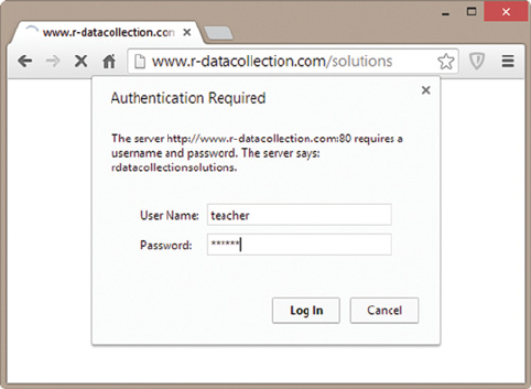
246 AUTOMATED DATA COLLECTION WITH R
Figure 9.1 Screenshot of HTTP authentication mask at http://www.r-datacollection.com/
materials/solutions
9.1.7 Connections via HTTPS
The secure transfer protocol HTTPS (see Section 5.3.1) becomes increasingly common. In
order to retrieve content from servers via HTTPS, we can draw on libcurl/RCurl which
support SSL connections. In fact, we do not have to care much about the encryption and SSL
negotiation details, as they are handled by libcurl in the background by default.
Let us consider an example. The Inter-university Consortium for Political and Social
Research (ICPSR) at the University of Michigan provides access to a huge archive of social
science data. We are interested in just a tiny fraction of it—some meta-information on survey
variables. At https://www.icpsr.umich.edu/icpsrweb/ICPSR/ssvd/search, the ICPSR offers a
elded search for variables. The search mask allows us to specify variable label, question text
or category label, and returns a list of results with some snippets of information. What makes
this page a good exercise is that it has to be accessed via HTTPS, as the URL in the browser
reveals. In principle, connecting to websites via HTTPS can be just as easy as this
R> url <- "https://www.icpsr.umich.edu/icpsrweb/ICPSR/ssvd/search"
R> getURL(url)
Error: SSL certificate problem, verify that the CA cert is OK.
Details:
error:14090086:SSL routines:SSL3_GET_SERVER_CERTIFICATE:certificate
verify failed
Setting up a successful connection does not seem to always be straightforward. The error
message states that the server certicate signed by a trusted certicate authority (CA)—
necessary to prove the server’s identity—could not be veried. This error could indicate that
the server should not be trusted because it is not able to provide a valid proof of its identity. In
this case, however, the reason for this error is different and we can easily remedy the problem.
What libcurl tries to do when connecting to a server via HTTPS is to access the locally
stored library of CA signatures to validate the server’s rst response. On some systems—ours
included—libcurl has difculties nding the relevant le (cacert.pem) on the local drive. We
SCRAPING THE WEB 247
therefore have to specify the path to the le manually and hand it to our gathering function
with the argument cainfo. We can either supply the directory where our browser stores its
library of certicates or use the le that comes with the installation of RCurl.
R> signatures = system.file("CurlSSL", cainfo = "cacert.pem",
package = "RCurl")
R> res <- getURL(url, cainfo = signatures)
Alternatively, we can update the bundle of CA root certicates. A current version can be
accessed at http://curl.haxx.se/ca/cacert.pem. In cases where validation of the server certicate
still fails, we can prevent libcurl from trying to validate the server altogether. This is done
with the ssl.verifypeer argument (see Nolan and Temple Lang 2014, p. 300).
R> res <- getURL(url, ssl.verifypeer = FALSE)
This might be a potentially risky choice if the server is in fact not trustworthy. After all,
it is the primary purpose of HTTPS to provide means to establish secure connections to a
veried server.
Returning to the example, we examine the GET form with which we can query the
ICPSR database. The action parameter reveals that the GET refers to /icpsrweb/ICPSR/
ssvd/variables. The <input> elements are variableLabel,questionText, and
categoryLabel. We re-specify the target URL in u_action and set up a curl handle.
It stores the CA signatures and can be used across multiple requests. Finally, we formulate a
getForm() call searching for questions that contain ‘climate change’ in their label, and
extract the number of results from the query.
R> url_action <- "https://www.icpsr.umich.edu/icpsrweb/ICPSR/ssvd/
variables?"
R> handle <- getCurlHandle(cainfo = signatures)
R> res <- getForm(url_action,
variableLabel = "climate+change",
questionText = "",
categoryLabel = "",
curl = handle)
R> str_extract(res, "Your query returned [[:digit:]]+ variables")
[1] "Your query returned 263 variables"
This is a minimal evaluation of our search results. We could easily extract more informa-
tion on the single questions and query other question specics, too.
9.1.8 Using cookies
Cookies are used to allow HTTP servers to re-recognize clients, because HTTP itself is a
stateless protocol that treats each exchange of request and response as though it were the rst
(see Section 5.2.1). With RCurl and its underlying libcurl library, cookie management with R
is quite easy. All we have to do is to turn it on and keep it running across several requests with
the use of a curl handle—setting and sending the right cookie at the right time is managed in
the background.
In this section, we draw on functions from the packages RCurl,XML, and stringr for HTTP Preparations
client support, HTML parsing, and XPath queries as well as convenient text manipulation.
Furthermore, we create an object info that logs information on exchanged information
248 AUTOMATED DATA COLLECTION WITH R
between our client and the servers we connect to. We also create a handle that is used
throughout this section.
R> info <- debugGatherer()
R> handle <- getCurlHandle(cookiejar = "",
followlocation = TRUE,
autoreferer = TRUE,
debugfunc = info$update,
verbose = TRUE,
httpheader = list(
from = "eddie@r-datacollection.com",
'user-agent' = str_c(R.version$version.string,
", ", R.version$platform)
))
The most important option for this section is the rst argument in the handle—
cookiejar = "". Specifying the cookiejar option even without supplying a le name
for the jar—a place to store cookie information in—activates cookie management by the
handle. The two options to follow (followlocation and autoreferer) are nice-to-have
options that preempt problems which might occur due to redirections to other resources. The
remaining options are known from above.
The general approach for using cookies with Ris to rely on RCurl’s cookie management
by reusing a handle with activated cookie management, like the one specied above, in
subsequent requests.
9.1.8.1 Filling an online shopping cart
Although cookie support is most likely needed for accessing webpages that require logins in
practice, the following example illustrates cookies with a bookshop shopping cart at Biblio,
a page that specializes in nding and ordering used, rare, and out-of-print books.
Let us browse to http://www.biblio.com/search.php?keyisbn=data and put some books
into our cart. For the sake of simplicity, the query string appended to the URL already issues
a search for books with data as keyword. Each time we select a book for our cart by clicking
on the add to cart button, we are redirected to the cart (http://www.biblio.com/cart.php). We
can go back to the search page, select another book and add it to the cart.
To replicate this from within R, we rst dene the URL leading to the search results page
(search_url) as well as the URL leading to the shopping cart (cart_url) for later use.
R> search_url <- "www.biblio.com/search.php?keyisbn=data"
R> cart_url <- "www.biblio.com/cart.php"
Next, we download the search results page and directly parse and save it in searchPage.
R> search_page <- htmlParse(getURL(url = search_url, curl = handle))
Adding items to the shopping cart is done via HTML forms.
R> xpathApply(search_page, "//div[@class='order-box'][position()<2]/
form")
[[1]]
<form class="ob-add-form" action="http://www.biblio.com/cart.php"
method="get">
SCRAPING THE WEB 249
<input type="hidden" name="bid" value="652559100" />
<input type="hidden" name="add" value="1" />
<input type="hidden" name="int" value="keyword_search" />
<input type="submit" value="Add to cart" class="add-cart-button"
title="Add this item to your cart" onclick="_gaq.push(['_trackEvent',
'cart_search_add', 'relevance', '1']);" />
</form>
attr(,"class")
[1] "XMLNodeSet"
We extract the book IDs to later add items to the cart.
R> xpath <- "//div[@class='order-box'][position()<4]/form/input
[@name='bid']/@value"
R> bids <- unlist(xpathApply(search_page, xpath, as.numeric))
R> bids
[1] 652559100 453475278 468759385
Now we add the rst three items from the search results page to the shopping cart by Requests with
cookies
sending the necessary information (bid,add, and int) to the server. Notice that by passing
the same handle to the request via the curl option, we automatically add received cookies
to our requests.
R> for (i in seq_along(bids)) {
res <- getForm(uri = cart_url, curl = handle, bid = bids[i],
add = 1, int = "keyword_search")
}
Finally, we retrieve the shopping cart and check out the items that have been stored.
R> cart <- htmlParse(getURL(url = cart_url, curl = handle))
R> clean <- function(x) str_replace_all(xmlValue(x), "(\t)|(\n\n)", "")
R> cat(xpathSApply(cart, "//div[@class='title-block']", clean))
DATA
by Hill, Anthony (ed)
Developing Language Through Design and Technology
by DATA
Guide to Design and technology Resources
by DATA
As expected, there are three items stored in the cart. Let us consider again the headers sent Reconsidering
the headers
with our requests and received from the server. We rst issued a request that did not contain
any cookies.
R> cat(str_split(info$value()["headerOut"], "\r")[[1]][1:13])
GET /search.php?keyisbn=data HTTP/1.1
Host: www.biblio.com
Accept: */*
from: eddie@r-datacollection.com
user-agent: R version 3.0.2 (2013-09-25), x86_64-w64-mingw32
250 AUTOMATED DATA COLLECTION WITH R
The server responded with the prompt to set two cookies—one called vis, the other
variation.
R> cat(str_split(info$value()["headerIn"], "\r")[[1]][1:14])
HTTP/1.1 200 OK
Server: nginx
Date: Thu, 06 Mar 2014 10:27:23 GMT
Content-Type: text/html; charset=UTF-8
Transfer-Encoding: chunked
Connection: keep-alive
Keep-Alive: timeout=60
Set-Cookie: vis=language%3Ade%7Ccountry%3A6%7Ccurrency%3A9%7Cvisitor
%3AVrCZ...; expires=Tue, 05-Mar-2019 10:27:21 GMT; path=/;
domain=.biblio.com; httponly
Set-Cookie: variation=res_a; expires=Fri, 07-Mar-2014 10:27:21 GMT;
path=/; domain=.biblio.com; httponly
Vary: User-Agent,Accept-Encoding
Expires: Fri, 07 Mar 2014 10:27:23 GMT
Cache-Control: max-age=86400
Cache-Control: no-cache
Our client responded with a new request, now containing the two cookies.
R> cat(str_split(info$value()["headerOut"], "\r")[[1]][1:13])
GET /cart.php?bid=652559100&add=1&int=keyword%5Fsearch HTTP/1.1
Host: www.biblio.com
Accept: */*
Cookie: variation=res_a; vis=language%3Ade%7Ccountry%3A6%7Ccurrency
%3A9%7Cvisitor%3AVrCZz...
from: eddie@r-datacollection.com
user-agent: R version 3.0.2 (2013-09-25), x86_64-w64-mingw32
If we had failed to supply the cookies, our shopping cart would have remained empty.
The following request is identical to the request made above—we use the same handler and
code—except that we use cookielist = "ALL" to reset all cookies collected so far.
R> cart <- htmlParse(getURL(url = cart_url, curl = handle,
cookielist = "ALL"))
R> clean <- function(x) str_replace_all(xmlValue(x), "(\t)|(\n\n)", "")
R> cat(xpathSApply(cart, "//div[@class='title-block']", clean))
Consequently, the cart is returned empty because without cookies the server has no way
of knowing which actions, like adding items to the shopping cart, have been taken so far.
9.1.8.2 Further tricks of the trade
The approach from above—dene and use a handle with enabled cookie management and let
RCurl and libcurl take care of further details of HTTP communication—will be sufcient in
most cases. Nevertheless, sometimes more control of the specics is needed. In the following
we will go through some further features in handling cookies with RCurl.
SCRAPING THE WEB 251
We have specied cookiejar = "" in the previous section to activate automatic Adding cookies
manually
cookie management. If a le name is supplied to this option, for example, cookiejar =
"cookies.txt", all cookies are stored in this le whenever cookielist = "FLUSH" is
specied as option to an RCurl function using the handle or via curlSetOpt().
R> handle <- getCurlHandle(cookiejar = "cookies.txt")
R> res <- getURL("http://httpbin.org/cookies/set?k1=v1&k2=v2",
curl = handle)
R> handle <- curlSetOpt(cookielist = "FLUSH", curl = handle)
An example of a cookie le looks as follows:
R> readLines("cookies.txt")
[1] "# Netscape HTTP Cookie File"
[2] "# http://curl.haxx.se/rfc/cookie_spec.html"
[3] "# This file was generated by libcurl! Edit at your own risk."
[4] ""
[5] "httpbin.org\tFALSE\t/\tFALSE\t0\tk2\tv2"
[6] "httpbin.org\tFALSE\t/\tFALSE\t0\tk1\tv1"
We can use the information in the le to get a set of initial cookies using the cookiefile
option.
R> new_handle <- getCurlHandle(cookiefile = "cookies.txt")
Besides writing collected cookies to a le, we can also clear the list of cookies collected
so far with cookielist="ALL".
R> getURL("http://httpbin.org/cookies", curl = new_handle,
cookielist = "ALL")
[1] "{\n\"cookies\": {\n\"k2\": \"v2\",\n\"k1\": \"v1\"n
}\n}"
Last but not least, although RCurl and libcurl will handle cookies set via HTTP reliably if
cookies are set by other technologies, for example, by JavaScript—it is necessary to provide
some cookies manually. We can do this by providing the cookie option with the exact
specication of the contents of cookies.
R> getURL("http://httpbin.org/cookies", cookie = "name=Eddie;age=32")
[1] "{\n\"cookies\": {\n\"name\": \"Eddie\",\n\"age\":
\"32\"\n}\n}"
9.1.9 Scraping data from AJAX-enriched webpages with
Selenium/Rwebdriver
We learned in Chapter 6 that accessing particular information in webpages may be impeded
when a site employs methods for dynamic data requests, especially through XHR objects. We
illustrated that in certain situations this problem can be circumvented through the use of Web
Developer Tools which can reveal the target source from which AJAX-enriched webpages
query their information. Unfortunately, this approach does not constitute a universal solution
to all extraction problems where dynamic data requests are involved. For one reason, the
252 AUTOMATED DATA COLLECTION WITH R
source may not be so easily spotted as in the stylized examples that we introduced but requires
time-consuming investigation of the respective code and considerably more knowledge about
JavaScript and the XHR object. Another problem that renders this approach infeasible is
that AJAX is frequently not directly responsible for accessing a specic data source but only
interacts with an intermediate server-side scripting language like PHP. PHP allows evaluating
queries and sending requests to a database, for example, a MySQL database (see Chapter 7),
and then feeds the returned data back to the AJAX callback function and into the DOM tree.
Effectively, such an approach would conceal the target source and eliminate the option of
directly accessing it.
In this section, we introduce a generalized approach to cope with dynamically rendered
webpages by means of browser control. The idea is the following: Instead of bypassing web
browsers, we leverage their capabilities of interpreting JavaScript and formulating changes to
the live DOM tree by directly including them into the scraping process. Essentially, this means
that all communication with a webpage is routed through a web browser session to which we
send and from which we receive information. There are numerous programs which allow such
an approach. Here, we introduce the Selenium/Webdriver framework for browser automation
(Selenium Project 2014a,b) and its implementation in Rvia the Rwebdriver package. We start
by presenting the problems caused by a running example. We then turn to illustrating the
basic idea behind Selenium/Webdriver, explain how to install the Rwebdriver package, and
show how to direct commands to the browser directly from the Rcommand line. Using the
running example, we discuss the implemented methods and how we can leverage them for
web scraping.
9.1.9.1 Case study: Federal Contributions Database
As a running example we try to obtain data from a database on nancial contributions to US
parties and candidates. The data have originally been collected and published by OpenSe-
crets.org under a non-restrictive license (Center for Responsive Politics 2014). A sample
of the data has been fed to a database that can be accessed at http://r-datacollection.com/
materials/selenium/dbQuery.html. As always, we start by trying to learn the structure of the
page and the way it requests and handles information of interest. The tool of choice for this
task are browser-implemented Web Developer Tools which were introduced in Section 6.3.
Let us go through the following steps:
1. Open a new browser window and go to http://r-datacollection.com/materials/selenium/
dbQuery.html.IntheNetwork tab of your Web Developer Tools you should spot that
opening the page has triggered requests of three additional les: dbQuery.html which
includes the front end HTML code as well as the auxiliary JavaScript code, jquery-
1.8.0.min.js which is the jQuery library, and bootstrap.css, a style sheet. The visual
display of the page should be more or less similar to the one shown in Figure 9.2.
2. Choose input values from the scroll-down menus and click the submit button.
Upon clicking, your Network tab should indicate the request of a le named
getEntry.php?y=2013&m=01&r=&p=&t=Tor similar, depending on the values you
have picked.
3. Take a look again at the page view to ensure that an HTML table has been created
at the lower end of the page. While it is not directly obvious where this information
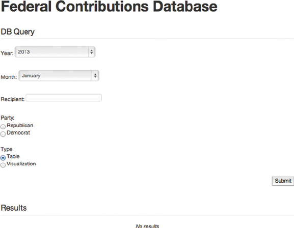
SCRAPING THE WEB 253
Figure 9.2 The Federal Contributions database
comes from, usually a request to a PHP le is employed to fetch information from an
underlying MySQL database using the parameter value pairs transmitted in the URL to
construct the query to the database. This complicates extraction matters, since working
directly with the database is usually not possible because we do not have the required
access information and are thus restricted to working with the retrieved output from
the PHP le.
9.1.9.2 Selenium and the Rwebdriver package
Selenium/Webdriver is an open-source suite of software with the primary purpose of providing
a coherent, cross-platform framework for testing applications that run natively in the browser.
In the development of web applications, testing is a necessary step to establish expected func-
tionality of the application, minimize potential security and accessibility issues, and guarantee
reliability under increased user trafc. Before the creation of Selenium this kind of testing
had been carried out manually—a tedious and error-prone undertaking. Selenium solves this
problem by providing drivers to control browser behavior such as clicks, scrolls, swipes,
and text inputs. This enables programmatic approaches to the problem by using a scripting
language to characterize sequences of user behaviors and report if the application fails.
Selenium’s capability to drive interactions with the webpage through the browser is of Installing the
Rwebdriver
package
more general use besides testing purposes. Since it allows to remote-control the browser, we
can work with and request information directly from the live DOM tree, that is, how the visual
display is presented in the browser window. Accessing Selenium functionality from within R
is possible via the Rwebdriver package. It is available from a GitHub repository and can be
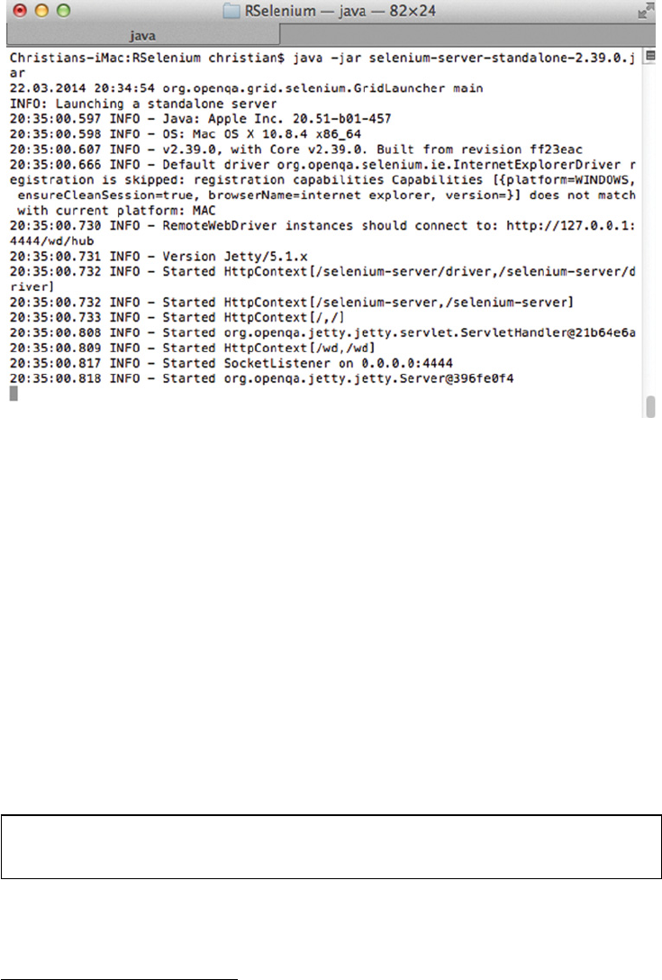
254 AUTOMATED DATA COLLECTION WITH R
Figure 9.3 Initializing the Selenium Java Server
installed with the install_github() function from the devtools package (Wickham and
Chang 2013).
R> library(devtools)
R> install_github(repo = "Rwebdriver", username = "crubba")
Getting started with Selenium Webdriver Using Selenium requires initiating the Sele-
nium Java Server. The server is responsible for launching and killing browsers as well as
receiving and interpreting the browser commands. The communication with the server from
inside the programming environment works via simple HTTP messages. To get the server up
and running, the Selenium server le needs to be downloaded from http://docs.seleniumhq.
org/download/ to the local le system. The server le follows the naming convention
(selenium-server-standalone-<version-number>.jar).5In order to initiate the server, open
the system prompt, change the directory to the jar-le location, and execute the le.
1cd Rwebdriver/
2java -jar selenium-server-standalone-2.39.0.jar
The console output should resemble the one printed in Figure 9.3. The server is now
initiated and waits for commands. The system prompt may be minimized and we can turn
5At the time of writing, the latest server version is 2.39.0.
SCRAPING THE WEB 255
our attention back to the Rconsole. Here, we rst load the Rwebdriver as well as the XML
package.
R> library(Rwebdriver)
R> library(XML)
The rst step is to create a new browser window. This can be accomplished through
the start_session() function which requires passing the address of the Java server—
by default http://localhost:4444/wd/hub/. Additionally, we pass firefox to the browser
argument to instruct the server to produce a Firefox browser window.
R> start_session(root = "http://localhost:4444/wd/hub/", browser =
"firefox")
Once the command is executed, the Selenium API opens a new Firefox window to which
we can now direct browser requests.
Using Selenium for web scraping We now return to the running example and explore some
of Selenium’s capabilities. Note that we are not introducing all functionality of the package
but focus our attention to functions most commonly used in the web scraping process. For a
full list of implemented methods, see Table 9.1.
Let us assume we wish to access the database through its introductory page at Accessing a
webpage
http://www.r-datacollection.com/materials/selenium/intro.html. To direct the browser to a
specic webpage, we can use post.url() with specied url parameter.
R> post.url(url = "http://www.r-datacollection.com/materials/
selenium/intro.html")
The browser should respond and display the intro webpage. When a page forwards the Retrieving the
current URL
browser to another page, it can be helpful to retrieve the current browser URL, since this may
differ from the one that was specied in the query. We can obtain the information through the
get.url() command.
R> get.url()
[1]"http://r-datacollection.com/materials/selenium/intro.html"
The returned output is a standard character vector. To pull the page title of the browser Retrieving the
page title
window, use page_title().
R> page_title()
[1]"The Federal Contributions Database"
To arrive at the form for querying the database, we need to perform a click on the Performing
clicks
enter button at the bottom right. Performing clicks with Selenium requires a two-step pro-
cess. First, we need to create an identier for the button element. Selenium allows spec-
ifying such an identier through multiple ways. Since we already know how to work
with XPath expressions (see Chapter 4), we will employ this method. By using the Web
Developer Tools, we can obtain the following XPath expression for the button element,
/html/body/div/div[2]/form/input. When we pass the XPath expression as a string

256 AUTOMATED DATA COLLECTION WITH R
Table 9.1 Overview of Selenium methods (v.0.1)
Command Arguments Output
start_session() root,browser Creates a new session
quit_session() Closes session
status() Queries the server’s current status
active_sessions() Retrieves information on active
sessions
post.url() url Opens new url
get.url() Receives URL from current
webpage
element_find() by,value Finds elements by method and the
value
element_xpath_find() value Finds elements corresponding to
XPath string value
element_ptext_find() value Finds elements corresponding to
text string value
element_css_find() value Finds elements corresponding to
CSS selector string value
element_click() ID,times,button Clicks on element ID
element_clear() ID Clears input value from element
ID’s text eld
page_back() times One page backward
page_forward() times One page forward
page_refresh() Refreshes current webpage
page_source() Receives HTML source string
page_title() Receives webpage title string
window_handle() Returns handle of the activated
window
window_handles() Returns all window handles in
current session
window_change() handle Changes focus to window with
handle
window_close() handle Closes window with handle
get_window_size() handle Returns vector of current window
size
post_window_size() size,handle Posts a new window size for
window handle
get.window_position() handle Returns x,ycoordinates of window
handle
post_window_position() position,handle Changes coordinates of window
handle
key terms Post keyboard term values

SCRAPING THE WEB 257
to the element_xpath_find() function, we are returned the corresponding element ID
from the live DOM. Let us go ahead and save the ID in a new object called buttonID.
R> buttonID <- element_xpath_find(value = "/html/body/div/div[2]/
form/input")
The second step is to actually perform the left-mouse click on the identied element. For
this task, we make use of element_click(), and pass buttonID as the ID argument.
R> element_click(ID = buttonID)
This causes the browser to change the page to the one displayed in Figure 9.2. Additionally, Window
handles
you might have observed a pop-up window opening upon clicking the button. The occurrence
of pop-ups generates a little complication, since they cause Selenium to switch the focus of
its activate window to the newly opened pop-up. To return focus to the database page, we
need to rst obtain all active window handles using window_handles().
R> allHandles <- window_handles()
To change the focus back on the database window, you can use the window_change()
function and pass the window handle that corresponds to the correct window. In this case, it
is the rst element in allHandles.6
R> window_change(allHandles[1])
Now that we have accessed the database page, we can start to query information from it. Identifying
elements
Let us try to fetch contribution records for Barack Obama from January 2013. To accomplish
this task, we change the value in the Month eld. Again, this requires obtaining the ID for
the Month input eld. From the Web Developer Tools we learn that the following XPath
expression is appropriate: '//*[@id="yearSelect"]'. At the same time, we save the IDs
for the month and the recipient text eld.
R> yearID <- element_xpath_find(value = '//*[@id="yearSelect"]')
R> monthID <- element_xpath_find(value = '//*[@id="monthSelect"]')
R> recipID <- element_xpath_find(value = '//*[@id="recipientSelect"]')
In order to change the year, we perform a mouse click on the year eld by executing
element_click() with the appropriate ID argument.
R> element_click(yearID)
Next, we need to pass the keyboard input that we wish to enter into the database eld. Passing
keyboard input
Since we are interested in records from the year 2013, we use the keys() function with the
rst argument set to the correct term.
R> keys("2013")
6Another option would be to close the window using close_window(). This automatically returns the focus to
the previous window.

258 AUTOMATED DATA COLLECTION WITH R
In a similar fashion, we do the same for the other elds.7
R> element_click(monthID)
R> keys("January")
R> element_click(recipID)
R> keys("Barack Obama")
We can now send the query to the database with a click on the submit button. Again, we
rst identify the button using XPath and pass the corresponding ID element to the clicking
function.
R> submitID <- element_xpath_find(value = '//*[@id="yearForm"]
/div/button')
R> element_click(submitID)
This action should have resulted in a new HTML table being displayed at the bottom ofAccessing
source code the page. To obtain this information, we can extract the underlying HTML code from the live
DOM tree and search the code for a table.
R> pageSource <- page_source()
R> moneyTab <- readHTMLTable(pageSource, which = 1)
With a few last processing steps, we can bring the information into a displayable format.
R> colnames(moneyTab) <- c("year", "name", "party", "contributor",
"state", "amount")
R> moneyTab <- moneyTab[-1, ]
R> head(moneyTab)
year name party contributor state amount
2 2013 Barack Obama D ROBERTS, GARY TX -50
3 2013 Barack Obama D TOENNIES, MICHAEL MR CO -55
4 2013 Barack Obama D PENTA, NEELAM NY -100
5 2013 Barack Obama D VALENSTEIN, JILL NY -15
6 2013 Barack Obama D SPRECHER KEATING, KAREN DC -100
7 2013 Barack Obama D FISCHER, DAMIEN CA -100
Concluding remarks The web scraping process laid out in this section departs markedly
from the techniques and tools we have previously outlined. As we have seen, Selenium
provides a powerful framework and a way for working with dynamically rendered webpages
when simple HTTP-based approaches fail. It helps keep in mind that this exibility comes
with a cost, since the browser itself takes some time to receive the request, process it, and
render the page. This has the potential to slow down the extraction process drastically, and we
therefore advise users to use Selenium only for tasks where other tools are unt. We oftentimes
nd using Selenium most helpful for describing transitions between multiple webpages and
posting clicks and keyboard commands to a browser window, but once we encounter solid
URLs, we switch back to the R-based HTTP methods outlined previously for speed purposes.
7If necessary, we can also remove any input from a text eld with the element_clear() function on the
respective element.

SCRAPING THE WEB 259
Besides the Rwebdriver package there is a package called Relenium which resembles the
package introduced in this chapter (Ramon and de Villa 2013). Although Relenium provides
a more straightforward initiation process of the Selenium server, it has, at the time of writing,
a more limited functionality.
9.1.10 Retrieving data from APIs
We have mentioned APIs in passing when introducing XML, JSON, and other fundamentals.
Generally, APIs encompass tools which enable programmers to connect their software with
“something else.” They are useful in programming software that relies on external soft- or
hardware because the developers do not have to go into the details of external soft- or hardware
mechanics.
When we talk about APIs in this book, we refer to web services or (web) APIs, that is, The rise of web
APIs
interfaces with web applications. We treat the terms “API” and “web service” synonymously,
although the term API encompasses a much larger body of software. The reason why APIs
are of importance for web data collection tasks is that more and more web applications offer
APIs which allow retrieving and processing data. With the rise of Web 2.0, where web APIs
provided the basis for many applications, application providers recognized that data on the
Web are interesting for many web developers. As APIs help make products more popular and
might, in the end, generate more advertising revenues, the availability of APIs has rapidly
increased.
The general logic of retrieving data from web APIs is simple. We illustrate it in Figure 9.4. Basic logic
The API provider sets up a service that grants access to data from the application or to the
application itself. The API user accesses the API to gather data or communicate with the
application. It may be necessary to write wrapper software for convenient data exchange
with the web service. Wrappers are functions that handle details of API access and data
transformation, for example, from JSON to Robjects. The modus operandi of APIs varies—
we shortly discuss the popular standards REST and SOAP further below. APIs provide data
in various formats. JSON has probably become the most popular data exchange format of
API provider
(e.g., Twitter, Yahoo!)
Web application
Web service / Data API
API user
User application
API wrapper software
User software (e.g., R)
Data formats:
JSON, XML,...
Modus operandi:
REST, SOAP,...
Figure 9.4 The mechanics of web APIs

260 AUTOMATED DATA COLLECTION WITH R
modern web APIs, but XML is still frequently used, and any other formats such as HTML,
images, CSVs, and binary data les are possible.
APIs are implemented for developers and thus must be understandable to humans. There-
Documentation
fore, an extensive documentation of features, functions, and parameters is often part of an API.
It gives programmers an overview of the content and form of information an API provides,
and what information it expects, for example, via queries.
Standardization of APIs helps programmers familiarize themselves with the mechanics of
Standards
an API quickly. There are several API standards or styles, the more popular ones being REST
and SOAP. It is important to note that in order to tap web services with R, we often do not
have to have any deeper knowledge of these techniques—either because others have already
programmed a handy interface to these APIs or because our knowledge about HTTP, XML,
and JSON sufces to understand the documentation of an API and to retrieve the information
we are looking for. We therefore consider them just briey.
REST stands for Representational State Transfer (Fielding 2000). The core idea behind
REST
REST is that resources are referenced (e.g., via URLs) and representations of these resources
are exchanged. Representations are actual documents like an HTML, XML, or JSON le. One
might think of a conversation on Twitter as a resource, and this resource could be represented
with JSON code or equally valid representations in other formats. This sounds just like what
the World Wide Web is supposed to be—and in fact one could say that the World Wide Web
itself conforms to the idea of REST. The development of REST is closely linked to the design
of HTTP, as the standard HTTP methods GET,POST,PUT, and DELETE are used for the
transfer of representations. GET is the usual method when the goal is to retrieve data. To
simplify matters, the difference between a GET request of a REST API and a GET request
our browser puts to a server when asking for web content is that (a) parameters are often
well-documented and (b) the response is simply the content, not any layout information.
POST,PUT, and DELETE are methods that are implemented when the user needs to create,
update, and delete content, respectively. This is useful for APIs that are connected to personal
accounts, such as APIs from social media platforms like Facebook or Twitter. Finally, a
RESTful API is an API that conrms to the REST constraints. The constraints include the
existence of a base URL to which query parameters can be added, a certain representation
(JSON, XML,...), and the use of standard HTTP methods.
Another web service standard we sometimes encounter is SOAP, originally an acronym
SOAP
for Simple Object Access Protocol. As the technology is rather difcult to understand and
implement, it is currently being gradually superseded by REST. SOAP-based services are fre-
quently offered in combination with a WSDL (Web Service Description Language) document
that fully describes all the possible methods as well as the data structures that are expected and
returned by the service. WSDL documents themselves are based on XML and can therefore
be interpreted by XML parsers. The resulting advantage of SOAP-based web services is that
users can automatically construct API call functions for their software environment based
on the WSDL, as the API’s functionality is fully described in the document. For more infor-
mation on working with SOAP in R, see Nolan and Temple Lang (2014, Chapter 12). The
authors provide the SSOAP package that helps work with SOAP and R(Temple Lang 2012b)
by transforming the rules documented in a WSDL document into Rfunctions and classes.8
Generating wrapper functions on-the-y has the advantage that programs can easily react to
8At the time of writing, the package is not yet listed on CRAN.

SCRAPING THE WEB 261
API changes. However, as the SOAP technology is becoming increasingly uncommon, we
focus on REST-based services in this section.
Using a RESTful API with Rcan be very simple and not very different from what we Example:
Yahoo Weather
RSS Feed
have learned so far regarding ordinary GET requests. As a toy example we consider Yahoo’s
Weather RSS Feed, which is documented at http://developer.yahoo.com/weather/. It provides
information on current weather conditions at any given place on Earth as well as a ve-day
forecast in the form of an RSS le, that is, an XML-style document (see Section 3.4.3). The
feed basically delivers the data part of what is offered at http://weather.yahoo.com/. We could
use the API to generate our own forecasts or to build an R-based weather gadget. According
to the Terms of Use in the documentation, the feeds are provided free of charge for personal,
non-commercial uses.
Making requests to the feed is pretty straightforward when studying the documentation.
All we have to specify is the location for which we want to get a feedback from the API
(the wparameter) and the preferred degrees unit (Fahrenheit or Celsius; the uparameter).
The location parameter requires a WOEID code, the Where On Earth Identier. It is a 32-
bit identier that is unique for every geographic entity (see http://developer.yahoo.com/geo/
geoplanet/guide/concepts.html). From a manual search on the Yahoo Weather application, we
nd that the WOEID of Hoboken, New Jersey, is 2422673. Calling the feed is simply done
using the HTTP GET syntax. We already know how to do this in R. We specify the API’s
base URL and make a GET request to the feed, providing the wparameter with the WOEID
and the uparameter for degrees in Celsius.
R> feed_url <- "http://weather.yahooapis.com/forecastrss"
R> feed <- getForm(feed_url, .params = list(w = "2422673", u = "c"))
As the retrieved RSS feed is basically just XML content, we can parse it with XML’s
parsing function.
R> parsed_feed <- xmlParse(feed)
The original RSS le is quite spacious, so we only provide the rst and last couple of
lines.
1<?xml version="1.0" encoding="UTF-8" standalone="yes"?>
2<rss xmlns:yweather="http://xml.weather.yahoo.com/ns/rss/1.0"
xmlns:geo="http://www.w3.org/2003/01/geo/wgs84_pos}" version="2.0">
3<channel>
4<title>Yahoo! Weather - Hoboken, NJ</title>
5<link>http://us.rd.yahoo.com/dailynews/rss/weather/Hoboken__NJ/*
http://weather.yahoo.com/forecast/USNJ0221_c.html</link>
6<description>Yahoo! Weather for Hoboken, NJ</description>
7<language>en-us</language>
8<lastBuildDate>Tue, 18 Feb 2014 7:35 am EST</lastBuildDate>
9<ttl>60</ttl>
10 <yweather:location city="Hoboken" region="NJ" country="United
States"/>
11 <yweather:units temperature="C" distance="km" pressure="mb"
speed="km/h"/>
12 <yweather:wind chill="-3" direction="40" speed="11.27"/>

262 AUTOMATED DATA COLLECTION WITH R
13 <yweather:atmosphere humidity="93" visibility="1.21"
pressure="1015.92" rising="2"/>
14 ...
15 <item>
16 ...
17 <yweather:condition text="Cloudy" code="26" temp="0" date="Tue,
18 Feb 2014 7:35 am EST"/>
18 <yweather:forecast day="Tue" date="18 Feb 2014" low="-2"
high="4" text="Rain/Snow" code="5"/>
19 <yweather:forecast day="Wed" date="19 Feb 2014" low="-2"
high="7" text="Showers" code="11"/>
20 <yweather:forecast day="Thu" date="20 Feb 2014" low="3" high="7"
text="Partly Cloudy" code="30"/>
21 <yweather:forecast day="Fri" date="21 Feb 2014" low="1"
high="12" text="Rain/Thunder" code="12"/>
22 <yweather:forecast day="Sat" date="22 Feb 2014" low="-1"
high="9" text="Partly Cloudy" code="30"/>
23 </item>
24 </channel>
25 </rss>
We can process the parsed XML object using standard XPath expressions and convenience
functions from the XML package. As an example, we extract the values of current weather
parameters which are stored in a set of attributes.
R> xpath <- "//yweather:location|//yweather:wind|//yweather:condition"
R> conditions <- unlist(xpathSApply(parsed_feed, xpath, xmlAttrs))
R> data.frame(conditions)
conditions
city Hoboken
region NJ
country United States
chill -3
direction 40
speed 11.27
text Cloudy
code 26
temp 0
date Tue, 18 Feb 2014 7:35 am EST
We also build a small data frame that contains the forecast statistics for the next 5 days.
R> location <- t(xpathSApply(parsed_feed, "//yweather:location", xmlAttrs))
R> forecasts <- t(xpathSApply(parsed_feed, "//yweather:forecast", xmlAttrs))
R> forecast <- merge(location, forecasts)
R> forecast
city region country day date low high text code
1 Hoboken NJ United States Tue 18 Feb 2014 -2 4 Rain/Snow 5
2 Hoboken NJ United States Wed 19 Feb 2014 -2 7 Showers 11
3 Hoboken NJ United States Thu 20 Feb 2014 3 7 Partly Cloudy 30
4 Hoboken NJ United States Fri 21 Feb 2014 1 12 Rain/Thunder 12
5 Hoboken NJ United States Sat 22 Feb 2014 -1 9 Partly Cloudy 30

SCRAPING THE WEB 263
Processing the result from a REST API query is entirely up to us if no Rinterface to a Web service
interfaces for R
web service exists. We could also construct convenient wrapper functions for the API calls.
Packages exist for some web services which offer convenience functions to pass Robjects to
the API and get back Robjects. Such functions are not too difcult to create once you are
familiar with an API’s logic and the data technology that is returned. Let us try to construct
such a wrapper function for the Yahoo Weather Feed example.
There are always many ways to specify wrapper functions for existing web services. We Building a
wrapper
function
want to construct a command that takes a place’s name as main argument and gives back the
current weather conditions or a forecast for the next few days. We have seen above that the
Yahoo Weather Feed needs a WOEID as input. To manually search for the corresponding
WOEID of a place and then feed it to the function seems rather inconvenient, so we want to
automate this part of the work as well. Indeed, there is another API that does this work for us.
At http://developer.yahoo.com/geo/geoplanet/ we nd a set of RESTful APIs subsumed under
the label Yahoo! GeoPlanet which offer a range of services. One of these services returns the
WOEID of a specic place.
http://where.yahooapis.com/v1/places.q(’northeld%20mn%20usa’)?appid=[yourappidhere]
The URL contains the query parameter appid. We have to obtain an app ID to be able
to use this service. Many web services require registration and sometimes even involve a
sophisticated authentication process (see next section). In our case we just have to register for
the Yahoo Developer Network to obtain an ID. We register our application named RWeather
at Yahoo. After providing the information, we get the ID and can add it to our API query.
In order to be able to reuse the ID without having to store it in the code, we save it in the R
options:9
R> options(yahooid = "t.2cnduc0BqpWb7qmlc14vEk8sbL7LijbHoKS.utZ0")
The call to the WOEID API is as follows. We start with the base URL and add the place we
are looking for in the URL’s placeholder between the parentheses. The sprintf() function
is useful because it allows pasting text within another string. We just have to mark the string
placeholder with %s.
R> baseurl <- "http://where.yahooapis.com/v1/places.q('%s')"
R> woeid_url <- sprintf(baseurl, URLencode("Hoboken, NJ, USA"))
Notice also that we have to encode the place name with URL encoding (see Section 5.1.2).
http://where.yahooapis.com/v1/places.q(’Hoboken,%20NJ,%20USA’)
Next we formulate a GET call to the API. We add our Yahoo app ID which we retrieve
from the options. The service returns an XML document which we directly parse into an
object named parsed_woeid.
R> parsed_woeid <- xmlParse((getForm(woeid_url, appid = getOption
("yahooid"))))
9See Section 9.1.6. Needless to say that the printed ID is ctional.

264 AUTOMATED DATA COLLECTION WITH R
The XML document itself looks as follows.
1<?xml version="1.0" encoding="UTF-8"?>
2<places xmlns="http://where.yahooapis.com/v1/schema.rng" xmlns:
yahoo="http://www.yahooapis.com/v1/base.rng" yahoo:start="0"
yahoo:count="1" yahoo:total="1">
3<place yahoo:uri="http://where.yahooapis.com/v1/place/2422673"
xml:lang="en-US">
4<woeid>2422673</woeid>
5<placeTypeName code="7">Town</placeTypeName>
6<name>Hoboken</name>
7<country type="Country" code="US" woeid="23424977">United
States</country>
8<admin1 type="State" code="US-NJ" woeid="2347589">New Jersey
</admin1>
9<admin2 type="County" code="" woeid="12589266">Hudson</admin2>
10 <admin3/>
11 <locality1 type="Town" woeid="2422673">Hoboken</locality1>
12 ...
13 <timezone type="Time Zone" woeid="56043648">America/New_York
</timezone>
14 </place>
15 </places>
There are several WOEIDs stored in the document, one for the country, one for the
state, and one for the town itself. We can extract the town WOEID with an XPath query
on the retrieved XML le. Note that the document comes with namespaces. We access the
<locality1> element where the WOEID is stored with the XPath expression //*[local-
name()='locality1'] which addresses the document’s local names.
R> woeid <- xpathSApply(parsed_woeid, "//*[local-name()='locality1']",
xmlAttrs)[2,]
R> woeid
woeid
"2422673"
Vo i l `
a, we have retrieved the corresponding WOEID. Recall that our goal was to construct
one function which returns the results of a query to Yahoo’s Weather Feed in a useful R
format. We have seen that such a function has to wrap around not only one, but two APIs—
the WOEID returner and the actual Weather Feed. The result of our efforts, a function named
getWeather(), are displayed in Figure 9.5.
The wrapper function splits into ve parts. The rst reports errors if the function’s
The wrapper
function arguments ask—to determine if current weather conditions or a forecast should be reported—
and temp—to set the reported degrees Celsius or Fahrenheit—are wrongly specied. The
second part (get woeid) replicates the call to the WOEID API which we have considered
in detail above. The third part (get weather feed) uses the WOEID and makes a call
to Yahoo’s Weather Feed. The fourth part (get current conditions) is evaluated if the
user asks for the current weather conditions at a given place. We have stored some condition

SCRAPING THE WEB 265
1getWeather <- function(place = "New York", ask = "current", temp = "c") {
2if (!ask %in% c("current","forecast")) {
3stop("Wrong ask parameter. Choose either 'current' or
'forecast'.")
4}
5if (!temp %in% c("c", "f")) {
6stop("Wrong temp parameter. Choose either 'c' for Celsius or
'f' for Fahrenheit.")
7}
8## get woeid
9base_url <- "http://where.yahooapis.com/v1/places.q('%s')"
10 woeid_url <- sprintf(base_url, URLencode(place))
11 parsed_woeid <- xmlParse((getForm(woeid_url, appid = getOption("
yahooid"))))
12 woeid <- xpathSApply(parsed_woeid, "//*[local-name()='locality1']",
xmlAttrs)[2,]
13 ## get weather feed
14 feed_url <- "http://weather.yahooapis.com/forecastrss"
15 parsed_feed <- xmlParse(getForm(feed_url, .params = list(w = woeid,
u = temp)))
16 ## get current conditions
17 if (ask == "current") {
18 xpath <- "//yweather:location|//yweather:condition"
19 conds <- data.frame(t(unlist(xpathSApply(parsed_feed, xpath,
xmlAttrs))))
20 message(sprintf("The weather in %s, %s, %s is %s. Current
temperature is %s degrees %s.", conds$city, conds$region,
conds$country, tolower(conds$text), conds$temp, toupper(temp)))
21 }
22 ## get forecast
23 if (ask == "forecast") {
24 location <-
data.frame(t(xpathSApply(parsed_feed, "//yweather:
location", xmlAttrs)))
25 forecasts <- data.frame(t(xpathSApply(parsed_feed,
"//yweather:forecast", xmlAttrs)))
26 message(sprintf("Weather forecast for %s, %s, %s:",
location$city, location$region, location$country))
27 return(forecasts)
28 }
29 }
Figure 9.5 An Rwrapper function for Yahoo’s Weather Feed
parameters in a data frame conds and input the results into a single sentence—not very useful
if we want to post-process the data, but handy if we just want to know what the weather is like
at the moment.10 If a forecast is requested, the function’s fth part is activated. It constructs
a data frame from the forecasts in the XML document and returns it, along with a short
message.
10Seasoned programmers will appreciate the possibility of getting a weather update without having to leave the
basement, not even the familiar programming environment.
266 AUTOMATED DATA COLLECTION WITH R
Let us try out the function. First, we ask for the current weather conditions in San
Francisco.
R> getWeather(place = "San Francisco", ask = "current", temp = "c")
The weather in San Francisco, CA, United States is cloudy. Current
temperature is 9 degrees C.
This call was successful. Note that Yahoo’s Weather API is tolerant concerning the denition
of the place. If place names are unique, we do not have to specify the state or country. If the
place is not unique (e.g., “Springeld”), the API automatically picks a default option. Next,
we want to retrieve a forecast for the weather in San Francisco.
R> getWeather(place = "San Francisco", ask = "forecast", temp = "c")
Weather forecast for San Francisco, CA, United States:
day date low high text code
1 Tue 18 Feb 2014 10 18 Partly Cloudy 30
2 Wed 19 Feb 2014 13 19 Partly Cloudy 30
3 Thu 20 Feb 2014 12 18 Cloudy 26
4 Fri 21 Feb 2014 11 17 Few Showers 11
5 Sat 22 Feb 2014 10 19 Partly Cloudy 30
We could easily expand the function by adding further parameters or returning more useful RWhere to nd
APIs on the
Web
objects. This example served to demonstrate how REST-based web services work in general
and how easy it is to tap them from within R. There are many more useful APIs on the Web.
At http://www.programmableweb.com/apis we get an overview of thousands of web APIs.
Currently, there are more than 11,000 web APIs listed as well as over 7,000 mashups, that
is, applications which make use and combine existing content from APIs. We provide some
additional advice on nding useful data sources, including APIs, in Section 9.4.
9.1.11 Authentication with OAuth
Many web services are open to anybody. In some cases, however, APIs require the user to reg-Authentication
and
authorization
ister and provide an individual key when making a request to the web service. Authentication
is used to trace data usage and to restrict access. Related to authentication is authorization.
Authorization means granting an application access to authentication details. For example, if
you use a third-party twitter client on your mobile device, you have authorized the app to use
your authentication details to connect to your Twitter account. We have learned about HTTP
authentication methods in Section 5.2.2. APIs often require more complex authentication via
a standard called OAuth.
OAuth is an important authorization standard serving a specic scenario. Imagine you
have an account on Twitter and regularly use it to inform your friends about what is currently
on your mind and to stay up to date about what is going on in your network. To stay tuned
when you are on the road, you use Twitter on your mobile phone. As you are not satised
with the standard functions the ofcial Twitter application offers, you rely on a third-party
client app (e.g., Tweetbot), an application that has been programmed by another company and
that offers additional functionality. In order to let the app display the tweets of people you
follow and give yourself the opportunity to tweet, you have to grant it some of your rights
on Twitter. What you should never want to do is to hand out your access information, that
is, login name and password, to anybody—not even the Twitter client. This is where OAuth

SCRAPING THE WEB 267
comes into play. OAuth differs from other authentication techniques in that it distinguishes
between the following three parties:
rThe service or API provider. The provider implements OAuth for his service and is
responsible for the website/server which the other parties access.
rThe data owners. They own the data and control which consumer (see next party) is
granted access to the data, and to what extent.
rThe data consumer or client. This is the application which wants to make use of the
owner’s data.
When we are working with R, we usually take two of the roles. First, we are data owners
when we want to authorize access to data from our own accounts of whatever web service.
Second, we are data consumers because we program a piece of Rsoftware that should be
authorized to access data from the API.
OAuth currently exists in two avors, OAuth 1.0 and OAuth 2.0 (Hammer-Lahav 2010; OAuth versions
Hardt 2012). They differ in terms of complexity, comfort, and security.11 However, there
have been controversies on the question whether OAuth is indeed more secure and useful
than its predecessor.12 As users, we usually do not have to make the choices between the two
standards; hence, we do not go into more into detail here. OAuth’s ofcial website can be
found at http://oauth.net/. More information, including a beginner’s guide and tutorials, are
available at http://hueniverse.com/oauth/.
How does authorization work in the OAuth framework? First of all, OAuth distinguishes The OAuth
workow
between three types of credentials: client credentials (or consumer key and secret), temporary
credentials (or request token and secret), and token credentials (or access token and secret).
Credentials serve as a proof for legitimate access to the data owner’s information at various
stages of the authorization process. Client credentials are used to register the application
with the provider. Client credentials authenticate the client. When we use Rto tap APIs,
we usually have to start with registering an application at the provider’s homepage which
we could call “My R-based program” or similar. In the process of registration, we retrieve
client credentials, that is, a consumer key and secret that is linked with our (and only our)
application. Temporary credentials prove that an application’s request for access tokens is
executed by an authorized client. If we set up our application to access data from a resource
owner (e.g., our own Twitter account), we have to obtain those temporary credentials, that is,
a request token and secret, rst. If the resource owner agrees that the application may access
his/her data (or parts of it), the application’s temporary credentials are authorized. They now
can be exchanged for token credentials, that is, an access token and secret. For future requests
to the API, the application now can use these access credentials and the user does not have
to provide his/her original authentication information, that is, username and password, for
this task.
The fact that several different types of credentials are involved in OAuth authorization OAuth use
with R
practice makes it clear that this is a more complicated process that encompasses several
11See “Introducing OAuth 2.0” by Eran Hammer-Lahav at http://hueniverse.com/2010/05/introducing-oauth-2-
0/.
12See “OAuth 2.0 and the Road to Hell” by Eran Hammer-Lahav at http://hueniverse.com/2012/07/oauth-2-0-
and-the-road-to-hell/.
268 AUTOMATED DATA COLLECTION WITH R
steps. Fortunately, we can rely on Rsoftware that facilitates OAuth registration. The ROAuth
package (Gentry and Lang 2013) provides a set of functions that help specify registration
requests from within R. A simplied OAuth registration interface is provided by the httr
package (Wickham 2012). We illustrate OAuth authentication in Rwith the commands from
the httr package.
oauth_endpoint() is used to dene OAuth endpoints at the provider side. Endpoints
are URLs that can be requested by the application to gain tokens for various steps of the autho-
rization process. These include an endpoint for the request token—the rst, unauthenticated
token—and the access token to exchange the unauthenticated for the authenticated token.
oauth_app() is used to create an application. We usually register an application manually
at the API provider’s website. After registration we obtain a consumer key and secret. We
copy and paste both into R.Theoauth_app() function simple bundles the consumer key and
secret to a list that can be used to request the access credentials. While the consumer key has
to be specied in the function, we can let the function fetch the consumer secret automatically
from the Renvironment by placing it there in the APPNAME_CONSUMER_SECRET option. The
benet of this approach is that we do not have to store the secret in our Rcode.
oauth1.0_token() and oauth2.0_token() are used to exchange the consumer key
and secret (stored in an object created with the oauth_app() function) for the access key
and secret. The function tries to retrieve these credentials from the access endpoint specied
with oauth_endpoint().
Finally, sign_oauth1.0() and sign_oauth2.0() are used to create a signature from
the received access token. This signature can be added to API requests from the registered
application—we do not have to pass our username and password.
We demonstrate by example how OAuth registration is done using Facebook’s Graph API.
Tapping the
Facebook
Graph API
The API grants access to publicly available user information and—if granted by the user—
selected private information. The use of the API requires that we have a Facebook account.
We rst have to register an application which we want to grant access to our prole. We go to
https://developers.facebook.com and sign in using our Facebook authentication information.
Next, we create a new application by clicking on Apps and Create a new app.Wehave
to provide some basic information and pass a check to prove that we are no robot. Now,
our application RDataCollectionApp is registered. We go to the app’s dashboard to retrieve
information on the app, that is, the App ID and the App secret. In OAuth terms, these are
consumer key and consumer secret.
Next,weswitchtoRto obtain the access key. Using httr’s functionality, we start by
dening Facebook’s OAuth endpoints. This works with the oauth_endpoint() function.
R> facebook <- oauth_endpoint(
R> authorize = "https://www.facebook.com/dialog/oauth",
R> access = "https://graph.facebook.com/oauth/access_token")
We bundle the consumer key and secret of our app in one object with the oauth_app()
function. Note that we have previously dumped the consumer secret in the Renvironment with
Sys.setenv(FACEBOOK_CONSUMER_SECRET = "3983746230hg8745389234...") to
keep this condential information out of the Rcode. oauth_app() automatically retrieves
it from the environment and writes it to the new fb_app object.
R> fb_app <- oauth_app("facebook", "485980054864321")

SCRAPING THE WEB 269
Now we have to exchange the consumer credentials with the access credentials. Face-
book’s Graph API uses OAuth 2.0,sowehavetousetheoauth2.0_token() function. How-
ever, before we execute it, we have to do some preparations. First, we add a website URL to our
app account in the browser. We do this in the Settings section by adding a website and specify-
ing a site URL. Usually this should work with the URL http://localhost:1410/ but you can also
call oauth_callback() to retrieve the callback URL the for the OAuth listener, a web server
that listens for the provider’s OAuth feedback.13 Second, we dene the scope of permissions
to apply for. A list of possible permissions can be found at https://developers.facebook.
com/docs/facebook-login/permissions/. We pick some of those and write them into the
permissions object.
R> permissions <- "user_birthday, user_hometown, user_location,
user_status, user_checkins, friends_birthday, friends_hometown,
friends_location, friends_relationships, friends_status, friends_
checkins, publish_actions, read_stream, export_stream"
Now we can ask for the access credentials. Again, we use httr’s oauth2.0_token()
command to perform OAuth 2.0 negotiations.
R> fb_token <- oauth2.0_token(facebook, fb_app, scope = permissions,
type = "application/x-www-form-urlencoded")
starting httpd help server ... done
Waiting for authentication in browser...
Authentication complete.
During the function call we approve the access in the browser. The authentication process
is successful. We use the received access credentials to generate a signature object.
R> fb_sig <- sign_oauth2.0(fb_token)
We are now ready to access the API from within R. Facebook’s web service provides a
large range of functions. Fortunately, there is an Rpackage named Rfacebook that makes the
API easily accessible (Barber´
a 2014). For example, we can access publicly available data
from Facebook users with
R> getUsers("hadleywickham", fb_sig, private_info = FALSE)
id name username first_name last_name ...
1 16910108 Hadley Wickham hadleywickham Hadley Wickham ...
The package also allows us to access information about our personal network.
R> friends <- getFriends(fb_sig, simplify = TRUE)
R> nrow(friends)
[1] 143
R> table(friends_info$gender)
female male
71 72
13This step departs from the simplied OAuth workow from above. Unfortunately, we often face departures
from the norm when working with OAuth and have to adapt the procedure.
270 AUTOMATED DATA COLLECTION WITH R
It provides a lot more useful functions. For a more detailed tutorial, check out http://
pablobarbera.com/blog/archives/3.html.
9.2 Extraction strategies
We have learned several methods to gather data from the Web. There are three standard proce-
dures. Scraping with HTTP and extracting information with regular expressions, information
extraction via XPath queries, and data gathering using APIs. They should usually be preferred
over each other in ascending order (i.e., scraping with regular expressions is least preferable
and gathering data via an API is most preferable), but there will be situations where one of the
approaches is not applicable or some of the techniques have to be combined. It thus makes
sense to become familiar with all of them.
In the following, we offer a general comparison between the different approaches. Each
scraping scenario is different, so some of the advantages or disadvantages of a method may
not apply for your task. Besides, as always, there is more than one way to skin a cat.
If data on a site are not provided for download in ready-made les or via an API, scraping
them off the screen is often the only alternative. With regular expressions and XPath queries we
have introduced two strategies to extract information from HTML or XML code. We continue
discussing both techniques according to some practical criteria which become relevant in the
process of web scraping, like robustness, complexity, exibility, or general power. Note that
these elaborations primarily target static HTML/XML content.
9.2.1 Regular expressions
Figure 9.6 provides a schema of the scraping procedure with regular expressions. In step ①,
we identify information on-site that follows a general pattern. The decision to use regular
expressions to scrape data or another approach depends on our intuition whether the informa-
tion is actually generalizable to a regular expression. In some cases, the data can be described
by means of a regular expression, but the pattern cannot distinguish from other irrelevant
content on the page. For example, if we identify important information wrapped in <b> tags,
this can be difcult to distinguish from other information marked with <b> tags. If data need
to be retained in their context, regular expressions also have a rough ride.
Step ②is to download the websites. Many of the methods described in Section 9.1 might
prove useful here. Additionally, regular expressions can already be of help in this step. They
could be used to assemble a list of URLs to be downloaded, or for URL manipulation (see
Section 9.1.3).
In step ③, the downloaded content is imported into R. When pursuing a purely regex-
based scraping strategy, this is done by simply reading the content as character data with the
readLines() or similar functions. When importing the textual data, we have to be excep-
tionally careful with the encoding scheme used for the original document, as we want to avoid
applying regular expressions to get rid of encoding errors. If you start using str_replace()
in order to get ¨
a, ´
o, or c¸, you are likely to have forgotten specifying the encoding argument in
the readLines() or the parsing function (see Section 8.3). Incidentally, regular expressions
do not make use of an HTML or XML DOM, so we do not need to parse the documents. In
fact, documents parsed with htmlParse() or xmlParse() cannot be accessed with regular
expressions directly. If we use regular expressions in combination with an XPath approach,
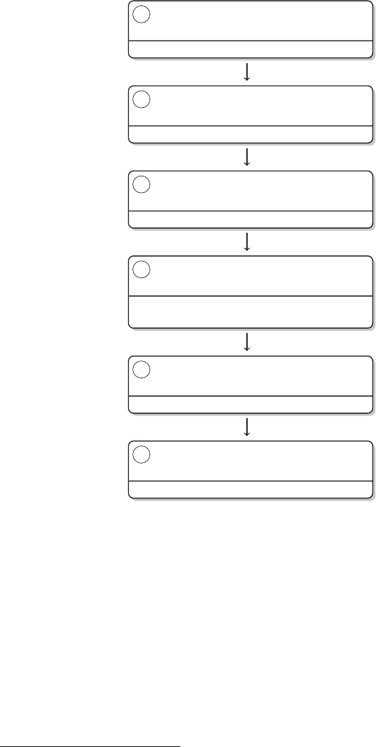
SCRAPING THE WEB 271
1Identify information that
follows a regular pattern
Browser, HTML source code, intuition
2Download documents / websites
RCurl, download.f ile(), regular expressions
3Import documents
readLines(), encoding
4Develop regular expression
General expression → optimal match
special case → optimal match
5Extract information
Regular expressions applied with stringr package
6Debug code
Inspection, validation
Figure 9.6 Scraping with regular expressions
we rst parse the document, extract information with XPath queries and nally modify the
retrieved content with regular expressions.
Step ④is the crucial one for successful web scraping with regular expressions. One has to
develop one or more regular expressions which extract the relevant information. The syntax
of regular expressions as implemented in Roften allows a set of different solutions. The
problem is that these solutions may not differ in the outcome they produce for a certain
sample of text to be regexed, but they can make a difference for new data. This makes
debugging very complex. There are some useful tools which help make regex development
more convenient, for example, http://regex101.com/ or http://www.regexplanet.com/.14 These
14For a more complete overview, see http://scraping.pro/10-best-online-regex-testers/
272 AUTOMATED DATA COLLECTION WITH R
pages offer instant feedback to given regular expressions on sample text input, which makes
the process of regex programming more interactive. In general, we follow one of two strategies
in regular expression programming. The rst is to start with a special case and to work toward
a more general solution that captures every piece. For example, only one bit of information
is matched with a regular expression—this is the information itself, as characters match
themselves. The second strategy is to start with a general expression and introduce restrictions
or exceptions that limit the number of matched strings to the desired sample. One could label
the rst approach the “inductive” and the second one “deductive.” The “deductive” approach
is probably more efcient because it starts at an abstract level—and regular expressions are
often meant to be abstract—, but usually requires more knowledge about regular expressions.
Another feasible strategy which could be located between the two is to start with several
rather different pieces of information to be matched and nd the pick lock that ts for all
of them.
As soon as the regular expression is programmed, extracting the information is the next
step (⑤). As shown in Chapter 8, the stringr package (Wickham 2010) is enormously useful
for this purpose, possibly in combination with apply-like functions (the native Rfunctions or
those provided by the plyr package (Wickham 2011)) for efcient looping over documents.
In the last step ⑥, the code has to be debugged. It is likely that applying regular expressions
on the full sample of strings reveals further problems, like false positives, that is, information
that has been matched should not be matched, or false negatives, that is, some information
to be matched is not matched. It is sometimes necessary to split documents or delete certain
parts before regexing them to exclude a bunch of false positives a priori.
9.2.1.1 Advantages of regular expressions for web scraping
What are the advantages of scraping with regular expressions? In the opinion of many seasoned
web scrapers, there are not too many. Nevertheless, we think that there are circumstances
under which a purely regex-based approach may be superior to any other strategy.
Regular expressions do not operate on context-dening parts of a document. This can be an
Robustness to
malformed
XML
advantage over an XPath strategy when the XML or HTML document is malformed. When
DOM parsers fail, regular expressions, ignorant as they are of DOM structure, continue
to search for information. Moreover, to retrieve information from a heterogeneous set of
documents, regular expressions can deal with them as long as they can be converted to a
plain-text format. Generally, regular expressions are powerful for parsing unstructured text.
String patterns can be the most efcient way to identify and extract content in a document.
Efciency
Imagine a situation where you want to scrape a list of URLs which are scattered across a
document and which share a common string feature like a running index. It is possible to
identify these URLs by searching for anchor tags, but you would have to sort out the URLs
you are looking for in a second step by means of a regular expression.
Regular expression scraping can be faster than XPath-based scraping, especially when
Speed
documents are large and parsing the whole DOM consumes a lot of time. However, the
speed argument cannot be generalized, and the construction of regular expressions or XPath
queries is also an aspect of speed. And after all, there are usually more important arguments
than speed.
Finally, regular expressions are a useful instrument for data-cleansing purposes as they
Power for data
cleansing enable us to get extracted information in the desired shape.
SCRAPING THE WEB 273
9.2.1.2 Disadvantages of regular expressions for web scraping
As soon as information in a document are connected, and should remain so after harvesting, Lack of context
sensitivity
regular expressions are stretched to their limits. Data without context are often rather uninter-
esting. Think back to the introductory example from Chapter 8. It was already a complex task
to extract telephone numbers from an unstructured document, but to match the corresponding
names is often hardly possible if a document does not follow a specic structure. When
scraping information from web pages, sticking to regular expressions as a standard scraping
tool means ignoring the virtue that sites are hierarchically or sometimes even semantically
structured by construction. Markup is structure, and while it is possible to exploit markup
with regular expressions, elements which are anchored in the DOM can usually be extracted
more efciently by means of XPath queries.
Besides, regular expressions are difcult to master. Building regular expressions is a Difcult to
develop and
debug
brain-teaser. It is sometimes very challenging to identify and then formulate the patterns of
information we need to extract. In addition, due to their complexity it is hard to read what is
going on in a regular expression. This makes it hard to debug regex scraping code when one
has not looked at the scraper for a while.
Many scraping tasks cannot be solved with regular expressions because the content to be Lack of
exibility
scraped is simply too heterogeneous. This means that it cannot be abstracted and formulated
as a generalized string pattern. The structure of XML/HTML documents is inherently hierar-
chical. Sometimes this hierarchy implies different levels of observations in your nal dataset.
It can be a very complex task to disentangle these information with regular expressions alone.
If regular expressions make use of nodes that structure the document, the regex strategy soon
becomes very fragile. Incremental changes in the document structure can break. We have
observed that such errors can be xed more easily when working with XPath.
The usefulness of regular expressions depends not least on the kind of information one
is looking for. If content on websites can be abstracted by means of a general string pattern,
regular expressions probably should be used, as they are rather robust toward changes in
the page layout. And even if you prefer to work with XPath, regular expressions are still an
important tool in the process. First, when parsing fails, regular expressions can constitute a
“last line of defense.” Second, when content has been scraped, the desired information is often
not available in atomic pieces but is still raw text. Regular expressions are extraordinarily
useful for data-cleaning tasks, such as string replacements, string deletions, and string splits.
In the third part of the book, we provide an application that relies mainly on regular
expressions to scrape data from web resources. In Chapter 13, we try to convert an unstructured
table—a “format” we sometimes encounter on the Web—into an appropriate Rdata structure.
9.2.2 XPath
Although the specics of scraping with XPath are different from regex scraping, the road
maps are quite similar. We have sketched the path of XPath scraping in Figure 9.7. First, we
identify the relevant information that is stored in an XML/HTML document and is therefore
accessible with XPath queries (step ①). In order to identify the source of information, we can
inspect the source code in our browser and rely on Web Developer Tools.
Step ②is equivalent to the regular expressions scraping approach. We download the
required resources to our local drive. In principle, we could bypass this step and instantly
parse the document “from the webpage.” Either way, the content has to be fetched from the
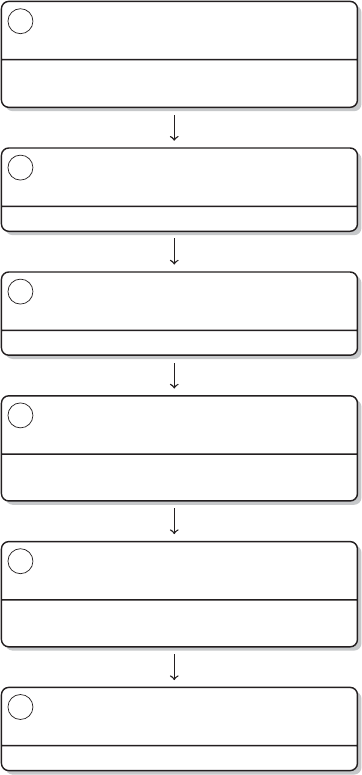
274 AUTOMATED DATA COLLECTION WITH R
1Identify information that is nested
in an XML/HTML document
Browser, XML/HTML source code,
Web Developer Tools
2Download documents / websites
RCurl, download.le(), regular expressions
3Parse document
xmlParse(), htmlParse(), encoding
4Develop XPath query
Backward induction, web developer tools,
SelectorGadget
5Extract information
XPath applied with XML package,
regular expressions
6Debug code
Inspection, validation
Figure 9.7 Scraping with XPath
server, and by rst storing it locally, we can repeat the parsing process without having to
scrape documents multiple times.
In step ③, we parse the downloaded documents using the parsers from the XML package.
We suggest addressing character-encoding issues in this step—the later we resolve potential
encoding problems, the more difcult it gets. We have learned about different techniques
of document subsetting and parsing (e.g., SAX parsing methods)—which method we chose
depends upon the requirements or restrictions of the data resources.
Next, we extract the actual information in step ④by developing one or more XPath
queries. The more often you work with XPath, the more intuitive this step becomes. For a
start, we recommend two basic procedures. The rst is to construct XPath expressions with
SelectorGadget (see Section 4.3.3). It returns an expression that usually works, but is likely
SCRAPING THE WEB 275
not the most efcient way to express what you want. The other strategy is the do-it-yourself
method. We nd it most intuitive to pursue a “backwards induction” approach here. This
means that we start by dening where the actual information is located and develop the
expression from there on, usually up the tree, until the expression uniquely identies the
information we are looking for. One could also label this a bottom-up search procedure—
regardless of how we name it, it helps construct expressions that are slim and potentially
more robust to major changes in the document structure.
Once we have constructed suitable XPath expressions, extracting the information from
the documents (step ⑤) is easy. We apply the expression with adequate functions from the
XML package. The most promising procedure is to use xpathSApply() in combination
with one of the XML extractor functions (see Table 4.4). In practice, steps ④and ⑤are not
distinct. Finding adequate XPath expressions is a continuous trial-and-error process and we
frequently jump between expression construction and information extraction. Additionally,
XML extractor functions often produce not as clear-cut results as we wish them to be, and
bringing the pieces of information into shape takes more than one iteration. Imagine, for
example, that we want to extract reviews from a shopping website. While each of these
reviews could be stored in a leaf in the DOM, we may want to extract more information that
is part of the text, either in a manifest (words, word counts) or latent (sentiments, classes)
manner. We can draw upon regular expressions or more advanced text mining algorithms to
gather information at this level.
In the nal step ⑥, we have to debug and maintain the code. Again, this is not literally
the last step, but part of an iterative process.
9.2.2.1 Advantages of XPath
We have stressed that we prefer XPath over regular expressions for scraping content from Naturally ts
XML/HTML
static HTML/XML. XPath is the ideal counterpart for working with XML-style les, as it
was explicitly designed for that purpose. This makes it the most powerful, exible, easy to
learn and write, and robust instrument to access content in XML/HTML les.
More specically, the fact that XPath was designed for XML documents makes queries Easy to read
and write
intuitive to write and read. This is all the more true when you compare it with regular
expressions, which are dened on the basis of content, not context. As context follows a
clearly dened structure, XPath queries are easier, especially for common cases.
XPath is an expressive language, as it allows the scraping task to be substantially informed Powerful and
exible
about a node of interest using a diverse set of characteristics. We can use a node’s name,
numeric or character features, its relation to other nodes, or content-like attributes. Single
nodes can be uniquely dened. Additionally, working with XPath is efcient because it allows
returning node sets with comparatively minimal code input.
As this strategy mainly relies on structural features of documents, XPath queries are robust Robust toward
changes in
content
to content changes. Certain content is fundamentally heterogeneous, such as press releases,
customer reviews, and Wikipedia entries. As long as the fundamental architecture of a page
remains the same, an XPath scraping strategy remains valid.
9.2.2.2 Disadvantages of XPath
Although XPath is generally superior for scraping tasks compared with regular expressions,
there are situations where XPath scraping fails.
276 AUTOMATED DATA COLLECTION WITH R
When the parser fails, that is, when it does not produce a valid representation of theRestriction to
valid XML
content
document, XPath queries are essentially useless. While our browser may be tolerant toward
broken HTML documents and still interpret them correctly, our RXML parser might not. If
we work on non-XML-style data, XPath expressions are of no help either.
Complementary to the advantages of regular expression scraping for clearly dened
Fragile in
fragile contexts patterns in a fragile environment, using XPath expressions to extract information is difcult
when the context is highly variable, for example when the layout of a webpage is constantly
altered.
9.2.3 Application Programming Interfaces
There is little doubt that gathering data from APIs/web services is the gold standard for web
data collection. Scraping data from HTML websites is often a difcult endeavor. We rst
have to identify in which slots of the HTML tree the relevant data are stored and how to
get rid of everything else that is not needed. APIs provide exactly the information we need,
without any redundant information. They standardize the process of data dissemination, but
also retain control for the provider over who accesses what data. Developers use different pro-
gramming languages and use data for many different purposes. Web services allow providing
standardized formats that most programming languages can deal with.
We illustrate the data collection procedure with APIs and Rin Figure 9.8. In step ①,we
have to nd an API and become familiar with the terms of use or limits and the available
methods. Commercial APIs can be very restrictive or offer no data at all if you do not
pay a monthly fee, so you should nd out early what you get for which payment. And do
not invest time for nothing—not all web services are well-maintained. Before you start to
program wrappers around an existing API, check whether the API is regularly updated. The
API directory at http://www.programmableweb.com/apis also indicates when services are
deprecated or moved to another place.
Steps ②and ③are optional. Some web services require the users to register. Authenti-
cation or authorization methods can be quite different. Sometimes it sufces to register by
email to obtain an individual key that has to be delivered with every request. Other ways
of authentication are based on user/password combinations. Authentication via OAuth as
described in Section 9.1.11 can be even more complex.
In step ④, we formulate a call to the API to request the resources. If we are lucky, we can
draw upon an existing set of Rfunctions that provide an interface to the API. We suggest some
possible repositories which may offer the desired piece of Rsoftware that helps work with
an API in Section 9.4. However, as the number of available web services increases quickly,
chances are that we have to program our own Rwrapper. Wrappers are pieces of software
which wrap around existing software—in our case to be able to use Rfunctions to call an
API and to make the data we retrieve from an API accessible for further work in R.
In step ⑤, we process the incoming data. How we do this depends upon the data format
delivered by the web service. In Chapter 3, we have learned how to use tools from the XML
and jsonlite packages to parse XML and JSON data and eventually convert them to Robjects.
Rpackages which provide ready-made interfaces to web services (see Section 9.4) usually
take care of this step and are therefore exceptionally handy to use.
As always, we should regularly check and debug our code (step ⑥). Be aware of the fact
that API features and guidelines can change over time.
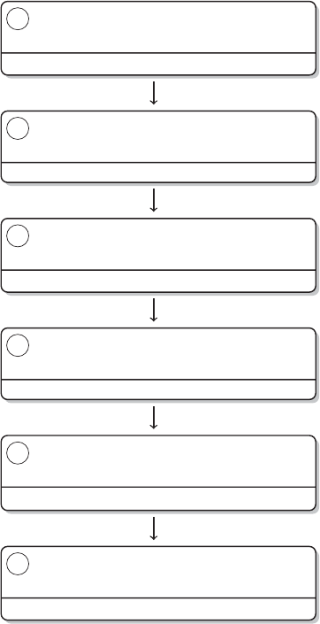
SCRAPING THE WEB 277
1Find API and get familiar with
terms of use / limits / methods
Browser, documentation
2Register application for API use,
retrieve and store keys
Browser
3Authenticate via OAuth
httr package
4Call API (optional: use existing
wrapper or program your own)
R
5Process incoming data
XML / jsonlite package
6Debug code
Inspection, validation
Figure 9.8 Data collection with APIs
9.2.3.1 Advantages of working with APIs
The advantages of web services over the other techniques stem from the fact that tapping ‘Pure’ data
collection
APIs is in fact not web scraping. Many of the disadvantages of screen scraping, malformed
HTML, other robustness to legal issues, do not apply to data collection with web services.
As a result, we can draw upon clean data structures and have higher trust in the collection
outcomes.
Further, by registering an application for an API we make an agreement between provider Standardized
data access
procedures
and user. In terms of stability, chances are higher that databases from maintained APIs are
updated regularly. When scraping data from HTML, we are often less sure about this. Some
APIs provide exclusive access to content which we could not otherwise access. In terms of
transparency, as data access procedures are standardized across many computer languages,
the data collection process of projects based on data from web services can be replicated in
other software environments as well.

278 AUTOMATED DATA COLLECTION WITH R
As the focus of web services is on the delivery of data, not layout, our code is generallyRobustness
more robust. Web services usually satisfy a certain demand and we are often not the only ones
interested in the data. If many people create interfaces to the API from various programming
environments, we can benet from this “wisdom of the crowds” and adding robustness to
our code.
To sum up, APIs provide important advantages which make them—if available—the
source of choice for any project that involves automated online data collection.
9.2.3.2 Disadvantages of working with APIs
The fact that the overwhelming majority of resources on the Web are still not accessed by
web APIs motivates large parts of this book. This is no drawback of web services as a tool
for data collection per se but merely reects the fact that there are more data sources on the
Web people like to work with than data providers who are willing to offer neat access to their
databases.
Although there are not many general disadvantages of using APIs for automated data
Dependency on
API providers collection, relying on web service infrastructure can have its own drawbacks. Data providers
can decide to limit their API’s functionality from one day to the other, as has happened with
popular social media APIs.
From the Rperspective, we have to acknowledge that we work in a software environmentLack of natural
connection to Rthat is not naturally connected to the data formats which plop out of ordinary web services.
However, the advantages of web services often easily outweigh the disadvantages, and
even more so because the potential disadvantages do not necessarily apply to every web
service and some of the drawbacks can partly be attributed to the other approaches as well.
9.3 Web scraping: Good practice
9.3.1 Is web scraping legal?
In the disclaimer of the book (see p. xix), we noted a caveat concerning the unauthorized
use or reproduction of somebody else’s intellectual work. As Dreyer and Stockton (2013)
put it: “Scraping inherently involves copying, and therefore one of the most obvious claims
against scrapers is copyright infringement.” Our advice is to work as transparently as possible
and document the sources of your data at any time. But even if one follows these rules,
where is the line between legal scraping of public content and violations of copyright or other
infringements of the law? Even for lawyers who are devoted to Internet issues the case of
web crawling seems to be a difcult matter. Additionally, as the prevailing law varies across
countries, we are unfortunately not able to give a comprehensive overview of what is legal
in which context. To get an impression of what currently seems to be regarded as illegal, we
offer some anecdotal evidence on past decisions. It should be clear, however, that you should
not rely on any of these cases to justify your doings.
Most of the prominent legal cases involve commercial interests. The usual scenario is
eBay v.
Bidder’s Edge that one company crawls information from another company, processes, and resells it. In the
classical case eBay v. Bidder’s Edge,15 eBay successfully defended itself against the use of
15http://en.wikipedia.org/wiki/EBay_v._Bidder%27s_Edge, https://www.law.upenn.edu/fac/pwagner/law619/
f2001/week11/bidders_edge.pdf

SCRAPING THE WEB 279
bots on their website. Bidder’s Edge (BE), a company that aggregated auction listings, had
used automated programs to crawl information from different auction sites. Users could then
search listings on their webpage instead of posing many requests to each of the auction sites.
According to the verdict,16
BE accessed the eBay site approximate 100,000 times a day. (...) eBay allege[d]
that BE activity constituted up to 1.53% of the number of requests received by
eBay, and up to 1.10% of the total data transferred by eBay during certain periods
in October and November of 1999.
Further,
eBay allege[d] damages due to BE’s activity totaling between $ 45,323 and
$ 61,804 for a ten month period including seven months in 1999 and the rst
three months in 2000.
The defendant did not steal information that was not public to anyone, but harmed the
plaintiff by causing a considerable amount of trafc on its servers. eBay also complained
about the use of deep links, that is, links that directly refer to content that is stored somewhere
“deeply” on the page. By using such links clients are able to circumvent the usual process of
a website visit.
In another case, Associated Press v. Meltwater, scraper’s rights were also curtailed.17 AP v.
Meltwater
Meltwater is a company that offers software which scrapes news information based on
specic keywords. Clients can order summaries on topics which contain excerpts of news
articles. Associated Press (AP) argued that their content was stolen by Meltwater and that
they need to license before distributing it. The judge’s argument in favor of the AP was that
Meltwater is rather a competitor of AP than an ordinary search engine like Google News.
From a more distant perspective, it is hard to see the difference to other news-aggregating
services like Google News (Essaid 2013b; McSherry and Opsahl 2013).
A case which was settled out of court was that of programmer Pete Warden who scraped Facebook v.
Pete Warden
basic information from Facebook users’ proles (Warden 2010). His idea was to use the data
to offer services that help manage communication and networks across services. He described
the process of scraping as “very easy” and in line with the robots.txt (see next section), an
informal web bot guideline Facebook had put on its pages. After he had put a rst visualization
of the data on his blog, Facebook contacted and pushed him to delete the data. According
to Warden, “Their contention was robots.txt had no legal force and they could sue anyone
for accessing their site even if they scrupulously obeyed the instructions it contained. The
only legal way to access any web site with a crawler was to obtain prior written permission”
(Warden 2010).
In the tragic case of Aaron Swartz, the core of contention was scientic work, not United States v.
Aaron Swartz
commercial reuse. Swartz, who co-created RSS (see Section 3.4.3), Markdown, and Infogami
(a predecessor of Reddit), was arrested in 2011 for having illegally downloaded millions of
articles from the article archive JSTOR. The case was dismissed after Swartz’ suicide in
January 2013 (United States District Court District of Massachusetts 2013).
16https://www.law.upenn.edu/fac/pwagner/law619/f2001/week11/bidders_edge.pdf
17https://www.eff.org/sites/default/les/ap_v._meltwater_sdny_copy.pdf

280 AUTOMATED DATA COLLECTION WITH R
In an interesting, thoughtful comment, Essaid (2013a) points out that the jurisdiction on
the issue of web scraping has changed direction several times over the last years, and there
seem to be no clear criteria about what is allowed and what is not, not even in a single judicial
system like the United States. Snell and Care (2013) deliver further anecdotal evidence and
put court decisions in the context of legal theories.
The lesson to be learned from these disconcerting stories is that it is not clear which
actions that can be subsumed under the “web scraping” label are actually illegal and which
are not. In this book we focus on very targeted examples, and republishing content for a
commercial purpose is a much more severe issue than just downloading pages and using
them for research or analysis. Most of the litigations we came across involved commercial
intentions. The Facebook v. Warden case has shown, however, that even following informal
rules like those documented in the robots.txt does not guard against prosecution. But after
all, as Frances Irwing from ScraperWiki puts it, “Google and Facebook effectively grew up
scraping,” and if there were signicant restrictions on what data can be scraped then the Web
would look very different today.18
In the next sections, we describe how to identify unofcial web scraping rules and how
to behave in general to minimize the risk of being put in a difcult position.
9.3.2 What is robots.txt?
When you start harvesting websites for your own purposes, you are most likely only a small
sh in the gigantic data ocean. Besides you, web robots (also named “crawlers,” “web spiders,”
or just “bots”) are hunting for content. Not all of these automatic harvesters act malevolently.
Without bots, essential services on the Web would not work. Search engines like Google or
Yahoo use web robots to keep their indices up-to-date. However, maintainers of websites
sometimes want to keep at least some of their content prohibited from being crawled, for
example, to keep their server trafc in check. This is what the robots.txt le is used for. This
“Robots Exclusion Protocol” tells the robots which information on the site may be harvested.
The robots.txt emerged from a discussion on a mailing list and was initiated by Martijn
The robots
exclusion
standard
Koster (1994). The idea was to specify which information may or may not be accessed by web
robots in a text le stored in the root directory of a website (e.g., www.r-datacollection.com/
robots.txt). The fact that robots.txt does not follow an ofcial standard has led to inconsis-
tencies and uncontrolled extensions of the grammar. There is a set of rules, however, that is
followed by most robots.txt on the Web. Rules are listed bot by bot. A set of rules for the
Googlebot robot could look as follows:
1User-agent: Googlebot
2Disallow: /images/
3Disallow: /private/
This tells the Googlebot robot, specied in the User-agent eld, not to crawl content
from the subdirectories /images/ and /private/. Recall from Section 5.2.1 that we can
use the User-Agent eld to be identiable. Well-behaved web bots are supposed to look for
18See Mark Ward’s article on business web scraping efforts at http://www.bbc.co.uk/news/technology-23988890.
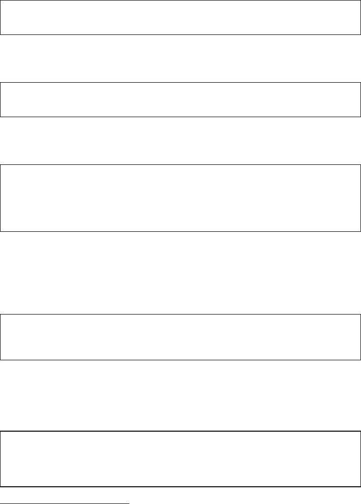
SCRAPING THE WEB 281
their name in the list of User-Agents in the robots.txt and obey the rules. The Disallow eld
can contain partial or full URLs. Rules can be generalized with the asterisk (*).
1User-agent: *
2Disallow: /private/
This means that any robot that is not explicitly recorded is disallowed to crawl the
/private/ subdirectory. A general ban is formulated as
1User-agent: *
2Disallow: /
Thesingleslash/encompasses the entire website. Several records are separated by one
or more empty lines.
1User-agent: Googlebot
2Disallow: /images/
3User-agent: Slurp
4Disallow: /images/
A frequently used extension of this basic set of rules is the use of the Allow eld. As
the name already states, such elds list directories which are explicitly accepted for scraping.
Combinations of Allow and Disallow rules enable webpage maintainers to exclude direc-
tories as a whole from crawling, but allow specic subdirectories or les within this directory
to be crawled.
1User-agent: *
2Disallow: /images/
3Allow: /images/public/
Another extension of the robots.txt standard is the Crawl-delay eld which asks crawlers
to pause between requests for a certain number of seconds. In the following robots.txt,
Googlebot is allowed to scrape everything except one directory, while all other users may
access everything but have to pause for 2 seconds between each request.19
1User-agent: *
2Crawl-delay: 2
3User-Agent: Googlebot
4Disallow: /search/
19The example is taken from the US Congress webpage: http://beta.congress.gov/

282 AUTOMATED DATA COLLECTION WITH R
One problem of using robots.txt is that it can become quite voluminous for large webpagesThe robots
<meta> tag with multiple subdirectories and les. In addition, the way some crawlers work makes them
ignorant to the centralized robots.txt. A disaggregated alternative to robots.txt is the robots
<meta> tag which can be stored in the header of an HTML le.
1<meta name="robots" content="noindex,nofollow" />
A well-behaved robot will refrain from indexing a page that contains this <meta> tag
because of the noindex valueinthecontent attribute and will not try to follow any link on
this page because of the nofollow value in the content attribute.
This book is not about web crawling, but focuses on retrieving content from specic sites
An Rparser for
robots.txt with a specic purpose. But what if we still have to scrape information from several sites
and do not want to manually inspect every single robots.txt le to program a well-behaved
web scraper? For this purpose, we wrote a program that parses robots.txt by means of regular
expressions and helps identify specic User-agents and corresponding rules of access. The
program is displayed in Figure 9.9.
The robotsCheck() program reads the robots.txt which is specied in the rst argument,
robotstxt. We can specify the bot or User-agent with the second argument, useragent.
Further, the function can return allowed and disallowed directories or les. This is specied
with the dirs parameter. We do not discuss this program in greater detail here, but it can
easily be extended so that a robot stops scraping pages that are stored in one of the disallowed
directories.
We test the program on the robots.txt le of Facebook. First, we specify the link to the le.
R> facebook_robotstxt <- "http://www.facebook.com/robots.txt"
Next, we retrieve the list of directories that is prohibited from being crawled by any bot
which is not otherwise listed. If we create our own bot, this is most likely the set of rules we
have to obey.
R> robotsCheck(robotstxt = facebook_robotstxt, useragent = "*",
dirs = "disallowed")
This bot is blocked from the site.
Facebook generally prohibits crawling from its pages. Just to see how the program works,
we make another call for a bot named “Yeti.”
R> robotsCheck(robotstxt = facebook_robotstxt, useragent = "Yeti",
dirs = "disallowed")
[1] "/ajax/" "/album.php" "/autologin.php"
[4] "/checkpoint/" "/contact_importer/" "/feeds/"
[7] "/file_download.php" "/l.php" "/p.php"
[10] "/photo.php" "/photo_comments.php" "/photo_search.php"
[13] "/photos.php" "/sharer/"
Facebook disallows the “Yeti” bot to access a set of directories. It is important to say that
robots.txt has little to do with a rewall against robots or any other protection mechanism. It
does not prevent a website from being crawled at all. Rather, it is an advice from the website
maintainer.

SCRAPING THE WEB 283
1robotsCheck <- function(robotstxt = "", useragent = "*", dirs =
"disallowed") {
2# packages
3require(stringr)
4require(RCurl)
5# read robots.txt
6bots <- getURL(robotstxt, cainfo = system.file("CurlSSL", "cacert.pem",
package = "RCurl"))
7write(bots, file = "robots.txt")
8bots <- readLines("robots.txt")
9# detect if defined bot is on the list
10 useragent <- ifelse(useragent == "*", "\\*", useragent)
11 bot_line1 <- which(str_detect(bots, str_c("[Uu]ser-
[Aa]gent:[ ]{0,}", useragent, "$"))) + 1
12 bot_listed <- ifelse(length(bot_line1)>0, TRUE, FALSE)
13 # identify all user-agents and user-agent after defined bot
14 ua_detect <- which(str_detect(bots, "[Uu]ser-[Aa]gent:[ ].+"))
15 uanext_line <- ua_detect[which(ua_detect == (bot_line1 - 1)) + 1]
16 # if bot is on the list, identify rules
17 bot_d_dir <- NULL
18 bot_a_dir <- NULL
19 bot_excluded <- 0
20 if (bot_listed) {
21 bot_eline <- which(str_detect(bots, "ˆ$"))
22 bot_eline_end <- length(which(bot_eline - uanext_line < 0))
23 bot_eline_end <- ifelse(bot_eline_end == 0, length(bots), bot_eline
[bot_eline_end])
24 botrules <- bots[bot_line1:bot_eline_end]
25 # extract forbidden directories
26 botrules_d <- botrules[str_detect(botrules, "[Dd]isallow")]
27 bot_d_dir <- unlist(str_extract_all(botrules_d, "/.{0,}"))
28 # extract allowed directories
29 botrules_a <- botrules[str_detect(botrules, "ˆ[Aa]llow")]
30 bot_a_dir <- unlist(str_extract_all(botrules_a, "/.{0,}"))
31 # bot totally excluded?
32 bot_excluded <- str_detect(bot_d_dir, "ˆ/$")
33 }
34 # return results
35 if (bot_excluded[1]) { message("This bot is blocked from the site.")}
36 if (dirs == "disallowed" & !bot_excluded[1]) { return(bot_d_dir) }
37 if (dirs == "allowed" & !bot_excluded[1]) { return(bot_a_dir) }
38 }
Figure 9.9 Rcode for parsing robots.txt les
To the best of our knowledge, there is no law which explicitly states that robots.txt contents
must not be disregarded. However, we strongly recommend that you have an eye on it every
time you work with a new website, stay identiable and in case of doubt contact the owner
in advance.
If you want to learn more about web robots and how robots.txt works, the page
http://www.robotstxt.org/ is a good start. It provides a more detailed explanation of the
syntax and a useful collection of Frequently Asked Questions.
284 AUTOMATED DATA COLLECTION WITH R
9.3.3 Be friendly!
Not everything that can be scraped should be scraped, and there are more and less polite
ways of doing it. The programs you write should behave nicely, provide you with the data
you need, and be efcient—in this order. We suggest that if you want to gather data from
a website or service, especially when the amount of data is considerable, try to stick to our
etiquette manual for web scraping. It is shown in Figure 9.10.
As soon as you have identied potentially useful data on the Web, you should look for an
“ofcial” way to gather the data. If you are lucky, the publisher provides ready-made les of
the data which are free to download or offers an API. If an API is available, there is usually
no reason to follow any of the other scraping strategies. APIs enable the provider to keep
control over who retrieves which data, how much of it, and how often.
As described in Section 9.2.2, accessing an API from within Rusually requires one orFriendly
cooperation
with APIs
more wrapper functions which pose requests to the API and process the output. If such
wrappers already exist, all you have to do is to become familiar with the program and use it.
Often, this requires the registration of an application (see Section 9.1.11). Be sure to document
the purpose of your program. Many APIs restrict the user to a certain amount of API calls
per day or similar limits. These limits should generally be obeyed.
If there is no API, there might still be a more comfortable way of getting the data than
Get into contact
with the data
providers
scraping them. Depending on the type and structure of the data, it can be reasonable to assume
that there is a database behind it. Virtually any data that you can access via HTTP forms is
likely to be stored in some sort of database or at least in a prestructured XML. Why not ask
proprietors of data rst whether they might grant you access to the database or les? The
larger the amount of data you are interested in, the more valuable it is for both providers and
you to communicate your interests in advance. If you just want to download a few tables,
however, bothering the website maintainer might be a little over the top.
Once you have decided that scraping the data directly from the page is the only feasible
Obey robots.txt
and terms of
use
solution, you should consider the Robots Exclusion Protocol if there is any. The robots.txt is
usually not meant to block individual requests to a site, but to prevent a webpage to be indexed
by a search engine or other meta search applications. If you want to gather information from a
page that documents disallowance of web robot activity in its robots.txt, you should reconsider
your task. Do you plan to scrape data in a bot-like manner? Has your task the potential to do
the web server any harm? In case of doubt, get into contact with the page administrator or
take a look at the terms of use, if there are any. Ensure that your plans are with no ill intent,
and stay identiable with an adequate use of the identifying HTTP header elds.
If what you are planning is neither illegal nor has the potential to harm the provider in
Scraping dos
and don’ts any way, there are still some scraping dos and don’ts you should consider with care.
As an example, we construct a small scraping program step-by-step, implementing all
techniques from the bouquet of friendly web scraping. Say we want to keep track of the 250
most popular movies as rated by users of the Internet Movie Database (IMDb). The ranking
is published at http://www.imdb.com/chart/top. Although the techniques implemented in this
example are a bit over the top as we do not actually scrape large amounts of data, the procedure
is the same for more voluminous tasks.
Suppose we have already worked through the checklist of questions of Figure 9.10 (as of
March 2014, there is no IMDb API) and have decided that there is no alternative to scraping
the content to work with the data. An inspection of IMDb’s robots.txt reveals that robots are
ofcially allowed to work in the /chart subdirectory.
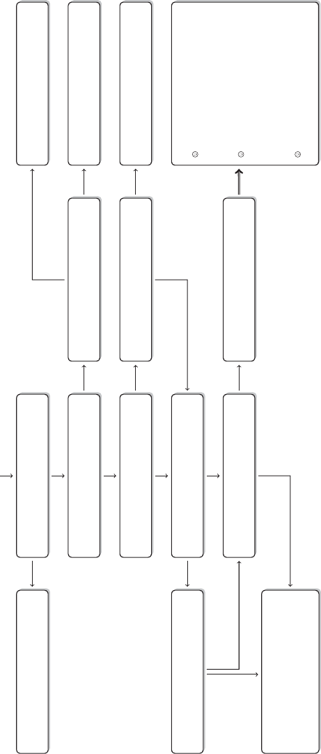
World Wide Web
Did you identify useful data on the
Web?
Is there an API that offers an
interface to a relevant database?
Do you assume a database to exist
behind the data?
Is there a robots.txt?
Are there terms of use which explicitly
deny the use of the webpage you have
in mind?
Is there an R package or project that
provides a wrapper?
Is there someone who grants you
access to the database?
Start scraping and consider all of the
aspects on the right
Check out how it works and use it
Get familiar with API output and
build your own wrapper
Retrieve the data from your personal
contact and save a lot of time
Scraping dos and don’ts
Stay identifiable with User-agent
and From header fields, i.e., do
not masquerade behind proxies or
browser-like user-agents
Reduce trfac: scrape as few
as possible, use gzip if avail-
able, choose lightweight formats,
monitor changes before scraping
(Last-Modified header field)
Do not bombard the server with un-
necessary requests
Try harder...
Does robots.txt permit bot action on
files you are interested in?
Reconsider your task. Speak to the
owner of the data if possible. If you
nevertheless start scraping, take into
account the “Scraping dos and don’ts”
on the right.
yes
no
no
no
no
yes
no
yes
yes
yes
no
yes
no
yes
yes
no
Figure 9.10 An etiquette manual for web scraping
286 AUTOMATED DATA COLLECTION WITH R
The standard scraping approach using the RCurl package would be something like
R> library(RCurl)
R> library(XML)
R> url <- "http://www.imdb.com/chart/top"
R> top <- getURL(url)
R> parsed_top <- htmlParse(top, encoding = "UTF-8")
R> top_table <- readHTMLTable(parsed_top)[[1]]
R> head(top_table[1:10, 1:3])
Rank & Title IMDb Rating
1 1. The Shawshank Redemption (1994) 9.2
2 2. The Godfather (1972) 9.2
3 3. The Godfather: Part II (1974) 9.0
4 4. The Dark Knight (2008) 8.9
5 5. Pulp Fiction (1994) 8.9
6 6. The Good, the Bad and the Ugly (1966) 8.9
7 7. Schindler’s List (1993) 8.9
8 8. 12 Angry Men (1957) 8.9
9 9. The Lord of the Rings: The Return of the King (2003) 8.9
10 10. Fight Club (1999) 8.8
The rst rule is to stay identiable. We have learned in Chapter 5 how this can be done.
When sending requests via HTTP, we can use the User-agent and From header elds.
Therefore, we respecify the GET request as
R> getURL(url, useragent = str_c(R.version$platform, R.version$version.
string, sep = ", "), httpheader = c(from = "eddie@datacollection.com"))
The second rule is to reduce trafc. To do so, we should accept compressed les. One can
specify which content codings to accept via the Accept-Encoding header eld. If we leave
this eld unspecied, the server delivers les in its preferred format. Therefore, we do not
have to specify the preferred compression style, which would probably be gzip, manually.
The XML parser which is used in the XML package can deal with gzipped XML documents.
We do not have to respecify the parsing command—the xmlParse() function automatically
detects compression and uncompresses the le rst.
Another trick to reduce trafc is applicable if we scrape the same resources multiple
times. What we can do is to check whether the resource has changed before accessing and
retrieving it. There are several ways to do so. First, we can monitor the Last-Modified
response header eld and make a conditional GET request, that is, access the resources
only if the le has been modied since the last access. We can make the call conditional
by delivering an If-Modified-Since or, depending on the mechanics of the function,
If-Unmodified-Since request header eld. In the IMDb example, this works as fol-
lows. First, we dene a curl handle with the debugGatherer() function to be able to
track our HTTP communication. Because we want to modify the HTTP header along the
way, we store the standard headers for identifying ourselves in an extra object to use and
redene it.
R> info <- debugGatherer()
R> httpheader <- list(from = "Eddie@r-datacollection.com", 'user-
agent' = str_c(R.version$version.string, ", ", R.version$platform))
R> handle <- getCurlHandle(debugfunc = info$update, verbose = TRUE)
SCRAPING THE WEB 287
We dene a new function getBest() that helps extract the best movies from the
IMDb page.
R> getBest <- function(doc) readHTMLTable(doc)[[1]][, 1:3]
Applying the function results in a data frame of the top 250 movies. To be able to analyze
it in a later step, we store it on our local drive in an .Rdata le called bestFilms.Rdata if it
does not exist already.
R> url <- "http://www.imdb.com/chart/top"
R> best_doc <- getURL(url)
R> best_vec <- getBest(best_doc)
R> if (!file.exists("bestFilms.Rdata")) {
save(best_vec, file = "bestFilms.Rdata")
}
R> head(best_vec)
Rank & Title IMDb Rating
1 1. The Shawshank Redemption (1994) 9,2
2 2. The Godfather (1972) 9,2
3 3. The Godfather: Part II (1974) 9,0
4 4. The Dark Knight (2008) 8,9
5 5. Pulp Fiction (1994) 8,9
6 6. The Good, the Bad and the Ugly (1966) 8,9
Now we want to update the le once in a while if and only if the IMDb page has been
changed since the last time we updated the le. We do that by using the If-Modified-Since
header eld in the HTTP request.
R> httpheader$"If-Modified-Since" <- "Tue, 04 Mar 2014 10:00:00 GMT"
R> best_doc <- getURL(url, curl = handle, httpheader = httpheader)
It becomes a little bit more complicated if we want to use the time stamp of our .Rdata
le’s last update. For this we have to extract the date and supply it in the right format to the
If-Modified-Since header eld. As the extraction and transformation of the date into the
format expected in HTTP request is cumbersome, we solve the problem once and put it into
two functions: httpDate() and file.date()—see Figure 9.11. You can download the
function from the book’s webpage with
R> writeLines(str_replace_all(getURL("http://www.r-datacollection.
com/materials/http/HTTPdate.r"),"\r",""),"httpdate.r")
Let us source the functions into our session and extract the date of last modication for
our best lms data le with a call to file.date().
R> source("http://www.r-datacollection.com/materials/http/HTTPdate.r")
R> (last_mod <- file.date("bestFilms.Rdata"))
[1] "2014-03-11 15:00:31 CET"

288 AUTOMATED DATA COLLECTION WITH R
1httpDate <- function(time="now", origin="1970-01-01", type="rfc1123"){
2if(time=="now") {
3tmp <- as.POSIXlt(Sys.time(), tz="GMT")
4}else{
5tmp <- as.POSIXlt(as.POSIXct(time, origin=origin), tz="GMT")
6}
7nday <- c("Sun", "Mon" , "Tue" ,
8"Wed", "Thu" , "Fri" ,
9"Sat")[tmp$wday+1]
10 month <- tmp$mon+1
11 nmonth <- c("Jan" , "Feb" , "Mar" ,
12 "Apr", "May" , "Jun" ,
13 "Jul" , "Aug", "Sep" ,
14 "Oct" , "Nov" , "Dec")[month]
15 mday <- formatC(tmp$mday, width=2, flag="0")
16 hour <- formatC(tmp$hour, width=2, flag="0")
17 min <- formatC(tmp$min , width=2, flag="0")
18 sec <- formatC(round(tmp$sec) , width=2, flag="0")
19 if(type=="rfc1123"){
20 return(paste0(nday, ", ",
21 mday," ", nmonth, " ", tmp$year+1900, " ",
22 hour, ":", min, ":", sec, " GMT") )
23 }else{
24 stop("Not implemented")
25 }
26 }
28 file.date <- function(filename, timezone=Sys.timezone() ) {
29 as.POSIXlt( min(unlist( file.info(filename)[4:6] )),
30 origin = "1970-01-01",
31 tz = timezone)
32 }
34 # usage:
35 # httpDate()
36 # httpDate( file.date("WorstFilms.Rdata") )
37 # httpDate("2001-01-02")
38 # httpDate("2001-01-02 18:00")
39 # httpDate("2001-01-02 18:00:01")
40 # httpDate(60*60*24*30.43827161*12*54+60*60*24*32)
41 # httpDate(-10*24*60*60,origin="2014-02-01")
Figure 9.11 Helper functions for handling HTTP If-Modied-Since header eld
Now we can pass the date to the If-Modified-Since header eld by making use of
httpDate().
R> httpheader$"If-Modified-Since" <- httpDate(last_mod)
R> best_doc <- getURL(url, curl = handle, httpheader = httpheader)
Via getCurlInfo() we can gather information on the last request and control the
status code.
R> getCurlInfo(handle)$response.code
[1] 200
SCRAPING THE WEB 289
If the status code of the response equals 200, we extract new information and update our data
le. If the server responds with the status code 304 for “not modied” we leave it as is.
R> if (getCurlInfo(handle)$response.code == 200) {
best_list <- getBest(best_doc)
save(best_list, file = "bestFilms.Rdata")
}
Using the If-Modified-Since header is not without problems. First, it is not clear what
the Last-Modified response header eld actually means. We would expect the server to
store the time the le was changed the last time. If the le contains dynamic content, however,
the header eld could also indicate the last modication of one of its component parts. In
fact, in the example the IMDb website is always delivered with a current time stamp, so the
le will always be downloaded—even if the ranking has not changed. We should therefore
rst monitor the updating frequency of the Last-Modified header eld before adapting our
scraper to it. Another problem can be that the server does not deliver a Last-Modified at
all, even though HTTP/1.1 servers should provide it (see Fielding et al. 1999, Chapters 14.25,
14.28, and 14.29).
Another strategy is to retrieve only parts of a le. We can do this by specifying the
libcurl option range which allows dening a byte range. If we know, for example, that
the information we need is always stored at the very beginning of a le, like a title, we
could truncate the document and specify our request function with range = "1-100" to
only receive the rst 100 bytes of the document. The drawbacks of this approach are that
not all servers support this feature and we cut a document in two, making it not inaccessible
with XPath.
In another scenario, we might want to download specic les from an index of les, but
only those which we have not been downloaded so far. We implement a check if the le
already exists on the local drive and start the download only if we have not already retrieved
it. The following generic code snippet shows how to do this. Say we have generated a vector
of HTML le names which are stored on a page like www.example.com with filenames
<- c("page1.html", "page2.html", page3.html). We can initiate a download of
the les that have not yet been downloaded with:
R> for (i in 1:length(filenames)) {
if (!file.exists(filenames[i])) {
download.file(str_c(url, filenames[i]), destfile = filenames[i])
}
}
The file.exists() function checks if the le already exists. If not, we download it.
To know in advance how many les are new, we can compare the two sets of le names—the
ones to be downloaded and the ones that are already stored in our folder—like this
R> existing_files <- list.files("directory_of_scraped_files")
R> online_files <- vector_of_online_files
R> new.files <- setdiff(online_files, existing_files)
The list.files() function lists the names of les stored in a given directory. The
setdiff() function compares the content of two vectors and returns the asymmetric differ-
ence, that is, elements that are part of the rst vector but not of the second. Note that these
code snippets works properly only if we download websites that carry a unique identier in

290 AUTOMATED DATA COLLECTION WITH R
the URL that remains constant over time, for example, a date, and if it is reasonable to assume
that the content of these pages has not changed, while the set of pages has.
We also do not want to bother the server with multiple requests. This is partly because many
requests per second can bring smaller servers to their knees, and partly because webmasters
are sensitive to crawlers and might block us if our scraper behaves this way. With Rit is
straightforward to restrict our scraper. We simply suspend execution of the request for a
time. In the following, a scraping function is programmed to process a stack of URLs and
is executed only after a pause of one second, which is specied with the Sys.sleep()
function.
R> for (i in 1:length(urls)) {
scrape_function(urls[1])
Sys.sleep(1)
}
There is no ofcial rule how often a polite scraper should access a page. As a rule of
thumb we try to make no more than one or two requests per second if Crawl-delay in the
robots.txt does not dictate more modest request behavior.
Finally, writing a modest scraper is not only a question of efciency but also of politeness.
There is often no reason to scrape pages daily or repeat the same task over and over again.
Although bandwidth costs have sunken over the years, server trafc still means real costs
to website maintainers. Our last piece of advice for creating well-behaved web scrapers is
therefore to make scrapers as efcient as possible. Practically, this means that if you have
a choice between several formats, choose the lightweight one. If you have to scrape from
an HTML page, it could prove useful to look for a “print version” or a “text only” version,
which is often much lighter HTML than the fully designed page. This helps both you to extract
content and the server who provides the resources. More generally, do not “overscrape” pages.
Carefully select the resources you want to exploit, and leave the rest untouched. In addition,
monitor your scraper regularly if you use it often. Webpage design can change quickly,
rendering your scraping approach useless. A broken scraper may still consume bandwidth
without any payoff.20
One nal remark. We do not think that there is a reason to feel generally bad for scraping
content from the Web. In all of the cases we present in this book this has nothing to do
with stealing any private property or cheap copying of content. Ideally, processing scraped
information comes with real added value.
9.4 Valuable sources of inspiration
Before starting to set up a scraping project, it is worthwhile to do some research on things
others have done. This might help with specic problems, but the Internet is also full of
more general inspirations for scraping applications and creative work with freely available
data. In the following, we would like to point you to some resources and projects we nd
extraordinarily useful or inspiring.
20Much of this advice is inspired by the excellent “Walking Softly” introduction to web scraping with Perl by
Hemenway and Calishain (2003).
SCRAPING THE WEB 291
The CRAN Task View on web technologies (http://cran.r-project.org/web/views/ CRAN Task
View
WebTechnologies.html) provides a very useful overview of what is possible with Rin terms
of accessing and parsing data from the Web. You will see that not all of the available packages
are covered in this book, which is partly due to the fact that the community is currently very
active in this eld, and partly because we intentionally tried to focus on the most useful pieces
of software. It might be a good exercise to set up an automated scraper that checks for updates
of this site from time to time.
GitHub is a hosting service for software projects or rather, users who publish their ongoing GitHub
coding work (https://github.com/). It is not restricted to any programming language, so
one can nd many users who publish Rcode. Hadley Wickham and Winston Chang have
provided the handy CRAN package devtools (Wickham and Chang 2013) which makes
it easy to install Rsoftware that is not published on CRAN but on GitHub using the
install_github() function.
rOpenSci (http://ropensci.org/) is a fascinating project that aims at establishing convenient rOpenSci
connections between Rand existing science or science-related APIs. Their motto is nothing
less than “Wrapping all science APIs.” This implies a philosophy of “meta-sharing”: The con-
tributors to this project share and maintain software that helps accessing open science data. As
we have shown in Section 9.1.10, maintenance of API access is indeed an important topic. The
project’s website provides Rpackages which serve as interfaces to several data repositories,
full-texts of journals and altmetrics data. Some of the packages are also available on CRAN,
some are stored on GitHub. To pick some examples, the rgbif package provides access to
the Global Biodiversity Information Facility API which covers several thousand datasets on
species and organisms (Chamberlain et al. 2013). The RMendeley package offers access to the
personal Mendeley database (Boettiger and Temple Lang 2012). And with the rfishbase pack-
age it is possible to access the database from www.shbase.org via R(Boettiger et al. 2014).
Further, the site offers a potentially helpful overview of Rpackages that enable access to sci-
ence APIs but that are not afliated with rOpenSci—http://ropensci.org/related/index.html.
It is well worth browsing this list to nd Rwrappers for APIs of popular sites such as Google
Maps, the New York Times, the NHL Real Time Scoring System Database, and many more.
All in all, the rOpenSci team works on an important goal for future scientic practice—the
proliferation and accessibility of open data.
Large parts of what we can do with Rand web scraping would likely not be possible with- Omega Project
out the work of the “Omega Project for Statistical Computing” at http://www.omegahat.org/.
The project’s core group is basically a Who is Who in R’s core development team with
Duncan Temple Lang being its most diligent contributor. With the creation of packages like
RCurl and XML the project laid the foundation to R-Web communication. Today, the project
makes available an impressive list of (not only) R-based software for interaction with web
services and database systems. Not all of them are updated regularly or are of immediate use
for standard web scraping tasks, but a look at the page is indispensable before any attempt
to program a new interface to whatever web service. Chances are that it has been already
done and published on this site. Many of the packages are also extensively discussed in an
impressive new book by Nolan and Temple Lang (2014), which is well worth a read.
Summary
In this chapter, we demonstrated the practical use of the techniques from the book’s rst part—
HTTP, HTML, regular expressions, and others—to retrieve information from webpages. Web
292 AUTOMATED DATA COLLECTION WITH R
scraping is more of a skill than a science. It is difcult to generalize web scraping practice,
as every scenario is different. In the rst part of this chapter, we picked some of the more
common scenarios you might encounter when collecting data from the Web in an automated
manner. If you felt overwhelmed from the vast amount of fundamental web technologies in
the rst part of the book, you might have been surprised how easy it is in many scenarios to
gather data from the Web with Rby relying on powerful network client interfaces like RCurl,
convenient packages for string processing like stringr, and easy-to-implement parsing tools
as provided by the XML package.
Regarding information extraction from web documents we sketched three broad strategies.
Regular expression scraping, XPath scraping, and data collection with interfaces to web APIs.
You will gure out for yourself which strategy serves your needs best in which scenarios
as soon as you become more experienced in web scraping. Our description of the general
procedure to automate data collection with each of the strategies may serve as a guideline.
One intention of our discussion of advantages and disadvantages of each of the strategies
was, however, to clarify that there is no single best web scraping strategy, and it pays of to be
familiar with each of the presented techniques.
We dedicated the last section of this chapter to an important topic, the good practice of
web scraping. Collecting data from websites is nothing inherently evil—successful business
models are based on massive online data collection and processing. However, some formal
and less formal rules we can and should obey exist. We have outlined an etiquette that gives
some rules of behavior when scraping the Web.
Having worked through this chapter you have learned the most important tools to gather
data from the Web with R. We discuss some more tricks of the trade in Chapter 11. If you
deal with text data, information extraction can be a more sophisticated matter. We present
some technical advice on how to handle text in Rand to estimate latent classes in texts in
Chapter 10.
Further reading
Many of the tutorials and how-to guides for web scraping with Rwhich can be found online
are rather case-specic and do not help much to decide which technique to use, how to behave
nicely, and so on. With regard to the foundations of Rtools to tap web resources, the recently
published book by Nolan and Temple Lang (2014) offers great detail, especially regarding
the use of RCurl and other packages which are not published on CRAN but serve specic,
yet potentially important tasks in web scraping. They also provide a more extensive view
on REST, SOAP, and XML-RPC. If you want to learn more about web services that rely on
the REST technology on the theoretical side, have a look at Richardson et al. (2013). Cerami
(2002) offers a more general picture of web services.
During the writing of this book, we found some books on practical web scraping inspiring,
interesting, or simply fun to read, and do not want to withhold them from you. “Webbots,
Spiders, and Screen Scrapers” by Schrenk (2012) is a fun-to-read introduction to scraping
and web bot programming with PHP and Curl. The focus is clearly on the latter, so if you
are interested in web bots and spiders, this book might be a good start. “Spidering Hacks”
by Hemenway and Calishain (2003) is a comprehensive collection of applications and case
studies on various scraping tasks. Their scraping workhorse is Perl, but the described hacks
SCRAPING THE WEB 293
serve as good inspiration for programming R-based scrapers, too. Finally, “Baseball Hacks”
by Adler (2006) is practically a large case study on scraping and data science mostly based
on Perl (for the scraping part) and R(for data analysis). If you nd the baseball scenario
entertaining, Adler’s hands-on book is a good companion on your way into data science.
Problems
1. What are important tools and strategies to build a scraper that behaves nicely on the
Web?
2. What is an good extraction strategy for HTML lists on static HTML pages? Explain
your choice.
3. Imagine you want to collect data on the occurrence of earthquakes on a weekly basis.
Inform yourself about possible online data sources and develop a data collection strategy.
Consider (1) an adequate scraping strategy, (2) a strategy for information extraction (if
needed), and (3) friendly data collection behavior on the Web.
4. Reconsider the CSV le download function in Section 9.1.1. Replicate the download
procedure with the data les for the primaries of the 2010 Gubernatorial Election.
5. Scraping data from Wikipedia, I: The Wikipedia article at http://en.wikipedia.org/wiki/
List_of_cognitive_biases provides several lists of various types of cognitive biases.
Extract the information stored in the table on social biases. Each of the entries in the
table points to another, more detailed article on Wikipedia. Fetch the list of references
from each of these articles and store them in an adequate Robject.
6. Scraping data from Wikipedia, II: Go to http://en.wikipedia.org/wiki/List_of_MPs_
elected_in_the_United_Kingdom_general_election,_1992 and extract the table con-
taining the elected MPs int the United Kingdom general election of 1992. Which party
has most Sirs?
7. Scraping data from Wikipedia, III: Take a look at http://en.wikipedia.org/wiki/List_of_
national_capitals_of_countries_in_Europe_by_area and extract the geographic coordi-
nates of each European country capital. In a second step, visualize the capitals on a
map. The code from the example in chapter 1 might be of help.
8. Write your own robots.txt le providing the following rules: (a) no Google bot is allowed
to scrape your web site, and (b) scraping your /private folder is generally not allowed.
9. Reconsider the R-based robots.txt parser on Figure 9.9. Use it as a start to construct a
program that makes any of your scrapers follow the rules of the robots.txt on any site.
The function has to fulll the following tasks: (a) identication of the robots.txt on any
given host if there is one, (b) check if a specic User-Agent is listed or not, (c) check if
the path to be scraped is disallowed or not, and (d) adhere to the results of (a), (b), and
(c). Consider scraping allowed if the robots.txt is missing.
10. Google Search allows the user to tune her request with a set of parameters. Make use
of these parameters and set up a program that regularly informs you about new search
results for your name.
294 AUTOMATED DATA COLLECTION WITH R
11. Reconsider the Yahoo Weather Feed from Section 9.1.10.
(a) Check out the wrapper function displayed in Figure 9.5 and rebuild it in R.
(b) The API returns a weather code that has not been evaluated so far (see also the
last column in the table on page 238). Read the API’s documentation to gure out
what the code stands for and implement the result in the feedback of the wrapper
function.
12. The CityBikes API at http://api.citybik.es/ provides free access to a global bike sharing
network. Choose a bike sharing service in a city of your choice and build an Rinterface
to it. The interface should enable the user to get information about the list of stations
and the number of available bikes at each of the stations. For a more advanced extension
of this API, implement a feature such that the function automatically returns the station
closest to a given geo-coordinate.
13. The New York Times provides a set of APIs at http://developer.nytimes.com/docs.In
order to use them, you have to sign up for an API key. Construct an Rinterface to their
best-sellers search API which can retrieve the current best-seller list and transform the
incoming JSON data to an Rdata frame.
14. Let us take another look at the Federal Contributions Database.
(a) Find out what happens when the window is not changed back from the pop-up
window. Does the code still work?
(b) Write a script building on the code outlined above that downloads all contributions
to Republication candidates from 2007 to 2011.
(c) Download all contributions from March 2011, but have the data returned in a plot.
Try to extract the amount and party information from the plot.
15. Apply Rwebdriver to other example les introduced in this book:
(a) fortunes2.html
(b) fortunes3.html
(c) rQuotes.php
(d) JavaScript.html

10
Statistical text processing
Any quantitative research project that hopes to make use of statistical analyses needs to
collect structured information. As we have demonstrated in countless examples up to this
point, the Web is an invaluable source of structured data that is ready for analysis upon
collection. Unfortunately, in terms of quantity such structured information is far outweighed
by unstructured content. The Internet is predominantly a vast collection of more or less
unclassied text.
Consequently, the advent of the widespread use of the Internet has seen a contemporaneous
interest in natural language processing—the automated processing of human language. This
is by no means coincidental. Never before have such massive amounts of machine-readable
text been available. In order to access such data, numerous techniques have been devised to
assign systematic meaning to unstructured text. This chapters seeks to elaborate several of
the available techniques to make use of unclassied data.
In a rst step, the next section presents a small running example that is used throughout the
chapter. Subsequently, Section 10.2 elaborates how to perform large-scale text operations in
R. Textual data can quickly become taxing on resources. While this is a more general concern
when dealing with textual data, it is particularly relevant in R, which was not designed to deal
with large-scale text analysis. We will introduce the tm package that allows the organization
and preparation of text and also provides the infrastructure for the analytical packages that
we will use throughout the remainder of the chapter (Feinerer 2008; Feinerer et al. 2008).
In terms of the techniques that are presented in order to make sense of unstructured
text data, we start out by presenting supervised methods in Section 10.3. This broad class
of techniques allows the categorization of text based on similarities to pre-classied text.
Simply put, supervised methods allow users to label texts based on how much they resemble
a hand-coded training set. The classic example in this area deals with the organization of text
into topical categories. Say we have 1000 texts of varied content. Imagine further that half of
the texts have been assigned a label of their topical emphasis. Using supervised methods we
Automated Data Collection with R: A Practical Guide to Web Scraping and Text Mining, First Edition.
Simon Munzert, Christian Rubba, Peter Meißner and Dominic Nyhuis.
© 2015 John Wiley & Sons, Ltd. Published 2015 by John Wiley & Sons, Ltd.

296 AUTOMATED DATA COLLECTION WITH R
can estimate the content of the unlabeled half.1Several supervised methods have been made
available in R. This chapter introduces the RTextTools package which provides a wrapper to a
number of the available packages. This allows a convenient access to several classiers from
within a single function call (Jurka et al. 2013).
A second approach to classifying text is presented in Section 10.4—unsupervised clas-
siers. In contrast to supervised learning algorithms that rely on similarities between pre-
classied and unlabeled text, unsupervised classiers estimate the categories along with the
membership of texts in the different categories. The major advantage of techniques in this
group is the possibility of circumventing the cumbersome hand-coding of training data. This
advantage comes at the price of having to interpret the content of the estimated categories
a posteriori.
As a word of caution we would like to point out that this chapter can only serve as a
cursory introduction to the topics in question. We investigate some of the most important
topics and packages that are available in R. It should be emphasized, however, that in many
instances we cannot do full justice to the details of the topics that are being covered. You
should be aware that if you care to deal with these types of models, there is a lot more out
there that might serve your purposes better than what is being presented in this chapter. We
provide some guidance for further readings in the last section of the chapter.
10.1 The running example: Classifying press releases
of the British government
Before turning to the statistical processing of text, let us collect some sample text data that will
serve as a running example throughout this chapter. For the running example, we want all the
data to be labeled such that we have a benchmark for the accuracy of our classiers. We have
selected press releases from the UK government as our test case. The data can be accessed at
https://www.gov.uk/government/announcements. Opening the website in a browser, you see
several selection options at the left side of the screen. We want to restrict our analysis to press
releases in all topics, from all departments, in all locations that were published before July
2010. At the time of writing this yields 747 results that conform to the request. The results
page presents the title of the press release, the date of publication, an acronym signaling the
publishing department, as well as the type of publication. For the statistical analysis in the
subsequent chapters, we will consider the publishing agency as a marker of the press releases’
content.
Notice how the URL of the page changes when you make the selections.
https://www.gov.uk/government/announcements?keywords=&announcem
ent_type_option=press-releases&topics[]=all&departments[]=all&
world_locations[]=all&from_date=&to_date=01%2F07%2F2010
1We are not technically restricted to statements on the overall topical content of texts. We can use the same
techniques to estimate the content of particular text aspects, say sentences, as long as we are able to provide some
pre-classied training data. The present chapter sticks to topical classication as the most common task in statistical
text analysis. As a side note, learning algorithms are not limited to the analysis of text at all and are used in such
diverse research elds as bio-informatics or speech and, more generally, pattern recognition.
STATISTICAL TEXT PROCESSING 297
You can clearly see how the selections we make become integrated into the URL. As
the data are not too large to be stored locally, we will, in accordance with our rules of good
practice in web scraping, start by downloading all 747 results onto our hard drive before
collecting the text data in a tm corpus in a subsequent step. Check out the source code of the
page. You will nd the rst results toward the end of the page. However, not all 747 results
are contained in the source code. To collect them, we have to use the link that is contained at
the bottom of the press releases. It reads
<a href="/government/announcements?announcement_type_option=press-
releases&departments%5B%5D=all&from_date=&keywords=&
page=2&to_date=01%2F07%2F2010&topics%5B%5D=all&world_
locations%5B%5D=all">Next page <span>2 of 19</span></a>
To assemble the links to all press releases, we collect the publication links in one page, Gathering
press release
hyperlinks
select the link to the next page, and repeat the process until we have all the relevant links.
This is achieved with the following short code snippet. First, we load the necessary scraping
packages.
R> library(RCurl)
R> library(XML)
R> library(stringr)
We move on to download all the results. Notice that because the content is stored on
an HTTPS server, we specify the location of our CA signatures (see Section 9.1.7 for
details).
R> all_links <- character()
R> new_results <- 'government/announcements?keywords=&announcement_
type_option=press-releases&topics[]=all&departments[]=all&world_
locations[]=all&from_date=&to_date=01%2F07%2F2010'
R> signatures = system.file("CurlSSL", cainfo = "cacert.pem",
package = "RCurl")
R> while(length(new_results) > 0){
R> new_results <- str_c("https://www.gov.uk/", new_results)
R> results <- getURL(new_results, cainfo = signatures)
R> results_tree <- htmlParse(results)
R> all_links <- c(all_links, xpathSApply(results_tree,
R> "//li[@id]//a",
R> xmlGetAttr,
R> "href"))
R> new_results <- xpathSApply(results_tree,
R> "//nav[@id='show-more-documents']
R> //li[@class='next']//a",
R> xmlGetAttr,
R> "href")
R> }
We are left with a vector of length 747 but possibly some changes have been made
since this book was published. Each entry contains the link to one press release. To be sure

298 AUTOMATED DATA COLLECTION WITH R
that your results are identical to ours, check the rst item in your vector. It should read
as follows
R> all_links[1]
[1] "/government/news/bianca-jagger-how-to-move-beyond-oil"
R> length(all_links)
[1] 747
To download all press releases, we iterate over our results vector.Download
procedure
R> for(i in 1:length(all_links)){
R> url <- str_c("https://www.gov.uk", all_links[i])
R> tmp <- getURL(url, cainfo = signatures)
R> write(tmp, str_c("Press_Releases/", i, ".html"))
R> }
If everything was proceeded correctly, you should nd the folder Press_Releases in your
working directory which contains all press releases as HTML les.
R> length(list.files("Press_Releases"))
[1] 747
R> list.files("Press_Releases")[1:3]
[1] "1.html" "10.html" "100.html"
10.2 Processing textual data
The widespread application of statistical text analysis is a fairly recent phenomenon. It
coincides with the almost universal storage of text in digital formats. Such massive amounts
of machine-readable text created the need to come up with methods to automate the processing
of content. A number of techniques in the tradition of performing statistical text analysis have
been implemented in R. Concurrently, infrastructures had to be implemented in order to
handle large collections of digital text. The current standard for statistical text analysis in R
is the tm package. It provides facilities to manage text collections and to perform the most
common data preparation operations prior to statistical text analysis.
10.2.1 Large-scale text operations—The tm package
Let us load all press releases that we have collected in the previous section into Rand store
them in a tm corpus.2Ordinarily, this could be accomplished by calling the relevant functions
on the entire directory in which we stored the press releases. In this case, however, the press
releases are still in the HTML format. Thus, before inputting them into a corpus, we want to
strip out all the tags and text that is not specic to the press release.
Let us consider the rst press release as an example. Open the press release in a browser
of your choice. The press release starts with the words “Bianca Jagger, Chair of the Bianca
Jagger Human Rights Foundation and a Council of Europe Goodwill Ambassador, has called
for a “Copernican revolution” in moving beyond carbon to a decentralized, sustainable energy
system.” There is more layout information in the document. In a real research project, one
might want to consider stripping out the additional noise. In addition to the text of the press
2A text corpus in linguistics simply refers to a structured collection of texts.

STATISTICAL TEXT PROCESSING 299
release we nd the publishing organization and the date of publication toward the top of the
page. We extract the rst two bits of information and store them along with the press release as
meta information. Let us investigate the source code of the press release. We nd that the press
release is stored after the tag <div class="block-4">. Thus, we get the release by calling
R> tmp <- readLines("Press_Releases/1.html")
R> tmp <- str_c(tmp, collapse = "")
R> tmp <- htmlParse(tmp)
R> release <- xpathSApply(tmp, "//div[@class='block-4']", xmlValue)
The extracted release is not evenly formatted since we discarded all the tags. However, as Extracting
meta
information
we will drop the sequence of the words later on, this is of no concern. Also, while we might
like to drop several bits of text like (opens in new window), this should not inuence
our estimation procedures.3Before iterating over our entire corpus of results, we write two
queries to extract the meta information. The information on the publishing organization is
stored under <span class="organisation lead", the information on the publishing
date under <dd class="change-notes">.
R> organisation <- xpathSApply(tmp, "//span[@class='organisation
lead']", xmlValue)
R> organisation
[1] "Foreign & Commonwealth Office"
R> publication <- xpathSApply(tmp, "//dd[@class='change-notes']",
xmlValue)
R> publication
[1] "Published 1 July 2010"
Now that we have all the necessary elements set up, we create a loop that performs Creating a
corpus
the operations on all press releases and stores the resulting information in a corpus. Such a
corpus is the central element for text operations in the tm package. It is created by calling the
Corpus() function on the rst press release we just assembled. The text release is wrapped
in a VectorSource() function call. This species that the corpus is created from text which
is stored in a character vector.4
R> library(tm)
R> release_corpus <- Corpus(VectorSource(release))
The corpus can be accessed just like any ordinary list by specifying the name of the Adding meta
information
object (release_corpus) and adding the subscript of the element that we are interested
in, enclosed by two square brackets. So far, we have only stored one element in our corpus
that we can call using release_corpus[[1]]. To add the two pieces of meta information
to the text, we use the meta() function. The variable species the document that we want
3Not discarding these technical pieces of text is identical to making the—not overly problematic—assumption
that particular governmental departments do not systematically include features such as external links more often
than others. If this were the case, then this could very well be picked up by the estimation procedures.
4Several alternatives have been implemented. We could, for example, create a text corpus from a directory
(DirSource()) directly if we did not have to extract the press releases from the HTML les—or if we cared to
store the entire source code in the text corpus.
Incidentally, using the Corpus() function creates a volatile corpus in the memory of Rthat is destroyed when
the program is terminated. Alternatively, we could have created a permanent corpus that is stored in a database
outside of R.

300 AUTOMATED DATA COLLECTION WITH R
the meta information to be assigned to and the second variable species the tag name of the
meta information, in our case we select organisation and publication. Note that we
select the rst organization for the meta information. Several press releases have more than
one organizational afliation. For convenience, we simply choose the rst one. Again, this
creates a little bit of imprecision in our data that should not throw off the classiers terribly.
R> meta(release_corpus[[1]], "organisation") <- organisation[1]
R> meta(release_corpus[[1]], "publication") <- publication
R> meta(release_corpus[[1]])
Available meta data pairs are:
Author :
DateTimeStamp: 2014-03-26 00:21:46
Description :
Heading :
ID : 1
Language : en
Origin :
User-defined local meta data pairs are:
$organisation
[1] "Foreign & Commonwealth Office"
$publication
[1] "Published 1 July 2010"
The meta information of any document can be accessed using the same function. Several
meta information tags are predened, such as Author and Language. Some are lled
automatically upon creation of the entry. At the bottom of the meta information we see
the two elements that we have created—the date of publication and the organization that has
published the press release. In the next step, we perform the operations that we have introduced
above for all the documents that we downloaded. We collect the text of the press release and
the two pieces of meta information and add them our corpus using simple concatenation
(c()). A potential problem of the automated document import is that the XPath queries may
fail on press releases which have a different layout. Usually, this should not be the case.
Nevertheless, if it did happen, our temporary corpus object tmp_corpus code would not
be created and the loop would fail. We therefore specify a condition to conduct the corpus
creation only if the release object exists, that is, has a length greater 0.5
R>n<-1
R> for(i in 2:length(list.files("Press_Releases/"))){
R> tmp <- readLines(str_c("Press_Releases/", i, ".html"))
R> tmp <- str_c(tmp, collapse = "")
R> tmp <- htmlParse(tmp)
R> release <- xpathSApply(tmp,
R> "//div[@class='block-4']",
R> xmlValue)
R> organisation <- xpathSApply(tmp,
R> "//span[@class='organisation lead']",
R> xmlValue)
5Such exceptions are typically the result of debugging our code when the functions fail.
STATISTICAL TEXT PROCESSING 301
R> publication <- xpathSApply(tmp,
R> "//dd[@class='change-notes']",
R> xmlValue)
R> if (length(release)!=0) {
R> n<-n+1
R> tmp_corpus <- Corpus(VectorSource(release))
R> release_corpus <- c(release_corpus, tmp_corpus)
R> meta(release_corpus[[n]], "organisation") <-
organisation[1]
R> meta(release_corpus[[n]], "publication") <- publication
R> }
R> }
A look at the full corpus reveals that all but one document have been added to the corpus
object.
R> release_corpus
A corpus with 746 text documents
Recall that meta information is internally linked to the document. In many cases we are Collect meta
information
from the corpus
interested in a tabular form of the meta data to perform further analyses. Such a table can be
collected using the prescindMeta() function. It allows selecting pieces of meta information
from the individual documents to input them into a common data.frame.
R> meta_data <- prescindMeta(release_corpus, c("organisation",
"publication"))
R> head(meta_data)
MetaID organisation publication
1 0 Foreign .... Publishe....
2 0 Ministry.... Publishe....
3 0 Ministry.... Publishe....
4 0 Departme.... Publishe....
5 0 Departme.... Publishe....
6 0 Departme.... Publishe....
Let us inspect the meta data for a moment. As a simple summary statistic we call a count
of the different publishing organizations. We nd that the publishing behavior of the various
governmental departments is fairly diverse. Assuming that the website of the UK government
truly collects all the press releases from all governmental departments we nd that while
two departments have released over 100 announcements, others have published less than
a dozen.
R> table(as.character(meta_data[, "organisation"]))
Cabinet Office
31
Department for Business, Innovation & Skills
65
Department for Communities and Local Government
22
Department for Culture, Media & Sport
12
302 AUTOMATED DATA COLLECTION WITH R
Department for Education
5
Department for Environment, Food & Rural Affairs
35
Department for Transport
13
Department for Work & Pensions
17
Department of Energy & Climate Change
20
Deputy Prime Minister's Office
3
Driver and Vehicle Licensing Agency
4
Foreign & Commonwealth Office
204
HM Treasury
14
Home Office
8
Ministry of Defence
177
Prime Minister's Office, 10 Downing Street
62
Scotland Office
16
Vehicle and Operator Services Agency
4
Wales Office
34
As we will elaborate in greater detail in the upcoming sections, we need a certain levelCorpus
ltering with
sFilter()
of coverage in each of the categories that we would like the classiers to pick up. Thus, we
discard all press releases from departments that have released 20 press statements or less.
There are eight departments that have published more than 20 press releases for the period
that is covered by the website up to July 2010. We select them to remain in the corpus. In
addition to the rare categories, we exclude the cabinet ofce and the prime minister’s ofce.
These bodies are potentially more difcult to classify as they are not bound to a particular
policy area. We perform the exclusion of documents using the sFilter() function. This
function takes the corpus in question as the rst argument and one or more value pairs of the
form "tag == 'value"'. Recall that the pipe operator (|) is equivalent to OR.
R> release_corpus <- release_corpus[sFilter(release_corpus, "
organisation == 'Department for Business, Innovation & Skills' |
organisation == 'Department for Communities and Local Government' |
organisation == 'Department for Environment, Food & Rural Affairs' |
organisation == 'Foreign & Commonwealth Office' |
organisation == 'Ministry of Defence' |
organisation == 'Wales Office"')]
R> release_corpus
A corpus with 537 text documents
STATISTICAL TEXT PROCESSING 303
Excluding the sparsely populated categories as well as the umbrella ofces, we are left Corpus
ltering with
tm_filter()
with a corpus of 537 documents. As a side note, corpus ltering is more generally applicable
in the tm package. For example, imagine we would like to extract all the documents that
contain the term “Afghanistan.” To do so, we apply the tm_filter() function which does
a full text search and returns all the documents that contain the term.
R> (afgh <- tm_filter(release_corpus,
FUN = function(x) any(str_detect(x, "Afghanistan"))))
A corpus with 131 text documents
We nd that no fewer than 131 documents out of our sample contain the term.
10.2.2 Building a term-document matrix
Let us now turn our attention to preparing the text data for the statistical analyses. A great
many applications in text classication take term-document matrices as input. Simply put,
a term-document matrix is a way to arrange text in matrix form where the rows represent
individual terms and columns contain the texts. The cells are lled with counts of how often
a particular term appears in a given text. Hence, while all the information on which terms
appear in a text is retained in this format, it is impossible to reconstruct the original text, as
the term-document matrix does not contain any information on location. To make this idea a
little clearer, consider a mock example of four sentences A, B, C, and D that read
A “Mary had a little lamb, little lamb”
B “whose eece was white as snow”
C “and everywhere that Mary went, Mary went”
D “the lamb was sure to go”
These four sentences can be rearranged in a matrix format as depicted in Table 10.1. The
majority of cells in the table are empty, which is a common case for term-document matrices.
The function in the tm package to turn a text corpus into a term-document matrix is
TermDocumentMatrix(). Calling this on our corpus of press releases yields
R> tdm <- TermDocumentMatrix(release_corpus)
R> tdm
A term-document matrix (23350 terms, 537 documents)
Non-/sparse entries: 99917/12439033
Sparsity : 99%
Maximal term length: 252
Weighting : term frequency (tf)
Not surprisingly, the resulting matrix is extremely sparse, meaning that most cells have
not a single entry (approximately 99%). In addition, upon closer inspection of the terms in the
rows, we nd that several are errors that can probably be traced back to unclean data sources.
This concern is validated by looking at the gure of Maximal term length that takes on
an improbably high value of 252.

304 AUTOMATED DATA COLLECTION WITH R
Table 10.1 Example of a term-document matrix
ABCD
a1...
and . . 1 .
as . 1 . .
had 1 . . .
everywhere . . 1 .
eece . 1 . .
go . . . 1
lamb 2 . . 1
little 2 . . .
Mary 1 . 2 .
to . . . 1
that . . 1 .
the . . . 1
snow . 1 . .
sure . . . 1
was . 1 . 1
went . . 2 .
white . 1 . .
whose . 1 . .
10.2.3 Data cleansing
10.2.3.1 Word removals
In order to take care of some of these errors, one typically runs several data preparation
operations. Furthermore, the data preparation addresses some of the concerns that are leveled
against (semi-)automated text classication which will be discussed in the next section. Sev-
eral preparation operations have been made available in tm. For example, one might consider
removing numbers and period characters from the texts without losing much information.
This can either be done on the raw textual data or while setting up the term-document matrix.
For convenience of exposition, we will run each of these functions on the original documents.
The main function we will be using in this section is tm_map(), which takes a functionRemoving
numbers and runs it on the entire corpus. To remove numbers in our documents, we call
R> release_corpus <- tm_map(release_corpus, removeNumbers)
We could use the removePunctuation() function to remove period characters. How-Removing
punctuation
characters
ever, this function simply removes punctuation without inserting white spaces. In case of
formatting errors of the text this might accidentally join two words. Thus, to be safe, we use
the str_replace_all() function from the stringr package. The additional arguments to
the function are simply added to the call to tm_map().6
6The downside of this operation is that it takes out all punctuation indiscriminately. If one cares to be a little
more elaborate, one might want to retain dashes within words, for example.

STATISTICAL TEXT PROCESSING 305
R> release_corpus <- tm_map(release_corpus, str_replace_all, pattern
= "[[:punct:]]", replacement = " ")
Another common operation is the removal of so-called stop words. Stop words are the Removing stop
words
most common words in a language that should appear quite frequently in all the texts.
However, for the estimation of the topics they should not be very helpful as we would expect
them to be evenly distributed across the different texts. Hence, the removal of stop words is
rather an operation that is performed to increase computational performance and less in order
to improve the estimation procedures. The list of English stop words that is implemented in
tm contains more than a hundred terms at the time of writing.
R> length(stopwords("en"))
[1] 174
R> stopwords("en")[1:10]
[1] "i" "me" "my" "myself" "we"
[6] "our" "ours" "ourselves" "you" "your"
Again, we remove these using the tm_map() function.
R> release_corpus <- tm_map(release_corpus, removeWords, words =
stopwords("en"))
Next, one typically converts all letters to lower case so that sentence beginnings would Removing
upper cases
not be treated differently by the algorithms.
R> release_corpus <- tm_map(release_corpus, tolower)
10.2.3.2 Stemming
The following operation is potentially of greater importance than those that have been intro-
duced so far. Many statistical analyses of text will perform a stemming of terms prior to
the estimation. What this operation does is to reduce the terms in documents to their stem,
thus combining words that have the same root. A number of stemming algorithms have been
proposed and there are implementations for different languages available in R. Once more,
we apply the relevant function from the tm package, stemDocument() via the tm_map()
function.7
R> library(SnowballC)
R> release_corpus <- tm_map(release_corpus, stemDocument)
10.2.4 Sparsity and n-grams
Now that we have performed all the document preparation that we would like to include
in our analysis, we can regenerate the term-document matrix. Note again that we did not
have to perform the single operations on the original texts. We could just as easily have
performed the operations concurrently with the generation of the term-document matrices.
This is accomplished via the control parameters in the TermDocumentMatrix() function.
7Note that the stemming procedure requires the SnowballC package to be installed.
306 AUTOMATED DATA COLLECTION WITH R
Note further that there are a number of common weighting operations available that are more
elaborate than the mere term frequency. For simplicity of exposition, we will not discuss them
in this chapter. Now let us see how the operations have changed the main parameters of our
term-document matrix.
R> tdm <- TermDocumentMatrix(release_corpus)
R> tdm
A term-document matrix (9452 terms, 537 documents)
Non-/sparse entries: 74000/5001724
Sparsity : 99%
Maximal term length: 34
Weighting : term frequency (tf)
The list of terms has become a lot cleaner and we also observe a more realistic value forSparse terms
the Maximal term length parameter. One more operation that is commonly performed is
the removal of sparse terms from a text corpus prior to running the classiers. The primary
reason for this operation is computational feasibility. Apart from that, the operation can also
be viewed as a safeguard against formatting errors in the data. If a term appears extremely
infrequently, it is possible that it contains an error. The downside of removing sparse terms
is, however, that sparse terms might provide valuable insight into the classication which is
stripped out. The following operation discards all terms that appear in 10 documents or less.
R> tdm <- removeSparseTerms(tdm, 1-(10/length(release_corpus)))
R> tdm
A term-document matrix (1546 terms, 537 documents)
Non-/sparse entries: 57252/772950
Sparsity : 93%
Maximal term length: 22
Weighting : term frequency (tf)
A common concern that is voiced against the statistical analysis of text in the way thatBigrams
is proposed in the subsequent two sections is its utter disregard of structure and context.
Furthermore, terms might have meaning associated to them that resides in several terms that
follow one after another rather than in single terms. Moreover, concerns are often voiced that
the methods have no way of dealing with negations. While there are diverse solutions to all of
these problems, one possibility is to construct term-document matrices on bigrams. Bigrams
are all two-word combinations in the text, that is, in the sentence “Mary had a little lamb,”
the bigrams are “Mary had,” “had a,” “a little,” and “little lamb.” Within the tm framework, a
term-document matrix of bigrams can easily be constructed using the Rinterface to the Weka
program using the RWeka package (Hornik et al. 2009; Witten and Frank 2005).
R> library(RWeka)
R> BigramTokenizer <- function(x){
R> NGramTokenizer(x, Weka_control(min = 2, max = 2))}
R> tdm_bigram <- TermDocumentMatrix(release_corpus,
R> control = list(
R> tokenize =
R> BigramTokenizer))
STATISTICAL TEXT PROCESSING 307
The disadvantages of a term-document matrix based on bigrams is the fact that the matrix
becomes substantially larger and even more sparse.
R> tdm_bigram
A term-document matrix (87040 terms, 537 documents)
Non-/sparse entries: 116592/46623888
Sparsity : 100%
Maximal term length: 39
Weighting : term frequency (tf)
Especially the former point is relevant, as the computational task grows with the size of
the matrix. In fact, depending on the specic task, the accuracy of classication using this
operationalization does not increase dramatically. What is more, some of the aforementioned
concerns are not too severe. Consider the negation problem. As long as negations are randomly
distributed they should not greatly inuence the classication task.
Before moving on, let us consider an interesting summary statistic of the resulting matrix.
Using the findAssocs() function, we are able to capture associations between terms in the
matrix. Specically, the function calculates the correlation between a term and all other terms
in the matrix.
R> findAssocs(tdm, "nuclear", .7)
nuclear
weapon 0.93
disarma 0.91
treati 0.90
materi 0.80
In the above call we request the associations for the term “nuclear” where the correlation
is 0.7 or higher. The output provides a matrix of all the terms for which this is true, along
with the correlation value. We nd that the stems “weapon,”“disarma,”“treati,” and “materi”
are most correlated with “nuclear” in the press releases that we collected.
10.3 Supervised learning techniques
In this and the following sections, we try to estimate the topical afliation of the documents
in the corpus. A rst and important distinction we have to make in this regard is the one
between latent and manifest characteristics of a document. Manifest characteristics describe
aspects of a text that are clearly observable in the text itself. For example, whether or not a
text contains numbers is typically not a quality up for debate. This is not the case for latent
characteristics of a text. The topical emphasis of a text might be very well debatable. This
distinction is important when thinking about the uncertainty that is part of our measure-
ments. In text classication, we can distinguish between different forms of uncertainty and
misclassication.
The rst kind of uncertainty resides in the algorithms themselves and can be traced back Simplifying
assumptions
to limited data availability and a number of simplifying assumptions one typically makes
when using the algorithms—not least the assumption that the sequence of the words in the
text has no effect on the topic it signals. This point becomes obvious when thinking about
the way the data are structured that is underlying our analysis. The so-called bag-of-word
308 AUTOMATED DATA COLLECTION WITH R
approaches hold that the mere presence or absence of a term is a strong indicator of a
text’s topical emphasis—regardless of its specic location. When creating a term-document
matrix of the texts, we discard any sequence information and treat the texts as collections
of words. Consider the following example. If you observe that a particular text contains
the terms “Roe,”“Wade,”“Planned,”and “Parenthood”you have a decent chance of correctly
guessing that the text in some way revolves around the issue of abortion. Moreover, many
classiers rely on the Na¨
ıve Bayes assumption. This suggests that observing one term in a
text is independent from observing another term. This is to say that the presence of one term
contributes independently to the probability that a text is written about a particular topic from
all other terms.
Apart from misclassications based on these simplifying assumptions, there is a second,
Origins of mis-
classication more fundamental aspect of uncertainty in text classication. This is related to the classi-
cation of latent traits in text. As the topical emphasis of a text is not a quantity that is
directly observable, there can even be misclassication by human coders. This leads to two
challenges in classifying latent traits. One, we are frequently faced with training data that was
human-coded and thus might contain errors. Two, it is difcult for us to differentiate between
the origins of a misclassication, that is, we cannot be certain whether a text is misclassied
for technical or conceptual reasons.
Regardless of the origin, misclassication often poses a formidable problem for social
Lack of
benchmarks scientists. Oftentimes, we would like to perform text classication and include the estimated
categories in a subsequent analysis in order to explain external factors. This second step
in a typical research program is frequently hampered by misclassication. In fact, in a real
research situation we have no way of knowing the degree of misclassication. If we did
have a benchmark, we would not need to perform text classication in the rst place. What
is worse, it cannot be assumed that classication errors are randomly distributed across the
categories, which would pose a less dramatic problem. Instead, the classication errors might
be systematically biased toward specic categories (Hopkins and King 2010).
Keeping these shortcomings of the techniques in mind, we now turn to the technical aspects
The
“supervised”in
supervised
methods
of supervised learners. The supervised in the term reects the commonality of classiers in this
class that some pre-coded data are used to estimate membership of non-classied documents.
The pre-coded data are called the training dataset. It is difcult to provide an estimate of
the size of the needed pre-coded data, as the accuracy of classication depends among other
things on the length of pre-coded documents and on how well the term usage in the documents
is separable, that is, the more the language in the classes differs the easier the classication
task. In general, however, the level of misclassication should decrease with the size of the
available training data. In addition, it is important to guarantee a sufcient coverage of all
categories in the training data. Recall that we discarded press releases from departments that
published 20 pieces or less. Even if the overall training data are sizable—which, in our case, it
is not—it is possible that one or several categories dominate the training data, thus providing
little information on what the algorithm might expect in the less covered categories.
The major advantage of supervised classiers is that they provide researchers with the
The advantage
of setting a
scheme
opportunity to specify a classication scheme of their choosing. Keeping in mind that we are
interested in a latent trait of the document, the topic, we could potentially be interested in a
number of other latent categories of documents, say, their ideological or sentiment orientation.
Supervised classiers provide a simple solution to estimating different properties by supplying
different training data for the estimation procedure. Before moving on to estimating the topical
emphasis in our corpus, let us introduce three supervised classiers.
STATISTICAL TEXT PROCESSING 309
10.3.1 Support vector machines
The rst model we will estimate below is the so-called support vector machine (SVM).
This model was selected as it is currently one of the most well-known and most commonly
applied classiers in supervised learning (D’Orazio et al. 2014). The SVM employs a spatial
representation of the data. In our application, the term occurrences which we stored in the
term-document matrices represent the spatial locations of our documents in high-dimensional
spaces. Recall that we supplied the group memberships, that is, publishing agencies, of the
documents in the training data. Using the SVMs, we try to t vectors between the document
features that best separate the documents into the various groups. Specically, we select the
vectors in a way that they maximize the space between the groups. After the estimation
we can classify new documents by checking on which sides of the vectors the features of
unlabeled documents come to lie and estimate the categorical membership accordingly. For
a more detailed introduction to SVMs, see Boswell (2002).
10.3.2 Random Forest
The second model which will be applied is the random forest classier. This classier creates
multiple decision trees and takes the most frequently predicted membership category of many
decision trees as the classication that is most likely to be accurate. To understand the logic,
let us consider a single tree rst. A decision tree models the group membership of the object
we care to classify based on various observed features. In the present case, we estimate the
topical category of documents based on the observed terms in the document. A single decision
tree consists of several layers that consecutively ask whether a particular feature is present or
absent in a document. The decisions at the branches are based on the observed frequencies of
presence and absence of features in the training dataset. In a classication of a new document
we move down the tree and consider whether the trained features are present or absent to
be able to predict the categorical membership of the document. The random forest classier
is an extension of the decision tree in that it generates multiple decision trees and makes
predictions based on the most frequent prediction from the various decision trees.
10.3.3 Maximum entropy
The last classication algorithm we have selected is the maximum entropy classier. We
have selected this model as it might be familiar to readers who have some experience with
advanced multivariate data analysis. The maximum entropy classier is analogous to the
multinomial logit model which is a generalization of the logit model. The logit model predicts
the probability of belonging to one of two categories. The multinomial logit model generalizes
this model to a situation where the dependent variable has more than two categories. In our
classication task we try to estimate the membership in six different topical categories.
10.3.4 The RTextTools package
Several packages have been made available in Rto perform supervised classication. For
the present exposition we turn to the RTextTools package. This package provides a wrapper
to several packages that have implemented one or several classiers. At the time of writing,
the package provides wrappers to nine different classication algorithms. Using a common
310 AUTOMATED DATA COLLECTION WITH R
framework, the RTextTools package allows a simple access to different classiers without
having to rearrange the data to the needs of the various packages, as well as a common
framework for evaluating the model t.
The most obvious advantage of applying several classiers to the same dataset lies in the
possibility that individual shortcomings of the classiers cancel each other out. It is often
most effective to choose the modal prediction of multiple classiers as the category that most
resembles the true state of the latent category of a text. For simplicity’s sake, the present
exposition will provide an introduction to three of the classiers. Nevertheless, all of the
algorithms perform an identical task in principle. In each case, the task of the classiers is
to assess the degree to which a text resembles the training dataset and to choose the best
tting label.
10.3.5 Application: Government press releases
Turning to the practical implementation, we rst need to rearrange the data a little so thatCreating a
Document-term
matrix
it conforms to the needs of the RTextTools package. First and foremost, the package takes
a document-term matrix as input. So far, we generated a term-document matrix but tm can
just as easily output document-term matrices. Appropriately enough the relevant function
is called DocumentTermMatrix(). After generating the new matrix we discard terms that
appear in ten documents or less. We assemble a vector of the labels that we collected from
the press releases using the prescindMeta() function that we have introduced above.
R> dtm <- DocumentTermMatrix(release_corpus)
R> dtm <- removeSparseTerms(dtm, 1-(10/length(release_corpus)))
R> dtm
A document-term matrix (537 documents, 1546 terms)
Non-/sparse entries: 57252/772950
Sparsity : 93%
Maximal term length: 22
Weighting : term frequency (tf)
R> org_labels <- unlist(prescindMeta(release_corpus, "organisa-
tion")[,2])
R> org_labels[1:3]
[1] "Foreign & Commonwealth Office" "Ministry of Defence"
[3] "Ministry of Defence"
Finally, we create a container with all relevant information for use in the estimation
procedures. This is done using the create_container() function from the RTextTools
package. Apart from the document-term matrix and the labels we have generated we specify
that the rst 400 documents are training data while we want the documents 401–537 to be
classied. We set the virgin attribute to FALSE, meaning that we have labels for all 537
documents.
R> library(RTextTools)
R> N <- length(org_labels)
R> container <- create_container(
dtm,
labels = org_labels,

STATISTICAL TEXT PROCESSING 311
trainSize = 1:400,
testSize = 401:N,
virgin = FALSE
)
The generated container object is an S4 object of class matrix_container. It contains
a set of objects that are used for the estimation procedures of the supervised learning methods:
R> slotNames(container)
[1] "training_matrix" "classification_matrix" "training_codes"
[4] "testing_codes" "column_names" "virgin"
In a next step, we simply supply the information that we have stored in the container Estimation
procedure
object to the models. This is done using the train_model() function.8
R> svm_model <- train_model(container, "SVM")
R> tree_model <- train_model(container, "TREE")
R> maxent_model <- train_model(container, "MAXENT")
Having set up the models, we want to use the model parameters to estimate the membership
of the remaining 137 documents. Recall that we do have information on their membership
which is stored in the container. This information is not used for estimating the membership
of the remaining documents. Instead, the membership is estimated solely on the basis of the
word vectors contained in the supplied matrix.
R> svm_out <- classify_model(container, svm_model)
R> tree_out <- classify_model(container, tree_model)
R> maxent_out <- classify_model(container, maxent_model)
Let us inspect the outcome for a moment. In all three models the output consists of a Evaluation
two-column data frame, where the rst column represents the estimated labels and the second
column provides an estimate of the probability of classication.
R> head(svm_out)
SVM_LABEL SVM_PROB
1 Foreign & Commonwealth Office 0.9854
2 Foreign & Commonwealth Office 0.8667
3 Foreign & Commonwealth Office 0.9900
4 Ministry of Defence 0.9878
5 Ministry of Defence 0.9842
6 Foreign & Commonwealth Office 0.5800
R> head(tree_out)
TREE_LABEL TREE_PROB
1 Foreign & Commonwealth Office 0.9848
2 Foreign & Commonwealth Office 0.9848
3 Foreign & Commonwealth Office 0.9615
4 Ministry of Defence 1.0000
5 Ministry of Defence 1.0000
6 Ministry of Defence 0.6667
8Note that we use the default settings for the three classiers. Using the additional arguments in the
train_model() function, we could change the default behavior.
312 AUTOMATED DATA COLLECTION WITH R
R> head(maxent_out)
MAXENTROPY_LABEL MAXENTROPY_PROB
1 Foreign & Commonwealth Office 1.0000
2 Foreign & Commonwealth Office 0.9960
3 Foreign & Commonwealth Office 1.0000
4 Ministry of Defence 1.0000
5 Ministry of Defence 1.0000
6 Foreign & Commonwealth Office 0.5204
Since we know the correct labels, we can investigate how often the algorithms have
misclassied the press releases. We construct a data frame containing the correct and the
predicted labels.
R> labels_out <- data.frame(
correct_label = org_labels[401:N],
svm = as.character(svm_out[,1]),
tree = as.character(tree_out[,1]),
maxent = as.character(maxent_out[,1]),
stringsAsFactors = F)
R> ## SVM performance
R> table(labels_out[,1] == labels_out[,2])
FALSE TRUE
20 117
R> prop.table(table(labels_out[,1] == labels_out[,2]))
FALSE TRUE
0.146 0.854
R> ## Random forest performance
R> table(labels_out[,1] == labels_out[,3])
FALSE TRUE
37 100
R> prop.table(table(labels_out[,1] == labels_out[,3]))
FALSE TRUE
0.2701 0.7299
R> ## Maximum entropy performance
R> table(labels_out[,1] == labels_out[,4])
FALSE TRUE
18 119
R> prop.table(table(labels_out[,1] == labels_out[,4]))
FALSE TRUE
0.1314 0.8686
We observe that the maximum entropy classier correctly classied 119 out of 137 or
about 87% of the documents correctly. The SVM fared just a little worse and got 117 out
STATISTICAL TEXT PROCESSING 313
of 137 or about 85% of the documents right. The worst classier in this application is the
random forest classier, which correctly estimates the publishing organization in merely 100
or 73% of cases.
At the beginning of this section, we have elaborated factors that might be driving errors
in topic classication. We suggested that above and beyond technical features of the models,
there are conceptual aspects of topic classication that might be driving errors, that is,
it might not always be self-evident which category a particular document belongs to. In
the present application, there is an additional feature that could potentially increase the
likelihood of topic misclassications. We classied press releases of the British government.
For convenience, we selected the publishing organization as a proxy for the document label.
However, as governmental departments deal with lots of different issues, it is likely that the
announcements cover a wide range of issues. Put differently, we might be able to boost the
classication accuracy by including more training data so that we have a more complete
image of the departmental tasks.
Having said that, we might in fact want to add that the classication outcome is remarkably What is driving
the results?
accurate, given how little data we input into the classier. Considering that some categories
have a coverage in the training data of little more than 20 documents, it is extraordinary
that we are able to get classication accuracy of roughly 80%. This puts the aforementioned
question on its head and asks not what is driving the errors in our results but rather what
is driving the classication accuracy. One common concern that is voiced against machine
learning is the inability of the researcher to know precisely what is driving results. As we are
not specifying variables like we are used to from classical regression analysis but are rather
just throwing loads of data at the models, it is difcult to know what prompts the results. It is
entirely possible that the algorithms are picking up something in the data that is not strictly
related to topics at all. Imagine that each departmental press release is signed by a particular
government ofcial. If this were the case the algorithms might pick up the different names as
the indicator that best separates the documents into the different categories.
In summary, the obvious advantage of supervised classiers stems from their ability to
apply a classication scheme of the researcher’s choice. Conversely, the most obvious disad-
vantage stems from the need to either collect labels or to manually code large chunks of the data
of interest that can serve as training data. In the next section, we introduce a way to circumvent
this latter disadvantage by automatically estimating the topical categories from the data.
10.4 Unsupervised learning techniques
An alternative to supervised techniques is the use of unsupervised text classication. The
main difference between the two lies in the fact that the latter does not require training data
in order to perform text categorization. Instead, categories are estimated from the documents
along with the membership in the categories. Especially for individual researchers without
supporting staff, unsupervised classication might seem like an attractive option for large-
scale text classication—while also conforming to the endeavor of this volume to automate
data collection.
The downside of unsupervised classication lies in the inability of researchers to specify Limits
a categorization scheme. Thus, instead of having to manually input content information, the
difculty in unsupervised classication lies in the interpretation of results in a context-free
analysis. Recall that we are estimating latent traits of texts. We established that texts express
314 AUTOMATED DATA COLLECTION WITH R
more than one latent category at a time. Consider as an example a research problem that
investigates agenda-setting of media and politics. Say we would like to classify a text corpus
of political statements and media reports. If we ran an unsupervised classication algorithm
on the entire corpus, it is quite possible that it might pick up differences in tonality rather than
in content. To put that in different terms, it might be that the unsupervised algorithms will
take the ideologically charged rhetoric of political statements to be different from the more
nuanced language that is used in political journalism. One possible solution for the problem
would be to run the classier on both classes of texts sequentially. Unfortunately, running a
pure unsupervised algorithm on the two parts of the corpus creates yet another problem, as
the categories in one run of the algorithm do not necessarily match up with the categories in
a second run. In fact, this poses a more general problem in supervised classication when a
researcher wants to match data thus classied to external data that is topically categorized,
say, survey responses.
Depending on the specic research goal, it is quite possible that one nds these features
of unsupervised classication an advantage of the technique rather than a disadvantage. For
instance, the fact that unsupervised methods generate categories out of themselves might
be interesting in research that is interested in the main lines of division in a text corpus.
Conversely, unsupervised classication often expects the researchers to specify the number
of categories that the corpus is to be grouped into. This requires some theoretically driven
account of the documents’ main lines of division.
10.4.1 Latent Dirichlet allocation and correlated topic models
The technique that we briey explore in the remainder of this section is called the Latent
Dirichlet Allocation (Blei et al. 2003). The model assumes that each document in a text corpus
consists of a mixture of topics. The terms in a document are assigned a probability value of
signaling a particular topic. Thus, the likelihood of a text belonging to particular categories is
driven by the pattern of words it contains and the probability with which they are associated
to particular topics. The number of categories that a corpus is to be split into is arbitrarily set
and should be carefully selected to reect the researcher’s interest and prior beliefs.
A shortcoming of the latent Dirichlet model is the inability to include relationships
between the various topics. This is to say that a document on topic A is not equally likely to
be about topic B, C, or D. Some topics are more closely related than others and being able
to include such relationships creates more realistic models of topical document content. To
include this intuition into their model, Blei and Lafferty (2006) have proposed the correlated
topic model which allows for a correlation of the relative prominence of topics in the
documents.
10.4.2 Application: Government press releases
Before turning to the more complex models of topical document content, we begin byShortening the
corpus investigating the similarity relationships between the documents using hierarchical clustering.
In this technique, we cluster similar texts on the basis of their mutual distances. As before, this
method also relies on the term occurrences. The hierarchical part in hierarchical clustering
means that the most similar texts are joined in small clusters which are then joined with other
texts to form larger clusters. Eventually all texts are joined if the distance criterion has been
relaxed enough.
STATISTICAL TEXT PROCESSING 315
For simplicity, we select the rst 20 texts of the categories “defence,”“Wales,”and “envi-
ronment, food & rural affairs”and store them in a shorter corpus.
R> short_corpus <- release_corpus[c(
which(tm_index(
release_corpus,
FUN = sFilter,
s = "organisation == 'Ministry of Defence"'
))[1:20],
which(tm_index(
release_corpus,
FUN = sFilter,
s = "organisation == 'Wales Office"'
))[1:20],
which(tm_index(
release_corpus,
FUN = sFilter,
s = "organisation == 'Department for
Environment, Food & Rural Affairs"'
))[1:20]
)]
R> table(as.character(prescindMeta(short_corpus, "organisation")[,2]))
Department for Environment, Food & Rural Affairs
20
Ministry of Defence
20
Wales Office
20
We create a document-term matrix of the shortened corpus and discard sparse terms. We
also set the names of the rows to the three categories.
R> short_dtm <- DocumentTermMatrix(short_corpus)
R> short_dtm <- removeSparseTerms(short_dtm, 1-(5/length(short_
corpus)))
R> rownames(short_dtm) <- c(rep("Defence", 20), rep("Wales", 20),
rep("Environment", 20))
The similarity measure in this application is the euclidean distance between the texts. To
calculate this metric, we subtract the count for each term in document A from the count in
document B, square the result, sum over the entire vector, and take the square root of the
result. This is done using the dist() function. The resulting matrix is clustered using the
hclust() function which clusters the resulting matrix by iteratively joining the two most
similar clusters. The similarities can be visually inspected using a dendrogram where the
clusters are increasingly joined from the bottom to the top. This is to say that the higher up
the clusters are joined, the more dissimilar they are.
R> dist_dtm <- dist(short_dtm)
R> out <- hclust(dist_dtm, method = "ward")
R> plot(out)
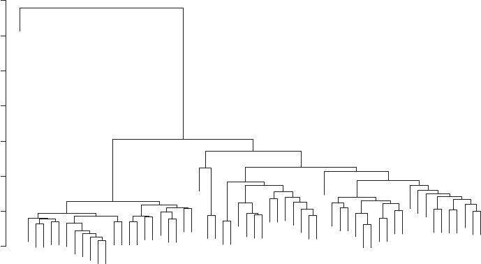
316 AUTOMATED DATA COLLECTION WITH R
Wales
Environment
Environment
Environment
Environment
Environment
Wales
Wales
Environment
Wales
Wales
Environment
Defence
Wales
Defence
Environment
Wales
Wales
Defence
Defence
Defence
Environment
Environment
Environment
Environment
Environment
Wales
Wales
Defence
Defence
Defence
Defence
Defence
Defence
Defence
Defence
Defence
Defence
Defence
Environment
Wales
Wales
Wales
Wales
Wales
Wales
Wales
Wales
Wales
Environment
Environment
Defence
Environment
Defence
Wales
Environment
Environment
Environment
Defence
Defence
0 20 40 60 80 100 120 140
Height
Figure 10.1 Output of hierarchical clustering of UK Government press releases
The resulting clusters roughly recover the topical emphasis of the various press releases
(see Figure 10.1). Particularly toward the lower end of the graph we nd that two press
releases from the same governmental department are frequently joined. However, as we move
up the dendrogram, the patterns become less clear. To a certain extent we nd a cluster of
the “environment”press releases at one end of the graph and particularly the “Wales” press
releases are mostly joined. Conversely, the press releases pertaining to “defence” are dispersed
across the various parts of the dendrogram.
Let us now move on to a veritable unsupervised classication of the texts—the Latent
Estimating
LDA Dirichlet Allocation. One implementation of the Latent Dirichlet model is provided in the
topicmodels package. The relevant function is supplied in the LDA() function. As we know
that our corpus consists of six “topics,” we select the number of topics to be estimated as
six. As before, the function takes the document-term matrix that we created in the previous
section as input.
R> library(topicmodels)
R> lda_out <- LDA(dtm, 6)
After calculating the model, we can determine the posterior probabilities of a document’s
topics as well as the probabilities of the terms’ topics using the function posterior().We
store the topics’ posterior probabilities in the data frame lda_topics and investigate the
mean probabilities assigned to the press releases of the government agencies. We set up a
6-by-6 matrix to store the mean topic probabilities by governmental body.
R> posterior_lda <- posterior(lda_out)
R> lda_topics <- data.frame(t(posterior_lda$topics))
R> ## Setting up matrix for mean probabilities
STATISTICAL TEXT PROCESSING 317
R> mean_topic_matrix <- matrix(
NA,
nrow = 6,
ncol = 6,
dimnames = list(
names(table(org_labels)),
str_c("Topic_", 1:6)
)
)
R> ## Filling matrix
R> for(i in 1:6){
mean_topic_matrix[i,] <- apply(lda_topics[, which(org_labels ==
rownames(mean_topic_matrix)[i])], 1, mean)
}
R> ## Outputting rounded matrix
R> round(mean_topic_matrix, 2)
Topic_1 Topic_2 Topic_3
Department for Business, Innovation & Skills 0.01 0.61 0.00
Department for Communities and Local Government 0.00 0.04 0.04
Department for Environment, Food & Rural Affairs 0.02 0.24 0.12
Foreign & Commonwealth Office 0.01 0.07 0.05
Ministry of Defence 0.49 0.02 0.25
Wales Office 0.00 0.10 0.33
Topic_4 Topic_5 Topic_6
Department for Business, Innovation & Skills 0.02 0.02 0.33
Department for Communities and Local Government 0.02 0.08 0.82
Department for Environment, Food & Rural Affairs 0.06 0.07 0.49
Foreign & Commonwealth Office 0.32 0.50 0.05
Ministry of Defence 0.13 0.05 0.06
Wales Office 0.04 0.13 0.39
We nd that some topics tend to be strongly associated with the press releases from
individual government agencies. For example, topic 2 is often highly associated with the
Department for Business, Innovation & Skills, topic 5 has a high probability of occurring in
announcements from the Foreign & Commonwealth Ofce. Topic 1 is most associated with
the Ministry of Defence. We investigate the estimated probabilities more thoroughly when
considering the correlated topic model.
Another way to investigate the estimated topics is to consider the most likely terms for Terms
associated with
topics
the topics and try to come up with a label that summarizes the terms. This is done using the
function terms().
R> terms(lda_out, 10)
Topic 1 Topic 2 Topic 3 Topic 4 Topic 5 Topic 6
[1,] "oper" "busi" "forc" "nation" "minist" "will"
[2,] "said" "bis" "defenc" "british" "will" "govern"
[3,] "command" "will" "royal" "forc" "foreign" "local"
[4,] "base" "univers" "arm" "peopl" "secretari" "new"
[5,] "royal" "depart" "servic" "will" "secur" "work"
[6,] "troop" "educ" "said" "afghan" "nuclear" "busi"
[7,] "forc" "gov" "day" "secur" "intern" "can"
[8,] "soldier" "skill" "will" "govern" "govern" "council"
[9,] "marin" "colleg" "personnel" "travel" "meet" "make"
[10,] "will" "innov" "fox" "can" "state" "communiti"

318 AUTOMATED DATA COLLECTION WITH R
Particularly topics 1, 3, and 4 have a focus on aspects of the military, the terms in topic
5 tend to relate to foreign affairs, the emphasis in topic 6 is local government and topic
2 is related to business and education. This ordering nicely reects the observations from
the previous paragraph. Nevertheless, we also nd that the dominance of press releases
by the department of defence results in topics that classify various aspects of the defence
announcements in multiple topics, thus lumping together the releases from other departments.
This is to say that while there is some plausible overlap between the known labels and the
estimated categories, this overlap is far from perfect.
Let us move on to estimating a correlated topic model to run a more realistic model of topic
Estimating
CTM mixtures. Again, we select the number of topics to be six since there are six governmental
organizations for which we include press releases.
R> ctm_out <- CTM(dtm, 6)
R> terms(ctm_out, 10)
Topic 1 Topic 2 Topic 3 Topic 4 Topic 5 Topic 6
[1,] "afghan" "foreign" "will" "forc" "govern" "will"
[2,] "said" "minist" "busi" "royal" "will" "new"
[3,] "forc" "will" "local" "arm" "wale" "work"
[4,] "oper" "secur" "govern" "command" "peopl" "project"
[5,] "local" "secretari" "bis" "defenc" "can" "provid"
[6,] "afghanistan" "intern" "council" "servic" "work" "plan"
[7,] "secur" "british" "new" "day" "must" "said"
[8,] "base" "meet" "year" "personnel" "right" "system"
[9,] "area" "nation" "depart" "oper" "said" "use"
[10,] "patrol" "nuclear" "fund" "air" "make" "build"
We now nd two topics—1 and 4—to be clearly related to matters of defense.9Topic 2
is associated with foreign affairs, topic 3 with local government. The terms of topic 5 in the
correlated topic model strongly suggest Welsh politics. A label for topic 6 is more difcult to
make out.
We can plot the document-specic probabilities to belong to one of the three topics. To
Evaluation of
posterior
probabilities
do so, we calculate the posterior probabilities of the topics and set up 2-by-3 panels to plot
the sorted probabilities of the topics in the press releases. The result is displayed in Figure
10.2. Note that to save space we only displayed two of the estimated six topics. We invite you
to run the models and plot all posterior probabilities yourself.
R> posterior_ctm <- posterior(ctm_out)
R> ctm_topics <- data.frame(t(posterior_ctm$topics))
R>
R> par(mfrow = c(2,3), cex.main = .8, pty = "s", mar = c(5, 5, 1, 1)
R> for(topic in 1:2){
R> for(orga in names(table(org_labels))){
R> tmp.data <- ctm_topics[topic, org_labels == orga]
R> plot(
R> 1:ncol(tmp.data),
R> sort(as.numeric(tmp.data)),
9Note that the numbers of the topics are arbitrary.
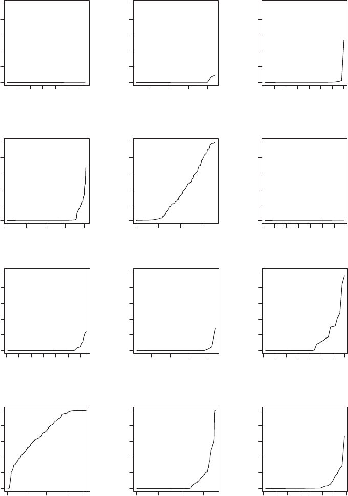
STATISTICAL TEXT PROCESSING 319
0 102030405060
0.0 0.2 0.4 0.6 0.8 1.0
Business, Innovation & Skills
Press releases
Posterior probability, topic 1
5101520
0.0 0.2 0.4 0.6 0.8 1.0
Communities and Local Government
Press releases
Posterior probability, topic 1
0 5 10 20 30
0.0 0.2 0.4 0.6 0.8 1.0
Environment, Food & Rural Affairs
Press releases
Posterior probability, topic 1
0 50 100 150 200
0.0 0.2 0.4 0.6 0.8 1.0
Foreign & Commonwealth Office
Press releases
Posterior probability, topic 1
0 50 100 150
0.0 0.2 0.4 0.6 0.8 1.0
Ministry of Defence
Press releases
Posterior probability, topic 1
0 5 10 15 20 25 30 35
0.0 0.2 0.4 0.6 0.8 1.0
Wales Office
Press releases
Posterior probability, topic 1
0 102030405060
0.0 0.2 0.4 0.6 0.8 1.0
Business, Innovation & Skills
Press releases
Posterior probability, topic 2
5101520
0.0 0.2 0.4 0.6 0.8 1.0
Communities and Local Government
Press releases
Posterior probability, topic 2
0 5 10 20 30
0.0 0.2 0.4 0.6 0.8 1.0
Environment, Food & Rural Affairs
Press releases
Posterior probability, topic 2
0 50 100 150 200
0.0 0.2 0.4 0.6 0.8 1.0
Foreign & Commonwealth Office
Press releases
Posterior probability, topic 2
0 50 100 150
0.0 0.2 0.4 0.6 0.8 1.0
Ministry of Defence
Press releases
Posterior probability, topic 2
0 5 10 15 20 25 30 35
0.0 0.2 0.4 0.6 0.8 1.0
Wales Office
Press releases
Posterior probability, topic 2
Figure 10.2 Output of Correlated Topic Model of UK Government press releases
320 AUTOMATED DATA COLLECTION WITH R
R> type = "l",
R> ylim = c(0,1),
R> xlab = "Press releases",
R> ylab = str_c("Posterior probability, topic ",
topic),
R> main = str_replace(orga, "Department for", "")
R> )
R> }
R> }
The gures are nicely aligned with expectations from looking at the terms most indicative
of the various topics. The posterior probability of topic 1 is highest in press releases from the
ministry of defense, whereas topic 2 has the highest probability in press releases from the
foreign ofce. In summary, we are able to make out some plausible agreement between our
labels and the estimated topical emphasis from the correlated topic model.
Summary
The chapter offered a brief introduction to statistical text processing. To make use of the
vast data on the Web, we often have to post-process collected information. Particularly when
confronted with textual data we need to assign systematic meaning to otherwise unstructured
data. We provided an introduction to a framework for performing statistical text processing
in R—the tm package—and two classes of techniques for making textual data applicable as
data in research projects: supervised and unsupervised classiers.
To summarize the techniques, the major advantage of supervised classication is the ability
of the researcher to specify the categories for the classication algorithm. The downside of
that benet is that supervised classiers typically require substantial amounts of training data
and thus manual labor. Conversely, the major advantage of unsupervised classication lies
in the ability of researchers to skip the coding of data by hand which comes at the price of
having to interpret the estimation results ex post.
At the end, we would like to add that there is a vibrant research in the eld of automated
analysis of text, such that this chapter is potentially one of the rst to contain somewhat dated
information. For example, some headway has been made to allow researchers to specify the
categories they are interested in without having to code a large chunk of the corpus for training
data. This is accomplished using seed words. They allow the researcher to specify words that
are most indicative of a particular category of interest (Gliozzo et al. 2009; Zagibalov and
Carroll 2008).
Further reading
We introduced the most important features of the tm package in the rst section of this chapter.
However, we have not explored its full potential. If you care to learn more about the package
check out the extensive introduction in Feinerer et al. (2008).
Natural language processing and the statistical analysis of text remain actively researched
topics. Therefore, there are both numerous contributions to the topic as well as research
papers with current developments in the eld. For further insight into the topics that were
STATISTICAL TEXT PROCESSING 321
introduced in this chapter take a look at Grimmer and Stewart (2013) for a brief but insightful
introduction to some of the topics that were discussed in this chapter. For a more extensive
treatment of the topics, see Manning et al. (2008).
A topic that is heavily researched in the area of automated text classication is the
classication of the sentiment or opinion in a text. We will return to this topic in Chapter 17
where we try to classify the sentiment in product reviews on http://www.amazon.com. For an
excellent introduction to the topic, take a look at Liu (2012).

11
Managing data projects
Deploying a successful data collection project requires more than knowledge of web tech-
nologies. The focus of this chapter is on Rand operation system functionality that will
be required for setting up and maintaining large-scale, automated data collection projects.
Additionally, we discuss good practices to organize and write code that adds robustness and
traceability in case of errors. In Section 11.1, we start by providing an overview of Rfunc-
tions for interacting with the local le system. In Section 11.2, we show methods for iterative
code execution for downloading pages or extracting relevant information from multiple web
documents. Section 11.3 provides a template for organizing extraction code and making it
more robust to failed specication. We conclude the chapter with an overview of system tools
that can executive Rscripts automatically, which is a key requirement for building datasets
from regularly updated Internet resources (Section 11.4).
11.1 Interacting with the le system
One type of Rfunction that appears frequently in data projects is dedicated to working
with les and folders on the local le system. Over the course of a data project, we are
continuously interacting with the le system of our operating system. Web documents are
stored locally, loaded into R, processed, and saved again after the post-processing or analysis.
The le system has an important role in the data collection and analysis workow and a
rm command over the hard drive constitutes a valuable auxiliary skill. For the numerous
virtues of a scripted approach, any interaction with the le management system should be
performed in a programmable fashion. Luckily, Rprovides an extensive list of functions for
interacting with the system and les located in it. Table 11.1 provides an overview of the
basic le management functions which we rely upon in the case studies and in data projects
more generally.
Automated Data Collection with R: A Practical Guide to Web Scraping and Text Mining, First Edition.
Simon Munzert, Christian Rubba, Peter Meißner and Dominic Nyhuis.
© 2015 John Wiley & Sons, Ltd. Published 2015 by John Wiley & Sons, Ltd.
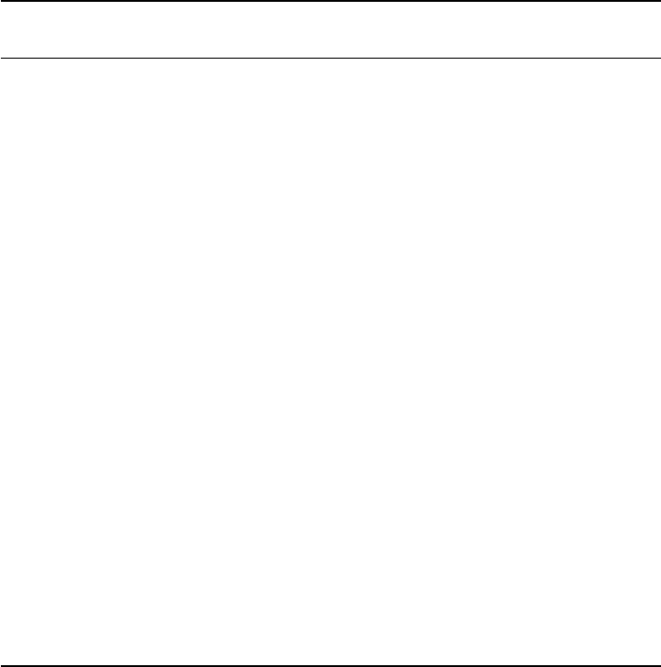
MANAGING DATA PROJECTS 323
Table 11.1 Basic Rfunctions for folder and le management
Function
Important
arguments Description
Functions for folder management
dir() path Returns character vector of the names of les
and directories in path
dir.create() path,recursive Creates new directory in path (only the last
element). If recursive=T all elements on
the path are created.
Functions for le management
file.path() ... Constructs a le path of character elements
file.info() path Returns character vector with information about
a le in path
file.exists() path Returns logical value whether a le already
exists in path
file.access() names,mode Tests les in names for existence (mode=0),
execute permission (mode=1), writing
permission (mode=2), read permission
(mode=4). Returns integer with values 0 for
success and −1 for failure
file.rename() from,to Renames a le in path from to a name in to
file.remove() path Deletes a le in path from the hard drive
file.append() file1,file2 Appends contents in file2 to file1
file.copy() from,to Creates a copy of a le in path from to path to
basename() path Returns the lowest level in a path
dirname() path Returns all but the lower level in a path
Functions for working with compressed les
zip() zipfile,files Create a zip le in path zipfile of files
unzip() zipfile,files Extracts specic files (all when unspecied)
from a zip le in path zipfile
Path arguments may usually be passed as complete or incomplete paths. In the latter case, paths are
expanded to the working directory (getwd()). File paths may be passed in abbreviated form without the
user’s home directory. (path.expand() is used to replace a leading tilde by the user’s home directory.)
11.2 Processing multiple documents/links
A frequently encountered task in web scraping is executing a piece of code repeatedly. In fact,
using a programming language for data collection is most valuable as it allows the researcher
to automate tasks that would otherwise have to be done in tedious and time-consuming
manual processing of every le, URL, or document. To exemplify, consider the problem of
downloading a bunch of HTML sites from a vector of URLs. Another job is the processing of
multiple web documents, such as the pages from a news website where the task is extracting
the text corpora, or the extraction of tabular information from economic indicators organized
in XML les to create a single database.

324 AUTOMATED DATA COLLECTION WITH R
This section illustrates that with only a little bit of overhead one can instruct Rto repeatedly
execute a function on a set of les and, thus, comfortably download countless pages or scan
thousands of documents and reassemble the extracted information. We introduce two ways
to accomplish this goal; the rst one is through the use of standard Rlooping structures and
the second one is through functionality from the plyr package.
11.2.1 Using for-loops
For illustrative purposes, we consider the set of 11 XML les that are located in the folder
/stocks.1The XML les contain stock information for four technology companies. Our interest
is in extracting the daily closing values for the Apple stock over all years (2003–2013). We
can divide this problem into two subtasks. First, we need to come up with an extraction code
that loads the le, extracts, and recasts the target information into the desired format. The
second task is executing the extraction code on all XML les. A straightforward approach
is to wrap the extraction code in a for-loop. Loops are standard programming structures that
help formulate an iterating statement over the set of documents from which information needs
to be extracted.
A rst step is to obtain the names of the les that we would like to process. To this end,
we use the dir() function to produce a character vector with all the le names in the current
directory. The le names are inserted into a new object called all_files and its content is
printed to the screen.
R> all_files <- dir("stocks")
R> all_files
[1] "stocks_2003.xml" "stocks_2004.xml" "stocks_2005.xml"
[4] "stocks_2006.xml" "stocks_2007.xml" "stocks_2008.xml"
[7] "stocks_2009.xml" "stocks_2010.xml" "stocks_2011.xml"
[10] "stocks_2012.xml" "stocks_2013.xml"
Next, we need to create a placeholder in which we can store the extracted stock information
from each le. Although it might be necessary to obtain a data frame at the end of the process
for analytical purposes, we set up a list as an intermediate data structure. Lists provide the
exibility to collect the information which we recast only afterwards. We create an empty
list that we name closing_stock and which serves as a container for the yearly stock
information from each le.
R> closing_stock <- list()
The core of the extraction routine consists of a for-loop over the number of elements
in the all_files character vector. This structure allows iterating over each of the les and
work on their contents individually.
R> for (i in 1:length(all_files)) {
path <- str_c("stocks/", all_files[i])
parsed_stock <- xmlParse(path)
closing_stock[[i]] <- xpathSApply(parsed_stock, "//Apple", getStock)
}
1You can nd the data on www.r-datacollection.com/materials.
MANAGING DATA PROJECTS 325
First, we construct the path of each XML le and save the information in a new object
called path. The information is needed for the next step, where we pass the path to the parsing
function xmlParse(). This creates the internal representation of the le inside a new object
called parsed_stock. Finally, we obtain the desired information from the parsed object by
means of an XPath statement. Here, we pull the entire Apple node and do the post-processing
in the extractor function, which we discuss below. The return value from xpathSApply()
is stored at the ith position our previously dened list. The get_stock() extractor function
is a custom function that works on the entire Apple node and returns the date and closing
value for each day.
R> getStock <- function(x) {
date <- xmlValue(x[["date"]])
value <- xmlValue(x[["close"]])
c(date, value)
}
We go ahead and unlist the container list to process each information individually and
put it into a more convenient data format. Here we go for a data frame and choose more
appropriate column names.
R> closing_stock <- unlist(closing_stock)
R> closing_stock <- data.frame(matrix(closing_stock, ncol = 2, byrow = T))
R> colnames(closing_stock) <- c("date", "value")
Finally, we recast the value information into a numerical vector and the date information
into a vector of class Date.
R> closing_stock$date <- as.Date(closing_stock$date, "%Y/%m/%d")
R> closing_stock$value <- as.numeric(as.character(closing_stock$value))
We are ready to create a visual representation of the extracted data. We use plot() to
create a time-series of the stock values. The result is displayed in Figure 11.1.
R> plot(closing_stock$date, closing_stock$value, type = "l", main
= "", ylab = "Closing stock", xlab = "Time")
2004 2006 2008 2010 2012 2014
0 100 300 500 700
Time
Closing stock
Figure 11.1 Time-series of Apple stock values, 2003–2013
326 AUTOMATED DATA COLLECTION WITH R
11.2.2 Using while-loops and control structures
A second control statement that we can use for iterations is the while() expression. Instead
of iterating over a xed sequence, it will run an expression as long as a particular condition
evaluates to TRUE. Consider the snippet below for an abstract usage of the expression.
R>a<-0
R> while(a < 3){
a<-a+1
print(a)
}
[1] 1
[1] 2
[1] 3
We set the ato 0 and while the ais lower than 3 it will continue looping. In each iteration
we add 1 to aand print the value of ato the screen. Once the ahas reached the critical value
of 3, the loop will break.
Apart from setting a condition in the while() statement that evaluates to FALSE at some
point, thus breaking the loop, we can also break a loop with an if() clause and a break
command.
R>a<-0
R> while(TRUE){
a<-a+1
print(a)
if(a >= 3){
break
}
}
[1] 1
[1] 2
[1] 3
In the above snippet, we set a condition in the while() statement that will always evaluate
to TRUE, thus creating an innite loop. Instead, in each iteration we test whether ais equal
to or greater than 0. If that condition is TRUE,thebreak is encountered which forces Rto
break the current loop. Notice how we used the if() clause in the snippet.
In web scraping practice, the while() statement is handy to iterate over a set of documents
where you do not know the total number of documents in advance. Consider the following
scenario. You care to download a selection of HTML documents where the link to additional
documents is embedded in the source code of the last inspected HTML document, say in a
linktoaNEXT document. If you do not happen to nd a counter at the bottom of the page that
contains information on the total number of pages, there is no way of specifying the number
of pages you can expect. In such a case, you can apply the while() statement to check for
the existence of a link before accessing the document.
R> # Load packages
R> library(XML)
R> library(stringr)
R>
R> # Mock URL
MANAGING DATA PROJECTS 327
R> url <- "http://www.example.com"
R>
R> # XPath expression to look for additional pages
R> xpath_for_next_page <- "//a[@class='NextPage']"
R>
R> #Create index for pages
R>i<-1
R>
R> # Collect mock URL and write to drive
R> current_document <- getURL(url)
R> write(tmp, str_c(i, ".html"))
R>
R> # Download additional pages while there are links to additional pages
R> while(length(xpathSApply(current_document, xpath_for_next_page,
xmlGetAttr, "href")) > 0){
R> current_url <- xpathSApply(current_document, xpath_for_next_page,
xmlGetAttr, "href")
R> current_document <- getURL(current_url)
R> write(current_document, str_c(i, ".html"))
R> i<-i+1
11.2.3 Using the plyr package
The data structure which we typically wish to produce is tabular with variables populating the
columns and each row presenting a case or unit of analysis. Producing tabular data structures
from multiple web documents can be achieved easily using functionality from the plyr package
(Wickham 2011) which allows performing an extraction routine more quickly on multiple
documents. To illustrate, let us run through the previous example in the plyr framework. As
the rst step, we construct the paths to the XML les on the local hard drive.
R> files <- str_c("stocks/", all_files)
We create a function getStock2() that parses an XML le and extracts relevant infor-
mation. This code is similar to the one we used before.
R> getStock2 <- function(file){
parsedStock <- xmlParse(file)
closing_stock <- xpathSApply(parsedStock,
"//Apple/date | //Apple/close",
xmlValue)
closing_stock <- as.data.frame(matrix(closing_stock,
ncol = 2,
byrow = TRUE))
}
The function returns an n×2 data frame with the rst column holding information on the
date and the second one on the closing stock. We are now set to evoke ldply() and initiate
the extraction process.
R> library(plyr)
R> appleStocks <- ldply(files, getStock2)
328 AUTOMATED DATA COLLECTION WITH R
For its input ldply() requires a list or a vector and it returns a dataframe. ldply()
executes getStock2() on every element in files and binds the results row-wise. We
conrm that the procedure has worked correctly by printing the rst ve lines to the console.
R> head(appleStocks, 3)
V1 V2
1 2013/11/13 520.634
2 2013/11/12 520.01
3 2013/11/11 519.048
If you are dealing with larger le stacks, plyr also provides the option parallel which,
if set to TRUE, parallelizes the code execution which can speed up the process.
11.3 Organizing scraping procedures
When you begin scraping the Web regularly, you will nd that numerous tasks come upDon’t repeat
yourself over and over again. One of the central principles of good coding practice states that you
should never repeat yourself. If you nd yourself rewriting certain lines of code or copy-
pasting elements of your code, then it is time to start thinking about organizing your code
in a more efcient way. Problems arise when you need to trace all the places in your
scripts where some particular functionality has been dened. The solution to this problem
is to wrap your code in functions and store them in dedicated places. Not only does this
guarantee that revisions happen in only one place, but it also greatly simplies the maintenance
of code.
Besides ensuring a better maintenance of code, writing functions also allows a general-
ization of functionality. This is a great improvement of your code when you want to apply
a sequence of operations to lots of data, as is often the case in web scraping. In fact, by
writing your code into functions you can frequently speed up the execution time of your R
code dramatically by applying the function on a list or a vector via one of the apply functions
from the plyr package as shown in the previous section. This section serves to elaborate how
to modularize your code by using functions.
We demonstrate the use of functions with a scenario that we already discussed in Section
9.1.4. Imagine that we want to collect all links from a website. We have learned that the XML
package provides the function getHTMLLinks() which makes link collection from HTML
documents quite convenient. In fact, this function is a good example for a function which
help tackle a frequently occurring task. Imagine that the function did not exist and we needed
to build it.
We have learned in Chapter 2 that links are stored in href attributes of <a> elements.
Our task is thus simply to collect the content of all nodes with this attribute. Let us begin
by loading the necessary packages and specifying a URL that will serve as our running
example.
R> library(RCurl)
R> library(XML)
R> url <- "http://www.buzzfeed.com"
MANAGING DATA PROJECTS 329
We can perform the task for this single website by calling and parsing it via htmlParse()
and collecting the relevant information via xpathSApply() .
R> parsed_page <- htmlParse(url)
R> links <- xpathSApply(parsed_page, "//a[@href]", xmlGetAttr, "href")
R> length(links)
[1] 945
Now imagine that we care to apply these steps to several websites. To apply these three Setting up
functions
steps to other sites we wrap them into a single function we call collectHref().Thisis
done by storing the necessary steps in an object and calling the function function().The
argument in the function call represents the object that the function is supposed to run on, in
this case the URL.
R> collectHref <- function(url){
parsed_page <- htmlParse(url)
links <- xpathSApply(parsed_page, "//a[@href]", xmlGetAttr, "href")
return(links)
}
Now we can simply run the function on various sites to collect all the links. First we apply
it to the URL we specied above and then we try out a second page.
R> buzzfeed <- collectHref("http://www.buzzfeed.com")
R> length(buzzfeed)
[1] 945
R> slate <- collectHref("http://www.slate.com")
R> length(slate)
[1] 475
We are able to generalize functions by adding arguments to it. For example, we can add a Adding
arguments
variable to our function that will discard all links that do not explicitly begin with http.This
could be done with a simple regular expression that detects whether a string begins in http,
using the str_detect() function from the stringr package.
R> collectHref <- function(url, begins.http){
if(!is.logical(begins.http)){
stop("begins.http must be a logical value")
}
parsed_page <- htmlParse(url)
links <- xpathSApply(parsed_page, "//a[@href]", xmlGetAttr, "href")
if(begins.http == TRUE){
links <- links[str_detect(links, "ˆhttp")]
}
return(links)
}
Notice that we also added a test to the function that checks whether begins.http is a
logical value. If not, the function will throw an error (produced by stop()) and not return
330 AUTOMATED DATA COLLECTION WITH R
any results. Let us run the altered function on our example URL, and set begins.http to
TRUE.
R> buzzfeed <- collectHref(url, begins.http = TRUE)
R> length(buzzfeed)
[1] 63
The vector of links has shrunk considerably. Now let us call the function on the base URL
again, but change the begins.http variable to the wrong type.
R> testPage <- collectHref(url, begins.http = "TRUE")
Error: begins.http must be a logical value
We can add any number of arguments to the function. In order not to have to specify
the value for each argument whenever we call the function, we can set predened values for
the arguments. For example, we can set begins.http to TRUE by default in the function
denition.
R> collectHref <- function(url, begins.http = TRUE){
if(!is.logical(begins.http)){
stop("begins.http must be a logical value")
}
parsed_page <- htmlParse(url)
links <- xpathSApply(parsed_page, "//a[@href]", xmlGetAttr, "href")
if(begins.http == TRUE){
links <- links[str_detect(links, "ˆhttp")]
}
return(links)
}
Thus, whenever we call the function, it will assume that we care to collect only those
links that explicitly contain the sequence http.
Once you start writing functions in R, you will nd that grouping them into topical lesStoring and
calling
functions
is the most sensible way to collect functions for use in various projects. The advantage of
generating a set of functions in modules ensures that you have to modify specic functions
only in one location and that you do not have to create the same functionality over and over
again with each project that you are beginning. Instead you can call the necessary module
when you start a new project, almost like you would load a library that you download from
CRAN.
A reasonable approach for storing such recurring functions is to create a dedicated folder
where functions are stored in dedicated Rscript les. Whenever you want to draw on one
of these functions, you can access them using the source() command. This automatically
evaluates code from foreign Rsource les. Imagine we have stored our function from above
in a le named collectHref.r. In order to run the command, we proceed as follows:
R> source("collectHref.r")
R> test_out <- collectHref("http://www.buzzfeed.com")
R> length(test_out)
[1] 63
Eventually you can also go one step further and create Rpackages yourself and upload
them to CRAN or GitHub .
MANAGING DATA PROJECTS 331
11.3.1 Implementation of progress feedback: Messages
and progress bars
When performing a web scraping task, it can often be useful to receive a visual feedback on
the progress that our program has made in order to get a sense of when your program will have
nished. A very basic version of such a feedback would be a simple textual printout directly
to the Rconsole. We can accomplish this with the cat() function. To illustrate, consider the
problem of downloading the stock XML les from the book homepage. The les are stored in
the following path: http://www.r-datacollection.com/materials/workow/stocks. Let us start
by building a character vector for their URLs and save them in a new object called links.
R> baseurl <- "http://www.r-datacollection.com/materials/workflow/stocks"
R> links <- str_c(baseurl, "/stocks_", 2003:2013, ".xml")
Next, we set up a loop over the length of links. Inside the loop, we download the le, Progress
feedback with
cat()
create a sensible name using basename() to return the source le name, and then write the
XML code to the local hard drive.
R> N <- length(links)
R> for(i in 1:N){
R> stocks <- getURL(links[i])
R> name <- basename(links[i])
R> write(stocks, file = str_c("stocks/", name))
R> cat(i, "of", N, "\n")
R> }
1of11
2of11
3of11
...
11 of 11
In the nal line, we ask Rto print the number of the document just downloaded to the
console. We append the message with a \nso each new output is written to a new line.
We can enrich the information in the feedback, for example, by adding the name of the
le that is currently being downloaded.
R> for(i in 1:N){
R> stocks <- getURL(links[i])
R> name <- basename(links[i])
R> write(html, file = str_c("stocks/", name))
R> cat(i, "of", N, "-", name, "\n")
R> }
1 of 11 - stocks_2003.xml
2 of 11 - stocks_2004.xml
3 of 11 - stocks_2005.xml
...
11 of 11 - stocks_2013.xml
In some cases, you might not want to get output on each individual case but only cre-
ate summary information. One possibility for this is to shorten the output by providing
332 AUTOMATED DATA COLLECTION WITH R
information on, say, each tenth download. We add an if() statement to our code such that
only those iterations are printed where the idivided by 10 does not result in a fraction.
R> for(i in 1:30)
if(i %% 10 == 0){
cat(i, "of", 30, "\n")
}
}
10 of 30
20 of 30
30 of 30
Incidentally, you might want to store the progress information in an external le for laterWriting
progress to a
log le
inspection to be able to trace potential errors. Possibly, this should consist of more extensive
information than what is printed to your screen. For example, you can use the write()
command to write the progress to a log le that is appended in each iteration. We begin by
creating an empty le on our local hard drive.
R> write("", "download.txt")
We then append the information that is written to the screen to the external le. To make
the information a little more useful for later inspection, we add information on the number
of characters in the downloaded le. We also add dashes and a space to visually separate the
various downloads.
R> N <- length(links)
R> for(i in 1:N){
R> stocks <- getURL(links[i])
R> name <- basename(links[i])
R> write(html, file = str_c("stocks/", name))
R> feedback <- str_c(i, "of", N, "-", name, "\n", sep = " ")
R> cat(feedback)
R> write(feedback, "download.txt", append = T)
R> write(nchar(stocks), "download.txt", append = T)
R> write("- - ----------
\n", "download.txt", append = T)
R> }
In many instances, the best feedback is textual. Nevertheless, you can also create otherUsing built-in
progress bars types of feedback. For instance, you can easily create a simple progress bar for your function
using the txtProgressBar() that is predened in R. For our example we start by initializing
a progress bar with the extreme values of 0 and N, that is 3. We set the style of the progress
bar to 3, which generates a progress bar that displays the percentage of the task that is done
at the right end of the bar.
R> progress_bar <- txtProgressBar(min = 0, max = N, style = 3)
Next, we download the documents once more with the shortest version of the code that
was introduced previously. We add the command setTxtProgressBar() to our call which
sets the value of the progress bar that we initialized above. The rst argument species which
progress bar we want to change the value of, the second argument sets the value, in this case

MANAGING DATA PROJECTS 333
the values 1, 2, and 3. We add a 1 second delay after each iteration using the Sys.sleep()
function, so you can clearly see the development of the progress bar.
R> for(i in 1:N){
R> stocks <- getURL(links[i])
R> name <- basename(links[i])
R> write(stocks, name)
R> setTxtProgressBar(progress_bar, i)
R> Sys.sleep(1)
R> }
|================================ | 73%
You can even create audio cues to signal that the execution of a piece of code is complete. Audio feedback
For example, the escape sequence \acalls the alert bell.2
R> for(i in 1:N){
R> tmp <- getURL(websites[i])
R> write(tmp, str_c(str_replace(websites[i], "http://www\\.", ""), ".
html"))
R> }
R> cat("\a")
Imagine a ping! when reading cat("\a") in the last code snippet.
11.3.2 Error and exception handling
When you start to scrape the Web seriously, you will begin to stumble across exceptions.
For example, websites might not be formatted consistently such that you will not nd all the
elements that you are looking for. It is sometimes difcult to build your functions sufciently
robust to be able to deal with all the exceptions. This section introduces some simple tech-
niques that can help you overcome such problems. Let us consider as an example the same
task that we have looked at in Section 11.3—downloading a list of websites. First, we expand
the list with a mistyped URL.
R> wrong_pages <- c("http://www.bozzfeed.com", links)
When we try to download the content of all of the sites to our hard drive using a simple The try()
function
loop over all the entries, we nd that this operation fails as the function is unable to collect
the rst entry in our vector. The problem with errors is that they break the execution of the
entire piece of code. Even though the remaining three entries could have been collected with
the code snippet as we have previously shown, the single false entry stops the execution
altogether. The simplest way to change this behavior is to wrap the getURL() expressions in
atry() statement.
R> for(i in 1:N){
R> url <- try(getURL(wrong_pages[i]))
R> if(class(url) != "try-error"){
2Users have implemented more fun notication sounds in R. Be sure to check out the pingr package (see
https://github.com/rasmusab/pingr).

334 AUTOMATED DATA COLLECTION WITH R
R> name <- basename(wrong_pages[i])
R> write(url, name)
R> }
R> }
Notice that we added a statement to test the class of the url object. If the object is of classThe
tryCatch()
function
try-error, we do not write the content of the object to the hard drive. The disadvantage of
wrapping code in try() statements is that you discard errors as inconsequential. This is a
strong assumption, as something has gone wrong in your code and frequently it makes sense
to consider more carefully what exception you encountered. Ralso offers the tryCatch()
function which is a more exible device for catching errors and dening actions to be
performed as errors occur. For example, you could log the error to consider the systematics
of the errors later on. First, we create a function that combines the two steps of our task in
a single function. We also set up a log le to export errors and the relevant URL during the
execution of the code.
R> collectHTML <- function(url){
R> html <- getURL(url)
R> write(html, basename(url))
R> }
R> write("", "error_log.txt")
We customize the error handling in the tryCatch() statement by making it print Not
available and the name of the website that cannot be accessed.3
R> for (i in 1:N) {
html <- tryCatch(collectHTML(site404[i]), error = function(err){
errMess <- str_c("Not available - ", site404[i])
write(str_c(errMess, "error_log.txt"))
})
}
11.4 Executing Rscripts on a regular basis
On many websites, smaller or larger parts of the contents are changed on a regular basis,
which renders these resources dynamic. To exemplify, imagine a news site that publishes new
articles every other hour or the press release repository of a non-governmental organization
that adds new releases sporadically.
Implicitly, we assumed so far that scraping can be carried out in a one-time job. Yet,
when dynamic web resources are concerned, it might be a key aspect of a data project to
collect information over a longer period of time. While nothing prevents us from manually
executing a script in regular intervals, this process is cumbersome and error-prone. This
3The added value of using the tryCatch() function compared to the try() statement in this case is fairly
limited, as the error messages of the former are similarly informative and could easily be written to an external
le. The added value of tryCatch() relative to try() stems from the fact that we can dene customized action
upon encounter of an error. The simple example only serves the purpose of exposition. For error handling with
specication of alternative behavior see Section 5.4.7.
MANAGING DATA PROJECTS 335
section discusses ways to free the data scientist from this responsibility by setting up a system
task that initiates the scraping automatically and in the background. To this end, we employ
tools that are built right into the architecture of all modern operating systems for scheduling
the execution of programs. We provide an introduction to these tools and show how an R
scraping script can be invoked in user-dened intervals.
We motivate this section with the problem of downloading information from http://www.r-
datacollection.com/materials/workow/rQuotes.php. Scraping this site is complicated by its
very dynamic nature—the site changes every minute and displays a different Rquote. We
set ourselves to the task of downloading a day’s worth of quotes. Clearly, a manual approach
is out of the question for obvious reasons. We approach the problem by rst assembling an
Rscript that allows downloading and storing information from one instance of the site. The
rst line loads the stringr package and the second makes sure that we have a folder called
quotes that serves as a container for the downloaded pages. The next three lines are overhead
for the le names that include the date and time of the download. The last line conducts the
download, using R’s built-in download.file() function. We save the downloading routine
under the name getQuotes.R.
R> library(stringr)
R> if (!file.exists("quotes")) dir.create("quotes")
R> time <- str_replace_all(as.character(Sys.time()), ":", "_")
R> fname <- str_c("quotes/rquote ", time, ".html")
R> url <- "http://www.r-datacollection.com/materials/workflow/rQuotes.php"
R> download.file(url = url, destfile = fname)
In the remainder of this section, we describe how to embed the Rscript with system
utilities for regular execution in predened intervals. We discuss solutions for Linux, Mac
OS, and Windows.
11.4.1 Scheduling tasks on Mac OS and Linux
For users working on a UNIX-like operating system such as Mac OS or Linux, we propose
using Cron for the creation and administration of time-based tasks. Cron is a preinstalled
general-purpose system utility that allows setting up so-called jobs that are being run period-
ically or at designated times in the background of the system.
For the administration of tasks, Cron uses a simple text-based table structure called a How Cron
works
crontab. A crontab includes information on the specic actions and the times when the
actions should be executed. Notice that Cron will run the jobs regardless of whether the user
is actually logged into the system or not. Although graphical interfaces exist to set up a task,
it is convenient and quick to edit tasks using a text editor. To create a new task, open a system
shell4and write.
1crontab -e
4Depending or your system, the shell may be accessed differently. On Mac OS open ‘Terminal,’ on Ubuntu nd
Terminal or press CTRL+ALT+T.
336 AUTOMATED DATA COLLECTION WITH R
Table 11.2 The ve eld Cron time format
Field Description Allowed values
MIN Minute eld 0–59
HOUR Hour eld 0–23 (0 =midnight)
DOM Day of Month eld 1–31
MON Month eld 1–12 or literals
DOW Day of Week eld 0–6 (0 =Sunday) or literals
Source: Adapted from http://www.thegeekstuff.com/2009/06/15-practical-
crontab-examples/
This command opens the crontab specic to your logged in user in the default editor of
your system. If you prefer a different text editor, prepend the command with the respective
editor’s name (e.g., nano,emacs,gedit). Conditional on the OS you use, the text le you are
being shown can be empty or include some general comments on how this le can be edited.
In any case, since crontab requires that each task has to appear on a separate line, go ahead
and point the prompt to the last line of the le. The general layout of a crontab follows the
pattern “[time][script],”where the script component refers to a shell command and the time
component describes the temporal pattern by which the script is executed.
Cron has its own time format to express chronological regularity. Essentially, this time
format consists of ve elds, separated by white space, that refer to the minute, hour, day,
month, and weekday on which the task is to be executed. Take a look at Table 11.2 to
learn about the allowed values for each of the ve time elds. Notice, that any of the ve
elds may be left unspecied which in the Cron time format is indicated by the asterisk
symbol *.
From this basic template, we can construct a wide range of temporal patterns for task
execution. To illustrate their capability, take a look at the following three specications.
15 16 * * * executes the script everyday quarter past four
15 16 * 1 * executes the script everyday quarter past four when the
month is January
15 16 * 1 0 executes the script everyday quarter past four when the
month is January and it’s Sunday
In any of these ve elds, one can produce an unconnected or connected series of time
units by using “,”or“-” respectively.
15 10-20 * * * executes the script quarter past every hour from 10 am
to8pm
15 10-20 * * 6,0 executes the script quarter past every hour from 10 am
to 8 pm on Saturdays and Sundays
In many circumstances, exact specication of a time is overly rigid for a given task.
Instead, one can use the Cron time schema to express the intention of having a task executed in

MANAGING DATA PROJECTS 337
certain time intervals. The preferred way to do this is by using a “*/n”construct that species
an interval of length nfor the respective time unit. To illustrate, consider the following
examples.
*/15 * * * * executes the script every 15 minutes
15 0 */2 * * executes the script 15 minutes past midnight on every second day
The second piece of information in any Cron job is the shell command that has to be Executing tasks
from the shell
executed regularly. If you have never worked with the shell before, think of it as a command
line based user-interface for accessing the operating system and installed programs (such as
R). In order to set up a new task for the execution of getQuotes.r every minute, we append
the following line to the crontab:
1*/1 * * * * cd [DIRECTORY] && Rscript getQuotes.r
We rst specify the chronological pattern “*/1****” for every-minute repeated
execution. This is followed by the scripting part, where we rst change the directory to the
folder in which getQuotes.r is saved and then use the Rscript-executable on getQuotes.r.
Rscript is a scripting front-end that should be used in cases when an Rscript is executed via
the shell. Once you have saved the crontab, the task is active and should be executed in the
background.
For the maintainability of Cron-induced Rroutines, it is helpful to retain an overview over
the outputs that are generated from the script, such as warnings or errors. The UNIX shell
allows to route the output of the Rscript to a log le by extending the Cron job as follows:
1*/1 * * * * cd [DIRECTORY] && Rscript getQuotes.r >> log.txt 2>&1
11.4.2 Scheduling tasks on Windows platforms
On Windows platforms, the Windows Task Scheduler is the tool for scheduling tasks. To nd
the tool click Start >All Programs >Accessories >System Tools >Scheduled Tasks.
To set up a new task, double-click on Create Task. From here, the procedure differs Working with
the Windows
Task Scheduler
according to your version of Windows, but the presented options should be very similar. On
Windows 7, we are presented with a window with ve tabs—General,Triggers,Actions,
Conditions, and Settings. Under General we can provide a name for the task. Here we put in
Testing R Batch Mode for a descriptive title.
In the eld Triggers we can add several triggers for starting the task—see Figure 11.2.
There are schedule triggers which start the task every day, week, or month and also triggers
that refer to events like the startup of the computer or when it is in idle mode, and many
more. To execute getQuotes.r every minute for 24 hours, we select On a schedule as general
trigger and dene that it should be executed only once but repeated every 1 minutes for 1
day. Last but not least, we should make sure that the start date and time of our one-time
scheduled task should be placed somewhere in the future when we will be done specifying
the schedule.
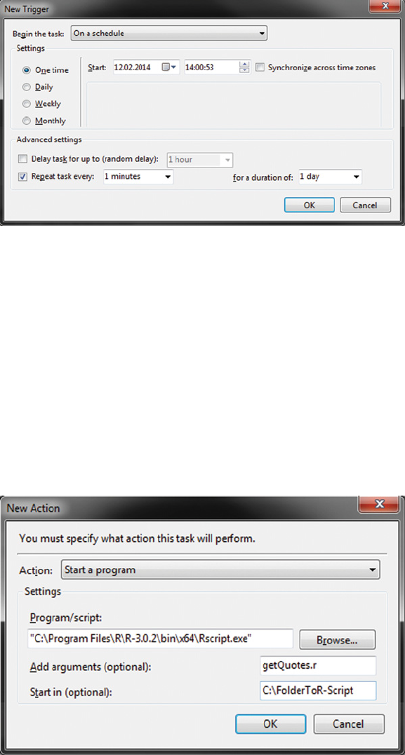
338 AUTOMATED DATA COLLECTION WITH R
Figure 11.2 Trigger selection on Windows platform
After the trigger specication we still have to tell the program what to do if the task is
triggered. The Actions tab is the right place to do that—see Figure 11.3. We choose Start a
program for action and use the browse button to select the destination of Rscript.exe, which
should be placed under, for example, C:\ProgramFiles\R\R-3.0.2\bin\x64\. Furthermore,
we add getQuotes.r in the Add arguments eld and type in the directory where the script is
placed in the Start in eld. If logging is needed we modify the procedure.
Program/script eld: replace Rscript.exe by R.exe
Add arguments eld: replace getQuotes.r by CMD BATCH –vanilla getQuotes.r
log.txt
Figure 11.3 Action selection on Windows platform
MANAGING DATA PROJECTS 339
While CMD BATCH tells Rto run in batch mode, –vanilla ensures that no Rproles
or saved workspaces are stored or restored that might interfere with the execution of the
script. log.txt provides the name for the logle. Now we can conrm our conguration
and click on Task Scheduler Library in the left panel to get a list of all tasks available on
our system.
Part Three
A BAG OF CASE STUDIES

Overview of all case studies
Scraping and information Main Important
Case study Description extraction via... packages functions
Collaboration
Networks in the
U.S. Senate
Scraping of bill cosponsorship data
from the US Senate at
thomas.loc.gov, assessment of
collaboration network structure
URL manipulation, regular
expressions
RCurl, stringr,
igraph
getURL(),
str_extract(),
graph.edgelist(),
get.adjacency()
Parsing Information
from
Semi-Structured
Documents
Scraping of climate data from
Californian weather stations
(ftp.wcc.nrcs.usda.gov),
construction of a regex-based
parser
FTP download, regular
expressions and string
manipulation tools
RCurl, stringr getURL(),
str_extract(),
str_replace()
Predicting the 2014
Academy Awards
using Twitter
Collection of tweets from Twitter
API (dev.twitter.com/docs/api/
streaming), frequency-based
prediction of Oscar winners
Persistent connection to
Streaming API via
streamR, regular
expressions
streamR,
twitteR,
lubridate,
stringr, plyr
filterStream(),
parseTweets(),
str_detect(),
agrep()
Mapping the
Geographic
Distribution of
Names
Scraping phone book data from
dastelefonbuch.de, extraction of
zip codes and matching with
geo-coordinates, creation of
family name maps
HTML forms,XPath and
regular expressions, R
geographic functionality
RCurl, stringr,
XML,
maptools,
maps, rgdal
getForm(),
htmlParse(),
xpathSApply(),
str_extract(),
function()
Gathering Data on
Mobile Phones
Scraping of mobile phone product
data from amazon.com, data
storage in SQLite database
URL manipulation, XPath
and regular expressions
RCurl, stringr,
XML,
RSQLite
htmlParse(),
xpathSApply(),
str_extract(),
dbGetQuery()
Analyzing
Sentiments of
Product Reviews
Extension of SQLite database with
customer reviews of mobile
phones at amazon.com,
dictionary and
classication-based sentiment
analysis
XPath, data preparation with
tm functionality, sentiment
dictionary, maximum
entropy and SVM
RCurl, string,
XML,
RSQLite,
tm,
RTextTools,
textcat
dbReadTable(),
dbGetQuery(),
tm_map(),
TermDocumentMa-
trix(),
classify_model()

12
Collaboration networks in
the US Senate
The inner workings of legislatures are inherently difcult to investigate. Political scientists
have been interested in collaborations among parliamentarians as explanatory factors in
legislative behavior for decades. Scholars have encountered difculties, however, in collecting
comprehensive data over time to investigate patterns of cooperation. The advent of large-scale,
machine-readable databases on legislative behavior have opened up promising new research
avenues in this regard. Among these, scholars have considered the possibility of treating bill
cosponsorships as proxies for legislative cooperation in the United States. We follow this lead
and investigate who cooperates with whom in the US Senate.
Every bill that is introduced to the US Senate is tied to one senator as its main sponsor, but
other senators are free to cosponsor a bill in order to support the bill’s content—a common
practice in senatorial procedures. In fact, in many instances, a bill will have numerous
cosponsors. Several authors have recently begun to truly appreciate the network-like structure
in bill cosponsorships that is best analyzed using network-analytic methodology.1Using the
rich and well accessible data source on bill cosigners provides researchers with an interesting
insight into the black box of collaboration among senators. What is more, bill cosponsorships
are moving targets. New proposals are constantly put on record. Being able to collect these
data automatically provides researchers with a unique opportunity to consider structural
changes in the networks as they are happening.
In this application, we generate the necessary data to replicate some of the analyses that
have been put forward in recent years. For simplicity’s sake, we only assemble data on bill
cosponsorships for the US Senate in the 111th Congress, which was in session from 2009 to
1For recent contributions on the topic, see Bratton and Rouse (2011), Burkett (1997), Cho and Fowler (2010),
Fowler (2006a), Fowler (2006b), and Zhang et al. (2008).
Automated Data Collection with R: A Practical Guide to Web Scraping and Text Mining, First Edition.
Simon Munzert, Christian Rubba, Peter Meißner and Dominic Nyhuis.
© 2015 John Wiley & Sons, Ltd. Published 2015 by John Wiley & Sons, Ltd.

344 AUTOMATED DATA COLLECTION WITH R
Table 12.1 Desired data structure for sponsorship matrix
Senator A Senator B Senator C ...
S.1 Cosponsor Sponsor Cosponsor ...
S.2 . . . ...
S.3 . Cosponsor Sponsor ...
S.4 . . Sponsor ...
S.5 . . . ...
S.6 Cosponsor . Cosponsor ...
S.7 Sponsor . . ...
⋮⋮ ⋮ ⋮⋱
The table displays a mock example of the dataset we wish to generate. The rows list each bill, the
columns list each senator. The cells display whether a senator was the main sponsor of a bill (Sponsor),
has cosponsored a bill (Cosponsor) or did not sign a bill at all (.).
2010. Sections 12.1 and 12.2 provide the technical details on how the underlying data sources
are generated. Again, our focus in this chapter is on data gathering; hence, we only analyze
the data with simple metrics. Section 12.3 gives a brief overview on how the data can be
employed—both descriptively and in a basic network application. Section 12.4 concludes the
chapter.
12.1 Information on the bills
Our rst task is to assemble a list of all sponsors and cosponsors on each bill. To keep matters
simple, we will only gather data for the 111th Senate, which ran from 2009 to 2010. As we
are more interested in the process of data gathering than in the actual application, there is
more than enough material in one senatorial term. Should you wish to analyze the data for an
actual application, it is fairly straightforward to adapt the script to encompass more legislative
periods.
Our specic goal in this section is to construct a matrix that holds information on whether
a senator has sponsored, cosponsored, or not participated at all in a given bill. A mock example
of the data structure is presented in Table 12.1. Storing the data in this format provides the
greatest exibility for subsequent analyses. We could, for example, be interested in analyzing
which senator was better able to collect cosponsors, or we might want to analyze which
Senators were often cosponsors on the same piece of legislation to nd collaboration clusters in
the Senate. We can easily rearrange the proposed table using the facilities of Rwithout having
to reassemble all the data from scratch if we tailor the table to a particular application from the
start. Furthermore, this data matrix even allows performing an ideal point estimation (Alem´
an
et al. 2009; Desposato et al. 2011; Peress 2010) that we will, however, not tackle in this chapter.
Let us have a look at the database. Luckily, the bills of the US Congress are stored in
a database that is relatively accessible at http://thomas.loc.gov.2The rst step in our web
2Rather inadvertently, this case study is an example of rapid changes in the Web and their consequences for web
scraping. The website of the Library of Congress at http://thomas.loc.gov/ will be retired by the end of 2014 and

COLLABORATION NETWORKS IN THE US SENATE 345
scraping exercise is an inspection of the way the data are stored. In order to be able to track
the scraping procedure,
1. Call http://thomas.loc.gov/home/thomas.php
2. Go to “Try the Advanced Search”
3. Click on “Browse Bills & Resolutions” right above it
4. Select “111” at the top of the page
5. On the resulting page click on “Senate Bills”
The resulting page holds the main information on the rst 100 of 4059 bills proposed dur- A scraping
strategy
ing the 111th Senate. Specically, we see the title of the proposed bill, its sponsor, the number
of cosponsors, and the latest major action for each item. Now click on Cosponsors of the rst
bill S.1. Apart from the previously mentioned elements, we additionally see a list of the bill’s
17 cosponsors. This page holds all the information we are interested in for now which greatly
facilitates our task. Check out the URL of the page—http://thomas.loc.gov/cgi-bin/bdquery/
D?d111:1:./list/bss/d111SN.lst:@@@P. Despite its somewhat peculiar format the numerator
of this piece of legislation, 1, is hidden right in the middle next to the senate term 111. To
be sure, click on the NEXT:COSPONSORS button. Now the URL reads http://thomas.loc
.gov/cgi-bin/bdquery/D?d111:2:./list/bss/d111SN.lst:@@@P:&summ2=m&. Disregarding
the altered ending of the URL, we notice that the middle of the URL now reads 2 for
the second bill in the 111th Senate.
As the attached ending is not a necessary prerequisite to get the information, we are
looking for, but is rather added due to the referral from one site to the next, we can safely
drop it. Choosing a random number, 42, we rewrite the original URL by hand to read
http://thomas.loc.gov/cgi-bin/bdquery/D?d111:42:./list/bss/d111SN.lst:@@@P. Works like
a charm. Now, in line with our rules of good practice in web scraping, we will download
the web pages of all 4059 bills to our local hard drive and try to read it out in the second
step.3We start our Rsession by loading some packages which we need for the rest of the
exercise.
R> library(RCurl)
R> library(stringr)
R> library(XML)
R> library(igraph)
The scraping function we set up comprises three simple steps—generating a unique URL Data retrieval
for every bill, downloading the page, and nally writing the page as HTML le to the local
replaced by the new domain http://congress.gov/ (see http://beta.congress.gov/about). At the time of writing both
http://thomas.loc.gov/ and http://beta.congress.gov/ were active. Changing websites frequently take us by surprise
and changes in the page structure or even complete shutdowns are rarely communicated as transparently as in this
case. On the upside, the case study demonstrates how data from abandoned sources can be used for analyses if they
are stored appropriately.
3You can skip this step by downloading the les provided on the book’s website.

346 AUTOMATED DATA COLLECTION WITH R
folder Bills_111. We have also added a simple progress indicator to monitor the downloading
process.
R> # Iterate over all 4059 pieces of legislation
R> for(i in 1:4059){
R> # Generate the unique URL for each piece of legislation
R> url <- str_c("http://thomas.loc.gov/cgi-bin/bdquery/D?d111:",
R> i, ":./list/bss/d111SN.lst:@@@P")
R> # Download the page
R> bill_result <- getURL(url,
R> useragent = R.version$version.string,
R> httpheader = c(from = "i@datacollection.com"))
R> # Write the page to local hard drive
R> write(bill_result, str_c("Bills_111/Bill_111_S", i, ".html"))
R> # Print progress of download
R> cat(i, "\n")
R> }
When you are nished downloading the data, inspect the source code of the rst bill inExtracting
sponsors and
cosponsors
a text editor of your choice. Notice that each senator—both sponsors and cosponsors—is
provided with links which makes the task all the easier for us as we simply have to extract all
the links in this specic format. Note the subtle difference in the link for the sponsor, Harry
Reid,
/cgi-bin/bdquery/?\&Db=d111\&querybd=@FIELD(FLD003+@4
((@1(Sen+Reid++Harry))+00952))
and the—alphabetically speaking—rst cosponsor, Mark Begich,
/cgi-bin/bdquery/?\&Db=d111\&querybd=@FIELD(FLD004+@4
((@1(Sen+Begich++Mark))+01898))
The former URL species that Harry Reid is in eld 3 (FLD003) and Mark Begich in
eld 4 (FLD004). So, apparently, the Congress website internally differentiates between the
sponsors and the cosponsors of a bill.
We can make use of this knowledge by writing two simple regular expressions to extract
all the “eld 3” links—there cannot be more than one in each site, as there is only one
sponsor for each bill—and all the “eld 4”links. To do so, we replace the senators’ names in
the form of Sen+Reid++Harry with a sequence of alphabetic, plus, and period characters—
[[:alpha:]+.]+?.4Then, we precede all the characters with special meanings in regular
expressions with two backslashes in order to have them interpreted literally.
R> sponsor_regex <- "FLD003\\+@4\\(\\(@1\\([[:alpha:]+.]+"
R> cosponsor_regex <- "FLD004\\+@4\\(\\(@1\\([[:alpha:]+.]+"
4Recall that we don’t need to precede the +and .characters with backslashes, as they loose their special meaning
inside a character class.
COLLABORATION NETWORKS IN THE US SENATE 347
Now that we have our regular expressions set up, let us go for a test drive. We load the
source code of the rst senate bill into Rand extract the link for the sponsor, as well as the
links for the cosponsors.
R> html_source <- readLines("Bills_111/Bill_111_1.html")
R> sponsor <- str_extract(html_source, sponsor_regex)
R> (sponsor <- sponsor[!is.na(sponsor)])
[1] "FLD003+@4((@1(Sen+Reid++Harry"
R> cosponsors <- unlist(str_extract_all(html_source, cosponsor_regex))
R> cosponsors[1:3]
[1] "FLD004+@4((@1(Sen+Begich++Mark" "FLD004+@4((@1(Sen+Bingaman++Jeff"
[3] "FLD004+@4((@1(Sen+Boxer++Barbara"
R> length(cosponsors)
[1] 17
No problems here. Before moving on we write a small function that rst extracts the Data cleansing
senators’ names in the parentheses, drops the parentheses, replaces the +signs with commas
and spaces, and, nally, takes out the leading Sen for convenience.
R> cleanUp <- function(x){
name <- str_extract(x, "[[:alpha:]+.]+$")
name <- str_replace_all(name, fixed("++"), ", ")
name <- str_replace_all(name, fixed("+"), " ")
name <- str_trim(str_replace(name, "Sen", ""))
return(name)
}
Applying the cleanUp() function to our previous results yields
R> cleanUp(sponsor)
[1] "Reid, Harry"
R> cleanUp(cosponsors)
[1] "Begich, Mark" "Bingaman, Jeff"
[3] "Boxer, Barbara" "Brown, Sherrod"
[5] "Casey, Robert P., Jr." "Clinton, Hillary Rodham"
[7] "Durbin, Richard" "Kennedy, Edward M."
[9] "Kerry, John F." "Klobuchar, Amy"
[11] "Lautenberg, Frank R." "Levin, Carl"
[13] "Lieberman, Joseph I." "McCaskill, Claire"
[15] "Menendez, Robert" "Schumer, Charles E."
[17] "Stabenow, Debbie"
Perfect. Now we want to run this code on our entire corpus. Before doing so, we would Exception and
error handling
like to add a couple of fail safes in order to ensure that the code actually extracts what we
want. In order to do so, we apply some knowledge on what the results should look like. The
rst thing we know is that there can only be one single sponsor for each bill. Accordingly,
we check whether our code returns either no sponsor or more than one sponsor.
The second fail safe is a little more tricky. A bill can have one, many, or no cosponsors
at all. Luckily, each site tells us the number of cosponsors it lists. We will read out this
348 AUTOMATED DATA COLLECTION WITH R
information and compare this number to the number of cosponsors we nd. Specically,
we look for the elements COSPONSOR(S) and COSPONSOR(some_number)in the source
code. If neither of these strings are present, we know something might be wrong. We also
know that if the number of cosponsors in these strings does not match our ndings, we better
double-check our results. We store these errors in a list for later inspection. We cannot store
the results in the proposed format from the beginning of this section, as we do not have a list
of all senators that have at one point (co-)sponsored a bill. Hence, we input our results into a
list of its own for the time being. The procedure is plotted in Figure 12.1.
After assembling the list of sponsors and errors, we investigate the latter.
R> length(error_collection)
[1] 18
There are 18 errors in the error_collection list—all of them related to a discrepancy
between the number of cosponsors recorded in the source code and the actual number
collected by our code. A manual inspection of these cases reveals that all of them can be
traced back to withdrawals of cosponsorship. We go back to them, load the source code
again, count the number of withdrawals on a bill, and shorten the cosponsors list by the right
amount—withdrawals are always last on the list.
R> for(i in 1:length(error_collection)){
bill_number <- as.numeric(error_collection[[i]][1])
html_source <- readLines(str_c("Bills_111/Bill_111_S", bill_number, ".
html"))
count_withdrawn <- unlist(
str_extract_all(
html_source,
"\\(withdrawn - [[:digit:]]{1,2}/[[:digit:]]{1,2}/[[:digit:]]{4}\\)"
)
)
sponsor_list[[str_c("S.", bill_number)]]$cosponsors <-
sponsor_list[[str_c("S.", bill_number)]]$cosponsors[1:(length(
sponsor_list[[str_c("S.", bill_number)]]$cosponsors) - length(
count_withdrawn))]
}
Now we have a complete list of all the senators that have either sponsored or cosponsored
legislation in the 111th US Senate. We inspect the data by unlisting it, thus inputting it into
a named character vector. Next, we deselect duplicates and print out the—alphabetically
ordered—rst ve senators.
R> all_senators <- unlist(sponsor_list)
R> all_senators <- unique(all_senators)
R> all_senators <- sort(all_senators)
R> head(all_senators)
[1] "Akaka, Daniel K." "Alexander, Lamar" "Barrasso, John"
[4] "Baucus, Max" "Bayh, Evan" "Begich, Mark"

COLLABORATION NETWORKS IN THE US SENATE 349
1error_collection <- list()
2sponsor_list <- list()
3# Iterate over all 4059 pieces of legislation
4for(i in 1:4059){
5# Read the ith result
6html_source <- readLines(str_c("/Bills_111/Bill_111_S", i, ".html"))
7# Extract and clean the sponsor
8sponsor <- unlist(str_extract_all(html_source, sponsor_regex))
9sponsor <- sponsor[!is.na(sponsor)]
10 sponsor <- cleanUp(sponsor)
11 # Extract and clean the cosponsors
12 cosponsors <- unlist(str_extract_all(html_source, cosponsor_regex))
13 cosponsors <- cleanUp(cosponsors)
14 # Input the results into the sponsor list
15 sponsor_list[[str_c("S.", i)]] <- list(sponsor = sponsor, cosponsors =
cosponsors)
16 # Collect potential points of error / number of cosponsors
17 fail_safe <- str_extract(html_source,
18 "COSPONSORS?\\(([[:digit:]]{1,3}|S)\\)")
19 fail_safe <- fail_safe[!is.na(fail_safe)]
20 # Error - no cosponsor string
21 if(length(fail_safe) == 0){
22 error_collection[[length(error_collection) + 1]] <- c(i, "String -
COSPONSOR - not found")
23 }
24 # Error - found more cosponsors than possible
25 if(fail_safe == "COSPONSOR(S)"){
26 if(length(cosponsors) > 0){
27 error_collection[[length(error_collection) + 1]] <- c(i, "Found
cosponsors where there should be none")
28 }
29 }else{
30 right_number <- str_extract(fail_safe, "[[:digit:]]+")
31 # Error - Found wrong number of cosponsors
32 if(length(cosponsors) != right_number){
33 error_collection[[length(error_collection) + 1]] <- c(i, "Did not
find the right number of cosponsors")
34 }
35 }
36 # Error - Found no sponsors
37 if(is.na(sponsor)){
38 error_collection[[length(error_collection) + 1]] <- c(i, "No sponsors
")
39 }
40 # Error - Found too many sponsors
41 if(length(sponsor) > 1){
42 error_collection[[length(error_collection) + 1]] <- c(i, "More than
one sponsor")
43 }
44 }
Figure 12.1 R procedure to collect list of bill sponsors

350 AUTOMATED DATA COLLECTION WITH R
In the following step, we set up the matrix for the data as proposed in the beginning ofCreating and
lling the
matrix
the section. First, we create an empty matrix.
R> sponsor_matrix <- matrix(NA, nrow = 4059, ncol = length(all_senators))
R> colnames(sponsor_matrix) <- all_senators
R> rownames(sponsor_matrix) <- paste("S.", seq(1, 4059), sep ="")
Finally, we iterate over our sponsor list to ll the correct cells.
R> for(i in 1:length(sponsor_list)){
sponsor_matrix[i, which(all_senators == sponsor_list[[i]]$sponsor)] <-
"Sponsor"
if(length(sponsor_list[[i]]$cosponsors) > 0){
for(j in 1:length(sponsor_list[[i]]$cosponsors)){
sponsor_matrix[i, which(all_senators == sponsor_list[[i]]
$cosponsors[j])] <- "Cosponsor"
}
}
}
R> sponsor_matrix[30:35,31:34]
Cornyn, John Crapo, Mike DeMint, Jim Dodd, Christopher J.
S.30 NA NA NA NA
S.31 NA NA NA NA
S.32 NA NA NA NA
S.33 NA NA NA NA
S.34 "Cosponsor" "Cosponsor" "Sponsor" NA
S.35 "Cosponsor" NA NA NA
12.2 Information on the senators
In this section, we want to collect some simple background information on the senators to use
in our analysis. Specically, we are interested in the party afliation and the home state of the
senators. We collect these data from the biographical archives of the Congress.5Let us check
out the source code of the website http://bioguide.congress.gov/biosearch/biosearch.asp.It
mainly consists of an HTML form that can be accessed using the postForm() command.
To request an answer from the form, we have to specify values for the different options the
form has. There are several types of input an HTML form can take—two out of which are
used in this case (see Section 9.1.5). There are three free inputs and three selections we can
make that come with a list of prespecied options. Let us take a look at the options rst by
collecting them from the source code of the website. Again, in line with our rules of good
practice, we start by storing the source code on our local hard drive before accessing it.
R> url <- "http://bioguide.congress.gov/biosearch/biosearch.asp"
R> form_page <- getURL(url)
R> write(form_page, "form_page.html")
5Writing a script for a little over 100 senators is in some senses a bit excessive, as it probably takes longer to
write a script to read out the website than to hand-code the data. However, doing so, we keep our analysis replicable
and make it easily extensible.
COLLABORATION NETWORKS IN THE US SENATE 351
Accessing the form with regular expressions yields
R> form_page <- str_c(readLines("form_page.html"), collapse = "")
R> destination <- str_extract(form_page, "<form.+?>")
R> cat(destination)
<form method="POST" action="http://bioguide.congress.gov/biosearch/
biosearch1.asp">
R> form <- str_extract(form_page, "<form.+?</form>")
R> cat(str_c(unlist(str_extract_all(form, "<INPUT.+?>")), collapse = "\n"))
<INPUT SIZE=30 NAME="lastname" VALUE="">
<INPUT SIZE=30 NAME="firstname" VALUE="">
<INPUT SIZE=4 NAME="congress" VALUE="">
<INPUT TYPE=submit VALUE="Search">
<INPUT TYPE=reset VALUE="Clear">
R> cat(str_c(unlist(str_extract_all(form, "<SELECT.+?>")), collapse = "\n"))
<SELECT NAME="position" SIZE=1>
<SELECT NAME="state" SIZE=1>
<SELECT NAME="party" SIZE=1>
We see the options firstname,lastname, and congress as the free elds and posi- Posting a form
tion,state, and party as the elds with given options. We are interested in a list of all the
senators in the 111th Senate, hence we specify these two values and leave the other elds open.
The URL destination is specied in the form tag. For this request, we use the RCurl package
which provides the useful postForm(). Note that the form expects application/x-www-
form-urlencoded encoded content, so we add the argument style = 'POST'.
R> senator_site <- postForm(uri =
R> "http://bioguide.congress.gov/biosearch/biosearch1.asp",
R> lastname = "",
R> firstname = "",
R> position = "Senator",
R> state = "",
R> party = "",
R> congress = "111",
R> style = 'POST'
R> )
R> write(senator_site, "senators.html")
The response to this call holds the information we are looking for. We collect the infor- Collecting
senator data
mation using the readHTMLTable() function.
R> senator_site <- readLines("senators.html", encoding = "UTF-8")
R> senator_site <- str_c(senator_site, collapse = "")
R> senators <- readHTMLTable(senator_site, encoding="UTF-8")[[2]]
R> senators <- as.data.frame(sapply(senators, as.character),
stringsAsFactors = F)
R> names(senators)[names(senators)=="Birth-Death"] <- "BiDe"
R> head(senators, 3)
Member Name BiDe Position Party State Congress(Year)
1 AKAKA, Daniel Kahikina 1924- Senator Democrat HI 111(2009-2010)
352 AUTOMATED DATA COLLECTION WITH R
2 ALEXANDER, Lamar 1940- Senator Republican TN 111(2009-2010)
3 BARRASSO, John A. 1952- Senator Republican WY 111(2009-2010)
Here is where things become a little messy. We would like to match the senators along
with their background information that we have collected in this section and stored in the
object senators to the data were collected in the previous section. Recall that we created an
object all_senators where we stored the names of all the senators that have at one point
either sponsored or cosponsored a piece of legislation.
R> senators$match_names <- senators[,1]
R> senators$match_names <- tolower(senators$match_names)
R> senators$match_names <- str_extract(senators$match_names, "[[:alpha:]]+")
R> all_senators_dat <- data.frame(all_senators)
R> all_senators_dat$match_names <- str_extract(all_senators_dat$all_senators,
"[[:alpha:]]+")
R> all_senators_dat$match_names <- tolower(all_senators_dat$match_names)
R> senators <- merge(all_senators_dat, senators, by = "match_names")
R> senators[,2] <- as.character(senators[,2])
R> senators[,3] <- as.character(senators[,3])
R> senators[,2] <- tolower(senators[,2])
R> senators[,3] <- tolower(senators[,3])
We match by last names but unfortunately, there are no less than eight senators in the
111th Senate of identical last names. We treat these duplicates by matching them by rst
name.
R> allDup <- function(x){
duplicated(x) | duplicated(x, fromLast = TRUE)
}
R> dup_senators <- senators[allDup(senators[,1]),]
R> senators <- senators[rownames(senators) %in% rownames(dup_senators) == F,]
R> dup_senators[str_detect(dup_senators[,3], "\\("), 3] <- str_replace_all
(dup_senators[str_detect(dup_senators[,3], "\\("), 3], ", .+?\\(",",")
R> dup_senators[str_detect(dup_senators[,3], "\\("), 3] <- str_replace_all(
dup_senators[str_detect(dup_senators[,3], "$"), 3], "$", "")
R> for(i in nrow(dup_senators):1){
if(str_detect(dup_senators[i, 2], str_extract(dup_senators[i, 3],
"[ˆ,][[:alpha:] .]+?$")) == F){
dup_senators <- dup_senators[-i,]
}
}
R> senators <- rbind(senators, dup_senators)
R> senators$rownames <- as.numeric(rownames(senators))
R> senators <- senators[order(senators$rownames),]
R> dim(senators)
[1] 109 9

COLLABORATION NETWORKS IN THE US SENATE 353
Finally, we replace the column names in the sponsor matrix with these shortened
identiers.
R> colnames(sponsor_matrix) <- senators$all_senators
Now that we have collected information on the bills and the Senators, we will briey
introduce how the data could be applied in a network analysis. If you simply care about data
collection, but not about network analysis, you can skip the following section without much
loss.
12.3 Analyzing the network structure
In order to analyze our data using network analysis techniques, we need to rearrange it to
conform to a format that the network packages understand. Two common ways to arrange
the data are an edge list or an adjacency list. In the former variant, we generate a two-column
matrix where each edge between two nodes or vertices is represented by naming the two
vertices an edge connects. In an adjacency list, on the other hand, we store the network
data in a nodes-by-nodes matrix, setting a cell to the number of connections between two
nodes. While an adjacency list would be computationally more efcient since our data have
multiple edges, that is, any two Senators might have been cosponsors on numerous bills—we,
nevertheless, create an edge list for coding convenience.
In the network analysis, we assume that there is an undirected relationship between Identifying
dyadic
relationships
each of the signatories of a particular bill, regardless of whether a senator is a sponsor or a
cosponsor. For example, assume there is a bill with one sponsor and three cosponsors. What
we would like to have is each possible dyadic relationship between these four actors (see
Table 12.2).
There is a simple function available in R—combn()—which we will use to nd all of
these dyadic relationships. We create an empty edge list matrix with two columns and iterate
over the matrix of sponsors and cosponsors from Section 12.1. In each iteration we take all
Table 12.2 Dyadic relationships between
four hypothetical actors
Node 1 Node 2
Senator A Senator B
Senator A Senator C
Senator A Senator D
Senator B Senator C
Senator B Senator D
Senator C Senator D
The table displays an example of the resulting
graph edge list. Specically, it displays all six pos-
sible dyadic combinations with four input senators.

354 AUTOMATED DATA COLLECTION WITH R
the non-empty elements from a row, nd all possible combinations, and attach the resulting
two-column matrix to our nal matrix.
R> edgelist_sponsors <- matrix(NA, nrow = 0, ncol = 2)
R> for(i in 1:nrow(sponsor_matrix)){
R> if(length(which(!is.na(sponsor_matrix[i,]))) > 1){
R> edgelist_sponsors <- rbind(
R> edgelist_sponsors,
R> t(combn(colnames(sponsor_matrix)[which(!is.na
(sponsor_matrix[i,]))], 2))
R> )
R> }
R> }
R> dim(edgelist_sponsors)
Performing this operation yields a matrix with a little over 180,000 edges, that is, there are
approximately 180,000 unique binary connections between the 109 senators in our dataset.
Now we would like to convert these data into the format used in the igraph package which
offers a range of tools and some decent plotting facilities.6Specifying that we are dealing
with an undirected network, the command is
R> sponsor_network <- graph.edgelist(edgelist_sponsors, directed = F)
12.3.1 Descriptive statistics
Before moving on to some real network analysis, let us inspect the data we have gathered.
Let us rst look at who sponsors/cosponsors most/least. To do so, we simply create a two-row
matrix where we collect the individual counts of being a sponsor and cosponsor for each
senator.
R> result <- matrix(
NA,
ncol = ncol(sponsor_matrix),
nrow = 2,
dimnames = list(
c("Sponsor", "Cosponsor"),
colnames(sponsor_matrix)
)
)
R> for(i in 1:ncol(sponsor_matrix)){
result[1, i] <- sum(sponsor_matrix[, i] == "Cosponsor", na.rm = T)
result[2, i] <- sum(sponsor_matrix[, i] == "Sponsor", na.rm = T)
}
R> result <- t(result)
Table 12.3 displays a subset of the results of this analysis. We see that Democrats have
been the most active sponsors in the 111th Senate, although to be fair they have a slightly
Heavy sponsors
6There are several good packages in Rto perform network analysis. If you are interested, check out the network,
statnet,andsna packages.

COLLABORATION NETWORKS IN THE US SENATE 355
Table 12.3 The ve top and bottom sponsors
Senator Sponsor Cosponsor
Brown, Sherrod (D-OH) 377 107
Gillibrand, Kirsten E. (D-NY) 357 74
Casey, Robert P., Jr. (D-PA) 355 99
Schumer, Charles E. (D-NY) 333 133
Kerry, John F. (D-MA) 321 96
Coons, Christopher A. (D-DE) 11 0
Goodwin, Carte Patrick (D-WV) 5 1
Salazar, Ken (D-CO) 4 6
Kirk, Mark Steven (R-IL) 2 1
Manchin, Joe, III (D-WV) 1 0
The tables displays the ve senators which have sponsored most and least legislation.
better chance of being at the top of the table as our table holds 65 Democratic Senators
compared to 43 Republicans and 2 independents.7
In the next descriptive statistic we care to nd out which senators have the strongest
binary connection with each other. The simplest way to do this is to convert our data to an
adjacency matrix where the greatest dyadic relationships are summed in a vertex by vertex
table. We get this table by making use of the export utility in the igraph package.
R> adj_sponsor <- get.adjacency(sponsor_network)
Naturally, the resulting matrix is symmetric, as we have no directed relationships.
Therefore, we discard the lower triangle of the matrix before calculating the greatest binary
relationships.
R> adj_sponsor[lower.tri(adj_sponsor)] <- 0
Finally, we extract the dyads with the strongest binary relationships. The results are
displayed in Table 12.4.
R> s10 <- min(sort(as.matrix(adj_sponsor), decreasing = T)[1:10])
R> max_indices <- which(as.matrix(adj_sponsor) >= s10, arr.ind = T)
R> export_names <- matrix(NA, ncol = 2, nrow = 10)
R> for(i in 1:nrow(max_indices)){
R> export_names[i, 1] <- rownames(adj_sponsor)[max_indices[i,1]]
R> export_names[i, 2] <- colnames(adj_sponsor)[max_indices[i,2]]
R> }
It is fairly obvious that the most active sponsors and co-sponsors would rank high in this
table as they have a greater probability to have a strong connection to any given other senator.
7To complicate matters, these gures overstate the simple probabilities of the Democratic Senators to be at the
top of the table, as a number of Democrats have left the Senate during the 111th Congress. Notably, both Robert
Byrd and Ted Kennedy died in ofce and Joe Biden, Hillary Clinton, and Ken Salazar resigned to work in the
administration.

356 AUTOMATED DATA COLLECTION WITH R
Table 12.4 The senators with the strongest binary connection
Senator 1 Senator 2
1 Brown, Sherrod (D-OH) Casey, Robert P., Jr. (D-PA)
2 Brown, Sherrod (D-OH) Durbin, Richard (D-IL)
3 Lautenberg, Frank R. (D-NJ) Menendez, Robert (D-NJ)
4 Brown, Sherrod (D-OH) Schumer, Charles E. (D-NY)
5 Durbin, Richard (D-IL) Schumer, Charles E. (D-NY)
6 Kerry, John F. (D-MA) Schumer, Charles E. (D-NY)
7 Menendez, Robert (D-NJ) Schumer, Charles E. (D-NY)
8 Brown, Sherrod (D-OH) Stabenow, Debbie (D-MI)
9 Casey, Robert P., Jr. (D-PA) Specter, Arlen (D-PA)
10 Schumer, Charles E. (D-NY) Gillibrand, Kirsten E. (D-NY)
12.3.2 Network analysis
Let us begin the analysis by visually inspecting the resulting network. As a rst step we
would like to simplify the network by turning multiple edges into unique edges and keeping
multiples as weights. This is accomplished using the simplify() function from the igraph
package.
R> E(sponsor_network)$weight <- 1
R> sponsor_network_weighted <- simplify(sponsor_network)
R> sponsor_network_weighted
R> head(E(sponsor_network_weighted)$weight)
After applying this simplication, our network still has more than 5000 unique edges—Plotting the
network much more than can be visually inspected. Hence, for the purpose of plotting we only display
those edges that conform to a cutoff point that we dene as follows: Only display those edges
that have an edge weight greater than the mean edge weight plus one standard deviation. This
operation yields the graph in Figure 12.2.
R> plot_sponsor <- sponsor_network_weighted
R> plot_sponsor <- delete.edges(plot_sponsor, which(E(plot_sponsor)$weight <
(mean(E(plot_sponsor)$weight) + sd(E(plot_sponsor)$weight))))
R> plot(plot_sponsor, edge.color = "lightgray", vertex.size = 0, ver-
tex.frame.color = NA, vertex.color = "white", vertex.label.color = "black")
We can clearly distinguish the two major parties in this graph as dense blocks. Interestingly,
there a numerous senators which are completely disconnected to the graph after applying the
thinning operation. If we go into a little more detail, there are a number of remarkable
ndings which conrm the intuition that cosponsorships are indeed a viable proxy for intra-
parliamentary collaboration. Consider Olympia Snowe from Maine at the center of the graph.
While still in ofce she was widely regarded as one of the most moderate Republicans in the
Senate, which is nicely reected in her being one of the only bridging nodes in the graph.
In fact, this nding is even more remarkable if one considers that she has numerous strong
connections to the Democratic party while her only strong connection to the Republican party
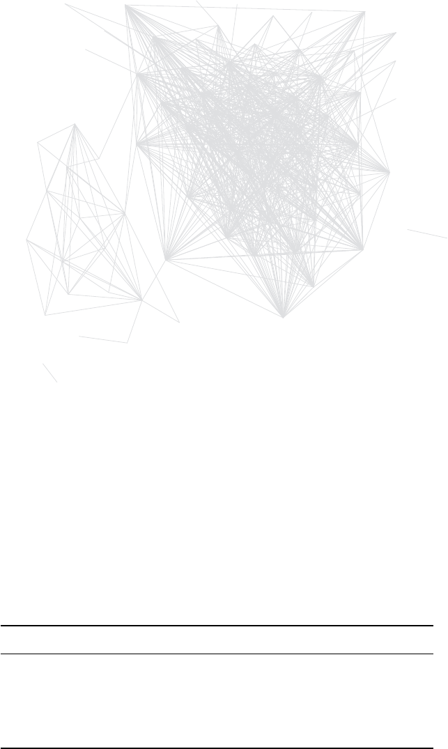
COLLABORATION NETWORKS IN THE US SENATE 357
begich, mark
bingaman, jeff
boxer, barbara
brown, sherrod
casey, robert p., jr.
clinton, hillary rodham
durbin, richard
kennedy, edward m.
kerry, john f.
klobuchar, amy
lautenberg, frank r.
levin, carl
lieberman, joseph i.
mccaskill, claire
menendez, robert
reid, harry
schumer, charles e.
stabenow, debbie
mikulski, barbara a.
wyden, ron
dodd, christopher j.
harkin, tom
inouye, daniel k.
akaka, daniel k.
shaheen, jeanne
feinstein, dianne
leahy, patrick j.
carper, thomas r.
conrad, kent
alexander, lamar bennett, robert f.
brown, scott p.
chambliss, saxby
collins, susan m.
corker, bob
snowe, olympia j.
voinovich, george v.
isakson, johnny
brownback, sam
burr, richard
coburn, tom
crapo, mike
demint, jim
ensign, john
enzi, michael b.
graham, lindsey
hatch, orrin g.
johanns, mike
kyl, jon
mccain, john
risch, james e.
roberts, pat
thune, john
vitter, david
wicker, roger f.
baucus, max
burris, roland
cantwell, maria
hagan, kay
murray, patty
reed, jack
sanders, bernard
tester, jon
whitehouse, sheldon
nelson, bill
rockefeller, john d., iv
lincoln, blanche l.
dorgan, byron l.
bayh, evan
feingold, russell d.
franken, al
specter, arlen
barrasso, john
bond, christopher s.
bunning, jim
cochran, thad
cornyn, john
hutchison, kay bailey
inhofe, james m.
lugar, richard g.
martinez, mel
mcconnell, mitch
sessions, jeff
grassley, chuck
gregg, judd
cardin, benjamin l.
johnson, tim kaufman, edward e.
merkley, jeff
landrieu, mary l.
murkowski, lisa
kohl, herb
gillibrand, kirsten e.
bennet, michael f.
lemieux, george s.
nelson, e. benjamin
pryor, mark l.
udall, mark
udall, tom
warner, mark r.
webb, jim
salazar, ken
byrd, robert c.
kirk, paul grattan, jr.
shelby, richard c.
coons, christopher a.
goodwin, carte patrick
kirk, mark steven
manchin, joe, iii
Figure 12.2 Cosponsorship network of senators
is Senator Richard Burr from North Carolina. Time and again, she was considered one of
the likely candidates for a party switch which nds a clear visual expression in our analysis.
By a similar token, consider Mary Landrieu from Louisiana. She is frequently labeled as one
of the most conservative Democrats in the Democratic party and indeed she also takes up a
central location in our graph.
Table 12.5 The ve most central actors
Senator Betweenness
Goodwin, Carte Patrick (D-WV) 2217
Salazar, Ken (D-CO) 2058
Clinton, Hillary Rodham (D-NY) 1062
Kirk, Paul Grattan, Jr. (D-MA) 618
Coons, Christopher A. (D-DE) 245
The tables displays the ve most central senators, based on their betweenness scores.
358 AUTOMATED DATA COLLECTION WITH R
Consider now a true network metric—the betweenness centrality. This measure describesBetweenness
centrality how central any given node is in the overall network, which is typically taken as an indicator
of inuence in a network. It is dened as the shortest path from all nodes to all other passing
through a node. The higher the score, the more central the actor’s position in the network.
Table 12.5 provides an overview of the ve most central actors, ranked by betweenness. We
nd that among the ve most central actors there are no less than two who went on to serve
as secretaries in the Obama Administration.
12.4 Conclusion
Scholars of parliamentary politics have recently begun employing large-scale data sources in
order to come to terms with long-standing research questions. Among the issues that have
come under scrutiny are patterns of intra-parliamentary collaboration. Using cosponsorships
as proxies for cooperation, a number of scholars have investigated these manifested networks.
This chapter has demonstrated how to assemble the necessary data to perform analyses of
the like that have been proposed in the literature. We have shown that the data informing
these analyses are vast. We were able to collect well over 100,000 unique dyadic relations in
a single senatorial term. In terms of substance, we have not delved deeply into the data but,
using very simple indicators, we were able to show that the data exhibit strong face validity.
First, moderate members of either party have been shown to take up plausible center points in
the network. Second, senators who are widely perceived as inuential members of the body
could indeed be shown to take up more central locations in the network.
As in many of the examples throughout this volume there are clear advantages of auto-
matically collecting the data as proposed here. We have only assembled a single senatorial
term, but the resulting dataset is immense. Never before have datasets of such size been in
the reach of single researchers interested in a particular topic. What is more, not only is the
data vast, it is also freely available to anyone who brings the right techniques to the table.
It can quickly be updated so that results are informed by current events. And nally, using
automatic data assembly one avoids the risk of coding errors in the data which are to be
expected when hand-coding a dataset of this size. We encourage you to assemble the data
yourselves, toy around with it and investigate the ad hoc claims in this exploratory chapter to
present some new insights on patterns of parliamentary collaboration.

13
Parsing information from
semistructured documents
We have learned how to handle and extract information from well-dened data structures
like XML or JSON. There are standardized methods for translating these formats into R
data structures. Content on the Web is highly heterogeneous, however. We are occasionally
confronted with data which are structured but in a format for which no parser exists.
In this chapter, we demonstrate how to construct a parser that is able to transform pure
character data into Rdata structures. As an example we identied climate data that are
offered by the Natural Resources Conservation Service at the United States Department of
Agriculture.1We focus on a set of text les that can be downloaded from an FTP server.2
While the download procedure is simple, the les cannot be put into an Rdata structure
directly. An excerpt from one of these les is shown in Figure 13.1. The displayed data are
structured in a way which is human-readable but not (yet) understandable by a computer
program. The main goal is to describe the structure in a way that a computer can handle them.
Over the course of the case study we make use of RCurl to list les on and retrieve them
from FTP servers and draw on R’s text manipulation capabilities to build a parser for the data
les. Regular expressions are a crucial tool to solve this task.
1The example is inspired by a short code snippet in the RCurl manual which demonstrates how do download
data from FTP servers (see http://cran.at.r-project.org/web/packages/RCurl/RCurl.pdf). The question is how to
post-process semistructured data of this sort with R.
2The National Water and Climate Center also provides a SOAP-based web service (see http://www.wcc.nrcs.
usda.gov/web_service/awdb_web_service_landing.htm). We ignore this tool for a moment and concentrate on the
raw text les to demonstrate how to extract information from semistructured contexts.
Automated Data Collection with R: A Practical Guide to Web Scraping and Text Mining, First Edition.
Simon Munzert, Christian Rubba, Peter Meißner and Dominic Nyhuis.
© 2015 John Wiley & Sons, Ltd. Published 2015 by John Wiley & Sons, Ltd.
360 AUTOMATED DATA COLLECTION WITH R
13.1 Downloading data from the FTP server
First, we load RCurl and stringr. As we have learned, RCurl provides functionality to access
data from FTP servers (see Section 9.1.2) and stringr offers consistent functions for string
processing with R.
R> library(RCurl)
R> library(stringr)
A folder called Data is created to store the retrieved data les. The data we are looking
for are stored on an FTP server and accessible at a single url which we store in ftp. Note that
this is only a rather tiny subdirectory—the server provides tons of additional climate data.
R> dir.create("Data")
R> ftp <- "ftp://ftp.wcc.nrcs.usda.gov/data/climate/table/
temperature/history/california/"
The RCurl function getURL() with option dirlistonly set to TRUE asks the FTP server
to return a list of les instead of downloading a le.
R> filelist <- getURL(ftp, dirlistonly = TRUE)
This is the returned list of les:
R> str_sub(filelist, 1, 119)
[1] "19l03s_tavg.txt\r\n19l03s_tmax.txt\r\n19l03s_tmin.txt\r\n19l05s_
tavg.txt\r\n19l05s_tmax.txt\r\n19l05s_tmin.txt\r\n19l06s_tavg.txt\r\n"
In order to identify the le names, we split the text by carriage returns (\r) and new line
characters (\n) and keep only those vector items that are not empty.
R> filelist <- unlist(str_split(filelist, "\r\n"))
R> filelist <- filelist[!filelist == ""]
R> filelist[1:3]
[1] "19l03s_tavg.txt" "19l03s_tmax.txt" "19l03s_tmin.txt"
A comparison with the les at the FTP interface reveals that we have succeeded in
identifying the le names. As we are not interested in minimum or maximum temperatures
for now, we use str_detect() to only keep les containing tavg in their le name.
R> filesavg <- str_detect(filelist, "tavg")
R> filesavg <- filelist[filesavg]
R> filesavg[1:3]
[1] "19l03s_tavg.txt" "19l05s_tavg.txt" "19l06s_tavg.txt"
To download the les we have to construct the full URLs that point to their location on
the server. We concatenate the base URL and the created vector of le names and retrieve a
vector of full URLs.
R> urlsavg <- str_c(ftp, filesavg)
R> length(urlsavg)
[1] 32
R> urlsavg[1]
PARSING INFORMATION FROM SEMISTRUCTURED DOCUMENTS 361
[1] "ftp://ftp.wcc.nrcs.usda.gov/data/climate/table/temperature/
history/california/19l03s_tavg.txt"
Having built the URLs for the 32 les, we can now loop over each URL and save the
text les to our local folder. We introduce a check if the le has previously been downloaded
using the file.exists() function and stop for 1 second after each server request. The les
themselves are downloaded with download.file() and stored in the Data folder.
R> for (i in seq_along(urlsavg)) {
fname <- str_c("Data/", filesavg[i])
if (!file.exists(fname)) {
download.file(urlsavg[i], fname)
Sys.sleep(1)
}
}
A brief inspection of the local folder reveals that we succeeded in downloading all 32 les.
R> length(list.files("Data"))
[1] 32
R> list.files("Data")[1:3]
[1] "19l03s_tavg.txt" "19l05s_tavg.txt" "19l06s_tavg.txt"
13.2 Parsing semistructured text data
Now that we have downloaded all the les we want, we can have a look at their content. Let
us reconsider Figure 13.1 which provides an example of the content of the les. Because they
are quite long—more than 1,000 lines, we only present a small sample.
Each le provides daily temperature data for one station in California ranging from 1987 A look at the
raw data
up to 2013. We see from the sample that for each year there is a separate section ending with --
--------. The rst line tells us something about the source of the data (/cdbs/ca/snot06),
followed by the year expressed as two digits (88) and the type of data that is presented (Aver-
age Air Temperature). Next is a line identifying the station at which the temperatures
were measured (Station : CA19L03S, HAGAN'S MEADOW), followed by a line express-
ing the unit in which the measurements are stored (Unit = degrees C).
After the header sections comes the actual data presented in a table, where columns Why base R
functions fail
indicate months and rows refer to days. If days do not exist within a month—like November
31—we nd three dashes in the cell: ----. Beneath the daily temperature we also nd a
section with monthly data that provides mean, maximum, and minimum temperatures for
each month. If the temperature data tables would be the only information provided and
the only information we were interested in, our task would be easy because Rcan handle
tables written in xed-width format: read.fwf() reads such data and transforms them
automatically into data frames. The problem is that we do not want to loose the information
from the header section because it tells us to which year and which station the temperatures
belong to.
When we proceed, it is important to think about which information should be extracted
and what the data should look like at the end. In the end a long table with daily temperatures
and variables for the day, month, and year when the temperatures were measured as well as

362 AUTOMATED DATA COLLECTION WITH R
1/cdbs/ca/snot06 88 Average Air Temperature
3Station : CA19L03S, HAGAN'S MEADOW
4------- Unit = degrees C
6day oct nov dec jan feb mar apr may [...]
7--- --- --- --- --- --- --- --- --- [...]
81 10 3 -0 -14 -9 -0 -1 -4 [...]
92 9 2 0 -10 -10 -2 -1 -5 [...]
10 3 10 -1 3 -3 -10 -1 3 1 [...]
12 [...]
14 31 2 --- -12 -4 --- -3 --- -0 [...]
16 mean 6 -0 -5 -3 -2 -0 2 4 [...]
17 max 11 6 5 3 2 6 7 11 [...]
18 min -3 -6 -15 -14 -10 -12 -3 -5 [...]
19 ----------
20 /cdbs/ca/snot06 89 Average Air Temperature
22 Station : CA19L03S, HAGAN'S MEADOW
23 ------- Unit = degrees C
25 day oct nov dec jan feb mar apr may [...]
27 [...]
Figure 13.1 Excerpt from a text le on temperature data from Californian weather stations,
accessible at ftp://ftp.wcc.nrcs.usda.gov/data/climate/table/temperature/history/california/
the station’s id and its name should do. The resulting data structure should look like the one
depicted in Table 13.1.
Because information is separated into sections, we should rst split the text to turn them
Import data
into separate vectors. To do this, we rst read in all the text les via readLines() and input
the resulting lines into a vector.
R> txt <- character()
R> for (i in 1:length(filesavg)) {
txt <- c(txt, readLines(str_c("Data/", filesavg[i])))
}
In a next step, we collapse the whole vector into one single line, where the newline
character (\n) marks the end of the original lines. We split that single line at each occurrence
of ----------\n, marking the end of a section.
R> txt <- str_c(txt, collapse = "\n")
R> txtparts <- unlist(str_split(txt, "----------\n"))

PARSING INFORMATION FROM SEMISTRUCTURED DOCUMENTS 363
Table 13.1 Desired data structure after parsing
day month year id name
1 1 1982 XYZ001784 Deepwood
2 1 1982 XYZ001784 Deepwood
... ... ... ... ...
31 12 1984 XYZ001786 Highwood
1 1 1985 XYZ001786 Highwood
……… … …
3 3 2003 XYZ001800 Northwood
4 3 2003 XYZ001800 Northwood
The resulting vector contains one section per line.
R> str_sub(txtparts[28:30], 1, 134)
[1] "\n***This data is provisional and subject to change.\n/cdbs/ca/snot06
84 Average Air Temperature\n\nStation : CA19L05S, BLUE LAKES\n---–"
[2] "/cdbs/ca/snot06 85 Average Air Temperature\n\nStation : CA19L05S,
BLUE LAKES\n------- Unit = degrees C\n\nday oct nov dec jan "
[3] "/cdbs/ca/snot06 86 Average Air Temperature\n\nStation : CA19L05S,
BLUE LAKES\n------- Unit = degrees C\n\nday oct nov dec jan "
In a text editor, this would look as follows:
R> cat(str_sub(txtparts[28], 1, 604))
***This data is provisional and subject to change.
/cdbs/ca/snot06 84 Average Air Temperature
Station : CA19L05S, BLUE LAKES
------- Unit = degrees C
day oct nov dec jan feb mar apr may jun jul aug sep
--- --- --- --- --- --- --- --- --- --- --- --- ---
1 1 2-3-4-1-2-8-1 1212 8
2 3 1-2-6-4 0-6-2 71412 9
3 3 2-3-3-5-2-4 0 6161111
4 5 5-6-1-4-4-1 3 6171112
5 8 5 -11 -0 -4 -5 -0 1 2 17 12 13
Now we need to do some cleansing to get rid of the statement saying that the data are
provisional and delete all lines of the vector that are empty.
R> txtparts <- str_replace(txtparts,"\n\\*\\*\\*This data is
provisional and subject to change.", "")
R> txtparts <- str_replace(txtparts,"ˆ\n", "")
R> txtparts <- txtparts[txtparts!=""]
Having inserted each section into a separate line, we can now build functions for extracting Extracting
information
information that can be applied to each line, as each line contains the same kind of information
364 AUTOMATED DATA COLLECTION WITH R
structured in the same way. We start by extracting the year in which the temperature was
measured. To do this, we build a regular expression that looks for a character sequence that
starts with two digits, followed by two white spaces, followed by Average Air Temperature:
"[[:digit:]]{2} Average Air Temperature". We then extract the digits from that
substring and append the two digits in a third step to a four digit year.
R> year <- str_extract(txtparts, "[[:digit:]]{2} Average Air Temperature")
R> year[1:4]
[1] "87 Average Air Temperature" "88 Average Air Temperature"
[3] "89 Average Air Temperature" "90 Average Air Temperature"
R> year <- str_extract(year, "[[:digit:]]{2}")
R> year <- ifelse(year < 20, str_c(20, year), str_c(19, year))
R> year <- as.numeric(year)
R> year[5:15]
[1] 1991 1992 1993 1994 1995 1996 1997 1998 1999 2000 2001
We also gather the stations’ names as well as the identication. For this we rst extract
the line where the station information is saved.
R> station <- str_extract(txtparts, "Station : .+?\n")
R> station[1:2]
[1] "Station : CA19L03S, HAGAN'S MEADOW\n"
[2] "Station : CA19L03S, HAGAN'S MEADOW\n"
We delete those parts that are of no interest to us—Station : and \n…
R> station <- str_replace_all(station, "(Station : )|(\n)", "")
R> station[1:2]
[1] "CA19L03S, HAGAN'S MEADOW" "CA19L03S, HAGAN'S MEADOW"
…and split the remaining text into one part that captures the id and one that contains the
name of the station.
R> station <- str_split(station, ", ")
R> station[1]
[[1]]
[1] "CA19L03S" "HAGAN'S MEADOW"
The splitting of the text results in a list where each list item contains two strings. The rst
string of each list item is the id while the second captures the name. To extract the rst and
second string from each list item, we apply the [operator to each item.
R> id <- sapply(station, "[", 1)
R> name <- sapply(station, "[", 2)
R> id[1:3]
[1] "CA19L03S" "CA19L03S" "CA19L03S"
R> name[1:3]
[1] "HAGAN'S MEADOW" "HAGAN'S MEADOW" "HAGAN'S MEADOW"
Now we can turn our attention to extracting the daily temperatures. The temperatures formExtracting
temperatures a table in xed-width format that can be read and transformed by read.fwf(). In the xed
width format each entry of a column has the same width of characters and lines are separated
PARSING INFORMATION FROM SEMISTRUCTURED DOCUMENTS 365
by newline characters or carriage returns or a combination of both. What we have to do is to
extract that part of each section that forms the xed width table and apply read.fwf() to it.
Our rst task is to extract the part that contains the temperature table. To do so, we use a
regular expression that extracts day and everything after.
R> temperatures <- str_extract(txtparts, "day.*")
Further below, we will write the next steps into a function that we can apply to each of the
temperature tables, but for now we go through the necessary steps using only one temperature
table to develop all the intermediate steps.
As read.fwf() expects a lename as input, we rst have to write our temperature table
into a temporary le using the tempfile() function.
R> tf <- tempfile()
R> writeLines(temperatures[5], tf)
We can then use read.fwf() to read the content back in. The width option tells the
function the column width in characters.
R> temptable <- read.fwf(tf, width=c(3, 7, rep(6, 11)), stringsAsFactors
=F)
R> temptable[c(1:5,32:38), 1:10]
V1 V2 V3 V4 V5 V6 V7 V8 V9 V10
1 day oct nov dec jan feb mar apr may jun
2 --- --- --- --- --- --- --- --- --- ---
31101-3-6-20227
4 2 9 -4 -7 -6 1 -3 -0 -4 6
5 3 8 -5 -5 -5 1 -3 -1 -2 6
3230 5-2-13-4----2377
33 31 5 --- -9 -3 --- 0 --- 7 ---
34 <NA> <NA> <NA> <NA> <NA> <NA> <NA> <NA> <NA> <NA>
35 mea n 6 -1 -7 -4 0 -5 -1 2 6
36max1075131687
37 min -0 -10 -22 -9 -2 -10 -6 -4 6
38 <NA> <NA> <NA> <NA> <NA> <NA> <NA> <NA> <NA> <NA>
There are several lines in the data that do not contain the data we need. Therefore, we
only keep lines 3–33 and also discard the rst column.
R> temptable <- temptable[3:33, -1]
In the next step, we transform the table into a vector. Using as.numeric() and unlist()
all numbers will be transferred to type numeric, while all cells containing only white spaces
or --- are set to NA.
R> temptable <- as.numeric(unlist(temptable))
Having discarded the table structure and kept only the temperatures, we now have to Reconstructing
tables
reconstruct the days and months belonging to the temperatures. Fortunately, unlist()
always decomposes data frames in the same way. It starts with all rows of the rst column and
appends the values of the following columns one by one. As we know that in the temperature
tables rows referred to days and columns to months, we can simply repeat the day sequence
1–31 twelve times to get the days right. Similarly, we have to repeat each month 31 times.
366 AUTOMATED DATA COLLECTION WITH R
Note that the order of the months differs from the usual 1–12 because the tables start with
October.
R> day <- rep(1:31, 12)
R> month <- rep(c(10:12, 1:9), each = 31)
Now we combine the information on the year of measurement and the weather station
with the temperatures and get the data for 1 year.
R> temptable <- data.frame(avgtemp = temptable, day = day, month =
month, year = year[5], name = name[5], id = id[5])
R> head(temptable, 3)
avgtemp day month year name id
1 10 1 10 1991 HAGAN'S MEADOW CA19L03S
2 9 2 10 1991 HAGAN'S MEADOW CA19L03S
3 8 3 10 1991 HAGAN'S MEADOW CA19L03S
To get all the data, we have to repeat the procedure for all les. For convenience we haveConstructing a
convenient
parser function
constructed a parsing function that takes a le name as argument and returns a ready-to-use
data frame. The code is shown in Figure 13.2. Applying the function yields:
R> tempData1 <- parseTemp(str_c("Data/", filesavg[1]))
R> dim(tempData1)
[1] 9551 6
R> tempData1[500:502, ]
avgtemp day month year id name
774 6 29 10 1989 CA19L03S HAGAN'S MEADOW
775 6 30 10 1989 CA19L03S HAGAN'S MEADOW
776 4 31 10 1989 CA19L03S HAGAN'S MEADOW
This looks like a successful parsing result. Furthermore, to conveniently parse all lesParsing all les
at once, we can create a wrapper function that takes a vector of le names as argument and
returns a combined data frame.
R> parseTemps <- function(filenames) {
tmp <- lapply(filenames, parseTemp)
tempData <- NULL
for (i in seq_along(tmp)) tempData <- rbind(tempData, tmp[[i]])
return(tempData)
}
Finally we apply the wrapper to all les in our folder.
R> tempData <- parseTemps(str_c("Data/", filesavg))
R> dim(tempData)
[1] 252463 6

PARSING INFORMATION FROM SEMISTRUCTURED DOCUMENTS 367
1parseTemp <- function(filename)
2# get text
3txt <- paste( readLines(filename), collapse="\n")
4# split text into year tables
5txtparts <- unlist(str_split(txt, "----------\n"))
6# cleansing
7txtparts <- str_replace(txtparts,
8"\n\\*\\*\\*This data is provisional and subject to change.", "")
9txtparts <- str_replace(txtparts,"ˆ\n","")
10 txtparts <- txtparts[txtparts!=""]
11 # get the year
12 year <- str_extract(txtparts,"[[:digit:]]{2} Average Air Temperature")
13 year <- str_extract(year,"[[:digit:]]{2}")
14 year <- ifelse(year < 20, str_c(20,year), str_c(19,year))
15 year <- as.numeric(year)
16 # get station and name
17 station <- str_extract(txtparts, "Station : .+?\n")
18 station <- str_replace_all(station, "(Station : )|(\n)", "")
19 station <- str_split(station,", ")
20 id <- sapply(station, '[', 1)
21 name <- sapply(station, '[', 2)
22 # extract part of the sections that contains daily temperatures
23 temperatures <- str_extract(txtparts, "day.*")
24 # prepare object to store temperature data
25 tempData <- data.frame(avgtemp = NA, day = NA, month = NA,
26 year = NA, id = "", name = "")
27 # generate day and month patterns matching the order of temperatures
28 day <- rep(1:31, 12)
29 month <- rep( c(10:12,1:9), each=31 )
30 # helper function
31 doTemp <- function(temperatures, year, name, id){
32 # write fixed width table into temporary file
33 tf <- tempfile()
34 writeLines(temperatures, tf)
35 # read in data and transform to data frame
36 temptable <- read.fwf(tf, width = c(3,7,6,6,6,6,6,6,6,6,6,6,6),
37 stringsAsFactors = F)
38 # keep only those lines and rows entailing day-temperatures
39 temptable <- temptable[3:33, -1]
40 # transform data frame of strings to vector of type numeric
41 temptable <- suppressWarnings(as.numeric(unlist(temptable)))
42 # combine data
43 temptable <- data.frame(avgtemp = temptable, day = day,
44 month = month, year = year, name = name, id = id)
45 # add data to tempData
46 tempData <<- rbind(tempData, temptable)
47 }
48 mapply(doTemp, temperatures, year, name, id)
49 tempData <- tempData[!is.na(tempData$avgtemp),]
50 return(tempData)
51 }
Figure 13.2 R-based parsing function for temperature text les
368 AUTOMATED DATA COLLECTION WITH R
13.3 Visualizing station and temperature data
We conclude the study with some examples of what to do with the data. First it would be nice
to know the location of the weather stations. We already know that they are in California, but
want to be a little more specic. Browsing the FTP server we nd a le that contains data
on the stations—station names, their position expressed as latitudes and longitudes as well as
their altitude. We download the le and read it in via read.csv() .
R> download.file("ftp://ftp.wcc.nrcs.usda.gov/states/ca/jchen/CA_
sites.dat", "Data_CA/CA_sites.dat")
R> stationData <- read.csv("Data_CA/CA_sites.dat", header = F, sep =
"|")[,-c(1,2,7:9)]
R> names(stationData) <- c("name","lat","lon","alt")
R> head(stationData,2)
name lat lon alt
1 ADIN MTN 4115 12046 6200
2 BLUE LAKES 3836 11955 8000
With regards to the map which we are going to use, we have to rescale the coordinates.
First, we multiply all longitudes by −1 to get general longitudes and divide all coordinates
by 100. Altitudes are measured in foot, so we transform them to meters.
R> stationData$lon <- stationData$lon * -1
R> stationData[, c("lat", "lon")] <- stationData[, c("lat", "lon")]/100
R> stationData$alt <- stationData$alt/3.2808399
R> stationData <- stationData[order(stationData$lat), ]
R> head(stationData, 2)
name lat lon alt
25 VIRGINIA LAKES RIDGE 38.05 -119.2 2804
14 LEAVITT LAKE 38.16 -119.4 2865
Now we plot the stations’ locations on a map. In R, there are several packages suitableDownloading
maps for plotting maps (see also Chapter 15). We choose RgoogleMaps which enables us to use
services provided by Google and OpenStreetMap to download maps that we can use for
plotting. We download map data from Open Street Maps using the GetMap.OSM() function.
With this function we dene a bounding box of coordinates and a scale factor. The map data
are saved on disk in PNG format as map.png and in an Robject called map for later use:
R> map <- GetMap.OSM(latR = c(37.5, 42), lonR = c(-125, -115), scale =
5000000, destfile = "map.png", GRAYSCALE = TRUE, NEWMAP = TRUE)
Now we can use PlotOnStaticMap() to print the weather stations’ locations on theMapping
stations map we previously downloaded. The result is presented in Figure 13.3.
R> png("stationmap.png", width = dim(readPNG("map.png"))[2], height =
dim(readPNG("map.png"))[1])
R> PlotOnStaticMap(map, lat = stationData$lat, lon = stationData$lon,
cex = 2, pch = 19, col = rgb(0, 0, 0, 0.5), add = FALSE)
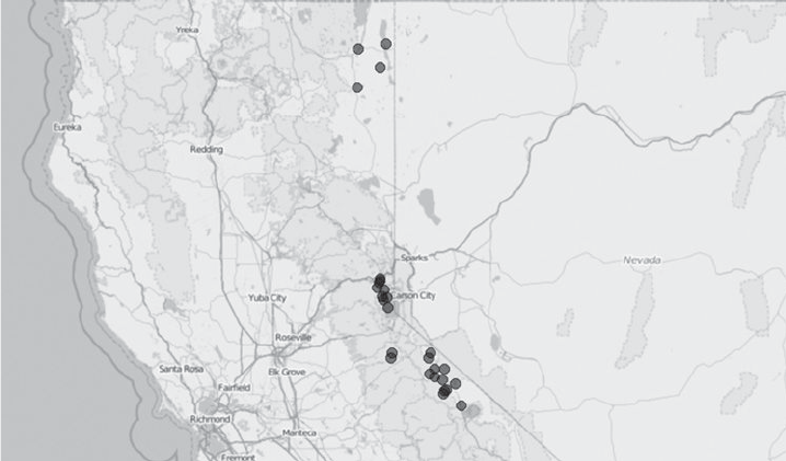
PARSING INFORMATION FROM SEMISTRUCTURED DOCUMENTS 369
Figure 13.3 Weather station locations on an OpenStreetMaps map
Finally, we visualize the temperature data. Let us look at the average temperatures per Creating
temperature
curves
month for six out of 27 stations. First, we aggregate the temperatures per month and station
using the aggregate() function.
R> monthlyTemp <- aggregate(x = tempData$avgtemp, by = list(name =
tempData$name, month = tempData$month), FUN = mean)
The stations we choose are representative of all others—we select three stations which
are placed north of the the mean latitude and three south of it. Furthermore, within each group
stations should differ regarding their altitude and should roughly match one station of the
other group. Looking through the candidates we nd the following stations to be tting and
extract their coordinates and their altitude:
R> stationNames <- c("ADIN MTN", "INDEPENDENCE CAMP", "SQUAW VALLEY
G.C.", "SPRATT CREEK", "LEAVITT MEADOWS","POISON FLAT")
R> stationAlt <- stationData[match(stationNames, stationData$name), ]$alt
R> stationLat <- stationData[match(stationNames, stationData$name), ]$lat
R> stationLon <- stationData[match(stationNames, stationData$name), ]$lon
Then, we prepare a plotting function to use on all plots. The function rst denes an
object called iffer that serves to select only those monthly temperatures that belong to the
station to be plotted. The overall average per station and month is plotted with adequate title
and axis labels. We add a horizontal line to mark 0◦C . To get an idea of the variation of
temperature measurements over time, we add the actual temperature measurements in a last
step as small gray dots.
R> plotTemps <- function(i){
R> iffer <- monthlyTemp$name == stationNames[i]
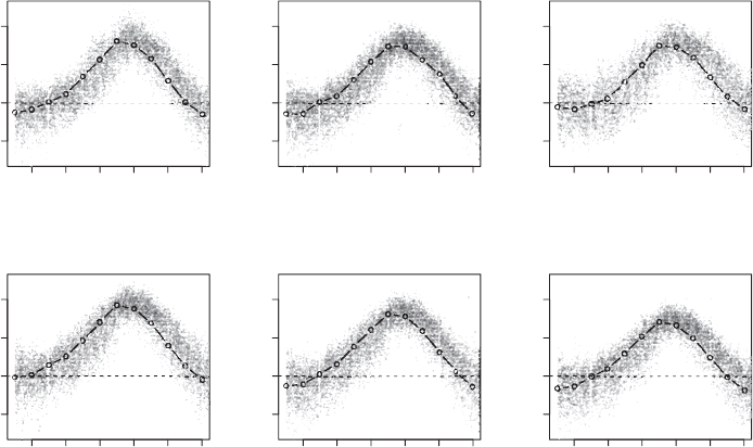
370 AUTOMATED DATA COLLECTION WITH R
−10 0 10 20
ADIN MTN (1890m)
Lat.= 41.15 Lon.= −120.46
24681012
Month
24681012
Month
24681012
Month
24681012
Month
24681012
Month
24681012
Month
Average temperature
−10 0 10 20
Average temperature
−10 0 10 20
Average temperature
−10 0 10 20
Average temperature
−10 0 10 20
Average temperature
−10 0 10 20
Average temperature
INDEPENDENCE CAMP (2134m)
Lat.= 39.27 Lon.= −120.17
SQUAW VALLEY G.C. (2499m)
Lat.= 39.11 Lon.= −120.15
SPRATT CREEK (1890m)
Lat.= 38.4 Lon.= −119.49
LEAVITT MEADOWS (2195m)
Lat.= 38.2 Lon.= −119.33
POISON FLAT (2408m)
Lat.= 38.3 Lon.= −119.38
Figure 13.4 Overall monthly temperature means for selected weather stations. Lines present
average monthly temperatures in degree Celsius for all years in the dataset. Small gray dots
are daily temperatures for all years within the dataset.
R> plot(monthlyTemp[iffer, c("month", "x")],
R> type = "b", main = str_c(stationNames[i],
R> "(",round(stationAlt[i]), "m)", "\n Lat.= ",
R> stationLat[i], " Lon.= ", stationLon[i]),
R> ylim = c(-15, 25), ylab = "average temperature")
R> abline(h = 0,lty = 2)
R> iffer2 <- tempData$name == stationNames[i]
R> points(tempData$month[iffer2] + tempData$day[iffer2] *0.032,
R> jitter(tempData$avgtemp[iffer2], 3),
R> col = rgb(0.2, 0.2, 0.2, 0.1), pch = ".")
R>}
Having dened the plot function, we loop through the selection of stations.
R> par(mfrow = c(2, 3))
R> for (i in seq_along(stationNames)) plotTemps(i)
Figure 13.4 presents the average monthly temperatures. Little surprisingly, the higher
the altitude of the station and the more north the station is located, the lower the average
temperatures.

14
Predicting the 2014 Academy
Awards using Twitter
Social media and the social network Twitter, in particular, have attracted the curiosity of
scientists from various disciplines. The fact that millions of people regularly interact with the
world by tweeting provides invaluable insight into people’s feelings, attitudes, and behavior.
An increasingly popular approach to make use of this vast amount of public communication
is to generate forecasts of various types of events. Twitter data have been used as a prediction
tool for elections (Tumasjan et al. 2011), spread of inuenza (Broniatowski et al. 2013;
Culotta 2010), movie sales (Asur and Huberman 2010), or the stock market (Bollen et al.
2011).
The idea behind these approaches is the “wisdom of the crowds” effect. The aggregated
judgment of many people has been shown to frequently be more precise than the judgment
of experts or even the smartest person in a group of forecasters (Hogarth 1978). In that sense,
if it is possible to infer forecasts from people’s tweets, one might expect a fairly accurate
forecast of the outcome of an event.
In this case study, we attempt to predict the winners of the 2014 Academy Awards using
the tweets in the days prior to the event. Specically, we try to predict the results of three
awards—best picture, best actress, and best actor. A similar effort to ours is proposed by
Ghomi et al. (2013). In the next section, we elaborate the data collection by introducing the
Twitter APIs and the specic setup we used to gather the tweets. Section 14.2 goes on to
elaborate the data preparation and the forecasts.
Automated Data Collection with R: A Practical Guide to Web Scraping and Text Mining, First Edition.
Simon Munzert, Christian Rubba, Peter Meißner and Dominic Nyhuis.
© 2015 John Wiley & Sons, Ltd. Published 2015 by John Wiley & Sons, Ltd.

372 AUTOMATED DATA COLLECTION WITH R
Table 14.1 Overview of selected functions from the twitteR package
Function Description Example
searchTwitter() Search for tweets that match a
certain query; the query
should be URL-encoded
and special query operators
can be used1
searchTwitter("#superbowl")
getUser() Gather information about
Twitter users with public
proles (or the API user )
getUser("RDataCollection")
getTrends() Pull trending topics from a
given location dened by a
WOEID
getTrends(2422673)
twListToDF() Convert list of twitteR class
objects into data frame
twListToDF(tweets)
14.1 Twitter APIs: Overview
Before turning to the Twitter-based forecasts, we provide an overview of the basic features
of Twitter’s APIs.2The range of features is vast and we will only make use of a tiny part, so
it is useful to get an intuition about the possibilities of Twitter’s web services. Twitter offers
various APIs for developers. They are documented at https://dev.twitter.com/docs.Usingthe
APIs requires authentication via OAuth (see Section 9.1.11). In the following, we shortly
discuss the REST API and the Streaming APIs.
14.1.1 The REST API
The REST API comprises a rich set of resources.3They offer access to the user’s account,
timeline, direct messages, friends, and followers. It is also possible to retrieve trending top-
ics for a specic location (WOEID; see Section 9.1.10) or to collect tweets that match
certain lter parameters, for example, keywords. Note, however, that there are restric-
tions regarding possibility to gather statuses retrospectively. There are also rate limits to
bear in mind. As both limits are subject to changes, we refer to the documentation at
https://dev.twitter.com/docs/rate-limiting/1.1 for details.
The twitteR package provides a wrapper for the REST API (Gentry 2013), thus we do not
have to specify GET and POST requests ourselves to connect to Twitter’s web service. The
package provides functionality to convert incoming JSON data into common Rdata structures.
We list a subset of the package’s functions which we nd most useful in Table 14.1. For a
1See https://dev.twitter.com/docs/using-search.
2We assume that you have a basic knowledge about how Twitter works. If not, check out the amusing introduction
at http://www.momthisishowtwitterworks.com/
3For a detailed overview, see https://dev.twitter.com/docs/api/1.1

PREDICTING THE 2014 ACADEMY AWARDS USING TWITTER 373
more detailed description of the package check out Jeff Gentry’s helpful introduction at
http://geoffjentry.hexdump.org/twitteR.pdf
14.1.2 The streaming APIs
Another set of Twitter APIs are subsumed under the label Streaming APIs. They allow low
latency access to Twitter’s global data stream, that is practically in real time.4In contrast to
the REST APIs, the Streaming APIs require a persistent HTTP connection. As long as the
connection is maintained, the application that taps the API streams data from one of the data
ows.
Several of these streams exist. First, Public Streams provide samples of the public data Types of
Streaming APIs
ow. Twitter offers about 1% of the full sample of Tweets to ordinary users of the API. The
sample can be ltered by certain predicates, for example, by user IDs, keywords, or locations.
For data mining purposes, this kind of stream might be one of the most interesting, as it
provides tools to scour Twitter by many criteria. In this case study, we will tap this API to
identify tweets that mention the 2014 Academy Awards by ltering a set of keywords. The
second type of Streaming API provides access to User Streams. This API returns tweets from
the user’s timeline. Again, we can lter tweets according to keywords or types of messages,
for example, only tweets from the user or tweets from her followings. Finally, the third type
of Streaming API is Site Streams which provides real-time updates from users for certain
services. This is basically not much different from User Streams but additionally indicates
the recipient of a tweet.5At the time of writing, the Site Streams API is in a restricted beta
status, so we refrain from going into more details.
Fortunately, we do not have to become experts with the inner workings of the streaming
APIs, as the streamR provides a convenient wrapper to access them with R(Barber´
a 2013).
Table 14.2 provides an overview of the most important functions that we have used to assemble
the dataset that we draw on for the predictions in the second part of this chapter.
14.1.3 Collecting and preparing the data
To collect the sample of tweets that revolve around the 2014 Academy Awards, we set up
a connection to the Streaming API. The connection was opened on February 28, 2014 and
closed on March 2, 2014, the day the 86th Academy Awards ceremony took place at the
Dolby Theatre in Hollywood.
We began by registering an application with Twitter to retrieve the necessary OAuth
credentials which allow tapping the Twitter services. A connection to the Streaming API was
established using the streamR interface. The command to initiate the collection was
R> filterStream("tweets_oscars.json", track = c("Oscars", "Oscars2014"),
timeout = 10800, oauth = twitCred)
We ltered the sample of tweets using filterStream() with the track option with
the keywords “Oscars” and “Oscars2014”, which matched any tweet that contained these
terms in the form of hash tags or pure text. We split the process into streams of 3 hours
each (60 ∗60 ∗3=10, 800 for the timeout argument) to store the incoming tweets in
4See the Streaming APIs’ documentation at https://dev.twitter.com/docs/api/streaming
5See also https://dev.twitter.com/docs/streaming-apis/streams/site

374 AUTOMATED DATA COLLECTION WITH R
Table 14.2 Overview of selected functions from the streamR package
Function Description Example
filterStream() Connection to the Public
Streams API; allows to
lter by keywords (track
argument), users (follow),
locations (locations),
and language
filterStream(file.name =
"superbowl_tweets.json",
track = "superbowl",
oauth = twitter_sig)’
sampleStream() Connection to the Public
Streams API; returns a
small random sample of
public tweets
sampleStream(file.name =
"tweets.json", timeout =
60, oauth = twitter_sig)’
userStream() Connection to the User
Streams API; returns
tweets from the user’s
timeline; allows to lter by
message type, keywords,
and location
sampleStream(userStream =
"mytweets.json", with =
"user", oauth =
twitter_sig)’
parseTweets() Parses the downloaded
tweets, that is, returns the
data in a data frame
parseTweets("tweets.json")’
manageable JSON les. All in all we collected around 10 GB of raw data, or approximately
2,000,000 tweets.
After the collection was complete, we parsed the single les using the parseTweets()
function in order to turn the JSON les into an Rdata frame. We merge all les into a single
data frame. Storing the table in the Rdata format reduced the memory consumption of the
collected tweets to around 300 MB.
R> tweets <- parseTweets("tweets_oscars.json", simplify = TRUE)
14.2 Twitter-based forecast of the 2014 Academy Awards
14.2.1 Visualizing the data
Before turning to the analysis of the content of the tweets, let us visually inspect the volume
of the data for a moment. Specically, we want to create a gure of the number of tweets per
hour in our search period from the end of February to the beginning of March, 2014.6The
easiest thing to aggregate the frequency of tweets by hour is to convert the character vector in
the dataset created_at to a true time variable of type POSIXct.Wemakeuseofthelubridate
package which facilitates working with dates and times (Grolemund and Wickham 2011).
We also set our locale to US English to be able to parse the English names of the months and
6The data are available at http://www.r-datacollection.com. We invite you to download the data and play around
with it yourself. Maybe you are able to spot something that we failed to make out with our simple analysis.

PREDICTING THE 2014 ACADEMY AWARDS USING TWITTER 375
week days. Chances are that you have to adapt the value in the Sys.setlocale() function
to the needs of your machine.7
R> library(lubridate)
R> Sys.setlocale("LC_TIME", "en_US.UTF-8")
To parse the time stamp in the dataset, we use the function as.POSIXct() where we
specify the variable, the timezone, and the format of the time stamp. Let us have a look at the
rst time stamp to get a sense of the format.
R> dat$created_at[1]
[1] "Fri Feb 28 10:11:14 +0000 2014"
We have to provide the information that is contained in the time stamp in abstract terms.
In this case the stamp contains the weekday (%a),themonth(%b), the day (%d), the time
(%H:%M:%S), an offset for the timezone (%z), and the year (%Y). We abstract the various
pieces of information with the percentage placeholders and let Rparse the values.
R> dat$time <- as.POSIXct(dat$created_at, tz = "UTC", format = "%a
%b %d %H:%M:%S %z %Y")
Now that we have created a veritable time stamp where Ris able to make sense of
the information that is contained in the stamp, we can use the convenience functions from
the lubridate package to round the time to the nearest hour. This is accomplished with the
round_date() function where we specify the unit argument to be hour.
R> dat$round_hour <- round_date(dat$time, unit = "hour")
We aggregate the values in a table, convert it to a data frame and discard the last entry as
we discontinued the collection around the time so it only contains censored information.
R> plot_time <- as.data.frame(table(dat$round_hour))
R> plot_time <- plot_time[-nrow(plot_time),]
Finally, we create a simple graph that displays the hourly tweets in the collection period
from February 28 to March 2 (see Figure 14.1). We observe a sharp increase in the volume
of tweets in the hours right before the beginning of the Academy Awards.
R> plot(plot_time[,2], type = "l", xaxt = "n", xlab = "Hour", ylab =
"Frequency")
R> axis(1, at = c(1, 20, 40, 60), labels = plot_time[c(1, 20, 40, 60),
1])
14.2.2 Mining tweets for predictions
In this part of the chapter, we use the stringr and the plyr packages. We begin by loading them.
R> library(stringr)
R> library(plyr)
7If you are operating on a Windows machine, the function has to be specied as Sys.setlocale("LC_TIME",
"English").
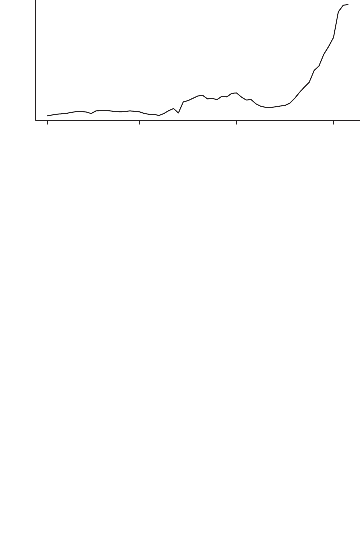
376 AUTOMATED DATA COLLECTION WITH R
0 50,000 100,000 150,000
Frequency
2014−02−28 10:00:00 2014−03−01 05:00:00 2014−03−02 01:00:00 2014−03−02 21:00:00
Figure 14.1 Tweets per hour on the 2014 Academy Awards
Let us inspect one line of the data frame to get a sense of what is available in the dataset:8
R> unlist(dat[1234,])
text
"RT @TheEllenShow: I'm very excited @Pharrell's performing his big
hit "Happy" at the #Oscars. Spolier alert: I'll be hiding in his hat."
retweet_count
"2383"
...
created_at
"Fri Feb 28 10:50:13 +0000 2014"
...
user_created_at
"Sun Jan 08 21:22:49 +0000 2012"
statuses_count
"475"
followers_count
"236"
favourites_count
"23"
...
friends_count
"132"
screen_name
"SophiaGracer007"
lotext
"rt @theellenshow: i'm very excited @pharrell's performing his big
hit "happy" at the #oscars. spolier alert: i'll be hiding in his hat."
time
"1393584613"
round_hour
"1393585200"
8We dropped some of the variables to save space.

PREDICTING THE 2014 ACADEMY AWARDS USING TWITTER 377
You nd that beside the actual text of the tweet there is a lot of the supplementary
information, not least the time stamp that we relied upon in the previous section. The last
three variables in the dataset are not created by twitter but were created by us. They contain
the text of the tweet that was converted to lower case using the tolower() function, as well
as the time (time) and the rounded time (round_hour).
Now, to look for references to the nominees for best actor, best actress, and best picture,
we simply create three vectors of search terms. The search terms for the actors and actresses
are simply the full name of the actor, in case of the lms we created two regular expressions
in the cases of “12 Years a Slave” and “The Wolf of Wall Street” as many users on Twitter
might have used either variation of the titles. Notice that we have specied all the vectors as
lower case as we intend to apply the search terms to the tweets in lower case.9
R> actor <- c(
"matthew mcconaughey",
"christian bale",
"bruce dern",
"leonardo dicaprio",
"chiwetel ejiofor"
)
R> actress <- c(
"cate blanchett",
"amy adams",
"sandra bullock",
"judi dench",
"meryl streep"
)
R> film <- c(
"(12|twelve) years a slave",
"american hustle",
"captain phillips",
"dallas buyers club",
"gravity",
"nebraska",
"philomena",
"(the )?wolf of wall street"
)
We go on to detect the search terms in the tweets by applying str_detect() to all tweets
in lower case (dat$lotext) via a call to lapply(). The results are converted to a common
data frame with ldply() and nally the column names are assigned meaningful names.
R> tmp_actor <- lapply(dat$lotext, str_detect, actor)
R> dat_actor <- ldply(tmp_actor)
R> colnames(dat_actor) <- c("mcconaughey", "bale", "dern", "dicaprio",
"ejiofor")
9We drop the movie “Her” as this creates a lot of noise and would require more elaborate methods than we use
in the subsequent discussion.

378 AUTOMATED DATA COLLECTION WITH R
R> tmp_actress <- lapply(dat$lotext, str_detect, actress)
R> dat_actress <- ldply(tmp_actress)
R> colnames(dat_actress) <- c("blanchett", "adams", "bullock", "dench",
"streep")
R> tmp_film <- lapply(dat$lotext, str_detect, film)
R> dat_film <- ldply(tmp_film)
R> colnames(dat_film) <- c("twelve_years", "american_hustle", "capt_
phillips", "dallas_buyers", "gravity", "nebraska", "philomena",
"wolf_wallstreet")
To inspect the results, we simply sum up the TRUE values. This is possible as the call to
sum() evaluates the TRUE values as 1, FALSE entries as 0.
R> apply(dat_actor, 2, sum)
mcconaughey bale dern dicaprio ejiofor
6190 1255 912 23479 1531
R> apply(dat_actress, 2, sum)
blanchett adams bullock dench streep
6790 5743 3272 765 3801
R> apply(dat_film, 2, sum)
twelve_years american_hustle capt_phillips dallas_buyers
11339 6122 2003 4560
gravity nebraska philomena wolf_wallstreet
22570 3602 2236 6741
We nd that Leonardo DiCaprio was more heavily debated compared to the actual winner
of the Oscar for best actor—Matthew McConaughey. In fact, there is a fairly wide gap
between DiCaprio and McConaughey. Conversely, the frequencies with which the nominees
for best actress were mentioned on Twitter are a little more evenly distributed. What is more,
the eventual winner of the trophy—Cate Blanchett—was in fact the one who received most
mentions overall. Finally, turning to the best picture we observe that it is not “12 Years a
Slave” that was most frequently mentioned but rather “Gravity” which was mentioned roughly
twice as often.
In case of the best actor and best actress, we decided to apply a sanity check. As some of
the names are fairly difcult to spell, we might potentially bias our counts against those actors
where this is the case. Accordingly, we performed an additional search that uses the agrep()
function which performs approximate matching.10 The results are summed up and unlisted
to get numeric vectors of length ve for both categories. Again, we assign meaningful names
to the resulting vectors.
R> tmp_actor2 <- lapply(actor, agrep, dat$lotext)
R> length_actor <- unlist(lapply(tmp_actor2, length))
10For details on approximate matching, see Chapter 8.
PREDICTING THE 2014 ACADEMY AWARDS USING TWITTER 379
R> names(length_actor) <- c("mcconaughey", "bale", "dern", "dicaprio",
"ejiofor")
R> tmp_actress2 <- lapply(actress, agrep, dat$lotext)
R> length_actress <- unlist(lapply(tmp_actress2, length))
R> names(length_actress) <- c("blanchett", "adams", "bullock", "dench",
"streep")
R> length_actor
mcconaughey bale dern dicaprio ejiofor
8034 1663 3672 29643 1912
R> length_actress
blanchett adams bullock dench streep
12556 6796 5464 1065 5250
The conclusions remain fairly stable, by and large. Leonardo DiCaprio was more heavily
debated than Matthew McConaughey prior to the Academy Awards and the winner of best
actress, Cate Blanchett, was most frequently mentioned after applying approximate matching.
14.3 Conclusion
Twitter is a rich playing ground for social scientists who are interested in the public debates
on countless subjects. In this chapter, we have provided a short introduction to the various
possibilities to collect data from Twitter and making it accessible for research. We have
discussed the streamR and twitteR packages to connect to the two main access points for
current and retrospective data collection.
In the specic application we have investigated whether the discussion on Twitter on the
nominees for best actor and actress as well as best picture for the 2014 Academy Awards in
the days prior to the awards reects the eventual winners. As this book is more concerned
with the data collection rather than the data analysis, the technique that was applied is almost
banal. We invite you to download the data from the accompanying website to this book and
play around with it yourself. Specically, we invite you to repeat our analysis and apply
a sentiment analysis (see Chapter 17) on the tweets to potentially improve the prediction
accuracy.

15
Mapping the geographic
distribution of names
The goal of this exercise is to collect data on the geographic distribution of surnames in
Germany. Such maps are a popular visualization in genealogical and onomastic research, that
is, research on names and their origins (Barratt 2008; Christian 2012; Osborn 2012). It has
been shown that in spite of increased labor mobility in the last decades, surnames that were
bound to a certain regional context continue to retain their geographic strongholds (Barrai
et al. 2001; Fox and Lasker 1983; Yasuda et al. 1974). Apart from their scientic value, name
maps have a more general appeal for those who are interested in the roots of their namesakes.
Plus, they visualize the data in one of the most beautiful and insightful ways—geographic
maps.
In this chapter, we briey introduce the visualization of geographic data in R. This can
be a difcult task, and if your data do not match the specications of the data treated in this
chapter, we recommend a look at Kahle and Wickham (2013) and Bivand et al. (2013b) for
more advanced visualization tools of spatial data with R. In order to acquire the necessary data,
we rely on the online directory of a German phone book provider (www.dastelefonbuch.de).
As a showcase, we visualize the geographical distribution of a set of surnames in Germany.
The goal is to write a program that can easily be fed with any surname to produce a surname
map with a single function call. Further, the call should return a data frame that contains all
of the scraped observations for further analysis.
The case study serves another purpose: It is not a storybook example of web scraping but
shows some of the pitfalls that may occur in reality—and how to deal with them. The case
study thus illustrates that textbook theory does not always match up with reality. Among the
problems we have to tackle are (a) incomplete and unsystematic data, (b) data that belong
Automated Data Collection with R: A Practical Guide to Web Scraping and Text Mining, First Edition.
Simon Munzert, Christian Rubba, Peter Meißner and Dominic Nyhuis.
© 2015 John Wiley & Sons, Ltd. Published 2015 by John Wiley & Sons, Ltd.

MAPPING THE GEOGRAPHIC DISTRIBUTION OF NAMES 381
together but are dispersed in the HTML tree, (c) limited “hits per page” functionality, and (d)
undocumented URL parameters.
15.1 Developing a data collection strategy
Before diving into the online phone book, we begin with some thoughts on the kind of
information we want to collect and whether a phone book is an appropriate source for
such information. The goal is to gain insight into the current distribution of surnames. The
distribution is dened by the universe of surnames in the German population, that is, around
80 million people. We want to collect data for descriptive as well as for secondary analyses.
The ideal source would provide a complete and up-to-date list of surnames of all inhabitants,
linked with precise geographic identiers. Such a list would raise severe privacy concerns.
By virtue of purpose, phone directories are open data sources. They provide information Benets
of phone
book data
on names and residencies, so they are a candidate to approximate the true distributions of
surnames. In terms of data quality, however, we have to ask ourselves: Are phone directories
a reliable and valid source? There is good reason to believe they are: First, they are updated
at least annually. Second, geographic identiers like streets and zip codes are usually precise
enough to assess people’s locations within a circle of less than 20 km. The fact that phone
books provide such accurate geographical identiers is actually the crucial property of the
data source in this exercise. It is difcult to come up with a freely available alternative.
On the downside, we have to be aware of the phone book’s limitations. First, not everybody Limitations of
phone book
data
has a phone and not every phone is listed in the phone directory. This problem has aggravated
with the proliferation of mobile phones. Second, phone books occasionally contain duplicates.
Using zip codes as geographic identiers adds some noise to the data, but this inaccuracy
is negligible. After all, we are interested in the big picture, not in pinpointing names at the
street level.
Regarding alternative data sources, there are several websites which provide ready-made
distribution maps, often based on phone book entries as well.1However, these pages usually
only offer aggregate statistics or remain vague about the source of the reported maps. The
same is true for commercial software that is frequently offered on these sites. Therefore, we
rely on online phone directories and produce our own maps.
In order to achieve the goals, we pursue the following strategies: Data collection
1. Identify an online phone directory that provides the information we need.
2. Become familiar with the page structure and choose an extraction procedure.
3. Apply the procedure: retrieve data, extract information, cleanse data, and document
unforeseen problems that occur during the coding
4. Visualize and analyze the data.
5. Generalize the scraping task.
1A nice overview of existing pages which offer name map services can be found at https://familysearch.org/
learn/wiki/en/Surname_Distribution_Maps

382 AUTOMATED DATA COLLECTION WITH R
Regarding our example, we have done some research on available online phone direc-
tories. There are basically two major providers in Germany, www.dastelefonbuch.de and
www.dasoertliche.de. Comparing the number of hits for a sample set of names, the results are
almost equivalent, so both providers seem to work with similar databases. The display of hits
is different, however. www.dastelefonbuch.de allows accessing a maximum of 2000 hits per
query and the number of hits per request can be adapted. Conversely, www.dasoertliche.de
offers 10,000 hits at most that are are displayed in bundles of 20s. As we prefer to minimize
the number of requests for reasons of efciency and scraping etiquette, we decide to use
www.dastelefonbuch.de as primary source of data for the exercise.
15.2 Website inspection
We start with a look at the robots.txt to check whether accessing the page’s content viaInspecting the
robots.txt automated methods is accepted at all (see Section 9.3.3). We nd that some bots are indeed
robota non grata (e.g., the Googlebot-Image and the trovitBot bot; see Figure 15.1). For other
undened bots, some directories are disallowed, for example, /scripts/ or /styles/.
The root path is not prohibited, so we can direct small automated requests to the site with a
1# robots.txt for http://www.dastelefonbuch.de/
2# sc 20130402_1.56, Vorgaengerversion: sc 20130128
3(...)
5User-agent: Googlebot-Image
6Disallow: /
8User-agent: trovitBot
9Disallow: /
11 User-agent: *
12 Disallow: /scripts/
13 Disallow: /styles/
14 Disallow: /katalog/scripts/
15 Disallow: /katalog/styles/
16 Disallow: /telefonbuch/scripts/
17 Disallow: /telefonbuch/styles/
18 (...)
20 # Sitemap files
21 Sitemap: http://www.dastelefonbuch.de/xml-sitemaps/
telefonbuch_nachnamen_sitemap_index.xml
22 Sitemap: http://www.dastelefonbuch.de/xml-sitemaps/
telefonbuch_behoerden_sitemap_index.xml
23 Sitemap: http://www.dastelefonbuch.de/xml-sitemaps/
telefonbuch_branchen_sitemap_index.xml
24 (...)
Figure 15.1 Excerpt from the robots.txt le on www.dastelefonbuch.de

MAPPING THE GEOGRAPHIC DISTRIBUTION OF NAMES 383
clear conscience. The bottom of the le reveals some interesting XML les. Accessing these
links, we nd large compressed XML les that apparently contain information on surnames
in all cities. This is potentially a powerful data source, as it might lead to the universe of
available surnames in the page’s database. We do not make use of the data, however, as it is
not immediately obvious how such a list could be used for our specic purpose.
We continue with a closer inspection of the page’s functionality and architecture. In the Examining
the page
architecture
simple search mode, we can specify two parameters—whom to search for (“Wer/Was”) and
where (“Wo”). Let us start with a sample request. We search for entries with the surname
“Feuerstein.”2In the left column, the total number of hits are reported (837), 149 of which
are businesses and 688 of which are private entries. We are only interested in private entries
and have already selected this subsample of hits. The hits themselves are listed in the middle
column of the page. Surname and, if available, rst name is reported in an entry’s rst row,
the address in the second. Some entries do not provide any address. In the rightmost column
on the page, the hits are already displayed on a map. This is the information we are looking
for, but it seems more convenient to scrape the data from the list of hits rather than from the
JavaScript-based map.3We also observe that the URL has changed after passing the request
to the server. In its complete form, it looks as follows:
http://www3.dastelefonbuch.de/?bi=76&kw=Feuerstein&cmd=search&seed=
1010762549&ort_ok=1&vert_ok=1&buab=622100&mergerid=A43F7DB343E7F461D
5506CA8A7DBB734&mdest=sec1.www1%2Csec2.www2%2Csec3.www3%2Csec4.www4
&recfrom=&ao1=1&ao2=0&sp=51&aktion=105
Evidently, passing the input form to the server has automatically added a set of parameters,
which can be observed in the URL’s query string, beginning after the ?sign.4As we need to set
these parameters with our program later on, we have to identify their meaning. Unfortunately,
there is no documentation in the page’s source code. Therefore, we try to detect their meaning
manually by playing around with them and comparing the displayed outputs. We nd that
the kw parameter contains the keyword we are searching for. Note that URL encoding is
required here, that is, we look for M%FCller instead of M¨
uller and so on. cmd=search is
the trigger for the search action, ao1=1 means that only private entries are shown. Some of
the parameters can be dropped without any changes in the displayed content. By manually
specifying some of the search parameters, we identify another useful parameter: reccount
denes the number of hits that are shown on the page. We know from search engine requests
that this number is usually limited to around 10–50 hits for efciency reasons. In this case, the
options displayed in the browser are 20, 50, and 100 hits per page. However, we can manually
specify the value in the URL and set it up to a maximum of 2000 hits. This is very useful,
as one single request sufces to scrape all available results. In general, inspecting the URL
before and after putting requests to the server often pays off in web scraping practice—and
not only for an ad-hoc URL manipulation strategy as proposed in Section 9.1.3. In this case,
we can circumvent the need to identify and scrape a large set of sites to download all hits.
Having said that, we can now start constructing the web scraper.
2‘Feuerstein’ means ‘Flint’ or ‘Firestone’ in German and is, as we will see, a rather uncommon name. The name
is quite well-known, as the German translation of the cartoon series ‘The Flintstones’ is ‘Die Feuersteins’.
3We will have a closer look at the data behind the map at the end of this chapter.
4An inspection of the source code reveals that this is done with hidden input elements.
384 AUTOMATED DATA COLLECTION WITH R
15.3 Data retrieval and information extraction
First, we load a couple of packages that are needed for the exercise. Beside the set of usual
suspects RCurl,XML, and stringr, we load three additional packages which provide helpful
functions for geographical work: maptools (Bivand and Lewin-Koh 2013), rgdal (Bivand et al.
2013a), maps (Brownrigg et al. 2013), and TeachingDemos (Snow 2013).
R> library(RCurl)
R> library(XML)
R> library(stringr)
R> library(maptools)
R> library(rgdal)
R> library(maps)
R> library(TeachingDemos)
We identied the parameters in the URL which tell the server to return a rendered HTMLThe GET
request page that meets our requirements. In order to retrieve the results of a search request for the
name “Feuerstein,” we use getForm() and specify the URL parameters in the .params
argument.
R> tb <- getForm("http://www.dastelefonbuch.de/",
R> .params = c(kw = "Feuerstein",
R> cmd = "search",
R> ao1 = "1",
R> reccount = "2000"))
Note that we set the reccount parameter to the maximum value of 2000 to ensure that
all hits that are retrievable with one request are actually captured. If the number of hits is
greater, we just get the rst 2000. We will discuss this shortcoming of our method further
below. The returned content is stored in the object tb which we write to the le phonebook_
feuerstein.html on our local drive.
R> dir.create("phonebook_feuerstein")
R> write(tb, file = "phonebook_feuerstein/phonebook_feuerstein.html")
We can now work with the ofine data and do not have to bother the server again—the
screen scraping part in the narrow sense of the word is nished. In order to be able to access
the information in the document by exploiting the DOM, we parse it with htmlParse() and
ensure that the original UTF-8 encoding is retained.
R> tb_parse <- htmlParse("phonebook_feuerstein/phonebook_feuerstein.html",
encoding = "UTF-8")
We can start extracting the entries. As a rst benchmark, we want to extract the total
number of results in order to check whether we are able to scrape all entries or only a subset.
The number is stored in the left column as “Privat (687).” In order to retrieve this number
from the HTML le, we start with an XPath query. We locate the relevant line in the HTML
MAPPING THE GEOGRAPHIC DISTRIBUTION OF NAMES 385
code—it is stored in an unordered list of anchors. We retrieve the anchor within that list that
contains the text pattern “Privat.”
R> xpath <- "//ul/li/a[contains(text(), 'Privat')]"
R> num_results <- xpathSApply(tb_parse, xpath, xmlValue)
R> num_results
[1] "\r\n Privat (687)"
In the next step, we extract the sequence of digits within the string using a simple regular
expression.
R> num_results <- as.numeric(str_extract(num_results, "[[:digit:]]+"))
R> num_results
[1] 687
As so often in web scraping, there is more than one way of doing it. We could replace the
XPath/regex query with a pure regex approach, eventually leading to the same result.
We now come to the crucial part of the matter, the extraction of names and geographic Data extraction
information. In order to locate the information in the tree, we inspect some of the elements
in the list of results. By using the “inspect element” or a similar option in our browser to
identify the data in the HTML tree (see Section 6.3), we nd that the name is contained in the
attribute title of an element <a> which is child of a <div> tag of class name. This position
in the tree can easily be generalized by means of an XPath expression.
R> xpath <- "//div[@class='name']/a[@title]"
R> surnames <- xpathSApply(tb_parse, xpath, xmlValue)
R> surnames[1:3]
[1] "\r\n\t\t\tBertsch-Feuerstein Lilli"
[2] "\r\n\t\t\tBierig-Feuerstein Brigitte u. Feuerstein Norbert"
[3] "\r\n\t\t\tBlatt Karl u. Feuerstein-Blatt Ursula"
Apart from redundant carriage return and line feed symbols which have to be removed
in the data-cleansing step, this seems to have worked well. Extracting the zip codes for
geographic localization is also simple. They are stored in the <span> elements with the
attribute itemprop="postal-code". Accordingly, we write
R> xpath <- "//span[@itemprop='postal-code']"
R> zipcodes <- xpathSApply(tb_parse, xpath, xmlValue)
R> zipcodes[1:3]
[1] " 64625" " 68549" " 68526"
When trying to match the names and the zip code vector, we realize that fetching both
pieces of information separately was not a good idea. The vectors have different lengths.
R> length(surnames)
[1] 687
R> length(zipcodes)
[1] 642
A total of 45 zip codes seem to be missing. A closer look at the entries in the HTML le
reveals that some entries lack an address and therefore a zip code. Unfortunately, the <span>
element with the attribute itemprop="postal-code" is also missing in these cases. If we
386 AUTOMATED DATA COLLECTION WITH R
were only interested in the location of hits, we could drop the names and just extract the zip
codes. To keep names and zip codes together for further analyses, however, we have to adapt
the extraction function.
In Section 4.2.2 we have encountered a tool that is of great help for this problem—XPath
Making use of
XPath axes axes. XPath axes help express the relations between nodes in a family tree analogy. This
means that they can be used to condition a selection on attributes of related nodes. This
is precisely what we need to extract names and zip codes that belong together. As names
without zip codes are meaningless for locating observations on a map, we want to extract
only those names for which a zip code is available. The necessary XPath expression is a bit
more complicated.
R> xpath <- "//span[@itemprop='postal-code']/ancestor::div[@class='
popupMenu']/preceding-sibling::div[@class='name']"
R> names_vec <- xpathSApply(tb_parse, xpath, xmlValue)
Let us consider this call step by step from back to front. What we are looking for is a <div>
object of class name.Itisthepreceding-sibling of a <div> object of class popupMenu.
This <div> element is the ancestor of a span element with attribute itemprop="postal-
code". Applying this XPath query to the parsed document with xpathSApply() returns a
vector of names which are linked to a zip code. By inverting the XPath expression, we extract
the zip codes as well.
R> xpath <- "//div[@class='name']/following-sibling::div[@class='
popupMenu']//span[@itemprop='postal-code']"
R> zipcodes_vec <- xpathSApply(tb_parse, xpath, xmlValue)
We compare the lengths of both vectors and nd that they are now of equal length.
R> length(names_vec)
[1] 642
R> length(zipcodes_vec)
[1] 642
In a last step, we remove the carriage returns (\r), line feeds (\n), horizontal tabs (\t),
and empty spaces in the names vector, coerce the zip code vector to be numeric, and merge
both variables in a data frame.
R> names_vec <- str_replace_all(names_vec, "(\\n|\\t|\\r| {2,})", "")
R> zipcodes_vec <- as.numeric(zipcodes_vec)
R> entries_df <- data.frame(plz = zipcodes_vec, name = names_vec)
R> head(entries_df)
plz name
1 64625 Bertsch-Feuerstein Lilli
2 68549 Bierig-Feuerstein Brigitte u. Feuerstein Norbert
3 68526 Blatt Karl u. Feuerstein-Blatt Ursula
4 50733 Feuerstein
5 63165 Feuerstein
6 69207 Feuerstein

MAPPING THE GEOGRAPHIC DISTRIBUTION OF NAMES 387
15.4 Mapping names
Regarding the scraping strategy outlined in the rst section, we have just completed step 3
after having retrieved the data, extracted the information, and cleansed the data. The next step
is to plot the scraped observations on a map. To do so, we have to (1) match geo-coordinates
to the scraped zip codes and (2) add them to a map.
After some research on the Web, we nd a dataset that links zip codes (“Postleitzahlen,” Geo-coding
phone book
entries
PLZ) and geographic coordinates. It is part of the OpenGeoDB project (http://opengeodb
.org/wiki/OpenGeoDB) and freely available. We save the le to our local drive and load it
into R.
R> dir.create("geo_germany")
R> download.file("http://fa-technik.adfc.de/code/opengeodb/PLZ.tab",
destfile = "geo_germany/plz_de.txt")
R> plz_df <- read.delim("geo_germany/plz_de.txt", stringsAsFactors
= FALSE, encoding = "UTF-8")
R> plz_df[1:3, ]
X.loc_id plz lon lat Ort
1 5078 1067 13.72 51.06 Dresden
2 5079 1069 13.74 51.04 Dresden
3 5080 1097 13.74 51.07 Dresden
We can easily merge the information to the entries_df data frame using the joint
identifying variable plz.
R> places_geo <- merge(entries_df, plz_df, by = "plz", all.x = TRUE)
R> places_geo[1:3, ]
plz name X.loc_id lon lat Ort
1 1159 Feuerstein Falk 5087 13.70 51.04 Dresden
2 1623 Feuerstein Regina 5122 13.30 51.17 Lommatzsch
3 2827 Feuerstein Wolfgang 5199 14.96 51.13 G¨
orlitz
In order to enrich the map with administrative boundaries, we rely on data from the Retrieving
shapeles
Global Administrative Areas database (GADM; www.gadm.org). It offers geographic data
for a multitude of countries in various le formats. The data’s coordinate reference system
is latitude/longitude and the WGS84 datum, which matches nicely with the coordinates from
the zip code data frame.5We download the zip le containing shapele data for Germany
and unzip it in a subdirectory:
R> download.file("http://biogeo.ucdavis.edu/data/gadm2/shp/DEU_adm.zip",
destfile = "geo_germany/ger_shape.zip")
R> unzip("geo_germany/ger_shape.zip", exdir = "geo_germany")
R> dir("geo_germany")
[1] "DEU_adm0.csv" "DEU_adm0.dbf" "DEU_adm0.prj" "DEU_adm0.shp"
[5] "DEU_adm0.shx" "DEU_adm1.csv" "DEU_adm1.dbf" "DEU_adm1.prj"
[9] "DEU_adm1.shp" "DEU_adm1.shx" "DEU_adm2.csv" "DEU_adm2.dbf"
[13] "DEU_adm2.prj" "DEU_adm2.shp" "DEU_adm2.shx" "DEU_adm3.csv"
[17] "DEU_adm3.dbf" "DEU_adm3.prj" "DEU_adm3.shp" "DEU_adm3.shx"
[21] "ger_shape.zip" "plz_de.txt" "read_me.pdf"
5If you want to learn more about geodetic systems that dene different projections, you may want to check out
http://en.wikipedia.org/wiki/Geodetic_datum and http://en.wikipedia.org/wiki/Map_projection
388 AUTOMATED DATA COLLECTION WITH R
The downloaded archive provides a set of les. A shapele actually consists of at leastWorking with
shapeles in Rthree les: The .shp le contains geographic data, the .dbf le contains attribute data attached
to geographic objects, and the .shx le contains an index for the geographic data. The .prj
les in the folder are optional and contain information about the shapele’s projection format.
Altogether, there are four shapeles in the archive for different levels of administrative bound-
aries. Using the maptools package (Bivand and Lewin-Koh 2013), we import and process
shapele data in R.ThereadShapePoly() function converts the shapele into an object
of class SpatialPolygonsDataFrame. It contains both vector data for the administrative
units (i.e., polygons) and substantive data linked to these polygons (therefore “DataFrame”).
We import two shapeles: the highest-level boundary, Germany’s national border, and the
second highest-level boundaries, the federal states. Additionally, we declare the data to be
projected according to the coordinate reference system WGS84 with the CRS() function and
the proj4string argument.
R> projection <- CRS("+proj=longlat +ellps=WGS84 +datum=WGS84")
R> map_germany <- readShapePoly(str_c(getwd(), "/geo_germany/DEU_adm0.shp"),
proj4string = projection)
R> map_germany_laender <- readShapePoly(str_c(getwd(),
"/geo_germany/DEU_adm1.shp"),
proj4string=projection)
Finally, we transform the coordinates of our entries to a SpatialPoints object that
harmonizes with the map data.
R> coords <- SpatialPoints(cbind(places_geo$lon, places_geo$lat))
R> proj4string(coords) <- CRS("+proj=longlat +ellps=WGS84 +datum=WGS84")
In order to get a better intuition of where people are located, we add the location of
Germany’s biggest cities as well. The maps package (Brownrigg et al. 2013) is extraordi-
narily useful for this purpose, as it contains a list of all cities around the world, including
their coordinates. We extract the German cities with a population greater than 450,000—an
arbitrary value that results in a reasonable number of cities displayed—and add two more
cities that are located in interesting areas.
R> data("world.cities")
R> cities_ger <- subset(world.cities,
country.etc == "Germany" &
(world.cities$pop > 450000 |
world.cities$name %in%
c("Mannheim", "Jena")))
R> coords_cities <- SpatialPoints(cbind(cities_ger$long,cities_ger$lat))
We compose the map sequentially by adding layer after layer. First, we plot the nationalGenerating the
map border, then we add the federal states boundaries. The scraped locations of the “Feuersteins”
are added with the points() function, as well as the cities’ locations. Finally, we add the
cities’ labels.
R> plot(map_germany)
R> plot(map_germany_laender, add = T)
R> points(coords$coords.x1, coords$coords.x2, pch = 20)
R> points(coords_cities, col = "black", , bg = "grey", pch = 23)
R> text(cities_ger$long, cities_ger$lat, labels = cities_ger$name, pos = 4)
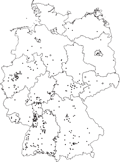
MAPPING THE GEOGRAPHIC DISTRIBUTION OF NAMES 389
Berlin
Bremen
Cologne
Dortmund
Dresden
Duisburg
Dusseldorf
Essen
Frankfurt
Hamburg
Hanover
Jena
Leipzig
Mannheim
Munich
Nuremberg
Stuttgart
Berlin
Bremen
Cologne
Dortmund
Dresden
Duisburg
Dusseldorf
Essen
Frankfurt
Hamburg
Hanover
Jena
Leipzig
Mannheim
Munich
Nuremberg
Stuttgart
Berlin
Bremen
Cologne
Dortmund
Dresden
Duisburg
Dusseldorf
Essen
Frankfurt
Hamburg
Hanover
Jena
Leipzig
Mannheim
Munich
Nuremberg
Stuttgart
Berlin
Bremen
Cologne
Dortmund
Dresden
Duisburg
Dusseldorf
Essen
Frankfurt
Hamburg
Hanover
Jena
Leipzig
Mannheim
Munich
Nuremberg
Stuttgart
Berlin
Bremen
Cologne
Dortmund
Dresden
Duisburg
Dusseldorf
Essen
Frankfurt
Hamburg
Hanover
Jena
Leipzig
Mannheim
Munich
Nuremberg
Stuttgart
Berlin
Bremen
Cologne
Dortmund
Dresden
Duisburg
Dusseldorf
Essen
Frankfurt
Hamburg
Hanover
Jena
Leipzig
Mannheim
Munich
Nuremberg
Stuttgart
Berlin
Bremen
Cologne
Dortmund
Dresden
Duisburg
Dusseldorf
Essen
Frankfurt
Hamburg
Hanover
Jena
Leipzig
Mannheim
Munich
Nuremberg
Stuttgart
Berlin
Bremen
Cologne
Dortmund
Dresden
Duisburg
Dusseldorf
Essen
Frankfurt
Hamburg
Hanover
Jena
Leipzig
Mannheim
Munich
Nuremberg
Stuttgart
Berlin
Bremen
Cologne
Dortmund
Dresden
Duisburg
Dusseldorf
Essen
Frankfurt
Hamburg
Hanover
Jena
Leipzig
Mannheim
Munich
Nuremberg
Stuttgart
Figure 15.2 Geographic distribution of “Feuersteins”
The result is provided in Figure 15.2. The distribution of hits reveals some interesting
facts. The largest cluster of Feuersteins lives in the southwestern part of Germany, in the area
near Mannheim.
15.5 Automating the process
Crafting maps from scraped surnames is an example of a task that is likely to be repeated over The benet of
speical-purpose
scraping
functions
and over again, with only slight modications. To round off the exercise, we develop a set
of functions which generalize the scraping, parsing, and mapping from above and offer some
useful options to adapt the process (see Section 11.3). In our case, the information for one
name rarely changes over time. It is thus of less interest to repeat the task for one surname.
Instead, we want to be able to quickly produce data and maps for any name.
We decide to split the procedure into three functions: a scraping function, a parsing and
data cleansing function, and a mapping function. While on the one side this means that we
have to call three functions to create a map, these functions are easier to debug and adapt.

390 AUTOMATED DATA COLLECTION WITH R
1namesScrape <- function(phonename, update.file = FALSE) {
2## transform phonename
3phonename <- tolower(phonename)
4## load libraries
5x <- c("stringr", "RCurl", "XML")
6lapply(x, require, character.only=T)
7## create folder
8dir.create(str_c("phonebook_", phonename), showWarnings = FALSE)
9filename <- str_c("phonebook_", phonename, "/phonebook_", phonename,
".html")
10 if (file.exists(filename) & update.file == FALSE) {
11 message("Data already scraped; using data from ", file.info(
filename)$mtime)
12 }else{
13 ## retrieve and save html
14 tb <- getForm("http://www.dastelefonbuch.de/",
15 .params = c(kw = phonename, cmd = "search", ao1 = "1", reccount
= "2000"))
16 write(tb, file = filename)
17 }
18 }
Figure 15.3 Generalized Rcode to scrape entries from www.dastelefonbuch.de
The code in Figures 15.3, 15.4, and 15.5 displays the result of our efforts. It is the condensed
version of the code snippets from above, enriched with some useful arguments for the function
sets namesScrape(),namesParse(), and namesPlot().
Usually, what distinguishes functions from ordinary code is that they (1) generalize a task
and (2) offer exibility in the form of arguments. It is always the choice of a function author
which parameters to keep variable, that is, easily modiable by the function user, and which
parameters to x. For our functions, we have implemented a set of arguments which is listed
in Table 15.1.
The choice of arguments is mainly focused on plotting the results. One could easily
Technical
considerations think of more options for the scraping process. We could allow more than one request at
once, explicitly obey the robots.txt,6or dene a User-agent header eld. With regards to
processing, we could have allowed specifying a directory where data and maps should be
saved. For reasons of brevity, we refrain from such ne-tuning work. However, anybody
should feel free to adapt and expand the function.
Let us consider the details of the code. In the scraping function namesScrape() (Fig-The functions
explained ure 15.3), phonename is the crucial parameter. We use the tolower() function (see Section
8.1) to achieve a consistent naming of les. Data are stored as follows: Using a call to
dir.create(), a directory is created where the HTML le and, if so desired, a PDF ver-
sion of the graph are stored. Scraping is only performed if the le does not exist. This is
checked with the file.exists() function or if the user explicitly requests that the le be
updated (option update.file == TRUE). Otherwise, a message referring to the existing
le is shown and the function loads the old data.
6In our example, it does not seem necessary to mind the robots.txt. We stay on one site and have already
investigated the scraping policy.

MAPPING THE GEOGRAPHIC DISTRIBUTION OF NAMES 391
1namesParse <- function(phonename) {
2filename <- str_c("phonebook_", phonename, "/phonebook_", phonename,
".html")
3## load libraries
4x <- c("stringr", "XML")
5lapply(x, require, character.only = TRUE)
6## parse html
7tb_parse <- htmlParse(filename, encoding = "UTF-8")
8## check number of hits
9xpath <- ’//ul/li/a[contains(text(), "Privat")]’
10 num_results <- xpathSApply(tb_parse, xpath, xmlValue)
11 num_results <- as.numeric(str_extract(num_results, ’[[:digit:]]+’))
12 if (num_results <= 2000) {
13 message(’Gross sample of ’, num_results, ’ entries retrieved.’)
14 }
15 if (num_results > 2000) {
16 message(num_results, ’ hits. Warning: No more than 2,000 entries
will be retrieved’)
17 }
18 ## retrieve zipcodes and names
19 xpath <- ’//div[@class="name"]/following-sibling::div[@class="
popupMenu"]//span[@itemprop="postal-code"]’
20 zipcodes_vec <- xpathSApply(tb_parse, xpath, xmlValue)
21 zipcodes_vec <- str_replace_all(zipcodes_vec, " ", "")
22 xpath <- ’//span[@itemprop="postal-code"]/ancestor::div[@class="
popupMenu"]/preceding-sibling::div[@class="name"]’
23 names_vec <- xpathSApply(tb_parse, xpath, xmlValue)
24 names_vec <- str_replace_all(names_vec, "(\\n|\\t|\\r| {2,})", "")
25 ## build data frame
26 entries_df <- data.frame(plz = as.numeric(zipcodes_vec), name =
names_vec)
27 ## match coordinates to zipcodes
28 plz_df <- read.delim("function_data/plz_de.txt", stringsAsFactors =
FALSE, encoding = "UTF-8")
29 geodf <- merge(entries_df, plz_df, by = "plz", all.x = TRUE)
30 geodf <- geodf[!is.na(geodf$lon),]
31 ## return data frame
32 geodf <- geodf[,!names(geodf) %in% "X.loc_id"]
33 return(geodf)
34 }
Figure 15.4 Generalized Rcode to parse entries from www.dastelefonbuch.de
In the parsing function namesParse() (Figure 15.4), the information extraction process
remains the same as above, except that the number of results is reported. The function prints a
warning if more than 2000 observations are found. This would mean that not the full sample
of observations is captured. Further, rst names are extracted from the names vector in a
rather simplistic manner by removing the surname. The function returns the data frame which
contains geographical and name information for further analysis and/or plotting.
Finally, the plotting function namesPlot() (Figure 15.5) uses the data frame and gen-
erates the map as outlined above. The function allows storing the plot locally as a PDF le.
We also add the option print.names to print the rst names of the observations.

392 AUTOMATED DATA COLLECTION WITH R
1namesPlot <- function(geodf, phonename, show.map = TRUE, save.pdf = TRUE,
2minsize.cities = 450000, add.cities = "",
3print.names = FALSE) {
4## load libraries
5x <- c("stringr", "maptools", "rgdal", "maps")
6lapply(x, require, character.only = TRUE)
7## prepare coordinates
8coords <- SpatialPoints(cbind(geodf$lon, geodf$lat))
9proj4string(coords) <- CRS("+proj=longlat +ellps=WGS84 +datum=WGS84")
10 ## prepare map
11 projection <- CRS("+proj=longlat +ellps=WGS84 +datum=WGS84")
12 map_germany <- readShapePoly("function_data/DEU_adm0.shp",
13 proj4string = projection)
14 map_germany_laender <- readShapePoly("function_data/DEU_adm1.shp",
15 proj4string = projection)
16 ## add big cities (from maps package)
17 data("world.cities")
18 cities_ger <- subset(world.cities, country.etc == "Germany" &
19 (world.cities$pop > minsize.cities |
20 world.cities$name %in% add.cities))
21 coords_cities <- SpatialPoints(cbind(cities_ger$long, cities_ger$lat))
22 ## produce map
23 i<-0
24 n<-1
25 while (i <= n) {
26 if (save.pdf == TRUE & i < n) {
27 pdf(file = str_c("phonebook_", phonename, "/map-",
28 phonename, ".pdf"), height = 10, width = 7.5,
29 family = "URWTimes")
30 }
31 if (show.map == TRUE | save.pdf == TRUE) {
32 par(oma = c(0, 0, 0, 0))
33 par(mar = c(0, 0, 2, 0))
34 par(mfrow = c(1, 1))
35 plot(map_germany)
36 plot(map_germany_laender, add = TRUE)
37 title(main = str_c("People named ", toupper(phonename),
38 " in Germany"))
39 if (print.names == FALSE) {
40 points(coords$coords.x1, coords$coords.x2,
41 col = rgb(10, 10, 10, max = 255),
42 bg = rgb(10, 10, 10, max = 255),
43 pch = 20, cex = 1)
44 } else {
45 text(coords$coords.x1, coords$coords.x2,
46 labels = str_replace_all(geodf$name,
47 ignore.case(phonename), ""), cex = .7)
48 }
49 points(coords_cities, col = "black", , bg = "grey", pch = 23)
50 shadowtext(cities_ger$long,cities_ger$lat,
51 labels = cities_ger$name, pos = 4,
52 col = "black", bg = "white", cex = 1.2)
53 }
54 if (save.pdf == TRUE & i < n) {
55 dev.off()
56 }
57 if (show.map == FALSE) {
58 i<-i+1
59 }
60 i<-i+1
61 }
62 }
Figure 15.5 Generalized Rcode to map entries from www.dastelefonbuch.de
MAPPING THE GEOGRAPHIC DISTRIBUTION OF NAMES 393
Table 15.1 Parameters of phone book scraping functions explained
Argument Description
phonename Main argument for namesScrape() and namesParse(); denes
the name for which entries should be retrieved
geodf Main argument for namesPlot; species data.frame object which
stores geographical information (object is usually returned by
namesParse())
update.file Logical value indicating whether the data should be scraped again or
if existing data should be used
show.map Logical value indicating whether Rshould automatically print a map
with the located observations
save.pdf Logical value indicating whether Rshould save the map as pdf
minsize.cities Numerical value setting the minimal size of cities to be included in
the plot
add.cities Character values dening names of further cities to be added to the
plot
print.names Logical value indicating whether people’s names should be plotted
We test the functions with a set of specications. First, we look at the distribution of
people named “Gruber,” displaying cities with more than 300,000 inhabitants.
R> namesScrape("Gruber")
R> gruber_df <- namesParse("Gruber", minsize.cities = 300000)
R> namesPlot(gruber_df, "Gruber", save.pdf = FALSE, show.map = FALSE)
Next, we scrape information for people named “Petersen.” We have done this before and
force the scraping function to update the le.
R> namesScrape("Petersen", update.file = TRUE)
R> petersen_df <- namesParse("Petersen")
9605 hits. Warning: No more than 2,000 entries will be retrieved
R> namesPlot(petersen_df, "Petersen", save.pdf = FALSE, show.map = FALSE)
Finally, we look at the distribution of the surname “Dimp.” We ask the function to plot
the surnames.
R> namesScrape("Dimpfl")
Data already scraped; using data from 2014-01-16 00:22:03
R> dimpfl_df <- namesParse("Dimpfl")
Gross sample of 109 entries retrieved.
R> namesPlot(dimpfl_df, "Dimpfl", save.pdf = FALSE, show.map = FALSE,
print.names = TRUE)
The output of all three calls is shown in Figure 15.6. We observe that both Gruber and
Dimp are clustered in the southern part of Germany, whereas Petersens live predominantly
in the very north. Note that for the Dimps we see rst names instead of dots.
Finally, we reconsider a technical concern of our scraping approach. Recall that in Section The JavaScript
parts
15.2 we noted that the search on www.dastelefonbuch.de also returns a map where the ndings
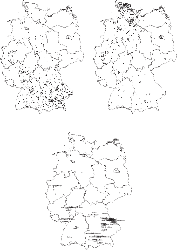
394 AUTOMATED DATA COLLECTION WITH R
People named GRUBER in Germany
Berlin
Bielefeld
Bochum
Bonn
Bremen
Cologne
Dortmund
Dresden
Duisburg
Dusseldorf
Essen
Frankfurt
Hamburg
Hanover
Leipzig
Mannheim
Munich
Nuremberg
Stuttgart
Wuppertal
Berlin
Bielefeld
Bochum
Bonn
Bremen
Cologne
Dortmund
Dresden
Duisburg
Dusseldorf
Essen
Frankfurt
Hamburg
Hanover
Leipzig
Mannheim
Munich
Nuremberg
Stuttgart
Wuppertal
Berlin
Bielefeld
Bochum
Bonn
Bremen
Cologne
Dortmund
Dresden
Duisburg
Dusseldorf
Essen
Frankfurt
Hamburg
Hanover
Leipzig
Mannheim
Munich
Nuremberg
Stuttgart
Wuppertal
Berlin
Bielefeld
Bochum
Bonn
Bremen
Cologne
Dortmund
Dresden
Duisburg
Dusseldorf
Essen
Frankfurt
Hamburg
Hanover
Leipzig
Mannheim
Munich
Nuremberg
Stuttgart
Wuppertal
Berlin
Bielefeld
Bochum
Bonn
Bremen
Cologne
Dortmund
Dresden
Duisburg
Dusseldorf
Essen
Frankfurt
Hamburg
Hanover
Leipzig
Mannheim
Munich
Nuremberg
Stuttgart
Wuppertal
Berlin
Bielefeld
Bochum
Bonn
Bremen
Cologne
Dortmund
Dresden
Duisburg
Dusseldorf
Essen
Frankfurt
Hamburg
Hanover
Leipzig
Mannheim
Munich
Nuremberg
Stuttgart
Wuppertal
Berlin
Bielefeld
Bochum
Bonn
Bremen
Cologne
Dortmund
Dresden
Duisburg
Dusseldorf
Essen
Frankfurt
Hamburg
Hanover
Leipzig
Mannheim
Munich
Nuremberg
Stuttgart
Wuppertal
Berlin
Bielefeld
Bochum
Bonn
Bremen
Cologne
Dortmund
Dresden
Duisburg
Dusseldorf
Essen
Frankfurt
Hamburg
Hanover
Leipzig
Mannheim
Munich
Nuremberg
Stuttgart
Wuppertal
Berlin
Bielefeld
Bochum
Bonn
Bremen
Cologne
Dortmund
Dresden
Duisburg
Dusseldorf
Essen
Frankfurt
Hamburg
Hanover
Leipzig
Mannheim
Munich
Nuremberg
Stuttgart
Wuppertal
People named PETERSEN in Germany
Berlin
Bremen
Cologne
Dortmund
Dresden
Duisburg
Dusseldorf
Essen
Frankfurt
Hamburg
Hanover
Leipzig
Munich
Nuremberg
Stuttgart
Berlin
Bremen
Cologne
Dortmund
Dresden
Duisburg
Dusseldorf
Essen
Frankfurt
Hamburg
Hanover
Leipzig
Munich
Nuremberg
Stuttgart
Berlin
Bremen
Cologne
Dortmund
Dresden
Duisburg
Dusseldorf
Essen
Frankfurt
Hamburg
Hanover
Leipzig
Munich
Nuremberg
Stuttgart
Berlin
Bremen
Cologne
Dortmund
Dresden
Duisburg
Dusseldorf
Essen
Frankfurt
Hamburg
Hanover
Leipzig
Munich
Nuremberg
Stuttgart
Berlin
Bremen
Cologne
Dortmund
Dresden
Duisburg
Dusseldorf
Essen
Frankfurt
Hamburg
Hanover
Leipzig
Munich
Nuremberg
Stuttgart
Berlin
Bremen
Cologne
Dortmund
Dresden
Duisburg
Dusseldorf
Essen
Frankfurt
Hamburg
Hanover
Leipzig
Munich
Nuremberg
Stuttgart
Berlin
Bremen
Cologne
Dortmund
Dresden
Duisburg
Dusseldorf
Essen
Frankfurt
Hamburg
Hanover
Leipzig
Munich
Nuremberg
Stuttgart
Berlin
Bremen
Cologne
Dortmund
Dresden
Duisburg
Dusseldorf
Essen
Frankfurt
Hamburg
Hanover
Leipzig
Munich
Nuremberg
Stuttgart
Berlin
Bremen
Cologne
Dortmund
Dresden
Duisburg
Dusseldorf
Essen
Frankfurt
Hamburg
Hanover
Leipzig
Munich
Nuremberg
Stuttgart
People named DIMPFL in Germany
Berlin
Bremen
Cologne
Dortmund
Dresden
Duisburg
Dusseldorf
Essen
Frankfurt
Hamburg
Hanover
Leipzig
Munich
Nuremberg
Stuttgart
Berlin
Bremen
Cologne
Dortmund
Dresden
Duisburg
Dusseldorf
Essen
Frankfurt
Hamburg
Hanover
Leipzig
Munich
Nuremberg
Stuttgart
Berlin
Bremen
Cologne
Dortmund
Dresden
Duisburg
Dusseldorf
Essen
Frankfurt
Hamburg
Hanover
Leipzig
Munich
Nuremberg
Stuttgart
Berlin
Bremen
Cologne
Dortmund
Dresden
Duisburg
Dusseldorf
Essen
Frankfurt
Hamburg
Hanover
Leipzig
Munich
Nuremberg
Stuttgart
Berlin
Bremen
Cologne
Dortmund
Dresden
Duisburg
Dusseldorf
Essen
Frankfurt
Hamburg
Hanover
Leipzig
Munich
Nuremberg
Stuttgart
Berlin
Bremen
Cologne
Dortmund
Dresden
Duisburg
Dusseldorf
Essen
Frankfurt
Hamburg
Hanover
Leipzig
Munich
Nuremberg
Stuttgart
Berlin
Bremen
Cologne
Dortmund
Dresden
Duisburg
Dusseldorf
Essen
Frankfurt
Hamburg
Hanover
Leipzig
Munich
Nuremberg
Stuttgart
Berlin
Bremen
Cologne
Dortmund
Dresden
Duisburg
Dusseldorf
Essen
Frankfurt
Hamburg
Hanover
Leipzig
Munich
Nuremberg
Stuttgart
Berlin
Bremen
Cologne
Dortmund
Dresden
Duisburg
Dusseldorf
Essen
Frankfurt
Hamburg
Hanover
Leipzig
Munich
Nuremberg
Stuttgart
Figure 15.6 Results of three calls of the namesPlot() function
MAPPING THE GEOGRAPHIC DISTRIBUTION OF NAMES 395
are located, which is essentially what we wanted to replicate. We argued that it seems easier
to scrape the entries from the list instead of the JavaScript object. Indeed, the inspection of
the source code of the page does not reveal any of the hits. But this is what we should expect
knowing how dynamic webpages are constructed, that is, by means of AJAX methods (see
Chapter 6). Therefore, we use the Web Developer Tools of our browser to identify the source
of information which is plotted in the map (see Section 6.3). We nd that the script initiates
the following GET request:
http://maps.dastelefonbuch.de/DasTelefonbuch/search.html?queryType=
whatOnly&x=1324400.3811369245&y=6699724.7656052755&width=3033021.
2837500004&height=1110477.1474374998&city=&searchTerm=Feuerstein&
shapeName=tb/CA912598AEB53A4D1862D89ACA54C42E_2&minZoomLevel=4&
maxZoomLevel=18&mapPixelWidth=1240&mapPixelHeight=454&order=distance
&maxHits=200
The interesting aspect about this is that this request returns an XML le that contains
essentially the same information that we scraped above along with coordinates that locate the
hits on the map. One could therefore directly target this le in order to scrape the relevant
information. Advantages would be that it is more likely that the XML le’s structure remains
more stable than the front-end page, making the scraper more robust to changes in the page
layout. Second, one could probably skip the step where zip codes and coordinates are matched.
However, some parameters in the related URL seem to further restrict the number of returned
hits, that is, the zoom level and margins of the plotted area. Further, the structure of the XML
document is largely identical with the relevant part of the HTML document we scraped above.
This means that the information extraction step should not be expected to be easier with the
XML document. Nevertheless, it is always worth looking behind the curtains of dynamically
rendered content on webpages, as there may be scenarios in which relevant data can only be
scraped this way.
Summary
The code presented in this chapter is only the rst step toward a thorough analysis of the
distribution of family names. There are several issues of data quality that should be considered
when the data are used for scientic purposes. First, there is the limitation of 2000 hits. As
the hits are sorted alphabetically, the truncation of the scraped sample is at least not entirely
random. Further, the data may contain duplicates or “false positives.” Even if one is not
interested in detailed research on the data, there is plenty of room for improvement in the
functions. The point representation of hits could be replaced by density maps to better
visualize regions where names occur frequently.
More general take-away points of this study are the following. When dealing with dynamic
content, it usually pays off to start with a closer look at the source code. One should rst get
a basic understanding of how parameters in a GET request work, what their limits are, and if
there are other ways to retrieve content than to posit requests via the input eld. Concerning
the use of geo data, the lesson learned is that it is easy to enrich scraped data with geo
information once a geographical identier is available. Mapping such information in Ris
possible, although not always straightforward. Finally, splitting the necessary tasks into a set
of specic functions can be useful and keeps the code manageable.

16
Gathering data on mobile phones
In this case study, we gather data on pricing, costumer rating, and sales ranks of a broad
range of mobile phones sold on amazon.com, wondering about the price segments covered
by leading producers of mobile phones. Amazon sells a broad range of products, allowing us
to get comprehensive summary of the products from each of the big mobile phone producers.
The case study makes use of the packages RCurl,XML, and stringr and it features search
page manipulation, link extraction, and page downloads using the RCurl curl handle. After
reading the case study, you should be able to search information in source code and to apply
XPath in real-life problems. Furthermore, within this case study a SQLite database is created
to store data in a consistent way and make it reusable for the next case study.
16.1 Page exploration
16.1.1 Searching mobile phones of a specic brand
Amazon sells all kinds of products. Our rst task is therefore to restrict the product search
to certain categories and specic producers. Furthermore, we have to nd a way to exclude
accessories or used phones.
Let us have a look at the Amazon website: www.amazon.com. Check out the search bar
Searching in
departments at the top of the page—see also Figure 16.1. In addition to typing in search keywords, we can
select the department in which we want to search. Do the following:
1. Type Apple into the search bar and press enter.
2. Select Cell Phones & Accessories from the search lter and click Go.
3. Now click on Unlocked Cell Phones in the departments lter section on the left hand
of the page.
Automated Data Collection with R: A Practical Guide to Web Scraping and Text Mining, First Edition.
Simon Munzert, Christian Rubba, Peter Meißner and Dominic Nyhuis.
© 2015 John Wiley & Sons, Ltd. Published 2015 by John Wiley & Sons, Ltd.
GATHERING DATA ON MOBILE PHONES 397
Figure 16.1 Amazon’s search form
4. Type in other producers of mobile phones and compare the resulting URLs—which
parts of the URL change?
5. Try to eliminate parts of the query string in the address of your browser and watch what
happens. Try to nd those query strings which are necessary to replicate the search
result and which can be left out.
The URL produced by searching for a specic producer in Unlocked Cell Phones in the
browser looks like this:
http://www.amazon.com/s/ref=nb_sb_noss_1?url=node%3D2407749011&eld-
keywords=Apple&rh=n%3A2335752011%2Cn%3A7072561011%2Cn%
3A2407749011%2Ck%3AApple
Trying to delete various parts of the URL we nd that the following URL is sufcient to
replicate the search results:
http://www.amazon.com/s/?url=node%3D2407749011&eld-keywords=Apple
The field-keywords part of the query string changes the keywords that are searched for,
while url restricts the search results to unlocked cell phones. We found a basic URL that
allows us to perform searches in the department of unlocked mobile phones and that we can
manipulate to get results for different keywords.
Browsing through the search results we nd that often phones of other producers are found Brand
restrictions
as well. A brand lter on the left-hand side of the page helps get rid of this noise. There are
two strategies to get the brand-restricted search results: We can either nd the rules according
to which the link is generated and generate the link ourselves or start with a non-restricted
search, extract the link for the restricted results, and later on use it to get ltered search results.
We go for the second solution because it is easier to implement. To learn more about how to
identify the link, we use the inspect element tool of our browser on the brand lter:
1<a href="/s/ref=sr_nr_p_89_0?rh=n%3A2335752011%2Cn%3A7072561011%
2Cn%3A2407749011%2Ck%3AApple%2Cp_89%3AApple&keywords=Apple
&ie=UTF8&qid=1389615535&rnid=2528832011" class=" ">
2<img style="margin-right:4px; " height="12" width="12" border="
0" align="top" alt="Apple" src="http://g-ecx.images-amazon.
com/images/G/01/nav2/buttons/checkbox_unselected_enabled._
V192545545_.jpg">
3<span class="refinementLink">Apple</span>
4</a>
398 AUTOMATED DATA COLLECTION WITH R
The link we are looking for is part of an <a> node. Unfortunately, the node has no specic
class, but it has a <span> node as child with a very specic class called refinementLink.
The content of the class is equal to the brand we want to restrict the search to—that should
do. Translating this observation into XPath means that we are looking for a <span> node
with class refinementLink for which the content of that node is equal to the keyword we
are searching for. From this <span> node, we want to move one level up to the parent and
select the parent’s href attribute:
1//span[@class="refinementLink" and text()="Apple"]/../@href
Now we have a way of restricting search results to specic producers, but the resultsSorting
are sorted in the default sorting order. Maybe sorting according to newness of the product
is a better idea. After searching for a product on the Amazon page, we are presented with a
drop-down list directly above the search results. It allows us to select one of several sorting
criteria. Let us choose Newest Arrivals to have new products listed rst. After selecting our
preferred sorting, a new element is added to the URL—&sort=date-desc-rank. We can
use it later on to construct an URL that produces sorted results.
Last but not least, we want to download more than the 24 products listed on the rst
Next page
results page. To do so, we need to select the next page. A link called Next Page at the bottom
of the page does the trick. Using the inspect element tool of our browser reveals that the link
is marked by a distinctive class attribute—pagnNext:
1<a title="Next Page" id="pagnNextLink" class="pagnNext" href="/
gp/search/ref=sr_pg_2?rh=n%3A2335752011%2Cn%3A7072561011%2Cn%
3A2407749011%2Ck%3AApple&page=2&sort=salesrank&
keywords=Apple&ie=UTF8&qid=1389618220">
2<span id="pagnNextString">Next Page</span>
3<span class="srSprite pagnNextArrow"></span>
4</a>
We search for <a> nodes with a next page class and extract their href attribute. This is
done using the following XPath expression:
1//a[@class='pagnNext']/@href
Later on we will use the links gathered in this way to download subsequent search
result pages.
Now we have all the elements set up to run product searches for unlocked mobile phones
The scraping
strategy of specic brands with a specic sorting. The following steps now have to be translated into
Rcode:
1. Specify the basic search URL for unlocked mobile phones and download the le.
2. Search and extract the brand ltering link from the source code of the downloaded le.
GATHERING DATA ON MOBILE PHONES 399
3. Append the sorting parameter to the query string of the beforehand extracted link and
download the page.
4. Search and extract the link to next page and download the next page. Repeat this step
as needed.
First, we load the necessary packages. The stringr package serves as the all-purpose tool Downloading
search pages
for extracting and manipulating text snippets, whereas XML and RCurl are the workhorses for
the scraping tasks. RCurl enables us to download several les via one connection and XML is
indispensable for HTML parsing and information extraction via XPath:
R> library(stringr)
R> library(XML)
R> library(RCurl)
Next we save the base URL for our searches and the rst producer we want to search for
in an object:
R> baseURL <- "http://www.amazon.com/s/ref=nb_sb_noss_2?url=node%3
D2407749011&field-keywords="
R> keyword <- "Apple"
Base URL and producer name are combined with a simple call to str_c() and the page
is downloaded and saved in an object:
R> url <- str_c(baseURL, keyword)
R> firstSearchPage <- getURL(url)
To issue XPath queries, we parse the page with htmlParse() and save it in an object:
R> parsedFirstSearchPage <- htmlParse(firstSearchPage)
We specify the XPath expression to extract the link for the brand restricted search results
by pasting the producer name into the XPath expression we outlined before:
R> xpath <- str_c('//span[@class="refinementLink" and text()="',
R> keyword,
R> '"]/../@href')
We use the XPath expression to extract the link and complete it with the base URL of the
server:
R> restSearchPageLink <- xpathApply(parsedFirstSearchPage, xpath)
R> restSearchPageLink <- unlist(as.character(restSearchPageLink))
R> restSearchPageLink <- str_c("http://www.amazon.com", restSearchPageLink)
Finally, we add the desired sorting to the query string of the URL:
R> restSearchPageLink <- str_c(restSearchPageLink, "&sort=date-desc-rank")

400 AUTOMATED DATA COLLECTION WITH R
…and download the page:
R> restrictedSearchPage <- getURL(restSearchPageLink)
This provides us with our rst search results page for products restricted to a specic
producer and the Unlocked Cell Phones product department.
Now we want to download further search results pages and store them in a list object.
First, we create the list object and save the rst search results page as its the rst element.
Next, the XPath expression that extracts the link for the next page is stored as well to make
the code more readable. We create a loop for the rst ve search pages. In every iteration we
extract the link for the next page and download and store the page in our list object:
R> SearchPages <- list()
R> SearchPages[[1]] <- restrictedSearchPage
R> xpath <- "//a[@class='pagnNext']/@href"
R> for (i in 2:5) {
nextPageLink <- xpathApply(htmlParse(SearchPages[[i - 1]]), xpath)
nextPageLink <- unlist(nextPageLink)
nextPageLink <- str_c("http://www.amazon.com", nextPageLink)
SearchPages[[i]] <- getURL(nextPageLink)
}
16.1.2 Extracting product information
In the previous section, we ran searches to collect our results. In this section, we gather the
necessary data from the results.
The rst information to be extracted are the product titles of the search results pages as
Title and
product page
links
well as the links to the product pages. Using the inspect element tool, we nd that links and
titles are part of a heading of level three—an <h3> node. Searching the source code for other
headings of level three reveals that they are only used for product titles and links to product
pages:
1<h3 class="newaps">
2<a href="http://www.amazon.com/Apple-iPhone-8GB-White-Sprint/
dp/B0074SQUBY/ref=sr_1_1?s=wireless&ie=UTF8&qid=
1389697991&sr=1-1&keywords=Apple">
3<span class="lrg bold">Apple iPhone 4 8GB (White) - Sprint
4</span>
5</a>
6</h3>
We apply this information and construct two XPath expressions, //h3/a/span for titles
and //h3/a for the links. As we have a whole list of search pages from which we want to
extract data, we wrap the extraction procedure into a function and use lapply() to extract

GATHERING DATA ON MOBILE PHONES 401
the information from all pages; rst the titles:
R> extractTitle <- function(x) {
unlist(xpathApply(htmlParse(x), "//h3/a/span", xmlValue))
}
R> titles <- unlist(lapply(SearchPages, extractTitle))
R> titles[1:3]
[1] "Apple iPhone 4 16GB (Black) - CDMA Verizon"
[2] "Apple iPhone 5s, Gold 16GB (Unlocked)"
[3] "Apple iPhone 4 16GB (Black) - AT&T"
then the links:
R> extractLink <- function(x) {
unlist(xpathApply(htmlParse(x), "//h3/a", xmlAttrs))
}
R> links <- unlist(lapply(SearchPages, extractLink))
R> links[1:3]
[1] "http://www.amazon.com/Apple-iPhone-16GB-Black-Verizon/dp/
B004ZLV5UE/ref=sr_1_1/181-2441251-9365168?s=wireless&ie=UTF8&qid=
1391539292&sr=1-1&keywords=Apple"
[2] "http://www.amazon.com/Apple-iPhone-5s-Gold-Unlocked/dp/
B00F3J4E5U/ref=sr_1_2/181-2441251-9365168?s=wireless&ie=UTF8&qid=
1391539292&sr=1-2&keywords=Apple"
[3] "http://www.amazon.com/Apple-iPhone-16GB-Black-AT/dp/
B004ZLV5PE/ref=sr_1_3/181-2441251-9365168?s=wireless&ie=UTF8&qid=
1391539292&sr=1-3&keywords=Apple"
For the retrieval of price, costumer rating, and sales rank, the search pages’ structure is Retrieving
product pages
hard to exploit or simply does not provide the information we seek. Therefore, we rst have
to download the individual product pages and extract the information from there.
To avoid establishing new connections for all the downloads—which is time consuming—
we create a handle that is reused for every call to getURL(). Furthermore, we want to give
the server a break every 10 downloads, so we split our link vector into chunks of size 10 and
loop over the list of chunks.1In every loop, we request 10 pages and append them to the list
object we created for storage and move to the next chunk. Last but not least we parse all the
pages and store them in another list object:
R> chunk <- function(x, n) split(x, ceiling(seq_along(x)/n))
R> Links <- chunk(links, 10)
R> curl <- getCurlHandle()
R> ProductPages <- list()
R> for (i in 1:length(Links)) {
ProductPages <- c(ProductPages, getURL(Links[[i]]))
Sys.sleep(2)
}
R> ParsedProductPages <- lapply(ProductPages, htmlParse)
1See the advice at http://stackoverow.com/a/3321659/1144966 for several chunking solutions.
402 AUTOMATED DATA COLLECTION WITH R
Having gathered all product pages, we move on to extracting the product price. Often,Extracting
prices several prices are displayed on a product page: list prices, prices for new items, prices for used
or refurbished items, and prices for products that are similar to the one selected. Using the
inspect elements tool on the price directly under the product title, we nd that it is enclosed
by a <span> node with id actualPriceValue. Translated to an XPath expression, it reads:
//span[@id="actualPriceValue"]. One problem is that some items are not in stock
anymore and the call to xpathApply() would return NULL for those items. To ensure that
for these products we record a price of NA instead of NULL we check for the length of the
xpathApply() result. If the length of the result is zero we replace it with NA. Below you
nd a source code snippet containing the price information we seek as well as the Rcode to
extract the information:
1<span id="actualPriceValue"><b class="priceLarge">$210.00</b></span>
R> extractPrice <- function(x) {
x <- xpathApply(x, "//span[@id=\"actualPriceValue\"]", xmlValue)
x <- unlist(x)
x <- str_extract(x, "[[:digit:]]*\\.[[:digit:]]*")
if (length(x) == 0)
x<-NA
return(as.numeric(x))
}
R> prices <- unlist(lapply(ParsedProductPages, extractPrice))
R> names(prices) <- NULL
R> prices[1:10]
[1] 210.0 710.0 240.0 319.0 354.9 208.9 239.9 359.9 420.0 565.1
This seems to work. Extracting the average customer ratings—ranging from one star toExtracting
customer
ratings
ve—works similar to the procedure we used for the prices. Directly under the product title
you nd a series of ve stars that are lled according to the average costumer rating. This
graphical representation is enclosed by a <span> node that contains the average rating in
its title attribute. We extract the information with an XPath expression: //span[contains
(@title,' out of 5 stars')]], and a call to xmlAttr() within xpathApply().The
rating is then extracted from the title with a regular expression:
1<span class="swSprite s_star_4_0 " title="3.6 out of 5 stars">
2<span>3.8 out of 5 stars</span>
3</span>
R> extractStar <- function(x) {
x <- xpathApply(x, "//span[contains(@title, ' out of 5 stars')]",
xmlValue)
if (length(x) == 0) {
x<-NA
} else {

GATHERING DATA ON MOBILE PHONES 403
x <- x[[1]]
x <- str_extract(x, "[[:digit:]]\\.?[[:digit:]]?")
}
return(as.numeric(x))
}
R> stars <- unlist(lapply(ParsedProductPages, extractStar))
R> names(stars) <- NULL
R> stars[1:10]
[1] 3.6 3.5 3.7 3.2 3.3 3.7 3.8 3.8 3.5 4.0
Further down on the page we nd a section called Product Details. In this section, further Extracting
sales ranks
information like the Amazon Standard Identication Number (ASIN), the product model, and
the sales rank on Amazon within the category of Cell Phones & Accessories are shown as
separate items. Let us start with extracting the sales rank which is enclosed in a <li> node of
id SalesRank. We extract the node with XPath and collect the rank with a regular expression
that looks for digits after a hash tag character and a second one that deletes everything which
is not a digit:
1<li id="SalesRank">
2<b>Amazon Best Sellers Rank:</b> #423 in Cell Phones &
Accessories (<a href="http://www.amazon.com/gp/bestsellers/
wireless/ref=pd_dp_ts_cps_1">See Top 100 in Cell Phones &
Accessories</a>)
3</li>
R> extractRank <- function(x) {
x <- unlist(xpathApply(x, "//li[@id='SalesRank']", xmlValue))
x <- str_extract(x, "#.*?in")
x <- str_replace_all(x, "[, in#]", "")
if (length(x) == 0)
x<-NA
return(as.numeric(x))
}
R> ranks <- unlist(lapply(ParsedProductPages, extractRank))
R> names(ranks) <- NULL
R> ranks[1:10]
[1] 423 502 542 617 789 885 1277 1380 1268 1567
Next, we extract the ASIN from the product page. This information will help us later Extracting the
ASIN
on to get rid of duplicates and to identify products. The ASIN is found in a list item that is
unfortunately not identied with an id attribute or a specic class:
1<li><b>ASIN:</b> B00FBSOXGI</li>
Nevertheless, we can specify its position as XPath expression by searching for a <b> node
that has a <li> node as parent and contains text of pattern ASIN. From this node, we move
404 AUTOMATED DATA COLLECTION WITH R
one level up the tree and select the text of the parent:
1//li/b[contains(text(), 'ASIN')]/../text()
R> extractASIN <- function(x) {
x <- xpathApply(x, "//li/b[contains(text(), 'ASIN')]/../text()",
xmlValue)
x <- str_trim(unlist(x))
if (length(x) == 0)
x<-NA
return(x)
}
R> asins <- unlist(lapply(ParsedProductPages, extractASIN))
R> names(asins) <- NULL
R> asins[1:5]
[1] "B004ZLV5UE" "B00F3J4E5U" "B004ZLV5PE" "B00598BY6W" "B005SSB0YO"
Finally, we extract the product model following the same strategy as before:Extracting the
product model
1<li><b>Item model number:</b> MC637LL/A</li>
R> extractModel <- function(x) {
xpath <- "//li/b[contains(text(), 'Item model number')]/../text()"
x <- xpathApply(x, xpath, xmlValue)
x <- str_trim(unlist(x))
if (length(x) == 0)
x<-NA
return(x)
}
R> models <- unlist(lapply(ParsedProductPages, extractModel))
R> models[1:5]
[1] " A1349" " 5s" " MC608LL/A" " iPhone 4" " MC924LL/A"
16.2 Scraping procedure
16.2.1 Retrieving data on several producers
Above we explored our data source step by step and developed solutions for various data
collection and extraction problems. So far, we only used one producer as an example and
have not gathered the data for others. To not have to repeat the whole code above for the
other producers as well, we have to put its solutions into functions for convenient reuse. The
functions can be loaded into our R-session via
R> source("amazonScraperFunctions.r")
GATHERING DATA ON MOBILE PHONES 405
After sourcing the functions, we set three global options: forceDownload is part of every
download function and setting it to TRUE will cause the the functions to redownload all pages
while setting it to FALSE will cause them to check whether or not the les to be downloaded
exist already and should not be downloaded again. KeyWords is a vector of producer names
that is also reused throughout the functions and denes for which producers mobile phone
product details should be collected. The nparameter stores a single number that is used to
determine how many search result pages should be gathered. With each search results page,
we gain 24 further links to product pages:
R> forceDownload <- FALSE
R> KeyWords <- c("Apple", "BlackBerry", "HTC", "LG", "Motorola",
"Nokia", "Samsung")
R>n<-5
After having set up our global options, we can use the sourced functions to collect search
and product pages and extract the information we seek. The steps we take match those carved
out in the exploration section before. We start with collecting search pages:
R> SearchPageList <- NULL
R> for (i in seq_along(KeyWords)) {
message(KeyWords[i])
SearchPageList <- c(SearchPageList, getSearchPages(KeyWords[i],
n, forceDownload))
}
…extract titles and product page links:
R> titles <- extractTitles(SearchPageList)
R> links <- extractLinks(SearchPageList)
…download product pages:
R> brands <- rep(KeyWords, each = n * 24)
R> productPages <- getProductPages(links, brands, forceDownload)
…and extract further data:
R> stars <- extractStars(productPages)
R> asins <- extractASINs(productPages)
R> models <- extractModels(productPages)
R> ranks <- extractRanks(productPages)
R> prices <- extractPrices(productPages)
16.2.2 Data cleansing
Although we have already done a lot of data cleansing along the way—trim leading and
trailing spaces from strings, extract digits, and transform them to type numeric, there are
still some tasks to do before we can begin to analyze our data. First of all, we recast the
information as a data frame and then try to get rid of duplicated products as best as possible.
406 AUTOMATED DATA COLLECTION WITH R
The rst task is simple, as the information has already been saved in vectors of the same
length with NAs where no information was collected. In addition to combining the information
gathered so far, we add the names of the downloaded product pages and use their last change
attribute (file.info(fname)$ctime) to store the time when the data were retrieved:
R> fnames <- str_c(brands, " ProductPage ", seq_along(brands), ".html")
R> phones <- data.frame(brands, prices, stars, ranks,
R> asins, models, titles, links,
R> fnames,
R> timestamp = file.info(
R> str_c("dataFull/", fnames)
R> )$ctime,
R> stringsAsFactors = FALSE)
Next, we only keep complete observations and exclude all observations with duplicated
ASINs, as this is the easiest way to make sure that we have no redundant data:
R> phones <- phones[complete.cases(phones), ]
R> phones <- phones[!duplicated(phones$asins), ]
16.3 Graphical analysis
To get an overview of the distribution of prices, costumer ratings, and sales ranks, we build
a gure containing several plots that show all three variables. We have seven producers and
also want to include an All category. Therefore, we specify a plotting function once and reuse
it to assemble a plot representing information in all three categories. The main idea is to use
transparent markers that allow for different shades of gray, resulting in black regions, where
products bulk together, and light or white regions, where products are sparse or non-existent.
Because sales ranks are only of ordinal scale, we have a hard time visualizing them directly.
For every plot, we take those ve products that rank highest in sales and visualize them
differently—white dots on dark background with horizontal and vertical lines extending to
the borders of each plot.
The plot function accepts a data frame as input and consequently starts with extracting
our three variables from it—allowing a data frame as input serves convenient reuse on subsets
of the data without repeating the subset three times. Next, we do a dummy plot that has
the right range for xand ybut do not plot any data. After that we add a modied x-axis
and guiding lines. Thereafter comes the plotting of data so that the guiding lines stay in the
background. The reason for this procedure is that we want to add guidelines but do not want
to overplot the actual data—hence, we do a dummy plot, plot the guidelines, and thereafter
plot the actual data. As color of the points we choose black but with an alpha value of 0.2—
rgb(0,0,0,0.2).Thergb() function allows us to specify colors by combining red, green,
and blue in different intensities. The alpha value which is the fourth parameter denes how
opaque the resulting color is and therewith allows for transparent plotting of markers. Last
but not least, we construct an index for the ve lowest numbers in Ranks—the highest sales
ranks—and plot vertical and horizontal lines at their coordinates as well as small white points
to distinguish them from the other products.
GATHERING DATA ON MOBILE PHONES 407
R> plotResults <- function(X, title="") {
Prices <- X$prices
Stars <- X$stars
Ranks <- X$ranks
plot(Prices, Stars, pch = 20, cex=10, col = "white",
ylim = c(1,5), xlim = c(0, 1000), main = title,
cex.main = 2, cex.axis = 2, xaxt = "n")
axis(1, at=c(0, 500, 1000), labels = c(0, 500, 1000), cex.axis=2)
# add guides
abline(v=seq(0, 1000, 100), col = "grey")
abline(h=seq(0, 5, 1), col = "grey")
# adding data
points(Prices, Stars, col=rgb(0, 0, 0, 0.2), pch = 20, cex = 7)
# mark 5 highest values
index <- order(Ranks)[1:5]
abline(v = Prices[index], col="black")
abline(h = Stars[index], col="black")
points(Prices[index], Stars[index], col = rgb(1, 1,1,1), pch = 20)
}
The result of our efforts is displayed in Figure 16.2.
With regard to costumer satisfaction, it is most interesting that there are differences not in
the level but in the range of costumer ratings. For example, for Apple products, costumers seem
to be coherently satised, whereas for Motorola products the range is much higher, suggesting
that quality and/or feature appealing does vary greatly in Motorola’s product palette. Another
result is that best sellers are usually in the segments of high costumer satisfaction except for
Nokia, who manage to have one of their best selling models at medium costumer satisfaction
levels.
12345
All
0 500 1000
12345
0 500 1000
1234 5
BlackBerry
0 500 1000
1234 5
HTC
0 500 1000
12345
LG
0 500 1000
12345
Motorola
0 500 1000
12345
Nokia
0 500 1000
12345
Samsung
0 500 1000
Costumer ratings
Prices
Figure 16.2 Prices, costumer rating, and best seller positioning of mobile phones. Black
dots mark placement of individual products and white dots with horizontal and vertical lines
mark the ve best selling items per plot
408 AUTOMATED DATA COLLECTION WITH R
16.4 Data storage
16.4.1 General considerations
At this stage, we might end the case study, having gathered all data needed and drawn our
conclusions. Or we might think about future applications and further extensions. Maybe we
want to track the development of prices and costumer ratings over time and repeat the data
gathering process. Maybe we want to add further product pages or simply gather data for other
producers as well. Our database grows larger and larger, gets more complex and someday we
realize that we do not have a clue how all the .Rdata and HTML les t together. Maybe we
should have built for the future a database tailored to our needs?
In this section, we will build up an SQLite database that captures the data we have extracted
so far and leaves room to add further information. These further information will be product
reviews that are collected, stored, and analyzed in the next case study. At the end, we will
have three functions that can be called as needed: one for creating the database and dening
its structure, one for resetting everything and start anew, and one for storing gathered data
within the database. Let us start with loading the necessary packages
R> library(RSQLite)
R> library(stringr)
…and establishing a connection to the database. Note that establishing a connection to aConnecting to a
database not existing database with RSQLite means that the package creates a new one with the name
supplied in dbConnect()—here amazonProductInfo.db:
R> sqlite <- dbDriver("SQLite")
R> con <- dbConnect(sqlite, "amazonProductInfo.db")
Having established a connection to the database, thinking about the design of the database
before storing everything in one table probably is a good idea to prevent having problems
later on. We rst have a look at our data again to recap what we have got:
R> names(phones)
[1] "brands" "prices" "stars" "ranks" "asins"
[6] "models" "titles" "links" "fnames" "timestamp"
R> phones[1:3, 1:7]
brands prices stars ranks asins models
1 Apple 210 3.6 423 B004ZLV5UE A1349
2 Apple 710 3.5 502 B00F3J4E5U 5s
3 Apple 240 3.7 542 B004ZLV5PE MC608LL/A
titles
1 Apple iPhone 4 16GB (Black) - CDMA Verizon
2 Apple iPhone 5s, Gold 16GB (Unlocked)
3 Apple iPhone 4 16GB (Black) - AT&T
So far our effort was on gathering data on phone models and all the data were stored inWhy databases
are useful one table. Having all the data in one table most of the time is convenient when analyzing and
plotting data within a statistics software, but needlessly complicates data management on the
GATHERING DATA ON MOBILE PHONES 409
long run. Imagine that we download another set of product information. We could simply
append those information to the already existing data frame. But over time model names and
ASINs would pile up redundantly—already it takes more than 600 rows to store only seven
producer names. Another fact to consider is the planned extension of the data collection.
When we add reviews to our data, there are usually several reviews for one product inating
the data even more. If extending the collection further with other still unknown data, further
problems in regard to redundancy and mapping may arise. To forestall these and similar
problems, it is best to split the data into several tables—see Section 7.2.2 for a discussion of
standard procedures to split data in databases.
16.4.2 Table denitions for storage
As our data are on phone models, we should start building a table that stores unique identiers
of phone models. The ASIN already provides such an identier, so we build a table that only
stores these strings and later on link all other data to that variable by using foreign keys.
Another feature we might want to add is the UNIQUE clause which ensures that no duplicates
enter the column, as it might happen that we gather new data on already existing phone
models—so we try to add already existing ASINs into the database which results in an
error—we use ON CONFLICT IGNORE to tell the database to do not issue an error but simply
ignore the query if it violates the unique constraint. The if(!dbExistsTable(...)) part
also is thought to prevent errors—if the table exists already, the function does not send the
query:
R> createPhones <- function(con){
if(!dbExistsTable(con,"phones")){
sql <- "CREATE TABLE phones (
id INTEGER NOT NULL PRIMARY KEY AUTOINCREMENT,
asin CHAR,
UNIQUE(asin) ON CONFLICT IGNORE);"
dbGetQuery(con, sql)
}else{
message("table already exists")
}
}
We set up similar functions createProducers(),createModels(), and cre-
ateLinks() to dene tables for producers, models, and links. They can be inspected in
the supplementary materials to this chapter.
Having set up functions for dening tables for ASINs, producers, models, and links that SQL query:
items table
ensure no redundant information is added to them, we now proceed with the table that should
store product specic data. Within the table price, average costumer rating, rank in the selling
list, title of the product page, the name of the downloaded le, and a time stamp should be
saved. Adding a time stamp column to the table serves to allow for downloading information
on the same phone model multiple times while allowing to discriminate between the time the
information was received. To link the rows of this table to the other information, we further-
more add id columns for the phones, producers, models, and links tables. The ON UPDATE
CASCADE part of the foreign key denition ensures that changes to the primary keys are passed
410 AUTOMATED DATA COLLECTION WITH R
through to the foreign keys. Also, we use a unique clause again to make sure no duplicated
rows are included:
R> createItems <- function(con){
if(!dbExistsTable(con,"items")){
sql <- "CREATE TABLE items (
id INTEGER NOT NULL PRIMARY KEY AUTOINCREMENT,
price REAL,
stars REAL,
rank INTEGER,
title TEXT,
fname TEXT,
time TEXT,
phones_id INTEGER NOT NULL REFERENCES phones(id)
ON UPDATE CASCADE,
producers_id INTEGER NOT NULL REFERENCES producers(id)
ON UPDATE CASCADE,
models_id INTEGER NOT NULL REFERENCES models(id)
ON UPDATE CASCADE,
links_id INTEGER NOT NULL REFERENCES links(id)
ON UPDATE CASCADE,
UNIQUE(
price, stars, rank, time,
phones_id, producers_id, models_id, links_id
) ON CONFLICT IGNORE);"
dbGetQuery(con, sql)
}else{
message("table already exists")
}
}
…now we have built tables for all data gathered so far.
16.4.3 Table denitions for future storage
The next tables are thought to store review information that will be collected in the next
case study. We start with a table for storing review information with columns for ASIN, the
number of stars given by the reviewer, the number of people who found a review useful or
not useful and the sum of both, the date the review was written, the title of the review, and of
course the actual text:
R> createReviews <- function(con){
if(!dbExistsTable(con,"reviews")){
sql <- "CREATE TABLE reviews (
id INTEGER NOT NULL PRIMARY KEY AUTOINCREMENT,
asin TEXT,
stars INTEGER,
helpfulyes INTEGER,
helpfulno INTEGER,
helpfulsum INTEGER,
GATHERING DATA ON MOBILE PHONES 411
date TEXT,
title TEXT,
text TEXT,
UNIQUE(asin, stars, date, title, text) ON CONFLICT IGNORE);"
dbGetQuery(con, sql)
}else{
message("table already exists")
}
}
An additional table stores meta information of all reviews on one model with columns for
ASIN, the number of times one star was assigned to the product up to the number of times
ve stars were assigned:
R> createReviewsMeta <- function(con){
if(!dbExistsTable(con,"reviewsMeta")){
sql <- "CREATE TABLE reviewsMeta (
id INTEGER NOT NULL PRIMARY KEY AUTOINCREMENT,
asin TEXT,
one INTEGER,
two INTEGER,
three INTEGER,
four INTEGER,
five INTEGER,
UNIQUE(asin) ON CONFLICT REPLACE);"
dbGetQuery(con, sql)
}else{
message("table already exists")
}
}
16.4.4 View denitions for convenient data access
While the tables created are good for storing data on models and model reviews consistently
and efcient, for retrieving data we probably would like to have something more convenient
that automatically puts together the data needed for a specic purpose. Therefore, we create
another set of virtual tables called views in database speak. The rst view is designed for
providing all information on items and therefore brings together information of the items,
producers, models, as well as the phones table by making use of JOIN:
R> createViewItemData <- function(con){
if(!dbExistsTable(con,"ItemData")){
sql <- "CREATE VIEW ItemData AS
SELECT items.id as itemid, price as itemprice,
stars as itemstars, rank as itemrank,
title as itemtitle, model, phones.asin as asin,
producer from items
JOIN producers on producers_id = producers.id
JOIN models on models_id = models.id
Join phones on phones_id = phones.id;"
412 AUTOMATED DATA COLLECTION WITH R
dbGetQuery(con, sql)
}else{
message("table already exists")
}
}
The next view provides data on reviews:
R> createViewReviewData <- function(con){
if(!dbExistsTable(con,"ReviewData")){
sql <- "CREATE VIEW ReviewData AS
SELECT phones.asin, reviews.id as reviewid,
stars as reviewstars, one as allrev_onestar,
two as allrev_twostar, three as allrev_threestar,
four as allrev_fourstar, five as allrev_fivestar,
helpfulyes, helpfulno, helpfulsum, date as reviewdate,
title as reviewtitle, text as reviewtext
FROM phones
JOIN reviews on phones.asin=reviews.asin
JOIN reviewsMeta on phones.asin=reviewsMeta.asin;"
dbGetQuery(con, sql)
}else{
message("table already exists")
}
}
Last but not least, we create a view that joins all data we have in one big table by joining
together ReviewData and ItemData:
R> createViewAllData <- function(con){
if(!dbExistsTable(con,"AllData")){
sql <- "CREATE VIEW AllData AS
SELECT * FROM ItemData
JOIN ReviewData on ItemData.asin = ReviewData.asin"
dbGetQuery(con, sql)
}else{
message("table already exists")
}
}
Having created functions for dening tables on product data and review data as well asWrapper
functions for
table denition
and deletion
for creating views for convenient data retrieval, we can wrap all these functions up in one
function called defineDatabase() and execute it:
R> defineDatabase <- function(con){
createPhones(con)
createProducers(con)
createModels(con)
createLinks(con)
createItems(con)
createReviews(con)
GATHERING DATA ON MOBILE PHONES 413
createReviewsMeta(con)
createViewItemData(con)
createViewReviewData(con)
createViewAllData(con)
}
To be able to reverse the process, we also dene a function called dropAll() that asks
the database which data tables and views exist and sends DROP TABLE and DROP VIEW
statements, respectively, to the database to delete them. Note however that this function
should be handled with care because calling it will result in loosing all data:
R> dropAll <- function(con){
sql <- "select 'drop table ' || name || ';' from sqlite_master
where type = 'table';"
tmp <- grep("sqlite_sequence",unlist(dbGetQuery(con,sql)),
value=T,invert=T)
for(i in seq_along(tmp)) dbGetQuery(con,tmp[i])
sql <- "select 'drop view ' || name || ';' from sqlite_master
where type = 'view';"
tmp <- grep("sqlite_sequence",unlist(dbGetQuery(con,sql)),
value=T,invert=T)
for(i in seq_along(tmp)) dbGetQuery(con,tmp[i])
}
16.4.5 Functions for storing data
So far we have build functions that dene the structure of the database, but no data at all was
added to the database. In the following, we will dene functions that take our phones data
(object phones) as argument and store bits of it in the right place. Later on we will put them
all in a wrapper function that takes care of creating the database if necessary, dening all
tables if necessary and adequately storing the data we pass to it.
Let us start with a function for storing ASINs. Although we could simply send all ASINs
to the database and let it handle the rest—remember that the phones table was designed to
ignore attempts to insert duplicated ASINs, it is faster to rst ask which ASINs are stored
within the database already and than only to add those that are missing. For each ASIN still
missing in the database, we create a SQL statement for adding the new ASIN to the database
and then send it:
R> addASINs <- function(x, con){
message("adding phones ...")
asinsInDB <- unlist(dbReadTable(con,"phones")["asin"])
asinsToAdd <- unique(x$asins[!(x$asins %in% asinsInDB)])
for(i in seq_along(asinsToAdd)){
sql <- str_c("INSERT INTO phones (asin) VALUES ('",
asinsToAdd[i], "') ;")
dbGetQuery(con, sql)
}
}
414 AUTOMATED DATA COLLECTION WITH R
The functions for adding producers (addProducers()), models (addModels()), and
links (addLinks()) follow the very same logic and are documented in the supplementary
materials to this chapter.
The next function adds the remaining, product specic data to the database. First, we read
in data from the phones, producers, models, and links tables to get up to date ids. Thereafter,
we start cycling through all rows of phones extracting information from the price, stars, rank,
title, fname, and time stamp variables. The next four lines match the ASIN of the current data
row to those stored in the phones table; the current producer to those stored in producers; the
current model to those stored in models and the current link to those stored in links for each
retrieving the corresponding id. Then all these information are combined to an SQL statement
that asks to add the data to the items table in the database. Last but not least the query is sent
to the database:
R> addItems <- function(x, con){
message("adding items ... ")
# get fresh infos from db
Phones <- dbReadTable(con, "phones")
Producers <- dbReadTable(con, "producers")
Models <- dbReadTable(con, "models")
Links <- dbReadTable(con, "links")
for(i in seq_along(x[,1])){
priceDB <- x$price[i]
starsDB <- x$stars[i]
rankDB <- x$rank[i]
titleDB <- str_replace(x$titles[i], "'", "''")
fnameDB <- x$fname[i]
timeDB <- x$timestamp[i]
phonesDB <- Phones$id[Phones$asin %in% x$asin[i]]
producersDB <- Producers$id[Producers$producer %in% x$brand[i]]
modelsDB <- Models$id[Models$model %in% x$model[i]]
linksDB <- Links$id[Links$link %in% x$link[i]]
sql <- str_c(" INSERT INTO items
(price, stars, rank, title, fname, time,
phones_id, producers_id, models_id, links_id)
VALUES
('",
str_c( priceDB, starsDB, rankDB,
titleDB, fnameDB, timeDB,
phonesDB, producersDB, modelsDB, linksDB,
sep="', '"),
"'); ")
dbGetQuery(con, sql)
}
}
As announced, we nally dene a wrapper function that establishes a connection to the
database, denes the table structure if not already done before and adds the data and when
nished closes the connection to the database again:
R> saveInDatabase <- function(x, DBname){
sqlite <- dbDriver("SQLite")
con <- dbConnect(sqlite, DBname)
GATHERING DATA ON MOBILE PHONES 415
defineDatabase(con)
addASINs(x, con)
addProducers(x, con)
addModels(x, con)
addLinks(x, con)
addItems(x, con)
dbDisconnect(con)
}
16.4.6 Data storage and inspection
Now we can write our data into the database:
R> saveInDatabase(phones, "amazonProductInfo.db")
…establish a connection to it:
R> sqlite <- dbDriver("SQLite")
R> con <- dbConnect(sqlite, "amazonProductInfo.db")
…and test if the data indeed has been saved correctly:
R> res <- dbReadTable(con, "phones")
R> dim(res)
[1] 623 2
R> res[1:3, ]
id asin
1 365 B0009FCAJA
2 390 B000CQVMYK
3 410 B000E95OAI

17
Analyzing sentiments
of product reviews
17.1 Introduction
In the previous chapter, we have assembled several pieces of structured information on
a collection of mobile phones from the Amazon website. We have studied how structural
features of the phones, most importantly the cost of the phones, are related to consumer
ratings. There is one important source of information on the phones we have disregarded so
far—the textual consumer ratings. In this chapter, we investigate whether we can make use
of the product reviews to estimate the consumer ratings. This might seem a fairly academic
exercise, as we have access to more structured information on consumer ratings in the form
of stars. Nevertheless, there are numerous circumstances where such structured information
on consumer reviews is not available. If we can successfully recover consumer ratings from
the mere texts, we have a powerful tool at our disposal to collect consumer sentiment in other
applications.
In fact, while structured consumer ratings provide extremely useful feedback for pro-
ducers, the information in textual reviews can be a lot more detailed. Consider the case of
a product review for a mobile phone like we investigate in the present application. Besides
reviewing the product itself, consumers make more detailed arguments on the specic product
parts that they like or dislike and where they nd fault with them. Researchers have made
some effort to collect this more specic review (Meng 2012; Mukherjee and Bhattacharyya
2012). In this exercise, our goal is more humble. We investigate whether we are able to
estimate the star that a reviewer has given to a product based on the textual review. To do so,
we apply the text mining functionality that was introduced in Chapter 10.
We start out in the next section by collecting the reviews from the webpage. We download
the les and store them in the previously created database. In the analytical part of the chapter,
we rst assess the possibility of using a dictionary-based approach to classify the reviews as
Automated Data Collection with R: A Practical Guide to Web Scraping and Text Mining, First Edition.
Simon Munzert, Christian Rubba, Peter Meißner and Dominic Nyhuis.
© 2015 John Wiley & Sons, Ltd. Published 2015 by John Wiley & Sons, Ltd.
ANALYZING SENTIMENTS OF PRODUCT REVIEWS 417
positive or negative. There are several English dictionaries where researchers have classied
terms as signaling either positive or negative sentiment. We check whether the appearance of
such signals in the reviews sufces to correctly classify the opinion of the review. In a nal
step, we use the text mining techniques to label the reviews based on the stars that reviewers
have given. We train the algorithms based on half of the data, estimate the second half, and
compare our estimates with the star reviews.
17.2 Collecting the data
As a rst step we collect the additional data—the textual product reviews—from the Amazon
website. We establish a connection to the database that we generated in the previous chapter.
The database contains information on the mobile phones, the price and structural features,
as well as the average number of stars that were assigned by the users. We download the
individual reviews from the website, extract the textual reviews and the associated stars from
the source code, and add the information to the database in a new table.
17.2.1 Downloading the les
Let us begin by loading the necessary packages for the operations in this section. For the
scraping and extraction tasks, we need stringr,XML, and RCurl.WealsoloadtheRSQLite
package to get the information in the database from the previous chapter and add the new
information to the existing database.
R> library(stringr)
R> library(XML)
R> library(RCurl)
R> library(RSQLite)
We establish a connection to the database using the dbDriver() and dbConnect() Establishing a
database
connection
functions:
R> sqlite <- dbDriver("SQLite")
R> con <- dbConnect(sqlite, "amazonProductInfo.db")
Now we can get data from the database using dbGetQuery(). What we need are the Tapping the
database
phones’ ASINs (Amazon Standard Identication Numbers) and the name of one of the phones’
product pages. As the information is stored in different tables of the database, we make use
of JOIN to merge them, where id from the phones table is matched with phones_id from
the items table.
R> sql <- "SELECT phones.asin, items.fname FROM phones
R> JOIN items
R> ON phones.id=phones_id;"
R> phonesData <- dbGetQuery(con,sql)
R> head(phonesData)
asin fname
1 B004ZLV5UE Apple ProductPage 1.html
2 B00F3J4E5U Apple ProductPage 2.html
3 B004ZLV5PE Apple ProductPage 3.html
418 AUTOMATED DATA COLLECTION WITH R
4 B00598BY6W Apple ProductPage 4.html
5 B005SSB0YO Apple ProductPage 5.html
6 B004ZLYBQ4 Apple ProductPage 6.html
We create the folder dataReviews via dir.create(), if it does not exist already, to store
the downloaded review pages and change the working directory to that folder.
R> if(!file.exists("dataReviews")) dir.create("dataReviews")
R> setwd("dataReviews")
The links to the review pages were part of the product pages we downloaded in the previousParsing
product pages case study and were saved in dataFull. Therefore, we read in those les via htmlParse()
to be able to extract the review page links.
R> productPageFiles <- str_c("../dataFull/", phonesData$fname)
R> productPages <- lapply(productPageFiles, htmlParse)
We write a function that collects links to reviews from the phones’ pages. This is done byExtracting
reviews looking for all <a> nodes that contain the text customer review. We generously discard
minor errors, as there are lots more reviews than we can possibly hope to analyze in this
application. Specically, we discard results of length 0 and give them a value of NA and we do
the same for links that create new reviews. We also discard the names of the resulting vector
and return the results.
R> extractReviewLinks <- function(x){
R> x <- xpathApply(x, "//a[contains(text(), 'customer review')]/@href",
R> as.character)[[1]]
R> if(length(x) == 0) x <- NA
R> if(str_detect(x, "create-review") & !is.na(x)) x <- NA
R> names(x) <- NULL
R> x
R> }
We apply our extractReviewLinks() function to all of the parsed phones’ product
pages and unlist the result to create a vector of links to the reviews.
R> reviewLinks <- unlist(lapply(productPages, extractReviewLinks))
To be able to manually inspect the pages where the review link is missing, we print the
names of those product pages to our console. It turns out they are all products where no single
review has been written.
R> noLink <- NULL
R> for(i in seq_along(reviewLinks)){
if(is.na(reviewLinks[i])){
noLink <- rbind(noLink, productPageFiles[i])
}
}
R> noLink[1:3]
[1] "../dataFull/Apple ProductPage 81.html"
[2] "../dataFull/Apple ProductPage 99.html"
[3] "../dataFull/Apple ProductPage 102.html"
ANALYZING SENTIMENTS OF PRODUCT REVIEWS 419
Finally, we add the host—http://www.amazon.com—to the links that we collected.
We discard the host where it is already part of the link and add it to all the links, except in
those cases where we set the entry to NA.
R> reviewLinks <- str_replace(reviewLinks, "http://www.amazon.com", "")
R> reviewLinks <- ifelse(is.na(reviewLinks), NA,
R> str_c("http://www.amazon.com", reviewLinks))
Now we are ready to download the rst batch of review pages. We collect the pages by Download
creating a le name that consists of the phones’ ASIN and an index of 0001. If the le does
not already exist on the hard drive and the entry is not missing in the link vector we download
the le, wrapping the function in a simple try() command. That way, if one download fails
it will not stop running the rest of the loop. We add a random waiting period to our downloads
to mimic human behavior and avoid being returned an error from amazon.com.Wealsoadd
two status messages to provide information on the progress of the download.
R> N <- length(reviewLinks)
R> for(i in seq_along(reviewLinks)){
R> # file name
R> fname <- str_c(phonesData[i, "asin"], "_0001.html")
R> # download
R> if(!file.exists(fname) & !is.na(reviewLinks[i])){
R> message("downloading")
R> try(download.file(reviewLinks[i], fname))
R> # sleep
R> sleep <- abs(rnorm(1)) + runif(1, 0, .25)
R> message("I have done ", i, " of ", N,
R> " - gonna sleep ", round(sleep, 2),
R> " seconds.")
R> Sys.sleep(sleep)
R> }
R> # size of file info
R> message(i, " size: ", file.info(fname)$size/1000, " KB")
R> }
Again, there is lots more information than we can possibly hope to analyze in this exercise,
which is why we generously discard errors. We generate a vector of all downloads that we
have collected so far—there should only be review sites that end in the pattern 001.html—
and remove pages with sizes of 0.
R> firstPages <- list.files(pattern = "001.html")
R> file.remove(firstPages[file.info(firstPages)$size == 0])
R> firstPages <- list.files(pattern = "001.html")
All remaining results are parsed and a list of all rst review pages is created.
R> HTML <- lapply(firstPages, htmlParse)
In most cases, there is more than one review page for each mobile phone. For the sake of
exposition, we download another four review pages, if available. To do so, we loop through
the HTML object from the previous step. We extract the rst link to the next review page
420 AUTOMATED DATA COLLECTION WITH R
by looking for an anode that contains the text Next and move one step down the tree to
the associated href. While such a link is available and we have not reached the maximum
number of review pages k—in our case ve, we download another page. We generate a
le name, download the link, and store it on our hard drive if it does not already exist. We
also parse the downloaded le to look for another Next review page link. This operation is
wrapped in a tryCatch() function, in case we fail to nd a link.
R> for(i in seq_along(HTML)){
R> # extract link
R> link <- xpathApply(
R> HTML[[i]],
R> "//a[contains(text(), 'Next')]/@href",
R> as.character
R> )[[1]]
R> # set k to 2
R> k <- 2
R> while(length(link) > 0 & k <= 5){
R> # gen filename
R> fname <- str_replace(
R> firstPages[i],
R> "[[:digit:]]{4}.html",
R> str_c(
R> str_pad(k, 4, side = "left", pad = "0"),
R> ".html"
R> )
R> )
R> message(i, ":", k, "... :", fname)
R> # download file
R> if(!file.exists(fname) & length(link) > 0){
R> download.file(link, fname, quiet = T)
R> message(" download to file name: ", fname)
R> Sys.sleep(abs(rnorm(1)) + runif(1, 0, .25))
R> }
R> htmlNext <- htmlParse(fname)
R> # extract link for next file
R> link <- tryCatch(
R> xpathApply(
R> htmlNext,
R> "//a[contains(text(), 'Next')]/@href",
R> as.character
R> )[[1]],
R> error = function(e){
R> message("xpath error")
R> NULL
R> }
R> )
R>#k+1
R> k<-k+1
R> }
R> }
ANALYZING SENTIMENTS OF PRODUCT REVIEWS 421
Finally, we generate a vector of all the les in our dataReviews directory that contain the
pattern .html. If all goes as planned, there should not be any le in the directory where this
condition is false. We remove les of sizes smaller than 50,000 bytes, as there are presumably
errors in these les.
R> tmp <- list.files(pattern = ".html")
R> file.remove(tmp[file.info(tmp)$size < 50000])
17.2.2 Information extraction
Having collected the review pages for the phones in our database, we now need to extract the
textual reviews and the associated ratings from the pages and add them to the database.
Before extracting the data on individual reviews, we rst extract some review meta
information on all reviews made for a specic phone. The meta information contains the
frequency of reviews giving a phone one up to ve stars. The strategy for extracting the meta
information is to use readHTMLTable() as the numbers are stored in a table node. To
extract only the information we need—the number of reviews per star—we compose a little
helper function—getNumbers()—that extracts one up to six digits. This function will be
applied to each cell of the table when readHTMLTable() is called.
First, we dene getNumbers() that extracts the value of a node and extracts digits
from it.
R> getNumbers <- function(node){
R> val <- xmlValue(node)
R> x <- str_extract(val, "[[:digit:]]{1,6}")
R> x
R> }
We create a vector of all the ASINs of those phones where we have access to customer
reviews by listing all the HTML les in the review directory, discarding the indices and
duplicate values.
R> FPAsins <- list.files(pattern="html$")
R> FPAsins <- unique(str_replace(FPAsins, "_.+", ""))
We create an empty data frame to store the meta information.
R> reviewsMeta <- data.frame(asin = FPAsins, one = NA, two = NA,
three = NA, four = NA, five = NA, stringsAsFactors = F)
Then, we loop through all our rst review pages stored in the list object HTML, extract
all tables via readHTMLTable(), and apply getNumbers() to all its elements. From the
resulting list of tables, we only keep the table called productSummary and from this only
the third variable. The extracted numbers are written into the ith line of reviewsMeta for
storage.
R> for(i in seq_along(HTML)){
R> tmp <- as.numeric(
R> readHTMLTable(
R> HTML[[i]],
R> elFun = getNumbers,
422 AUTOMATED DATA COLLECTION WITH R
R> stringsAsFactors = F
R> )$productSummary$V3
R> )
R> print(tmp)
R> reviewsMeta[i, c("one", "two", "three", "four", "five")] <- tmp[1:5]
R> }
We also compute the sum and the mean consumer rating per phone.
R> reviewsMeta$sum <- apply(reviewsMeta[, c("one", "two", "three",
R> "four", "five")], 1, sum)
R> reviewsMeta$mean <- (reviewsMeta$one +
R> reviewsMeta$two * 2 +
R> reviewsMeta$three * 3 +
R> reviewsMeta$four * 4 +
R> reviewsMeta$five * 5
R> ) / reviewsMeta$sum
Having extracted the meta information, we now turn to the review specic information.
What we would like to have in the resulting data frame are the ASIN, how many stars the
reviewer gave the product, how many users found the review helpful and not helpful, the date
the review was written, the title of the review, and the text of the review. To store the
information, we rst create an empty data frame.
R> reviews <- data.frame(asin = NA, stars = 0, helpfulyes = 0,
helpfulno = 0, helpfulsum = 0, date = "", title = "", text = "",
stringsAsFactors = F)
The next block of code might seem a little complicated but it is really only a series ofA purpose-built
extraction
function
simple steps that is executed for all ASINs and all review pages belonging to the same ASIN.
First of all, we use two loops for extracting the data. The outer loop with index irefers to
the ASINs. The inner loop with index krefers to the one up to ve review pages we collected
for that product. The outer loop retrieves the le names of the review pages belonging to that
product and stores them in files. It stores the ASIN for these review pages in asin and
posts a progress message to the console.
In the inner loop, we rst parse one le and store its representation in html.Next,we
extract the value of all review nodes in a vector for later extraction of the consumer ratings
and supplementary variables. All reviews are enclosed by a div node with style='margin-
left:0.5em;. As this distinctive text pattern is easy to extract with a regular expression,
we directly extract the value of the whole node instead of specifying a more elaborate XPath
that would need further extraction via regular expressions anyways.
The information whether or not people found the review helpful is always given in the
following form. 1 of 1 people found the following review helpful. We make use of this pattern
by extracting a string—as short as possible—that starts with one up to ve digits and ends
with people. We extract all sequences of digits from the substring and use these numbers to
ll up the helpful variables—helpfulyes,helpfulno, and helpfulsum.
The consumer rating given to the product also follows a distinct pattern, for example, 5.0
out of 5 stars. To collect this, we extract a substring starting with a digit dot digit and ending
with stars and extract the rst digit from the substring to get the rating.
ANALYZING SENTIMENTS OF PRODUCT REVIEWS 423
The text of the reviews is extracted using XPath again as it has a distinct class—
reviewText. We look for a div node with this class and specify that xpathApply should
return the value of this node. Note, that both title and text of the reviews might contain
single quotation marks that might later on interfere with the SQL statements. Therefore, we
replace every single quotation mark by a sequence of two single quotation marks. Most SQL
databases will recognize this as a way to escape single quotation marks and store only one
single quotation mark.
The title and date are both located in a span node which is a child of a div node, which
is a child of another div that encloses all review information. The span’s class is distinct
in this subpath and while the title is set in bold—a bnode—the date is enclosed by a nobr
node. With two calls to xpathApply() we extract the value for each path.
As there are up to 10 reviews per page, all information—helpful variables, consumer
rating, text, title, and date—result in vectors. These vectors are combined via cbind() into
the matrix tmp and appended via rbind() to the prepared data frame reviews.
R> for(i in seq_along(FPAsins)){
R> # gather file names for ASIN
R> files <- list.files(pattern = FPAsins[i])
R> asin <- FPAsins[i]
R> message(i, " / ", length(FPAsins), " ... doing: ", asin)
R> # loop through files with same asin
R> for(k in seq_along(files)){
R> # parsing one file
R> html <- htmlParse(files[k])
R> # base path for each review : "//div[@style='margin-left:0.5em;']"
R> reviewValue <- unlist( xpathApply(
R> html,
R> "//div[@style='margin-left:0.5em;']",
R> xmlValue))
R> # helpful
R> helpful <- str_extract(reviewValue,
R> "[[:digit:]]{1,5}.*?[[:digit:]]{1,5} people")
R> helpful <- str_extract_all(helpful,"[[:digit:]]{1,5}")
R> helpfulyes <- as.numeric(unlist(lapply(helpful,'[',1)))
R> helpfulno <- as.numeric(unlist(lapply(helpful,'[',2)))
R> - helpfulyes
R> helpfulsum <- helpfulyes + helpfulno
R> # stars
R> stars <- str_extract(reviewValue,
R> "[[:digit:]]\\.[[:digit:]] out of 5 stars")
R> stars <- as.numeric(str_extract(stars, "[[:digit:]]"))
R> # text
R> text <- unlist(xpathApply(
R> html, "//div[@style='margin-left:0.5em;']
R> /div[@class='reviewText']", xmlValue))
R> text <- str_replace_all(text, "'", "''")
R> # title
R> title <- unlist(xpathApply(
R> html, "//div[@style='margin-left:0.5em;']
R> /div/span[@style='vertical-align:middle;']/b",
R> xmlValue))
R> title <- str_replace_all(title, "'", "''")
R> # date

424 AUTOMATED DATA COLLECTION WITH R
R> date <- unlist(xpathApply(
R> html, "//div[@style='margin-left:0.5em;']
R> /div/span[@style='vertical-align:middle;']/nobr",
R> xmlValue))
R> # putting it together
R> tmp <- cbind(asin, stars, helpfulyes, helpfulno,
R> helpfulsum, date, title, text)
R> reviews <- rbind(reviews, tmp)
R> }
R> }
Finally, we keep only those lines of reviews where the rst line is not NA to get rid of
the dummy data we introduced to create the data frame in the rst place.
R> reviews <- reviews[!is.na(reviews$asin),]
17.2.3 Database storage
Now that we have gathered all the data we need, it is time to store it in the database. There
are two tables in the database that are set up to include the data: reviewsMeta for review
data at the level of products and reviews for data at the level of individual reviews. For both
tables, we construct SQL INSERT statements for each line of the data frame and loop through
them to input the information into the database. The SQL statements for inserting data into
the reviewsMeta table should have the following abstract form:
1INSERT INTO reviewsMeta (col1, col2, col3)
2VALUES ('val1', 'val2', 'val3');
To achieve this, we use two calls to str_c(). The inner call combines the values to be
stored in a string, where each value is separated by ', '. These strings are then enclosed by
the rest of the statement INSERT INTO ... (' and '); to complete the statement.
R> SQL <- str_c(" INSERT INTO reviewsMeta
(asin, one, two, three, four, five)
VALUES
('",
str_c(
reviewsMeta[, "asin"],
reviewsMeta[, "one"],
reviewsMeta[, "two"],
reviewsMeta[, "three"],
reviewsMeta[, "four"],
reviewsMeta[, "five"],
sep="', '")
,"'); ")
ANALYZING SENTIMENTS OF PRODUCT REVIEWS 425
The rst two entries in the resulting vector of statements look as follows
R> cat(SQL[1])
INSERT INTO reviewsMeta
(asin, one, two, three, four, five)
VALUES
('B0009FCAJA', '79', '74', '41', '35', '136');
R> cat(SQL[2])
INSERT INTO reviewsMeta
(asin, one, two, three, four, five)
VALUES
('B000AA7KZI', '45', '24', '12', '9', '13');
Now we can loop through the vector and send each statement via dbGetQuery() to the
database.
R> for(i in seq_along(SQL)) dbGetQuery(con, SQL[i])
The process for storing the data of the individual reviews is similar to the one presented
for reviewsMeta. First, we combine values and SQL statement snippets to form a vector
of statements, and then we loop through them and use dbGetQuery() to send them to the
database.
R> SQL <- str_c(" INSERT INTO reviews
(asin, stars, helpfulyes, helpfulno,
helpfulsum, date, title, text)
VALUES
('",
str_c(
reviews[, "asin"],
reviews[, "stars"],
reviews[, "helpfulyes"],
reviews[, "helpfulno"],
reviews[, "helpfulsum"],
reviews[, "date"],
reviews[, "title"],
reviews[, "text"],
sep="', '")
,"'); ")
Again, consider the rst entry in the resulting vector of statements.
R> cat(SQL[1])
INSERT INTO reviews
(asin, stars, helpfulyes, helpfulno,
helpfulsum, date, title, text)
VALUES
('B0009FCAJA', '5', '4', '1', '5', 'June 20, 2007',
'One of the best in the market...', 'Have owned two in the past two
years and my daughter has another one. Reliable, inexpensive,
practical, easy to use. Tons of accesories and add-ons. One of the
best, if not the best, Motorola has ever made.');
R> for(i in seq_along(SQL)) dbGetQuery(con,SQL[i])
426 AUTOMATED DATA COLLECTION WITH R
17.3 Analyzing the data
Now that we have the reviews in a common database, we can go on to perform the sentiment
scoring of the texts. After some data preparation in the next section, we make a rst try by
scoring the texts based on a sentiment dictionary. We go on to estimate the sentiment of the
reviews using the structured information to assess whether we are able to train a classier
that recovers the sentiment of the texts that are not in the training corpus.
Let us begin by setting up a connection to the database and listing all the available tables
Connecting to
the database in the database.
R> sqlite <- dbDriver("SQLite")
R> con <- dbConnect(sqlite, "amazonProductInfo.db")
R> dbListTables(con)
[1] "AllData" "ItemData" "ReviewData"
[4] "items" "links" "models"
[7] "phones" "producers" "reviews"
[10] "reviewsMeta" "sqlite_sequence"
We read the AllData table to a data.frame and output the column names and the
dimensions of the dataset. AllData is a view—a virtual table—combining information from
several tables into one.
R> allData <- dbReadTable(con, "AllData")
R> names(allData)
[1] "itemid" "itemprice" "itemstars"
[4] "itemrank" "itemtitle" "model"
[7] "asin" "producer" "asin.1"
[10] "reviewid" "reviewstars" "allrev_onestar"
[13] "allrev_twostar" "allrev_threestar" "allrev_fourstar"
[16] "allrev_fivestar" "helpfulyes" "helpfulno"
[19] "helpfulsum" "reviewdate" "reviewtitle"
[22] "reviewtext"
R> dim(allData)
[1] 4254 22
17.3.1 Data preparation
For data preparation, we rely on the tm package that was already introduced in Chapter 10. We
also apply the textcat package to classify the language of the text and the RTextTools package
to perform the text mining operations further below. vioplot provides a plotting function that
is used in the next section.
R> library(tm)
R> library(textcat)
R> library(RTextTools)
R> library(vioplot)
Before setting up the text corpus, we try to discard reviews that were not written in English.Dropping
non-english
texts
We do this by using the textcat package which categorizes the language of a text by considering
the sequence of letters. Each language has a particular pattern of letter sequences. We can

ANALYZING SENTIMENTS OF PRODUCT REVIEWS 427
make use of this information by counting the sequences—so-called n-grams—in a text and
comparing the empirical patterns to reference texts of known language.1The classication
method is fairly accurate but some misclassications are bound to happen. Due to the data
abundance, we discard all texts that are estimated to not be written in English. We also discard
reviews where the review text is missing.
R> allData$language <- textcat(allData$reviewtext)
R> dim(allData)
R> allData <- allData[allData$language == "english",]
R> allData <- allData[!is.na(allData$reviewtext),]
R> dim(allData)
[1] 3748 23
Next, we set up a corpus of all the textual reviews.
R> reviews <- Corpus(VectorSource(allData$reviewtext))
We also perform the preparation steps that were introduced in Chapter 10, that is, we
remove numbers, punctuation, and stop words; convert the texts to lower case; and stem the
terms.
R> reviews <- tm_map(reviews, removeNumbers)
R> reviews <- tm_map(reviews, str_replace_all, pattern =
"[[:punct:]]", replacement = " ")
R> reviews <- tm_map(reviews, removeWords, words = stopwords("en"))
R> reviews <- tm_map(reviews, tolower)
R> reviews <- tm_map(reviews, stemDocument, language = "english")
R> reviews
A corpus with 3748 text documents
17.3.2 Dictionary-based sentiment analysis
The simplest way to score the sentiment of a text is to count the positively and negatively
charged terms in a document. Researchers have proposed numerous collections of terms
expressing sentiment. In this application, we use the dictionary that is provided by Hu and Liu
(2004) and Liu et al. (2005).2It consists of two lists of several thousand terms that reveal the
sentiment orientation of a text. We load the lists and discard the irrelevant introductory lines.
R> pos <- readLines("opinion-lexicon-English/positive-words.txt")
R> pos <- pos[!str_detect(pos, "ˆ;")]
R> pos <- pos[2:length(pos)]
R> neg <- readLines("opinion-lexicon-English/negative-words.txt")
R> neg <- neg[!str_detect(neg, "ˆ;")]
R> neg <- neg[2:length(neg)]
1For an introduction to the topic, see Ramisch (2008). Generally speaking, non-English reviews should not
deteriorate our estimates terribly, regardless of the specic technique that we apply. In case of the dictionary-based
approach, non-English reviews should be assigned neutral values as barely any of the emotionally charged terms
would appear in the texts. Conversely, statistical text mining techniques should fail to classify non-English texts but
this should not have a strong effect on the overall classication accuracy of the English texts.
2The dataset is available at http://www.cs.uic.edu/∼liub/FBS/opinion-lexicon-English.rar (last accessed February
15, 2014).
428 AUTOMATED DATA COLLECTION WITH R
We stem the lists using the stemDocument() function and discard duplicates.
R> pos <- stemDocument(pos, language = "english")
R> pos <- pos[!duplicated(pos)]
R> neg <- stemDocument(neg, language = "english")
R> neg <- neg[!duplicated(neg)]
Let us have a brief look at a sample of positive and negative terms to check whether the
dictionary contains plausible entries.
R> set.seed(123)
R> sample(pos, 10)
[1] "exalt" "sleek" "gratitud" "tidi" "valiant"
[6] "ardent" "light-heart" "top-notch" "lyric" "hottest"
R> sample(neg, 10)
[1] "unview" "impun" "plea" "martyrdom-seek"
[5] "calam" "tumultu" "dissolut" "avaric"
[9] "flag" "unsteadi"
The randomly drawn words seem to plausibly reect positive and negative sentiment—
although we hope that no reviewed phone is reviewed as suitable for martyrdom seekers.
We go on to create a term-document matrix where the terms are listed in rows and the texts
are listed in columns. In an ordinary term-document matrix, the frequency of the terms in
the texts would be displayed in the cells. Instead, we count each term only once, regardless
of the frequency with which it appears in the text. We thus argue that the simple presence
or absence of the terms in the texts is a more robust summary indicator of the sentiment
orientation of the texts. This is done by adding the control option weighting of the
function TermDocumentMatrix() to weightBin. We also discard terms that appear in ve
reviews or less.
R> tdm.reviews.bin <- TermDocumentMatrix(reviews, control = list
(weighting = weightBin))
R> tdm.reviews.bin <- removeSparseTerms(tdm.reviews.bin,
1-(5/length(reviews)))
R> tdm.reviews.bin
A term-document matrix (2212 terms, 3748 documents)
Non-/sparse entries: 121032/8169544
Sparsity : 99%
Maximal term length: 12
Weighting : binary (bin)
To calculate the sentiment of the text, we shorten the matrices to contain only those termsComputing
sentiments with a known orientation—separated by positive and negative terms. We sum up the entries
for each text to get a vector of frequencies of positive and negative terms in the texts. To
summarize the overall sentiment of the text, we calculate the difference between positive and
negative terms and discard differences of zero, that is, reviews that do not contain any charged
terms or where the positive and negative terms cancel each other out.
R> pos.mat <- tdm.reviews.bin[rownames(tdm.reviews.bin) %in% pos, ]
R> neg.mat <- tdm.reviews.bin[rownames(tdm.reviews.bin) %in% neg, ]
R> pos.out <- apply(pos.mat, 2, sum)

ANALYZING SENTIMENTS OF PRODUCT REVIEWS 429
R> neg.out <- apply(neg.mat, 2, sum)
R> senti.diff <- pos.out - neg.out
R> senti.diff[senti.diff == 0] <- NA
Let us inspect the results of the sentiment coding. First, we call some basic distributional
properties.
R> summary(senti.diff)
Min. 1st Qu. Median Mean 3rd Qu. Max. NA's
-6.00 2.00 3.00 4.36 6.00 51.00 260
The mean review is positive (4.36 positive words on average), but the extremes are
considerable, especially concerning the upper end of the distribution. The most positive text
contains a net of 51 positive terms.3What this summary indicates is the obstacle of extreme
variation in the length of the reviews.
R> range(nchar(allData$reviewtext))
[1] 76 23995
While the shortest review contains no more than 76 characters, the largest stemmed (!)
review encompasses no fewer than 23,995. Students occasionally submit shorter term papers.
Since we consider the differences between positive and negative reviews this should not
be a dramatic problem. Nevertheless, we divide the sentiment difference by the number of
characters in the review to get the estimates on a common metric. First, we set up a data frame
with data that we want to plot and discard observations where the estimated sentiment is 0.
R> plot.dat <- data.frame(
sentiment = senti.diff/nchar(allData$reviewtext),
stars = allData$reviewstars)
R> plot.dat <- plot.dat[!is.na(plot.dat$sentiment),]
Using the vioplot() function from the vioplot package, we create a violin plot, a box Visualizing
sentiments
plot-kernel density plot hybrid (Adler 2005; Hintze and Nelson 1998).
R> vioplot(
R> plot.dat$sentiment[plot.dat$stars == 1],
R> plot.dat$sentiment[plot.dat$stars == 2],
R> plot.dat$sentiment[plot.dat$stars == 3],
R> plot.dat$sentiment[plot.dat$stars == 4],
R> plot.dat$sentiment[plot.dat$stars == 5],
R> horizontal = T,
R> col = "grey")
R> axis(2, at = 3, labels = "Stars in review", line = 1, tick = FALSE)
R> axis(1, at = 0.01, labels = "Estimated sentiment by number of
characters", line = 1, tick = FALSE)
The result is plotted in Figure 17.1. We nd that the order of estimated sentiment is
in line with the structured reviews. The more stars a reviewer has given a product, the
3A closer inspection of the data reveals that the reviewer comments on a Google Nexus 4 phone—you be the
judge whether the phone justies such enthusiasm.
430 AUTOMATED DATA COLLECTION WITH R
–0.04 –0.02 0.00 0.02 0.04 0.06
12345
Stars in review
Estimated sentiment by number of characters
Figure 17.1 Violin plots of estimated sentiment versus product rating in Amazon reviews
better the sentiment that is expressed in the textual review and vice versa. However, there is
also a considerable overlap of the ve categories and even for one-star ratings we have an
overall mean positive sentiment. Apparently, our estimates only roughly capture the expressed
sentiment.
One alternative to estimating the sentiment of the review text is to consider the sentiment
that is expressed in the headline. The advantage of this is that the headline often contains
a summary statement of the review and is thus more easily accessible to a sentiment
estimation. We create a corpus of the review titles and perform the same data preparation
as before.
R> # Set up the corpus of titles
R> titles <- Corpus(VectorSource(allData$reviewtitle))
R> titles
R> # Perform data preparation
R> titles <- tm_map(titles, removeNumbers)
R> titles <- tm_map(titles, str_replace_all, pattern =
"[[:punct:]]", replacement = " ")
R> titles <- tm_map(titles, removeWords, words = stopwords("en"))
R> titles <- tm_map(titles, tolower)
R> titles <- tm_map(titles, stemDocument, language = "english")
R> # Set up term-document matrix
R> tdm.titles <- TermDocumentMatrix(titles)
R> tdm.titles <- removeSparseTerms(tdm.titles, 1-(5/length(titles)))
R> tdm.titles
ANALYZING SENTIMENTS OF PRODUCT REVIEWS 431
R> # Calculate the sentiment
R> pos.mat.tit <- tdm.titles[rownames(tdm.titles) %in% pos, ]
R> neg.mat.tit <- tdm.titles[rownames(tdm.titles) %in% neg, ]
R> pos.out.tit <- apply(pos.mat.tit, 2, sum)
R> neg.out.tit <- apply(neg.mat.tit, 2, sum)
R> senti.diff.tit <- pos.out.tit - neg.out.tit
R> senti.diff.tit[senti.diff.tit == 0] <- NA
Since the sentiment difference has fewer than 10 distinct values in this case, we plot the
estimates as points rather than as density distributions. For the same reason, we do not divide
our results by the number of characters in the titles, as they are all of roughly the same length.
A random jitter is added to the points before plotting. As there are only ve categories in
the structured reviews, we can better inspect our results visually if we add some noise to
the points.
R> plot(jitter(senti.diff.tit), jitter(allData$reviewstars),
R> col = rgb(0, 0, 0, 0.4),
R> ylab = "Stars in Review",
R> xlab = "Estimated sentiment"
R> )
R> abline(v = 0, lty = 3)
Again, we observe a rough overlap between the number of stars that were assigned by
the reviewers and the estimated sentiment in the title (see Figure 17.2). Nevertheless, our
–3 –2 –1 0 1 2 3 4
12345
Estimated sentiment
Stars in review
Figure 17.2 Estimated sentiment in Amazon review titles versus product rating. The data
are jittered on both axes.
432 AUTOMATED DATA COLLECTION WITH R
estimates are frequently somewhat off the mark. We therefore move on to an alternative text
mining technique in the next section.
17.3.3 Mining the content of reviews
Chapter 10 discussed the possibilities of applying text mining to estimate the topical categories
of text. This is done by assigning labels to a portion of a text corpus and estimating the labels
for the unlabeled texts based on similarities in the word usages. There is no technical constraint
on the type of label that we can try to estimate. This is to say that we do not necessarily have
to estimate the topical emphasis of a text. We might as well estimate the sentiment that is
expressed in a text as long as we have a labeled training set.
We set up a document-term matrix that is required by the RTextTools package. We removeDocument-term
matrix the sparse terms and set up the container for the estimation. The rst 2000 reviews are assigned
to the training set and the remaining batch of roughly 2000 we use for testing the accuracy of
the models.
R> dtm.reviews <- DocumentTermMatrix(reviews)
R> dtm.reviews <- removeSparseTerms(dtm.reviews, 1-(5/length(reviews)))
R> N <- length(reviews)
R> container <- create_container(
R> dtm.reviews,
R> labels = allData$reviewstars,
R> trainSize = 1:2000,
R> testSize = 2001:N,
R> virgin = F
R> )
R> dtm.reviews
A document-term matrix (3748 documents, 2212 terms)
Non-/sparse entries: 121032/8169544
Sparsity : 99%
Maximal term length: 12
Weighting : term frequency (tf)
We train the maximum entropy and support vector models and classify the test set ofMaximum
entropy and
SVM
reviews.
R> maxent.model <- train_model(container, "MAXENT")
R> svm.model <- train_model(container, "SVM")
R> maxent.out <- classify_model(container, maxent.model)
R> svm.out <- classify_model(container, svm.model)
Finally, we create a data frame of the results, along with the correct labels.
R> labels.out <- data.frame(
R> correct.label = as.numeric(allData$reviewstars[2001:N]),
R> maxent = as.numeric(maxent.out[,1]),
R> svm = as.numeric(svm.out[,1])
R> )
ANALYZING SENTIMENTS OF PRODUCT REVIEWS 433
12345
12345
Estimated stars
True stars
Figure 17.3 Maximum entropy classication results of Amazon reviews
As before, we plot the results as a point cloud and add a random jitter to the points for
visibility.
R> plot(jitter(labels.out[,2]), jitter(labels.out[,1]),
R> xlab = "Estimated stars",
R> ylab = "True stars"
R> )
R> plot(jitter(labels.out[,3]), jitter(labels.out[,1]),
R> xlab = "Estimated stars",
R> ylab = "True stars"
R> )
The results are displayed in Figures 17.3 and 17.4—the data are jittered on both axes.
Using either classier we nd that both procedures result in fairly accurate predictions of the
number of stars in the review based on the textual review.
There are more classiers implemented in the RTextTools package. Go ahead and try to
estimate other models on the dataset. You simply have to adapt the algorithm parameter
in the train_model() function.4You might also like to generate the modal estimate from
multiple classiers in order to further improve the accuracy of the sentiment classication of
the textual reviews.
4On the available algorithms with RTextTools, see the documentation of the function using ?train_model.
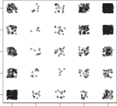
434 AUTOMATED DATA COLLECTION WITH R
12345
12345
Estimated stars
True stars
Figure 17.4 Support vector machine classication results of Amazon reviews
17.4 Conclusion
In this chapter, we have applied two techniques for scoring the sentiment that is expressed in
texts. On the one hand, we have estimated the sentiment of product reviews based on the terms
that are used in the reviews. On the other, we have shown that supervised text classication
is not necessarily restricted to the topical category of texts. We can classify various aspects
in texts, as long as there is a labeled training set.
The scoring of the texts is simplied in this instance, as product reviews refer to precisely
one object—the product. This is to say that negative terms anywhere in the texts will most
likely refer to the product that is being reviewed. Compare this to a journalistic text where
multiple objects might be discussed in a way that it is not straightforward to estimate the
object that a negative term refers to. Consequently, we cannot as easily make the implicit
assumption of the analyses in this chapter that a term anywhere in the text refers to one
particular object. Moreover, the sentiment in a product review is also simple to score as it is
written to explicitly express a sentiment. Again, compare this to a journalistic text. While the
text might in fact express a sentiment toward a topic or toward particular actors, the sentiment
is ordinarily expressed in more subtle ways.

References
Adler D. 2005. vioplot: Violin Plot. R package version 0.2. http://wsopuppenkiste.wiso.uni-
goettingen.de/ dadler
Adler J. 2006. Baseball Hacks. O’Reilly, Sebastopol, CA.
Adler J. 2009. R in a Nutshell. A Desktop Quick Reference. O’Reilly, Sebastopol, CA.
Alem´
an E, Calvo E, Jones MP, and Kaplan N. 2009. Comparing cosponsorship and roll-call ideal points.
Legislative Studies Quarterly 34(1), 87–116.
Asur S and Huberman BA. 2010. Predicting the future with social media. http://arxiv.org/abs/
1003.5699v1 (Last accessed March 21, 2014).
Barber´
a P. 2013. streamR: Access to Twitter Streaming API via R. R package version 0.1. http://CRAN.R-
project.org/package=streamR
Barber´
a P. 2014. Rfacebook: Access to Facebook API via R. R package version 0.3. http://CRAN.R-
project.org/package=Rfacebook
Barrai I, Rodriguez-Larralde A, Marnolini E, Manni F, and Scapolini C. 2001. Isonymy structure of
USA population. American Journal of Physical Anthropology 114(2), 109–123.
Barratt N. 2008. Who Do You Think You Are? Encyclopedia of Genealogy: The Denite Reference Guide
to Tracing Your Family History. HarperCollins, New York, NY.
Beaulieu A. 2009. Learning SQL. O’Reilly, Sebastopol, CA.
Berners-Lee T. 1989. Information management: A proposal. http://www.w3.org/History/1989/proposal
.html (Last accessed February 26, 2014).
Berners-Lee T. 2000. Weaving the Web: The Original Design and Ultimate Destiny of the World Wide
Web by its Inventor. HarperCollins, New York, NY.
Berners-Lee T, Fielding R, and Frystyk H. 1996. Hypertext transfer protocol—http/1.0. RFC 1945.
http://tools.ietf.org/html/rfc1945 (Last accessed December 14, 2013).
Bhushan A. 1971. A le transfer protocol. RFC 114. http://tools.ietf.org/html/rfc114 (Last accessed
December 16, 2013).
Bivand R and Lewin-Koh N. 2013. maptools: Tools for Reading and Handling Spatial Objects.R
package version 0.8-27. http://CRAN.R-project.org/package=maptools
Bivand R, Keitt T, and Rowlingson B. 2013a. rgdal: Bindings for the Geospatial Data Abstraction
Library. R package version 0.8-14. http://CRAN.R-project.org/package=rgdal
Automated Data Collection with R: A Practical Guide to Web Scraping and Text Mining, First Edition.
Simon Munzert, Christian Rubba, Peter Meißner and Dominic Nyhuis.
© 2015 John Wiley & Sons, Ltd. Published 2015 by John Wiley & Sons, Ltd.
436 REFERENCES
Bivand RS, Pebesma E, and G´
omez-Rubio V. 2013b. Applied Spatial Data Analysis with R UseR! Series
2nd edn. Springer, Heidelberg/New York.
Blei DM and Lafferty JD. 2006. Correlated topic models. http://www.cs.cmu.edu/ lafferty/pub/ctm.pdf
(Last accessed March 12, 2014).
Blei DM, Ng AY, and Jordan MI. 2003. Latent dirichlet allocation. Journal of Machine Learning 3,
993–1022.
Boettiger C and Temple Lang D. 2012. RMendeley: Interface to Mendeley API Methods. R package
version 0.1-2. http://CRAN.R-project.org/package=RMendeley
Boettiger C, Temple Lang D, and Wainwright PC. 2014. rshbase: R Interface to FishBASE. R package
version 0.2-2. http://CRAN.R-project.org/package=rshbase
Bollen J, Mao H, and Zeng X. 2011. Twitter mood predicts the stock market. Journal of Computer
Science 2(1), 1–8.
Boswell D. 2002. Introduction to support vector machines. http://www.work.caltech.edu/boswell/
IntroToSVM.pdf (Last accessed March 12, 2014).
Bratton K and Rouse SM. 2011. Networks in the legislative arena: How group dynamics affect cospon-
sorship. Legislative Studies Quarterly 36(3), 423–460.
Broniatowski DA, Paul MJ, and Dredze M. 2013. National and local inuenza surveillance
through twitter: An analysis of the 2012-2013 inuenza epidemic. Plos One 8(12), doi:10.1371/
journal.pone.0083672.
Brownrigg R, Minka TP, Becker RA, and Wilks AR. 2013. maps: Draw Geographical Maps. R package
version 2.3-6. http://CRAN.R-project.org/package=maps
Burkett T. 1997. Cosponsorship in the United States Senate: A Network Analysis of Senate Communi-
cation and Leadership, 1973-1990. University of South Carolina, Columbia.
Castro E and Hyslop B. 2014. HTML and CSS: Visual QuickStart Guide. Peachpit Press.
Center for Responsive Politics. 2014. http://www.opensecrets.org/ (Last accessed March 1, 2014).
Cerami E. 2002. Web Services Essentials. O’Reilly, Sebastopol, CA.
Chamberlain S, Boettiger C, Ram K, Barve V, and Mcglinn D. 2013. rgbif: Interface to the Global
Biodiversity Information Facility API. R package version 0.4.0.
Chamberlin DD and Boyce RF. 1974. Sequel: A Structured English Query Language. Proceedings of
the 1974 ACM SIGFIDET Workshop on Data Description, Access and Control, May 1974, Ann
Arbor, MI, pp. 249–264.
Chesney T. 2006. An empirical examination of Wikipedia’s credibility. First Monday 11(11),
doi:10.5210/fm.v11i11.1413.
Cho WKT and Fowler JH. 2010. Legislative success in a small world: Social network analysis and the
dynamics of congressional legislation. Journal of Politics 72(1), 124–135.
Christian P. 2012. The Genealogist’s Internet: The Essential Guide to Researching Your Family History
Online. 5th revised edition. A & C Black Business Information and Development, London.
Clauson KA, Polen HH, Boulos MNK, and Dzenowagis JH. 2008. Scope, completeness, and accuracy
of drug information in wikipedia. The Annals of Pharmacotherapy 42(12), 1814–1821.
Codd EF. 1970. A relational model of data for large shared data banks. Communications of the ACM
13(6), 377–387.
Conway J, Eddelbuettel D, Nishiyama T, Prayaga SK (during 2008), and Tifn N. 2013. RPostgreSQL:
R Interface to the PostgreSQL Database System. R package version 0.4.
Couture-Beil A. 2013. rjson: JSON for R. R package version 0.2.13. http://CRAN.R-project
.org/package=rjson
Crawley MJ. 2012. The R Book. 2nd edn. John Wiley & Sons, Hoboken, NJ.
Crockford D. 2008. JavaScript: The Good Parts. O’Reilly, Sebastopol, CA.
REFERENCES 437
Culotta A. 2010. Detecting inuenza outbreaks by analyzing twitter messages. http://arxiv.org/
pdf/1007.4748v1 (Last accessed September 03, 2014).
Dailey D. 2010. An SVG primer for today’s browsers. http://www.w3.org/Graphics/SVG/IG/resources/
svgprimer.html (Last accessed October 15, 2013).
Denis Mukhin DAJ and Luciani J. 2013. ROracle: OCI based Oracle Database Interface for R. 1.1-10.
Desposato SW, Kearney MC, and Crisp BF. 2011. Using cosponsorship to estimate ideal points.
Legislative Studies Quarterly 36(4), 531–565.
Dierks T and Allen C. 1999. The tls protocol version 1.0. RFC 2246. http://tools.ietf.org/html/rfc2246
(Last accessed December 12, 2013).
D’Orazio V, Landis S, Palmer G, and Schrodt P. 2014. Separating the wheat from the chaff: Applications
of automated document classication using support vector machines. http://pan.oxfordjournals.org/
content/early/2014/01/29/pan.mpt030.full. pdf+html (Last accessed March 12, 2014).
D¨
oring H. 2013. The collective action of data collection: A data infrastructure on parties, elections and
cabinets. European Union Politics 14(1), 161–178.
Dreyer AJ and Stockton J. 2013. Internet ‘data scraping’: A primer for counseling clients. New York
Law Journal July, 1–3.
Eisenberg JD. 2002. SVG Essentials. O’Reilly, Sebastopol, CA.
Essaid R. 2013a. Is web scraping illegal? Depends on what the meaning of the word is
is. http://www.distilnetworks.com/is-web-scraping-illegal-depends-on-what-the-meaning-of-the-
word-is-is/ (Last accessed January 26, 2014).
Essaid R. 2013b. Scraping just got a lot more dangerous. http://www.distilnetworks.com/scraping-just-
got-a-lot-more-dangerous/ (Last accessed January 26, 2014).
Fall KR and Stevens WR. 2011. TCP/IP Illustrated, Volume 1: The Protocols. Addison-Wesley Profes-
sional, Indianapolis, IN.
Feinerer I. 2008. A text mining framework in R and its applications. Doctoral Thesis. Vienna University
of Economics and Business Administration.
Feinerer I, Hornik K, and Meyer D. 2008. Text mining infrastructure in R. Journal of Statistical Software
25(5), 1–54.
Ferguson N, Schneier B, and Kohno T. 2010. Cryptography Engineering: Design Principles and
Practical Applications. John Wiley & Sons.
Fielding R, Gettys J, Mogul J, Frystyk H, Masinter L, Leach P, and Berners-Lee T. 1999. Hypertext
transfer protocol – http/1.1. RFC 2616.
Fielding RT. 2000. Architectural styles and the design of network-based software architectures. Doctoral
Thesis. University of California.
Flanagan D. 2011. JavaScript: The Denitive Guide. O’Reilly, Sebastopol, CA.
Forouzan BA. 2010. TCP/IP Protocol Suite. McGraw-Hill, Boston, MA.
Fowler JH. 2006a. Connecting the congress: A study of cosponsorship networks. Political Analysis
14(4), 456–487.
Fowler JH. 2006b. Legislative cosponsorship networks in the us house and senate. Social Networks
28(4), 454–465.
Fox WR and Lasker GW. 1983. The distribution of surname frequencies. International Statistical Review
51, 81–87.
Franks J, Hallam-Baker P, Hostetler J, Lawrence S, Leach P, Luotonen A, and Stewart L. 1999. Http
authentication: Basic and digest access authentication. RFC 2617. http://tools.ietf.org/html/rfc2617
(Last accessed December 14, 2013).
Freier A, Karlton P, and Kocher P. 2011. The secure sockets layer (ssl) protocol version 3.0. RFC 6101.
http://tools.ietf.org/html/rfc6101 (Last accessed December 14, 2013).
438 REFERENCES
Garnkel S. 2002. Web Security, Privacy and Commerce. O’Reilly, Sebastopol, CA.
Gennick J. 2011. SQL Pocket Guide. 3rd edn. O’Reilly, Sebastopol, CA.
Gentry J. 2013. twitteR: R Based Twitter Client. R package version 1.1.7. http://CRAN.R-
project.org/package=twitteR
Gentry J and Lang DT. 2013. ROAuth: R Interface for OAuth. R package version 0.9.3. http://CRAN.R-
project.org/package=ROAuth
Ghomi AA, Shirzadi E, and Movassaghi A. 2013. Predicting the Academy Awards’ result by analyzing
tweets. Global Journal of Science, Engineering and Technology.8, 39–47.
Giles J. 2005. Internet encyclopae dias go head to head. Nature 438, 900–901.
Gillespie P. 2012. Pronouncing sql: S-q-l or sequel? http://patorjk.com/blog/2012/01/26/pronouncing-
sql-s-q-l-or-sequel/ (Last accessed August 11, 2014).
Gliozzo A, Strapparava C, and Dagan I. 2009. Improving text categorization bootstrapping via unsu-
pervised learning. ACM Transactions on Speech and Language Processing 6(1), 1–24.
Google. 2014. Chrome devtools. https://developers.google.com/chrome-developer-tools/ (Last
accessed August 3, 2014).
Gourley D and Totty B. 2002. HTTP. The Denitive Guide. O’Reilly, Sebastopol, CA.
Grimmer J and Stewart BM. 2013. Text as data: The promise and pitfalls of automatic content analysis
methods for political texts. Political Analysis 21(3), 267–297.
Grolemund G and Wickham H. 2011. Dates and times made easy with lubridate. Journal of Statistical
Software 40(3), 1–25.
Hammer-Lahav E. 2010. The Oauth 1.0 protocol. RFC 5849. http://tools.ietf.org/html/rfc5849 (Last
accessed February 25, 2014).
Hardt D. 2012. The Oauth 2.0 authorization framework. RFC 6749. http://tools.ietf.org/html/rfc6749
(Last accessed February 25, 2014).
Harold ER and Means WS. 2004. XML in a Nuthsell: A Desktop Quick Reference. 3rd edn. O’Reilly,
Sebastopol, CA.
Harrington JL. 2009. Relational Database Design and Implementation. Morgan Kaufmann Series in
Data Management Systems. 3rd edn. Elsevier, Amsterdam.
Hemenway K and Calishain T. 2003. Spidering Hacks. O’Reilly, Sebastopol, CA.
Hintze JL and Nelson RD. 1998. Violin plots: A box plot-density trace synergism. The American
Statistician 52(2), 181–184.
Hogarth RM. 1978. A note on aggregating opinions. Organizational Behavior and Human Performance
21, 40–46.
Holdener III AT. 2008. Ajax: The Denitive Guide. O’Reilly, Sebastopol, CA.
Holzner S. 2003. XPath Kick Start: Navigating XML with XPath 1.0 and 2.0. Sams Publishing, Indi-
anapolis, IN.
Hopkins D and King G. 2010. A method of automated nonparametric content analysis for social science.
American Journal of Political Science 54(1), 229–247.
Hornik K, Buchta C, and Zeileis A. 2009. Open-source machine learning: R meets weka. Computational
Statistics 24(2), 225–232.
Hu M and Liu B. 2004. Mining and Summarizing Customer Reviews. Proceedings of the ACM SIGKDD
International Conference on Knowledge Discovery and Data Mining (KDD-2004), August 2004,
Seattle, WA.
James DA and DebRoy S. 2013. RMySQL: R Interface to the MySQL Database. Version 0.9-3.
http://biostat.mc.vanderbilt.edu/RMySQL (Last accessed August 29, 2013).
Jurka TP, Collingwood L, Boydstun AE, Grossman E, and Atteveldt WV. 2013. Rtexttools: A supervised
learning package for text classication. The R Journal 5(1), 6–12.
REFERENCES 439
Kahle D and Wickham H. 2013. ggmap: Spatial visualization with ggplot2. The R Journal 5(1), 144–161.
Kerr O. 2013. District court holds that intentionally circumventing ip address ban is ‘access
without authorization’ under the cfaa http://www.volokh.com/2013/08/18/district-court-holds-
that-intentionally-circumventing-ip-address-block-is-unauthorized-access-under-the-cfaa/ (Last
accessed March 11, 2014).
Koster M. 1994. Important: Spiders, robots and web wanderers. http://inkdroid.org/tmp/www-
talk/4113.html (Last accessed January 24, 2014).
Kriegel A and Trukhnov BM. 2008. SQL Bible. 2nd edn. John Wiley & Sons, Hoboken, NJ.
Leithner A, Maurer-Ertl W, Glehr M, Friesenbichler J, Leithner K, and Windhager R. 2010. Wikipedia
and osteosarcoma: A trustworthy patients’ information? Journal of the American Medical Informatics
Association 17(4), 373–374.
Liu B. 2012. Sentiment Analysis and Opinion Mining. Morgan and Claypool, San Rafael, CA.
Liu B, Hu M, and Cheng J. 2005. Opinion Observer: Analyzing and Comparing Opinions on the Web.
Proceedings of the 14th International World Wide Web Conference (WWW-2005), May 2005, Chiba,
Japan.
Liu C and Albitz P. 2006. DNS and BIND. O’Reilly, Sebastopol, CA.
Manning CD, Paghavan P, and Sch¨
utze H. 2008. Introduction to Information Retrieval. Cambridge
University Press, Cambridge.
McJones P, Bamford R, Blasgen M, Chamberlin D, Cheng J, Daudenarde JJ, Finkelstein S, Gray J, Jolls
B, Lindsay B, Lorie R, Mehl J, Miller R, Mohan C, Nauman J, Pong M, Price T, Putzolu F, Schkolnick
M, Selinger B, Selinger P, Slutz D, Traiger I, Wade B, and Yost B. 1997. The 1995 SQL reunion:
People, projects, and politics. http://www.scs.stanford.edu/∼dbg/readings/SRC-1997-018.pdf (Last
accessed October 30, 2013).
McSherry C and Opsahl K. 2013. AP. v. Meltwater: Disappointing ruling for news search. https://www
.eff.org/deeplinks/2013/03/ap-v-meltwater-disappointing-ruling-news-search (Last accessed January
26, 2014).
Meng Y. 2012. Sentiment analysis: A study on product features. Dissertation. University of Nebraska,
Lincoln.
Mukherjee S and Bhattacharyya P. 2012. Feature specic sentiment analysis for product reviews.
In: Computational Linguistics and Intelligent Text Processing. Gelbukh A, ed. Springer, Berlin.
pp. 475–487.
Murrell P. 2009. Introduction to Data Technologies. Chapman & Hall/CRC, Boca Raton, FL.
Mozilla Developer Network. 2013. XPath. https://developer.mozilla.org/en-US/docs/Web/XPath (Last
accessed March 10, 2014).
Niederst Robbins J. 2013. HTML5 Pocket Reference. O’Reilly, Sebastopol, CA.
Nolan D and Temple Lang D. 2014. XML and Web Technologies for Data Sciences with R. Use R!.
Springer, New York, NY.
O’Neil C and Schutt R. 2013. Doing Data Science. Straight Talk from the Frontline. O’Reilly, Sebastopol,
CA.
Ooms J. 2013. A practical and consistent mapping between JSON data and R objects. http://cran.r-
project.org/web/packages/jsonlite/vignettes/json-mapping.pdf (Last accessed February 2, 2014).
Ooms J and Temple Lang D. 2014. jsonlite: A Smarter JSON Encoder/Decoder for R. R package version
0.9.3. http://CRAN.R-project.org/package=jsonlite
Osborn H. 2012. Genealogy: Essential Research Methods. Robert Hale Ltd, London.
Paar C and Pelzl J. 2011. Understanding Cryptography: A Textbook for Students and Practitioners.
Springer, New York, NY.
Pebesma EJ and Bivand RS. 2005. Classes and methods for spatial data in R. RNews5(2), 9–13.
440 REFERENCES
Peress M. 2010. Estimating proposal and status quo locations using voting and cosponsorship data.
http://www.rochester.edu/College/faculty/mperess/Proposals_and_Status_Q uos.pdf (Last accessed
October 8, 2012).
Postel J and Reynolds J. 1985. File transfer protocol (ftp). RFC 959. http://tools.ietf.org/html/rfc959
(Last accessed December 15, 2013).
Princeton University. 2010a. About WordNet.http://wordnet.princeton.edu (Last accessed February 27,
2014).
Princeton University. 2010b. License and Commercial Use of WordNet. http://wordnet.princeton
.edu/wordnet/license/ (Last accessed February 27, 2014).
R Special Interest Group on Databases. 2013. DBI: R Database Interface. R package version 0.2-7.
http://cran.r-project.org/web/packages/DBI/index.html (Last accessed August 13, 2014).
Ramisch C. 2008. N-gram models for language detection. http://www.inf.ufrgs.br/∼ceramisch/
download_les/courses/Master_FRANCE/ENSIMAG_2008_2/Ingenierie_des_Langues_et_de_la_
Parole/Rapport.pdf (Last accessed March 22, 2014).
Ramon L and de Villa AR. 2013. Relenium. Selenium for R. http://lluisramon.github.io/relenium/ (Last
accessed March 24, 2014).
Ray ET. 2003. Learning XML. 2nd edn. O’Reilly, Sebastopol, CA.
Reavley N, Mackinnon A, Morgan A, Alvarez-Jimenez M, Hetrick S, Killackey E, Nelson B, Purcell
R, Yap M, and Jorm A. 2012. Quality of information sources about mental disorders: a comparison
of Wikipedia with centrally controlled web and printed sources. Psychological Medicine 42(8),
1753–1762.
Rector LH. 2008. Comparison of Wikipedia and other encyclopedias for accuracy, breadth, and depth
in historical articles. Reference Services Review 36(1), 7–22.
Richardson L, Amundsen M, and Ruby S. 2013. RESTful Web APIs. O’Reilly, Sebastopol, CA.
Ripley B and Lapsley M. 2013. RODBC: ODBC Database Access. Version 1.3-7, Lapsley participated
from 1999 to 2002.
Selenium Project. 2014a. Selenium Commands – Selenese. Selenium Documentation. http://docs
.seleniumhq.org (Last accessed March 24, 2014).
Selenium Project. 2014b. Selenium Documentation.http://docs.seleniumhq.org/docs/ (Last accessed
March 24, 2014).
Schrenk M. 2012. Webbots, Spiders, and Screen Scrapers. A Guide to Developing Internet Agents with
PHP/Curl , 2nd ed. No Starch Press, San Francisco, CA.
Snell J and Care D. 2013. Use of online data in the big data era: Legal issues raised by the
use of web crawling and scraping tools for analytics purposes. http://about.bloomberglaw.com/
practitioner-contributions/legal-issues-raised-by-the-use-of-web-crawling-and-scraping-tools-for-
analytics-purposes/ (Last accessed January 26, 2014).
Snow G. 2013. TeachingDemos: Demonstrations for Teaching and Learning. R package version 2.9.
http://CRAN.R-project.org/package=TeachingDemos
Stenberg D. 2013. libcurl: The multiprotocol le transfer library. http://curl.haxx.se (Last accessed
December 13, 2013).
Stepp M, Miller J, and Kirst V. 2012. Web Programming Step by Step, 2nd edn. Step by Step Publishing,
http://www.stepbystepselfpublishing.net/
Teetor P. 2011. R Cookbook. O’Reilly, Sebastopol, CA.
Temple Lang D. 2012a. RCurl philosophy. http://www.omegahat.org/RCurl/philosophy.html (Last
accessed December 13, 2013).
Temple Lang D. 2012b. SSOAP: Client-Side SOAP Access for S. R package version 0.9-1.
http://www.omegahat.org/SSOAP,http://www.omegahat.org,http://www.omegahat.org/bugs
REFERENCES 441
Temple Lang D. 2013a. RCurl: General Network (HTTP/FTP/...) Client Interface for R. R package
version 1.95-4.1. http://CRAN.R-project.org/package=RCurl
Temple Lang D. 2013b. RJSONIO: Serialize R Objects to JSON, JavaScript Object Notation. R package
version 1.0-3. http://CRAN.R-project.org/package=RJSONIO
Temple Lang D. 2013c. XML: Tools for Parsing and Generating XML Within R and S-Plus. R package
version 3.95-0.2. http://CRAN.R-project.org/package=XML
Temple Lang D, Keles S, and Dudoit S. 2012. RHTMLForms: Programmatically Create R Func-
tions Corresponding to Web/HTML Forms. R package version 0.6-0. http://www.omegahat.org/
RHTMLForms
Tennison J. 2001. XSLT and XPath on the Edge. John Wiley & Sons, Hoboken, NJ.
Torgo L. 2010. Data Mining with R: Learning with Case Studies. Chapman & Hall/CRC, Boca
Raton, FL.
Tumasjan A, Sprenger TO, Sandner PG, and Welpe IM. 2011. Election forecasts with twitter. How 140
characters reect the political landscape. Social Science Computer Review 29(4), 402–418.
United States District Court District of Massachusetts. 2013. USA v. Swartz. http://pacer.mad.uscourts
.gov/dc/cgi-bin/recentops.pl?lename=gorton/pdf/swartz%20protective%20order%20mo.pdf (Last
accessed January 26, 2014).
W3C. 1999. W3C. http://www.w3.org/TR/xpath/ (Last accessed December 2, 2013).
Warden P. 2010. How i got sued by Facebook. http://petewarden.com/2010/04/05/how-i-got-sued-by-
facebook/ (Last accessed January 26, 2014).
Wickham H. 2010. Stringr: Modern, consistent string processing. The R Journal 2(2), 38–40.
Wickham H. 2011. The split-apply-combine strategy for data analysis. Journal of Statistical Software
40(1), 1–29.
Wickham H. 2012. httr: Tools for Working with URLs and HTTP. R package version 0.2. http://CRAN.R-
project.org/package=httr
Wickham H and Chang W. 2013. devtools: Tools to Make Developing R Code Easier. R package version
1.4.1. http://CRAN.R-project.org/package=devtools
Wikipedia. 2014. Niccol`
o Machiavelli.
Witten IH and Frank E. 2005. Data Mining: Practical Machine Learning Tools and Techniques, 2nd
ed. Morgan Kaufmann, San Francisco, CA.
Wong C. 2000. HTTP Pocket Reference. O’Reilly, Sebastopol, CA.
Yasuda N, Cavalli-Sforza L, Skolnick M, and Moroni A. 1974. The evolution of surnames: An analysis
of their distribution and extinction. Theoretical Population Biology 5(1), 123–142.
Zagibalov T and Carroll J. 2008. Automatic Seed Word Selection for Unsupervised Sentimen Classica-
tion of Chinese Text. Proceedings of the 22nd International Conference on Computational Linguistics,
August 2008, Manchester, UK, pp. 1073–1080.
Zakas NC. 2010. High Performance JavaScript. O’Reilly, Sebastopol, CA.
Zhang Y, Friend AJ, Traud AL, Porter MA, Fowler JH, and Mucha PJ. 2008. Community structure in
congressional cosponsorship networks. Physica A 387(7), 1705–1712.
Zhao Y. 2012. R and Data Mining. Examples and Case Studies. Elsevier Academic Press, Waltham,
MA.
Zumel N and Mount J. 2014. Practical Data Science with R. Manning, Greenwich, CT.

General index
AJAX, 11, 149–163, 252
Amazon, 396, 416
AP v. Meltwater, 279
APIs, 68, 71, 150, 221, 259–266, 372
advantages and disadvantages, 277
REST, 260
SOAP, 260
when and how to use, 276
with R, 261
ASCII, 216
Asynchronous JavaScript and XML, see
AJAX
Authentication, 121–123, 266
Authorization, 266
Base64, 111, 121, 245
Berners-Lee, Tim, 17, 101
beta.congress.gov, 345
Binary format, 223
Bots, see Web robots
Boyce, Raymond F., 167
CA certicate, 246, 297
Carriage return, 106, 227, 360, 385, 386
Cascading Style Sheets, see CSS
Chamberlin, Donald D., 167
Character encoding, 44, 214–216, 270
Closing tag, see End tag
Closure function, 37
Codd, Edgar F., 166
Cookies, 112, 119–121, 247
CRAN, 226, 291, 330
Crawlers, see Web robots
Cron, 335
CSS, 26, 28, 39, 256
CSV, 223
curl, 127
Curl handle, 236
curl.haxx.se, 127
Data, 165
collection costs, xvi
cleansing, 3, 272, 347, 426
collection automation, xvi
quality, 7
science, xv, xvii
storage, 165, 408
types, 174
Data project management, 322–339
control structures, 326
error and exception handling, 333–334
le system management, 322–323
for-loops, 324
messages, 331–333
processing multiple documents, 323–
328
progress bars, 331–333
scheduling, 334
while-loops, 326
writing functions, 328–334
Automated Data Collection with R: A Practical Guide to Web Scraping and Text Mining, First Edition.
Simon Munzert, Christian Rubba, Peter Meißner and Dominic Nyhuis.
© 2015 John Wiley & Sons, Ltd. Published 2015 by John Wiley & Sons, Ltd.
GENERAL INDEX 443
Databases, 13, 164, 166, 408
advanced features, 174–175
combined keys, 170
DBMS, 165, 166
foreign keys, 170, 180
in R, 188–192
keys, 168
normal forms, 171
normalization, 170
ODBC, 188
primary keys, 170, 180
query, 167
RDBMS, 166
redundancy and exclusiveness, 168
relations, 167
storage, 424
tables, 167
views, 175, 411
Deep link, 279
DNS, 102, 105
DOCTYPE, see DTD
Document Object Model, see DOM
Document Type Denition, see DTD
DOM, 33, 34, 66, 272
parsing, see Parsing
validation, 34
DTD, 23, 51, 59
Dynamic HTML, see AJAX
eBay v. Bidder’s Edge, 278
Eich, Brendan, 150
Election Markup Language (EML), 77
Encoding, see Character encoding
End tag, 20, 44, 45
Extensible Markup Language, see XML
Facebook, 268, 282
Facebook v. Pete Warden, 279
Fielding, Roy, 101
FTP, 126, 226, 359
commands, 227
extended passive mode, 227
FTP archives on the Web, 228
Geographical data, 3, 60, 368, 380
GET, 29, 235
GitHub, xx, 253, 291, 330
Google, xxi, 29, 105, 368
gzip, 110
Hostname, 101, 105
HTML, 2, 10, 17–39, 149
attributes, 20
buttons, 29
checkboxes, 29
comments, 22
entities, 22
elds, 29
forms, 128
HTML5, 17
hyperlinks, 24
line breaks, 23
links, 233
lists, 233
special characters, 22
syntax, 19, 24
tables, 32, 234
tags, 18, 20
<a>, 20, 24
<b>,26
<br>,20
<dd>,27
<div>,27
<dl>,27
<fieldset>,29
<form>,29
<h1,h2,h3,...>,27
<h1,h2,h3,...>, 400
<i>,26
<input>,29
<link>,26
<meta>,25
<ol>,27
<option>,29
<p>,27
<script>, 30, 150, 151
<select>,29
<span>,27
<strong>,26
<table>,32
<td>,32
<textarea>,29
<th>,32
<title>,20
444 GENERAL INDEX
HTML (Continued )
<tr>,32
<ul>,27
tree structure, 21
HTTP, 11, 25, 29, 101–149
authentication, see Authentication
body, 106
client, 102
CONNECT, 108
DELETE, 108
GET, 108, 128–129
handlers, 132–133
HEAD, 108
header, 106, 107
header elds, 107, 109–115
Accept-Encoding, 110, 286
Accept, 110
Allow, 110
Authorization, 111, 121
Connection, 113
Content-Encoding, 111
Content-Length, 111
Content-Type, 111
Cookie, 111, 119
From, 112, 119, 225
Host, 112
If-Modified-Since, 112, 286
Last-Modified, 113, 286
Location, 113
Proxy-Authorization, 113
Proxy-Connection, 113
Referer, 114, 118
Server, 114
Set-Cookie, 114, 119
User-Agent, 114, 117, 225, 280
Vary, 115
Via, 115, 123
WWW-Authenticate, 115, 121
X-Forwarded-For, 123
identication, 116–121
messages, 106–107
methods, 260
OPTIONS, 108
options, 133–139
persistent connection, 113
port, 103, 105
POST, 108, 129–130
PUT, 108
request methods, 104, 108
response, 104
status codes, 108
TRACE, 108
httpbin.org, 116
HTTPS, 124–126, 246, 297
Hypertext Markup Language, see HTML
IANA, 107
ICPSR, 246
inkscape.org, 58
Inspect element, 19, 397, 398, 402
IP (Internet Protocol), 102
IP address, 105, 123
JavaScript, 30–32, 68, 71, 150–154, 395
DOM manipulation, 154, 151–154
event handlers, 150, 153, 155
functionality, 150
Same Origin Policy, 155
scraping, 153, 156
syntax, 152
JavaScript Object Notation, see JSON
jQuery, 150, 152
JSON, 10, 68–76, 259
array, 69
data types, 70
encoding, 71
import and export, 72
parser, 158
syntax, 69–71
validation, 71
json.org, 71
Levenshtein distance, 211
libcurl, 118, 127, 226, 246, 247
libxml2, 33
Line feed, 106, 227, 385, 386
Markup language, 17, 18, 41, 71, 80
MIME (Internet media) type, 26, 107, 110
mysql.com, 177
Name maps, 380
Network analysis, 343, 353–358
Node, 34
Node set, 34, 35, 37, 81
GENERAL INDEX 445
OAuth, 221, 266–270, 276, 372
Omega Project, 291
Opening tag, see Start tag
OpenStreetMap, 368
parlgov.org, 193
Parser, see Parsing
Parsing, 32–38, 60, 80, 270, 272, 274, 359,
361
event-driven parsing, 66–68
Password storage, 245, 263
Percent encoding, see URL encoding
Perl, xvii, 207
PHP, xvii, 129, 252
Plain text, 11, 22, 223
planetr.stderr.org, 58
POST, 29, 235
programmableweb.com, 276
Proxies, see Proxy servers
Proxy servers, 115, 123–124
Public key cryptography, 125
Python, xvii
Query language, see XPath
Query string, 30
R, xv, xvii
CRAN Task View, xx
introduction, xvi, xix–xx
packages, xvii
reasons to use, xvii–xix
workow, xviii
r-bloggers.com, 58
r-datacollection.com, xx, 13, 19, 101
regex101.com, 271
regexplanet.com, 271
Regular expressions, 4, 12, 198–205, 225,
270, 346
advantages and disadvantages, 272
backreferencing, 205
case-insensitive matching, 199
character classes, 201
debugging, 272
exact character matching, 198–200
avors, 207
generalized matching, 200
generalizing, 205
greedy quantication, 203
matching beginnings and ends, 199
metacharacters, 204
pipe operator, 200
quantiers, 202
shortcuts, 204
when and how to use, 270
with R, 197
Relational database, see Databases
REST, 260
robotstxt.org, 283
rOpenSci, 291
RSS, 11, 55–58, 261, 279
rssboard.org, 57
Ruby, xvii
Scrapers, see Web scraping
scraping.pro, 271
SelectorGadget, 98, 274
Selenium, 12, 162, 221, 252, 253
SMTP, 105
SOAP, 260
Spiders, see Web robots
SQL, 13, 167, 175–195
clauses, 184
data control language (DCL), 175, 177
data denition language (DDL), 176
data manipulation language (DML), 176,
180
in R, 188–192
MySQL, 177, 181, 191, 253
SEQUEL, 167
SQLite, 177, 408
syntax, 176
transaction control language (TCL), 176,
187
Sring processing
number removal, 304
word removal, 304
SSL, 124, 246
Stack Overow, xx
Start tag, 20, 45
Statistical text processing, 295–321, 416
corpus, 298
correlated topic models, 314
dictionary methods, 416
document-term matrix, 310, 432
446 GENERAL INDEX
Statistical text processing (Continued )
hierarchical clustering, 315
latent Dirichlet allocation, 314
maximum entropy, 309, 432
n-grams, 305
punctuation removal, 304
random forest, 309
sentiment analysis, 426–432
sparsity, 305
supervised methods, 295, 307–313
support vector machine, 432
support vector machine (SVM), 309
term-document matrix, 303
text operations, 298–307
unsupervised methods, 296, 313–320
String processing
approximate matching, 211
character matching, 198
counting, 209
detection, 209
duplicating, 210
joining, 210
padding, 210
replacement, 209
splitting, 209
stemming, 305
stop word removal, 305
string location, 208
substring extraction, 208
trimming, 210
with regular expressions, see Regular
expressions
Structured Query Language, see SQL
Super assignment operator, 37
SVG, 11, 58–60, 77
TCP, 102, 105
Text mining, 12, see Statistical text
processing
thomas.loc.gov, 344
TLS, 124
Transparency International, 228
Twitter, 7, 10, 71, 77, 266, 371
U.S. Senate, 343
UNESCO, 1
United States v. Aaron Swartz, 279
URI, 54
URL, 104–106, 228
encoding, 106, 263, 383
format, 105
query string, 105
scheme, 105
syntax, 104–106
User Agent, 114, 117, 280
useragentstring.com, 117
UTF-8, 215, 384
w3.org, 59, 60, 105
W3C, 17, 38, 58, 79, 80, 150
w3schools.com, 106
Weather data, 359
Web 2.0, 259
Web application, 149
Web client, 101
Web Developer Tools (WDT), 98, 158–161,
255, 395
Web robot, xxi
Web robots, 222, 280
Web scraping, xxi, 222
accessing FTP servers, 226–228
convenience functions, 232–235
copyright, xxi, 278
data retrieval, 221
Dealing with AJAX, 251–259
dos and don’ts, 284–290
downloading les, 223–226
etiquette, 222, 284–290, 382
extraction strategies, 270–278
form handling, 243–245
GET forms, 236–239
HTML forms, 235–245
HTTP authentication, 245
information extraction, 221
JavaScript-generated content, 251–259
legal issues, xxi, 278–280
POST forms, 239–243
Retrieval via HTTPS, 246–247
robots.txt, 222, 280–283, 382
URL manipulation, 228–232
Using cookies, 247–251
workow, 221, 322–339
Web services, see APIs
Webdriver, see Selenium
GENERAL INDEX 447
whatismyipaddress.com, 105
WHATWG, 17
Wikipedia, 1, 7
Windows Task Scheduler, 337
Windows-1252, 215
WordNet, 236
World Heritage Sites in Danger, 1
Wrapper function, 259, 263, 264, 276, 366
WSDL, 260
XHR, 150, 154–158, 251
XML, 10, 41–68, 259
attributes, 45–46
CDATA, 49
commenting, 49
elements, 42, 44–45
encoding, 44
escape sequences, 48
extensions, 54–60
handler, 66
namespaces, 53–54, 96–97
naming rules, 48
nodes, 46
parsing, 60–62
predicates, 63
root element, 42
Schema (XSD), 52
schemas, 52, 54
syntax, 43–51
transformation into Robjects, 65–66
tree structure, 46–47, 81, 84
valid vs. wellformed, 51
versions, 44
XMLHttpRequest, see XHR
xmlvalidation.com, 51
XPath, 11, 45, 63, 79–100, 398
advantages and disadvantages, 275
attribute extraction, 90
Boolean functions, 91
element extraction, 93–98
extractor functions, 93
namespaces, 96–97
node relations (axes), 84–86, 386
operators, 87
partial matching, 91, 92
pipe operator, 83
predicates
numerical, 87–91
regex, 91
textual, 91–92
selection expressions, 83
syntax, 81–92
versions, 80
when and how to use, 273
wildcard operator, 83
Yahoo Weather RSS Feed, 261
YouTube, 71

Package index
DBI, 188, 189
devtools, 254, 291
httr, 126, 268
igraph, 345, 354
jsonlite, 71, 74
lubridate, 374
maps, 2, 5, 384, 388
maptools, 384
network, 354
pingr, 333
plyr, 73, 224, 236, 272, 327
Rcpp, xviii
RCurl, 116, 117, 126, 160, 222, 225, 226,
236, 242, 245–247, 297, 345, 351,
360, 384, 396, 399, 417
Relenium, 259
Rfacebook, 269
rfishbase, 291
rgbif, 291
rgdal, 384
RgoogleMaps, 368
RHTMLForms, 243
rjson,71
RJSONIO,71
RMendeley, 291
RMySQL, 188
ROAuth, 268
RODBC, 177, 188, 191
ROracle, 188
RPostgreSQL, 188
RSQLite, 177, 188, 189, 408, 417
RTextTools, 296, 309, 310, 426, 432
Rwebdriver, 252, 253
RWeka, 306
sna, 354
SnowballC, 305
sp, 164
SSOAP, 260
statnet, 354
stringr, 2, 4, 72, 94, 197, 207–211, 222,
236, 247, 272, 297, 329, 335, 345,
360, 384, 396, 399, 417
tau, 216
TeachingDemos, 384
textcat, 426
tm, 295, 298, 426
topicmodels, 316
vioplot, 426, 429
XML, 2, 33, 61, 63, 65, 80, 93, 222, 223,
232, 236, 247, 261, 297, 345, 384,
396, 399, 417
Automated Data Collection with R: A Practical Guide to Web Scraping and Text Mining, First Edition.
Simon Munzert, Christian Rubba, Peter Meißner and Dominic Nyhuis.
© 2015 John Wiley & Sons, Ltd. Published 2015 by John Wiley & Sons, Ltd.

Function index
aggregate(), 369
all(), 214
any(), 303
apply(), 214, 318
args(), 244
as.POSIXct(), 375
base64(), 122
base64Decode(), 122
basename(), 323, 331
basicTextGatherer(), 132
cat(), 117, 331
ceiling(), 401
character(), 297
classify_model(), 432
cleanUp(), 347
close(),74
close_window(), 257
collectHref(), 329
combn(), 354
contains(), 385
Corpis(), 299, 430
createFunction(), 243
create_container(), 310,
432
CRS(), 388
CTM(), 318
curlOptions(), 131, 137
curlPerform(), 131
curlSetOpt(), 251
curlVersion(), 124
data(), 388
data.frame(), 316
dbConnect(), 408, 417
dbDataType(), 190
dbDriver(), 408, 417
dbExistsTable(), 190, 409
dbGetInfo(), 190
dbGetQuery(), 189, 409, 417, 425
dbListTables(), 190
dbReadTable(), 190, 415
dbRemoveTable(), 190
dbSendQuery(), 189
dbWriteTable(), 190
debugGatherer(), 132, 140, 236, 238,
248, 286
dim(),4
dir(), 323
dir.create(), 323, 390, 418
dirname(), 323
DirSource(), 299
dist(), 315
do.call(), 73, 236
DocumentTermMatrix(), 310, 432
download.file(), 127, 224, 225, 335,
387, 420
dupCurlHandle(), 133, 137
duplicated(), 406, 428
Automated Data Collection with R: A Practical Guide to Web Scraping and Text Mining, First Edition.
Simon Munzert, Christian Rubba, Peter Meißner and Dominic Nyhuis.
© 2015 John Wiley & Sons, Ltd. Published 2015 by John Wiley & Sons, Ltd.
450 FUNCTION INDEX
element_click(), 257
element_xpath_find(), 257
Encoding(), 215
fetch(), 189
file(),74
file.access(), 323
file.append(), 323
file.copy(), 323
file.date(), 287
file.exists(), 224, 287, 323, 335, 390,
418
file.info(), 323, 421
file.path(), 323
file.remove(), 323, 421
file.rename(), 323
fileUpload(), 242
filterStream(), 374
findAssocs(), 307
fixed(), 204
for(), 324
formFunction(), 243
fromJSON(), 72, 74
ftpUpload(), 228
function(), 329, 401
get.adjacency(), 355
get.url(), 255
getBinaryURL(), 128, 225
getCurlErrorClassNames(), 143
getCurlHandle(), 133, 225, 228, 230,
236, 247, 248, 286, 401
getCurlInfo(), 141
getForm(), 129, 238, 247, 249, 384
getFriends(), 269
getHTMLExternalFiles(), 233
getHTMLFormDescription(), 243
getHTMLLinks(), 223, 232, 328
GetMap.OSM(), 368
getOption(), 245
getTrends(), 372
getURL(), 117, 128, 160, 226, 230, 237,
245, 246, 248, 297, 360, 399
getURLContent(), 128
getUser(), 372
getUsers(), 269
graph.edgelist(), 354
gregexpr(), 211
grep(), 198, 212
grepl(), 198, 211, 212, 214
gsub(), 211
handleInfo(), 142
hclust(), 315
head(),4
hist(),6
htmlParse(), 2, 33, 61, 80, 229, 232,
237, 248, 270, 297, 329, 384, 399, 418
htmlTreeParse(),35
httpDate(), 287
iconv(), 215
iconvlist(), 215
install_github(), 254, 291
invisible(),38
is.ascii(), 216
is.locale(), 216
is.utf8(), 216
isValidJSON(),71
jitter(), 431
keys(), 257
lapply(), 74, 133, 236, 401, 418
LDA(), 316
ldply(), 327
length(), 297
library(),2
list(), 138
list.files(), 298, 361
listCurlOptions(), 133
llply(), 231
l_ply(), 224, 228, 230
make.unique(), 212
map(),5
matrix(), 350
merge(), 387
meta(), 300
names(), 127
nchar(), 211
NGramTokenizer(), 306
FUNCTION INDEX 451
oauth1.0_token(), 268
oauth2.0_token(), 269
oauth_2.0_token(), 268
oauth_app(), 268
oauth_endpoint(), 268
odbcDataSources(), 192
odbcGetInfo(), 191
options(), 137, 139, 245
order(), 318
page_title(), 255
parseTweets(), 374
paste(), 211
paste0(), 211
path.expand(), 323
PlotOnStaticMap(), 368
pmatch(), 212
png(), 368
post.url(), 255
posterior(), 316
postForm(), 130, 240, 351
prescindMeta(), 301, 310
print(), 33, 80
rbind.fill(), 73, 236
read.csv(), 225, 368
read.delim(), 387
read.fwf(), 361, 365
readHTMLList(), 232, 233
readHTMLTable(), 2, 232, 234, 240,
421
readHTMLTable(), 351
readLines(), 33, 232, 251, 270, 299,
362, 427
readShapePoly(), 388
regexprl(), 211
regmatches(), 211
removeNumbers(), 304, 427
removePunctuation(), 304
removeSparseTerms(), 306, 310, 428,
430, 432
removeWords(), 305, 427
robotsCheck(), 282
sample(), 428
sampleStream(), 374
sapply(), 73, 214, 351, 364
save(), 287
searchTwitter(), 372
seq_along(), 249, 401, 419
set.seed(), 428
setdiff(), 289
setTxtProgressBar(), 333
sFilter(), 302
sign_oauth1.0(), 268
sign_oauth2.0(), 268, 269
simplify(), 356
slotNames(), 311
source(), 330
SpatialPoints(), 388
split(), 401
sprintf(),95
sqlFetch(), 192
sqlTables(), 191
start_session(), 255
stemDocument(), 305, 427, 428
stopwords(), 305
strsplit(), 211
str_c(), 208, 210, 211, 224, 229, 297,
361, 399, 418, 424
str_count(), 208, 209, 211
str_detect(), 3, 72, 208, 209, 211,
212, 223, 225, 231, 303, 329, 360, 418,
427
str_dup(), 208, 210, 211
str_extract(), 4, 94, 198, 208, 211,
230, 364, 385
str_extract_all(), 3, 198, 208, 211,
225, 227
str_length(), 208, 210, 211
str_locate(), 208, 211
str_locate_all(), 208, 211
str_pad(), 208, 210, 211
str_replace(), 208, 209, 211, 270,
419
str_replace_all(), 208, 209, 211, 249,
364, 386
str_split(), 136, 208, 209, 211, 227,
238, 249, 250,360, 362
str_split_fixed(), 208, 209, 211
str_sub(), 4, 132, 208, 211, 360
str_trim(), 208, 210, 211
sub(), 211
subset(), 388
452 FUNCTION INDEX
Sys.getlocale(), 215
Sys.setlocale(), 375
Sys.sleep(), 227, 230, 290, 361, 401,
419
system.file(), 247, 297
t(), 236, 316
tempfile(), 365
TermDocumentMatrix(), 303, 428,
430
terms(), 317
tm_filter(), 303
tm_m(), 304
tm_map(), 427, 430
toJSON(), 72, 74
tolower(), 94, 305, 390, 427
train_model(), 311, 432
try(), 227, 230, 333
tryCatch(), 143, 334, 420
twListToDF(), 372
txtProgressBar(), 332
unlist(), 198
unzip(), 323, 387
URLdecode(), 106
URLencode(), 106
userStream(), 374
VectorSource(), 299, 430
vioplot(), 429
Weka_control(), 306
while(), 297, 326
window_change(), 257
window_handles(), 257
write(), 227, 230, 298
writeBin(), 128, 225
writeLines(),74
xmlAttrs(),93
xmlAttrsToDF(), 236
xmlChildren(),93
xmlEventParse(), 62, 67
xmlGetAttr(), 93, 94
xmlInternalTreeParse(),62
xmlName(), 63, 93
xmlNamespaceDefinitions(),97
xmlNativeTreeParse(),62
xmlParse(), 61, 96, 270
xmlRoot(),63
xmlSApply(),65
xmlSize(), 63, 93
xmlToDataFrame(), 66, 72
xmlToList(),66
xmlTreeParse(),62
xmlValue(), 65, 93, 94, 234, 249, 402
xpathApply(), 236, 418
xpathSApply(), 82, 93, 229, 248, 297,
329, 385, 399, 402
zip(), 323
