Print Preview C:\TEMP\Apdf_2541_3068\home\AppData\Local\PTC\Arbortext\Editor\.aptcache\ae2yk5ik/tf2yk5pe Simulink Control Design User's Guide
User Manual:
Open the PDF directly: View PDF ![]() .
.
Page Count: 1017 [warning: Documents this large are best viewed by clicking the View PDF Link!]
- toc
- Steady-State Operating Points
- Steady-State Operating Point (Trimming)
- View and Modify Operating Points
- Choosing Between Simulation Snapshot and Operating Point from Sp
- Examples and How To
- More About
- Steady-State Operating Points (Trimming) from Specifications
- Steady-State Operating Point Search (Trimming)
- Examples and How To
- More About
- Which States in the Model Must Be at Steady State?
- Steady-State Operating Points from State Specifications
- Code Alternative
- Related Examples
- More About
- Steady-State Operating Point to Meet Output Specification
- Related Examples
- More About
- Initialize Steady-State Operating Point Search Using Simulation
- Compute Steady-State Operating Points for SimMechanics Models
- More About
- Batch Compute Steady-State Operating Points
- See Also
- Change Operating Point Search Optimization Settings
- Code Alternative
- Related Examples
- More About
- Import and Export Specifications For Operating Point Search
- Batch Compute Operating Points with Single Model Compilation
- Steady-State Operating Points from Simulation
- Simulate Simulink Model at Specific Operating Point
- Related Examples
- Handling Blocks with Internal State Representation
- Synchronize Simulink Model Changes with Operating Point Specific
- Linearization
- Linearizing Nonlinear Models
- Specify Model Portion to Linearize
- Specifying Subsystem, Loop, or Block to Linearize
- More About
- Opening Feedback Loops
- More About
- Ways to Specify Portion of Model to Linearize
- Specify Portion of Model to Linearize in Simulink Model
- More About
- Specify Portion of Model to Linearize in Linear Analysis Tool
- Edit Portion of Model to Linearize in Linear Analysis Tool
- Select Bus Elements as Linear Analysis Points
- Code Alternative
- Filtering Options
- Related Examples
- Plant Linearization
- Code Alternative
- Related Examples
- Open-Loop Response of Control System for Stability Margin Analys
- Linearize at Model Operating Point
- Linearize at Trimmed Operating Point
- Code Alternative
- Related Examples
- Linearize at Simulation Snapshots and Triggered Events
- Linearize at Simulation Snapshot
- Code Alternative
- Related Examples
- Linearize at Triggered Simulation Events
- Related Examples
- Visualize Linear System at Multiple Simulation Snapshots
- Examples and How To
- Visualize Linear System of a Continuous-Time Model Discretized D
- Examples and How To
- Visualize Linear System at Trigger-Based Simulation Events
- Examples and How To
- Ordering States in Linearized Model
- Time-Domain Validation of Linearization
- Frequency-Domain Validation of Linearization
- Validate Linearization in Frequency Domain using Linear Analysis
- Step 1. Linearize Simulink model.
- Step 2. Create sinestream input signal.
- Step 3. Select the plot to display the estimation result.
- Step 4. Estimate frequency response.
- Step 5. Examine estimation results.
- Choosing Frequency-Domain Validation Input Signal
- Visualize Models
- Generate MATLAB Code for Repeated or Batch Linearization
- Troubleshooting Linearization
- Linearization Troubleshooting Overview
- Check Operating Point
- Related Examples
- Check Linearization I/O Points Placement
- More About
- Check Loop Opening Placement
- More About
- Check Phase of Frequency Response for Models with Time Delays
- Check Individual Block Linearization Values
- Check Large Models
- Related Examples
- Check Multirate Models
- Controlling Block Linearization
- When You Need to Specify Linearization for Individual Blocks
- Specify Linear System for Block Linearization Using MATLAB Expre
- Specify D-Matrix System for Block Linearization Using Function
- Linearization Configuration Function
- Code Alternative
- Augment the Linearization of a Block
- Models with Time Delays
- Perturbation Level of Blocks Perturbed During Linearization
- Linearizing Blocks with Nondouble Precision Data Type Signals
- Event-Based Subsystems (Externally Scheduled Subsystems)
- Models with Pulse Width Modulation (PWM) Signals
- Related Examples
- Specifying Linearization for Model Components Using System Ident
- Linearizing Hard Drive Model
- Finding a Linear Model for PWM Component
- Specifying the Linearization for PWM Component
- Speeding Up Linearization of Complex Models
- Exact Linearization Algorithm
- Frequency Response Estimation
- Frequency Response Model Applications
- What Is a Frequency Response Model?
- Model Requirements
- Estimation Requires Input and Output Signals
- Creating Input Signals for Estimation
- Modifying Input Signals for Estimation
- Estimate Frequency Response Using Linear Analysis Tool
- Step 1. Open Simulink model and Linear Analysis Tool.
- Step 2. Create an input signal for estimation.
- Step 3. Estimate frequency response.
- Estimate Frequency Response with Linearization-Based Input Using
- Step 1. Linearize Simulink model.
- Step 2. Create sinestream input signal.
- Step 3. Select the plot to display the estimation result.
- Step 4. Estimate frequency response.
- Step 5. Examine estimation results.
- Estimate Frequency Response (MATLAB Code)
- Prerequisites
- Analyzing Estimated Frequency Response
- Troubleshooting Frequency Response Estimation
- When to Troubleshoot
- Time Response Not at Steady State
- What Does This Mean?
- How Do I Fix It?
- FFT Contains Large Harmonics at Frequencies Other than the Input
- What Does This Mean?
- How Do I Fix It?
- Time Response Grows Without Bound
- What Does This Mean?
- How Do I Fix It?
- Time Response Is Discontinuous or Zero
- What Does This Mean?
- How Do I Fix It?
- Time Response Is Noisy
- What Does This Mean?
- How Do I Fix It?
- Effects of Time-Varying Source Blocks on Frequency Response Esti
- Effects of Noise on Frequency Response Estimation
- Estimating Frequency Response Models with Noise Using Signal Pro
- Estimating Frequency Response Models with Noise Using System Ide
- Generate MATLAB Code for Repeated or Batch Frequency Response Es
- Managing Estimation Speed and Memory
- Designing Compensators
- Choosing a Compensator Design Approach
- Introduction to Automatic PID Tuning
- What Plant Does the PID Tuner See?
- PID Tuning Algorithm
- Designing Controllers with the PID Tuner
- Designing Two-Degree-of-Freedom PID Controllers
- Tuning a PID Controller Within a Model Reference
- Troubleshooting Automatic PID Tuning
- Designing a Simulink PID Controller (2DOF) Block for a Reactor
- Introduction of the PID Controller (2DOF) Block
- Opening the Model
- Design Overview
- Opening the PID Tuner
- Initial PID Design
- Design for Disturbance Rejection in the Basic Design Mode
- Design for Disturbance Rejection in the Extended Design Mode
- Completing PID Design with Set-point Weighting
- Designing PID Controller in Simulink with Estimated Frequency Re
- Opening the Model
- PID Tuner Obtaining a Plant Model with Zero Gain From Linearizat
- Obtaining Estimated Frequency Response Data Using Sinestream Sig
- Designing PI with the FRD System in PID Tuner
- Simulating Closed-Loop Performance in Simulink Model
- Designing a Family of PID Controllers for Multiple Operating Poi
- Opening the Plant Model
- Introduction to Gain Scheduling
- Obtaining Linear Plant Models for Multiple Operating Points
- Designing PID Controllers for the Plant Models
- Design and Analysis of Control Systems
- Model Verification
- Monitoring Linear System Characteristics in Simulink Models
- Defining a Linear System for Model Verification Blocks
- Verifiable Linear System Characteristics
- Model Verification at Default Simulation Snapshot Time
- Model Verification at Multiple Simulation Snapshots
- Model Verification Using Simulink Control Design and Simulink Ve
- Function Reference
- Class Reference
- Alphabetical List
- Block Reference
- Blocks — Alphabetical List
- Model Advisor Checks
- Examples
- Index
- Steady-State Operating Points

Simulink®Control Design™
User’s Guide
R2012b

How to Contact MathWorks
www.mathworks.com Web
comp.soft-sys.matlab Newsgroup
www.mathworks.com/contact_TS.html Technical Support
suggest@mathworks.com Product enhancement suggestions
bugs@mathworks.com Bug reports
doc@mathworks.com Documentation error reports
service@mathworks.com Order status, license renewals, passcodes
info@mathworks.com Sales, pricing, and general information
508-647-7000 (Phone)
508-647-7001 (Fax)
The MathWorks, Inc.
3 Apple Hill Drive
Natick, MA 01760-2098
For contact information about worldwide offices, see the MathWorks Web site.
Simulink®Control Design™ User’s Guide
© COPYRIGHT 2004–2012 by The MathWorks, Inc.
The software described in this document is furnished under a license agreement. The software may be used
or copied only under the terms of the license agreement. No part of this manual may be photocopied or
reproduced in any form without prior written consent from The MathWorks, Inc.
FEDERAL ACQUISITION: This provision applies to all acquisitions of the Program and Documentation
by, for, or through the federal government of the United States. By accepting delivery of the Program
or Documentation, the government hereby agrees that this software or documentation qualifies as
commercial computer software or commercial computer software documentation as such terms are used
or defined in FAR 12.212, DFARS Part 227.72, and DFARS 252.227-7014. Accordingly, the terms and
conditions of this Agreement and only those rights specified in this Agreement, shall pertain to and govern
theuse,modification,reproduction,release,performance,display,anddisclosureoftheProgramand
Documentation by the federal government (or other entity acquiring for or through the federal government)
and shall supersede any conflicting contractual terms or conditions. If this License fails to meet the
government’s needs or is inconsistent in any respect with federal procurement law, the government agrees
to return the Program and Documentation, unused, to The MathWorks, Inc.
Trademarks
MATLAB and Simulink are registered trademarks of The MathWorks, Inc. See
www.mathworks.com/trademarks for a list of additional trademarks. Other product or brand
names may be trademarks or registered trademarks of their respective holders.
Patents
MathWorks products are protected by one or more U.S. patents. Please see
www.mathworks.com/patents for more information.
Revision History
June 2004 Online only New for Version 1.0 (Release 14)
October 2004 Online only Revised for Version 1.1 (Release 14SP1)
March 2005 Online only Revised for Version 1.2 (Release 14SP2)
September 2005 Online only Revised for Version 1.3 (Release 14SP3)
March 2006 Online only Revised for Version 2.0 (Release 2006a)
September 2006 Online only Revised for Version 2.0.1 (Release 2006b)
March 2007 Online only Revised for Version 2.1 (Release 2007a)
September 2007 Online only Revised for Version 2.2 (Release 2007b)
March 2008 Online only Revised for Version 2.3 (Release 2008a)
October 2008 Online only Revised for Version 2.4 (Release 2008b)
March 2009 Online only Revised for Version 2.5 (Release 2009a)
September 2009 Online only Revised for Version 3.0 (Release 2009b)
March 2010 Online only Revised for Version 3.1 (Release 2010a)
September 2010 Online only Revised for Version 3.2 (Release 2010b)
April 2011 Online only Revised for Version 3.3 (Release 2011a)
September 2011 Online only Revised for Version 3.4 (Release 2011b)
March 2012 Online only Revised for Version 3.5 (Release 2012a)
September 2012 Online only Revised for Version 3.6 (Release 2012b)

Contents
Steady-State Operating Points
1
Steady-State Operating Point (Trimming) ........... 1-2
What Is a Steady-State Operating Point? .............. 1-2
What Is an Operating Point in Simulink Control
Design? ....................................... 1-3
Simulink Model States Included in Operating Point
Object ......................................... 1-4
Advantages of Using Simulink Control Design vs. Simulink
Operating Point Search .......................... 1-5
View and Modify Operating Points .................. 1-7
View Model Initial Condition in Linear Analysis Tool .... 1-7
Modify Operating Point in Linear Analysis Tool ........ 1-8
View and Modify Operating Point Object (MATLAB
Code) ......................................... 1-10
Choosing Between Simulation Snapshot and Operating
Point from Specifications ........................ 1-12
Steady-State Operating Points (Trimming) from
Specifications ................................... 1-14
Steady-State Operating Point Search (Trimming) ....... 1-14
Which States in the Model Must Be at Steady State? .... 1-15
Steady-State Operating Points from State Specifications .. 1-16
Steady-State Operating Point to Meet Output
Specification ................................... 1-21
Initialize Steady-State Operating Point Search Using
Simulation Snapshot ............................ 1-24
ComputeSteady-StateOperatingPointsforSimMechanics
Models ........................................ 1-29
Batch Compute Steady-State Operating Points ......... 1-32
Change Operating Point Search Optimization Settings ... 1-35
Import and Export Specifications For Operating Point
Search .......................................... 1-37
v

Batch Compute Operating Points with Single Model
Compilation ..................................... 1-39
Steady-State Operating Points from Simulation ...... 1-41
Simulation Snapshot Operating Points ................ 1-41
Compute Operating Points at Simulation Snapshots ..... 1-41
Simulate Simulink Model at Specific Operating
Point ........................................... 1-44
Handling Blocks with Internal State Representation .. 1-46
Operating Point Object Excludes Blocks with Internal
States ......................................... 1-46
Identifying Blocks with Internal States in Your Model ... 1-47
Configuring Blocks with Internal States for Steady-State
Operating Point Search .......................... 1-47
Synchronize Simulink Model Changes with Operating
Point Specifications ............................. 1-49
Synchronize Simulink Model Changes with Linear Analysis
Tool .......................................... 1-49
Synchronize Simulink Model Changes with Existing
Operating Point Specification Object ................ 1-52
Linearization
2
Linearizing Nonlinear Models ...................... 2-2
What Is Linearization? ............................. 2-2
Applications of Linearization ........................ 2-4
Linearization in Simulink Control Design ............. 2-5
Choosing Linearization Tools ........................ 2-6
Model Requirements for Exact Linearization ........... 2-9
Operating Point Impact on Linearization .............. 2-10
Specify Model Portion to Linearize .................. 2-11
Specifying Subsystem, Loop, or Block to Linearize ....... 2-11
Opening Feedback Loops ........................... 2-12
vi Contents
Ways to Specify Portion of Model to Linearize .......... 2-14
Specify Portion of Model to Linearize in Simulink Model .. 2-14
Specify Portion of Model to Linearize in Linear Analysis
Tool .......................................... 2-16
Edit Portion of Model to Linearize in Linear Analysis
Tool .......................................... 2-21
SelectBusElementsasLinearAnalysisPoints ......... 2-23
Plant Linearization ................................ 2-28
Open-Loop Response of Control System for Stability
Margin Analysis ................................. 2-32
What Is Open-Loop Response? ....................... 2-32
Compute Open-Loop Response ....................... 2-33
Linearize at Model Operating Point ................. 2-38
Linearize Simulink Model .......................... 2-38
Visualize Bode Response of Simulink Model During
Simulation ..................................... 2-42
Linearize at Trimmed Operating Point .............. 2-52
Linearize at Simulation Snapshots and Triggered
Events .......................................... 2-57
Linearize at Simulation Snapshot .................... 2-57
Linearize at Triggered Simulation Events ............. 2-60
Visualize Linear System at Multiple Simulation
Snapshots ..................................... 2-64
Visualize Linear System of a Continuous-Time Model
Discretized During Simulation .................... 2-70
Visualize Linear System at Trigger-Based Simulation
Events ........................................ 2-75
Ordering States in Linearized Model ................ 2-76
Control State Order of Linearized Model using Linear
Analysis Tool ................................... 2-76
Control State Order of Linearized Model using MATLAB
Code .......................................... 2-79
Time-Domain Validation of Linearization ............ 2-81
Validate Linearization in Time Domain ............... 2-81
vii
Choosing Time-Domain Validation Input Signal ........ 2-83
Frequency-Domain Validation of Linearization ...... 2-85
Validate Linearization in Frequency Domain using Linear
Analysis Tool ................................... 2-85
Choosing Frequency-Domain Validation Input Signal .... 2-89
Visualize Models ................................... 2-91
Customize Characteristics of Plot in Linear Analysis
Tool .......................................... 2-91
Print Plot to MATLAB Figure in Linear Analysis Tool ... 2-91
Generate Additional Response Plots of Linearized
System ........................................ 2-92
Add Linear System to Existing Response Plot .......... 2-93
Generate MATLAB Code for Repeated or Batch
Linearization ................................... 2-94
Troubleshooting Linearization ...................... 2-96
Linearization Troubleshooting Overview .............. 2-96
Check Operating Point ............................. 2-104
Check Linearization I/O Points Placement ............. 2-104
Check Loop Opening Placement ...................... 2-105
Check Phase of Frequency Response for Models with Time
Delays ........................................ 2-105
Check Individual Block Linearization Values ........... 2-105
Check Large Models ............................... 2-108
Check Multirate Models ............................ 2-109
Controlling Block Linearization .................... 2-112
When You Need to Specify Linearization for Individual
Blocks ........................................ 2-112
Specify Linear System for Block Linearization Using
MATLAB Expression ............................ 2-113
Specify D-Matrix System for Block Linearization Using
Function ....................................... 2-114
Augment the Linearization of a Block ................. 2-117
Models with Time Delays ........................... 2-122
Perturbation Level of Blocks Perturbed During
Linearization ................................... 2-124
Linearizing Blocks with Nondouble Precision Data Type
Signals ........................................ 2-125
viii Contents

Event-Based Subsystems (Externally Scheduled
Subsystems) ................................... 2-127
Models with Pulse Width Modulation (PWM) Signals .. 2-135
Specifying Linearization for Model Components Using
System Identification ............................ 2-137
Speeding Up Linearization of Complex Models ....... 2-144
FactorsThatImpactLinearization Performance ........ 2-144
Blocks with Complex Initialization Functions .......... 2-144
Disabling the Linearization Inspector in the Linear
Analysis Tool ................................... 2-144
Batch Linearization of Large Simulink Models ......... 2-145
Exact Linearization Algorithm ...................... 2-146
Continuous-Time Models ........................... 2-146
Multirate Models .................................. 2-147
Perturbation of Individual Blocks .................... 2-148
User-Defined Blocks ............................... 2-150
Look Up Tables ................................... 2-151
Frequency Response Estimation
3
Frequency Response Model Applications ............ 3-3
What Is a Frequency Response Model? ............... 3-4
Model Requirements ............................... 3-6
Estimation Requires Input and Output Signals ....... 3-7
Creating Input Signals for Estimation ............... 3-9
Supported Input Signals ............................ 3-9
Creating Sinestream Input Signals ................... 3-9
Creating Chirp Input Signals ........................ 3-19
ix
Modifying Input Signals for Estimation .............. 3-24
Modifying Sinestream Input Signal Using Linear Analysis
Tool .......................................... 3-24
Modifying Sinestream Input Signal (MATLAB Code) .... 3-26
Estimate Frequency Response Using Linear Analysis
Tool ............................................ 3-28
Estimate Frequency Response with
Linearization-Based Input Using Linear Analysis
Tool ............................................ 3-32
Estimate Frequency Response (MATLAB Code) ...... 3-37
Analyzing Estimated Frequency Response ........... 3-40
View Simulation Results ........................... 3-40
Interpret Frequency Response Estimation Results ...... 3-43
Analyze Simulated Output and FFT at Specific
Frequencies .................................... 3-45
Annotate Frequency Response Estimation Plots ........ 3-47
Displaying Estimation Results for Multiple-Input
Multiple-Output (MIMO) Systems .................. 3-48
Troubleshooting Frequency Response Estimation .... 3-49
When to Troubleshoot .............................. 3-49
Time Response Not at Steady State ................... 3-49
FFT Contains Large Harmonics at Frequencies Other than
the Input Signal Frequency ....................... 3-53
Time Response Grows Without Bound ................ 3-55
Time Response Is Discontinuous or Zero ............... 3-57
Time Response Is Noisy ............................ 3-59
Effects of Time-Varying Source Blocks on Frequency
Response Estimation ............................ 3-62
Setting Time-Varying Sources to Constant for Estimation
Using Linear Analysis Tool ....................... 3-62
Setting Time-Varying Sources to Constant for Estimation
(MATLAB Code) ................................ 3-69
Effects of Noise on Frequency Response Estimation .. 3-72
xContents

Estimating Frequency Response Models with Noise
Using Signal Processing Toolbox .................. 3-74
Estimating Frequency Response Models with Noise
Using System Identification Toolbox .............. 3-76
Generate MATLAB Code for Repeated or Batch
Frequency Response Estimation .................. 3-78
Managing Estimation Speed and Memory ............ 3-80
Ways to Speed up Frequency Response Estimation ...... 3-80
Speeding Up Estimation Using Parallel Computing ..... 3-82
Managing Memory During Frequency Response
Estimation ..................................... 3-86
Designing Compensators
4
Choosing a Compensator Design Approach .......... 4-2
Introduction to Automatic PID Tuning .............. 4-3
What Plant Does the PID Tuner See? ................ 4-4
PID Tuning Algorithm ............................. 4-5
Designing Controllers with the PID Tuner ........... 4-6
Prerequisites for PID Tuning ........................ 4-6
Opening the Tuner ................................ 4-6
Analyzing the Design in the PID Tuner ............... 4-8
Refining the Design ................................ 4-11
Verifying the PID Design in Your Simulink Model ....... 4-14
Tuning at a Different Operating Point ................ 4-15
Designing Two-Degree-of-Freedom PID Controllers .. 4-18
About Two-Degree-of-Freedom PID Controllers ......... 4-18
Tuning Two-Degree-of-Freedom PID Controllers ........ 4-18
xi

Tuning a PID Controller Within a Model Reference ... 4-20
Troubleshooting Automatic PID Tuning ............. 4-23
Cannot Find a Good Design in the PID Tuner .......... 4-23
Simulated Response Does Not Match the PID Tuner
Response ...................................... 4-24
Cannot Find an Acceptable PID Design in the Simulated
Model ......................................... 4-25
Controller Performance Deteriorates When Switching Time
Domains ....................................... 4-26
When Tuning the PID Controller, the D Gain Has a
Different Sign from the I Gain ..................... 4-27
Designing a Simulink PID Controller (2DOF) Block for
aReactor ....................................... 4-29
Designing PID Controller in Simulink with Estimated
Frequency Response ............................. 4-43
Designing a Family of PID Controllers for Multiple
Operating Points ................................ 4-50
Design and Analysis of Control Systems ............. 4-57
Compensator Design Process Overview ................ 4-57
Beginning a Compensator Design Task ................ 4-57
Selecting Blocks to Tune ............................ 4-59
Selecting Closed-Loop Responses to Design ............ 4-62
Selecting an Operating Point ........................ 4-64
Creating a SISO Design Task ........................ 4-67
Completing the Design ............................. 4-78
Model Verification
5
Monitoring Linear System Characteristics in Simulink
Models ......................................... 5-2
xii Contents

Defining a Linear System for Model Verification
Blocks .......................................... 5-4
Verifiable Linear System Characteristics ............ 5-5
Model Verification at Default Simulation Snapshot
Time ........................................... 5-6
Model Verification at Multiple Simulation
Snapshots ...................................... 5-15
Model Verification Using Simulink Control Design and
Simulink Verification Blocks ..................... 5-25
Function Reference
6
Linearization Analysis I/Os ......................... 6-2
Steady-State Operating Points ...................... 6-3
Linearization ...................................... 6-4
Frequency Response Estimation .................... 6-5
Interface for Compensator Tuning .................. 6-6
xiii

Class Reference
7
Alphabetical List
8
Block Reference
9
Operating Points .................................. 9-2
Linear Analysis Plots .............................. 9-3
Model Verification ................................. 9-4
Blocks — Alphabetical List
10
Model Advisor Checks
11
Simulink Control Design Checks .................... 11-2
Identify time-varying source blocks interfering with
frequency response estimation ..................... 11-3
xiv Contents

xvi Contents

1
Steady-State Operating
Points
•“Steady-State Operating Point (Trimming)” on page 1-2
•“View and Modify Operating Points” on page 1-7
•“Choosing Between Simulation Snapshot and Operating Point from
Specifications” on page 1-12
•“Steady-State Operating Points (Trimming) from Specifications” on page
1-14
•“Import and Export Specifications For Operating Point Search” on page
1-37
•“Batch Compute Operating Points with Single Model Compilation” on page
1-39
•“Steady-State Operating Points from Simulation” on page 1-41
•“Simulate Simulink Model at Specific Operating Point” on page 1-44
•“Handling Blocks with Internal State Representation” on page 1-46
•“Synchronize Simulink Model Changes with Operating Point Specifications”
on page 1-49

1Steady-State Operating Points
Steady-State Operating Point (Trimming)
In this section...
“What Is a Steady-State Operating Point?” on page 1-2
“What Is an Operating Point in Simulink®Control Design™?” on page 1-3
“Simulink Model States Included in Operating Point Object” on page 1-4
“Advantages of Using Simulink®Control Design™ vs. Simulink Operating
PointSearch”onpage1-5
What Is a Steady-State Operating Point?
An operating point of a dynamic system defines the overall state of this
system at a specific time. For example, in a car engine model, variables
such as engine speed, throttle angle, engine temperature, and surrounding
atmospheric conditions typically describe the operating point.
Asteady-state operating point of the model, also called equilibrium or trim
condition, includes state variables that do not change with time.
A model might have several steady-state operating points. For example, a
hanging pendulum has two steady-state operating points. A stable steady-state
operating point occurs when a pendulum hangs straight down. That is, the
pendulum position does not change with time. When the pendulum position
deviates slightly, the pendulum always returns to equilibrium; small changes
in the operating point do not cause the system to leave the region of good
approximation around the equilibrium value.
An unstable steady-state operating point occurs when a pendulum points
upward. As long as the pendulum points exactly upward, it remains in
equilibrium. However, when the pendulum deviates slightly from this
position, it swings downward and the operating point leaves the region
around the equilibrium value.
When using optimization search to compute operating points for a nonlinear
system, your initial guesses for the states and input levels must be in the
neighborhood of the desired operating point to ensure convergence.
1-2
Steady-State Operating Point (Trimming)
When linearizing a model with multiple steady-state operating points, it
is important to have the right operating point. For example, linearizing a
pendulum model around the stable steady-state operating point produces a
stable linear model, whereas linearizing around the unstable steady-state
operating point produces an unstable linear model.
What Is an Operating Point in Simulink Control
Design?
The operating point of a model consists of the model initial states and
root-level input signals.
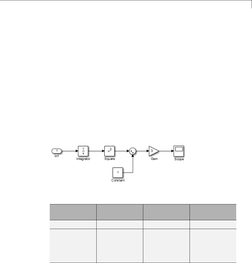
For example, this Simulink®model has an operating point that consists of
two variables:
•Root input level set to 1
•Integrator block state set to 5
The next table summarizes the operating point values of this Simulink model.
Block Block Input Block
Operation
Block Output
Integrator 1
Square 5, setby
the initial
conditionx0 = 5
of the Integrator
block
squares 25
1-3
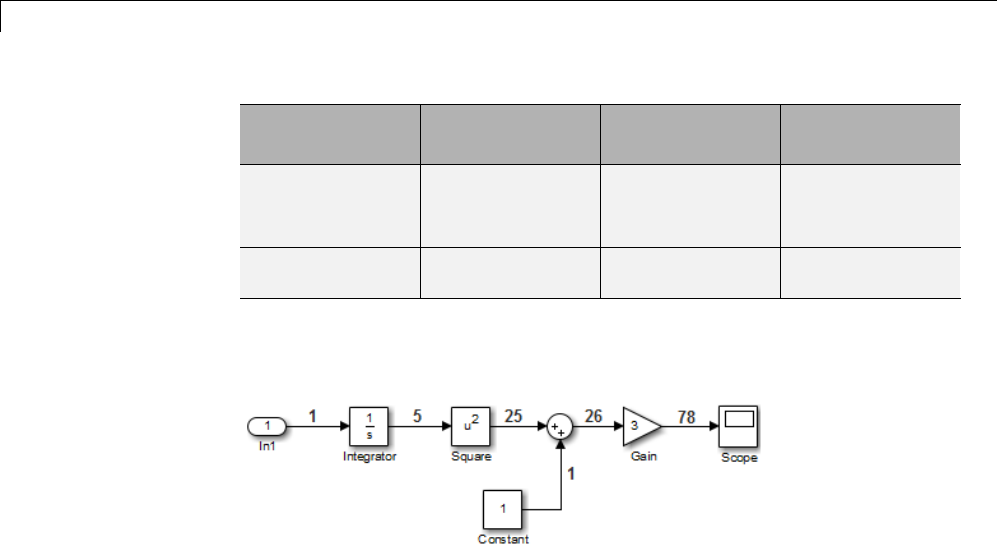
1Steady-State Operating Points
Block Block Input Block
Operation
Block Output
Sum 25 from Square
block, 1 from
Constant block
sums 26
Gain 26 multiplies by 3 78
The next block diagram shows how the model input and the initial state of the
Integrator block propagate through the model during simulation.
If your model initial states and inputs already represent the desired
steady-state operating conditions, you can use this operating point for
linearization or control design.
Examples and How To
•“Steady-State Operating Points from State Specifications” on page 1-16
•“Steady-State Operating Point to Meet Output Specification” on page 1-21
More About
“Simulink Model States Included in Operating Point Object” on page 1-4
Simulink Model States Included in Operating Point
Object
The operating point object in Simulink Control Design™ includes the tunable
states in your Simulink model.
1-4

Steady-State Operating Point (Trimming)
Theoperatingpointobjectexcludesstates of blocks that have internal
representation, such as Backlash, Memory, and Stateflow blocks.
Block Type Block Example Included in Operating
Point?
Blocks with
double-precision
real-valued states
Integrator, State Space,
Transfer Function
Yes
Root-level inport
blocks with
double-precision
real-valued inputs
Inport Yes
Blocks with internal
state representation
that impact block
output
Backlash, Memory,
Stateflow
No
More About
•“Handling Blocks with Internal State Representation” on page 1-46
•“Steady-State Operating Point (Trimming)” on page 1-2
Advantages of Using Simulink Control Design vs.
Simulink Operating Point Search
Simulink provides trim for steady-state operating point search. How is
trim different from findop in Simulink Control Design for performing an
optimization-based operating point search?
Simulink Control Design operating point search provides these advantages to
using trim:
1-5

1Steady-State Operating Points
Simulink Control
Design Operating
Point Search
Simulink Operating
Point Search
Graphical-user
interface
Yes No
Only trim is available.
Multiple
optimization
methods
Yes No
Only one optimization
method
Constrain state,
input, and output
variables using
upper and lower
bounds
Yes No
Specify the output
value of blocks that
are not connected
to root model
outports
Yes No
Steady-operating
points for models
with discrete states
Yes No
Model reference
support
Yes No
SimMechanics™
integration
Yes No
1-6

View and Modify Operating Points
View and Modify Operating Points
In this section...
“View Model Initial Condition in Linear Analysis Tool” on page 1-7
“Modify Operating Point in Linear Analysis Tool” on page 1-8
“View and Modify Operating Point Object (MATLAB Code)” on page 1-10
View Model Initial Condition in Linear Analysis Tool
This example shows how to view the model initial condition in the Linear
Analysis Tool.
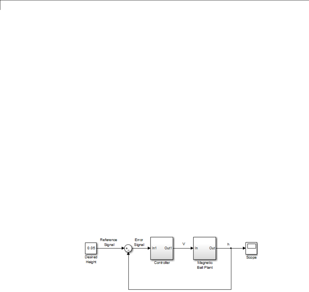
1Open the Simulink model.
sys = 'magball';
open_system(sys)
2In the Simulink Editor, select Analysis > Control Design > Linear
Analysis.
The Linear Analysis Tool for the model opens.
3Click in the Exact Linearization tab.
This action opens the Model Initial Condition Viewer, which shows the
model initial condition (default operating point).
1-7
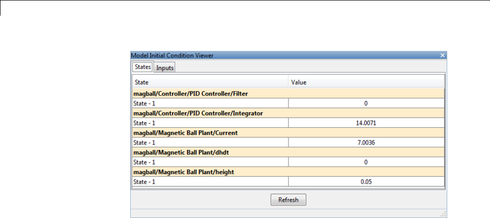
1Steady-State Operating Points
You cannot edit the Model Initial Condition operating point using the
Linear Analysis Tool. To edit the initial conditions of the model, change
the appropriate parameter of the relevant block in your Simulink model.
For example, double-click the magball/Magnetic Ball Plant/Current
block to open the Block Parameters dialog box and edit the value in the
Initial condition box. Click OK.
Modify Operating Point in Linear Analysis Tool
This example shows how to modify an existing operating point in the Linear
Analysis Tool.
1Open Simulink model.
sys = 'magball';
open_system(sys)
Opening magball loads the operating points magball_op1 and magball_op2
into the MATLAB®Workspace.
2In the Simulink Editor, select Analysis > Control Design > Linear
Analysis.
The Linear Analysis Tool for the model opens.
3Choose magball_op1 from the Operating Point list.
1-8

View and Modify Operating Points
4Click adjacent to the Operating Point list.
The magball_op1 editor opens. Use this dialog box to view and edit this
operating point.
1-9
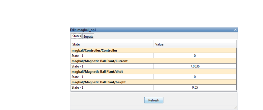
1Steady-State Operating Points
Select the state or input Value to edit its value.
You cannot edit an operating point that you created by trimming a model
in the Linear Analysis Tool.
View and Modify Operating Point Object (MATLAB
Code)
This example shows how to view and modify the states in the Simulink model
using an operating point object.
1Create operating point object from Simulink model.
sys = 'watertank';
load_system(sys)
op = operpoint(sys)
The operating point op contains the states and input levels of the Simulink
model.
2Set the value of the first state.
op.States(1).x = 1.26;
3View the operating pointobjectstatevalues.
op.States
1-10

View and Modify Operating Points
(1.) watertank/PID Controller/Integrator
x: 1.26
(2.) watertank/Water-Tank System/H
x: 1
Note When you modify your Simulink model after creating an operating
point object, use update to update your operating point object.
1-11

1Steady-State Operating Points
Choosing Between Simulation Snapshot and Operating
Point from Specifications
You can find steady-state operating points (or trim conditions) from
specificationsoratspecificsimulationtimes(orsimulationsnapshots).
Choosing which approach to use for computing your operating point depends
on what you know about the operating point.
Use optimization-based steady-state operating point search when you know
some of the operating point states and model input or output signal levels.
Successful operating point search finds an operating point very close to a true
steady-state solution.
Optimization-based search produces poor results when you specify:
•Initial guesses for steady-state operating point values that are far away
from the desired steady-state operating point.
•Incompatible input, output, or state constraints at equilibrium.
This is equivalent to overconstraining the optimization search.
Use the simulation-based approach when the simulation time is sufficiently
short for the model to reach steady state. The algorithms extracts operating
point values when the simulation reaches steady state. You must also specify
the initial conditions that drive the model to steady state.
Simulation-based computations produce poor operating point results when
you specify:
•Simulation time that is insufficiently longtodrivethemodeltosteadystate.
•Initial conditions do not cause the model to reach true equilibrium.
NoteIf your Simulink model has internal states, do not linearize this model
at the operating point you compute from a simulation snapshot. Instead, try
linearizing the model using a simulation snapshot or at an operating point
from optimization-based search.
1-12


1Steady-State Operating Points
Steady-State Operating Points (Trimming) from
Specifications
In this section...
“Steady-State Operating Point Search (Trimming)” on page 1-14
“Which States in the Model Must Be at Steady State?” on page 1-15
“Steady-State Operating Points from State Specifications” on page 1-16
“Steady-StateOperatingPointtoMeetOutputSpecification”onpage1-21
“Initialize Steady-State Operating Point Search Using Simulation
Snapshot” on page 1-24
“Compute Steady-State Operating Points for SimMechanics Models” on
page 1-29
“Batch Compute Steady-State Operating Points” on page 1-32
“Change Operating Point Search Optimization Settings” on page 1-35
Steady-State Operating Point Search (Trimming)
You can compute a steady-state operating point (or equilibrium operating
point) using numerical optimization methods to meet your specifications. The
resulting operating point consists of the equilibrium state values and model
input levels.
Optimization-based operating point computation requires you to specify
initial guesses and constraints on the key operating point states, input levels,
and model output signals.
You can usually improve your optimization results using simulation to
initialize the optimization. For example, you can extract the initial values
oftheoperatingpointatasimulation time when the model reaches the
neighborhood of steady state.
Optimization-based operating point search lets you specify and constrain the
following variables at equilibrium:
•Initial state values
1-14

Steady-State Operating Points (Trimming) from Specifications
•States at equilibrium
•Maximum or minimum bounds on state values, input levels, and output
levels
•Known (fixed) state values, input levels, or output levels
Your operating point search might not converge to a steady-state operating
point when you overconstrain the optimization. You can overconstrain the
optimization by specifying incompatible constraints or initial guesses that are
far away from the desired solution.
You can also control the accuracy of your operating point search by configuring
the optimization algorithm settings.
Examples and How To
“Change Operating Point Search Optimization Settings” on page 1-35
More About
“Which States in the Model Must Be at Steady State?” on page 1-15
Which States in the Model Must Be at Steady State?
When configuring a steady-state operating point search, you do not always
need to specify all states to be at equilibrium. A pendulum is an example of a
system where it is possible to find an operating point with all states at steady
state. However, for other types of systems, there may not be an operating
point where all states are at equilibrium, and the application does not require
that all operating point states be at equilibrium.
For example, suppose you build an automobile model for a cruise control
application with these states:
•Vehicle position and velocity
•Fuel and air flow rates into the engine
If your goal is to study the automobile behavior at constant cruising velocity,
you need an operating point with the velocity, air flow rate, and fuel flow rate
1-15
1Steady-State Operating Points
at steady state. However, the position of the vehicle is not at steady state
because the vehicle is moving at constant velocity. The lack of steady state
of the position variable is fine for the cruise control application because the
position does not have significant impact on the cruise control behavior. In
this case, you do not need to overconstrain the optimization search for an
operating point by require that all states should be at equilibrium.
Similar situations also appear in aerospace systems when analyzing the
dynamics of an aircraft under different maneuvers.
Steady-State Operating Points from State
Specifications
This example shows how to compute a steady-state operating point, or
equilibrium operating point, by specifying known (fixed) equilibrium states
and minimum state values.
Code Alternative
Use findop to find operating point from specifications. For examples and
additional information, see the findop reference page.
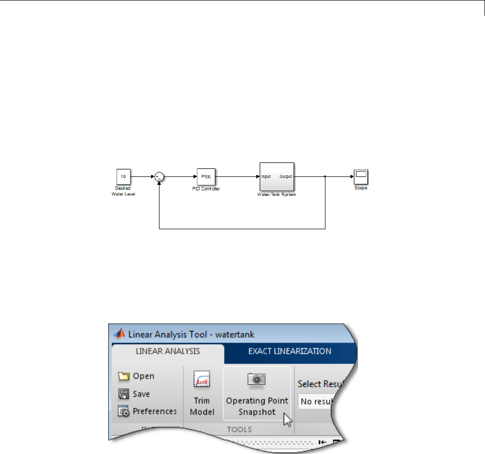
1Open Simulink model.
sys = 'magball';
open_system(sys)
2In the Simulink Editor, select Analysis > Control Design > Linear
Analysis.
The Linear Analysis Tool for the model opens.
1-16
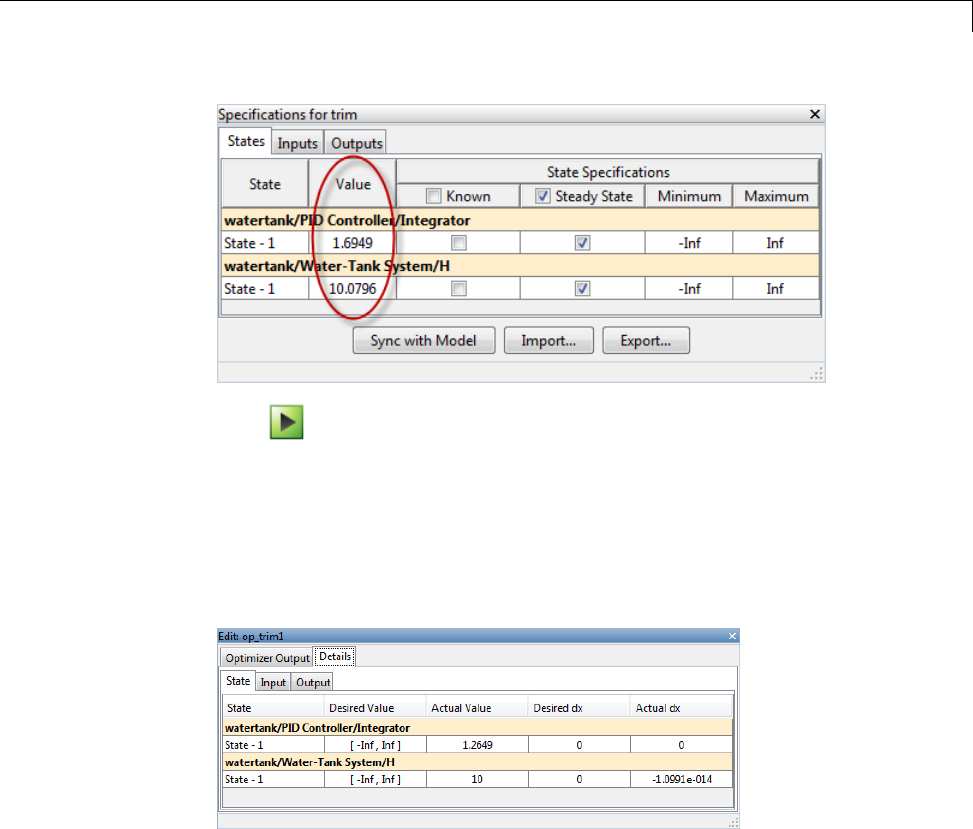
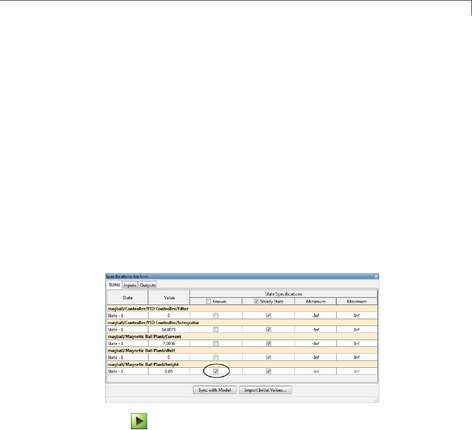
Steady-State Operating Points (Trimming) from Specifications
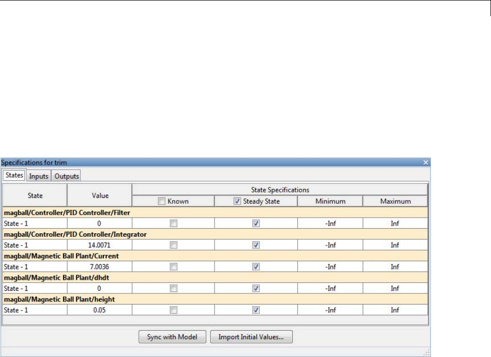
3In the Linear Analysis tab, click Trim Model.ThenclickSpecifications.
The Specifications for trim dialog box opens.
By default, the software specifies all model states to be at equilibrium
(as shown by the check marks in the Steady State column). The Inputs
and Outputs tabs are empty because this model does not have root-level
input and output ports.
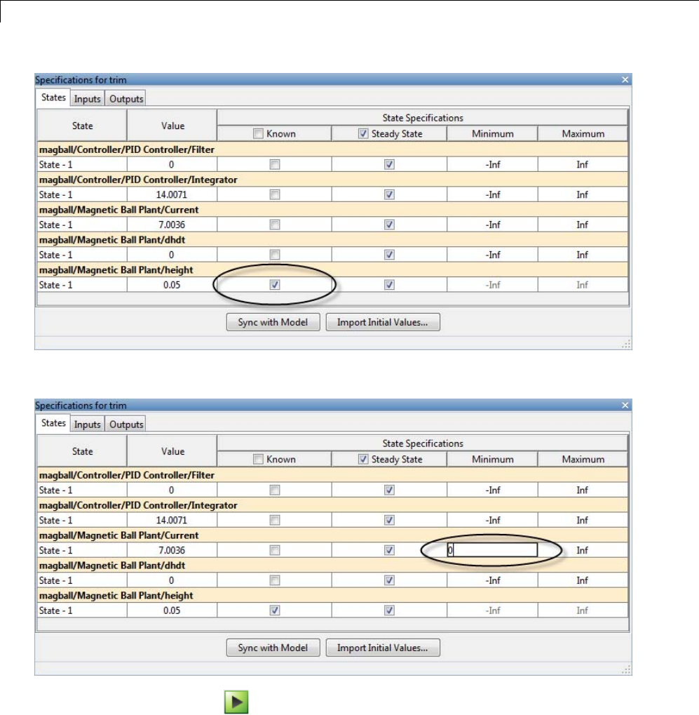
4In the States tab, select Known for the height state.
The height of the ball matches the reference signal height (specified in the
Desired Height block as 0.05). This height value should remain fixed
during the optimization.
1-17
1Steady-State Operating Points
5Enter 0for the minimum bound of the Current state.
6Click to compute the operating point.
1-18
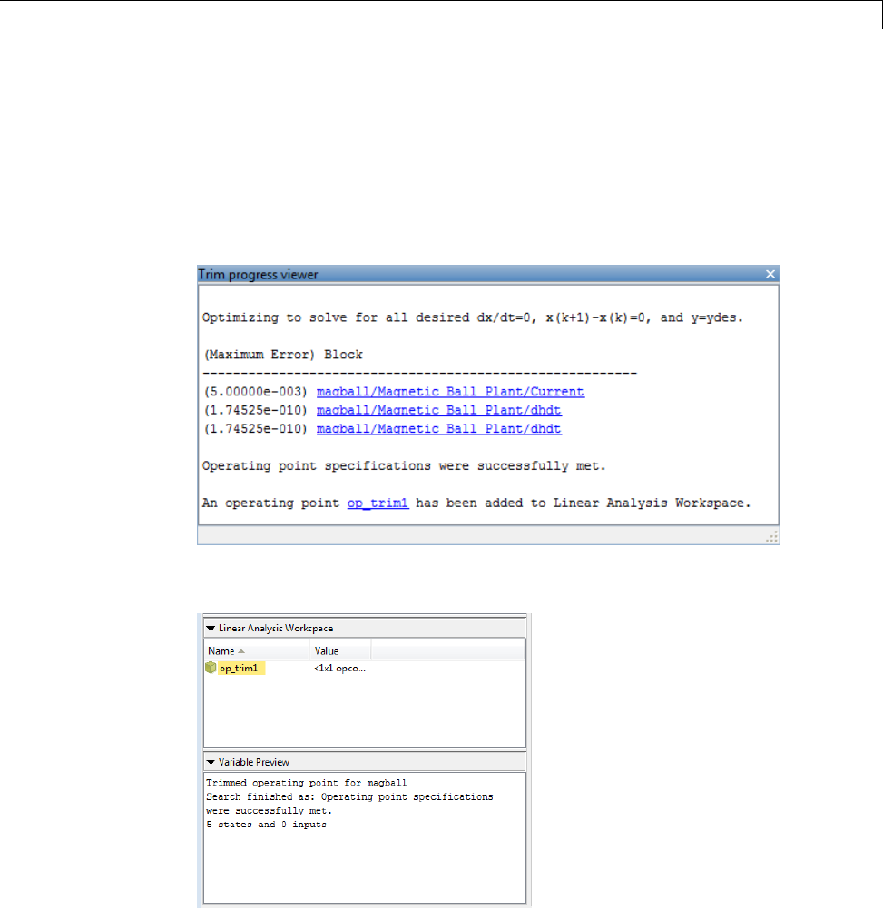
Steady-State Operating Points (Trimming) from Specifications
This action uses numerical optimization to find the operating point that
meets your specifications.
The Trim progress viewer shows that the optimization algorithm
terminated successfully. The (Maximum Error) Block area shows the
progress of reducing the error of a specific state or output during the
optimization.
Anewvariable,op_trim1, appears in the Linear Analysis Workspace.
7Double-click op_trim1 in Linear Analysis Workspace to evaluate
whether the resulting operating point values meet the specifications.
1-19

1Steady-State Operating Points
The Actual dx values are about 0, which indicates that the operating point
meets the steady state specification.
The Actual Value of the states falls within the Desired Value bounds.
8(Optional) To automatically generate a MATLAB script, click Trim and
select Generate MATLAB Script.
The generated script contains commands for computing the operating point
for this example.
Related Examples
•“Steady-State Operating Point to Meet Output Specification” on page 1-21
•“Change Operating Point Search Optimization Settings” on page 1-35
•“Initialize Steady-State Operating Point Search Using Simulation
Snapshot” on page 1-24
1-20
Steady-State Operating Points (Trimming) from Specifications
•“Compute Steady-State Operating Points for SimMechanics Models” on
page 1-29
•“Simulate Simulink Model at Specific Operating Point” on page 1-44
•“Batch Compute Steady-State Operating Points” on page 1-32
More About
•“Steady-State Operating Point (Trimming)” on page 1-2
•“Choosing Between Simulation Snapshot and Operating Point from
Specifications” on page 1-12
Steady-State Operating Point to Meet Output
Specification
This example shows how to specify an output constraint of an engine speed
for computing the engine steady-state operating point.
1Open Simulink model.
sys = 'scdspeed';
open_system(sys);
2In the Simulink Editor, select Analysis > Control Design > Linear
Analysis.
The Linear Analysis Tool for the model opens.
3In the Linear Analysis tab, click Trim Model.ThenclickSpecifications.
1-21
1Steady-State Operating Points
The Specifications for trim dialog box appears.
4Examine the linearization outputs for scdspeed in the Outputs tab.
Currently there are no outputs specified for scdspeed.
5In the Simulink Editor, right-click the output signal from the rad/s to
rpm block. Select Linear Analysis Points > Output Constraint.
This action adds the output signal constraint marker to the model.
The output signal from the rad/s to rpm block now appears under the
Outputs tab.
6Select Known and enter 2000 RPMfortheenginespeedastheoutput
signal value. Press Enter.
1-22
Steady-State Operating Points (Trimming) from Specifications
7Click to find a new steady-state operating point that meets the
specified output signal constraint.
8Double-click op_trim1 in Linear Analysis Workspace to evaluate
whether the resulting operating point values meet the specifications.
In the States tab, the Actual dx values are either zero or about zero.
This result indicates that the operating point meets the steady state
specification.
In the Outputs tab, the Actual Value and the Desired Value are both
2000.
1-23
1Steady-State Operating Points
Related Examples
•“Steady-State Operating Points from State Specifications” on page 1-16
•“Change Operating Point Search Optimization Settings” on page 1-35
•“Initialize Steady-State Operating Point Search Using Simulation
Snapshot” on page 1-24
•“Compute Steady-State Operating Points for SimMechanics Models” on
page 1-29
•“Simulate Simulink Model at Specific Operating Point” on page 1-44
•“Batch Compute Steady-State Operating Points” on page 1-32
More About
•“Steady-State Operating Point (Trimming)” on page 1-2
•“Choosing Between Simulation Snapshot and Operating Point from
Specifications” on page 1-12
Initialize Steady-State Operating Point Search Using
Simulation Snapshot
•“Initialize Operating Point Search Using Linear Analysis Tool” on page 1-24
•“Initialize Operating Point Search (MATLAB Code)” on page 1-27
Initialize Operating Point Search Using Linear Analysis Tool
ThisexampleshowshowtousetheLinearAnalysisTooltoinitializethe
values of an operating point search using a simulation snapshot.
1-24
Steady-State Operating Points (Trimming) from Specifications
If you know the approximate time when the model reaches the neighborhood
of a steady-state operating point, you can use simulation to get the state
values to be used as the initial condition for numerical optimization.
1Open Simulink model.
sys = ('watertank');
open_system(sys)
2In the Simulink Editor, select Analysis > Control Design > Linear
Analysis.
The Linear Analysis Tool for the model opens.
3In the Linear Analysis tab, click Operating Point Snapshot
The Operating Point Snapshots tab opens.
4Enter 10 in the Simulation Snapshot Times field to extract the operating
point at this simulation time. Press Enter.
1-25
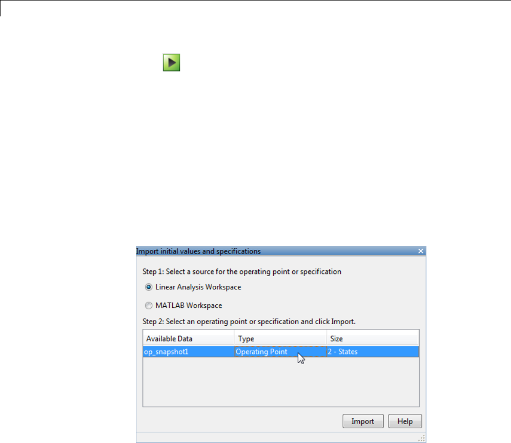
1Steady-State Operating Points
Click to take a snapshot of the system at the specified time.
op_snapshot1 appears in the Linear Analysis Workspace.Thesnapshot,
op_snapshot1,c
ontains all state values of the system at the specified time.
5In the Linear Analysis tab, click Trim Model.ThenclickSpecifications.
The Specifications for trim dialog box appears.
6Click Import.
The Import initial values and specifications dialog opens.
7Select op_snapshot1 and click Import to initialize the operating point
states with the values you obtained from the simulation snapshot.
The state values displayed in the Specifications for trim dialog box update
to reflect the new values.
1-26
Steady-State Operating Points (Trimming) from Specifications
8Click to find the optimized operating point using the states at t=10
as the initial values.
9Double-click op_trim1 in Linear Analysis Workspace to evaluate
whether the resulting operating point values meet the specifications.
The Actualdxvalues are near zero. This result indicates that the
operating point meets the steady state specifications.
Initialize Operating Point Search (MATLAB Code)
This example show how to use initopspec to initialize operating point object
values for optimization-based operating point search.
1Open Simulink model.
sys = 'watertank';
load_system(sys);
1-27

1Steady-State Operating Points
2Extract an operating point from simulation after 10 time units.
opsim = findop(sys,10);
3Create operating point specification object.
By default, all model states are specified to be at steady state.
opspec = operspec(sys);
4Configure initial values for operating point search.
opspec = initopspec(opspec,opsim);
5Find the steady state operating point that meets these specifications.
[op,opreport] = findop(sys,opspec)
bdclose(sys);
opreport describes the optimization algorithm status at the end of the
operating point search.
Operating Report for the Model watertank.
(Time-Varying Components Evaluated at time t=0)
Operating point specifications were successfully met.
States:
----------
(1.) watertank/PID Controller/Integrator
x: 1.26 dx: 0 (0)
(2.) watertank/Water-Tank System/H
x: 10 dx: -1.1e-014 (0)
Inputs: None
----------
Outputs: None
----------
dx, which is the time derivative of each state, is effectively zero. This value
of the state derivative indicates that the operating point is at steady state.
1-28

Steady-State Operating Points (Trimming) from Specifications
Related Examples
•“Steady-State Operating Points from State Specifications” on page 1-16
More About
•“Change Operating Point Search Optimization Settings” on page 1-35
•“Steady-State Operating Point (Trimming)” on page 1-2
Compute Steady-State Operating Points for
SimMechanics Models
Thisexampleshowshowtocomputethe steady-state operating point of a
SimMechanics model from specifications.
Note You must have installed SimMechanics software to execute this
example on your computer.
1Open the SimMechanics model.
sys = 'scdmechconveyor';
open_system(sys);
1-29
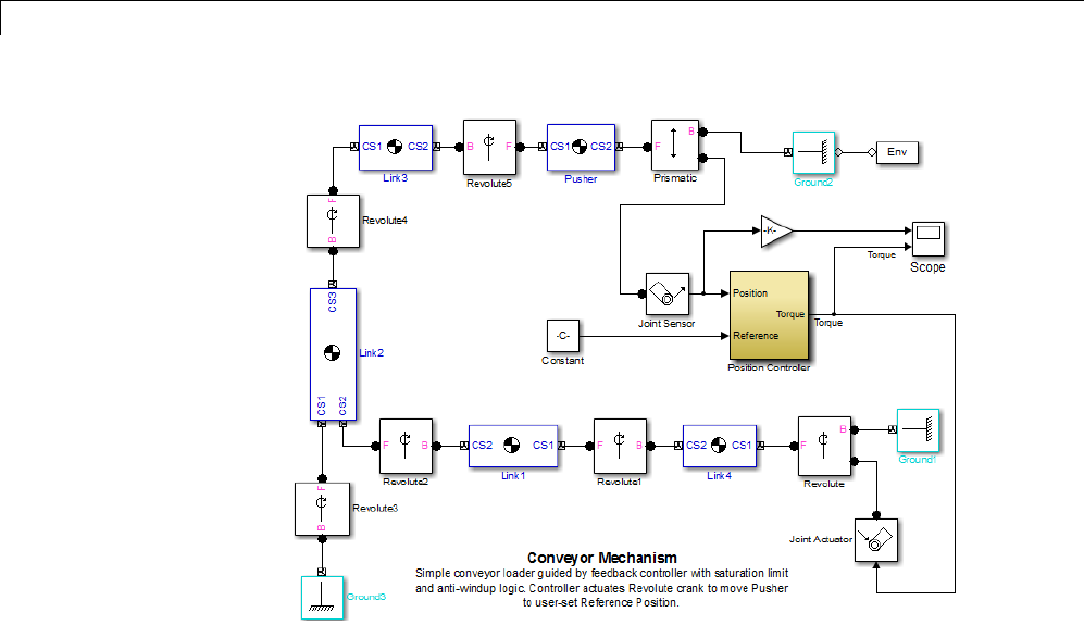
1Steady-State Operating Points
2Double-click the Env block to open the Block Parameters dialog box.
3In the Parameters tab, select Trimming as the Analysis mode.ClickOK.
1-30
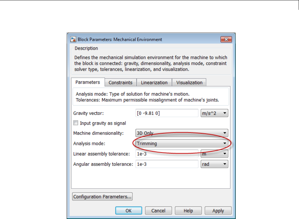
Steady-State Operating Points (Trimming) from Specifications
This action adds an output port to the model with constraints that must be
satisfied to a ensure a consistent SimMechanics machine.
4In the Simulink Editor, select Analysis > Control Design > Linear
Analysis.
The Linear Analysis Tool for the model opens.
5In the Linear Analysis tab, click Trim Model.ThenclickSpecifications.
The Specifications for trim dialog box appears.
By default, the software specifies all model states to be at equilibrium
(as shown in the Steady State column). The Outputs tab shows the
1-31
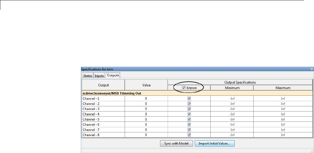
1Steady-State Operating Points
error constraints in the system that must be set to zero for steady-state
operating point search.
6Select Known in the Outputs tab to set all constraints to 0.
You can now specify additional constraints on the operating point states and
input levels, and find the steady-state operating point for this model.
After you finish steady-state operating point search for the SimMechanics
model, reset the Analysis mode to Forward dynamics in the Env block
parameters dialog box.
More About
•“Change Operating Point Search Optimization Settings” on page 1-35
Batch Compute Steady-State Operating Points
Thisexampleshowshowtobatchcomputesteady-stateoperatingpointsfora
model using generated MATLAB code.
If you are new to writing scripts, use the Linear Analysis Tool to interactively
configure your operating points search. You can use Simulink Control Design
to automatically generate a script based on your Linear Analysis Tool settings.
1Open the Simulink model.
sys = 'magball';
1-32
Steady-State Operating Points (Trimming) from Specifications
open_system(sys);
2Open the Linear Analysis Tool for the model.
In the Simulink Editor, select Analysis > Control Design > Linear
Analysis.
3Open the Specifications for trim dialog box.
In the Linear Analysis tab, click Trim Model.TheTrim Model tab
should open.
Click Specifications.
By default, the software specifies all model states to be at equilibrium (as
shownintheSteady State column).
4In the States tab, select the Known check box for the magball/Magnetic
Ball Plant/height state.
5Click to compute the operating point using numerical optimization.
The Trim progress viewer shows that the optimization algorithm
terminated successfully. The (Maximum Error) Block area shows the
progress of reducing the error of a specific state or output during the
optimization.
6Click Generate MATLAB Code in the Trim list to automatically generate
a MATLAB script.
1-33

1Steady-State Operating Points
The MATLAB Editor window opens with the generated script.
7Edit the script:
aRemove unneeded comments from the generated script.
bDefine initial height variable height with values at which to compute
operating points.
cAdd a for loop around the operating point search code to compute a
steady-state operating point for each height value.
Your script should now look similar to this (excluding most comments):
function [op,opreport] = myoperatingpointsearch
%% Specify the model name
sys = 'magball';
load_system(sys)
%% Create operating point specification object
opspec = operspec(sys)
% State (5) - magball/Magnetic Ball Plant/height
% - Default model initial conditions are used to initialize optimization.
opspec.States(5).Known = true;
%% Create the options
opt = linoptions('DisplayReport','iter');
%% Specify the initial heights at which to compute operating points
height = [0.05;0.1;0.15];
%% Loop over height values to find the corresponding steady state
%% operating points
for ct = 1:numel(height)
% Set the initial height in the specification
opspec.States(5).x = height(ct);
% Trim the model
[op(ct),oprep(ct)] = findop(sys,opspec,opt);
end
1-34

Steady-State Operating Points (Trimming) from Specifications
See Also
findop
Change Operating Point Search Optimization Settings
This example shows how to control the accuracy of your operating point
search by configuring the optimization algorithm.
Typically, you adjust the optimization settings based on the operating point
search report, which is automatically created after each search.
Code Alternative
Use linoptions to configure optimization algorithm settings for findop.
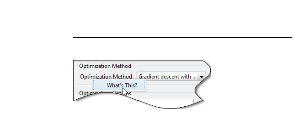
1In the Linear Analysis Tool, open the Linear Analysis tab. Click Trim
Model and click Optimization Options.
This action opens the Options for trim dialog box.
2Change the appropriate optimization settings.
This table lists the most common optimization settings.
Optimization Status Option to Change Comment
Optimization ends before
completing (too few iterations)
Maximum iterations Increase the number of
iterations
State derivative or error in
output constraint is too large
Function tolerance or
Constraint tolerance
(depending on selected
algorithm)
Decrease the tolerance value
1-35
1Steady-State Operating Points
Note Youcangethelponeachoptionbyright-clickingtheoptionlabeland
selecting What’s This?.
Related Examples
•“Steady-State Operating Points from State Specifications” on page 1-16
•“Steady-State Operating Point to Meet Output Specification” on page 1-21
•“Batch Compute Steady-State Operating Points” on page 1-32
More About
•“Steady-State Operating Point (Trimming)” on page 1-2
1-36

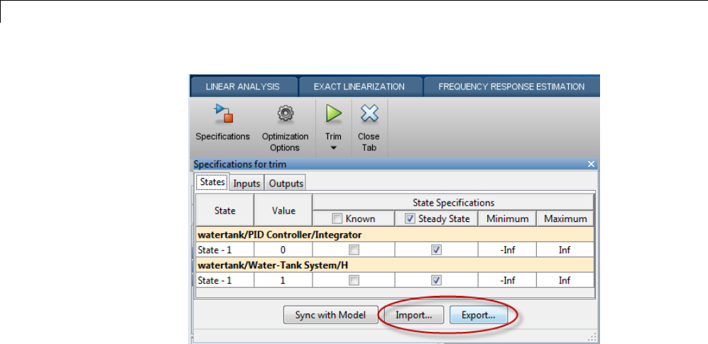
Import and Export Specifications For Operating Point Search
Import and Export Specifications For Operating Point
Search
When you modify an operating point specification in the Linear Analysis Tool,
you can export the specification to the MATLAB workspace or the Linear
Analysis Tool workspace. Exported specifications are saved as operating
point specifications objects (see operspec). Exporting specifications can be
useful when you expect to perform multiple trimming operations using the
same or a very similar set of specifications. Additionally, you can export
interactively-edited operating point specifications when you want to use the
findop command to perform multiple trimming operations with a single
compilation of the model. (See “Batch Compute Operating Points with Single
Model Compilation” on page 1-39.)
You can also import saved operating point specifications to the Linear
Analysis Tool and use them to interactively compute trimmed operating
points. Importing a specification can be useful when you want to trim a model
to a specification that is similar to one you previously saved. In that case, you
can import the specification to the Linear Analysis Tool and interactively
change it. You can then export the modified specification, or compute a
trimmed operating from it.
To import or save an operating point specification:
1In the Linear Analysis Tool, on the Linear Analysis Tab, click Trim Model
to open the Trim Model Tab.
2Click Specifications to open the Specifications for trim dialog box.
3Click Import to import a saved operating point specification from the
Linear Analysis Workspace or the MATLAB Workspace. Click Export to
save an operating point specification to the Linear Analysis Workspace or
the MATLAB Workspace.
1-37
1Steady-State Operating Points
For more information about operating point specifications, see the operspec
and findop reference pages.
1-38

Batch Compute Operating Points with Single Model Compilation
Batch Compute Operating Points with Single Model
Compilation
This example shows how to find operating points for multiple operating point
specifications with a single model compilation using the findop command.
Each time you call findop, the software compiles the Simulink model. To find
operating points for multiple specifications, you can give findop avectorof
operating point specifications. Then findop only compiles the model once.
1Open Simulink model.
sys = 'scdspeed';
open_system(sys);
2Create operating point specification object.
opspec1 = operspec(sys);
By default, all model states are specified to be at steady state.
3Configure the output specification.
blk = [sys '/rad//s to rpm'];
opspec1 = addoutputspec(opspec1,blk,1);
opspec1.Outputs(1).Known = true;
opspec1.Outputs(1).y = 1500;
opspec1 specifies a stead-state operating point in which the output of the
block rad/s to rpm is fixed at 500.
Note Alternatively, you can configure an operating point specification
using the Linear Analysis Tool and export the specification to the MATLAB
workspace. See “Import and Export Specifications For Operating Point
Search” on page 1-37 for more information.
4Create and configure additional operating point specifications.
opspec2 = copy(opspec1);
1-39

1Steady-State Operating Points
opspec2.Outputs(1).y = 2000;
opspec3 = copy(opspec1);
opspec3.Outputs(1).y = 2500;
Using the copy command creates an independent operating point
specification that you can edit without changing opspec1.Here,the
specifications opspec2 and opspec3 are identical to opspec1,exceptforthe
target output level.
5Find the operating points that meet each of the three output specifications.
opspecs = [opspec1,opspec2,opspec3];
ops = findop(sys,opspecs);
bdclose(sys);
Pass the three operating point specifications to findop in the vector
opspecs. When you give findop a vector of operating point specifications,
it finds all the operating points with only one model compilation. ops is a
vector of operating point objects for the model scdspeed that correspond to
the three specifications in the vector.
1-40

Steady-State Operating Points from Simulation
Steady-State Operating Points from Simulation
In this section...
“Simulation Snapshot Operating Points” on page 1-41
“Compute Operating Points at Simulation Snapshots” on page 1-41
Simulation Snapshot Operating Points
You can compute a steady-state operating point (or equilibrium operating
point) from model simulation. The resulting operating point consists of the
state values and model input levels at the specified simulation time.
Simulation-based operating point computation requires that you configure
your model by specifying:
•Initial conditions that cause your modeltoconvergetoequilibrium
•Simulation time at which the model reaches equilibrium
You can use the simulation snapshot operating point to initialize the trim
point search.
Note If your Simulink model has internal states, do not linearize this model
at the operating point you compute from a simulation snapshot. Instead, try
linearizing the model using a simulation snapshot or at an operating point
from optimization-based search.
Compute Operating Points at Simulation Snapshots
This example shows how to use the Linear Analysis Tool to compute an
operating point at specified simulation times (or simulation snapshots).
Code Alternative
Use findop to compute operating point at simulation snapshot. For examples
and additional information, see the findop reference page.
1-41
1Steady-State Operating Points
1Open Simulink model.
sys = 'magball';
open_system(sys);
2In the Simulink Editor, select Analysis > Control Design > Linear
Analysis.
The Linear Analysis Tool for the model opens, with the default operating
point being set to the model initial condition.
3In the Linear Analysis tool, click the Operating Point Snapshots tab.
4Specify [1,10] in the Simulation Snapshot Times field. Press Enter.
This vector specifies operating points at t=1and t=10.
5Click to take a snapshot of the system at the specified times.
A new variable, op_snapshot1,appearsintheLinear Analysis
Workspace.op_snapshot1 contains the two operating points.
6Double-click op_snapshot1 to see the resulting operating points. Select an
operating point of interest from the Select Operating Point list to see it.
1-42
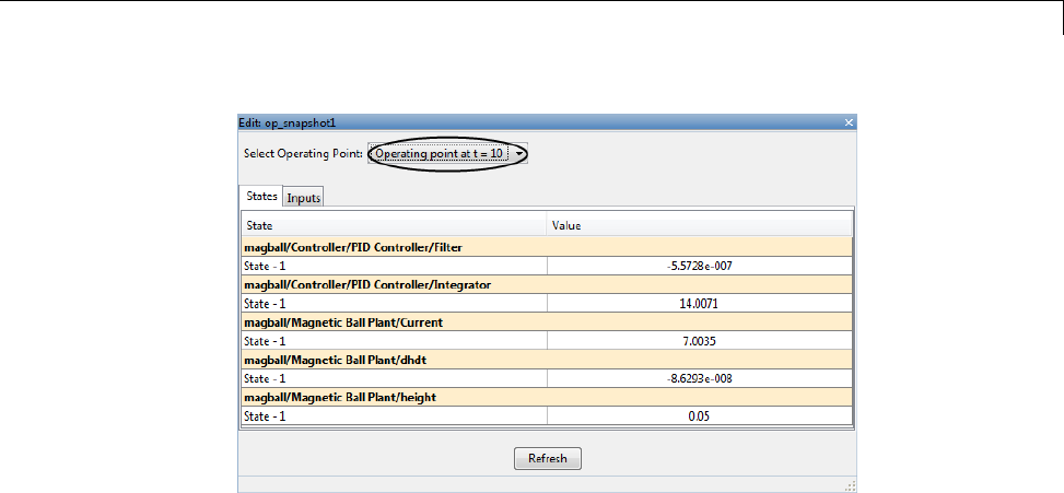
Steady-State Operating Points from Simulation
For example, to evaluate your operating point from a simulation snapshot:
1Initialize the model at the operating point (see “Simulate Simulink Model
at Specific Operating Point” on page 1-44)
2Add Scope blocks to show the output signals that should reach steady state
during the simulation.
3Run the simulation to check whether these key signals are at steady state.
More About
•“Choosing Between Simulation Snapshot and Operating Point from
Specifications” on page 1-12
1-43
1Steady-State Operating Points
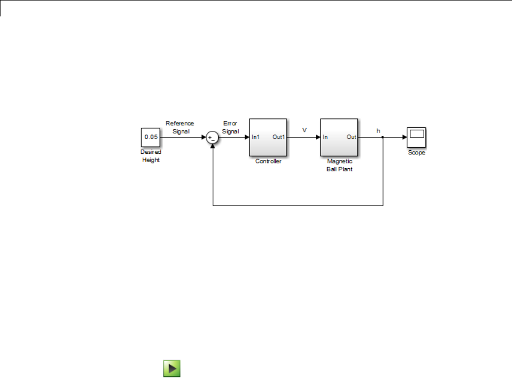
Simulate Simulink Model at Specific Operating Point
This example shows how to initialize a model at a specific operating point for
simulation.
1Compute a steady-state operating point, as described in “Compute
Operating Points at Simulation Snapshots” on page 1-41.
2In the Linear Analysis Tool, double-click the operating point variable in
the Linear Analysis Workspace.
The Edit dialog box opens.
3Click Initialize model.
The Initialize Model dialog box opens.
1-44
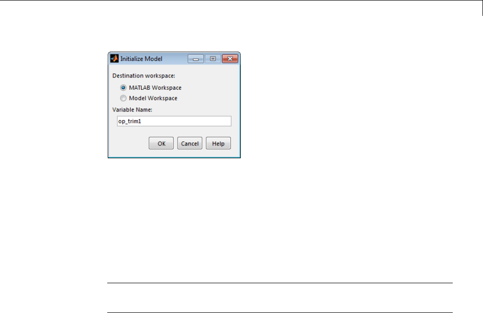
Simulate Simulink®Model at Specific Operating Point
4Use the default Variable Name for the operating point object.
Alternatively, you can edit this variable name.
Click OK to export the operating pointtotheMATLABWorkspace.
This action also sets the operating point values in the Data Import/Export
pane of the Configuration Parameters dialog box. Simulink uses this
operating point as initial conditions when simulating the model.
Tip If you want to store this operating point with the model, export the
operating point to the Model Workspace instead.
In the Simulink Editor, select Simulation > Run to simulate the model
starting at the specified operating point.
Related Examples
•“Steady-State Operating Points from State Specifications” on page 1-16
•“Compute Operating Points at Simulation Snapshots” on page 1-41
1-45

1Steady-State Operating Points
Handling Blocks with Internal State Representation
In this section...
“Operating Point Object Excludes Blocks with Internal States” on page 1-46
“Identifying Blocks with Internal States in Your Model” on page 1-47
“Configuring Blocks with Internal States for Steady-State Operating Point
Search” on page 1-47
Operating Point Object Excludes Blocks with Internal
States
The operating point object used for linearization and control design does not
include these Simulink blocks with internal state representation:
•Memory blocks
•Transport Delay and Variable Transport Delay blocks
•Disabled Action Subsystem blocks
•Backlash blocks
•MATLAB Function blocks with persistent data
•Rate Transition blocks
•Stateflow®blocks
•S-Function blocks with states not registered as Continuous or Double
Value Discrete
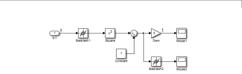
For example, if you compute a steady-state operating point for this Simulink
model, the resulting operating point object does not include the Backlash
block states because these states have an internal representation. If you use
this operating point object to initialize a Simulink model, the initial conditions
of the Backlash blocks might be incompatible with the operating point.
1-46
Handling Blocks with Internal State Representation
Identifying Blocks with Internal States in Your Model
Generate a list of blocks that have internal state representations.
sldiagnostics(sys,'CountBlocks')
where sys is your model, specified as a string. This command also returns the
number of occurrences of each block.
Configuring Blocks with Internal States for
Steady-State Operating Point Search
Blocks with internal states can cause problems for steady-state operating
point search (trimming). Where there is no direct feedthrough,theinputto
the block at the current time does not determine the output of the block at
the current time.
To fix this issues for Memory blocks, Transport Delay, or Variable Transport
Delay blocks, select the Direct feedthrough of input during linearization
option in the Block Parameters dialog box before searching for an operating
point or linearizing a model at a steady state. This setting makes such blocks
behave as if they have a gain of 1 during operating point search.
For example, the next model includes a Transport Delay block. In this case,
you cannot find a steady state operating point using optimization because the
output of the Transport Delay is always zero. Because the reference signal is
1, the input to the Plant block must be nonzero to get the plant block to have
an output of 1 and be at steady state.
1-47
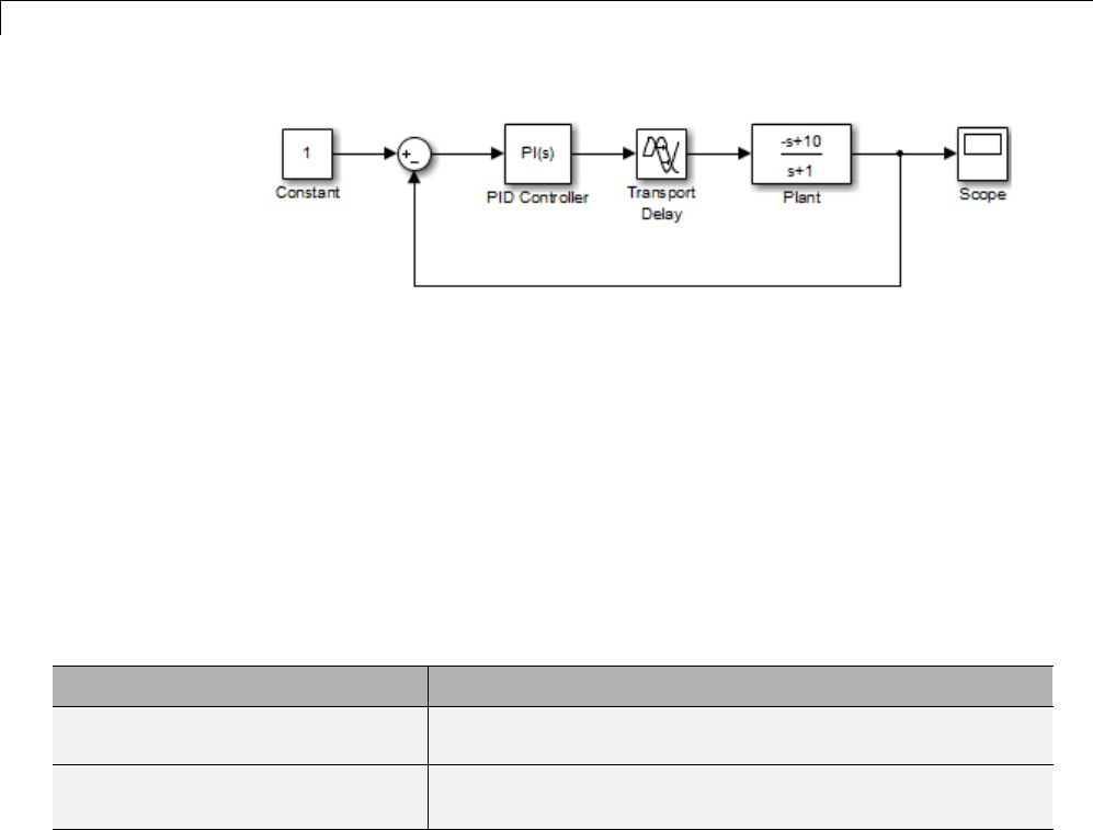
1Steady-State Operating Points
To fix this issue, select the Direct feedthrough of input during
linearization option in the Block Parameters dialog box before searching for
an operating point. This setting lets the PID Controller block push a nonzero
value to the Plant block.
For other blocks with internal states, determine whether the output of the
block impacts the state derivatives or desired output levels before computing
operating points. If the block impacts these derivatives or output levels,
consider replacing it using a configurable subsystem.
You can also set direct feedthrough options at the command-line instead of
using the block parameter dialog box.
Block Command to specify direct feedthrough
Memory
set_param(blockname,'LinearizeMemory','on')
Transport Delay or Variable
Transport Delay set_param(blockname,'TransDelayFeedthrough','on')
1-48

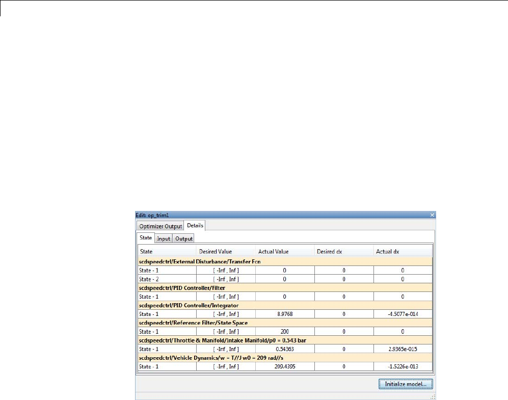
Synchronize Simulink®Model Changes with Operating Point Specifications
Synchronize Simulink Model Changes with Operating
Point Specifications
In this section...
“Synchronize Simulink Model Changes with Linear Analysis Tool” on page
1-49
“Synchronize Simulink Model Changes with Existing Operating Point
Specification Object” on page 1-52
Synchronize Simulink Model Changes with Linear
Analysis Tool
This example shows how to update the operating point specifications in the
Linear Analysis Tool to reflect changes to the Simulink model.
Modifying your Simulink model can change, add, or remove states, inputs,
or outputs, which changes the operating point. If you change your model
while the Linear Analysis Tool is open, you must sync the operating point
specifications in the Linear Analysis Tool to reflect the changes in the model.
1Open Simulink model.
sys = ('scdspeedctrl');
open_system(sys)
2In the Simulink Editor, select Analysis > Control Design > Linear
Analysis.
The Linear Analysis Tool for the model opens, with the default operating
point being set to the model initial condition.
3In the Linear Analysis tab, click Trim Model.ThenclickSpecifications.
The Specifications for trim dialog box appears.
1-49

1Steady-State Operating Points
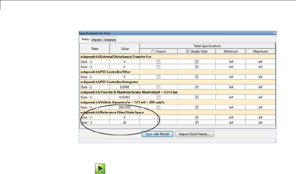
The Reference Filter block contains just one state.
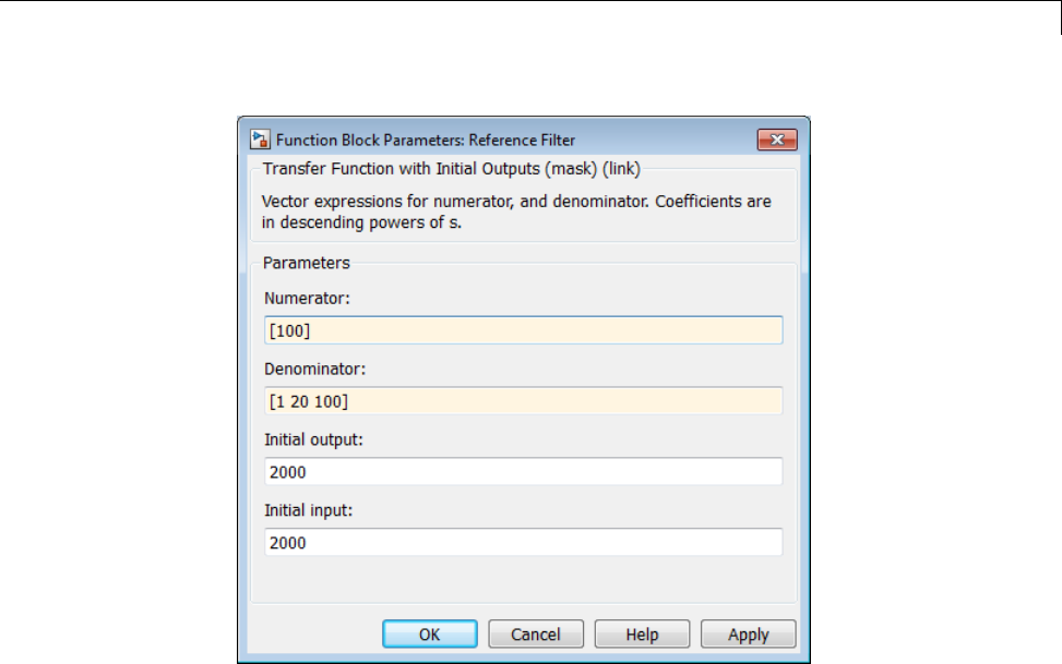
4In the Simulink Editor, double-click the Reference Filter block. Change the
Numerator of the transfer function to 100,andchangetheDenominator
to [1 20 100].ClickOK.
1-50
Synchronize Simulink®Model Changes with Operating Point Specifications
This change adds a state to the Simulink model.
5In the Specifications for trim dialog, click Sync with Model to synchronize
the operating point specifications in the Linear Analysis Tool with the
model.
1-51
1Steady-State Operating Points
The dialog now shows two states for the Reference Filter block.
6Click to compute the operating point.
Synchronize Simulink Model Changes with Existing
Operating Point Specification Object
This example shows how to use update to update the operating point
specification object after you update the Simulink model.
1Open Simulink model.
sys = 'scdspeedctrl';
open_system(sys);
2Create operating point specification object.
By default, all model states are specified to be at steady state.
opspec = operspec(sys);
3In the Simulink Editor, double-click the Reference Filter block. Change the
Numerator of the transfer function to [100] and the Denominator to
[1 20 100]. Click OK.
1-52

Synchronize Simulink®Model Changes with Operating Point Specifications
4Find the steady state operating point that meets these specifications.
op = findop(sys,opspec)
This command results in an error because the changes to your model are
not reflected in your operating point specification object:
??? The model scdspeedctrl has been modified and the operating point
object is out of date. Update the object by calling the function
update on your operating point object.
5Update the operating point specification object with changes to the model.
Repeat the operating point search.
opspec = update(opspec);
op = findop(sys,opspec)
bdclose(sys);
1-53

1Steady-State Operating Points
After updating the operating point specifications object, the optimization
algorithm successfully finds the operating point.
1-54

2
Linearization
•“Linearizing Nonlinear Models” on page 2-2
•“Specify Model Portion to Linearize” on page 2-11
•“Plant Linearization” on page 2-28
•“Open-Loop Response of Control System for Stability Margin Analysis”
on page 2-32
•“Linearize at Model Operating Point” on page 2-38
•“Linearize at Trimmed Operating Point” on page 2-52
•“Linearize at Simulation Snapshots and Triggered Events” on page 2-57
•“Ordering States in Linearized Model” on page 2-76
•“Time-Domain Validation of Linearization” on page 2-81
•“Frequency-Domain Validation ofLinearization”onpage2-85
•“Visualize Models” on page 2-91
•“Generate MATLAB Code for Repeated or Batch Linearization” on page
2-94
•“Troubleshooting Linearization” on page 2-96
•“Controlling Block Linearization” on page 2-112
•“Models with Pulse Width Modulation (PWM) Signals” on page 2-135
•“Specifying Linearization for Model Components Using System
Identification” on page 2-137
•“Speeding Up Linearization of Complex Models” on page 2-144
•“Exact Linearization Algorithm” on page 2-146

2Linearization
Linearizing Nonlinear Models
In this section...
“What Is Linearization?” on page 2-2
“Applications of Linearization” on page 2-4
“Linearization in Simulink®Control Design™” on page 2-5
“Choosing Linearization Tools” on page 2-6
“Model Requirements for Exact Linearization” on page 2-9
“Operating Point Impact on Linearization” on page 2-10
What Is Linearization?
Linearization is a linear approximation of a nonlinear system that is valid in
a small region around the operating point.
For example, suppose that the nonlinear function is yx=2.Linearizingthis
nonlinear function about the operating point x=1, y=1 results in a linear
function yx=−21
.
Near the operating point, yx=−21
is a good approximation to yx=2.Away
from the operating point, the approximation is poor.
The next figure shows a possible region of good approximation for the
linearization of yx=2. The actual region of validity depends on the nonlinear
model.
2-2
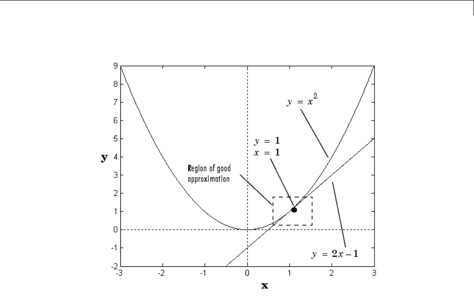
Linearizing Nonlinear Models
Extending the concept of linearization to dynamic systems, you can write
continuous-time nonlinear differential equations in this form:
xt f xt ut t
yt g xt ut t
() (), (),
() (), (), .
In these equations, x(t) represents the system states, u(t)representsthe
inputs to the system, and y(t) represents the outputs of the system.
A linearized model of this system is valid in a small region around the
operating point t=t0,x(t0)=x0,u(t0)=u0,andy(t0)=g(x0,u0,t0)=y0.
To represent the linearized model, define new variables centered about the
operating point:
2-3

2Linearization
δ
δ
δ
xt xt x
ut ut u
yt yt y
() ()
() ()
() ()
=−
=−
=−
0
0
0
The linearized model in terms of δx,δu,andδyis valid when the values
of these variables are small:
δδδ
δδδ
xt A xt B ut
yt C xt D ut
() () ()
() () ()
=+
=+
Examples and How To
•“Linearize Simulink Model” on page 2-38
•“Plant Linearization” on page 2-28
•“Open-Loop Response of Control System for Stability Margin Analysis”
on page 2-32
•“Visualize Bode Response of Simulink Model During Simulation” on page
2-42
More About
•“Applications of Linearization” on page 2-4
•“Choosing Linearization Tools” on page 2-6
Applications of Linearization
Linearization is useful in model analysis and control design applications.
Exact linearization of the specified nonlinear Simulink model produces linear
state-space, transfer-function, or zero-pole-gain equationsthatyoucanuseto:
•PlottheBoderesponseoftheSimulinkmodel.
•Evaluate loop stability margins by computing open-loop response.
•Analyze and compare plant response near different operating points.
•Design linear controller
2-4

Linearizing Nonlinear Models
Classical control system analysis and design methodologies require linear,
time-invariant models. Simulink Control Design automatically linearizes
the plant when you tune your compensator. See “Choosing a Compensator
Design Approach” on page 4-2.
•Analyze closed-loop stability.
•Measure the size of resonances in frequency response by computing
closed-loop linear model for control system.
•Generate controllers with reduced sensitivity to parameter variations and
modeling errors (requires Robust Control Toolbox™).
Linearization in Simulink Control Design
You can use Simulink Control Design to linearize continuous-time,
discrete-time, or multirate Simulink models. The resulting linear
time-invariant model is in state-space form.
Simulink Control Design uses a block-by-block approach to linearize models,
instead of using full-model perturbation. This block-by-block approach
individually linearizes each block in your Simulink model and combines the
results to produce the linearization of the specified system.
The block-by-block linearization approach has several advantages to
full-model numerical perturbation:
•Most Simulink blocks have preprogrammed linearization that provides
SimulinkControlDesignanexactlinearizationofeachblockatthe
operating point.
•You can configure blocks to use custom linearizations without affecting
your model simulation.
See “Controlling Block Linearization” on page 2-112.
•Simulink Control Design automatically removes nonminimal states.
•Ability to specify linearization to be uncertain (requires Robust Control
Toolbox)
More About
“Exact Linearization Algorithm” on page 2-146
2-5

2Linearization
Choosing Linearization Tools
•“Choosing Simulink®Control Design™ Linearization Tools” on page 2-6
•“Choosing Exact Linearization Versus Frequency Response Estimation”
on page 2-7
•“Linearization Using Simulink®Control Design™ Versus Simulink” on
page 2-7
Choosing Simulink Control Design Linearization Tools
Simulink Control Design lets you perform linear analysis of nonlinear models
using a graphical user interface, functions, or blocks.
Linearization Tool When to Use
Linear Analysis Tool •Interactively explore Simulink
model linearization under different
operating conditions.
•Diagnose linearization issues.
•Automatically generate MATLAB
code for batch linearization.
MATLAB command-line
interface
•Batch linearize over multiple model
configurations or operating points.
•Linearize a Simulink model for
command-line analysis of poles and
zeros, plot responses, and control
design.
Linear Analysis Plots blocks
•Visualize linear characteristics of your
Simulink model during simulation.
•View bounds on linear characteristics
of your Simulink model on plots.
•Optionally, check that the linear
characteristics of your Simulink
model satisfy specified bounds.
2-6

Linearizing Nonlinear Models
Linearization Tool When to Use
Note Linear Analysis Plots blocks
do not support code generation. You
can only use these blocks in Normal
simulation mode.
Choosing Exact Linearization Versus Frequency Response
Estimation
In most cases, you should use exact linearization instead of frequency
response estimation to obtaining a linear approximation of a Simulink model.
Exact linearization:
•Is faster because it does not require simulation of the Simulink model.
•Returns a parametric (state-space).
Frequency response estimation returns frequency response data. To create
a transfer function or a state-space model from the resulting frequency
response data requires an extra step using System Identification Toolbox™
to fit a model.
Use frequency response estimation:
•To validate exact linearization accuracy.
•When you Simulink model contains discontinuities or non-periodic
event-based dynamics.
•To study the impact of amplitude size on frequency response.
See Describing Function Analysis of Nonlinear Simulink Models.
Linearization Using Simulink Control Design Versus Simulink
How is Simulink linmod different from Simulink Control Design functionality
for linearizing nonlinear models?
2-7

2Linearization
Although both Simulink Control Design and Simulinklinmod perform
block-by-block linearization, Simulink Control Design functionality is
enhanced by a more flexible user interface and Control System Toolbox™
numerical algorithms.
Simulink Control Design
Linearization
Simulink Linearization
Graphical-user interface Yes
See “Linearize Simulink Model”
on page 2-38.
No
Flexibility in defining
which portion of the
model to linearize
Yes. Lets you specify
linearization I/O points at any
level of a Simulink model, either
graphically or programmatically
without having to modify your
model.
See“LinearizeatTrimmed
Operating Point” on page 2-52.
No. Only root-level linearization
I/O points, which is equivalent to
linearizing the entire model.
Requires that you add
and configure additional
Linearization Point blocks.
Open-loop analysis Yes. Lets you open feedback loops
without deleting feedback signals
in the model.
See “Open-Loop Response of
Control System for Stability
Margin Analysis” on page 2-32.
Yes, but requires that you delete
feedback signals in your model to
open the loop
Control linear model
state ordering
Yes
See “Ordering States in
Linearized Model” on page
2-76.
No
Control linearization of
individual blocks
Yes. Lets you specify custom
linearization behavior for both
blocks and subsystems.
See “Controlling Block
Linearization” on page 2-112.
No
2-8

Linearizing Nonlinear Models
Simulink Control Design
Linearization
Simulink Linearization
Linearization
diagnostics
Yes. Identifies problematic
blocks and lets you examine the
linearization value of each block.
See “Linearization
Troubleshooting Overview”
on page 2-96.
No
Block detection and
reduction
Yes. Block reduction detects
blocks that do not contribute to
the overall linearization yielding
a minimal realization.
No
Control of rate
conversion algorithm
for multirate models
Yes No
Model Requirements for Exact Linearization
Exact linearization supports most Simulink blocks.
However, Simulink blocks with strong discontinuities or event-based
dynamics linearize (correctly) to zero or large (infinite) gain. Sources of
event-based or discontinuous behavior exist in models that have Simulink
Control Design requires special handling of models that include:
•Blocks from Discontinuities library
•Stateflow charts
•Triggered subsystems
•Pulse width modulation (PWM) signals
For most applications, the states in your Simulink model should be at steady
state. Otherwise, your linear model is only valid over a small time interval.
More About
“Exact Linearization Algorithm” on page 2-146
2-9
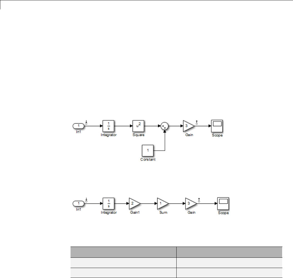
2Linearization
Operating Point Impact on Linearization
Choosing the right operating point for linearization is critical for obtaining an
accurate linear model. The linear model is an approximation of the nonlinear
model that is valid only near the operating point at which you linearize the
model.
Although you specify which Simulink blocks to linearize, all blocks in the
model affect the operating point.
A nonlinear model can have two very different linear approximations when
you linearize about different operating points.
The linearization result for this model is shown next, with the initial condition
for the integration x0=0.
This table summarizes the different linearization results for two different
operating points.
Operating Point Linearization Result
Initial Condition = 5, State x1 =5 30/s
Initial Condition = 0, State x1 =0 0
2-10

Specify Model Portion to Linearize
Specify Model Portion to Linearize
In this section...
“Specifying Subsystem, Loop, or Block to Linearize” on page 2-11
“Opening Feedback Loops” on page 2-12
“Ways to Specify Portion of Model to Linearize” on page 2-14
“Specify Portion of Model to Linearize in Simulink Model” on page 2-14
“Specify Portion of Model to Linearize in Linear Analysis Tool” on page 2-16
“Edit Portion of Model to Linearize in Linear Analysis Tool” on page 2-21
“Select Bus Elements as Linear Analysis Points” on page 2-23
Specifying Subsystem, Loop, or Block to Linearize
Simulink Control Design lets you specify the subsystem, loop, or block to
linearize using linearization input and output points (linearization I/O points).
Alinearization input point defines the input signal to the linear model. A
linearization output point defines the output signal of the linear model.
You can linearize:
•Closed or open loop responses using a linearization input point on the input
signal to the portion of the model you want to linearize, and a linearization
output point at the output signal of that portion of the model.
•Specific subsystem or block.
In this case, linearization I/O points are the input and output signals
corresponding to the subsystem or block.
You can define other linear models using additional types of linear analysis
points:
•Input-Output Point — Linearization output point immediately follows
a linearization input point. This type of linearization I/O point is useful
for measuring sensitivity to output disturbances.
2-11

2Linearization
•Output-Input Point — Linearization input point immediately follows a
linearization output point. This type of linearization I/O point is useful
for robust control. You can use the resulting transfer function in the mu
analysis of your system.
Linearization I/O points are pure annotations and do not impact model
simulation.
More About
“Ways to Specify Portion of Model to Linearize” on page 2-14
Opening Feedback Loops
If your model contains one or more feedback loops, you can choose to linearize
an open-loop or a closed-loop system.
Simulink Control Design lets you remove the effects of the feedback loop by
inserting an open loop point without having to manually break signal lines.
In fact, for nonlinear models, do not open the loop by manually removing the
feedback signal from the model; this action changes the model operating point
and produces a different linear model.
Note If a model is already linear, it has the same form regardless of the
operating point.
Correct placement of the loop opening is critical to obtaining the right linear
model. For example, you might want to linearize only the plant model in a
feedback control loop.
To understand the difference between open-loop and closed-loop analysis,
consider this single-loop control system.
2-12
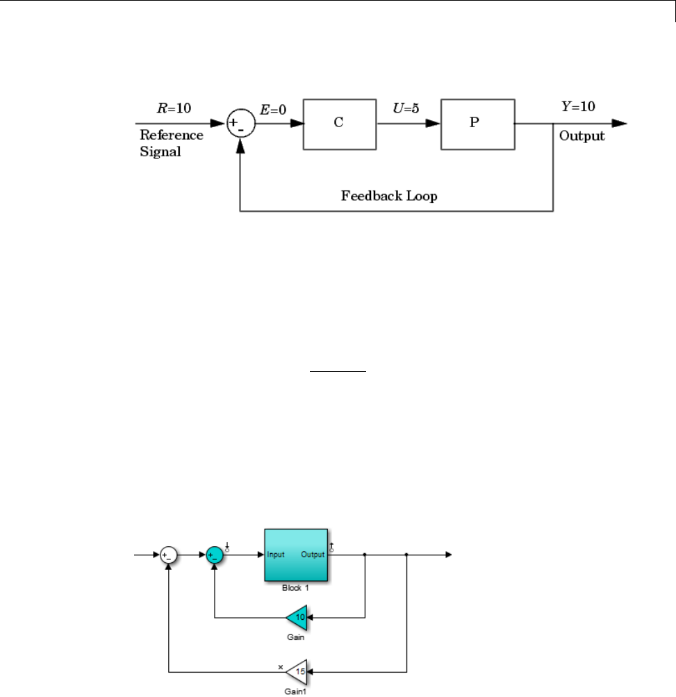
Specify Model Portion to Linearize
Suppose you want to linearize the plant, P, about an equilibrium operating
point of the model.
To linearize only the plant P, you must open the loop at the output of the P
block. If you do not open the loop, and if Cand Parelinear,thelinearized
model between Uand Yis Ps
CsPs
()
() ()1+.
The loop opening does not need to be in the same location as the linearization
input or output point. For example, the next figure shows a loop opening
after the gain on the outer feedback loop, which removes the effect of this
loop from the linearization. To check whether you correctly excluded the
feedback signal, linearize the model and highlight the blocks included in
the linearization.
2-13

2Linearization
In this example, placing a loop opening at the same location as the
linearization output point also removes the effect of the inner loop from the
linearization.
More About
•“Ways to Specify Portion of Model to Linearize” on page 2-14
•“Highlighting Linearized Blocks” on page 2-103
Ways to Specify Portion of Model to Linearize
There are several ways to specify linearization inputs, outputs, and
loop-opening locations (linear analysis points or linearization I/O sets)that
define the portion of the model you want to linearize. Each method has its
ownadvantages. Youcan:
•Specify linearization I/O points and loop openings directly in the model. An
advantage of this method is that the locations of linearization I/O points
and loop openings are shown graphically in the model. However, specifying
linearization I/O sets this way changes the model.
•Interactively define linearization I/O sets using the Linear Analysis Tool.
The Create linearization I/O set dialog box in the Linear Analysis Tool
allows you to define one or more I/O sets for your model interactively. This
approach does not make changes to the model.
•Define linearization I/O sets at the command line using linio. This method
also allows you to define one or more I/O sets without changing the model.
Specify Portion of Model to Linearize in Simulink
Model
To specify linearization I/O points and loop openings directly in your Simulink
model:
1Right-click on the signal you want to define as a linearization input point
or output point.
This action opens a context menu on the signal.
2Hover the cursor over Linear Analysis Points in the context menu.
2-14
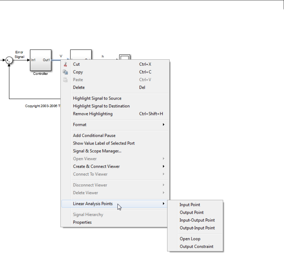
Specify Model Portion to Linearize
A submenu appears listing types of linear analysis points.
3Select the type of linear analysis point you want to define at the signal.
For example, to specify that the signal is a linearization input point, select
Input Point.
4To insert an open loop point at the signal, select Linear Analysis
Points > Open Loop from the context menu.
2-15

2Linearization
When you specify linearization inputs and outputs or loop openings, markers
appear in your model indicating the linear analysis point type.
5Repeat steps 2–4 for all signals you want to define as linearization I/O points
or open loop points.
Specifying linear analysis points using the context menu changes the model
(makes the model “dirty”).
More About
•“Specifying Subsystem, Loop, or Block to Linearize” on page 2-11
•“Opening Feedback Loops” on page 2-12
•“Ways to Specify Portion of Model to Linearize” on page 2-14
Specify Portion of Model to Linearize in Linear
Analysis Tool
You use linearization inputs, outputs, and loop-opening locations
(linearization I/O sets) to specify which portion of the model to linearize.
You can specify one or more linearization I/O sets interactively in the Linear
Analysis Tool, without introducing changes to the model.
To access the Create linearization I/O set dialog box:
1Click the Exact Linearization or Frequency Response Estimation tab.
2-16
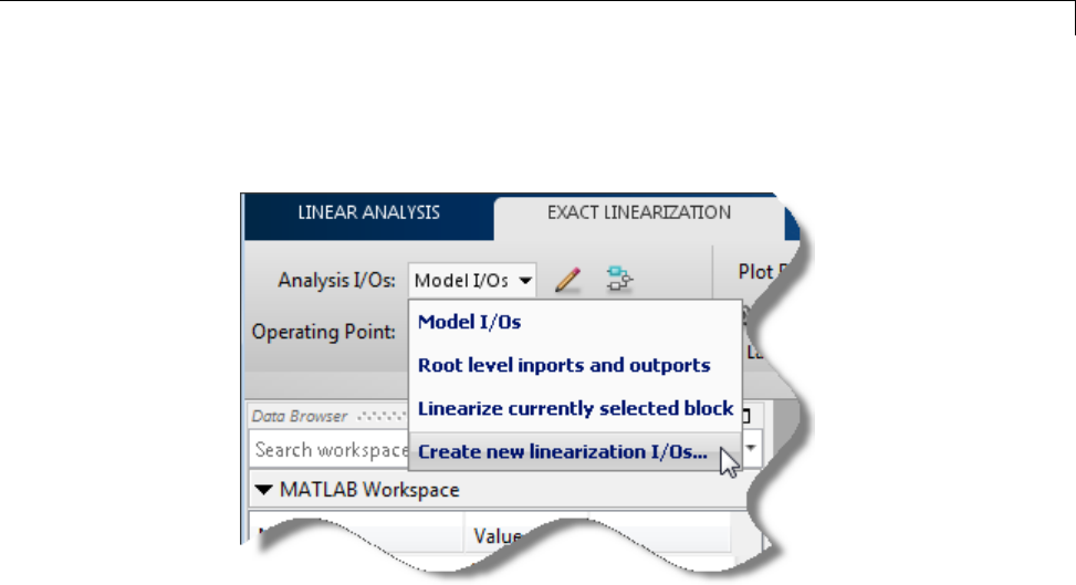
Specify Model Portion to Linearize
2From the Analysis I/Os drop-down list, select Create new linearization
I/Os.
The Create linearization I/O set dialog box opens.
Create Linearization I/O Set
To create a new linearization I/O set:
1In your Simulink model, select a signal that you want to define as a
linearization input or output point.
The selected signal appears in the Create linearization I/O set dialog box
under Currently selected signals.
2-17
2Linearization
2In the Create linearization I/O set dialog box, click the signal name under
Currently selected signals.
3Click Add. The signal appears in the list of Analysis I/Os.
4Select the linearization point type from the Configuration drop-down list.
For example, if you want the selected signal to be a linearization output
point, select Output.
5If you want the signal to be a loop opening point, click the Open Loop
check box.
2-18

Specify Model Portion to Linearize
6Repeat steps 1–5 for any other signals you want to define as linearization
I/O points.
Tip To highlight in the Simulink model the blocks that are included in the
linearization specified by the current list of Analysis I/Os, click Highlight.
7After you define all the signals for the I/O set, enter a name for the I/O set
in the Variable name box.
8Click OK.
The Create linearization I/O set dialog box closes. A new linearization I/O set
appears in the Linear Analysis Workspace of the Linear Analysis Tool. The
new linearization I/O set displays the name you specified.
2-19
2Linearization
The newly created linearization I/O set is automatically selected in the
Analysis I/Os menu for either the Exact Linearization or Frequency
Response Estimation tab, dependingonwhichyouselectedoriginally.
2-20

Specify Model Portion to Linearize
Creating linearization I/O sets in the Linear Analysis Tool does not change
the Simulink model. You can create multiple I/O sets for a single model.
More About
•“Specifying Subsystem, Loop, or Block to Linearize” on page 2-11
•“Opening Feedback Loops” on page 2-12
•“Ways to Specify Portion of Model to Linearize” on page 2-14
Edit Portion of Model to Linearize in Linear Analysis
Tool
You can interactively edit a linearization I/O set stored in the Linear Analysis
Workspace using the Linear Analysis Tool Edit dialog box.
Open Edit Dialog Box
To open the Edit dialog box for editing a linearization set, either:
•In the Linear Analysis Workspace, double-click the I/O set.
•Click either the Exact Linearization or Frequency Response Estimation
tab. If the I/O set is selected in the Analysis I/Os menu, click the edit icon
next to the Analysis I/Os menu.
Either of these actions opens the I/O set edit dialog box for the linearization
I/O set. You can now edit the I/O set as needed. When you have finished
editing, click to close the dialog box and save your changes.
Tip To highlight in the Simulink model the blocks that are included in the
linearization specified by the current list of Analysis I/Os, click Highlight.
Add Signal to I/O Set
To add a linearization input point, output point, or loop opening to the
linearization I/O set:
2-21
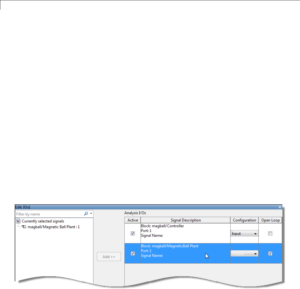
2Linearization
1In your Simulink model, select a signal that you want to add to the
linearization I/O set.
The selected signal appears in the Create linearization I/O set dialog box
under Currently selected signals.
2In the Create linearization I/O set dialog box, click the signal name under
Currently selected signals.
3Click Add. The signal appears in the list of Analysis I/Os.
4Select the linear analysis point type from the Configuration drop-down
list. For example, if you want the selected signal to be a linearization
output point, select Output.
5If you want the signal to be a loop opening point, click the Open Loop
check box.
Remove Signal from I/O Set
To remove a linearization input point, output point, or loop opening from the
linearization I/O set:
1Select the signal in the list of Analysis I/Os.
2Click Delete to remove the signal from the linearization I/O set.
2-22

Specify Model Portion to Linearize
Change Linear Analysis Point Type
To change the type of linear analysis point type for a signal, locate the signal
in the list of Analysis I/Os. Then, use the Configuration drop-down list and
the Open Loop check box for the signal to define the type of linear analysis
point.
For example, if you want the signal to be a linearization output point, select
Output from the Configuration drop-down list. If you want the signal not to
be an open loop point, verify that the Open Loop check box is cleared.
SelectBusElementsasLinearAnalysisPoints
This example shows how to select individual elements in a bus signal as
linearization input/output (I/O) points. Linearization I/O points define the
portion of the model to linearize.
Code Alternative
Use linio to specify model signals as linearization I/O points and loop
openings. For examples and additional information, see the linio reference
page.
1Open Simulink model.
sys = 'sldemo_mdlref_bus';
open_system(sys)
2In the Simulink Editor, define portion of the model to linearize:
aRight-click the COUNTERBUS signal, and select Linear Analysis
Points > Select Bus Element.
This option appears only if Mux blocks used to create bus signals
in the Configuration Parameters > Diagnostics > Connectivity
pane is error. Otherwise, right-clicking the bus signal lets you specify
all elements in the bus as linearization input or output points.
The Select Linearization Points in the Bus dialog box opens, which
shows signals contained in the COUNTERBUS bus signal.
2-23
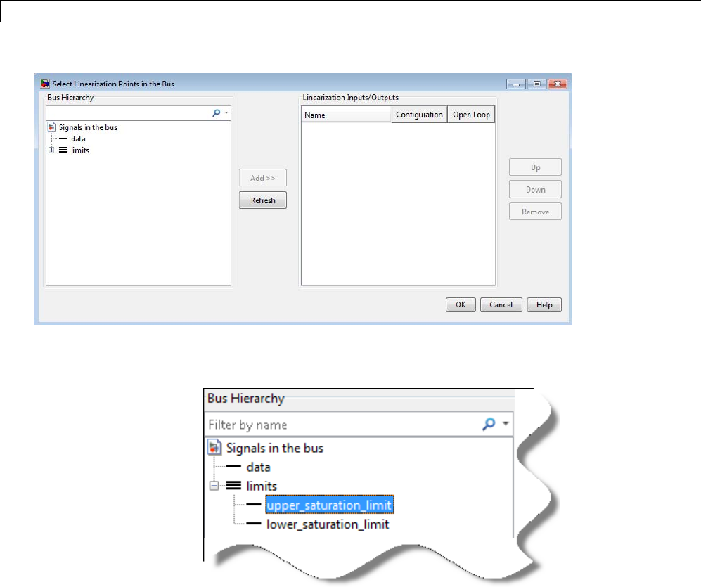
2Linearization
bIn the Bus Hierarchy area, expand the bus named limits. Then, select
upper_saturation_limit.
2-24
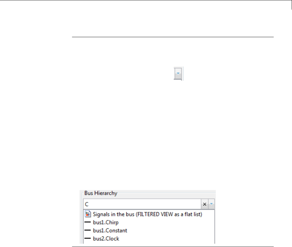
Specify Model Portion to Linearize
Tip For large buses, you can enter search text for filtering element
names in the Filter by name edit box. The name match is case-sensitive.
Additionally, you can enter a MATLAB regular expression.
To modify the filtering options, click adjacent to the Filter by name
edit box.
Filtering Options
•Enable regular expression
MATLAB regular expression for filtering signal names. For example,
entering t$ displays all signals whose names end with a lowercase t
(and their immediate parents).
•Show filtered results as a flat list
Flat list format to display the list of filtered signals.
By default, filtered signals are displayed using a tree format. The flat
list format uses dot notation to reflect the hierarchy of bus signals.
aClick Add.
The selected signal now appears in the Linearization Inputs/Outputs
area, and is configured as a linearization input point.
2-25
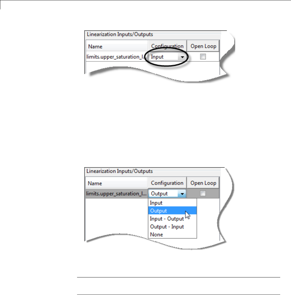
2Linearization
Click OK.
bRight-click the OUTPUTBUS signal, and select Linear Analysis
Points > Select Bus Element.
cIn the Bus Hierarchy area, expand the bus named limits,andselect
upper_saturation_limit.
dClick Add to add the selected signal to the Linearization
Inputs/Outputs area.
eSelect Output in the Configuration column.
Click OK.
Tip In the Simulink Editor, select Display > Signals &
Ports > Linearization Indicators to view the linearization I/O markers.
2-26
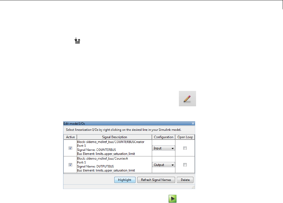
Specify Model Portion to Linearize
You can select multiple elements in thesamebuswithdifferentI/Otypes.
The marker appears on the bus signal to indicate multiple bus element
selections with different I/O types.
3In the Simulink Editor, select Analysis > Control Design > Linear
Analysis.
The Linear Analysis Tool for the model opens.
Click the Exact Linearization tab. Click adjacent to the Analysis
I/Os list to see the bus elements selected as linearization I/O points.
4In the Exact Linearization tab, click to linearize the model using the
model initial condition as the operating point.
Related Examples
•“Linearize Simulink Model” on page 2-38
•“Plant Linearization” on page 2-28
•“Open-Loop Response of Control System for Stability Margin Analysis”
on page 2-32
2-27

2Linearization
Plant Linearization
This example shows how to use the Linear Analysis Tool to linearize a plant
subsystem at the model operating point. The model operating point consists
of the model initial state values and input signals.
Use this simpler approach instead of defining linearization I/O points when
the plant is a subsystem or a block.
Code Alternative
Use linearize. For examples and additional information, see the linearize
reference page.
1Open a Simulink model.
sys = 'watertank';
open_system(sys)
2Open the Linear Analysis Tool.
In the Simulink model window, right-click the Water-Tank System block
and select Linear Analysis > Linearize Block.
3View the block selected for linearization.
Click adjacent to the Analysis I/Os drop-down menu.
The Water Tank System block is highlighted.
4In the Plot Result drop-down menu, select New Bode.
2-28
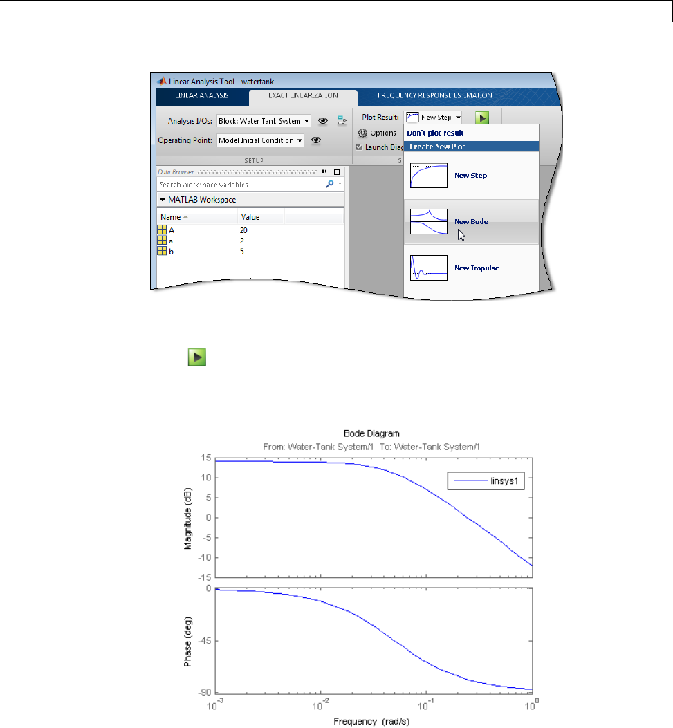
Plant Linearization
5Linearize the plant.
Click .
TheBodep
lot of the linearized plant appears.
2-29
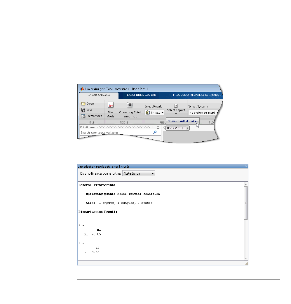
2Linearization
The linearization result, linsys1, appears in the Linear Analysis
Workspace.
6View the resulting linear plant model.
In the Linear Analysis tab, choose linsys1 from the Select Result list.
In the Select Report list, choose Show result details.
The Linearization results dialog box for linsys1 opens.
Tip Drag and drop linsys1 from the Linear Analysis Workspace to
the MATLAB Workspace to export it to the base workspace for further
analysis.
2-30

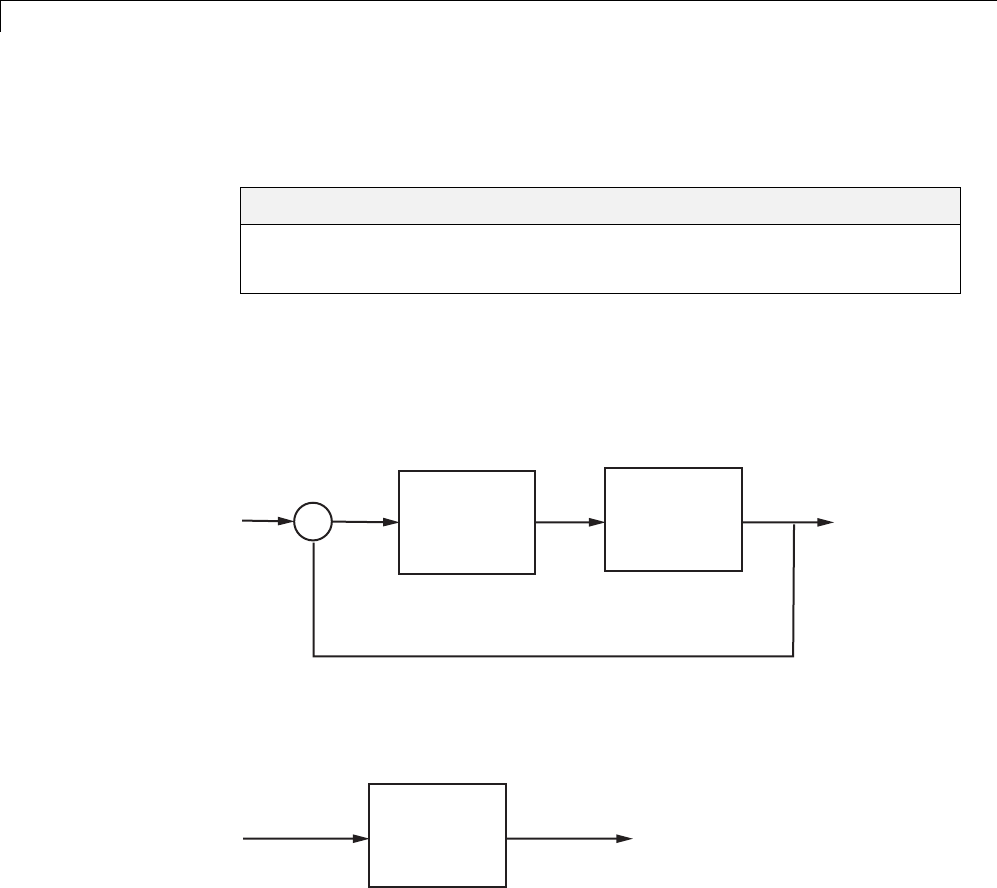
2Linearization
Open-Loop Response of Control System for Stability
Margin Analysis
In this section...
“What Is Open-Loop Response?” on page 2-32
“Compute Open-Loop Response” on page 2-33
What Is Open-Loop Response?
Open-loop response is the combined response of the plant and the controller,
excluding the effect of the feedback loop. For example, the next block diagram
shows a single-loop control system.
P(s)
C(s)
+-
Open-loop response corresponds to the linear response of the plant and the
controller. If C(s) and P(s) are linear, the corresponding linear systems is
C(s)P(s).
C(s)P(s)
In Simulink Control Design, the linearization I/O points and the loop opening
that correspond to open-loop response look something like this:
2-32
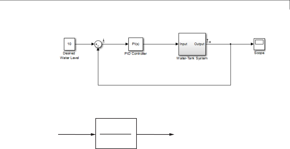
Open-Loop Response of Control System for Stability Margin Analysis
However,ifthereisnoloopopeningattheoutputofWater-TankSystem
block, the resulting linear model is different:
P(s)
1 + C(s)P(s)
Compute Open-Loop Response
ThisexampleshowshowtousetheLinearAnalysisTooltoanalyzethe
open-loop response of a control system.
Compute a linear model of the combined controller-plant system without the
effects of the feedback signal. Use a Bode plot of the resulting linear model to
see the open-loop response.
1Open Simulink model.
sys = 'watertank';
open_system(sys)
The Water-Tank System block represents the plant in this control system
and contains all of the system nonlinearities.
2-33

2Linearization
2Open the Linear Analysis Tool for the model.
In the Simulink Editor, select Analysis > Control Design > Linear
Analysis.
3In the Simulink Editor, define the portion of the model to linearize:
aRight-click the PID Controller block input signal (the output of the Sum
block). Select Linear Analysis Points > Input Point.
bRight-click the Water-Tank System output signal, and select Linear
Analysis Points > Output Point.
cRight-click the Water-Tank System output signal and select Linear
Analysis Points > Open Loop.
Annotations appear in the model indicating which signals are designated
as linearization I/O points.
Tip Alternatively, if you do not want to introduce changes to the Simulink
model, you can specify the linearization I/O points in the Linear Analysis
Tool. See “Specify Portion of Model to Linearize in Linear Analysis Tool”
on page 2-16.
2-34
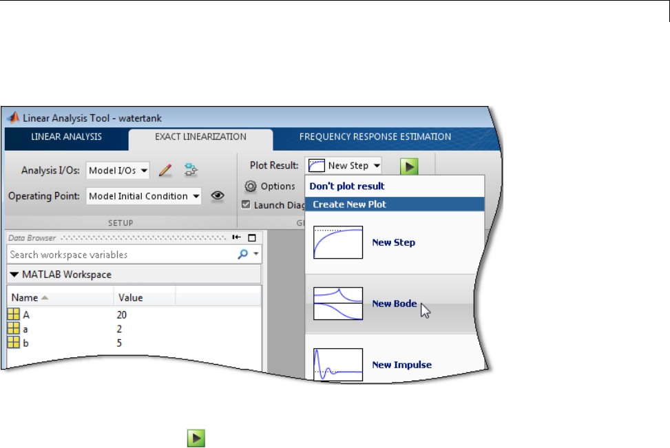
Open-Loop Response of Control System for Stability Margin Analysis
4In the Plot Result list of the Linear Analysis Tool, select New Bode.
5Linearize the model.
Click .
The Bode plot of the open-loop response appears.
6View the minimum stability margins for the model.
Right-click the plot and select Characteristics > Minimum Stability
Margins.
2-35
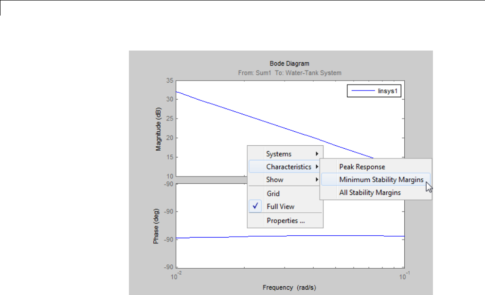
2Linearization
The Bode plot displays the phase margin marker. Click the marker to show
a data tip that contains the phase margin value.
2-36
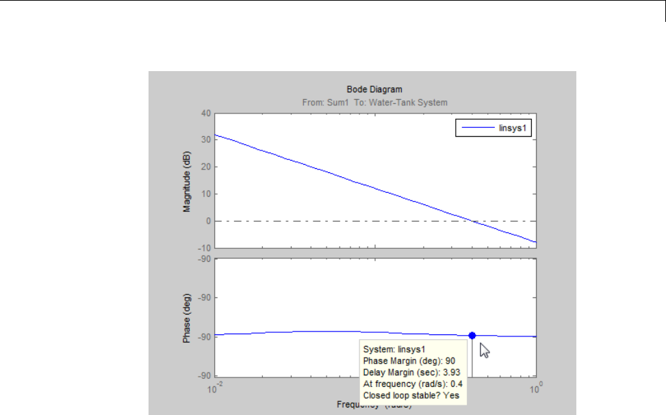
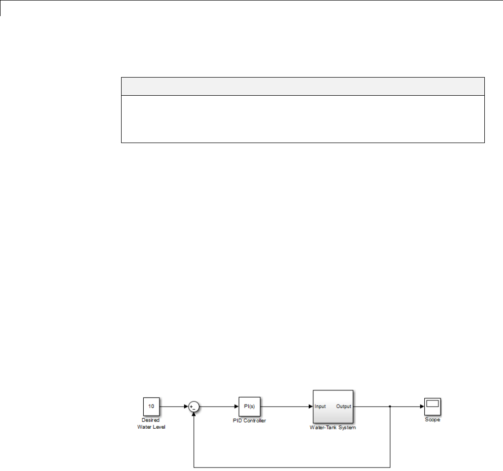
2Linearization
Linearize at Model Operating Point
In this section...
“Linearize Simulink Model” on page 2-38
“Visualize Bode Response of Simulink Model During Simulation” on page
2-42
Linearize Simulink Model
ThisexampleshowshowtousetheLinear Analysis Tool to linearize a model
at the operating point specified in the model. The model operating point
consists of the model initial state values and input signals.
Code Alternative
Use linearize. For examples and additional information, see the linearize
reference page.
1Open Simulink model.
sys = 'watertank';
open_system(sys)
The Water-Tank System block represents the plant in this control system
and includes all of the system nonlinearities.
2Open the Linear Analysis Tool for the model.
In the Simulink Editor, select Analysis > Control Design > Linear
Analysis.
2-38
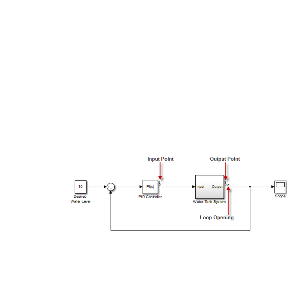
Linearize at Model Operating Point
3In the Simulink Editor, define the portion of the model to linearize:
aRight-click the PID Controller block output signal, which is the input to
the plant. Select Linear Analysis Points > Input Point.
bRight-click the Water-Tank System output signal, and select Linear
Analysis Points > Output Point.
4Right-click the Water-Tank System output signal and select Linear
Analysis Points > Open Loop.
Inserting this open loop point removes the effects of the feedback signal on
the linearization without changing the model operating point.
When you add linear analysis points, marker appear at their locations
in the model.
Tip Alternatively, if you do not want to introduce changes to the Simulink
model, you can specify the linearization I/O points in the Linear Analysis
Tool. See “Specify Portion of Model to Linearize in Linear Analysis Tool”
on page 2-16.
5In the Plot Result list, select a visualization.
For example, select New Bode.
2-39
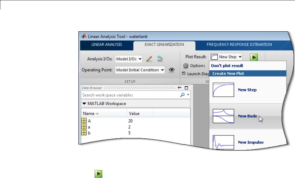
2Linearization
6Linearize the model.
Click .
The Bode plot of the linearized system appears.
2-40
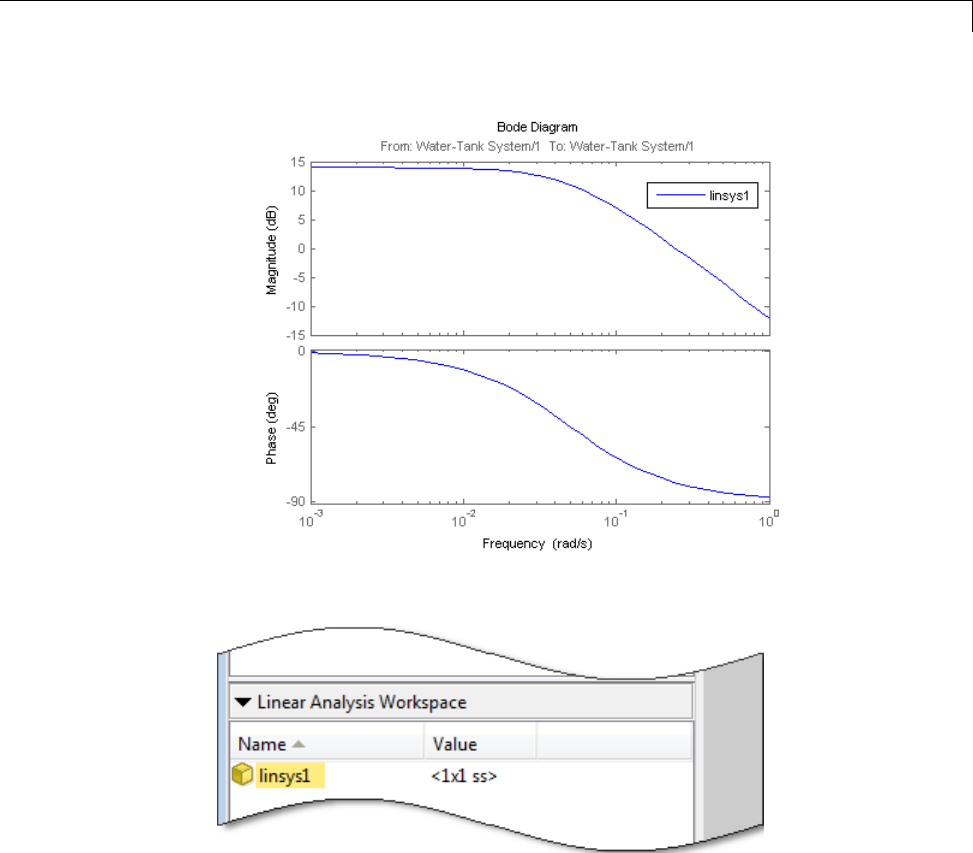
2Linearization
•“Open-Loop Response of Control System for Stability Margin Analysis”
on page 2-32
•“Visualize Bode Response of Simulink Model During Simulation” on page
2-42
Visualize Bode Response of Simulink Model During
Simulation
This example shows how to visualize linear system characteristics of
a nonlinear Simulink model during simulation, computed at the model
operating point (simulation snapshot time of 0).
1Open Simulink model.
For example:
watertank
2Open the Simulink Library Browser by selecting View > Library
Browser in the model window.
3Add a plot block to the Simulink model.
aIn the Simulink Control Design library, select Linear Analysis
Plots.
bDrag and drop a block, such as the Bode Plot block, into the model
window.
The model now resembles the following figure.
2-42

Linearize at Model Operating Point
4Double-click the block to open the Block Parameters dialog box.
2-43
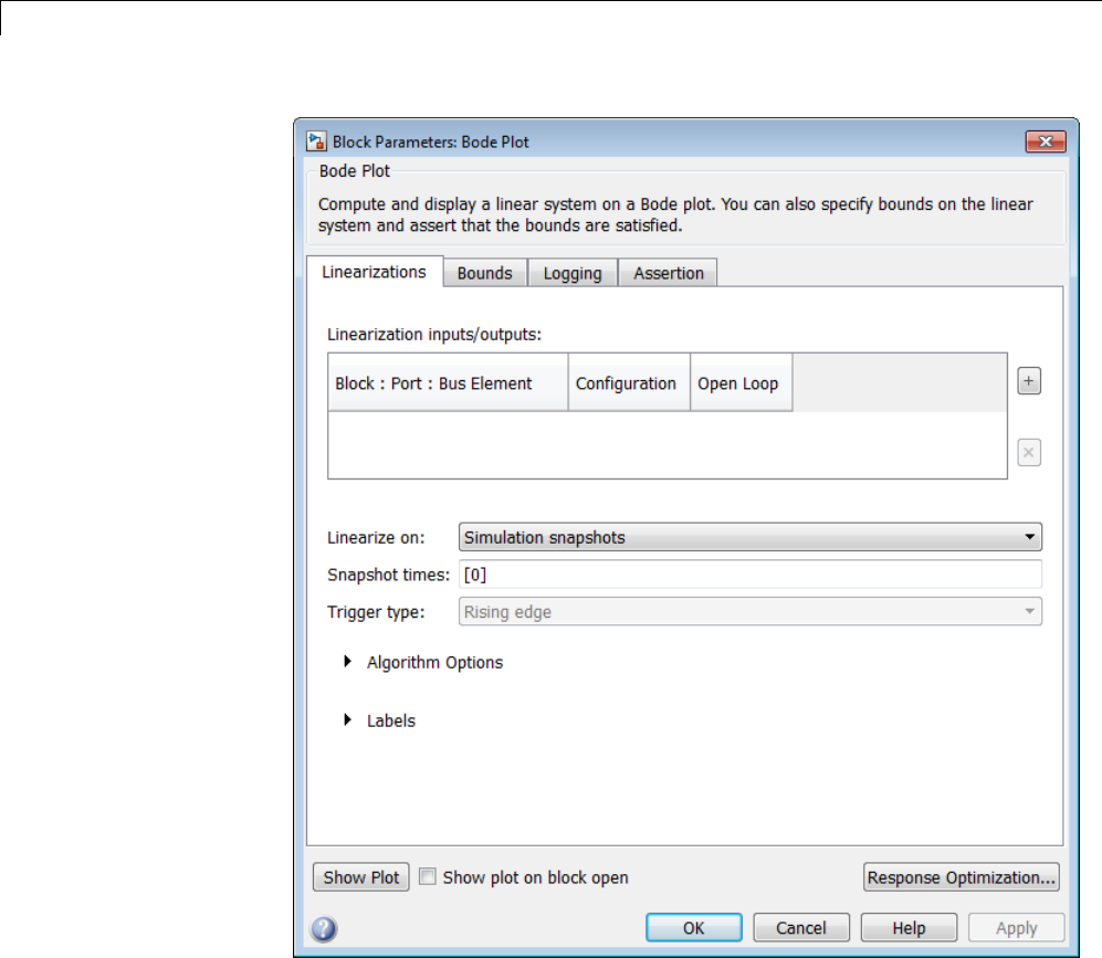
2Linearization
To learn more about the block parameters, see the block reference pages.
5Specify the linearization I/O points.
2-44
Linearize at Model Operating Point
Tip If your model already contains I/O points, the block automatically
detects these points and displays them.
aTo specify an input:
iClick adjacent to the Linearization inputs/outputs table.
The Block Parameters dialog expands to display a Click a signal
in the model to select it area.
ii In the Simulink model, click the output signal of the PID Controller
block to select it.
The Click a signal in the model to select it area updates to display
the selected signal.
2-45
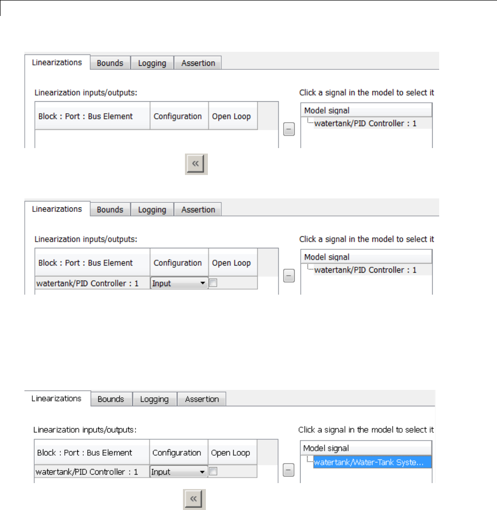
2Linearization
iii Click to add the signal to the Linearization inputs/outputs
table.
bTo specify an output:
iv In the Simulink model, click the output signal of the Water-Tank
System block to select it.
The Click a signal in the model to select it area updates to display
the selected signal.
vClick to add the signal to the Linearization inputs/outputs
table.
2-46
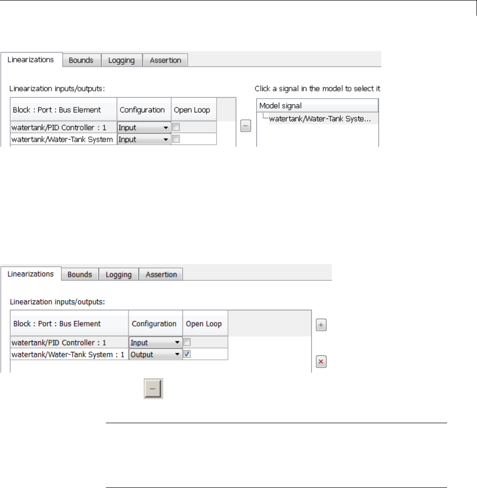
Linearize at Model Operating Point
vi In the Configuration drop-down list of the Linearization
inputs/outputs table, select Output for watertank/Water-Tank
System : 1.
vii Select the Open Loop option for watertank/Water-Tank System
:1.
The Linearization inputs/outputs table now resembles the following
figure.
cClick to collapse the Click a signal in the model to select it area.
Tip Alternatively, before you add the Linear Analysis Plots block,
right-click the signals in the Simulink model and select Linear Analysis
Points > Input Points and Linear Analysis Points > Output Points.
Linearization I/O annotations appear in the model and the selected signals
appear in the Linearization inputs/outputs table.
6Save the linear system.
2-47
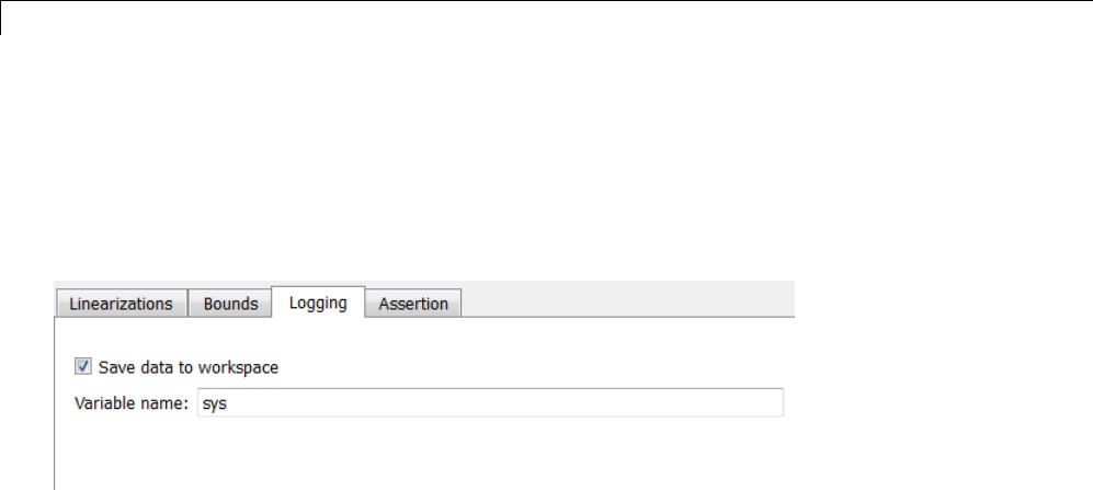
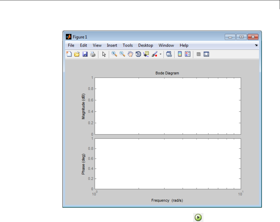
Linearize at Model Operating Point
8Plot the linear system characteristics by clicking in the plot window.
Alternatively, you can simulate the model from the model window.
The software linearizes the portion of the model between the linearization
input and output at the default simulation time of 0, specified in Snapshot
times parameter in the Block Parameters dialog box, and plots the Bode
magnitude and phase.
After the simulation completes, the plot window resembles the following
figure.
2-49
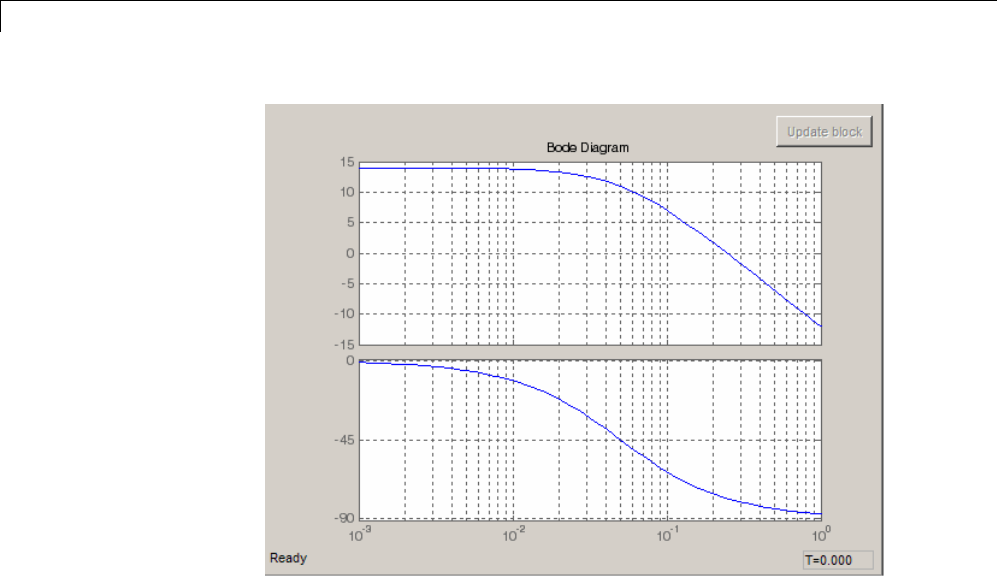
2Linearization
The computed linear system is saved as sys in the MATLAB workspace. sys
is a structure with time and values fields. To view the structure, type:
sys
This command returns the following results:
sys =
time: 0
values: [1x1 ss]
blockName: 'watertank/Bode Plot'
•The time field contains the default simulation time at which the linear
system is computed.
•The values field is a state-space object which stores the linear system
computed at simulation time of 0. To learn more about the properties of
state-space objects, see ss in the Control System Toolbox documentation.
2-50

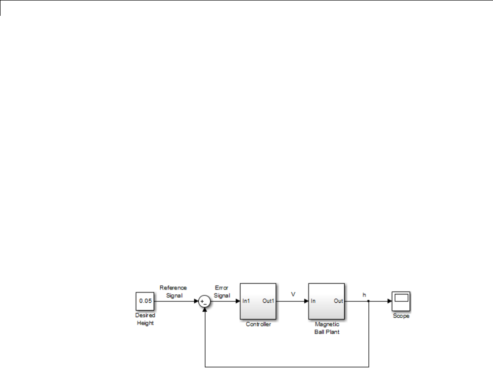
2Linearization
Linearize at Trimmed Operating Point
ThisexampleshowshowtousetheLinear Analysis Tool to linearize a model
at a trimmed steady-state operating point (equilibrium operating point).
The operating point is trimmed by specifying constraints on the operating
point values, and performing an optimization search that meets these state
and input value specifications.
Code Alternative
Use linearize. For examples and additional information, see the linearize
reference page.
1Open the Simulink model.
sys = 'magball';
open_system(sys)
2Open the Linear Analysis Tool for the model.
In the Simulink model window, select Analysis > Control
Design > Linear Analysis.
3In the Simulink model window, define the portion of the model to linearize
for this linearization task:
aRight-click the Controller block output signal (input signal to the plant).
Select Linear Analysis Points > Input Point.
bRight-click the Magnetic Ball Plant output signal, and select Linear
Analysis Points > Output Point.
2-52

Linearize at Trimmed Operating Point
cRight-click the Magnetic Ball Plant output signal again, and select
Linear Analysis Points > Open Loop.
Annotations appear in the model indicating which signals are designated
as linearization I/O points.
Tip Alternatively, if you do not want to introduce changes to the Simulink
model, you can specify the linearization I/O points in the Linear Analysis
Tool. See “Specify Portion of Model to Linearize in Linear Analysis Tool”
on page 2-16.
4In the Linear Analysis Tool, select Trim model,intheOperating Point
list.
Click Specifications.
By default, all model states are specified to be at equilibrium (as shown in
the Steady State column).
2-53
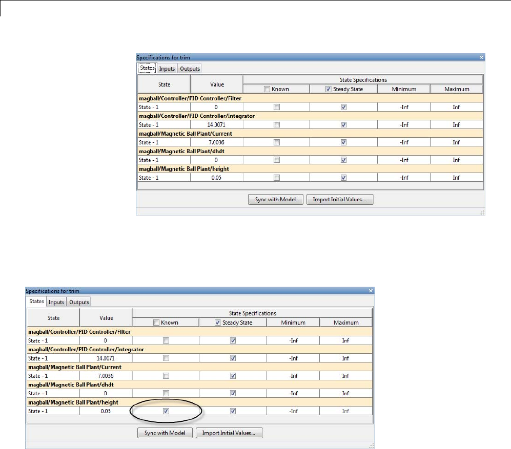
2Linearization
5In the States tab, select Known for the height state.
The height of the ball should match the reference signal height. This height
value should remain fixed during the optimization.
6Enter 0for the minimum bound of the Current block state.
2-54
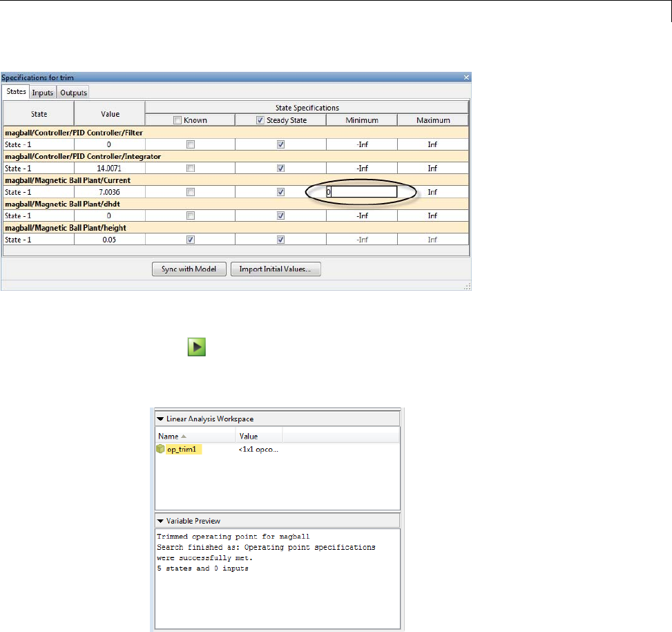
Linearize at Trimmed Operating Point
7Compute the operating point.
Click .
Anewvariable,op_trim1, appears in the Linear Analysis Workspace.
8Selecttheoperatingpointtobeusedforlinearization.
In the Exact Linearization tab, select op_trim1 from the Operating
Point list.
2-55
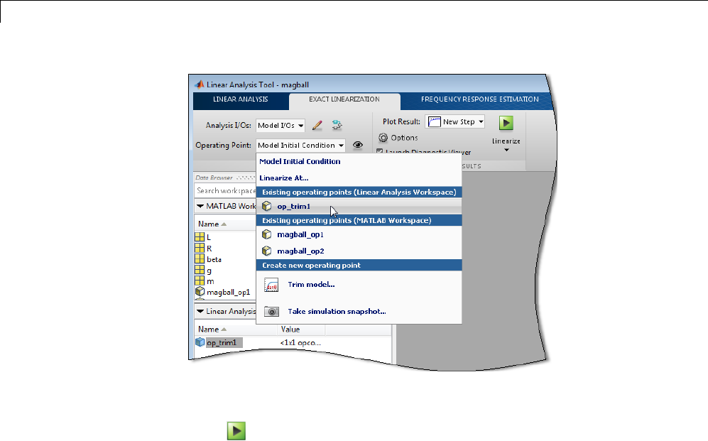
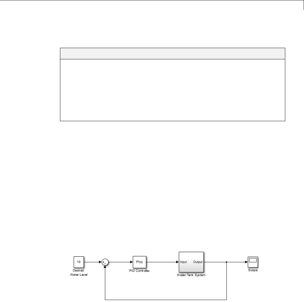
Linearize at Simulation Snapshots and Triggered Events
Linearize at Simulation Snapshots and Triggered Events
In this section...
“Linearize at Simulation Snapshot” on page 2-57
“Linearize at Triggered Simulation Events” on page 2-60
“Visualize Linear System at Multiple Simulation Snapshots” on page 2-64
“Visualize Linear System of a Continuous-Time Model Discretized During
Simulation” on page 2-70
“Visualize Linear System at Trigger-Based Simulation Events” on page 2-75
Linearize at Simulation Snapshot
ThisexampleshowshowtousetheLinear Analysis Tool to linearize a model
by simulating the model and extracting the state and input levels of the
system at specified simulation times.
Code Alternative
Use linearize. For examples and additional information, see the linearize
reference page.
1Open the Simulink model.
sys = 'watertank';
open_system(sys)
2Open the Linear Analysis Tool for the model.
2-57
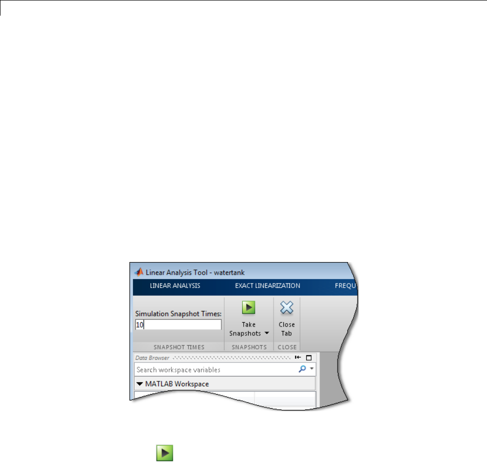
2Linearization
In the Simulink model window, select Analysis > Control
Design > Linear Analysis.
3In the Simulink model window, define the portion of the model to linearize:
•Right-click the PID Controller block output signal (input signal to the
plant model). Select Linear Analysis Points > Input Point.
•Right-click the Water-Tank System output signal, and select Linear
Analysis Points > Output Point.
•Right-click the Water-Tank System output signal, and select Linear
Analysis Points > Open Loop.
4In the Linear Analysis Tool, select Take simulation snapshot in the
Operating Point list.
5In the Simulation Snapshot Times field, enter 10 to extract the
operating point at this simulation time.
6Take a snapshot of the system at the specified time.
Click .
The operating point op_snapshot1 appears in the Linear Analysis
Workspace.
2-58
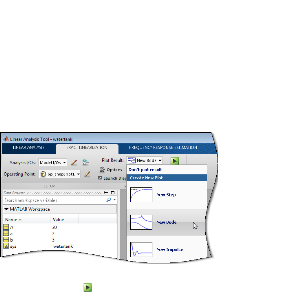
Linearize at Simulation Snapshots and Triggered Events
Tip To linearize the model at several operating points, specify a vector of
simulation times in the Simulation Snapshot Times field. For example,
entering [1 10] results in two linear models, one linearized at t=1and
the other at t=10.
7In the Exact Linearization tab, select op_snapshot1 in the Operating
Point list.
8In the Plot Result list, select a visualization.
Select New Bode.
9Linearize the model.
Click .
The Bode plot of the linearized system appears. This Bode plot looks like a
stable first-order response, as expected.
2-59
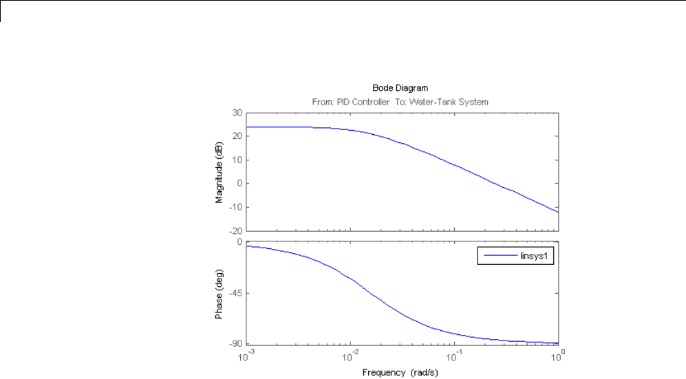
2Linearization
10 Double click linsys1 in the Linear Analysis Workspace to see the state
space representation of the linear model.
11 Close Simulink model.
bdclose(sys);
Related Examples
•“Linearize at Triggered Simulation Events” on page 2-60
•“Visualize Linear System at Multiple Simulation Snapshots” on page 2-64
•“Visualize Linear System of a Continuous-Time Model Discretized During
Simulation” on page 2-70
•“Visualize Linear System at Trigger-Based Simulation Events” on page 2-75
Linearize at Triggered Simulation Events
ThisexampleshowshowtousetheLinear Analysis Tool to linearize a model
at specific events in time. Linearization events can be trigger-based events
2-60
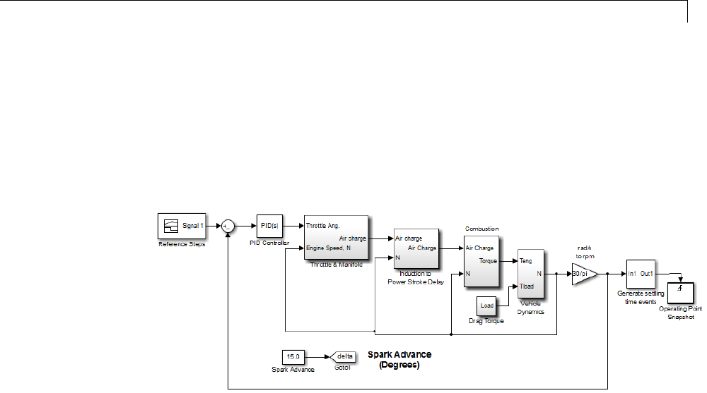
Linearize at Simulation Snapshots and Triggered Events
or function-call events. Specifically, the model will be linearized at the
steady-state operating points 2500, 3000, and 3500 rpm.
1Open Simulink model.
sys = 'scdspeedtrigger';
open_system(sys)
To help identify when the system is at steady state, the Generate settling
time events block generates settling events. This block sends rising edge
trigger signals to the Operating Point Snapshot block when the engine
speed settles near 2500, 3000, and 3500 rpm for a minimum of 5 seconds.
2-61
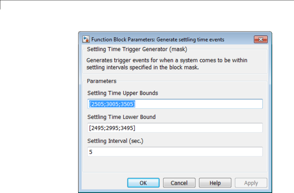
2Linearization
The model already includes the Trigger-Based Operating Point Snapshot
block from the Simulink Control Design library. This block linearizes
the model when it receives rising edge trigger signals from the Generate
settling time events block.
2Compute the steady-state operating point at 60 time units.
op = findop(sys,60);
This command simulates the model for 60 time units, and extracts the
operating points at each simulation event that occurs during this time
interval.
3Define the portion of the model to linearize.
io(1) = linio('scdspeedtrigger/Reference Steps',1,'in');
io(2) = linio('scdspeedtrigger/rad//s to rpm',1,'out');
2-62
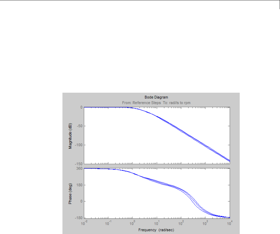
Linearize at Simulation Snapshots and Triggered Events
4Linearize the model.
linsys = linearize(sys,op(1:3),io);
5Compare linearized models at 500, 3000, and 3500 rpm using Bode plots of
the closed-loop transfer functions.
bode(linsys);
Related Examples
•“Linearize at Simulation Snapshot” on page 2-57
•“Visualize Linear System at Multiple Simulation Snapshots” on page 2-64
•“Visualize Linear System of a Continuous-Time Model Discretized During
Simulation” on page 2-70
•“Visualize Linear System at Trigger-Based Simulation Events” on page 2-75
2-63
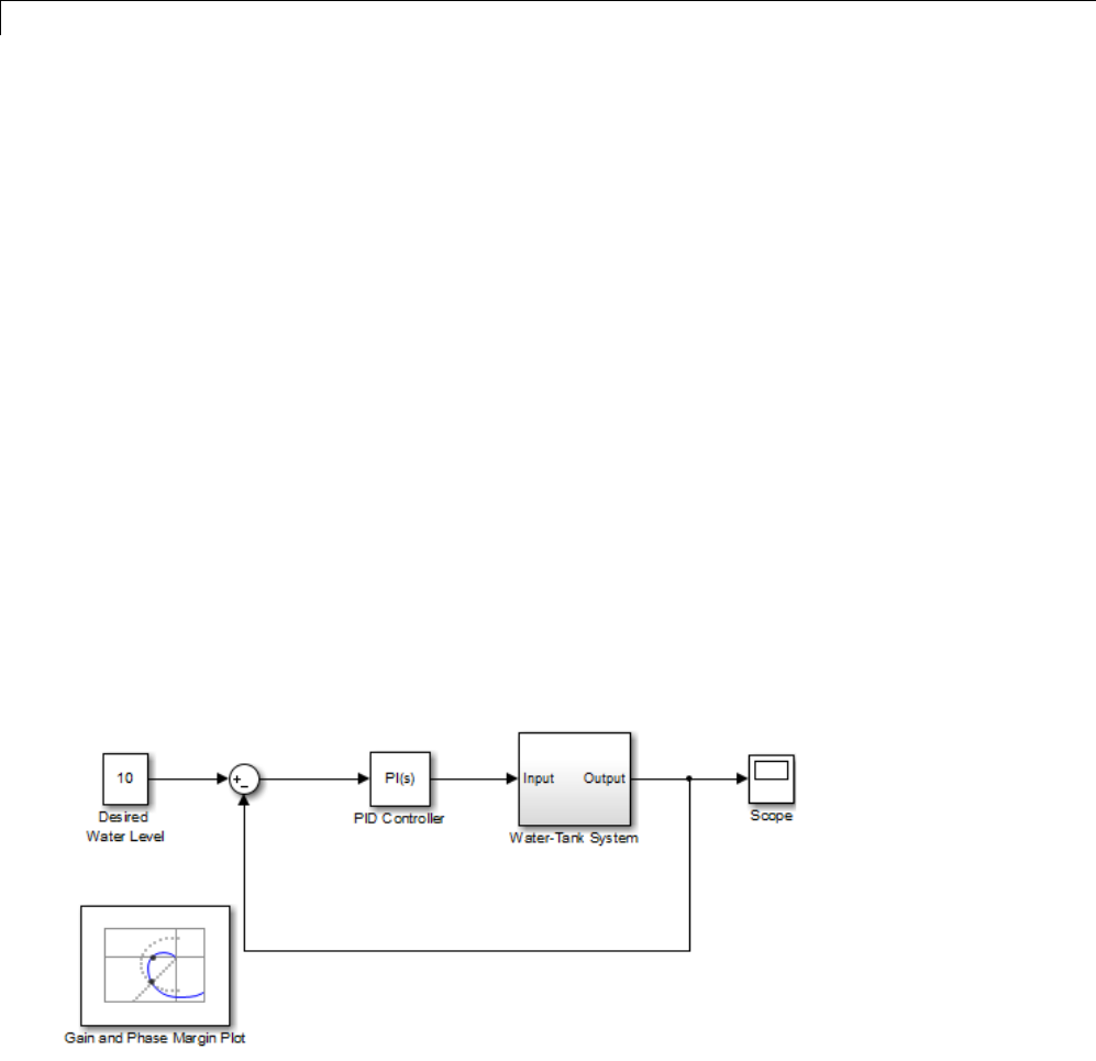
2Linearization
Visualize Linear System at Multiple Simulation
Snapshots
This example shows how to visualize linear system characteristics of a
nonlinear Simulink model at multiple simulation snapshots.
1Open Simulink model.
For example:
watertank
2Open the Simulink Library Browser by selecting View > Library
Browser in the model window.
3Add a plot block to the Simulink model.
aIn the Simulink Control Design library, select Linear Analysis
Plots.
bDrag and drop a block, such as the Gain and Phase Margin Plot block,
into the Simulink model window.
The model now resembles the following figure.
4Double-click the block to open the Block Parameters dialog box.
To learn more about the block parameters, see the block reference pages.
2-64
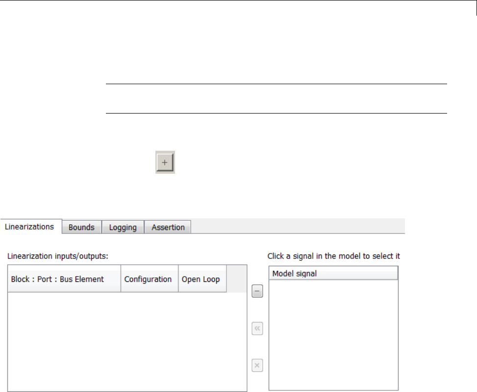
Linearize at Simulation Snapshots and Triggered Events
5Specify the linearization I/O points.
Tip If your model already contains I/O points, the block automatically
detects these points and displays them.
aTo specify an input:
iClick adjacent to the Linearization inputs/outputs table.
The Block Parameters dialog expands to display a Click a signal
in the model to select it area.
ii In the Simulink model, click the output signal of the PID Controller
block to select it.
The Click a signal in the model to select it area updates to display
the selected signal.
2-65

2Linearization
iii Click to add the signal to the Linearization inputs/outputs
table.
bTo specify an output:
iv In the Simulink model, click the output signal of the Water-Tank
System block to select it.
The Click a signal in the model to select it area updates to display
the selected signal.
vClick to add the signal to the Linearization inputs/outputs
table.
2-66

Linearize at Simulation Snapshots and Triggered Events
vi In the Configuration drop-down list of the Linearization
inputs/outputs table, select Output for watertank/Water-Tank
System : 1.
vii Select the Open Loop option for watertank/Water-Tank System
:1.
The Linearization inputs/outputs table now resembles the following
figure.
cClick to collapse the Click a signal in the model to select it area.
Tip Alternatively, before you add the Linear Analysis Plots block,
right-click the signals in the Simulink model and select Linear Analysis
Points > Input Points and Linear Analysis Points > Output Points.
Linearization I/O annotations appear in the model and the selected signals
appear in the Linearization inputs/outputs table.
6Specify simulation snapshot times.
2-67
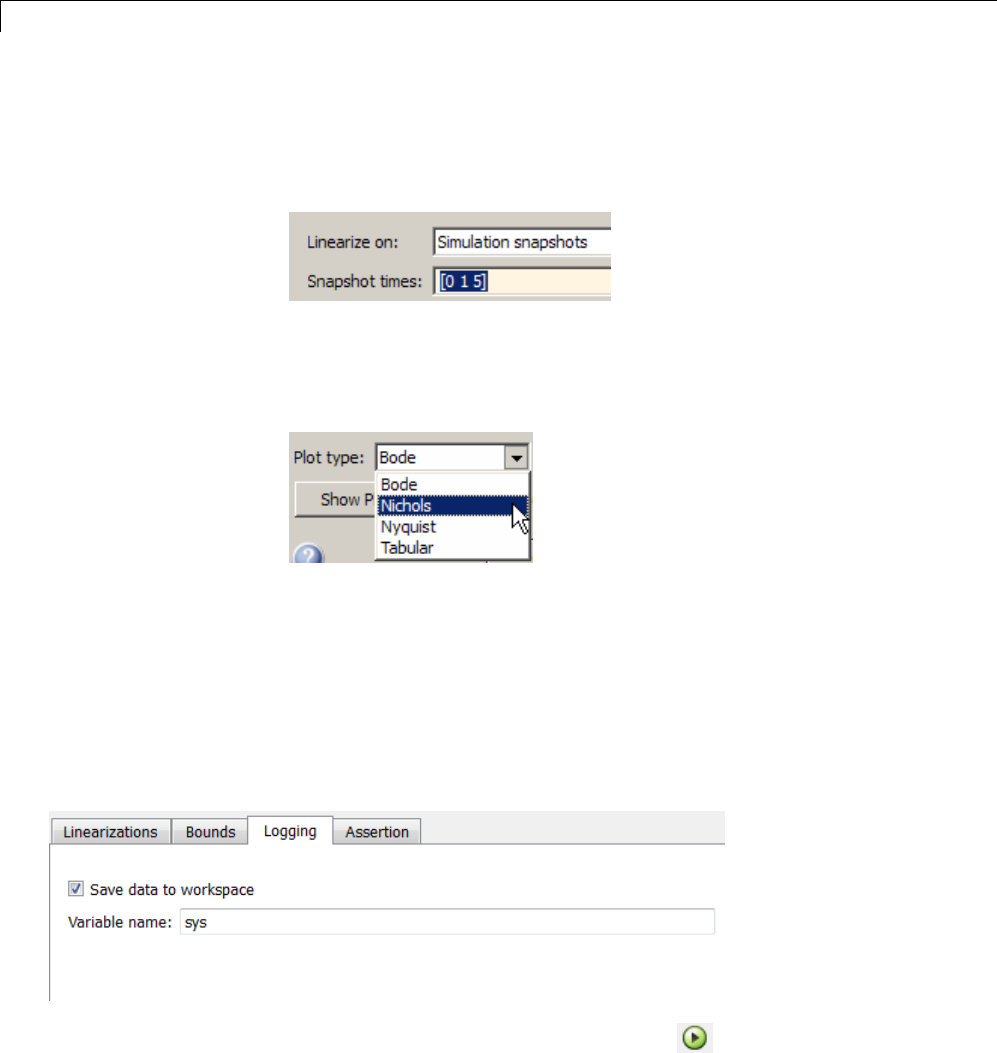
2Linearization
aIn the Linearizations tab, verify that Simulation snapshots is
selected in Linearize on.
bIn the Snapshot times field, type [0 1 5].
7Specify a plot type to plot the gain and phase margins. The plot type is
Bode by default.
aSelect Nichols in Plot type
bClick Show Plot to open an empty Nichols plot.
8Save the linear system.
aSelect the Logging tab.
bSelect the Save data to workspace option and specify a variable name
in the Variable name field.
The Logging tab now resembles the following figure.
9Plot the gain and phase margins by clicking in the plot window.
2-68
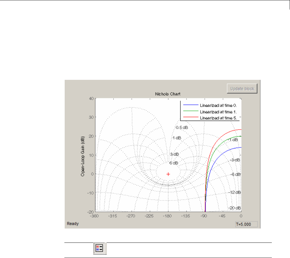
Linearize at Simulation Snapshots and Triggered Events
The software linearizes the portion of the model between the linearization
input and output at the simulation times of 0, 1 and 5 and plots gain and
phase margins.
After the simulation completes, the plot window resembles the following
figure.
Tip Click to view the legend.
The computed linear system is saved as sys in the MATLAB workspace. sys
is a structure with time and values fields. To view the structure, type:
sys
This command returns the following results:
2-69

2Linearization
sys =
time: [3x1 double]
values: [4-D ss]
blockName: 'watertank/Gain and Phase Margin Plot'
•The time field contains the simulation times at which the model is
linearized.
•The values field is an array of state-space objects which store the linear
systems computed at the specified simulation times.
Examples and How To
•“Visualize Bode Response of Simulink Model During Simulation” on page
2-42
•“Visualize Linear System at Trigger-Based Simulation Events” on page 2-75
•“Visualize Linear System of a Continuous-Time Model Discretized During
Simulation” on page 2-70
•“Linearize at Simulation Snapshot” on page 2-57
•“Linearize at Triggered Simulation Events” on page 2-60
Visualize Linear System of a Continuous-Time Model
Discretized During Simulation
This example shows how to discretize a continuous-time model during
simulation and plot the model’s discretized linear behavior.
1Open the Simulink model:
scdcstr
2-70
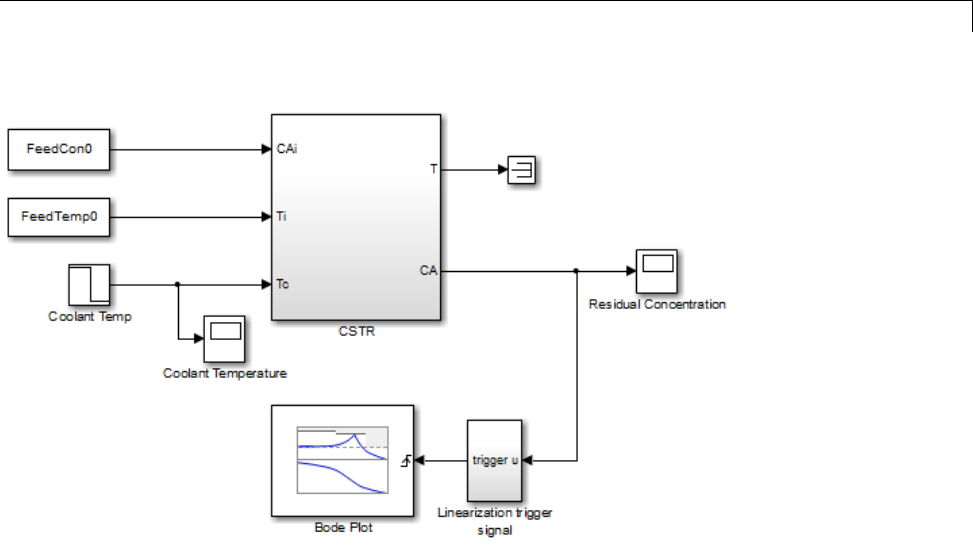
Linearize at Simulation Snapshots and Triggered Events
In this model, the Bode Plot block has already been configured with:
•Input point at the coolant temperature input Coolant Temp
•Output point at the residual concentration output CA
•Settingstolinearizethemodelonarisingedgeofanexternaltrigger.
The trigger signal is modeled in the Linearization trigger signal
block inthemodel.
•Saving the computed linear system in the MATLAB workspace as
LinearReactor.
To view these configurations, double-click the block.
2-71
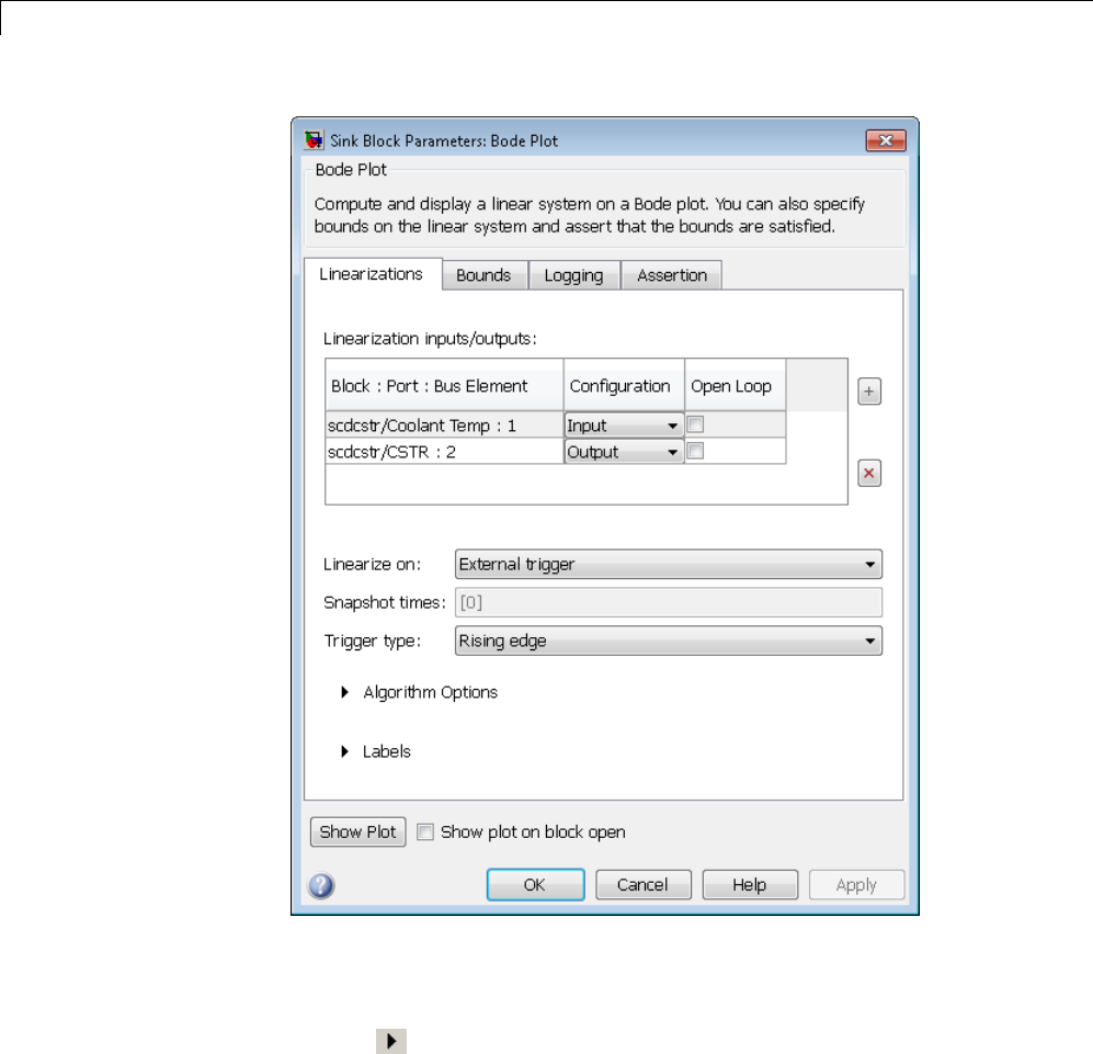
2Linearization
To learn more about the block parameters, see the block reference pages.
2Specify the sample time to compute the discrete-time linear system.
aClick adjacent to Algorithm Options.
The option expands to display the linearization algorithm options.
2-72
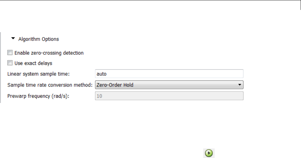
Linearize at Simulation Snapshots and Triggered Events
bSpecify a sample time of 2 in the Linear system sample time field.
To learn more about this option, see the block reference page.
3Click Show Plot to open an empty Bode plot window.
4Plot the Bode magnitude and phase by clicking in the plot window.
During simulation, the software:
•Linearizes the model on encountering a rising edge.
•Converts the continuous-time model into a discrete-time linear model
with a sample time of 2. This conversion uses the default Zero-Order
Hold method to perform the sample time conversion.
The software plots the discrete-time linear behavior in the Bode plot
window. After the simulation completes, the plot window resembles
the following figure.
2-73
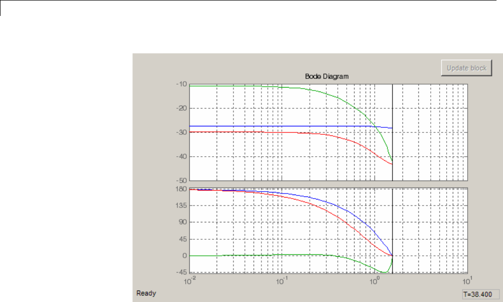
2Linearization
The plot shows the Bode magnitude and phase up to the Nyquist frequency,
which is computed using the specified sample time. The vertical line on the
plot represents the Nyquist frequency.
Examples and How To
•“Visualize Bode Response of Simulink Model During Simulation” on page
2-42
•“Visualize Linear System at Multiple Simulation Snapshots” on page 2-64
•“Visualize Linear System at Trigger-Based Simulation Events” on page 2-75
•“Linearize at Simulation Snapshot” on page 2-57
•“Linearize at Triggered Simulation Events” on page 2-60
2-74

Linearize at Simulation Snapshots and Triggered Events
Visualize Linear System at Trigger-Based Simulation
Events
Plotting Linear System Characteristics of a Chemical Reactor shows how
to plot the Bode magnitudeandphaseofareactor. Thereactortransitions
through different operating points corresponding to trigger-based simulation
events.
Examples and How To
•“Visualize Bode Response of Simulink Model During Simulation” on page
2-42
•“Visualize Linear System at Multiple Simulation Snapshots” on page 2-64
•“Visualize Linear System of a Continuous-Time Model Discretized During
Simulation” on page 2-70
•“Linearize at Simulation Snapshot” on page 2-57
•“Linearize at Triggered Simulation Events” on page 2-60
2-75

2Linearization
Ordering States in Linearized Model
In this section...
“Control State Order of Linearized Model using Linear Analysis Tool” on
page 2-76
“Control State Order of Linearized Model using MATLAB Code” on page
2-79
Control State Order of Linearized Model using Linear
Analysis Tool
This example shows how to control the order of the states in your linearized
model. This state order appears in linearization results.
1Open and configure the model for linearization.
sys = 'magball';
open_system(sys)
sys_io(1)=linio('magball/Controller',1,'in');
sys_io(2)=linio('magball/Magnetic Ball Plant',1,'out','on');
setlinio(sys,sys_io);
opspec = operspec(sys);
op = findop(sys,opspec);
These commands specify the plant linearization and compute the
steady-state operating point.
2Open the Linear Analysis Tool for the model.
In the Simulink model window, select Analysis > Control
Design > Linear Analysis.
3Open the Options for exact linearization dialog box.
In the Exact Linearization tab, click Options.
2-76
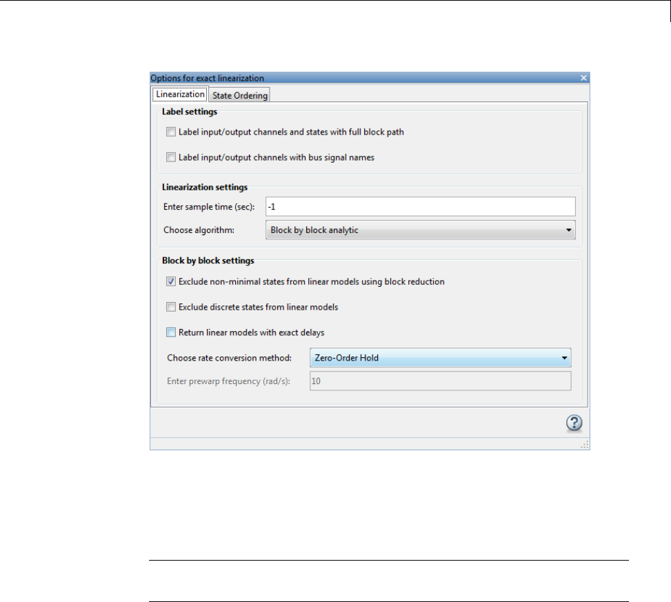
Ordering States in Linearized Model
4In the State Ordering tab, select the Enable state ordering check box.
5Specify the desired state order using the Move Up and Move Down
buttons.
Tip If you change the model while its Linear Analysis Tool is open, click
Sync with Model to update the list of states.
2-77
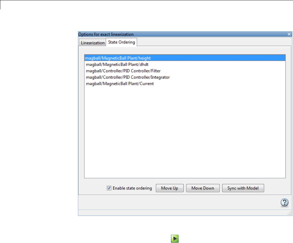
2Linearization
6Linearize the model.
In the Linear Analysis Tool, click .
A new linearized model, linsys1, appears in the Linear Analysis
Workspace.
7View the order of the model states for the linearized model by opening
the Linearization result dialog box.
Click the Linear Analysis tab. Choose Show result details in the
Select Report list.
2-78
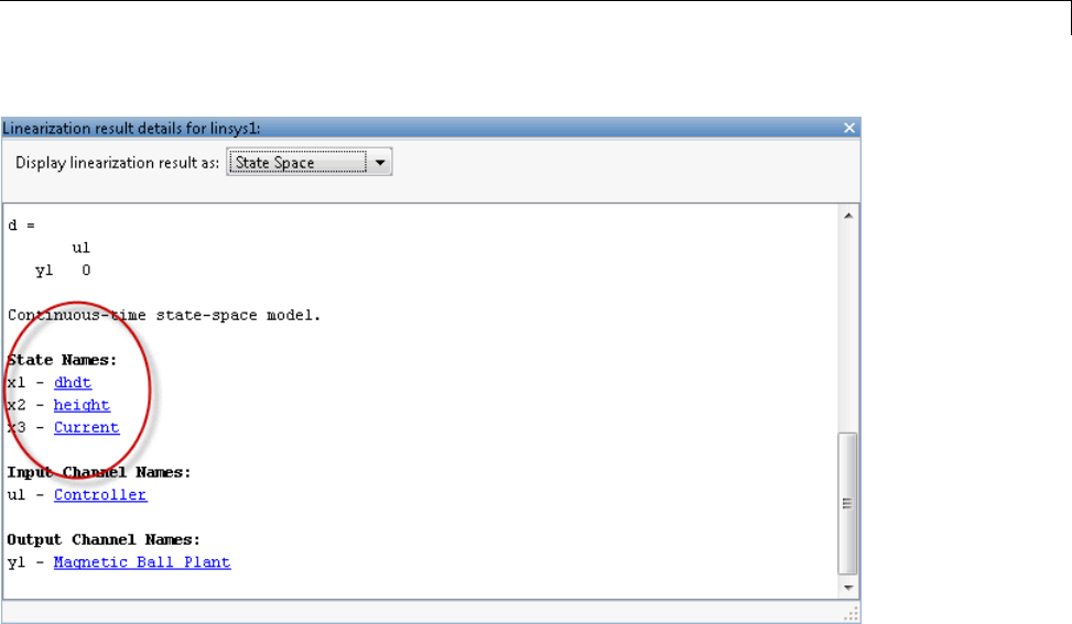
Ordering States in Linearized Model
The linear model states appear in the specified order.
Control State Order of Linearized Model using
MATLAB Code
This example shows how to control the order of the states in your linearized
model. This state order appears in linearization results.
1Load and configure the model for linearization.
sys = 'magball';
load_system(sys);
sys_io(1)=linio('magball/Controller',1,'in');
sys_io(2)=linio('magball/Magnetic Ball Plant',1,'out','on');
opspec = operspec(sys);
op = findop(sys,opspec);
These commands specify the plant linearization and compute the
steady-state operating point.
2-79

2Linearization
2Linearize the model, and show the linear model states.
linsys = linearize(sys,sys_io);
linsys.StateName
The linear model states are in default order. The linear model includes only
the states in the linearized blocks, and not the states of the full model.
ans =
'height'
'Current'
'dhdt'
3Define a different state order.
stateorder = {'magball/Magnetic Ball Plant/height';...
'magball/Magnetic Ball Plant/dhdt';...
'magball/Magnetic Ball Plant/Current'};
4Linearize the model again and show the linear model states.
linsys = linearize(sys,sys_io,'StateOrder',stateorder);
linsys.StateName
The linear model states are now in the specified order.
ans =
'height'
'dhdt'
'Current'
2-80

Time-Domain Validation of Linearization
Time-Domain Validation of Linearization
In this section...
“Validate Linearization in Time Domain” on page 2-81
“Choosing Time-Domain Validation Input Signal” on page 2-83
Validate Linearization in Time Domain
This example shows how to validate linearization results by comparing the
simulated output of the nonlinear model and the linearized model.
1Linearize Simulink model.
For example:
sys = 'watertank';
load_system(sys);
sys_io(1)=linio('watertank/PID Controller',1,'in');
sys_io(2)=linio('watertank/Water-Tank System',1,'out','on');
opspec = operspec(sys);
op = findop(sys,opspec);
linsys = linearize(sys,op,sys_io);
If you linearized your model in the Linear Analysis Tool, you must export
the linear model to the MATLAB workspace.
2Create input signal for validation. For example, a step input signal:
input = frest.createStep('Ts',0.1,...
'StepTime',1,...
'StepSize',1e-5,...
'FinalTime',500);
3Simulate the Simulink model using the input signal.
[~,simout] = frestimate(sys,op,sys_io,input);
simout is the simulated output of the nonlinear model.
2-81
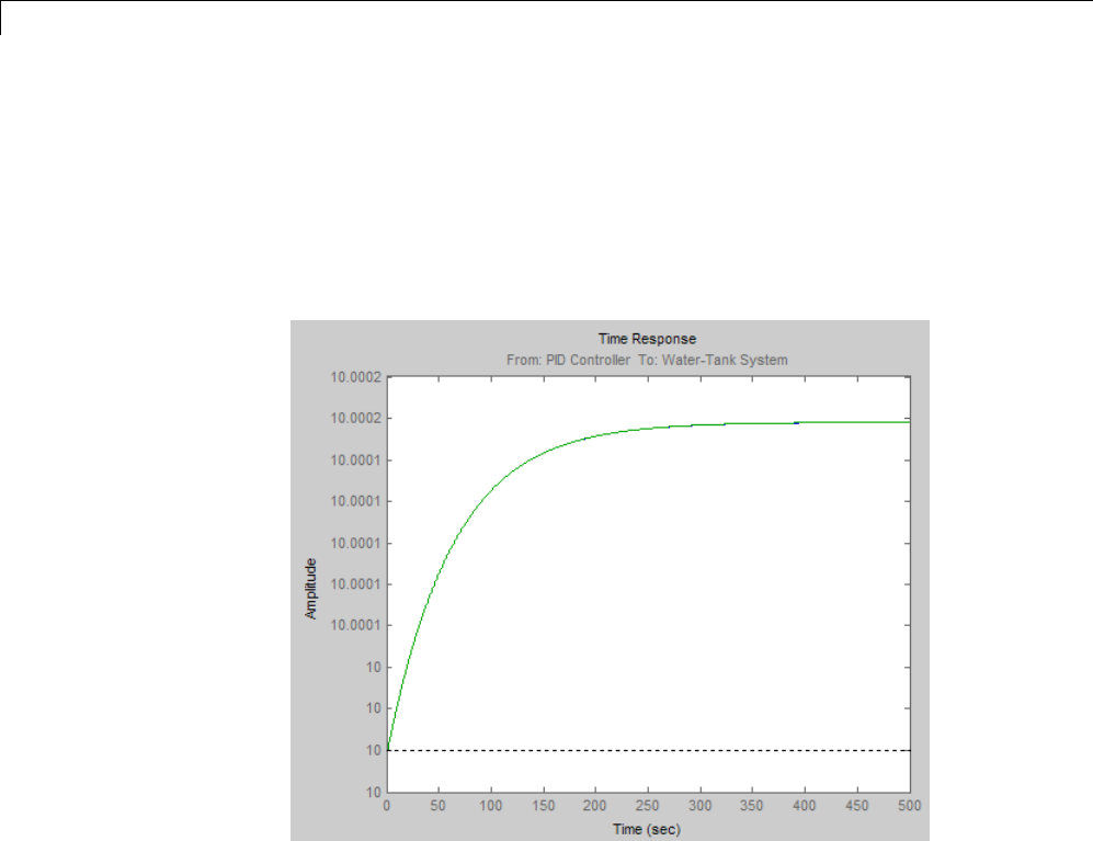
2Linearization
4Simulate the linear model sys, and compare the time-domain responses of
the linear and nonlinear Simulink model.
frest.simCompare(simout,linsys,input)
The step response of the nonlinear model and linearized model are close,
which validates that the linearization is accurate.
5Increase the amplitude of the step signal from 1.0e-005 to 1.
input = frest.createStep('Ts',0.1,...
'StepTime',1,...
'StepSize',1,...
'FinalTime',500);
6Repeat the frequency response estimation with the increased amplitude
oftheinputsignal,andcomparethistimeresponseplottotheexact
linearization results.
[~,simout2] = frestimate(sys,op,sys_io,input);
2-82
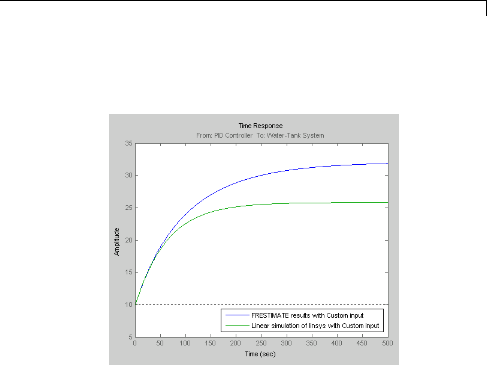
Time-Domain Validation of Linearization
frest.simCompare(simout2,linsys,input)
legend('FRESTIMATE results with Custom input',...
'Linear simulation of linsys with Custom input',...
'Location','SouthEast')
The step response of linear system you obtained using exact linearization
does not match the step response of the estimated frequency response with
large input signal amplitude.
This result indicates that linear model obtained using exact linearization
does not behave linearly you begin to deviate from the specified operating
point.
Choosing Time-Domain Validation Input Signal
For time-domain validation of linearization, use frest.createStep to create
a step signal. Use the step signal as an input to frest.simCompare,which
compares the simulated output of the nonlinear model and the linearized
model.
2-83

2Linearization
The step input helps you assess whether the linear model accurately captures
thedominanttimeconstantsasitgoes through the step transients.
The step input also shows whether you correctly captured the DC gain of
the Simulink model by comparing the final value of the exact linearization
simulation with the frequency response estimation.
2-84

Frequency-Domain Validation of Linearization
Frequency-Domain Validation of Linearization
In this section...
“Validate Linearization in Frequency Domain using Linear Analysis Tool”
on page 2-85
“Choosing Frequency-Domain Validation Input Signal” on page 2-89
Validate Linearization in Frequency Domain using
Linear Analysis Tool
Thisexampleshowshowtovalidatelinearizationresultsusinganestimated
linear model.
In this example, you linearize a Simulink model using the model initial
conditions. You then estimate the frequency response of the model using
thesameoperatingpoint(modelinitialcondition). Finally, you compare the
estimated response to the exact linearization result.
Step 1. Linearize Simulink model.
•Open a Simulink model.
sys = 'scdDCMotor';
open_system(sys);
•Open the Linear Analysis Tool for the model.
In the Simulink model window, select Analysis > Control
Design > Linear Analysis.
•Select a visualization for the linearized model.
In the Plot Result list, choose New Bode.
•Linearize the model.
Click .
A new linearized model, linsys1, appears in the Linear Analysis
Workspace.
2-85
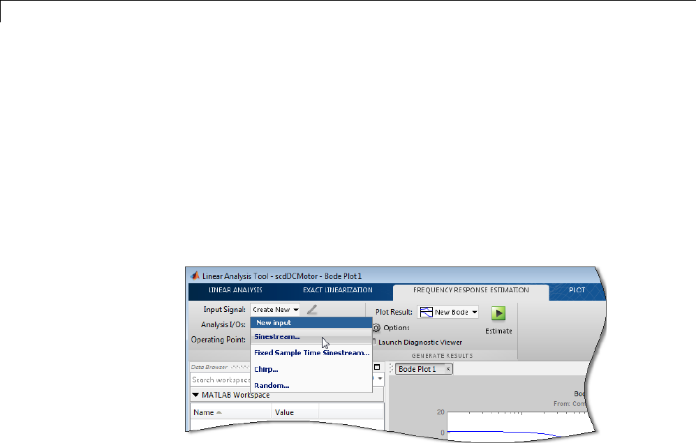
2Linearization
Thesoftwareusedthemodelinitialconditions as the operating point to
generate linsys1.
Step 2. Create sinestream input signal.
•Click the Frequency Response Estimation tab.
In this tab, you estimate the frequency response of the model.
•Open the Create sinestream input dialog box.
Select Sinestream from the Input Signal list.
•Initialize the input signal frequencies and parameters based on the
linearized model.
Click Initialize frequencies and parameters.
2-86
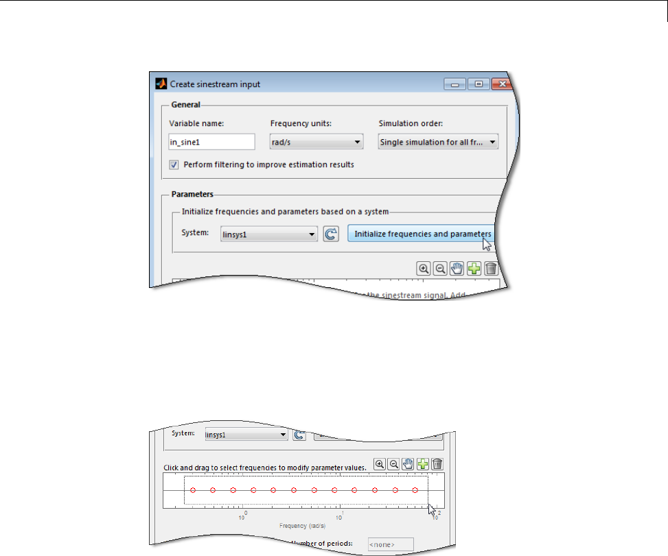
Frequency-Domain Validation of Linearization
The Frequency content viewer is populated with frequency points. The
software chooses the frequencies and input signal parameters automatically
based on the dynamics of linsys1.
•In the Frequency content viewer of the Create sinestream input dialog
box, select all the frequency points.
•Modify the amplitude of the input signal.
Enter1intheAmplitude box.
•ClickOK.
The input signal in_sine1 appears in the Linear Analysis Workspace.
Step 3. Select the plot to display the estimation result.
2-87
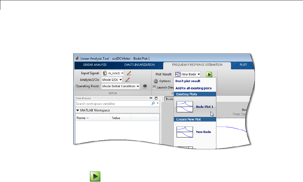
2Linearization
In the Plot Result list, choose Bode Plot 1 to add the next computed linear
system to Bode Plot 1.
Step 4. Estimate frequency response.
Click .
The estimated system, estsys1, appears in the Linear Analysis Workspace.
Step 5. Examine estimation results.
Bode Plot 1 now shows the Bode responses for the estimated model and
the linearized model.
2-88
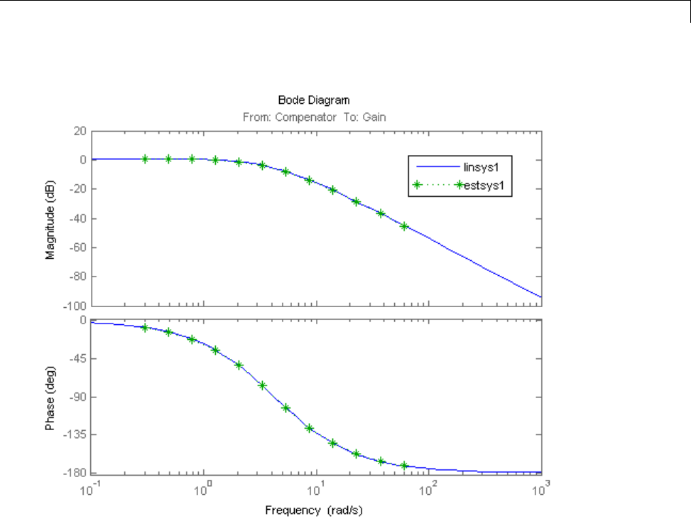
Frequency-Domain Validation of Linearization
The frequency response for the estimated model matches that of the linearized
model.
Choosing Frequency-Domain Validation Input Signal
For frequency-domain validation of linearization, create a sinestream signal.
By analyzing one sinusoidal frequency at a time, the software can ignore
some of the impact of nonlinear effects.
2-89

2Linearization
Input Signal Use When See Also
Sinestream All linearization inputs and
outputs are on continuous
signals.
frest.Sinestream
Sinestream with fixed sample
time
Oneormoreofthe
linearization inputs and
outputsisonadiscretesignal
frest.createFixedTsSinestream
You can easily create a sinestream signal based on your linearized model. The
software uses the linearized model characteristics to accurately predict the
number of sinusoid cycles at each frequency to reach steady state.
When diagnosing the frequency response estimation, you can use the
sinestream signal to determine whetherthetimeseriesateachfrequency
reaches steady state.
Concepts •“Creating Input Signals for Estimation” on page 3-9
2-90
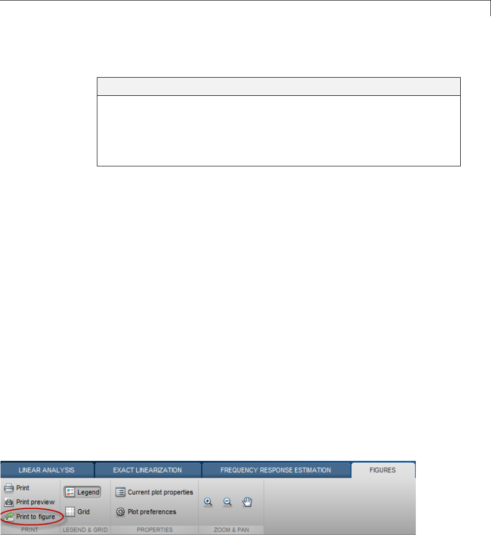
Visualize Models
Visualize Models
In this section...
“Customize Characteristics of Plot in Linear Analysis Tool” on page 2-91
“Print Plot to MATLAB Figure in Linear Analysis Tool” on page 2-91
“Generate Additional Response Plots of Linearized System” on page 2-92
“Add Linear System to Existing Response Plot” on page 2-93
Customize Characteristics of Plot in Linear Analysis
Tool
To change the characteristics of an existing plot, such as the title, axis labels,
or text styles:
1In the Linear Analysis Tool, in the Figures tab, in the select the plot you
want to customize.
2In the Properties section, click Currentplotpropertiesto open the
Property Editor.
3Edit plot properties as desired. Plots are updated as you make changes.
Click Close when you are finished.
Print Plot to MATLAB Figure in Linear Analysis Tool
You can export a plot from the Linear Analysis Tool to a MATLAB figure
window. To do so:
1After creating a plot, in the Figures tab, select the plot you want to export.
2In the Print section, print click Print to Figure.
2-91
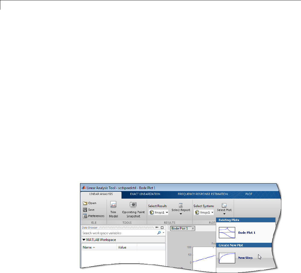
2Linearization
A MATLAB figure window opens containing the plot.
Generate Additional Response Plots of Linearized
System
This example shows how to generate additional response plots of a linearized
system in the Linear Analysis Tool.
1Linearize a model and create a plot of the response, such as shown in
“Linearize at Model Operating Point” on page 2-38.
2In the Linear Analysis Tool, click the Linear Analysis tab.
3In the Select System list, select the system for which you want to create
anewplot.
For example, select linsys1.
4In the Select Plot list, select a plot to add.
For example, select New Step.
This action generates Step Plot 1, which shows the step response for
linsys1.
2-92

Visualize Models
Tip To view both plots at the same time, select a layout on the View tab,
Tiles section.
Add Linear System to Existing Response Plot
There are two ways to add a linear system from the MATLAB Workspace or
the Linear Analysis Workspace to an existing plot in the Linear Analysis Tool.
•Drag the linear system onto the plot from the MATLAB Workspace or the
Linear Analysis Workspace.
•On the Linear Analysis tab, in the Plots section, select the linear system
from the Select System menu. Then select the exiting plot from the
Select Plot menu.
2-93
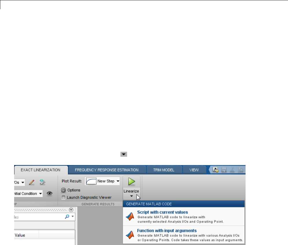
2Linearization
Generate MATLAB Code for Repeated or Batch
Linearization
This topic shows how to generate MATLAB code for linearization from
the Linear Analysis Tool. You can generate either a MATLAB script or
a MATLAB function. Generated MATLAB scripts are useful when you
want to programmatically reproduce a result you obtained interactively. A
generated MATLAB function allows you to perform multiple linearizations
with systematic variations in linearization parameters such as operating
point (batch linearization).
To generate MATLAB code for linearization:
1In the Linear Analysis Tool, on the Exact Linearization tab, interactively
configure the analysis I/Os, operating point, and other parameters for
linearization.
2Click Linearize to open the Generate Matlab Code menu.
3Selectthetypeofcodeyou want to generate:
•Script with current values — Generate a MATLAB script that uses
your configured parameter values. Select this option when you want to
repeatthesamelinearizationattheMATLABcommandline.
•Function with input arguments — Generate a MATLAB function
that takes analysis I/Os and operating points as input arguments. Select
2-94

Generate MATLAB®Code for Repeated or Batch Linearization
this option when you want to perform multiple linearizations using
different parameter values (batch linearization).
To use a generated MATLAB function for batch linearization, you can create a
MATLAB script with a for loop that cycles through values of the parameter
you want to vary. Call the generated MATLAB function in each iteration of
the loop.
2-95

2Linearization
Troubleshooting Linearization
In this section...
“Linearization Troubleshooting Overview” on page 2-96
“Check Operating Point” on page 2-104
“Check Linearization I/O Points Placement” on page 2-104
“Check Loop Opening Placement” on page 2-105
“Check Phase of Frequency Response for Models with Time Delays” on
page 2-105
“Check Individual Block Linearization Values” on page 2-105
“Check Large Models” on page 2-108
“Check Multirate Models” on page 2-109
Linearization Troubleshooting Overview
•“Troubleshooting Checklist” on page 2-96
•“State-Space, Transfer Function, and Zero-Pole-Gain Equations of Linear
Model” on page 2-100
•“Linearization Diagnostics” on page 2-101
•“Highlighting Linearized Blocks” on page 2-103
Troubleshooting Checklist
If you do not get good linearization results, use the Linear Analysis Tool’s
troubleshooting tools. For example, use the Diagnostic Messages tab and
the Linearization Inspector tab that are available in the Diagnostic viewer.
To open the Diagnostic viewer, see “Linearization Diagnostics” on page 2-101.
2-96
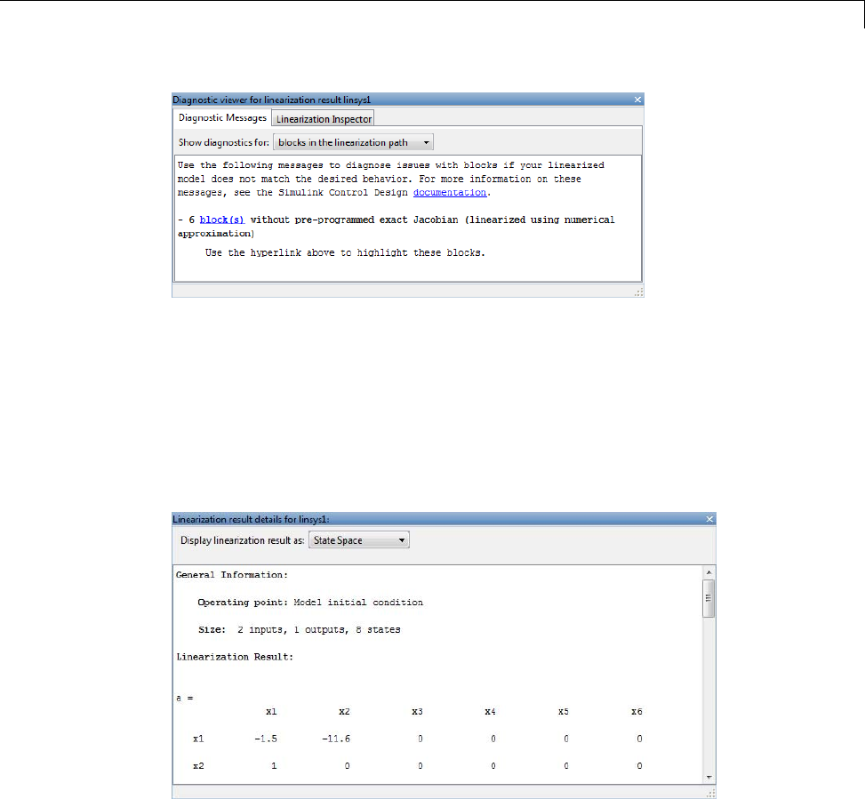
Troubleshooting Linearization
You can also use Linearization result dialog box for troubleshooting. To open
the Linearization result dialog box:
1After linearizing the model, in the Linear Analysis tab of the Linear
Analysis Tool, select the model of interest in the Select Result list.
2In the Select Report list, select Show result details to open the
Linearization result dialog box for the selected model.
2-97

2Linearization
Where to Look Learn More Signs of Successful
Linearization
Signs of
Unsuccessful
Linearization
Linear analysis
plot, generated after
linearization.
Create plots, as
described in “Visualize
Models” on page 2-91.
Time- or
frequency-domain
plot characteristics
(e.g., rise time,
bandwidth) capture
system dynamics.
Response plot
characteristics do not
capture the dynamics
of your system.
For example, Bode
plot gain is too
large or too small, or
pole-zero plot contains
unexpected poles or
zeros.
Linear model
equations in the
Linearization result
details dialog box.
View other
linear model
representations,
as described in
“State-Space, Transfer
Function, and
Zero-Pole-Gain
Equations of Linear
Model” on page 2-100.
State-space matrices
show expected number
of states.
You might see fewer
states in the linear
modelthaninyour
Simulink model
because, in many
cases, the path
between linearization
input and output
points do not reach all
the model states.
Polesandzerosarein
correct location.
Results show only D=
0or D=Inf.
2-98

Troubleshooting Linearization
Where to Look Learn More Signs of Successful
Linearization
Signs of
Unsuccessful
Linearization
Click in the
Exact Linearization
tab.
“Highlighting
Linearized Blocks”
on page 2-103
Highlighted blocks
in the Simulink
model that represent
the portion of the
model you wanted to
linearize.
Missing blocks in
the linearization
path might indicate
incorrect linearization
input or output
point placement,
or that a critical
block unexpectedly
linearizes to zero, or
that critical blocks
are connected in a
path to a block that
linearizes to zero. See
“Check Linearization
I/O Points Placement”
on page 2-104.
Extra blocks in
the linearization
path might indicate
incorrect loop opening
placement. See
“Check Loop Opening
Placement” on page
2-105.
Linearization
diagnostics in
the Diagnostic
Messages tab of
the Diagnostic viewer.
“Linearization
Diagnostics” on page
2-101
Message indicates
that there are no
problematic blocks in
the linearization.
Oneormorewarnings
about specific
problematic blocks.
See “Check Individual
Block Linearization
Values” on page 2-105.
2-99
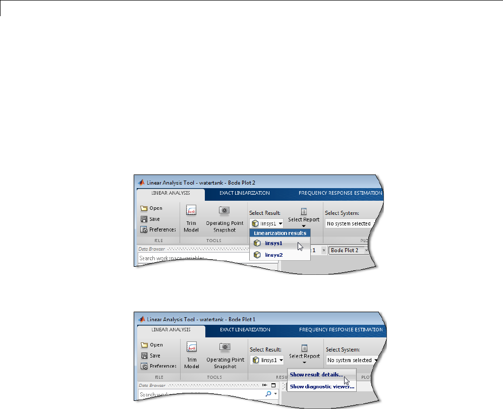
2Linearization
State-Space, Transfer Function, and Zero-Pole-Gain Equations
of Linear Model
You can view the linear model equations in the Linearization result dialog
box of the Linear Analysis Tool.
To open the Linearization result details dialog box:
1After linearizing the model, in the Linear Analysis tab, select the desired
linear model from the Select Result list.
2Select Show result details from the Select Report list.
The Linearization result dialog box opens.
Linear model equations display in state-space form, by default. Alternatively,
youcanviewtheZeroPoleGainorTransferFunctionrepresentationinthe
Display linearization result as list.
2-100
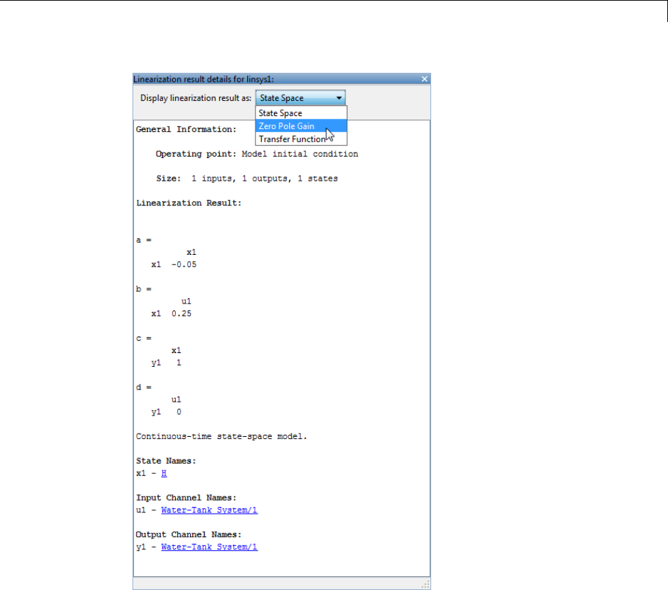
Troubleshooting Linearization
Linearization Diagnostics
You can view diagnostic information about the linearization of specific blocks
in the Diagnostic Messages tab of the Diagnostic viewer of the Linear
Analysis Tool. The Diagnostic Messages tab also suggests corrective
actions.
2-101
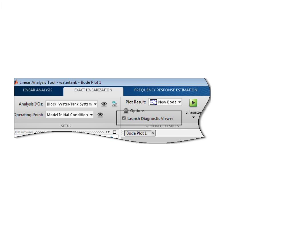
2Linearization
Specifically, the Diagnostic Messages tab flags blocks with configuration
warnings, unsupported blocks, and blocks that automatically linearize using
numerical perturbation.
1In the Linear Analysis Tool, before linearizing the model, select the
Launch Diagnostic Viewer check box in the Exact Linearization tab.
This action ensures that the software logs the diagnostics for the linearized
model.
The Diagnostic Messages dialog for the model will open after you linearize
the model.
Tip You can also open the Diagnostic viewer for a model by choosing the
model intheSelect Result list in the Linear Analysis tab of the Linear
Analysis Tool. Then choose Show diagnostic viewer in the Select
Report list.
2In the Diagnostic Messages dialog box, the Show diagnostics for list
provides the following options:
•all blocks in the Simulink model —Usewhenyoususpectthat
certain blocks are inappropriately excluded from linearization. For
example, blocks that linearize to zero (and shouldn’t) are excluded from
the linearization path.
•blocks in the linearization path — Use when you are sure that all of
the blocks that should be included in the linearization are included. That
2-102
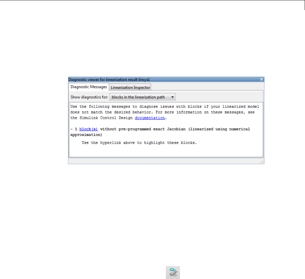
Troubleshooting Linearization
is, your linearization I/O points and any loop openings are set correctly,
and blocks do not inappropriately linearize to zero.
In this example, the model contains one block that is linearized using
numerical perturbation.
3To investigate the flagged block, click the block link to highlight the
corresponding block in the model.
If the linearization results are poor, you can use the Linearization Inspector
to explore linearization values of individual blocks.
Highlighting Linearized Blocks
You can highlight blocks in your model to help you diagnose linearization
issues.
To highlight all of the blocks included in the linearization:
•In the Linear Analysis Tool, click in the Exact Linearization tab.
Blocksthatlinearizetozerodonotappearhighlightedinthemodel. Use
the Simulink Control Design Diagnostic Messages tab to identify the
blocks that cause the linearization of certain blocks to be zero.
To remove highlighting in the model:
•In the Simulink model, select View> Remove Highlighting.
2-103

2Linearization
More About
•“Check Linearization I/O Points Placement” on page 2-104.
•“Check Loop Opening Placement” on page 2-105.
Check Operating Point
To diagnose whether you used the correct operating point for linearization,
simulate the model at the operating point you used for linearization.
The linearization operating point is incorrect when the critical signals in
the model:
•Have unexpected values.
•Are not at steady state.
To fix problem, compute a steady-state operating point and repeat the
linearization at this operating point.
Related Examples
•“Simulate Simulink Model at Specific Operating Point” on page 1-44
•“Steady-State Operating Points (Trimming) from Specifications” on page
1-14
Check Linearization I/O Points Placement
After linearizing the model, highlight which block are included in the
linearization.
Blocks might be missing from the linearization path for different reasons.
Incorrect placement linearization I/O points can result in inappropriately
excluded blocks from linearization. To fix the problem, specify correct
linearization I/O points and repeat the linearization.
Blocks that linearize to zero (and other blocks on the same path) are
excluded from linearization. To fix this problem, troubleshoot linearization
2-104

Troubleshooting Linearization
of individual blocks, as described in “Check Individual Block Linearization
Values” on page 2-105.
More About
•“Highlighting Linearized Blocks” on page 2-103
•“Specifying Subsystem, Loop, or Block to Linearize” on page 2-11
Check Loop Opening Placement
Incorrect loop opening placement causes unwanted feedback signals in the
linearized model.
To fix the problem, use block highlighting to identify which blocks are
included in the linearization. If undesired blocks are included, place the loop
opening on a different signal and repeat the linearization.
More About
•“Highlighting Linearized Blocks” on page 2-103
•“Opening Feedback Loops” on page 2-12
Check Phase of Frequency Response for Models with
Time Delays
When the Bode plot shows insufficient lag in phase for a model containing
time delays, the cause might be Padé approximation of time delays in your
Simulink model.
See “Models with Time Delays” on page 2-122.
Check Individual Block Linearization Values
In the Linear Analysis Tool, check the Diagnostic Messages tab of the
Diagnostic viewer for blocks with configuration warnings, unsupported blocks,
and blocks that automatically linearize using numerical perturbation. Click
the block link to view the highlighted block in the model.
2-105
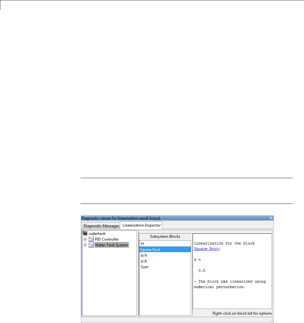
2Linearization
After identifying the blocks flagged in the Diagnostic Messages tab, view
the linearization values of these blocks in the Linearization Inspector
tab of the Diagnostic viewer.
1In the Linear Analysis Tool, select the linear model for which to display
linearization results.
aIn the Linear Analysis tab, use the Select Result list to select the
model.
bIn the Select Report list, select Show diagnostic viewer to open
the Diagnostic viewer dialog box.
cIn the Diagnostic viewer dialog box, click the Linearization Inspector
tab.
2Select the specific subsystem or block.
For example, in the watertank model, select the Water-Tank System
subsystem. Then, in Subsystem Blocks, select the Square Root block.
Tip Right-click anywhere in the Subsystem Blocks list, and select Show
only blocks in linearization path. This action filters the list to include
only the linearized blocks.
2-106
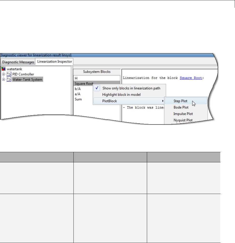
Troubleshooting Linearization
3Plot the response of the linearized block.
For example, right-click the Square Root block under Subsystem
Blocks,andselectPlotBlock > Step Plot.
The step response of the block is displayed.
4Troubleshoot individual blocks.
Block or Subsystem Type Comment Possible Fix
Incompatible with
linearization
Some blocks are implemented
without analytic Jacobians
and do not support numerical
perturbation.
Define custom linearization for
affected block as an expression
or function. See “Controlling
Block Linearization” on page
2-112
Event-based subsystem Linearization of event-based
subsystems is zero because
such subsystems do not trigger
during linearization.
When possible, specify a
custom event-based subsystem
linearization as a lumped
average model or periodic
function call subsystem. See
“Event-Based Subsystems
(Externally Scheduled
Subsystems)” on page 2-127.
2-107

2Linearization
Block or Subsystem Type Comment Possible Fix
Simulink blocks in
Discontinuities library,
such as Deadzone, Saturation,
and Quantizer blocks
The Discontinuities library
blocks typically have poor
linearization results when the
operating point that is close to
the discontinuity.
If you want the linearization to
be a gain of 1, select Treat as
gain when linearizing in the
block parameters dialog box.
Define custom linearization for
affected block as an expression
or function. See “Controlling
Block Linearization” on page
2-112.
Model reference block Linearization is not fully
compatible with model
reference blocks with
Accelerator simulation mode.
Always set each Model (model
reference) block to use Normal
simulation mode, instead of
Accelerator mode.
Blocks that linearize using
numerical perturbation,
instead of using
preprogrammed analytic
Jacobians
Blocks that are located near
discontinuous regions, such
as S-Functions, MATLAB
function blocks, or lookup
tables, are sensitive to
numerical perturbation levels.
If the perturbation level is too
small, the block linearizes to
zero.
Change the numerical
perturbation level of the
block. See “Perturbation Level
of Blocks Perturbed During
Linearization” on page 2-124.
Blocks that have nondouble
precision inputs signals and
states linearize to zero.
Use the Linearization
Inspector tab to view the
block linearization.
Convert nondouble-precision
data types to double precision.
See “Linearizing Blocks with
Nondouble Precision Data
Type Signals” on page 2-125
Check Large Models
Troubleshooting the linearization of large models is easier using a
divide-and-conquer strategy.
Systematically linearize specific model components independently and check
whether that component has the expected linearization.
2-108

Troubleshooting Linearization
Related Examples
“Plant Linearization” on page 2-28
Check Multirate Models
Incorrect sampling time and rate conversion method can cause poor
linearization results in multirate models.
•“Change Sampling Time of Linear Model” on page 2-109
•“Change Linearization Rate Conversion Method” on page 2-110
Change Sampling Time of Linear Model
The sampling time of the linear model displays in the Linearization results
dialog box, below the linear equations.
By default, the software chooses the slowest sample time of the multirate
model. If the default sampling time is not appropriate, specify a different
linearization sample time and repeat.
In Linear Analysis Tool:
1In the Exact Linearization tab, click Options.
The Options for exact linearization dialog box opens.
2In the Linearization tab, enter the desired sample time in the Enter
sample time (sec) box. Press Enter.
-1 specifies that the software linearizes at the slowest sample rate in the
model.
0specifies a continuous-time linear model.
At the command line, specify the SampleTime linearization option.
For example:
opt = linoptions;
opt.SampleTime = 0.01;
2-109

2Linearization
Change Linearization Rate Conversion Method
When you linearize models with multiple sample times, such as a discrete
controller with a continuous plant, a rate conversion algorithm generates a
single-rate linear model. The rate conversion algorithm affects linearization
results.
In the Linear Analysis Tool:
1Select Options in the Exact Linearization tab.
2Click the Linearization tab to select the appropriate rate conversion
method from the Choose rate conversion method list.
Rate Conversion Method When to Use
Zero-Order Hold Use when you need exact
discretization of continuous
dynamics in the time-domain for
staircase inputs.
Tustin Use when you need good
frequency-domain matching
between a continuous-time system
and the corresponding discretized
system, or between an original
system and the resampled system.
Tustin with Prewarping Use when you need good
frequency domain matching at
a particular frequency between the
continuous-time system and the
corresponding discretized system,
orbetweenanoriginalsystemand
the resampled system.
Upsampling when possible
(Zero-Order Hold, Tustin, and
Tustin with Prewarping)
Upsample discrete states when
possibletoensuregainandphase
matching of upsampled dynamics.
You can only upsample when the
newsampletimeisaninteger
multiple of the sampling time of
the original system. Otherwise,
2-110

Troubleshooting Linearization
Rate Conversion Method When to Use
the software uses an alternate rate
conversion method.
At the command line, specify the RateConversionMethod linearization option.
For example:
opt = linoptions;
opt.RateConversionMethod = 'tustin';
See Also
linoptions
Related Examples
Linearization of Multirate Models
Linearization Using Different Rate Conversion Methods
2-111

2Linearization
Controlling Block Linearization
In this section...
“When You Need to Specify Linearization for Individual Blocks” on page
2-112
“Specify Linear System for Block Linearization Using MATLAB Expression”
on page 2-113
“Specify D-Matrix System for Block Linearization Using Function” on
page 2-114
“Augment the Linearization of a Block” on page 2-117
“Models with Time Delays” on page 2-122
“Perturbation Level of Blocks Perturbed During Linearization” on page
2-124
“Linearizing Blocks with Nondouble Precision Data Type Signals” on page
2-125
“Event-Based Subsystems (Externally Scheduled Subsystems)” on page
2-127
When You Need to Specify Linearization for
Individual Blocks
Simulink blocks with sharp discontinuities produce poor linearization results.
Typically, you must specify a custom linearization for such blocks.
When your model operates in a region away from the point of discontinuity,
the linearization is zero. A block with discontinuity linearizing to zero can
cause the linearization of the system to be zero when this block multiplies
other blocks.
For other types of blocks, you can specify the block linearization as a:
•Linear model in the form of a D-matrix
•Control System Toolbox model object
2-112
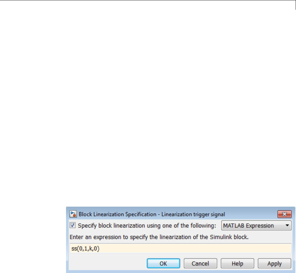
Controlling Block Linearization
•Robust Control Toolbox uncertain state space or uncertain real object
(requires Robust Control Toolbox software)
Specify Linear System for Block Linearization Using
MATLAB Expression
Thisexampleshowshowtospecifythelinearization of any block, subsystem,
or model reference without having to replace this block in your Simulink
model.
1Right-click the block in the model, and select Linear Analysis > Specify
Linearization.
The Block Linearization Specification dialog box opens.
2In the Specify block linearization using a list, select MATLAB
Expression.
3In the text field, enter an expression that specifies the linearization.
For example, specify the linearization as an integrator with a gain of k,
G(s)=k/s.
In state-space form, this transfer function corresponds to ss(0,1,k,0).
Click OK.
4Linearize the model.
2-113
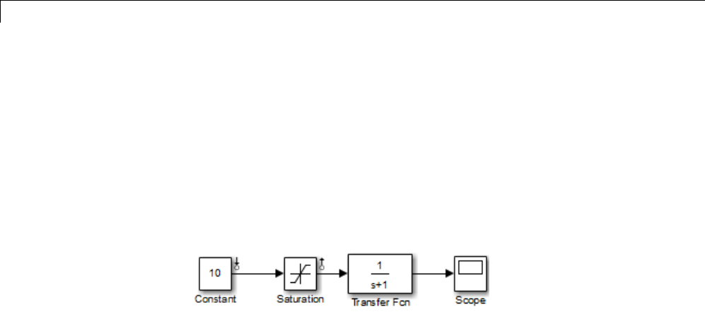
2Linearization
Specify D-Matrix System for Block Linearization
Using Function
This example shows how to specify custom linearization for a saturation block
using a function.
1Open Simulink model.
sys = 'scdConfigBlockFcn';
open_system(sys)
2Linearize the model at the model operating point.
io = getlinio(sys);
linsys = linearize(sys,io)
Thepresenceofthesaturationblockscausesthemodeltolinearizetozero.
d=
Desired Wat
Water-Tank S 0
Static gain.
3Write a function that defines the saturation block linearization.
For example, the next configuration function defines the saturation
block linearization based on the level of the block input signal. Your
configuration function must be on the MATLAB path during linearization.
Linearization Configuration Function
The input to the function, BlockData, is a structure that the software
creates automatically when you configure the linearization of the
Saturation block to use the function.
function blocklin = mySaturationLinearizationFcn(BlockData)
2-114

Controlling Block Linearization
% This function customizes the linearization of a saturation block
% based on the block input signal level, U:
% BLOCKLIN = 0 when |U| > saturation limit
% BLOCKLIN = 1 when |U| < saturation limit
% BLOCKLIN = 1/2 when U = saturation limit
% Get saturation limit.
satlimit = BlockData.Parameters.Value;
% Compute linearization based on the input signal
% level to the block.
if abs(BlockData.Inputs) > satlimit
blocklin = 0;
elseif abs(BlockData.Inputs) < satlimit
blocklin = 1;
else
blocklin = 1/2;
end
4In the Simulink model, right-click the Saturation block, and select Linear
Analysis > Specify Linearization.
The Block Linearization Specification dialog box opens.
5Select the Specify block linearization using one of the following
check box, and choose Configuration Function from the list.
Configure the linearization function:
•Enter the function name. In this example, the function name is
mySaturationLinearizationFcn.
•Specify the function parameters. mySaturationLinearizationFcn
requires the saturation limit value, which the user must specify before
linearization.
Enter the variable name satlimit in Parameter Value.Enterthe
corresponding descriptive name in the Parameter Name column,
SaturationLimit.
•Click OK.
2-115
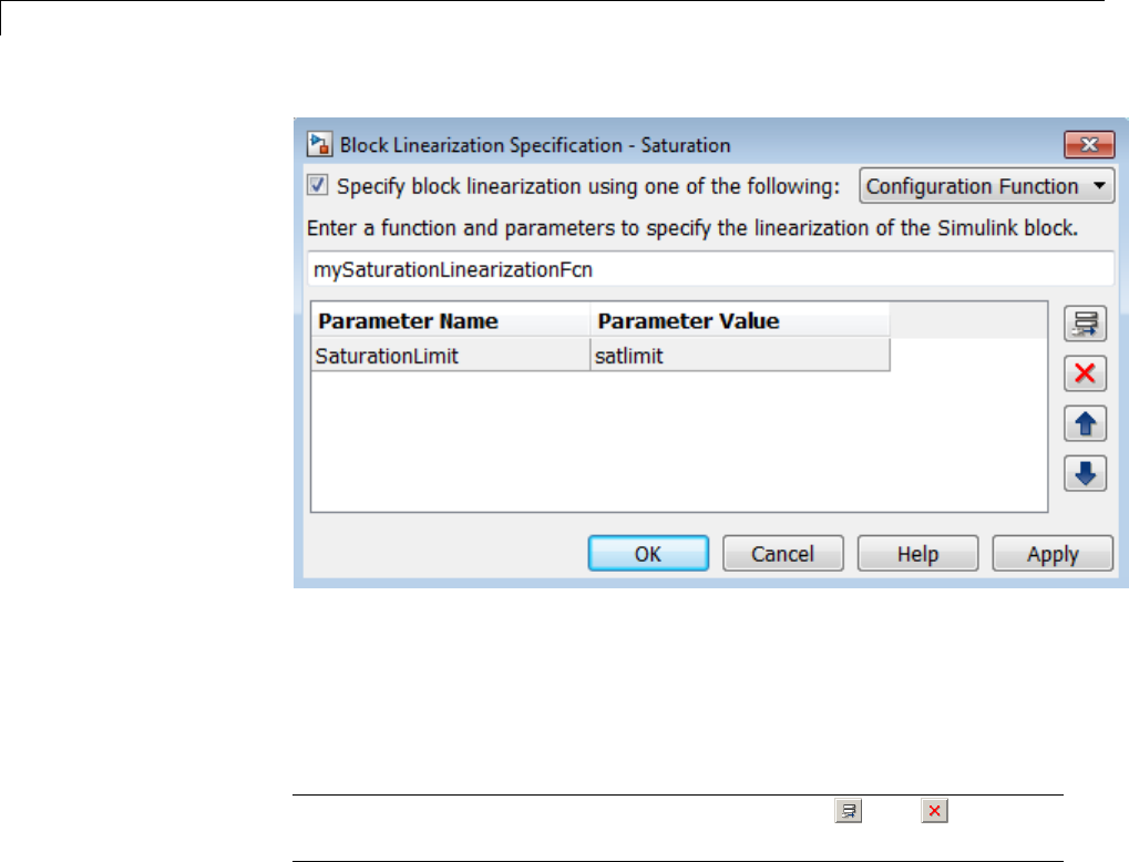
2Linearization
Configuring the Block Linearization Specification dialog box updates
the model to use the specified linearization function for linearizing the
Saturation Block. Specifically, this configuration automatically populates
the Parameters field of the BlockData structure, which is the input
argument to the configuration function.
Note You can add function parameters by clicking .Use to delete
selected parameters.
Code Alternative
This code is equivalent to configuring the Block Linearization Specification
dialog box:
satblk = 'scdConfigBlockFcn/Saturation';
set_param(satblk,'SCDEnableBlockLinearizationSpecification','on');
rep = struct('Specification','mySaturationLinearizationFcn',...
'Type','Function',...
'ParameterNames','SaturationLimit',...
2-116

Controlling Block Linearization
'ParameterValues','satlimit');
set_param(satblk,'SCDBlockLinearizationSpecification',rep);
6Define the saturation limit, which is a parameter required by the
linearization function of the Saturation block.
satlimit = 10;
7Linearize the model using the custom linearization of the Saturation block.
linsys_cust = linearize(sys,io)
The system linearized to:
d=
Desired Wat
Water-Tank S 0.5
Static gain.
Augment the Linearization of a Block
This example shows how to augment the linearization of a block with
additional time delay dynamics, using a block linearization specification
function.
1Open Simulink model.
mdl = 'scdFcnCall';
open_system(mdl)
2-117
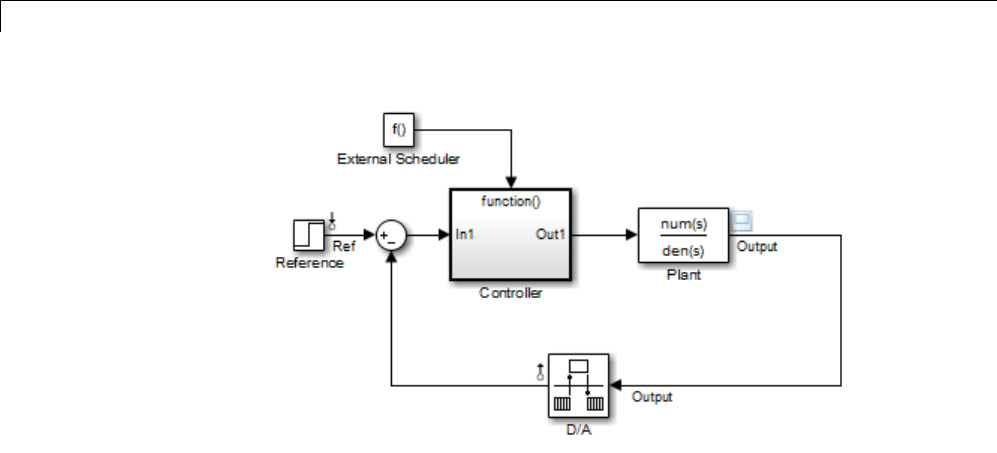
2Linearization
This model includes a continuous time plant, Plant, and a discrete-time
controller, Controller.TheD/A block discretizes the plant output with
asamplingtimeof0.1s. TheExternal Scheduler block triggers the
controller to execute with the same period, 0.1 s. However, the trigger has
an offset of 0.05 s relative to the discretized plant output. For that reason,
the controller does not process a change in the reference signal until 0.05
s after the change occurs. This offset introduces a time delay of 0.05 s
into the model.
2(Optional) Linearize the closed-loop model at the model operating point
without specifying a linearization for the Controller block.
io = getlinio(mdl);
sys_nd = linearize(mdl,io);
The getlinio function returns the linearization input and output points
that are already defined in the model.
3(Optional) Check the linearization result by frequency response estimation.
input = frest.Sinestream(sys_nd);
sysest = frestimate(mdl,io,input);
bode(sys_nd,'g',sysest,'r*',{input.Frequency(1),input.Frequency(end)})
legend('Linearization without delay',...
'Frequency Response Estimation','Location','SouthWest')
2-118

Controlling Block Linearization
The exact linearization does not account for the time delay introduced
by the controller execution offset. A discrepancy results between the
linearized model and the estimated model, especially at higher frequencies.
4Write a function to specify the linearization of the Controller block that
includesthetimedelay.
The following configuration function defines a linear system that equals
the default block linearization multiplied by a time delay. Save this
configuration function to a location on your MATLAB path. (For this
example, the function is already saved as scdAddDelayFcn.m.)
function sys = scdAddDelayFcn(BlockData)
sys = BlockData.BlockLinearization*thiran(0.05,0.1);
2-119

2Linearization
The input to the function, BlockData, is a structure that the
software creates automatically each time it linearizes the block.
When you specify a block linearization configuration function, the
software automatically passes BlockData to the function. The field
BlockData.BlockLinearization contains the current linearization of
the block.
This configuration function approximates the time delay as a thiran
filter. The filter indicates a discrete-time approximation of the fractional
time delay of 0.5 sampling periods. (The 0.05 s delay has a sampling time
of 0.1 s).
5Specify the configuration function scdAddDelayFcn as the linearization
for the Controller block.
aRight-click the Controller block, and select Linear Analysis
> Specify Linearization.
bSelect the Specify block linearization using one of the following
check box. Then, select Configuration Function from the drop-down
list.
cEnter the function name scdAddDelayFcn in the text box.
scdAddDelayFcn has no parameters, so leave the parameter table blank.
dClick OK.
2-120
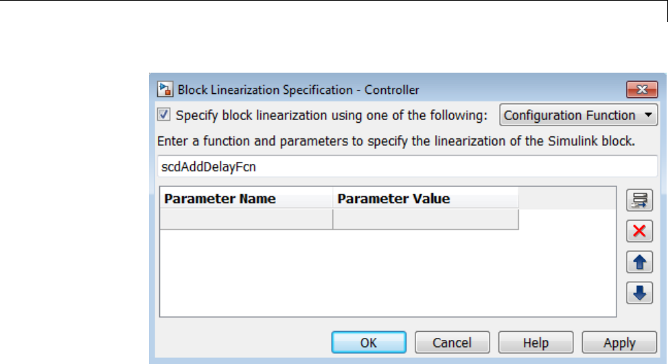
Controlling Block Linearization
6Linearize the model using the specified block linearization.
sys_d = linearize(mdl,io);
The linear model sys_d is a linearization of the closed-loop model that
accountsforthetimedelay.
7(Optional) Compare the linearization that includes the delay with the
estimated frequency response.
bode(sys_d,'b',sys_nd,'g',sysest,'r*',...
{input.Frequency(1),input.Frequency(end)})
legend('Linearization with delay','Linearization without delay',...
'Frequency Response Estimation','Location','SouthWest')
2-121
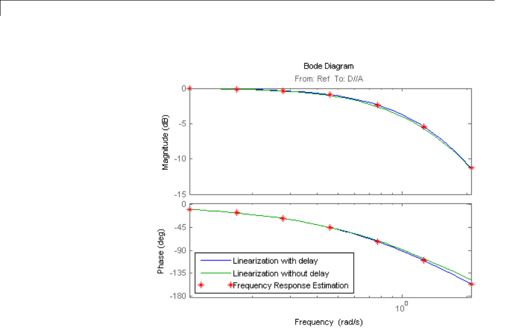
2Linearization
The linear model obtained with the specified block linearization now
accounts for the time delay. This linear model is therefore a much better
match to the real frequency response of the Simulink model.
Models with Time Delays
•“Choosing Approximate Versus Exact Time Delays” on page 2-122
•“Specifying Exact Representation of Time Delays” on page 2-123
Choosing Approximate Versus Exact Time Delays
Simulink Control Design lets you choose whether to linearize models using
exact representation or Pade approximation of continuous time delays. How
you treat time delays during linearization depends on your nonlinear model.
2-122

Controlling Block Linearization
Simulink blocks that model time delays are:
•Transport Delay block
•Variable Time Delay block
•Variable Transport Delay block
•Delay block
•Unit Delay block
By default, linearization uses Pade approximation for representing time
delays in your linear model.
Use Pade approximation to represent time delays when:
•Applying more advanced control design techniques to your linear plant,
such as LQR or H-infinity control design.
•Minimizing the time to compute a linear model.
Specify to linearize with exact time delays for:
•Minimizing errors that result from approximating time delays
•PID tuning or loop-shaping control design methods in Simulink Control
Design
•Discrete-time models (to avoid introducing additional states to the model)
The software treats discrete-time delays as internal delays in the linearized
model. Such delays do not appear as additional states in the linearized
model.
Specifying Exact Representation of Time Delays
Before linearizing your model:
•In the Linear Analysis Tool:
1In the Exact Linearization tab, click Options .
This action opens the Options for exact linearization dialog box.
2-123

2Linearization
2In the Linearization tab, select the Return linear model with exact
delay(s) check box.
•At the command line:
Use linoptions to specify the UseExactDelayModel option.
Related Examples
Linearizing Models with Delays
More About
•“Models with Time Delays” in the Control System Toolbox documentation
•“Time-Delay Approximation” in the Control System Toolbox documentation
Perturbation Level of Blocks Perturbed During
Linearization
Blocks that do not have preprogrammed analytic Jacobians linearize using
numerical perturbation.
•“Change Block Perturbation Level” on page 2-124
•“Perturbation Levels of Integer Valued Blocks” on page 2-125
Change Block Perturbation Level
This example shows how to change the perturbation level to the Magnetic
Ball Plant block in the magball model. Changing the perturbations level
changes the linearization results.
The default perturbation size is 10-5(1+|x|), where xis the operating point
value of the perturbed state or the input.
Open the model before changing the perturbation level.
To change the perturbation level of the states to 10 1
7−+
()
x,wherexis
the state value, type:
blockname='magball/Magnetic Ball Plant'
2-124

Controlling Block Linearization
set_param(blockname,'StatePerturbationForJacobian','1e-7')
To change the perturbation level of the input to 10 1
7−+
()
x,wherexis the
input signal value:
1Open the system and get the block port handles.
sys = 'magball';
open_system(sys);
blockname = 'magball/Magnetic Ball Plant';
ph = get_param(blockname,'PortHandles')
2Get the handle to the inport value.
p_in = ph.Inport(1)
3Set the inport perturbation level.
set_param(p_in,'PerturbationForJacobian','1e-7')
Perturbation Levels of Integer Valued Blocks
A custom block that requires integer input ports for indexing might have
linearization issues when this block:
•Does not support small perturbations in the input value
•Accepts double-precision inputs
To fix the problem, try setting the perturbation level of such a block to zero
(which sets the block linearization to a gain of 1).
Linearizing Blocks with Nondouble Precision Data
Type Signals
You can linearize blocks that have nondouble precision data type signals as
either inputs or outputs, and have no preprogrammed exact linearization.
Without additional configuration, such blocks automatically linearize to zero.
For example, logical operator blocks have Boolean outputs and linearize to 0.
2-125

2Linearization
Linearizing blocks that have nondouble precision data type signals requires
converting all signals to double precision. This approach only works when
your model can run correctly in full double precision.
When you have only a few blocks impacted by the nondouble precision data
types, use a Data Type Conversion block to fix this issue.
When you have many nondouble precision signals, you can override all data
types with double precision using the Fixed Point Tool.
•“Overriding Data Types Using Data Type Conversion Block” on page 2-126
•“Overriding Data Types Using Fixed Point Tool” on page 2-127
Overriding Data Types Using Data Type Conversion Block
Convert individual signals to double precision before linearizing the model by
inserting a Data Type Conversion block. This approach works well for model
that have only a few affected blocks.
After linearizing the model, remove the Data Type Conversion block from
your model.
Note Overriding nondouble data types is not appropriate when the model
relies on these data types, such as relying on integer data types to perform
truncation from floats.
Forexample,considerthemodelconfigured to linearize the Square block at
an operating point where the input is 1. The resulting linearized model should
be 2, but the input to the Square block is Boolean. This signal of nondouble
precision date type results in linearization of zero.
In this case, inserting a Data Type Conversion block converts the input signal
to the Square block to double precision.
2-126
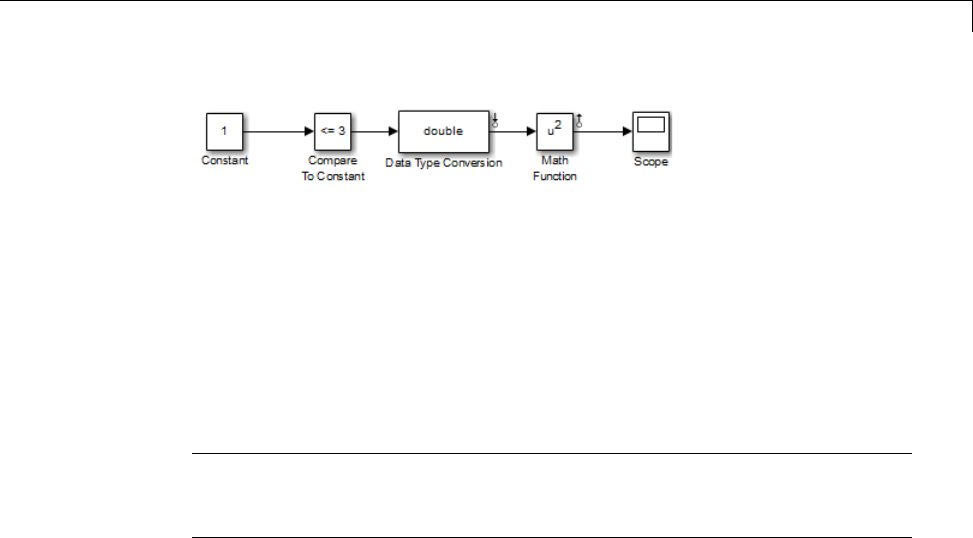
Controlling Block Linearization
Overriding Data Types Using Fixed Point Tool
When you linearize a model that contains nondouble data types but still
runs correctly in full double precision, you can override all data types with
doubles using the Fixed Point Tool. Use this approach when you have many
nondouble precision signals.
After linearizing the model, restore your original settings.
Note Overriding nondouble data types is not appropriate when the model
relies on these data types, such as relying on integer data types to perform
truncationfromfloats.
1In the Simulink model, select Analysis > Fixed Point Tool.
The Fixed Point Tool opens.
2In the Data type override menu, select Double.
This setting uses double precision values for all signals during linearization.
3Restore settings when linearization completes.
Event-Based Subsystems (Externally Scheduled
Subsystems)
•“Linearizing Event-Based Subsystems” on page 2-128
•“Approaches for Linearizing Event-Based Subsystems” on page 2-128
•“Periodic Function Call Subsystems for Modeling Event-Based Subsystems”
on page 2-129
•“Approximating Event-Based Subsystems Using Curve Fitting
(Lump-Average Model)” on page 2-132
2-127

2Linearization
Linearizing Event-Based Subsystems
Event-based subsystems (triggered subsystems) and other event-based models
require special handling during linearization.
Executing a triggered subsystem depends on previous signal events, such as
zero crossings. However, because linearization occurs at a specific moment in
time, the trigger event never happens.
An example of an event-based subsystem is an internal combustion (IC)
engine.Whenanenginepistonapproachesthetopofacompressionstroke,a
spark causes combustion. The timing of the spark for combustion is dependent
on the speed and the position of the engine crankshaft.
In the scdspeed model, triggered subsystems generate events when the
pistons reach both the top and bottom of the compression stroke. Linearization
in the presence of such triggered subsystems is not meaningful.
Approaches for Linearizing Event-Based Subsystems
You can obtain a meaningful linearization of triggered subsystems, while still
preserving the simulation behavior, by recasting the event-based dynamics as
one of the following:
•Lumped average model that approximates the event-based behavior over
time.
•Periodic function call subsystem, with Normal simulation mode.
Inthecaseofperiodicalfunctioncallsubsystems, the subsystem linearizes
to the sampling at which the subsystem is periodically executed.
In many control applications, the controller is implemented as a discrete
controller, but the execution of the controller is driven by an external
scheduler. You can use such linearized plant models when the controller
subsystem is marked as a Periodic Function call subsystem.
If recasting event-based dynamics does not produce good linearization results,
try frequency response estimation. See “Estimate Frequency Response Using
Linear Analysis Tool” on page 3-28.
2-128

Controlling Block Linearization
Periodic Function Call Subsystems for Modeling Event-Based
Subsystems
This example shows how to use periodic function call subsystems to
approximate event-based dynamics for linearization.
1Open Simulink model.
sys = 'scdPeriodicFcnCall';
open_system(sys)
2Linearize model at the model operating point.
io = getlinio(sys);
linsys = linearize(sys,io)
The linearization is zero because the subsystem is not a periodic function
call.
d=
Desired Wat
Water-Tank S 0
Static gain.
Now, specify the Externally Scheduled Controller block as a Periodic
Function Call Subsystem.
3Double-click the Externally Scheduled Controller (Function-Call
Subsystem) block.
Double-click the function block to open the Block Parameters dialog box.
2-129
2Linearization
4Set Sample time type to be periodic.
Leave the Sample time valueas0.01,whichrepresentsthesampletime
of the function call.
5Linearize the model.
linsys2 = linearize(sys,io)
a=
HIn
tegrator
H0.
9956 0.002499
Integrator -0.0007774 1
2-130
Controlling Block Linearization
b=
Desired Wat
H 0.003886
Integrator 0.0007774
c=
H Integrator
Water-Tank S 1 0
d=
Desired Wat
Water-Tank S 0
Sampling time: 0.01
Discrete-time model.
6Plot step response.
step(linsys2)
2-131
2Linearization
7Close the model.
bdclose(sys);
Approximating Event-Based Subsystems Using Curve Fitting
(Lump-Average Model)
This example shows how to use curve fitting to approximate event-based
dynamics of an engine.
The scdspeed model linearizes to zero because scdspeed/Throttle &
Manifold/Intake Manifold is an event-triggered subsystem.
You can approximate the event-based dynamics of the scdspeed/Throttle
& Manifold/Intake Manifold subsystem by adding the Convert to mass
charge block inside the subsystem.
The Convert to mass charge block approximates the relationship between Air
Charge, Manifold Pressure, and Engine Speed as a quadratic polynomial.
2-132

Controlling Block Linearization
Air Charge p Engine Speed p Manifold Pressure p =× +× +×
12 3
(MManifold Pressure
p Manifold Pressure Engine Speed
)2
4
+× × + pp5
If measured data for internal signals is not available, use simulation data
from the original model to compute the unknown parameters p1,p2,p3,p4,and
p5using a least squares fitting technique.
When you have measured data for internal signals, you can use the Simulink
Design Optimization™ software to compute the unknown parameters. See
Engine Speed Model Parameter Estimation to learn more about computing
model parameters, linearizing this approximated model, and designing a
feedback controlled for the linear model.
The next figure compares the simulations of the original event-based model
and the approximated model. Each of the pulses corresponds to a step change
in the engine speed. The size of the step change is between 1500 and 5500.
Thus, you can use the approximated model to accurately simulate and
linearize the engine between 1500 RPM and 5500 RPM.
2-133
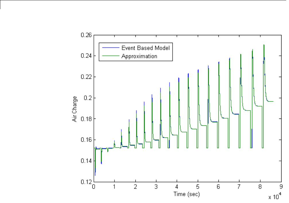
2Linearization
2-134
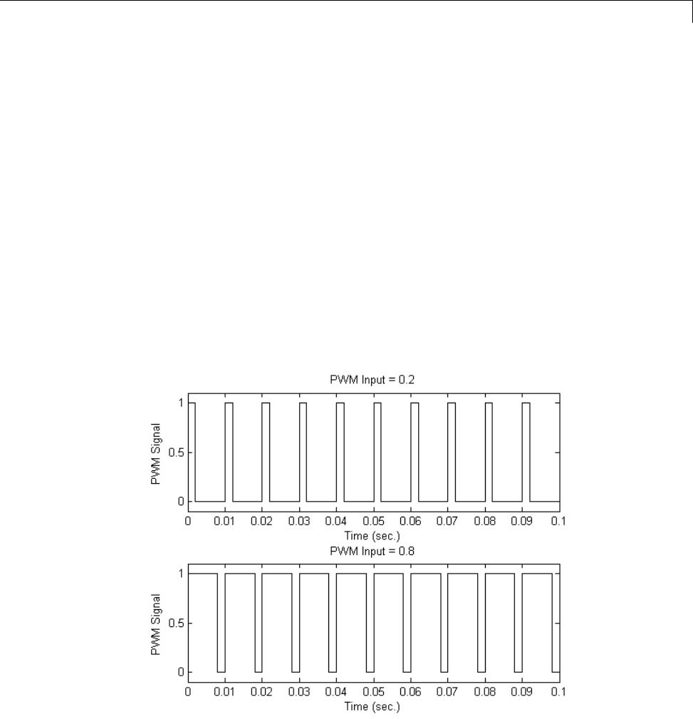
Models with Pulse Width Modulation (PWM) Signals
Models with Pulse Width Modulation (PWM) Signals
This example shows how to configure models that use Pulse Width Modulation
(PWM) input signals for linearization. For linearization, specify a custom
linearization of the subsystem that takes the DC signal to be a gain of 1.
Many industrial applications use Pulse Width Modulation (PWM) signals
because such signals are robust in the presence of noise.
ThenextfigureshowstwoPWMsignals.Inthetopplot,aPWMsignalwitha
20% duty cycle represents a 0.2 V DC signal. A 20% duty cycle corresponding
to 1 V signal for 20% of the cycle, followed by a value of 0 V signal for 80% of
the cycle. The average signal value is 0.2 V.
In the bottom plot, a PWM signal with an 80% duty cycle represent a 0.8
VDCsignal.
2-135
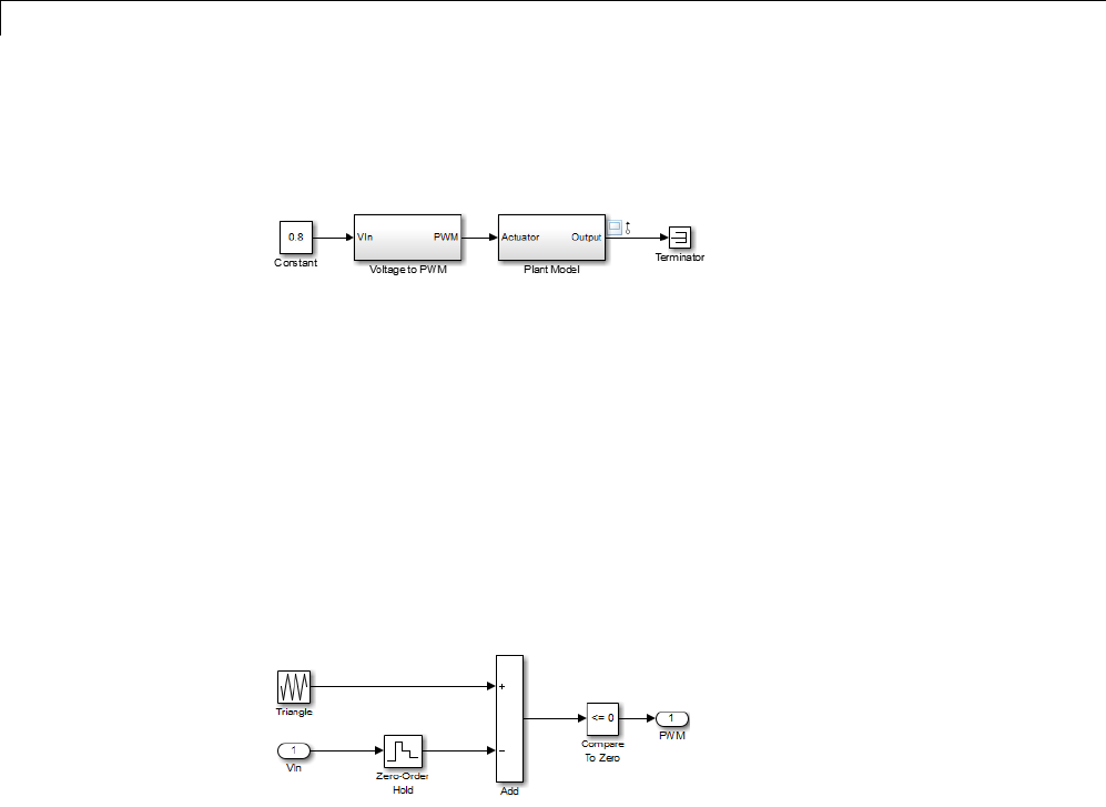
2Linearization
For example, in the scdpwm model, a PWM signal is converted to a constant
signal.
When linearizing a model containing PWM signals there are two effects of
linearization you should consider:
•The signal level at the operating point is one of the discrete values within
the PWM signal, not the DC signal value. For example, in the model above,
the signal level is either 0 or 1, not 0.8. This change in operating point
affects the linearized model.
•The creation of the PWM signal within the subsystem Voltage to PWM,
showninth
e next figure, uses the Compare to Zero block. Such comparator
blocks do not linearize well due to their discontinuities and the nondouble
outputs.
Related Examples
Specifying Custom Linearizations for Simulink Blocks
2-136
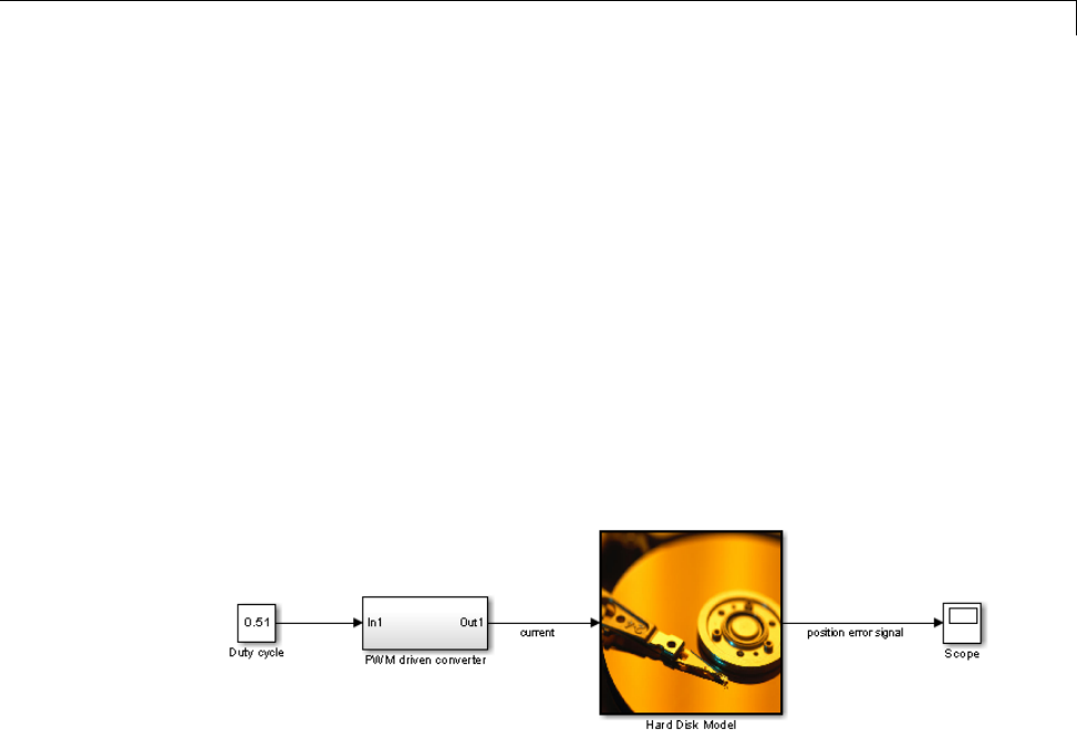
Specifying Linearization for Model Components Using System Identification
Specifying Linearization for Model Components Using
System Identification
This example shows how to use System Identification Toolbox to identify a
linear system for a model component that does not linearize well and use the
identified system to specify its linearization. Note that running this example
requires SimPowerSystems in addition to System Identification Toolbox.
Linearizing Hard Drive Model
Open the simulink model for the hard drive.
model = 'scdpwmharddrive';
open_system(model);
In this model, the hard drive plant is driven by a current source. The current
source is implemented by a circuit that is driven by a Pulse Width Modulation
(PWM) signal so that its output can be adjusted by the duty cycle. For
detailsoftheharddrivemodel,seetheexample"DigitalServoControlofa
Hard-Disk Drive" in Control System Toolbox™ examples.
PWM-driven circuits usually have high frequency switching components,
such as the MOSFET transistor in this model, whose average behavior is not
well defined. Thus, exact linearization of this type of circuits is problematic.
When you linearize the model from duty cycle input to the position error,
the result is zero.
io(1) = linio('scdpwmharddrive/Duty cycle',1,'in');
io(2) = linio('scdpwmharddrive/Hard Disk Model',1,'out');
sys = linearize(model,io)
2-137

2Linearization
sys =
d=
Duty cycle
position err 0
Static gain.
Finding a Linear Model for PWM Component
You can use frequency response estimation to obtain the frequency response
of the PWM-driven current source and use the result to identify a linear
model for it. The current signal has a discrete sample time of 1e-7. Thus, you
need to use a fixed sample time sinestream signal. Create a signal that has
frequencies between 2K and 200K rad/s.
idinput = frest.createFixedTsSinestream(Ts,{2000,200000});
idinput.Amplitude = 0.1;
You can then define the input and output points for PWM-driven circuit and
run the frequency response estimation with the sinestream signal.
pwm_io(1) = linio('scdpwmharddrive/Duty cycle',1,'in');
pwm_io(2) = linio('scdpwmharddrive/PWM driven converter',1,'out','on');
sysfrd = frestimate(model,pwm_io,idinput);
Using the N4SID command from System Identification Toolbox, you can
identify a second-order model using the frequency response data. Then,
compare the identified model to the original frequency response data.
sysid = ss(tfest(idfrd(sysfrd),2));
bode(sysid,sysfrd,'r*');
2-138
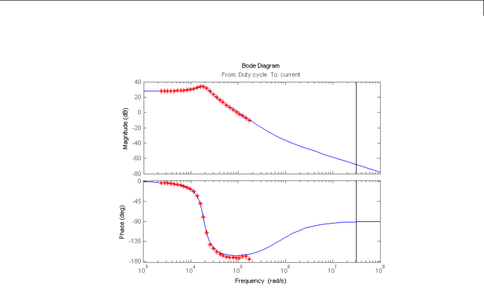
Specifying Linearization for Model Components Using System Identification
We used frequency response data with frequencies between 2K and 200K
rad/s. The identified model has a flat magnitude response for frequencies
smaller than 2K. However, our estimation did not have include for those
frequencies. Assume that you would like to make sure the response is flat by
checking the frequency response for 20 and 200 rad/s. To do so, create another
input signal with those frequencies in it.
lowfreq = [20 200];
inputlow = frest.createFixedTsSinestream(Ts,lowfreq)
The sinestream input signal:
Frequency : [20 200] (rad/s)
Amplitude : 1e-05
SamplesPerPeriod : [3141593 314159]
NumPeriods : 4
RampPeriods : 0
FreqUnits (rad/s,Hz): rad/s
2-139

2Linearization
SettlingPeriods : 1
ApplyFilteringInFRESTIMATE (on/off) : on
SimulationOrder (Sequential/OneAtATime): Sequential
Intheinputsignalparameters,wecanseethathavingaveryfastsample
rate of 1e-7 seconds (10 MHz sampling frequency) for the frequencies 20 and
200 rad/s cause high SamplesPerPeriod values of 3141593 and 314159.
Considering that each frequency has 4 periods, frequency response estimation
would log output data with around 14 millions samples. This would require a
lot of memory and it is quite likely that you might run into memory issues
running the estimation.
Obviously, you do not need such a high sampling rate for analyzing 20 and
200 rad/s frequencies. You can use a smaller sampling rate to avoid memory
issues:
Tslow = 1e-4;
wslow = 2*pi/Tslow;
inputlow = frest.createFixedTsSinestream(Tslow,wslow./round(wslow./lowfreq)
inputlow.Amplitude = 0.1;
To make the model compatible with the smaller sampling rate, resample the
output data point using a rate transition block as in the modified model:
modellow = 'scdpwmharddrive_lowfreq';
open_system(modellow);
2-140
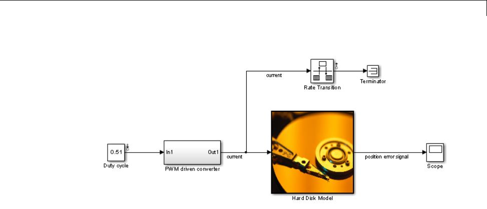
Specifying Linearization for Model Components Using System Identification
You can now run the analysis for the low frequencies and compare it against
identification result.
load scdpwmharddrive_lowfreqresults.mat
% sysfrdlow = frestimate(modellow,getlinio(modellow),inputlow);
bode(sysid,sysfrdlow,'r*');
bdclose(modellow);
2-141
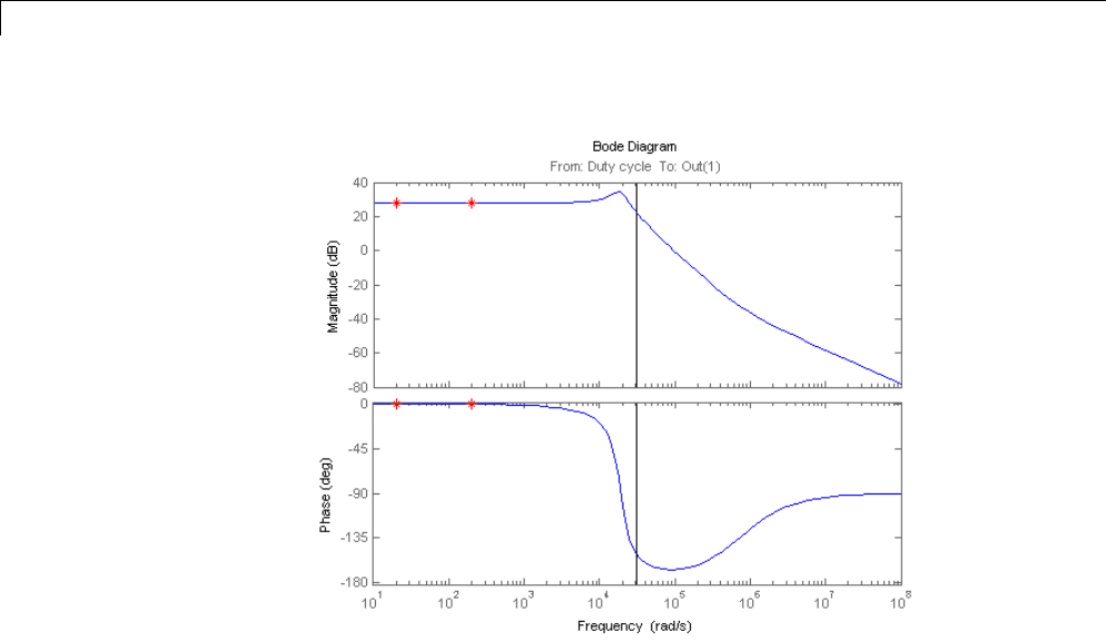
2Linearization
Specifying the Linearization for PWM Component
As you verified using the frequency response estimation, the low-frequency
dynamics of the PWM-driven component are captured well by the identified
system. Now you can make linearization use this system as the linearization
of the PWM-driven component. To do so, specify block linearization of that
subsystem as follows:
pwmblock = 'scdpwmharddrive/PWM driven converter';
set_param(pwmblock,'SCDEnableBlockLinearizationSpecification','on');
rep = struct('Specification','sysid',...
'Type','Expression',...
'ParameterNames','',...
'ParameterValues','');
set_param(pwmblock,'SCDBlockLinearizationSpecification',rep);
set_param('scdpwmharddrive/Duty cycle','SampleTime','Ts_plant');
Linearizing the model after specifying the linearization of the PWM
component gives us a non-zero result:
2-142
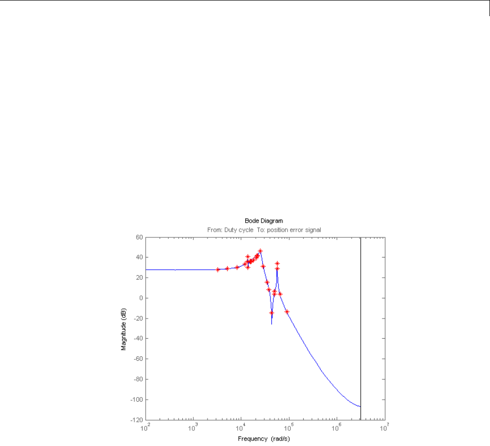
Specifying Linearization for Model Components Using System Identification
sys = linearize(model,io);
You might still like to validate this linearization result using frequency
response estimation. Doing this as below verifies that our linearization result
is quite accurate and all the resonances exist in the actual dynamics of the
model.
valinput = frest.Sinestream(sys);
valinput = fselect(valinput,3e3,1e5);
valinput.Amplitude = 0.1;
sysval = frestimate(model,io,valinput);
bodemag(sys,sysval,'r*');
Close the model:
bdclose('scdpwmharddrive');
2-143

2Linearization
Speeding Up Linearization of Complex Models
In this section...
“Factors That Impact Linearization Performance” on page 2-144
“Blocks with Complex Initialization Functions” on page 2-144
“Disabling the Linearization Inspector in the Linear Analysis Tool” on
page 2-144
“Batch Linearization of Large Simulink Models” on page 2-145
Factors That Impact Linearization Performance
Large Simulink models and blocks with complex initialization functions can
slow linearization.
In most cases, the time it takes to linearize a model is directly related to the
time it takes to update the block diagram.
Blocks with Complex Initialization Functions
Use the MATLAB Profiler to identify complex bottlenecks in block
initialization functions.
In the MATLAB Profiler, run the command:
set_param(modelname,'SimulationCommand','update')
Disabling the Linearization Inspector in the Linear
Analysis Tool
You can speed up the linearization of large models by disabling the
Linearization Diagnostics Viewer in the Linear Analysis Tool.
The Linearization Diagnostic Viewer stores and tracks linearization values of
individual blocks, which can impact linearization performance.
In the Linear Analysis Tool, in the Exact Linearization tab, clear the
Launch Diagnostic Viewer check box.
2-144

Speeding Up Linearization of Complex Models
Tip Alternatively, you can disable the Linearization Diagnostic Viewer
globally in the Simulink Control Design tab of the MATLAB preferences
dialog box. Clear the Launch diagnostic viewer for exact linearizations
in the linear analysis tool check box. This global preference persists from
session to session until you change this preference.
Batch Linearization of Large Simulink Models
When batch linearizing a large model that contains only a few varying
parameters, you can use linlftfold to reduce the computational load.
See Computing Multiple Linearizations of Models with Block Variations
More Efficiently.
2-145

2Linearization
Exact Linearization Algorithm
In this section...
“Continuous-Time Models” on page 2-146
“Multirate Models” on page 2-147
“Perturbation of Individual Blocks” on page 2-148
“User-Defined Blocks” on page 2-150
“Look Up Tables” on page 2-151
Continuous-Time Models
Simulink Control Design lets you linearize continuous-time nonlinear
systems. The resulting linearized model is in state-space form.
In continuous time, the state space equations of a nonlinear system are:
xt f xt ut t
yt g xt ut t
() (), (),
() (), (),
=
()
=
()
where x(t) are the system states, u(t) are the input signals, and y(t)arethe
output signals.
To describe the linearized model, define a new set of variables of the states,
inputs, and outputs centered about the operating point:
δ
δ
δ
xt xt x
ut ut u
yt yt y
() ()
() ()
() ()
=−
=−
=−
0
0
0
The output of the system at the operating point is y(t0)=g(x0,u0,t0)=y0.
The linearized state-space equations in terms of δx(t), δu(t), and δy(t)are:
2-146

Exact Linearization Algorithm
δδδ
δδδ
xt A xt B ut
yt C xt D ut
() () ()
() () ()
=+
=+
where A,B,C,andDare constant coefficient matrices. These matrices are
the Jacobians of the system, evaluated at the operating point:
Af
xBf
u
Cg
xDg
u
txu txu
txu txu
=∂
∂=∂
∂
=∂
∂=∂
∂
000 000
000 000
,, ,,
,, ,,
This linear time-invariant approximation to the nonlinear system is valid in
a region around the operating point at t=t0,x(t0)=x0,andu(t0)=u0.Inother
words, if the values of the system states, x(t), and inputs, u(t), are close
enough to the operating point, the system behaves approximately linearly.
The transfer function of the linearized model is the ratio of the Laplace
transform of δy(t) and the Laplace transform of δu(t):
Ps Ys
Us
lin () ()
()
=δ
δ
Multirate Models
Simulink Control Design lets you linearize multirate nonlinear systems. The
resulting linearized model is in state-space form.
Multirate models include states with different sampling rates. In multirate
models, the state variables change values at different times and with different
frequencies. Some of the variables might change continuously.
The general state-space equations of a nonlinear, multirate system are:
2-147

2Linearization
xt f xt x k x k ut t
xk f xt x k
mm
()
=
() ( )
()
()
()
+=
() ( )
,,, ,,
() ,
11
11 1 1 1
1,,, , ,
() , ,, ,,
xk utt
xk fxtxk x k ut
mm
mm i m m
()
()
()
+=
() ( )
()
()
111 tt
yt gxt x k x k ut t
mm
()
()
=
() ( )
()
()
()
,,, ,,
11
where k1,..., kmare integer values and tk1,..., tkmare discrete times.
The linearized equations that approximate this nonlinear system as a
single-rate discrete model are:
δδδ
δδδ
xAxBu
yCxDu
kkk
kkk
+≈+
≈+
1
The rate of the linearized model is typically the least common multiple of the
sample times, which is usually the slowest sample time.
For more information, see Linearization of Multirate Models .
Perturbation of Individual Blocks
Simulink Control Design linearizes blocks that do not have preprogrammed
linearization using numerical perturbation. The software computes block
linearization by numerically perturbing the states and inputs of the block
about the operating point of the block.
The block perturbation algorithm introduces a small perturbation to the
nonlinear block and measures the response to this perturbation. The default
difference between the perturbed value and the operating point value is
10 1
5−+
()
x,wherexis the operating point value. The software uses this
perturbation and the resulting responsetocomputethelinearstate-space
of this block.
In general, a continuous-time nonlinear Simulink block in state-space form
is given by:
2-148

Exact Linearization Algorithm
xt f xt ut t
yt g xt ut t
() (), (),
() (), (), .
In these equations, x(t) represents the states of the block, u(t) represents the
inputs of the block, and y(t) represents the outputs of the block.
A linearized model of this system is valid in a small region around the
operating point t=t0,x(t0)=x0,u(t0)=u0,andy(t0)=g(x0,u0,t0)=y0.
To describe the linearized block, define a new set of variables of the states,
inputs, and outputs centered about the operating point:
δ
δ
δ
xt xt x
ut ut u
yt yt y
() ()
() ()
() ()
=−
=−
=−
0
0
0
The linearized state-space equations in terms of these new variables are:
δδδ
δδδ
xt A xt B ut
yt C xt D ut
() () ()
() () ()
=+
=+
A linear time-invariant approximation to the nonlinear system is valid in a
region around the operating point.
The state-space matrices A,B,C,andDof this linearized model represent
the Jacobians of the block.
To compute the state-space matrices during linearization, the software
performs these operations:
1Perturbs the states and inputs, one at a time, and measures the response of
the system to this perturbation by computing δ
xand δy.
2Computes the state-space matrices using the perturbation and the
response.
2-149

2Linearization
Ai
xx
xx Bi
xx
uu
Ci
y
xo
pi o
uo
pi o
x
pi pi
(:, ) , (:, )
(:, )
,,
,,
=−
−=−
−
=
ppi pi
y
xx Di
yy
uu
o
pi o
uo
pi o
,,
,,
,(:,)
−
−=−
−
where
•xp,i is the state vector whose ith component is perturbed from the operating
point value.
•xois the state vector at the operating point.
•up,i is the input vector whose ith component is perturbed from the operating
point value.
•uois the input vector at the operating point.
•
xxpi,
is the value of
xat xp,i,uo.
•
xupi,
is the value of
xat up,i,xo.
•
xois the value of
xat the operating point.
•yxpi,
is the value of yat xp,i,uo.
•yupi,
is the value of yat up,i,xo.
•yois the value of yat the operating point.
User-Defined Blocks
All user defined blocks such as S-Function and MATLAB Function blocks, are
compatible with linearization. These blocks are linearized using numerical
perturbation.
User-defined blocks do not linearize when these blocks use nondouble
precision data types.
2-150


2Linearization
2-152

3
Frequency Response
Estimation
•“Frequency Response Model Applications” on page 3-3
•“What Is a Frequency Response Model?” on page 3-4
•“Model Requirements” on page 3-6
•“Estimation Requires Input and Output Signals” on page 3-7
•“Creating Input Signals for Estimation” on page 3-9
•“Modifying Input Signals for Estimation” on page 3-24
•“Estimate Frequency Response Using Linear Analysis Tool” on page 3-28
•“Estimate Frequency Response with Linearization-Based Input Using
Linear Analysis Tool” on page 3-32
•“Estimate Frequency Response (MATLAB Code)” on page 3-37
•“Analyzing Estimated Frequency Response” on page 3-40
•“Troubleshooting Frequency Response Estimation” on page 3-49
•“Effects of Time-Varying Source Blocks on Frequency Response Estimation”
on page 3-62
•“Effects of Noise on Frequency Response Estimation” on page 3-72
•“Estimating Frequency Response Models with Noise Using Signal
Processing Toolbox” on page 3-74
•“Estimating Frequency Response Models with Noise Using System
Identification Toolbox” on page 3-76


Frequency Response Model Applications
Frequency Response Model Applications
You can estimate the frequency response of a Simulink model as a frequency
response model (frd object), without modifying your Simulink model.
Applications of frequency response models include:
•Validating exact linearization results.
Frequency response estimation uses a different algorithm to compute a
linear model approximation and serves as an independent test of exact
linearization. See “Frequency-Domain Validation of Linearization” on page
2-85.
•Analyzing linear model dynamics.
Designing controller for the plant represented by the estimated frequency
response using Control System Toolbox software.
•Estimating parametric models.
See “Estimating Frequency Response Models with Noise Using System
Identification Toolbox” on page 3-76.
3-3
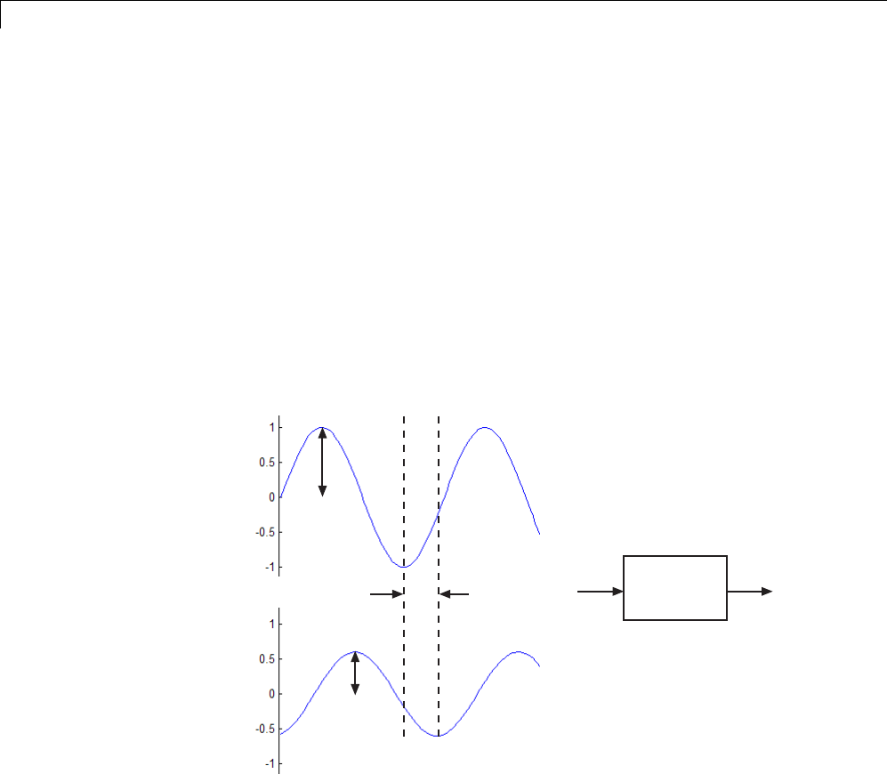
3Frequency Response Estimation
What Is a Frequency Response Model?
Frequency response describes the steady-state response of a system to
sinusoidal inputs.
For a linear system, a sinusoidal input of frequency ω:
ut A t
u
() sin=
results in an output that is also a sinusoid with the same frequency, but with
a different amplitude and phase θ:
yt A t
y
() sin( )=+
q
A
A
u
y
u(t)
y(t)
G(s)
u(t) y(t)
Linear System
3-4

What Is a Frequency Response Model?
Frequency response G(s) for a stable system describes the amplitude change
and phase shift as a function of frequency:
Gs Ys
Us
Gs G j A
A
Yj
Xj
y
u
() ()
()
() ( )
()
()tan
=
==
=∠ = −
1imaginary paart of
real part of
Gj
Gj
()
()
⎛
⎝
⎜⎞
⎠
⎟
where Y(s)andU(s) are the Laplace transforms of y(t)andu(t), respectively.
3-5
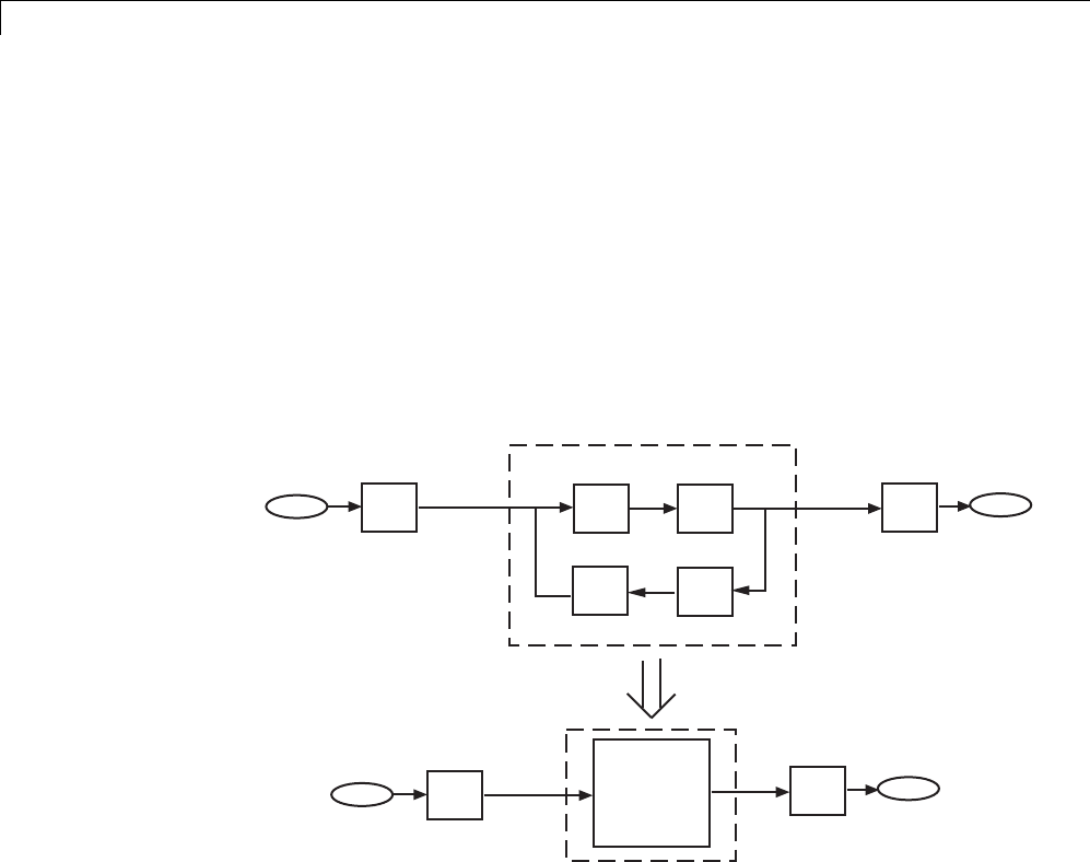
3Frequency Response Estimation
Model Requirements
You can estimate the frequency response of one or more blocks in a stable
Simulink model at steady state.
Your model can contain any Simulink blocks, including blocks with
event-based dynamics. Examples of blocks with event-based dynamics
include Stateflow charts, triggered subsystems, pulse width modulation
(PWM) signals.
u(t) y(t)
Estimate frequency response
for these blocks
Frequency
response
model
You should disable the following types of blocks before estimation:
•Blocks that simulate random disturbances (noise).
For alternativeswaystomodelsystemswithnoise,see“Estimating
Frequency Response Models with Noise Using Signal Processing Toolbox”
on page 3-74.
•Source blocks that generate time-varying outputs that interfere with the
estimation. See “Effects of Time-Varying Source Blocks on Frequency
Response Estimation” on page 3-62.
3-6
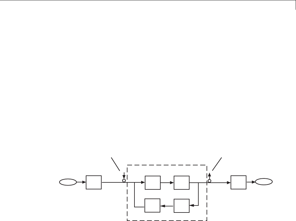
Estimation Requires Input and Output Signals
Estimation Requires Input and Output Signals
Frequency response estimation requires an input signal at the linearization
input point to excite the model at frequencies of interest, such as a chirp or
sinestream signal. A sinestream input signal is a series of sinusoids, where
each sine wave excites the system for a period of time. You can inject the
input signal anywhere in your model and log the simulated output, without
having to modify your model.
Frequency response estimation adds the input signal you design to the
existing Simulink signals at the linearization input point, and simulates
the model to obtain the output at the linearization output point. For more
information about supported input signals and their impact on the estimation
algorithm, see “Creating Input Signals for Estimation” on page 3-9.
u(t)
Linearization
input
y(t)
Linearization
output
Estimate frequency response
for these blocks
For multiple-input multiple-output (MIMO) systems, frequency response
estimation injects the signal at each input channel separately to simulate
the corresponding output signals. The estimation algorithm uses the inputs
and the simulated outputs to compute the MIMO frequency response. If you
want to inject different input signal at the linearization input points of a
multiple-input system, treat your system as separate single-input systems.
Perform independent frequency response estimations for each linearization
input point using frestimate, and concatenate your frequency response
results.
Frequency response estimation correctly handles open-loop linearization
input and output points. For example, if the input linearization point is open,
3-7

3Frequency Response Estimation
the input signal you design adds to the constant operating point value. The
operating point is the initial output of the block with a loop opening.
The estimated frequency response is related to the input and output signals
as:
Gs yt
est
() ()
≈fast Fourier transform of
fast Fourier transforrm ut
est ()
where uest(t) is the injected input signal and yest(t) is the corresponding
simulated output signal.
3-8

Creating Input Signals for Estimation
Creating Input Signals for Estimation
In this section...
“Supported Input Signals” on page 3-9
“Creating Sinestream Input Signals” on page 3-9
“Creating Chirp Input Signals” on page 3-19
Supported Input Signals
Frequency response estimation uses sinestream or chirp input signals.
Sinusoidal Signal When to Use
Sinestream Recommended for most situations. Especially useful
when:
•Your system contains strong nonlinearities.
•You require highly accurate frequency response
models.
See “Creating Sinestream Input Signals” on page
3-9.
Chirp •Your system is nearly linear in the simulation
range.
•You want to quickly obtain a response for a lot of
frequency points.
See “Creating Chirp Input Signals” on page 3-19.
Creating Sinestream Input Signals
•“What Is a Sinestream Signal?” on page 3-10
•“Create Sinestream Signals Using Linear Analysis Tool” on page 3-10
•“Create Sinestream Signals (MATLAB Code)” on page 3-13
3-9
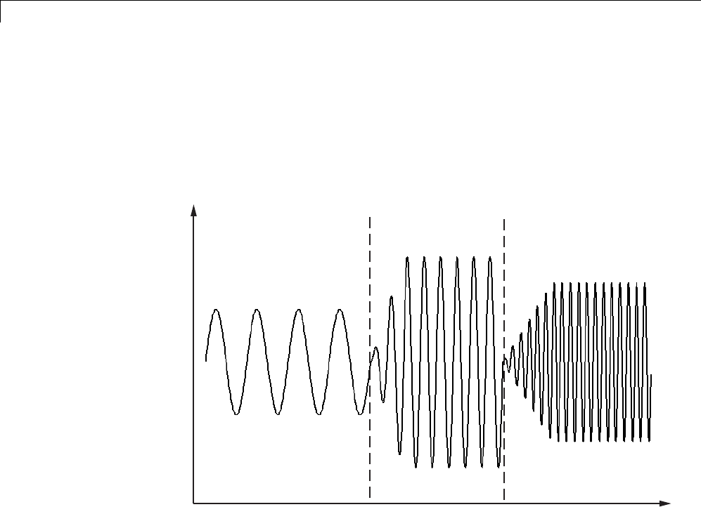
3Frequency Response Estimation
•“How Frequency Response Estimation Treats Sinestream Inputs” on page
3-15
What Is a Sinestream Signal?
Asinestream signal consists of several adjacent sine waves of varying
frequencies. Each frequency excites the system for a period of time.
Amplitude
Time
fff
123
Create Sinestream Signals Using Linear Analysis Tool
This example shows how to create a sinestream input signal based upon a
linearized model using the Linear Analysis Tool.
1Obtain a linearized model, linsys1.
For example, see “Linearize Simulink Model” on page 2-38, which shows
how to linearize a model.
2In the Linear Analysis Tool, click the Frequency Response Estimation
tab. In the Input Signal list, select Sinestream.
3-10
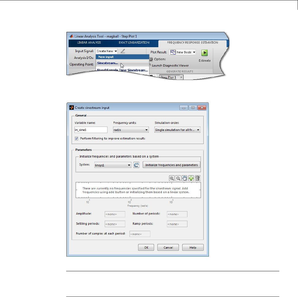
Creating Input Signals for Estimation
The Create sinestream input dialog box opens.
Note Selecting Sinestream creates a continuous-time signal. To generate
adi
screte-time signal, choose Fixed Sample Time Sinestream from
the Input Signal list.
3In the System list, select linsys1.ClickInitialize frequencies and
parameters.
3-11
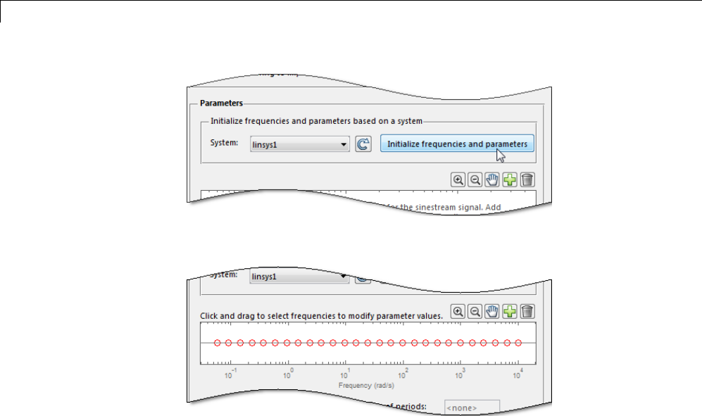
3Frequency Response Estimation
This action adds frequency points to the Frequency content viewer.
The software automatically selects frequency points based on the dynamics
of linsys1. The software also automatically determines other parameters
of the sinestream signal, including:
•amplitude
•number of periods
•settling periods
•ramp periods
•number of samples at each period
3-12
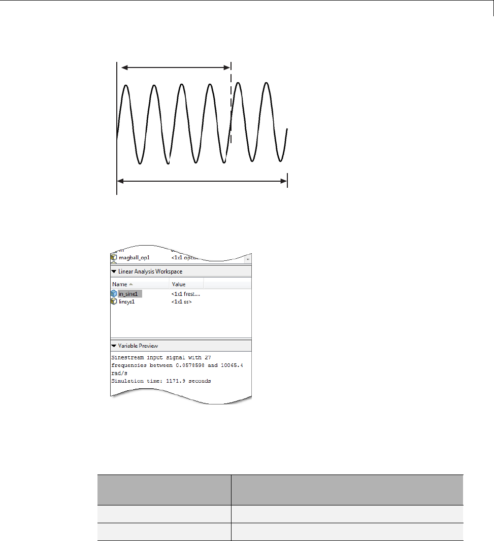
Creating Input Signals for Estimation
SettlingPeriods
NumPeriods
4Click OK to create the sinestream input signal. A new input signal,
in_sine1,appearsintheLinear Analysis Workspace.
Create Sinestream Signals (MATLAB Code)
You can create a sinestream signal from both continuous-time and
discrete-time signals in Simulink models using the following commands:
Signal at Input
Linearization Point
Command
Continuous frest.Sinestream
Discrete frest.createFixedTsSinestream
3-13

3Frequency Response Estimation
Create a sinestream signal in the most efficient way using a linear model that
accurately represents your system dynamics:
input = frest.Sinestream(sys)
sys is the linear model you obtained using exact linearization.
You can also define a linear system based on your insight about the system
using the tf,zpk,andss commands.
For example, create a sinestream signal from a linearized model:
magball
io(1) = linio('magball/Desired Height',1);
io(2) = linio('magball/Magnetic Ball Plant',...
1,'out');
sys = linearize('magball',io);
input = frest.Sinestream(sys)
The resulting input signal stores the frequency values as Frequency.
frest.Sinestream automatically specifies NumPeriods and SettlingPeriods
for each frequency:
Frequency : [0.05786;0.092031;0.14638 ...] (rad/s)
Amplitude : 1e-005
SamplesPerPeriod : 40
NumPeriods : [4;4;4;4 ...]
RampPeriods : 0
FreqUnits (rad/s,Hz): rad/s
SettlingPeriods : [1;1;1;1 ...]
ApplyFilteringInFRESTIMATE (on/off) : on
SimulationOrder (Sequential/OneAtATime): Sequential
For more information about sinestream options, see the frest.Sinestream
reference page.
You can plot your input signal using plot(input).
The mapping between the parameters of the Create sinestream input dialog
box in the Linear Analysis Tool and the options of frest.Sinestream is as
follows:
3-14

Creating Input Signals for Estimation
Create sinestream input dialog
box
frest.Sinestream option
Amplitude 'Amplitude'
Number of periods 'NumPeriods'
Settling periods 'SettlingPeriods'
Ramp periods 'RampPeriods'
Number of samples at each period 'SamplesPerPeriod'
How Frequency Response Estimation Treats Sinestream Inputs
Frequency response estimation using frestimate performs the following
operations on a sinestream input signal:
1Injects the sinestream input signal you design, uest(t), at the linearization
input point.
3-15

3Frequency Response Estimation
2Simulates the output at the linearization output point.
frestimate adds the signal you design to existing Simulink signals at
the linearization input point.
u(t)
u (t)
y(t)
est
3-16
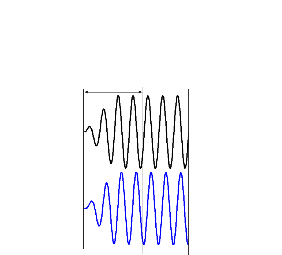
Creating Input Signals for Estimation
3Discards the SettlingPeriods portion of the output (and the corresponding
input) at each frequency.
The simulated output at each frequency has a transient portion and steady
state portion. SettlingPeriods corresponds to the transient components
of the output and input signals. The periods following SettlingPeriods
areconsideredtobeatsteadystate.
SettlingPeriods
Input
Output
4Filters the remaining portion of the output and the corresponding input
signals at each input frequency using a bandpass filter.
When a model is not at steady state, the response contains low-frequency
transient behavior. Filtering typically improves the accuracy of your model
by removing the effects of frequencies other than the input frequencies.
3-17
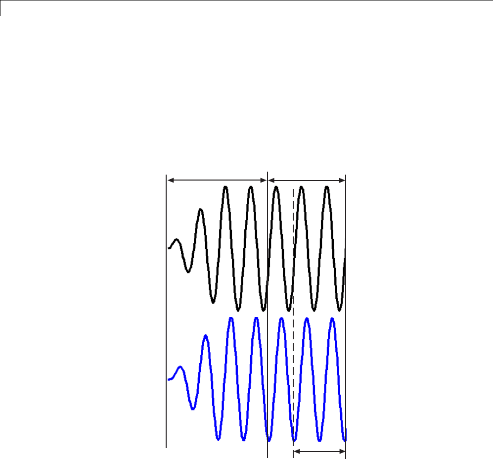
3Frequency Response Estimation
These frequencies are problematic when your sampled data has finite
length. These effects are called spectral leakage.
frestimate uses a finite impulse response (FIR) filter. The software sets
the filter order to match the number of samples in a period such that any
transients associated with filtering appear only in the first period of the
filtered steady-state output. After filtering, frestimate discards the first
period of the input and output signals.
SettlingPeriods
Filtered
portion
Used for
estimation
Input
Output
You can specify to disable filtering during estimation using the signal
ApplyFilteringInFRESTIMATE property.
3-18
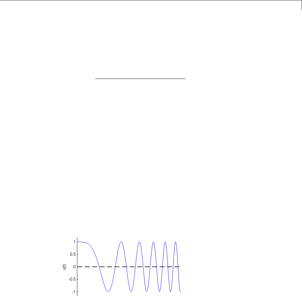
Creating Input Signals for Estimation
5Estimates the frequency response of the processed signal by computing
the ratio of the fast Fourier transform of the filtered steady-state portion
of the output signal yest(t) and the fast Fourier transform of the filtered
input signal uest(t):
Gs yt
est
() ()
≈fast Fourier transform of
fast Fourier transforrm ut
est ()
To compute the response at each frequency, frestimate uses only the
simulation output at that frequency.
Creating Chirp Input Signals
•“What Is a Chirp Signal?” on page 3-19
•“Create Chirp Signals Using Linear Analysis Tool” on page 3-19
•“Create Chirp Signals (MATLAB Code)” on page 3-22
What Is a Chirp Signal?
The swept-frequency cosine (chirp) input signal excites your system at a range
of frequencies, such that the input frequency changes instantaneously.
Alternatively, you can use the sinestream signal, which excites the system at
each frequency for several periods. See “Supported Input Signals” on page 3-9
for more information about choosing your signal.
Create Chirp Signals Using Linear Analysis Tool
This example shows how to create a chirp input signal based upon a linearized
model using the Linear Analysis Tool.
3-19
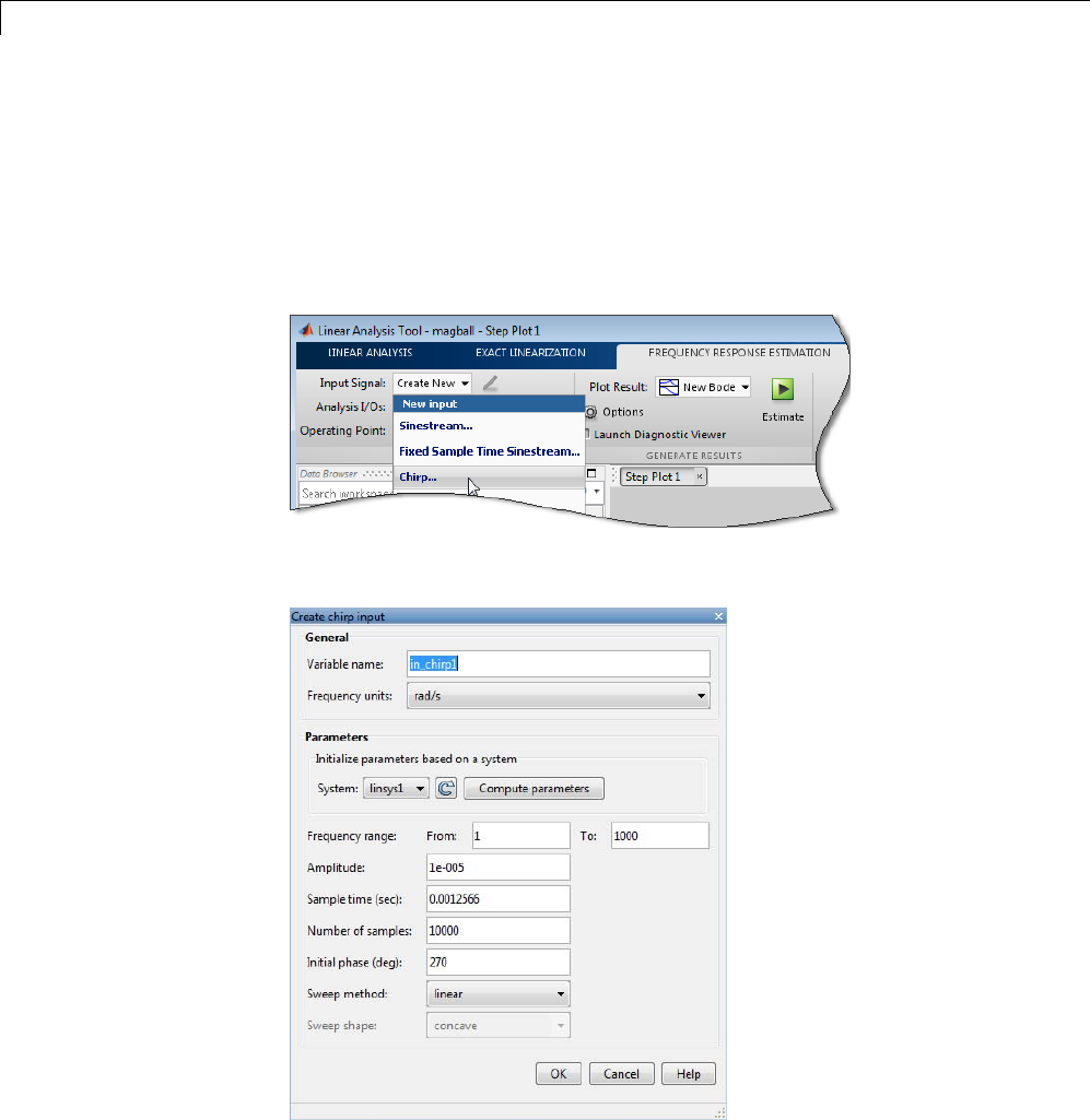
3Frequency Response Estimation
1Obtain a linearized model, linsys1.
For example, see “Linearize Simulink Model” on page 2-38, which shows
how to linearize a model.
2In the Linear Analysis Tool, click the Frequency Response Estimation
tab. In the Input Signal list, select Chirp.
The Create chirp input dialog box opens.
3In the System list, select linsys1 selected. Click Compute parameters.
3-20
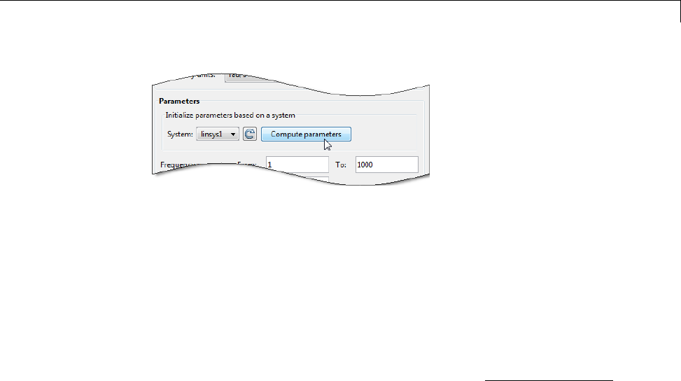
Creating Input Signals for Estimation
The software automatically selects frequency points based on the dynamics
of linsys1. The software also automatically determines other parameters
of the chirp signal, including:
•frequency range at which the linear system has interesting dynamics
(see the From and To boxes of Frequency Range).
•amplitude.
•sample time. To avoid aliasing, the Nyquist frequency of the signal is
five times the upper end of the frequency range, 2
5
*max( )FreqRange .
•number of samples.
•initial phase.
•sweep method
•sweep shape.
4Click OK to create the chirp input signal. A new input signal in_chirp1
appears in the Linear Analysis Workspace.
3-21
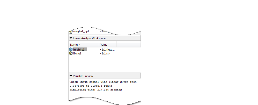
3Frequency Response Estimation
Create Chirp Signals (MATLAB Code)
Create a chirp signal in the most efficient way using a linear model that
accurately represents your system dynamics:
input = frest.Chirp(sys)
sys can be the linear model you obtained using exact linearization techniques.
You can also define a linear system based on your insight about the system
using the tf,zpk,andss commands.
For example, create a chirp signal from a linearized model:
magball
io(1) = linio('magball/Desired Height',1);
io(2) = linio('magball/Magnetic Ball Plant',...
1,'out');
sys = linearize('magball',io);
input = frest.Chirp(sys)
3-22

Creating Input Signals for Estimation
The input signal is:
FreqRange : [0.0578598408615998 10065.3895573969] (rad/s)
Amplitude : 1e-005
Ts : 0.00012484733494616 (sec)
NumSamples : 1739616
InitialPhase : 270 (deg)
FreqUnits (rad/s or Hz): rad/s
SweepMethod(linear/ : linear
quadratic/
logarithmic)
For more information about chirp signal properties, see the frest.Chirp
reference page.
You can plot your input signal using plot(input).
The mapping between the parameters of the Create chirp input dialog box in
the Linear Analysis Tool and the options of frest.Chirp is as follows:
Create chirp input dialog box frest.Chirp option
Frequency range > From First element associated with the
'FreqRange' option
Frequency range > To Second element associated with the
'FreqRange' option
Amplitude 'Amplitude'
Sample time (sec) 'Ts'
Number of samples 'NumSamples'
Initial phase (deg) 'InitialPhase'
Sweep method 'SweepMethod'
Sweep shape 'Shape'
3-23
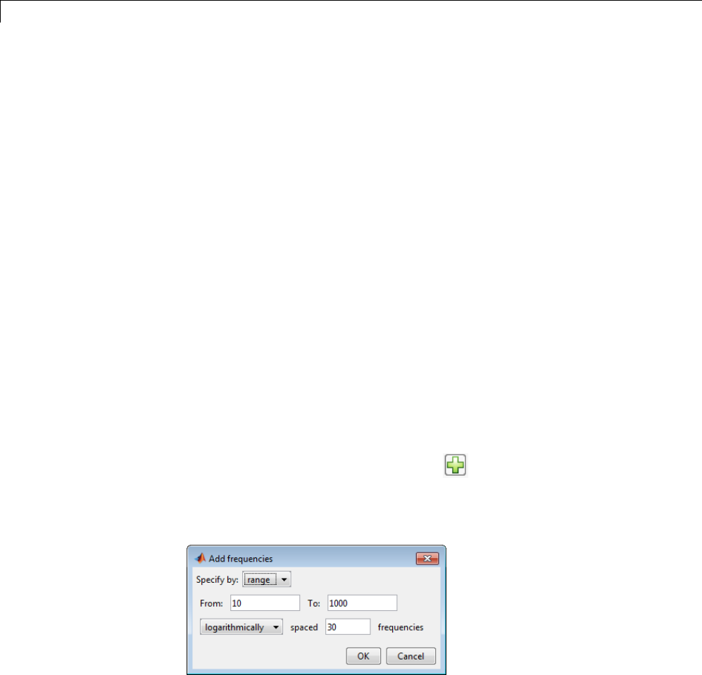
3Frequency Response Estimation
Modifying Input Signals for Estimation
When the frequency response estimation produces unexpected results,
you can try modifying the input signal properties in the ways described in
“Troubleshooting Frequency Response Estimation” on page 3-49.
Modifying Sinestream Input Signal Using Linear
Analysis Tool
Add Frequency Points to Sinestream Input Signal
This example shows how to add frequency points to an existing sinestream
input signal using the Linear Analysis Tool.
1Create a sinestream input signal, in_sine1,asshownin“Create
Sinestream Signals Using Linear Analysis Tool” on page 3-10.
2Double-click in_sine1 in the Linear Analysis Workspace area of the Linear
Analysis Tool.
The Edit sinestream dialog box opens.
3In the Frequency content viewer, click in the Frequency content
toolbar.
The Add frequencies dialog box opens.
4Enter the frequency range of the points to be added.
5Click OK to add the specified frequency points to in_sine1.
3-24
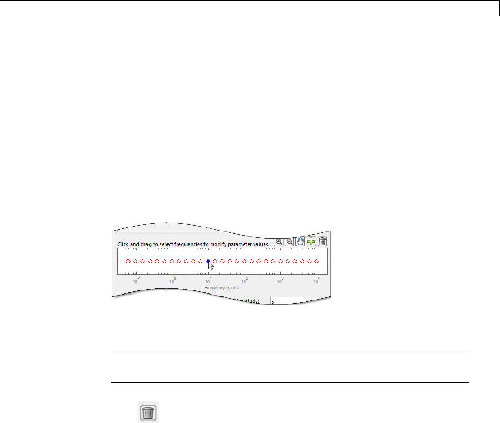
Modifying Input Signals for Estimation
Delete Frequency Point from Sinestream Input Signal
Thisexampleshowshowtodeletefrequencypointsfromanexisting
sinestream input signal using the Linear Analysis Tool.
1Create a sinestream input signal, in_sine1,asshownin“Create
Sinestream Signals Using Linear Analysis Tool” on page 3-10.
2Double-click in_sine1 in the Linear Analysis Workspace area of the Linear
Analysis Tool.
The Edit sinestream dialog box opens.
3In the Frequency content viewer, select the frequency point to delete.
The selected point appears blue.
Tip To select multiple frequency points, click and drag across the frequency
points of interest.
4Click in the Frequency content toolbar to delete the selected frequency
point(s) from the Frequency content viewer.
5Click OK to save the modified input signal.
Modify Parameters for a Frequency Point in Sinestream Input
Signal
This example shows how to modify signal parameters of an existing
sinestream input signal using the Linear Analysis Tool.
3-25
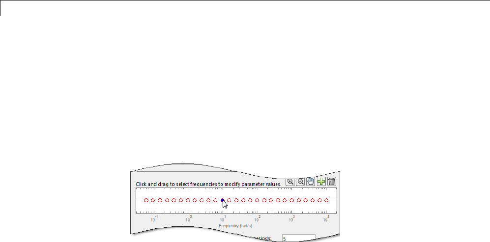
3Frequency Response Estimation
1Create a sinestream input signal, in_sine1,asshownin“Create
Sinestream Signals Using Linear Analysis Tool” on page 3-10.
2Double-click in_sine1 in the Linear Analysis Workspace area of the Linear
Analysis Tool.
The Edit sinestream dialog box opens.
3In the Frequency content viewer, select the frequency point(s) to delete.
The selected point(s) appears blue.
4Enter the new values for the signal parameters.
If the parameter value is <mixedvalue>, the parameter has different values
for some of the frequency points selected.
5Click OK to save the modified input signal.
Modifying Sinestream Input Signal (MATLAB Code)
For example, suppose that you used a sinestream input signal, and the output
at a specific frequency did not reach steady state. In this case, you can modify
the characteristics of the sinestream input at the corresponding frequency.
input.NumPeriods(index)=NewNumPeriods;
input.SettlingPeriods(index)=NewSettlingPeriods;
where index is the frequency value index of the sine wave you want to modify.
NewNumPeriods and NewSettlingPeriods are the new values of NumPeriods
and SettlingPeriods,respectively.
To modify several signal properties at a time, you can use the set command.
For example:
3-26

Modifying Input Signals for Estimation
input = set(input,'NumPeriods',NewNumPeriods,...
'SettlingPeriods',NewSettlingPeriods)
After modifying the input signal, repeat the estimation.
3-27

3Frequency Response Estimation
Estimate Frequency Response Using Linear Analysis Tool
This example shows how to perform frequency response estimation for a
model using the Linear Analysis Tool.
Step 1. Open Simulink model and Linear Analysis Tool.
•Open Simulink model.
sys = 'scdDCMotor';
open_system(sys);
•Open the Linear Analysis Tool for the model.
In the Simulink Editor, select Analysis > Control Design > Linear
Analysis.
Step 2. Create an input signal for estimation.
•Click the Frequency Response Estimation tab.
•Open the Create sinestream input dialog box.
In the Input Signal list, select Sinestream.
3-28
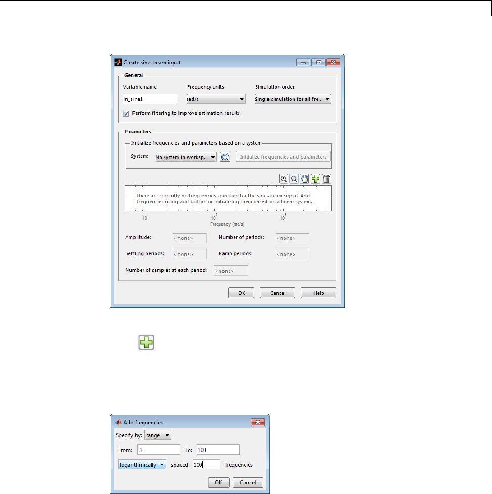
Estimate Frequency Response Using Linear Analysis Tool
•Open the Add frequencies dialog box.
Click to add frequency points to the input signal.
•Specify the frequency range for the input.
Enter .1 in the From box and 100 in the To box. Enter 100 in the box
for the number of frequency points.
Click OK.
3-29
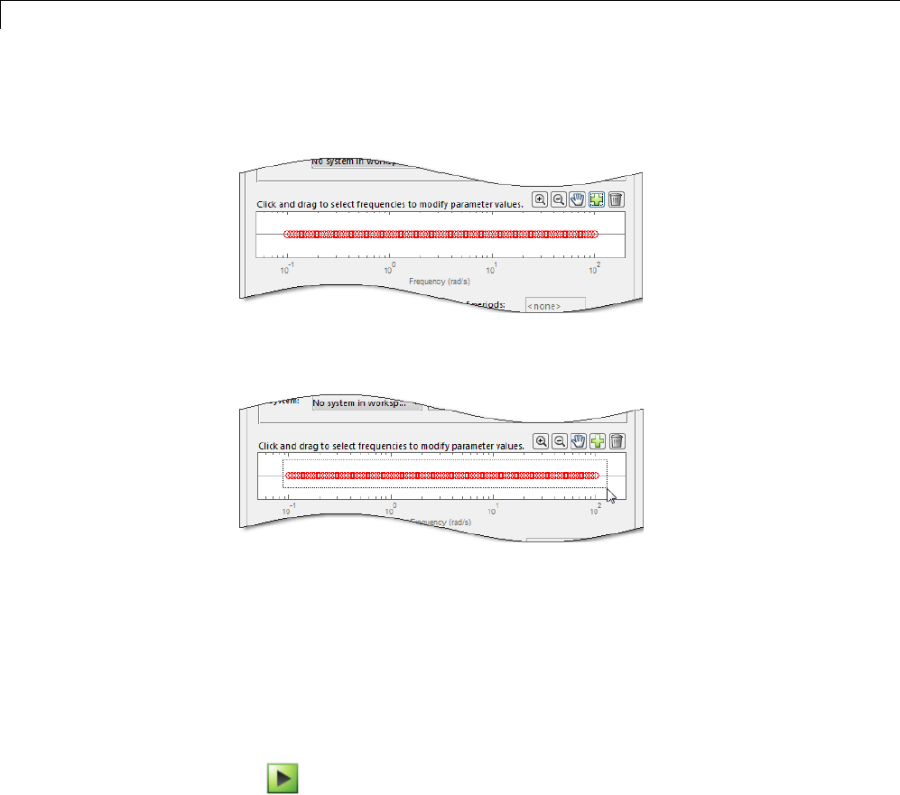
3Frequency Response Estimation
The added points are visible in the Frequency content viewer of the Create
sinestream input dialog box.
•In the Frequency content viewer of the Create sinestream input dialog
box, select all the frequency points.
•Specify the amplitude of the input signal.
Enter 1 in the Amplitude box.
•Create the input sinestream signal.
Click OK. The new input signal, in_sine1,appearsintheLinear
Analysis Workspace.
Step 3. Estimate frequency response.
Click . The frequency response estimation result, estsys1,appearsin
the Linear Analysis Workspace.
3-30
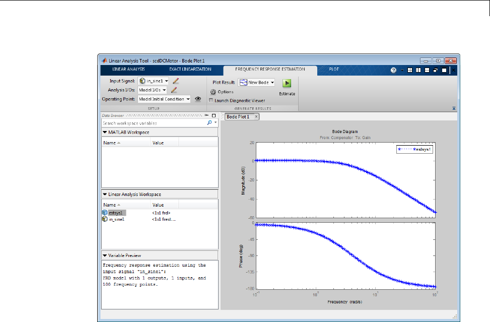
Estimate Frequency Response Using Linear Analysis Tool
3-31

3Frequency Response Estimation
Estimate Frequency Response with Linearization-Based
Input Using Linear Analysis Tool
This example shows how to perform frequency response estimation for a
model using the Linear Analysis Tool. The input signal used for estimation is
based on the linearization of the model.
Step 1. Linearize Simulink model.
•Open Simulink model.
sys = 'scdDCMotor';
open_system(sys);
•Open the Linear Analysis Tool for the model.
In the Simulink Editor, select Analysis > Control Design > Linear
Analysis.
•In the Plot Result list, choose New Bode.
•Linearize the model.
Click . A new linearized model, linsys1, appears in the Linear
Analysis Workspace.
Thesoftwareusedthemodelinitialconditions as the operating point to
generate linsys1.
3-32
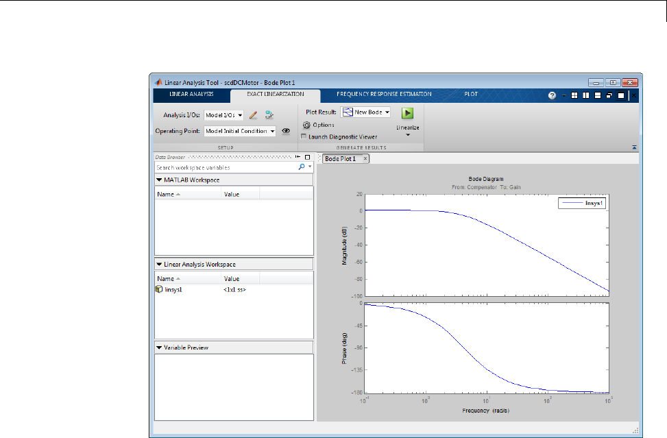
Estimate Frequency Response with Linearization-Based Input Using Linear Analysis Tool
Step 2. Create sinestream input signal.
•Click the Frequency Response Estimation tab.
In this tab, you estimate the frequency response of the model.
•Open the Create sinestream input dialog box.
Select Sinestream from the Input Signal list to open the Create
sinestream input dialog box.
3-33
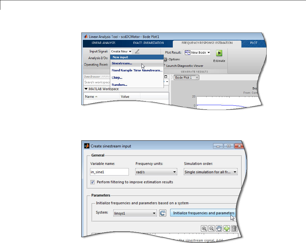
3Frequency Response Estimation
•Initialize the input signal frequencies and parameters based on linsys1.
Click Initialize frequencies and parameters.
The Frequency content viewer is populated with frequency points. The
software chooses the frequencies and input signal parameters automatically
based on the dynamics of linsys1.
•In the Frequency content viewer of the Create sinestream input dialog
box, select all the frequency points.
3-34

Estimate Frequency Response with Linearization-Based Input Using Linear Analysis Tool
•Specify the amplitude of the input signal.
Enter 1 in the Amplitude box.
•Create the input sinestream signal.
Click OK.Theinputsignalin_sine1 appears in the Linear Analysis
Workspace.
Step 3. Select the plot to display the estimation result.
In the Plot Result list, choose Bode Plot 1 to add the next computed linear
system to Bode Plot 1.
Step 4. Estimate frequency response.
Click . The estimated system, estsys1,appearsintheLinear Analysis
Workspace.
3-35
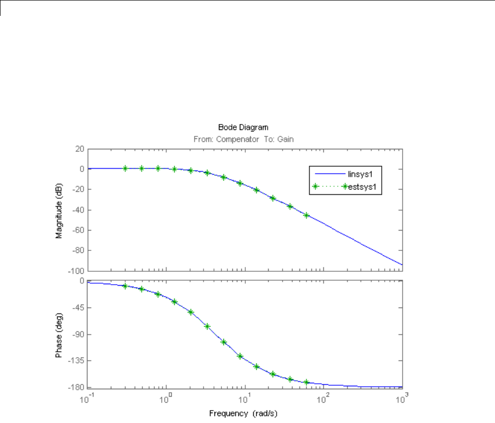
3Frequency Response Estimation
Step 5. Examine estimation results.
Bode Plot 1 now shows the Bode responses for the estimated model and
the linearized model.
The frequency response for the estimated model matches that of the linearized
model.
3-36

Estimate Frequency Response (MATLAB®Code)
Estimate Frequency Response (MATLAB Code)
Prerequisites
•Open Simulink model.
Example:
mdl = 'f14';
open_system(mdl)
To learn more about general model requirements, see “Model
Requirements” on page 3-6.
•Create an input signal for estimation.
Example:
io(1) = linio('f14/Sum1',1)
io(2) = linio('f14/Gain5',1,'out')
sys = linearize('f14',io);
input = frest.Sinestream(sys)
See “Creating Input Signals for Estimation” on page 3-9.
•(Optional) If your model has not reached steady state, initialize the model
at a steady state operating point.
You can check whether your model is at steady state by simulating the
model. See operspec and findop reference pages.
1Use linearization I/O points to specify input and output points for frequency
response estimation.
Example:
io(1) = linio('f14/Sum1',1)
io(2) = linio('f14/Gain5',1,'out')
Caution Avoid placing I/O points on bus signals.
3-37

3Frequency Response Estimation
For more information about linearization I/O points, see “Specify Model
Portion to Linearize” on page 2-11 and the linio reference page.
2Identify all source blocks that generate time-varying signals in the signal
path of the linearization outputs. Such time-varying signals can interfere
with the signal at the linearization output points and produce inaccurate
estimation results.
aFirst, use frest.findSources to identify time-varying source blocks
that can interfere with estimation. frest.findSources finds all
time-varying source blocks in the signal path of the linearization output
points.
Example:
Identify the time-varying source blocks in the f14 model:
srcblks = frest.findSources('f14',io);
bNext, to disable these blocks during estimation, use frestimateOptions.
For example:
opts = frestimateOptions;
opts.BlocksToHoldConstant = srcblks;
For more information, see the frest.findSources and frestimateOptions
reference pages.
3Estimate the frequency response.
Example:
[sysest,simout] = frestimate('f14',io,input,opts)
sysest is the estimated frequency response. simout is the simulated
output that is a Simulink.Timeseries object.
For more information about syntax and argument descriptions, see the
frestimate reference page.
3-38
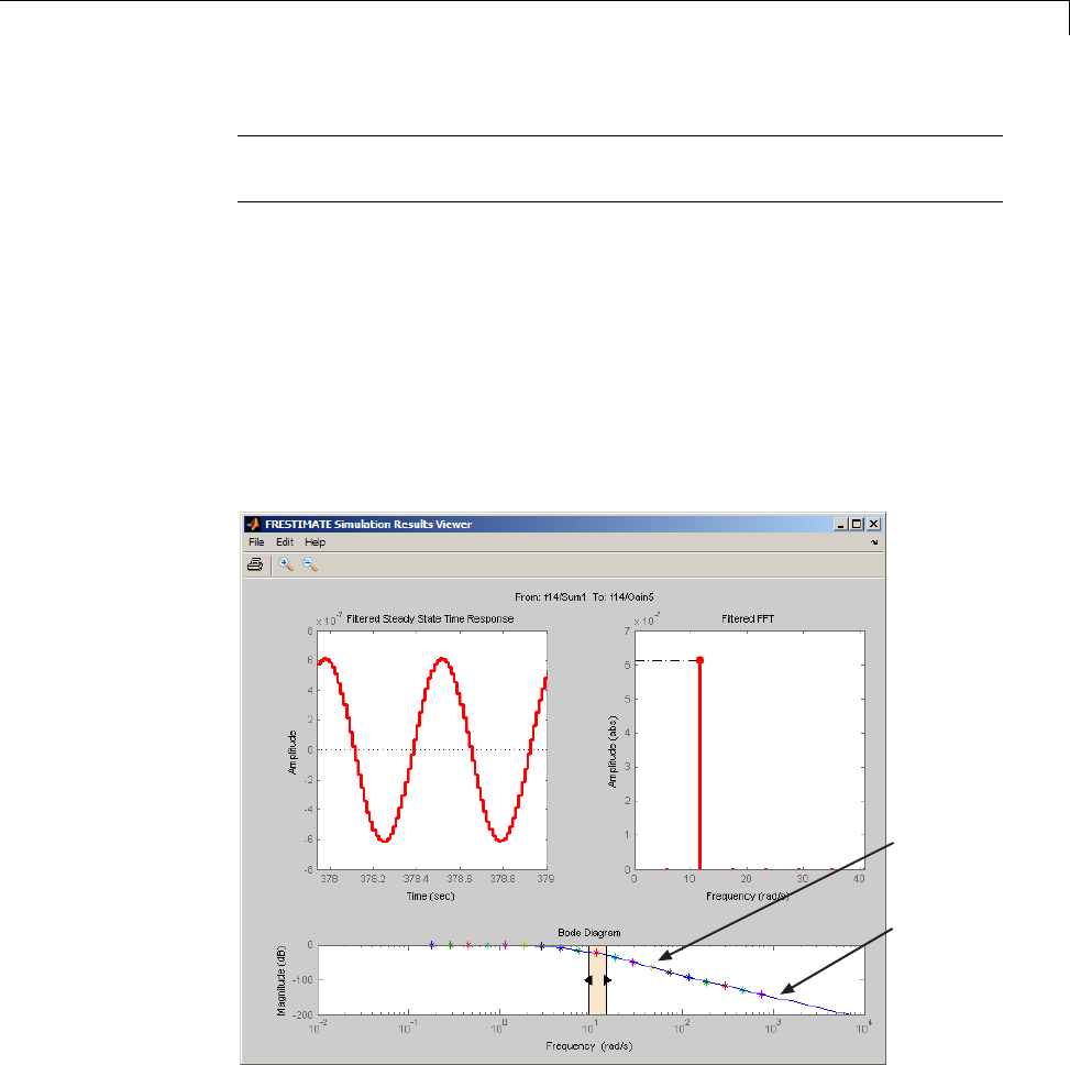
Estimate Frequency Response (MATLAB®Code)
Tip To speed up your estimation or decrease memory requirements, see
“Managing Estimation Speed and Memory” on page 3-80.
4Open the Simulation Results Viewer to analyze the estimated frequency
response. For example:
frest.simView(simout,input,sysest);
You can compare the estimated frequency response (sysest) to a system
you linearized using exact linearization (sys):
frest.simView(simout,input,sysest,sys);
Exact
linearization
results
Estimated
frequency
response
For more information, see “Analyzing Estimated Frequency Response”
on page 3-40.
3-39
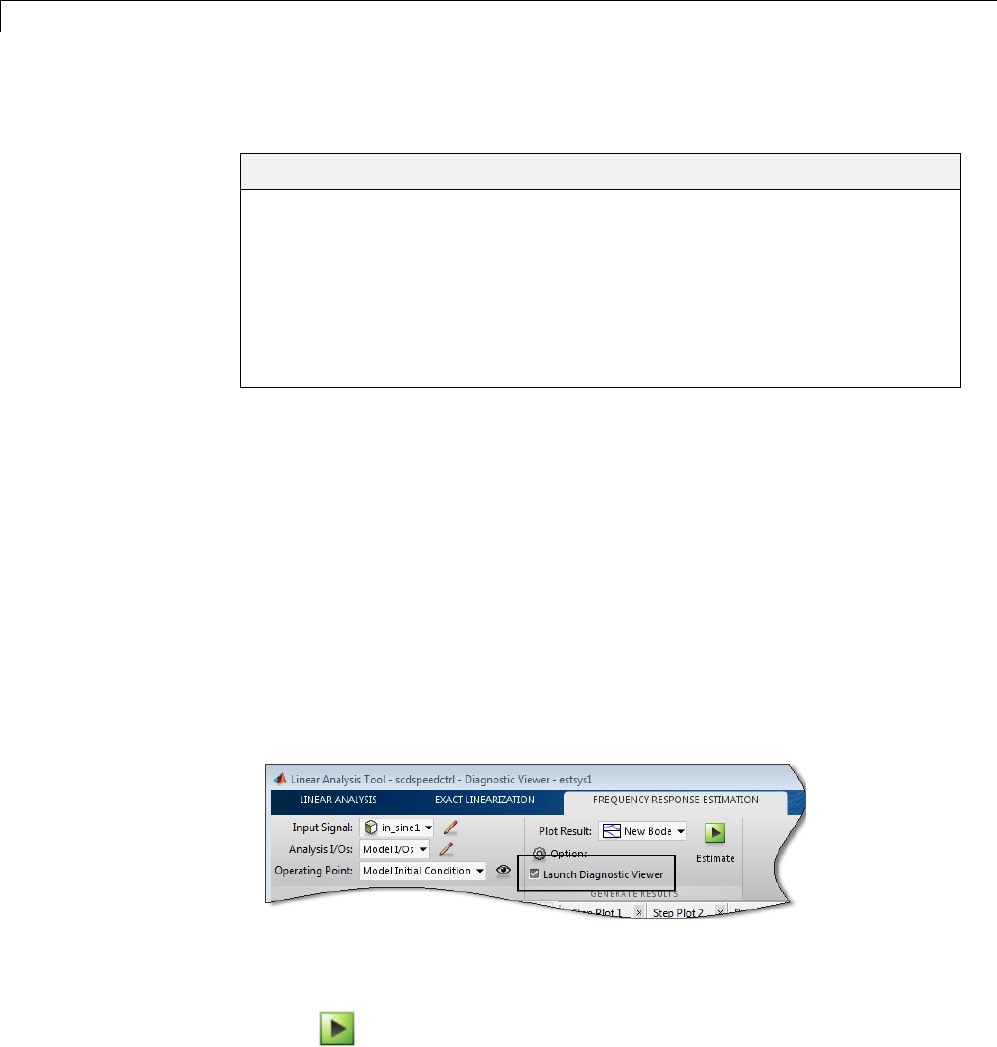
3Frequency Response Estimation
Analyzing Estimated Frequency Response
In this section...
“View Simulation Results” on page 3-40
“Interpret Frequency Response Estimation Results” on page 3-43
“Analyze Simulated Output and FFT at Specific Frequencies” on page 3-45
“Annotate Frequency Response Estimation Plots” on page 3-47
“Displaying Estimation Results for Multiple-Input Multiple-Output
(MIMO) Systems” on page 3-48
View Simulation Results
View Simulation Results Using Linear Analysis Tool
Use the Diagnostic Viewer to analyze the results of your frequency response
estimation, obtained by performing the steps in “Estimate Frequency
Response Using Linear Analysis Tool” on page 3-28.
To open the Diagnostic Viewer after performing frequency response
estimation in the Linear Analysis Tool:
1In the Frequency Response Estimation tab, before performing the
estimation task, select the Launch Diagnostic Viewer check box.
This action sets the Diagnostic Viewer to open when the frequency response
estimation is performed.
2Click to estimate the frequency response of the model.
3-40
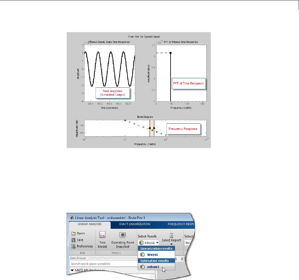
Analyzing Estimated Frequency Response
The Diagnostic Viewer appears in the plot pane.
To open the Diagnostic Viewer to view an estimated model in the Linear
Analysis Tool:
1In the Linear Analysis Tab, select the estimated model using the Select
Result list.
2Select Show diagnostic viewer in the Show Report list.
3-41
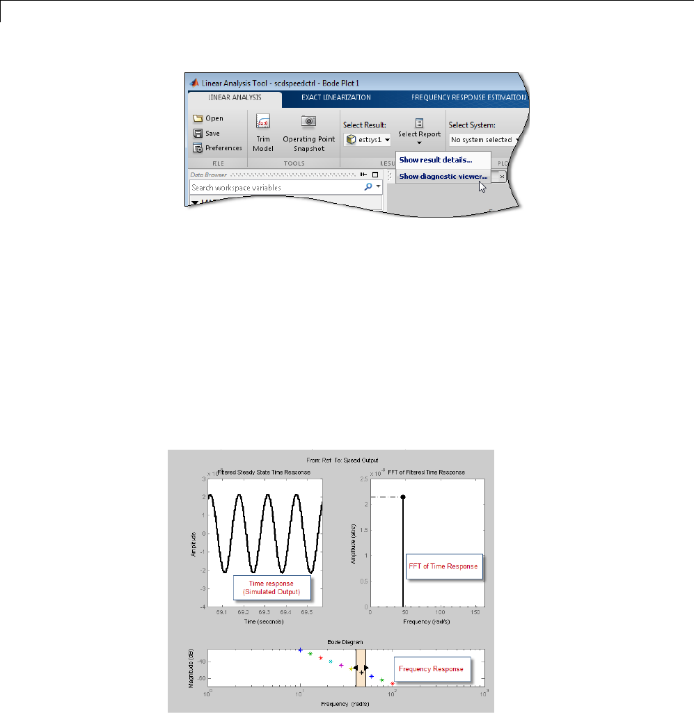
3Frequency Response Estimation
View Simulation Results (MATLAB Code)
Use the Simulation Results Viewer to analyze the results of your frequency
response estimation, obtained by performing the steps in “Estimate Frequency
Response (MATLAB Code)” on page 3-37.
Open the Simulation Results Viewer using:
frest.simView(simout,input,sysest)
where simout is the simulated output, input is the input signal you created,
and sysest is the estimated frequency response.
3-42
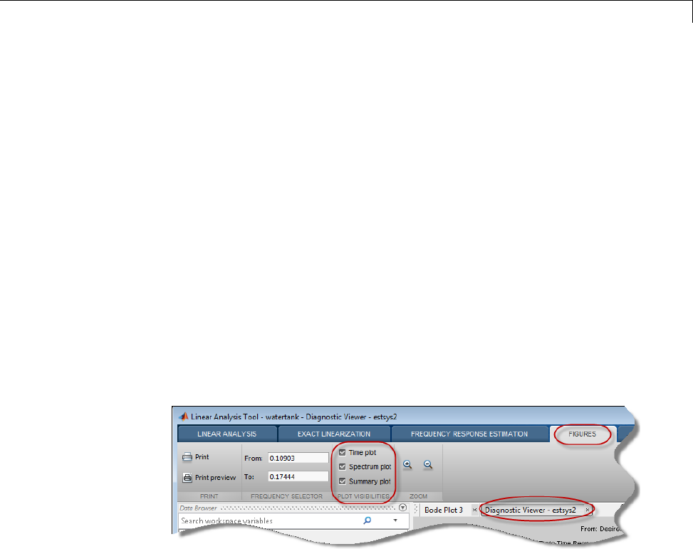
Analyzing Estimated Frequency Response
Interpret Frequency Response Estimation Results
By default, the Simulation Results Viewer shows these plots:
•“Select Plots Displayed in Simulation Results Viewer” on page 3-43
•“Frequency Response” on page 3-43
•“Time Response(SimulatedOutput)”onpage3-44
•“FFT of Time Response” on page 3-44
Select Plots Displayed in Simulation Results Viewer
•To select the plots displayed in the Diagnostic Viewer using the Linear
Analysis Tool:
1In the Figures tab, select the Diagnostic Viewer plot.
2In the Plot Visibilities section, select the check boxes for the plots
that you want to view.
To modify plot settings, such as axis frequency units, right-click on a plot,
and select the corresponding option.
•To select the plots displayed in the Simulation Results Viewer, choose the
corresponding plot from the Edit > Plots menu. To modify plot settings,
such as axis frequency units, right-click a plot, and select the corresponding
option.
Frequency Response
Use the Bode plot to analyze the frequency response. If the frequency response
does not match the dynamics of your system, see “Troubleshooting Frequency
3-43

3Frequency Response Estimation
Response Estimation” on page 3-49 for information about possible causes and
solutions. While troubleshooting, you can use the Bode plot controls to view
the time response at the problematic frequencies.
You can usually improve estimation results by either modifying your input
signal or disabling the model blocks that drive your system away from the
operating point, and repeating the estimation.
Time Response (Simulated Output)
Use this plot to check whether the simulated output is at steady state at
specific frequencies. If the response has not reached steady state, see “Time
Response Not at Steady State” on page 3-49 for possible causes and solutions.
If you used the sinestream input for estimation, check both the filtered and the
unfiltered time response. You can toggle the display of filtered and unfiltered
output by right-clicking the plot and selecting Show filtered steady state
output only. If both the filtered and unfiltered response appear at steady
state, then your model must be at steady state. You can explore other possible
causes in “Troubleshooting FrequencyResponseEstimation” on page 3-49.
Note If you used the sinestream input for estimation, toggling the filtered
and unfiltered display only updates the Time Response and FFT plots. This
selection does not change estimation results. For more information about
filtering during estimation, see “How Frequency Response Estimation Treats
Sinestream Inputs” on page 3-15.
FFT of Time Response
Use this plot to analyze the spectrum of the simulated output.
For example, you can use the spectrum to identify strong nonlinearities. When
the FFT plot shows large amplitudes at frequencies other than the input
signal, your model is operating outside of linear range. If you are interested in
analyzing the linear response of your system for small perturbations, explore
possible solutions in “FFT Contains Large Harmonics at Frequencies Other
than the Input Signal Frequency” on page 3-53.
3-44
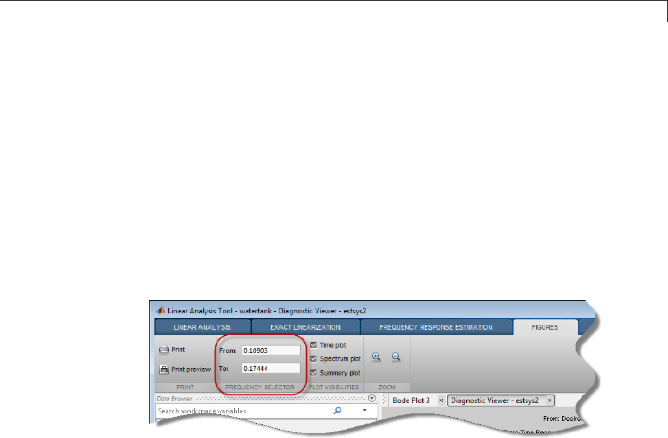
Analyzing Estimated Frequency Response
Analyze Simulated Output and FFT at Specific
Frequencies
Using the Diagnostic Viewer in Linear Analysis Tool
To analyze the results in the Diagnostic Viewer, use the controls in the
Figures tab of the Linear Analysis Tool.
1In the Figures tab, select the Diagnostic Viewer plot.
2In the Frequency Selector section, specify the frequency range that you
want to inspect. Use the frequency units used in the Bode plot in the
Diagnostic Viewer.
Using the Simulation Results Viewer
In the Simulation Results Viewer, use Bode controls to display the simulated
output and its spectrum at specific frequencies.
If you used the sinestream input signal in the estimation:
•Drag arrows individually to display the time response and FFT at specific
frequencies.
•Dragtheshadedregiontoshiftthetime response and FFT to a different
frequency range.
3-45
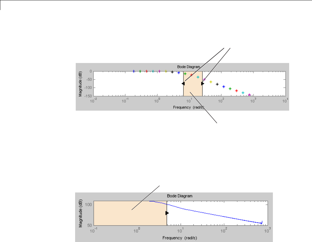
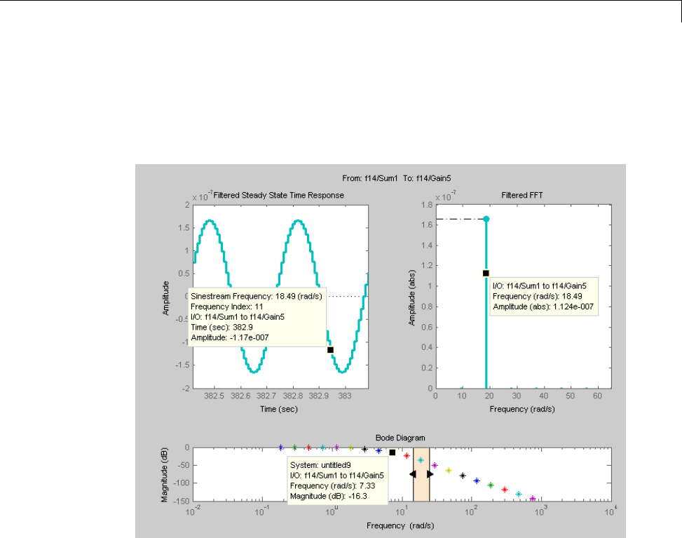
Analyzing Estimated Frequency Response
Annotate Frequency Response Estimation Plots
You can display a data tip on the Time Response, FFT, and Bode plots in the
Simulation Results Viewer by clicking the corresponding curve. Dragging
the data tip updates the information.
Data tips are useful for correcting poor estimation results at a specific
sinestream frequency, which requires you to modify the input at a specific
frequency. You can use the data tip to identify the frequency index where the
response does not match your system.
In the previous figure, the Time Response data tip shows that the frequency
index is 11. You can use this frequency index to modify the corresponding
portion of the input signal. For example, to modify the NumPeriods and
SettlingPeriods properties of the sinestream signal, using MATLAB code:
input.NumPeriods(11) = 80;
3-47
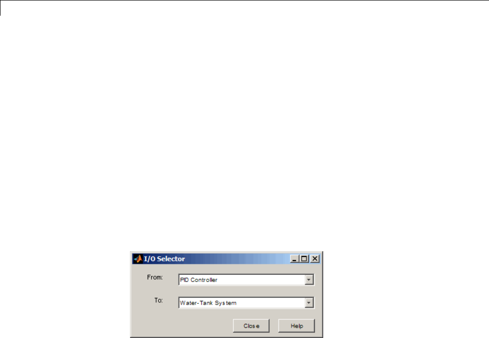
3Frequency Response Estimation
input.SettlingPeriods(11) = 75;
To modify the sinestream in the Linear Analysis Tool, see “Modifying
Sinestream Input Signal Using Linear Analysis Tool” on page 3-24
Displaying Estimation Results for Multiple-Input
Multiple-Output (MIMO) Systems
For MIMO systems, view frequency response information for specific input
and output channels:
1In the Simulation Results Viewer, right-click any plot, and select I/O
Selector.
2Choose the input channel in the From list. Choose the output channel in
the To list.
3-48

Troubleshooting Frequency Response Estimation
Troubleshooting Frequency Response Estimation
In this section...
“When to Troubleshoot” on page 3-49
“Time Response Not at Steady State” on page 3-49
“FFT Contains Large Harmonics at Frequencies Other than the Input
Signal Frequency” on page 3-53
“TimeResponseGrowsWithoutBound”onpage3-55
“Time Response Is Discontinuous or Zero” on page 3-57
“TimeResponseIsNoisy”onpage3-59
When to Troubleshoot
After you estimate the frequency response, you can analyze the results. If the
frequency response plot does not match the expected behavior of your system,
you can use the time response and FFT plots to help you improve the results.
If your estimation is slow or you run out of memory during estimation, see
“Managing Estimation Speed and Memory” on page 3-80.
Time Response Not at Steady State
What Does This Mean?
This time response has not reached steady state.
3-49
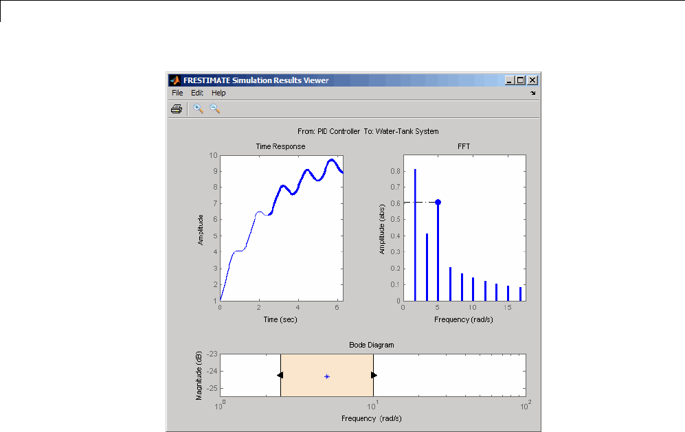
3Frequency Response Estimation
This plot shows a steady-state time response.
3-50

Troubleshooting Frequency Response Estimation
Because frequency response estimation requires steady-state input and
output signals, transients produce inaccurate estimation results.
For sinestream input signals, transients sometimes interfere with the
estimation either directly or indirectly through spectral leakage. For chirp
input signals, transients interfere with estimation.
3-51

3Frequency Response Estimation
How Do I Fix It?
Possible Cause Action
Model cannot initialize to
steady state.
•Increase the number of periods for
frequencies that do not reach steady
state by changing the NumPeriods
and SettlingPeriods properties. See
“Modifying Input Signals for Estimation”
on page 3-24.
•Disable all time-varying source blocks in
your model and repeat the estimation. See
“Effects of Time-Varying Source Blocks on
Frequency Response Estimation” on page
3-62.
(Sinestream input) Not
enough periods for the
output to reach steady state.
•Increase the number of periods for
frequencies that do not reach steady
state by changing the NumPeriods and
SettlingPeriods. See “Modifying Input
Signals for Estimation” on page 3-24.
•Check that filtering is enabled during
estimation. You enable filtering by
setting the ApplyFilteringInFRESTIMATE
option to on. For information about
how estimation uses filtering, see the
frestimate reference page.
(Chirp input) Signal sweeps
through the frequency range
too quickly.
Increase the simulation time by increasing
NumSamples. See “Modifying Input Signals
for Estimation” on page 3-24.
After you try the suggested actions, recompute the estimation either:
•At all frequencies
•In a particular frequency range (only for sinestream input signals)
To recompute the estimation in a particular frequency range:
3-52

Troubleshooting Frequency Response Estimation
1Determine the frequencies for which you want to recompute the estimation
results. Then, extract a portion of the sinestream input signal at these
frequencies using fselect.
For example, these commands extract a sinestream input signal between
10 and 20 rad/s from the input signal input:
input2 = fselect(input,10,20);
2Modify the properties of the extracted sinestream input signal input2,as
described in “Modifying Input Signals for Estimation” on page 3-24.
3Estimate the frequency response sysest2 with the modified input signal
using frestimate.
4Merge the original estimated frequency response sysest and the
recomputed estimated frequency response sysest2:
aRemove data from sysest at the frequencies in sysest2 using fdel.
For example:
sysest = fdel(sysest,input2.Frequency)
bConcatenate the original and recomputed responses using fcat.For
example:
sys_combined = fcat(sysest2,sysest)
You can analyze the recomputed frequency response, as described in
“Analyzing Estimated Frequency Response” on page 3-40.
For an example of frequency response estimation with time-varying source
blocks, see “Effects of Time-Varying Source Blocks on Frequency Response
Estimation” on page 3-62
FFT Contains Large Harmonics at Frequencies Other
than the Input Signal Frequency
What Does This Mean?
When the FFT plot shows large amplitudes at frequencies other than the
input signal, your model is operating outside the linear range. This condition
3-53
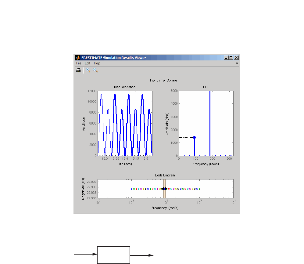
3Frequency Response Estimation
can causes problems when you want to analyze your linear system response to
small perturbations.
For models operating in the linear range, the input amplitude A1in y(t) must
be larger than the amplitudes of other harmonics, A2and A3.
model
u(t) y(t)
ut A
yt A A A
() sin( )
( ) sin( ) sin( ) sin(
=+
=+++++
111
11122233
33) ...+
3-54

Troubleshooting Frequency Response Estimation
How Do I Fix It?
Adjusttheamplitudeofyourinputsignaltodecreasetheimpactofother
harmonics, and repeat the estimation. Typically, you should decrease the
input amplitude level to keep the model operating in the linear range.
For more information about modifying signal amplitudes, see one of the
following:
•frest.Sinestream
•frest.Chirp
•“Modifying Input Signals for Estimation” on page 3-24
Time Response Grows Without Bound
What Does This Mean?
Whenthetimeresponsegrowswithoutbound, frequency response estimation
results are inaccurate. Frequency response estimation is only accurate close
to the operating point.
3-55
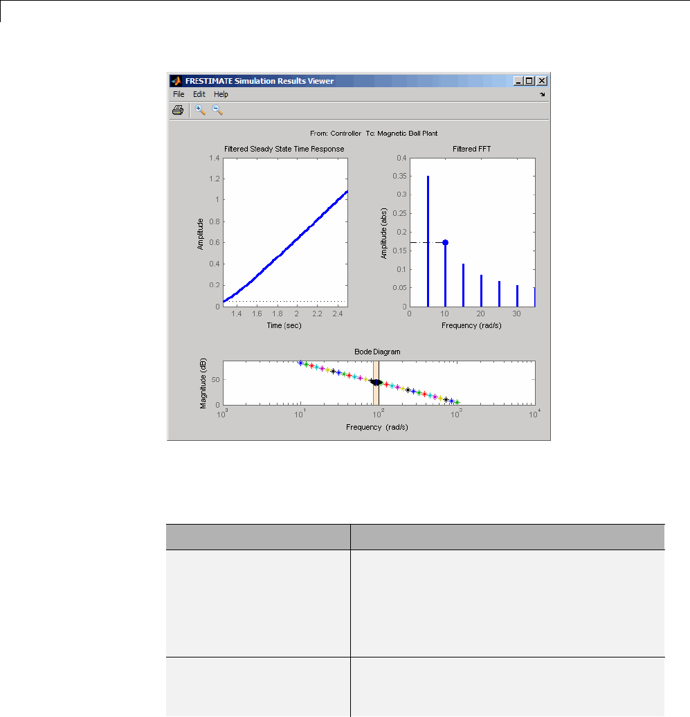
3Frequency Response Estimation
How Do I Fix It?
Try the suggested actions listed the table and repeat the estimation.
Possible Cause Action
Model is unstable. You cannot estimate the frequency response
using frestimate.Instead,useexact
linearization to get a linear representation of
your model. See “Linearize at Model Operating
Point” on page 2-38 or the linearize reference
page.
Stable model is not at
steady state.
Disable all source blocks in your model, and
repeat the estimation using a steady-state
operating point. See “Steady-State Operating
3-56
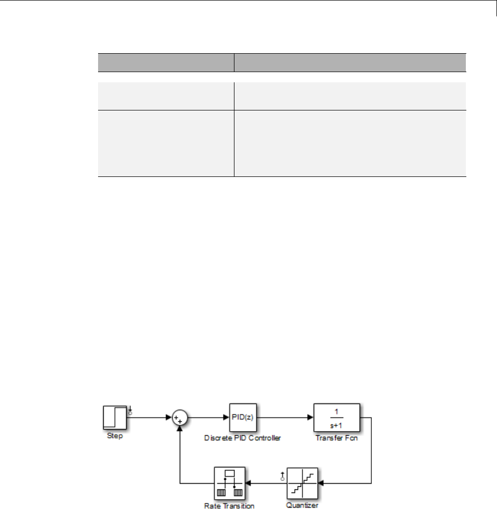
Troubleshooting Frequency Response Estimation
Possible Cause Action
Points (Trimming) from Specifications” on
page 1-14.
Stable model captures a
growing transient.
If the model captures a growing transient,
increase the number of periods in the input
signal by changing NumPeriods. Repeat the
estimation using a steady-state operating
point.
Time Response Is Discontinuous or Zero
What Does This Mean?
Discontinuities or noise in the time response indicate that the amplitude of
your input signal is too small to overcome the effects of the discontinuous
blocks in your model. Examples of discontinuous blocks include Quantizer,
Backlash, and Dead Zones.
If you used a sinestream input signal and estimated with filtering, turn
filtering off in the Simulation Results Viewer to see the unfiltered time
response.
The following model with a Quantizer block shows an example of the impact
of an input signal that is too small. When you estimate this model, the
unfiltered simulation output includes discontinuities.
3-57
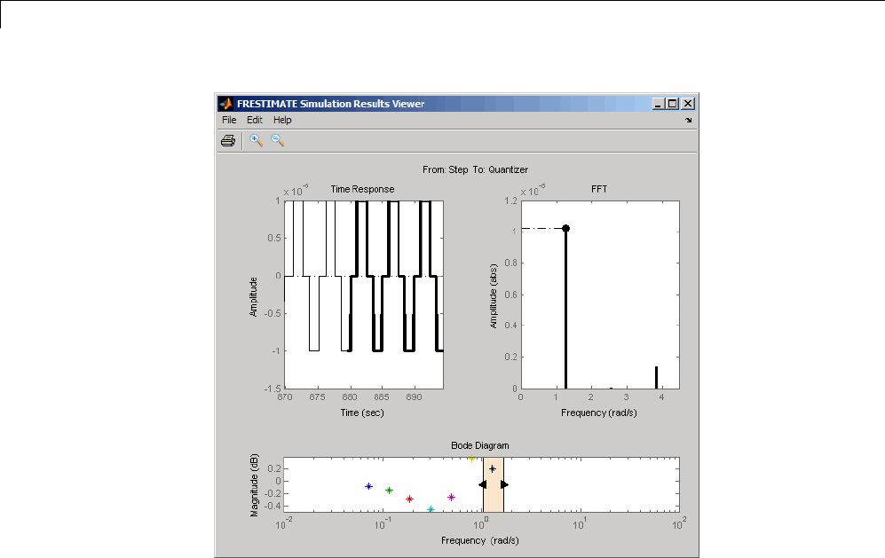
3Frequency Response Estimation
How Do I Fix It?
Increase the amplitude of your input signal, and repeat the estimation.
With a larger amplitude, the unfiltered simulated output of the model with a
Quantizer block is smooth.
3-58
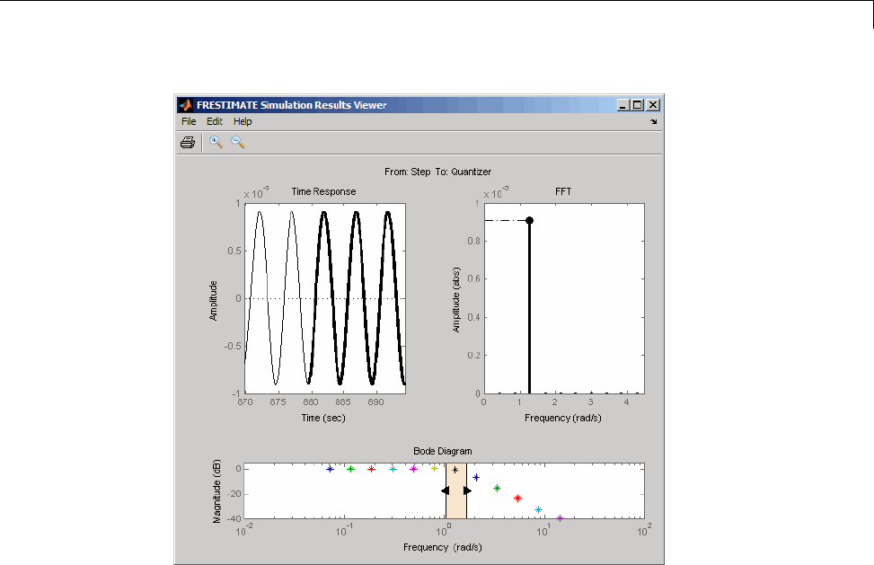
Troubleshooting Frequency Response Estimation
For more information about modifying signal amplitudes, see one of the
following:
•frest.Sinestream
•frest.Chirp
•“Modifying Input Signals for Estimation” on page 3-24
Time Response Is Noisy
What Does This Mean?
Whenthetimeresponseisnoisy,frequency response estimation results may
be biased.
3-59
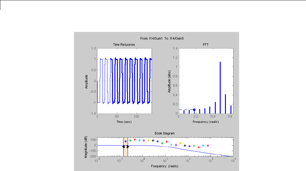
3Frequency Response Estimation
How Do I Fix It?
frestimate does not support estimating frequency response estimation of
Simulink models with blocks that model noise. Locate such blocks with
frest.findSources and disable them using the BlocksToHoldConstant
option of frestimate.
If you need to estimate a model with noise, use frestimate to simulate
an output signal from your Simulink model for estimation—without
modifying your model. Then, use the Signal Processing Toolbox™ or System
Identification Toolbox software to estimate a model.
To simulate the output of your model in response to a specified input signal:
3-60

Troubleshooting Frequency Response Estimation
1Create a random input signal. For example:
in = frest.Random('Ts',0.001,'NumSamples',1e4);
You can also specify your own custom signal as a timeseries object. For
example:
t = 0:0.001:10;
y = sin(2*pi*t);
in_ts = timeseries(y,t);
2Simulate the model to obtain the output signal. For example:
[sysest,simout] = frestimate(model,op,io,in_ts)
The second output argument of frestimate,simout,isa
Simulink.Timeseries object that stores the simulated output. in_ts is
the corresponding input data.
3Generate timeseries objects before using with other MathWorks®
products:
input = generateTimeseries(in_ts);
output = simout{1}.Data;
You can use data from timeseries objects directly in Signal Processing
Toolbox software, or convert these objects to System Identification Toolbox
data format. For examples, see “Estimating Frequency Response Models
with Noise Using Signal Processing Toolbox” on page 3-74 and “Estimating
Frequency Response Models with Noise Using System Identification
Toolbox” on page 3-76.
For a related example, see “Effects of Noise on Frequency Response
Estimation” on page 3-72.
3-61

3Frequency Response Estimation
Effects of Time-Varying Source Blocks on Frequency
Response Estimation
Setting Time-Varying Sources to Constant for
Estimation Using Linear Analysis Tool
This example illustrates the effects of time-varying sources on estimation.
The example also shows how to set time-varying sources to be constant during
estimation to improve estimation results.
1Open the Simulink model.
sys = 'scdspeed_ctrlloop';
open_system(sys);
2Linearize the model.
aSet the Engine Model block to normal mode for accurate linearization.
set_param('scdspeed_ctrlloop/Engine Model','SimulationMode','Normal')
bOpen the Linear Analysis Tool for the model.
In the Simulink Editor, select Analysis > Control Design > Linear
Analysis.
cSelect the visualization for the linearized model.
In the Plot Result list, select New Bode.
dClick .
The linearized model, linsys1,appearsintheLinear Analysis
Workspace.
3Create an input sinestream signal for the estimation.
aOpen the Create sinestream input dialog box.
In the Frequency Response Estimation tab, select Sinestream in
the Input Signal list.
bOpen the Add frequencies dialog box.
3-62
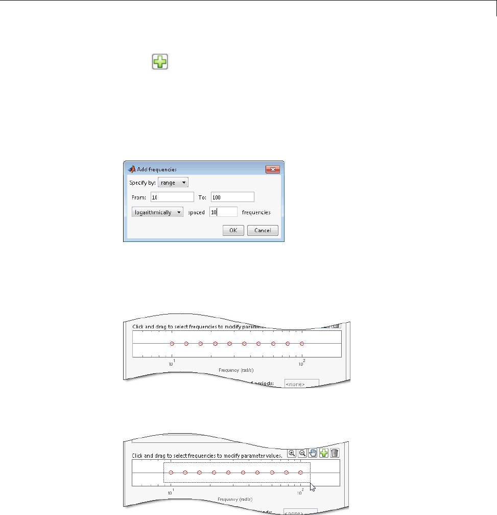
Effects of Time-Varying Source Blocks on Frequency Response Estimation
Click .
cSpecify the input sinestream frequency range and number of frequency
points.
Enter 100 in the To box.
Enter 10 in the box for the number of frequency points.
Click OK.
The added points are visible in the Frequency content viewer of the
Create sinestream input dialog box.
dIn the Frequency content viewer of the Create sinestream input dialog
box, select all the frequency points.
eSpecify input sinestream parameters.
3-63

3Frequency Response Estimation
For this example, change the Number of periods and Settling periods
to ensure that the model reaches steady-state for each frequency point in
the input sinestream.
Enter 30 in the Number of periods box.
Enter 25 in the Settling periods box.
fCreate the input sinestream.
Click OK. The new input signal, in_sine1,appearsintheLinear
Analysis Workspace.
4Select the visualization for the estimated model.
In the Plot Result list of the Linear Analysis Tool, select Bode Plot 1.
5Set the Diagnostic Viewer to open when estimation is performed.
Select the Launch Diagnostic Viewer check box.
6Estimate the frequency response for the model.
Click . The frequency response estimation result, estsys1,appearsin
the Linear Analysis Workspace.
7Compare the estimated model and the linearized model.
aClick the Diagnostic Viewer - estsys1 tab in the plot pane of the
Linear Analysis Tool.
bClick and drag linsys1 onto the Diagnostic Viewer to add linsys1 to
the Diagnostic Viewer plots.
cClick the Figures tab of the Linear Analysis Tool.
3-64
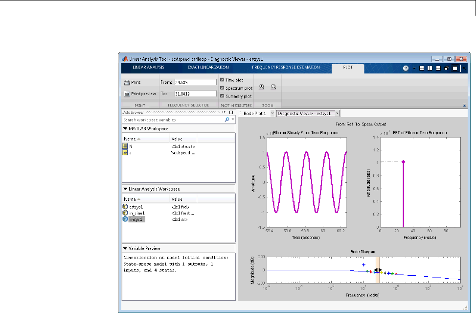
Effects of Time-Varying Source Blocks on Frequency Response Estimation
dConfigure the Diagnostic Viewer to show only the frequency point where
the estimation and linearization results do not match.
In the Frequency Selector section, enter 9 in the From box and 11 in
the To box to set the frequency range that is analyzed in the Diagnostic
Viewer.
3-65
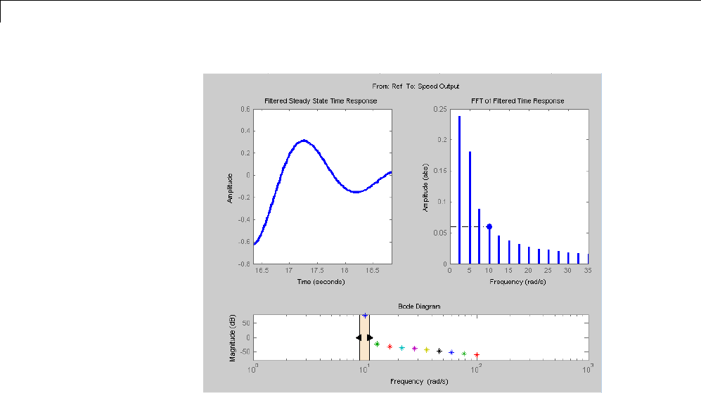
3Frequency Response Estimation
The Filtered Steady State Time Response plot depicts a signal that
is not sinusoidal.
eView the unfiltered time response.
Right-click the Filtered Steady State Time Response plot and clear
the Show filtered steady state output only option.
3-66
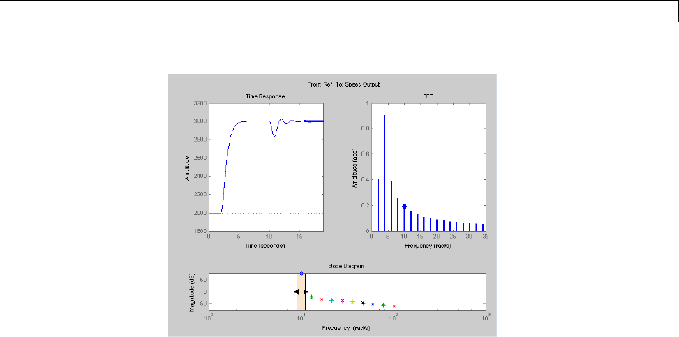
Effects of Time-Varying Source Blocks on Frequency Response Estimation
The step input and external disturbances drive the model away from
the operating point that the linearized model uses. This prevents the
response from reaching steady-state. To correct this problem, find and
disable the time-varying source blocks that interfere with the estimation.
Then estimate the frequency response of the model again.
8Find and disable the time-varying sources within the model.
aOpen the Options for frequency response estimation dialog box.
On the Frequency Response Estimation tab, in the Generate
Results section, click Options.
bIn the Time Varying Sources tab, click Find and add time varying
source blocks automatically.
This action populates the time varying sources list with the block paths
ofthetimevaryingsourcesinthemodel. These sources will be held
constant during estimation.
3-67
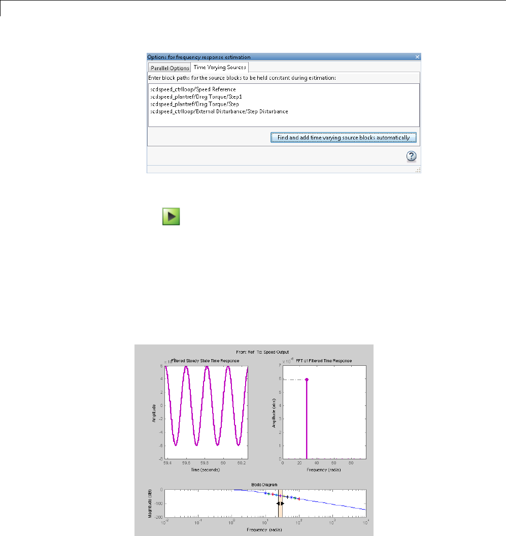
3Frequency Response Estimation
9Estimate the frequency response for the model.
Click . The frequency response estimation result for the model,
estsys2,appearsintheLinear Analysis Workspace.
10 Compare the newly estimated model and the linearized model.
Click on the Diagnostic Viewer - estsys2 tab in the plot area of the
Linear Analysis Tool.
Click and drag linsys1 onto the Diagnostic Viewer to add linsys1 to the
Diagnostic Viewer plots.
3-68

Effects of Time-Varying Source Blocks on Frequency Response Estimation
The frequency response obtained by holding the time-varying sources
constant matches the exact linearization results.
Setting Time-Varying Sources to Constant for
Estimation (MATLAB Code)
Compare the linear model obtained using exact linearization techniques with
the estimated frequency response:
% Open the model
mdl = 'scdspeed_ctrlloop';
open_system(mdl)
io = getlinio(mdl);
% Set the model reference to normal mode for accurate linearization
set_param('scdspeed_ctrlloop/Engine Model','SimulationMode','Normal')
% Linearize the model
sys = linearize(mdl,io);
% Estimate the frequency response between 10 and 100 rad/s
in = frest.Sinestream('Frequency',logspace(1,2,10),'NumPeriods',30,'SettlingPeriods',25);
[sysest,simout] = frestimate(mdl,io,in);
% Compare the results
frest.simView(simout,in,sysest,sys)
The linearization results do not match the estimated frequency response for
thefirsttwofrequencies.Toviewtheunfiltered time response, right-click the
time response plot, and uncheck Show filtered steady state output only.
3-69
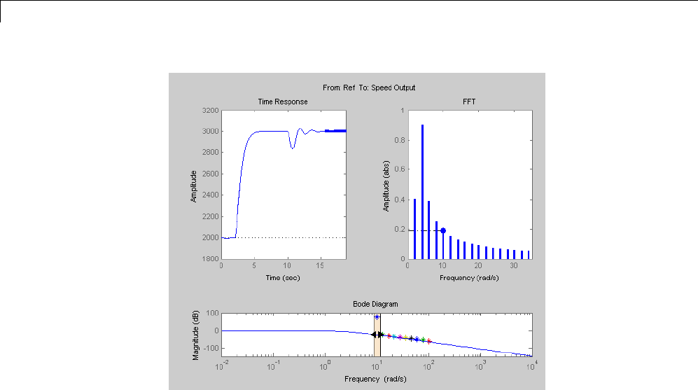
3Frequency Response Estimation
The step input and external disturbances drive the model away from the
operating point, preventing the response from reaching steady-state. To
correct this problem, find and disable these time-varying source blocks that
interfere with the estimation.
Identify the time-varying source blocks using frest.findSources:
srcblks = frest.findSources(mdl,io);
Create a frestimate options set to disable the blocks.
opts = frestimateOptions;
opts.BlocksToHoldConstant = srcblks;
Repeat the frequency response estimation using the optional input argument
opts.
[sysest2,simout2] = frestimate(mdl,io,in,opts);
frest.simView(simout2,in,sysest2,sys);
3-70
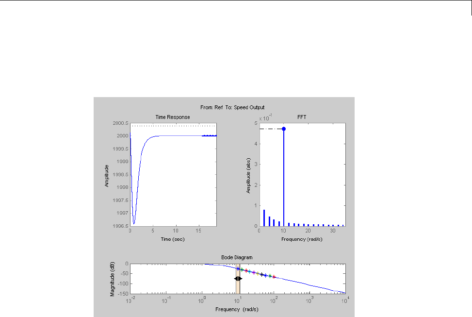
Effects of Time-Varying Source Blocks on Frequency Response Estimation
Now the resulting frequency response matches the exact linearization results.
To view the unfiltered time response, right-click the time response plot, and
uncheck Show filtered steady state output only.
3-71

3Frequency Response Estimation
Effects of Noise on Frequency Response Estimation
Compare the linear model obtained using exact linearization techniques with
the estimated frequency response:
mdl = 'f14';
open_system(mdl)
io(1) = linio('f14/Sum1',1)
io(2) = linio('f14/Gain5',1,'out')
sys = linearize(mdl,io);
in = frest.Sinestream(sys);
[sysest,simout] = frestimate(mdl,io,in);
frest.simView(simout,in,sysest,sys)
The resulting frequency response does not match the linearization results
due to the effects of the Pilot and Wind Gust Disturbance blocks. To view
the effects of effects of the noise on the time response of the first frequency,
right-click the time response plot and select Show filtered steady state
output only.
3-72
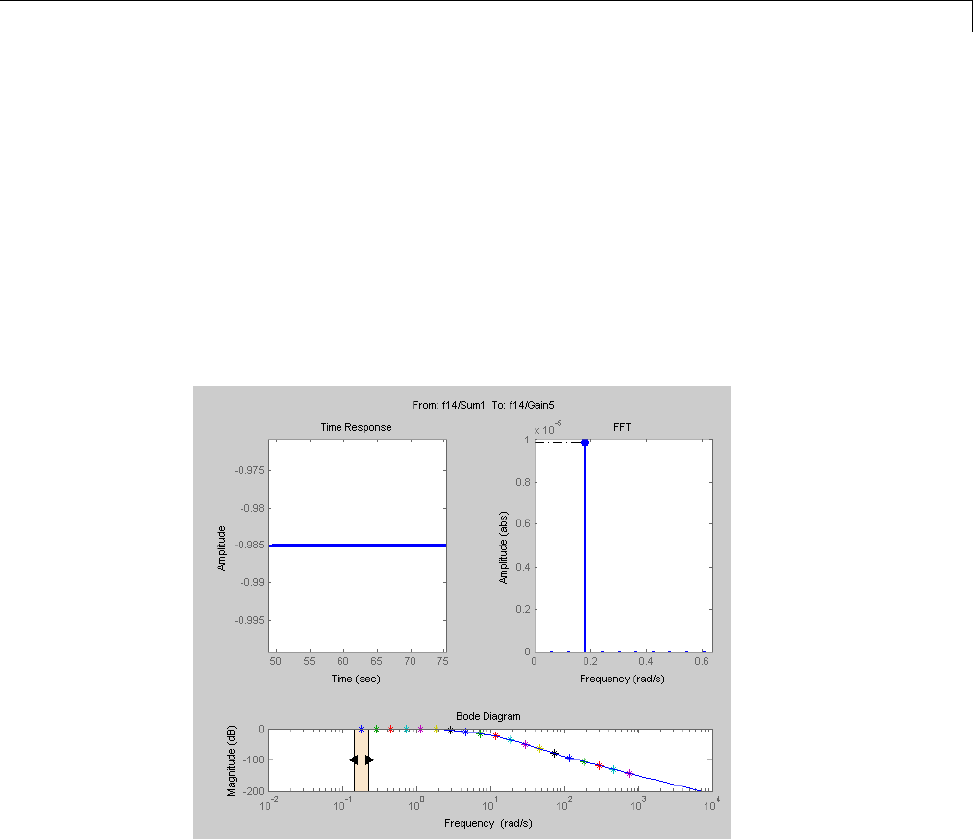
Effects of Noise on Frequency Response Estimation
Locate the source blocks:
srcblks = frest.findSources(mdl,io);
Repeat the frequency response estimation with the source blocks disabled:
opts = frestimateOptions('BlocksToHoldConstant',srcblks);
[sysest,simout] = frestimate(mdl,io,in,opts);
frest.simView(simout,in,sysest,sys);
The resulting frequency response matches the exact linearization results.
3-73

3Frequency Response Estimation
Estimating Frequency Response Models with Noise Using
Signal Processing Toolbox
Open the Simulink model, and specify which portion of the model to linearize:
load_system('magball');
io(1) = linio('magball/Desired Height',1);
io(2) = linio('magball/Magnetic Ball Plant',1,'out');
Create a random input signal for simulation:
in = frest.Random('Ts',0.001,'NumSamples',1e4);
Linearize the model at a steady-state operating point:
op = findop('magball',operspec('magball'),...
linoptions('DisplayReport','off'));
sys = linearize('magball',io,op);
Simulate the model to obtain the output at the linearization output point:
[sysest,simout] = frestimate('magball',io,in,op);
Estimate a frequency response model using Signal Processing Toolbox
software, which includes windowing and averaging:
input = generateTimeseries(in);
output = detrend(simout{1}.Data,'constant');
[Txy,F] = tfestimate(input.Data(:),...
output,hanning(4000),[],4000,1/in.Ts);
systfest = frd(Txy,2*pi*F);
Compare the results of analytical linearization and tfestimate:
ax=axes;
h = bodeplot(ax,sys,'b',systfest,'g',systfest.Frequency);
setoptions(h,'Xlim',[10,1000],'PhaseVisible','off');
legend(ax,'Linear model using LINEARIZE','Frequency response using Signal Processing Toolbox',...
'Location','SouthWest')
3-74
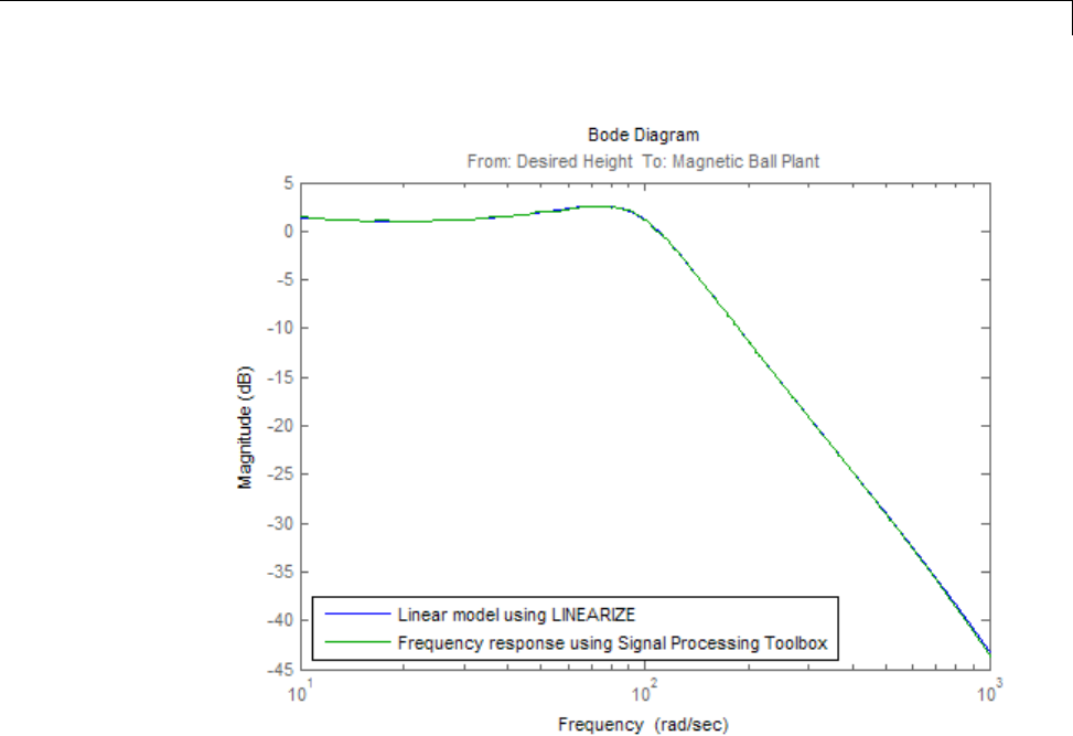
Estimating Frequency Response Models with Noise Using Signal Processing Toolbox™
In this case, the Signal Processing Toolbox command tfestimate gives a
more accurate estimation than frestimate duetowindowingandaveraging.
3-75

3Frequency Response Estimation
Estimating Frequency Response Models with Noise Using
System Identification Toolbox
Open the Simulink model, and specify which portion of the model to linearize:
load_system('magball');
io(1) = linio('magball/Desired Height',1);
io(2) = linio('magball/Magnetic Ball Plant',1,'out');
Compute the steady-state operating point, and linearize the model:
op = findop('magball',operspec('magball'),...
linoptions('DisplayReport','off'));
sys = linearize('magball',io,op);
Create a chirp signal, and use it to estimate the frequency response:
in = frest.Chirp('FreqRange',[1 1000],...
'Ts',0.001,...
'NumSamples',1e4);
[~,simout] = frestimate('magball',io,op,in);
Use System Identification Toolbox softwaretoestimateafifth-order,
state-space model. Compare the results of analytical linearization and the
state-space model:
input = generateTimeseries(in);
output = simout{1}.Data;
data = iddata(output,input.Data(:),in.Ts);
sys_id = n4sid(detrend(data),5,'cov','none');
bodemag(sys,ss(sys_id('measured')),'r')
legend('Linear model obtained using LINEARIZE',...
'State-space model using System Identification Toolbox',...
'Location','SouthWest')
3-76
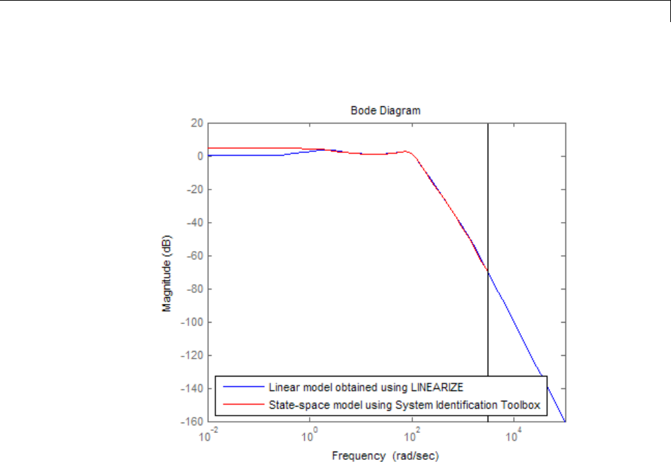
Estimating Frequency Response Models with Noise Using System Identification Toolbox™
3-77
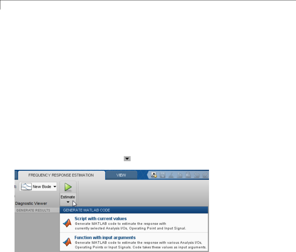
3Frequency Response Estimation
GenerateMATLABCodeforRepeatedorBatchFrequency
Response Estimation
This topic shows how to generate MATLAB code for frequency response
estimation from the Linear Analysis Tool. You can generate either a MATLAB
script or a MATLAB function. Generated MATLAB scripts are useful when
you want to programmatically reproduce a result you obtained interactively.
A generated MATLAB function allows you to perform multiple estimations
with systematic variations in estimation parameters such as operating point
(batch estimation).
To generate MATLAB code for estimation:
1In Linear Analysis Tool, on the Frequency Response Estimation tab,
interactively configure the input signal, analysis I/Os, operating point, and
other parameters for frequency response estimation.
2Click Estimate to open the Generate Matlab Code menu.
3Selectthetypeofcodeyou want to generate:
•Script with current values — Generate a MATLAB script that
uses your configured parameter values. Select this option when you
want to repeat the same frequency response estimation at the MATLAB
command line.
•Function with input arguments — Generate a MATLAB function
that takes analysis I/Os, operating points, and input signals as input
3-78

Generate MATLAB®Code for Repeated or Batch Frequency Response Estimation
arguments. Select this option when you want to perform multiple
frequency response estimations using different parameter values (batch
estimation).
To use a generated MATLAB function for batch estimation, you can create a
MATLAB script with a for loop that cycles through values of the parameter
you want to vary. Call the generated MATLAB function in each iteration of
the loop.
3-79

3Frequency Response Estimation
Managing Estimation Speed and Memory
In this section...
“Ways to Speed up Frequency Response Estimation” on page 3-80
“Speeding Up Estimation Using Parallel Computing” on page 3-82
“ManagingMemoryDuringFrequencyResponse Estimation” on page 3-86
Ways to Speed up Frequency Response Estimation
The most time consuming operation during frequency response estimation is
the simulation of your Simulink model. You can try to speed up the estimation
using any of the following ways:
•“Reducing Simulation Stop Time” on page 3-80
•“Specifying Accelerator Mode” on page 3-82
•“Using Parallel Computing” on page 3-82
Reducing Simulation Stop Time
The time it takes to perform frequency response estimation depends on the
simulation stop time.
To obtain the simulation stop time, select the input signal in the Linear
Analysis Workspace are of the Linear Analysis Tool. The simulation time will
be displayed in the Variable Preview.
3-80
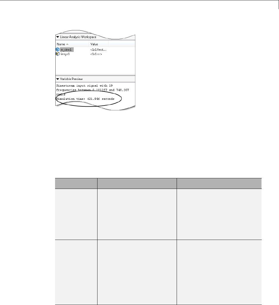
Managing Estimation Speed and Memory
To obtain the simulation stop time from the input signal using MATLAB Code:
tfinal = getSimulationTime(input)
where input is the input signal. The simulation stop time, tfinal,servesas
an indicator of the frequency response estimation duration.
You can reduce the simulation time by modifying your signal properties.
Input Signal Action Caution
Sinestream Decrease the number of
periods per frequency
NumPeriods,especiallyat
lower frequencies.
You model must be at
steady state to achieve
accurate frequency response
estimation. Reducing the
number of periods might not
excite your model long enough
to reach steady state.
Chirp Decrease the signal sample
time Ts or the number of
samples NumSamples.
The frequency resolution
of the estimated response
depends on the number
of samples NumSamples.
Decreasing the number
of samples decreases the
frequency resolution of
the estimated frequency
response.
3-81

3Frequency Response Estimation
For information about modifying input signals, see “Modifying Input Signals
for Estimation” on page 3-24.
Specifying Accelerator Mode
You can try to speed up frequency response estimation by specifying the
Rapid Accelerator or Accelerator mode in Simulink.
For more information, see “What Is Acceleration?” in the Simulink
documentation.
Using Parallel Computing
You can try to speed up frequency response estimation using parallel
computing in the following situations:
•Your model has multiple inputs.
•Your single-input model uses a sinestream input signal, where the
sinestream SimulationOrder property has the value 'OneAtATime'.
For information on setting this option, see the frest.Sinestream reference
page.
In these situations, frequency response estimation performs multiple
simulations. If you have installed the Parallel Computing Toolbox™ software,
youcanrunthesemultiplesimulationsinparallelonmultipleMATLAB
sessions (pool of MATLAB workers).
For more information about using parallel computing, see “Speeding Up
Estimation Using Parallel Computing” on page 3-82.
Speeding Up Estimation Using Parallel Computing
You can use parallel computing to speed up frequency response estimation
that performs multiple simulations, as described in “Using Parallel
Computing” on page 3-82.
Parallel computing for frequency response estimation requires the following
operations:
3-82

Managing Estimation Speed and Memory
•“Configuring MATLAB for Parallel Computing” on page 3-83
•“Estimating Frequency Response Using Parallel Computing (MATLAB
Code)” on page 3-85
Configuring MATLAB for Parallel Computing
•“Configuring Parallel Computing on Multicore Processors” on page 3-83
•“Configuring Parallel Computing on Multiprocessor Networks” on page 3-83
After you configure your system for parallel computing, estimate using
parallel computing. For further information, see “Estimating Frequency
Response Using Parallel Computing (MATLAB Code)” on page 3-85.
Configuring Parallel Computing on Multicore Processors. With a
Parallel Computing Toolbox license, you can establish a pool of parallel
MATLAB sessions in addition to the MATLAB client.
To start a pool of MATLAB sessions in local configuration, type the following
inputattheMATLABprompt:
matlabpool open local
To learn more, see the matlabpool reference page in the Parallel Computing
Toolbox documentation.
Configuring Parallel Computing on Multiprocessor Networks. Using
parallel computing on a multiprocessor network requires Parallel Computing
Toolbox software and the MATLAB Distributed Computing Server™ software.
To learn more, see the Parallel Computing Toolbox and MATLAB Distributed
Computing Server documentation.
To configure a multiprocessor network for parallel computing:
1Create a cluster profile to include any model file dependencies. See “Cluster
Profiles” in the Parallel Computing Toolbox documentation.
2Open the pool of MATLAB workers using the profile. See “Cluster Profiles”
in the Parallel Computing Toolbox documentation.
3-83
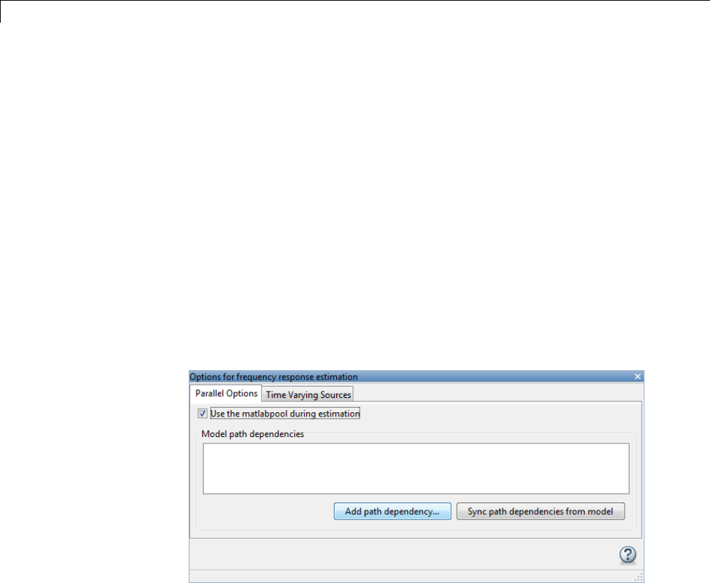
3Frequency Response Estimation
Opening the pool allows the remote workers to access the file dependencies
included in the user configuration file.
Estimating Frequency Response Using Parallel Computing
Using Linear Analysis Tool
After you configure your parallel computing settings, as described in
“Configuring MATLAB for Parallel Computing” on page 3-83, you can estimate
the frequency response of a Simulink model using the Linear Analysis Tool.
1In the Frequency Response Estimation tab of the Linear Analysis
Tool, click Options.
This action opens the Options for frequency response estimation dialog box.
2In the Parallel Options tab, select the Use the matlabpool during
estimation check box.
This action sets the estimation to use the matlabpool.
3(Optional) Click Add path dependecy.
The Browse For Folder dialog box opens. Navigate and select the directory
to add to the model path dependencies.
Click OK.
3-84

Managing Estimation Speed and Memory
Tip Alternatively, manually specify the paths in the Model path
dependencies list. You can specify the paths separated with a new line.
4(Optional) Click Sync path dependencies from model.
This action finds the model path dependencies in your Simulink model and
adds them to the Model path dependencies list box.
Estimating Frequency Response Using Parallel Computing
(MATLAB Code)
After you configure your parallel computing settings, as described in
“Configuring MATLAB for Parallel Computing” on page 3-83, you can
estimate the frequency response of a Simulink model.
1Find the paths to files that your Simulink model requires to run, called
path dependencies.
dirs = frest.findDepend(model)
dirs is a cell array of strings containing path dependencies, such as
referenced models, data files, and S-functions.
For more information about this command, see the frest.findDepend
reference page.
To learn more about model dependencies, see “What Are Model
Dependencies?” and “Scope of Dependency Analysis” in the Simulink
documentation.
2(Optional) Check that dirs includes all path dependencies. Append any
missing paths to dirs:
dirs = vertcat(dirs,'\\hostname\C$\matlab\work')
3(Optional) Check that all workers have access to the paths in dirs.
If any of the paths resides on your local drive, specify that all workers can
access your local drive. For example, this command converts all references
3-85

3Frequency Response Estimation
totheCdrivetoanequivalentnetworkaddressthatisaccessibletoall
workers:
dirs = regexprep(dirs,'C:/','\\\\hostname\\C$\\')
4Enable parallel computing and specify model path dependencies by creating
an options object using the frestimateOptions command:
options = frestimateOptions('UseParallel','on','ParallelPathDependencies',dirs)
Tip To enable parallel computing for all estimations, select the global
preference Use the matlabpool in FRESTIMATE command check box
in the MATLAB preferences. If your model has path dependencies, you
must create your own frequency response options object that specifies the
path dependencies before beginning estimation.
5Estimate the frequency response:
[sysest,simout] = frestimate('model',io,input,options)
For an example of using parallel computing to speed up estimation, see
Speeding Up Frequency Response Estimation Using Parallel Computing.
Managing Memory During Frequency Response
Estimation
Frequency response estimation terminates when the simulation data exceed
available memory. Insufficient memory occurs in the following situations:
•Your model performs data logging during a long simulation. A sinestream
input signal with four periods at a frequency of 1e-3 rad/s runs a Simulink
simulation for 25,000 s. If you are logging signals using To Workspace
blocks, this length of simulation time might cause memory problems.
•A model with an output point discrete sample time of 1e-8 s that simulates
at 5-Hz frequency (0.2 s of simulation per period), results in 02
18
2
.
e−=
million samples of data per period. Typically, this amount of data requires
over 300 MB of storage.
3-86

Managing Estimation Speed and Memory
To avoid memory issues while estimating frequency response:
1Disable any signal logging in your Simulink model.
Tolearnhowyoucanidentifywhichmodel components log signals and
disable signal logging, see “Signal Logging”.
2Try one or more of the actions listed in the following sections:
•“Model-Specific Ways to Avoid Memory Issues” on page 3-87
•“Input-Signal-Specific Ways to Avoid Memory Issues” on page 3-88
3Repeat the estimation.
Model-Specific Ways to Avoid Memory Issues
To avoid memory issues, try one or more of the actions listed in the following
table, as appropriate for your model type.
Model Type Action
Models with fast discrete sample
time specified at output point
Insert a Rate Transition block at the
output point to lower the sample
rate, which decreases the amount of
logged data. Move the linearization
output point to the output of the
Rate Transition block before you
estimate. Ensure that the location
of the original output point does
not have aliasing as a result of rate
conversion.
3-87

3Frequency Response Estimation
Model Type Action
Original location
of output point
New location
of output point
For information on determining
sample rate, see “View Sample Time
Information”. If your estimation
is slow, see “Ways to Speed up
Frequency Response Estimation” on
page 3-80.
Models with multiple input and
output points (MIMO models)
•Estimate the response for all
input/output combinations
separately. Then, combine the
results into one MIMO model
using the data format described in
“Frequency-Response Model”.
•Use parallel computing to run
the independent simulations in
parallel on different computers.
See “Speeding Up Estimation
Using Parallel Computing” on
page 3-82.
Input-Signal-Specific Ways to Avoid Memory Issues
To avoid memory issues, try one or more of the actions listed in the following
table, as appropriate for your input signal type.
3-88

Managing Estimation Speed and Memory
Input Signal Type Action
Sinestream •Remove low frequencies from your
input signal for which you do not
need the frequency response.
•Modify the sinestream signal
to estimate each frequency
separately by setting the
SimulationOrder option to
OneAtATime.Thenestimate
using a frestimate syntax
that does not request the
simulated time-response output
data, for example sysest =
frestimate(model,io,input).
•Use parallel computing to run
independent simulations in
parallel on different computers.
See “Speeding Up Estimation
Using Parallel Computing” on
page 3-82.
•Divide the input signal into
multiple signals using fselect.
Estimate the frequency response
for each signal separately using
frestimate.Then,combine
results using fcat.
Chirp Create separate input signals that
divide up the swept frequency
range of the original signal into
smaller sections using frest.Chirp.
Estimate the frequency response
for each signal separately using
frestimate. Then, combine results
using fcat.
Random Decrease the number of samples in
the random input signal by changing
NumSamples before estimating. See
3-89


4
Designing Compensators
•“Choosing a Compensator Design Approach” on page 4-2
•“Introduction to Automatic PID Tuning” on page 4-3
•“What Plant Does the PID Tuner See?” on page 4-4
•“PID Tuning Algorithm” on page 4-5
•“Designing Controllers with the PID Tuner” on page 4-6
•“Designing Two-Degree-of-Freedom PID Controllers” on page 4-18
•“Tuning a PID Controller Within a Model Reference” on page 4-20
•“Troubleshooting Automatic PID Tuning” on page 4-23
•“Designing a Simulink PID Controller (2DOF) Block for a Reactor” on page
4-29
•“Designing PID Controller in Simulink with Estimated Frequency
Response” on page 4-43
•“Designing a Family of PID Controllers for Multiple Operating Points”
on page 4-50
•“Design and Analysis of Control Systems” on page 4-57

4Designing Compensators
Choosing a Compensator Design Approach
Simulink Control Design provides two tools to tune Simulink blocks, such as
Transfer function and PID Controller blocks:
•PID Tuner
•SISO Design Tool
Use the following table to determine which tool supports what you want to do.
PID Tuner SISO Design Tool
Supported Blocks PID Controller
PID Controller 2DOF
Linear blocks
Loop Structure Single-loop control
systems
Single- or multi-loop
control systems
Control Design
Approach
Simple automatic
PID gain tuning by
specifying system
response time and
stability margins
Graphically tune poles
and zeros on design
plots, such as Bode,
root locus, and Nichols
Use a PID, LQG, IMC,
Robust Control Loop
Shaping, and Simulink
Design Optimization
automated tuning
method
Analysis of Control
System Performance
Step response for
reference tracking and
disturbance rejection
Open-loop Bode and
Nichols charts
Any combination of
responses for any
input reference or
disturbance in your
Simulink model using
SISO Tool LTIViewer
If you have a nonlinear plant, the software automatically linearizes your
model before tuning the controller blocks.
4-2

Introduction to Automatic PID Tuning
Introduction to Automatic PID Tuning
You can use the Simulink Control Design PID Tuner to tune PID gains
automatically in a Simulink model containing a PID Controller or PID
Controller (2DOF) block. The PID Tuner allows you to achieve a good balance
between performance and robustness for either one- or two-degree-of-freedom
PID controllers.
The PID Tuner:
•Automatically computes a linear model of the plant in your model. The
PID Tuner considers the plant to be the combination of all blocks between
the PID controller output and input. Thus, the plant includes all blocks
in the control loop, other than the controller itself. See “What Plant Does
the PID Tuner See?” on page 4-4.
•Automatically computes an initial PID design with a good trade-off between
performance and robustness. The PID Tuner bases the initial design upon
the open-loop frequency response of the linearized plant. See “PID Tuning
Algorithm” on page 4-5.
•Provides the PID Tuner GUI to help you interactively refine the
performance of the PID controller to meet your design requirements. See
“Designing Controllers with the PID Tuner” on page 4-6.
You can use the PID Tuner to design one- or two-degree-of-freedom PID
controllers. You can often achieve both good setpoint tracking and good
disturbance rejection using a one-degree-of-freedom PID controller. However,
depending upon the dynamics in your model, using a one-degree-of-freedom
PID controller can require a trade-off between setpoint tracking and
disturbance rejection. In such cases, if you need both good setpoint tracking
and good disturbance rejection, use a two-degree-of-freedom PID Controller.
For examples of tuning one- and two-degree-of-freedom PID compensators,
see:
•Automated Tuning of Simulink PID Controller Block
•“Designing a Simulink PID Controller (2DOF) Block for a Reactor” on page
4-29
4-3

4Designing Compensators
What Plant Does the PID Tuner See?
ThePIDTunerconsidersastheplantallblocksintheloopbetweenthePID
Controller block output and input. The blocks in your plant can include
nonlinearities. Because automatic tuning requires a linear model, the PID
Tuner computes a linearized approximation of the plant in your model.
This linearized model is an approximation to a nonlinear system, which is
generally valid in a small region around a given operating point of the system.
By default, the PID Tuner linearizes your plant using the initial conditions
specified in your Simulink model as the operating point. The linearized plant
can be of any order and can include any time delays. The PID tuner designs a
controller for the linearized plant.
In some circumstances, however, you want to design a PID controller for a
different operating point from the one defined by the model initial conditions.
For example:
•The Simulink model has not yet reached steady-state at the operating
point specified by the model initial conditions, and you want to design a
controller for steady-state operation.
•You are designing multiple controllers for a gain-scheduling application
and must design each controller for a different operating point.
In such cases, change the operating point used by the PID Tuner. See
“Opening the Tuner” on page 4-6.
For more information about linearization, see “Linearizing Nonlinear Models”
on page 2-2.
4-4

PID Tuning Algorithm
PID Tuning Algorithm
Typical PID tuning objectives include:
•Closed-loop stability — The closed-loop system output remains bounded for
bounded input.
•Adequate performance — The closed-loop system tracks reference changes
and suppresses disturbances as rapidly as possible. The larger the loop
bandwidth (the frequency of unity open-loop gain), the faster the controller
responds to changes in the reference or disturbances in the loop.
•Adequate robustness — The loop design has enough gain margin and phase
margin to allow for modeling errors or variations in system dynamics.
MathWorks algorithm for tuning PID controllers meets these objectives
by tuning the PID gains to achieve a good balance between performance
and robustness. The algorithm designs an initial controller by choosing
a bandwidth to achieve that balance, based upon the open-loop frequency
response of your linearized model. When you interactively change the
response time, bandwidth, or phase margin using the PID Tuner interface, the
algorithm computes new PID gains. (See “Designing Controllers with the PID
Tuner” on page 4-6 for information about using the PID Tuner interactively.)
4-5

4Designing Compensators
Designing Controllers with the PID Tuner
In this section...
“Prerequisites for PID Tuning” on page 4-6
“Opening the Tuner” on page 4-6
“Analyzing the Design in the PID Tuner” on page 4-8
“Refining the Design” on page 4-11
“Verifying the PID Design in Your Simulink Model” on page 4-14
“Tuning at a Different Operating Point” on page 4-15
Prerequisites for PID Tuning
Before you can use the PID Tuner, you must:
•Create a Simulink model containing a PID Controller or PID Controller
(2DOF) block. Your model can have one or more PID blocks, but you can
only tune one PID block at a time.
-If you are tuning a multi-loop control system with coupling between the
loops, consider using other Simulink Control Design tools instead of
the PID Tuner. See “Design and Analysis of Control Systems” on page
4-57 and Cascaded Multi-Loop/Multi-Compensator Feedback Design
for more information.
-The PID Controller blocks support vector signals. However, using the
PID Tuner requires scalar signals at the block inputs.
Your plant (all blocks in the control loop other than the controller) can
be linear or nonlinear. The plant can also be of any order, and have any
time delays.
•Configure the PID block settings, such as controller type, controller form,
time domain, sample time. See the PID Controller or PID Controller
(2DOF) block reference pages for more information about configuring these
settings.
Opening the Tuner
To open the PID Tuner and view the initial compensator design:
4-6

Designing Controllers with the PID Tuner
1Open the Simulink model by typing the model name at the MATLAB
command prompt.
2Double-click the PID Controller block to open the block dialog box.
3In the block dialog box, click Tune to launch the PID Tuner.
When you launch the PID Tuner, the following actions occur:
The PID Tuner automatically linearizes the plant at the operating point
specified by the model initial conditions, as described in “What Plant Does the
PID Tuner See?” on page 4-4. If you want to design a controller for a different
operating point, see “Tuning at a Different Operating Point” on page 4-15.
Note If the plant model in the PID loop linearizes to zero on launch, the PID
Tuner provides the Obtain plant model dialog box. This dialog box allows
you to obtain a new plant model by either:
•Linearizing at a different operating point (see “Tuning at a Different
Operating Point” on page 4-15).
•Importing an LTI model object representing the plant. For example, you
can import frequency response data (an frd model) obtained by frequency
response estimation. For more information, see Designing PID Controller
in Simulink with Estimated Frequency Response.
•The PID Tuner computes an initial compensator design using the algorithm
described in “PID Tuning Algorithm” on page 4-5.
•The PID Tuner displays the closed-loop step reference tracking response
for the initial compensator design in the PID Tuner dialog box. For
comparison, the display also includes the closed-loop response for the gains
specified in the PID Controller block, if that closed loop is stable, as shown
in the following figure.
4-7

4Designing Compensators
Tip After the tuner launches, you can close the PID Controller block dialog
box.
Analyzing the Design in the PID Tuner
To determine whether the compensator design meets your requirements, you
can analyze the system response using the response plots. Select a response
plot from the Response drop-down menu.
4-8
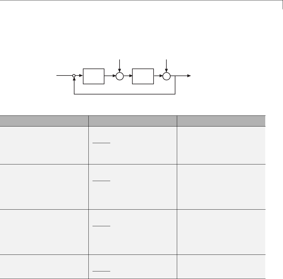
Designing Controllers with the PID Tuner
The PID Tuner computes the responses based upon the following single-loop
control architecture:
PID
Gy
+
-
rC
Plant
d1
+
+
d2
+
+
u
Thefollowingtablesummarizes the available responses.
Response Plotted System Description
Reference tracking
CG
CG1+(from rto y)
Shows the closed-loop system
response to a change in
setpoint. Use when your
design specifications include
setpoint tracking.
Controller effort
C
CG1+(from rto u)
Shows the closed-loop
controller output response
to a change in setpoint. Use
when your design is limited by
practical constraints, such as
controller saturation.
Input disturbance
Rejection G
CG1+(from d1to y)
Shows the closed-loop system
response to load disturbance
(a disturbance at the plant
input). Use when your design
specifications include input
disturbance rejection.
Output disturbance
Rejection 1
1+CG (from d2to y)
Shows the closed-loop system
response to measurement
noise.
4-9

4Designing Compensators
Response Plotted System Description
Open-loop CG Shows response of the
open-loop controller-plant
system. Use for
frequency-domain design.
Use when your design
specifications include
robustness criteria such
as open-loop gain margin and
phase margin.
Plant GShows the plant response. Use
to examine plant dynamics.
Use the Plot drop-down menu to choose Step plot (time-domain response) or
Bode plot (frequency-domain response).
You can view the values for system characteristics, such as peak response and
gain margin, either:
•Directly on the response plot — Use the right-click menu to add
characteristics, which appear as blue markers. Then, left-click the marker
to display the corresponding data panel.
•In the Performance and robustness table — To display this table, click
the Show Parameters arrow .
4-10
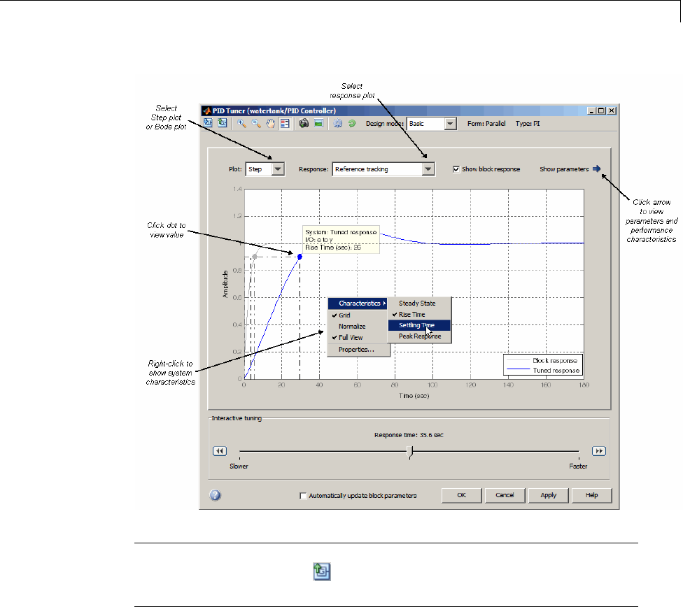
Designing Controllers with the PID Tuner
Tip To perform further analysis on the plant model, click the Export plant
model to workspace button to export the plant to the MATLAB workspace
as an LTI object.
Refining the Design
If the response of the initial controller design does not meet your
requirements, you can interactively adjust the design. The PID Tuner gives
you twowaystorefinethecontrollerdesign:
4-11
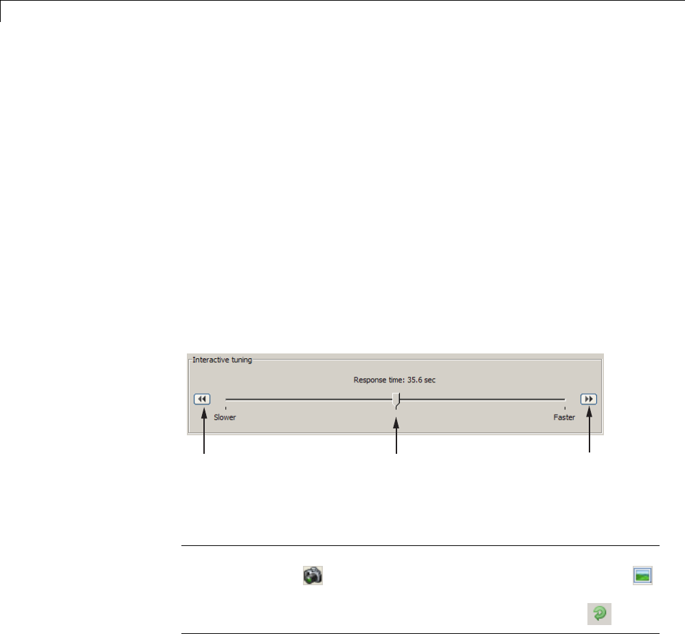
4Designing Compensators
•Adjust response time. Make the closed-loop response of the controlled
system faster or slower.
•Separately adjust loop bandwidth and phase margin. The larger the loop
bandwidth, the faster the controller responds to changes in the reference or
disturbances in the loop. The larger the phase margin, the more robust the
controller is against modeling errors or variations in plant dynamics.
Adjusting Response Time to Tune Parameters
To adjust response time to tune the controller response:
1In the PID Tuner, select Basic (the default option) from the Design mode
drop-down menu.
2MovetheResponsetimeslidertofind a PID controller that provides a
slower or faster response for your system.
Move slider to adjust
response time
Decrease
response time
by 10x
(less aggressive)
Increase
response time
by 10x
(more aggressive)
Tip To store a design and continue tuning without losing the design, click
the camera button . To retrieve this design, click the picture button .
To revert to the initial controller design, click the revert button .
3Analyze the compensator design to determine if it meets your design
requirements, as described in “Analyzing the Design in the PID Tuner”
on page 4-8.
•If the design meets your requirements, go to step 4.
4-12
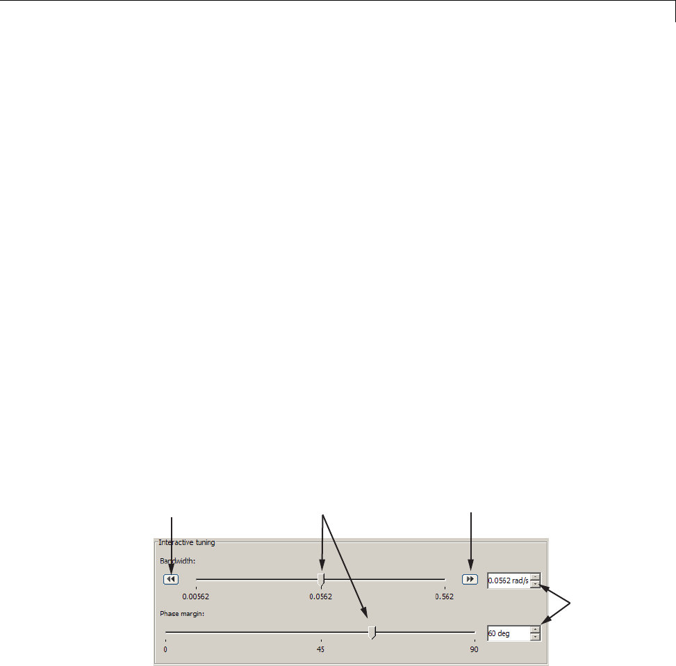
Designing Controllers with the PID Tuner
•If the design does not meet your requirements, try adjusting the
bandwidth and phase margin. For instructions, see “Adjusting
Bandwidth and Phase Margin to Tune Parameters” on page 4-13.
4If you find a compensator design that meets your requirements, verify
that it behaves in a similar way in the nonlinear Simulink model. For
instructions, see “Verifying the PID Design in Your Simulink Model” on
page 4-14.
Adjusting Bandwidth and Phase Margin to Tune Parameters
To adjust bandwidth and phase margin to tune the controller response:
1In the PID Tuner, select Extended from the Design mode drop-down
menu.
2Adjust the bandwidth and phase margin to find a PID controller with an
adequate balance between performance and robustness by:
•Moving the slider bar
•Entering a value in the text field
•Incrementally adjusting the value in the text field using the up and
down arrows
Move sliders to
adjust bandwidth
and phase margin
Increase slider
range by 10x
Decrease slider
range by 10x
Enter known
values or
adjust using
arrows
Theresponsetimeisgivenby2/wc,wherewcis the bandwidth. Therefore,
decreasing the bandwidth makes the controller less aggressive. Increasing
the bandwidth makes the controller more aggressive.
4-13

4Designing Compensators
For continuous-time systems, bandwidth is a finite positive real number.
For discrete-time systems, bandwidth is a positive real number less than
/Ts,whereTsis the PID Controller block sample time.
Decreasing the phase margin decreases robustness. Increasing the phase
margin increases robustness. Phase margin must be a number in the
range 0-90 degrees.
Tip To store a design and continue tuning without losing the design, click
the camera button . To retrieve this design, click the picture button .
To revert to the initial controller design, click the revert button .
3Analyze the compensator design to determine if it meets your design
requirements, as described in “Analyzing the Design in the PID Tuner”
on page 4-8.
•If the design meets your requirements, go to step 4.
•If you cannot find a compensator to meet your requirements by adjusting
bandwidth and phase margin, see “Cannot Find a Good Design in the
PID Tuner” on page 4-23.
4If you find a compensator design that meets your requirements, verify that
this design behaves in a similar way in the nonlinear Simulink model.
For instructions, see “Verifying the PID Design in Your Simulink Model”
on page 4-14.
Verifying the PID Design in Your Simulink Model
In the PID Tuner, you tune the compensator using a linear model of your
plant. First,youfindagoodcompensatordesigninthePIDTuner. Then,
verify that the tuned controller meets your design requirements when applied
to the nonlinear plant in your Simulink model.
To verify the compensator design in the nonlinear Simulink model:
4-14

Designing Controllers with the PID Tuner
1In the PID Tuner, click Apply to update the Simulink PID Controller block
with the tuned PID parameters.
Tip To update PID block parameters automatically as you tune the
controller in the PID Tuner, select Automatically update block
parameters.
2Simulate the Simulink model, and evaluate whether the simulation output
meets your design requirements.
Because the PID Tuner works with a linear model of your plant, the simulated
response sometimes does not match the response in the PID Tuner. See
“Simulated Response Does Not Match the PID Tuner Response” on page 4-24
for more information.
If the simulated response does not meet your design requirements, see
“CannotFindanAcceptablePIDDesignintheSimulatedModel”onpage4-25.
Tuning at a Different Operating Point
By default, the PID Tuner linearizes your plant and designs a controller at
the operating point specified by the initial conditions in your Simulink model.
In some cases, this operating point can differ from the operating point you
want to design a controller for. For example, you want to design a controller
for your system at steady-state. However, the Simulink model is not at
steady-state at the operating point specified in the model. In this case, change
the operating point that the PID Tuner uses for linearizing your plant and
designing a controller.
To set a new operating point for the PID Tuner, use one of the following
methods. The method you choose depends upon the information you have
about your desired operating point:
Known State Values Yield the Desired Operating Conditions
1Close the PID Tuner.
4-15

4Designing Compensators
2Set the initial conditions of the components of your model to the values that
yield the desired operating conditions.
3Click Tune in the PID Controller dialog box to launch the PID Tuner. The
PID Tuner linearizes the plant using the new default operating point and
designs a new initial controller for the new linear plant model.
After the PID Tuner generates a new initial controller design, continue from
“Analyzing the Design in the PID Tuner” on page 4-8.
Your Model Has Desired Operating Conditions at a Known
Time
1Click the Design with new plant model button in the PID Tuner to open
the Obtain plant model dialog box.
2Select Linearizing the Simulink model at simulation snapshot time
and enter a time value. Enter a time at which you expect the model to have
the desired equilibrium operating conditions.
3Click OK. The PID tuner linearizes the plant using the new operating point
and designs a new initial controller for the new linear plant model.
After the PID Tuner generates a new initial controller design, continue from
“Analyzing the Design in the PID Tuner” on page 4-8.
You Computed an Operating Point in the Control and
Estimation Tools Manager
1In the Control and Estimation Tools Manager, right-click on the node
corresponding to the saved operating point. Select Export to Workspace
to export your operating point to the MATLAB workspace.
2In the PID Tuner, click the Design with new plant model button to
open the Obtain plant model dialog box.
3Select Importing an LTI system or linearizing at an operating point
defined in MATLAB workspace.
4-16

Designing Controllers with the PID Tuner
4Select your exported operating point in the table. The operating point you
select appears highlighted.
5Click OK. The PID tuner linearizes the plant using the operating point at
the snapshot time and designs a new initial controller for the new linear
plant model.
After the PID Tuner generates a new initial controller design, continue from
“Analyzing the Design in the PID Tuner” on page 4-8.
4-17
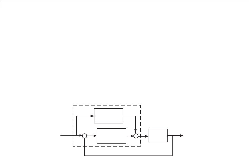
4Designing Compensators
Designing Two-Degree-of-Freedom PID Controllers
Use the PID Tuner to tune two-degree-of-freedom PID Controller (2DOF)
blocks to achieve both good setpoint tracking and good disturbance rejection.
About Two-Degree-of-Freedom PID Controllers
A two-degree-of-freedom PID compensator, commonly known as an ISA-PID
compensator, is equivalent to a feedforward compensator and a feedback
compensator, as shown in the following figure.
Feedfoward
compensator
Plant
Feedback
compensator
+
-
y
Two-degree-of-freedom
PID Controller
r
+
-
The feedforward compensator is PD and the feedback compensator is PID.
In the PID Controller (2DOF) block, the setpoint weights band cdetermine
the strength of the proportional and derivative action in the feedforward
compensator. See the PID Controller (2DOF) block reference page for more
information.
Tuning Two-Degree-of-Freedom PID Controllers
The PID Tuner tunes the PID gains P,I,D,andN. The tuner does not
automatically tune the setpoint weights band c. However, you can use the
PID Tuner to tune a two-degree-of-freedom PID controller by the following
process:
1Use the PID Tuner to tune the PID gains P,I,D,andNto meet your
disturbance rejection requirement.
4-18

Designing Two-Degree-of-Freedom PID Controllers
To tune this portion of the compensator, follow the procedure for tuning
a one-degree-of-freedom PID compensator, as described in “Analyzing the
Design in the PID Tuner” on page 4-8. and “Refining the Design” on page
4-11. Focus on the disturbance rejection plot to make sure that the tuned
controller meets your disturbance rejection requirements.
2After you have tuned the PID gains P,I,D,andN, update the PID Controller
(2DOF) block with the tuned parameters. To update the block, click Apply
in the PID Tuner, or select the Automatically update block parameters
check box.
3Adjust the setpoint weights band cof the feedforward portion of the
compensator to meet your setpoint tracking requirements as follows:
In the PID Controller (2DOF) block dialog box, enter values for the setpoint
weights band cbetween 0and 1.
To reduce undesirable controller response to sudden changes in the
reference signal (derivative kick), set cto 0. Typically, give bavalueinthe
range 0-1. Smaller bvalues generally result in slower reference tracking.
However, band cvalues do not affect loop stability or disturbance rejection.
4Evaluate whether the compensator design meets your design requirements
by viewing a simulation of the Simulink mode as described in “Verifying
the PID Design in Your Simulink Model” on page 4-14.
4-19
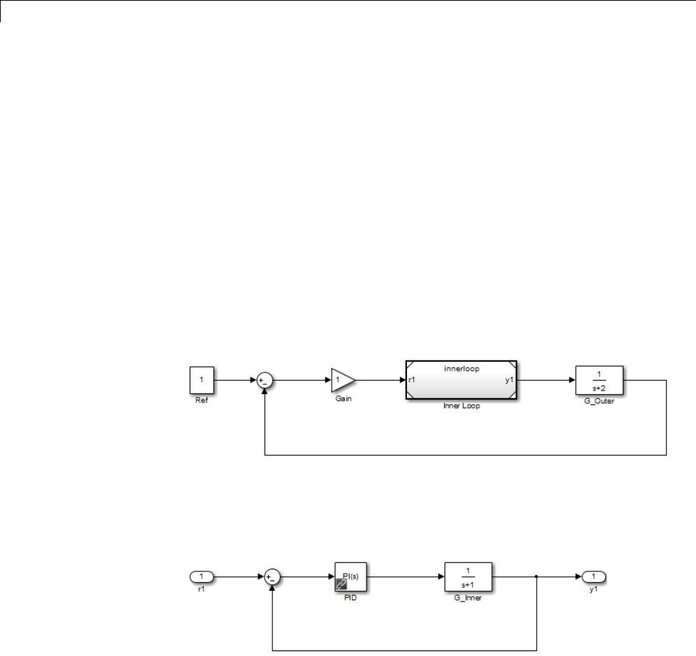
4Designing Compensators
Tuning a PID Controller Within a Model Reference
This example shows how to tune a PID controller block contained in a
referenced model.
When you launch the PID Tuner from a PID controller block in a model that
is referenced in one or more open models, the software prompts you to specify
which open model is the top-level model for linearization and tuning. The
referenced model must be in normal mode.
For more information about model referencing, see “Overview of Model
Referencing” in the Simulink documentation.
1Open the model.
open('model_ref_pid');
The block Inner Loop is a referenced model that contains the PID
Controller block to tune.
2Double-click Inner Loop to open the referenced model.
The referenced model innerloop contains a PID controller block, PID.
3Double-click the PID controller block PID to open the block dialog box.
4-20
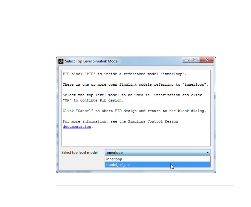
Tuning a PID Controller Within a Model Reference
4Click Tune in the block dialog box.
The software prompts you to select which open model is the top-level model
for linearization and tuning.
Note The software only identifies open models containing the model
reference. The PID Tuner does not detect models that contain the model
reference but are not open.
Selecting innerloop causes the PID Tuner to disregard model_ref_pid.
Instead, the PID Tuner tunes the PID Controller block for the plant
G_Inner alone, as if there were no outer loop.
Alternatively, you can select model_ref_pid as the top-level model. When
you do so, the PID Tuner considers the dynamics of both the inner and
outer loops, and tunes with both loops closed. In this case, PID controller
sees the effective plant (1+G_Outer*Gain)*G_Inner.
4-21


Troubleshooting Automatic PID Tuning
Troubleshooting Automatic PID Tuning
This section explains some procedures that can help you obtain better results
from the PID Tuner if the basic procedures yield unsatisfactory controller
performance.
In this section...
“Cannot Find a Good Design in the PID Tuner” on page 4-23
“Simulated Response Does Not Match the PID Tuner Response” on page
4-24
“Cannot Find an Acceptable PID Design in the Simulated Model” on page
4-25
“Controller Performance Deteriorates When Switching Time Domains”
on page 4-26
“When Tuning the PID Controller, the D Gain Has a Different Sign from
theIGain”onpage4-27
Cannot Find a Good Design in the PID Tuner
What This means
You have adjusted the PID Tuner sliders, but you cannot find a design that
meets your design requirements when you analyze the PID Tuner response
plots.
How to Fix It
Try a different PID controller type. It is possible that your controller type is
not the best choice for your plant or your requirements.
For example, the closed-loop step response of a P- or PD-controlled system
can settle on a value that is offset from the setpoint. If you require a zero
steady-state offset, adding an integrator (using a PI or PID controller) can
give better results.
As another example, in some cases a PI controller does not provide adequate
phase margin. You can instead try a PID controller to give the tuning
4-23

4Designing Compensators
algorithm extra degrees of freedom to satisfy both speed and robustness
requirements simultaneously.
To switch controller types, in the PID Controller block dialog box:
•Select a different controller type from the Controller drop-down menu.
•Click Apply to save the change.
•Click Tune to instruct the PID Tuner to tune the parameters for the new
controller type.
If you cannot find any satisfactory controller with the PID Tuner, PID control
possibly is not sufficient for your requirements. You can design more complex
controllers using the SISO Design Tool. For more information, see “Design
and Analysis of Control Systems” on page 4-57.
Simulated Response Does Not Match the PID Tuner
Response
What This Means
When you run your Simulink model using the PID gains computed by the PID
Tuner, the simulation output differs from the PID Tuner response plot.
There are several reasons why the simulated model can differ from the PID
Tuner response plot. If the simulated result meets your design requirements
(despite differing from the PID Tuner response), you do not need to refine
the design further. If the simulated result does not meet your design
requirements,see“CannotFindanAcceptablePIDDesignintheSimulated
Model” on page 4-25.
Some causes for a difference between the simulated and PID Tuner responses
include:
•The reference signals or disturbance signals in your Simulink model differ
from the step signals the PID Tuner uses. If you need step signals to
evaluate the performance of the PID controller in your model, change the
reference signals in your model to step signals.
4-24
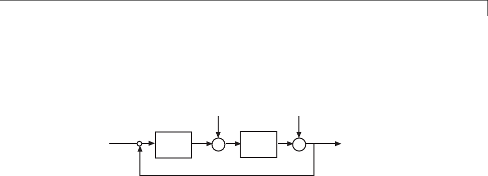
Troubleshooting Automatic PID Tuning
•The structure of your model differs from the loop structure that the PID
Tuner designs for. The PID Tuner assumes the loop configuration shown in
the following figure.
PID
Gy
+
-
rC
Plant
d1
+
+
d2
+
+
u
As the figure illustrates, the PID Tuner designs for a PID in the feedforward
path of a unity-gain feedback loop. If your Simulink model differs from
this structure, or injects a disturbance signal in a different location, your
simulated response differs from the PID Tuner response.
•You have enabled nonlinear features in the PID Controller block in your
model, such as saturation limits or anti-windup circuitry. The PID Tuner
ignores nonlinear settings in the PID Controller block, which can cause the
PID Tuner to give a different response from the simulation.
•Your Simulink model has strong nonlinearities in the plant that make the
linearization invalid over the full operating range of the simulation.
•You selected an operating point using the PID Tuner that is different from
the operating point saved in the model. In this case, the PID Tuner has
designed a controller for a different operating point than the operating
point that begins the simulation. Simulate your model using the PID Tuner
operating point by initializing your Simulink model with this operating
point. See “Simulate Simulink Model at Specific Operating Point” on page
1-44.
Cannot Find an Acceptable PID Design in the
Simulated Model
What This Means
You tune the PID Controller using the PID Tuner and run your Simulink
model with the tuned PID gains. However, the simulated response of your
model does not meet your design requirements.
4-25

4Designing Compensators
How to Fix It
In some cases, PID control is not adequate to meet the control requirements
for your plant. If you cannot find a design that meets your requirements
when you simulate your model, consider using a more complex controller. See
“Design and Analysis of Control Systems” on page 4-57.
If you have enabled saturation limits in the PID Controller block without
antiwindup circuitry, enable antiwindup circuitry. You can enable antiwindup
circuitry in two ways:
•Activate the PID Controller block antiwindup circuitry on the PID
Advanced tab of the block dialog box.
•Use the PID Controller block tracking mode to implement your own
antiwindup circuitry external to the block. Activate the PID Controller
block tracking mode on the PID Advanced tab of the block dialog box.
To learn more about both ways of implementing antiwindup circuitry, see
Anti-Windup Control Using a PID Controller.
After enabling antiwindup circuitry, run the simulation again to see whether
controller performance is acceptable.
If the loop response is still unacceptable, try slowing the response of the PID
controller. Todoso,reducetheresponsetimeorthebandwidthinthePID
Tuner. See “Adjusting Response Time to Tune Parameters” on page 4-12 and
“Adjusting Bandwidth and Phase Margin to Tune Parameters” on page 4-13.
If you still cannot find an acceptable controller with antiwindup circuitry
enabled in the PID Controller block, consider using a more complex controller.
See “Design and Analysis of Control Systems” on page 4-57.
Controller Performance Deteriorates When Switching
Time Domains
What This Means
You obtain a well-tuned continuous-time PID controller. Then, you convert
the controller time domain using the Time Domain selector button in the
4-26

Troubleshooting Automatic PID Tuning
PID Controller block dialog box. The controller performs poorly or even
becomes unstable when you convert the controller to discrete time.
How To Fix It
In some cases, you can improve performance by adjusting the sample time by
trial and error. However, this procedure can yield a poorly tuned controller,
especially where your application imposes a limit on the sample time. Instead,
if you change time domains and the response deteriorates, click Tunein the
PID Controller block dialog to design a new controller.
Note If the plant and controller time domains differ, the PID Tuner
discretizes the plant (or converts the plant to continuous time) to match the
controller time domain. If the plant and controller both use discrete time, but
have different sample times, the PID Tuner resamples the plant to match the
controller. All conversions use the tustin method (see “Continuous-Discrete
Conversion Methods” in the Control System Toolbox User’s Guide).
When Tuning the PID Controller, the D Gain Has a
Different Sign from the I Gain
What This Means
When you use the PID Tuner to design a controller, the resulting derivative
gain Dcan have a different sign from the integral gain I. The PID Tuner
always returns a stable controller, even if one or more gains are negative.
For example, the following expression gives the PID controller transfer
function in Ideal form:
cP s
Ds
s
N
PDN s I N s IN
ss N
=++
+
⎛
⎝
⎜
⎜
⎜
⎜
⎞
⎠
⎟
⎟
⎟
⎟
=+
()
++
()
+
+
()
11
1
12
For a stable controller, all three numerator coefficients require positive
values. Because Nis positive, IN > 0 requires that Iis also positive.
4-27

4Designing Compensators
However, the only restriction on Dis (1 + DN) > 0. Therefore, as long as
DN > –1, a negative Dstill yields a stable PID controller.
SimilarreasoningappliesforanycontrollertypeandfortheParallel
controller form. For more information about controller transfer functions, see
the PID Controller block reference page.
4-28

Designing a Simulink PID Controller (2DOF) Block for a Reactor
Designing a Simulink PID Controller (2DOF) Block for a
Reactor
This example shows how to use PID Tuner to tune a Simulink PID Controller
(2DOF) block.
Introduction of the PID Controller (2DOF) Block
With a 2DOF PID controller, also known as ISA-PID controller, you can
achieve good performance for both reference tracking and disturbance
rejection. It contains a standard PID controller in the feedback loop and adds
a pre-filter to the reference signal. The pre-filter helps produce a smoother
transientresponsetoset-pointchanges. In this example, you use a Simulink
PID Controller (2DOF) block to control a continuous stirred tank reactor
(CSTR) and you design this 2DOF PID controller in the PID Tuner.
A typical design workflow with the PID Tuner involves the following tasks:
(1) Launch the PID Tuner. When launching, the software automatically
computes a linear plant model from the Simulink model and designs an
initial controller.
(2) Tune the controller in the PID Tuner by manually adjusting design criteria
in two design modes. The tuner computes PID parameters that robustly
stabilize the system.
(3) Export the parameters of the designed controller back to the PID
Controller block and verify controller performance in Simulink.
Opening the Model
Open the CSTR control model and take a few moments to explore it.
open_system('scdcstrctrlpidblock');
4-29
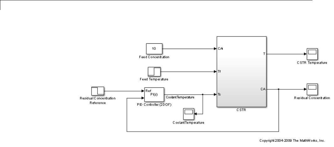
4Designing Compensators
The CSTR plant is initialized at an equilibrium operating point. The nominal
value of the residual concentration is 1.96 mol/L, which is the initial condition
of the Residual Concentration Reference block and the Integrator1
block in the CSTR subsystem.
The initial condition of the integrator I0 in the PID controller block is
determined by the equilibrium operating point. In this example, since we
have a PI controller in parallel form,
I0 = u0 - ((b-1)*y0*P)
where u0 is the steady state controller output (300), and y0 is the steady
state plant output (1.96). Since bis 1, I0=*u0*=300.
For background, see Seborg, D.E. et al., "Process Dynamics and Control", 2nd
Ed., 2004, Wiley, pp.34-36.
Design Overview
In this example, control the residual concentration of the CSTR by
manipulating reactor coolant temperature. The overall design requirements
are:
4-30
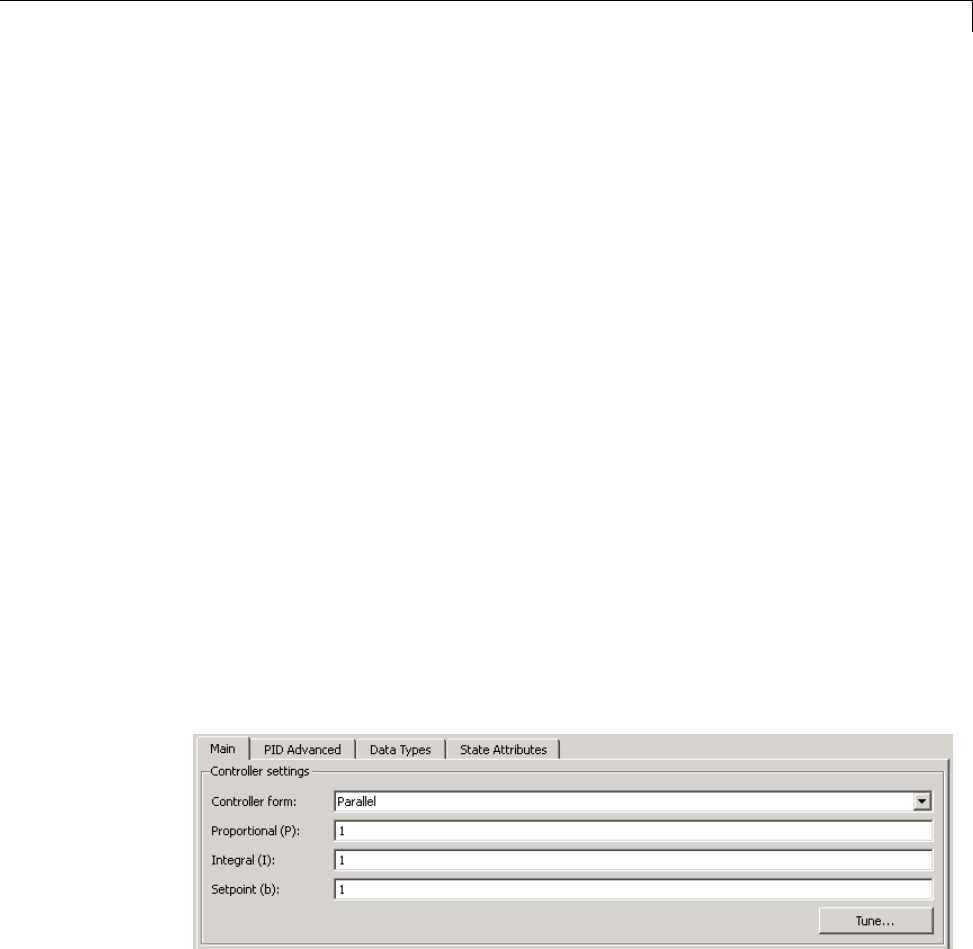
Designing a Simulink PID Controller (2DOF) Block for a Reactor
•Track a sudden decrease of 0.5 in the reference signal from a Simulink
step block Residual Concentration Reference. The detailed design
requirements are:
Settling time under 10 seconds
Zero steady-state error to the step reference input
Overshoot below 0.1
•Reject a 5 degree sudden increase in the feed temperature from a Simulink
step block Feed Temperature. The detailed design requirements are:
Settling time under 10 seconds
Peak deviation from steady state below 0.1
In this example you design a PI controller PID Controller (2DOF) in
the PID Tuner to achieve good responses in both reference tracking and
disturbance rejection.
Opening the PID Tuner
To launch the PID Tuner, double-click the PID Controller block to open its
block dialog. In the Main tab, click Tune.
After you launch the PID Tuner, close the PID block dialog and move the
PID Tuner beside the Simulink model. Also, open the residual concentration
scope window.
4-31

4Designing Compensators
Initial PID Design
When the PID Tuner launches, the software computes a linearized plant
model. The software automatically identifies the plant input and output, and
uses the current operating point for the linearization. The plant can have
any order and can have time delays.
The PID Tuner computes an initial PI controller to achieve a reasonable
tradeoff between performance and robustness. By default, step reference
tracking performance displays in the plot.
Click the Show parameters arrow to view controller parameters P, I, b, and
a set of performance and robustness measurements. In this example, the
initial PI controller design gives a settling time of 4.4 second, which meets
the requirement.
The following figure shows the PID Tuner dialog with initial design:
4-32
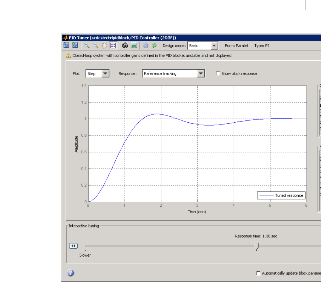
Designing a Simulink PID Controller (2DOF) Block for a Reactor
To test the initial design on the nonlinear model, click Apply in the PID
Tuner. This writes the parameters back to the PID block in the Simulink
model. Run a simulation and view the closed-loop response:
4-33
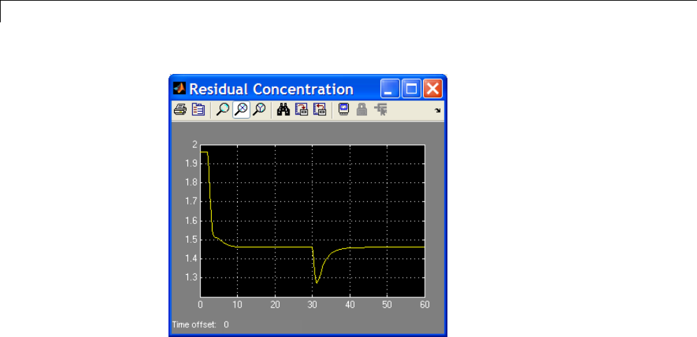
4Designing Compensators
The transient response of disturbance rejection shows that its peak deviation
is about 0.2, which exceeds the design requirement. You need to reduce the
peak deviation by at least 50% using the PID Tuner.
Design for Disturbance Rejection in the Basic Design Mode
The PID Tuner provides step plot for different loop responses such as
reference tracking (from r to y) and controller efforts (from r to u), etc. In this
example since the disturbance occurs at the reactor feed temperature, the
closestplotyoucangetistheinputdisturbance rejection plot that assumes a
step disturbance occurs at the input of the plant model.
The following figure shows the disturbance rejection performance with initial
controller:
4-34
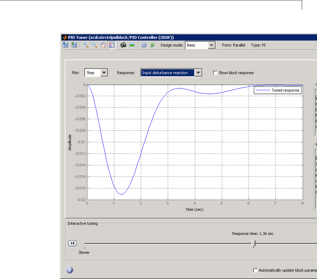
Designing a Simulink PID Controller (2DOF) Block for a Reactor
You need to reduce the peak deviation from -0.019 to -0.009 (about 50%).
First, try to reduce the peak deviation using the Basic design mode, which is
the mode selected when the Tuner opens. Move the response time slider to
the right to decrease the response time and make controller more aggressive.
But you cannot meet the design requirements because reducing the peak
4-35
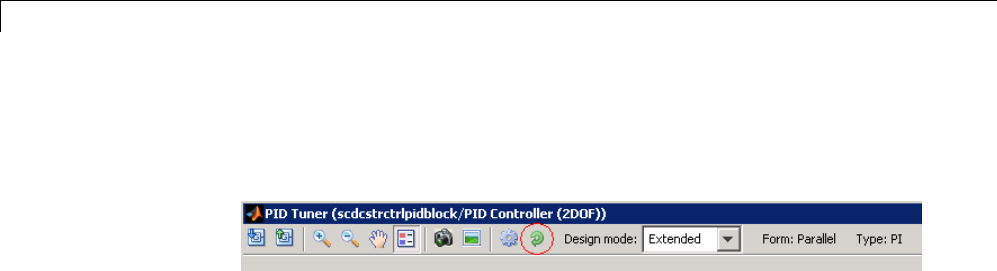
4Designing Compensators
deviation makes the settling time too long. To return to the initial automated
design result, click the reset button in the toolbar that is the last button
with green arrow.
Design for Disturbance Rejection in the Extended Design Mode
In the PID Tuner Extended design mode, you have more flexibility to adjust
controller performance. You need some knowledge of frequency domain
control design technology to take full advantage of this design mode.
To switch to the Extended design mode, select Extended in the Design
Mode drop-down menu in the toolbar.
The following figure shows the PID Tuner in Extended design mode with
the initial design:
4-36
Designing a Simulink PID Controller (2DOF) Block for a Reactor
Increasing the bandwidth makes the controller more aggressive and reduces
the peak deviation. To maintain the settling time of disturbance rejection
below 10 seconds, you also need to reduce the desired phase margin. This is
4-37

4Designing Compensators
a typical tradeoff between performance and robustness in controller design.
Viewtheeffectsofyourchangeintheresponseplot. Youcanmoveboth
sliders to reduce the peak deviation to 0.007 while maintain the settling time
within 10 seconds. One way to achieve this is:
•Bandwidth of 4 rad/sec
•Phase margin of 25 degree
The following figure shows disturbance rejection performance:
4-38
Designing a Simulink PID Controller (2DOF) Block for a Reactor
To test the new design on the nonlinear model, click Apply in the PID Tuner.
Run a simulation and view the closed-loop response:
4-39
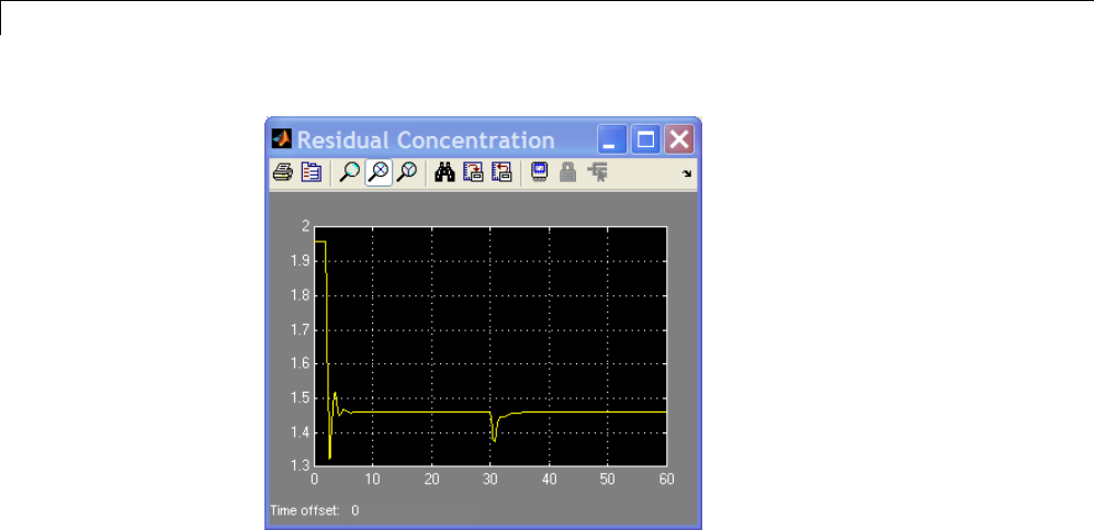
4Designing Compensators
The disturbance rejection performance satisfies the requirements. However,
because the controller is very aggressive, the overshoot of reference tracking
exceeds the limit. You need to adjust the pre-filter in the 2DOF PID block to
improve the reference tracking performance.
Completing PID Design with Set-point Weighting
The parameter bin an ISA PI or PID controller is the set-point weight on the
reference signal feeding into the proportional gain of the controller. It has a
range between 0 and 1, and its default value is 1. By reducing its value, the
reference tracking performance becomes smoother. In this example, open
the PID block dialog and set bto 0.
Because band Pare changed, you need to adjust the initial condition of the
integrator I0 inthePIDcontrollerblocktomakesuretheinitialoperating
point is still at equilibrium. Since the relationship is
I0 = u0 - ((b-1)*y0*P)
where u0 is 300 and y0 is 1.96. With Pfrom PID Tuner (-153.5) and bfrom
manual adjustment (0), I0 becomes -0.8267. Update the initial condition of
the integrator with this value and the simulation will start at the equilibrium
operating point.
4-40
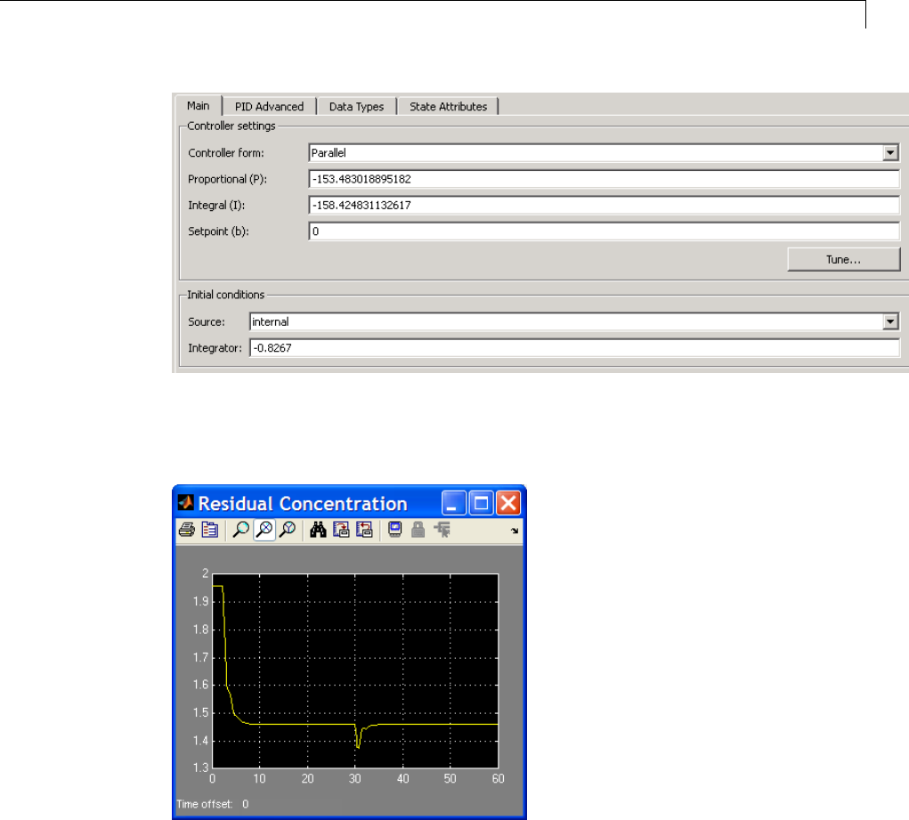
Designing a Simulink PID Controller (2DOF) Block for a Reactor
The following figure shows that there is no overshoot in reference tracking
with the updated design.
In summary, to design a 2DOF PID controller with balanced performance in
reference tracking and disturbance rejection, use the PID Tuner to achieve
good disturbance rejection and then manually adjust set-point weights b
and/or cin the block dialog to achieve good reference tracking. Notice that
4-41

4Designing Compensators
changing band cdoes not affect closed-loop stability or disturbance rejection
performance.
bdclose('scdcstrctrlpidblock')
4-42
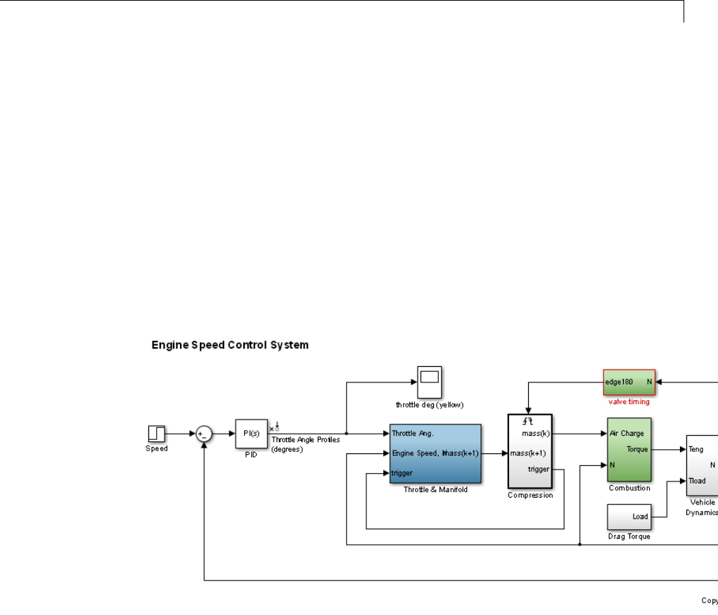
Designing PID Controller in Simulink with Estimated Frequency Response
Designing PID Controller in Simulink with Estimated
Frequency Response
This example shows how to design a PI controller with frequency response
estimated from a plant built in Simulink. This is an alternative PID design
workflow when the linearized plant model is invalid for PID design (for
example, when the plant model has zero gain).
Opening the Model
Open the engine control model and take a few moments to explore it.
mdl = 'scdenginectrlpidblock';
open_system(mdl)
The PID loop includes a PI controller in parallel form that manipulates the
throttle angle to control the engine speed. The PI controller has default gains
that makes the closed loop system oscillate. We want to design the controller
using the PID Tuner that is launched from the PID block dialog.
open_system([mdl '/Engine Speed (rpm)'])
sim(mdl);
4-43
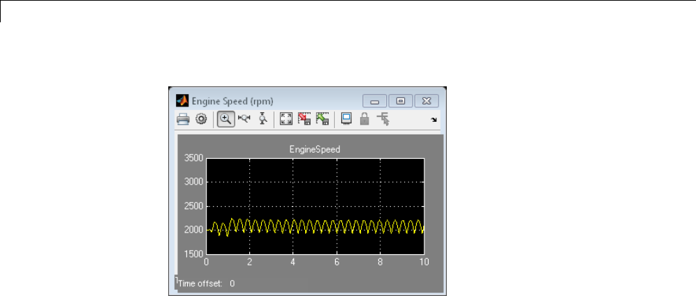
4Designing Compensators
PID Tuner Obtaining a Plant Model with Zero Gain From Linearization
In this example, the plant seen by the PID block is from throttle angle to
engine speed. Linearization input and output points are already defined
at the PID block output and the engine speed measurement respectively.
Linearization at the initial operating point gives a plant model with zero gain.
% Hide scope
close_system([mdl '/Engine Speed (rpm)'])
% Obtain the linearization input and output points
io = getlinio(mdl);
% Linearize the plant at initial operating point
linsys = linearize(mdl,io)
linsys=
d=
Throttle Ang
EngineSpeed 0
Static gain.
The reason for obtaining zero gain is that there is a triggered subsystem
"Compression"inthelinearizationpathandtheanalyticalblock-by-block
4-44
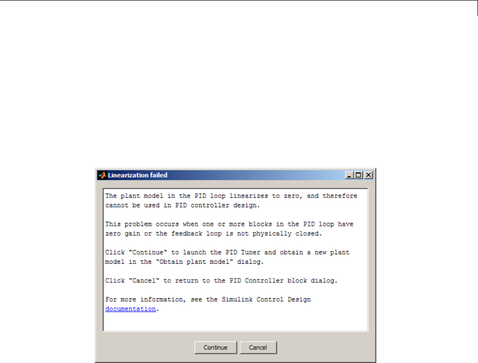
Designing PID Controller in Simulink with Estimated Frequency Response
linearization does not support events-based subsystems. Since the PID Tuner
uses the same approach to obtain a linear plant model, the PID Tuner also
obtains a plant model with zero gain and reject it during the launching
process.
To launch the PID Tuner, open the PID block dialog and click Tune button.
An information dialog shows up and indicates that the plant model linearized
at initial operating point has zero gain and cannot be used to design a PID
controller.
Thealternativewaytoobtainalinearplant model is to directly estimate the
frequency response data from the Simulink model, create an FRD system in
MATLAB Workspace, and import it back to the PID Tuner to continue PID
design.
Obtaining Estimated Frequency Response Data Using Sinestream Signals
Sinestream input signal is the most reliable input signal for estimating an
accurate frequency response of a Simulink model using frestimate command.
More information on how to use frestimate canbefoundintheexample
4-45
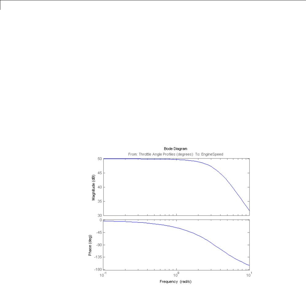
4Designing Compensators
"Frequency Response Estimation Using Simulation-Based Techniques" in
Simulink Control Design examples.
In this example, we create a sine stream that sweeps frequency from 0.1 to
10 rad/sec. Its amplitude is set to be 1e-3. You can inspect the estimation
results using the bode plot.
% Construct sine signal
in = frest.Sinestream('Frequency',logspace(-1,1,50),'Amplitude',1e-3);
% Estimate frequency response
sys = frestimate(mdl,io,in); % this command may take a few minutes to fini
s
% Display Bode plot
figure;
bode(sys);
Designing PI with the FRD System in PID Tuner
SYS is a FRD system that represents the plant frequency response at the
initial operating point. To use it in the PID Tuner, we need to import it after
4-46
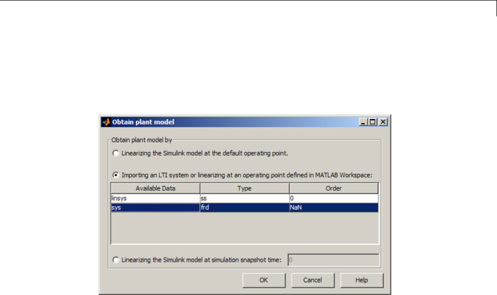
Designing PID Controller in Simulink with Estimated Frequency Response
the Tuner is launched. Open the PID block dialog and click Tune button
again. When the information dialog shows up, click "Continue" to resume the
launching process. After the PID Tuner is launched, an "Obtain Plant Model"
dialog shows up and asks you to import a new plant model for PID design.
Clicktheradiobuttoninthemiddle,select "sys" from the list, and click "OK"
to import the FRD system into the PID Tuner. The automated design returns
a stabilizing controller. Select "Open-loop" as the response in the Bode plot
and the plot shows reasonable gain and phase margin. Time domain response
plots are not available for FRD plant models.
4-47
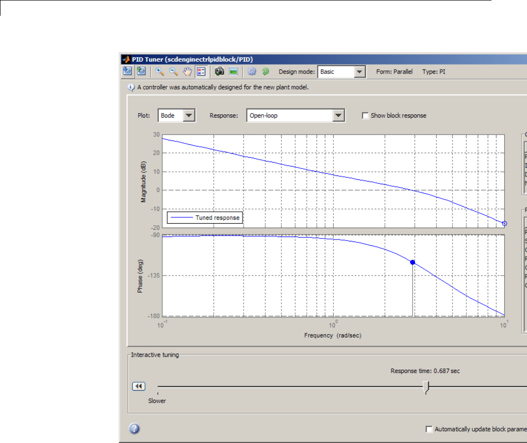
4Designing Compensators
Click "OK" button in the PID Tuner. The PID Tuner writes the P and I gains
to the PID block and closes.
Simulating Closed-Loop Performance in Simulink Model
4-48
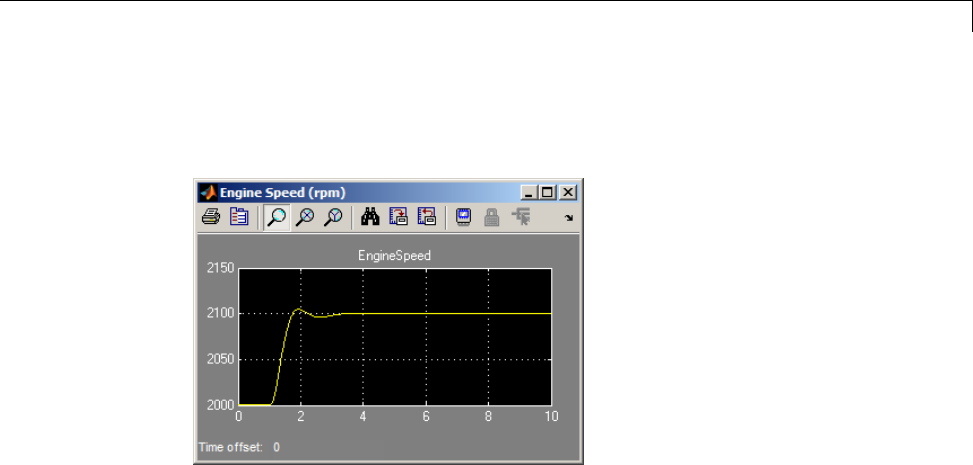
Designing PID Controller in Simulink with Estimated Frequency Response
Simulation in Simulink shows that the new PI controller provides good
performance when controlling the nonlinear model.
Close the model.
bdclose(mdl);
4-49

4Designing Compensators
Designing a Family of PID Controllers for Multiple
Operating Points
This example shows how to design an array of PID controllers for a nonlinear
plant in Simulink that operates over a wide range of operating points.
Opening the Plant Model
The plant is a continuous stirred tank reactor (CSTR) that operates over a
wide range of operating points. A single PID controller can effectively use the
coolant temperature to regulate the output concentration around a small
operating range that the PID controller is designed for. But since the plant is
a strongly nonlinear system, control performance degrades if operating point
changes significantly. The closed-loop system can even become unstable.
Open the CSTR plant model.
mdl = 'scdcstrctrlplant';
open_system(mdl)
4-50
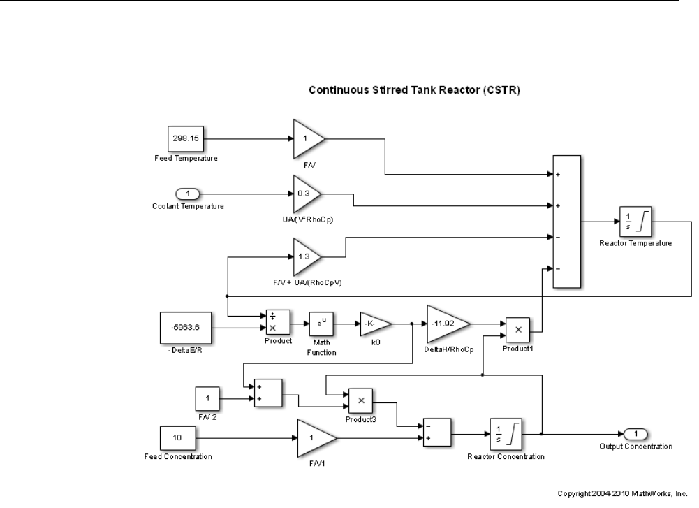
Designing a Family of PID Controllers for Multiple Operating Points
For background, see Seborg, D.E. et al., "Process Dynamics and Control", 2nd
Ed., 2004, Wiley, pp.34-36.
Introduction to Gain Scheduling
Acommonapproachtosolvethenonlinear control problem is using gain
scheduling with linear controllers. Generally speaking designing a gain
scheduling control system takes four steps:
(1) Obtain a plant model for each operating region. The usual practice
is to linearize the plant at several equilibrium operating points.
(2) Design a family of linear controllers such as PID for the plant
4-51

4Designing Compensators
models obtained in the previous step.
(3) Implement a scheduling mechanism such that the controller
coefficients such as PID gains are changed based on the values of the
scheduling variables. Smooth (bumpless) transfer between controllers
is required to minimize disturbance to plant operation.
(4) Assess control performance with simulation.
For more background reading on gain scheduling, see a survey paper from
W.J.RughandJ.S.Shamma: "Researchon gain scheduling", Automatica,
Issue 36, 2000, pp.1401-1425.
In this example, we focus on designing a family of PID controllers for the
CSTRplantdescribedinstep1and2.
Obtaining Linear Plant Models for Multiple Operating Points
The output concentration C is used to identify different operating regions.
The CSTR plant can operate at any conversion rate between low conversion
rate (C=9) and high conversion rate (C=2). In this example, divide the whole
operating range into 8 regions represented by C = 2, 3, 4, 5, 6, 7, 8 and 9.
In the following loop, first compute equilibrium operating points with the
findop command. Then linearize the plant at each operating point with the
linearize command.
% Obtain default operating point
op = operspec(mdl);
% Set the value of output concentration C to be known
op.Outputs.Known = true;
% Specify operating regions
C=[23456789];
% Initialize an array of state space systems
Plants = rss(1,1,1,8);
for ct = 1:length(C)
% Compute equilibrium operating point corresponding to the value of C
op.Outputs.y = C(ct);
opoint = findop(mdl,op,linoptions('DisplayReport','off'));
% Linearize plant at this operating point
Plants(:,:,ct) = linearize(mdl, opoint);
4-52

Designing a Family of PID Controllers for Multiple Operating Points
end
Since the CSTR plant is nonlinear, we expect different characteristics among
the linear models. For example, plant models with high and low conversion
rates are stable, while the others are not.
isstable(Plants,'elem')'
ans =
11000011
Designing PID Controllers for the Plant Models
To design multiple PID controllers in batch, we can use the pidtune
command. The following command will generate an array of PID controllers
in parallel form. The desired open loop crossover frequency is at 1 rad/sec and
the phase margin is the default value of 60 degrees.
% Design controllers
Controllers = pidtune(Plants,'pidf',pidtuneOptions('Crossover',1));
% Display controller for C=4
Controllers(:,:,4)
ans =
1s
Kp + Ki * --- + Kd * --------
s Tf*s+1
with Kp = -12.5, Ki = -0.108, Kd = -14.4, Tf = 0.00875
Continuous-time PIDF controller in parallel form.
Plot the closed loop responses for step set-point tracking as below:
4-53
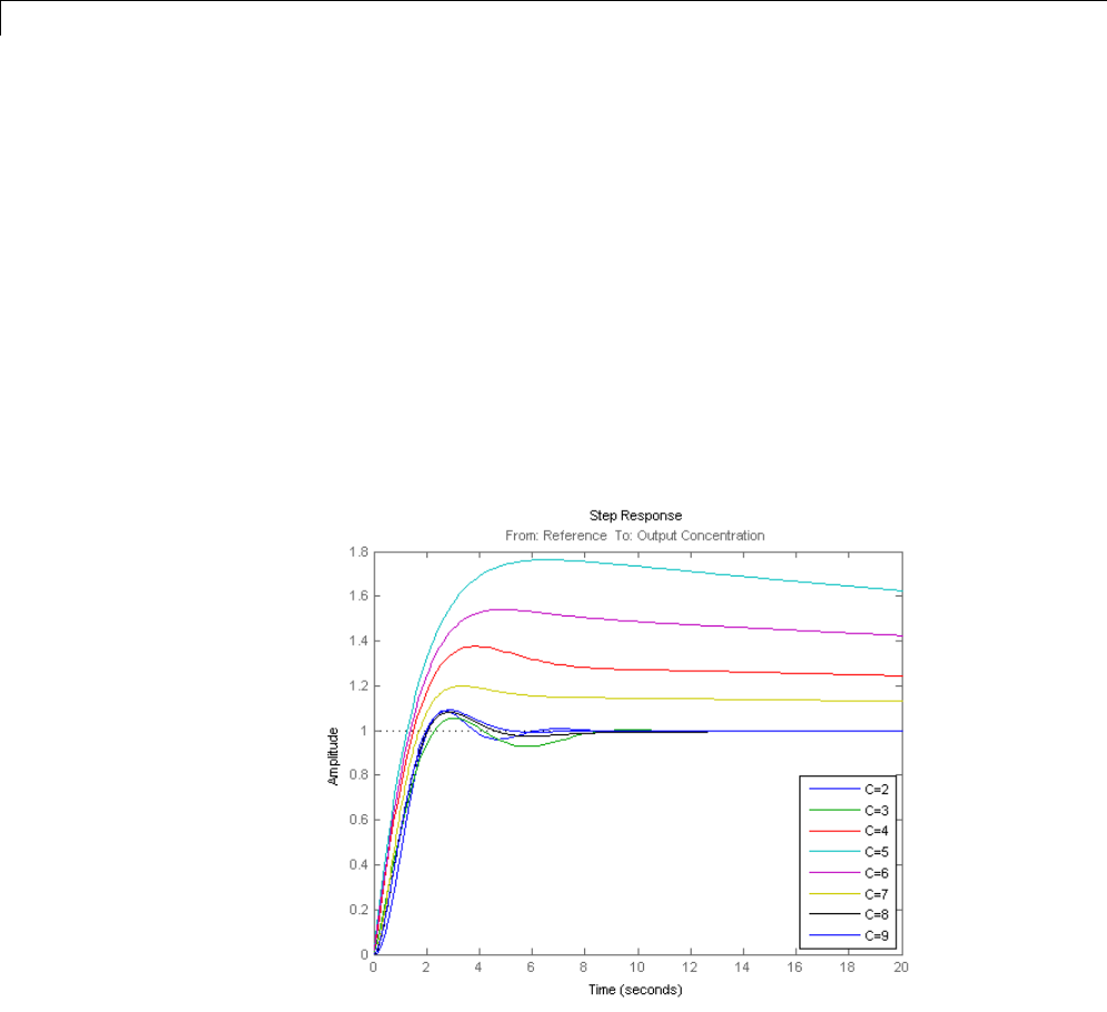
4Designing Compensators
% Construct closed-loop systems
clsys = feedback(Plants*Controllers,1);
% Plot closed-loop responses
figure;
hold on
for ct =1:length(C)
% Select a system from the LTI array
sys = clsys(:,:,ct);
set(sys,'Name',['C=',num2str(C(ct))],'InputName','Reference');
% Plot step response
stepplot(sys,20);
end
legend('show','location','southeast')
All the closed loops are stable but the overshoots of the loops with unstable
plants (C=4, 5, 6 and 7) are too large. It can be improved by increasing the
open loop bandwidth to 10 rad/sec.
% Design controllers for unstable plant models
4-54

Designing a Family of PID Controllers for Multiple Operating Points
Controllers(:,:,3:6) = pidtune(Plants(:,:,3:6),'pidf',10);
% Display controller for C=4
Controllers(:,:,4)
ans =
1s
Kp + Ki * --- + Kd * --------
s Tf*s+1
with Kp = -163, Ki = -13.2, Kd = -138, Tf = 0.0471
Continuous-time PIDF controller in parallel form.
All the closed loop responses are satisfactory now.
% Construct closed-loop systems
clsys = feedback(Plants*Controllers,1);
% Plot closed-loop responses
figure;
hold on
for ct =1:length(C)
% Select a system from the LTI array
sys = clsys(:,:,ct);
set(sys,'Name',['C=',num2str(C(ct))],'InputName','Reference');
% Plot step response
stepplot(sys,20);
end
legend('show','location','southeast')
4-55
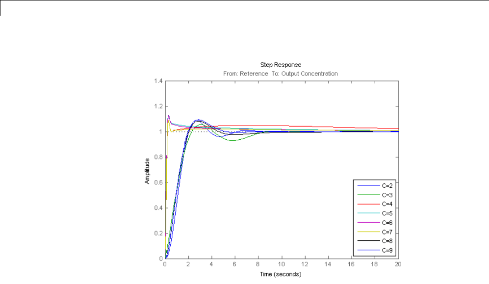
4Designing Compensators
We designed an array of PID controllers and each of them should give
reasonable performance around the local operating point. The next step is
to implement the scheduling mechanism, which is beyond the scope of this
example.
Close the model.
bdclose(mdl);
4-56

Design and Analysis of Control Systems
Design and Analysis of Control Systems
In this section...
“Compensator Design Process Overview” on page 4-57
“Beginning a Compensator Design Task” on page 4-57
“Selecting Blocks to Tune” on page 4-59
“Selecting Closed-Loop Responses to Design” on page 4-62
“Selecting an OperatingPoint”onpage4-64
“Creating a SISO Design Task” on page 4-67
“Completing the Design” on page 4-78
Compensator Design Process Overview
Compensator design in the Control and Estimation Tools Manager involves
the following steps:
1“Selecting Blocks to Tune” on page 4-59
2“Selecting Closed-Loop Responses to Design” on page 4-62
3“Selecting an Operating Point” on page 4-64
4“Creating a SISO Design Task” on page 4-67
5“Completing the Design” on page 4-78
Beginning a Compensator Design Task
Before you begin this compensator design example, close the Control and
Estimation Tools Manager.
To begin a new compensator design task for the scdmagball_freeform model:
1Enter scdmagball_freeform at the MATLAB command line to open the
scdmagball_freeform model.
4-57
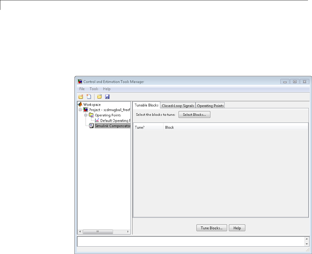
4Designing Compensators
2Select Analysis > Control Design > Compensator Design from the
scdmagball_freeform window.
The Control and Estimation Tools Manager opens and creates a new
compensator design task, as shown in the following figure.
The project tree in the left pane of the Control and Estimation Tools Manager
now shows a Simulink Compensator Design Task node as part of
Project - scdmagball_freeform in addition to the Operating Points node.
Youcanselectanodewithinthetreetodisplay its contents in the right pane.
•For information on the Tunable Blocks pane within the Simulink
Compensator Design Task node, refer to “Selecting Blocks to Tune”
on page 4-59.
4-58

Design and Analysis of Control Systems
•For information on the Closed-Loop Signals pane within the Simulink
Compensator Design Task node, refer to “Selecting Closed-Loop
Responses to Design” on page 4-62.
•For information on the Operating Points node or the Operating Points
pane within the Simulink Compensator Design Task node, refer to
“Selecting an Operating Point” on page 4-64.
Selecting Blocks to Tune
How to Select Blocks to Tune
This section continues the scdmagball_freeform example from “Beginning a
Compensator Design Task” on page 4-57. At this stage in the example, you
have already created a compensator design task.
In this step of the compensator design, you select the blocks in your model to
tune from a list of tunable blocks in your model. Tunable blocks are blocks that
you can tune using the SISO Design Tool to achieve the desired response of
your system. Typically, these blocks serve as the compensators in your model.
In this example, you tune the compensator block called Controller inside the
Controller subsystem of the scdmagball_freeform model. To select this block
as the block to tune:
1Select the Simulink Compensator Design Task node.
2In the Tunable Blocks pane, click Select Blocks.TheSelectBlocks
to Tune dialog box opens.
3Select the Controller subsystem in the left pane to display that subsystem’s
tunable blocks within the center pane. Within the center pane, select the
check box next to the Controller block’s name.
4-59
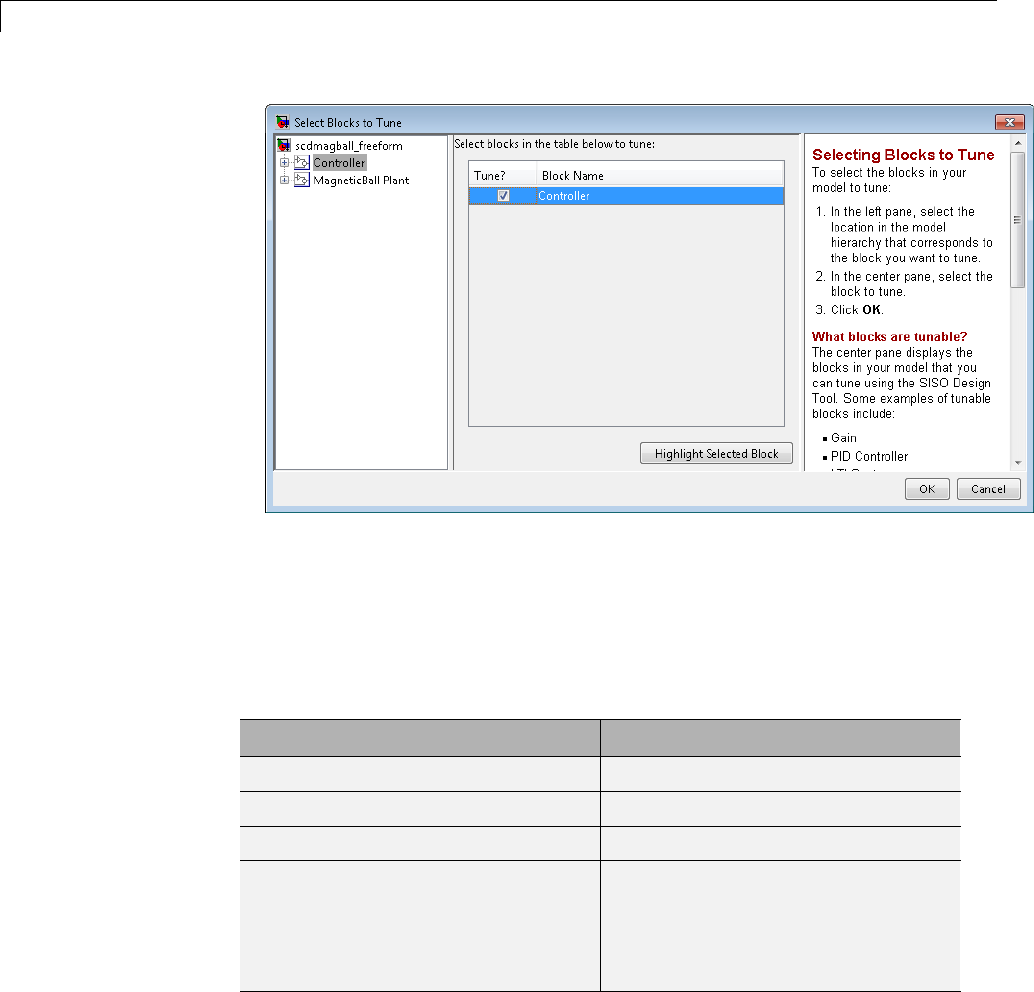
4Designing Compensators
4Click OK to apply your selections and close the dialog box.
What Blocks Are Tunable?
You can tune parameters in the blocks shown in the following table using
Simulink Control Design software. The block input and output signals for
tunable blocks must have scalar, double-precision values.
Tunable Blocks Simulink Library
Gain Math Operations
LTI System Control System Toolbox
Discrete Filter Discrete
PID Controller
(one-degree-of-freedom only)
•Continuous
•Discrete
•Simulink Extras Additional
Linear
4-60

Design and Analysis of Control Systems
Tunable Blocks Simulink Library
State-space blocks •Continuous
•Discrete
•Simulink Extras Additional
Linear
Zero-pole blocks •Continuous
•Discrete
•Simulink Extras Additional
Linear
Transfer function blocks •Continuous
•Discrete
•Simulink Extras Additional
Linear
You can also tune the following versions of the blocks listed in the table:
•Blocks with custom configuration functions associated with a masked
subsystem
•Blocks discretized using the Simulink Model Discretizer
Note If your model contains Model blocks with normal-mode model
references to other models, you can select tunable blocks in the referenced
models for compensator design.
Creating Custom Configuration Functions
When you have masked subsystems that you want to tune in your model, they
will not automatically appear in the list of tunable blocks. For them to appear
in the list, you need to create a custom configuration function for the masked
subsystem. The custom configuration function serves the following functions:
•It informs the Simulink Control Design software that you want this block
to be available for tuning.
4-61

4Designing Compensators
•ItdetermineshowyouwanttheSISODesignTasktotreattheblock;it
describes the relationship between the block mask parameters and the
poles and zeros of the transfer function.
To learn how to create a custom configuration function, see Tuning Custom
Masked Subsystems.
Selecting Closed-Loop Responses to Design
This section continues the scdmagball_freeform example from “Selecting
Blocks to Tune” on page 4-59. At this stage in the example a compensator
design task has been created, and tunable blocks have been selected.
In this step of the compensator design task, you will select the closed loops
whose responses you want to design in your model. A closed-loop system is
defined by an input point, such as a reference or disturbance signal, and an
output point, such as a measured output or actuator signal.
In this example you will design the response of the closed-loop system from
the reference signal to the output of the plant model. To set up linear analysis
points to define this closed-loop system, perform the following steps:
1On the scdmagball_freeform model diagram, position the mouse on the
Reference signal between the Desired Height block and the Sum block.
Right-click and select Linear Analysis Points > Input Point from the
menu to add an input point.
2Position the mouse on the signal line at the output of the Magnetic Ball
Plant block. Right-click and select Linear Analysis Points > Output
Point from the menu to add an output point.
4-62
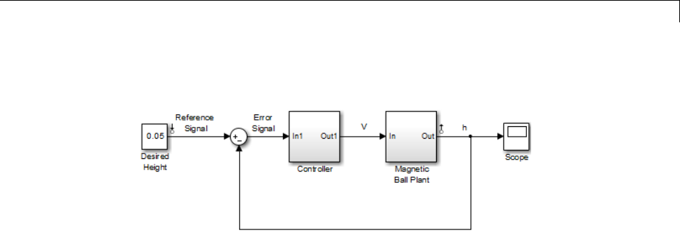
Design and Analysis of Control Systems
The model should now appear as follows:
4-63
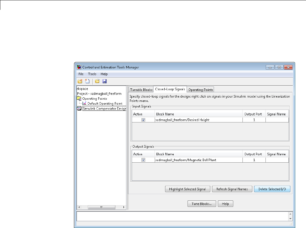
4Designing Compensators
Within the Control and Estimation Tools Manager, click the Closed-Loop
Signals tab of the Simulink Compensator Design Task node to view the
input and output points in the model.
Within this pane you can view the input and output signals in the model and
use the Active column to select the ones you want to use to define closed-loop
systems for compensator design.
Selecting an Operating Point
This section continues the scdmagball_freeform example from “Selecting
Closed-Loop Responses to Design” on page 4-62. At this stage in the example,
a compensator design task has been created, tunable blocks have been
selected, and closed-loop signals have been selected.
4-64

Design and Analysis of Control Systems
In this step of the compensator design task, you will select the operating
point that you want to use in the compensator design. The Simulink Control
Design software uses the operating point when it linearizes the model before
creating a SISO Design Task.
Note A compensator designed for the linearized model is likely to control the
behavior of the nonlinear model only in a small region around the operating
pointthatthemodelwaslinearizedat. Therefore it is important that the
linearization of the model is accurate and the selection of the operating point
about which the system is linearized is an important step in the compensator
design process.
To import an operating point for compensator design, perform the following
steps:
1Select the Operating Points node in the Control and Estimation Tools
Manager.
2Click the Import button, in the bottom-right corner of the Control and
Estimation Tools Manager.
3In the Operating Point Import dialog box, select MAT-file as the location
to import from.
4Click Browse and locate the file
scdmagball_freeform_operating_point.mat that you previously
saved. If you did not previously save an operating point, browse to
matlabroot/toolbox/slcontrol/slctrldemos/scdmagball_freeform_operating_p
o
5Click Open to return to the Operating Point Import dialog box.
The Operating Point Import dialog box now shows all the operating points
available within the selected MAT-file. In this case just a single operating
point is contained in the MAT-file.
4-65
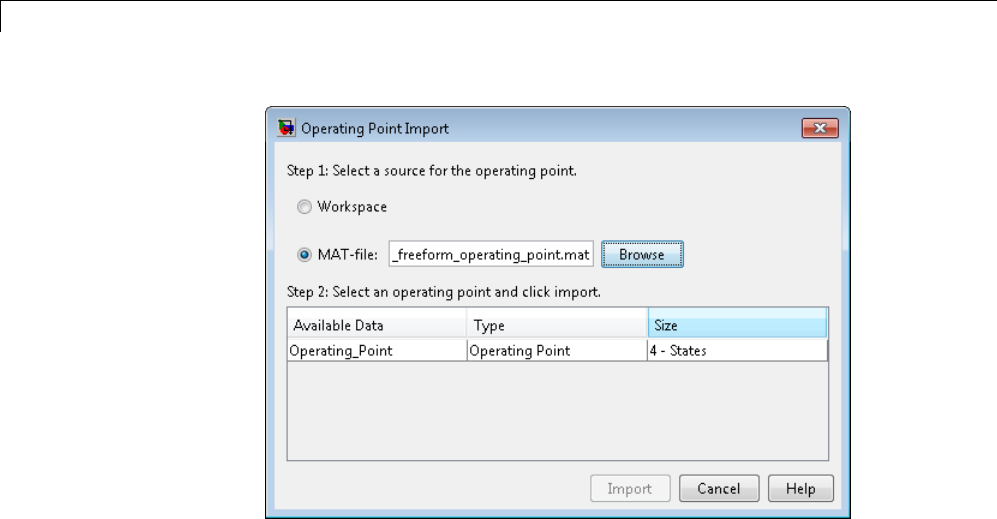
4Designing Compensators
6Select this operating point and click Import to import it into the Control
and Estimation Tools Manager.
Click the Operating Points tab in the Simulink Compensator Design
Task node to select an operating point for the compensator design. For
this example, you should use the operating point that you just imported,
called Operating_Point. To specify this operating point, first select the
Linearize at one of the following operating points option. Then select
Operating_Point in the list, as shown in the following figure.
4-66
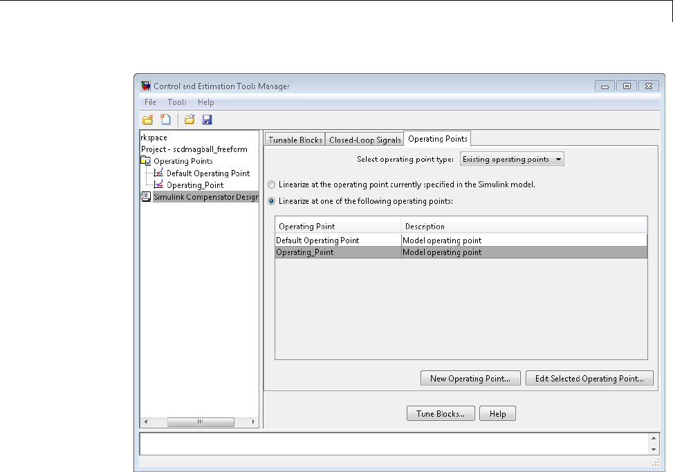
Design and Analysis of Control Systems
Creating a SISO Design Task
•“What is a SISO Design Task?” on page 4-67
•“Configuring Design Plots” on page 4-68
•“Configuring Analysis Plots” on page 4-71
•“Control Design Linearization Options” on page 4-76
•“Designing Compensators for Plants with Time Delays” on page 4-77
What is a SISO Design Task?
This section continues the scdmagball_freeform example from “Selecting an
Operating Point” on page 4-64. At this stage in the example, a compensator
4-67

4Designing Compensators
design task has been created, and tunable blocks, closed-loop signals, and an
operating point have been selected.
In this step of the compensator design task, you will create and configure a
SISO Design Task in the Control and Estimation Tools Manager. The SISO
Design Task includes several tools for tuning the response of SISO systems:
•A graphical editing environment in the SISO Design Tool window that
contains design plots such as root-locus, and Bode diagrams
•An LTI Viewer window where you can view time and frequency analysis
plots of the system
•A compensator editor where you can directly edit the block mask
parameters or the poles and zeros of compensators in your system
•A tool that automatically generates compensators using PID, internal
model control (IMC), or linear-quadratic-Gaussian (LQG) methods (uses
the Control System Toolbox software)
•Optimization-based tuning methods that automatically tunes the system
to satisfy design requirements (available when you have the Simulink
Design Optimization product)
The Design Configuration Wizard guides you through the selection of the
open- and closed-loop systems you want to design and the configuration of the
design and analysis plots you want to use in the SISO Design Task.To
launch the wizard, click Tune Blocks in the Simulink Compensator Design
Task node. The wizard opens in a separate window.
The first page of the wizard provides an overview of the design configuration
process and lists some issues to consider when selecting design and analysis
plots. Click Next to continue to step 1 of the design configuration process on
thesecondpageofthewizard.
Configuring Design Plots
In step 1, select the open- and closed-loop systems that you want to design in
your model, and up to six corresponding design plots you want to use.
Open-loop design allows you to design the response of a closed feedback loop
in your model by artificially opening the loop and designing the response of
4-68
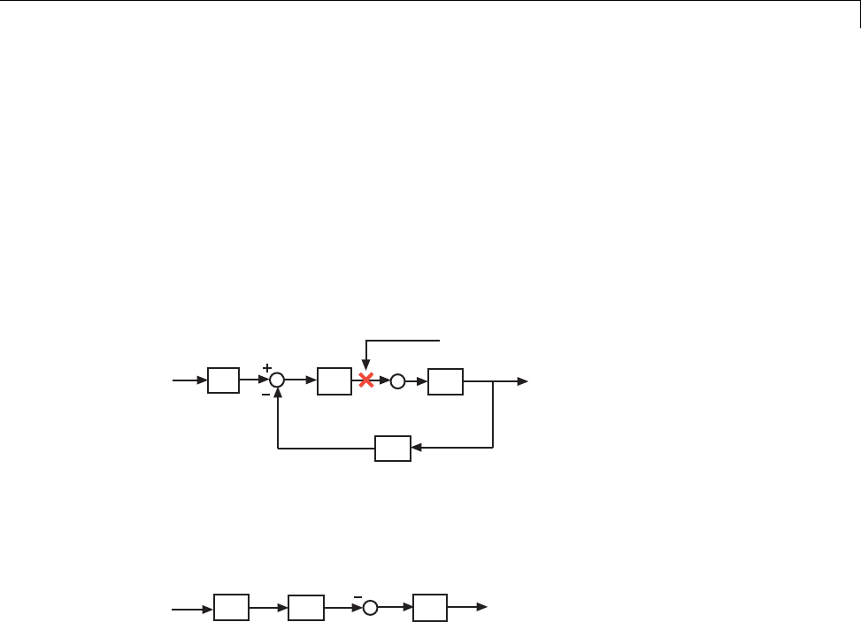
Design and Analysis of Control Systems
this open-loop system. The open-loop design plots use rules of linear control
theory to determine the dynamics of the closed-loop system from those of the
open-loop system. Open-loop design is typically used to tune compensators
that lie inside feedback loops.
A set of default open-loop systems is created for your model, shown in the
lower half of the wizard. To create these open-loop systems, the software
artificially opens the feedback loop at the output signal of each tunable block
(at the X in the following figure) and unwraps the closed-loop system to create
the corresponding open-loop system.
CP
H
F
loop opening
point
The unwrapped open-loop system, which is -CPH, is shown in the following
figure. The open-loop design plots show the negative of the unwrapped
open-loop, which is CPH. This configuration allows you to design controllers
using a negative feedback architecture.
PHC
Note that elements that are outside the feedback loop, such as the prefilter F,
are not seen in the open-loop system.
In this example, you will tune the response of Open Loop 1 which is defined
by a loop opening at the output of the Controller block. This open-loop system
contains the plant model and the controller. To design this system, select
Open Loop 1 from the menu next to Plot 1 in the wizard.
Next, select a design plot to use for this open-loop system. Design plots
are interactive plots within the SISO Design Tool. You can use them to
graphically tune parameters and manually move, add, or remove poles and
zeros of the tunable blocks to tune and design the dynamics of open- and
closed-loop systems in your model. The following table shows the design plots,
along with their uses, available in the SISO Design Tool.
4-69
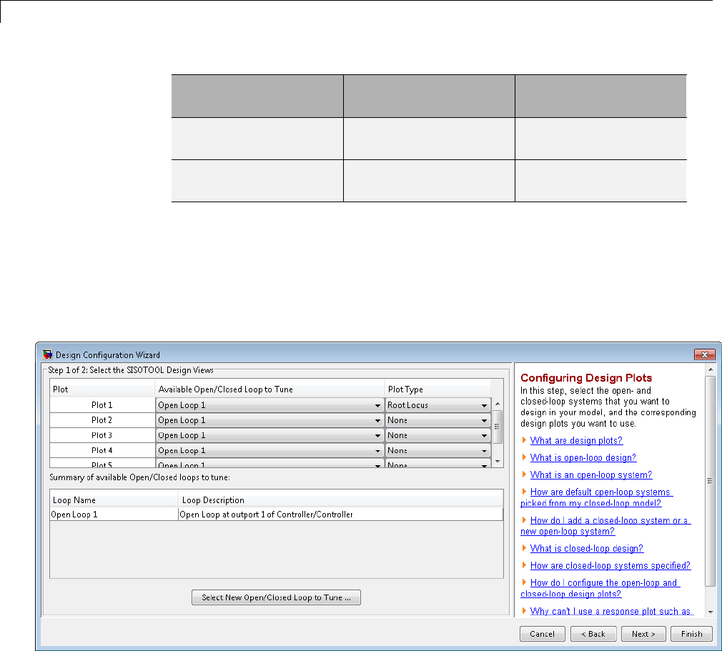
4Designing Compensators
Type of Design Plot Available Plots in the
SISO Design Tool
Use to tune blocks
that act as
Open-loop Root Locus, Nichols,
Open-loop bode
Feedback elements
Closed-loop Closed-loop bode Feedforward or prefilter
elements
You can also use the design plots to specify requirements for stability,
performance, or both to use in using optimization-based automated tuning.
For this example, select Root Locus from the menu next to Plot 1 to use this
plot type as the design plot for Open Loop 1. Step 1 of the wizard should now
look similar to the following figure.
Click Next to proceed to step 2 of the wizard.
4-70

Design and Analysis of Control Systems
Configuring Analysis Plots
In this step, select the closed-loop responses that you want to view while
designing your model, and the corresponding analysis plots you want to use
to view them.
Analysisplotsareplotsthatshowtheresponsesordynamicsofaclosedor
open loop systems or tunable blocks in your model. Although you cannot
directly edit the analysis plots by graphically moving gains, poles, zeros, etc.,
changes that you make in the design plots, compensator editor, or automated
design tools will affect the responses in the analysis plots. Possible analysis
plots include
•Step response
•Impulse response
•Bode and Bode magnitude
•Nyquist
•Nichols
•Pole/Zero
You can use analysis plots to
•Analyze closed-loop, open-loop, and tuned block responses in your control
system.
•Define stability and performance requirements for optimization-based
automated tuning.
For this example, select Step from the menu for Plot 1 to create a step
response analysis plot.
Next, select the closed-loop system that you want to display in this plot. A
closed-loop system is a system that has not had any feedback loops opened for
open-loop design. It typically defines the system whose response you want
to control and it lies between the input and output signals of interest, for
example between a reference signal and the plant output signal.
4-71
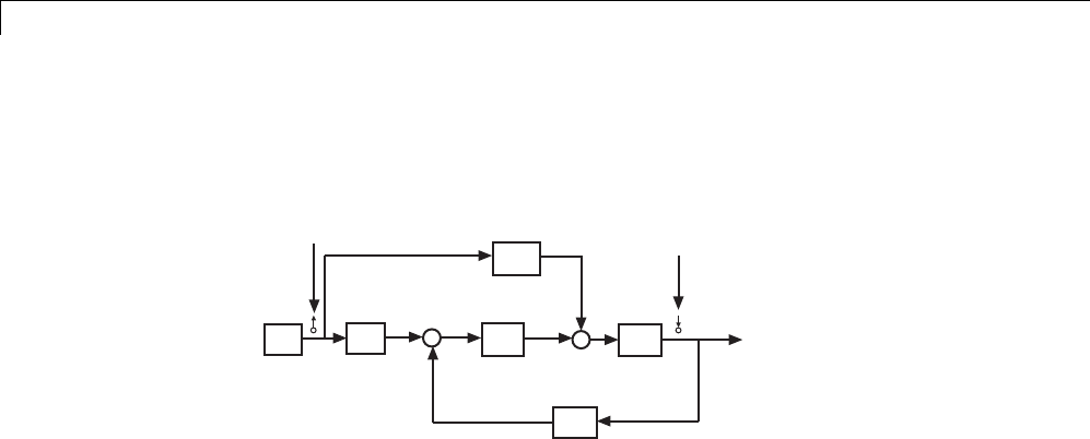
4Designing Compensators
Linearization input and output points placed on signal lines in your model
define closed-loop systems. The closed-loop system includes all blocks in the
path between the input and the output.
CP
H
RF
FF
Closed-loop control system
Input point Output point
The software automatically displays a list of up to four closed-loop systems in
your model, based on the input and output points on the signal lines. In this
example, only one closed-loop system appears in the wizard, the closed-loop
from the Desired Height signal to the output of the Magnetic Ball Plant
Model, because the system only has one input and one output point. You can
add additional closed-loop responses, as well as open-loop and tunable block
responses. To add a new response, click the Add Responses button and
completetheSelectaNewResponsetoAnalyzedialogbox.
To display the current closed-loop system in the step response plot of Plot 1,
select the check box under Plot 1 to the left of the closed-loop system. Step 2
of the wizard should now look similar to the following figure.
4-72
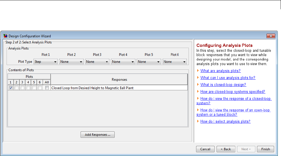
Design and Analysis of Control Systems
Click Finish to complete the wizard and create the SISO Design Task
underneath the Simulink Compensator Design Task node within the
Control and Estimation Tools Manager, as shown in the following figure.
4-73
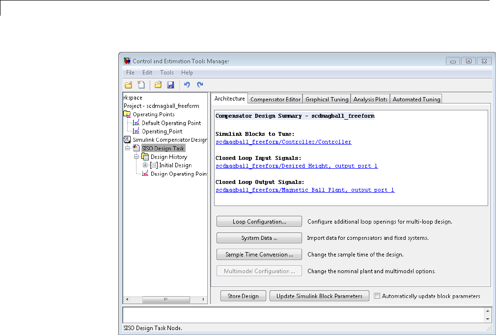
4Designing Compensators
The SISO Design Task also includes the design plots you configured in the
Design Configuration Wizard. They appear within the SISO Design Tool
window, as shown in the following figure.
4-74
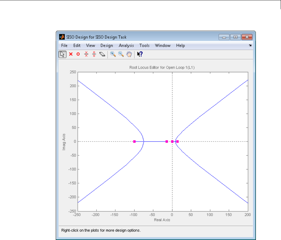
Design and Analysis of Control Systems
In addition, the SISO Design Task also includes the analysis plots you
configured in the Design Configuration Wizard. They appear within the LTI
Viewer window, as shown in the following figure.
4-75
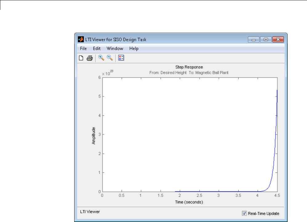
4Designing Compensators
Control Design Linearization Options
To modify or adjust the settings used to linearize a model when creating a
SISO Design Task, click the Simulink Compensator Design Task node,
and then select Tools > Options. The Options dialog box opens.
4-76

Design and Analysis of Control Systems
Specify the linearization sample time and rate conversion method. If, for the
Rate conversion method parameter, you specify Tustin W/Prewarping,
you must also specify a pre-warp frequency.
Designing Compensators for Plants with Time Delays
You can design compensators for plants with time delays using the tools in
the SISO Design Task. These tools automatically create a linear model of your
plant. Within this model, you can represent time delays in two ways—using
Padé approximation or exact delay.
To represent time
delays in the
linear plant model
using...
You must...
Padé approximation
representations
Specify the Padé order in the Block Parameters
window for each Simulink blocks with delays.
Exact delay
representations
Open the Simulink Compensator Design Task, and
select Tools > Options. Then, in the Options dialog
box, select Enable design of linearized control
systems with exact delay(s).
4-77

4Designing Compensators
Note Some tools do not support exact time delays and automatically compute
a Padé approximation for delays. In this case, you receive a notification.
The software uses the Padé order specified in SISO Tool Preferences and
ignores the Padé order specified in your block. For more information, see
“Time Delays Pane”.
For more information on the linearizing models with time delays, see “Models
with Time Delays” on page 2-122. For more information on the tools available
for compensator design, see “Tools for Compensator Design” on page 4-78.
Completing the Design
•“Tools for Compensator Design” on page 4-78
•“Storing and Retrieving Designs” on page 4-83
•“Writing the Design to the Simulink Model” on page 4-85
•“Compare and Contrast the SISO Design Task and Enhanced SISO Design
Task” on page 4-87
•“Design Operating Point Node” on page 4-90
•“SISO Tool Options” on page 4-91
Tools for Compensator Design
This section continues the scdmagball_freeform example from “Creating a
SISO Design Task” on page 4-67. At this stage in the example, a compensator
design task has been created, tunable blocks, closed-loop signals, and an
operating point have been selected, design and analysis plots have been
created, and a SISO Design Task node has been created in the Control and
Estimation Tools Manager.
In this step of the compensator design task, you will complete the design of
the compensator in the scdmagball_freeform model, using the SISO Design
Task node. For a more detailed discussion of the SISO Design Task node,
refer to the Control System Toolbox documentation.
4-78

Design and Analysis of Control Systems
The SISO Design Task node contains five panes with various tools for
designing the compensators in your system.
•Architecture:
-Configure loops for multi-loop design by opening signals to remove the
effects of other feedback loops.
-Import compensators into your system.
-Convert the sample time of the system or switch between different
sample times to design different compensators.
•Compensator Editor:
-Directly edit the poles, zeros, and gains of the compensator.
-Add or remove poles and zeros to the compensators.
•Graphical Tuning:
-Configure design plots in the SISO Design Tool.
-Use design plots to graphically manipulate the response of the system.
•Analysis Plots:
-Configure analysis plots in the LTI Viewer.
-Use analysis plots to view the response of open- or closed-loop systems.
•Automated Tuning: Design compensators using one of several automated
methods.
-Automatically generate compensators using PID, internal model control
(IMC), or linear-quadratic-Gaussian (LQG) methods (uses Control
System Toolbox software).
-Use optimization-based methods that automatically tune the system
to satisfy design requirements (available when you have the Simulink
Design Optimization product).
You can use any of these design methods, or a combination of methods, to
design the compensators for your system. A suitable final design for the
Controller of the scdmagball_freeform model is:
•Gain: -16000
4-79

4Designing Compensators
•Integrator at the origin
•Complex zeros at -10±10i
•Real pole at -1000
You can use the Compensator Editor in the SISO Design Task node to
specify these settings. The initial design contains an integrator at the origin.
Specify the remaining settings as follows:
•Gain — Enter -16000 in the text box to the right of the equal sign in the
Compensator area.
•Complex zeros — In the Dynamics table, right-click and then select
Add Pole/Zero > Complex Zero. Select the new complex zero in the
Dynamics table. In the Edit Selected Dynamics table:
-Enter -10 in the Real Part field.
-Enter 10 in the Imaginary Part field.
•Real pole — In the Dynamics table, right-click and then select Add
Pole/Zero > Real Pole. Select the new real pole in the Dynamics table.
In the Edit Selected Dynamics table:
-Enter -1000 in the Location field.
The Control and Estimation Tools Manager should now appear similar to
the following:
4-80
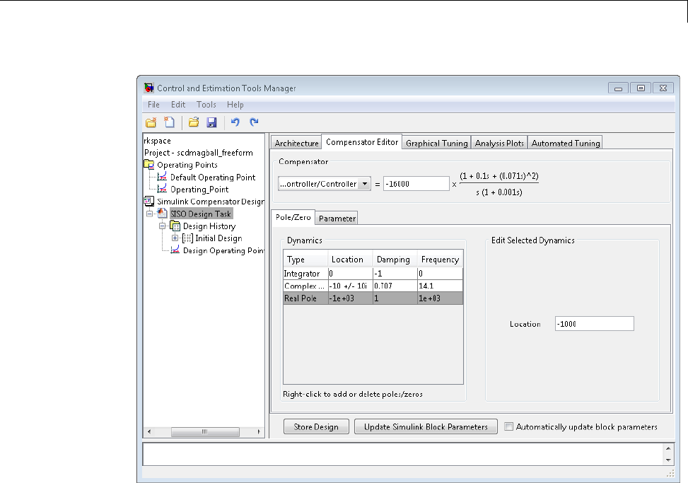
Design and Analysis of Control Systems
With these settings, the root-locus diagram and step-response plot should
look similar to the following figures.
4-81
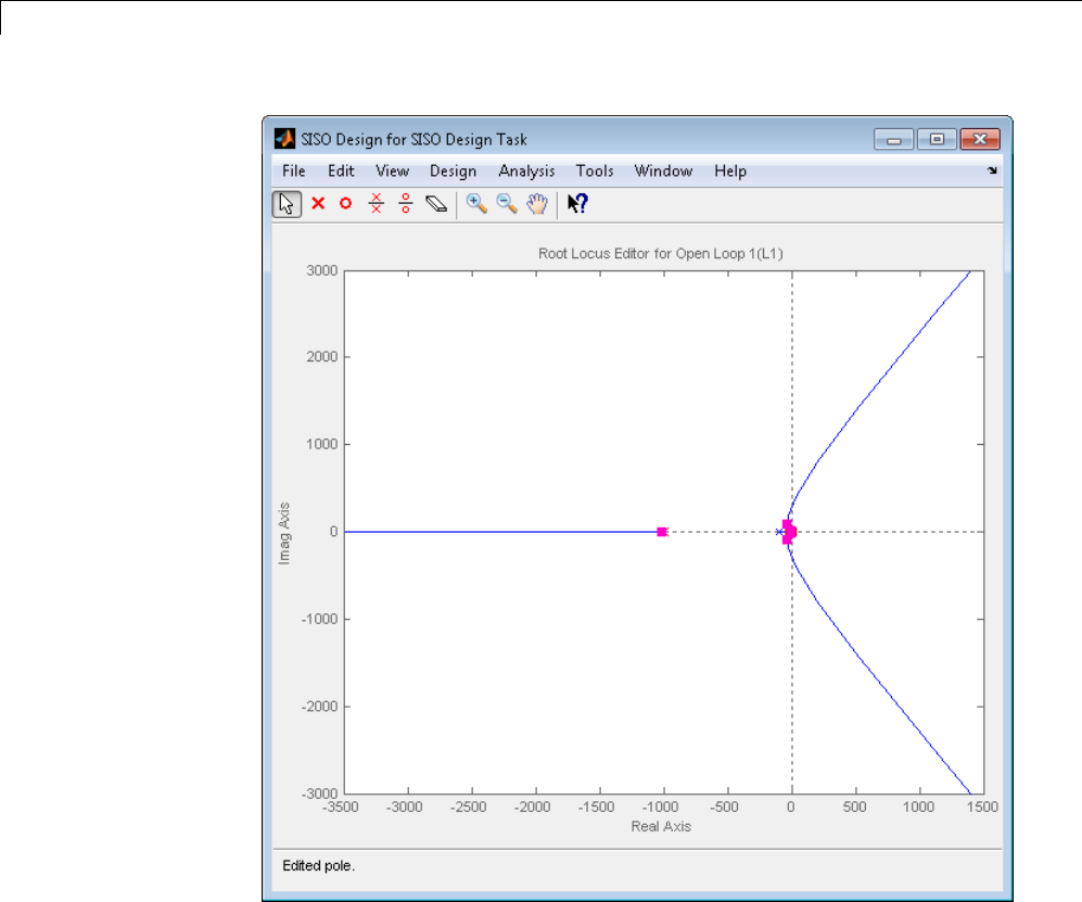
4Designing Compensators
4-82
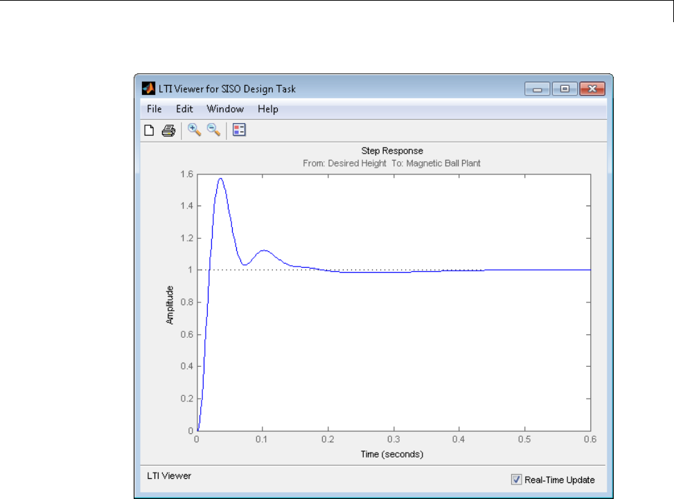
Design and Analysis of Control Systems
Storing and Retrieving Designs
WhenyoudesignacompensatorwithinaSimulink Compensator Design
Task, you can store the current design. You can retrieve the stored design at
any time. This storage and retrieval capability lets you continue designing
and still be able to return to a previously saved version of the design.
This section continues the example from “Completing the Design” on page
4-78. At this stage in the example, a compensator has been designed to
control the system. To store the design within the SISO Design Task node,
perform the following steps:
4-83
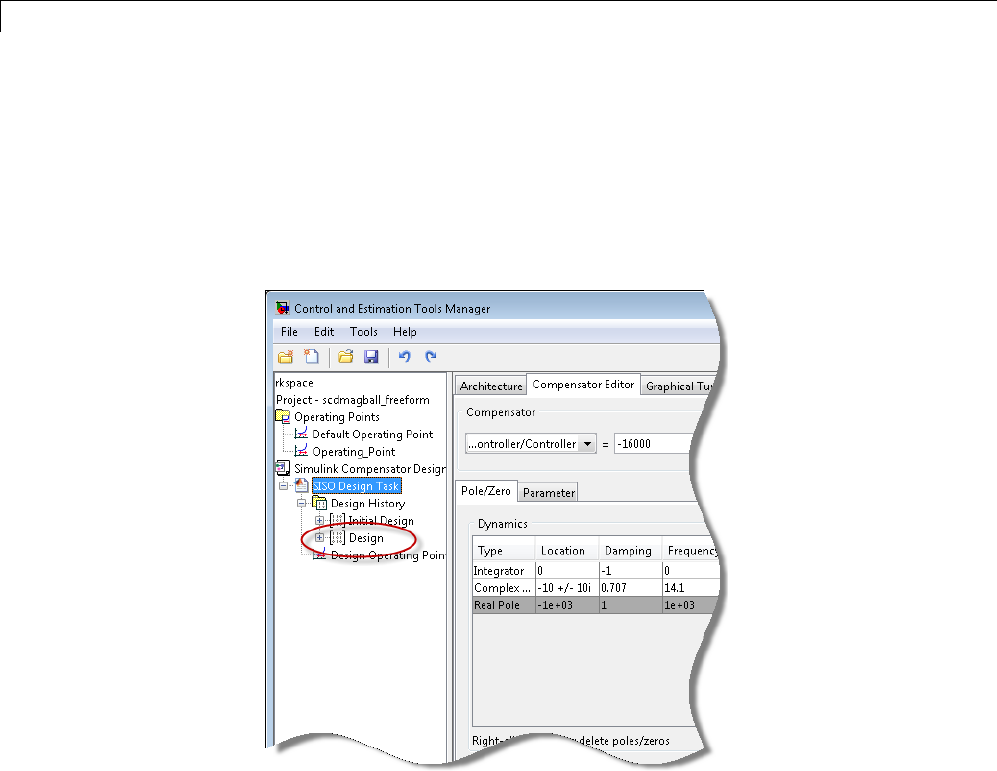
4Designing Compensators
1Select the SISO Design Task node in the Control and Estimation Tools
Manager.
2Underneath the SISO Design Task panes, click the Store Design button.
Clicking this button adds the current design to the Design History node as
shown in the following figure. The default name for the design is Design.
To rename the design to something more descriptive:
1Right-click the Design node underneath the Design History node.
2Select Rename from the right-click menu.
3Enter a name for your design. For this example, call the design
scdmagball_freeform Design.
The Control and Estimation Tools Manager should now appear as follows:
4-84
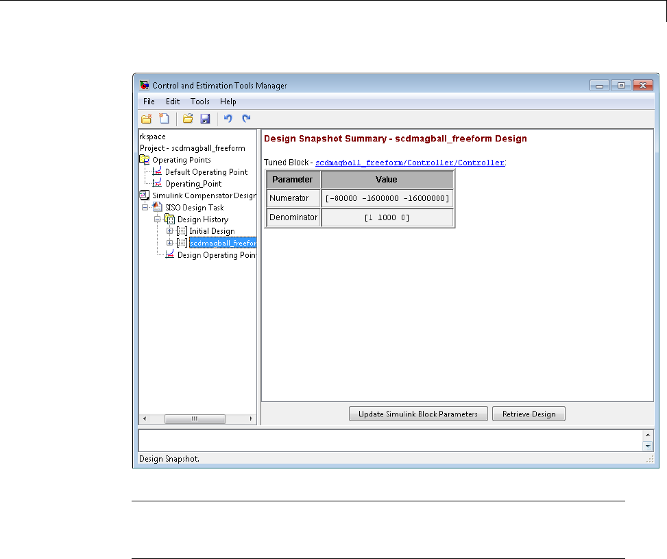
Design and Analysis of Control Systems
Note After you store a compensator design, you can continue to refine it. If
you make undesired changes, you can retrieve the stored design by selecting it
in the Design History node and then clicking the Retrieve Design button.
Writing the Design to the Simulink Model
When designing a compensator within a Simulink Compensator Design
Task node, you can write the compensator design to the Simulink model.
This is useful when
•You want to see how the current design performs in the full nonlinear
model.
4-85

4Designing Compensators
•Youhavecompletedthedesignandyouwanttoupdatethemodelwiththe
newly designed parameters.
When you write the compensator design to your Simulink model:
•If the block parameters are numerical, the software writes new numerical
values to the tuned block.
•If the block parameters are variables in the base workspace or the model
workspace (including Simulink.Parameter objects), the software writes
the tuned values to those variables. The block parameters remain the
workspace variables.
TherearetwowaystowritethedesigntoyourSimulinkmodel:
•Write the tuned parameters to your model when you have finished your
design — Click the Design node of the Control and Estimation Tools
Manager and click the Update Simulink Block Parameters button.
•Automatically update the block parameters as you tune the design — select
the Design History node in the Control and Estimation Tools Manager
and click the checkbox next to Automatically update block parameters.
For example, continue the example from “Storing and Retrieving Designs” on
page 4-83. At this stage in the example you have designed a compensator to
control the system and stored the design within the SISO Design Task node.
To write the stored design to the scdmagball_freeform model, perform the
following steps:
1Select the scdmagball_freeform Design node under the Design History
node in the Control and Estimation Tools Manager.
2Click the Update Simulink Block Parameters button.
You can now simulate the scdmagball_freeform model containing the newly
designed Controller block.
After simulation, the Scope block of the scdmagball_freeform model should
look similar to the following figure.
4-86
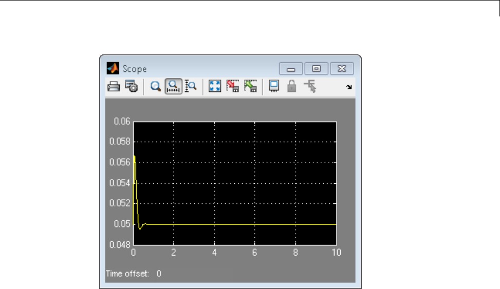
Design and Analysis of Control Systems
The system is now stable and the height of the magnetic ball settles at the
desired height of 0.05 m.
Compare and Contrast the SISO Design Task and Enhanced
SISO Design Task
The SISO Design Task is a graphical user interface (GUI) that simplifies
the task of designing controllers. This section describes the similarities and
differences between the SISO Design Task, which is available in the Control
System Toolbox product, and the enhanced SISO Design Task, which is
available with the Simulink Control Design product.
The following figure shows the SISO Design Task as it appears in the Control
and Estimation Tools Manager.
4-87
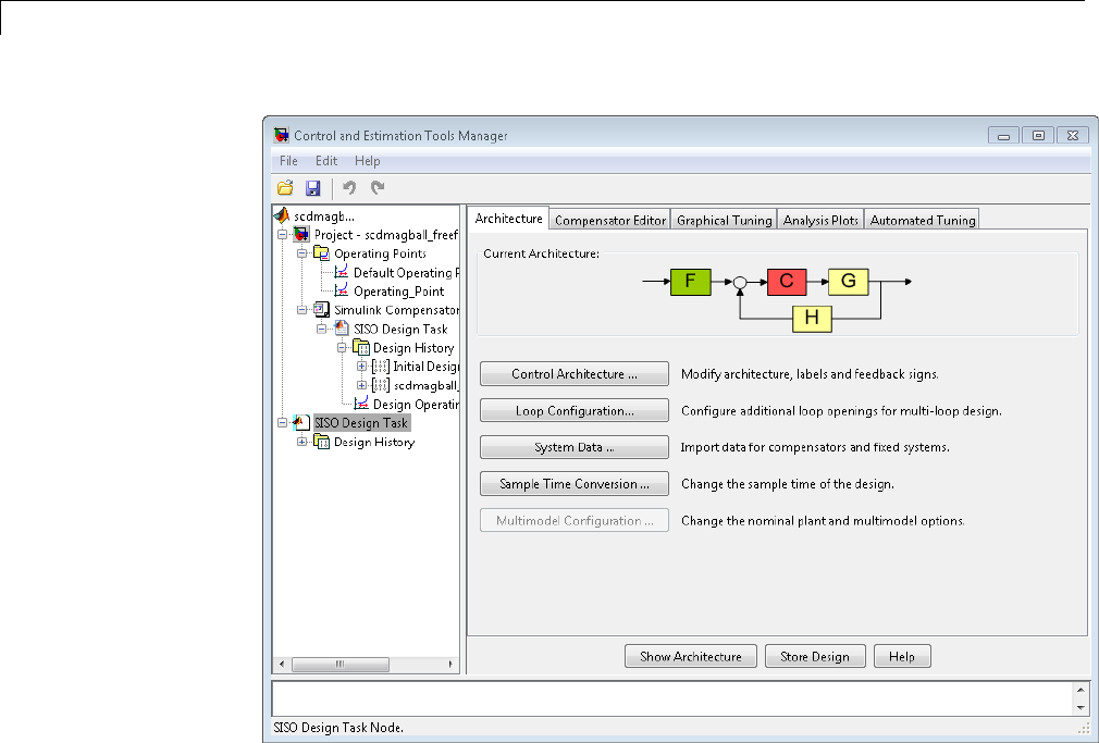
4Designing Compensators
The following figure shows the enhanced SISO Design Task as it appears
under the Simulink Compensator Design Task node in the Control and
Estimation Tools Manager.
4-88
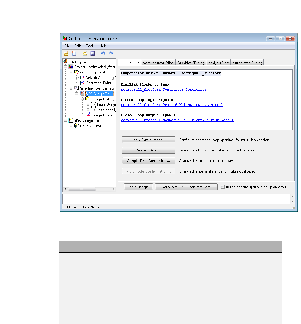
Design and Analysis of Control Systems
The following table summarizes the similarities and differences between the
SISO Design Task and the enhanced SISO Design Task:
Similarities Differences
•Similar layout
•Graphical Tuning, Analysis Plots,
and Automated Tuning panes
have the same functionality. For
more information about these
tabs, see “Tools for Compensator
Design” on page 4-78.
•Architecture tab — The SISO Tool
lets you change the architecture of
your system. In contrast, once you
create a SISO Design Task you
cannot add or delete blocks from
your model. Also, the Architecture
tab in the SISO Design Task
node summarizes the Simulink
Blocks to Tune, Closed Loop Input
4-89

4Designing Compensators
Similarities Differences
Signals, and Closed Loop Output
Signals.
•Compensator Editor tab — The
SISO Design Tool lets you tune
the poles and zeros of your system.
The enhanced SISO Design Tool
lets you tune the poles, zeros,
and parameters of your system.
For more information, see
Tuning Simulink Blocks in the
Compensator Editor.
•When you are satisfied with
your system’s performance, the
enhanced SISO Design Tool lets
you click Update Simulink
Block Parameters to write the
parameters back to your Simulink
model.
For additional information, see:
•“Creating a SISO Design Task” on page 4-67
•“SISO Design Tool” in the Control System Toolbox documentation
Design Operating Point Node
The Design Operating Point node is located inside the Design History
node of the Control and Estimation Tools Manager.
4-90

Design and Analysis of Control Systems
The States pane describes the operating point the GUI used to linearize the
model. When creating the SISO Design Task node, you can use this pane to
import a different operating point and to populate the SISO Design Task
node with a linear model evaluated at the new operating point.
SISO Tool Options
To modify the precision of the numbers calculated by SISO Tool, click the
SISO Design Task node, and then select Tools > Options. The SISOTool
Options dialog box opens.
4-91

4Designing Compensators
If you select the Use full precision check box, the SISO Tool uses the full
double-precision data type when writing back to the Simulink block dialog
box. If you clear this check box, use Custom: n digits of precision to
specify the precision you want.
For additional information, see “Creating a SISO Design Task” on page 4-67.
4-92

5
Model Verification
•“Monitoring Linear System Characteristics in Simulink Models” on page 5-2
•“Defining a Linear System for Model Verification Blocks” on page 5-4
•“Verifiable Linear System Characteristics” on page 5-5
•“Model Verification at Default Simulation Snapshot Time” on page 5-6
•“Model Verification at Multiple Simulation Snapshots” on page 5-15
•“Model Verification Using Simulink®Control Design™ and Simulink
Verification Blocks” on page 5-25

5Model Verification
Monitoring Linear System Characteristics in Simulink
Models
Simulink Control Design software provides Model Verification blocks to
monitor time- and frequency-domain characteristics of a linear system
computed from a nonlinear Simulink model during simulation.
Use these blocks to:
•Verify that the linear system characteristics of any nonlinear Simulink
model, including the following, remain within specified bounds during
simulation:
-Continuous- or discrete-time models
-Multi-rate models
-Models with time delays, represented using exact delay or Padé
approximation
-Discretized linear models computed from continuous-time models
-Continuous-time models computed from discrete-time models
-Resampled discrete-time models
The linear system can be Single-Input Single-Output (SISO) or Multi-Input
Multi-Output (MIMO).
•View specified bounds and bound violations on linear analysis plots.
Tip These blocks are same as the Linear Analysis Plots blocks except for
different default settings of the bound parameters.
•Save the computed linear system to the MATLAB workspace.
The verification blocks assert when the linear system characteristic does not
satisfy a specified bound, i.e., assertion fails. A warning message, reporting
the assertion failure, appears at the MATLAB prompt. When assertion fails,
you can:
5-2

Monitoring Linear System Characteristics in Simulink®Models
•Stop the simulation and bring that block into focus.
•Evaluate a MATLAB expression.
You can use these blocks with the Simulink Model Verification blocks to design
complex logic for assertion. For an example, see “Model Verification Using
Simulink®Control Design™ and Simulink Verification Blocks” on page 5-25.
If you have Simulink Verification and Validation™ software, you can use
the Verification Manager tool in the Signal Builder to construct simulation
tests for your model. For an example, see Verifying Frequency-Domain
Characteristics of an Aircraft.
Note These blocks do not support code generation and can only be used
in Normal simulation mode.
5-3

5Model Verification
Defining a Linear System for Model Verification Blocks
To assert that the linear system characteristics satisfy specified bounds, the
Model Verification blocks compute a linear system from a nonlinear Simulink
model.
For the software to compute a linear system, you must specify:
•Linearization inputs and outputs
Linearization inputs and outputs define the portion of the model to
linearize. A linearization input defines an input while a linearization
output defines an output of the linearized model. To compute a MIMO
linear system, specify multiple inputs and outputs.
•When to compute the linear system
You can compute the linear system and assert bounds at:
-Default simulation snapshot time. Typically, simulation snapshots are
the times when your model reaches steady state.
-Multiple simulation snapshots.
-Trigger-based simulation events
For more information, see the following examples:
•“Model Verification at Default Simulation Snapshot Time” on page 5-6
•“Model Verification at Multiple Simulation Snapshots” on page 5-15
5-4

Verifiable Linear System Characteristics
Verifiable Linear System Characteristics
Thefollowingtablesummarizesthelinear system characteristics you can
specify bounds on and assert that the bounds are satisfied during simulation.
Block Plot Type Bounds on…
Check Bode
Characteristics
Bode Upper and lower Bode
magnitude
Check Gain and Phase
Margins
•Bode
•Nichols
•Nyquist
•Table
Gain and phase
margins
Check Nichols
Characteristics
Nichols •Open-loop gain and
phase
•Closed-loop peak
gain
Check Pole-Zero
Characteristics
Pole-Zero Approximate
second-order
characteristics, such as
settling time, percent
overshoot, damping
ratio and natural
frequency, on the pole
locations
Check Singular Value
Characteristics
Singular Value Upper and lower
singular values
Check Linear
Step Response
Characteristics
Step Response Step response
characteristics
Specify the bounds in the Bounds tab of the block’s Block Parameters dialog
box or programmatically. For more information, see the corresponding block
reference pages.
5-5
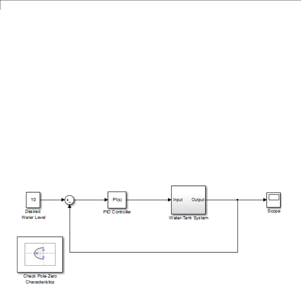
5Model Verification
Model Verification at Default Simulation Snapshot Time
This example shows how to assert that bounds on the linear system
characteristics of a nonlinear Simulink model, computed at the default
simulation snapshot time of 0, are satisfied during simulation.
1Open a nonlinear Simulink model. For example:
watertank
2Open the Simulink Library Browser by selecting View > Library
Browser in the Simulink Editor.
3Add a model verification block to the Simulink model.
aIn the Simulink Control Design library, select Model Verification.
bDrag and drop a block, such as the Check Pole-Zero Characetristics
block, into the Simulink Editor.
The model now resembles the following figure.
4Double-click the block to open the Block Parameters dialog box.
5-6
Model Verification at Default Simulation Snapshot Time
To learn more about the block parameters, see the block reference pages.
5Specify the linearization input and output to compute the closed-loop poles
and zeros.
aTo specify an input:
iClick adjacent to the Linearization inputs/outputs table.
5-7
5Model Verification
The Block Parameters dialog expands to display a Click a signal
in the model to select it area.
ii In the Simulink model, click the output signal of the PID Controller
block to select it.
The Click a signal in the model to select it area updates to display
the selected signal.
iii Click to add the signal to the Linearization inputs/outputs
table.
5-8
Model Verification at Default Simulation Snapshot Time
bTo specify an output:
iv In the Simulink model, click the output signal of the Water-Tank
System block to select it.
The Click a signal in the model to select it area updates to display
the selected signal.
vClick toaddthesignaltotheLinearization inputs/outputs
table.
vi In the Configuration drop-down list of the Linearization
inputs/outputs table, select Output for watertank/Water-Tank
System: 1.
5-9
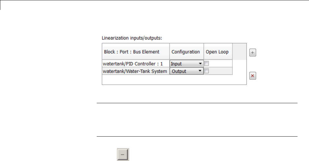
5Model Verification
Note Because the Open Loop check-box for
watertank/Water-Tank System : 1 is clear, the I/Os include the
feedback loop in the Simulink model. The software computes the poles
and zeros of the closed-loop system.
vii Click to collapse the Click a signal in the model to select
it area.
6Specify bounds for assertion. In this example, you use the default
approximate second-order bounds, specified in Bounds tab of the Block
Parameters dialog box.
5-10
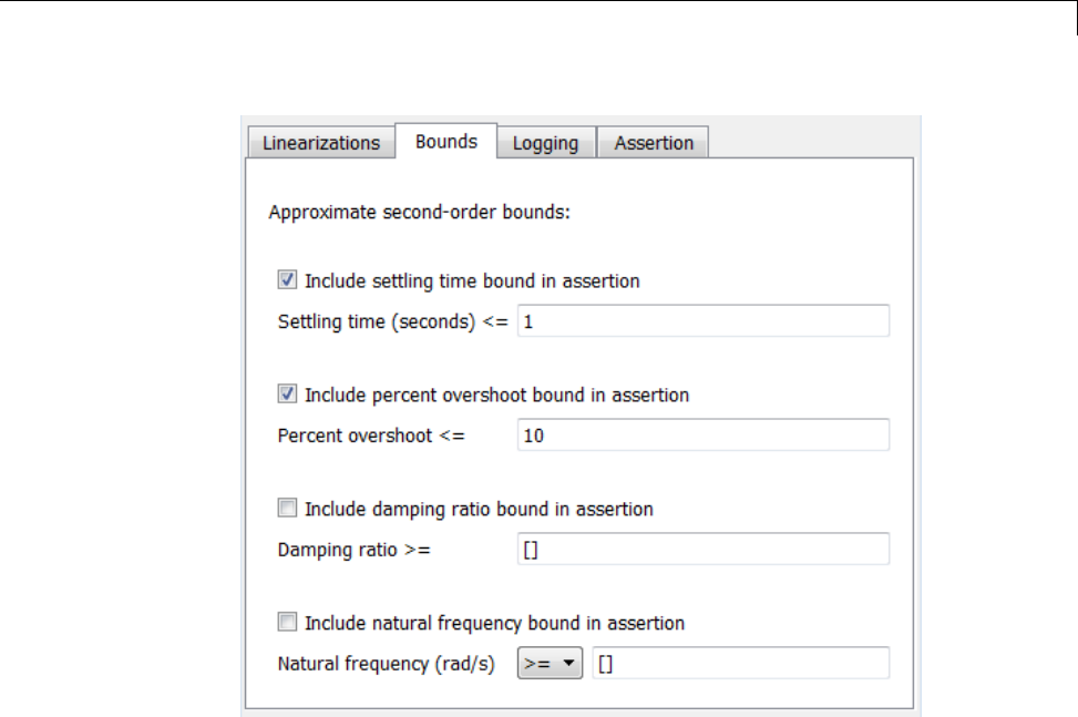
Model Verification at Default Simulation Snapshot Time
View the bounds on the pole-zero map by clicking Show Plot to open a
plot window.
5-11
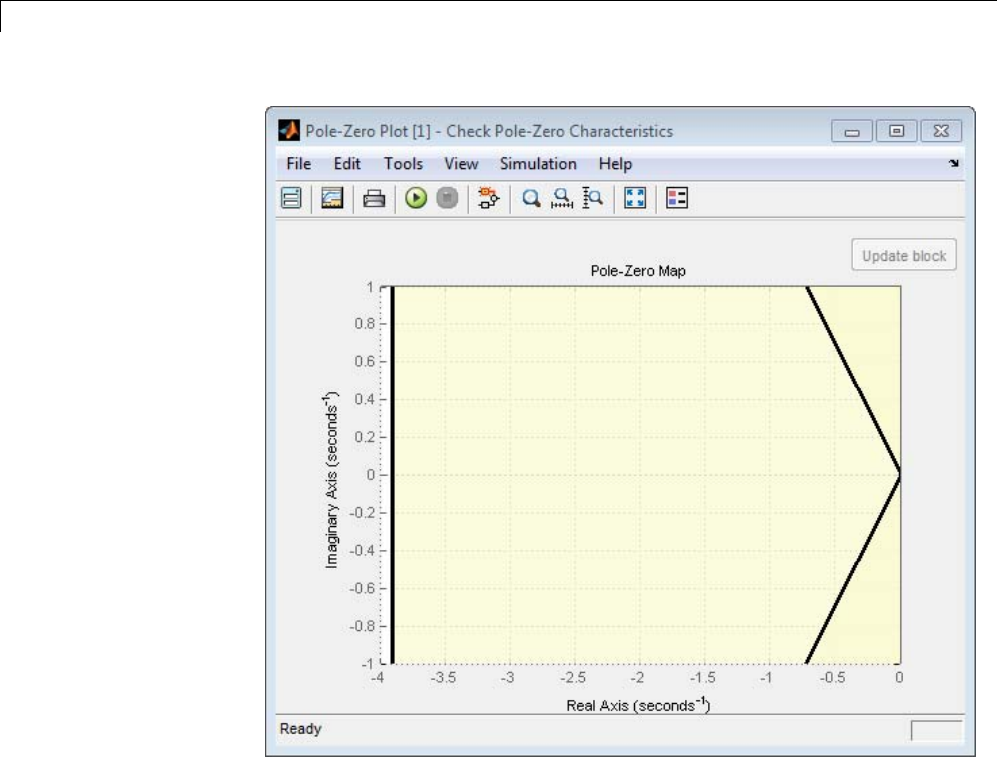
5Model Verification
7Stop the simulation if assertion fails by selecting Stop simulation when
assertion fails in the Assertion tab.
5-12
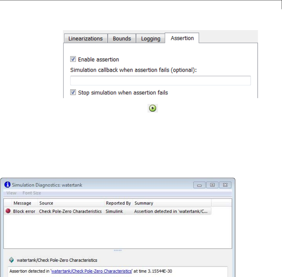
Model Verification at Default Simulation Snapshot Time
8Simulate the model by clicking in the plot window.
Alternatively, you can simulate the model from the Simulink Editor.
The software linearizes the portion of the model between the linearization
input and output at the default simulation time of 0, specified in Snapshot
times block parameter. When the software detects that a pole violates a
specified bound, the simulation stops and the following windows appear:
•Simulation Diagnostics window, reporting the block that asserts.
•Simulink Editor, highlighting the block that asserts.
5-13

5Model Verification
The closed-loop pole and zero locations of the computed linear system
appear as xand omarkings in the plot window. You can also view the
bound violationintheplot.
5-14
Model Verification at Multiple Simulation Snapshots
Model Verification at Multiple Simulation Snapshots
This example shows how to:
•Add multiple bounds.
•Check that the linear system characteristics of a nonlinear Simulink model
satisfy the bounds at multiple simulation snapshots
•Modify bounds graphically
•Disable bounds during simulation
1Open a nonlinear Simulink model. For example:
watertank
2Open the Simulink Library Browser by selecting View > Library
Browser in the Simulink Editor.
3Add a model verification block to the Simulink model.
aIn the Simulink Control Design library, select Model Verification.
bDrag and drop a block, such as the Check Bode Characteristics block,
into the Simulink Editor.
The model now resembles the following figure.
5-15
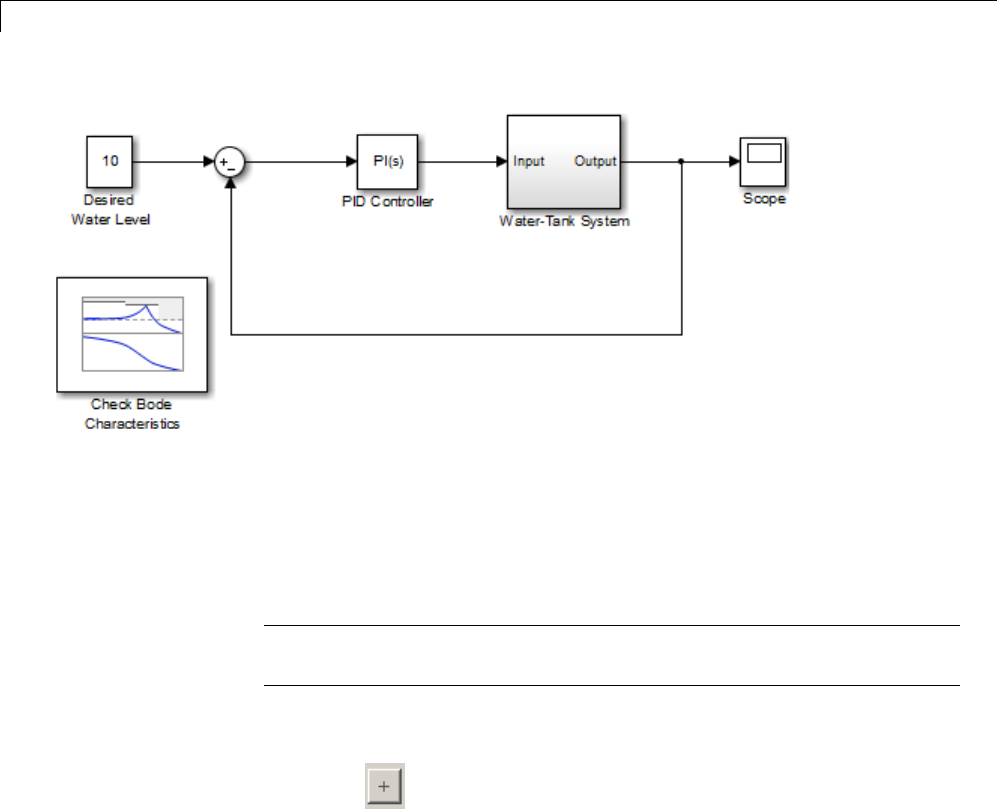
5Model Verification
4Double-click the block to open the Block Parameters dialog box.
To learn more about the block parameters, see the block reference pages.
5Specify the linearization I/O points.
Tip If your model already contains I/O points, the block automatically
detects these points and displays them.
aTo specify an input:
iClick adjacent to the Linearization inputs/outputs table.
The Block Parameters dialog expands to display a Click a signal
in themodeltoselectitarea.
5-16
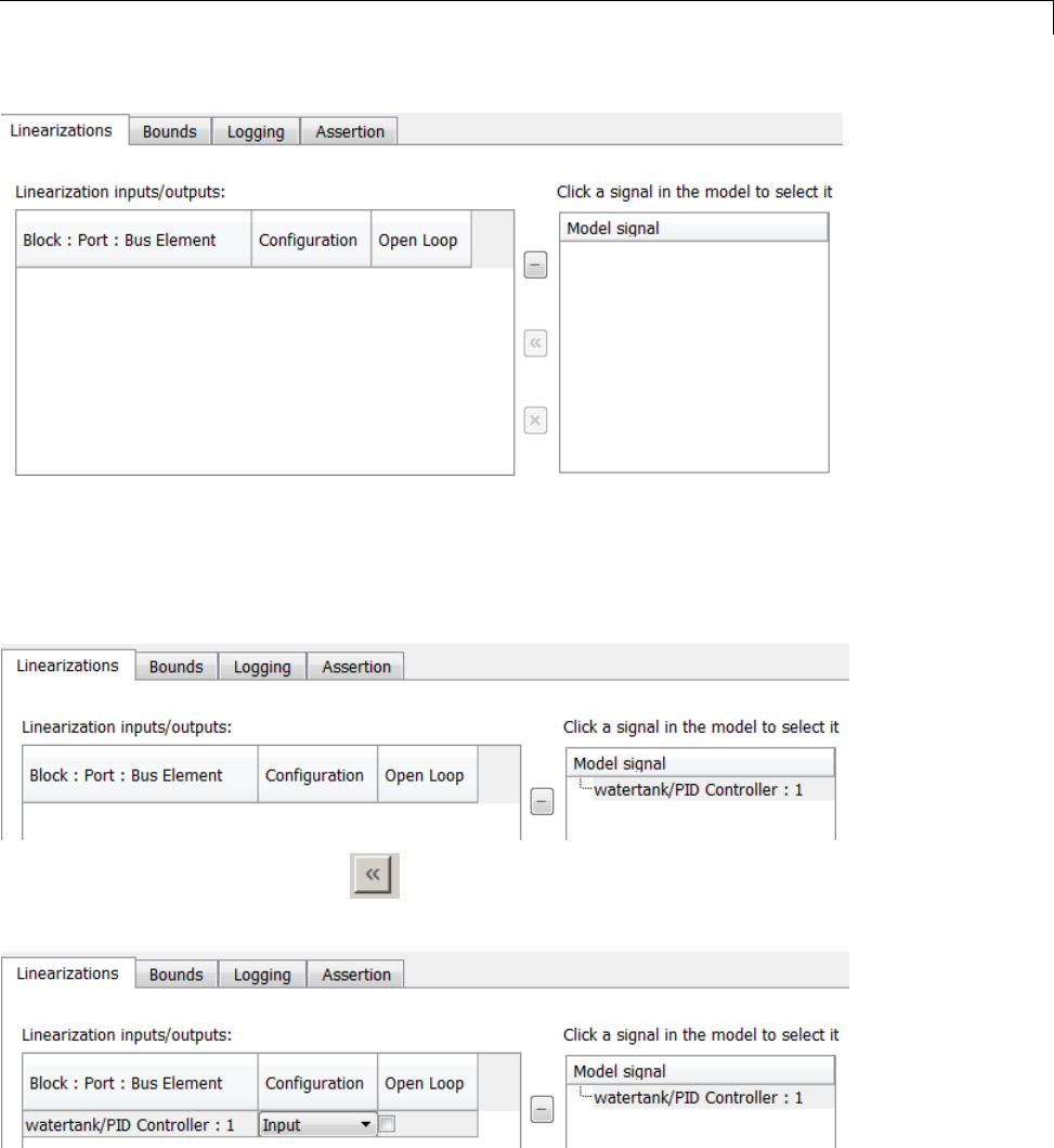
Model Verification at Multiple Simulation Snapshots
ii In the Simulink model, click the output signal of the PID Controller
block to select it.
The Click a signal in the model to select it area updates to display
the selected signal.
iii Click to add the signal to the Linearization inputs/outputs
table.
5-17
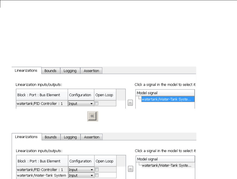
5Model Verification
bTo specify an output:
iv In the Simulink model, click the output signal of the Water-Tank
System block to select it.
The Click a signal in the model to select it area updates to display
the selected signal.
vClick to addthesignaltotheLinearization inputs/outputs
table.
vi In the Configuration drop-down list of the Linearization
inputs/outputs table, select Output for watertank/Water-Tank
System : 1.
vii Select the Open Loop option for watertank/Water-Tank System
:1.
The Linearization inputs/outputs table now resembles the following
figure.
5-18
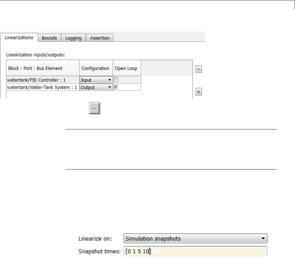
Model Verification at Multiple Simulation Snapshots
cClick to collapse the Click a signal in the model to select it area.
Tip Alternatively, before you add the Linear Analysis Plots block,
right-click the signals in the Simulink model and select Linear Analysis
Points > Input Point and Linear Analysis Points > Output Point.
Linearization I/O annotations appear in the model and the selected signals
appear in the Linearization inputs/outputs table.
6Specify simulation snapshot times.
aIn the Linearizations tab, verify that Simulation snapshots is
selected in Linearize on.
bIn the Snapshot times field, type [0 1 5 10].
7Specify multiple bound segments for assertion in the Bounds tab of the
Block Parameters dialog box. In this example, enter the following lower
magnitude bounds:
•Frequencies (rad/s) —{[0.001 0.003],[0.01 0.04]}
•Magnitudes (dB) —{[20 20],[15 15]}
5-19
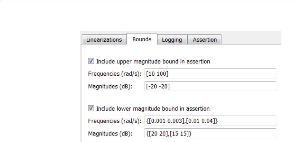
5Model Verification
Click Apply to apply the parameter changes to the block.
Click ShowPlotto view the bounds on the Bode magnitude plot.
5-20
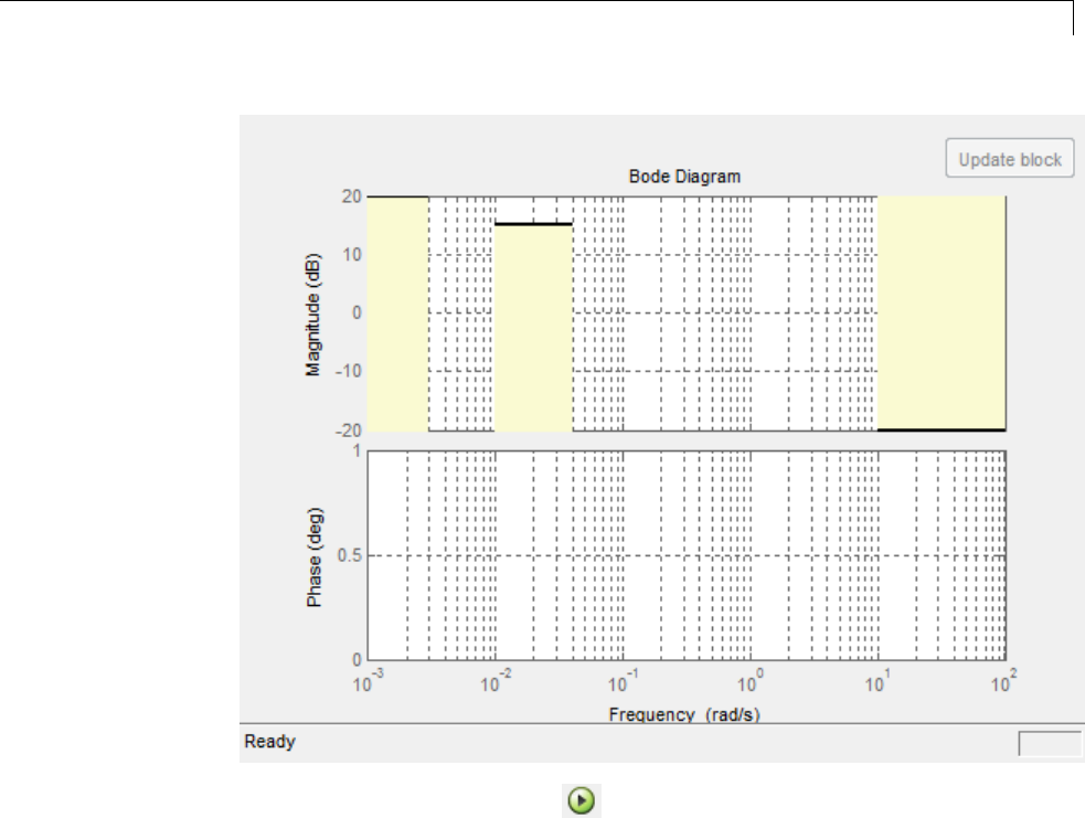
Model Verification at Multiple Simulation Snapshots
8Simulate the model by clicking in the plot window.
Alternatively, you can simulate the model from the Simulink Editor.
The software linearizes the portion of the model between the linearization
input and output at the simulation times of 0,1, 5 and 10. When the
software detects that the linear system computed at times 0 and 1 violate a
specified lower magnitude bound, the following warning messages appear
at the MATLAB prompt:
Warning: Assertion detected in 'watertank_check_bode/Check Bode
Characteristics' at time 0
Warning: Assertion detected in 'watertank_check_bode/Check Bode
Characteristics' at time 1
5-21
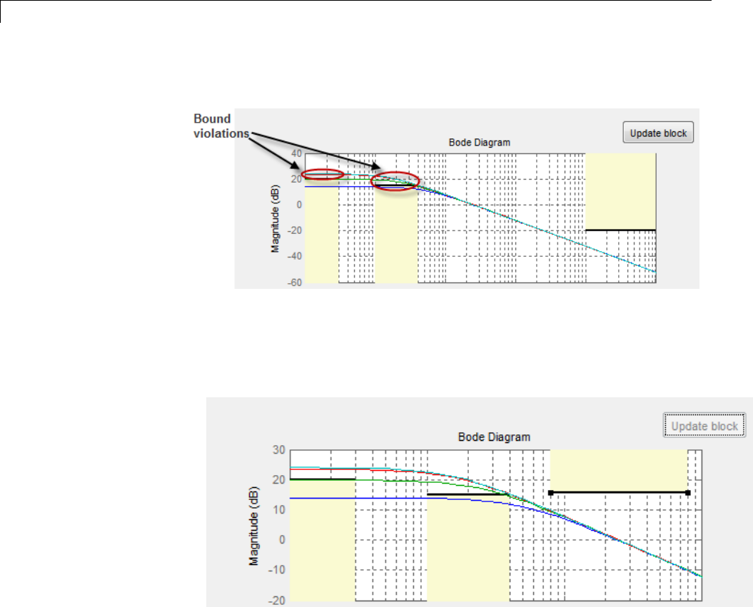
5Model Verification
You can also view the bound violations in the plot window.
9Modify a bound graphically. For example, to modify the upper magnitude
bound graphically:
aIn the plot window, click the bound segment to select it and then drag
it to the desired location.
bClickUpdate block to update the new values in the Bounds tab of the
Block Parameters dialog box.
5-22
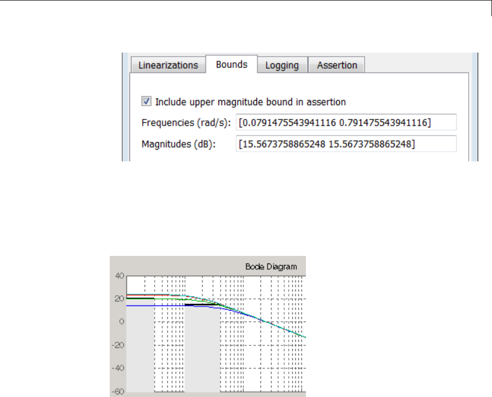
Model Verification at Multiple Simulation Snapshots
10 Disable the lower bounds to exclude them from asserting. Clear the
Include lower magnitude bounds in assertion option in the Block
Parameters dialog box. Then, click Apply.
The lower bounds are now grey-out in the plot window, indicating that
they are excluded from assertion.
11 Resimulate the model to check if bounds are satisfied.
The software satisfies the specified upper magnitude bound, and therefore
thesoftwarenolongerreportsanassertionfailure.
5-23
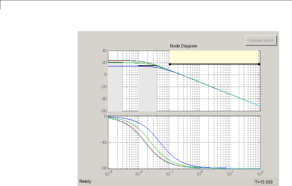
5Model Verification
5-24
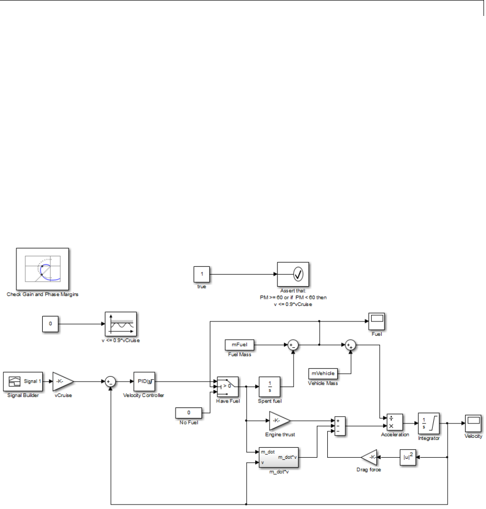
Model Verification Using Simulink®Control Design™ and Simulink®Verification Blocks
Model Verification Using Simulink Control Design and
Simulink Verification Blocks
This example shows how to use a combination of Simulink Control Design and
Simulink verification blocks, to assert that the linear system characteristics
satisfy one of the following bounds:
•Phase margin greater than 60 degrees
•Phase margin less than 60 degrees and the velocity less than or equal to
90% of the cruise velocity.
1Open the Simulink model of an aircraft.
scdmultiplechecks
5-25
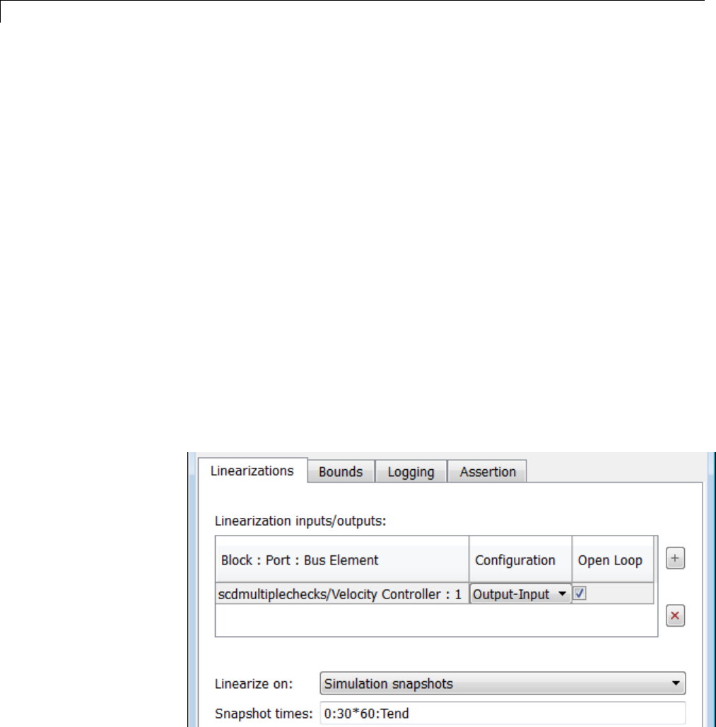
5Model Verification
The aircraft model is based on a long-haul passenger aircraft flying at
cruising altitude and speed. The aircraft starts with a full fuel load and
follows a pre-specified 8-hour velocity profile. The model is a simplified
version of a velocity control loop, which adjusts the fuel flow rate to control
the aircraft velocity.
The model includes blocks to model:
•Fuel consumption and resulting changes in aircraft mass
•Nonlinear draft effects limiting aircraft velocity
Constants used in the model, such as the drag coefficient, are defined in
the model workspace and initialized from a script.
The v <= 0.9*vCruise and Assert that: PM >= 60 or if PM < 60
then v <= 0.9*vCruise blocks are Check Static Upper Bound and
Assertion blocks, respectively, from the Simulink Model Verification
library. In this example, you use these blocks with the Check Gain and
Phase Margins block to design a complex logic for assertion.
2View the linearization input, output and settings in the Linearizations
tab of the Check Gain and Phase Margins block parameters dialog box.
5-26
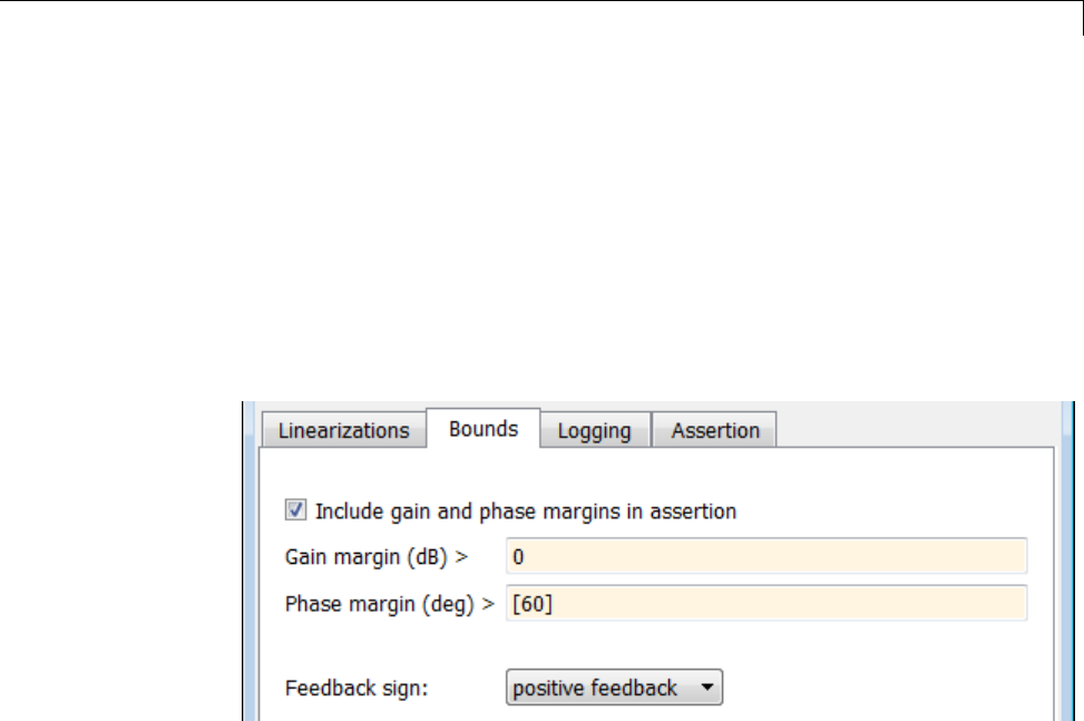
Model Verification Using Simulink®Control Design™ and Simulink®Verification Blocks
The model has already been configured with:
•Linearization input and output for computing gain and phase margins
•Settings to compute the linear system
The software linearizes the loop seen by the Velocity Controller block every
30 minutes of simulated time and computes the gain and phase margins.
3Specify phase margin bounds in the Bounds tab of the Check Gain and
Phase Margins block.
In this example, the linearization input and output include the summation
block with negative feedback. Change the Feedback sign,usedtocompute
the margin, to positive feedback.
To view the phase margins to be computed later during simulation, specify
Tabular in Plot type,andclickShow Plot.
4Design assertion logic that causes the verification blocks to assert when the
phase margin is greater than 60 degrees or if the phase margin is less than
60 degrees, the velocity is less than or equal to 90% the cruise velocity.
aIn the Check Gain and Phase Margins Block Parameters dialog box,
select Output assertion signal and click Apply.
This action adds an output port z-1 to the block.
5-27

5Model Verification
bDouble-click the v <= 0.9*vCruise block and specify the block
parameters, as shown in the following figure. After setting the
parameters, click Apply.
These parameters configure the block to:
•Check if the aircraft velocity exceeds the cruise velocity by 0.9 times
•Add an output port to the block
cConnect the Check Gain and Phase Margins, v <= 0.9*vCruise and
Assert that: PM >= 60 or if PM < 60 then v <= 0.9*vCruise
blocks, as shown in the following figure.
5-28
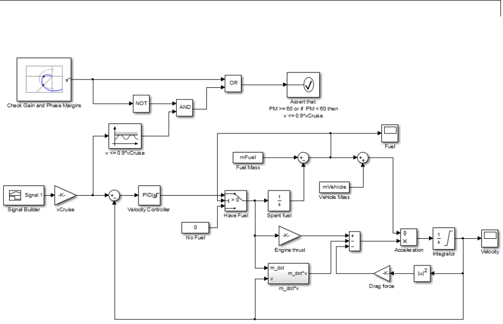
Model Verification Using Simulink®Control Design™ and Simulink®Verification Blocks
This connection causes the Assert that: PM >= 60 or if PM < 60
then v <= 0.9*vCruise block to assert and stop the simulation if the
phase margin is less than 60 degrees and the velocity is greater than
90% of the cruise velocity.
Alternatively, you can type scdmultiplechecks_final at the MATLAB
prompt to open a Simulink model already configured with these settings.
5Simulate the model by selecting Simulation > Run in the Simulink Editor.
During simulation:
•The v <= 0.9*vCruise block asserts multiple times and warnings
appear at the MATLAB prompt.
•The Check Gain and Phase Margins block asserts two times and
warnings appear at the MATLAB prompt. You can also view the phase
margins that violate the bound in the plot window.
5-29

5Model Verification
•The Assert that: PM >= 60 or if PM < 60 then v <=
0.9*vCruise does not encounter the assertion condition. Therefore,
no warnings appear at the MATLAB prompt for this block and the
simulation does not stop.
5-30

6
Function Reference
Linearization Analysis I/Os (p. 6-2) Functions for creating and setting
linearization analysis I/Os
Steady-State Operating Points
(p. 6-3)
Functions for creating and working
with operating points
Linearization (p. 6-4) Functions for linearizing Simulink
models
Frequency Response Estimation
(p. 6-5)
Functions for estimating frequency
response models
Interface for Compensator Tuning
(p. 6-6)
Interface for Control System Design
and Analysis in Simulink

6Function Reference
Linearization Analysis I/Os
get Properties of linearization I/Os and
operating points
getlinio Linearization input/output (I/O)
settings for Simulink model, Linear
Analysis Plots or Model Verification
block
linio Define linearization input/output
(I/O) points for Simulink model
set Set properties of linearization I/Os
and operating points
setlinio Specify linearization input/output
(I/O) points for Simulink model,
Linear Analysis Plots block, or
Model Verification block
6-2

Steady-State Operating Points
Steady-State Operating Points
addoutputspec Add output specification to operating
point specification
copy Copy operating point or operating
point specification
findop Steady-state operating point
from specifications (trimming) or
simulation
get Properties of linearization I/Os and
operating points
getinputstruct Input structure from operating point
getstatestruct State structure from operating point
getxu States and inputs from operating
points
initopspec Initialize operating point
specification values
operpoint Create operating point for Simulink
model
operspec Operating point specifications
set Set properties of linearization I/Os
and operating points
setxu Set states and inputs in operating
points
update Update operating point object with
structural changes in model
6-3

6Function Reference
Linearization
frest.simCompare Plot time-domain simulation of
nonlinear and linear models
getlinio Linearization input/output (I/O)
settings for Simulink model, Linear
Analysis Plots or Model Verification
block
getlinplant Compute open-loop plant model from
Simulink diagram
linearize Linear approximation of Simulink
model or block
linio Define linearization input/output
(I/O) points for Simulink model
linlft Linearize model while removing
contribution of specified blocks
linlftfold Combine linearization results from
specified blocks and model
linoptions Set options for linearization and
finding operating points
operpoint Create operating point for Simulink
model
6-4

Frequency Response Estimation
Frequency Response Estimation
frest.Chirp Swept-frequency cosine signal
frest.createFixedTsSinestream Sinestream input signal with fixed
sample time
frest.createStep Step input signal
frest.findDepend List of model path dependencies
frest.findSources Identify time-varying source blocks
frest.Random Random input signal for simulation
frest.simCompare Plot time-domain simulation of
nonlinear and linear models
frest.simView Plot frequency response model in
time- and frequency-domain
frest.Sinestream Signal containing series of sine
waves
frestimate Frequency response estimation of
Simulink models
frestimateOptions Options for frequency response
estimation
fselect Extract sinestream signal at
specified frequencies
generateTimeseries Generate time-domain data for input
signal
getSimulationTime Final time of simulation for
frequency response estimation
6-5

6Function Reference
Interface for Compensator Tuning
getIOTransfer (slTunable) Tunable model of closed-loop
transfer function between specified
inputs and outputs
getLoopTransfer (slTunable) Tunable model of open-loop transfer
function at specified location
looptune (slTunable) Tune MIMO feedback loops in
Simulink
slTunable Interface for control system tuning
of Simulink models
6-6

7
Class Reference

slTunable
Purpose Interface for control system tuning of Simulink models
Description slTunable provides an interface between a Simulink model and the
tuning commands slTunable.systune and slTunable.looptune.
(Using these tuning commands requires Robust Control Toolbox
software). slTunable allows you to:
•Specify the control architecture.
•Extract information about the control system, such as linearized
open-loop and closed-loop responses.
•Designateandparametrizeblockstobetuned.
Because tuning commands such as systune operate on linear
models, the slTunable interface automatically computes and stores a
linearization of your Simulink model. (For more information about
linearization, see linearize). slTunable also parametrizes the tunable
portion of your control system. You can use slTunable and its methods
for tuning and analyzing the control system.
Commands that query the linearization stored in the slTunable
interface automatically relinearize the Simulink model if you
have changed any properties of the slTunable interface since the
last linearization. Such commands include slTunable.systune,
slTunable.looptune,slTunable.getIOTransfer,and
slTunable.getLoopTransfer.
Construction ST = slTunable(mdl,tunedblocks) creates an slTunable interface
ST for tuning the blocks tunedblocks of the Simulink model mdl.
Creating ST automatically parametrizes the blocks specified by
tunedblocks.TheinterfaceST also stores a linearization of mdl,
computed at the operating point and linearization I/O points specified
in the model.
ST = slTunable(mdl,tunedblocks,io) further specifies a vector io of
linearization I/O points for analysis and tuning of the control system.
7-2

slTunable
ST = slTunable(mdl,tunedblocks,io,op) also specifies an operating
point op for linearizing the model.
ST = slTunable(...,options) specifies additional options for
linearizing mdl.
ST = slTunable(...,Name,Value) sets the additional properties of
ST specified by one or more Name,Value pair arguments. Name is a
property name, and Value is the corresponding value. Name must
appear inside single quotes (''). You can specify several name-value
pair arguments in any order as Name1,Value1,...,NameN,ValueN.
Specifying properties of ST in this way saves repeated linearization by
ensuring that the interface is fully configured before linearizing the
model.
Input Arguments
mdl
String specifying name of Simulink model.
tunedblocks
String or cell array of strings specifying the Simulink block
or blocks to tune. You can specify an abbreviated block name
provided that the string matches the end of the full block path
and unambiguously identifies the block to tune.
slTunable automatically parametrizes the blocks listed in
tunedblocks. To override the default parametrization, use
slTunable.setBlockParam.
io
Vector of I/O points for linearization, tuning, and analysis of
the control system. (For more information about I/O points, see
linio.) These I/O points specify which signals are model inputs,
outputs, and loop opening locations. Only signals specified in io
or added with slTunable.addIO are available in the interface ST
for tuning and analysis.
7-3

slTunable
op
Operating point specification for linearizing mdl.Formore
information about operating point specifications, see operpoint
and findop.
options
Option set specifying additional options for the linearization of
mdl.Use
linoptions to create options. For information about
available options, see the linoptions reference page.
Name-Value Pair Arguments
Specify optional comma-separated pairs of Name,Value arguments,
where Name istheargumentnameandValue is the corresponding
value. Name must appear inside single quotes (''). You can
specify several name and value pair arguments in any order as
Name1,Value1,...,NameN,ValueN.
Controls
Cell array of strings specifying the controller outputs that drive
the actuators in the control system. These strings correspond
to signal names in mdl.
The Controls and Measurements properties of ST define the
boundary between the plant and controller in mdl for tuning with
slTunable.looptune.
Use slTunable.addControl to specify additional control signals
in the Controls property of an existing slTunable interface.
Default: 0-by-1 cell array
IOs
Cell array of strings specifying the input and output signals
available for analysis and tuning. Each signal is characterized by:
•Full path in the model, either:
7-4

slTunable
BlockPath/PortNumber[SignalName]
or
BlockPath/PortNumber[BusElement1.BusElement2]
•Linearization I/O type 'in','out','inout',or'outin'.
ST.IOs automatically includes all the linearization I/O points
specified in the model. To remove a linearization I/O from
ST.IOs, delete a row from the cell array. For example, the
following command deletes the second I/O from ST.IOs.
ST.IOs(2,:) = [];
To add a linearization I/O to ST,useslTunable.addIO.
For more information about linearization I/O points, see linio.
Default: 0-by-2 cell array
LinearizeOptions
Options set for linearizing mdl.Uselinoptions to create
the options set. Use slTunable.linearize to relinearize
mdl and update the slTunable interface after changing
LinearizeOptions.
Measurements
Cell array of strings specifying the sensor outputs that feed the
controller in the control system. These strings correspond to
signal names in mdl.TheControls and Measurements properties
of ST define the boundary between the plant and controller in mdl
for tuning with slTunable.looptune.
Use slTunable.addMeasurement to specify additional
measurement signals in the Measurement property of an existing
slTunable interface.
7-5

slTunable
Default: 0-by-1 cell array
ModelName
String specifying the name of the model being analyzed or tuned.
ModelName is set by the input argument mdl.
Notes
User notes. This property can store any text as a string or cell
array of strings. For example:
ST.Notes = 'This model was created on Jan. 1st, 2011.';
Default: {}
Openings
Cell array of strings specifying signal locations in mdl where
feedback loops are broken. The loop openings are enforced in all
tuning and validation commands such as slTunable.looptune
and slTunable.loopview.
Loop opening locations are stored in the Openings property as the
full path name of the corresponding signal in mdl,either:
BlockPath/PortNumber[SignalName]
or
BlockPath/PortNumber[BusElement1.BusElement2]
Use slTunable.addOpening toaddadditionalloopopenings
to the Opening property of an existing slTunable interface. To
remove a loop opening location, delete a row from the cell array.
For example, the following command deletes the second I/O from
ST.Openings.
ST.Openings(2,:) = [];
Default: 0-by-1 cell array
7-6

slTunable
OperatingPoint
Operating point specification for linearizing mdl.Use
slTunable.linearize to relinearize mdl and update the
slTunable interface after changing OperatingPoint.
For more information about operating point specifications, see
operpoint and findop.
Ts
Working sampling time for analysis and tuning. mdl is linearized
at this sampling time.
Default: 0
Switches
Cell array specifying signal locations in mdl where feedback
loops may be broken for analysis or tuning purposes. Switches
differs from Openings in that the loop openings specified in
Openings are always enforced in tuning and analysis. In contrast,
locations specified in Switches are closed by default unless you
explicitly specify them open. Youcanspecifyswitchlocations
as openings in commands such as slTunable.getIOTransfer,
slTunable.getLoopTransfer,orTuningGoal.LoopShape.
Switch locations are stored in the Switches property as the full
path name of the corresponding signal in mdl,either:
BlockPath/PortNumber[SignalName]
or
BlockPath/PortNumber[BusElement1.BusElement2]
Use slTunable.addSwitch to add additional loop openings to
the Switches property of an existing slTunable interface. To
remove a loop opening location, delete a row from the cell array.
For example, the following command deletes the second I/O from
ST.Switches.
7-7

slTunable
ST.Switches(2,:) = [];
Default: 0-by-1 cell array
TunedBlocks
Cell array of strings specifying full paths to the tuned blocks in
mdl.
When you create an slTunable interface, the TunedBlocks
property is automatically populated with the blocks you specify
in the tunedblocks input. To specify additional tunable
blocks in an existing an existing slTunable interface, use
slTunable.addBlock
Properties Controls
Cell array of strings specifying the controller outputs that drive
the actuators in the control system. These strings correspond
to signal names in mdl.
The Controls and Measurements properties of ST define the
boundary between the plant and controller in mdl for tuning with
slTunable.looptune.
Use slTunable.addControl to specify additional control signals
in the Controls property of an existing slTunable interface.
Default: 0-by-1 cell array
IOs
Cell array of strings specifying the input and output signals
available for analysis and tuning. Each signal is characterized by:
•Full path in the model, either:
BlockPath/PortNumber[SignalName]
or
7-8

slTunable
BlockPath/PortNumber[BusElement1.BusElement2]
•Linearization I/O type 'in','out','inout',or'outin'.
ST.IOs automatically includes all the linearization I/O points
specified in the model. To remove a linearization I/O from
ST.IOs, delete a row from the cell array. For example, the
following command deletes the second I/O from ST.IOs.
ST.IOs(2,:) = [];
To add a linearization I/O to ST,useslTunable.addIO.
For more information about linearization I/O points, see linio.
Default: 0-by-2 cell array
LinearizeOptions
Options set for linearizing mdl.Uselinoptions to create
the options set. Use slTunable.linearize to relinearize
mdl and update the slTunable interface after changing
LinearizeOptions.
Measurements
Cell array of strings specifying the sensor outputs that feed the
controller in the control system. These strings correspond to
signal names in mdl.TheControls and Measurements properties
of ST define the boundary between the plant and controller in mdl
for tuning with slTunable.looptune.
Use slTunable.addMeasurement to specify additional
measurement signals in the Measurement property of an existing
slTunable interface.
Default: 0-by-1 cell array
ModelName
7-9

slTunable
String specifying the name of the model being analyzed or tuned.
ModelName is set by the input argument mdl.
Notes
User notes. This property can store any text as a string or cell
array of strings. For example:
ST.Notes = 'This model was created on Jan. 1st, 2011.';
Default: {}
Openings
Cell array of strings specifying signal locations in mdl where
feedback loops are broken. The loop openings are enforced in all
tuning and validation commands such as slTunable.looptune
and slTunable.loopview.
Loop opening locations are stored in the Openings property as the
full path name of the corresponding signal in mdl,either:
BlockPath/PortNumber[SignalName]
or
BlockPath/PortNumber[BusElement1.BusElement2]
Use slTunable.addOpening toaddadditionalloopopenings
to the Opening property of an existing slTunable interface. To
remove a loop opening location, delete a row from the cell array.
For example, the following command deletes the second I/O from
ST.Openings.
ST.Openings(2,:) = [];
Default: 0-by-1 cell array
OperatingPoint
7-10

slTunable
Operating point specification for linearizing mdl.Use
slTunable.linearize to relinearize mdl and update the
slTunable interface after changing OperatingPoint.
For more information about operating point specifications, see
operpoint and findop.
Ts
Working sampling time for analysis and tuning. mdl is linearized
at this sampling time.
Default: 0
Switches
Cell array specifying signal locations in mdl where feedback
loops may be broken for analysis or tuning purposes. Switches
differs from Openings in that the loop openings specified in
Openings are always enforced in tuning and analysis. In contrast,
locations specified in Switches are closed by default unless you
explicitly specify them open. Youcanspecifyswitchlocations
as openings in commands such as slTunable.getIOTransfer,
slTunable.getLoopTransfer,orTuningGoal.LoopShape.
Switch locations are stored in the Switches property as the full
path name of the corresponding signal in mdl,either:
BlockPath/PortNumber[SignalName]
or
BlockPath/PortNumber[BusElement1.BusElement2]
Use slTunable.addSwitch to add additional loop openings to
the Switches property of an existing slTunable interface. To
remove a loop opening location, delete a row from the cell array.
For example, the following command deletes the second I/O from
ST.Switches.
7-11

slTunable
ST.Switches(2,:) = [];
Default: 0-by-1 cell array
TunedBlocks
Cell array of strings specifying full paths to the tuned blocks in
mdl.
When you create an slTunable interface, the TunedBlocks
property is automatically populated with the blocks you specify
in the tunedblocks input. To specify additional tunable
blocks in an existing an existing slTunable interface, use
slTunable.addBlock
Methods
addBlock Add block to list of tuned blocks
addControl Add control signal to list of control
signals in interface
addIO Add I/O points list of linearization
I/Os in interface
addMeasurement Add measurement signal to list of
measurement signals in interface
addOpening Add new opening location to list
of loop openings in interface
addSwitch Add switch location to list of loop
opening switches in interface
getBlockParam Get parametrization of a
particular tuned block in
slTunable interface
getBlockRateConversion Query rate conversion method of
tunable block
7-12

slTunable
getBlockValue Current value of a particular
tuned block in slTunable
interface
getIOTransfer Tunable model of closed-loop
transfer function between
specified inputs and outputs
getLoopTransfer Tunable model of open-loop
transfer function at specified
location
linearize Relinearize Simulink model to
update slTunable interface
looptune Tune MIMO feedback loops in
Simulink
loopview Graphically analyze results of
control system tuning
readBlockValue Update tuned block values from
Simulink model
setBlockParam Specify parametrization for
specified tuned block
setBlockRateConversion Set rate conversion method of
tunable block
setBlockValue Set current value of
parametrization for specified
block
showBlockValue Display current value of block
parametrizations
showTunable Display current value of block
parametrizations
7-13
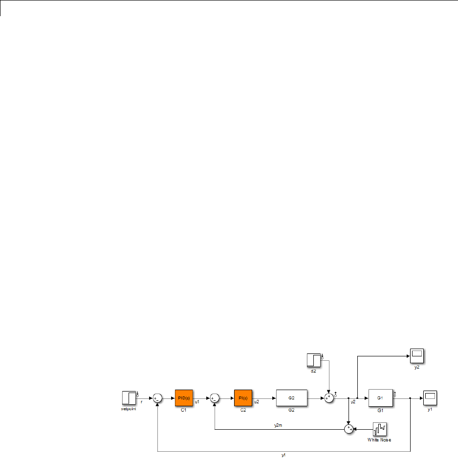
slTunable
systune Tune fixed-structure control
system parameters in Simulink
writeBlockValue Update block values in Simulink
model
Copy
Semantics
To make an independently modifiable copy of an slTunable interface,
use the copy command. For example:
ST = copy(STO)
creates an slTunable interface ST that initially contains identical values
to ST0 for all properties. You can now modify ST without changing ST0.
slTunable is a handle class. To learn more about how handle
classes affect copy operations, see Copying Objects in the MATLAB
Programming Fundamentals documentation.
Examples Create and Configure slTunable Interface
Create and configure a slTunable interface for tuning the Simulink
model rct_cascade using slTunable.looptune.
Open the Simulink model.
open_system('rct_cascade')
Create the slTunable interface for rct_cascade.
7-14

slTunable
tunedblocks = {'C1','C2'};
ST0 = slTunable('rct_cascade',tunedblocks);
The tunable blocks of this model are the PID controllers, C1 and C2.
This command creates the slTunable interface ST0 with those tunable
blocks.
Specify the control and measurement signals of the control system.
addControl(ST0,'u2');
addMeasurement(ST0,{'y1','y2m'});
The commands slTunable.addControl and
slTunable.addMeasurement add the specified signals to the Controls
and Measurements properties of ST0.
Control and measurement signals define the boundary between plant
and controller for tuning with slTunable.looptune.Inrct_cascade,
the actuator signal is u2, the output of the inner-loop controller. The
measurement signals are y1 and y2m, each of which feeds into a portion
of the cascaded controller.
Specify the signal y1 as a location for an optional loop opening (a switch).
addSwitch(ST0,'y1');
When tuning a cascade control system, it can be useful to impose certain
requirements on the inner loop that are enforced with the outer loop
open. However, such a control system also has overall requirements are
enforced with all loops closed. Therefore, add a switch location, instead
of a loop opening location.
You can now use ST0 to tune the control system with
slTunable.looptune.
Algorithms slTunable linearizes your Simulink model using the algorithms
described in “Exact Linearization Algorithm” on page 2-146.
Tutorials • “Tuning Control Systems in Simulink”
7-15

slTunable
How To • “Set Up Your Control System for Tuning with systune”
• “Specifying Design Requirements for systune”
• “Set Up Your Control System for Tuning with looptune”
• “Performance and Robustness Specifications for looptune”
7-16

8
Alphabetical List

addoutputspec
Purpose Add output specification to operating point specification
Syntax opnew=addoutputspec(op,'block',portnumber)
Alternatives As an alternative to the addoutputspec function, add output
specifications with the Simulink Control Design GUI. See “Steady-State
Operating Point to Meet Output Specification” on page 1-21.
Description opnew=addoutputspec(op,'block',portnumber) adds an output
specification for a Simulink model to an existing operating point
specification, op, created with operspec. The signal being constrained
by the output specification is indicated by the name of the block,
'block', and the port number, portnumber,thatitoriginatesfrom.
You can edit the output specification within the new operating
point specification object, opnew,toincludetheactualconstraintsor
specifications for the signal. Use the new operating point specification
object with the function findop to find operating points for the model.
This function automatically compiles the Simulink model, given in the
property Model of op, to find the block’s output portwidth.
Examples Create an operating point specification for the model magball.
op=operspec('magball')
This specification returns the object op.Notethattherearenooutports
in this model and no outputs in the object op.
Operating Specification for the Model magball.
(Time-Varying Components Evaluated at time t=0)
States:
----------
(1.) magball/Controller/PID Controller/Filter
spec: dx = 0, initial guess: 0
(2.) magball/Controller/PID Controller/Integrator
spec: dx = 0, initial guess: 14
8-2

addoutputspec
(3.) magball/Magnetic Ball Plant/Current
spec: dx = 0, initial guess: 7
(4.) magball/Magnetic Ball Plant/dhdt
spec: dx = 0, initial guess: 0
(5.) magball/Magnetic Ball Plant/height
spec: dx = 0, initial guess: 0.05
Inputs: None
----------
Outputs: None
----------
To add an output specification to the signal between the Controller block
and the Magnetic Ball Plant block, use the function addoutputspec.
newop=addoutputspec(op,'magball/Controller',1)
This function adds the output specification is added to the operating
point specification object.
Operating Specification for the Model magball.
(Time-Varying Components Evaluated at time t=0)
States:
----------
(1.) magball/Controller/PID Controller/Filter
spec: dx = 0, initial guess: 0
(2.) magball/Controller/PID Controller/Integrator
spec: dx = 0, initial guess: 14
(3.) magball/Magnetic Ball Plant/Current
spec: dx = 0, initial guess: 7
(4.) magball/Magnetic Ball Plant/dhdt
spec: dx = 0, initial guess: 0
(5.) magball/Magnetic Ball Plant/height
spec: dx = 0, initial guess: 0.05
8-3

addoutputspec
Inputs: None
----------
Outputs:
----------
(1.) magball/Controller
spec: none
Edit the output specification to constrain this signal to be 14.
newop.Outputs(1).Known=1, newop.Outputs(1).y=14
The final output specification is displayed.
Operating Specification for the Model magball.
(Time-Varying Components Evaluated at time t=0)
States:
----------
(1.) magball/Controller/PID Controller/Filter
spec: dx = 0, initial guess: 0
(2.) magball/Controller/PID Controller/Integrator
spec: dx = 0, initial guess: 14
(3.) magball/Magnetic Ball Plant/Current
spec: dx = 0, initial guess: 7
(4.) magball/Magnetic Ball Plant/dhdt
spec: dx = 0, initial guess: 0
(5.) magball/Magnetic Ball Plant/height
spec: dx = 0, initial guess: 0.05
Inputs: None
----------
Outputs:
----------
(1.) magball/Controller
spec: y = 0
8-4

addoutputspec
See Also findop |operspec |operpoint
8-5

copy
Purpose Copy operating point or operating point specification
Syntax op_point2=copy(op_point1)
op_spec2=copy(op_spec1)
Description op_point2=copy(op_point1) returns a copy of the operating point object
op_point1. You can create op_point1 with the function operpoint.
op_spec2=copy(op_spec1) returns a copy of the operating point
specification object op_spec1. You can create op_spec1 with the
function operspec.
Note The command op_point2=op_point1 does not create a copy of
op_point1 but instead creates a pointer to op_point1. In this case, any
changes made to op_point2 arealsomadetoop_point1.
Examples Create an operating point object for the model, magball.
opp=operpoint('magball')
The operating point is displayed.
Operating Point for the Model magball.
(Time-Varying Components Evaluated at time t=0)
States:
----------
(1.) magball/Controller/PID Controller/Filter
x: 0
(2.) magball/Controller/PID Controller/Integrator
x: 14
(3.) magball/Magnetic Ball Plant/Current
x: 7
(4.) magball/Magnetic Ball Plant/dhdt
x: 0
8-6

copy
(5.) magball/Magnetic Ball Plant/height
x: 0.05
Inputs: None
----------
Create a copy of this object, opp.
new_opp=copy(opp)
An exact copy of the object is displayed.
Operating Point for the Model magball.
(Time-Varying Components Evaluated at time t=0)
States:
----------
(1.) magball/Controller/PID Controller/Filter
x: 0
(2.) magball/Controller/PID Controller/Integrator
x: 14
(3.) magball/Magnetic Ball Plant/Current
x: 7
(4.) magball/Magnetic Ball Plant/dhdt
x: 0
(5.) magball/Magnetic Ball Plant/height
x: 0.05
Inputs: None
----------
See Also operpoint |operspec
8-7

findop
Purpose Steady-state operating point from specifications (trimming) or
simulation
Syntax [op,opreport] = findop(sys,opspec)
[op,opreport] = findop(sys,opspec,options)
op = findop(sys,tsnapshot)
Description [op,opreport] = findop(sys,opspec) returns the steady-state
operating point of the model that meets the specifications opspec.The
Simulink model must be open. If opspec is a vector of operating points
specifications, findop returns a vector of corresponding operating
points.
[op,opreport] = findop(sys,opspec,options) searches for the
operating point of the model using additional optimization algorithm
options specified by options.
op = findop(sys,tsnapshot) simulates the model and extracts
operating points at the simulation snapshot time instants (snapshots)
tsnapshot.
Tips •Initialize operating point search at a simulation snapshot or a
previously computed operating point using initopspec.
•Linearize the model at the operating point op using linearize.
Input
Arguments
sys
Simulink model name, specified as a string inside single quotes ('').
opspec
Operating point specification object for the model sys,specifiedusing
operspec.
opspec can also be a vector of operating point specification objects. If
opspec is a vector of operating points specifications, findop returns a
vector of corresponding operating points. In this case, findop needs to
compile the model only once. Using a vector of operating points allows
8-8

findop
youtofindmultipletrimmedoperating points without the overhead of
compiling the model for each trimming computation.
options
Algorithm options, specified using linoptions.
tsnapshot
Simulation snapshot time instants when to extract the operating point
of the model, specified as a scalar or vector.
Output
Arguments
op
Operating point object.
After creating the operating point object, you can modify the operating
point states and input levels. For example, op.States(1).x stores the
state values of the first model state, and op.Inputs(1).u stores the
input level of the first inport block.
The operating point object has these properties:
•Model — Simulink model name. String.
•States — State operating points of the Simulink model. Vector of
data structures, where each data structure represents the states of
one Simulink block. Each States structure has these fields:
xSimulink block state values, specified as a
vector of states.
Ts (Only for discrete-time states) Sample time
and offset of each Simulink block state,
specified as a vector.
Description Block state description, specified as a string.
Nx (read only) Number of states in the Simulink block.
Block Simulink block name.
8-9

findop
SampleType State time rate can have the values:
•'CSTATE' — Continuous-time state
-'DSTATE' — Discrete-time state.
inReferencedModel Determine whether the sates is inside a
reference model:
•1— State is inside a reference model.
-0— State is in the current model file.
•Inputs — Input levels at the operating point. Vector of data
structures, where each data structure represents the input levels of
one root-level inport block in the Simulink block. Each Inputs data
structure has these fields:
uInport block input levels at the operating
point, specified as a vector of input levels.
Description Inport block input description, specified as
astring.
Block Inport block name.
PortWidth Number of inport block signals.
•Time — Time instants for evaluating the time-varying functions in
the model.
If opspec is a vector of operating point specification objects, then op is a
vector of corresponding operating points.
opreport
Optimization results report object.
8-10

findop
This report displays automatically even when you suppress the output
using a semicolon. You can avoid displaying the report by using
linoptions to set the DisplayReport field in options to 'off'.
The opreport object has these properties:
•Model —Model property value of the op object.
•Inputs —Inputs property value of the op object.
•Outputs —Outputs property value of the op object with the addition
of yspec, which is the desired yvalue.
•States —States property value of the op object with the addition
of dx, which are the state derivative values.
•Time —Time property value of the op object.
•TerminationString — Optimization termination condition, stored
as a string.
•OptimizationOutput — Optimization algorithm results, returned
as a structure with these fields:
iterations
funcCount
lssteplength
stepsize
algorithm
firstorderopt
constrviolation
message
For more information about the optimization algorithm, see the
Optimization Toolbox™ documentation.
8-11

findop
Definitions Steady-State Operating Point (Trim Condition)
Asteady-state operating point of the model, also called equilibrium or
trim condition, includes state variables that do not change with time.
A model might have several steady-state operating points. For example,
a hanging pendulum has two steady-state operating points. A stable
steady-state operating point occurs when a pendulum hangs straight
down. That is, the pendulum position does not change with time.
When the pendulum position deviates slightly, the pendulum always
returns to equilibrium; small changes in the operating point do not
cause the system to leave the region of good approximation around
the equilibrium value.
An unstable steady-state operating point occurs when a pendulum points
upward. As long as the pendulum points exactly upward, it remains in
equilibrium. However, when the pendulum deviates slightly from this
position, it swings downward and the operating point leaves the region
around the equilibrium value.
When using optimization search to compute operating points for a
nonlinear system, your initial guesses for the states and input levels
must be in the neighborhood of the desired operating point to ensure
convergence.
When linearizing a model with multiplesteady-stateoperating points, it
is important to have the right operating point. For example, linearizing
a pendulum model around the stable steady-state operating point
produces a stable linear model, whereas linearizing around the unstable
steady-state operating point produces an unstable linear model.
Examples Steady-State Operating Point (Trimming) From Specifications
This example shows how to use findop to compute an operating point of
a model from specifications.
1Open Simulink model.
sys = 'watertank';
load_system(sys);
8-12

findop
2Create operating point specification object.
opspec = operspec(sys)
By default, all model states are specified to be at steady state.
Operating Specification for the Model watertank.
(Time-Varying Components Evaluated at time t=0)
States:
----------
(1.) watertank/PID Controller/Integrator
spec: dx = 0, initial guess: 0
(2.) watertank/Water-Tank System/H
spec: dx = 0, initial guess: 1
Inputs: None
----------
Outputs: None
----------
operspec extracts the default operating point of the Simulink model
with two states. The model does not have any root-level inport blocks
and no root-level outport blocks or output constraints.
3Configure specifications for the first model state.
opspec.States(1).SteadyState = 1;
opspec.States(1).x = 2;
opspec.States(1).Min = 0;
Thefirststatemustbeatsteadystateandhaveaninitialvalueof2
with a lower bound of 0.
4Configure specifications for the second model state.
opspec.States(2).Known = 1;
opspec.States(2).x = 10;
8-13

findop
The second state sets the desired height of the water in the tank at
10. Configuring the height as a known value keeps this value fixed
when computing the operating point.
5Find the operating point that meets these specifications.
[op,opreport] = findop(sys,opspec)
bdclose(sys);
opreport describes how closely the optimization algorithm met the
specifications at the end of the operating point search.
Operating Report for the Model watertank.
(Time-Varying Components Evaluated at time t=0)
Operating point specifications were successfully met.
States:
----------
(1.) watertank/PID Controller/Integrator
x: 1.26 dx: 0 (0)
(2.) watertank/Water-Tank System/H
x: 10 dx: 0 (0)
Inputs: None
----------
Outputs: None
----------
dx indicates the time derivative of each state. The actual dx values of
zero indicate that the operating point is at steady state. The desired
dx value is in parentheses.
Steady-State Operating Point to Meet Output Specification
This example shows how to specify an output constraint for computing
the steady-state operating point of a model.
8-14

findop
1Open Simulink model.
sys = 'scdspeed';
open_system(sys);
2Create operating point specification object.
opspec = operspec(sys);
By default, all model states are specified to be at steady state.
3Configure the output specification.
blk = [sys '/rad//s to rpm'];
opspec = addoutputspec(opspec,blk,1);
opspec.Outputs(1).Known = true;
opspec.Outputs(1).y = 2000;
addoutputspec adds to the operating point specification an output
specification for the output of the block rad/s to rpm. This output
specification, stored in opspec.Outputs(1), allows you to specify
a fixed output value for that block as part of the operating point
specification. Setting the Known attribute of the output specification
to true ensures that the fixed output level is a constraint in the
operating point search.
4Find the operating point that meets the output specification.
op = findop(sys,opspec);
bdclose(sys);
Operating Point Search Report:
---------------------------------
Operating Report for the Model scdspeed.
(Time-Varying Components Evaluated at time t=0)
Operating point specifications were successfully met.
States:
8-15

findop
----------
(1.) scdspeed/Throttle & Manifold/Intake Manifold/p0 = 0.543 bar
x: 0.544 dx: 2.66e-13 (0)
(2.) scdspeed/Vehicle Dynamics/w = T//J w0 = 209 rad//s
x: 209 dx: -8.48e-12 (0)
Inputs:
----------
(1.) scdspeed/Throttle perturbation
u: 0.00382 [-Inf Inf]
Outputs:
----------
(1.) scdspeed/rad//s to rpm
y: 2e+03 (2e+03)
The search report shows that the operating point search was
successful. op is an operating point object that specifies a steady-state
operating point for the model scdspeed, in which the output of the
rad/s to rpm block is 2000.
Operating Points for Multiple Specification Sets
Find operating points for multiple operating point specifications with a
single model compilation.
Each time you call findop, the software compiles the Simulink model.
To find operating points for multiple specifications, you can give findop
a vector of operating point specifications. Then findop only compiles
the model once.
1Open Simulink model.
sys = 'scdspeed';
open_system(sys);
2Create operating point specification object.
8-16

findop
opspec1 = operspec(sys);
By default, all model states are specified to be at steady state.
3Configure the output specification.
blk = [sys '/rad//s to rpm'];
opspec1 = addoutputspec(opspec1,blk,1);
opspec1.Outputs(1).Known = true;
opspec1.Outputs(1).y = 1500;
opspec1 specifies a stead-state operating point in which the output of
the block rad/s to rpm is fixed at 500.
Note Alternatively, you can configure an operating point
specification using the Linear Analysis Tool and export the
specification to the MATLAB workspace. See “Import and Export
Specifications For Operating Point Search” on page 1-37 for more
information.
4Create and configure additional operating point specifications.
opspec2 = copy(opspec1);
opspec2.Outputs(1).y = 2000;
opspec3 = copy(opspec1);
opspec3.Outputs(1).y = 2500;
Using the copy command creates an independent operating point
specification that you can edit without changing opspec1.Here,the
specifications opspec2 and opspec3 are identical to opspec1,except
for the target output level.
5Find the operating points that meet each of the three output
specifications.
8-17

findop
opspecs = [opspec1,opspec2,opspec3];
ops = findop(sys,opspecs);
bdclose(sys);
Pass the three operating point specifications to findop in the
vector opspecs. When you give findop avectorofoperatingpoint
specifications, it finds all the operating points with only one model
compilation. ops is a vector of operating point objects for the model
scdspeed that correspond to the three specifications in the vector.
Initialize Steady-State Operating Point Search Using Simulation
This example shows how to use findop to compute an operating point of
a model from specifications, where the initial state values are extracted
from a simulation snapshot.
1Open Simulink model.
sys = 'watertank';
load_system(sys);
2Extract an operating point from simulation after 10 time units.
opsim = findop(sys,10);
3Create operating point specification object.
By default, all model states are specified to be at steady state.
opspec = operspec(sys);
4Configure initial values for operating point search.
opspec = initopspec(opspec,opsim);
5Find the steady state operating point that meets these specifications.
[op,opreport] = findop(sys,opspec)
8-18

findop
bdclose(sys);
opreport describes the optimization algorithm status at the end of
the operating point search.
Operating Report for the Model watertank.
(Time-Varying Components Evaluated at time t=0)
Operating point specifications were successfully met.
States:
----------
(1.) watertank/PID Controller/Integrator
x: 1.26 dx: 0 (0)
(2.) watertank/Water-Tank System/H
x: 10 dx: -1.1e-014 (0)
Inputs: None
----------
Outputs: None
----------
dx, which is the time derivative of each state, is effectively zero.
Thisvalueofthestatederivativeindicatesthattheoperatingpoint
is at steady state.
Steady-State Operating Points at Simulation Snapshots
This example shows how to use findop to extract operating points of a
model from specifications snapshots.
1Open Simulink model.
sys = 'magball';
load_system(sys);
2Extract an operating point from simulation at 10 and 20 time units.
8-19

findop
op = findop(sys,[10,20]);
3Display the first operating point.
op(1)
Operating Point for the Model magball.
(Time-Varying Components Evaluated at time t=10)
States:
----------
(1.) magball/Controller/PID Controller/Filter
x: 5.47e-007
(2.) magball/Controller/PID Controller/Integrator
x: 14
(3.) magball/Magnetic Ball Plant/Current
x: 7
(4.) magball/Magnetic Ball Plant/dhdt
x: 8.44e-008
(5.) magball/Magnetic Ball Plant/height
x: 0.05
Inputs: None
----------
4Display the second operating point.
op(2)
Operating Point for the Model magball.
(Time-Varying Components Evaluated at time t=20)
States:
----------
(1.) magball/Controller/PID Controller/Filter
x: 2.07e-007
(2.) magball/Controller/PID Controller/Integrator
x: 14
8-20

findop
(3.) magball/Magnetic Ball Plant/Current
x: 7
(4.) magball/Magnetic Ball Plant/dhdt
x: 3.19e-008
(5.) magball/Magnetic Ball Plant/height
x: 0.05
Inputs: None
----------
View Operating Point Object
This example shows how to use get to display the operating point
states, inputs, and outputs.
sys = 'watertank';
load_system(sys);
op = operpoint(sys)
get(op.States(1))
Synchronize Simulink Model Changes With Operating Point
Specification
This example shows how to use update to update an existing operating
point specification object after you update the Simulink model.
1Open Simulink model.
sys = 'scdspeedctrl';
open_system(sys);
2Create operating point specification object.
By default, all model states are specified to be at steady state.
opspec = operspec(sys);
8-21
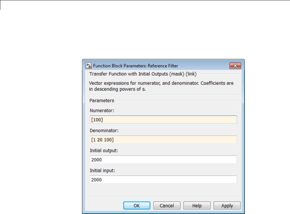
findop
3In the Simulink Editor, double-click the Reference Filter block.
Change the Numerator of the transfer function to [100] and the
Denominator to [1 20 100]. Click OK.
4Find the steady state operating point that meets these specifications.
op = findop(sys,opspec)
This command results in an error because the changes to your model
are not reflected in your operating point specification object:
??? The model scdspeedctrl has been modified and the operating point
object is out of date. Update the object by calling the function
update on your operating point object.
8-22

findop
5Update the operating point specification object with changes to the
model. Repeat the operating point search.
opspec = update(opspec);
op = findop(sys,opspec)
bdclose(sys);
After updating the operating point specifications object, the
optimization algorithm successfully finds the operating point.
Algorithms By default, findop uses the optimizer graddescent_elim.Tousea
different optimizer, change the value of OptimizerType in options
using linoptions.
findop automatically sets these Simulink model properties for
optimization:
•BufferReuse = 'off'
•RTWInlineParameters = 'on'
•BlockReductionOpt = 'off'
After the optimization completes, Simulink restores the original model
properties.
Alternatives As an alternative to the findop command, find operating points using
the Linear Analysis Tool. See the following examples:
•“Steady-State Operating Points from State Specifications” on page
1-16
•“Steady-State Operating Point to Meet Output Specification” on page
1-21
See Also initopspec |linearize |linoptions |operspec |addoutputspec
Tutorials • “Steady-State Operating Point (Trimming)” on page 1-2
•“ChoosingBetweenSimulationSnapshot and Operating Point from
Specifications” on page 1-12
8-23


frest.Chirp
Purpose Swept-frequency cosine signal
Syntax input = frest.Chirp(sys)
input = frest.Chirp('OptionName',OptionValue)
Description input = frest.Chirp(sys)creates a swept-frequency cosine input
signal based on the dynamics of a linear system sys.
input = frest.Chirp('OptionName',OptionValue) creates a
swept-frequency cosine input signal using the options specified by
comma-separated name/value pairs.
To view a plot of your input signal, type plot(input).Toobtain
a timeseries for your input signal, use the generateTimeseries
command.
Input
Arguments
sys
Linear system for creating a chirp signal based on the dynamic
characteristics of this system. You can specify the linear system based
on known dynamics using tf,zpk,orss.Youcanalsoobtainthelinear
system by linearizing a nonlinear system.
The resulting chirp signal automatically sets these options based on the
linear system:
•'FreqRange' are the frequencies at which the linear system has
interesting dynamics.
•'Ts' is set to avoid aliasing such that the Nyquist frequency of the
signal is five times the upper end of the frequency range.
•'NumSamples' is set such that the frequency response estimation
includes the lower end of the frequency range.
Other chirp options have default values.
’OptionName’,OptionValue
Signal characteristics, specified as comma-separated pairs of option
name string and the option value.
8-25

frest.Chirp
Option Name Option Value
'Amplitude' Signal amplitude.
Default: 1e-5
'FreqRange' Signal frequencies, specified as either:
•Two-element vector, for example [w1 w2]
•Two-element cell array, for example {w1 w2}
Default: [1,1000]
'FreqUnits' Frequency units:
•'rad/s'—Radians per second
•'Hz'—Hertz
Changing frequency units does not impact
frequency response estimation.
Default: 'rad/s'
'Ts' Sample time of the chirp signal in seconds. The
default setting avoids aliasing.
Default: 2
5
*max( )FreqRange
'NumSamples' Number of samples in the chirp signal. Default
setting ensures that the estimation includes the
lower end of the frequency range.
Default: 4
Ts FreqRange*min( )
8-26
frest.Chirp
Option Name Option Value
'SweepMethod' Method for evolution of instantaneous frequency:
•'linear' (default)—Specifies the instantaneous
frequency sweep fi(t):
f t f t where f f t
if
() ( )/=+ = −
010
βensures that the signal maintains the desired
frequency breakpoint f1at final time tf.
f
t
f
t
f1 > f2 f1 < f2
•'logarithmic'—Specifies the instantaneous
frequency sweep fi(t) given by
f t f where f
f
ittf
()=× =
⎛
⎝
⎜⎞
⎠
⎟
01
0
1
f
t
f
t
f1 > f2 f1 < f2
•'quadratic'—Specifies the instantaneous
frequency sweep fi(t):
8-27
frest.Chirp
Option Name Option Value
f t f t where f f t
ii
() ( )/=+ = −
02102
Also specify the shape of the quadratic using the
'Shape' option.
'Shape' Use when you set 'SweepMethod' to 'quadratic'
to describe the shape of the parabola in the positive
frequency axis:
•'concave'—Concave quadratic sweeping shape.
f
t
f
t
f1 > f2 f1 < f2
•'convex'—Convex quadratic sweeping shape.
f
t
f
t
f1 > f2 f1 < f2
'InitialPhase' Initial phase of the Chirp signal in degrees.
Default: 270
Examples Create a chirp input signal:
input = frest.Chirp('Amplitude',1e-3,'FreqRange',[10 500],'NumSamples',20000)
8-28


frest.createFixedTsSinestream
Purpose Sinestream input signal with fixed sample time
Syntax input = frest.createFixedTsSinestream(ts)
input = frest.createFixedTsSinestream(ts,{wmin wmax})
input = frest.createFixedTsSinestream(ts,w)
input = frest.createFixedTsSinestream(ts,sys)
input = frest.createFixedTsSinestream(ts,sys,{wmin wmax})
input = frest.createFixedTsSinestream(ts,sys,w)
Description input = frest.createFixedTsSinestream(ts) creates sinestream
input signal in which each frequency has the same fixed sample time
ts in seconds. The signal has 30 frequencies between 1 and ωs,where
s
s
t
=2isthesamplerateinradianspersecond.Thesoftwareadjusts
the SamplesPerPeriod option to ensure that each frequency has the
same sample time. Use when your Simulink model has linearization
input I/Os on signals with discrete sample times.
input = frest.createFixedTsSinestream(ts,{wmin wmax}) creates
sinestream input signal with up to 30 frequencies logarithmically
spaced between wmin and wmax in radians per second.
input = frest.createFixedTsSinestream(ts,w) creates sinestream
input signal with frequencies w, specified as a vector of frequency values
in radians per second. The values of wmust satisfy wNts
=2
for integer
Nsuchthatthesamplerate
s
s
t
=2is an integer multiple of each
element of w.
input = frest.createFixedTsSinestream(ts,sys) creates
sinestream input signal with a fixed sample time ts.Thesignal’s
frequencies, settling periods, and number of periods automatically set
based on the dynamics of a linear system sys.
8-30

frest.createFixedTsSinestream
input = frest.createFixedTsSinestream(ts,sys,{wmin
wmax}) creates sinestream input signal with up to 30 frequencies
logarithmically spaced between wmin and wmax in radians per second.
input = frest.createFixedTsSinestream(ts,sys,w) creates
sinestream input signal at frequencies w, specified as a vector of
frequency values in radians per second. The values of wmust satisfy
wNts
=2
for integer Nsuch that the sample rate ts is an integer
multiple of each element of w.
Examples Create a sinusoidal input signal with the following characteristics:
•Sample time of 0.02 sec
•Frequencies of the sinusoidal signal are between 1 rad/s and 10 rad/s
input = frest.createFixedTsSinestream(0.02,{1, 10});
See Also frest.Sinestream |frestimate
How To • “Creating Input Signals for Estimation” on page 3-9
• “Estimate Frequency Response (MATLAB Code)” on page 3-37
• “Estimate Frequency Response Using Linear Analysis Tool” on page
3-28
8-31

frest.createStep
Purpose Step input signal
Syntax input = frest.createStep('OptionName',OptionValue)
Description input = frest.createStep('OptionName',OptionValue)creates a
step input signal as a MATLAB timeseries object using the options
specified by comma-separated name/value pairs.
Plot your input signal using plot(input).
Input
Arguments
’OptionName’,OptionValue
Signal characteristics, specified as comma-separated pairs of option
name string and the option value.
Option Name Option Value
'Ts' Sample time of the step input in seconds.
Default:1e-3
'StepTime' Time in seconds when the output jumps
from 0 to the StepSize parameter.
Default:1
'StepSize' Value of the step signal after time reaches
and exceeds the StepTime parameter.
Default:1
'FinalTime Final time of the step input signal in
seconds.
Default:10
Examples Create step signal:
input = frest.createStep('StepTime',3,'StepSize',2)
8-32


frest.findDepend
Purpose List of model path dependencies
Syntax dirs = frest.findDepend(model)
Description dirs = frest.findDepend(model)returns paths containing Simulink
model dependencies required for frequency response estimation using
parallel computing. model is the Simulink model to estimate. dirs is
a cell array, where each element is a path string. dirs is empty when
frest.findDepend does not detect any model dependencies. Append
paths to dirs when the list of paths is empty or incomplete.
frest.findDepend does not return a complete list of model dependency
paths when the dependencies are undetectable.
Examples Specify model path dependencies for parallel computing:
% Copy referenced model to temporary folder.
pathToLib = scdpathdep_setup;
% Add folder to search path.
addpath(pathToLib);
% Open Simulink model.
mdl = 'scdpathdep';
open_system(mdl);
% Get model dependency paths.
dirs = frest.findDepend(mdl)
% The resulting path is on a local drive, C:/.
% Replace C:/ with valid network path accessible to remote workers.
dirs = regexprep(dirs,'C:/','\\\\hostname\\C$\\')
% Enable parallel computing and specify the model path dependencies.
options = frestimateOptions('UseParallel','on','ParallelPathDependencies',dirs)
See Also frestimate
8-34


frest.findSources
Purpose Identify time-varying source blocks
Syntax blocks = frest.findSources(model)
blocks = frest.findSources(model,io)
Description blocks = frest.findSources(model) finds all time-varying source
blocks in the signal path of any linearization output point marked in
the Simulink model model.
blocks = frest.findSources(model,io) finds all time-varying
source blocks in the signal path of any linearization output point
specified in the array of linear analysis points io.
Tips •Use frest.findSources to identify time-varying source blocks
that can interfere with frequency response estimation. To
disablesuchblockstoestimate frequency response, set the
BlocksToHoldConstant option of frestimateOptions equal to
blocks or a subset of blocks. Then, estimate the frequency
response using frestimate.
•Sometimes, model includes referenced models containing source
blocks in the signal path of a linearization output point. In such
cases, set the referenced models to normal simulation mode to ensure
that frest.findSources locates them. Use the set_param command
to set SimulationMode of any referenced models to Normal before
running frest.FindSources.
Input
Arguments
model
String containing the name, in single quotes, of the Simulink model
in which you are identifying time-varying source blocks for frequency
response estimation.
io
Array of linearization I/O points.
The elements of io are linearization I/O objects that you create
with getlinio or linio.frest.findSources uses only the output
8-36

frest.findSources
points to locate time-varying source blocks that can interfere with
frequency response estimation. See “Algorithms” on page 8-41 for more
information.
Output
Arguments
blocks
Array of Simulink.BlockPath objects identifying the block paths of all
time-varying source blocks in model that can interfere with frequency
response estimation. The blocks argument includes time-varying
source blocks inside subsystems and normal-mode referenced models.
If you provide io,blocks contains all time-varying source blocks
contributing to the signal at the output points in io.
If you do not provide io,blocks contains all time-varying source blocks
contributing to the signal at the output points marked in model.
Examples Estimate the frequency response of a model having time-varying source
blocks. This example shows the use of frest.findSources to identify
time-varying source blocks that interfere with frequency response
estimation. You can also see the use of BlocksToHoldConstant option
of frestimateOptions to disable time-varying source blocks in the
estimation.
Load the model scdspeed_ctrlloop.
mdl = 'scdspeed_ctrlloop';
open_system(mdl)
% Convert referenced model to normal mode for accuracy
set_param('scdspeed_ctrlloop/Engine Model',...
'SimulationMode','Normal');
First, view the effects of time-varying source blocks on frequency
response estimation. To do so, perform the estimation without disabling
time-varying source blocks.
In this example, linearization I/O points are already defined in the
model. Use the getlinio command to get the I/O points for frestimate.
8-37

frest.findSources
io = getlinio(mdl)
Define a sinestream signal and compute the estimated frequency
response sysest.
in = frest.Sinestream('Frequency',logspace(1,2,10),...
'NumPeriods',30,'SettlingPeriods',25);
[sysest,simout] = frestimate(mdl,io,in);
Perform exact linearization, and compare to the estimated response.
sys = linearize(mdl,io);
bodemag(sys,sysest,'r*')
8-38
frest.findSources
The estimated frequency response does not match the exact
linearization. The mismatch occurs because time-varying source blocks
in the model prevent the response from reaching steady state.
Find the time-varying blocks using frest.findSources.
srcblks = frest.findSources(mdl);
srcblks is an array of block paths corresponding to the time-varying
source blocks in the model. To examine the result, index into the array.
For example, entering
8-39

frest.findSources
srcblks(2)
returns the result
ans =
Simulink.BlockPath
Package: Simulink
Block Path:
'scdspeed_ctrlloop/Engine Model'
'scdspeed_plantref/Drag Torque/Step1'
Now you can estimate the frequency response without the contribution of
the time-varying source blocks. To do so, set the BlocksToHoldConstant
option of frestimateOptions equal to srcblks, and run the estimation.
opts = frestimateOptions
opts.BlocksToHoldConstant = srcblks
% Run frestimate again with blocks disabled
[sysest2,simout2] = frestimate(mdl,io,in,opts);
The frequency response estimate now provides a good match to the
exact linearization result.
bodemag(sys,sysest2,'r*')
8-40
frest.findSources
Algorithms To locate time-varying source blocks that can interfere with frequency
response estimation, frest.findSources begins at each linearization
output point in the model. From each output point, the algorithm traces
every signal path backward block by block. The algorithm reports any
source block (a block with no input port) it discovers, unless that source
block is a Constant or Ground block.
The frest.findSources algorithm traces every signal path that can
affect the signal value at each linearization output point in the model.
The paths traced include:
•Signal paths inside virtual and nonvirtual subsystems.
8-41
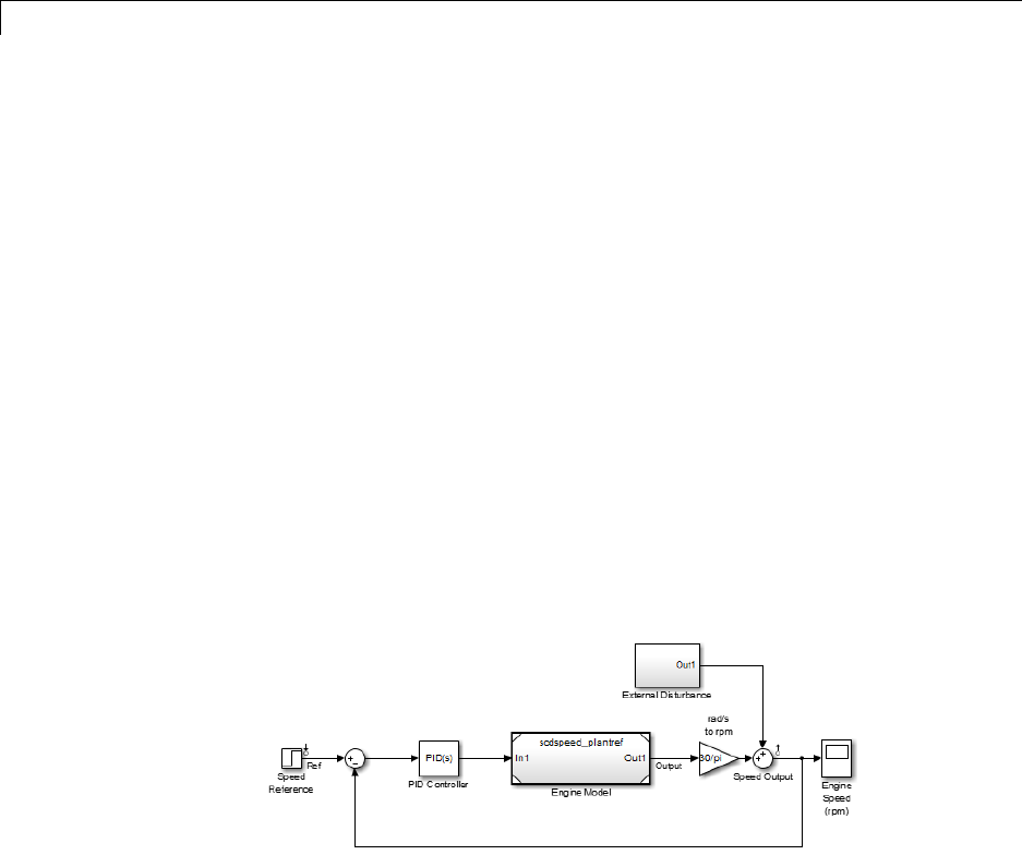
frest.findSources
•Signal paths inside normal-mode referenced models. Set all
referenced models to normal simulation mode before using
frest.findSources to ensure that the algorithm identifies source
blocks within the referenced models.
•Signals routed through From and Goto blocks, or through Data Store
Read and Data Store Write blocks.
•Signals routed through switches. The frest.findSources algorithm
assumes that any pole of a switch can be active during frequency
response estimation. The algorithm therefore follows the signal back
through all switch inputs.
For example, consider the model scdspeed_ctrlloop. This model has
one linearization output point, located at the output of the Sum block
labeled Speed Output.(Thefrest.findSources algorithm ignores
linearization input points.) Before running frest.findSources,
convert the referenced model to normal simulation mode:
set_param('scdspeed_ctrlloop/Engine Model',...
'SimulationMode','Normal');
You can now run frest.findSources to identify the time-varying
source blocks using the linearization output point defined in the model.
srcblks = frest.findSources('scdspeed_ctrlloop');
The algorithm begins at the output point and traces back through the
Sum block Speed Output.OneinputtoSpeed Output is the subsystem
8-42
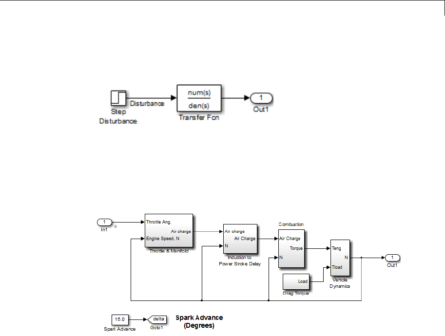
frest.findSources
External Disturbance. The algorithm enters the subsystem, finds the
source block labeled Step Disturbance, and reports that block.
The Sum block Speed Output has another input, which the algorithm
traces back into the referenced model Engine Model.Engine Model
contains several subsystems, and the algorithm traces the signal
through these subsystems to identify any time-varying source blocks
present.
For example, the Combustion subsystem includes the From block
marked delta that routes the signal from the Spark Advance source.
Because Spark Advance is a constant source block, however, the
algorithm does not report the presence of the block.
The algorithm continues the trace until all possible signal paths
contributing to the signal at each linearization output point are
examined.
Alternatives You can use the Simulink Model Advisor to determine whether
time-varying source blocks exist in the signal path of output linear
analysis points in your model. To do so, use the Model Advisor check
8-43

frest.findSources
“Identify time-varying source blocks interfering with frequency response
estimation.” For more information about using the Model Advisor, see
Consulting the Model Advisor in the Simulink User’s Guide.
See Also frestimate |frestimateOptions
How To • “Effects of Time-Varying Source Blocks on Frequency Response
Estimation” on page 3-62
8-44

frest.Random
Purpose Random input signal for simulation
Syntax input = frest.Random('OptionName',OptionValue)
input = frest.Random(sys)
Description input = frest.Random('OptionName',OptionValue) creates the
Random input signal using the options specified by comma-separated
name/value pairs.
input = frest.Random(sys) creates a Random input signal based on
the dynamics of a linear system sys.
To view a plot of your input signal, type plot(input).Toobtain
a timeseries for your input signal, use the generateTimeseries
command.
Input
Arguments
sys
Linear system for creating a random signal based on the dynamic
characteristics of this system. You can specify the linear system based
on known dynamics using tf,zpk,orss.Youcanalsoobtainthelinear
system by linearizing a nonlinear system.
The resulting random signal automatically sets these options based
on the linear system:
•Ts is set such that the Nyquist frequency of the signal is five times
the upper end of the frequency range to avoid aliasing issues.
•NumSamples is set such that the frequency response estimation
includes the lower end of the frequency range.
Other random options have default values.
’OptionName’,OptionValue
Signal characteristics, specified as comma-separated pairs of option
name string and the option value.
8-45

frest.Random
Option Name Option Value
'Amplitude' Signal amplitude.
Default:1e-5
'Ts' Sample time of the chirp signal in seconds.
Default:1e-3
'NumSamples' Number of samples in the Random signal.
Default:1e4
'Stream' Random number stream you create using the
MATLAB command RandStream.Thestateof
the stream you specify stores with the input
signal. This stored state allows the software
to return the same result every time you use
generateTimeseries and frestimate with the
input signal.
Default: Default stream of the MATLAB session
Examples Create a Random input signal with 1000 samples taken at 100 Hz and
amplitude of 0.02:
input = frest.Random('Amplitude',0.02,'Ts',1/100,'NumSamples',1000);
Create a Random input signal using multiplicative lagged Fibonacci
generator random stream:
% Specify the random number stream
stream = RandStream('mlfg6331_64','Seed',0);
% Create the input signal
8-46

frest.Random
input = frest.Random('Stream',stream);
See Also frest.Sinestream |frest.Random |frestimate |
generateTimeseries |getSimulationTime
How To • “Creating Input Signals for Estimation” on page 3-9
• “Estimate Frequency Response (MATLAB Code)” on page 3-37
• “Estimate Frequency Response Using Linear Analysis Tool” on page
3-28
8-47

frest.simCompare
Purpose Plot time-domain simulation of nonlinear and linear models
Syntax frest.simCompare(simout,sys,input)
frest.simCompare(simout,sys,input,x0)
[y,t] = frest.simCompare(simout,sys,input)
[y,t,x] = frest.simCompare(simout,sys,input,x0)
Description frest.simCompare(simout,sys,input) plots both
•Simulation output, simout, of the nonlinear Simulink model
You obtain the output from the frestimate command.
•Simulation output of the linear model sys for the input signal input
The linear simulation results are offset by the initial output values
in the simout data.
frest.simCompare(simout,sys,input,x0) plots the frequency
response simulation output and the simulation output of the linear
model with initial state x0. Because you specify the initial state, the
linear simulation result is not offset by the initial output values in the
simout data.
[y,t] = frest.simCompare(simout,sys,input) returns the linear
simulation output response yand the time vector tfor the linear model
sys with the input signal input. Thissyntaxdoesnotdisplayaplot.
The matrix yhasasmanyrowsastimesamples(length(t)) and as
manycolumnsassystemoutputs.
[y,t,x] = frest.simCompare(simout,sys,input,x0) also returns
the state trajectory xfor the linear state space model sys with initial
state x0.
Examples Compare a time-domain simulation of the Simulink watertank model
and its linear model representation:
% Create input signal for simulation
input = frest.createStep('FinalTime',100);
8-48

frest.simCompare
% Open the Simulink model
watertank
% Specify the operating point for the estimation
watertank_spec = operspec('watertank');
op = findop('watertank',watertank_spec)
% Specify portion of model to estimate
io(1)=linio('watertank/PID Controller',1,'in');
io(2)=linio('watertank/Water-Tank System',1,'out');
% Estimate the frequency response of the watertank model
[sysest,simout] = frestimate('watertank',op,io,input)
sys = linearize('watertank',op,io);
frest.simCompare(simout,sys,input);
The software returns the following plot.
8-49
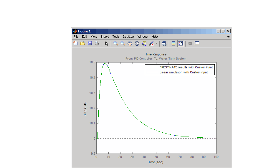
frest.simCompare
See Also frestimate |frest.simView
8-50

frest.simView
Purpose Plot frequency response model in time- and frequency-domain
Syntax frest.simView(simout,input,sysest)
frest.simView(simout,input,sysest,sys)
Description frest.simView(simout,input,sysest) plots the following frequency
response estimation results:
•Time-domain simulation simout of the Simulink model
•FFT of time-domain simulation simout
•Bode of estimated system sysest
This Bode plot is available when you create the input signal
using frest.Sinestream or frest.Chirp.Inthisplot,youcan
interactively select frequencies or a frequency range for viewing the
results in all three plots.
You obtain simout and sysest from the frestimate command using
the input signal input.
frest.simView(simout,input,sysest,sys) includes the linear
system sys in the Bode plot when you create the input signal using
frest.Sinestream or frest.Chirp. Use this syntax to compare the
linear system to the frequency response estimation results.
Examples Estimate the closed-loop of the watertank Simulink model and analyze
the results:
% Open the Simulink model
watertank
% Specify portion of model to linearize and estimate
io(1)=linio('watertank/PID Controller',1,'in');
io(2)=linio('watertank/Water-Tank System',1,'out');
% Specify the operating point for the linearization and estimation
watertank_spec = operspec('watertank');
op = findop('watertank',watertank_spec);
8-51
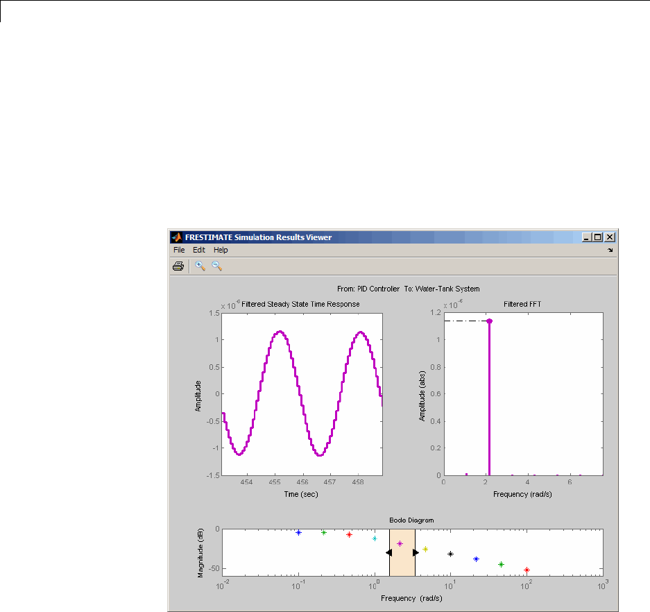
frest.simView
% Create input signal for simulation
input = frest.Sinestream('Frequency',logspace(-1,2,10));
% Estimate the frequency response of the watertank model
[sysest,simout] = frestimate('watertank',op,io,input);
% Analyze the estimation results
frest.simView(simout,input,sysest)
See Also frestimate |frest.simCompare
How To • “Analyzing Estimated Frequency Response” on page 3-40
8-52


frest.Sinestream
Purpose Signal containing series of sine waves
Syntax input = frest.Sinestream(sys)
input = frest.Sinestream('OptionName',OptionValue)
Description input = frest.Sinestream(sys)creates a signal with a series of
sinusoids based on the dynamics of a linear system sys.
input = frest.Sinestream('OptionName',OptionValue)creates
a signal with a series of sinusoids, where each sinusoid frequency
lasts for a specified number of periods, using the options specified by
comma-separated name/value pairs.
To view a plot of your input signal, type plot(input).Toobtain
a timeseries for your input signal, use the generateTimeseries
command.
Input
Arguments
sys
Linear system for creating a sinestream signal based on the dynamic
characteristics of this system. You can specify the linear system based
on known dynamics using tf,zpk,orss.Youcanalsoobtainthelinear
system by linearizing a nonlinear system.
The resulting sinestream signal automatically sets these options based
on the linear system:
•'Frequency' are the frequencies at which the linear system has
interesting dynamics.
•'SettlingPeriods' is the number of periods it takes the system to
reach steady state at each frequency in 'Frequency'.
•'NumPeriods' is (3 + SettlingPeriods) to ensure that each
frequency excites the system at specified amplitude for at least three
periods.
•For discrete systems only, 'SamplesPerPeriod' is set such that all
frequencies have the same sample time as the linear system.
Other sinestream options have default values.
8-54

frest.Sinestream
’OptionName’,OptionValue
Signal characteristics, specified as comma-separated pairs of option
name string and the option value.
Option Name Option Value
'Frequency' Signal frequencies, specified as either a scalar or a
vector of frequency values.
Default:logspace(1,3,50)
'Amplitude' Signal amplitude at each frequency, specified as either:
•Scalar to set all frequencies to same value
•Vector to set each frequencies to a different value
Default:1e-5
'SamplesPerPeriod' Number of samples for each period for each signal
frequency, specified as either:
•Scalar to set all frequencies to same value
•Vector to set each frequencies to a different value
Default:40
'FreqUnits' Frequency units:
•'rad/s'—Radians per second
•'Hz'—Hertz
Default:'rad/s'
8-55
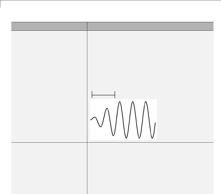
frest.Sinestream
Option Name Option Value
'RampPeriods' Number of periods for ramping up the amplitude of each
sine wave to its maximum value, specified as either:
•Scalar to set all frequencies to same value
•Vector to set each frequencies to a different value
Use this option to ensure a smooth response when your
input amplitude changes.
Default:0
RampPeriods
'NumPeriods' Number of periods each sine wave is at maximum
amplitude, specified as either:
•Scalar to set all frequencies to same value
•Vector to set each frequencies to a different value
Default:max(3 RampPeriods+SettlingPeriods,,2)
8-56
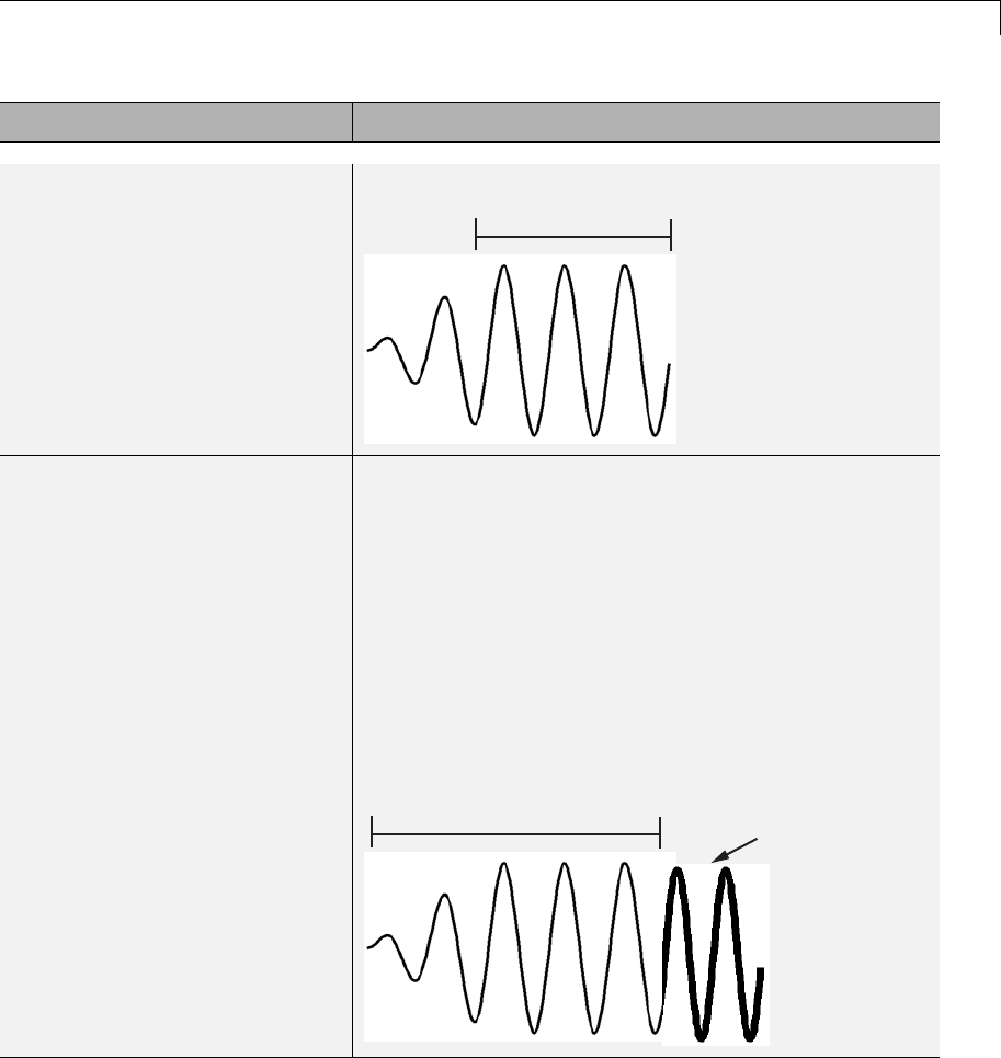
frest.Sinestream
Option Name Option Value
NumPeriods
'SettlingPeriods' Number of periods corresponding to the transient
portion of the simulated response at a specific
frequency, before the system reaches steady state,
specified as either:
•Scalar to set all frequencies to same value
•Vector to set each frequencies to a different value
Before performing the estimation, frestimate discards
this number of periods from the output signals.
Default:1
SettlingPeriods
Bold periods
for estimation
8-57

frest.Sinestream
Option Name Option Value
'ApplyFilteringInFRESTIMATE' Frequency-selective FIR filtering of the input signal
before estimating the frequency response using
frestimate.
•'on' (default)
•'off'
For more information, see the frestimate algorithm.
'SimulationOrder' The order in which frestimate injects the individual
frequencies of the input signal into your Simulink
model during simulation.
•'Sequential' (default) — frestimate injects one
frequency after the next into your model in a single
Simulink simulation using variable sample time.
To use this option, your Simulink model must use a
variable-step solver.
•'OneAtATime' —frestimate injects each frequency
during a separate Simulink simulation of your model.
Before each simulation, frestimate initializes your
Simulink model to the operating point specified for
estimation. If you have Parallel Computing Toolbox
installed,youcanruneachsimulationinparallel
to speed up estimation using parallel computing.
For more information, see “Speeding Up Estimation
Using Parallel Computing” on page 3-82.
Examples Create a sinestream signal having several different frequencies. For
each frequency, specify an amplitude, a number of periods at maximum
amplitude, a ramp-up period, and a number of settling periods.
8-58
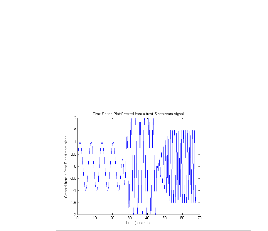
frest.Sinestream
1Create sinestream signal.
input = frest.Sinestream('Frequency',[1 2.5 5],...
'Amplitude',[1 2 1.5],...
'NumPeriods',[4 6 12],...
'RampPeriods',[0 2 6],...
'SettlingPeriods',[1 3 7]);
2(Optional) Plot the sinestream signal.
plot(input)
Create a sinusoidal input signal with the following characteristics:
•50 frequencies spaced logarithmically between 10 Hz and 1000 Hz
•All frequencies have amplitude of 1e-3
•Sampled with a frequency 10 times the frequency of the signal
(meaning ten samples per period)
8-59

frest.Sinestream
% Create the input signal
input = frest.Sinestream('Amplitude',1e-3,'Frequency',logspace(1,3,50),...
'SamplesPerPeriod',10,'FreqUnits','Hz');
See Also frest.Chirp |frest.Random |frestimate |generateTimeseries |
frest.createFixedTsSinestream |getSimulationTime
How To • “Creating Input Signals for Estimation” on page 3-9
• “Estimate Frequency Response (MATLAB Code)” on page 3-37
• “Estimate Frequency Response Using Linear Analysis Tool” on page
3-28
• “Speeding Up Estimation Using Parallel Computing” on page 3-82
8-60

frestimate
Purpose Frequency response estimation of Simulink models
Syntax sysest = frestimate(model,io,input)
sysest = frestimate(model,op,io,input)
[sysest,simout] = frestimate(model,op,io,input)
[sysest,simout] = frestimate(model,op,io,input,options)
Description sysest = frestimate(model,io,input)estimates frequency response
model sysest.model is a string that specifies the name of your
Simulink model. input can be a sinestream, chirp, or random signal, or
a MATLAB timeseries object. io specifies the linearization I/O object,
which you either obtain using getlinio or create using linio.I/O
points cannot be on bus signals. The estimation occurs at the operating
point specified in the Simulink model.
sysest = frestimate(model,op,io,input)initializes the model at
the operating point op before estimating the frequency response model.
Create op using either operpoint or findop.
[sysest,simout] = frestimate(model,op,io,input)estimates
frequency response model and returns the simulated output simout.
This output is a cell array of Simulink.Timeseries objects with
dimensions m-by-n.mis the number of linearization output points, and n
is the number of input channels.
[sysest,simout] = frestimate(model,op,io,input,options)uses
the frequency response options (options) to estimate the frequency
response. Specify these options using frestimateOptions.
Examples Estimating frequency response for a Simulink model:
% Create input signal for simulation:
input = frest.Sinestream('Frequency',logspace(-3,2,30));
% Open the Simulink model:
watertank
% Specify portion of model to estimate:
8-61
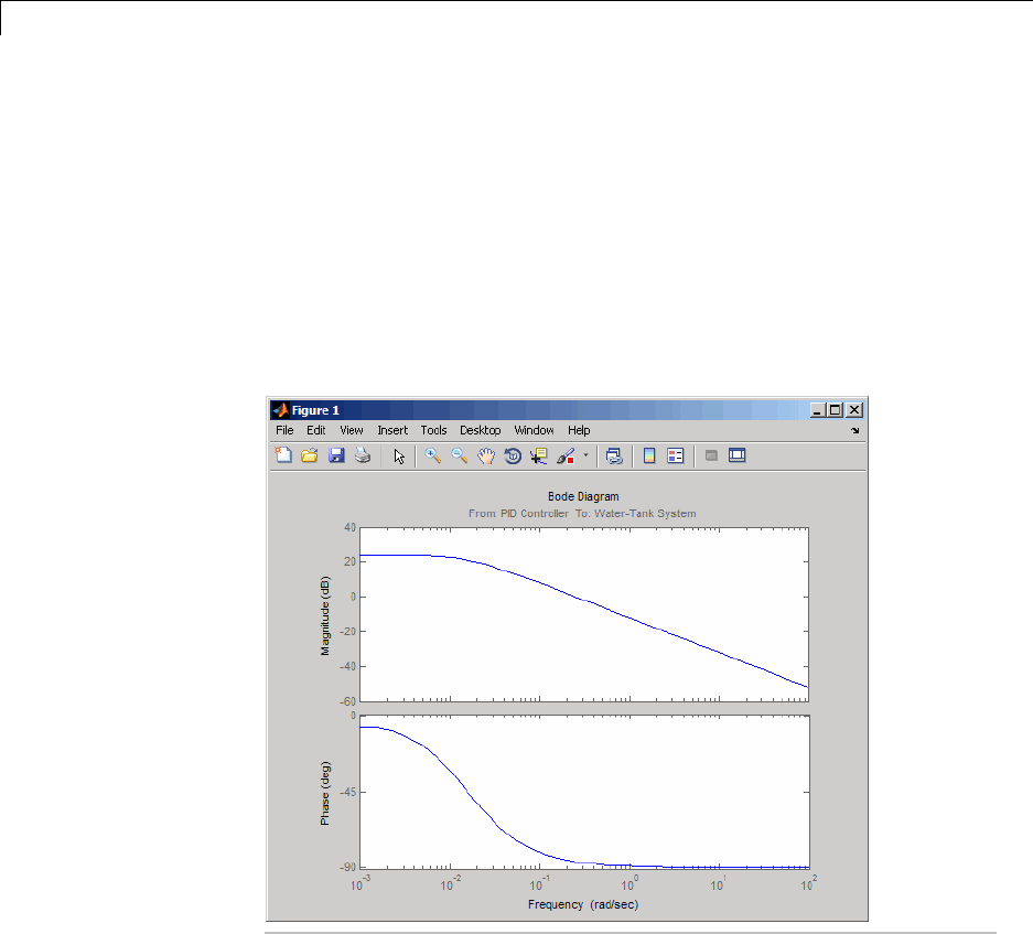
frestimate
io(1)=linio('watertank/PID Controller',1,'in');
io(2)=linio('watertank/Water-Tank System',1,'out','on');
% Specify the steady state operating point for the estimation.
watertank_spec = operspec('watertank');
op = findop('watertank',watertank_spec);
% Estimate frequency response of specified blocks:
sysest = frestimate('watertank',op,io,input);
bode(sysest)
Validate exact linearization results using estimated frequency response
of a Simulink model:
% Open the Simulink model:
watertank
8-62

frestimate
% Specify portion of model to estimate:
io(1)=linio('watertank/PID Controller',1,'in');
io(2)=linio('watertank/Water-Tank System',1,'out');
% Specify operating point for linearization and estimation:
watertank_spec = operspec('watertank');
op = findop('watertank',watertank_spec);
% Linearize the model:
sys = linearize('watertank',op,io);
% Estimate the frequency response of the watertank model
input = frest.Sinestream('Frequency',logspace(-1,2,10));
[sysest,simout] = frestimate('watertank',op,io,input);
% Compare linearization and estimation results in frequency domain:
frest.simView(simout,input,sysest,sys)
8-63
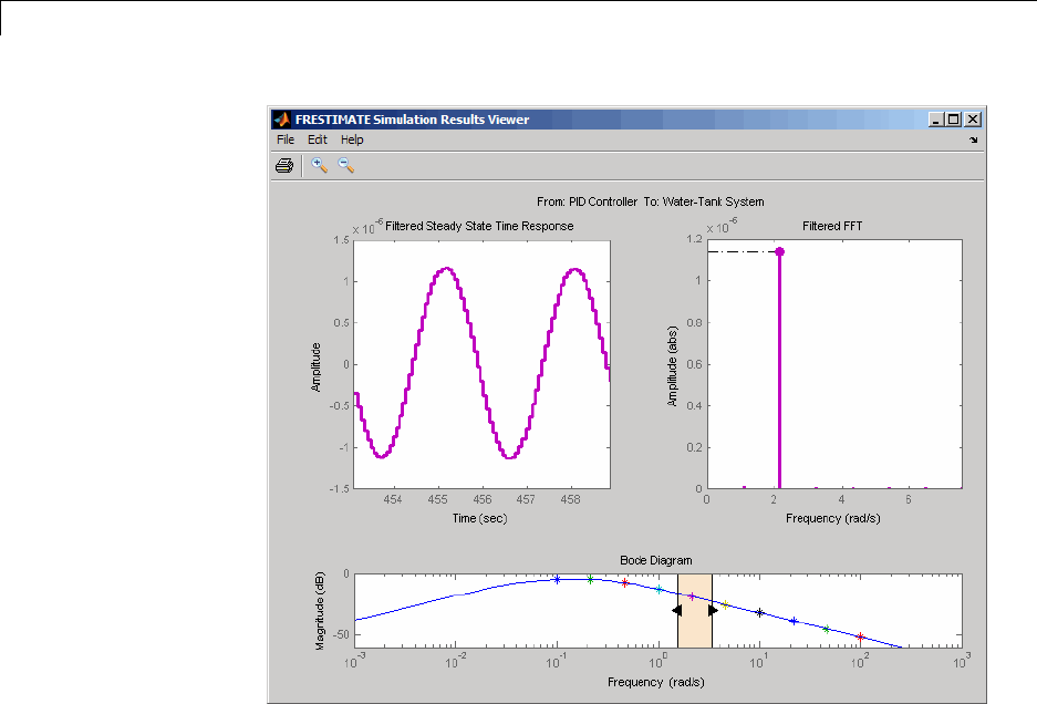
frestimate
Algorithms frestimate performs the following operations when you use the
sinestream signal:
1Injects the sinestream input signal you design, uest(t),atthe
linearization input point.
8-64
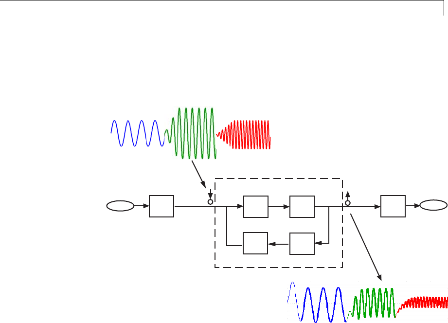
frestimate
2Simulates the output at the linearization output point.
frestimate adds the signal you design to existing Simulink signals
at the linearization input point.
u(t)
u (t)
y(t)
est
8-65
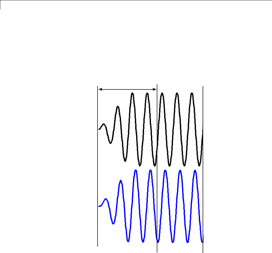
frestimate
3Discards the SettlingPeriods portion of the output (and the
corresponding input) at each frequency.
The simulated output at each frequency has a transient portion and
steady state portion. SettlingPeriods corresponds to the transient
components of the output and input signals. The periods following
SettlingPeriods are considered to be at steady state.
SettlingPeriods
Input
Output
4Filters the remaining portion of the output and the corresponding
input signals at each input frequency using a bandpass filter.
Because most models are not at steady state, the response might
8-66

frestimate
contain low-frequency transient behavior. Filtering typically
improves the accuracy of your modelbyremovingtheeffectsof
frequencies other than the input frequencies, which are problematic
when sampling and analyzing data of finite length. These effects
are called spectral leakage.
8-67
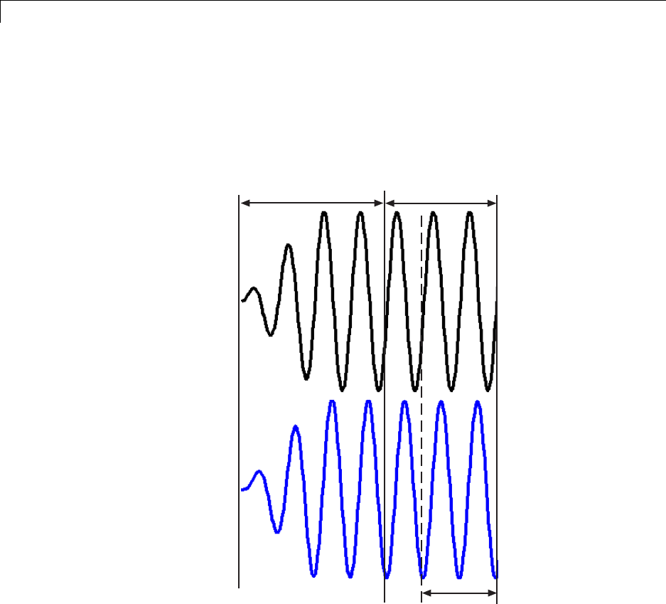
frestimate
Any transients associated with filtering are only in the first period of
the filtered steady-state output. After filtering, frestimate discards
the first period of the input and output signals. frestimate uses a
finite impulse response (FIR) filter, whose order matches the number
of samples in a period.
SettlingPeriods
Filtered
portion
Used for
estimation
Input
Output
5Estimates the frequency response of the processed signal by
computing the ratio of the fast Fourier transform of the filtered
8-68

frestimate
steady-state portion of the output signal yest(t) and the fast Fourier
transform of the filtered input signal uest(t):
Frequency sponse Model fft of y t
fft of u t
est
est
Re ()
()
=
To compute the response at each frequency, frestimate uses only
the simulation output at that frequency.
See Also frest.Sinestream |frest.Chirp |frest.Random |frest.simView
|frestimateOptions |getSimulationTime
How To • “Estimate Frequency Response (MATLAB Code)” on page 3-37
• “Estimate Frequency Response Using Linear Analysis Tool” on page
3-28
• “Speeding Up Estimation Using Parallel Computing” on page 3-82
8-69

frestimateOptions
Purpose Options for frequency response estimation
Syntax options = frestimateOptions
options = frestimateOptions('OptionName',OptionValue)
Description options = frestimateOptions creates a frequency response
estimation options object options with default settings. Pass this
object to the function frestimate to use these options for frequency
response estimation.
options = frestimateOptions('OptionName',OptionValue) creates
a frequency response estimation options object options using the
options specified by comma-separated name/value pairs.
Input
Arguments
’OptionName’,OptionValue
Estimation options, specified as comma-separated pairs of option name
string and the option value.
Option Name Option Value
'BlocksToHoldConstant' An array of Simulink.BlockPath that specifies
the paths of time-varying source blocks to hold
constant during frequency response estimation. Use
frest.findSources to identify time-varying source
blocks that can interfere with frequency response
estimation.
Default:empty
'UseParallel' Set to 'on' to enable parallel computing for
estimations with the frestimate command.
Default:'off'
'ParallelPathDependencies' A cell array of strings that specifies the path
dependencies required to execute the model
to estimate. All the workers in the MATLAB
pool must have access to the folders listed in
'ParallelPathDependencies'.
Default:empty
8-70

frestimateOptions
Examples Identify and disable time-varying source blocks for frequency response
estimation.
% Open Simulink model.
mdl = 'scdspeed_ctrlloop';
open_system(mdl)
% Convert referenced subsystem to normal mode.
set_param('scdspeed_ctrlloop/Engine Model','SimulationMode','Normal')
;
% Get I/O points and create sinestream.
io = getlinio(mdl)
in = frest.Sinestream('Frequency',logspace(1,2,10),'NumPeriods',30,..
.
'SettlingPeriods',25);
% Identify time-varying source blocks.
srcblks = frest.findSources(mdl)
% Create options set specifying blocks to hold constant
opts = frestimateOptions
opts.BlocksToHoldConstant = srcblks
% Run frestimate
[sysest,simout] = frestimate(mdl,io,in,opts)
Enable parallel computing and specify the model path dependencies.
% Copy referenced model to temporary folder.
pathToLib = scdpathdep_setup;
% Add folder to search path.
addpath(pathToLib);
% Open Simulink model.
mdl = 'scdpathdep';
open_system(mdl);
8-71

frestimateOptions
% Get model dependency paths.
dirs = frest.findDepend(mdl)
% The resulting path is on a local drive, C:/.
% Replace C:/ with valid network path accessible to remote workers.
dirs = regexprep(dirs,'C:/','\\\\hostname\\C$\\')
% Enable parallel computing and specify the model path dependencies.
options = frestimateOptions('UseParallel','on','ParallelPathDependencies',dirs)
Alternatives You can enable parallel computing for all models with no path
dependencies. To do so, select the Use the matlabpool in
FRESTIMATE command check box in the MATLAB preferences.
When you select this check box and use the frestimate command, you
do not need to provide a frequency response options object.
If your model has path dependencies, you must create your own
frequency response options object that specifies the path dependencies.
Use the ParallelPathDependencies option before beginning the
estimation.
See Also frestimate |frest.findSources
8-72

fselect
Purpose Extract sinestream signal at specified frequencies
Syntax input2 = fselect(input,fmin,fmax)
input2 = fselect(input,index)
Description input2 = fselect(input,fmin,fmax) extracts a portion of the
sinestream input signal input in the frequency range between fmin
and fmax.Specifyfmin and fmax in the same frequency units as the
sinestream signal.
input2 = fselect(input,index) extracts a sinestream signal at
specific frequencies, specified by the vector of indices index.
Examples Extract the second frequency in a sinestream signal:
% Create the input signal
input = frest.Sinestream('Frequency',[1 2.5 5],...
'Amplitude',[1 2 1.5],...
'NumPeriods',[4 6 12],...
'RampPeriods',[0 2 6]);
% Extract a sinestream signal for the second frequency
input2 = fselect(input,2)
% Plot the extracted input signal
plot(input2)
See Also frestimate |frest.Sinestream |fdel
How To • “TimeResponseNotatSteadyState”onpage3-49
8-73

generateTimeseries
Purpose Generate time-domain data for input signal
Syntax ts = generateTimeseries(input)
Description ts = generateTimeseries(input) creates a MATLAB timeseries
object ts from the input signal input.input can be a sinestream, chirp,
or random signal. For chirp and random signals, that time vector of ts
has equally spaced time values, ranging from 0 to Ts(NumSamples-1).
Examples Create timeseries object for chirp signal:
input = frest.Chirp('Amplitude',1e-3,'FreqRange',...
[10 500],'NumSamples',20000);
ts = generateTimeseries(input)
See Also frestimate |frest.Sinestream |frest.Chirp |frest.Random
8-74

get
Purpose Properties of linearization I/Os and operating points
Syntax get(ob)
get(ob,'PropertyName')
ob.PropertyName
Description get(ob) displays all properties and corresponding values of the object,
ob, which can be a linearization I/O object, an operating point object,
or an operating point specification object. Create ob using findop,
getlinio,linio,operpoint,oroperspec.
get(ob,'PropertyName') returns the value of the property,
PropertyName, within the object, ob.Theobject,ob,canbea
linearization I/O object, an operating point object, or an operating
point specification object. Create ob using findop,getlinio,linio,
operpoint,oroperspec.
ob.PropertyName is an alternative notation for displaying the value of
the property, PropertyName,oftheobject,ob.Theobject,ob, can be
a linearization I/O object, an operating point object, or an operating
point specification object. Create ob using findop,getlinio,linio,
operpoint,oroperspec.
Examples Create an operating point object, op, for the Simulink model, magball.
op=operpoint('magball');
Get a list of all object properties using the get function with the object
name as the only input.
get(op)
This returns the properties of op and their current values.
Model: 'magball'
States: [5x1 opcond.StatePoint]
Inputs: [0x1 double]
Time: 0
8-75

get
Version: 2
To view the value of a particular property of op, supply the property
name as an argument to get. For example, to view the name of the
model associated with the operating point object, type:
V=get(op,'Model')
which returns
V=
magball
Because op is a structure, you can also view any properties or fields
using dot-notation, as in this example.
W=op.States
This notation returns a vector of objects containing information about
the states in the operating point.
(1.) magball/Controller/PID Controller/Filter
x: 0
(2.) magball/Controller/PID Controller/Integrator
x: 14
(3.) magball/Magnetic Ball Plant/Current
x: 7
(4.) magball/Magnetic Ball Plant/dhdt
x: 0
(5.) magball/Magnetic Ball Plant/height
x: 0.05
Use get to view details of W. For example:
get(W(2),'x')
returns
ans =
8-76

get
14.0071
See Also findop |getlinio |linio |operpoint |operspec |set
8-77

getinputstruct
Purpose Input structure from operating point
Syntax in_struct = getinputstruct(op_point)
Description in_struct = getinputstruct(op_point) extracts a structure of input
values, in_struct, from the operating point object, op_point.The
structure, in_struct, uses the same format as Simulink software which
allows you to set initial values for inputs in the model within the Data
Import/Export pane of the Configuration Parameters dialog box.
Examples Create an operating point object for the f14 model:
op_f14=operpoint('f14');
Extract an input structure from the operating point object:
inputs_f14=getinputstruct(op_f14)
This extraction returns
inputs_f14 =
time: 0
signals: [1x1 struct]
To view the values of the inputs within this structure, use dot-notation
to access the values field:
inputs_f14.signals.values
In this case, the value of the input is 0.
See Also getstatestruct |getxu |operpoint
8-78

getlinio
Purpose Linearization input/output (I/O) settings for Simulink model, Linear
Analysis Plots or Model Verification block
Syntax io = getlinio('sys')
io = getlinio('blockpath')
Alternatives As an alternative to the getlinio function, view linearization I/Os
in the:
•Analysis I/Os pane of the Linearization Task node in the Control
and Estimation Tools Manager GUI for Simulink models.
•Linearization inputs/outputs table in the Linearizations tab of
the Block Parameters dialog box for Linear Analysis Plots or Model
Verification blocks.
Description io = getlinio('sys') finds all linearization inputs/outputs (I/Os) in
the Simulink model, sys, and returns a vector of objects, io. Each object
represents a linearization annotation in the model and is associated
with an output port of a Simulink block. Before running getlinio,use
the right-click menu to insert the linearization annotations, or I/Os, on
the signal lines of the model diagram.
io = getlinio('blockpath') finds all I/Os in a Linear Analysis Plots
block or a Model Verification block. blockpath isthefullpathtothe
block. io is a vector of objects and has an entry for each linearization
port used by the block.
Each object within the vector, io, has the following properties:
Active Set this value to 'on', when the I/O is used for
linearization, and 'off' otherwise
Block Name of the block with which the I/O is
associated
OpenLoop Set this value to 'on', when the feedback loop
at the I/O is open, and 'off',whenitisclosed
8-79

getlinio
PortNumber Integer referring to the output port with which
the I/O is associated
Type Choose one of the following linearization I/O
types:
•'in': linearization input point
•'out': linearization output point
•'outin': linearization output then input
point
•'inout': linearization input then output
point
BusElement Bus element name with which the I/O is
associated. Empty string ('')iftheI/Oisnot
a bus element.
Description String description of the I/O object
You can edit this I/O object to change its properties. Alternatively, you
can change the properties of io using the set function. To upload an
edited I/O object to the Simulink model diagram, use the setlinio
function. Use I/O objects with the function linearize to create linear
models.
Examples Find linearization inputs/outputs in a Simulink model.
Before creating a vector of I/O objects using getlinio,youmustadd
linearization annotations representing the I/Os, such as input points or
output points, to a Simulink model.
1Open a Simulink model.
magball
8-80

getlinio
2Right-click the signal line between the Magnetic Ball Plant and the
Controller. Select Linear Analysis Points > Input Point from the
menu to place an input point on this signal line.
A small arrow pointing toward a small circle just above the signal
line represents the input point.
3Right-click the signal line after the Magnetic Ball Plant. Select
Linear Analysis Points > Output Point from the menu to place
an output point on this signal line.
A small arrow pointing away from a small circle just above the signal
line represents the output point.
4Create a vector of I/O objects for this model.
io=getlinio('magball')
This syntax returns a formatted display of the linearization I/Os.
2x1 vector of Linearization IOs:
--------------------------
1. Linearization input located at the following signal:
- Block: magball/Controller
- Port: 1
2. Linearization output with a loop opening located at the following signal:
- Block: magball/Magnetic Ball Plant
- Port: 1
io is a vector with two entries representing the two linearization
annotations previously set in the model diagram. MATLAB also
displays:
•The linearization I/O type (input or output)
•Whether the IO is a loop opening
•Block name associated with the I/O
8-81
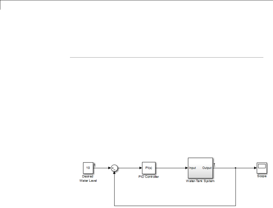
getlinio
•Port number associated with the I/O
By default, the I/Os have no loop openings. Display the properties of
each I/O object in more detail using the get function.
This example shows how to find linearization inputs/outputs in a Linear
Analysis Plots block to update the I/Os.
1Open the watertank model, and specify input and output (I/O).
aRight-click the Desired Water Level output signal, and select
Linear Analysis Points > Input Point.
bRight-click the Water-Tank System output signal, and select
Linear Analysis Points > Output Point.
The linearization I/O markers appear in the model, as shown in the
next figure.
Alternatively, you can use linio.
2Drag and drop a Bode Plot block from the Simulink Control Design
Linear Analysis Plots library into the Simulink Editor.
3Find all I/Os used by the Bode Plot block.
io = getlinio('watertank/Bode Plot')
When you drag and drop the block, the block I/Os are set to the model
I/Os. The following results appear at the MATLAB prompt:
8-82

getlinio
2x1 vector of Linearization IOs:
--------------------------
1. Linearization input located at the following signal:
- Block: watertank/Desired Water Level
- Port: 1
2. Linearization output located at the following signal:
- Block: watertank/Water-Tank System
- Port: 1
4Open the loop specified by the block I/Os.
io(2).OpenLoop = 'on';
Note The loop opening does not affect the model I/Os.
5Update the I/O in the Bode Plot block.
oldio = setlinio('watertank/Bode Plot',io)
See Also get |linearize |linio |set |setlinio
8-83

getlinplant
Purpose Compute open-loop plant model from Simulink diagram
Syntax [sysp,sysc] = getlinplant(block,op)
[sysp,sysc] = getlinplant(block,op,options)
Description [sysp,sysc] = getlinplant(block,op) Computes the open-loop
plant seen by a Simulink block labeled block (where block specifies
the full path to the block). The plant model, sysp,andlinearizedblock,
sysc, are linearized at the operating point op.
[sysp,sysc] = getlinplant(block,op,options) Computes the
open-loop plant seen by a Simulink block labeled block,usingthe
linearization options specified in options.
Examples To compute the open-loop model seen by the Controller block in the
Simulink model magball, first create an operating point object using
the function findop. In this case, you find the operating point from
simulation of the model.
magball
op=findop('magball',20);
Next, compute the open-loop model seen by the block
magball/Controller,withthegetlinplant function.
[sysp,sysc]=getlinplant('magball/Controller',op)
The output variable sysp gives the open-loop plant model as follows:
a=
Current dhdt height
Current -100 0 0
dhdt -2.801 0 196.2
height 0 1 0
b=
Controller
Current 50
8-84

getlinplant
dhdt 0
height 0
c=
Current dhdt height
Sum2 0 0 -1
d=
Controller
Sum2 0
Continuous-time model.
See Also findop |linoptions |operpoint |operspec
8-85

getSimulationTime
Purpose Final time of simulation for frequency response estimation
Syntax tfinal = getSimulationTime(input)
Description tfinal = getSimulationTime(input) returns the final time of the
Simulink simulation performed during frequency response estimation
using the input signal input.Alteringinput to reduce the final
simulation time can help reduce the time it takes to perform frequency
response estimation.
Input
Arguments
input
Input signal for frequency response estimation with the frestimate
command.
The input signal input must be either:
•A sinestream input signal, created in the Linear Analysis Tool or
created with frest.Sinestream
•A chirp input signal, created in the Linear Analysis Tool or created
with frest.Chirp
•A random input signal, created in the Linear Analysis Tool or created
with frest.Random
Output
Arguments
tfinal
Final time of simulation performed during frequency response
estimation using the input signal input.
For example, the command sysest = frestimate(mdl,io,input)
performs frequency response estimation on the Simulink model specified
by mdl with the linearization I/O set io. The estimation uses the input
signal input.Thecommand
tfinal = getSimulationTime(input)
returns the simulation time at theendofthesimulationperformed
by frestimate.
8-86

getSimulationTime
Examples Simulation Time for Frequency Response Estimation
Create a sinestream input signal and calculate the final simulation time
of an estimation using that signal.
input = frest.Sinestream('Amplitude',1e-3,...
'Frequency',logspace(1,3,50),...
'SamplesPerPeriod',40,'FreqUnits','Hz');
tfinal = getSimulationTime(input)
tfinal =
4.4186
The sinestream signal input includes 50 frequencies spaced
logarithmically between 10 Hz and 1000 Hz. Each frequency is sampled
40 times per period.
The resulting tfinal indicates that frequency response estimation of
any model with this input signal would simulate the model for 4.4186 s.
See Also frestimate | frest.Sinestream | frest.Chirp | frest.Random
Related
Examples
•“Creating Sinestream Input Signals” on page 3-9
•“Creating Chirp Input Signals” on page 3-19
Concepts •“Ways to Speed up Frequency Response Estimation” on page 3-80
8-87

getstatestruct
Purpose State structure from operating point
Syntax x_struct = getstatestruct(op_point)
Description x_struct = getstatestruct(op_point) extracts a structure of state
values, x_struct, from the operating point object, op_point.The
structure, x_struct, uses the same format as Simulink software which
allows you to set initial values for states in the model within the Data
Import/Export pane of the Configuration Parameters dialog box.
Examples Create an operating point object for the magball model:
op_magball=operpoint('magball');
Extract a state structure from the operating point object:
states_magball=getstatestruct(op_magball)
This extraction returns
states_magball =
time: 0
signals: [1x5 struct]
To view the values of the states within this structure, use dot-notation
to access the values field:
states_magball.signals.values
This dot-notation returns
ans =
0
ans =
8-88

getstatestruct
14.0071
ans =
7.0036
ans =
0
ans =
0.0500
See Also getinputstruct |getxu |operpoint
8-89

getxu
Purpose States and inputs from operating points
Syntax x = getxu(op_point)
[x,u] = getxu(op_point)
[x,u,xstruct] = getxu(op_point)
Description x = getxu(op_point) extracts a vector of state values, x,fromthe
operating point object, op_point. The ordering of states in xis the same
as that used by Simulink software.
[x,u] = getxu(op_point) extracts a vector of state values, x,anda
vector of input values, u, from the operating point object, op_point.
States in xand inputs in uareorderedinthesamewayasforSimulink.
[x,u,xstruct] = getxu(op_point) extracts a vector of state values,
x,avectorofinputvalues,u, and a structure of state values, xstruct,
from the operating point object, op_point. The structure of state
values, xstruct, has the same format as that returned from a Simulink
simulation. States in xand xstruct and inputs in uare ordered in the
same way as for Simulink.
Examples Create an operating point object for the magball model by typing:
op=operpoint('magball');
To view the states within this operating point, type:
op.States
which returns
(1.) magball/Controller/PID Controller/Filter
x: 0
(2.) magball/Controller/PID Controller/Integrator
x: 14
(3.) magball/Magnetic Ball Plant/Current
x: 7
(4.) magball/Magnetic Ball Plant/dhdt
8-90

getxu
x: 0
(5.) magball/Magnetic Ball Plant/height
x: 0.05
To extract a vector of state values, with the states in an ordering that is
compatible with Simulink, along with inputs and a state structure, type:
[x,u,xstruct]=getxu(op)
This syntax returns:
x=
0.0500
0
14.0071
7.0036
0
u=
[]
xstruct =
time: 0
signals: [1x5 struct]
View xstruct in more detail by typing:
xstruct.signals
This syntax displays:
ans =
8-91

getxu
1x5 struct array with fields:
values
dimensions
label
blockName
stateName
inReferencedModel
sampleTime
View each component of the structure individually. For example:
xstruct.signals(1).values
ans =
0
or
xstruct.signals(2).values
ans =
7.0036
You can import these vectors and structures into Simulink as initial
conditions or input vectors or use them with setxu,tosetstateand
input values in another operating point.
See Also operpoint |operspec
8-92

initopspec
Purpose Initialize operating point specification values
Syntax opnew=initopspec(opspec,oppoint)
opnew=initopspec(opspec,x,u)
opnew=initopspec(opspec,xstruct,u)
Alternatives As an alternative to the initopspec function, initialize operating point
specification values in the Create Operating Points pane in the
Operating Points node within the Simulink Control Design GUI. See
“Steady-State Operating Points (Trimming) from Specifications” on
page 1-14.
Description opnew=initopspec(opspec,oppoint) initializes the operating point
specification object, opspec, with the values contained in the operating
point object, oppoint. The function returns a new operating point
specification object, opnew.Createopspec with the function operspec.
Create oppoint with the function operpoint or findop.
opnew=initopspec(opspec,x,u) initializes the operating point
specification object, opspec, with the values contained in the state
vector, x, and the input vector, u. The function returns a new operating
point specification object, opnew.Createopspec with the function
operspec. You can use the function getxu to create xand uwith the
correct ordering.
opnew=initopspec(opspec,xstruct,u) initializes the operating point
specification object, opspec, with the values contained in the state
structure, xstruct, and the input vector, u. The function returns a
new operating point specification object, opnew.Createopspec with
the function operspec. You can use the function getstatestruct
or getxu to create xstruct and the function getxu to create uwith
the correct ordering. Alternatively, you can save xstruct to the
MATLAB workspace after a simulation of the model. See the Simulink
documentation for more information on these structures.
Examples Create an operating point using findop by simulating the magball
model and extracting the operating point after 20 time units.
8-93

initopspec
oppoint=findop('magball',20)
This syntax returns the following operating point:
Operating Point for the Model magball.
(Time-Varying Components Evaluated at time t=20)
States:
----------
(1.) magball/Controller/PID Controller/Filter
x: 2.33e-007
(2.) magball/Controller/PID Controller/Integrator
x: 14
(3.) magball/Magnetic Ball Plant/Current
x: 7
(4.) magball/Magnetic Ball Plant/dhdt
x: 3.6e-008
(5.) magball/Magnetic Ball Plant/height
x: 0.05
Inputs: None
----------
Use these operating point values as initialvaluesinanoperatingpoint
specification object.
opspec=operspec('magball');
newopspec=initopspec(opspec,oppoint)
The new operating point specification object is displayed.
Operating Specification for the Model magball.
(Time-Varying Components Evaluated at time t=0)
States:
----------
(1.) magball/Controller/PID Controller/Filter
8-94

initopspec
spec: dx = 0, initial guess: 2.33e-007
(2.) magball/Controller/PID Controller/Integrator
spec: dx = 0, initial guess: 14
(3.) magball/Magnetic Ball Plant/Current
spec: dx = 0, initial guess: 7
(4.) magball/Magnetic Ball Plant/dhdt
spec: dx = 0, initial guess: 3.6e-008
(5.) magball/Magnetic Ball Plant/height
spec: dx = 0, initial guess: 0.05
Inputs: None
----------
Outputs: None
----------
You can now use this object to find operating points by optimization.
See Also findop |getstatestruct |getxu |operpoint |operspec
8-95

linearize
Purpose Linear approximation of Simulink model or block
Syntax linsys = linearize(sys,io)
linsys = linearize(sys,op)
linsys = linearize(sys,op,io)
linsys = linearize(sys,op,io,options)
[linsys,op] = linearize(sys,io,tsnapshot)
linsys = linearize(sys,op,io,'StateOrder',stateorder)
linblock = linearize(sys,op,blockpath)
linsys = linearize(sys,blocksub,op,io)
Description linsys = linearize(sys,io) linearizes the nonlinear Simulink model
defined by the linearization I/O points io. Linearization uses the
operating point that corresponds to the initial states and input levels in
the Simulink model.
linsys = linearize(sys,op) linearizes the entire Simulink model
such that the linearization I/O points are the root-level inport and
output blocks in sys. Linearization uses the operating point op.
linsys = linearize(sys,op,io) linearizes the model specified by
linearization I/O points io.
linsys = linearize(sys,op,io,options) uses algorithm options
specified in options.
[linsys,op] = linearize(sys,io,tsnapshot) linearizes the model
atoneormoresimulationtimestsnapshot. Returns the operating
point op that corresponds to the simulation snapshot. Omit io when
you want to use the root-level inport and output blocks in sys as
linearization I/O points.
linsys = linearize(sys,op,io,'StateOrder',stateorder) returns
a linear model with a specified state order.
linblock = linearize(sys,op,blockpath) linearizes the block in
the model sys specified by the blockpath. Linearization uses the
operating point op.
8-96

linearize
linsys = linearize(sys,blocksub,op,io) linearizes the nonlinear
Simulink model defined by the linearization I/O points io.blocksub
defines the analytic linearization of blocks that do not linearize
successfully, such as blocks with discontinuities or triggered
subsystems. Omit the operating point op when you want to use the
model operating point. Omit io whenyouwanttousetheroot-level
inport and output blocks in sys as linearization I/O points.
Input
Arguments
sys
Simulink model name, specified as a string inside single quotes ('').
io
Linearization I/O object, specified using linio.
If the linearization input and output points are stored in the model
workspace, extract these points from the model into io using getlinio.
io must correspond to the Simulink model sys.
op
Operating point object, specified using operpoint or findop.
op must correspond to the Simulink model sys.
options
Algorithm options, specified using linoptions.
tsnapshot
Simulation snapshot time instants when to linearize the model,
specified as a scalar or vector.
stateorder
State order in linearization results, specified as a cell array of block
paths for blocks with states. Each block path is string of the form
model/subsystem/block that uniquely identifies a block in the model.
8-97

linearize
The order of the block paths in the cell array should match the desired
order of the linearized model states.
blockpath
Block to linearize, specified as a full block path. A block path is string
of the form model/subsystem/block that uniquely identifies a block in
the model.
blocksub
Desired block linearization, specified for blocks that do not have
analytic linearization.
blocksub is an n-by-1 structure, where nis the number of blocks for
which you specify the linearization. blocksub has these fields:
•Name — Block path corresponding to the block for which you want to
specify the linearization.
blocksub.Name is a string of the form model/subsystem/block that
uniquely identifies a block in the model.
•Value — Desired linearization of the block, specified as a structure
with these fields:
Specification — Block linearization, specified as a string. The
string can include a MATLAB expression or function that returns
one of the following:
-Linear model in the form of a D-matrix
-ControlSystemToolboxLTImodelobject
-Robust Control Toolbox uncertain state space or uncertain real
object (requires Robust Control Toolbox software)
If blocksub.Value.Specification is a MATLAB expression, this
expression must follow the resolution rules , as described in “Symbol
Resolution”.
If blocksub.Value.Specification is a function, this function must
have one input argument, BlockData, which is a structure that
8-98

linearize
the software creates automatically and passes to the specification
function. BlockData has the following fields:
-BlockName is the name of the Simulink block with the specified
linearization.
-Parameters is a structure array containing the evaluated values
for the block. Each element of the array has the fields 'Name'
and 'Value', which contain the name and evaluated value,
respectively, for the parameter.
-Inputs is an array of input values.
-ny is the number of output channels of the block linearization.
-nu is the number of input channels of the block linearization.
-Type — Specification type, specified as one of these strings:
'Expression'
'Function'
-ParameterNames — Linearization function parameter names,
specified as a comma-separated list of strings. Specify only when
blocksub.Value.Type = 'Function' and your block linearization
function requires input parameters. These parameters only impact
the linearization of the specified block
You must also specify the corresponding
blocksub.Value.ParameterValues field.
-ParameterValues — Linearization function parameter values that
correspond to blocksub.Values.ParameterNames.Specifyonly
when blocksub.Value.Type = 'Function'.
blocksub.Value.ParameterValues is a comma separated list of
values. The order of parameter values must correspond to the
order of parameter names in blocksub.Value.ParameterNames.
-BlockLinearization is a state-space (ss) model that is
the current default linearization of the block. You can use
BlockData.BlockLinearization in the specification function
to specify a block linearization that depends on the default
8-99

linearize
linearization, such as the default linearization multiplied by a
time delay.
Output
Arguments
linsys
Linear time-invariant state-space model that approximates the
nonlinear model specified by linearization I/O points io.
linsys is returned as an ss object.
op
Operating point corresponding the simulation snapshot of the states
and input levels at tsnapshot, returned as an operating point object.
Thisisthesameobjectasreturnedusingoperpoint or findop.
View op values to determine whether the model was linearized at a
reasonable operating point.
linblock
Linear time-invariant state-space model that approximates the
specified nonlinear block, returned as an ss object.
Examples Linearization at Model Operating Point
This example shows how to use linearize to linearize a model at
the operating point specified in the model. The model operating point
consists of the model initial state values and input signals.
1Open Simulink model.
sys = 'watertank';
load_system(sys);
open_system(sys)
The Water-Tank System block represents the plant in this control
system and contains all of the system nonlinearities.
8-100

linearize
2Specify to linearize the Water-Tank System block using linearization
I/O points.
sys_io(1)=linio('watertank/PID Controller',1,'in');
sys_io(2)=linio('watertank/Water-Tank System',1,'out');
Each linearization I/O point is associated with a block outport. For
example, to specify a linearization input point at the Water-Tank
System block input, you must associate this input point with the
outport of the PID Controller block.
sys_io is an object array that includes two linearization I/O objects.
The first object, sys_io(1), specifies the linearization input point
on the first watertank/PID Controller output signal. The second
object, sys_io(2), specifies the linearization output point on the first
watertank/Water-Tank System output signal.
Note When there are multiple block output signals and you want to
specify an output port other than the first output, enter the desired
output port number as the second argument of linio.
3Update the model ports to include the linearization I/O points.
setlinio(sys,sys_io)
4Open the loop.
sys_io(2).OpenLoop='on';
This command removes the effects of the feedback signal on the
linearization without changing the model operating point.
8-101

linearize
Note Do not open the loop by manually removing the feedback
signal from the model. Removing the signal manually changes the
operating point of the model.
5Update the model to reflect the modified linearization I/O object.
setlinio(sys,sys_io);
This command also adds the loop opening marker to the model.
When you add input points, output points, or loop openings,
linearization I/O markers appear in the model. Use these to visualize
your linearization points.
6Linearize the Water-Tank System block at the model operating point.
linsys = linearize(sys,sys_io);
bdclose(sys);
linsys is a state-space model object.
7Plot a Bode plot of the linearized model.
bode(linsys)
8-102
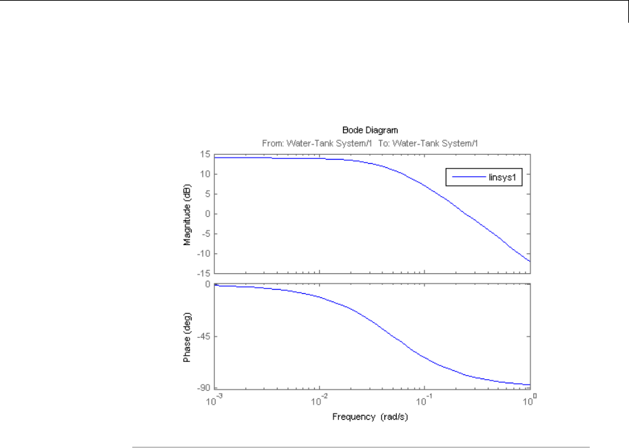
linearize
The resulting Bode plot looks like a stable first-order response, as
expected.
Linearization at Simulation Snapshot
This example shows how to use linearize to linearize a model by
simulating the model and extracting the state and input levels of the
system at specified simulation times.
1Open Simulink model.
sys = 'watertank';
load_system(sys);
The Water-Tank System block represents the plant in this control
system and contains all of the system nonlinearities.
8-103
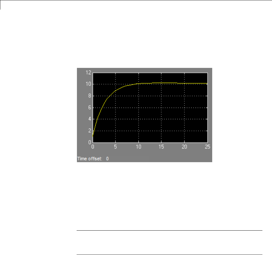
linearize
2Simulate the model to determine the time when the model reaches
steady state.
The Scope block shows that the system reaches steady state at
approximately 20 time units.
3Specify to linearize the open-loop Water-Tank System.
sys_io(1)=linio('watertank/PID Controller',1,'in');
sys_io(2)=linio('watertank/Water-Tank System',1,'out','on');
The last input argument for computing sys_io(2) opens the
feedback loop.
Note Do not open the loop by manually removing the feedback
signal from the model. Removing the signal manually changes the
operating point of the model.
4Linearize the Water-Tank System block at a simulation time of
20time units.
8-104
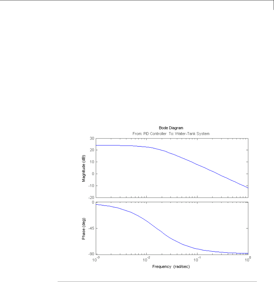
linearize
tsnapshot = 20;
linsys = linearize(sys,sys_io,tsnapshot);
bdclose(sys);
linsys is a state-space model object.
5Plot a Bode plot of the linearized model.
bode(linsys)
The resulting Bode plot looks like a stable first-order response, as
expected.
Linearization at Trimmed Operating Point
8-105

linearize
This example shows how to use linearize to linearize a model using a
trimmed operating point.
1Open Simulink model.
sys = 'watertank';
load_system(sys);
2Create operating point specification object.
opspec = operspec(sys);
By default, all model states are specified to be at steady state.
3Find the steady-state operating point using trim analysis.
op = findop(sys,opspec);
4Specify to linearize the open-loop Water-Tank System.
sys_io(1)=linio('watertank/PID Controller',1,'in');
sys_io(2)=linio('watertank/Water-Tank System',1,'out','on');
5Linearize the Water-Tank System block at the trimmed operating
point.
linsys = linearize(sys,op,sys_io);
bdclose(sys);
linsys is a state-space model object.
Linearization at Multiple Simulation Snapshots
This example shows how to use linearize to linearize a model at
multiple simulation snapshots.
1Open Simulink model.
8-106

linearize
sys = 'magball';
load_system(sys);
2Specify to linearize the open-loop Water-Tank System.
sys_io(1)=linio('watertank/PID Controller',1,'in');
sys_io(2)=linio('watertank/Water-Tank System',1,'out','on');
3Define the simulation times at which to linearize the model.
tsnapshot = [10,20];
linsys = linearize(sys,sys_io,tsnapshot);
bdclose(sys);
Plant Linearization at Model Operating Point
This example shows how to use linearize to linearize a subsystem at
the model operating point.
Use this approach instead of defining linearization I/O points when the
plant is a subsystem or a block.
1Open Simulink model.
sys = 'watertank';
load_system(sys);
blockpath = 'watertank/Water-Tank System';
2Linearize the Water-Tank System block.
linsys = linearize(sys,blockpath);
bdclose(sys);
Algorithms By default, linearize automatically sets the Simulink model
properties:
•BufferReuse = 'off'
•RTWInlineParameters = 'on'
8-107

linearize
•BlockReductionOpt = 'off'
After the linearization completes, Simulink restores the original model
properties.
Alternatives Use the Control and Estimation Tools Manager. For example, see
“Linearize at Model Operating Point” on page 2-38.
See Also findop |linlftfold
How To • “Linearize at Model Operating Point” on page 2-38
• “Linearize at Trimmed Operating Point” on page 2-52
8-108

linio
Purpose Define linearization input/output (I/O) points for Simulink model
Syntax io = linio('blockname',portnum)
io = linio('blockname',portnum,type)
io = linio('blockname',portnum,type,openloop)
io = linio('blockname',portnum,type,openloop,
'buselementname')
Alternatives As an alternative to the linio function, create linearization I/O settings
by using the right-click menu on the model diagram.
Description io = linio('blockname',portnum) creates a linearization
input/output (I/O) object for the signal that originates from the outport
with port number portnum of the block blockname in a Simulink
model. The default I/O type is 'in',andthedefaultOpenLoop property
is 'off'.Useio with linearize to create linearized models.
io = linio('blockname',portnum,type) creates a linearization
I/O object with specified type of linearization I/O type. Available
linearization I/O types are:
•'in', linearization input point
•'out', linearization output point
•'inout', linearization input then output point
•'outin', linearization output then input point
•'none',nolinearizationinput/output point
io = linio('blockname',portnum,type,openloop) creates a
linearization I/O object with specified loop-opening status openloop.
The openloop property is 'off' when the I/O point is not an open-loop
pointandissetto'on' when the I/O point is an open-loop point.
io =
linio('blockname',portnum,type,openloop,'buselementname')
creates a linearization I/O object for the element buselementname at
the bus signal that originates from the portnum of blockname.
8-109

linio
Examples This example shows how to create linearization I/O settings for a
Simulink model.
1Create an I/O setting for the signal originating from the Controller
block of the magball model.
io(1)=linio('magball/Controller',1)
By default, this I/O is an input point.
1x1 vector of Linearization IOs:
--------------------------
1. Linearization input located at the following signal:
- Block: magball/Controller
- Port: 1
2Create a second I/O setting within the object, io.
io(2)=linio('magball/Magnetic Ball Plant',1,'out','on')
This I/O originates from the Magnetic Ball Plant block, is an output
point and is also an open-loop point.
1x2 vector of Linearization IOs:
--------------------------
1. Linearization input located at the following signal:
- Block: magball/Controller
- Port: 1
2. Linearization output with a loop opening located at the following signal:
- Block: magball/Magnetic Ball Plant
- Port: 1
Select Individual Bus Element as Linearization I/O point
This example shows how to create a linearization I/O setting for
individualbuselementsinabussignal.
8-110
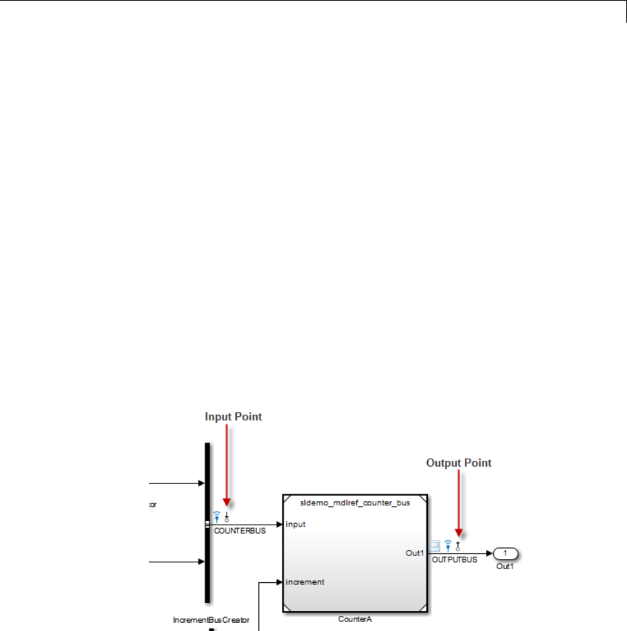
linio
1Open Simulink model.
sys = 'sldemo_mdlref_bus';
open_system(sys);
2Specify to linearize the CounterA block using linearization I/O points
on an individual bus element.
io(1) = linio('sldemo_mdlref_bus/COUNTERBUSCreator',1,'in',...
'off','limits.upper_saturation_limit');
io(2) = linio('sldemo_mdlref_bus/CounterA',1,'out','off',...
'limits.upper_saturation_limit');
3Update the model to reflect the linearization I/O object.
setlinio(sys,io)
set_param(sys,'ShowLinearizationAnnotations','on')
The linearization I/O markers appear in the model. Use these
markers to visualize your linearization points.
4Linearize the model at the model operating point.
8-111

linlft
Purpose Linearize model while removing contribution of specified blocks
Syntax lin_fixed = linlft(sys,io,blocks)
[lin_fixed,lin_blocks] = linlft(sys,io,blocks)
Description lin_fixed = linlft(sys,io,blocks) linearizes the Simulink model
named sys while removing the contribution of certain blocks. Specify
the full block pathnames of the blocks to ignore in the cell array of
strings called blocks. The linearization occurs at the operating point
specified in the Simulink model, which includes the ignored blocks. You
can optionally specify linearization points (linear analysis points) in the
I/O object io. The resulting linear model lin_fixed has this form:
sys
... ...
In Out
Block 1 Out
Block 2 Out
Block n Out
Block 1 In
Block 2 In
Block n In
The top channels In and Out correspond to the linearization points you
specify in the I/O object io. The remaining channels correspond to the
connection to the ignored blocks.
When you use linlft and specify the ’block-by-block’ linearization
algorithm in linoptions, you can use all the variations of the input
arguments for linearize.
You can linearize the ignored blocks separately using linearize,and
then combine the linearization results using linlftfold.
[lin_fixed,lin_blocks] = linlft(sys,io,blocks) returns the
linearizations for each of the blocks specified in blocks.Ifblocks
is a string identifying a single block path, lin_blocks is a single
state-space (ss) model. If blocks is a cell array identifying multiple
blocks, lin_blocks is a cell array of state-space models. The full block
path for each block in lin_blocks is stored in the Notes property of
the state-space model.
8-113
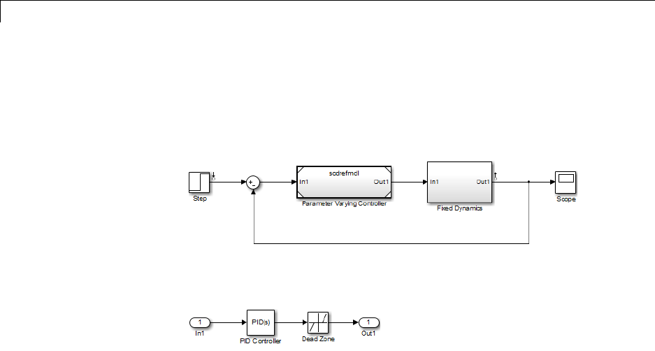
linlft
Examples Linearize the following parts of the scdtopmdl Simulink model
separately, and then combine the results:
•Fixed portion, which contains everything except the Parameter
Varying Controller model reference
•Parameter Varying Controller model reference, which references
the scdrefmdl model
% Open the Simulink model
topmdl = 'scdtopmdl';
% Linearize the model without the Parameter Varying Controller
io = getlinio(topmdl);
blocks = {'scdtopmdl/Parameter Varying Controller'};
sys_fixed = linlft(topmdl,io,blocks);
% Linearize the Parameter Varying Controller
refmdl = 'scdrefmdl';
sys_pv = linearize(refmdl);
% Combine the results
BlockSubs(1) = struct('Name',blocks{1},'Value',sys_pv);
sys_fold = linlftfold(sys_fixed,BlockSubs);
See Also linlftfold |linearize |linio |getlinio |operpoint
8-114
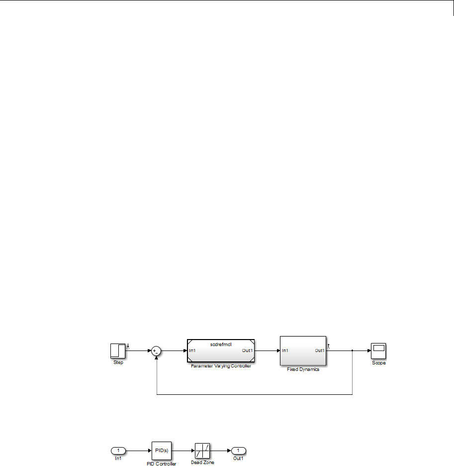
linlftfold
Purpose Combine linearization results from specified blocks and model
Syntax lin = linlftfold(lin_fixed,blocksubs)
Description lin = linlftfold(lin_fixed,blocksubs) combines the following
linearization results into one linear model lin:
•Linear model lin_fixed, which does not include the contribution of
specified blocks in your Simulink model
You compute lin_fixed using linlft.
•Block linearizations for the blocks excluded from lin_fixed
You specify the block linearizations in a structure array blocksubs,
which contains two fields:
-'Block' is a string specifying the Simulink block to replace.
-'Value' is the value of the linearization for each block.
Examples Linearize the following parts of the scdtopmdl Simulink model
separately and then combine the results:
•Fixed portion, which contains everything except the Parameter
Varying Controller model reference
•Parameter Varying Controller model reference, which references
the scdrefmdl model
% Open the Simulink model
8-115

linlftfold
topmdl = 'scdtopmdl';
% Linearize the model without the Parameter Varying Controller
io = getlinio(topmdl);
blocks = {'scdtopmdl/Parameter Varying Controller'};
sys_fixed = linlft(topmdl,io,blocks);
% Linearize the Parameter Varying Controller
refmdl = 'scdrefmdl';
sys_pv = linearize(refmdl);
% Combine the results
BlockSubs(1) = struct('Name',blocks{1},'Value',sys_pv);
sys_fold = linlftfold(sys_fixed,BlockSubs);
See Also linlft |linearize |linio |getlinio |operpoint
8-116

linoptions
Purpose Set options for linearization and finding operating points
Syntax opt=linoptions
opt=linoptions('Property1','Value1','Property2','Value2',
...)
Alternatives As an alternative to the linoptions function, set options for
linearization and finding operating points in the Simulink Control
Design GUI.
Description opt=linoptions creates a linearization optionsobjectwiththe
default settings. The variable, opt, is passed to the functions findop
and linearize to specify options for finding operating points and
linearization.
opt=linoptions('Property1','Value1','Property2','Value2',...)
creates a linearization options object, opt,in which the option given
by Property1 is set to the value given in Value1, the option given by
Property2 is set to the value given in Value2,etc. Thevariable,opt,
is passed to the functions findop and linearize to specify options for
finding operating points and linearization.
The following options can be set with linoptions:
LinearizationAlgorithm Set to 'numericalpert' to enable numerical-perturbation
linearization (as in Simulink 3.0 software) where root-level
inports and states are numerically perturbed. Linearization
annotations are ignored and root-level inports and outports
are used instead.
Default is 'blockbyblock'.
SampleTime Thetimeatwhichthesignalissampled. Nonzero for discrete
systems, 0for continuous systems, -1 (default) to use the
longest sample time that contributes to the linearized model.
8-117

linoptions
UseFullBlockNameLabels Set to 'off' (default) to use truncated names for the
linearization I/Os and states in the linearized model. Set to
'on' to use the full block path to name the linearization I/Os
and states in the linearized models.
UseBusSignalLabels Set to 'off' (default) to use bus signal channel number to
label I/Os on bus signals in your linearization results. Set to
'on' to use bus signal names to label I/Os on bus signals in
your linearization results. Bus signal names appear in the
results when the I/O points are located at the output of the
following blocks:
•Root-level inport block containing a bus object
•Bus creator block
•Subsystem block whose source traces back to one of the
following:
-Output of a bus creator block
-Root-level inport by passing through only virtual or
nonvirtual subsystem boundaries
Note You cannot use this option when your model has
mux/bus mixtures. For information on how to avoid buses
used as muxes, see “Avoid Mux/Bus Mixtures” in the Simulink
documentation.
8-118
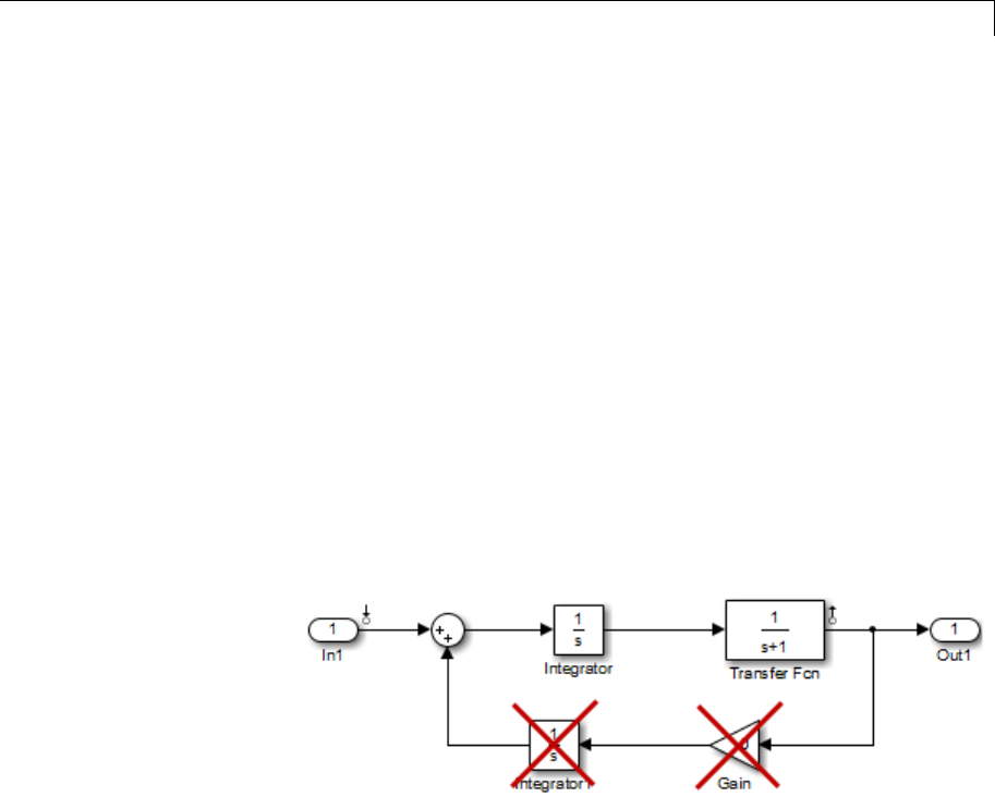
linoptions
BlockReduction Set to 'on' (default) to eliminate from the linearized model
those blocks that are not in the path of the linearization. Block
reduction eliminates the states of blocks in dead linearization
paths from your linearization results. Some examples of dead
linearization paths are linearization paths that include:
•Blocks that linearize to zero
•Switch blocks that are not active along the path
•Disabled subsystems
•Signals marked as open-loop linearization points
The linearization result of the model shown in the following
figure includes only two states. It does not include states from
the two blocks outside the linearization path. These states do
not appear because these blocks are on a dead linearization
path with a block that linearizes to zero (the zero gain block).
Set to 'off' to return a linearized model that includes all of
the states of the model.
IgnoreDiscreteStates Set to 'on' when performing continuous linearization
(SampleTime set to 0) to remove any discrete states from
the linearization and accept the D value for all blocks with
discrete states. Set to 'off' (default) to include discrete
states.
8-119

linoptions
RateConversionMethod When you linearize a multirate system, set this option to one
of the following rate conversion methods:
•'zoh' (default)tousethezeroorderrateconversion
method
•'tustin' to use the Tustin (bilinear) method
•'prewarp' to use the Tustin approximation with
prewarping
•'upsampling_zoh' to upsample discrete states when
possible and to use 'zoh' otherwise
•'upsampling_tustin' to upsample discrete states when
possible and to use 'tustin' otherwise
•'upsampling_prewarp' to upsample discrete states when
possible and to use 'prewarp' otherwise
Note When you select 'prewarp' or 'upsampling_prewarp',
set the PreWarpFreq option to the desired prewarp frequency.
Note You can only upsample when you convert discrete
states to a new sample time that is an integer-value-times
faster than the sampling time of the original system.
For more information, and examples, on methods and
algorithms for rate conversions and linearization of multirate
models, see:
•Linearization of Multirate Models
•Linearization Using Different Rate Conversion Methods
•“Continuous-Discrete Conversion Methods” in the Control
System Toolbox documentation
8-120

linoptions
PreWarpFreq The critical frequency Wc (in rad/sec) used by the 'prewarp'
option when linearizing a multirate system.
UseExactDelayModel Set to 'on' to return a linear model with an exact delay
representation. Set to 'off' (default) to return a model with
approximate delays.
NumericalPertRel Set the perturbation level for obtaining the linear model
(default value is 1e-5). The perturbation of the system’s
states is specified by:
NumericalPertRel NumericalPertRel+× ×
−
10 3x
The perturbation of the system’s inputs is specified by:
NumericalPertRel NumericalPertRel+× ×
−
10 3u
NumericalXPert Individually set the perturbation levels for the system’s states
using an operating point object. Use the operpoint function
to create an operating point object for the model.
NumericalUPert Individually set the perturbation levels for the system’s
inputs using an operating point object. Use the operpoint
function to create an operating point object for the model.
OptimizationOptions Set options for use with the optimization algorithms. These
optionsarethesameasthosesetwithoptimset.Formore
information on these algorithms, see the Optimization
Toolbox documentation.
OptimizerType Set optimizer type to be used by trim optimization if the
Optimization Toolbox software is installed. The available
optimizer types are:
8-121

linoptions
•graddescent_elim, the default optimizer, enforces an
equality constraint to force the time derivatives of states
to be zero (dx/dt=0,x(k+1)=x(k)) and the output signals
to be equal to their specified ‘Known’ value. The optimizer
fixes the states, x,andinputs,u, that are marked as
‘Known’ in an operating point specification and then
optimizes the remaining variables.
•graddescent, enforces an equality constraint to force
thetimederivativesofstatestobezero(
dx/dt=0,
x(k+1)=x(k)) and the output signals to be equal to their
specified ‘Known’ value. findop also minimizes the error
between the states, x,andinputs,u, that are marked as
‘Known’inanoperatingpointspecification. If there are not
any inputs or states marked as ‘Known’, findop attempts
to minimize the deviation between the initial guesses for x
and uandtheirtrimmedvalues.
•lsqnonlin fixes the states, x,andinputs,u,thatare
marked as ’Known’ in an operating point specification and
optimizes the remaining variables. The algorithm then
tries to minimize both the error in the time derivatives of
the states (dx/dt=0,x(k+1)=x(k)) and the error between
the outputs and their specified ’Known’ value.
•simplex uses the same cost function as lsqnonlin with the
direct search optimization routine found in fminsearch.
See the Optimization Toolbox documentation for more
information on these algorithms. If you do not have
the Optimization Toolbox software, you can access the
documentation at http://www.mathworks.com/support/.
DisplayReport Set to 'on' to display the operating point summary report
when running findop.Setto'off' to suppress the display
of this report.
8-122

linoptions
See Also findop |linearize
8-123

operpoint
Purpose Create operating point for Simulink model
Syntax op = operpoint('sys')
Alternatives As an alternative to the operpoint function, create operating points
in the Operating Points node of the Simulink Control Design GUI.
See “Steady-State Operating Points (Trimming) from Specifications”
on page 1-14.
Description op = operpoint('sys') returns an object, op, containing the
operating point of a Simulink model, sys.Usetheobjectwiththe
function linearize to create linearized models. The operating point
object properties are:
•“Model” on page 8-124
•“States” on page 8-124
•“Inputs” on page 8-125
•“Time” on page 8-125
Edit the properties of this object directly or with the set function.
Model
Model specifies the name of the Simulink model that this operating
point object refers to.
States
States describes the operating points of states in the Simulink model.
The States property is a vector of state objects that contains the
operating point values of the states. There is one state object per block
that has a state in the Simulink model. The States object has the
following properties:
Nx Number of states in the block. This property
is read-only.
Block Block with which the states are associated.
8-124

operpoint
xVector containing the values of states in the
block.
Ts Vectorcontainingthesampletimeandoffset
for the state.
SampleType Set this value to CSTATE, for a continuous state,
or DSTATE for a discrete state.
inReferencedModel Set this value to 1, when the state is inside a
referenced model, or 0,whenitisnot.
Description Text string describing the block.
Inputs
Inputs is a vector of input objects that contains the input levels at the
operating point. There is one input object per root-level inport block in
the Simulink model. The Inputs object has the following properties:
Block Inport block with which the input vector is
associated
PortWidth Width of the corresponding inport
uVector containing the input level at the
operating point
Description Text string describing the input
Time
Time specifies the time at which any time-varying functions in the
model are evaluated.
Examples To create an operating point object for the Simulink model magball,
type:
op = operpoint('magball')
which returns the following:
8-125

operpoint
Operating Point for the Model magball.
(Time-Varying Components Evaluated at time t=0)
States:
----------
(1.) magball/Controller/PID Controller/Filter
x: 0
(2.) magball/Controller/PID Controller/Integrator
x: 14
(3.) magball/Magnetic Ball Plant/Current
x: 7
(4.) magball/Magnetic Ball Plant/dhdt
x: 0
(5.) magball/Magnetic Ball Plant/height
x: 0.05
Inputs: None
----------
MATLAB software displays the name of the model, the time at which
any time-varying functions in the model are evaluated, the names of
blocks containing states, and the values of the states at the operating
point. In this example there are four blocks that contain states in the
model and four entries in the States object. The first entry contains
two states. MATLAB also displays the Inputs although there are not
any in this model. To view the properties of op in more detail, use the
get function.
See Also get |linearize |operspec |set |update
8-126

operspec
Purpose Operating point specifications
Syntax opspec = operspec(sys)
Description opspec = operspec(sys) returns the operating point specifications
object for steady state operating point analysis using findop.The
Simulink model must be open.
Tips •Use get to display the operating point specification object properties.
Input
Arguments
sys
Simulink model name, specified as a string inside single quotes ('').
Output
Arguments
opspec
Operating point specification object.
After creating the operating point object, you can modify the operating
point states and input levels. For example, opspec.States(1).Known
=1
specifies that the first model state value is known, and the value
of the known state opspec.States(1).x = 2.
The operating point object has these properties:
•Model — Simulink model name. String.
•States — State operating point specification. Vector of data
structures, where each data structure represents the states of one
Simulink block. Each States structure has these fields:
8-127

operspec
xSimulink block state values, specified as a
vector of states.
Also set the Known field of the States property
for known state values that remain fixed
during operating point search.
Known Known state value specification:
•1— Known value that is fixed during
operating point search.
-0(default) — Unknown value to be found
by optimization.
Also specify the known operating point values
using the xfield of the States structure.
SteadyState Steady state value specification:
•1(default) — Equilibrium state.
-0— Nonequilibrium state.
Min Minimum bounds on the state value, specified
asascalarorvector.
Max Maximum bounds on the state value, specified
asascalarorvector.
Ts (Only for discrete-time states) Sample time
and offset of each Simulink block state,
specified as a vector.
Description Block state description, specified as a string.
Nx(read only) Number of states in the Simulink block.
Block Simulink block name.
8-128

operspec
SampleType State time rate can have the values:
•'CSTATE' — Continuous-time state
-'DSTATE' — Discrete—time state.
inReferencedModel Determine whether the sates is inside a
reference model:
•1— State is inside a reference model.
-0— State is in the current model file.
•Inputs — Input level specifications at the operating point. Vector
of input specification objects, where each object represents the input
levels of one root-level inport block in the Simulink block. Each input
specification object has these properties:
uInport block input levels at the operating
point, specified as a vector of input levels.
Also set the Known field of the Inputs property
for known input levels that remain fixed
during operating point search.
Known Known input level specification:
•1— Known input level that is fixed during
operating point search.
-0(default) — Unknown input level to be
found by optimization.
Also specify the known operating point input
levels using the uproperty of the input
specification object.
Min Minimum bounds on the input level, specified
asascalarorvector.
8-129

operspec
Max Maximum bounds on the input level, specified
asascalarorvector.
Description Inport block input description, specified as
astring.
Block Inport block name.
PortWidth Number of inport block signals.
•Outputs — Output level specifications at the operating point. Vector
of output specification objects, where each object represents one
output specification per root-level output block in the Simulink block.
You can constrain additional output levels using addoutputspec to
add another output specification.
Each output specification object has these properties:
yOutport block output levels at the operating
point, specified as a vector of output levels.
Also set the Known field of the Outputs
property for known output levels that remain
fixed during operating point search.
Known Known output level specification:
•1— Known output level constraint that
must be met during operating point search.
-0(default) — Unknown input level to be
found by optimization.
Also specify the known operating point output
levels using the yproperty of the output
specification object.
8-130

operspec
Min Minimum bounds on the output level,
specified as a scalar or vector.
Max Maximum bounds on the output level,
specified as a scalar or vector.
Description Outport block input description, specified as
astring.
Block Outport block name.
PortWidth Number of outport block signals.
•Time — Time instants for evaluating the time-varying functions in
the model.
Examples Steady-State Operating Point (Trimming) From Specifications
This example shows how to use findop to compute an operating point of
a model from specifications.
1Open Simulink model.
sys = 'watertank';
load_system(sys);
2Create operating point specification object.
opspec = operspec(sys)
By default, all model states are specified to be at steady state.
Operating Specification for the Model watertank.
(Time-Varying Components Evaluated at time t=0)
States:
----------
(1.) watertank/PID Controller/Integrator
8-131

operspec
spec: dx = 0, initial guess: 0
(2.) watertank/Water-Tank System/H
spec: dx = 0, initial guess: 1
Inputs: None
----------
Outputs: None
----------
operspec extracts the default operating point of the Simulink model
with two states. The model does not have any root-level inport blocks
and no root-level outport blocks or output constraints.
3Configure specifications for the first model state.
opspec.States(1).SteadyState = 1;
opspec.States(1).x = 2;
opspec.States(1).Min = 0;
Thefirststatemustbeatsteadystateandhaveaninitialvalueof2
with a lower bound of 0.
4Configure specifications for the second model state.
opspec.States(2).Known = 1;
opspec.States(2).x = 10;
The second state sets the desired height of the water in the tank at
10. Configuring the height as a known value keeps this value fixed
when computing the operating point.
5Find the operating point that meets these specifications.
[op,opreport] = findop(sys,opspec)
bdclose(sys);
opreport describes how closely the optimization algorithm met the
specifications at the end of the operating point search.
8-132

operspec
Operating Report for the Model watertank.
(Time-Varying Components Evaluated at time t=0)
Operating point specifications were successfully met.
States:
----------
(1.) watertank/PID Controller/Integrator
x: 1.26 dx: 0 (0)
(2.) watertank/Water-Tank System/H
x: 10 dx: 0 (0)
Inputs: None
----------
Outputs: None
----------
dx indicates the time derivative of each state. The actual dx values of
zero indicate that the operating point is at steady state. The desired
dx value is in parentheses.
Initialize Steady-State Operating Point Search Using Simulation
This example shows how to use findop to compute an operating point of
a model from specifications, where the initial state values are extracted
from a simulation snapshot.
1Open Simulink model.
sys = 'watertank';
load_system(sys);
2Extract an operating point from simulation after 10 time units.
opsim = findop(sys,10);
3Create operating point specification object.
8-133

operspec
By default, all model states are specified to be at steady state.
opspec = operspec(sys);
4Configure initial values for operating point search.
opspec = initopspec(opspec,opsim);
5Find the steady state operating point that meets these specifications.
[op,opreport] = findop(sys,opspec)
bdclose(sys);
opreport describes the optimization algorithm status at the end of
the operating point search.
Operating Report for the Model watertank.
(Time-Varying Components Evaluated at time t=0)
Operating point specifications were successfully met.
States:
----------
(1.) watertank/PID Controller/Integrator
x: 1.26 dx: 0 (0)
(2.) watertank/Water-Tank System/H
x: 10 dx: -1.1e-014 (0)
Inputs: None
----------
Outputs: None
----------
dx, which is the time derivative of each state, is effectively zero.
Thisvalueofthestatederivativeindicatesthattheoperatingpoint
is at steady state.
8-134

operspec
Operating Point (Trim Analysis) With Output Constraint
Thisexampleshowshowtouseaddoutputspec to specify an output
constraint to the operating point specification object for computing the
operating point.
1Open Simulink model.
sys = 'scdspeed';
load_system(sys);
2Create operating point specification object.
opspec = operspec(sys)
By default, opspec specifies that the operating point is at steady
state, or equilibrium.
Operating Specification for the Model scdspeed.
(Time-Varying Components Evaluated at time t=0)
States:
----------
(1.) scdspeed/Throttle & Manifold/Intake Manifold/p0 = 0.543 bar
spec: dx = 0, initial guess: 0.543
(2.) scdspeed/Vehicle Dynamics/w = T//J w0 = 209 rad//s
spec: dx = 0, initial guess: 209
Inputs:
----------
(1.) scdspeed/Throttle perturbation
initial guess: 0
Outputs: None
----------
operspec extracts the default operating point of the Simulink
model with two states and one root-level inport block. There are no
root-level outport blocksoroutputconstraints.
8-135

operspec
3Fix the first output port of the Vehicle Dynamics to 2000 RPM.
opspec = addoutputspec(op_spec,'scdspeed/rad//s to rpm',1);
opspec.Outputs.Known = 1;
opspec.Outputs.y = 2000;
4Find the operating point that meets this specification.
op = findop(sys,op_spec)
Operating Point Search Report:
---------------------------------
Operating Report for the Model scdspeed.
(Time-Varying Components Evaluated at time t=0)
Operating point specifications were successfully met.
States:
----------
(1.) scdspeed/Throttle & Manifold/Intake Manifold/p0 = 0.543 bar
x: 0.544 dx: 2.66e-013 (0)
(2.) scdspeed/Vehicle Dynamics/w = T//J w0 = 209 rad//s
x: 209 dx: -8.48e-012 (0)
Inputs:
----------
(1.) scdspeed/Throttle perturbation
u: 0.00382 [-Inf Inf]
Outputs:
----------
(1.) scdspeed/rad//s to rpm
y: 2e+003 (2e+003)
See Also addoutputspec |findop |update
8-136

set
Purpose Set properties of linearization I/Os and operating points
Syntax set(ob)
set(ob,'PropertyName',val)
ob.PropertyName=val
Description set(ob) displays all editable properties of the object, ob, which can be
a linearization I/O object, an operating point object, or an operating
point specification object. Create ob using findop,getlinio,linio,
operpoint,oroperspec.
set(ob,'PropertyName',val) sets the property, PropertyName,ofthe
object, ob, to the value, val.Theobject,ob, can be a linearization I/O
object, an operating point object, or an operating point specification
object. Create ob using findop,getlinio,linio,operpoint,or
operspec.
ob.PropertyName=val is an alternative notation for assigning the value,
val, to the property, PropertyName,oftheobject,ob.Theobject,ob,can
be a linearization I/O object, an operating point object, or an operating
point specification object. Create ob using findop,getlinio,linio,
operpoint,oroperspec.
Examples Create an operating point object for the Simulink model, magball:
op_cond=operpoint('magball');
Use the set function to get a list of all editable properties of this object:
set(op_cond)
This function returns the properties of op_cond.
ans =
Model: {}
States: {}
Inputs: {}
Time: {}
8-137

set
To set the value of a particular property of op_cond,providethe
property name and the desired value of this property as arguments to
set. For example, to change the name of the model associated with the
operating point object from 'magball' to 'Magnetic Ball',type:
set(op_cond,'Model','Magnetic Ball')
To view the property value and verify that the change was made, type:
op_cond.Model
which returns
ans =
Magnetic Ball
Because op_cond is a structure, you can set any properties or fields
using dot-notation. First, produce a list of properties of the second
States object within op_cond,asfollows:
set(op_cond.States(2))
which returns
ans =
Nx: {}
Block: {}
StateName: {}
x: {}
Ts: {}
SampleType: {}
inReferencedModel: {}
Description: {}
Now,usedot-notationtosetthexproperty to 8:
8-138

set
op_cond.States(2).x=8;
To view the property and verify thatthechangewasmade,type
op_cond.States(2)
which displays
(1.) magball/Magnetic Ball Plant/Current
x: 8
See Also findop |get |linio |operpoint |operspec |setlinio
8-139

setlinio
Purpose Specify linearization input/output (I/O) points for Simulink model,
Linear Analysis Plots block, or Model Verification block
Syntax oldio = setlinio('sys',io)
oldio = setlinio('blockpath',io)
Alternatives As an alternative to the setlinio function, edit linearization I/Os using
the:
•Analysis I/Os tab of the Linearization Task node in the Control
and Estimation Tools Manager GUI for Simulink models.
•Linearization inputs/outputs table and Click a signal in
the model to select it in the Linearizations tab of the Block
Parameters dialog box for Linear Analysis Plots or Model Verification
blocks.
Description oldio = setlinio('sys',io) assigns the settings in the vector of
linearization input/output (I/O) objects, io, to the Simulink model,
sys. These settings appear as annotations on the signal lines. Use the
function getlinio or linio to create the linearization I/O objects. You
cansaveI/OobjectstodiskinaMAT-fileandusethemlatertorestore
linearization settings in a model.
oldio = setlinio('blockpath',io) assigns the settings in io as
the linearization I/Os in a Linear Analysis Plots block or a Model
Verification block. blockpath is the full path to the block.
Examples This example shows how to assign linearization input/output settings
to a Simulink model.
Before assigning I/O settings to a Simulink model using setlinio,
you must create a vector of I/O objects representing linearization
annotations, such as input points or output points, on a Simulink model.
1Open a Simulink model.
magball
8-140
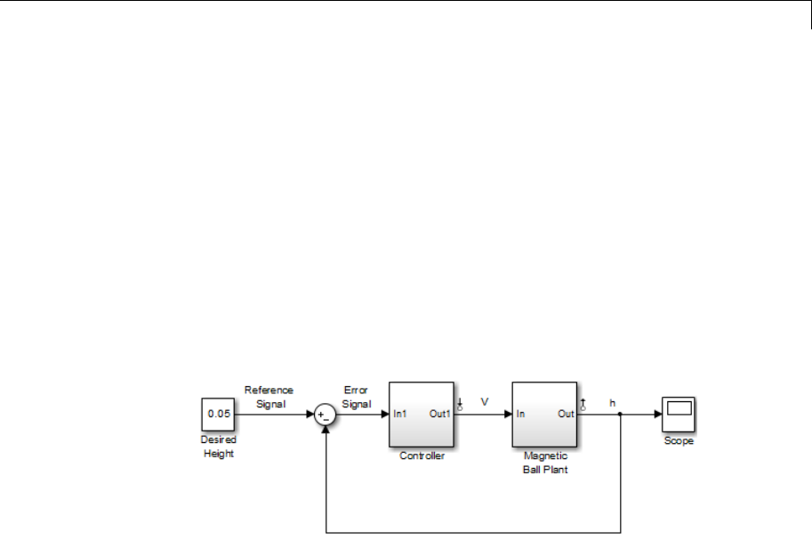
setlinio
2Right-click the signal line between the Magnetic Ball Plant and the
Controller. Select Linear Analysis Points > Input Point from the
menu to place an output point on this signal line. Notice a small
arrow pointing away from a small circle just above the signal line.
This arrow represents the output point.
3Right-click the signal line after the Magnetic Ball Plant. Select
Linear Analysis Points > Output Point from the menu to place
another output point on this signal line.
The model diagram should now look similar to that in the following
figure:
4Create an I/O object with the getlinio function:
io=getlinio('magball')
5Modify io by editing the object or by using the set function.
io(1).Type='in';
io(2).OpenLoop='on';
6Assign the new settings in io to the model.
oldio=setlinio('magball',io)
This assignment returns the old I/O settings (that have been replaced
by the settings in io).
8-141
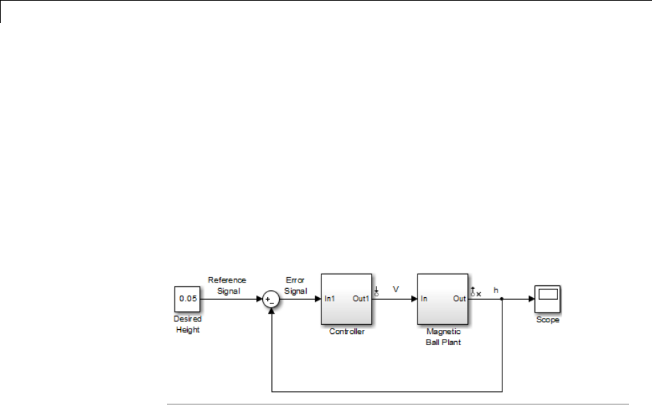
setlinio
2x1 vector of Linearization IOs:
--------------------------
1. Linearization input located at the following signal:
- Block: magball/Controller
- Port: 1
2. Linearization output located at the following signal:
- Block: magball/Magnetic Ball Plant
- Port: 1
The model diagram now looks similar to the following figure.
Update linearization input/output settings in a Linear Analysis
Plots block
This example shows how to update linearization input/output settings
in a Linear Analysis Plots block.
1Open the watertank model, and specify input and output (I/O).
aRight-click the Desired Water Level output signal, and select
Linear Analysis Points > Input Point.
bRight-click the Water-Tank System output signal, and select
Linear Analysis Points > Output Point.
The linearization I/O markers appear in the model, as shown in the
next figure.
8-142
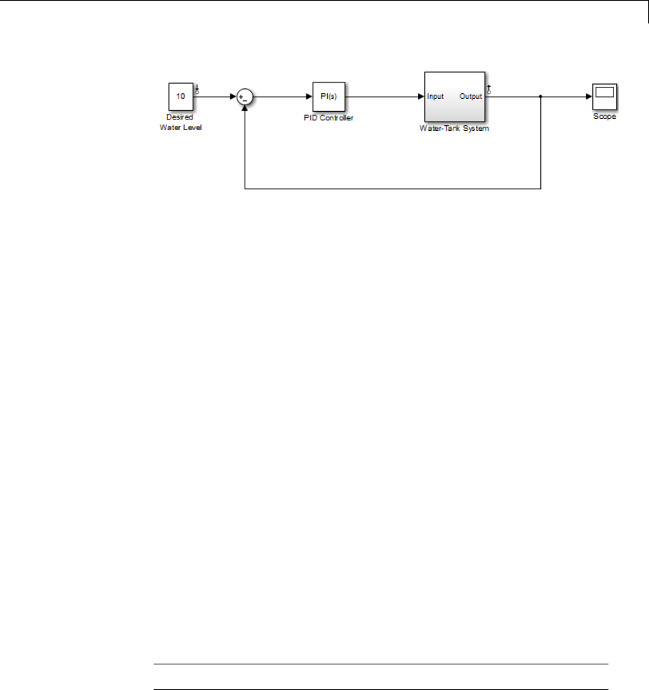
setlinio
Alternatively, you can use linio.
2Drag and drop a Bode Plot block from the Simulink Control Design
Linear Analysis Plots library into the Simulink Editor.
3Find all I/Os used by the Bode Plot block.
io = getlinio('watertank/Bode Plot')
When you drag and drop the block, the block I/Os are set to the model
I/Os. The following results appear at the MATLAB prompt:
2x1 vector of Linearization IOs:
--------------------------
1. Linearization input located at the following signal:
- Block: watertank/Desired Water Level
- Port: 1
2. Linearization output located at the following signal:
- Block: watertank/Water-Tank System
- Port: 1
4Open the loop specified by the block I/Os.
io(2).OpenLoop = 'on';
Note The loop opening does not affect the model I/Os.
8-143

setlinio
5Update the I/O in the Bode Plot block.
oldio = setlinio('watertank/Bode Plot',io)
See Also get |getlinio |linio |set
8-144

setxu
Purpose Set states and inputs in operating points
Syntax op_new=setxu(op_point,x,u)
Alternatives As an alternative to the setxu function, set states and inputs of
operating points with the Simulink Control Design GUI.
Description op_new=setxu(op_point,x,u) sets the states and inputs in the
operating point, op_point, with the values in xand u. A new operating
point containing these values, op_new, is returned. The variable xcan
be a vector or a structure with the same format as those returned from a
Simulink simulation. The variable ucan be a vector. Both xand ucan be
extracted from another operating point object with the getxu function.
Examples Open the Simulink model F14 by typing f14 at the command line.
Select Simulation > Model Configuration Parameters > Data
Import/Export.IntheSave to workspace pane, select Final states.
In the Save options pane, select Structure from Format.This
selection saves the final states of the model to the workspace after a
simulation.
Start the simulation. After it has run, a new variable, xFinal, should
be in the workspace. This variable is a structure with two properties,
time and signals.
Create an operating point object for F14 by typing:
op_point=operpoint('f14')
All states are initially set to 0. Set the states in this object to be the
values in xFinal. Set the input to be 9.
newop=setxu(op_point,xFinal,9)
The new operating point is displayed as follows:
Operating Point for the Model f14.
(Time-Varying Components Evaluated at time t=0)
8-145

setxu
States:
----------
(1.) f14/Actuator Model
x: -0.032
(2.) f14/Aircraft Dynamics Model/Transfer Fcn.1
x: 0.56
(3.) f14/Aircraft Dynamics Model/Transfer Fcn.2
x: 678
(4.) f14/Controller/Alpha-sensor Low-pass Filter
x: 0.392
(5.) f14/Controller/Pitch Rate Lead Filter
x: 0.133
(6.) f14/Controller/Proportional plus integral compensator
x: 0.166
(7.) f14/Controller/Stick Prefilter
x: 0.1
(8.) f14/Dryden Wind Gust Models/Q-gust model
x: 0.114
(9.) f14/Dryden Wind Gust Models/W-gust model
x: 0.46
x: -2.05
Inputs:
-----------
(1.) f14/u
u: 9
See Also getxu |initopspec |operpoint |operspec
8-146

slTunable.addBlock
Purpose Add block to list of tuned blocks
Syntax addBlock(ST,blockID)
Description addBlock(ST,blockID) adds the block referenced by blockID to the
TunedBlocks property of the slTunable interface ST.TheTunedBlocks
property lists the tunable blocks in the control system described by ST.
Input
Arguments
ST
slTunable interface describing the control system to be tuned.
blockID
String or cell array of strings identifying one or more blocks to
add to the TunedBlocks property of ST. You can specify blocks
with an abbreviated block name provided that the string matches
the end of the full block path and unambiguously identifies the
block to add.
Examples Create an slTunable interface for the Simulink model rct_cascade
and add a block to the list of tuned blocks in the interface.
open_system('rct_cascade')
ST0 = slTunable('rct_cascade','C1');
addBlock(ST0,'C2');
See Also slTunable |slTunable.addMeasurement |slTunable.addIO |
slTunable.addControl
8-147

slTunable.addControl
Purpose Add control signal to list of control signals in slTunable interface
Syntax addControl(ST,signalID)
Description addControl(ST,signalID) adds the signals referenced by signalID
to the Controls property of the slTunable interface ST.TheControls
signals are generated by the controller and drive the actuators in the
control system described by ST.TheControls and Measurements
signals together define the boundary between the plant and controller
subsystems for tuning with slTunable.looptune.Youcanalsouse
Controls signals as inputs, outputs, or loop-opening locations when
specifying TuningGoal requirements for control system tuning.
Input
Arguments
ST
slTunable interface describing the control system to be tuned.
signalID
String or cell array of strings identifying one or more signals to
add to the Controls property of ST. Each string can be one of
the following:
•Signal name, for example 'torque'
•Block path for a block with a single output port, for example
'Motor/PID'
•Path to block and port originating the signal, for example
'Engine Model/1' or 'Engine Model/torque'
Alternatively, you can specify signalID as a linearization I/O
object or vector of linearization I/O objects (see linio).
Examples Specify Control Signal in Control System to Be Tuned
This example shows how to specify control signals in an slTunable
interface for tuning the Simulink model rct_cascade:
8-148
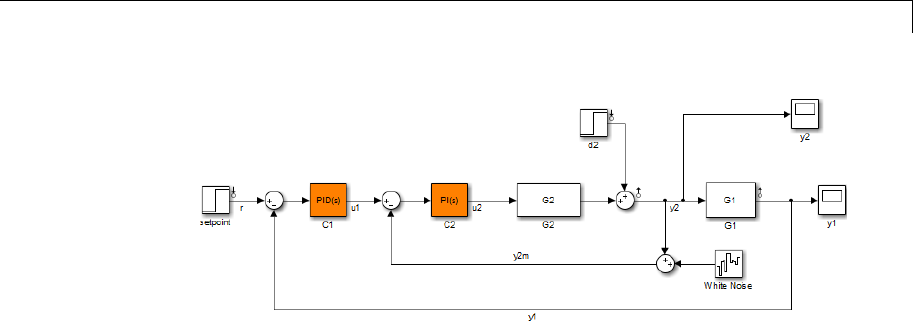
slTunable.addControl
Create an slTunable interface for the model.
open_system('rct_cascade')
tunedblocks = {'C1','C2'};
ST0 = slTunable('rct_cascade',tunedblocks);
Specify the control signal for the control system.
addControl(ST0,'u2');
In rct_cascade, the control signal (the actuator signal) is u2,the
output of the inner-loop controller.
See Also slTunable |slTunable.addMeasurement |slTunable.addIO |
slTunable.addOpening |slTunable.addSwitch
8-149

slTunable.addIO
Purpose Add I/O points list of linearization I/Os in slTunable interface
Syntax addIO(ST,signalID,type)
addIO(ST,iopoint)
Description addIO(ST,signalID,type) adds the signal locations referenced by
signalID to the IOs property of the slTunable interface ST.Thetype
argument specifies whether each I/O type is input, output, input/output,
or output/input.
addIO(ST,iopoint) reads the signal path and I/O type from the
linearization I/O point object iopoint.
Input
Arguments
ST
slTunable interface describing a Simulink model.
signalID
String or cell array of strings identifying one or more signals
to add to the IOs property of ST. Each string can be one of the
following:
•Signal name, for example 'torque'
•Block path for a block with a single output port, for example
'Motor/PID'
•Path to block and port originating the signal, for example
'Engine Model/1' or 'Engine Model/torque'
type
String specifying the I/O type of signalID. The type can be one of
the following:
•'in' —AddsignalID to the IOs property of ST as an input
point
•'out' — Output point
8-150

slTunable.addIO
•'inout' — Input/output point
•'outin' — Output/input point
If signalID is an array of signal names, type is an array of the
same length. The kth entry in type specifies the type of the kth
entry in signalID.
For more information about linearization I/O point types, see
linio.
iopoint
Linearization I/O object or vector of linearization I/O objects (see
linio).
Examples Create a slTunable interface for tuning the Simulink model
rct_cascade. Add an input point at the signal u1, and an input/output
pointatthesignaly2m.
open_system('rct_cascade')
tunedblocks = {'C1','C2'};
ST0 = slTunable('rct_cascade',tunedblocks);
addIO(ST0,'u1','in');
addIO(ST0,'y2m','inout');
See Also slTunable |slTunable.addMeasurement |slTunable.addControl |
slTunable.addOpening |slTunable.addSwitch |linio
How To • “Specifying Subsystem, Loop, or Block to Linearize” on page 2-11
8-151

slTunable.addMeasurement
Purpose Add measurement signal to list of measurement signals in slTunable
interface
Syntax addMeasurement(ST,signalID)
Description addMeasurement(ST,signalID) adds the signals referenced by
signalID to the Measurements property of the slTunable interface ST.
The Measurements signals are generated by the plant and used by the
controller in the control system described by ST.TheControls and
Measurements signals together define the boundary between the plant
and controller subsystems for tuning with slTunable.looptune.You
can also use Measurements signals as inputs, outputs, or loop-opening
locations when specifying TuningGoal requirements for control system
tuning.
Input
Arguments
ST
slTunable interface describing the control system to be tuned.
signalID
String or cell array of strings identifying one or more signals to
add to the Measurements property of ST. Each string can be one of
the following:
•Signal name, for example 'speed'
•Block path for a block with a single output port, for example
'"Engine/SpeedSensor'
•Path to block and port originating the signal, for example
'Engine Model/1' or 'Engine Model/speed'
Alternatively, you can specify signalID as a linearization I/O
object or vector of linearization I/O objects (see linio).
8-152
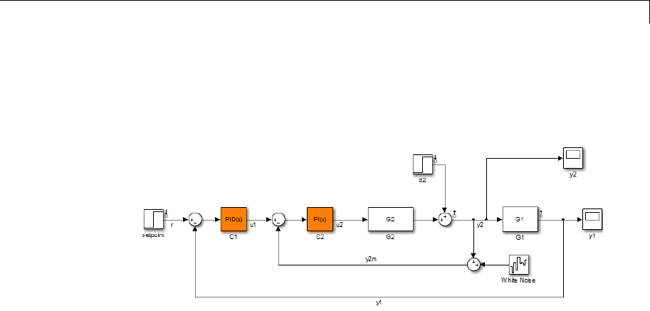
slTunable.addMeasurement
Examples Specify Measurement Signals in Control System to Be Tuned
This example shows how to specify measurement signals in an
slTunable interface for tuning the Simulink model rct_cascade:
Create an slTunable interface for the model.
open_system('rct_cascade')
tunedblocks = {'C1','C2'};
ST0 = slTunable('rct_cascade',tunedblocks);
Specify the measurement signal for the control system.
addMeasurement(ST0,{'y1','y2m'});
In rct_cascade, the measurement signals are y1 and y2m,eachof
which feeds into a portion of the cascaded controller.
See Also slTunable |slTunable.addControl |slTunable.addIO |
slTunable.addOpening |slTunable.addSwitch
8-153

slTunable.addOpening
Purpose Add new opening location to list of loop openings in slTunable interface
Syntax addOpening(ST,signalID)
Description addOpening(ST,signalID) adds the signal locations referenced by
signalID to the Openings property of the slTunable interface ST.
Loop openings are enforced at Openings locations for all tuning and
analysis commands involving ST.
Tips •To add a location where a loop opening is optionally
enforced for a particular analysis or tuning requirement, use
slTunable.addSwitch.
Input
Arguments
ST
slTunable interface describing a Simulink model.
signalID
String or cell array of strings identifying one or more signals to
add to the Openings property of ST. Each string can be one of
the following:
•Signal name, for example 'u'
•Block path for a block with a single output port, for example
'Motor/PID'
•Path to block and port originating the signal, for example
'Controller/1' or 'Controller/u'
Examples Create a slTunable interface for tuning the Simulink model
rct_cascade. Add a loop opening location at the signal y1.
open_system('rct_cascade')
tunedblocks = {'C1','C2'};
ST0 = slTunable('rct_cascade',tunedblocks);
addOpening(ST0,'y1');
8-154

slTunable.addOpening
The loop opening at y1 is enforced for all tuning and analysis commands
involving ST0.
See Also slTunable |slTunable.addMeasurement |slTunable.addIO |
slTunable.addControl |slTunable.addSwitch
8-155

slTunable.addSwitch
Purpose Add switch location to list of loop opening switches in slTunable
interface
Syntax addSwitch(ST,signalID)
Description addSwitch(ST,signalID) adds the locations of the signals referenced
by signalID to the Switches property of the slTunable interface
ST. Switches are locations where you can optionally open a loop for
tuning and analysis commands involving ST.YoucanalsouseSwitches
signals as inputs, outputs, or loop-opening locations when specifying
TuningGoal requirements for control system tuning.
Tips •To add a location where a loop opening is always enforced for all
analysis or tuning requirement, use slTunable.addOpening.
Input
Arguments
ST
slTunable interface describing a Simulink model.
signalID
String or cell array of strings identifying one or more signals to
add to the Switches property of ST. Each string can be one of
the following:
•Signal name, for example 'u'
•Block path for a block with a single output port, for example
'Motor/PID'
•Path to block and port originating the signal, for example
'Controller/1' or 'Controller/u'
Examples Specify Switch Location in Control System to Be Tuned
This example shows how to specify a location for an optional loop
opening (a switch) in an slTunable interface for tuning the Simulink
model rct_cascade:
8-156

slTunable.addSwitch
Create an slTunable interface for the model.
open_system('rct_cascade')
tunedblocks = {'C1','C2'};
ST0 = slTunable('rct_cascade',tunedblocks);
Specify theswitchlocation.
addSwitch(ST0,'y1');
When tuning a cascade control system, it can be useful to impose certain
requirements on the inner loop that are enforced with the outer loop
open. However, such a control system also has overall requirements are
enforced with all loops closed. Adding a switch instead of a loop opening
at y1 allows you to compute some responses with the outer loop open,
and other responses with the outer loop closed.
See Also slTunable |slTunable.addMeasurement |slTunable.addIO |
slTunable.addControl |slTunable.addOpening
8-157

slTunable.getBlockParam
Purpose Get parametrization of a particular tuned block in slTunable interface
Syntax blockparam = getBlockParam(ST,block)
Description blockparam = getBlockParam(ST,block) returns the parametrization
used to tune the Simulink block, block.
Tips The slTunable interface automatically associates a parametric model
with each Simulink block listed in the TunedBlocks property of ST.
This parametrization expresses each tunable block as a Control Design
Block or a tunable genss model. The parametrization specifies which
parameters are tuned by commands such as slTunable.systune
or slTunable.looptune.UsegetBlockParam to access this
parametrization. The tunable parameters of ST are the union of the
parametrizations of all tunable blocks in ST.
Input
Arguments
ST
slTunable interface describing a Simulink model.
block
String identifying a single block in the TunedBlocks property of
ST. You can specify the block with an abbreviated block name,
provided that the string matches the end of the full block path
and unambiguously identifies the block.
Output
Arguments
blockparam
Parametrization of block. The parametrization is either:
•A tunable Control Design Block.
•A tunable genss model, if you specified a parametrization for
block using slTunable.setBlockParam.
•An empty array ([]), if slTunable cannot parametrize
block.Youcanuse
slTunable.setBlockParam to specify a
parametrization for such blocks.
8-158

slTunable.getBlockParam
Examples Create an slTunable interface for the Simulink model rct_cascade
and examine the block parametrization of one of the tunable blocks.
open_system('rct_cascade')
tunedblocks = {'C1','C2'};
ST0 = slTunable('rct_cascade',tunedblocks);
TC = getBlockParam(ST0,'C1')
These commands produce the result:
Parametric continuous-time PID controller "rct_cascade_C1" with formula:
1s
Kp + Ki * --- + Kd * --------
s Tf*s+1
and tunable parameters: Kp, Ki, Kd, Tf.
The block C1 is a PID Controller block. Therefore, its parametrization
in ST0 is a ltiblock.pid (a Control Design Block).
See Also slTunable |slTunable.getBlockValue |slTunable.setBlockParam
|genss |ltiblock.pid
How To • “Supported Blocks for Tuning in Simulink”
8-159

slTunable.getBlockRateConversion
Purpose Query rate conversion method of tunable block
Syntax method = getBlockRateConversion(ST,block)
[method,pwfreq] = getBlockRateConversion(ST,block)
Description method = getBlockRateConversion(ST,block) returns the rate
conversion method currently associated with a tunable block in an
slTunable interface.
[method,pwfreq] = getBlockRateConversion(ST,block) also
returns the prewarp frequency, when method is 'tustin'.
Tips •Use getBlockRateConversion to query the rate conversion method
that the slTunable interface uses when converting the sampling
time of the block parametrization.
For example, you might use the slTunable interfacetotunea
mixed-rate Simulink model having a discrete-time controller and
a continuous time plant. Tuning commands such as looptune
or systune tune the model in continuous time. When you use
writeBlockValue to write tuned parameters back to the Simulink
model, writeBlockValue automatically discretizes the tuned
parametrization using the block rate conversion method associated
with the block.
Input
Arguments
ST
slTunable interface describing a Simulink model.
block
String identifying a single tunable block in the TunedBlocks
property of ST. You can specify the block with an abbreviated
block name, provided that the string matches the end of the full
block path and unambiguously identifies the block.
8-160

slTunable.getBlockRateConversion
Output
Arguments
method
Discretization method associated with the tunable block, returned
as one of the following:
•'zoh' — Zero-order hold method
•'tustin' —Tustinmethod
pwfreq
Prewarp frequency for the Tustin method, returned as a positive
scalar.
If the discretization method associated with the tunable block is
zero-order hold or Tustin without prewarp, then pwfreq is 0.
Examples Create an slTunable interface describing the Simulink model
rct_dmcNotch. Query and change the rate conversion method
associated with a tunable block in the model.
Open the Simulink model.
open_system('rct_dmcNotch')
8-161
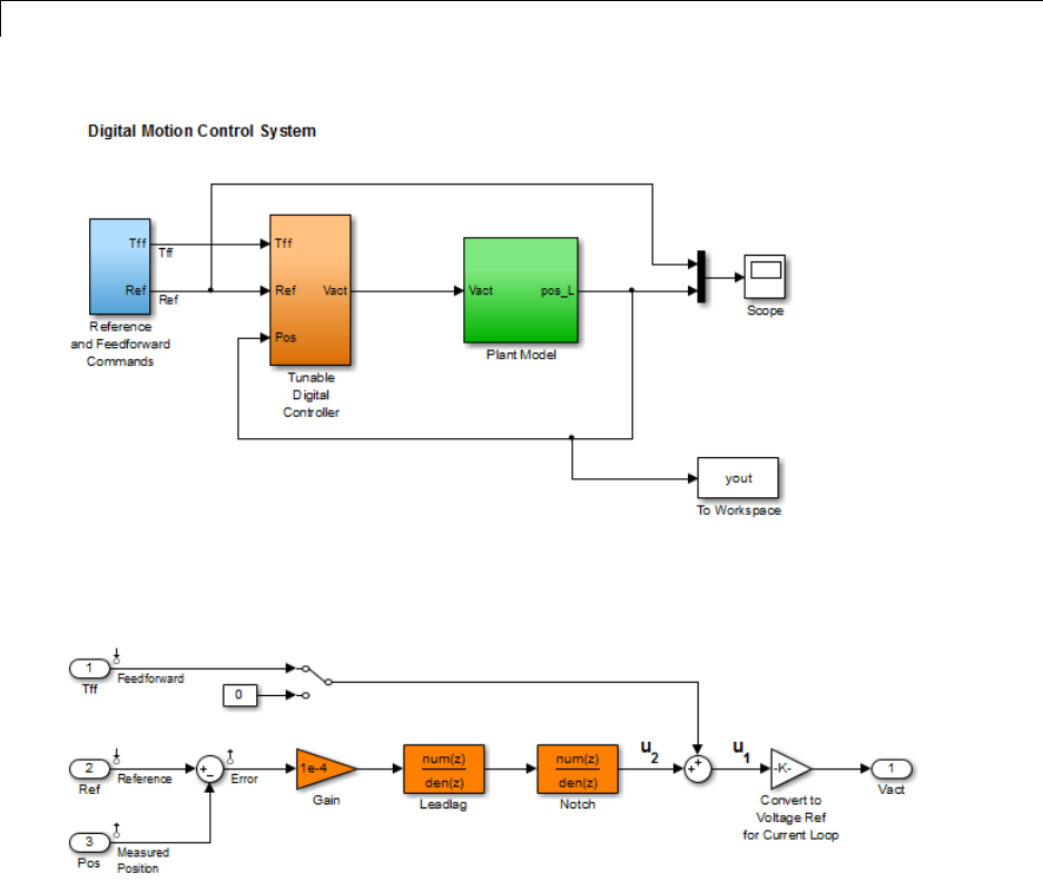
slTunable.getBlockRateConversion
Double-click the Tunable Digital Controller subsystem to see the
tunable blocks.
Create an slTunable interface for the model with the tunable blocks
showninorange.
ST = slTunable('rct_dmcNotch',{'Gain','Leadlag','Notch'});
The LeadLag and Notch blocks are discrete-time blocks. You might tune
this control system in continuous time (for example, using looptune or
8-162

slTunable.getBlockRateConversion
systune), and write the tuned parameters back to the Simulink model.
If you do so, slTunable.writeBlockValue automatically discretizes
the resulting tuned blocks using the discretization method associated
with the Simulink block. Query the discretization method associated
with the Notch block.
method = getBlockRateConversion(ST,'Notch')
method =
zoh
The result shows that the zero-order-hold (zoh) method is currently
associated with the Notch block. This block represents a notch filter.
Therefore, you might get better discretization results using the Tustin
discretization method with a prewarp at the notch frequency. Assume
that the tuned notch frequency is 340 rad/s.
wn = 340;
setBlockRateConversion(ST,'Notch','tustin',wn)
This command sets the rate conversion method of the Notch block
to the Tustin method with a prewarp at the notch frequency.
slTunable.writeBlockValue now discretizes the tuned block using
this method.
For a more detailed treatment of this example, see “Tuning of a Digital
Motion Control System”.
See Also slTunable |slTunable.writeBlockValue |
slTunable.setBlockRateConversion
Tutorials • “Tuning of a Digital Motion Control System”
How To • “Continuous-Discrete Conversion Methods”
8-163

slTunable.getBlockValue
Purpose Current value of a particular tuned block in slTunable interface
Syntax val = getBlockValue(ST,block)
Description val = getBlockValue(ST,block) returns the current value of the
parametrization of the Simulink block block.Thestringblock should
designate one of the tuned blocks in the control system described by
the slTunable interface ST.
Tips •The slTunable interface automatically associates a parametric
model with each Simulink block listed in the TunedBlocks property
of ST. This parametrization expresses each tunable block as a
Control Design Block or a tunable genss model. The parametrization
specifies which parameters are tuned by commands such as
slTunable.looptune.UsegetBlockValue to access the value of
this parametrization after tuning.
•The current value of the block parametrization in the slTunable
interface ST can differ from the actual value of the corresponding
block in the Simulink model. Use slTunable.readBlockValue
or slTunable.writeBlockValue to align the value of the
parametrization in ST with the actual block value in the model.
Input
Arguments
ST
slTunable interface describing a Simulink model.
block
String identifying a single block in the TunedBlocks property of
ST. You can specify the block with an abbreviated block name,
provided that the string matches the end of the full block path
and unambiguously identifies the block.
Output
Arguments
val
Current value of the parametrization of block in ST. The current
value is a numeric LTI model such as pid,ss,ortf.
8-164

slTunable.getBlockValue
Examples Create an slTunable interface for the Simulink model rct_cascade
and examine the current value of the block parametrization of one of
thetunableblocks.
open_system('rct_cascade')
tunedblocks = {'C1','C2'};
ST0 = slTunable('rct_cascade',tunedblocks);
val = getBlockValue(ST0,'C1')
These commands produce the result:
Continuous-time PI controller in parallel form:
1
Kp+Ki*---
s
With Kp = 0.1, Ki = 0.1
The block C1 is a PID Controller block. Therefore, the value of its
parametrization in ST0 is a pid controller model.
Use getBlockValue after tuning an slTunable interface with
slTunable.systune or slTunable.looptune.
See Also slTunable |slTunable.getBlockParam |slTunable.setBlockParam
|slTunable.setBlockValue |slTunable.writeBlockValue
8-165

slTunable.getIOTransfer
Purpose Tunable model of closed-loop transfer function between specified inputs
and outputs
Syntax T = getIOTransfer(ST,input,output)
T = getIOTransfer(ST,input,output,openings)
T = getIOTransfer(ST)
Description T = getIOTransfer(ST,input,output) returns the linearized
closed-loop response of the control system described by the slTunable
interface ST. The response Tis a genss model of the response from
input to output.
T = getIOTransfer(ST,input,output,openings) computes Twith
feedback loops opened at the locations specified by openings.
T = getIOTransfer(ST) returns the response from all inputs to all
outputs. This syntax is equivalent to setting inputs and outputs to
the union of the IOs,Controls,andMeasurements properties of ST.
Input
Arguments
ST
slTunable interface describing a Simulink model.
inputs
String or cell array of strings specifying the signals that are
inputs to the closed-loop response. Each signal in inputs must
be present in the IOs,Controls,Measurements,orSwitches
properties of ST.ForsignalsinST.IOs, only signals of type in,
inout,oroutin can be used in inputs.ThegetIOTransfer
command treats a signal in Controls,Measurements,orSwitches
as a disturbance signal entering at the specified location.
You can specify an abbreviated signal path in inputs provided the
string matches the end of the full signal path and unambiguously
identifies the signal.
Default: 0-by-1 cell array
8-166

slTunable.getIOTransfer
outputs
String or cell array of strings specifying the signals that are
outputs of the closed-loop response. Each signal in outputs must
be present in the IOs,Controls,orMeasurements properties of
the slTunable interface ST.ForsignalsinST.IOs, only signals of
type out,inout,oroutin can be used in outputs.
You can specify an abbreviated signal path in outputs
provided the string matches the end of the full signal path and
unambiguously identifies the signal.
Default: 0-by-1 cell array
openings
String or cell array of strings specifying the locations at which
feedback loops are opened for the computation of T.Specify
the locations as the names of signals listed in the Controls,
Measurements,orSwitches properties of ST.Loopopeningslisted
in the Openings property of ST are always open.
You can specify an abbreviated signal path in openings
provided the string matches the end of the full signal path and
unambiguously identifies the signal.
Default: 0-by-1 cell array
Output
Arguments
T
Tunable genss model of the response from inputs input to
outputs output.Ifinput and output are omitted, Tis the
response from all inputs to all outputs listed in the IOs,Controls,
and Measurements properties of ST.
Tcaptures the dependence of the response on the parameters of
thetunableblocksintheTunedBlocks property of ST. The current
values of the tunable parameters of Tare equal to the current
parameter values in ST. Therefore, you can use getIOTransfer
8-167

slTunable.getIOTransfer
after tuning ST with slTunable.systune or slTunable.looptune
to examine closed-loop responses of the tuned control system.
See Also slTunable |slTunable.loopview |slTunable.getLoopTransfer
|genss
Tutorials • “Tuning Control Systems in Simulink”
• “Tuning Multi-Loop Control Systems”
• “Decoupling Controller for a Distillation Column”
• “Tuning of a Digital Motion Control System”
• “Fixed-Structure Autopilot for a Passenger Jet”
8-168

slTunable.getLoopTransfer
Purpose Tunable model of open-loop transfer function at specified location
Syntax L = getLoopTransfer(ST,location)
L = getLoopTransfer(ST,location,sign)
L = getLoopTransfer(ST,location,openings)
L = getLoopTransfer(ST,location,openings,sign)
Description L = getLoopTransfer(ST,location) returns the linearized
point-to-point open-loop transfer function of the control system
described by the slTunable interface ST. The point-to-point open-loop
transfer function Lis the open-loop response obtained by injecting
signals at location and measuring the return signals at the same
point.
L = getLoopTransfer(ST,location,sign) specifies the feedback
sign for computing the open-loop response. By default, Lis the
positive-feedback open-loop transfer function. Set sign to -1 to
compute the negative-feedback open-loop transfer function.
L = getLoopTransfer(ST,location,openings) computes Lwith
additional loop openings at the locations specified by openings.
L = getLoopTransfer(ST,location,openings,sign) specifies both
additional loop openings and the sign.
Input
Arguments
ST
slTunable interface describing a Simulink model.
location
String or cell array of strings specifying signal locations at which
to compute a point-to-point open loop transfer function. Each
signal in location must be present in the Switches,Controls,
or Measurements properties of the slTunable interface ST.Use
a cell array to specify multiple locations and compute a MIMO
loop transfer.
8-169

slTunable.getLoopTransfer
You can specify an abbreviated signal path in location
provided the string matches the end of the full signal path and
unambiguously identifies the signal.
sign
Feedback sign. sign takes the following values:
•+1 (default) — getLoopTransfer returns the positive-feedback
open-loop transfer function, computed by injecting sine waves
at the locations specified in location and measuring the return
signals at the same point. The closed-loop transfer function
is feedback(L,1,+1).
•-1 —getLoopTransfer returns the negative-feedback
open-loop transfer function. The negative-feedback transfer
function is –1 times the positive-feedback transfer function.
The closed-loop transfer function is feedback(L,1).
Set sign to -1 if you intend to use the open-loop transfer function
Lin applications that assume the negative-feedback definition
of L. Many classical design and analysis techniques use the
negative-feedback convention. For example, the Nyquist or root
locus design techniques usually assume that Lis defined such
that the closed-loop transfer function is feedback(L,1).
Default: +1
openings
String or cell array of strings specifying additional locations at
which feedback loops are opened for the computation of L.Specify
the locations as the names of signals listed in the Controls,
Measurements,orSwitches properties of ST.Loopopeningslisted
in the Openings property of ST are always open.
You can specify an abbreviated signal path in openings
provided the string matches the end of the full signal path and
unambiguously identifies the signal.
8-170

slTunable.getLoopTransfer
Default: {0x1 cell}
Output
Arguments
L
Tunable genss model of the point-to-point response measured
at location.Iflocation is a cell array identifying multiple
signals, Lis a MIMO response.
Lcaptures the dependence of the response on the parameters of
thetunableblocksintheTunedBlocks property of ST. The current
values of the tunable parameters of Lare equal to the current
parameter values in L. Therefore, you can use getLoopTransfer
after tuning ST with slTunable.systune or slTunable.looptune
to examine open-loop responses of the tuned control system.
See Also slTunable |slTunable.loopview |slTunable.getIOTransfer |
genss
Tutorials • “Validating Results”
• “Tuning of a Digital Motion Control System”
8-171

slTunable.linearize
Purpose Relinearize Simulink model to update slTunable interface
Syntax linearize(ST0)
blockvals = linearize(ST0)
Description linearize(ST0) relinearizes the Simulink model described by the
slTunable interface ST0.Uselinearize to update the stored linear
representation of the Simulink model in ST0 after you make changes to
the Simulink model. The update to ST0 includes:
•Updating the parametrization of the control architecture according to
the blocks specified in the TunedBlocks property of ST0.
Note To synchronize tuned block current values with the Simulink
model, use slTunable.readBlockValue.
•Evaluating the fixed (nontunable) portion of the control system.
•Computing a new linearization of the Simulink model, using the
I/Os specified in the IOs,Openings,andSwitches properties of
ST0, respectively. The new linearization uses the operating point
and linearization options specified in the OperatingPoint and
LinearizeOptions properties of ST0, respectively.
blockvals = linearize(ST0) returns a cell array containing the
current values from the Simulink model of the tunable blocks stored in
the TunedBlocks property of STO.
Tips •You do not need to use slTunable.linearize every time you
change properties of the slTunable interface. Commands
that query the linearization stored in the slTunable interface
automatically relinearize the Simulink model if you have
changed any properties of ST0 since the last linearization. These
commands include slTunable.systune,slTunable.looptune,
slTunable.getIOTransfer,andslTunable.getLoopTransfer.You
8-172

slTunable.linearize
can optionally use slTunable.linearize to force relinearization or
control when relinearization occurs.
Input
Arguments
ST0
slTunable interface describing the control system to be tuned.
Output
Arguments
blockvals
Current values of the tunable blocks of ST0.blockvals is a cell
array of state-space (ss) models. Each entry in blockvals is
the current value of the corresponding entry in the TunedBlocks
property of ST0.
Examples Update the linearization in an slTunable interface to use new
linearization options.
Create the slTunable interface.
open_system('rct_cascade');
tunedblocks = {'C1','C2'};
ST0 = slTunable('rct_cascade',tunedblocks);
Create a linearization options set, and update the linearization stored
in STO.
opts = linoptions('BlockReduction','off');
ST0.LinearizeOptions = opts;
linearize(ST0);
The linearization uses the options stored in the LinearizeOptions
property of ST0.
Algorithms slTunable.linearize linearizes your Simulink model using the
algorithms described in “Exact Linearization Algorithm” on page 2-146.
8-173

slTunable.linearize
See Also slTunable |slTunable.systune |slTunable.looptune |
slTunable.getLoopTransfer |slTunable.getIOTransfer |
slTunable.readBlockValue |linearize
8-174

slTunable.looptune
Purpose Tune MIMO feedback loops in Simulink
Syntax [ST,gam,info] = looptune(ST0,wc)
[ST,gam,info] = looptune(ST0,wc,Req1,Req2,...)
[ST,gam,info] = looptune(...,options)
Description [ST,gam,info] = looptune(ST0,wc) tunes the Simulink control
system described by the slTunable interface ST0 to meet the following
default requirements:
•Bandwidth — Gain crossover for each loop falls in the frequency
interval wc
•Performance — Integral action at frequencies below wc
•Robustness — Adequate stability margins and gain roll-off at
frequencies above wc
[ST,gam,info] = looptune(ST0,wc,Req1,Req2,...) tunes the
feedback loop to meet additional design requirements specified in one or
more tuning goal objects Req.Omitwc to use the requirements specified
in the Req objects instead of an explicit target crossover frequency and
the default performance and robustness requirements.
[ST,gam,info] = looptune(...,options) specifies further options,
including target gain margin, target phase margin, and computational
options for the tuning algorithm.
Tips •slTunable.looptune allows you to use the Robust Control Toolbox
tuning command looptune on a control system described in a
Simulink model. Using slTunable provides an interface between the
Simulink model and the looptune command, allowing you to identify
the tunable components of the system for looptune to tune. Using
slTunable.looptune requires Robust Control Toolbox software.
8-175

slTunable.looptune
Input
Arguments
ST0
slTunable interface object representing the Simulink control
system to tune. For information on how to create and configure
the slTunable interface, see the slTunable reference page.
wc
Vector specifying the target crossover region [wcmin,wcmax].
The looptune command attempts to tune all loops in the control
system so that the open-loop gain crosses 0 dB within the target
crossover region.
Ascalarwc specifies the target crossover region [wc/2,2*wc].
Req
One or more TuningGoal objects specifying design requirements.
Available requirement types include:
•TuningGoal.Tracking — Setpoint tracking requirement
•TuningGoal.Gain — Limit on transfer function gain
•TuningGoal.LoopShape — Target shape for open-loop response
For a complete list of the design requirements you can specify, see
“Performance and Robustness Specifications for looptune”.
options
Set of options for the looptune algorithm, specified using
looptuneOptions.SeelooptuneOptions for information about
the available options, including target gain margin and phase
margin.
Output
Arguments
ST
Tuned version of ST0.
Use slTunable.loopview to graphically validate the design.
Use slTunable.writeBlockValue to apply the tuned parameter
values to the Simulink model.
8-176

slTunable.looptune
gam
Parameter indicating degree of success at meeting all tuning
constraints. A value of gam <= 1 indicates that all requirements
are satisfied. A value of gam >> 1 indicates failure to meet at
least one requirement. Use slTunable.loopview to visualize the
tuned result and identify the unsatisfied requirement.
For best results, use the RandomStart option in looptuneOptions
to obtain several minimization runs. Setting RandomStart to
an integer N>0causes looptune to run the optimization N
additional times, beginning from parameter values it chooses
randomly. You can examine gam for each run to help identify an
optimization result that meets your design requirements.
info
Structure containing the following tuning data:
•Optimal I/O scalings Di and Do
•Requirement parameters and weighting functions
To use the data in info,usethecommandloopview(ST,info) to
visualize tuning constraints and validate the tuned design. See
slTunable.loopview for more information.
See Also slTunable |TuningGoal.Tracking |TuningGoal.Gain |
TuningGoal.LoopShape |slTunable.systune |slTunable.loopview
|slTunable.getLoopTransfer |slTunable.getIOTransfer |
slTunable.writeBlockValue |looptuneOptions
Tutorials • “Tuning Control Systems in Simulink”
• “Decoupling Controller for a Distillation Column”
• “Tuning of a Digital Motion Control System”
• “Tuning of a Two-Loop Autopilot”
8-177

slTunable.looptune
How To • “How looptune Sees a Control System”
• “Set Up Your Control System for Tuning with looptune”
• “Performance and Robustness Specifications for looptune”
8-178

slTunable.loopview
Purpose Graphically analyze results of control system tuning
Syntax loopview(ST)
loopview(ST,info)
Description loopview(ST) plots characteristics of the control system described by
the slTunable interface ST.
Use loopview to analyze the performance of a tuned control system you
obtain using slTunable.looptune.
loopview plots the singular values of:
•Open-loop frequency responses G*C and C*G. The controller Cand
plant Gare the linearized portions of the Simulink model defined by
the Controls and Measurements properties of ST.
•Sensitivity function S = inv(1+G*C) and complementary sensitivity
T = 1-S
•Normalized multi-loop disk margins (see loopmargin). loopview
plots the:
-Maximum stability margin
-Tuned (optimized) stability margin
-Actual (achieved) stability margin
Use the stability margin plot to verify that the tuned control system
has the desired stability margin. The normalized margin value
should be less than 1 at all frequencies.
For more information about singular values, see sigma.
loopview(ST,info) uses the info structure returned by
slTunable.looptune. This syntax also plots the target and tuned
values of tuning constraints imposed on the system. Additional plots
include:
8-179

slTunable.loopview
•Maximum allowed singular values for the sensitivity functions Sand
T. The curve marked S/T Max shows the maximum allowed Son the
low-frequency side of the plot, and the maximum allowed Ton the
high-frequency side. These curves are the constraints that looptune
imposes on Sand Tto enforce the target crossover range wc.
•Target and tuned values of constraints imposed by any tuning goal
requirements you used with looptune.
Use loopview with the info structure to assist in troubleshooting
when tuning fails to meet all requirements.
Input
Arguments
ST
slTunable interface describing the Simulink model to analyze.
info
info structure returned by slTunable.looptune during control
system tuning.
Alternatives For analyzing Control System Toolbox models tuned with looptune,
use loopview.
See Also looptune |loopview |slTunable.looptune
Tutorials • “Decoupling Controller for a Distillation Column”
• “Tuning of a Two-Loop Autopilot”
8-180

slTunable.readBlockValue
Purpose Update tuned block values from Simulink model
Syntax readBlockValue(ST)
readBlockValue(ST,block)
Description readBlockValue(ST) updates the current value of the block
parametrization of the interface ST to match the blocks values in the
corresponding Simulink model. This command only updates Simulink
blocks parametrized by Control Design Blocks. For information about
block parametrization, see slTunable.getBlockParam.
readBlockValue(ST,block) updates parameters only for the block or
blocks specified by block.
Input
Arguments
ST
slTunable interface describing a Simulink model.
block
String or cell array of strings identifying blocks in the
TunedBlocks property of ST to update with values read from the
Simulinkmodel. Youcanspecifyablockwithanabbreviated
block name, provided that the string matches the end of the full
block path and unambiguously identifies the block.
See Also slTunable |slTunable.writeBlockValue |
slTunable.getBlockParam |slTunable.getBlockValue |
slTunable.setBlockValue |slTunable.showBlockValue
8-181

slTunable.setBlockParam
Purpose Specify parametrization for specified tuned block
Syntax setBlockParam(ST,block,TC)
Description setBlockParam(ST,block,TC) assigns the tunable model TC as the
parametrization of the tunable block, block,oftheslTunable interface
ST.UsingsetBlockParam overrides the default parametrization for the
specified block. Doing so defines how the block should be parametrized
and which parameters of the block are tuned by tuning commands
involving ST.
Tips •The slTunable interface stores a parametrization of each
blocks listed in the TunedBlocks property of the interface. This
parametrization specifies which parameters are tuned by commands
such as slTunable.looptune.UsesetBlockParam to override
the default block parametrization or specify how to parametrize
composite Simulink blocks such as subsystems.
•In some cases, slTunable.writeBlockValue cannot write tuned
parameter values from a custom parametrization to the Simulink
model. slTunable.writeBlockValue can only write tuned parameter
values when the value is compatible with the default parametrization.
For example, you might override the default parametrization
of a static Gain block (ltiblock.gain) with a transfer function,
(ltiblock.tf). In that case, slTunable.writeBlockValue errors
unless the current value of the custom parametrization transfer
function is a static gain.
Input
Arguments
ST
slTunable interface describing a Simulink model.
block
String identifying a single block in the TunedBlocks property of
ST. You can specify the block with an abbreviated block name,
provided that the string matches the end of the full block path
and unambiguously identifies the block.
8-182
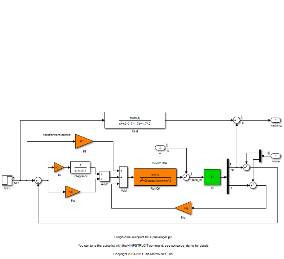
slTunable.setBlockParam
TC
Parametrization to assign to block. Express the parametrization
as a tunable Control Design Block or genss model.
Examples Create an slTunable interface describing the Simulink model
rct_concorde and specify the parametrization of a tunable block.
Open the Simulink model.
open_system('rct_concorde')
Create an slTunable interface for the model with the tunable blocks
showninorange.
ST = slTunable('rct_concorde',{'Ki','Kp','Kq','Kf','RollOff'});
Examine the default parametrization of the filter block Rolloff.
8-183

slTunable.setBlockParam
getBlockParam(ST,'RollOff')
Parametric continuous-time transfer function "rct_concorde_RollOff".
This transfer function has 0 zeros, 2 poles, and 3 tunable parameters.
Use "tf(M)" to see the current value and "get(M)" to see all properties.
The default parametrization is a generic second-order transfer function
in which all coefficients are free to vary independently. The desired
parametrization is a second-order filter where the coefficients are
constrained by the relationship
Fs
ss
ro n
nn n
2
22
2
.
Create a genss model representing the desired parametrization, and
setitastheparametrizationofthe'RollOff' block in ST.
wn = realp('wn', 3);
zeta = realp('zeta',0.8);
Fro = tf(wn^2,[1 2*zeta*wn wn^2]);
setBlockParam(ST,'RollOff',Fro)
Tuning commands such as slTunable.systune now use this
constrained parametrization of the RollOff block of ST.
This custom parametrization is compatible with the default
parametrization of the Simulink block. Therefore, you can use
slTunable.writeBlockValue to write the tuned values back to the
block.
See Also slTunable |slTunable.getBlockValue |slTunable.getBlockParam
|slTunable.writeBlockValue |slTunable.systune |genss
How To • “Supported Blocks for Tuning in Simulink”
8-184

slTunable.setBlockRateConversion
Purpose Set rate conversion method of tunable block
Syntax setBlockRateConversion(ST,block,method)
setBlockRateConversion(ST,block,method,pwfreq)
Description setBlockRateConversion(ST,block,method) setstherateconversion
method currently associated with a tunable block in an slTunable
interface.
setBlockRateConversion(ST,block,method,pwfreq) also sets the
prewarp frequency, when method is 'tustin'.
Tips •Use setBlockRateConversion to query the rate conversion method
that the slTunable interface uses when converting the sampling
time of the block parametrization.
For example, you might use the slTunable interfacetotunea
mixed-rate Simulink model having a discrete-time controller and
a continuous time plant. Tuning commands such as looptune
or systune tune the model in continuous time. When you use
writeBlockValue to write tuned parameters back to the Simulink
model, writeBlockValue automatically discretizes the tuned
parametrization using the block rate conversion method associated
with the block.
For information about choosing discretization methods, see
“Continuous-Discrete Conversion Methods”.
Input
Arguments
ST
slTunable interface describing a Simulink model.
block
String identifying a single tunable block in the TunedBlocks
property of ST. You can specify the block with an abbreviated
block name, provided that the string matches the end of the full
block path and unambiguously identifies the block.
method
8-185

slTunable.setBlockRateConversion
Discretization method associated with the tunable block, specified
as one of the following:
•'zoh' — Zero-order hold method
•'tustin' —Tustinmethod
pwfreq
Prewarp frequency for the Tustin method, specified as a positive
scalar.
For Tustin without prewarp, use pwfreq = 0. For zero-order
hold, pwfreq is ignored.
Default: 0
Examples Create an slTunable interface describing the Simulink model
rct_dmcNotch. Query and change the rate conversion method
associated with a tunable block in the model.
Open the Simulink model.
open_system('rct_dmcNotch')
8-186
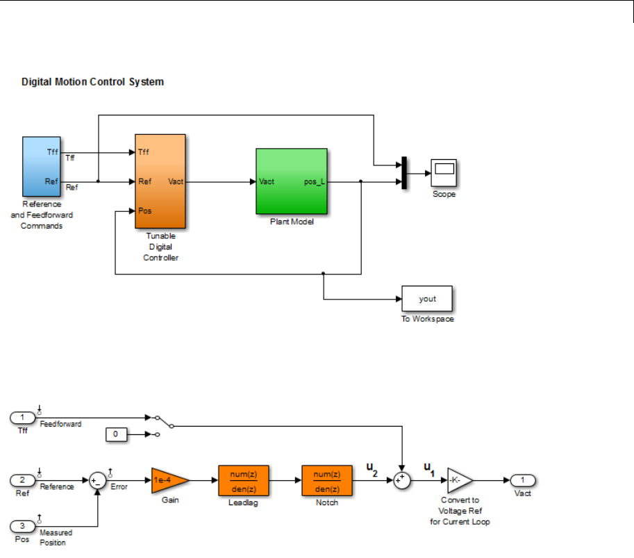
slTunable.setBlockRateConversion
Double-click the Tunable Digital Controller subsystem to see the
tunable blocks.
Create an slTunable interface for the model with the tunable blocks
showninorange.
ST = slTunable('rct_dmcNotch',{'Gain','Leadlag','Notch'});
The LeadLag and Notch blocks are discrete-time blocks. You might tune
this control system in continuous time (for example, using looptune or
8-187

slTunable.setBlockRateConversion
systune), and write the tuned parameters back to the Simulink model.
If you do so, slTunable.writeBlockValue automatically discretizes
the resulting tuned blocks using the discretization method associated
with the Simulink block. Query the discretization method associated
with the Notch block.
method = getBlockRateConversion(ST,'Notch')
method =
zoh
The result shows that the zero-order-hold (zoh) method is currently
associated with the Notch block. This block represents a notch filter.
Therefore, you might get better discretization results using the Tustin
discretization method with a prewarp at the notch frequency. Assume
that the tuned notch frequency is 340 rad/s.
wn = 340;
setBlockRateConversion(ST,'Notch','tustin',wn)
This command sets the rate conversion method of the Notch block
to the Tustin method with a prewarp at the notch frequency.
slTunable.writeBlockValue now discretizes the tuned block using
this method.
For a more detailed treatment of this example, see “Tuning of a Digital
Motion Control System”.
See Also slTunable |slTunable.writeBlockValue |
slTunable.getBlockRateConversion
Tutorials • “Tuning of a Digital Motion Control System”
How To • “Continuous-Discrete Conversion Methods”
8-188

slTunable.setBlockValue
Purpose Set current value of parametrization for specified block
Syntax setBlockValue(ST,block,val)
setBlockValue(ST,M)
Description setBlockValue(ST,block,val) sets to val thecurrentvalueof
the parametrization of the Simulink block block in the slTunable
interface ST.Theparametrizationofblock must be a tunable Control
Design Block.
setBlockValue(ST,M) updates the current values of the tunable
parameters in ST to match the corresponding values of tunable
parameters in the Generalized LTI Model M. Only parameters common
to ST and Mare updated. Use this syntax to update ST after obtaining M
by tuning with commands such as systune,looptune,orhinsfstruct.
Tips •The slTunable interface automatically associates a parametric
model with each Simulink block listed in the TunedBlocks property
of ST. This parametrization expresses each tunable block as a
Control Design Block or a tunable genss model. The parametrization
specifies which parameters are tuned by commands such as
slTunable.looptune.UseslTunable.getBlockValue to access the
current value of this parametrization.
•You can use setBlockValue to initialize the tunable parameters
of blocks parametrized by Control Design Blocks before tuning
ST with a tuning command such as slTunable.systune or
slTunable.looptune.
Input
Arguments
ST
slTunable interface describing a Simulink model.
block
String identifying a single block in the TunedBlocks property of
ST. You can specify the block with an abbreviated block name,
provided that the string matches the end of the full block path
and unambiguously identifies the block.
8-189

slTunable.setBlockValue
val
New initial or current value for the block parametrization.
The value val canbeanyvaluethatiscompatiblewiththe
parametrization of block without changing the size, type, or
sampling time the parametrization of block. For example, if
the parametrization of block is a ltiblock.pid model, valid
types for val include ltiblock.pid,anumericpid controller
model, or a numeric tf model that represents a PID controller.
setBlockValue uses the parameter values of val to set the
current value of the parametrization of block.
setBlockValue changes the current value of the block
parametrization but does not change the parametrization
itself. To change the parametrization (for example, to change
the block parametrization from ltiblock.pid to a three-pole
ltiblock.tf), use slTunable.setBlockParam.
M
Generalized LTI Model that has at least some parameters in
common with ST.
See Also slTunable |slTunable.getBlockParam |slTunable.setBlockParam
|slTunable.getBlockValue |slTunable.writeBlockValue
Tutorials • “Fixed-Structure Autopilot for a Passenger Jet”
8-190

slTunable.showBlockValue
Purpose Display current value of block parametrizations
Syntax showBlockValue(ST)
Description showBlockValue(ST) is the same as showTunable(ST) for slTunable
interface objects.
See Also slTunable.showTunable
8-191

slTunable.showTunable
Purpose Display current value of block parametrizations
Syntax showTunable(ST)
Description showTunable(ST) displays the current values of the parametric models
associate with each tunable block in the slTunable interface ST.
Tips •The slTunable interface automatically associates a parametric
model with each Simulink block listed in the TunedBlocks property
of ST. This parametrization expresses each tunable block as a Control
Design Block or a tunable genss model. The showBlockValue
command displays the current values of these tunable blocks.
Input
Arguments
ST
slTunable interface describing a Simulink model.
Examples Create an slTunable interface describing the Simulink model
rct_concorde and display the values of the parametrizations of the
tunable blocks.
Open the Simulink model.
open_system('rct_concorde')
8-192
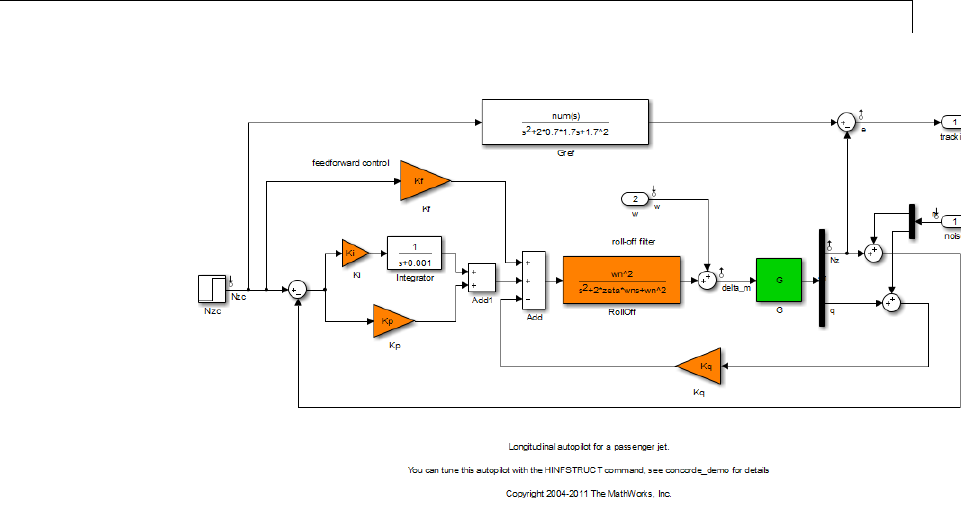
slTunable.showTunable
Create an slTunable interface for the model with the tunable blocks
showninorange.
ST = slTunable('rct_concorde',{'Ki','Kp','Kq','Kf','RollOff'});
Examine the default parametrization values of the blocks.
showTunable(ST)
Block "rct_concorde/Ki" =
d=
u1
y1 0
Static gain.
-----------------------------------
Block "rct_concorde/Kp" =
8-193

slTunable.showTunable
d=
u1
y1 0
Static gain.
-----------------------------------
Block "rct_concorde/Kq" =
d=
u1
y1 0
Static gain.
-----------------------------------
Block "rct_concorde/Kf" =
d=
u1
y1 0
Static gain.
-----------------------------------
Block "rct_concorde/RollOff" =
Transfer function:
9
---------------
s^2+4.8s+9
The default parametrization for the four gain blocks is a static gain,
with current value 0. The default parametrization for the filter RollOff
is a second-order transfer function.
8-194

slTunable.showTunable
Use slTunable.setBlockValue to change the current values of
the parameters. Use slTunable.setBlockParam to change the
parametrization.
See Also slTunable |slTunable.writeBlockValue |
slTunable.getBlockValue |slTunable.setBlockValue |
slTunable.readBlockValue
8-195

slTunable.systune
Purpose Tune fixed-structure control system parameters in Simulink
Syntax [ST,fSoft] = systune(ST0,SoftReqs)
[ST,fSoft,gHard] = systune(ST0,SoftReqs,HardReqs)
[ST,fSoft,gHard] = systune(ST0,SoftReqs,HardReqs,options)
[ST,fSoft,gHard,info] = systune( ___ )
Description [ST,fSoft] = systune(ST0,SoftReqs) tunes the free parameters
of the Simulink control system described by the slTunable interface
ST0.The
systune command tunes the parameters subject to the soft
tuning requirements SoftReqs, and returns the best achieved soft
constraint values as fSoft.
[ST,fSoft,gHard] = systune(ST0,SoftReqs,HardReqs) tunes the
control system to minimize the soft tuning requirements subject to hard
tuning requirements (constraints), and returns the best achieved values
for the hard constraints.
[ST,fSoft,gHard] = systune(ST0,SoftReqs,HardReqs,options)
specifies options for the optimization.
[ST,fSoft,gHard,info] = systune( ___ )also returns detailed
information about each optimization run.
Tips •slTunable.systune allows you to use the Robust Control Toolbox
tuning command systune on a control system described in a
Simulink model. Using slTunable provides an interface between the
Simulink model and the systune command, allowing you to identify
the tunable components of the system for systune to tune. Using
slTunable.systune requires Robust Control Toolbox software.
Input
Arguments
ST0
slTunable interface object representing the Simulink control
system to tune. For information on how to create and configure
the slTunable interface, see the slTunable reference page.
SoftReqs
8-196

slTunable.systune
Soft tuning requirements (objectives) for tuning the control
system, specified as a vector of TuningGoal requirement
objects such as TuningGoal.Tracking,TuningGoal.Gain,or
TuningGoal.Margins. (See “Specifying Design Requirements for
systune” for a complete list.)
systune tunes the tunable parameters of the control system to
minimize the soft tuning requirements, subject to the hard tuning
requirements (if any).
HardReqs
Hard tuning requirements (constraints) for tuning the control
system, specified as a vector of TuningGoal requirement
objects such as TuningGoal.Tracking,TuningGoal.Gain,or
TuningGoal.Margins. (See “Specifying Design Requirements for
systune” for a complete list.)
systune converts each hard tuning requirement to a normalized
scalar value. systune then optimizes the free parameters
minimize those normalized values.
Default: []
options
Options for the tuning algorithm, specified as an options set you
create with systuneOptions. Available options include:
•Number of additional optimizations to run starting from
random initial values of the free parameters
•Tolerance for terminating the optimization
•Flag for using parallel processing
Output
Arguments
ST
Tuned version of ST0.
8-197

slTunable.systune
Use viewSpec to graphically validate the design. Use
slTunable.writeBlockValue to apply the tuned parameter
values to the Simulink model.
fSoft
Best achieved soft constraint values, returned as a vector.
systune converts the soft requirements to a function of the free
parameters of the control system. The command then tunes
the parameters to minimize that function subject to the hard
constraints. (See “Algorithms” on page 8-201.) fSoft contains the
best achieved value for each of the soft constraints, in order of the
constraints in SoftReqs.fSoft values are only meaningful when
the hard constraints are satisfied.
gHard
Best achieved hard constraint values, returned as a vector.
systune converts the hard requirements to a function of the free
parameters of the control system. The command then tunes the
parameters to drive those values below 1. (See “Algorithms” on
page 8-201.) gHard contains the best achieved value for each of
the hard constraints, in order of the constraints in HardReqs.If
all values are less than 1, then the hard constraints are satisfied.
info
Detailed information about each optimization run, returned as a
data structure. In addition to examining detailed results of the
optimization, you can use info as an input to viewSpec when
validating a tuned MIMO system. info contains scaling data
that viewSpec needs for correct evaluation of MIMO open-loop
requirements such as loop shapes and stability margins.
The fields of info are:
Run
Run number, returned as a scalar. If you use the
RandomStart option of systuneOptions to perform multiple
8-198

slTunable.systune
optimization runs, info is a struct array, and info.Run is
the index.
Iterations
Total number of iterations performed during run, returned
as a scalar.
fBest
Best overall soft constraint value, returned as a scalar.
systune converts the soft requirements to a function of the
free parameters of the control system. The command then
tunes the parameters to minimize that function subject to
the hard constraints. (See “Algorithms” on page 8-201.)
info.fBest is the maximum soft constraint value at the
final iteration. This value is only meaningful when the hard
constraints are satisfied.
gBest
Best overall hard constraint value, returned as a scalar.
systune converts the hard requirements to a function of the
free parameters of the control system. The command then
tunes the parameters to drive those values below 1. (See
“Algorithms” on page 8-201.) info.gBest is the maximum
hard constraint value at the final iteration. This value must
be less than 1 for the hard constraints to be satisfied.
fSoft
Individual soft constraint values, returned as a vector.
systune converts each soft requirement to a normalized
value that is a function of the free parameters of the
control system. The command then tunes the parameters
to minimize that value subject to the hard constraints.
(See “Algorithms” on page 8-201.) info.fSoft contains the
individual values of the soft constraints at the end of each
run. The values are in order of the constraints in SoftReqs.
gHard
8-199

slTunable.systune
Individual hard constraint values, returned as a vector.
systune converts each hard requirement to a normalized
value that is a function of the free parameters of the
control system. The command then tunes the parameters
to minimize those values. A hard requirement is satisfied if
its value is less than 1. (See “Algorithms” on page 8-201.)
info.gHard contains the individual values of the hard
constraints at the end of each run. The values are in order
of the constraints in HardReqs.
MinDecay
Minimum decay rate of closed-loop poles, returned as a
vector.
By default, closed-loop pole locations of the tuned system
are constrained to satisfy Re(p) < –10–7.UsetheMinDecay
option of systuneOptions to change this constraint.
Blocks
Tuned values of tunable blocks and parameters in the tuned
control system CL, returned as a structure. You can also
use getBlockValue or showBlockValue to access the tuned
parameter values.
LoopScaling
Optimal diagonal scaling for evaluating MIMO tuning
requirements, returned as a state-space model.
When applied to multiloop control systems,
TuningGoal.LoopShape and TuningGoal.Margins
requirements can be sensitive to the scaling of the individual
loop transfer functions to which they apply. systune
automatically corrects scaling issues and returns the
optimal diagonal scaling matrix das a state-space model
in info.LoopScaling.
The loop channels associated with each diagonal entry of
Dare listed in info.LoopScaling.InputName.Thescaled
8-200

slTunable.systune
loop transfer is D\L*D,whereLis the open-loop transfer
measured at the locations info.LoopScaling.InputName.
Algorithms Let xbe the vector of tunable parameters in the control system to tune.
systune converts each soft and hard tuning requirement SoftReqs(i)
and HardReqs(j) into normalized values fi(x)andgj(x), respectively.
systune then solves the minimization problem:
Minimize max
ii
fx
subject to max
jj
gx
1,for xxx
min max
.
xmin and xmax are the minimum and maximum values of the free
parameters.
systune returns a control system ST with parameters tuned to the
values that best solve the minimization problem. systune also
returns the best achieved values of fi(x)andgj(x), as fSoft and gHard
respectively.
For information about the functions fi(x)andgj(x) for each type of
constraint, see the reference pages for each TuningGoal requirement
object.
For information about the optimization algorithms, see [1].
systune computes the H∞norm using the algorithm of [2] and
structure-preserving eigensolvers from the SLICOT library. For more
information about the SLICOT library, see http://slicot.org.
Examples Tune Control System to Soft Constraints
Tune the following control system to soft requirements for tracking,
roll-off, stability margin, and disturbance rejection.
8-201
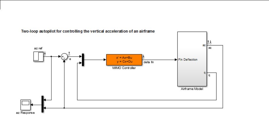
slTunable.systune
Create and configure an slTunable interfacetothemodel.
open_system('rct_airframe2')
ST0 = slTunable('rct_airframe2','MIMO Controller');
addControl(ST0,'delta fin');
ThesecommandscreateanslTunable interfacetothemodelandspecify
the MIMO Controller block as the tunable portion of the control system.
The model already has linearization input points on the signals az
ref,delta fin,andaz. These signals are therefore available for
specifying as inputs for tuning requirements. Similarly, you can use the
linearization output points eand az is outputs for tuning requirements.
The addControl command adds delta fin to the Controls signals of
the slTunable interface. Doing so makes delta fin available as both
input and output for specifying tuning requirements.
Specify tuning requirements for tracking, roll-off, stability margin, and
disturbance rejection.
Req1 = TuningGoal.Tracking('az ref','az',1);
Req2 = TuningGoal.Gain('delta fin','delta fin',tf(25,[1 0]));
Req3 = TuningGoal.Margins('delta fin',7,45);
8-202

slTunable.systune
MaxGain = frd([2 200 200],[0.02 2 200]);
Req4 = TuningGoal.Gain('delta fin','az',MaxGain);
Req1 constrains az to track az ref. The requirement Req2 imposes
a roll-off requirement by specifying a gain profile for the open-loop
point-to-point transfer function measured at delta fin.The
requirement Req3 imposes open-loop gain and phase margins on that
same point-to-point transfer function. Finally, Req4 rejects disturbances
to az injected at delta fin, by specifying a maximum gain profile
between those two points.
Tune the model using these tuning requirements.
Options = systuneOptions('RandomStart',3);
[ST1,fSoft,~,Info] = systune(ST0,[Req1,Req2,Req3,Req4],Options);
Final: Soft = 1.13, Hard = -Inf, Iterations = 55
Final: Soft = 1.5, Hard = -Inf, Iterations = 75
Final: Soft = 1.13, Hard = -Inf, Iterations = 92
ST1 is a tuned version of the slTunable interface to the control system
that contains the tuned values of the tunable parameters of the MIMO
controller in the model.
The RandomStart option causes systune to perform three independent
optimization runs beginning at different random values of the tunable
parameters. The displayed value Soft is the largest normalized soft
constraint value for each optimization run.
Examine the best achieved values of the soft constraints.
fSoft =
1.1327 1.1327 0.5140 1.1327
Only Req3, the stability margin requirement, is met for all frequencies.
The other values are close to but exceed 1, indicating violations of the
requirements for at least some frequencies. Use viewSpec to visualize
8-203

slTunable.systune
the tuned control system performanceagainsttherequirements,andto
determine whether the violations are acceptable.
References
[1] P. Apkarian and D. Noll, "Nonsmooth H-infinity Synthesis." IEEE
Transactions on Automatic Control, Vol. 51, Number 1, 2006, pp. 71–86.
[2] Bruisma, N.A. and M. Steinbuch, "A Fast Algorithm to Compute the
H∞-Norm of a Transfer Function Matrix," System Control Letters,14
(1990), pp. 287-293.
See Also slTunable |systune |TuningGoal.Tracking |TuningGoal.Gain
|TuningGoal.Margins |TuningGoal.WeightedGain |
TuningGoal.Variance |TuningGoal.WeightedVariance
|TuningGoal.LoopShape |TuningGoal.Poles |
TuningGoal.StableController
How To • “Specifying Design Requirements for systune”
• “Tuning Control Systems in Simulink”
• “Control of a Linear Electric Actuator”
• “Multi-Loop Controller for the Westland Lynx Helicopter”
•“ReliableControlofaFighterJet”
8-204

slTunable.writeBlockValue
Purpose Update block values in Simulink model
Syntax writeBlockValue(ST)
writeBlockValue(ST,block)
Description writeBlockValue(ST) writes tuned parameter values from the control
system description ST to the Simulink model that ST describes.
writeBlockValue(ST,block) updates only the block or blocks specified
by block.
Tips •Use writeBlockValue to apply tuned parameter values to the
Simulink model, for example for validating tuned values in the full
nonlinear model.
•writeBlockValue skips blocks that:
-Have no default parametrization
-Have a parametrization specified with slTunable.setBlockParam
that is not compatible with the default parametrization.
For example, you might specify the parametrization of a
susbsystem or S-Function block in your model. In that case,
slTunable.writeBlockValue cannot write the tuned parameter
values to the model.
Input
Arguments
ST
slTunable interface describing a Simulink model.
block
String or cell array of strings identifying blocks in the
TunedBlocks property of ST to write back to the Simulink model.
You can specify a block with an abbreviated block name, provided
that the string matches the end of the full block path and
unambiguously identifies the block.
See Also slTunable |slTunable.readBlockValue |slTunable.getBlockValue
|slTunable.setBlockValue |slTunable.showBlockValue
8-205

slTunable.writeBlockValue
Tutorials • “Tuning of a Digital Motion Control System”
• “Control of a Linear Electric Actuator”
How To • “Supported Blocks for Tuning in Simulink”
8-206

update
Purpose Update operating point object with structural changes in model
Syntax update(op)
Alternatives As an alternative to the update function, update operating point objects
using the Sync with Model button in the Simulink Control Design
GUI.
Description update(op) updates an operating point object, op,toreflectany
changes in the associated Simulink model, such as states being added
or removed.
Examples Open the magball model:
magball
Create an operating point object for the model:
op=operpoint('magball')
This syntax returns:
Operating Point for the Model magball.
(Time-Varying Components Evaluated at time t=0)
States:
----------
(1.) magball/Controller/PID Controller/Filter
x: 0
(2.) magball/Controller/PID Controller/Integrator
x: 14
(3.) magball/Magnetic Ball Plant/Current
x: 7
(4.) magball/Magnetic Ball Plant/dhdt
x: 0
(5.) magball/Magnetic Ball Plant/height
x: 0.05
8-207
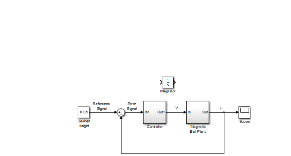
update
Inputs: None
----------
Add an Integrator block to the model, as shown in the following figure.
Update the operating point to include this new state:
update(op)
The new operating point appears:
Operating Point for the Model magball.
(Time-Varying Components Evaluated at time t=0)
States:
----------
(1.) magball/Controller/PID Controller/Filter
x: 0
(2.) magball/Controller/PID Controller/Integrator
x: 14
(3.) magball/Magnetic Ball Plant/Current
x: 7
(4.) magball/Magnetic Ball Plant/dhdt
x: 0
(5.) magball/Magnetic Ball Plant/height
8-208

update
x: 0.05
(6.) magball/Integrator
x: 0
Inputs: None
----------
See Also operpoint |operspec
8-209

update
8-210


Linear Analysis Plots
Linear Analysis Plots
Bode Plot Bode plot of linear system
approximated from nonlinear
Simulink model
Gain and Phase Margin Plot Gain and phase margins of linear
system approximated from nonlinear
Simulink model
Linear Step Response Plot Step response of linear system
approximated from nonlinear
Simulink model
Nichols Plot Nichols plot of linear system
approximated from nonlinear
Simulink model
Pole-Zero Plot Pole-zero plot of linear system
approximated from nonlinear
Simulink model
Singular Value Plot Singular value plot of linear system
approximated from nonlinear
Simulink model
9-3

9Block Reference
Model Verification
Check Bode Characteristics Check that Bode magnitude bounds
are satisfied during simulation
Check Gain and Phase Margins Check that gain and phase margin
bounds are satisfied during
simulation
Check Linear Step Response
Characteristics
Check that step response bounds on
linear system are satisfied during
simulation
Check Nichols Characteristics Check that gain and phase bounds
on Nichols response are satisfied
during simulation
Check Pole-Zero Characteristics Check that bounds on pole locations
are satisfied during simulation
Check Singular Value
Characteristics
Check that singular value bounds
are satisfied during simulation
9-4

10
Blocks — Alphabetical List

Bode Plot
Purpose Bode plot of linear system approximated from nonlinear Simulink model
Library Simulink Control Design
Description This block is same as the Check Bode Characteristics block except for
different default parameter settings in the Bounds tab.
Compute a linear system from a nonlinear Simulink model and plot
the linear system on a Bode plot.
During simulation, the software linearizes the portion of the model
between specified linearization inputs and outputs, and plots the
magnitude and phase of the linear system.
The Simulink model can be continuous- or discrete-time or multirate,
and can have time delays. The linear system can be Single-Input
Single-Output (SISO) or Multi-Input Multi-Output (MIMO). For MIMO
systems, the plots for all input/output combinations are displayed.
You can specify piecewise-linear frequency-dependent upper and lower
magnitude bounds and view them on the Bode plot. You can also check
that the bounds are satisfied during simulation:
•If all bounds are satisfied, the block does nothing.
•If a bound is not satisfied, the block asserts, and a warning message
appears at the MATLAB prompt. You can also specify that the block:
-Evaluate a MATLAB expression.
-Stop the simulation and bring that block into focus.
During simulation, the block can also output a logical assertion signal:
•If all bounds are satisfied, the signal is true (1).
•If a bound is not satisfied, the signal is false (0).
For MIMO systems, the bounds apply to the Bode responses of linear
systems computed for all input/output combinations.
10-2

Bode Plot
You can add multiple Bode Plot blocks to compute and plot the
magnitude and phase of various portions of the model.
You can save the linear system as a variable in the MATLAB workspace.
The block does not support code generation and can be used only in
Normal simulation mode.
Parameters The following table summarizes the Bode Plot block parameters,
accessible via the block parameter dialog box.
Task Parameters
Specify inputs
and outputs
(I/Os).
In Linearizations tab:
•“Linearization inputs/outputs” on
page 10-287.
•“Click a signal in the model to
select it” on page 10-290.
Specify
settings.
In Linearizations tab:
•“Linearize on” on page 10-294.
•“Snapshot times” on page 10-296.
•“Trigger type” on page 10-297.
Specify
algorithm
options.
In Algorithm Options of
Linearizations tab:
•“Enable zero-crossing detection”
on page 10-298.
•“Use exact delays” on page
10-300.
•“Linear system sample time” on
page 10-301.
Configure
linearization.
10-3

Bode Plot
Task Parameters
•“Sample time rate conversion
method” on page 10-303.
•“Prewarp frequency (rad/s)” on
page 10-306.
Specify labels
for linear
system I/Os
and state
names.
In Labels of Linearizations tab:
•“Use full block names” on page
10-307.
•“Use bus signal names” on page
10-309.
Plot the linear system. Show Plot
(Optional) Specify bounds on
magnitude of the linear system
for assertion.
In Bounds tab:
•“Include upper magnitude bound
in assertion” on page 10-30.
•“Include lower magnitude bound
in assertion” on page 10-36.
Specify assertion options (only
when you specify bounds on the
linear system).
In Assertion tab:
•“Enable assertion” on page
10-325.
•“Simulation callback when
assertion fails (optional)” on page
10-327.
•“Stop simulation when assertion
fails” on page 10-328.
•“Output assertion signal” on page
10-329.
10-4
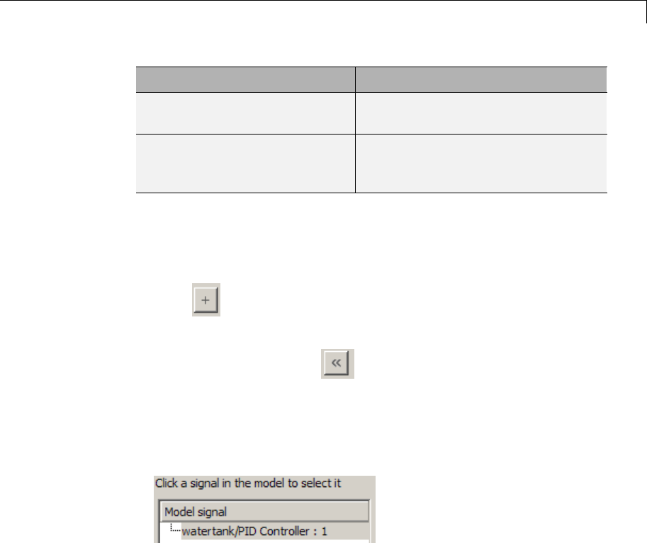
Bode Plot
Task Parameters
Save linear system to MATLAB
workspace.
“Save data to workspace” on page
10-323 in Logging tab.
Display plot window instead of
block parameters dialog box on
double-clicking the block.
“Show plot on block open” on page
10-331.
Linearization inputs/outputs
Linearization inputs and outputs that define the portion of a nonlinear
Simulink model to linearize.
1Click .
The dialog box expands to display a Click a signal in the model to
select it area and a new button.
2Select a signal in the Simulink Editor.
The selected signal appears as a Model signal in the Click a signal
in the model to select it area.
3(Optional) For buses, expand the bus signal to select an individual
element.
10-5

Bode Plot
Tip Forlargebuses,youcanentersearchtextforfilteringelement
names in the Filter by name edit box. The name match is
case-sensitive. Additionally, you can enter MATLAB regular
expression.
To modify the filtering options, click .
Filtering Options
•“Enable regular expression” on page 10-291
•“Show filtered results as aflatlist”onpage10-292
4Click to add the signal to the Linearization inputs/outputs
table.
The table displays the following information about the selected signal:
10-6

Bode Plot
Block : Port : Bus
Element
Name of the block associated with the input/output. The
number adjacent to the block name is the port number where
the selected bus signal is located. The last entry is the
selected bus element name.
Configuration Type of linearization point:
•Input — An input point.
•Output —Anoutputpoint.
•Input-Output — An input point immediately followed by
an output point.
•Output-Input — An output point immediately followed
by an input point.
•None — Signal selected but not specified as a linearization
input or output.
Open Loop If your model contains one or more feedback loops, you
can choose to linearize an open- or closed-loop system. For
example, you might want to linearize only the plant model
within a feedback control loop. When such a feedback loop
is present, select this option to insert an open loop point
and remove the effect of the loop without manually breaking
signal lines.
For determining gain and phase margins, in most cases, you
open the loop.
Note If you simulate the model without specifying an input or output,
the software does not compute a linear system. Instead, you see a
warning message at the MATLAB prompt.
Settings
No default
10-7


Bode Plot
Click a signal in the model to select it
Enables signal selection in the Simulink model. Appears only when
you click .
When this option appears, you also see the following changes:
•Anew button.
Use to add a selected signal as a linearization input or output in the
Linearization inputs/outputs table. For more information, see
Linearization inputs/outputs.
•changes to .
UsetocollapsetheClick a signal in the model to select it area.
Settings
No default
Command-Line Information
Use the getlinio and setlinio commands to select signals as
linearization inputs and outputs.
See Also
Plot Linear Characteristics of Simulink Models During Simulation
“Model Verification at Default Simulation Snapshot Time” on page 5-6
10-9

Bode Plot
Enable regular expression
Enable the use of MATLAB regular expressions for filtering signal
names. For example, entering t$ in the Filter by name edit box
displays all signals whose names end with a lowercase t(and their
immediate parents). For details, see “Regular Expressions”.
Settings
Default: On
On
Allow use of MATLAB regular expressions for filtering signal
names.
Off
Disable use of MATLAB regular expressions for filtering signal
names. Filtering treats the text you enter in the Filter by name
edit box as a literal string.
Dependencies
Selecting the Options button on the right-hand side of the Filter by
name edit box ( ) enables this parameter.
10-10

Bode Plot
Show filtered results as a flat list
Uses a flat list format to display the list of filtered signals, based on the
search text in the Filter by name edit box. The flat list format uses
dot notation to reflect the hierarchy of bus signals. The following is an
example of a flat list format for a filtered set of nested bus signals.
Settings
Default: Off
On
Display the filtered list of signalsusingaflatlistformat,
indicating bus hierarchies with dot notation instead of using a
tree format.
Off
Display filtered bus hierarchies using a tree format.
10-11

Bode Plot
Dependencies
Selecting the Options button on the right-hand side of the Filter by
name edit box ( ) enables this parameter.
10-12

Bode Plot
Linearize on
When to compute the linear system during simulation.
Settings
Default: Simulation snapshots
Simulation snapshots
Specific simulation time, specified in Snapshot times.
Use when you:
•Know one or more times when the model is at steady-state
operating point
•Want to compute the linear systems at specific times
External trigger
Trigger-based simulation event. Specify the trigger type in
Trigger type.
Use when a signal generated during simulation indicates
steady-state operating point.
Selecting this option adds a trigger port to the block. Use this port
to connect the block to the trigger signal.
For example, for an aircraft model, you might want to compute
the linear system whenever the fuel mass is a fraction of the
maximum fuel mass. In this case, model this condition as an
external trigger.
Dependencies
•Setting this parameter to Simulation snapshots enables Snapshot
times.
•Setting this parameter to External trigger enables Trigger type.
Command-Line Information
Parameter: LinearizeAt
10-13


Bode Plot
Snapshot times
One or more simulation times. The linear system is computed at these
times.
Settings
Default: 0
•For a different simulation time, enter the time. Use when you:
-Want to plot the linear system at a specific time
-Know the approximate time when the model reaches steady-state
operating point
•For multiple simulation times, enter a vector. Use when you want to
compute and plot linear systems at multiple times.
Snapshot times must be less than or equal to the simulation time
specified in the Simulink model.
Dependencies
Selecting Simulation snapshots in Linearize on enables this
parameter.
Command-Line Information
Parameter: SnapshotTimes
Type: string
Value: 0|positive real number |vector of positive real
numbers
Default: 0
See Also
Plot Linear Characteristics of Simulink Models During Simulation
“Model Verification at Default Simulation Snapshot Time” on page 5-6
10-15

Bode Plot
Trigger type
Trigger type of an external trigger for computing linear system.
Settings
Default: Rising edge
Rising edge
Rising edge of the external trigger signal.
Falling edge
Falling edge of the external trigger signal.
Dependencies
Selecting External trigger in Linearize on enables this parameter.
Command-Line Information
Parameter: TriggerType
Type: string
Value: 'rising' |'falling'
Default: 'rising'
See Also
Plot Linear Characteristics of Simulink Models During Simulation
“Model Verification at Default Simulation Snapshot Time” on page 5-6
10-16

Bode Plot
Enable zero-crossing detection
Enable zero-crossing detection to ensure that the software computes the
linear system characteristics at the following simulation times:
•The exact snapshot times, specified in Snapshot times.
As shown in the following figure, when zero-crossing detection is
enabled, the variable-step Simulink solver simulates the model at the
snapshot time Tsnap.Tsnap may lie between the simulation time steps
Tn-1 and Tnwhich are automatically chosen by the solver.
Computes linear system
characteristics at this time point
Time
Tn-1 Tn
Tsnap
•The exact times when an external trigger is detected, specified in
Trigger type.
As shown in the following figure, when zero-crossing detection is
enabled, the variable-step Simulink solver simulates the model at the
time, Ttrig, when the trigger signal is detected. Ttrig may lie between
the simulation time steps Tn-1 and Tnwhich are automatically chosen
by the solver.
Computes linear system
characteristics at this time point
Time
Amplitude
1
0Tn-1 Tn
Ttrig
Trigger signal
For more information on zero-crossing detection, see “Zero-Crossing
Detection” in the Simulink User Guide.
10-17

Bode Plot
Settings
Default: On
On
Compute linear system characteristics at the exact snapshot time
or exact time when a trigger signal is detected.
This setting is ignored if the Simulink solver is fixed step.
Off
Compute linear system characteristics at the simulation time
steps that the variable-step solver chooses. The software may not
compute the linear system at the exact snapshot time or exact
time when a trigger signal is detected.
Command-Line Information
Parameter: ZeroCross
Type: string
Value: 'on' |'off'
Default: 'on'
See Also
Plot Linear Characteristics of Simulink Models During Simulation
“Model Verification at Default Simulation Snapshot Time” on page 5-6
10-18

Bode Plot
Use exact delays
How to represent time delays in your linear model.
Use this option if you have blocks in your model that have time delays.
Settings
Default: Off
On
Return a linear model with exact delay representations.
Off
Return a linear model with Padé approximations of delays, as
specified in your Transport Delay and Variable Transport Delay
blocks.
Command-Line Information
Parameter: UseExactDelayModel
Type: string
Value: 'on' |'off'
Default: 'off'
See Also
Plot Linear Characteristics of Simulink Models During Simulation
“Model Verification at Default Simulation Snapshot Time” on page 5-6
10-19

Bode Plot
Linear system sample time
Sample time of the linear system computed during simulation.
Use this parameter to:
•Compute a discrete-time system with a specific sample time from a
continuous-time system
•Resample a discrete-time system with a different sample time
•Compute a continuous-time system from a discrete-time system
When computing discrete-time systems from continuous-time systems
and vice-versa, the software uses the conversion method specified in
Sample time rate conversion method.
Settings
Default: auto
auto. Computes the sample time as:
•0, for continuous-time models.
•For models that have blocks with different sample times
(multi-rate models), least common multiple of the sample
times. For example, if you have a mix of continuous-time and
discrete-time blocks with sample times of 0, 0.2 and 0.3, the
sample time of the linear model is 0.6.
Positive finite value.Usetocompute:
•A discrete-time linear system from a continuous-time system.
•A discrete-time linear system from another discrete-time
system with a different sample time
0
Usetocomputeacontinuous-timelinearsystemfroma
discrete-time model.
Command-Line Information
Parameter: SampleTime
10-20


Bode Plot
Sample time rate conversion method
Method for converting the sample time of single- or multi-rate models.
This parameter is used only when the value of Linear system sample
time is not auto.
Settings
Default: Zero-Order Hold
Zero-Order Hold
Zero-order hold, where the control inputs are assumed piecewise
constant over the sampling time Ts. For more information, see
“Zero-Order Hold” in Control System Toolbox User’s Guide.
This method usually performs better in time domain.
Tustin (bilinear)
Bilinear (Tustin) approximation without frequency prewarping.
The software rounds off fractional time delays to the nearest
multiple of the sampling time. For more information, see “Tustin
Approximation” in Control System Toolbox User’s Guide.
This method usually perform better in the frequency domain.
Tustin with Prewarping
Bilinear (Tustin) approximation with frequency prewarping. Also
specify the prewarp frequency in Prewarp frequency (rad/s).
For more information, see “Tustin Approximation” in Control
System Toolbox User’s Guide.
This method usually perform better in the frequency domain. Use
this method to ensure matching at frequency region of interest.
Upsampling when possible, Zero-Order Hold otherwise
Upsample a discrete-time system when possible and use
Zero-Order Hold otherwise.
10-22

Bode Plot
You can upsample only when you convert discrete-time system to
a new sample time that is an integer-value-times faster than the
sampling time of the original system.
Upsampling when possible, Tustin otherwise
Upsample a discrete-time system when possible and use Tustin
(bilinear) otherwise.
You can upsample only when you convert discrete-time system to
a new sample time that is an integer-value-times faster than the
sampling time of the original system.
Upsampling when possible, Tustin with Prewarping otherwise
Upsample a discrete-time system when possible and use Tustin
with Prewarping otherwise. Also, specify the prewarp frequency
in Prewarp frequency (rad/s).
You can upsample only when you convert discrete-time system to
a new sample time that is an integer-value-times faster than the
sampling time of the original system.
Dependencies
Selecting either:
•Tustin with Prewarping
•Upsampling when possible, Tustin with Prewarping
otherwise
enables Prewarp frequency (rad/s).
Command-Line Information
Parameter: RateConversionMethod
Type: string
Value: 'zoh' |'tustin' |'prewarp'|'upsampling_zoh'|
'upsampling_tustin'|'upsampling_prewarp'
Default: 'zoh'
10-23


Bode Plot
Prewarp frequency (rad/s)
Prewarp frequency for Tustin method, specified in radians/second.
Settings
Default: 10
Positive scalar value, smaller than the Nyquist frequency before and
after resampling. A value of 0 corresponds to the standard Tustin
method without frequency prewarping.
Dependencies
Selecting either
•Tustin with Prewarping
•Upsampling when possible, Tustin with Prewarping
otherwise
in Sample time rate conversion method enablesthisparameter.
Command-Line Information
Parameter: PreWarpFreq
Type: string
Value: 10 |positive scalar value
Default: 10
See Also
Plot Linear Characteristics of Simulink Models During Simulation
“Model Verification at Default Simulation Snapshot Time” on page 5-6
10-25

Bode Plot
Use full block names
How the state, input and output names appear in the linear system
computed during simulation.
The linear system is a state-space object and system states and
input/output names appear in following state-space object properties:
Input, Output or State Name Appears in Which State-Space
Object Property
Linearization input name InputName
Linearization output name OutputName
State names StateName
Settings
Default: Off
On
Show state and input/output names with their path through the
model hierarchy. For example, in the chemical reactor model,
a state in the Integrator1 block of the CSTR subsystem appears
with full path as scdcstr/CSTR/Integrator1.
Off
Show only state and input/output names. Use this option when the
signal name is unique and you know where the signal is location
in your Simulink model. For example, a state in the Integrator1
block of the CSTR subsystem appears as Integrator1.
Command-Line Information
Parameter: UseFullBlockNameLabels
Type: string
Value: 'on' |'off'
Default: 'off'
See Also
Plot Linear Characteristics of Simulink Models During Simulation
10-26


Bode Plot
Use bus signal names
How to label signals associated with linearization inputs and outputs
on buses, in the linear system computed during simulation (applies only
when you select an entire bus as an I/O point).
Selecting an entire bus signal is not recommended. Instead, select
individual bus elements.
You cannot use this parameter when your model has mux/bus mixtures.
Settings
Default: Off
On
Use the signal names of the individual bus elements.
Bus signal names appear when the input and output are at the
output of the following blocks:
•Root-level inport block containing a bus object
•Bus creator block
•Subsystem block whose source traces back to one of the
following blocks:
—Output of a bus creator block
—Root-level inport block by passing through only virtual or
nonvirtual subsystem boundaries
Off
Use the bus signal channel number.
Command-Line Information
Parameter: UseBusSignalLabels
Type: string
Value: 'on' |'off'
Default: 'off'
10-28


Bode Plot
Include upper magnitude bound in assertion
Check that the Bode response satisfies upper magnitude bounds,
specified in Frequencies (rad/sec) and Magnitude (dB),during
simulation. The software displays a warning if the magnitude violates
the upper bounds.
This parameter is used for assertion only if Enable assertion in the
Assertion tab is selected.
You can specify multiple upper magnitude bounds on the linear system.
The bounds also appear on the Bode magnitude plot. If you clear
Enable assertion, the bounds are not used for assertion but continue
to appear on the plot.
Settings
Default:
•Off for Bode Plot block.
•On for Check Bode Characteristics block.
On
Check that the magnitude satisfies the specified upper bounds,
during simulation.
Off
Do not check that the magnitude satisfies the specified upper
bounds, during simulation.
Tips
•Clearing this parameter disables the upper magnitude bounds and
the software stops checking that the bounds are satisfied during
simulation. The bound segments are also greyed out on the plot.
10-30

Bode Plot
•If you specify both upper and lower magnitude bounds but want to
include only the lower bounds for assertion, clear this parameter.
•To only view the bounds on the plot, clear Enable assertion.
Command-Line Information
Parameter: EnableUpperBound
Type: string
Value: 'on' |'off'
Default: 'off' for Bode Plot block, 'on' for Check Bode
Characteristics block.
See Also
Plot Linear Characteristics of Simulink Models During Simulation
“Model Verification at Default Simulation Snapshot Time” on page 5-6
10-31

Bode Plot
Frequencies (rad/sec)
Frequencies for one or more upper magnitude bound segments, specified
in radians/sec.
Specify the corresponding magnitudes in Magnitude (dB).
Settings
Default:
[] for Bode Plot block
[10 100] for Check Bode Characteristics block
Must be specified as start and end frequencies:
•Positive finite numbers for a single bound with one edge
•Matrix of positive finite numbers for a single bound with multiple
edges
For example, type [0.1 1;1 10] for two edges at frequencies [0.1 1]
and [1 10].
•Cell array of matrices with positive finite numbers for multiple
bounds
Tips
•To assert that magnitudes that correspond to the frequencies
are satisfied, select both Include upper magnitude bound in
assertion and Enable assertion.
•You can add or modify frequencies from the plot window:
-To add new frequencies, right-click the plot, and select
Bounds > New Bound. Select Upper gain limit in Design
requirement type, and specify the frequencies in the Frequency
column. Specify the corresponding magnitudes in the Magnitude
column.
-To modify the frequencies, drag the bound segment. Alternatively,
right-click the segment, and select Bounds > Edit Bound.
Specify the new frequencies in the Frequency column.
10-32

Bode Plot
You must click Update Block before simulating the model.
Command-Line Information
Parameter: UpperBoundFrequencies
Type: string
Value: [] |[10 100]|positive finite numbers |matrix of
positive finite numbers |cell array of matrices with
positive finite numbers. Must be specified inside single quotes
('').
Default: '[]' for Bode Plot block, '[10 100]' for Check Bode
Characteristics block
See Also
Plot Linear Characteristics of Simulink Models During Simulation
“Model Verification at Default Simulation Snapshot Time” on page 5-6
10-33

Bode Plot
Magnitudes (dB)
Magnitude values for one or more upper magnitude bound segments,
specified in decibels.
Specify the corresponding frequencies in Frequencies (rad/sec).
Settings
Default:
[] for Bode Plot block
[-20 -20] for Check Bode Characteristics block
Must be specified as start and end magnitudes:
•Finite numbers for a single bound with one edge
•Matrix of finite numbers for a single bound with multiple edges
For example, type [–10 –10; –20 –20] for two edges at magnitudes
[–10 –10] and [–20 –20].
•Cell array of matrices with finite numbers for multiple bounds
Tips
•To assert that magnitude bounds are satisfied, select both Include
upper magnitude bound in assertion and Enable assertion.
•You can add or modify magnitudes from the plot window:
-To add a new magnitude, right-click the plot, and select
Bounds > New Bound. Select Upper gain limit in Design
requirement type, and specify the magnitude in the Magnitude
column. Specify the corresponding frequencies in the Frequency
column.
-To modify the magnitudes, drag the bound segment. Alternatively,
right-click the segment, and select Bounds > Edit Bound.
Specify the new magnitudes in the Magnitude column.
You must click Update Block before simulating the model.
10-34

Bode Plot
Command-Line Information
Parameter: UpperBoundMagnitudes
Type: string
Value: [] |[-20 -20] |finite numbers |matrix of finite
numbers |cell array of matrices with finite numbers.Must
be specified inside single quotes ('').
Default: '[]' for Bode Plot block, '[-20 -20]' for Check Bode
Characteristics block.
See Also
Plot Linear Characteristics of Simulink Models During Simulation
“Model Verification at Default Simulation Snapshot Time” on page 5-6
10-35

Bode Plot
Include lower magnitude bound in assertion
Check that the Bode response satisfies lower magnitude bounds,
specified in Frequencies (rad/sec) and Magnitude (dB),during
simulation. The software displays a warning if the magnitude violates
the lower bounds.
This parameter is used for assertion only if Enable assertion in the
Assertion tab is selected.
You can specify multiple lower magnitude bounds on the linear system
computed during simulation. The bounds also appear on the Bode
magnitude plot. If you clear Enable assertion, the bounds are not
used for assertion but continue to appear on the plot.
Settings
Default:
•Off for Bode Plot block.
•On for Check Bode Characteristics block
On
Check that the magnitude satisfies the specified lower bounds
during simulation.
Off
Do not check that the magnitude satisfies the specified upper
bounds during simulation.
Tips
•Clearing this parameter disables the lower magnitude bound and
the software stops checking that the bounds are satisfied during
simulation. The bound segments are also greyed out on the plot.
10-36
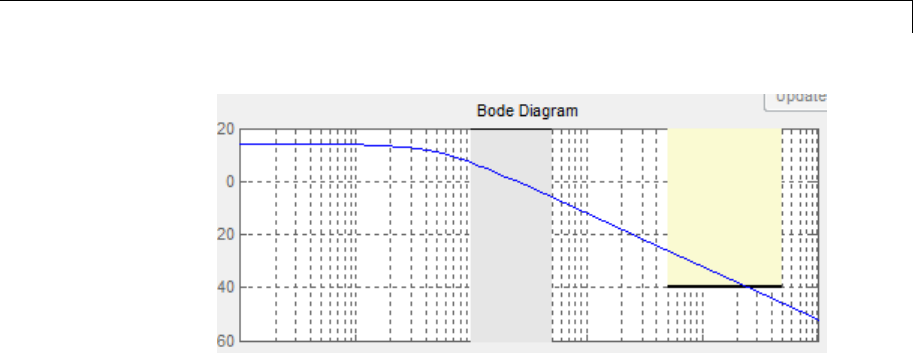
Bode Plot
•If you specify both upper and lower magnitude bounds on the Bode
magnitude but want to include only the upper bound for assertion,
clear this parameter.
•To only view the bound on the plot, clear Enable assertion.
Command-Line Information
Parameter: EnableLowerBound
Type: string
Value: 'on' |'off'
Default: 'off' for Bode Plot block, 'on' for Check Bode
Characteristics block
See Also
Plot Linear Characteristics of Simulink Models During Simulation
“Model Verification at Default Simulation Snapshot Time” on page 5-6
10-37

Bode Plot
Frequencies (rad/sec)
Frequencies for one or more lower magnitude bound segments, specified
in radians/sec.
Specify the corresponding magnitudes in Magnitude (dB).
Settings
Default:
[] for Bode Plot block
[0.1 1] for Check Bode Characteristics block
Must be specified as start and end frequencies:
•Positive finite numbers for a single bound with one edge
•Matrix of positive finite numbers for a single bound with multiple
edges
Forexample,type[0.11;110]tospecifytwoedgeswithfrequencies
[0.1 1] and [1 10].
•Cell array of matrices with positive finite numbers for multiple
bounds
Tips
•To assert that magnitude bounds that correspond to the frequencies
are satisfied, select both Include lower magnitude bound in
assertion and Enable assertion.
•You can add or modify frequencies from the plot window:
-To add a new frequencies, right-click the plot, and select
Bounds > New Bound. Select Lower gain limit in Design
requirement type, and specify the frequencies in the Frequency
column. Specify the corresponding magnitudes in the Magnitude
column.
-To modify the frequencies, drag the bound segment. Alternatively,
right-click the segment, and select Bounds > Edit Bound.
Specify the new frequencies in the Frequency column.
10-38

Bode Plot
You must click Update Block before simulating the model.
Command-Line Information
Parameter: LowerBoundFrequencies
Type: string
Value: [] |[0.1 1] |positive finite numbers |matrix of
positive finite numbers |cell array of matrices with
positive finite numbers. Must be specified inside single quotes
('').
Default: '[]' for Bode Plot block, '[0.1 1]' for Check Bode
Characteristics block.
See Also
Plot Linear Characteristics of Simulink Models During Simulation
“Model Verification at Default Simulation Snapshot Time” on page 5-6
10-39

Bode Plot
Magnitudes (dB)
Magnitude values for one or more lower magnitude bound segments,
specified in decibels.
Specify the corresponding frequencies in Frequencies (rad/sec).
Settings
Default:
[] for Bode Plot block
[20 20] for Check Bode Characteristics block
Must be specified as start and end magnitudes:
•Finite numbers for a single bound with one edge
•Matrix of finite numbers for a single bound with multiple edges
For example, type [20 20; 40 40] for two edges with magnitudes [20
20] and [40 40].
•Cell array of matrices with finite numbers for multiple bounds
Tips
•To assert that magnitude bounds are satisfied, select both Include
lower magnitude bound in assertion and Enable assertion.
•If Include lower magnitude bound in assertion is not selected,
the bound segment is disabled on the plot.
•To only view the bound on the plot, clear Enable assertion.
•You can add or modify magnitudes from the plot window:
-To add a new magnitude, right-click the plot, and select
Bounds > New Bound. Select Lower gain limit in Design
requirement type and specify the magnitude in the Magnitude
column. Specify the corresponding frequencies in the Frequency
column.
10-40

Bode Plot
-To modify the magnitudes, drag the bound segment. Alternatively,
right-click the segment, and select Bounds > Edit Bound.
Specify the new magnitude values in the Magnitude column.
You must click Update Block before simulating the model.
Command-Line Information
Parameter: LowerBoundMagnitudes
Type: string
Value: [] |[20 20] |finite numbers |matrix of finite
numbers |cell array of matrices with finite numbers.Must
be specified inside single quotes ('').
Default: '[]' for Bode Plot block, '[20 20]' for Check Bode
Characteristics block.
See Also
Plot Linear Characteristics of Simulink Models During Simulation
“Model Verification at Default Simulation Snapshot Time” on page 5-6
10-41

Bode Plot
Save data to workspace
Save one or more linear systems as a variable in MATLAB workspace to
perform further linear analysis or control design.
The workspace variable is a structure with time and values fields:
•The time field stores the simulation time at which the linear system
is computed.
•The values field is a state-space object which stores the linear
system. If the linear system is computed at multiple simulation
times, values is an array of state-space objects.
Settings
Default: Off
On
Save the computed linear system to MATLAB workspace.
Off
Do not save the computed linear system to MATLAB workspace.
Dependencies
This parameter enables Variable name.
Command-Line Information
Parameter: SaveToWorkspace
Type: string
Value: 'on' |'off'
Default: 'off'
See Also
Plot Linear Characteristics of Simulink Models During Simulation
“Model Verification at Default Simulation Snapshot Time” on page 5-6
10-42

Bode Plot
Variable name
Name of the workspace variable that stores one or more linear systems
computed during simulation.
The name must be unique among the variable names used in all data
logging model blocks, such as Linear Analysis Plot blocks, Model
Verification blocks, Scope blocks, To Workspace blocks, and simulation
return variables such as time, states, and outputs.
Settings
Default: sys
String.
Dependencies
Save data to workspace enables this parameter.
Command-Line Information
Parameter: SaveName
Type: string
Value: sys |any string. Must be specified inside single quotes
('').
Default: 'sys'
See Also
Plot Linear Characteristics of Simulink Models During Simulation
“Model Verification at Default Simulation Snapshot Time” on page 5-6
10-43

Bode Plot
Enable assertion
Enable the block to check that bounds specified and included for
assertion in the Bounds tab are satisfied during simulation. Assertion
failsifaboundisnotsatisfied. Awarning, reporting the assertion
failure, appears at the MATLAB prompt.
If assertion fails, you can optionally specify that the block:
•Execute a MATLAB expression, specified in Simulation callback
when assertion fails (optional).
•Stop the simulation and bring that block into focus, by selecting Stop
simulation when assertion fails.
For the Linear Analysis Plots blocks, this parameter has no effect
because no bounds are included by default. If you want to use the
Linear Analysis Plots blocks for assertion, specify and include
bounds in the Bounds tab.
Clearing this parameter disables assertion, i.e., the block no longer
checks that specified bounds are satisfied. The block icon also updates
to indicate that assertion is disabled.
In the Configuration Parameters dialog box of the Simulink model, the
Model Verification block enabling option in the Debugging area of
Data Validity node, lets you to enable or disable all model verification
blocks in a model, regardless of the setting of this option.
Settings
Default: On
10-44

Bode Plot
On
Check that bounds included for assertion in the Bounds tab
are satisfied during simulation. A warning, reporting assertion
failure, is displayed at the MATLAB prompt if bounds are violated.
Off
Do not check that bounds included for assertion are satisfied
during simulation.
Dependencies
This parameter enables:
•Simulation callback when assertion fails (optional)
•Stop simulation when assertion fails
Command-Line Information
Parameter: enabled
Type: string
Value: 'on' |'off'
Default: 'on'
See Also
Plot Linear Characteristics of Simulink Models During Simulation
“Model Verification at Default Simulation Snapshot Time” on page 5-6
10-45

Bode Plot
Simulation callback when assertion fails (optional)
MATLAB expression to execute when assertion fails.
Because the expression is evaluated in the MATLAB workspace, define
all variables used in the expression in that workspace.
Settings
No Default
AMATLABexpression.
Dependencies
Enable assertion enables this parameter.
Command-Line Information
Parameter: callback
Type: string
Value: '' |MATLAB expression
Default: ''
See Also
Plot Linear Characteristics of Simulink Models During Simulation
“Model Verification at Default Simulation Snapshot Time” on page 5-6
10-46

Bode Plot
Stop simulation when assertion fails
Stop the simulation when a bound specified in the Bounds tab is
violated during simulation, i.e., assertion fails.
If you run the simulation from the Simulink Editor, the Simulation
Diagnostics window opens to display an error message. Also, the block
where the bound violation occurs is highlighted in the model.
Settings
Default: Off
On
Stop simulation if a bound specified in the Bounds tab is violated.
Off
Continue simulation if a bound is violated with a warning
message at the MATLAB prompt.
Tips
•Because selecting this option stops the simulation as soon as the
assertion fails, assertion failures that might occur later during the
simulation are not reported. If you want all assertion failures to be
reported, do not select this option.
Dependencies
Enable assertion enables this parameter.
Command-Line Information
Parameter: stopWhenAssertionFail
Type: string
Value: 'on' |'off'
Default: 'off'
See Also
Plot Linear Characteristics of Simulink Models During Simulation
“Model Verification at Default Simulation Snapshot Time” on page 5-6
10-47

Bode Plot
Output assertion signal
Output a Boolean signal that, at each time step, is:
•True (1) if assertion succeeds, i.e., all bounds are satisfied
•False (1)ifassertionfails,i.e.,aboundisviolated.
The output signal data type is Boolean only if the Implement logic
signals as Boolean data option in the Optimization pane of the
Configuration Parameters dialog box of the Simulink model is selected.
Otherwise, the data type of the output signal is double.
Selecting this parameter adds an output port to the block that you can
connect to any block in the model.
Settings
Default:Off
On
Output a Boolean signal to indicate assertion status. Adds a
port to the block.
Off
Do not output a Boolean signal to indicate assertion status.
Tips
•Use this parameter to design complex assertion logic. For an
example, see “Model Verification Using Simulink®Control Design™
and Simulink Verification Blocks” on page 5-25.
Command-Line Information
Parameter: export
Type: string
Value: 'on' |'off'
Default: 'off'
See Also
Plot Linear Characteristics of Simulink Models During Simulation
10-48


Bode Plot
Show plot on block open
Open the plot window instead of the Block Parameters dialog box when
you double-click the block in the Simulink model.
Usethisparameterifyouprefertoopenandperformtasks,suchas
adding or modifying bounds, in the plot window instead of the Block
Parameters dialog box. If you want to access the block parameters from
the plot window, select Edit or click .
For more information on the plot, see Show Plot.
Settings
Default: Off
On
Open the plot window when you double-click the block.
Off
Open the Block Parameters dialog box when double-clicking the
block.
Command-Line Information
Parameter: LaunchViewOnOpen
Type: string
Value: 'on' |'off'
Default: 'off'
See Also
Plot Linear Characteristics of Simulink Models During Simulation
“Model Verification at Default Simulation Snapshot Time” on page 5-6
10-50

Bode Plot
Show Plot Open the plot window.
Use the plot to view:
•Linear system characteristics computed from the nonlinear Simulink
model during simulation
You must click this button before you simulate the model to view
the linear characteristics.
You can display additional characteristics, such as the peak response
time and stability margins, of the linear system by right-clicking the
plot and selecting Characteristics.
•Bounds on the linear system characteristics
You can specify bounds in the Bounds tab of the Block Parameters
dialog box or right-click the plot and select Bounds > New Bound.
For more information on the types of bounds you can specify on each
plot, see “Verifiable Linear System Characteristics” on page 5-5 in
the User’s Guide.
You can modify bounds by dragging the bound segment or by
right-clicking the plot and selecting Bounds > Edit Bound. Before
you simulate the model, click Update Block to update the bound
value in the block parameters.
Typical tasks that you perform in the plot window include:
•Opening the Block Parameters dialog box by clicking or selecting
Edit.
•Finding the block that the plot window corresponds to by clicking
or selecting View > Highlight Simulink Block.Thisactionmakes
the Simulink Editor active and highlights the block.
•Simulating the model by clicking or selecting Simulation > Run.
This action also linearizes the portion of the model between the
specified linearization input and output.
10-51

Bode Plot
•Adding legend on the linear system characteristic plot by clicking .
See Also Check Bode Characteristics
Tutorials •“Visualize Bode Response of Simulink Model During Simulation”
on page 2-42
•“Visualize Linear System at Multiple Simulation Snapshots” on page
2-64
•“Visualize Linear System of a Continuous-Time Model Discretized
During Simulation” on page 2-70
•Plotting Linear System Characteristics of a Chemical Reactor
10-52

Check Bode Characteristics
Purpose Check that Bode magnitude bounds are satisfied during simulation
Library Simulink Control Design
Description This block is same as the Bode Plot block except for different default
parameter settings in the Bounds tab.
Check that upper and lower magnitude bounds on the Bode response
of a linear system, computed from a nonlinear Simulink model, are
satisfied during simulation.
The Simulink model can be continuous-time, discrete-time or multi-rate
and can have time delays. The computed linear system can be
Single-Input Single-Output (SISO) or Multi-Input Multi-Output
(MIMO).
During simulation, the software linearizes the portion of the model
between specified linearization inputs and outputs, computes the Bode
magnitude and phase, and checks that the magnitude satisfies the
specified bounds.
•If all bounds are satisfied, the block does nothing.
•If a bound is not satisfied, the block asserts, and a warning message
appears at the MATLAB prompt. You can also specify that the block:
-Evaluate a MATLAB expression.
-Stop the simulation and bring that block into focus.
During simulation, the block can also output a logical assertion signal:
•If all bounds are satisfied, the signal is true (1).
•If a bound is not satisfied, the signal is false (0).
For MIMO systems, the bounds apply to the Bode responses computed
for all input/output combinations.
10-53

Check Bode Characteristics
You can add multiple Check Bode Characteristics blocks in your model
to check upper and lower Bode magnitude bounds on various portions of
the model.
You can also plot the magnitude and phase on a Bode plot and
graphically verify that the magnitude satisfies the bounds.
This block and the other Model Verification blocks test that the
linearized behavior of a nonlinear Simulink model is within specified
bounds during simulation.
•When a model does not violate any bound, you can disable the block
by clearing the assertion option. If you modify the model, you can
re-enable assertion to ensure that your changes do not cause the
model to violate a bound.
•When a model violates any bound, you can use Simulink Design
Optimization software to optimize the linear system to meet the
specified requirements in this block.
You can save the linear system as a variable in the MATLAB workspace.
The block does not support code generation and can be used only in
Normal simulation mode.
Parameters ThefollowingtablesummarizestheCheck Bode Characteristics block
parameters, accessible via the block parameter dialog box. For more
information, see “Parameters” on page 10-3 in the Bode Plot block
reference page.
10-54

Check Bode Characteristics
Task Parameters
Specify
inputs and
outputs
(I/Os).
In Linearizations tab:
•Linearization inputs/outputs
•Click a model signal to add
it as a linearization I/O
Specify
settings.
In Linearizations tab:
•Linearize on
•Snapshot times
•Trigger type
Specify
algorithm
options.
In Linearizations tab:
•Enable zero-crossing
detection
•Use exact delays
•Linear system sample time
•Sample time rate conversion
method
•Prewarp frequency (rad/s)
Configure
linearization.
Specify labels
for linear
system I/Os
and state
names.
In Linearizations tab:
•Use full block names
•Use bus signal names
10-55

Check Bode Characteristics
Task Parameters
Specify bounds on the linear
system for assertion.
In Bounds tab:
•Include upper magnitude
bound in assertion
•Include lower magnitude
bound in assertion
Specify assertion options (only
when you specify bounds on the
linear system).
In Assertion tab:
•Enable assertion
•Simulation callback when
assertion fails (optional)
•Stop simulation when
assertion fails
•Output assertion signal
Save linear system to MATLAB
workspace.
Save data to workspace in
Logging tab.
View bounds violations
graphically in a plot window.
Show Plot
Display plot window instead of
block parameters dialog box on
double-clicking the block.
Show plot on block open
See Also Bode Plot
Tutorials •“Model Verification at Default Simulation Snapshot Time” on page
5-6
•“Model Verification at Multiple Simulation Snapshots” on page 5-15
•“Model Verification Using Simulink®Control Design™ and Simulink
Verification Blocks” on page 5-25
10-56


Check Gain and Phase Margins
Purpose Check that gain and phase margin bounds are satisfied during
simulation
Library Simulink Control Design
Description This block is same as the Gain and Phase Margin Plot block except for
different default parameter settings in the Bounds tab.
Check that bounds on gain and phase margins of a linear system,
computed from a nonlinear Simulink model, are satisfied during
simulation.
The Simulink model can be continuous-time, discrete-time or
multirate and can have time delays. Because you can specify only
one linearization input/output pair in this block, the linear system is
Single-Input Single-Output (SISO).
During simulation, the software linearizes the portion of the model
between specified linearization inputs and outputs, computes the gain
and phase margins, and checks that the gain and phase margins satisfy
the specified bounds.
•If all bounds are satisfied, the block does nothing.
•If a bound is not satisfied, the block asserts, and a warning message
appears at the MATLAB prompt. You can also specify that the block:
-Evaluate a MATLAB expression.
-Stop the simulation and bring that block into focus.
During simulation, the block can also output a logical assertion signal:
•If all bounds are satisfied, the signal is true (1).
•If a bound is not satisfied, the signal is false (0).
You can add multiple Check Gain and Phase Margins blocks in your
model to check gain and phase margin bounds on various portions of
the model.
10-58

Check Gain and Phase Margins
You can also plot the gain and phase margins on a Bode, Nichols or
Nyquist plot or view the margins in a table and verify that the gain and
phase margins satisfy the bounds.
This block and the other Model Verification blocks test that the
linearized behavior of a nonlinear Simulink model is within specified
bounds during simulation.
•When a model does not violate any bound, you can disable the block
by clearing the assertion option. If you modify the model, you can
re-enable assertion to ensure that your changes do not cause the
model to violate a bound.
•When a model violates any bound, you can use Simulink Design
Optimization software to optimize the linear system to meet the
specified requirements in this block.
You can save the linear system as a variable in the MATLAB workspace.
The block does not support code generation and can be used only in
Normal simulation mode.
Parameters The following table summarizes the Gain and Phase Margin Plot block
parameters, accessible via the block parameter dialog box. For more
information, see “Parameters” on page 10-79 in the Gain and Phase
Margin Plot block reference page.
Task Parameters
Specify
inputs and
outputs
(I/Os).
In Linearizations tab:
•Linearization inputs/outputs
•Click a model signal to add
it as a linearization I/O
Specify
settings.
In Linearizations tab:
•Linearize on
Configure
linearization.
10-59

Check Gain and Phase Margins
Task Parameters
•Snapshot times
•Trigger type
Specify
algorithm
options.
In Linearizations tab:
•Enable zero-crossing
detection
•Use exact delays
•Linear system sample time
•Sample time rate conversion
method
•Prewarp frequency (rad/s)
Specify labels
for linear
system I/Os
and state
names.
In Linearizations tab:
•Use full block names
•Use bus signal names
Specify bounds on gain and
phasemarginsofthelinear
system for assertion.
Include gain and phase
margins in assertion in Bounds
tab.
Specify assertion options (only
when you specify bounds on the
linear system).
In Assertion tab:
•Enable assertion
•Simulation callback when
assertion fails (optional)
•Stop simulation when
assertion fails
•Output assertion signal
10-60

Check Gain and Phase Margins
Task Parameters
Save linear system to MATLAB
workspace.
Save data to workspace in
Logging tab.
View bounds violations
graphically in a plot window.
Show Plot
Display plot window instead of
block parameters dialog box on
double-clicking the block.
Show plot on block open
See Also Gain and Phase Margin Plot
Tutorials •“Model Verification at Default Simulation Snapshot Time” on page
5-6
•“Model Verification at Multiple Simulation Snapshots” on page 5-15
•“Model Verification Using Simulink®Control Design™ and Simulink
Verification Blocks” on page 5-25
•Verifying Frequency-Domain Characteristics of an Aircraft
How To “Monitoring Linear System Characteristics in Simulink Models” on
page 5-2
10-61

Check Linear Step Response Characteristics
Purpose Check that step response bounds on linear system are satisfied during
simulation
Library Simulink Control Design
Description This block is same as the Linear Step Response Plot block except for
different default parameter settings in the Bounds tab.
Check that bounds on step response characteristics of a linear system,
computed from a nonlinear Simulink model, are satisfied during
simulation.
The Simulink model can be continuous-time, discrete-time or
multirate and can have time delays. Because you can specify only
one linearization input/output pair in this block, the linear system is
Single-Input Single-Output (SISO).
During simulation, the software linearizes the portion of the model
between specified linearization inputs and outputs, computes the step
response and checks that the step response satisfies the specified
bounds:
•If all bounds are satisfied, the block does nothing.
•If a bound is not satisfied, the block asserts, and a warning message
appears at the MATLAB prompt. You can also specify that the block:
-Evaluate a MATLAB expression.
-Stop the simulation and bring that block into focus.
During simulation, the block can also output a logical assertion signal:
•If all bounds are satisfied, the signal is true (1).
•If a bound is not satisfied, the signal is false (0).
You can add multiple Check Linear Step Response Characteristics
blocks in your model to check step response bounds on various portions
of the model.
10-62

Check Linear Step Response Characteristics
You can also plot the step response and graphically verify that the step
response satisfies the bounds.
This block and the other Model Verification blocks test that the
linearized behavior of a nonlinear Simulink model is within specified
bounds during simulation.
•When a model does not violate any bound, you can disable the block
by clearing the assertion option. If you modify the model, you can
re-enable assertion to ensure that your changes do not cause the
model to violate a bound.
•When a model violates any bound, you can use Simulink Design
Optimization software to optimize the linear system to meet the
specified requirements in this block.
You can save the linear system as a variable in the MATLAB workspace.
The block does not support code generation and can be used only in
Normal simulation mode.
Parameters The following table summarizes the Linear Step Response Plot block
parameters, accessible via the block parameter dialog box. For more
information, see “Parameters” on page 10-125 in the Linear Step
Response Plot block reference page.
Task Parameters
Specify
inputs and
outputs
(I/Os).
In Linearizations tab:
•Linearization inputs/outputs
•Click a model signal to add
it as a linearization I/O
Specify
settings.
In Linearizations tab:
•Linearize on
•Snapshot times
Configure
linearization.
10-63

Check Linear Step Response Characteristics
Task Parameters
•Trigger type
Specify
algorithm
options.
In Linearizations tab:
•Enable zero-crossing
detection
•Use exact delays
•Linear system sample time
•Sample time rate conversion
method
•Prewarp frequency (rad/s)
Specify labels
for linear
system I/Os
and state
names.
In Linearizations tab:
•Use full block names
•Use bus signal names
Specify bounds on the linear
system for assertion.
Includestepresponsebounds
in assertion in Bounds tab.
Specify assertion options (only
when you specify bounds on the
linear system).
In Assertion tab:
•Enable assertion
•Simulation callback when
assertion fails (optional)
•Stop simulation when
assertion fails
•Output assertion signal
Save linear system to MATLAB
workspace.
Save data to workspace in
Logging tab.
10-64

Check Linear Step Response Characteristics
Task Parameters
View bounds violations
graphically in a plot window.
Show Plot
Display plot window instead of
block parameters dialog box on
double-clicking the block.
Show plot on block open
See Also Linear Step Response Plot
Tutorials •“Model Verification at Default Simulation Snapshot Time” on page
5-6
•“Model Verification at Multiple Simulation Snapshots” on page 5-15
•“Model Verification Using Simulink®Control Design™ and Simulink
Verification Blocks” on page 5-25
•Verifying Frequency-Domain Characteristics of an Aircraft
How To “Monitoring Linear System Characteristics in Simulink Models” on
page 5-2
10-65

Check Nichols Characteristics
Purpose Check that gain and phase bounds on Nichols response are satisfied
during simulation
Library Simulink Control Design
Description ThisblockissameastheNicholsPlotblock except for different default
parameter settings in the Bounds tab.
Check that open- and closed-loop gain and phase bounds on Nichols
response of a linear system, computed from a nonlinear Simulink model,
are satisfied during simulation.
The Simulink model can be continuous-time, discrete-time or
multirate and can have time delays. Because you can specify only
one linearization input/output pair in this block, the linear system is
Single-Input Single-Output (SISO).
During simulation, the software linearizes the portion of the model
between specified linearization inputs and outputs, computes the
magnitude and phase, and checks that the gain and phase satisfy the
specified bounds:
•If all bounds are satisfied, the block does nothing.
•If a bound is not satisfied, the block asserts, and a warning message
appears at the MATLAB prompt. You can also specify that the block:
-Evaluate a MATLAB expression.
-Stop the simulation and bring that block into focus.
During simulation, the block can also output a logical assertion signal:
•If all bounds are satisfied, the signal is true (1).
•If a bound is not satisfied, the signal is false (0).
You can add multiple Check Nichols Characteristics blocks in your
model to check gain and phase bounds on various portions of the model.
10-66

Check Nichols Characteristics
You can also plot the linear system on a Nichols plot and graphically
verify that the Nichols response satisfies the bounds.
This block and the other Model Verification blocks test that the
linearized behavior of a nonlinear Simulink model is within specified
bounds during simulation.
•When a model does not violate any bound, you can disable the block
by clearing the assertion option. If you modify the model, you can
re-enable assertion to ensure that your changes do not cause the
model to violate a bound.
•When a model violates any bound, you can use Simulink Design
Optimization software to optimize the linear system to meet the
specified requirements in this block.
You can save the linear system as a variable in the MATLAB workspace.
The block does not support code generation and can be used only in
Normal simulation mode.
Parameters The following table summarizes the Nichols Plot block parameters,
accessible via the block parameter dialog box. For more information, see
“Parameters” on page 10-172 in the Nichols Plot block reference page.
Task Parameters
Specify
inputs and
outputs
(I/Os).
In Linearizations tab:
•Linearization inputs/outputs
•Click a model signal to add
it as a linearization I/O
Specify
settings.
In Linearizations tab:
•Linearize on
•Snapshot times
Configure
linearization.
10-67

Check Nichols Characteristics
Task Parameters
•Trigger type
Specify
algorithm
options.
In Linearizations tab:
•Enable zero-crossing
detection
•Use exact delays
•Linear system sample time
•Sample time rate conversion
method
•Prewarp frequency (rad/s)
Specify labels
for linear
system I/Os
and state
names.
In Linearizations tab:
•Use full block names
•Use bus signal names
Specify bounds on gains and
phases of the linear system for
assertion.
In Bounds tab:
•Include gain and phase
margins in assertion
•Include closed-loop peak
gaininassertion
•Include open-loop
gain-phase bound in
assertion
10-68

Check Nichols Characteristics
Task Parameters
Specify assertion options (only
when you specify bounds on the
linear system).
In Assertion tab:
•Enable assertion
•Simulation callback when
assertion fails (optional)
•Stop simulation when
assertion fails
•Output assertion signal
Save linear system to MATLAB
workspace.
Save data to workspace in
Logging tab.
View bounds violations
graphically in a plot window.
Show Plot
Display plot window instead of
block parameters dialog box on
double-clicking the block.
Show plot on block open
See Also Nichols Plot
Tutorials •“Model Verification at Default Simulation Snapshot Time” on page
5-6
•“Model Verification at Multiple Simulation Snapshots” on page 5-15
•“Model Verification Using Simulink®Control Design™ and Simulink
Verification Blocks” on page 5-25
•Verifying Frequency-Domain Characteristics of an Aircraft
How To “Monitoring Linear System Characteristics in Simulink Models” on
page 5-2
10-69

Check Pole-Zero Characteristics
Purpose Check that bounds on pole locations are satisfied during simulation
Library Simulink Control Design
Description This block is same as the Pole-Zero Plot block except for different
default parameter settings in the Bounds tab.
Check that approximate second-order bounds on the pole locations of a
linear system, computed from a nonlinear Simulink model, are satisfied
during simulation.
The Simulink model can be continuous-time, discrete-time or
multirate and can have time delays. Because you can specify only
one linearization input/output pair in this block, the linear system is
Single-Input Single-Output (SISO).
During simulation, the software linearizes the portion of the model
between specified linearization inputs and outputs, computes the poles
and zeros, and checks that the poles satisfy the specified bounds:
•If all bounds are satisfied, the block does nothing.
•If a bound is not satisfied, the block asserts, and a warning message
appears at the MATLAB prompt. You can also specify that the block:
-Evaluate a MATLAB expression.
-Stop the simulation and bring that block into focus.
During simulation, the block can also output a logical assertion signal:
•If all bounds are satisfied, the signal is true (1).
•If a bound is not satisfied, the signal is false (0).
You can add multiple Check Pole-Zero Characteristics blocks in your
model to check approximate second-order bounds on various portions of
the model.
You can also plot the poles and zeros on a pole-zero map and graphically
verify that the poles satisfy the bounds.
10-70

Check Pole-Zero Characteristics
This block and the other Model Verification blocks test that the
linearized behavior of a nonlinear Simulink model is within specified
bounds during simulation.
•When a model does not violate any bound, you can disable the block
by clearing the assertion option. If you modify the model, you can
re-enable assertion to ensure that your changes do not cause the
model to violate a bound.
•When a model violates any bound, you can use Simulink Design
Optimization software to optimize the linear system to meet the
specified requirements in this block.
You can save the linear system as a variable in the MATLAB workspace.
The block does not support code generation and can be used only in
Normal simulation mode.
Parameters The following table summarizes the Pole-Zero Plot block parameters,
accessible via the block parameter dialog box. For more information, see
“Parameters” on page 10-230 in the Pole-Zero Plot block reference page.
Task Parameters
Specify
inputs and
outputs
(I/Os).
In Linearizations tab:
•Linearization inputs/outputs
•Click a model signal to add
it as a linearization I/O
Specify
settings.
In Linearizations tab:
•Linearize on
•Snapshot times
•Trigger type
Configure
linearization.
10-71

Check Pole-Zero Characteristics
Task Parameters
Specify
algorithm
options.
In Linearizations tab:
•Enable zero-crossing
detection
•Use exact delays
•Linear system sample time
•Sample time rate conversion
method
•Prewarp frequency (rad/s)
Specify labels
for linear
system I/Os
and state
names.
In Linearizations tab:
•Use full block names
•Use bus signal names
Specify bounds on the linear
system for assertion.
In Bounds tab:
•Include settling time bound
in assertion
•Include percent overshoot
bound in assertion
•Include damping ratio
bound in assertion
•Include natural frequency
bound in assertion
10-72

Check Pole-Zero Characteristics
Task Parameters
Specify assertion options (only
when you specify bounds on the
linear system).
In Assertion tab:
•Enable assertion
•Simulation callback when
assertion fails (optional)
•Stop simulation when
assertion fails
•Output assertion signal
Save linear system to MATLAB
workspace.
Save data to workspace in
Logging tab.
View bounds violations
graphically in a plot window.
Show Plot
Display plot window instead of
block parameters dialog box on
double-clicking the block.
Show plot on block open
See Also Pole-Zero Plot
Tutorials •“Model Verification at Default Simulation Snapshot Time” on page
5-6
•“Model Verification at Multiple Simulation Snapshots” on page 5-15
•“Model Verification Using Simulink®Control Design™ and Simulink
Verification Blocks” on page 5-25
•Verifying Frequency-Domain Characteristics of an Aircraft
How To “Monitoring Linear System Characteristics in Simulink Models” on
page 5-2
10-73

Check Singular Value Characteristics
Purpose Check that singular value bounds are satisfied during simulation
Library Simulink Control Design
Description This block is same as the Singular Value Plot block except for default
parameter settings in the Bounds tab:
Check that upper and lower bounds on singular values of a linear
system, computed from a nonlinear Simulink model, are satisfied
during simulation.
The Simulink model can be continuous-time, discrete-time or multi-rate
and can have time delays. The computed linear system can be
Single-Input Single-Output (SISO) or Multi-Input Multi-Output
(MIMO).
During simulation, the software linearizes the portion of the model
between specified linearization input and output, computes the singular
values, and checks that the values satisfy the specified bounds:
•If all bounds are satisfied, the block does nothing.
•If a bound is not satisfied, the block asserts, and a warning message
appears at the MATLAB prompt. You can also specify that the block:
-Evaluate a MATLAB expression.
-Stop the simulation and bring that block into focus.
During simulation, the block can also output a logical assertion signal:
•If all bounds are satisfied, the signal is true (1).
•If a bound is not satisfied, the signal is false (0).
For MIMO systems, the bounds apply to the singular values computed
for all input/output combinations.
You can add multiple Check Singular Value Characteristics blocks in
your model to check upper and lower singular value bounds on various
portions of the model.
10-74

Check Singular Value Characteristics
You can also plot the singular values on a singular value plot and
graphically verify that the values satisfy the bounds.
This block and the other Model Verification blocks test that the
linearized behavior of a nonlinear Simulink model is within specified
bounds during simulation.
•When a model does not violate any bound, you can disable the block
by clearing the assertion option. If you modify the model, you can
re-enable assertion to ensure that your changes do not cause the
model to violate a bound.
•When a model violates any bound, you can use Simulink Design
Optimization software to optimize the linear system to meet the
specified requirements in this block.
You can save the linear system as a variable in the MATLAB workspace.
The block does not support code generation and can be used only in
Normal simulation mode.
Parameters The following table summarizes the Singular Value Plot block
parameters, accessible via the block parameter dialog box. For more
information, see “Parameters” on page 10-284 in the Singular Value
Plot block reference page.
Task Parameters
Specify
inputs and
outputs
(I/Os).
In Linearizations tab:
•Linearization inputs/outputs
•Click a model signal to add
it as a linearization I/O
Specify
settings.
In Linearizations tab:
•Linearize on
•Snapshot times
Configure
linearization.
10-75

Check Singular Value Characteristics
Task Parameters
•Trigger type
Specify
algorithm
options.
In Linearizations tab:
•Enable zero-crossing
detection
•Use exact delays
•Linear system sample time
•Sample time rate conversion
method
•Prewarp frequency (rad/s)
Specify labels
for linear
system I/Os
and state
names.
In Linearizations tab:
•Use full block names
•Use bus signal names
Specify bounds on the linear
system for assertion.
In Bounds tab:
•Includeuppersingularvalue
bound in assertion
•Include lower singular value
bound in assertion
Specify assertion options (only
when you specify bounds on the
linear system).
In Assertion tab:
•Enable assertion
•Simulation callback when
assertion fails (optional)
•Stop simulation when
assertion fails
•Output assertion signal
10-76

Check Singular Value Characteristics
Task Parameters
Save linear system to MATLAB
workspace.
Save data to workspace in
Logging tab.
View bounds violations
graphically in a plot window.
Show Plot
Display plot window instead of
block parameters dialog box on
double-clicking the block.
Show plot on block open
See Also Singular Value Plot
Tutorials •“Model Verification at Default Simulation Snapshot Time” on page
5-6
•“Model Verification at Multiple Simulation Snapshots” on page 5-15
•“Model Verification Using Simulink®Control Design™ and Simulink
Verification Blocks” on page 5-25
•Verifying Frequency-Domain Characteristics of an Aircraft
How To “Monitoring Linear System Characteristics in Simulink Models” on
page 5-2
10-77

Gain and Phase Margin Plot
Purpose Gain and phase margins of linear system approximated from nonlinear
Simulink model
Library Simulink Control Design
Description This block is same as the Check Gain and Phase Margins block except
for different default parameter settings in the Bounds tab.
Compute a linear system from a nonlinear Simulink model and view
the gain and phase margins on a Bode, Nichols or Nyquist plot.
Alternatively, you can view the margins in a table. By default, the
margins are computed using negative feedback for the closed-loop
system.
During simulation, the software linearizes the portion of the model
between specified linearization inputs and outputs, and plots the linear
system on the specified plot type.
The Simulink model can be continuous- or discrete-time or multirate
and can have time delays. Because you can specify only one linearization
input/output pair in this block, thelinearsystemisSingle-Input
Single-Output (SISO).
You can specify only one gain and phase margin bound each and view
them on the selected plot or table. The block does not support multiple
gain and phase margin bounds. You can also check that the bounds
are satisfied during simulation:
•If all bounds are satisfied, the block does nothing.
•If a bound is not satisfied, the block asserts, and a warning message
appears at the MATLAB prompt. You can also specify that the block:
-Evaluate a MATLAB expression.
-Stop the simulation and bring that block into focus.
During simulation, the block can also output a logical assertion signal:
•If all bounds are satisfied, the signal is true (1).
10-78

Gain and Phase Margin Plot
•If a bound is not satisfied, the signal is false (0).
You can add multiple Gain and Phase Margin Plot blocks to compute
and plot the gain and phase margins of various portions of the model.
You can save the linear system as a variable in the MATLAB workspace.
The block does not support code generation and can be used only in
Normal simulation mode.
Parameters The following table summarizes the Gain and Phase Margin Plot block
parameters, accessible via the block parameter dialog box.
Task Parameters
Specify inputs and
outputs (I/Os).
In Linearizations
tab:
•“Linearization
inputs/outputs”
on page 10-287.
•“Click a signal in
the model to select
it” on page 10-290.
Specify settings. In Linearizations
tab:
•“Linearize on” on
page 10-294.
•“Snapshot times”
on page 10-296.
•“Trigger type” on
page 10-297.
Specify algorithm
options.
In Algorithm
Options of
Linearizations tab:
Configure
linearization.
10-79

Gain and Phase Margin Plot
Task Parameters
•“Enable
zero-crossing
detection” on page
10-298.
•“Use exact delays”
on page 10-300.
•“Linear system
sample time” on
page 10-301.
•“Sample time
rate conversion
method” on page
10-303.
•“Prewarp
frequency (rad/s)”
on page 10-306.
Specify labels for
linear system I/Os
and state names.
In Labels of
Linearizations tab:
•“Use full block
names” on page
10-307.
•“Use bus signal
names” on page
10-309.
Specify plot type for viewing gain and phase
margins.
“Plot type” on page
10-120.
Plot the linear system. Show Plot
10-80

Gain and Phase Margin Plot
Task Parameters
Specify the feedback sign for closed-loop gain
and phase margins.
“Feedback sign”
on page 10-110 in
Bounds tab.
(Optional) Specify bounds on gain and phase
margins of the linear system for assertion.
“Include gain and
phase margins in
assertion” on page
10-106 in Bounds
tab.
Specify assertion options (only when you
specify bounds on the linear system).
In Assertion tab:
•“Enable assertion”
on page 10-325.
•“Simulation
callback when
assertion fails
(optional)” on page
10-327.
•“Stop simulation
when assertion
fails” on page
10-328.
•“Output assertion
signal” on page
10-329.
Save linear system to MATLAB workspace. “Save data to
workspace” on page
10-323 in Logging
tab.
Display plot window instead of block
parameters dialog box on double-clicking the
block.
“Show plot on block
open” on page 10-331.
10-81

Gain and Phase Margin Plot
Linearization inputs/outputs
Linearization inputs and outputs that define the portion of a nonlinear
Simulink model to linearize.
1Click .
The dialog box expands to display a Click a signal in the model to
select it area and a new button.
2Select a signal in the Simulink Editor.
The selected signal appears as a Model signal in the Click a signal
in the model to select it area.
3(Optional) For buses, expand the bus signal to select an individual
element.
Tip Forlargebuses,youcanentersearchtextforfilteringelement
names in the Filter by name edit box. The name match is
case-sensitive. Additionally, you can enter MATLAB regular
expression.
To modify the filtering options, click .
Filtering Options
•“Enable regular expression” on page 10-291
•“Show filtered results as a flat list” on page 10-292
10-82
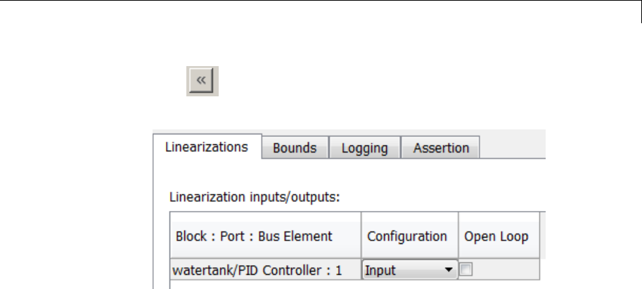
Gain and Phase Margin Plot
4Click to add the signal to the Linearization inputs/outputs
table.
The table displays the following information about the selected signal:
Block : Port : Bus
Element
Name of the block associated with the input/output. The
number adjacent to the block name is the port number where
the selected bus signal is located. The last entry is the
selected bus element name.
Configuration Type of linearization point:
•Input — An input point.
•Output —Anoutputpoint.
•Input-Output — An input point immediately followed by
an output point.
•Output-Input — An output point immediately followed
by an input point.
•None — Signal selected but not specified as a linearization
input or output.
Open Loop If your model contains one or more feedback loops, you
can choose to linearize an open- or closed-loop system. For
example, you might want to linearize only the plant model
within a feedback control loop. When such a feedback loop
is present, select this option to insert an open loop point
10-83

Gain and Phase Margin Plot
and remove the effect of the loop without manually breaking
signal lines.
For determining gain and phase margins, in most cases, you
open the loop.
Note If you simulate the model without specifying an input or output,
the software does not compute a linear system. Instead, you see a
warning message at the MATLAB prompt.
Settings
No default
Command-Line Information
Use the getlinio and setlinio commands to specify linearization
inputs and outputs.
See Also
Plot Linear Characteristics of Simulink Models During Simulation
“Model Verification at Default Simulation Snapshot Time” on page 5-6
10-84

Gain and Phase Margin Plot
Click a signal in the model to select it
Enables signal selection in the Simulink model. Appears only when
you click .
When this option appears, you also see the following changes:
•Anew button.
Use to add a selected signal as a linearization input or output in the
Linearization inputs/outputs table. For more information, see
Linearization inputs/outputs.
•changes to .
UsetocollapsetheClick a signal in the model to select it area.
Settings
No default
Command-Line Information
Use the getlinio and setlinio commands to select signals as
linearization inputs and outputs.
See Also
Plot Linear Characteristics of Simulink Models During Simulation
“Model Verification at Default Simulation Snapshot Time” on page 5-6
10-85

Gain and Phase Margin Plot
Enable regular expression
Enable the use of MATLAB regular expressions for filtering signal
names. For example, entering t$ in the Filter by name edit box
displays all signals whose names end with a lowercase t(and their
immediate parents). For details, see “Regular Expressions”.
Settings
Default: On
On
Allow use of MATLAB regular expressions for filtering signal
names.
Off
Disable use of MATLAB regular expressions for filtering signal
names. Filtering treats the text you enter in the Filter by name
edit box as a literal string.
Dependencies
Selecting the Options button on the right-hand side of the Filter by
name edit box ( ) enables this parameter.
10-86

Gain and Phase Margin Plot
Show filtered results as a flat list
Uses a flat list format to display the list of filtered signals, based on the
search text in the Filter by name edit box. The flat list format uses
dot notation to reflect the hierarchy of bus signals. The following is an
example of a flat list format for a filtered set of nested bus signals.
Settings
Default: Off
On
Display the filtered list of signalsusingaflatlistformat,
indicating bus hierarchies with dot notation instead of using a
tree format.
Off
Display filtered bus hierarchies using a tree format.
10-87

Gain and Phase Margin Plot
Dependencies
Selecting the Options button on the right-hand side of the Filter by
name edit box ( ) enables this parameter.
10-88

Gain and Phase Margin Plot
Linearize on
When to compute the linear system during simulation.
Settings
Default: Simulation snapshots
Simulation snapshots
Specific simulation time, specified in Snapshot times.
Use when you:
•Know one or more times when the model is at steady-state
operating point
•Want to compute the linear systems at specific times
External trigger
Trigger-based simulation event. Specify the trigger type in
Trigger type.
Use when a signal generated during simulation indicates
steady-state operating point.
Selecting this option adds a trigger port to the block. Use this port
to connect the block to the trigger signal.
For example, for an aircraft model, you might want to compute
the linear system whenever the fuel mass is a fraction of the
maximum fuel mass. In this case, model this condition as an
external trigger.
Dependencies
•Setting this parameter to Simulation snapshots enables Snapshot
times.
•Setting this parameter to External trigger enables Trigger type.
Command-Line Information
Parameter: LinearizeAt
10-89


Gain and Phase Margin Plot
Snapshot times
One or more simulation times. The linear system is computed at these
times.
Settings
Default: 0
•For a different simulation time, enter the time. Use when you:
-Want to plot the linear system at a specific time
-Know the approximate time when the model reaches steady-state
operating point
•For multiple simulation times, enter a vector. Use when you want to
compute and plot linear systems at multiple times.
Snapshot times must be less than or equal to the simulation time
specified in the Simulink model.
Dependencies
Selecting Simulation snapshots in Linearize on enables this
parameter.
Command-Line Information
Parameter: SnapshotTimes
Type: string
Value: 0|positive real number |vector of positive real
numbers
Default: 0
See Also
Plot Linear Characteristics of Simulink Models During Simulation
“Model Verification at Default Simulation Snapshot Time” on page 5-6
10-91

Gain and Phase Margin Plot
Trigger type
Trigger type of an external trigger for computing linear system.
Settings
Default: Rising edge
Rising edge
Rising edge of the external trigger signal.
Falling edge
Falling edge of the external trigger signal.
Dependencies
Selecting External trigger in Linearize on enables this parameter.
Command-Line Information
Parameter: TriggerType
Type: string
Value: 'rising' |'falling'
Default: 'rising'
See Also
Plot Linear Characteristics of Simulink Models During Simulation
“Model Verification at Default Simulation Snapshot Time” on page 5-6
10-92

Gain and Phase Margin Plot
Enable zero-crossing detection
Enable zero-crossing detection to ensure that the software computes the
linear system characteristics at the following simulation times:
•The exact snapshot times, specified in Snapshot times.
As shown in the following figure, when zero-crossing detection is
enabled, the variable-step Simulink solver simulates the model at the
snapshot time Tsnap.Tsnap may lie between the simulation time steps
Tn-1 and Tnwhich are automatically chosen by the solver.
Computes linear system
characteristics at this time point
Time
Tn-1 Tn
Tsnap
•The exact times when an external trigger is detected, specified in
Trigger type.
As shown in the following figure, when zero-crossing detection is
enabled, the variable-step Simulink solver simulates the model at the
time, Ttrig, when the trigger signal is detected. Ttrig may lie between
the simulation time steps Tn-1 and Tnwhich are automatically chosen
by the solver.
Computes linear system
characteristics at this time point
Time
Amplitude
1
0Tn-1 Tn
Ttrig
Trigger signal
For more information on zero-crossing detection, see “Zero-Crossing
Detection” in the Simulink User Guide.
10-93

Gain and Phase Margin Plot
Settings
Default: On
On
Compute linear system characteristics at the exact snapshot time
or exact time when a trigger signal is detected.
This setting is ignored if the Simulink solver is fixed step.
Off
Compute linear system characteristics at the simulation time
steps that the variable-step solver chooses. The software may not
compute the linear system at the exact snapshot time or exact
time when a trigger signal is detected.
Command-Line Information
Parameter: ZeroCross
Type: string
Value: 'on' |'off'
Default: 'on'
See Also
Plot Linear Characteristics of Simulink Models During Simulation
“Model Verification at Default Simulation Snapshot Time” on page 5-6
10-94

Gain and Phase Margin Plot
Use exact delays
How to represent time delays in your linear model.
Use this option if you have blocks in your model that have time delays.
Settings
Default: Off
On
Return a linear model with exact delay representations.
Off
Return a linear model with Padé approximations of delays, as
specified in your Transport Delay and Variable Transport Delay
blocks.
Command-Line Information
Parameter: UseExactDelayModel
Type: string
Value: 'on' |'off'
Default: 'off'
See Also
Plot Linear Characteristics of Simulink Models During Simulation
“Model Verification at Default Simulation Snapshot Time” on page 5-6
10-95

Gain and Phase Margin Plot
Linear system sample time
Sample time of the linear system computed during simulation.
Use this parameter to:
•Compute a discrete-time system with a specific sample time from a
continuous-time system
•Resample a discrete-time system with a different sample time
•Compute a continuous-time system from a discrete-time system
When computing discrete-time systems from continuous-time systems
and vice-versa, the software uses the conversion method specified in
Sample time rate conversion method.
Settings
Default: auto
auto. Computes the sample time as:
•0, for continuous-time models.
•For models that have blocks with different sample times
(multi-rate models), least common multiple of the sample
times. For example, if you have a mix of continuous-time and
discrete-time blocks with sample times of 0, 0.2 and 0.3, the
sample time of the linear model is 0.6.
Positive finite value.Usetocompute:
•A discrete-time linear system from a continuous-time system.
•A discrete-time linear system from another discrete-time
system with a different sample time
0
Usetocomputeacontinuous-timelinearsystemfroma
discrete-time model.
Command-Line Information
Parameter: SampleTime
10-96


Gain and Phase Margin Plot
Sample time rate conversion method
Method for converting the sample time of single- or multi-rate models.
This parameter is used only when the value of Linear system sample
time is not auto.
Settings
Default: Zero-Order Hold
Zero-Order Hold
Zero-order hold, where the control inputs are assumed piecewise
constant over the sampling time Ts. For more information, see
“Zero-Order Hold” in Control System Toolbox User’s Guide.
This method usually performs better in time domain.
Tustin (bilinear)
Bilinear (Tustin) approximation without frequency prewarping.
The software rounds off fractional time delays to the nearest
multiple of the sampling time. For more information, see “Tustin
Approximation” in Control System Toolbox User’s Guide.
This method usually perform better in the frequency domain.
Tustin with Prewarping
Bilinear (Tustin) approximation with frequency prewarping. Also
specify the prewarp frequency in Prewarp frequency (rad/s).
For more information, see “Tustin Approximation” in Control
System Toolbox User’s Guide.
This method usually perform better in the frequency domain. Use
this method to ensure matching at frequency region of interest.
Upsampling when possible, Zero-Order Hold otherwise
Upsample a discrete-time system when possible and use
Zero-Order Hold otherwise.
10-98

Gain and Phase Margin Plot
You can upsample only when you convert discrete-time system to
a new sample time that is an integer-value-times faster than the
sampling time of the original system.
Upsampling when possible, Tustin otherwise
Upsample a discrete-time system when possible and use Tustin
(bilinear) otherwise.
You can upsample only when you convert discrete-time system to
a new sample time that is an integer-value-times faster than the
sampling time of the original system.
Upsampling when possible, Tustin with Prewarping otherwise
Upsample a discrete-time system when possible and use Tustin
with Prewarping otherwise. Also, specify the prewarp frequency
in Prewarp frequency (rad/s).
You can upsample only when you convert discrete-time system to
a new sample time that is an integer-value-times faster than the
sampling time of the original system.
Dependencies
Selecting either:
•Tustin with Prewarping
•Upsampling when possible, Tustin with Prewarping
otherwise
enables Prewarp frequency (rad/s).
Command-Line Information
Parameter: RateConversionMethod
Type: string
Value: 'zoh' |'tustin' |'prewarp'|'upsampling_zoh'|
'upsampling_tustin'|'upsampling_prewarp'
Default: 'zoh'
10-99


Gain and Phase Margin Plot
Prewarp frequency (rad/s)
Prewarp frequency for Tustin method, specified in radians/second.
Settings
Default: 10
Positive scalar value, smaller than the Nyquist frequency before and
after resampling. A value of 0 corresponds to the standard Tustin
method without frequency prewarping.
Dependencies
Selecting either
•Tustin with Prewarping
•Upsampling when possible, Tustin with Prewarping
otherwise
in Sample time rate conversion method enablesthisparameter.
Command-Line Information
Parameter: PreWarpFreq
Type: string
Value: 10 |positive scalar value
Default: 10
See Also
Plot Linear Characteristics of Simulink Models During Simulation
“Model Verification at Default Simulation Snapshot Time” on page 5-6
10-101

Gain and Phase Margin Plot
Use full block names
How the state, input and output names appear in the linear system
computed during simulation.
The linear system is a state-space object and system states and
input/output names appear in following state-space object properties:
Input, Output or State Name Appears in Which State-Space
Object Property
Linearization input name InputName
Linearization output name OutputName
State names StateName
Settings
Default: Off
On
Show state and input/output names with their path through the
model hierarchy. For example, in the chemical reactor model,
a state in the Integrator1 block of the CSTR subsystem appears
with full path as scdcstr/CSTR/Integrator1.
Off
Show only state and input/output names. Use this option when the
signal name is unique and you know where the signal is location
in your Simulink model. For example, a state in the Integrator1
block of the CSTR subsystem appears as Integrator1.
Command-Line Information
Parameter: UseFullBlockNameLabels
Type: string
Value: 'on' |'off'
Default: 'off'
See Also
Plot Linear Characteristics of Simulink Models During Simulation
10-102


Gain and Phase Margin Plot
Use bus signal names
How to label signals associated with linearization inputs and outputs
on buses, in the linear system computed during simulation (applies only
when you select an entire bus as an I/O point).
Selecting an entire bus signal is not recommended. Instead, select
individual bus elements.
You cannot use this parameter when your model has mux/bus mixtures.
Settings
Default: Off
On
Use the signal names of the individual bus elements.
Bus signal names appear when the input and output are at the
output of the following blocks:
•Root-level inport block containing a bus object
•Bus creator block
•Subsystem block whose source traces back to one of the
following blocks:
—Output of a bus creator block
—Root-level inport block by passing through only virtual or
nonvirtual subsystem boundaries
Off
Use the bus signal channel number.
Command-Line Information
Parameter: UseBusSignalLabels
Type: string
Value: 'on' |'off'
Default: 'off'
10-104


Gain and Phase Margin Plot
Include gain and phase margins in assertion
Check that the gain and phase margins are greater than the values
specified in Gain margin (dB) > and Phase margin (deg) >,during
simulation. The software displays a warning if the gain or phase margin
is less than or equals the specified value.
By default, negative feedback, specified in Feedback sign,isused
to compute the margins.
This parameter is used for assertion only if Enable assertion in the
Assertion tab is selected.
You can view the gain and phase margin bound on one of the following
plot types:
•Bode
•Nichols
•Nyquist
•Table
If you clear Enable assertion, the bounds are not used for assertion
but continue to appear on the plot.
Settings
Default:
•Off for Gain and Phase Margin Plot block.
•On for Check Gain and Phase Margins block.
On
Check that the gain and phase margins satisfy the specified
values, during simulation.
Off
Do not check that the gain and phase margins satisfy the specified
values, during simulation.
10-106

Gain and Phase Margin Plot
Tips
•Clearing this parameter disables the gain and phase margin bounds
and the software stops checking that the gain and phase margins
satisfy the bounds during simulation. The gain and phase margin
bounds are also disabled on the plot.
•Toonlyviewthegainandphasemarginontheplot,clearEnable
assertion.
Command-Line Information
Parameter: EnableMargins
Type: string
Value: 'on' |'off'
Default: 'off' for Gain and Phase Margin Plot block, 'on' for
Check Gain and Phase Margins block
See Also
Plot Linear Characteristics of Simulink Models During Simulation
“Model Verification at Default Simulation Snapshot Time” on page 5-6
10-107

Gain and Phase Margin Plot
Gain margin (dB) >
Gain margin, specified in decibels.
By default, negative feedback, specified in Feedback sign,isusedto
compute the gain margin.
You can specify only one gain margin bound on the linear system in
this block.
Settings
Default:
[] for Gain and Phase Margin Plot block.
20 for Check Gain and Phase Margins block.
Positive finite number.
Tips
•To assert that the gain margin is satisfied, select both Include gain
and phase margins in assertion and Enable assertion.
•To modify the gain margin from the plot window, right-click the plot,
and select Bounds > Edit Bound. Specify the new gain margin in
Gain margin >.YoumustclickUpdate Block before simulating
the model.
Command-Line Information
Parameter: GainMargin
Type: string
Value: [] |20 |positive finite number.Mustbespecified
inside single quotes ('').
Default: '[]' for Gain and Phase Margin Plot block, '20' for Check
Gain and Phase Margins block.
See Also
Plot Linear Characteristics of Simulink Models During Simulation
“Model Verification at Default Simulation Snapshot Time” on page 5-6
10-108

Gain and Phase Margin Plot
Phase margin (deg) >
Phase margin, specified in degrees.
By default, negative feedback, specified in Feedback sign,isusedto
computethephasemargin.
You can specify only one phase margin bound on the linear system in
this block.
Settings
Default:
[] for Gain and Phase Margin Plot block.
30 for Check Gain and Phase Margins block.
Positive finite number.
Tips
•To assert that the phase margin is satisfied, select both Include
gain and phase margins in assertion and Enable assertion.
•To modify the phase margin from the plot window, right-click the
plot, and select Bounds > Edit Bound.Specifythenewphase
margin in Phase margin >.YoumustclickUpdate Block before
simulating the model.
Command-Line Information
Parameter: PhaseMargin
Type: string
Value: [] |30 |positive finite number.Mustbespecified
inside single quotes ('').
Default: '[]' for Gain and Phase Margin Plot block, '30' for Check
Gain and Phase Margins block.
See Also
Plot Linear Characteristics of Simulink Models During Simulation
“Model Verification at Default Simulation Snapshot Time” on page 5-6
10-109

Gain and Phase Margin Plot
Feedback sign
Feedback sign to determine the gain and phase margins of the linear
system, computed during simulation.
To determine the feedback sign, check if the path defined by the
linearization inputs and outputs include the feedback Sum block:
•If the path includes the Sum block, specify positive feedback.
•IfthepathdoesnotincludetheSum block, specify the same feedback
sign as the Sum block.
For example, in the aircraft model, the Check Gain and Phase Margins
block includes the negative sign in the summation block. Therefore,
the Feedback sign is positive.
Settings
Default: negative feedback
negative feedback
Use when the path defined by the linearization inputs/outputs
does not include the Sum block and the Sum block feedback sign
is -.
positive feedback
Use when:
•The path defined by the linearization inputs/outputs includes
the Sum block.
•The path defined by the linearization inputs/outputs does not
include the Sum block and the Sum block feedback sign is +.
Command-Line Information
Parameter: FeedbackSign
Type: string
Value: '-1' |'+1'
Default: '-1'
10-110


Gain and Phase Margin Plot
Save data to workspace
Save one or more linear systems as a variable in MATLAB workspace to
perform further linear analysis or control design.
The workspace variable is a structure with time and values fields:
•The time field stores the simulation time at which the linear system
is computed.
•The values field is a state-space object which stores the linear
system. If the linear system is computed at multiple simulation
times, values is an array of state-space objects.
Settings
Default: Off
On
Save the computed linear system to MATLAB workspace.
Off
Do not save the computed linear system to MATLAB workspace.
Dependencies
This parameter enables Variable name.
Command-Line Information
Parameter: SaveToWorkspace
Type: string
Value: 'on' |'off'
Default: 'off'
See Also
Plot Linear Characteristics of Simulink Models During Simulation
“Model Verification at Default Simulation Snapshot Time” on page 5-6
10-112

Gain and Phase Margin Plot
Variable name
Name of the workspace variable that stores one or more linear systems
computed during simulation.
The name must be unique among the variable names used in all data
logging model blocks, such as Linear Analysis Plot blocks, Model
Verification blocks, Scope blocks, To Workspace blocks, and simulation
return variables such as time, states, and outputs.
Settings
Default: sys
String.
Dependencies
Save data to workspace enables this parameter.
Command-Line Information
Parameter: SaveName
Type: string
Value: sys |any string. Must be specified inside single quotes
('').
Default: 'sys'
See Also
Plot Linear Characteristics of Simulink Models During Simulation
“Model Verification at Default Simulation Snapshot Time” on page 5-6
10-113

Gain and Phase Margin Plot
Enable assertion
Enable the block to check that bounds specified and included for
assertion in the Bounds tab are satisfied during simulation. Assertion
failsifaboundisnotsatisfied. Awarning, reporting the assertion
failure, appears at the MATLAB prompt.
If assertion fails, you can optionally specify that the block:
•Execute a MATLAB expression, specified in Simulation callback
when assertion fails (optional).
•Stop the simulation and bring that block into focus, by selecting Stop
simulation when assertion fails.
For the Linear Analysis Plots blocks, this parameter has no effect
because no bounds are included by default. If you want to use the
Linear Analysis Plots blocks for assertion, specify and include
bounds in the Bounds tab.
Clearing this parameter disables assertion, i.e., the block no longer
checks that specified bounds are satisfied. The block icon also updates
to indicate that assertion is disabled.
In the Configuration Parameters dialog box of the Simulink model, the
Model Verification block enabling option in the Debugging area of
Data Validity node, lets you to enable or disable all model verification
blocks in a model, regardless of the setting of this option.
Settings
Default: On
10-114

Gain and Phase Margin Plot
On
Check that bounds included for assertion in the Bounds tab
are satisfied during simulation. A warning, reporting assertion
failure, is displayed at the MATLAB prompt if bounds are violated.
Off
Do not check that bounds included for assertion are satisfied
during simulation.
Dependencies
This parameter enables:
•Simulation callback when assertion fails (optional)
•Stop simulation when assertion fails
Command-Line Information
Parameter: enabled
Type: string
Value: 'on' |'off'
Default: 'on'
See Also
Plot Linear Characteristics of Simulink Models During Simulation
“Model Verification at Default Simulation Snapshot Time” on page 5-6
10-115

Gain and Phase Margin Plot
Simulation callback when assertion fails (optional)
MATLAB expression to execute when assertion fails.
Because the expression is evaluated in the MATLAB workspace, define
all variables used in the expression in that workspace.
Settings
No Default
AMATLABexpression.
Dependencies
Enable assertion enables this parameter.
Command-Line Information
Parameter: callback
Type: string
Value: '' |MATLAB expression
Default: ''
See Also
Plot Linear Characteristics of Simulink Models During Simulation
“Model Verification at Default Simulation Snapshot Time” on page 5-6
10-116

Gain and Phase Margin Plot
Stop simulation when assertion fails
Stop the simulation when a bound specified in the Bounds tab is
violated during simulation, i.e., assertion fails.
If you run the simulation from the Simulink Editor, the Simulation
Diagnostics window opens to display an error message. Also, the block
where the bound violation occurs is highlighted in the model.
Settings
Default: Off
On
Stop simulation if a bound specified in the Bounds tab is violated.
Off
Continue simulation if a bound is violated with a warning
message at the MATLAB prompt.
Tips
•Because selecting this option stops the simulation as soon as the
assertion fails, assertion failures that might occur later during the
simulation are not reported. If you want all assertion failures to be
reported, do not select this option.
Dependencies
Enable assertion enables this parameter.
Command-Line Information
Parameter: stopWhenAssertionFail
Type: string
Value: 'on' |'off'
Default: 'off'
See Also
Plot Linear Characteristics of Simulink Models During Simulation
“Model Verification at Default Simulation Snapshot Time” on page 5-6
10-117

Gain and Phase Margin Plot
Output assertion signal
Output a Boolean signal that, at each time step, is:
•True (1) if assertion succeeds, i.e., all bounds are satisfied
•False (1)ifassertionfails,i.e.,aboundisviolated.
The output signal data type is Boolean only if the Implement logic
signals as Boolean data option in the Optimization pane of the
Configuration Parameters dialog box of the Simulink model is selected.
Otherwise, the data type of the output signal is double.
Selecting this parameter adds an output port to the block that you can
connect to any block in the model.
Settings
Default:Off
On
Output a Boolean signal to indicate assertion status. Adds a
port to the block.
Off
Do not output a Boolean signal to indicate assertion status.
Tips
•Use this parameter to design complex assertion logic. For an
example, see “Model Verification Using Simulink®Control Design™
and Simulink Verification Blocks” on page 5-25.
Command-Line Information
Parameter: export
Type: string
Value: 'on' |'off'
Default: 'off'
See Also
Plot Linear Characteristics of Simulink Models During Simulation
10-118


Gain and Phase Margin Plot
Plot type
Plot to view gain and phase margins of the linear system computed
during simulation.
Settings
Default: Bode
Bode
Bode plot.
Nichols
Nichols plot
Nyquist
Nyquist plot
Tabular
Table.
Right-click the Bode , Nichols or Nyquist plot and select
Characteristics > Minimum Stability Margins to view gain and
phase margins. The table displays the computed margins automatically.
Command-Line Information
Parameter: PlotType
Type: string
Value: 'bode' |'nichols' |'nyquist' |'table'
Default: 'bode'
See Also
Plot Linear Characteristics of Simulink Models During Simulation
“Model Verification at Default Simulation Snapshot Time” on page 5-6
10-120

Gain and Phase Margin Plot
Show plot on block open
Open the plot window instead of the Block Parameters dialog box when
you double-click the block in the Simulink model.
Usethisparameterifyouprefertoopenandperformtasks,suchas
adding or modifying bounds, in the plot window instead of the Block
Parameters dialog box. If you want to access the block parameters from
the plot window, select Edit or click .
For more information on the plot, see Show Plot.
Settings
Default: Off
On
Open the plot window when you double-click the block.
Off
Open the Block Parameters dialog box when double-clicking the
block.
Command-Line Information
Parameter: LaunchViewOnOpen
Type: string
Value: 'on' |'off'
Default: 'off'
See Also
Plot Linear Characteristics of Simulink Models During Simulation
“Model Verification at Default Simulation Snapshot Time” on page 5-6
Show Plot Open the plot window.
Use the plot to view:
•Linear system characteristics computed from the nonlinear Simulink
model during simulation
10-121

Gain and Phase Margin Plot
You must click this button before you simulate the model to view
the linear characteristics.
You can display additional characteristics, such as the peak response
time and stability margins, of the linear system by right-clicking the
plot and selecting Characteristics.
•Bounds on the linear system characteristics
You can specify bounds in the Bounds tab of the Block Parameters
dialog box or right-click the plot and select Bounds > New Bound.
For more information on the types of bounds you can specify on each
plot, see “Verifiable Linear System Characteristics” on page 5-5 in
the User’s Guide.
You can modify bounds by dragging the bound segment or by
right-clicking the plot and selecting Bounds > Edit Bound. Before
you simulate the model, click Update Block to update the bound
value in the block parameters.
Typical tasks that you perform in the plot window include:
•Opening the Block Parameters dialog box by clicking or selecting
Edit.
•Finding the block that the plot window corresponds to by clicking
or selecting View > Highlight Simulink Block.Thisactionmakes
the Simulink Editor active and highlights the block.
•Simulating the model by clicking or selecting Simulation > Run.
This action also linearizes the portion of the model between the
specified linearization input and output.
•Adding legend on the linear system characteristic plot by clicking .
See Also Check Gain and Phase Margins
Tutorials •“Visualize Bode Response of Simulink Model During Simulation”
on page 2-42
10-122


Linear Step Response Plot
Purpose Step response of linear system approximated from nonlinear Simulink
model
Library Simulink Control Design
Description This block is same as the Check Linear Step Response Characteristics
block except for different default parameter settings in the Bounds tab.
Compute a linear system from a nonlinear Simulink model and plot
the linear step response.
During simulation, the software linearizes the portion of the model
between specified linearization inputs and outputs, and plots the step
response of the linear system.
The Simulink model can be continuous- or discrete-time or multirate
and can have time delays. Because you can specify only one linearization
input/output pair in this block, thelinearsystemisSingle-Input
Single-Output (SISO).
You can specify step response bounds and view them on the plot. You
can also check that the bounds are satisfied during simulation:
•If all bounds are satisfied, the block does nothing.
•If a bound is not satisfied, the block asserts, and a warning message
appears at the MATLAB prompt. You can also specify that the block:
-Evaluate a MATLAB expression.
-Stop the simulation and bring that block into focus.
During simulation, the block can also output a logical assertion signal:
•If all bounds are satisfied, the signal is true (1).
•If a bound is not satisfied, the signal is false (0).
YoucanaddmultipleLinearStepResponsePlotblockstocomputeand
plot the linear step response of various portions of the model.
10-124

Linear Step Response Plot
You can save the linear system as a variable in the MATLAB workspace.
The block does not support code generation and can be used only in
Normal simulation mode.
Parameters The following table summarizes the Linear Step Response Plot block
parameters, accessible via the block parameter dialog box.
Task Parameters
Specify inputs and
outputs (I/Os).
In Linearizations
tab:
•“Linearization
inputs/outputs”
on page 10-287.
•“Click a signal in
the model to select
it” on page 10-290.
Specify settings. In Linearizations
tab:
•“Linearize on” on
page 10-294.
•“Snapshot times”
on page 10-296.
•“Trigger type” on
page 10-297.
Specify algorithm
options.
In Algorithm
Options of
Linearizations tab:
•“Enable
zero-crossing
Configure
linearization.
10-125

Linear Step Response Plot
Task Parameters
detection” on page
10-298.
•“Use exact delays”
on page 10-300.
•“Linear system
sample time” on
page 10-301.
•“Sample time
rate conversion
method” on page
10-303.
•“Prewarp
frequency (rad/s)”
on page 10-306.
Specify labels for
linear system I/Os
and state names.
In Labels of
Linearizations tab:
•“Use full block
names” on page
10-307.
•“Use bus signal
names” on page
10-309.
Plot the linear system. Show Plot
(Optional) Specify bounds on step response of
the linear system for assertion.
Include step response
bound in assertion in
Bounds tab.
10-126

Linear Step Response Plot
Task Parameters
Specify assertion options (only when you
specify bounds on the linear system).
In Assertion tab:
•“Enable assertion”
on page 10-325.
•“Simulation
callback when
assertion fails
(optional)” on page
10-327.
•“Stop simulation
when assertion
fails” on page
10-328.
•“Output assertion
signal” on page
10-329.
Save linear system to MATLAB workspace. “Save data to
workspace” on page
10-323 in Logging
tab.
Display plot window instead of block
parameters dialog box on double-clicking the
block.
“Show plot on block
open” on page 10-331.
Linearization inputs/outputs
Linearization inputs and outputs that define the portion of a nonlinear
Simulink model to linearize.
1Click .
10-127
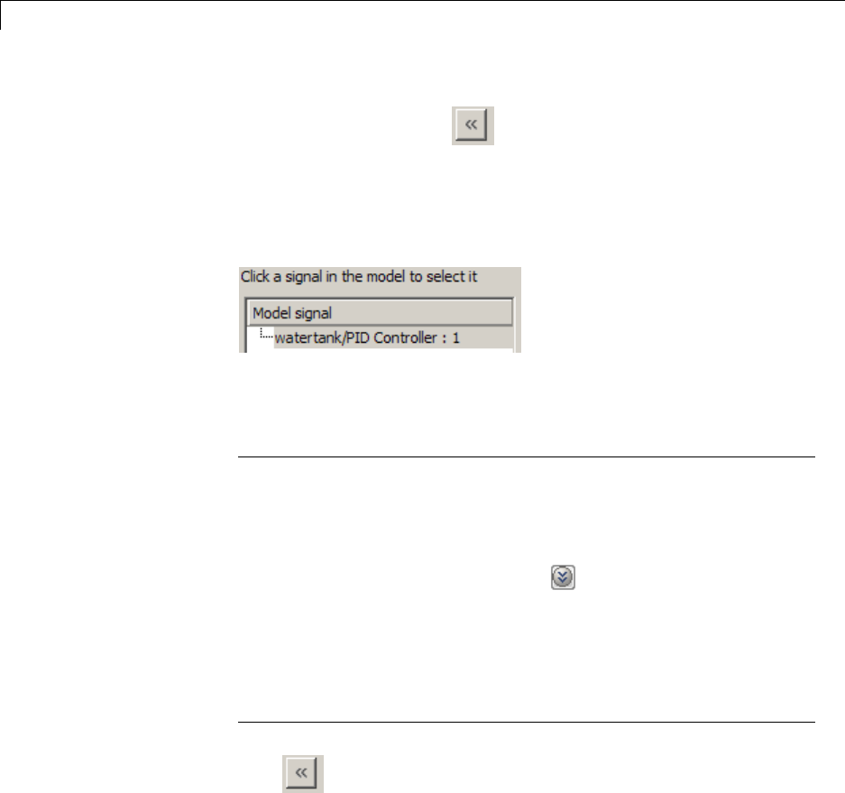
Linear Step Response Plot
The dialog box expands to display a Click a signal in the model to
select it area and a new button.
2Select a signal in the Simulink Editor.
The selected signal appears as a Model signal in the Click a signal
in the model to select it area.
3(Optional) For buses, expand the bus signal to select an individual
element.
Tip For large buses, you can enter search text for filtering element
names in the Filter by name edit box. The name match is
case-sensitive. Additionally, you can enter MATLAB regular
expression.
To modify the filtering options, click .
Filtering Options
•“Enable regular expression” on page 10-291
•“Show filtered results as aflatlist”onpage10-292
4Click to add the signal to the Linearization inputs/outputs
table.
10-128
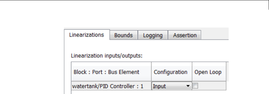
Linear Step Response Plot
The table displays the following information about the selected signal:
Block : Port : Bus
Element
Name of the block associated with the input/output. The
number adjacent to the block name is the port number where
the selected bus signal is located. The last entry is the
selected bus element name.
Configuration Type of linearization point:
•Input — An input point.
•Output —Anoutputpoint.
•Input-Output — An input point immediately followed by
an output point.
•Output-Input — An output point immediately followed
by an input point.
•None — Signal selected but not specified as a linearization
input or output.
Open Loop If your model contains one or more feedback loops, you
can choose to linearize an open- or closed-loop system. For
example, you might want to linearize only the plant model
within a feedback control loop. When such a feedback loop
is present, select this option to insert an open loop point
and remove the effect of the loop without manually breaking
signal lines.
10-129

Linear Step Response Plot
For determining gain and phase margins, in most cases, you
open the loop.
Note If you simulate the model without specifying an input or output,
the software does not compute a linear system. Instead, you see a
warning message at the MATLAB prompt.
Settings
No default
Command-Line Information
Use the getlinio and setlinio commands to specify linearization
inputs and outputs.
See Also
Plot Linear Characteristics of Simulink Models During Simulation
“Model Verification at Default Simulation Snapshot Time” on page 5-6
10-130

Linear Step Response Plot
Click a signal in the model to select it
Enables signal selection in the Simulink model. Appears only when
you click .
When this option appears, you also see the following changes:
•Anew button.
Use to add a selected signal as a linearization input or output in the
Linearization inputs/outputs table. For more information, see
Linearization inputs/outputs.
•changes to .
UsetocollapsetheClick a signal in the model to select it area.
Settings
No default
Command-Line Information
Use the getlinio and setlinio commands to select signals as
linearization inputs and outputs.
See Also
Plot Linear Characteristics of Simulink Models During Simulation
“Model Verification at Default Simulation Snapshot Time” on page 5-6
10-131

Linear Step Response Plot
Enable regular expression
Enable the use of MATLAB regular expressions for filtering signal
names. For example, entering t$ in the Filter by name edit box
displays all signals whose names end with a lowercase t(and their
immediate parents). For details, see “Regular Expressions”.
Settings
Default: On
On
Allow use of MATLAB regular expressions for filtering signal
names.
Off
Disable use of MATLAB regular expressions for filtering signal
names. Filtering treats the text you enter in the Filter by name
edit box as a literal string.
Dependencies
Selecting the Options button on the right-hand side of the Filter by
name edit box ( ) enables this parameter.
10-132
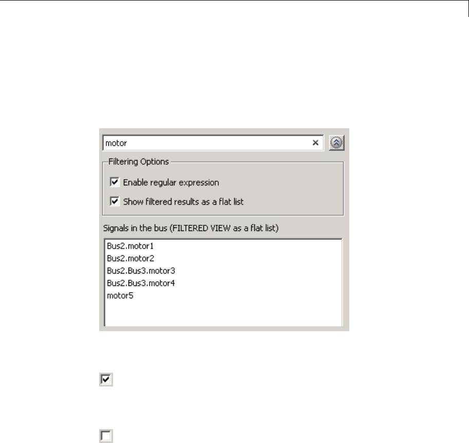
Linear Step Response Plot
Show filtered results as a flat list
Uses a flat list format to display the list of filtered signals, based on the
search text in the Filter by name edit box. The flat list format uses
dot notation to reflect the hierarchy of bus signals. The following is an
example of a flat list format for a filtered set of nested bus signals.
Settings
Default: Off
On
Display the filtered list of signalsusingaflatlistformat,
indicating bus hierarchies with dot notation instead of using a
tree format.
Off
Display filtered bus hierarchies using a tree format.
10-133

Linear Step Response Plot
Dependencies
Selecting the Options button on the right-hand side of the Filter by
name edit box ( ) enables this parameter.
10-134

Linear Step Response Plot
Linearize on
When to compute the linear system during simulation.
Settings
Default: Simulation snapshots
Simulation snapshots
Specific simulation time, specified in Snapshot times.
Use when you:
•Know one or more times when the model is at steady-state
operating point
•Want to compute the linear systems at specific times
External trigger
Trigger-based simulation event. Specify the trigger type in
Trigger type.
Use when a signal generated during simulation indicates
steady-state operating point.
Selecting this option adds a trigger port to the block. Use this port
to connect the block to the trigger signal.
For example, for an aircraft model, you might want to compute
the linear system whenever the fuel mass is a fraction of the
maximum fuel mass. In this case, model this condition as an
external trigger.
Dependencies
•Setting this parameter to Simulation snapshots enables Snapshot
times.
•Setting this parameter to External trigger enables Trigger type.
Command-Line Information
Parameter: LinearizeAt
10-135


Linear Step Response Plot
Snapshot times
One or more simulation times. The linear system is computed at these
times.
Settings
Default: 0
•For a different simulation time, enter the time. Use when you:
-Want to plot the linear system at a specific time
-Know the approximate time when the model reaches steady-state
operating point
•For multiple simulation times, enter a vector. Use when you want to
compute and plot linear systems at multiple times.
Snapshot times must be less than or equal to the simulation time
specified in the Simulink model.
Dependencies
Selecting Simulation snapshots in Linearize on enables this
parameter.
Command-Line Information
Parameter: SnapshotTimes
Type: string
Value: 0|positive real number |vector of positive real
numbers
Default: 0
See Also
Plot Linear Characteristics of Simulink Models During Simulation
“Model Verification at Default Simulation Snapshot Time” on page 5-6
10-137

Linear Step Response Plot
Trigger type
Trigger type of an external trigger for computing linear system.
Settings
Default: Rising edge
Rising edge
Rising edge of the external trigger signal.
Falling edge
Falling edge of the external trigger signal.
Dependencies
Selecting External trigger in Linearize on enables this parameter.
Command-Line Information
Parameter: TriggerType
Type: string
Value: 'rising' |'falling'
Default: 'rising'
See Also
Plot Linear Characteristics of Simulink Models During Simulation
“Model Verification at Default Simulation Snapshot Time” on page 5-6
10-138

Linear Step Response Plot
Enable zero-crossing detection
Enable zero-crossing detection to ensure that the software computes the
linear system characteristics at the following simulation times:
•The exact snapshot times, specified in Snapshot times.
As shown in the following figure, when zero-crossing detection is
enabled, the variable-step Simulink solver simulates the model at the
snapshot time Tsnap.Tsnap may lie between the simulation time steps
Tn-1 and Tnwhich are automatically chosen by the solver.
Computes linear system
characteristics at this time point
Time
Tn-1 Tn
Tsnap
•The exact times when an external trigger is detected, specified in
Trigger type.
As shown in the following figure, when zero-crossing detection is
enabled, the variable-step Simulink solver simulates the model at the
time, Ttrig, when the trigger signal is detected. Ttrig may lie between
the simulation time steps Tn-1 and Tnwhich are automatically chosen
by the solver.
Computes linear system
characteristics at this time point
Time
Amplitude
1
0Tn-1 Tn
Ttrig
Trigger signal
For more information on zero-crossing detection, see “Zero-Crossing
Detection” in the Simulink User Guide.
10-139

Linear Step Response Plot
Settings
Default: On
On
Compute linear system characteristics at the exact snapshot time
or exact time when a trigger signal is detected.
This setting is ignored if the Simulink solver is fixed step.
Off
Compute linear system characteristics at the simulation time
steps that the variable-step solver chooses. The software may not
compute the linear system at the exact snapshot time or exact
time when a trigger signal is detected.
Command-Line Information
Parameter: ZeroCross
Type: string
Value: 'on' |'off'
Default: 'on'
See Also
Plot Linear Characteristics of Simulink Models During Simulation
“Model Verification at Default Simulation Snapshot Time” on page 5-6
10-140

Linear Step Response Plot
Use exact delays
How to represent time delays in your linear model.
Use this option if you have blocks in your model that have time delays.
Settings
Default: Off
On
Return a linear model with exact delay representations.
Off
Return a linear model with Padé approximations of delays, as
specified in your Transport Delay and Variable Transport Delay
blocks.
Command-Line Information
Parameter: UseExactDelayModel
Type: string
Value: 'on' |'off'
Default: 'off'
See Also
Plot Linear Characteristics of Simulink Models During Simulation
“Model Verification at Default Simulation Snapshot Time” on page 5-6
Linear system sample time
Sample time of the linear system computed during simulation.
Use this parameter to:
•Compute a discrete-time system with a specific sample time from a
continuous-time system
•Resample a discrete-time system with a different sample time
•Compute a continuous-time system from a discrete-time system
10-141

Linear Step Response Plot
When computing discrete-time systems from continuous-time systems
and vice-versa, the software uses the conversion method specified in
Sample time rate conversion method.
Settings
Default: auto
auto. Computes the sample time as:
•0, for continuous-time models.
•For models that have blocks with different sample times
(multi-rate models), least common multiple of the sample
times. For example, if you have a mix of continuous-time and
discrete-time blocks with sample times of 0, 0.2 and 0.3, the
sample time of the linear model is 0.6.
Positive finite value.Usetocompute:
•A discrete-time linear system from a continuous-time system.
•A discrete-time linear system from another discrete-time
system with a different sample time
0
Usetocomputeacontinuous-timelinearsystemfroma
discrete-time model.
Command-Line Information
Parameter: SampleTime
Type: string
Value: auto |Positive finite value |0
Default: auto
See Also
Plot Linear Characteristics of Simulink Models During Simulation
“Model Verification at Default Simulation Snapshot Time” on page 5-6
10-142

Linear Step Response Plot
10-143

Linear Step Response Plot
Sample time rate conversion method
Method for converting the sample time of single- or multi-rate models.
This parameter is used only when the value of Linear system sample
time is not auto.
Settings
Default: Zero-Order Hold
Zero-Order Hold
Zero-order hold, where the control inputs are assumed piecewise
constant over the sampling time Ts. For more information, see
“Zero-Order Hold” in Control System Toolbox User’s Guide.
This method usually performs better in time domain.
Tustin (bilinear)
Bilinear (Tustin) approximation without frequency prewarping.
The software rounds off fractional time delays to the nearest
multiple of the sampling time. For more information, see “Tustin
Approximation” in Control System Toolbox User’s Guide.
This method usually perform better in the frequency domain.
Tustin with Prewarping
Bilinear (Tustin) approximation with frequency prewarping. Also
specify the prewarp frequency in Prewarp frequency (rad/s).
For more information, see “Tustin Approximation” in Control
System Toolbox User’s Guide.
This method usually perform better in the frequency domain. Use
this method to ensure matching at frequency region of interest.
Upsampling when possible, Zero-Order Hold otherwise
Upsample a discrete-time system when possible and use
Zero-Order Hold otherwise.
10-144

Linear Step Response Plot
You can upsample only when you convert discrete-time system to
a new sample time that is an integer-value-times faster than the
sampling time of the original system.
Upsampling when possible, Tustin otherwise
Upsample a discrete-time system when possible and use Tustin
(bilinear) otherwise.
You can upsample only when you convert discrete-time system to
a new sample time that is an integer-value-times faster than the
sampling time of the original system.
Upsampling when possible, Tustin with Prewarping otherwise
Upsample a discrete-time system when possible and use Tustin
with Prewarping otherwise. Also, specify the prewarp frequency
in Prewarp frequency (rad/s).
You can upsample only when you convert discrete-time system to
a new sample time that is an integer-value-times faster than the
sampling time of the original system.
Dependencies
Selecting either:
•Tustin with Prewarping
•Upsampling when possible, Tustin with Prewarping
otherwise
enables Prewarp frequency (rad/s).
Command-Line Information
Parameter: RateConversionMethod
Type: string
Value: 'zoh' |'tustin' |'prewarp'|'upsampling_zoh'|
'upsampling_tustin'|'upsampling_prewarp'
Default: 'zoh'
10-145

Linear Step Response Plot
See Also
Plot Linear Characteristics of Simulink Models During Simulation
“Model Verification at Default Simulation Snapshot Time” on page 5-6
Prewarp frequency (rad/s)
Prewarp frequency for Tustin method, specified in radians/second.
Settings
Default: 10
Positive scalar value, smaller than the Nyquist frequency before and
after resampling. A value of 0 corresponds to the standard Tustin
method without frequency prewarping.
Dependencies
Selecting either
•Tustin with Prewarping
•Upsampling when possible, Tustin with Prewarping
otherwise
in Sample time rate conversion method enablesthisparameter.
Command-Line Information
Parameter: PreWarpFreq
Type: string
Value: 10 |positive scalar value
Default: 10
See Also
Plot Linear Characteristics of Simulink Models During Simulation
“Model Verification at Default Simulation Snapshot Time” on page 5-6
10-146

Linear Step Response Plot
Use full block names
How the state, input and output names appear in the linear system
computed during simulation.
The linear system is a state-space object and system states and
input/output names appear in following state-space object properties:
Input, Output or State Name Appears in Which State-Space
Object Property
Linearization input name InputName
Linearization output name OutputName
State names StateName
Settings
Default: Off
On
Show state and input/output names with their path through the
model hierarchy. For example, in the chemical reactor model,
a state in the Integrator1 block of the CSTR subsystem appears
with full path as scdcstr/CSTR/Integrator1.
Off
Show only state and input/output names. Use this option when the
signal name is unique and you know where the signal is location
in your Simulink model. For example, a state in the Integrator1
block of the CSTR subsystem appears as Integrator1.
Command-Line Information
Parameter: UseFullBlockNameLabels
Type: string
Value: 'on' |'off'
Default: 'off'
See Also
Plot Linear Characteristics of Simulink Models During Simulation
10-147

Linear Step Response Plot
“Model Verification at Default Simulation Snapshot Time” on page 5-6
Use bus signal names
How to label signals associated with linearization inputs and outputs
on buses, in the linear system computed during simulation (applies only
when you select an entire bus as an I/O point).
Selecting an entire bus signal is not recommended. Instead, select
individual bus elements.
You cannot use this parameter when your model has mux/bus mixtures.
Settings
Default: Off
On
Use the signal names of the individual bus elements.
Bus signal names appear when the input and output are at the
output of the following blocks:
•Root-level inport block containing a bus object
•Bus creator block
•Subsystem block whose source traces back to one of the
following blocks:
—Output of a bus creator block
—Root-level inport block by passing through only virtual or
nonvirtual subsystem boundaries
Off
Use the bus signal channel number.
Command-Line Information
Parameter: UseBusSignalLabels
Type: string
Value: 'on' |'off'
10-148


Linear Step Response Plot
Include step response bound in assertion
Check that the linear step response satisfies all the characteristics
specified in:
•Final value
•Rise time and %Rise
•Settling time and % Settling
•% Overshoot
•% Undershoot
The software displays a warning if the step response violates the
specified values.
This parameter is used for assertion only if Enable assertion in the
Assertion tab is selected.
10-150
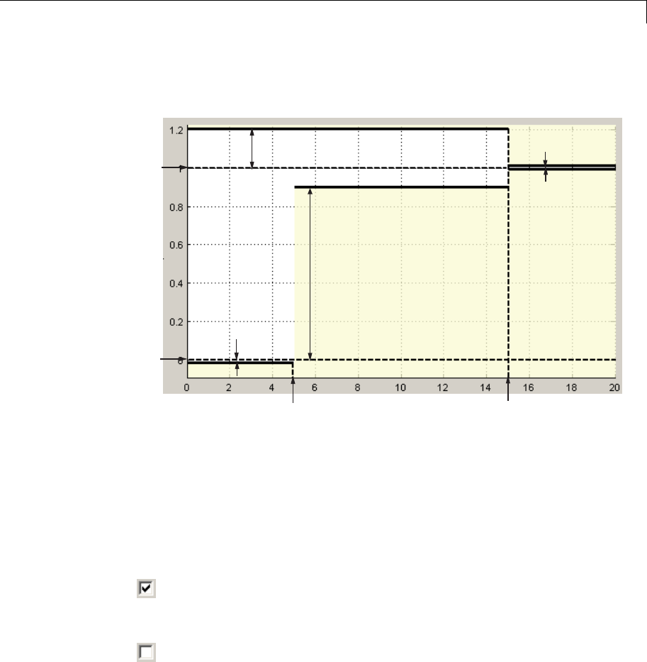
Linear Step Response Plot
Theboundsalsoappearonthestepresponseplot,asshowninthe
next figure.
Settling time
Rise time
% Undershoot
% Settling
% Overshoot
% Rise
Final
value
Initial
value
If you clear Enable assertion, the bounds are not used for assertion
but continue to appear on the plot.
Settings
Default:
•Off for Linear Step Response Plot block.
•On for Check Linear Step Response Characteristics block.
On
Check that the step response satisfies the specified bounds,
during simulation.
Off
Do not check that the step response satisfies the specified bounds,
during simulation.
10-151

Linear Step Response Plot
Tips
•Clearing this parameter disables the step response bounds and
the software stops checking that the bounds are satisfied during
simulation. The bound segments are also greyed out on the plot.
•To only view the bounds on the plot, clear Enable assertion.
Command-Line Information
Parameter: EnableStepResponseBound
Type: string
Value: 'on' |'off'
Default: 'off' for Linear Step Response Plot block, 'on' for Check
Linear Step Response Characteristics block.
See Also
Plot Linear Characteristics of Simulink Models During Simulation
“Model Verification at Default Simulation Snapshot Time” on page 5-6
10-152

Linear Step Response Plot
Final value
Final value of the output signal level in response to a step input.
Settings
Default:
•[] for Linear Step Response Plot block
•1for Check Linear Step Response Characteristics block
Finite real scalar.
Tips
•To assert that final value is satisfied, select both Include step
response bound in assertion and Enable assertion.
•Tomodifythefinalvaluefromtheplotwindow,dragthe
corresponding bound segment. Alternatively, right-click the segment,
and select Bounds > Edit. SpecifythenewvalueinFinal value.
You must click Update Block before simulating the model.
Command-Line Information
Parameter: FinalValue
Type: string
Value: [] |1|finite real scalar. Must be specified inside
single quotes ('').
Default: '[]' for Linear Step Response Plot block, '1' for Check
Linear Step Response Characteristics block.
See Also
Plot Linear Characteristics of Simulink Models During Simulation
“Model Verification at Default Simulation Snapshot Time” on page 5-6
10-153

Linear Step Response Plot
Rise time
Time taken, in seconds, for the step response to reach a percentage of
the final value specified in %Rise.
Settings
Default:
•[] for Linear Step Response Plot block
•5for Check Linear Step Response Characteristics block
Finite positive real scalar, less than the settling time.
Tips
•Toassertthattherisetimeissatisfied,selectbothInclude step
response bound in assertion and Enable assertion.
•To modify the rise time from the plot window, drag the corresponding
bound segment. Alternatively, right-click the segment, and select
Bounds > Edit.SpecifythenewvalueinRise time.Youmustclick
Update Block before simulating the model.
Command-Line Information
Parameter: RiseTime
Type: string
Value: [] |5|finite positive real scalar.Mustbespecified
inside single quotes ('').
Default: '[]' for Linear Step Response Plot block, '5' for Check
Linear Step Response Characteristics block.
See Also
Plot Linear Characteristics of Simulink Models During Simulation
“Model Verification at Default Simulation Snapshot Time” on page 5-6
10-154

Linear Step Response Plot
%Rise
ThepercentageoffinalvalueusedwiththeRise time.
Settings
Default:
Minimum: 0
Maximum: 100
•[] for Linear Step Response Plot block
•80 for Check Linear Step Response Characteristics block
Positive scalar, less than (100 – % settling).
Tips
•To assert that the percent rise is satisfied, select both Include step
response bound in assertion and Enable assertion.
•To modify the percent rise from the plot window, drag the
corresponding bound segment. Alternatively, right-click the segment,
and select Bounds > Edit.Specifythenewvaluein%Rise.You
must click Update Block before simulating the model.
Command-Line Information
Parameter: PercentRise
Type: string
Value: [] |80 |positive scalar between 0 and 100.Mustbe
specified inside single quotes ('').
Default: '[]' for Linear Step Response Plot block, '80' for Check
Linear Step Response Characteristics block.
See Also
Plot Linear Characteristics of Simulink Models During Simulation
“Model Verification at Default Simulation Snapshot Time” on page 5-6
10-155

Linear Step Response Plot
Settling time
The time, in seconds, taken for the step response to settle within a
specified range around the final value. This settling range is defined as
the final value plus or minus the percentage of the final value, specified
in % Settling.
Settings
Default:
•[] for Linear Step Response Plot block
•7for Check Linear Step Response Characteristics block
Finite positive real scalar, greater than rise time.
Tips
•To assert that the settling time is satisfied, select both Include step
response bound in assertion and Enable assertion.
•To modify the settling time from the plot window, drag the
corresponding bound segment. Alternatively, right-click the segment,
and select Bounds > Edit.SpecifythenewvalueinSettling time.
You must click Update Block before simulating the model.
Command-Line Information
Parameter: SettlingTime
Type: string
Value: [] |7|positive finite real scalar.Mustbespecified
inside single quotes ('').
Default: '[]' for Linear Step Response Plot block, '7' for Check
Linear Step Response Characteristics block.
See Also
Plot Linear Characteristics of Simulink Models During Simulation
“Model Verification at Default Simulation Snapshot Time” on page 5-6
10-156

Linear Step Response Plot
% Settling
The percentage of the final value that defines the settling range of the
Settling time.
Settings
Default:
Minimum: 0
Maximum: 100
•[] for Linear Step Response Plot block
•1for Check Linear Step Response Characteristics block
Real number, less than (100 – % rise) and less than % overshoot.
Tips
•To assert that the percent settling is satisfied, select both Include
step response bound in assertion and Enable assertion.
•To modify the percent settling from the plot window, drag the
corresponding bound segment. Alternatively, right-click the segment,
and select Bounds > Edit.Specifythenewvaluein% Settling.You
must click Update Block before simulating the model.
Command-Line Information
Parameter: PercentSettling
Type: string
Value: [] |1|real value between 0 and 100.Mustbespecified
inside single quotes ('').
Default: '[]' for Linear Step Response Plot block, '1' for Check
Linear Step Response Characteristics block.
See Also
Plot Linear Characteristics of Simulink Models During Simulation
“Model Verification at Default Simulation Snapshot Time” on page 5-6
10-157

Linear Step Response Plot
% Overshoot
The amount by which the step response can exceed the final value,
specified as a percentage.
Settings
Default:
Minimum: 0
Maximum: 100
•[] for Linear Step Response Plot block
•10 for Check Linear Step Response Characteristics block
Real number, greater than % settling.
Tips
•To assert that the percent overshoot is satisfied, select both Include
step response bound in assertion and Enable assertion.
•To modify the percent overshoot from the plot window, drag the
corresponding bound segment. Alternatively, right-click the segment,
and select Bounds > Edit.Specifythenewvaluein% Overshoot.
You must click Update Block before simulating the model.
Command-Line Information
Parameter: PercentOvershoot
Type: string
Value: [] |10 |real value between 0 and 100.Mustbe
specified inside single quotes ('').
Default: '[]' for Linear Step Response Plot block, '10' for Check
Linear Step Response Characteristics block.
See Also
Plot Linear Characteristics of Simulink Models During Simulation
“Model Verification at Default Simulation Snapshot Time” on page 5-6
10-158

Linear Step Response Plot
% Undershoot
Theamountbywhichthestepresponsecanundershoottheinitial
value, specified as a percentage.
Settings
Default:
Minimum: 0
Maximum: 100
•[] for Linear Step Response Plot block
•1for Check Linear Step Response Characteristics block
Real number.
Tips
•To assert that the percent undershoot is satisfied, select both Include
step response bound in assertion and Enable assertion.
•To modify the percent undershoot from the plot window, drag the
corresponding bound segment. Alternatively, right-click the segment,
and select Bounds > Edit.Specifythenewvaluein%Undershoot.
You must click Update Block before simulating the model.
Command-Line Information
Parameter: PercentUndershoot
Type: string
Value: [] |1|real value between 0 and 100.Mustbespecified
inside single quotes ('').
Default: '1'
See Also
Plot Linear Characteristics of Simulink Models During Simulation
“Model Verification at Default Simulation Snapshot Time” on page 5-6
10-159

Linear Step Response Plot
Save data to workspace
Save one or more linear systems as a variable in MATLAB workspace to
perform further linear analysis or control design.
The workspace variable is a structure with time and values fields:
•The time field stores the simulation time at which the linear system
is computed.
•The values field is a state-space object which stores the linear
system. If the linear system is computed at multiple simulation
times, values is an array of state-space objects.
Settings
Default: Off
On
Save the computed linear system to MATLAB workspace.
Off
Do not save the computed linear system to MATLAB workspace.
Dependencies
This parameter enables Variable name.
Command-Line Information
Parameter: SaveToWorkspace
Type: string
Value: 'on' |'off'
Default: 'off'
See Also
Plot Linear Characteristics of Simulink Models During Simulation
“Model Verification at Default Simulation Snapshot Time” on page 5-6
10-160

Linear Step Response Plot
Variable name
Name of the workspace variable that stores one or more linear systems
computed during simulation.
The name must be unique among the variable names used in all data
logging model blocks, such as Linear Analysis Plot blocks, Model
Verification blocks, Scope blocks, To Workspace blocks, and simulation
return variables such as time, states, and outputs.
Settings
Default: sys
String.
Dependencies
Save data to workspace enables this parameter.
Command-Line Information
Parameter: SaveName
Type: string
Value: sys |any string. Must be specified inside single quotes
('').
Default: 'sys'
See Also
Plot Linear Characteristics of Simulink Models During Simulation
“Model Verification at Default Simulation Snapshot Time” on page 5-6
10-161

Linear Step Response Plot
Enable assertion
Enable the block to check that bounds specified and included for
assertion in the Bounds tab are satisfied during simulation. Assertion
failsifaboundisnotsatisfied. Awarning, reporting the assertion
failure, appears at the MATLAB prompt.
If assertion fails, you can optionally specify that the block:
•Execute a MATLAB expression, specified in Simulation callback
when assertion fails (optional).
•Stop the simulation and bring that block into focus, by selecting Stop
simulation when assertion fails.
For the Linear Analysis Plots blocks, this parameter has no effect
because no bounds are included by default. If you want to use the
Linear Analysis Plots blocks for assertion, specify and include
bounds in the Bounds tab.
Clearing this parameter disables assertion, i.e., the block no longer
checks that specified bounds are satisfied. The block icon also updates
to indicate that assertion is disabled.
In the Configuration Parameters dialog box of the Simulink model, the
Model Verification block enabling option in the Debugging area of
Data Validity node, lets you to enable or disable all model verification
blocks in a model, regardless of the setting of this option.
Settings
Default: On
10-162

Linear Step Response Plot
On
Check that bounds included for assertion in the Bounds tab
are satisfied during simulation. A warning, reporting assertion
failure, is displayed at the MATLAB prompt if bounds are violated.
Off
Do not check that bounds included for assertion are satisfied
during simulation.
Dependencies
This parameter enables:
•Simulation callback when assertion fails (optional)
•Stop simulation when assertion fails
Command-Line Information
Parameter: enabled
Type: string
Value: 'on' |'off'
Default: 'on'
See Also
Plot Linear Characteristics of Simulink Models During Simulation
“Model Verification at Default Simulation Snapshot Time” on page 5-6
10-163

Linear Step Response Plot
Simulation callback when assertion fails (optional)
MATLAB expression to execute when assertion fails.
Because the expression is evaluated in the MATLAB workspace, define
all variables used in the expression in that workspace.
Settings
No Default
AMATLABexpression.
Dependencies
Enable assertion enables this parameter.
Command-Line Information
Parameter: callback
Type: string
Value: '' |MATLAB expression
Default: ''
See Also
Plot Linear Characteristics of Simulink Models During Simulation
“Model Verification at Default Simulation Snapshot Time” on page 5-6
10-164

Linear Step Response Plot
Stop simulation when assertion fails
Stop the simulation when a bound specified in the Bounds tab is
violated during simulation, i.e., assertion fails.
If you run the simulation from the Simulink Editor, the Simulation
Diagnostics window opens to display an error message. Also, the block
where the bound violation occurs is highlighted in the model.
Settings
Default: Off
On
Stop simulation if a bound specified in the Bounds tab is violated.
Off
Continue simulation if a bound is violated with a warning
message at the MATLAB prompt.
Tips
•Because selecting this option stops the simulation as soon as the
assertion fails, assertion failures that might occur later during the
simulation are not reported. If you want all assertion failures to be
reported, do not select this option.
Dependencies
Enable assertion enables this parameter.
Command-Line Information
Parameter: stopWhenAssertionFail
Type: string
Value: 'on' |'off'
Default: 'off'
See Also
Plot Linear Characteristics of Simulink Models During Simulation
“Model Verification at Default Simulation Snapshot Time” on page 5-6
10-165

Linear Step Response Plot
Output assertion signal
Output a Boolean signal that, at each time step, is:
•True (1) if assertion succeeds, i.e., all bounds are satisfied
•False (1)ifassertionfails,i.e.,aboundisviolated.
The output signal data type is Boolean only if the Implement logic
signals as Boolean data option in the Optimization pane of the
Configuration Parameters dialog box of the Simulink model is selected.
Otherwise, the data type of the output signal is double.
Selecting this parameter adds an output port to the block that you can
connect to any block in the model.
Settings
Default:Off
On
Output a Boolean signal to indicate assertion status. Adds a
port to the block.
Off
Do not output a Boolean signal to indicate assertion status.
Tips
•Use this parameter to design complex assertion logic. For an
example, see “Model Verification Using Simulink®Control Design™
and Simulink Verification Blocks” on page 5-25.
Command-Line Information
Parameter: export
Type: string
Value: 'on' |'off'
Default: 'off'
See Also
Plot Linear Characteristics of Simulink Models During Simulation
10-166


Linear Step Response Plot
Show plot on block open
Open the plot window instead of the Block Parameters dialog box when
you double-click the block in the Simulink model.
Usethisparameterifyouprefertoopenandperformtasks,suchas
adding or modifying bounds, in the plot window instead of the Block
Parameters dialog box. If you want to access the block parameters from
the plot window, select Edit or click .
For more information on the plot, see Show Plot.
Settings
Default: Off
On
Open the plot window when you double-click the block.
Off
Open the Block Parameters dialog box when double-clicking the
block.
Command-Line Information
Parameter: LaunchViewOnOpen
Type: string
Value: 'on' |'off'
Default: 'off'
See Also
Plot Linear Characteristics of Simulink Models During Simulation
“Model Verification at Default Simulation Snapshot Time” on page 5-6
Show Plot Open the plot window.
Use the plot to view:
•Linear system characteristics computed from the nonlinear Simulink
model during simulation
10-168

Linear Step Response Plot
You must click this button before you simulate the model to view
the linear characteristics.
You can display additional characteristics, such as the peak response
time and stability margins, of the linear system by right-clicking the
plot and selecting Characteristics.
•Bounds on the linear system characteristics
You can specify bounds in the Bounds tab of the Block Parameters
dialog box or right-click the plot and select Bounds > New Bound.
For more information on the types of bounds you can specify on each
plot, see “Verifiable Linear System Characteristics” on page 5-5 in
the User’s Guide.
You can modify bounds by dragging the bound segment or by
right-clicking the plot and selecting Bounds > Edit Bound. Before
you simulate the model, click Update Block to update the bound
value in the block parameters.
Typical tasks that you perform in the plot window include:
•Opening the Block Parameters dialog box by clicking or selecting
Edit.
•Finding the block that the plot window corresponds to by clicking
or selecting View > Highlight Simulink Block.Thisactionmakes
the Simulink Editor active and highlights the block.
•Simulating the model by clicking or selecting Simulation > Run.
This action also linearizes the portion of the model between the
specified linearization input and output.
•Adding legend on the linear system characteristic plot by clicking .
See Also Check Linear Step Response Characteristics
Tutorials •“Visualize Bode Response of Simulink Model During Simulation”
on page 2-42
10-169


Nichols Plot
Purpose Nichols plot of linear system approximated from nonlinear Simulink
model
Library Simulink Control Design
Description This block is same as the Check Nichols Characteristics block except for
different default parameter settings in the Bounds tab.
Compute a linear system from a nonlinear Simulink model and plot the
linear system on a Nichols plot.
During simulation, the software linearizes the portion of the model
between specified linearization inputs and outputs, and plots the
open-loop gain and phase of the linear system.
The Simulink model can be continuous- or discrete-time or multirate
and can have time delays. Because you can specify only one linearization
input/output pair in this block, thelinearsystemisSingle-Input
Single-Output (SISO).
You can specify multiple open- and closed-loop gain and phase bounds
and view them on the Nichols plot. You can also check that the bounds
are satisfied during simulation:
•If all bounds are satisfied, the block does nothing.
•If a bound is not satisfied, the block asserts, and a warning message
appears at the MATLAB prompt. You can also specify that the block:
-Evaluate a MATLAB expression.
-Stop the simulation and bring that block into focus.
During simulation, the block can also output a logical assertion signal:
•If all bounds are satisfied, the signal is true (1).
•If a bound is not satisfied, the signal is false (0).
You can add multiple Nichols Plot blocks to compute and plot the gains
and phases of various portions of the model.
10-171

Nichols Plot
You can save the linear system as a variable in the MATLAB workspace.
The block does not support code generation and can be used only in
Normal simulation mode.
Parameters The following table summarizes the Nichols Plot block parameters,
accessible via the block parameter dialog box.
Task Parameters
Specify inputs and
outputs (I/Os).
In Linearizations
tab:
•“Linearization
inputs/outputs”
on page 10-287.
•“Click a signal in
the model to select
it” on page 10-290.
Specify settings. In Linearizations
tab:
•“Linearize on” on
page 10-294.
•“Snapshot times”
on page 10-296.
•“Trigger type” on
page 10-297.
Specify algorithm
options.
In Algorithm
Options of
Linearizations tab:
•“Enable
zero-crossing
Configure
linearization.
10-172

Nichols Plot
Task Parameters
detection” on page
10-298.
•“Use exact delays”
on page 10-300.
•“Linear system
sample time” on
page 10-301.
•“Sample time
rate conversion
method” on page
10-303.
•“Prewarp
frequency (rad/s)”
on page 10-306.
Specify labels for
linear system I/Os
and state names.
In Labels of
Linearizations tab:
•“Use full block
names” on page
10-307.
•“Use bus signal
names” on page
10-309.
Plot the linear system. Show Plot
Specify the feedback sign for closed-loop gain
and phase margins.
“Feedback sign”
on page 10-216 in
Bounds tab.
10-173

Nichols Plot
Task Parameters
(Optional) Specify bounds on gains and
phases of the linear system for assertion.
In Bounds tab:
•Include gain and
phase margins in
assertion.
•Include closed-loop
peak gain in
assertion.
•Include open-loop
gain-phase bound
in assertion.
Specify assertion options (only when you
specify bounds on the linear system).
In Assertion tab:
•“Enable assertion”
on page 10-325.
•“Simulation
callback when
assertion fails
(optional)” on page
10-327.
•“Stop simulation
when assertion
fails” on page
10-328.
•“Output assertion
signal” on page
10-329.
10-174
Nichols Plot
Task Parameters
Save linear system to MATLAB workspace. “Save data to
workspace” on page
10-323 in Logging
tab.
Display plot window instead of block
parameters dialog box on double-clicking the
block.
“Show plot on block
open” on page 10-331.
Linearization inputs/outputs
Linearization inputs and outputs that define the portion of a nonlinear
Simulink model to linearize.
1Click .
The dialog box expands to display a Click a signal in the model to
select it area and a new button.
2Select a signal in the Simulink Editor.
The selected signal appears as a Model signal in the Click a signal
in the model to select it area.
3(Optional) For buses, expand the bus signal to select an individual
element.
10-175

Nichols Plot
Tip Forlargebuses,youcanentersearchtextforfilteringelement
names in the Filter by name edit box. The name match is
case-sensitive. Additionally, you can enter MATLAB regular
expression.
To modify the filtering options, click .
Filtering Options
•“Enable regular expression” on page 10-291
•“Show filtered results as aflatlist”onpage10-292
4Click to add the signal to the Linearization inputs/outputs
table.
The table displays the following information about the selected signal:
10-176

Nichols Plot
Block : Port : Bus
Element
Name of the block associated with the input/output. The
number adjacent to the block name is the port number where
the selected bus signal is located. The last entry is the
selected bus element name.
Configuration Type of linearization point:
•Input — An input point.
•Output —Anoutputpoint.
•Input-Output — An input point immediately followed by
an output point.
•Output-Input — An output point immediately followed
by an input point.
•None — Signal selected but not specified as a linearization
input or output.
Open Loop If your model contains one or more feedback loops, you
can choose to linearize an open- or closed-loop system. For
example, you might want to linearize only the plant model
within a feedback control loop. When such a feedback loop
is present, select this option to insert an open loop point
and remove the effect of the loop without manually breaking
signal lines.
For determining gain and phase margins, in most cases, you
open the loop.
Note If you simulate the model without specifying an input or output,
the software does not compute a linear system. Instead, you see a
warning message at the MATLAB prompt.
Settings
No default
10-177


Nichols Plot
Click a signal in the model to select it
Enables signal selection in the Simulink model. Appears only when
you click .
When this option appears, you also see the following changes:
•Anew button.
Use to add a selected signal as a linearization input or output in the
Linearization inputs/outputs table. For more information, see
Linearization inputs/outputs.
•changes to .
UsetocollapsetheClick a signal in the model to select it area.
Settings
No default
Command-Line Information
Use the getlinio and setlinio commands to select signals as
linearization inputs and outputs.
See Also
Plot Linear Characteristics of Simulink Models During Simulation
“Model Verification at Default Simulation Snapshot Time” on page 5-6
10-179

Nichols Plot
Enable regular expression
Enable the use of MATLAB regular expressions for filtering signal
names. For example, entering t$ in the Filter by name edit box
displays all signals whose names end with a lowercase t(and their
immediate parents). For details, see “Regular Expressions”.
Settings
Default: On
On
Allow use of MATLAB regular expressions for filtering signal
names.
Off
Disable use of MATLAB regular expressions for filtering signal
names. Filtering treats the text you enter in the Filter by name
edit box as a literal string.
Dependencies
Selecting the Options button on the right-hand side of the Filter by
name edit box ( ) enables this parameter.
10-180

Nichols Plot
Show filtered results as a flat list
Uses a flat list format to display the list of filtered signals, based on the
search text in the Filter by name edit box. The flat list format uses
dot notation to reflect the hierarchy of bus signals. The following is an
example of a flat list format for a filtered set of nested bus signals.
Settings
Default: Off
On
Display the filtered list of signalsusingaflatlistformat,
indicating bus hierarchies with dot notation instead of using a
tree format.
Off
Display filtered bus hierarchies using a tree format.
10-181

Nichols Plot
Dependencies
Selecting the Options button on the right-hand side of the Filter by
name edit box ( ) enables this parameter.
10-182

Nichols Plot
Linearize on
When to compute the linear system during simulation.
Settings
Default: Simulation snapshots
Simulation snapshots
Specific simulation time, specified in Snapshot times.
Use when you:
•Know one or more times when the model is at steady-state
operating point
•Want to compute the linear systems at specific times
External trigger
Trigger-based simulation event. Specify the trigger type in
Trigger type.
Use when a signal generated during simulation indicates
steady-state operating point.
Selecting this option adds a trigger port to the block. Use this port
to connect the block to the trigger signal.
For example, for an aircraft model, you might want to compute
the linear system whenever the fuel mass is a fraction of the
maximum fuel mass. In this case, model this condition as an
external trigger.
Dependencies
•Setting this parameter to Simulation snapshots enables Snapshot
times.
•Setting this parameter to External trigger enables Trigger type.
Command-Line Information
Parameter: LinearizeAt
10-183


Nichols Plot
Snapshot times
One or more simulation times. The linear system is computed at these
times.
Settings
Default: 0
•For a different simulation time, enter the time. Use when you:
-Want to plot the linear system at a specific time
-Know the approximate time when the model reaches steady-state
operating point
•For multiple simulation times, enter a vector. Use when you want to
compute and plot linear systems at multiple times.
Snapshot times must be less than or equal to the simulation time
specified in the Simulink model.
Dependencies
Selecting Simulation snapshots in Linearize on enables this
parameter.
Command-Line Information
Parameter: SnapshotTimes
Type: string
Value: 0|positive real number |vector of positive real
numbers
Default: 0
See Also
Plot Linear Characteristics of Simulink Models During Simulation
“Model Verification at Default Simulation Snapshot Time” on page 5-6
10-185

Nichols Plot
Trigger type
Trigger type of an external trigger for computing linear system.
Settings
Default: Rising edge
Rising edge
Rising edge of the external trigger signal.
Falling edge
Falling edge of the external trigger signal.
Dependencies
Selecting External trigger in Linearize on enables this parameter.
Command-Line Information
Parameter: TriggerType
Type: string
Value: 'rising' |'falling'
Default: 'rising'
See Also
Plot Linear Characteristics of Simulink Models During Simulation
“Model Verification at Default Simulation Snapshot Time” on page 5-6
10-186
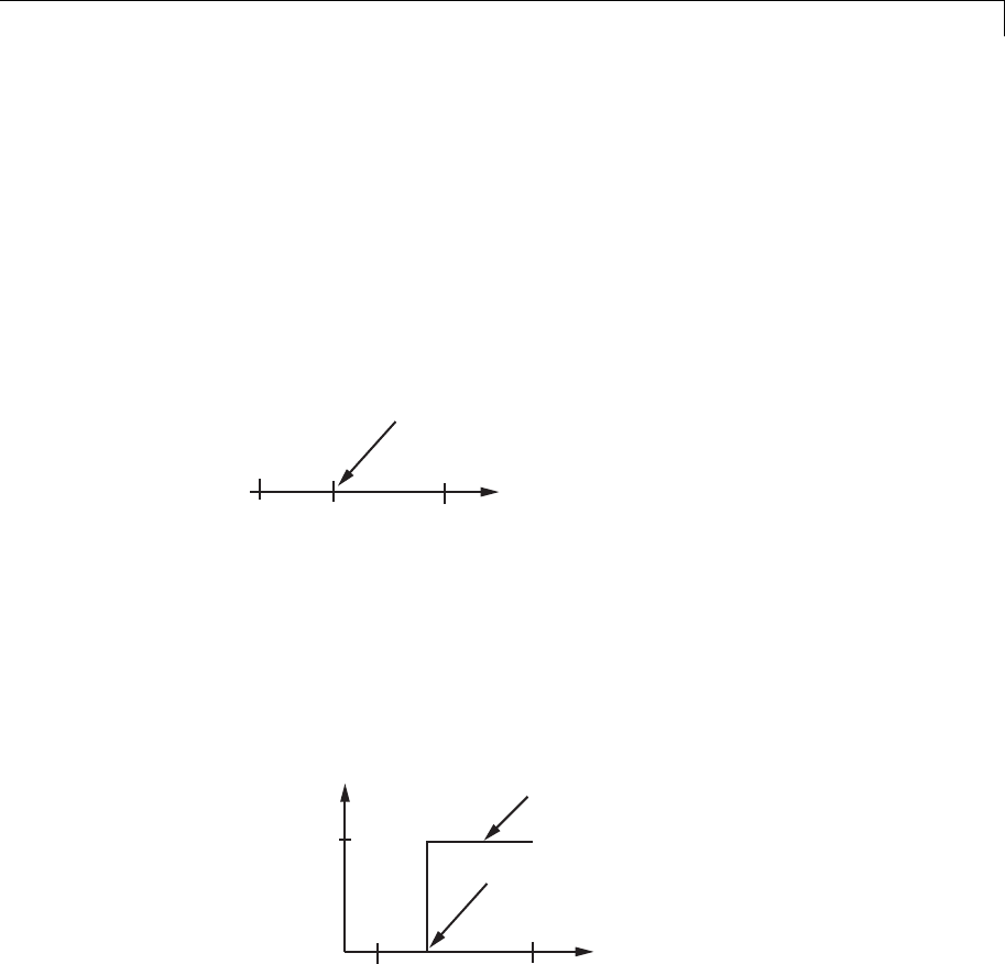
Nichols Plot
Enable zero-crossing detection
Enable zero-crossing detection to ensure that the software computes the
linear system characteristics at the following simulation times:
•The exact snapshot times, specified in Snapshot times.
As shown in the following figure, when zero-crossing detection is
enabled, the variable-step Simulink solver simulates the model at the
snapshot time Tsnap.Tsnap may lie between the simulation time steps
Tn-1 and Tnwhich are automatically chosen by the solver.
Computes linear system
characteristics at this time point
Time
Tn-1 Tn
Tsnap
•The exact times when an external trigger is detected, specified in
Trigger type.
As shown in the following figure, when zero-crossing detection is
enabled, the variable-step Simulink solver simulates the model at the
time, Ttrig, when the trigger signal is detected. Ttrig may lie between
the simulation time steps Tn-1 and Tnwhich are automatically chosen
by the solver.
Computes linear system
characteristics at this time point
Time
Amplitude
1
0Tn-1 Tn
Ttrig
Trigger signal
For more information on zero-crossing detection, see “Zero-Crossing
Detection” in the Simulink User Guide.
10-187

Nichols Plot
Settings
Default: On
On
Compute linear system characteristics at the exact snapshot time
or exact time when a trigger signal is detected.
This setting is ignored if the Simulink solver is fixed step.
Off
Compute linear system characteristics at the simulation time
steps that the variable-step solver chooses. The software may not
compute the linear system at the exact snapshot time or exact
time when a trigger signal is detected.
Command-Line Information
Parameter: ZeroCross
Type: string
Value: 'on' |'off'
Default: 'on'
See Also
Plot Linear Characteristics of Simulink Models During Simulation
“Model Verification at Default Simulation Snapshot Time” on page 5-6
10-188

Nichols Plot
Use exact delays
How to represent time delays in your linear model.
Use this option if you have blocks in your model that have time delays.
Settings
Default: Off
On
Return a linear model with exact delay representations.
Off
Return a linear model with Padé approximations of delays, as
specified in your Transport Delay and Variable Transport Delay
blocks.
Command-Line Information
Parameter: UseExactDelayModel
Type: string
Value: 'on' |'off'
Default: 'off'
See Also
Plot Linear Characteristics of Simulink Models During Simulation
“Model Verification at Default Simulation Snapshot Time” on page 5-6
10-189

Nichols Plot
Linear system sample time
Sample time of the linear system computed during simulation.
Use this parameter to:
•Compute a discrete-time system with a specific sample time from a
continuous-time system
•Resample a discrete-time system with a different sample time
•Compute a continuous-time system from a discrete-time system
When computing discrete-time systems from continuous-time systems
and vice-versa, the software uses the conversion method specified in
Sample time rate conversion method.
Settings
Default: auto
auto. Computes the sample time as:
•0, for continuous-time models.
•For models that have blocks with different sample times
(multi-rate models), least common multiple of the sample
times. For example, if you have a mix of continuous-time and
discrete-time blocks with sample times of 0, 0.2 and 0.3, the
sample time of the linear model is 0.6.
Positive finite value.Usetocompute:
•A discrete-time linear system from a continuous-time system.
•A discrete-time linear system from another discrete-time
system with a different sample time
0
Usetocomputeacontinuous-timelinearsystemfroma
discrete-time model.
Command-Line Information
Parameter: SampleTime
10-190


Nichols Plot
Sample time rate conversion method
Method for converting the sample time of single- or multi-rate models.
This parameter is used only when the value of Linear system sample
time is not auto.
Settings
Default: Zero-Order Hold
Zero-Order Hold
Zero-order hold, where the control inputs are assumed piecewise
constant over the sampling time Ts. For more information, see
“Zero-Order Hold” in Control System Toolbox User’s Guide.
This method usually performs better in time domain.
Tustin (bilinear)
Bilinear (Tustin) approximation without frequency prewarping.
The software rounds off fractional time delays to the nearest
multiple of the sampling time. For more information, see “Tustin
Approximation” in Control System Toolbox User’s Guide.
This method usually perform better in the frequency domain.
Tustin with Prewarping
Bilinear (Tustin) approximation with frequency prewarping. Also
specify the prewarp frequency in Prewarp frequency (rad/s).
For more information, see “Tustin Approximation” in Control
System Toolbox User’s Guide.
This method usually perform better in the frequency domain. Use
this method to ensure matching at frequency region of interest.
Upsampling when possible, Zero-Order Hold otherwise
Upsample a discrete-time system when possible and use
Zero-Order Hold otherwise.
10-192

Nichols Plot
You can upsample only when you convert discrete-time system to
a new sample time that is an integer-value-times faster than the
sampling time of the original system.
Upsampling when possible, Tustin otherwise
Upsample a discrete-time system when possible and use Tustin
(bilinear) otherwise.
You can upsample only when you convert discrete-time system to
a new sample time that is an integer-value-times faster than the
sampling time of the original system.
Upsampling when possible, Tustin with Prewarping otherwise
Upsample a discrete-time system when possible and use Tustin
with Prewarping otherwise. Also, specify the prewarp frequency
in Prewarp frequency (rad/s).
You can upsample only when you convert discrete-time system to
a new sample time that is an integer-value-times faster than the
sampling time of the original system.
Dependencies
Selecting either:
•Tustin with Prewarping
•Upsampling when possible, Tustin with Prewarping
otherwise
enables Prewarp frequency (rad/s).
Command-Line Information
Parameter: RateConversionMethod
Type: string
Value: 'zoh' |'tustin' |'prewarp'|'upsampling_zoh'|
'upsampling_tustin'|'upsampling_prewarp'
Default: 'zoh'
10-193


Nichols Plot
Prewarp frequency (rad/s)
Prewarp frequency for Tustin method, specified in radians/second.
Settings
Default: 10
Positive scalar value, smaller than the Nyquist frequency before and
after resampling. A value of 0 corresponds to the standard Tustin
method without frequency prewarping.
Dependencies
Selecting either
•Tustin with Prewarping
•Upsampling when possible, Tustin with Prewarping
otherwise
in Sample time rate conversion method enablesthisparameter.
Command-Line Information
Parameter: PreWarpFreq
Type: string
Value: 10 |positive scalar value
Default: 10
See Also
Plot Linear Characteristics of Simulink Models During Simulation
“Model Verification at Default Simulation Snapshot Time” on page 5-6
10-195

Nichols Plot
Use full block names
How the state, input and output names appear in the linear system
computed during simulation.
The linear system is a state-space object and system states and
input/output names appear in following state-space object properties:
Input, Output or State Name Appears in Which State-Space
Object Property
Linearization input name InputName
Linearization output name OutputName
State names StateName
Settings
Default: Off
On
Show state and input/output names with their path through the
model hierarchy. For example, in the chemical reactor model,
a state in the Integrator1 block of the CSTR subsystem appears
with full path as scdcstr/CSTR/Integrator1.
Off
Show only state and input/output names. Use this option when the
signal name is unique and you know where the signal is location
in your Simulink model. For example, a state in the Integrator1
block of the CSTR subsystem appears as Integrator1.
Command-Line Information
Parameter: UseFullBlockNameLabels
Type: string
Value: 'on' |'off'
Default: 'off'
See Also
Plot Linear Characteristics of Simulink Models During Simulation
10-196


Nichols Plot
Use bus signal names
How to label signals associated with linearization inputs and outputs
on buses, in the linear system computed during simulation (applies only
when you select an entire bus as an I/O point).
Selecting an entire bus signal is not recommended. Instead, select
individual bus elements.
You cannot use this parameter when your model has mux/bus mixtures.
Settings
Default: Off
On
Use the signal names of the individual bus elements.
Bus signal names appear when the input and output are at the
output of the following blocks:
•Root-level inport block containing a bus object
•Bus creator block
•Subsystem block whose source traces back to one of the
following blocks:
—Output of a bus creator block
—Root-level inport block by passing through only virtual or
nonvirtual subsystem boundaries
Off
Use the bus signal channel number.
Command-Line Information
Parameter: UseBusSignalLabels
Type: string
Value: 'on' |'off'
Default: 'off'
10-198


Nichols Plot
Include gain and phase margins in assertion
Check that the gain and phase margins are greater than the values
specified in Gain margin (dB) > and Phase margin (deg) >,during
simulation. The software displays a warning if the gain or phase margin
is less than or equal to the specified value.
By default, negative feedback, specified in Feedback sign,isused
to compute the margins.
This parameter is used for assertion only if Enable assertion in the
Assertion tab is selected.
You can specify multiple gain and phase margin bounds on the linear
system. The bounds also appear on the Nichols plot. If you clear
Enable assertion, the bounds are not used for assertion but continue
to appear on the plot.
Settings
Default:
•Off for Nichols Plot block.
•On for Check Nichols Characteristics block.
On
Check that the gain and phase margins satisfy the specified
values, during simulation.
Off
Do not check that the gain and phase margins satisfy the specified
values, during simulation.
Tips
•Clearing this parameter disables the gain and phase margin bounds
and the software stops checking that the gain and phase margins
satisfy the bounds during simulation. The bounds are also greyed
out on the plot.
•Toonlyviewthegainandphasemarginontheplot,clearEnable
assertion.
10-200

Nichols Plot
Command-Line Information
Parameter: EnableMargins
Type: string
Value: 'on' |'off'
Default: 'off' for Nichols Plot block, 'on' for Check Nichols
Characteristics block
See Also
Plot Linear Characteristics of Simulink Models During Simulation
“Model Verification at Default Simulation Snapshot Time” on page 5-6
10-201

Nichols Plot
Gain margin (dB) >
Gain margin, in decibels.
By default, negative feedback, specified in Feedback sign,isusedto
compute the gain margin.
Settings
Default:
[] for Nichols Plot block.
20 for Check Nichols Characteristics block.
•Positive finite number for one bound.
•Cell array of positive finite numbers for multiple bounds.
Tips
•To assert that the gain margin is satisfied, select both Include gain
and phase margins in assertion and Enable assertion.
•You can add or modify gain margins from the plot window:
-To add new gain margin, right-click the plot, and select
Bounds > New Bound.Select
Gain margin in Design
requirement type, and specify the margin in Gain margin.
-To modify the gain margin, drag the segment. Alternatively,
right-click the plot, and select Bounds > Edit Bound.Specifythe
new gain margin in Gain margin >.
You must click Update Block before simulating the model.
Command-Line Information
Parameter: GainMargin
Type: string
Value: [] |20 |positive finite value.Mustbespecifiedinside
single quotes ('').
Default: '[]' for Nichols Plot block, '20' for Check Nichols
Characteristics block.
10-202


Nichols Plot
Phase margin (deg) >
Phase margin, in degrees.
By default, negative feedback, specified in Feedback sign,isusedto
computethephasemargin.
Settings
[] for Nichols Plot block.
30 for Check Nichols Characteristics block.
•Positive finite number for one bound.
•Cell array of positive finite numbers for multiple bounds.
Tips
•To assert that the phase margin is satisfied, select both Include
gain and phase margins in assertion and Enable assertion.
•You can add or modify phase margins from the plot window:
-To add new phase margin, right-click the plot, and select
Bounds > New Bound.Select
Phase margin in Design
requirement type, and specify the margin in Phase margin.
-To modify the phase margin, drag the segment. Alternatively,
right-click the bound, and select Bounds > Edit Bound.Specify
the new phase margin in Phase margin >.
You must click Update Block before simulating the model.
Command-Line Information
Parameter: PhaseMargin
Type: string
Value: [] |30 |positive finite value.Mustbespecifiedinside
single quotes ('').
Default: '[]' for Nichols Plot block, '30' for Check Nichols
Characteristics block.
See Also
Plot Linear Characteristics of Simulink Models During Simulation
10-204


Nichols Plot
Include closed-loop peak gain in assertion
Check that the closed-loop peak gain is less than the value specified
in Closed-loop peak gain (dB) <, during simulation. The software
displays a warning if the closed-loop peak gain is greater than or equal
to the specified value.
By default, negative feedback, specified in Feedback sign,isusedto
compute the closed-loop peak gain.
This parameter is used for assertion only if Enable assertion in the
Assertion tab is selected.
You can specify multiple closed-loop peak gain bounds on the linear
system. The bound also appear on the Nichols plot as an m-circle. If
you clear Enable assertion, the bounds are not used for assertion
but continue to appear on the plot.
Settings
Default: Off
On
Check that the closed-loop peak gain satisfies the specified value,
during simulation.
Off
Do not check that the closed-loop peak gain satisfies the specified
value, during simulation.
Tips
•Clearing this parameter disables the closed-loop peak gain bound and
the software stops checking that the peak gain satisfies the bounds
during simulation. The bounds are greyed out on the plot.
10-206

Nichols Plot
•To only view the closed-loop peak gain on the plot, clear Enable
assertion.
Command-Line Information
Parameter: EnableCLPeakGain
Type: string
Value: 'on' |'off'
Default: 'off'
See Also
Plot Linear Characteristics of Simulink Models During Simulation
“Model Verification at Default Simulation Snapshot Time” on page 5-6
10-207

Nichols Plot
Closed-loop peak gain (dB) <
Closed-loop peak gain, in decibels.
By default, negative feedback, specified in Feedback sign,isused
to compute the margins.
Settings
Default []
•Positive or negative finite number for one bound.
•Cell array of positive or negative finite numbers for multiple bounds.
Tips
•To assert that the gain margin is satisfied, select both Include
closed-loop peak gain in assertion and Enable assertion.
•You can add or modify closed-loop peak gains from the plot window:
-To add the closed-loop peak gain, right-click the plot, and select
Bounds > New Bound.Select
Closed-Loop peak gain in
Design requirement type, and specify the gain in Closed-Loop
peak gain <.
-To modify the closed-loop peak gain, drag the segment.
Alternatively, right-click the bound, and select Bounds > Edit
Bound. Specify the new closed-loop peak gain in Closed-Loop
peak gain <.
You must click Update Block before simulating the model.
Command-Line Information
Parameter: CLPeakGain
Type: string
Value: [] |positive or negative number |cell array of
positive or negative numbers. Must be specified inside single
quotes ('').
Default: '[]'
10-208


Nichols Plot
Include open-loop gain-phase bound in assertion
Check that the Nichols response satisfies open-loop gain and phase
bounds, specified in Open-loop phases (deg) and Open-loop gains
(dB), during simulation. The software displays a warning if the Nichols
response violates the bounds.
This parameter is used for assertion only if Enable assertion in the
Assertion tab is selected.
You can specify multiple gain and phase bounds on the linear systems
computed during simulation. The bounds also appear on the Nichols
plot. If you clear Enable assertion, the bounds are not used for
assertion but continue to appear on the plot.
Settings
Default: Off
On
Check if the Nichols response satisfies the specified open-loop
gain and phase bounds, during simulation.
Off
Do not check if the Nichols response satisfies the specified
open-loop gain and phase bounds, during simulation.
Tips
•Clearing this parameter disables the gain-phase bound and the
software stops checking that the gain and phase satisfy the bound
during simulation. The bound segments are also greyed out on the
plot.
10-210
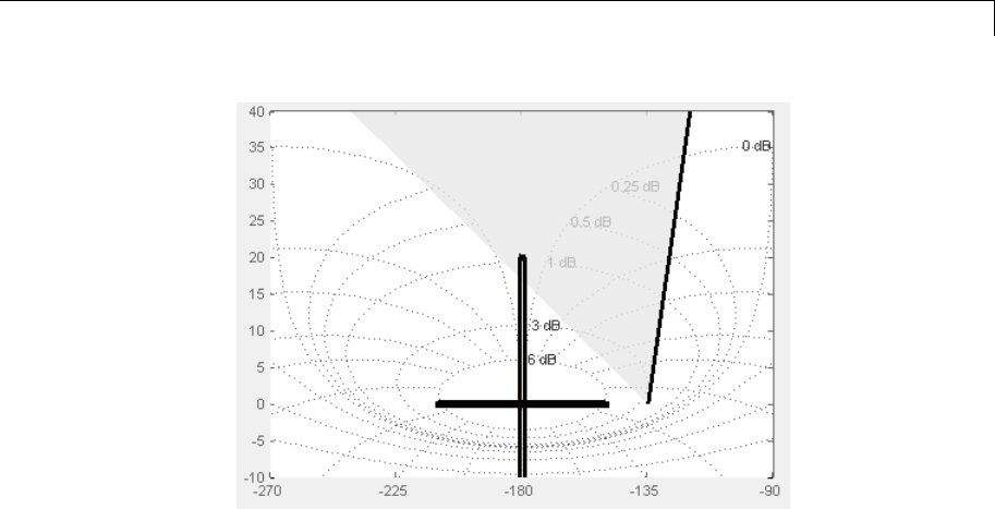
Nichols Plot
•To only view the bound on the plot, clear Enable assertion.
Command-Line Information
Parameter: EnableGainPhaseBound
Type: string
Value: 'on' |'off'
Default: 'off'
10-211

Nichols Plot
Open-loop phases (deg)
Open-loop phases, in degrees.
Specify the corresponding open-loop gains in Open-loop gains (dB).
Settings
Default: []
Must be specified as start and end phases:
•Positive or negative finite numbers for a single bound with one edge
•Matrix of positive or negative finite numbers , for a single bound
with multiple edges
•Cell array of matrices with finite numbers for multiple bounds
Tips
•To assert that the open-loop gains and phases are satisfied, select
both Include open-loop gain-phase bound in assertion and
Enable assertion.
•You can add or modify open-loop phases from the plot window:
-To add a new phases, right-click the plot, and select
Bounds > New Bound.Select
Gain-Phase requirement in
Design requirement type, and specify the phases in the
Open-Loop phase column. Specify the corresponding gains in
the Open-Loop gain column.
-To modify the phases, drag the bound segment. Alternatively,
right-click the segment, and select Bounds > Edit Bounds.
Specify the new phases in the Open-Loop phase column.
You must click Update Block before simulating the model.
Command-Line Information
Parameter: OLPhases
Type: string
Value: [] |positive or negative finite numbers |matrix
of positive or negative finite numbers |cell array of
10-212


Nichols Plot
Open-loop gains (dB)
Open-loop gains, in decibels.
Specify the corresponding open-loop phases in Open-loop phases
(deg).
Settings
Default: []
Must be specified as start and end gains:
•Positive or negative number for a single bound with one edge
•Matrix of positive or negative finite numbers for a single bound with
multiple edges
•Cell array of matrices with finite numbers for multiple bounds
Tips
•To assert that the open-loop gains are satisfied, select both Include
open-loop gain-phase bound in assertion and Enable assertion.
•You can add or modify open-loop gains from the plot window:
-To add a new gains, right-click the plot, and select Bounds > New
Bound. Select Gain-Phase requirement in Design
requirement type, and specify the gains in the Open-Loop
phase column. Specify the phases in the Open-Loop phase
column.
-To modify the gains, drag the bound segment. Alternatively,
right-click the segment, and select Bounds > Edit Bounds.
Specify the new gains in the Open-Loop gain column.
You must click Update Block before simulating the model.
Command-Line Information
Parameter: OLGains
Type: string
10-214

Nichols Plot
Value: [] |positive or negative number |matrix of positive
or negative finite numbers |cell array of matrices with
finite numbers. Must be specified inside single quotes ('').
Default: '[]'
See Also
Plot Linear Characteristics of Simulink Models During Simulation
“Model Verification at Default Simulation Snapshot Time” on page 5-6
10-215

Nichols Plot
Feedback sign
Feedback sign to determine the closed-loop gain and phase
characteristics of the linear system, computed during simulation.
To determine the feedback sign, check if the path defined by the
linearization inputs and outputs include the feedback Sum block:
•If the path includes the Sum block, specify positive feedback.
•IfthepathdoesnotincludetheSum block, specify the same feedback
sign as the Sum block.
For example, in the aircraft model, the Check Gain and Phase Margins
block includes the negative sign in the summation block. Therefore,
the Feedback sign is positive.
Settings
Default: negative feedback
negative feedback
Use when the path defined by the linearization inputs/outputs
does not include the Sum block and the Sum block feedback sign
is -.
positive feedback
Use when:
•The path defined by the linearization inputs/outputs includes
the Sum block.
•The path defined by the linearization inputs/outputs does not
include the Sum block and the Sum block feedback sign is +.
Command-Line Information
Parameter: FeedbackSign
Type: string
Value: '-1' |'+1'
Default: '-1'
10-216


Nichols Plot
Save data to workspace
Save one or more linear systems as a variable in MATLAB workspace to
perform further linear analysis or control design.
The workspace variable is a structure with time and values fields:
•The time field stores the simulation time at which the linear system
is computed.
•The values field is a state-space object which stores the linear
system. If the linear system is computed at multiple simulation
times, values is an array of state-space objects.
Settings
Default: Off
On
Save the computed linear system to MATLAB workspace.
Off
Do not save the computed linear system to MATLAB workspace.
Dependencies
This parameter enables Variable name.
Command-Line Information
Parameter: SaveToWorkspace
Type: string
Value: 'on' |'off'
Default: 'off'
See Also
Plot Linear Characteristics of Simulink Models During Simulation
“Model Verification at Default Simulation Snapshot Time” on page 5-6
10-218

Nichols Plot
Variable name
Name of the workspace variable that stores one or more linear systems
computed during simulation.
The name must be unique among the variable names used in all data
logging model blocks, such as Linear Analysis Plot blocks, Model
Verification blocks, Scope blocks, To Workspace blocks, and simulation
return variables such as time, states, and outputs.
Settings
Default: sys
String.
Dependencies
Save data to workspace enables this parameter.
Command-Line Information
Parameter: SaveName
Type: string
Value: sys |any string. Must be specified inside single quotes
('').
Default: 'sys'
See Also
Plot Linear Characteristics of Simulink Models During Simulation
“Model Verification at Default Simulation Snapshot Time” on page 5-6
10-219

Nichols Plot
Enable assertion
Enable the block to check that bounds specified and included for
assertion in the Bounds tab are satisfied during simulation. Assertion
failsifaboundisnotsatisfied. Awarning, reporting the assertion
failure, appears at the MATLAB prompt.
If assertion fails, you can optionally specify that the block:
•Execute a MATLAB expression, specified in Simulation callback
when assertion fails (optional).
•Stop the simulation and bring that block into focus, by selecting Stop
simulation when assertion fails.
For the Linear Analysis Plots blocks, this parameter has no effect
because no bounds are included by default. If you want to use the
Linear Analysis Plots blocks for assertion, specify and include
bounds in the Bounds tab.
Clearing this parameter disables assertion, i.e., the block no longer
checks that specified bounds are satisfied. The block icon also updates
to indicate that assertion is disabled.
In the Configuration Parameters dialog box of the Simulink model, the
Model Verification block enabling option in the Debugging area of
Data Validity node, lets you to enable or disable all model verification
blocks in a model, regardless of the setting of this option.
Settings
Default: On
10-220

Nichols Plot
On
Check that bounds included for assertion in the Bounds tab
are satisfied during simulation. A warning, reporting assertion
failure, is displayed at the MATLAB prompt if bounds are violated.
Off
Do not check that bounds included for assertion are satisfied
during simulation.
Dependencies
This parameter enables:
•Simulation callback when assertion fails (optional)
•Stop simulation when assertion fails
Command-Line Information
Parameter: enabled
Type: string
Value: 'on' |'off'
Default: 'on'
See Also
Plot Linear Characteristics of Simulink Models During Simulation
“Model Verification at Default Simulation Snapshot Time” on page 5-6
10-221

Nichols Plot
Simulation callback when assertion fails (optional)
MATLAB expression to execute when assertion fails.
Because the expression is evaluated in the MATLAB workspace, define
all variables used in the expression in that workspace.
Settings
No Default
AMATLABexpression.
Dependencies
Enable assertion enables this parameter.
Command-Line Information
Parameter: callback
Type: string
Value: '' |MATLAB expression
Default: ''
See Also
Plot Linear Characteristics of Simulink Models During Simulation
“Model Verification at Default Simulation Snapshot Time” on page 5-6
10-222

Nichols Plot
Stop simulation when assertion fails
Stop the simulation when a bound specified in the Bounds tab is
violated during simulation, i.e., assertion fails.
If you run the simulation from the Simulink Editor, the Simulation
Diagnostics window opens to display an error message. Also, the block
where the bound violation occurs is highlighted in the model.
Settings
Default: Off
On
Stop simulation if a bound specified in the Bounds tab is violated.
Off
Continue simulation if a bound is violated with a warning
message at the MATLAB prompt.
Tips
•Because selecting this option stops the simulation as soon as the
assertion fails, assertion failures that might occur later during the
simulation are not reported. If you want all assertion failures to be
reported, do not select this option.
Dependencies
Enable assertion enables this parameter.
Command-Line Information
Parameter: stopWhenAssertionFail
Type: string
Value: 'on' |'off'
Default: 'off'
See Also
Plot Linear Characteristics of Simulink Models During Simulation
“Model Verification at Default Simulation Snapshot Time” on page 5-6
10-223

Nichols Plot
Output assertion signal
Output a Boolean signal that, at each time step, is:
•True (1) if assertion succeeds, i.e., all bounds are satisfied
•False (1)ifassertionfails,i.e.,aboundisviolated.
The output signal data type is Boolean only if the Implement logic
signals as Boolean data option in the Optimization pane of the
Configuration Parameters dialog box of the Simulink model is selected.
Otherwise, the data type of the output signal is double.
Selecting this parameter adds an output port to the block that you can
connect to any block in the model.
Settings
Default:Off
On
Output a Boolean signal to indicate assertion status. Adds a
port to the block.
Off
Do not output a Boolean signal to indicate assertion status.
Tips
•Use this parameter to design complex assertion logic. For an
example, see “Model Verification Using Simulink®Control Design™
and Simulink Verification Blocks” on page 5-25.
Command-Line Information
Parameter: export
Type: string
Value: 'on' |'off'
Default: 'off'
See Also
Plot Linear Characteristics of Simulink Models During Simulation
10-224


Nichols Plot
Show plot on block open
Open the plot window instead of the Block Parameters dialog box when
you double-click the block in the Simulink model.
Usethisparameterifyouprefertoopenandperformtasks,suchas
adding or modifying bounds, in the plot window instead of the Block
Parameters dialog box. If you want to access the block parameters from
the plot window, select Edit or click .
For more information on the plot, see Show Plot.
Settings
Default: Off
On
Open the plot window when you double-click the block.
Off
Open the Block Parameters dialog box when double-clicking the
block.
Command-Line Information
Parameter: LaunchViewOnOpen
Type: string
Value: 'on' |'off'
Default: 'off'
See Also
Plot Linear Characteristics of Simulink Models During Simulation
“Model Verification at Default Simulation Snapshot Time” on page 5-6
Show Plot Open the plot window.
Use the plot to view:
•Linear system characteristics computed from the nonlinear Simulink
model during simulation
10-226

Nichols Plot
You must click this button before you simulate the model to view
the linear characteristics.
You can display additional characteristics, such as the peak response
time and stability margins, of the linear system by right-clicking the
plot and selecting Characteristics.
•Bounds on the linear system characteristics
You can specify bounds in the Bounds tab of the Block Parameters
dialog box or right-click the plot and select Bounds > New Bound.
For more information on the types of bounds you can specify on each
plot, see “Verifiable Linear System Characteristics” on page 5-5 in
the User’s Guide.
You can modify bounds by dragging the bound segment or by
right-clicking the plot and selecting Bounds > Edit Bound. Before
you simulate the model, click Update Block to update the bound
value in the block parameters.
Typical tasks that you perform in the plot window include:
•Opening the Block Parameters dialog box by clicking or selecting
Edit.
•Finding the block that the plot window corresponds to by clicking
or selecting View > Highlight Simulink Block.Thisactionmakes
the Simulink Editor active and highlights the block.
•Simulating the model by clicking or selecting Simulation > Run.
This action also linearizes the portion of the model between the
specified linearization input and output.
•Adding legend on the linear system characteristic plot by clicking .
See Also Check Nichols Characteristics
Tutorials •“Visualize Bode Response of Simulink Model During Simulation”
on page 2-42
10-227


Pole-Zero Plot
Purpose Pole-zero plot of linear system approximated from nonlinear Simulink
model
Library Simulink Control Design
Description ThisblockissameastheCheckPole-Zero Characteristics block except
for different default parameter settings in the Bounds tab.
Compute a linear system from a Simulink model and plot the poles and
zeros on a pole-zero map.
During simulation, the software linearizes the portion of the model
between specified linearization inputs and outputs, and plots the poles
and zeros of the linear system.
The Simulink model can be continuous- or discrete-time or multirate
and can have time delays. Because you can specify only one linearization
input/output pair in this block, thelinearsystemisSingle-Input
Single-Output (SISO).
You can specify multiple bounds that approximate second-order
characteristics on the pole locations and view them on the plot. You can
also check that the bounds are satisfied during simulation:
•If all bounds are satisfied, the block does nothing.
•If a bound is not satisfied, the block asserts, and a warning message
appears at the MATLAB prompt. You can also specify that the block:
-Evaluate a MATLAB expression.
-Stop the simulation and bring that block into focus.
During simulation, the block can also output a logical assertion signal:
•If all bounds are satisfied, the signal is true (1).
•If a bound is not satisfied, the signal is false (0).
You can add multiple Pole-Zero Plot blocks to compute and plot the
poles and zeros of various portions of the model.
10-229

Pole-Zero Plot
You can save the linear system as a variable in the MATLAB workspace.
The block does not support code generation and can be used only in
Normal simulation mode.
Parameters The following table summarizes the Pole-Zero Plot block parameters,
accessible via the block parameter dialog box.
Task Parameters
Specify inputs and
outputs (I/Os).
In Linearizations
tab:
•“Linearization
inputs/outputs”
on page 10-287.
•“Click a signal in
the model to select
it” on page 10-290.
Specify settings. In Linearizations
tab:
•“Linearize on” on
page 10-294.
•“Snapshot times”
on page 10-296.
•“Trigger type” on
page 10-297.
Specify algorithm
options.
In Algorithm
Options of
Linearizations tab:
•“Enable
zero-crossing
Configure
linearization.
10-230

Pole-Zero Plot
Task Parameters
detection” on page
10-298.
•“Use exact delays”
on page 10-300.
•“Linear system
sample time” on
page 10-301.
•“Sample time
rate conversion
method” on page
10-303.
•“Prewarp
frequency (rad/s)”
on page 10-306.
Specify labels for
linear system I/Os
and state names.
In Labels of
Linearizations tab:
•“Use full block
names” on page
10-307.
•“Use bus signal
names” on page
10-309.
Plot the linear system. Show Plot
10-231

Pole-Zero Plot
Task Parameters
(Optional) Specify bounds on pole-zero for
assertion.
In Bounds tab:
•Include settling
time bound in
assertion.
•Include percent
overshoot bound in
assertion.
•Include damping
ratio bound in
assertion.
•Include natural
frequency bound in
assertion.
Specify assertion options (only when you
specify bounds on the linear system).
In Assertion tab:
•“Enable assertion”
on page 10-325.
•“Simulation
callback when
assertion fails
(optional)” on page
10-327.
•“Stop simulation
when assertion
fails” on page
10-328.
•“Output assertion
signal” on page
10-329.
10-232

Pole-Zero Plot
Task Parameters
Save linear system to MATLAB workspace. “Save data to
workspace” on page
10-323 in Logging
tab.
Display plot window instead of block
parameters dialog box on double-clicking the
block.
“Show plot on block
open” on page 10-331.
Linearization inputs/outputs
Linearization inputs and outputs that define the portion of a nonlinear
Simulink model to linearize.
1Click .
The dialog box expands to display a Click a signal in the model to
select it area and a new button.
2Select a signal in the Simulink Editor.
The selected signal appears as a Model signal in the Click a signal
in the model to select it area.
3(Optional) For buses, expand the bus signal to select an individual
element.
10-233
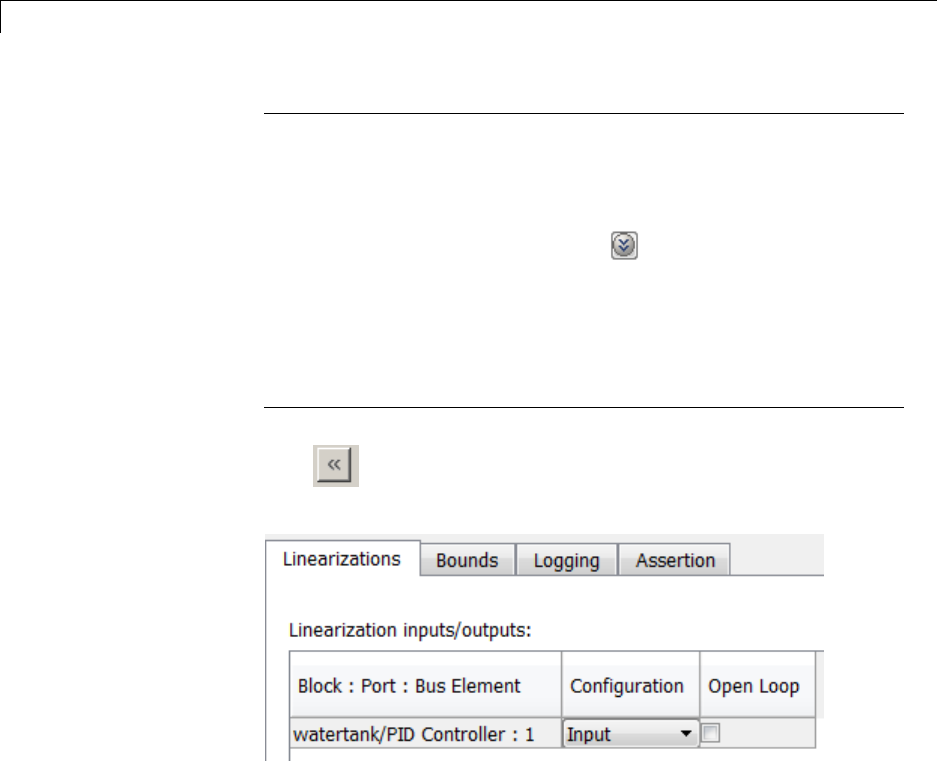
Pole-Zero Plot
Tip Forlargebuses,youcanentersearchtextforfilteringelement
names in the Filter by name edit box. The name match is
case-sensitive. Additionally, you can enter MATLAB regular
expression.
To modify the filtering options, click .
Filtering Options
•“Enable regular expression” on page 10-291
•“Show filtered results as aflatlist”onpage10-292
4Click to add the signal to the Linearization inputs/outputs
table.
The table displays the following information about the selected signal:
10-234

Pole-Zero Plot
Block : Port : Bus
Element
Name of the block associated with the input/output. The
number adjacent to the block name is the port number where
the selected bus signal is located. The last entry is the
selected bus element name.
Configuration Type of linearization point:
•Input — An input point.
•Output —Anoutputpoint.
•Input-Output — An input point immediately followed by
an output point.
•Output-Input — An output point immediately followed
by an input point.
•None — Signal selected but not specified as a linearization
input or output.
Open Loop If your model contains one or more feedback loops, you
can choose to linearize an open- or closed-loop system. For
example, you might want to linearize only the plant model
within a feedback control loop. When such a feedback loop
is present, select this option to insert an open loop point
and remove the effect of the loop without manually breaking
signal lines.
For determining gain and phase margins, in most cases, you
open the loop.
Note If you simulate the model without specifying an input or output,
the software does not compute a linear system. Instead, you see a
warning message at the MATLAB prompt.
Settings
No default
10-235


Pole-Zero Plot
Click a signal in the model to select it
Enables signal selection in the Simulink model. Appears only when
you click .
When this option appears, you also see the following changes:
•Anew button.
Use to add a selected signal as a linearization input or output in the
Linearization inputs/outputs table. For more information, see
Linearization inputs/outputs.
•changes to .
UsetocollapsetheClick a signal in the model to select it area.
Settings
No default
Command-Line Information
Use the getlinio and setlinio commands to select signals as
linearization inputs and outputs.
See Also
Plot Linear Characteristics of Simulink Models During Simulation
“Model Verification at Default Simulation Snapshot Time” on page 5-6
10-237

Pole-Zero Plot
Enable regular expression
Enable the use of MATLAB regular expressions for filtering signal
names. For example, entering t$ in the Filter by name edit box
displays all signals whose names end with a lowercase t(and their
immediate parents). For details, see “Regular Expressions”.
Settings
Default: On
On
Allow use of MATLAB regular expressions for filtering signal
names.
Off
Disable use of MATLAB regular expressions for filtering signal
names. Filtering treats the text you enter in the Filter by name
edit box as a literal string.
Dependencies
Selecting the Options button on the right-hand side of the Filter by
name edit box ( ) enables this parameter.
10-238

Pole-Zero Plot
Show filtered results as a flat list
Uses a flat list format to display the list of filtered signals, based on the
search text in the Filter by name edit box. The flat list format uses
dot notation to reflect the hierarchy of bus signals. The following is an
example of a flat list format for a filtered set of nested bus signals.
Settings
Default: Off
On
Display the filtered list of signalsusingaflatlistformat,
indicating bus hierarchies with dot notation instead of using a
tree format.
Off
Display filtered bus hierarchies using a tree format.
10-239

Pole-Zero Plot
Dependencies
Selecting the Options button on the right-hand side of the Filter by
name edit box ( ) enables this parameter.
10-240

Pole-Zero Plot
Linearize on
When to compute the linear system during simulation.
Settings
Default: Simulation snapshots
Simulation snapshots
Specific simulation time, specified in Snapshot times.
Use when you:
•Know one or more times when the model is at steady-state
operating point
•Want to compute the linear systems at specific times
External trigger
Trigger-based simulation event. Specify the trigger type in
Trigger type.
Use when a signal generated during simulation indicates
steady-state operating point.
Selecting this option adds a trigger port to the block. Use this port
to connect the block to the trigger signal.
For example, for an aircraft model, you might want to compute
the linear system whenever the fuel mass is a fraction of the
maximum fuel mass. In this case, model this condition as an
external trigger.
Dependencies
•Setting this parameter to Simulation snapshots enables Snapshot
times.
•Setting this parameter to External trigger enables Trigger type.
Command-Line Information
Parameter: LinearizeAt
10-241


Pole-Zero Plot
Snapshot times
One or more simulation times. The linear system is computed at these
times.
Settings
Default: 0
•For a different simulation time, enter the time. Use when you:
-Want to plot the linear system at a specific time
-Know the approximate time when the model reaches steady-state
operating point
•For multiple simulation times, enter a vector. Use when you want to
compute and plot linear systems at multiple times.
Snapshot times must be less than or equal to the simulation time
specified in the Simulink model.
Dependencies
Selecting Simulation snapshots in Linearize on enables this
parameter.
Command-Line Information
Parameter: SnapshotTimes
Type: string
Value: 0|positive real number |vector of positive real
numbers
Default: 0
See Also
Plot Linear Characteristics of Simulink Models During Simulation
“Model Verification at Default Simulation Snapshot Time” on page 5-6
10-243

Pole-Zero Plot
Trigger type
Trigger type of an external trigger for computing linear system.
Settings
Default: Rising edge
Rising edge
Rising edge of the external trigger signal.
Falling edge
Falling edge of the external trigger signal.
Dependencies
Selecting External trigger in Linearize on enables this parameter.
Command-Line Information
Parameter: TriggerType
Type: string
Value: 'rising' |'falling'
Default: 'rising'
See Also
Plot Linear Characteristics of Simulink Models During Simulation
“Model Verification at Default Simulation Snapshot Time” on page 5-6
10-244

Pole-Zero Plot
Enable zero-crossing detection
Enable zero-crossing detection to ensure that the software computes the
linear system characteristics at the following simulation times:
•The exact snapshot times, specified in Snapshot times.
As shown in the following figure, when zero-crossing detection is
enabled, the variable-step Simulink solver simulates the model at the
snapshot time Tsnap.Tsnap may lie between the simulation time steps
Tn-1 and Tnwhich are automatically chosen by the solver.
Computes linear system
characteristics at this time point
Time
Tn-1 Tn
Tsnap
•The exact times when an external trigger is detected, specified in
Trigger type.
As shown in the following figure, when zero-crossing detection is
enabled, the variable-step Simulink solver simulates the model at the
time, Ttrig, when the trigger signal is detected. Ttrig may lie between
the simulation time steps Tn-1 and Tnwhich are automatically chosen
by the solver.
Computes linear system
characteristics at this time point
Time
Amplitude
1
0Tn-1 Tn
Ttrig
Trigger signal
For more information on zero-crossing detection, see “Zero-Crossing
Detection” in the Simulink User Guide.
10-245

Pole-Zero Plot
Settings
Default: On
On
Compute linear system characteristics at the exact snapshot time
or exact time when a trigger signal is detected.
This setting is ignored if the Simulink solver is fixed step.
Off
Compute linear system characteristics at the simulation time
steps that the variable-step solver chooses. The software may not
compute the linear system at the exact snapshot time or exact
time when a trigger signal is detected.
Command-Line Information
Parameter: ZeroCross
Type: string
Value: 'on' |'off'
Default: 'on'
See Also
Plot Linear Characteristics of Simulink Models During Simulation
“Model Verification at Default Simulation Snapshot Time” on page 5-6
10-246

Pole-Zero Plot
Use exact delays
How to represent time delays in your linear model.
Use this option if you have blocks in your model that have time delays.
Settings
Default: Off
On
Return a linear model with exact delay representations.
Off
Return a linear model with Padé approximations of delays, as
specified in your Transport Delay and Variable Transport Delay
blocks.
Command-Line Information
Parameter: UseExactDelayModel
Type: string
Value: 'on' |'off'
Default: 'off'
See Also
Plot Linear Characteristics of Simulink Models During Simulation
“Model Verification at Default Simulation Snapshot Time” on page 5-6
10-247

Pole-Zero Plot
Linear system sample time
Sample time of the linear system computed during simulation.
Use this parameter to:
•Compute a discrete-time system with a specific sample time from a
continuous-time system
•Resample a discrete-time system with a different sample time
•Compute a continuous-time system from a discrete-time system
When computing discrete-time systems from continuous-time systems
and vice-versa, the software uses the conversion method specified in
Sample time rate conversion method.
Settings
Default: auto
auto. Computes the sample time as:
•0, for continuous-time models.
•For models that have blocks with different sample times
(multi-rate models), least common multiple of the sample
times. For example, if you have a mix of continuous-time and
discrete-time blocks with sample times of 0, 0.2 and 0.3, the
sample time of the linear model is 0.6.
Positive finite value.Usetocompute:
•A discrete-time linear system from a continuous-time system.
•A discrete-time linear system from another discrete-time
system with a different sample time
0
Usetocomputeacontinuous-timelinearsystemfroma
discrete-time model.
Command-Line Information
Parameter: SampleTime
10-248


Pole-Zero Plot
Sample time rate conversion method
Method for converting the sample time of single- or multi-rate models.
This parameter is used only when the value of Linear system sample
time is not auto.
Settings
Default: Zero-Order Hold
Zero-Order Hold
Zero-order hold, where the control inputs are assumed piecewise
constant over the sampling time Ts. For more information, see
“Zero-Order Hold” in Control System Toolbox User’s Guide.
This method usually performs better in time domain.
Tustin (bilinear)
Bilinear (Tustin) approximation without frequency prewarping.
The software rounds off fractional time delays to the nearest
multiple of the sampling time. For more information, see “Tustin
Approximation” in Control System Toolbox User’s Guide.
This method usually perform better in the frequency domain.
Tustin with Prewarping
Bilinear (Tustin) approximation with frequency prewarping. Also
specify the prewarp frequency in Prewarp frequency (rad/s).
For more information, see “Tustin Approximation” in Control
System Toolbox User’s Guide.
This method usually perform better in the frequency domain. Use
this method to ensure matching at frequency region of interest.
Upsampling when possible, Zero-Order Hold otherwise
Upsample a discrete-time system when possible and use
Zero-Order Hold otherwise.
10-250

Pole-Zero Plot
You can upsample only when you convert discrete-time system to
a new sample time that is an integer-value-times faster than the
sampling time of the original system.
Upsampling when possible, Tustin otherwise
Upsample a discrete-time system when possible and use Tustin
(bilinear) otherwise.
You can upsample only when you convert discrete-time system to
a new sample time that is an integer-value-times faster than the
sampling time of the original system.
Upsampling when possible, Tustin with Prewarping otherwise
Upsample a discrete-time system when possible and use Tustin
with Prewarping otherwise. Also, specify the prewarp frequency
in Prewarp frequency (rad/s).
You can upsample only when you convert discrete-time system to
a new sample time that is an integer-value-times faster than the
sampling time of the original system.
Dependencies
Selecting either:
•Tustin with Prewarping
•Upsampling when possible, Tustin with Prewarping
otherwise
enables Prewarp frequency (rad/s).
Command-Line Information
Parameter: RateConversionMethod
Type: string
Value: 'zoh' |'tustin' |'prewarp'|'upsampling_zoh'|
'upsampling_tustin'|'upsampling_prewarp'
Default: 'zoh'
10-251


Pole-Zero Plot
Prewarp frequency (rad/s)
Prewarp frequency for Tustin method, specified in radians/second.
Settings
Default: 10
Positive scalar value, smaller than the Nyquist frequency before and
after resampling. A value of 0 corresponds to the standard Tustin
method without frequency prewarping.
Dependencies
Selecting either
•Tustin with Prewarping
•Upsampling when possible, Tustin with Prewarping
otherwise
in Sample time rate conversion method enablesthisparameter.
Command-Line Information
Parameter: PreWarpFreq
Type: string
Value: 10 |positive scalar value
Default: 10
See Also
Plot Linear Characteristics of Simulink Models During Simulation
“Model Verification at Default Simulation Snapshot Time” on page 5-6
10-253

Pole-Zero Plot
Use full block names
How the state, input and output names appear in the linear system
computed during simulation.
The linear system is a state-space object and system states and
input/output names appear in following state-space object properties:
Input, Output or State Name Appears in Which State-Space
Object Property
Linearization input name InputName
Linearization output name OutputName
State names StateName
Settings
Default: Off
On
Show state and input/output names with their path through the
model hierarchy. For example, in the chemical reactor model,
a state in the Integrator1 block of the CSTR subsystem appears
with full path as scdcstr/CSTR/Integrator1.
Off
Show only state and input/output names. Use this option when the
signal name is unique and you know where the signal is location
in your Simulink model. For example, a state in the Integrator1
block of the CSTR subsystem appears as Integrator1.
Command-Line Information
Parameter: UseFullBlockNameLabels
Type: string
Value: 'on' |'off'
Default: 'off'
See Also
Plot Linear Characteristics of Simulink Models During Simulation
10-254


Pole-Zero Plot
Use bus signal names
How to label signals associated with linearization inputs and outputs
on buses, in the linear system computed during simulation (applies only
when you select an entire bus as an I/O point).
Selecting an entire bus signal is not recommended. Instead, select
individual bus elements.
You cannot use this parameter when your model has mux/bus mixtures.
Settings
Default: Off
On
Use the signal names of the individual bus elements.
Bus signal names appear when the input and output are at the
output of the following blocks:
•Root-level inport block containing a bus object
•Bus creator block
•Subsystem block whose source traces back to one of the
following blocks:
—Output of a bus creator block
—Root-level inport block by passing through only virtual or
nonvirtual subsystem boundaries
Off
Use the bus signal channel number.
Command-Line Information
Parameter: UseBusSignalLabels
Type: string
Value: 'on' |'off'
Default: 'off'
10-256


Pole-Zero Plot
Include settling time bound in assertion
Check that the pole locations satisfy approximate second-order bounds
on the settling time, specified in Settling time (sec) <=.Thesoftware
displays a warning if the poles lie outside the region defined by the
settling time bound.
This parameter is used for assertion only if Enable assertion in the
Assertion tab is selected.
You can specify multiple settling time bounds on the linear system. The
bounds also appear on the pole-zero plot. If you clear Enable assertion,
the bounds are not used for assertion but continue to appear on the plot.
Settings
Default:
•Off for Pole-Zero Plot block.
•On for Check Pole-Zero Characteristics block.
On
Check that each pole lies in the region defined by the settling
time bound, during simulation.
Off
Do not check that each pole lies in the region defined by the
settling time bound, during simulation.
Tips
•Clearing this parameter disables the settling time bounds and
the software stops checking that the bounds are satisfied during
simulation. The bounds are also greyed out on the plot.
10-258
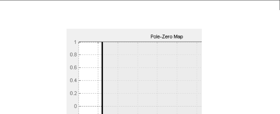
Pole-Zero Plot
•If you also specify other bounds, such as percent overshoot, damping
ratio or natural frequency, but want to exclude the settling time
bound from assertion, clear this parameter.
•To only view the bounds on the plot, clear Enable assertion.
Command-Line Information
Parameter: EnableSettlingTime
Type: string
Value: 'on' |'off'
Default:'off' for Pole-Zero Plot block, 'on' for Check Pole-Zero
Characteristics block.
See Also
Plot Linear Characteristics of Simulink Models During Simulation
“Model Verification at Default Simulation Snapshot Time” on page 5-6
10-259

Pole-Zero Plot
Settling time (sec) <=
Settling time, in seconds, of the second-order system.
Settings
Default:
[] for Pole-Zero Plot block
1for Check Pole-Zero Characteristics block
•Finite positive real scalar for one bound.
•Cell array of finite positive real scalars for multiple bounds.
Tips
•To assert that the settling time bounds are satisfied, select both
Include settling time bound in assertion and Enable assertion.
•You can add or modify settling time bounds from the plot window:
-To add a new settling time bound, right-click the plot, and select
Bounds > New Bound.SpecifythenewvalueinSettling time.
-To modify a settling time bound, drag the corresponding
bound segment. Alternatively, right-click the bound and select
Bounds > Edit.SpecifythenewvalueinSettling time (sec) <.
You must click Update Block before simulating the model.
Command-Line Information
Parameter: SettlingTime
Type: string
Value: [] |1|finite positive real scalar|cell array of
finite positive real scalars. Must be specified inside single
quotes ('').
Default: '[]' for Pole-Zero Plot block, '1' for Check Pole-Zero
Characteristics block.
See Also
Plot Linear Characteristics of Simulink Models During Simulation
“Model Verification at Default Simulation Snapshot Time” on page 5-6
10-260

Pole-Zero Plot
Include percent overshoot bound in assertion
Check that the pole locations satisfy approximate second-order bounds
on the percent overshoot, specified in Percent overshoot <=.The
software displays a warning if the poles lie outside the region defined
by the percent overshoot bound.
This parameter is used for assertion only if Enable assertion in the
Assertion tab is selected.
You can specify multiple percent overshoot bounds on the linear system.
The bounds also appear on the pole-zero plot. If you clear Enable
assertion, the bounds are not used for assertion but continues to
appear on the plot.
Settings
Default:
Off for Pole-Zero Plot block.
On for Check Pole-Zero Characteristics block.
On
Check that each pole lies in the region defined by the percent
overshoot bound, during simulation.
Off
Do not check that each pole lies in the region defined by the
percent overshoot bound, during simulation.
Tips
•Clearing this parameter disables the percent overshoot bounds and
the software stops checking that the bounds are satisfied during
simulation. The bounds are also greyed out on the plot.
10-261
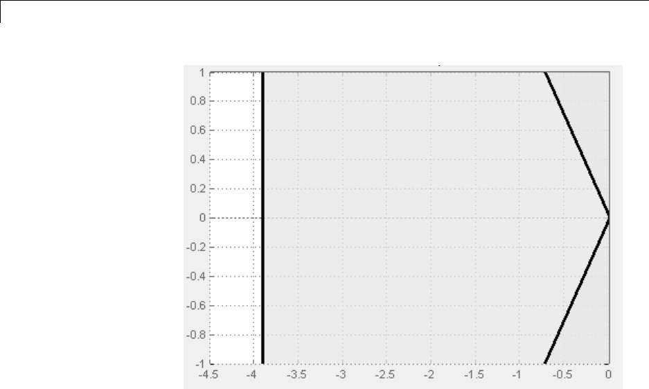
Pole-Zero Plot
•If you specify other bounds, such as settling time, damping ratio or
natural frequency, but want to exclude the percent overshoot bound
from assertion, clear this parameter.
•To only view the bounds on the plot, clear Enable assertion.
Command-Line Information
Parameter: EnablePercentOvershoot
Type: string
Value: 'on' |'off'
Default: 'off' for Pole-Zero Plot block, 'on' for Check Pole-Zero
Characteristics block.
See Also
Plot Linear Characteristics of Simulink Models During Simulation
“Model Verification at Default Simulation Snapshot Time” on page 5-6
10-262

Pole-Zero Plot
Percent overshoot <=
Percent overshoot of the second-order system.
Settings
Default:
[] for Pole-Zero Plot block
10 for Check Pole-Zero Characteristics block
Minimum: 0
Maximum: 100
•Real scalar for single percent overshoot bound.
•Cell array of real scalars for multiple percent overshoot bounds.
Tips
•The percent overshoot p.o can be expressed in terms of the damping
ratio ζ,as:
po e.. .
/
=−−
100 12
πζ ζ
•To assert that the percent overshoot bounds are satisfied, select both
Include percent overshoot bound in assertion and Enable
assertion.
•You can add or modify percent overshoot bounds from the plot
window:
-To add a new percent overshoot bound, right-click the plot, and
select Bounds > New Bound. Select Percent overshoot in
Design requirement type and specify the value in Percent
overshoot <.
-To modify a percent overshoot bound, drag the corresponding
bound segment. Alternatively, right-click the bound, and
select Bounds > Edit. Specify the new damping ratio for the
corresponding percent overshoot value in Damping ratio >.
You must click Update Block before simulating the model.
10-263

Pole-Zero Plot
Command-Line Information
Parameter: PercentOvershoot
Type: string
Value: [] |10 |real scalar between 0 and 100 |cell array
of real scalars between 0 and 100.Mustbespecifiedinside
single quotes ('').
Default: '[]' for Pole-Zero Plot block, '10' for Check Pole-Zero
Characteristics block.
See Also
Plot Linear Characteristics of Simulink Models During Simulation
“Model Verification at Default Simulation Snapshot Time” on page 5-6
10-264

Pole-Zero Plot
Include damping ratio bound in assertion
Check that the pole locations satisfy approximate second-order bounds
on the damping ratio, specified in Damping ratio >=.Thesoftware
displays a warning if the poles lie outside the region defined by the
damping ratio bound.
This parameter is used for assertion only if Enable assertion in the
Assertion tab is selected.
You can specify multiple damping ratio bounds on the linear system.
The bounds also appear on the pole-zero plot. If you clear Enable
assertion, the bounds are not used for assertion but continues to
appear on the plot.
Settings
Default: Off
On
Check that each pole lies in the region defined by the damping
ratio bound, during simulation.
Off
Do not check that each pole lies in the region defined by the
damping ratio bound, during simulation.
Tips
•Clearing this parameter disables the damping ratio bounds and
the software stops checking that the bounds are satisfied during
simulation. The bounds are also greyed out on the plot.
10-265

Pole-Zero Plot
•If you specify other bounds, such as settling time, percent overshoot
or natural frequency, but want to exclude the damping ratio bound
from assertion, clear this parameter.
•To only view the bounds on the plot, clear Enable assertion.
Command-Line Information
Parameter: EnableDampingRatio
Type: string
Value: 'on' |'off'
Default: 'off'
See Also
Plot Linear Characteristics of Simulink Models During Simulation
“Model Verification at Default Simulation Snapshot Time” on page 5-6
10-266

Pole-Zero Plot
Damping ratio >=
Damping ratio of the second-order system.
Settings
Default: []
Minimum: 0
Maximum: 1
•Finite positive real scalar for single damping ratio bound.
•Cell array of finite positive real scalars for multiple damping ratio
bounds.
Tips
•The damping ratio ζ, and percent overshoot p.o are related as:
po e.. .
/
=−−
100 12
πζ ζ
•To assert that the damping ratio bounds are satisfied, select
both Include damping ratio bound in assertion and Enable
assertion.
•You can add or modify damping ratio bounds from the plot window:
-To add a new damping ratio bound, right-click the plot and
select Bounds > New Bound. Select Damping ratio in Design
requirement type and specify the value in Damping ratio >.
-To modify a damping ratio bound, drag the corresponding bound
segment or right-click it and select Bounds > Edit.Specifythe
new value in Damping ratio >.
You must click Update Block before simulating the model.
Command-Line Information
Parameter: DampingRatio
Type: string
10-267

Pole-Zero Plot
Value: [] |finite positive real scalar between 0 and 1 |
cell array of finite positive real scalars between 0 and
1. Must be specified inside single quotes ('').
Default: '[]'
See Also
Plot Linear Characteristics of Simulink Models During Simulation
“Model Verification at Default Simulation Snapshot Time” on page 5-6
10-268

Pole-Zero Plot
Include natural frequency bound in assertion
Check that the pole locations satisfy approximate second-order bounds
on the natural frequency, specified in Natural frequency (rad/sec).
The natural frequency bound can be greater than, less than or equal
oneormorespecificvalues. Thesoftwaredisplaysawarningifthepole
locations do not satisfy the region defined by the natural frequency
bound.
This parameter is used for assertion only if Enable assertion in the
Assertion tab is selected.
You can specify multiple natural frequency bounds on the linear system.
The bounds also appear on the pole-zero plot. If Enable assertion is
cleared, the bounds are not used for assertion but continue to appear
on the plot.
Settings
Default: Off
On
Check that each pole lies in the region defined by the natural
frequency bound, during simulation.
Off
Do not check that each pole lies in the region defined by the
natural frequency bound, during simulation.
Tips
•Clearing this parameter disables the natural frequency bounds and
the software stops checking that the bounds are satisfied during
simulation. The bounds are also greyed out on the plot.
10-269
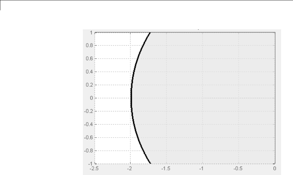
Pole-Zero Plot
•If you also specify settling time, percent overshoot or damping ratio
bounds and want to exclude the natural frequency bound from
assertion, clear this parameter.
•To only view the bounds on the plot, clear Enable assertion.
Command-Line Information
Parameter: NaturalFrequencyBound
Type: string
Value: 'on' |'off'
Default: 'off'
10-270

Pole-Zero Plot
Natural frequency (rad/sec)
Natural frequency of the second-order system.
Settings
Default: []
•Finite positive real scalar for single natural frequency bound.
•Cell array of finite positive real scalars for multiple natural frequency
bounds.
Tips
•To assert that the natural frequency bounds are satisfied, select both
Include natural frequency bound in assertion and Enable
assertion.
•You can add or modify natural frequency bounds from the plot
window:
-To add a new natural frequency bound, right-click the plot and
select Bounds > New Bound. Select Natural frequency in
Design requirement type and specify the natural frequency
in Natural frequency.
-To modify a natural frequency bound, drag the corresponding
bound segment or right-click it and select Bounds > Edit.Specify
thenewvalueinNatural frequency.
You must click Update Block before simulating the model.
Command-Line Information
Parameter: NaturalFrequency
Type: string
Value: [] |positive finite real scalar |cell array of
positive finite real scalars. Must be specified inside single
quotes ('').
Default: '[]'
See Also
Plot Linear Characteristics of Simulink Models During Simulation
10-271


Pole-Zero Plot
Save data to workspace
Save one or more linear systems as a variable in MATLAB workspace to
perform further linear analysis or control design.
The workspace variable is a structure with time and values fields:
•The time field stores the simulation time at which the linear system
is computed.
•The values field is a state-space object which stores the linear
system. If the linear system is computed at multiple simulation
times, values is an array of state-space objects.
Settings
Default: Off
On
Save the computed linear system to MATLAB workspace.
Off
Do not save the computed linear system to MATLAB workspace.
Dependencies
This parameter enables Variable name.
Command-Line Information
Parameter: SaveToWorkspace
Type: string
Value: 'on' |'off'
Default: 'off'
See Also
Plot Linear Characteristics of Simulink Models During Simulation
“Model Verification at Default Simulation Snapshot Time” on page 5-6
10-273

Pole-Zero Plot
Variable name
Name of the workspace variable that stores one or more linear systems
computed during simulation.
The name must be unique among the variable names used in all data
logging model blocks, such as Linear Analysis Plot blocks, Model
Verification blocks, Scope blocks, To Workspace blocks, and simulation
return variables such as time, states, and outputs.
Settings
Default: sys
String.
Dependencies
Save data to workspace enables this parameter.
Command-Line Information
Parameter: SaveName
Type: string
Value: sys |any string. Must be specified inside single quotes
('').
Default: 'sys'
See Also
Plot Linear Characteristics of Simulink Models During Simulation
“Model Verification at Default Simulation Snapshot Time” on page 5-6
10-274

Pole-Zero Plot
Enable assertion
Enable the block to check that bounds specified and included for
assertion in the Bounds tab are satisfied during simulation. Assertion
failsifaboundisnotsatisfied. Awarning, reporting the assertion
failure, appears at the MATLAB prompt.
If assertion fails, you can optionally specify that the block:
•Execute a MATLAB expression, specified in Simulation callback
when assertion fails (optional).
•Stop the simulation and bring that block into focus, by selecting Stop
simulation when assertion fails.
For the Linear Analysis Plots blocks, this parameter has no effect
because no bounds are included by default. If you want to use the
Linear Analysis Plots blocks for assertion, specify and include
bounds in the Bounds tab.
Clearing this parameter disables assertion, i.e., the block no longer
checks that specified bounds are satisfied. The block icon also updates
to indicate that assertion is disabled.
In the Configuration Parameters dialog box of the Simulink model, the
Model Verification block enabling option in the Debugging area of
Data Validity node, lets you to enable or disable all model verification
blocks in a model, regardless of the setting of this option.
Settings
Default: On
10-275

Pole-Zero Plot
On
Check that bounds included for assertion in the Bounds tab
are satisfied during simulation. A warning, reporting assertion
failure, is displayed at the MATLAB prompt if bounds are violated.
Off
Do not check that bounds included for assertion are satisfied
during simulation.
Dependencies
This parameter enables:
•Simulation callback when assertion fails (optional)
•Stop simulation when assertion fails
Command-Line Information
Parameter: enabled
Type: string
Value: 'on' |'off'
Default: 'on'
See Also
Plot Linear Characteristics of Simulink Models During Simulation
“Model Verification at Default Simulation Snapshot Time” on page 5-6
10-276

Pole-Zero Plot
Simulation callback when assertion fails (optional)
MATLAB expression to execute when assertion fails.
Because the expression is evaluated in the MATLAB workspace, define
all variables used in the expression in that workspace.
Settings
No Default
AMATLABexpression.
Dependencies
Enable assertion enables this parameter.
Command-Line Information
Parameter: callback
Type: string
Value: '' |MATLAB expression
Default: ''
See Also
Plot Linear Characteristics of Simulink Models During Simulation
“Model Verification at Default Simulation Snapshot Time” on page 5-6
10-277

Pole-Zero Plot
Stop simulation when assertion fails
Stop the simulation when a bound specified in the Bounds tab is
violated during simulation, i.e., assertion fails.
If you run the simulation from the Simulink Editor, the Simulation
Diagnostics window opens to display an error message. Also, the block
where the bound violation occurs is highlighted in the model.
Settings
Default: Off
On
Stop simulation if a bound specified in the Bounds tab is violated.
Off
Continue simulation if a bound is violated with a warning
message at the MATLAB prompt.
Tips
•Because selecting this option stops the simulation as soon as the
assertion fails, assertion failures that might occur later during the
simulation are not reported. If you want all assertion failures to be
reported, do not select this option.
Dependencies
Enable assertion enables this parameter.
Command-Line Information
Parameter: stopWhenAssertionFail
Type: string
Value: 'on' |'off'
Default: 'off'
See Also
Plot Linear Characteristics of Simulink Models During Simulation
“Model Verification at Default Simulation Snapshot Time” on page 5-6
10-278

Pole-Zero Plot
Output assertion signal
Output a Boolean signal that, at each time step, is:
•True (1) if assertion succeeds, i.e., all bounds are satisfied
•False (1)ifassertionfails,i.e.,aboundisviolated.
The output signal data type is Boolean only if the Implement logic
signals as Boolean data option in the Optimization pane of the
Configuration Parameters dialog box of the Simulink model is selected.
Otherwise, the data type of the output signal is double.
Selecting this parameter adds an output port to the block that you can
connect to any block in the model.
Settings
Default:Off
On
Output a Boolean signal to indicate assertion status. Adds a
port to the block.
Off
Do not output a Boolean signal to indicate assertion status.
Tips
•Use this parameter to design complex assertion logic. For an
example, see “Model Verification Using Simulink®Control Design™
and Simulink Verification Blocks” on page 5-25.
Command-Line Information
Parameter: export
Type: string
Value: 'on' |'off'
Default: 'off'
See Also
Plot Linear Characteristics of Simulink Models During Simulation
10-279

Pole-Zero Plot
“Model Verification at Default Simulation Snapshot Time” on page 5-6
Show plot on block open
Open the plot window instead of the Block Parameters dialog box when
you double-click the block in the Simulink model.
Usethisparameterifyouprefertoopenandperformtasks,suchas
adding or modifying bounds, in the plot window instead of the Block
Parameters dialog box. If you want to access the block parameters from
the plot window, select Edit or click .
For more information on the plot, see Show Plot.
Settings
Default: Off
On
Open the plot window when you double-click the block.
Off
Open the Block Parameters dialog box when double-clicking the
block.
Command-Line Information
Parameter: LaunchViewOnOpen
Type: string
Value: 'on' |'off'
Default: 'off'
See Also
Plot Linear Characteristics of Simulink Models During Simulation
“Model Verification at Default Simulation Snapshot Time” on page 5-6
Show Plot Open the plot window.
Use the plot to view:
10-280

Pole-Zero Plot
•Linear system characteristics computed from the nonlinear Simulink
model during simulation
You must click this button before you simulate the model to view
the linear characteristics.
You can display additional characteristics, such as the peak response
time and stability margins, of the linear system by right-clicking the
plot and selecting Characteristics.
•Bounds on the linear system characteristics
You can specify bounds in the Bounds tab of the Block Parameters
dialog box or right-click the plot and select Bounds > New Bound.
For more information on the types of bounds you can specify on each
plot, see “Verifiable Linear System Characteristics” on page 5-5 in
the User’s Guide.
You can modify bounds by dragging the bound segment or by
right-clicking the plot and selecting Bounds > Edit Bound. Before
you simulate the model, click Update Block to update the bound
value in the block parameters.
Typical tasks that you perform in the plot window include:
•Opening the Block Parameters dialog box by clicking or selecting
Edit.
•Finding the block that the plot window corresponds to by clicking
or selecting View > Highlight Simulink Block.Thisactionmakes
the Simulink Editor active and highlights the block.
•Simulating the model by clicking or selecting Simulation > Run.
This action also linearizes the portion of the model between the
specified linearization input and output.
•Adding legend on the linear system characteristic plot by clicking .
See Also Check Pole-Zero Characteristics
10-281

Pole-Zero Plot
Tutorials •“Visualize Bode Response of Simulink Model During Simulation”
on page 2-42
•“Visualize Linear System at Multiple Simulation Snapshots” on page
2-64
•“Visualize Linear System of a Continuous-Time Model Discretized
During Simulation” on page 2-70
•Plotting Linear System Characteristics of a Chemical Reactor
10-282

Singular Value Plot
Purpose Singular value plot of linear system approximated from nonlinear
Simulink model
Library Simulink Control Design
Description This block is same as the Check Singular Value Characteristics block
except for different default parameter settings in the Bounds tab.
Compute a linear system from a nonlinear Simulink model and plot the
linear system on a singular value plot.
During simulation, the software linearizes the portion of the model
between specified linearization inputs and outputs, and plots the
singular values of the linear system.
The Simulink model can be continuous- or discrete-time or multirate,
and can have time delays. The linear system can be Single-Input
Single-Output (SISO) or Multi-Input Multi-Output (MIMO). For MIMO
systems, the plots for all input/output combinations are displayed.
You can specify piecewise-linear frequency-dependent upper and lower
singular value bounds and view them on the plot. You can also check
that the bounds are satisfied during simulation:
•If all bounds are satisfied, the block does nothing.
•If a bound is not satisfied, the block asserts, and a warning message
appears at the MATLAB prompt. You can also specify that the block:
-Evaluate a MATLAB expression.
-Stop the simulation and bring that block into focus.
During simulation, the block can also output a logical assertion signal:
•If all bounds are satisfied, the signal is true (1).
•If a bound is not satisfied, the signal is false (0).
For MIMO systems, the bounds apply to the singular values of linear
systems computed for all input/output combinations.
10-283

Singular Value Plot
You can add multiple Singular Value Plot blocks to compute and plot
the singular values of various portions of the model.
You can save the linear system as a variable in the MATLAB workspace.
The block does not support code generation and can be used only in
Normal simulation mode.
Parameters The following table summarizes the Singular Value Plot block
parameters, accessible via the block parameter dialog box.
Task Parameters
Specify inputs and
outputs (I/Os).
In Linearizations
tab:
•“Linearization
inputs/outputs”
on page 10-287.
•“Click a signal in
the model to select
it” on page 10-290.
Specify settings. In Linearizations
tab:
•“Linearize on” on
page 10-294.
•“Snapshot times”
on page 10-296.
•“Trigger type” on
page 10-297.
Specify algorithm
options.
In Algorithm
Options of
Linearizations tab:
Configure
linearization.
10-284

Singular Value Plot
Task Parameters
•“Enable
zero-crossing
detection” on page
10-298.
•“Use exact delays”
on page 10-300.
•“Linear system
sample time” on
page 10-301.
•“Sample time
rate conversion
method” on page
10-303.
•“Prewarp
frequency (rad/s)”
on page 10-306.
Specify labels for
linear system I/Os
and state names.
In Labels of
Linearizations tab:
•“Use full block
names” on page
10-307.
•“Use bus signal
names” on page
10-309.
Plot the linear system. Show Plot
10-285

Singular Value Plot
Task Parameters
(Optional) Specify bounds on singular values
for assertion.
In Bounds tab:
•Include upper
singular value
bound in assertion.
•Include lower
singular value
bound in assertion.
Specify assertion options (only when you
specify bounds on the linear system).
In Assertion tab:
•“Enable assertion”
on page 10-325.
•“Simulation
callback when
assertion fails
(optional)” on page
10-327.
•“Stop simulation
when assertion
fails” on page
10-328.
•“Output assertion
signal” on page
10-329.
Save linear system to MATLAB workspace. “Save data to
workspace” on page
10-323 in Logging
tab.
Display plot window instead of block
parameters dialog box on double-clicking the
block.
“Show plot on block
open” on page 10-331.
10-286
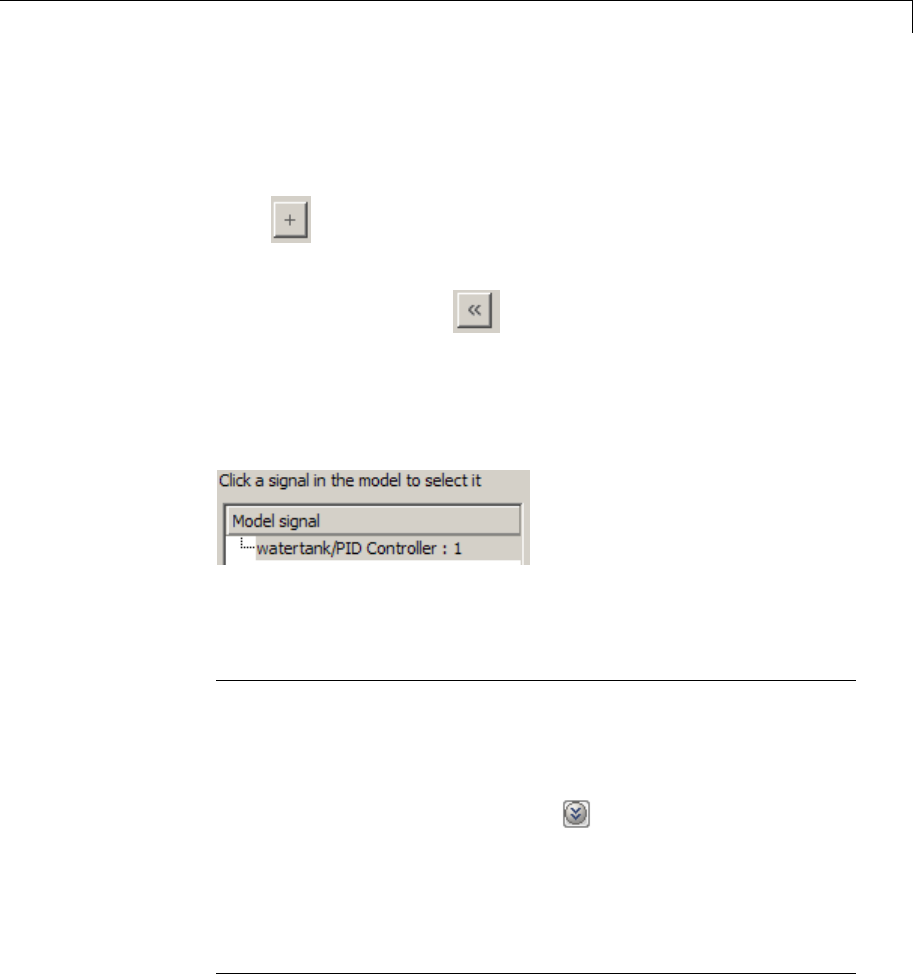
Singular Value Plot
Linearization inputs/outputs
Linearization inputs and outputs that define the portion of a nonlinear
Simulink model to linearize.
1Click .
The dialog box expands to display a Click a signal in the model to
select it area and a new button.
2Select a signal in the Simulink Editor.
The selected signal appears as a Model signal in the Click a signal
in the model to select it area.
3(Optional) For buses, expand the bus signal to select an individual
element.
Tip Forlargebuses,youcanentersearchtextforfilteringelement
names in the Filter by name edit box. The name match is
case-sensitive. Additionally, you can enter MATLAB regular
expression.
To modify the filtering options, click .
Filtering Options
•“Enable regular expression” on page 10-291
•“Show filtered results as a flat list” on page 10-292
10-287
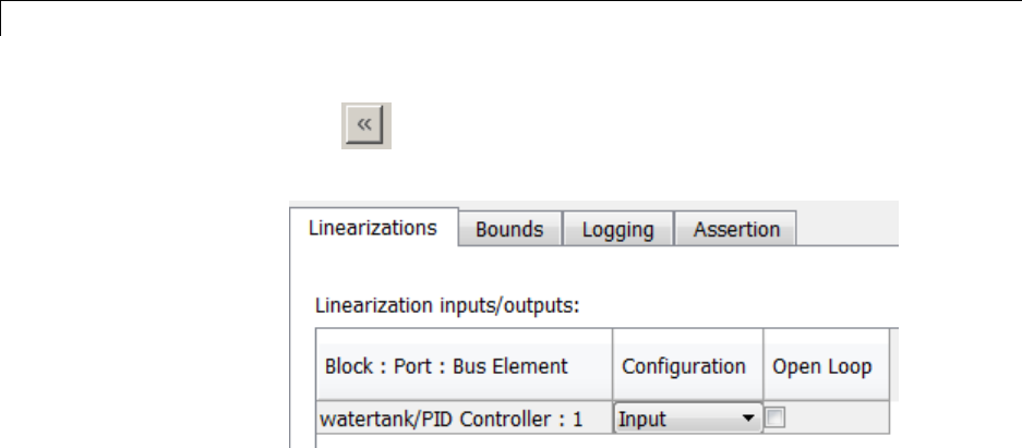
Singular Value Plot
4Click to add the signal to the Linearization inputs/outputs
table.
The table displays the following information about the selected signal:
Block : Port : Bus
Element
Name of the block associated with the input/output. The
number adjacent to the block name is the port number where
the selected bus signal is located. The last entry is the
selected bus element name.
Configuration Type of linearization point:
•Input — An input point.
•Output —Anoutputpoint.
•Input-Output — An input point immediately followed by
an output point.
•Output-Input — An output point immediately followed
by an input point.
•None — Signal selected but not specified as a linearization
input or output.
Open Loop If your model contains one or more feedback loops, you
can choose to linearize an open- or closed-loop system. For
example, you might want to linearize only the plant model
within a feedback control loop. When such a feedback loop
is present, select this option to insert an open loop point
10-288

Singular Value Plot
and remove the effect of the loop without manually breaking
signal lines.
For determining gain and phase margins, in most cases, you
open the loop.
Note If you simulate the model without specifying an input or output,
the software does not compute a linear system. Instead, you see a
warning message at the MATLAB prompt.
Settings
No default
Command-Line Information
Use the getlinio and setlinio commands to specify linearization
inputs and outputs.
See Also
Plot Linear Characteristics of Simulink Models During Simulation
“Model Verification at Default Simulation Snapshot Time” on page 5-6
10-289

Singular Value Plot
Click a signal in the model to select it
Enables signal selection in the Simulink model. Appears only when
you click .
When this option appears, you also see the following changes:
•Anew button.
Use to add a selected signal as a linearization input or output in the
Linearization inputs/outputs table. For more information, see
Linearization inputs/outputs.
•changes to .
UsetocollapsetheClick a signal in the model to select it area.
Settings
No default
Command-Line Information
Use the getlinio and setlinio commands to select signals as
linearization inputs and outputs.
See Also
Plot Linear Characteristics of Simulink Models During Simulation
“Model Verification at Default Simulation Snapshot Time” on page 5-6
10-290

Singular Value Plot
Enable regular expression
Enable the use of MATLAB regular expressions for filtering signal
names. For example, entering t$ in the Filter by name edit box
displays all signals whose names end with a lowercase t(and their
immediate parents). For details, see “Regular Expressions”.
Settings
Default: On
On
Allow use of MATLAB regular expressions for filtering signal
names.
Off
Disable use of MATLAB regular expressions for filtering signal
names. Filtering treats the text you enter in the Filter by name
edit box as a literal string.
Dependencies
Selecting the Options button on the right-hand side of the Filter by
name edit box ( ) enables this parameter.
10-291
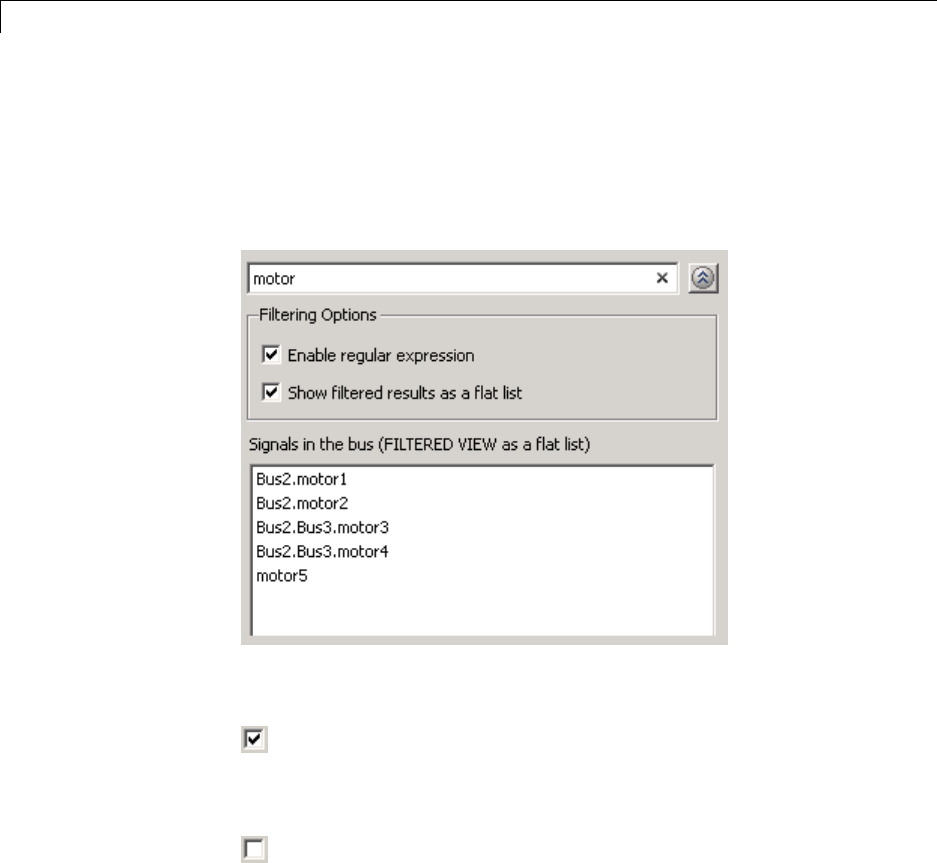
Singular Value Plot
Show filtered results as a flat list
Uses a flat list format to display the list of filtered signals, based on the
search text in the Filter by name edit box. The flat list format uses
dot notation to reflect the hierarchy of bus signals. The following is an
example of a flat list format for a filtered set of nested bus signals.
Settings
Default: Off
On
Display the filtered list of signalsusingaflatlistformat,
indicating bus hierarchies with dot notation instead of using a
tree format.
Off
Display filtered bus hierarchies using a tree format.
10-292

Singular Value Plot
Dependencies
Selecting the Options button on the right-hand side of the Filter by
name edit box ( ) enables this parameter.
10-293

Singular Value Plot
Linearize on
When to compute the linear system during simulation.
Settings
Default: Simulation snapshots
Simulation snapshots
Specific simulation time, specified in Snapshot times.
Use when you:
•Know one or more times when the model is at steady-state
operating point
•Want to compute the linear systems at specific times
External trigger
Trigger-based simulation event. Specify the trigger type in
Trigger type.
Use when a signal generated during simulation indicates
steady-state operating point.
Selecting this option adds a trigger port to the block. Use this port
to connect the block to the trigger signal.
For example, for an aircraft model, you might want to compute
the linear system whenever the fuel mass is a fraction of the
maximum fuel mass. In this case, model this condition as an
external trigger.
Dependencies
•Setting this parameter to Simulation snapshots enables Snapshot
times.
•Setting this parameter to External trigger enables Trigger type.
Command-Line Information
Parameter: LinearizeAt
10-294


Singular Value Plot
Snapshot times
One or more simulation times. The linear system is computed at these
times.
Settings
Default: 0
•For a different simulation time, enter the time. Use when you:
-Want to plot the linear system at a specific time
-Know the approximate time when the model reaches steady-state
operating point
•For multiple simulation times, enter a vector. Use when you want to
compute and plot linear systems at multiple times.
Snapshot times must be less than or equal to the simulation time
specified in the Simulink model.
Dependencies
Selecting Simulation snapshots in Linearize on enables this
parameter.
Command-Line Information
Parameter: SnapshotTimes
Type: string
Value: 0|positive real number |vector of positive real
numbers
Default: 0
See Also
Plot Linear Characteristics of Simulink Models During Simulation
“Model Verification at Default Simulation Snapshot Time” on page 5-6
10-296

Singular Value Plot
Trigger type
Trigger type of an external trigger for computing linear system.
Settings
Default: Rising edge
Rising edge
Rising edge of the external trigger signal.
Falling edge
Falling edge of the external trigger signal.
Dependencies
Selecting External trigger in Linearize on enables this parameter.
Command-Line Information
Parameter: TriggerType
Type: string
Value: 'rising' |'falling'
Default: 'rising'
See Also
Plot Linear Characteristics of Simulink Models During Simulation
“Model Verification at Default Simulation Snapshot Time” on page 5-6
10-297

Singular Value Plot
Enable zero-crossing detection
Enable zero-crossing detection to ensure that the software computes the
linear system characteristics at the following simulation times:
•The exact snapshot times, specified in Snapshot times.
As shown in the following figure, when zero-crossing detection is
enabled, the variable-step Simulink solver simulates the model at the
snapshot time Tsnap.Tsnap may lie between the simulation time steps
Tn-1 and Tnwhich are automatically chosen by the solver.
Computes linear system
characteristics at this time point
Time
Tn-1 Tn
Tsnap
•The exact times when an external trigger is detected, specified in
Trigger type.
As shown in the following figure, when zero-crossing detection is
enabled, the variable-step Simulink solver simulates the model at the
time, Ttrig, when the trigger signal is detected. Ttrig may lie between
the simulation time steps Tn-1 and Tnwhich are automatically chosen
by the solver.
Computes linear system
characteristics at this time point
Time
Amplitude
1
0Tn-1 Tn
Ttrig
Trigger signal
For more information on zero-crossing detection, see “Zero-Crossing
Detection” in the Simulink User Guide.
10-298

Singular Value Plot
Settings
Default: On
On
Compute linear system characteristics at the exact snapshot time
or exact time when a trigger signal is detected.
This setting is ignored if the Simulink solver is fixed step.
Off
Compute linear system characteristics at the simulation time
steps that the variable-step solver chooses. The software may not
compute the linear system at the exact snapshot time or exact
time when a trigger signal is detected.
Command-Line Information
Parameter: ZeroCross
Type: string
Value: 'on' |'off'
Default: 'on'
See Also
Plot Linear Characteristics of Simulink Models During Simulation
“Model Verification at Default Simulation Snapshot Time” on page 5-6
10-299

Singular Value Plot
Use exact delays
How to represent time delays in your linear model.
Use this option if you have blocks in your model that have time delays.
Settings
Default: Off
On
Return a linear model with exact delay representations.
Off
Return a linear model with Padé approximations of delays, as
specified in your Transport Delay and Variable Transport Delay
blocks.
Command-Line Information
Parameter: UseExactDelayModel
Type: string
Value: 'on' |'off'
Default: 'off'
See Also
Plot Linear Characteristics of Simulink Models During Simulation
“Model Verification at Default Simulation Snapshot Time” on page 5-6
10-300

Singular Value Plot
Linear system sample time
Sample time of the linear system computed during simulation.
Use this parameter to:
•Compute a discrete-time system with a specific sample time from a
continuous-time system
•Resample a discrete-time system with a different sample time
•Compute a continuous-time system from a discrete-time system
When computing discrete-time systems from continuous-time systems
and vice-versa, the software uses the conversion method specified in
Sample time rate conversion method.
Settings
Default: auto
auto. Computes the sample time as:
•0, for continuous-time models.
•For models that have blocks with different sample times
(multi-rate models), least common multiple of the sample
times. For example, if you have a mix of continuous-time and
discrete-time blocks with sample times of 0, 0.2 and 0.3, the
sample time of the linear model is 0.6.
Positive finite value.Usetocompute:
•A discrete-time linear system from a continuous-time system.
•A discrete-time linear system from another discrete-time
system with a different sample time
0
Usetocomputeacontinuous-timelinearsystemfroma
discrete-time model.
Command-Line Information
Parameter: SampleTime
10-301


Singular Value Plot
Sample time rate conversion method
Method for converting the sample time of single- or multi-rate models.
This parameter is used only when the value of Linear system sample
time is not auto.
Settings
Default: Zero-Order Hold
Zero-Order Hold
Zero-order hold, where the control inputs are assumed piecewise
constant over the sampling time Ts. For more information, see
“Zero-Order Hold” in Control System Toolbox User’s Guide.
This method usually performs better in time domain.
Tustin (bilinear)
Bilinear (Tustin) approximation without frequency prewarping.
The software rounds off fractional time delays to the nearest
multiple of the sampling time. For more information, see “Tustin
Approximation” in Control System Toolbox User’s Guide.
This method usually perform better in the frequency domain.
Tustin with Prewarping
Bilinear (Tustin) approximation with frequency prewarping. Also
specify the prewarp frequency in Prewarp frequency (rad/s).
For more information, see “Tustin Approximation” in Control
System Toolbox User’s Guide.
This method usually perform better in the frequency domain. Use
this method to ensure matching at frequency region of interest.
Upsampling when possible, Zero-Order Hold otherwise
Upsample a discrete-time system when possible and use
Zero-Order Hold otherwise.
10-303

Singular Value Plot
You can upsample only when you convert discrete-time system to
a new sample time that is an integer-value-times faster than the
sampling time of the original system.
Upsampling when possible, Tustin otherwise
Upsample a discrete-time system when possible and use Tustin
(bilinear) otherwise.
You can upsample only when you convert discrete-time system to
a new sample time that is an integer-value-times faster than the
sampling time of the original system.
Upsampling when possible, Tustin with Prewarping otherwise
Upsample a discrete-time system when possible and use Tustin
with Prewarping otherwise. Also, specify the prewarp frequency
in Prewarp frequency (rad/s).
You can upsample only when you convert discrete-time system to
a new sample time that is an integer-value-times faster than the
sampling time of the original system.
Dependencies
Selecting either:
•Tustin with Prewarping
•Upsampling when possible, Tustin with Prewarping
otherwise
enables Prewarp frequency (rad/s).
Command-Line Information
Parameter: RateConversionMethod
Type: string
Value: 'zoh' |'tustin' |'prewarp'|'upsampling_zoh'|
'upsampling_tustin'|'upsampling_prewarp'
Default: 'zoh'
10-304


Singular Value Plot
Prewarp frequency (rad/s)
Prewarp frequency for Tustin method, specified in radians/second.
Settings
Default: 10
Positive scalar value, smaller than the Nyquist frequency before and
after resampling. A value of 0 corresponds to the standard Tustin
method without frequency prewarping.
Dependencies
Selecting either
•Tustin with Prewarping
•Upsampling when possible, Tustin with Prewarping
otherwise
in Sample time rate conversion method enablesthisparameter.
Command-Line Information
Parameter: PreWarpFreq
Type: string
Value: 10 |positive scalar value
Default: 10
See Also
Plot Linear Characteristics of Simulink Models During Simulation
“Model Verification at Default Simulation Snapshot Time” on page 5-6
10-306

Singular Value Plot
Use full block names
How the state, input and output names appear in the linear system
computed during simulation.
The linear system is a state-space object and system states and
input/output names appear in following state-space object properties:
Input, Output or State Name Appears in Which State-Space
Object Property
Linearization input name InputName
Linearization output name OutputName
State names StateName
Settings
Default: Off
On
Show state and input/output names with their path through the
model hierarchy. For example, in the chemical reactor model,
a state in the Integrator1 block of the CSTR subsystem appears
with full path as scdcstr/CSTR/Integrator1.
Off
Show only state and input/output names. Use this option when the
signal name is unique and you know where the signal is location
in your Simulink model. For example, a state in the Integrator1
block of the CSTR subsystem appears as Integrator1.
Command-Line Information
Parameter: UseFullBlockNameLabels
Type: string
Value: 'on' |'off'
Default: 'off'
See Also
Plot Linear Characteristics of Simulink Models During Simulation
10-307


Singular Value Plot
Use bus signal names
How to label signals associated with linearization inputs and outputs
on buses, in the linear system computed during simulation (applies only
when you select an entire bus as an I/O point).
Selecting an entire bus signal is not recommended. Instead, select
individual bus elements.
You cannot use this parameter when your model has mux/bus mixtures.
Settings
Default: Off
On
Use the signal names of the individual bus elements.
Bus signal names appear when the input and output are at the
output of the following blocks:
•Root-level inport block containing a bus object
•Bus creator block
•Subsystem block whose source traces back to one of the
following blocks:
—Output of a bus creator block
—Root-level inport block by passing through only virtual or
nonvirtual subsystem boundaries
Off
Use the bus signal channel number.
Command-Line Information
Parameter: UseBusSignalLabels
Type: string
Value: 'on' |'off'
Default: 'off'
10-309


Singular Value Plot
Include upper singular value bound in assertion
Check that the singular values satisfy upper bounds, specified in
Frequencies (rad/sec) and Magnitude (dB), during simulation. The
software displays a warning during simulation if the singular values
violate the upper bound.
This parameter is used for assertion only if Enable assertion in the
Assertion tab is selected.
You can specify multiple upper singular value bounds on the linear
system. The bounds also appear on the singular value plot. If you clear
Enable assertion, the bounds are not used for assertion but continue
to appear on the plot.
Settings
Default:
•Off for Singular Value Plot block.
•On for Check Singular Value Characteristics block.
On
Check that the singular value satisfies the specified upper bounds,
during simulation.
Off
Do not check that the singular value satisfies the specified upper
bounds, during simulation.
Tips
•Clearing this parameter disables the upper singular value bounds
and the software stops checking that the bounds are satisfied during
simulation. The bound segments are also greyed out on the plot.
10-311
Singular Value Plot
•If you specify both upper and lower singular value bounds but want
to include only the lower bounds for assertion, clear this parameter.
•To only view the bound on the plot, clear Enable assertion.
Command-Line Information
Parameter: EnableUpperBound
Type: string
Value: 'on' |'off'
Default: 'off' forSingularValuePlotblock,'on' for Check
Singular Value Characteristics block.
See Also
Plot Linear Characteristics of Simulink Models During Simulation
“Model Verification at Default Simulation Snapshot Time” on page 5-6
10-312

Singular Value Plot
Frequencies (rad/sec)
Frequencies for one or more upper singular value bound segments,
specified in radians/sec.
Specify the corresponding magnitudes in Magnitude (dB).
Settings
Default:
[] for Singular Value Plot block
[0.1 100] for Check Singular Value Characteristics block
Must be specified as start and end frequencies:
•Positive finite numbers for a single bound with one edge
•Matrix of positive finite numbers for a single bound with multiple
edges
For example, type [0.1 1;1 10] for two edges at frequencies [0.1 1]
and [1 10].
•Cell array of matrices with positive finite numbers for multiple
bounds.
Tips
•To assert that magnitudes that correspond to the frequencies are
satisfied, select both Include upper singular value bound in
assertion and Enable assertion.
•You can add or modify frequencies from the plot window:
-To add new frequencies, right-click the plot, and select
Bounds > New Bound. Select Upper gain limit in Design
requirement type, and specify the frequencies in the Frequency
column. Specify the corresponding magnitudes in the Magnitude
column.
-To modify the frequencies, drag the bound segment. Alternatively,
right-click the segment, and select Bounds > Edit Bound.
Specify the new frequencies in the Frequency column.
10-313

Singular Value Plot
You must click Update Block before simulating the model.
Command-Line Information
Parameter: UpperBoundFrequencies
Type: string
Value: [] |[0.1 100] |positive finite numbers |matrix
of positive finite numbers |cell array of matrices with
positive finite numbers. Must be specified inside single quotes
('').
Default: '[]' for Singular Value Plot block, '[0.1 100]' for Check
Singular Value Characteristics block.
See Also
Plot Linear Characteristics of Simulink Models During Simulation
“Model Verification at Default Simulation Snapshot Time” on page 5-6
10-314

Singular Value Plot
Magnitudes (dB)
Magnitude values for one or more upper singular value bound segments,
specified in decibels.
Specify the corresponding frequencies in Frequencies (rad/sec).
Settings
Default:
[] for Singular Value Plot block
[0 0] for Check Singular Value Characteristics block
Must be specified as start and end magnitudes:
•Finite numbers for a single bound with one edge
•Matrix of finite numbers for a single bound with multiple edges
For example, type [0 0; 10 10] for two edges at magnitudes [0 0] and
[10 10].
•Cell array of matrices with finite numbers for multiple bounds
Tips
•To assert that magnitudes are satisfied, select both Include upper
singular value bound in assertion and Enable assertion.
•You can add or modify magnitudes from the plot window:
-To add a new magnitude, right-click the plot, and select
Bounds > New Bound. Select Upper gain limit in Design
requirement type, and specify the magnitude in the Magnitude
column. Specify the corresponding frequencies in the Frequency
column.
-To modify the magnitudes, drag the bound segment. Alternatively,
right-click the segment, and select Bounds > Edit Bound.
Specify the new magnitudes in the Magnitude column.
You must click Update Block before simulating the model.
10-315

Singular Value Plot
Command-Line Information
Parameter: UpperBoundMagnitudes
Type: string
Value: [] |[0 0] |finite numbers |matrix of finite numbers
|cell array of matrices with finite numbers.Mustbe
specified inside single quotes ('').
Default: '[]' forSingularValuePlotblock,'[0 0]' for Check
Singular Value Characteristics block.
See Also
Plot Linear Characteristics of Simulink Models During Simulation
“Model Verification at Default Simulation Snapshot Time” on page 5-6
10-316

Singular Value Plot
Include lower singular value bound in assertion
Check that the singular values satisfy lower bounds, specified in
Frequencies (rad/sec) and Magnitude (dB), during simulation. The
software displays a warning if the singular values violate the lower
bound.
This parameter is used for assertion only if Enable assertion in the
Assertion tab is selected.
You can specify multiple lower singular value bounds on the linear
system. The bounds also appear on the singular value plot. If you clear
Enable assertion, the bounds are not used for assertion but continue
to appear on the plot.
Settings
Default: Off
On
Check that the singular value satisfies the specified lower bounds,
during simulation.
Off
Do not check that the singular value satisfies the specified lower
bounds, during simulation.
Tips
•Clearing this parameter disables the upper bounds and the software
stops checking that the bounds are satisfied during simulation. The
boundsegmentsarealsogreyedoutintheplotwindow.
10-317
Singular Value Plot
•If you specify both lower and upper singular value bounds but want
to include only the upper bounds for assertion, clear this parameter.
•To only view the bound on the plot, clear Enable assertion.
Command-Line Information
Parameter: EnableLowerBound
Type: string
Value: 'on' |'off'
Default: 'off'
See Also
Plot Linear Characteristics of Simulink Models During Simulation
“Model Verification at Default Simulation Snapshot Time” on page 5-6
10-318

Singular Value Plot
Frequencies (rad/sec)
Frequencies for one or more lower singular value bound segments,
specified in radians/sec.
Specify the corresponding magnitudes in Magnitude (dB).
Settings
Default []
Must be specified as start and end frequencies:
•Positive finite numbers for a single bound with one edge
•Matrix of positive finite numbers for a single bound with multiple
edges
For example, type [0.01 0.1;0.1 1] to specify two edges with
frequencies [0.01 0.1] and [0.1 1].
•Cell array of matrices with positive finite numbers for multiple
bounds.
Tips
•To assert that magnitude bounds that correspond to the frequencies
are satisfied, select both Include lower singular value bound in
assertion and Enable assertion.
•You can add or modify frequencies from the plot window:
-To add new frequencies, right-click the plot, and select
Bounds > New Bound. Select Lower gain limit in Design
requirement type and specify the frequencies in the Frequency
column. Specify the corresponding magnitudes in the Magnitude
column.
-To modify the frequencies, drag the bound segment. Alternatively,
right-click the segment, and select Bounds > Edit Bound.
Specify the new frequencies in the Frequency column.
You must click Update Block before simulating the model.
10-319

Singular Value Plot
Command-Line Information
Parameter: LowerBoundFrequencies
Type: string
Value: [] |positive finite numbers |matrix of positive
finite numbers |cell array of matrices with positive
finite numbers. Must be specified inside single quotes ('').
Default: '[]'
See Also
Plot Linear Characteristics of Simulink Models During Simulation
“Model Verification at Default Simulation Snapshot Time” on page 5-6
10-320

Singular Value Plot
Magnitudes (dB)
Magnitude values for one or more lower singular value bound segments,
specified in decibels.
Specify the corresponding frequencies in Frequencies (rad/sec).
Settings
Default []
Must be specified as start and end magnitudes:
•Finite numbers for a single bound with one edge
•Matrix of finite numbers for a single bound with multiple edges
For example, type [0 0; 10 10] for two edges with magnitudes [0 0]
and [10 10].
•Cell array of matrices with finite numbers for multiple bounds
Tips
•To assert that magnitudes are satisfied, select both Include lower
singular value bound in assertion and Enable assertion.
•You can add or modify magnitudes from the plot window:
-To add new magnitudes, right-click the plot, and select
Bounds > New Bound. Select Lower gain limit in Design
requirement type, and specify the magnitudes in the Magnitude
column. Specify the corresponding frequencies in the Frequency
column.
-To modify the magnitudes, drag the bound segment. Alternatively,
right-click the segment, and select Bounds > Edit Bound.
Specify the new magnitudes in the Magnitude column.
You must click Update Block before simulating the model.
Command-Line Information
Parameter: LowerBoundFrequencies
Type: string
10-321

Singular Value Plot
Value: [] |finite number |matrix of finite numbers |cell
array of matrices with finite numbers.Mustbespecified
inside single quotes ('').
Default: '[]'
See Also
Plot Linear Characteristics of Simulink Models During Simulation
“Model Verification at Default Simulation Snapshot Time” on page 5-6
10-322

Singular Value Plot
Save data to workspace
Save one or more linear systems as a variable in MATLAB workspace to
perform further linear analysis or control design.
The workspace variable is a structure with time and values fields:
•The time field stores the simulation time at which the linear system
is computed.
•The values field is a state-space object which stores the linear
system. If the linear system is computed at multiple simulation
times, values is an array of state-space objects.
Settings
Default: Off
On
Save the computed linear system to MATLAB workspace.
Off
Do not save the computed linear system to MATLAB workspace.
Dependencies
This parameter enables Variable name.
Command-Line Information
Parameter: SaveToWorkspace
Type: string
Value: 'on' |'off'
Default: 'off'
See Also
Plot Linear Characteristics of Simulink Models During Simulation
“Model Verification at Default Simulation Snapshot Time” on page 5-6
10-323

Singular Value Plot
Variable name
Name of the workspace variable that stores one or more linear systems
computed during simulation.
The name must be unique among the variable names used in all data
logging model blocks, such as Linear Analysis Plot blocks, Model
Verification blocks, Scope blocks, To Workspace blocks, and simulation
return variables such as time, states, and outputs.
Settings
Default: sys
String.
Dependencies
Save data to workspace enables this parameter.
Command-Line Information
Parameter: SaveName
Type: string
Value: sys |any string. Must be specified inside single quotes
('').
Default: 'sys'
See Also
Plot Linear Characteristics of Simulink Models During Simulation
“Model Verification at Default Simulation Snapshot Time” on page 5-6
10-324

Singular Value Plot
Enable assertion
Enable the block to check that bounds specified and included for
assertion in the Bounds tab are satisfied during simulation. Assertion
failsifaboundisnotsatisfied. Awarning, reporting the assertion
failure, appears at the MATLAB prompt.
If assertion fails, you can optionally specify that the block:
•Execute a MATLAB expression, specified in Simulation callback
when assertion fails (optional).
•Stop the simulation and bring that block into focus, by selecting Stop
simulation when assertion fails.
For the Linear Analysis Plots blocks, this parameter has no effect
because no bounds are included by default. If you want to use the
Linear Analysis Plots blocks for assertion, specify and include
bounds in the Bounds tab.
Clearing this parameter disables assertion, i.e., the block no longer
checks that specified bounds are satisfied. The block icon also updates
to indicate that assertion is disabled.
In the Configuration Parameters dialog box of the Simulink model, the
Model Verification block enabling option in the Debugging area of
Data Validity node, lets you to enable or disable all model verification
blocks in a model, regardless of the setting of this option.
Settings
Default: On
10-325

Singular Value Plot
On
Check that bounds included for assertion in the Bounds tab
are satisfied during simulation. A warning, reporting assertion
failure, is displayed at the MATLAB prompt if bounds are violated.
Off
Do not check that bounds included for assertion are satisfied
during simulation.
Dependencies
This parameter enables:
•Simulation callback when assertion fails (optional)
•Stop simulation when assertion fails
Command-Line Information
Parameter: enabled
Type: string
Value: 'on' |'off'
Default: 'on'
See Also
Plot Linear Characteristics of Simulink Models During Simulation
“Model Verification at Default Simulation Snapshot Time” on page 5-6
10-326

Singular Value Plot
Simulation callback when assertion fails (optional)
MATLAB expression to execute when assertion fails.
Because the expression is evaluated in the MATLAB workspace, define
all variables used in the expression in that workspace.
Settings
No Default
AMATLABexpression.
Dependencies
Enable assertion enables this parameter.
Command-Line Information
Parameter: callback
Type: string
Value: '' |MATLAB expression
Default: ''
See Also
Plot Linear Characteristics of Simulink Models During Simulation
“Model Verification at Default Simulation Snapshot Time” on page 5-6
10-327

Singular Value Plot
Stop simulation when assertion fails
Stop the simulation when a bound specified in the Bounds tab is
violated during simulation, i.e., assertion fails.
If you run the simulation from the Simulink Editor, the Simulation
Diagnostics window opens to display an error message. Also, the block
where the bound violation occurs is highlighted in the model.
Settings
Default: Off
On
Stop simulation if a bound specified in the Bounds tab is violated.
Off
Continue simulation if a bound is violated with a warning
message at the MATLAB prompt.
Tips
•Because selecting this option stops the simulation as soon as the
assertion fails, assertion failures that might occur later during the
simulation are not reported. If you want all assertion failures to be
reported, do not select this option.
Dependencies
Enable assertion enables this parameter.
Command-Line Information
Parameter: stopWhenAssertionFail
Type: string
Value: 'on' |'off'
Default: 'off'
See Also
Plot Linear Characteristics of Simulink Models During Simulation
“Model Verification at Default Simulation Snapshot Time” on page 5-6
10-328

Singular Value Plot
Output assertion signal
Output a Boolean signal that, at each time step, is:
•True (1) if assertion succeeds, i.e., all bounds are satisfied
•False (1)ifassertionfails,i.e.,aboundisviolated.
The output signal data type is Boolean only if the Implement logic
signals as Boolean data option in the Optimization pane of the
Configuration Parameters dialog box of the Simulink model is selected.
Otherwise, the data type of the output signal is double.
Selecting this parameter adds an output port to the block that you can
connect to any block in the model.
Settings
Default:Off
On
Output a Boolean signal to indicate assertion status. Adds a
port to the block.
Off
Do not output a Boolean signal to indicate assertion status.
Tips
•Use this parameter to design complex assertion logic. For an
example, see “Model Verification Using Simulink®Control Design™
and Simulink Verification Blocks” on page 5-25.
Command-Line Information
Parameter: export
Type: string
Value: 'on' |'off'
Default: 'off'
See Also
Plot Linear Characteristics of Simulink Models During Simulation
10-329


Singular Value Plot
Show plot on block open
Open the plot window instead of the Block Parameters dialog box when
you double-click the block in the Simulink model.
Usethisparameterifyouprefertoopenandperformtasks,suchas
adding or modifying bounds, in the plot window instead of the Block
Parameters dialog box. If you want to access the block parameters from
the plot window, select Edit or click .
For more information on the plot, see Show Plot.
Settings
Default: Off
On
Open the plot window when you double-click the block.
Off
Open the Block Parameters dialog box when double-clicking the
block.
Command-Line Information
Parameter: LaunchViewOnOpen
Type: string
Value: 'on' |'off'
Default: 'off'
See Also
Plot Linear Characteristics of Simulink Models During Simulation
“Model Verification at Default Simulation Snapshot Time” on page 5-6
Show Plot Open the plot window.
Use the plot to view:
•Linear system characteristics computed from the nonlinear Simulink
model during simulation
10-331

Singular Value Plot
You must click this button before you simulate the model to view
the linear characteristics.
You can display additional characteristics, such as the peak response
time and stability margins, of the linear system by right-clicking the
plot and selecting Characteristics.
•Bounds on the linear system characteristics
You can specify bounds in the Bounds tab of the Block Parameters
dialog box or right-click the plot and select Bounds > New Bound.
For more information on the types of bounds you can specify on each
plot, see “Verifiable Linear System Characteristics” on page 5-5 in
the User’s Guide.
You can modify bounds by dragging the bound segment or by
right-clicking the plot and selecting Bounds > Edit Bound. Before
you simulate the model, click Update Block to update the bound
value in the block parameters.
Typical tasks that you perform in the plot window include:
•Opening the Block Parameters dialog box by clicking or selecting
Edit.
•Finding the block that the plot window corresponds to by clicking
or selecting View > Highlight Simulink Block.Thisactionmakes
the Simulink Editor active and highlights the block.
•Simulating the model by clicking or selecting Simulation > Run.
This action also linearizes the portion of the model between the
specified linearization input and output.
•Adding legend on the linear system characteristic plot by clicking .
See Also Check Singular Value Characteristics
Tutorials •“Visualize Bode Response of Simulink Model During Simulation”
on page 2-42
10-332

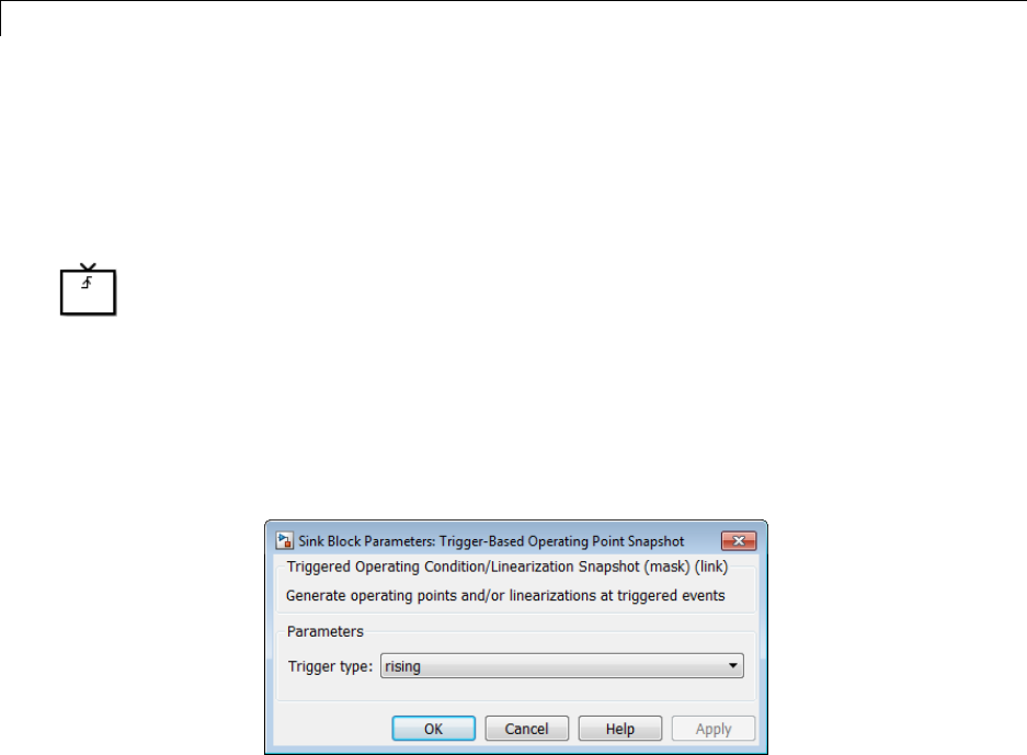
Trigger-Based Operating Point Snapshot
Purpose Generate operating points, linearizations, or both at triggered events
Library Simulink Control Design
Description Attach this block to a signal in a model when you want to take a
snapshot of the system’s operating point at triggered events such as
when the signal crosses zero or when the signal sends a function call.
You can also perform a linearization at these events. To extract the
operating point or perform the linearization, you need to simulate
the model using either the findop or linearize functions or the
simulation snapshots option in the Control and Estimation Tools
Manager.
Choose the trigger type in the Block Parameters dialog box, as shown in
the following figure.
The possible trigger types are
•rising: the signal crosses zero while increasing.
•falling: the signal crosses zero while decreasing.
•either: the signal crosses zero while either increasing or decreasing.
•function-call: the signal send a function call.
10-334

Trigger-Based Operating Point Snapshot
Note Computing Operating Point Snapshots at Triggered Events
illustrates how to use this block.
See Also findop,linearize
10-335

Trigger-Based Operating Point Snapshot
10-336

11
Model Advisor Checks

11 Model Advisor Checks
Simulink Control Design Checks
11-2

Simulink®Control Design™ Checks
Identify time-varying source blocks interfering with
frequency response estimation
Identify all time-varying source blocks in the signal path of any output
linearization point marked in the Simulink model.
Description
Frequency response estimation uses the steady-state response of a Simulink
model to a specified input signal. Time-varying source blocks in the signal
path prevent the response from reaching steady-state. In addition, when
such blocks appear in the signal path, the resulting response is not purely a
response to the specified input signal. Thus, time-varying source blocks can
interfere with accurate frequency response estimation.
This check finds and reports all the time-varying source blocks which appear
in the signal path of any output linearization output points currently marked
on the Simulink model. The report:
•Includes blocks in subsystems and in referenced models that are in normal
simulation mode
•Excludes any blocks specified as BlocksToHoldConstant in the
frestimateOptions object you enter as the input parameter
For more information about the algorithm that identifies time-varying source
blocks, see the frest.findSources reference page.
Input Parameters
FRESTIMATE options object to compare results against
Provide the paths of any blocks to exclude from the check. Specify the
block paths as an array of Simulink.BlockPath objects. This array is
stored in the BlocksToHoldConstant fieldofanoptionsetyoucreate
with frestimateOptions.SeethefrestimateOptions reference page
for more information.
11-3

11 Model Advisor Checks
Results and Recommended Actions
Condition Recommended Action
Source blocks exist whose
output reaches linearization
output points currently
marked on the model.
Consider holding these source blocks constant during frequency
response estimation.
Use the frest.findSources command to identify time-varying
source blocks at the command line. Then use the
BlocksToHoldConstant option of frestimateOptions to pass
theseblockstothefrestimate command. For example,
% Get linearization I/Os from the model.
mdl = 'scdengine';
io = getlinio(mdl);
% Find time-varying source blocks.
blks = frest.findSources(mdl,io);
% Create options set with blocks to hold constant.
opts = frestimateOptions;
opts.BlocksToHoldConstant = blks;
% Run estimation with the options.
in = frest.Sinestream;
sysest = frestimate(mdl,io,in,opts);
For more information and examples, see the
frest.findSources and frestimateOptions reference pages.
Tip
Sometimes, the model includes referenced models containing source blocks
in the signal path of an output linearization point. In such cases, set the
referenced models to normal simulation mode to ensure that this check locates
them. Use the set_param command to set SimulationMode of any referenced
models to Normal before running the check.
See Also
•“Estimate Frequency Response Using Linear Analysis Tool” on page 3-28
•“Effects of Time-Varying Source Blocks on Frequency Response Estimation”
on page 3-62
11-4

Simulink®Control Design™ Checks
•frest.findSources reference page
•frestimateOptions reference page
•frestimate reference page
11-5

11 Model Advisor Checks
11-6

A
Examples
Use this list to find examples in the documentation.

AExamples
Frequency Response Estimation
“Effects of Time-Varying Source Blocks on Frequency Response
Estimation” on page 3-62
“Effects of Noise on Frequency Response Estimation” on page 3-72
“Estimating Frequency Response Models with Noise Using Signal
Processing Toolbox” on page 3-74
“Estimating Frequency Response Models with Noise Using System
Identification Toolbox” on page 3-76
A-2

Index
IndexA
add linearization input and output 10-5 10-82
10-127 10-175 10-233 10-287
addoutputspec function 8-2
B
bus signal names 10-28 10-104 10-148 10-198
10-256 10-309
C
closed-loop gain on Nichols plot 10-208
compensator design
analysis plots 4-71
beginning a task 4-57
closed-loop responses 4-62
creating a SISO Design Task 4-67
design methods 4-78
design plots 4-68
open-loop systems 4-68
operating points 4-64
overview 4-2
retrieving designs 4-83
storing designs 4-83
time delays 4-77
tunable blocks 4-59
writing to Simulink model 4-85
configuration parameters
pane
Open-loop gains (dB): 10-214
Control and Estimation Tools Manager
compensator design task 4-57
SISO Design Task 4-67
copy function 8-6
D
damping ratio on pole-zero plot 10-267
delays
compensator design 4-77
E
enable assertion 10-44 10-114 10-162 10-220
10-275 10-325
enable zero-crossing detection 10-17 10-93
10-139 10-187 10-245 10-298
equilibrium operating point 1-2
from simulation 1-41
from specifications 1-14
equilibrium states
from simulation 1-41
from specifications 1-14
F
final value of step response 10-153
frequencies for lower magnitude bound 10-38
frequencies for lower singular value
bound 10-319
frequencies for upper magnitude bound 10-32
frequencies for upper singular value
bound 10-313
G
gain margin bound 10-108
gain margin bound on Nichols plot 10-202
get function 8-75
getinputstruct function 8-78
getlinio function 8-79
getlinplant function 8-84
getstatestruct function 8-88
getxu function 8-90
I
include closed-loop peak gain 10-206
include damping ratio on pole-zero plot 10-265
include gain and phase margins 10-106
Index-1

Index
include gain and phase margins on Nichols
plot 10-200
include lower magnitude bound 10-36
include lower singular value bound 10-317
include natural frequency on pole-zero
plot 10-269
include open-loop gain-phase bound 10-210
include percent overshoot bound on pole-zero
plot 10-261
include settling time bound on pole-zero
plot 10-258
include step response bound 10-150
include upper magnitude bound 10-30
include upper singular value bound 10-311
initopspec function 8-93
L
linearization
using simulation event 2-60
using simulation snapshot 2-57
linearize on 10-13 10-89 10-135 10-183 10-241
10-294
linio function 8-109
linoptions function 8-117
lower magnitude bound 10-40
lower singular value bound magnitude 10-321
O
open-loop phases 10-212
operating point
at simulation snapshot 1-41
equilibrium 1-2
from simulation snapshot 1-41
initialize simulation 1-44
initializing optimization search 1-24
meet output specifications 1-21
optimization settings 1-35
SimMechanics model 1-29
steady state 1-2
steady states from simulation 1-41
steady states from specifications 1-14
trimming 1-14
operpoint function 8-124
output assertion signal 10-48 10-118 10-166
10-224 10-279 10-329
P
percent overshoot 10-158
percent overshoot on pole-zero plot 10-263
percent rise 10-155
percent settling 10-157
percent undershoot 10-159
phase margin bound 10-109 to 10-110
phase margin bound on Nichols plot 10-204
PID
automatic tuning 4-3
plot type for gain and phase margins 10-120
prewarp frequency 10-25 10-101 10-146 10-195
10-253 10-306
R
retrieving compensator designs 4-83
rise time 10-154
S
sample time 10-20 10-96 10-141 10-190 10-248
10-301
Sample time rate conversion method 10-22 10-98
10-144 10-192 10-250 10-303
save data to workspace 10-42 10-112 10-160
10-218 10-273 10-323
select signal 10-9 10-85 10-131 10-179 10-237
10-290
set function 8-137
setlinio function 8-140
settling time 10-156
Index-2

Index
settling time on pole-zero plot 10-260
setxu function 8-145
show plot on block open 10-50 10-121 10-168
10-226 10-280 10-331
simulation
initialize operating point 1-44
simulation callback 10-46 10-116 10-164 10-222
10-277 10-327
SISO Design Task
creating 4-67
Snapshot times 10-15 10-91 10-137 10-185
10-243 10-296
steady state operating point 1-2
from simulation 1-41
from specifications 1-14
Stop simulation when assertion fails 10-47
10-117 10-165 10-223 10-278 10-328
storing compensator designs 4-83
T
trigger type 10-16 10-92 10-138 10-186 10-244
10-297
trim condition 1-2
trimming 1-14
U
update function 8-207
upper magnitude bound 10-34
upper singular value bound magnitude 10-315
use exact delays 10-19 10-95 10-141 10-189
10-247 10-300
V
variable name for saved linear system 10-43
10-113 10-161 10-219 10-274 10-324
Index-3
