Print Preview C:\TEMP\Apdf_2541_3068\home\AppData\Local\PTC\Arbortext\Editor\.aptcache\ae384hih/tf384yff Simulink User's Guide
User Manual:
Open the PDF directly: View PDF ![]() .
.
Page Count: 2839 [warning: Documents this large are best viewed by clicking the View PDF Link!]
- toc
- Introduction to Simulink
- Simulink Basics
- Start the Simulink Software
- Open a Model
- Load a Model
- Save a Model
- How to Tell If a Model Needs Saving
- Save a Model for the First Time
- Model Names
- Save a Previously Saved Model
- What Happens When You Save a Model?
- Saving Models in the SLX File Format
- Saving Models with Different Character Encodings
- Export a Model to a Previous Simulink Version
- Save from One Earlier Simulink Version to Another
- Simulink Editor
- Zoom and Pan Block Diagrams
- Update a Block Diagram
- Copy Models to Third-Party Applications
- Print a Block Diagram
- Generate a Model Report
- End a Simulink Session
- Keyboard and Mouse Shortcuts for Simulink
- Simulink Demos Are Now Called Examples
- Simulation Stepping
- How Simulink Works
- How Simulink Works
- Modeling Dynamic Systems
- Simulating Dynamic Systems
- Model Compilation
- Link Phase
- Simulation Loop Phase
- Solvers
- Zero-Crossing Detection
- Algebraic Loops
- What Is an Algebraic Loop?
- Problems Caused by Algebraic Loops
- Identifying Algebraic Loops in Your Model
- What If I Have an Algebraic Loop in My Model?
- Simulink Algebraic Loop Solver
- Removing Algebraic Loops
- Additional Techniques to Help the Algebraic Loop Solver
- Changing Block Priorities Does Not Remove Algebraic Loops
- Artificial Algebraic Loops
- Simulink Basics
- Modeling Dynamic Systems
- Creating a Model
- Create an Empty Model
- Populate a Model
- Select Modeling Objects
- Specify Block Diagram Colors
- Connect Blocks
- Align, Distribute, and Resize Groups of Blocks
- Annotate Diagrams
- Create a Subsystem
- Subsystem Advantages
- Two Ways to Create a Subsystem
- Create a Subsystem by Adding the Subsystem Block
- Create a Subsystem by Grouping Existing Blocks
- Subsystem Execution
- Navigate Model Hierarchy
- Label Subsystem Ports
- Control Access to Subsystems
- Interconvert Subsystems and Block Diagrams
- Empty Subsystems and Block Diagrams
- Control Flow Logic
- Callback Functions
- Model Workspaces
- Symbol Resolution
- Consult the Model Advisor
- About the Model Advisor
- Start the Model Advisor
- Overview of the Model Advisor Window
- Overview of the Model Advisor Dashboard
- Run Model Advisor Checks
- Run Checks Using Model Advisor Dashboard
- Highlight Model Advisor Analysis Results
- Fix a Warning or Failure
- Revert Changes Using Restore Points
- View and Save Model Advisor Reports
- Run the Model Advisor Programmatically
- Check Support for Libraries
- Model Advisor Limitations
- Consult the Upgrade Advisor
- Manage Model Versions
- Model Discretizer
- Working with Sample Times
- What Is Sample Time?
- Specify Sample Time
- Designate Sample Times
- Specify Block-Based Sample Times Interactively
- Specify Port-Based Sample Times Interactively
- Specify Block-Based Sample Times Programmatically
- Specify Port-Based Sample Times Programmatically
- Access Sample Time Information Programmatically
- Specify Sample Times for a Custom Block
- Determining Sample Time Units
- Change the Sample Time After Simulation Start Time
- View Sample Time Information
- Print Sample Time Information
- Types of Sample Time
- Block Compiled Sample Time
- Sample Times in Subsystems
- Sample Times in Systems
- Resolve Rate Transitions
- How Propagation Affects Inherited Sample Times
- Monitor Backpropagation in Sample Times
- Referencing a Model
- Overview of Model Referencing
- Create a Model Reference
- Convert a Subsystem to a Referenced Model
- Referenced Model Simulation Modes
- View a Model Reference Hierarchy
- Model Reference Simulation Targets
- Simulink Model Referencing Requirements
- Parameterize Model References
- Conditional Referenced Models
- Protected Model
- Use Protected Model in Simulation
- Inherit Sample Times
- Refresh Model Blocks
- S-Functions with Model Referencing
- Buses in Referenced Models
- Signal Logging in Referenced Models
- Model Referencing Limitations
- Creating Conditional Subsystems
- About Conditional Subsystems
- Enabled Subsystems
- Triggered Subsystems
- Triggered and Enabled Subsystems
- Function-Call Subsystems
- Conditional Execution Behavior
- Modeling Variant Systems
- Exploring, Searching, and Browsing Models
- Model Explorer Overview
- Model Explorer: Model Hierarchy Pane
- What You Can Do with the Model Hierarchy Pane
- Simulink Root
- Base Workspace
- Configuration Preferences
- Model Nodes
- Displaying Partial or Whole Model Hierarchy Contents
- Displaying Linked Library Subsystems
- Displaying Masked Subsystems
- Linked Library and Masked Subsystems
- Displaying Node Contents
- Navigating to the Block Diagram
- Working with Configuration Sets
- Expanding Model References
- Cutting, Copying, and Pasting Objects
- Model Explorer: Contents Pane
- Control Model Explorer Contents Using Views
- Organize Data Display in Model Explorer
- Filter Objects in the Model Explorer
- Workspace Variables in Model Explorer
- Search Using Model Explorer
- Model Explorer: Property Dialog Pane
- Finder
- Model Browser
- Model Dependency Viewer
- About Model Dependency Views
- Opening the Model Dependency Viewer
- Manipulating a Dependency View
- Changing Dependency View Type
- Excluding Block Libraries from a File Dependency View
- Including Simulink Blocksets in a File Dependency View
- Changing View Orientation
- Expanding or Collapsing Views
- Zooming a Dependency View
- Moving a Dependency View
- Rearranging a Dependency View
- Displaying and Hiding a Dependency View's Legend
- Displaying Full Paths of Referenced Model Instances
- Refreshing a Dependency View
- Browsing Dependencies
- Saving a Dependency View
- Printing a Dependency View
- View Linked Requirements in Models and Blocks
- Managing Model Configurations
- About Model Configurations
- Multiple Configuration Sets in a Model
- Share a Configuration for Multiple Models
- Share a Configuration Across Referenced Models
- Convert Configuration Set to Configuration Reference
- Propagate a Configuration Reference
- Undo a Configuration Reference Propagation
- Manage a Configuration Set
- Create a Configuration Set in a Model
- Create a Configuration Set in the Base Workspace
- Open a Configuration Set in the Configuration Parameters Dialog
- Activate a Configuration Set
- Set Values in a Configuration Set
- Copy, Delete, and Move a Configuration Set
- Save a Configuration Set
- Load a Saved Configuration Set
- Copy Configuration Set Components
- Manage a Configuration Reference
- Create and Attach a Configuration Reference
- Resolve a Configuration Reference
- Activate a Configuration Reference
- Manage Configuration Reference Across Referenced Models
- Change Parameter Values in a Referenced Configuration Set
- Save a Referenced Configuration Set
- Load a Saved Referenced Configuration Set
- Why is the Build Button Not Available for a Configuration Refere
- About Configuration Sets
- About Configuration References
- Model Configuration Command Line Interface
- Overview
- Load and Activate a Configuration Set at the Command Line
- Save a Configuration Set at the Command Line
- Create a Freestanding Configuration Set at the Command Line
- Create and Attach a Configuration Reference at the Command Line
- Attach a Configuration Reference to Multiple Models at the Comma
- Get Values from a Referenced Configuration Set
- Change Values in a Referenced Configuration Set
- Obtain a Configuration Reference Handle
- Use refresh When Replacing a Referenced Configuration Set
- Configuring Models for Targets with Multicore Processors
- Introduction to Concurrent Execution
- Design Considerations
- Modeling Process for Concurrent Execution
- Configure Your Model
- Baseline Analysis Using Configuration Defaults
- Customize Concurrent Execution Settings
- Interpret Simulation Results
- Build and Download to a Multicore Target
- Concurrent Execution Example Model
- Command-Line Interface
- Modeling Best Practices
- Managing Projects
- Organize Large Modeling Projects
- Try Simulink Project Tools with the Airframe Project
- Explore the Airframe Project
- Set Up the Project Files and Open the Simulink Project Tool
- View, Search, and Sort Project Files
- Automate Project Startup and Shutdown Tasks
- Open and Run Frequently Used Files
- Review Changes in Modified Files
- Run Project Integrity Checks
- Run Dependency Analysis
- Commit Modified Files
- Upgrade Model Files to SLX and Preserve Revision History
- View Source Control and Project Information
- Create a New Simulink Project
- Analyze Project Dependencies
- Manage Project Files
- Automate Project Startup and Run Frequent Tasks
- Run Batch Functions on Project Files
- Use Source Control with Projects
- Retrieve and Check Out Files Under Source Control
- Review Changes and Commit Modified Files
- Use Templates to Create Standard Project Settings
- Archive Projects in Zip Files
- Analyze Model Dependencies
- Creating a Model
- Simulating Dynamic Systems
- Running Simulations
- Simulation Basics
- Control Execution of a Simulation
- Specify Simulation Start and Stop Time
- Choose a Solver
- Interact with a Running Simulation
- Save and Restore Simulation State as SimState
- Diagnose Simulation Errors
- Running a Simulation Programmatically
- About Programmatic Simulation
- Run Simulation Using the sim Command
- Control Simulation using the set_param Command
- Run Parallel Simulations
- Error Handling in Simulink Using MSLException
- Visualizing and Comparing Simulation Results
- Inspecting and Comparing Logged Signal Data
- Inspect Signal Data with Simulation Data Inspector
- Requirements for Recording Data
- Record Simulation Data
- Import Logged Signal Data
- Load Previously Recorded Data from a MAT-file
- Inspect Signal Data
- Compare Signal Data
- Comparison of One Signal From Multiple Simulations
- Compare All Logged Signal Data From Multiple Simulations
- Create Simulation Data Inspector Report
- Export Results in the Simulation Data Inspector Tool
- How the Simulation Data Inspector Tool Aligns Signals
- How the Simulation Data Inspector Tool Compares Time Series Data
- Customize the Simulation Data Inspector Interface
- Overview
- Open the Simulation Data Inspector Tool
- Why Is the Simulation Data Inspector Tool Empty?
- Add/Delete a Column in the Signal Browser Table
- Modify Grouping in Signal Browser Table
- Rename a Run
- Specify the Line Configuration
- Select a Run or Signal Option in the Signal Browser Table
- Display Run Properties
- Modify a Plot in the Simulation Data Inspector Tool
- Toolbar
- Limitations of the Simulation Data Inspector Tool
- Record and Inspect Signal Data Programmatically
- Analyzing Simulation Results
- Improving Simulation Performance and Accuracy
- Performance Advisor
- Consult the Performance Advisor
- About the Performance Advisor
- Prepare to Use Performance Advisor
- Start the Performance Advisor
- Overview of the Performance Advisor Window
- Performance Advisor Workflow
- Create Baseline
- Run Performance Advisor Checks
- View and Save Performance Advisor Reports
- Understand Performance Advisor Analysis Results
- Fix a Warning
- Review the Actions Taken
- Save Your Model
- Performance Advisor Limitations
- Consult the Performance Advisor
- Simulink Debugger
- Introduction to the Debugger
- Debugger Graphical User Interface
- Debugger Command-Line Interface
- Debugger Online Help
- Start the Simulink Debugger
- Start a Simulation
- Run a Simulation Step by Step
- Set Breakpoints
- Display Information About the Simulation
- Display Information About the Model
- Accelerating Models
- What Is Acceleration?
- How Acceleration Modes Work
- Code Regeneration in Accelerated Models
- Choosing a Simulation Mode
- Design Your Model for Effective Acceleration
- Perform Acceleration
- Interact with the Acceleration Modes Programmatically
- Run Accelerator Mode with the Simulink Debugger
- Capture Performance Data
- Running Simulations
- Managing Blocks
- Working with Blocks
- About Blocks
- Add Blocks
- Edit Blocks
- Set Block Properties
- Change the Appearance of a Block
- Display Port Values
- Control and Displaying the Sorted Order
- Access Block Data During Simulation
- Configure a Block for Code Generation
- Working with Block Parameters
- Working with Lookup Tables
- About Lookup Table Blocks
- Anatomy of a Lookup Table
- Lookup Tables Block Library
- Guidelines for Choosing a Lookup Table
- Enter Breakpoints and Table Data
- Characteristics of Lookup Table Data
- Methods for Estimating Missing Points
- Edit Existing LookupTables
- When to Use the Lookup Table Editor
- Layout of the Lookup Table Editor
- Browsing Lookup Table Blocks
- Editing Table Values
- Working with Table Data of Standard Format
- Working with Table Data of Nonstandard Format
- How to Propagate Changes in the Lookup Table Editor to Workspace
- How to Register a Customization Function for the Lookup Table Ed
- What Happens When Multiple Customization Functions Exist
- How to Respond to Prompts in the Lookup Table Editor
- Example of Propagating a Change for Table Data of Nonstandard Fo
- Importing Data from an Excel Spreadsheet
- Adding and Removing Rows and Columns in a Table
- Displaying N-Dimensional Tables in the Editor
- Plotting Lookup Tables
- Editing Custom Lookup Table Blocks
- Create a Logarithm Lookup Table
- Prelookup and Interpolation Blocks
- Optimize Generated Code for Lookup Table Blocks
- Update Lookup Table Blocks to New Versions
- Lookup Table Glossary
- Working with Block Masks
- Block Masks
- How Mask Parameters Work
- Mask Code Execution
- Mask Terminology
- Mask a Block
- Create mask
- Define mask parameters
- Set mask parameter values
- Draw Mask Icon
- Draw static icon
- Draw dynamic icon
- Additional examples
- Create Mask Documentation
- Initialize Mask
- Best Practices for Masking
- Considerations for Masking Model Blocks
- Masks on Blocks in User Libraries
- Promote Underlying Block Parameters to Mask
- Create Custom Interface for Simulink Blocks
- Rules for Promoting Parameters
- Mask Blocks and Promote Parameters
- Operate on Existing Masks
- Calculate Values Used Under the Mask
- Control Masks Programmatically
- Create Dynamic Mask Dialog Boxes
- Create Dynamic Masked Subsystems
- How Do I Debug Masks That Use MATLAB Code?
- Creating Custom Blocks
- When to Create Custom Blocks
- Types of Custom Blocks
- Comparison of Custom Block Functionality
- Expanding Custom Block Functionality
- Create a Custom Block
- Custom Block Examples
- Working with Block Libraries
- Using the MATLAB Function Block
- Integrate MATLAB Algorithm in Model
- What Is a MATLAB Function Block?
- Why Use MATLAB Function Blocks?
- Create Model That Uses MATLAB Function Block
- Code Generation Readiness Tool
- Check Code Using the Code Generation Readiness Tool
- Debugging a MATLAB Function Block
- MATLAB Function Block Editor
- MATLAB Function Reports
- About MATLAB Function Reports
- Location of MATLAB Function Reports
- Opening MATLAB Function Reports
- Description of MATLAB Function Reports
- Viewing Your MATLAB Function Code
- Viewing Call Stack Information
- Viewing the Compilation Summary Information
- Viewing Error and Warning Messages
- Viewing Variables in Your MATLAB Code
- Keyboard Shortcuts for the MATLAB Function Report
- Report Limitations
- varargin and varargout
- Loop Unrolling
- Dead Code
- Structures
- Column Headings on Variables Tab
- Multiline Matrices
- Type Function Arguments
- Size Function Arguments
- Add Parameter Arguments
- Resolve Signal Objects for Output Data
- Types of Structures in MATLAB Function Blocks
- Attach Bus Signals to MATLAB Function Blocks
- How Structure Inputs and Outputs Interface with Bus Signals
- Rules for Defining Structures in MATLAB Function Blocks
- Index Substructures and Fields
- Create Structures in MATLAB Function Blocks
- Assign Values to Structures and Fields
- Initialize a Matrix Using a Non-Tunable Structure Parameter
- Define and Use Structure Parameters
- Limitations of Structures and Buses in MATLAB Function Blocks
- What Is Variable-Size Data?
- How MATLAB Function Blocks Implement Variable-Size Data
- Enable Support for Variable-Size Data
- Declare Variable-Size Inputs and Outputs
- Filter a Variable-Size Signal
- Enumerated Types Supported in MATLAB Function Blocks
- Define Enumerated Data Types for MATLAB Function Blocks
- Add Inputs, Outputs, and Parameters as Enumerated Data
- Basic Approach for Adding Enumerated Data to MATLAB Function Blo
- Instantiate Enumerated Data in MATLAB Function Blocks
- Control an LED Display
- Operations on Enumerated Data
- Using Enumerated Data in MATLAB Function Blocks
- Share Data Globally
- When Do You Need to Use Global Data?
- Using Global Data with the MATLAB Function Block
- Choosing How to Store Global Data
- How to Use Data Store Memory Blocks
- How to Use Simulink.Signal Objects
- Using Data Store Diagnostics to Detect Memory Access Issues
- Limitations of Using Shared Data in MATLAB Function Blocks
- Add Frame-Based Signals
- Create Custom Block Libraries
- Use Traceability in MATLAB Function Blocks
- Include MATLAB Code as Comments in Generated Code
- Enhance Code Readability for MATLAB Function Blocks
- Speed Up Simulation with Basic Linear Algebra Subprograms
- Control Run-Time Checks
- Track Object Using MATLAB Code
- Learning Objectives
- Tutorial Prerequisites
- Example: The Kalman Filter
- Files for the Tutorial
- Tutorial Steps
- Copying Files Locally
- Setting Up Your C Compiler
- About the ex_kalman00 Model
- Adding a MATLAB Function Block to Your Model
- Checking the ex_kalman11 Model
- Simulating the ex_kalman11 Model
- Modifying the Filter to Accept a Fixed-Size Input
- Using the Filter to Accept a Variable-Size Input
- Debugging the MATLAB Function Block
- Generating C Code
- Best Practices Used in This Tutorial
- Best Practice — Saving Incremental Code Updates
- Key Points to Remember
- Where to Learn More
- Filter Audio Signal Using MATLAB Code
- Learning Objectives
- Tutorial Prerequisites
- Example: The LMS Filter
- Files for the Tutorial
- Tutorial Steps
- Copying Files Locally
- Setting Up Your C Compiler
- Running the acoustic_environment Model
- Adding a MATLAB Function Block to Your Model
- Calling Your MATLAB Code As an Extrinsic Function for Rapid Prot
- Simulating the noise_cancel_01 Model
- Why Does the Filter Reset Every 2 Seconds?
- Modifying the Filter to Use Streaming
- Adding Adapt and Reset Controls
- Generating Code
- Optimizing the LMS Filter Algorithm
- Design Considerations for C/C++ Code Generation
- When to Generate Code from MATLAB Algorithms
- Which Code Generation Feature to Use
- Prerequisites for C/C++ Code Generation from MATLAB
- MATLAB Code Design Considerations for Code Generation
- Expected Differences in Behavior After Compiling MATLAB Code
- Why Are There Differences?
- Character Size
- Order of Evaluation in Expressions
- Termination Behavior
- Size of Variable-Size N-D Arrays
- Size of Empty Arrays
- Floating-Point Numerical Results
- When computer hardware uses extended precision registers
- For certain advanced library functions
- For implementation of BLAS library functions
- NaN and Infinity Patterns
- Code Generation Target
- MATLAB Class Initial Values
- Variable-Size Support for Code Generation
- MATLAB Language Features Supported for C/C++ Code Generation
- Functions Supported for Code Generation
- Functions Supported for Code Generation — Alphabetical List
- Functions Supported for Code Generation — Categorical List
- Aerospace Toolbox Functions
- Arithmetic Operator Functions
- Bit-Wise Operation Functions
- Casting Functions
- Communications System Toolbox Functions
- Complex Number Functions
- Computer Vision System Toolbox Functions
- Data Type Functions
- Derivative and Integral Functions
- Discrete Math Functions
- Error Handling Functions
- Exponential Functions
- Filtering and Convolution Functions
- Fixed-Point Toolbox Functions
- Histogram Functions
- Image Processing Toolbox Functions
- Input and Output Functions
- Interpolation and Computational Geometry
- Linear Algebra
- Logical Operator Functions
- MATLAB Compiler Functions
- Matrix and Array Functions
- Nonlinear Numerical Methods
- Polynomial Functions
- Relational Operator Functions
- Rounding and Remainder Functions
- Set Functions
- Signal Processing Functions in MATLAB
- Signal Processing Toolbox Functions
- Special Values
- Specialized Math
- Statistical Functions
- String Functions
- Structure Functions
- Trigonometric Functions
- System Objects Supported for Code Generation
- Defining MATLAB Variables for C/C++ Code Generation
- Variables Definition for Code Generation
- Best Practices for Defining Variables for C/C++ Code Generation
- Eliminate Redundant Copies of Variables in Generated Code
- Reassignment of Variable Properties
- Dynamically sized variables
- Variables reused in the code for different purposes
- Define and Initialize Persistent Variables
- Reuse the Same Variable with Different Properties
- Avoid Overflows in for-Loops
- Supported Variable Types
- Defining Data for Code Generation
- Code Generation for Variable-Size Data
- What Is Variable-Size Data?
- Variable-Size Data Definition for Code Generation
- Bounded Versus Unbounded Variable-Size Data
- Control Memory Allocation of Variable-Size Data
- Specify Variable-Size Data Without Dynamic Memory Allocation
- Variable-Size Data in Code Generation Reports
- Define Variable-Size Data for Code Generation
- C Code Interface for Arrays
- Troubleshooting Issues with Variable-Size Data
- Diagnosing and Fixing Size Mismatch Errors
- Assigning Variable-Size Matrices to Fixed-Size Matrices
- Empty Matrix Reshaped to Match Variable-Size Specification
- Performing Binary Operations on Fixed and Variable-Size Operands
- Diagnosing and Fixing Errors in Detecting Upper Bounds
- Using Nonconstant Dimensions in a Matrix Constructor
- Incompatibilities with MATLAB in Variable-Size Support for Code
- Incompatibility with MATLAB for Scalar Expansion
- Incompatibility with MATLAB in Determining Size of Variable-Size
- Incompatibility with MATLAB in Determining Size of Empty Arrays
- Incompatibility with MATLAB in Vector-Vector Indexing
- Incompatibility with MATLAB in Matrix Indexing Operations for Co
- Dynamic Memory Allocation Not Supported for MATLAB Function Bloc
- Restrictions on Variable Sizing in Toolbox Functions Supported f
- Code Generation for MATLAB Structures
- Structure Definition for Code Generation
- Structure Operations Allowed for Code Generation
- Define Scalar Structures for Code Generation
- Define Arrays of Structures for Code Generation
- Make Structures Persistent
- Index Substructures and Fields
- Reference substructure field values individually using dot notat
- Reference field values individually in structure arrays
- Do not reference fields dynamically
- Assign Values to Structures and Fields
- Field properties must be consistent across structure-to-structur
- Do not use field values as constants
- Do not assign mxArrays to structures
- Pass Large Structures as Input Parameters
- Code Generation for Enumerated Data
- Enumerated Data Definition for Code Generation
- Enumerated Types Supported for Code Generation
- When to Use Enumerated Data for Code Generation
- Generate Code for Enumerated Data from MATLAB Function Blocks
- Define Enumerated Data for Code Generation
- Instantiate Enumerated Types for Code Generation
- Operations on Enumerated Data Allowed for Code Generation
- Include Enumerated Data in Control Flow Statements
- Customize Enumerated Types Based on Simulink.IntEnumType
- Control Names of Enumerated Type Values in Generated Code
- Change and Reload Enumerated Data Types
- Restrictions on Use of Enumerated Data in for-Loops
- Do not use enumerated data as the loop counter variable in for-
- Toolbox Functions That Support Enumerated Types for Code Generat
- Code Generation for MATLAB Classes
- Code Generation for Function Handles
- Function Handles Definition for Code Generation
- Define and Pass Function Handles for Code Generation
- Function Handle Limitations for Code Generation
- Function handles must be scalar values.
- You cannot use the same bound variable to reference different fu
- You cannot pass function handles to or from extrinsic functions.
- You cannot pass function handles to or from primary functions.
- You cannot view function handles from the debugger
- Defining Functions for Code Generation
- Specify Variable Numbers of Arguments
- Supported Index Expressions
- Apply Operations to a Variable Number of Arguments
- Implement Wrapper Functions
- Pass Property/Value Pairs
- Variable Length Argument Lists for Code Generation
- Do not use varargin or varargout in top-level functions
- Use curly braces {} to index into the argument list
- Verify that indices can be computed at compile time
- Do not write to varargin
- Calling Functions for Code Generation
- Resolution of Function Calls in MATLAB Generated Code
- Resolution of Files Types on Code Generation Path
- Compilation Directive %#codegen
- Call Local Functions
- Call Supported Toolbox Functions
- Call MATLAB Functions
- Generating Efficient and Reusable Code
- Working with Blocks
- Managing Data
- Working with Data
- Data Types
- About Data Types
- Data Types Supported by Simulink
- Fixed-Point Data
- Enumerations
- Bus Objects
- Block Support for Data and Numeric Signal Types
- Create Signals of a Specific Data Type
- Specify Block Output Data Types
- Specify Data Types Using Data Type Assistant
- Display Port Data Types
- Data Type Propagation
- Data Typing Rules
- Typecast Signals
- Validate a Floating-Point Embedded Model
- Validate a Single-Precision Model
- Data Objects
- About Data Object Classes
- About Data Object Methods
- Using the Model Explorer to Create Data Objects
- About Object Properties
- Changing Object Properties
- Handle Versus Value Classes
- Comparing Data Objects
- Saving and Loading Data Objects
- Using Data Objects in Simulink Models
- Creating Persistent Data Objects
- Data Object Wizard
- Define Level-2 Data Classes
- Define data class
- Optional: Add properties to data class
- Optional: Add initialization code to data class
- Optional: Define custom storage classes
- Optional: Define custom attributes for custom storage classes
- Alternate way of defining level-2 data classes
- Supported Property Types
- Upgrade Level-1 Data Classes
- Infrastructure for Extending Simulink Data Classes
- Define Level-1 Data Classes
- Associating User Data with Blocks
- Design Minimum and Maximum
- Data Types
- Enumerations and Modeling
- About Simulink Enumerations
- Define Simulink Enumerations
- Use Enumerated Data in Simulink Models
- Simulink Constructs that Support Enumerations
- Simulink Enumeration Limitations
- Importing and Exporting Simulation Data
- Using Simulation Data
- Export Simulation Data
- Data Format for Exported Simulation Data
- Limit Amount of Exported Data
- Control Samples to Export for Variable-Step Solvers
- Export Signal Data Using Signal Logging
- Configure a Signal for Signal Logging
- View Signal Logging Configuration
- Enable Signal Logging for a Model
- Override Signal Logging Settings
- Access Signal Logging Data
- Techniques for Importing Signal Data
- Import Data to Model a Continuous Plant
- Import Data to Test a Discrete Algorithm
- Import Data for an Input Test Case
- Import Signal Logging Data
- Import Data to Root-Level Input Ports
- Import and Map Data to Root-Level Inports
- Import MATLAB timeseries Data
- Import Structures of timeseries Objects for Buses
- Import Simulink.Timeseries and Simulink.TsArray Data
- Import Data Arrays
- Import MATLAB Time Expression Data
- Import Data Structures
- Import and Export States
- Working with Data Stores
- About Data Stores
- Data Stores with Data Store Memory Blocks
- Data Stores with Signal Objects
- Access Data Stores with Simulink Blocks
- Data Store Examples
- Log Data Stores
- Logging Local and Global Data Store Values
- Supported Data Types, Dimensions, and Complexity for Logging Dat
- Data Store Logging Limitations
- Logging Data Stores Created with a Data Store Memory Block
- Logging Icon for the Data Store Memory Block
- Logging Data Stores Created with a Simulink.Signal Object
- Accessing Data Store Logging Data
- Order Data Store Access
- Data Store Diagnostics
- Data Stores and Software Verification
- Working with Data
- Managing Signals
- Working with Signals
- Signal Basics
- Signal Types
- Virtual Signals
- Signal Values
- Signal Names and Labels
- Signal Label Propagation
- Signal Dimensions
- Determine Output Signal Dimensions
- Display Signal Sources and Destinations
- Signal Ranges
- Initialize Signals and Discrete States
- About Initialization
- Using Block Parameters to Initialize Signals and Discrete States
- Using Signal Objects to Initialize Signals and Discrete States
- Using Signal Objects to Tune Initial Values
- Example: Using a Signal Object to Initialize a Subsystem Output
- Initialization Behavior Summary for Signal Objects
- Test Points
- Display Signal Attributes
- Signal Groups
- Using Composite Signals
- About Composite Signals
- Virtual and Nonvirtual Buses
- Create and Access a Bus
- Nest Buses
- Bus-Capable Blocks
- Bus Objects
- Bus Object API
- Manage Bus Objects with the Bus Editor
- Store and Load Bus Objects
- Map Bus Objects to Models
- Filter Displayed Bus Objects
- Customize Bus Object Import and Export
- Connect Buses to Inports and Outports
- Specify Initial Conditions for Bus Signals
- Combine Buses into an Array of Buses
- Bus Data Crossing Model Reference Boundaries
- Buses and Libraries
- Avoid Mux/Bus Mixtures
- Buses in Generated Code
- Composite Signal Limitations
- Working with Variable-Size Signals
- Variable-Size Signal Basics
- Simulink Models Using Variable-Size Signals
- S-Functions Using Variable-Size Signals
- Simulink Block Support for Variable-Size Signals
- Variable-Size Signal Limitations
- Working with Signals
- Customizing Simulink Environment and Printed Models
- Customizing the Simulink User Interface
- Add Items to Model Editor Menus
- Disable and Hide Model Editor Menu Items
- Disable and Hide Dialog Box Controls
- Customize the Library Browser
- Registering Customizations
- PrintFrame Editor
- Customizing the Simulink User Interface
- Running Models on Target Hardware
- About Run on Target Hardware Feature
- Work with Arduino Hardware
- Install Support for Arduino Hardware
- Open Block Libraries for Arduino Hardware
- Run Model on Arduino Hardware
- Tune and Monitor Models Running on Arduino Mega 2560 Hardware
- Use Serial Communications with Arduino Hardware
- Detect and Fix Task Overruns on Arduino Hardware
- Troubleshoot Running Models on Arduino Hardware
- Configure Host COM Port Manually
- Work with BeagleBoard Hardware
- Install Support for BeagleBoard Hardware
- Replace Firmware on BeagleBoard Hardware
- Choose the Type of Serial Cable
- Connect to Serial Port on BeagleBoard Hardware
- Configure Network Connection with BeagleBoard Hardware
- Get IP Address of BeagleBoard Hardware
- Open Block Library for BeagleBoard Hardware
- Run Model on BeagleBoard Hardware
- Tune and Monitor Model Running on BeagleBoard Hardware
- Detect and Fix Task Overruns on BeagleBoard Hardware
- Work with LEGO MINDSTORMS NXT Hardware
- Install Support for LEGO MINDSTORMS NXT Hardware
- Replace Firmware on NXT Brick
- Open Block Library for LEGO MINDSTORMS NXT Hardware
- Run Model on NXT Brick
- Tune Parameters and Monitor Data in a Model Running on NXT Brick
- Detect and Fix Task Overruns on NXT Brick
- Exchange Data Between Two NXT Bricks
- Set Up A Bluetooth Connection
- Work with PandaBoard Hardware
- Install Support for PandaBoard Hardware
- Replace Firmware on PandaBoard Hardware
- Choose the Type of Serial Cable
- Connect to Serial Port on PandaBoard Hardware
- Configure Network Connection with PandaBoard Hardware
- Get IP Address of PandaBoard Hardware
- Open Block Library for PandaBoard Hardware
- Run Model on PandaBoard Hardware
- Tune and Monitor Model Running on PandaBoard Hardware
- Detect and Fix Task Overruns on PandaBoard Hardware
- Access the Linux Desktop Directly Using Desktop Computer Periphe
- Access the Linux Desktop Remotely Using VNC
- Configure Wi-Fi on PandaBoard Hardware
- Examples
- Simulink Basics
- How Simulink Works
- Creating a Model
- Executing Commands From Models
- Working with Lookup Tables
- Creating Block Masks
- Creating Custom Simulink Blocks
- Working with Blocks
- Data Management
- Code Generation for Variable-Size Data
- Code Generation for Structures
- Code Generation for Enumerated Data
- Code Generation for Function Handles
- Using Variable-Length Argument Lists
- Optimizing Generated Code
- Index
- Introduction to Simulink
- tables
- Designations of Sample Time Information
- Data Transfer Options
- Data Protection and Synchronization APIs that Embedded Coder and
- Column Options for the Inspect Signals and Compare Signals Tabs
- Column Options for Compare Runs Tab
- Modeling Requirements
- Speed and Code Generation Requirements
- Supported Computer Vision System Toolbox System Objects
- Supported Communications System Toolbox System Objects
- Supported DSP System Toolbox System Objects

Simulink®
User’s Guide
R2012b

How to Contact MathWorks
www.mathworks.com Web
comp.soft-sys.matlab Newsgroup
www.mathworks.com/contact_TS.html Technical Support
suggest@mathworks.com Product enhancement suggestions
bugs@mathworks.com Bug reports
doc@mathworks.com Documentation error reports
service@mathworks.com Order status, license renewals, passcodes
info@mathworks.com Sales, pricing, and general information
508-647-7000 (Phone)
508-647-7001 (Fax)
The MathWorks, Inc.
3 Apple Hill Drive
Natick, MA 01760-2098
For contact information about worldwide offices, see the MathWorks Web site.
Simulink®User’s Guide
© COPYRIGHT 1990–2012 by The MathWorks, Inc.
The software described in this document is furnished under a license agreement. The software may be used
or copied only under the terms of the license agreement. No part of this manual may be photocopied or
reproduced in any form without prior written consent from The MathWorks, Inc.
FEDERAL ACQUISITION: This provision applies to all acquisitions of the Program and Documentation
by, for, or through the federal government of the United States. By accepting delivery of the Program
or Documentation, the government hereby agrees that this software or documentation qualifies as
commercial computer software or commercial computer software documentation as such terms are used
or defined in FAR 12.212, DFARS Part 227.72, and DFARS 252.227-7014. Accordingly, the terms and
conditions of this Agreement and only those rights specified in this Agreement, shall pertain to and govern
theuse,modification,reproduction,release,performance,display,anddisclosureoftheProgramand
Documentation by the federal government (or other entity acquiring for or through the federal government)
and shall supersede any conflicting contractual terms or conditions. If this License fails to meet the
government’s needs or is inconsistent in any respect with federal procurement law, the government agrees
to return the Program and Documentation, unused, to The MathWorks, Inc.
Trademarks
MATLAB and Simulink are registered trademarks of The MathWorks, Inc. See
www.mathworks.com/trademarks for a list of additional trademarks. Other product or brand
names may be trademarks or registered trademarks of their respective holders.
Patents
MathWorks products are protected by one or more U.S. patents. Please see
www.mathworks.com/patents for more information.
Revision History
November 1990 First printing New for Simulink 1
December 1996 Second printing Revised for Simulink 2
January 1999 Third printing Revised for Simulink 3 (Release 11)
November 2000 Fourth printing Revised for Simulink 4 (Release 12)
July 2002 Fifth printing Revised for Simulink 5 (Release 13)
April 2003 Online only Revised for Simulink 5.1 (Release 13SP1)
April 2004 Online only Revised for Simulink 5.1.1 (Release 13SP1+)
June 2004 Sixth printing Revised for Simulink 5.0 (Release 14)
October 2004 Seventh printing Revised for Simulink 6.1 (Release 14SP1)
March 2005 Online only Revised for Simulink 6.2 (Release 14SP2)
September 2005 Eighth printing Revised for Simulink 6.3 (Release 14SP3)
March 2006 Online only Revised for Simulink 6.4 (Release 2006a)
March 2006 Ninth printing Revised for Simulink 6.4 (Release 2006a)
September 2006 Online only Revised for Simulink 6.5 (Release 2006b)
March 2007 Online only Revised for Simulink 6.6 (Release 2007a)
September 2007 Online only Revised for Simulink 7.0 (Release 2007b)
March 2008 Online only Revised for Simulink 7.1 (Release 2008a)
October 2008 Online only Revised for Simulink 7.2 (Release 2008b)
March 2009 Online only Revised for Simulink 7.3 (Release 2009a)
September 2009 Online only Revised for Simulink 7.4 (Release 2009b)
March 2010 Online only Revised for Simulink 7.5 (Release 2010a)
September 2010 Online only Revised for Simulink 7.6 (Release 2010b)
April 2011 Online only Revised for Simulink 7.7 (Release 2011a)
September 2011 Online only Revised for Simulink 7.8 (Release 2011b)
March 2012 Online only Revised for Simulink 7.9 (Release 2012a)
September 2012 Online only Revised for Simulink 8.0 (Release 2012b)

Contents
Introduction to Simulink
Simulink Basics
1
Start the Simulink Software ........................ 1-2
Open the MATLAB Software ........................ 1-2
Open the Library Browser .......................... 1-2
Open the Simulink Editor .......................... 1-3
Open a Model ..................................... 1-4
What Happens When You Open a Model ............... 1-4
Open an Existing Model ............................ 1-4
Models with Different Character Encodings ............ 1-5
Avoid Initial Model Open Delay ...................... 1-5
Load a Model ...................................... 1-7
Save a Model ...................................... 1-8
HowtoTellIfaModelNeedsSaving .................. 1-8
Save a Model for the First Time ...................... 1-9
Model Names ..................................... 1-9
Save a Previously Saved Model ...................... 1-9
What Happens When You Save a Model? .............. 1-9
Saving Models in the SLX File Format ................ 1-10
Saving Models with Different Character Encodings ...... 1-13
Export a Model to a Previous Simulink Version ......... 1-14
Save from One Earlier Simulink Version to Another ..... 1-15
Simulink Editor ................................... 1-17
Editor Layout .................................... 1-17
Undoing Commands ............................... 1-21
Window Management .............................. 1-21
Zoom and Pan Block Diagrams ..................... 1-23
v

Update a Block Diagram ........................... 1-25
Updating the Diagram ............................. 1-25
Simulation Updates the Diagram .................... 1-25
Update Diagram at Edit Time ....................... 1-25
Copy Models to Third-Party Applications ............ 1-27
Print a Block Diagram ............................. 1-28
Print Interactively or Programmatically ............... 1-28
Systems to Print .................................. 1-28
Title Block Print Frame ............................ 1-30
Paper Size and Orientation ......................... 1-31
Diagram Positioning and Sizing ...................... 1-31
Tiled Printing .................................... 1-32
Print Sample Time Legend .......................... 1-35
Generate a Model Report ........................... 1-36
Model Report Options .............................. 1-37
Printing Limitations ............................... 1-38
End a Simulink Session ............................ 1-40
Keyboard and Mouse Shortcuts for Simulink ......... 1-41
Model Viewing Shortcuts ........................... 1-41
Block Editing Shortcuts ............................ 1-41
Line Editing Shortcuts ............................. 1-43
Signal Label Editing Shortcuts ...................... 1-43
Annotation Editing Shortcuts ....................... 1-43
Simulink Demos Are Now Called Examples .......... 1-44
Simulation Stepping
2
Simulation Stepping ............................... 2-2
About Simulation Stepping ......................... 2-2
Simulation Stepper Graphical Cues .................. 2-5
Current Limitations ............................... 2-9
vi Contents

Step Through a Simulation ......................... 2-12
Configure Simulation Stepping ...................... 2-12
Forward and Backward Stepping ..................... 2-12
Conditional Breakpoints ............................ 2-18
How Simulink Works
3
How Simulink Works ............................... 3-2
Modeling Dynamic Systems ......................... 3-3
Block Diagram Semantics ........................... 3-3
Creating Models .................................. 3-4
Time ............................................ 3-5
States ........................................... 3-5
Block Parameters ................................. 3-9
Tunable Parameters ............................... 3-9
Block Sample Times ............................... 3-9
Custom Blocks .................................... 3-10
Systems and Subsystems ........................... 3-11
Signals .......................................... 3-16
Block Methods .................................... 3-16
Model Methods ................................... 3-17
Simulating Dynamic Systems ....................... 3-18
Model Compilation ................................ 3-18
Link Phase ....................................... 3-19
Simulation Loop Phase ............................. 3-19
Solvers .......................................... 3-21
Zero-Crossing Detection ............................ 3-23
Algebraic Loops ................................... 3-39
vii

Modeling Dynamic Systems
Creating a Model
4
Create an Empty Model ............................ 4-2
Create a Model Template ........................... 4-2
Populate a Model .................................. 4-4
Copy Blocks to Your Model .......................... 4-4
Browse Block Libraries ............................. 4-4
Search Block Libraries ............................. 4-5
Copy Blocks to Models ............................. 4-5
Select Modeling Objects ............................ 4-6
Select an Object ................................... 4-6
Select Multiple Objects ............................. 4-6
Specify Block Diagram Colors ...................... 4-8
Set Block Diagram Colors Interactively ............... 4-8
Platform Differences for Custom Colors ............... 4-9
Choose a Custom Color ............................. 4-9
Define a Custom Color ............................. 4-10
Specify Colors Programmatically ..................... 4-11
Connect Blocks .................................... 4-12
Automatically Connect Blocks ....................... 4-12
Manually Connect Blocks ........................... 4-15
Disconnect Blocks ................................. 4-21
Align, Distribute, and Resize Groups of Blocks ....... 4-22
Annotate Diagrams ................................ 4-23
Add and Edit Annotations .......................... 4-23
Summary of Annotations Properties Dialog Box ......... 4-28
Annotation Callback Functions ...................... 4-29
Associate Click Functions with Annotations ............ 4-30
Annotations API .................................. 4-32
TeX Formatting Commands in Annotations ............ 4-32
Create Annotations Programmatically ................ 4-34
viii Contents
Create a Subsystem ................................ 4-36
Subsystem Advantages ............................. 4-36
Two Ways to Create a Subsystem .................... 4-36
Create a Subsystem by Adding the Subsystem Block ..... 4-37
Create a Subsystem by Grouping Existing Blocks ....... 4-37
Subsystem Execution .............................. 4-39
Navigate Model Hierarchy .......................... 4-39
Label Subsystem Ports ............................. 4-42
Control Access to Subsystems ....................... 4-42
Interconvert Subsystems and Block Diagrams .......... 4-43
Empty Subsystems and Block Diagrams ............... 4-43
Control Flow Logic ................................ 4-44
Equivalent C Language Statements .................. 4-44
Conditional Control Flow Logic ...................... 4-44
While and For Loops ............................... 4-47
Callback Functions ................................ 4-54
What You Can Do with Callback Functions ............ 4-54
Callback Tracing .................................. 4-55
Create Model Callback Functions .................... 4-55
Create Block Callback Functions ..................... 4-58
Port Callback Parameters .......................... 4-63
Callback Function Tasks ........................... 4-64
Model Workspaces ................................. 4-67
Model Workspace Differences from MATLAB
Workspace ..................................... 4-67
Troubleshooting Memory Issues ...................... 4-68
Simulink.ModelWorkspace Data Object Class .......... 4-68
Change Model Workspace Data ...................... 4-69
Specify Data Sources ............................... 4-72
Symbol Resolution ................................. 4-76
Symbols ......................................... 4-76
Symbol Resolution Process .......................... 4-76
Numeric Values with Symbols ....................... 4-78
Other Values with Symbols ......................... 4-78
Limit Signal Resolution ............................ 4-79
Explicit and Implicit Symbol Resolution ............... 4-80
Consult the Model Advisor ......................... 4-81
ix

About the Model Advisor ........................... 4-81
Start the Model Advisor ............................ 4-82
Overview of the Model Advisor Window ............... 4-85
Overview of the Model Advisor Dashboard ............. 4-87
Run Model Advisor Checks .......................... 4-88
Run Checks Using Model Advisor Dashboard ........... 4-91
Highlight Model Advisor Analysis Results ............. 4-93
FixaWarningorFailure ........................... 4-95
Revert Changes Using Restore Points ................. 4-99
View and Save Model Advisor Reports ................ 4-101
Run the Model Advisor Programmatically ............. 4-104
Check Support for Libraries ......................... 4-104
Model Advisor Limitations .......................... 4-105
Consult the Upgrade Advisor ........................ 4-105
Manage Model Versions ............................ 4-107
How Simulink Helps You Manage Model Versions ....... 4-107
Model File Change Notification ...................... 4-108
Specify the Current User ........................... 4-110
Manage Model Properties ........................... 4-110
Log Comments History ............................. 4-117
Version Information Properties ...................... 4-119
Model Discretizer .................................. 4-122
What Is the Model Discretizer? ...................... 4-122
Requirements .................................... 4-122
Discretize a Model from the Model Discretizer GUI ...... 4-122
View the Discretized Model ......................... 4-132
Discretize Blocks from the Simulink Model ............ 4-135
Discretize a Model from the MATLAB Command
Window ....................................... 4-146
Working with Sample Times
5
What Is Sample Time? .............................. 5-2
Specify Sample Time ............................... 5-3
Designate Sample Times ........................... 5-3
xContents
Specify Block-Based Sample Times Interactively ........ 5-6
Specify Port-Based Sample Times Interactively ......... 5-6
Specify Block-Based Sample Times Programmatically ... 5-7
Specify Port-Based Sample Times Programmatically ..... 5-8
Access Sample Time Information Programmatically ..... 5-8
Specify Sample Times for a Custom Block ............. 5-8
Determining Sample Time Units ..................... 5-8
Change the Sample Time After Simulation Start Time ... 5-8
View Sample Time Information ..................... 5-9
View Sample Time Display .......................... 5-9
Sample Time Legend ............................... 5-10
Print Sample Time Information ..................... 5-13
Types of Sample Time .............................. 5-14
Discrete Sample Time .............................. 5-14
Continuous Sample Time ........................... 5-15
Fixed in Minor Step ............................... 5-15
Inherited Sample Time ............................. 5-15
Constant Sample Time ............................. 5-16
Variable Sample Time ............................. 5-17
Triggered Sample Time ............................ 5-18
Asynchronous Sample Time ......................... 5-18
Block Compiled Sample Time ...................... 5-20
Sample Times in Subsystems ....................... 5-21
Sample Times in Systems ........................... 5-22
Purely Discrete Systems ............................ 5-22
Hybrid Systems ................................... 5-25
ResolveRateTransitions ........................... 5-28
How Propagation Affects Inherited Sample Times .... 5-29
Process for Sample Time Propagation ................. 5-29
Simulink Rules for Assigning Sample Times ........... 5-29
Monitor Backpropagation in Sample Times .......... 5-31
xi

Referencing a Model
6
Overview of Model Referencing ..................... 6-2
About Model Referencing ........................... 6-2
Referenced Model Advantages ....................... 6-5
Masking Model Blocks ............................. 6-6
Models That Use Model Referencing .................. 6-7
Model Referencing Resources ........................ 6-7
Create a Model Reference .......................... 6-8
Convert a Subsystem to a Referenced Model ......... 6-12
Conversion Process ................................ 6-12
Select Subsystems to Convert ....................... 6-12
Prepare the Model for Conversion .................... 6-13
Run a Conversion Tool ............................. 6-16
Connect the Model Block and Perform Other
Post-Conversion Tasks ........................... 6-18
Convert a Masked Subsystem ....................... 6-19
Referenced Model Simulation Modes ................ 6-21
Simulation Modes for Referenced Models .............. 6-21
Specify the Simulation Mode ........................ 6-23
Mixing Simulation Modes ........................... 6-23
Using Normal Mode for Multiple Instances of Referenced
Models ........................................ 6-25
Accelerating a Freestanding or Top Model ............. 6-33
View a Model Reference Hierarchy .................. 6-35
Display Version Numbers ........................... 6-35
Model Reference Simulation Targets ................ 6-37
Simulation Targets ................................ 6-37
Build Simulation Targets ........................... 6-38
Simulation Target Output File Control ................ 6-39
Parallel Building for Large Model Reference Hierarchies .. 6-42
Simulink Model Referencing Requirements .......... 6-45
About Model Referencing Requirements ............... 6-45
xii Contents
Name Length Requirement ......................... 6-45
Configuration Parameter Requirements ............... 6-45
Model Structure Requirements ...................... 6-50
Parameterize Model References .................... 6-52
Introduction ...................................... 6-52
Global Nontunable Parameters ...................... 6-53
Global Tunable Parameters ......................... 6-53
Using Model Arguments ............................ 6-53
Conditional Referenced Models ..................... 6-59
Kinds of Conditional Referenced Models ............... 6-59
Working with Conditional Referenced Models .......... 6-60
Create Conditional Models .......................... 6-61
Reference Conditional Models ....................... 6-63
Simulate Conditional Models ........................ 6-64
Generate Code for Conditional Models ................ 6-64
Requirements for Conditional Models ................. 6-65
Protected Model ................................... 6-67
Use Protected Model in Simulation .................. 6-68
Inherit Sample Times .............................. 6-70
How Sample-Time Inheritance Works for Model Blocks .. 6-70
Conditions for Inheriting Sample Times ............... 6-70
Determining Sample TimeofaReferencedModel ....... 6-71
Blocks That Depend on Absolute Time ................ 6-71
Blocks Whose Outputs Depend on Inherited Sample
Time .......................................... 6-73
Refresh Model Blocks .............................. 6-74
S-Functions with Model Referencing ................ 6-75
S-Function Support for Model Referencing ............. 6-75
Sample Times .................................... 6-75
S-Functions with Accelerator Mode Referenced Models ... 6-76
Using C S-Functions in Normal Mode Referenced
Models ........................................ 6-77
Protected Models .................................. 6-77
Simulink Coder Considerations ...................... 6-77
xiii

Buses in Referenced Models ........................ 6-78
Signal Logging in Referenced Models ................ 6-79
Model Referencing Limitations ..................... 6-80
Introduction ...................................... 6-80
Limitations on All Model Referencing ................. 6-80
Limitations on Normal Mode Referenced Models ........ 6-83
Limitations on Accelerator Mode Referenced Models ..... 6-84
Limitations on PIL Mode Referenced Models ........... 6-87
Creating Conditional Subsystems
7
About Conditional Subsystems ...................... 7-2
Enabled Subsystems ............................... 7-4
What Are Enabled Subsystems? ..................... 7-4
Creating an Enabled Subsystem ..................... 7-5
Blocks that an Enabled Subsystem Can Contain ........ 7-11
Using Blocks with Constant Sample Times in Enabled
Subsystems .................................... 7-15
Triggered Subsystems .............................. 7-20
What Are Triggered Subsystems? .................... 7-20
Using Model Referencing Instead of a Triggered
Subsystem ..................................... 7-22
Creating a Triggered Subsystem ..................... 7-22
Blocks That a Triggered Subsystem Can Contain ....... 7-23
Triggered and Enabled Subsystems ................. 7-24
What Are Triggered and Enabled Subsystems? ......... 7-24
Creating a Triggered and Enabled Subsystem .......... 7-25
A Sample Triggered and Enabled Subsystem ........... 7-26
Creating Alternately Executing Subsystems ............ 7-27
Function-Call Subsystems .......................... 7-30
xiv Contents

Conditional Execution Behavior .................... 7-32
What Is Conditional Execution Behavior? .............. 7-32
Propagating Execution Contexts ..................... 7-34
Behavior of Switch Blocks .......................... 7-35
Displaying Execution Contexts ...................... 7-36
Disabling Conditional Execution Behavior ............. 7-37
Displaying Execution Context Bars ................... 7-37
Modeling Variant Systems
8
Working with Variant Systems ...................... 8-2
Overview of Variant Systems ........................ 8-2
Workflow for Implementing Variant Systems ........... 8-3
Set Up Model Variants ............................. 8-5
Model Variants Block Overview ...................... 8-5
Example of a Model Variants Block ................... 8-7
Configuring the Model Variants Block ................ 8-9
Disabling and Enabling Model Variants ............... 8-12
Parameterizing Model Variants ...................... 8-12
Requirements, Limitations, and Tips for Model Variants .. 8-13
Model Variants Example ........................... 8-14
Set Up Variant Subsystems ......................... 8-15
Variant Subsystem Block Overview ................... 8-15
Example of a Variant Subsystem Block ................ 8-17
Configuring the Variant Subsystem Block ............. 8-20
Disabling and Enabling Subsystem Variants ........... 8-23
Variant Subsystem Block Requirements ............... 8-23
Variant Subsystem Example ........................ 8-24
Set Up Variant Control ............................. 8-25
Creating Control Variables .......................... 8-25
Saving Variant Components ......................... 8-26
Example Variant Control Variables ................... 8-26
Using Enumerated Types for Variant Control Variable
Values ........................................ 8-27
xv

SelecttheActiveVariant ........................... 8-29
What Is an Active Variant? ......................... 8-29
Selecting the Active Variant for Simulation ............ 8-29
Checking and Opening the Active Variant ............. 8-30
Overriding Variant Conditions ....................... 8-30
About Variant Objects ............................. 8-32
What Is a Variant Object? .......................... 8-32
Creating Variant Objects ........................... 8-32
Reusing Variant Objects ............................ 8-33
Variant Condition ................................. 8-34
Code Generation of Variants ........................ 8-36
Variant System Reference .......................... 8-37
Custom Storage Classes ............................ 8-37
Blocks ........................................... 8-37
Exploring, Searching, and Browsing Models
9
Model Explorer Overview .......................... 9-2
What You Can Do Using the Model Explorer ........... 9-2
Opening the Model Explorer ......................... 9-2
Model Explorer Components ........................ 9-3
The Main Toolbar ................................. 9-4
Adding Objects ................................... 9-5
Customizing the Model Explorer Interface ............. 9-5
Basic Steps for Using the Model Explorer .............. 9-6
Focusing on Specific Elements of a Model or Chart ...... 9-7
Model Explorer: Model Hierarchy Pane ............. 9-9
What You Can Do with the Model Hierarchy Pane ...... 9-9
Simulink Root .................................... 9-10
Base Workspace .................................. 9-10
Configuration Preferences .......................... 9-11
Model Nodes ..................................... 9-11
Displaying Partial or Whole Model Hierarchy Contents .. 9-12
Displaying Linked Library Subsystems ................ 9-13
xvi Contents
Displaying Masked Subsystems ...................... 9-14
Linked Library and Masked Subsystems .............. 9-14
Displaying Node Contents .......................... 9-14
Navigating to the Block Diagram ..................... 9-15
Working with Configuration Sets ..................... 9-15
Expanding Model References ........................ 9-15
Cutting, Copying, and Pasting Objects ................ 9-17
Model Explorer: Contents Pane ..................... 9-19
Contents Pane Tabs ............................... 9-19
Data Displayed in the Contents Pane ................. 9-22
Link to the Currently Selected Node .................. 9-22
Horizontal Scrolling in the Object Property Table ....... 9-23
Working with the Contents Pane ..................... 9-24
Editing Object Properties ........................... 9-25
Control Model Explorer Contents Using Views ....... 9-26
Using Views ...................................... 9-26
Customizing Views ................................ 9-29
Managing Views .................................. 9-30
Organize Data Display in Model Explorer ............ 9-36
Layout Options ................................... 9-36
Sorting Column Contents ........................... 9-36
Grouping by a Property ............................ 9-37
Changing the Order of Property Columns .............. 9-41
Adding Property Columns .......................... 9-42
Hiding or Removing Property Columns ................ 9-43
Marking Nonexistent Properties ..................... 9-45
Filter Objects in the Model Explorer ................ 9-46
Controlling the Set of Objects to Display ............... 9-46
Using the Row Filter Option ........................ 9-46
Filtering Contents ................................. 9-48
Workspace Variables in Model Explorer ............. 9-52
Finding Variables That Are Used by a Model or Block .... 9-52
Finding Blocks That Use a Specific Variable ........... 9-55
Finding Unused Workspace Variables ................. 9-56
Editing Workspace Variables ........................ 9-58
Exporting Workspace Variables ...................... 9-60
Importing Workspace Variables ...................... 9-62
xvii
Search Using Model Explorer ....................... 9-63
Searching in the Model Explorer ..................... 9-63
The Search Bar ................................... 9-64
Showing and Hiding the Search Bar .................. 9-64
Search Bar Controls ............................... 9-64
Search Options ................................... 9-66
Search Button .................................... 9-68
Refining a Search ................................. 9-69
Model Explorer: Property Dialog Pane .............. 9-70
What You Can Do with the Dialog Pane ............... 9-70
Showing and Hiding the Dialog Pane ................. 9-70
Editing Properties in the Dialog Pane ................. 9-70
Finder ............................................ 9-73
Find Model Objects ................................ 9-73
Filter Options .................................... 9-75
Search Criteria ................................... 9-76
Model Browser .................................... 9-80
About the Model Browser ........................... 9-80
Navigating with the Mouse ......................... 9-82
Navigating with the Keyboard ....................... 9-82
Showing Library Links ............................. 9-82
Showing Masked Subsystems ........................ 9-82
Model Dependency Viewer ......................... 9-83
About Model Dependency Views ..................... 9-83
Opening the Model Dependency Viewer ............... 9-88
Manipulating a Dependency View .................... 9-89
Browsing Dependencies ............................ 9-95
Saving a Dependency View .......................... 9-95
Printing a Dependency View ........................ 9-95
View Linked Requirements in Models and Blocks .... 9-96
Overview of Requirements Features in Simulink ........ 9-96
Highlighting Requirements in a Model ................ 9-97
Viewing Information About a Requirements Link ....... 9-99
Navigating to Requirements from a Model ............. 9-100
Filtering Requirements in a Model ................... 9-101
xviii Contents

Managing Model Configurations
10
About Model Configurations ........................ 10-2
Multiple Configuration Sets in a Model .............. 10-3
Share a Configuration for Multiple Models ........... 10-4
Share a Configuration Across Referenced Models .... 10-6
Manage a Configuration Set ........................ 10-12
Create a Configuration Set in a Model ................ 10-12
Create a Configuration Set in the Base Workspace ...... 10-12
Open a Configuration Set in the Configuration Parameters
Dialog Box ..................................... 10-13
Activate a Configuration Set ........................ 10-13
Set Values in a Configuration Set .................... 10-14
Copy, Delete, and Move a Configuration Set ............ 10-14
Save a Configuration Set ........................... 10-15
Load a Saved Configuration Set ...................... 10-16
Copy Configuration Set Components .................. 10-16
Manage a Configuration Reference .................. 10-18
Create and Attach a Configuration Reference ........... 10-18
Resolve a Configuration Reference ................... 10-19
Activate a Configuration Reference ................... 10-21
Manage Configuration Reference Across Referenced
Models ........................................ 10-22
Change Parameter Values in a Referenced Configuration
Set ........................................... 10-23
Save a Referenced Configuration Set .................. 10-23
Load a Saved Referenced Configuration Set ............ 10-24
Why is the Build Button Not Available for a Configuration
Reference? ..................................... 10-25
About Configuration Sets .......................... 10-26
What Is a Configuration Set? ........................ 10-26
What Is a Freestanding Configuration Set? ............ 10-27
Model Configuration Preferences ..................... 10-28
xix

About Configuration References .................... 10-29
What Is a Configuration Reference? .................. 10-29
Why Use Configuration References? .................. 10-29
Unresolved Configuration References ................. 10-30
Configuration Reference Limitations .................. 10-31
Configuration References for Models with Older Simulation
Target Settings ................................. 10-31
Model Configuration Command Line Interface ....... 10-33
Overview ........................................ 10-33
Load and Activate a Configuration Set at the Command
Line .......................................... 10-34
Save a Configuration Set at the Command Line ......... 10-35
Create a Freestanding Configuration Set at the Command
Line .......................................... 10-36
Create and Attach a Configuration Reference at the
Command Line ................................. 10-37
Attach a Configuration ReferencetoMultipleModelsatthe
Command Line ................................. 10-38
Get Values from a Referenced Configuration Set ........ 10-39
Change Values in a Referenced Configuration Set ....... 10-39
Obtain a Configuration Reference Handle ............. 10-40
Use refresh When Replacing a Referenced Configuration
Set ........................................... 10-41
Configuring Models for Targets with Multicore
Processors
11
Introduction to Concurrent Execution .............. 11-2
About Configuring Models for Concurrent Execution ..... 11-2
Supported Targets ................................. 11-3
Helpful Terms .................................... 11-3
Software Requirements ............................ 11-4
Design Considerations ............................. 11-5
Modeling for Concurrency ........................... 11-5
Simulation Limitations ............................. 11-9
xx Contents

Modeling Process for Concurrent Execution ......... 11-11
Configure Your Model .............................. 11-12
Creating a Concurrent Execution Configuration Set ..... 11-12
Creating and Propagating a Configuration Reference .... 11-13
Baseline Analysis Using Configuration Defaults ...... 11-17
Customize Concurrent Execution Settings ........... 11-19
Configuring Data Transfer Communications ........... 11-19
Configuring Periodic Tasks ......................... 11-21
Configuring Aperiodic Triggers and Tasks ............. 11-22
Mapping Blocks to Tasks ........................... 11-24
Interpret Simulation Results ....................... 11-26
Introduction ...................................... 11-26
Default Configuration .............................. 11-27
Sample Configured Model with Multiple Target Tasks ... 11-28
How Simulink Determines Data Transfer Requirements .. 11-31
Build and Download to a Multicore Target ........... 11-32
Generating Code .................................. 11-32
Configuring Embedded Coder for Native Threads
Example ....................................... 11-42
Build and Download ............................... 11-43
Profile and Evaluate ............................... 11-44
Concurrent Execution Example Model .............. 11-45
Modeling Concurrent ExecutiononMulti-CoreTargets ... 11-45
Command-Line Interface ........................... 11-55
Modeling Best Practices
12
General Considerations when Building Simulink
Models ......................................... 12-2
xxi

Avoiding Invalid Loops ............................. 12-2
Shadowed Files ................................... 12-4
Model Building Tips ............................... 12-6
Model a Continuous System ........................ 12-8
Best-Form Mathematical Models .................... 12-11
Series RLC Example ............................... 12-11
Solving Series RLC Using Resistor Voltage ............ 12-12
Solving Series RLC Using Inductor Voltage ............ 12-13
Model a Simple Equation ........................... 12-15
Componentization Guidelines ...................... 12-17
Componentization ................................. 12-17
Componentization Techniques ....................... 12-17
General Componentization Guidelines ................ 12-18
Summary of Componentization Techniques ............ 12-19
Subsystems Summary .............................. 12-21
Libraries Summary ................................ 12-25
Model Referencing Summary ........................ 12-29
Modeling Complex Logic ........................... 12-36
Modeling Physical Systems ......................... 12-37
Modeling Signal Processing Systems ................ 12-38
Managing Projects
13
Organize Large Modeling Projects .................. 13-2
What Are Simulink Projects? ........................ 13-2
Get Started with Your Project ....................... 13-2
Try Simulink Project Tools with the Airframe
Project ......................................... 13-4
xxii Contents
Explore the Airframe Project ........................ 13-4
Set Up the Project Files and Open the Simulink Project
Tool .......................................... 13-5
View, Search, and Sort Project Files .................. 13-5
Automate Project Startup and Shutdown Tasks ......... 13-7
Open and Run Frequently Used Files ................. 13-9
Review Changes in Modified Files .................... 13-10
Run Project Integrity Checks ........................ 13-12
Run Dependency Analysis .......................... 13-12
Commit Modified Files ............................. 13-15
Upgrade Model Files to SLX and Preserve Revision
History ........................................ 13-15
View Source Control and Project Information ........... 13-21
Create a New Simulink Project ..................... 13-23
Create a New Project to Manage Existing Files ......... 13-23
Add Files to the Project ............................. 13-26
Create a New Project from an Archived Project ......... 13-28
Open Recent Projects .............................. 13-29
Change the Project Name, Root, Description, and Startup
Folder ......................................... 13-30
Analyze Project Dependencies ...................... 13-32
What Is Dependency Analysis? ...................... 13-32
Choose Files and Run Dependency Analysis ............ 13-33
Check Dependencies Results and Resolve Problems ..... 13-35
Investigate Dependencies Graph ..................... 13-38
Options for Analyzing Model Dependencies ............ 13-43
Manage Project Files ............................... 13-44
Choose Views of Files to Manage ..................... 13-44
Group and Sort File Views .......................... 13-45
Search and Filter File Views ........................ 13-46
Work with Project Files ............................ 13-47
Back Out Changes ................................. 13-49
Label Files ....................................... 13-49
Automate Project Startup and Run Frequent Tasks ... 13-52
Create Shortcuts .................................. 13-52
Use Shortcuts to Find and Run Frequent Tasks ......... 13-53
Automate Startup Tasks with Shortcuts ............... 13-54
Automate Shutdown Tasks with Shortcuts ............. 13-57
xxiii
RunBatchFunctionsonProjectFiles ............... 13-58
Use Source Control with Projects ................... 13-60
About Source Control with Projects ................... 13-60
Add a Project to Source Control ...................... 13-61
View or Change Project Source Control ................ 13-68
Register Model Files with Source Control Tools ......... 13-70
Subversion Integration with Projects ................. 13-70
Write a Source Control Adapter with the SDK .......... 13-75
Retrieve and Check Out Files Under Source Control .. 13-76
Retrieve a Working Copy of a Project from Source
Control ........................................ 13-76
Refresh Status of Project Files ....................... 13-81
Update Revisions of Project Files ..................... 13-84
Check Out Files ................................... 13-86
Review Changes and Commit Modified Files ......... 13-89
View Modified Files ................................ 13-89
Review Changes .................................. 13-91
Precommit Actions ................................ 13-93
Commit Modified Files ............................. 13-94
Revert Local Changes and Release Locks .............. 13-94
Resolve Conflicts .................................. 13-95
Work with Derived Files in Projects .................. 13-96
Use Templates to Create Standard Project Settings ... 13-97
Use Templates for Standard Project Setup ............. 13-97
Create a Template from Your Current Project .......... 13-97
View and Validate Templates ........................ 13-99
Create a New Project Using a Template ............... 13-100
Import New Templates ............................. 13-100
Example Templates ................................ 13-101
Archive Projects in Zip Files ........................ 13-103
Analyze Model Dependencies ....................... 13-104
What Are Model Dependencies? ...................... 13-104
Generate Manifests ................................ 13-105
Command-Line Dependency Analysis ................. 13-112
Edit Manifests .................................... 13-114
xxiv Contents

Compare Manifests ................................ 13-117
Export Files in a Manifest .......................... 13-118
Scope of Dependency Analysis ....................... 13-120
Best Practices for Dependency Analysis ............... 13-123
Use the Model Manifest Report ...................... 13-124
Simulating Dynamic Systems
Running Simulations
14
Simulation Basics ................................. 14-2
Control Execution of a Simulation .................. 14-3
Start a Simulation ................................. 14-3
Pause or Stop a Simulation ......................... 14-5
UseBlockstoStoporPauseaSimulation .............. 14-5
Specify Simulation Start and Stop Time ............. 14-8
Choose a Solver ................................... 14-9
What Is a Solver? ................................. 14-9
Choosing a Solver Type ............................. 14-10
Choosing a Fixed-Step Solver ........................ 14-13
Choosing a Variable-Step Solver ..................... 14-17
Choosing a Jacobian Method for an Implicit Solver ...... 14-24
Interact with a Running Simulation ................. 14-31
Save and Restore Simulation State as SimState ...... 14-32
Overview of the SimState ........................... 14-32
Save the SimState ................................. 14-33
Restore the SimState .............................. 14-35
Change the States of a Block within the SimState ....... 14-37
SimState Interface Checksum Diagnostic .............. 14-37
Limitations of the SimState ......................... 14-38
Using SimState within S-Functions .................. 14-38
xxv

Diagnose Simulation Errors ........................ 14-39
Response to Run-Time Errors ....................... 14-39
Simulation Diagnostics Viewer ...................... 14-39
Create Custom Simulation Error Messages ............ 14-41
Running a Simulation Programmatically
15
About Programmatic Simulation .................... 15-2
RunSimulationUsingthesimCommand ............ 15-3
Single-Output Syntax for the sim Command ........... 15-3
Examples of Implementing the sim Command .......... 15-4
Calling sim from within parfor ....................... 15-5
Backwards Compatible Syntax ...................... 15-5
Control Simulation using the set_param Command ... 15-7
RunSimulationfromanS-Function .................. 15-7
Run Parallel Simulations ........................... 15-8
Overview of Calling sim from within parfor ............ 15-8
sim in parfor with Rapid Accelerator Mode ............. 15-9
Workspace Access Issues ........................... 15-10
Resolving Workspace Access Issues ................... 15-11
Data Concurrency Issues ........................... 15-12
Resolving Data Concurrency Issues ................... 15-13
Error Handling in Simulink Using MSLException .... 15-15
Error Reporting in a Simulink Application ............. 15-15
The MSLException Class ........................... 15-15
Methods of the MSLException Class .................. 15-15
Capturing Information about the Error ................ 15-15
xxvi Contents

Visualizing and Comparing Simulation Results
16
View Simulation Results ........................... 16-2
What Are Scope Blocks, Signal Viewers, Test Points and
Data Logging? .................................. 16-2
Scope Block and Scope Signal Viewer Differences ....... 16-3
Why Use Signal Generators and Signal Viewers Instead of
Source Blocks and Scope Blocks? ................... 16-4
Signal Viewer Tasks ............................... 16-6
About Signal Viewers .............................. 16-6
Attaching a Signal Viewer .......................... 16-6
Adding Signals to a Signal Viewer .................... 16-8
Displaying a Signal Viewer ......................... 16-9
Saving Data to MATLAB Workspace .................. 16-10
Plotting the Viewer Data ........................... 16-10
Scope Signal Viewer Tasks ......................... 16-11
Adding a Legend to a Scope Signal Viewer ............. 16-11
Creating a Multiple Axes Scope Signal Viewer .......... 16-11
Scope Signal Viewer Characteristics ................ 16-14
Scope Signal Viewer Toolbar ........................ 16-14
Scope Signal Viewer Context Menu ................... 16-15
Scope Signal Viewer Parameters Dialog Box ........... 16-16
Line Styles with Scope Signal Viewer ................. 16-19
Parameter Settings and Performance with Scope Signal
Viewer ........................................ 16-20
Signal Generator Tasks ............................ 16-21
Attaching a Signal Generator. ....................... 16-21
Removing a Generator ............................. 16-22
Signal and Scope Manager ......................... 16-23
About the Signal & Scope Manager ................... 16-23
Opening the Signal and Scope Manager ............... 16-24
Changing Generator or Viewer Parameters ............ 16-25
Adding Signals to a Viewer ......................... 16-25
Removing a Generator or Viewer from a Simulink Model .. 16-25
Viewing Test Point Data ............................ 16-26
xxvii

Signal Selector .................................... 16-27
About the Signal Selector ........................... 16-27
Select signals for object ............................. 16-28
Model Hierarchy .................................. 16-28
Inputs/Signals List ................................ 16-28
Inspecting and Comparing Logged Signal Data
17
Inspect Signal Data with Simulation Data Inspector .. 17-2
Requirements for Recording Data ................... 17-4
Record Simulation Data ............................ 17-5
Import Logged Signal Data ......................... 17-7
Import Signal Data from the Base Workspace .......... 17-7
Import Signal Data from a MAT-File ................. 17-9
Load Previously Recorded Data from a MAT-file ..... 17-10
Inspect Signal Data ................................ 17-11
Overview ........................................ 17-11
View Signal Data .................................. 17-11
Create a View of Multiple Plots ...................... 17-13
Explore Signal Data in a Multiple Plot View ........... 17-16
Replace a Run in a View ............................ 17-17
Copy a View in the Inspect Signals Tab ............... 17-20
Delete a View in the Inspect Signals Tab .............. 17-21
Export a View in the Inspect Signals Tab .............. 17-22
Import a View in the Inspect Signals Tab .............. 17-22
Compare Signal Data .............................. 17-23
Comparison of One Signal From Multiple
Simulations ..................................... 17-25
xxviii Contents
Compare All Logged Signal Data From Multiple
Simulations ..................................... 17-28
Create Simulation Data Inspector Report ............ 17-32
Export Results in the Simulation Data Inspector
Tool ............................................ 17-34
Save Data to a MAT-File ........................... 17-34
How the Simulation Data Inspector Tool Aligns
Signals ......................................... 17-35
Inspect Signals: Aligning Signals for Replacing a Run ... 17-35
Compare Runs: Aligning Signals for Comparing Signal
Data .......................................... 17-36
How the Simulation Data Inspector Tool Compares
Time Series Data ................................ 17-37
How Tolerances Are Applied ........................ 17-37
Customize the Simulation Data Inspector Interface ... 17-38
Overview ........................................ 17-38
Open the Simulation Data Inspector Tool .............. 17-39
Why Is the Simulation Data Inspector Tool Empty? ..... 17-39
Add/DeleteaColumnintheSignalBrowserTable ....... 17-40
Modify Grouping in Signal Browser Table ............. 17-42
Rename a Run .................................... 17-44
Specify the Line Configuration ....................... 17-45
Select a Run or Signal Option in the Signal Browser
Table ......................................... 17-46
Display Run Properties ............................. 17-49
Modify a Plot in the Simulation Data Inspector Tool ..... 17-49
Toolbar .......................................... 17-51
Limitations of the Simulation Data Inspector Tool .... 17-54
Record and Inspect Signal Data Programmatically ... 17-55
Overview ........................................ 17-55
Run Management ................................. 17-55
Signal Management ............................... 17-56
Import/Export Data ................................ 17-57
Comparison Results ............................... 17-57
xxix

Create a Run in the Simulation Data Inspector ......... 17-57
Compare Signal Data .............................. 17-58
Compare Runs of Simulation Data ................... 17-58
Record Data During Parallel Simulations .............. 17-60
Analyzing Simulation Results
18
Viewing Output Trajectories ....................... 18-2
Viewing and Exporting Simulation Data ............... 18-2
Using the Scope Block .............................. 18-2
Using Return Variables ............................ 18-3
Using the To Workspace Block ....................... 18-3
Using the Simulation Data Inspector Tool ............. 18-4
Linearizing Models ................................ 18-5
About Linearizing Models ........................... 18-5
Linearization with Referenced Models ................ 18-7
Linearization Using the ’v5’ Algorithm ................ 18-9
Finding Steady-State Points ........................ 18-11
Improving Simulation Performance and
Accuracy
19
About Improving Performance and Accuracy ........ 19-2
SpeedUpSimulation ............................... 19-3
Comparing Performance ........................... 19-5
Performance of the Simulation Modes ................. 19-5
Measure Performance .............................. 19-7
xxx Contents

Improve Acceleration Mode Performance ............ 19-9
Techniques ....................................... 19-9
CCompilers ...................................... 19-10
Improve Simulation Accuracy ...................... 19-11
Performance Advisor
20
Consult the Performance Advisor ................... 20-2
About the Performance Advisor ...................... 20-2
Prepare to Use Performance Advisor .................. 20-3
Start the Performance Advisor ....................... 20-3
Overview of the Performance Advisor Window .......... 20-3
Performance Advisor Workflow ...................... 20-6
Create Baseline ................................... 20-6
Run Performance Advisor Checks .................... 20-8
View and Save Performance Advisor Reports ........... 20-11
Understand Performance Advisor Analysis Results ...... 20-14
Fix a Warning .................................... 20-16
Review the Actions Taken .......................... 20-16
Save Your Model .................................. 20-17
Performance Advisor Limitations .................... 20-17
Simulink Debugger
21
Introduction to the Debugger ....................... 21-2
Debugger Graphical User Interface ................. 21-3
Displaying the Graphical Interface ................... 21-3
Toolbar .......................................... 21-4
Breakpoints Pane ................................. 21-5
Simulation Loop Pane .............................. 21-6
Outputs Pane ..................................... 21-7
Sorted List Pane .................................. 21-8
xxxi
Status Pane ...................................... 21-9
Debugger Command-Line Interface ................. 21-10
Controlling the Debugger ........................... 21-10
Method ID ....................................... 21-10
Block ID ......................................... 21-10
Accessing the MATLAB Workspace ................... 21-11
Debugger Online Help ............................. 21-12
Start the Simulink Debugger ....................... 21-13
Starting from a Model Window ...................... 21-13
Starting from the Command Window ................. 21-13
Start a Simulation ................................. 21-15
Run a Simulation Step by Step ...................... 21-17
Introduction ...................................... 21-17
Block Data Output ................................ 21-18
Stepping Commands ............................... 21-19
Continuing a Simulation ........................... 21-20
Running a Simulation Nonstop ...................... 21-20
Set Breakpoints ................................... 21-22
About Breakpoints ................................ 21-22
Setting Unconditional Breakpoints ................... 21-22
Setting Conditional Breakpoints ..................... 21-25
Display Information About the Simulation ........... 21-28
Display Block I/O ................................. 21-28
Display Algebraic Loop Information .................. 21-30
Display System States ............................. 21-31
Display Solver Information ......................... 21-32
Display Information About the Model ............... 21-33
Display Model’s Sorted Lists ........................ 21-33
Display a Block ................................... 21-34
xxxii Contents

Accelerating Models
22
What Is Acceleration? .............................. 22-2
How Acceleration Modes Work ...................... 22-3
Overview ........................................ 22-3
Normal Mode ..................................... 22-3
Accelerator Mode .................................. 22-4
Rapid Accelerator Mode ............................ 22-5
Code Regeneration in Accelerated Models ........... 22-7
Structural Changes That Cause Rebuilds .............. 22-7
Determining If the Simulation Will Rebuild ............ 22-7
Choosing a Simulation Mode ....................... 22-11
Simulation Mode Tradeoffs ......................... 22-11
Comparing Modes ................................. 22-12
Decision Tree ..................................... 22-14
Design Your Model for Effective Acceleration ........ 22-16
Select Blocks for Accelerator Mode ................... 22-16
Select Blocks for Rapid Accelerator Mode .............. 22-17
Control S-Function Execution ....................... 22-17
Accelerator and Rapid Accelerator Mode Data Type
Considerations ................................. 22-18
Behavior of Scopes and Viewers with Rapid Accelerator
Mode ......................................... 22-18
Factors Inhibiting Acceleration ...................... 22-19
Perform Acceleration .............................. 22-22
Customize the Build Process ........................ 22-22
Run Acceleration Mode from the User Interface ......... 22-23
Making Run-Time Changes ......................... 22-25
Interact with the Acceleration Modes
Programmatically ............................... 22-26
Why Interact Programmatically? ..................... 22-26
Build Accelerator Mode MEX-files .................... 22-26
Control Simulation ................................ 22-26
xxxiii

Simulate Your Model .............................. 22-27
Customize the Acceleration Build Process .............. 22-28
Run Accelerator Mode with the Simulink Debugger .. 22-29
Advantages of Using Accelerator Mode with the
Debugger ...................................... 22-29
HowtoRuntheDebugger .......................... 22-29
When to Switch Back to Normal Mode ................ 22-30
Capture Performance Data ......................... 22-31
What Is the Profiler? ............................... 22-31
How the Profiler Works ............................ 22-31
Enabling the Profiler .............................. 22-33
How to Save Simulink Profiler Results ................ 22-36
Managing Blocks
Working with Blocks
23
About Blocks ...................................... 23-2
What Are Blocks? ................................. 23-2
Block Tool Tips ................................... 23-2
Virtual Blocks .................................... 23-2
Add Blocks ........................................ 23-4
Ways to Add Blocks ................................ 23-4
Add Blocks by Browsing or Searching with the Library
Browser ....................................... 23-5
Copy Blocks from a Model .......................... 23-5
AddFrequentlyUsedBlocks ........................ 23-6
Add Blocks Programmatically ....................... 23-8
Edit Blocks ........................................ 23-9
Copy Blocks in a Model ............................. 23-9
Copy Blocks Between Windows ...................... 23-10
Move Blocks ...................................... 23-11
Delete Blocks ..................................... 23-13
xxxiv Contents
Comment Out Blocks .............................. 23-14
Set Block Properties ............................... 23-15
Block Properties Dialog Box ......................... 23-15
General Block Properties ........................... 23-16
Block Annotation Properties ........................ 23-17
Block Callbacks ................................... 23-19
Create Block Annotations Programmatically ........... 23-21
Change the Appearance of a Block .................. 23-22
Change a Block Orientation ......................... 23-22
Resize a Block .................................... 23-24
Displaying Parameters Beneath a Block ............... 23-25
Drop Shadows .................................... 23-25
Manipulate Block Names ........................... 23-26
Specify Block Color ................................ 23-28
Display Port Values ................................ 23-29
Port Value Data Tips .............................. 23-29
Display Value for a Port ............................ 23-30
Control the Port Value Display ...................... 23-31
Displayed Value When No Data Is Available ........... 23-32
Port Value Display Limitations ...................... 23-33
Control and Displaying the Sorted Order ............ 23-35
What Is Sorted Order? ............................. 23-35
Display the Sorted Order ........................... 23-35
Sorted Order Notation ............................. 23-36
How Simulink Determines the Sorted Order ........... 23-45
Assign Block Priorities ............................. 23-47
Rules for Block Priorities ........................... 23-48
Block Priority Violations ............................ 23-51
Access Block Data During Simulation ............... 23-53
About Block Run-Time Objects ...................... 23-53
Access a Run-Time Object .......................... 23-53
Listen for Method Execution Events .................. 23-54
Synchronizing Run-Time Objects and Simulink
Execution ...................................... 23-55
Configure a Block for Code Generation .............. 23-57
xxxv

Working with Block Parameters
24
About Block Parameters ........................... 24-2
Set Block Parameters .............................. 24-4
Display a Block Parameter Dialog Box ................ 24-4
Specify Parameter Values .......................... 24-6
About Parameter Values ............................ 24-6
Use Workspace Variables in Parameter Expressions ..... 24-6
Resolve Variable References in Block Parameter
Expressions .................................... 24-7
Use Parameter Objects to Specify Parameter Values ..... 24-7
Determine Parameter Data Types .................... 24-7
Check Parameter Values ........................... 24-9
About Value Checking ............................. 24-9
Blocks That Perform Parameter Range Checking ....... 24-9
Specify Ranges for Parameters ....................... 24-10
Perform Parameter Range Checking .................. 24-11
Tunable Parameters ............................... 24-13
About Tunable Parameters .......................... 24-13
Tune a Block Parameter ............................ 24-13
Inline Parameters ................................. 24-14
About Inlined Parameters .......................... 24-14
Specify Some Parameters as Noninline ................ 24-14
Structure Parameters .............................. 24-16
About Structure Parameters ........................ 24-16
Define Structure Parameters ........................ 24-17
Referencing Structure Parameters ................... 24-17
Structure Parameter Arguments ..................... 24-18
Tunable Structure Parameters ...................... 24-19
Parameter Structure Limitations .................... 24-20
xxxvi Contents

Working with Lookup Tables
25
About Lookup Table Blocks ......................... 25-2
Anatomy of a Lookup Table ......................... 25-4
Lookup Tables Block Library ....................... 25-5
Guidelines for Choosing a Lookup Table ............. 25-7
Data Set Dimensionality ............................ 25-7
Data Set Numeric and Data Types ................... 25-7
Data Accuracy and Smoothness ...................... 25-8
Dynamics of Table Inputs ........................... 25-8
Efficiency of Performance ........................... 25-8
Summary of Lookup Table Block Features ............. 25-10
Enter Breakpoints and Table Data .................. 25-11
Entering Data in a Block Parameter Dialog Box ........ 25-11
Entering Data in the Lookup Table Editor ............. 25-13
Entering Data Using Inports of the Lookup Table Dynamic
Block ......................................... 25-16
Characteristics of Lookup Table Data ............... 25-18
Sizes of Breakpoint Data Sets and Table Data .......... 25-18
Monotonicity of Breakpoint Data Sets ................. 25-19
Representation of Discontinuities in Lookup Tables ..... 25-20
Formulation of Evenly Spaced Breakpoints ............ 25-22
Methods for Estimating Missing Points .............. 25-23
About Estimating Missing Points .................... 25-23
Interpolation Methods ............................. 25-23
Extrapolation Methods ............................. 25-24
Rounding Methods ................................ 25-25
Example Output for Lookup Methods ................. 25-26
Edit Existing LookupTables ........................ 25-28
When to Use the Lookup Table Editor ................. 25-28
Layout of the Lookup Table Editor ................... 25-28
Browsing Lookup Table Blocks ...................... 25-29
xxxvii

Editing Table Values ............................... 25-30
Working with Table Data of Standard Format .......... 25-32
Working with Table Data of Nonstandard Format ....... 25-36
Importing Data from an Excel Spreadsheet ............ 25-53
Adding and Removing Rows and Columns in a Table .... 25-55
Displaying N-Dimensional Tables in the Editor ......... 25-56
Plotting Lookup Tables ............................. 25-57
Editing Custom Lookup Table Blocks ................. 25-61
Create a Logarithm Lookup Table ................... 25-63
Prelookup and Interpolation Blocks ................. 25-66
Optimize Generated Code for Lookup Table Blocks ... 25-67
Remove Code That Checks for Out-of-Range Inputs ..... 25-67
Optimize Breakpoint Spacing in Lookup Tables ......... 25-69
Update Lookup Table Blocks to New Versions ........ 25-71
Comparison of Blocks with Current Versions ........... 25-71
Compatibility of Models with Older Versions of Lookup
Table Blocks ................................... 25-72
How to Update Your Model ......................... 25-73
What to Expect from the Model Advisor Check .......... 25-74
Lookup Table Glossary ............................. 25-77
Working with Block Masks
26
Block Masks ....................................... 26-2
What Are Masks? ................................. 26-2
When to Use Masks? ............................... 26-2
How Mask Parameters Work ........................ 26-4
Mask Code Execution .............................. 26-7
Mask Code Placement .............................. 26-7
xxxviii Contents
Drawing Command Execution ....................... 26-7
Initialization Command Execution ................... 26-8
Callback Code Execution ........................... 26-9
Mask Terminology ................................. 26-11
Mask a Block ...................................... 26-12
Draw Mask Icon ................................... 26-15
Create Mask Documentation ........................ 26-17
Initialize Mask .................................... 26-19
Mask Editor Initialization Pane ...................... 26-19
Dialog variables ................................... 26-20
Initialization Commands ........................... 26-21
Initialization Command Limitations .................. 26-21
Best Practices for Masking ......................... 26-22
Use These Best Practices ........................... 26-22
Avoid These Practices .............................. 26-22
Considerations for Masking Model Blocks ........... 26-23
Referenced Model Name ............................ 26-23
Variable Workspace ............................... 26-24
MasksonBlocksinUserLibraries .................. 26-25
About Masks and User-Defined Libraries .............. 26-25
Masking a Block for Inclusion in a User Library ........ 26-25
Masking a Block that Resides in a User Library ........ 26-25
Masking a Block Copied from a User Library ........... 26-26
Promote Underlying Block Parameters to Mask ...... 26-27
Create Custom Interface for Simulink Blocks ........ 26-31
Rules for Promoting Parameters .................... 26-36
General Rules .................................... 26-36
Promotion from directly masked block ................ 26-36
xxxix
Promotion from child blocks within subsystems ......... 26-37
Links created from masked blocks .................... 26-37
Mask Blocks and Promote Parameters ............... 26-38
Mask Built-In Blocks Directly and Within Subsystems ... 26-38
Create Custom Interface for Multiple Parameters in
Subsystem ..................................... 26-38
Operate on Existing Masks ......................... 26-42
Change a Block Mask .............................. 26-42
View Mask Parameters ............................. 26-42
Look Under Block Mask ............................ 26-43
Remove and Cache Mask ........................... 26-43
Restore Cached Mask .............................. 26-45
Permanently Delete Mask .......................... 26-45
Calculate Values Used Under the Mask .............. 26-46
Control Masks Programmatically ................... 26-49
Use Simulink.Mask and Simulink.MaskParameter ..... 26-49
Use get_param and set_param ...................... 26-50
Predefined Masked Dialog Box Parameters ............ 26-52
Notes on Mask Parameter Storage ................... 26-54
Create Dynamic Mask Dialog Boxes ................. 26-56
About Dynamic Masked Dialog Boxes ................. 26-56
Show parameter .................................. 26-57
Enable parameter ................................. 26-57
Setting Masked Block Dialog Box Parameters .......... 26-57
Setting Nested Masked Block Parameters ............. 26-59
Create Dynamic Masked Subsystems ................ 26-61
Allow library block to modify its contents .............. 26-61
Create Self-Modifying Masks for Library Blocks ........ 26-61
Evaluate Blocks Under Self-Modifying Mask ........... 26-65
How Do I Debug Masks That Use MATLAB Code? ..... 26-67
Code Written in Mask Editor ........................ 26-67
Code Written Using MATLAB Editor/Debugger ......... 26-67
xl Contents

Creating Custom Blocks
27
When to Create Custom Blocks ..................... 27-2
Types of Custom Blocks ............................ 27-3
MATLAB Function Blocks .......................... 27-3
Subsystem Blocks ................................. 27-4
S-Function Blocks ................................. 27-4
Comparison of Custom Block Functionality .......... 27-7
Custom Block Considerations ........................ 27-7
Modeling Requirements ............................ 27-10
Speed and Code Generation Requirements ............. 27-13
Expanding Custom Block Functionality ............. 27-17
Create a Custom Block ............................. 27-18
How to Design a Custom Block ...................... 27-18
Defining Custom Block Behavior ..................... 27-20
Deciding on a Custom Block Type .................... 27-21
Placing Custom Blocks in a Library ................... 27-27
Adding a Graphical User Interface to a Custom Block .... 27-28
Adding Block Functionality Using Block Callbacks ...... 27-37
Custom Block Examples ............................ 27-43
Creating Custom Blocks from Masked Library Blocks .... 27-43
Creating Custom Blocks from MATLAB Functions ...... 27-43
Creating Custom Blocks from S-Functions ............. 27-44
Working with Block Libraries
28
About Block Libraries and Linked Blocks ............ 28-2
Block Libraries ................................... 28-2
Benefits of Block Libraries .......................... 28-2
Library Browser .................................. 28-2
xli

Linked Blocks .................................... 28-2
CreateandWorkwithLinkedBlocks ................ 28-4
About Linked Blocks ............................... 28-4
Create a Linked Block .............................. 28-4
Update a Linked Block ............................. 28-5
Modify Linked Blocks .............................. 28-6
Find a Linked Block’s Prototype ..................... 28-7
Find Linked Blocks in a Model ....................... 28-7
Work with Library Links ........................... 28-8
Display Library Links .............................. 28-8
Lock Links to Blocks in a Library .................... 28-9
Disable Links to Library Blocks ...................... 28-11
Restore Disabled or Parameterized Links .............. 28-12
Check and Set Link Status Programmatically .......... 28-16
Break a Link to a Library Block ...................... 28-18
Fix Unresolved Library Links ....................... 28-19
Create Block Libraries ............................. 28-20
Create a Library .................................. 28-20
Create a Sublibrary ................................ 28-21
Modify and Lock Libraries .......................... 28-21
Make Backward-Compatible Changes to Libraries ...... 28-22
Add Libraries to the Library Browser ............... 28-32
Display a Library in the Library Browser .............. 28-32
Example of a Minimal slblocks.m File ................. 28-32
Add More Descriptive Information in slblocks.m ........ 28-33
Using the MATLAB Function Block
29
Integrate MATLAB Algorithm in Model .............. 29-4
Defining Local Variables for Code Generation .......... 29-4
What Is a MATLAB Function Block? ................. 29-6
Calling Functions in MATLAB Function Blocks ......... 29-6
xlii Contents
Why Use MATLAB Function Blocks? ................. 29-8
Create Model That Uses MATLAB Function Block .... 29-9
Adding a MATLAB Function Block to a Model .......... 29-9
Programming the MATLAB Function Block ............ 29-10
Building the Function and Checking for Errors ......... 29-12
Defining Inputs and Outputs ........................ 29-14
Code Generation Readiness Tool .................... 29-16
What Information Does the Code Generation Readiness
Tool Provide? ................................... 29-16
Summary Tab .................................... 29-17
Code Structure Tab ................................ 29-18
See Also ......................................... 29-21
Check Code Using the Code Generation Readiness
Tool ............................................ 29-22
Run Code Generation Readiness Tool at the Command
Line .......................................... 29-22
Run the Code Generation Readiness Tool From the Current
Folder Browser ................................. 29-22
Debugging a MATLAB Function Block ............... 29-23
How Debugging Affects Simulation Speed ............. 29-23
Enabling and Disabling Debugging ................... 29-23
Debugging the Function in Simulation ................ 29-23
Watching Function Variables During Simulation ........ 29-27
Checking for Data Range Violations .................. 29-29
Debugging Tools .................................. 29-29
MATLAB Function Block Editor .................... 29-33
Customizing the MATLAB Function Block Editor ....... 29-33
MATLAB Function Block Editor Tools ................ 29-33
Editing and Debugging MATLAB Function Block Code ... 29-34
Ports and Data Manager ........................... 29-37
MATLAB Function Reports ......................... 29-51
About MATLAB Function Reports .................... 29-51
Location of MATLAB Function Reports ................ 29-51
Opening MATLAB Function Reports .................. 29-52
Description of MATLAB Function Reports ............. 29-52
xliii
Viewing Your MATLAB Function Code ................ 29-52
Viewing Call Stack Information ...................... 29-54
Viewing the Compilation Summary Information ........ 29-54
Viewing Error and Warning Messages ................ 29-54
Viewing Variables in Your MATLAB Code ............. 29-56
Keyboard Shortcuts for the MATLAB Function Report ... 29-61
Report Limitations ................................ 29-62
Type Function Arguments .......................... 29-64
About Function Arguments ......................... 29-64
Specifying Argument Types ......................... 29-64
Inheriting Argument Data Types ..................... 29-66
Built-In Data Types for Arguments ................... 29-67
Specifying Argument Types with Expressions .......... 29-68
Specifying Simulink Fixed Point Data Properties ....... 29-68
Size Function Arguments ........................... 29-72
Specifying Argument Size ........................... 29-72
Inheriting Argument Sizes from Simulink ............. 29-72
Specifying Argument Sizes with Expressions ........... 29-73
Add Parameter Arguments ......................... 29-75
Resolve Signal Objects for Output Data .............. 29-76
Implicit Signal Resolution .......................... 29-76
Eliminating Warnings for Implicit Signal Resolution in the
Model ......................................... 29-76
Disabling Implicit Signal Resolution for a MATLAB
Function Block ................................. 29-77
Forcing Explicit Signal Resolution for an Output Data
Signal ......................................... 29-77
Types of Structures in MATLAB Function Blocks ..... 29-78
Attach Bus Signals to MATLAB Function Blocks ..... 29-79
Structure Definitions in Example .................... 29-79
Bus Objects Define Structure Inputs and Outputs ....... 29-79
How Structure Inputs and Outputs Interface with Bus
Signals ......................................... 29-81
Working with Virtual and Nonvirtual Buses ........... 29-81
xliv Contents
Rules for Defining Structures in MATLAB Function
Blocks .......................................... 29-82
Index Substructures and Fields ..................... 29-83
Create Structures in MATLAB Function Blocks ...... 29-84
Assign Values to Structures and Fields .............. 29-86
InitializeaMatrixUsingaNon-TunableStructure
Parameter ...................................... 29-88
Define and Use Structure Parameters ............... 29-91
Defining Structure Parameters ...................... 29-91
FIMATH Properties of Non-Tunable Structure
Parameters .................................... 29-91
Limitations of Structures and Buses in MATLAB
Function Blocks ................................. 29-93
What Is Variable-Size Data? ........................ 29-94
How MATLAB Function Blocks Implement
Variable-Size Data ............................... 29-95
Enable Support for Variable-Size Data .............. 29-96
Declare Variable-Size Inputs and Outputs ........... 29-97
Filter a Variable-Size Signal ........................ 29-98
About the Example ................................ 29-98
Simulink Model ................................... 29-98
Source Signal ..................................... 29-99
MATLAB Function Block: uniquify ................... 29-99
MATLAB Function Block: avg ....................... 29-101
Variable-Size Results .............................. 29-102
xlv
Enumerated Types Supported in MATLAB Function
Blocks .......................................... 29-105
Define Enumerated Data Types for MATLAB Function
Blocks .......................................... 29-106
Add Inputs, Outputs, and Parameters as Enumerated
Data ............................................ 29-107
Basic Approach for Adding Enumerated Data to
MATLAB Function Blocks ........................ 29-109
Instantiate Enumerated Data in MATLAB Function
Blocks .......................................... 29-110
Control an LED Display ............................ 29-111
About the Example ................................ 29-111
Class Definition: switchmode ........................ 29-111
Class Definition: led ............................... 29-112
Simulink Model ................................... 29-112
MATLAB Function Block: checkState ................. 29-113
How the Model Displays Enumerated Data ............ 29-114
Operations on Enumerated Data .................... 29-115
Using Enumerated Data in MATLAB Function
Blocks .......................................... 29-116
When to Use Enumerated Data ...................... 29-116
Limitations of Enumerated Types .................... 29-116
Share Data Globally ............................... 29-117
When Do You Need to Use Global Data? ............... 29-117
Using Global Data with the MATLAB Function Block .... 29-117
Choosing How to Store Global Data ................... 29-118
How to Use Data Store Memory Blocks ................ 29-120
How to Use Simulink.Signal Objects .................. 29-122
Using Data Store Diagnostics to Detect Memory Access
Issues ......................................... 29-124
Limitations of Using Shared Data in MATLAB Function
Blocks ........................................ 29-125
xlvi Contents
Add Frame-Based Signals .......................... 29-126
About Frame-Based Signals ......................... 29-126
Supported Types for Frame-Based Data ............... 29-126
Adding Frame-Based Data in MATLAB Function Blocks .. 29-127
Examples of Frame-Based Signals in MATLAB Function
Blocks ........................................ 29-128
Create Custom Block Libraries ..................... 29-132
When to Use MATLAB Function Block Libraries ........ 29-132
How to Create Custom MATLAB Function Block
Libraries ...................................... 29-132
Example: Creating a Custom Signal Processing Filter Block
Library ........................................ 29-133
Code Reuse with Library Blocks ..................... 29-145
Debugging MATLAB Function Library Blocks .......... 29-149
Properties You Can Specialize Across Instances of Library
Blocks ........................................ 29-150
Use Traceability in MATLAB Function Blocks ........ 29-151
Extent of Traceability in MATLAB Function Blocks ..... 29-151
Traceability Requirements .......................... 29-151
Basic Workflow for Using Traceability ................ 29-152
Tutorial: Using Traceability in a MATLAB Function
Block ......................................... 29-153
Include MATLAB Code as Comments in Generated
Code ........................................... 29-156
HowtoIncludeMATLABCodeasCommentsinthe
Generated Code ................................. 29-156
Location of Comments in Generated Code .............. 29-157
Including MATLAB Function Help Text in the Function
Banner ........................................ 29-160
Limitations of MATLAB Source Code as Comments ..... 29-160
EnhanceCodeReadabilityforMATLABFunction
Blocks .......................................... 29-162
Requirements for Using Readability Optimizations ...... 29-162
Converting If-Elseif-Else Code to Switch-Case
Statements .................................... 29-162
ExampleofConvertingCodefor If-Elseif-Else Decision
Logic to Switch-Case Statements ................... 29-165
xlvii

Speed Up Simulation with Basic Linear Algebra
Subprograms .................................... 29-171
How MATLAB Function Blocks Use the Basic Linear
Algebra Subprograms (BLAS) Library .............. 29-171
When to Disable BLAS Library Support ............... 29-171
HowtoDisableBLASLibrarySupport ................ 29-172
Supported Compilers .............................. 29-172
Control Run-Time Checks .......................... 29-173
Types of Run-Time Checks .......................... 29-173
When to Disable Run-Time Checks ................... 29-173
HowtoDisableRun-TimeChecks .................... 29-174
Track Object Using MATLAB Code .................. 29-175
Learning Objectives ............................... 29-175
Tutorial Prerequisites .............................. 29-176
Example: The Kalman Filter ........................ 29-176
Files for the Tutorial ............................... 29-179
Tutorial Steps .................................... 29-181
Best Practices Used in This Tutorial .................. 29-201
Key Points to Remember ........................... 29-201
Where to Learn More .............................. 29-201
Filter Audio Signal Using MATLAB Code ............ 29-203
Learning Objectives ............................... 29-203
Tutorial Prerequisites .............................. 29-203
Example: The LMS Filter ........................... 29-204
Files for the Tutorial ............................... 29-207
Tutorial Steps .................................... 29-208
Design Considerations for C/C++ Code
Generation
30
When to Generate Code from MATLAB Algorithms ... 30-2
When Not to Generate Code from MATLAB Algorithms .. 30-2
Which Code Generation Feature to Use .............. 30-4
xlviii Contents

Prerequisites for C/C++ Code Generation from
MATLAB ........................................ 30-6
MATLAB Code Design Considerations for Code
Generation ...................................... 30-7
See Also ......................................... 30-8
Expected Differences in Behavior After Compiling
MATLAB Code .................................. 30-9
Why Are There Differences? ......................... 30-9
Character Size .................................... 30-9
Order of Evaluation in Expressions ................... 30-9
Termination Behavior .............................. 30-10
Size of Variable-Size N-D Arrays ..................... 30-10
Size of Empty Arrays .............................. 30-11
Floating-Point Numerical Results .................... 30-11
NaN and Infinity Patterns .......................... 30-12
Code Generation Target ............................ 30-12
MATLAB Class Initial Values ....................... 30-12
Variable-Size Support for Code Generation ............ 30-12
MATLAB Language Features Supported for C/C++ Code
Generation ...................................... 30-13
MATLAB Language Features Not Supported for C/C++
Code Generation ................................ 30-14
Functions Supported for Code Generation
31
Functions Supported for Code Generation —
Alphabetical List ................................ 31-2
Functions Supported for Code Generation —
Categorical List ................................. 31-54
Aerospace Toolbox Functions ........................ 31-55
Arithmetic Operator Functions ...................... 31-55
Bit-Wise Operation Functions ....................... 31-56
Casting Functions ................................. 31-56
Communications System Toolbox Functions ............ 31-57
xlix

Complex Number Functions ......................... 31-57
Computer Vision System Toolbox Functions ............ 31-58
Data Type Functions ............................... 31-59
Derivative and Integral Functions .................... 31-59
Discrete Math Functions ........................... 31-60
Error Handling Functions .......................... 31-60
Exponential Functions ............................. 31-60
Filtering and Convolution Functions .................. 31-61
Fixed-Point Toolbox Functions ....................... 31-61
Histogram Functions .............................. 31-70
Image Processing Toolbox Functions .................. 31-70
Input and Output Functions ........................ 31-71
Interpolation and Computational Geometry ............ 31-71
Linear Algebra .................................... 31-71
Logical Operator Functions ......................... 31-72
MATLAB Compiler Functions ....................... 31-72
Matrix and Array Functions ......................... 31-73
Nonlinear Numerical Methods ....................... 31-77
Polynomial Functions .............................. 31-77
Relational Operator Functions ....................... 31-77
Rounding and Remainder Functions .................. 31-78
Set Functions ..................................... 31-78
Signal Processing Functions in MATLAB .............. 31-79
Signal Processing Toolbox Functions .................. 31-79
Special Values .................................... 31-84
Specialized Math .................................. 31-84
Statistical Functions ............................... 31-85
String Functions .................................. 31-85
Structure Functions ............................... 31-86
Trigonometric Functions ............................ 31-86
System Objects Supported for Code Generation
32
System Objects Supported for Code Generation ...... 32-2
Code Generation for System Objects .................. 32-2
Computer Vision System Toolbox System Objects ....... 32-2
Communications System Toolbox System Objects ....... 32-7
DSP System Toolbox System Objects .................. 32-13
lContents

Defining MATLAB Variables for C/C++ Code
Generation
33
Variables Definition for Code Generation ............ 33-2
Best Practices for Defining Variables for C/C++ Code
Generation ...................................... 33-3
Define Variables By Assignment Before Using Them .... 33-3
Use Caution When Reassigning Variables ............. 33-6
Use Type Cast Operators in Variable Definitions ........ 33-6
Define Matrices Before Assigning Indexed Variables ..... 33-6
Eliminate Redundant Copies of Variables in Generated
Code ........................................... 33-7
When Redundant Copies Occur ...................... 33-7
How to Eliminate Redundant Copies by Defining
Uninitialized Variables ........................... 33-7
Defining Uninitialized Variables ..................... 33-8
Reassignment of Variable Properties ................ 33-9
Define and Initialize Persistent Variables ............ 33-10
Reuse the Same Variable with Different Properties ... 33-11
When You Can Reuse the Same Variable with Different
Properties ..................................... 33-11
When You Cannot Reuse Variables ................... 33-12
Limitations of Variable Reuse ....................... 33-14
Avoid Overflows in for-Loops ....................... 33-16
Supported Variable Types .......................... 33-18
li

Defining Data for Code Generation
34
Data Definition for Code Generation ................ 34-2
Code Generation for Complex Data ................. 34-4
Restrictions When Defining Complex Variables ......... 34-4
Expressions Containing Complex Operands Yield Complex
Results ........................................ 34-5
Code Generation for Characters .................... 34-6
Code Generation for Variable-Size Data
35
What Is Variable-Size Data? ........................ 35-2
Variable-Size Data Definition for Code Generation ... 35-3
Bounded Versus Unbounded Variable-Size Data ...... 35-4
Control Memory Allocation of Variable-Size Data ..... 35-5
Specify Variable-Size Data Without Dynamic Memory
Allocation ....................................... 35-6
Fixing Upper Bounds Errors ........................ 35-6
Specifying Upper Bounds for Variable-Size Data ........ 35-6
Variable-Size Data in Code Generation Reports ...... 35-10
What Reports Tell You About Size .................... 35-10
How Size Appears in Code Generation Reports ......... 35-11
How to Generate a Code Generation Report ............ 35-11
Define Variable-Size Data for Code Generation ....... 35-12
When to Define Variable-Size Data Explicitly .......... 35-12
lii Contents

Using a Matrix Constructor with Nonconstant
Dimensions .................................... 35-13
Inferring Variable Size from Multiple Assignments ...... 35-13
Defining Variable-Size Data Explicitly Using
coder.varsize ................................... 35-14
C Code Interface for Arrays ........................ 35-19
C Code Interface for Statically Allocated Arrays ........ 35-19
Troubleshooting Issues with Variable-Size Data ...... 35-20
Diagnosing and Fixing Size Mismatch Errors ........... 35-20
Diagnosing and Fixing Errors in Detecting Upper
Bounds ........................................ 35-22
Incompatibilities with MATLAB in Variable-Size
Support for Code Generation ..................... 35-24
Incompatibility with MATLAB for Scalar Expansion ..... 35-24
Incompatibility with MATLAB in Determining Size of
Variable-Size N-D Arrays ......................... 35-26
Incompatibility with MATLAB in Determining Size of
Empty Arrays .................................. 35-27
Incompatibility with MATLAB in Vector-Vector
Indexing ....................................... 35-28
Incompatibility with MATLAB in Matrix Indexing
Operations for Code Generation ................... 35-29
Dynamic Memory Allocation Not Supported for MATLAB
Function Blocks ................................. 35-30
Restrictions on Variable Sizing in Toolbox Functions
Supported for Code Generation ................... 35-31
Common Restrictions .............................. 35-31
Toolbox Functions with Variable Sizing Restrictions ..... 35-32
Code Generation for MATLAB Structures
36
Structure Definition for Code Generation ............ 36-2
liii

Structure Operations Allowed for Code Generation ... 36-3
Define Scalar Structures for Code Generation ........ 36-4
Restrictions When Using struct ..................... 36-4
Restrictions When Defining Scalar Structures by
Assignment .................................... 36-4
Adding Fields in Consistent Order on Each Control Flow
Path .......................................... 36-4
Restriction on Adding New Fields After First Use ....... 36-5
Define Arrays of Structures for Code Generation ..... 36-7
Ensuring Consistency of Fields ...................... 36-7
Using repmat to Define an Array of Structures with
Consistent Field Properties ....................... 36-7
Defining an Array of Structures Using Concatenation .... 36-8
Make Structures Persistent ......................... 36-9
Index Substructures and Fields ..................... 36-10
Assign Values to Structures and Fields .............. 36-12
Pass Large Structures as Input Parameters .......... 36-13
Code Generation for Enumerated Data
37
Enumerated Data Definition for Code Generation .... 37-2
Enumerated Types Supported for Code Generation ... 37-3
Enumerated Type Based on Simulink.IntEnumType ..... 37-3
When to Use Enumerated Data for Code Generation .. 37-4
Generate Code for Enumerated Data from MATLAB
Function Blocks ................................. 37-5
liv Contents

Define Enumerated Data for Code Generation ....... 37-6
Naming Enumerated Types for Code Generation ........ 37-7
Instantiate Enumerated Types for Code Generation .. 37-8
Operations on Enumerated Data Allowed for Code
Generation ...................................... 37-9
Assignment Operator, = ............................ 37-9
RelationalOperators,<><=>===~= ................ 37-9
Cast Operation ................................... 37-10
Indexing Operation ................................ 37-10
Control Flow Statements: if, switch, while ............. 37-11
Include Enumerated Data in Control Flow
Statements ...................................... 37-12
if Statement with Enumerated Data Types ............ 37-12
switch Statement with Enumerated Data Types ........ 37-13
while Statement with Enumerated Data Types ......... 37-16
Customize Enumerated Types Based on
Simulink.IntEnumType .......................... 37-18
Control Names of Enumerated Type Values in
Generated Code ................................. 37-19
Change and Reload Enumerated Data Types ......... 37-21
Restrictions on Use of Enumerated Data in
for-Loops ....................................... 37-22
Toolbox Functions That Support Enumerated Types for
Code Generation ................................ 37-23
Code Generation for MATLAB Classes
38
MATLAB Classes Definition for Code Generation ..... 38-2
lv

Language Limitations .............................. 38-2
Code Generation Features Not Compatible with Classes .. 38-4
Defining Class Properties for Code Generation ......... 38-5
CallstoBaseClassConstructor ...................... 38-6
Classes That Support Code Generation .............. 38-8
Memory Allocation Requirements ................... 38-9
Generate Code for MATLAB Value Classes ........... 38-10
Generate Code for MATLAB Handle Classes and System
Objects ......................................... 38-16
MATLAB Classes in Code Generation Reports ........ 38-19
What Reports Tell You About Classes ................. 38-19
How Classes Appear in Code Generation Reports ....... 38-19
How to Generate a Code Generation Report ............ 38-21
Troubleshooting Issues with MATLAB Classes ....... 38-22
Class class does not have a property with name name ... 38-22
Code Generation for Function Handles
39
Function Handles Definition for Code Generation .... 39-2
Define and Pass Function Handles for Code
Generation ...................................... 39-3
Function Handle Limitations for Code Generation ... 39-5
lvi Contents

Defining Functions for Code Generation
40
Specify Variable Numbers of Arguments ............. 40-2
Supported Index Expressions ....................... 40-3
Apply Operations to a Variable Number of
Arguments ...................................... 40-4
When to Force Loop Unrolling ....................... 40-4
Using Variable Numbers of Arguments in a for-Loop .... 40-5
Implement Wrapper Functions ..................... 40-7
Passing Variable Numbers of Arguments from One
Function to Another ............................. 40-7
Pass Property/Value Pairs .......................... 40-8
Variable Length Argument Lists for Code
Generation ...................................... 40-10
Calling Functions for Code Generation
41
Resolution of Function Calls in MATLAB Generated
Code ........................................... 41-2
Key Points About Resolving Function Calls ............ 41-4
Compile Path Search Order ......................... 41-4
When to Use the Code Generation Path ............... 41-5
Resolution of Files Types on Code Generation Path ... 41-6
Compilation Directive %#codegen ................... 41-8
Call Local Functions ............................... 41-9
lvii

Call Supported Toolbox Functions .................. 41-10
Call MATLAB Functions ............................ 41-11
Declaring MATLAB Functions as Extrinsic Functions ... 41-12
Calling MATLAB Functions Using feval ............... 41-16
How MATLAB Resolves Extrinsic Functions During
Simulation ..................................... 41-16
Working with mxArrays ............................ 41-17
Restrictions on Extrinsic Functions for Code Generation .. 41-19
LimitonFunctionArguments ....................... 41-19
Generating Efficient and Reusable Code
42
Unroll for-Loops ................................... 42-2
Inline Functions ................................... 42-3
Eliminate Redundant Copies of Function Inputs ..... 42-4
Generate Reusable Code ........................... 42-6
Managing Data
Working with Data
43
Data Types ........................................ 43-2
About Data Types ................................. 43-2
Data Types Supported by Simulink ................... 43-3
Fixed-Point Data .................................. 43-4
Enumerations .................................... 43-6
Bus Objects ...................................... 43-6
Block Support for Data and Numeric Signal Types ...... 43-7
Create Signals of a Specific Data Type ................ 43-7
lviii Contents
Specify Block Output Data Types .................... 43-8
Specify Data Types Using Data Type Assistant ......... 43-15
Display Port Data Types ............................ 43-27
Data Type Propagation ............................. 43-28
Data Typing Rules ................................ 43-28
Typecast Signals .................................. 43-29
Validate a Floating-Point Embedded Model ............ 43-29
Validate a Single-Precision Model .................... 43-30
Data Objects ...................................... 43-37
AboutDataObjectClasses .......................... 43-37
AboutDataObjectMethods ......................... 43-38
Using the Model Explorer to Create Data Objects ....... 43-40
About Object Properties ............................ 43-42
Changing Object Properties ......................... 43-42
Handle Versus Value Classes ........................ 43-44
Comparing Data Objects ............................ 43-46
Saving and Loading Data Objects .................... 43-46
Using Data Objects in Simulink Models ............... 43-46
Creating Persistent Data Objects .................... 43-47
Data Object Wizard ................................ 43-47
Define Level-2 Data Classes ......................... 43-53
Supported Property Types ......................... 43-58
Upgrade Level-1 Data Classes ....................... 43-59
Infrastructure for Extending Simulink Data Classes .. 43-61
Disadvantages of Level-1 Data Class Infrastructure ..... 43-61
Features of Level-2 Data Class Infrastructure .......... 43-61
Other Differences between Level-1 and Level-2 Data
Classes ........................................ 43-62
Define Level-1 Data Classes ......................... 43-63
About Packages and Data Classes .................... 43-63
DefineLevel-1DataClasses ......................... 43-64
Working with Classes .............................. 43-67
Enumerated Property Types ........................ 43-76
Enabling Custom Storage Classes .................... 43-79
lix

Associating User Data with Blocks .................. 43-80
Design Minimum and Maximum .................... 43-81
Use of Design Minimum and Maximum ............... 43-81
Valid Values for Design Minimum and Maximum ....... 43-81
Enumerations and Modeling
44
About Simulink Enumerations ...................... 44-2
Define Simulink Enumerations ..................... 44-3
Workflow to Define a Simulink Enumeration ........... 44-3
Create Simulink Enumeration Class .................. 44-3
Customize Simulink Enumeration .................... 44-4
SaveEnumerationinaMATLABFile ................. 44-7
Change and Reload Enumerations .................... 44-7
Import Enumerations Defined Externally to MATLAB ... 44-8
Use Enumerated Data in Simulink Models ........... 44-10
Simulate with Enumerations ........................ 44-10
Specify Enumerations as Data Types ................. 44-12
Get Information About Enumerations ................. 44-13
Enumeration Value Display ......................... 44-13
Instantiate Enumerations .......................... 44-15
Enumerated Values in Computation .................. 44-19
Simulink Constructs that Support Enumerations ..... 44-22
Overview ........................................ 44-22
Block Support .................................... 44-22
Class Support .................................... 44-24
Logging Enumerated Data .......................... 44-24
Importing Enumerated Data ........................ 44-24
Simulink Enumeration Limitations ................. 44-25
Enumerations and Scopes .......................... 44-25
Enumerated Types for Switch Blocks ................. 44-25
Nonsupport of Enumerations ........................ 44-25
lx Contents

Importing and Exporting Simulation Data
45
Using Simulation Data ............................. 45-3
Working with Simulation Data ...................... 45-3
Export Simulation Data ............................ 45-4
Simulation Data .................................. 45-4
Approaches for Exporting Signal Data ................ 45-4
Enable Simulation Data Export ...................... 45-6
View Logged Simulation Data With the Simulation Data
Inspector ...................................... 45-7
Data Format for Exported Simulation Data .......... 45-8
Data Format for Block-Based Exported Data ........... 45-8
Data Format for Model-Based Exported Data ........... 45-8
Signal Logging Format ............................. 45-8
Logged Data Store Format .......................... 45-9
State and Output Data Format ...................... 45-9
Limit Amount of Exported Data ..................... 45-14
Decimation ....................................... 45-14
Limit Data Points to Last ........................... 45-14
Control Samples to Export for Variable-Step Solvers .. 45-16
Output Options ................................... 45-16
Refine Output .................................... 45-16
Produce Additional Output .......................... 45-17
Produce Specified Output Only ...................... 45-18
Export Signal Data Using Signal Logging ............ 45-19
Signal Logging .................................... 45-19
Signal Logging Workflow ........................... 45-19
Signal Logging Limitations ......................... 45-20
Configure a Signal for Signal Logging ............... 45-21
Enable Logging for a Signal ......................... 45-21
Specify Logging Name ............................. 45-23
Limit the Data Logged for a Signal ................... 45-25
lxi
View Signal Logging Configuration ................. 45-27
Approaches for Viewing the Signal Logging
Configuration .................................. 45-27
Use Simulink Editor to View Signal Logging
Configuration .................................. 45-28
Use Signal Logging Selector to View Signal Logging
Configuration .................................. 45-30
Use Model Explorer to View Signal Logging
Configuration .................................. 45-32
Enable Signal Logging for a Model .................. 45-34
Enable and Disable Logging Globally for a Model ....... 45-34
Specify the Signal Logging Data Format ............... 45-34
Specify a Name for the Signal Logging Data ............ 45-40
Override Signal Logging Settings ................... 45-41
Benefits of Overriding Signal Logging Settings ......... 45-41
Two Interfaces for Overriding Signal Logging Settings ... 45-41
Scope of Signal Logging Setting Overrides ............. 45-42
Signal Logging Selector ............................ 45-42
Command-Line Interface for Overriding Signal Logging
Settings ....................................... 45-48
Access Signal Logging Data ......................... 45-53
View Signal Logging Data .......................... 45-53
Signal Logging Object .............................. 45-54
View Logged Signal Data with the Simulation Data
Inspector ...................................... 45-54
Programmatically Access Logged Signal Data Saved in
Dataset Format ................................. 45-55
Programmatically Access Logged Signal Data Saved in
ModelDataLogs Format .......................... 45-57
Techniques for Importing Signal Data ............... 45-61
Signal Data Import Techniques Summary ............. 45-61
Comparison of Techniques .......................... 45-62
Time and Signal Values for Imported Data ............. 45-64
Import Data to Model a Continuous Plant ............ 45-67
Share Simulation Data Across Models ................ 45-67
Example of Importing Data to Model a Continuous
Plant ......................................... 45-67
lxii Contents
Import Data to Test a Discrete Algorithm ............ 45-70
Specify a Signal-Only Structure ...................... 45-70
Example of Importing Data to Test a Discrete Algorithm .. 45-70
Import Data for an Input Test Case ................. 45-71
Guidelines for Importing a Test Case ................. 45-71
Example of Test Case Data ......................... 45-71
Use From Workspace Block to Import an Input Test
Case .......................................... 45-72
Use Signal Builder Block to Import an Input Test Case .. 45-73
Import Signal Logging Data ........................ 45-75
Import Data to Root-Level Input Ports .............. 45-77
Root-Level Input Ports ............................. 45-77
Enable Data Import ............................... 45-77
Input Data ....................................... 45-77
Import Bus Data .................................. 45-80
Import and Map Data to Root-Level Inports .......... 45-81
MAT-File for Import and Mapping .................... 45-83
Import and Map Signal Data ........................ 45-85
Import and Map Bus Data .......................... 45-89
Create Custom Mapping File Function ................ 45-95
Import MATLAB timeseries Data .................... 45-98
Specify Time Dimension ............................ 45-98
Models with Multiple Root Inport Blocks .............. 45-99
Import Structures of timeseries Objects for Buses .... 45-100
Define Structure of MATLAB timeseries Objects for a Bus
Signal ......................................... 45-100
Convert Simulink.TsArray Objects ................... 45-100
Use a Structure of MATLAB timeseries Objects to Import
Bus Signals .................................... 45-101
Import Simulink.Timeseries and Simulink.TsArray
Data ............................................ 45-104
Use MATLAB Timeseries for New Models ............. 45-104
Simulink.TsArray Data ............................ 45-104
lxiii

Import Data Arrays ................................ 45-105
Data Array Format ................................ 45-105
Specify the Input Expression ........................ 45-105
Import MATLAB Time Expression Data .............. 45-107
Specify the Input Expression ........................ 45-107
Import Data Structures ............................ 45-108
Data Structures ................................... 45-108
One Structure for All Ports or a Structure for Each Port .. 45-109
Specify Signal Data ................................ 45-109
Specify Time Data ................................. 45-110
Examples of Specifying Signal and Time Data .......... 45-111
Import and Export States .......................... 45-113
State Information ................................. 45-113
Save State Information ............................. 45-113
Import Initial States ............................... 45-118
Import and Export State Information for Referenced
Models ........................................ 45-120
Working with Data Stores
46
About Data Stores ................................. 46-2
Local and Global Data Stores ........................ 46-2
When to Use a Data Store .......................... 46-3
Create Data Stores ................................ 46-3
Access Data Stores ................................ 46-4
Configure Data Stores .............................. 46-5
Data Stores with Buses and Arrays of Buses ........... 46-5
Data Stores with Data Store Memory Blocks ......... 46-8
Creating the Data Store ............................ 46-8
Specifying Data Store Memory Block Attributes ........ 46-8
Data Stores with Signal Objects ..................... 46-12
Creating the Data Store ............................ 46-12
lxiv Contents
Local and Global Data Stores ........................ 46-12
Specifying Signal Object Data Store Attributes ......... 46-12
Access Data Stores with Simulink Blocks ............ 46-14
Writing to a Data Store ............................. 46-14
Reading from a Data Store .......................... 46-14
Accessing a Global Data Store ....................... 46-15
Accessing Specific Bus and Matrix Elements ........... 46-16
Data Store Examples ............................... 46-23
Overview ........................................ 46-23
Local Data Store Example .......................... 46-23
Global Data Store Example ......................... 46-24
Log Data Stores ................................... 46-26
Logging Local and Global Data Store Values ........... 46-26
Supported Data Types, Dimensions, and Complexity for
Logging Data Stores ............................. 46-26
Data Store Logging Limitations ...................... 46-27
Logging Data Stores Created with a Data Store Memory
Block ......................................... 46-27
Logging Icon for the Data Store Memory Block ......... 46-28
Logging Data Stores Created with a Simulink.Signal
Object ......................................... 46-28
Accessing Data Store Logging Data ................... 46-29
Order Data Store Access ........................... 46-31
About Data Store Access Order ...................... 46-31
Ordering Access Using Function Call Subsystems ....... 46-31
Ordering Access Using Block Priorities ................ 46-35
Data Store Diagnostics ............................. 46-38
About Data Store Diagnostics ....................... 46-38
Detecting Access Order Errors ....................... 46-38
Detecting Multitasking Access Errors ................. 46-41
Detecting Duplicate Name Errors .................... 46-43
Data Store Diagnostics in the Model Advisor ........... 46-45
Data Stores and Software Verification ............... 46-46
lxv

Managing Signals
Working with Signals
47
Signal Basics ...................................... 47-2
About Signals .................................... 47-2
Creating Signals .................................. 47-3
Signal Line Styles ................................. 47-4
Signal Properties .................................. 47-5
Testing Signals ................................... 47-6
Signal Types ...................................... 47-8
Summary of Signal Types ........................... 47-8
Control Signals ................................... 47-9
Composite (Bus) Signals ............................ 47-9
Virtual Signals .................................... 47-11
About Virtual Signals .............................. 47-11
Mux Signals ...................................... 47-11
Signal Values ...................................... 47-15
Signal Data Types ................................. 47-15
Signal Dimensions, Size, and Width .................. 47-15
Complex Signals .................................. 47-16
Initializing Signal Values ........................... 47-16
Viewing Signal Values ............................. 47-17
Displaying Signal Values in Model Diagrams ........... 47-17
Exporting Signal Data ............................. 47-18
Signal Names and Labels ........................... 47-19
Signal Names .................................... 47-19
Signal Labels ..................................... 47-22
Signal Label Propagation .......................... 47-24
Propagated Signal Labels ........................... 47-24
Blocks That Support Signal Label Propagation ......... 47-25
Display Propagated Signal Labels .................... 47-25
How Simulink Propagates Signal Labels .............. 47-26
lxvi Contents
Signal Dimensions ................................. 47-34
About Signal Dimensions ........................... 47-34
Simulink Blocks that Support Multidimensional Signals .. 47-35
Determine Output Signal Dimensions ............... 47-36
About Signal Dimensions ........................... 47-36
Determining the Output Dimensions of Source Blocks ... 47-36
Determining the Output Dimensions of Nonsource
Blocks ........................................ 47-37
Signal and Parameter Dimension Rules ............... 47-37
Scalar Expansion of Inputs and Parameters ............ 47-38
Display Signal Sources and Destinations ............ 47-41
About Signal Highlighting .......................... 47-41
Highlighting Signal Sources ......................... 47-41
Highlighting Signal Destinations ..................... 47-42
Removing Highlighting ............................. 47-43
Resolving Incomplete Highlighting to Library Blocks .... 47-43
Signal Ranges ..................................... 47-44
About Signal Ranges ............................... 47-44
Blocks That Allow Signal Range Specification .......... 47-44
Specifying Ranges for Signals ....................... 47-45
Checking for Signal Range Errors .................... 47-46
Initialize Signals and Discrete States ................ 47-51
About Initialization ................................ 47-51
Using Block Parameters to Initialize Signals and Discrete
States ......................................... 47-52
Using Signal Objects to Initialize Signals and Discrete
States ......................................... 47-52
Using Signal Objects to Tune Initial Values ............ 47-53
Example: Using a Signal Object to Initialize a Subsystem
Output ........................................ 47-55
Initialization Behavior Summary for Signal Objects ..... 47-56
Test Points ........................................ 47-58
What Is a Test Point? .............................. 47-58
Designating a Signal as a Test Point .................. 47-58
Displaying Test Point Indicators ..................... 47-60
lxvii

Display Signal Attributes ........................... 47-61
Ports & Signals Menu .............................. 47-61
Port Data Types .................................. 47-62
Design Ranges .................................... 47-62
Signal Dimensions ................................ 47-63
Signal to Object Resolution Indicator ................. 47-64
Wide Nonscalar Lines .............................. 47-65
Signal Groups ..................................... 47-66
About Signal Groups ............................... 47-66
Signal Builder Window ............................. 47-66
Creating Signal Group Sets ......................... 47-72
Editing Waveforms ................................ 47-102
Signal Builder Time Range ......................... 47-108
Exporting Signal Group Data ........................ 47-109
Printing, Exporting, and Copying Waveforms .......... 47-109
Simulating with Signal Groups ...................... 47-110
Simulation Options Dialog Box ...................... 47-111
Using Composite Signals
48
About Composite Signals ........................... 48-2
Composite Signal Terminology ....................... 48-2
Types of Simulink Buses ............................ 48-3
View Information about Buses ....................... 48-3
Buses and Muxes .................................. 48-7
Bus Objects ...................................... 48-8
Bus Code ........................................ 48-8
Virtual and Nonvirtual Buses ....................... 48-10
Virtual and Nonvirtual Buses ....................... 48-10
Choosing Between Virtual and Nonvirtual Buses ....... 48-11
Creating Nonvirtual Buses .......................... 48-12
Nonvirtual Bus Sample Times ....................... 48-13
Automatic Bus Conversion .......................... 48-13
Explicit Bus Conversion ............................ 48-13
Create and Access a Bus ............................ 48-15
lxviii Contents
Nest Buses ........................................ 48-17
Circular Bus Definitions ............................ 48-18
Bus-Capable Blocks ................................ 48-19
Bus Objects ....................................... 48-20
About Bus Objects ................................. 48-20
Bus Object Capabilities ............................. 48-21
Associating Bus Objects with Simulink Blocks .......... 48-21
Bus Object API .................................... 48-23
Manage Bus Objects with the Bus Editor ............ 48-24
Introduction ...................................... 48-24
Open the Bus Editor ............................... 48-25
Display Bus Objects ............................... 48-26
Create Bus Objects ................................ 48-29
Create Bus Elements .............................. 48-32
Nest Bus Definitions ............................... 48-35
Change Bus Entities ............................... 48-38
Export Bus Objects ................................ 48-42
Import Bus Objects ................................ 48-44
Close the Bus Editor ............................... 48-44
Store and Load Bus Objects ........................ 48-46
MATLAB Code Files ............................... 48-46
MATLAB Data Files (MAT-Files) .................... 48-47
Database or Other External Source Files .............. 48-47
Map Bus Objects to Models ......................... 48-48
Use a Rigorous Naming Convention .................. 48-48
Filter Displayed Bus Objects ........................ 48-49
Filter by Name ................................... 48-50
Filter by Relationship .............................. 48-51
Change Filtered Objects ............................ 48-53
Clear the Filter ................................... 48-54
Customize Bus Object Import and Export ............ 48-55
Prerequisites for Customization ...................... 48-56
lxix
Writing a Bus Object Import Function ................ 48-56
Writing a Bus Object Export Function ................ 48-57
Registering Customizations ......................... 48-58
Changing Customizations ........................... 48-59
Connect Buses to Inports and Outports .............. 48-61
Connect Buses to Root Level Inports .................. 48-61
Connect Buses to Root Level Outports ................ 48-61
Connect Buses to Nonvirtual Inports .................. 48-61
Connect Buses to Model, Stateflow, and MATLAB Function
Blocks ........................................ 48-64
Connect Multi-Rate Buses to Referenced Models ........ 48-64
Specify Initial Conditions for Bus Signals ............ 48-65
Bus Signal Initialization ............................ 48-65
Create Initial Condition (IC) Structures ............... 48-67
ThreeWaystoInitializeBusSignalsUsingBlock
Parameters .................................... 48-72
Setting Diagnostics to Support Bus Signal Initialization .. 48-76
Combine Buses into an Array of Buses ............... 48-77
What Is an Array of Buses? ......................... 48-77
Benefits of an Array of Buses ........................ 48-79
Blocks That Support Arrays of Buses ................. 48-80
Array of Buses Limitations .......................... 48-81
Define an Array of Buses ........................... 48-83
Using an Array of Buses in a Model ................... 48-86
Generated Code for an Array of Buses ................. 48-89
Convert a Model to Use an Array of Buses ............. 48-90
Bus Data Crossing Model Reference Boundaries ..... 48-93
Buses and Libraries ................................ 48-94
Avoid Mux/Bus Mixtures ........................... 48-95
Introduction ...................................... 48-95
Using Diagnostics for Mux/Bus Mixtures .............. 48-96
Using the Model Advisor for Mux/Bus Mixtures ......... 48-100
Correcting Buses Used as Muxes ..................... 48-101
Bus to Vector Block Compatibility Issues .............. 48-103
Avoiding Mux/Bus Mixtures When Developing Models ... 48-104
lxx Contents

Buses in Generated Code ........................... 48-105
Composite Signal Limitations ....................... 48-106
Working with Variable-Size Signals
49
Variable-Size Signal Basics ......................... 49-2
About Variable-Size Signals ......................... 49-2
Creating Variable-Size Signals ...................... 49-2
How Variable-Size Signals Propagate ................. 49-3
Empty Signals .................................... 49-4
Subsystem Initialization of Variable-Size Signals ....... 49-4
Simulink Models Using Variable-Size Signals ........ 49-6
Variable-Size Signal Generation and Operations ........ 49-6
Variable-Size Signal Length Adaptation ............... 49-10
Mode-Dependent Variable-Size Signals ................ 49-14
S-Functions Using Variable-Size Signals ............. 49-20
Level-2 MATLAB S-Function with Variable-Size
Signals ........................................ 49-20
C S-Function with Variable-Size Signals .............. 49-21
Simulink Block Support for Variable-Size Signals .... 49-23
Simulink Block Data Type Support ................... 49-23
Conditionally Executed Subsystem Blocks ............. 49-23
Switching Blocks .................................. 49-24
Variable-Size Signal Limitations .................... 49-26
lxxi

Customizing Simulink Environment and
Printed Models
Customizing the Simulink User Interface
50
Add Items to Model Editor Menus ................... 50-2
About Adding Items ............................... 50-2
Code for Adding Menu Items ........................ 50-2
Define Menu Items ................................ 50-4
Register Menu Customizations ...................... 50-10
Callback Info Object ............................... 50-11
Debugging Custom Menu Callbacks .................. 50-11
Menu Tags ....................................... 50-11
Disable and Hide Model Editor Menu Items .......... 50-16
About Disabling and Hiding Model Editor Menu Items ... 50-16
Example: Disabling the New Model Command on the
Simulink Editor’s File Menu ...................... 50-16
Creating a Filter Function .......................... 50-16
Registering a Filter Function ........................ 50-17
Disable and Hide Dialog Box Controls ............... 50-18
About Disabling and Hiding Controls ................. 50-18
Disable a Button on a Dialog Box .................... 50-19
Write Control Customization Callback Functions ....... 50-20
Dialog Box Methods ............................... 50-20
Dialog Box and Widget IDs .......................... 50-21
Register Control Customization Callback Functions ..... 50-22
Customize the Library Browser ..................... 50-24
Reorder Libraries ................................. 50-24
Disable and Hide Libraries .......................... 50-24
Customize the Library Browser Menu ................. 50-25
Registering Customizations ........................ 50-27
About Registering User Interface Customizations ....... 50-27
Customization Manager ............................ 50-27
lxxii Contents

PrintFrame Editor
51
PrintFrame Editor Overview ....................... 51-2
AboutthePrintFrameEditor ....................... 51-2
What PrintFrames Are ............................. 51-3
Start the PrintFrame Editor ........................ 51-6
Help for the PrintFrame Editor ...................... 51-7
Close the PrintFrame Editor ........................ 51-7
Print Frame Process ............................... 51-7
Design the Print Frame ............................ 51-8
Before You Begin .................................. 51-8
Variable and Static Information ..................... 51-8
Single Use or Multiple Use Print Frames .............. 51-8
Specify the Print Frame Page Setup ................. 51-9
Create Borders (Rows and Cells) .................... 51-11
First Steps ....................................... 51-11
Add and Remove Rows ............................. 51-11
Add and Remove Cells ............................. 51-12
Resize Rows and Cells .............................. 51-12
Print Frame Size .................................. 51-12
Add Information to Cells ........................... 51-14
Adding Information to Cells ......................... 51-14
Text Information .................................. 51-15
Variable Information .............................. 51-15
Multiple Entries in a Cell ........................... 51-16
Change Information in Cells ........................ 51-18
AligntheInformationinaCell ...................... 51-18
Edit Text Strings .................................. 51-18
Remove and Copy Entries ........................... 51-19
Change the Font Characteristics ..................... 51-20
Save and Open Print Frames ....................... 51-22
Save a Print Frame ................................ 51-22
Open a Print Frame ............................... 51-22
lxxiii

Print Block Diagrams with Print Frames ............ 51-23
Create and Use a Print Frame ...................... 51-26
About the Example ................................ 51-26
Create the Print Frame ............................ 51-27
Print the Block Diagram with the Print Frame ......... 51-30
Running Models on Target Hardware
About Run on Target Hardware Feature
52
About Run on Target Hardware Feature ............. 52-2
Work with Arduino Hardware
53
Install Support for Arduino Hardware ............... 53-2
Open Block Libraries for Arduino Hardware ......... 53-10
From the Command Line ........................... 53-10
From the Simulink Library Browser .................. 53-11
Run Model on Arduino Hardware ................... 53-13
Prepare Models That Use Model Reference ............. 53-14
See Also ......................................... 53-14
Tune and Monitor Models Running on Arduino Mega
2560 Hardware .................................. 53-15
About External Mode .............................. 53-15
Run Your Model in External Mode ................... 53-16
Stop External Mode ............................... 53-18
Use Serial Communications with Arduino Hardware .. 53-19
lxxiv Contents

Hardware ........................................ 53-19
Transmit Serial Data .............................. 53-20
Receive Serial Data ................................ 53-21
Detect and Fix Task Overruns on Arduino Hardware .. 53-22
Troubleshoot Running Models on Arduino
Hardware ....................................... 53-24
Block Produces Zeros in Simulation ................... 53-24
“Could not automatically set host COM port” ........... 53-24
Configure Host COM Port Manually ................. 53-26
Work with BeagleBoard Hardware
54
Install Support for BeagleBoard Hardware .......... 54-2
Replace Firmware on BeagleBoard Hardware ........ 54-9
Choose the Type of Serial Cable ..................... 54-24
Connect to Serial Port on BeagleBoard Hardware .... 54-25
See Also ......................................... 54-29
Configure Network Connection with BeagleBoard
Hardware ....................................... 54-30
Get IP Address of BeagleBoard Hardware ........... 54-34
Open Block Library for BeagleBoard Hardware ...... 54-36
Run Model on BeagleBoard Hardware ............... 54-39
Prepare Models That Use Model Reference ............. 54-40
See Also ......................................... 54-41
lxxv

Tune and Monitor Model Running on BeagleBoard
Hardware ....................................... 54-42
About External Mode .............................. 54-42
Run Your Simulink Model in External Mode ........... 54-43
Stop External Mode ............................... 54-45
Detect and Fix Task Overruns on BeagleBoard
Hardware ....................................... 54-46
Work with LEGO MINDSTORMS NXT Hardware
55
Install Support for LEGO MINDSTORMS NXT
Hardware ....................................... 55-2
Replace Firmware on NXT Brick .................... 55-7
Open BlockLibraryforLEGOMINDSTORMSNXT
Hardware ....................................... 55-11
Run ModelonNXTBrick ........................... 55-14
Prepare Models That Use Model Reference ............. 55-15
Tune Parameters and Monitor Data in a Model Running
on NXT Brick ................................... 55-16
About External Mode .............................. 55-16
Run Your Simulink Model in External Mode ........... 55-17
Stop External Mode ............................... 55-18
Set COM Port Number Manually ..................... 55-19
Detect and Fix Task Overruns on NXT Brick ......... 55-22
Exchange Data Between Two NXT Bricks ............ 55-23
Tips for Use Bluetooth Blocks ....................... 55-23
Add Bluetooth Blocks to your Models ................. 55-23
Configure Bluetooth Slave .......................... 55-27
Configure Bluetooth Master ......................... 55-28
lxxvi Contents

Set Up A Bluetooth Connection ..................... 55-31
Work with PandaBoard Hardware
56
Install Support for PandaBoard Hardware ........... 56-2
Replace Firmware on PandaBoard Hardware ........ 56-9
Choose the Type of Serial Cable ..................... 56-22
Connect to Serial Port on PandaBoard Hardware .... 56-23
See Also ......................................... 56-27
Configure Network Connection with PandaBoard
Hardware ....................................... 56-28
Get IP Address of PandaBoard Hardware ............ 56-32
Open Block Library for PandaBoard Hardware ...... 56-35
Run Model on PandaBoard Hardware ............... 56-38
Prepare Models That Use Model Reference ............. 56-39
See Also......................................... 56-40
Tune and Monitor Model Running on PandaBoard
Hardware ....................................... 56-41
About External Mode .............................. 56-41
Run Your Simulink Model in External Mode ........... 56-42
Stop External Mode ............................... 56-44
Detect and Fix Task Overruns on PandaBoard
Hardware ....................................... 56-45
Access the Linux Desktop Directly Using Desktop
Computer Peripherals ........................... 56-46
lxxvii

Access the Linux Desktop Remotely Using VNC ...... 56-48
Configure Wi-Fi on PandaBoard Hardware .......... 56-50
Examples
A
Simulink Basics ................................... A-2
How Simulink Works ............................... A-3
Creating a Model .................................. A-4
Executing Commands From Models ................. A-5
Working with Lookup Tables ....................... A-6
Creating Block Masks .............................. A-7
Creating Custom Simulink Blocks ................... A-8
Working with Blocks ............................... A-9
Data Management ................................. A-10
Code Generation for Variable-Size Data ............. A-11
Code Generation for Structures ..................... A-12
Code Generation for Enumerated Data .............. A-13
Code Generation for Function Handles .............. A-14
Using Variable-Length Argument Lists .............. A-15
lxxviii Contents

lxxx Contents


1
Simulink Basics
The following sections explain how to perform basic tasks when using the
Simulink®product.
•“Start the Simulink Software” on page 1-2
•“Open a Model” on page 1-4
•“Load a Model” on page 1-7
•“Save a Model” on page 1-8
•“Simulink Editor” on page 1-17
•“Zoom and Pan Block Diagrams” on page 1-23
•“Update a Block Diagram” on page 1-25
•“Copy Models to Third-Party Applications” on page 1-27
•“Print a Block Diagram” on page 1-28
•“Generate a Model Report” on page 1-36
•“End a Simulink Session” on page 1-40
•“Keyboard and Mouse Shortcuts for Simulink” on page 1-41
•“Simulink Demos Are Now Called Examples” on page 1-44
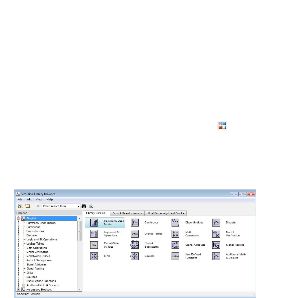
1Simulink®Basics
Start the Simulink Software
Open the MATLAB Software
To start the Simulink software, first start the MATLAB®technical computing
environment. For details about starting MATLAB, see “Starting and Exiting
the MATLAB Program”.
Open the Library Browser
To start Simulink Library Browser from MATLAB, use one of these
approaches:
•On the MATLAB toolbar, click the Simulink button ( ).
•At the MATLAB prompt, enter the simulink command.
The Library Browser opens. It displays a tree-structured view of the Simulink
block libraries installed on your system. The Simulink library window
displays icons representing the pre-installed block libraries.
1-2

Start the Simulink®Software
Note On computers running the Windows®operating system, you can display
the Simulink library window by right-clicking the Simulink node in the
Library Browser window.
To create models, copy blocks from the Library Browser into a model window
in the Simulink Editor.
Open the Simulink Editor
Use one of the following approaches to open the Simulink Editor:
•Open an existing model. For example, at the MATLAB prompt, enter the
name of a model. For details, see “Open an Existing Model” on page 1-4.
•In the Library Browser, select File > Open. Choose a model or enter
thefilenameofthemodel.
•AttheMATLABprompt,usetheopen_system command. For example,
to open a model named vdp:
open_system('vdp')
Note To have the Simulink Editor display properly, use 32-bit color mode.
Typically, remote desktop connections (for example, a VNC connection) use a
default color mode of 16-bits or less.
1-3

1Simulink®Basics
Open a Model
In this section...
“What Happens When You Open a Model” on page 1-4
“OpenanExistingModel”onpage1-4
“Models with Different Character Encodings” on page 1-5
“Avoid Initial Model Open Delay” on page 1-5
What Happens When You Open a Model
Opening a model brings the model into memory and displays the model
graphically in the Simulink Editor.
You can also bring a model into memory without displaying it, as described in
“Load a Model” on page 1-7.
Open an Existing Model
To open an existing model, use one of these approaches:
•(Windows operating systems only) On the Library Browser toolbar, click
the Open button.
•In the Library Browser or the Simulink Editor, select File > Open.
Chooseamodelorenterthefilenameofthemodel.
•AttheMATLABcommandprompt,enterthenameofthemodel,without
thefileextension(e.g.,.slx) . The model must be in the current folder
or on the path.
Note IfyouhaveanearlierversionoftheSimulinksoftware,andyouwant
to open a model that was created in a later version, first use the later version
to save the model in a format compatible with the earlier version. Then open
the model in the earlier version. For details, see “Export a Model to a Previous
Simulink Version” on page 1-14.
1-4

Open a Model
Models with Different Character Encodings
If you open a model created in a MATLAB software session configured to
support one character set encoding (for example, Shift_JIS), in a session
configured to support another character encoding (for example, US_ASCII),
Simulink displays a warning for SLX files. For MDL files, you might see a
warning or an error message, depending on whether it can encode the model,
using the current character encoding. The warning or error message specifies
the encoding of the current session and the encoding used to create the model.
To display the model’s text correctly:
1Close all models open in the current session.
2Use the slCharacterEncoding command to change the character encoding
of the current MATLAB software session to that of the model as specified
in the warning message.
3Reopen the model.
You can now edit and save the model.
Simulink can check if models contain characters unsupported in the current
locale. For more details, see “Check file for foreign characters” and “Saving
Models with Different Character Encodings” on page 1-13.
Avoid Initial Model Open Delay
The first model that you open in a MATLAB session takes longer to open than
do subsequent models. This is because MATLAB does not load the Simulink
product into memory until the first time that you open a Simulink model. This
just-in-time loading of the Simulink product reduces the MATLAB startup
time and avoids unnecessary consumption of system memory.
To avoid the initial model opening delay, you can have MATLAB load the
Simulink software when the MATLAB product starts up. You can issue the
command to load Simulink at MATLAB startup from one of two places:
•The -r command line option
•The MATLAB startup.m file
1-5

1Simulink®Basics
Use one of these commands:
•load_simulink — loads the Simulink product
•simulink — loads the Simulink product and opens the Simulink Library
Browser
For example, to load the Simulink product when the MATLAB software starts
up on a computer running the Microsoft®Windows operating system, create a
desktop shortcut with the following target:
matlabroot\bin\win32\matlab.exe -r load_simulink
Similarly, the following command loads the Simulink software when the
MATLAB software starts up on Macintosh and Linux®computers:
matlab -r load_simulink
1-6

LoadaModel
LoadaModel
Loading a model brings it into memory but does not display it graphically.
Tip To both bring a model into memory and display it graphically, open the
model as described in “Open a Model” on page 1-4.
After you load a model (as distinct from opening it), you can work with the
model programmatically as if it were visible. However, you cannot use the
Simulink Editor to edit the model unless you open the model.
You cannot load a model using the Simulink Editor or Library Browser.
To load a model programmatically, at the MATLAB command prompt, enter
the load_system command. Specify the model to be loaded. For example,
to load the vdp model:
load_system('vdp')
1-7
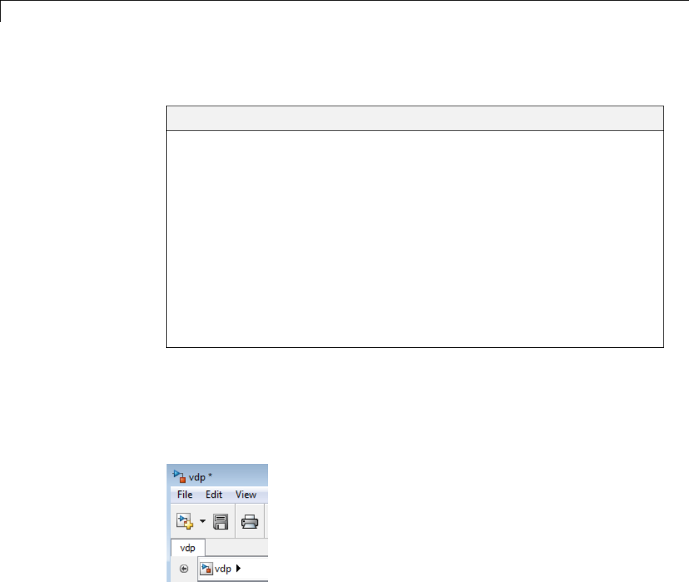
1Simulink®Basics
Save a Model
In this section...
“How to Tell If a Model Needs Saving” on page 1-8
“SaveaModelfortheFirstTime”onpage1-9
“Model Names” on page 1-9
“Save a Previously Saved Model” on page 1-9
“What Happens When You Save a Model?” on page 1-9
“Saving Models in the SLX File Format” on page 1-10
“Saving Models with Different Character Encodings” on page 1-13
“Export a Model to a Previous Simulink Version” on page 1-14
“Save from One Earlier Simulink Version to Another” on page 1-15
How to Tell If a Model Needs Saving
To tell whether a model needs saving, look at the title bar in the Simulink
Editor. If the model needs saving, an asterisk appears next to the model
name in the title bar.
To determine programmatically whether a model needs saving, use the model
parameter Dirty. For example:
if strcmp(get_param(gcs, 'Dirty'), 'on')
save_system;
end
1-8

Save a Model
Save a Model for the First Time
To save a model for the first time, in the Simulink Editor, select File > Save.
Provide a location and name for the model file.
Model Names
Model file names must start with a letter and can contain letters, numbers,
and underscores. The file name must not be the same as that of a MATLAB
software command.
The total number of characters must not be greater than a certain maximum,
usually 63 characters. To find out whether the maximum for your system is
greater than 63 characters, use the MATLAB namelengthmax command.
Save a Previously Saved Model
If you are saving a model whose model file was previously saved:
•To replace the file contents, in the Simulink Editor, select File > Save.
•To save the model with a new name or location, in the Simulink Editor,
select File > Save As.
Note Seealso“UpgradeModelstoSLX”onpage1-10.
What Happens When You Save a Model?
Simulink saves the model by generating a specially formatted file called the
model file that contains the block diagram and block properties. The Simulink
software follows this process while saving a model:
1If the model file already exists, Simulink renames the model file as a
temporary file.
2All block PreSaveFcn callback routines execute first, then the block
diagram PreSaveFcn callback routine executes.
3Simulink writes the model file to a new file using the same name and, by
default, an extension of .slx.
1-9

1Simulink®Basics
4All block PostSaveFcn callback routines execute, then the block diagram
PostSaveFcn callback routine executes.
5Simulink deletes the temporary file.
If an error occurs during this process, Simulink:
•Renames the temporary file to the name of the original model file
•Writes the current version of the model to a file with an .err extension
•Issues an error message
If an error occurs in Step 2 of the save process, then Step 3 is omitted and
Steps 4 and 5 are performed.
Saving Models in the SLX File Format
SaveNewModelsasSLX
You save new models and libraries in the SLX format by default, with file
extension .slx. SLX is a compressed package that conforms to the Open
Packaging Conventions (OPC) interoperability standard. SLX stores model
information using Unicode UTF-8 in XML and other international formats.
Saving Simulink models in the SLX format:
•Typically reduces file size comparedtoMDL.Thefilesizereduction
between MDL and SLX varies depending on the model.
•Solves some problems in previous releases with loading and saving MDL
files containing Korean and Chinese characters.
You can specify your file format for saving new models and libraries with the
Simulink preference “File format for new models and libraries”.
Upgrade Models to SLX
If you upgrade an MDL file to SLX file format, the file contains the same
information as the MDL file, and you always have a backup file. All
functionality and APIs that currently exist for working with models, such as
the get_param and set_param commands, are also available when using
1-10

Save a Model
the SLX file format. If you upgrade an MDL file to SLX file format without
changing the model name or location, then Simulink creates a backup file by
renaming (if writable) and Simulink does not remove the MDL file.
IfyousaveanexistingMDLfileusingFile > Save, Simulink respects the
file’s current format and saves your model in MDL format.
To save an existing MDL file in the SLX file format,
1Select File > Save As.
2Leave the default Save as type as SLX, and click Save.
Simulink saves your model in SLX format, and creates a backup file
by renaming the MDL (if writable) to mymodel.mdl.releasename, e.g.,
mymodel.mdl.R2010b.
Alternatively, use save_system:
save_system mymodel mymodel.slx
This command creates mymodel.slx, and if the existing file mymodel.mdl is
writable it is renamed mymodel.mdl.releasename.
SLX files take precedence over MDL files, so if both exist with the same name
and you do not specify a file extension, you load the SLX file.
Simulink Projects can help you migrate files to SLX. For an example, see
“Upgrade Model Files to SLX and Preserve Revision History” on page 13-15.
Caution If you use third-party source control tools, be sure to register
the model file extension .slx as a binary file format. If you do not, these
third-party tools might corrupt SLX files when you submit them.
1-11

1Simulink®Basics
Operations
with Possible
Compatibility
Considerations when
using SLX
What Happens Action
Hard-coded references
to file names with
extension .mdl.
Scripts cannot find or
process models saved
with new file extension
.slx.
Make your code work
with both the .mdl and
.slxextension.
Use functions like
which and what instead
of strings with .mdl.
Third-party source
control tools that
assume a text format
by default.
Binary format of
SLX files can cause
third-party tools to
corrupt the files when
you submit them.
Register .slx as a
binary file format with
third-party source
control tools. Also
recommended for .mdl
files. See “Register
Model Files with Source
Control Tools” on page
13-70.
Changing character
encodings.
Some cases are
improved, e.g., SLX
solves some problems
in previous releases
with loading and saving
MDL files containing
Korean and Chinese
characters. However,
sharing models between
different locales
remains problematic.
See “SLX Files and
Character Encodings”
on page 1-14.
The format of content within MDL and SLX files is subject to change.
To operate on model data, use documented APIs (such as get_param,
find_systemand Simulink.MDLInfo.
1-12

Save a Model
Saving Models with Different Character Encodings
•“Differences in Character Encodings” on page 1-13
•“SLX Files and Character Encodings” on page 1-14
Differences in Character Encodings
When you save a model, the current character encoding is used to encode the
text stored in the model file. This can lead to model corruption if you save a
model whose original encoding differs from current encoding.
If you change character encoding, it is possible to introduce characters
that cannot be represented in the current encoding. If this is the case, the
model is saved as model.err,wheremodel is the model name, leaving the
original model file unchanged. Simulink also displays an error message that
specifies the line and column number of the first character which cannot
be represented.
To recover from this error, either:
•Save the model in SLX format (see “Saving Models in the SLX File Format”
on page 1-10).
•Use the following procedure to locate and remove characters one by one.
1Use a text editor to find the character in the .err file at the position
specified by the save error message.
2Find and delete the corresponding character in the open model and
resave the model.
3Repeat this process until you are able to save the model without error.
It’s possible that your model’s original encoding can represent all the text
changes that you’ve made in the current session, albeit incorrectly. For
example, suppose you open a model whose original encoding is A in a session
whose current encoding is B. Further suppose that you edit the model to
include a character that has different encodings in A and B and then save the
model. If in addition the encoding for x in B is the same as the encoding
for y in A, and if you insert x in the model while B is in effect, save the
model, and then reopen the model with A in effect the Simulink software will
display x as y. To alert you to the possibility of such corruptions, the software
1-13

1Simulink®Basics
displays a warning message whenever you save a model in which the current
and original encoding differ but the original encoding can encode, possibly
incorrectly, all of the characters to be saved in the model file.
SLX Files and Character Encodings
Saving Simulink models in the SLX format typically reduces file size and
solves some problems in previous releases with loading and saving MDL files
containing Korean and Chinese characters.
Considerations for choosing a model file format:
•Use SLX if you are loading and saving models with Korean or Chinese
characters
•Use SLX if you would benefit from a compressed model file
•Whether you use SLX or MDL, Simulink can detect and warn if models
contain characters unsupported in the current locale. For SLX, you can use
the Model Advisor to help you, see “Check file for foreign characters”.
Export a Model to a Previous Simulink Version
You can export (save) a model created with the latest version of the Simulink
software in a format used by an earlier version, such as Simulink 7.0
(R2007b). For example, you might want to perform such an export to make a
model available to colleagues who only have access to a previous version of
the Simulink product.
To export a model in an earlier format:
1In the Simulink Editor, select File > Save. This saves a copy in the latest
version of Simulink. This step avoids compatibility problems.
2Simulink Editor, select File > Export > Export Model To Previous
Version.
The Export To Previous Version dialog box appears.
3In the dialog box, from the Save as type list, select the previous version to
which to export the model.
1-14

Save a Model
4Click the Save button.
When you export a model to a previous version’s format, the model is saved
in the earlier format, regardless of whether the model contains blocks and
features that were introduced after that version. If the model does contain
blocks or use features that postdate the earlier version, the model might not
give correct results when you run it in the earlier version of Simulink software.
In addition, Simulink converts blocks that postdate an earlier version into
yellow empty masked Subsystem blocks. For example, if you export a model
to Release R2007b, and the model contains Polynomial blocks, Simulink
converts the Polynomial blocks into yellow empty masked Subsystem blocks.
Simulink also removes any unsupported functionality from the model.
Save from One Earlier Simulink Version to Another
You can open a model created in an earlier version of Simulink and export
that model to a different earlier version. To prevent compatibility problems,
use the following procedure if you need to save a model from one earlier
version to another earlier version.
1Use the current version of Simulink to open the model created with the
earlier version.
2Before you make any changes, save the model in the current version by
selecting File > Save.
After saving the model in the current version, you can change and resave
it as needed.
3Save the model in the earlier version of Simulink by selecting File >
Export > Export Model To Previous Version.
4Start the earlier Simulink version and use it to open the model that you
exported to that earlier version.
5Save the model in the earlier version by selecting File > Save.
You can now use the model in the earlier version of Simulink exactly as you
could if it had been created in that version.
1-15

1Simulink®Basics
See also the Simulink preferences that can help you work with models from
earlier versions:
•“Do not load models created with a newer version of Simulink”
•“Save backup when overwriting a file created in an older version of
Simulink”
1-16
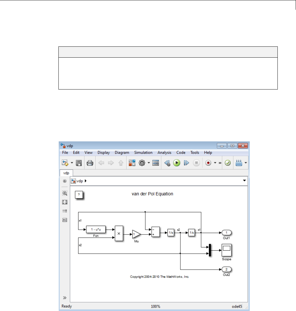
Simulink®Editor
Simulink Editor
In this section...
“Editor Layout” on page 1-17
“Undoing Commands” on page 1-21
“Window Management” on page 1-21
Editor Layout
Opening a Simulink model or library displays the model or library in the
Simulink Editor. For more information, see “Open the Simulink Editor” on
page 1-3.
1-17
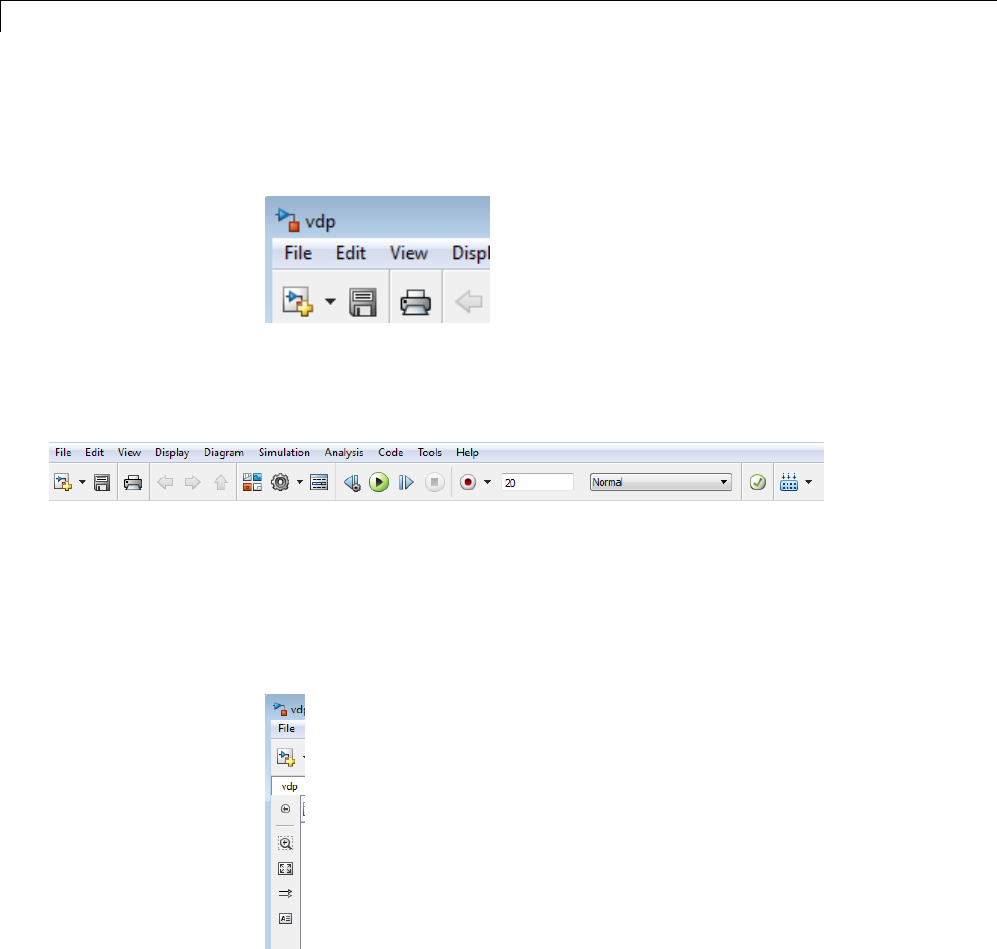
1Simulink®Basics
The Simulink Editor has the following major sections:
•Title bar
Inthetopleftcorner,thetitlebardisplaysthenameofthemodelor
subsystem that is open in the model window.
•Menu bar and toolbar
At the top of the Simulink Editor, you can access commands to work with
models. Several buttons in the toolbar provide quick access to commonly
used Simulink Editor menu options. Other buttons in the toolbar open
other Simulink tools, such as the Model Explorer (for details, see “Open
Simulink Tools from the Toolbar” on page 1-20).
•Palette
The icons in the vertical bar on the right side of the Simulink Editor
perform very common tasks, such as adding an annotation.
•Explorer bar
1-18
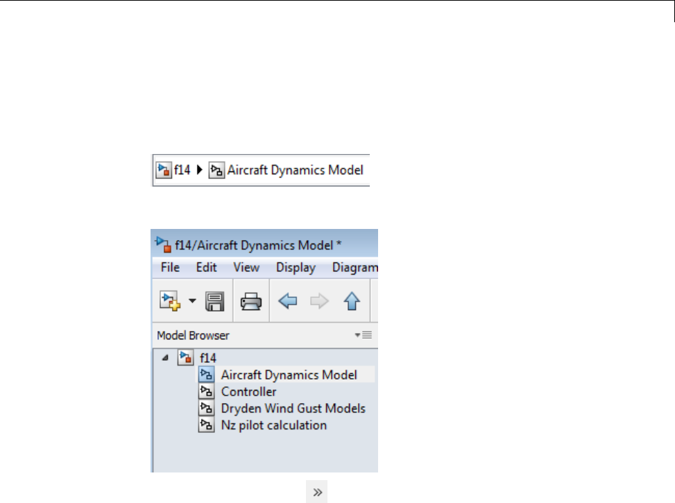
Simulink®Editor
The breadcrumb shows the systems that you have open in the editor. Select
a system in the breadcrumb to open that system in the model window. If
you click in the Explorer bar whitespace, you can edit the hierarchy. Also,
the down arrow at the right side of the Explorer bar provides a history.
•Model Browser
Click the double arrows in the bottom left corner of the Simulink Editor
to open or close a tree-structured view of the model in the editor.
•Canvas — The canvas is area where you edit the block diagram. You can
use the mouse and keyboard to create and connect blocks, select and move
blocks, edit block labels, display block dialog boxes, and so on.
To display context menus specific to a particular model object in the canvas,
such as a block, right-click the object.
•Status information — Near the top of the editor, you can see (and reset)
the simulation time and the simulation mode. The bottom status line
shows the status of Simulink processing, the zoom factor, and the solver.
1-19
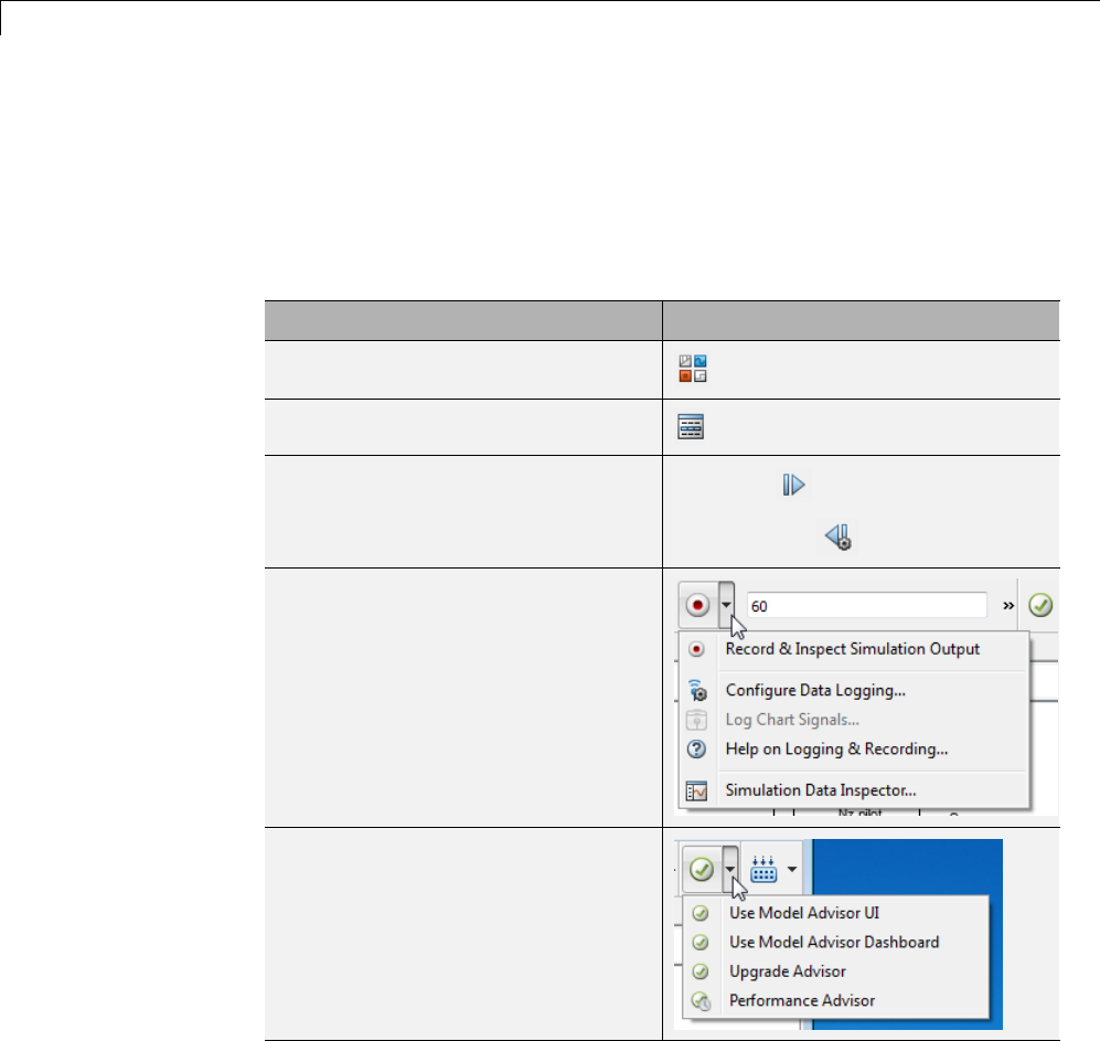
1Simulink®Basics
Open Simulink Tools from the Toolbar
The Simulink Editor toolbar provides several buttons for quick access to
other Simulink tools.
For buttons that have associated menu options, clicking the button invokes
the first menu option.
Tools Buttons and Associated Menus
Library Browser
Model Explorer
Simulation Stepper Next Step
Previous Step
Simulation Data Inspector
Advisor Tools
1-20

Simulink®Editor
Undoing Commands
You can cancel the effects of up to 101 consecutive operations. To undo
commands, selectEdit > Undo. Repeat until you get to the command that
you want to undo. You can undo operations such as:
•Adding, deleting, or moving a block
•Adding, deleting, or moving a line
•Adding, deleting, or moving a model annotation
•Editing a block name
•Creating a subsystem (see “Undoing Subsystem Creation” on page 4-39
for more information)
To reverse the effects of an Undo command, select Edit > Redo.
Window Management
One Simulink Editor Per Model
When you open a model, that model appears in its own Simulink Editor
window. For example, if you have one model already open, and then you open
a second model, the second model appears in a second Simulink Editor.
To open the same model in two separate Simulink Editor windows, at the
MATLAB command prompt, enter the open_system command, using the
window argument. For example, if you already have the vdp model open, then
to openanotherinstanceofthevdp model in a separate Simulink Editor,
enter:
open_system ('vdp', 'window')
Open a Subsystem
The Simulink Editor displays only one active window at a time. By default,
if you open a Subsystem block, the opened subsystem replaces (in terms of
being displayed in the model window) the model from which you opened the
subsystem.
1-21
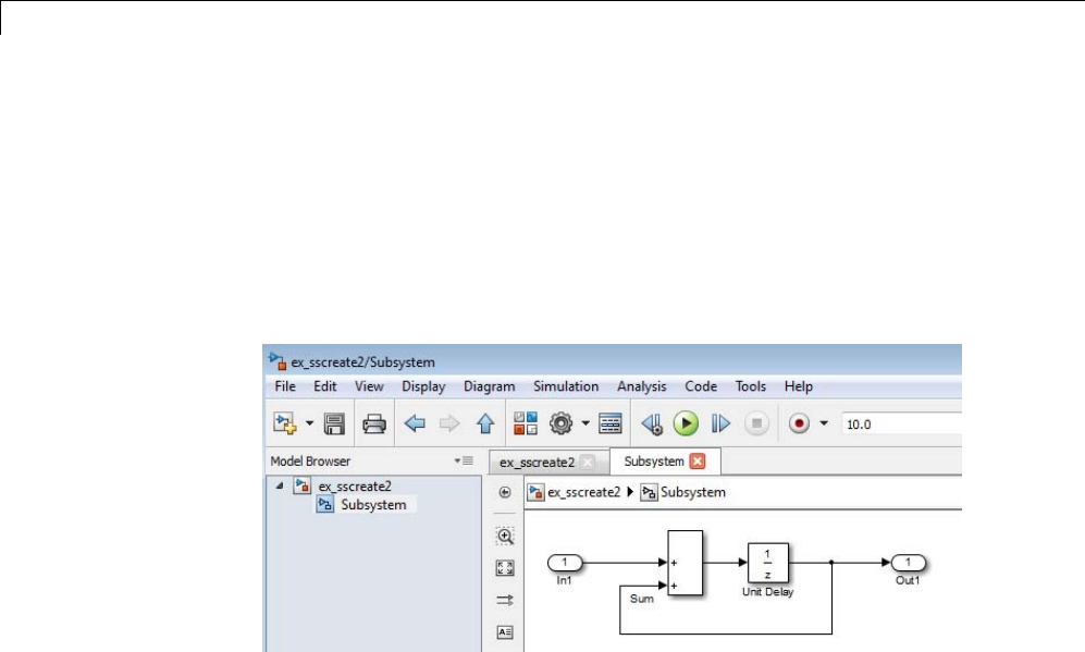
1Simulink®Basics
You can use tabs in the Simulink Editor to make it easier to navigate between
model windows for the top model and subsystems. To open a subsystem in a
separate tab:
1Right-click the Subsystem block.
2From the context-menu, select Open In New Tab. In the example below,
there are separate tabs for the ex_sscreate2 model and for the Subsystem.
Navigate between the top model and subsystems by clicking the appropriate
tab. Or, choose an option following options from the View > Navigate menu,
such as Back,Back to Parent,orPrevious Tab.
For more information about opening subsystems, see “Navigate Model
Hierarchy” on page 4-39.
Open a Referenced Model
If you open a Model block, the referenced model opens in a separate Simulink
Editor.
Bring the MATLAB Desktop Forward
Simulink Editor windows open on top of the MATLAB desktop. To bring the
MATLAB desktop back to the top of your screen, in the Simulink Editor,
select View > MATLAB Desktop.
1-22

Zoom and Pan Block Diagrams
Zoom and Pan Block Diagrams
You can enlarge or shrink the view of the block diagram in the current
Simulink Editor window.
Goal of Zoom or Pan What You Do
Enlarge the model
diagram incrementally
Select View > Zoom In or press Ctrl++.
Enlarge the model
diagram dynamically
Roll the mouse scroll wheel forward.
Zoom by a factor of two,
displaying the selected
model object 1In the palette, drag the zoom button ( )to
the object that you want to include in the
enlarged view.
2Press the left mouse button.
Zoom until the whole
model diagram just fits in
the current window
Select View > Fit to View or press
Spacebar.
Zoom and pan
1Roll the mouse scroll wheel forward.
2Release the scroll wheel.
3Hold the scroll wheel down and pan to the
desired positioning by moving the mouse.
4Release the scroll wheel.
To disable the zoom and pan behavior for
the scroll wheel, clear the File > Simulink
Preferences > Editor Defaults > Scroll
wheel controls zooming preference.
Pan with the mouse Hold down por qand drag mouse.
Shrink the model diagram
incrementally
Select View > Zoom Out.
1-23

1Simulink®Basics
Goal of Zoom or Pan What You Do
Shrink the model diagram
dynamically
Roll the mouse scroll wheel backward.
Restore the model diagram
to 100%
Select View > Normal View (100%) or press
Alt+1.
Go back in pan/zoom
history
b
Go forward in pan/zoom
history
t
To disable the zoom and pan behavior for the scroll wheel, clear the File >
Simulink Preferences > Editor Defaults > Scroll wheel controls
zooming preference. If you hold the CRTL key and use the scroll wheel, the
scroll wheel behavior is the opposite of how the preference is set.
1-24

Update a Block Diagram
Update a Block Diagram
Updating the Diagram
You can leave many attributes of a block diagram, such as signal data types
and sample times, unspecified. The Simulink software then infers the values
of block diagram attributes, based on the block connectivity and attributes
that you specify. The process that Simulink uses is known as updating the
diagram.
Simulink attempts to infer the most appropriate values for attributes that
you do not specify. If Simulink cannot infer an attribute, it halts the update
and displays an error dialog box.
Simulation Updates the Diagram
Simulink updates the block diagram at the start of a simulation. The updated
diagram provides the simulation with the results of the latest changes that
youhavemadetoamodel.
Update Diagram at Edit Time
As you create a model, at any point you can have Simulink update the
diagram. Updating the diagram periodically can help you to identify and fix
potential simulation issues as you develop the model. This approach can
make it easier to identify the sources of problems by focusing on a set of recent
changes. Also, the update diagram processing takes less time than performing
a simulation, so you can identify issues more efficiently.
To update the diagram at edit time, use one of these approaches:
•In the Simulink Editor, select Simulation > Update Diagram.
•Press Ctrl-D.
For example:
1Create the following model.
1-25
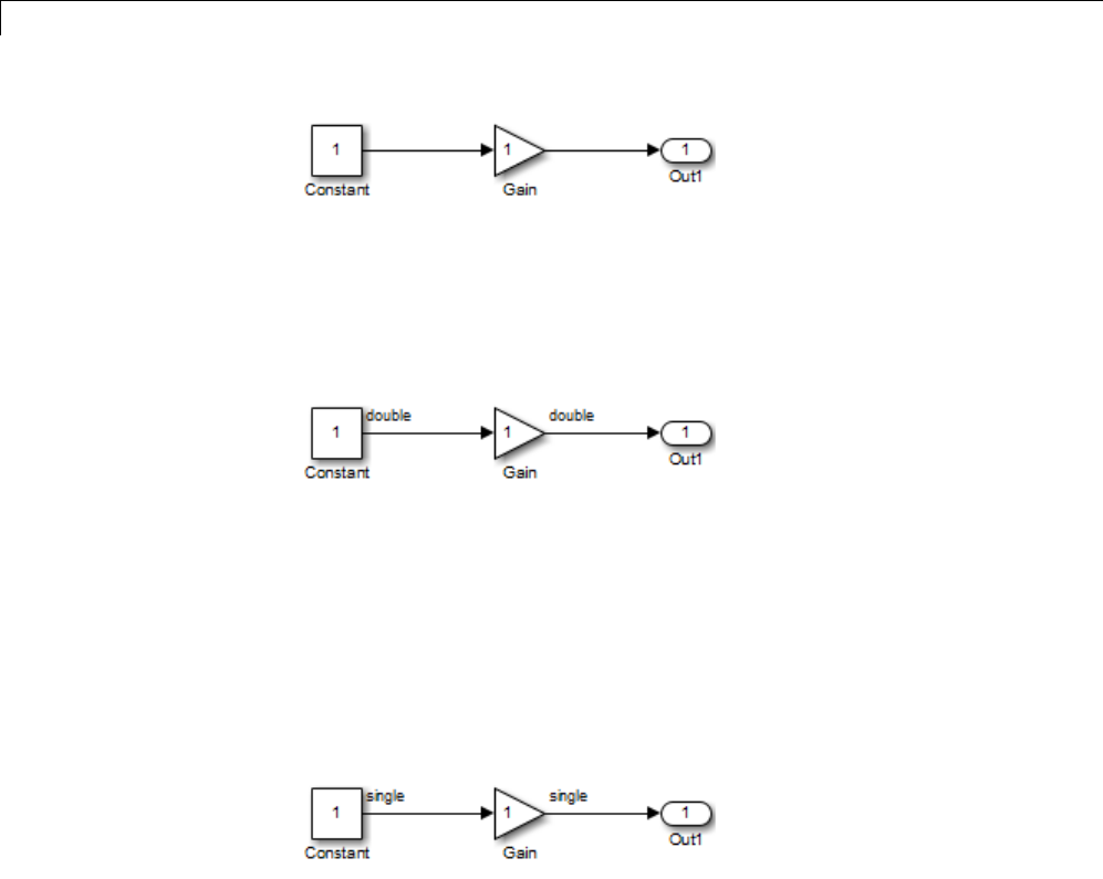
1Simulink®Basics
2In the Simulink Editor, select Display > Signals & Ports > Port Data
Types.
The data types of the output ports of the Constant and Gain blocks appear.
The data type of both ports is double, the default value.
3In the Constant block parameters dialog box, set Output data type to
single.
The output port data type displays on the block diagram do not reflect
this change.
4In the Simulink Editor, select Simulation > Update Diagram.
The updated block diagram reflects the change that you made previously.
In this example, Simulink infers a data type for the output of the Gain
block. This is because you did not specify a data type for the block. The
inferred data type inferred is single, because single precision is all that
is necessary to simulate the model accurately, given that the precision of
the block input is single.
1-26

Copy Models to Third-Party Applications
Copy Models to Third-Party Applications
On a computer running the Microsoft Windows operating system, you can:
1Copy a Simulink product model to the Windows operating system clipboard.
2Paste the model from the clipboard to a third-party application, such as
word processing software.
You can copy a model in either bitmap or metafile format. You can then
paste the clipboard model to an application that accepts figures in bitmap or
metafile format. For a description of how to set up the figure settings and
save a figure to the clipboard on a Windows platform, see “Exporting to the
Windows or Macintosh Clipboard”.
1-27

1Simulink®Basics
Print a Block Diagram
In this section...
“Print Interactively or Programmatically” on page 1-28
“Systems to Print” on page 1-28
“Title Block Print Frame” on page 1-30
“Paper Size and Orientation” on page 1-31
“Diagram Positioning and Sizing” on page 1-31
“Tiled Printing” on page 1-32
“Print Sample Time Legend” on page 1-35
Print Interactively or Programmatically
You can print a block diagram:
•Interactively in the Simulink Editor, by selecting File > Print.
•Programmatically, by using the MATLAB print command.
To control some additional aspects of printing a block diagram, use the
param_set command with model parameters.
Systems to Print
From the Simulink Editor
To specify what systems in a block diagram that you want to print:
1In the Simulink Editor, select File>Print>Print.
The Print Model dialog box appears.
2In the Options section, select one of the following:
•Current system — The current system only
1-28

Print a Block Diagram
•Current system and above — The current system and all systems
above it in the model hierarchy
•Current system and below — The current system and all systems
below it in the model hierarchy, with the option of looking into the
contents of masked and library blocks
•All systems — All systems in the model, with the option of looking into
the contents of masked and library blocks
To print the contents of masked subsystems that are at or below the level of
the current block, select the Look under mask dialog check box. When
you print all systems, the top-level system is the current block, so Simulink
looks under all masked blocks.
To print the contents of library blocks that are systems, in the Print Model
dialog box, select the Expand unique library links check box. Only one copy
is printed, regardless of how many copies of the block that the model contains.
The print log lists the blocks and systems printed. To print the print log,
select the Include Print Log check box.
With the Print Command
The format of the print command is
print -ssys -device -tileall -pagespfilename
sys is the name of the system to be printed. Precede the system name
with the -s switch identifier. The name of the system is the only required
argument. The system must be open or must have been open during the
current session. If the system name contains spaces or takes more than one
line, you need to specify the name as a string.
The print command prints only the system that you specify. The command
does not have options to specify the scope of the systems to be printed (for
example, current system and below). To specify the scope of the systems to
be printed, use the Simulink Editor.
1-29

1Simulink®Basics
This example shows how to print the currently selected subsystem
(Controller).
open_system('f14');
open_system('f14/Controller');
print(['-s', gcs])
Thisexampleshowshowtoprintthecontentsofasubsystemnamed
Controller in the current system.
open_system('f14');
print -sController
This example shows how to print the contents of a subsystem named Aircraft
Dynamics Model.
open_system('sldemo_clutch');
print (['-sAircraft Dynamics Model'])
To print a system whose name appears on multiple lines, assign the newline
character to a variable and use that variable in the print command. This
example shows how to print a subsystem whose name, Aircraft Dynamics
Model, appears on three lines.
open_system('f14');
cr = sprintf('\n');
print (['-sAircraft' cr 'Dynamics' cr 'Model'])
The device specifies the device type. For a list of device types, see the
documentation for the print function.
The filename is a PostScript®file to which you save the output. If filename
exists, it is replaced. If filename does not include an extension, an
appropriate one is appended.
Title Block Print Frame
A title block print frame is a border that contains information relevant to the
block diagram, such as the name of the block diagram. After you create a
print frame, you can print a block diagram with a print frame:
1-30

Print a Block Diagram
1In the Simulink Editor, select File>Print>Print.
The Print Model dialog box appears.
2Select the Frame check box.
3In the adjacent edit box, enter the path to the title block frame.
To create a customized title block frame, use the MATLAB frame editor. For
information about using the frame editor to create title block frames, see
“Custom Print Frames”.
Paper Size and Orientation
On Windows platforms, you can use the Simulink Editor to specify the type
and orientation of the paper for printing a model.
1Select File>Print>PageSetup.
The Print Setup dialog box appears.
2In the Paper and Orientations section, set the fields for paper size and
orientation.
On all platforms, you can set the paper orientation alone, using the MATLAB
orient command.
On all platforms, you can also set the paper type and orientation by using the
set_param command with the model’s PaperType andPaperOrientation
properties, respectively (see “Model Parameters”).
Diagram Positioning and Sizing
To position and size the model diagram on the printed page, use the
set_param command with a model’s PaperPositionMode and PaperPosition
parameters.
The value of the PaperPosition parameter is a vector of form [left bottom
width height]. The first two elements specify the bottom-left corner of a
rectangular area on the page, measuredfromthepage’sbottom-left corner.
The last two elements specify the width and height of the rectangle.
1-31

1Simulink®Basics
If you set the PaperPositionMode parameter to manual, Simulink positions
(and scales, if necessary) the model diagram to fit inside the specified print
rectangle. If PaperPositionMode is auto, Simulink centers the model
diagram on the printed page, scaling the diagram, if necessary, to fit the page.
For example, these commands print the block diagram of the vdp model in the
lower-left corner of a U.S. letter-size page in landscape orientation.
open_system('vdp');
set_param('vdp', 'PaperType', 'usletter');
set_param('vdp', 'PaperOrientation', 'landscape');
set_param('vdp', 'PaperPositionMode', 'manual');
set_param('vdp', 'PaperPosition', [0.5 0.5 4 4]);
print -svdp
Tiled Printing
By default, each block diagram is scaled during the printing process so that
it fits on a single page. That is, the size of a small diagram is increased or
the size of a large diagram is decreased to confine its printed image to one
page. In the case of a large diagram, scaling can make the printed image
difficult to read.
By contrast, tiled printing enables you to print even the largest block
diagrams without sacrificing clarity and detail. Tiled printing allows you to
distribute a block diagram over multiple pages. You can control the number
of pages over which Simulink prints the block diagram, and hence, the total
size of the printed diagram.
Also, you can set different tiled-print settings for each of the systems in
your model. Consequently, you can customize the appearance of all printed
images to best suit your needs. The following sections describe how to use
tiled printing.
Enable Tiled Printing
To enable tiled printing for a model or subsystem, use one of these approaches:
•In the Simulink Editor, select File > Print > Enable Tiled Printing.
•At the MATLAB command prompt:
1-32
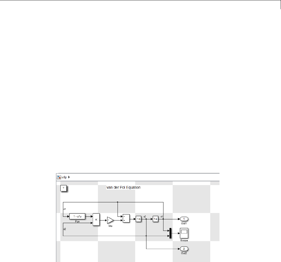
Print a Block Diagram
1Use the set_param command to set the PaperPositionMode parameter
to tiled (see ).
2Use the print command with the -tileall argument.
For example, to open the f14 model and enable tiled printing for the
Controller subsystem, enter:
open_system('f14');
set_param('f14/Controller', 'PaperPositionMode', 'tiled');
print('-sf14/Controller', '-tileall')
Display Page Boundaries
Displaying the page boundaries in the Simulink Editor can help you to
visualizethemodelsizeandlayoutwithrespecttothepage. Tomakethe
page boundaries visible, select File>Print>ShowPageBoundaries.
Simulink renders the page boundaries on the Simulink Editor canvas. If tiled
printing is enabled, Simulink represents page boundaries with a checkerboard
pattern. Each checkerboard square indicates the extent of a separate page.
If tiled printing is disabled, only a single page appears on the canvas.
To display the page boundaries programmatically, use the set_param
command, with the system’s ShowPageBoundaries parameter set to on (see
“Model Parameters”). For example:
1-33

1Simulink®Basics
open_system('vdp');
set_param('vdp', 'ShowPageBoundaries', 'on')
Scaling and Margins
To scale the block diagram so that more or less of it appears on a single tiled
page, use the set_param command with the TiledPageScale parameter. By
default, its value is 1. Values greater than 1proportionally scale the diagram
such that it occupies a smaller percentage of the tiled page, while values
between 0and 1proportionally scale the diagram such that it occupies a larger
percentage of the tiled page. For example, a TiledPageScale of 0.5 makes the
printed diagram appear twice its size on a tiled page, while a TiledPageScale
of 2makes the printed diagram appear half its size on a tiled page.
To specify the margin sizes associated with tiled pages, use the set_param
command with the TiledPaperMargins parameter. The value of
TiledPaperMargins is a vector of form [left top right bottom].Each
element specifies the size of the margin at a particular edge of the page.
The value of the PaperUnits parameter determines the margin’s units of
measurement. Each margin to 0.5 inches by default. By decreasing the
margin sizes, you can increase the printable area of the tiled pages.
Range of Tiled Pages
By default, Simulink prints all of a system’s tiled pages.
On a Microsoft Windows platform, to specify a range of tiled page numbers to
print, you can use the Simulink Editor.
1In the Simulink Editor, select File>Print>Print.
The Print Model dialog box appears.
2In the Options section, select Current system and Enable tiled printing
for all systems.
3InthePrintrangesectioninthemiddleofthedialogbox,selectPages and
enter a page range.
1-34

Print a Block Diagram
To specify a range of tiled page numbers programmatically, use the print
command with the -tileall argument and the -pages argument. Append to
-pages a two-element vector that specified the range.
Note Simulink uses a row-major scheme to numbertiledpages. Forexample,
the first page of the first row is 1, the second page of the first row is 2, and
so on.
For example, to print the second, third, and fourth pages:
open_system('vdp');
print('-svdp', '-tileall', '-pages[2 4]')
Print Sample Time Legend
You can print a legend that contains sample time information for your entire
system, including any subsystems. The legend appears on a separate page
fromthemodel. Toprintasampletimelegend:
•In the Simulink Editor, select File>Print>Print.
The Print Model dialog box appears.
•In the Options section select, select Print Sample Time Legend.
For more information about the contents and the settings of the legend, see
“ViewSampleTimeInformation”onpage5-9.
1-35

1Simulink®Basics
Generate a Model Report
A model report is an HTML document that describes the structure and
content of a model. The report includes block diagrams of the model and its
subsystems and the settings of its block parameters.
Tip If you have the SimulinkReport Generator™ installed, you can generate
a detailed report about a system. To do so, in the Simulink Editor, select
File > Reports > System Design Description. For more information, see
“System Design Description”.
To generate a model report for the current model:
1In the Simulink Editor, select File > Print > Print Details.
The Print Details dialog box appears.
2Select the desired report options. For details, see “Model Report Options”
on page 1-37.
3Select Print.
The Simulink software generates the HTML report and displays the report in
your default HTML browser.
1-36
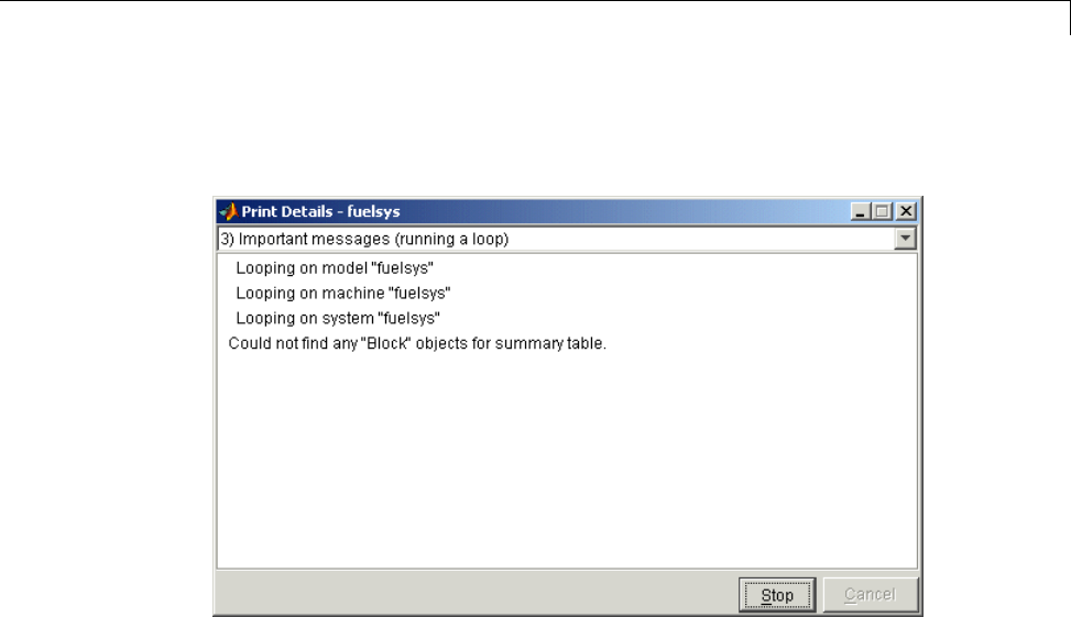
Generate a Model Report
While generating the report, Simulinkdisplaysstatusmessagesona
messages pane that replaces the options pane on the Print Details dialog box.
Select the detail level of the messages from the list at the top of the messages
pane. When the report generation process begins, the Print button changes
to a Stop button. To terminate the report generation, press Stop.Whenthe
report generation process finishes, the Stop button changes to an Options
button. Clicking this button redisplays the report generation options, allowing
you to generate another report without having to reopen the Print Details
dialog box.
Model Report Options
Use the Print Details dialog box allows you to specify the following report
options.
Directory
The folder where the HTML report is stored. The options include your
system’s temporary folder (the default), your system’s current folder, or
another folder whose path you specify in the adjacent edit field.
1-37

1Simulink®Basics
Increment filename to prevent overwriting old files
Creates a unique report file name each time you generate a report for the
same model in the current session. This preserves each report.
Current object
Include only the currently selected object in the report.
Current and above
Include the current object and all levels of the model above the current object
in the report.
Current and below
Include the current object and all levels below the current object in the report.
Entire model
Include the entire model in the report.
Look under mask dialog
Include the contents of masked subsystems in the report.
Expand unique library links
Include the contents of library blocks that are subsystems. The report
includes a library subsystem only once even if it occurs in more than one
place in the model.
Printing Limitations
Printing Properties (Windows)
On Windows platforms, the File>Print>Printdialog box includes:
•Printing options, such as the printer to use, the print range, the number of
copies, and which systems to print.
1-38

Generate a Model Report
•AProperties button, which displays additional printing properties, such
as paper orientation and resizing options. In R2012b, Simulink ignores the
settings for these additional printing properties. Simulink only uses the
settings in the main Print dialog box.
Printer Name (Mac)
On Mac platforms, the printer name that you specify in the File > Print >
Print dialog box must:
•Use only alphanumeric characters (letters and numbers), and not special
characters such as an underscore or ampersand (&)
•Include no blank spaces
1-39

1Simulink®Basics
End a Simulink Session
To terminate a Simulink software session, close all Simulink windows.
To terminate a MATLAB software session, choose one of these commands
from the File menu:
•On a computer running the Microsoft Windows operating system: Exit
MATLAB
•On a UNIX®system, system: Quit MATLAB
1-40

Keyboard and Mouse Shortcuts for Simulink®
Keyboard and Mouse Shortcuts for Simulink
In this section...
“Model Viewing Shortcuts” on page 1-41
“Block Editing Shortcuts” on page 1-41
“Line Editing Shortcuts” on page 1-43
“Signal Label Editing Shortcuts” on page 1-43
“Annotation Editing Shortcuts” on page 1-43
Model Viewing Shortcuts
The following table lists keyboard shortcuts for viewing models.
Task Shortcut
Zoom in Ctrl++
Zoom out Ctrl+-
Zoom to normal (100%) Alt+1
Pan Hold the mouse scroll wheel down and drag
the mouse
Fit diagram to screen Spacebar
Pan with mouse Hold down por qand drag mouse
Go back in pan/zoom history b
Go forward in pan/zoom
history
t
Delete selection Delete or Backspace
Move selection Make selection and use arrow keys
Block Editing Shortcuts
The following table lists mouse and keyboard actions that apply to blocks.
1-41

1Simulink®Basics
Task Shortcut
Select one block Left mouse button (LMB)
Select multiple blocks Shift +LMB
Copy block from another
window
Drag block
Move block Drag block
Rotate block clockwise Ctrl+R or Ctrl+Y
Rotate block
counterclockwise
Ctrl+Shift+R
Flip block Ctrl+I
Duplicate block Ctrl+C,thenCtrl+V
Connect blocks Select output port, hover over input port, and
press Ctrl +LMB
Disconnect block Shift + drag block
Create subsystem from
selected blocks
Ctrl+G
Open selected subsystem Enter
Go to parent of selected
subsystem
Esc
Look under a block mask Ctrl + U
1-42

Keyboard and Mouse Shortcuts for Simulink®
Line Editing Shortcuts
The following table lists mouse and keyboard actions that apply to lines.
Task Shortcut
Select one line Left mouse button (LMB)
Select multiple lines Shift +LMB
Draw branch line Ctrl + drag line; or RMB and drag line
Route lines around blocks Shift +drawlinesegments
Move line segment Drag segment
Move vertex Drag vertex
Signal Label Editing Shortcuts
The next table lists mouse and keyboard actions that apply to signal labels.
Action Shortcut
Create signal label Double-click line, then enter label
Copy signal label Ctrl + drag label
Move signal label LMB + drag label
Edit signal label Clickinlabel,thenedit
Annotation Editing Shortcuts
The next table lists mouse and keyboard actions that apply to annotations.
Action Shortuct
Create annotation Double-click in diagram, then enter text
Copy annotation Ctrl+C then Ctrl+V
Move annotation Drag annotation
Edit annotation Click in text, then edit
1-43
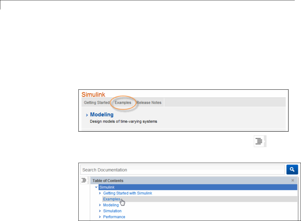
1Simulink®Basics
Simulink Demos Are Now Called Examples
Starting in R2012b, Simulink models and videos that were previously called
demos are now called examples. There are two ways to access these examples
from the Help browser:
•At the top of the product landing page, click Examples.
•On any documentation page, click the Table of Contents button ,and
then select Examples.
You can filter documentation search results to display only examples.
1-44
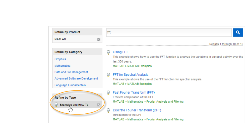
Simulink®Demos Are Now Called Examples
For more information about changes to the Help browser, see the R2012b
MATLAB Release Notes.
1-45

1Simulink®Basics
1-46

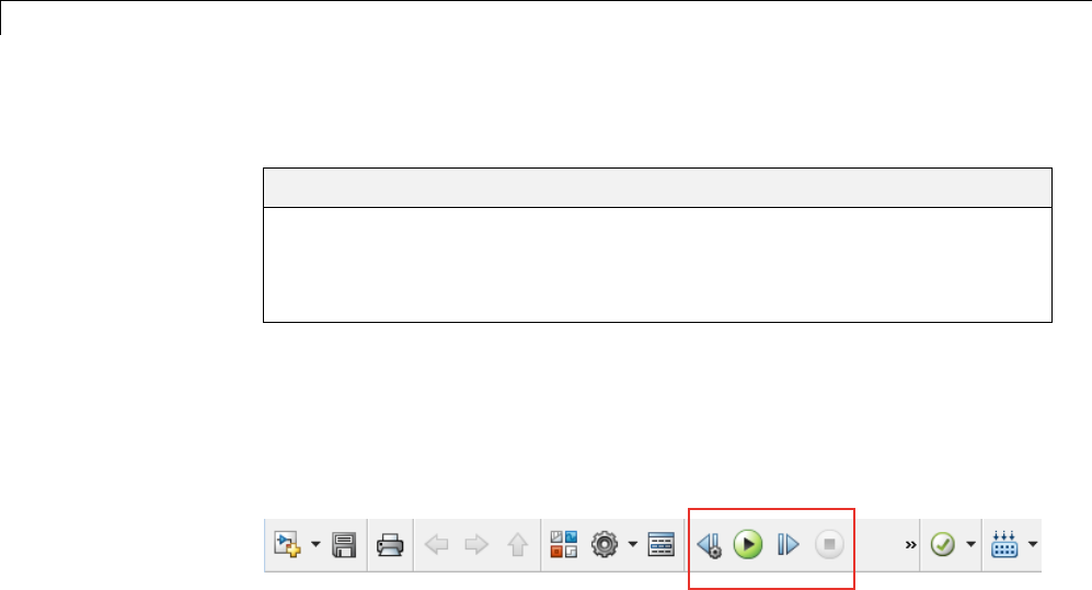
2Simulation Stepping
Simulation Stepping
In this section...
“About Simulation Stepping” on page 2-2
“Simulation Stepper Graphical Cues” on page 2-5
“Current Limitations” on page 2-9
About Simulation Stepping
The Simulation Stepper steps through the major time steps of a simulation
without changing the course of a simulation. The Simulation Stepper is
available from the Simulink Editor toolbar:
With Simulation Stepper, you can:
•Start and stop simulation of Simulink models
•Step forward and backward through a simulation
•Change from stepping backward to running with the Play button
•Change from running to paused (Pause button) or step backward (if
backward stepping is enabled)
•Add conditional breakpoints
•Add breakpoints at simulation time
You can use the stepping capabilities to perform actions such as analyze
plotted data at a particular moment in simulation time.
The stepping backward capability requires capturing simulation snapshots.
A simulation snapshot at a particular simulation time captures all the
information required to continue a simulation from that point. A simulation
snapshot contains simulation state (SimState) and possibly information
related to logged data and visualization blocks.
2-2

Simulation Stepping
The Simulink software can store simulation state only when it is stepping
forward through a simulation. When stepping backward, the software uses
the simulation snapshot, stored as SimState, to restore the previous state
of the simulation.
Stepping backward does not mean that the model is simulating backward.
Stepping backward involves loading a previously captured snapshot of the
model. When stepping forward again, the model is simulated from that point
and new snapshots are captured.
Simulation Stepper Versus Simulink Debugger
The Simulation Stepper and the Simulink Debugger both enable you to start,
stop, and step through a model simulation. Both allow you to use breakpoints
as part of a debugging session. However, Simulation Stepper and Simulink
Debugger are very different in their intended use. Simulation Stepper lets
you see all the data in between major steps. Simulink Debugger lets you
enteramajorstep.
Use the following table as a guideline:
Action Simulation Stepper Simulink Debugger
Look at state of system
after executing a major
time step.
XX
Observe dynamics of
the entire model from
step to step.
X
Step simulation
backward.
X
Pause across major
steps.
X
Control a Stateflow®
debugging session.
X
Step through
simulation by major
steps.
X
2-3

2Simulation Stepping
Action Simulation Stepper Simulink Debugger
Monitor single block
dynamics (for example,
output, update, and so
forth) during a single
major time step.
X
Look at state of system
while executing a major
time step.
X
Observe solver
dynamics during a
single major step.
X
Showvariousstagesof
Simulink simulation.
X
Pause within a major
step.
X
Step through
asimulation
block-by-block.
X
Command-line
interface.
X
To better understand the difference between Simulation Stepper and
Simulink Debugger, you need a good understand of the simulation process.
(For more information, see “How S-Functions Work”.)
In particular, use Simulink Debugger for advanced debugging scenarios
that involve custom blocks (such as S-functions). In this case, the Simulink
Debugger can help you analyze the issues with a particular block method.
Simulink Debugger also gives you finer control on breakpoints. It also gives
you finer control to step from one method to another block method within a
time step. For more information on the debugger, see “Introduction to the
Debugger” on page 21-2.
2-4
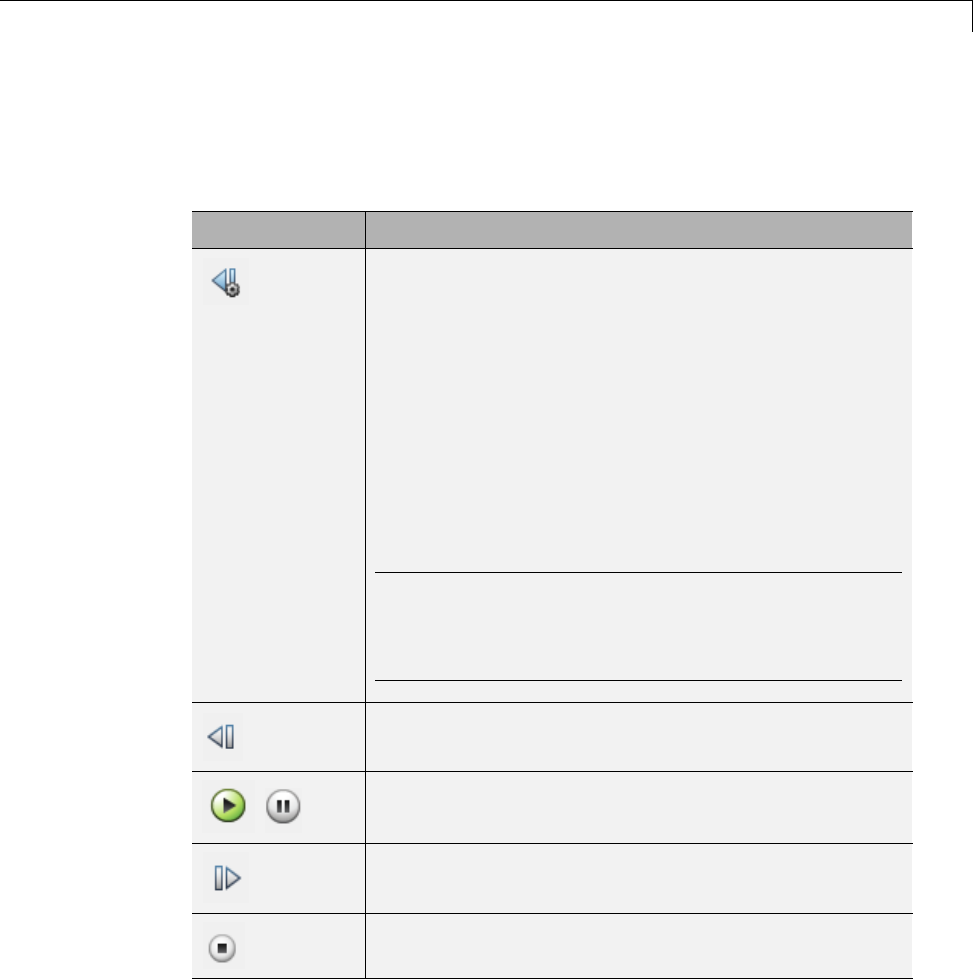
Simulation Stepping
Simulation Stepper Graphical Cues
Simulation Stepper Toolbar Icons
Icon Action
Displays the Simulation Stepping Options dialog box,
which affect Simulation Stepper performance. You can
configure stepping options such as pausing after a specific
simulation time and enabling stepping backward. This
button is available until you enable previous stepping
in the dialog box and start the simulation. To access
this dialog box again, select Simulation > Simulation
Stepping Options.
In conjunction with enabling the step back capability,
you must also simulate the model or step it forward to
save snapshots for the step backward capability.
Tip Snapshots for stepping backward are available only
within the duration of a simulation. The Simulation
Stepper does not save the steps for step backward across
simulations.
Steps the simulation to a previously captured simulation
snapshot. Stepping to the final step ends the simulation.
,
Starts/pauses/continues simulation.
Stepsthesimulationforward.
Stops the simulation.
2-5
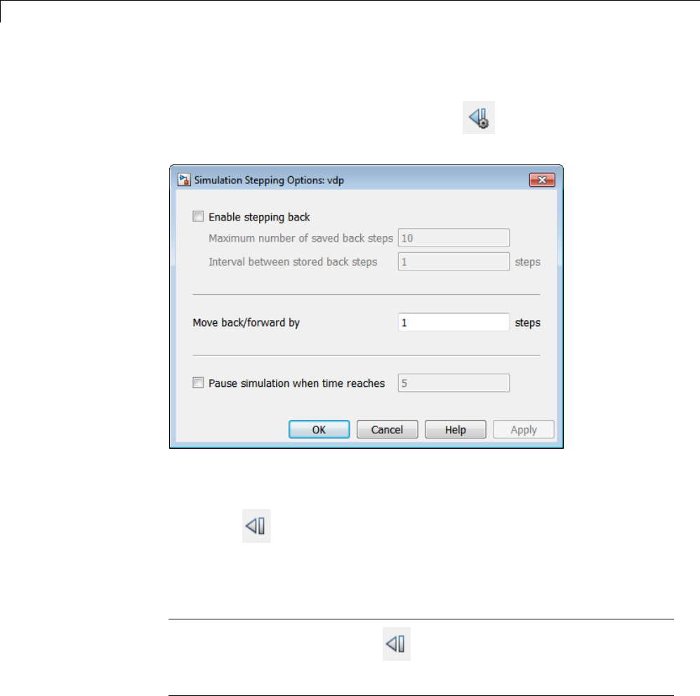
2Simulation Stepping
Simulation Stepping Options Dialog Box
Click the Simulation Stepping Options icon ( )todisplaytheSimulation
Stepping Options dialog box.
Use this dialog box to specify how you want to step through a simulation.
When you enable stepping backward and start the simulation, the icon
changes to ,sothatyoucanstepbackward.
If you enter an invalid value, the dialog box reverts all settings to the values
that were last applied.
Note When the icon changes to , you cannot access this dialog box from
the toolbar. To access this dialog box again, select Simulation > Simulation
Stepping Options.
2-6

Simulation Stepping
When the simulation is running and there are no saved back steps (but
stepping back is enabled), the icon changes to (disabled state).
The Simulation Stepping Options dialog box contains the following
parameters. For any setting, you can change the value while the simulation
is running or paused.
Parameter Operation
Enable stepping back Select check box to enable backward
stepping.
Maximum number of saved back
steps
Enter maximum number of
snapshots that the software can
capture. A snapshot at a particular
simulation time captures all the
information required to continue
a simulation from that point. For
more information, see “Simulation
Snapshots” on page 2-14.
Interval between stored back
steps
Enter the number of major time
steps to take between capturing
simulation snapshots. For more
information, see “Simulation
Snapshots” on page 2-14.
Move back/forward by Enter the number of major time
steps for a single call to step forward
or backward. For more information,
see “Simulation Snapshots” on page
2-14.
Pause simulation when time
reaches
Select check box to pause simulation
when time reaches the specified
time(s). This value can be a scalar
value, or a vector of times. Specifying
avectorofpausetimesisequivalent
to specifying multiple separate pause
times for a single simulation. You
can specify pause times as variables
in the model or MATLAB workspace.
2-7
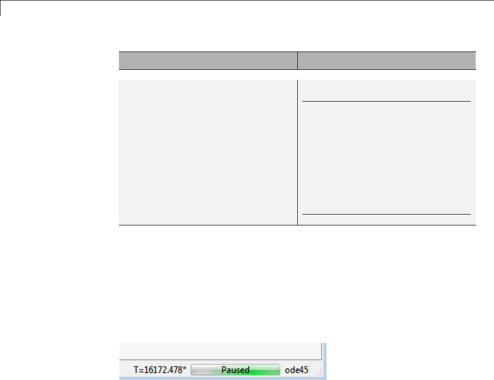
2Simulation Stepping
Parameter Operation
Note The stepper does not alter
thecourseofthesimulation. Asa
consequence, specifying a value for
a pause time does not necessarily
pause the simulation at exactly that
time. Instead, the simulation pauses
at whatever simulation time is
closest to the requested pause time,
without going below it.
Simulation Stepper Pause Status
The status bar at the bottom of the Simulink Editor displays the simulation
time of the last completed simulation step. While a simulation is running,
the editor updates the time display to indicate where the simulation is. This
display is an approximation because the status bar is not updated at every
simulation time step. When you pause a simulation, the status bar display
time catches up to the actual time of the last completed step.
When you use Simulation Stepper to step through a simulation, the time on
the status bar updates at every major time step of the simulation. The value
that is displayed (the time of the last completed step) might not always be the
same as the time of the solver. This event occurs because of the difference
in the way that different solvers propagate the simulation time in a single
iteration of the simulation loop. Simulation Stepper pauses at a single
position within the simulation loop. However, some solvers perform their time
advance before the stepper pauses and others perform their time advance after
the stepper pauses, which then becomes part of the next step. As result, for
some solvers, the solver time is always one major step ahead of the time of the
last model output. When this condition occurs, and the simulation is paused,
the status bar time displays an asterisk next to it. The asterisk indicates that
2-8

Simulation Stepping
the solver in this simulation has already advanced past the displayed time
(which is the time of the last completed simulation step). Continuous and
variable step discrete solvers exhibit this behavior. Other solvers do not cause
theasterisktobedisplayedbecausethetimesaresynchronized.
Current Limitations
•Thereisnocommand-lineinterfacefortheSimulationStepper.
•Simulation stepping (forward and backward) is available for only Normal
and Accelerator modes.
•The step back capability relies on SimState (“Save and Restore Simulation
State as SimState” on page 14-32) technology for saving and restoring the
state of a simulation. As a result, the step back capability is available only
for models that support SimState.
•Some blocks do not support backwards stepping for reasons other than
SimState support. Overall, the presence of any of the following blocks in a
model prevents the model from being enabled for backward stepping:
-S-functions that have P-work vectors but do not declare their SimState
compliance level, or declare it to be unknown or disallowed (see
“S-Function Compliance with the SimState”).
-SimMechanics™ First Generation blocks
-Model blocks configured for Accelerator mode.
-SimEvents®blocks
•MATLAB Function blocks generally support stepping backward. However,
use of certain constructs in the MATLAB code of this block might prevent
this block from supporting backward stepping. The following scenarios
prevent the MATLAB Function from being fully supported or stepping
backward:
-Persistent variables of opaque data type. Attempts to step back under
this condition result in an error message based on the specific variable
type.
-Extrinsic functions calls that might contain state (such as properties of
objects or persistent data of functions). No warnings or error messages
are displayed, but the result will likely be incorrect.
2-9

2Simulation Stepping
-Calls to custom C code (through MEX function calls) that might not
contain static variables. No warnings or error messages are displayed,
but the result will likely be incorrect.
•Some visualization blocks do not support stepping backward. Because
these blocks are not critical to the state of the simulation, there are no
errors or warnings issued when back stepping is performed on a model
that contains these blocks:
-XY Graph
-Floating Scope
-Signal Viewer
-Auto Correlator
-Cross Correlator
-Spectrum Analyzer
-Averaging Spectrum Analyzer
-Power Spectral Density
-Averaging Power Spectral Density
-Floating Bar Plot
-3Dof Animation
-MATLAB Animation
-VR Sink
-Any blocks that implement custom visualization in their output method
(for example, an S-function that outputs to a MATLAB figure) are not
fully compliant with backward stepping because the block method
Output is not executed during backward stepping. While the state of
such blocks remain consistent with the simulation time (if the blocks
comply with SimState) the visualization component will be inconsistent
until the next step forward of the simulation.
Because these block do not affect the numerical result of a simulation, the
back stepping is not disabled for these blocks. Note that the values these
blocks output are inaccurate until the simulation is stepped forward again.
2-10

Simulation Stepping
•Port values displays do not always update when stepping backward. Upon
stepping backward, if the port value is unavailable, the unavailable label
is displayed.
•Simulation Stepper steps through the major time steps of a simulation
without changing the course of a simulation. Choosing a refine factor
greater than unity produces loggable outputs at times in between of the
majortimestepsofthesolver. Thesetimesarenotmajortimesteps,and
stepping to a model state at those times is not possible.
•You cannot add conditional breakpoints on inputs to, outputs from, or
signals inside variant subsystems.
If the simulation is run with the Enable stepping back check box selected,
the Simulink software checks the capability of the model to step back. As a
result, it might display a warning at the MATLAB command prompt. In
some cases, the step backward capability might not be supported for that
simulation. The step back capability is then disabled for the duration of that
simulation (until the model is terminated, at which point the setting resets to
the originally requested value).
2-11
2Simulation Stepping
Step Through a Simulation
In this section...
“Configure Simulation Stepping” on page 2-12
“Forward and Backward Stepping” on page 2-12
“Conditional Breakpoints” on page 2-18
Configure Simulation Stepping
To control aspects of the simulation stepping operations, such as to enable
stepping backward or limiting how many simulation snapshots to capture,
use the Simulation Stepping Options dialog box. You can access this dialog
box in one of the following ways:
•In the Simulation toolbar, click the button, the Next icon.
•If the button is no longer available, or if you prefer to use the menu
bar, select Simulation > Simulation Stepping Options.
For a description of the options, see “Simulation Stepping Options Dialog
Box” on page 2-6.
Forward and Backward Stepping
This topic describes how to step forward and backward through a simulation.
1In the MATLAB Command Window, type
vdp
The model and its associated scope are displayed.
2In the Simulation toolbar, click .The
Simulation Stepping Options dialog box is displayed.
2-12
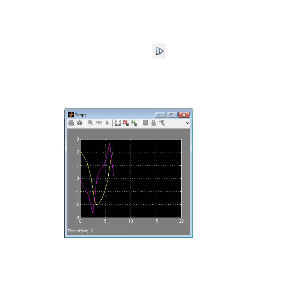
Step Through a Simulation
3Click the Enable previous stepping check box, then click OK.
4In the Simulation toolbar, click .
Thesimulationsimulatesonestep.Atthesametime,thesoftwarestores
the simulation snapshot for that step.
5Repeatedly click the Next button to continue stepping forward and storing
simulation data. For example, 25 clicks plots data that looks like:
If you clear the Enable previous stepping check box, the software clears
the stored snapshot cache.
Note You must step forward before you can step backward to create the
simulation state that the step backward operation requires.
2-13

2Simulation Stepping
6In the Simulation toolbar, click one or more times to step backward
to the previously stepped simulation snapshot.
The scope updates to show that data has been removed from the scope.
Simulation Snapshots
In the Simulation Stepping Options dialog box, you can specify options for
snapshot capturing:
•The maximum number of snapshots to capture while simulating forward.
The greater the number of steps, the more memory the simulation will
occupy. This number can impact simulation speed.
•The number of steps to skip between snapshots. This capability enables
you to create snapshots of simulation state at periodic intervals, such
2-14
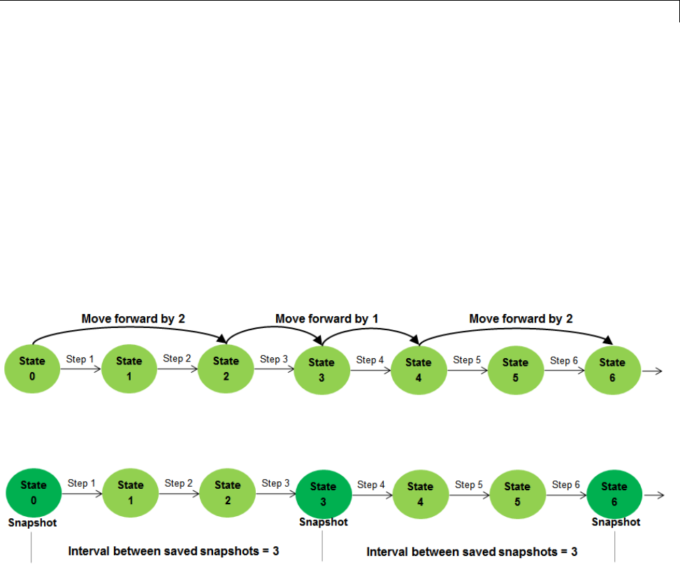
Step Through a Simulation
as every three steps. This interval is independent of the number of
steps taken in either the forward or backward direction. Because taking
simulation snapshots affects simulation speed, saving snapshots at larger
intervals can improve simulation speed (compared to setting this interval
to a smaller number).
The following figure illustrates how the stepper can move along the steps
of a simulation. In this case, the stepper first pauses the simulation after
two major steps, then again after two consecutive single major steps, and
the again after two major steps. The number of simulation steps between
stepper pauses is the Move back/forward by setting in the stepper
options dialog box. You can change this setting during simulation as shown
in the following figure.
The following figure illustrates snapshot captures where the interval
between stored snapshots is three.
In the following figure, the number of steps to skip between snapshots is
three at first, but after the fourth step, the number of steps changes to one.
This example illustrates the flexibility of the stepper, which allows you to
change the stepping options while stepping forward. In this example, at the
fourth step, the Simulation Stepping Options dialog box was used to change
the snapshot steps from three to one. This capability is most useful when
you want to capture more snapshots around a simulation time of interest.
2-15
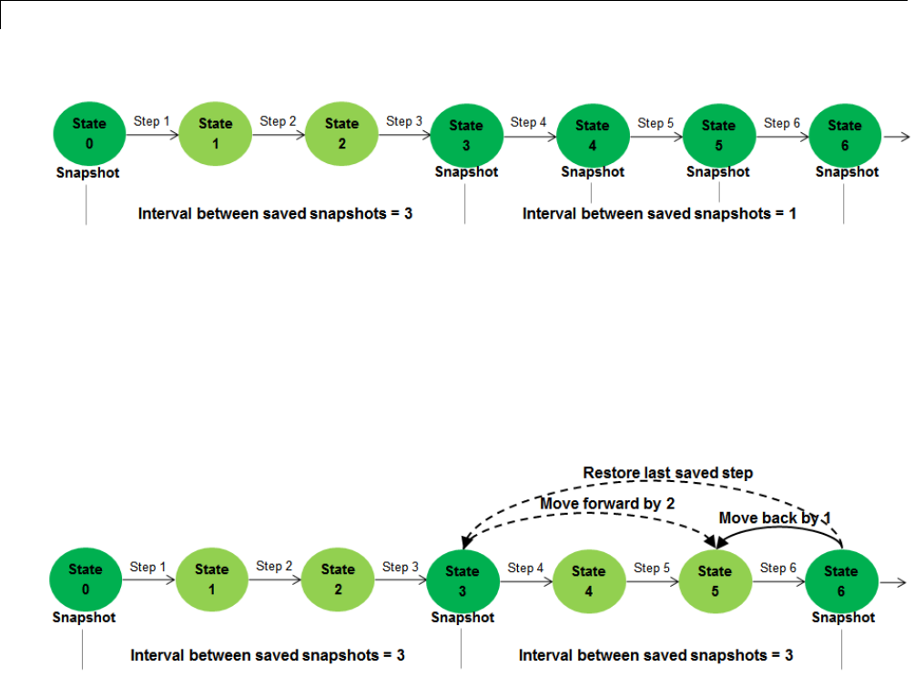
2Simulation Stepping
The following figure illustrates how the snapshots settings of the stepper
can change the action for stepping backward. For example, suppose
that the interval between snapshots is set to 3 (simulation steps), and
starting at a certain simulation time (corresponding to state 6 in the
following figure), the stepper Move back/forward by setting is set to 1.
To accomplish this task, the stepper first restores the simulation state to
the last saved snapshot (state 3), and then simulates for two major times
steps to arrive at the desired state (5). This capability is helpful for memory
usage and simulation performance.
Stepping to the final step ends the simulation. This means that stepping
backward after reaching the end of simulation is not possible unless you
restart the simulation.
Tune Parameters
While using the stepper, if the simulation is in a paused state, you can change
tunable parameters, including some solver settings.
Although you can change tunable parameters when a simulation is paused (as
part of stepping or by using the Pause button), changes to the solver step size
2-16

Step Through a Simulation
take effect when the solver advances the simulation time. For some solvers,
this occurs after the next simulation step is taken.
The Simulation Stepper takes into account the size of a movement (Move
back/forward by) and the frequency of saving backward steps (Interval
between stored back steps). If you specify a frequency that is larger than
the step size, the stepper first steps back to the last saved step, then simulates
forward until the total step count difference reaches the size of the step. Note
that new tunable parameters are applied when simulating forward. For
this reason, in a scenario like this, if you change tunable parameters before
stepping back, the resulting simulation output might not match the previous
simulation output at that step.
For example, assume a snapshot save frequency of 3 and a step size of 1 ( see
the previous figure). The stepper first steps back to the last saved step, up
to three steps, then simulates forward until the total step count difference
reaches one. If you change tunable parameters before stepping back, the
resulting simulation output might not match the previous simulation output
at that step.
Referenced Models
When using the stepper and Model block, the referenced model uses the
stepping options of the top model for the duration of a simulation. In addition,
the stepper dialog box of the referenced model serves as a direct link to the
settings of the top model. As a result, changing the stepper settings through
the referenced model during simulation also changes the stepper settings
of the top model. When the simulation ends, the stepper settings of the
referenced model revert to the original values.
This table illustrates this behavior for the Move back/forward by parameter
(number of steps):
2-17

2Simulation Stepping
Simulation Off Simulation On Changed
Referenced Model
Setting
Simulation Off
Top Model Original
top model
number
of steps
(OrgTopModel)
Number of steps =
OrgTopModel
New number
of steps
(NewRefModel)
copied from
referenced model
Keeps value
NewRefModel
Referenced
Model
Original
referenced
model
number
of steps
(OrgRefModel)
Number of steps =
OrgTopModel
New number
of steps =
NewRefModel
Reverts to original
referenced model
number of steps
OrgRefModel
Simulation Stepper and Stateflow Debugger
When you debug a Stateflow chart (for example, when the simulation stops at
a Stateflow breakpoint), Simulation Stepper changes to contain additional
buttons to control the Stateflow debugging session. When the Stateflow
debugging session ends, the default Simulation Stepper interface is reinstated.
For more information about controlling the Stateflow debugger through the
Simulink Editor toolbar, see “Control Chart Execution in the Debugger”.
Conditional Breakpoints
The Simulation Stepper allows you to set conditional breakpoints for scalar
signals. A conditional breakpoint is a breakpoint that is triggered based on a
certain expression evaluated on a signal. When the breakpoint is triggered,
the corresponding simulation pauses.
Note When simulation arrives at a conditional breakpoint, simulation does
not stop immediately when the block is executed. Instead, simulation stops
only after the current simulation step completes.
To set a conditional breakpoint for a signal:
2-18
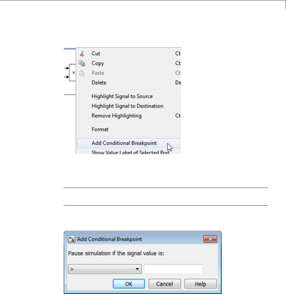
Step Through a Simulation
1Right-click that signal and select Add Conditional Breakpoint.
Alternatively, select the signal then, from the menu bar, select
Simulation>Debug>AddConditionalBreakpoint.
Note You cannot add conditional breakpoints on inputs to, outputs from,
or signals inside variant subsystems.
This action displays the Add Conditional Breakpoint dialog box.
2From the drop-down list, select the condition for this signal:
2-19
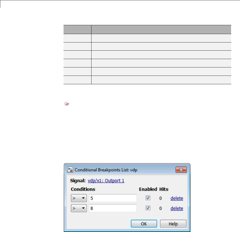
2Simulation Stepping
Condition Pause simulation if the signal value is...
>Greater than the specified value.
>= Greaterthanorequaltothespecifiedvalue.
=Equal to the specified value.
~= Not equal to the specified value.
<= Less than or equal to the specified value.
<Less than the specified value.
3Enter the signal value at which you want simulation to pause. The affected
signal line is updated with a conditional breakpoint icon like the following,
.
You can add multiple conditional breakpoints to a signal line.
4To view a summary of the conditional breakpoints and edit them, left-click
the conditional breakpoint icon. (Alternatively, from the menu bar,
select Simulation > Debug > Conditional Breakpoints List.) A
Conditional Breakpoints List dialog box like the following is displayed. If
the conditional breakpoints list is empty, a message pops up to warn you
that there are no conditional breakpoints.
In this dialog box, you can:
•Change the condition for the signal value.
2-20

Step Through a Simulation
•Change the value of the signal.
•Disable and enable the conditional breakpoint.
•Delete the condition.
Condition values:
•Must be numeric. They cannot be expressions.
•Cannot be NaN.
5Click OK when done and simulate the model.
2-21

2Simulation Stepping
2-22


3How Simulink®Works
How Simulink Works
Simulink is a software package that enables you to model, simulate, and
analyze systems whose outputs change over time. Such systems are often
referred to as dynamic systems. The Simulink software can be used to explore
thebehaviorofawiderangeofreal-world dynamic systems, including
electrical circuits, shock absorbers, braking systems, and many other
electrical, mechanical, and thermodynamic systems. This section explains
how Simulink works.
Simulating a dynamic system is a two-step process. First, a user creates a
block diagram, using the Simulink model editor, that graphically depicts
time-dependent mathematical relationships among the system’s inputs,
states, and outputs. The user then commands the Simulink software to
simulate the system represented by the model from a specified start time to
aspecifiedstoptime.
For more information on this process, see:
•“Modeling Dynamic Systems” on page 3-3
•“Simulating Dynamic Systems” on page 3-18
3-2

Modeling Dynamic Systems
Modeling Dynamic Systems
In this section...
“Block Diagram Semantics” on page 3-3
“Creating Models” on page 3-4
“Time” on page 3-5
“States” on page 3-5
“Block Parameters” on page 3-9
“Tunable Parameters” on page 3-9
“Block Sample Times” on page 3-9
“Custom Blocks” on page 3-10
“Systems and Subsystems” on page 3-11
“Signals” on page 3-16
“Block Methods” on page 3-16
“Model Methods” on page 3-17
Block Diagram Semantics
A classic block diagram model of a dynamic system graphically consists
of blocks and lines (signals). The history of these block diagram models
is derived from engineering areas such as Feedback Control Theory and
Signal Processing. A block within a block diagram defines a dynamic system
in itself. The relationships between each elementary dynamic system in a
block diagram are illustrated by the use of signals connecting the blocks.
Collectively the blocks and lines in a block diagram describe an overall
dynamic system.
The Simulink product extends these classic block diagram models by
introducing the notion of two classes of blocks, nonvirtual blocks and virtual
blocks. Nonvirtual blocks represent elementary systems. Virtual blocks exist
for graphical and organizational convenience only: they have no effect on
the system of equations described by the block diagram model. You can use
virtual blocks to improve the readability of your models.
3-3

3How Simulink®Works
In general, blocks and lines can be used to describe many “models of
computations.” One example would be a flow chart. A flow chart consists of
blocks and lines, but one cannot describe general dynamic systems using
flow chart semantics.
The term “time-based block diagram” is used to distinguish block diagrams
that describe dynamic systems from that of other forms of block diagrams,
and the term block diagram (or model) is used to refer to a time-based block
diagram unless the context requires explicit distinction.
To summarize the meaning of time-based block diagrams:
•Simulink block diagrams define time-based relationships between signals
and state variables. The solution of a block diagram is obtained by
evaluating these relationships over time, where time starts at a user
specified “start time” and ends at a user specified “stop time.” Each
evaluation of these relationships is referred to as a time step.
•Signals represent quantities that change over time and are defined for all
points in time between the block diagram’s start and stop time.
•The relationships between signals and state variables are defined by a set
of equations represented by blocks. Each block consists of a set of equations
(block methods). These equations define a relationship between the input
signals, output signals and the state variables. Inherent in the definition
of a equation is the notion of parameters, which are the coefficients found
within the equation.
Creating Models
The Simulink product provides a graphical editor that allows you to create
and connect instances of block types (see “Connect Blocks” on page 4-12)
selected from libraries of block types (see “Block Libraries”) via a library
browser. Libraries of blocks are provided representing elementary systems
that can be used as building blocks. The blocks supplied with Simulink are
called built-in blocks. Users can also create their own block types and use
the Simulink editor to create instances of them in a diagram. User-defined
blocks are called custom blocks.
3-4
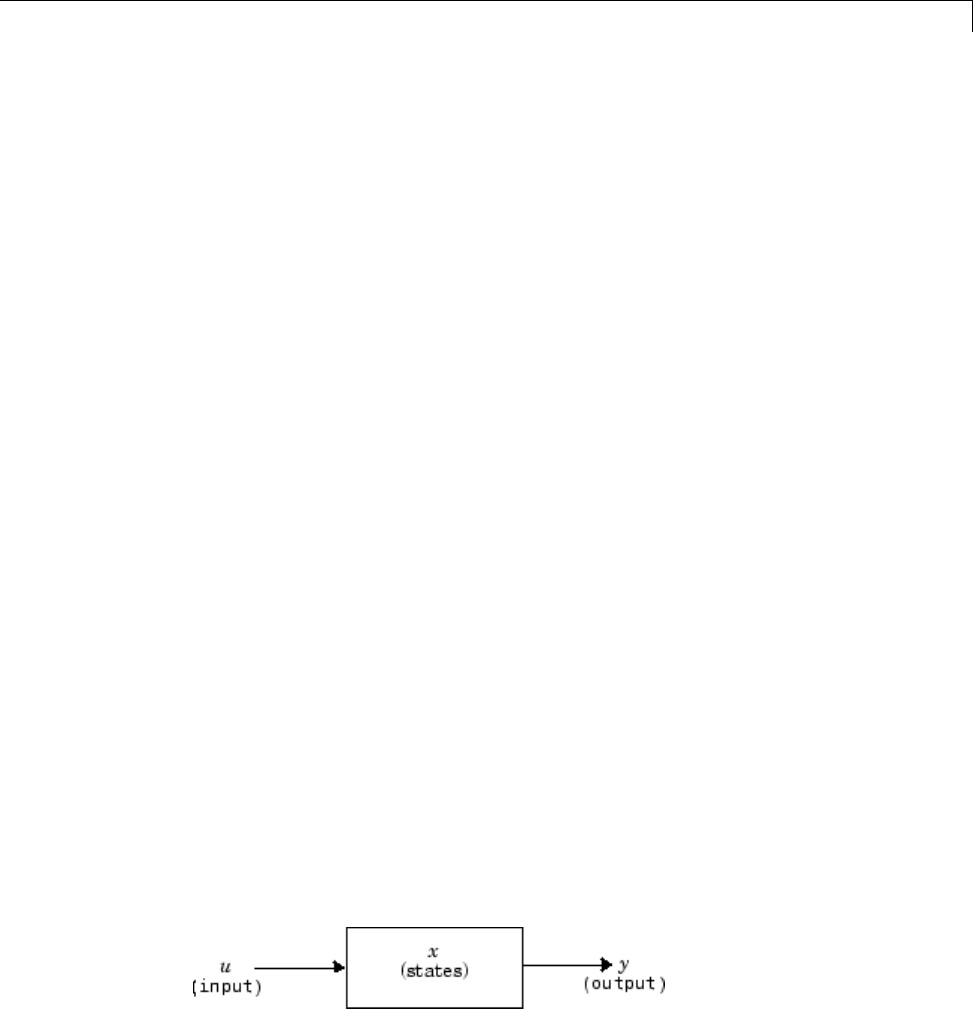
Modeling Dynamic Systems
Time
Time is an inherent component of block diagrams in that the results of a block
diagram simulation change with time. Put another way, a block diagram
represents the instantaneous behaviorofadynamicsystem. Determining
a system’s behavior over time thus entails repeatedly solving the model at
intervals, called time steps, from the start of the time span to the end of the
time span. The process of solving a model at successive time steps is referred
to as simulating the system that the model represents.
States
Typically the current values of some system, and hence model, outputs are
functions of the previous values of temporal variables. Such variables are
called states. Computing a model’s outputs from a block diagram hence
entails saving the value of states at the current time step for use in computing
the outputs at a subsequent time step. This task is performed during
simulation for models that define states.
Two types of states can occur in a Simulink model: discrete and continuous
states. A continuous state changes continuously. Examples of continuous
states are the position and speed of a car. A discrete state is an approximation
of a continuous state where the state is updated (recomputed) using finite
(periodic or aperiodic) intervals. An example of a discrete state would be the
position of a car shown on a digital odometer where it is updated every second
as opposed to continuously. In the limit, as the discrete state time interval
approaches zero, a discrete state becomes equivalent to a continuous state.
Blocks implicitly define a model’s states. In particular, a block that needs
some or all of its previous outputs to compute its current outputs implicitly
defines a set of states that need to be savedbetweentimesteps.Suchablock
is said to have states.
The following is a graphical representation of a block that has states:
3-5

3How Simulink®Works
Blocks that define continuous states include the following standard Simulink
blocks:
•Integrator
•State-Space
•Transfer Fcn
•Variable Transport Delay
•Zero-Pole
The total number of a model’s states is the sum of all the states defined
by all its blocks. Determining the number of states in a diagram requires
parsing the diagram to determine the types of blocks that it contains and then
aggregating the number of states defined by each instance of a block type
that defines states. This task is performed during the Compilation phase
of a simulation.
Working with States
The following facilities are provided for determining, initializing, and logging
a model’s states during simulation:
•The model command displays information about the states defined by a
model, including the total number of states defined by the model, the block
that defines each state, and the initial value of each state.
•The Simulink debugger displays the value of a state at each time step
during a simulation, and the Simulink debugger’s states command
displays information about the model’s current states (see “Debugging”).
•The Data Import/Export pane of a model’s Configuration Parameters
dialog box (see “Import and Export States” on page 45-113) allows you to
specify initial values for a model’s states, and to record the values of the
states at each time step during simulation as an array or structure variable
in the MATLAB workspace.
•The Block Parameters dialog box (and the ContinuousStateAttributes
parameter) allows you to give names to states for those blocks (such as the
Integrator) that employ continuous states. This can simplify analyzing
data logged for states, especially when a block has multiple states.
3-6

Modeling Dynamic Systems
The Two Cylinder Model with Load Constraints model illustrates the
logging of continuous states.
Continuous States
Computing a continuous state entails knowing its rate of change, or
derivative. Since the rate of change of a continuous state typically itself
changes continuously (i.e., is itself a state), computing the value of a
continuous state at the current time step entails integration of its derivative
from the start of a simulation. Thus modeling a continuous state entails
representing the operation of integration and the process of computing
the state’s derivative at each point in time. Simulink block diagrams use
Integrator blocks to indicate integration and a chain of blocks connected to
an integrator block’s input to represent the method for computing the state’s
derivative. The chain of blocks connected to the integrator block’s input is the
graphical counterpart to an ordinary differential equation (ODE).
In general, excluding simple dynamic systems, analytical methods do not
exist for integrating the states of real-world dynamic systems represented
by ordinary differential equations. Integrating the states requires the use
of numerical methods called ODE solvers. These various methods trade
computational accuracy for computational workload. The Simulink product
comes with computerized implementations of the most common ODE
integration methods and allows a user to determine which it uses to integrate
states represented by Integrator blocks when simulating a system.
Computing the value of a continuous state at the current time step entails
integrating its values from the start of the simulation. The accuracy of
numerical integration in turn depends on the size of the intervals between
time steps. In general, the smaller the time step, the more accurate the
simulation. Some ODE solvers, called variable time step solvers, can
automatically vary the size of the time step, based on the rate of change
of the state, to achieve a specified level of accuracy over the course of a
simulation. The user can specify the size of the time step in the case of
fixed-step solvers, or the solver can automatically determine the step size in
the case of variable-step solvers. To minimize the computation workload, the
variable-step solver chooses the largest step size consistent with achieving an
overall level of precision specified by the user for the most rapidly changing
model state. This ensures that all model states are computed to the accuracy
specified by the user.
3-7

3How Simulink®Works
Discrete States
Computing a discrete state requires knowing the relationship between its
value at the current time step and its value at the previous time step. This is
referred to this relationship as the state’s update function. A discrete state
depends not only on its value at the previous time step but also on the values
of a model’s inputs. Modeling a discrete state thus entails modeling the state’s
dependency on the systems’ inputs at the previous time step. Simulink block
diagrams use specific types of blocks, called discrete blocks, to specify update
functions and chains of blocks connected to the inputs of discrete blocks to
model the dependency of a system’s discrete states on its inputs.
As with continuous states, discrete states set a constraint on the simulation
timestepsize. Specifically,thestepsizemustensurethatallthesample
times of the model’s states are hit. This task is assigned to a component of the
Simulink system called a discrete solver. Two discrete solvers are provided: a
fixed-step discrete solver and a variable-step discrete solver. The fixed-step
discrete solver determines a fixed step size that hits all the sample times
of all the model’s discrete states, regardless of whether the states actually
change value at the sample time hits. By contrast, the variable-step discrete
solver varies the step size to ensure that sample time hits occur only at times
when the states change value.
Modeling Hybrid Systems
A hybrid system is a system that has both discrete and continuous states.
Strictly speaking, any model that has both continuous and discrete sample
timesistreatedasahybridmodel,presuming that the model has both
continuous and discrete states. Solving such a model entails choosing a
step size that satisfies both the precision constraint on the continuous state
integration and the sample time hit constraint on the discrete states. The
Simulink software meets this requirement by passing the next sample time
hit, as determined by the discrete solver, as an additional constraint on
the continuous solver. The continuous solver must choose a step size that
advances the simulation up to but not beyond the time of the next sample
time hit. The continuous solver can take a time step short of the next sample
time hit to meet its accuracy constraint butitcannottakeastepbeyondthe
next sample time hit even if its accuracy constraint allows it to.
You can simulate hybrid systems using any one of the integration methods,
but certain methods are more effective than others. For most hybrid systems,
3-8

Modeling Dynamic Systems
ode23 and ode45 are superior to the other solvers in terms of efficiency.
Because of discontinuities associated with the sample and hold of the discrete
blocks, do not use the ode15s and ode113 solvers for hybrid systems.
Block Parameters
Key properties of many standard blocks are parameterized. For example,
the Constant value of the Simulink Constant block is a parameter. Each
parameterized block has a block dialog that lets you set the values of the
parameters. You can use MATLAB expressions to specify parameter values.
Simulink evaluates the expressions before running a simulation. You can
change the values of parameters during a simulation. This allows you to
determine interactively the most suitable value for a parameter.
A parameterized block effectively represents a family of similar blocks. For
example, when creating a model, you can set the Constant value parameter of
each instance of the Constant block separately so that each instance behaves
differently. Because it allows each standard block to represent a family of
blocks, block parameterization greatly increases the modeling power of the
standard Simulink libraries. See “Block Parameters” on page 3-9 and “Block
Libraries” for more information.
Tunable Parameters
Many block parameters are tunable. A tunable parameter is a parameter
whose value can be changed without recompiling the model (see “Model
Compilation” on page 3-18 for more information on compiling a model). For
example, the gain parameter of the Gain block is tunable. You can alter the
block’s gain while a simulation is running. If a parameter is not tunable and
the simulation is running, the dialog box control that sets the parameter
is disabled.
When you change the value of a tunable parameter, the change takes effect
at the start of the next time step. See “Block Parameters” on page 3-9 and
“Tunable Parameters” on page 24-13 for more information.
Block Sample Times
Every Simulink block has a sample time which defines when the block will
execute . Most blocks allow you to specify the sample time via a SampleTime
3-9

3How Simulink®Works
parameter. Common choices include discrete, continuous, and inherited
sample times.
Common Sample
Time Types
Sample Time Examples
Discrete [Ts,T
o]Unit Delay, Digital
Filter
Continuous [0, 0] Integrator, Derivative
Inherited [–1, 0] Gain, Sum
For discrete blocks, the sample time is a vector [Ts, To] where Ts is the time
interval or period between consecutive sample times and To is an initial offset
to the sample time. In contrast, the sample times for nondiscrete blocks are
represented by ordered pairs that use zero, a negative integer, or infinity to
represent a specific type of sample time (see “View Sample Time Information”
on page 5-9). For example, continuous blocks have a nominal sample time of
[0, 0] and are used to model systems in which the states change continuously
(e.g., a car accelerating). Whereas youindicatethesampletimetypeofan
inherited block symbolically as [–1, 0] and Simulink then determines the
actual value based upon the context of the inherited block within the model.
Note that not all blocks accept all types of sample times. For example, a
discrete block cannot accept a continuous sample time.
For a visual aid, Simulink allows the optional color-coding and annotation of
any block diagram to indicate the type and speed of the block sample times.
You can capture all of the colors and the annotations within a legend (see
“View Sample Time Information” on page 5-9).
For a more detailed discussion of sample times, see “Sample Time”
Custom Blocks
You can create libraries of custom blocks that you can then use in your models.
You can create a custom block either graphically or programmatically. To
create a custom block graphically, you draw a block diagram representing
the block’s behavior, wrap this diagram in an instance of the Simulink
Subsystem block, and provide the block with a parameter dialog, using the
3-10

Modeling Dynamic Systems
Simulink block mask facility. To create a block programmatically, you create
a MATLAB file or a MEX-file that contains the block’s system functions (see
“S-Function Basics”). The resulting file is called an S-function. You then
associate the S-function with instances of the Simulink S-Function block in
your model. You can add a parameter dialog to your S-Function block by
wrapping it in a Subsystem block and adding the parameter dialog to the
Subsystem block. See “Block Creation” for more information.
Systems and Subsystems
A Simulink block diagram can consist of layers. Each layer is defined by a
subsystem. A subsystem is part of the overall block diagram and ideally has
no impact on the meaning of the block diagram. Subsystems are provided
primarily to help with the organizational aspects of a block diagram.
Subsystems do not define a separate block diagram.
The Simulink software differentiates between two different types of
subsystems: virtual and nonvirtual. The primary difference is that nonvirtual
subsystems provide the ability to control when the contents of the subsystem
are evaluated.
Virtual Subsystems
Virtual subsystems provide graphical hierarchy in models. Virtual
subsystems do not impact execution. During model execution, the Simulink
engine flattens all virtual subsystems, i.e., Simulink expands the subsystem
in place before execution. This expansion is very similar to the way macros
work in a programming language such as C or C++. Roughly speaking, there
will be one system for the top-level block diagram which is referred to as
the root system, and several lower-level systems derived from nonvirtual
subsystems and other elements in the block diagram. You will see these
systems in the Simulink Debugger. The act of creating these internal systems
is often referred to as flattening the model hierarchy.
Nonvirtual Subsystems
Nonvirtual subsystems, which are drawn with a bold border, provide
execution and graphical hierarchy in models. Nonvirtual subsystems are
executed as a single unit (atomic execution) by the Simulink engine. You
can create conditionally executed subsystems that are executed only when
3-11

3How Simulink®Works
a precondition—such as a trigger, an enable, a function-call, or an action—
occurs (see “Conditional Subsystems”). Simulink always computes all inputs
used during the execution of a nonvirtual subsystem before executing the
subsystem. Simulink defines the following nonvirtual subsystems.
Atomic subsystems. The primary characteristic of an atomic subsystem is
that blocks in an atomic subsystem execute as a single unit. This provides
the advantage of grouping functional aspects of models at the execution
level. Any Simulink block can be placed in an atomic subsystem, including
blocks with different execution rates. You can create an atomic subsystem by
selecting the Treat as atomic unit option on a virtual subsystem (see the
Atomic Subsystem block for more information).
Enabled subsystems. An enabled subsystem behaves similarly to an
atomic subsystem, except that it executes only when the signal driving the
subsystem enable port is greater than zero. To create an enabled subsystem,
place an Enable Port block within a Subsystem block. You can configure an
enabled subsystem to hold or reset the states of blocks within the enabled
subsystem prior to a subsystem enabling action. Simply select the States
when enabling parameter of the Enable Port block. Similarly, you can
configure each output port of an enabled subsystem to hold or reset its output
prior to the subsystem disabling action. Select the Output when disabled
parameter in the Outport block.
Triggered subsystems. You create a triggered subsystem by placing a
trigger port block within a subsystem. The resulting subsystem executes
when a rising or falling edge with respect to zero is seen on the signal driving
the subsystem trigger port. The direction of the triggering edge is defined by
the Trigger type parameter on the trigger port block. Simulink limits the
type of blocks placed in a triggered subsystem to blocks that do not have
explicit sample times (i.e., blocks within the subsystem must have a sample
time of -1) because the contents of a triggered subsystem execute in an
aperiodic fashion. A Stateflow chart can also have a trigger port which is
defined by using the Stateflow editor. Simulink does not distinguish between
a triggered subsystem and a triggered chart.
3-12

Modeling Dynamic Systems
Function-call subsystems. A function-call subsystem is a subsystem that
another block can invoke directly during a simulation. It is analogous to a
function in a procedural programming language. Invoking a function-call
subsystem is equivalent to invoking the output and update methods of the
blocks that the subsystem contains in sorted order. The block that invokes
a function-call subsystem is called the function-call initiator. Stateflow,
Function-Call Generator, and S-function blocks can all serve as function-call
initiators. To create a function-call subsystem, drag a Function-Call
Subsystem block from the Ports & Subsystems library into your model and
connect a function-call initiator to the function-call port displayed on top of the
subsystem. You can also create a function-call subsystem from scratch by first
creating a Subsystem block in your model and then creating a Trigger block in
the subsystem and setting the Trigger block Trigger type to function-call.
You can configure a function-call subsystem to be triggered (the default) or
periodic by setting its Sample time type to be triggered or periodic,
respectively. A function-call initiator can invoke a triggered function-call
subsystem zero, once, or multiple times per time step. The sample times of all
the blocks in a triggered function-call subsystem must be set to inherited (-1).
A function-call initiator can invoke a periodic function-call subsystem only
once per time step and must invoke the subsystem periodically. If the
initiator invokes a periodic function-call subsystem aperiodically, Simulink
halts the simulation and displays an error message. The blocks in a periodic
function-call subsystem can specify a noninherited sample time or inherited
(-1) sample time. All blocks that specify a noninherited sample time must
specify the same sample time, that is, if one block specifies .1 as its sample
time, all other blocks must specify a sample time of .1 or -1. If a function-call
initiator invokes a periodic function-call subsystem at a rate that differs from
thesampletimespecifiedbytheblocksinthesubsystem,Simulinkhaltsthe
simulation and displays an error message.
3-13

3How Simulink®Works
Enabled and triggered subsystems. You can create an enabled and
triggered subsystem by placing a Trigger Port block and an Enable Port block
within a Subsystem block. The resulting subsystem is essentially a triggered
subsystem that executes when the subsystem is enabled and a rising or
falling edge with respect to zero is seen on the signal driving the subsystem
trigger port. The direction of the triggering edge is defined by the Trigger
type parameter on the trigger port block. Because the contents of a triggered
subsystem execute in an aperiodic fashion, Simulink limits the types of blocks
placed in an enabled and triggered subsystem to blocks that do not have
explicit sample times. In other words, blocks within the subsystem must
haveasampletimeof-1).
Action subsystems. Action subsystems can be thought of as an intersection
of the properties of enabled subsystems and function-call subsystems. Action
subsystems are restricted to a single sample time (e.g., a continuous, discrete,
or inherited sample time). Action subsystems must be executed by an action
subsystem initiator. This is either an If block or a Switch Case block. All
action subsystems connected to a given action subsystem initiator must have
the same sample time. An action subsystem is created by placing an Action
Port block within a Subsystem block. The subsystem icon will automatically
adapt to the type of block (i.e., If or Switch Case block) that is executing the
action subsystem.
Action subsystems can be executed atmostoncebytheactionsubsystem
initiator. Action subsystems give you control over when the states reset via
the States when execution is resumed parameter on the Action Port
block. Action subsystems also give you control over whether or not to hold
the outport values via the Output when disabled parameter on the outport
block. This is analogous to enabled subsystems.
Action subsystems behave very similarly to function-call subsystems because
they must be executed by an initiator block. Function-call subsystems can be
executed more than once at any given time step whereas action subsystems can
be executed at most once. This restriction means that a larger set of blocks
(e.g., periodic blocks) can be placed in action subsystems as compared to
function-call subsystems. This restriction also means that you can control
how the states and outputs behave.
3-14

Modeling Dynamic Systems
While iterator subsystems. A while iterator subsystem will run multiple
iterations on each model time step. The number of iterations is controlled by
the While Iterator block condition. A while iterator subsystem is created by
placing a While Iterator block within a subsystem block.
A while iterator subsystem is very similar to a function-call subsystem in that
it can run for any number of iterations at a given time step. The while iterator
subsystem differs from a function-call subsystem in that there is no separate
initiator (e.g., a Stateflow Chart). In addition, a while iterator subsystem
has access to the current iteration number optionally produced by the While
Iterator block. A while iterator subsystem also gives you control over whether
or not to reset states when starting via the States when starting parameter
on the While Iterator block.
For iterator subsystems. A for iterator subsystem will run a fixed number
of iterations at each model time step. The number of iterations can be an
external input to the for iterator subsystem or specified internally on the For
Iterator block. A for iterator subsystem is created by placing a For Iterator
block within a subsystem block.
A for iterator subsystem has access to the current iteration number that is
optionally produced by the For Iterator block. A for iterator subsystem also
gives you control over whether or not to reset states when starting via the
States when starting parameterontheForIteratorblock. Aforiterator
subsystem is very similar to a while iterator subsystem with the restriction
that the number of iterations during any given time step is fixed.
For each subsystems. The for each subsystem allows you to repeat an
algorithm for individual elements (or subarrays) of an input signal. Here,
the algorithm is represented by the set of blocks in the subsystem and is
applied to a single element (or subarray) of the signal. You can configure the
decomposition of the subsystem inputs into elements (or subarrays) using the
For Each block, which resides in the subsystem. The For Each block also
allows you to configure the concatenation of individual results into output
signals. An advantage of this subsystem is that it maintains separate sets of
states for each element or subarray that it processes. In addition, for certain
models, the for each subsystem improves the code reuse of the code generated
by Simulink Coder™.
3-15

3How Simulink®Works
Signals
The term signal refers to a time varying quantity that has values at all
points in time. You can specify a wide range of signal attributes, including
signal name, data type (e.g., 8-bit, 16-bit, or 32-bit integer), numeric type
(real or complex), and dimensionality (one-dimensional, two-dimensional, or
multidimensional array). Many blocks can accept or output signals of any
data or numeric type and dimensionality. Others impose restrictions on the
attributes of the signals they can handle.
On the block diagram, signals are represented with lines that have an
arrowhead. The source of the signal corresponds to the block that writes to the
signal during evaluation of its block methods (equations). The destinations of
the signal are blocks that read the signal during the evaluation of the block’s
methods (equations).
Agoodwayt
o understand the definition of a signal is to consider a classroom.
The teacher is the one responsible for writing on the white board and the
students read what is written on the white board when they choose to. This
is also true of Simulink signals: a reader of the signal (a block method) can
choose to read the signal as frequently or infrequently as so desired.
For more information about signals, see “Signals”.
Block Methods
Blocks represent multiple equations. These equations are represented as
block methods. These block methods are evaluated (executed) during the
execution of a block diagram. The evaluation of these block methods is
performedwithinasimulationloop,whereeachcyclethroughthesimulation
loop represents the evaluation of the block diagram at a given point in time.
Method Types
Names are assigned to the types of functions performed by block methods.
Common method types include:
•Outputs
Computes the outputs of a block given its inputs at the current time step
and its states at the previous time step.
3-16

Modeling Dynamic Systems
•Update
Computes the value of the block’s discrete states at the current time step,
given its inputs at the current time step and its discrete states at the
previous time step.
•Derivatives
Computes the derivatives of the block’s continuous states at the current
time step, given the block’s inputs and the values of the states at the
previous time step.
Method Naming Convention
Block methods perform the same types of operations in different ways for
different types of blocks. The Simulink user interface and documentation uses
dot notation to indicate the specific function performed by a block method:
BlockType.MethodType
For example, the method that computes the outputs of a Gain block is referred
to as
Gain.Outputs
The Simulink debugger takes the naming convention one step further and
usestheinstancenameofablocktospecifyboththemethodtypeandthe
block instance on which the method is being invoked during simulation, e.g.,
g1.Outputs
Model Methods
In addition to block methods, a set of methods is provided that compute the
model’s properties and its outputs. The Simulink software similarly invokes
these methods during simulation to determine a model’s properties and its
outputs. The model methods generally perform their tasks by invoking block
methods of the same type. For example, the model Outputs method invokes
the Outputs methods of the blocks that it contains in the order specified by
the model to compute its outputs. The model Derivatives method similarly
invokes the Derivatives methods of theblocksthatitcontainstodetermine
the derivatives of its states.
3-17

3How Simulink®Works
Simulating Dynamic Systems
In this section...
“Model Compilation” on page 3-18
“Link Phase” on page 3-19
“Simulation Loop Phase” on page 3-19
“Solvers” on page 3-21
“Zero-Crossing Detection” on page 3-23
“Algebraic Loops” on page 3-39
Model Compilation
The first phase of simulation occurs when the system’s model is open and
you simulate the model. In the Simulink Editor, select Simulation > Run.
Running the simulation causes the Simulink engine to invoke the model
compiler. The model compiler converts the model to an executable form, a
process called compilation. In particular, the compiler:
•Evaluates the model’s block parameter expressions to determine their
values.
•Determines signal attributes, e.g., name, data type, numeric type, and
dimensionality, not explicitly specified by the model and checks that each
block can accept the signals connected to its inputs.
•A process called attribute propagation is used to determine unspecified
attributes. This process entails propagating the attributes of a source
signal to the inputs of the blocks that it drives.
•Performs block reduction optimizations.
•Flattens the model hierarchy by replacing virtual subsystems with the
blocks that they contain (see “Solvers” on page 3-21).
•Determines the block sorted order (see “Control and Displaying the Sorted
Order” on page 23-35 for more information).
3-18

Simulating Dynamic Systems
•Determines the sample times of all blocks in the model whose sample times
you did not explicitly specify (see “How Propagation Affects Inherited
Sample Times” on page 5-29).
Link Phase
In this phase, the Simulink engine allocates memory needed for working
areas (signals, states, and run-time parameters) for execution of the block
diagram. It also allocates and initializes memory for data structures that
store run-time information for each block. For built-in blocks, the principal
run-time data structure for a block is called the SimBlock. It stores pointers
to a block’s input and output buffers and state and work vectors.
Method Execution Lists
In the Link phase, the Simulink engine also creates method execution lists.
These lists list the most efficient order in which to invoke a model’s block
methods to compute its outputs. The block sorted order lists generated during
the model compilation phase is used to construct the method execution lists.
Block Priorities
You can assign update priorities to blocks (see “Assign Block Priorities” on
page 23-47). The output methods of higher priority blocks are executed before
those of lower priority blocks. The priorities are honored only if they are
consistent with its block sorting rules.
Simulation Loop Phase
Once the Link Phase completes, the simulation enters the simulation loop
phase. In this phase, the Simulink engine successively computes the states
and outputs of the system at intervals from the simulation start time to the
finish time, using information provided by the model. The successive time
points at which the states and outputs are computed are called time steps.
The length of time between steps is called the step size. The step size depends
on the type of solver (see “Solvers” on page 3-21) used to compute the system’s
continuous states, the system’s fundamentalsampletime(see“SampleTimes
in Systems” on page 5-22), and whether the system’s continuous states have
discontinuities (see “Zero-Crossing Detection” on page 3-23).
3-19

3How Simulink®Works
The Simulation Loop phase has two subphases: the Loop Initialization phase
and the Loop Iteration phase. The initialization phase occurs once, at the
start of the loop. The iteration phase is repeated once per time step from the
simulation start time to the simulation stop time.
At the start of the simulation, the model specifies the initial states and
outputs of the system to be simulated. At each step, new values for the
system’s inputs, states, and outputs are computed, and the model is updated
to reflect the computed values. At the end of the simulation, the model reflects
the final values of the system’s inputs, states, and outputs. The Simulink
software provides data display and logging blocks. You can display and/or log
intermediate results by including these blocks in your model.
Loop Iteration
At each time step, the Simulink engine:
1Computes the model’s outputs.
The Simulink engine initiates this step by invoking the Simulink model
Outputs method. The model Outputs method in turn invokes the model
system Outputs method, which invokes the Outputs methods of the blocks
that the model contains in the order specified by the Outputs method
execution lists generated in the Link phase of the simulation (see “Solvers”
on page 3-21).
The system Outputs method passes the following arguments to each
block Outputs method: a pointer to the block’s data structure and to its
SimBlock structure. The SimBlock data structures point to information
that the Outputs method needs to compute the block’s outputs, including
the location of its input buffers and its output buffers.
2Computes the model’s states.
The Simulink engine computes a model’s states by invoking a solver. Which
solver it invokes depends on whether the model has no states, only discrete
states, only continuous states, or both continuous and discrete states.
If the model has only discrete states, the Simulink engine invokes the
discrete solver selected by the user. The solver computes the size of the
time step needed to hit the model’s sample times. It then invokes the
3-20

Simulating Dynamic Systems
Update method of the model. The model Update method invokes the
Update method of its system, which invokes the Update methods of each of
the blocks that the system contains in the order specified by the Update
method lists generated in the Link phase.
If the model has only continuous states, the Simulink engine invokes the
continuous solver specified by the model. Depending on the solver, the
solver either in turn calls the Derivatives method of the model once or
enters a subcycle of minor time steps where the solver repeatedly calls
the model’s Outputs methods and Derivatives methods to compute the
model’s outputs and derivatives at successive intervals within the major
timestep. Thisisdonetoincreasetheaccuracy of the state computation.
The model Outputs method and Derivatives methods in turn invoke their
corresponding system methods, which invoke the block Outputs and
Derivatives in the order specified by the Outputs and Derivatives methods
execution lists generated in the Link phase.
3Optionally checks for discontinuities in the continuous states of blocks.
A technique called zero-crossing detection is used to detect discontinuities
in continuous states. See “Zero-Crossing Detection” on page 3-23 for more
information.
4Computes the time for the next time step.
Steps 1 through 4 are repeated until the simulation stop time is reached.
Solvers
A dynamic system is simulated by computing its states at successive time
steps over a specified time span, using information provided by the model.
The process of computing the successive states of a system from its model is
known as solving the model. No single method of solving a model suffices for
all systems. Accordingly, a set of programs, known as solvers, are provided
that each embody a particular approach to solving a model. The Configuration
Parameters dialog box allows you to choose the solver most suitable for your
model (see “Choosing a Solver Type” on page 14-10).
3-21

3How Simulink®Works
Fixed-Step Solvers Versus Variable-Step Solvers
The solvers provided in the Simulink software fall into two basic categories:
fixed-step and variable-step.
Fixed-step solvers solve the model at regular time intervals from the beginning
to the end of the simulation. The size of the interval is known as the step size.
You can specify the step size or let the solver choose the step size. Generally,
decreasing the step size increases the accuracy of the results while increasing
thetimerequiredtosimulatethesystem.
Variable-step solvers vary the step size during the simulation, reducing the
step size to increase accuracy when a model’s states are changing rapidly
and increasing the step size to avoid taking unnecessary steps when the
model’s states are changing slowly. Computing the step size adds to the
computational overhead at each step but can reduce the total number of steps,
and hence simulation time, required to maintain a specified level of accuracy
for models with rapidly changing or piecewise continuous states.
Continuous Versus Discrete Solvers
The Simulink product provides both continuous and discrete solvers.
Continuous solvers use numerical integration to compute a model’s continuous
states at the current time step based on the states at previous time steps and
the state derivatives. Continuous solvers rely on the individual blocks to
compute the values of the model’s discrete states at each time step.
Mathematicians have developed a wide variety of numerical integration
techniques for solving the ordinary differential equations (ODEs) that
represent the continuous states of dynamic systems. An extensive set of
fixed-step and variable-step continuous solvers are provided, each of which
implements a specific ODE solution method (see “Choosing a Solver Type”
on page 14-10).
Discrete solvers exist primarily to solve purely discrete models. They compute
the next simulation time step for a model and nothing else. In performing
these computations, they rely on each block in the model to update its
individual discrete states. They do not compute continuous states.
3-22

Simulating Dynamic Systems
Note You must use a continuous solver to solve a model that contains both
continuous and discrete states. You cannot use a discrete solver because
discrete solvers cannot handle continuous states. If, on the other hand, you
select a continuous solver for a model with no states or discrete states only,
Simulink software uses a discrete solver.
Two discrete solvers are provided: A fixed-step discrete solver and a
variable-step discrete solver. The fixed-step solver by default chooses a step
size and hence simulation rate fast enough to track state changes in the fastest
block in your model. The variable-step solver adjusts the simulation step size
to keep pace with the actual rate of discrete state changes in your model. This
can avoid unnecessary steps and hence shorten simulation time for multirate
models (see “Sample Times in Systems” on page 5-22 for more information).
Minor Time Steps
Some continuous solvers subdivide the simulation time span into major and
minor time steps, where a minor time step represents a subdivision of the
major time step. The solver produces a result at each major time step. It
uses results at the minor time steps to improve the accuracy of the result at
the major time step.
Shape Preservation
Usually the integration step size is only related to the current step size and
the current integration error. However, for signals whose derivative changes
rapidly, you can obtain a more accurate integration results by including the
derivative input information at eachtimestep. Todoso,enabletheModel
Configuration Parameters > Solver > Shape Preservation option.
Zero-Crossing Detection
A variable-step solver dynamically adjusts the time step size, causing it to
increase when a variable is changing slowly and to decrease when the variable
changes rapidly. This behavior causes the solver to take many small steps in
the vicinity of a discontinuity because the variable is rapidly changing in this
region. This improves accuracy but can lead to excessive simulation times.
3-23

3How Simulink®Works
TheSimulinksoftwareusesatechniqueknownaszero-crossing detection to
accurately locate a discontinuity without resorting to excessively small time
steps. Usually this technique improves simulation run time, but it can cause
some simulations to halt before the intended completion time.
Two algorithms are provided in the Simulink software: Nonadaptive and
Adaptive. For information about these techniques, see “Zero-Crossing
Algorithms” on page 3-33.
Demonstrating Effects of Excessive Zero-Crossing Detection
The Simulink software comes with three models that illustrate zero-crossing
behavior: sldemo_bounce_two_integrators,sldemo_doublebounce,and
sldemo_bounce.
•The sldemo_bounce_two_integrators model demonstrates how excessive
zero crossings can cause a simulation to halt before the intended completion
time unless you use the adaptive algorithm.
•The sldemo_bounce model uses a better model design than
sldemo_bounce_two_integrators.
•The sldemo_doublebounce model demonstrates how the adaptive
algorithm successfully solves a complex system with two distinct
zero-crossing requirements.
3-24
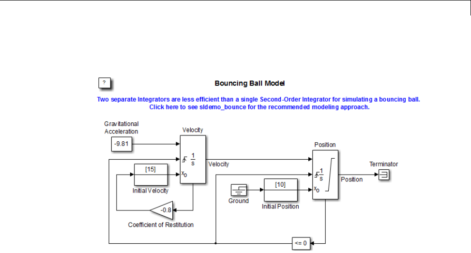
Simulating Dynamic Systems
The Bounce Model with Two Integrators.
1At the MATLAB command prompt, type sldemo_bounce_two_integrators
to load the example.
2Once the block diagram appears, set the Model Configuration
Parameters > Solver > Algorithm parameter to Nonadaptive.
3Also in the Solver pane, set the Stop time parameter to 20 s.
4Run the model. In the Simulink Editor, select Simulation > Run.
5After the simulation completes, click the Scope block window to see the
results.
You may need to click on Autoscale to view the results in their entirety.
3-25
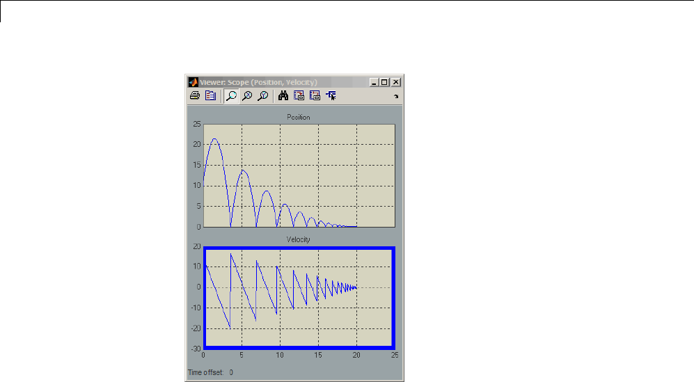
3How Simulink®Works
6Use the scope zoom controls to closely examine the last portion of the
simulation. You can see that the velocity is hovering just above zero at the
last time point.
3-26

Simulating Dynamic Systems
7Change the simulation Stop time edit box in the Simulink Editor toolbar
to 25 seconds, and run the simulation again.
8This time the simulation halts with an error shortly after it passes the
simulated20secondtimepoint.
Excessive chattering as the ball repeatedly approaches zero velocity has
caused the simulation to exceed the default limit of 1000 for the number of
consecutive zero crossings allowed. Although you can increase this limit by
adjusting the Model Configuration Parameters > Solver > Number
of consecutive zero crossings parameter. In this case, making that
change does not allow the simulation to simulate for 25 seconds.
9Also in the Solver pane, from the Algorithm pull down menu, select the
Adaptive algorithm.
10 Run the simulation again.
11 This time the simulation runs to completion because the adaptive algorithm
prevented an excessive number of zero crossings from occurring.
3-27
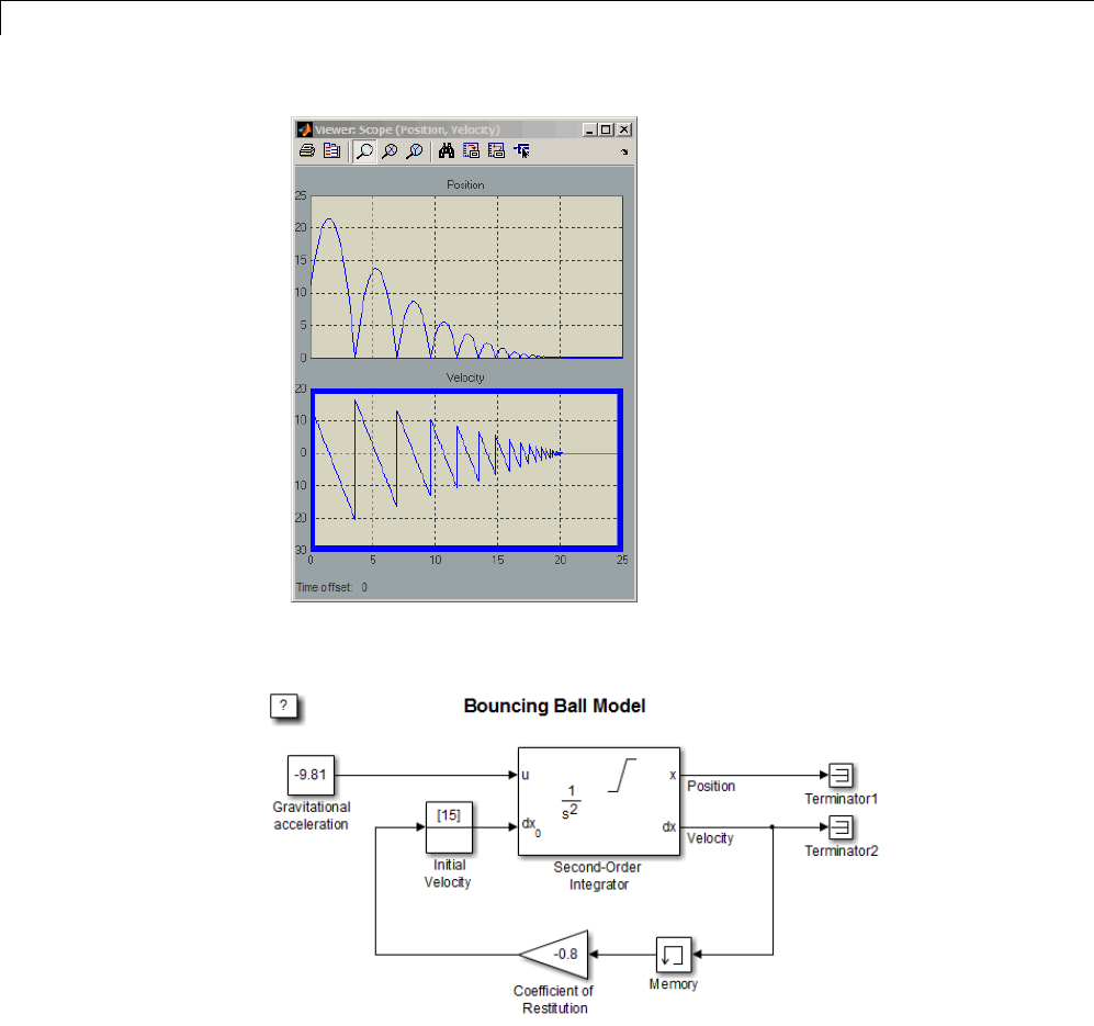
3How Simulink®Works
Bounce Model with a Second-Order Integrator.
3-28
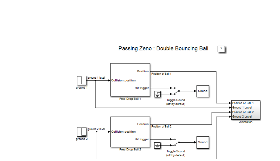
Simulating Dynamic Systems
The Double-Bounce Model.
1At the MATLAB command prompt, type sldemo_doublebounce to load the
example. The model and an animation window open. In the animation
window, two balls are resting on two platforms.
2In the animation window, click the Nonadaptive button to run the
example using the nonadaptive algorithm. This is the default setting used
by the Simulink software for all models.
3The ball on the right is given a larger initial velocity and has Consequently,
the two balls hit the ground and recoil at different times.
4The simulation halts after 14 seconds because the ball on the left exceeded
the number of zero crossings limit. The ball on the right is left hanging in
mid air.
5An error message dialog opens. Click OK to close it.
6Click on the Adaptive button to run the simulation with the adaptive
algorithm.
3-29
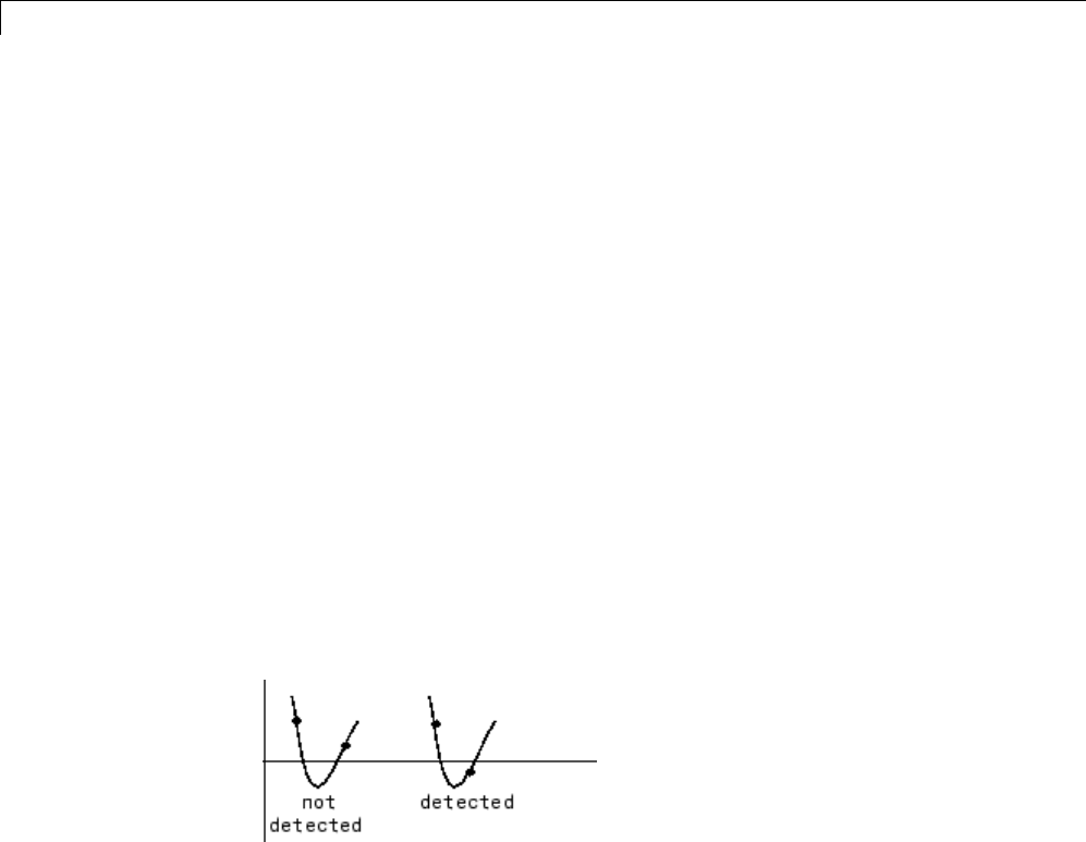
3How Simulink®Works
7Notice that this time the simulation runs to completion, even after the
ground shifts out from underneath the ball on the left at 20 seconds.
How the Simulator Can Miss Zero-Crossing Events
The bounce and double-bounce models show that high-frequency fluctuations
about a discontinuity (’chattering’) can cause a simulation to prematurely halt.
It is also possible for the solver to entirely miss zero crossings if the solver
error tolerances are too large. This is possible because the zero-crossing
detection technique checks to see if the value of a signal has changed sign
after a major time step. A sign change indicates that a zero crossing has
occurred, and the zero-crossing algorithm will then hunt for the precise
crossing time. However, if a zero crossing occurs within a time step, but the
values at the beginning and end of the step do not indicate a sign change, the
solver steps over the crossing without detecting it.
The following figure shows a signal that crosses zero. In the first instance,
the integrator steps over the event because the sign has not changed between
time steps. In the second, the solver detects change in sign and so detects
the zero-crossing event.
Preventing Excessive Zero Crossings
Use the following table to prevent excessive zero-crossing errors in your model.
3-30

Simulating Dynamic Systems
Make this
change...
How to make this
change...
Rationale for making
this change...
Increase the
number of
allowed zero
crossings
Increase the value of the
Number of consecutive
zero crossings.option
on the Solver pane in the
Configuration Parameters
dialog box.
This may give your model
enough time to resolve the
zero crossing.
Relax the
Signal
threshold
Select Adaptive from the
Algorithm pull down and
increase the value of the
Signal threshold option
on the Solver pane in the
Configuration Parameters
dialog box.
The solver requires less
time to precisely locate
the zero crossing. This
can reduce simulation
time and eliminate an
excessive number of
consecutive zero-crossing
errors. However, relaxing
the Signal threshold may
reduce accuracy.
Use the
Adaptive
Algorithm
Select Adaptive from the
Algorithm pull down on
the Solver pane in the
Configuration Parameters
dialog box.
This algorithm
dynamically adjusts the
zero-crossing threshold,
which improves accuracy
and reduces the number of
consecutive zero crossings
detected. With this
algorithm you have the
option of specifying both
the Time tolerance and
the Signal threshold.
3-31

3How Simulink®Works
Make this
change...
How to make this
change...
Rationale for making
this change...
Disable
zero-crossing
detection for a
specific block
1Clear the Enable
zero-crossing
detection check box
on the block’s parameter
dialog box.
2Select Use local
settings from
the Zero-crossing
control pull down
on the Solver pane
of the Configuration
Parameters dialog box.
Locally disabling
zero-crossing detection
prevents a specific
block from stopping the
simulation because of
excessive consecutive zero
crossings. All other blocks
continue to benefit from the
increased accuracy that
zero-crossing detection
provides.
Disable
zero-crossing
detection for the
entire model
Select Disable all
from the Zero-crossing
control pull down on
the Solver pane of the
Configuration Parameters
dialog box.
This prevents zero
crossings from being
detected anywhere in your
model. A consequence is
that your model no longer
benefits from the increased
accuracy that zero-crossing
detection provides.
If using the
ode15s solver,
consider
adjusting the
order of the
numerical
differentiation
formulas
Select a value from the
Maximum order pull down
on the Solver pane of the
Configuration Parameters
dialog box.
For more information, see
“Maximum order”.
Reduce the
maximum step
size
Enter a value for the
Max step size option on
the Solver pane of the
Configuration Parameters
dialog box.
This can insure the solver
takes steps small enough
to resolve the zero crossing.
However, reducing the
step size can increase
simulation time, and
3-32

Simulating Dynamic Systems
Make this
change...
How to make this
change...
Rationale for making
this change...
is seldom necessary
when using the Adaptive
algorithm.
Zero-Crossing Algorithms
The Simulink software includes two zero-crossing detection algorithms:
Nonadaptive and Adaptive.
To choose the algorithm, either use the Algorithm option in the Solver pane
of the Configuration Parameter dialog box, or use the ZeroCrossAlgorithm
command. The command can either be set to 'Nonadaptive' or 'Adaptive'.
The Nonadaptive algorithm is provided for backwards compatibility with
older versions of Simulink and is the default. It brackets the zero-crossing
event and uses increasingly smaller time steps to pinpoint when the zero
crossing has occurred. Although adequate for many types of simulations, the
Nonadaptive algorithm can result in very long simulation times when a high
degree of ’chattering’ (high frequency oscillation around the zero-crossing
point) is present.
The Adaptive algorithm dynamically turns the bracketing on and off, and
is a good choice when:
•The system contains a large amount of chattering.
•You wish to specify a guard band (tolerance) around which the zero crossing
is detected.
The Adaptive algorithm turns off zero-crossing bracketing (stops iterating) if
either of the following are satisfied:
•The zero crossing error is exceeded. This is determined by the value
specified in the Signal threshold option in the Solver pane of the
Configuration Parameters dialog box. This can also be set with the
ZCThreshold command. The default is Auto,butyoucanenteranyreal
number greater than zero for the tolerance.
3-33
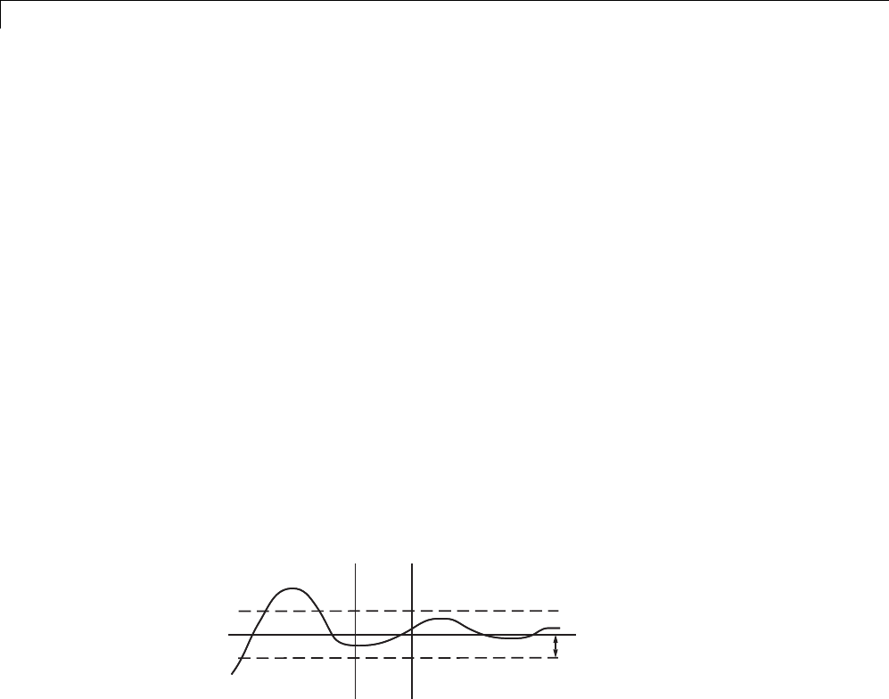
3How Simulink®Works
•The system has exceeded the number of consecutive zero crossings specified
in the Number of consecutive zero crossings option in the Solver pane
of the Configuration Parameters dialog box. Alternatively, this can be set
with the MaxConsecutiveZCs command.
Understanding Signal Threshold
The Adaptive algorithm automatically sets a tolerance for zero-crossing
detection. Alternatively, you can set the tolerance by entering a real number
greaterthanorequaltozerointheConfiguration Parameters Solver pane,
Signal threshold pull down. This option only becomes active when the
zero-crossing algorithm is set to Adaptive.
This graphic shows how the Signal threshold sets a window region around
the zero-crossing point. Signals falling within this window are considered
as being at zero.
Signal
Threshold
Tn-1 Tn
The zero-crossing event is bracketed by time steps Tn-1 and Tn.Thesolver
iteratively reduces the time steps until the state variable lies within the band
defined by the signal threshold, or until the number of consecutive zero
crossings equals or exceeds the value in the Configuration Parameters Solver
pane, Number of consecutive zero crossings pull down.
It is evident from the figure that increasing the signal threshold increases the
distance between the time steps which will be executed. This often results in
faster simulation times, but might reduce accuracy.
3-34

Simulating Dynamic Systems
How Blocks Work with Zero-Crossing Detection
A block can register a set of zero-crossing variables, each of which is a function
of a state variable that can have a discontinuity. The zero-crossing function
passes through zero from a positive or negative value when the corresponding
discontinuity occurs. The registered zero-crossing variables are updated at
the end of each simulation step, and any variable that has changed sign is
identified as having had a zero-crossing event.
If any zero crossings are detected, the Simulink software interpolates between
the previous and current values of each variable that changed sign to estimate
thetimesofthezerocrossings(thatis,thediscontinuities).
Blocks That Register Zero Crossings. The following table lists blocks that
register zero crossings and explains how the blocks use the zero crossings:
Block Description of Zero Crossing
Abs One: to detect when the input signal crosses zero in
either the rising or falling direction.
Backlash Two: one to detect when the upper threshold is engaged,
and one to detect when the lower threshold is engaged.
Compare To
Constant
One: to detect when the signal equals a constant.
Compare To Zero One: to detect when the signal equals zero.
Dead Zone Two: one to detect when the dead zone is entered (the
input signal minus the lower limit), and one to detect
when the dead zone is exited (the input signal minus
the upper limit).
Enable One: If an Enable port is inside of a Subsystem block,
it provides the capability to detect zero crossings.
See the Enable Subsystem block for details “Enabled
Subsystems” on page 7-4.
From File One: to detect when the input signal has a discontinuity
in either the rising or falling direction
From Workspace One: to detect when the input signal has a discontinuity
in either the rising or falling direction
3-35

3How Simulink®Works
Block Description of Zero Crossing
If One: to detect when the If condition is met.
Integrator If the reset port is present, to detect when a reset
occurs.
If the output is limited, there are three zero crossings:
one to detect when the upper saturation limit is
reached, one to detect when the lower saturation limit
is reached, and one to detect when saturation is left.
MinMax One: for each element of the output vector, to detect
when an input signal is the new minimum or maximum.
Relational
Operator
One: to detect when the specified relation is true.
Relay One: if the relay is off, to detect the switch-on point. If
the relay is on, to detect the switch-off point.
Saturation Two: one to detect when the upper limit is reached or
left, and one to detect when the lower limit is reached
or left.
Second-Order
Integrator
Five: two to detect when the state xupperorlower
limit is reached; two to detect when the state dx/dt
upper or lower limit is reached; and one to detect when
a state leaves saturation.
Sign One: to detect when the input crosses through zero.
Signal Builder One: to detect when the input signal has a discontinuity
in either the rising or falling direction
Step One: to detect the step time.
Switch One: to detect when the switch condition occurs.
Switch Case One: to detect when the case condition is met.
3-36

Simulating Dynamic Systems
Block Description of Zero Crossing
Trigger One: If a Triggered port is inside of a Subsystem block,
it provides the capability to detect zero crossings. See
the Triggered Subsystem block for details: “Triggered
Subsystems” on page 7-20.
Enabled and
Triggered
Subsystem
Two: one for the enable port and one for the trigger
port. See the Triggered and Enabled Subsystem block
for details: “Triggered and Enabled Subsystems” on
page 7-24
Note Zero-crossing detection is also available for a Stateflow chart that uses
continuous-time mode. See “Configuring a Stateflow Chart to Update in
Continuous Time” in the Stateflow documentation for more information.
Implementation Example: Saturation Block. An example of a Simulink
block that registers zero crossings is the Saturation block. Zero-crossing
detection identifies these state events in the Saturation block:
•The input signal reaches the upper limit.
•The input signal leaves the upper limit.
•The input signal reaches the lower limit.
•The input signal leaves the lower limit.
Simulink blocks that define their own state events are considered to have
intrinsic zero crossings. Use the Hit Crossing block to receive explicit
notification of a zero-crossing event. See “Blocks That Register Zero
Crossings” on page 3-35 for a list of blocks that incorporate zero crossings.
The detection of a state event depends on the construction of an internal
zero-crossing signal. This signal is not accessible by the block diagram. For
the Saturation block, the signal that is used to detect zero crossings for the
upper limit is zcSignal = UpperLimit -u,whereuis the input signal.
Zero-crossing signals have a direction attribute, which can have these values:
3-37

3How Simulink®Works
•rising — A zero crossing occurs when a signal rises to or through zero, or
when a signal leaves zero and becomes positive.
•falling — A zero crossing occurs when a signal falls to or through zero, or
when a signal leaves zero and becomes negative.
•either — A zero crossing occurs if either a rising or falling condition occurs.
For the Saturation block’s upper limit, the direction of the zero crossing is
either. This enables the entering and leaving saturation events to be detected
using the same zero-crossing signal.
3-38

Simulating Dynamic Systems
Algebraic Loops
•“What Is an Algebraic Loop?” on page 3-39
•“Problems Caused by Algebraic Loops” on page 3-43
•“Identifying Algebraic Loops in Your Model” on page 3-43
•“What If I Have an Algebraic Loop in My Model?” on page 3-47
•“Simulink Algebraic Loop Solver” on page 3-49
•“Removing Algebraic Loops” on page 3-51
•“Additional Techniques to Help the Algebraic Loop Solver” on page 3-53
•“Changing Block Priorities Does Not Remove Algebraic Loops” on page 3-54
•“Artificial Algebraic Loops” on page 3-54
What Is an Algebraic Loop?
•“Algebraic Loops in Simulink” on page 3-39
•“Mathematical Definition of an Algebraic Loop” on page 3-41
•“Meaning of Algebraic Loops in Physical Systems” on page 3-42
Algebraic Loops in Simulink. An algebraic loop in a Simulink model occurs
when a signal loop exists with only direct feedthrough blocks within the loop.
Direct feedthrough means that the block output depends on the value of an
input port; the value of the input directly controls the value of the output.
Non-direct-feedthrough blocks maintain a State variable. Two examples are
the Integrator or Unit Delay block.
Some Simulink blocks have input ports with direct feedthrough. The software
cannot compute the output of these blocks without knowing the values of the
signals entering the blocks at these input ports at the current time step.
Some examples of blocks with direct feedthrough inputs are:
•Math Function block
•Gain block
3-39
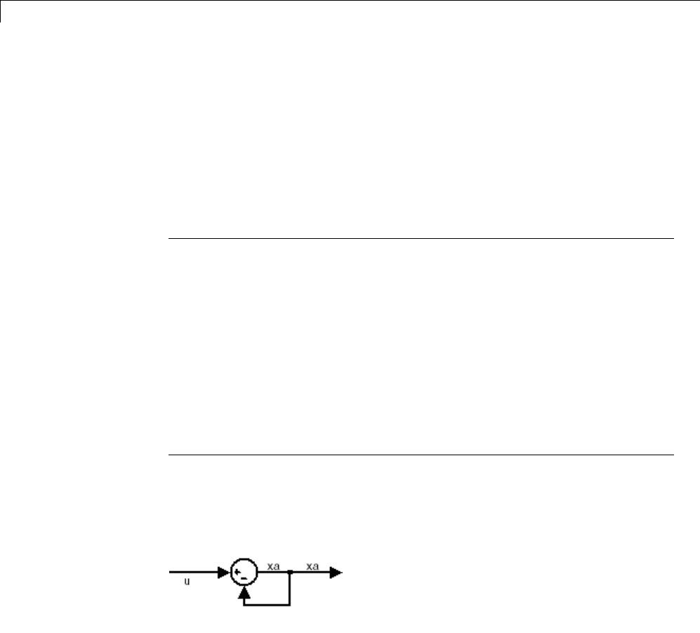
3How Simulink®Works
•Product block
•State-Space block, when the D matrix coefficient is nonzero
•Sum block
•Transfer Fcn block, when the numerator and denominator are of the same
order
•Zero-Pole block, when the block has as many zeros as poles
Tip To determine if a block has direct feedthrough:
1Double-click the block.
The block parameter dialog box opens.
2Click the Help button in the block parameter dialog box.
The block reference page opens.
3Scroll to the Characteristics section of the block reference page, which
lists whether or not that block has direct feedthrough.
An example of an algebraic loop is the following simple loop. Note that this is
not a recommended modeling pattern.
Mathematically, this loop implies that the output of the Sum block is an
algebraic variable xathat is constrained to equal the first input uminus xa
(forexample,xa=u–xa). The solution of this simple loop is xa=u/2.
3-40

Simulating Dynamic Systems
Mathematical Definition of an Algebraic Loop. Simulink contains a
suite of numerical solvers for simulating ordinary differential equations
(ODEs), which are systems of equations that you can write as:
xfxt=(,),
xis the state vector and tis the independent time variable.
Some systems of equations contain additional constraints that involve the
independent variable and the state vector, but not the derivative of the state
vector. Such systems are differential algebraic equations (DAEs),notODEs.
The term algebraic refers to equations that do not involve any derivatives.
You can express DAEs that arise in engineering in a semi-explicit form:
xfxx
gxx
a
a
=
=
(, ,)
(, ,),
t
t0
•fand gcan be vector functions.
•The first equation is the differential equation.
•The second equation is the algebraic equation.
•The vector of differential variables is x.
•The vector of algebraic variables is xa.
In Simulink models, algebraic loops are algebraic constraints. Models with
algebraic loops define a system of differential algebraic equations. Simulink
does not solve DAEs directly. Simulink solves the algebraic equations (the
algebraic loop) numerically for xaat each step of the ODE solver.
The following Simulink model is equivalent to this system of equations in
semi-explicit form:
xfxxt x
gxx t x u x
aa
aa
==
==−+−
(, ,)
(, ,) .02
3-41
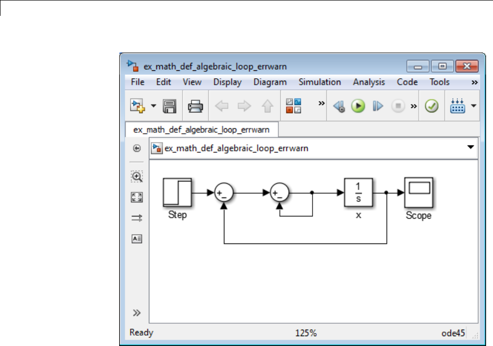
3How Simulink®Works
At each step of the ODE solver, the algebraic loop solver must solve the
algebraic constraint for xabefore calculating the derivative
x.
Meaning of Algebraic Loops in Physical Systems. Algebraic constraints
can occur when modeling physical systems,oftenduetoconservation
laws,suchasconservationofmassandenergy. Youcanalsousealgebraic
constraints to impose design constraints on system responses in a dynamic
system.
Choosing a particular coordinate system for a model can also result in an
algebraic constraint. In most cases, you can eliminate algebraic loops,
as described in “Removing Algebraic Loops” on page 3-51, to produce an
ordinary differential equation (ODE). However, this technique may be too
time consuming if you have a large, complex model.
3-42

Simulating Dynamic Systems
MathWorks®offers the Simscape™ software that extends Simulink by
providing tools to model systems that span mechanical, electrical, hydraulic,
and other physical domains as physical networks.
Simscape software automatically constructs the differential algebraic
equations (DAEs) that characterize the behavior of a Simulink model. These
equations are integrated with the rest of the model, and the Simscape
software solves the DAEs directly. The variables for the components in the
different physical domains are solved simultaneously, thereby avoiding
problems with algebraic loops.
Problems Caused by Algebraic Loops
If your model contains an algebraic loop:
•You cannot generate code for the model.
•The Simulink algebraic loop solver might not be able to solve the algebraic
loop.
•While Simulink is trying to solve the algebraic loop, the simulation might
execute slowly.
For most models, the algebraic loop solver is computationally expensive for
the first time step. Simulink solves subsequent time steps rapidly because
a good starting point for xais available from the previous time step.
Identifying Algebraic Loops in Your Model
•“Algebraic Loop Diagnostic” on page 3-43
•“Highlighting Algebraic Loops Using the Algebraic Loop Diagnostic” on
page 3-44
•“Highlighting Algebraic Loops Using the ashow Debugger Command” on
page 3-45
Algebraic Loop Diagnostic. Simulink detects algebraic loops during
simulation initialization, for example, when you update your diagram. You
can set the Algebraic loop diagnostic to report an error or warning if the
software detects any algebraic loops in your model.
3-43

3How Simulink®Works
In the Configuration Parameters dialog box, on the main Diagnostics pane,
set the Algebraic loop parameter as follows.
Setting Simulation Response
none Simulink tries to solve the algebraic loop;
reports an error only if the algebraic loop
cannot be solved.
warning Algebraic loops result in warnings. Simulink
tries to solve the algebraic loop; reports an error
only if the algebraic loop cannot be solved.
error Algebraic loops stop the initialization.
If you want Simulink to try to solve the loop, select none or warning.Ifyou
want to review the loop before Simulink tries to solve the loop, select error.
Highlighting Algebraic Loops Using the Algebraic Loop Diagnostic. To
highlight algebraic loops in the Simulink Editor when updating or simulating
a model:
1Open the sldemo_hydcyl model:
sldemo_hydcyl
2Open the Configuration Parameters dialog box by selecting
Simulation > Model Configuration Parameters.
3On the Diagnostics pane, set the Algebraic loop parameter to error.
If the Simulink software finds an algebraic loop in the model, it should stop
the simulation and report an error.
4Click OK to save the setting.
5Click the Start simulation button.
When Simulink detects an algebraic loop during initialization, the
simulation stops. The Diagnostics Viewer displays an error message and
lists all the blocks in the model that are part of that algebraic loop.
3-44
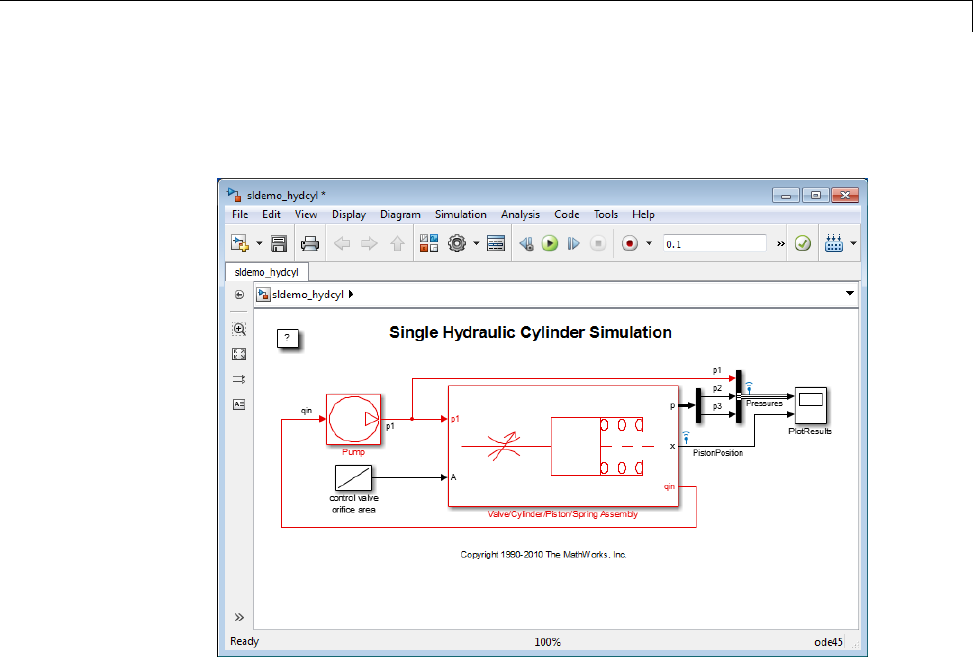
Simulating Dynamic Systems
In the Simulink Editor, the software highlights the blocks and signals that
constitute the loop in red.
6To restore the diagram to its original colors, close the Diagnostics Viewer.
7Close the sldemo_hydcyl model without saving the changes.
In the next section, the ashow debugger command shows that this model
actually has two algebraic loops.
Highlighting Algebraic Loops Using the ashow Debugger Command.
The Simulink debugger allows you to step through a model simulation. To use
the ashow command to highlight algebraic loops:
1Open the sldemo_hydcyl model.
By default, the Algebraic loop parameter for this model is set to none.
3-45

3How Simulink®Works
2Start the Simulink debugger. In the Simulink Editor, select Simulation >
Debug > Debug Model.
3Click the Start/Continue button to start the debugger.
4In the MATLAB Command Window, type:
ashow
The software lists the two algebraic loops in the sldemo_hydcyl model and
the number of blocks in each algebraic loop.
Found 2 Algebraic loop(s):
System number#Algebraic loop id, number of blocks in loop
- 0#1, 9 blocks in loop
- 0#2, 4 blocks in loop
5To list the blocks in the first algebraic loop, in the MATLAB Command
Window, enter the following command:
ashow 0#1
The software opens the Control Valve Flow subsystem in the
Valve/Cylinder/Piston/Spring Assembly subsystem, highlights that
algebraic loop in the model, and lists the nine blocks in the algebraic loop:
- sldemo_hydcyl/Valve//Cylinder//Piston//Spring Assembly/Control Valve Flow/IC
- sldemo_hydcyl/Valve//Cylinder//Piston//Spring Assembly/Control Valve Flow/signed sqrt
- sldemo_hydcyl/Valve//Cylinder//Piston//Spring Assembly/Control Valve Flow/Product
- sldemo_hydcyl/Valve//Cylinder//Piston//Spring Assembly/laminar flow pressure drop
- sldemo_hydcyl/Valve//Cylinder//Piston//Spring Assembly/Sum7
- sldemo_hydcyl/Pump/IC
- sldemo_hydcyl/Valve//Cylinder//Piston//Spring Assembly/Control Valve Flow/Sum1 (algebraic v
- sldemo_hydcyl/Pump/Sum1
- sldemo_hydcyl/Pump/leakage (algebraic variable)
6In the Simulink debugger, click Close.
7At the MATLAB command prompt, press Enter to restore the default
MATLAB command prompt.
3-46

Simulating Dynamic Systems
What If I Have an Algebraic Loop in My Model?
If Simulink reports an algebraic loop in your model, the algebraic loop solver
might be able to solve the loop. If Simulink cannot solve the loop, there are
several techniques to eliminate the loop.
The following workflow helps you evaluate what techniques to try to eliminate
an algebraic loop. Some of those techniques are described in the following
sections.
3-47
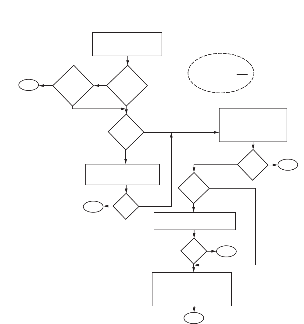
3How Simulink®Works
Yes
Simulink detects
an algebraic loop
Can
Simulink
solve the
algebraic
loop?
Is the
solution
correct
and
efficient?
Done
No
Yes
Yes
Yes
No
No
Modify model
(may have side effects)
Modify
model or
adjust model
settings?
Adjust
model
settings
Change algorithm
(TrustRegion / LineSearch)
Change solver parameters
*
*
Loop
solved? Done
Is
there a
DAE?
Algebraic constraint does not exist.
Add delays
Add real dynamics (e.g., sensor)
Convert to Simscape model (if
physical system)
Eliminate nonzero matrix
If you are generating code
for your model, you must
eliminate the
algebraic loop.
Use IC block
Convert atomic subsystem
to virtual
Enable Minimize algebraic
loop occurrences
Restructure model
*
*
*
*
Algebraic constraint exists. Convert
DAE to ODE by restructuring
underlying equations
No
Loop
solved? Done
*
*
*
*
Yes Loop
solved?
Done
No
Done
No
Yes
3-48
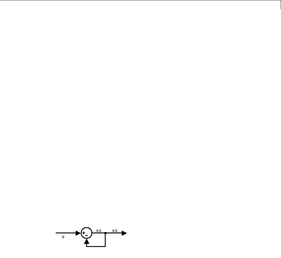
Simulating Dynamic Systems
Simulink Algebraic Loop Solver
•“How the Algebraic Loop Solver Works” on page 3-49
•“Trust-Region and Line-Search Algorithms in the Algebraic Loop Solver”
on page 3-50
•“Limitations of the Algebraic Loop Solver” on page 3-50
How the Algebraic Loop Solver Works. When a model contains an
algebraic loop, the Simulink software uses a nonlinear solver at each time
step to solve the algebraic loop. The solver performs iterations to determine
thesolutiontothealgebraicconstraint (if possible). As a result, models with
algebraic loops can run more slowly than models without algebraic loops.
The algebraic loop solver requires:
•One block where the loop solver can break the loop and attempt to solve
the loop
•Real double signals
•The underlying algebraic constraint must be a smooth function
For example, suppose your model has a Sum block with two inputs—one
additive, the other subtractive. If you feed the output of the Sum block to one
of the inputs, you create an algebraic loop where all of the blocks include
direct feedthrough.
The Sum block cannot compute the output without knowing the input.
Simulink detects the algebraic loop, and the algebraic loop solver solves the
loop using an iterative loop. In the Sum block example, the software computes
the correct result as follows:
xa(t)=u(t)/2.
3-49

3How Simulink®Works
The algebraic loop solver uses a gradient-based search method, which requires
continuous first derivatives of the algebraic constraint that correspond to
the algebraic loop. As a result, if the algebraic loop contains discontinuities,
the algebraic loop solver might fail.
Trust-Region and Line-Search Algorithms in the Algebraic Loop
Solver. The Simulink algebraic loop solver uses one of two algorithms to
solve algebraic loops: trust region and line search. By default, the algebraic
loop solver uses the trust-region algorithm.
If the algebraic loop solver cannot solve the algebraic loop with the trust-region
algorithm, try simulating the model using the line-search algorithm.
To switch to the line-search algorithm, at the MATLAB command line, enter:
set_param(model_name, 'AlgebraicLoopSolver', 'LineSearch');
To switch back to the trust-region algorithm, at the MATLAB command line,
enter:
set_param(model_name, 'AlgebraicLoopSolver', 'TrustRegion');
For more information, see:
•“Trust-Region Methods for Nonlinear Minimization” in the Optimization
Toolbox™ documentation.
•“Line Search” in the Optimization Toolbox documentation.
Limitations of the Algebraic Loop Solver. Algebraic loop solving is an
iterative process. The Simulink algebraic loop solver is successful only if the
algebraic loop converges to a definite answer. When the loop fails to converge,
or converges too slowly, the simulation exits with an error.
The algebraic loop solver cannot solve algebraic loops that contain any of
the following:
•Blocks with discrete-valued outputs
•Blocks with nondouble or complex outputs
•Discontinuities
3-50
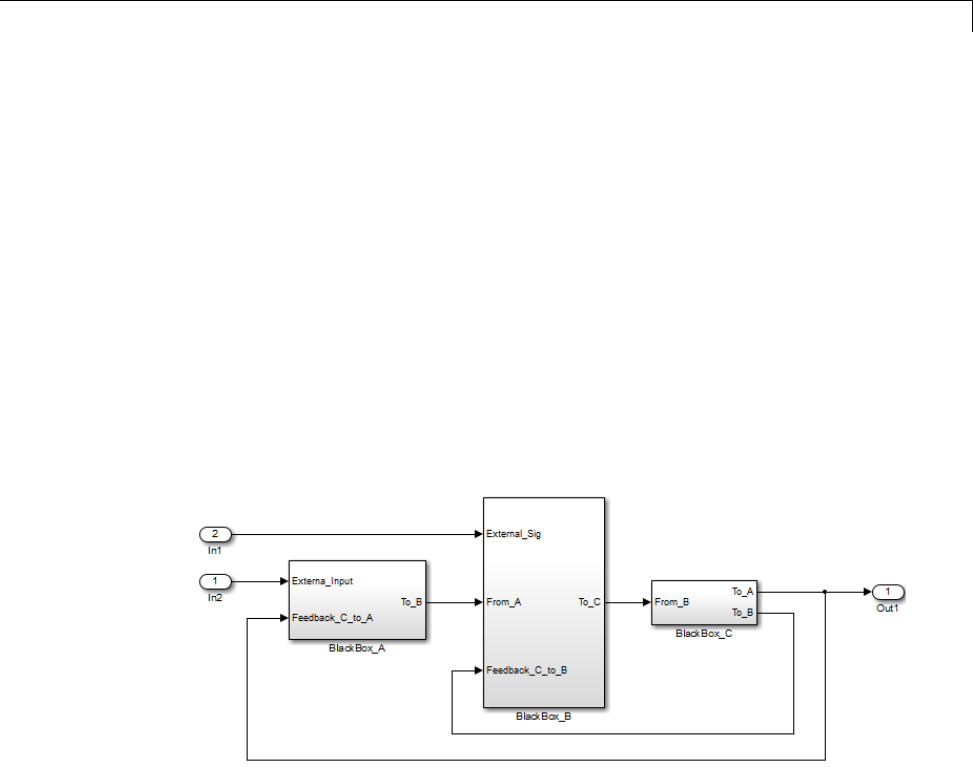
Simulating Dynamic Systems
•Stateflow charts
Removing Algebraic Loops
Introducing a Delay.
Algebraic loops can occur in large models when atomic subsystems create
feedback loops.
In the following generic model, there are two algebraic loops that involve
subsystems.
•BlackBox_A —> BlackBox_B —> BlackBox_C —> BlackBox_A
•BlackBox_B —> BlackBox_C —> BlackBox_B
When you update this model, Simulink detects the loop BlackBox_A —>
BlackBox_B —> BlackBox_C —> BlackBox_A.
Since you do not know the contents of these subsystems, you must break the
loops by adding a Unit Delay block outside the subsystems. There are three
ways to use the Unit Delay to break these loops:
•Add a unit delay between BlackBox_A and BlackBox_C
•Add a unit delay between BlackBox_B and BlackBox_C
•Add unit delays to both algebraic loops
3-51
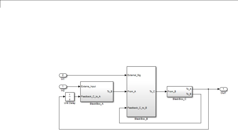
3How Simulink®Works
Add a unit delay between BlackBox_A and BlackBox_C
If you add a unit delay on the feedback signal between the subsystems
BlackBox_A and BlackBox_C, you introduce the minimum number of unit
delays (1) to the system. By introducing the delay before BlackBox_A,
BlackBox_B and BlackBox_C use data from the current time step.
Add a unit delay between BlackBox_B and BlackBox_C
If you add a unit delay between the subsystems BlackBox_B and BlackBox_C,
you break the algebraic loop between BlackBox_B and BlackBox_C. In
addition, you break the loop between BlackBox_A and BlackBox_C, because
that signal completes the algebraic loop. By inserting the Unit Delay block
before BlackBox_C, BlackBox_C now works with data from the previous time
step only.
3-52
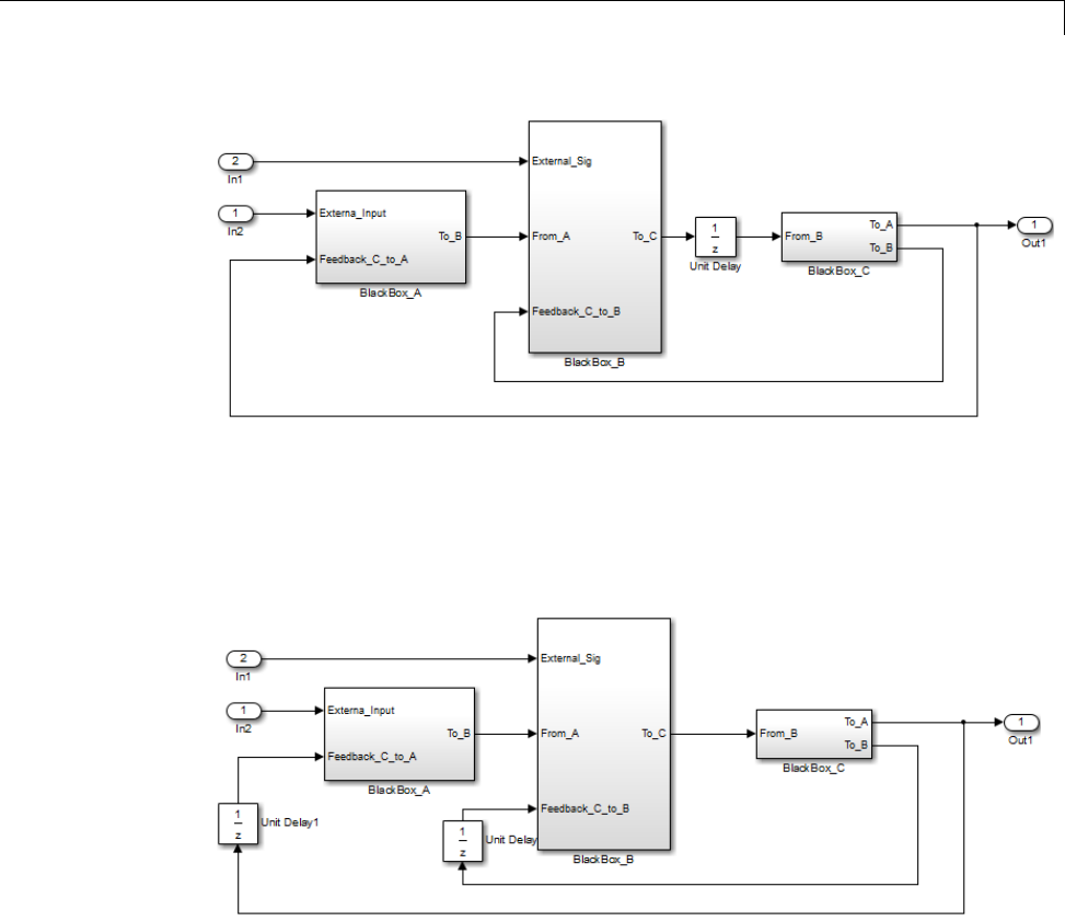
Simulating Dynamic Systems
Add unit delays to both algebraic loops
In the following example, you insert Unit Delay blocks to break both algebraic
loops. In this model, BlackBox_A and BlackBox_B use data from the previous
time step. BlackBox_C uses data from the current time step.
Additional Techniques to Help the Algebraic Loop Solver
If the Simulink software cannot solve the algebraic loop, the software reports
an error. If the Simulink algebraic loop solver cannot solve the algebraic loop,
use one of the following techniques to solve the loop manually:
3-53

3How Simulink®Works
•Restructure the underlying DAEs using techniques such as differentiation
or change of coordinates. These techniques put the DAEs in a form that is
easier for the algebraic loop solver to solve.
•Convert the DAEs to ODEs, which eliminates any algebraic loops.
•“Create Initial Guesses Using the IC and Algebraic Constraint Blocks”
on page 3-54
Create Initial Guesses Using the IC and Algebraic Constraint Blocks.
Your model might contain loops for which the loop solver cannot converge
without a good, initial guess for the algebraic states. You can specify an initial
guess for the algebraic state variables, but use this technique only when you
think the loop is legitimate.
Therearetwowaystospecifyaninitialguess:
•Place an IC block in the algebraic loop.
•Specify an initial guess for a signal in an algebraic loop using an Algebraic
Constraint block.
Changing Block Priorities Does Not Remove Algebraic Loops
During the updating phase of simulation, Simulink determines the order in
which to execute the block methods during simulation. This block invocation
ordering is the sorted order.
If you assign priorities to nonvirtual blocks to indicate to Simulink their
execution order relative to other blocks, the algebraic loop solver does not
honor these priorities when attempting to solve any algebraic loops.
Artificial Algebraic Loops
•“What Is an Artificial Algebraic Loop?” on page 3-55
•“Eliminating Artificial Algebraic Loops Caused by Atomic Subsystems”
on page 3-57
•“Bundled Signals That Create Artificial Algebraic Loops” on page 3-57
•“Model and Block Parameters for Diagnosing and Eliminating Artificial
Algebraic Loops” on page 3-62
3-54
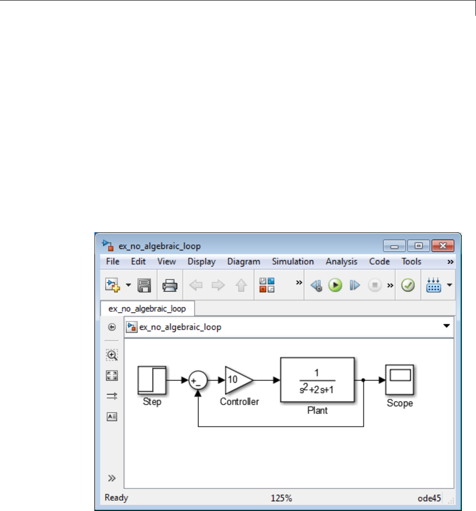
Simulating Dynamic Systems
•“Block Reduction and Artificial Algebraic Loops” on page 3-63
•“How Simulink Eliminates Artificial Algebraic Loops” on page 3-68
•“When Simulink Cannot Eliminate Artificial Algebraic Loops” on page 3-75
•“Managing Large Models with Artificial Algebraic Loops” on page 3-77
What Is an Artificial Algebraic Loop?. An artificial algebraic loop occurs
when an atomic subsystem or Model block causes Simulink to detect an
algebraic loop, even though the contents of the subsystem do not contain an
algebraic constraint. When you create an atomic subsystem, all Inport blocks
are direct feedthrough, resulting in an algebraic loop.
The following model does not contain an algebraic loop. The model simulates
without error.
3-55
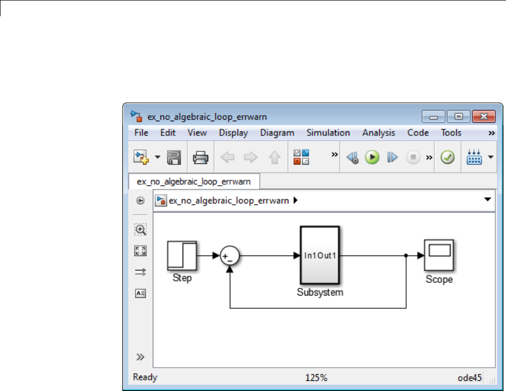
3How Simulink®Works
Suppose you enclose the Controller and Plant blocks in a subsystem and, in
the Subsystem Parameters dialog box, select Treat as atomic unit to make
the subsystem atomic.
When simulating this model, Simulink detects an algebraic loop because the
subsystem is direct feedthrough, even though the path within the atomic
subsystem is not direct feedthrough.
In the Configuration Parameters dialog box, on the main Diagnostics pane,
if you set the Algebraic loop parameter to error, Simulink stops the
simulation with an algebraic loop error.
3-56

Simulating Dynamic Systems
Eliminating Artificial Algebraic Loops Caused by Atomic Subsystems.
One way to eliminate an artificial algebraic loop caused by an atomic
subsystem is to convert the atomic subsystem to a virtual subsystem. Doing
so has no effect on the behavior of the model.
When the subsystem is atomic and you simulate the model, Simulink invokes
the algebraic loop solver. The algebraic loop solver terminates after one
iteration. The algebraic loop is automatically solved because there is no
algebraic constant. After you make the subsystem virtual, during simulation,
Simulink does not invoke the algebraic loop solver.
To convert an atomic subsystem to a virtual subsystem:
1Open the model that contains the atomic subsystem.
2Right-click the atomic subsystem and select Subsystem Parameters.
3Clear the Treat as atomic unit parameter.
4Click OK to save the changes and close the dialog box.
5Save the model.
If you replace the atomic subsystem with a virtual subsystem and the
simulation still fails with an algebraic loop error, you probably have one of the
following elsewhere in your model:
•An algebraic constraint
•An artificial algebraic loop not caused by this atomic subsystem
Examine your model, try to identify the location of the algebraic loop, and use
some of the techniques described in this section to solve the loop.
Bundled Signals That Create Artificial Algebraic Loops. Some models
bundle signals together. This bundling might cause Simulink to detect
an algebraic loop, even when an algebraic constraint does not exist. If you
redirect one or more signals, you might remove the artificial algebraic loop.
The following linearized model simulates the dynamics of a two-tank system
fed by a single pump. In this model:
3-57
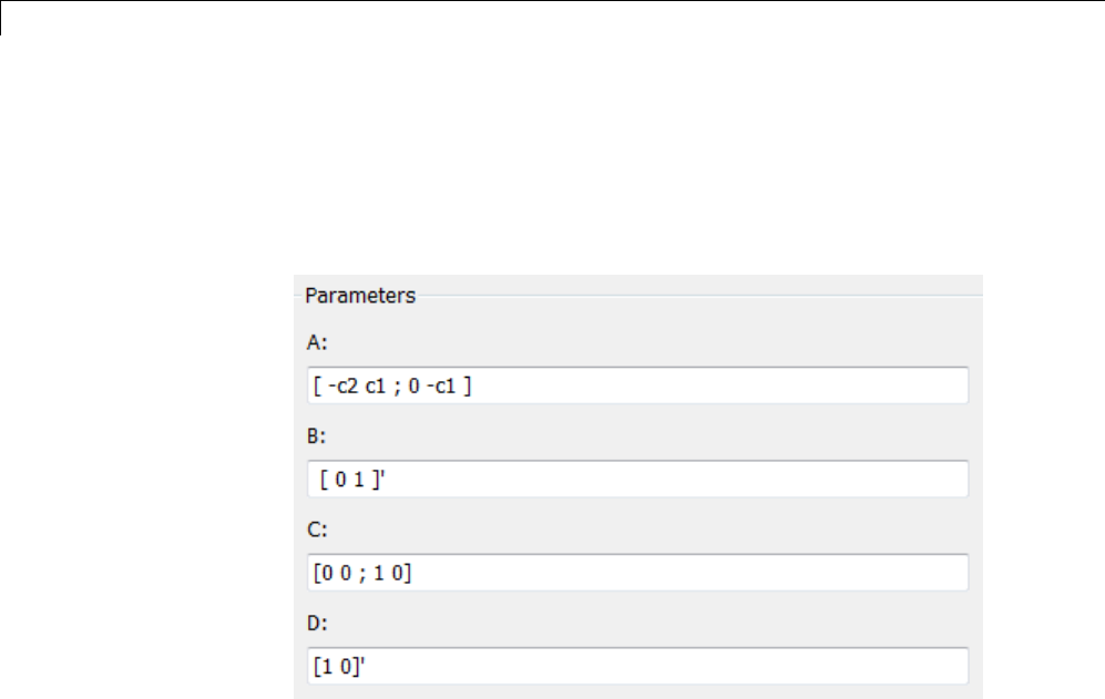
3How Simulink®Works
•Output q1 is the rate of the fluid flow into the tank from the pump.
•Output h2 is the height of the fluid in the second tank.
•The State-Space block defines the dynamic response of the tank system to
the pump operation:
•The output from the State-Space block is a vector that contains q1 and h2.
3-58
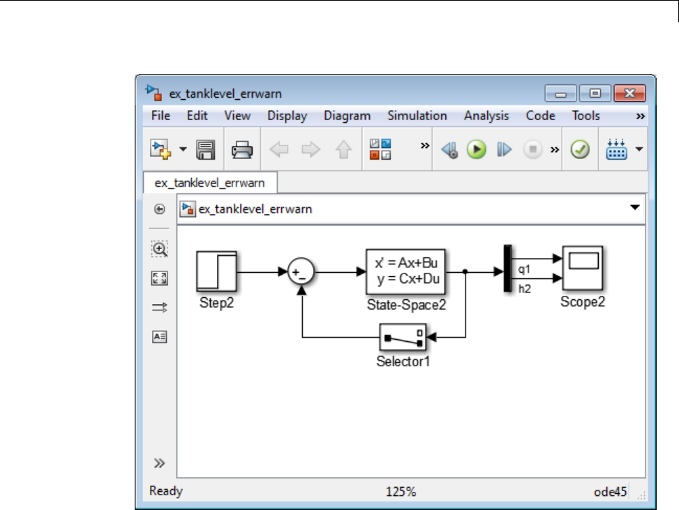
Simulating Dynamic Systems
If you simulate this model with the Algebraic loop parameter set to warn
or error, Simulink identifies the algebraic loop.
3-59
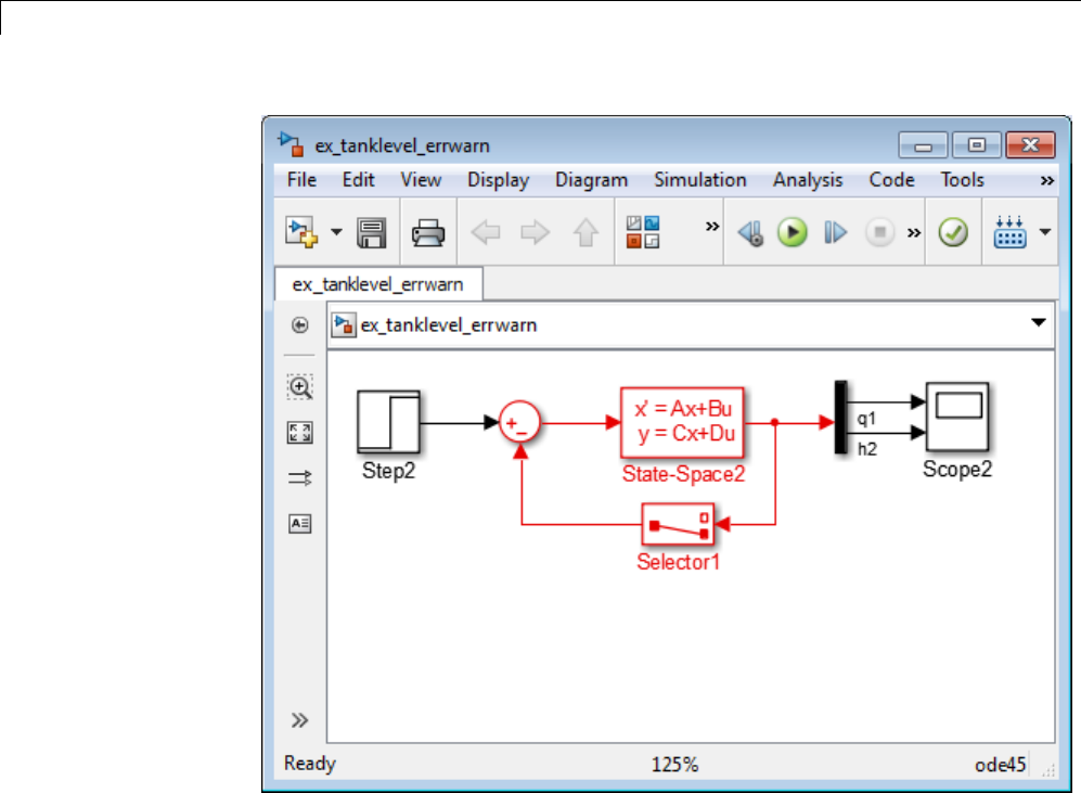
3How Simulink®Works
To eliminate this algebraic loop:
1Change the Cand Dmatrices as follows:
3-60
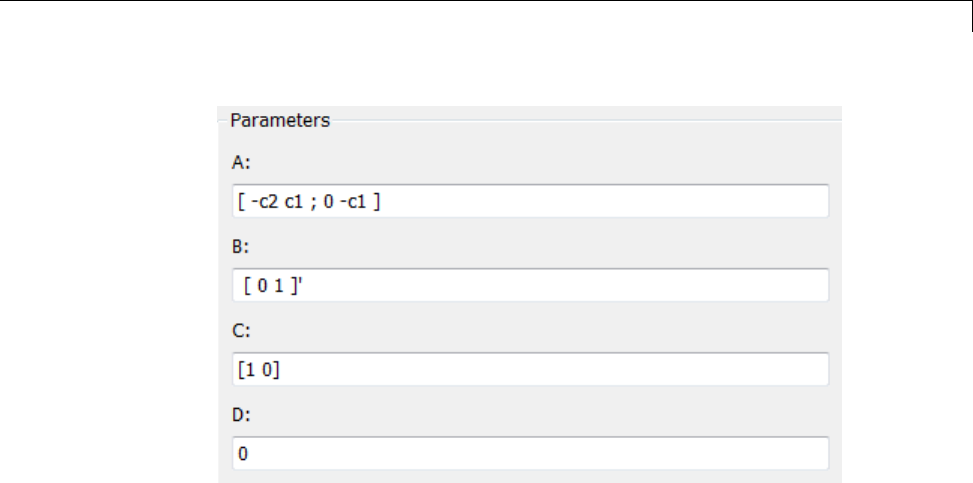
Simulating Dynamic Systems
2Pass q1 directly to the Scope instead of through the State-Space block.
Now, the input (q1) does not pass directly to the output (the Dmatrix
is 0), so the State-Space block no longer has direct feedthrough. The
feedback signal has only one element now, so the Selector block is no longer
necessary, as you can see in the following model.
3-61
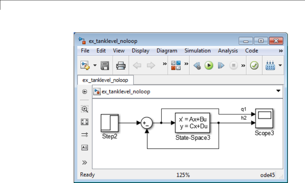
3How Simulink®Works
Model and Block Parameters for Diagnosing and Eliminating
Artificial Algebraic Loops. There are two parameters to consider when you
think that your model has an artificial algebraic loop:
•Minimize algebraic loop occurrences parameter — Specify that
Simulink try to eliminate any artificial algebraic loops for:
-Atomic subsystems — In the Subsystem Parameters dialog box, select
Minimize algebraic loop occurrences.
-Model blocks — For the referenced model, in the Configuration
Parameters dialog box, on the Model Referencing pane, select
Minimize algebraic loop occurrences
•Minimize algebraic loop parameter — If the Minimize algebraic loop
occurrences parameter has no effect, specifies what diagnostic action
Simulink takes.
3-62

Simulating Dynamic Systems
The Minimize algebraic loop parameter is in the Configuration
Parameters dialog box, on the main Diagnostics pane. The diagnostic
actions for this parameter are:
Setting Simulation Response
none Simulink takes no action.
warning Simulink displays a warning that the
Minimize algebraic loop occurrences
parameter has no effect.
error Simulink terminates the simulation and
displays an error that the Minimize
algebraic loop occurrences parameter has
no effect.
Block Reduction and Artificial Algebraic Loops. When you enable the
Block reduction optimization in the Configuration Parameters dialog box,
Simulink collapses certain groups of blocks into a single, more efficient block,
or removes them entirely. Enabling block reduction results in faster execution
during model simulation and in generated code.
Enabling block reduction may also help Simulink solve artificial algebraic
loops.
Consider the following example model.
3-63
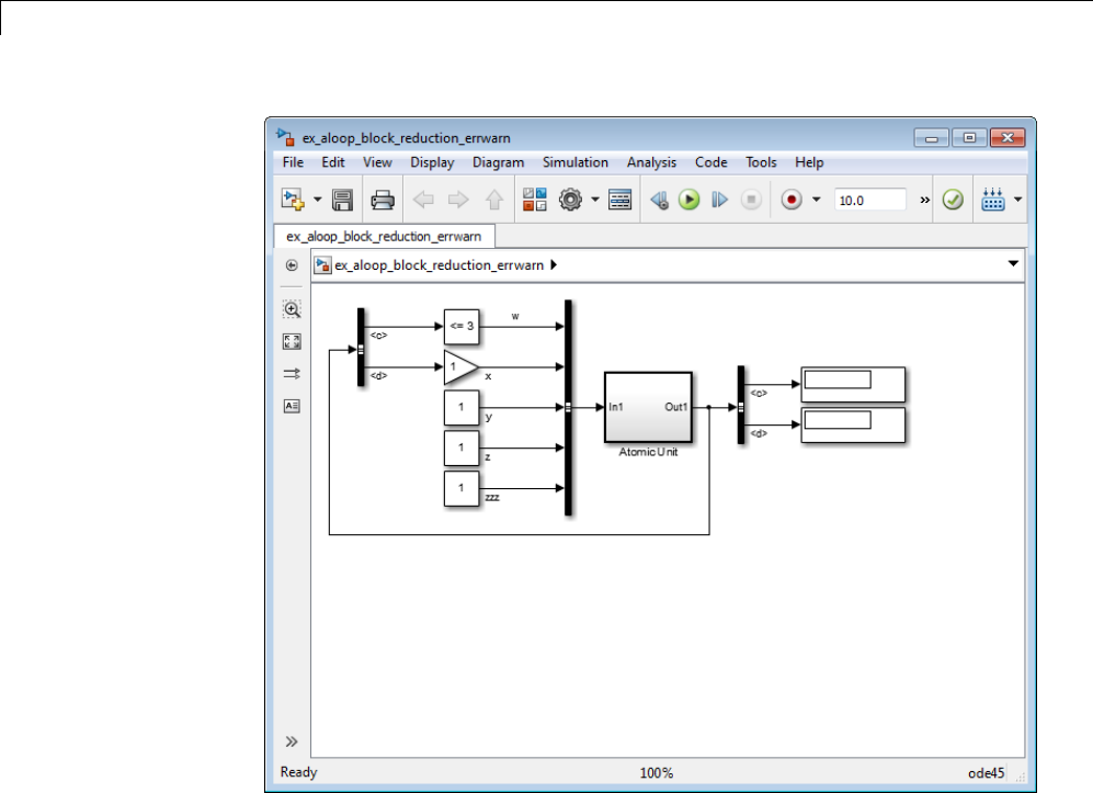
3How Simulink®Works
3-64
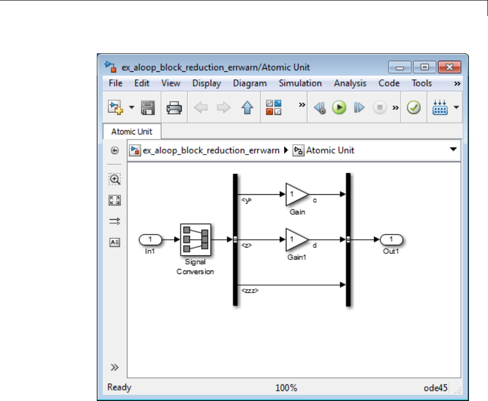
Simulating Dynamic Systems
Initially, block reduction is turned off. When you simulate this model, the
Atomic Unit subsystem and Gain and Compare to Constant blocks are part
of an algebraic loop that Simulink cannot solve.
3-65
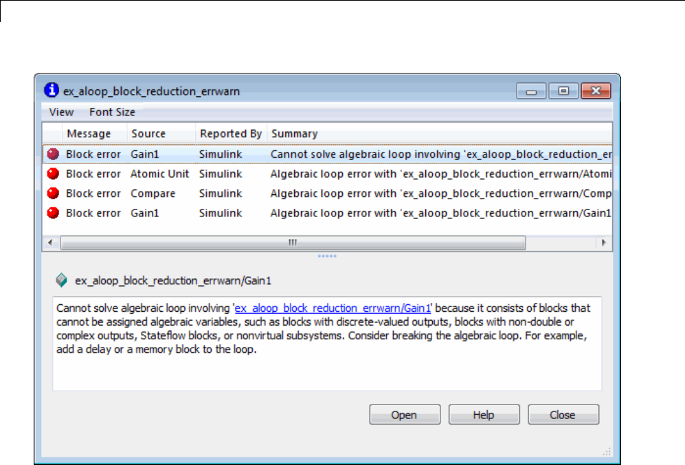
3How Simulink®Works
If you enable block reduction and sorted order, and resimulate the model,
Simulink does not display the sorted order for blocks that have been reduced.
You can now quickly see which blocks have been reduced.
3-66
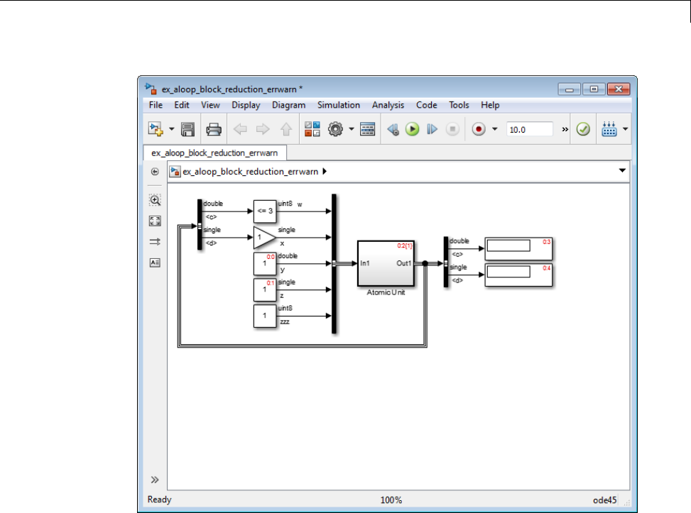
Simulating Dynamic Systems
The Compare to Constant and Gain blocks have been eliminated from the
model, so they no longer generate an algebraic loop error. The Atomic Unit
subsystem generates a warning:
Warning: If the inport 'ex_aloop_block_reduction_errwarn/
Atomic Unit/In1' of subsystem 'ex_aloop_block_reduction_errwarn/
Atomic Unit' involves direct feedback, then an algebraic loop
exists, which Simulink cannot remove. Consider clearing the
'Minimize algebraic loop occurrences' parameter to avoid this
warning.
3-67
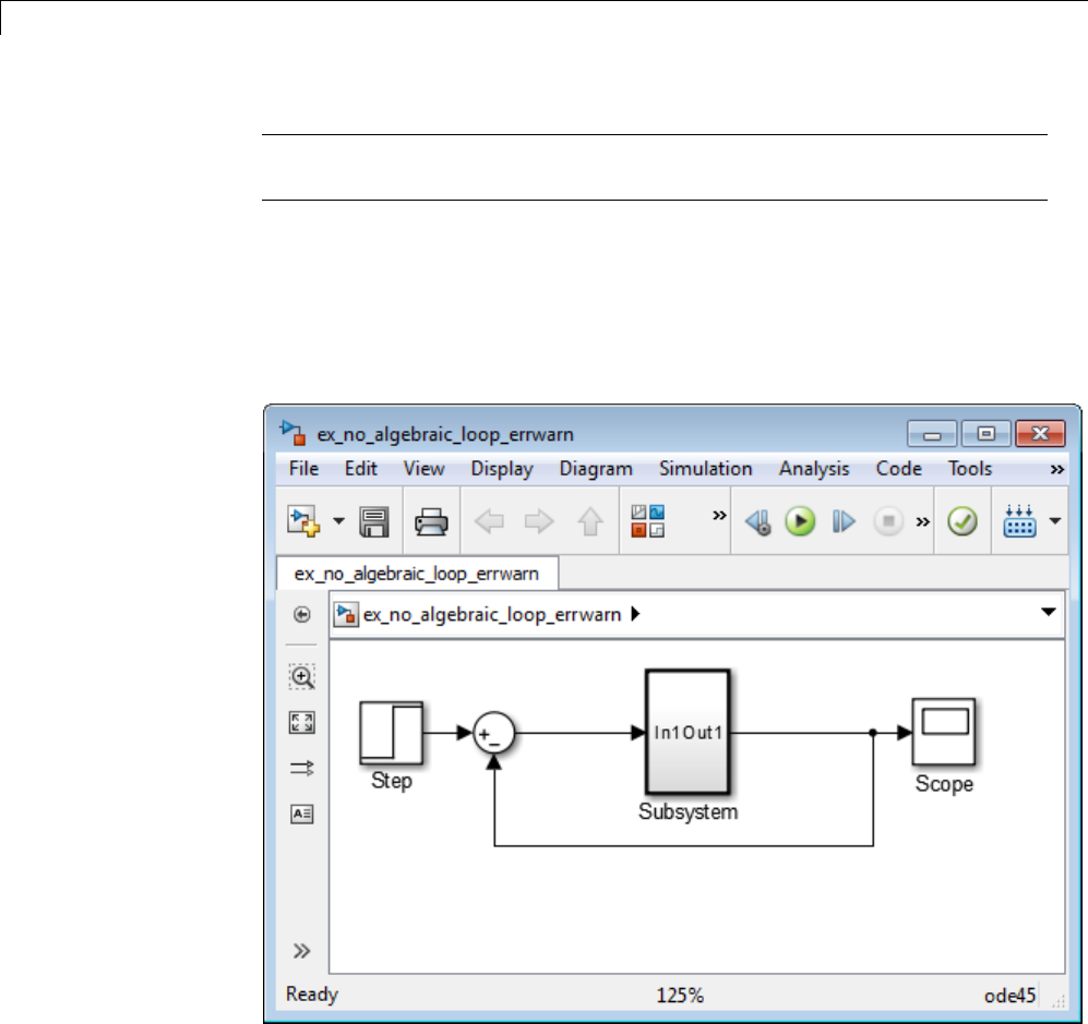
3How Simulink®Works
Tip Use Bus Selector blocks to pass only the required signals into atomic
subsystems.
How Simulink Eliminates Artificial Algebraic Loops. When you enable
Minimize algebraic loop occurrences, Simulink tries to eliminate
artificial algebraic loops. This section describes this process, using this model,
which from contains an atomic subsystem that causes an artificial algebraic
loop.
The contents of the atomic subsystem are not direct feedthrough, but
Simulink identifies the atomic subsystem as direct feedthrough.
3-68
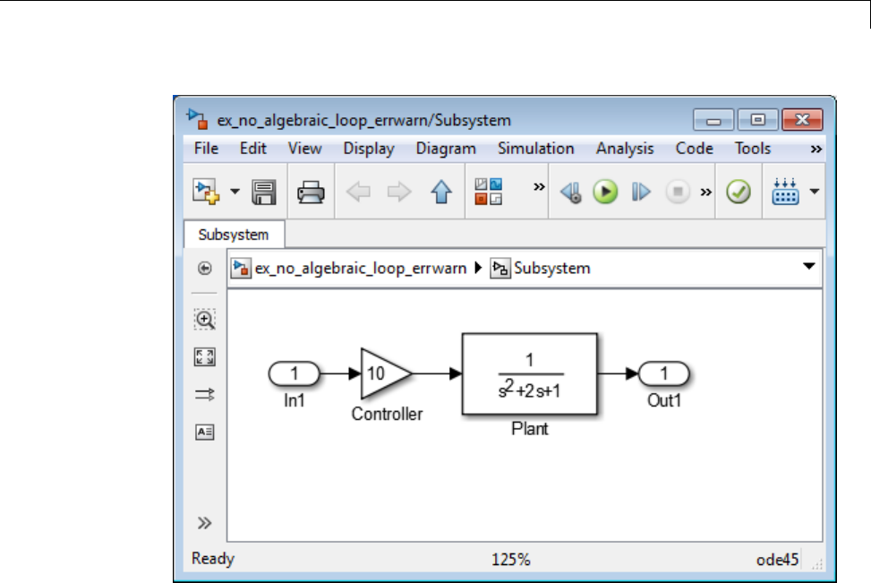
Simulating Dynamic Systems
If the Algebraic loop diagnostic is set to error, simulating the model results
in an error because the model contains an artificial algebraic loop involving
its atomic subsystem.
ToseehowSimulinktriestoeliminatethis algebraic loop, follow these steps:
1Create the model from the preceding graphics, with the atomic subsystem
that causes the artificial algebraic loop.
2Select Simulation > Model Configuration Parameters.
3In the Configuration Parameters dialog box, on the main Diagnostics
pane,settheAlgebraic loop parameter to warning or none.
3-69
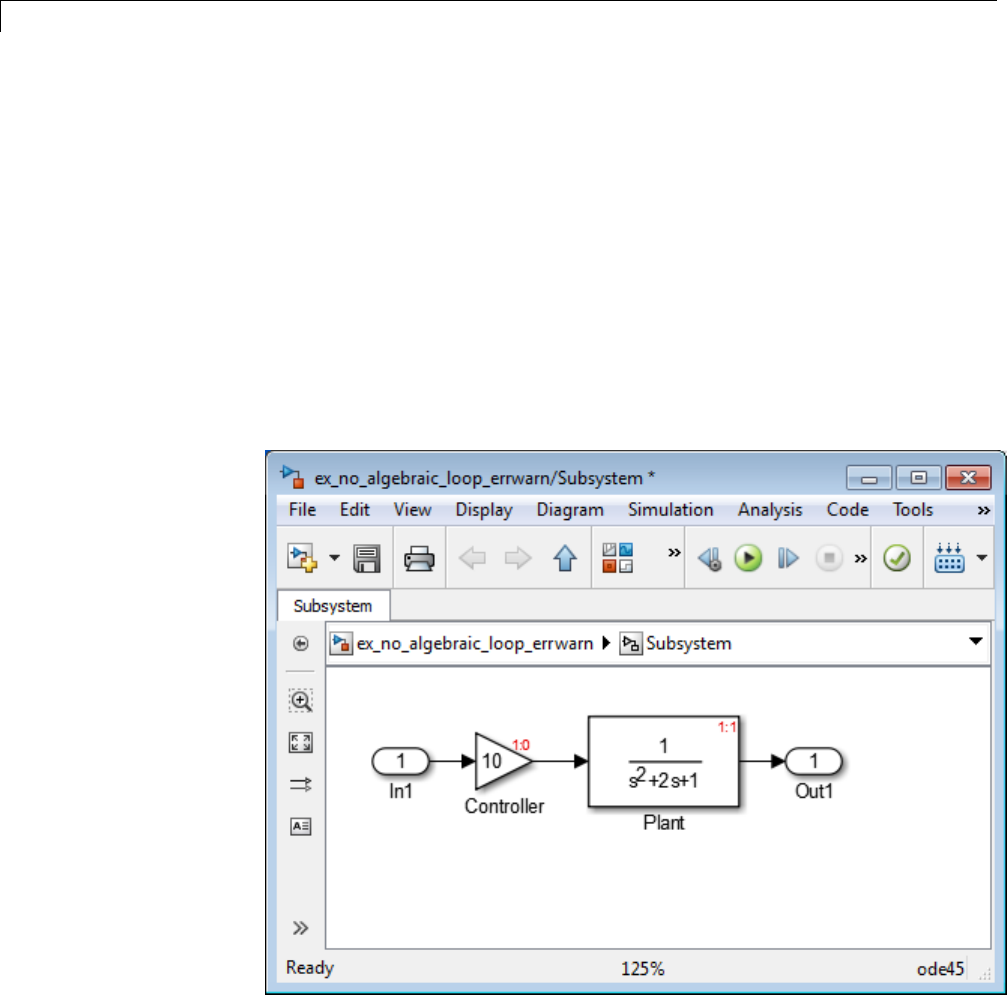
3How Simulink®Works
4On the Data Import/Export pane, make sure the Signal logging
parameter is disabled. If signal logging is enabled, Simulink cannot
eliminate artificial algebraic loops.
5Click OK.
6To display the sorted order for this model and the atomic subsystem, select
Format > Block Displays > Sorted Order.
Reviewing the sorted order might help you understand how to eliminate
the artificial algebraic loop.
All the blocks in the subsystem execute at the same level: 1. (0 is the lowest
level, indicating the first blocks to execute.)
3-70

Simulating Dynamic Systems
Note For more information about sorted order, see “Control and
Displaying the Sorted Order” on page 23-35.
7In the top-level model, right-click the subsystem and select Subsystem
Parameters.
8Select Minimize algebraic loop occurrences.
This parameter indicates to Simulink to try to eliminate the algebraic loop
that contains the atomic subsystem when it simulates the model.
9Click OK.
10 Click Simulation > Update Diagram to recalculate the sorted order.
Now there are two levels of sorted order inside the subsystem: 1 and 2.
3-71
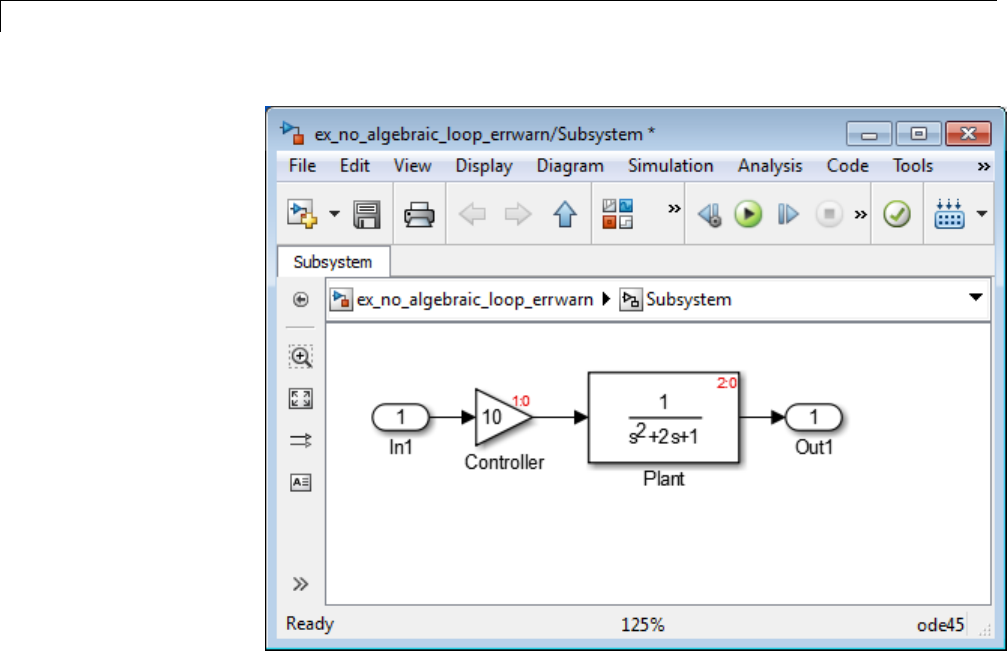
3How Simulink®Works
To eliminate the artificial algebraic loop, Simulink tries to make the input of
the subsystem or referenced model non-direct feedthrough.
When you simulate a model, all the blocks first execute their mdlOutputs
method, and then their mdlDerivatives and mdlUpdate methods.
In the original version of this model, the execution of the mdlOutputs method
starts with the Plant block because the Plant block is non-direct feedthrough.
The execution finishes with the Controller block.
3-72
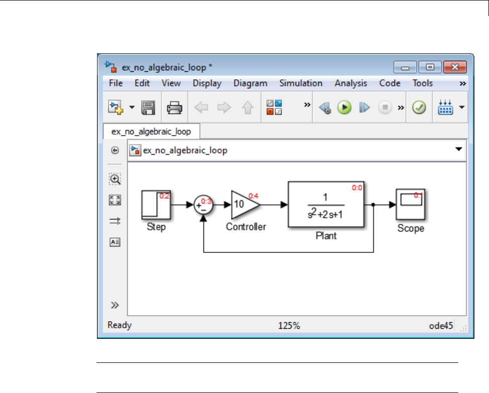
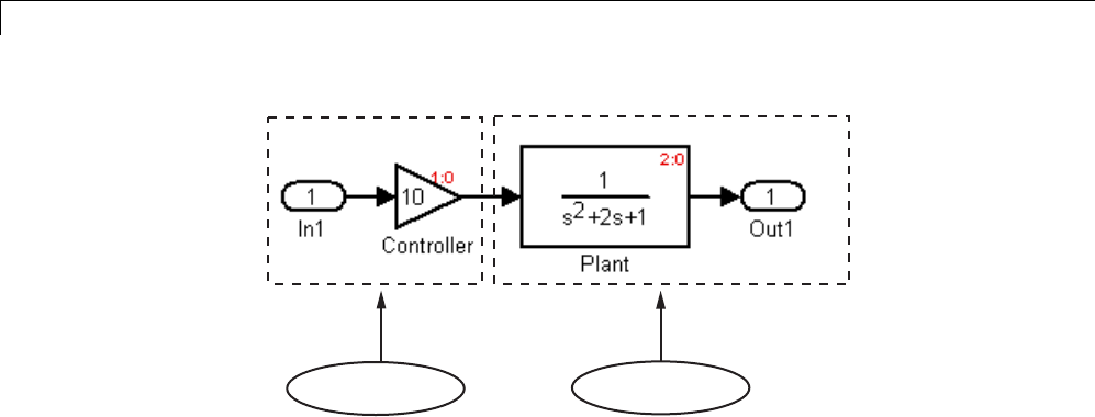
3How Simulink®Works
Atomic unit 1 Atomic unit 2
The following conditions are true:
•Atomic unit 2 is not direct feedthrough.
•Atomic unit 1 has only a mdlOutputs method.
The output of Atomic unit 1 is needed only by the mdlDerivatives or
mdlUpdate methods of Atomic unit 2. Simulink can execute what normally
wouldhavebeenexecutedduringthemdlOutput method of Atomic unit 1 in
the mdlDerivatives methods of Atomic unit 2.
The new execution order for the model is:
•mdlOutputs method of model
-mdlOutputs method of Atomic unit 2
-mdlOutputs methods of other blocks
•mdlDerivatives method of model
-mdlOutputs method of Atomic unit 1
-mdlDerivatives method of Atomic unit 2
-mdlDerivatives method of other blocks
For the Minimize algebraic loop occurrences techniquetobesuccessful,
the subsystem or referenced model must have a non-direct-feedthrough block
connected directly to an Inport. Simulink can then set the DirectFeedthrough
3-74
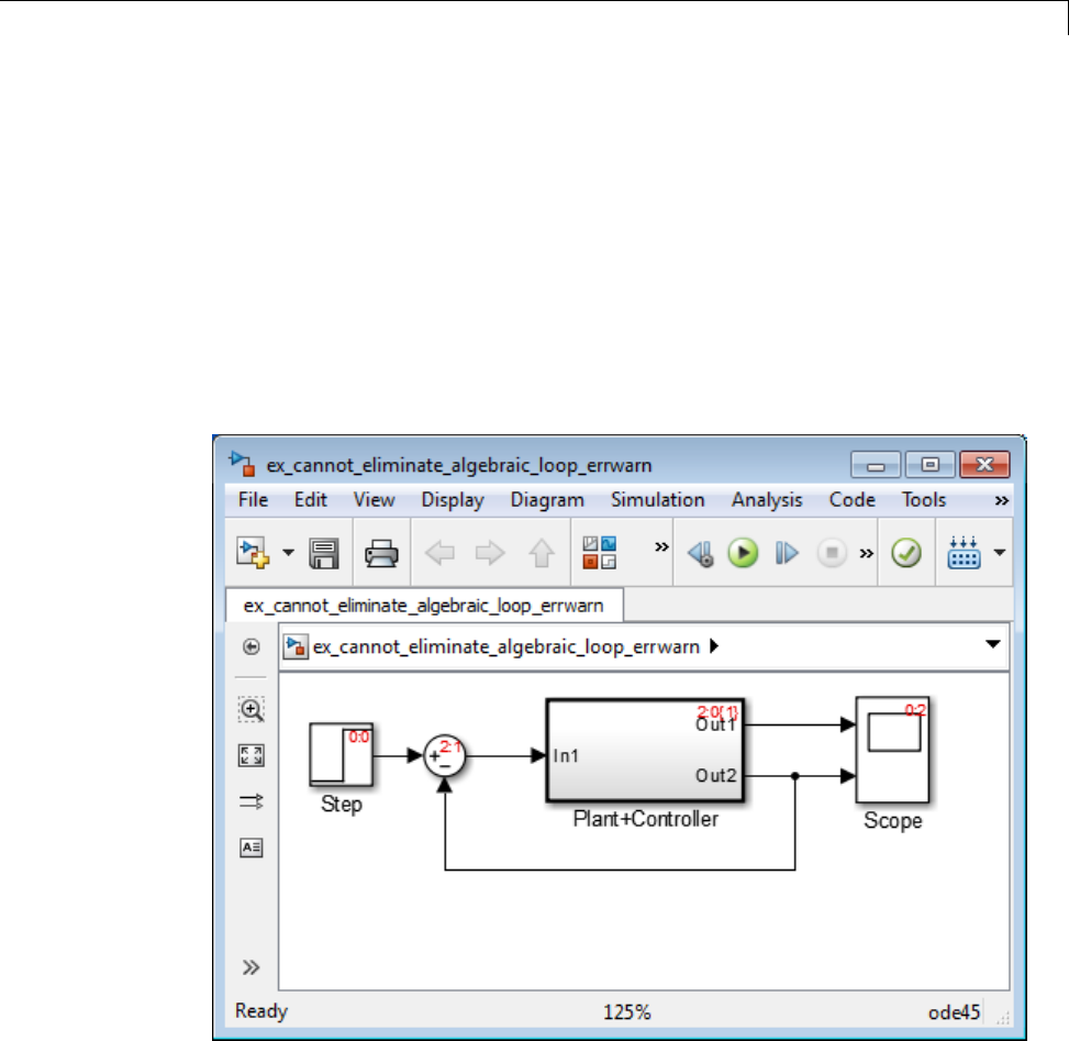
Simulating Dynamic Systems
property of the block Inport to false to indicate that the input port does
not have direct feedthrough.
When Simulink Cannot Eliminate Artificial Algebraic Loops. Setting
the Minimize algebraic loop occurrences parameter does not always
work. Simulink cannot change the DirectFeedthrough property of an Inport
for an atomic subsystem if the Inport is connected to an Outport only through
direct-feedthrough blocks.
Consider the following model. The subsystem Plant+Controller causes an
algebraic loop, but it has an extra Gain block and an extra output.
3-75
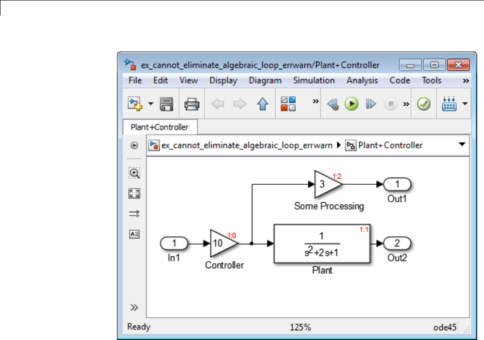
3How Simulink®Works
Simulink cannot move the mdlOutputs method of the Controller block to the
mdlDerivative method of an Atomic unit 1 because the output of the atomic
subsystem depends on the output of the Controller block. You cannot make
the subsystem non-direct-feedthrough.
You can modify this model to eliminate the artificial algebraic loop by
redefining the atomic subsystem by adding additional Inport and Gain
blocks, as you can see in the following model. Doing so makes In1
non-direct-feedthrough and In2 direct feedthrough, breaking the algebraic
loop.
3-76
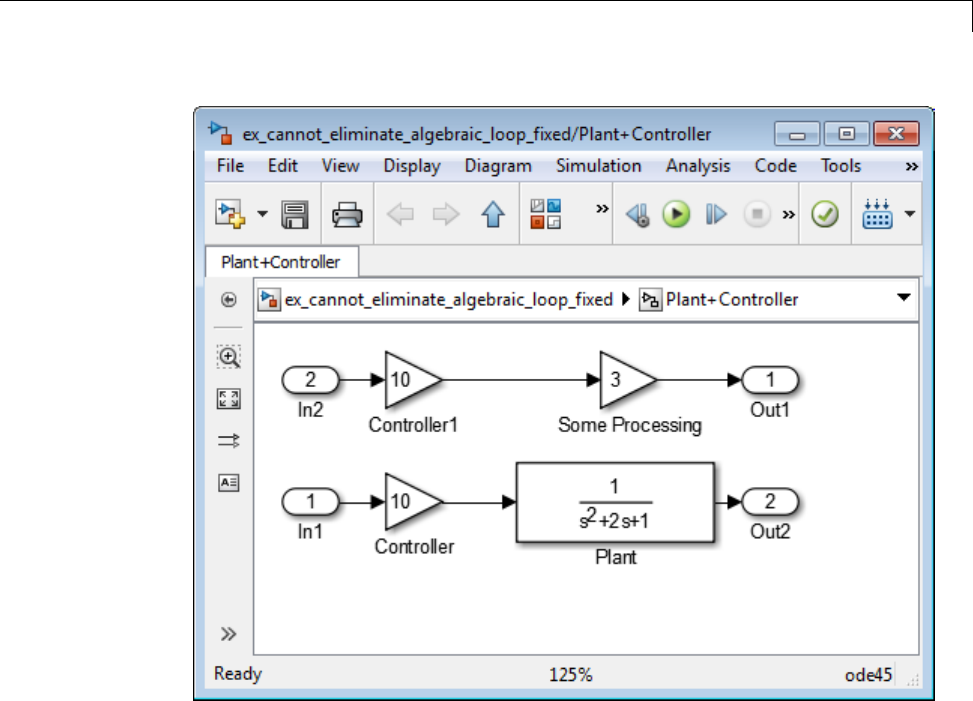
Simulating Dynamic Systems
Managing Large Models with Artificial Algebraic Loops. For
large models with algebraic loops, MathWorks recommends the following
techniques:
•Avoid creating loops that contain discontinuities or nondouble data types.
The Simulink algebraic loop solver is gradient-based and must solve
algebraic constraints to high precision.
•Develop a scheme for clearly identifying atomic subsystems as direct
feedthrough or not direct feedthrough. Use a visual scheme such as coloring
the blocks or defining a block-naming convention.
•Ifyouplantogeneratecodeforyourmodel,enabletheMinimize
algebraic loop occurrences parameter for all atomic subsystems. When
3-77

3How Simulink®Works
possible, make sure that the input ports for the atomic subsystems are
connected directly to non-direct-feedthrough blocks.
•Avoid combining non-direct-feedthrough and direct-feedthrough paths
using the Bus Creator or Mux blocks. Simulink might not be able to
eliminate any resulting artificial algebraic loops. Instead, consider
clustering the non-direct-feedthrough and direct-feedthrough objects in
separate subsystems.
Use Bus Selector blocks to pass only the required signals into atomic
subsystems.
3-78

Modeling Dynamic Systems
•Chapter 4, “Creating a Model”
•Chapter 5, “Working with Sample Times”
•Chapter 6, “Referencing a Model”
•Chapter 7, “Creating Conditional Subsystems”
•Chapter 8, “Modeling Variant Systems”
•Chapter 9, “Exploring, Searching, and Browsing Models”
•Chapter 10, “Managing Model Configurations”
•Chapter 11, “Configuring Models for Targets with Multicore
Processors”
•Chapter 12, “Modeling Best Practices”
•Chapter 13, “Managing Projects”

4
Creating a Model
•“Create an Empty Model” on page 4-2
•“Populate a Model” on page 4-4
•“Select Modeling Objects” on page 4-6
•“Specify Block Diagram Colors” on page 4-8
•“Connect Blocks” on page 4-12
•“Align, Distribute, and Resize Groups of Blocks” on page 4-22
•“Annotate Diagrams” on page 4-23
•“Create a Subsystem” on page 4-36
•“Control Flow Logic” on page 4-44
•“Callback Functions” on page 4-54
•“Model Workspaces” on page 4-67
•“Symbol Resolution” on page 4-76
•“Consult the Model Advisor” on page 4-81
•“Manage Model Versions” on page 4-107
•“Model Discretizer” on page 4-122

4Creating a Model
Create an Empty Model
To create an empty model:
1Open the Library Browser, by typing simulink at the MATLAB command
line.
2In the Library Browser, select File>New>Modelor click the New
model button ( ).
The Simulink software creates an empty model in memory and displays the
empty model in a Simulink Editor window.
Create a Model Template
When you create a model, Simulink uses defaults for many configuration
parameters. For example, by default new models have a white canvas, the
ode45 solver, and a visible toolbar. If these or other defaults do not meet your
needs, use the Simulink model construction functions listed in “Modeling
Basics” to write a function that creates a model with the defaults that you
prefer. For example, the following function creates a model that has a green
canvas and uses the ode3 solver:
function new_model(modelname)
% NEW_MODEL Create a new, empty Simulink model
% NEW_MODEL('MODELNAME') creates a new model with
% the name 'MODELNAME'. Without the 'MODELNAME'
% argument, the new model is named 'my_untitled'.
if nargin == 0
modelname = 'my_untitled';
end
% create and open the model
open_system(new_system(modelname));
% set default screen color
set_param(modelname, 'ScreenColor', 'green');
% set default solver
4-2

Create an Empty Model
set_param(modelname, 'Solver', 'ode3');
% save the model
save_system(modelname);
4-3

4Creating a Model
Populate a Model
In this section...
“Copy Blocks to Your Model” on page 4-4
“Browse Block Libraries” on page 4-4
“Search Block Libraries” on page 4-5
“Copy Blocks to Models” on page 4-5
Copy Blocks to Your Model
Use the Simulink Library Browser as the source for populating your model.
In the Library Browser, browse and search blocks from built-in and user
libraries. Copy blocks from the Library Browser to your model in the
Simulink Editor.
To open the Library Browser, at the MATLAB command line, enter:
simulink
For details, see “Open the Simulink Library Browser”.
For information about creating your own libraries and adding them to the
Library Browser, see “Block Libraries”.
Browse Block Libraries
The Libraries pane on the left displays a tree-structured folder of the block
libraries on your system. Initially, the Simulink library is selected and its
top level is open. You can scroll the pane and expand and collapse libraries
and sublibraries to browse the libraries on your system and the blocks that
the libraries contain.
The contents of the library that you select in the Libraries pane appear in
the Library tab to the right of the pane. The contents can be sublibraries,
blocks, or a mixture of the two. An icon and a name identifies each member of
the selected library.
To open a sublibrary, use one of the following approaches:
4-4

Populate a Model
•Select the library in the Libraries pane.
•Double-click the library in the Library tab.
To get help for a block:
1Right-click the block.
2From the context menu, select Help.
The help text and the context menu are the same as what appear when you
right-click an instance of that block in a model.
Search Block Libraries
To search for library blocks whose names contain a specified character string:
1In the Library Browser, in Search text field, enter the search character
string.
2Press Return or click Search.
The browser searches all libraries for blocks whose names match the specified
string. The browser displays the results in the Found pane. The pane shows
the blocks from each library separately.
By default, the search finds any substring and is not case-sensitive. To change
these defaults or to enable use of MATLAB regular expressions in the Search
field, click the Library Browser Options button and select the appropriate
commands. Work with blocks that you find by searching just as you do with
blocks that you find by selecting a library.
Copy Blocks to Models
To copy a block from the Library Browser into a model, drag and drop the
library block into the model window at the location where you want to create
the copy. Simulink copies the block to the model at the point that you select.
The resulting block retains a link to its source library. Updates to the source
library automatically propagate to all of its linked copies. See “Libraries”
for information about library links.
4-5

4Creating a Model
Select Modeling Objects
In this section...
“Select an Object” on page 4-6
“Select Multiple Objects” on page 4-6
Select an Object
To select a modeling object (for example, a block or line), click it. When you
place the cursor on a block, small black square handles appear at the corners
of the block. Placing the cursor on a line highlights part of the line in blue.
Clicking a block or line highlights the whole object in blue. For example, the
figure below shows a selected Sine Wave block.
Selectinganobjectbyclickingitdeselectsanyotherselectedobjects.
Select Multiple Objects
To select more than one object, use one of these approaches:
•Select objects one at a time.
•Use a bounding box to select objects located near each other.
•Selecttheentiremodel.
Select Multiple Objects One at a Time
To select more than one object by selecting each object individually, hold down
the Shift key and click each object that you want to select.
To deselect a selected object, click the object again while holding down the
Shift key.
Select Multiple Objects Using a Bounding Box
To select more than one object in the same area of the window, draw a
bounding box around the objects. This type of selection is also known as
“marquee selection” and “drag selection.”
4-6
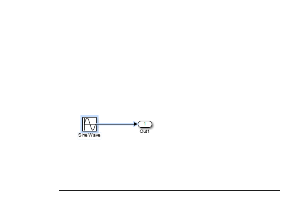
Select Modeling Objects
1Define the starting corner of a bounding box. Position the cursor (pointer)
at one corner of the box, then press and hold the left mouse button.
2Dragthecursortotheoppositecornerof the box. A blue rectangle encloses
the selected blocks and lines.
3Release the mouse button. Simulink selects all blocks and lines that are
at least partially enclosed by the bounding box. For example, in the figure
below, the bounding box enclosed at least part of the Sine Wave and the
linefromtheSineWaveblock.
Select All Objects
To select all objects in the active window, select Edit > Select All.
Note To create a subsystem, you cannot select all blocks and signals . For
more information, see “Create a Subsystem” on page 4-36.
4-7

4Creating a Model
Specify Block Diagram Colors
In this section...
“Set Block Diagram Colors Interactively” on page 4-8
“Platform Differences for Custom Colors” on page 4-9
“Choose a Custom Color” on page 4-9
“Define a Custom Color” on page 4-10
“Specify Colors Programmatically” on page 4-11
Set Block Diagram Colors Interactively
You can specify the foreground and background colors of any block or
annotation in a diagram, as well as the background color of the diagram.
Type of Color How to Set
Block diagram background Select Diagram > Format >
Canvas Color.
Block or annotation background
1Select the blocks and annotations.
2Select Diagram > Format >
Background Color
Block or annotation foreground
1Select the blocks and annotations.
2Select Diagram > Format >
Foreground Color
In all cases, you see a menu of color choices. Choose the desired color from the
menu. If you select a color other than Custom, the background or foreground
color of the diagram or diagram element changes to the selected color.
4-8
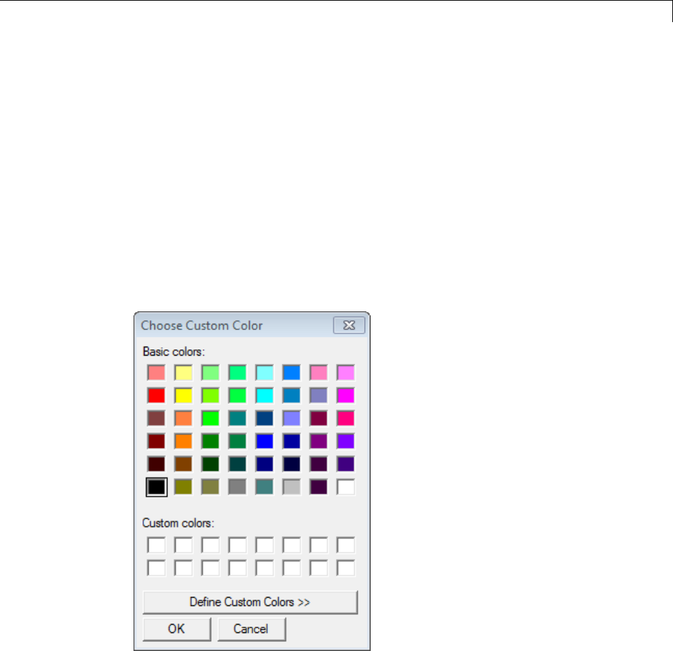
Specify Block Diagram Colors
Platform Differences for Custom Colors
On Mac platforms, choosing Custom invokes the Mac color picker interface.
Usethecolorpickertochoose and define custom colors.
On Windows and Linux platforms, use the Simulink interface, as described in:
•“Choose a Custom Color” on page 4-9
•“Define a Custom Color” on page 4-10
Choose a Custom Color
If you choose Custom, and there are no custom colors already defined,
Simulink displays the Choose Custom Color dialog box.
If you choose Custom, and there are custom colors already defined, Simulink
displays the Select Color dialog box.
4-9
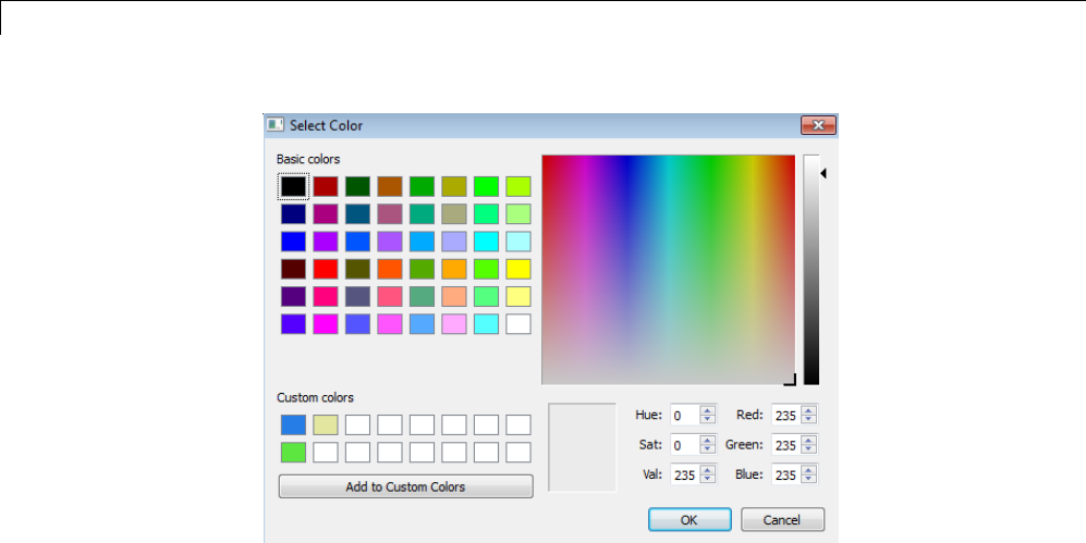
4Creating a Model
The Select Color dialog box displays a palette of basic colors and a palette of
already defined custom colors. To choose a color from either palette, click
the color and then click OK.
Define a Custom Color
To define the first custom color, in the Choose Custom Color dialog box, click
the Define Custom Colors button.
The dialog box expands to display the Select Color dialog box. To define a
custom color:
1Specify the color using one of these approaches:
•Enter the red, green, and blue components of the color as values between
0 (darkest) and 255 (brightest).
•Enter hue, saturation, and luminescence components of the color as
values in the range 0 to 255.
•Move the hue-saturation cursor to select the hue and saturation of the
desiredcolorandtheluminescencecursor to select the luminescence
of the desired color.
4-10

Specify Block Diagram Colors
2Adjust the values until the color in the box to the right of the custom colors
palette is the custom color that you want.
3Click the Add to Custom Colors button.
To replace an existing custom color, select the custom color in the custom
color palette before defining the new custom color.
Specify Colors Programmatically
You can use the set_param command at the MATLAB command line or
in a MATLAB program to set parameters that determine the background
color of a diagram and the background color and foreground color of diagram
elements. The following table summarizes the parameters that control block
diagram colors.
Parameter Determines
Block diagram
background
ScreenColor
Block and annotation
background
BackgroundColor
Block and annotation
foreground
ForegroundColor
Set the color parameter to either a named color or an RGB value.
•Named color: 'black','white','red','green','blue','cyan',
'magenta','yellow','gray','lightBlue','orange','darkGreen'
•RBG value: '[r,g,b]'
where r,g,andbare the red, green, and blue components of the color
normalized to the range 0.0 to 1.0.
For example, the following command sets the background color of the
currently selected system or subsystem to a light green color:
set_param(gcs, 'ScreenColor', '[0.3, 0.9, 0.5]')
4-11

4Creating a Model
Connect Blocks
In this section...
“Automatically Connect Blocks” on page 4-12
“Manually Connect Blocks” on page 4-15
“Disconnect Blocks” on page 4-21
Automatically Connect Blocks
You can have the Simulink software connect blocks automatically. This
eliminates the need to draw the connecting lines yourself. When connecting
blocks, Simulink routes the lines around intervening blocks to avoid cluttering
the diagram.
Autoconnect Two Blocks
When connecting two blocks with multiple ports, Simulink draws as many
connections as possible between the two blocks.
To autoconnect two blocks:
1Select the source block. In this example, the Sine Wave block is the source
block.
4-12
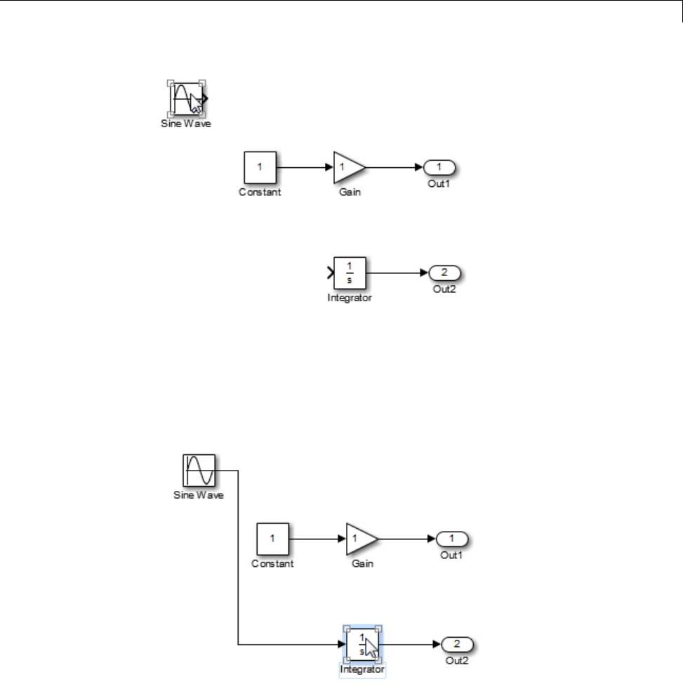
Connect Blocks
2Hold down Ctrl and left-click the destination block. In this example, the
Integrator block is the destination block.
The source block is connected to the destination block, and the lines are
routed around intervening blocks if necessary.
4-13
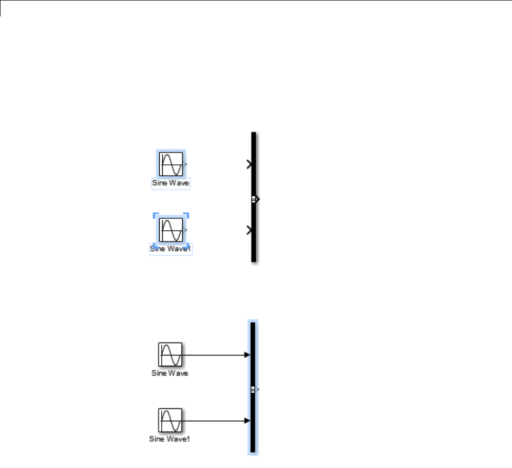
4Creating a Model
Connect Groups of Blocks
To connect a group of source blocks to a destination block:
1Select the source blocks.
2Hold down Ctrl and left-click the destination block.
To connect a source block to a group of destination blocks:
1Select the destination blocks.
4-14
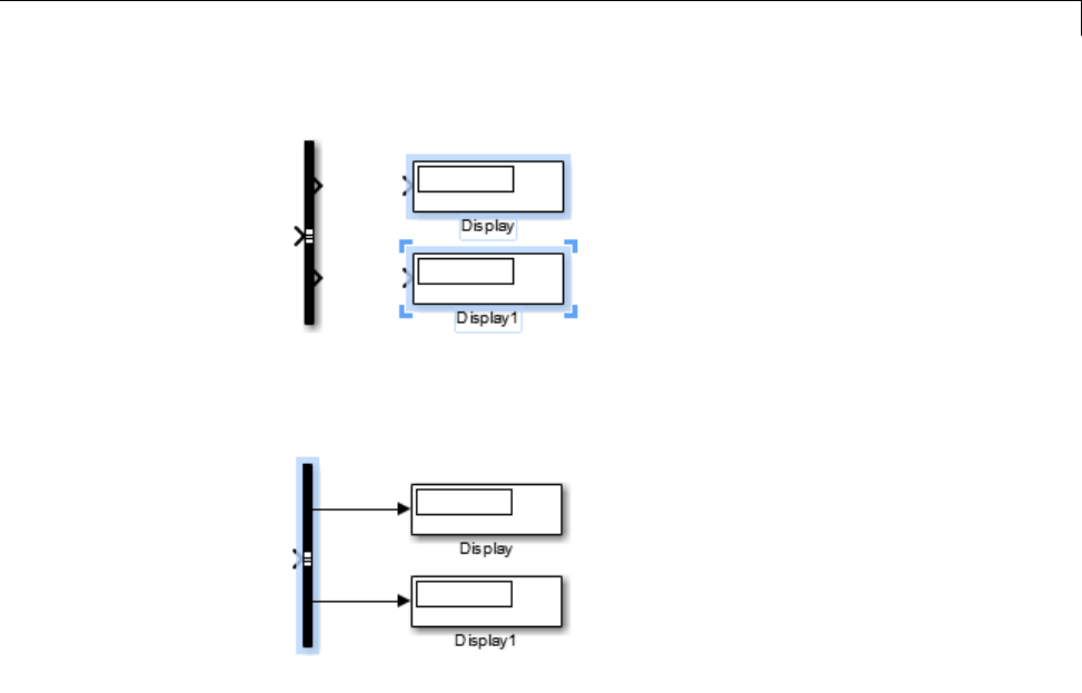
Connect Blocks
2Hold down Ctrl and left-click the source block.
Manually Connect Blocks
You can draw lines manually between blocks or between lines and blocks.
You might want to do this if you need to control the path of the line or to
createabranchline.
Draw a Line Between Blocks
You can create lines either from output to input ports, or from input to output
ports. For example, to connect the output port of a Constant block to the
inputportofGainblock:
1Position the cursor over the output port of the Constant block. You do not
need to position the cursor precisely on the port.
4-15
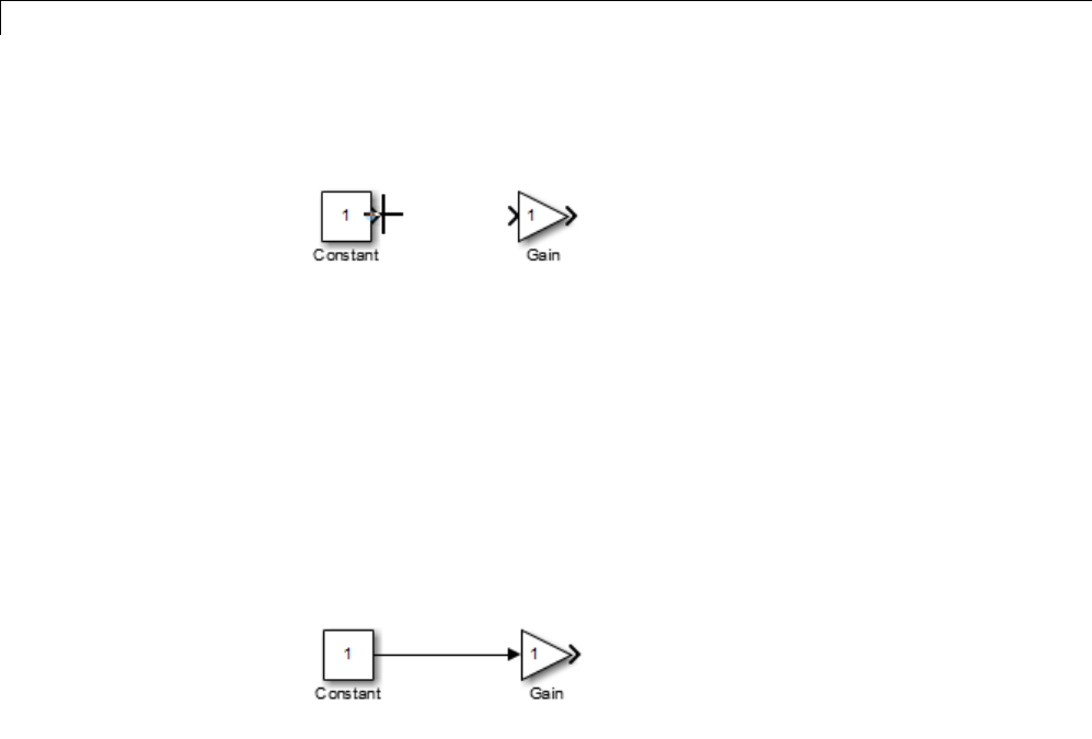
4Creating a Model
The cursor shape changes to crosshairs.
2Hold down the left mouse button.
3Drag the cursor to the input port of the Gain block. Position the cursor on
or near the port or in the block. If you position the cursor in the block, the
line connects to the closest input port.
4Release the mouse button. A connecting line with an arrow showing the
direction of the signal flow replaces the port symbol.
The arrow appears at the appropriate input port, and the signal is the same.
Draw a Branch Line
Abranch line is a line that starts from an existing line and carries its signal to
the input port of a block. Both the existing line and the branch line represent
the same signal. Use branch lines to connect a signal to more than one block.
4-16
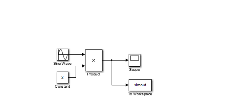
Connect Blocks
This example shows how to connect the Product block output to both the
Scope block and the To Workspace block.
To add a branch line:
1Position the cursor on the line where you want the branch line to start.
2While holding down the Ctrl key, press and hold down the left or right
mouse button.
3Drag the cursor to the input port of the target block, then release the
mouse button and the Ctrl key.
Draw Line Segments
Manually draw line segments when you want to draw:
•Line segments differently than autoconnect feature draws the lines
•A line, before you copy the block to which the line connects
To draw a line segment:
1Draw a line from the block port to an unoccupied area of the canvas.
Release the mouse button where you want the line segment to end.
The cursor turns into a circle, and blue arrow guides appear.
4-17
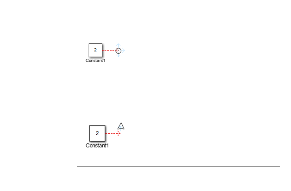
4Creating a Model
2For each additional line segment, position the cursor over the blue arrow
guide that points in the direction in which youwanttodrawalinesegment.
The cursor turns into an empty arrowhead.
Tip To reroute the whole line instead of extending it, select the end of
thelineitselfwhenthecirclecursoris displayed and drag the line end to
a new location.
3Drag the cursor to draw the second line segment and release the mouse
button to finish drawing the line.
Move a Line Segment
To move a line segment:
1Position the cursor on the segment that you want to move.
2Press and hold down the left mouse button.
3Drag the cursor to the desired location and release the mouse button.
4-18
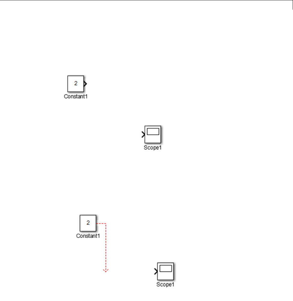
Connect Blocks
Draw a Diagonal Line
You cannot draw a single diagonal line between two ports. You can draw very
short line segments connecting to each port, with a longer diagonal segment
in the middle. For example, suppose you position two blocks as shown below:
To approximate a diagonal line:
1Draw a short line segment from the output port of the Constant block.
2Attheendofthefirstlinesegment,drawasecondlinesegment.
3Draw a third line segment to connect to the Scope block.
4-19
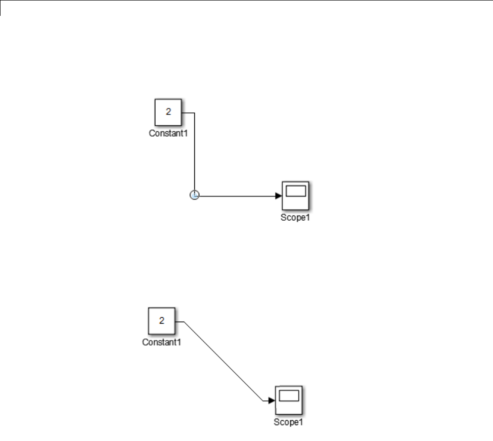
4Creating a Model
4Position the cursor at the bend of the second and third line segments. The
cursor turns into a circle.
5Hold the Shift keydownanddragthecursortomakethesecondline
segment a diagonal.
Move a Line Vertex
To move a vertex of a line:
1Position the cursor on the vertex, then press and hold down the left mouse
button.
4-20
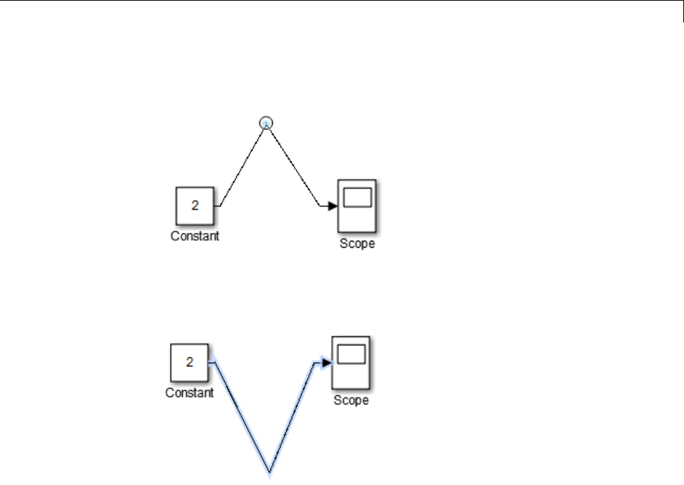
Connect Blocks
The cursor changes to a circle.
2Drag the vertex to the desired location.
3Releasethemousebutton.
Insert a Block in a Line
You can insert a block in a line, if the block has only one input and one output.
1Drag theblockoverthelineinwhichyouwanttoinserttheblock.
2Release the mouse button. Simulink inserts the block for you at the point
where you drop the block.
Disconnect Blocks
To disconnect a block from its connecting lines, hold down the Shift key,
then drag the block to a new location.
4-21

4Creating a Model
Align, Distribute, and Resize Groups of Blocks
To align, distribute, or resize a group of blocks:
1Select the blocks that you want to align, as described in “Select Multiple
Objects” on page 4-6.
Simulink highlights one of the selected blocks. Simulink uses the
highlighted block as the reference for aligning the other selected blocks.
For example, in the following model, the Constant block is the alignment
reference block.
One of the selected blocks displays empty selection handles. The model
editor uses this block as the reference for aligning the other selected blocks.
If you want another block to serve as the alignment reference, click that
block.
2From the Diagram > Arrange menu, select an alignment, distribution, or
sizing option. For example, select Align Top to align the top edges of the
selected blocks with the top edge of the reference block.
4-22

Annotate Diagrams
Annotate Diagrams
In this section...
“Add and Edit Annotations” on page 4-23
“Summary of Annotations Properties Dialog Box” on page 4-28
“Annotation Callback Functions” on page 4-29
“Associate Click Functions with Annotations” on page 4-30
“Annotations API” on page 4-32
“TeX Formatting Commands in Annotations” on page 4-32
“Create Annotations Programmatically” on page 4-34
Add and Edit Annotations
Annotations provide textual information to document a model. You can add
an annotation to any unoccupied area of your block diagram.
Add an Annotation
To add an annotation:
1Double-click an unoccupied area of the block diagram. A small rectangle
appears and the cursor changes to an insertion point.
4-23

4Creating a Model
2Type the annotation contents. Each line is centered in the rectangle that
surrounds the annotation.
Alternatively, from the Simulink Editor palette (to the left of the model),
select the Annotation button ( ) and either drag the cursor into the model
window or click in the model window.
Move an Annotation
To move an annotation, drag it to a new location.
Annotations Properties Dialog Box
As an alternative to directly editing an annotation, you can use the Annotation
properties dialog box to specify the contents and format of the currently
selected annotation and to associate a click function with the annotation. The
Annotations properties dialog box consolidates the options for specifying the
content and appearance of an annotation.
To display the Annotation properties dialog box for an annotation:
1Select an annotation.
2Select Diagram > Properties.
The Annotation properties dialog box opens.
4-24
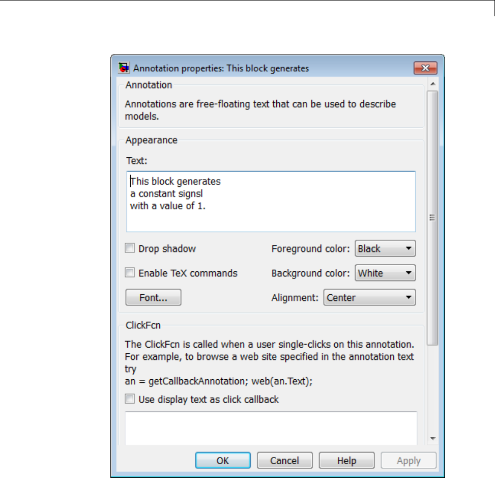
Annotate Diagrams
Edit an Annotation
To edit an annotation directly, select the annotation.
4-25

4Creating a Model
•To insert characters, click between two characters to position the insertion
point, then insert text.
•To replace characters, drag the mouse to select a range of text to replace,
then enter the new text.
To edit annotation text using the Annotations properties dialog box, edit
the Text field.
Change Annotation Font
To change the annotation font:
1Select the annotation.
2Select Diagram > Format > Font Style.
3Select a font and size from the dialog box.
To change the annotation font using the Annotations properties dialog box,
press the Font button.
Use TeX commands
To use TeX (LaTeX) commands in an annotation:
1Select the annotation.
2Select Diagram > Format > Enable TeX Commands.
3Enter TeX commands.
As an alternative, to enable the use of TeX commands using the Annotations
properties dialog box, select Enable TeX commands.
For details, see “TeX Formatting Commands in Annotations” on page 4-32.
Text Alignment
To change the text alignment (left, center, or right) in an annotation:
1Select the annotation.
4-26

Annotate Diagrams
2Select Diagram > Format > Text Alignment.
3Select an alignment option, such as Center.
As an alternative, to change the annotation text alignment using the
Annotations properties dialog box, use the Alignment field.
Background Color or Text Color
To change the background color or text color of an annotation:
1Select the annotation.
2Set the annotation background color by selecting Diagram > Format >
Background.
3Set the annotation text color by selecting Diagram > Format >
Foreground.
As an alternative, to change the background color or text color using the
Annotations properties dialog box:
•To specify the color of the annotation box, use the Background color field.
•To specify the annotation text color of the annotation box, use the
Foreground color field.
Border or Drop Shadow
To specify a border for the annotation:
1Select the annotation.
2Select the annotation background color by selecting Diagram > Format >
Annotation Border.
To specify a drop shadow for the annotation(togiveita3-Dappearance),in
the Annotations properties dialog box, select Drop shadow.
Delete an Annotation
To delete an annotation, do one of the following:
4-27

4Creating a Model
•Draw a selection box that includes part of the annotation and press Delete.
•Select all of the text in the annotation, press Delete, and move the cursor.
Summary of Annotations Properties Dialog Box
The dialog box includes the following controls.
Text
Displays the current text of the annotation. Edit this field to change the
annotation text.
Enable TeX commands
Enables the use of TeX formatting commands in this annotation. For details,
see “TeX Formatting Commands in Annotations” on page 4-32.
Font
Displays a font chooser dialog box. Use the font chooser to change the font
used to render the annotation’s text.
Foreground color
Specifies the color of the annotation text.
Background color
Specifies the color of the background of the bounding box of the annotation.
Alignment
Specifies the alignment of the annotation text relative to its bounding box.
ClickFcn
SpecifiesMATLABcodetobeexecuted when a user single-clicks this
annotation. Simulink stores the code entered in this field with the model. For
details, see “Associate Click Functions with Annotations” on page 4-30.
4-28

Annotate Diagrams
Use display text as click callback
Treats the Text field as the annotation click function. The specified text must
be a valid MATLAB expression comprising symbols that are defined in the
MATLAB workspace when the user clicks this annotation. For details, see
“Associate Click Functions with Annotations” on page 4-30. Selecting this
option disables the ClickFcn edit field.
Annotation Callback Functions
You can make an annotation interactivebyaddingacallback. Forexample,
you can use an annotation click callback function to set up a link from
annotation text.
You can associate the following callback functions with annotations.
Click Function
A click function is a MATLAB function that Simulink invokes when a user
single-clicks an annotation. You can associate a click function with any model
annotation (for details, see “Associate Click Functions with Annotations”
on page 4-30).
You can use click functions to add hyperlinks and custom command “buttons”
to a model. For example, you can use a click function to allow a user to display
the values of workspace variables referenced by the model or to open related
models simply by clicking on annotations displayed on the block diagram.
Simulink uses the color blue to display the text of annotations associated
with click functions.
Load Function
This function is invoked when it loads the model containing the associated
annotation. To associate a load function with an annotation, set the LoadFcn
property of the annotation to the desired function (see “Annotations API”
on page 4-32).
4-29
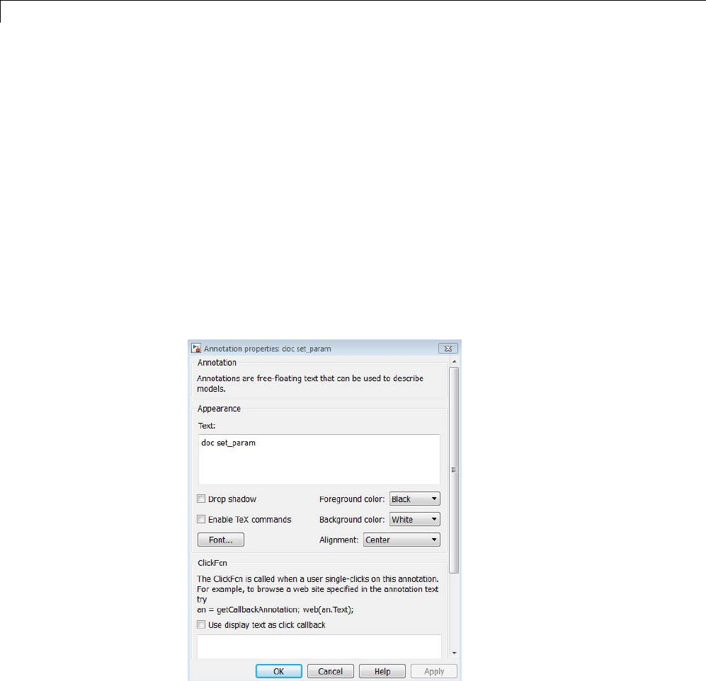
4Creating a Model
Delete function
This function is invoked before deleting the associated annotation. To
associate a delete function with an annotation, set the DeleteFcn property of
the annotation to the desired function (see “Annotations API” on page 4-32).
Associate Click Functions with Annotations
Use one of two ways to associate a click function with an annotation with
either the Annotation Properties dialog box (see “Summary of Annotations
Properties Dialog Box” on page 4-28) or a separately defined function.
•Specify the annotation itself as the click function.
Enter a valid MATLAB expression in the Text field and check the Use
display text as click callback.
4-30
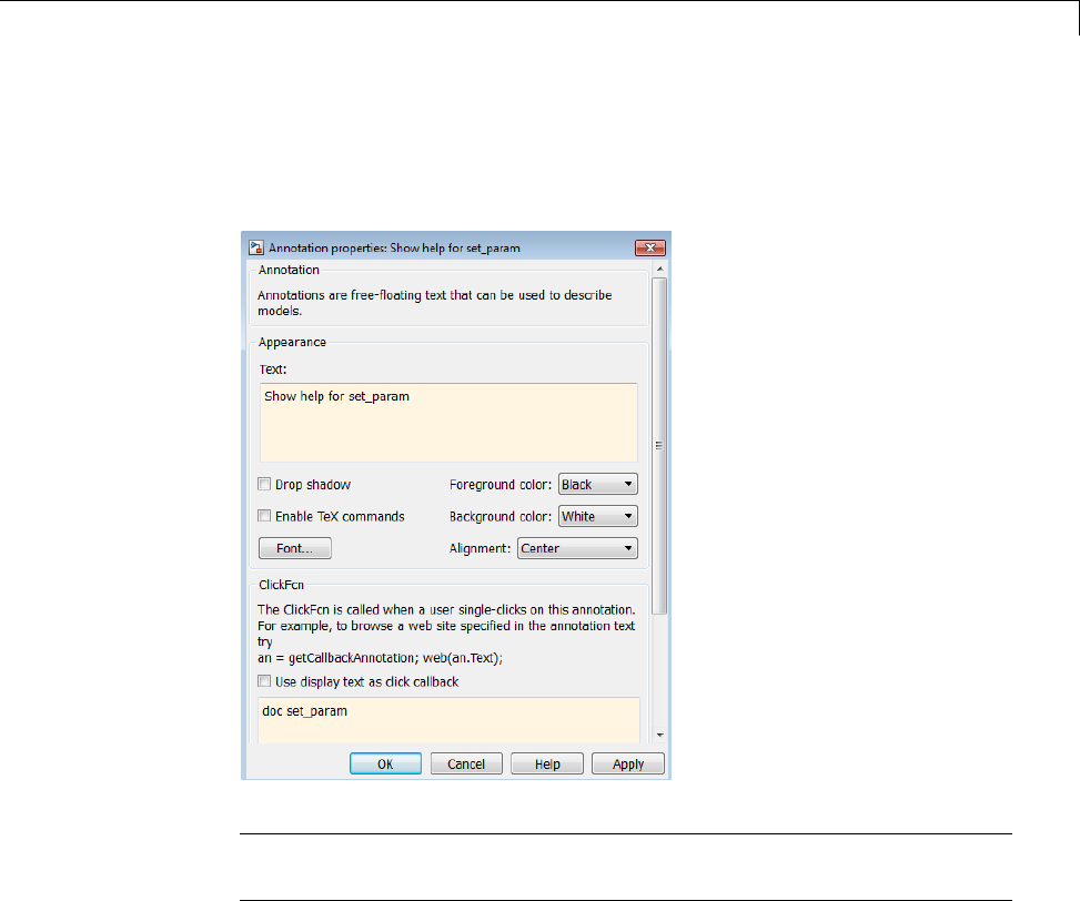
Annotate Diagrams
•Specify a separately defined click function.
Enter the MATLAB code that defines the click function in the ClickFcn
edit field.
Note YoucanalsouseMATLABcodetoassociate a click function with an
annotation. See “Annotations API” on page 4-32 for more information.
Select and Edit Annotations Associated with Click Functions
If you associate an annotation with a click function, then you cannot select
the annotation by clicking on it. Instead, use a boundary box to select the
annotation.
To move the annotation, use the up, down, right, or left arrow keys.
4-31

4Creating a Model
Similarly, you cannot edit the annotation text by clicking on the text. To edit
the annotation:
1Drag select the annotation.
2Right-click the selected annotation.
3In the context menu, select Properties.
4In the Properties dialog box, in the Text field, edit the text.
Annotations API
To use MATLAB code to get and set the properties of annotations, use:
•Simulink.Annotation class
Set the properties of annotations, by using MATLAB code. For example,
annotation load functions (see “Load Function” on page 4-29).
•getCallbackAnnotation function
Get the Simulink.Annotation object for the annotation associated with
the currently executing annotation callback function. Use this function to
determine which annotation was clicked to invoke the current callback.
This function is also useful if you write a callback function in a separate
MATLAB file contains multiple callback calls.
TeX Formatting Commands in Annotations
You can use TeX formatting commands to include mathematical and other
symbols and Greek letters in block diagram annotations.
4-32

Annotate Diagrams
To use TeX commands in an annotation:
1Select the annotation.
2Select Diagram > Format > Enable TeX Commands.
3Enter or edit the text of the annotation, using TeX commands where needed
to achieve the desired appearance.
4-33
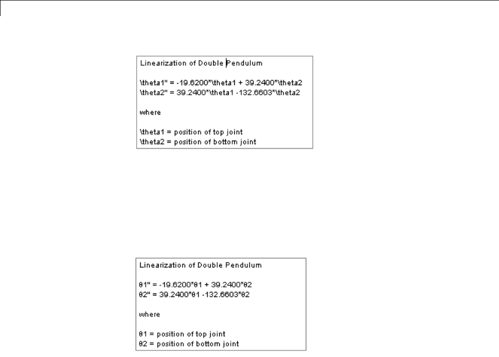
4Creating a Model
See “Mathematical Symbols, Greek Letters, and TeX Characters” in
the MATLAB documentation for information about the supported TeX
formatting commands.
4Deselect the annotation by clicking outside it or press the Esc key.
The text reflects the TeX formatting.
Create Annotations Programmatically
To create annotations at the command line or in a MATLAB program, use the
add_block command.
add_block('built-in/Note','path/text','Position', ...
[center_x,0,0,center_y]);
where path isthepathofthediagramtobeannotated,text is the text of
the annotation, and [center_x,0,0,center_y] is the position of the center
of the annotation in pixels relative to the upper left corner of the diagram.
For example:
new_system('test')
4-34
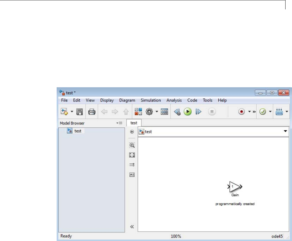
Annotate Diagrams
open_system('test')
add_block('built-in/Gain', 'test/Gain', 'Position', ...
[260, 125, 290, 155])
add_block('built-in/Note','test/programmatically created', ...
'Position', [550 0 0 180])
The code creates the following model, which includes an annotation.
To delete an annotation, use the find_system command to get the annotation
handle. Then use the delete function to delete the annotation. For example:
delete(find_system(gcs, 'FindAll', 'on', 'type', 'annotation'));
4-35

4Creating a Model
Create a Subsystem
In this section...
“Subsystem Advantages” on page 4-36
“Two Ways to Create a Subsystem” on page 4-36
“Create a Subsystem by Adding the Subsystem Block” on page 4-37
“CreateaSubsystembyGroupingExistingBlocks”onpage4-37
“Subsystem Execution” on page 4-39
“Navigate Model Hierarchy” on page 4-39
“Label Subsystem Ports” on page 4-42
“Control Access to Subsystems” on page 4-42
“Interconvert Subsystems and Block Diagrams” on page 4-43
“Empty Subsystems and Block Diagrams” on page 4-43
Subsystem Advantages
A subsystem is a set of blocks that you replace with a single block called a
Subsystem block. As your model increases in size and complexity, you can
simplify it by grouping blocks into subsystems. Using subsystems has these
advantages:
•Helps reduce the number of blocks displayed in your model window.
•Keeps functionally related blocks together.
•Establishes a hierarchical block diagram, where a Subsystem block is on
one layer and the blocks that make up the subsystem are on another.
For additional information about how subsystems compare to other Simulink
componentization techniques, see “Componentization Guidelines” on page
12-17.
TwoWaystoCreateaSubsystem
You can create a subsystem in two ways:
4-36
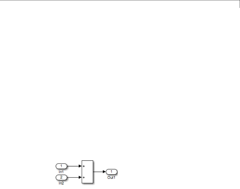
Create a Subsystem
•Add a Subsystem block to your model, then open that block and add the
blocks that it contains to the subsystem window.
•Add the blocks that make up the subsystem, then group those blocks into a
subsystem.
Create a Subsystem by Adding the Subsystem Block
To create a subsystem before adding the blocks that it contains, add a
Subsystem block to the model, thenaddtheblocksthatmakeupthe
subsystem.
1Copy the Subsystem block from the Ports & Subsystems library into your
model.
2Open the Subsystem block by double-clicking it.
3In the empty Subsystem window, createthesubsystem.UseInportblocks
to represent input from outside the subsystem and Outport blocks to
represent external output.
For example, this subsystem includes a Sum block and Inport and Outport
blocks to represent input to and output from the subsystem.
Create a Subsystem by Grouping Existing Blocks
If your model already contains the blocks that you want to convert to a
subsystem, create the subsystembygroupingthoseblocks.
1Select individual blocks that you want to include in a subsystem. To select
multiple blocks that are in one area of the model, click the left mouse
button and drag the cursor to create a bounding box that encloses the
blocks and the connecting lines that you want to include in the subsystem.
For more information, see “Select Multiple Objects Using a Bounding Box”
on page 4-6.
4-37
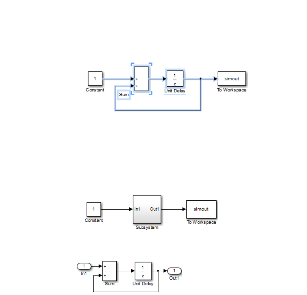
4Creating a Model
For example, this figure shows a model that represents a counter. The
bounding box selects the Sum and Unit Delay blocks.
When you release the mouse button, the two blocks and all the connecting
lines are selected.
2Select Diagram > Subsystems & Model Reference > Create
SubsystemfromSelection. A Subsystem block replaces the selected
blocks.
3Resize the Subsystem block so the port labels are readable.
If you open the Subsystem block, the underlying system opens. For example:
Notice that Simulink adds Inport and Outport blocks to represent input from
and output to blocks outside the subsystem.
4-38
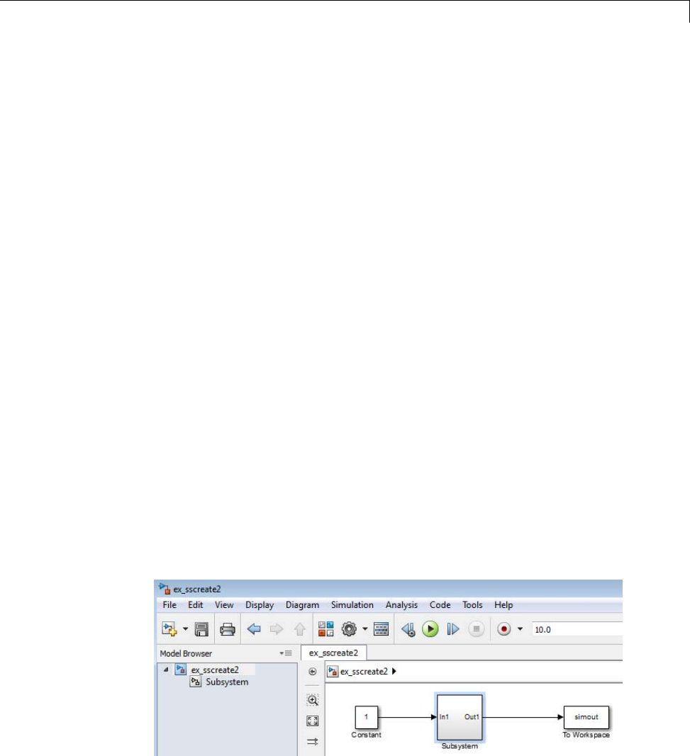
Create a Subsystem
As with all blocks, you can change the name of the Subsystem block. To
customize the appearance and dialog box of the block, you can mask the
subsystem (see “Masking”).
Undoing Subsystem Creation
Right after you create subsystem by grouping blocks (see “Create a Subsystem
by Grouping Existing Blocks” on page 4-37), you can undo that operation. To
undo subsystem creation, select Edit > Undo Subsystem Creation.
Subsystem Execution
You can configure a subsystem to execute either conditionally or
unconditionally.
•An unconditionally executed subsystem always executes.
•A conditionally executed subsystem may or may not execute, depending on
the value of an input signal. For details, see “Conditional Subsystems”.
Navigate Model Hierarchy
Subsystems allow you to create a hierarchical model comprising many layers.
You can navigate this hierarchy using the “Model Browser” on page 9-80 or
with Simulink Editor model navigation commands.
To open a subsystem using the Simulink Editor context menu for the
Subsystem block:
1In the Simulink Editor, right-click the Subsystem block.
4-39

4Creating a Model
2From the context menu, select one of these options:
•Open —Openthesubsystem,inthesamewindowandtabasusedfor
the top model.
•Open In New Tab — Open the subsystem, creating an additional tab
for the subsystem.
•Open In New Window— Open the subsystem, opening a new Simulink
Editor window.
4-40
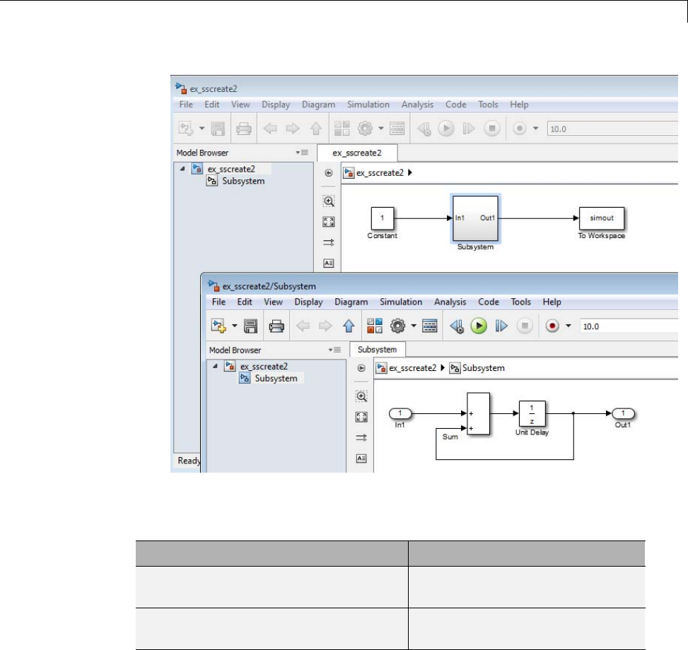
Create a Subsystem
For any operation to open a subsystem, you can use a keyboard shortcut to
have the subsystem open in a new tab or window:
Where to Open the Subsystem Keyboard Shortcut
In a new tab Hold the CTRL key while opening
the subsystem.
In a new window Hold the SHIFT key while
opening the subsystem.
To display the parent of a subsystem:
1Open the tab that contains the subsystem.
2Select View > Navigate > Up to Parent.
4-41

4Creating a Model
Label Subsystem Ports
By default, Simulink labels ports on a Subsystem block. The labels are the
names of the Inport and Outport blocks that connect the subsystem to blocks
outside of the subsystem.
You can specify how Simulink labels the ports of a subsystem.
1Select the Subsystem block.
2Select one of the labeling options from Diagram > Format > Port
Labels menu (for example, From Port Block Name).
Control Access to Subsystems
You can control user access to subsystems. For example, you can prevent a
user from viewing or modifying the contents of a library subsystem while still
allowingtheusertoemploythesubsysteminamodel.
Note This method does not necessarily prevent a user from changing the
access restrictions. To hide proprietary information that is in a subsystem,
consider using protected model referencing models (see “Protected Model”
on page 6-67).
To restrict access to a library subsystem, open the subsystem parameter
dialog box and set Read/Write permissions to one of these values:
•ReadOnly: A user can view the contents of the library subsystem but
cannot modify the reference subsystem without disabling its library link or
changing its Read/Write permissions to ReadWrite.
•NoReadOrWrite: A user cannot view the contents of the library subsystem,
modify the reference subsystem, or change reference subsystem
permissions.
Both options allow a user to employ the library subsystem in models by
creating links (see “Libraries”). For more information about subsystem access
options, see the Subsystem block documentation.
4-42

Create a Subsystem
Note You do not receive a response if you attempt to view the contents
of a subsystem whose Read/Write permissions parameter is set to
NoReadOrWrite. For example, when double-clicking such a subsystem,
Simulink does not open the subsystem and does not display any messages.
Interconvert Subsystems and Block Diagrams
To interconvert subsystems and block diagrams, use one of these functions:
Simulink.SubSystem.copyContentsToBlockDiagram
Copies the contents of a subsystem to an empty block diagram.
Simulink.BlockDiagram.copyContentsToSubSystem
Copies the contents of a block diagram to an empty subsystem.
Empty Subsystems and Block Diagrams
To empty subsystems and block diagrams, use one of these functions:
Simulink.SubSystem.deleteContents
Deletes the contents of a subsystem.
Simulink.BlockDiagram.deleteContents
Deletes the contents of a block diagram.
4-43

4Creating a Model
Control Flow Logic
In this section...
“Equivalent C Language Statements” on page 4-44
“Conditional Control Flow Logic” on page 4-44
“While and For Loops” on page 4-47
Equivalent C Language Statements
You can use block diagrams to model control flow logic equivalent to the
following C programming language statements:
•for
•if-else
•switch
•while
Conditional Control Flow Logic
You can use the following blocks to perform conditional control flow logic.
C Statement Equivalent Blocks
if-else If, If Action Subsystem
switch Switch Case, Switch Case Action Subsystem
If-Else Control Flow
The following diagram represents if-else control flow.
4-44
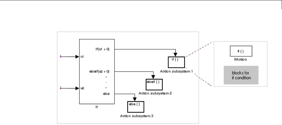
Control Flow Logic
Construct an if-else control flow diagram as follows:
1Provide data inputs to the If block for constructing if-else conditions.
In the If block parameters dialog box, set inputs to the If block. Internally,
the inputs are designated as u1, u2,..., un and are used to construct
output conditions.
2In the If block parameters dialog box, set output port if-else conditions
for the Ifblock.
In the If block parameters dialog box, set Output ports. Use the input
values u1, u2, ..., un to express conditions for the if, elseif, and else
condition fields in the dialog box. Of these, only the if field is required.
You can enter multiple elseif conditions and select a check box to enable
the else condition.
3Connect each condition output port to an Action subsystem.
Connect each if, elseif, and else condition output port on the If block to a
subsystem to be executed if the port’s case is true.
Create these subsystems by placing an Action Port block in a subsystem.
This creates an atomic Action subsystem with a port named Action, which
you then connect to a condition on the If block.
4-45
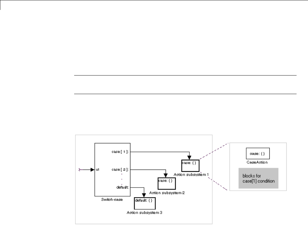
4Creating a Model
Once connected, the subsystem takes on the identity of the condition it is
connected to and behaves like an enabled subsystem.
For more detailed information, see the If and Action Port blocks.
Note All blocks in an Action subsystem driven by an If or Switch Case block
must run at the same rate as the driving block.
Switch Control Flow
The following diagram represents switch control flow.
Construct a switch control flow statement as follows:
1Provide a data input to the argument input of the Switch Case block.
TheinputtotheSwitchCaseblockistheargumenttotheswitch control
flow statement. This value determines the appropriate case to execute.
Noninteger inputs to this port are truncated.
2Add cases to the Switch Case block based on the numeric value of the
argument input.
Using the parameters dialog box of the Switch Case block, add cases to the
Switch Case block. Cases can be single or multivalued. You can also add an
4-46

Control Flow Logic
optional default case, which is true if no other cases are true. Once added,
these cases appear as output ports on the Switch Case block.
3Connect each Switch Case block case output port to an Action subsystem.
Each case output of the Switch Case block is connected to a subsystem to be
executed if the port’s case is true. You create these subsystems by placing
an Action Port block in a subsystem. This creates an atomic subsystem
with a port named Action, which you then connect to a condition on the
Switch Case block. Once connected, the subsystem takes on the identity of
the condition and behaves like an enabled subsystem. Place all the block
programming executed for that case in this subsystem.
For more detailed information, see documentation for the Switch Case and
Action Port blocks.
Note After the subsystem for a particular case executes, an implied break
executes, which exits the switch control flow statement altogether. Simulink
switch control flow statement implementations do not exhibit the “fall
through” behavior of C switch statements.
While and For Loops
Use the following blocks to perform while and for loops.
C Statement Equivalent Blocks
do-while While Iterator Subsystem
for For Iterator Subsystem
while While Iterator Subsystem
While Loops
The following diagram illustrates a while loop.
4-47
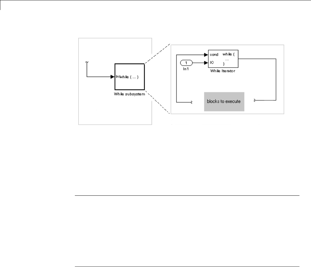
4Creating a Model
In this example, Simulink repeatedly executes the contents of the While
subsystem at each time step until a condition specified by the While Iterator
block is satisfied. In particular, for each iteration of the loop specified by the
While Iterator block, Simulink invokes the update and output methods of all
the blocksintheWhilesubsysteminthesameorderthatthemethodswould
be invoked if they were in a noniterated atomic subsystem.
Note Simulation time does not advance during execution of a While
subsystem’s iterations. Nevertheless, blocks in a While subsystem treat each
iteration as a time step. As a result, in a While subsystem, the output of
ablockwith states (that is, a block whose output depends on its previous
input), reflects the value of its input at the previous iteration of the while
loop. The output does not reflectthatblock’sinputattheprevioussimulation
time step. For example, a Unit Delay block in a While subsystem outputs the
value of its input at the previous iteration of the while loop, not the value at
the previous simulation time step.
Construct a while loop as follows:
1Place a While Iterator block in a subsystem.
The host subsystem label changes to while {...},toindicatethatitis
modeling a while loop. These subsystems behave like triggered subsystems.
4-48

Control Flow Logic
This subsystem is host to the block programming that you want to iterate
with the While Iterator block.
2Provide a data input for the initial condition data input port of the While
Iterator block.
The While Iterator block requires an initial condition data input (labeled
IC) for its first iteration. This must originate outside the While subsystem.
If this value is nonzero, the first iteration takes place.
3Provide data input for the conditions port of the While Iterator block.
Conditions for the remaining iterations are passed to the data input port
labeled cond. Input for this port must originate inside the While subsystem.
4(Optional) Set the While Iterator block to output its iterator value through
its properties dialog.
The iterator value is 1 for the first iteration and is incremented by 1 for
each succeeding iteration.
5(Optional) Change the iteration of the While Iterator block to do-while
through its properties dialog.
This changes the label of the host subsystem to do {...} while.With
ado-while iteration, the While Iteration block no longer has an initial
condition (IC) port, because all blocks in the subsystem are executed once
before the condition port (labeled cond)ischecked.
6Create a block diagram in the subsystem that defines the subsystem’s
outputs.
Note The diagram must not contain blocks with continuous states (for
example, blocks from the Continuous block library). The sample times of
all the blocks must be either inherited (-1)orconstant(inf).
For more information, see the While Iterator block.
4-49
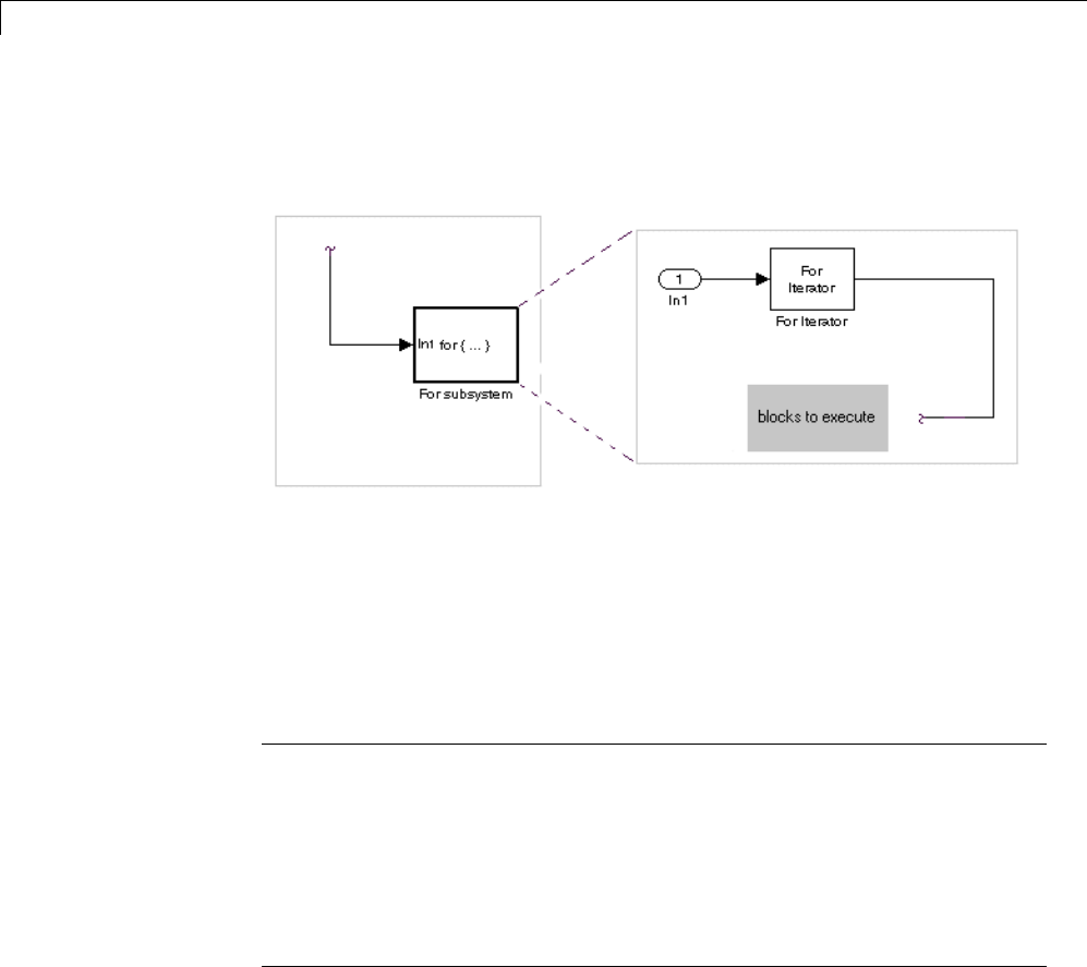
4Creating a Model
Modeling For Loops
The following diagram represents a for loop:
In this example, Simulink executes the contents of the For subsystem
multiples times at each time step. The input to the For Iterator block specifies
the number of iterations . For each iteration of the for loop, Simulink invokes
the update and output methods of all the blocks in the For subsystem in the
same order that it invokes the methods if they are in a noniterated atomic
subsystem.
Note Simulation time does not advance during execution of a For subsystem’s
iterations. Nevertheless, blocks in a For subsystem treat each iteration as a
time step. As a result, in a For subsystem, the output of a block with states
(that is, a block whose output depends on its previous input) reflects the value
of its input at the previous iteration of the for loop. The output does not reflect
that block’s input at the previous simulation time step. For example, a Unit
Delay block in a For subsystem outputs the value of its input at the previous
iteration of the for loop, not the value at the previous simulation time step.
Construct a for loop as follows:
1Drag a For Iterator Subsystem block from the Library Browser or Library
window into your model.
4-50
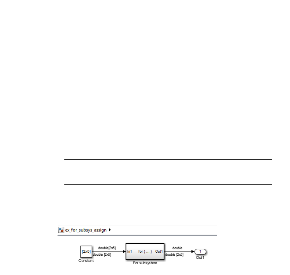
Control Flow Logic
2(Optional) Set the For Iterator block to take external or internal input for
the number of iterations it executes.
Through the properties dialog of the For Iterator block you can set it to take
input for the number of iterations through the port labeled N. This input
must come from outside the For Iterator Subsystem.
You can also set the number of iterations directly in the properties dialog.
3(Optional)SettheForIteratorblocktooutputitsiteratorvalueforusein
the block programming of the For Iterator Subsystem.
The iterator value is 1 for the first iteration and is incremented by 1 for
each succeeding iteration.
4Create a block diagram in the subsystem that defines the subsystem’s
outputs.
Note The diagram must not contain blocks with continuous states (for
example, blocks from the Continuous block library). The sample times of
all the blocks must be either inherited (-1)orconstant(inf).
The For Iterator block works well with the Assignment block to reassign
values in a vector or matrix. The following example shows the use of a For
Iterator block. Note the matrix dimensions in the data being passed.
4-51
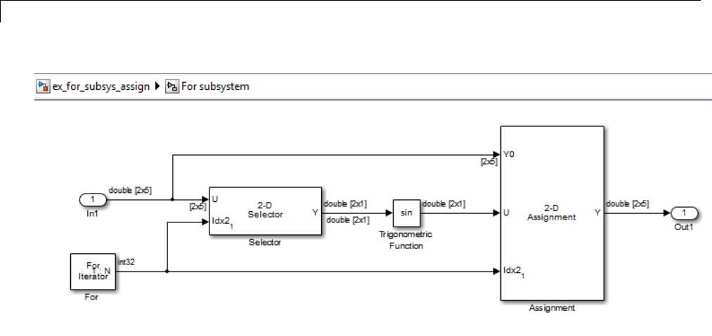
4Creating a Model
The above example outputs the sine value of an input 2-by-5 matrix (2 rows,
5 columns) using a For subsystem containing an Assignment block. The
process isasfollows.
1A2-by-5m
atrix is input to the Selector block and the Assignment block.
2The Selector block strips off a 2-by-1 matrix from the input matrix at the
column value indicated by the current iteration value of the For Iterator
block.
3The sine of the 2-by-1 matrix is taken.
4The sine value 2-by-1 matrix is passed to an Assignment block.
5The Assignment block, which takes the original 2-by-5 matrix as one of
its inputs, assigns the 2-by-1 matrix back into the original matrix at the
column location indicated by the iteration value.
The rows specified for reassignment in the property dialog for the
Assignment block in the above example are [1,2]. Because there are only
two rows in the original matrix, you could also have specified -1 for the
rows,(thatis,allrows).
4-52

Control Flow Logic
Note The Trigonometric Function block is already capable of taking the
sine of a matrix. The above example uses the Trigonometric Function
block only as an example of changing each element of a matrix with the
collaboration of an Assignment block and a For Iterator block.
4-53

4Creating a Model
Callback Functions
In this section...
“What You Can Do with Callback Functions” on page 4-54
“Callback Tracing” on page 4-55
“Create Model Callback Functions” on page 4-55
“Create Block Callback Functions” on page 4-58
“Port Callback Parameters” on page 4-63
“Callback Function Tasks” on page 4-64
What You Can Do with Callback Functions
Callback functions are a powerful way to customize your Simulink model. A
callback is a function that executes when you perform various actions on
your model, such as clicking on a block or starting a simulation. You can use
callbacks to execute a MATLAB script or other MATLAB commands. You can
use block, port, or model parameters to specify callback functions.
Common tasks that you can achieve by using callback functions include:
•Loading variables into the MATLAB workspace automatically when you
open your Simulink model
•Executing a MATLAB script by double-clicking on a block
•Executing a series of commands before starting a simulation
•Executing commands when a block diagram is closed
For examples of these tasks, see “Callback Function Tasks” on page 4-64.
4-54

Callback Functions
For related tasks, see
•“Model Workspaces” on page 4-67 for loading and modifying variables
required by your model
•“Analyze Model Dependencies” on page 13-104 for analyzing model and
block callbacks, and identifying and packaging files required by your model
Callback Tracing
Use callback tracing to determine the callbacks that Simulink invokes and in
what order the it invokes them when you open or simulate a model.
To enable callback tracing, do one of the following:
•In the Preferences dialog box, select the Callback tracing.
•Execute set_param(0, 'CallbackTracing', 'on').
This option causes the callbacks to appear in the MATLAB Command
Window as they are invoked. This option applies to all Simulink models,
not just models that are open when you the preference is enabled.
Create Model Callback Functions
You can create model callback functions interactively or programmatically.
To create model callbacks interactively, use the Callbacks pane of the model’s
Model Properties dialog box (see “Specifying Callbacks” on page 4-111).
To create a callback programmatically, use the set_param command to assign
a MATLAB expression that implements the function to the model parameter
corresponding to the callback (see “Model Callback Functions” on page 4-56).
For example, this command evaluates the variable testvar when the user
double-clicks the Test block in mymodel:
set_param('mymodel/Test', 'OpenFcn', testvar)
You can examine the clutch system model, sldemo_clutch, for routines
associated with many model callbacks. This model defines the following
callbacks:
4-55

4Creating a Model
•PreLoadFcn
•PostLoadFcn
•StartFcn
•StopFcn
•CloseFcn
Model Callback Functions
Model Callback
Function When Executed
CloseFcn Before the block diagram is closed. Any
ModelCloseFcn and DeleteFcn callbacks set on
blocks in the model are called prior to the model’s
CloseFcn.TheDestroyFcn callback of any blocks in
the model is called after the model’s CloseFcn.
ContinueFcn Before the simulation continues.
InitFcn At start of model simulation.
PauseFcn After the simulation pauses.
PostLoadFcn After the model is loaded. Defining a callback
routine for this parameter might be useful for
generating an interface that requires that the model
has already been loaded.
Note If you make structural changes with
PostLoadFcn, the function does not set the model
Dirty flag to indicate unsaved changes. You can
close the model without being prompted to save.
4-56

Callback Functions
Model Callback
Function When Executed
PostSaveFcn After the model is saved.
Note If you make structural changes with
PostSaveFcn, the function does not set the model
Dirty flag to indicate unsaved changes. You can
close the model without being prompted to save.
PreLoadFcn Before the model is loaded. Defining a callback
routine for this parameter might be useful for
loading variables used by the model.
Note In a PreLoadFcn callback routine, the
get_param command does not return the model’s
parameter values because the model is not yet
loaded.
In a PreLoadFcn routine, get_param returns:
•The default value for a standard model parameter
such as solver
•An error message for a model parameter added
with add_param
In a PostLoadFcn callback routine, however,
get_param returns the model’s parameter values
because the model is loaded.
PreSaveFcn Before the model is saved.
StartFcn Before the simulation starts.
StopFcn After the simulation stops. Output is written to
workspace variables and files before the StopFcn is
executed.
4-57

4Creating a Model
Note Beware of adverse interactions between callback functions of models
referenced by other models. (See “Model Reference”.) For example, suppose:
•Model A references model B.
•Model A’s OpenFcn creates variables in the MATLAB workspace.
•Model B’s CloseFcn clears the MATLAB workspace.
•Simulating model A requires rebuilding model B.
Rebuilding B entails opening and closing model B and hence invoking model
B’s CloseFcn, which clears the MATLAB workspace, including the variables
created by A’s OpenFcn.
Create Block Callback Functions
You can create block callback functions interactively or programmatically.
To create block callbacks interactively:
1Right-click a block.
2In the context menu, select Properties.
3In the Block Properties dialog box, select the Callback tab.
4Create the callback function. For details, see “Block Callbacks” on page
23-19.
To create a callback programmatically, use the set_param command to assign
a MATLAB expression that implements thefunctiontotheblockparameter
corresponding to the callback. For details, see “Block Callback Parameters”
on page 4-59.
4-58

Callback Functions
Note A callback for a masked subsystem cannot directly reference the
parameters of the masked subsystem (see “Masking”). Simulink evaluates
block callbacks in the MATLAB base workspace, whereas the mask
parameters reside in the masked subsystem’s private workspace. A block
callback, however, can use get_param to obtain the value of a mask
parameter. For example:
get_param(gcb, 'gain')
where gain is the name of a mask parameter of the current block.
Block Callback Parameters
This table lists the parameters for which you can define block callback
routines, and indicates when those callback routines execute. Routines that
execute before or after actions take place occur immediately before or after
the action.
Parameter When Executed
ClipboardFcn When the block is copied or cut to the system
clipboard.
CloseFcn When the block is closed using the close_system
command. The CloseFcn is not called when you
interactively close the block, when you interactively
close the subsystem or model containing the block,
or when you close the subsystem or model containing
the block using close_system.
ContinueFcn Before the simulation continues.
CopyFcn After a block is copied. The callback is recursive for
Subsystem blocks (that is, if you copy a Subsystem
block that contains a block for which the CopyFcn
parameter is defined, the routine is also executed).
The routine is also executed if an add_block
command is used to copy the block.
4-59

4Creating a Model
Parameter When Executed
DeleteChildFcn After a block or line is deleted in a subsystem. If
the block has a DeleteFcn or DestroyFcn,those
functions are executed prior to the DeleteChildFcn.
Only Subsystem blocks have a DeleteChildFcn
callback.
DeleteFcn After a block is graphically deleted, e.g., when you
graphically delete the block, invoke delete_block
on the block, or close the model containing the
block. When the DeleteFcn is called, the block
handle is still valid and can be accessed using
get_param.TheDeleteFcn callback is recursive for
Subsystem blocks. If the block is graphically deleted
by invoking delete_block or by closing the model,
after deletion the block is destroyed from memory
and the block’s DestroyFcn is called.
DestroyFcn When the block has been destroyed from memory
(for example, when you invoke delete_block on
either the block or a subsystem containing the block
or close the model containing the block). If the block
was not previously graphically deleted, the block’s
DeleteFcn is called prior to the DestroyFcn.When
the DestroyFcn is called, the block handle is no
longer valid.
ErrorFcn When an error has occurred in a subsystem. Only
Subsystem blocks have an ErrorFcn callback. For
more information, see “Subsystem Error Function
Callback” on page 4-62.
InitFcn Before the block diagramiscompiledandbefore
block parameters are evaluated.
LoadFcn After the block diagram is loaded. This callback is
recursive for Subsystem blocks.
ModelCloseFcn Before the block diagram is closed. When the model
is closed, the block’s ModelCloseFcn is called prior
to its DeleteFcn. This callback is recursive for
Subsystem blocks.
4-60

Callback Functions
Parameter When Executed
MoveFcn When the block is moved or resized.
NameChangeFcn After a block’s name or path changes. When a
Subsystem block’s path changes, the Subsystem
block recursively calls this function for all blocks
that it contains after calling its own NameChangeFcn
routine.
OpenFcn When the block is opened. Generally, use this
parameter with Subsystem blocks. The routine is
executed when you double-click the block or when an
open_system commandiscalledwiththeblockas
an argument. The OpenFcn parameter overrides the
normal behavior associated with opening a block,
which is to display the block’s dialog box or to open
the subsystem.
ParentCloseFcn Before closing a subsystem containing the block or
when the block is made part of a new subsystem
using the new_system command or in the Simulink
Editor, select Diagram > Subsystem & Model
ReferenceCreate Subsystem from Selection .
The ParentCloseFcn of blocks at the root model
level is not called when the model is closed.
PauseFcn After the simulation pauses.
PostSaveFcn After the block diagram is saved. This callback is
recursive for Subsystem blocks.
PreCopyFcn Before a block is copied. The callback is recursive for
Subsystem blocks (that is, if you copy a Subsystem
block that contains a block for which the PreCopyFcn
parameter is defined, that routine is also executed).
The block’s CopyFcn is called after all PreCopyFcn
callbacks are executed, unless the PreCopyFcn
invokes the error command either explicitly or via a
command used in any PreCopyFcn.ThePreCopyFcn
is also executed if an add_block command is used to
copy the block.
4-61

4Creating a Model
Parameter When Executed
PreDeleteFcn Before a block is graphically deleted (for example,
when the user graphically deletes the block
or invokes delete_block on the block). The
PreDeleteFcn is not called when the model
containing the block is closed. The block’s
DeleteFcn is called after the PreDeleteFcn,unless
the PreDeleteFcn invokes the error command
either explicitly or via a command used in the
PreDeleteFcn.
PreSaveFcn Before the block diagram is saved. This callback is
recursive for Subsystem blocks.
StartFcn After the block diagram is compiled and before the
simulation starts. In the case of an S-Function
block, StartFcn executes immediately before the
first execution of the block’s mdlProcessParameters
function. For more information, see “S-Function
Callback Methods”.
StopFcn At any termination of the simulation. In the case
of an S-Function block, StopFcn executes after the
block’s mdlTerminate function executes. For more
information, see “S-Function Callback Methods”.
UndoDeleteFcn When a block deletion is undone.
Note Do not call the run command from within model or block callbacks.
Doing so can result in unexpected behavior (such as errors or incorrect
results) if a Simulink model is loaded, compiled, or simulated from inside
a MATLAB function.
Subsystem Error Function Callback
The callback error function should have the following form:
newException = errorHandler(subsys, errorType, originalException)
where
4-62

Callback Functions
•errorHandler is the name of the callback function
•subsys is a handle to the subsystem in which the error occurred
•errorType is a Simulink string indicating the type of error that occurred
•originalException is an MSLException (see “Error Handling in Simulink
Using MSLException” on page 15-15)
•newException is an MSLException specifying the error message to be
displayed to the user
If you provide the original exception, then you do not need to specify the
subsystem and the error type.
The following command sets the ErrorFcn of the subsystem subsys to call
the errorHandler callback function
set_param(subsys,'ErrorFcn','errorHandler')
In such calls to set_param,donotincludetheinputargumentsofthecallback
function. Simulink displays the error message errorMsg returned by the
callback function.
Subsystem Error Function Callback: Compatibility
Considerations
In terms of backward compatibility, the following command works but is
not recommended:
errorMsg = errorHandler(subsys, errorType)
where errorMsg is a string containing the error message.
Port Callback Parameters
Block input and output ports have a single callback function parameter,
ConnectionCallback. This parameter allows you to set callbacks on ports
that are triggered every time the connectivity of these ports changes.
Examples of connectivity changes include adding a connection from the port
to a block, deleting a block connected to the port, and deleting, disconnecting,
or connecting branches or lines to the port.
4-63

4Creating a Model
Use get_param to get the port handle of a port and set_param to set the
callback on the port. The callback function must have one input argument
thatrepresentstheporthandle,buttheinputargumentisnotincludedin
the call to set_param. For example, suppose the currently selected block has
a single input port. The following code fragment sets foo as the connection
callback on the input port.
phs = get_param(gcb, 'PortHandles');
set_param(phs.Inport, 'ConnectionCallback', 'foo');
where, foo is defined as:
function foo(portHandle)
Callback Function Tasks
The following sections describe simple examples for commonly used callback
routines.
•“Load Variables Automatically When Opening a Model” on page 4-64
•“Execute a MATLAB Script by Double-Clicking a Block” on page 4-65
•“Execute Commands Before Starting Simulation” on page 4-66
Load Variables Automatically When Opening a Model
You can use the PreloadFcn callback to automatically preload variables into
the MATLAB workspace when you open your model.
Parameters in different parts of the Simulink model might require some
variables. For example, if you have a model that contains a Gain block and
the gain is specified as K, Simulink looks for the variable Kto be defined. You
can automatically define Kevery time the model is opened.
You can define variables, such as K, in a MATLAB script. You can use the
PreLoadFcn callback to execute the MATLAB script.
To create model callbacks interactively, in the Simulink Editor, select File >
Model Properties > Model Properties and use the Callbacks tab to edit
callbacks (see “Specifying Callbacks” on page 4-111).
4-64

Callback Functions
To create a callback programmatically, at the MATLAB command prompt,
enter the following :
set_param('mymodelname','PreloadFcn', 'expression')
where expression is a valid MATLAB command or a MATLAB script that
exists in your MATLAB search path.
For example, if your model is called modelname.slx and your variables are
defined in a MATLAB script called loadvar.m, you would type the following:
set_param('modelname','PreloadFcn', 'loadvar')
Now save the model. Every time you subsequently open this model, the
loadvar function will execute. You can see the variables from the loadvar.m
declared in the MATLAB workspace.
Execute a MATLAB Script by Double-Clicking a Block
You can use the OpenFcn callback to automatically execute MATLAB scripts
when the you double-click a block. MATLAB scripts can perform many
different tasks, such as defining variables for a block, making a call to
MATLAB that brings up a plot of simulated data, or generating a GUI.
The OpenFcn overrides the normal behavior which occurs when opening a
block (its parameter dialog box is displayed or a subsystem is opened).
To create block callbacks interactively, open the block’s Block Properties
dialog box and use the Callbacks tab to edit callbacks (see “Block Callbacks”
on page 23-19).
To create the OpenFcn callback programmatically, click the block to which you
want to add this property, then enter the following at the MATLAB command
prompt:
set_param(gcb,'OpenFcn','expression')
where expression is a valid MATLAB command or a MATLAB script that
exists in your MATLAB search path.
4-65

4Creating a Model
The following example shows how tosetupthecallbacktoexecutea
MATLAB script called myfunction.m when double clicking a subsystem
called mysubsystem.
set_param('mymodelname/mysubsystem','OpenFcn','myfunction')
Execute Commands Before Starting Simulation
You can use the StartFcn callback to automatically execute commands before
the simulation starts.
For example, you can make all of the Scope blocks that exist in a model come
to the forefront before running the simulation. Create a simple MATLAB
script named openscopes.m and save it on your MATLAB search path, as
shown in the following code.
% openscopes.m
% Brings scopes to forefront at beginning of simulation.
blocks = find_system(bdroot,'BlockType','Scope');
% Finds all of the scope blocks on the top level of your
% model to find scopes in subsystems, give the subsystem
% names. Type help find_system for more on this command.
for i = 1:length(blocks)
set_param(blocks{i},'Open','on')
end
% Loops through all of the scope blocks and brings them
% to the forefront
After you create this MATLAB script, set the StartFcn for the model to call
the script. For example,
set_param('mymodelname','StartFcn','openscopes')
Now every time you run the model, all of the Scope blocks automatically open
in the forefront.
4-66

Model Workspaces
Model Workspaces
In this section...
“Model Workspace Differences from MATLAB Workspace” on page 4-67
“Troubleshooting Memory Issues” on page 4-68
“Simulink.ModelWorkspace Data Object Class” on page 4-68
“Change Model Workspace Data” on page 4-69
“Specify Data Sources” on page 4-72
Model Workspace Differences from MATLAB
Workspace
Each model is provided with its own workspace for storing variable values.
The model workspace is similar to the base MATLAB workspace except that:
•Variables in a model workspace are visible only in the scope of the model.
If both the MATLAB workspace and a model workspace define a variable
of the same name, and the variable does not appear in any intervening
masked subsystem or model workspaces, the Simulink software uses
the value of the variable in the model workspace. A model’s workspace
effectively provides it with its own name space, allowing you to create
variables for the model without risk of conflict with other models.
•When the model is loaded, the workspace is initialized from a data source.
The data source can be a Model file, a MAT-file, a MATLAB file, or
MATLAB code stored in the model file. For more information, see “Data
source” on page 4-72.
•You can interactively reload and save MAT-file, MATLAB file, and
MATLAB code data sources.
•Only Simulink.Parameter and Simulink.Signal objects for which the
storage class is set to Auto canresideinamodelworkspace. Youmust
create all other Simulink data objects in the base MATLAB workspace
to ensure the objects are unique within the global Simulink context and
accessible to all models.
4-67

4Creating a Model
Note Subclasses of Simulink.Parameter and Simulink.Signal classes,
including mpt.Parameter and mpt.Signal objects (Embedded Coder®
license required), can reside in a model workspace only if their storage
class is set to Auto.
•In general, parameter variables in a model workspace are not tunable.
However, you can tune model workspace variables declared as model
arguments for referenced models. For more information, see “Using Model
Arguments” on page 6-53.
Note When resolving references to variables used in a referenced model, the
variables of the referenced model are resolved as if the parent model did
not exist. For example, suppose a referenced model references a variable
that is defined in both the parent model’s workspace and in the MATLAB
workspace but not in the referenced model’sworkspace. Inthiscase,the
MATLAB workspace is used.
Troubleshooting Memory Issues
When you use a workspace variable as a block parameter, Simulink creates a
copy of the variable during the compilation phase of the simulation and stores
the variable in memory. This can cause your system to run out of memory
during simulation, or in the process of generating code. Your system might
run out of memory if you have:
•Large models with many parameters
•Models with parameters that have a large number of elements
This issue does not affect the amount of memory that is used to represent
parameters in generated code.
Simulink.ModelWorkspace Data Object Class
An instance of the Simulink.ModelWorkspace class describes a model
workspace. Simulink creates an instance of this class for each model that
4-68

Model Workspaces
youopenduringaSimulinksession. The methods associated with this class
can be used to accomplish a variety of tasks related to the model workspace,
including:
•Listing the variables in the model workspace
•Assigning values to variables
•Evaluating expressions
•Clearing the model workspace
•Reloading the model workspace from the data source
•Saving the model workspace to a specified MAT-file or MATLAB file
•SavingtheworkspacetotheMAT-fileorMATLABfilethattheworkspace
designates as its data source
Change Model Workspace Data
The procedure for modifying a workspace depends on the data source of the
model workspace.
Change Workspace Data Whose Source Is the Model File
If the data sources of a model workspace is data stored in the model, you can
use Model Explorer or MATLAB commands to change the model’s workspace
(see“UseMATLABCommandstoChangeWorkspaceData”onpage4-71).
For example, to create a variable in a model workspace:
1Open the Model Explorer by selecting View > Model Explorer.
2In the Model Explorer Model Hierarchy pane, select the model workspace.
3Select Add > MATLAB Variable.
You can similarly use the Add menu or toolbar to add a
Simulink.Parameter object to a model workspace.
To change the value of a model workspace variable:
1Open the Model Explorer by selecting View > Model Explorer.
4-69

4Creating a Model
2In the Model Explorer Model Hierarchy pane, select the model workspace.
3In the Contents pane, select the variable.
4In the Contents pane or in Dialog pane, edit the value displayed.
To delete a model workspace variable:
1Open the Model Explorer by selecting View > Model Explorer.
2In the Model Explorer Model Hierarchy pane, select the model workspace.
3In Contents pane, select the variable.
4Select Edit > Delete.
Change Workspace Data Whose Source Is a MAT-File or
MATLAB File
You can use Model Explorer or MATLAB commands to modify workspace
data whose source is a MAT-file or MATLAB file.
To make the changes permanent, in the Model Workspace dialog box, use the
Save To Source button to save the changes to the MAT-file or MATLAB file.
1Open the Model Explorer by selecting View > Model Explorer.
2In the Model Explorer Model Hierarchy pane, right-click the workspace.
3Select the Properties menu item.
4In the Model Workspace dialog box, use the Save To Source button to
savethechangestotheMAT-fileorMATLABfile.
To discard changes to the workspace, in the Model Workspace dialog box, use
the Reinitialize From Source button.
Changing Workspace Data Whose Source Is MATLAB Code
The safest way to change data whose source is MATLAB code is to edit and
reload the source. Edit the MATLAB code and then in the Model Workspace
4-70

Model Workspaces
dialog box, use Reinitialize From Source button to clear the workspace
and re-execute the code.
To save and reload alternative versions of the workspace that result from
editing the MATLAB code source or the workspace variables themselves, see
“Exporting Workspace Variables” on page 9-60 and “Importing Workspace
Variables” on page 9-62.
Use MATLAB Commands to Change Workspace Data
To use MATLAB commands to change data in a model workspace, first get
the workspace for the currently selected model:
hws = get_param(bdroot, 'modelworkspace');
This command returns a handle to a Simulink.ModelWorkspace object
whose properties specify the source of thedatausedtoinitializethemodel
workspace. Edit the properties to change the data source.
Usetheworkspacemethodsto:
•List, set, and clear variables
•Evaluate expressions in the workspace
•Save and reload the workspace
For example, the following MATLAB code creates variables specifying model
parameters in the model workspace, saves the parameters, modifies one of
them, and then reloads the workspace to restore it to its previous state.
hws = get_param(bdroot, 'modelworkspace');
hws.DataSource = 'MAT-File';
hws.FileName = 'params';
hws.assignin('pitch', -10);
hws.assignin('roll', 30);
hws.assignin('yaw', -2);
hws.saveToSource;
hws.assignin('roll', 35);
hws.reload;
4-71
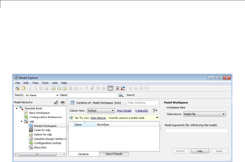
4Creating a Model
Specify Data Sources
To specify a data source for a model workspace, in the Model Explorer, use the
Model Workspace dialog box. To display the dialog box for a model workspace:
1Open the Model Explorer by selecting View > Model Explorer.
2In the Model Hierarchy pane, right-click the model workspace.
3Select the Properties menu item, which opens the Model Workspace
dialog box.
To use MATLAB commands to change data in a model workspace, see “Use
MATLAB Commands to Change Workspace Data” on page 4-71.
Data source
The Data source field in the Model Workspace dialog box includes the
following data source options for a workspace:
•Model File
Specifies that the data source is the model itself.
•MAT-File
4-72
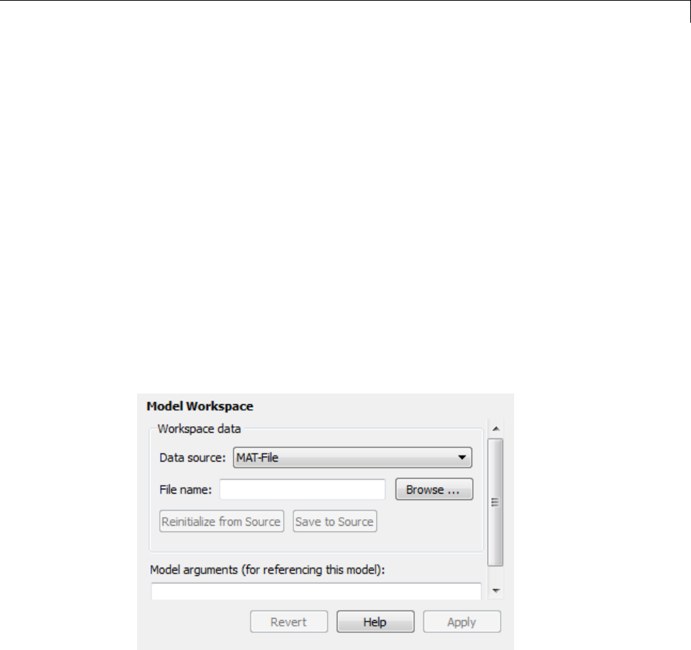
Model Workspaces
Specifies that the data source is a MAT file. Selecting this option causes
additional controls to appear (see “MAT-File and MATLAB File Source
Controls” on page 4-73).
•MATLAB File
Specifies that the data source is a MATLAB file. Selecting this option
causes additional controls to appear (see “MAT-File and MATLAB File
Source Controls” on page 4-73).
•MATLAB Code
Specifies that the data source is MATLAB code stored in the model file.
Selecting this option causes additional controls to appear (see “MATLAB
Code Source Controls” on page 4-74).
MAT-File and MATLAB File Source Controls
Selecting MAT-File or MATLAB File as the Data source for a workspace
causes the Model Workspace dialog box to display additional controls.
File name. Specifies the file name or path name of the MAT-file or MATLAB
file that is the data source for the selected workspace. If you specify a file
name, the name must reside on the MATLAB path.
4-73
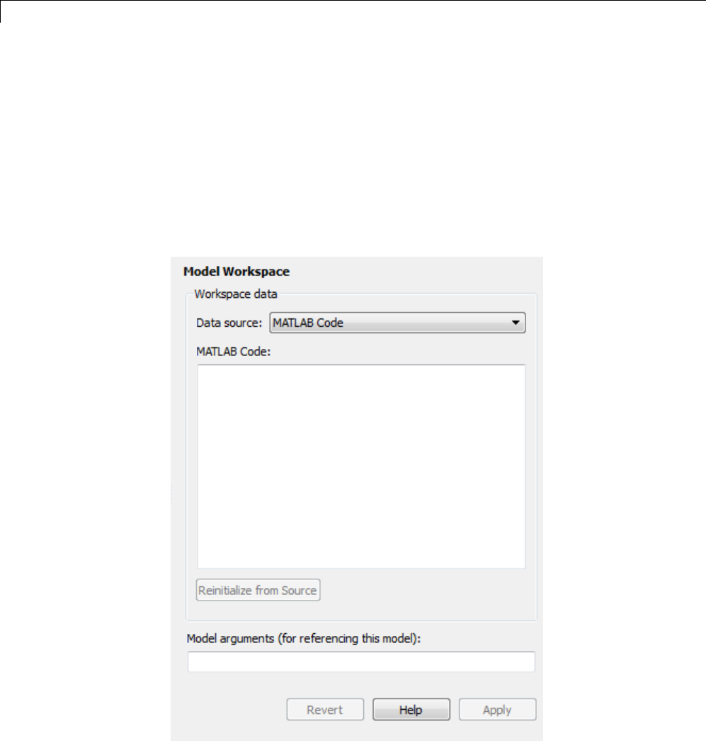
4Creating a Model
Reinitialize From Source. Clears the workspace and reloads the data from
theMAT-fileorMATLABfilespecifiedbytheFile name field.
Save To Source. Saves the workspace in the MAT-file or MATLAB file
specified by the File name field.
MATLAB Code Source Controls
Selecting MATLAB Code as the Data source for a workspace causes the Model
Workspace dialog box to display additional controls.
4-74

Model Workspaces
MATLAB Code. Specifies MATLAB code that initializes the selected
workspace. To change the initialization code, edit this field, then select the
Reinitialize from source button on the dialog box to clear the workspace
and execute the modified code.
Reinitialize from Source. Clears the workspace and executes the contents
of the MATLAB Code field.
Model Arguments (For Referencing This Model)
Specifies arguments that can be passed to instances of a model that another
model references. For more information, see “Using Model Arguments” on
page 6-53.
4-75

4Creating a Model
Symbol Resolution
In this section...
“Symbols” on page 4-76
“Symbol Resolution Process” on page 4-76
“Numeric Values with Symbols” on page 4-78
“Other Values with Symbols” on page 4-78
“Limit Signal Resolution” on page 4-79
“Explicit and Implicit Symbol Resolution” on page 4-80
Symbols
When you create a Simulink model, youcanusesymbolstoprovidevalues
and definitions for many types of entities in the model. Model entities that
you can define with symbols include block parameters, configuration set
parameters,datatypes,signals,signal properties, and bus architecture.
A symbol that provides a value or definition must be a legal MATLAB
identifier. Such an identifier starts with an alphabetic character, followed by
alphanumeric or underscore characters up to the length given by the function
namelengthmax. You can use the function isvarname to determine whether a
symbol is a legal MATLAB identifier.
A symbol provides a value or definition in a Simulink model by corresponding
to some item that:
•Exists in an accessible workspace
•Has a name that matches the symbol
•Provides the required information
Symbol Resolution Process
The process of finding an item that corresponds to a symbol is called symbol
resolution or resolving the symbol. The matching item can provide the needed
information directly, or it can itself be a symbol. A symbol must resolve to
some other item that provides the information.
4-76

Symbol Resolution
When the Simulink software compiles a model, it tries to resolve every symbol
in the model, except symbols in MATLAB code that runs in a callback or as
part of mask initialization. Depending on the particular case, the item to
which a symbol resolves can be a variable, object, or function.
Simulink attempts to resolve a symbol by searching through the accessible
workspaces in hierarchical order for a MATLAB variable or Simulink object
whosenameisthesameasthesymbol.
The search path is identical for every symbol. The search begins with the
block that uses the symbol, or is the source of a signal that is named by the
symbol, and proceeds upward. Except when simulation occurs via the sim
command, the search order is:
1Any mask workspaces, in order from the block upwards (see “How Mask
Parameters Work” on page 26-4)
2The model workspace of the model that contains the block (see “Model
Workspaces” on page 4-67)
3The MATLAB base workspace (see “What Is the MATLAB Workspace?”)
If Simulink finds a matching item in the course of this search, the search
terminates successfully at that point, and the symbol resolves to the matching
item. The result is the same as if the value of that item had appeared literally
instead of the symbol that resolved to the item. An object defined at a lower
level shadows any object defined at a higher level.
If no matching item exists on the search path, Simulink attempts to evaluate
the symbol as a function. If the function is defined and returns an appropriate
value, the symbol resolves to whatever the function returned. Otherwise, the
symbol remains unresolved, and an error occurs. Evaluation as a function
occurs as the final step whenever a hierarchical search terminates without
having found a matching workspace variable.
If the model that contains the symbol is a referenced model, and the search
reaches the model workspace but does not succeed there, the search jumps
directly to the base workspace without trying to resolve the symbol in
the workspace of any parent model. Thus a given symbol resolves to the
same item, irrespective of whether the model that contains the symbol is
4-77

4Creating a Model
a referenced model. For information about model referencing, see “Model
Reference”.
Numeric Values with Symbols
You can specify any block parameter that requires a numeric value by
providing a literal value, a symbol, or an expression, which can contain
symbols and literal values. Each symbol is resolved separately, as if none of
the others existed. Different symbols in an expression can thus resolve to
items on different workspaces, and to different types of item.
When a single symbol appears and resolves successfully, its value provides the
value of the parameter. When an expression appears, and all symbols resolve
successfully, the value of the expression provides the value of the parameter.
If any symbol cannot be resolved, or resolves to a value of inappropriate type,
an error occurs.
For example, suppose that the Gain parameter of a Gain block is given as
cos(a*(b+2)).Thesymbolcos will resolve to the MATLAB cosine function,
and aand bmust resolve to numeric values, which can be obtained from the
same or different types of items in the same or different workspaces. If the
symbols resolve to numeric values, the value returned by the cosine function
becomes the value of the Gain parameter.
Other Values with Symbols
Most symbols and expressions that use them provide numeric values, but the
same techniques that provide numeric values can provide any type of value
that is appropriate for its context.
Another common use of symbols is to name objects that provide definitions
of some kind. For example, a signal name can resolve to a signal object
(Simulink.Signal) that defines the properties of the signal, and a Bus
Creator block Data type parameter can name a bus object (Simulink.Bus)
that defines the properties of the bus. You can use symbols for many
purposes, including:
•Define data types
•Specify input data sources
4-78

Symbol Resolution
•Specify logged data destinations
For hierarchical symbol resolution, all of these different uses of symbols,
whether singly or in expressions, are the same. Each symbol is resolved, if
possible, independently of any others, and the result becomes available where
thesymbolappeared.Theonlydifferencebetweenonesymbolandanotheris
thespecificitemtowhichthesymbolresolvesandtheusemadeofthatitem.
The only requirement is that every symbol must resolve to something that
can legally appear at the location of the symbol.
Limit Signal Resolution
Hierarchical symbol resolution traverses the complete search path by default.
You can truncate the search path by using the Permit Hierarchical
Resolution option of any subsystem. This option controls what happens if
the search reaches that subsystem without resolving to a workspace variable.
The Permit Hierarchical Resolution values are:
•All
Continue searching up the workspace hierarchy trying to resolve the
symbol. This is the default value.
•None
Do not continue searching up the hierarchy.
•ExplicitOnly
Continue searching up the hierarchy only if the symbol specifies a block
parameter value, data store memory (where no block exists), or a signal or
state that explicitly requires resolution. Do not continue searching for an
implicit resolution. See “Explicit and Implicit Symbol Resolution” on page
4-80 for more information.
If the search does not find a match in the workspace, and terminates
because the value is ExplicitOnly or None, Simulink evaluates the symbol
as a function. The search succeeds or fails depending on the result of the
evaluation, as previously described.
4-79

4Creating a Model
Explicit and Implicit Symbol Resolution
Models and some types of model entities have associated parameters that can
affect symbol resolution. For example, suppose that a model includes a signal
named Amplitude, and that a Simulink.Signal object named Amplitude
exists in an accessible workspace. If the Amplitude signal’s Signal name
must resolve to Simulink signal object option is checked, the signal will
resolvetotheobject. See “Signal Properties Controls” for more information.
If the option is not checked, the signal may or may not resolve to the object,
depending on the value of Configuration Parameters > Data Validity >
Signal resolution. This parameter can suppress resolution to the object
even though the object exists, or it can specify that resolution occurs on the
basis of the name match alone. For more information, see “Diagnostics Pane:
Data Validity” > “Signal resolution”.
ResolutionthatoccursbecauseanoptionsuchasSignal name must resolve
to Simulinksignalobjectrequires it is called explicit symbol resolution.
Resolution that occurs on the basis of name match alone, without an explicit
specification, is called implicit symbol resolution.
Tip Implicit symbol resolution can be useful for fast prototyping. However,
when you are done prototypying, consider using explicit symbol resolution,
because implicit resolution slows performance, complicates model validation,
and can have nondeterministic effects.
4-80

Consult the Model Advisor
Consult the Model Advisor
In this section...
“About the Model Advisor” on page 4-81
“Start the Model Advisor” on page 4-82
“Overview of the Model Advisor Window” on page 4-85
“Overview of the Model Advisor Dashboard” on page 4-87
“Run Model Advisor Checks” on page 4-88
“Run Checks Using Model Advisor Dashboard” on page 4-91
“Highlight Model Advisor Analysis Results” on page 4-93
“Fix a Warning or Failure” on page 4-95
“Revert Changes Using Restore Points” on page 4-99
“View and Save Model Advisor Reports” on page 4-101
“Run the Model Advisor Programmatically” on page 4-104
“Check Support for Libraries” on page 4-104
“Model Advisor Limitations” on page 4-105
“Consult the Upgrade Advisor” on page 4-105
About the Model Advisor
The Model Advisor checks a model or subsystem for conditions and
configuration settings that can result in inaccurate or inefficient simulation
of the system that the model represents. If you have a Simulink Coder
or Simulink Verification and Validation™ license, the Model Advisor can
also check for model settings that result in generation of inefficient code
or code unsuitable for safety-critical applications. (For more information
about using the Model Advisor in code generation applications, see “Advice
About Optimizing Models for Code Generation” in the Simulink Coder
documentation.)
The Model Advisor produces a report that lists the suboptimal conditions or
settings that it finds, suggesting better model configuration settings where
appropriate. In some cases, the Model Advisor provides mechanisms for
4-81

4Creating a Model
automatically fixing warnings and failures or fixing them in batches. For
more information on individual checks, see “Simulink Checks”.
Software is inherently complex and may not be completely free of
errors. Model Advisor checks might contain bugs. MathWorks reports
known bugs brought to its attention on its Bug Report system at
http://www.mathworks.com/support/bugreports/. The bug reports are an
integral part of the documentation for each release. Examine periodically all
bug reports for a release as such reports may identify inconsistencies between
the actual behavior of a release you are using and the behavior described
in this documentation.
While applying Model Advisor checks to your model will increase the
likelihood that your model does not violate certain modeling standards
or guidelines, their application cannot guarantee that the system being
developed will be safe or error-free. It is ultimately your responsibility to
verify, using multiple methods, that the system being developed provides its
intended functionality and does not include any unintended functionality.
Start the Model Advisor
TherearetwoModelAdvisorGUIstorunchecksthatverifythesyntaxof
your model: the Model Advisor window and the Model Advisor dashboard.
If you want
to ...
Use the ... Set Options ...
Consistently
run the same
set of checks on
your model.
Model Advisor
dashboard. The
Model Advisor
dashboard does
not reload
checks for an
analysis, saving
analysis time.
1From the Model Editor,
select Analysis > Model
Advisor > Options.
2In the Model Advisor Options
window, for the Default GUI, select
Model Advisor Dashboard.
Select checks
torunonyour
model.
Model Advisor
window. 1From the Model Editor,
select Analysis > Model
Advisor > Options.
4-82

Consult the Model Advisor
If you want
to ...
Use the ... Set Options ...
2In the Model Advisor Options
window, for the Default GUI, select
Model Advisor.
Before starting the Model Advisor, ensure that the current folder is writable.
If the folder is not writable, when you start the Model Advisor, you see an
error message.
The Model Advisor uses the Simulink project (slprj) folder to store reports
and other information. If this folder does not exist in the current folder, the
Model Advisor creates it.
To start the Model Advisor, use any of the following methods:
To open the
Model Advisor
window or
Model Advisor
dashboard ...
For a... Do this action:
From the Model
Editor
Model or
subsystem 1Select Analysis > Model
Advisor > Model Advisor or
Model Advisor Dashboard.
Alternately, on the Model Editor
toolbar drop-down list, select
Model Advisor or Model Advisor
Dashboard.
4-83

4Creating a Model
To open the
Model Advisor
window or
Model Advisor
dashboard ...
For a... Do this action:
Note Clicking opens
the Model Advisor GUI set
in the Analysis > Model
Advisor > Options interface.
2In the System Selector window,
select the model or subsystem that
you want.
3Click OK.
From the Model
Explorer
Model In the Contents pane, select Advice
for model.model is the name of the
model that you want to check. (For
more information, see “Model Explorer
Overview” on page 9-2.)
From the context
menu
Subsystem Right-click the subsystem that you
want to check and select Model
Advisor.
Programmatically Model or
subsystem
At the MATLAB prompt, enter
modeladvisor(model).model is
a handle or name of the model or
subsystem that you want to check.
(For more information, see the
modeladvisor function reference
page.)
4-84
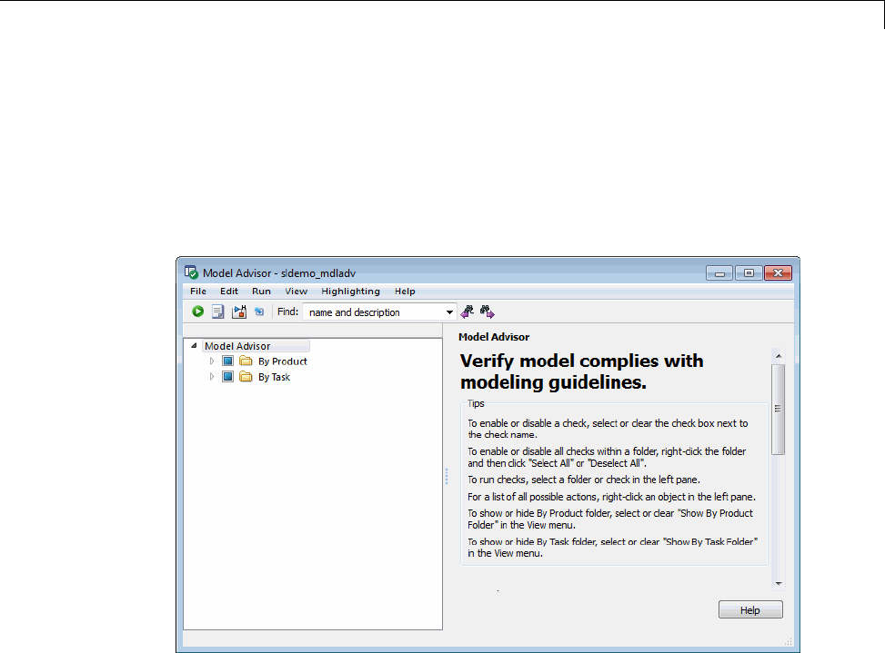
Consult the Model Advisor
Overview of the Model Advisor Window
When you start the Model Advisor, the Model Advisor window displays two
panes. TheleftpaneliststhefoldersintheModelAdvisor. Expandingthe
folders displays the available checks. The right pane provides instructions on
how to view, enable, and disable checks. It also provides a legend describing
the displayed symbols.
You can:
•Select By Task to display checks related to specific tasks, such as updating
the model to be compatible with the current Simulink version.
•Select some or all of the checks using the check boxes or context menus for
the checks, and then run one or all selected checks.
•Reset the status of the checks to not run by right-clicking Model Advisor
in the right pane and selecting Reset from the context menu.
•Specify input parameters for some checks to run (for an example, see
“Check for proper Merge block usage” in the Product > Simulink folder).
4-85

4Creating a Model
To find checks and folders, enter text in the Find: field and click the Find
Next button ( ). The Model Advisor searches in check names, folder
names, and analysis descriptions for the text.
To customize the Model Advisor checks shown in the left pane, on the toolbar,
you can select:
•View > Show By Product Folder
•View > Show By Task Folder
To run the selected checks, on the toolbar of the Model Advisor window, click
Run selected checks ().
After running checks, the Model Advisor displays the results in the right
pane. Additionally, the Model Advisor generates an HTML report of the check
results. You can view this report in a separate browser window by clicking
either Open Report ()ortheReport link at the folder level.
To view the analysis results for individual checks, you can specify that the
Model Advisor use color highlighting on the model diagram. To enable Model
Advisor highlighting, do one of the following in the Model Advisor window, on
the toolbar:
•Select Highlighting > Model Advisor Highlighting.
•ClicktheEnable Model Advisor highlighting toggle button ( ).
When you use highlighting on the model diagram, you can specify that the
Model Advisor highlight model blocks that are excluded from individual
Model Advisor checks. On the toolbar of the Model Advisor window, select
Highlighting > Highlight exclusions. If you have a Simulink Verification
and Validation license, you can create or modify exclusions to the Model
Advisor checks.
To switch to the Model Advisor dashboard, click the Switch to Model
Advisor Dashboard toggle button ( ).
4-86
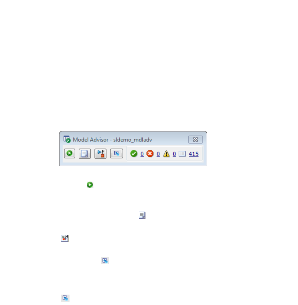
Consult the Model Advisor
Note When you open the Model Advisor for a model that you have previously
checked, the Model Advisor initially displays the check results generated
the last time that you checked the model. If you recheck the model, the new
results replace the previous results in the Model Advisor window.
Overview of the Model Advisor Dashboard
Using the Model Advisor dashboard, you can efficiently check that your
model complies with modeling guidelines. When you use the Model Advisor
dashboard, the Model Advisor does not reload checks for an analysis, saving
analysis time.
To run checks, on the Model Advisor dashboard toolbar, click Run model
advisor ().
After running checks, the Model Advisor generates an HTML report of the
check results. You can view this report in a separate browser window by
clicking the Open Report ().
To view highlighted results, click the Highlighting results toggle button
().
To switch to the Model Advisor window, click the Switch to Model Advisor
toggle button ( ).
Tip Use the Model Advisor window to select and view checks. To open the
Model Advisor window, click the Switch to Model Advisor toggle button
().
4-87

4Creating a Model
Run Model AdvisorChecks
To perform checks on your model and view the results:
1Open your model. For example, open the Model Advisor example model:
sldemo_mdladv.
2Start the Model Advisor.
aFrom the Model Editor, select Analysis > Model Advisor > Model
Advisor.
Alternately, from the Model Editor toolbar drop-down list, select
Model Advisor.
bIn the System Selector window, select the model or system that you want
to review. For example, sldemo_mdladv,andclickOK.
The Model Advisor window opens and displays checks for the
sldemo_mdladv model.
3In the left pane, expand the By Product folder to display the subfolders.
Then expand the Simulink folder to display the available checks.
4In the left pane, select the By Product folder. The right pane changes to
aBy Product view.
4-88
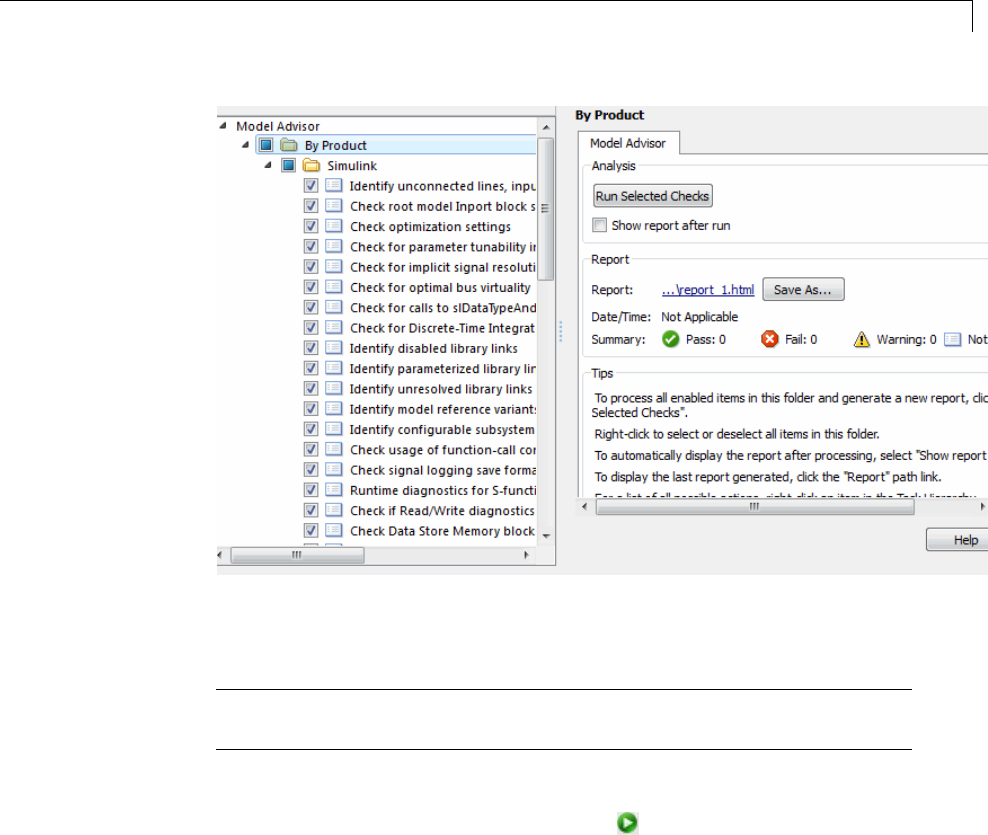
Consult the Model Advisor
5After you run the checks, select the Show report after run check box to
see an HTML report of check results.
Tip Use the Model Advisor window for interactive fixing of warnings and
failures. Model Advisor reports are best for viewing a summary of checks.
6Run the selected checks by clicking the Run Selected Checks button.
Alternately, select Run selected checks (). After the Model Advisor
runs the checks, an HTML report displays the check results in a browser
window.
4-89

4Creating a Model
7Return to the Model Advisor window, which shows the check results.
8Select an individual check to open a detailed view of the results in the right
pane. For example, selecting Identify unconnected lines, input ports,
and output ports changes the right pane to the following view. Use this
view to examine and exercise a check individually.
9In the Model Advisor window, click the Enable Model Advisor
highlighting toggle button ( ). Checks with highlighted results have
an icon.
4-90
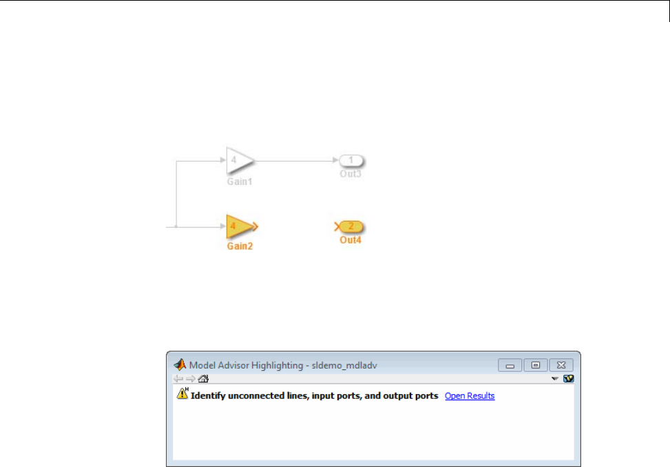
Consult the Model Advisor
•The model window opens. The blocks causing the Identify
unconnected lines, input ports, and output ports check warning
are highlighted in yellow.
•The Model Advisor Highlighting information window opens with a link
to the Model Advisor window. In the Model Advisor window, you can
find more information about the check results and how to correct the
warning condition.
10 After reviewing these check results in the Model Advisor window, you
canchoosetofixwarningsorfailures as described in “Fix a Warning or
Failure” on page 4-95.
Run Checks Using Model Advisor Dashboard
To run checks on your model using the Model Advisor dashboard:
1Open your model. For example, open the Model Advisor model,
sldemo_mdladv.
2Start the Model Advisor dashboard.
aFrom the Model Editor, select Analysis > Model Advisor > Model
Advisor Dashboard .
4-91
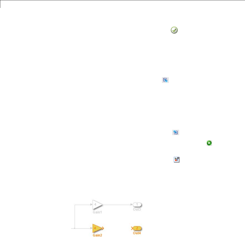
4Creating a Model
Alternately, from the Model Editor toolbar drop-down list, select
Model Advisor Dashboard.
bIn the System Selector window, select the model or system that you want
to review. For example, sldemo_mdladv and click OK.
The Model Advisor dashboard opens.
3Optionally, select or view checks to run on your model by clicking the
Switch to Model Advisor toggle button ( ). The Model Advisor window
opens.
aFor example, in the Model Advisor window, open the By Product folder
and select checks:
Identify unconnected lines, input ports, and output ports
Check root model Inport block specifications
bSwitch back to the Model Advisor dashboard by clicking the Switch to
Model Advisor Dashboard toggle button ( ).
4On the Model Advisor dashboard, click Run model advisor ()torun
the checks.
5Click the Highlighting results toggle button ( ) to view highlighted
results.
•The model window opens. The blocks causing the Identify
unconnected lines, input ports, and output ports check warning
are highlighted in yellow.
•The Model Advisor Highlighting information window opens with a link
to the Model Advisor window. In the Model Advisor window, you can
4-92
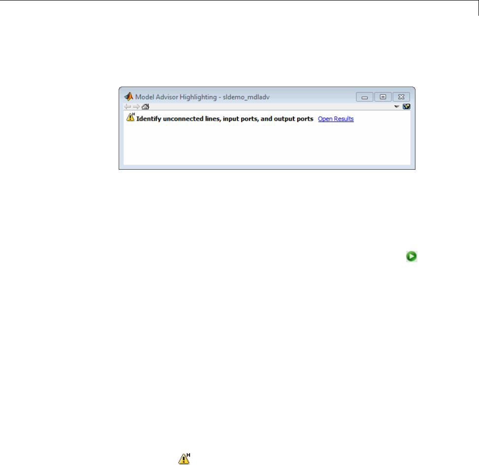
Consult the Model Advisor
find more information about the check results and how to correct the
warning condition.
6After reviewing the check results, you can choose to fix warnings or failures
as described in “Fix a Warning or Failure” on page 4-95. For example,
fix the Identify unconnected lines, input ports, and output ports
check warning:
aConnect model blocks Gain2 and Out4.
bOn the Model Advisor dashboard, click Run model advisor ()to
rerun the checks. The Model Advisor does not reload all the available
checks, saving analysis time.
The Identify unconnected lines, input ports, and output ports check
passes.
Highlight Model Advisor Analysis Results
You can use color highlighting on the model diagram to indicate the analysis
results for individual Model Advisor checks. Blocksthatpassacheck,faila
check, or cause a check warning are highlighted in color in the model window.
Model Advisor highlighting is available for the following:
•Simulink blocks
•Stateflow charts
After you run a Model Advisor analysis, checks with highlighted results are
indicated with an icon in the Model Advisor window.
To use Model Advisor highlighting:
1Run Model Advisor checks on your model.
4-93
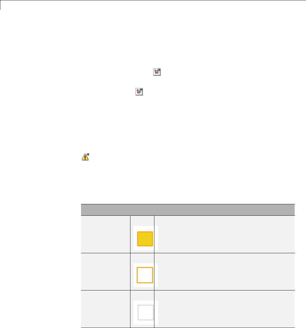
4Creating a Model
2Enable Model Advisor highlighting by doing one of the following:
•On the toolbar of the Model Advisor window, select
Highlighting > Model Advisor Highlighting.
•On the toolbar of the Model Advisor window, click the Enable
highlighting button ( ).
•On the toolbar of the Model Advisor Dashboard, click the Highlighting
results button ( ).
3Optionally, to view model blocks that are excluded from the Model Advisor
checks, select Highlighting > Highlight exclusions on the Model
Advisor window toolbar. If you have a Simulink Verification and Validation
license, you can create or modify exclusions to the Model Advisor checks .
4In the left pane of the Model Advisor window, select a check with
highlighted results. Checks with highlighted results are indicated with the
icon. Highlighting is not available for all checks.
Both the model window and a Model Advisor Highlighting information
window open. The Model Advisor Highlighting information window
provides a link to the Model Advisor window, where you can review the
check results.
Highlight Colors in the model window
Yellow with
orange border
Blocks that cause the check failure or warning.
White with
orange border
Subsystem with blocks that cause the check
warning or failure.
White with
gray border
Blocks or subsystems without highlighting.
4-94
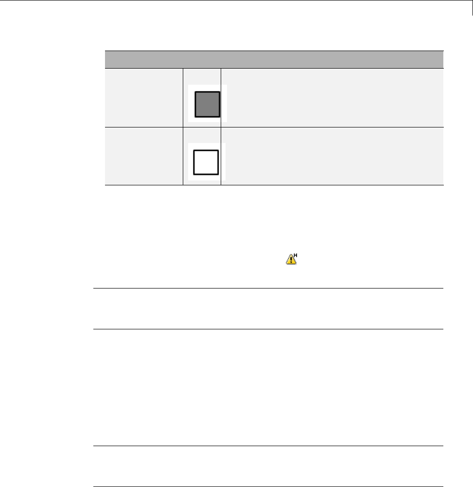
Consult the Model Advisor
Highlight Colors in the model window
Gray with
black border
Blocks that are excluded from the check.
White with
black border
Subsystems that are excluded from the check.
5After reviewing the check results inboththemodelwindowandtheModel
Advisor window, you can choose to fix warningsorfailuresasdescribedin
“Fix a Warning or Failure” on page 4-95.
6To view highlighted results for another check, in the left pane of the Model
Advisor window, select a check with an icon.
Tip If a check warns or fails and the model window highlights all blocks in
gray, closely examine the results in the Model Advisor window. A Model
Advisorcheckmightfailorwarnduetoyourparameterordiagnosticsettings.
Fix a Warning or Failure
Checks fail when a model or submodel has a suboptimal condition. A warning
result is informational. You can choose to fix the reported issue, or move on to
the next task. For more information on why a specific check does not pass, see
the check documentation. You can use Model Advisor highlighting to identify
model objects that cause a check warning or failure.
Caution When you fix a warning or failure, rerun all checks to update the
results of all checks. If you do not rerun all checks, the Model Advisor might
report an invalid check result.
To fix warnings and failures:
4-95
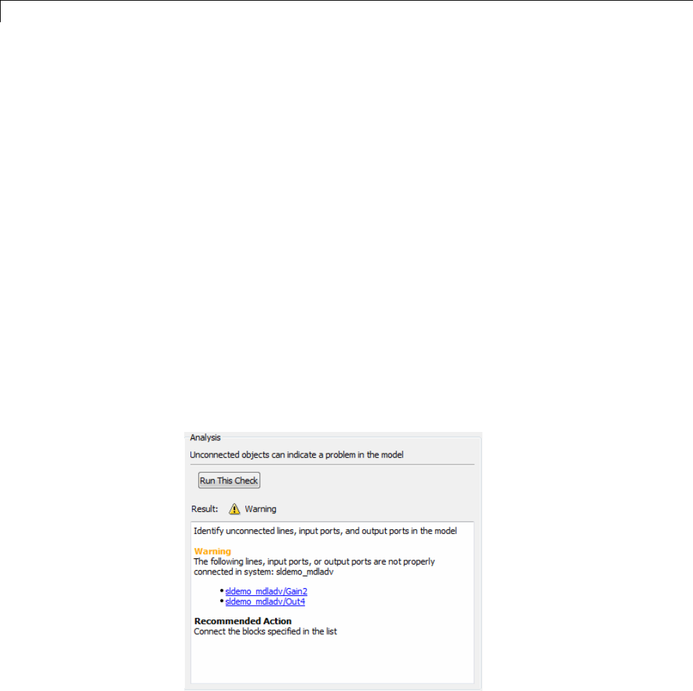
4Creating a Model
•Follow the instructions in the Analysis Result box to manually fix any
warning or failure. See “Manually Fix Warnings or Failures” on page 4-96.
•Use the Action box, when available, to automatically fix all failures. See
“Automatically Fix Warnings or Failures” on page 4-97.
•Use the Model Advisor Results Explorer, when available, to batch-fix
failures. See “Batch-Fix Warnings or Failures” on page 4-98.
Manually Fix Warnings or Failures
All checks have an Analysis Result box that describes the recommended
actions to manually fix warnings or failures.
To manually fix warnings or failures within a task:
1Optionally, save a model and data restore point so you can undo the
changes that you make. For more information, see “Revert Changes Using
Restore Points” on page 4-99.
2In the Analysis Result box, review the recommended actions. Use the
information to make changes to your model.
3Rerun the check to verify that it passes.
4-96

Consult the Model Advisor
Caution When you fix a warning or failure, rerun all checks to update
the results of all checks. If you do not rerun all checks, the Model Advisor
might report an invalid check result.
Automatically Fix Warnings or Failures
Some checks have an Action box where you can automatically fix failures.
The action box applies all of the recommended actions listed in the Analysis
Result box.
Caution Before automatically fixing failures, review the Analysis Result
box to ensure that you want to apply all of the recommended actions. If you
do not want to apply all of the recommended actions, do not use this method
to fix warnings or failures.
To automatically fix all warnings or failures within a check:
1Optionally, save a model and data restore point so you can undo the
changes that you made by clicking the Modify All button. For more
information, see “Revert Changes Using Restore Points” on page 4-99.
2In the Action box, click Modify All.
The Action Result box displays a table of changes.
3Rerun the check to verify that it passes.
Caution When you fix a warning or failure, rerun all checks to update
the results of all checks. If you do not rerun all checks, the Model Advisor
might report an invalid check result.
4-97

4Creating a Model
Batch-Fix Warnings or Failures
Some checks in the Model Advisor have an Explore Result button that starts
the Model Advisor Result Explorer. The Model Advisor Result Explorer allows
you to quickly locate, view, and change elements of a model.
The Model Advisor Result Explorer helps you to modify only the items that
the Model Advisor is checking.
If a check does not pass and you want to explore the results and make batch
changes:
1Optionally, save a model and data restore point so you can undo any
changes that you make. For more information, see “Revert Changes Using
Restore Points” on page 4-99.
2In the Analysis box, click Explore Result.
The Model Advisor Result Explorer window opens.
3Use the Model Advisor Result Explorer to modify block parameters.
4In the Model Advisor window, rerun the check to verify that it passes.
Caution When you fix a warning or failure, rerun all checks to update
the results of all checks. If you do not rerun all checks, the Model Advisor
might report an invalid check result.
4-98
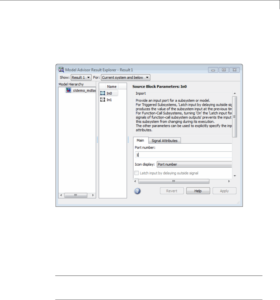
Consult the Model Advisor
In the following example, run Check root model Inport block
specifications for the sldemo_mdladv model. The result is a warning.
Clicking the Explore Result button opens the Model Advisor Result Explorer
window.
Revert Changes Using Restore Points
The Model Advisor provides a model and data restore point capability for
reverting changes that you made in responsetoadvicefromtheModel
Advisor. A restore point is a snapshot in time of the model, base workspace,
and Model Advisor. The Model Advisor maintains restore points for the model
or subsystem of interest through multiple sessions of MATLAB.
Caution A restore point saves only the current working model, base
workspace variables, and Model Advisor tree. It does not save other items,
such as libraries and referenced submodels.
4-99
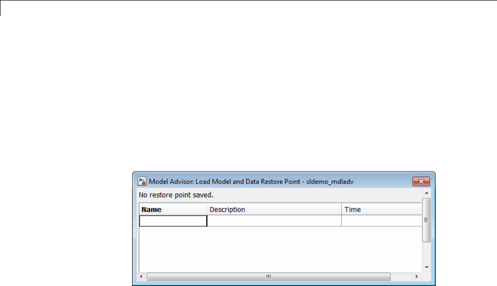
4Creating a Model
Save a Restore Point
You can save a restore point and give it a name and optional description, or
allow the Model Advisor to automatically name the restore point for you.
To save a restore point:
1Go to File > Save Restore Point As.
The Save Model and Data Restore Point dialog box opens.
2In the Name field, enter a name for the restore point.
3In the Description field, you can optionally add a description to help you
identify the restore point.
4Click Save.
The Model Advisor saves a restore point of the current model, base
workspace, and Model Advisor status.
Toquicklysavearestorepoint,gotoFile > Save Restore Point.TheModel
Advisor saves a restore point with the name autosaven.nis the sequential
number of the restore point. If you use this method, you cannot change the
name of, or add a description to, the restore point.
LoadaRestorePoint
To load a restore point:
4-100
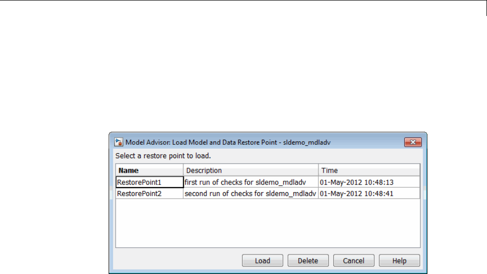
Consult the Model Advisor
1Optionally, save a model and data restore point so you can undo any
changes that you make.
2Go to File > Load Restore Point.
The Load Model and Data Restore Point dialog box opens.
3Select the restore point that you want.
4Click Load.
The Model Advisor issues a warning that the restoration will remove all
changes that you made after saving the restore point.
5Click Load to load the restore point that you selected.
The Model Advisor reverts the model, base workspace, and Model Advisor
status.
View and Save Model Advisor Reports
When the Model Advisor runs checks, it generates an HTML report of check
results. Each folder in the Model Advisor contains a report for all of the
checks in that folder and the subfolders within that folder.
View Model Advisor Reports
You can access any report by selecting a folder and clicking the link in the
Report box.
4-101
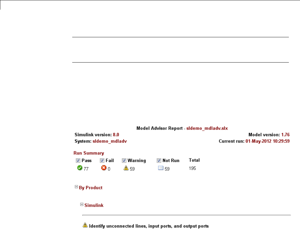
4Creating a Model
Tip While you can fix warnings and failures through Model Advisor reports,
use the Model Advisor window for interactive fixing of warnings and failures.
Model Advisor reports are best for viewing a summary of checks.
As you run checks, the Model Advisor updates the reports with the latest
information for each check in the folder. When you run the checks at different
times, a message appears in the report. Time stamps indicate when checks
have been run. The time of the current run appears at the top right of
the report. Checks that occurred during previous runs have a time stamp
following the check name.
To show only what you are interested in viewing, you can manipulate the
report.
•To view only the checks with the status that you are interested in, next to
the Run Summary status, select the appropriate check boxes. For example,
you can remove the checks that have not run by clearing the check box
next to the Not Run status.
•Minimize folder results in the report by clicking the minus sign next to the
folder name. When you minimize a folder, the report is updated to display
a run summary for that folder:
4-102
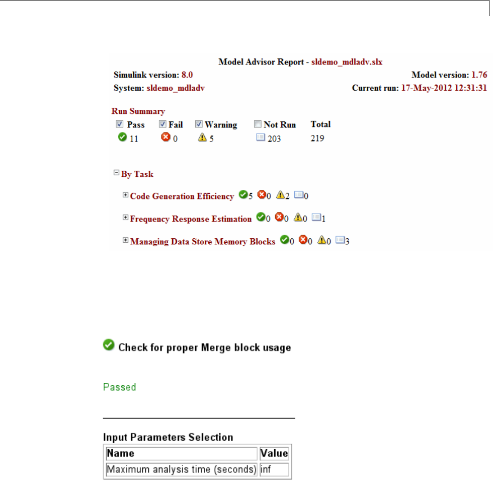
Consult the Model Advisor
Some checks have input parameters specified in the right pane of the Model
Advisor. For example, Check for proper Merge block usage has an input
parameter for Maximum analysis time (seconds). Whenyourunchecks
with input parameters, the Model Advisor displays the values of the input
parameters in the HTML report.
For more information, see the EmitInputParametersToReport property of
the Simulink.ModelAdvisor class.
4-103

4Creating a Model
Save Model Advisor Reports
You can archive a Model Advisor report by saving it to a new location.
1In the Model Advisor window, navigate to the folder that contains the
report that you want to save.
2Select the folder that you want. The right pane of the Model Advisor
window displays information about that folder, including a Report box.
3In the Report box, click Save As. A save as dialog box opens.
4In the save as dialog box, navigate to the location where you want to save
the report, and click Save. The Model Advisor saves the report to the new
location.
Note If you rerun the Model Advisor, the report is updated in the working
folder,notinthesavelocation.
You can find the full path to the report in the title bar of the
report window. Typically, the report is in the working folder:
slprj/modeladvisor/model_name.
Run the Model Advisor Programmatically
IfyouhavealicenseforSimulinkVerification and Validation, you can create
MATLAB scripts and functions that run the Model Advisor programmatically.
For example, you can create a function to check whether your model passes a
specified set of the Model Advisor checks every time that you open the model,
start a simulation, or, if you have Simulink Coder, generate code from the
model. For more information, see the ModelAdvisor.run function in the
Simulink Verification and Validation documentation.
Check Support for Libraries
There are Model Advisor checks available to verify the syntax of library
models. When you use the Model Advisor to check a library model, the Model
Advisor window indicates (~) checks that do not check libraries. To determine
if you can run the check on library models, you can also refer to the check
4-104

Consult the Model Advisor
documentation, “Capabilities and Limitations”. You cannot use checks that
require model compilation. If you have a license for Simulink Verification
and Validation, you can use an API to create custom checks which support
library models.
Model Advisor Limitations
When you use the Model Advisor to check systems, the following limitations
apply:
•If you rename a system, you must restart the Model Advisor to check that
system.
•In systems that contain a variant subsystem, the Model Advisor checks
only the active subsystem.
•Checks do not search in model blocks or subsystem blocks with the
block parameter Read/Write set to NoReadorWrite. However, on a
check-by-check basis, Model Advisor checks do search in library blocks and
masked subsystems.
For limitations that apply to specific checks, see the Limitations section
within the documentation of each check.
Consult the Upgrade Advisor
Use the Upgrade Advisor to help you upgrade and improve models with the
current release. The Upgrade Advisor can identify cases where you can
benefit by changing your model to use new features and settings in Simulink.
The Advisor provides advice for transitioning to new technologies, and
upgrading a model hierarchy.
The Upgrade Advisor can also help identifycaseswhenamodelwillnotwork
because changes and improvements in Simulink require changes to a model.
The Upgrade Advisor offers options to perform recommended actions
automatically or instructions for manual fixes.
You can open the Upgrade Advisor in the following ways:
4-105

4Creating a Model
1From the Model Editor, select Analysis > Model Advisor > Upgrade
Advisor
2From the MATLAB command line, use the upgradeadvisor function:
upgradeadvisor modelname
3Alternatively, you can open the Upgrade Advisor from the Model Advisor.
aUnder By Task checks, expand the folder Upgrading to the Current
Simulink Version and select the check Open the Upgrade Advisor.
bIn the right pane under Recommended Action,clickthelinkOpenthe
Upgrade Advisor . This action closes the Model Advisor and opens the
Upgrade Advisor.
In the Upgrade Advisor, you create reports and run checks in the same way
as when using the Model Advisor.
•Select the top Upgrade Advisor node in the left pane to run all selected
checks and create a report.
•Select each individual check to open a detailed view of the results in the
right pane. View the analysis results for recommended actions to manually
fix warnings or failures. In some cases, the Upgrade Advisor provides
mechanisms for automatically fixing warnings and failures.
Caution When you fix a warning or failure, rerun all checks to update the
results of all checks. If you do not rerun all checks, the Upgrade Advisor
might report an invalid check result.
For more information on individual checks, see
•“Model Upgrades” for upgrade checks only
•“Simulink Checks” for all upgrade and advisor checks
.
4-106

Manage Model Versions
Manage Model Versions
In this section...
“How Simulink Helps You Manage Model Versions” on page 4-107
“Model File Change Notification” on page 4-108
“Specify the Current User” on page 4-110
“Manage Model Properties” on page 4-110
“Log Comments History” on page 4-117
“Version Information Properties” on page 4-119
How Simulink Helps You Manage Model Versions
TheSimulinksoftwarehasthesefeaturestohelpyoutomanagemultiple
versions of a model:
•Use Simulink Projects to manage your project files, connect to source
control, review modified files and compare revisions. See “Simulink
Projects”.
•Model File Change Notification helps you manage work with source control
operations and multiple users. See “Model File Change Notification” on
page 4-108.
•As you edit a model, the Simulink software generates version information
about the model, including a version number, who created and last updated
the model, and an optional comments history log. The Simulink software
automatically saves these version properties with the model.
-Use the Model Properties dialog box to view and edit some of the version
information stored in the model and specify history logging.
-The Model Info block lets you display version information as an
annotation block in a model diagram.
-You can access Simulink version parameters from the MATLAB
command line or a MATLAB script.
•See Simulink.MDLInfo to extract information from a model file without
loading the block diagram into memory. You can use MDLInfo to query
4-107
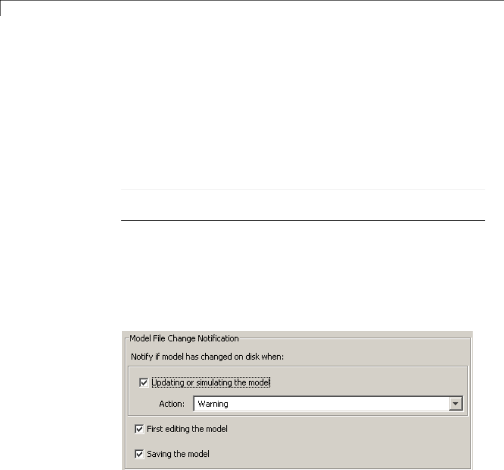
4Creating a Model
model version and Simulink version, find the names of referenced models
without loading the model into memory, and attach arbitrary metadata to
your model file.
Model File Change Notification
You can use the Simulink Preferences window to specify whether to notify if
the model has changed on disk when updating, simulating, editing, or saving
the model. This can occur, for example, with source control operations and
multiple users.
Note To programmatically check whether the model has changed on disk
since it was loaded, use the function slIsFileChangedOnDisk.
To access the Simulink Preferences window, use one of these approaches:
•In the Simulink Model Browser, select File > Simulink Preferences.
•From the MATLAB Toolstrip, in the Home tab, in the Environment
section, select Preferences.ClicktheLaunch Simulink Preferences
button .
The Model File Change Notification options are in the right pane. You can
use the three independent options as follows:
4-108

Manage Model Versions
•If you select the Updating or simulating the model check box, you can
choose what form of notification you want from the Action list:
-Warning — in the MATLAB command window.
-Error — in the MATLAB command window if simulating from the
command line, or if simulating from a menu item, in the Simulation
Diagnostics window.
-Reload model (if unmodified) — if the model is modified, you see the
prompt dialog. If unmodified, the model is reloaded.
-Show prompt dialog — in the dialog, you can choose to close and reload,
or ignore the changes.
•If you select the First editing the model check box, and the file has
changed on disk, and the block diagram is unmodified in Simulink:
-Any command-line operation that causes the block diagram to be
modified (e.g., a call to set_param) will result in a warning:
Warning: Block diagram 'mymodel' is being edited but file has
changed on disk since it was loaded. You should close and
reload the block diagram.
-Any graphical operation that modifies the block diagram (e.g., adding a
block) causes a warning dialog to appear.
•If you select the Saving the model check box, and the file has changed
on disk:
-The save_system function displays an error, unless the
OverwriteIfChangedOnDisk option is used.
-Saving the model by using the menu (File > Save)orakeyboard
shortcut causes a dialog to be shown. In the dialog, you can choose to
overwrite, save with a new name, or cancel the operation.
For more options to help you work with source control and multiple users, see
“Simulink Projects”.
4-109

4Creating a Model
Specify the Current User
When you create or update a model, your name is logged in the model for
version control purposes. The Simulink software assumes that your name
is specified by at least one of the following environment variables: USER,
USERNAME,LOGIN,orLOGNAME. If your system does not define any of these
variables, the Simulink software does not update the user name in the model.
UNIX systems define the USER environment variable and set its value to the
name you use to log on to your system. Thus, if you are using a UNIX system,
you do not have to do anything to enable the Simulink software to identify
you as the current user.
Windows systems, on the other hand, might define some or none of the
“user name” environment variables that the Simulink software expects,
depending on the version of Windows installed on your system and whether it
is connected to a network. Use the MATLAB command getenv to determine
which of the environment variables is defined. For example, enter
getenv('user')
at the MATLAB command line to determine whether the USER environment
variable exists on your Windows system. If not, you must set it yourself.
On Windows, set the USER environment variable (if it is not already defined).
Manage Model Properties
You can use the Model Properties dialog box to view and edit model
information (including some version parameters), callback functions, history,
and the model description. To open the dialog box,
•In a model, select File > Model Properties.
•In a library, select File > Library Properties.
Library Properties includes an additional tab, Forwarding Table,
for specifying the mapping from old library blocks to new library
blocks. For information on using the Fowarding Table, see “Make
Backward-Compatible Changes to Libraries” on page 28-22.
4-110
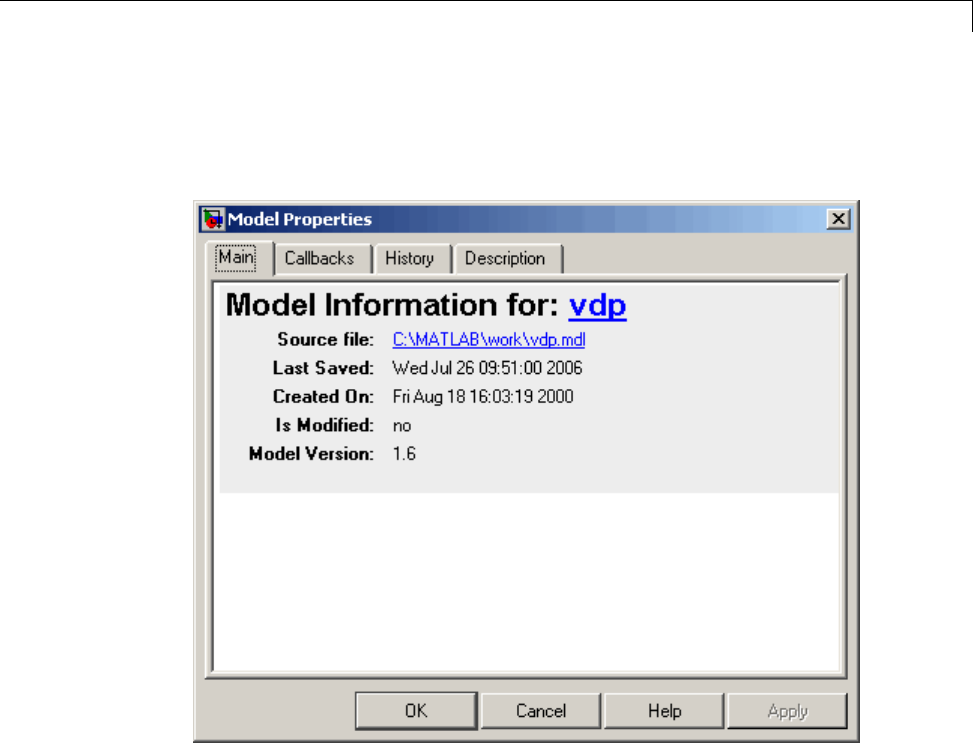
Manage Model Versions
Model Properties and Library Properties both include the tabs Main Model
Information, Callbacks, History and Description. The controls in the shared
tabs are described next on this page.
The dialog box includes the following panes.
Viewing Model Information
The Main pane summarizes information about the current version of this
model, such as whether the model is modified, the Model Version, and Last
Saved date. You can edit some of this information in the History tab, see
“Viewing and Editing Model Information and History” on page 4-112.
Specifying Callbacks
Use the Callbacks pane to specify functions to be invoked at specific points
in the simulation of the model.
4-111
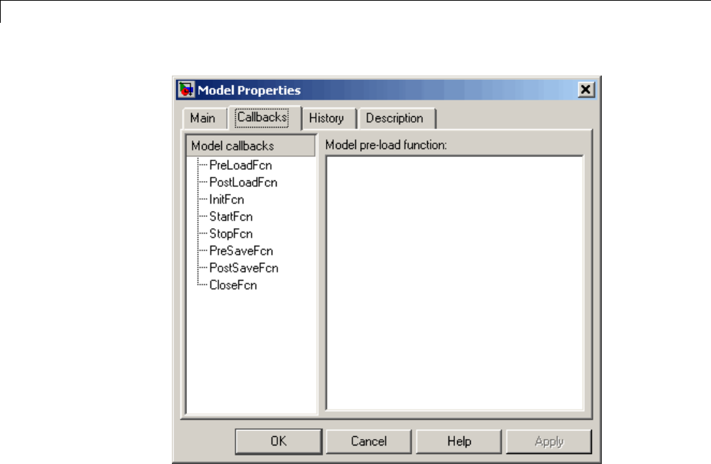
4Creating a Model
In the left pane, select the callback. In the right pane, enter the name of the
function you want to be invoked for the selected callback. See “Create Model
Callback Functions” on page 4-55 for information on the callback functions
listed on this pane.
Viewing and Editing Model Information and History
Use the History pane to view and edit model information, and to enable,
view, and edit this model’s change history in the lower Model history field.
To use the history controls see “Log Comments History” on page 4-117.
4-112
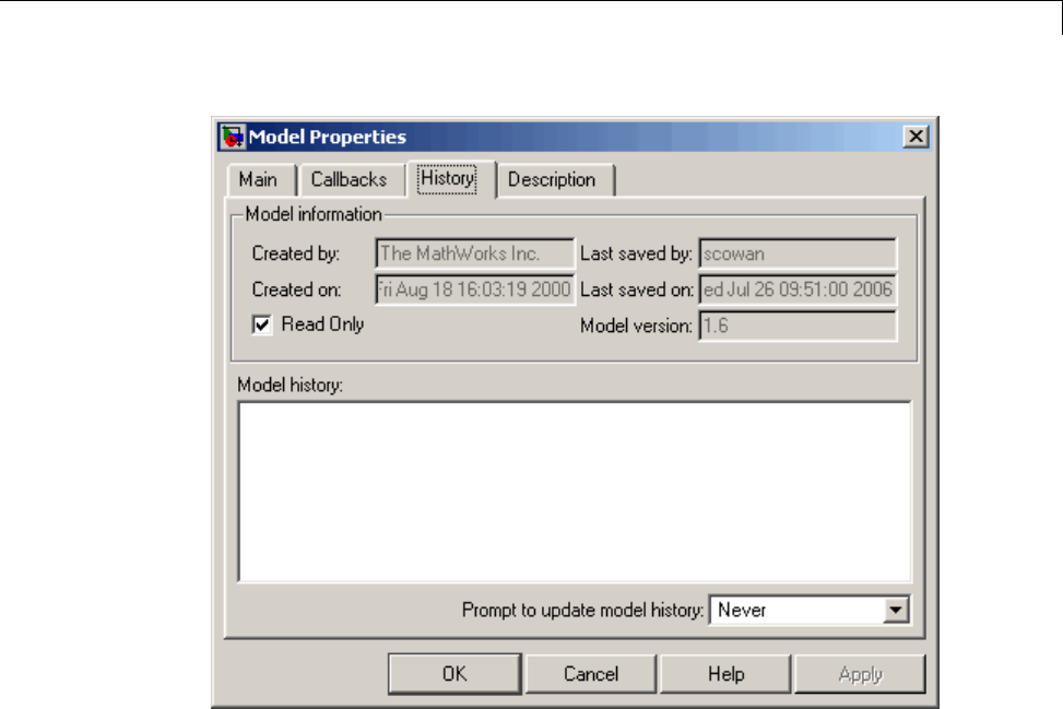
Manage Model Versions
Viewing Model Information. When the Read Only check box is selected,
you can view but not edit the following grayed out fields.
•Created by
Name of the person who created this model. The Simulink software sets
this property to the value of the USER environment variable when you
create the model.
•Created on
Date and time this model was created.
•Last saved by
Name of the person who last saved this model. The Simulink software sets
the value of this parameter to the value of the USER environment variable
when you save a model.
4-113

4Creating a Model
•Last saved on
Date that this model was last saved. The Simulink software sets the value
of this parameter to the system date and time whenever you save a model.
•Model version
Version number for this model.
Editing Model Information. Clear the Read Only check box to edit model
information. When the check box is deselected, the dialog box shows the
format strings or values for the following fields. You can edit all but the
Created on field, as described.
4-114
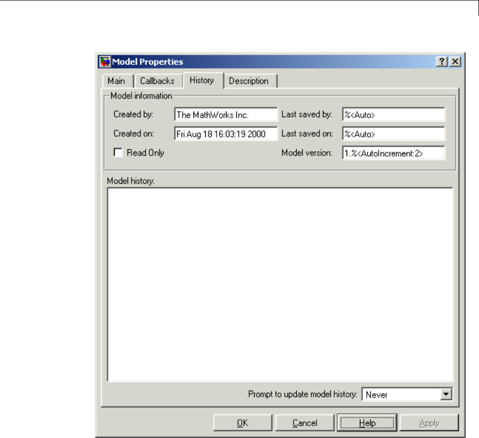
Manage Model Versions
•Created by
Name of the person who created this model. The Simulink software sets
this property to the value of the USER environment variable when you
createthemodel. Editthisfieldtochangethevalue.
•Created on
4-115

4Creating a Model
Date and time this model was created. Do not edit this field.
•Last saved by
Enter a format string describing the format used to display the Last saved
by value in the History pane and the ModifiedBy entry in the history log
and Model Info blocks. The value of this field can be any string. The string
can include the tag %<Auto>. Simulink replaces occurrences of this tag with
the current value of the USER environment variable.
•Last saved on
Enter a format string describing the format used to display the Last saved
on date in the History pane and the ModifiedOn entry in the history log
and the in Model Info blocks. The value of this field can be any string.
The string can contain the tag %<Auto>. The Simulink software replaces
occurrences of this tag with the current date and time.
•Model version
Enter a format string describing the format used to display the model
version number in the Model Properties pane and in Model Info blocks.
The value of this parameter can be any text string. The text string can
include occurrences of the tag %<AutoIncrement:#> where #is an integer.
Simulink replaces the tag with an integer when displaying the model’s
version number. For example, it displays the tag
1.%<AutoIncrement:2>
as
1.2
Simulink increments # by 1 when saving the model. For example, when
you save the model,
1.%<AutoIncrement:2>
becomes
1.%<AutoIncrement:3>
and the model version number is reported as 1.3.
4-116
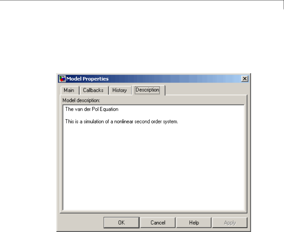
Manage Model Versions
Viewing and Editing the Model Description
UsetheDescriptionpanetoenteradescription of the model. You can view
the model description by typing help followed by the model name at the
MATLAB prompt. The contents of the Model description field appear in
the Command Window.
Log Comments History
You can create and store a record of changes to a model in the model itself.
The Simulink software compiles the history automatically from comments
that you or other users enter when they save changes to a model. For more
flexibility adding labels and comments to models and submissions, see instead
“Simulink Projects”.
4-117
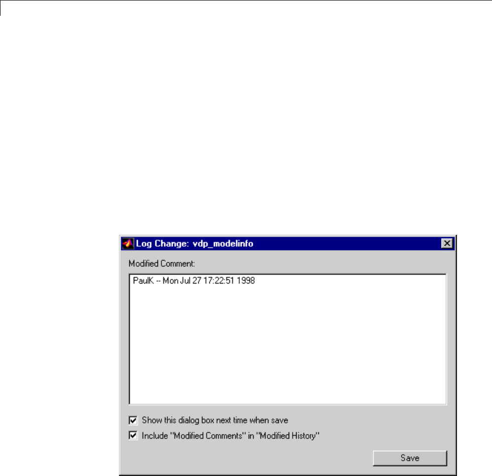
4Creating a Model
Logging Changes
To start a change history,
1Select File > Model Properties.
2In the Model Properties dialog box, select the History tab.
3Select When saving model from the Prompt to update model history
list.
This causes Simulink to prompt you to enter a comment when saving the
model.
The next time you save the model, the Log Change dialog box prompts you
to enter a comment.
For example you could describe changes that you have made to the model
since the last time you saved it. To add an item to the model’s change history,
4-118

Manage Model Versions
enter the item in the Modified Comments edit field and click Save.The
information is stored in the model’s change history log.
If you do not want to enter an item for this session, clear the Include
"Modified Comments" in "Modified History" option.
To discontinue change logging, either:
•In the Log Change dialog box, clear the check box Show this dialog box
next time when save.
•In the Model Properties dialog box History pane, select Never from the
Prompt to update model history list.
Viewing and Editing the Model History Log
In the Model Properties dialog box you can view and edit the model history on
the History tab.
The model history text field displays the history for the model in a scrollable
text field. To change the model history, edit the contents of this field.
Version Information Properties
Some version information is stored as model parameters in a model. You can
access this information from the MATLAB command line or from a MATLAB
script, using the Simulink get_param command.
The following table describes the model parameters used by Simulink to store
version information.
Property Description
Created Date created.
Creator Name of the person who created this
model.
4-119

4Creating a Model
Property Description
Description User-entered description of this model.
Enteroreditadescriptiononthe
Description tab of the Model Properties
dialog box. You can view the model
description by typing
help 'mymodelname'
at the MATLAB command line.
LastModifiedBy Name of the user who last saved the model.
LastModifiedDate Date when the model was last saved.
ModifiedBy Current value of the user name of the
person who last modified this model.
When you save, this information is saved
with the file as LastModifiedBy.
ModifiedByFormat Format of the ModifiedBy parameter.
Value can be any string. The string can
include the tag %<Auto>.TheSimulink
software replaces the tag with the current
value of the USER environment variable.
ModifiedDateFormat Format of the ModifiedDate parameter.
Value can be any string. The string
can include the tag %<Auto>. Simulink
replaces the tag with the current date and
time when saving the model.
ModifiedComment Comment entered by user who last
updated this model.
ModifiedHistory History of changes to this model.
4-120

Manage Model Versions
Property Description
ModelVersion Version number.
ModelVersionFormat Format of model version number. Can be
any string. The string can contain the
tag %<AutoIncrement:#> where #is an
integer. Simulink replaces the tag with #
when displaying the version number. It
increments #when saving the model.
LibraryVersion is a block parameter for a linked block. LibraryVersion is
the ModelVersion of the library at the time the link was created.
For source control version information, see instead “Simulink Projects”.
4-121

4Creating a Model
Model Discretizer
In this section...
“What Is the Model Discretizer?” on page 4-122
“Requirements” on page 4-122
“Discretize a Model from the Model Discretizer GUI” on page 4-122
“View the Discretized Model” on page 4-132
“Discretize Blocks from the Simulink Model” on page 4-135
“Discretize a Model from the MATLAB Command Window” on page 4-146
What Is the Model Discretizer?
Model Discretizer selectively replaces continuous Simulink blocks with
discrete equivalents. Discretization is a critical step in digital controller
design and for hardware in-the-loop simulations.
You can use the Model Discretizer to:
•Identify a model’s continuous blocks
•Change a block’s parameters from continuous to discrete
•Apply discretization settings to all continuous blocks in the model or
selected blocks
•Create configurable subsystems that contain multiple discretization
candidates along with the original continuous block(s)
•Switch among the different discretization candidates and evaluate the
resulting model simulations
Requirements
To use Model Discretizer, you must have a Control System Toolbox™ license,
Version 5.2 or later.
Discretize a Model from the Model Discretizer GUI
To discretize a model:
4-122

Model Discretizer
•Start the Model Discretizer
•Specify the Transform Method
•Specify the Sample Time
•Specify the Discretization Method
•Discretize the Blocks
4-123
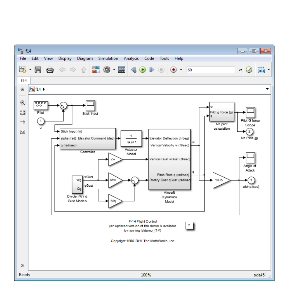
4Creating a Model
The f14 model shows the steps in discretizing a model.
4-124
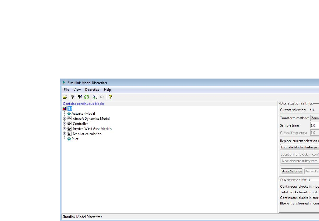
Model Discretizer
Start Model Discretizer
To open the tool, in the Simulink Editor, select Analysis > Control
Design > Model Discretizer.
The Simulink Model Discretizer opens.
Alternatively, you can open Model Discretizer from the MATLAB Command
Window using the slmdldiscui function.
The following command opens the Simulink Model Discretizer window
with the f14 model:
slmdldiscui('f14')
To open a new model or library from Model Discretizer, select File > Load
model.
4-125

4Creating a Model
Specify the Transform Method
The transform method specifies the type of algorithms used in the
discretization. For more information on the different transform methods, see
the Control System Toolbox documentation.
The Transform method drop-down list contains the following options:
•zero-order hold
Zero-order hold on the inputs.
•first-order hold
Linear interpolation of inputs.
•tustin
Bilinear (Tustin) approximation.
•tustin with prewarping
Tustin approximation with frequency prewarping.
•matched pole-zero
Matched pole-zero method (for SISO systems only).
Specify the Sample Time
Enter the sample time in the Sample time field.
You can specify an offset time by entering a two-element vector for discrete
blocks or configurable subsystems. The first element is the sample time and
the second element is the offset time. For example, an entry of [1.0 0.1]
would specify a 1.0 second sample time with a 0.1 second offset. If no offset is
specified, the default is zero.
You can enter workspace variables when discretizing blocks in the s-domain.
See “Discrete blocks (Enter parameters in s-domain)” on page 4-127.
Specify the Discretization Method
Specify the discretization method in the Replace current selection with
field. The options are
4-126

Model Discretizer
•“Discrete blocks (Enter parameters in s-domain)” on page 4-127
Creates a discrete block whose parameters are retained from the
corresponding continuous block.
•“Discrete blocks (Enter parameters in z-domain)” on page 4-128
Creates a discrete block whose parameters are “hard-coded“ values placed
directly into the block’s dialog.
•“Configurable subsystem (Enter parameters in s-domain)” on page 4-129
Create multiple discretization candidates using s-domain values for the
current selection. A configurable subsystem can consist of one or more
blocks.
•“Configurable subsystem (Enter parameters in z-domain)” on page 4-130
Create multiple discretization candidates in z-domain for the current
selection. A configurable subsystem can consist of one or more blocks.
Discrete blocks (Enter parameters in s-domain). Creates a discrete block
whose parameters are retained from the corresponding continuous block.
Thesampletimeandthediscretizationparametersarealsoontheblock’s
parameter dialog box.
The block is implemented as a masked discrete block that uses c2d to
transform the continuous parameters to discrete parameters in the mask
initialization code.
Theseblockshavetheuniquecapabilityof reverting to continuous behavior if
thesampletimeischangedtozero.Enteringthesampletimeasaworkspace
variable ('Ts', for example) allows for easy changeover from continuous to
discrete and back again. See “Specify the Sample Time” on page 4-126.
Note Parameters are not tunable when Inline parameters is selected in
the model’s Configuration Parameters dialog box.
4-127
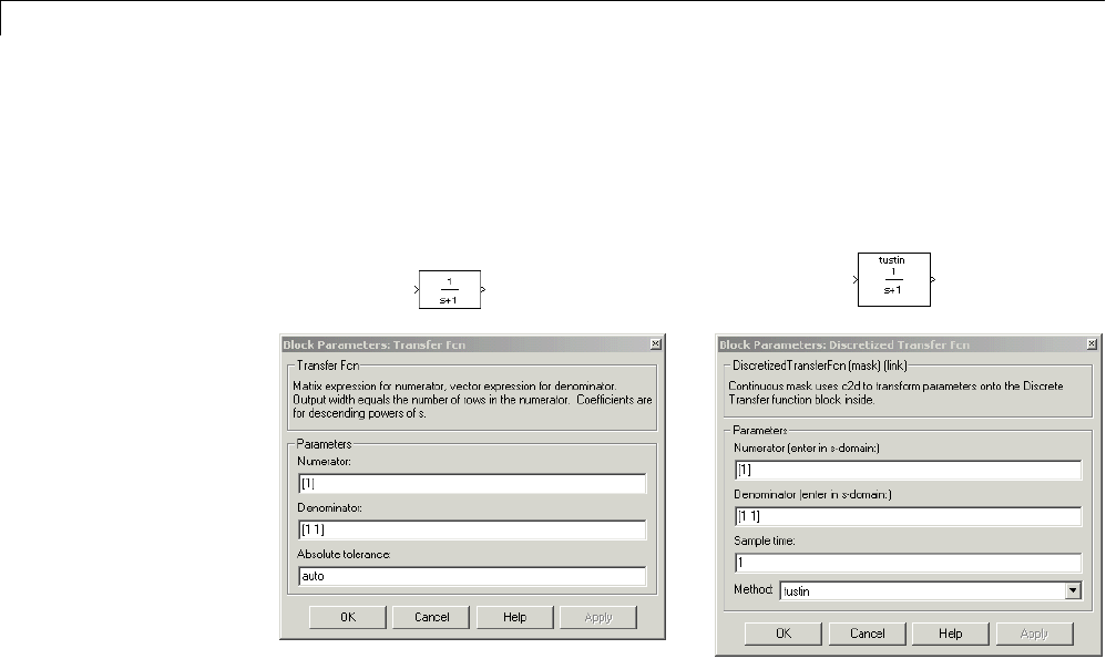
4Creating a Model
The following figure shows a continuous Transfer Function block next to a
Transfer Function block that has been discretized in the s-domain. The Block
Parameters dialog box for each block appears below the block.
Discrete blocks (Enter parameters in z-domain). Creates a discrete block
whose parameters are “hard-coded” values placed directly into the block’s
dialog box. Model Discretizer uses the c2d function to obtain the discretized
parameters, if needed.
For more help on the c2d function, type the following in the Command
Window:
help c2d
4-128
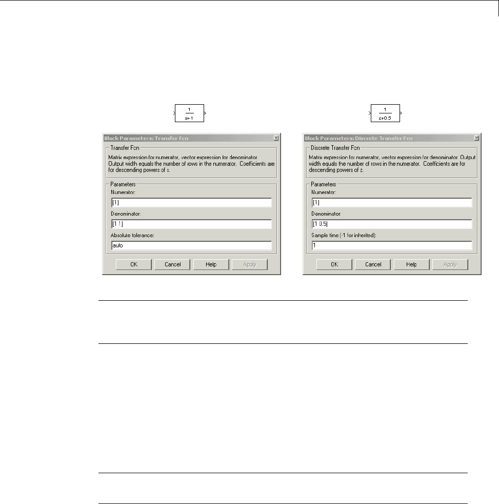
Model Discretizer
The following figure shows a continuous Transfer Function block next to a
Transfer Function block that has been discretized in the z-domain. The Block
Parameters dialog box for each block appears below the block.
Note If you want to recover exactly the original continuous parameter values
after the Model Discretization session, you should enter parameters in the
s-domain.
Configurable subsystem (Enter parameters in s-domain). Create
multiple discretization candidates using s-domain values for the current
selection. A configurable subsystem can consist of one or more blocks.
The Location for block in configurable subsystem field becomes active
when this option is selected. This option allows you to either create a new
configurable subsystem or overwrite an existing one.
Note The current folder must be writable in order to save the library or
libraries for the configurable subsystem option.
4-129

4Creating a Model
Configurable subsystem (Enter parameters in z-domain). Create
multiple discretization candidates in z-domain for the current selection. A
configurable subsystem can consist of one or more blocks.
The Location for block in configurable subsystem field becomes active
when this option is selected. This option allows you to either create a new
configurable subsystem or overwrite an existing one.
Note The current folder must be writable in order to save the library or
libraries for the configurable subsystem option.
Configurable subsystems are stored in a library containing the discretization
candidates and the original continuous block. The library will be named
<model name>_disc_lib and it will be stored in the current . For example
a library containing a configurable subsystem created from the f14 model
will be named f14_disc_lib.
If multiple libraries are created from the same model, then the filenames
will increment accordingly. For example, the second configurable subsystem
library created from the f14 modelwillbenamedf14_disc_lib2.
You can open a configurable subsystem library by right-clicking on the
subsystem in the model and selecting Link options > Go to library block
from the pop-up menu.
Discretize the Blocks
To discretize blocks that are linked to a library, you must either discretize the
blocks in the library itself or disable the library links in the model window.
You can open the library from Model Discretizer by selecting Load model
from the File menu.
You can disable the library links by right-clicking on the block and selecting
Link options -> Disable link from the pop-up menu.
There are two methods for discretizing blocks.
4-130

Model Discretizer
Select Blocks and Discretize.
1Select a block or blocks in the Model Discretizer tree view pane.
To choose multiple blocks, press and hold the Ctrl button on the keyboard
while selecting the blocks.
Note You must select blocks from the Model Discretizer tree view. Clicking
blocks in the editor does not select them for discretization.
2Select Discretize current block from the Discretize menu if a single
block is selected or select Discretize selected blocks from the Discretize
menu if multiple blocks are selected.
You can also discretize the current block by clicking the Discretize button,
shown below.
Store the Discretization Settings and Apply Them to Selected Blocks
in the Model.
1Enter the discretization settings for the current block.
2Click Store Settings.
This adds the current block with its discretization settings to the group
of preset blocks.
3Repeatsteps1and2,asnecessary.
4Select Discretize preset blocks from the Discretize menu.
4-131

4Creating a Model
Deleting a Discretization Candidate from a Configurable
Subsystem
You can delete a discretization candidate from a configurable subsystem by
selecting it in the Location for block in configurable subsystem field and
clicking the Delete button, shown below.
Undoing a Discretization
To undo a discretization, click the Undo discretization button, shown below.
Alternatively, you can select Undo discretization from the Discretize
menu.
This operation undoes discretizations in the current selection and its children.
For example, performing the undo operation on a subsystem will remove
discretization from all blocks in all levels of the subsystem’s hierarchy.
View the Discretized Model
Model Discretizer displays the model in a hierarchical tree view.
Viewing Discretized Blocks
The block’s icon in the tree view becomes highlighted with a “z” when the
block has been discretized.
4-132
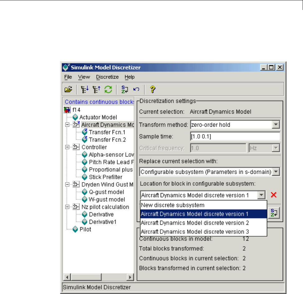
Model Discretizer
The following figure shows that the Aircraft Dynamics Model subsystem has
been discretized into a configurable subsystem with three discretization
candidates.
The other blocks in this f14 model have not been discretized.
4-133
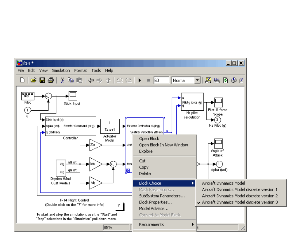
4Creating a Model
The following figure shows the Aircraft Dynamics Model subsystem of the f14
example model after discretization into a configurable subsystem containing
the original continuous model and three discretization candidates.
4-134
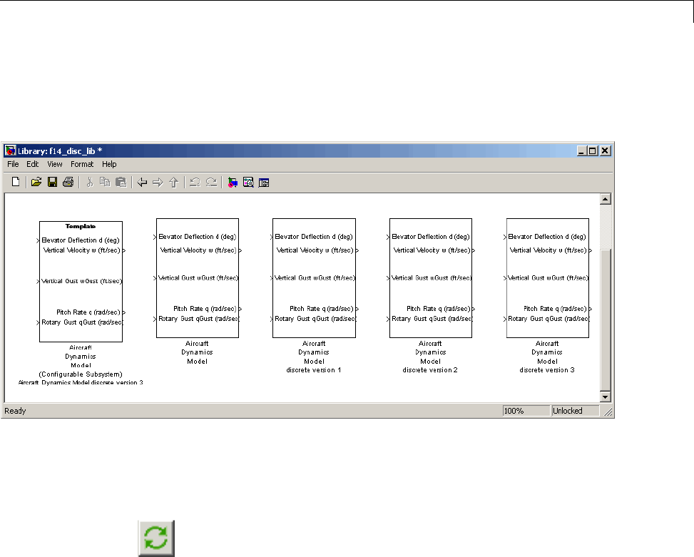
Model Discretizer
The following figure shows the library containing the Aircraft Dynamics
Model configurable subsystem with the original continuous model and three
discretization candidates.
Refreshing Model Discretizer View of the Model
To refresh Model Discretizer’s tree view of the model when the model has been
changed, click the Refresh button, shown below.
Alternatively, you can select Refresh from the View menu.
Discretize Blocks from the Simulink Model
You can replace continuous blocks in a Simulink software model with the
equivalent blocks discretized in the s-domain using the Discretizing library.
The procedure below shows how to replace a continuous Transfer Fcn block in
the Aircraft Dynamics Model subsystem of the f14 model with a discretized
Transfer Fcn block from the Discretizing Library. The block is discretized
4-135
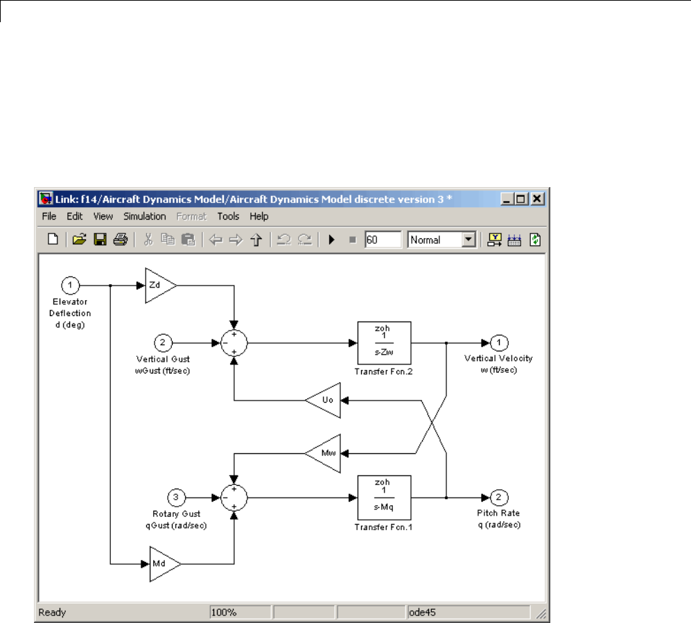
4Creating a Model
in the s-domain with a zero-order hold transform method and a two second
sample time.
1Open the f14 model.
2Open the Aircraft Dynamics Model subsystem in the f14 model.
3Open the Discretizing library window.
Enter discretizing at the MATLAB command prompt.
4-136
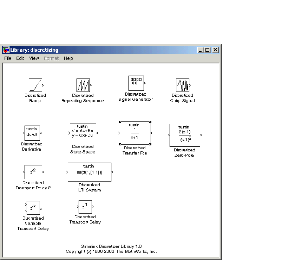
Model Discretizer
The Library: discretizing window opens.
This library contains s-domain discretized blocks.
4Add the Discretized Transfer Fcn (with initial states) block to the
f14/Aircraft Dynamics Model window.
4-137
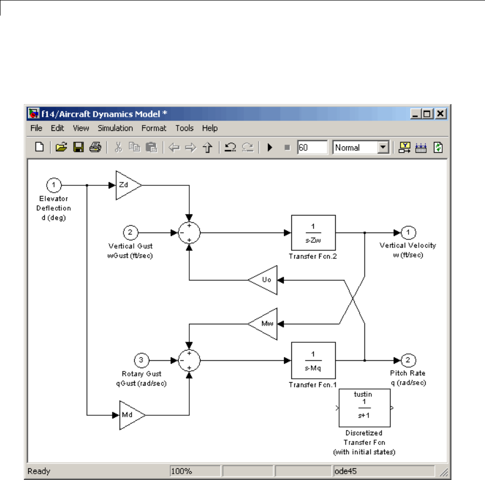
4Creating a Model
aClick the Discretized Transfer Fcn block in the Library: discretizing
window.
bDrag it into the f14/Aircraft Dynamics Model window.
5Open the parameter dialog box for the Transfer Fcn.1 block.
4-138
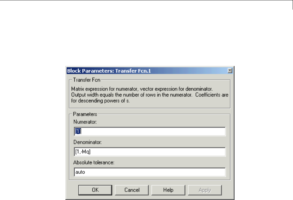
Model Discretizer
Double-click the Transfer Fcn.1 block in the f14/Aircraft Dynamics
Model window.
The Block Parameters: Transfer Fcn.1 dialog box opens.
6Open the parameter dialog box for the Discretized Transfer Fcn block.
Double-click the Discretized Transfer Fcn block in the f14/Aircraft
Dynamics Model window.
4-139
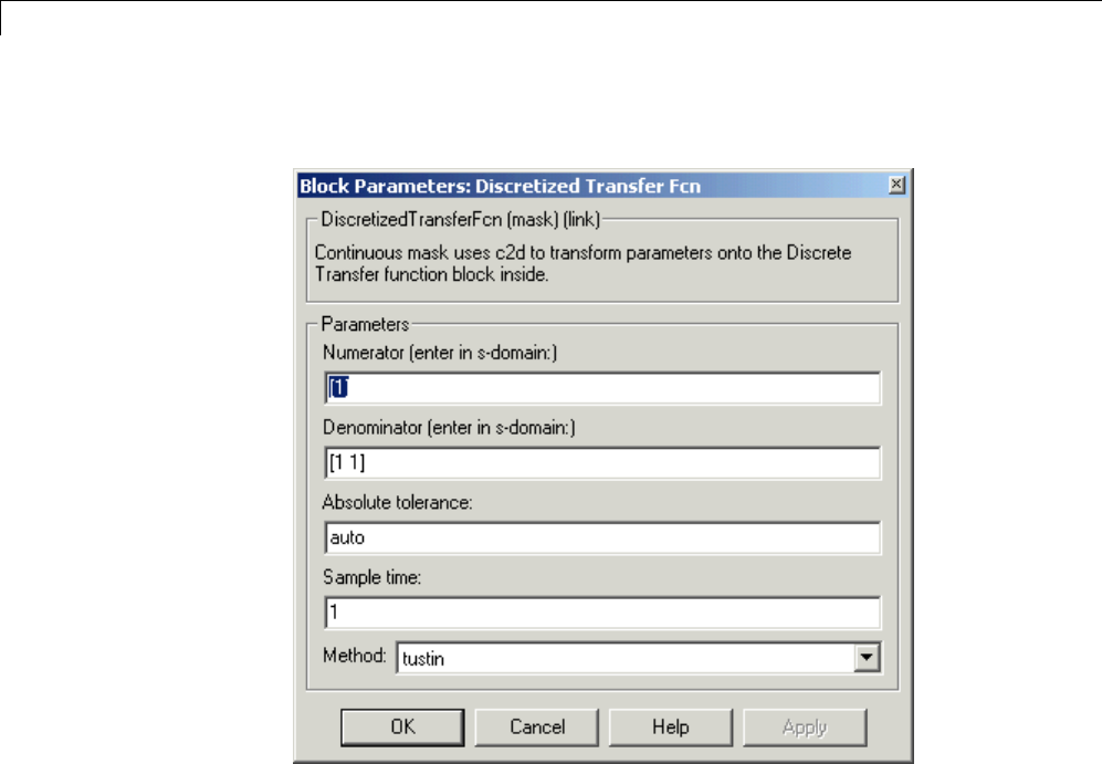
4Creating a Model
The Block Parameters: Discretized Transfer Fcn dialog box opens.
4-140
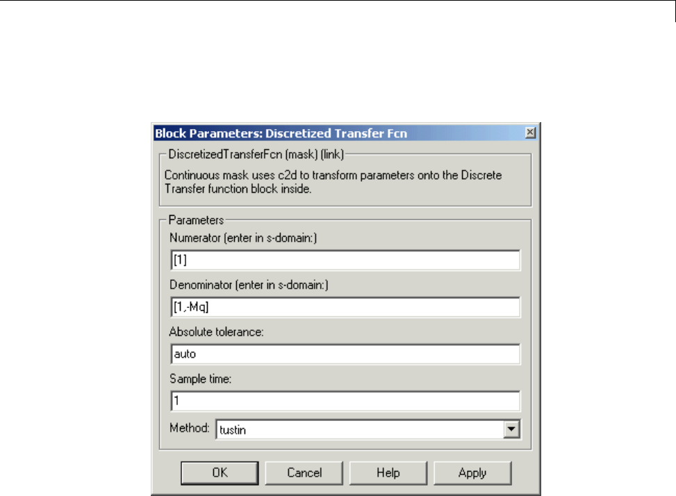
Model Discretizer
Copy the parameter information from the Transfer Fcn.1 block’s dialog box
to the Discretized Transfer Fcn block’s dialog box.
7Enter 2in the Sample time field.
8Select zoh from the Method drop-down list.
4-141
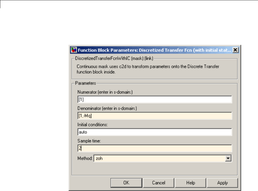
4Creating a Model
The parameter dialog box for the Discretized Transfer Fcn now looks like
this.
9Click OK.
4-142
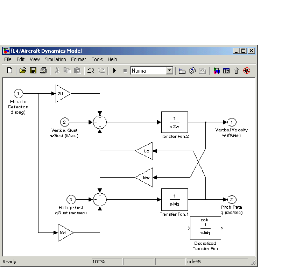
Model Discretizer
The f14/Aircraft Dynamics Model window now looks like this.
10 Delete the original Transfer Fcn.1 block.
aClick the Transfer Fcn.1 block.
bPress the Delete key.
4-143
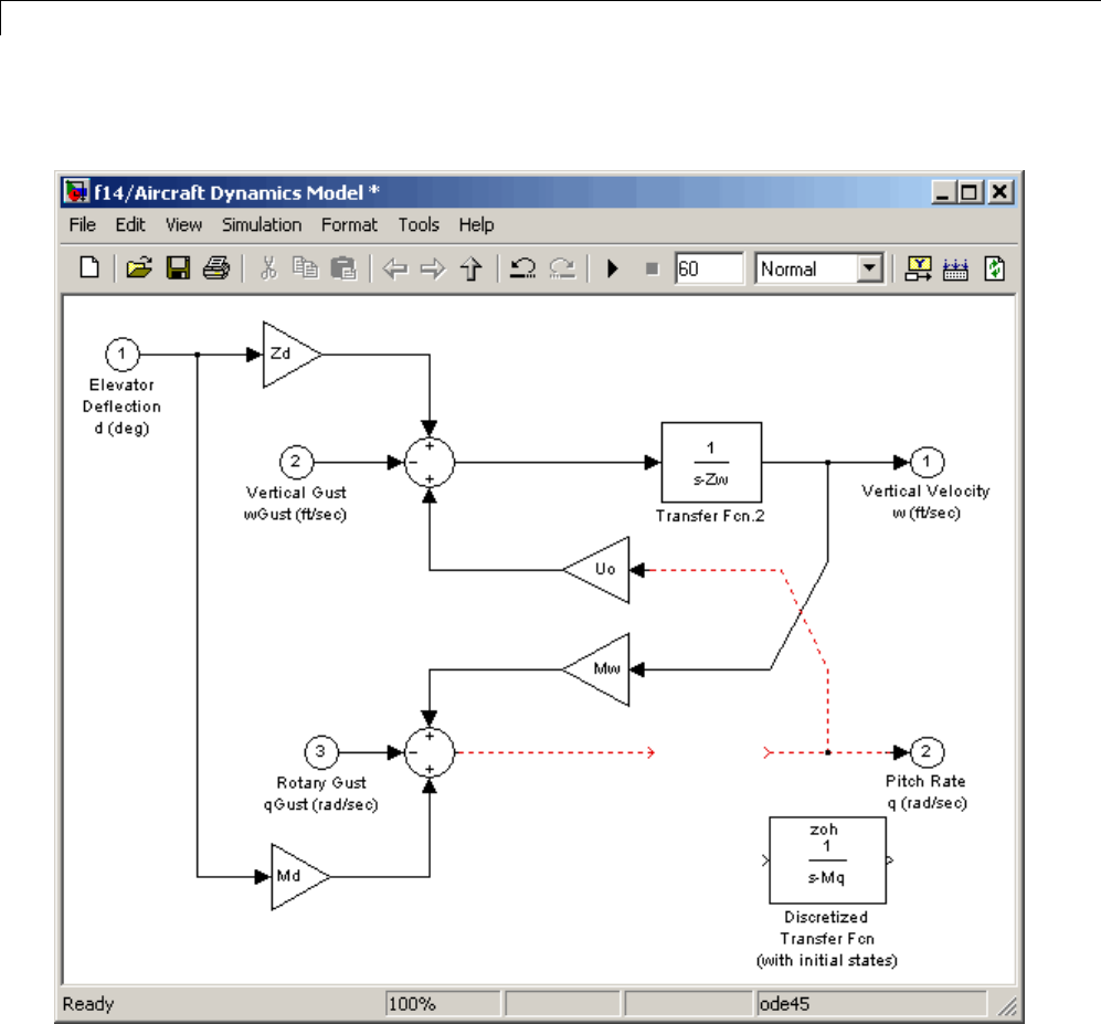
4Creating a Model
The f14/Aircraft Dynamics Model window now looks like this.
11 Add the Discretized Transfer Fcn block to the model.
aClick the Discretized Transfer Fcn block.
bDrag the Discretized Transfer Fcn block into position to complete the
model.
4-144
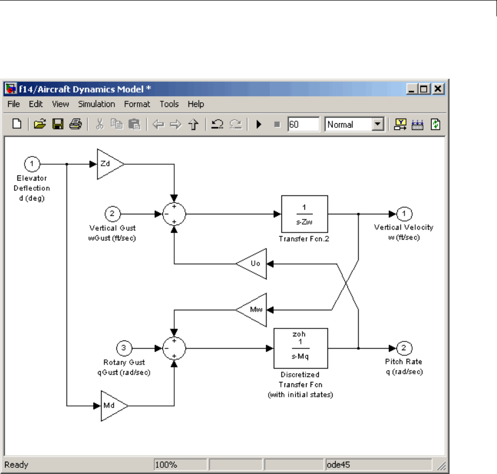
Model Discretizer
The f14/Aircraft Dynamics Model window now looks like this.
4-145

4Creating a Model
Discretize a Model from the MATLAB Command
Window
Use the sldiscmdl function to discretize Simulink software models from the
MATLAB Command Window. You can specify the transform method, the
sample time, and the discretization method with the sldiscmdl function.
For example, the following command discretizes the f14 model in the s-domain
with a 1-second sample time using a zero-order hold transform method:
sldiscmdl('f14',1.0,'zoh')
4-146

5
Working with Sample Times
•“WhatIsSampleTime?”onpage5-2
•“Specify Sample Time” on page 5-3
•“View Sample Time Information” on page 5-9
•“Print Sample Time Information” on page 5-13
•“Types of Sample Time” on page 5-14
•“Block Compiled Sample Time ” on page 5-20
•“Sample Times in Subsystems” on page 5-21
•“Sample Times in Systems” on page 5-22
•“Resolve Rate Transitions” on page 5-28
•“How Propagation Affects Inherited Sample Times” on page 5-29
•“Monitor Backpropagation inSampleTimes”onpage5-31

5Working with Sample Times
What Is Sample Time?
The sample time of a block is a parameter that indicates when, during
simulation, the block produces outputs and if appropriate, updates its internal
state. The internal state includes but is not limited to continuous and discrete
states that are logged.
Note DonotconfusetheSimulinkusageofthetermsampletimewiththe
engineering sense of the term. In engineering, sample time refers to the rate
at which a discrete system samples its inputs. Simulink allows you to model
single-rate and multirate discrete systems and hybrid continuous-discrete
systems through the appropriate setting of block sample times that control
the rate of block execution (calculations).
For many engineering applications, you need to control the rate of block
execution. In general, Simulink provides this capability by allowing you
to specify an explicit SampleTime parameterintheblockdialogoratthe
command line. Blocks that do not have a SampleTime parameter have an
implicit sample time. You cannot specify implicit sample times. Simulink
determines them based upon the context of the block in the system. The
Integrator block is an example of a block that has an implicit sample time.
Simulink automatically sets its sample time to 0.
Sample times can be port-based or block-based. For block-based sample times,
all of the inputs and outputs of the block run at the same rate. For port-based
sample times, the input and output ports can run at different rates.
Sample times can also be discrete, continuous, fixed in minor step, inherited,
constant, variable, triggered, or asynchronous. The following sections discuss
thesesampletimetypes,aswellassampletimepropagationandrate
transitions between block-based or port-based sample times. You can use
this information to control your block execution rates, debug your model,
and verify your model.
5-2

Specify Sample Time
Specify Sample Time
In this section...
“Designate Sample Times” on page 5-3
“Specify Block-Based Sample Times Interactively” on page 5-6
“Specify Port-Based Sample Times Interactively” on page 5-6
“Specify Block-Based Sample Times Programmatically” on page 5-7
“Specify Port-Based Sample Times Programmatically” on page 5-8
“Access Sample Time Information Programmatically” on page 5-8
“Specify Sample Times for a Custom Block” on page 5-8
“Determining Sample Time Units” on page 5-8
“Change the Sample Time After Simulation Start Time” on page 5-8
Designate Sample Times
Simulink allows you to specify a block sample time directly as a numerical
value or symbolically by defining a sample time vector. In the case of a
discrete sample time, the vector is [Ts,To]whereTsis the sampling period
and Tois the initial time offset. For example, consider a discrete model that
produces its outputs every two seconds. If your base time unit is seconds, you
can directly set the discrete sample time by specifying the numerical value of
2as the SampleTime parameter. Because the offset value is zero, you do not
need to specify it; however, you can enter [2,0]intheSample time field.
For nondiscrete blocks, the components of the vector are symbolic values
that represent one of the types in “Types of Sample Time” on page 5-14. The
following table summarizes these types and the corresponding sample time
values. The table also defines the explicit nature of each sample time type
and designates the associated color and annotation. Because an inherited
sample time is explicit, you can specify it as [-1, 0] or as -1.Whereas,a
triggeredsampletimeisimplicit;onlySimulinkcanassignthesampletime
of [-1, -1]. (For more information about colors and annotations, see “View
Sample Time Information” on page 5-9.)
5-3

5Working with Sample Times
Designations of Sample Time Information
Sample Time
Type
Sample
Time
Color Annotation Explicit
Discrete [Ts,T
o]In descending
order of
speed: red,
green, blue,
light blue,
dark green,
orange
D1, D2, D3, D4,
D5, D6, D7,...
Di
Yes
Continuous [0, 0] black Cont Yes
Fixed in minor
step
[0, 1] gray FiM Yes
Inherited [–1, 0] N/A N/A Yes
Constant [Inf, 0] magenta Inf Yes
Variable [–2,Tvo]brown V1, V2,... Vi No
Hybrid N/A yellow N/A No
Triggered [–1, –1] cyan TNo
Asynchronous [–1, –n] purple A1, A2,... Ai No
The color that is assigned to each block depends on its sample time relative
to other sample times in the model. This means that the same sample time
may be assigned different colors in a parent model and in models that it
references. (See “Model Reference”.)
For example, suppose that a model defines three sample times: 1,2,and3.
Further, suppose that it references a model that defines two sample times: 2
and 3. In this case, blocks operating at the 2sample rate appear as green in
the parent model and as red in the referenced model.
It is important to note that Mux and Demux blocks are simply grouping
operators; signals passing through them retain their timing information. For
this reason, the lines emanating from a Demux block can have different colors
if they are driven by sources having different sample times. In this case, the
5-4
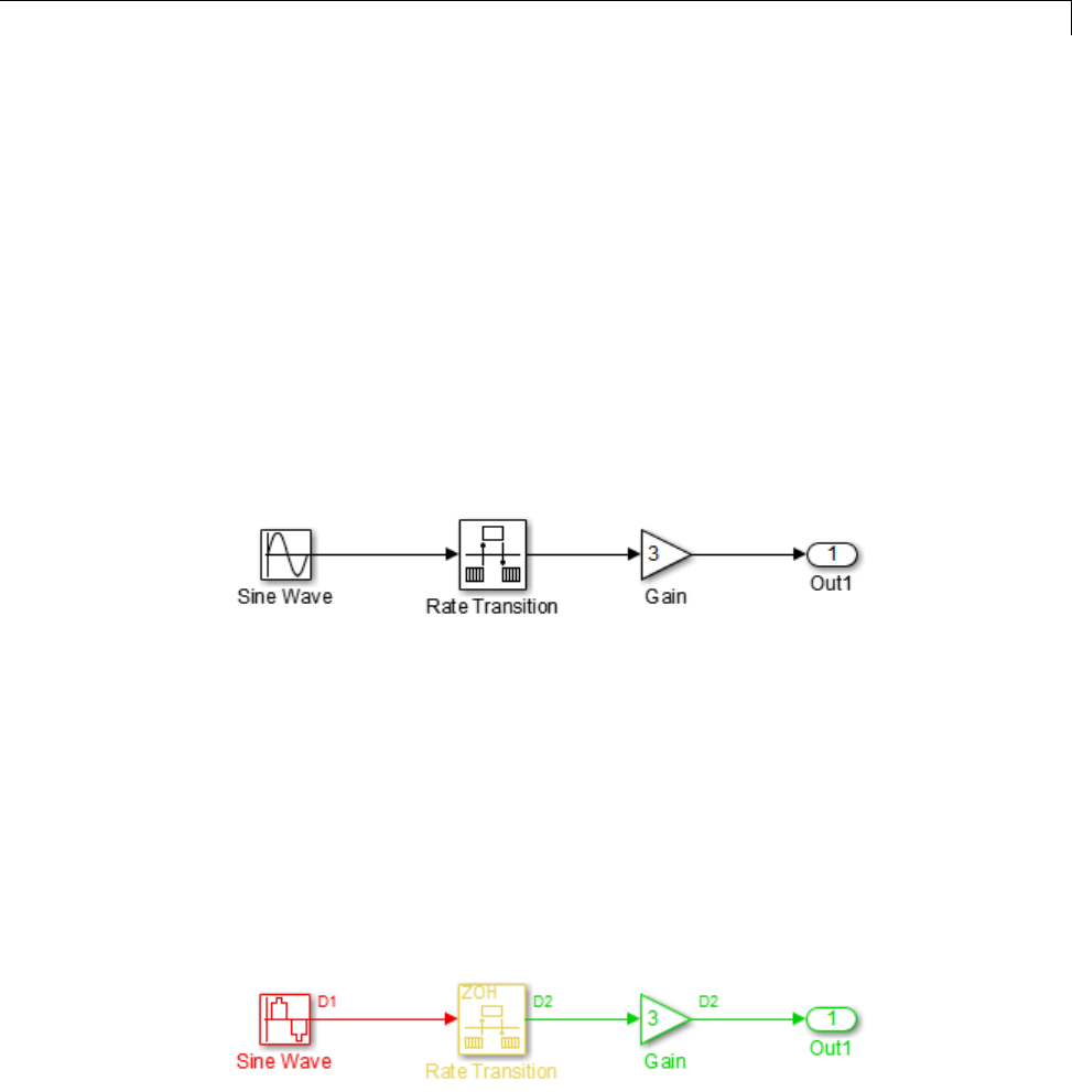
Specify Sample Time
Mux and Demux blocks are color coded as hybrids (yellow) to indicate that
they handle signals with multiple rates.
Similarly, Subsystem blocks that contain blocks with differing sample times
are also colored as hybrids, because there is no single rate associated with
them. If all the blocks within a subsystem run at a single rate, the Subsystem
block is colored according to that rate.
You can use the explicit sample time values in this table to specify sample
times interactively or programmatically for either block-based or port-based
sample times.
The following model, ex_specify_sample_time, serves as a reference for
this section.
ex_specify_sample_time
In this example, set the sample time of the input sine wave signal to 0.1.The
goal is to achieve an output sample time of 0.2. The Rate Transition block
serves as a zero-order hold. The resulting block diagram after setting the
sample times and simulating the model is shown in the following figure. (The
colors and annotations indicate that this is a discrete model.)
Sample Time 0.1 Sample Time 0.2
ex_specify_sample_time after Setting Sample Times
5-5

5Working with Sample Times
Specify Block-Based Sample Times Interactively
To set the sample time of a block interactively:
1In the Simulink model window, double-click the block. The block parameter
dialog box opens.
2Enter the sample time in the Sample time field.
3Click OK.
Following is a figure of a parameters dialog box for the Sine Wave block after
entering 0.1 in the Sample time field.
Enter the sample time
value in this field
Specify Port-Based Sample Times Interactively
The Rate Transition block has port-based sample times. You can set the
output port sample time interactively by completing the following steps:
5-6
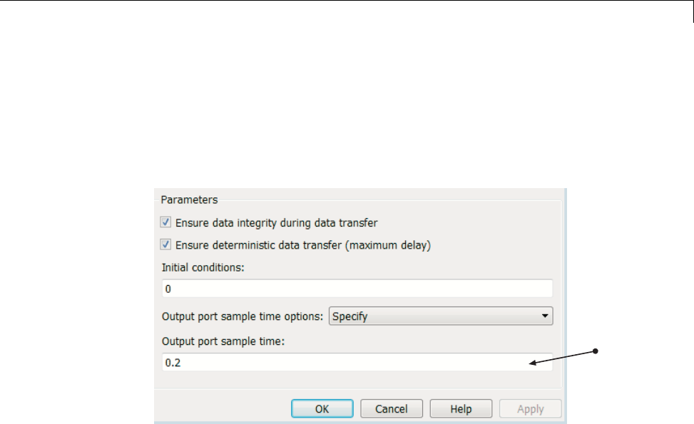
Specify Sample Time
1Double-click the Rate Transition block. The parameters dialog box opens.
2Leave the drop-down menu choice of the Output port sample time
options as Specify.
3Replace the -1 in the Output port sample time field with 0.2.
Enter sample time
in Output port
sample time field
4Click OK.
FormoreinformationaboutthesampletimeoptionsintheRateTransition
parameters dialog box, see the Rate Transition reference page.
Specify Block-Based Sample Times Programmatically
To set a block sample time programmatically, set its SampleTime parameter
to the desired sample time using the set_param command. For example, to
set the sample time of the Gain block in the “Specify_Sample_Time” model to
inherited (-1), enter the following command:
set_param('Specify_Sample_Time/Gain','SampleTime','[-1, 0]')
As with interactive specification, you can enter just the first vector component
if the second component is zero.
set_param('Specify_Sample_Time/Gain','SampleTime','-1')
5-7

5Working with Sample Times
Specify Port-Based Sample Times Programmatically
To set the output port sample time of the Rate Transition block to 0.2,use
the set_param command with the parameter OutPortSampleTime:
set_param('Specify_Sample_Time/Rate Transition',...
'OutPortSampleTime', '0.2')
Access Sample Time Information Programmatically
To access all sample times associated with a model, use the API
Simulink.BlockDiagram.getSampleTimes.
To access the sample time of a single block, use the API
Simulink.Block.getSampleTimes.
Specify Sample Times for a Custom Block
You can design custom blocks so that the input and output ports operate at
different sample time rates. For information on specifying block-based and
port-based sample times for S-functions, see “Sample Times” .
Determining Sample Time Units
Since the execution of a Simulink model is not dependent on a specific set of
units, you must determine the appropriate base time unit for your application
and set the sample time values accordingly. For example, if your base time
unit is second, then you would represent a sample time of 0.5 second by
setting the sample time to 0.5.
Change the Sample Time After Simulation Start Time
To change a sample time after simulation begins, you must stop the
simulation, reset the SampleTime parameter, and then restart execution.
5-8

View Sample Time Information
View Sample Time Information
In this section...
“ViewSampleTimeDisplay”onpage5-9
“Sample Time Legend” on page 5-10
View Sample Time Display
Simulink models can display color coding and annotations that represent
specific sample times. As shown in the table Designations of Sample Time
Informationonpage5-4,eachsampletimetypehasoneormorecolors
associated with it. You can display the blocks and signal lines in color, the
annotations in black, or both the colors and the annotations. To choose one
of these options:
1In the Simulink model window, select Display > Sample Time.
2Select Colors,Annotations,orAll.
Selecting All results in the display of both the colors and the annotations.
Regardless of your choice, Simulink performs an Update Diagram
automatically. To turn off the colors and annotations:
1Select Display > Sample Time.
2Select Off.
Simulink performs another Update Diagram automatically.
5-9
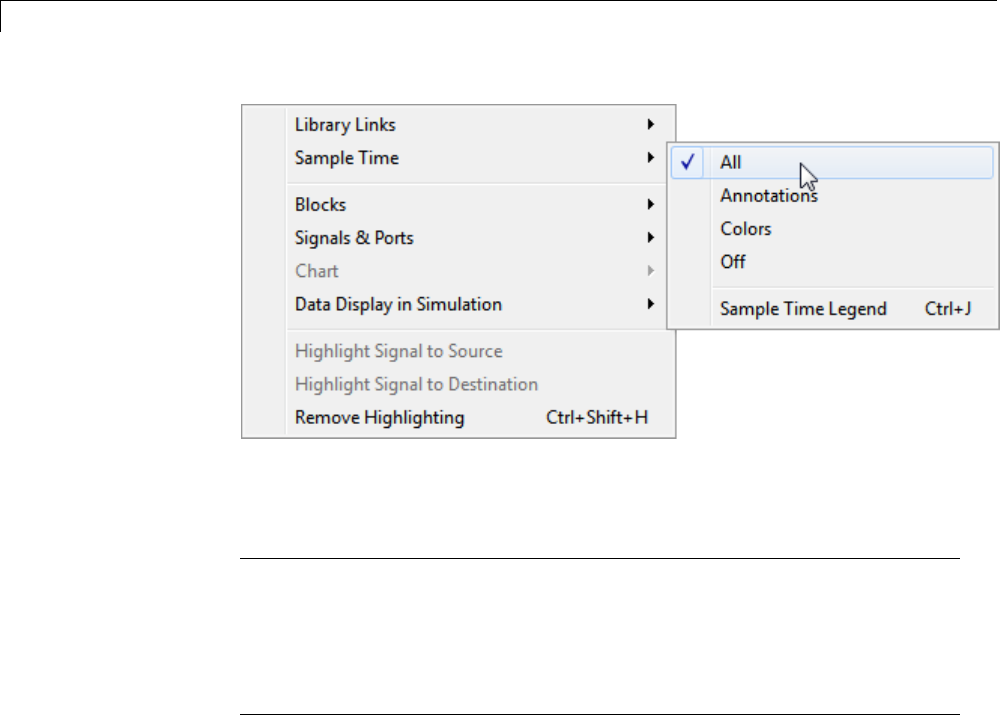
5Working with Sample Times
Your Sample Time Display choices directly control the information that the
Sample Time Legend displays.
Note The discrete sample times in the table Designations of Sample Time
Information on page 5-4 represent a special case. Five colors indicate the
fastest through the fifth fastest discrete rate. A sixth color, orange, represents
all rates that are slower than the fifth discrete rate. You can distinguish
between these slower rates by looking at the annotations on their respective
signal lines.
Sample Time Legend
You can view the Sample Time Legend for an individual model or for multiple
models. Additionally, you can prevent the legend from automatically opening
when you select options on the Sample Time menu.
Viewing the Legend
To assist you with interpreting your block diagram, a Sample Time Legend
is available that contains the sample time color, annotation, description, and
value for each sample time in the model. You can use one of three methods
to view the legend, but upon first opening the model, you must first perform
an Update Diagram.
5-10

View Sample Time Information
1In the Simulink model window, select Simulation > Update Diagram.
2Select Display > Sample Time > Sample Time Legend or press Ctrl +J.
In addition, whenever you select Colors,Annotations,orAll from the
Sample Time menu, Simulink updates the model diagram and opens
the legend by default. The legend contents reflect your Sample Time
Display choices. By default orifyouhaveselectedOff, the legend contains
a description of the sample time and the sample time value. If you turn
colors on, the legend displays the appropriate color beside each description.
Similarly, if you turn annotations on, the annotations appear in the legend.
The legend does not provide a discrete rate for all types of sample times. For
asynchronous and variable sample times, the legend displays a link to the
block that controls the sample time in place of the sample time value. Clicking
one of these links highlights the corresponding block in the block diagram. The
rate listed under hybrid and asynchronous hybrid models is “Not Applicable”
because these blocks do not have a single representative sample time.
Note TheSampleTimeLegenddisplaysallof the sample times in the model,
including those that are not associated with any block. For example, if the
fixed step size is 0.1 and all of the blocks have a sample time of 0.2, then both
rates (i.e., 0.1 and 0.2) appear in the legend.
For subsequent viewings of the legend, repeat the Update Diagram to access
the latest known information.
Turning the Legend Off
If you do not want to view the legend upon selecting Sample Time Display:
1In the Simulink model window, select File > Simulink Preferences.
2Scroll to the bottom of the main Preferences pane.
3Clear Openthesampletimelegendwheneverthesampletime
display is changed.
5-11
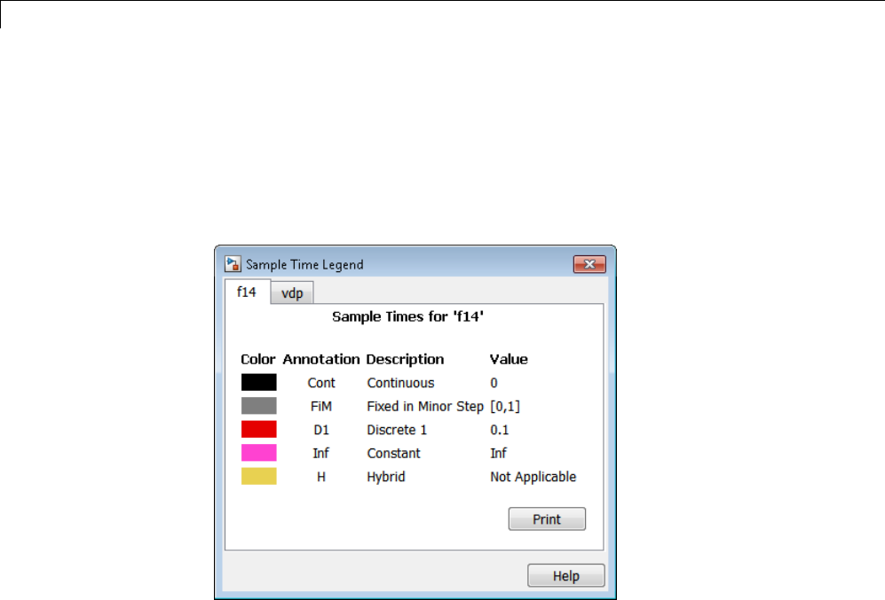
5Working with Sample Times
Viewing Multiple Legends
IfyouhavemorethanonemodelopenandyouviewtheSample Time
Legend for each one, a single legend window appears with multiple
tabs. Each tab contains the name of the model and the respective legend
information. The following figure shows the tabbed legends for the f14 and
vdp models.
5-12

Print Sample Time Information
Print Sample Time Information
You can print the sample time information in the Sample Time Legend by
using either of these methods:
•IntheSampleTimeLegendwindow,clickPrint.
•Print the legend from the Print Model dialog box:
1In the model window, select File > Print.
2Under Options, select the check box beside Print Sample Time
Legend.
3Click OK.
5-13

5Working with Sample Times
Types of Sample Time
In this section...
“Discrete Sample Time” on page 5-14
“Continuous Sample Time” on page 5-15
“Fixed in Minor Step” on page 5-15
“Inherited Sample Time” on page 5-15
“Constant Sample Time” on page 5-16
“Variable Sample Time” on page 5-17
“Triggered Sample Time” on page 5-18
“Asynchronous Sample Time” on page 5-18
Discrete Sample Time
Given a block with a discrete sample time, Simulink executes the block output
or update method at times
tnTT
nso
=+
where the sample time period Tsis always greater than zero and less than
the simulation time, Tsim . The number of periods ( n)isanintegerthat
must satisfy:
0≤≤nT
T
sim
s
As simulation progresses, Simulink computes block outputs only once at each
of these fixed time intervals of tn. These simulation times, at which Simulink
executes the output method of a block for a given sample time, are referred
to as sample time hits. Discrete sample times are the only type for which
sample time hits are known apriori.
If you need to delay the initial sample hit time, you can define an offset, To.
The Unit Delay block is an example of a block with a discrete sample time.
5-14

Types of Sample Time
Continuous Sample Time
Unlike the discretesampletime,continuoussample hit times are divided into
major time steps and minor time steps, where the minor steps represent
subdivisions of the major steps (see “Minor Time Steps” on page 3-23). The
ODE solver you choose integrates all continuous states from the simulation
starttimetoagiven major or minor time step. The solver determines the
times of the minor steps and uses the results at the minor time steps to
improve the accuracy of the results at the major time steps. However, you
see the block output only at the major time steps.
To specify that a block, such as the Derivative block, is continuous, enter [0,
0] or 0 in the Sample time field of the block dialog.
Fixed in Minor Step
If the sample time of a block is set to [0, 1], the block becomes fixedinminor
step.Fort
his setting, Simulink does not execute the block at the minor time
steps; updates occur only at the major time steps. This process eliminates
unnecessary computations of blocks whose output cannot change between
major steps.
While you can explicitly set a block to be fixed in minor step, more typically
Simulink sets this condition as either an inherited sample time or as an
alteration to a user specification of 0(continuous). This setting is equivalent
to, and therefore converted to, the fastest discrete rate when you use a
fixed-step solver.
Inherited Sample Time
If a block sample time is set to [–1, 0] or –1, the sample time is inherited and
Simulink determines the best sample time for the block based on the block
context within the model. Simulink performs this task during the compilation
stage; the original inherited setting never appears in a compiled model.
Therefore, you never see inherited ([–1, 0]) in the Sample Time Legend. (See
“View Sample Time Information” on page 5-9.)
Examples of inherited blocks include the Gain and Add blocks.
All inherited blocks are subject to the processofsampletimepropagation,as
discussed in “How Propagation Affects Inherited Sample Times” on page 5-29
5-15

5Working with Sample Times
Constant Sample Time
Specifying a constant (Inf) sample time is a request for an optimization for
which the block executes only once during model initialization. Simulink
honors such requests if all of the following conditions hold:
•The Inline parameters check box is selected on the Configuration
Parameters dialog box Optimization >Signal and Parameters pane
(see the “Optimization Pane: Signals and Parameters”).
•The block has no continuous or discrete states.
•The block allows for a constant sample time.
•The block does not drive an output port of a conditionally executed
subsystem (see “Enabled Subsystems” on page 7-4).
•The block has no tunable parameters.
One exception is an empty subsystem. A subsystem that has no blocks—not
even an input or output block—always has a constant sample time regardless
of the status of the conditions listed above.
This optimization process speeds up the simulation by eliminating the need to
recompute the block output at each step. Instead, during each model update,
Simulink first establishes the constant sample time of the block and then
computes the initial values of its output ports. Simulink then uses these
values, without performing any additional computations, whenever it needs
the outputs of the block.
Note The Simulink block library includes several blocks, such as the
MATLAB S-Function block, the Level-2 MATLAB S-Function block, and the
Model block, whose ports can produce outputs at different sample rates. It is
possible for some of the ports of such blocks to have a constant sample time.
These ports produce outputs only once—at the beginning of a simulation. Any
other ports produce output at their respective sample times.
If Simulink cannot honor the request to use the optimization, then Simulink
treats the block as if it had specified an inherited sample time (–1 ).
5-16
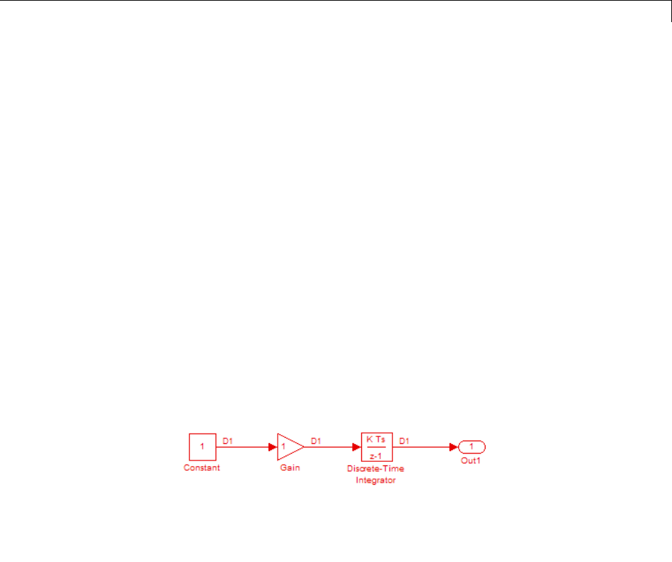
Types of Sample Time
OnespecificcaseforwhichSimulinkrejects the request is when parameters
are tunable. By definition, you can change the parameter values of a block
having tunable parameters; therefore, the block outputs are variable rather
than constant. For such cases, Simulink performs sample time propagation
(see “How Propagation Affects Inherited Sample Times” on page 5-29) to
determine the block sample time.
An example of a Constant block with tunable parameters is shown below
(ex_inline_parameters_off.SincetheInline parameters option is
disabled, the Constant value parameteristunableandthesampletime
cannot be constant, even if it is set to Inf. To ensure accurate simulation
results, Simulink treats the sample time of the Constant block as inherited
and uses sample time propagation to calculate the sample time. The
Discrete-Time Integrator block is the first block, downstream of the Constant
block, which does not inherit its sample time. The Constant block, therefore,
inheritsthesampletimeof1from the Integrator block via backpropagation.
TT T T
ssss
==−= =−Inf 1 1 1
Inline Parameters Off
Variable Sample Time
Blocks that use a variable sample time have an implicit SampleTime
parameter that the block specifies; the block tells Simulink when to run it.
The compiled sample time is [–2, Tvo]whereTvo is a unique variable offset.
The Pulse Generator block is an example of a block that has a variable sample
time. Since Simulink supports variable sample times for variable-step solvers
5-17

5Working with Sample Times
only, the Pulse Generator block specifies a discrete sample time if you use a
fixed-step solver.
To learn how to write your own block that uses a variable sample time, see “C
MEX S-Function Examples”.
Triggered Sample Time
If a block is inside of a triggered-type (e.g., function-call, enabled and
triggered, or iterator) subsystem, the block may have either a triggered or a
constant sample time. You cannot specify the triggered sample time type
explicitly. However, to achieve a triggered type during compilation, you must
set the block sample time to inherited (–1). Simulink then determines the
specific times at which the block computes its output during simulation. One
exception is if the subsystem is an asynchronous function call, as discussed in
the following section.
Asynchronous Sample Time
An asynchronous sample time is similar to a triggered sample time. In both
cases, it is necessary to specify an inherited sample time because the Simulink
engine does not regularly execute the block. Instead, a run-time condition
determines when the block executes. Forthecaseofanasynchronoussample
time, an S-function makes an asynchronous function call.
The differences between these sample time types are:
•Only a function-call subsystem can have an asynchronous sample time.
(See “Function-Call Subsystems” on page 7-30.)
•The source of the function-call signal is an S-function having the option
SS_OPTION_ASYNCHRONOUS.
•The asynchronous sample time can also occur when a virtual block is
connected to an asynchronous S-function or an asynchronous function-call
subsystem.
•The asynchronous sample time is important to certain code-generation
applications. (See “Handle Asynchronous Events”.)
•Thesampletimeis[, ]−−1n.
5-18

Types of Sample Time
For an explanation of how to use blocks to model and generate code for
asynchronous event handling, see “Rate Transitions and Asynchronous
Blocks”.
5-19

5Working with Sample Times
Block Compiled Sample Time
During the compilation phase of a simulation, Simulink determines the
sample time of a block from its SampleTime parameter (if it has an explicit
sample time), its block type (if it has an implicit sample time), or by its context
within the model. This compiled sample time determines the sample rate of
a block during simulation. You can determinethecompiledsampletimeof
any block in a model by first updating the model and then getting the block
CompiledSampleTime parameter, using the get_param command.
5-20

Sample Times in Subsystems
Sample Times in Subsystems
Subsystems fall into two categories: triggered and nontriggered. For
triggered subsystems, in general, the subsystem gets its sample time from the
triggering signal. One exception occurs when you use a Trigger block to create
a triggered subsystem. If you set the block Trigger type to function-call
and the Sample time type to periodic,theSampleTime parameter becomes
active. In this case, you specify the sample time of theTriggerblock,whichin
turn, establishes the sample time of the subsystem.
The four nontriggered subsystems are virtual, enabled, atomic, and action.
Simulink calculates the sample times of virtual and enabled subsystems
based on the respective sample times of their contents. The atomic subsystem
is a special case in that the subsystem block has a SampleTime parameter.
Moreover,forasampletimeotherthanthedefaultvalueof–1,theblocks
inside the atomic subsystem can have only a value of Inf,–1,ortheidentical
(discrete) value of the subsystem SampleTime parameter. If the atomic
subsystemisleftasinherited,Simulink calculates the block sample time
in the same manner as the virtual and enabled subsystems. However, the
main purpose of the subsystem SampleTime parameteristoallowforthe
simultaneous specification of a large number of blocks, within an atomic
subsystem, that are all set to inherited. Finally, the sample time of the action
subsystem is set by the If block or the Switch Case block.
5-21

5Working with Sample Times
Sample Times in Systems
In this section...
“Purely Discrete Systems” on page 5-22
“Hybrid Systems” on page 5-25
Purely Discrete Systems
A purely discrete system is composed solely of discrete blocks and can be
modeled using either a fixed-step or a variable-step solver. Simulating
a discrete system requires that the simulator take a simulation step at
every sample time hit. For a multirate discrete system—a system whose
blocks Simulink samples at different rates—the steps must occur at integer
multiples of each of the system sample times. Otherwise, the simulator
might miss key transitions in the statesofthesystem.Thestepsizethatthe
Simulink software chooses depends on the type of solver you use to simulate
the multirate system and on the fundamental sample time.
The fundamental sample time of a multirate discrete system is the largest
double that is an integer divisor of the actual sample times of the system. For
example, suppose that a system has sample times of 0.25 and 0.50 seconds.
The fundamental sample time in this case is 0.25 seconds. Suppose, instead,
thesampletimesare0.50and0.75seconds. Thefundamentalsampletime
is again 0.25 seconds.
The importance of the fundamental sample time directly relates to whether
you direct the Simulink software to use a fixed-step or a variable-step discrete
solver to solve your multirate discrete system. A fixed-step solver sets the
simulation step size equal to the fundamental sample time of the discrete
system. In contrast, a variable-step solver varies the step size to equal the
distance between actual sample time hits.
The following diagram illustrates the difference between a fixed-step and a
variable-step solver.
5-22
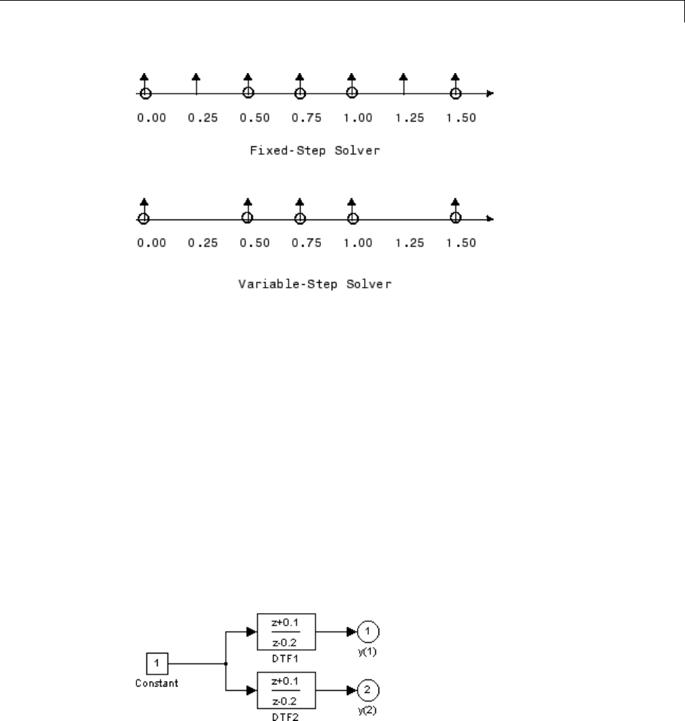
Sample Times in Systems
In the diagram, the arrows indicate simulation steps and circles represent
sample time hits. As the diagram illustrates, a variable-step solver requires
fewer simulation steps to simulate a system, if the fundamental sample time
is less than any of the actual sample times of the system being simulated.
On the other hand, a fixed-step solver requires less memory to implement
and is faster if one of the system sample times is fundamental. This can be
an advantage in applications that entail generating code from a Simulink
model (using Simulink Coder). In either case, the discrete solver provided
by Simulink is optimized for discrete systems; however, you can simulate a
purely discrete system with any one of the solvers and obtain equivalent
results.
Consider the following example of a simple multirate system. For this
example, the DTF1 Discrete Transfer Fcn block’s Sample time is set to
[1 0.1], which gives it an offset of 0.1.TheSample time of the DTF2
Discrete Transfer Fcn block is set to 0.7,withnooffset.Thesolverissettoa
variable-step discrete solver.
5-23
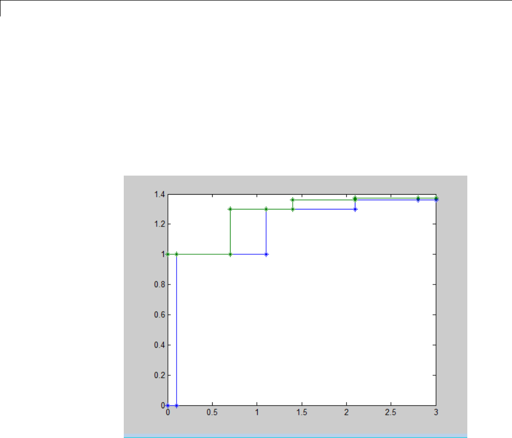
5Working with Sample Times
Running the simulation and plotting the outputs using the stairs function
simOut = sim('ex_dtf','StopTime', '3');
t = simOut.find('tout')
y = simOut.find('yout')
stairs(t,y, '-*')
produces the following plot.
(For information on the sim command. see “Run Simulation Using the sim
Command” on page 15-3. )
As the figure demonstrates, because the DTF1 block has a 0.1 offset, the
DTF1 block has no output until t=0.1. Similarly, the initial conditions of
the transfer functions are zero; therefore, the output of DTF1, y(1), is zero
before this time.
5-24
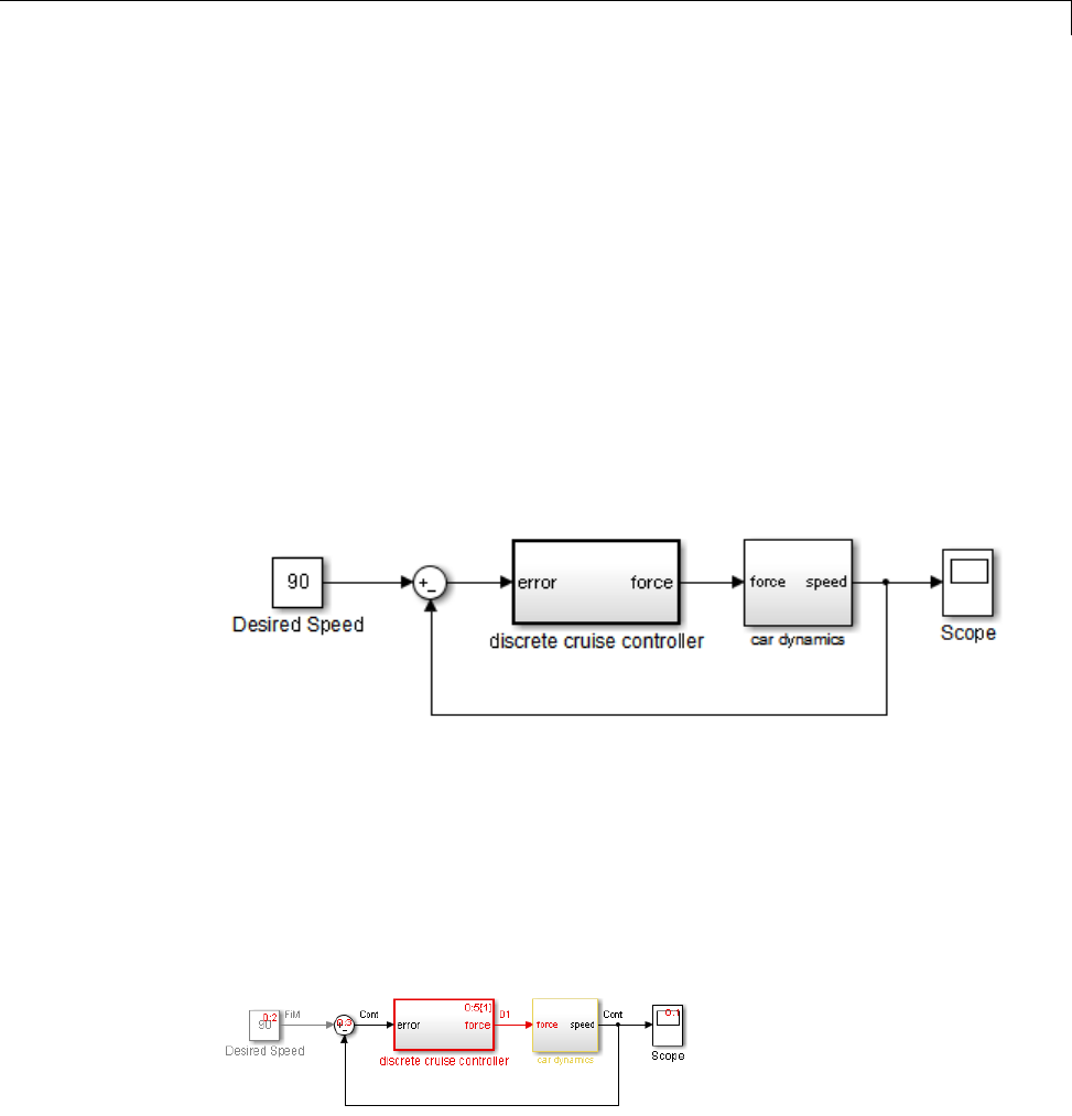
Sample Times in Systems
Hybrid Systems
Hybrid systems contain both discrete and continuous blocks and thus have
both discrete and continuous states. However, Simulink solvers treat any
system that has both continuous and discrete sample times as a hybrid
system. For information on modeling hybrid systems, see “Modeling Hybrid
Systems” on page 3-8.
In block diagrams, the term hybrid applies to both hybrid systems (mixed
continuous-discrete systems) and systems with multiple sample times
(multirate systems). Such systems turn yellow in color when you perform
an Update Diagram with Sample Time Display Colors turned ’on’. As an
example, consider the following model that contains an atomic subsystem,
“Discrete Cruise Controller”, and a virtual subsystem, “Car Dynamics”. (See
ex_execution_order.)
Car Model
With the Sample Time option set to All,anUpdate Diagram turns the
virtual subsystem yellow, indicating that it is a hybrid subsystem. In this
case, the subsystem is a true hybrid system since it has both continuous
and discrete sample times. As shown below, the discrete input signal, D1,
combines with the continuous velocity signal, v, to produce a continuous input
to the integrator.
Car Model after an Update Diagram
5-25
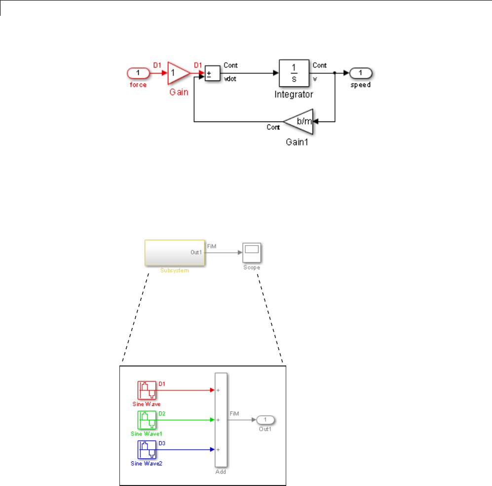
5Working with Sample Times
Car Dynamics Subsystem after an Update Diagram
Now consider a multirate subsystem that contains three Sine Wave source
blocks, each of which has a unique sample time — 0.2, 0.3, and 0.4,
respectively.
Multirate Subsystem after an Update Diagram
5-26

Sample Times in Systems
An Update Diagram turns the subsystem yellow because the subsystem
contains more than one sample time. As shown in the block diagram, the
Sine Wave blocks have discrete sample times D1, D2, and D3 and the output
signal is fixed in minor step.
In assessing a system for multiple sample times, Simulink does not consider
either constant [inf, 0] or asynchronous [–1, –n] sample times. Thus a
subsystem consisting of one block with a constant sample time and one block
with a discrete sample time will not be designated as hybrid.
The hybrid annotation and coloring are very useful for evaluating whether
or not the subsystems in your model have inherited the correct or expected
sample times.
5-27

5Working with Sample Times
ResolveRateTransitions
In general, a rate transition exists between two blocks if their sample times
differ, that is, if either of their sample-time vector components are different.
The exceptions are:
•Aconstantsampletime(
[Inf, 0]) never has a rate transition with any
other rate.
•A continuous sample time (black) and the fastest discrete rate (red) never
has a rate transition if you use a fixed-step solver.
•A variable sample time and fixed in minor step do not have a rate transition.
You can resolve rate transitions by inserting rate transition blocks and by
using two diagnostic tools. For the single-tasking execution mode, the Single
task rate transition diagnostic allows you to set the level of Simulink rate
transition messages. The Multitask rate transition diagnostic serves the
same function for multitasking execution mode. These execution modes
directly relate to the type of solver in use: Variable-step solvers are always
single-tasking; fixed-step solvers may be explicitly set as single-tasking or
multitasking.
For a detailed discussion on rate transitions, see “Single-Tasking and
Multitasking Execution Modes” and “Handle Rate Transitions”.
5-28
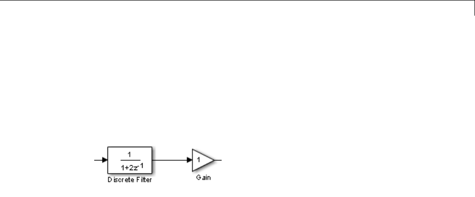
How Propagation Affects Inherited Sample Times
How Propagation Affects Inherited Sample Times
During a model update, for example at the beginning of a simulation, Simulink
uses a process called sample time propagation to determine the sample times
of blocks that inherit their sample times. The figure below illustrates a
Discrete Filter block with a sample time period Tsdriving a Gain block.
Because the output of the Gain block is the input multiplied by a constant,
itsoutputchangesatthesamerateasthefilter. Inotherwords,theGain
block has an effective sample rate equal to the sample rate of the filter. The
establishment of such effective rates is the fundamental mechanism behind
sample time propagation in Simulink.
Process for Sample Time Propagation
Simulink uses the following basic process to assign sample times to blocks
that inherit their sample times:
1Propagate known sample time information forward.
2Propagate known sample time information backward.
3Apply a set of heuristics to determine additional sample times.
4Repeat until all sample times are known.
Simulink Rules for Assigning Sample Times
A block having a block-based sample time inherits a sample time based on
the sample times of the blocks connected to its inputs, and in accordance
with the following rules:
5-29

5Working with Sample Times
If... then
all of the inputs have the same
sample time and the block can accept
that sample time
Simulink assigns the sample time to
the block
the inputs have different discrete
sample times and all of the input
sample times are integer multiples
of the fastest input sample time
Simulink assigns the sample time of
the fastest input to the block . (This
assignment assumes that the block
can accept the fastest sample time.)
the inputs have different discrete
sample times, some of the input
sample times are not integer
multiples of the fastest sample time,
and the model uses a variable-step
solver
Simulink assigns a
fixed-in-minor-step sample time to
the block.
the inputs have different discrete
sample times, some of the input
sample times are not integer
multiples of the fastest sample
time, the model uses a fixed-step
solver, and Simulink can compute
the greatest common integer divisor
(GCD)ofthesampletimescoming
into the block,
Simulink assigns the GCD sample
time to the block. Otherwise,
Simulink assigns the fixed step size
of the model to the block.
the sample times of some of the
inputs are unknown, or if the block
cannot accept the sample time
Simulink determines a sample
time for the block based on a set of
heuristics.
5-30
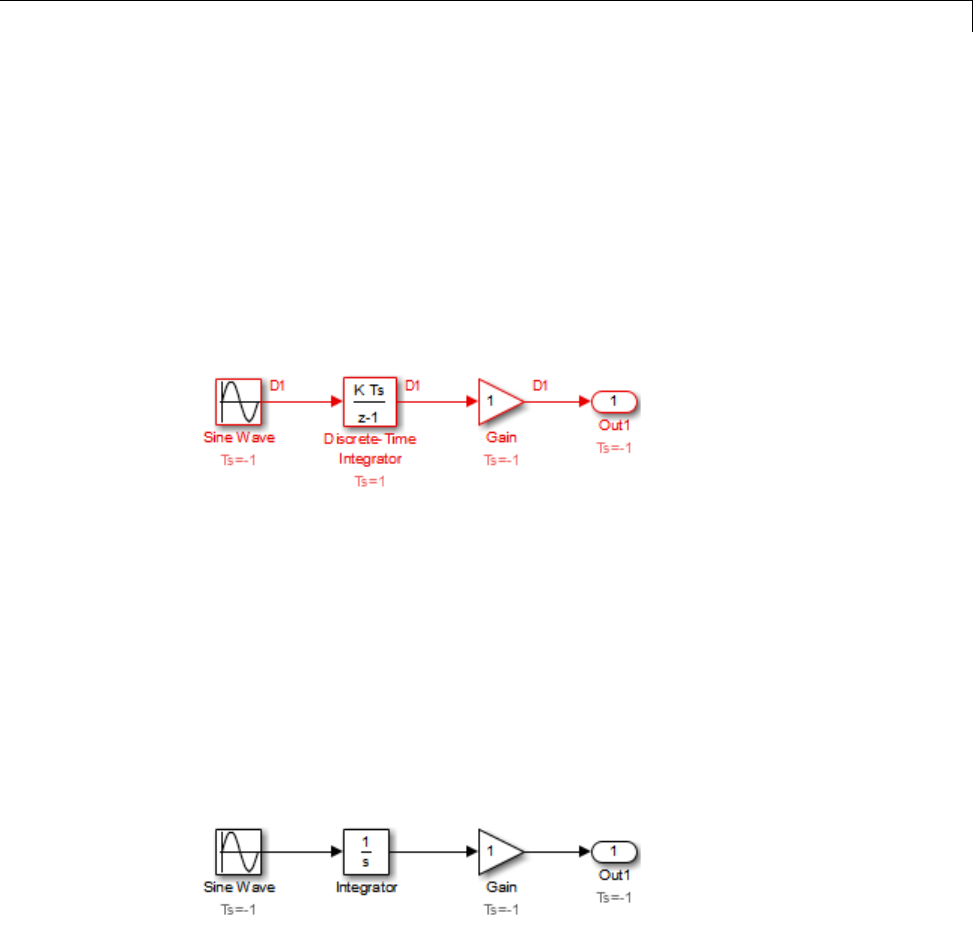
Monitor Backpropagation in Sample Times
Monitor Backpropagation in Sample Times
When you update or simulate a model that specifies the sample time of a
source block as inherited (–1), the sample time of the source block may be
backpropagated; Simulink may set the sample time of the source block to be
identical to the sample time specified by or inherited by the block connected
to the source block. For example, in the model below, the Simulink software
recognizesthattheSineWaveblockisdriving a Discrete-Time Integrator
block whose sample time is 1;soitassignstheSineWaveblockasample
time of 1.
You can verify this sample time setting by selecting Sample Time > Colors
from the Simulink Display menu and noting that both blocks are red.
Because the Discrete-Time Integrator block looks at its input only during its
sample hit times, this change does not affect the results of the simulation, but
does improve the simulation performance.
Now replacing the Discrete-Time Integrator block with a continuous
Integrator block, as shown in the model below, causes the Sine Wave and
Gain blocks to change to continuous blocks. You can test this change by
selecting Simulation > Update Diagram to update the colors; both blocks
now appear black.
5-31

5Working with Sample Times
Note Backpropagation makes the sample times of model sources dependent
on block connectivity. If you change the connectivity of a model whose sources
inherit sample times, you can inadvertently change the source sample times.
For this reason, when you update or simulate a model, by default, Simulink
displays warnings at the command line if the model contains sources that
inherit their sample times.
5-32

6
Referencing a Model
•“Overview of Model Referencing” on page 6-2
•“Create a Model Reference” on page 6-8
•“Convert a Subsystem to a Referenced Model” on page 6-12
•“Referenced Model Simulation Modes” on page 6-21
•“View a Model Reference Hierarchy” on page 6-35
•“Model Reference Simulation Targets” on page 6-37
•“Simulink Model Referencing Requirements” on page 6-45
•“Parameterize Model References” on page 6-52
•“Conditional Referenced Models” on page 6-59
•“Protected Model” on page 6-67
•“Use Protected Model in Simulation” on page 6-68
•“Inherit Sample Times” on page 6-70
•“Refresh Model Blocks” on page 6-74
•“S-Functions with Model Referencing” on page 6-75
•“Buses in Referenced Models” on page 6-78
•“Signal Logging in Referenced Models” on page 6-79
•“Model Referencing Limitations” on page 6-80

6Referencing a Model
Overview of Model Referencing
In this section...
“About Model Referencing” on page 6-2
“Referenced Model Advantages” on page 6-5
“Masking Model Blocks” on page 6-6
“Models That Use Model Referencing” on page 6-7
“Model Referencing Resources” on page 6-7
About Model Referencing
You can include one model in another by using Model blocks. Each instance
of a Model block represents a reference to another model, called a referenced
model or submodel. For simulation and code generation, the referenced
model effectively replaces the Model block that references it. The model that
contains a referenced model is its parent model. A collection of parent and
referenced models constitute a model reference hierarchy. A parent model and
all models subordinate to it comprise a branch of the reference hierarchy.
The interface of a referenced model consists of its input and output ports (and
control ports, in the case of a conditional referenced model) and its parameter
arguments. A Model block displays inputs and outputs corresponding to the
root-level inputs and outputs of the model it references. These ports enable
you to incorporate the referenced model into the block diagram of the parent
model.
For example, the sldemo_mdref_basic model includes Model
blocks that reference three instances of the same referenced model,
sldemo_mdlref_counter.
6-2
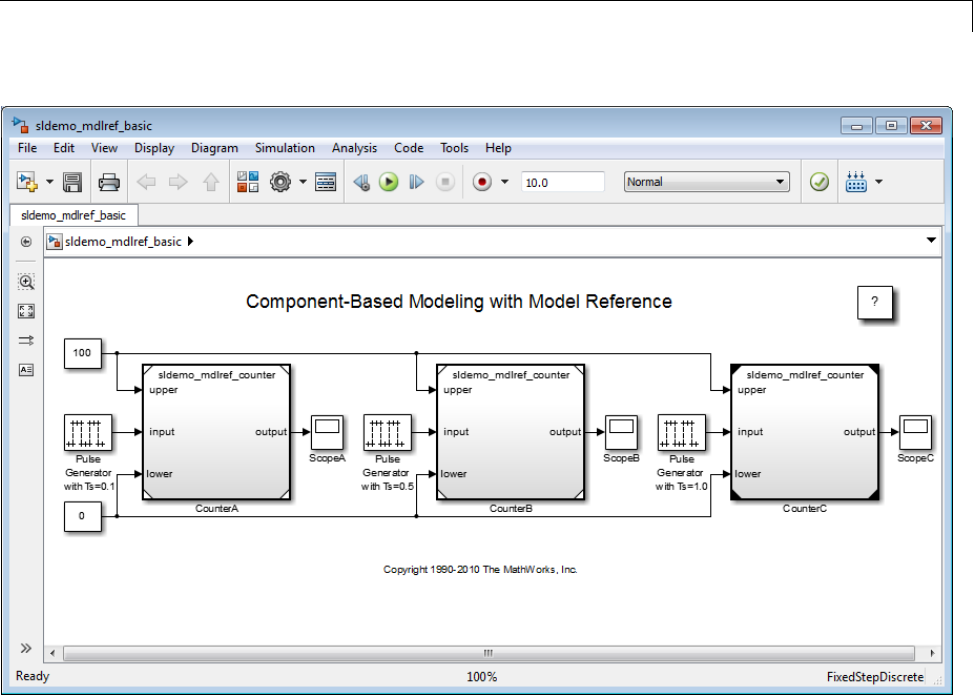
Overview of Model Referencing
Use the ports on a Model block to connect the submodel to other elements of
the parent model. Connecting a signal to a Model block port has the same
effect as connecting the signal to the corresponding port in the submodel.
For example, the Model block CounterA has three inputs: two Constant
blocks and a Pulse Generator block with a sample time of .1. The Model block
CounterB also has three inputs: the same two Constant blocks, and a Pulse
Generator block with a sample time of .5. Each Model block has an output to
a separate Scope block.
The referenced model includes Inport and Outport blocks (and possibly
Trigger or Enable blocks) to connect to the parent model. The
sldemo_mdlref_counter model has three Inport blocks (upper, input, and
lower) and one Outport block (output).
6-3
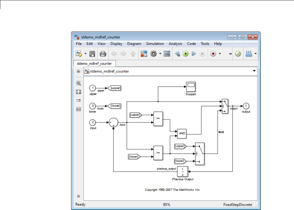
6Referencing a Model
A referenced model can itself contain Model blocks and thus reference
lower-level models, to any depth. The top model is the topmost model in a
hierarchy of referenced models. Where only one level of model reference exists,
the parent model and top model are the same. To prevent cyclic inheritance, a
Model block cannot refer directly or indirectly to a model that is superior to it
in the model reference hierarchy. This figure shows cyclic inheritance.
6-4

Overview of Model Referencing
Top model A
Model A B
Model B
Referenced
models
A parent model can contain multiple Model blocks that reference the same
submodel as long as the submodel does not define global data. The submodel
can also appear in other parent models at any level. You can parameterize a
referenced model to provide tunability for all instances of the model. Also,
you can parameterize a referenced model to let different Model blocks specify
different values for variables that define the behavior of the submodel. See
“Parameterize Model References” on page 6-52 for details.
By default, the Simulink software executes a top model interpretively, just
as it would if the model did not include submodels. Simulink can execute a
referenced model interpretively, as if it were an atomic subsystem, or by
compiling the submodel to code and executing the code. See “Referenced
Model Simulation Modes” on page 6-21 for details.
You can use a referenced model as a standalone model, if it does not depend
on data that is available only from a higher-level model. An appropriately
configured model can function as both a standalone model and a referenced
model, without changing the model or any entities derived from it.
Referenced Model Advantages
Like subsystems, referenced models allow you to organize large models
hierarchically; Model blocks can represent major subsystems. Like libraries,
referenced models allow you to use the same capability repeatedly without
having to redefine it. However, referenced models provide several advantages
that are unavailable with subsystems and/or library blocks:
•Modular development
6-5

6Referencing a Model
You can develop a referenced model independently from the models that
use it.
•Model Protection
You can obscure the contents of a referenced model, allowing you to
distribute it without revealing the intellectual property that it embodies.
•Inclusion by reference
Youcanreferenceamodelmultipletimeswithouthavingtomake
redundant copies, and multiple models can reference the same model.
•Incremental loading
Simulink loads a referenced model at the point it needs to use the model,
which speeds up model loading.
•Accelerated simulation
Simulink can convert a referenced model to code and simulate the model by
running the code, which is faster than interactive simulation.
•Incremental code generation
Accelerated simulation requires code generation only if the model has
changed since the code was previously generated.
•Independent configuration sets
The configuration set used by a referenced model can differ from the
configuration set of its parent or other referenced models.
For additional information about how model referencing compares to other
Simulink componentization techniques, see “Componentization Guidelines”
on page 12-17. For a video summarizing advantages of model referencing, see
Modular Design Using Model Referencing
Masking Model Blocks
You can use the masking facility to create custom dialog boxes and icons for
Model blocks. Masked dialog boxes can make it easier to specify additional
parameters for Model blocks. For information about block masks, see
“Masking”.
6-6

Overview of Model Referencing
Models That Use Model Referencing
Simulink includes several models that illustrate model referencing.
The Introduction to Managing Data with Model Reference example
introduces the basic concepts and workflow related to managing data with
model referencing. To explore these topics in more detail, select the Detailed
Workflow for Managing Data with Model Reference example.
In addition, the sldemo_absbrake modelrepresentsawheelspeedcalculation
as a Model block within the context of an anti-lock braking system (ABS).
Model Referencing Resources
The following are the most commonly needed resources for working with
model referencing:
•The Model block, which represents a model that another model
references. See the Model block parameters in “Ports & Subsystems
Library Block Parameters” for information about accessing a Model block
programmatically.
•The Configuration Parameters > Diagnostics > Model Referencing
pane, which controls the diagnosis of problems encountered in model
referencing. See “Diagnostics Pane: Model Referencing” for details.
•The Configuration Parameters > Model Referencing pane, which
provides options that control model referencing and list files on which
referenced models depend. See “Model Referencing Pane” for details.
6-7

6Referencing a Model
Create a Model Reference
A model becomes a submodel when a Model block in some other model
references it. Any model can function as a submodel, and such use does not
preclude using it as a separate model also.
For a video introducing how to create model references, see Getting Started
with Model Referencing.
To create a reference to a model (submodel) in another model (parent model):
1If the folder containing the submodel you want to reference is not on the
MATLAB path, add the folder to the MATLAB path.
2In the submodel:
•Enable Configuration Parameters > Optimization > Inline
parameters. You must enable Inline parameters for all models in a
model reference hierarchy except the top model in the hierarchy. See
“Inline Parameter Requirements” on page 6-49 for details.
•Set Configuration Parameters > Model Referencing > Total
number of instances allowed per top model to:
–One, if the hierarchy uses the model at most once
–Multiple, to use the model more than once per top model. To reduce
overhead, specify Multiple only when necessary.
–Zero, which precludes referencing the model
3Create an instance of the Model block in the parent model by dragging a
Model block instance from the Ports & Subsystems library to the parent
model. The new block is initially unresolved (specifies no submodel) and
has the following appearance:
6-8
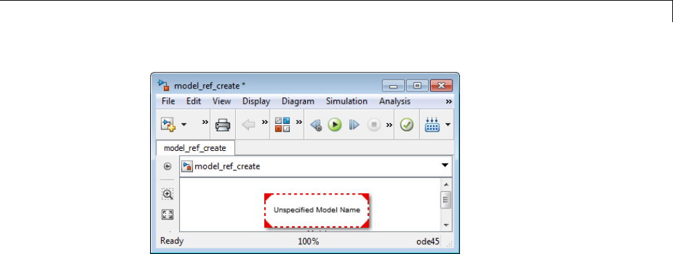
Create a Model Reference
4Open the new Model block’s parameter dialog box by double-clicking the
Model block. See “Navigating a Model Block” for more about accessing
Model block parameters.
6-9
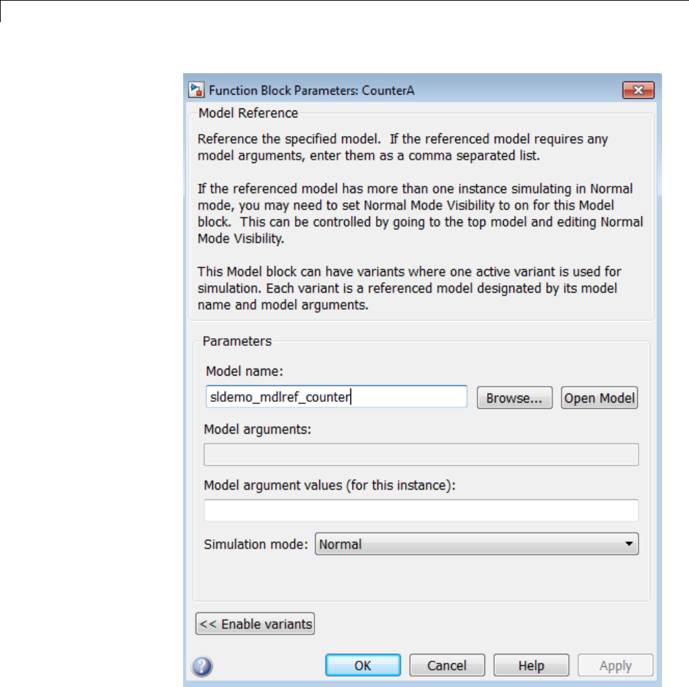
6Referencing a Model
6-10

Create a Model Reference
5Enter the name of the submodel in the Model name field. This name must
contain fewer than 60 characters. (See “Name Length Requirement” on
page 6-45.)
•For information about Model Arguments and Model argument
values, see “Using Model Arguments” on page 6-53.
•For information about the Simulation mode, see “Referenced Model
Simulation Modes” on page 6-21.
6Click OK or Apply.
If the referenced model contains any root-level inputs or outputs, Simulink
displays corresponding input and output ports on the Model block instance
that you have created. Use these ports to connect the referenced model to
other ports in the parent model.
A signal that connects to a Model block is functionally the same signal outside
and inside the block. Therefore that signal is subject to the restriction
that a given signal can have at most one associated signal object. See
Simulink.Signal for more information. For information about connecting a
bus signal to a referenced model, see “Bus Usage Requirements” on page 6-50.
6-11

6Referencing a Model
Convert a Subsystem to a Referenced Model
Conversion Process
The process for converting a subsystem to a referenced model involves these
tasks:
1“Select Subsystems to Convert” on page 6-12.
2“Prepare the Model for Conversion” on page 6-13.
3“Run a Conversion Tool” on page 6-16.
4“Connect the Model Block and Perform Other Post-Conversion Tasks” on
page 6-18.
Select Subsystems to Convert
Model referencing offers several benefits for modeling large, complex systems
and for team-based development, as summarized in “Referenced Model
Advantages” on page 6-5.
Subsystems or libraries are better suited for some modeling goals than
model referencing. Many large models involve using a combination of
subsystems and referenced models. For information to help you to decide
which subsystems to convert to referenced models, see “Componentization
Guidelines” on page 12-17.
The types of subsystems that you can convert to a referenced model are:
•Atomic Subsystem
•“Triggered Subsystems” on page 7-20
•“Enabled Subsystems” on page 7-4
•“Triggered and Enabled Subsystems” on page 7-24
•“Function-Call Subsystems” on page 7-30
6-12

Convert a Subsystem to a Referenced Model
Note If you want to create a referenced model that accepts an
asynchronous function call, see “Asynchronous Support Limitations”.
If you convert a masked subsystem, you might need to perform some
additional tasks to maintain the same general behavior that the masked
subsystem provided. For details, see “Convert a Masked Subsystem” on page
6-19.
Prepare the Model for Conversion
Simulink provides a tool that you can use to convert a subsystem to a
referenced model.
When the conversion tool identifies a change that you need to make to a model
orsubsystemtosupporttheconversion, the conversion processing stops.
The conversion tool reports conversion issues one at a time. To perform the
conversion efficiently, before using the conversion tool, consider modifying
your model as described in the following steps.
When you run the conversion tool, it will flag any additional model
modifications that you may need to make.
1Save a backup copy of the model.
You can use the backup copy of the model to help you to configure the model
after performing the conversion. For example, if you convert a masked
subsystem and want to have a masked Model block, you might want to copy
information from the masked subsystem into the masked Model block.
Also, you can revert to the original version of the model if you decide not to
convert the subsystem after you have started to modify the model, or if the
conversion processing is unsuccessful.
2Use the Configuration Parameters dialog box to set the following model
configuration parameters.
aSelect Optimization > Inline parameters.
6-13

6Referencing a Model
bSet Diagnostics > Data Validity > Signal resolution to Explicit
only.
cSet Diagnostics > Connectivity > Mux blocks used to create bus
signals to Error. For information about proper mux usage, see “Avoid
Mux/Bus Mixtures” on page 48-95.
As an alternative for steps b and c, consider using the associated Model
Advisor checks.
3Configure subsystem interfaces to the model.
Subsystem
Interface
What to Look For Model Modification
Goto or From
blocks
Crossing of subsystem
boundaries.
Add input or output ports to the
subsystem. Reconfigure the model as
necessary to reflect the added ports.
Data stores Data Store Memory blocks
accessed by Data Store Read or
Data Store Write blocks from
outside of the subsystem.
Replace the Data Store Memory block
with a global data store. Define a global
data store with a Simulink.Signal
object. For details, see “Data Stores
with Signal Objects” on page 46-12.
Tunable
parameters
Global tunable parameters
listed in the dialog box that
opens when you select the
Configuration Parameters >
Optimization > Signals and
Parameters > Configure
button.
Use tunablevars2parameterobjects
to create a Simulink.Parameter object
for each tunable parameter.
The Simulink.Parameter objects must
have a non-Auto storage class.
For more information, see “Parameterize
Model References” on page 6-52 and
“Tunable Parameters” on page 3-9.
4Configure the subsystem and its contents.
6-14

Convert a Subsystem to a Referenced Model
Subsystem
Configuration
What to Look For Model Modification
Inactive
subsystem
variants
Variant Subsystem
blocks.
Make active the subsystem
variantthatyouwantto
convert. The conversion tool
does not convert inactive
subsystem variants.
To have the new Model
block behave similar to the
subsystem variant, convert
each variant subsystem
separately.
For details, see “Set Up
Variant Subsystems” on page
8-15.
Function-call signals
that cross virtual
subsystem boundaries.
Move the Function-Call
Generator block inside of the
subsystem that you want to
convert.
Function-call outputs. Change the function-call
outputs to data triggers.
Function calls
Wide function-call ports. Eliminate wide signals for
function-call subsystems.
Sample times Sample time of an
Inport block that does
not match the sample
time of the block driving
the Inport.
Insert Rate Transition blocks
where appropriate.
Inport blocks Merged Inport blocks. Configure the model to avoid
merged Inport blocks. See the
Merge block documentation.
Constant
blocks
Constant blocks that
input to subsystems.
Consider moving the Constant
blocks into the subsystem.
6-15

6Referencing a Model
Subsystem
Configuration
What to Look For Model Modification
Bus signals that enter
and exit a subsystem.
Match signal names and bus
element names for blocks
inside of the subsystem.
Duplicate signal names
in buses.
Make signal names of the bus
elements unique.
Buses
Signal names that are
not valid MATLAB
identifiers. A valid
identifier is a character
string of letters, digits,
and underscores, such
that the first character
is a letter, and the
length of the string
is less than or equal
to the value returned
by the namelengthmax
function.
Change any invalid signal
namestobevalidMATLAB
identifiers.
Run a Conversion Tool
Run a conversion tool, using one of these approaches:
•From the context menu of the subsystem, select Subsystem & Model
Reference > Convert to> ReferencedModel.
•Use the Simulink.SubSystem.convertToModelReference command.
This function provides more capabilities than the Referenced Model
menu option. For example, with the function, you can replace a subsystem
with an equivalent Model block in a single operation.
Simulink saves the contents of the subsystem as a new model, then creates
and opens an untitled model that contains a Model block whose referenced
model is the new model.
6-16

Convert a Subsystem to a Referenced Model
Model Name
Simulink automatically provides a model name that is based on the block
name and is unique in the MATLAB path. This name always contains fewer
than 60 characters.
Error Handling
During the conversion, if an error occurs, the outcome depends on the kind
of error.
•For some errors, a message box appears that gives you the choice of
cancelling or continuing.
Before you continue, note any changes that you want to make after the
conversion. If you cancel, then the conversion tool exits.
•If continuing is impossible, Simulink cancels the conversion without
offeringachoicetocontinue.IfthenewModelblockhasnot been created,
then the model is not affected by the conversion tool processing.
What Gets Copied by the Conversion?
The conversion tool copies the following elements from the original model to
the newly created referenced model:
•Configuration sets – If the referencing model uses a configuration set
that is not a referenced configuration set, then the conversion tool copies
that entire configuration set to the referenced model.
If the referencing model uses a referenced configuration set, then both the
referencing and referenced models use the same referenced configuration
set.
•Variables – All of the model workspace variables of the original model are
copied into the model workspace of the referenced model.
•Requirements links – Requirements links created with the Simulink
Verification and Validation software (for example, requirements links to
blocks and signals) are copied. Any requirements links on the subsystem
that you convert are transferred to the new Model block.
6-17

6Referencing a Model
Connect the Model Block and Perform Other
Post-Conversion Tasks
After you successfully complete the conversion:
1Connect the referenced model.
aDelete the subsystem block from the source model.
bCopy the new Model block to the location of the deleted subsystem block.
Simulink automatically reconnects all signals. The source model is a
parent model that contains the referenced model.
2For root Inport blocks in the new referenced model, check the Interpolate
data parameter to make sure it is appropriate. For details, see the Inport
block documentation.
3(Optional) Delete unused duplicate variables.
The conversion tool copies into the model workspace of the referenced
model (for example, ModelB) all of the model workspace variables of the
referencing model (ModelA). This step results in duplicate variables in the
two model workspaces. To improve the reliability of your model in case the
model changes in the future, consider removing unused variables or moving
variables that are used by both ModelA and ModelB:
•For a model workspace variable used only by the referencing model
(ModelA), delete the variable from the model workspace of the referenced
model (ModelB).
•For a model workspace variable used only by the referenced model
(ModelB), delete the variable from the model workspace of the referencing
model (ModelA).
•For model workspace variables used by both the referencing and
referenced model, consider moving that variable to the base workspace.
4(Optional) To achieve similar results in the new referenced model as you
did by using the Variant Subsystem block, convert each of the variant
subsystems to referenced models, and then use a Model Variants block. For
more information, see “Set Up Model Variants” on page 8-5.
6-18

Convert a Subsystem to a Referenced Model
If you convert a masked subsystem, you may need to perform some additional
tasks to maintain the same general behavior that the masked subsystem
provided. For details, see “Convert a Masked Subsystem” on page 6-19.
Convert a Masked Subsystem
Perform the tasks described in:
•“Select Subsystems to Convert” on page 6-12.
•“Prepare the Model for Conversion” on page 6-13.
•“Run a Conversion Tool” on page 6-16.
•“Connect the Model Block and Perform Other Post-Conversion Tasks” on
page 6-18.
If the subsystem that you converted contains a mask, then you might want
to mask the Model block in your new referenced model (see “Masking”).
Configure the referenced model to support the functionality that was in the
masked subsystem.
Note The referenced model does not support the functionality that you can
achieve with mask initialization code to create masked parameters.
Masked
Subsystem
Functionality
Referenced Model Configuration
Masked
parameters 1In the model workspace of the referenced model,
create a variable for each masked parameter.
2In the Model Explorer, select the Model Workspace
node. In the Dialog pane, in the Model arguments
parameter, enter the variables that you want to be
model arguments.
6-19

6Referencing a Model
Masked
Subsystem
Functionality
Referenced Model Configuration
3In the new Model block, for the Model arguments
parameter, specify the values for the model
arguments.
Masked callbacks,
icons, ports, and
documentation
In the backup copy of the masked subsystem, open
the Mask Editor and select the content to copy into to
masked Model block.
In the Mask Editor for the new Model block, copy the
appropriate content from the masked subsystem that
you converted.
6-20

Referenced Model Simulation Modes
Referenced Model Simulation Modes
In this section...
“Simulation Modes for Referenced Models” on page 6-21
“Specify the Simulation Mode” on page 6-23
“Mixing Simulation Modes” on page 6-23
“Using Normal Mode for Multiple Instances of Referenced Models” on page
6-25
“Accelerating a Freestanding or Top Model” on page 6-33
Simulation Modes for Referenced Models
Simulink executes the top model in a model reference hierarchy just as
it would if no referenced models existed. All Simulink simulation modes
areavailabletothetopmodel. Simulink can execute a referenced model
in any of four modes: Normal, Accelerator, Software-in-the-loop (SIL), or
Processor-in-the-loop (PIL).
Normal Mode
Simulink executes a Normal mode submodel interpretively. Normal mode,
compared to other simulation modes:
•Requires no delay for code generation or compilation
•Works with more Simulink and Stateflow tools, supporting tools such as:
-Scopes, port value display, and other output viewing tools
•Scopes work with Accelerator mode referenced models, but require
using the Signal & Scope Manager and adding test points to signals.
Adding or removing a test point necessitates rebuilding the SIM
target for a model, which can be time-consuming.
-Model coverage analysis
-Stateflow debugging and animation
•Provides more accurate linearization analysis
•SupportsmoreS-functionsthan Accelerator mode does
6-21

6Referencing a Model
Normal mode executes slower than Accelerator mode does.
Simulation results for a given model are nearly the same in either Normal
or Accelerator mode. Trivial differences can occur due to differences in the
optimizations and libraries that you use.
You can use Normal mode with multiple instances of a referenced model.
For details, see “Using Normal Mode for Multiple Instances of Referenced
Models” on page 6-25.
Accelerator Mode
Simulink executes an Accelerator mode submodel by creating a MEX-file (or
simulation target) for the submodel, then running the MEX-file. See “Model
Reference Simulation Targets” on page 6-37 for more information. Accelerator
mode:
•Takes time for code generation and code compilation
•Does not fully support some Simulink tools, such as Model Coverage and
the Simulink Debugger.
•Executes faster than Normal mode
Simulation results for a given model are nearly identical in either Normal
or Accelerator mode. Trivial differences can occur due to differences in the
optimizations and libraries that you use.
Software-in-the-Loop (SIL) Mode
Simulink executes a SIL-mode referenced model by generating production
code using the model reference target for the submodel. This code is compiled
for, and executed on, the host platform.
With SIL mode, you can:
•Verify generated source code without modifying the original model
•Reuse test harnesses for the original model with the generated source code
SIL mode provides a convenient alternativetoPILsimulationwhenthe
target hardware is not available.
6-22

Referenced Model Simulation Modes
This option requires Embedded Coder software.
For more information, see “Numerical Equivalence Testing” in the Embedded
Coder documentation.
Processor-in-the-Loop (PIL) Mode
Simulink executes a PIL-mode referenced model by generating production
code using the model reference target for the submodel. This code is
cross-compiled for, and executed on, a target processor or an equivalent
instruction set simulator.
With PIL mode, you can:
•Verify deployment object code on target processors without modifying the
original model
•Reuse test harnesses for the original model with the generated source code
This option requires Embedded Coder software.
For more information, see “Numerical Equivalence Testing” in the Embedded
Coder documentation.
Specify the Simulation Mode
The Model block for each instance of a referenced model controls its simulation
mode. Tosetorchangethesimulationmodeforasubmodel:
1Access the block parameter dialog box for the Model block. (See “Navigating
a Model Block”.)
2Set the Simulation mode parameter.
3Click OK or Apply.
Mixing Simulation Modes
The following table summarizes the relationship between the simulation
mode of the parent model and its submodels.
6-23

6Referencing a Model
Parent Model
Simulation Mode
Submodel Simulation Modes
Normal •Submodels can use Normal, Accelerator, SIL,
or PIL mode.
•A submodel can execute in Normal mode only
if every model that is superior to it in the
hierarchy also executes in Normal mode. A
Normal mode path then extends from the top
model through the model reference hierarchy
down to the Normal mode submodel.
Accelerator •All subordinate models must also execute in
Accelerator mode.
•When a Normal mode model is subordinate to
an Accelerator mode model, Simulink posts
a warning and temporarily overrides the
Normal mode specification.
•When a SIL-mode or PIL-mode model is
subordinate to an Accelerator mode model, an
error occurs.
SIL •All subordinate models also execute in SIL
mode regardless of the simulation mode
specified by their Model blocks.
•TheSILmodeModelblockusesthemodel
reference targets of the blocks beneath.
•Only one Model block, starting at the top
of a model reference hierarchy, can execute
at a time in SIL mode. See “Simulation
Mode Override Behavior in Model Reference
Hierarchy”.
PIL •All subordinate models also execute in PIL
mode regardless of the simulation mode
specified by their Model blocks.
•The PIL mode Model block uses the model
reference targets of the blocks beneath.
6-24

Referenced Model Simulation Modes
Parent Model
Simulation Mode
Submodel Simulation Modes
•Only one Model block, starting at the top
of a model reference hierarchy, can execute
at a time in PIL mode. See “Simulation
Mode Override Behavior in Model Reference
Hierarchy”.
For more information about SIL and PIL modes, see in the Embedded Coder
documentation:
•“Code Interfaces for SIL and PIL”
•“SIL and PIL Simulation Support and Limitations”
Using Normal Mode for Multiple Instances of
Referenced Models
You can simulate a model that has multiple references in Normal mode.
Normal Mode Visibility
All instances of a Normal mode referenced model are part of the simulation.
However, Simulink displays only one instance in a model window; that
instance is determined by the Normal Mode Visibility setting. Normal mode
visibility includes the display of Scope blocks and data port values.
If you do not set Normal Mode Visibility, Simulink picks one instance of each
Normal mode model to display.
After a simulation, if you try to open a referenced model from a Model block
that has Normal Mode Visibility set to off, Simulink displays a warning.
For a description of how to set up your model to control which instance of
a referenced model in Normal mode has visibility and to ensure proper
simulation of the model, see “Specify the Instance That Has Normal Mode
Visibility” on page 6-28.
6-25
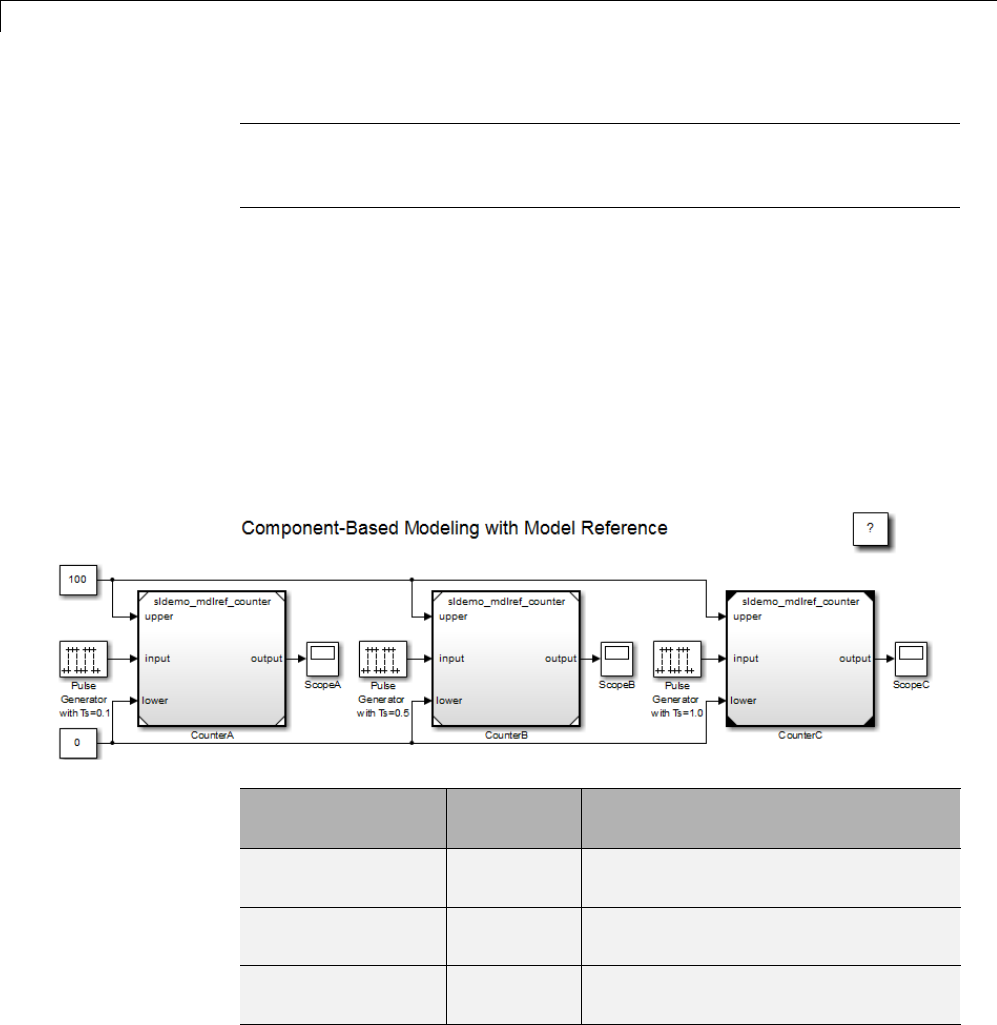
6Referencing a Model
Note If you change the Normal Mode Visibility setting for a referenced
model, you must simulate the top model in the model reference hierarchy to
make use of the new setting.
Examples of a Model with Multiple Referenced Instances in
Normal Mode
sldemo_mdlref_basic. The sldemo_mdlref_basic model has three
Model blocks (CounterA,CounterB,andCounterC) that each reference the
sldemo_mdlref_counter model.
If you update the diagram, the sldemo_mdlref_basic displays different icons
for each of the three Model blocks that reference sldemo_mdlref_counter.
Model Block Icon
Corners
Simulation Mode and Normal
Mode Visibility Setting
CounterA White Normal mode, with Normal Mode
Visibility enabled
CounterB Gray
corners
Normal mode, with Normal Mode
Visibility disabled
CounterC Black
corner
Accelerator mode (Normal Mode
Visibility is not applicable)
6-26
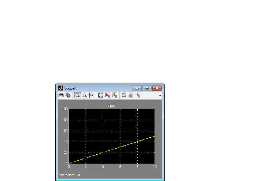
Referenced Model Simulation Modes
If you do the following steps, then the ScopeA block appears as shown below:
1Simulate sldemo_mdlref_basic.
2Open the sldemo_mdlref_counter model.
3Open the ScopeA block.
That ScopeA block reflects the results of simulating the CounterA Model
block, which has Normal Mode Visibility enabled.
If you try to open mdlref_counter model from the CounterB Model block (for
example, by double-clicking the Model block), ScopeA in mdlref_counter still
showstheresultsoftheCounterA Model block, because that is the Model
block with Normal Mode Visibility set to on.
sldemo_mdlref_depgraph. The sldemo_mdlref_depgraph model shows
the use of the Model Dependency Viewer for a model that has multiple Normal
mode instances of a referenced model. The model shows what you need to do
to set up a model with multiple referenced instances in Normal mode.
6-27

6Referencing a Model
Set Up a Model with Multiple Instances of a Referenced Model
in Normal Mode
This section describes how to set up a model to support the use of multiple
instances of Normal mode referenced models.
1Set the Configuration Parameters > Model Referencing > Total
number of instances allowed per top model parameter to Multiple.
If you cannot use the Multiple setting for your model, because of the
requirements described in the “Total number of instances allowed per top
model” parameter documentation, then you can have only one instance of
that referenced model be in Normal mode.
2For each instance of the referenced model that you want to be in Normal
mode, in the block parameters dialog box for the Model block, set the
Simulation Mode parameter to Normal. Ensure that all the ancestors in
the hierarchy for that Model block are in Normal mode.
The corners of icons for Model blocks that are in Normal mode can be white
(empty), or gray after you update the diagram or simulate the model.
3(If necessary) Modify S-functions used by the model so that they work with
multiple instances of referenced models in Normal mode. For details, see
“Supporting the Use of Multiple Instances of Referenced Models That Are
in Normal Mode”.
By default, Simulink assigns Normal mode visibility to one of the instances.
After you have performed the steps in this section, you can specify a
non-default instance to have Normal mode visibility. For details, see “Specify
the Instance That Has Normal Mode Visibility” on page 6-28.
Specify the Instance That Has Normal Mode Visibility
This section describes how to specify Normal Mode Visibility for an instance
other than the one that an instance that Simulink selects automatically.
You need to:
1(Optionally) “Determine Which Instance Has Normal Mode Visibility” on
page 6-29.
6-28

Referenced Model Simulation Modes
2“Set Normal Mode Visibility” on page 6-30.
3Simulate the top model to apply the new Normal Mode Visibility settings.
Determine Which Instance Has Normal Mode Visibility. If you do not
already know which instance currently has Normal mode visibility, you can
determinethatbyusingoneoftheseapproaches:
•If you update the diagram and have made no other changes to the model,
then you can navigate through the model hierarchy to examine the Model
blocks that reference the model that you are interested in. The Model block
that has white corners has Normal Mode Visibility enabled.
•When you are editing a model or during compilation, use the
ModelReferenceNormalModeVisibilityBlockPath parameter.
If you use this parameter while editing a model, you must update the
diagram before you use this parameter.
The result is a Simulink.BlockPath object that is the block path for the
Model block that references the model that has Normal Mode Visibility
enabled. For example:
get_param('sldemo_mdlref_basic',...
'ModelReferenceNormalModeVisibilityBlockPath')
ans =
Simulink.BlockPath
Package: Simulink
Block Path:
'sldemo_mdlref_basic/CounterA'
•For a top model that is being simulated or that is in a compiled state, you
can use the CompiledModelBlockInstancesBlockPath parameter. For
example:
a = get_param('sldemo_mdlref_depgraph',...
'CompiledModelBlockInstancesBlockPath')
a=
6-29

6Referencing a Model
sldemo_mdlref_F2C: [1x1 Simulink.BlockPath]
sldemo_mdlref_heater: [1x1 Simulink.BlockPath]
sldemo_mdlref_outdoor_temp: [1x1 Simulink.BlockPath]
Set Normal Mode Visibility. To enable Normal Mode Visibility for a
different instance of the referenced model than the instance that currently
has Normal Mode Visibility, use one of these approaches:
•Navigate to the top model and select the Diagram > Subsystem & Model
Reference > Model Block Normal Mode Visibility menu item.
The Model Block Normal Mode Visibility dialog box appears. That dialog
box includes instructions in the right pane. For additional details about
the dialog box, see “Model Block Normal Mode Visibility Dialog Box” on
page 6-31.
•From the MATLAB command line, set the
ModelReferenceNormalModeVisibility parameter.
For input, you can specify:
-An array of Simulink.BlockPath objects. For example:
bp1 = Simulink.BlockPath({'mVisibility_top/Model', ...
'mVisibility_mid_A/Model'});
bp2 = Simulink.BlockPath({'mVisibility_top/Model1', ...
'mVisibility_mid_B/Model1'});
bps = [bp1, bp2];
set_param(topMdl, 'ModelBlockNormalModeVisibility', bps);
-A cell array of cell arrays of strings, with the strings being paths to
individual blocks and models. Thefollowingexamplehasthesame
effect as the preceding example (which shows how to specify an array
of Simulink.BlockPath objects):
p1 = {'mVisibility_top/Model', 'mVisibility_mid_A/Model'};
p2 = {'mVisibility_top/Model1', 'mVisibility_mid_B/Model1'};
set_param(topMdl, 'ModelBlockNormalModeVisibility', {p1, p2});
-An empty array, to specify the use of the Simulink default selection of
the instance that has Normal mode visibility. For example:
6-30

Referenced Model Simulation Modes
set_param(topMdl, 'ModelBlockNormalModeVisibility', []);
Using an empty array is equivalent to clearing all the check boxes in the
Model Block Normal Mode Visibility dialog box.
Note You cannot change Normal Mode Visibility during a simulation.
Model Block Normal Mode Visibility Dialog Box
If you have a model that has multiple instances of a referenced model in
Normal mode, you can use the Block Model Normal Mode Visibility dialog box
to set Normal Mode Visibility for a specific instance. For a description of
Normal mode visibility, see “Normal Mode Visibility” on page 6-25.
Alternatively, you can set the ModelReferenceNormalModeVisibility
parameter. For information about how to specify an instance of a referenced
model that is in Normal mode that is different than the instance automatically
selected by Simulink, see “Specify the Instance That Has Normal Mode
Visibility” on page 6-28.
Open the Model Block Normal Mode Visibility Dialog Box. To open
the Model Block Normal Mode Visibility dialog box, navigate to the top model
and select Diagram > Subsystem & Model Reference > Model Block
Normal Mode Visibility.
The dialog box for the sldemo_mdlref_basic model, with the hierarchy pane
expanded, looks like this:
6-31
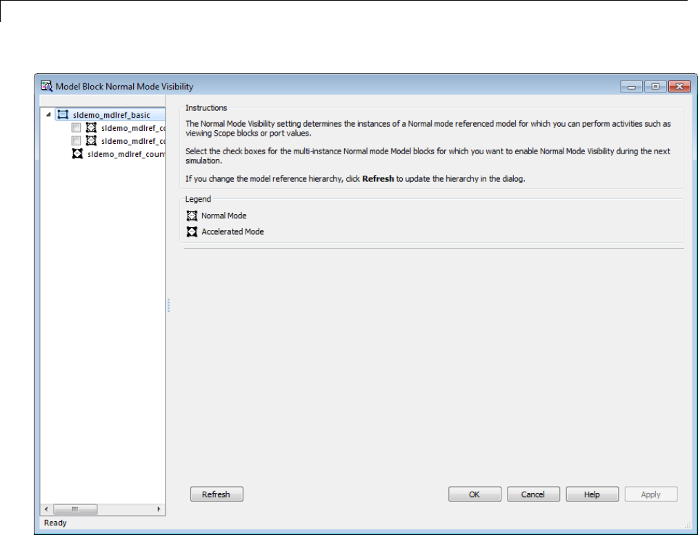
6Referencing a Model
The model hierarchy pane shows a partial model hierarchy for the model from
which you opened the dialog box. The hierarchy stops at the first Model block
that is not in Normal mode. The model hierarchy pane does not display Model
blocks that reference protected models.
Select a Model for Normal Mode Visibility.
The dialog box shows the complete model block hierarchy for the top model.
The Normal mode instances of referenced models have check boxes. Select
the check box for the instance of each model that you want to have Normal
mode visibility.
6-32
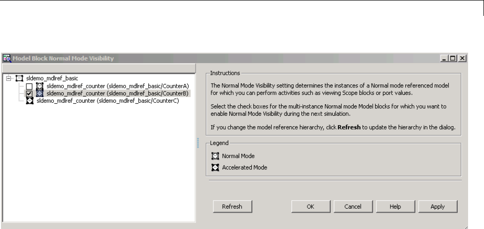
Referenced Model Simulation Modes
When you select a model, Simulink:
•Selects all ancestors of that model
•Deselects all other instances of that model
When a model is deselected, Simulink deselects all children of that model.
Opening a Model from the Model Block Normal Mode Visibility
Dialog Box. You can open a model from the Model Block Normal Mode
Visibilitydialogboxbyright-clickingthemodelinthemodelhierarchypane
and clicking Open.
Refreshing the Model Reference Hierarchy. To ensure the model
hierarchy pane of the Model Block Normal Mode Visibility dialog box reflects
the current model hierarchy, click Refresh.
Accelerating a Freestanding or Top Model
You can use Simulink Accelerator mode or Rapid Accelerator mode to
achieve faster execution of any Simulink model, including a top model in
a model reference hierarchy. For details about Accelerator mode, see the
“Acceleration” documentation. For information about Rapid Accelerator
mode, see “Rapid Simulations”.
6-33

6Referencing a Model
When you execute a top model in Simulink Accelerator mode or Rapid
Accelerator mode, all submodels execute in Accelerator mode. For any
submodel that specifies Normal mode, Simulink displays an warning message.
Be careful not confuse Accelerator mode execution of a referenced model with:
•Accelerator mode execution of a freestanding or top model, as described
in “Acceleration”
•Rapid Accelerator mode execution of a freestanding or top model, as
described in “Rapid Simulations”
While the different types of acceleration share many capabilities and
techniques, they have different implementations, requirements, and
limitations.
6-34
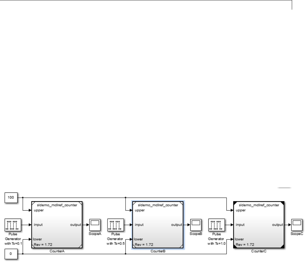
View a Model Reference Hierarchy
View a Model Reference Hierarchy
Simulink provides tools and functions that you can use to examine a model
reference hierarchy:
•Model Dependency Viewer — Shows the structure the hierarchy lets
youopenconstituentmodels. TheReferenced Model Instances view
displays Model blocks differently to indicate Normal, Accelerator, and PIL
modes. See “Model Dependency Viewer” on page 9-83 for more information.
•view_mdlrefs function — Invokes the Model Dependency Viewer to
display a graph of model reference dependencies.
•find_mdlrefs function — Finds all models directly or indirectly
referenced by a given model.
Display Version Numbers
To display the version numbers of the models referenced by a model,
for the parent model, choose Display > Blocks > Block Version for
Referenced Models. Simulink displays the version numbers in the icons of
the corresponding Model block instances.
The version number displayed on a Model block icon refers to the version
of the model used to either:
•Create the block
•Refresh the block most recently changed
6-35


Model Reference Simulation Targets
Model Reference Simulation Targets
In this section...
“Simulation Targets” on page 6-37
“Build Simulation Targets” on page 6-38
“SimulationTargetOutputFileControl”onpage6-39
“Parallel Building for Large Model Reference Hierarchies” on page 6-42
Simulation Targets
Asimulation target,orSIM target, is a MEX-file that implements a referenced
model that executes in Accelerator mode. Simulink invokes the simulation
target as needed during simulation to compute the behavior and outputs
of the referenced model. Simulink uses the same simulation target for all
Accelerator mode instances of a given referenced model anywhere in a
reference hierarchy.
IfyouhaveaSimulinkCoderlicense,becarefulnottoconfusethesimulation
target of a submodel with any of these other types of target:
•Hardware target — A platform for which Simulink Coder generates code
•System target — A file that tells Simulink Coder how to generate code
for particular purpose
•Rapid Simulation target (RSim) — A system target file supplied with
Simulink Coder
•Model reference target — A library module that contains Simulink Coder
code for a referenced model
Simulink creates a simulation target only for a submodel that has one or
more Accelerator mode instances in a reference hierarchy. A submodel that
executes only in Normal mode always executes interpretively and does not
use a simulation target. When one or more instance of a submodel executes in
Normalmode,andoneormoreinstance executes in Accelerator mode:
•Simulink creates a simulation target for the Accelerator mode instances.
6-37

6Referencing a Model
•The Normal mode instances do not use that simulation target.
Because Accelerator mode requires code generation, it imposes some
requirements and limitations that do not apply to Normal mode. Aside
from these constraints, you can generally ignore simulation targets and
their details when you execute a referenced model in Accelerator mode. See
“Limitations on Accelerator Mode Referenced Models” on page 6-84 for details.
Build Simulation Targets
Simulink by default generates the needed target from the referenced model:
•If a simulation target does not exist at the beginning of a simulation
•When you perform an update diagram for a parent model
If the simulation target already exists, then by default Simulink checks
whether the submodel has structural changes since the target was last
generated. If so, Simulink regenerates the target to reflect changes in the
model. For details about how Simulink detects whether to rebuild a model
reference target, see the “Rebuild” parameter documentation.
You can change this default behavior to modify the rebuild criteria or specify
that Simulink always or never rebuilds targets. See “Rebuild” for details.
To generate simulation targets interactively for Accelerator mode referenced
models,dooneofthesesteps:
•Update the diagram on a model that directly or indirectly references the
model that is in Accelerator mode
•Execute the slbuild command with appropriate arguments at the
MATLAB command line
While generating a simulation target, Simulink displays status messages at
the MATLAB command line to enable you to monitor the target generation
process. Target generation entails generating and compiling code and linking
the compiled target code with compiled code from standard code libraries
to create an executable file.
6-38

Model Reference Simulation Targets
Reduce Change Checking Time
You can reduce the time that Simulink spends checking whether any or all
simulation targets require rebuilding by setting configuration parameter
values as follows:
•In all referenced models throughout the hierarchy, set Configuration
Parameters > Diagnostics > Data Validity > Signal resolution to
Explicit only. (See “Signal resolution”.)
•To minimize change detection time, consider setting Configuration
Parameters > Model Referencing > Rebuild options to If any
changes in known dependencies detected on the top model. See
“Rebuild”.
These parameter values exist in the configuration set of a referenced model,
not in the individual Model block, so setting either value for any instance of a
referenced model sets it for all instances of that model.
Simulation Target Output File Control
Simulink creates simulation targets in the slprj subfolder of the working
folder. If slprj does not exist, Simulink creates it.
Note Simulink Coder code generation also uses the slprj folder.
Subdirectories in slprj provide separate places for simulation code, Simulink
Coder code, and other files. For details, see “Control the Location for
Generated Files”.
By default, the files generated by Simulink diagram updates and model builds
are placed in a build folder, the root of which is the current working folder
(pwd). However, in some situations, you might want the generated files to go
to a root folder outside the current working folder. For example:
•You need to keep generated files separate from the models and other source
materials used to generate them.
•You want to reuse or share previously-built simulation targets without
having to set the current working folder back to a previous working folder.
6-39
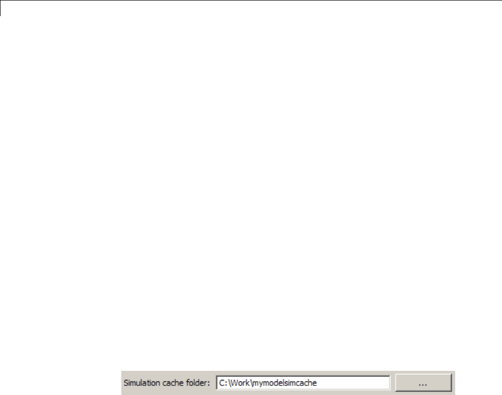
6Referencing a Model
You might also want to separate generated simulation artifacts from
generated production code.
To allow you to control the output locations for the files generated by diagram
updates and model builds, the software allows you to separately specify the
simulation cache folder build folder. The simulation cache folder is the root
folder in which to place artifacts used for simulation.
To specify the simulation cache folder, use one of these approaches:
•Use the CacheFolder MATLAB session parameter.
•Open the Simulink Preferences dialog box (File > Simulink Preferences)
and specify a location on your file system for the Simulation cache
folder,which,ifspecified,providestheinitialdefaultsfortheMATLAB
session parameters.
Control Output Location for Model Build Artifacts Used for
Simulation
The Simulink preference Simulation cache folder provides control over
the output location for files generated by Simulink diagram updates. The
preference appears in the Simulink Preferences Window, Main Pane, in the
File generation control group. To specify the root folder location for files
generated by Simulink diagram updates, set the preference value by entering
or browsing to a folder path, for example:
The folder path that you specify provides the initial default for the MATLAB
session parameter CacheFolder. When you initiate a Simulink diagram
update, any files generated are placed in a build folder at the root location
specified by CacheFolder (if any), rather than in the current working folder
(pwd).
For example, using a 32-bit Windows host platform, if you set the Simulation
cache folder to 'C:\Work\mymodelsimcache' and then simulate the model
rtwdemo_capi, files are generated into the specified folder as follows:
6-40
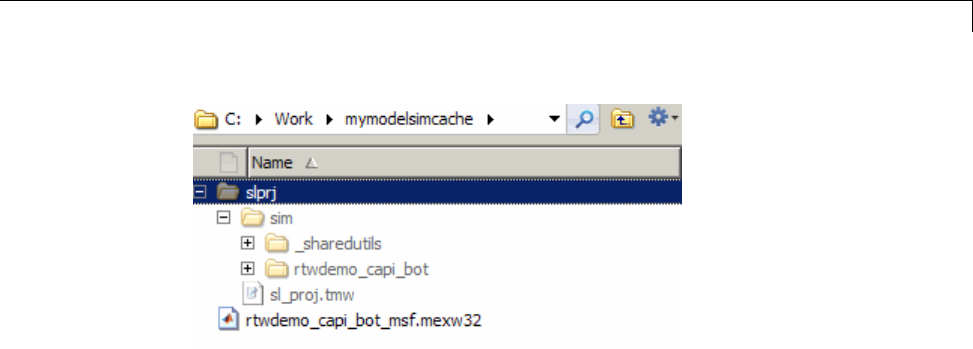
Model Reference Simulation Targets
As an alternative to using the Simulink preferences GUI to set Simulation
cache folder, you also can get and set the preference value from the
command line using get_param and set_param. For example,
>> get_param(0, 'CacheFolder')
ans =
''
>> set_param(0, 'CacheFolder', fullfile('C:','Work','mymodelsimcache'))
>> get_param(0, 'CacheFolder')
ans =
C:\Work\mymodelsimcache
Also, you can choose to override the Simulation cache folder preference
value for the current MATLAB session.
Override Build Folder Settings for the Current MATLAB Session
The Simulink preferences Simulation cache folder and Code generation
folder provide the initial defaults for the MATLAB session parameters
CacheFolder and CodeGenFolder, which determine where files generated
by Simulink diagram updates and model builds are placed. However,
you can override these build folder settings during the current MATLAB
session, using the Simulink.fileGenControl function. This function
allows you to directly manipulate the MATLAB session parameters, for
6-41

6Referencing a Model
example, overriding or restoring the initial default values. The values
you set using Simulink.fileGenControl expire at the end of the current
MATLAB session. For more information and detailed examples, see the
Simulink.fileGenControl function reference page.
Parallel Building for Large Model Reference
Hierarchies
In a parallel computing environment, you can increase the speed of diagram
updates for models containing large model reference hierarchies by building
referenced models that are configured in Accelerator mode in parallel
whenever conditions allow. For example, if you have Parallel Computing
Toolbox™ software, updating of each referenced model can be distributed
across the cores of a multicore host computer. If you additionally have
MATLAB Distributed Computing Server™ (MDCS) software, updating of
each referenced model can be distributed across remote workers in your
MATLAB Distributed Computing Server configuration.
To take advantage of parallel building for a model reference hierarchy:
1Set up a pool of local and/or remote MATLAB workers in your parallel
computing environment.
aMake sure that Parallel Computing Toolbox software is licensed and
installed.
bTouseremoteworkers,makesurethat MATLAB Distributed Computing
Server software is licensed and installed.
cIssue appropriate MATLAB commands to set up the worker pool, for
example, matlabpool 4.
2In the Configuration Parameters dialog box, go to the Model Referencing
pane and select the Enable parallel model reference builds option.
This selection enables the parameter MATLAB worker initialization
for builds.
6-42

Model Reference Simulation Targets
For MATLAB worker initialization for builds, select one of the
following values:
•None if the software should perform no special worker initialization.
Specify this value if the child models in the model reference hierarchy do
not rely on anything in the base workspace beyond what they explicitly
setup(forexample,withamodelloadfunction).
•Copy base workspace if the software should attempt to copy the base
workspace to each worker. Specify this value if you use a setup script to
prepare the base workspace for all models to use.
•Load top model if the software should load the top model on each
worker. Specify this value if the top model in the model reference
hierarchy handles all of the base workspace setup (for example, with a
model load function).
3Optionally, inspect the model reference hierarchy to determine, based on
model dependencies, which models will be built in parallel. For example,
you can use the Model Dependency Viewer from the Simulink Tools menu.
4Update your model. Messages in the MATLAB command window record
when each parallel or serial build starts and finishes.
The performance gain realized by using parallel builds for updating referenced
models depends on several factors, including how many models can be built
in parallel for a given model referencing hierarchy, the size of the referenced
models, and parallel computing resources such as number of local and/or
remote workers available and the hardware attributes of the local and remote
machines (amount of RAM, number of cores, and so on).
The following notes apply to using parallel builds for updating model
reference hierarchies:
•For local pools, the host machine should have an appropriate amount of
RAM available for supporting the number of local workers (MATLAB
sessions) that you plan to use. For example, setting matlabpool to 4 results
in five MATLAB sessions on your machine, each using approximately 120
MB of memory at startup.
•Remote MDCS workers participating in a parallel build must use a common
platform and compiler.
6-43

6Referencing a Model
•A consistent MATLAB environment must be set up in each MATLAB
worker session as in the MATLAB client session — for example, all
shared base workspace variables, MATLAB path settings, and so forth.
OneapproachistousethePreLoadFcn callback of the top model. If you
configure your model to load the topmodelwitheachMATLABworker
session, its preload function can be used for any MATLAB worker session
setup.
6-44

Simulink®Model Referencing Requirements
Simulink Model Referencing Requirements
In this section...
“About Model Referencing Requirements” on page 6-45
“Name Length Requirement” on page 6-45
“Configuration Parameter Requirements” on page 6-45
“Model Structure Requirements” on page 6-50
About Model Referencing Requirements
A model reference hierarchy must satisfy various Simulink requirements, as
described in this section. Some limitations also apply, as described in “Model
Referencing Limitations” on page 6-80.
Name Length Requirement
The name of a referenced model must contain fewer than 60 characters,
exclusive of the .slx or .mdl suffix. An error occurs if the name of a
referenced model is too long.
Configuration Parameter Requirements
A referenced model uses a configuration set in the same way that any other
model does, as described in “Manage a Configuration Set” on page 10-12. By
default, every model in a hierarchy has its own configuration set. Each model
uses its configuration set the same way that it would if the model executed
independently.
Because each model can have its own configuration set, configuration
parameter values can be different in different models. Furthermore, some
parameter values are intrinsically incompatible with model referencing. The
Simulink response to an inconsistent or unusable configuration parameter
depends on the parameter:
•Where an inconsistency has no significance, or a trivial resolution exists
that carries no risk, Simulink ignores or resolves the inconsistency without
posting a warning.
6-45

6Referencing a Model
•Where a nontrivial and possibly acceptable solution exists, Simulink
resolves the conflict silently, resolves it with a warning, or generates an
error. See “Model configuration mismatch” for details.
•Wherenoacceptableresolutionispossible, Simulink generates an error.
Change some or all parameter values to eliminate the problem.
Manually eliminating all configuration parameter incompatibilities can be
tedious when:
•A model reference hierarchy contains many submodels that have
incompatible parameter values
•A changed parameter value must propagate to many submodels
You can control or eliminate such overhead by using configuration references
to assign an externally stored configuration set to multiple models. See
“Manage a Configuration Reference” on page 10-18 for details.
Note Configuration parameters on the Code Generation pane of the
Configuration Parameters dialog box do not affect simulation in either
Normal or Accelerated mode. Code Generation parameters affect only code
generation by Simulink Coder itself. Accelerated mode simulation requires
code generation to create a simulation target. Simulink uses default values
for all Code Generation parameters when generating the target, and
restores the original parameter values after code generation is complete.
The tables in the following sections list Configuration parameter options
that can cause problems if set:
•In certain ways, as indicated in the table
•Differently in a referenced model than in a parent model
Where possible, Simulink resolves violations of these requirements
automatically, but most cases require changes to the parameters in some
or all models.
6-46

Simulink®Model Referencing Requirements
Configuration Requirements for All Referenced Model
Simulation
Dialog Box Pane Option Requirement
Start time The start time of the
top model and all
referenced models must
be the same, but need
not be zero.
Stop time Simulink uses Stop
time of the top
model for simulation,
overriding any differing
Stop time in a
submodel.
Solver
Type
Solver
The Type and Solver
of the top model
apply throughout the
hierarchy. See “Solver
Requirements” on page
6-48.
Data Import/Export Initial state Can be on for the top
model,butmustbeoff
for a referenced model.
Inline parameters Can be on or off
for a top model, but
must be on for a
referenced model.
See “Inline Parameter
Requirements” on page
6-49.
Optimization
Application lifespan
(days)
Must be the same for
top and referenced
models.
6-47

6Referencing a Model
Dialog Box Pane Option Requirement
Model Referencing Total number of
instances allowed
per top model
Must not be Zero in
a referenced model.
Specifying One rather
than Multiple is
preferable or required
in some cases. See
“Model Instance
Requirements” on page
6-49.
Hardware
Implementation
Embedded hardware
options
All values must be
the same for top and
referenced models.
Solver Requirements. Model referencing works with both fixed-step and
variable-step solvers. All models in a model reference hierarchy use the same
solver, which is always the solver specified by the top model. An error occurs
ifthesolvertypespecifiedbythetopmodelisincompatiblewiththesolver
type specified by any submodel.
Top Model Solver
Type
Submodel Solver
Type
Compatibility
Fixed Step Fixed Step Allowed
Variable Step Variable Step Allowed
Variable Step Fixed-step Allowed unless the
submodel is multi-rate
and specifies both
a discrete sample
time and a continuous
sample time
Fixed Step Variable Step Error
If an incompatibility exists between the top model solver and any submodel
solver, one or both models must change to use compatible solvers. For
information about solvers, see “Solvers” on page 3-21 and “Choose a Solver”
on page 14-9.
6-48

Simulink®Model Referencing Requirements
Inline Parameter Requirements. Simulink requires enabling
Configuration Parameters > Optimization > Inline parameters (see
“Inline parameters”) for all referenced models in a reference hierarchy. The
top model can enable or disable inline parameters. If a referenced model
disables inlined parameters, and you try to simulate the parent model:
•For a Normal mode submodel, Simulink generates an error and cancels the
build. All models and compiled files remain unchanged after the failed
build.
•For an Accelerator mode submodel, Simulink temporarily enables inline
parameters, posts no warning, and builds the model. Inline parameters
remain disabled after the build completes.
Simulink ignores tunable parameter specifications in the Model Parameter
Configuration dialog box for both the top model and referenced models. Do not
use this dialog box to override the inline parameters optimization for selected
parameters to permit them to be tuned. Instead, see “Parameterize Model
References” on page 6-52 for alternate techniques.
Model Instance Requirements. A referenced model must specify that it
is available to be referenced, and whether it can be referenced at most once
or can have multiple instances. The Configuration Parameters > Model
Referencing > Total number of instances allowed per top model
parameter provides this specification. See “Total number of instances allowed
per top model” for more information. The possible values for this parameter
are:
•Zero — A model cannot reference this model. An error occurs if a reference
to the model occurs in another model.
•One — A model reference hierarchy can reference the model at most once.
An error occurs if more than one instance of the model exists. This value is
sometimes preferable or required.
•Multiple — A model hierarchy can reference the model more than once, if
it contains no constructs that preclude multiple reference. An error occurs
if the model cannot be multiply referenced, even if only one reference exists.
Setting Total number of instances allowed per top model to Multiple
for a model that is referenced only once can reduce execution efficiency
6-49

6Referencing a Model
slightly. However, this setting does not affect data values that result from
simulation or from executing code Simulink Coder generates. Specifying
Multiple when only one model instance exists avoids having to change or
rebuild the model when reusing the model:
•In the same hierarchy
•Multiple times in a different hierarchy
Some model properties and constructs require setting Total number of
instances allowed per top model to One. For details, see “General
Reusability Limitations” on page 6-81 and “Accelerator Mode Reusability
Limitations” on page 6-85.
Model Structure Requirements
The following requirements relate to the structure of a model reference
hierarchy.
Signal Propagation Requirements
The signal name must explicitly appear on any signal line connected to an
Outport block of a referenced model. A signal connected to an unlabeled line
of an Outport block of a referenced model cannot propagate out of the Model
block to the parent model.
Bus Usage Requirements
A bus that propagates between a parent model and a referenced model must be
nonvirtual. Use the same bus object to specify the properties of the bus in both
the parent and the referenced model. Define the bus object in the MATLAB
workspace. See “About Composite Signals” on page 48-2 for more information.
Sample Time Requirements
The first nonvirtual block connected to a root-level Inport or Outport block
of a referenced model must have the same sample time as the port to which
it connects. Use Rate Transition blocks to match input and output sample
times, as illustrated in the following diagram.
6-50
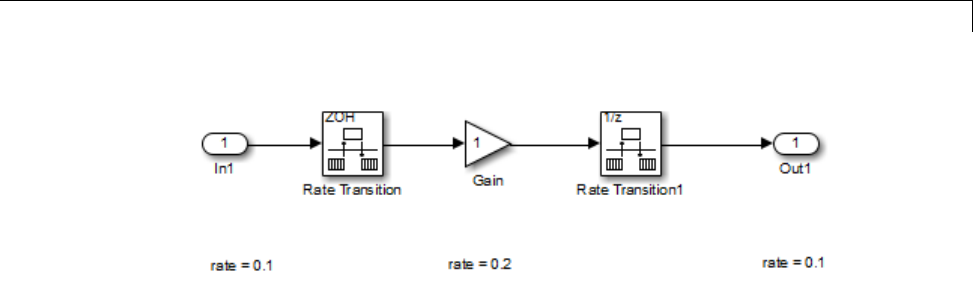
Simulink®Model Referencing Requirements
6-51

6Referencing a Model
Parameterize Model References
In this section...
“Introduction” on page 6-52
“Global Nontunable Parameters” on page 6-53
“Global Tunable Parameters” on page 6-53
“Using Model Arguments” on page 6-53
Introduction
A parameterized referenced model obtains values that affect the behavior of
the referenced model from some source outside the model. Changing the
values changes the behavior of the model, without recompiling the model.
Due to the constraints described in “Inline Parameter Requirements” on
page 6-49, you cannot use the Model Parameter Configuration dialog box to
parameterize referenced models. Simulink provides three other techniques
that you can use to parameterize referenced models:
•Global nontunable parameters
•Global tunable parameters
•Model arguments
Global parameters work the same way with referenced models that they do
with any other model construct. Each global parameter has the same value
in every instance of a referenced model that uses it. Model arguments allow
youtoprovidedifferentvaluestoeach instance of a referenced model. Each
instance can then behave differently from the others. The effect is analogous
to calling a function more than once with different arguments in each call.
You can use a structure parameter to group variables for parameterizing
model references. For details, see “Structure Parameters” on page 24-16.
6-52

Parameterize Model References
Global Nontunable Parameters
Aglobal nontunable parameter is a MATLAB variable or a
Simulink.Parameter object whose storage class is auto.Theparametermust
exist in the MATLAB workspace.
Using a global nontunable parameter in a referenced model sets the
parameter value before the simulation begins. This allows you to control the
behavior of the referenced model. All instances of the model use the same
value. You cannot change the value during simulation, but you can change
it between one simulation and the next. The change requires rebuilding the
model in which the change occurs, but not any models that it references. See
“Specify Parameter Values” on page 24-6 for details.
Global Tunable Parameters
Aglobal tunable parameter is a Simulink.Parameter object whose storage
classisot
her than auto. The parameter exists in the MATLAB workspace.
Using a global tunable parameter in a referenced model allows you to control
the behavior of the referenced model by setting the parameter value. All
instances of the model use the same value. You can change the value during
simulation or between one simulation and the next. The change does not
require rebuilding the model in which the change occurs, or any models that
it references. See “Tunable Parameters” on page 24-13 for details.
To reference a model that uses tunable parameters defined with the “Model
Parameter Configuration Dialog Box”, change the model to implement
tunability another way. To facilitate this task, Simulink provides a
command that converts tunable parameters specified in the Model
Parameter Configuration dialog box to global tunable parameters. See
tunablevars2parameterobjects for details.
Using Model Arguments
Model arguments let you parameterize references to the same model so that
each instance of the model behaves differently. Without model arguments, a
variable in a referenced model has the same value in every instance of the
model. Declaring a variable to be a model argument allows each instance of
the model to use a different value for that variable.
6-53

6Referencing a Model
To create model arguments for a referenced model:
1Create MATLAB variables in the model workspace.
2Add the variables to a list of model arguments associated with the model.
3Specify values for those variables separately in each Model block that
references the model
The values specified in the Model block replace the values of the MATLAB
variables for that instance of the model.
A referenced model that uses model arguments can also appear as a top model
or a standalone model. No Model block then exists to provide model argument
values. The model uses the values of the MATLAB variables themselves, as
defined in the model workspace. Thus, you can use the same model without
change as a top model, a standalone model, and a parameterized referenced
model.
The sldemo_mdlref_datamngt model demonstrates techniques for using
model arguments. The model passes model argument values to referenced
models through masked Model blocks. Suchmaskingcanbeconvenient,but
is independent of the definition and use of model arguments themselves. See
“Masking” for information about masking.
The rest of this section describes techniques for declaring and using model
arguments to parameterize a referenced model independently of any Model
block masking. The steps are:
•Create MATLAB variables in the model workspace.
•Register the variables to be model arguments.
•Assign values to those arguments in Model blocks.
Creating the MATLAB Variables
To create MATLAB variables for use as model arguments:
1Open the model for which you want to define model arguments.
2Open the Model Explorer.
6-54
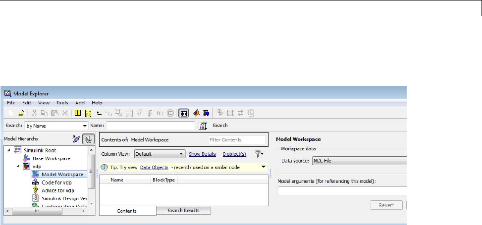
Parameterize Model References
3In the Model Explorer Model Hierarchy pane, select the workspace
of the model:
4From Model Explorer’s Add menu, select MATLAB Variable.
A new MATLAB variable appears in the Contents pane with a default
name and value.
5In the Contents pane:
aChangethedefaultnameofthenewMATLABvariabletoanamethat
you want to declare as a model argument.
bIf you also use the model as a top or standalone model, specify the value
for that variable for use in that context. This value must be numeric.
cIfthevariabletypedoesnotmatchthedimensionsandcomplexityof
the model argument, specify a value that has the correct type. This
type must be numeric.
6Repeat adding and naming MATLAB variables until you have defined all
the variables that you need.
Register the Model Arguments
To register MATLAB variables as model arguments:
1Again, in the Model Explorer Model Hierarchy pane, select the workspace
of the model.
6-55

6Referencing a Model
The Dialog pane displays the Model Workspace dialog.
2In the Model Workspace dialog, enter the names of the MATLAB variables
that you want to declare as model arguments. Use a comma-separated
list in the Model arguments field.
For example, suppose you added two MATLAB variables named
init_value and incr, and you declared them to be model arguments. The
Contents and Dialog panes of the Model Explorer could look like this:
3Click Apply to confirm the entered names.
Assign Model Argument Values
If a model declares model arguments, assign values to those arguments in
each Model block that references the model. Failing to assign a value to a
model argument causes an error: the value of the model argument does not
default to the value of the corresponding MATLAB variable. That value is
availableonlytoastandaloneortopmodel. Toassignvaluestothearguments
of a referenced model:
1Open the block parameters dialog box oftheModelblockbyright-clicking
the block and choosing Block Parameters (ModelReference) from the
context menu.
6-56
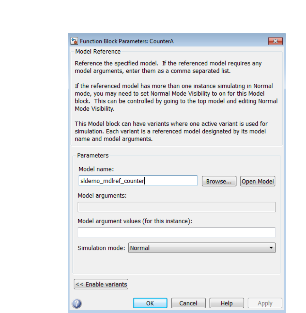
Parameterize Model References
The second field, Model arguments,specifiesthesameMATLAB
variables, in the same order, that you previously typed into the Model
6-57

6Referencing a Model
arguments field of the Model Workspace dialog. This field is not editable.
It provides a reminder of which model arguments need values assigned,
and in what order.
2In the Model argument values field, enter a comma-delimited list of
values for the model arguments that appear in the Model arguments
field. Simulink assigns the values to arguments in positional order, so they
must appear in the same order as the corresponding arguments.
You can enter the values as literal values, variable names, MATLAB
expressions, and Simulink parameter objects. Any symbols used resolve to
values as described in “Symbol Resolution Process” on page 4-76. All values
must be numeric (including objects with numeric values).
Note Simulink generates an error if you use a model argument in an
expression that is nontunable because of “Tunable Expression Limitations”.
The value for each argument must have the same dimensions and
complexity as the MATLAB variable that defines the model argument in
the model workspace. The data types need not match. If necessary, the
Simulink software casts a model argument value to the data type of the
corresponding variable.
3Click OK or Apply to confirm the values for the Model block.
When the model executes in the context of that Model block, the Model
arguments have the values specified in the Model argument values field
of the Model block.
6-58

Conditional Referenced Models
Conditional Referenced Models
In this section...
“Kinds of Conditional Referenced Models” on page 6-59
“Working with Conditional Referenced Models” on page 6-60
“Create Conditional Models” on page 6-61
“Reference Conditional Models” on page 6-63
“Simulate Conditional Models” on page 6-64
“Generate Code for Conditional Models” on page 6-64
“Requirements for Conditional Models” on page 6-65
KindsofConditionalReferencedModels
You can set up referenced models so that they execute conditionally, similar
to conditional subsystems. For information about conditional subsystems, see
“About Conditional Subsystems” on page 7-2.
You can use the following kinds of conditionally executed referenced models:
•Enabled
•Triggered
•Enabled and triggered
•Function-call
Enabled Models
UseanEnableblocktoinsertanenableportinamodel. Addanenableport
to a model if you want a referenced model to execute at each simulation step
for which the control signal has a positive value.
To see an example of an enabled subsystem,seeenablesub. A corresponding
enabled referenced model would use the same blocks as are in the enabled
subsystem.
6-59

6Referencing a Model
Triggered Models
Use a Trigger block to insert a trigger port in a model. Add a trigger port to a
model if you want to use an external signal to trigger the execution of that
model. You can add a trigger port to a root-level model or to a subsystem.
This section focuses on models that contain a trigger port with an edge-based
trigger type (rising,falling,oreither).
To view a model that illustrates how you can use trigger ports in referenced
models, see the Introduction to Managing Data with Model Reference
example. In that example, see the “Top Model: Scheduling Calls to the
Referenced Model” section.
Triggered and Enabled Models
A triggered and enabled model executes once at the time step for which a
trigger event occurs, if the enable control signal has a positive value at that
step.
Function-Call Models
Simulink allows certain blocks to control execution of a referenced model
during a time step, using a function-call signal. Examples of such blocks are a
Function-Call Generator or an appropriately configured custom S-function.
See “Function-Call Subsystems” on page 7-30 for more information. A
referenced model that you can invoke in this way is a function-call model.
For an example of a function-call model, see the sldemo_mdlref_fcncall
model.
Working with Conditional Referenced Models
Use a similar approach for each kind of conditionally executed referenced
model for these tasks:
•“Create Conditional Models” on page 6-61
•“Reference Conditional Models” on page 6-63
•“Simulate Conditional Models” on page 6-64
•“Generate Code for Conditional Models” on page 6-64
6-60

Conditional Referenced Models
Each kind of conditionally executed model has some model creating
requirements. For details, see “Requirements for Conditional Models” on
page 6-65.
Create Conditional Models
To create a conditional model:
1At the root level of the referenced model, insert one of the following blocks:
Kind of Model Blocks to Insert
Enabled Enable
Triggered Trigger
Triggered and Enabled Trigger and Enable
Function-Call Trigger
For an enabled model, go to Step 3.
2For the Trigger block, set the Trigger type parameter, based on the kind
of model:
Kind of Model Trigger Type Parameter Setting
Triggered
Triggered and enabled
One of the following:
•rising
•falling
•either
Function-Call function-call
3Create and connect other blocks to implement the model.
Enabled model example:
6-61
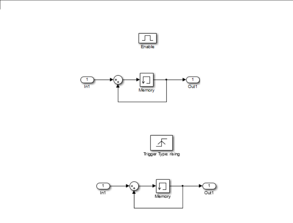
6Referencing a Model
Triggered model example:
Function-call model example:
6-62
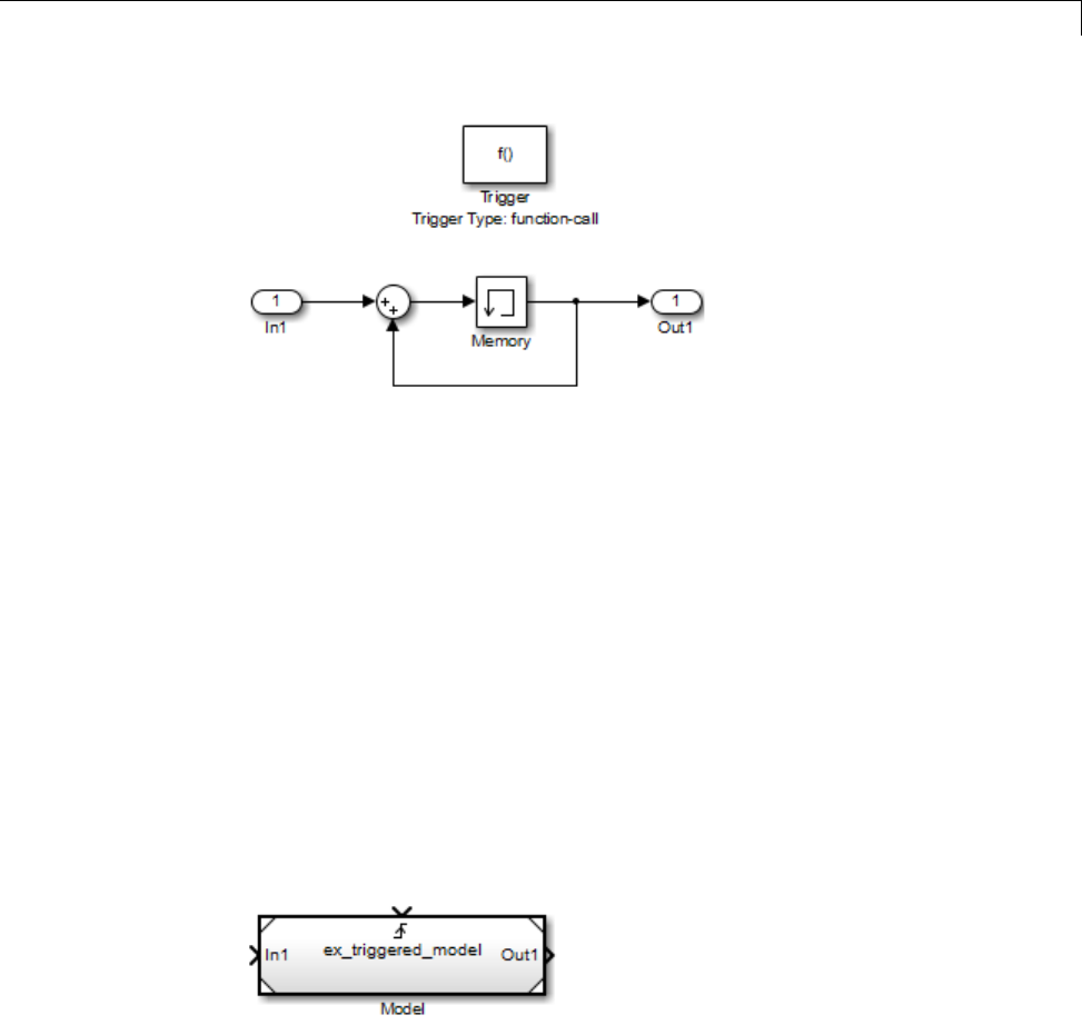
Conditional Referenced Models
4Ensure that the model satisfies the requirements for a conditional model.
See the appropriate section:
•“Enabled Model Requirements” on page 6-65
•“Triggered Model Requirements” on page 6-65
•“Function-Call Model Requirements” on page 6-65
Reference Conditional Models
To create a reference to a conditional model:
1Add a Model block to the model that you want to reference the triggered
model. See “Create a Model Reference” on page 6-8 for details.
The top of the Model block displays an icon that corresponds to the kind of
port used in the referenced model. For example, for a triggered model, the
top of the Model block displays the following icon.
For enabled, triggered, and triggered and enabled models, go to Step 3.
2For a function-call model, connect a Stateflow chart, Function-Call
Generator block, or other function-call-generating block to the function-call
port of the Model block. The signal connected to the port must be scalar.
6-63

6Referencing a Model
3Create and connect other blocks to implement the parent model.
4Ensure that the referencing model satisfies the conditions for model
referencing. See “Simulink Model Referencing Requirements” on page 6-45
and “Model Referencing Limitations” on page 6-80 for details.
Simulate Conditional Models
Use Normal, Accelerator, or Rapid Acceleratormodetosimulateaconditional
model.
You can run a standalone simulation of a referenced model. A standalone
simulation is useful for unit testing, because it provides consistent data
across simulations, in terms of data type, dimension, and sample time. In
the Trigger or Enable block, in the Signal Attributes pane of the Block
Parameters dialog box, specify values to lock down the signal data type,
dimension, and sample time.
To run a standalone simulation of a conditional model, specify the inputs
using the Configuration Parameters > Data Import/Export > Input
parameter. The following conditions apply when you use the “Input”
parameter for trigger and enable port inputs:
•Use the last data input for the trigger or enable input. For a triggered and
enabled model, use the last data input for the trigger input.
•Ifyoudonotprovideanyinputvalues,thesimulationuseszeroasthe
default values.
For details about how to specify the input, see “Techniques for Importing
Signal Data” on page 45-61.
You can log data to determine which signal caused the model to run. For the
Trigger or Enable block, in the Main pane of the Block Parameters dialog box,
select Show output port.
Generate Code for Conditional Models
You can build model reference Simulink Coder and SIM targets for referenced
modelsthatcontainatriggerorenableport. You cannot generate standalone
SimulinkCoderorPILcode. Forinformation about code generation for
6-64

Conditional Referenced Models
referenced models, see “Reusable Code and Referenced Models” and “Generate
Code for Referenced Models”.
Requirements for Conditional Models
Conditional models must meet the requirements for:
•Conditional subsystems (see “Conditional Subsystems”)
•Referenced models (see “Simulink Model Referencing Requirements” on
page 6-45)
In addition, conditional models must meet the requirements described below.
Enabled Model Requirements
•Multi-rate enabled models cannot use multi-tasking solvers. You must
use single-tasking.
•For models with enable ports at the root, if the model uses a fixed-step
solver, the fixed-step size of the model must not exceed the rate for any
block in the model.
•The signal attributes of the enable port in the referenced model must be
consistent with the input that the Model block provides to that enable port.
Triggered Model Requirements
The signal attributes of the trigger port in the referenced model must be
consistent with the input that the Model block provides to that trigger port.
Function-Call Model Requirements
•A function-call model cannot have an outport driven only by Ground
blocks, including hidden Ground blocks inserted by Simulink. To meet
this requirement, do the following:
1Insert a Signal Conversion block into the signal connected to the outport.
2Enable the Exclude this block from ’Block reduction’ optimization
option of the inserted block.
6-65

6Referencing a Model
•The referencing model must trigger the function-call model at the rate
specified by the Configuration Parameters > Solver 'Fixed-step
size' option if the function-call model meets both these conditions:
-It specifies a fixed-step solver
-It contains one or more blocks that use absolute or elapsed time
Otherwise, the referencing model can trigger the function-call model at
any rate.
•A function-call model must not have direct internal connections between its
root-level input and output ports. Simulink does not honor the None and
Warning settings for the Invalid root Inport/Outport block connection
diagnostic for a referenced function-call model. It reports all invalid root
port connections as errors.
•If the Sample time type is periodic, the sample-time period must not
containanoffset.
•The signal connected to a function-call port of a Model block must be scalar.
6-66

Protected Model
Protected Model
A protected model provides the ability to deliver a model without revealing
the intellectual property of the model. A protected model is a referenced
model that hides all block and line information. It does not use encryption
technology. Creating a protected model requires a Simulink Coder license.
However, you can simulate a protected model with only a Simulink license. A
third party that receives a protected model must match the platform and the
version of Simulink for which the protected model was generated.
You cannot view the contents of a protected model, therefore you cannot log
signals in a protected model. Protected models do not appear in the model
hierarchy in the Model Explorer.
Simulating a protected model requires that the protected model:
•Be available somewhere on the MATLAB path.
•Be referenced by a Model block in a model that executes in Normal or
Accelerator mode. To run in Accelerator mode, the protected model must
include code generation capabilities.
•Receives from the Model block the values needed by any defined model
arguments.
•Connects via the Model block to input and output signals that match the
input and output signals of the protected model.
To locate protected models in your model:
•The MATLAB Folder Browser shows a small image of a lock on the node
for the protected model file.
•A Model block that references a protected model shows a small image of a
shield in the lower left corner of the Model block.
For more information, see “Use Protected Model in Simulation” on page
6-68. For more information about creating protected referenced models, see
“Protect a Referenced Model”.
6-67

6Referencing a Model
Use Protected Model in Simulation
When you receive a protected model it might be included in a protected model
package. The package could include additional files, such as a harness model
and a MAT-file. A protected model file has an .slxp extension. A typical
workflow for using a protected model in a simulation is:
1If necessary, unpack the files according to any accompanying directions.
2If there is a MAT-file containing workspace definitions, load that MAT-file.
3If there is a harness model, copy the Model block referencing the protected
model into your model.
4If a protected model report was generated when the protected model was
created, double-click the Model block to open it. In the Summary of the
report, check that your Simulink versionandplatformmatchthesoftware
and platform used to create the protected model.
5Connect signals to the Model block that match its input and output port
requirements.
6Provide any needed model argument values. See “Assign Model Argument
Values” on page 6-56.
There are also other ways to include the protected model into your model:
•Use your own Model block rather than the Model block in the harness
model.
Note When you change a Model block to reference a protected model,
the Simulation mode of the block becomes Accelerator. You cannot
change the mode.
•Start with the harness model, add more constructs to it, and use it in
your model.
•Use the protected model as a variant in a Model Variant block, as described
in “Set Up Model Variants” on page 8-5.
6-68

Use Protected Model in Simulation
•Apply a mask to the Model block that references the protected model. See
“Masking”.
•Configure a callback function, such as LoadFcn,toloadtheMAT-file
automatically. See “Callback Functions” on page 4-54.
Now you can simulate the model that includes the protected model. Because
the protected model is set to Accelerator mode, the simulation produces the
same outputs that it did when used in Accelerator mode in the source model.
6-69

6Referencing a Model
Inherit Sample Times
In this section...
“How Sample-Time Inheritance Works for Model Blocks” on page 6-70
“Conditions for Inheriting Sample Times” on page 6-70
“Determining Sample Time of a Referenced Model” on page 6-71
“Blocks That Depend on Absolute Time” on page 6-71
“Blocks Whose Outputs Depend on Inherited Sample Time” on page 6-73
How Sample-Time Inheritance Works for Model
Blocks
The sample times of a Model block are the sample times of the model that
it references. If the referenced model must run at specific rates, the model
specifies the required rates. Otherwise, the referenced model inherits its
sample time from the parent model.
Placing a Model block in a triggered, function call, or iterator subsystem relies
on the ability to inherit sample times. Additionally, allowing a Model block
to inherit sample time maximizes its reuse potential. For example, a model
might fix the data types and dimensions of all its input and output signals.
You could reuse the model with different sample times (for example, discrete
at 0.1 or discrete at 0.2, triggered, and so on).
Conditions for Inheriting Sample Times
A referenced model inherits its sample time if the model:
•Does not have any continuous states
•Specifies a fixed-step solver and the Fixed-step size is auto
•Contains no blocks that specify sample times (other than inherited or
constant)
•Does not contain any S-functions that use their specific sample time
internally
6-70

Inherit Sample Times
•Has only one sample time (not counting constant and triggered sample
time) after sample time propagation
•Does not contain any blocks, including Stateflow charts, that use absolute
time, as listed in “Blocks That Depend on Absolute Time” on page 6-71
•Does not contain any blocks whose outputs depend on inherited sample
time, as listed in “Blocks Whose Outputs Depend on Inherited Sample
Time” on page 6-73.
You can use a referenced model that inheritsitssampletimeanywherein
a parent model. By contrast, you cannot use a referenced model that has
intrinsic sample times in a triggered, function call, or iterator subsystem. To
avoid rate transition errors, ensure that blocks connected to a referenced
model with intrinsic samples times operate at the same rates as the
referenced model.
Determining Sample Time of a Referenced Model
To determine whether a referenced model can inherit its sample time, set the
Periodic sample time constraint on the Solver configuration parameters
dialog pane to Ensure sample time independent. If the model is unable
to inherit sample times, this setting causes Simulink to display an error
message when building the model. See “Periodic sample time constraint”
for more about this option.
To determine the intrinsic sample time of a referenced model, or the fastest
intrinsic sample time for multirate referenced models:
1Update the model that references the model
2Select a Model block within the parent model
3Enter the following at the MATLAB command line:
get_param(gcb, 'CompiledSampleTime')
Blocks That Depend on Absolute Time
The following Simulink blocks depend on absolute time, and therefore
preclude a referenced model from inheriting sample time:
6-71

6Referencing a Model
•Backlash (only when the model uses a variable-step solver and the block
uses a continuous sample time)
•Chirp Signal
•Clock
•Derivative
•Digital Clock
•Discrete-Time Integrator (only when used in triggered subsystems)
•From File
•From Workspace
•Pulse Generator
•Ramp
•Rate Limiter
•Repeating Sequence
•Signal Generator
•Sine Wave (only when the Sine type parameter is Time-based)
•Stateflow (only when the chart uses the reserved word tto reference time)
•Step
•To File
•To Workspace (only when logging to Timeseries or Structure With Time
format)
•Transport Delay
•Variable Time Delay
•Variable Transport Delay
Some blocks other than Simulink blocks depend on absolute time. See the
documentation for the blocksets that you use.
6-72

Inherit Sample Times
Blocks Whose Outputs Depend on Inherited Sample
Time
Using a block whose output depends on an inherited sample time in a
referenced model can cause simulation to produce unexpected or erroneous
results. For this reason, when building a submodel that does not need to
run at a specified rate, Simulink checks whether the model contains any
blocks whose outputs are functions of the inherited simulation time. This
includes checking S-Function blocks. If Simulink finds any such blocks,
it specifies a default sample time. Simulink displays an error if you have
set the Configuration Parameters > Solver > Periodic sample time
constraint toEnsure sample time independent. See “Periodic sample time
constraint” for more about this option.
The outputs of the following built-in blocks depend on inherited sample time.
The outputs of these blocks preclude a referenced model from inheriting its
sample time from the parent model:
•Discrete-Time Integrator
•From Workspace (if it has input data that contains time)
•Probe (if probing sample time)
•Rate Limiter
•Sine Wave
Simulink assumes that the output of an S-function does not depend on
inherited sample time unless the S-function explicitly declares the contrary.
See “Sample Times” for information on how to create S-functions that declare
whether their output depends on their inherited sample time.
To avoid simulation errors with referenced models that inherit their sample
time, do not include S-functions in the referenced models that fail to declare
whether their output depends on their inherited sample time. By default,
Simulink warns you if your model contains such blocks when you update or
simulate the model. See “Unspecified inheritability of sample time” for details.
6-73

6Referencing a Model
Refresh Model Blocks
Refreshing a Model block updates its internal representation to reflect
changes in the interface of the model that it references.
Examples of when to refresh a Model block include:
•Refresh a Model block that references model that has gained or lost a port.
•Refresh all the Model blocks that reference a model whose interface has
changed.
You do not need to refresh a Model block if the changes to the interface of the
referenced model do not affect how the referenced model interfaces to its
parent.
To update a specific Model block, from the context menu of the Model block,
select Diagram > Subsystem & Model Reference > Refresh Selected
Model Block.
To refresh all Model blocks in a model (as well as linked blocks in a library or
model), in the Simulink Editor select Diagram > Refresh Blocks.Youcan
also refresh a model by starting a simulation or generating code.
You can use Simulink diagnostics to detect changes in the interfaces of
referenced models that could require refreshing the Model blocks that
reference them. The diagnostics include:
•Model block version mismatch
•Port and parameter mismatch
6-74

S-Functions with Model Referencing
S-Functions with Model Referencing
In this section...
“S-Function Support for Model Referencing” on page 6-75
“SampleTimes”onpage6-75
“S-Functions with Accelerator Mode Referenced Models” on page 6-76
“Using C S-Functions in Normal Mode Referenced Models” on page 6-77
“Protected Models” on page 6-77
“Simulink®Coder™ Considerations” on page 6-77
S-Function Support for Model Referencing
Each kind of S-function provides its own level of support for model referencing.
Type of S-Function Support for Model Referencing
Level-1 MATLAB
S-function
Not supported
Level-2 MATLAB
S-function
•Supports Normal and Accelerator mode
•Accelerator mode requires a TLC file
Handwritten C MEX
S-function
•Supports Normal and Accelerator mode
•May be inlined with TLC file
S-Function Builder Supports Normal and Accelerator mode
Legacy Code Tool Supports Normal and Accelerator mode
Sample Times
Simulink software assumes that the output of an S-function does not depend
on an inherited sample time unless the S-function explicitly declares a
dependence on an inherited sample time.
You can control inheriting sample time by using
ssSetModelReferenceSampleTimeInheritanceRule in different ways,
6-75

6Referencing a Model
depending on whether an S-function permits or precludes inheritance. For
details,see“InheritedSampleTimeforReferencedModels”.
S-Functions with Accelerator Mode Referenced
Models
For a referenced model that executes in Accelerator mode, set the
Configuration Parameters > Model Referencing > Total number of
instances allowed per top model to One if the model contains an S-function
that is either:
•Inlined, but has not set the SS_OPTION_WORKS_WITH_CODE_REUSE flag
•Not inlined
Inlined S-Functions with Accelerator Mode Referenced Models
For Accelerator mode referenced models, if the referenced model
contains an S-function that should be inlined using a Target Language
Compiler file, the S-function must use the ssSetOptions macro to set the
SS_OPTION_USE_TLC_WITH_ACCELERATOR option in its mdlInitializeSizes
method. The simulation target does not inline the S-function unless the
S-function sets this option.
A referenced model cannot use noninlined S-functions in the following cases:
•The model uses a variable-step solver.
•Simulink Coder generated the S-function.
•The S-function supports use of fixed-point numbers as inputs, outputs,
or parameters.
•The model is referenced more than once in the model reference hierarchy.
To work around this limitation, use Normal mode.
•The S-function uses string parameters.
6-76

S-Functions with Model Referencing
Using C S-Functions in Normal Mode Referenced
Models
Under certain conditions, when a C S-function appears in a referenced model
that executes in Normal mode, successful execution is impossible. For details,
see “S-Functions in Normal Mode Referenced Models”.
Use the ssSetModelReferenceNormalModeSupport SimStruct function to
specify whether an S-function can be used in a Normal mode referenced model.
You may need to modify S-functions that are used by a model so that the
S-functions work with multiple instances of referenced models in Normal
mode. The S-functions must indicate explicitly that they support multiple
exec instances. For details, see “Supporting the Use of Multiple Instances
of Referenced Models That Are in Normal Mode”.
Protected Models
A protected model cannot use non-inlined S-functions directly or indirectly.
Simulink Coder Considerations
A referenced model in Accelerator mode cannot use S-functions generated by
the Simulink Coder software.
Noninlined S-functions in referenced models are supported when generating
Simulink Coder code.
The Simulink Coder S-function target does not support model referencing.
For general information about using Simulink Coder and model referencing,
see “Model Reference”.
6-77

6Referencing a Model
Buses in Referenced Models
To have bus data cross model reference boundaries, use a nonvirtual bus. Use
abusobject(
Simulink.Bus)todefinethebus.
For an example of a model referencing model that uses buses, see
sldemo_mdref_bus. For more information, see “Bus Data Crossing Model
Reference Boundaries” on page 48-93.
6-78

Signal Logging in Referenced Models
Signal Logging in Referenced Models
In a referenced model, you can log any signal configured for signal logging.
Use the Signal Logging Selector to select a subset or all of the signals
configured for signal logging for a model reference hierarchy. For details, see
“Models with Model Referencing: Overriding Signal Logging Settings” on
page 45-45.
6-79

6Referencing a Model
Model Referencing Limitations
In this section...
“Introduction” on page 6-80
“Limitations on All Model Referencing” on page 6-80
“Limitations on Normal Mode Referenced Models” on page 6-83
“Limitations on Accelerator Mode Referenced Models” on page 6-84
“Limitations on PIL Mode Referenced Models” on page 6-87
Introduction
The following limitations apply to model referencing. In addition, a model
reference hierarchy must satisfy all the requirements listed in “Simulink
Model Referencing Requirements” on page 6-45.
Limitations on All Model Referencing
Index Base Limitations
In two cases, Simulink does not propagate 0-based or 1-based indexing
information to referenced-model root-level ports connected to blocks that:
•Accept indexes (such as the Assignment block)
•Produce indexes (such as the For Iterator block)
An example of a block that accepts indexes is the Assignment block. An
example of a block that produces indexes is the For Iterator block.
The two cases result in a lack of propagation that can cause Simulink to fail
to detect incompatible index connections. These two cases are:
•If a root-level input port of the referenced model connects to index inputs
in the model that have different 0-based or 1-based indexing settings,
Simulink does not set the 0-based or 1-based indexing property of the
root-level Inport block.
6-80

Model Referencing Limitations
•If a root-level output port of the referenced model connects to index outputs
in the model that have different 0-based or 1-based indexing settings,
Simulink does not set the 0-based or 1-based indexing property of the
root-level Outport block.
General Reusability Limitations
If a referenced model has any of the following characteristics, the model
must specify Configuration Parameters > Model Referencing > Total
number of instances allowed per top model as One.Nootherinstances
of the model can exist in the hierarchy. An error occurs if you do not set the
parameter correctly, or if more than one instance of the model exists in the
hierarchy. The model characteristics that require that the Total number of
instances allowed per top model setting be One are:
•The model contains any To File blocks
•The model references another model which is set to single instance
•The model contains a state or signal with non-auto storage class
•The model uses any of the following Stateflow constructs:
-Stateflow graphical functions
-Machine-parented data
BlockMaskLimitations
•Mask callbacks cannot add Model blocks. Also, mask callbacks cannot
change the Model block name or simulation mode. These invalid callbacks
generate an error.
•If a mask specifies the name of the model that a Model block references, the
mask must provide the name of the referenced model directly. You cannot
useaworkspacevariabletoprovidethename.
•The mask workspace of a Model block is not available to the model that the
Mask block references. Any variable that the referenced model uses must
resolvetoeitheroftheseworkspaces:
-A workspace that the referenced model defines
-The MATLAB base workspace
6-81

6Referencing a Model
For information about creating and using block masks, see “Masking”.
Simulink Tool Limitations
Working with the Simulink Debugger in a parent model, you can set
breakpoints at Model block boundaries. Setting those breakpoints allows
you to look at the input and output values of the Model block. However, you
cannot set a breakpoint inside the model that the Model block references. See
“Debugging” for more information.
Stateflow Limitations
You cannot reference a model multiple times in the same model reference
hierarchy if that model that contains a Stateflow chart that:
•Contains exported graphical functions
•Is part of a Stateflow model that contains machine-parented data
Subsystem Limitations
•YoucannotplaceaModelblockinaniteratorsubsystem,iftheModelblock
references a model that contains Assignment blocks that are not in an
iterator subsystem.
•In a configurable subsystem with a Model block, during model update, do
not change the subsystem that the configurable subsystem selects.
Other Limitations
•Referenced models can only use asynchronous rates if the model meets
both of these conditions:
-An external source drives the asynchronous rate through a root-level
Inport block.
-The root-level Inport block outputs a function-call signal. See
Asynchronous Task Specification.
•A referenced model can input or output only those user-defined data types
that are fixed-point or that Simulink.DataType or Simulink.Bus objects
define.
6-82

Model Referencing Limitations
•To initialize the states of a model that references other models with states,
specify the initial states in structure or structure with time format. For
more information, see “Import and Export State Information for Referenced
Models” on page 45-120.
•A referenced model cannot directly access the signals in a multi-rate
bus. To overcoming this limitation, see Connecting Multi-Rate Buses to
Referenced Models.
•A continuous sample time cannot be propagated to a Model block that is
sample-time independent.
•Goto and From blocks cannot cross model reference boundaries.
•You cannot print a referenced model from a top model.
•To use a masked subsystem in a referenced model that uses model
arguments, do not create in the mask workspace a variable that derives
its value from a mask parameter. Instead, use blocks under the masked
subsystem to perform the calculations for the mask workspace variable.
Limitations on Normal Mode Referenced Models
Normal Mode Visibility for Multiple Instances of a Referenced
Model
You can simulate a model that has multiple instances of a referenced model
that are in Normal mode. All of the instances of the referenced model are
part of the simulation. However, Simulink displays only one of the instances
in a model window. The Normal Mode Visibility setting determines which
instance Simulink displays. Normal Mode Visibility includes the display of
Scope blocks and data port values.
To set up your model to control which instance of a referenced model in
Normal mode has visibility and to ensure proper simulation of the model, see
“Set Up a Model with Multiple Instances of a Referenced Model in Normal
Mode” on page 6-28.
Simulink Profiler
In Normal mode, enabling the Simulink Profiler on a parent model does not
enable profiling for referenced models. You must enable profiling separately
for each referenced model. See “Capture Performance Data” on page 22-31.
6-83

6Referencing a Model
Limitation with Sim Viewing Devices in Rapid Accelerator Mode
When set to Normal mode, a Model block with a sim viewing device is not
updated during Rapid Accelerator simulation.
Limitations on Accelerator Mode Referenced Models
Subsystem Limitations
If you generate code for an atomic subsystem as a reusable function, when you
use Accelerator mode, the inputs or outputs that connect the subsystem to a
referenced model can affect code reuse. See “Reusable Code and Referenced
Models” for details.
Simulink Tool Limitations
Simulink tools that require access to the internal data or the configuration
of a model have no effect on referenced models executing in Accelerator
mode. Specifications made and actions taken by such tools are ignored
and effectively do not exist. Examples of tools that require access to model
internal data or configuration include:
•Model Coverage
•Simulink Report Generator
•Simulink Debugger
•Simulink Profiler
Runtime Checks
Some blocks include runtime checks that are disabled when you include the
block in a referenced model in Accelerator mode. Examples of these blocks
include Assignment, Selector, and MATLAB Function blocks)
Data Logging Limitations
The following logging methods have no effect when specified in referenced
models executing in Accelerator mode:
•To Workspace blocks (for formats other than Timeseries)
6-84

Model Referencing Limitations
•Scope blocks
•All types of runtime display, such as Port Values Display
During simulation, the result is the same as if the constructs did not exist.
Accelerator Mode Reusability Limitations
You must set Configuration Parameters > Model Referencing > Total
number of instances allowed per top model to One for a referenced model
that executes in Accelerator mode and has any of the following characteristics:
•A subsystem that is marked as function
•An S-function that is:
-Inlined but has not set the option SS_OPTION_WORKS_WITH_CODE_REUSE
-Not inlined
•A function-call subsystem that:
-Has been forced by Simulink to be a function
-Is called by a wide signal
An error occurs in either of these cases:
•You do not set the parameter correctly.
•Another instances of the model exists in the hierarchy, in either Normal
mode or Accelerator mode
Customization Limitations
•For restrictions that apply to grouped custom storage classes in referenced
models in Accelerator mode, see “Custom Storage Class Limitations”.
•Simulation target code generation for referenced models in Accelerator
mode does not support data type replacement.
6-85

6Referencing a Model
S-Function Limitations
•If a referenced model in Accelerator mode contains an S-function that should
be inlined using a Target Language Compiler file, the S-function must use
the ssSetOptions macro to set the SS_OPTION_USE_TLC_WITH_ACCELERATOR
option in its mdlInitializeSizes method. The simulation target does not
inline the S-function unless the S-function sets this option.
•You cannot use the Simulink Coder S-function target in a referenced model
in Accelerator mode.
•A referenced model in Accelerator mode cannot use noninlined S-functions
in the following cases:
-The model uses a variable-step solver.
-Simulink Coder generated the S-function.
-The S-function supports use of fixed-point numbers as inputs, outputs,
or parameters.
-The S-function uses string parameters.
-The model is referenced more than once in the model reference hierarchy.
To work around this limitation:
1Make copies of the referenced model.
2Assign different names to the copies.
3Reference a different copy at each location that needs the model.
MATLAB Function Block Limitation
A MATLAB Function block in a referenced model that executes in Accelerator
mode cannot call MATLAB functions.
Stateflow Limitation
A Stateflow chart in a referenced model that executes in Accelerator mode
cannot call MATLAB functions.
Target Limitations
•The Simulink Coder grt_malloc targets do not support model referencing.
6-86

Model Referencing Limitations
•The Simulink Coder S-function target does not support model referencing.
Other Limitations
•When you create a model, you cannot use that model as an Accelerator
mode referenced model until you have saved the model to disk. You can
work around this limitation by setting the model to Normal mode. See
“Specify the Simulation Mode” on page 6-23.
•When the sim command executes a referenced model in Accelerator mode,
the source workspace is always the MATLAB base workspace.
•Accelerator mode does not support the External mode option. If you
enable the External mode option, Accelerator mode ignores it.
Limitations on PIL Mode Referenced Models
•Only one branch (top model and all subordinates) in a model reference
hierarchy can execute in PIL mode.
•If you create a model, you cannot use that model as a PIL mode referenced
model until you have saved the model to disk. To work around this
limitation, set the model to Normal mode. See “Specify the Simulation
Mode” on page 6-23.
For more information about using PIL mode with model referencing, see
“Model Reference” in the Embedded Coder documentation.
6-87

6Referencing a Model
6-88


7Creating Conditional Subsystems
About Conditional Subsystems
A subsystem is a set of blocks that have been replaced by a single block called
a Subsystem block. This chapter describes a special kind of subsystem for
which execution can be externally controlled. For information that applies to
all subsystems, see “Create a Subsystem” on page 4-36.
Aconditional subsystem,alsoknownasaconditionally executed subsystem,is
a subsystem whose execution depends on the value of an input signal. The
signal that controls whether a subsystem executes is called the control signal.
The signal enters a subsystem block at the control input.
Conditional subsystems can be very useful when you are building complex
models that contain components whose execution depends on other
components. Simulink supports the following types of conditional subsystems:
•An enabled subsystem executes while the control signal is positive. It starts
execution at the time step where the control signal crosses zero (from
the negative to the positive direction) and continues execution as long as
the control signal remains positive. For a more detailed discussion, see
“Enabled Subsystems” on page 7-4.
•Atriggered subsystem executes once each time a trigger event occurs. A
trigger event can occur on the rising or falling edge of a trigger signal,
which can be continuous or discrete. For more information about triggered
subsystems, see “Triggered Subsystems” on page 7-20.
•Atriggered and enabled subsystem executes once at the time step for which
a trigger event occurs if the enable control signal has a positive value at
that step. See “Triggered and Enabled Subsystems” on page 7-24 for more
information.
•Acontrol flow subsystem executes one or more times at the current time
step when enabled by a control flow block. A control flow block implements
control logic similar to that expressed by control flow statements of
programming languages (e.g., if-then,while,do,andfor). See “Control
Flow Logic” on page 4-44 for more information.
7-2

About Conditional Subsystems
Note The Simulink software imposes restrictions on connecting blocks
withaconstantsampletimetotheoutput port of a conditional subsystem.
See “Using Blocks with Constant Sample Times in Enabled Subsystems”
on page 7-15 for more information.
For examples of conditional subsystems, see:
•Simulink Subsystem Semantics
•Triggered Subsystems
•Enabled Subsystems
•Advanced Enabled Subsystems
7-3
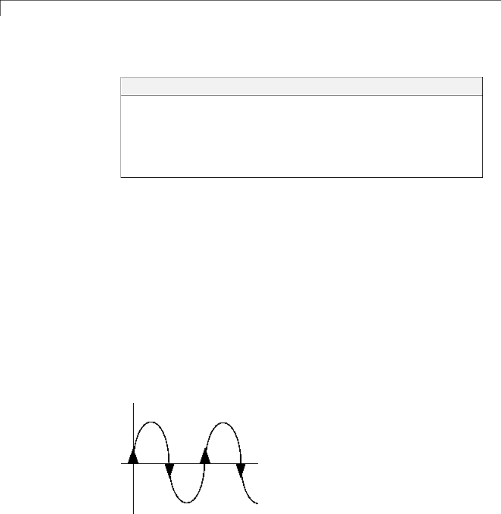
7Creating Conditional Subsystems
Enabled Subsystems
In this section...
“What Are Enabled Subsystems?” on page 7-4
“Creating an Enabled Subsystem” on page 7-5
“Blocks that an Enabled Subsystem Can Contain” on page 7-11
“Using Blocks with Constant Sample Times in Enabled Subsystems” on
page 7-15
What Are Enabled Subsystems?
Enabled subsystems are subsystems that execute at each simulation step for
which the control signal has a positive value.
An enabled subsystem has a single control input, which can be a scalar or
avector.
•If the input is a scalar, the subsystem executes if the input value is greater
than zero.
•If the input is a vector, the subsystem executes if any one of the vector
elements is greater than zero.
For example, if the control input signal is a sine wave, the subsystem is
alternately enabled and disabled. This behavior is shown in the following
figure, where an up arrow signifies enable and a down arrow disable.
7-4

Enabled Subsystems
The Simulink software uses the zero-crossing slope method to determine
whether an enable event is to occur. If the signal crosses zero and its slope is
positive, then the subsystem becomes enabled. If the slope is negative at the
zero crossing, then the subsystem becomes disabled. Note that a subsystem
is only enabled or disabled at major time steps. Therefore, if zero-crossing
detection is turned off and the signal crosses zero during a minor time step,
then the subsystem will not become enabled (or disabled) until the next
major time step.
Creating an Enabled Subsystem
You create an enabled subsystem by copying an Enable block from the Ports &
Subsystems library into a Subsystem block. An enable symbol and an enable
control input port is addedtotheSubsystemblock.
Setting Initial Conditions for an Enabled Subsystem
You can set the initial output of an enabled subsystem using the subsystems
Outport blocks. The initial output value can be either explicitly specified, or
inherited from its input signal.
Specifying Initial Conditions. To specify the initial output value of the
subsystem:
1Double-click each Outport block in the subsystem to open its block
parameters dialog box.
2In the Source of initial output value drop-down list, select Dialog.
3Specify a valid value for the Initial output parameter. Valid values
include the empty matrix. But Inf and Nan are not valid values.
7-5

7Creating Conditional Subsystems
If you select Dialog, you can also specify what happens to the output when the
subsystem is disabled. For more information, see the next section: “Setting
Output Values While the Subsystem Is Disabled” on page 7-7.
Inheriting Initial Conditions. The Outport block can inherit an initial
outputvalueforthesubsystemfrom the following sources:
•Output port of another conditionally executed subsystem
•Merge block (with Initial output specified)
•Function-Call Model Reference block
•Constant block (simplified initialization mode only)
•IC block (simplified initialization mode only)
The procedure you use to inherit the initial conditions of the subsystem
differs depending on whether you are using classic initialization mode or
simplified initialization mode.
To inherit initial conditions in classic initialization mode:
1Double-click each Outport block in the subsystem to open its block
parameters dialog box.
2In the Source of initial output value drop-down list, select Dialog .
3Set the Initial output parameter to [] (empty matrix).
4Click OK.
Note For all other driving blocks, specify an explicit initial output value.
To inherit initial conditions in simplified initialization mode:
1Double-click each Outport block in the subsystem to open its block
parameters dialog box.
2In the Source of initial output value drop-down list, select Input
signal.
7-6

Enabled Subsystems
3Click OK.
The Initial output and Output when disabled parameters are disabled,
and both values are inherited from the input signal.
For more information on classic and simplified initialization mode, see
“Underspecified initialization detection”.
Setting Output Values While the Subsystem Is Disabled
Although an enabled subsystem does not execute while it is disabled, the
output signal is still available to other blocks. While an enabled subsystem
is disabled, you can choose to hold the subsystem outputs at their previous
values or reset them to their initial conditions.
Open the block parameters dialog box for each Outport block and for the
Output when disabled parameter, select one of the choices.
•Choose held to maintain the most recent value.
•Choose reset to revert to the initial condition. Set the Initial output to
the initial value of the output.
7-7
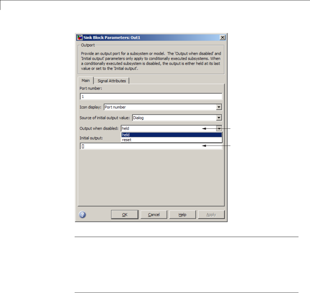
7Creating Conditional Subsystems
Set the Outport output while
the subsystem is disabled
Initial condition and
value when reset
Note If you are connecting the output of a conditionally executed subsystem
to a Merge block, set Output when disabled to held to ensure consistent
simulation results.
If you are using simplified initialization mode, you must select held when
connecting a conditionally executed subsystem to a Merge block. For more
information, see “Underspecified initialization detection”.
7-8
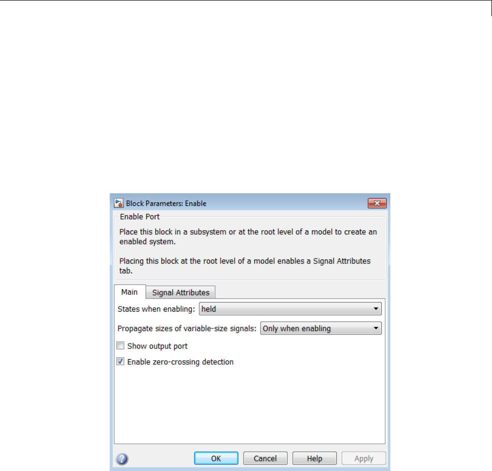
Enabled Subsystems
Setting States When the Subsystem Becomes Enabled
When an enabled subsystem executes, you can choose whether to hold
the subsystem states at their previous values or reset them to their initial
conditions.
To do this, open the Enable block parameters dialog box and select one of the
choices for the States when enabling parameter:
•Choose held to cause the states to maintain their most recent values.
•Choose reset to cause the states to revert to their initial conditions.
7-9

7Creating Conditional Subsystems
Note If you are using simplified initialization mode, the subsystem elapsed
time is always reset during the first execution after becoming enabled,
whether or not the subsystem is configured to reset on enable.
For more information on simplified initialization mode, see “Underspecified
initialization detection”.
Outputting the Enable Control Signal
An option on the Enable block dialog box lets you output the enable control
signal. To output the control signal, select the Show output port check box.
7-10
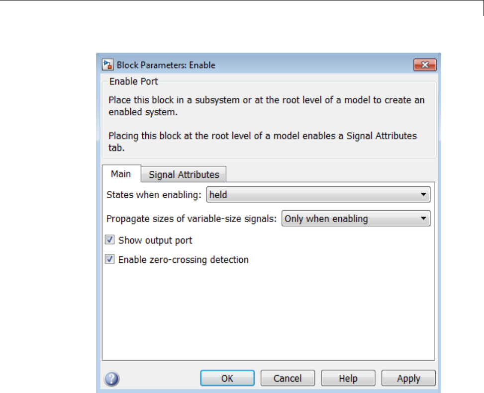
Enabled Subsystems
This feature allows you to pass the control signal down into the enabled
subsystem, which can be useful where logic within the enabled subsystem is
dependent on the value or values contained in the control signal.
Blocks that an Enabled Subsystem Can Contain
An enabled subsystem can contain any block, whether continuous or discrete.
Discrete blocks in an enabled subsystem execute only when the subsystem
executes, and only when their sample times are synchronized with the
7-11

7Creating Conditional Subsystems
simulation sample time. Enabled subsystems and the model use a common
clock.
Note Enabled subsystems can contain Goto blocks. However, only state ports
can connect to Goto blocks in an enabled subsystem. In the sldemo_clutch
model, see the Locked subsystem for an example of how to use Goto blocks in
an enabled subsystem.
For example, this system contains four discrete blocks and a control signal.
The discrete blocks are:
•Block A, which has a sample time of 0.25 second
•Block B, which has a sample time of 0.5 second
•Block C, within the enabled subsystem, which has a sample time of 0.125
second
•Block D, also within the enabled subsystem, which has a sample time of
0.25 second
The enable control signal is generated by a Pulse Generator block, labeled
Signal E, which changes from 0 to 1 at 0.375 second and returns to 0 at 0.875
second.
7-12
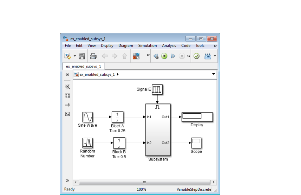
Enabled Subsystems
7-13
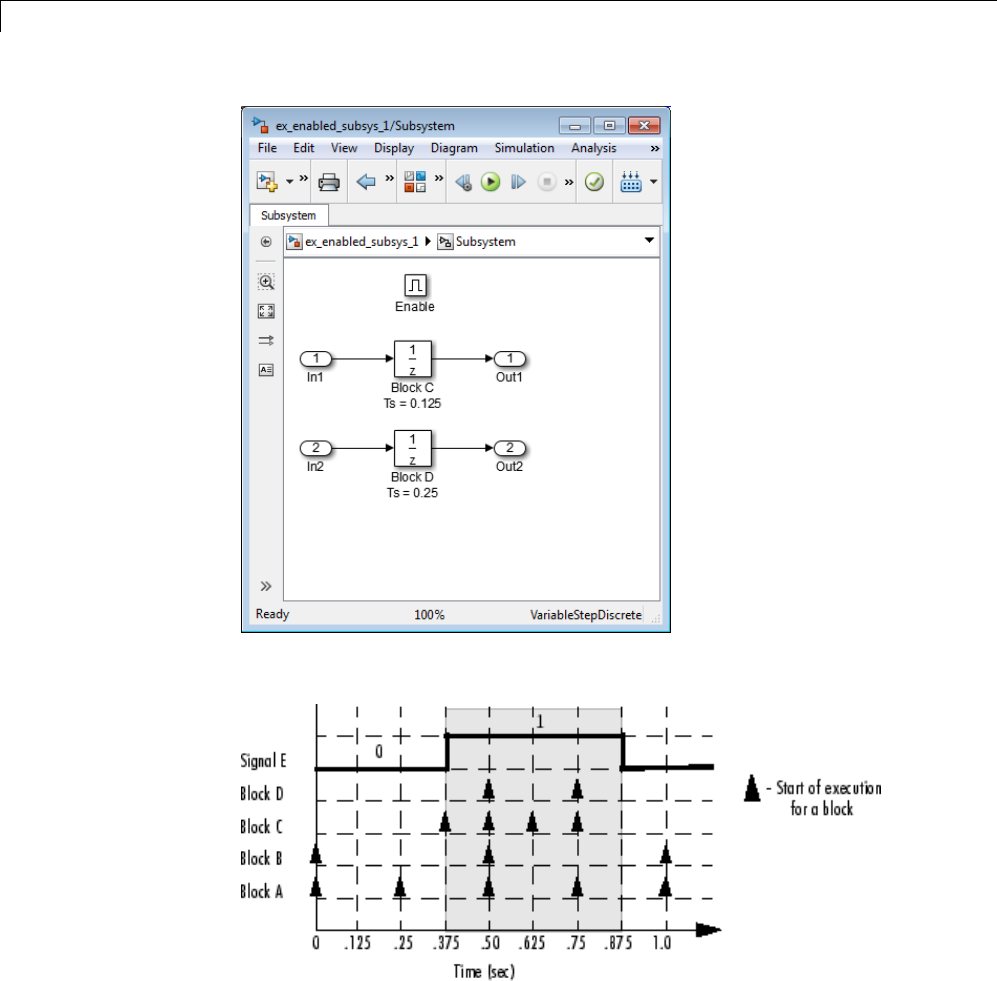
7Creating Conditional Subsystems
The chart below indicates when the discrete blocks execute.
BlocksAandBexecuteindependentlyof the enable control signal because
they are not part of the enabled subsystem. When the enable control signal
7-14

Enabled Subsystems
becomes positive, blocks C and D execute at their assigned sample rates until
theenablecontrolsignalbecomeszeroagain. NotethatblockCdoesnot
execute at 0.875 second when the enable control signal changes to zero.
Using Blocks with Constant Sample Times in Enabled
Subsystems
Certain restrictions apply when you connect blocks with constant sample
times (see “Constant Sample Time” on page 5-16) to the output port of a
conditional subsystem.
•An error appears when you connect a Model or S-Function block with
constant sample time to the output port of a conditional subsystem.
•The sample time of any built-in block with a constant sample time is
converted to a different sample time, such as the fastest discrete rate in
the conditional subsystem.
To avoid the error or conversion, either manually change the sample time of
the block to a non-constant sample time or use a Signal Conversion block.
The example below shows how to use the Signal Conversion block to avoid
these errors.
Consider the following model ex_enabled_subsys_2.mdl.
7-15
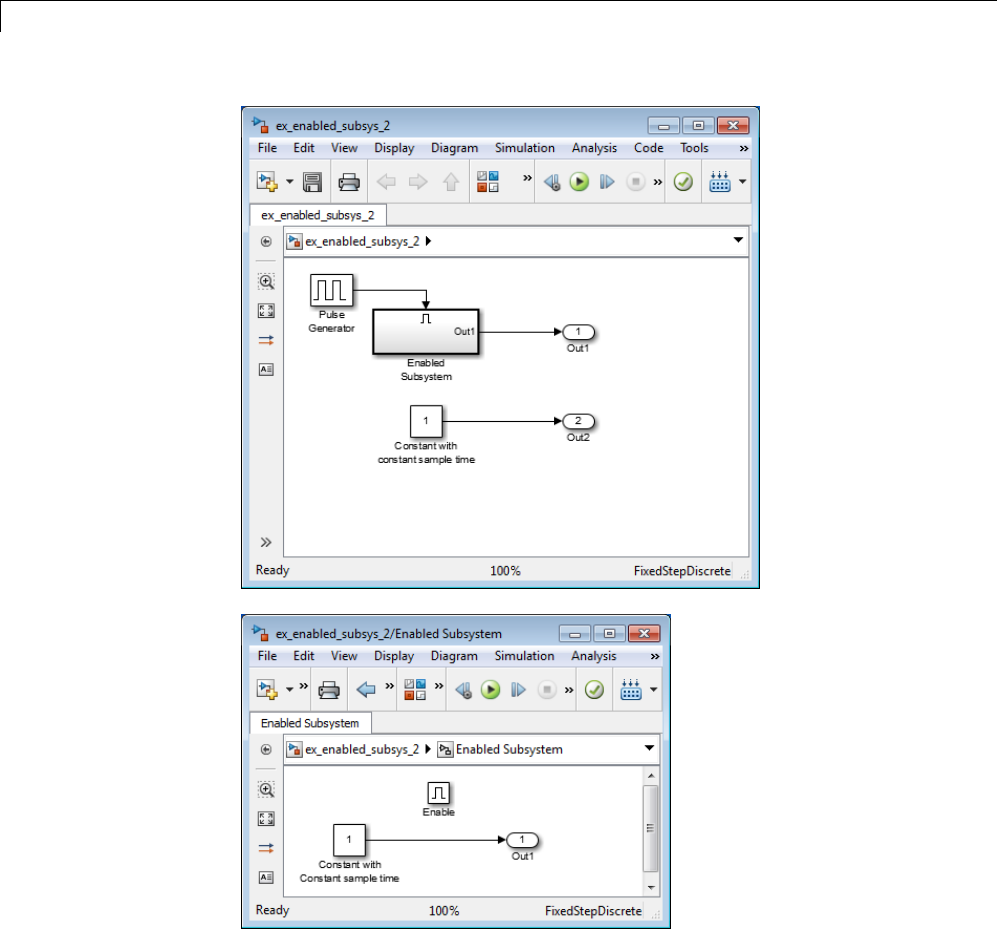
7Creating Conditional Subsystems
The two Constant blocks in this model have constant sample times. When
you simulate the model, the Simulink software converts the sample time of
the Constant block inside the enabled subsystem to the rate of the Pulse
Generator. If you simulate the model with sample time colors displayed
7-16
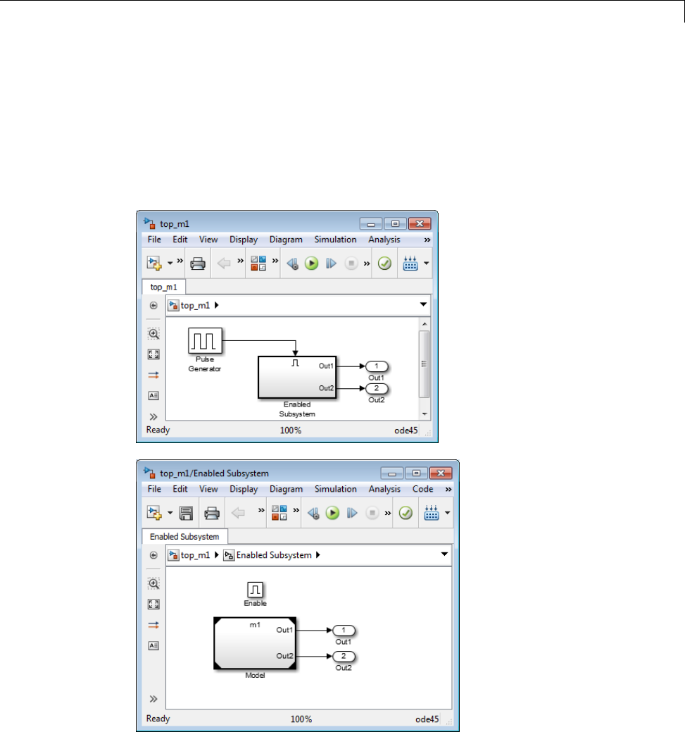
Enabled Subsystems
(see “View Sample Time Information”onpage5-9),thePulseGenerator
and Enabled Subsystem blocks are colored red. However, the Constant
and Outport blocks outside of the enabled subsystem are colored magenta,
indicating that these blocks still have a constant sample time.
Suppose the model above is referenced from a Model block inside an enabled
subsystem, as shown below. (See “Model Reference”.)
7-17
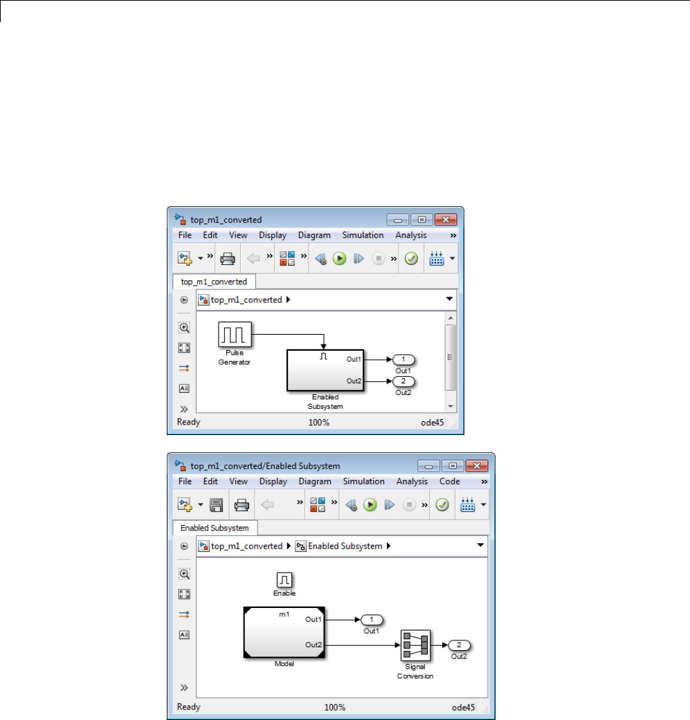
7Creating Conditional Subsystems
An error appears when you try to simulate the top model, indicating that the
second output of the Model block may not be wired directly to the enabled
subsystem output port because it has a constant sample time. (See “Model
Reference”.)
To avoid this error, insert a Signal Conversion block between the second
output of the Model block and the Outport block of the enabled subsystem.
7-18

Enabled Subsystems
This model simulates with no errors. With sample time colors displayed,
the Model and Enabled Subsystem blocks are colored yellow, indicating that
these are hybrid systems. In this case, the systems are hybrid because they
contain multiple sample times.
7-19
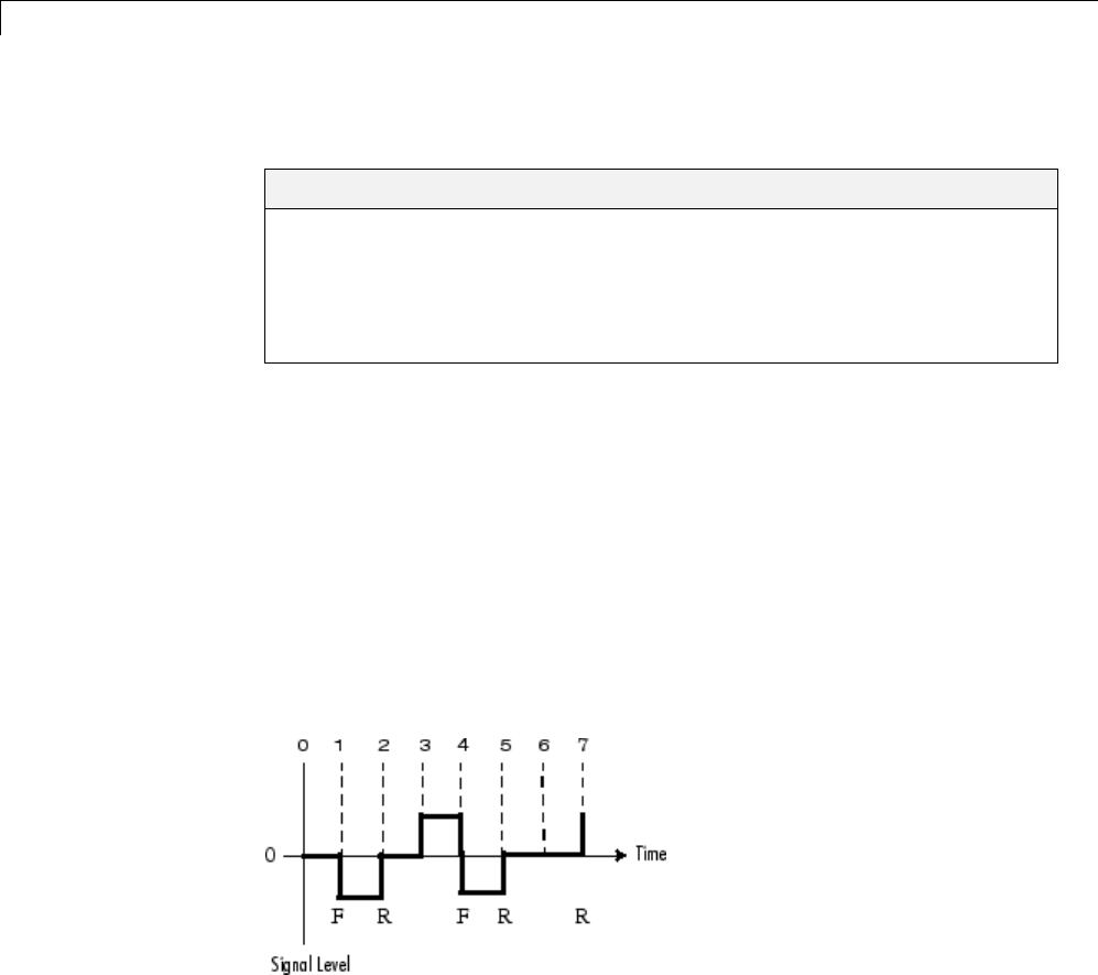
7Creating Conditional Subsystems
Triggered Subsystems
In this section...
“What Are Triggered Subsystems?” on page 7-20
“Using Model Referencing Instead of a Triggered Subsystem” on page 7-22
“Creating a Triggered Subsystem” on page 7-22
“Blocks That a Triggered Subsystem Can Contain” on page 7-23
What Are Triggered Subsystems?
Triggered subsystems are subsystems that execute each time a trigger event
occurs.
A triggered subsystem has a single control input, called the trigger input,that
determines whether the subsystem executes. You can choose from three types
of trigger events to force a triggered subsystem to begin execution:
For example, in the following timing diagram for a discrete system, a rising
trigger(R)doesnotoccurattimestep3because the signal remains at zero for
only one time step prior to the rise.
A simple example of a triggered subsystem is illustrated.
7-20
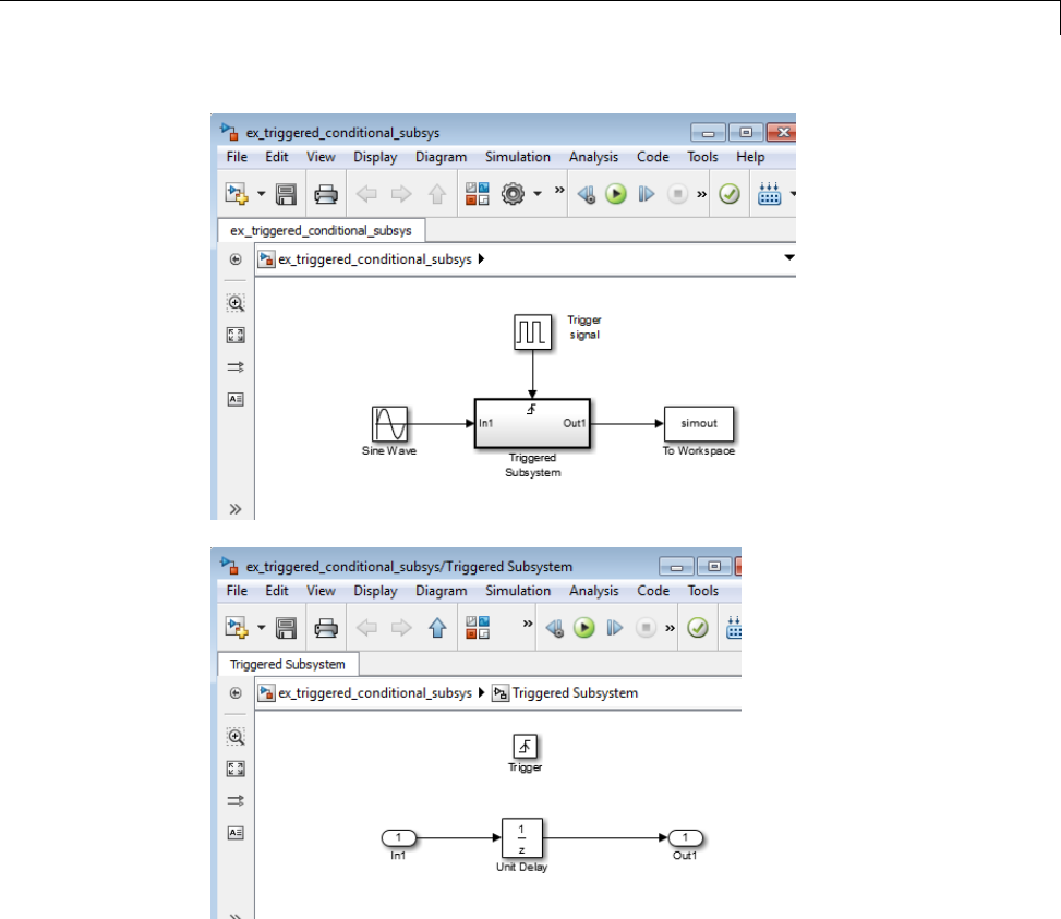
Triggered Subsystems
In this example, the subsystem is triggered on the rising edge of the square
wave trigger control signal.
7-21

7Creating Conditional Subsystems
Using Model Referencing Instead of a Triggered
Subsystem
You can use triggered ports in referenced models. Add a trigger port to a
referenced model to create a simpler, cleaner model than when you include
either:
•A triggered subsystem in a referenced model
•A Model block in a triggered subsystem
For information about using trigger ports in referenced models, see
“Conditional Referenced Models” on page 6-59.
To convert a subsystem to use model referencing, see “Convert a Subsystem to
a Referenced Model” on page 6-12.
Creating a Triggered Subsystem
You create a triggered subsystem by copying the Trigger block from the Ports
& Subsystems library into a subsystem. The Simulink software adds a trigger
symbol and a trigger control input port to the Subsystem block.
To select the trigger type, open the Trigger block dialog box and select one of
the choices for the Trigger type parameter.
Different symbols appear on the Trigger and Subsystem blocks to indicate
rising and falling triggers (or either). This figure shows the trigger symbols
on Subsystem blocks.
7-22

Triggered Subsystems
Outputs and States Between Trigger Events
Unlike enabled subsystems, triggered subsystems always hold their outputs
at the last value between triggering events. Also, triggered subsystems
cannot reset their states when triggered; the states of any discrete block is
held between trigger events.
Outputting the Trigger Control Signal
An option on the Trigger block dialog box lets you output the trigger control
signal. To output the control signal, select the Show output port check box.
In the Output data type field, specify the data type of the output signal as
auto,int8,ordouble.Theauto option causes the data type of the output
signal to be the data type (either int8 or double)oftheporttowhichthe
signal connects.
Blocks That a Triggered Subsystem Can Contain
All blocks in a triggered subsystem must have either inherited (-1)or
constant (inf) sample time. This is to indicate that the blocks in the triggered
subsystem run only when the triggered subsystem itself runs, for example,
when it is triggered. This requirement means that a triggered subsystem
cannot contain continuous blocks, such as the Integrator block.
7-23
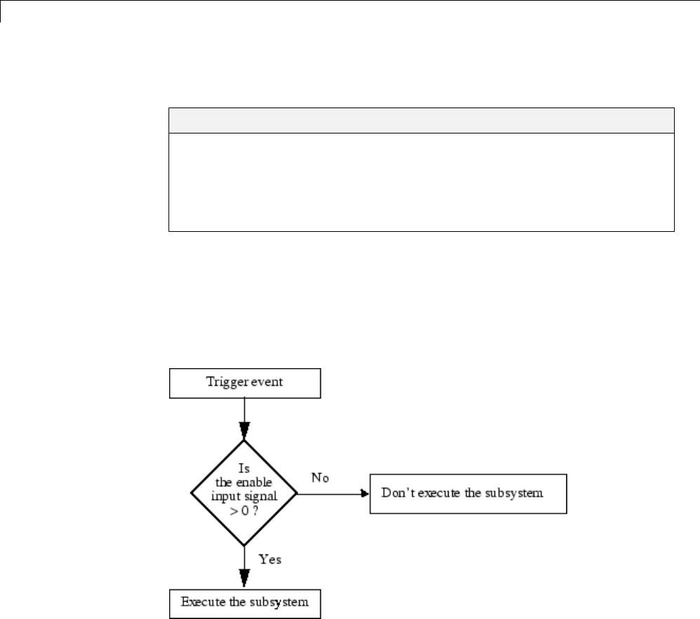
7Creating Conditional Subsystems
TriggeredandEnabledSubsystems
In this section...
“What Are Triggered and Enabled Subsystems?” on page 7-24
“Creating a Triggered and Enabled Subsystem” on page 7-25
“A Sample Triggered and Enabled Subsystem” on page 7-26
“Creating Alternately Executing Subsystems” on page 7-27
What Are Triggered and Enabled Subsystems?
A third kind of conditional subsystem combines two types of conditional
execution. The behavior of this type of subsystem, called a triggered and
enabled subsystem, is a combination of the enabled subsystem and the
triggered subsystem, as shown by this flow diagram.
Atr
iggered and enabled subsystem contains both an enable input port and
at
rigger input port. When the trigger event occurs, the enable input port is
checked to evaluate the enable control signal. If its value is greater than zero,
the subsystem is executed. If both inputs are vectors, the subsystem executes
if at least one element of each vector is nonzero.
7-24

Triggered and Enabled Subsystems
The subsystem executes once at the timestepatwhichthetriggerevent
occurs.
Creating a Triggered and Enabled Subsystem
You create a triggered and enabled subsystem by dragging both the Enable
and Trigger blocks from the Ports & Subsystems library into an existing
subsystem. The Simulink software adds enable and trigger symbols and
enable and trigger control inputs to the Subsystem block.
You can set output values when a triggered and enabled subsystem is disabled
as you would for an enabled subsystem. For more information, see “Setting
Output Values While the Subsystem Is Disabled” on page 7-7. Also, you can
specify what the values of the states are when the subsystem is reenabled.
See “Setting States When the Subsystem Becomes Enabled” on page 7-9.
Set the parameters for the Enable and Trigger blocks separately. The
procedures are the same as those described for the individual blocks.
7-25
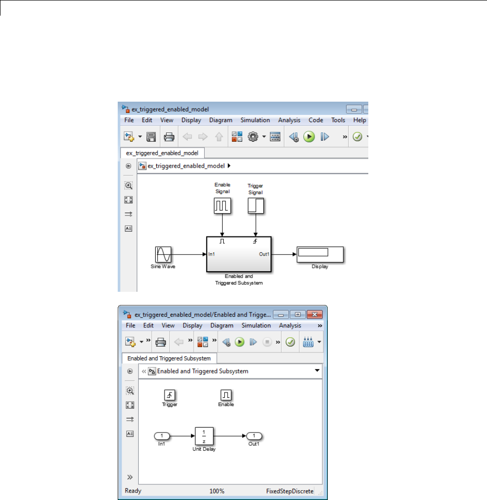
7Creating Conditional Subsystems
A Sample Triggered and Enabled Subsystem
A simple example of a triggered and enabled subsystem is illustrated in the
following model.
7-26

Triggered and Enabled Subsystems
Creating Alternately Executing Subsystems
You can use conditional subsystems in combination with Merge blocks to
create sets of subsystems that execute alternately, depending on the current
state of the model.
7-27
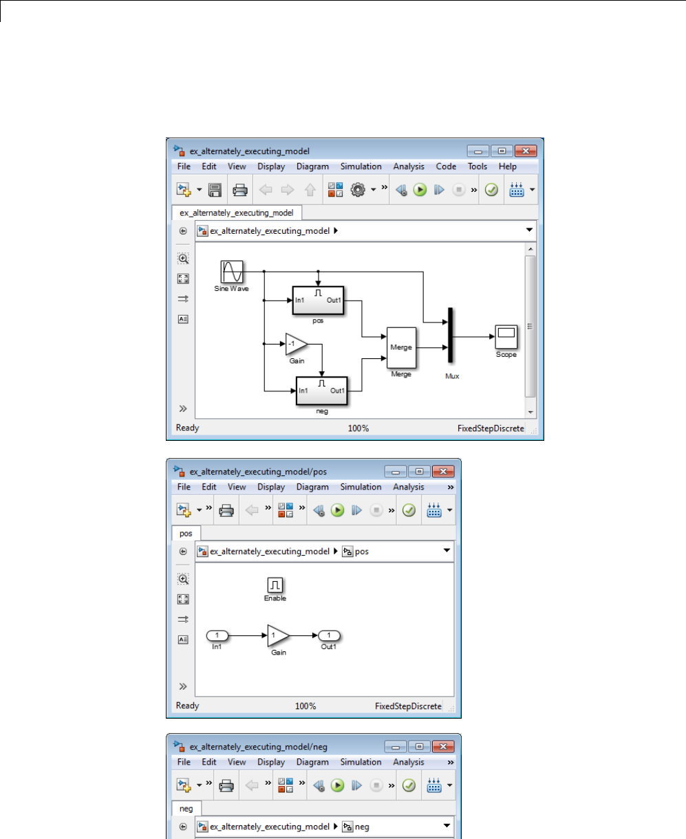
7Creating Conditional Subsystems
The following figure shows a model that uses two enabled blocks and a Merge
block to model a full-wave rectifier – a device that converts AC current to
pulsating DC current.
7-28
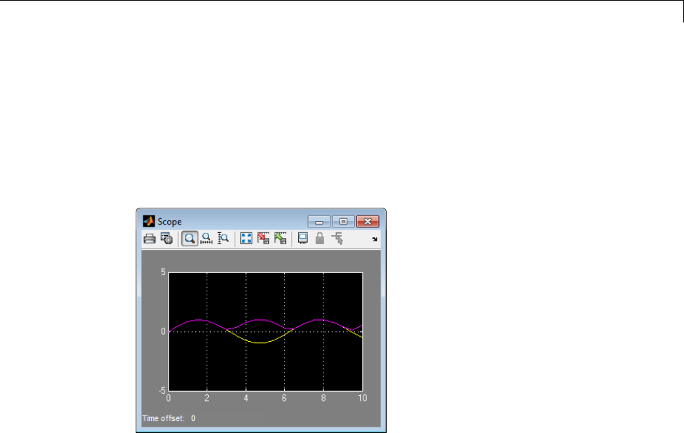
Triggered and Enabled Subsystems
The block labeled pos is enabled when the AC waveform is positive; it passes
the waveform unchanged to its output. The block labeled neg is enabled when
the waveform is negative; it inverts the waveform. The Merge block passes
the output of the currently enabled block to the Mux block, which passes the
output, along with the original waveform, to the Scope block.
The Scope creates the following display.
7-29

7Creating Conditional Subsystems
Function-Call Subsystems
A function-call subsystem is a subsystem that another block can invoke
directly during a simulation. It is analogous to a function in a procedural
programming language. Invoking a function-call subsystem is equivalent to
invoking the output methods (See “Block Methods” on page 3-16) of the blocks
that the subsystem contains in sorted order (See “How Simulink Determines
theSortedOrder”onpage23-45). Theblock that invokes a function-call
subsystem is called the function-call initiator. Stateflow, Function-Call
Generator, and S-function blocks can all serve as function-call initiators.
To create a function-call subsystem, drag a Function-Call Subsystem
block from the Ports & Subsystems library into your model and connect
a function-call initiator to the function-call port displayed on top of the
subsystem. You can also create a function-call subsystem from scratch. First
create a Subsystem block in your model and then create a Trigger block in
the subsystem. Next, on the Trigger block parameters pane, set the Trigger
type to function-call.
You can configure a function-call subsystem to be triggered (the default) or
periodic by setting the Sample time type of its Trigger port to be triggered
or periodic, respectively. A function-call initiator can invoke a triggered
function-call subsystem zero, once, or multiple times per time step. The
sample times of all the blocks in a triggered function-call subsystem must be
set to inherited (-1).
A function-call initiator can invoke a periodic function-call subsystem
only once per time step and must invoke the subsystem periodically. If
the initiator invokes a periodic function-call subsystem aperiodically, the
simulation is halted and an error message is displayed. The blocks in a
periodic function-call subsystem can specify a noninherited sample time or
inherited (-1) sample time. All blocks that specify a noninherited sample time
must specify the same sample time. For example, if one block specifies 0.1 as
the sample time, all other blocks must specify a sample time of 0.1 or -1.If
a function-call initiator invokes a periodic function-call subsystem at a rate
that differs from the sample time specified by the blocks in the subsystem, the
simulation halts and an error message appears.
7-30

Function-Call Subsystems
Note During range checking, the design minimum and maximum are
back-propagated to the actual source port of the function-call subsystem, even
when the function-call subsystem is not enabled.
To prevent this back propagation, add a Signal Conversion block and a
Signal Specification block after the source port, set the Output of the Signal
Conversion block to Signal copy, and specify the design minimum and
maximum on the Signal Specification block instead of specifying them on
the source port.
For more information about function-call subsystems, see “Function-Call
Subsystems” in “Writing S-Functions” in the online documentation.
7-31
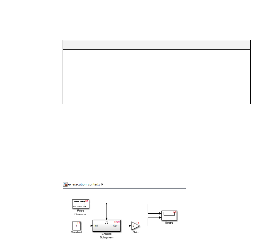
7Creating Conditional Subsystems
Conditional Execution Behavior
In this section...
“What Is Conditional Execution Behavior?” on page 7-32
“Propagating Execution Contexts” on page 7-34
“Behavior of Switch Blocks” on page 7-35
“Displaying Execution Contexts” on page 7-36
“Disabling Conditional Execution Behavior” on page 7-37
“Displaying Execution Context Bars” on page 7-37
What Is Conditional Execution Behavior?
To speed the simulation of a model, by default the Simulink software avoids
unnecessary execution of blocks connected to Switch, Multiport Switch, and
of conditionally executed blocks. This behavior is conditional execution (CE)
behavior. You can disable this behavior for all Switch and Multiport Switch
blocks in a model, or for specific conditional subsystems. See “Disabling
Conditional Execution Behavior” on page 7-37.
The following model illustrates conditional execution behavior.
7-32
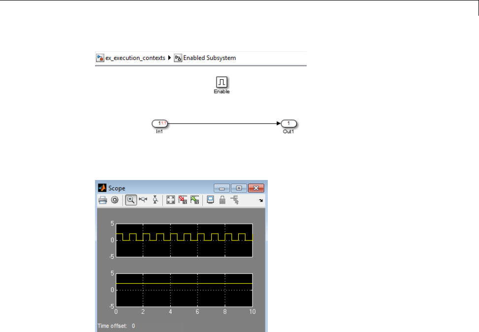
Conditional Execution Behavior
TheScopeblockshowsthesimulationresult:
This model:
•Has the Display > Signals & Ports > Execution Context Indicator
menu option enabled.
•The Pulse Generator block has the following parameter settings:
-Pulse type —Sample based
-Period —100
-Pulse width —50
-Phase delay —50
-Sample Time —0.01
7-33

7Creating Conditional Subsystems
•The Gain block’s sorted order (1:2) is second (2) in the enabled subsystem’s
execution context (1).
•The Enabled Subsystem block has the Propagate execution context
across subsystem boundary parameter enabled.
•In the enabled subsystem, the Out1 block has the following parameter
settings:
-Initial output —[]
-Output when disabled —held
The outputs of the Constant block and Gain blocks are computed only while
the enabled subsystem is enabled (for example, at time steps 0.5 to 1.0 and 1.5
to 2.0). This behavior is necessary because the output of the Constant block
is required and the input of the Gain block changes only while the enabled
subsystem is enabled. When CE behavior is off, the outputs of the Constant
and Gain blocks are computed at every time step, regardless of whether the
outputs are needed or change.
In this example, the enabled subsystem is regarded as defining an execution
context for the Constant and Gain blocks. Although the blocks reside
graphically in the root system of the model, the Simulink software invokes
the block methods during simulation as if the blocks reside in the enabled
subsystem. This is indicated in the sorted order labels displayed on the
diagram for the Constant and Gain blocks. The notations list the subsystem’s
(id = 1) as the execution context for the blocks even though the blocks exist
graphically at the root level (id = 0) of the model. The Gain block’s sorted
order (1:2) is second (2) in the enabled subsystem’s execution context (1).
Propagating Execution Contexts
In general, the Simulink software defines an execution context as a set of
blocks to be executed as a unit. At model compilation time, the Simulink
software associates an execution context with the model’s root system and
with each of its nonvirtual subsystems. Initially, the execution context of
the root system and each nonvirtual subsystem is simply the blocks that
it contains.
When compiling, each block in the model is examined to determine whether it
meets the following conditions:
7-34

Conditional Execution Behavior
•The block output is required only by a conditional subsystem or the block
input changes only as a result of the execution of a conditionally executed
subsystem.
•The execution context of the subsystem can propagate across the subsystem
boundaries.
•The output of the block is not a test point (see “Test Points” on page 47-58).
•The block is allowed to inherit its conditional execution context.
The Simulink software does not allow some built-in blocks, such as the
Delay block, ever to inherit their execution context. Also, S-Function
blocks can inherit their execution context only if they specify the
SS_OPTION_CAN_BE_CALLED_CONDITIONALLY option.
•The block is not a multirate block.
•The block sample time is set to inherited (-1).
If a block meets these conditions and execution context propagation is
enabled for the associated conditional subsystem (see “Disabling Conditional
Execution Behavior” on page 7-37), the Simulink software moves the block
into the execution context of the subsystem. This ensures that the block
methods execute during the simulation loop only when the corresponding
conditional subsystem executes.
Note Execution contexts are not propagated to blocks having a constant
sample time.
Behavior of Switch Blocks
This behavior treats the input branches of a Switch or Multiport Switch block
as invisible, conditional subsystems, each of which has its own execution
context. This CE is enabled only when the control input of the switch selects
the corresponding data input. As a result, switch branches execute only when
selected by switch control inputs.
7-35
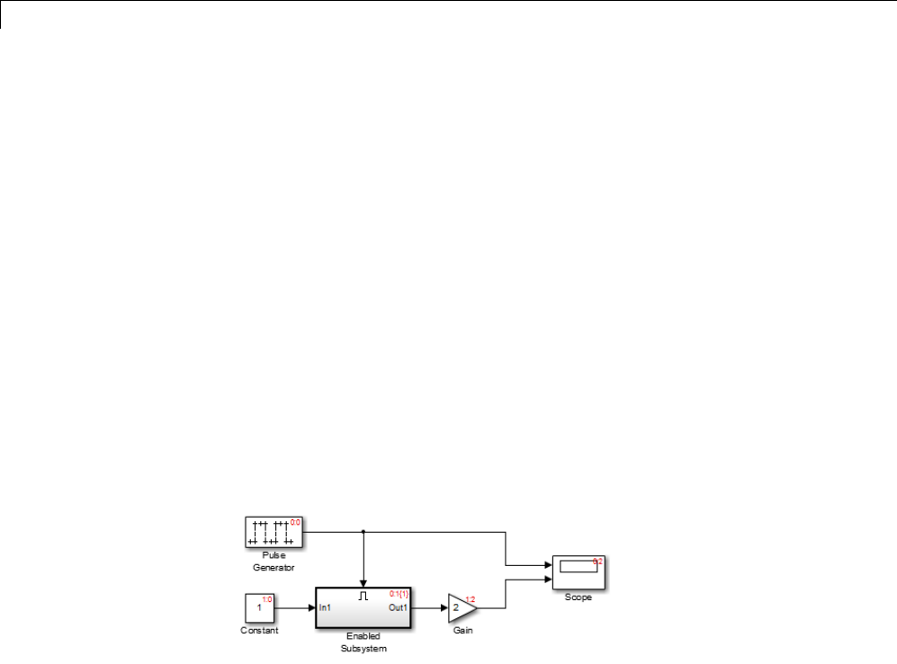
7Creating Conditional Subsystems
Displaying Execution Contexts
To determine the execution context to which a block belongs, in the Simulink
Editor, select Display > Blocks > Sorted Execution Order.Thesorted
order index for each block in the model is displayed in the upper-right corner
of the block. The index has the format s:b,wheresspecifies the subsystem to
whose execution context the block belongs and bis an index that indicates the
block sorted order in the execution context of the subsystem. For example,
0:0 indicates that the block is the first block in the execution context of the
root subsystem.
If a bus is connected to a block input, the block sorted order is displayed as
s:B. For example, 0:B indicates that the block belongs to the execution context
of the root system and has a bus connected to its input.
The sorted order index of conditional subsystems is expanded to include
the system ID of the subsystem itself in curly brackets as illustrated in the
following figure.
In this example, the sorted order index of the enabled subsystem is 0:1{1}.
The 0indicates that the enabled subsystem resides in the root system of the
model. The first 1indicates that the enabled subsystem is the second block on
the sorted list of the root system (zero-based indexing). The 1in curly brackets
indicates that the system index of the enabled subsystem itself is 1. Thus any
block whose system index is 1belongs to the execution context of the enabled
subsystem and hence executes when it does. For example, the fact that the
Constant block has an index of 1:0 indicates that it is the first block on the
sorted list of the enabled subsystem, even though it resides in the root system.
7-36
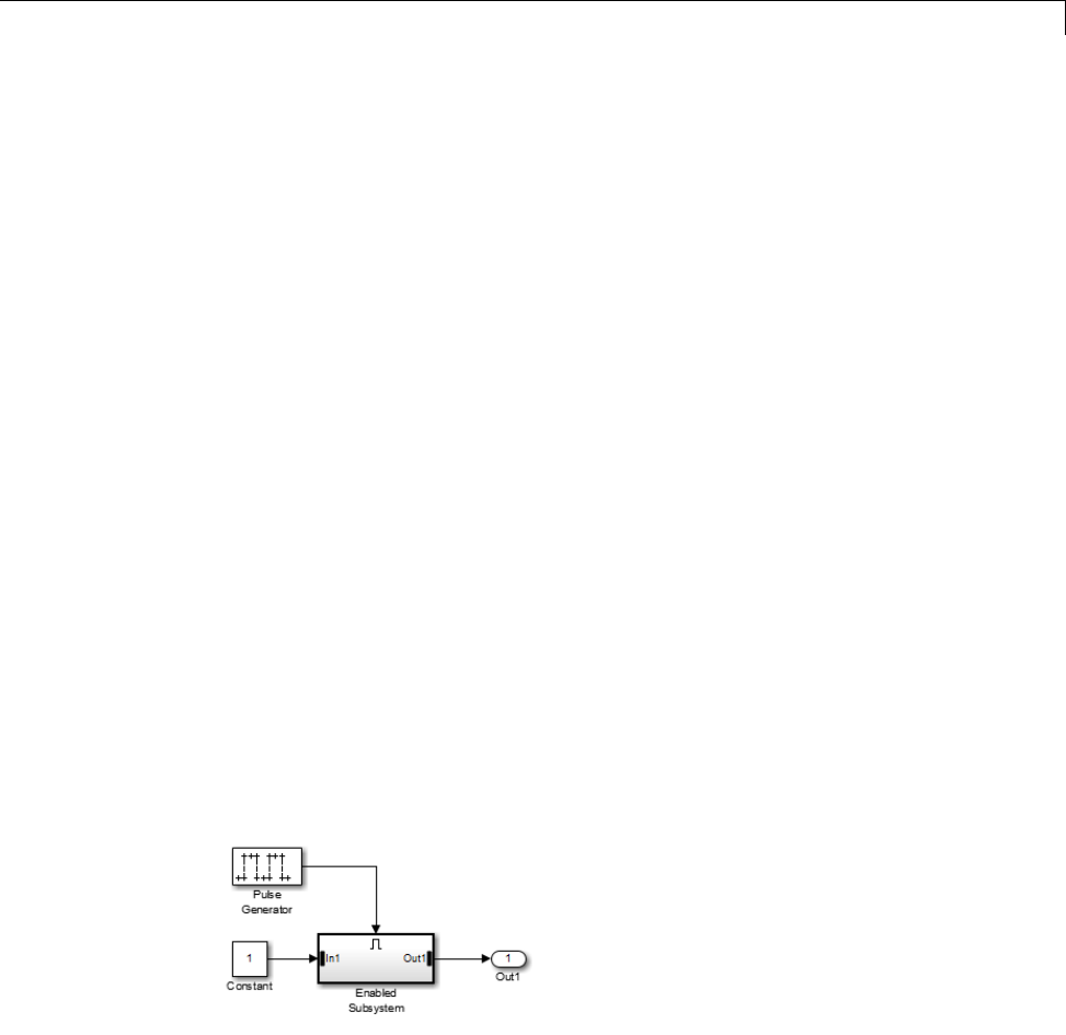
Conditional Execution Behavior
Disabling Conditional Execution Behavior
To disable conditional execution behavior for all Switch and Multiport Switch
blocks in a model,turnofftheConditional input branch execution
optimization ontheOptimization pane of the Configuration Parameters
dialog box (see “Optimization Pane: General”). To disable conditional
execution behavior for a specific conditional subsystem, clear the Propagate
execution context across subsystem boundary check box on the
subsystem parameter dialog box.
Even if this option is enabled, the execution context of the subsystem cannot
propagate across its boundaries under either of the following circumstances:
•The subsystem is a triggered subsystem with a latched input port.
•The subsystem has one or more output ports that specify an initial
condition other than []. In this case, a block connected to the subsystem
output cannot inherit the execution context of the subsystem.
Displaying Execution Context Bars
Simulink can optionally display bars next to the ports of subsystems across
which execution contexts cannot propagate. To display the bars, select
Display > Signals & Ports > Execution Context Indicator.
For example, it displays bars on subsystems from which no block can inherit
its execution context. In the following figure, the context bars appear next to
the In1 and Out1 ports of the Enabled Subsystem block.
7-37

7Creating Conditional Subsystems
7-38

8
Modeling Variant Systems
•“Working with Variant Systems” on page 8-2
•“Set Up Model Variants” on page 8-5
•“Set Up Variant Subsystems” on page 8-15
•“Set Up Variant Control” on page 8-25
•“Select the Active Variant” on page 8-29
•“About Variant Objects” on page 8-32
•“Code Generation of Variants” on page 8-36
•“Variant System Reference” on page 8-37

8Modeling Variant Systems
WorkingwithVariantSystems
In this section...
“Overview of Variant Systems” on page 8-2
“Workflow for Implementing Variant Systems” on page 8-3
Overview of Variant Systems
Many applications require the ability to customize a model to fit different
specifications, without replacing or duplicating the model. For example, a
design engineer has a model that simulates an automobile. Various models of
an automobile can have many similarities, yet differ in specific ways, such
as fuel usage, engine size, or emission standards.
With blocks for variant systems, Simulink provides techniques to customize a
model for different applications through design and simulation:
•The Model Variants block references two or more models, where the
referenced model used during simulation is the active variant.
•The Variant Subsystem block consists of a set of subsystems, where the
subsystem used during simulation is the active variant.
Each variant, active or inactive, has an object. Simulink evaluates the variant
objectstodeterminetheactivevariant.
You can parameterize the variant object by making it dependent on the
values of variables and objects in the MATLAB base workspace. For a quick
overview, see “Model Variants Block Overview” on page 8-5 and “Variant
Subsystem Block Overview” on page 8-15.
You can programmatically switch the active variant by modifying the values
of variant control variables in the base workspace. Alternatively, you can
manually override the variant selection on the block parameter dialog box.
Both variant models and variant subsystems use variants in a similar
workflow. For more information, see “Workflow for Implementing Variant
Systems” on page 8-3.
8-2

Working with Variant Systems
For alternative techniques to customize a model for different specifications,
see:
Technique Reference
Change data values in the base
workspace.
“Tunable Parameters” on page 3-9
Select alternate subsystems from a
library.
Configurable Subsystem block
Use a mask to change a subsystem. “Create Dynamic Masked
Subsystems” on page 26-61
Change the arguments to a
parameterized referenced model.
“Parameterize Model References” on
page 6-52
Workflow for Implementing Variant Systems
You can implement a variant system in your model by using the Model
Variants block or the Variant Subsystem block. Both blocks use a similar
workflow.
1Create the subsystems or referenced models that you want to use as
variants.
2Set up your model to use the variants. Add the Model Variants block or the
Variant Subsystem block, depending on your application.Usetheblocksto:
aSpecify variant models or subsystems.
bCreate a variant object to associate with each variant.
cDefine a condition for each variant. When the condition is true,
Simulink uses this active variant for simulation.
For more information, see “Set Up Model Variants” on page 8-5 and “Set
Up Variant Subsystems” on page 8-15.
3Create the control variables for evaluating variant conditions and selecting
the active variant. See “Set Up Variant Control” on page 8-25 and “Select
the Active Variant” on page 8-29.
8-3

8Modeling Variant Systems
4Simulate using the active variant.
5Modify the variant specification to select another variant and simulate
again.
6Generate code for the active variant or all variants, depending on your
application. See “Code Generation of Variants” on page 8-36.
7Save the control variables and objects for your variants from the base
workspace as described in “Exporting Workspace Variables” on page 9-60.
8-4

Set Up Model Variants
Set Up Model Variants
In this section...
“Model Variants Block Overview” on page 8-5
“Example of a Model Variants Block” on page 8-7
“Configuring the Model Variants Block” on page 8-9
“Disabling and Enabling Model Variants” on page 8-12
“Parameterizing Model Variants” on page 8-12
“Requirements, Limitations, and Tips for Model Variants” on page 8-13
“Model Variants Example” on page 8-14
Model Variants Block Overview
Model variants provide multiple implementations of a referenced model, with
only one implementation active during simulation. You can programmatically
swap the active implementation with another, without modifying the model.
For example, you could use variants to switch between data types, such as
double and int8, by specifying different data types in your referenced models.
8-5
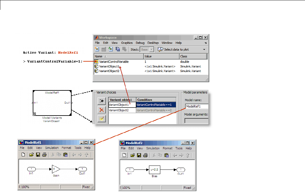
8Modeling Variant Systems
A Model Variants block can reference multiple models, using variants as
follows:
•Each variant has a variant object that you associate with it.
•Each variant has a condition that you specify. When compiling the model,
Simulink tests each variant to determine which condition is true.The
variant with the true condition becomes the active variant.
•Only one variant can be the active variant for a Model Variants block.
•The active variant is the referenced model used for simulation.
You specify the model variant associations in the Model Reference Parameter
dialog box, in the Variant choices table.
8-6

Set Up Model Variants
The Model Variants block parameters specification must include at least:
•The name of a variant object, in the Variant object column of the Variant
choices table
•Thenameofareferencedmodel,intheModel name column of the
Variant choices table
•A simulation mode, in the Simulation mode field of the Model
parameters section
•Values in the Model argument values field of the Model parameters
section, if a referenced model has arguments
Instructions for specifying model variants are in “Configuring the Model
Variants Block” on page 8-9.
Example of a Model Variants Block
To view the example model, either click AutoMRVar,orexecute:
addpath([docroot '/toolbox/simulink/ug/examples/variants/mdlref/']);
open('AutoMRVar');
8-7
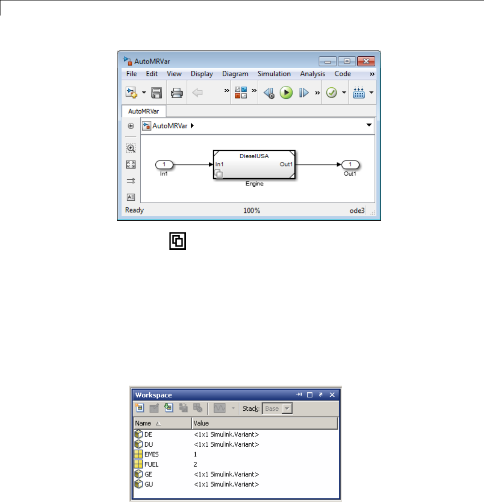
8Modeling Variant Systems
•The icon appears in the lower-left corner to indicate that the block
uses variants.
•The name of the variant that was active the last time you saved the model
appears at the top of the block.
•When you change the active variant and press Ctrl+K, the variant block
refreshes and its name changes.
•When you open the example model, a callback function loads a MAT-file
that populates the base workspace with the variables and objects that the
model uses. The base workspace contains the variant control variables
and variant objects.
8-8
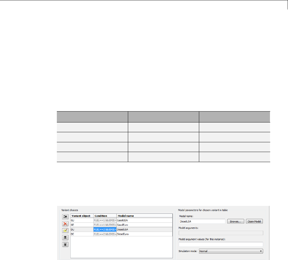
Set Up Model Variants
The example implements the following application:
•An automobile that can use either a diesel or a gasoline engine
•Each engine must meet either the European or American (USA) emission
standard
AutoMRVar implements the automobile application using the Model Variants
block, named Engine.TheEngine block specifies four variant referenced
models. Each referenced model represents one permutation of engine fuel and
emission standards.
Variant Object Variant Condition Model Name
GU FUEL==1 && EMIS==1 GasolUSA
GE FUEL==1 && EMIS==2 GasolEuro
DU FUEL==2 && EMIS==1 DieselUSA
DE FUEL==2 && EMIS==2 DieselEuro
To see how to specify these variants, in the Simulink Editor, right-click the
Engine block, and select Block Parameters (ModelReference) or select
Diagram > Block Parameters (ModelReference).ViewtheVariant
choices table in the dialog box.
For instructions, see “Configuring the Model Variants Block” on page 8-9.
Configuring the Model Variants Block
To add and configure a Model Variants block to specify your variants, do
the following:
8-9
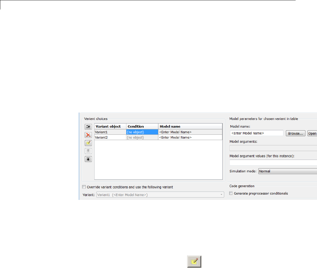
8Modeling Variant Systems
1From the Simulink Library Browser, add a Model Variants block to your
model:
Simulink > Ports and Subsystems→Model Variants block.
2To configure your variants, open the Model Variants block dialog box.
In the Simulink Editor, right-click the Model Variants block, and select
Block Parameters (ModelReference) or select Diagram > Block
Parameters (ModelReference).
The Model Variants block parameters dialog box opens.
3Specify the variant name in the Variant object column of the Variant
choices table. Double-click the default Variant1 name, then type the
name of the variant object. For an existing variant object, Simulink
retrieves the variant condition for the object when you press Enter or
click away from the Variant object.
4To specify the Condition that determines which variant is active, click the
Create/Edit selected variant button . For the selected variant
choice, you create a variant object in the base workspace if necessary, or
edit an existing variant. The Simulink.Variant parameter dialog box opens.
aSpecify the Condition for the variant object. For example, FUEL==1
&& EMIS==1.Donot surround the condition with parentheses or single
quotes.
8-10

Set Up Model Variants
When the variant object condition evaluates to true at compile time, the
referenced model associated with the variant becomes the active variant.
bClick Apply to check the expression, then click OK.
5Choose a referenced model to associate with the variant object.
aIn the Variant choices table, click to select a variant.
bEnter the model name into either the Model name table cell, or the
Model name field for the chosen variant, in the Model parameters
for chosen variant in table pane to the right of the table. To specify
a protected model, use the extension .slxp. See “Protected Model” on
page 6-67.
Alternatively, to find a model, click the Browse button next to the
Model name field. Select the model, and click Open.Themodelname
appears in the Model name column and edit box.
c(Optional) For the selected model, you can also click Open Model
to check which model you are specifying, specify model arguments
(see “Parameterizing Model Variants” on page 8-12), or specify the
Simulation mode. All simulation modes work with model variants. See
“Referenced Model Simulation Modes” on page 6-21.
dClick Apply to associate the referenced model with its variant object.
6To add another variant, click the Add a new variant button .
AnewVariant choices table row appears below the other variant choices.
7Repeat the previous steps until you have specified all your referenced
models and their associated variant objects. For information on the other
buttons, see the Model Variants block page.
8Click OK to close the Model Variants dialog box.
Note Your variant conditions might require you to define control variables
in the base workspace before they can be evaluated. See “Creating Control
Variables” on page 8-25 and “Saving Variant Components” on page 8-26.
8-11

8Modeling Variant Systems
For next steps, see “Select the Active Variant” on page 8-29. The model
diagram displays the new active variant on the block when you refresh the
block by pressing Ctrl+K.
Disabling and Enabling Model Variants
You can disable model variants without losing your variant settings. After
you enable variants, they remain enabled until you explicitly disable them.
You can close and reopen the Model Variants block without affecting the
variant specification.
To disable variants from your Model block or Model Variants block:
1Right-clicktheblockandselectBlock Parameters (ModelReference) to
open the block parameters dialog box.
2Select the Disable Variants button. Disabling variants:
•Hides the Block parameter dialog box for variants
•Leaves the active variant as the model name and the execution
environment when the variants were disabled
•Ignores subsequent changes to variant control variables, variant
conditions, and other models, other than the current model.
Ifyoudecidetoreenablevariants,selecttheEnable Variants button.
•The Model block or Model Variants block remembers your previous variant
specifications as they were before.
•The Model block or Model Variants block selects an active variant according
to the current base workspace variables and conditions.
You can also override variants and specify the active variant. See “Overriding
Variant Conditions” on page 8-30.
Parameterizing Model Variants
You can parameterize any or all variants of the Model Variants block. You
can parameterize some variants but choose not to parameterize others. You
can also parameterize different variants differently from one another.
8-12

Set Up Model Variants
To parameterize a variant (referenced model) of a Model Variants block,
specify the necessary values in the Model parameters for chosen variant
in table section using the Model argument values field. You can use
the same values as for any referenced model. For more information, see
“Parameterize Model References” on page 6-52.
Requirements, Limitations, and Tips for Model
Variants
A Model Variants block and its referenced models must satisfy the
requirements in “Simulink Model Referencing Requirements” on page 6-45
and “Model Referencing Limitations” on page 6-80. You can nest Model
Variants blocks to any level.
Note Requirements and limitations that apply to code generation are in
“Limitations on Generating Code for Variants”.
Tips for working with model variants:
•A Model Variants block can log only those signals that the referenced model
specifies as logged. If a model is a variant model, or contains a variant
model, then you can either log all logged signals or log no logged signals.
The Signal Logging Selector configuration for the model must be in one
of these states:
-The Logging Mode is set to Log all signals as specified in
model.
-The Logging Mode is set to Override signals and the check box for
the model block is either checked ( )orempty( ). The check box
cannot be filled ( ).
For more information about logging referenced models, see “Models with
Model Referencing: Overriding Signal Logging Settings” on page 45-45.
To enable logging programmatically, use the DefaultDataLogging
parameter.
8-13

8Modeling Variant Systems
•You can enable or suppress warning messages about mismatches between
a Model Variants block and its referenced model by setting diagnostics on
the “Diagnostics Pane: Model Referencing”.
•During model compilation, Simulink evaluates variant objects before
calling the model InitFcn callback. Therefore, do not modify the condition
of the variant object in the InitFcn callback.
Model Variants Example
Toseeaexamplethatshowshowtodefineavariantmodelin
Simulink , click sldemo_mdlref_variants.IntheHelpBrowser
select: Simulink > Examples > Modeling Features > Model
Reference > Model Reference Variants.
8-14

Set Up Variant Subsystems
Set Up Variant Subsystems
In this section...
“Variant Subsystem Block Overview” on page 8-15
“Example of a Variant Subsystem Block” on page 8-17
“Configuring the Variant Subsystem Block” on page 8-20
“Disabling and Enabling Subsystem Variants” on page 8-23
“Variant Subsystem Block Requirements” on page 8-23
“Variant Subsystem Example” on page 8-24
Variant Subsystem Block Overview
A variant subsystem provides multiple implementations of a subsystem, with
only one implementation active during simulation. You can programmatically
swaptheactiveimplementationwithanother, without modifying the model.
8-15
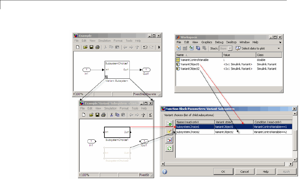
8Modeling Variant Systems
A Variant Subsystem block consists of multiple subsystems as follows:
•Each subsystem has a variant object that you associate with it.
•The subsystem whose variant object condition is true becomes the active
variant.
•A Variant Subsystem block can have only one active variant.
•The active variant is the subsystem used for simulation.
The specifications of the Variant Subsystem block parameters dialog box
must include:
•The name of a variant object, in the Variant object column of the Variant
choices table.
•The variant object must have a conditional expression that evaluates to
true or false.
8-16
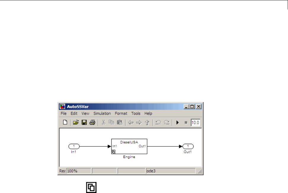
Set Up Variant Subsystems
Instructions for specifying a variant subsystem are in “Configuring the
Variant Subsystem Block” on page 8-20.
Example of a Variant Subsystem Block
To view the example model, either click AutoSSVar,orexecute:
addpath([docroot '/toolbox/simulink/ug/examples/variants/mdlref/']);
open('AutoSSVar');
•An icon appears in the lower-left corner to indicate that the block uses
variants.
•The name of the variant that was active the last time you saved the model
appears at the top of the block.
•When you change the active variant and refresh the diagram by pressing
Ctrl+K, the variant block name changes.
•When you open the example model, a callback function loads a MAT-file
that populates the base workspace with the variables and objects that the
model uses. The base workspace contains the variant control variables
and variant objects.
8-17
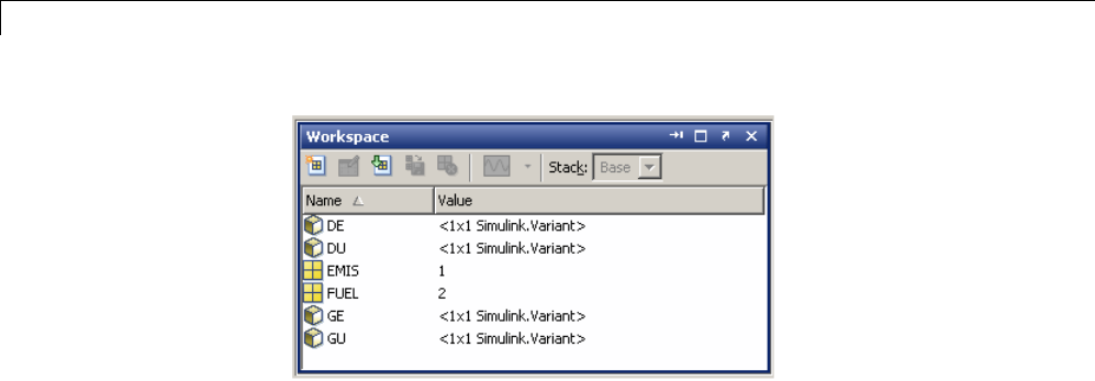
8Modeling Variant Systems
The example model illustrates the same application as the “Example of a
Model Variants Block” on page 8-7, but using variant subsystems instead of
variant referenced models. Both examples show the use of variants for the
following cases:
•An automobile that can use either a diesel or a gasoline engine
•Each engine must meet either the European or American (USA) emission
standard
The example model, AutoSSVar, implements the application using a Variant
Subsystem block, named Engine.TheEngine block consists of a set of four
subsystems. Each subsystem represents one permutation of engine fuel and
emission standards.
Double-click the Variant Model block, Engine, to view the child subsystems.
8-18
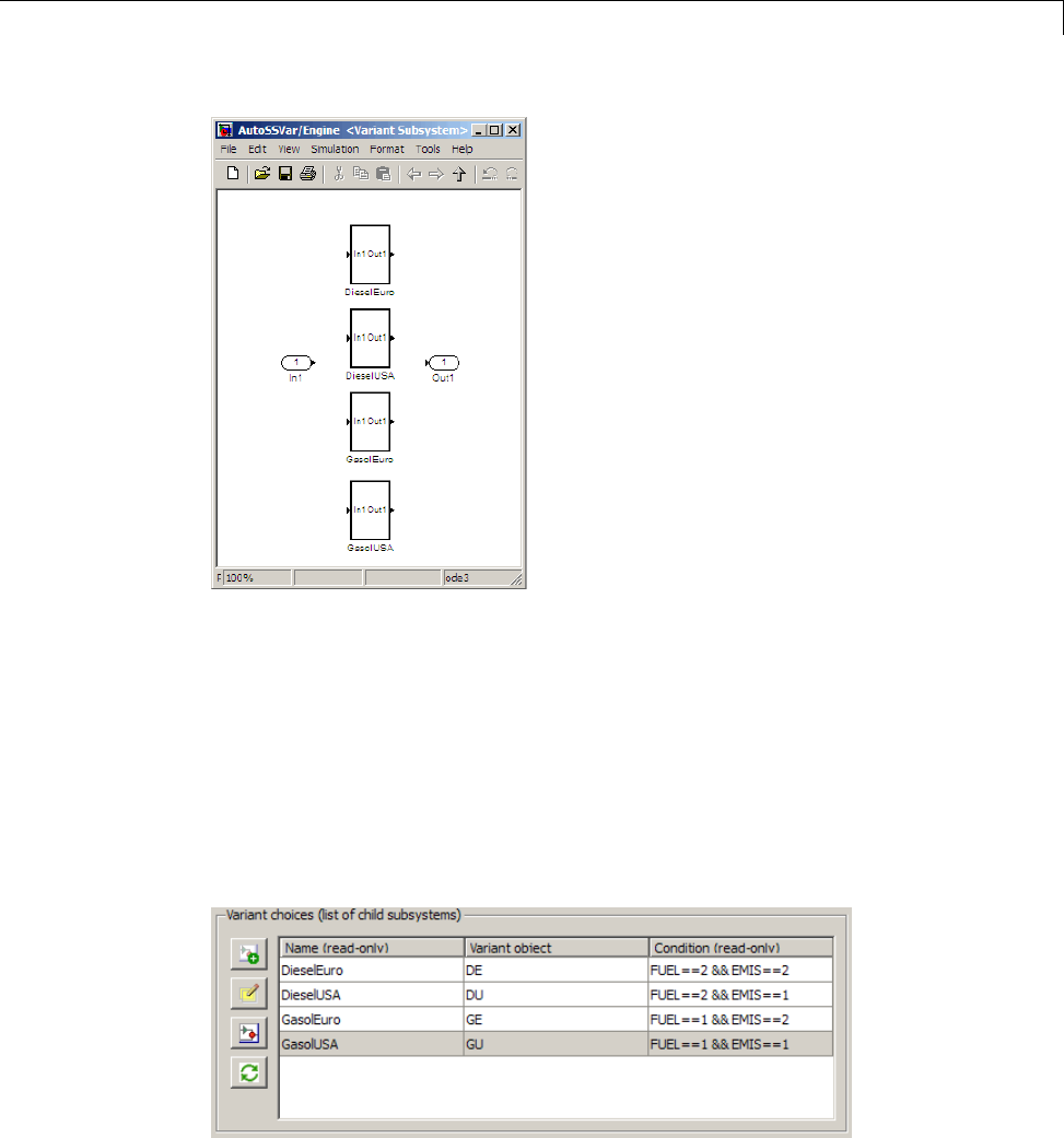
Set Up Variant Subsystems
The subsystem diagram for a Variant Subsystem block has no connections.
The only blocks allowed in the Variant Subsystem block diagram are Inport,
Outport, and Subsystem blocks. If you are generating code for a Variant
Subsystem block, see “Restrictions on Variant Subsystem Code Generation”.
To view how to specify these variants, in the Simulink Editor, right-click
the Engine block, and select Block Parameters (Subsystem) or select
Diagram > Block Parameters (Subsystem).
View the Variant choices (list of child subsystems) table in the dialog
box, as shown in the following figure.
8-19
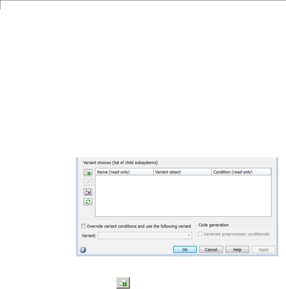
8Modeling Variant Systems
For instructions, see “Configuring the Variant Subsystem Block” on page 8-20.
Configuring the Variant Subsystem Block
To add and configure a Variant Subsystem block to specify your variants,
do the following:
1From the Simulink Library Browser, add a Variant Subsystem block to
your model:
Simulink > Ports and Subsystems > Variant Subsystem block
2To configure your variants, open the Variant Subsystem block dialog box.
In the Simulink Editor, right-click the Variant Subsystem block, Engine,
and select Block Parameters (Subsystem) or select Diagram > Block
Parameters (Subsystem).
The Variant Subsystem block parameters dialog box opens.
3Add a new subsystem choice in the Variant Subsystem block. In the
Variant choices table, click the Create and add a new subsystem
choice button . A new variant choice appears in the table and a new
Subsystem block appears in the Variant Subsystem block diagram window.
8-20

Set Up Variant Subsystems
4Rename the subsystem in the Variant Subsystem block diagram window,
and open and configure the subsystem as desired. You can drag and drop
existing subsystems into the new variant subsystem.
Note
•The Inport, Outport, and Connection Port blocks in the Variant
Subsystem block must be identical to the corresponding inports and
outports of its child subsystems.
•Inside the Variant Subsystem block diagram, you cannot create any
lines connecting blocks.
5Return to the Variant Subsystem parameter dialog box. In the Variant
object column of the Variant choices table, specify the variant name in
the row of the subsystem you just configured. Double-click the default
name, then type the name of the variant object. For an existing variant
object, Simulink retrieves the variant condition for the object when you
press Enter or click away from the Variant object.IntheVariant
choices table, double-click the Variant object field in the row of the
subsystem you just configured. Specify the name for the Variant object.
6To specify the Condition that determines which variant is active, click the
Create/Edit selected variant button . For the selected variant
choice, you create a variant object in the base workspace if necessary, or
edit an existing variant. The Simulink.Variant parameter dialog box opens.
8-21
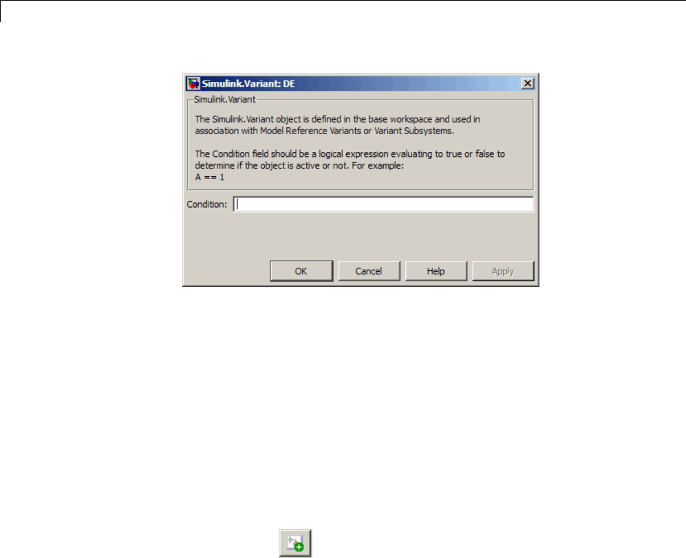
8Modeling Variant Systems
aSpecify the Condition for the variant object. For example, FUEL==2
&& EMIS==2.
When the variant object condition evaluates to true at compile time, the
subsystem associated with the variant becomes the active variant.
bClick Apply to check the expression, then click OK.
The Variant choices table is updated with the condition for the
new variant object. Simulink also created the variant object as a
Simulink.Variant object in the base workspace. If you use a variant
control variable in the Condition expression, you must create the variant
control variables in thebaseworkspace.
7To add another variant, click the Create and add a new subsystem
choice button
8Repeat the previous steps until you have specified all your variant
subsystems and their associated variant objects.
For more information on the block controls, see the Variant Subsystem
block page.
9Click OK to close the Variant Subsystem dialog box.
8-22

Set Up Variant Subsystems
Note Your variant conditions might require you to define control variables
in the base workspace before they can be evaluated. See “Creating Control
Variables” on page 8-25 and “Saving Variant Components” on page 8-26.
For next steps, see “Select the Active Variant” on page 8-29. The model
diagram does not display the new active variant on the block until you refresh
the diagram by pressing Ctrl+K.
Disabling and Enabling Subsystem Variants
You can disable individual subsystem choices. To ignore a subsystem for
simulation and code generation, you can comment out the variant object in
the Variant Choices table as follows:
1In the Variant choices table, double-click the name of the variant object.
2Add a ’%’ to the beginning of the variant object name.
3Click Apply and OK.
To enable the subsystem variant again, remove the %’ from the variant object
name.
You can also override variants and specify the active variant. See “Overriding
Variant Conditions” on page 8-30.
Variant Subsystem Block Requirements
A Variant Subsystem block must meet the following requirements:
•The Inport, Outport, and Connection Port blocks in the Variant Subsystem
block must be identical to the corresponding inports and outports of its
child subsystems.
•Inside the Variant Subsystem block diagram, you cannot create any lines
connecting blocks.
8-23

8Modeling Variant Systems
You can nest Variant Subsystem blocks to any level. The hierarchy resulting
from nesting must satisfy all applicable requirements and limitations when
you compile the model or generate code for it.
Note Requirements and limitations that apply to code generation are in
“Limitations on Generating Code for Variants”.
Variant Subsystem Example
To see an example that shows how to define a variant subsystem,
click sldemo_variant_subsystems. In the Help Browser, select:
Simulink > Examples > Modeling Features > Subsystems > Variant
Subsystems.
8-24

Set Up Variant Control
Set Up Variant Control
In this section...
“Creating Control Variables” on page 8-25
“Saving Variant Components” on page 8-26
“Example Variant Control Variables” on page 8-26
“Using Enumerated Types for Variant Control Variable Values” on page
8-27
Creating Control Variables
You must create variant control variables to control which variant is active.
You create variant control variables in the same way for variant subsystems
or variant models.
To specify the condition of a variant object, you can use MATLAB variables,
or Simulink.Parameter objects that reside in the base workspace. The
conditions of the variant objects determine which variant is the active
variant. At the MATLAB command line or in the Model Explorer, create
variant control variables to match your specified conditions. Before compiling
or simulating, you set the variant control variables to values that specify the
environment in which you want to simulate.
Note To control variants using meaningful readable names, you can use
aSimulink.Parameter object of enumerated type to define the variant
condition. See “Using Enumerated Types for Variant Control Variable
Values” on page 8-27.
At the MATLAB Command Window or in the Model Explorer, create variant
control variables:
•In the MATLAB Command Window
For example,
EMIS = 1
8-25

8Modeling Variant Systems
FUEL=2
•In the Model Explorer
1Select the Base Workspace.
2Select Add > MATLAB Variable.
3Name the variable and specify its value.
Each technique creates the variant control variables in the base workspace.
Note A variant control variable for code generation must be a Simulink
parameter that meets the requirements described in “Generate Preprocessor
Conditionals for Variant Systems”.
Saving Variant Components
Variant control variables and variantobjectsexistinthebaseworkspace.
If you want to reload variant control variables or variant objects with your
model, you must save them to a MAT-file.
Example Variant Control Variables
The example AutoMRVar uses the control variables EMIS and FUEL. Depending
on the values of EMIS and FUEL,youcanseewhichvariantisactive.
Variant Control
Variables
Variant Object Active Variant
(Model Block or
Subsystem Block)
FUEL=1 and EMIS=1 GU GasolUSA
FUEL=1 and EMIS=2 GE GasolEuro
FUEL=2 and EMIS=1 DU DieselUSA
FUEL=2 and EMIS=2 DE DieselEuro
To try an example changing control variables:
1Open AutoMRVar.
8-26

Set Up Variant Control
2Specify FUEL=2 and EMIS=2 in the base workspace. When you choose these
values for the variant control variables, the variant condition associated
with the variant object DE is true. Therefore, the active variant is
DieselEuro, and the model AutoMRVar uses DieselEuro as its referenced
model during simulation.
3Press Ctrl+K to updated the active variant.
Note To control variants using meaningful readable names, you can use
aSimulink.Parameter object of enumerated type to define the variant
condition. See “Using Enumerated Types for Variant Control Variable
Values” on page 8-27.
For an example explaining control variables for variant subsystems, including
the use of enumerated types, see the example sldemo_variant_subsystems.
Using Enumerated Types for Variant Control Variable
Values
You can use enumerated types to give meaningful names to the integers that
you use as values of variant control variables. For more information about
defining and using enumerated types, see “About Simulink Enumerations”
on page 44-2. For example, suppose you defined the following enumerated
class, whose elements represent vehicle properties:
classdef(Enumeration) VarParams < Simulink.IntEnumType
enumeration
gasoline(1)
diesel(2)
USA(1)
European(2)
end
end
With the class VarParams defined, you can use meaningful names to specify
variant control variables and variant conditions. For example, you can
substitute names for the integers for variant control variables EMIS and FUEL.
8-27

8Modeling Variant Systems
EMIS = VarParams.USA
FUEL = VarParams.diesel
Using the techniques described in “About Variant Objects” on page 8-32,
the variant objects are:
GU=Simulink.Variant('FUEL==VarParams.gasoline && EMIS==VarParams.USA')
GE=Simulink.Variant('FUEL==VarParams.gasoline && EMIS==VarParams.European')
DU=Simulink.Variant('FUEL==VarParams.diesel && EMIS==VarParams.USA')
DE=Simulink.Variant('FUEL==VarParams.diesel && EMIS==VarParams.European')
Specifying meaningful names rather than integers as the values of variant
control variables facilitates creating complex variant specifications. It also
clarifies the generated code, which contains the names of the values rather
than integers.
For an example explaining the use of enumerated types with variants, see the
example sldemo_variant_subsystems.
8-28

Select the Active Variant
Select the Active Variant
In this section...
“What Is an Active Variant?” on page 8-29
“Selecting the Active Variant for Simulation” on page 8-29
“Checking and Opening the Active Variant” on page 8-30
“Overriding Variant Conditions” on page 8-30
What Is an Active Variant?
The active variant is the variant Simulink uses when simulating your model.
An active variant can be either:
•A referenced model of a Model Variants block, or
•A subsystem of a Variant Subsystem block.
You control variants by setting conditions. Simulink determines the active
variant by which variant object condition evaluates to true at compile time.
Selecting the Active Variant for Simulation
You select the active variant in the same way for variant models or variant
subsystems.
You can switch the active variant by:
•Programmatically modifying the values of variant control variables or
parameters in the base workspace
•Using the Variant menu to choose a variant. Right-click the block or select
Diagram > Variant > Override using > variant choice.
•Manually overriding the variant selection on the block parameter dialog box
The condition of the variant objects determine which variant is active. You
define the condition using variant control variables or parameters defined
inthebaseworkspace,soyoucanmodifythevaluesofthevariantcontrol
8-29

8Modeling Variant Systems
variables to select the active variant. See “Creating Control Variables” on
page 8-25.
You can also override the variant conditions and manually select one active
variant. For instructions, see “Overriding Variant Conditions” on page 8-30.
Checking and Opening the Active Variant
Whenyouopenamodel,variantblocksdisplay the name of the variant that
was active the last time the model was saved.
When the active variant changes (for example, when you change the control
variables for variant conditions), you can update the variant block name by
pressing Ctrl+K to refresh.
You can use the Variant menu to open the active variant. Right-click the
block or select Diagram > Variant > Open > (active variant)
Tofindthenameoftheactivevariantforthe currently selected block, enter
at the command line:
get_param(gcb, 'ActiveVariant')
Overriding Variant Conditions
You can specify one variant as the active variant. You can either:
•Use the Variant menu to choose a variant. Right-click the block or select
Diagram > Variant > Override using > variant choice.
•Manually override the variant selection on the block parameter dialog box.
In both the Model Variants and Variant Subsystem block parameters dialog
boxes, use the “Override variant conditions and use following variant”
parameter, at the bottom left.
8-30
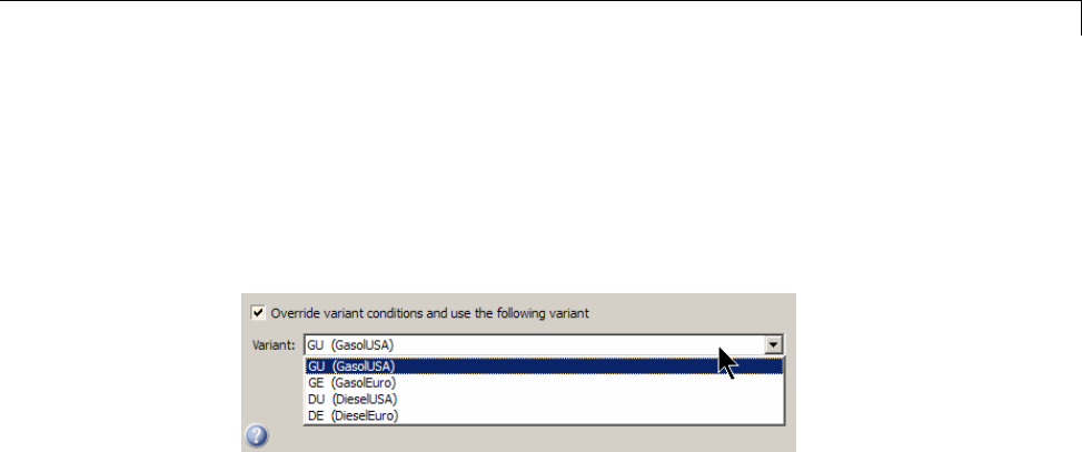
Select the Active Variant
1Select the parameter Override variant conditions and use following
variant. The “Variant” parameter becomes enabled.
2Click the Variant drop-down list and select a variant object from the list.
In the Model Variants block, the list shows each variant and the associated
model name.
In the Variant Subsystem block, the list shows only variant object names.
Checkthevariantchoicestableforthenameofthesubsystemassociated
with each variant.
3After you make the change, click Apply or OK. The variant object that you
specified becomes the active variant, overriding all other specifications that
determine which variant is active. The variant remains active until you
either select a different variant from the drop-down list, or clear Override
variant conditions and use following variant.
8-31

8Modeling Variant Systems
About Variant Objects
In this section...
“What Is a Variant Object?” on page 8-32
“Creating Variant Objects” on page 8-32
“Reusing Variant Objects” on page 8-33
“Variant Condition” on page 8-34
What Is a Variant Object?
A variant object is an instance of the Simulink.Variant class in the base
workspace. You can use the controls in the variant blocks to create variant
objects. Alternatively, you can create variant objects in the Model Explorer or
at the command line.
The variant object can have any unique legal name. The value of the variant
object specifies a variant condition.
Each variant object corresponds to a different simulation environment. When
compiling the model, Simulink tests the variant condition specified by each
variant object. The variant object whose variant condition is true designates
the active variant. The active variant determines which variant is used
during simulation. You must organize the variant objects for a model variant
or a variant subsystem so that, when the model compiles, only one variant
condition is true based on the current base workspace values.
Note You cannot use the same variant object more than once in the same
variant block, because a conflict occurs when that variant condition is true.
The same type of conflict occurs in a variant block where two different variant
objects both evaluate to true. For more information, see “Reusing Variant
Objects” on page 8-33.
Creating Variant Objects
There are three techniques for defining variant objects for your applications.
Choose the technique that complements your workflow.
8-32

About Variant Objects
•Using the Create variant option
Click the Create/Edit selected variant buttonineithertheModel
Variants block or the Variant Subsystem block dialog boxes. Specify the
condition in the dialog box and click Apply. The blocks create variant
objects for you in the base workspace, as described in “Configuring the
Model Variants Block” on page 8-9 and “Configuring the Variant Subsystem
Block” on page 8-20.
•In the Model Explorer
1Select the Base Workspace.
2Select Add > Simulink Variant.
The Model Explorer creates a new variant object named Variant in
the base workspace.
3Specify the name and condition for the variant object in the same way
as from the variant blocks.
•In the MATLAB Command Window
Enter code like the following to define your variant object name and
condition:
variantObjectName=Simulink.Variant(conditionExpression)
For example:
DU=Simulink.Variant('FUEL==2 && EMIS==1')
Reusing Variant Objects
For simplicity, the example models, AutoMRVar and AutoSSVar, show only one
variant block. A variant block refers to a Model Variants block or a Variant
Subsystem block. Your applications may use multiple variant blocks.
Some applications have multiple variant blocks that might reuse some of
the same variant objects associated with their variants (referenced models
or subsystems). For example, a model or subsystem of an automobile might
include many capabilities that change depending on the applicable fuel and
emission standards. To meet those different requirements using variants,
you can use the same variant object in multiple variant blocks. To do this,
associate the variant object with the same, or a different, variant in each
8-33

8Modeling Variant Systems
of the variant blocks. The variant blocks change their selected variants in
synchrony as variant control variable values change. The separate uses of the
variant object do not affect one another.
Other applications might associate multiple variant objects to one variant in a
Model Variants block. To do this, you can assign each of the variant objects
to a different parameterization or execution mode of the referenced model
variant. The separate uses of the referenced model do not affect one another.
Reusing variant objects, subsystems, and referenced models allows you to
globally reconfigure a model hierarchy to suit different environments by doing
nothing more than changing variant control variable values. No matter how
many simulation environments you define, selecting an environment requires
only setting variable or parameter values appropriately in the base workspace.
Variant Condition
A variant condition is the value of the variant object. Specify a Boolean
expression that references at least one base workspace variable or parameter.
The expression can include:
•MATLAB variables defined in the base workspace
•Simulink.Parameter objects defined in the base workspace
•Scalar variables
•Enumerated values
•Operators ==,!=,&&,||,~
•Parentheses for grouping
For instructions on specifying variant conditions, see “Configuring the Model
Variants Block” on page 8-9 and “Configuring the Variant Subsystem Block”
on page 8-20.
For instructions on variant control variables, see “Set Up Variant Control”
on page 8-25.
8-34


8Modeling Variant Systems
Code Generation of Variants
Generating code from variants depends on your MathWorks code generation
software.
•Simulink Coder generates code only for the variant that is active in your
system.
•Embedded Coder generates code for all variants, unless you override
variant conditions and specify a variant for code generation.
-By default, Embedded Coder generates code for all variants. The
generated code for each variant is surrounded by C preprocessor
conditionals, #if,#elif,and#endif. At C compile time, the
preprocessor conditionals select the active variant and determine which
code to execute.
-You can specify a single variant for code generation by using the
Override variant conditions and use following variant option in
the Model Variants block or Variant Subsystem block.
For instructions, see “Generate Preprocessor Conditionals for Variant
Systems”.
8-36

Variant System Reference
Variant System Reference
In this section...
“Custom Storage Classes” on page 8-37
“Blocks” on page 8-37
Custom Storage Classes
Reference information for Simulink classes used in implementing variants:
•Simulink.Parameter for variant control variables
•Simulink.Variant for variant objects
Blocks
Reference information for blocks used in implementing variants:
•Model Variants block
•Variant Subsystem block
8-37

8Modeling Variant Systems
8-38

9
Exploring, Searching, and
Browsing Models
•“Model Explorer Overview” on page 9-2
•“Model Explorer: Model Hierarchy Pane” on page 9-9
•“Model Explorer: Contents Pane” on page 9-19
•“Control Model Explorer Contents Using Views” on page 9-26
•“Organize Data Display in Model Explorer” on page 9-36
•“Filter Objects in the Model Explorer” on page 9-46
•“Workspace Variables in Model Explorer” on page 9-52
•“Search Using Model Explorer” on page 9-63
•“Model Explorer: Property Dialog Pane” on page 9-70
•“Finder” on page 9-73
•“Model Browser” on page 9-80
•“Model Dependency Viewer” on page 9-83
•“View Linked Requirements in Models and Blocks” on page 9-96

9Exploring, Searching, and Browsing Models
Model Explorer Overview
In this section...
“What You Can Do Using the Model Explorer” on page 9-2
“Opening the Model Explorer” on page 9-2
“Model Explorer Components” on page 9-3
“The Main Toolbar” on page 9-4
“Adding Objects” on page 9-5
“Customizing the Model Explorer Interface” on page 9-5
“Basic Steps for Using the Model Explorer” on page 9-6
“Focusing on Specific Elements of a Model or Chart” on page 9-7
What You Can Do Using the Model Explorer
Use the Model Explorer to quickly view, modify, and add elements of Simulink
models, Stateflow charts, and workspace variables. The Model Explorer
provides several ways for you to focus on specific elements (for example,
blocks, signals, and properties) without your having to navigate through the
model diagram or chart.
Opening the Model Explorer
To open the Model Explorer, use one of these approaches:
•From the Simulink Editor View menu, select Model Explorer or select
the Model Explorer icon from the toolbar.
•In an open model in the Simulink Editor, right-click a block and from the
context menu, select Explore.
•In an open Stateflow chart, right-click in the drawing area and from the
context menu, select Explore.
•At the MATLAB command line, enter daexplr.
9-2
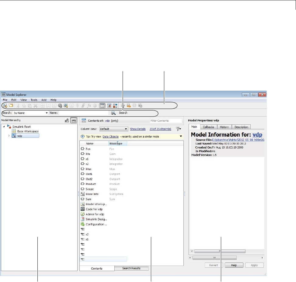
Model Explorer Overview
Model Explorer Components
By default, the Model Explorer opens with three panes (Model Hierarchy,
Contents,andDialog), a main toolbar, and a search bar.
Search bar Main toolbar
Model Hierarchy pane Contents pane Dialog pane
9-3
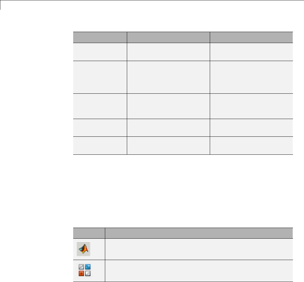
9Exploring, Searching, and Browsing Models
Component Purpose Documentation
Main toolbar Execute Model Explorer
commands
“The Main Toolbar” on
page 9-4
Search bar Perform a search within
the context of the selected
node in Model Hierarchy
pane.
“Search Using Model
Explorer” on page 9-63
Model
Hierarchy pane
Navigate and explore
model, chart, and
workspace nodes
“Model Explorer: Model
Hierarchy Pane” on page
9-9
Contents pane Display and modify model
or chart objects
“Model Explorer: Contents
Pane” on page 9-19
Dialog pane View and change the
details of object properties
“Model Explorer: Property
Dialog Pane” on page 9-70
The Main Toolbar
The main toolbar at the top of the Model Explorer provides buttons you click
to perform Model Explorer operations. Most of the toolbar buttons perform
actions that you can also perform using Model Explorer menu items.
The toolbar buttons in the following table perform actions that you cannot
perform using Model Explorer menus:
Button Usage
Bring the MATLAB window to the front.
Display the Simulink Library Browser.
If you have Simulink Verification and Validation installed, you can use
additional toolbar buttons relating to requirements links.
9-4
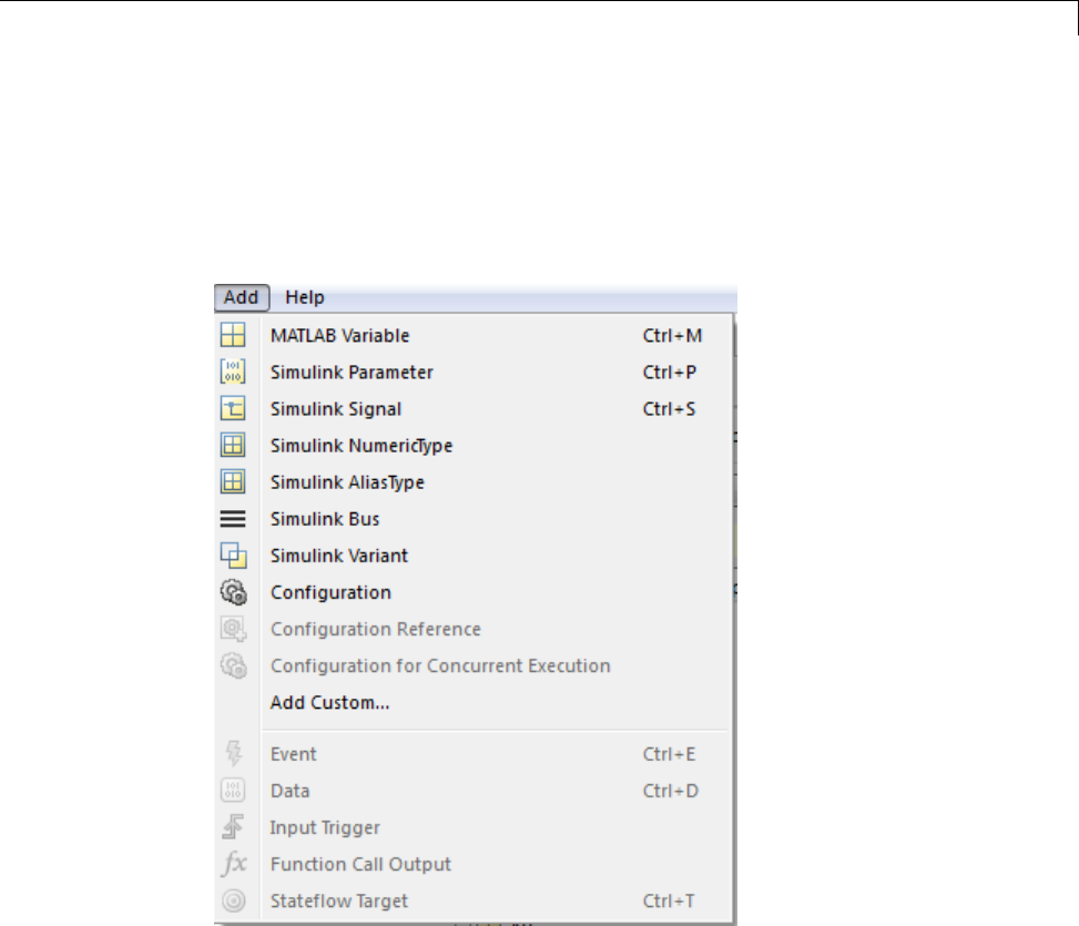
Model Explorer Overview
Adding Objects
You can use the Model Explorer to add many kinds of objects to a model, chart,
or workspace. The types of objects that you can add depend on what node you
select in the Model Hierarchy pane. Use toolbar buttons or the Add menu
to add objects. The Add menu lists the kinds of objects you can add.
Customizing the Model Explorer Interface
You can customize the Model Explorer interface in several ways. This section
describes how to show or hide the main toolbar and how to control the font
size.
Other ways you can customize the Model Explorer interface include:
9-5

9Exploring, Searching, and Browsing Models
•“Marking Nonexistent Properties” on page 9-45
•“Showing and Hiding the Search Bar” on page 9-64
•“Showing and Hiding the Dialog Pane” on page 9-70
Showing and Hiding the Main Toolbar
To show or hide the main toolbar, in the Model Explorer select View >
Toolbars > Main Toolbar.
Controlling the Font Size
You can change the font size in the Model Explorer panes:
•To increase the font size, press the Ctrl + Plus Sign (+).
Alternatively, from the Model Explorer View menu, select Increase Font
Size.
•To decrease the font size, press the Ctrl + Minus Sign (-).
Alternatively, from the Model Explorer View menu, select Decrease
Font Size.
Note The changes remain in effect for the Model Explorer and in the
Simulink dialog boxes across Simulink sessions.
Basic Steps for Using the Model Explorer
Use the Model Explorer to perform a wide range of activities relating to
viewing and changing model and chart elements. You can perform activities
in any order, using panes in the order you choose. Your actions in one pane
often affect other panes.
For example, if you want to edit properties of objects in a model, you might
use a general workflow such as:
1Open a model.
2Open the Model Explorer.
9-6

Model Explorer Overview
3Select the model in the Model Hierarchy pane, specifying whether the
Model Explorer displays only the current system or the whole system
hierarchy of the current system
4Control what model information the Contents pane displays, and how it
displays that information, by using a combination of:
•The View > Column View option to control which property columns to
display
•The View > Row Filter option to control which types of objects to
display
•Techniques to directly manipulate column headings
5Identify model elements with specific values, using the search bar.
6Edit the values for model elements, in either the Contents pane or the
Dialog pane. To edit workspace variables, you can use the Variable Editor.
Focusing on Specific Elements of a Model or Chart
As you explore a model or chart, you might want to narrow the contents that
you see in the Model Explorer to particular elements of a model or chart.
You can use several different techniques. Thefollowingtablesummarizes
techniques for controlling what content the Model Explorer displays and how
the contents appear.
Technique When to Use Documentation
Show partial or whole
model hierarchy
contents
To control how much of
a hierarchical model to
display
“Displaying Partial or
Whole Model Hierarchy
Contents” on page 9-12
Use the Row Filter
option
To focus on, or hide, a
specific kind of a model
object, such as signals
“Using the Row Filter
Option” on page 9-46
9-7

9Exploring, Searching, and Browsing Models
Technique When to Use Documentation
Search To find objects that
might not be currently
displayed
“Search Using Model
Explorer” on page 9-63
Filter contents To focus on specific
objects in the Contents
pane, based on a search
string
“Filtering Contents” on
page 9-48
Once you have the general set of data that you are interested in, you can use
the following techniques to organize the display of contents.
Technique When to Use Documentation
Sort To quickly organize
data for a property
in ascending or
descending order
“Sorting Column
Contents” on page
9-36
Group by property
column
To logically group data
based on values for a
property
“How to Group by a
Property Column” on
page 9-39
Use column views To display a named
subset of property
columns to apply to
different kinds of
nodes in the Model
Hierarchy pane
“Control Model
Explorer Contents
Using Views” on page
9-26
Add, delete, or
rearrange property
table columns
To customize property
columns
“Organize Data Display
in Model Explorer” on
page 9-36
9-8

Model Explorer: Model Hierarchy Pane
Model Explorer: Model Hierarchy Pane
In this section...
“What You Can Do with the Model Hierarchy Pane” on page 9-9
“Simulink Root” on page 9-10
“Base Workspace” on page 9-10
“Configuration Preferences” on page 9-11
“Model Nodes” on page 9-11
“Displaying Partial or Whole Model Hierarchy Contents” on page 9-12
“Displaying Linked Library Subsystems” on page 9-13
“Displaying Masked Subsystems” on page 9-14
“LinkedLibraryandMaskedSubsystems”onpage9-14
“Displaying Node Contents” on page 9-14
“Navigating to the Block Diagram” on page 9-15
“Working with Configuration Sets” on page 9-15
“Expanding Model References” on page 9-15
“Cutting, Copying, and Pasting Objects” on page 9-17
What You Can Do with the Model Hierarchy Pane
The Model Hierarchy pane displays a tree-structured view of the Simulink
model and Stateflow chart hierarchy. Use the Model Hierarchy pane to
navigate to the part of the model and chart hierarchy that you want to explore.
9-9
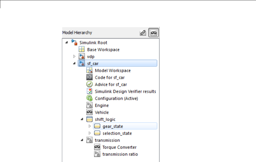
9Exploring, Searching, and Browsing Models
Simulink Root
The first node in the hierarchy represents the Simulink root. Expand the
root node to display nodes representing the MATLAB workspace, Simulink
models, and Stateflow charts that are in the current session.
Base Workspace
This node represents the MATLAB workspace. The MATLAB workspace is
the base workspace for Simulink models and Stateflow charts. Variables
defined in this workspace are visible to all open models and charts.
For information about exporting and importing workspace variables, see
“Exporting Workspace Variables” on page 9-60 and “Importing Workspace
Variables” on page 9-62.
9-10

Model Explorer: Model Hierarchy Pane
Configuration Preferences
To display a Configuration Preferences node in the expanded Simulink
Root node, enable the View > Show Configuration Preferences option.
Selecting this node displays the preferred configuration for new models
(see “Manage a Configuration Set” on page 10-12). You can change the
preferred configuration by editing the displayed settings and using the Model
Configuration Preferences dialog box to save the settings (see “Model
Configuration Preferences” on page 10-28).
Model Nodes
Expanding a model or chart node in the Model Hierarchy pane displays
nodes representing the following elements, as applicable for the models and
charts you have open.
Node Description
Model workspace For information about how to use the Model Explorer
to work with model workspace variables, see the
following sections:
•“Finding Variables That Are Used by a Model or
Block” on page 9-52
•“Finding Blocks That Use a Specific Variable” on
page 9-55
•“Editing Workspace Variables” on page 9-58
•“Exporting Workspace Variables” on page 9-60
•“Importing Workspace Variables” on page 9-62
•“Model Workspaces” on page 4-67
Configuration sets For information about adding, deleting, saving,
and moving configuration sets, see “Manage a
Configuration Set” on page 10-12.
Top-level
subsystems
Expand a node representing a subsystem to display
underlying subsystems, if any.
9-11
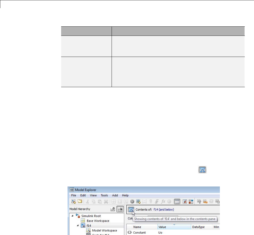
9Exploring, Searching, and Browsing Models
Node Description
Model blocks Expand model blocks to show contents of referenced
models (see “Expanding Model References” on page
9-15).
Stateflow charts •Expand a node representing a Stateflow chart to
display the top-level states of the chart.
•Expand a node representing a state to display its
substates.
Displaying Partial or Whole Model Hierarchy
Contents
By default, the Model Explorer displays objects for the system that you select
in the Model Hierarchy pane. It does not display data for child systems.
You can override that default, so that the Model Explorer displays objects
for the whole hierarchy of the currently selected system. To toggle between
displaying only the current system and displaying the whole system hierarchy
of the current system, use one of these techniques:
•Select View > Show Current System and Below.
•Click the Show Current System and Below button ( )atthetopof
the Contents pane.
When you select the Show Current System and Below option:
•The Model Hierarchy pane highlights in pale blue the current system
and its child systems.
9-12

Model Explorer: Model Hierarchy Pane
•After the path in the Contents of field, the text (and below) appears.
•The appearance of the Show Current System and Below button at the
top of the Contents pane and in the View menu changes.
•The status bar indicates the scope of the displayed objects when you hover
over the Show Current System and Below button.
Loading very large models for the current system and below can be slow. To
stop the loading process at any time, either click the Show Current System
and Below button or click another node in the tree hierarchy.
If you show the current system and below, you might want to change the view
to better reflect the displayed system contents. For details about views, see
“Control Model Explorer Contents Using Views” on page 9-26.
The setting for the Show Current System and Below option is persistent
across Simulink sessions.
Displaying Linked Library Subsystems
By default, the Model Explorer does not display the contents of linked library
subsystems in the Model Hierarchy pane. To display the contents of linked
library subsystems, use one of these approaches:
•At the top of the Model Hierarchy pane, click the Show/Hide Library
Links button ( ).
•From the View menu, select Show Library Links.
Library-linked subsystems are visible in the Contents pane, regardless of
how you configure the Model Hierarchy pane.
Note Search does not find elements in linked library or masked subsystems
that are not displayed in the Model Hierarchy pane.
9-13

9Exploring, Searching, and Browsing Models
Displaying Masked Subsystems
By default, the Model Explorer does not display the contents of masked
subsystems in theModel Hierarchy pane. To display the contents of masked
subsystems, useoneoftheseapproaches:
•At the top of theModel Hierarchy pane, click the Show/Hide Masked
Subsystems button ( ).
•From the View menu, select Show Masked Subsystems.
Masked subsystems are visible in the Contents pane, regardless of how you
configure the Model Hierarchy pane.
Linked Library and Masked Subsystems
For subsystems that are both library-linked and masked, how you set the
linked library subsystems and masked subsystems options affects which
subsystems appear in the Model Hierarchy pane, as described in the
following table.
Settings Subsystems Displayed in the
Model Hierarchy Pane
Show Library Links
Hide Masked Subsystems
Only library-linked, unmasked
subsystems
Hide Library Links
Show Masked Subsystems
Only masked subsystems that are
not library-linked subsystems
Show Library Links
Show Masked Subsystems
All library-linked or masked
subsystems
Displaying Node Contents
Select the object in the Model Hierarchy pane whose contents you want to
display in the Contents pane.
9-14
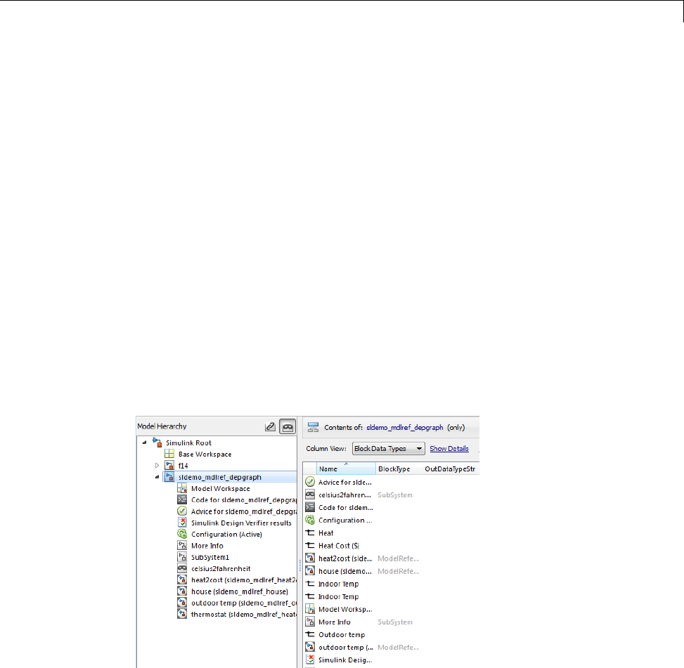
Model Explorer: Model Hierarchy Pane
Navigating to theBlockDiagram
To open a graphical object (for example, a model, subsystem, or chart) in an
editor window, right-click the object in the Model Hierarchy pane. From the
context menu, select Open.
Working with Configuration Sets
See “Manage a Configuration Set” on page 10-12 for information about using
the Model Hierarchy pane to perform tasks such as adding, deleting, saving,
and moving configuration sets.
Expanding Model References
To browse a model that includes Model blocks, you can expand the
Model Hierarchy pane nodes of the Model blocks. For example, the
sldemo_mdlref_depgraph model includes Model blocks that reference other
models. If youopenthesldemo_mdlref_depgraph model and expand that
model nodeintheModel Hierarchy pane, you see that the model contains
several Model blocks, including heat2cost.
To browse a model referenced by a Model block:
1Right-click the referenced model node in the Model Hierarchy pane.
9-15
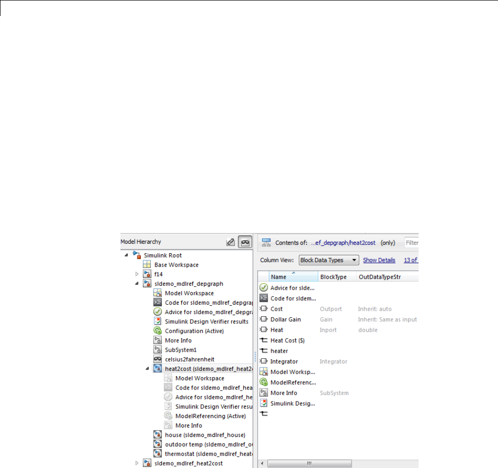
9Exploring, Searching, and Browsing Models
2From the context menu, choose Open Model.
•The referenced model opens.
•The Model Hierarchy pane indicates that you can expand the Model
block node.
•The Model Hierarchy pane displays a separate expandable node for
the referenced model (read-only).
•The Contents pane displays objects corresponding to the Model block
node (read-only).
For example, if you right-click the heat2cost Model block node and select the
Open Model option, the Contents pane displays the objects corresponding
to the heat2cost Model block. You can expand the heat2cost node.
You can browse the contents of the referencedmodel,butyoucannoteditthe
model objects that are underneath the Model block.
9-16
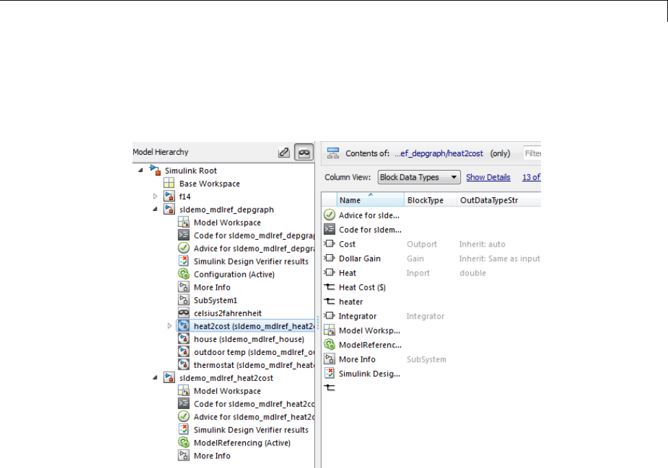
Model Explorer: Model Hierarchy Pane
Editing the Referenced Model
To edit the referenced model, expand the referenced model node in the Model
Hierarchy pane. For example, expand the sldemo_mdlref_heat2cost node:
You can now edit the properties of object in the referenced model.
For information about referenced models, see “Model Reference”.
Cutting, Copying, and Pasting Objects
To cut, copy, and paste workspace objects from one workspace into another
workspace:
1In the Contents pane, right-click on the workspace object you want to
cut or copy.
2From the context menu, select Cut or Copy.
9-17

9Exploring, Searching, and Browsing Models
•You can also cut a workspace object by selecting in the Contents pane
Edit > Cut or by clicking the Cut button ( ).
•You can also copy a workspace object by selecting Edit > Copy or by
clicking the Copy button ( ).
3If you want to paste the workspace object that you cut or copied, in the
Model Hierarchy pane, right-click the workspace into which you want to
paste the object, and select Paste.
•You can also paste the object by selecting Edit > Paste or by clicking
the Paste button ( ).
You can also perform cut, copy, and paste operations by selecting an object
and performing drag and drop operations.
9-18

Model Explorer: Contents Pane
Model Explorer: Contents Pane
In this section...
“Contents Pane Tabs” on page 9-19
“Data Displayed in the Contents Pane” on page 9-22
“Link to the Currently Selected Node” on page 9-22
“Horizontal Scrolling in the Object Property Table” on page 9-23
“Working with the Contents Pane” on page 9-24
“Editing Object Properties” on page 9-25
Contents Pane Tabs
The Contents pane displays one of two tables containing information about
models and charts, depending on the tab that you select:
•The Contents tab displays an object property table for the node that you
select in the Model Hierarchy pane.
•The Search Results tab displays the search results table (see “Search
Using Model Explorer” on page 9-63).
Optionally, you can also open a column view details section in the Contents
pane. The following graphic shows the Contents pane with the column view
details section opened.
9-19
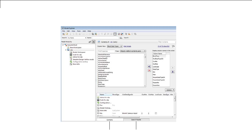
9Exploring, Searching, and Browsing Models
Contents tab
Search Results tab
To open the column view details section, click Show Details,atthetopof
the Contents pane.
9-20
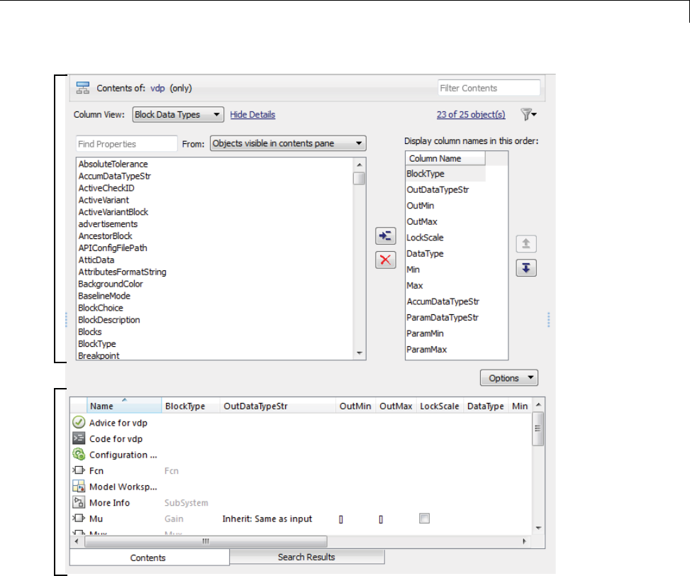
Model Explorer: Contents Pane
Column
View
Details
section
Object
Property
Table
section
The Column view details section provides an interface for customizing
the column view (hidden by default).
The Object property table section displays a table of model and chart object
data (open by default).
9-21

9Exploring, Searching, and Browsing Models
Data Displayed in the Contents Pane
In the object property table section of the Contents tab and in the Search
Results tab:
•Table columns correspond to object properties (for example, Name and
BlockType).
•Table rows correspond to objects (for example, blocks, and states).
The objects and properties displayed in the Contents pane depend on:
•The column view that you select in the Contents pane
•The node thatyouselectintheModel Hierarchy pane
•The kind of object (for example, subsystem, chart, or configuration set) that
you select in the Model Hierarchy pane
•The View > Row Filter options that you select
For more information about controlling which objects and properties to
display intheContents pane, see:
•“Control Model Explorer Contents Using Views” on page 9-26
•“Organize Data Display in Model Explorer” on page 9-36
•“Filter Objects in the Model Explorer” on page 9-46
Link to the Currently Selected Node
The Contents of link at the top left side of the Contents pane links to the
currently selected node in the Model Hierarchy pane. The model data
displayed in the Contents pane reflects the setting of the Current System
and Below option. In the following example, Contents of links to the vdp
model, which is the currently selected node.
9-22
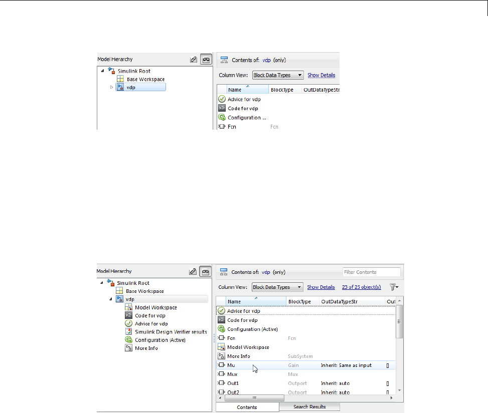
Model Explorer: Contents Pane
Horizontal Scrolling in the Object Property Table
The object property table displays the first two columns (the object icon and
the Name property) persistently. These columns remain visible, regardless of
how far you scroll to the right.
For example, the following image shows the initial display of the object
property table for the vdp model. The ParamDataTypeStr column is too far
to the righttobedisplayed.
The next image shows the results of scrolling to the right. The icon and Name
columns remain visible, but now you can see the ParamDataTypeStr column.
9-23
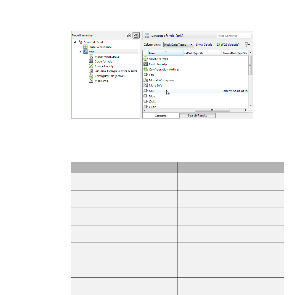
9Exploring, Searching, and Browsing Models
Working with the Contents Pane
The following table summarizes the key tasks to control what is displayed
in the Contents.
Task Documentation
Control which kinds of objects to
display.
“Using the Row Filter Option” on
page 9-46
Search within the selected set of
objects.
“Search Using Model Explorer” on
page 9-63
Specify a set of properties to display
based on the kind of node.
“Control Model Explorer Contents
Using Views” on page 9-26
Group data based on unique values
in a property column.
“GroupingbyaProperty”onpage
9-37
Manage views (for example, save
and export a view).
“Managing Views” on page 9-30
Add, remove, or rearrange columns. “Organize Data Display in Model
Explorer” on page 9-36
Edit object property values. “Editing Object Properties” on page
9-25
9-24

Model Explorer: Contents Pane
Editing Object Properties
To open a properties dialog box for an object in the Model Hierarchy
pane, right-click the object, and from the context menu, select Properties.
Alternatively, click an object and from the Edit menu, select Properties.
You can change modifiable properties in the Contents pane (for example, a
block name) by editing the displayed value. To edit a value, first select the
row that contains the value, and then click the value. An edit control replaces
the value (for example, an edit field for text values or a list for a range of
values). For workspace variables that are arrays or structures, you can use
the Variable Editor. Use the edit control to change the value of the selected
property.
To assign the same property value to multiple objects in the Contents
pane, select the objects and then change one of the selected objects to have
the new property value. An edit control replaces the value with <edit>,
indicating that you are doing batch editing. The Model Explorer assigns the
new property value to the other selected objects, as well.
You can also change property values using the Dialog pane. See “Model
Explorer: Property Dialog Pane” on page 9-70.
9-25

9Exploring, Searching, and Browsing Models
Control Model Explorer Contents Using Views
In this section...
“Using Views” on page 9-26
“Customizing Views” on page 9-29
“Managing Views” on page 9-30
Using Views
What Is a Column View?
A view in the Model Explorer is a named set of properties.
The Model Explorer uses views to specify sets of property columns to display
in the Contents pane.
ForeachkindofnodeintheModel Hierarchy pane, certain properties are
most relevant for the objects displayed in the Contents pane. For example,
for a Simulink model node, such as a model or subsystem, some properties
thatareusefultodisplayinclude:
•BlockType (block type)
•OutDataTypeStr (output data type)
•OutMin (minimum value for the block output)
Generally, a column view does not contain the total set of properties for
all the objects in a node. Specifying a subset of properties to display can
streamline the task of exploring and editing model and chart object properties
and increase the density of the data displayed in the Contents pane.
What You Can Capture in a View
You can use a view to capture the following characteristics of the model
information to show in the Model Explorer:
•Properties that you want to display in the Contents pane (see “Customizing
Views” on page 9-29)
9-26

Control Model Explorer Contents Using Views
•Layout of the Contents pane (for example, grouping by property, the order
of property columns, and sorting), as described in “Organize Data Display
in Model Explorer” on page 9-36.
Use Standard Views or Customized Views
You can use views in the following ways:
•Use the standard views shippedwiththeModelExplorer
•Customize the standard views
•Create your own views
Automatically Applied Views
ThefirsttimeyouopentheModelExplorer, the software automatically applies
one of the standard views to the node you select in the Model Hierarchy
pane. The Model Explorer applies a view based on the kind of node you select.
The Model Explorer assigns one of four categories of nodes in the Model
Hierarchy pane. The Model Explorer initially associates a default view with
each node category. The four node categories are:
Node Category Kinds of Hierarchy
Nodes Included
Initial Associated
View
Simulink Models, subsystems,
and root level models
Block Data Types
Workspace Base and model
workspace objects
Data Objects
Stateflow Stateflow charts and
states
Stateflow
Other Objects that do not fit
into one of the first
three categories; for
example, configuration
sets
Default
9-27

9Exploring, Searching, and Browsing Models
The Column View field at the top of the Contents pane displays the view
that the Model Explorer is currently using.
If you select a view. In the Contents pane, from the Column View
list, you can select a different view. If you select a different view, then the
Model Explorer associates that view with the category of the current node.
For example, suppose the selected node in the Model Hierarchy pane is a
Simulink model, and the current view is Data Objects.Ifyouchangethe
view to Signals, then when you select another Simulink model node, the
Model Explorer uses the Signals view. See “Selecting a View Manually”
on page 9-28.
Selecting a View Manually
By default, the Model Explorer automatically applies a view, based on the
category of node that you select and the last view used for that node. You can
manually select a view from the Column View list that better meets your
current task.
You can shift from the default mode of having the Model Explorer
automatically apply views to a mode in which you must manually select a
view to change views.
To enable the manual view selection mode:
1Select View > Column View > Manage Views.
The View Manager dialog box opens.
2In the View Manager dialog box, click the Options button and clear
Change View Automatically.
In the manual view selection mode, if you switch to a different kind of node in
the Model Hierarchy pane that has a different view associated with it, the
Contents pane displays a yellow informational bar suggesting a view to use.
9-28
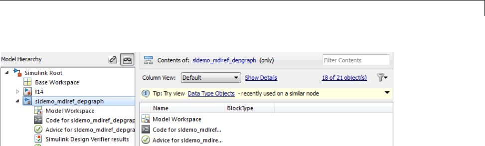
Control Model Explorer Contents Using Views
Tip interface. Thetipinterfaceappearsimmediatelyabovetheobject
property table.
The tip does not appear if you use automatic view selection.
To hide the currently displayed tip, from the menu button on the right-hand
side of the tip bar, select Hide This Tip.
The tip interface displays a link for changing the current view to a suggested
view. To choose the suggested view displayed in the tip bar, click the link.
Initially, the suggested view is the default view associated with a node. If you
associate a different view with a node category, then the tip suggests the most
recently selected view when you select similar nodes.
To change from manual specification of views to automatic specification,
from the tip interface, select the down arrow and then the Change View
Automatically menu item.
Customizing Views
If a standard view does not meet your needs, you can either modify the view
or create a new view.
You can customize the object property table represented by the current view
in several ways, as described in these sections:
•“Adding Property Columns” on page 9-42
•“Hiding or Removing Property Columns” on page 9-43
•“Changing the Order of Property Columns” on page 9-41
9-29

9Exploring, Searching, and Browsing Models
How the Model Explorer Saves Your Customizations
As you modify the object property table, you change the current view
definition.
The Model Explorer saves the following changes to the object property table
as part of the column view definition:
•Grouping by property
•Sorting in a column
•Changing the order of property columns
•Adding a property column
•Hiding and removing property columns
When you change from one view to another view, the Model Explorer saves
any customizations that you have made to the previous view.
For example, suppose you use the Block Data Types view and you remove
the LockScale property column. If you then switch to use the Data Objects
view, and later use the Block Data Types view again, the Block Data Types
view no longer includes the LockScale column that you deleted.
At the end of a Simulink session, the Model Explorer saves the view
customizations that you made during that session. When you reopen the
Model Explorer, Simulink uses the customized view, reflecting any changes
thatyoumadetotheviewintheprevioussession.
Managing Views
If a standard view does not meet your needs, you can either modify the view
orcreateanewview.See“CustomizingViews”onpage9-29.
You can manage views (for example, create a new view or export a view)
using the View Manager dialog box.
Opening the View Manager Dialog Box
To open the View Manager dialog box, select the Manage Views option
from either:
9-30

Control Model Explorer Contents Using Views
•The View > Column View menu
•The options listed when you click the Options button in the column view
details section
The View Manager dialog box displays a list of defined views and provides
tools for you to manage views.
You can manage views in several ways, including:
•“Creating a New View” on page 9-32
•“Deleting Views” on page 9-33
•“Reordering Views” on page 9-33
•“Exporting Views” on page 9-33
•“Importing Views” on page 9-34
•“Resetting Views to Factory Settings” on page 9-34
9-31

9Exploring, Searching, and Browsing Models
Creating a New View
To create a new view that has a new name, you can use one of these
approaches:
•Copy an existing view, rename it, and customize the view.
•Create a completely new view.
After you create a new view, you can customize the view as described in
“Customizing Views” on page 9-29.
Copying and renaming an existing view. You can build a new view
by copying an existing view, renaming it, and optionally customizing the
renamed view. In the View Manager dialog box:
1Select the view that you want to use as the starting point for your new view.
2Click the Copy button.
A new row appears at the bottom of the View Manager table of views. The
new row contains the name of the view you copied, followed by a number in
parentheses. For example, if you copy the Stateflow view, the initial name
of the copied view is Stateflow (1).
Creating a completely new view. To create a completely view, in the View
Manager dialog box, click the New button. A new view row appears at the
bottom of the View Manager dialog box list of views.
Naming and describing a new view. Once you create a view, you can
name the view and provide a description of the view:
1Double-click New View in the left column of the table of views and replace
the text with a name for the view.
2Double-click Description in the table and replace the text with a
description of the view.
3Click OK.
9-32

Control Model Explorer Contents Using Views
Deleting Views
To delete a view from the Column View list of views:
1In the View Manager dialog box, select one or more views that you want to
remove from the list.
2Click the Delete button or the Delete key.
3Click OK.
Deleting a view using the View Manager dialog box permanently deletes that
view from the Model Explorer interface.
If you think you or someone else might want to use a view again, consider
exporting the view before you delete it (see “Exporting Views” on page 9-33).
Reordering Views
To change the position of a view in the Column View list, in the View
Manager dialog box:
1Select one or more views that you wish to move up or down one row in
thetableofviews.
2Click the up or down arrow buttons to the right of the table of views.
Repeat this step until the view appears where you want it to be in the table.
3Click OK.
Exporting Views
To export views that you or others can then import, in the View Manager
dialog box:
1In the View Manager dialog box, select one or more views that you want to
export.
2Click the Export button.
An Export Views dialog box opens, with check marks next to the views
that you selected.
9-33

9Exploring, Searching, and Browsing Models
3Click OK.
An Export to File Name dialog box opens.
4Navigate to the folder to which you want to export the view.
By default, the Model Explorer exports views to the MATLAB current
folder.
5Specify the file name for the exported view.
The file format is .mat.
6Click OK.
Importing Views
To import view files from another location for use by the Model Explorer:
1In the View Manager dialog box, click the Import button.
The Select .mat File to Import dialog box opens.
2Navigate to the folder from which you want to import the view.
3SelecttheMAT-filecontainingtheview that you want to import and then
click Open.
A confirmation dialog box opens. Click OK to import the view.
The imported view appears at the bottom of the Column View list of views.
The Model Explorer automatically renames the view if a name conflict occurs.
Resetting Views to Factory Settings
You can reset (restore) the original definition of a specific standard view (that
is, a view shipped with the Model Explorer) if that view is the current view.
To do so, click the Options button in the column view details section and
select Reset This View to Factory Settings.
9-34

Control Model Explorer Contents Using Views
To reset the factory settings for all standardviewsinonestep,intheView
Manager dialog box, click the Options button and select Reset All Views
to Factory Settings.
Note When you reset all views, the Model Explorer removes all the custom
views you have created. Before you reset views to factory settings, export any
views that you will want to use in the future.
9-35

9Exploring, Searching, and Browsing Models
Organize Data Display in Model Explorer
In this section...
“Layout Options” on page 9-36
“Sorting Column Contents” on page 9-36
“GroupingbyaProperty”onpage9-37
“Changing the Order of Property Columns” on page 9-41
“Adding Property Columns” on page 9-42
“HidingorRemovingPropertyColumns”onpage9-43
“Marking Nonexistent Properties” on page 9-45
Layout Options
You can control how the object property table and Search Results pane
organize the layout of property information by:
•Sorting column contents
•Grouping by a property
•Changing the order of property columns
•Adding a property column
•Hiding and removing property columns
Sorting Column Contents
To sort the column contents in ascending order, click the heading of the
property column. A triangle pointing up appears in the column heading.
To change the order from ascending to descending, or from descending to
ascending, click the heading of the column again.
For example, if properties are in ascending order, based on the Name property
(the default), click the heading of the Name column to display objects by name,
in descending order.
9-36
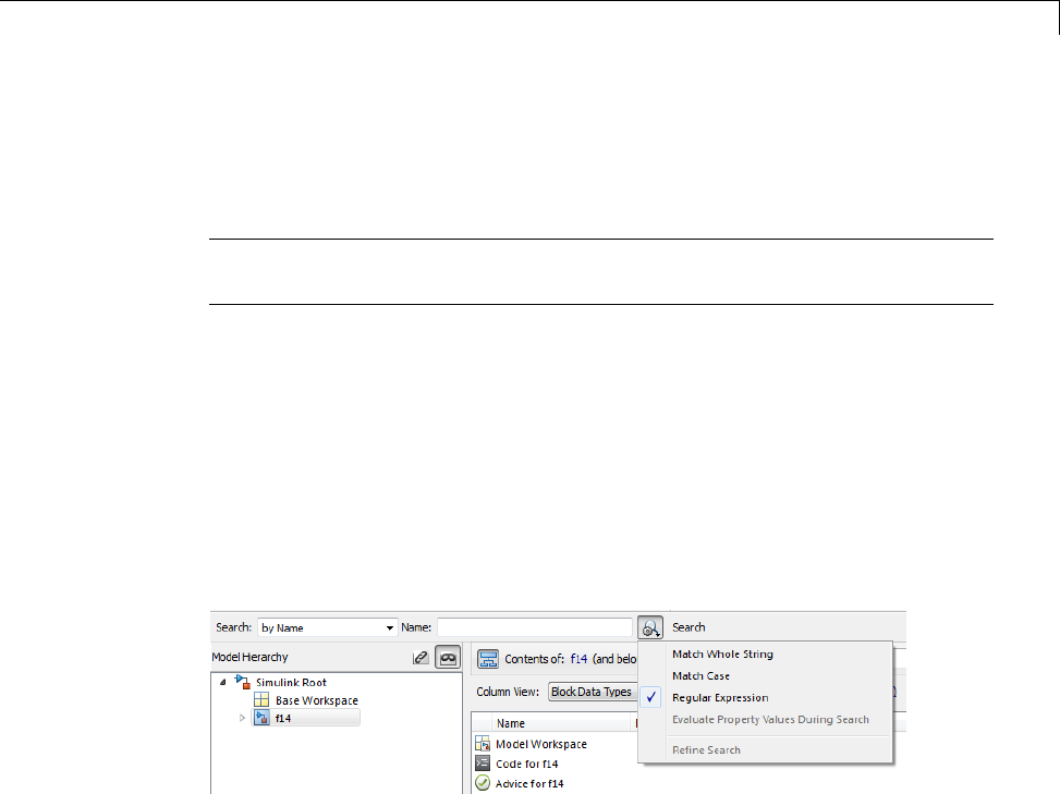
Organize Data Display in Model Explorer
By default, the Contents pane displays its contents in ascending order,
based on the name of the object. Objects that have no values in any property
columns appear at the end of the object property table.
Note When you group by property, the Model Explorer applies sorting of
column contents within each group.
Grouping by a Property
Organizing Contents by Property Values
When you explore a model, you might want to focus on all objects with the
same property value. One approach is to group data by a property column.
For example, suppose that you want to see all of the blocks in the f14 model.
You could perform the following search.
The search results obscure the whole path name for lower-level nodes:
9-37
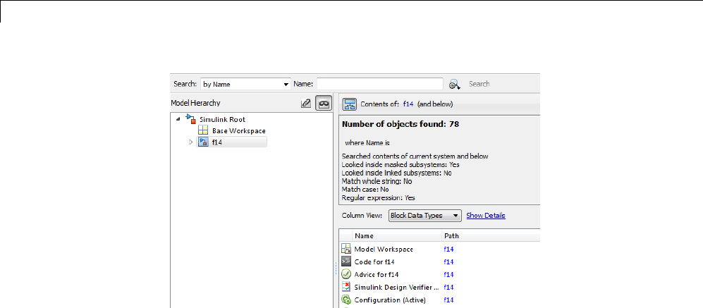
9Exploring, Searching, and Browsing Models
By groupingonthePath property column, you see the whole path for
lower-level nodes.
9-38
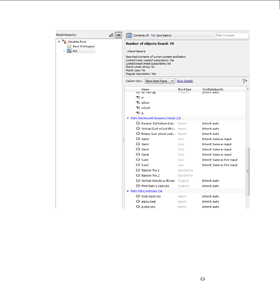
Organize Data Display in Model Explorer
You can also collapse groups to focus on specific portions of a model.
How to Group by a Property Column
To group by a property:
1In the object property table, right-click the column heading of the property
by which you want to group contents.
You can group by object icons, such as a block icon ( ), which represents a
type of object. Right-click the empty column heading in the first column.
2From the context menu, select the Group By This Column menu item.
9-39

9Exploring, Searching, and Browsing Models
Sorting with Grouped Data
When you group by property, the Model Explorer applies sorting of column
contents within each group.
Expanding and Collapsing Grouped Data
By default, Model Explorer displays groups in expanded form. That is, all the
objects in each group are visible. You can collapse and expand groups.
•To collapse the contents of a group, click the minus sign icon for that group.
•To expand a group, click the plus sign.
•To collapse or expand all the groups, right-click anywhere in the object
property table and select either the Collapse All Groups menu item
(Shift+C)orExpand All Groups menu item (Shift+E).
Hiding the Group Column
By default, the property column that you use for grouping appears in the
property table. That property also appears in the top row for each group.
To hide the group column in the property table, use one of the following
approaches:
•From the View menu, clear the Show Group Column check box.
•Right-click a column heading in the property table and clear the Show
Group Column check box.
Persistence of Grouped Data Settings
If you group by a property, that grouping is saved as part of the view
definition.
When you select a different node in the Model Hierarchy pane, the contents
for the new node are grouped by that same property. However, all groups are
expanded, even if you had collapsed all groups before switching nodes.
9-40

Organize Data Display in Model Explorer
Grouping Search Results
You can use grouping to organize the Search Results pane. The grouping
that you apply to the Search Results pane also applies to the object property
table, if that property is in the table. If the search results include a property
that is not in the object property table, and you group on that property, then
the Model Explorer removes the grouping setting that was in effect in the
object property table.
Changing the Order of Property Columns
Object Icon and Name Columns Are Always First
The first two columns of every object property table are the object icon column
(the column with a blank column heading) and the Name property column. You
cannot hide, remove, or change the location of the first two columns.
How to Change the Order of Property Columns
To change the order of property columns in the object property table, use one
of these approaches:
•In the object property table, select a column heading and drag it to a new
location in the table.
This approach avoids opening the column view details section and makes it
easier to move a column a short distance to the right or left.
•In the column view details section, select one or more property columns
and move them up or down in the list, using the arrow buttons to the
right of the list.
This approach allows you to move several property columns in one step, but
it moves the selected columns right or left by only one column at a time.
To move a property column by using the view details interface:
1In the Display column names in this order list on the right side of
the column view details section, select one or more property columns
that you want to move.
9-41
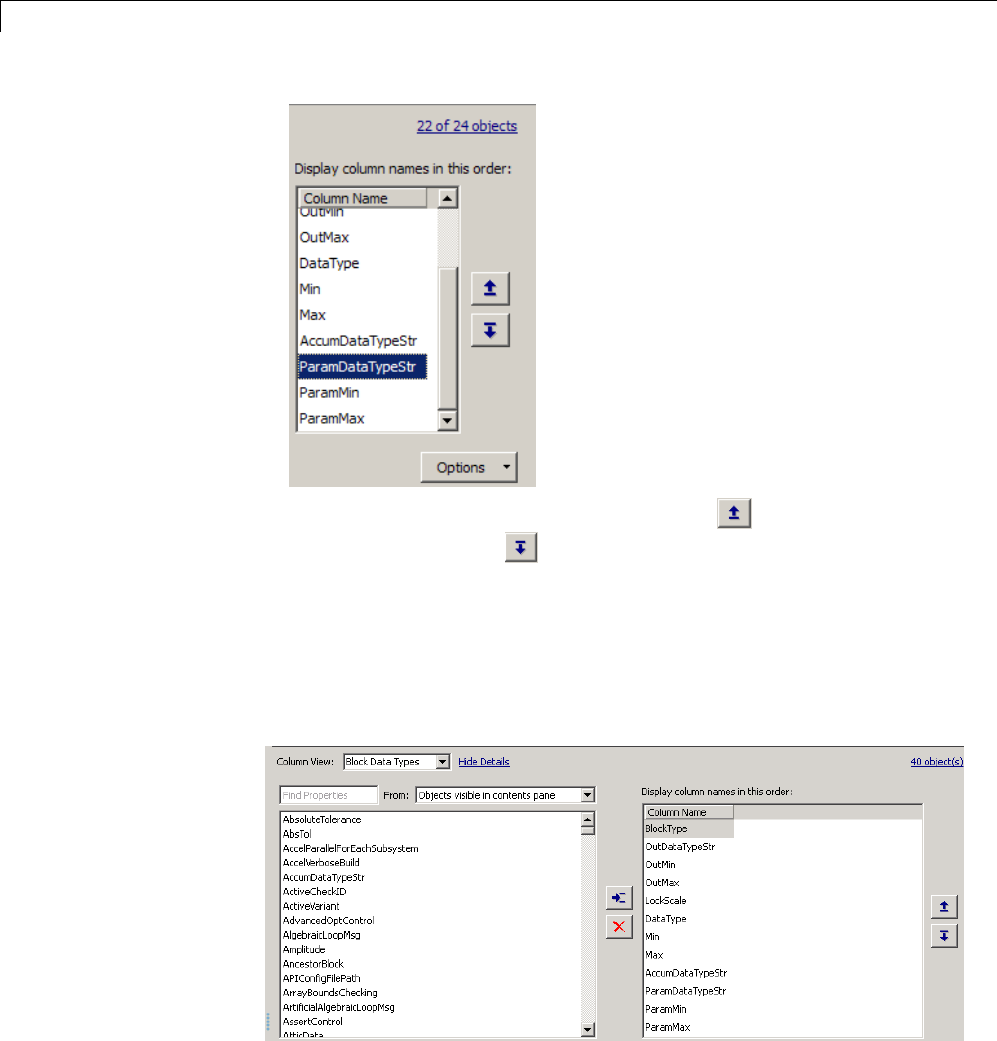
9Exploring, Searching, and Browsing Models
2Click the Move column left in view button ( )ortheMove column
right in view button ( ).
Adding Property Columns
To add property columns to a view:
1If you do not have the column view details section of the Contents pane
already open, then at the top of the Contents pane, select Show Details.
9-42

Organize Data Display in Model Explorer
2In the list of properties on left side of the column view details section, select
one or more properties that you want to add.
•The list displays property names in alphabetical order. You can use the
Find Properties search box in the column view details section to search
for properties that contain the text string that you enter. You can specify
the scope of the search with the From list to the right of the search box.
3In the list of column names on the right side, select the property column
thatyouwanttobetotheleftofthepropertycolumnsyouinsert.
4Click the Display property as column in view button ( )
Adding a Path Property Column
The Model Explorer provides a shortcut for adding a Path property column to
aview. Toa
dd a Path property column:
1Right-click the column heading in the object property table to the right of
which you want to insert a Path column.
2From the context menu, select Insert Path.
Hiding or Removing Property Columns
You can choose between two approaches to hide (remove) a property column
from the object property table. Hiding and removing a column both have the
same result. You can:
•Hide a column using the context menu for a column heading. This approach
avoids needing to open the column view details section.
•Remove a column using the column view details interface. This approach
allows you to delete several properties in one step.
Hiding a Column Using the Column Heading Context Menu
1Right-click the column heading of the column that you want to remove.
2From the context menu, select Hide.
9-43
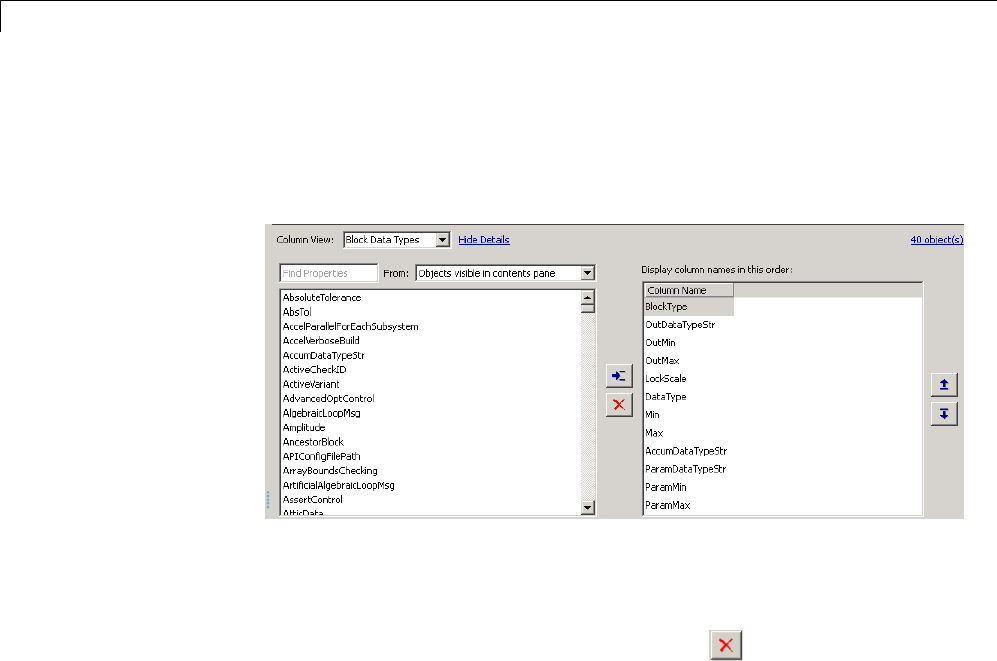
9Exploring, Searching, and Browsing Models
Removing a Column Using the Column View Details Interface
1If you do not have the column view details section of the Contents pane
already open, then at the top of the Contents pane, select Show Details.
2In the column view details section of the Contents pane, in the Display
columnnamesinthisorderlist, select one or more properties that you
want to remove.
3Click the Remove column from view button ( )ortheDelete key.
Inserting Recently Hidden or Removed Columns
The Model Explorer maintains a list of columns you hide or remove for each
view during a Simulink session.
To add a recently hidden or removed column back into a view:
1Right-click the column heading of the column to the right of which you
want to insert a recently hidden column.
2From the context menu, select Insert Recently Hidden Columns.
3Select the column that you want to insert.
See “Hiding or Removing Property Columns” on page 9-43.
9-44
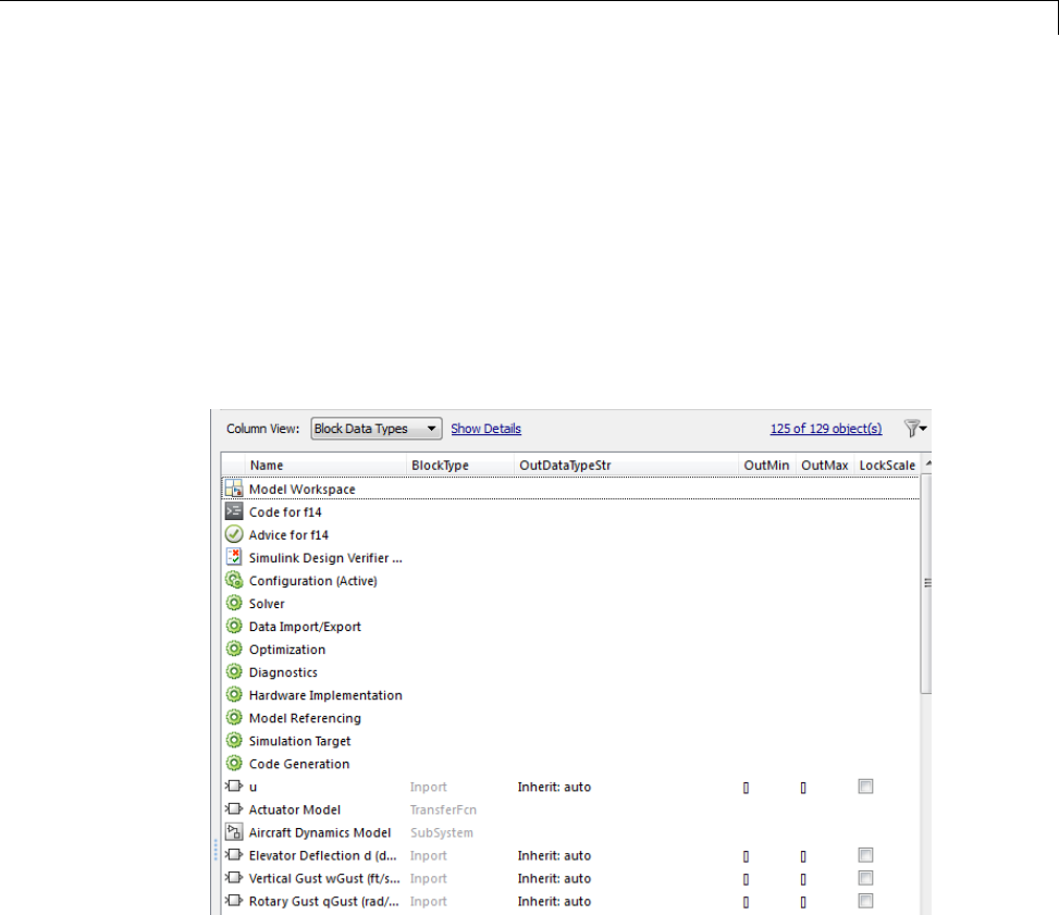
Organize Data Display in Model Explorer
Marking Nonexistent Properties
Usually, some of the properties that the Contents pane displays do not apply
to all the displayed objects (in other words, some objects do not have values
set). By default, the Model Explorer displays a dash (–) to mark properties
that do not have avalue.
If you want the Model Explorer to display a blank (instead of the default dash)
in property cellsthathavenovalues,cleartheView > Show Nonexistent
Properties as“–”option. The Contents pane looks similar to the following
graphic:
9-45
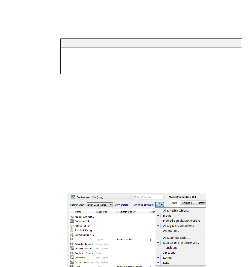
9Exploring, Searching, and Browsing Models
Filter Objects in the Model Explorer
In this section...
“Controlling the Set of Objects to Display” on page 9-46
“Using the Row Filter Option” on page 9-46
“Filtering Contents” on page 9-48
Controlling the Set of Objects to Display
Two techniques that you can use to control the set of objects that the
Contents pane displays are:
•Using the Row Filter option
•Filtering contents
For a summary of other techniques, see “Focusing on Specific Elements of a
Model or Chart” on page 9-7.
Using the Row Filter Option
You can filter the kinds of objects that the Contents pane displays:
1Open the Row Filter options menu. In the Model Explorer, at the top-right
corner of the Contents pane, click the Row Filter button.
9-46
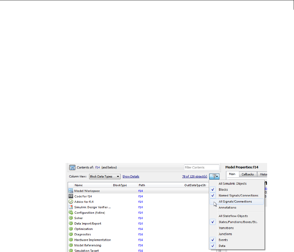
Filter Objects in the Model Explorer
An alternative way to open the Row Filter menu is to select View > Row
Filter.
By default, the Contents pane displays these kinds of objects for the
selected node:
•Blocks
•Signals and connections
•Stateflow states, functions, and boxes
•Stateflow events
•Stateflow data
2Clear the kinds of objects that you do not want to display in the Contents
pane, or enable any cleared options to display more kinds of objects. For
example, clear All Signals/Connections to prevent the display of signal
and connection objects in the Contents pane.
Object Count
The top-right portion of the Contents pane includes an object counter,
indicating how many objects the Contents pane is displaying.
9-47
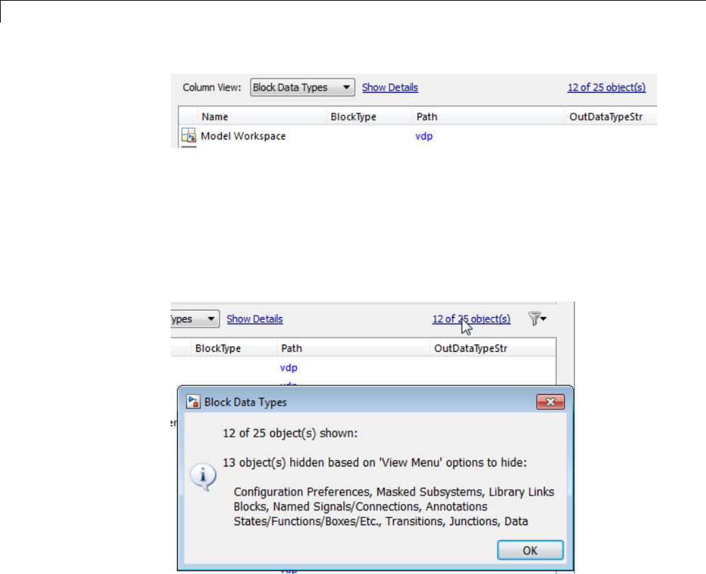
9Exploring, Searching, and Browsing Models
When you use the Row Filter option to filter objects, the object count
indicator reflects that the Contents pane displays a subset of all the model
and chart objects.
To view an explanation of the current object count, click the object count link
(for example, 12 of 25 objects). That link displays a pop-up information
box:
Filtering Contents
To refine the display of objects that are currently displayed in the Contents
pane, you can use the Filter Contents text box at the top of the Contents
pane to specify search strings for filtering a subset of objects.
9-48
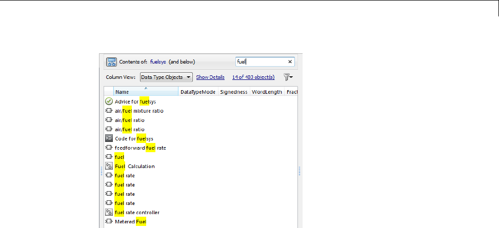
Filter Objects in the Model Explorer
Using the Filter Contents text box can help you to find specific objects
within the set of objects, based on a particular object name, property value, or
property that is of interest to you. For example, if you enter the text string
fuel in the Filter Contents edit box, the Model Explorer displays results
similar to those shown above. The results highlight the text string that you
specified.
Specifying Filter Text Strings
As you enter text in the Filter Contents text box, the Model Explorer
performs a dynamic search, displaying results that reflect the text as you
enter it.
The text strings you enter must be in the format consistent with the guidelines
described in the following sections.
Case Sensitivity. By default, the Model Explorer ignores case as it performs
the filtering.
To specify that you want the Model Explorer to respect case sensitivity for
atextstringthatyouenter,putthattextstringinquotationmarks. For
example, if you want to restrict the filtering to display only objects that
include the text Fuel (with a capital F), enter "Fuel" (with quotation marks).
9-49
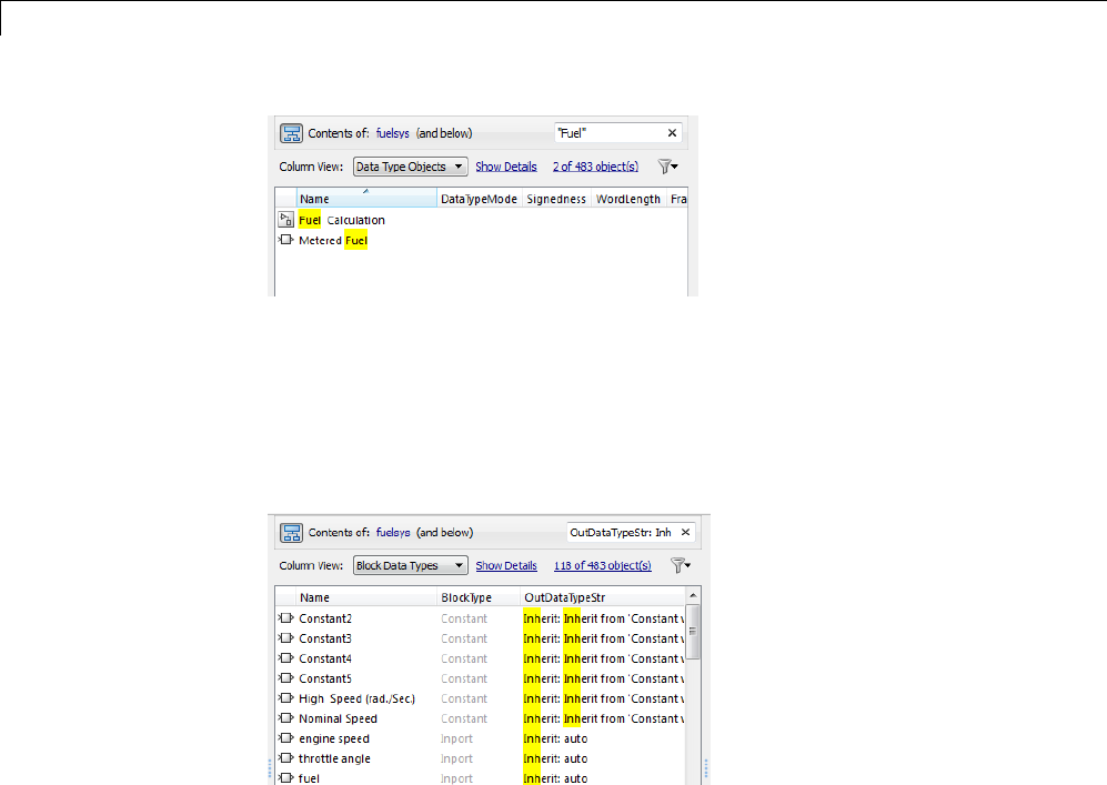
9Exploring, Searching, and Browsing Models
Specifying Property Values. To restrict the filtering to apply to values for
a specific property, specify the property name followed by a colon (:) and
then the value. For example, to filter the contents to display only objects
whose OutDataTypeStr property has a value that includes Inherit,enter
OutDataTypeStr: Inherit (alternatively, you could put the whole string in
quotation marks to enforce case sensitivity):
Wildcards and MATLAB Expressions Not Supported. The Model
Explorer does not recognize wildcard characters, such as an asterisk (*), as
having any special meaning. For example, if you enter fuel* in the Filter
Contents text box, you get no results, even if several objects contain the
text string fuel.
Also, if you specify a MATLAB expression, in the Filter Contents text box,
the Model Explorer interprets that string as literal text, not as a MATLAB
expression.
Clearing the Filtered Contents
To redisplay the object property table as it appeared before you filtered the
contents, click the Xin the Filter Contents text box.
9-50

Filter Objects in the Model Explorer
Filtering Removes Grouping
If you have set up grouping on a column, then when you filtering contents,
the Model Explorer does not retain that grouping.
9-51

9Exploring, Searching, and Browsing Models
Workspace Variables in Model Explorer
In this section...
“Finding Variables That Are Used by a Model or Block” on page 9-52
“Finding Blocks That Use a Specific Variable” on page 9-55
“Finding Unused Workspace Variables” on page 9-56
“Editing Workspace Variables” on page 9-58
“Exporting Workspace Variables” on page 9-60
“Importing Workspace Variables” on page 9-62
Finding Variables That Are Used by a Model or Block
In the Model Explorer, you can get a list of variables that a model or block
uses. The following approach is one way to get that list of variables:
1In the Contents pane, right-click the block for which you want to find
the variables that it uses.
2Select the Find Referenced Variables menu item.
9-52
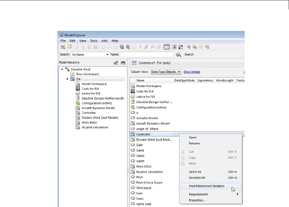
Workspace Variables in Model Explorer
Model Explorer returns results similar to these:
9-53
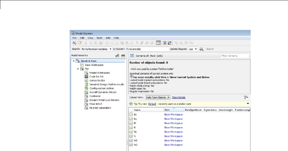
9Exploring, Searching, and Browsing Models
For performance, Model Explorer uses cached information from the last
compiled version of the model. If you want to recompile the model, either do
so manually or, in the Model Explorer, set the Update diagram field to
yes and repeat the search.
You can also use the following approaches to find variables that a model or
block uses:
•In the Model Explorer, in the Model Hierarchy pane, right-click a block
or modelnodeandselecttheFind Referenced Variables menu item.
•In the Model Explorer, in the search bar, use the for Referenced
Variables search type option.
•In the Model Editor, right-click a block, subsystem, or in the canvas and
select the Find Referenced Variables menu item. Clicking the canvas
returns results for the whole model.
The Simulink.findVars function provides additional options for returning
information about workspace variables that is not available from the Model
ExplorerorModelEditor.
9-54

Workspace Variables in Model Explorer
For information about limitations when finding referenced variables, see the
Simulink.findVars documentation.
Using the Set of Returned Variables
For a variable in the set of returned variables, you can find the blocks that use
that variable (for details, see “Finding Blocks That Use a Specific Variable” on
page 9-55). Also, you can export variables from the returned set of variables.
For details, see “Exporting Workspace Variables” on page 9-60.
Finding Blocks That Use a Specific Variable
You can use the Model Explorer to get a list of blocks that use a specific
workspace variable. One way to get that list of blocks is to right-click a
variable in the Contents pane and select the Find Where Used menu item.
For example:
1Open the f14 model.
2Open the Model Explorer.
3In the Model Hierarchy pane, select the Base Workspace node.
4In the Contents pane, right-click the Mq variable and select the Find
Where Used menu item.
5In the Hierarchy dialog box that appears, select f14.TheModelExplorer
displays output similar to this:
9-55

9Exploring, Searching, and Browsing Models
The property columns whose values include Mq represent the block
parameters that use the Mq variable. If those property columns are not
already in the view, then the Model Explorer adds them to the end of the
search results display.
You can also find blocks that use a specific variable, by using one of these
approaches:
•In the search bar, select the for Variable Usage search type option.
•In the Search Results pane, right-click a variable and select the Find
Where Used menu item.
If you do not find the variable that you are looking for because that variable is
not in the currently selected system, try selecting View > Show Current
System and Below and repeat the search.
Finding Unused Workspace Variables
YoucanusetheModelExplorertogetalist of variables that are defined in
a workspace but not used by a model or block. One way to get that list of
variables is to right-click a workspace name in the Model Hierarchy pane
and select the Find Unused Variables menu item. For example:
1Open the f14 model.
2Open the Model Explorer.
3In the search toolbar, set the Update diagram field to yes.
4In the Model Hierarchy pane, right-click the Base Workspace node and
select the Find Unused Variables menu item.
9-56
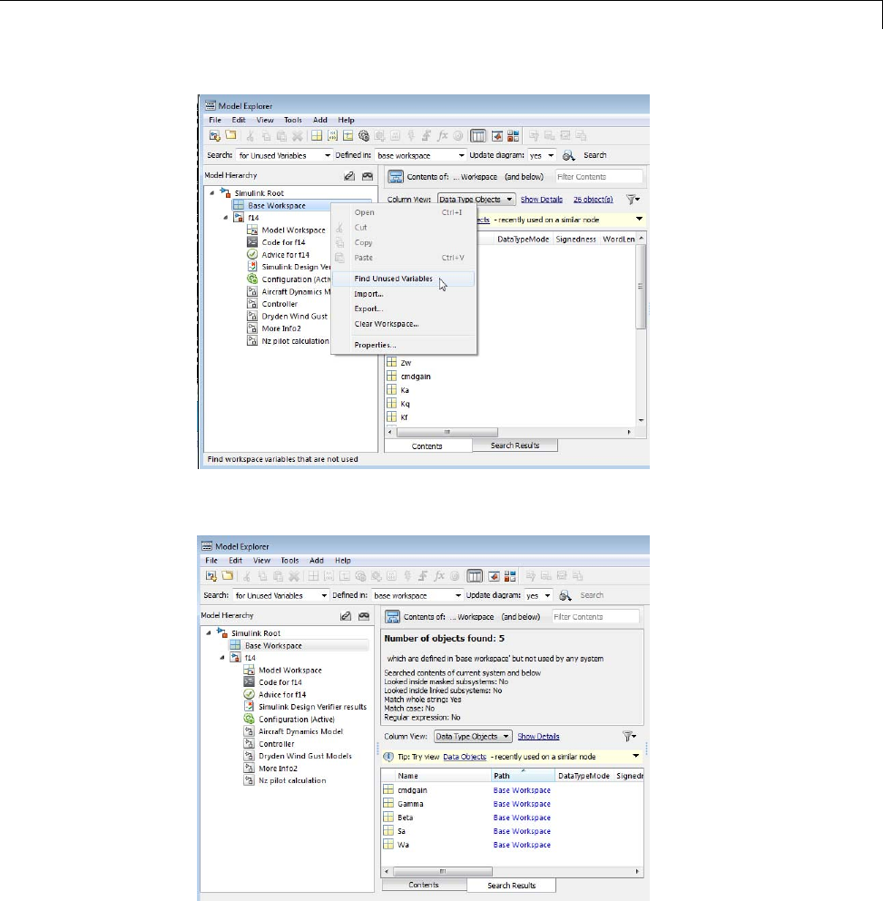
Workspace Variables in Model Explorer
5The Model Explorer displays output similar to this:
9-57
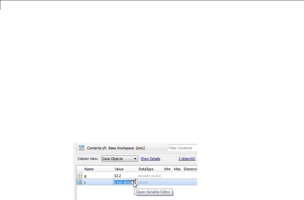
9Exploring, Searching, and Browsing Models
The Simulink.findVars function provides additional options for returning
information about unused workspace variables that is not available from
the Model Explorer or Model Editor.
Editing Workspace Variables
In the Model Explorer Contents pane, you can use the Variable Editor to edit
variables from the MATLAB workspace or model workspace. The Variable
Editor is available for editing large arrays and structures.
To open the Variable Editor for a variable that is an array or structure:
1ClicktheValuecellforthevariable.
2Select the Variable Editor icon.
The Variable Editor opens:
9-58

Workspace Variables in Model Explorer
Right-click in an edit box to open a context menu with several editing options:
You can resize and move the Variable Editor. The Contents pane reflects the
edits that you make in the Variable Editor.
Whenyoufinishediting,theVariable Editor closes when you click the Close
button in the upper right corner of the editor or when you click outside of
the editor.
9-59

9Exploring, Searching, and Browsing Models
Exporting Workspace Variables
You can export (save) a set of variables listed in the Model Explorer, exporting
either individual variables or all the variables in the base or model workspace.
One possible workflow is to export the set of variables returned with the
Find Referenced Variables option or the Simulink.findVars function.
For details, see “Finding Variables That Are Used by a Model or Block” on
page 9-52.
Note All the variables that you export must be from the same workspace.
To export all the variables in a workspace in the Model Explorer to a MATLAB
code file orMAT-file:
1Select the variables that you want to export.
aTo select all the variables in a workspace, right-click the workspace
node (for example, Base Workspace)andselecttheExport menu item.
For example:
9-60
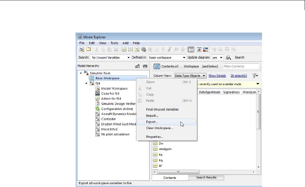
Workspace Variables in Model Explorer
bTo select individual variables, in the Contents pane, select the variables
that you want to export. Right-click one of the highlighted variables and
select the Export Selected menu item.
If the Contents pane has data grouped by a property, selecting the top line
in a group does not select all the variables in that group. For details about
grouped data, see“Grouping by a Property” on page 9-37.
2Specify whether to save the variables in a MATLAB code file or a MAT-file.
TheMATLABcodefileformatiseasiertoread,iseditable,andsupports
version control. The MAT-file format is binary, which has performance
advantages.
IfyouspecifyaMATLABcodefileformat,theModelExplorermaycreate
an associated MAT-file, reflecting the name of the MATLAB code file, but
with an extension of .mat instead of .m.
3Specify a name and location for the file.
9-61

9Exploring, Searching, and Browsing Models
4If the file already exists, Model Explorer displays a dialog box asking you to
choose one of these options:
•Overwrite entire file
–Replaces all variables in the target file with the selected variables,
which are stored in alphabetical order.
•Update variables that exist in file and append new variables
to file
–Updates existing variables in place and appends new variables.
•Only update variables that exist in file
–Updates existing variables, but does not add any new variables, which
eliminates potentially extraneous variables.
Importing Workspace Variables
You can import (load) a set of variables from a file into the base workspace or
into a model workspace using the Model Explorer. When you import variables
into a workspace, the Model Explorer overwrites existing variables and adds
any new variables.
To import variables into a workspace:
1In the Model Hierarchy pane, right-click the workspace into which you
want to import variables.
2Select the Import menu item.
3IntheImportfromFiledialogbox,selectaMATLABcodefileorMAT-file
for the variables that you want to import.
Note If you import a MATLAB code file, then Simulink also imports the
associated MAT-file.
9-62

Search Using Model Explorer
Search Using Model Explorer
In this section...
“Searching in the Model Explorer” on page 9-63
“The Search Bar” on page 9-64
“Showing and Hiding the Search Bar” on page 9-64
“Search Bar Controls” on page 9-64
“Search Options” on page 9-66
“Search Button” on page 9-68
“Refining a Search” on page 9-69
Searching in the Model Explorer
Use the Model Explorer search bar to search for specific objects from the node
you select in the Model Hierarchy pane.
The Model Explorer displays search results in the Search Results tab of
the Contents pane.
The search results appear in a table that is similar to the object property table
in the Contents tab. The search results table uses the current column view
(the object property table) definition as a starting point, and adds relevant
properties that are not already included in the current view. Any additional
property columns added to the Search Results pane do not affect the view
definition.
If you modify the property columns in the search results table that also
appear in the property table view, the changes you make affect both tables.
For example, if you hide OutMax column in the search results table, and the
OutMax column was also in the object property view table, then the OutMax
columnishiddeninbothtables. However, if in the search results table you
reorder where the Complexity column appears, if the view does not include
the Complexity property, then that change to the search results table does
not affect the view.
You can edit property values in the search results table.
9-63
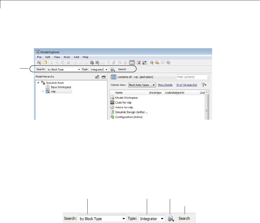
9Exploring, Searching, and Browsing Models
The Search Bar
The search bar appears at the top of the Model Explorer window.
Search
bar
Showing and Hiding the Search Bar
By default, the search bar is visible. To show or hide the search bar, select or
clear the View > Toolbars > Search Bar option.
Search Bar Controls
The search bar includes the following controls:
Select
search
type
Specify
search
criteria Start
search
Select
search
options
Search Type
Use the Search Type control to specify the type of objects or properties to
include in the search.
9-64

Search Using Model Explorer
Search Type Option Description
by Name Searches a model or chart for all
objects that have the specified string
inthenameoftheobject. See
“Search Strings” on page 9-68.
by Property Name Searches for objects that have a
specified property. Specify the
target property name from a list of
properties that objects in the search
domain can have.
by Property Value Searches for objects with a property
valuethatmatchesthevalueyou
specify. Specify the name of the
property,thevaluetobematched,
and the type of match (for example,
equals, less than, or greater than).
See “Search Strings” on page 9-68.
by Block Type Searches for blocks of a specified
block type. Select the target block
type from the list of types contained
in the currently selected model.
by Stateflow Type Searches for Stateflow objects of a
specified type.
for Variable Usage Searches for blocks that use
variables defined in a workspace.
Select the base workspace or a
model workspace (model name) and,
optionally, the name of a variable.
See “Search Strings” on page 9-68.
for Referenced Variables Searches for variables that a model
or block uses. Specify the name of
the model or block in the by System
field. The model or block must be in
the Model Hierarchy pane.
9-65

9Exploring, Searching, and Browsing Models
Search Type Option Description
for Unused Variables Searches for variables that are
defined in a workspace but not used
by any model or block. Select the
name of the workspace from the
drop-down list for the in Workspace
field.
for Library Links Searches for library links in the
current model.
by Class Searches for Simulink objects of a
specified class.
for Fixed Point Capable Searches a model for all blocks that
support fixed-point computations.
for Model References Searches a model for references to
other models.
by Dialog Prompt Searches a model for all objects
whose dialogs contain the prompt
you specify. See “Search Strings” on
page 9-68.
by String Searches a model for all objects in
which the string you specify occurs.
See “Search Strings” on page 9-68.
Search Options
Use the Search Options control to specify the scope and how to apply search
strings.
Search Option Description
Match Whole String Do not allow partial string matches
(for example, do not allow sub to
match substring).
Match Case Considers case when matching
strings (for example, Gain does not
match gain).
9-66

Search Using Model Explorer
Search Option Description
Regular Expression Considers a string to be matched as
a regular expression.
Evaluate Property Values
During Search
Applies only for searches by property
value. If enabled, the option causes
the Model Explorer to evaluate the
value of each property as a MATLAB
expression and compare the result
to the search value. If this option
is disabled (the default), the Model
Explorer compares the unevaluated
property value to the search value.
Refine Search Initiates a secondary search that
provides additional search criteria to
refine the initial search results. The
second search operation searches for
objects that meet both the original
and the new search criteria (see
“Refining a Search” on page 9-69).
By default, the Model Explorer searches for objects in the system that you
select in the Model Hierarchy pane. It does not search in child systems. You
can override that default, so that the Model Explorer searches for objects
in the whole hierarchy of the currently selected system. To toggle between
searching only in the current system and searching in the whole system
hierarchy of the current system, use one of these techniques:
•Select View > Show Current System and Below.
•Click the Show Current System and Below button at the top of the
Contents pane.
9-67
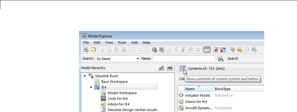
9Exploring, Searching, and Browsing Models
Search Strings
By default, search strings are case-insensitive and are treated as regular
expressions.
By default, the search allows partial string matches. You cannot use wildcard
characters in search strings. For example, if you enter *1 as a name search
string, you get no search results unless there is an item whose name starts
with the two characters *1.Ifthereisanout1 item, the search results do
not include that item.
Search Button
Click the Search button to start the search specified by the current settings
of the search bar on the object selected in the Model Hierarchy pane. The
Model Explorer displays the results of the search in the Search Results pane.
The top of the Search Results pane displays a summary of the results,
including the scope of the search and the search criteria that you specified.
9-68
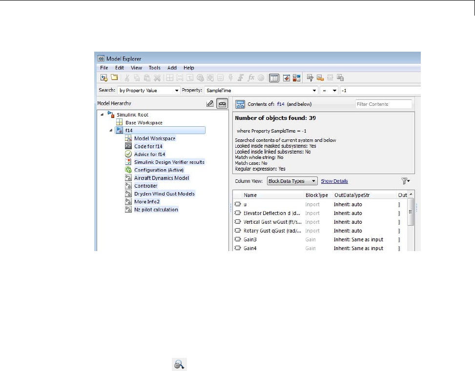
Search Using Model Explorer
You can edit the results displayed in the Search Results pane. For example,
to change all objects found by a search to have the same property value,
select the objects in the Search Results pane and change the property value
of one of the objects.
RefiningaSearch
To refine the previous search, in the search bar, click the Select Search
Options button ( )andselectRefine Search.ARefine button replaces
the Search button on the search bar. Use the search bar to define new search
criteria and then click the Refine button. The Model Explorer searches for
objects that match both the previous search criteria and the new criteria.
9-69

9Exploring, Searching, and Browsing Models
Model Explorer: Property Dialog Pane
In this section...
“WhatYouCanDowiththeDialogPane”onpage9-70
“Showing and Hiding the Dialog Pane” on page 9-70
“Editing Properties in the Dialog Pane” on page 9-70
What You Can Do with the Dialog Pane
You can use the Dialog pane to view and change properties of objects that
you select in the Model Hierarchy pane or in the Contents pane.
Showing and Hiding the Dialog Pane
By default, the Dialog pane appears in the Model Explorer, to the right of
the Contents pane. To show or hide the Dialog pane, use one of these
approaches:
•From the View menu, select Show Dialog Pane.
•From the main toolbar, click the Dialog View button ( ).
Editing Properties in the Dialog Pane
To edit property values using the Dialog pane:
1In the Contents pane, select an object (such as a block or signal). The
Dialog pane displays the properties of the object you selected.
9-70
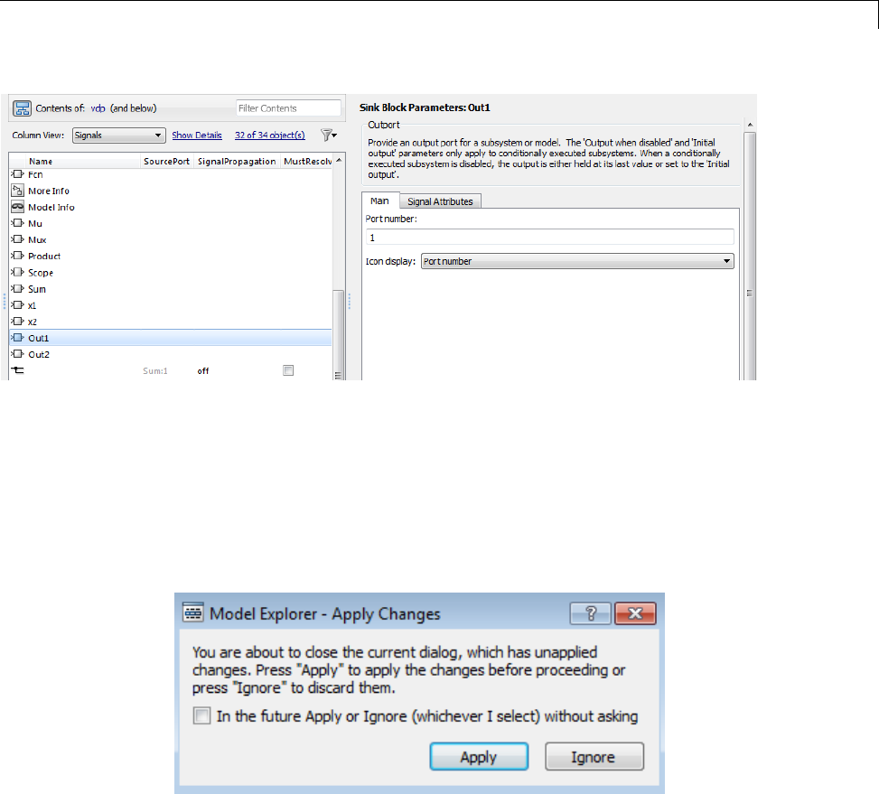
Model Explorer: Property Dialog Pane
2Change a property (for example, the port number of an Outport block)
in the Dialog pane.
3Click Apply to accept the change, or click Revert to return to the original
value.
By default, clicking outside a dialog box with unapplied changes causes the
Apply Changes dialog box to appear:
ClickApply to accept the changes or Ignore to revert to the original settings.
To prevent display of the Apply Changes dialog box:
1In the dialog box, click the InthefutureApplyorIgnore(whicheverI
select) without asking check box.
9-71

9Exploring, Searching, and Browsing Models
2If you want Simulink to apply changes without warning you, press Apply.
If you want Simulink to ignore changes without warning you, press Ignore.
To restore display of the Apply Changes dialog box, from the Tools menu,
select Prompt if dialog has unapplied changes.
9-72
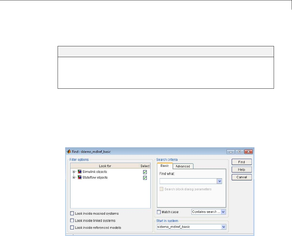
Finder
Finder
In this section...
“Find Model Objects” on page 9-73
“Filter Options” on page 9-75
“Search Criteria” on page 9-76
Find Model Objects
Use the Finder to locate blocks, signals, states, or other objects in a model.
1Open the Finder. In the Simulink Editor, either select Edit > Find,or
press Ctrl+F.
2In the Filter options area, specify the kinds of objects to look for, and
wheretosearchforthem. See“FilterOptions”onpage9-75.
3In the Search criteria area, specify the criteria that objects must meet to
satisfy your search request. See “Search Criteria” on page 9-76.
4If you have more than one system or subsystem open, click the Start in
system list. From this list, select the system or subsystem where you want
the search to begin.
5Click Find.
9-73
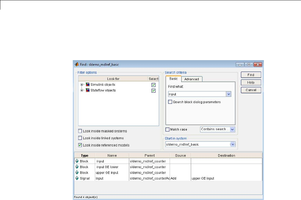
9Exploring, Searching, and Browsing Models
The Finder searches the selected system for objects that meet the criteria that
you have specified. Any objects that satisfy the criteria appear in the results
panel at the bottom of the dialog box.
Display a Found Object
To display a found object, double-click its entry in the search results list.
Simulink opens the system or subsystem that contains the object (if necessary)
and highlights and selects the object.
To sort the results list based on the values in a column, click the button at the
top of that column. For example, to sort the results by object type, click the
Type button. To sort the list in ascending order, click the button once. To sort
the list in descending order, click the button twice.
To display the parameters or properties of an object, right-click the object in
the list. From the context menu, select Parameter or Properties.
If you close a model that has objects in the Finder search results list, then
double-clicking a found object from that model does not open the model. To
9-74
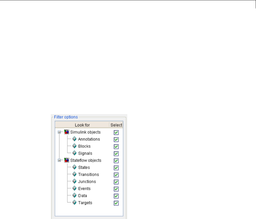
Finder
open an object that was in the Finder search results list, simply rerun the
search by clicking the Find button.
Filter Options
To specify the kinds of objects to look for, and where to search for them, use
the Filter options panel.
Object Type List
Theobjecttypelistliststhetypesofobjects that the Finder can find. To
exclude a type of object from the Finder search, clear the check box for the
object.
Specifying Kinds of Systems To Search
You can configure the Finder to search inside masked systems, linked library
systems, and referenced models. The search starts with the system that you
specify in the Start in system field.
9-75

9Exploring, Searching, and Browsing Models
Object Type Option Where the Finder Searches
Look inside masked systems Inside masked subsystems
Look inside linked systems Inside subsystems linked to libraries
Look inside referenced models Inside referenced models, down
through a model reference hierarchy
Note The Finder loads unopened
referenced models. You can stop the
search by using the pop-up cancel
dialog box.
If you select more than one option, then the Finder searches in systems that
fit any of the specified options. For example, if you select the Look inside
linked systems and Look inside referenced models options, then the
Finder:
•Searches in linked library systems and referenced models that are not
in a masked system
•Does not search inside:
-Masked systems, including those that are in linked library systems or
referenced models
-Linked library systems or model referenced models, if the system or
model is in a masked system
Search Criteria
To specify the criteria that objects must meet to satisfy your search request,
use the Search criteria panel.
Basic
To search for an object whose name matches a specified text string, use the
Basic panel. Enter search text in the Find what edit box. To reuse previous
search text, select the appropriate search text from the dropdown list.
9-76
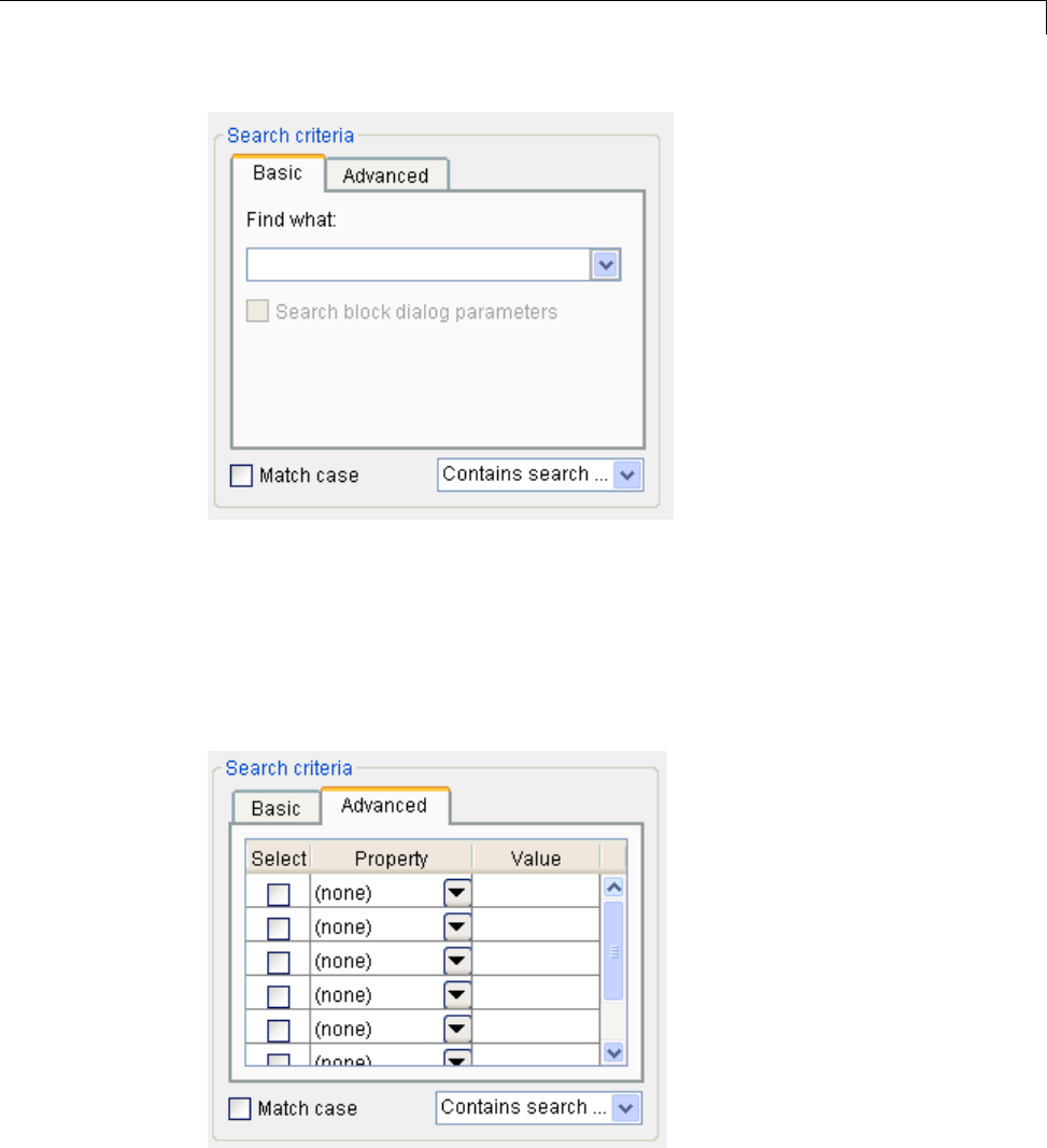
Finder
To include dialog parameters in the search, select Search block dialog
parameters.
Advanced
To specify a set of as many as seven properties that an object must have to
satisfy your search request, use the Advanced panel.
9-77

9Exploring, Searching, and Browsing Models
To specify a property, enter its name in one of the cells in the Property
column or select the property from the property list of a cell. To display the
property list, select the down arrow button next to the cell. Next enter the
value of the property in the Value column. When you enter a property name,
the Finder checks the check box next to the property name in the Select
column. This indicates that the property is to be included in the search. To
exclude the property, clear the check box.
Match case
Select this option if you want the Finder to consider case when matching
search text against the value of an object property.
Other match options
Next to the Match case option is a dropdown list that specifies other match
options.
•Matches search string
Specifies a match if the property value and the search text are identical
except possibly for case.
•Contains search string
Specifies a match if a property value includes the search text.
•Regular expression
Specifies that the search text should be treated as a regular expression
when matched against property values. The following characters have
special meanings when they appear in a regular expression.
Character Meaning
^Matches start of string.
$Matches end of string.
.Matches any character.
\Escape character. Causes the next character to have its
ordinary meaning. For example, the regular expression
\.. matches .a and .2 and any other two-character
string that begins with a period.
9-78

Finder
Character Meaning
*Matches zero or more instances of the preceding
character. For example, ba* matches b,ba,baa,andso
on.
+Matches one or more instances of the preceding
character. For example, ba+ matches ba,baa,etc.
[] Indicates a set of characters that can match the current
character. A hyphen can be used to indicate a range
of characters. For example, [a-zA-Z0-9_]+ matches
foo_bar1 but not foo$bar.A^indicates a match
when the current character is not one of the following
characters. For example, [^0-9] matches any character
that is not a digit.
\w Matches a word character (same as [a-z_A-Z0-9]).
\W Matches a nonword character (same as [^a-z_A-Z0-9]).
\d Matches a digit (same as [0-9]).
\D Matches a nondigit (same as [^0-9]).
\s Matches white space (same as [ \t\r\n\f]).
\S Matchesnonwhitespace(sameas[^ \t\r\n\f]).
\<WORD\> Matches WORD where WORD is any string of word
characters surrounded by white space.
9-79

9Exploring, Searching, and Browsing Models
Model Browser
In this section...
“About the Model Browser” on page 9-80
“Navigating with the Mouse” on page 9-82
“Navigating with the Keyboard” on page 9-82
“Showing Library Links” on page 9-82
“Showing Masked Subsystems” on page 9-82
About the Model Browser
The Model Browser enables you to
•Navigate a model hierarchically
•Open systems in a model
•Determine the blocks contained in a model
Note The browser is available only on Microsoft Windows platforms.
To display the Model Browser, in the Simulink Editor, select View > Model
Browser > Show Model Browser.
9-80
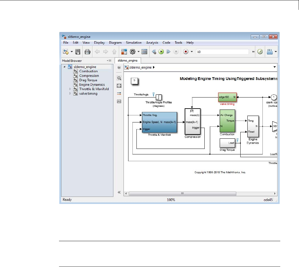
Model Browser
The model window splits into two panes. The left pane displays the browser, a
tree-structured view of the block diagram displayed in the right pane.
Note The Browser initially visible preference causes Simulink to open
models by default in the Model Browser. To set this preference, in the
Simulink Editor, select File > Simulink Preferences.
The top entry in the tree view corresponds to your model. A button next to the
model name allows you to expand or contract the tree view. The expanded
view shows the model’s subsystems. A button next to a subsystem indicates
that the subsystem itself contains subsystems. You can use the button to
list the subsystem’s children. To view the block diagram of the model or
any subsystem displayed in the tree view, select the subsystem. You can
9-81

9Exploring, Searching, and Browsing Models
use either the mouse or the keyboard to navigate quickly to any subsystem
inthetreeview.
Navigating with the Mouse
Click any subsystem visible in the tree view to select it. Click the + button
next to any subsystem to list the subsystems that it contains. Click the button
again to contract the entry.
Navigating with the Keyboard
Use the up/down arrows to move the current selection up or down the tree
view. Use the left/right arrow or +/- keys on your numeric keypad to expand
an entry that contains subsystems.
Showing Library Links
The Model Browser can include or omit library links from the tree view of a
model. Use the Preferences dialog box to specify whether to display library
links by default. To toggle display of library links, select Show Library
Links from the Model Browser Options submenu of the View menu.
Showing Masked Subsystems
The Model Browser can include or omit masked subsystems from the tree
view. If the tree view includes masked subsystems, selecting a masked
subsystem in the tree view displays its block diagram in the diagram
view. Use the Preferences dialog box to specify whether to display masked
subsystems by default. To toggle display of masked subsystems, select Show
Masked Subsystems from the Model Browser Options submenu of the
View menu.
9-82

Model Dependency Viewer
Model Dependency Viewer
In this section...
“About Model Dependency Views” on page 9-83
“Opening the Model Dependency Viewer” on page 9-88
“Manipulating a Dependency View” on page 9-89
“Browsing Dependencies” on page 9-95
“Saving a Dependency View” on page 9-95
“Printing a Dependency View” on page 9-95
About Model Dependency Views
The Model Dependency Viewer displays a dependency view of a model. The
dependency view is a graph of all the models and libraries referenced directly
or indirectly by the model. You can use the dependency view to quickly
find and open referencedlibrariesandmodels. Toidentifyandpackageall
required files, see instead “Analyze Model Dependencies” on page 13-104.
The Model Dependency Viewer allows you to choose between the following
types of dependency views of a model reference hierarchy.
•“File Dependency View” on page 9-83
•“Referenced Model Instances View” on page 9-85
•“Processor-in-the-Loop Mode Indicator” on page 9-87
•“Warning Icon” on page 9-88
File Dependency View
Afile dependency view shows the model and library files referenced by a
top model. A referenced model or library file appears only once in the view
even if it is referenced more than once in the model hierarchy displayed in
the view. A file dependency view consists of a set of blocks connected by
arrows. Blue blocks represent model files; brown boxes, libraries. Arrows
represent dependencies. For example, the arrows in the following view
9-83
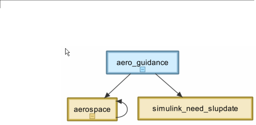
9Exploring, Searching, and Browsing Models
indicate that the aero_guidance model references two libraries: aerospace
and simulink_need_slupdate.
An arrow that points to the library from which it emerges indicates that the
library references itself, i.e., blocks in the library reference other blocks
in that same library. For example, the preceding view indicates that the
aerospace library references itself.
A file dependency view optionally includes a legend that identifies the model
in the view and the date and time the view was created.
9-84
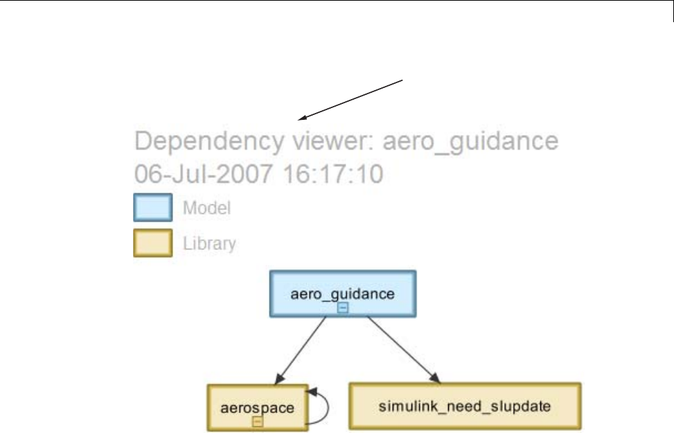
Model Dependency Viewer
Legend
Referenced Model Instances View
Areferenced model instances view shows every reference to a model in a
model reference hierarchy (see “Model Reference”) rooted at the top model
targeted by the view. If a model hierarchy references the same model more
than once, the referenced model appears multiple times in the instance view,
once for each reference. For example, the following view indicates that the
model reference hierarchy rooted at sldemo_mdlref_depgraph contains two
references to the model sldemo_mdlref_F2C.
9-85
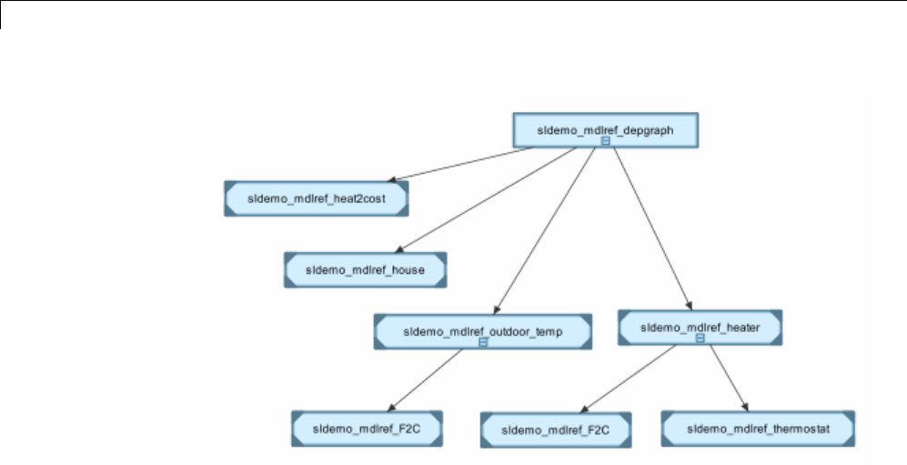
9Exploring, Searching, and Browsing Models
In an instance view, boxes represent a top model and model references.
Boxes representing accelerated-mode instances (see “Referenced Model
Simulation Modes” on page 6-21) have filled triangles in their corners; boxes
representing normal-mode instances, have unfilled triangles in their corners.
For example, the following diagram indicates that one of the references to
sldemo_mdlref_F2C operates in normal mode; the other, in accelerated mode.
9-86
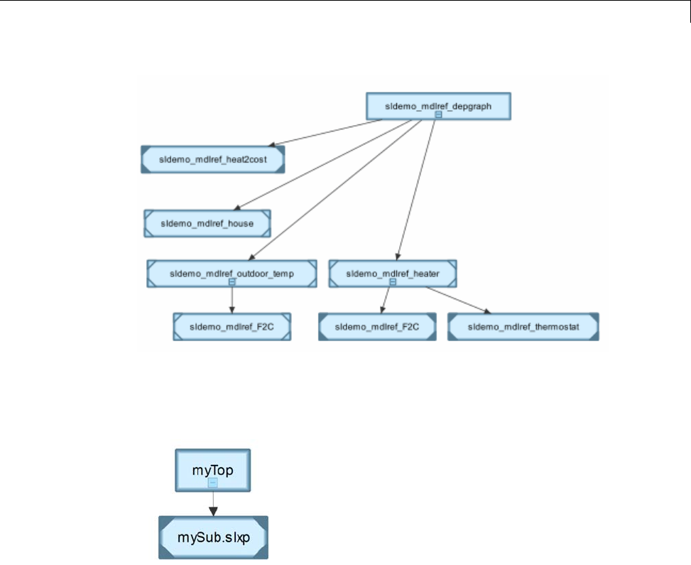
Model Dependency Viewer
Boxes representing protected referenced models models have a lock icon, and
the model name has the .slxp extension. Protected referenced model boxes
have no expand(+)/collapse(–) button.
Processor-in-the-Loop Mode Indicator
An instance view appends PIL to the names of models that run in
Processor-in-the-Loop mode (see “Specify the Simulation Mode” on page 6-23).
For example, the following dependency instance view indicates that the model
named rtwdemo_pil_component runs in processor-in-the-loop mode.
9-87
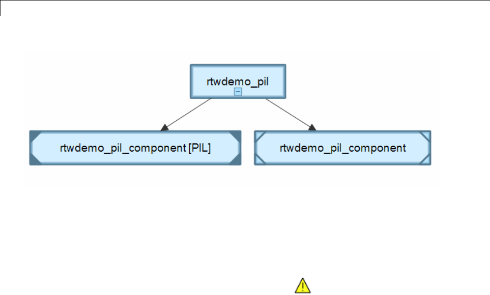
9Exploring, Searching, and Browsing Models
Warning Icon
An instance view displays warning icons on instance boxes to indicate that a
reference is configured to run in Normal mode actually runs in Accelerated
mode because it is directly or indirectly referenced by another model reference
that runs in Accelerated mode.
The warning icon is a yellow triangle .
Opening the Model Dependency Viewer
The Model Dependency Viewer displays a graph of all the models and libraries
referenced directly or indirectly by the model. You can use the dependency
viewer to quickly find and open referenced libraries and models.
To display a dependency view for a model:
1Open the model.
2Select Analysis > Model Dependencies > Model Dependency
Viewer, then select the type of view you want to see:
•Models & Libraries
•Models Only
•Referenced Model Instances
9-88
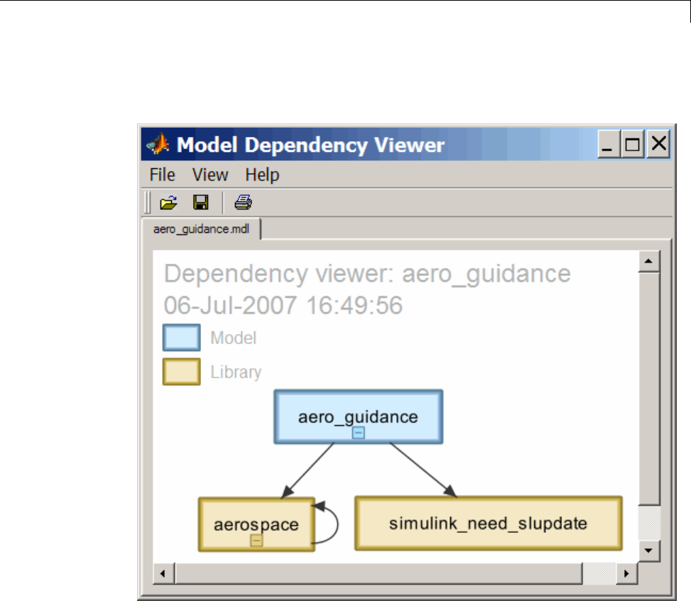
Model Dependency Viewer
The Model Dependency Viewer appears, displaying a dependency view
of the model.
Manipulating a Dependency View
The Model Dependency Viewer allows you to manipulate dependency views in
various ways. See the following topics for more information:
•“Changing Dependency View Type” on page 9-90
•“Excluding Block Libraries from a File Dependency View” on page 9-90
9-89

9Exploring, Searching, and Browsing Models
•“Including Simulink Blocksets in a File Dependency View” on page 9-90
•“Changing View Orientation” on page 9-91
•“Expanding or Collapsing Views” on page 9-91
•“Zooming a Dependency View” on page 9-92
•“Moving a Dependency View” on page 9-92
•“Rearranging a Dependency View” on page 9-93
•“Displaying and Hiding a Dependency View’s Legend” on page 9-93
•“Displaying Full Paths of Referenced Model Instances” on page 9-93
•“Refreshing a Dependency View” on page 9-94
Changing Dependency View Type
You can change the type of dependency view displayed in the viewer.
To change the type of dependency view, in the Model Dependency Viewer:
•Select View > Dependency Type > Model File Dependencies (see
“File Dependency View” on page 9-83 )
or
•Select View > Dependency Type > Referenced Model Instances (see
“Referenced Model Instances View” on page 9-85 ).
Excluding Block Libraries from a File Dependency View
By default a file dependency view includes libraries on which a model depends.
To exclude block libraries:
•Deselect View > Include Libraries.
Including Simulink Blocksets in a File Dependency View
By default, a file dependency view omits MathWorks block libraries when
View > Include Libraries is selected.
To include libraries supplied by MathWorks:
9-90
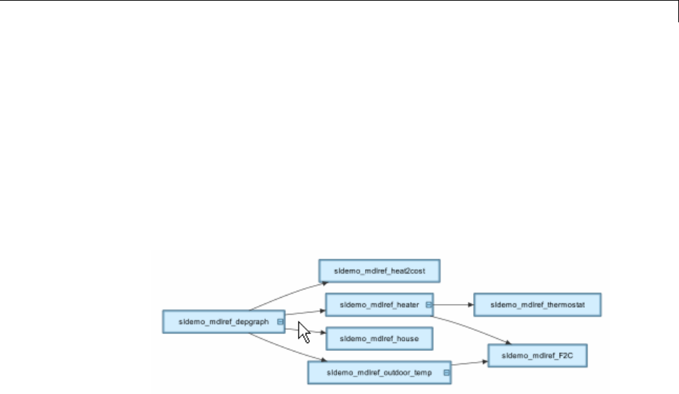
Model Dependency Viewer
•Select View > Show MathWorks Dependencies.
Changing View Orientation
By default the orientation of the dependency graph displayed in the viewer is
vertical.
To change the orientation to horizontal:
•Select View > Orientation > Horizontal.
Expanding or Collapsing Views
You can expand or collapse each model or library in the dependency view to
display or hide the dependencies for that model or library.
To expand or collapse views:
•Click the expand(+)/collapse(-) button on the box representing the model or
library to expand or collapse that view.
9-91
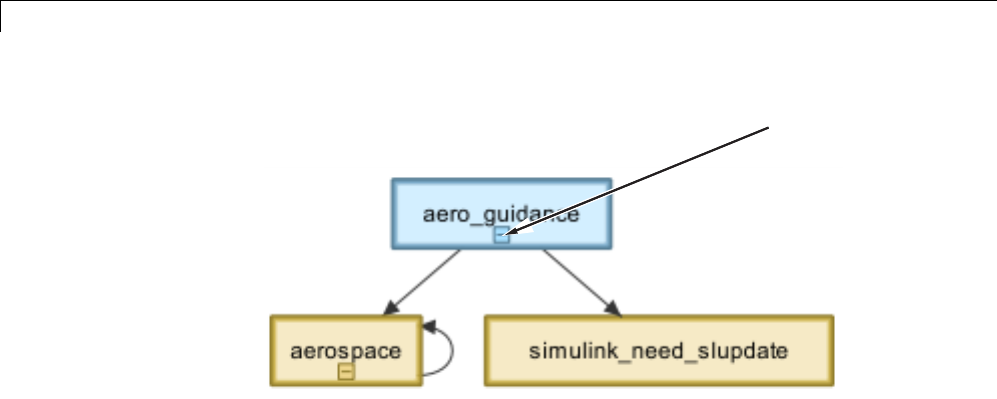
9Exploring, Searching, and Browsing Models
Expand/Collapse
Button
Zooming a Dependency View
You can enlarge or reduce the size of the dependency graph displayed in the
viewer.
To zoom a dependency view in or out, do either of the following:
•Press and hold down the spacebar key and then press the +or -key on
the keyboard.
•Move the scroll wheel on your mouse forward or backward.
To fit the view to the viewer window:
•Press and release the spacebar key.
Moving a Dependency View
You can move a dependency view to another location in the viewer window.
To move the dependency view:
1Movethecursorovertheview.
2Press your keyboard’s space bar and your mouse’s left button
simultaneously.
3Move the cursor to drag the view to another location.
9-92

Model Dependency Viewer
Rearranging a Dependency View
You can rearrange a dependency view by moving the blocks representing
models and libraries. This can make a complex view easier to read.
To move a block to another location:
1Select the block you want to move by clicking it.
2Drag and drop the block in the new location.
Displaying and Hiding a Dependency View’s Legend
The dependency view can display a legend that identifies the model in the
viewandthedateandtimetheviewwascreated.
To display or hide a dependency view’s legend:
•Select View > Show Legend from the viewer’s menu bar.
Displaying Full Paths of Referenced Model Instances
In an instance view (see “Referenced Model Instances View” on page 9-85) ,
you can display the full path of a model reference in a tooltip or in the box
representing the reference.
To display the full path in a tooltip:
•Move the cursor over the box representing the reference in the view.
A tooltip appears, displaying the path displays the full path of the Model
block corresponding to the instance.
9-93
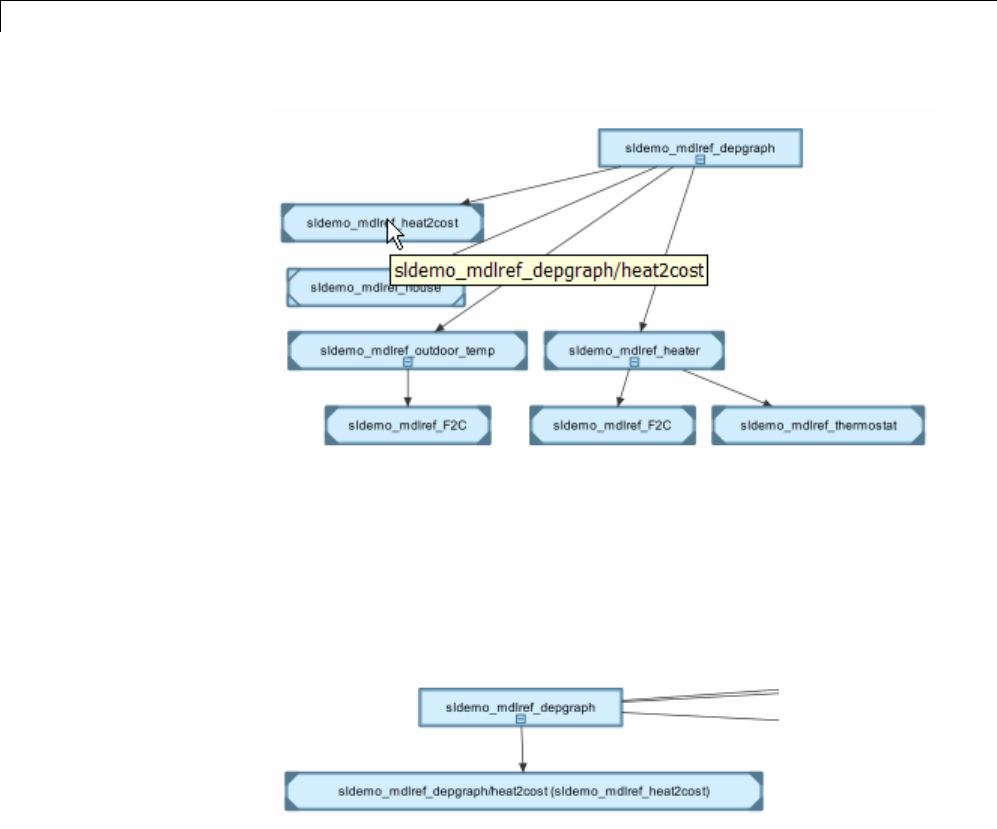
9Exploring, Searching, and Browsing Models
To display full paths in the boxes representing the instances:
•Select View > Show Full Path.
Each box in the instance view now displays the path of the Model block
corresponding to the instance. The name of the referenced model appears
in parentheses as illustrated in the following figure.
Refreshing a Dependency View
After changing a model displayed in a dependency view or any of its
dependencies, you must update the view to reflect any dependency changes.
To update the view:
•Select View > Refresh from the dependency viewer’s menu bar.
9-94

Model Dependency Viewer
Browsing Dependencies
You can use a dependency view to browse a model’s dependencies:
•To open a model or library displayed in the view, double-click its block.
•To display the Model block corresponding to an instance in an instance
view, right-click the instance and select Highlight Block from the menu
that appears.
•To open all models displayed in the view, select File > Open All Models
from the viewer’s menu bar.
•To save all models displayed in the view, select File > Save All Models.
•To close all models displayed in the view, select File > Close All Models.
Saving a Dependency View
You can save a dependency view for later viewing.
To save the current view:
•Select File > Save As from the viewer’s menu bar, then enter a name
for the view.
To reopentheview:
•Select File > Open from any viewer’s menu bar, then select the view you
want to open.
Printing a Dependency View
To print a dependency view:
•Select File > Print from the dependency viewer’s menu bar.
9-95

9Exploring, Searching, and Browsing Models
View Linked Requirements in Models and Blocks
In this section...
“Overview of Requirements Features in Simulink” on page 9-96
“Highlighting Requirements in a Model” on page 9-97
“Viewing Information About a Requirements Link” on page 9-99
“Navigating to Requirements from a Model” on page 9-100
“Filtering Requirements in a Model” on page 9-101
Overview of Requirements Features in Simulink
If your Simulink model has links to requirements in external documents,
you can review these links. To identify which model objects satisfy certain
design requirements, use the following requirements features available in
Simulink software:
•Highlighting objects in your model that have links to external requirements
•Viewing information about a requirements link
•Navigating from a model object to its associated requirement
•Filtering requirements highlighting based on specified keywords
Having a Simulink Verification and Validation license enables you to perform
the following additional tasks, using the Requirements Management Interface
(RMI):
•Adding new requirements
•Changing existing requirements
•Deleting existing requirements
•Applying user tags to requirements
•Creating reports about requirements links in your model
•Checking the validity of the links between the model objects and the
requirements documents
9-96

View Linked Requirements in Models and Blocks
Highlighting Requirements in a Model
You can highlight a model to identify which objects in the model have links
to requirements in external documents. Both the Simulink Editor and the
Model Explorer provide this capability.
•“Highlighting a Model Using the Simulink Editor” on page 9-97
•“Highlighting a Model Using the Model Explorer” on page 9-98
Note If your model contains a Model block whose referenced model
contains requirements, those requirements are not highlighted. If you have
Simulink Verification and Validation, you can view this information only in
requirements reports. To generate requirements information for referenced
models and then see highlighted snapshots of those requirements, follow the
steps in “Report for Requirements in Model Blocks”.
Highlighting a Model Using the Simulink Editor
If you are working in the Simulink Editor and want to see which model
objects in the slvnvdemo_fuelsys_officereq model have requirements,
follow these steps:
1Open the example model:
slvnvdemo_fuelsys_officereq
2Select Analysis > Requirements > Highlight Model.
Two types of highlighting indicate model objects with requirements:
•Yellow highlighting indicates objects that have requirements links for
the object itself.
•Orange outline indicates objects, such as subsystems, whose child objects
have requirements links.
9-97

9Exploring, Searching, and Browsing Models
Objects that do not have requirements are colored gray.
3To remove the highlighting from the model, select Analysis >
Requirements > Unhighlight Model. Alternatively, you can right-click
anywhere in the model, and select Remove Highlighting.
While a model is highlighted, you can still manage the model and its contents.
Highlighting a Model Using the Model Explorer
If you are working in Model Explorer and want to see which model objects
have requirements, follow these steps:
1Open the example model:
9-98

View Linked Requirements in Models and Blocks
slvnvdemo_fuelsys_officereq
2Select View > Model Explorer.
3To highlight all model objects with requirements, click the Highlight
items with requirements on model icon ( ).
The Model Editor window opens, and all objects in the model with
requirements are highlighted.
Note If you are running a 64-bit version of MATLAB, when you navigate to
a requirement in a PDF file, the file opens at the top of the page, not at the
bookmark location.
Viewing Information About a Requirements Link
Using Simulink, you can view detailed information about a requirements
link, such as identifying the location and type of document that contains
the requirement.
Note You can only modify the requirements information if you have a
Simulink Verification and Validation license.
For example, to view information about the requirements link from the MAP
Sensor block in the slvnvdemo_fuelsys_officereq example model, follow
these steps:
1Open the example model:
slvnvdemo_fuelsys_officereq
2Right-click the MAP sensor block, and select Requirements > Edit/Add
Links.
The Requirements dialog box opens and displays the following information
about the requirements link:
9-99

9Exploring, Searching, and Browsing Models
•The description of the link (which is the actual text of the requirement).
•The Microsoft Excel®workbook named
slvnvdemo_FuelSys_TestScenarios.xlsx, which contains the linked
requirement.
•The requirements text, which appears in the named cell
Simulink_requirement_item_2 in the workbook.
•The user tag test, which is associated with this requirement.
Navigating to Requirements from a Model
Navigating from the Model Object
You can navigate directly from a model object to that object’s associated
requirement. When you take these steps, the external requirements document
opens in the application, with the requirements text highlighted.
1Open the example model:
slvnvdemo_fuelsys_officereq
2Open the fuel rate controller subsystem.
3To open the linked requirement, right-click the Airflow calculation
subsystem and select Requirements > 1. “Mass airflow estimation”.
The Microsoft Word document
slvnvdemo_FuelSys_DesignDescription.docx, opens with the section 2.1
Mass airflow estimation selected.
Note If you are running a 64-bit version of MATLAB, when you navigate to
a requirement in a PDF file, the file opens at the top of the page, not at the
bookmark location.
Navigating from a System Requirements Block
Sometimes you want to see all the requirements links at a given level of the
model hierarchy. In such cases, you can insert a System Requirements block
9-100

View Linked Requirements in Models and Blocks
to collect all requirements links in the model or subsystem. The System
Requirements block does not list requirements links for any blocks for that
model or subsystem.
For example, you can insert the System Requirements block at the top level of
the slvnvdemo_fuelsys_officereq model, and navigate to the requirements
using the links inside the block.
1Open the example model:
slvnvdemo_fuelsys_officereq
2Select Analysis > Requirements > Highlight Model.
3In the slvnvdemo_fuelsys_officereq model, open the fuel rate controller
subsystem.
The Airflow calculation subsystem has a requirements link.
4Open the Airflow calculation subsystem.
5Select View > Library Browser
6On the Libraries pane, click the Simulink Verification and Validation
library.
This library contains only one block—the System Requirements block.
7Drag a System Requirements block into the Airflow calculation subsystem.
The RMI software collects and displays any requirements links for that
subsystem.
8Double-click 1. “Mass airflow subsystem”.
The Microsoft Word document,
slvnvdemo_FuelSys_DesignDescription.docx,opens,withthesection
2.1 Mass airflow estimation selected.
Filtering Requirements in a Model
•“Filtering Requirements Highlighting by User Tag” on page 9-102
9-101

9Exploring, Searching, and Browsing Models
•“Filtering Options for Highlighting Requirements” on page 9-103
Filtering Requirements Highlighting by User Tag
Some requirements links in your model can have one or more associated user
tags. User tags are keywords that you create to categorize a requirement,
for example, design or test.
For example, in the slvnvdemo_fuelsys_officereq model, the requirements
link from the MAP sensor block has the user tag test.
To highlight only all the blocks that have a requirement with the user tag
test:
1Open the example model:
slvnvdemo_fuelsys_officereq
2In the Simulink Editor, select Analysis > Requirements > Settings.
The Requirements Settings dialog box opens. If you do not have a Simulink
Verification and Validation license, the Filters tab is the only option
available.
By default, your model has no requirements filtering enabled.
3Select Filter links by user tags when highlighting and reporting
requirements.
4In the Include links with any of these tags text box, delete design,
and enter test.
5Press Enter.
6Highlight the slvnvdemo_fuelsys_officereq model for requirements.
Select Analysis > Requirements > Highlight Model.
In the top-level model, only the MAP sensor block and the Test inputs
block are highlighted.
9-102

View Linked Requirements in Models and Blocks
7Todisablethefilteringbyusertag,selectAnalysis > Requirements >
Settings,andclearFilter links by user tags when highlighting and
reporting requirements.
The model highlighting updates immediately.
Filtering Options for Highlighting Requirements
On the Filters tab, you select options that designate which objects with
requirements are highlighted. The following table describes these settings,
which apply to all requirements in your model for the duration of your
MATLAB session.
Option Description
Filter links by user tags when
highlighting and reporting
requirements
Enables filtering for highlighting
and reporting, based on specified
user tags.
Include links with any of these
tags
Highlights all objects whose
requirements match at least one
of the specified user tags. The tag
names must match exactly. Separate
multiple user tags with commas or
spaces.
Exclude links with any of these
tags
Excludes from the highlighting all
objects whose requirements match
at least one of the specified user
tags. The tag names must match
exactly. Separate multiple user tags
with commas or spaces.
9-103

9Exploring, Searching, and Browsing Models
Option Description
Apply same filters in context
menus
Disables navigation links in
context menus for all objects whose
requirements do not match at least
one of the specified user tags.
Under Link type filters,Disable
DOORS surrogate item links in
context menus
Disables links to IBM®Rational®
DOORS®surrogate items from the
context menus when you right-click
a model object. This option does not
depend on current user tag filters.
9-104

10
Managing Model
Configurations
•“About Model Configurations” on page 10-2
•“Multiple Configuration Sets in a Model” on page 10-3
•“Share a Configuration for Multiple Models” on page 10-4
•“Share a Configuration Across Referenced Models” on page 10-6
•“Manage a Configuration Set” on page 10-12
•“Manage a Configuration Reference” on page 10-18
•“About Configuration Sets” on page 10-26
•“About Configuration References” on page 10-29
•“Model Configuration Command Line Interface” on page 10-33

10 Managing Model Configurations
About Model Configurations
A model configuration is a named set of values for the parameters of a model.
It is referred to as a configuration set. Every new model is created with
a default configuration set, called Configuration, that initially specifies
default values for the model parameters. You can change the default values
for new models by setting the Model Configuration Preferences. For more
information, see “Model Configuration Preferences” on page 10-28.
You can subsequently create and modify additional configuration sets and
associate them with the model. The configuration sets associated with a
model can specify different values for any or all configuration parameters.
For more information, see “About Configuration Sets” on page 10-26. For
examples on how to use configuration sets, see:
•“Multiple Configuration Sets in a Model” on page 10-3
•“Manage a Configuration Set” on page 10-12
By default, a configuration set resides within a single model so that only
that model can use it. Alternatively, you can store a configuration set
independently, so that other models can use it. A configuration set that
exists outside any model is a freestanding configuration set. Each model that
uses a freestanding configuration set defines a configuration reference that
points to the freestanding configuration set. A freestanding configuration
set allows you to single-source a configuration set for several models. For
more information, see “About Configuration References” on page 10-29. For
examples on how to use configuration references, see:
•“Share a Configuration for Multiple Models” on page 10-4
•“Share a Configuration Across Referenced Models” on page 10-6
•“Manage a Configuration Reference” on page 10-18
10-2

Multiple Configuration Sets in a Model
Multiple Configuration Sets in a Model
A model can include many different configuration sets. This capability is
useful if you want to compare the difference in simulation output after
changing the values of several parameters. Attaching additional configuration
sets allows you to quickly switch the active configuration.
1To create additional configuration sets in your model, in the Model
Explorer, select your model node in the Model Hierarchy pane and do one
of the following:
•Right-click the model node and select Configuration > Add
Configuration.
•Right-click an existing configuration set. In the context menu, select
Copy.
2To import a previously saved configuration set, right-click the model node
and select Configuration > Import. In the Import Configuration From
File dialog box, select a configuration file.
3To modify the newly added configuration set, in the Model Hierarchy pane,
select the configuration node. In the Contents pane, select a component,
and then modify any parameters whicharedisplayedintherightpane.
4To make the new configuration set theactiveconfiguration,inthe
configuration set context menu, select Activate. In the Model Hierarchy
pane, the new configuration set name is now displayed as (Active).
5To simulate your model using a different configuration set, switch the
active configuration by repeating step 4.
10-3

10 Managing Model Configurations
Share a Configuration for Multiple Models
To share a configuration set between models, the configuration set must
be a configuration set object in the base workspace and you must create a
configuration reference in your model to reference the configuration set object.
You can create configuration references in other models that also point to the
same configuration set object.
For example, first convert an existing configuration set in your model to a
configuration reference:
1Open the Model Explorer.
2In the Model Hierarchy pane, right-click the active configuration set to
share.
3In the configuration set context menu, select Convert to Configuration
Reference, which opens a dialog box. Alternatively, you can right-click the
model node and select Configuration > Convert Active Configuration
to Reference.
4In the Convert Active Configuration to Reference dialog box, use the default
configuration set object name, configSetObj,ortypeaname.
5Click OK, which creates a configuration reference in the model and a
configuration set object in the base workspace. The configuration reference
points to the configuration set object, which has the same values as the
original active configuration set. The configuration reference name in the
Model Hierarchy is now marked as (Active).
6To change the name of the configuration reference, select it in the Model
Hierarchy, and in the right pane, change the Name field.
To share the preceding configuration set, which is stored as configSetObj in
the base workspace, create a configuration reference in another model:
1In the Model Hierarchy pane, right-click the model node.
2In the context menu, select Configuration > Add Configuration
Reference.
10-4

Share a Configuration for Multiple Models
3The Create Configuration Reference dialog box opens. Specify the name of
the configuration set object, configSetObj, in the base workspace.
4To make the new configuration reference the active configuration, in the
Model Hierarchy, right-click the configuration reference. In the context
menu, select Activate.
Both models now contain a configuration reference that points to the same
configuration set object in the base workspace. Before saving and closing
your models, follow the instructions to “Save a Referenced Configuration Set”
on page 10-23. If you do not save the referenced configuration set from the
base workspace, when you reopen your model, the configuration reference is
unresolved. To set up your model to automatically load the configuration set
object, see “Callback Functions” on page 4-54.
10-5
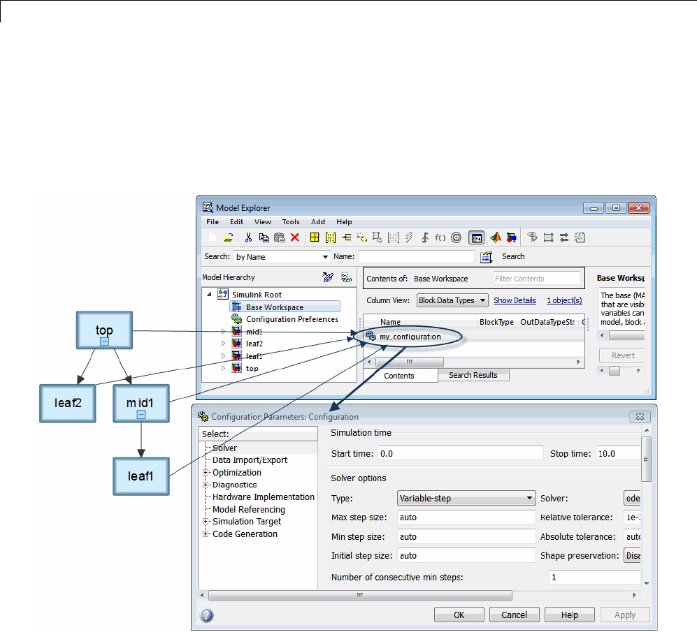
10 Managing Model Configurations
Share a Configuration Across Referenced Models
If you have a model reference hierarchy, you might want the top model
and the referenced models to share the same configuration set. You can
use a configuration reference in each of the models to reference the same
configuration set object in the base workspace.
In the diagram, each model shown in the Model Dependency Viewer specifies
the configuration reference, my_configuration, as its active configuration
set. my_configuration points to the freestanding configuration set,
Configuration. Therefore, the parameter values in Configuration apply
to all four models. Any parameter change in Configuration applies to all
four models.
10-6
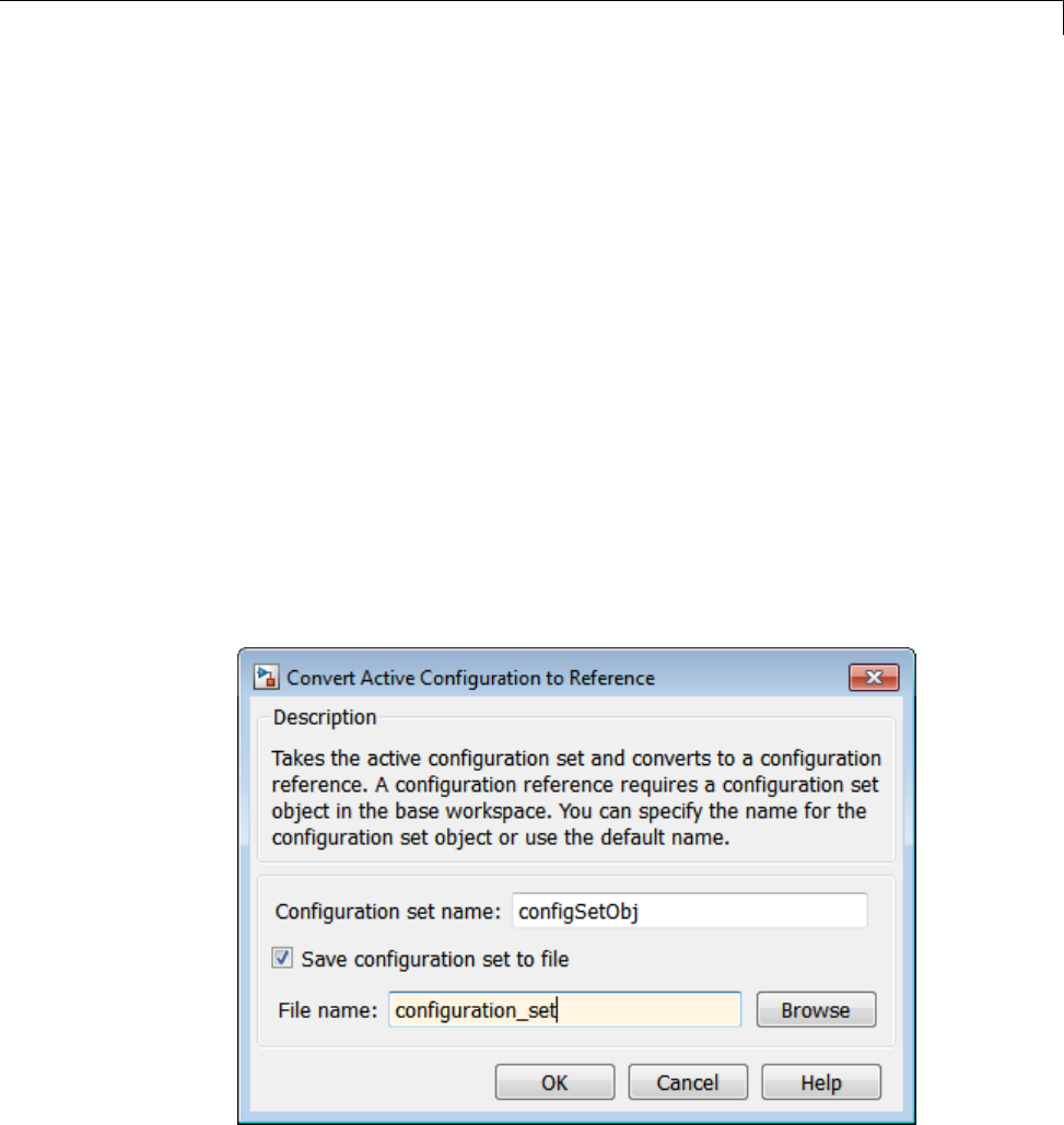
Share a Configuration Across Referenced Models
Convert Configuration Set to Configuration Reference
In the top model, you must convert theactiveconfigurationsettoa
configuration reference:
1Open the sldemo_mdlref_depgraph model and the Model Explorer.
2In the Model Hierarchy pane, expand the top model,
sldemo_mdlref_depgraph. In the list, right-click Configuration
(Active). In the context menu, select Convert to Configuration
Reference.
3In the Configuration set name field, specify a name for the configuration
set object, or use the default name, configSetObj. This configuration set
object is stored in the base workspace.
4Optionally, you can save the configuration set to a MAT-file. Select Save
configuration set to file. This enables the File name parameter.
5In the File name field, specify a name for the MAT-file.
10-7

10 Managing Model Configurations
6Click OK.
The original configuration set is now stored as a configuration set object,
configSetObj, in the base workspace. The configuration set is also stored
in a MAT-file, configuration_set.mat. The active configuration for the top
model is now a configuration reference. This configuration reference points to
the configuration set object in the base workspace.
Propagate a Configuration Reference
Now that the top model contains an active configuration reference, you can
propagate this configuration reference to all of the child models. Propagation
creates a copy of the top model configuration reference in each referenced
model. For each referenced model, the configuration reference is now the
active configuration. The configuration references point to the configuration
set object, configSetObj,inthebaseworkspace.
1In the Model Explorer, in the Model Hierarchy pane, expand the
sldemo_mdlref_depgraph node.
10-8
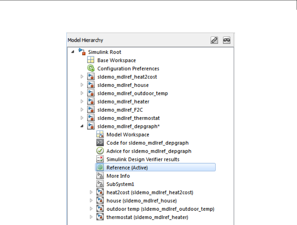
Share a Configuration Across Referenced Models
2Right-click the active configuration reference, Reference (Active).Inthe
context menu, select Propagate to Referenced Models.
3In the Configuration Reference Propagation dialog box, select the check box
for each referenced model. In this example, they are already selected.
4Verify that your current folder is a writable folder. The propagation
mechanism saves the original configuration parameters for each referenced
model so that you can undo the propagation. Click Propagate.
5In the Propagation Confirmation dialog box, click OK.
10-9
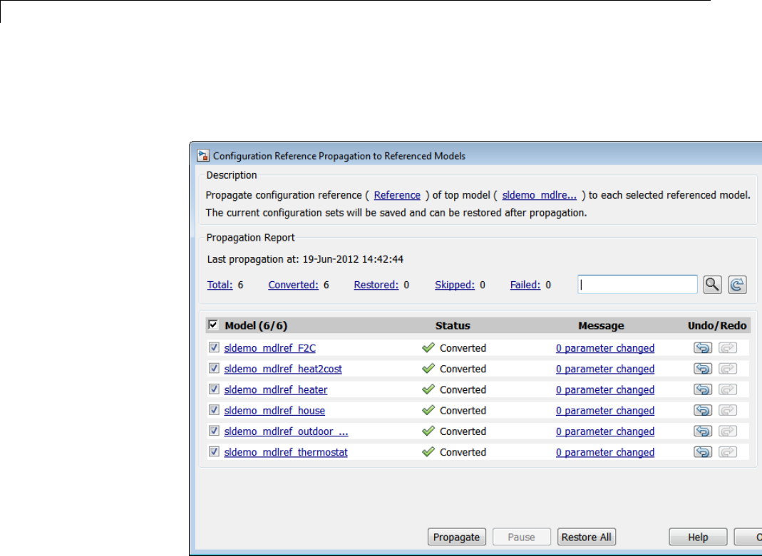
10 Managing Model Configurations
6In the Configuration Reference Propagation dialog box, the Propagation
Report is updated and the Status for each referenced model is marked as
Converted.
Undo a Configuration Reference Propagation
After propagating a configuration reference from a top model to the referenced
models, you can undo the propagation for all referenced models by clicking
Restore All. If you want to undo the propagation for individual referenced
models, in the Undo/Redo column, click the Undo button. The Propagation
Report is updated and the Status for the referenced model is set to Restored.
10-10
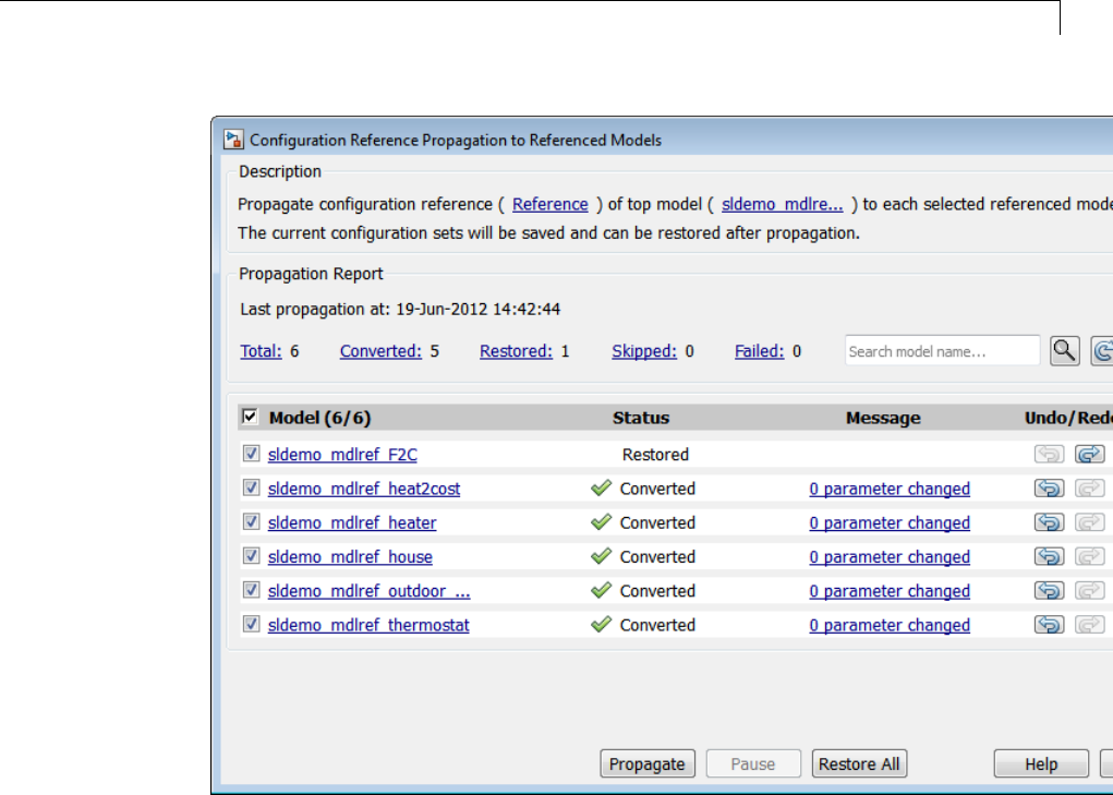
Share a Configuration Across Referenced Models
10-11

10 Managing Model Configurations
Manage a Configuration Set
In this section...
“Create a Configuration Set in a Model” on page 10-12
“CreateaConfigurationSetintheBaseWorkspace”onpage10-12
“OpenaConfigurationSetintheConfiguration Parameters Dialog Box” on
page 10-13
“Activate a Configuration Set” on page 10-13
“Set Values in a Configuration Set” on page 10-14
“Copy, Delete, and Move a Configuration Set” on page 10-14
“Save a Configuration Set” on page 10-15
“Load a Saved Configuration Set” on page 10-16
“Copy Configuration Set Components” on page 10-16
Create a Configuration Set in a Model
1Open the Model Explorer.
2In the Model Hierarchy pane, select the model name.
3You can create a new configuration set in any of the following ways:
•From the Add menu, select Configuration.
•On the toolbar, click the Add Configuration button .
•In the Model Hierarchy pane, right-click an existingconfigurationset
and copy and paste the configuration set.
Create a Configuration Set in the Base Workspace
1Open the Model Explorer.
2In the Model Hierarchy pane, select Base Workspace.
3You can create a new configuration set object in the following ways:
•From the Add menu, select Configuration
10-12
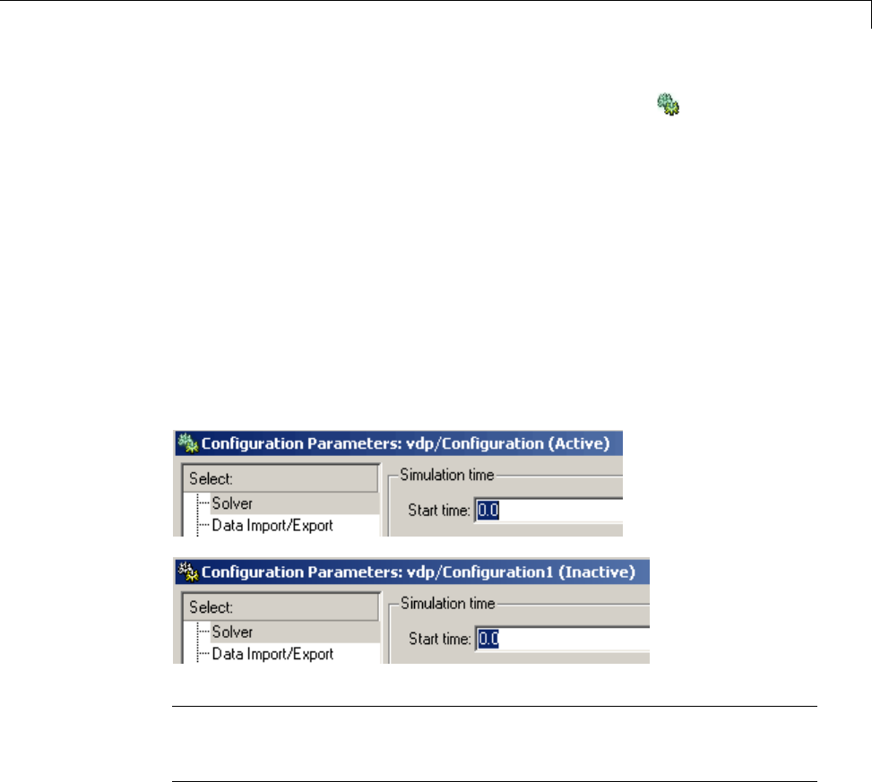
Manage a Configuration Set
•In the toolbar, click the Add Configuration button
4The configuration set object appears in the Contents pane, with the default
name, ConfigSet.
OpenaConfigurationSetintheConfiguration
Parameters Dialog Box
In the Model Explorer, to open the Configuration Parameters dialog box for
a configuration set, right-click the configuration set’s node to display the
context menu, then select Open. You can open the Configuration Parameters
dialog box for any configuration set, whether or not it is active.
The title bar of the dialog box indicates whether the configuration set is active
or inactive.
Note Every configuration set has its own Configuration Parameters dialog
box. As you change the state of a configuration set, the title bar of the dialog
box changes to reflect the state.
Activate a Configuration Set
Only one configuration set associated with a model is active at any given
time. The active set determines the current values of the model parameters.
You can change the active or inactive set at any time (except when executing
the model). In this way, you can quickly reconfigure a model for different
10-13

10 Managing Model Configurations
purposes, for example, testing and production, or apply standard configuration
settings to new models.
To activate a configuration set, right-click the configuration set node to
display the context menu, then select Activate.
Set Values in a Configuration Set
To set the value of a parameter in a configuration set, in the Model Explorer:
1In the Model Hierarchy, select the configuration set node.
2In the Contents pane, select the component from where the parameter
resides.
3In the Dialog pane, edit the parameter value.
Copy, Delete, and Move a Configuration Set
You can use edit commands on the Model Explorer Edit or context menus or
object drag-and-drop operations to delete, copy, and move configuration sets
among models displayed in the Model Hierarchy pane.
For example, to copy a configuration set from one model to another:
1In the Model Hierarchy pane, right-click the configuration set node that
you want to copy.
2Select Copy in the configuration set context menu.
3Right-click the model node in which you want to create the copy.
4Select Paste from the model context menu.
To copy the configuration set using object drag-and-drop, hold down the right
mousebuttonanddragtheconfigurationsetnodetothenodeofthemodelin
which you want to create the copy.
To move a configuration set from one model to another using drag-and-drop,
hold the left mouse button down and drag the configuration set node to the
node of the destination model.
10-14

Manage a Configuration Set
Note You cannot move or delete an active configuration set from a model.
Save a Configuration Set
You can save the settings of configuration sets as MATLAB functions or
scripts. Using the MATLAB function or script, you can share and archive
model configuration sets. You can also compare the settings in different
configuration sets by comparing the MATLAB functions or scripts of the
configuration sets.
To save an active or inactive configuration set from the Model Explorer:
1Open the model.
2Open the Model Explorer.
3Save the configuration set:
aIn the Model Hierarchy pane:
•Right-click the model node and select Configuration > Export
Active Configuration Set.
•Right-click a configuration set and select Export.
•Select the model. In the Contents pane, right-click a configuration
set and select Export.
bIntheExportConfigurationSettoFiledialogbox,specifythenameof
thefileandthefiletype.Ifyouspecifya.m extension, the file contains
a function that creates a configuration set object. If you specify a .mat
extension, the file contains a configuration set object.
Note Donotspecifythenameofthefiletobethesameasamodelname.
Ifthefileandmodelhavethesamename, the software cannot determine
which file contains the configuration set object when loading the file.
cClick Save. The Simulink software saves the configuration set.
10-15

10 Managing Model Configurations
Load a Saved Configuration Set
You can load configuration sets that you previously saved as MATLAB
functions or scripts.
To load a configuration set from the Model Explorer:
1Open the model.
2Open the Model Explorer.
3In the Model Hierarchy pane, right-click the model and select
Configuration > Import.
4In the Import Configuration Set From File dialog box, select the .m file that
contains the function to create the configuration set object, or the .mat file
that contains the configuration set object.
5Click Open. The Simulink software loads the configuration set.
Note If you load a configuration set object that contains an invalid custom
target, the software sets the “System target file” parameter to ert.tlc.
6Optionally, activate the configuration set. For more information, see
“Activate a Configuration Set” on page 10-13.
Copy Configuration Set Components
To copy a configuration set component from one configuration set to another:
1Select the component in the Model Explorer Contents pane.
2From either the Model Explorer Edit menu or the component context
menu, select Copy.
3Select the configuration set into which you want to copy the component.
4From either the Model Explorer Edit menu or the component context
menu, select Paste.
10-16

Manage a Configuration Set
Note The copy replaces the component of the same name in the destination
configuration set. For example, if you copy the Solver component of
configuration set A and paste it into configuration set B, the copy replaces
the existing Solver component in B.
10-17

10 Managing Model Configurations
Manage a Configuration Reference
In this section...
“Create and Attach a Configuration Reference” on page 10-18
“Resolve a Configuration Reference” on page 10-19
“Activate a Configuration Reference” on page 10-21
“Manage Configuration Reference Across Referenced Models” on page 10-22
“Change Parameter Values in a Referenced Configuration Set” on page
10-23
“Save a Referenced Configuration Set” on page 10-23
“Load a Saved Referenced Configuration Set” on page 10-24
“Why is the Build Button Not Available for a Configuration Reference?” on
page 10-25
Create and Attach a Configuration Reference
To use a configuration reference, it must point to freestanding configuration
set. Create a freestanding configuration set before creating a configuration
reference, see “Create a Configuration Set in the Base Workspace” on page
10-12.
To create a configuration reference:
1In the Model Explorer, in the Model Hierarchy pane, select the model.
2Click the Add Reference tool or select Add > Configuration
Reference. The Create Configuration Reference dialog box opens.
3Specify the Configuration set name of the configuration set object in
the base workspace to be referenced.
4Click OK. If you chose to create a configuration reference without first
creating a configuration set object, a dialog box opens asking if you would
like to continue. If you choose:
10-18
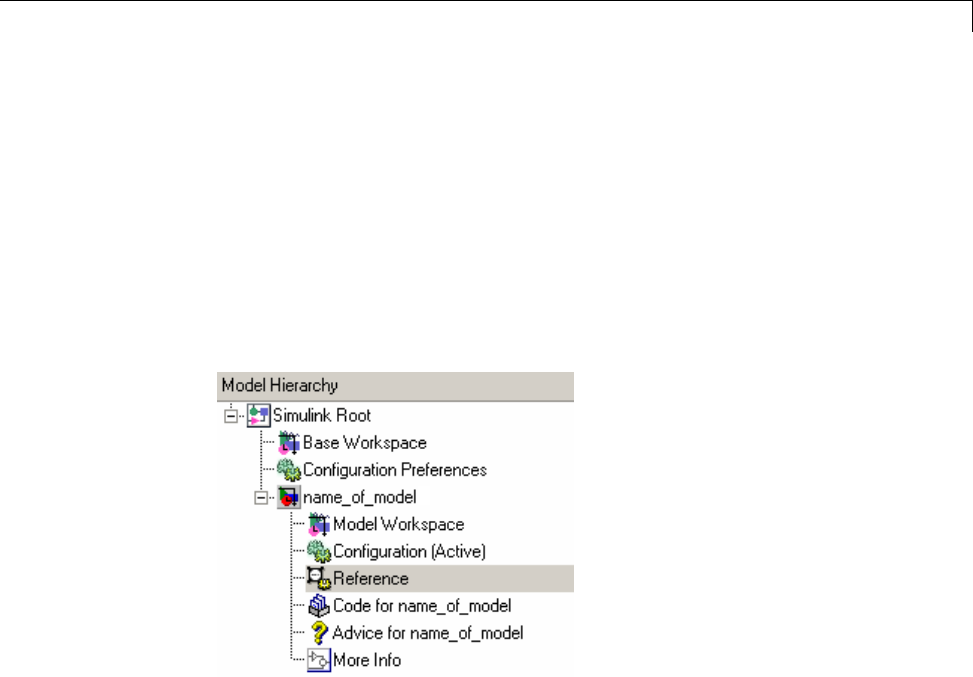
Manage a Configuration Reference
•Yes, an unresolved configuration reference is created. For more
information, see “Unresolved Configuration References” on page 10-30.
Follow the instructions in“Resolve a Configuration Reference” on page
10-19.
•No, then the configuration reference is not created. Follow the
instructions in“Create a Configuration Set in the Base Workspace” on
page 10-12, and then return to step 1 above.
5A new configuration reference appears in the Model Hierarchy under the
selected model. The default name of the new reference is Reference.
Resolve a Configuration Reference
An unresolved configuration reference is a configuration reference that is not
pointing to a valid configuration set object.
To resolve a configuration reference:
1In the Model Hierarchy pane, select the unresolved configuration reference
or right-click the configuration reference, and select Open from the context
menu.
The Configuration Reference dialog box opens in the Dialog pane or a
separate window.
10-19
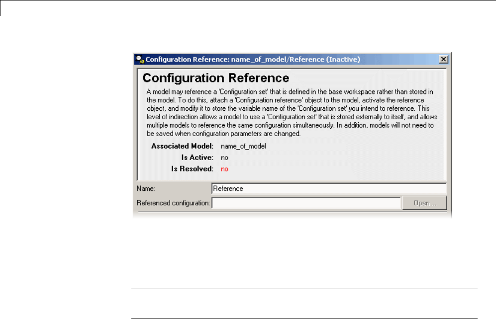
10 Managing Model Configurations
2Specify the Referenced configuration set to be a configuration set
object already in the base workspace. If one does not exist, see “Create a
Configuration Set in the Base Workspace” on page 10-12.
Tip Do not specify the name of a configuration reference. If you nest a
configuration reference, an error occurs.
3Click OK or Apply.
If you specified a Referenced configuration that exists in the base
workspace, the Is Resolved field in the dialog box changes to yes.
10-20
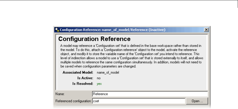
Manage a Configuration Reference
Activate a Configuration Reference
After you create a configuration reference and attach it to a model, you can
activate it so that it is the active configuration.
•In the GUI, from the context menu of the configuration reference, select
Activate.
•From the API, execute setActiveConfigSet, specifying the configuration
reference as the second argument.
When a configuration reference is active, the Is Active field of the
Configuration Reference dialog box changes to yes. Also, the Model Explorer
shows the name of the reference with the suffix (Active).
10-21
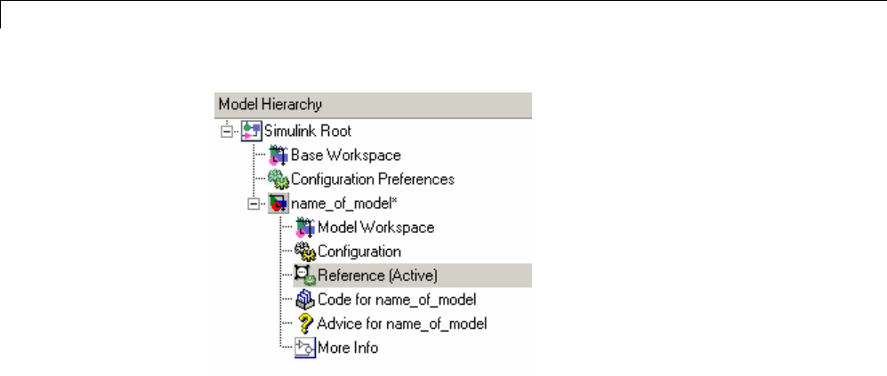
10 Managing Model Configurations
The freestanding configuration set of the active reference now provides the
configuration parameters for the model.
Manage Configuration Reference Across Referenced
Models
In a model hierarchy, you can share a configuration reference across
referenced models. Using the Configuration Reference Propagation dialog box,
you can propagate a configuration reference of a top model to an individual
referenced model or to all referenced models in the model hierarchy. The
dialog box provides:
•A list of referenced models in the top model.
•The ability to select only specific referenced models for propagation.
•After propagation, the status for the converted configuration for each
referenced model.
•A view of the changed parameters after the propagation.
•The ability to undo the configuration reference and restore the previous
configuration settings for a referenced model.
To open the dialog box, in the Model Explorer, in the model hierarchy pane,
right-click the configuration reference node of a model. In the context menu,
10-22
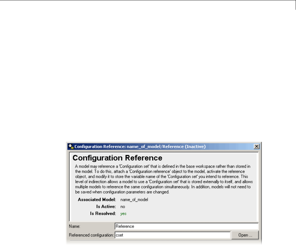
Manage a Configuration Reference
select Propagate to Referenced Models. For an example, see “Share a
Configuration Across Referenced Models” on page 10-6.
Change Parameter Values in a Referenced
Configuration Set
To obtain a referenced configuration set:
1In the Model Hierarchy pane, select the configuration reference, or
right-click the configuration reference, and select Open from the context
menu.
The Configuration Reference dialog box appears in the Dialog pane or in
a separate window.
2To the right of the Referenced configuration field, click Open.The
Configuration Parameters dialog box opens. You can now change and apply
parametervaluesasyouwould for any configuration set.
Save a Referenced Configuration Set
If your model uses a configuration reference to specify the model configuration,
before closing your model, you need to save the referenced configuration set to
a MAT-file or MATLAB script.
10-23

10 Managing Model Configurations
1In the Model Explorer, in the Model Hierarchy, select Base Workspace.
2In the Contents pane, right-click the name of the referenced configuration
set object.
3From the context menu, select Export Selected.
4Specify the filename for saving the configuration set as either a MAT-file
or a MATLAB script.
Tip When you reopen the model you must load the saved configuration set,
otherwise, the configuration reference is unresolved. To set up your model
to automatically load the configuration set object, see “Callback Functions”
on page 4-54.
Load a Saved Referenced Configuration Set
If your model uses a configuration reference to specify the model configuration,
you need to load the referenced configuration set from a MAT-file or MATLAB
script to the base workspace.
1In the Model Explorer, in the Model Hierarchy, right-click Base
Workspace.
2From the context menu, select Import.
3Specify the filename for the saved configuration set and select OK. The
configuration set object appears in the base workspace.
Tip When you reopen the model you must load the saved configuration set,
otherwise, the configuration reference is unresolved. To set up your model
to automatically load the configuration set object, see “Callback Functions”
on page 4-54.
10-24

Manage a Configuration Reference
Why is the Build Button Not Available for a
Configuration Reference?
The Code Generation pane of the Configuration Parameters dialog box
contains a Build button. Its availability depends on whether the configuration
set displayed by the dialog box resides in a model or is a freestanding
configuration set.
•When the pane displays a configuration set stored in a model, the Build
button is available. Click it to generate and compile code for the model.
•When the pane displays a freestanding configuration set, the Build button
is unavailable. The configuration set does not know which (if any) models
link to it.
To provide the same capabilities whether a configuration set resides in a
model or is freestanding, the Configuration Reference dialog box contains a
Build button. This button has the same capability as its equivalent in the
Configuration Parameters dialog box. It operates on the model that contains
the configuration reference.
10-25

10 Managing Model Configurations
About Configuration Sets
In this section...
“What Is a Configuration Set?” on page 10-26
“What Is a Freestanding Configuration Set?” on page 10-27
“Model Configuration Preferences” on page 10-28
What Is a Configuration Set?
A configuration set comprises groups of related parameters called components.
Every configuration set includes the following components:
•Solver
•Data Import/Export
•Optimization
•Diagnostics
•Hardware Implementation
•Model Referencing
•Simulation Target
Some MathWorks products that work with Simulink, such as Simulink Coder,
define additional components. If such a product is installed on your system,
the configuration set also contains the components that the product defines.
When you select any model configuration, the Model Configuration dialog
appears in the Model Explorer Dialog pane. In this location, you can edit the
name and description of your configuration.
10-26
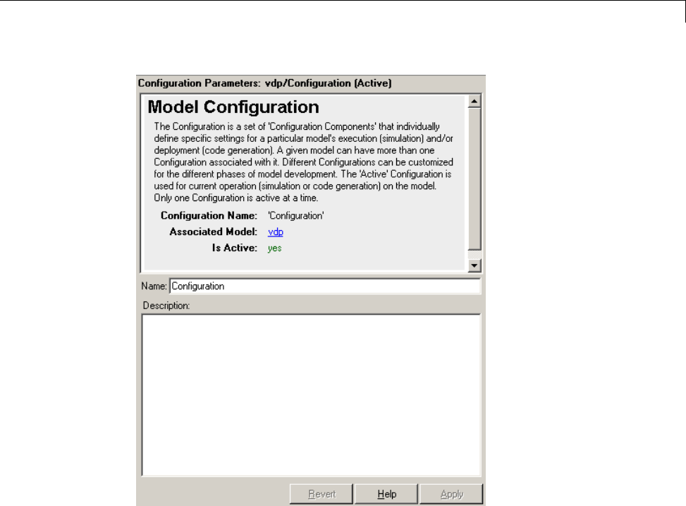
About Configuration Sets
What Is a Freestanding Configuration Set?
A freestanding configuration set is a configuration set object,
Simulink.ConfigSet, stored in the base workspace. To use a freestanding
configuration set as the configuration for a model, you must create a
configuration reference in the model that references it. You can create a
freestanding configuration set in the base workspace in these ways:
•Create a new configuration set object.
•Copy a configuration set that resides within a model to the base workspace.
•Load a configuration set from a MAT-file.
10-27

10 Managing Model Configurations
You can store any number of configuration sets in the base workspace by
assigning each set to a different MATLAB variable.
Note Although you can store a configuration set in a model and point to it
with a base workspace variable, such a configuration set is not freestanding.
Using it in a configuration reference causes an error.
Model Configuration Preferences
Model Configuration Preferences are the preferred configuration for new
models. You can change the preferred configuration by editing the settings in
the Model Explorer.
1Select View > Show Configuration Preferences to display the
Configuration Preferences node in the expanded Simulink Root node.
2Under the Simulink Root node, select Configuration Preferences .The
Model Configuration Preferences dialog box opens in the Dialog pane.
3In the Contents pane, select components and change any parameter
values.
10-28

About Configuration References
About Configuration References
In this section...
“What Is a Configuration Reference?” on page 10-29
“Why Use Configuration References?” on page 10-29
“Unresolved Configuration References” on page 10-30
“Configuration Reference Limitations” on page 10-31
“Configuration References for Models with Older Simulation Target
Settings” on page 10-31
What Is a Configuration Reference?
A configuration reference in a model is a reference to a configuration set
objectinthebaseworkspace.Amodelthathasaconfiguration reference that
points to a freestanding configuration set uses that configuration set when
configuration reference is active. The model then has the same configuration
parameters as if the referenced configuration set resides directly in the model.
You can attach any number of configuration references to a model. Each
reference must have a unique name. For more information, see “Why Use
Configuration References?” on page 10-29. For an example on how to use
configuration references, see “Share a Configuration for Multiple Models” on
page 10-4 or “Create and Attach a Configuration Reference” on page 10-18.
Tip Save or export the configuration set object. Otherwise, when you reopen
your model the configuration reference is unresolved. To set up your model
to automatically load the configuration set object, see “Callback Functions”
on page 4-54.
Why Use Configuration References?
You can use configuration references and freestanding configuration sets to:
•Assign the same configuration set to any number of models
10-29

10 Managing Model Configurations
Each model that uses a given configuration set contains a configuration
reference that points to a MATLAB variable. The value of that variable is a
freestanding configuration set. All the models share that configuration set.
Changing the value of any parameter in the set changes it for every model
that uses the set. Use this feature to reconfigure many submodels quickly
and ensure consistent configuration of parent models and referenced
models.
•Replace the configuration sets of any number of models without
changing the model files
When multiple models use configuration references to access a freestanding
configuration set, assigning a different set to the MATLAB variable assigns
that set to all models. Use this feature to maintain a library of configuration
sets and assign them to any number of models in a single operation.
•Use different configuration sets for a referenced model used in
different contexts without changing the model file
A submodel that uses different configuration sets in different contexts
contains a configuration reference that specifies the submodel configuration
set as a variable. When you call an instance of the submodel, Simulink
software assigns that variable a freestanding configuration set for the
current context.
Unresolved Configuration References
When a configuration reference does not reference a valid configuration set,
the Is Resolved field of the Configuration Reference dialog box has the value
no. If you activate an unresolved configuration reference, no warning or error
occurs. However, an unresolved configuration reference that is active provides
no configuration parameter values to the model. Therefore:
•Fields that display values known only by accessing a configuration
parameter, like Stop Time in the model window, are blank.
•Trying to build the model, simulate it, generate code for it, or otherwise
require it to access configuration parameter values, causes an error.
For more information, see “Resolve a Configuration Reference” on page 10-19.
10-30

About Configuration References
Configuration Reference Limitations
•You cannot nest configuration references. Only one level of indirection is
available, so a configuration reference cannot link to another configuration
reference. Each reference must specify a freestanding configuration set.
•If you replace the base workspace variable and configuration set that
configuration references use, execute refresh for each reference that
usesthereplacedvariableandset. See“Userefresh When Replacing a
Referenced Configuration Set” on page 10-41.
•If you activate a configuration reference when using a custom target, the
ActivateCallback function does not trigger to notify the corresponding
freestanding configuration set. Likewise, if a freestanding configuration
set switches from one target to another, the ActivateCallback function
does not trigger to notify the new target. This behavior occurs, even if an
active configuration reference points to that target. For more information
about ActivateCallback functions, see “rtwgensettings Structure” in the
Simulink Coder documentation.
Configuration References for Models with Older
Simulation Target Settings
Suppose that you have a nonlibrary model that contains one of these blocks:
•MATLAB Function
•Stateflow chart
•Truth Table
•Attribute Function
In R2008a and earlier, this type of nonlibrary model does not store simulation
target (or sfun) settings in the configuration parameters. Instead, the model
stores the settings outside any configuration set.
When you load this older type of model, the simulation target settings migrate
to parameters in the active configuration set.
•Iftheactiveconfigurationsetresides internally with the model, the
migration happens automatically.
10-31

10 Managing Model Configurations
•If the model uses an active configuration reference to point to a
configuration set in the base workspace, the migration process is different.
The following sections describe the two types of migration for nonlibrary
models that use an active configuration reference.
Default Migration Process That Disables the Configuration
Reference
Becausemultiplemodelscanshareaconfigurationsetinthebaseworkspace,
loading a nonlibrary model cannot automatically change any parameter
values in that configuration set. By default, these actions occur during loading
of a model to ensure that simulation results are the same, no matter which
version of the software that you use:
•A copy of the configuration set in the base workspace attaches to the model.
•The simulation target settings migrate to the corresponding parameters in
this new configuration set.
•The new configuration set becomes active.
•The old configuration reference becomes inactive.
A warning message appears in the MATLAB Command Window to describe
those actions. Although this process ensures consistent simulation results
for the model, it disables the configuration reference that links to the
configuration set in the base workspace.
10-32

Model Configuration Command Line Interface
Model Configuration Command Line Interface
In this section...
“Overview” on page 10-33
“Load and Activate a Configuration Set at the Command Line” on page
10-34
“Save a Configuration Set at the Command Line” on page 10-35
“Create a Freestanding Configuration Set at the Command Line” on page
10-36
“Create and Attach a Configuration Reference at the Command Line” on
page 10-37
“Attach a Configuration Reference to Multiple Models at the Command
Line” on page 10-38
“Get Values from a Referenced Configuration Set” on page 10-39
“Change Values in a Referenced Configuration Set” on page 10-39
“Obtain a Configuration Reference Handle” on page 10-40
“Use refresh When Replacing a Referenced Configuration Set” on page
10-41
Overview
An application programming interface (API) lets you create and manipulate
configuration sets at the command line or in a script. The API includes the
Simulink.ConfigSet and Simulink.ConfigSetRef classes and the following
functions:
•attachConfigSet
•attachConfigSetCopy
•detachConfigSet
•getConfigSet
•getConfigSets
•setActiveConfigSet
10-33

10 Managing Model Configurations
•getActiveConfigSet
•openDialog
•closeDialog
•Simulink.BlockDiagram.saveActiveConfigSet
•Simulink.BlockDiagram.loadActiveConfigSet
These functions, along with the methods and properties of
Simulink.ConfigSet class, allow you to create a script to:
•Create and modify configuration sets.
•Attach configuration sets to a model.
•Set the active configuration set for a model.
•Open and close configuration sets.
•Detach configurationsetsfromamodel.
•Save configuration sets.
•Load configuration sets.
For examples using the preceding functions and the Simulink.ConfigSet
class, see the function and class reference pages.
Load and Activate a Configuration Set at the
Command Line
To load a configuration set from a MATLAB function or script:
1Use the getActiveConfigSet or getConfigSet function to get a handle to
the configuration set that you want to update.
2Call the MATLAB function or execute the MATLAB script to load the saved
configuration set.
3Optionally, use the attachConfigSet function to attach the configuration
set to the model. To avoid configuration set naming conflicts, set
allowRename to true.
10-34

Model Configuration Command Line Interface
4Optionally, use the setActiveConfigSet function to activate the
configuration set.
Alternatively, to load a configuration set at the command line and make it
the active configuration set:
1Open the model.
2Use the Simulink.BlockDiagram.loadActiveConfigSet function to load
the configuration set and make it active.
Note Ifyouloadaconfigurationsetwiththesamenameasthe:
•Active configuration set, the software overwrites the active configuration
set.
•Inactive configuration set that is associated with the model, the software
detaches the inactive configuration from the model.
Save a Configuration Set at the Command Line
To save an active or inactive configuration set as a MATLAB function or script:
1Use the getActiveConfigSet or getConfigSet function to get a handle to
the configuration set.
2Use the saveAs method of the Simulink.Configset class to save the
configuration set as a function or script.
Alternatively, to save the active configuration set:
1Open the model.
2Use the Simulink.BlockDiagram.saveActiveConfigSet function to save
the active configuration set.
10-35

10 Managing Model Configurations
Create a Freestanding Configuration Set at the
Command Line
Copy a Configuration Set Stored in a Model
Create a freestanding configuration settobereferencedbyaconfiguration
reference in several models. You must copy any configuration set obtained
from an existing model, otherwise, cset refers to the existing configuration
set stored in the model, rather than a new freestanding configuration set in
the base workspace. For example, use one of the following:
•
cset = copy (getActiveConfigSet(model))
•
cset = copy (getConfigSet(model, ConfigSetName))
model is any open model, and ConfigSetName isthenameofanyconfiguration
set attached to the model.
Read a Configuration Set from a MAT-File
To use a freestanding configuration set across multiple MATLAB sessions,
you can save it to a MAT-file. To create the MAT-file, you first copy the
configuration set to a base workspace variable, then save the variable to the
MAT-file:
save (workfolder/ConfigSetName.mat, cset)
workfolder is a working folder, ConfigSetName.mat istheMAT-filename,
and cset isabaseworkspacevariablewhosevalueistheconfigurationset
to save. When you later reopen your model, you can reload the configuration
set into the variable:
load (workfolder/ConfigSetName.mat)
To execute code that reads configuration sets from MAT-files, use one of these
techniques:
•The preload function of a top model
10-36

Model Configuration Command Line Interface
•The MATLAB startup script
•Interactive entry of load statements
Create and Attach a Configuration Reference at the
Command Line
To create and populate a configuration reference, Simulink.ConfigSetRef,
using the API:
1Create the reference:
cref = Simulink.ConfigSetRef
2Change the default name if desired:
cref.Name = 'ConfigSetRefName'
3Specify the referenced configuration set:
cref.WSVarName = 'cset'
Tip Do not specify the name of a configuration reference. If you nest a
configuration reference, an error occurs.
4Attach the reference to a model:
attachConfigSet(model,cref, true)
The third argument is optional and authorizes renaming to avoid a name
conflict.
Using a configuration reference with an invalid configuration set, WSVarName,
generates an error and is called an unresolved configuration reference. The
GUI equivalent of WSVarName is Referenced configuration.Youcanlater
use the API or GUI to provide the name of a freestanding configuration
set. For more information, see “Unresolved Configuration References” on
page 10-30.
10-37

10 Managing Model Configurations
Attach a Configuration ReferencetoMultipleModels
at the Command Line
After you create a configuration reference and attach it to a model, you can
attach copies of the reference to any other models. Each model has its own
copy of any configuration reference attached to it, just as each model has its
own copy of any attached configuration set.
IfyouusetheGUI,attachinganexisting configuration reference to another
model automatically attaches a distinct copy to the model. If necessary
to prevent name conflict, the GUI adds or increments a digit at the end
ofthenameofthecopiedreference. IfyouusetheAPI,besuretocopythe
configuration reference explicitly before attaching it, with statements like:
cref = copy (getConfigSet(model,ConfigSetRefName))
attachConfigSet (model,cref, true)
If you omit the copy operation, cref becomes a handle to the original
configuration reference, rather than a copy of the reference. Any attempt to
use cref causes an error. If you omit the argument true to attachConfigSet,
the operation fails if a name conflict exists.
The following example shows code for obtaining a freestanding configuration
set and attaching references to it from two models. After the code executes,
one of the models contains an internal configuration set and a configuration
reference that points to a freestanding copy of that set. If the internal copy
is an extra copy, you can remove it with detachConfigSet,asshowninthe
last line of the example.
open_system('model1')
% Get handle to local cset
cset = getConfigSet('model1', 'Configuration')
% Create freestanding copy; original remains in model
cset1 = copy(cset)
% In the original model, create a configuration
% reference to the cset copy
cref1 = Simulink.ConfigSetRef
cref1.WSVarName = 'cset1'
10-38

Model Configuration Command Line Interface
% Attach the configuration reference to the model
attachConfigSet('model1', cref1, true)
% In a second model, create a configuration
% reference to the same cset
open_system('model2')
% Rename if name conflict occurs
attachConfigSetCopy('model2', cref1, true)
% Delete original cset from first model
detachConfigSet('model1', 'Configuration')
Get Values from a Referenced Configuration Set
You can use get_param on a configuration reference to obtain parameter
values from the linked configuration set, as if the reference object were
the configuration set itself. Simulink software retrieves the referenced
configuration set and performs the indicated get_param on it.
For example, if configuration reference cref links to configuration set cset,
the following operations give identical results:
get_param (cset, 'StopTime')
get_param (cref, 'StopTime')
Change Values in a Referenced Configuration Set
By operating on only a configuration reference, you cannot change the
referenced configuration set parameter values. If you execute:
set_param (cset, 'StopTime', '300')
set_param (cref, 'StopTime', '300') % ILLEGAL
the first operation succeeds, but the second causes an error. Instead, you
must obtain the configuration set itself and change it directly, using the
GUI or the API.
To obtain a referenced configuration set using the API:
1Follow the instructions in “Obtain a Configuration Reference Handle” on
page 10-40.
10-39

10 Managing Model Configurations
2Obtain the configuration set cset from the configuration reference cref:
cset =cref.getRefConfigSet
You can now use set_param on cset to change parameter values. For
example:
set_param (cset, 'StopTime', '300')
Tip If you want to change parameter values through the GUI, execute:
cset.openDialog
The Configuration Parameters dialog box opens on the specified
configuration set.
Obtain a Configuration Reference Handle
Most functions and methods that operate on a configuration reference take a
handle to the reference. When you create a configuration reference:
cref = Simulink.ConfigSetRef
the variable cref contains a handle to the reference. If you do not already
have a handle, you can obtain one by executing:
cref = getConfigSet(model,'ConfigSetRefName')
ConfigSetRefName is the name of the configuration reference as it appears in
the Model Explorer, for example, Reference.Youspecifythisnamebysetting
the Name field in the Configuration Reference dialog box or executing:
cref.Name = 'ConfigSetRefName'
The technique for obtaining a configuration reference handle is the same
technique you use to obtain a configuration set handle. Wherever the same
operation applies to both configuration sets and configuration references,
applicable functions and methods overload to perform correctly with either
class.
10-40

Model Configuration Command Line Interface
Use refresh When Replacing a Referenced
Configuration Set
You can replace the base workspace variable and configuration set that a
configuration reference uses. However, the pointer from the configuration
reference to the configuration set becomes invalid. To avoid this situation,
execute:
cref.refresh
cref is the configuration reference. If you do not execute “refresh”, the
configuration reference continues tousethepreviousinstanceofthebase
workspace variable and its configuration set. This example illustrates the
problem.
% Create a new configuration set
cset1 = Simulink.ConfigSet;
% Set a non-default stop time
set_param (cset1, 'StopTime', '500')
% Create a new configuration reference
cref1 = Simulink.ConfigSetRef;
% Resolve the configuration reference to the configuration set
cref1.WsVarName = 'cset1';
% Attach the configuration reference to an untitled model
attachConfigSet('untitled', cref1, true)
% Set the active configuration set to the reference
setActiveConfigSet('untitled','Reference')
% Replace config set in the base workspace
cset1 = Simulink.ConfigSet;
% Call to refresh is commented out!
% cref1.refresh;
% Set a different stop time
set_param (cset1, 'StopTime', '75')
10-41

10 Managing Model Configurations
If you simulate the model, the simulation stops at 500, not 75. Calling
cref1.refresh as shown prevents the problem.
10-42

11
Configuring Models for
Targets with Multicore
Processors
•“Introduction to Concurrent Execution” on page 11-2
•“Design Considerations” on page 11-5
•“Modeling Process for Concurrent Execution” on page 11-11
•“Configure Your Model” on page 11-12
•“Baseline Analysis Using Configuration Defaults” on page 11-17
•“Customize Concurrent Execution Settings” on page 11-19
•“Interpret Simulation Results” on page 11-26
•“Build and Download to a Multicore Target” on page 11-32
•“Concurrent Execution Example Model” on page 11-45
•“Command-Line Interface” on page 11-55

11 Configuring Models for Targets with Multicore Processors
Introduction to Concurrent Execution
In this section...
“About Configuring Models for Concurrent Execution” on page 11-2
“Supported Targets” on page 11-3
“Helpful Terms” on page 11-3
“Software Requirements” on page 11-4
About Configuring Models for Concurrent Execution
Configuring your model for concurrent execution in the Simulink environment
enables you to capture and simulate the effects of deploying your design to a
multicore system. A model that is configured for concurrent execution gives
you control over how a design should execute on a multicore target. It allows
thedesigntobemappedintoconcurrentlyexecutingtasks. Subsequently,
the Simulink environment enables the simulation of the mapped design by
identifying data transfer points and by simulating the mapped design in
conjunction with data transfer latencies. You can deploy the design to a
multicore system using Simulink Coder, Embedded Coder, and xPC Target™
software.
You can use simulation results to identify whether a mapping scheme is
suitable with respect to the functional characteristics of the design. You can
also explore alternate partitioning schemes using a mapping interface. In
addition, you can use profiling results on the deployed design to validate if the
mapping scheme is efficiently using the multicore system.
•Create a new model configuration or extend existing configurations for
concurrent execution.
•Use the Model block to define potential opportunities for concurrency in
your design.
•Set up and configure concurrent on-target tasks using a task editing
interface.
•Use either the GUI or command-line interface to iteratively map design
partitions (based on Model blocks) to tasks and find optimal concurrent
execution scenarios.
11-2

Introduction to Concurrent Execution
•Generate code that uses threading APIs on Windows, Linux, or xPC Target
platforms for on-target execution.
Supported Targets
You can build and download concurrent execution models for the following
targets using system target files:
•Linux, Windows, and Mac OS using ert.tlc and grt.tlc.
•xPC Target using xpctarget.tlc and xpctargetert.tlc.
•Linux and Windows using idelink_ert.tlc and idelink_grt.tlc.
•Embedded Linux and VxWorks®using idelink_ert.tlc and
idelink_grt.tlc.
Note Deploying to embedded Linux and VxWorks targets requires the
Embedded Coder product.
You cannot build and download a model, configured for concurrent execution,
for field-programmable gate arrays (FPGAs) and programmable logic
controllers (PLCs). For FPGA optimization and hardware utilization
techniques, see the “Streaming, Resource Sharing, and Delay Balancing”
chapter of the HDL Coder™ User’s Guide.
Helpful Terms
Task — Object that corresponds to a thread of execution on a target. From
within the Simulink environment, you can specify tasks, configure their
properties, and map Model blocks to them.
Task configuration — Configuration properties that apply to the set of tasks
set up for your multicore system.
Trigger — Abstraction of operating system timers, signals, interrupts, and
system events.
11-3

11 Configuring Models for Targets with Multicore Processors
Aperiodic trigger — Event trigger that has no inherent periodicity, such
as an interrupt. When multiple triggers coexist, the software assumes that
they are asynchronous to each other.
Periodic triggers —Periodiceventtriggersuchasanoperatingsystem
trigger.
Software Requirements
•To build and download your model, you must have Simulink Coder software
installed.
•To build and download your model to an xPC Target system, you must
have xPC Target software installed. You must also have a multicore target
system supported by the xPC Target product.
11-4

Design Considerations
Design Considerations
In this section...
“Modeling for Concurrency” on page 11-5
“Simulation Limitations” on page 11-9
Modeling for Concurrency
A model configured for concurrent execution is defined as a model designed
to execute concurrently on a real-time multicore target. In this situation,
different pieces of the model ultimately execute in concurrent threads on the
target environment. Modeling for concurrent execution allows the designer to
factor in the effect of the concurrent execution semantics within the model, to
simulate and to provide initial conditions for data transfer points.
Note The simulation itself does not require a multicore host. The current
simulation engine uses only one thread to simulate.
Modeling for concurrency is an iterative process. It ultimately deploys a
model on a multicore target environment while making the best use of the
computational power provided by the multiple cores. To support the iterative
workflow, Simulink provides a mapping interface that allows you to map the
potential concurrency in the design to the actual concurrency available on the
target. A model configured for concurrent execution consists of three parts:
•A model that has identified blocks for concurrent execution
•A description of the available concurrency in terms of the number of tasks
and their periodicities
•A mapping that places the identified blocks in the model into actual tasks
for concurrent execution
These parts constitute a mapped model. To manage mapped models, Simulink
software provides:
•Explicit control over task configuration and how blocks are mapped to tasks
11-5
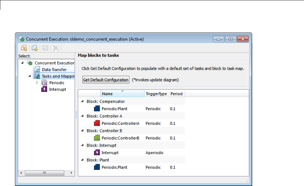
11 Configuring Models for Targets with Multicore Processors
•Control over how data is communicated between tasks
11-6
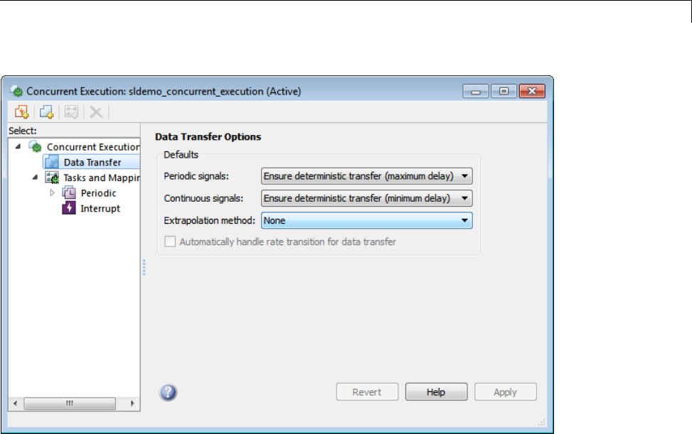
Design Considerations
•Simulation of a mapped model that allows you to validate a desired
functionality against the data transfer requirements of a particular
mapping
To validate if a particular mapping is an acceptable design, first validate that
the mapped model produces the desired simulation traces. Simulation results
vary from mapping to mapping because each mapping imposes communication
(data transfer) requirements that might cause the Simulink software to treat
certain signal lines as delays for data transfer. Ultimately, however, you
must evaluate the mapping on the target, and profile the behavior to measure
whether the mapping meets the computational requirements and makes
good use of the available computational power of the target platform. This
evaluation and profiling are beyond the scope of the software.
Identifying Opportunities for Concurrent Execution
To use the software mapping interface, a model must first specify
opportunities for concurrency by identifying blocks for concurrent execution.
11-7

11 Configuring Models for Targets with Multicore Processors
Use Model blocks (referenced models) to identify potential opportunities for
concurrent execution. A Model block defines a unit of functionality that the
software can map for execution in one or more target tasks. More precisely,
you can map a multirate Model block that contains Nrates to exactly Ntasks,
the periodicity of which agree with the respective rates. You can map several
Model blocks to the same task. Map a Model block that contains continuous
blocks to a task, the period of which agrees with the fundamental sample time
of the model. You can specify the fundamental sample time of the model in
the Fixed-step size (fundamental sample time) of the Solver pane in the
Configuration Parameters dialog box.
Because Model blocks must be used to express opportunities for concurrency,
a design must consist entirely of Model blocks. You can also use virtual
connectivity blocks to organize the block diagram, including:
•Goto and From blocks
•Ground and Terminator blocks
•Inport and Outport blocks
•Virtual subsystem blocks that contain permitted blocks
A model configured for concurrent execution reports an error diagnostic if any
other blocks are detected. Place all other blocks in one or more referenced
models.
Also consider signal lines when designing for concurrent execution. Depending
on the mapping, any signal line can potentially be identified as a data transfer
point. In particular, if the source port of a signal originates in a block from
one task and the destination port is to a block in another task, the Simulink
software identifies that signal as a data transfer point.
Algebraic Loops
An algebraic constraint or algebraic loop might impose tight coupling
between tasks and can lead to severe computational penalties. Therefore, a
model configured for concurrent execution cannot contain algebraic loops or
algebraic constraints that originate from physical modeling in a referenced
model. This condition makes an algebraic loop fully contained in a task.
11-8

Design Considerations
However, the use of Model blocks might lead to artificial algebraic loops.
This condition might occur if Simulink cannot identify if a break point is
encapsulated within a referenced model. In such situations, use one of the
following methods to remove artificial algebraic loops:
•In the referenced model Configuration Execution dialog box, select Model
Referencing > Minimize algebraic loop occurrences.
•Insert a Memory or Unit Delay block as the first block at the relevant input
port of the referenced model.
Additionally, if the model is configured for the Embedded Coder target
(ert.tlc), in the Configuration Parameters dialog box, clear the Code
Generation > Interface > Single output/update function check box.
This last operation prevents optimizations that can lead to artificial algebraic
loops.
Simulation Limitations
When modeling for concurrent execution, configure the model to use the
fixed-step solver.
Do not use the following modes of simulation for models in the concurrent
execution environment:
•External mode
•Logging to MAT-files
•Processor-in-the-loop (PIL) simulation mode
•Software-in-the-loop (SIL) simulation mode
•If you are simulating your model using Rapid Accelerator mode, the
top-level model cannot contain a root level Inport block that outputs
function calls.
In the Configuration Parameters dialog box, set the Diagnostics > Sample
Time > Multitask conditionally executed subsystem and
Diagnostics > Data Validity > Multitask data store parameters to error.
In addition, for all Rate Transition blocks within the Model blocks:
11-9

11 Configuring Models for Targets with Multicore Processors
•Select the Ensure data integrity during data transfer check box.
•Clear the Ensure deterministic data transfer (maximum delay) check
box.
11-10

Modeling Process for Concurrent Execution
Modeling Process for Concurrent Execution
You can model for concurrent execution using the following general workflow.
These steps assume that you have a model that meets the modeling guidelines
in “Design Considerations” on page 11-5.
1Configure your model for concurrent execution.
2Perform baseline analysis of your model for concurrent execution.
3Explicitly set configuration values in the concurrent execution
configuration.
4Simulate the model and evaluate the results
5As necessary, refine the results.
6Build and download the model to the multicore target and evaluate the
results.
7As necessary, refine the results.
11-11

11 Configuring Models for Targets with Multicore Processors
Configure Your Model
You can use configuration references or configuration sets to configure a
model for concurrent execution.
If Your Model Has... Create...
A single-level model, or if it
has multiple descendants, such
as reference models, and the
descendants do not share the same
configuration settings.
A configuration set for a single
model. For more information, see
“Creating a Concurrent Execution
Configuration Set” on page 11-12.
A top-level model and multiple
descendants, such as referenced
models, all of which share the same
configuration settings.
A configuration reference object that
can be shared between all models in
the hierarchy. For more information,
see “Creating and Propagating a
Configuration Reference” on page
11-13.
Creating a Concurrent Execution Configuration Set
You can create a concurrent execution configuration set from an existing
configuration set, or create a new configuration set:
1In the Simulink model editor, select View > Model Explorer.
The Model Explorer window is displayed.
2In the Model Explorer window:
11-12

Configure Your Model
To... Do...
Preserve existing configuration
settings for your model, convert
an existing configuration set to a
concurrent execution configuration
set.
Expand the node for the model.
Under the model, right-click
Configuration, then select Show
Concurrent Execution options.
Create new configuration settings,
add a new concurrent execution
configuration set.
Expand the node for the model.
Right-click the model node and
select Configuration > Add
Configuration for Concurrent
Execution.
Activate the configuration set
by right-clicking it and selecting
Activate.
3In the third column of the Model Explorer window, the Solver pane is
updated to display an Allow tasks to execute concurrently on target
check box. Click the Configure Tasks button.
If you want to create a configuration reference, see “Creating and Propagating
a Configuration Reference” on page 11-13. Otherwise, to begin configuring the
model for concurrent execution, see “Baseline Analysis Using Configuration
Defaults” on page 11-17.
Creating and Propagating a Configuration Reference
This topic assumes that you have an existing concurrent execution
configuration. If you have not yet created one, see “Creating a Concurrent
Execution Configuration Set” on page 11-12.
For more information on configuration references, see “About Configuration
References” on page 10-29. This topic describes one way to create and
propagate a configuration reference.
1In the Simulink model editor, select View > Model Explorer.
The Model Explorer window is displayed.
11-13
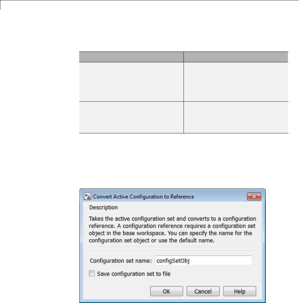
11 Configuring Models for Targets with Multicore Processors
2In the Model Explorer window, expand the node for the model and do one
of the following:
To... Do...
Preserve existing configuration
settings for your model, convert
an existing configuration set to a
concurrent execution configuration
set.
Right-click and select
Configuration > Show
Concurrent Execution options.
Create new configuration settings,
add a new concurrent execution
configuration set.
Right-click and select
Configuration > Add
Configuration for Concurrent
Execution.
3Activate the configuration set by right-clicking it and selecting Activate.
4In the Model Hierarchy column, right-click Configuration > Convert to
Configuration Reference.
A Convert Active Configuration to Reference dialog box is displayed.
5Click OK to accept the default name for the configuration reference.
11-14
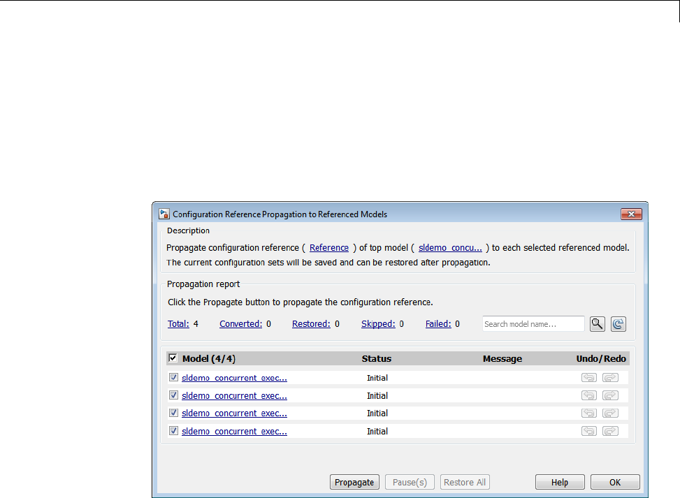
Configure Your Model
The configuration is converted to a configuration reference.
6To share the configuration reference with the other referenced models in
the model hierarchy, activate the configuration reference, then right-click
it and select Configuration > Propagate to Referenced Models.
A Propagate to Referenced Models dialog box is displayed.
7Click Propagate to propagate the configuration reference.
A propagation confirmation dialog box is displayed.
8Click OK to continue.
The hierarchy of each referenced model is updated with the configuration
reference.
9Click OK.
10 In the Model Explorer, in the left column, select the Reference (Active)
node.
11-15
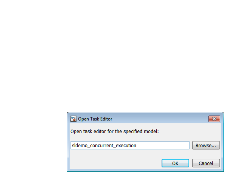
11 Configuring Models for Targets with Multicore Processors
The right column changes to display the Configuration Parameters
reference pane.
11 In the Configuration Parameters reference pane, click the Open button
of the Referenced configuration parameter.
The Configuration Parameters dialog box is displayed.
12 Navigate to the Solver node.
13 Click the Allow tasks to execute concurrently on target check box
and click Configure Tasks button.
The Open Task Editor dialog window is displayed.
Consider saving the configuration reference to MAT-file if you want to use
it in future MATLAB sessions. To save the configuration reference named
configSetObj, enter the following command in the MATLAB Command
Window:
save configsetobj.mat configSetObj
To load the saved configuration reference into another MATLAB session,
enter the following command in the MATLAB Command Window:
load configsetobj.mat
To begin configuring the model for concurrent execution, see “Baseline
Analysis Using Configuration Defaults” on page 11-17.
11-16

Baseline Analysis Using Configuration Defaults
Baseline Analysis Using Configuration Defaults
Perform an automatic baseline analysis of the model. This step allows you to
identify initial bottlenecks in the model execution.
1In the Concurrent Execution dialog box, select the Tasks and Mapping node.
The Map blocks to tasks pane is displayed.
2Click the Get Default Configuration button.
3Select Yes in the resulting dialog box.
This button updates the diagram.
Upon a successful update, the software:
•Creates one periodic task for each periodic sample time in the model.
•Creates one aperiodic trigger for each function-call input in the model.
•Configures the block-to-task mapping so that each block maps to a task
based on sample time analysis.
If the software reports a diagnostic during the update phase, the analysis
might not complete. In this case, address the modeling issues reported in the
diagnostics before continuing.
The following is the automatic baseline analysis for the
sldemo_concurrent_execution model.
11-17
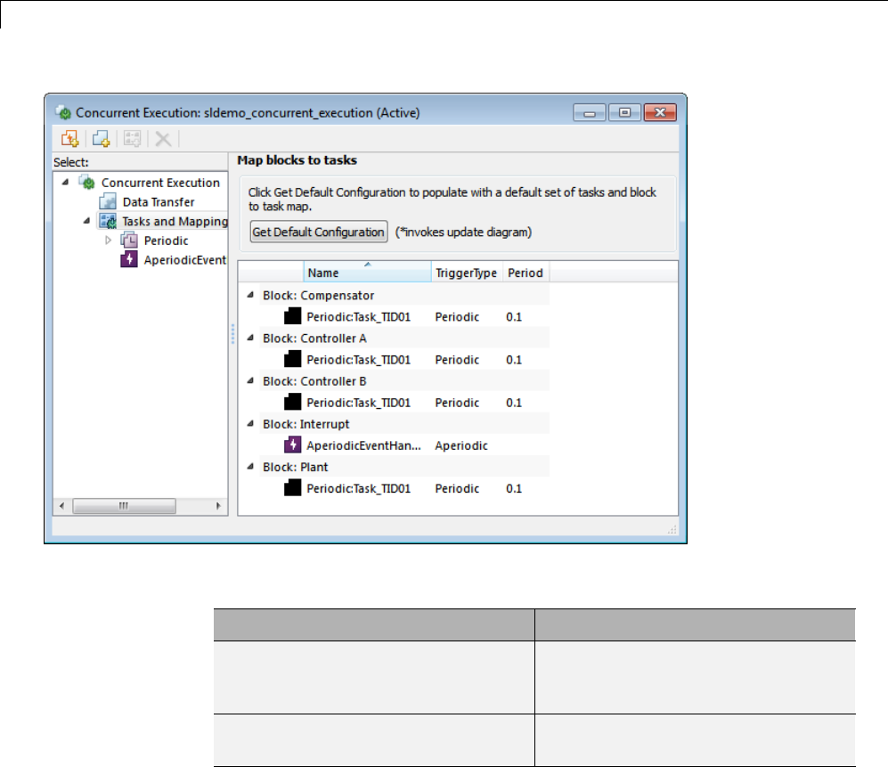
11 Configuring Models for Targets with Multicore Processors
When the analysis is complete, decide on your next step.
To... Go to...
Explicitly configure how data is
transferred to override the settings
detected by automatic analysis.
“Customize Concurrent Execution
Settings” on page 11-19
Simulate the model. “Interpret Simulation Results” on
page 11-26
11-18

Customize Concurrent Execution Settings
Customize Concurrent Execution Settings
After you set configuration defaults using automatic analysis, you might want
to fine-tune simulation results by performing operations such as explicitly
creating a different number of tasks or setting data transfer parameters.
Note If you do not want to customize concurrent execution settings, in
the Concurrent Execution pane clear the Enable explicit model
partitioning for concurrent behavior check box. Clearing this check box
allows the model to use rate-based tasks and ignores task-to-block mappings.
Configuring Data Transfer Communications
Use the Data Transfer Options pane to define communications between
tasks.
Data Transfer Options
Data Transfer Type Simulation Deployment
Ensure data integrity
only.
Data transfer is
simulated using a
one-stepdelay.
Simulink Coder ensures
data integrity during
data transfer. Data is
transferred as soon as
possible.
Ensure deterministic
transfer (maximum
delay).
Data transfer is
simulated using a
one-step delay.
Ensure deterministic
transfer (minimum
delay).
Data transfer occurs
within the same step.
Simulink Coder
ensures data transfer
is identical with
simulation.
•For continuous signals, the Simulink software uses extrapolation methods
to compensate for numerical errors that were introduced due to delays
and discontinuities in data transfer.
•For signals that are configured for Ensure Data Integrity Only and
Ensure deterministic transfer (maximum delay) data transfers, you
11-19
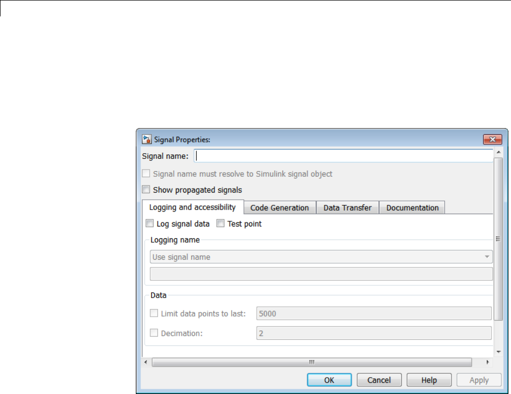
11 Configuring Models for Targets with Multicore Processors
might need to provide an initial condition to avoid numerical errors. You
can specify this initial condition in the Data Transfer tab of the Signal
Properties dialog box. To access this dialog box, right-click the signal
line and select Properties from the context menu. A dialog box like the
following is displayed.
1From the Data Transfer Options on page 11-19 table, determine how you
want your tasks to communicate.
2In the Concurrent Execution dialog box, select Data Transfer defaults
and apply the settings from step 1.
11-20

Customize Concurrent Execution Settings
3Apply your changes.
Configuring Periodic Tasks
Ifyouwanttoexploretheeffectsofincreasing the concurrency on your model
execution, you can create additional periodic tasks in your model.
1In the Concurrent Execution dialog box, right-click on the Periodic node
and select Add task.
A task node appears in the Configuration Execution hierarchy.
2Select the task node and enter a name and period for the task, then click
Apply.
The task node is renamed to the name you enter.
3Optionally, specify a color for the task. The color illustrates the
block-to-task mapping. If you do not assign a color, Simulink chooses a
11-21

11 Configuring Models for Targets with Multicore Processors
default color. If you enable sample time colors for your model, the software
honors the setting.
4Click Apply as necessary.
When the periodic tasks are complete, configure the aperiodic (interrupt)
tasks as necessary. If you do not need aperiodic tasks, continue to “Mapping
Blocks to Tasks” on page 11-24.
Configuring Aperiodic Triggers and Tasks
1To create an aperiodic trigger, in the Concurrent Execution dialog box,
right-click the Concurrent Execution node and click the Add aperiodic
trigger icon.
AnodenamedInterruptNappears in the configuration tree hierarchy.
2Select Interrupt.
This node represents an aperiodic trigger for your system.
3Specify the name of the trigger and configure the aperiodic trigger source.
Depending on your deployment target, choose either Posix Signal
(Linux/VxWorks 6.x) or Event (Windows).ForPOSIX
®signals, specify
the signal number to use for delivering the aperiodic event. For Windows
events, specify the name of the event.
11-22
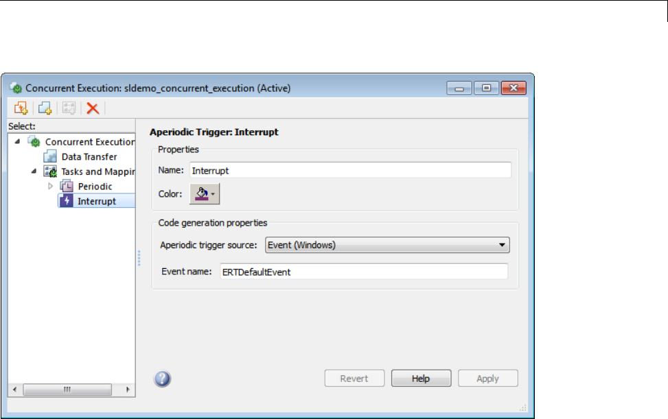
Customize Concurrent Execution Settings
4Click Apply.
Thesoftwareservicesaperiodictriggers as soon as the system can respond to
the trigger. If you want to process the trigger response using a task:
1Right-click the Interrupt node and select Add task.
A new task node appears under the Interrupt node.
2Specify the name of the new task node.
3Optionally, specify a color for the task. The color illustrates the
block-to-task mapping. If you do not assign a color, Simulink chooses
a default color.
4Click Apply.
11-23

11 Configuring Models for Targets with Multicore Processors
Youcandeletetasks(bothperiodicandaperiodic)aswellastriggersby
right-clicking them in the pane and selecting Delete.
When the aperiodic tasks are complete, continue to “Mapping Blocks to
Tasks” on page 11-24.
Mapping Blocks to Tasks
After you simulate and evaluate a model that has automatic analysis defaults,
you are likely to want to redo the block-to-task mappings. If you have
specified new tasks and triggers explicitly, you must map the blocks to the
newly created tasks and triggers.
1In the Concurrent Execution dialog box, click the Tasks and Mapping node.
The Map blocks to tasks pane appears.
2If you changed the model by adding or removing blocks, consider using
automatic analysis by clicking the Get Default Configuration button.
If you added a new Model block, a select task entry appears under the
block.
3If you want to add a new task to a block, in the Name column, right-click a
task under the block and select add new entry.
4To assign a task for the entry, left-click the box in the Name column and
select a task from the list. For example:
11-24
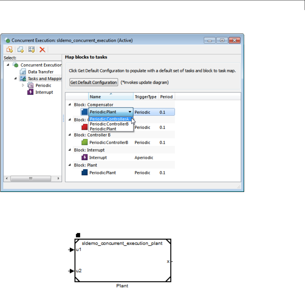
Customize Concurrent Execution Settings
The block-to-task mapping icon appears on the top-left corner of the Model
block. If a Model block is assigned to multiple tasks, multiple task icons
are displayed in the top-left corner. For example:
5Click Apply.
When the mapping is complete, simulate the model again (see “Interpret
Simulation Results” on page 11-26).
11-25

11 Configuring Models for Targets with Multicore Processors
Interpret Simulation Results
In this section...
“Introduction” on page 11-26
“Default Configuration” on page 11-27
“Sample Configured Model with Multiple Target Tasks” on page 11-28
“How Simulink Determines Data Transfer Requirements” on page 11-31
Introduction
A model configured for concurrent execution is a model that is designed
to execute concurrently on a real-time multicore target. Simulink enables
you to simulate such models and observe the effects of task-to-task data
transfer. You can also observe how this transfer can impact the numerical
characteristics of the model.
Note The simulation itself does not require a multicore target. The number
of tasks that you use to simulate the design is determined by other factors
and does not impose any requirements on the number of tasks modeled by
the design. Factors that influence the concurrency of the simulation include
the use of the Basic Linear Algebra Subprograms (BLAS) library, Rapid
Accelerator mode, and the MATLAB parfor command.
Consider the model sldemo_concurrent_execution.Tounderstand
simulation results, compare the signal xin two scenarios:
•Default configuration — The target has exactly one periodic task and all
blocks are mapped to execute within this task. In this configuration, the
target does not allow for any concurrent execution.
•Sample configuration — The target has three periodic tasks and all blocks
are mapped to execute concurrently in these tasks.
11-26
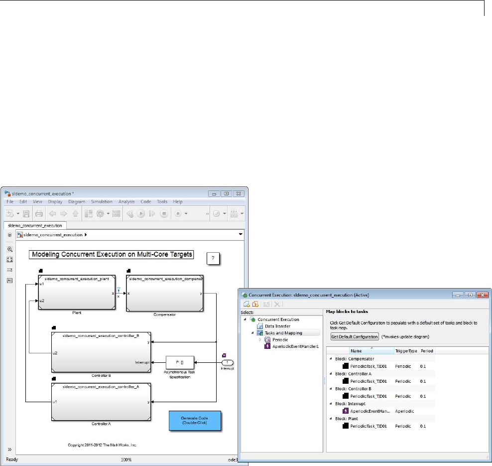
Interpret Simulation Results
Default Configuration
In the following example, the model is configured as described in “Baseline
Analysis Using Configuration Defaults” on page 11-17. Because this model
contains only one sample time (continuous sample time), the automatic
analysis configures the target with one task and maps all blocks to run in that
task. The period of the task is selected as 0.1, which agrees with the fixed-step
size of the model. Because the design has only one task, no task-to-task
data transfer is needed. Therefore, simulation of the model should produce
the same numeric results as if the model is not configured for concurrent
execution.
11-27

11 Configuring Models for Targets with Multicore Processors
Note Configuring a model with automatic analysis always configures a model
to minimize task-to-task communication requirements. In particular, only
those communications that require rate transitions are included in the design.
Configure the model to inspect data using the Simulation Data Inspector by
clicking the Record & Inspect Simulation Output button in the toolbar.
(Alternatively, in the Configuration Parameters dialog box, select the Data
Input and Output > Record and inspect simulation output button).
After you enable the Simulation Data Inspector, click Simulate > Run to
simulate the model using the single task configuration. After simulation,
launch the Simulation Data Inspector as directed in the editor. Observe that
the tool has recorded the simulation results for the signal labeled x.
Sample Configured Model with Multiple Target Tasks
In the Concurrent Execution dialog box, create two additional tasks and map
the ControllerA block to the first additional task and the ControllerB block to
the second additional task.
1Open the Concurrent Execution dialog box.
2Click the Add Task button twice.
3Select the first added task and label it ControllerA.
4Select the second added task and label it ControllerB.
5In the Map blocks to tasks pane, check that the ControllerA block is
assigned to execute within the ControllerA task and the ControllerB block
is assigned to execute within the ControllerB task.
11-28
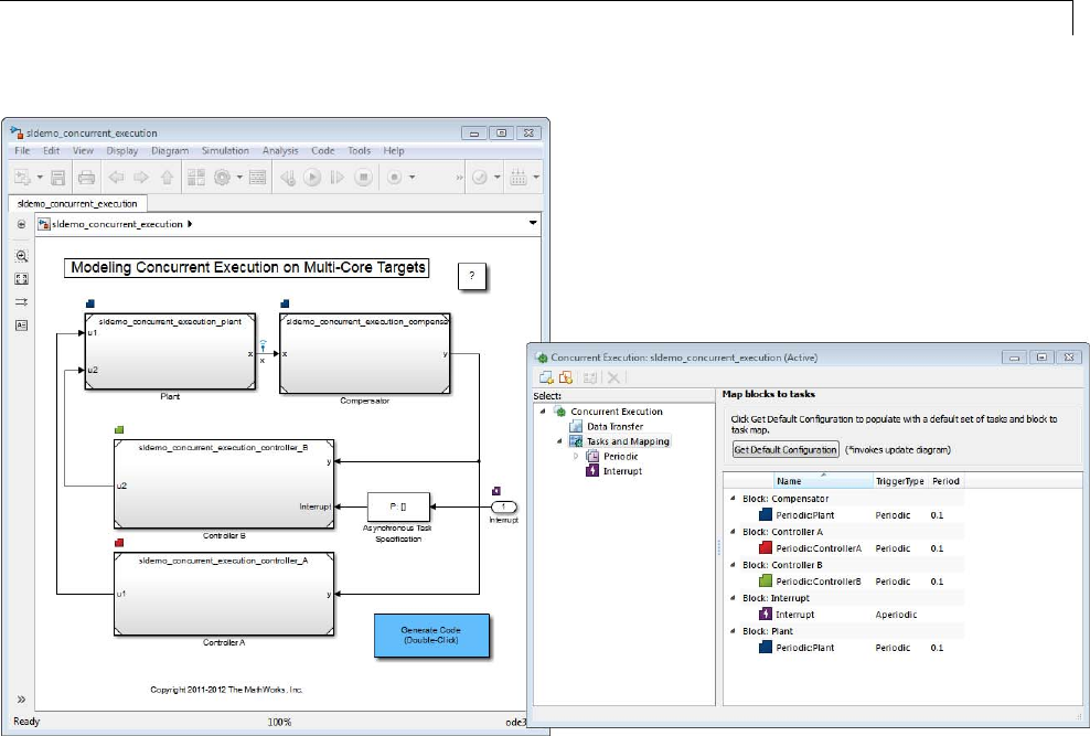
Interpret Simulation Results
6Simulate the model again.
7After simulation completes, compare the results for the default and custom
configurations using the Simulation Data Inspector.
11-29
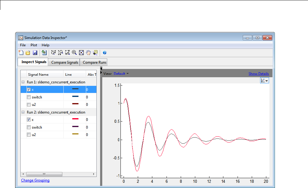
11 Configuring Models for Targets with Multicore Processors
To understand the source of the phase margin, observe that:
•For the first run of the model, signal x, identified by the black line, shows a
default task configuration.
•In the second run of the model, signal x, identified by the red line, shows a
custom task configuration and the effects of communication latencies from
lines crossing task boundaries. This is different from the first run, which
has only one periodic task and therefore, no communication latencies.
•The default setting for data transfer is to ensure determinism, so the data
transfer is deterministic (see Data Transfer Options on page 11-19).
Because the data transfer is deterministic, the simulated model takes into
account a unit delay to capture the effects of data transfer. This delay causes
a small phase margin in the mapped design. The delay agrees with the step
size of the model, which is 0.1. This delay is the least possible delay that the
software can impose on the signal.
11-30

Interpret Simulation Results
How Simulink Determines Data Transfer
Requirements
The software determines data transfer based on how the blocks are mapped to
tasks. When a model is simulated, either from an update diagram or upon
code generation, Simulink software examines the block-to-task mapping
and determines which signals must be configured for task-to-task data
transfer. The software considers only the signals where the source of the
signal originates from one task and the destination of the signal resides in a
different task. You can specify global options that control data transfer (see
Data Transfer Options on page 11-19). You can also override these options for
each signal from the Data Transfer pane of the Signal Properties dialog box.
Therefore, the block-to-task mapping dictates which blocks execute in which
tasks. Consequently, this mapping also dictates which signals you configure
for task-to-task data transfer.
11-31

11 Configuring Models for Targets with Multicore Processors
Build and Download to a Multicore Target
In this section...
“Generating Code” on page 11-32
“Configuring Embedded Coder for Native Threads Example” on page 11-42
“Build and Download” on page 11-43
“Profile and Evaluate” on page 11-44
Generating Code
To generate code, in the Simulink editor window, select Tools > Code
Generation > Build Model. This code can run concurrently on a multicore
target with Simulink Coder or Embedded Coder software. The coder generates
all target-dependent code for thread creation, thread synchronization,
interrupt service routines, and signal handlers and data transfer. The source
files of the mapped model (for example, model.c and model.h)donotcontain
target-dependent code for setting up the execution of threads. However,
target-dependent code might exist for data transfer types, which generate
target-specific data protection or semaphore application programming
interface (API) calls.
Foreachperiodictask,SimulinkCoder combines the output and update
methods of the blocks mapped to that task and binds these methods to a
target-specific thread. Additionally, for each periodic task that contains
continuous states, a separate solver instance is generated in the source file of
the mapped model. This mapped model can concurrently run the continuous
parts of the model. (The generated solver instances share the solver type
specified in the Solver of the Configuration Parameters dialog box of the
mapped model.)
For each aperiodic task or aperiodic trigger, Simulink Coder combines the
output and update methods of the blocks mapped to that task and binds these
to a target-specific Interrupt Service Routine (ISR) or to a target-specific
event handler.
Following is an example of generated code in the source file of a mapped
model. This code shows the functions generated for the mapped model:
11-32

Build and Download to a Multicore Target
•Two solver instances
•Three periodic tasks with two of them having continuous states
•Two aperiodic tasks
•Two aperiodic triggers
/*
* This function updates continuous states using the ODE3 fixed-step
* solver algorithm
*/
static void Periodic_Task1_rt_ertODEUpdateContinuousStates(RTWSolverInfo *si )
{}
/*
* This function updates continuous states using the ODE3 fixed-step
* solver algorithm
*/
static void Periodic_Task2_rt_ertODEUpdateContinuousStates(RTWSolverInfo *si )
{}
/* OutputUpdate for Task: Periodic_Task1 */
void Periodic_Task1_step(void) /* Sample time: [0.1s, 0.0s] */
{
Periodic_Task1_rt_ertODEUpdateContinuousStates(&task_M[0]->solverInfo);
}
/* OutputUpdate for Task: Periodic_Task2 */
void Periodic_Task2_step(void) /* Sample time: [0.2s, 0.0s] */
{
Periodic_Task2_rt_ertODEUpdateContinuousStates(&task_M[1]->solverInfo);
}
/* OutputUpdate for Task: Periodic_Task3 */
void Periodic_Task3_step(void) /* Sample time: [0.1s, 0.0s] */
{}
11-33

11 Configuring Models for Targets with Multicore Processors
/* OutputUpdate for Task: Periodic_Task4 */
void Periodic_Task4_step(void) /* Sample time: [0.2s, 0.0s] */
{}
/* OutputUpdate for Task:Interrupt1_asyncTask1 */
void Interrupt1_asyncTask1(void)
{}
/* OutputUpdate for Task:Interrupt2_asyncTask2 */
void Interrupt2_asyncTask2(void)
{}
/* OutputUpdate for Task:Interrupt3 */
void Interrupt3(void)
{}
/* OutputUpdate for Task:Interrupt4 */
void Interrupt4(void)
{}
In addition, for continuous signals, the coder produces code for the
extrapolation method that you select. There are four types of extrapolation
methods: zero-order hold, linear, quadratic, and none. None is an ideal case
when the two communicating tasks synchronize in minor steps.
The following code snippets contain the generated task functions in the source
file of the mapped model. The sldemo_concurrent_execution model has
been modified so that:
•ControllerA/u1 uses Ensure data Integrity only option in the Signal
Properties dialog box.
•Plant is remapped to a new task that executes concurrently with
Compensator. The data transfer from Plant to Compensator is Ensure
deterministic transfer (minimum delay).
The coder makes sure that the data transfer between concurrently executing
tasks behave as described Data Transfer Options on page 11-19.
11-34

Build and Download to a Multicore Target
Generate Code to Share Data in a Concurrent Environment
For Ensure data integrity only, the generated code allows data to be
shared in a concurrent environment. This is achieved with a double-buffer
algorithm (for same rate data transfer) and a triple buffer algorithm (for
rate-transition data transfer) and target-specific protection code for the buffer
flag management. The following example shows code generated using the
sldemo_concurrent_execution model:
1Open the Signal Properties dialog box for ControllerA/u1 and select Data
Integrity Only as the data transfer handling option from the Data
Transfer pane.
2To generate code, select Code > C/C++ Code > Build Model.
The coder generates code like the following. This code is for ControllerA/u1
on the Linux platform.
/* Output for Task: Periodic_ControllerA */
void Periodic_ControllerA_output(void) /* Sample time: [0.1s, 0.0s] */
{
/* TaskTransBlk: '<Root>/TaskTransAtController AOut1' */
sldemo_concurrent_execution_DWork.
TaskTransAtControllerAOut1_buf_3[sldemo_concurrent_execution_DWork.fw_buf_3]
= sldemo_concurrent_execution_B.ControllerA;
rtw_pthread_mutex_lock(sldemo_concurrent_execution_DWork.mw_buf_3);
sldemo_concurrent_execution_DWork.fw_buf_3 = 1 -
sldemo_concurrent_execution_DWork.fw_buf_3;
rtw_pthread_mutex_unlock(sldemo_concurrent_execution_DWork.mw_buf_3);
}
/* Output for Task: Periodic_Plant */
void Periodic_Plant_output(void) /* Sample time: [0.0s, 0.0s] */
{
if (rtmIsMajorTimeStep(task_M[2])) {
/* TaskTransBlk: '<Root>/TaskTransAtPlantIn1' */
rtw_pthread_mutex_lock(sldemo_concurrent_execution_DWork.mw_buf_3);
wrBufIdx = 1 - sldemo_concurrent_execution_DWork.fw_buf_3;
rtw_pthread_mutex_unlock(sldemo_concurrent_execution_DWork.mw_buf_3);
sldemo_concurrent_execution_B.TaskTransAtPlantIn1 =
11-35

11 Configuring Models for Targets with Multicore Processors
sldemo_concurrent_execution_DWork.TaskTransAtControllerAOut1_buf_3[wrBufIdx];
}
}
void MdlInitialize(void)
{
sldemo_concurrent_execution_DWork.fw_buf_3 = 0;
rtw_pthread_mutex_init(&sldemo_concurrent_execution_DWork.mw_buf_3);
}
Generate Code for Maximum Capacity During Data Transfer
For Ensure deterministic transfer (maximum delay), the generated
code for the task transition is ANSI®C code with writing and reading to
and from double buffers. In the Signal Properties dialog box, you provide a
value for the Initial Condition value that initializes the buffer used for the
first read operation.
The software generates code like the following. This example is for
ControllerB/u1 on the Linux platform.
/* Output for Task: Periodic_ControllerB */
void Periodic_ControllerB_output(void) /* Sample time: [0.1s, 0.0s] */
{
sldemo_concurrent_execution_DWork.
TaskTransAtControllerBOut1_buf_4[sldemo_concurrent_execution_DWork.fw_buf_4]
= sldemo_concurrent_execution_B.ControllerB;
sldemo_concurrent_execution_DWork.fw_buf_4 = 1 -
sldemo_concurrent_execution_DWork.fw_buf_4;
}
/* Output for Task: Periodic_Plant */
void Periodic_Plant_output(void) /* Sample time: [0.0s, 0.0s] */
{
if (rtmIsMajorTimeStep(task_M[2])) {
11-36

Build and Download to a Multicore Target
/* TaskTransBlk: '<Root>/TaskTransAtPlantIn2' */
sldemo_concurrent_execution_B.TaskTransAtPlantIn2 =
sldemo_concurrent_execution_DWork.
TaskTransAtControllerBOut1_buf_4[sldemo_concurrent_execution_DWork.fr_buf_4];
sldemo_concurrent_execution_DWork.fr_buf_4 = 1 -
sldemo_concurrent_execution_DWork.fr_buf_4;
}
}
void MdlInitialize(void)
{
/* InitializeConditions for TaskTransBlk: '<Root>/TaskTransAtController BOut1' */
sldemo_concurrent_execution_DWork.fw_buf_4 = 0;
}
Generated Code for Maximum Data Integrity During Data
Transfer
For Ensure deterministic transfer (minimum delay), the generated code
for the data transfer makes sure that the task reading the data is waiting
for the task writing the data to complete its computation of the data. This
behavior produces target-specific code for data synchronization (for example,
semaphores).
The software generates code like the following. This example code is for
Plant/x on the Linux platform.
/*
* This function updates continuous states using the ODE3 fixed-step
* solver algorithm
*/
11-37

11 Configuring Models for Targets with Multicore Processors
static void Periodic_Compensator_rt_ertODEUpdateContinuousStates(RTWSolverInfo
*si )
{
/* TaskTransBlk: '<Root>/TaskTransAtCompensatorIn1' */
if (sldemo_concurrent_execution_DWork.br_buf_5) {
sldemo_concurrent_execution_DWork.br_buf_5 = FALSE;
} else {
rtw_pthread_sem_wait(sldemo_concurrent_execution_DWork.sw_buf_5);
sldemo_concurrent_execution_B.TaskTransAtCompensatorIn1 =
sldemo_concurrent_execution_DWork.TaskTransAtPlantOut1_buf_5;
rtw_pthread_sem_post(sldemo_concurrent_execution_DWork.sr_buf_5);
if (rtmIsMajorTimeStep(task_M[0])) {
sldemo_concurrent_execution_DWork.br_buf_5 = TRUE;
}
}
/* End of TaskTransBlk: '<Root>/TaskTransAtCompensatorIn1' */
}
/* Output for Task: Periodic_Plant */
void Periodic_Plant_output(void) /* Sample time: [0.0s, 0.0s] */
{
if (rtmIsMajorTimeStep(task_M[3])) {
/* TaskTransBlk: '<Root>/TaskTransAtPlantOut1' */
rtw_pthread_sem_wait(sldemo_concurrent_execution_DWork.sr_buf_5);
sldemo_concurrent_execution_DWork.TaskTransAtPlantOut1_buf_5 =
sldemo_concurrent_execution_B.x;
rtw_pthread_sem_post(sldemo_concurrent_execution_DWork.sw_buf_5);
}
void MdlInitialize(void)
{
/* InitializeConditions for TaskTransBlk: '<Root>/TaskTransAtPlantOut1' */
sldemo_concurrent_execution_DWork.fw_buf_5 = 0;
rtw_pthread_sem_create(&sldemo_concurrent_execution_DWork.sw_buf_5, 0);
}
11-38

Build and Download to a Multicore Target
Threading APIs
For Embedded Coder targets and generic real-time targets, the generated
code from a mapped model creates a thread for each task and automatically
leverages the threading APIs supported by the operating system running
on the host machine.
•If the host machine is a Windows platform, the generated code will create
and run Windows threads.
•If the host machine is Linux or Mac OS platform, the generated code will
create and run POSIX pthreads.
Aspect of
Concurrent
Execution
Linux
Implementation
Windows
Implementation
Mac OS
Implementation
Periodic triggering
event
POSIX timer Windows timer Not applicable
Aperiodic triggering
event
POSIX real-time
signal
Windows event POSIX non-real-time
signal
Aperiodic trigger For blocks mapped
to an aperiodic task:
thread waiting for a
signal
For blocks mapped to
an aperiodic trigger:
signal action
Thread waiting for an
event
For blocks mapped
to an aperiodic task:
thread waiting for a
signal
For blocks mapped to
an aperiodic trigger:
signal action
Threads POSIX Windows POSIX
11-39

11 Configuring Models for Targets with Multicore Processors
Aspect of
Concurrent
Execution
Linux
Implementation
Windows
Implementation
Mac OS
Implementation
Threads priority Assigned based on
sample time: fastest
task has highest
priority
Priority class
inherited from the
parent process.
Assigned based on
sample time: fastest
task has highest
priority for the first
three fastest tasks.
The rest of the tasks
share the lowest
priority.
Assigned based on
sample time: fastest
task has highest
priority
Example of overrun
detection
Yes Yes No
The data transfer between concurrently executing tasks behave as described
in Data Transfer Options on page 11-19. The coders use the following APIs on
supported targets for this behavior:
Data Protection and Synchronization APIs that Embedded Coder and Generic Real-Time
Targets Use
API Linux Implementation Windows
Implementation
Mac OS
Implementation
Data protection
API
•pthread_mutex_init
•pthread_mutex_-
destroy
•pthread_mutex_lock
•pthread_mutex_-
unlock
•CreateMutex
•CloseHandle
•WaitForSingleObject
•ReleaseMutex
•pthread_mutex_init
•pthread_mutex_-
destroy
•pthread_mutex_lock
•pthread_mutex_-
unlock
Synchronization
API
•sem_init
•sem_destroy
•CreateSemaphore
•CloseHandle
•sem_open
•sem_unlink
11-40

Build and Download to a Multicore Target
Data Protection and Synchronization APIs that Embedded Coder and Generic Real-Time
Targets Use (Continued)
API Linux Implementation Windows
Implementation
Mac OS
Implementation
•sem_wait
•sem_post
•WaitForSingle-
Object
•ReleaseSemaphore
•sem_wait
•sem_post
The main() code is always dynamically generated. The general structure of
the generated main file is depicted in the following pseudocode:
main()
{
Model_initialize();
For_each_periodic_task
{
Create_synchronization_event(periodic_task);
Create_thread(periodic_task);
}
For_each_aperiodic_task
{
Create_external_event(aperiodic_task);
Create_thread(aperiodic_task);
}
Create_timer();
Create_thread(Periodic_task_scheduler);
For_each_aperiodic_trigger
{
Hookup_isr_to_aperiodic_event();
}
Wait_for_stopping();
Cleanup();
Model_terminate();
return 0;
11-41

11 Configuring Models for Targets with Multicore Processors
}
Periodic_task_scheduler()
{
Wait_for_event_from_timer(clock);
For_each_periodic_task
{
If periodic_task has a sample time hit
Set the event to run the task
}
}
Periodic_Task()
{
Wait_for_event(Periodic_task_scheduler);
Run the appropriate periodic_task();
}
Aperiodic_Task()
{
Wait_for_aperiodic_event();
Run the appropriate aperiodic_task();
}
Isr()
{
Run the appropriate aperiodic_trigger ();
}
Configuring Embedded Coder for Native Threads
Example
To generate code for an Embedded Coder target, in the Configuration
Execution dialog box:
•Select the Code Generation > Templates > Generate an example
main program check box.
•From the Code Generation > Templates > Target Operating System
list, select NativeThreadsExample.
11-42
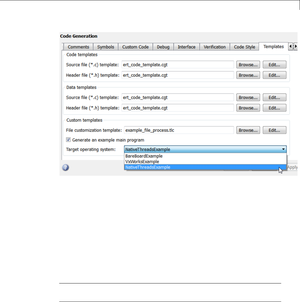
Build and Download to a Multicore Target
Build and Download
You can build and download concurrent execution models for the following
targets using system target files:
•Linux, Windows, and Mac OS using ert.tlc and grt.tlc.
•xPC Target using xpctarget.tlc and xpctargetert.tlc.
•Linux and Windows using idelink_ert.tlc and idelink_grt.tlc.
•Embedded Linux and VxWorks using idelink_ert.tlc and
idelink_grt.tlc.
Note Deploying to embedded Linux and VxWorks targets requires the
Embedded Coder product.
You cannot generate code for C++ (Encapsulated) language option.
11-43

11 Configuring Models for Targets with Multicore Processors
Profile and Evaluate
Profile the execution of your code on the multicore system using a
profiling tool like that provided in the xPC Target software. Profiling
lets you identify the areas in your model that are execution bottlenecks.
You can analyze the execution time of each task and find the task that
takes most of the execution time. For example, if you are using the xPC
Target profiling tool, you can compare the average execution times of the
tasks. If a task is computation-intensive, or does not satisfy real-time
requirements and overruns, you can break it into multiple tasks that are less
computation-intensive and that can run concurrently.
Based on this analysis, you can then explicitly change the mapping of Model
blocks to efficiently use the concurrency available on your multicore system
(see “Mapping Blocks to Tasks” on page 11-24).
11-44

Concurrent Execution Example Model
Concurrent Execution Example Model
For an interactive example of a model that has been configured to work in a
concurrent execution environment:
1In the MATLAB Command Window, click the question mark.
The Documentation Center window opens.
2Navigate to Simulink > Examples > Modeling Features > Modeling
Concurrency > Modeling Concurrent Execution on Multi-Core
Targets.
Modeling Concurrent Execution on Multi-Core Targets
This model shows how you can use Simulink and Simulink Coder™ to
realize concurrent execution of a model on a multicore target. Additionally,
the example also illustrates how simulation captures effects of on-target
concurrent execution, such as the transfer of data between tasks.
Example Requirements
If you want to generate code for this model, ensure that Simulink Coder™
is installed. Note, when you simulate the example, Simulink and Simulink
Coder™ might generate code in a Simulink project folder created in the
current working folder. If you do not want to (or cannot) generate files in this
folder, change the current working folder to a suitable folder.
topmdl = 'sldemo_concurrent_execution';
open_system(topmdl);
curDir = pwd;
cd(tempdir);
11-45
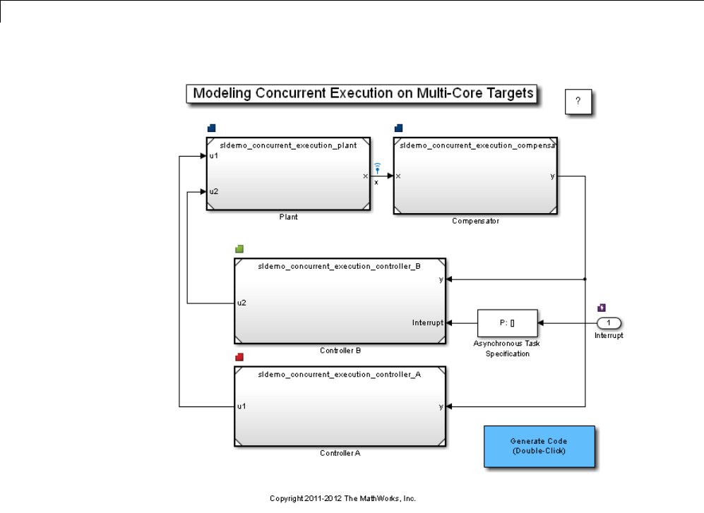
11 Configuring Models for Targets with Multicore Processors
Overview of the Model
To take advantage of the concurrent execution feature, use Model blocks to
partition your model into portions that can potentially execute concurrently.
Open the model and examine its partitioning into four Model blocks: Plant,
Compensator, ControllerA, and ControllerB. This example also shows how
you can specify and simulate the effects of asynchronous external inputs to
your system via the root input port Interrupt of ControllerB.
Starting with a Default Configuration
This model has been configured for concurrent execution on a target. For
more information, see the documentation.
11-46

Concurrent Execution Example Model
Use the Concurrent Execution dialog to configure your model for concurrent
executiononthetarget. OpentheConcurrent Execution dialog.
Each element of the Concurrent Execution dialog tree-view allows
configuration of the following model aspects:
•Data Transfer - Allows default configuration of the data transfer options
between tasks (you can override these by configuring each signal through
the signal properties dialog)
•Tasks and Mapping - Allows explicit mapping of blocks to tasks
•Periodic - Allows specification and configuration of periodic tasks
•Interrupt - Allows specification and configuration of aperiodic tasks
As a first step, set up the model to behave in non-concurrent fashion to identify
bottlenecks in execution. You can use the Get Default Configuration
buttonintheTasks and Mapping pane to do this. Alternatively, click on
the following link. You can now simulate the default configuration of the
model with all Model blocks mapped to a single periodic task Task_TID01 and
a single aperiodic trigger AperiodicEventHandler1.Observetheoutputs
of ControllerB in the scope.
11-47
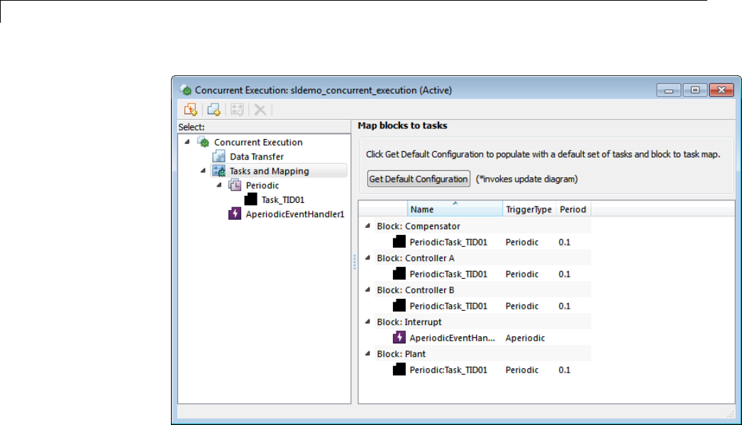
11 Configuring Models for Targets with Multicore Processors
Exploring Concurrent Execution
This example is a fairly simple model illustrating the basic elements of
concurrent execution. In a real-world application model, you might see
bottlenecks due to all blocks mapped to a single periodic task as with the
default configuration for this example.
Assume that you have significant computation in all four Model blocks which
needs to be mapped to separate tasks on a multicore target platform. To
experiment with a different mapping for the Model blocks, change the task
configuration to create new tasks, and map the blocks to the newly created
tasks. Do this automatically using the following link or by following the
instructions below.
To change the task mapping, first create tasks. Both periodic and aperiodic
tasks (not used in this model) are supported. Refer to the documentation for
more information about configuring aperiodic tasks.
11-48

Concurrent Execution Example Model
1Click the Add Task button on the toolbar to create a new task. You can
configure Name,Period (i.e., sample time) and Color of the newly created
task. Rename the task to Plant. Change the period attribute of the task to
be 0.1.ClicktheApplybuttontosaveyour changes. Similarly, create two
more tasks named ControllerA and ControllerB, both with period 0.1.
2Click the Add aperiodic trigger button on the toolbar to create a new
aperiodic trigger. You can configure an aperiodic trigger to generate
an aperiodic event, e.g., to simulate the effects of an interrupt on the
system. You can also configure the behavior of aperiodic triggers during
simulation and code generation. To configure the simulation behavior,
open the Configuration Parameters dialog box for the top-level model,
select the Data Import/Export pane, and select the Input check box. This
parameter specifies the time points at which the external aperiodic trigger
is generated. This example is pre-configured to generate the aperiodic
trigger at time points 4 and 7.
3Click Tasks and Mapping node. Change the mapping of
Block:Compensator by clicking the task Periodic:Task_TID01 in
the Name column and changing it to Periodic:Plant from the task
drop-down list. Similarly, change the mapping of Block:ControllerA to
Periodic:ControllerA,Block:ControllerB to Periodic:ControllerB,
Block:Plant to Periodic:Plant,andBlock:Interrupt to
AperiodicEventHandler1.
Now, simulate the model and examine the effects of your mapping. The
Simulink editor shows the inter task communication via the new icons on
the signals between the Model blocks. The icon on the signal indicates
that inter task communication introduces a unit delay in the communication
between each pair of tasks.
11-49
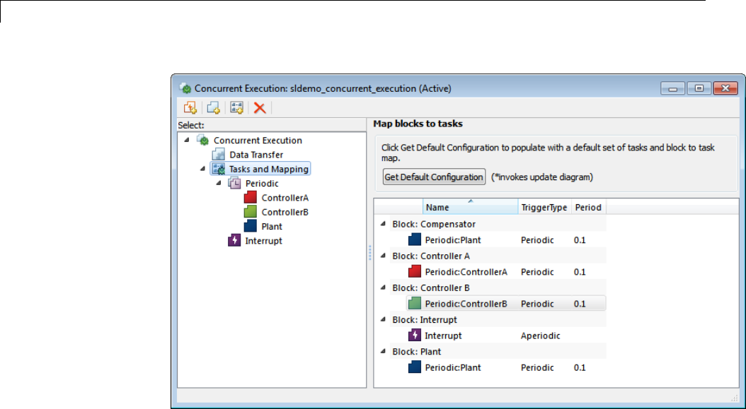
11 Configuring Models for Targets with Multicore Processors
% Enable the external inputs to the system.
set_param(topmdl, 'LoadExternalInput', 'on');
%Get Active Configuration Set
csTop = getActiveConfigSet(topmdl);
% Get the task configuration.
tc = csTop.concurrentExecutionComponents;
% Get the block handles for mapping.
plantBlkH = get_param([topmdl '/Plant'], 'Handle');
compensatorBlkH = get_param([topmdl '/Compensator'], 'Handle');
controlABlkH = get_param([topmdl '/Controller A'], 'Handle');
controlBBlkH = get_param([topmdl '/Controller B'], 'Handle');
interruptBlkH = get_param([topmdl '/Interrupt'], 'Handle');
% Delete any previously created tasks
periodicTrigger = tc.Triggers(1);
11-50

Concurrent Execution Example Model
periodicTasks = periodicTrigger.Tasks;
tnames = {periodicTasks.Name};
for i = 1:length(periodicTasks)
periodicTrigger.deleteTask(tnames{i});
end
% Delete Aperiodic Trigger
aperiodicTrigger = tc.Triggers(2);
tc.deleteTrigger(aperiodicTrigger);
% Create and configure new tasks.
plant = periodicTrigger.addTask('Plant');
controlA = periodicTrigger.addTask('ControllerA');
controlB = periodicTrigger.addTask('ControllerB');
interruptSource = tc.addAperiodicTrigger('Interrupt');
plant.Period = '0.1';
controlA.Period = '0.1';
controlB.Period = '0.1';
% Perform mapping of blocks to tasks.
tc.map(plantBlkH, plant);
tc.map(compensatorBlkH, plant);
tc.map(controlABlkH, controlA);
tc.map(controlBBlkH, controlB);
tc.map(interruptBlkH, interruptSource);
% Launch Concurrent Execution dialog
Simulink.SoftwareTarget.concurrentExecution(topmdl, ...
'OpenDialog', ...
'Configuration');
sim(topmdl);
Viewing Simulation Results
You can use the Simulation Data Inspector to view the simulation results.
Note that the output of Block:ControllerB (u2) becomes zero around points
4 and 7 because of the occurrence of the aperiodic event (switch). After the
event, the output continues to settle down to zero. To further observe the
11-51
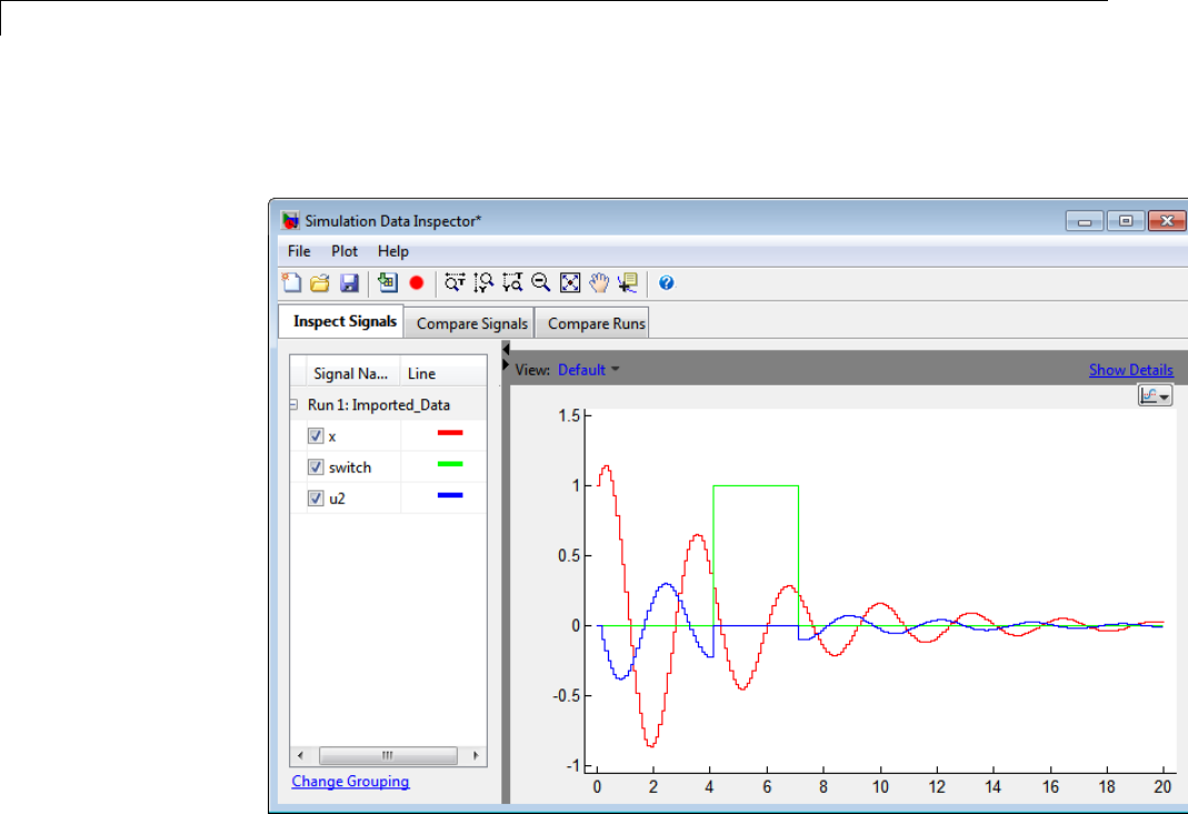
11 Configuring Models for Targets with Multicore Processors
effect of the aperiodic trigger on the system, alter the time points at which the
aperiodic event trigger is generated.
Configuring Inter Task Communication
You can change the modes of the inter task communication between the
Model blocks in the model to better suit design criteria. Do this by clicking
the following link or by following these instructions:
Click on Data Transfer node of the Concurrent Execution dialog. In the Data
Transfer Options pane, change Defaults > Periodic signals to Ensure
data integrity only by selecting it. Click Apply to save the changes.
Now, simulate the model. The lock icon on the signals between the Model
blocks indicates that data transfer between concurrent tasks is performed in
11-52

Concurrent Execution Example Model
data-integrity-only mode. For fine-grained control on the data transfer modes
between tasks at the level of individual signals, see the documentation.
Generating Code
1To generate code for the model, save the model after performing the
preceding steps. You can change to a temporary folder so that the original
example model remains unchanged.
2Depending on the host platform that you use for running this example, you
might need to change the code generation properties of the aperiodic trigger.
You can configure aperiodic triggers to generate code using POSIX signals
or Windows events. To generate code using POSIX signals to represent
the aperiodic triggers, select the AperiodicEventHandler1 node in the
Concurrent Execution dialog. For the ’Aperiodic trigger source’ parameter,
choose ’POSIX Signal (Linux/VxWorks 6.x)’. For the ’Signal number’
parameter, enter a valid signal number, [2, SIGRTMAX-SIGRTMIN-1], to
represent the POSIX signal to represent this aperiodic trigger. To generate
aperiodic triggers using Windows Events, for the ’Aperiodic trigger source’
parameter, choose ’Event (Windows)’. Enter a name to represent this
aperiodic trigger.
3Generate code from the model.
4In the code generation report, click grt_main.c to view the threads created
for tasks. Because you created three tasks in the task configuration, you
will see three threads created in the main() function. Depending on the
platform that you are using to view this example, you will see that either
Windows or POSIX threads are used for tasks. You will also see that either
Windows events or POSIX signal handlers are generated corresponding to
the aperiodic trigger.
5Open sldemo_concurrent_execution.c to view the output/update
functions that are mapped to tasks. For example, Periodic_Plant_output
corresponds to the task Plant,Periodic_ControllerA_output
corresponds to the task ControllerA, etc. Observe that a
function AperiodicEventHandler1 is generated for the aperiodic
trigger. This function is associated with a signal handler
sigHandler_AperiodicEventHandler1 generated in grt_main.c.Ifyou
chose Windows events, you will observe a similar function generated for
the aperiodic trigger.
11-53

11 Configuring Models for Targets with Multicore Processors
Closing the Models
close_system(topmdl, 0);
close_system([topmdl,'_plant'], 0);
close_system([topmdl,'_compensator'], 0);
close_system([topmdl,'_controller_A'], 0);
close_system([topmdl,'_controller_B'], 0);
cd(curDir);
Conclusion
This example illustrates a simple workflow using Simulink and Simulink
Coder™ to examine the effects of concurrent execution on a multicore
target. You can iteratively apply this workflow to optimize performance of a
real-world application on a multicore xPC Target™ environment, along with
the on-target profiling capability of xPC Target™.
11-54

Command-Line Interface
Command-Line Interface
The previous topics describe how to configure models for concurrent
execution using the Simulink Configuration Execution dialog box.
You can also perform the configuration using a command-line
interface. The following classes, their methods and properties, and the
Simulink.SoftwareTarget.concurrentExecution function comprise this
interface:
To... Use...
Create a configuration
set for concurrent
execution
Simulink.SoftwareTarget.concurrentExecution
Specify aperiodic
trigger
Simulink.SoftwareTarget.AperiodicTrigger
Specify periodic trigger Simulink.SoftwareTarget.PeriodicTrigger
Specify aperiodic
trigger for POSIX
targets
Simulink.SoftwareTarget.PosixSignalHandler
Specify task that
models unit of
concurrent execution
Simulink.SoftwareTarget.Task
Configure model for
concurrent execution
Simulink.SoftwareTarget.TaskConfiguration
Specify base class for
PeriodicTrigger and
AperiodicTrigger
Simulink.SoftwareTarget.WindowsEventHandler
Describe aperiodic
trigger for Windows
target
Simulink.SoftwareTarget.Trigger
Configure concurrent
execution data
transfers
Simulink.GlobalDataTransfer
11-55

11 Configuring Models for Targets with Multicore Processors
11-56

12
Modeling Best Practices
•“General Considerations when Building Simulink Models” on page 12-2
•“Model a Continuous System” on page 12-8
•“Best-Form Mathematical Models” on page 12-11
•“Model a Simple Equation” on page 12-15
•“Componentization Guidelines” on page 12-17
•“Modeling Complex Logic” on page 12-36
•“Modeling Physical Systems” on page 12-37
•“Modeling Signal Processing Systems” on page 12-38

12 Modeling Best Practices
General Considerations when Building Simulink Models
In this section...
“Avoiding Invalid Loops” on page 12-2
“Shadowed Files” on page 12-4
“Model Building Tips” on page 12-6
Avoiding Invalid Loops
You can connect the output of a block directly or indirectly (i.e., via other
blocks) to its input, thereby, creating a loop. Loops can be very useful. For
example, you can use loops to solve differential equations diagrammatically
(see “Model a Continuous System” on page 12-8) or model feedback control
systems. However, it is also possible to create loops that cannot be simulated.
Common types of invalid loops include:
•Loops that create invalid function-call connections or an attempt to
modify the input/output arguments of a function call (see “Function-Call
Subsystems”onpage7-30foradescription of function-call subsystems)
•Self-triggering subsystems and loops containing non-latched triggered
subsystems (see “Triggered Subsystems”onpage7-20intheUsing
Simulink documentation for a description of triggered subsystems and
Inport in the Simulink reference documentation for a description of
latched input)
•Loops containing action subsystems
The Subsystem Examples block library in the Ports & Subsystems library
contains models that illustrates examples of valid and invalid loops involving
triggered and function-call subsystems. Examples of invalid loops include
the following models:
•simulink/Ports&Subsystems/sl_subsys_semantics/Triggered
subsystem/sl_subsys_trigerr1 (sl_subsys_trigerr1)
•simulink/Ports&Subsystems/sl_subsys_semantics/Triggered
subsystem/sl_subsys_trigerr2 (sl_subsys_trigerr2)
12-2
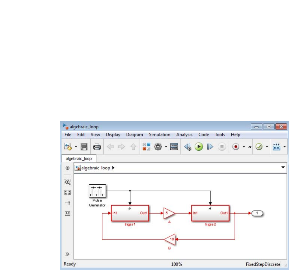
General Considerations when Building Simulink®Models
•simulink/Ports&Subsystems/sl_subsys_semantics/Function-call
systems/sl_subsys_fcncallerr3 (sl_subsys_fcncallerr3)
You might find it useful to study these examples to avoid creating invalid
loops in your own models.
Detecting Invalid Loops
To detect whether your model contains invalid loops, select Update Diagram
from the model’s Simulation menu. If the model contains invalid loops, the
invalid loops are highlighted. This is illustrated in the following model ,
and displays an error message in the Simulation Diagnostics Viewer.
12-3
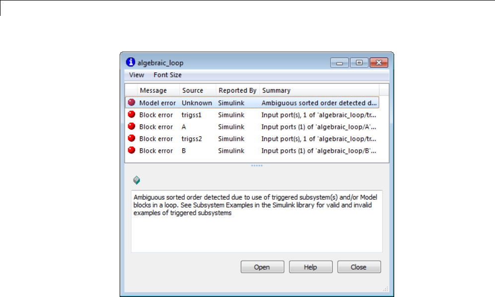
12 Modeling Best Practices
Shadowed Files
If there are two Model files with the same name (e.g. mylibrary.slx)on
the MATLAB path, the one higher on the path is loaded, and the one lower
onthepathissaidtobe"shadowed".
The rules Simulink software uses to find Model files are similar to those used
by MATLAB software. See "How the Search Path Determines Which Function
to Use" in the MATLAB documentation. However, there is an important
difference between how Simulink block diagrams and MATLAB functions are
handled: a loaded block diagram takes precedence over any unloaded ones,
regardless of its position on the MATLAB path. This is done for performance
reasons, as part of the Simulink software’s incremental loading methodology.
The precedence of a loaded block diagram over any others can have important
implications, particularly since a block diagram can be loaded without the
corresponding Simulink window being visible.
12-4

General Considerations when Building Simulink®Models
Making Sure the Correct Block Diagram Is Loaded
When using libraries and referenced models, a block diagram may be loaded
without showing its window. If the MATLAB path or the current MATLAB
folder changes while block diagrams are in memory, these block diagrams
may interfere with the use of other files of the same name. For example,
after a change of folder, a loaded but invisible library may be used instead
of the one the user expects.
To see an example:
1Enter sldemo_hydcyl4 to open the Simulink model sldemo_hydcyl4.
2Use the find_system command to see which block diagrams are in memory:
find_system('type','block_diagram')
ans =
'hydlib'
'sldemo_hydcyl4'
Note that a Simulink library, hydlib, has been loaded, but is currently
invisible.
3Now close sldemo_hydcyl4.Runthefind_system command again, and
you will see that the library is still loaded.
If you change to another folder which contains a different library called
hydlib, and try to run a model in that folder, the library in that folder would
not be loaded because the block diagram of the same name in memory takes
precedence. This can lead to problems including:
•Simulation errors
•"Bad Link" icons on blocks which are library links
•Wrong results
To prevent these conditions, it is necessary to close the library explicitly as
follows:
12-5

12 Modeling Best Practices
close_system('hydlib')
Then, when the Simulink software next needs to use a block in a library called
hydlib it will use the file called hydlib.slx which is highest on the MATLAB
path at the time. Alternatively, to make the library visible, enter:
open_system('hydlib')
Detecting and Fixing Problems
When updating a block diagram, the Simulink software checks the position
of its file on the MATLAB path and will issue a warning if it detects that
another file of the same name exists and is higher on the MATLAB path.
The warning reads:
The file containing block diagram 'mylibrary' is shadowed
by a file of the same name higher on the MATLAB path.
This may indicate that the wrong file called mylibrary.slx is being used. To
see which file called mylibrary.slx is loaded into memory, enter:
which mylibrary
C:\work\Model1\mylibrary.slx
To see all the files called mylibrary which are on the MATLAB path,
including MATLAB scripts, enter:
which -all mylibrary
C:\work\Model1\mylibrary.slx
C:\work\Model2\mylibrary.slx % Shadowed
To close the block diagram called mylibrary and let the Simulink software
load the file which is highest on the MATLAB path, enter:
close_system('mylibrary')
Model Building Tips
Here are some model-building hints you might find useful:
12-6

General Considerations when Building Simulink®Models
•Memory issues
In general, more memory will increase performance.
•Using hierarchy
More complex models often benefit fromaddingthehierarchyofsubsystems
to the model. Grouping blocks simplifies the top level of the model and can
make it easier to read and understand the model. For more information,
see “Create a Subsystem” on page 4-36. The Model Browser provides useful
information about complex models (see “Model Browser” on page 9-80).
•Cleaning up models
Well organized and documented models are easier to read and understand.
Signal labels and model annotations can help describe what is happening
in a model. For more information, see “Signal Names and Labels” on page
47-19 and “Annotate Diagrams” on page 4-23.
•Modeling strategies
If several of your models tend to use the same blocks, you might find it
easier to save these blocks in a model. Then, when you build new models,
just open this model and copy the commonly used blocks from it. You can
create a block library by placing a collection of blocks into a system and
saving the system. You can then access the system by typing its name in
the MATLAB Command Window.
Generally, when building a model, design it first on paper, then build it
using the computer. Then, when you start putting the blocks together
into a model, add the blocks to the model window before adding the lines
that connect them. This way, you can reduce how often you need to open
block libraries.
12-7
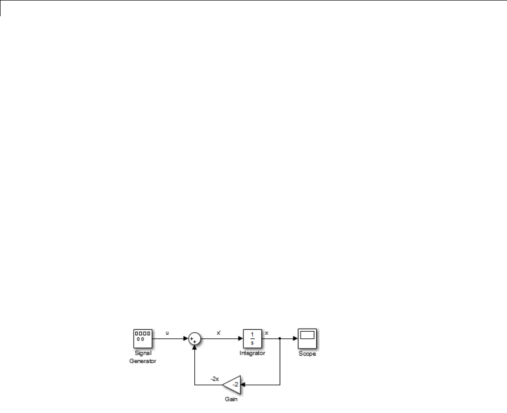
12 Modeling Best Practices
Model a Continuous System
To model the differential equation
x´=–2x(t)+u(t),
where u(t) is a square wave with an amplitude of 1and a frequency of 1
rad/sec, use an integrator block and a gain block. The Integrator block
integrates its input x´ to produce x. Other blocks needed in this model include
a Gain block and a Sum block. To generate a square wave, use a Signal
Generator block and select the Square Wave form but change the default
units to radians/sec. Again, view the output using a Scope block. Gather the
blocks and define the gain.
In this model, to reverse the direction of the Gain block, select the block, then
use the Diagram > Rotate & Flip > Flip Block command. To create the
branch line from the output of the Integrator block to the Gain block, hold
down the Ctrl key while drawing the line. For more information, see “Draw a
Branch Line” on page 4-16.
Now you can connect all the blocks.
An important concept in this model is the loop that includes the Sum block,
the Integrator block, and the Gain block. In this equation, xis the output of
theIntegratorblock. Itisalsotheinputtotheblocksthatcomputex´,on
which it is based. This relationship is implemented using a loop.
12-8
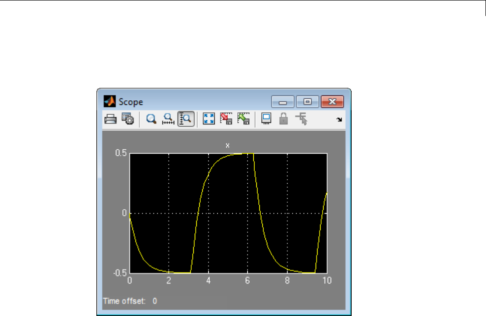
Model a Continuous System
The Scope displays xat each time step. For a simulation lasting 10 seconds,
theoutputlookslikethis:
The equation you modeled in this example can also be expressed as a transfer
function. The model uses the Transfer Fcn block, which accepts uas input
and outputs x. So, the block implements x/u. If you substitute sx for x´in
the above equation, you get
sx =–2x+u.
Solving for xgives
x=u/(s+2)
or,
x/u=1/(s+2).
The Transfer Fcn block uses parameters to specify the numerator and
denominator coefficients. In this case, the numerator is 1and the denominator
12-9

12 Modeling Best Practices
is s+2. Specify both terms as vectors of coefficients of successively decreasing
powers of s.
In this case the numerator is [1] (or just 1) and the denominator is [1 2].
The results of this simulation are identical to those of the previous model.
12-10
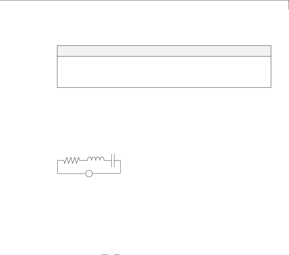
Best-Form Mathematical Models
Best-Form Mathematical Models
In this section...
“Series RLC Example” on page 12-11
“Solving Series RLC Using Resistor Voltage” on page 12-12
“Solving Series RLC Using Inductor Voltage” on page 12-13
Series RLC Example
You can often formulate the mathematical system you are modeling in several
ways. Choosing the best-form mathematical model allows the simulation to
execute faster and more accurately. For example, consider a simple series
RLC circuit.
RLC
VAC
According to Kirchoff’s voltage law, the voltage drop across this circuit is
equal to the sum of the voltage drop across each element of the circuit.
VVVV
AC R L C
=++
Using Ohm’s law to solve for the voltage across each element of the circuit,
the equation for this circuit can be written as
VRiL
di
dt C itdt
AC
t
=+ +−∞
∫
1()
You can model this system in Simulink by solving for either the resistor
voltage or inductor voltage. Which you choose to solve for affects the structure
of the model and its performance.
12-11
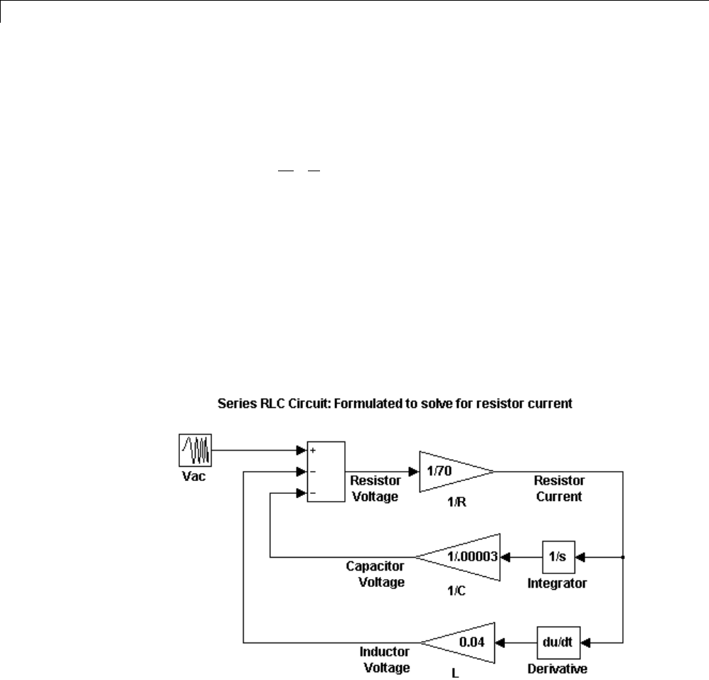
12 Modeling Best Practices
Solving Series RLC Using Resistor Voltage
Solving the RLC circuit for the resistor voltage yields
VRi
Ri V L di
dt C itdt
R
AC
t
=
=−−
−∞
∫
1()
Circuit Model
The following diagram shows this equation modeled in Simulink where Ris
70,Cis 0.00003,andLis 0.04. The resistor voltage is the sum of the voltage
source, the capacitor voltage, and the inductor voltage. You need the current
in the circuit to calculate the capacitor and inductor voltages. To calculate
the current, multiply the resistor voltage by a gain of 1/R. Calculate the
capacitor voltage by integrating the current and multiplying by a gain of 1/C.
Calculate the inductor voltage by taking the derivative of the current and
multiplying by a gain of L.
This formulation contains a Derivative block associated with the inductor.
Whenever possible, you should avoid mathematical formulations that
require Derivative blocks as they introduce discontinuities into your system.
Numerical integration is used to solve the model dynamics though time.
12-12

Best-Form Mathematical Models
These integration solvers take small steps through time to satisfy an accuracy
constraint on the solution. If the discontinuity introduced by the Derivative
block is too large, it is not possible for the solver to step across it.
In addition, in this model the Derivative, Sum, and two Gain blocks create
an algebraic loop. Algebraic loops slow down the model’s execution and can
produce less accurate simulation results. See “Algebraic Loops” on page 3-39
for more information.
Solving Series RLC Using Inductor Voltage
To avoid using a Derivative block, formulate the equation to solve for the
inductor voltage.
VL
di
dt
Ldi
dt VRi
Citdt
L
AC
t
=
=−−
−∞
∫
1()
Circuit Model
The following diagram shows this equation modeled in Simulink. The
inductor voltage is the sum of the voltage source, the resistor voltage, and the
capacitor voltage. You need the current in the circuit to calculate the resistor
and capacitor voltages. To calculate the current, integrate the inductor
voltage and divide by L. Calculate the capacitor voltage by integrating the
current and dividing by C. Calculate the resistor voltage by multiplying the
current by a gain of R.
12-13
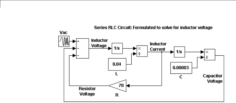
12 Modeling Best Practices
This model contains only integrator blocks and no algebraic loops. As a result,
the model simulates faster and more accurately.
12-14

Model a Simple Equation
Model a Simple Equation
To model the equation that converts Celsius temperature to Fahrenheit
TF= 9/5(TC)+32
First, consider the blocks needed to build the model:
•A Ramp block to input the temperature signal, from the Sources library
•A Constant block to define a constant of 32, also from the Sources library
•A Gain block to multiply the input signal by 9/5, from the Math Operations
library
•A Sum block to add the two quantities, also from the Math Operations
library
•A Scope block to display the output, from the Sinks library
Next, gather the blocks into your model window.
Assign parameter values to the Gain and Constant blocks by opening
(double-clicking) each block and entering the appropriate value. Then, click
the OK button to apply the value and close the dialog box.
12-15
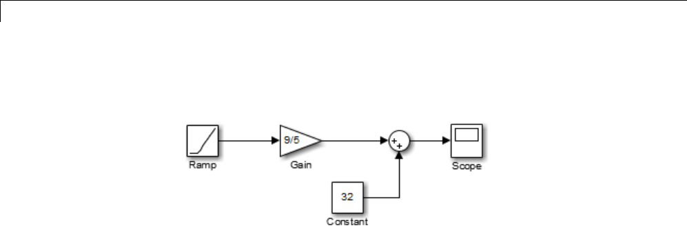
12 Modeling Best Practices
Now, connect the blocks.
The Ramp block inputs Celsius temperature. Open that block and change the
Initial output parameter to 0. The Gain block multiplies that temperature
by the constant 9/5. The Sum block adds the value 32 to the result and
outputs the Fahrenheit temperature.
Open the Scope block to view the output. Now, choose Run from the
Simulation menu to run the simulation. The simulation runs for 10 seconds.
12-16

Componentization Guidelines
Componentization Guidelines
Componentization
A component is a piece of your design, a unit level item, or a subassembly,
that you can work on without needing the higher level parts of the model.
Componentization involves organizing your model into components.
Componentization provides many benefits for organizations that develop large
Simulink models that consist of many functional pieces. The benefits include:
•Meeting development process requirements, such as:
-Component reuse
-Team-based development
-Intellectual property protection
-Unit testing
•Improving performance for:
-Model loading
-Simulation speed
-Memory usage
Componentization Techniques
Key componentization techniques that you can use with Simulink include:
•Subsystems
•Libraries
•Model referencing
These componentization techniques support a wide range of modeling
requirements for models that vary in size and complexity. Most large models
use a combination of componentization techniques. For example, you can
include subsystems in referenced models, and include referenced models in
subsystems. As another example, a large model might use model reference
12-17

12 Modeling Best Practices
Accelerator blocks at the top level component partitions and blend model
reference Accelerator and atomic subsystem libraries at lower levels.
Simulink provides tools to convert from subsystems to model referencing.
Because of the differences between subsystems and model referencing,
switching from subsystems to model referencing can involve several steps
(see Converting a Subsystem to a Referenced Model). Consider scalability
and support for anticipated future modeling requirements, such as how a
modelislikelytogrowinsizeandcomplexityandpossiblecodegeneration
requirements. Designing a scalable architecture can avoid later conversion
costs.
General Componentization Guidelines
This table provides high-level guidelines about the kinds of modeling goals
and models for which subsystems, libraries, and model referencing are each
particularly well suited.
Componentization
Technique
Modeling Goals for Which the Technique Is
Well Suited
Subsystems •Add hierarchy to organize and visually
simplify a model.
•Maximize design reuse with inherited
attributes for context-dependent behavior.
Libraries •Provide a frequently used, and infrequently
changed, modeling utility.
•Reuse components repeatedly in a model or in
multiple models.
Model referencing •Develop a referenced model independently
from the models that use it.
•Obscure the contents of a referenced model,
allowing you to distribute it without revealing
the intellectual property that it embodies.
•Reference a model multiple times without
having to make redundant copies.
12-18

Componentization Guidelines
Componentization
Technique
Modeling Goals for Which the Technique Is
Well Suited
•Facilitate changes by multiple people, with
defined interfaces for top-level components.
•Improve the overall performance by using
incremental model loading, update diagram,
simulation, and code generation for large
models (for example, a model with 10,000
blocks).
•Perform unit testing.
•Simplify debugging for large models.
•Generate code that reflects the model
structure.
For a more detailed comparison of these modeling techniques, see “Summary
of Componentization Techniques” on page 12-19.
Summary of Componentization Techniques
This section compares subsystems, libraries, and model referencing. The table
includes recommendations and notes about a range of modeling requirements
and features.
To see more information about a specific requirement or feature, click a link
in a table cell.
Modeling
Requirement
or Feature Subsystems Libraries
Model
Referencing
Development Process
Component
reuse
Not supported Well suited Well suited
Team-based
development
Not supported Supported, with
limitations
Well suited
12-19

12 Modeling Best Practices
Modeling
Requirement
or Feature Subsystems Libraries
Model
Referencing
Intellectual
property
protection
Not supported Not supported Well suited
Unit testing Supported, with
limitations
Supported, with
limitations
Well suited
Performance
Model loading
speed
Supported, with
limitations
Well suited Well suited
Simulation
speed for
large models
Supported, with
limitations
Supported, with
limitations
Well suited
Memory Supported, with
limitations
Supported, with
limitations
Well suited
Artificial
algebraic loop
avoidance
Well suited Well suited Supported, with
limitations
Features
Signal
property
inheritance
Well suited Well suited Supported, with
limitations
State
initialization
Well suited Well suited Supported, with
limitations
Tunability Well suited Well suited Supported, with
limitations
Buses Well suited Well suited Supported, with
limitations
S-functions Well suited Well suited Supported, with
limitations
12-20

Componentization Guidelines
Modeling
Requirement
or Feature Subsystems Libraries
Model
Referencing
Model
configuration
settings
Well suited Well suited Supported, with
limitations
Tools Well suited Well suited Supported, with
limitations
Code
generation
Supported, with
limitations
Supported, with
limitations
Well suited
For each modeling technique, you can see a summary table that includes
the more detailed information included in the links in the above summary
table of componentization techniques:
•“Subsystems Summary” on page 12-21
•“Libraries Summary” on page 12-25
•“Model Referencing Summary” on page 12-29
Subsystems Summary
This section provides guidelines for using subsystems for each of the modeling
requirements and features highlighted in the “Summary of Componentization
Techniques” on page 12-19.
For additional information about subsystems, see:
•Creating Subsystems
•“Conditional Subsystems”
12-21

12 Modeling Best Practices
Modeling
Requirement or
Feature
Guidelines for Subsystems
Development Process
Component reuse Not supported
•Copy a subsystem to reuse it in a model.
•Subsystem copies are independent of each other.
•Save a subsystem by saving the model that
contains the subsystem.
•Configuration management for subsystems is
difficult.
Team-based
development
Not supported
•For subsystems in a model, Simulink provides no
direct interface with source control tools.
•Tocreateorchangeasubsystem,youneedto
open the parent model’s file. This can lead to file
contention when multiple people want to work on
multiple subsystems in a model.
Intellectual
property protection
Not supported
Use model referencing protected models instead.
Unit testing Supported, with limitations
•For coverage testing, use Signal Builder and source
blocks.
•Each time a subsystem changes, you need to copy
the subsystem to a harness model.
•The test harness may have different Simulink sort
orders, due to virtual boundaries.
•Test harness files require configuration
management overhead.
Performance
12-22

Componentization Guidelines
Modeling
Requirement or
Feature
Guidelines for Subsystems
Model loading
speed
Supported, with limitations
Loading a model loads all subsystems at one time.
There is no incremental loading.
Simulation speed
for large models
Supported, with limitations
•To speed simulation, use Accelerator or Rapid
Accelerator simulation mode.
•Simulation mode applies to the whole model.
Model referencing provides a finer level of control
for simulation modes.
Memory Supported, with limitations
Memory use for simulation and code generation is
comparable for subsystems and libraries. For models
with over 500 blocks, model reference Accelerator
mode can significantly reduce memory usage for
simulation and code generation.
Artificial algebraic
loop avoidance
Well suited
•Virtual subsystems avoid artificial algebraic loops.
•For nonvirtual subsystems, consider enabling the
Subsystem block parameter Minimize algebraic
loop occurrences.
Features
Signal property
inheritance
Well suited
•Inheriting signal properties from outside of the
subsystem boundary avoids your having to specify
properties for every signal.
•Propagation of signal properties can lead to
Simulink using signal properties that you did not
anticipate.
12-23

12 Modeling Best Practices
Modeling
Requirement or
Feature
Guidelines for Subsystems
State initialization Well suited
You can initialize states of subsystems.
Tunability Well suited
•Tune subsystems using a block parameterization
or masked subsystems.
•Control tunability using Configuration
Parameters > Optimization > Signals and
Parameters > Inline parameters.
Buses Well suited
Subsystems do not require the use of bus objects for
virtual buses.
S-functions Well suited
Subsystems support inlined or noninlined S-functions.
Model
configuration
settings
Well suited
A subsystem uses the model configuration settings of
the model that contains the subsystem.
Tools Well suited
Subsystems provide extensive support for Simulink
tools.
Code generation Supported, with limitations
•To generate code for a subsystem by itself,
right-click the Subsystem block and select a code
generation option.
•As an optimization, Simulink attempts to recognize
identical subsystems. For detected identical
subsystems, the generated code includes only one
copy of code for the multiple subsystems.
12-24

Componentization Guidelines
Modeling
Requirement or
Feature
Guidelines for Subsystems
•For virtual subsystems, you cannot specify file or
function code partitions for code generation.
Libraries Summary
This section provides guidelines for using libraries for each of the modeling
requirements and features highlighted in the “Summary of Componentization
Techniques” on page 12-19.
For additional information about libraries, see “Libraries”.
Modeling
Requirement or
Feature
Guidelines for Libraries
Development Process
Component reuse Well suited
•Access a collection of well-defined utility blocks.
•Create a component once and reuse it in models.
•Link to the same library block multiple times
without creating multiple copies.
•Link to the same library block from multiple
models.
•Restrict write access to library components.
•Maintain one truth: propagate changes from a
single library block to all blocks that link to that
library.
•Disable a link to allow independent changes to a
linked block.
•Managing library links adds some overhead.
12-25

12 Modeling Best Practices
Modeling
Requirement or
Feature
Guidelines for Libraries
•Save library in a file similar to a Simulink model,
but you cannot simulate the file contents.
Team-based
development
Supported, with limitations
•Place library files in source control for version
control and configuration management.
•Maintain one truth: propagate changes from a
single library block to all blocks that link to that
library.
•To reduce file contention, use one subsystem per
library.
•Link to the same library block from multiple
models.
•Restrict write access to library component.
•See General Reusability Limitations.
Intellectual
property protection
Not supported
Use model referencing protected models instead.
Unit testing Supported, with limitations
•For coverage testing, use Signal Builder and
source blocks.
•Test harness may have different Simulink sort
orders, due to virtual boundaries.
•Test harness files require configuration
management overhead.
Performance
12-26

Componentization Guidelines
Modeling
Requirement or
Feature
Guidelines for Libraries
Model loading speed Well suited
Simulink incrementally loads a library at the point
needed during editing, updating a diagram, or
simulating a model.
Simulation speed
for large models
Supported, with limitations
•To speed simulation, use Accelerator or Rapid
Accelerator simulation mode.
•Simulation mode applies to the whole model.
Model referencing provides a finer level of control
for simulation modes.
Memory Supported, with limitations
•Simulink incrementally loads libraries at the point
needed during editing, updating a diagram, or
simulating a model.
•Simulink duplicates library block instances during
block update.
•Memory usage for simulation and code generation
is comparable for subsystems and libraries. For
models with over 500 blocks, model reference
Accelerator mode can significantly reduce memory
usage for simulation and code generation.
Artificial algebraic
loop avoidance
Well suited
•Virtual subsystems avoid artificial algebraic loops.
•For nonvirtual subsystems, consider enabling the
Subsystem block parameter Minimize algebraic
loop occurrences.
Features
12-27

12 Modeling Best Practices
Modeling
Requirement or
Feature
Guidelines for Libraries
Signal property
inheritance
Well suited
•Inheriting signal properties from outside of the
library block boundary avoids your having to
specify properties for every signal.
•Propagation of signal properties can lead to
Simulink using signal properties that you did not
anticipate.
State initialization Well suited
You can initialize states of library blocks.
Tunability Well suited
•Tune library blocks using block parameterization
or masked subsystems.
•Control tunability using Configuration
Parameters > Optimization > Signals and
Parameters > Inline parameters.
Buses Well suited
Librariesdonotrequiretheuseofbusobjectsfor
virtual buses.
S-functions Well suited
Libraries support inlined and noninlined S-functions.
Model configuration
settings
Well suited
•Library models do not have model configuration
settings.
•A referenced library block uses the model
configuration setting of the model that contains
that block.
12-28

Componentization Guidelines
Modeling
Requirement or
Feature
Guidelines for Libraries
Tools Supported, with limitations
There are some limitations for using some Simulink
tools, such as the Model Advisor, with libraries.
Code generation Supported, with limitations
•As an optimization, Simulink attempts to recognize
identical subsystems. For detected identical
subsystems, the generated code includes only one
copy of code for the multiple subsystems.
•For virtual subsystems, you cannot specify file or
function code partitions for code generation.
Model Referencing Summary
This section provides guidelines for using model referencing for each of
the modeling requirements and features highlighted in the “Summary of
Componentization Techniques” on page 12-19.
For additional information about model referencing, see:
•“Model Reference”
•Simulink Model Referencing Requirements
•Model Referencing Limitations
12-29

12 Modeling Best Practices
Modeling
Requirement or
Feature
Guidelines for Model Referencing
Development Process Requirements
Component reuse Well suited
•Create a standalone component once and reuse it
in multiple models.
•Reference the same model multiple times without
creating multiple copies.
•Reference the same model from multiple models.
•Model referencing uses specified boundaries for
preserving component integrity.
Team-based
development
Well suited
•For version control and configuration management,
you can place model reference files in a source
control system.
•Design, create, simulate, and test a referenced
model independently from the model that
references it.
•Link to the same model reference from multiple
models.
•Changes made to a referenced model apply to all
instances of that referenced model.
•Simulink does not limit access for changing a
model reference.
•You save a referenced model in a separate file from
the model that references it. Using separate files
helps to avoid file contention.
12-30

Componentization Guidelines
Modeling
Requirement or
Feature
Guidelines for Model Referencing
Intellectual
property protection
Well suited
•Use the protected model feature to obscure
contents of a referenced model in a distributed
model.
•Creating a protected model feature requires a
Simulink Coder license. Using a protected model
does not require a Simulink Coder license.
Unit testing Well suited
•Test components independently to isolate
behaviors, by simulating them standalone.
•You can eliminate unit retest for unchanged
components.
•Use a data-defined test harness, with MATLAB
test vectors and direct coverage collection.
•For coverage testing, use root inports and outports.
Performance
Model loading speed Well suited
•Simulink incrementally loads a referenced model
at the point needed during editing, updating a
diagram, or simulating a model.
•If a simulation target build is required, first-time
loading can be slow.
12-31

12 Modeling Best Practices
Modeling
Requirement or
Feature
Guidelines for Model Referencing
Simulation speed
for large models
Well suited
•Simulate a referenced model standalone.
•The Model block has an option for specifying the
simulation mode.
•You can improve rebuild performance by selecting
the appropriate setting for the Configuration
Parameters > Model Referencing > Rebuild
parameter.
•Simulation through code generation can have a
slow start-up time, which might be undesirable
during prototyping.
•See “Limitations on Normal Mode Referenced
Models” on page 6-83, “Limitations on Accelerator
Mode Referenced Models” on page 6-84, and
“Limitations on PIL Mode Referenced Models” on
page 6-87.
Memory Well suited
•Simulink loads a referenced model at the point
that model is needed for navigation during editing,
updating a diagram, or simulating a model.
•Use model reference Accelerator mode to reduce
memory usage, incrementally loading a compiled
version of a referenced model.
Artificial algebraic
loop avoidance
Supported, with limitations
Consider enabling Configuration Parameters >
Model Referencing > Minimize algebraic loop
occurrences.
Features
12-32

Componentization Guidelines
Modeling
Requirement or
Feature
Guidelines for Model Referencing
Signal property
inheritance
Supported, with limitations
•Inherit sample time when the referenced model is
sample-time independent. You cannot propagate
acontinuoussampletimetoaModelblockthatis
sample-time independent.
•Model block is context-independent, so it cannot
inherit signal properties. Explicitly set input and
output signal properties.
•Use a bus object to define the signal data type of a
bussignalthatispassedintoareferencedmodel.
•Goto and From block lines cannot cross model
referencing boundaries.
•
•See Index Base Limitations.
State initialization Supported, with limitations
•You can initialize states from the top model.
•Use either the structure format or structure with
time format to initialize the states of a top model
and the models that it references.
•To use the SimState (simulation state) feature
with model referencing, simulate all Model blocks
in Normal mode.
•See “Import and Export State Information for
Referenced Models” on page 45-120.
12-33

12 Modeling Best Practices
Modeling
Requirement or
Feature
Guidelines for Model Referencing
Tunability Supported, with limitations
•To have each instance of a referenced model use
different values, use model arguments in the
Model block.
•To have each instance of a referenced model use
thesamevalues,useSimulink.Parameter objects.
•To have each instance of a referenced model use
thesamevalues,useSimulink.Parameter objects.
By default, all other parameters are inlined.
Buses Supported, with limitations
You must use bus objects for bus signals that cross
referenced model boundaries (for example, global
data stores, root inports, root outports).
S-functions Supported, with limitations
Model referencing generally supports inlined or
noninlined S-functions. See “S-Function Limitations”
on page 6-86.
Model configuration
settings
Supported, with limitations
•To apply the same model configuration settings to
all models in a model hierarchy, use a referenced
configuration set.
•Configuration settings for the root model and
referenced models must be consistent. However,
not all configuration settings need to be the same
across the model hierarchy.
12-34

Componentization Guidelines
Modeling
Requirement or
Feature
Guidelines for Model Referencing
Tools Supported, with limitations
•There are some limitations for using some
Simulink tools, such as the Simulink Debugger,
with model referencing.
•For details, see “Simulink Tool Limitations” on
page 6-82.
Code generation Well suited
•By default, model referencing generates code
incrementally.
•You can improve rebuild performance by selecting
the appropriate setting for the Configuration
Parameters > Model Referencing > Rebuild
parameter.
•Model referencing requires the use of bus objects.
For information about the impact of bus objects
for code generation, in the Embedded Coder
documentation, see “Buses”.
12-35

12 Modeling Best Practices
Modeling Complex Logic
To model complex logic in a Simulink model, consider using Stateflow
software.
Stateflow extends Simulink with a design environment for developing state
charts and flow graphs. Stateflow provides the language elements required
to describe complex logic in a natural, readable, and understandable form.
It is tightly integrated with MATLAB and Simulink products, providing an
efficient environment for designing embedded systems that contain control,
supervisory, and mode logic.
For more information on Stateflow software, see “Stateflow”.
12-36

Modeling Physical Systems
Modeling Physical Systems
TomodelphysicalsystemsintheSimulink environment, consider using
Simscape software.
Simscape extends Simulink with tools for modeling systems spanning
mechanical, electrical, hydraulic, and other physical domains as physical
networks. It provides fundamental building blocks from these domains to let
you create models of custom components. The MATLAB based Simscape
language enables text-based authoring of physical modeling components,
domains, and libraries.
For more information on Simscape software, see “Simscape”.
12-37

12 Modeling Best Practices
Modeling Signal Processing Systems
Tomodelsignalprocessingsystemsinthe Simulink environment, consider
using DSP System Toolbox™ software.
DSP System Toolbox provides algorithms and tools for the design and
simulation of signal processing systems. These capabilities are provided
as MATLAB functions, MATLAB System objects, and Simulink blocks.
The system toolbox includes design methods for specialized FIR and IIR
filters, FFTs, multirate processing, and DSP techniques for processing
streaming data and creating real-time prototypes. You can design adaptive
and multirate filters, implement filters using computationally efficient
architectures, and simulate floating-point digital filters. Tools for signal I/O
from files and devices, signal generation, spectral analysis, and interactive
visualization enable you to analyze system behavior and performance. For
rapid prototyping and embedded system design, the system toolbox supports
fixed-point arithmetic and C or HDL code generation.
For more information on DSP System Toolbox software, see “DSP System
Toolbox”.
12-38

13
Managing Projects
•“Organize Large Modeling Projects” on page 13-2
•“Try Simulink Project Tools with the Airframe Project” on page 13-4
•“Create a New Simulink Project” on page 13-23
•“Analyze Project Dependencies” on page 13-32
•“Manage Project Files” on page 13-44
•“Automate Project Startup and Run Frequent Tasks” on page 13-52
•“Run Batch Functions on Project Files” on page 13-58
•“Use Source Control with Projects” on page 13-60
•“Retrieve and Check Out Files Under Source Control” on page 13-76
•“Review Changes and Commit Modified Files” on page 13-89
•“UseTemplatestoCreateStandard Project Settings” on page 13-97
•“Archive Projects in Zip Files” on page 13-103
•“Analyze Model Dependencies” on page 13-104

13 Managing Projects
Organize Large Modeling Projects
In this section...
“What Are Simulink Projects?” on page 13-2
“Get Started with Your Project” on page 13-2
What Are Simulink Projects?
You can use Simulink Projects to help you organize your work. Find all your
required files; manage and share files, settings, and user-defined tasks; and
interact with source control.
Projects can promote more efficient team work and individual productivity
by helping you to:
•Find all the files that belong with your project.
•Share projects using built-in integration with the Subversion client, an
external source control tool.
•View and label modified files for peer review workflows.
•Create standard ways to initialize and shut down a project.
•Create, store, and easily access common operations.
See the Web page
http://www.mathworks.com/products/simulink/simulink-projects/ for
the latest information, downloads, and videos.
Get Started with Your Project
To get started with managing your files in a project:
1Try an example project to see how the tools can help you organize your
work. See “Try Simulink Project Tools with the Airframe Project” on page
13-4.
2Create a new project. See “Create a New Simulink Project” on page 13-23.
13-2

Organize Large Modeling Projects
3Use the Dependency Analysis view to analyze your project and check
required files. See “Analyze Project Dependencies” on page 13-32.
4Explore views of your files. See “Manage Project Files” on page 13-44.
5Create shortcuts to save and run frequent tasks. See “Automate Project
Startup and Run Frequent Tasks” on page 13-52.
6Run operations on batches of files. See “Run Batch Functions on Project
Files” on page 13-58.
7If you use a source control integration, you can use the Modified Files
view to review changes, compare revisions, and commit modified files. If
you want to use source control with your project, see “Use Source Control
with Projects” on page 13-60.
13-3

13 Managing Projects
Try Simulink Project Tools with the Airframe Project
In this section...
“Explore the Airframe Project” on page 13-4
“Set Up the Project Files and Open the Simulink Project Tool” on page 13-5
“View, Search, and Sort Project Files” on page 13-5
“Automate Project Startup and Shutdown Tasks” on page 13-7
“OpenandRunFrequentlyUsedFiles”onpage13-9
“Review Changes in Modified Files” on page 13-10
“Run Project Integrity Checks” on page 13-12
“Run Dependency Analysis” on page 13-12
“Commit Modified Files” on page 13-15
“Upgrade Model Files to SLX and Preserve Revision History” on page 13-15
“View Source Control and Project Information” on page 13-21
Explore the Airframe Project
Try an example Simulink project to see how the tools can help you organize
your work. Projects can help you to manage:
•Your design (model and library files, .m,.mat, and other files, source code
for S-functions, data)
•A set of actions to use with your project (run setup code, open models,
simulate, build, run shutdown code).
•Working with files under source control (check out, compare revisions,
tag or label, and check in)
The Airframe example shows how to:
1Set up and browse some example project files, under local revision control.
2Examine project shortcuts to run setup and shutdown tasks, and access
frequently used files and tasks.
13-4

Try Simulink®Project Tools with the Airframe Project
3Analyze dependencies in the example project and locate required files that
are not yet in the project.
4Modify some project files, find and review modified files, compare to an
ancestor version, and commit modified files to source control.
5Explore views of project files only, modified files, and all files under the
project root folder.
Follow the steps below to explore the example project.
Set Up the Project Files and Open the Simulink
Project Tool
Run this command to create a working copy of the project files and open the
project:
sldemo_slproject_airframe
The project example copies files to your temporary folder so that you can edit
them and put them under local revision control.
The Simulink Project Tool opens and loads the project. The project is
configured to run some startup tasks, including changing the current working
folder to the project root folder.
View, Search, and Sort Project Files
1Click the Project Files view to manage the files within your project. Only
thefilesthatareinyourprojectareshown.
2Click the All Files view to see all the files in your sandbox. This view shows
all the files that are under the project root, not just the files that are in the
project. This view is useful for adding files to the project that exist within
your sandbox, but which are not yet part of the project.
3To find particular files or file types, in any file view, type in the search box
or click the Filter button next to the search box.
13-5
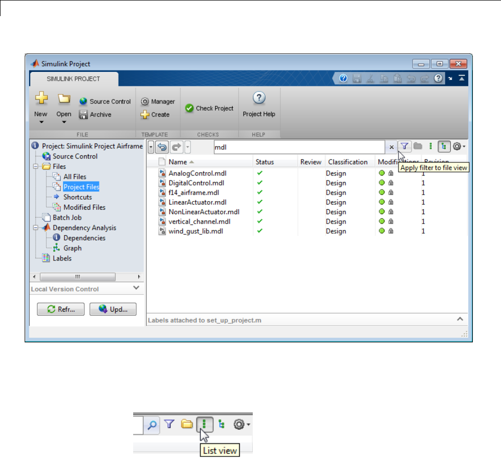
13 Managing Projects
Click the xto clear the search.
4To view files as a list instead of a tree, click the List view button at the
top right.
5To sort files and to customize the columns that you want to show, click the
"cog" icon Actions button at the far right of the search box.
13-6

Try Simulink®Project Tools with the Airframe Project
6You can dock and undock the Simulink Project Tool into the MATLAB
Desktop. If you want to maximize space for viewing your project files,
undock the Simulink Project Tool.
Automate Project Startup and Shutdown Tasks
You can use shortcuts to automatically run startup or shutdown tasks, and to
easily find files within a large project.
1Click the Shortcuts node to view the startup tasks and other shortcuts.
2If you see a tree view, click the List view button at the top right of the
Simulink Project Tool to view the shortcuts as a list of files.
13-7
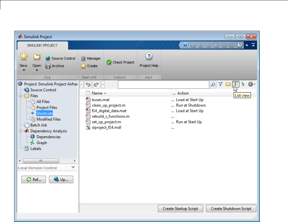
13 Managing Projects
In this example, you can see that:
•Some files are set as Run at Startup shortcuts. Startup shortcut
files automatically run (.m files), load (.mat files), and open (Simulink
models) when you open the project. You can use these shortcuts to set up
the environment for your project. The file set_up_project.m sets the
MATLAB path, and defines where to create the slprj folder. Open the
set_up_project.m file to view how it works. The following lines use the
project API to get the current project:
p = Simulink.ModelManagement.Project.CurrentProject;
projectRoot = p.getRootDirectory;
13-8

Try Simulink®Project Tools with the Airframe Project
•Another file is set as a Run at Shutdown shortcut. This type
of file runs before the current project closes. In this example, the
file clean_up_project.m resets the environment changes made by
set_up_project.m.
To create new startup or shutdown shortcuts, select the Project Files view,
right-click a file, and select Create Shortcut. Go to the Shortcuts view to set
an existing shortcut to Run at Startup or Run at Shutdown.
Open and Run Frequently Used Files
You can use shortcuts to make scripts easier to find in a large project. In this
example, the script that regenerates S-Functions is a shortcut so that a new
user of the project can easily find it. You can also make the top-level model, or
models, within a project easier to find. In this example, the top-level model,
slproject_f14.mdl,isashortcut.
Use the example shortcuts:
1Double-click the shortcut slproject_f14.mdl to open the root model
for this project. This model will not run until you compile a required
S-Function.
2Right-click the shortcut rebuild_s_functions.m and select Run to
generate the S-Function. Open this file to view how it works.
Note This shortcut builds a MEX-file. If you do not have a compiler set
up, then first run the following command:
mex -setup
13-9
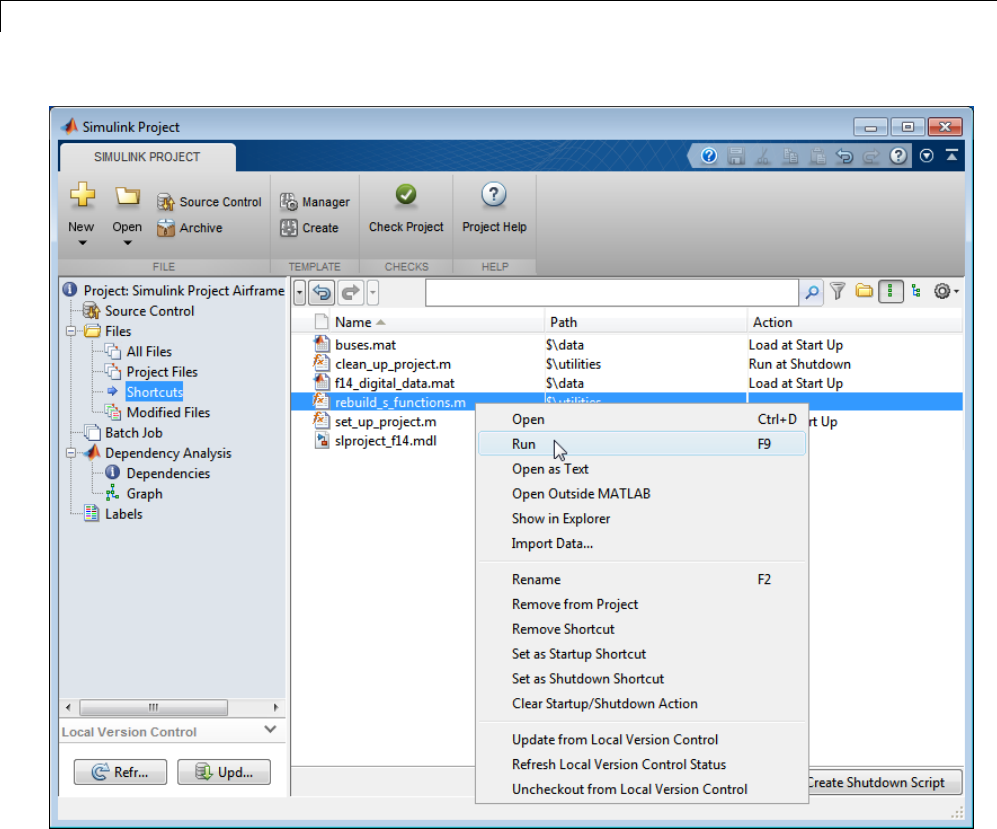
13 Managing Projects
3To create new shortcuts, select the Project Files view, right-click a file,
and select Create Shortcut.
Review Changes in Modified Files
1Open and make changes to one of the utility MATLAB files. You can
double-click to open files for editing from the Simulink Project, or right-click
and select Open.MakeachangeintheEditorandsavethefile.
13-10
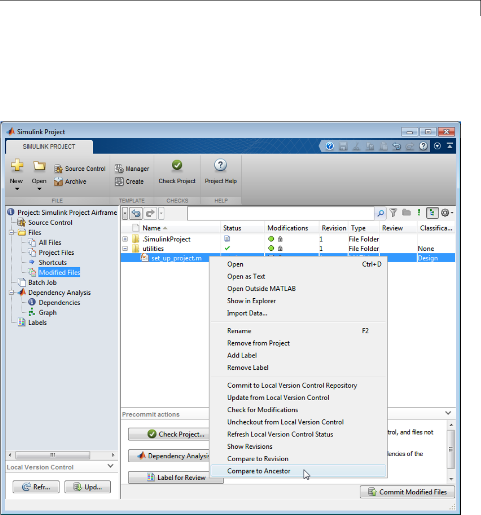
Try Simulink®Project Tools with the Airframe Project
2In the Simulink Project Tool, click the Modified Files node to see the files
that you have modified.
3To review changes, right-click a file in the Modified Files view and select
Compare to Ancestor.
13-11

13 Managing Projects
The MATLAB Comparison Tool opens a report comparing the modified
version of the file in your sandbox against its ancestor stored in the version
control tool. Comparison type depends on the file you select. If you select a
Simulink model, and you have Simulink Report Generator installed, this
command runs a Simulink XML comparison.
Run Project Integrity Checks
In the Modified Files view, click Check Project to run the project integrity
checks to look for missing files, files that should be added to source control or
retrieved from source control, and other issues. The checks dialog can offer
automatic fixes to problems found. Click the Fix button to view recommended
actions and decide whether to make the changes.
Close the Project Integrity Checks dialog box.
For an example using the project checks to fix issues, see the later steps in
“Upgrade Model Files to SLX and Preserve Revision History” on page 13-15.
Run Dependency Analysis
Run a file dependency analysis on the modified files in your project, to check
that you have all the required files added to the project.
1In the Modified Files view, click the Dependency Analysis button to
perform analysis on the modified files.
The Simulink Project Tool opens the Dependency Analysis view with your
modified files selected for analysis.
13-12
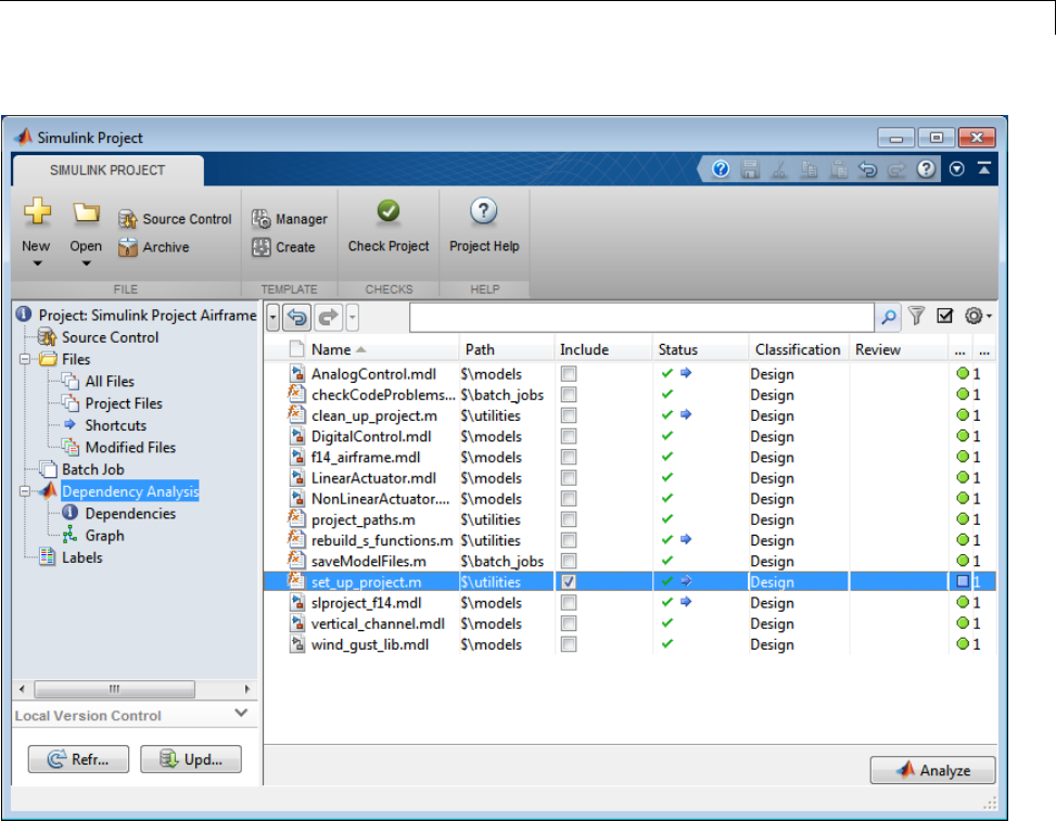
Try Simulink®Project Tools with the Airframe Project
2Add all files to the analysis. Click the list of files, and then press Ctrl+Ato
select all files. Right-click and select Include.
3Click the Analyze button.
4Review reported problem files. Observe that Problem files automatically
appears in the search box for filtering your file views.
5Observe that the S-Function binary file, timesthree.mexw64,isrequired
by the project but is not currently part of it. Click the problem file to view
where it is used in the table below, in the Used By column.
13-13
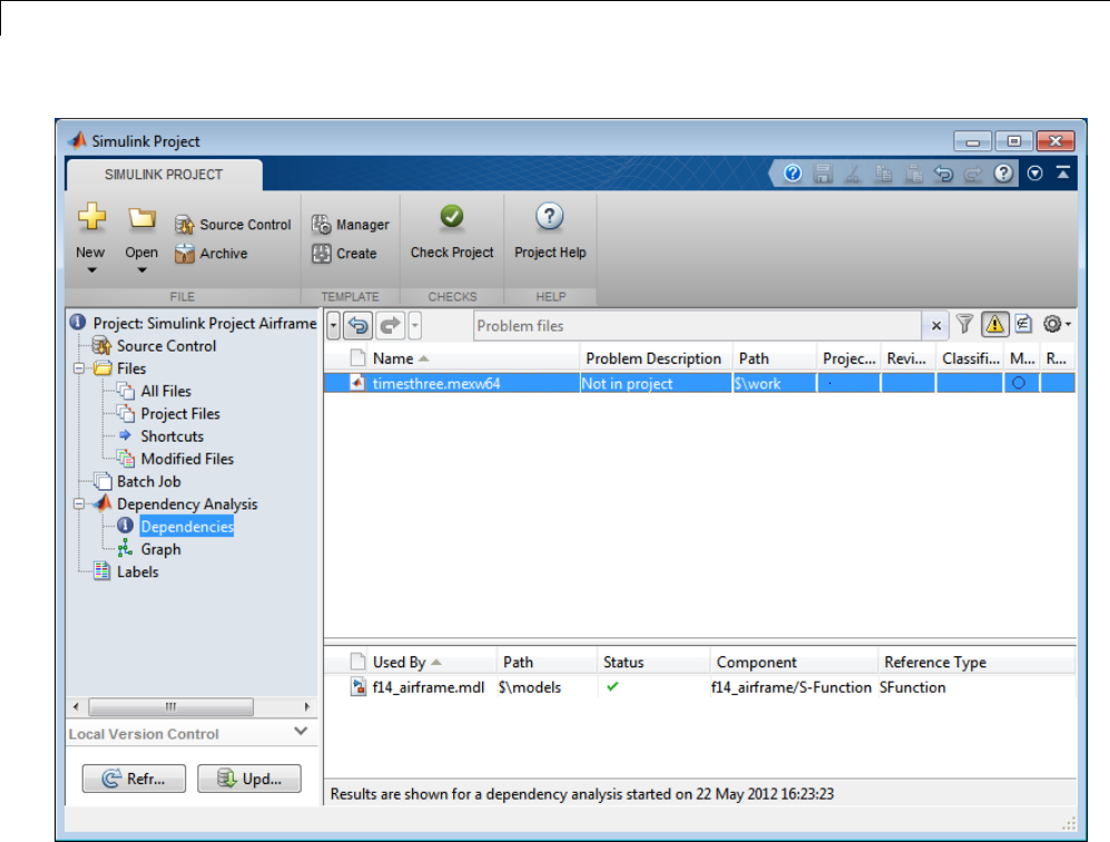
13 Managing Projects
You might want to add binary files to your project or, as in this project,
provide a utility script that regenerates them from the source code that
is part of the project.
6Right-click the problem file and select Add External File.Youremove
the file from the problem files list, and the next time you run dependency
analysis, this file will not be marked as a problem file.
7Click the Graph node to view the dependency graph of the project
structure. Try some right-click options to customize the graph.
13-14
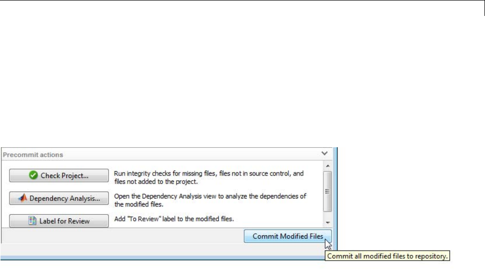
Try Simulink®Project Tools with the Airframe Project
Commit Modified Files
1Return to the Modified Files view, and click Check Project again to make
sure your changes are ready to commit. When you are satisfied with the
results of the checks, commit your modified files.
2To commit your changes to source control, click the Commit Modified
Files button.
The Modified Files list includes a .SimulinkProject folder. The files
stored in the .SimulinkProject folder are internal project definition files
generated by your changes. These definition files allow you to add a label to
a file without checking it out. You should never need to view the definition
files directly unless you need to merge them, but they are shown so that
you know about all the files being committed to the source control system.
See “Project Definition Files” on page 13-91.
3Enter a comment for your submission, and click Submit.
Upgrade Model Files to SLX and Preserve Revision
History
Simulink Projects help you upgrade model files from MDL format to SLX
format. You can use the Project Integrity checks to automatically add the new
SLX file to your project, remove the MDL file from the project, and preserve
the revision history of your MDL file with the new SLX file. You can then
commit your changes to source control and maintain the continuity of your
model file history.
13-15
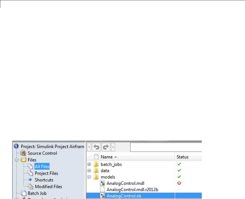
13 Managing Projects
The following steps show how the project tools can help you migrate files to
SLX, using the Airframe example project. If you have not done the previous
example steps, you can run this command to open a new copy of the project:
sldemo_slproject_airframe
1In the Project Files view, right-click the model file AnalogControl.mdl,
and select Open.
2Select File > Save As.
3Ensure that Save as type is SLX, and click Save. SLX is the default
unless you change your preferences.
4SelecttheAllFilesviewtoseetheresults. Clickthetreeview
button and expand the models folder. Simulink saves your model in
SLX format, and creates a backup file by renaming the MDL file to
mymodel.mdl.releasename. The project also reports the original name
of the MDL file as missing.
5To resolve these issues, click Check Project on the Simulink Project tab
to run the project integrity checks. The checks look for MDL files converted
to SLX, and offer automatic fixes if that check fails.
6Click the Fix button to view recommended actions and decide whether
to make the changes.
13-16
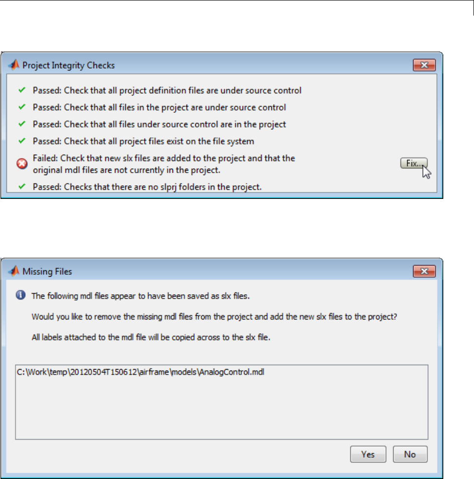
Try Simulink®Project Tools with the Airframe Project
When you click Fix, the Missing Files dialog box offers to remove the
missing MDL file from the project and add the new SLX file to the project.
Click Yes to perform the fix.
Project checks rerun after you click Fix, in case there are remaining issues.
13-17
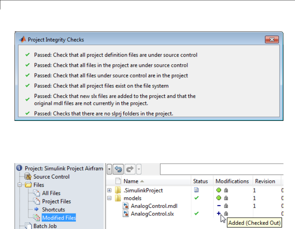
13 Managing Projects
Close the Project Integrity Checks dialog.
7Select the Modified Files view. Expand the models folder and check the
Modifications column to see that the newly created SLX file has been added
to the project, and the original MDL file is scheduled for removal.
8Click Commit Modified Files. Enter a comment for your submission in
the dialog, for example, Convert to SLX,andclickSubmit.
9Select the All Files view to see that your backup file
AnalogControl.mdl.r2012b is still present, along with the new
SLX file.
13-18
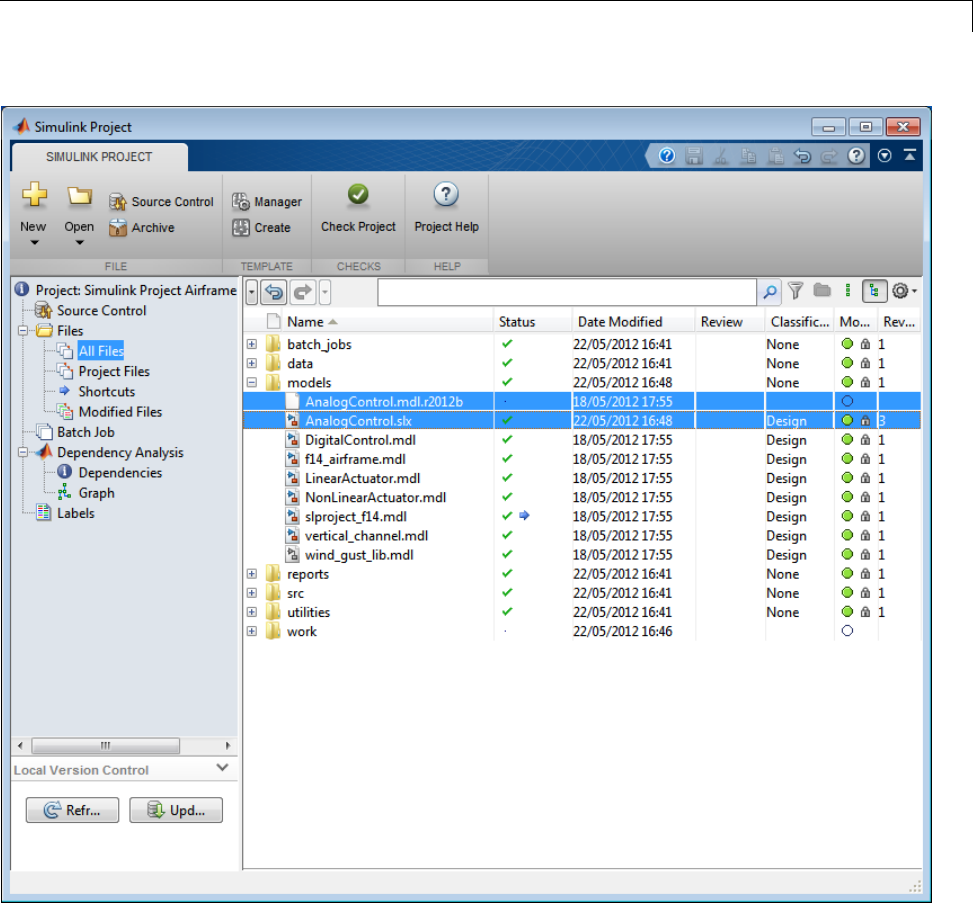
Try Simulink®Project Tools with the Airframe Project
10 Select the Project Files view to see that only the new SLX file is now
included in the project, and the backup file is not included in the project.
13-19
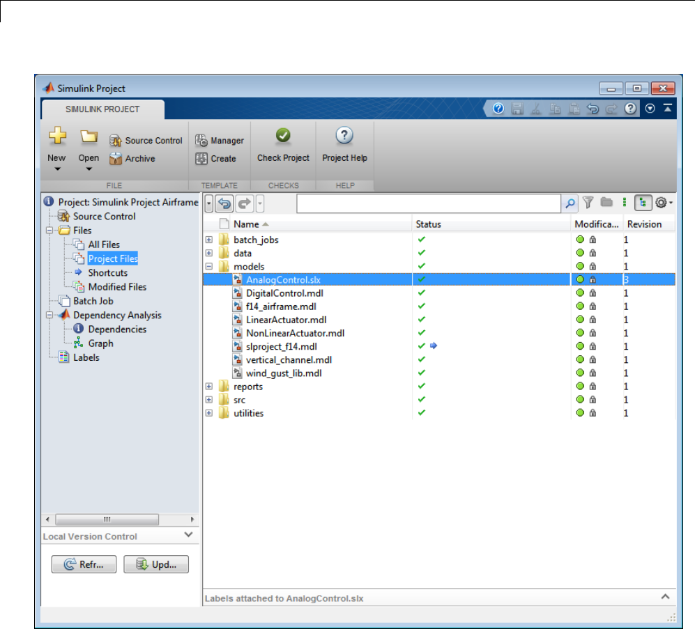
13 Managing Projects
11 Right-click the model file AnalogControl.slx and select Show Revisions.
The File Revisions dialog box opens, and you can verify that the previous
revision is AnalogControl.mdl. The revision history of your previous
model file is preserved with the new SLX file.
13-20
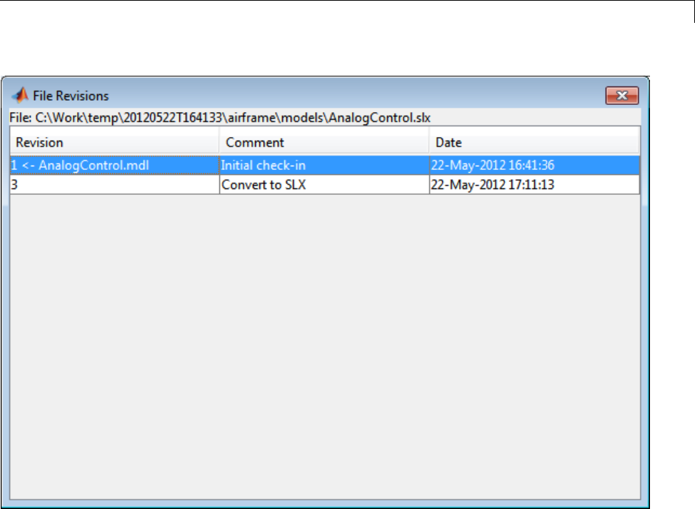
Try Simulink®Project Tools with the Airframe Project
View Source Control and Project Information
1Click the Source Control node to see information about the source control
tool being used by the current project. The Airframe example project is
under the control of the Local Version Control tool.
13-21

13 Managing Projects
For source control information on individual files (e.g., modified, checked
out), see the Modifications column in the Files views.
2Click the root tree node Project: Simulink Project Airframe to see
information about the currently open project, including a description and
the location of the project root folder.
13-22

Create a New Simulink®Project
Create a New Simulink Project
In this section...
“Create a New Project to Manage Existing Files” on page 13-23
“Add Files to the Project” on page 13-26
“Create a New Project from an Archived Project” on page 13-28
“Open Recent Projects” on page 13-29
“Change the Project Name, Root, Description, and Startup Folder” on
page 13-30
Create a New Project to Manage Existing Files
If you already have files that you want to organize into a project, with or
without source control, use the following steps for a new project.
Note If you want to retrieve your project from a source control repository,
see instead “Retrieve a Working Copy of a Project from Source Control” on
page 13-76.
To create a new project to manage your files, either:
•From MATLAB, on the Home tab, in the File section, select
New > Simulink Project > Blank.
•From the Model Editor, select File>New>SimulinkProject.
•From the Simulink Project Tool, on the Simulink Project tab, in the File
section, select New.
TheCreateSimulinkProject dialog box appears.
13-23
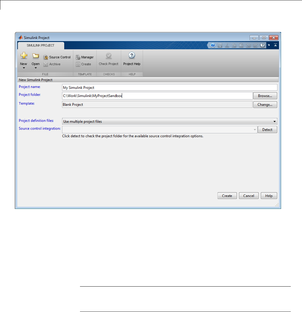
13 Managing Projects
1Enter the project name.
2Select a project folder. The default is your current folder.
3(Optional) Click Detect to check the project folder for source control
integration options. If your selected folder is under source control that the
project can recognize, the Source control integration field reports the
detected source control. You can change available source control tools here.
Note You can put the project under source control later by using the
Source Control node in the Project tree. See “Use Source Control with
Projects” on page 13-60.
13-24

Create a New Simulink®Project
The next example shows the project has detected SVN in the selected
project folder, and so the project selects Built-In SVN Integration.
4(Optional) Change the template.
•Leave the default Blank Project template if you want to create a blank
project without any preconfigured structure or utilities. Use the blank
template if you are creating a project in a folder that already contains
files.
•Change the template if you want to create a project with some
preconfigured settings to guide you with setting up your project.
–Try the Project Environment template if you are creating a project
in a new folder and intend to add files later. Click Change next to
Template to open a dialog box and select the Project Environment
13-25

13 Managing Projects
template. You can view information about the template settings in
the description field. The Project Environment template can create
a new project with a preconfigured structure, and utilities to configure
the path and environment with startup and shutdown shortcuts. For
example, the path utilities help set up your search path to ensure
dependency analysis can detect project files. You can modify any of
these files, folders, and settings later.
–Similarly, try the Code Generation Example template to set up a
project with settings for production code generation of a plant and
controller. This template requires Simulink Coder and Embedded
Coder. See “Example Templates” on page 13-101.
–If you create your own templates, you can select them in the Select a
Template dialog box. See “Use Templates to Create Standard Project
Settings” on page 13-97.
Note A warning tells you when your chosen template will overwrite any
files in the chosen location.
5(Optional) Change project definition files.
Use multiple project files is better for avoiding merging issues on
shared projects.
Use a single project file is faster but is likely to cause merge issues
when multiple users submit changes in the same project to a source control
tool. See “Project Definition Files” on page 13-91.
6Click Create to create your new project.
The Simulink Project Tool displays the empty Project Files list for your chosen
project root. Your project does not yet contain any files. You need to select
files to add. For next steps, see “Add Files to the Project” on page 13-26.
Add Files to the Project
The All Files node in the Project tree shows all files in your project folder.
Files under your chosen project root are not included in your project until you
13-26
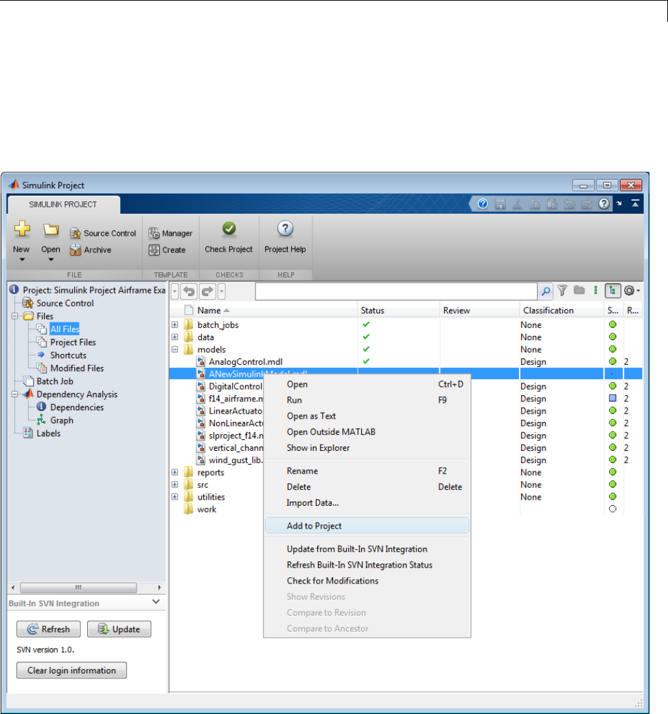
Create a New Simulink®Project
add them. You might not want to include all files in your project. You can
add files to your project from the All Files view.
In the All Files view, select files or folders, right-click and select Add to
Project or Add to Project (including child files).
13-27

13 Managing Projects
To add and remove project files at the command line, see the
Simulink.ModelManagement.Project.CurrentProject reference page.
To help you set up your project with all required files, see “Choose Files and
Run Dependency Analysis” on page 13-33.
To configure your project to automatically run startup and shutdown tasks,
see “Automate Project Startup and Run Frequent Tasks” on page 13-52.
Create a New Project from an Archived Project
To create a new project from an archived project, either:
•From MATLAB, on the Home tab, in the File section, select
New > Simulink Project > From Archive.
•From the Simulink Project Tool, on the Simulink Project tab, select
New > New Project from Zip Archive
13-28

Create a New Simulink®Project
Open Recent Projects
Note You can have one project open. If you open another project, any
currently open project closes. Having multiple projects open could cause
conflicts.
To open recent projects:
•From MATLAB, on the Home tab, in the File section, select Open and
then select your project under the Recent Simulink Projects list.
From the Current Folder browser, you can open projects by double-clicking
your .prj file.
•From the Simulink Project Tool, on the Simulink Project tab, select a
recent project to open from the Open > Recent list.
Alternatively, to browse for a project from the Simulink Project Tool:
-For projects created or saved in Release 2012b or later, select
Open > Open Project File. Browse and select your project .prj file,
and click OK to load the project.
-For projects last saved in Release 2012a or earlier, select
Open > Open Project by Folder. Navigate to the folder containing
the .SimulinkProject folder, and click OK to load the project.
Subsequently, you can use Open Project File.
To open the Simulink Project Tool:
•From the MATLAB command line, enter:
simulinkproject
•From the Library Browser or Simulink Editor, select View > Simulink
Project.
13-29

13 Managing Projects
Tip Create a MATLAB shortcut for opening or giving focus to the Simulink
Project Tool by dragging this command to the toolstrip from the Command
History or Command Window:
simulinkproject
Change the Project Name, Root, Description, and
Startup Folder
Use the Project tree node if you want to edit the project name or add a
description. If you edit the name or description, click Apply to save your
changes.
You can view the project root folder, and click Set as Current Folder to
change the current working folder to your project root. You can change your
project root by moving your entire project on your file system, and reopening
your project in its new location. All project file paths are stored as relative
paths.
The check box option Change current folder to project root on start
up is selected by default. Clear the check box if you do not want to change
to the project root folder on startup.
You can also configure startup shortcut scripts that set the current folder
and perform other setup tasks. If you configure startup shortcuts to set the
current folder, your shortcut setting takes precedence over the check box at
the Project node. To set up shortcuts, see “Automate Project Startup and
Run Frequent Tasks” on page 13-52.
13-30
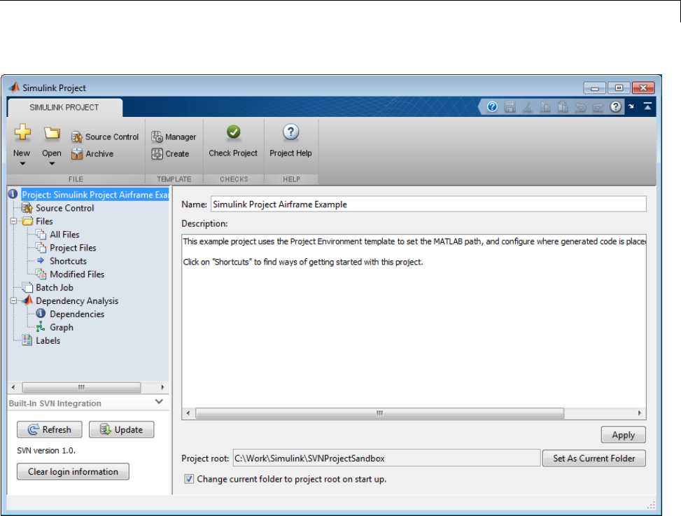
Create a New Simulink®Project
13-31

13 Managing Projects
Analyze Project Dependencies
In this section...
“What Is Dependency Analysis?” on page 13-32
“Choose Files and Run Dependency Analysis” on page 13-33
“Check Dependencies Results and Resolve Problems” on page 13-35
“Investigate Dependencies Graph” on page 13-38
“Options for Analyzing Model Dependencies” on page 13-43
What Is Dependency Analysis?
You can analyze project structure and discover files required by your project
with the Dependency Analysis view.
•You can use dependency analysis to help you set up your project with all
required files. For example, you can add a top-level model to your project,
analyze the model dependencies, and then add all dependent files to your
project.
•You can run dependency analysis at any point in your workflow when you
want to check that all required files are in the project. For example, you
can check dependencies again before submitting a version of your project
to source control.
•You can use the Graph view of your dependency analysis to analyze the
structure of your project visually. From the graph, you can examine your
project structure and perform file operations such as adding labels and
opening files.
Note You can analyze only files within your project. If your project is new,
you must add initial files to the project before running dependency analysis.
Click the All Files node under Management in the Project tree. Select the files
you want to analyze, right-click, and select Add to Project.
13-32

Analyze Project Dependencies
Choose Files and Run Dependency Analysis
1In the Project tree, click Dependency Analysis.
Files in your project are shown in the list.
2To specify which files to analyze, select the check boxes in the Include
column.
If you click the Dependency Analysis button in the Modified Files view, you
open the Dependency Analysis view with your modified files preselected.
To include or exclude all files, press Ctrl+Ato select all files, then
right-click and select Include or Exclude.
13-33
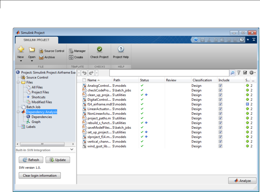
13 Managing Projects
3If desired, use the search box or Filter button to alter the list of files
displayed.
You see a message under the list if your filtering hides some of the files
selected for dependency analysis. To show all files selected for analysis,
click the button to the right of the search box to show only included files.
13-34
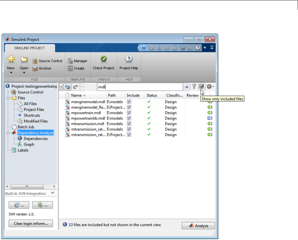
Analyze Project Dependencies
4Click Analyze to discover required files.
The view changes to the Dependencies node to show your results in list
form.
Check Dependencies Results and Resolve Problems
If dependency analysis finds any problems, the Simulink Project Tool displays
the problem files. The search box shows that the list is filtered to show only
Problem files.
13-35
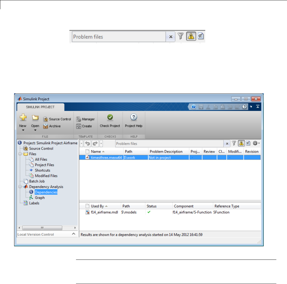
13 Managing Projects
The list reports dependent files that you should review because they are
required by the project but not currently in the project or missing.
1Click each file in the Problem list to see where they are being used by other
files in the project, under Used By in the lower pane.
Note If you clear the search box, you can return to viewingonlyproblem
files or external files by clicking the toolbar buttons to the right of the
search box.
13-36
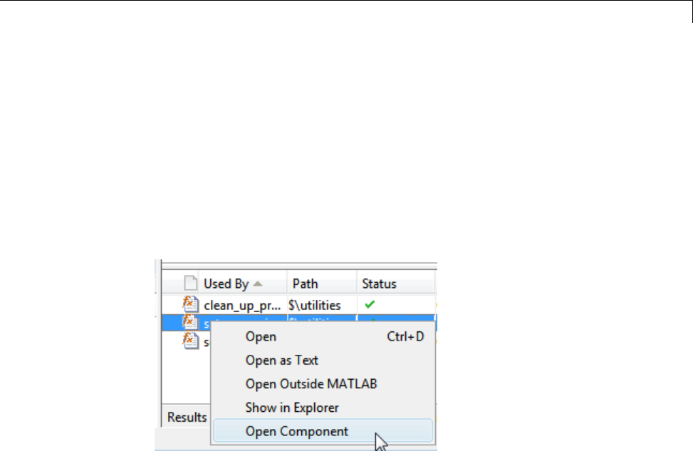
Analyze Project Dependencies
2In the dependencies table, check the Problem Description and Project
Status of dependent files, and if desired right-click to add any required files
that are not in the project. You can select multiple files. For example,
press Ctrl+Ato select all files in the dependent files list, right-click, and
select Add to Project.
3To open the referencing component for editing, right-click a file in the
Used By table and select Open Component. The referencing file opens.
MATLAB files open in the MATLAB Editor, and Simulink models open in
the Model Editor with the block highlighted.
4If you want to remove files from the Problem list but not add them to
the project, you can right-click to select Add External File.Thefile
disappears from the Problem list. Next time you run dependency analysis,
this file will not appear in the Problem list. To view all external files, click
the Show only external files button to the right of the search box.
You might not want to add all required files to the project. For example,
you might want to exclude derived S-Function binary files that the source
code in your project can generate. See “Work with Derived Files in Projects”
on page 13-96.
Check the Status message and the Path for dependent files, where $
indicates the project root. Check if required files are outside your project
root—you cannot add such files to your project. This dependency might
not indicate a problem if the file is on your path and is a utility or other
resource that is not part of your project. Use dependency analysis to ensure
that you understand your design’s dependencies.
13-37
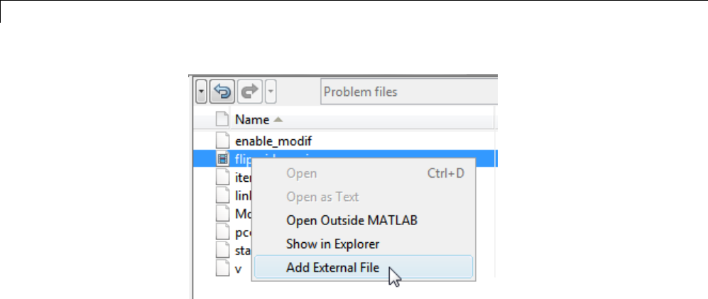
13 Managing Projects
5If you decide the file needs to be part of your project, copy or move it within
the project root, add it the project and the path, and remember to remove
the original from the path.
6Clear the search box to view all identified dependencies. Click files to view
wheretheyareused. AlsotrytheGraph view to investigate your project
dependencies graphically. See “Investigate Dependencies Graph” on page
13-38.
Investigate Dependencies Graph
To investigate dependencies visually, click Graph in the tree under
Dependency Analysis.
1To highlight dependencies of selected files, right-click the graph canvas
and select Highlight Dependencies, and then click graph items to view
their highlighted dependencies. You can highlight upstream, downstream,
and circular dependencies.
13-38
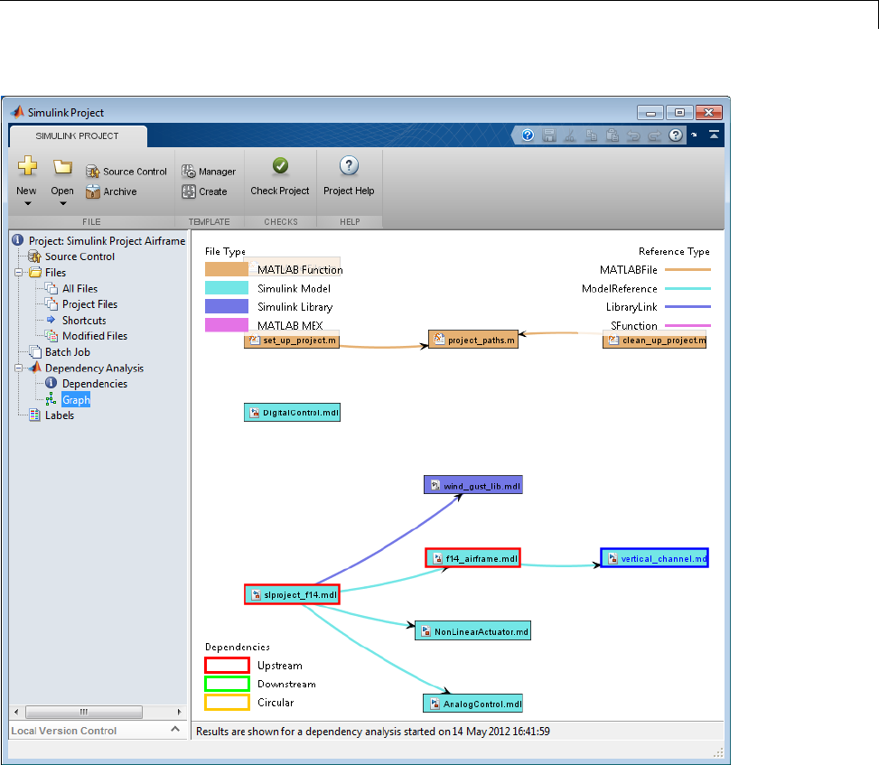
Analyze Project Dependencies
2Right-click the graph canvas to Filter by File Type,andselectthefile
types you want to display or hide.
13-39
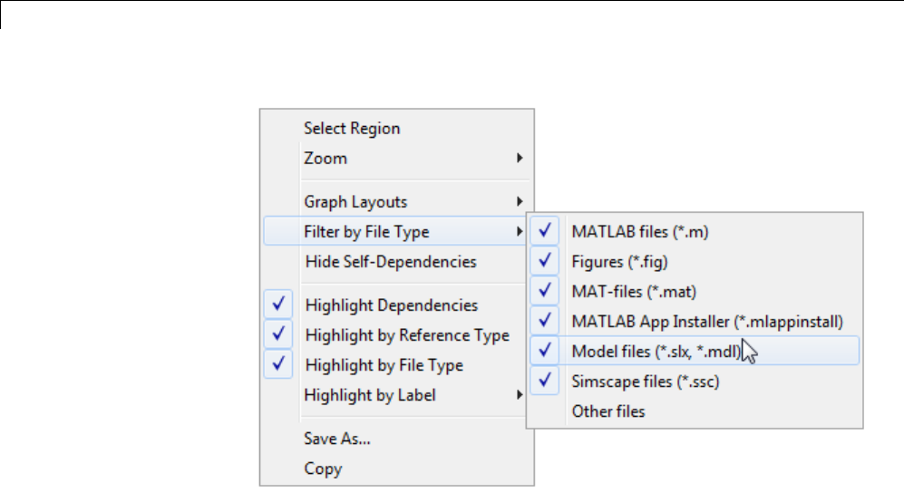
13 Managing Projects
3Right-click the graph canvas to highlight all graph items by file type and
reference type. The following example shows a project dependency graph
with many file types and reference types highlighted.
13-40
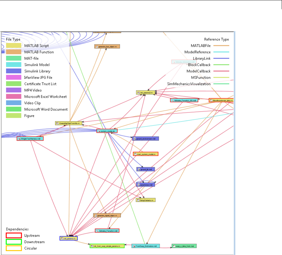
Analyze Project Dependencies
4Right-click the graph canvas to Highlight by Labels, and select a category
of labels to use for highlighting. For example, you might want to see which
files have the label To Review. The following example shows highlighting
of custom labels to show Engine Type in the project.
13-41
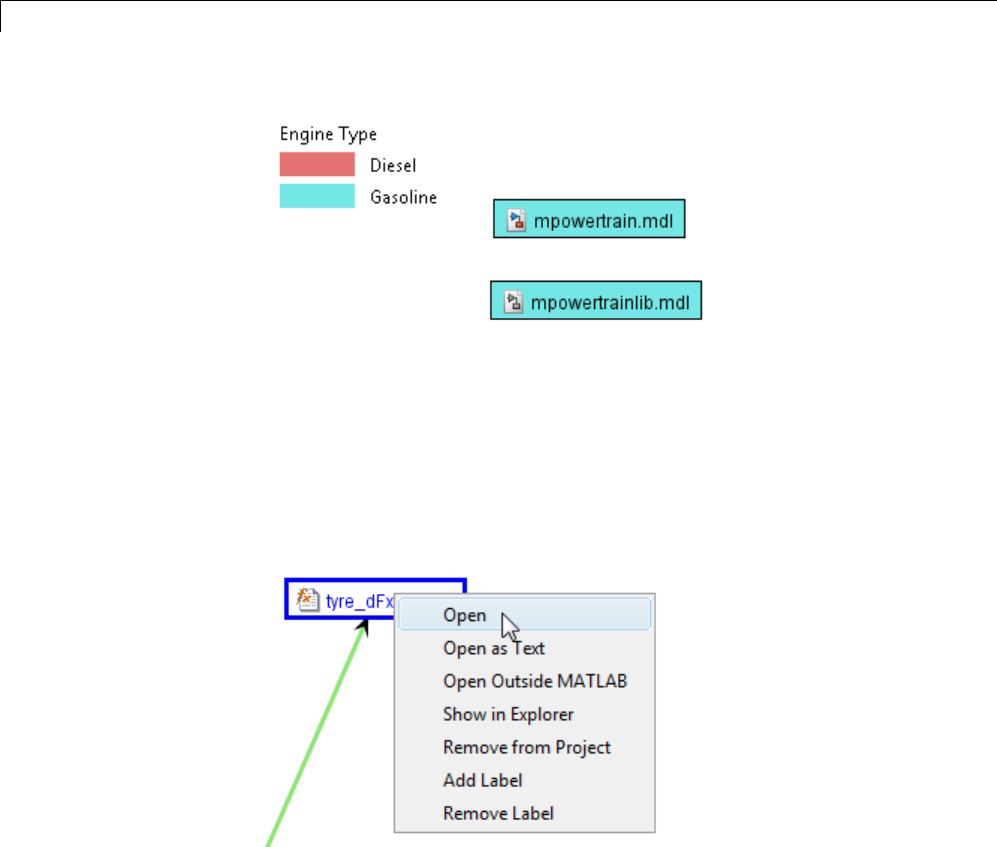
13 Managing Projects
5Right-click the graph canvas to try different graph layouts and change
zoom. You can also control zoom with a mouse wheel, or use the keyboard.
Press +and –to zoom in or out, press space to fit to view.
6Right-click files in the graph to perform operations such as Open,Add
Label,orRemove from Project. You can also double-click to open a file.
You can perform file operations on multiplefiles. Toselectmultiplefiles,
press Shift and drag the mouse to enclose the files. Hold down Ctrl to
multiselect and add to any existing selection. Press Fto fit the view to
the currently selected files.
7You can select Hide Self-Dependencies if you want a simpler view of
other graph items. For example, a library that contains multiple blocks
that use another block in the same library shows many self-references.
13-42

Analyze Project Dependencies
Self-referencing files do not introduce any new file dependencies, so you
can hide these self-dependencies if you want to simplify the graph. The
layout regenerates whenever you change the graph.
8To save the graph as a .png image file, right-click and select Save As,
or select Copy to copy the image to your clipboard for pasting into other
documents.
Options for Analyzing Model Dependencies
You can use the Simulink Project Tool to analyze file dependencies for your
entire project. For detailed dependency analysis of a specific model, use the
manifest tools instead to control more options. Use the manifest tools if you
want to:
•Save the list of the model dependencies to a manifest file.
•Create a report to identify where dependencies arise.
•Control the scope of dependency analysis.
•Identify required toolboxes.
See “Analyze Model Dependencies” on page 13-104.
13-43

13 Managing Projects
Manage Project Files
In this section...
“Choose Views of Files to Manage” on page 13-44
“Group and Sort File Views” on page 13-45
“Search and Filter File Views” on page 13-46
“Work with Project Files” on page 13-47
“Back Out Changes” on page 13-49
“Label Files” on page 13-49
Choose Views of Files to Manage
Use the Project Files views to explore project files, interact with source
control, view modified or labeled files, and save tasks or shortcuts.
1In the Project tree, use the nodes under Files to choose the view with the
files you want to manage:
•All Files — View all files within your project folder (or projectroot).
This list can be different from the list in the Project Files node. For
example, you might want to exclude some files under projectroot from
your project, such as SVN or CVS source control folders.
•Project Files — View only files added to your project. This list can be
different from the list of all files within your project folder.
•Shortcuts — View files you have specified as shortcuts for frequent
tasks, such as opening top-level models, running startup or shutdown
code and other tasks, or simulating models. You can set up shortcuts
to run when you open or close your project, or to run manually. The
Shortcuts node is blank until you create shortcuts from the All Files or
Project Files views. See “Automate Project Startup and Run Frequent
Tasks” on page 13-52.
•Modified Files — View only files with changes. This view is available
only if you are using a source control integration with your project. See
“Review Changes and Commit Modified Files” on page 13-89.
13-44
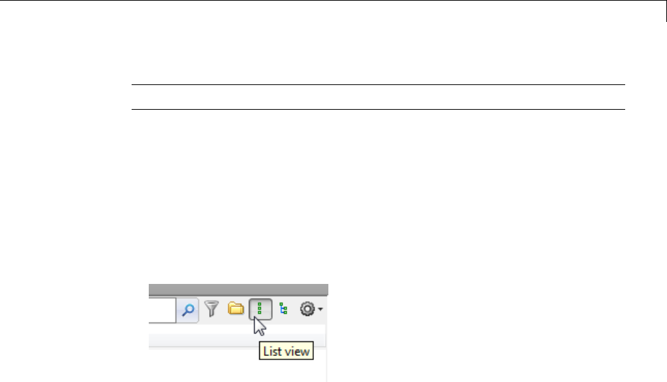
Manage Project Files
Note To access previous projects, see “Open Recent Projects” on page 13-29.
Group and Sort File Views
To group and sort the views in all Files nodes:
•Use the List view or Tree view buttons at top right to switch between a flat
list of files and a hierarchical tree of files.
In a list view, you can click the Hide Folders button if you want to view
only files.
•Click the Actions cog button at top right (next to the Tree view button) to
select the columns to show and select groupings, for example, to sort by
Review Status labels or any labels you have defined.
13-45
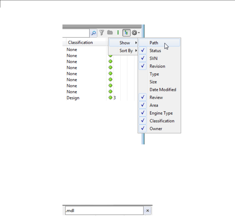
13 Managing Projects
Search and Filter File Views
Use the search box or Filter button to alter the list of files displayed. In all
the file views, and in batch job and dependency analysis nodes, you can use
the searchboxandfilteringtools.
•Type a search term in the search box, for example, part of a file name, or a
file extension. You can use wildcards, such as *.m to find only MATLAB
files,or*.m* to find both MATLAB and model files.
Click the xto clear the search.
•Click the filter button to the right of the search box to build a filter for
the current view.
13-46
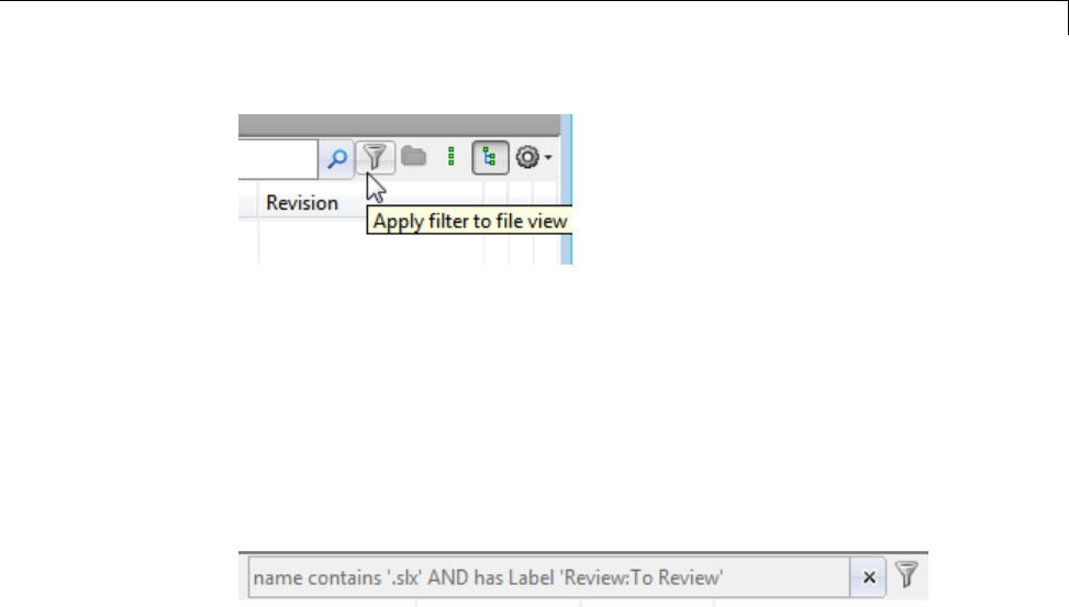
Manage Project Files
In the Filter Builder dialog box you can select multiple filter criteria to
apply using names, project status, and labels. Press Ctrl to multiselect
labels.
The dialog reports the resulting filter at the bottom, for example:
Filter = file name contains '.mdl' AND project status
is 'In project' AND has Label 'Engine Type:Diesel'
When you click OK, the search box shows the filter you are applying.
Click the xto clear the filter.
Work with Project Files
In all Files nodes, use the right-click menus to perform actions on the files
that you are viewing. Right-click a file (or selected multiple files) to perform
project options such as:
•Open or run files.
•Add and remove files from the project.
•Add, change and remove labels. See “Label Files” on page 13-49.
•Create entry point shortcuts (for example, code to run at startup or
shutdown, open models, simulate, or generate code). See “Automate Project
Startup and Run Frequent Tasks” on page 13-52.
•If a source control interface is enabled, you can also:
-Refresh source control status.
-Update from source control.
-Check for modifications.
13-47
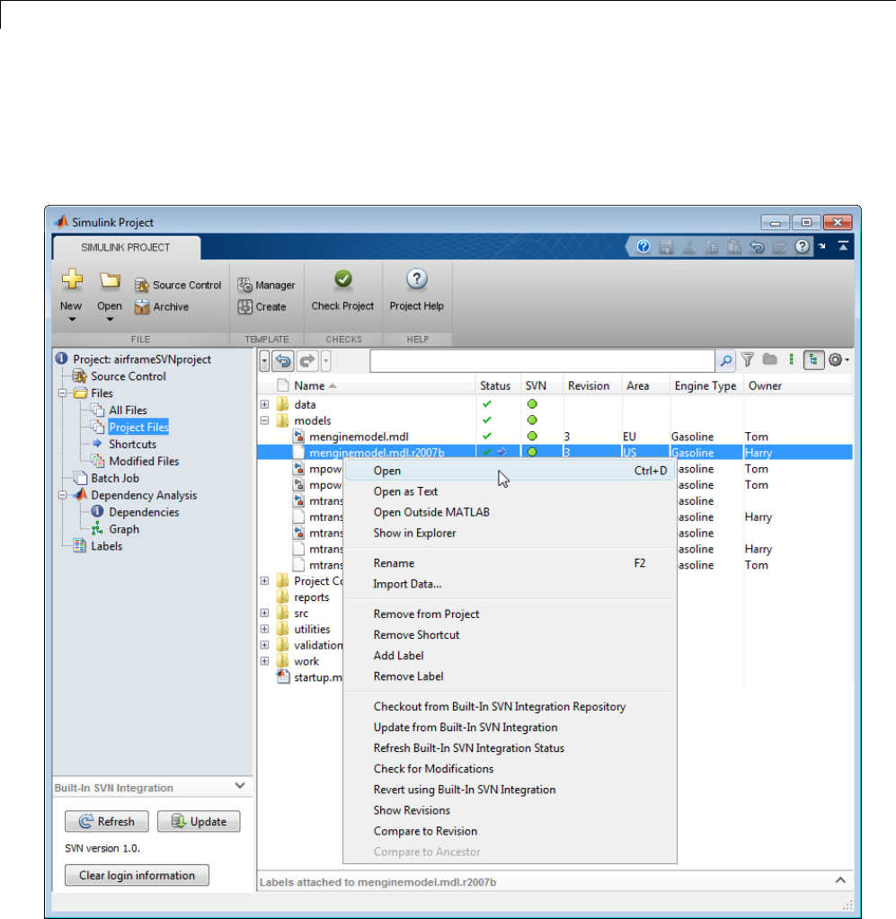
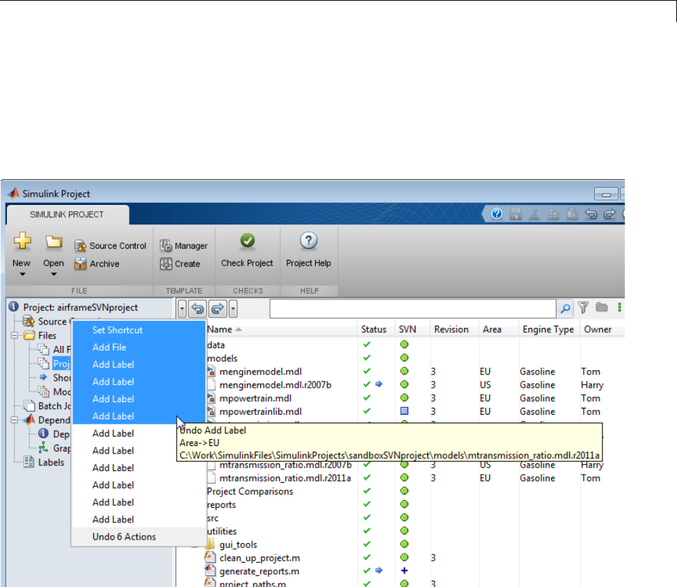
Manage Project Files
Back Out Changes
Use the Undo buttons to back out recent changes. Use the Undo or Redo
buttons and their drop-down list buttons to undo or redo recent actions in
the project. You can select multiple actions to undo. Hover over each action
to view details in a tooltip.
Label Files
Use labels to organize your files. The project automatically applies built-in
labels for file categories. You can create your own labels.
•In the Files views, right-click a file (or multiple selected files) to add or
remove labels. Once added to a file, a label persists across revisions of
the file.
13-49

13 Managing Projects
•In the Files views, you can organize lists by labels. Use the Actions button
(cog icon at top right) and select Sort By.
•Use the Labels tree node to create new label categories.
1To add a new category of labels, right-click in the blank areas of the
Categories list and select Create New.
aIn the dialog box, enter a name for the new category.
bIf only one label of the category can be attached to a file at a time, then
select the check box Single Valued.
13-50

Manage Project Files
For example, if you want to create a category with labels for Prototype
and Release and want to apply only one of those labels to any specific
file, then select Single Valued to ensure only one label can be attached.
cIf desired, change the Type selection to change the data type that can be
stored in the label, e.g., double,logical,integer,string,ornone.
dClick Create to create your new category.
2To add a new label in your new category, right-click in the blank areas of
the Labels list and select Create New.
aInthedialogbox,enteranameforthenewlabel.
bClick OK to create the label.
cRepeat to create more labels in your selected category.
3To delete labels, right-click user-defined categories and labels and select
Remove. You cannot delete built-in labels.
To add labels at the command line, see the
Simulink.ModelManagement.Project.CurrentProject reference page.
13-51

13 Managing Projects
Automate Project Startup and Run Frequent Tasks
In this section...
“Create Shortcuts” on page 13-52
“Use Shortcuts to Find and Run Frequent Tasks” on page 13-53
“Automate Startup Tasks with Shortcuts” on page 13-54
“Automate Shutdown Tasks with Shortcuts” on page 13-57
Create Shortcuts
Use shortcuts for your common project tasks and to make it easy to find and
access important files andoperations.Forexample,findandopentopmodels,
run startup code (e.g., change the path or load data), simulate models, or run
shutdown code. The Shortcuts node is blank until you add shortcuts. You can
create shortcuts from the Files node, in the All Files or Project Files view.
1To add a shortcut, right-click a file in the All Files or Project Files view
and select Create Shortcut.
2After you add shortcuts, use the Shortcuts node to use, change, or remove
your shortcuts. You can specify Startup, Shutdown, or basic shortcuts.
•Startup shortcuts run when you open your project.
•Shutdown shortcuts run when you close your project.
•Run basic shortcuts manually by right-clicking.
13-52
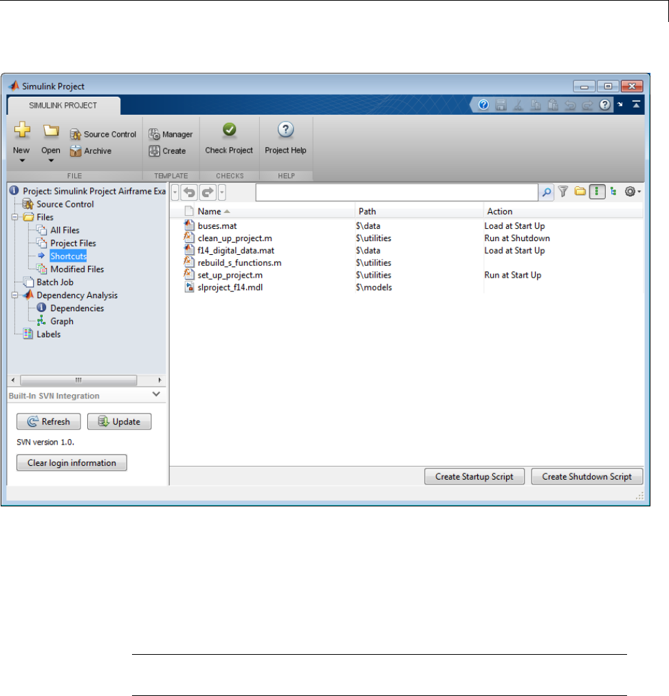
Automate Project Startup and Run Frequent Tasks
Use Shortcuts to Find and Run Frequent Tasks
Use shortcuts to make it easy to find and access important files and
operations, for yourself and any other project users. You can use shortcuts
to make top models or scripts easier to find in a large project, so that a new
user of the project can easily find it.
Note Shortcuts are included when you commit your modified files to source
control, so you can share shortcuts with other project users.
13-53
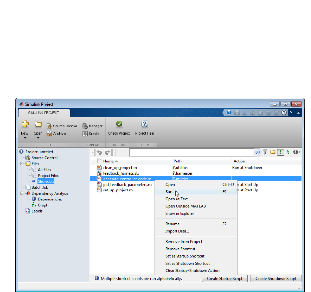
13 Managing Projects
To use your shortcuts:
1Click the Shortcuts node.
In the Shortcuts view, it can be useful to switch to List view. Click the
List view button at top right.
2Right-click the shortcut file and select an action, e.g., Open or Run.
Automate Startup Tasks with Shortcuts
You can use startup shortcuts to set up the environment for your project.
To configure your shortcut to run when you open your project:
13-54

Automate Project Startup and Run Frequent Tasks
1Click the Shortcuts node.
2Right-click the shortcut file and select Set as Startup Shortcut.
TheActioncolumndisplaysRun at Start Up.
Startup shortcut files are automatically run (.m files), loaded (.mat files), and
opened (Simulink models) when you open the project.
Startup shortcut scripts can have any name. You do not need to use
startup.m.
Note Remember that files named startup.m on the MATLAB path run
when you start MATLAB. If your startup.m file calls the project with the
CurrentProject class, you might see an error because no project is loaded
yet. To avoid the error, rename the file and use it as a project startup shortcut
instead.
You can view an example in the sldemo_slproject_airframe project, where
the file set_up_project.m sets the MATLAB path, and defines where to
create the slprj folder.
You can change back to a basic shortcut by selecting Clear
Startup/Shutdown Action.
13-55
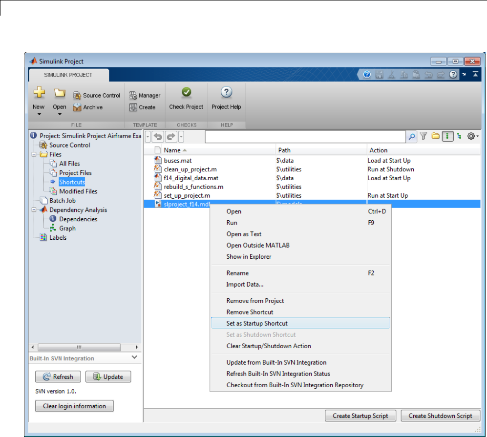
13 Managing Projects
Projects warn if you have more than one startup shortcut, because they run in
alphabetical order, which you might not want. If execution order is important,
consider creating another script that calls all the others, and use that script
as your only startup shortcut.
13-56

Automate Project Startup and Run Frequent Tasks
Note Be aware that shortcuts are included when you commit your modified
files to source control, so any startup shortcutsyoucreatewillalsorunfor
any other project users.
Automate Shutdown Tasks with Shortcuts
To configure your shortcut to run when you close your project:
1Click the Shortcuts node.
2Right-click the shortcut file and select Set as Shutdown Shortcut.
TheActioncolumndisplaysRun at Shutdown.
You can use shutdown shortcuts to clean up the environment for the
current project when you close it. Shutdown shortcuts should undo the
settings applied in startup shortcuts. You can view an example in the
sldemo_slproject_airframe project.
You can change back to a basic shortcut by selecting Clear
Startup/Shutdown Action.
Note Be aware that shortcuts are included when you commit your modified
files to source control, so any shutdown shortcuts you create will also run
foranyotherprojectusers.
13-57

13 Managing Projects
Run Batch Functions on Project Files
Select the Batch Job view to create and run functions on selected project files.
To create a batch function to use on your files:
1Click Create.
The MATLAB Editor opens a new untitled file containing a simple example
batch job. The instructions guide you to create a batch job with the correct
function signature.
2Edit the function to perform the desired action on each file.
3Save the function file on your MATLAB path.
To use the batch job from the Simulink Project Tool:
1In the Batch Job view, select the check boxes of project files you want to
include in the batch job. Only selected files are included in the batch job.
If the batch function can determine if a file it is given is appropriate, you
might want to include all files. The batch function operates only on the
appropriate subset of the included files. For example, the batch job function
saveModelFiles in the airframe project checks that the file is a Simulink
model, and does nothing if it is not. Include all files if you want your batch
function to check all files.
To select multiple files, Shift or Ctrl+click, and then right-click a file and
selectInclude or Exclude.
2Click Browse to locate your batch job function file, or enter the name of
your batch function.
3Click Run Batch Job.
The Simulink Project Tool displays the results in the Batch Job Results
column.
13-58
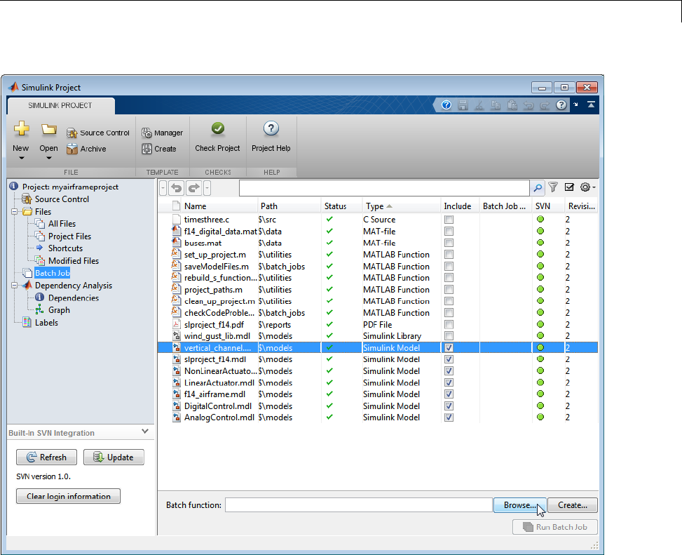
Run Batch Functions on Project Files
For example batch jobs, see Running Batch Jobs with a Simulink Project. This
example shows how to apply a batch job function to a set of files managed by a
Simulink Project. The example batch job function saveModelFiles identifies
and saves any loaded Simulink model files that contain unsaved changes. This
action can be useful to perform before committing changes to source control.
Open the example airframe project to view example batch job files
saveModelFiles and checkCodeProblems. See “Try Simulink Project Tools
with the Airframe Project” on page 13-4.
13-59

13 Managing Projects
Use Source Control with Projects
In this section...
“About Source Control with Projects” on page 13-60
“Add a Project to Source Control” on page 13-61
“View or Change Project Source Control” on page 13-68
“Register Model Files with Source Control Tools” on page 13-70
“Subversion Integration with Projects” on page 13-70
“Write a Source Control Adapter with the SDK” on page 13-75
About Source Control with Projects
You can use the Simulink Project Tool to work with source control.
Projects automatically recognize supported source control applications when
you create a new project in a folder under source control and click Detect.
Simulink projects contain interfaces to:
•Subversion®(SVN) — See “Subversion Integration with Projects” on page
13-70.
•A local version control tool — Project examples use the light-weight local
version control tool so you can try out source control operations after a
single command. The local version control tool is designed for a single
user for example purposes only. See “Try Simulink Project Tools with the
Airframe Project” on page 13-4.
You can add your project to source control to use the built-in SVN integration
that comes with Simulink projects.
When your project is under source control, you can use these project features:
•“Retrieve and Check Out Files Under Source Control” on page 13-76
•“Review Changes and Commit Modified Files” on page 13-89
13-60

Use Source Control with Projects
AddaProjecttoS
ource Control
Check your sandbox folder is on a local hard disk, not a network location.
Caution Using a network folder with SVN is slow and currently has known
bugs, e.g., http://subversion.tigris.org/issues/show_bug.cgi?id=3053. Instead,
use local sandbox folders.
To add source control to a newly created project or an existing one:
1Select the Source Control node in the project tree.
2Under Available Source Control Integrations,clickAdd project to
source control.
13-61
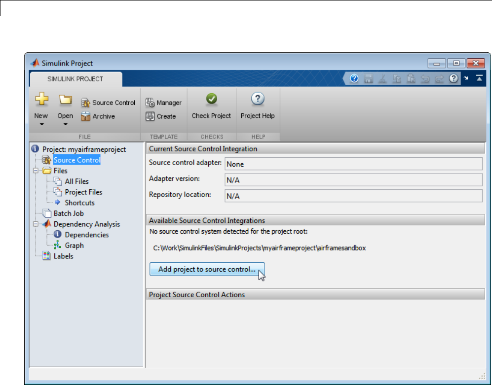
13 Managing Projects
3On the Add to Source Control dialog box, leave the default Source control
integration selected to use Built-In SVN Integration.
4Next to Repository path,clickChange.
13-62

Use Source Control with Projects
5On the Specify SVN Repository URL dialog box, either select an existing
repository or create a new one.
13-63
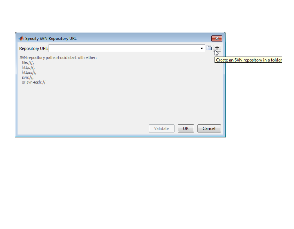
13 Managing Projects
•To specify an existing repository, click theBrowsebuttontotheright
of the Repository URL box, paste a URL into the box, or use the
drop-down list to select a recent repository.
•To create a new repository, click the Create button to the right of the
Repository URL box. A file browser opens. Create a new folder where
you want to create the new repository and click Select Folder.Donot
place the new repository inside the existing project folder.
CautionCreate new repository is for single users only. See “Create
Subversion Repository” on page 13-74.
The Simulink Project Tool creates a repository in your folder and you
returntotheSpecifySVNRepositoryURL dialog box. The URL of your
new repository is specified in the Repository URL box, and the project
automatically selects the trunk folder.
6Click Validate to check the path to your selected repository. If you have
problems, check the dialog messages for required path styles.
13-64
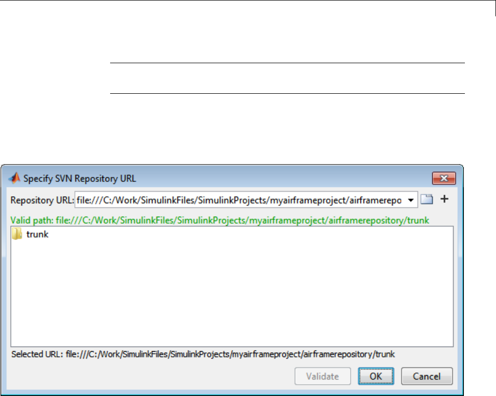
Use Source Control with Projects
Caution Use file:// URLs only for single user repositories. For more
information, see “Create Subversion Repository” on page 13-74.
When your path is valid, you can browse the repository folders. Select the
trunk folder if needed, and verify the selected URL at the bottom of the
dialog box. If you created a new repository, trunk is automatically selected.
7Click OK to return to the Add to Source Control dialog box.
8Click Convert to finish adding the project to source control.
13-65
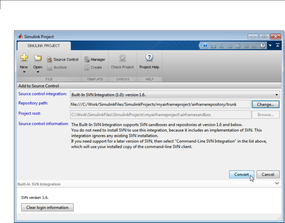
13 Managing Projects
The project runs integrity checks.
13-66
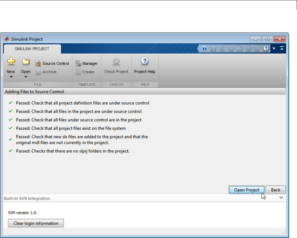
Use Source Control with Projects
9Click Open Project to return to your project.
10 If you created a new repository, you need to add your files to it. To commit
files to your new repository:
aSelect the Modified Files view. All your project files should be in the
Modified Files list.
bClick Commit Modified Files to commit the first version of your
files to the new repository. A dialog box opens, where you can enter a
comment and click Submit.
13-67
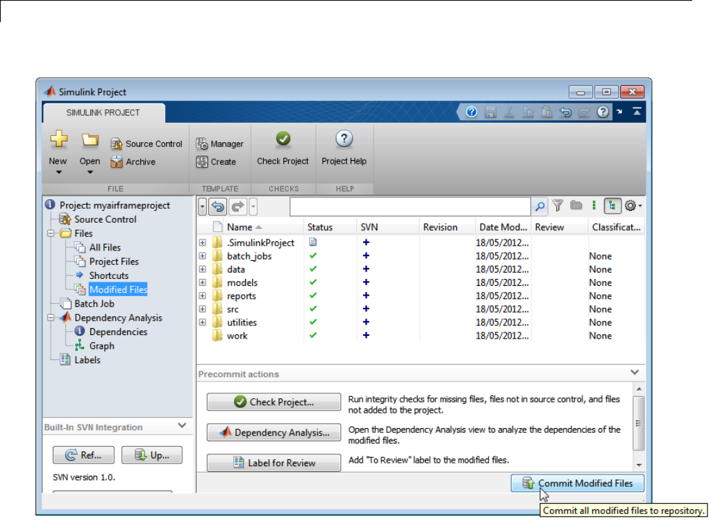
13 Managing Projects
For more information about the default Built-In SVN Integration, see “Select
Subversion Source Control” on page 13-71.
View or Change Project Source Control
•“Viewing Source Control Type and Repository” on page 13-69
•“Adding, Changing, or Removing Source Control” on page 13-69
•“Tagging Files” on page 13-70
13-68
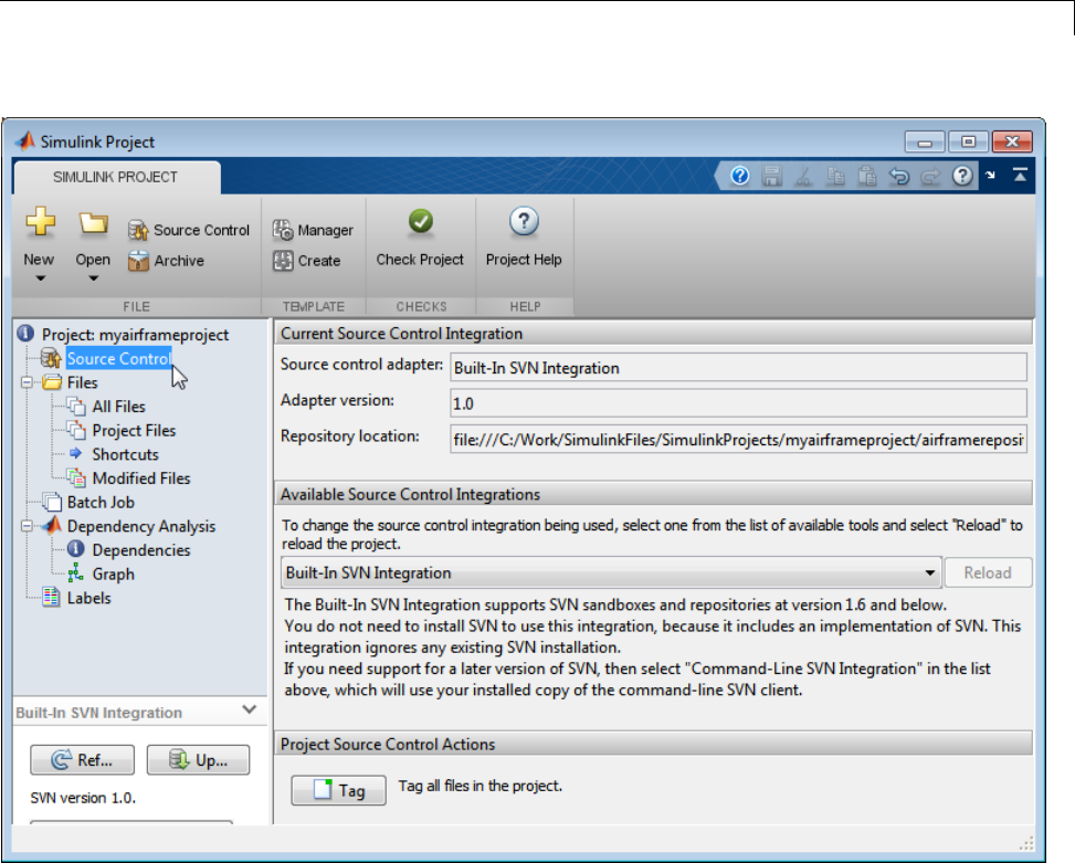
Use Source Control with Projects
Viewing Source Control Type and Repository
The Source Control node in the project tree shows details of the current source
control tool, the adapter interfacing to source control in your current project,
and the repository location.
Adding, Changing, or Removing Source Control
To add source control to a newly created project or an existing one, under
Available Source Control Integrations, select Add project to source
control. See “Add a Project to Source Control” on page 13-61.
13-69

13 Managing Projects
Usethesamecontroltoremoveaproject from source control by selecting No
source control integration and clicking Reload. For example, this action
might be useful when you are preparing a project to create a template from it,
and you want to avoid accidentally committing unwanted changes. You can
later select your previous source control from the list again.
Tagging Files
Use tags to identify specific revisions of all project files. In the Source Control
node, click the Tag button under Project Source Control Actions. Specify the
text for the tag. This action adds your tag to every project file.
Not every source control has the concept of tags. To use tags with SVN, you
need the standard folder structure in your repository and you need to check
out your files from trunk. See “Create Subversion Repository” on page 13-74
Register Model Files with Source Control Tools
If you use third-party source control tools,besuretoregisteryourmodelfile
extensions (.mdl and .slx) as binary formats. If you do not, these third-party
tools might corrupt your model files when you submit them, by changing
end-of-line characters, expanding tokens, keyword substitution, or attempting
to automerge. Corruption can occur whether you use the source control tools
outside of Simulink or if you try submitting files from the Simulink Project
Tool without first registering your file formats.
You should also check that other file extensions are registered as binary to
avoid corruption at check-in for files such as .mat,.xlsx,.jpg,.pdf,.docx,
etc.
For instructions, see “Register Model Files with Subversion” on page 13-73
Subversion Integration with Projects
•“Select Subversion Source Control” on page 13-71
•“Built-In SVN Integration” on page 13-71
•“Command-Line SVN Integration (Compatibility Mode)” on page 13-72
•“Register Model Files with Subversion” on page 13-73
13-70

Use Source Control with Projects
•“Create Subversion Repository” on page 13-74
Select Subversion Source Control
To use SVN in your project, you can useanyofthefollowingworkflows:
•Create a new project in a folder already under SVN source control and
click Detect. See “Create a New Project to Manage Existing Files” on
page 13-23.
•Add source control to a project. See “Add a Project to Source Control” on
page 13-61.
•Retrieve files from an existing SVN repository and create a new project. See
“Retrieve a Working Copy of a Project from Source Control” on page 13-76.
When you add to source control or retrieve from source control, you can
optionally change the SVN integration in the Source control integration
list.
SVN Version You Want to Use SVN Integration to Select
SVN version 1.7 or below
(no installation steps required)
“Built-In SVN Integration” on page
13-71
Other SVN version
(requires additional installation
steps)
“Command-Line SVN Integration
(Compatibility Mode)” on page 13-72
Note Also, you can check for updated
downloads on the Simulink Projects Web page:
http://www.mathworks.com/products/simulink/simulink-projects/
Built-In SVN Integration
Select the Built-In SVN Integration for use with SVN sandboxes and
repositories at version 1.7 and below.
You do not need to install SVN to use this integration because Built-In SVN
Integration includes an implementation of SVN. This integration ignores
13-71

13 Managing Projects
any existing SVN installation. If you need support for a later version of
SVN, then select Command-Line SVN Integration (compatibility mode)
instead.
The Built-In SVN Integration supports secure logins and moving @ folders.
Command-Line SVN Integration (Compatibility Mode)
Note Select Command-Line SVN Integration (compatibility mode) only
if you need to use a later version of SVN than 1.7. Otherwise, use Built-In
SVN Integration instead, for more features, improved performance, and no
need to install an additional command-line SVN client.
If you select Command-Line SVN Integration (compatibility mode),you
must also install a command-line SVN client.
Command-line SVN integration communicates with any Subversion (SVN)
client that supports the command-line interface. Install an SVN client that
supports the command-line interface, and then you can use this integration
with the Simulink Project Tool.
TortoiseSVN does not support the command-line interface. However, you can
continue to use TortoiseSVN from Windows Explorer after installing another
SVN client that supports the command-line interface. Ensure that the major
version numbers match, e.g., both clients should be SVN 1.7.
You can find Subversion clients on this Web page:
http://subversion.apache.org/packages.html
.
If you try to rename a file in a project under SVN source control, and the
folder name contains an @ character, you see an error because command-line
SVN treats all characters after the @ symbol to be a peg revision value.
13-72

Use Source Control with Projects
Register Model Files with Subversion
If you do not register your model file extension as binary, Subversion may add
annotations to conflicted Simulink files and attempt automerge. This corrupts
model files so you cannot load the models in Simulink.
To avoid this problem when using Subversion, follow these steps to register
your file extensions:
1Locate your SVN config file, e.g.:
C:\Users\myusername\AppData\Roaming\Subversion\config,
or C:\Documents and Settings\username\Application
Data\Subversion\config on Windows, or in ~/.subversion on Linux or
Mac OS X.
2Add the following lines to the end of the config file, and SVN will no longer
add annotations to Simulink files on conflict, and will never attempt an
automerge.
*.mdl = svn:mime-type= application/octet-stream
*.mat = svn:mime-type=application/octet-stream
*.slx = svn:mime-type= application/octet-stream
13-73

13 Managing Projects
Create Subversion Repository
You can create an SVN repository when adding a project to source control.
See “Add a Project to Source Control” on page 13-61.
Caution Creating new repositories is provided for local single-user access
only, for testing and debugging. Do not use for multiple users or you risk
corrupting the repository.
When you use Simulink Projects to create a repository, you create a repository
using the file:// protocol. Subversion documentation strongly recommends
only single users access a repository directly via file:// URLs. See the Web
page:
http://svnbook.red-bean.com/en/1.7/svn-book.html#svn.serverconfig.choosing.recomm
e
It is not recommended to allow multiple users to access a repository directly
via file:// URLs. You risk corrupting the repository. Use file:// URLs
only for single user repositories.
When you want to share a repository, you need to set up a server. You can use
svnserve or the Apache™ SVN module. See the Web page references:
http://svnbook.red-bean.com/en/1.7/svn-book.html#svn.serverconfig.svnserve
http://svnbook.red-bean.com/en/1.7/svn-book.html#svn.serverconfig.httpd
On Windows, search the Web for Subversion servers that you can set up in
afewclicks.
To enable tagging within projects when using SVN, create your repository
with the standard tags,trunk,andbranch folders, and check out your files
from trunk. This structure is recommended by the Subversion project. See
the Web page:
http://svn.apache.org/repos/asf/subversion/trunk/doc/user/svn-best-practices.html
.
You can create an SVN repository with the standard structure from the
project, and the project automatically selects the trunk folder.
13-74

Use Source Control with Projects
After you create a repository with this structure, you can use the Tag button
in the Project Source Control node to add tags to all your project files. Tag
errors if you do not create a tags folder in your repository.
Write a Source Control Adapter with the SDK
Simulink provides a Software Development Kit (SDK) that you can use to
integrate Simulink Projects with third-party source control tools.
The SDK provides instructions for writing an adapter to a source control tool
that has a published API that can be called from Java™.
You must create a .jar file which implements a collection of Java interfaces
and a Java Manifest file, which defines a set of required properties.
The SDK also provides example source code, Javadoc, and files for validating,
building, and testing your source control adapter. Build and test your own
interfaces using the example as a guide, then you can use your source control
adapter with Simulink Projects.
1To extract the contents of the SDK, enter:
run(fullfile(matlabroot,'toolbox','simulink','simulink','slproject',...
'adapterSDK','extractSDK'))
Select a folder to place the cm_adapter_SDK folder and files inside, and
click OK.
2Locate the new folder cm_adapter_SDK, and open the file
cm_adapter_SDK_guide.pdf for instructions.
13-75

13 Managing Projects
Retrieve and Check Out Files Under Source Control
In this section...
“Retrieve a Working Copy of a Project from Source Control” on page 13-76
“Refresh Status of Project Files” on page 13-81
“Update Revisions of Project Files” on page 13-84
“CheckOutFiles”onpage13-86
Retrieve a Working Copy of a Project from Source
Control
To create or update a new local copy of a project by retrieving files from source
control:
1From MATLAB, on the Home tab, in the File section, select
New > Simulink Project > From Source Control.
Alternatively, from the Simulink Project Tool, on the Simulink Project
tab, select Source Control.
The Source Control dialog box appears.
13-76
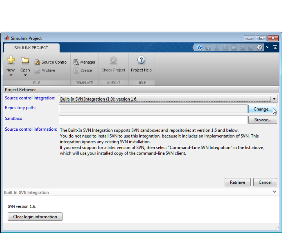
Retrieve and Check Out Files Under Source Control
2(Optional) Select your source control interface from the Source Control
Adapters drop-down list.
Leave the default Built-In SVN Integration to use the default SVN
integration with your project. For more information on SVN support, see
“Select Subversion Source Control” on page 13-71.
3Click Change to select the Repository Path that you want to retrieve files
from.
The Specify Repository URL dialog box opens.
13-77

13 Managing Projects
aClick the Generate URL from folder button to the right of the
Repository URL box to browse for your repository location.
Select the folder containing your repository and click OK.
The retriever generates a URL for you in the Repository URL field.
Alternatively, manually enter or paste the Repository URL.
bClick Validate to check the repository path.
If the path is invalid, check the URL against your source control
repository browser.
Caution Use file:// URLs only for single user repositories. For more
information, see “Create Subversion Repository” on page 13-74.
cIf necessary, select a deeper folder in the repository tree. The example
shows trunk selected, and the Selected URL displays at the bottom of
the dialog box.
13-78
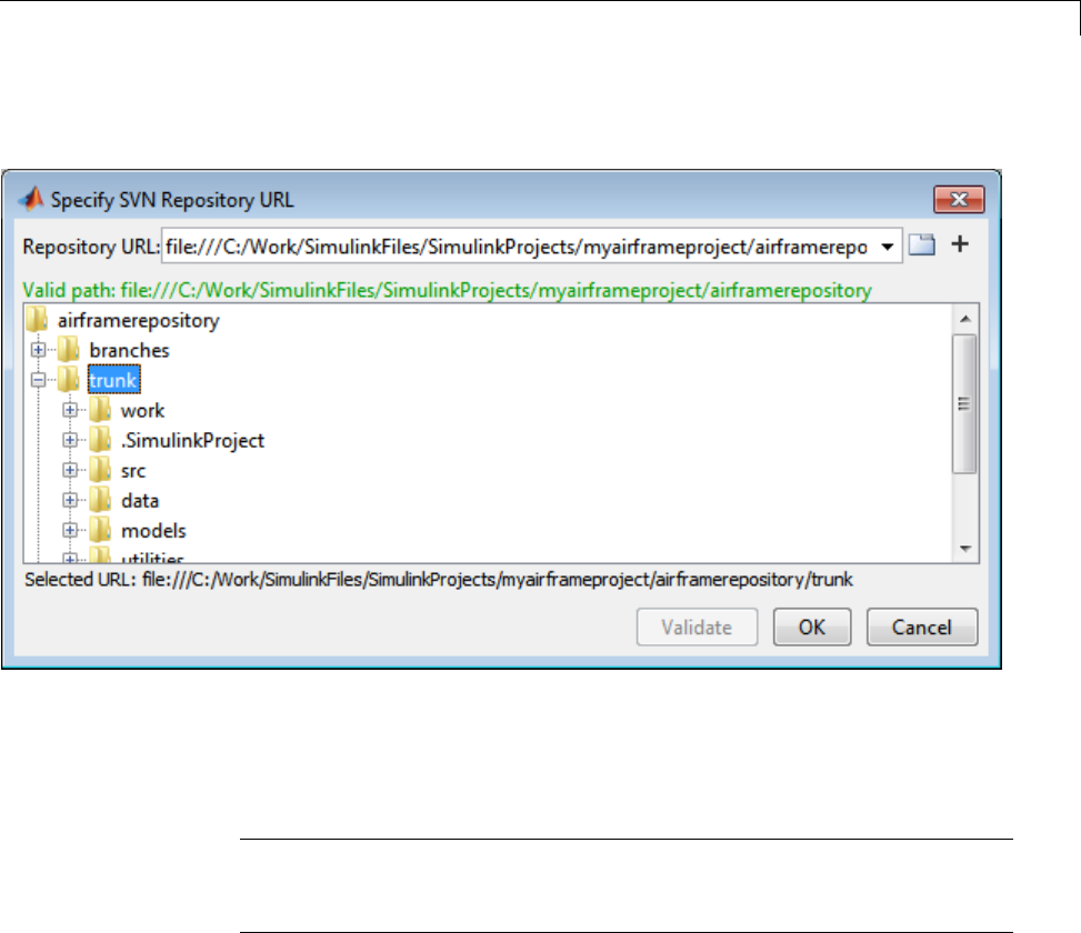
Retrieve and Check Out Files Under Source Control
The retriever uses the Selected URL when you click OK.
dClick OK to continue and return to the Project Retriever.
4Click Browse to select the sandbox folder where you want to put the
retrieved files for your new project.
Caution Using a network folder with SVN is slow and currently has
known bugs e.g., http://subversion.tigris.org/issues/show_bug.cgi?id=3053.
Instead, use local sandbox folders.
13-79
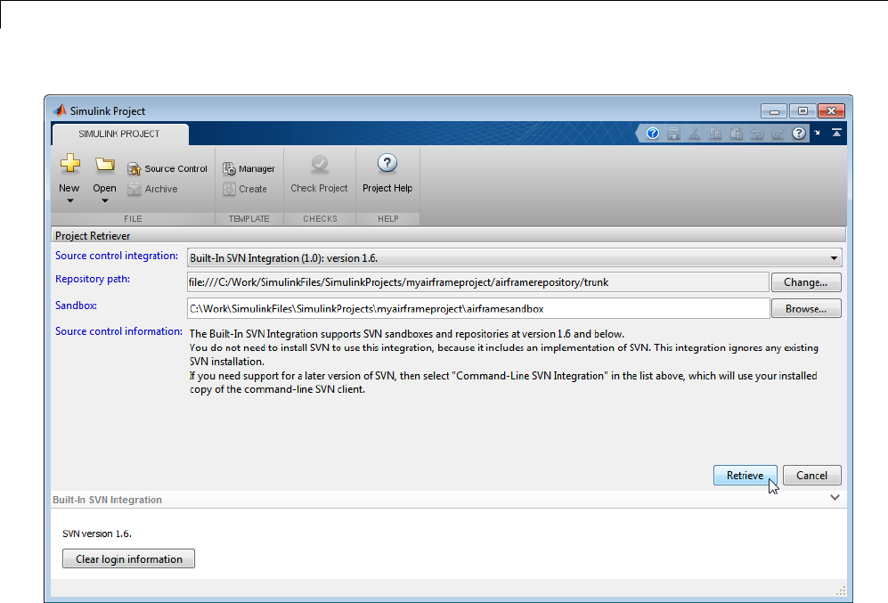
13 Managing Projects
5Click Retrieve.
6Watch the Built-In SVN Integration paneformessagesastheproject
retrieves your files from source control.
If you are retrieving files to update an existing project, your project opens.
7If you are retrieving files to a new sandbox, a dialog appears to report that
the files in the repository have been checked out to your selected sandbox
folder, and to check whether you want to create a project in the folder.
Click Yes to continue creating the project. Click No to leave the files on
disk and return to the retriever.
8When you click Yes, the new project controls appear.
aEnter a project name.
13-80

Retrieve and Check Out Files Under Source Control
bClick Detect to identify the source control in the project folder.
cClick Create to finish creating the new project in your new sandbox.
The Simulink Project Tool displays the empty Project Files list for your chosen
project root. Your project does not yet contain any files. You need to select
files to add. For next steps, see “Add Files to the Project” on page 13-26.
Refresh Status of Project Files
To check the status of individual files, right-click files in any view to select
Refresh. This action queries the local sandbox state and checks for changes
made with another tool. For SVN, Refresh does not contact the repository.
13-81
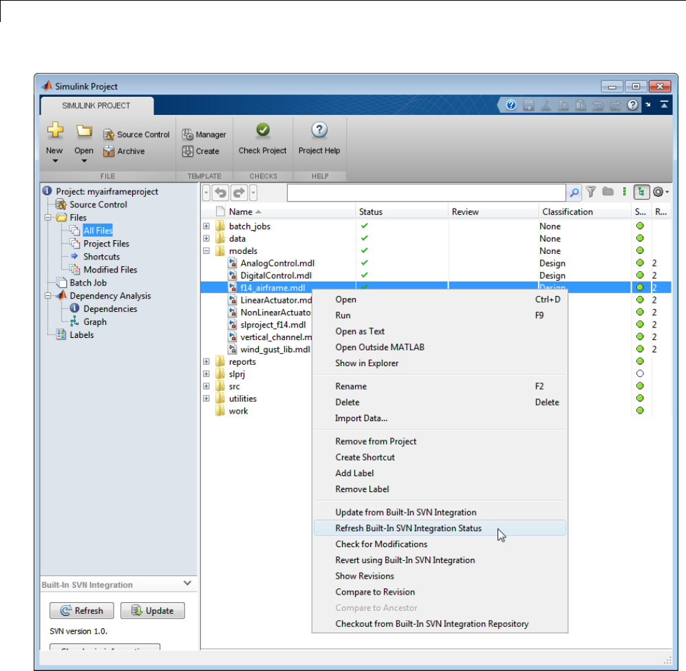
13 Managing Projects
To check source control status of all project files, click the Refresh button in
the source control pane at bottom left. The source control pane title depends
13-82
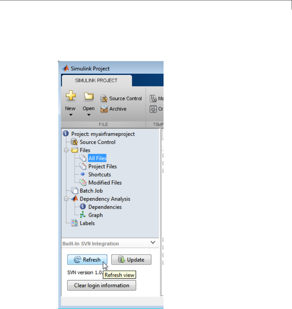
Retrieve and Check Out Files Under Source Control
on your source control, for example, Built-In SVN Integration. The source
control pane reports source control messages, and the buttons in the pane
applytothewholeproject.
13-83

13 Managing Projects
Refresh refreshes the view of the source control status for all files under
projectroot.WhenyouclickRefresh, this updates the information shown
in the Revision column and the source control status column (e.g., SVN or
Modifications column). Hover over the Modifications row to see the tooltip
showing the source control status of a file, e.g., Modified (Checked Out).
For SVN repositories that require login, you can click Clear login
information to clear your login information.
Update Revisions of Project Files
To get the latest revisions of all project files from the source control repository,
click the Update button in the source control pane. The source control pane
title depends on your source control, for example, Built-In SVN Integration.
13-84
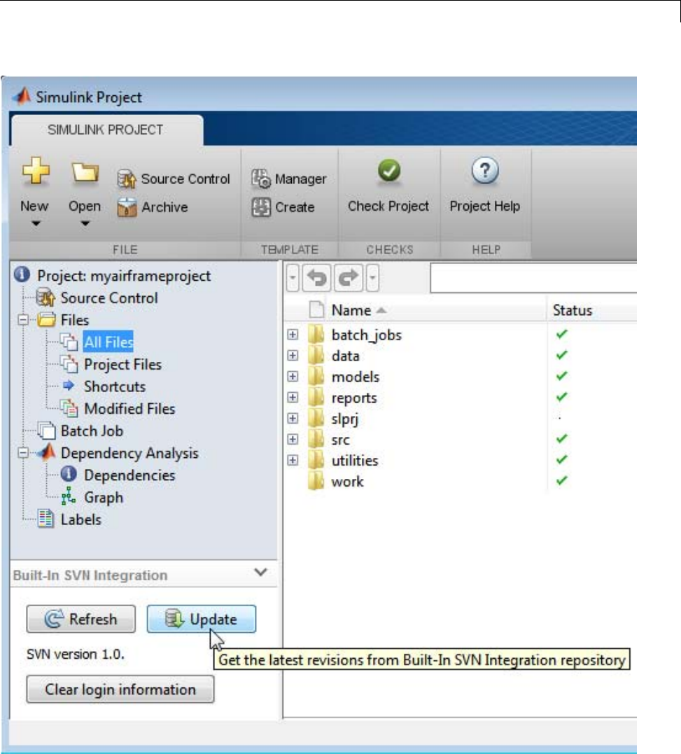
Retrieve and Check Out Files Under Source Control
13-85

13 Managing Projects
To update selected files, right-click and select Update from Built-In SVN
Integration Repository to get fresh local copies of the selected file from
the repository.
Check Out Files
To check out files,
1In any Files view, click to select a file, or press Shift+click to select
multiple files.
2Right-click the selected files and select Checkout from Source Control.
The menu wording for Source Control is specific to your selected source
control, e.g., for SVN, Checkout from Built-In SVN Integration
Repository.
13-86
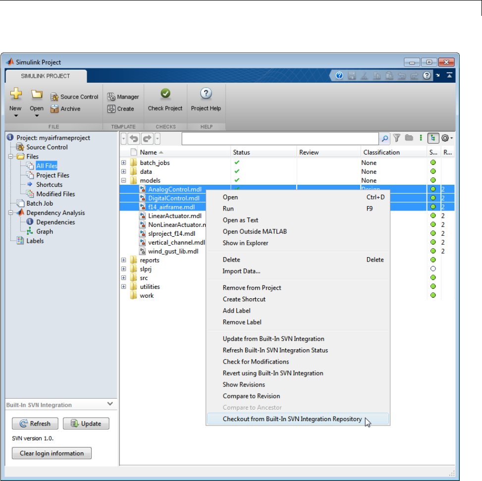
Retrieve and Check Out Files Under Source Control
13-87

13 Managing Projects
Note With SVN, use Checkout from Built-In SVN Integration
Repository to get a lock on a file. This option does not modify the file in
your local sandbox.
To get a fresh local copy of the file from the repository, select Update from
Built-In SVN Integration Repository.
For next steps, see “Review Changes and Commit Modified Files” on page
13-89.
13-88
Review Changes and Commit Modified Files
Review Changes and Commit Modified Files
In this section...
“View Modified Files” on page 13-89
“Review Changes” on page 13-91
“Precommit Actions” on page 13-93
“Commit Modified Files” on page 13-94
“Revert Local Changes and Release Locks” on page 13-94
“Resolve Conflicts” on page 13-95
“Work with Derived Files in Projects” on page 13-96
View Modified Files
The Modified Files node is visible only if you are using source control
integration with your project.
UsetheModifiedFilesnodetoreview,analyze, label, and commit modified
files. Lists of modified files are sometimes called changesets.TheModified
Files node aids the reviewing process.
In the Modified Files view, it can be useful to switch to List view. Use the List
view or Tree view buttons at top right.
As in the other Files nodes, in the Modified Files view you can right-click files
or multiple selected files to:
•Add and remove labels.
•Update from source control.
13-89
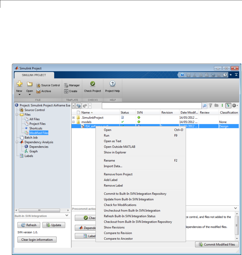
13 Managing Projects
•Uncheckout from source control.
•Commit to repository.
•Refresh source control status.
•Compare against selected revision or ancestor.
13-90

Review Changes and Commit Modified Files
Project Definition Files
The files in .SimulinkProject are project definition files generated by your
changes. The project definition files allow you to create shortcuts and add
labels to files without checking them out, and add other metadata such as a
project description. Project definition files also define which files are added to
your project.
Any changes you make to your project (e.g., to shortcuts, labels, categories,
or files in the project) generate changes in the .SimulinkProject folder.
These files store the definition of your project in XML files whose format
is subject to change.
You should never need to view project definition files directly, except when
the source control tool requires a merge. The files are shown so that you
know about all the files being committed to the source control system. See
“Resolve Conflicts” on page 13-95.
Review Changes
To review changes in modified files, right-click selected files to view revision
logs and compare against another revision or ancestor.
•Select Show Revisions to open the File Revisions dialog box and browse
the history of a file. In the table, you can view SVN information about
who previously committed the file, when they committed it, and the log
messages.
•Select Compare to Revision to open a dialog where you can select the
revision you want to compare. You can select multiple files and select a
revision to compare against for each file. When you click Compare,your
comparisons run and the Comparison Tool displays reports.
•Select Compare to Ancestor to run a comparison with the last checked
out version in the sandbox. The Comparison Tool displays a report.
13-91
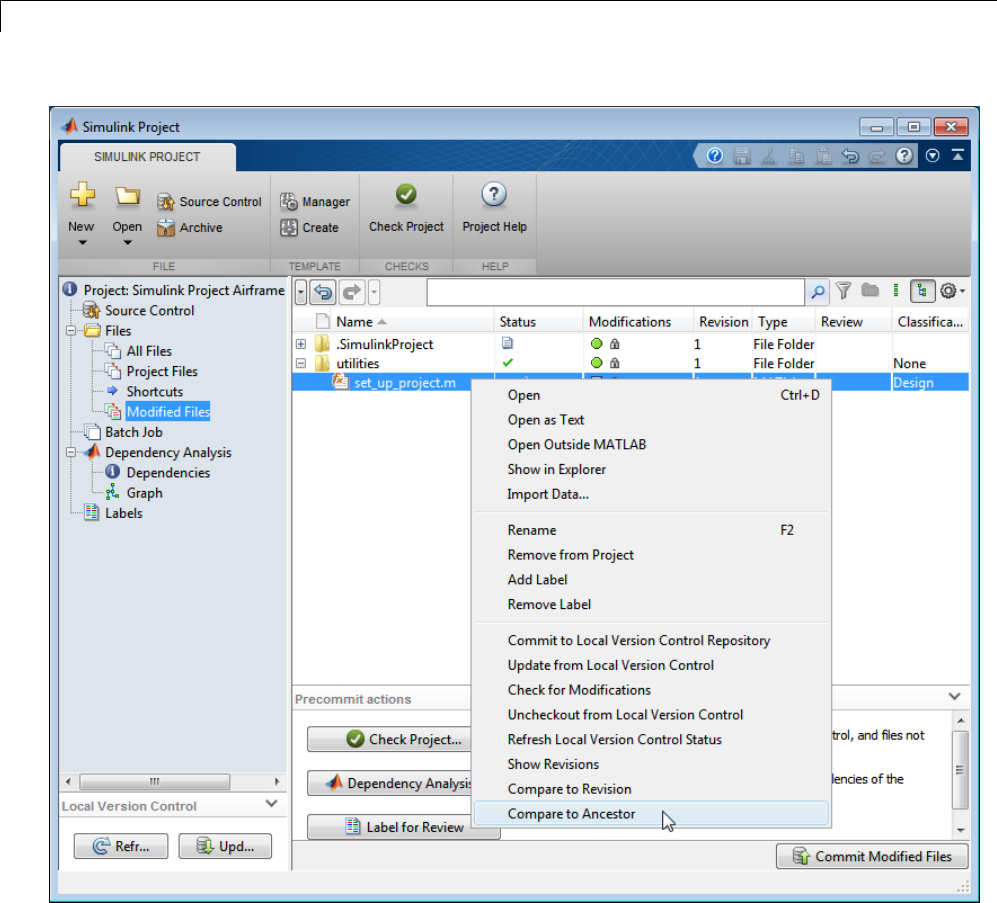
13 Managing Projects
When reviewing changes, you can merge Simulink models from the
Comparison Tool report (requires Simulink Report Generator).
13-92
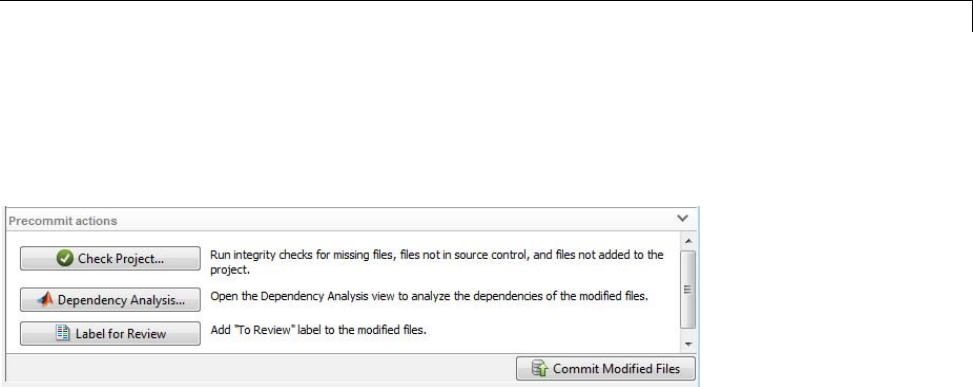
Review Changes and Commit Modified Files
Precommit Actions
The Precommit actions pane in the Modified Files view contains tools you
might want to use before committing your changes to source control.
•Click the Check Project button to check the integrity of the project. For
example, is everything under source control in the project? Are all project
files under source control? A dialog box reports results. You can click for
details and follow prompts to fix problems, e.g., if you would like to add
files to your repository.
For an example showing how the checks can help you, see “Upgrade Model
Files to SLX and Preserve Revision History” on page 13-15.
This function is also in the Simulink Project tab (Check Project)soyou
can run the checks from any project view.
For more information on some problems the checks can fix, see “Work with
Derived Files in Projects” on page 13-96.
•If you want to check for required files, click the Dependency Analysis
button to open the Dependency Analysis view, with your modified files
selected for analysis. You can optionally change the check box selections
before clicking Analyze. You can use the dependency tools to analyze the
structure of your project. See “Analyze Project Dependencies” on page
13-32.
•If you want to add the label To Review to all files in your changeset, click
the Label for Review button.
13-93
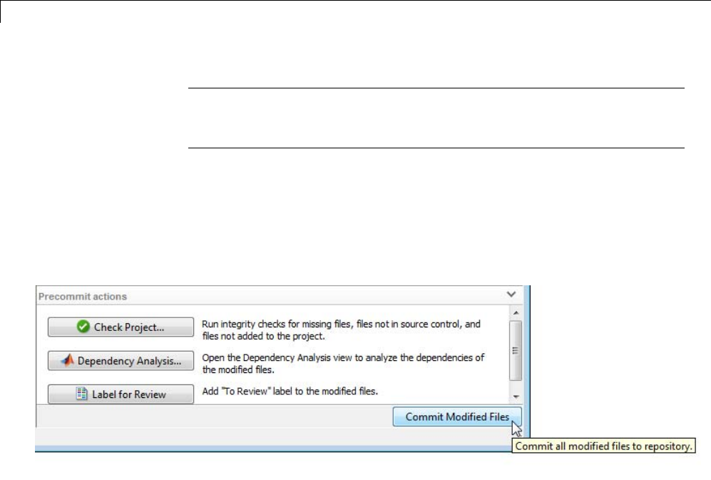
13 Managing Projects
Note The files in .SimulinkProject are project definition files generated
by your changes, and these files are not labeled. See “Project Definition
Files” on page 13-91.
Commit Modified Files
To commit your changes to source control:
1Click the Commit Modified Files button to check in all files in the
modified files list.
2A dialog prompts you to enter comments for your submission.
3Click Submit or Cancel.
Revert Local Changes and Release Locks
If you want to roll back local changes, right-click a file and select Uncheckout
from Built-In SVN Integration Repository to release locks and revert to
the version in the last sandbox update (e.g., the last version you synchronized
or retrieved from the repository).
Select Revert using Built-In SVN Integration Repository to choose a
revision to revert to.
13-94
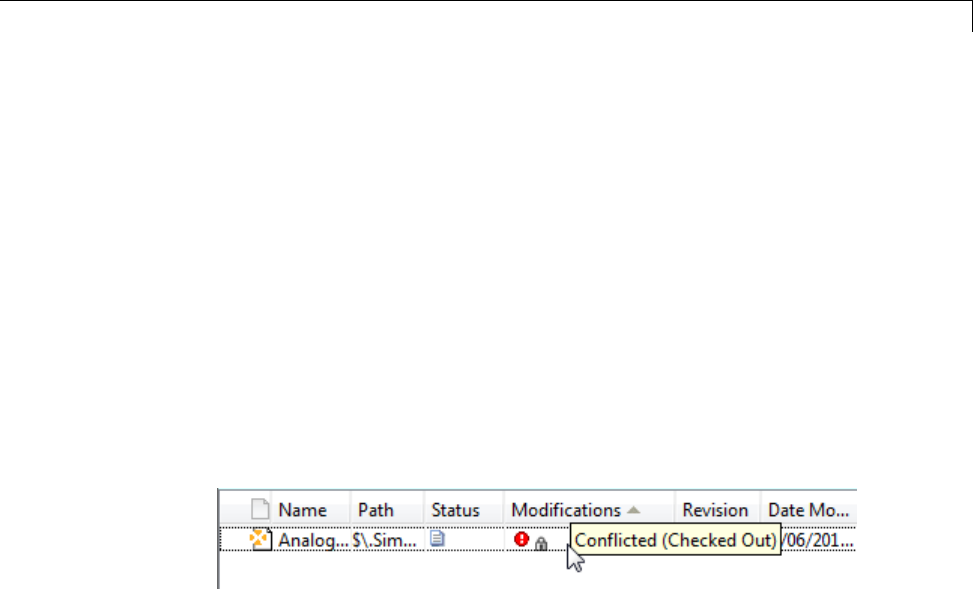
Review Changes and Commit Modified Files
Resolve Conflicts
If two people both change the same file in different sandboxes, you get a
conflict message when you try to commit your modified files. You can also
get conflicts in your project definition files. For example, if two people both
change the labels attached to a file, you can get a conflict in one of the project
definition files in the .SimulinkProject folder.
To resolve conflict problems:
1Look for conflicted files in the Modified Files view.
2ItcanbeusefultoswitchtoListview. Click List view at the top right.
3Check the source control status column (e.g., the SVN or Modifications
column) for files with a red icon. The tooltip shows Conflicted.
4Examine the conflict. You might want to select Compare to Ancestor
to run a comparison with the last checked out version in the sandbox, or
Compare to Revision to select revisions for comparison.
In the Comparison Tool, examine the report to see how the files have
changed.
5Resolve the conflict. In the Comparison Tool report, you can merge changes
between revisions (requires Simulink Report Generator). For example, you
can merge project file labels and shortcuts.
You might want to open files from the project to make changes and resolve
theconflict. Ifyouneedtochangelabelsmanually,see“LabelFiles”on
page 13-49, or to change the project description, see the Project node.
6When you are satisfied that you have resolved the changes and want to
commit the version in your sandbox, right-click the file and select Mark
Conflict Resolved. You can now commit your file.
13-95

13 Managing Projects
Work with Derived Files in Projects
You might not want to include derived and temporary files in your project or
commit them to source control. Use Check Project in the Precommit Actions
pane or the Simulink Project tab to check the integrity of the project. If you
add the slprj folder to a project, the project checks advise you to remove this
from the project and offer to make the fix. The checks recommend a best
practice of not adding derived and temporary files to source control.
You might not want to commit derived files, such as .mex*, the contents of the
slprj folder,sccprj folder, or other code generation folders, because they
can cause problems. For example:
•With a source control that can do file locking, users can encounter conflicts.
If slprj is under source control and a user generates code, this changes
most of the files under slprj and locks those files. Other users then cannot
generate code because they get file permission errors. The slprj folder is
also used for simulation via code generation (e.g., with model reference or
Stateflow), so locking these files can have a big impact on a team. The
same problems arise with binaries, such as .mex*.
•Deleting slprj is quite commonly required. However, deleting slprj
causes problems such as “not a working copy” errors if the folder is under
some source control tools (e.g., SVN).
•If you want to check in the generated code as an artifact of the process,
then it is common to copy some of the files out of the slprj cache folder and
into a separate location that is part of the project. That way the temporary
cache folder can be deleted whenever required. See the packNGo function to
discover the list of generated code files, and use the project API to add to
the project with appropriate metadata.
•The slprj folder can contain a large number of small files. This can have
aper
formance impact with some source control tools when each of those
files has to be checked to see if it is up-to-date.
13-96

Use Templates to Create Standard Project Settings
Use Templates to Create Standard Project Settings
In this section...
“Use Templates for Standard Project Setup” on page 13-97
“Create a Template from Your Current Project” on page 13-97
“View and Validate Templates” on page 13-99
“Create a New Project Using a Template” on page 13-100
“Import New Templates” on page 13-100
“Example Templates” on page 13-101
Use Templates for Standard Project Setup
You can use templates to create and reuse a standard project structure. You
can use templates to make consistent projects across teams. You could use
templates to create new projects that:
•Use a standard folder structure.
•Set up a company standard environment, for example, with company
libraries on the path.
•Have access to tools such as company Model Advisor checks.
•Use company standard startup and shutdown scripts.
•Share labels and categories.
When your existing project is in a state that others would find useful, or
you want to reuse, then you can create a template from it and use it when
creating new projects.
Create a Template from Your Current Project
You can create a template from an existing project, and then use the template
to create new projects.
To create a template from your current project, on the Simulink Project tab,
in the Template section, select Create.
13-97

13 Managing Projects
To use the template when creating new projects, you must put the template
onthetemplatepath. Ifthefolderwhereyoucreatethenewtemplateis
not already on the template path, you can add folders to the path later in
theTemplateManager.
When you create a new template, it contains the structure and all the contents
of the current project, so that you can reuse scripts and other files for your
standard project setup. Before creating the template, create and edit a new
copy of the project to contain only the files you want to reuse.
To create a template from an existing project that is under version control:
1Get a new working copy of the project. See “Retrieve a Working Copy of a
Project from Source Control” on page 13-76.
2To avoid accidentally committing changes to your project that you have
made only to create the template, you might want to stop using source
control with this sandbox. In the Source Control view, click Select an
available source control integration and select None to remove this
sandbox from source control.
3Remove the files that you do not want in the template. For example, you
might want to reuse only the utility functions, startup and shutdown
scripts, and labels. In the Project Files view, right-click unwanted files
and select Remove from Project.
4On the Simulink Project tab, in the Template section, click Create.
5To verify that your template behaves as you expect, create a new empty
project that uses your new template.
To make changes to an existing template:
1Create a new empty project using the template you want to modify.
2Make the desired changes to the project.
3On the Simulink Project tab, in the Template section, click Create.
Either create a new template, or overwrite the existing template.
13-98
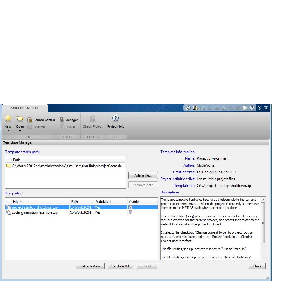
Use Templates to Create Standard Project Settings
View and Validate Templates
UsetheTemplateManagertoviewadefault template, or locate and validate
template files. On the Simulink Project tab, in the Template section,
click Manager.
Click the templates in the Templates pane to view the Description.
For example, the Project Environment template shows you how to specify
options to:
•Setupandresetthefoldersonthepathwhenyouopenorclosetheproject.
13-99

13 Managing Projects
•Define the location of the folder (slprj) for generated code and other
temporary files.
•Run standard scripts at startup and shutdown.
•Include information in a template about names, authors, and description.
See also “Example Templates” on page 13-101.
In the Template Manager you can:
•Validate that a template is usable to create new projects.
•AddfolderstothetemplatepathtomaketemplatesvisibleintheNew
Project dialog Templates list.
•Specify which templates to make visible in the Templates list.
Create a New Project Using a Template
To try using the Project Environment template, select it when creating a
new project.
Use the Templates list to select a template during project creation. Only
templates on the template path appear in the dialog.
Note If you create a project in a folder that already contains files, you are
warned if there are any collisions with the template. The template will
overwrite the existing files if you choose to continue.
Import New Templates
You can use templates to share information and best practices. New templates
can be created by you, your colleagues, or downloaded from MATLAB Central:
http://www.mathworks.com/matlabcentral/
.
Youneedtoimportanewtemplatetomakeitavailableforuseinnewprojects.
13-100

Use Templates to Create Standard Project Settings
1On the Simulink Project tab, in the Template section, click Manager.
2Click Import.
3Browse to the zip file that contains the new template.
4Select a location on the template path to save the new template. Click
Import to validate the template and import it. If validation fails, then it
will not be imported.
Example Templates
Project Environment Template
Try the Project Environment template if you are creating a project in a
new folder and intend to add files later. You can view information about
the template settings in the description field of the Template Manager. The
Project Environment template can create a new project with a preconfigured
structure, and utilities to configure the path and environment with startup
and shutdown shortcuts. For example, the path utilities help set up your
search path to ensure dependency analysis can detect project files. You can
modify any of these files, folders, and settings later. To try the template,
select the Project Environment template when creating a new project.
The utilities set_up_project.m,clean_up_project.m and project_paths.m
configure the path and settings when you open and close the project. The
startup shortcut changes current folder to the project root. The utilities set
the folder (slprj) where generated code and other temporary files are created
for the current project, and reset that folder to the default location when
the project is closed. Shortcuts provide quick access to frequently required
models and tasks.
Code Generation Example Template
Try the Code Generation Example template to set up a project with settings
for production code generation of a plant and controller. This template
requires Simulink Coder and Embedded Coder. To try the template, select
the Code Generation Example template when creating a new project.
The utilities set_up_project.m,clean_up_project.m and project_paths.m
configure the path and settings when you open and close the project, as
13-101

13 Managing Projects
in the Project Environment template. These utilities set the folder (slprj)
where generated code and other temporary files are created for the current
project, and reset that folder to the default location when the project is closed.
The startup shortcut also changes the current folder to the project root.
Other shortcuts define the controller parameters as a tunable structure in
the generated code. Shortcuts provide quick access to frequently required
models and tasks.
The settings of the model feedback_control are changed to be suitable
for production code generation. Settings are changed as the Model Advisor
recommends in the checks for both By Product > Embedded Coder and By
Task > Code Efficiency,including:
•System Target File is set to ert.tlc.
•Code Generation reporting is enabled.
•The following diagnostics are set:
-BusSignalsTreatedAsVectors, Connectivity pane, set to Error.
-Model Initialisation,Underspecified initialization detection set
to Simplified
•The following optimizations are enabled:
-All Data Initialisation Optimizations
-Saturation maths operations for floating point to integer conversion
(and vice versa)
-Inline parameters, Inline Invariant Signals
After you create the project, open the model feedback_harness to examine
the controller and plant models.
Right-click to run the project shortcut generate_controller_code.m to
generate code for the controller and display a code generation report.
13-102

Archive Projects in Zip Files
Archive Projects in Zip Files
To package and share project files, you can export all project files to a zip file.
For example, you can share a zipped project with people who do not have
access to the connected source control tool.
1On the Simulink Project tab, select Archive.Afilebrowseropens.
2(Optional) Edit the zip file name and change the destination folder. By
default, the file myprojectname.zip is created in the current working
folder.
3Click Save.
The archive command exports a complete project.
To create a new project from an archived project, on the Simulink Project
tab, selectNew > New Project from Zip Archive.
Locate thearchivezipfiletoextract.
13-103

13 Managing Projects
Analyze Model Dependencies
In this section...
“What Are Model Dependencies?” on page 13-104
“Generate Manifests” on page 13-105
“Command-Line Dependency Analysis” on page 13-112
“Edit Manifests” on page 13-114
“Compare Manifests” on page 13-117
“Export Files in a Manifest” on page 13-118
“Scope of Dependency Analysis” on page 13-120
“Best Practices for Dependency Analysis” on page 13-123
“Use the Model Manifest Report” on page 13-124
What Are Model Dependencies?
Each Simulink model requires a set of files to run successfully. These
files can include referenced models, data files, S-functions, and other files
without which the model cannot run. These required files are called model
dependencies.
Dependency Analysis
Requirements
Tools to Choose
Find required files for an entire
project
Use dependency analysis from the
Simulink Project Tool. See “Analyze
Project Dependencies” on page 13-32.
Detailed dependency analysis of a
specific model with control of more
options
Use the manifest tools from your
model. See “Generate Manifests” on
page 13-105. Generate a manifest if
you want to:
•Save the list of the model
dependencies to a manifest file.
•Create a report to identify where
dependencies arise.
13-104

Analyze Model Dependencies
Dependency Analysis
Requirements
Tools to Choose
•Control the scope of dependency
analysis.
•Identify required toolboxes.
After you generate a manifest for a model to determine its dependencies,
you can:
•View the files required by your model in a manifest file.
•Tracedependenciesusingthereporttounderstandwhyaparticularfile
or toolbox is required by a model.
•Package the model with its required files into a zip file to send to another
Simulink user.
•Compare older and newer manifests for the same model.
•Save a specific version of the model and its required files in a revision
control system.
You can also view the libraries and models referenced by your model
in a graphical format using the Model Dependency Viewer. See “Model
Dependency Viewer” on page 9-83.
Generate Manifests
Generating a manifest performs the dependency analysis and saves the list of
model dependencies to a manifest file. You must generate the manifest before
using any of the other Simulink Manifest Tools.
Note The model dependencies identified in a manifest depend upon the
Analysis Scope options you specify. For example, performing an analysis
without selecting Find Library Links might not find all the Simulink
blocksets that your model requires, because they are often included in a model
as library links. See “Manifest Analysis Scope Options” on page 13-109.
13-105

13 Managing Projects
To generate a manifest:
1Select Analysis > Model Dependencies > Generate Manifest.
The Generate Model Manifest dialog box appears.
13-106
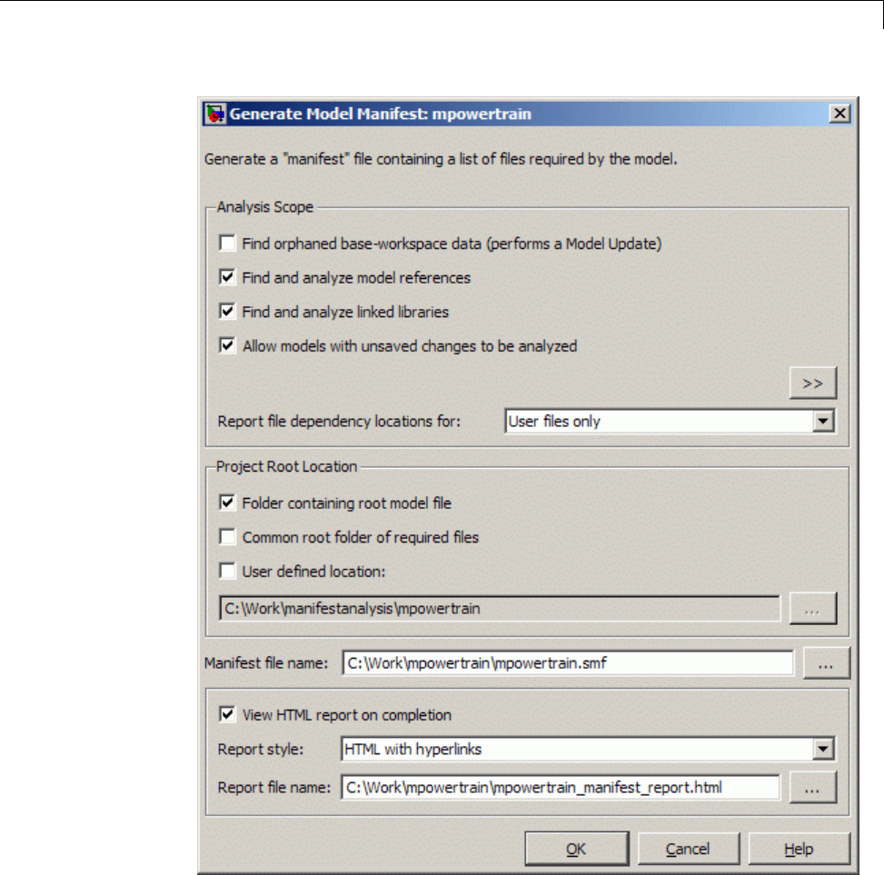
Analyze Model Dependencies
2Click OK to generate a manifest and report using the default settings.
Alternatively you can first change the following settings:
13-107

13 Managing Projects
•Select the Analysis scope check boxes to specify the type of
dependencies you want to detect (see “Manifest Analysis Scope Options”
on page 13-109).
•Control whether to report file dependency locations by selecting Report
file dependency locations for:
–User files only (default) — only report locations where
dependencies are upon user files. Use this option if you want to
understand the interdependencies of your own code and do not care
about the locations of dependencies on MathWorks products. This
option speeds up report creation and streamlines the report.
–All files — report all locations where dependencies are introduced,
including all dependencies on MathWorks products. This is the
slowest option and the most verbose report. Use this option if you need
to trace all dependencies to understand why a particular file or toolbox
is required by a model. If you need to analyze many references, it can
be helpful to sort the results by clicking the report column headers.
–None — do not report any dependency locations. This is the fastest
option and the most streamlined report. Use this option if you want
to discover and package required files and do not require all the
information about file references.
•If desired, change the Project Root Location. Select one of the
check box options: Folder containing root model file (the default),
Common root folder of required files,orUser-defined location —
for this option, enter a path in the edit box, or browse to a location.
•If desired, edit the Manifest file name and location in which to save
the file.
•Use the check box View HTML report on completion to
specify if you want to generate a report when you generate the
manifest. You can edit the Report file name or leave the default,
mymodelname_manifest_report.html. You can set the Report style to
Plain HTML or HTML with Hyperlinks.
When you click OK Simulink generates a manifest file containing a list of the
model dependencies. If you selected View HTML report on completion,
the Model Manifest Report appears after Simulink generates the manifest.
See “Use the Model Manifest Report” on page 13-124 for an example.
13-108

Analyze Model Dependencies
The manifest is an XML file with the extension .smf located (by default) in
the same folder as the model itself.
Manifest Analysis Scope Options
The Simulink Manifest Tools allow you to specify the scope of analysis when
generating the manifest. The dependencies identified by the analysis depend
upon the scope you specify.
The following table describes the Analysis Scope options.
Check Box Option Description
Find orphaned base
workspace data (performs
a Model Update)
Searches for base workspace variables the
model requires, that are not defined in any
file in this Manifest.
If Model Update fails you see an error
message. Either clear this analysis option
to generate a manifest without a Model
Update, or try a manual Model Update
to find out more about the problem. For
example your model may require variables
that are not present in the workspace (e.g.,
if a block parameter defines a variable that
you forgot to load manually).
Find and analyze model
references
Searches for Model blocks in the model,
and identifies any referenced models as
dependencies.
Find and analyze linked
libraries
Searches for links to library blocks in the
model, and identifies any library links as
dependencies.
Allow models with
unsaved changes to be
analyzed
Select this check box only if you want to
allow analysis of unsaved changes.
Click the >> button on the right to show the following advanced analysis
options.
13-109

13 Managing Projects
Check Box Option Description
Find S-functions Searches for S-Function blocks in the model,
and identifies S-function files (MATLAB
code and C) as dependencies. See the source
code item in “Special Cases” on page 13-122.
Analyze model and block
callbacks (including
Interpreted MATLAB
Function blocks)
Searches for file dependencies introduced
bythecodeinInterpretedMATLAB
Function blocks, block callbacks, and model
callbacks. For more detail on how callbacks
are analyzed, see “Code Analysis” on page
13-121.
Find files required for
code generation
Searches for file dependencies introduced
by Simulink Coder custom code, and
Embedded Coder templates. If you do not
have a code generation product, this check
is off by default, and produces a warning if
you select it.
This includes analysis of all configuration
sets (not just the Active set) and
STF_make_rtw_hook functions, and locates
system target files and Code Replacement
Library definition files (.m or .mat). See
also “Required Toolboxes” on page 13-126,
and the source code item in “Special Cases”
on page 13-122.
Find data files (e.g. in
“From File” blocks)
Searches for explicitly referenced data files,
such as those in From File blocks, and
identifies those files as dependencies. See
“Special Cases” on page 13-122.
Analyze Stateflow charts Searches for file dependencies introduced
through the use of syntax such as
ml.mymean(myvariable) in models that
use Stateflow.
13-110

Analyze Model Dependencies
Check Box Option Description
Analyze code in MATLAB
Functions blocks
Searches for MATLAB Function blocks
in the model, and identifies any file
dependencies (outside toolboxes) introduced
in the code. Toolbox dependencies
introduced by a MATLAB Function block
are not detected.
Find requirements
documents
Searches for requirements documents
linked using the Requirements
Management Interface. Note that
requirements links created with Telelogic®
DOORS software are not included in
manifests. For more information, see
“Links Between Models and Requirements”
in the Simulink Verification and Validation
documentation.This option is disabled if
you do not have a Simulink Verification and
Validation license, and Simulink ignores
any requirements links in your model.
Analyze files in “user
toolboxes”
Searches for file dependencies introduced
by files in user-defined toolboxes. See
“Special Cases” on page 13-122.
Analyze MATLAB files Searches for file dependencies introduced
by MATLAB files called from the model.
For example, if this option is selected and
you have a callback to mycallback.m,then
the referenced file mycallback.m is also
analyzed for further dependencies. See
“Code Analysis” on page 13-121.
Store MATLAB code
analysis warnings in
manifest
Saves any warnings in the manifest.
See also “Scope of Dependency Analysis” on page 13-120 for more information.
13-111

13 Managing Projects
Command-Line Dependency Analysis
•“Check File Dependencies” on page 13-112
•“Check Toolbox Dependencies” on page 13-112
Check File Dependencies
To programmatically check for file dependencies, use the function
dependencies.fileDependencyAnalysis as follows.
[files,missing,depfile,manifestfile]=
dependencies.fileDependencyAnalysis('modelname', 'manifestfile')
This returns the following:
•files —ace
ll array of strings containing the full-paths of all existing files
referencedbythemodelmodelname.
•missing —a cell array of strings containing the names all files that are
referenced by the model modelname, but cannot be found.
•depfile — returns the full path of the user dependencies (.smd) file, if it
exists, that stores the names of any files you manually added or excluded.
Simulinkusesthe.smd file to remember your changes the next time you
generate a manifest. See “Edit Manifests” on page 13-114.
•manifestfile — (optional input) specify the name of the manifest file to
create.Notethatthesuffix
.smf is always added to the user-specified name.
If you specify the optional input, manifestfile, then the command
creates a manifest file with the specified name and path manifestfile.
manifestfile canbeafull-pathorjustafilename(inwhichcasethe
file is created in the current folder).
If you try this analysis on an example model, it returns an empty list of
required files because the standard MathWorks installation includes all the
files required for the example models.
Check Toolbox Dependencies
To check which toolboxes are required, use the function
dependencies.toolboxDependencyAnalysis as follows:
13-112

Analyze Model Dependencies
[names,dirs] = dependencies.toolboxDependencyAnalysis(files_in)
files_in must be a cell array of strings containing .m or model files on the
MATLAB path. Simulink model names (without file extension) are also
allowed.
This returns the following:
•names — a cell-array of toolbox names required by the files in files_in.
•dirs — a cell-array of the toolbox folders.
Note The method toolboxDependencyAnalysis looks for toolbox
dependencies of the files in files_in but does not analyze any subsequent
dependencies.
If you want to find all detectable toolbox dependencies of your model and
the files it depends on:
1Call fileDependencyAnalysis on your model.
For example:
[files, missing, depfile, manifestfile] = dependencies.fileDependencyAnalysis('mymodel')
files =
'C:\Work\manifest\foo.m'
'C:\Work\manifest\mymodel'
missing =
[]
depfile =
[]
manifestfile =
[]
2Call toolboxDependencyAnalysis on the files output of step 1.
For example:
13-113

13 Managing Projects
tbxes = dependencies.toolboxDependencyAnalysis(files)
tbxes =
[1x24 char] 'MATLAB' 'Simulink Coder' 'Simulink'
To view long product names examine the tbxes cell array as follows:
tbxes{:}
ans =
Image Processing Toolbox
ans =
MATLAB
ans =
Simulink Coder
ans =
Simulink
For command line dependency analysis, the analysis uses the default settings
for analysis scope to determine required toolboxes. For example, if you have
code generation products, then the check Find files required for code
generation is on by default and Simulink Coder is always reported as
required. See “Required Toolboxes” on page 13-126 for more examples of
how your installed products and analysis scope settings can affect reported
toolbox requirements.
Edit Manifests
After you generate a manifest, you can view the list of files identified as
dependencies, and manually add or delete files from the list.
To edit the list of required files in a manifest:
1Select Analysis > Model Dependencies > Edit Manifest Contents.
13-114
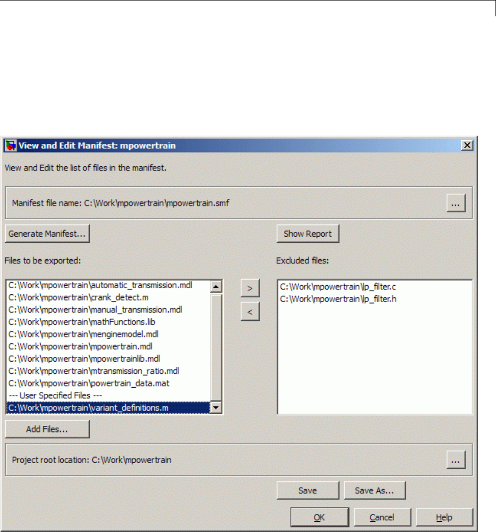
Analyze Model Dependencies
Alternatively, if you are viewing a manifest report you can click Edit in
the top Actions box, or you can click View and Edit Manifest in the
Export Manifest dialog box.
The View and Edit Manifest dialog box appears, showing the latest
manifest for the current model.
13-115

13 Managing Projects
Note You can open a different manifest by clicking the Browse for
manifest file button . If you have not generated a manifest, select
Generate Manifest to open the Generate Model Manifest dialog box (see
“Generate Manifests” on page 13-105).
2Examine the Files to be exported list on the left side of the dialog box.
This list shows the files identified as dependencies.
3To add a file to the manifest:
aClick Add Files.
The Add Files to Manifest dialog box opens.
bSelectthefileyouwanttoadd,thenclickOpen.
TheselectedfileisaddedtotheFiles to be exported list.
4To remove afilefromthemanifest:
aSelect thefileyouwanttoremovefromtheFiles to be exported list.
bClick the Exclude selected files button .
The selected file is moved to the Excluded files list.
Note If you add a file to the manifest and then exclude it, that file is
removed from the dialog (it is not added to the Excluded files list).
Only files detected by the Simulink Manifest Tools are included in the
Excluded files list.
5If desired, change the Project Root Location.
6Click Save to save your changes to the manifest file.
Simulink saves the manifest (.smf) file, and creates a user dependencies
(.smd) file that stores the names of any files you manually added or
13-116

Analyze Model Dependencies
excluded. Simulink uses the .smd file to remember your changes the
next time you generate a manifest, so you do not need to repeat manual
editing. For example, you might want to exclude source code or include a
copyright document every time you generate a manifest for exporting to
a customer. The user dependencies (.smd)filehasthesamenameand
folder as the model. By default, the user dependencies (.smd)fileisalso
included in the manifest.
Note If the user dependencies (.smd) file is read-only, a warning is
displayed when you save the manifest.
7To view the Model Manifest Report for the updated manifest, click Show
Report.
An updated Model Manifest Report appears, listing the required files and
toolboxes, and details of references to other files. See “Use the Model
Manifest Report” on page 13-124 for an example.
8When you are finished editing the manifest, click OK.
Compare Manifests
You can compare two manifests to see how the list of model dependencies
differs between two models, or between two versions of the same model. You
can also compare a manifest with a folder or a ZIP file.
To compare manifests:
1From the Current Folder browser, right-click a manifest file and select
Compare Against > Choose.
Alternatively, from your model, select Analysis > Model
Dependencies > Compare Manifests.
The dialog box Select Files or Folders for Comparison appears.
2In the dialog box Select Files or Folders for Comparison, select files to
compare, and the comparison type.
aUse the drop-down lists or browse to select manifest files to compare.
13-117

13 Managing Projects
bSelect the Comparison type. For two manifests you can select:
•Simulink manifest comparison — Select for a manifest file list
comparison reporting new, removed and changed files. The report
contains links to open files and compare files that differ. You can
use a similar file List comparison for comparing a manifest to a
folder or a ZIP file.
•Simulink manifest comparison (printable) — Select for a
printable Model Manifest Differences Report without links. The report
provides details about each manifest file, and lists the differences
between the files.
3View the report in the Comparison Tool comparing the file names, dates,
and sizes stored in the manifests.
Be aware the details stored in the manifest may differ from the files on
disk. If you click a “compare” link in the report, you see warnings if there
are problems such as size mismatches, or if the tool cannot find those files
on disk.
For more information on the Comparison Tool, see “Comparing Files and
Folders” in the MATLAB Desktop Tools and Development Environment
documentation.
Export Files in a Manifest
You can export copies of the files listed inthemanifesttoaZIPfile. Exporting
thefilesallowsyoutopackagethemodelwith its required files into a single
ZIP file, so you can easily send it to another user or save it in a revision
control system.
To export your model with its required files:
1Select Analysis > Model Dependencies > Export Files in Manifest.
Alternatively, if you are viewing a manifest report you can click Export in
the top Actions box.
The Export Files in Manifest dialog box appears, showing the latest
manifest for the current model.
13-118
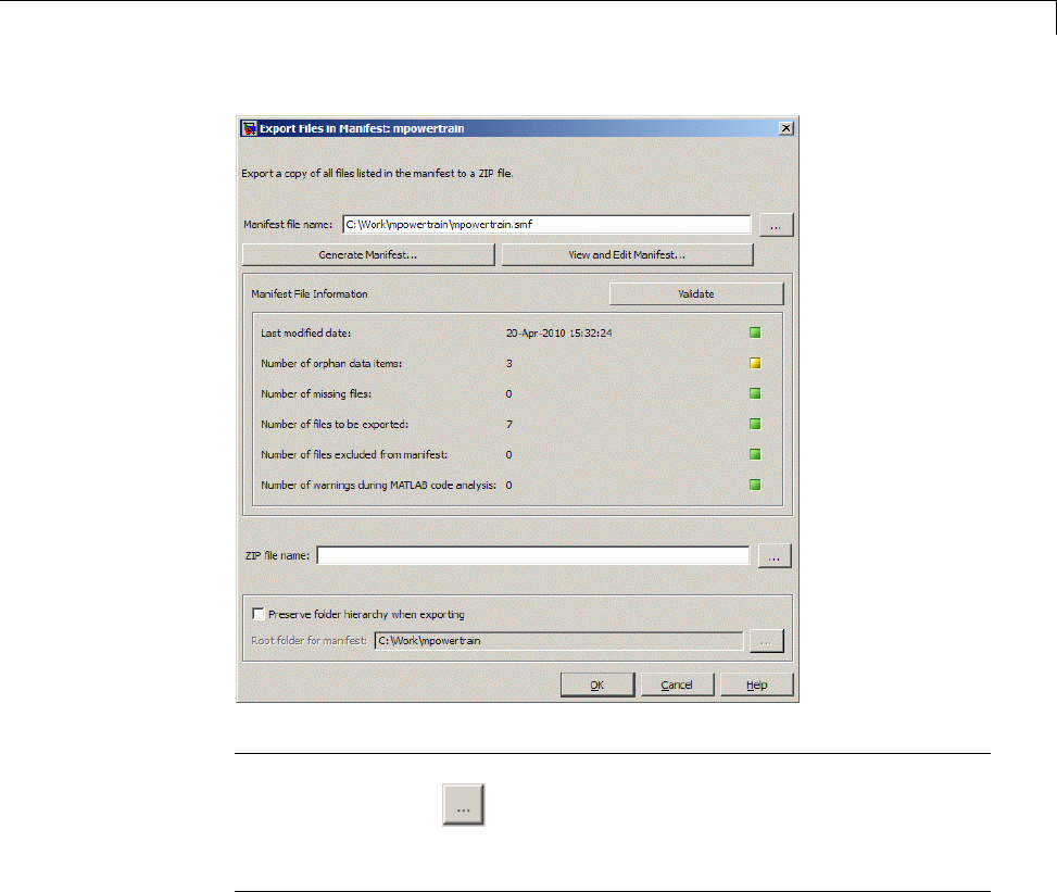
Analyze Model Dependencies
Note You can export a different manifest by clicking the Browse for
manifest file button . If you have not generated a manifest, select
Generate Manifest to open the Generate Model Manifest dialog box (see
“Generate Manifests” on page 13-105).
2If you want to view or edit the manifest before exporting it, click View
and Edit Manifest to view or change the list of required files. See “Edit
Manifests” on page 13-114. When you close the View and Edit Manifest
dialog box, you return to the Export Files in Manifest dialog box.
3Click Validate to check the manifest. Validation reports information
about possible problems such as missing files, warnings, and orphaned
base workspace data.
13-119

13 Managing Projects
4EntertheZIPfilenametowhichyouwanttoexportthemodel.
5Select Preserve folder hierarchy when exporting if you want to keep
folder structure for your exported model and files. Then, select the root
folder to use for this structure (usually the same as the Project Root
Location on the Generate Manifest dialog box).
Note You must select Preserve folder hierarchy if you are exporting a
model that uses an .m file inside a MATLAB class (to maintain the folder
structure of the class), or if the model refers to files in other folders (to
ensuretheexportedfilesmaintainthesamerelativepaths).
6Click OK.
The model and its file dependencies areexportedtothespecifiedZIPfile.
Scope of Dependency Analysis
The Simulink Manifest Tools identify required files and list them in an XML
file called a manifest. When Simulink generates a manifest file, it performs
a static analysis on your model, which means that the model does not need
to be capable of performing an “update diagram” operation (see “Update a
Block Diagram” on page 1-25). The only exception to this is when you select
the analysis option Find orphaned base workspace data (performs a
Model Update).
You can specify the type of dependencies you want to detect when you
generate the manifest. See “Manifest Analysis Scope Options” on page 13-109.
For more information on what the tool analyzes, refer to the following sections:
•“Analysis Limitations” on page 13-121
•“Code Analysis” on page 13-121
•“Special Cases” on page 13-122
13-120

Analyze Model Dependencies
Analysis Limitations
The analysis might not find all files required by your model (for examples,
see “Code Analysis” on page 13-121).
The analysis might not report certain blocksets or toolboxes required by a
model. You should be aware of this limitation when sending a model to
another user. Blocksets that do not introduce dependence on any files (such
as Simulink Fixed Point™) cannot be detected. Some SimEvents blocks do
not introduce a detectable dependence on SimEvents.
To include dependencies that the analysis cannot detect, you can add
additional file dependencies to a manifest file using the View/Edit Manifest
Contents option (see “Edit Manifests” on page 13-114).
Code Analysis
When the Simulink Manifest Tools encounter MATLAB code, for example in
a model or block callback, or in a .m file S-function, they attempt to identify
the files it references. If those files contain MATLAB code, and the analysis
scope option Analyze MATLAB files is selected, the referenced files are also
analyzed. This function is similar to depfun but with some enhancements:
•Files that are in MathWorks toolboxes are not analyzed.
•Strings passed into calls to eval,evalc,andevalin are analyzed.
•File names passed to load,fopen,xlsread,importdata,dlmread,
wk1read,andimread are identified.
File names passed to load, etc., are identified only if they are literal strings.
For example:
load('mydatafile')
load mydatafile
The following example, and anything more complicated, is not identified as a
file dependency:
str = 'mydatafile';
load(str);
Similarly, arguments to eval, etc., are analyzed only if they are literal strings.
13-121

13 Managing Projects
The Simulink Manifest Tools look inside MAT-files to find the names of
variables to be loaded. This enables them to distinguish reliably between
variable names and function names in block callbacks.
If a model depends upon a file for which both .m and .p files exist, then the
manifest reports both, and, if the Analyze MATLAB files option is selected,
the .m file is analyzed.
Special Cases
The following list contains additional information about specific cases:
•If your model references a user-defined MATLAB class created using the
Data Class Designer, for example called MyPackage.MyClass,allfiles
inside the folder MyPackage and its subfolders are added to the manifest.
Warning Theanalysisaddsallfilesintheclass,whichincludes
any source control files such as .svn or .cvs. You may want to edit
the manifest to remove these files.
•A user-defined toolbox must have a properly configured Contents.m file.
The Simulink Manifest Tools search user-defined toolboxes as follows:
-If you have a Contents.m file in folder X, any file inside a subfolder of X
is considered part of your toolbox.
-If you have a Contents.m file in folder X/X, any file inside all subfolders
of the “outer” folder Xwill be considered part of your toolbox.
For more information on the format of a Contents.m file, see ver.
•If your S-functions require TLC files, these are detected.
•IfyouhaveSimscape,yourSimscapecomponentsareanalyzed. Seealso
“Required Toolboxes” on page 13-126 for other effects of your installed
products on manifests.
•If you create a UI using GUIDE and add this to a model callback, then the
dependency analysis detects the .m and .fig file dependencies.
•If you have a dependence on source code, such as .c,.h files, these files are
not analyzed at all to find any files that they depend upon. For example,
subsequent #include calls inside .h files are not detected. To make such
files detectable, you can add them as dependent files to the "header file"
13-122

Analyze Model Dependencies
section of the Custom Code pane of the Simulink Coder section of the
Configuration Parameters dialog box (or specify them with rtwmakecfg).
Alternatively, to include dependencies that the analysis cannot detect, you
can add additional file dependencies to a manifest file using the View/Edit
Manifest Contents option (see “Edit Manifests” on page 13-114).
•Various blocksets and toolboxes can introduce a dependence on a file
through their additional source blocks. If the analysis scope option Find
data files (e.g. in “From File” blocks) is selected, the analysis detects
file dependencies introduced by the following blocks:
Product Blocks
DSP System Toolbox From Wave File (Obsolete) block
(Microsoft Windows operating
system only)
From Multimedia File block
(Windows only)
Computer Vision System Toolbox™ Image From File block
Read Binary File block
Simulink 3D Animation™ VR Sink block
The option Find data files also detects dependencies introduced by setting
a "Model Workspace" for a model to either MAT-File or MATLAB Code.
Best Practices for Dependency Analysis
The starting point for dependency analysis is the model itself. Make sure
that the model refers to any data files it needs, even if you would normally
load these manually. For example, add code to the model’s PreLoadFcn to
load them automatically, e.g.,
load mydatafile
load('my_other_data_file.mat')
This way, the Simulink Manifest Tools can add them to the manifest. For
more detail on callback analysis, see the notes on code analysis (see “Code
Analysis” on page 13-121).
13-123

13 Managing Projects
More generally, ensure that the model creates or loads any variables it uses,
either in model callbacks or in scripts called from model callbacks. This
reduces the possibility of the Simulink Manifest Tools confusing variable
names with function names when analyzing block callbacks.
If you plan to export the manifest after creating it, ensure that the model does
not refer to any files by their absolute paths, for example:
load C:\mymodel\mydata\mydatafile.mat
Absolute paths can become invalid when you export the model to another
machine. If referring to files in other folders, do it by relative path, for
example:
load mydata\mydatafile.mat
Select Preserve folder hierarchy when exporting, so that the exported files
are in the same locations relative to each other. Also, choose a root folder so
that all the files listed in the manifest are inside it. Otherwise, any files
outsidetherootarecopiedintoanewfoldercalledexternal underneath the
root, and relative paths to those files become invalid.
If you are exporting a model that uses a .m file inside a MATLAB class (in a
folder called @myclass, for example), you must select the Preserve folder
hierarchy check box when exporting, to maintain the folder structure of
the class.
Always test exported ZIP files by extracting the contents to a new location on
your computer and testing the model. Be aware that in some cases required
files may be on your path but not in the ZIP file, if your path contains
references to folders other than MathWorks toolboxes.
Use the Model Manifest Report
•“Report Sections” on page 13-125
•“Required Toolboxes” on page 13-126
•“Example Model Manifest Report” on page 13-126
13-124

Analyze Model Dependencies
Report Sections
If you selected View HTML report on completion in the Generate Model
Manifest dialog box, the Model Manifest Report appears after Simulink
generates the manifest. The report shows:
•Analysis date
•Actions panel — Provides links to conveniently regenerate, edit or
compare the manifest, and export the files in the manifest to a ZIP file.
•Model Reference and Library Link Hierarchy — Links you can click
to open models.
•Files used by this model — Required files, with paths relative to the
projectroot.
You can sort the results by clicking the report column headers.
•Toolboxes required by this model. For details see “Required Toolboxes”
on page 13-126.
•References in this model — This section provides details of references to
other files so you can identify where dependencies arise. You control the
scope of this section with the Report file dependency locations options
on the Generate Manifest dialog box. You can choose to include references
to user files only, all files or no files. See “Generate Manifests” on page
13-105. Use this section of the report to trace dependencies to understand
why a particular file or toolbox is required by a model. If you need to
analyze many references, it can be helpful to sort the results by clicking
the report column headers.
•Folders referenced by this model
•Orphaned base workspace variables — If you selected the analysis
option Find orphaned base workspace data, this section reports any
base workspace variables the model requires that are not defined in a file
in this manifest.
•Warnings generated while analyzing MATLAB code —Youcan
opt out of this section by clearing the Store MATLAB code analysis
warnings in manifest analysis option.
•Dependency analysis settings — Records the details of the analysis
scope options.
13-125

13 Managing Projects
See the examples shown in “Example Model Manifest Report” on page 13-126.
Required Toolboxes
In the report, the “Toolboxes required by this model” section lists all products
required by the model that the analysis can detect. Be aware that the analysis
might not report certain blocksets or toolboxes required by a model, e.g.,
blocksets that do not introduce dependence on any files (such as Simulink
Fixed Point) cannot be detected. Some MathWorks files under toolbox/shared
can report only requiring MATLAB instead of their associated toolbox.
The results reported can be affected by your analysis scope settings and your
installed products. For example:
•If you have code generation products and select the scope option “Find
files required for code generation”, then:
-Simulink Coder software is always reported as required.
-If you also have an .ert system target file selected then Embedded
Coder software is always reported as required.
•If you clear the Find library links option, then the analysis cannot find
a dependence on, for example, someBlockSet, and so no dependence is
reported upon the block set.
•If you clear the Analyze MATLAB files option, then the analysis cannot
find a dependence upon fuzzy.m, and so no dependence is reported upon
the Fuzzy Logic Toolbox™.
Example Model Manifest Report
You should always check the Dependency analysis settings sectioninthe
Model Manifest Report to see the scope of analysis settings used to generate it.
Following are portions of a sample report.
13-126
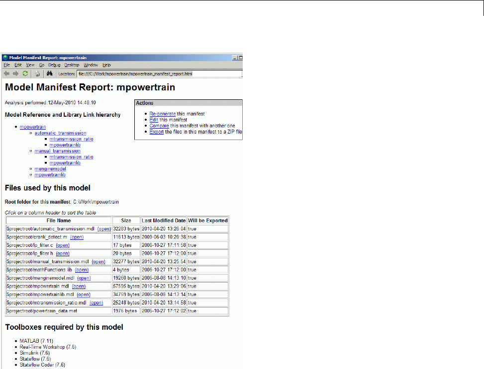
Analyze Model Dependencies
13-127
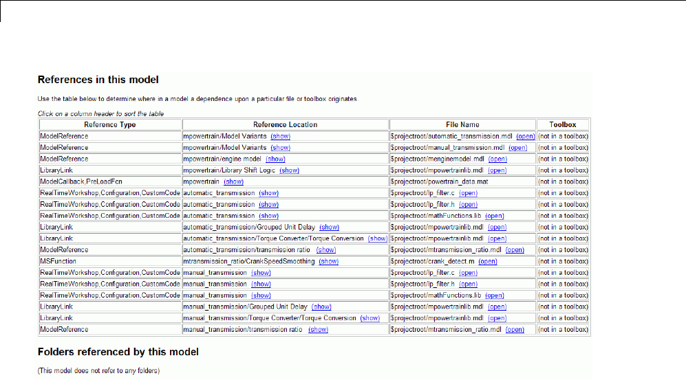
13 Managing Projects
13-128
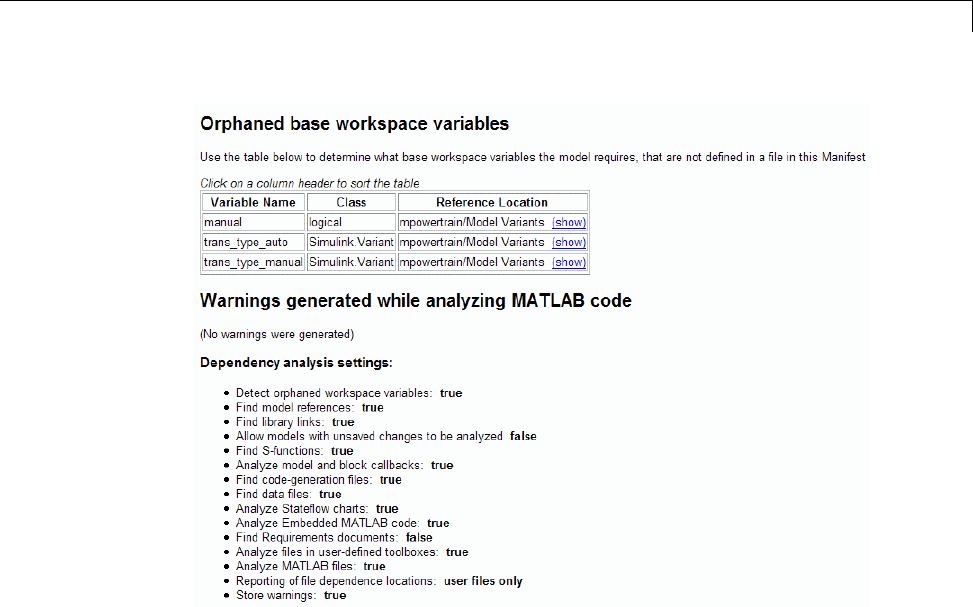
Analyze Model Dependencies
13-129

13 Managing Projects
13-130

Simulating Dynamic Systems
•Chapter 14, “Running Simulations”
•Chapter 15, “Running a Simulation Programmatically”
•Chapter 16, “Visualizing and Comparing Simulation Results”
•Chapter 17, “Inspecting and Comparing Logged Signal Data”
•Chapter 18, “Analyzing Simulation Results”
•Chapter 19, “Improving Simulation Performance and Accuracy”
•Chapter 20, “Performance Advisor”
•Chapter 21, “Simulink Debugger”
•Chapter 22, “Accelerating Models”

14
Running Simulations
•“Simulation Basics” on page 14-2
•“Control Execution of a Simulation” on page 14-3
•“Specify Simulation Start and Stop Time” on page 14-8
•“ChooseaSolver”onpage14-9
•“Interact with a Running Simulation” on page 14-31
•“Save and Restore Simulation State as SimState” on page 14-32
•“Diagnose Simulation Errors” on page 14-39

14 Running Simulations
Simulation Basics
You can simulate a model at any time simply by clicking the Run button on
the Model Editor displaying the model. See “Start a Simulation” on page 14-3.
However, before starting the simulation, you might want to specify various
simulation options, such as the simulation’s start and stop time and the type
of solver used to solve the model at each simulation time step.
With Simulink software, you can create multiple model configurations,
called configuration sets, modify existing configuration sets, and switch
configuration sets with a click of a mouse button (see “Manage a Configuration
Set” on page 10-12 for information on creating and selecting configuration
sets).
Once you have defined or selected a model configuration set that meets your
needs, you can start the simulation. The simulation runs from the specified
start time to the specified stop time. While the simulation is running, you can
interact with the simulation in various ways, stop or pause the simulation
(see “Pause or Stop a Simulation” on page 14-5), and launch simulations of
other models.
If an error occurs during a simulation, Simulink halts the simulation and
the Simulation Diagnostics Viewer pops up that helps you to determine the
cause of the error.
14-2
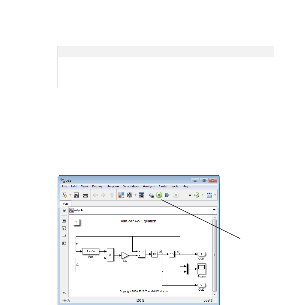
Control Execution of a Simulation
Control Execution of a Simulation
In this section...
“Start a Simulation” on page 14-3
“Pause or Stop a Simulation” on page 14-5
“Use Blocks to Stop or Pause a Simulation” on page 14-5
Start a Simulation
This sections explains how to run a simulation interactively using this model.
See “Run Simulation Using the sim Command” on page 15-3 and “Control
Simulation using the set_param Command” on page 15-7 for information
on running a simulation from a program, an S-function, or the MATLAB
command line.
To start the execution of a model, from the Simulation menu of the Model
Editor, select Run or click the Run button on the model toolbar.
Run button
14-3
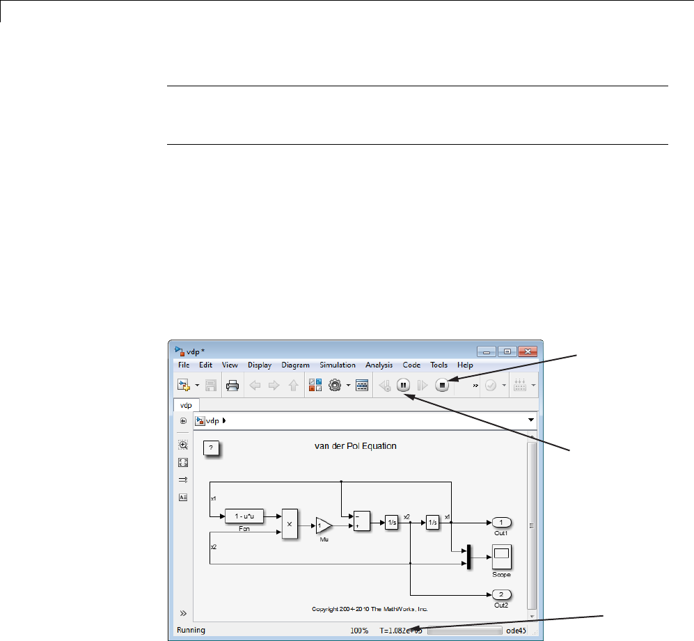
14 Running Simulations
Note A common mistake is to start a simulation while the Simulink block
library is the active window. Make sure that your model window is the active
window before starting a simulation.
The model execution begins at the start time that you specify on the
Configuration Parameters dialog box. Execution continues until an error
occurs, until you pause or terminate the simulation, or until the simulation
reaches the stop time as specified on the Configuration Parameters dialog box.
While the simulation is running, a progress bar at the bottom of the model
window shows how far the simulation has progressed. A Pause command
replaces the Run command on the Simulation menu. A Pause command
appears on the menu and replaces the Run buttononthemodeltoolbar.
Stop button
Pause button
Time
Your computer beeps to signal the completion of the simulation.
14-4

Control Execution of a Simulation
PauseorStopaSi
mulation
Select the Pause command or button to pause the simulation. Once Simulink
completes the execution of the current time step, it suspends the simulation.
When you select Pause, the menu item and the button change to Continue.
(The button has the same appearance as the Run button). You can resume a
suspended simulation at the next time step by choosing Continue.
To terminate execution of the model, select the Stop button or the Stop
Simulation menu item. Simulink completes the execution of the current time
step and then terminates the simulation. Subsequently selecting the Run
menu item or button restarts the simulation at the first time step specified on
the Configuration Parameters dialog box.
If the model includes any blocks that write output to a file or to the workspace,
or if you select output options on the Configuration Parameters dialog box,
the Simulink software writes the data when the simulation is terminated
or suspended.
Use BlockstoStoporPauseaSimulation
Using Stop Blocks
You can use the Stop Simulation block to terminate a simulation when the
input totheblockisnonzero.TousetheStopSimulationblock:
1Drag a copy of the Stop Simulation block from the Sinks library and drop it
into your model.
2Connect the Stop Simulation block to a signal whose value becomes nonzero
at the specified stop time.
For example, this model stops the simulation when the input signal reaches
10.
14-5

14 Running Simulations
If the block input is a vector, any nonzero element causes the simulation
to terminate.
Creating Pause Blocks
You can use an Assertion block to pause the simulation when the input signal
to the block is zero. To create a pause block:
1Drag a copy of the Assertion block from the Model Verification library and
drop it into your model.
2Connect the Assertion block to a signal whose value becomes zero at the
desired pause time.
3Open the Block Parameters dialog box of the Assertion block .
•Enter the following commands into the Simulation callback when
assertion fails field:
set_param(bdroot,'SimulationCommand','pause'),
disp(sprintf('\nSimulation paused.'))
•Uncheck the Stop simulation when assertion fails option.
4Click OK to apply the changes and close this dialog box.
The following model uses a similarly configured Assertion block, in
conjunction with the Relational Operator block, to pause the simulation when
the simulation time reaches 5.
14-6
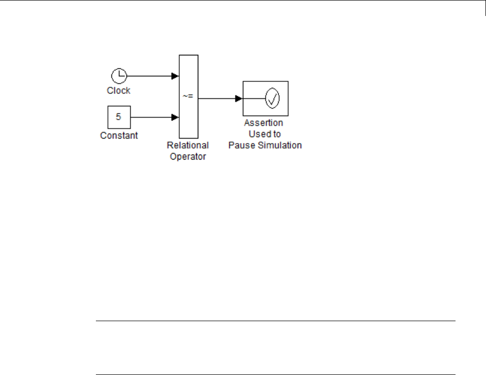
Control Execution of a Simulation
When the simulation pauses, the Assertion block displays the following
message at the MATLAB command line.
Simulation paused
Warning: Assertion detected in 'assertion_as_pause/
Assertion Used to Pause Simulation' at time 5.000000
You can resume the suspended simulation by choosing Continue from the
Simulation menu on the model editor, or by selecting the Continue button
in the toolbar.
Note The Assertion block uses the set_param command to pause the
simulation. See “Control Simulation using the set_param Command” on page
15-7 for more information on using the set_param command to control the
execution of a Simulink model.
14-7

14 Running Simulations
Specify Simulation Start and Stop Time
By default, simulations start at 0.0 s and end at 10.0 s.
Note In the Simulink software, time and all related parameters (such as
sample times) are implicitly in seconds. If you choose to use a different time
unit, you must scale all parameters accordingly.
The Solver configuration pane allows you to specify other start and stop times
for the currently selected simulation configuration. See “Solver Pane” for more
information. On computers running the Microsoft Windows operating system,
you can also specify the simulation stop time in the Simulation menu.
Note Simulation time and actual clock timearenotthesame.Forexample,
if running a simulation for 10 s usually does not take 10 s as measured on a
clock. The amount of time it actually takes to run a simulation depends on
many factors including the complexity of the model, the step sizes, and the
computer speed.
14-8

Choose a Solver
Choose a Solver
In this section...
“What Is a Solver?” on page 14-9
“Choosing a Solver Type” on page 14-10
“Choosing a Fixed-Step Solver” on page 14-13
“Choosing a Variable-Step Solver” on page 14-17
“Choosing a Jacobian Method for an Implicit Solver” on page 14-24
What Is a Solver?
A solver is a component of the Simulink software. The Simulink product
provides an extensive library of solvers, each of which determines the time
of the next simulation step and applies a numerical method to solve the set
of ordinary differential equations that represent the model. In the process
of solving this initial value problem, the solver also satisfies the accuracy
requirements that you specify. To help you choose the solver best suited for
your application, “Choosing a Solver Type” on page 14-10 provides background
on the different types of solvers while “Choosing a Fixed-Step Solver” on page
14-13 and “Choosing a Variable-Step Solver” on page 14-17 provide guidance
on choosing a specific fixed-step or variable-step solver, respectively.
The following table summarizes the types of solvers in the Simulink library
and provides links to specific categories. All of these solvers can work with
the algebraic loop solver.
Discrete Continuous Variable-Order
Explicit Not Applicable “Explicit Fixed-Step
Continuous Solvers”
on page 14-14
Not Applicable
Fixed-Step
Implicit Not Applicable “Implicit Fixed-Step
Continuous Solvers”
on page 14-16
Not Applicable
14-9

14 Running Simulations
Discrete Continuous Variable-Order
Explicit “Choosing a
Variable-Step Solver”
on page 14-17
“Explicit Continuous
Variable-Step Solvers”
on page 14-18
“Variable-Order
Solvers” on page 14-13
Variable-Step
Implicit “Implicit Continuous
Variable-Step Solvers”
on page 14-19
“Variable-Order
Solvers” on page 14-13
Note
1The fixed-step discrete solvers do not solve for discrete states; each
block calculates its discrete states independent of the solver. For more
information, see “Discrete versus Continuous Solvers” on page 14-12
2Every solver in the Simulink library can perform on models that contain
algebraic loops.
For information on tailoring the selected solver to your model, see “Improve
Simulation Accuracy” on page 19-11.
Choosing a Solver Type
The Simulink library of solvers is divided into two major types in the “Solver
Pane”: fixed-step and variable-step. You can further divide the solvers
within each of these categories as: discrete or continuous, explicit or implicit,
one-step or multistep, and single-order or variable-order.
Fixed-Step versus Variable-Step Solvers
Both fixed-step and variable-step solvers compute the next simulation time
as the sum of the current simulation time and a quantity known as the step
size. With a fixed-step solver, the step size remains constant throughout
the simulation. In contrast, with a variable-step solver, the step size can
vary from step to step, depending on the model dynamics. In particular,
a variable-step solver increases or reduces the step size to meet the error
14-10
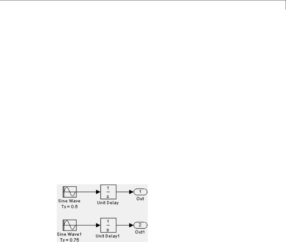
Choose a Solver
tolerances that you specify. The Type control on the Simulink Solver
configuration pane allows you to select either of these two types of solvers.
The choice between the two types depends on how you plan to deploy your
model and the model dynamics. If you plan to generate code from your model
and run the code on a real-time computer system, choose a fixed-step solver
to simulate the model because you cannotmapthevariable-stepsizetothe
real-time clock.
If you do not plan to deploy your model as generated code, the choice between
a variable-step and a fixed-step solver depends on the dynamics of your
model. A variable-step solver might shorten the simulation time of your model
significantly. A variable-step solver allows this savings because, for a given
level of accuracy, the solver can dynamically adjust the step size as necessary
and thus reduce the number of steps. Whereas the fixed-step solver must
use a single step size throughout the simulation based upon the accuracy
requirements. To satisfy these requirements throughout the simulation, the
fixed-step solver might require a very small step.
The following model shows how a variable-step solver can shorten simulation
time for a multirate discrete model.
This model generates outputs at two different rates: every 0.5 s and every
0.75 s. To capture both outputs, the fixed-step solver must take a time step
every 0.25 s (the fundamental sample time for the model).
[0.0 0.25 0.5 0.75 1.0 1.25 1.5 ...]
By contrast, the variable-step solver needs to take a step only when the model
generates an output.
14-11

14 Running Simulations
[0.0 0.5 0.75 1.0 1.5 ...]
This scheme significantly reduces the number of time steps required to
simulate the model.
Ifyouwishtoachieveevenlyspacedsteps, you must use the format 0.4*[0.0:
100.0] rather than [0.0:0.4:40].
Discrete versus Continuous Solvers
When you set the Type control of the Solver configuration pane to
fixed-step or to variable-step,theadjacentSolver control allows you to
choose a specific solver. Both sets of solvers comprise two types: discrete
and continuous. Discrete and continuous solvers rely on the model blocks
to compute the values of any discrete states. Blocks that define discrete
states are responsible for computing the values of those states at each time
step. However, unlike discrete solvers, continuous solvers use numerical
integration to compute the continuous states that the blocks define .
Therefore, when choosing a solver, you must first determine whether you
need to use a discrete solver or a continuous solver.
If your model has no continuous states, then Simulink switches to either the
fixed-step discrete solver or the variable-step discrete solver. If instead your
model has continuous states, you must choose a continuous solver from the
remaining solver choices based on the dynamics of your model. Otherwise,
an error occurs.
Explicit versus Implicit Solvers
While you can apply either an implicit or explicit continuous solver, the
implicit solvers are designed specifically for solving stiff problems whereas
explicit solvers are used to solve nonstiff problems. A generally accepted
definition of a stiff system is a system that has extremely different time scales.
Compared to the explicit solvers, the implicit solvers provide greater stability
for oscillatory behavior, but they are also computationally more expensive;
they generate the Jacobian matrix and solve the set of algebraic equations at
every time step using a Newton-like method. To reduce this extra cost, the
implicit solvers offer a Solver Jacobian method parameter that allows you
to improve the simulation performance of implicit solvers. See “Choosing a
Jacobian Method for an Implicit Solver” on page 14-24 for more information.
14-12

Choose a Solver
One-Step versus Multistep Solvers
The Simulink solver library provides both one-step and multistep solvers.
The one-step solvers estimate y(tn)using the solution at the immediately
preceding time point, y(tn-1), and the values of the derivative at a number of
points between tnand tn-1.Thesepointsareminor steps.
The multistep solvers use the results at several preceding time steps to
compute the current solution. Simulink provides one explicit multistep solver,
ode113, and one implicit multistep solver, ode15s. Both are variable-step
solvers.
Variable-Order Solvers
Two variable-order solvers, ode15s and ode113, are part of the solver
library. Thesesolversusemultipleorderstosolvethesystemofequations.
Specifically, the implicit, variable-step ode15s solver uses first-order through
fifth-order equations while the explicit, variable-step ode113 solver uses
first-order through thirteenth-order. For ode15s, you can limit the highest
order applied via the Maximum Order parameter. For more information, see
“Maximum Order” on page 14-20.
Choosing a Fixed-Step Solver
About the Fixed-Step Discrete Solver
The fixed-step discrete solver computes the time of the next simulation step
by adding a fixed step size to the current time. The accuracy and the length of
time of the resulting simulation depends on the size of the steps taken by the
simulation: the smaller the step size, the more accurate the results are but the
longer the simulation takes. You can allow the Simulink software to choose
the size of the step (the default) or you can choose the step size yourself. If you
choose the default setting of auto, and if the model has discrete sample times,
then Simulink sets the step size to the fundamental sample time of the model.
Otherwise, if no discrete rates exist, Simulink sets the size to the result of
dividingthedifferencebetweenthesimulationstartandstoptimesby50.
14-13

14 Running Simulations
Note If you try to use the fixed-step discrete solver to update or simulate a
model that has continuous states, an error message appears. Thus, selecting
a fixed-step solver and then updating or simulating a model is a quick way to
determine whether the model has continuous states.
About Fixed-Step Continuous Solvers
The fixed-step continuous solvers, like the fixed-step discrete solver, compute
the next simulation time by adding a fixed-size time step to the current time.
For each of these steps, the continuous solvers use numerical integration to
compute the values of the continuous states for the model. These values are
calculated using the continuous states at the previous time step and the state
derivatives at intermediate points (minor steps) between the current and the
previous time step. The fixed-step continuous solvers can, therefore, handle
models that contain both continuous and discrete states.
Note In theory, a fixed-step continuous solver can handle models that
contain no continuous states. However, that would impose an unnecessary
computational burden on the simulation. Consequently, Simulink uses the
fixed-step discrete solver for a model that contains no states or only discrete
states, even if you specify a fixed-step continuous solver for the model.
Two types of fixed-step continuous solvers that Simulink provides are: explicit
and implicit. (See “Explicit versus Implicit Solvers” on page 14-12 for more
information). The difference between these two types lies in the speed and
the stability. An implicit solver requires more computation per step than an
explicit solver but is more stable. Therefore, the implicit fixed-step solver that
Simulink provides is more adept at solving a stiff system than the fixed-step
explicit solvers.
Explicit Fixed-Step Continuous Solvers. Explicit solvers compute the
value of a state at the next time step as an explicit function of the current
values of both the state and the state derivative. Expressed mathematically
for a fixed-step explicit solver:
xn xn h Dxn( ) () ()+= +∗1
14-14

Choose a Solver
where xis the state, Dx is a solver-dependent function that estimates the
state derivative, his the step size, and nindicates the current time step.
Simulink provides a set of explicit fixed-step continuous solvers. The solvers
differ in the specific numerical integration technique that they use to compute
the state derivatives of the model. The following table lists each solver and
the integration technique it uses.
Solver Integration Technique Order of Accuracy
ode1 Euler’s Method First
ode2 Heun’s Method Second
ode3 Bogacki-Shampine Formula Third
ode4 Fourth-Order Runge-Kutta
(RK4) Formula
Fourth
ode5 Dormand-Prince (RK5)
Formula
Fifth
ode8 Dormand-Prince RK8(7)
Formula
Eighth
The table lists the solvers in order of the computational complexity of the
integration methods they use, from the least complex (ode1)tothemost
complex (ode8).
None of these solvers has an error control mechanism. Therefore, the
accuracy and the duration of a simulation depends directly on the size of the
steps taken by the solver. As you decrease the step size, the results become
more accurate, but the simulation takes longer. Also, for any given step size,
the more computationally complex the solver is, the more accurate are the
simulation results.
If you specify a fixed-step solver type for a model, then by default, Simulink
selects the ode3 solver, which can handle both continuous and discrete states
with moderate computational effort. As with the discrete solver, if the model
has discrete rates (sample times), then Simulink sets the step size to the
fundamental sample time of the model by default. If the model has no discrete
rates, Simulink automatically uses the result of dividing the simulation total
duration by 50. Consequently, the solver takes a step at each simulation
14-15

14 Running Simulations
time at which Simulink must update the discrete states of the model at its
specified sample rates. However, it does not guarantee that the default solver
accurately computes the continuous states of a model. Therefore, you might
need to choose another solver, a different fixed step size, or both to achieve
acceptable accuracy and an acceptable simulation time.
Implicit Fixed-Step Continuous Solvers. An implicit fixed-step solver
computes the state at the next time step as an implicit function of the state
at the current time step and the state derivative at the next time step. In
other words:
xn xn h Dxn()() ()+− −∗ +=110
Simulink provides one implicit fixed-step solver : ode14x. Thissolverusesa
combination of Newton’s method and extrapolation from the current value to
compute the value of a state at the next time step. You can specify the number
of Newton’s method iterations and the extrapolation order that the solver uses
to compute the next value of a model state (see “Fixed-step size (fundamental
sample time)”). The more iterations and the higher the extrapolation
order that you select, the greater the accuracy you obtain. However, you
simultaneously create a greater computational burden per step size.
Process for Choosing a Fixed-Step Continuous Solver
Any of the fixed-step continuous solvers in the Simulink product can simulate
a model to any desired level of accuracy, given a small enough step size.
Unfortunately, it generally is not possible, or at least not practical, to decide a
priori which combination of solver and step size will yield acceptable results
for the continuous states in the shortest time. Determining the best solver for
a particular model generally requires experimentation.
Following is the most efficient way to choose the best fixed-step solver for
your model experimentally.
1Choose error tolerances. For more information, see “Specifying Error
Tolerances for Variable-Step Solvers” on page 14-22.
2Use one of the variable-step solvers to simulate your model to the level of
accuracy that you desire. Start with ode45. If your model runs slowly,
your problem might be stiff and need an implicit solver. The results of this
14-16

Choose a Solver
step give a good approximation of the correct simulation results and the
appropriate fixed step size.
3Use ode1 to simulate your model at the default step size for your model.
Compare the simulation results for ode1 with the simulation for the
variable-step solver. If the results are the same for the specified level of
accuracy, you have found the best fixed-step solver for your model, namely
ode1. You can draw this conclusion because ode1 is the simplest of the
fixed-step solvers and hence yields the shortest simulation time for the
current step size.
4If ode1 does not give satisfactory results, repeat the preceding steps
with each of the other fixed-step solvers until you find the one that gives
accurate results with the least computational effort. The most efficient way
to perform this task is to use a binary search technique:
aTry ode3.
bIf ode3 gives accurate results, try ode2.Ifode2 gives accurate results, it
is the best solver for your model; otherwise, ode3 is the best.
cIf ode3 does not give accurate results, try ode5.Ifode5 gives accurate
results, try ode4.Ifode4 gives accurate results, select it as the solver for
your model; otherwise, select ode5.
dIf ode5 does not give accurate results, reduce the simulation step size and
repeat the preceding process. Continue in this way until you find a solver
that solves your model accurately with the least computational effort.
Choosing a Variable-Step Solver
When you set the Type control of the Solver configuration pane to
Variable-step,theSolver control allows you to choose one of the
variable-step solvers. As with fixed-step solvers, the set of variable-step
solvers comprises a discrete solver and a subset of continuous solvers.
However, unlike the fixed-step solvers, the step size varies dynamically based
on the local error.
The choice between the two types of variable-step solvers depends on whether
the blocks in your model define states and, if so, the type of states that they
14-17

14 Running Simulations
define. If your model defines no states or defines only discrete states, select
the discrete solver. In fact, if a model has no states or only discrete states,
Simulink uses the discrete solver to simulate the model even if you specify a
continuous solver. If the model has continuous states, the continuous solvers
use numerical integration to compute the values of the continuous states
atthenexttimestep.
About Variable-Step Continuous Solvers
The variable-step solvers in the Simulink product dynamically vary the step
size during the simulation. Each of these solvers increases or reduces the step
size using its local error control to achieve the tolerances that you specify.
Computing the step size at each time step adds to the computational overhead
but can reduce the total number of steps, and the simulation time required to
maintain a specified level of accuracy.
You can further categorize the variable-step continuous solvers as: one-step
or multistep, single-order or variable-order, and explicit or implicit. (See
“Choosing a Solver Type” on page 14-10 for more information.)
Explicit Continuous Variable-Step Solvers
The explicit variable-step solvers are designed for nonstiff problems. Simulink
provides three such solvers: ode45,ode23,andode113.
ODE
Solver
One-Step
Method
Multistep
Method
Order of
Accuracy
Method
ode45 XMedium Runge-Kutta,
Dormand-Prince (4,5)
pair
ode23 XLow
Runge-Kutta (2,3) pair of
Bogacki & Shampine
ode113 XVariable,
Low to
High
PECE Implementation of
Adams-Bashforth-Moutlon
14-18

Choose a Solver
ODE
Solver
Tips on When to Use
ode45 In general, the ode45 solver is the best to apply as a first try for
most problems. For this reason, ode45 is the default solver for
models with continuous states. This Runge-Kutta (4,5) solver is
a fifth-order method that performs a fourth-order estimate of
the error. This solver also uses a fourth-order “free” interpolant,
which allows for event location and smoother plots.
The ode45 is more accurate and faster than ode23.Iftheode45
is slow computationally, your problem may be stiff and thus in
need of an implicit solver.
ode23 The ode23 canbemoreefficientthantheode45 solver at crude
error tolerances and in the presence of mild stiffness. This solver
provides accurate solutions for “free” by applying a cubic Hermite
interpolation to the values andslopescomputedattheendsof
astep.
ode113 For problems with stringent error tolerances or
for computationally intensive problems, the
Adams-Bashforth-Moulton PECE solver can be more
efficient than ode45.
Implicit Continuous Variable-Step Solvers
If your problem is stiff, try using one of the implicit variable-step solvers:
ode15s,ode23s,ode23t,orode23tb.
ODE
Solver
One-Step
Method
Multistep
Method
Order
of
Accuracy
Solver
Reset
Method
Max.
Order
Method
ode15s XVariable,
Low to
Medium
XX
Numerical Differentiation
Formulas (NDFs)
ode23s XLow Second-order, modified
Rosenbrock formula
14-19

14 Running Simulations
ODE
Solver
One-Step
Method
Multistep
Method
Order
of
Accuracy
Solver
Reset
Method
Max.
Order
Method
ode23t XLowX
Trapezoidal rule using a
“free” interpolant
ode23tb X Low X TR-BDF2
Solver Reset Method. For three of the stiff solvers — ode15s,ode23t,and
ode23tb— a drop-down menu for the Solver reset method appears on the
Solver Configuration pane. This parameter controls how the solver treats a
reset caused, for example, by a zero-crossing detection. The options allowed
are Fast and Robust. The former setting specifies that the solver does not
recompute the Jacobian for a solver reset, whereas the latter setting specifies
that the solver does. Consequently, the Fast setting is faster computationally
but might use a small step size for certain cases. To test for such cases, run
the simulation with each setting and compare the results. If there is no
difference, you can safely use the Fast setting and save time. If the results
differ significantly, try reducing the step size for the fast simulation.
Maximum Order. For the ode15s solver, you can choose the maximum
order of the numerical differentiation formulas (NDFs) that the solver applies.
Since the ode15s uses first- through fifth-order formulas, the Maximum order
parameter allows you to choose 1 through 5. For a stiff problem, you may
want to start with order 2.
Tips for Choosing a Variable-Step Implicit Solver. The following table
provides tips relating to the application of variable-step implicit solvers. For
an example comparing the behavior of these solvers, see sldemo_solvers.
14-20

Choose a Solver
ODE
Solver
Tips on When to Use
ode15s ode15s is a variable-order solver based on the numerical
differentiation formulas (NDFs). NDFs are related to, but
are more efficient than the backward differentiation formulas
(BDFs), which are also known as Gear’s method. The ode15s
solver numerically generates the Jacobian matrices. If you
suspect that a problem is stiff, or if ode45 failed or was highly
inefficient, try ode15s. As a rule, start by limiting the maximum
order of the NDFs to 2.
ode23s ode23s is based on a modified Rosenbrock formula of order 2.
Because it is a one-step solver, it can be more efficient than
ode15s at crude tolerances. Like ode15s,ode23s numerically
generates the Jacobian matrix for you. However, it can solve
certain kinds of stiff problems for which ode15s is not effective.
ode23t The ode23t solver is an implementation of the trapezoidal rule
using a “free” interpolant. Use this solver if your model is only
moderately stiff and you need a solution without numerical
damping. (Energy is not dissipated when you model oscillatory
motion.)
ode23tb ode23tb is an implementation of TR-BDF2, an implicit
Runge-Kutta formula with two stages. The first stage is a
trapezoidal rule step while the second stage uses a backward
differentiation formula of order 2. By construction, the method
uses the same iteration matrix in evaluating both stages. Like
ode23s, this solver can be more efficient than ode15s at crude
tolerances.
Note For a stiff problem, solutions can change on a time scale that is very
small as compared to the interval of integration, while the solution of interest
changes on a much longer time scale. Methods that are not designed for
stiff problems are ineffective on intervals where the solution changes slowly
because these methods use time steps small enough to resolve the fastest
possible change. For more information, see Shampine, L. F., Numerical
Solution of Ordinary Differential Equations, Chapman & Hall, 1994.
14-21
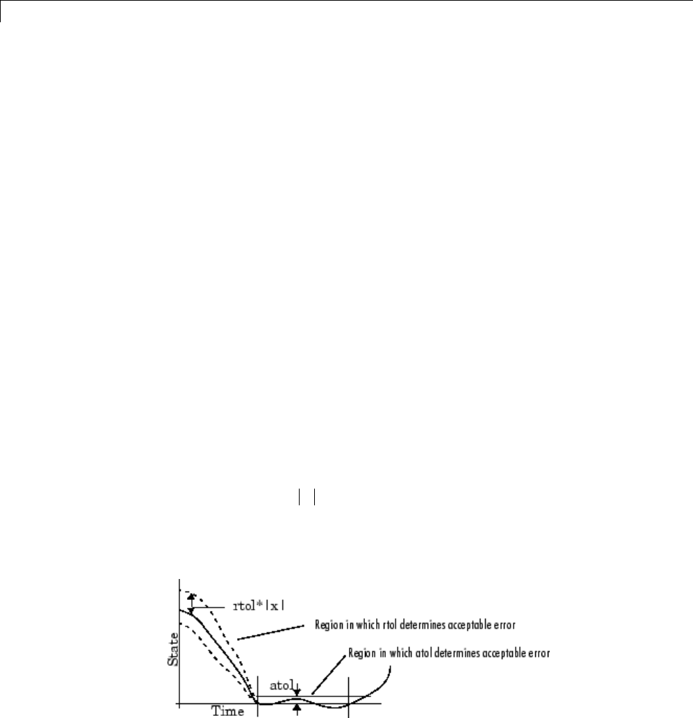
14 Running Simulations
Support for Zero-Crossing Detection
Both the variable-step discrete and continuous solvers use zero-crossing
detection (see “Zero-Crossing Detection” on page 3-23) to handle continuous
signals.
Specifying Error Tolerances for Variable-Step Solvers
Local Error. The variable-step solvers use standard control techniques to
monitor the local error at each time step. During each time step, the solvers
compute the state values at the end of the step and determine the local
error—the estimated error of these state values. They then compare the
local error to the acceptable error, which is a function of both the relative
tolerance (rtol) and the absolute tolerance (atol). If the local error is greater
than the acceptable error for any one state, the solver reduces the step size
and tries again.
•The Relative tolerance measures the error relative to the size of each state.
The relative tolerance represents a percentage of the state value. The
default, 1e-3, means that the computed state is accurate to within 0.1%.
•Absolute tolerance is a threshold error value. This tolerance represents the
acceptable error as the value of the measured state approaches zero.
The solvers require the error for the ith state, ei,tosatisfy:
ertolxatol
iii
≤×max( , ).
The following figure shows a plot of a state and the regions in which the
relativetoleranceandtheabsolutetolerance determine the acceptable error.
14-22

Choose a Solver
Absolute Tolerances. Your model has a global absolute tolerance that you
can set on the Solver pane of the Configuration Parameters dialog box. This
tolerance applies to all states in the model. You can specify auto or a real
scalar. If you specify auto (the default), Simulink initially sets the absolute
toleranceforeachstateto1e-6. Asthesimulationprogresses,theabsolute
toleranceforeachstateresetstothemaximumvaluethatthestatehas
assumedsofar,timestherelativetolerance for that state. Thus, if a state
changes from 0 to 1 and reltol is 1e-3, then by the end of the simulation,
abstol becomes1e-3also.Ifastategoesfrom0to1000,thenabstol changes
to 1.
If the computed setting is not suitable,youcandetermineanappropriate
setting yourself. You might have to run a simulation more than once to
determine an appropriate value for the absolute tolerance.
Several blocks allow you to specify absolute tolerance values for solving the
model states that they compute or that determine their output:
•Integrator
•Second-Order Integrator Limited
•Variable Transport Delay
•Transfer Fcn
•State-Space
•Zero-Pole
The absolute tolerance values that you specify for these blocks override the
global settings in the Configuration Parameters dialog box. You might want
to override the global setting if, for example, the global setting does not
provide sufficient error control for all of your model states because they vary
widely in magnitude. The block absolute tolerance can be set to:
•auto
•–1(same as auto)
•real scalar
•real vector (having a dimension equal to the number of corresponding
continuous states in the block)
14-23

14 Running Simulations
Tips. Ifyoudochoosetosettheabsolutetolerance,keepinmindthattoolow
of a value causes the solver to take too many steps in the vicinity of near-zero
state values. As a result, the simulation is slower.
On the other hand, if you choose too high of an absolute tolerance, your
results can be inaccurate as one or more continuous states in your model
approach zero.
Once the simulation is complete, you can verify the accuracy of your results
by reducing the absolute tolerance and running the simulation again. If the
results of these two simulations are satisfactorily close, then you can feel
confident about their accuracy.
Choosing a Jacobian Method for an Implicit Solver
About the Solver Jacobian
For implicit solvers, Simulink must compute the solver Jacobian,which
is a submatrix of the Jacobian matrix associated with the continuous
representation of a Simulink model. In general, this continuous
representation is of the form:
xfxtu
ygxtu
=
=
(,,)
(,,).
The Jacobian, J, formed from this system of equations is:
J
f
x
f
u
g
x
g
u
AB
CD
=
∂
∂
∂
∂
∂
∂
∂
∂
⎛
⎝
⎜
⎜
⎜
⎜
⎞
⎠
⎟
⎟
⎟
⎟
=⎛
⎝
⎜⎞
⎠
⎟.
In turn, the solver Jacobian is the submatrix, Jx.
JA
f
x
x==
∂
∂.
14-24

Choose a Solver
Sparsity of Jacobian. For many physical systems, the solver Jacobian Jxis
sparse, meaning that many of the elements of Jxare zero.
Consider the following system of equations:
xfxx
xfx
xfx
1113
222
332
=
=
=
(, )
()
().
From this system, you can derive a sparsity pattern that reflects the structure
of the equations. The pattern, a Boolean matrix, has a 1 for each xithat
appears explicitly on the right-hand side of an equation. You thereby attain:
Jx pattern,=
⎛
⎝
⎜
⎜
⎜
⎞
⎠
⎟
⎟
⎟
101
010
010
As discussed in “Full and Sparse Perturbation Methods” on page 14-28 and
“Full and Sparse Analytical Methods” on page 14-30 respectively, the Sparse
Perturbation Method and the Sparse Analytical Method may be able to take
advantage of this sparsity pattern to reduce the number of computations
necessary and thereby improve performance.
Solver Jacobian Methods
When you choose an implicit solver from the Solver pane of the Configuration
Parameters dialog box, a parameter called Solver Jacobian method and
a drop-down menu appear. This menu has five options for computing the
solver Jacobian: auto,Sparse perturbation,Full perturbation,Sparse
analytical,andFull analytical.
14-25
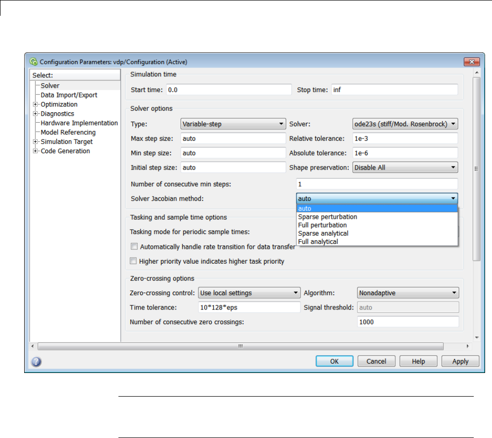
14 Running Simulations
Note If you set Automatic solver parameter selection to warning or
error in the Solver Diagnostics pane, and you choose a different solver
method than Simulink, you might receive a warning or an error.
Limitations. The solver Jacobian methods have the following limitations
associated with them.
•If you select an analytical Jacobian method, but one or more blocks in
the model do not have an analytical Jacobian, then Simulink applies a
perturbation method.
14-26
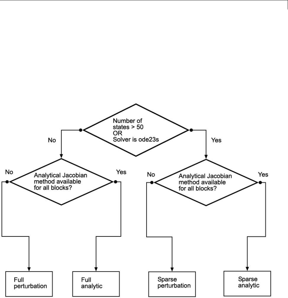
Choose a Solver
•If you select sparse perturbation and your model contains data store blocks,
Simulink applies the full perturbation method.
Heuristic ’auto’ Method
The default setting for the Solver Jacobian method is auto.Selectingthis
choice causes Simulink to perform a heuristic to determine which of the
remaining four methods best suits your model. This algorithm is depicted in
the following flowchart.
14-27

14 Running Simulations
Because the sparse methods are beneficial for models having a large number
of states, the heuristic chooses a sparse method if more than 50 states exist
in your model. The logic also leads to a sparse method if you specify ode23s
because, unlike other implicit solvers, ode23s generates a new Jacobian at
every time step. A sparse analytical or a sparse perturbation method is,
therefore, highly advantageous. The heuristic also ensures that the analytical
methods are used only if every block in your model can generate an analytical
Jacobian.
Full and Sparse Perturbation Methods
The full perturbation method was the standard numerical method that
Simulink used to solve a system. For this method, Simulink solves the full set
of perturbation equations and uses LAPACK for linear algebraic operations.
This method is costly from a computational standpoint, but it remains the
recommended method for establishing baseline results.
Thesparseperturbationmethodattemptstoimprovetherun-time
performancebytakingmathematical advantage of the sparse Jacobian
pattern. Returning to the sample system of three equations and three states,
xfxx
xfx
xfx
1113
222
332
=
=
=
(, )
()
().
The solver Jacobian is:
14-28

Choose a Solver
J
f
x
f
x
f
x
f
x
f
x
f
x
f
x
f
x
f
x
x=
∂
∂
∂
∂
∂
∂
∂
∂
∂
∂
∂
∂
∂
∂
∂
∂
∂
∂
⎛1
1
1
2
1
3
2
1
2
2
2
3
3
1
3
2
3
3
⎝⎝
⎜
⎜
⎜
⎜
⎜
⎜
⎜
⎜
⎞
⎠
⎟
⎟
⎟
⎟
⎟
⎟
⎟
⎟
=
+Δ −
Δ
+Δfx xxx f
x
fxx xx
11 12 3 1
1
11 2 2 3
( ,,) (, ,))(,,)
( ,,) (,
−
Δ
+Δ −
Δ
+Δ −
Δ
f
x
fxxx x f
x
fx xxx f
x
fx
1
2
11 2 3 3 1
3
21 123 2
1
21
xxxxf
x
fxxx x f
x
fx xxx f
2232
2
2123 3 2
3
31 123 3
+Δ −
Δ
+Δ −
Δ
+Δ −
,) (,, )
( ,,)
ΔΔ
+Δ −
Δ
+Δ −
Δ
⎛
⎝
⎜
⎜
⎜
⎜
⎜
⎜
⎜
⎜x
fxx xx f
x
fxxx x f
x
1
312 23 3
2
3123 3 3
3
(, , ) (, , )
⎞⎞
⎠
⎟
⎟
⎟
⎟
⎟
⎟
⎟
⎟
It is, therefore, necessary to perturb each of the three states three times and
to evaluate the derivative function three times. For a system with nstates,
this method perturbs the states ntimes.
By applying the sparsity pattern and perturbing states x1and x2together,
this matrix reduces to:
J
fx xx xx f
x
fxxx x f
x
fx
x=
+Δ +Δ −
Δ
+Δ −
Δ
11 12 2 3 1
1
11 2 3 3 1
3
21
0
0
(, ,) (,, )
(++Δ +Δ −
Δ
+Δ +Δ −
Δ
⎛
⎝
⎜
⎜
⎜
⎜
⎜
xx xx f
x
fx xx xx f
x
12 23 2
2
31 12 23 3
2
0
00
,,)
(, ,)
⎜⎜
⎜
⎜
⎞
⎠
⎟
⎟
⎟
⎟
⎟
⎟
⎟
⎟
The solver can now solve columns 1 and 2 in one sweep. While the sparse
perturbation method saves significant computation, it also adds overhead to
compilation. It might even slow down the simulation if the system does not
have a large number of continuous states. A tipping point exists for which you
14-29

14 Running Simulations
obtain increased performance by applying this method. In general, systems
having a large number of continuous states are usually sparse and benefit
from the sparse method.
Thesparseperturbationmethod,likethesparseanalyticalmethod,uses
UMFPACK to perform linear algebraic operations. Also, the sparse
perturbation method supports both RSim and Rapid Accelerator mode.
Full and Sparse Analytical Methods
The full and sparse analytical methods attempt to improve performance
by calculating the Jacobian using analytical equations rather than the
perturbation equations. The sparse analytical method, also uses the sparsity
information to accelerate the linear algebraic operations required to solve
the ordinary differential equations.
Sparsity Pattern
For details on how to access and interpret the sparsity pattern in MATLAB,
see sldemo_metro.
Support for Code Generation
While the sparse perturbation method supports RSim, the sparse analytical
method does not. Consequently, regardless of which sparse method you select,
any generated code uses the sparse perturbation method.
14-30

Interact with a Running Simulation
Interact with a Running Simulation
You can perform certain operations interactively while a simulation is
running. You can do the following:
•Modify some configuration parameters, including the stop time and the
maximum step size
•Click a line to see the signal carried on that line on a floating (unconnected)
Scope or Display block
•Modify the parameters of a block, as long as you do not cause a change in
the:
-Number of states, inputs, or outputs
-Sample time
-Number of zero crossings
-Vector length of any block parameters
-Length of the internal block work vectors
-Dimension of any signals
•Display block data tips (see “Block Tool Tips” on page 23-2)
You cannot make changes to the structure of the model, such as adding or
deleting lines or blocks, during a simulation. To make these kinds of changes,
stop the simulation, make the change, then start the simulation again to
see the results of the change.
14-31

14 Running Simulations
Save and Restore Simulation State as SimState
In this section...
“Overview of the SimState” on page 14-32
“Save the SimState” on page 14-33
“Restore the SimState” on page 14-35
“Change the States of a Block within the SimState” on page 14-37
“SimState Interface Checksum Diagnostic” on page 14-37
“Limitations of the SimState” on page 14-38
“Using SimState within S-Functions” on page 14-38
Overview of the SimState
In real-world applications, you simulate a Simulink model repeatedly to
analyze the behavior of a system for different input, boundary conditions, or
operating conditions. In many applications, a start-up phase with significant
dynamic behavior is common to multiple simulations. For example, the
cold start take-off of a gas turbine engine occurs before each set of aircraft
maneuvers. Ideally, you would simulate this start-up phase once, save the
simulation state at the end of the start-up phase, and then use this simulation
state or SimState as the initial state for each set of conditions or maneuvers.
The Simulink SimState feature allows you to save all run-time data necessary
for restoring the simulation state of a model. A SimState includes both the
logged and internal state of every block (e.g., continuous states, discrete
states, work vectors, zero-crossing states) and the internal state of the
Simulink engine (e.g., the data of the ODE solver).
You can save a SimState:
•At the final Stop time
•WhenyouinterruptasimulationwiththePause or Stop button
•When you use a block (e.g., the Stop block) to stop a simulation
14-32

Save and Restore Simulation State as SimState
At a later time, you can restore the SimState and use it as the initial
conditions for any number of simulations.
Note The Final states option of the Data Import/Export pane in Simulink
saves only logged states—the continuous and discrete states of blocks—which
are a subset of the complete simulation state of the model. Hence you cannot
use the Final states to save and restore the complete simulation state as
the initial state of a new simulation.
Save the SimState
Saving the SimState Interactively
To save the complete SimState at the beginning of the final step:
1In the Simulink model window, select Simulation > Configuration
Parameters.
2Navigate to the Data Import/Export pane.
3Select the Final states check box. The Save complete SimState in final
state check box becomes active.
4Select the Save complete SimState in final state check box.
5In the adjacent field, enter a variable name for the SimState.
6Simulate the model by selecting Simulation > Run.
14-33
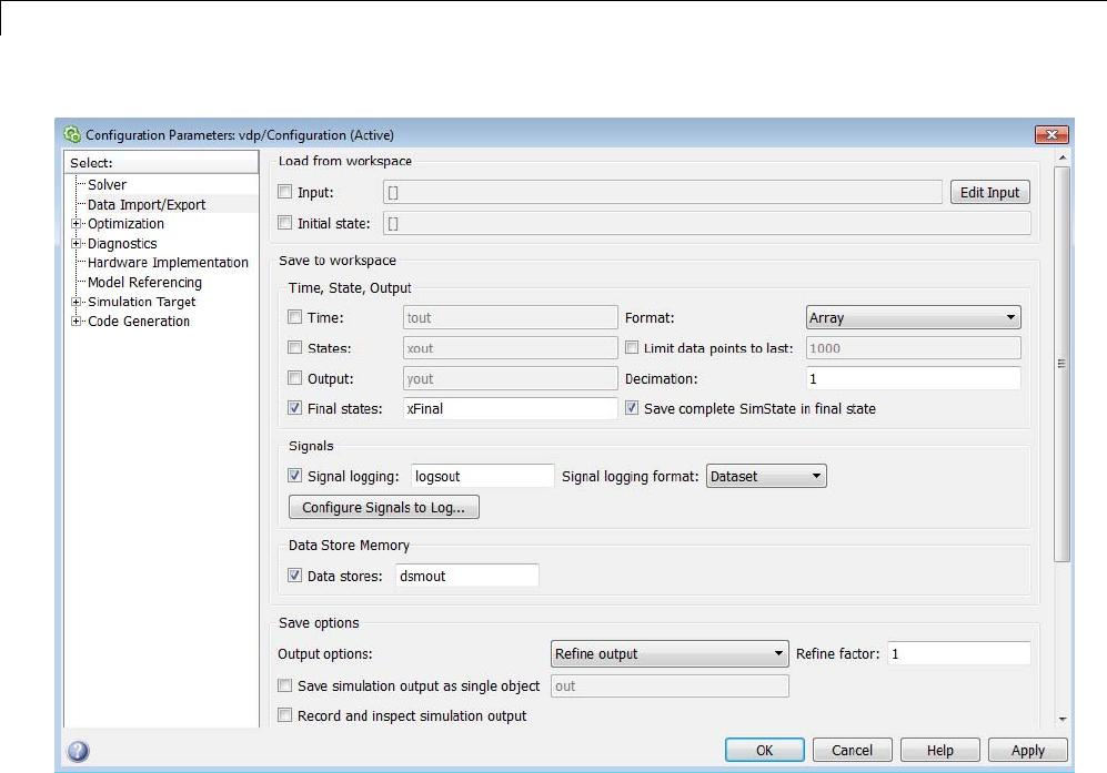
14 Running Simulations
Saving the SimState Programmatically
You can save the SimState at the beginning of the final step programmatically
using the sim command in conjunction with the set_param command with the
SaveCompleteFinalSimState parameter set to on:
set_param(mdl, 'SaveFinalState', 'on', 'FinalStateName',...
[mdl 'SimState'],'SaveCompleteFinalSimState', 'on')
simOut = sim(mdl, 'StopTime', tstop)
set_param(mdl, 'SaveFinalState', 'off')
14-34
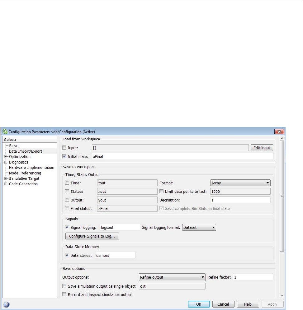
Save and Restore Simulation State as SimState
Restore the SimState
Restoring the SimState Interactively
You can restore the SimState interactively.
In the Data Import/Export pane:
1Under Load fromworkspace, select the check box next to Initial state.
The adjacent field becomes active.
2Enter the name of the variable containing the SimState in the field.
In the Solver pane of the Configuration Parameters window:
14-35

14 Running Simulations
1Keep the Start time set to its original value.
2Set the Stop time to the sum of the original simulation time plus the new
additional simulation time.
3Click OK.
The Start time must maintain its original value because it is a reference
value for all time and time-dependent variables in both the original and the
current simulations. For example, a block may save and restore the number
of sample time hits that occurred since the beginning of simulation as the
SimState . For clarity, consider a model that you ran from 0 s to 100 s and
that you now wish to run from 100 s to 200 s. The Start time is 0 s for both
the original simulation (0 s to 100 s) and for the current simulation (100 s to
200 s). And 100 s is the initial time of the current simulation. Also, if the block
had ten sample time hits during the original simulation, Simulink recognizes
thatthenextsampletimehitwillbetheeleventhrelevantto0s(not100s).
Restoring the SimState Programmatically
Use the set_param command to specify the initial condition as the SimState.
set_param(mdl, 'LoadInitialState', 'on', 'InitialState',...
[mdl 'SimState']);
simOut = sim(mdl, 'StopTime', tstop)
Restoring a SimState Saved in an Earlier Version of Simulink
You can now use SimState objects saved in earlier releases (R2010a or later)
to restore the SimState of a model. You can see the version of Simulink used
tosavetheSimStatebyexaminingthe’version’ field of the SimState object.
Simulink detects if the SimState object provided as the initial state was
saved in the current release. By default, the Simulink software reports an
error message if the SimState was not saved in the current release. You
may configure the diagnostic to allow Simulink to report the message as a
warningandtrytorestoreasmanyofthevaluesaspossible. Toenable
this best-effort restoration, go to the Diagnostics pane of the Configuration
Parameter dialog box and set the message for SimState object from earlier
release to warning. You can also set the diagnostic programmatically using
the set_param command.
14-36
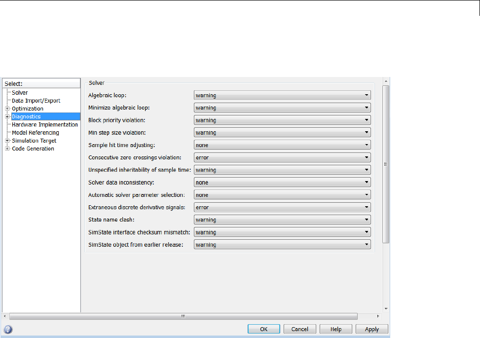
Save and Restore Simulation State as SimState
set_param(mdl, 'SimStateOlderReleaseMsg', 'warning');
Change the States of a Block within the SimState
You can use the loggedStates to get or set the SimState.TheloggedStates
field has the same structure as xout.signals if xout is the state log that
Simulink exports to the workspace.
SimState Interface Checksum Diagnostic
The SimState interface checksum is primarily based upon the configuration
settings of your model. A diagnostic, ’SimState interface checksum mismatch’,
resides on the Diagnostics pane of the Configuration Parameters dialog box.
You can set this diagnostic to ’none’, ’warning’, or ’error” to receive a warning
or an error if the interface checksum of the restored SimState does not match
the current interface checksum of the model. Such mismatches may occur
when you try to simulate using a solver that is different from the one that
14-37

14 Running Simulations
generated the saved SimState. Simulink permits such solver changes. For
example, you can use a solver such as ode15s, to solve the initial stiff portion
of a simulation, save the final SimState, and then continue the simulation
with the restored SimState and using ode45. In other words, this diagnostic
is purely to serve your own purposes for detecting solver changes.
Limitations of the SimState
Several limitations exist for the SimState:
•You can use only the Normal or the Accelerator mode of simulation.
•You cannot save the SimState in Normal mode and restore it in Accelerator
mode, or vice versa.
•You can save the SimState only at the final stop time or at the execution
time at which you pause or stop the simulation.
•By design, Simulink does not save user data, run-time parameters, or logs
of the model.
•The SimState feature does not support code generation, including Model
Reference in accelerated modes.
•You cannot make any structural changes to the model between the time
at which you save the SimState and the time at which you restore the
simulation using the SimState. For example, you cannot add or remove
a block after saving the SimState without repeating the simulation and
saving the new SimState.
•You cannot input the SimState to model functions.
Using SimState within S-Functions
Special APIs for C and Level-2 MATLAB S-functions are available, which
enable the S-functions to work with the SimState. For information on how
to implement these APIs within S-functions, see “S-Function Compliance
with the SimState”.
14-38

Diagnose Simulation Errors
Diagnose Simulation Errors
In this section...
“ResponsetoRun-TimeErrors”onpage14-39
“Simulation Diagnostics Viewer” on page 14-39
“Create Custom Simulation Error Messages” on page 14-41
Response to Run-Time Errors
If errors occur during a simulation, the Simulink software halts the
simulation, opens the subsystems that caused the error (if necessary), and
displays the errors in the Simulation Diagnostics Viewer. The following
sections explain how to use the viewer to determine the cause of the errors,
and how to create custom error messages.
Simulation Diagnostics Viewer
The viewer comprises an Error Summary pane and an Error Message pane.
14-39
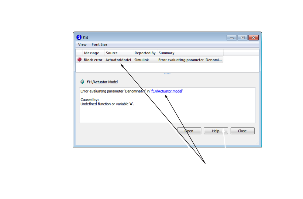
14 Running Simulations
Click to display
error source.
Error Summary Pane
The upper pane lists the errors that caused the simulation to terminate. The
pane displays the following information for each error.
Message. Messagetype(forexample,block error, warning, or log)
Source. Name of the model element (for example, a block) that caused the
error
Reported By. Component that reported the error (for example, the Simulink
product, the Stateflow product, or the Simulink Coder product).
Summary. Error message, abbreviated to fit in the column
14-40
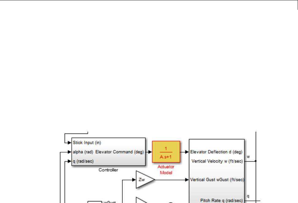
Diagnose Simulation Errors
You can remove any of these columns of information to make room for
other columns. To remove a column, select the View menu and uncheck
the corresponding item.
Error Message Pane
The lower pane initially contains the contents of the first error message listed
in the top pane. You can display the contents of other messages by clicking
their entries in the upper pane.
In addition to displaying the viewer, the Simulink software opens (if
necessary) the subsystem that contains the first error source and highlights
the source.
You can display the sources of other errors by clicking: anywhere in the error
messageintheupperpane;thenameofthe error source in the error message
(highlighted in blue); or the Open buttonontheviewer.
Changing Font Size
To change the size of the font used to display errors, select Increase Font
Size or Decrease Font Size from the Font Size menu of the viewer.
Create Custom Simulation Error Messages
The Simulation Diagnostics Viewer displays the output of any instance of
the MATLAB error function executed during a simulation. Such instances
include those invoked by block or model callbacks, or by S-functions that you
create or that the MATLAB Function block executes.
14-41
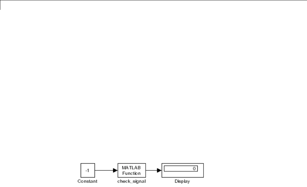
14 Running Simulations
You can use the MATLAB error function in callbacks, S-functions or the
MATLAB Function block to create custom error messages specific to your
application. Capabilities available for messages include:
•Display the contents of a text string
•Includehyperlinkstoanobject
•Link to an HTML file
Displaying A Text String
To display the contents of a text string, pass the string enclosed by quotation
marks to the error function.
The following example shows how you can make the user-created function
check_signal display the string Signal is negative.
The MATLAB Function block invokes the following function:
function y=check_signal(x)
if x<0
error('Signal is negative');
else
y=x;
end
Executing this model causes a runtime error and starts the debugger when
you click the OK button of the runtime error message. When you quit the
debugger, an error message in the Simulation Diagnostics window.
14-42
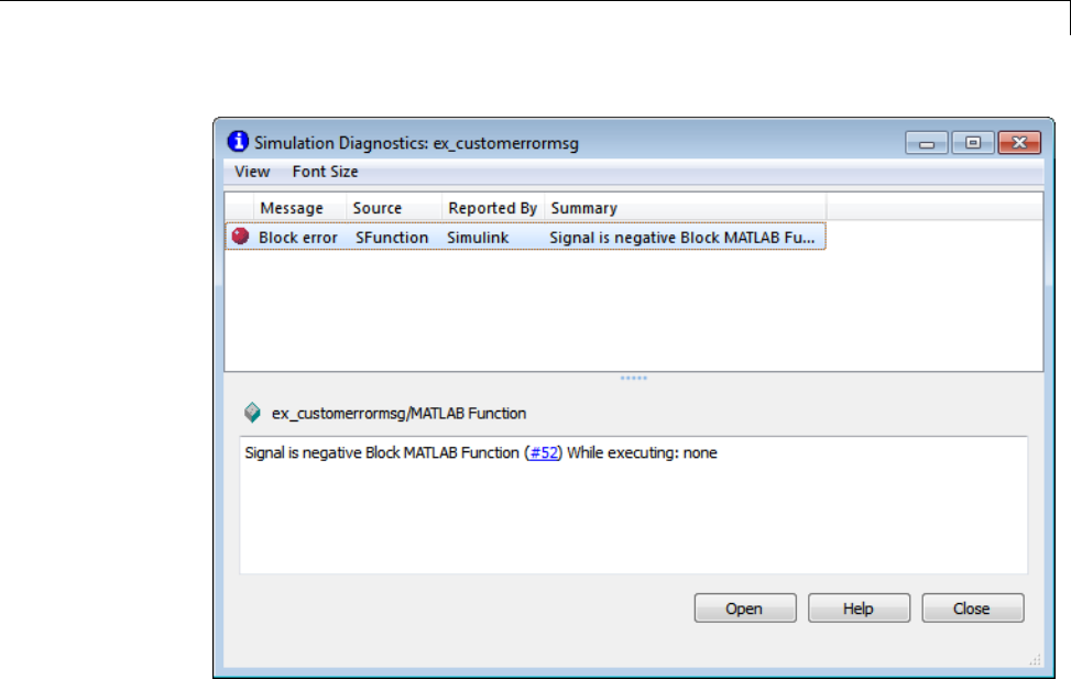
Diagnose Simulation Errors
Creating Hyperlinks to Files, Directories, or Blocks
To include a hyperlink to a block, file, orfolderintheerrormessage,include
the path to the item enclosed in quotation marks.
•error ('Error evaluating parameter in block "mymodel/Mu"')
displays a text hyperlink to the block Mu in the model “mymodel”. Clicking
the hyperlink displays the block in the model window.
•error ('Error reading data from "c:/work/test.data"')
displays a text hyperlink to the file test.data in the error message.
Clicking the link displays the file in your preferred MATLAB editor.
•error ('Could not find data in folder "c:/work"')
displays a text hyperlink to the c:/work folder. Clicking the link opens a
system command window (shell) and sets its working folder to c:/work.
14-43
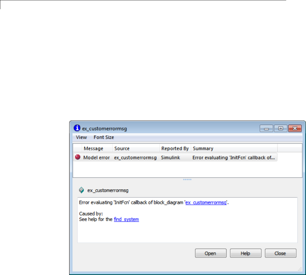
14 Running Simulations
Creating Programmatic Hyperlinks
You can create a hyperlink that, when clicked, causes the evaluation of a
MATLAB expression. For example, the following model InitFcn callback
displays an error, when the model starts, with a hyperlink to help for the
find_system command.
error('See help for the <a href="matlab:doc
find_system">find_system</a>
In this example, the Simulation Diagnostics window displays a hyperlink
labeled find_system. Clicking the link opens the documentation for the
find_system command in the MATLAB Help browser.
14-44


15 Running a Simulation Programmatically
About Programmatic Simulation
Entering simulation commands in the MATLAB Command Window or
from a MATLAB file enables you to run unattended simulations. You can
perform Monte Carlo analysis by changing the parameters randomly and
executing simulations in a loop. You can use either the sim command or
the set_param command to run a simulation programmatically. To run
simulations simultaneously, you can call sim from within a parfor loop under
specific conditions.
15-2

Run Simulation Using the sim Command
Run Simulation Using the sim Command
In this section...
“Single-Output Syntax for the sim Command” on page 15-3
“Examples of Implementing the sim Command” on page 15-4
“Calling sim from within parfor” on page 15-5
“Backwards Compatible Syntax” on page 15-5
Single-Output Syntax for the sim Command
The general form of the command syntax for running a simulation is:
SimOut = sim('model', Parameters)
where model is the name of the block diagram and Parameters can be
a list of parameter name-value pairs, a structure containing parameter
settings, or a configuration set. The sim command returns, SimOut,asingle
Simulink.SimulationOutput object that contains all of the simulation
outputs (logged time, states, and signals). This syntax is the “single-output
format” of the sim command.
SimOut =sim('model', 'Param1', Value1,'Param2', Value2...);
SimOut =sim('model', ParameterStruct);
SimOut =sim('model', ConfigSet);
During simulation, the specified parametersoverridethevaluesintheblock
diagram configuration set. The original configuration values are restored at
the end of simulation. If you wish to simulate the model without overriding
any parameters, and you want the simulation results returned in the
single-output format, then you must do one of the following:
•select Save simulation output as single object on the Data
Import/Export pane of the Configuration Parameters dialog box
•specify the ReturnWorkspaceOutputs parameter value as ’on’inthe sim
command:
SimOut = sim('model', 'ReturnWorkspaceOutputs', 'on');
15-3

15 Running a Simulation Programmatically
To log the model time, states, or outputs, use the Configuration Parameters
Data Import/Export dialog box. To log signals, either use a block such as
the To Workspace block or the Scope block, or use the Signal and Scope
Manager to log results directly.
For complete details of the sim command syntax, see the sim reference page.
Examples of Implementing the sim Command
Following are examples that show the application of each of the three formats
for specifying parameter values using the single-output format of the sim
command.
Specifying Parameter Name-Value Pairs
In the following example, the sim syntax specifies the model name, vdp,
followed by consecutive pairs of parameter name and parameter value. For
example, the value of the SimulationMode parameter is rapid.
simOut = sim('vdp','SimulationMode','rapid','AbsTol','1e-5',...
'SaveState','on','StateSaveName','xoutNew',...
'SaveOutput','on','OutputSaveName','youtNew');
simOutVars = simOut.who;
yout = simOut.get('youtNew');
Specifying a Parameter Structure
Thefollowingexampleshowshowtospecifyparametername-valuepairs
as a structure to the sim command.
paramNameValStruct.SimulationMode = 'rapid';
paramNameValStruct.AbsTol = '1e-5';
paramNameValStruct.SaveState = 'on';
paramNameValStruct.StateSaveName = 'xoutNew';
paramNameValStruct.SaveOutput = 'on';
paramNameValStruct.OutputSaveName = 'youtNew';
simOut = sim('vdp',paramNameValStruct);
15-4

Run Simulation Using the sim Command
Specifying a Configuration Set
The following example shows how to create a configuration set and use it
with the sim syntax.
model = 'vdp';
load_system(model)
simMode = get_param(model, 'SimulationMode');
set_param(model, 'SimulationMode', 'rapid')
cs = getActiveConfigSet(model);
model_cs = cs.copy;
set_param(model_cs,'AbsTol','1e-5',...
'SaveState','on','StateSaveName','xoutNew',...
'SaveOutput','on','OutputSaveName','youtNew')
simOut = sim(model, model_cs);
set_param(model, 'SimulationMode', simMode)
The block diagram parameter, SimulationMode, is not part of the
configuration set, but is associated with the model. Therefore, the set_param
command saves and restores the original simulation mode by passing the
model rather than the configuration set.
Calling sim from within parfor
For information on how to run simultaneous simulations by calling sim from
within parfor, see “Run Parallel Simulations” on page 15-8.
Backwards Compatible Syntax
The following syntax is now obsolete but will be maintained for backwards
compatibility with Simulink Versions 7.3 or earlier releases.
[T,X,Y]=sim('model',Timespan,Options,UT)
[T,X,Y1,...,Yn]=sim('model',Timespan,Options,UT)
If only one right-hand side argument exists, then Simulink automatically
saves the time, the state and the output to the specified left-hand side
arguments. You can explicitly switch to the single-output format by changing
the defaults.
15-5

15 Running a Simulation Programmatically
If you do not specify any left-hand side arguments, then Simulink
determines what data to log based on the workspace I/O settings of the Data
Import/Export pane of the Configuration Parameters dialog box.
TThetimevectorreturned.
XThe state returned in matrix or structure format. The
state matrix contains continuous states followed by
discrete states.
YThe output returned in matrix or structure format.
For block diagram models, this variable contains all
root-level blocks.
Y1,...,Yn The outports, which can only be specified for diagram
models. Here nmust be the number of root-level blocks.
Each outport will be returned in the Y1,...,Yn variables.
’model’ The name of a block diagram model.
Timespan The timespan can be one of the following: TFinal,
[TStart TFinal], or [TStart OutputTimes TFinal].
Output times are time points which will be returned in
T, but in general Twill include additional time points.
Options Optional simulation parameters created in a structure
by the simset command using name-value pairs.
UT Optional external inputs. For supported expressions, see
“Enable Data Import” on page 45-77.
Simulink only requires the first parameter. Simulink takes all defaults from
the block diagram, including unspecified options. If you specify any optional
arguments, your specified settings override the settings in the block diagram.
Specifying the right-hand side argument of sim as the empty matrix, [ ],
causes Simulink to use the default for the argument.
To specify the single-output format for sim(’model’, Timespan,Options,UT),
set the ’ReturnWorkspaceOutputs’ option of the options structure to ’on’.
See also simset and simget.
15-6

Control Simulation using the set_param Command
Control Simulation using the set_param Command
You can use the set_param command to start, stop, pause, or continue a
simulation, to update a block diagram, or to write all data logging variables to
thebaseworkspace.Theformatoftheset_param command is:
set_param('sys', 'SimulationCommand', 'cmd')
where 'sys'isthenameofthesystemand'cmd'is 'start','stop',
'pause','continue','update',or'WriteDataLogs'.
Similarly, you can use the get_param command to check the status of a
simulation. The format of the get_param function call for this use is
get_param('sys', 'SimulationStatus')
The Simulink software returns 'stopped','initializing','running',
'paused','updating','terminating',or'external' (used with the
Simulink Coder product).
Note If you use matlab -nodisplay to start a session, then you cannot use
set_param to run your simulation session.
RunSimulationfromanS-Function
S-functions can use the set_param command to control simulation execution.
A C MEX S-function can use the mexCallMATLAB macro to call the set_param
command itself.
15-7

15 Running a Simulation Programmatically
Run Parallel Simulations
In this section...
“Overview of Calling sim from within parfor” on page 15-8
“sim in parfor with Rapid Accelerator Mode” on page 15-9
“Workspace Access Issues” on page 15-10
“Resolving Workspace Access Issues” on page 15-11
“Data Concurrency Issues” on page 15-12
“Resolving Data Concurrency Issues” on page 15-13
Overview of Calling sim from within parfor
The MATLAB parfor command allows you to run parallel Simulink
simulations. Calling sim from within a parfor loop is often advantageous for
performing multiple simulation runs of the same model for different inputs
or for different parameter settings. For example, you may save significant
simulation time performing parameter sweeps and Monte Carlo analyses
by running them in parallel. Note that running parallel simulations using
parfor does not currently support decomposing your model into smaller
connected pieces and running the individual pieces simultaneously on
multiple workers.
Normal, Accelerator, and Rapid Accelerator simulation modes are supported
by sim in parfor. (See “Choosing a Simulation Mode” on page 22-11 for
details on selecting a simulation mode and “Design Your Model for Effective
Acceleration” on page 22-16 for optimizing simulation run times.) For other
simulations modes, you need to address any workspace access issues and
data concurrency issues in order to produce useful results. Specifically, the
simulations need to create separately named output files and workspace
variables; otherwise, each simulation will overwrite the same workspace
variables and files, or possibly have collisions trying to write variables and
files simultaneously.
For more information on code regeneration and parameter handling in Rapid
Accelerator mode, see “Parameter Handling in Rapid Accelerator Mode” on
page 22-8.
15-8

Run Parallel Simulations
For details about the parfor command, see parfor.
Note All simulation modes require a homogeneous file system. The workers
and the callers must be on the same operating system and have the same type
of file system (for example, NTFS or FAT).
Note If you open models inside a parfor statement you should close them
again using bdclose all to avoid leaving temporary files behind.
sim in parfor with Rapid Accelerator Mode
Running Rapid Accelerator simulations in parfor combines speed with
automatic distribution of a prebuilt executable to the parfor workers. As a
result, this mode eliminates duplication of the update diagram phase.
To run parallel simulations in Rapid Accelerator simulation mode using the
sim and parfor commands, you must:
•Configure the model to run in Rapid Accelerator simulation mode
•Ensure that the Rapid Accelerator target is already built and up to date
•Disable the Rapid Accelerator target up-to-date check by setting the sim
command option RapidAcceleratorUpToDateCheck to ’off’.
To satisfy the second condition, you can only change parameters between
simulations that do not require a model rebuild. In other words, the structural
checksum of the model must remain the same. Hence, you can change only
tunable block diagram parameters and tunable run-time block parameters
between simulations. For a discussion on tunable parameters that do not
require a rebuild subsequent to their modifications, see “Determining If the
Simulation Will Rebuild” on page 22-7.
As for the third condition, the following sample code shows how to disable the
up-to-date check using the sim command.
15-9

15 Running a Simulation Programmatically
matlabpool open
% Load the model and set parameters
model = 'vdp';
load_system(model)
% Build the Rapid Accelerator target
rtp = Simulink.BlockDiagram.buildRapidAcceleratorTarget(model);
% Run parallel simulations
parfor i=1:4
simOut{i} = sim(model,'SimulationMode', 'rapid',...
'RapidAcceleratorUpToDateCheck', 'off',...
'SaveTime', 'on',...
'StopTime', num2str(10*i));
end
matlabpool close
In this example, the call to the buildRapidAcceleratorTarget
function generates code once. Subsequent calls to sim with the
RapidAcceleratorUpToDateCheck option off guarantees that code is not
regenerated. Data concurrency issues are thus resolved.
For a detailed example of this method of running parallel simulations, refer to
the Rapid Accelerator Simulations Using PARFOR.
Workspace Access Issues
In order to run sim in parfor, you must first open a MATLAB pool of workers
using the matlabpool command. The parfor command then runs the code
within the parfor loop in these MATLAB worker sessions. The MATLAB
workers, however, do not have access to the workspace of the MATLAB client
session where the model and its associated workspace variables have been
loaded. Hence, if you load a model and define its associated workspace
variables outside of and before a parfor loop, then neither is the model
loaded, nor are the workspace variables defined in the MATLAB worker
sessions where the parfor iterations are executed. This is typically the case
when you define model parameters or external inputs in the base workspace
of the client session. These scenarios constitute workspace access issues.
15-10

Run Parallel Simulations
Resolving Workspace Access Issues
When a Simulink model is loaded into memory in a MATLAB client session,
it is only visible and accessible in that MATLAB session; it is not accessible
in the memory of the MATLAB worker sessions. Similarly, the workspace
variables associated with a model that are defined in a MATLAB client
session (such as parameters and external inputs) are not automatically
available in the worker sessions. You must therefore ensure that the model is
loaded and that the workspace variables referenced in the model are defined
in the MATLAB worker session by using the following two methods.
•In the parfor loop, use the sim command to load the model and to set
parameters that change with each iteration. (Alternative: load the model
and then use the g(s)et_param command(s) to set the parameters in the
parfor loop)
•In the parfor loop, use the MATLAB evalin and assignin commands
to assign data values to variables.
Alternatively, you can simplify the management of workspace variables
by defining them in the model workspace. These variables will then be
automatically loaded when the model is loaded into the worker sessions.
There are, however, limitations to this method. For example, you cannot have
tunable parameters in a model workspace. For a detailed discussion on the
model workspace, see “Model Workspaces” on page 4-67.
Specifying Parameter Values Using the sim Command
Use the sim command in the parfor loop to set parameters that change
with each iteration.
% Run parallel simulations of a model that does not
% result in data concurrency issues
model = 'vdp';
paramName = 'StopTime';
paramValue = {'10', '20', '30', '40'};
parfor i=1:4
simOut{i} = sim(model, ...
paramName, paramValue{i}, ...
'SaveTime', 'on');
end
15-11

15 Running a Simulation Programmatically
An equivalent method is to load the model and then use the set_param
command to set the paramName in the parfor loop.
Specifying Variable Values Using the assignin Command
You can pass the values of model or simulation variables to the MATLAB
workers by using the assignin or the evalin command. The following
example illustrates how to use this method to load variable values into the
appropriate workspace of the MATLAB workers.
parfor i = 1:4
assignin('base', 'extInp', externalInput{i})
% 'extInp' is the name of the variable in the base
% workspace which contains the External Input data
simOut{i} = sim(model, 'ExternalInput', 'extInp');
end
For further details, see the Rapid Accelerator Simulations Using PARFOR
example.
Data Concurrency Issues
Data concurrency issues refer to scenarios for which software makes
simultaneous attempts to access the same file for data input or output. In
Simulink, they primarily occur as a result of the nonsequential nature of
the parfor loop during simultaneous execution of Simulink models. The
most common incidences arise when code is generated or updated for a
simulation target of a Stateflow, Model block or MATLAB Function block
during parallel computing. The cause, in this case, is that Simulink tries to
concurrently access target data from multiple worker sessions. Similarly,
To File blocks may simultaneously attempt to log data to the same files
during parallel simulations and thus cause I/O errors. Or a third-party
blockset or user-written S-function may cause a data concurrency issue while
simultaneously generating code or files.
A secondary cause of data concurrency is due to the unprotected access of
network ports. This type of error occurs, for example, when a Simulink
product provides blocks that communicate via TCP/IP with other applications
during simulation. One such product is the HDL Verifier™ for use with the
Mentor Graphics® ModelSim® HDL simulator.
15-12

Run Parallel Simulations
Resolving Data Concurrency Issues
The core requirement of parfor is the independence of the different
iterations of the parfor body. This restriction is not compatible with the core
requirement of simulation via incremental code generation, for which the
simulation target from a prior simulation is reused or updated for the current
simulation. Hence during the parallel simulation of a model that involves
code generation (such as Accelerator mode simulation), Simulink makes
concurrent attempts to access (update) the simulation target . However, you
can avoid such data concurrency issues bycreatingatemporaryfolderwithin
the parfor loop and then adding several lines of MATLAB code to the loop to
perform the following steps:
1Change the current folder to the temporary, writable folder.
2In the temporary folder, load the model, set parameters and input vectors,
and simulate the model.
3Return to the original, current folder.
4Remove the temporary folder and temporary path.
In this manner, you avoid concurrency issues by loading and simulating the
model within a separate temporary folder. Following are examples that use
this method to resolve common concurrency issues.
A Model with Stateflow, MATLAB Function Block, or Model
Block
In this example, either the model is configured to simulate in Accelerator mode
or it contains a Stateflow, a MATLAB Function block, or a Model block (for
example, sf_bounce,sldemo_autotrans,orsldemo_modelref_basic). For these
cases, Simulink generates code during the initialization phase of simulation.
Simulating such a model in parfor would cause code to be generated to the
same files, while the initialization phase is running on the worker sessions.
As illustrated below, you can avoid such data concurrency issues by running
each iteration of the parfor body in a different temporary folder.
parfor i=1:4
15-13

15 Running a Simulation Programmatically
cwd = pwd;
addpath(cwd)
tmpdir = tempname;
mkdir(tmpdir)
cd(tmpdir)
load_system(model)
% set the block parameters, e.g., filename of To File block
set_param(someBlkInMdl, blkParamName, blkParamValue{i})
% set the model parameters by passing them to the sim command
out{i} = sim(model, mdlParamName, mdlParamValue{i});
cd(cwd)
rmdir(tmpdir,'s')
rmpath(cwd)
end
Note that you can also avoid other concurrency issues due to file I/O errors by
using a temporary folder for each iteration of the parfor body.
A Model with To File Blocks
If you simulate a model with To File blocks from inside of a parfor loop, the
nonsequential nature of the loop may cause file I/O errors. To avoid such
errors during parallel simulations, you can either use the temporary folder
idea above or use the sim command in Rapid Accelerator mode with the option
to append a suffix to the file names specified in the model To File blocks.
By providing a unique suffix for each iteration of the parfor body, you can
avoid the concurrency issue.
parfor i=1:4
sim(model, ...
'ConcurrencyResolvingToFileSuffix', num2str(i),...
'SimulationMode', 'rapid');
end
15-14

Error Handling in Simulink®Using MSLException
Error Handling in Simulink Using MSLException
Error Reporting in a Simulink Application
Simulink allows you to report an error by throwing an exception using the
MSLException object , which is a subclass of the MATLAB MException class.
As with the MATLAB MException object, you can use a try-catch block with
aMSLException object construct to capture information about the error. The
primary distinction between the MSLException and the MException objects is
that the MSLException object has the additional property of handles. These
handles allow you to identify the object associated with the error.
The MSLException Class
The MSLException class has five properties: identifier,message,stack,
cause,andhandles. The first four of these properties are identical to those
of MException. For detailed information about them, see “Properties of the
MException Class”. The fifth property, handles, is a cell array with elements
that are double array. These elements contain the handles to the Simulink
objects (blocks or block diagrams) associated with the error.
Methods of the MSLException Class
The methods for the MSLException class are identical to those of the
MException class. For details of these methods, see MException.
Capturing Information about the Error
The structure of the Simulink try-catch block for capturing an exception is:
try
Perform one or more operations
catch E
if isa(E, 'MSLException')
...
end
If an operation within the try statement causes an error, the catch statement
catches the exception (E). Next, an if isa conditional statement tests to
15-15

15 Running a Simulation Programmatically
determine if the exception is Simulink specific, i.e., an MSLException.In
other words, an MSLException is a type of MException.
The following code example how to get the handles associated with an error.
errHndls = [];
try
sim('ModelName', ParamStruct);
catch e
if isa(e,'MSLException')
errHndls = e.handles{1}
end
end
You can see the results by examining e. They will be similar to the following
output:
e=
MSLException
Properties:
handles: {[7.0010]}
identifier: 'Simulink:Parameters:BlkParamUndefined'
message: [1x87 char]
cause: {0x1 cell}
stack: [0x1 struct]
Methods, Superclasses
To identify the name of the block that threw the error, use the getfullname
command. For the present example, enter the following command at the
MATLAB command line:
getfullname(errHndls)
If a block named Mu threw an error from a model named vdp, MATLAB
would respond to the getfullname command with:
ans =
15-16

Error Handling in Simulink®Using MSLException
vdp/Mu
15-17

15 Running a Simulation Programmatically
15-18

16
Visualizing and Comparing
Simulation Results
•“View Simulation Results” on page 16-2
•“Signal Viewer Tasks” on page 16-6
•“Scope Signal Viewer Tasks” on page 16-11
•“Scope Signal Viewer Characteristics” on page 16-14
•“Signal Generator Tasks” on page 16-21
•“Signal and Scope Manager” on page 16-23
•“Signal Selector” on page 16-27
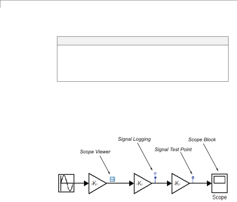
16 Visualizing and Comparing Simulation Results
View Simulation Results
In this section...
“What Are Scope Blocks, Signal Viewers, Test Points and Data Logging?”
on page 16-2
“Scope Block and Scope Signal Viewer Differences” on page 16-3
“Why Use Signal Generators and Signal Viewers Instead of Source Blocks
and Scope Blocks?” on page 16-4
What Are Scope Blocks, Signal Viewers, Test Points
and Data Logging?
Scope blocks, signal viewers, test points, and data logging provide ways for
you to display and capture results from your simulations.
These icons represent the various data display and data capture devices:
•To perform basic signal viewer tasks, see “Signal Viewer Tasks” on page
16-6 and “Scope Signal Viewer Tasks” on page 16-11.
•For detailed information on signal viewers, see “Signal and Scope Manager”
on page 16-23.
•For information on signal logging, see “Export Signal Data Using Signal
Logging” on page 45-19.
16-2

View Simulation Results
•For information on signal Test Points, see “Test Points” on page 47-58.
•For information on Scope Blocks, see Scope.
Scope Block and Scope Signal Viewer Differences
Use Scope blocks and scope signal viewers to display simulation results, but
as shown in this table, they have different characteristics.
Characteristic Scope Signal Viewer Scope Block
Interface Attach to signal using Signal
Selector or context menu
See “Signal Selector” on
page 16-27
See “Scope Signal Viewer
Context Menu” on page
16-15
Drag from Library Browser
Scope of
Control
All viewers centrally
managed from Signal
and Scope Manager
See “Signal and Scope
Manager” on page 16-23.
Each managed individually
Signals per
axis
Multiple One nonbus signal per
axis or multiple signals fed
through a mux or a bus
Axes per
scope
Multiple
“Creating a Multiple Axes
Scope Signal Viewer” on
page 16-11
Multiple
Data
handling
Save data to a signal logging
object
Save variable data to
workspace as structures or
arrays
16-3

16 Visualizing and Comparing Simulation Results
Characteristic Scope Signal Viewer Scope Block
Data logging Log data to model-wide data
object
See
Simulink.SimulationData.Dataset
and
Simulink.ModelDataLogs
None
Scrolling
display data
capability
Yes No
Display •Data markers
•Legends
•Color and line codes
distinguish signals
Color and line codes
distinguish signals
Graph
Refresh
Period
Adjustable Fixed
Display of
Minor Steps
The viewer does not display
minor steps regardless of
the value of the Refine
parameter setting.
Only displays major
time step values. The
scope displays additional
interpolated points between
major time steps if specified
bytherefineparameter.
Why Use Signal Generators and Signal Viewers
Instead of Source Blocks and Scope Blocks?
You should use signal generators and signal viewers instead of Source and
Scope blocks when you want to:
•Navigate to and attach signal generators or signal viewers deep within a
model hierarchy.
•Centrally manage all signal generators and signal viewers present in
your model.
16-4

View Simulation Results
•Use the display features provided by signal viewers that are not available
in Scope blocks.
•Reduce clutter in your block diagram. Because signal viewers attach
directly to signals, it is not necessary for you to route them to a Scope block.
This results in fewer signal routes in your block diagram.
•View data from referenced models. See “Test Points” on page 47-58 for
more information.
16-5

16 Visualizing and Comparing Simulation Results
Signal Viewer Tasks
In this section...
“About Signal Viewers” on page 16-6
“Attaching a Signal Viewer” on page 16-6
“Adding Signals to a Signal Viewer” on page 16-8
“Displaying a Signal Viewer” on page 16-9
“Saving Data to MATLAB Workspace” on page 16-10
“Plotting the Viewer Data” on page 16-10
About Signal Viewers
•Signal viewers are not the same as Scope blocks. For an explanation of
the differences, see “Scope Block and Scope Signal Viewer Differences”
on page 16-3.
•Signal viewers do not show signal labels on the axis, display the simulation
minor time step values, or work with Simulink Report Generator.
•Not all signal viewer features are supported when you simulate your model
in Rapid Accelerator mode. See “Behavior of Scopes and Viewers with
Rapid Accelerator Mode” on page 22-18.
•The Help button for a signal viewer is located on the parameters dialog box
for a specific viewer type. For more information, see“Scope Signal Viewer
Parameters Dialog Box” on page 16-16 .
Signal viewer
Attaching a Signal Viewer
If you want to,
•Quickly connect or disconnect a scope signal viewer, use the context menu.
•Review all of the signal viewers and the signals connected to them, use the
Signal and Scope Manager.
16-6

Signal Viewer Tasks
Using the Context Menu
To attach a signal viewer with the signal content menu,
1On your Simulink block diagram, right-click a signal, and then from the
context menu, select Create & Connect Viewer.
2From the list that appears, select the type of signal viewer you want to
attach.
If you attach a scope signal viewer, a viewer window opens. You must run
thesimulationafteryouattachtheviewerfortheinformationtobeplotted.
Using the Signal and Scope Manager
To attach a scope signal viewer using the Scope & Signal Manager,
1On your Simulink block diagram, right-click a signal, and then from the
context menu, select Signal & Scope Manager.TheSignal&Scope
Manager dialog box opens.
2In the Types pane and under the Viewers node, expand a product node to
show the viewers installed and available to you.
Note The Simulink Scope displayed in the Signal and Scope Manager
TypespaneisnotthesameastheSimulinkScopeBlock. Foran
explanation of the differences, see “Scope Block and Scope Signal Viewer
Differences” on page 16-3.
16-7
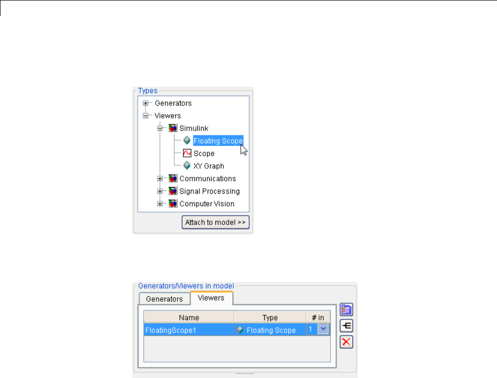
16 Visualizing and Comparing Simulation Results
3Under an expanded product node, select a viewer, and then click the
Attach to model button.
TheviewerisaddedtoatableintheViewers tab in the Generators/Viewers
in model pane. The table lists the viewers in your model.
Each row corresponds to a viewer. The columns specify each viewer name,
type, and number of inputs. If a viewer accepts a variable number of
inputs, the #inentry for the viewer contains a pull-downlistthatdisplays
the range of inputs that the viewer can accept. To change the number of
inputs accepted by the viewer, select a value from the pull-down list.
Adding Signals to a Signal Viewer
To add additional traces to an existing signal viewer,
1In the Simulink Editor, right-click a signal.
16-8
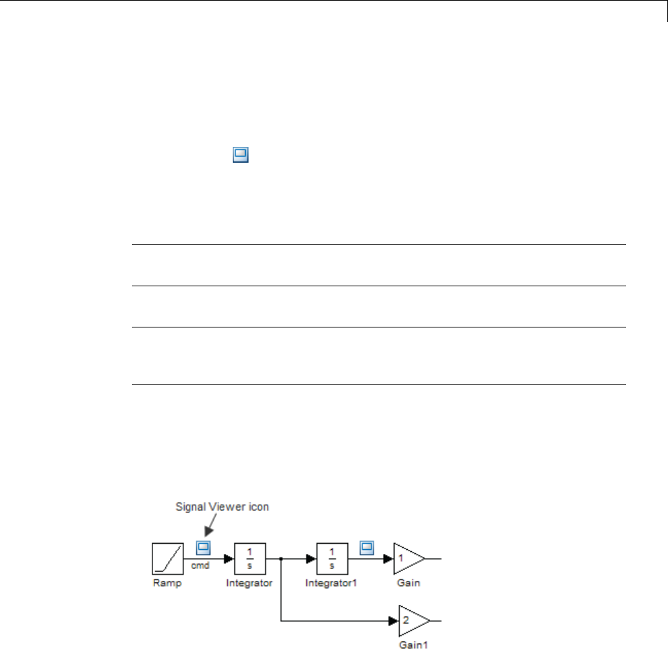
Signal Viewer Tasks
2From the signal context menu, point to Create & Connect Viewer,and
then from the submenu, point to a product.
3From the list, select the signal viewer you want to attach to the signal.
Aviewerion is added to the signal line.
You can also add signals to a signal viewer with the Signal and Scope
Manager. See “Signal and Scope Manager” on page 16-23.
Note Youmustrunasimulationforthenewsignaltracetodisplayina
viewer.
Note If you add or remove signals from a Signal Viewer, the Signal Viewer
title and legends update only when you run a simulation, and then open the
viewer.
Displaying a Signal Viewer
1Right-click a signal viewer icon. From the context menu, point to Open
Viewer, and then select a viewer from the list.
Depending on the type of signal viewer, the following happens:
•Scope and Floating Scope — A Viewer: Scope window opens with a graph
of the signals attached to the viewer.
16-9

16 Visualizing and Comparing Simulation Results
•XY Graph — A Sink Block Parameters dialog box opens. After running a
simulation, a Viewer: XY Graph window opens with a graph of the X and
Y signals attached to the viewer.
2Customize the signal viewer to better visualize the simulation results.
Saving Data to MATLAB Workspace
To save the data displayed on the viewer to the MATLAB workspace, perform
the following steps:
1In the Viewer toolbar, click the parameters icon .
2Click the History tab.
3Select Save to model signal logging object (logsout).
4In the Logging name field, enter a logging variable name.
5Assignanametothesignalintheblockdiagram,forexample,x1.
6Run the simulation by selecting Simulation > Start.
You can now view the data in the MATLAB Command Window by entering
the following commands:
logsout.unpack('all')
data = x1.Data
x1.time
where x1isthenameofthesignal.
Plotting the Viewer Data
You can plot the data interactively or programmatically.
•Simulation Data Inspector — plot the data as explained in “Inspect
Signal Data” on page 17-11.
•Simplot — plot the data from the command line using the simplot
command (see simplot). The resulting figure looks identical to the viewer
window and can be annotated using the Plot Editing Tools.
16-10

Scope Signal Viewer Tasks
Scope Signal Viewer Tasks
In this section...
“Adding a Legend to a Scope Signal Viewer” on page 16-11
“Creating a Multiple Axes ScopeSignalViewer”onpage16-11
AddingaLegendtoaScopeSignalViewer
1In a Scope signal viewer window, right-click.
2From the context menu, select Legends.
The viewer draws a box and identifies each signal with the name of the
signal. If a signal does not have a name, the legend uses the name of the
originating block or subsystem.
3To move a legend to another location on the graph, left-click and drag the
legend box.
For information about the color and line styles in the Viewer window, see
“Line Styles with Scope Signal Viewer” on page 16-19.
Creating a Multiple Axes Scope Signal Viewer
You can add multiple plots (called axes)toascopesignalviewer. Eachaxes
can have different y-axis settings.
To create a viewer with more than one axes.
1Open the Signal and Scope manager. Add a signal Scope or Floating Scope
signal viewer to your model. See “Attaching a Signal Viewer” on page 16-6.
2From the #indrop-down list, select the total number of axes for the graph.
16-11
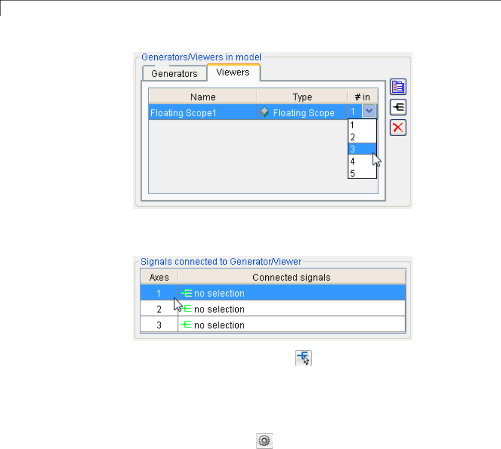
16 Visualizing and Comparing Simulation Results
3In the Signals connected to Generator/Viewer section, select the first
axis.
4Click the Signal Selector button . The Signal Selector dialog box
opens.
5Select the signal or signals to add to this axis, and then close the dialog.
6Repeat steps 3 to 5 until you have added signals to all of the axes.
7Click the parameters icon to display the scope signal viewer, and then
run the simulation.
16-12
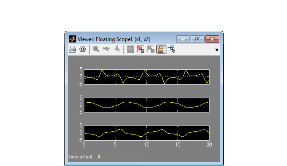
Scope Signal Viewer Tasks
16-13
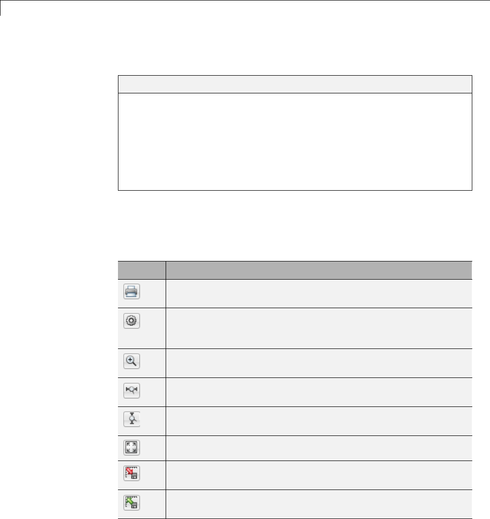
16 Visualizing and Comparing Simulation Results
Scope Signal Viewer Characteristics
In this section...
“Scope Signal Viewer Toolbar” on page 16-14
“Scope Signal Viewer Context Menu” on page 16-15
“Scope Signal Viewer Parameters Dialog Box” on page 16-16
“Line Styles with Scope Signal Viewer” on page 16-19
“Parameter Settings and Performance with Scope Signal Viewer” on page
16-20
Scope Signal Viewer Toolbar
The signal viewer toolbar is attached to each scope signal viewer. It has the
following controls.
Icon Function
Opens the Print dialog box so you can print the contents of a
Scope Viewer window.
Opens the Scope parameters dialog for modifying display
characteristics. For details, see “Scope Signal Viewer Parameters
Dialog Box” on page 16-16.
Simultaneously zooms in on the xand yaxes. The zoom feature
is not active while the simulation is running.
Use this button to zoom in on the xaxis only. The zoom feature is
not active while the simulation is running.
Use this button to zoom in on the yaxis only. The zoom feature is
not active while the simulation is running.
Automatically scales the axis to fully display all signals.
Stores the current axis settings so you can apply them to the
next simulation.
Restores the graph setting values saved by the most recent Save
axes settings command.
16-14
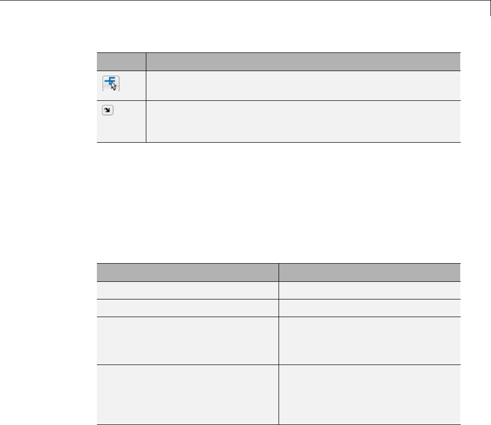
Scope Signal Viewer Characteristics
Icon Function
Activates the Signal Selector. For more information, see “Signal
Selector” on page 16-27.
Docks and undocks the Scope Viewer. When you dock the Scope
Viewer, it is placed within the MATLAB Command Window and
automatically resized.
Scope Signal Viewer Context Menu
The scope signal viewer context menu is a convenient way to make simple
changes to a viewer without navigatingtoaScopeorFloatingScope
parameters dialog box.
Within a Scope signal viewer window, right-click to display the context menu.
It contains the following controls.
Control Function
Legends Adds a legend to your scope viewer.
Autoscale Automatically scales the viewer axis.
Signal selection Displays the Signal Selector dialog.
For information, see “Signal
Selector” on page 16-27
Axes properties Displays the Axis Properties dialog.
You can manually set the minimum
and maximum range for the yaxis
here.
16-15

16 Visualizing and Comparing Simulation Results
Control Function
Scope parameters Displays the Scope parameters
dialog.
For information, see “Scope Signal
Viewer Parameters Dialog Box” on
page 16-16.
Tick labels Displays the Tick Labels dialog.
From here you can turn on and off
various tick options.
Scope Signal Viewer Parameters Dialog Box
To open a Scope or Floating Scope parameters dialog box,
•On the scope toolbar, click
There are three tabs on the dialog box:
•General — set the axis characteristics and the sampling decimation value
•History — control the amount of stored and displayed data
•Performance — control the scope refresh rate.
General Tab
With this tab you control the number of axes, the time range, and the
appearance of your graph.
Number of axes. Set the number of axes in this data field. Each axis is
displayed as a separate graph within a single Scope Viewer.
An example of this is shown in “Adding Signals to a Signal Viewer” on page
16-8.
Time Range. Change the x-axislimitsbyenteringanumberorauto in
the Time range field.
16-16

Scope Signal Viewer Characteristics
Entering a number of seconds causes each screen to display the amount of
data that corresponds to that number of seconds. Enter auto to set the x-axis
to the duration of the simulation.
Note Do not enter variable names in these fields.
Tick labels. Specifies whether to label axes ticks. The options are:
Option Effect
all Places ticks on the outside of all axes
inside Places tick labels inside all axes
(available only on signal viewers)
bottom axis only Places tick labels outside the bottom
axes
Scroll. When you select this option, the scope continuously scrolls the
displayed signals to the left to keep as much data in view as will fit on the
screen at any one time.
In contrast, when this option is not selected, the scope draws a screen full of
data from left to right until the screen is full, erases the screen, and draws
the next screen full of data. This loop is repeated until the end of simulation
time. The effects of this option are discernible only when drawing is slow, for
example, when the model is very large or has a very small step size.
Note In some cases, the simulation slows when the simulation runs with the
scroll option selected. See “Parameter Settings and Performance with Scope
Signal Viewer” on page 16-20.
Data markers. Displays a marker at each data point on the Scope Viewer
screen.
Legends. Displays a legend on the scope that indicates the line style used
to display each signal.
16-17

16 Visualizing and Comparing Simulation Results
Decimation. Logs every Nth data point, where N is the number entered
in the edit field.
For example, suppose that the input signal to your Scope block has a fixed
sample time of 0.1 s. If you enter a value of 2, data points for this viewer will
be recorded at times 0.0, 0.2, 0.4....
History Tab
With this tab you control the amount of data that the Scope signal viewer
stores, displays and stores to the workspace. The values that appear in these
fields are the values that are used in the next simulation.
Limit data points to last. Limits the number of data points saved to the
workspace. Select the Limit data points to last check box and enter a value
in its data field.
The Scope relies on its data history for zooming and autoscaling operations. If
the number of data points is limited to 1,000 and the simulation generates
2,000 data points, only the last 1,000 are available for regenerating the
display.
Savetomodelsignalloggingobject. At the end of the simulation, this
option saves the data displayed on the Scope Viewer . The data is saved in the
Simulink.ModelDataLogs object used to log data for the model (see “Export
Signal Data Using Signal Logging” on page 45-19 for more information).
For this option to take effect, you must also enable signal logging for the
model as a whole. To do this, check the Signal logging option on the Data
Import/Export pane of the Model Configuration Parameters dialog box.
For new models, use the Dataset logging format. If you use the Dataset
format for signal logging, then Simulink does not log the signals configured to
be logged in the Signal Viewer. Explicitly mark the signal for signal logging
by using the Signal Properties dialog box. To access the Signal Properties
dialog box, right-click a signal and from the context menu, select Properties.
16-18

Scope Signal Viewer Characteristics
Logging Name. Specifies the name under which to store the viewer’s
data in the model’s Simulink.ModelDataLogs object. The name must
be different from the log names specified by other signal viewers or for
other signals, subsystems, or model references logged in the model’s
Simulink.ModelDataLogs object.
Performance Tab
Controls how frequently the Scope signal viewer is refreshed. Reducing the
refresh rate can speed up the simulation in some cases.
Note For information about additional scope signal viewer parameters that
can affect performance, see “Parameter Settings and Performance with Scope
Signal Viewer” on page 16-20.
This tab contains the following controls.
Refresh Period. Select the units in which the refresh period is expressed.
Options are either seconds or frames, where a frame is the width of the scope’s
screen in seconds. This is the value of the scope’s Time range parameter.
Refresh Slider. Sets the refresh rate.
Dragthesliderbuttontotherighttoincrease the refresh period and hence
decrease the refresh rate.
Freeze Button. Controls refresh.
Click the button to freeze (stop refreshing) or unfreeze the Scope Viewer.
Line Styles with Scope Signal Viewer
If a signal contains multiple elements such as a vector or matrix, the viewer
distinguishes the elements with different line styles. If a signal has more
than four elements, the viewer cycles through the line styles. The line styles
retain the color of the signal.
16-19

16 Visualizing and Comparing Simulation Results
Signal Element Scope Viewer
1
2
3
4
Parameter Settings and Performance with Scope
Signal Viewer
In some cases, when a Scope signal viewer needs to display a large number
of data points, the simulation slows down. When this happens, you can
improve simulation performance by adjusting the settings of some of the
viewer parameters. Try one or a combination of the following until you are
satisfied with the simulation performance.
•Turn off scroll mode.
•Reducethetimerange.
•Use decimation to reduce the number of data points.
•Increase the refresh period to decrease the refresh rate.
•Limit the number of data points that the viewer saves to the workspace.
16-20

Signal Generator Tasks
Signal Generator Tasks
In this section...
“Attaching a Signal Generator.” on page 16-21
“Removing a Generator” on page 16-22
Attaching a Signal Generator.
If you want to,
•Quickly connect or disconnect a Signal Generator, use the context menu.
•Review all of the Signal Generators and their signals, use the Signal and
Scope Manager.
Using the Context Menu
To add additional traces to an existing signal viewer,
1In the Simulink Editor, right-click the input to a block.
2From the context menu, point to Create & Connect Generator,andthen
from the submenu, point to a product.
3From the list, select the generator you want as input to the block.
The name of the generator you choose appears in a box connected to the
block input.
4Double-clickthenametoeditthegeneratorname.
5Right-click the name and select Generator Parameters to display a
dialog box where you can change the generator parameters.
6Right-click the name and select Properties todisplayadialogboxwhere
you can change the signal properties.
Using the Signal and Scope Manager
To attach a Signal Generator using the Signal and Scope Manager,
16-21

16 Visualizing and Comparing Simulation Results
1Right-click the input to a block, and then from the signal context menu
select Signal & Scope Manager.
2In the Types pane and under the Generators node, expand a product node
to show the generator installed and available to you.
3Under an expanded product node, select a generator, and then click the
Attach to model button.
The viewer is added to a table in the Generators tab in the
Generators/Viewers in model pane. The table lists the generators in your
model.
Each row corresponds to a generator. The columns specify each generator
name and type.
Clicking on the name of a generator displays the connected signals. For
instance, the constant is shown connected to the second input of the sum
block.
Removing a Generator
To remove the generator from the block diagram.
1Right-click a generator.
2From the context menu, select Disconnect Generator.
16-22

Signal and Scope Manager
Signal and Scope Manager
In this section...
“About the Signal & Scope Manager” on page 16-23
“Opening the Signal and Scope Manager” on page 16-24
“Changing Generator or Viewer Parameters” on page 16-25
“Adding Signals to a Viewer” on page 16-25
“RemovingaGeneratororViewerfromaSimulinkModel”onpage16-25
“Viewing Test Point Data” on page 16-26
About the Signal & Scope Manager
The Signal & Scope Manager is a user interface to Signal Generator and
Viewer objects. Using the Signal and Scope Manager you can manage from
a central place all signal generators and viewers.
Note The Signal and Scope Manager requires that you have Java enabled
when you start MATLAB. This is the default.
Signal Generator and Viewer Objects
The small icons identifying a viewer or generator are called Viewer and
Generator Objects. These objects are not the same as scope blocks or signal
blocks. Generator and Viewer Objects are managed by the Signal and Scope
Manager, and are placed on signals. Blocks are dragged from the Library
browser and are not managed by the Signal and Scope manager.
16-23

16 Visualizing and Comparing Simulation Results
Opening the Signal and Scope Manager
1In the Simulink Editor window, select Diagram > Signals &
Ports > Signal & Scope Manager.
The Signal & Scope Manger window opens.
16-24

Signal and Scope Manager
Alternatively within your model, right click a signal line and from the
context menu, select Signal & Scope Manager.
Changing Generator or Viewer Parameters
1OpentheSignal&ScopeManagerwindow.
2To the right side of the Generators/Viewers pane, click the parameters
button .
The generator or viewer window opens.
3From the toolbar, select the parameters button .Reviewandchange
parameters.
Adding Signals to a Viewer
Use the Signal Selector to add signals to a Viewer.
1To the right side of the Generators/Viewers pane, click the Signal Selector
button .
The Signal Selector window opens. Use the Signal Selector to connect and
disconnect generators and viewers.
2From the signals pane, select the check boxes for the signals you want to
display in the selected viewer.
Tip After adding the new signals, run a simulation to make them visible.
Removing a Generator or Viewer from a Simulink
Model
1In the Generators/Viewers pane, select either a listed generator for viewer.
2On the right side, click the Delete button .
16-25

16 Visualizing and Comparing Simulation Results
The selected generator or viewer is removed from the table.
Viewing Test Point Data
You can use a Signal Viewer available from the Signal and Scope Manager
to view any signal that is defined as a test point in a submodel. A test point
is a signal that is guaranteed to be observable when using a signal viewer
in a model.
Note With some signal viewers (for example, XY Graph, To Video Display,
Matrix Viewer, Spectrum Scope, and Vector Scope), you cannot use the Signal
Selector to select signals with test points in referenced models.
For more information, see “Test Points” on page 47-58.
16-26
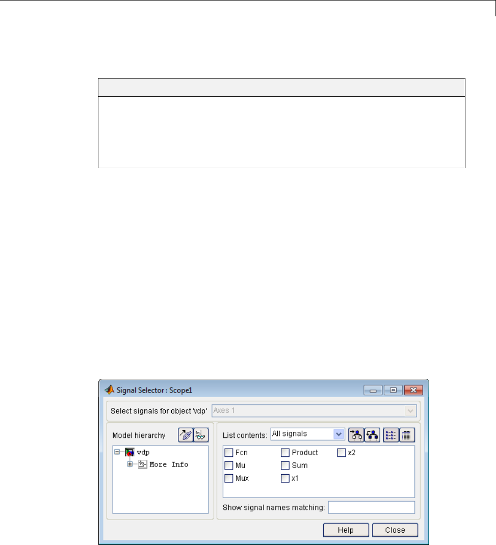
Signal Selector
Signal Selector
In this section...
“About the Signal Selector” on page 16-27
“Select signals for object” on page 16-28
“Model Hierarchy” on page 16-28
“Inputs/Signals List” on page 16-28
About the Signal Selector
The Signal Selector allows you to connect a generator or viewer object (see
“Attaching a Signal Viewer” on page 16-6 and “Attaching a Signal Generator.”
on page 16-21) or a Floating Scope block to other block inputs and outputs.
It appears when you click the Signal selection button for a generator or
viewer object in the Signal & Scope Manager or on the toolbar of the Floating
Scope window.
The Signal Selector that appears when you click the Signal selection button
applies only to the currently selected generatororviewerobject(orthe
Floating Scope). If you want to connect blocks to another generator or viewer
object, you must select the object in the Signal & Scope Manager and launch
another instance of the Signal Selector. The object used to launch a particular
instance of the Signal Selector is called that instance’s owner.
16-27
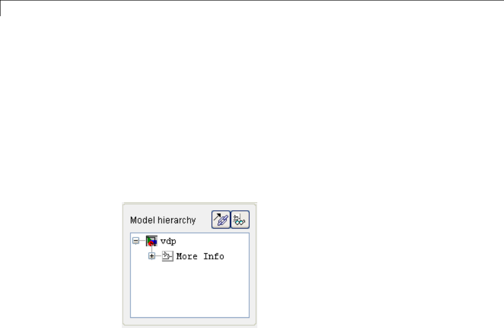
16 Visualizing and Comparing Simulation Results
Select signals for object
This list box allows you to select the owner output port (in the case of signal
generators) or display axis (in the case of signal viewers) to which you want to
connect blocks in your model.
The list box is enabled only if the signal generator has multiple outputs or
the signal viewer has multiple axes.
Model Hierarchy
This tree-structured list lets you select any subsystem in your model.
Selecting a subsystem causes the adjacent port list to display the ports
available for connection in the selected subsystem. To display subsystems
included as library links in your model, click the Follow links button at
the top of the Model hierarchy control. To display subsystems contained
by masked subsystems, click the Look under masks button at the top
of the panel.
Inputs/Signals List
The contents of this panel displays input ports available for connection to the
Signal Selector’s owner if the owner is a signal generator or signals available
for connection to the owner if the owner is a signal viewer.
If the Signal Selector’s owner is a signal generator, the inputs/signals list by
default lists each input port in the system selected in the model hierarchy tree
that is either unconnected or connected to a signal generator.
16-28
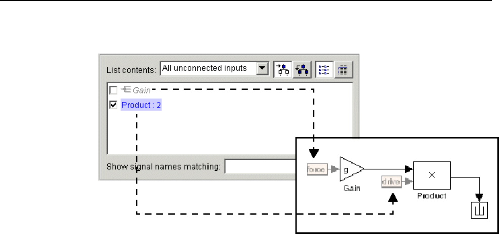
Signal Selector
The label for each entry indicates the name of the block of which the port is an
input. If the block has more than one input, the label indicates the number of
the displayed port. A greyed label indicates that the port is connected to a
signal generator other than the Signal Selectors’ owner. Selecting the check
box next to a port’s entry in the list connects the Signal Selector’s owner to
the port, replacing, if necessary, the signal generator previously connected
to the port.
To display more information on each signal, click the Detailed view button
atthetopofthepane. Thedetailedviewshowsthepathanddatatypeof
each signal and whether the signal is a test point. The controls at the top
and bottom of the panel let you restrict the amount of information shown
in the ports list.
•To show named signals only, select Named signals only from the List
contents control at the top of the pane.
•To show only signals selected in the Signal Selector, select Selected
signals only from the List contents control.
•To show test point signals only, select Testpointed/Logged signals only
from the List contents control.
16-29

16 Visualizing and Comparing Simulation Results
•To show only signals whose signals match a specified string of characters,
enter the characters in the Show signals matching control at the bottom
of the Signals pane and press the Enter key.
•To show the selected types of signals for all subsystems below the currently
selected subsystem in the model hierarchy, click the Current and Below
button at the top of the Signals pane.
To select or deselect a signal in the Signals pane, click its entry or use the
arrow keys to move the selection highlight to the signal entry and press the
Enter key. You can also move the selection highlight to a signal entry by
typing the first few characters of its name (enough to uniquely identify it).
Note You can continue to select and deselect signals on the block diagram
with the Signal Selector open. For example, shift-clicking a line in the block
diagram adds the corresponding signal to the set of signals that you previously
selected with the Signal Selector. If the simulation is running when you open
and use the Signal Selector, Simulink updates the Signal Selector to reflect
signal selection changes you have made on the block diagram. However, the
changes do not appear until you select the Signal Selector window itself. You
can also use the Signal Selector before running a model. If no simulation is
running, selecting a signal in the model does not change the Signal Selector.
16-30

17
Inspecting and Comparing
Logged Signal Data
•“Inspect Signal Data with Simulation Data Inspector” on page 17-2
•“Requirements for Recording Data” on page 17-4
•“Record Simulation Data” on page 17-5
•“Import Logged Signal Data” on page 17-7
•“Load Previously Recorded Data from a MAT-file” on page 17-10
•“Inspect Signal Data” on page 17-11
•“Compare Signal Data” on page 17-23
•“Comparison of One Signal From Multiple Simulations” on page 17-25
•“Compare All Logged Signal Data From Multiple Simulations” on page
17-28
•“Create Simulation Data Inspector Report” on page 17-32
•“Export Results in the Simulation Data Inspector Tool” on page 17-34
•“How the Simulation Data Inspector Tool Aligns Signals” on page 17-35
•“How the Simulation Data Inspector Tool Compares Time Series Data” on
page 17-37
•“Customize the Simulation Data Inspector Interface” on page 17-38
•“Limitations of the Simulation Data Inspector Tool” on page 17-54
•“Record and Inspect Signal Data Programmatically” on page 17-55

17 Inspecting and Comparing Logged Signal Data
Inspect Signal Data with Simulation Data Inspector
The Simulation Data Inspector software provides the capability to inspect and
compare time series data at several stages of your workflow:
•Model design: Inspect and compare simulation data after making changes
to the model diagram or its configuration.
•Testing your model: Compare simulation data with different input data
•Code generation: Compare simulation data and generated code output of
your model
You can compare variable-step data, fixed-step solver data from Simulink
and Simulink Coder, and fixed-step output with external data. “How the
Simulation Data Inspector Tool Aligns Signals” on page 17-35 describes how
signals are aligned between runs. “How the Simulation Data Inspector Tool
Compares Time Series Data” on page 17-37 describes how aligned signal
data are compared.
A typical workflow for inspecting and comparing signal data is:
1Set up your model to log signal data, as in “Export Signal Data Using
Signal Logging” on page 45-19.
2Open the Simulation Data Inspector tool, as described in “Open the
Simulation Data Inspector Tool” on page 17-39.
3Simulate your model and record simulation data or import logged signal
data, as described in “Record Simulation Data” on page 17-5 and “Import
Logged Signal Data” on page 17-7.
4Configure the Signal Browser table and specify how you want to graph the
data, as described in “Customize the Simulation Data Inspector Interface”
on page 17-38.
5Inspect signals to quickly determine if the run satisfies requirements, as
described in “Inspect Signal Data” on page 17-11.
6If the run is unsatisfactory, delete it. Repeat steps 3 and 4 to collect the
desired simulation runs for comparing data.
17-2

Inspect Signal Data with Simulation Data Inspector
7Optionally assign tolerances to signals and graphically inspect the applied
tolerances.
8Compare individual signals in the same run, or from different runs, as
described in “Compare Signal Data” on page 17-23.
9Compare all of the imported signal data from multiple runs, as described
in “Compare All Logged Signal Data From Multiple Simulations” on page
17-28.
10 Determine which signals have discrepancies within the specified tolerances.
Plot and analyze the discrepancies of any two signals.
11 Save the imported signal data and comparison results, as described in
“Export Results in the Simulation Data Inspector Tool” on page 17-34.
The Simulation Data Inspector software provides a command-line interface.
For more information, see “Record and Inspect Signal Data Programmatically”
on page 17-55
.
17-3

17 Inspecting and Comparing Logged Signal Data
Requirements for Recording Data
The Simulation Data Inspector tool records the following data configured on
the “Data Import/Export Pane” of the Configuration Parameter dialog box:
•States and Output,ifFormat is Structure with time,orifFormat is
Array or Structure and Time is logged.
•Signal logging
•Data stores
The Simulation Data Inspector tool supports the following data imported from
MAT-files and the MATLAB base workspace:
•Simulink.Timeseries and MATLAB timeseries objects
•Simulink.SimulationData.Dataset or Simulink.ModelDataLogs objects
•Data in Structure with time format
The Simulation Data Inspector supports output from the following blocks:
•Scope (Structure with time and Array format)
•To File (Timeseries format)
•To Workspace (Timeseries or Structure With Time format)
17-4

Record Simulation Data
Record Simulation Data
To set the Simulation Data Inspector to automatically import data after a
simulation run:
1Set up your model to log signal data, as in “Export Signal Data Using
Signal Logging” on page 45-19.
2Select Simulation > Model Configuration Parameters to open the
Configuration Parameters dialog box.
3On the Data Import/Export pane:
•Select the Signal logging parameter.
•Select the Record and inspect simulation output parameter.
4On the Simulink Editor toolbar, click the Record button arrow.
Select Simulation Data Inspector from the list. The Simulation Data
Inspector opens.
5On the Simulink Editor toolbar, the Record button is already pressed
because in step 3 you selected the configuration parameter Data
Import/Export > Record and inspect simulation output.Youcan
click the Record button to toggle on and off recording data for a simulation.
6Simulate your model. When the simulation is done, the data automatically
appears within a new run in the Simulation Data Inspector tool. To modify
the run name, see “Rename a Run” on page 17-44.
7To import another simulation run, leave the Record button selected, and
simulate your model again. When the simulation is done, the data appears
as another new run.
8When you are done importing data for your simulations, click the Record
button. If the Record button is not selected, data from simulations
are not imported into the tool and the configuration parameter Data
17-5

17 Inspecting and Comparing Logged Signal Data
Import/Export > Record and inspect simulation output is not
selected.
17-6

Import Logged Signal Data
Import Logged Signal Data
Before importing data into the Simulation Data Inspector tool, you must
have previously logged signal data to the base workspace or to a MAT-file.
For information on how to log signal data, see “Export Signal Data Using
Signal Logging” on page 45-19.
Import Signal Data from the Base Workspace
Using the Data Import tool, you can import data from the base workspace.
1Open the Data Import tool by selecting the Import Data button or
selecting File > Import Data.
2Select BaseWorkspace.Datafrom
logsout,xout,andyout appear in
the table.
17-7
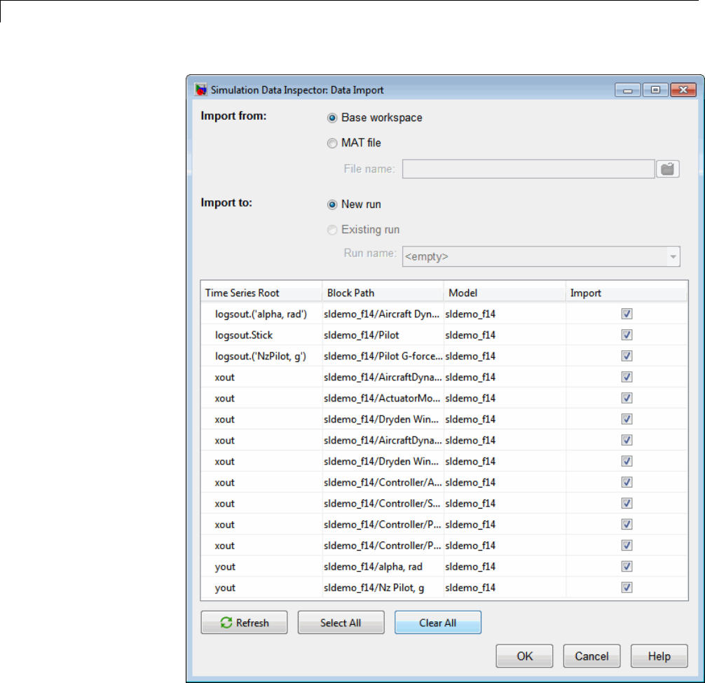
17 Inspecting and Comparing Logged Signal Data
3Select the Import check box to import a signal. Clear the Import check
box for signals that you do not want. You can also use the Select All and
Clear All buttons for mass selection or clearing of all signals.
17-8
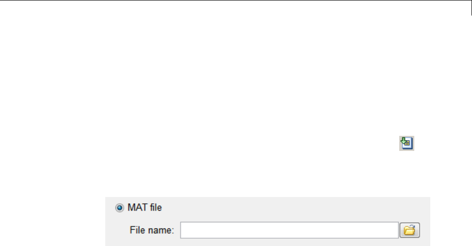
Import Logged Signal Data
4Click OK. The selected signals are displayed in the Signal Browser table.
Import Signal Data from a MAT-File
With the Data Import tool, you can select a subset of signals from a MAT-file
to import into the Simulation Data Inspector tool. Follow the steps to import
aMAT-File.
1Open the Data Import tool by selecting the Import Data button or
selecting File > Import Data.
2For Import From,selectMAT file.TheFile name parameter is enabled.
3The Data Import tool locates a MAT-file in the current directory.
Alternatively, click the Open folder button to browse for your MAT-file.
The data from the MAT-file populates the data table.
4Specify Import To by selecting New Run or Existing Run.Ifyouselect
Existing Run, select a run from the Run Name list.
5Select the Import check box to import signals. Clear the Import check
box for signals that you do not want. You can also use the Select All and
Clear All buttons for selection or clearing of all the signals.
6Click OK.
17-9

17 Inspecting and Comparing Logged Signal Data
Load Previously Recorded Data from a MAT-file
To load signal data from a MAT-file, which was created from the Simulation
Data Inspector tool:
1On the Simulation Data Inspector toolbar, click the Open button or
select File > Open.
2SelectthenameoftheMAT-file.
3Click OK. Data stored in the MAT-file is displayed in the Simulation
Data Inspector tool.
17-10

Inspect Signal Data
Inspect Signal Data
Overview
On the Inspect Signals tab you can inspect logged signal data. On the left
pane you can open the Signal Browser table to view and configure signal and
run properties (see “Customize the Simulation Data Inspector Interface” on
page 17-38). On the right pane you can create different plot views. With a
view of multiple plots, you can group signals to better view your data. For
example, you can group the same signal from different simulation runs, group
signals with a similar range of values, or normalize a subset of your signal
data. The following examples use the sldemo_f14 model.
•“View Signal Data” on page 17-11
•“Create a View of Multiple Plots” on page 17-13
•“Explore Signal Data in a Multiple Plot View” on page 17-16
•“Replace a Run in a View” on page 17-17
•“Copy a View in the Inspect Signals Tab” on page 17-20
•“DeleteaViewintheInspectSignalsTab”onpage17-21
•“Export a View in the Inspect Signals Tab” on page 17-22
•“Import a View in the Inspect Signals Tab” on page 17-22
View Signal Data
1Configure a model to log signal data. This example uses the sldemo_f14
model configured to log signals: q, rad/sec,Stick,andNzPilot, g.
For more information, see “Export Signal Data Using Signal Logging” on
page 45-19.
2On the Simulink Editor, click the Record button arrow and select
Simulation Data Inspector from the list.
3To record simulation data, click the Record button so that it is selected.
17-11
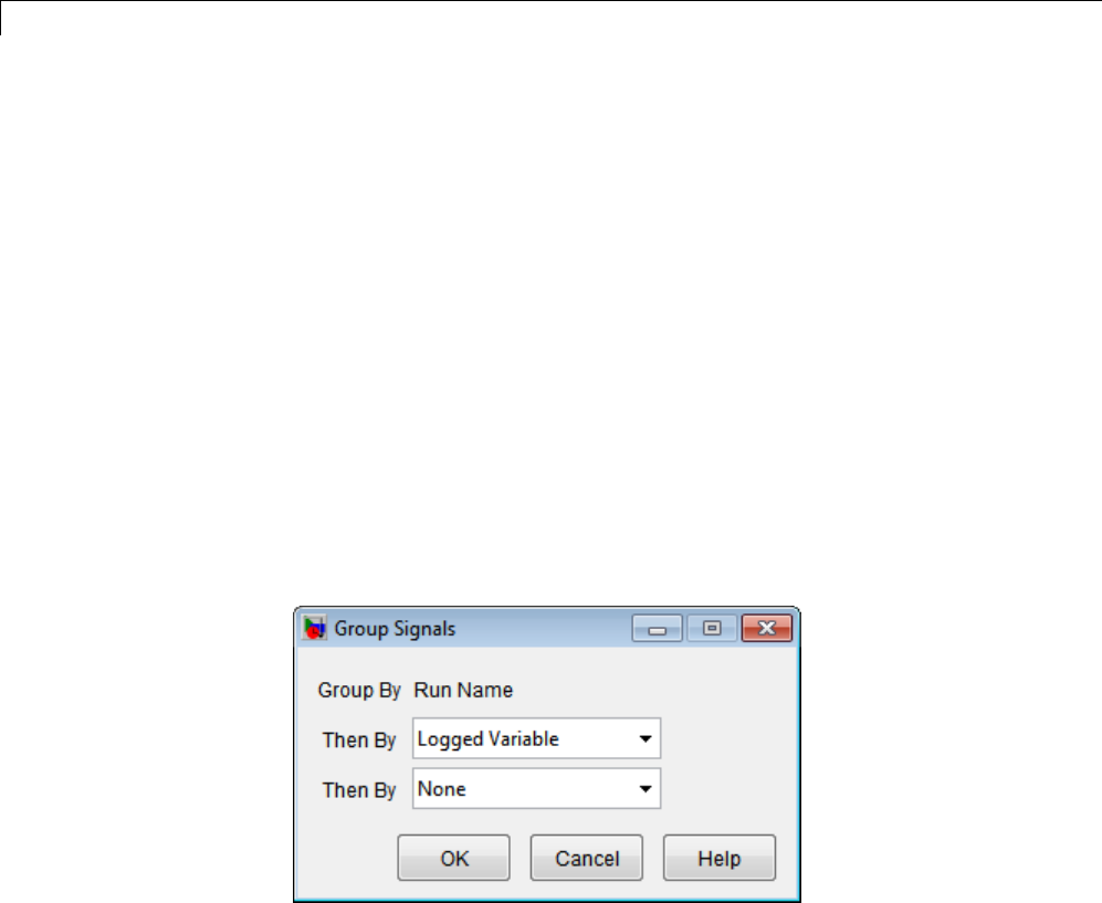
17 Inspecting and Comparing Logged Signal Data
4Simulate your model. The Simulation Data Inspector tool records and
displays the simulation data. Instead of recording data from a simulation,
you can import signal data from previous simulation runs, see “Import
Logged Signal Data” on page 17-7.
5If the Inspect Signals tab is not already selected, select it. By default, the
Inspect Signals tab displays the Signal Browser table which contains
a row for each signal, organized by simulation runs. You can expand or
collapse any of the runs to view the logged signals in a run. For more
information, see “Customize the Simulation Data Inspector Interface” on
page 17-38.
6Right-click the Signal Browser table title bar. Select Columns and uncheck
Block Name and Block Path.
7Right-click the Signal Browser table title bar. Select Group Signals.In
the Group Signal dialog box, in the first drop-down box, select Logged
Variable. Select None in the second drop-down box. Click OK.
8Expand logsout to view the logged signals.
9“Specify the Line Configuration” on page 17-45 for each signal.
10 To specify the synchronization method, right-click the Signal Browser table
title bar. Select Columns and check Synchronization Method.TheSync
Method column is displayed in the table. For each signal, click the field
for the Sync Method column and select a method from the list. In this
example, the synchronization method is union.
17-12

Inspect Signal Data
11 Repeat step 5 for the Interpolation Method.
12 Click the Plot column for a signal. On the right pane of the Simulation
Data Inspector tool, the signal data is displayed in the graph.
13 To select multiple signals, hold down Ctrl and select each signal by clicking
arow.InthePlot column, select a check box. All of the highlighted signals
are now selected for plotting.
14 To create a report of the results, see “Create Simulation Data Inspector
Report” on page 17-32.
Create a View of Multiple Plots
Before creating a view of multiple plots, the Simulation Data Inspector tool
must contain signal data. You can obtain signal data by either recording
simulation data or importing data into the Simulation Data Inspector tool.
17-13

17 Inspecting and Comparing Logged Signal Data
For more information, see “Record Simulation Data” on page 17-5 or “Import
Logged Signal Data” on page 17-7.
1On the right pane, on the View toolbar, click Show Details.
2In the View Name column, click the field which displays Default.Typein
a new name for the view. In this example, the name is sldemo_f14_plot4.
3In the Layout column, click the field that displays 1x1.Aplotmatrix
opens. To create a view of 4 plots, select the 2x2 matrix.
17-14
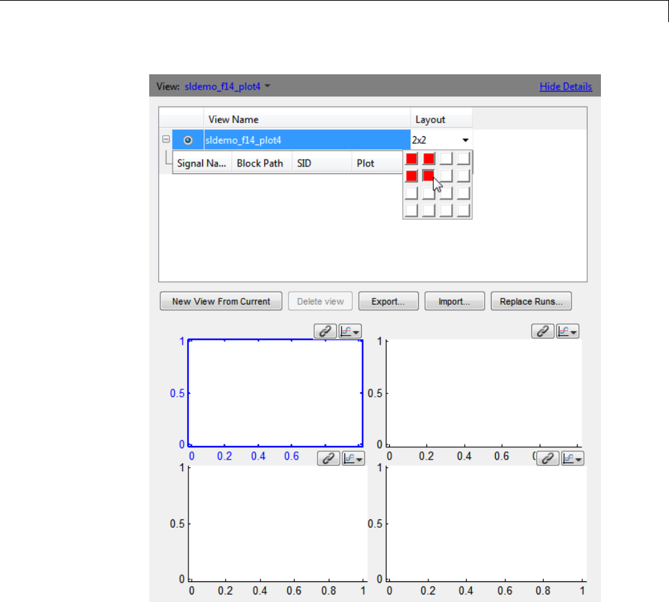
Inspect Signal Data
4To select a plot, click it. The selected plot is outlined in blue.
5Once a plot is selected, on the left pane in the Signal Browser table, select a
signal in the Plot column to add to the selected plot. In this example, a
signal from Run 1 is displayed in each plot in the sldemo_f14_plot1 view.
17-15
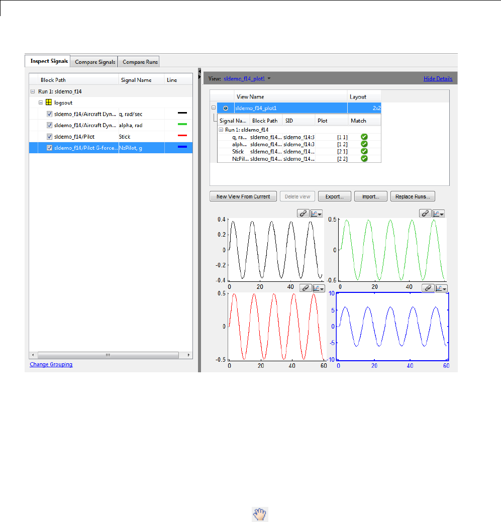
17 Inspecting and Comparing Logged Signal Data
For the selected plot [2,2], the signal or signals are shaded in the Inspect
Signals table to indicate which signals are in the selected plot.
Explore Signal Data in a Multiple Plot View
Linked Plots in a View
Plots within a view can be linked together to enable synchronized panning
and zooming. When you create a view, by default, plots in a view are linked
together. The following toolbar operations synchronize across linked plots:
•Panalongthetimeaxis:
17-16
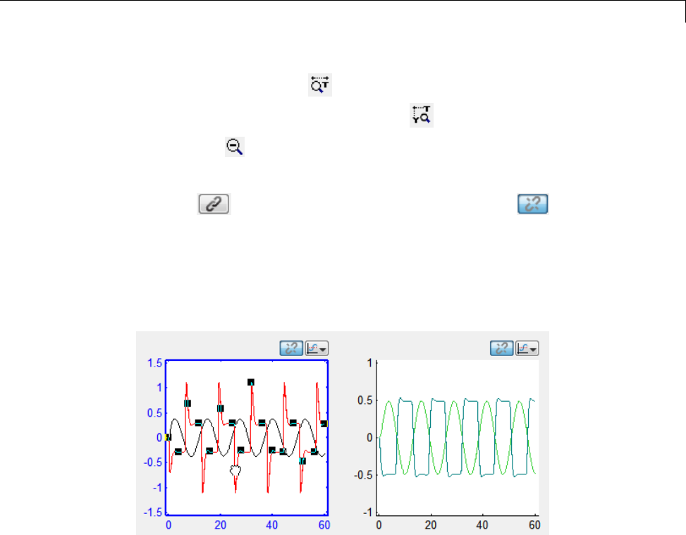
Inspect Signal Data
•Zoom on the time axis:
•Zoom on the time and data value axis:
•Zoom out:
To determine if a plot in a view is linked, at the top of each plot, locate the
link icon .Ifa plot is unlinked, the broken link icon is displayed
and the plot pans and zooms independently.
Move Signals Between Plots in a View
To move a signal from one plot to another, click and hold a signal (markers
appear).
Drag the signal to another plot, and the signal is now displayed in the other
plot.
For more information on working with plots, see “Modify a Plot in the
Simulation Data Inspector Tool” on page 17-49.
Replace a Run in a View
In this example, the Simulation Data Inspector tool contains three runs of
data. To quickly swap out the data from one run with data from another
run, do the following:
17-17
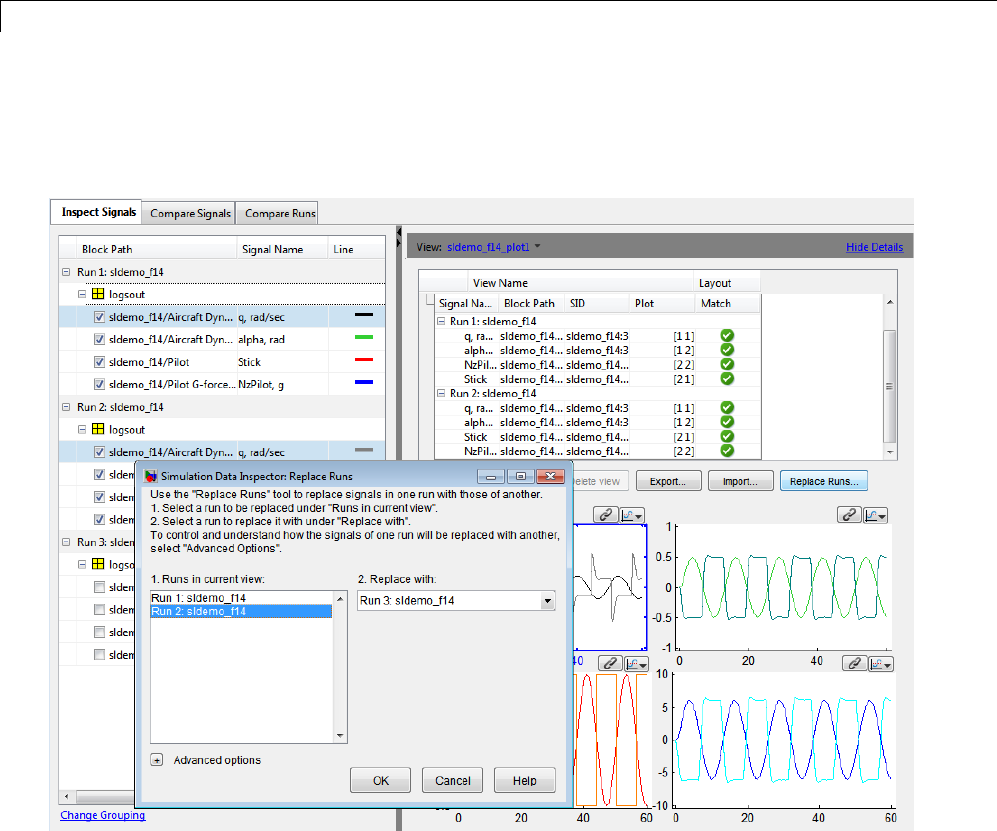
17 Inspecting and Comparing Logged Signal Data
1Select a view. In this example, the view is sldemo_f14_plot1.
2Click Replace runs..., which opens the Replace runs dialog box.
3To replace the signal data in Run 2 with the signal data from another run,
in the Runs in current view list, select Run 2: sldemo_f14. Only the
signals in the view are replaced
4In the Replace with list, select Run 3: sldemo_f14.
5To specify how the signal data in Run 2 is replaced with Run 3,expand
Advanced options. In this example, the Simulation Data Inspector first
attempts to align the signals by Data Source,thenbyBlock Path,and
17-18
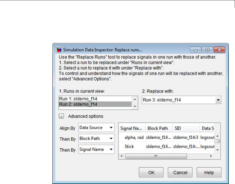
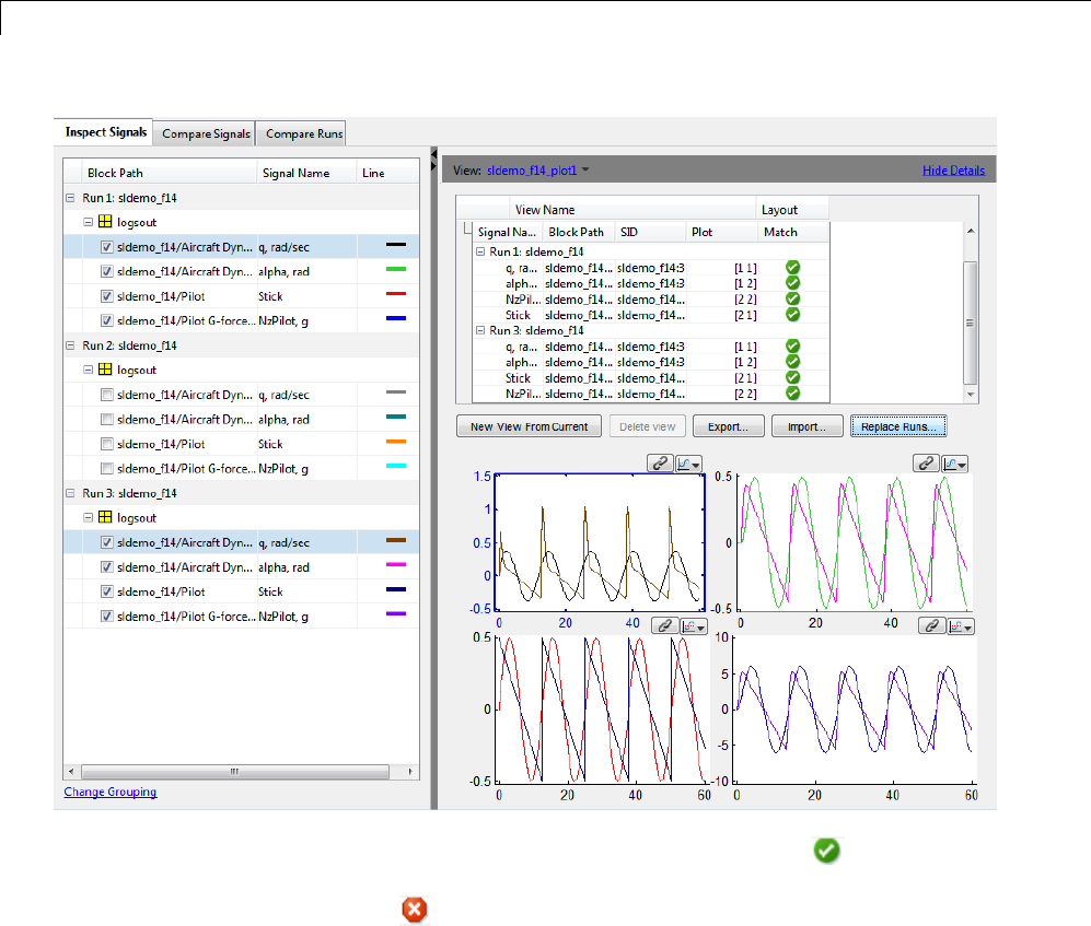
17 Inspecting and Comparing Logged Signal Data
The View Details table now includes Run 3 instead of Run 2.Run 3 lists
signals from Run 2.TheMatch column displays a for a signal that
aligned with a signal in Run 3. If a signal did not align, the Match column
displays a .
Copy a View in the Inspect Signals Tab
To copy a view:
1On the right pane, in the View toolbar, click Show Details to open the
View Details table.
17-20
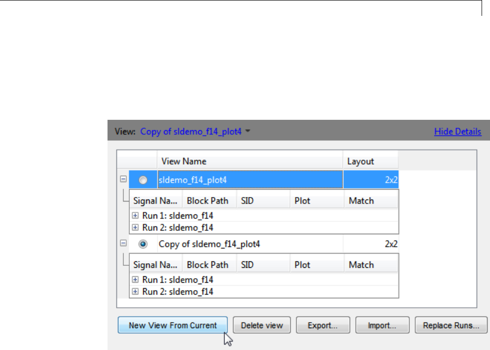
Inspect Signal Data
2Select the view to copy. Be sure to select the option button next to the
View Name in the table.
3Click the New view from current button. Anewviewisdisplayedin
the View Details table
4Select the new view, Copy of sldemo_f14_plot4, and rename it.
Delete a View in the Inspect Signals Tab
To delete a view:
1On the right pane, in the View toolbar, click Show Details to open the
View Details table.
2In the View Details table, select the view to delete by selecting the
corresponding option button.
3Click the Delete View button.
17-21

17 Inspecting and Comparing Logged Signal Data
Note The View Details table always includes one view.
Export a View in the Inspect Signals Tab
To export a view to a MAT-file:
1On the right pane, in the View toolbar, click Show Details to open the
View Details table.
2Click the Export button and specify a file.
3This saves the view, but not the data, into a MAT-file. To save the data and
the view, see “Export Results in the Simulation Data Inspector Tool” on
page 17-34.
Import a View in the Inspect Signals Tab
To reload a saved view from a MAT-file:
1On the right pane, in the View toolbar, click Show Details to open the
View Details table.
2Click the Import button and specify a file.
Note This only imports the configuration of the view, which is how the
signal data is plotted among the multiple plots. The actual signal data
is not imported.
3To include signal data in the Simulation Data Inspector tool, you can record
simulation data (see “Record Simulation Data” on page 17-5), or import
data (see “Import Logged Signal Data” on page 17-7).
17-22
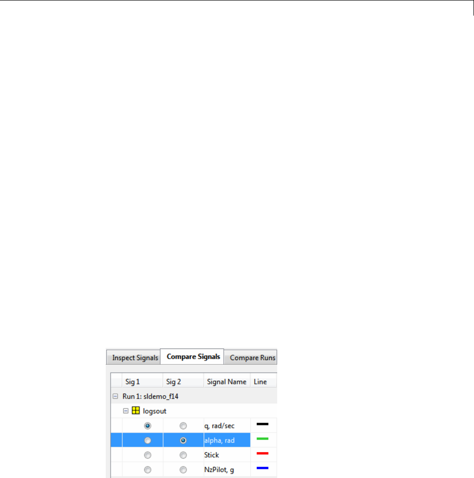
Compare Signal Data
Compare Signal Data
In the Simulation Data Inspector tool, you can use the Compare Signals tab
of the Signal Browser table for comparing two signals. To compare two signals:
1Open the Simulation Data Inspector tool. See “Open the Simulation Data
Inspector Tool” on page 17-39.
2Record simulation data or import data into the Simulation Data Inspector
tool. See “Record Simulation Data” on page 17-5 or “Import Logged Signal
Data” on page 17-7.
3If it is not already selected, select the Compare Signals tab. By default,
Signal Browser table on the Compare Signals tab displays a row for each
signal data, organized by simulation runs. For more information, see
“Customize the Simulation Data Inspector Interface” on page 17-38.
4“Specify the Line Configuration” on page 17-45 for the signals that you
are comparing.
5In the Sig 1 column, click one signal for plotting. In this column, you can
select only one signal.
6In the Sig2column, click one signal for plotting. In this column, you can
select only one signal.
The Signals graph displays the signal data and the Difference graph
displays the difference and tolerance values.
17-23
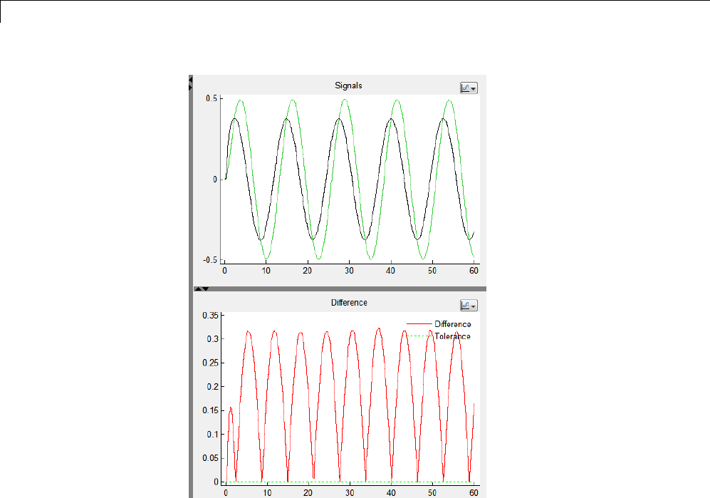

Comparison of One Signal From Multiple Simulations
Comparison of One Signal From Multiple Simulations
In the Simulation Data Inspector tool, you can use the Compare Signals tab
to compare the same signal from two different simulation runs. To compare
two data runs for a signal:
1Open the Simulation Data Inspector tool. See “Open the Simulation Data
Inspector Tool” on page 17-39.
2Record simulation data or import data for two simulation runs. For more
information, see “Record Simulation Data” on page 17-5 or “Import Logged
Signal Data” on page 17-7.
3Select the Compare Signals tab. By default, the Signal Browser table on
the Compare Signals tab displays a row for each signal data, organized
by simulation runs. For more information on modifying the Signal Browser
table, see “Customize the Simulation Data Inspector Interface” on page
17-38.
4“Specify the Line Configuration” on page 17-45 for the signals that you
are comparing.
5To change the relative tolerance and absolute tolerance, add the Rel
Tol and Abs Tol columns to the Signal Browser table. Double-click the
corresponding fields for a signal and type in a value.
6In the Sig 1 column, click one signal from the first simulation run for
plotting. In this column, you can select only one signal.
7In the Sig 2 column, click a signal from another simulation run for plotting.
In this column, you can select only one signal.
17-25
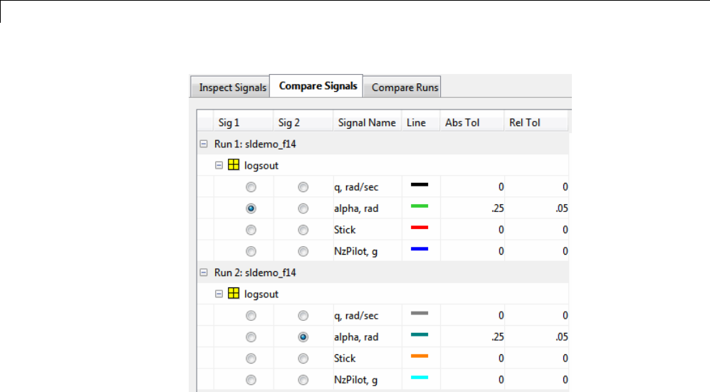
17 Inspecting and Comparing Logged Signal Data
Once two signals are selected, the Signals graph displays the signal data
and the Difference graph displays the difference and tolerance values.
17-26
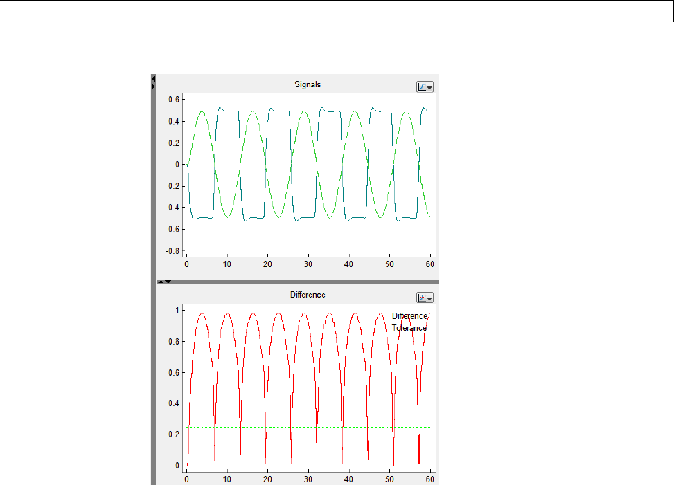
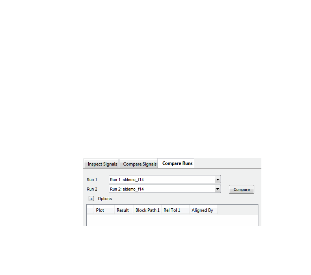
17 Inspecting and Comparing Logged Signal Data
Compare All Logged Signal Data From Multiple Simulations
In the Simulation Data Inspector tool, you can use the Compare Runs tab
to compare all signal data from two different simulation runs. To compare
two runs:
1Open the Simulation Data Inspector tool. See “Open the Simulation Data
Inspector Tool” on page 17-39.
2Record simulation data or import data from multiple simulation runs, for
more information, see “Record Simulation Data” on page 17-5 or “Import
Logged Signal Data” on page 17-7.
3Select the Compare Runs tab.
4From the Run 1 and Run 2 drop-down lists, select two different runs.
Note The number in a column name indicates the run number. For
example, Abs Tol 1 refers to the absolute tolerance values for signals of
the run specified for Run 1.Abs Tol 2 refers to the absolute tolerance
values for signals of the run specified for Run 2.
5Select the Options button to specify the signal alignment.
17-28
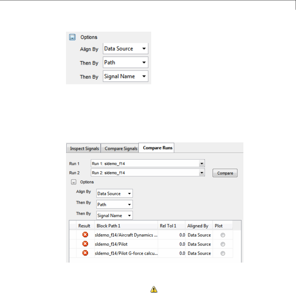
Compare All Logged Signal Data From Multiple Simulations
The Simulation Data Inspector aligns signals according to Align By and
Then By parameters. For more informationonsignalalignment,see“How
the Simulation Data Inspector Tool Aligns Signals” on page 17-35.
6Click the Compare button. The Comparison Results table lists all signals
from Run 1 with a result. In this example, the comparison results of the
aligned signals did not match.
The Simulation Data Inspector only compares signals from Run 1 that are
aligned with a signal from Run 2.IfasignalfromRun 1 did not align with
asignalfromRun 2,thentheRun 1 signal is listed in the Comparison
Results table with a warning .
7To modify the relative tolerance and absolute tolerance, add the Abs Tol 1
column to the Signal Browser table. Double-click the corresponding fields
for a signal and type in a value.
17-29
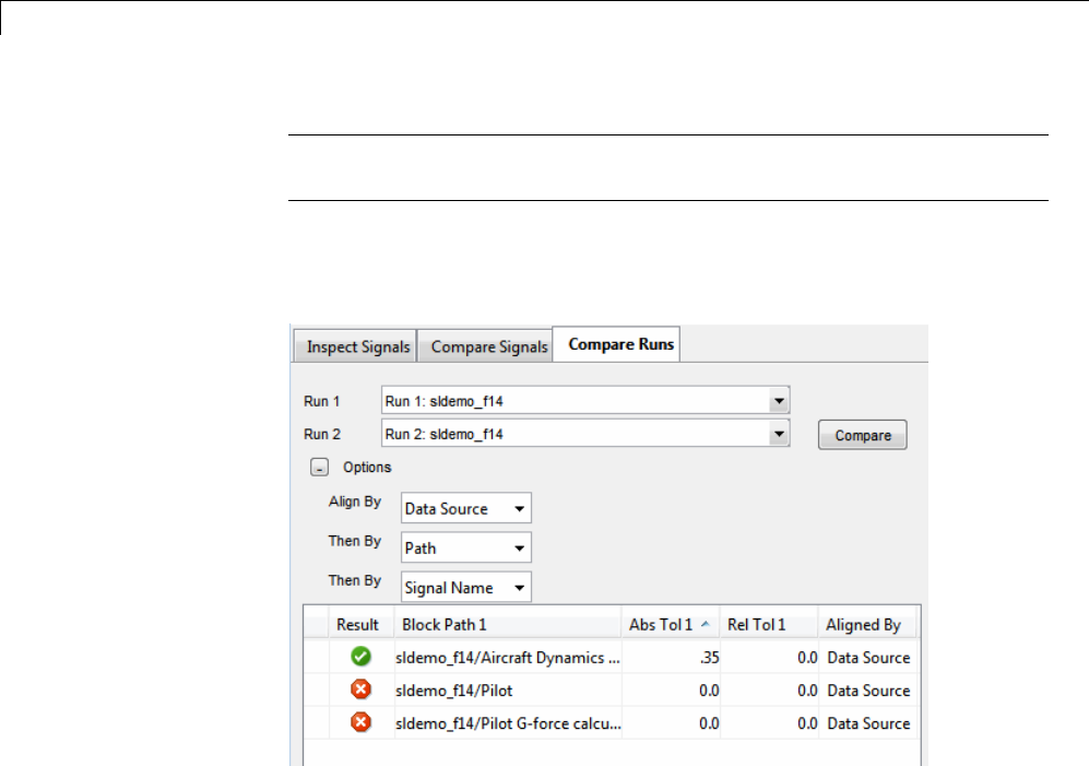
17 Inspecting and Comparing Logged Signal Data
Note Tolerances specified in the other tab views do not carry over to the
Compare Runs tab.
8To see a signal that is within the acceptable tolerance across two simulation
runs, set the absolute tolerance in column Abs Tol 1 to .35.
9To plot a signal, in the plot column select the option button for
sldemo_f14/Pilot G-force calculation.TheSignals graph displays
the signal data for the two runs. The Difference graph displays the
difference and tolerance values.
17-30
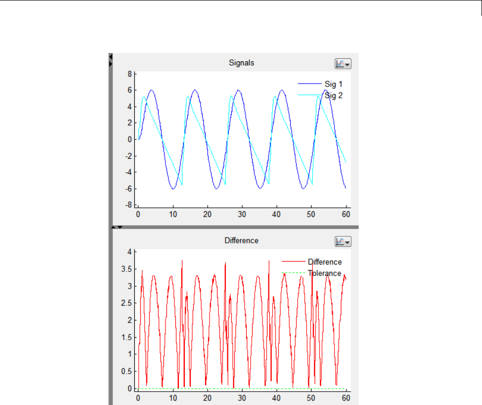
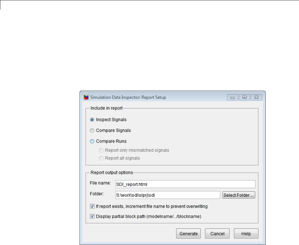
17 Inspecting and Comparing Logged Signal Data
Create Simulation Data Inspector Report
To create a report of the current view and data in the Simulation Data
Inspector:
1In the Menu Bar, select File > Generate Report.TheReportSetup
dialog box opens.
2In the Include in report section, specify which tab to include in the report.
For the Compare Runs tab, you can select Report only mismatched
signals only to shorten the report or select Report all signals which
includes all logged signals in the designated runs.
3Specify the File name and Folder,orusethedefault.
17-32

Create Simulation Data Inspector Report
4Optionally, select If report exists, increment file name to prevent
overwriting, which appends and increments a number to the file name of
the report to preserve earlier versions of the report file.
5Optionally, select Display partial block path
(modelname/.../blockname), which shortens the block path string
generated for the report.
6Click Generate. The report opens automatically.
17-33

17 Inspecting and Comparing Logged Signal Data
Export Results in the Simulation Data Inspector Tool
The Simulation Data Inspector tool provides the capability to save data
collected by the tool to a MAT-file that you can later reload. The format of
theMAT-fileisdifferentfromtheformat of a MAT-file created from the
base workspace.
Save Data to a MAT-File
To save signal data and views to aMAT-File,dothefollowing:
1Click Save or select File > Save.
2Typethenameofthefile.
3Click OK.Y
our data and views are now saved in a MAT-file that you can
load back into the Simulation Data Inspector.
17-34

How the Simulation Data Inspector Tool Aligns Signals
How the Simulation Data Inspector Tool Aligns Signals
When the Simulation Data Inspector tool aligns signals across simulation
runs, it attempts to match signals between runs by using metadata stored
for each signal. You can specify the metadata used to align signals. The
metadata options are: Data Source,Path,SID,andSignal Name.Bydefault,
the Simulation Data Inspector tool is configured to first align signals by Data
Source,thenbyPath,andthenbySignal Name.
To modify the signal alignment specifications see “Inspect Signals: Aligning
Signals for Replacing a Run” on page 17-35 or “Compare Runs: Aligning
Signals for Comparing Signal Data” on page 17-36.
Inspect Signals: Aligning Signals for Replacing a Run
To modify how signals are aligned on the Inspect Signals tab, do the
following:
1Click the Inspect Signals tab.
2On the right pane, click Show details.
3Click theReplace runs... button. The Replace Runs dialog opens.
4Select Advanced options,whichdisplaystheAlign By and Then By
parameters.
5Specify the Align By and Then By parameters from the drop-down lists.
When replacing a run, the Simulation Data Inspector tool attempts to align
only the signals selected in the current view. Once those signals are aligned,
in the view, the aligned signal data from the first run is replaced with signal
data from another run. The View Details table displays the signals from
the replaced run as follows:
17-35
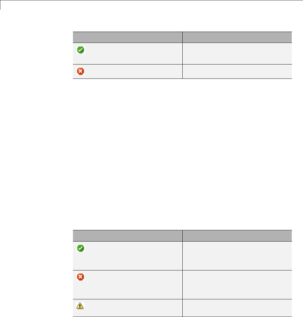
17 Inspecting and Comparing Logged Signal Data
Status Result
•Signal aligned
•Signal data is replaced in the view
Signal not aligned
Compare Runs: Aligning Signals for Comparing
Signal Data
To modify how signals are aligned on the Compare Runs tab, do the
following:
1Click the Compare Runs tab.
2Select the Options button, which displays the Align By and Then By
parameters.
3Specify the Align By and Then By parameters from the drop-down lists.
4Click Compare, to align the signal data and compare the aligned signal
data.
After signals are aligned from Run 1 with signals from Run 2,theSimulation
Data Inspector tool compares only the aligned signals. The Comparison
Results table displays the results of all signals from Run 1 as follows:
Status Comparison Result
•Signal aligned
•Signal data from two runs
matched within the tolerance
•Signal aligned
•Signal data from two runs did not
match within the tolerance
Signal from Run 1 did not align with
asignalfromRun 2
17-36

How the Simulation Data Inspector Tool Compares Time Series Data
How the Simulation Data Inspector Tool Compares Time
Series Data
To compare time series data, the Simulation Data Inspector:
1Converts Simulink time series data to MATLAB time series data.
2Aligns the time vectors using the default synchronization method union.
To change the synchronization method for a signal, add the Sync Method
column to the Signal Browser table and choose a method.
3Aligns the data vectors using the default interpolation method, zoh
(zero-order hold). To change the interpolation method for a signal, add the
Interp Method column to the Signal Browser table and choose a method.
4Differences the data.
5Applies the specified tolerances for plotting the Difference .Formore
information, see “How Tolerances Are Applied” on page 17-37.
How Tolerances Are Applied
The default values for the relative tolerance and absolute tolerance for a
signal is 0. If you specify tolerances, then the Simulation Data Inspector tool
calculates the tolerances as follows:
tolerance = max(absoluteTolerance, relativeTolerance*abs(baselineData));
To change the relative tolerance and absolute tolerance, add the Rel Tol and
Abs Tol columns to the Signal Browser table. Double-click the corresponding
fields for a signal and type in a value.
17-37
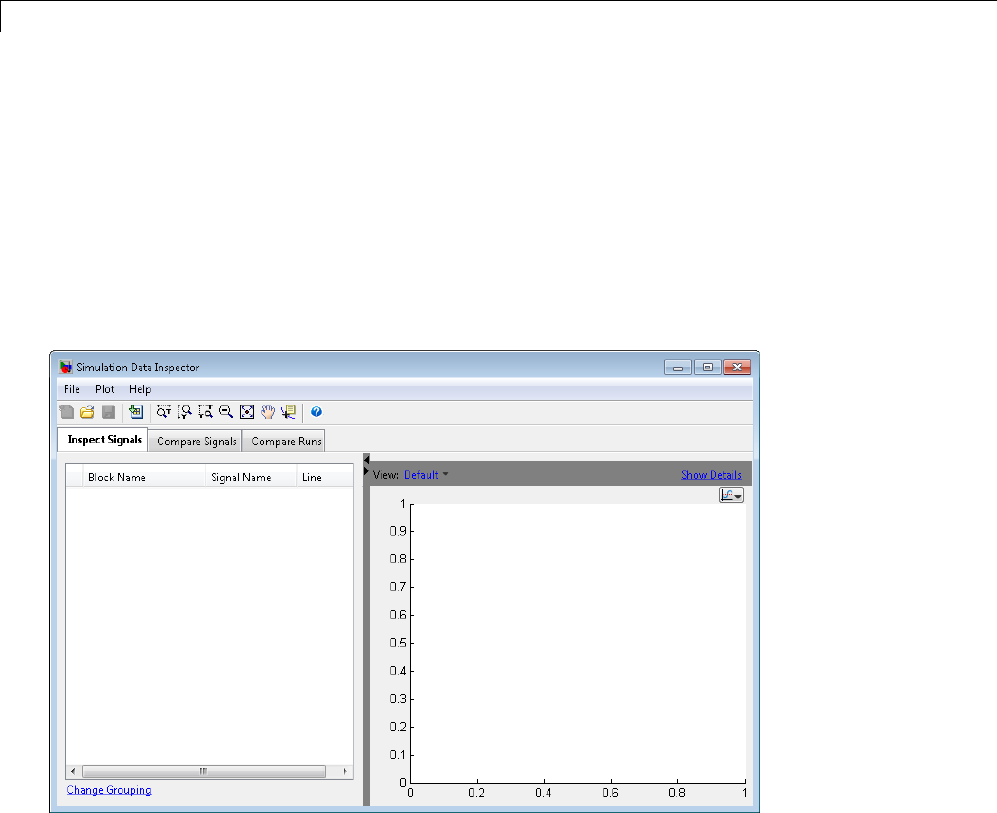
17 Inspecting and Comparing Logged Signal Data
Customize the Simulation Data Inspector Interface
Overview
The Simulation Data Inspector tool provides the capability to inspect and
compare time series data. There are several methods for launching the
Simulation Data Inspector tool, see “Open the Simulation Data Inspector
Tool” on page 17-39 to choose the method that best supports your workflow.
The Simulation Data Inspector tool appears as follows,
The Simulation Data Inspector Window includes the following elements:
•Menu Bar
•“Toolbar” on page 17-51
•Three tabs: Inspect Signals,Compare Signals,andCompare Runs
TheSignalBrowsertableappearsonthethreetabs: Inspect Signals,
Compare Signals,andCompare Runs. You can customize the information
displayed in the Signal Browser table by performing the following tasks:
17-38

Customize the Simulation Data Inspector Interface
•“Add/Delete a Column in the Signal Browser Table” on page 17-40
•“ModifyGroupinginSignalBrowser Table” on page 17-42
•“Rename a Run” on page 17-44
•“Select a Run or Signal Option in the Signal Browser Table” on page 17-46
•“Display Run Properties” on page 17-49
The Plot View displays in the right pane of the Simulation Data Inspector
tool. To modify a plot, refer to the following:
•“Specify the Line Configuration” on page 17-45
•“Modify a Plot in the Simulation Data Inspector Tool” on page 17-49
Open the Simulation Data Inspector Tool
To launch the Simulation Data Inspector tool, choose one of the following
methods:
•MATLAB command-line:Enter
Simulink.sdi.view
•Simulink Editor:ClicktheRecord button arrow.
Select Simulation Data Inspector from the list.
Why Is the Simulation Data Inspector Tool Empty?
There are several methods for populating the Simulation Data Inspector
with data.
•If you are using the record button to simulate and record data, you must
specify your model to export signals. For more information, see:
-“Export Simulation Data” on page 45-4
-“Export Signal Data Using Signal Logging” on page 45-19
17-39
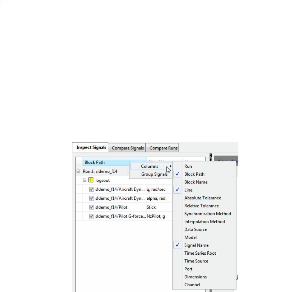
17 Inspecting and Comparing Logged Signal Data
After your model is configured to export signal data, see “Record Simulation
Data” on page 17-5.
•If you want to view previously logged signal data, see “Import Logged
Signal Data” on page 17-7.
For a list of Simulink data export formats that are not supported in the
Simulation Data Inspector, see “Limitations of the Simulation Data Inspector
Tool” on page 17-54.
Add/Delete a Column in the Signal Browser Table
To add or remove a column, right-click the Signal Browser table title bar.
Select Columns and click an option on the list. The column is displayed in
the table.
17-40

Customize the Simulation Data Inspector Interface
Column Options for the Inspect Signals and Compare Signals Tabs
Column Option Value
Run Name of a simulation run
Block Path Path to the source block for the
signal
Block Name Name of the source block
Line Line style
Absolute Tolerance Positive number (user-specified)
Relative Tolerance Positive number (user-specified)
Synchronization Method Method to align time vector:
union,intersection,uniform
(user-specified)
Interpolation Method Method to align data: zoh,linear
(user-specified)
Data Source Name for the data
(logsout.Stick.Data)
Model Modelnameforthesignaldata
Signal Signal name for the data (Stick)
Time Series Root String signifying the name of
the Simulink.Timeseries object
(logsout.Stick.Time)
Time Source String signifying the array
containing the time data
(logsout.Stick.Time)
Port Index of the output port that emits
the signal logged
Dimensions Number of dimensions of the signal
Channel Channel of matrix data
17-41

17 Inspecting and Comparing Logged Signal Data
Column Options for Compare Runs Tab
Column Option Value
Result Result of the comparison for the
signal across the specified runs
Block Path •Run 1: Block Path
•Run 2: Block Path
Data Source String identifying the data source
•Run 1: Data Source
•Run 2: Data Source
SID “Simulink Identifier”
•Run 1: SID
•Run 2: SID
Absolute Tolerance Positive number (user-specified)
Relative Tolerance Positive number (user specified)
Synchronization Method Method to align time vector:
union,intersection,uniform
(user-specified)
Interpolation Method Method to align data: zoh,linear
(user-specified)
Channel 1 Channel of matrix data
After selecting a column option, the new column is added to the table in the
order that it appears in the options list.
Modify Grouping in Signal Browser Table
You can customize the organization of your logged data in the Signal Browser
table. By default, data is first organized by run. You can then organize your
data by model hierarchy, logged variable, or no hierarchy.
If your model contains referenced models to view, you can group your data by
model hierarchy and then by the logged variables. To change the grouping
in the Signal Browser table:
17-42
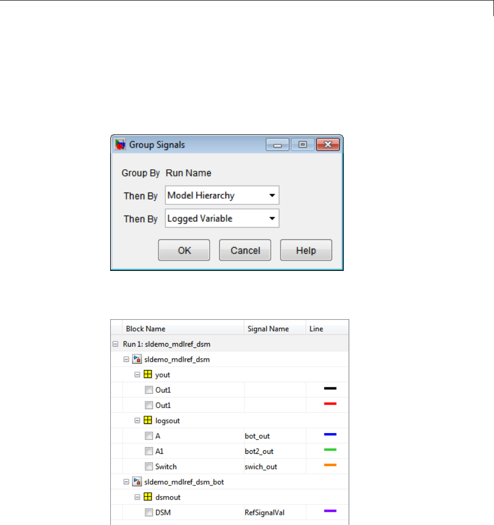
Customize the Simulation Data Inspector Interface
1Right-click the Signal Browser table and select Group Signals.
2In the Group Signals dialog box, in the first Then By list, select Model
Hierarchy.
3In the second Then By list, select Logged Variable.
4Click OK. The Signal Browser table groups the signal data by model and
then by the logged variables.
17-43
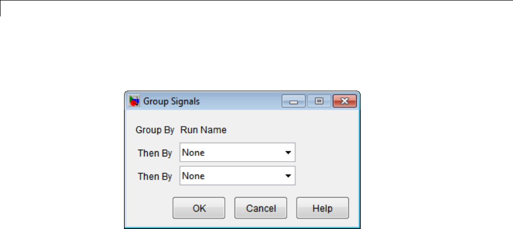
17 Inspecting and Comparing Logged Signal Data
To remove the hierarchy and display a simple list of logged signals, you can
select None in the Group Signals dialog box.
Rename a Run
To rename a run name:
1If the Signal Browser table is not grouped by run, right-click the table and
in the menu select Group By > Run.
2Double-click the Run row.
17-44
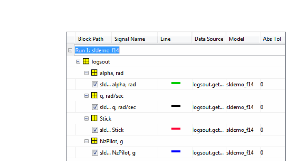
Customize the Simulation Data Inspector Interface
3TypethenewrunnameandpressEnter.
Specify the Line Configuration
1Click in the Line column of a signal and click the down arrow. The Line
dialog box opens.
17-45
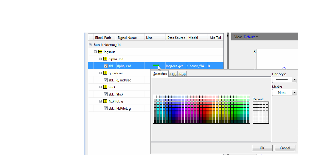
17 Inspecting and Comparing Logged Signal Data
2Specify the color, Line Style,andMarker for the signal.
3Click OK.
Select a Run or Signal Option in the Signal Browser
Table
In the Signal Browser table, right-click a run or signal for a menu list of
options.
17-46
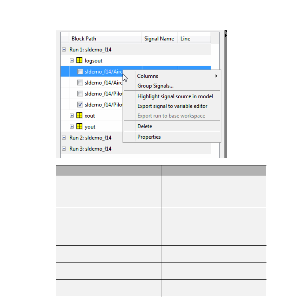
Customize the Simulation Data Inspector Interface
To... Select...
Display the list of Column options.
See Column Options for the Inspect
Signals and Compare Signals Tabs
on page 17-41
Columns
Group signal data by the specified
options: Run,Block Path,Data
Source,Model,andSignal Name
(thisoptiondoesnotappearinthe
Compare Runs tab)
Group By
Highlight the source of the selected
signal in the model diagram
Highlight signal source in model
Open the Variable Editor and
display the selected signal data
Export signal to variable editor
Save signal data in the run to the
base workspace
Export run to base workspace
17-47
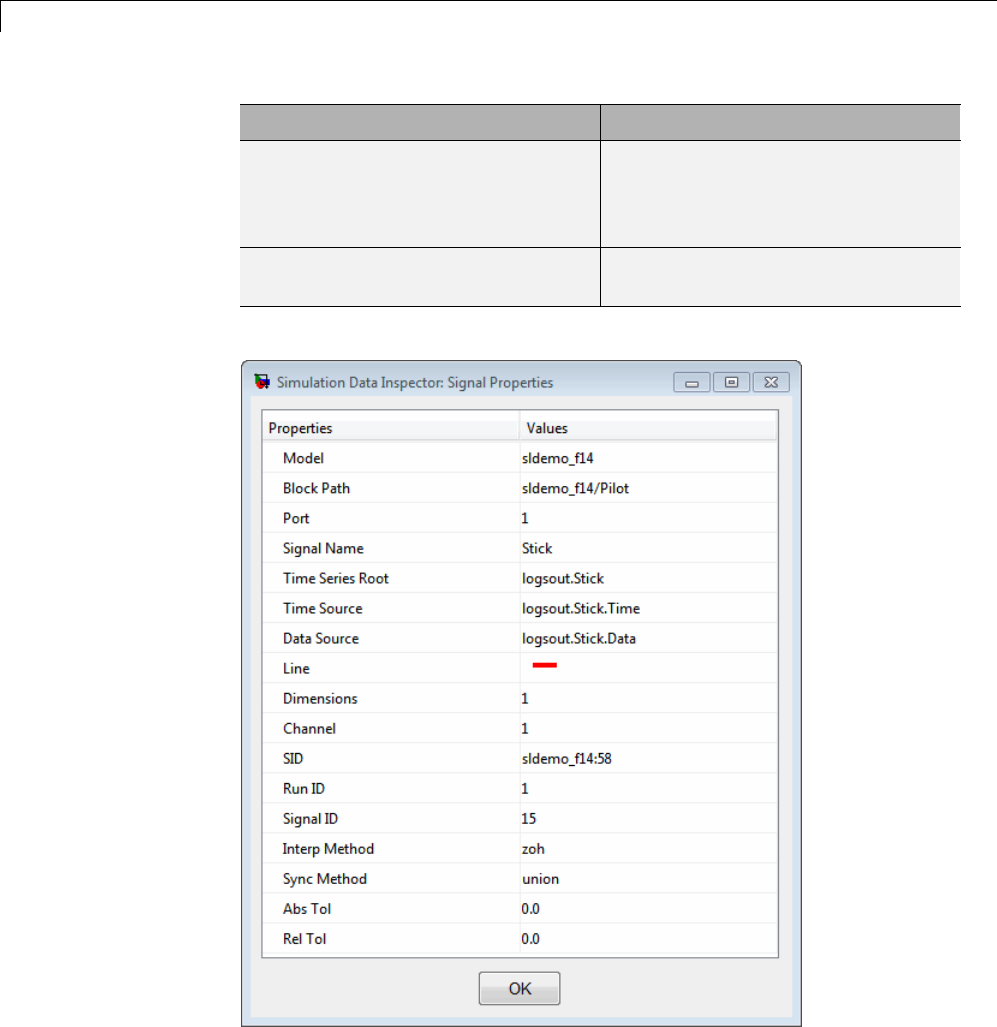
17 Inspecting and Comparing Logged Signal Data
To... Select...
Delete the highlighted signal in the
Signal Browser table (this option
does not appear in the Compare
Runs tab)
Delete
Display the signal properties of the
selected signal
Properties
The Signal Properties dialog box displays the following signal information.
17-48
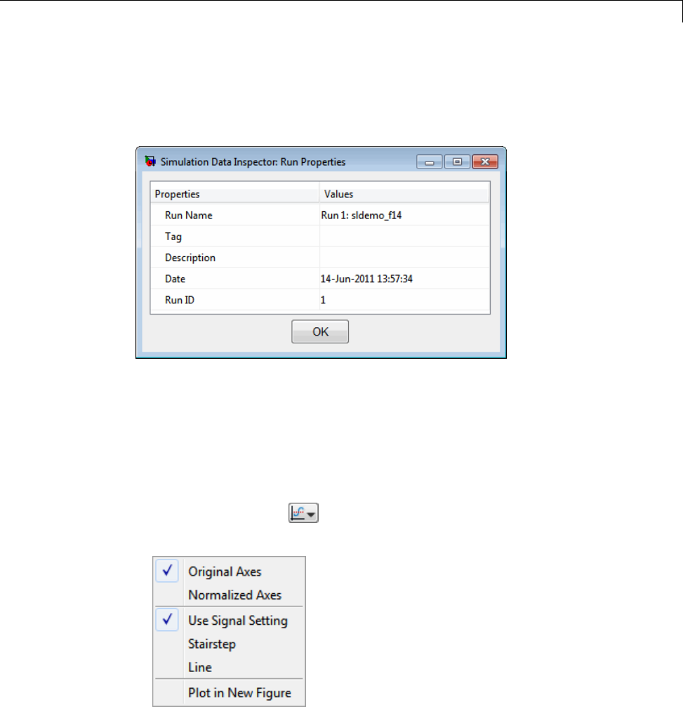
Customize the Simulation Data Inspector Interface
Display Run Properties
In the Signal Browser table, right-click a run name to view a list of options. To
open the Run Properties dialog box, from the options list, select Properties.
Modify a Plot in the Simulation Data Inspector Tool
To modify a plot, you can:
•Toolbar: Select icons to zoom into data, move the plot, or add a data
point to the plot. For more information on these icons, see the “Toolbar”
on page 17-51 section.
•Plot options:Click on the plot to select alternatives for plotting
the data.
17-49
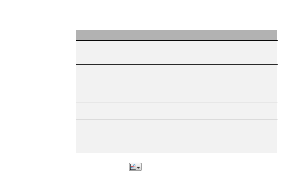
17 Inspecting and Comparing Logged Signal Data
To... Simulation Data Inspector...
Original Axes Plots the data according to the
maximum and minimum values of
the data points. (default)
Normalized Axes Normalizes the data for each signal
from 1to 1along the y-axis. If the
data is already within that range,
the data is displayed as a constant
at 1.
Stairstep Plots the data as a stairstep plot.
(default)
Line Interpolates the data points and
produces a linear plot.
Plot in New Figure Launches the graph in a MATLAB
figure window.
•New figure:Click on the plot and select Plot in New Figure.The
plot opens in a new figure window.
17-50
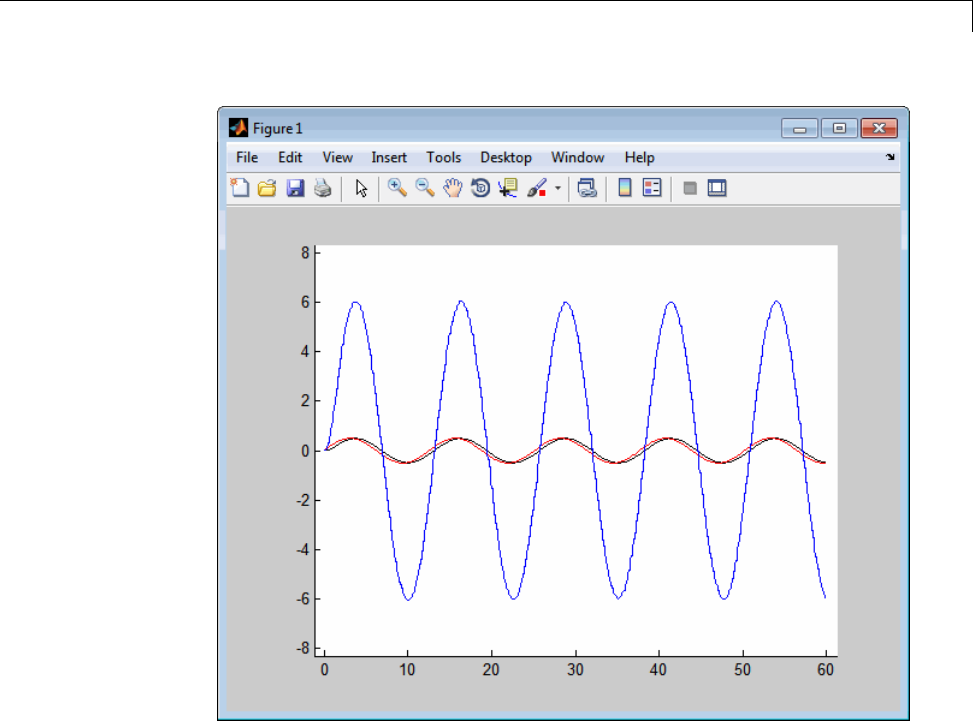
Customize the Simulation Data Inspector Interface
For more information on plotting and customizing your data plots using
the GUI tools, see “Figures, Plots, and Graphs”.
To view an example, see “Create, Save, and Print a Figure”.
Toolbar
The toolbar contains the following command buttons.
17-51
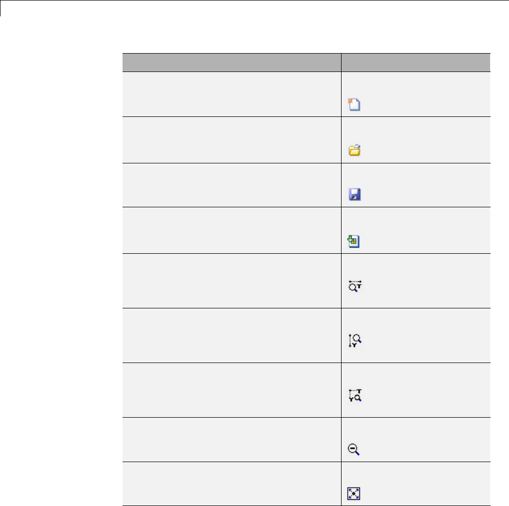
17 Inspecting and Comparing Logged Signal Data
To... Click...
Clear the Simulation Data Inspector of all
data.
New
Open a MAT-file previously saved from the
Simulation Data Inspector.
Open
Save data in Simulation Data Inspector to
aMAT-file.
Save
Launches the Data Import tool. Import Data
Zoom in along the time axis. After selecting
the icon, on the graph, click and hold the left
mouse button and drag the mouse to select
an area toenlarge.
Zoom in T
Zoom in along the data value axis. After
selecting the icon, on the graph, click and
hold the left mouse button and drag the
mouse to select an area to enlarge.
Zoom in T
Zoom inonasectionofthegraphalongboth
axes. After selecting the icon, on the graph,
click and hold the left mouse button, and
drag the mouse to select an area to enlarge.
Zoom in T and Y
Zoom out from the graph. After selecting
the icon, click the graph to incrementally
zoomout.
ZoomOut
Fit the plot to the graph. After selecting the
icon, click the graph to enlarge the plot to
fill the graph.
Fit to View
17-52

Customize the Simulation Data Inspector Interface
To... Click...
Move the plot in the graph up, down, left, or
right. After selecting the icon, on the graph,
click and hold the left mouse button and
move the mouse to the area of the graph
that you want to view.
Pan
Display the Tand Yvalues of a data point
in the plot. After selecting the icon, click a
point on the line to view a data point.
Data Cursor
17-53

17 Inspecting and Comparing Logged Signal Data
Limitations of the Simulation Data Inspector Tool
The following Simulink data export formats are not supported if time is not
logged:
•Structure
•Array
The following Simulink data types are not supported:
•Complex data, int64 and unit64
•Enumerated data types
The Simulation Data Inspector tool supports up to 3–dimensional time series
data.
17-54

Record and Inspect Signal Data Programmatically
Record and Inspect Signal Data Programmatically
Overview
Using the Simulation Data Inspector API, you can plot signal data, compare
two signals, and compare two simulation runs of data. You can use the
Simulink.sdi.createRun function to add simulation output data to the
Simulation Data Inspector. Once the Simulation Data Inspector contains
signal data, you can perform the following tasks:
To... Use...
View signal data, open the
Simulation Data Inspector tool
Simulink.sdi.view
Compare the data of two signals Simulink.sdi.compareSignals
Compare the output of two
simulation runs
Simulink.sdi.compareRuns
Run Management
Simulation Data Inspector software creates and manages a list of simulation
runs. Each run is an instance of a Simulink.sdi.Run object. This object
contains all of the simulation data and metadata for that simulation run.
To... Use...
Get the number of runs currently in
the Simulation Data Inspector
Simulink.sdi.getRunCount
Get therunIDfromthelistof
simulation runs in the Simulation
Data Inspector
Simulink.sdi.getRunIDByIndex
Determine if a run ID corresponds
to a run currently in the Simulation
DataInspector
Simulink.sdi.isValidRunID
Add more data to a run currently in
theSimulationDataInspector
Simulink.sdi.addToRun
17-55

17 Inspecting and Comparing Logged Signal Data
To... Use...
Make a copy of a run currently in the
Simulation Data Inspector
Simulink.sdi.copyRun
Delete a run from the Simulation
Data Inspector
Simulink.sdi.deleteRun
Get simulation data for a run in the
Simulation Data Inspector
Simulink.sdi.getRun
Manages output signal data and
metadata of a simulation run
Simulink.sdi.Run class
Get the Simulink.sdi.Signal object
corresponding to the given signal ID
Simulink.sdi.Run.getSignal method
Get the Simulink.sdi.Signal object
corresponding to the index into the
array signals in the run
Simulink.sdi.Run.getSignalByIndex
method
Get the signal ID corresponding to
the index into the array signals in
the run
Simulink.sdi.Run.getSignalIDByIndex
method
Determine if a signal ID corresponds
to a signal currently in the run
Simulink.sdi.Run.isValidSignalID
method
Signal Management
Each Simulink.sdi.Run object contains a Simulink.sdi.Signal object for each
output signal data. This object contains all of the simulation data for the
signal and its metadata.
To... Use...
Get the simulation data and
metadata for a signal from one
simulation run.
Simulink.sdi.getSignal
Manages a signal’s time series data
and metadata for one simulation
run.
Simulink.sdi.Signal class
17-56

Record and Inspect Signal Data Programmatically
Import/Export Data
To... Use...
Save signal data currently in the
Simulation Data Inspector
Simulink.sdi.save
Load previously saved Simulation
Data Inspector session
Simulink.sdi.load
Clear all data from the Simulation
Data Inspector
Simulink.sdi.clear
Comparison Results
To... Use...
Manage the results of
comparing two runs
(Simulink.sdi.compareRuns creates
the Simulink.sdi.DiffRunResult
object)
Simulink.sdi.DiffRunResult class
Manage the results of
comparing two signals (
Simulink.sdi.compareSignals
createsthe
Simulink.sdi.DiffSignalResult
object)
Simulink.sdi.DiffSignalResult class
Create a Run in the Simulation Data Inspector
To populate the Simulation Data Inspector with runs of simulation data,
you must first simulate your model and then call Simulink.sdi.createRun.
When using the API, the Simulation Data Inspector does not automatically
record simulation data. To create a run of simulation data, you can use the
following code:
%Op
en the model 'sldemo_f14'
load_system('sldemo_f14');
17-57

17 Inspecting and Comparing Logged Signal Data
% Configure model "sldemo_f14" for logging and simulate
simOut = sim('sldemo_f14', 'SaveOutput','on', ...
'SaveFormat', 'StructureWithTime', ...
'ReturnWorkspaceOutputs', 'on');
% Create a Simulation Data Inspector run
[runID,runIndex,signalIDs] = Simulink.sdi.createRun('My Run',...
'namevalue',{'MyData'},{simOut});
Compare Signal Data
To compare the simulation data for two signals, you can use the following code:
% Configure model "f14" for logging and simulate
simOut = sim('sldemo_f14', 'SaveOutput','on', ...
'SaveFormat', 'StructureWithTime', ...
'ReturnWorkspaceOutputs','on');
% Create a Simulation Data Inspector run and get signal IDs
[~, ~, signalIDs] = Simulink.sdi.createRun('My Run', ...
'namevalue', {'MyData'}, {simOut});
sig1 = signalIDs(1);
sig2 = signalIDs(2);
% Compare two signals, which returns the results in an instance of
% Simulink.sdi.diffSignalResult
diff = Simulink.sdi.compareSignals(sig1, sig2);
% Find if the signal data match
match = diff.match;
% Get the tolerance used in Simulink.sdi.compareSignals
tolerance = diff.tol;
Compare Runs of Simulation Data
To compare the signal data between two simulation runs, you can use the
following code:
% Configure model "sldemo_f14" for logging and simulate
set_param('sldemo_f14/Pilot','WaveForm','square');
17-58

Record and Inspect Signal Data Programmatically
simOut = sim('sldemo_f14', 'SaveOutput','on', ...
'SaveFormat', 'StructureWithTime', ...
'ReturnWorkspaceOutputs', 'on');
% Create a Simulation Data Inspector run, Simulink.sdi.Run, from
% simOut in the base workspace
runID1 = Simulink.sdi.createRun('First Run','namevalue',{'simOut'},...
{simOut});
% Simulate again
set_param('sldemo_f14/Pilot','WaveForm','sawtooth');
simOut = sim('sldemo_f14', 'SaveOutput','on', ...
'SaveFormat', 'StructureWithTime', ...
'ReturnWorkspaceOutputs', 'on');
% Create another Simulation Data Inspector run
runID2 = Simulink.sdi.createRun('Second Run','namevalue',{'simOut'},...
{simOut});
% Compare two runs, the result is stored in a
% Simulink.sdi.DiffRunResult object
difference = Simulink.sdi.compareRuns(runID1, runID2);
% Number of comparisons in result
numComparisons = difference.count;
% Iterate through each result element
for i = 1:numComparisons
% Get signal result at index i
signalResult = difference.getResultByIndex(i);
% Get signal IDs for each comparison result
sig1 = signalResult.signalID1;
sig2 = signalResult.signalID2;
% Display if signals match or not
displayStr = 'Signals with IDs %d and %d %s \n';
if signalResult.match
fprintf(displayStr, sig1, sig2, 'match');
else
17-59

17 Inspecting and Comparing Logged Signal Data
fprintf(displayStr, sig1, sig2, 'do not match');
end
end
Record Data During Parallel Simulations
To record and view the results from parallel simulations, use the following
methods to get and set the location of the Simulation Data Inspector
repository:
•Simulink.sdi.getSource
•Simulink.sdi.setSource
•Simulink.sdi.refresh
This example shows how to run multiple simulations in a parfor loop and
record each run in the Simulation Data Inspector tool.
Open the Simulation Data Inspector.
Simulink.sdi.view;
Load the model.
mdl = 'sldemo_f14';
load_system(mdl);
Get the location of the simulation data repository.
src = Simulink.sdi.getSource();
Open MATLAB pool with 4 workers.
matlabpool(4);
Run the simulation in a parfor loop.
parfor i=1:4
% Set the location of the simulation data repository of this
% worker to be the same for aggregating the data
Simulink.sdi.setSource(src);
% Run the simulation
17-60

Record and Inspect Signal Data Programmatically
simOut = sim(mdl,'SaveOutput','on',...
'SaveFormat','StructureWithTime',...
'ReturnWorkspaceOutputs','on');
% Create a simulation run in the Simulink Data Inspector
Simulink.sdi.createRun(['Run' num2str(i)],'namevalue',...
{'simout'},{simOut});
end
Close the MATLAB pool and all of the models.
matlabpool close;
bdclose all;
Refresh the Simulation Data Inspector
Simulink.sdi.refresh();
17-61

17 Inspecting and Comparing Logged Signal Data
17-62

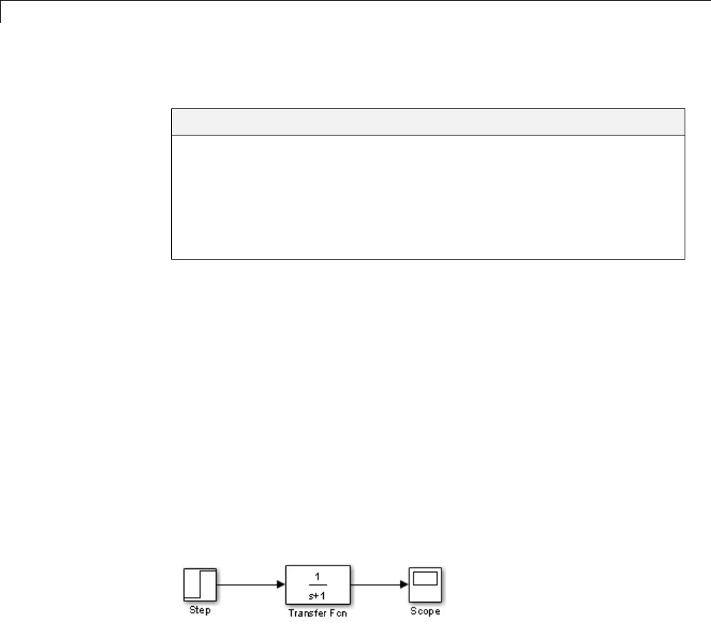
18 Analyzing Simulation Results
Viewing Output Trajectories
In this section...
“Viewing and Exporting Simulation Data” on page 18-2
“Using the Scope Block” on page 18-2
“Using Return Variables” on page 18-3
“Using the To Workspace Block” on page 18-3
“Using the Simulation Data Inspector Tool” on page 18-4
ViewingandExportingSimulationData
You can use several approaches to view output trajectories. Some approaches
display output trajectories during simulation. Other approaches export signal
values to the MATLAB workspace during simulation for later retrieval and
analysis.
The following sections describe several approaches for viewing output
trajectories. For additional information about exporting simulation data, see
“Export Simulation Data” on page 45-4.
Using the Scope Block
You can display output trajectories on a Scope block during simulation as
illustrated by the following model.
The display on the Scope shows the output trajectory. The Scope block enables
youtozoominonanareaofinterestorsavethedatatotheworkspace.
The XY Graph block enables you to plot one signal against another.
18-2
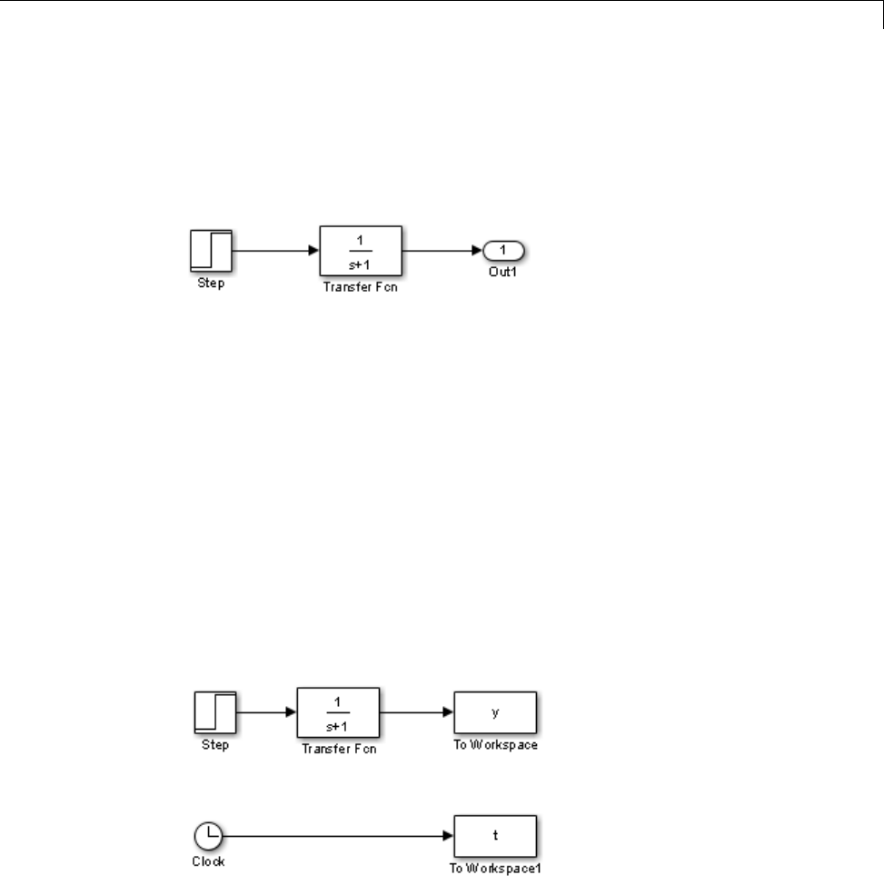
Viewing Output Trajectories
Using Return Variables
By returning time and output histories, you can use the plotting commands
provided in the MATLAB software to display and annotate the output
trajectories.
The block labeled Out is an Outport block from the Ports & Subsystems
library. The output trajectory, yout, is returned by the integration solver. For
more information, see “Data Import/Export Pane”.
YoucanalsorunthissimulationfromtheSimulation menu by specifying
variables for the time, output, and states on the Data Import/Export pane
of the Configuration Parameters dialog box. You can then plot these results
using
plot(tout,yout)
Using the To Workspace Block
The To Workspace block can be used to return output trajectories to the
workspace. The following model illustrates this use:
The variables yand tappear in the workspace when the simulation is
complete. You store the time vector by feeding a Clock block into a To
18-3
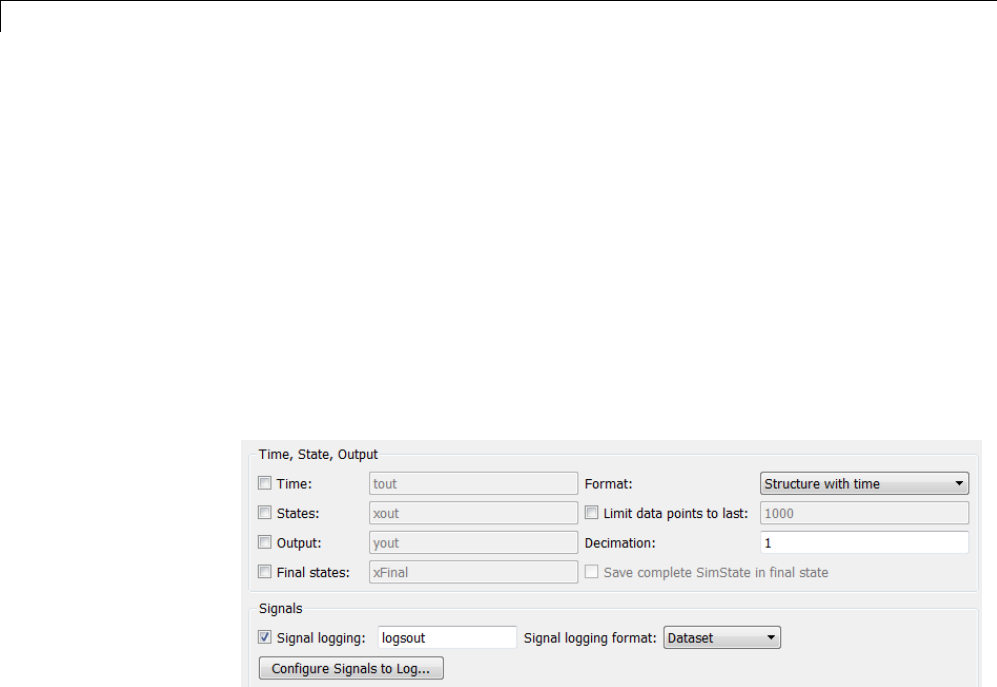
18 Analyzing Simulation Results
Workspace block. You can also acquire thetimevectorbyenteringavariable
name for the time on the Data Import/Export pane of the Configuration
Parameters dialog box, for menu-driven simulations, or by returning it using
the sim command (see “Data Import/Export Pane” for more information).
The To Workspace block can accept an array input, with each input element’s
trajectory stored in the resulting workspace variable.
Using the Simulation Data Inspector Tool
By configuring your model to log signal data to the base workspace, you
can view the output in the Simulation Data Inspector tool. On the Data
Import/Export pane of the Configuration Parameters dialog box
Select the following parameters:
•Time:enable
•States: enable
•Output: enable
•Signal logging:enable
•Format:specify
Structure with time
For more information on the Simulation Data Inspector tool, see “Inspect
Signal Data with Simulation Data Inspector” on page 17-2.
18-4
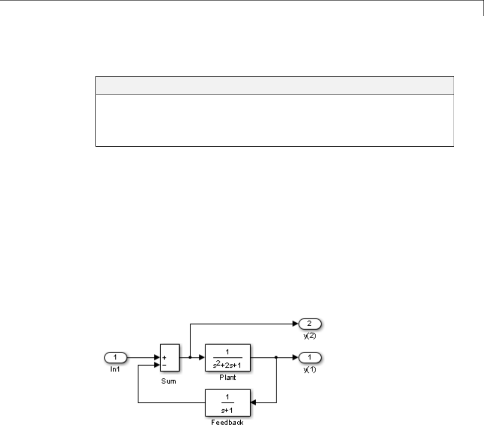
Linearizing Models
Linearizing Models
In this section...
“About Linearizing Models” on page 18-5
“Linearization with Referenced Models” on page 18-7
“Linearization Using the ’v5’ Algorithm” on page 18-9
About Linearizing Models
The Simulink product provides the linmod,linmod2,anddlinmod functions to
extract linear models in the form of the state-space matrices A,B,C,andD.
State-space matrices describe the linear input-output relationship as
xAxBu
yCxDu
=+
=+,
where x,u,andyare state, input, and output vectors, respectively. For
example, the following model is called lmod.
18-5

18 Analyzing Simulation Results
To extract the linear model of this system, enter this command.
[A,B,C,D] = linmod('lmod')
A=
-2 -1 -1
100
01-1
B=
1
0
0
C=
010
00-1
D=
0
1
Inputs and outputs must be defined using Inport and Outport blocks from the
Ports & Subsystems library. Source and sink blocks do not act as inputs and
outputs. Inport blocks can be used in conjunction with source blocks, using
a Sum block. Once the data is in the state-space form or converted to an
LTI object, you can apply functions in the Control System Toolbox product
for further analysis:
•Conversion to an LTI object
sys = ss(A,B,C,D);
•Bode phase and magnitude frequency plot
bode(A,B,C,D) or bode(sys)
•Linearized time response
step(A,B,C,D) or step(sys)
impulse(A,B,C,D) or impulse(sys)
lsim(A,B,C,D,u,t) or lsim(sys,u,t)
18-6

Linearizing Models
You can use other functions in the Control System Toolbox and the Robust
Control Toolbox™ products for linear control system design.
When the model is nonlinear, an operating point can be chosen at which
to extract the linearized model. Extra arguments to linmod specify the
operating point.
[A,B,C,D] = linmod('sys', x, u)
For discrete systems or mixed continuous and discrete systems, use the
function dlinmod for linearization. This function has the same calling syntax
as linmod except that the second right-hand argument must contain a sample
time at which to perform the linearization.
Linearization with Referenced Models
You can use linmod to extract a linear model from a Simulink environment
that contains Model blocks.
Note In Normal mode, the linmod command applies the block-by-block
linearization algorithm on blocks inside the referenced model. If the
Model block is in Accelerator mode, the linmod command uses numerical
perturbation to linearize the referenced model. Due to limitations on
linearizing multirate Model blocks in Accelerator mode, you should use
Normal mode simulation for all models referenced by Model blocks when
linearizing with referenced models. For an explanation of the block-by-block
linearization algorithm, see the Simulink Control Design™ documentation.
Forexample,considerthef14 model mdlref_f14. The Aircraft Dynamics
Model block refers to the model mdlref_dynamics.
18-7
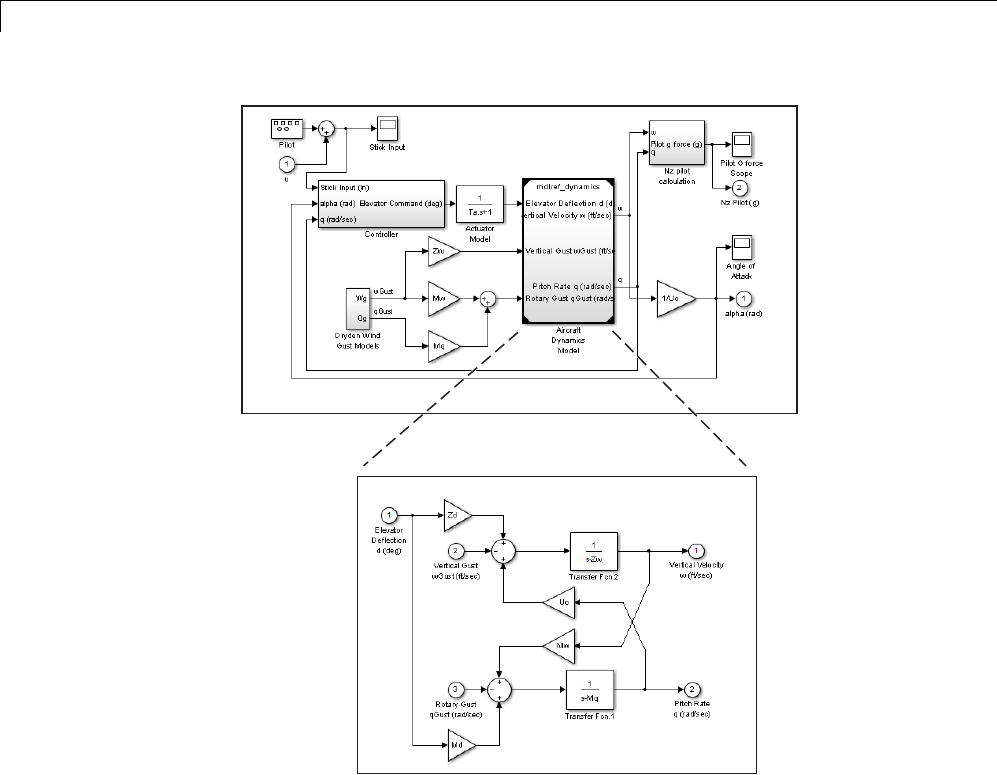
18 Analyzing Simulation Results
To linearize the mdlref_f14 model, call the linmod command on the top
mdlref_f14 model as follows.
[A,B,C,D] = linmod('mdlref_f14')
The resulting state-space model corresponds to the complete f14 model,
including the referenced model.
You can call linmod with a state and input operating point for models that
contain Model blocks. When using operating points, the state vector xrefers
tothetotalstatevectorforthetopmodel and any referenced models. You
18-8

Linearizing Models
must enter the state vector using the structure format. To get the complete
state vector, call
x = Simulink.BlockDiagram.getInitialState(topModelName)
Linearization Using the ’v5’ Algorithm
Calling the linmod command with the 'v5' argument invokes the
perturbation algorithm created prior to MATLAB software version 5.3. This
algorithm also allows you to specify the perturbation values used to perform
the perturbation of all the states and inputs of the model.
[A,B,C,D]=linmod('sys',x,u,para,xpert,upert,'v5')
Using linmod with the 'v5' option to linearize a model that contains
Derivative or Transport Delay blocks can be troublesome. Before linearizing,
replace these blocks with specially designed blocks that avoid the problems.
These blocks are in the Simulink Extras library in the Linearization
sublibrary.
You access the Extras library by opening the Blocksets & Toolboxes icon:
•For the Derivative block, use the Switched derivative for linearization.
•For the Transport Delay block, use the Switched transport delay for
linearization. (Using this block requires that you have the Control System
Toolbox product.)
When using a Derivative block, you can also try to incorporate the derivative
term in other blocks. For example, if you have a Derivative block in series
with a Transfer Fcn block, it is better implemented (although this is not
always possible) with a single Transfer Fcn block of the form
s
sa+.
In this example, the blocks on the left of this figure can be replaced by the
block on the right.
18-9

18 Analyzing Simulation Results
18-10
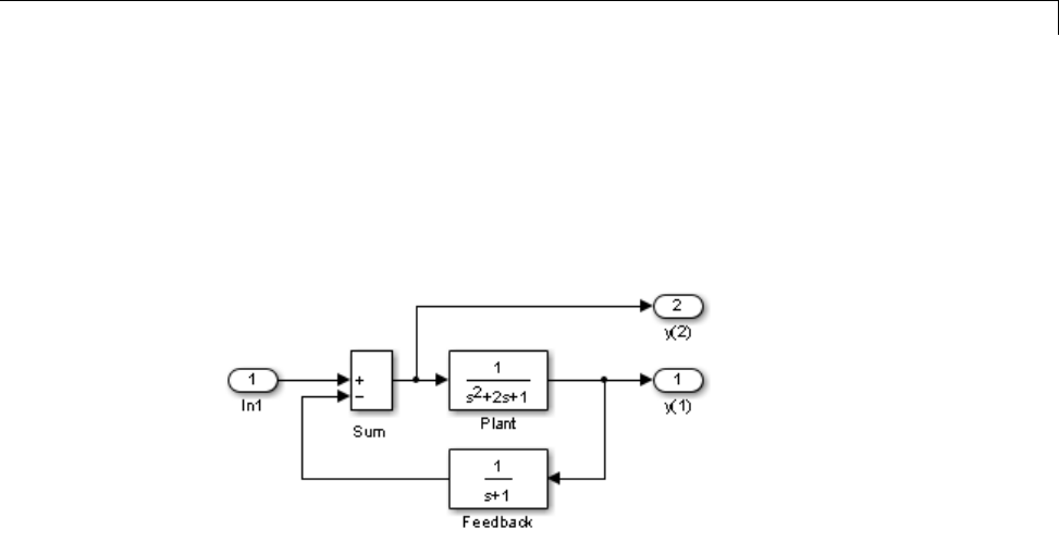
Finding Steady-State Points
Finding Steady-State Points
The Simulink trim function uses a model to determine steady-state points of
a dynamic system that satisfy input, output, and state conditions that you
specify. Consider, for example, this model, called ex_lmod.
You can use the trim function to find the values of the input and the states
that set both outputs to 1. First, make initial guesses for the state variables
(x) and input values (u), then set the desired value for the output (y).
x = [0; 0; 0];
u=0;
y = [1; 1];
Use index variables to indicate which variables are fixed and which can vary.
ix = []; % Don't fix any of the states
iu = []; % Don't fix the input
iy = [1;2]; % Fix both output 1 and output 2
18-11

18 Analyzing Simulation Results
Invoking trim returns the solution. Your results might differ because of
roundoff error.
[x,u,y,dx] = trim('lmod',x,u,y,ix,iu,iy)
x=
0.0000
1.0000
1.0000
u=
2
y=
1.0000
1.0000
dx =
1.0e-015 *
-0.2220
-0.0227
0.3331
Note that there might be no solution to equilibrium point problems. If that
is the case, trim returns a solution that minimizes the maximum deviation
from the desired result after first trying to set the derivatives to zero. For a
description of the trim syntax, see trim.
18-12


19 Improving Simulation Performance and Accuracy
About Improving Performance and Accuracy
Simulation performance and accuracy can be affected by many things,
including the model design and choice of configuration parameters.
The solvers handle most model simulations accurately and efficiently with
their default parameter values. However, some models yield better results
if you adjust solver parameters. Also, if you know information about your
model’s behavior, your simulation results can be improved if you provide
this information to the solver.
19-2

Speed Up Simulation
SpeedUpSimulation
Slow simulation speed can have many causes. Here are a few:
•Your model includes an Interpreted MATLAB Function block. When a
model includes an Interpreted MATLAB Function block, the MATLAB
interpreter is called at each time step, drastically slowing down the
simulation. Use the built-in Fcn block or the Math Function block
whenever possible.
•Your model includes a MATLAB file S-function. MATLAB file S-functions
also cause the MATLAB interpreter to be called at each time step.
Consider either converting the S-function to a subsystem or to a C-MEX file
S-function.
•Your model includes a Memory block. Using a Memory block causes the
variable-order solvers (ode15s and ode113)toberesetbacktoorder1at
each time step.
•The maximum step size is too small. If you changed the maximum step
size, try running the simulation again with the default value (auto).
•Did you ask for too much accuracy? The default relative tolerance (0.1%
accuracy) is usually sufficient. For models with states that go to zero, if
the absolute tolerance parameter is too small, the simulation can take too
many steps around the near-zero state values. See the discussion of error
in “Maximum order”.
•Thetimescalemightbetoolong. Reducethetimeinterval.
•The problem might be stiff, but you are using a nonstiff solver. Try using
ode15s.
•The model uses sample times that are not multiples of each other. Mixing
sample times that are not multiples of each other causes the solver to take
small enough steps to ensure sample time hits for all sample times.
•The model contains an algebraic loop. The solutions to algebraic loops are
iteratively computed at every time step. Therefore, they severely degrade
performance. For more information, see “Algebraic Loops” on page 3-39.
•Your model feeds a Random Number block into an Integrator block. For
continuous systems, use the Band-Limited White Noise block in the
Sources library.
19-3

19 Improving Simulation Performance and Accuracy
•Your model contains a scope viewer that displays a large number of
data points. Try adjusting the viewer parameter settings that can
affect performance. For more information, see “Parameter Settings and
Performance with Scope Signal Viewer” on page 16-20.
19-4

Comparing Performance
Comparing Performance
In this section...
“Performance of the Simulation Modes” on page 19-5
“Measure Performance” on page 19-7
Performance of the Simulation Modes
The Accelerator and Rapid Accelerator modes give the best speed
improvement compared to Normal mode when simulation execution time
exceeds the time required for code generation. For this reason, the Accelerator
and Rapid Accelerator modes generally perform better than Normal mode
when simulation execution times are several minutes or more. However,
models with a significant number of Stateflow or MATLAB Function blocks
might show only a small speed improvement over Normal mode because in
Normal mode these blocks also simulate through code generation.
Including tunable parameters in your model can also increase the simulation
time.
The figure shows in general terms the performance of a hypothetical model
simulated in Normal, Accelerator, and Rapid Accelerator modes.
19-5
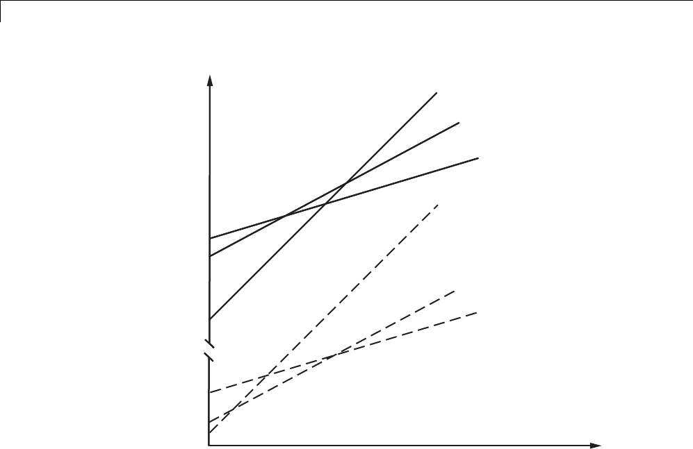
19 Improving Simulation Performance and Accuracy
Simulation Stop Time or Number of Major Time Steps
minutes
Normal
Accelerator
Rapid Accelerator
Normal
Accelerator
Rapid Accelerator
seconds
all targets
up to date
all targets
out of date
Elapsed Time
Performance When the Target Must Be Rebuilt
The solid lines in the figure show performance when the target code must be
rebuilt (“all targets out of date”). For this hypothetical model, the time scale
is on the order of minutes, but it could be longer for more complex models.
As generalized in the figure, the time required to compile the model in Normal
modeislessthanthetimerequiredtobuildeithertheAcceleratortargetor
Rapid Accelerator executable. It is evident from the figure that for small
simulation stop times Normal mode results in quicker overall simulation
times than either Accelerator mode or Rapid Accelerator mode.
The crossover point where Accelerator mode or Rapid Accelerator mode result
in faster execution times depends on the complexity and content of your
model. For instance, those models running in Accelerator mode containing
19-6

Comparing Performance
large numbers of blocks using interpreted code (see “Select Blocks for
Accelerator Mode” on page 22-16) mightnotrunmuchfasterthantheywould
in Normal mode unless the simulation stop time is very large. Similarly,
models with a large number of Stateflow Chart blocks or MATLAB Function
blocks might not show much speed improvement over Normal mode unless
the simulation stop times are long.
For illustration purposes, the graphic represents a model with a large number
of Stateflow Chart blocks or MATLAB Function blocks. The curve labeled
“Normal” would have much smaller initial elapsed time than shown if the
model did not contain these blocks.
Performance When the Targets Are Up to Date
As shown by the broken lines in the figure (“all targets up to date”) the time
for the Simulink software to determine if the Accelerator target or the Rapid
Accelerator executable are up to date is significantly less than the time
required to generate code (“all targets out of date”). You can take advantage
of this characteristic when you wish to test various design tradeoffs.
For instance, you can generate the Accelerator mode target code once and use
it to simulate your model with a series of gain settings. This is an especially
efficient way to use the Accelerator or Rapid Accelerator modes because this
type of change does not result in the target code being regenerated. This
means the target code is generated the first time the model runs, but on
subsequent runs the Simulink code spends only the time necessary to verify
that the target is up to date. This process is much faster than generating
code, so subsequent runs can be significantly faster than the initial run.
Because checking the targets is quicker than code generation, the crossover
pointissmallerwhenthetargetisuptodatethanwhencodemustbe
generated. This means subsequent runs of your model might simulate faster
in Accelerator or Rapid Accelerator mode when compared to Normal mode,
even for short stop times.
Measure Performance
You can use the tic,toc,andsim commands to compare Accelerator mode or
Rapid Accelerator mode execution times to Normal mode.
19-7

19 Improving Simulation Performance and Accuracy
1Use load_system to load your model into memory without opening a
window.
2From the Simulation > Mode menu, select Normal.
3Use the tic,toc,andsim commands at the command line prompt to
measure how long the model takes to simulate in Normal mode:
tic,[t,x,y]=sim('myModel',10000);toc
tic and toc work together to record and return the elapsed time and
display a message such as the following:
Elapsed time is 17.789364 seconds.
4Select either Accelerator or Rapid Accelerator from the
Simulation > Mode menu, and build an executable for the model by
clicking the Run button. The acceleration modes use this executable
in subsequent simulations as long as the model remains structurally
unchanged. “Code Regeneration in Accelerated Models” on page 22-7
discusses the things that cause your model to rebuild.
5Rerun the compiled model at the command prompt:
tic,[t,x,y]=sim('myModel',10000);toc
6The elapsed time displayed shows the run time for the accelerated model.
For example:
Elapsed time is 12.419914 seconds.
Thedifferenceinelapsedtimes(5.369450secondsinthisexample)showsthe
improvement obtained by accelerating your model.
19-8

Improve Acceleration Mode Performance
Improve Acceleration Mode Performance
In this section...
“Techniques” on page 19-9
“C Compilers” on page 19-10
Techniques
To get the best performance when accelerating your models:
•Verify that the Configuration Parameters dialog box settings are as follows:
On this pane... Set... To...
Solver Diagnostics Solver data
inconsistency
none
Data Validity
Diagnostics
Array bounds
exceeded
none
Optimization Signal storage reuse selected
•Disable Stateflow debugging and animation.
•Inline user-written S-functions (these are TLC files that direct the Simulink
CodersoftwaretocreateCcodefortheS-function).See“ControlS-Function
Execution” on page 22-17 for a discussion on how the Accelerator mode and
Rapid Accelerator mode work with inlined S-functions.
For information on how to inline S-functions, consult “Insert S-Function
Code”.
•When logging large amounts of data (for instance, when using the
Workspace I/O, To Workspace, To File, or Scope blocks), use decimation or
limit the output to display only the last part of the simulation.
•Customize the code generation process to improve simulation speed. See
“Customize the Build Process” on page 22-22 for details.
19-9

19 Improving Simulation Performance and Accuracy
CCompilers
On computers running the Microsoft Windows operating system, the
Accelerator and Rapid Accelerator modes use the default 32-bit C compiler
supplied by MathWorks to compile your model. If you have a C compiler
installed on your PC, you can configure the mex command to use it instead.
You might choose to do this if your C compiler produces highly optimized
code since this would further improve acceleration, or if you wish to use a
64-bit compiler.
Note For an up-to-date list of 32- and 64-bit C compilers that are compatible
with MATLAB software for all supported computing platforms, see:
http://www.mathworks.com/support/compilers/current_release/
19-10

Improve Simulation Accuracy
Improve Simulation Accuracy
To check your simulation accuracy, run the simulation over a reasonable time
span. Then, either reduce the relative tolerance to 1e-4 (the default is 1e-3)
or reduce the absolute tolerance and run it again. Compare the results of
both simulations. If the results are not significantly different, you can feel
confident that the solution has converged.
If the simulation misses significant behavior at its start, reduce the initial step
size to ensure that the simulation does not step over the significant behavior.
If the simulation results become unstable over time,
•Your system might be unstable.
•If you are using ode15s, you might need to restrict the maximum order to
2 (the maximum order for which the solver is A-stable) or try using the
ode23s solver.
If the simulation results do not appear to be accurate,
•For a model that has states whose values approach zero, if the absolute
tolerance parameter is too large, the simulation takes too few steps around
areas of near-zero state values. Reduce this parameter value or adjust it
for individual states in the Integrator dialog box.
•If reducing the absolute tolerances does not sufficiently improve the
accuracy, reduce the size of the relative tolerance parameter to reduce the
acceptable error and force smaller step sizes and more steps.
Certain modeling constructs can also produce unexpected or inaccurate
simulation results.
•A Source block that inherits its sample time can produce different
simulation results if, for example, the sample times of the downstream
blocks are modified (see “How Propagation Affects Inherited Sample
Times” on page 5-29).
•A Derivative block found in an algebraic loop can result in a loss in solver
accuracy.
19-11

19 Improving Simulation Performance and Accuracy
19-12

20
Performance Advisor

20 Performance Advisor
Consult the Performance Advisor
In this section...
“About the Performance Advisor” on page 20-2
“Prepare to Use Performance Advisor” on page 20-3
“Start the Performance Advisor” on page 20-3
“Overview of the Performance Advisor Window” on page 20-3
“Performance Advisor Workflow” on page 20-6
“Create Baseline” on page 20-6
“Run Performance Advisor Checks” on page 20-8
“View and Save Performance Advisor Reports” on page 20-11
“Understand Performance Advisor Analysis Results” on page 20-14
“Fix a Warning” on page 20-16
“Review the Actions Taken” on page 20-16
“Save Your Model” on page 20-17
“Performance Advisor Limitations” on page 20-17
About the Performance Advisor
Whatever the level of complexity of the model, you might want to improve
simulation performance. The Performance Advisor checks a model for
conditions and configuration settings that can result in slower simulation of
the system that the model represents. The Performance Advisor produces a
report that lists the suboptimal conditions or settings that it finds, suggesting
better model configuration settings where appropriate. The Performance
Advisor provides mechanisms for automatically fixing warning or allowing
you to fix them manually. For more information on individual Performance
Advisor checks, see “Simulink Performance Advisor Checks”.
For more guidelines, see Improving Simulation Performance in Simulink.
20-2

Consult the Performance Advisor
Prepare to Use Performance Advisor
Before you use the Performance Advisor:
•Make a backup copy of your original model.
•Check that the original model can simulate without error.
•Close all applications, including Web browsers. Only the MATLAB
Command Window, the model you want to analyze, and the Performance
Advisor tool should be running. The running of other applications can
change the performance of model simulation and the ability of Performance
Advisor to measure accurately.
Start the Performance Advisor
Start the Performance Advisor in one of the following ways:
•To start the Performance Advisor from the Simulink Editor menus, select
Analysis > Performance Tools > Performance Advisor.
•To start the Performance Advisor from the Simulink Editor toolbar, on the
Simulink Editor, on the drop-down list, select Performance Advisor.
•To start the Performance Advisor from the MATLAB Command Window,
type performanceadvisor('model_name'). For example:
performanceadvisor('vdp')
Overview of the Performance Advisor Window
When you start the Performance Advisor, the Performance Advisor window
displays two panes. The left pane lists the folders in the Performance Advisor.
Expanding the folders displays the available checks. The right pane provides
instructions on how to view and specify which checks you want to run. It also
provides a legend describing the displayed symbols.
20-3
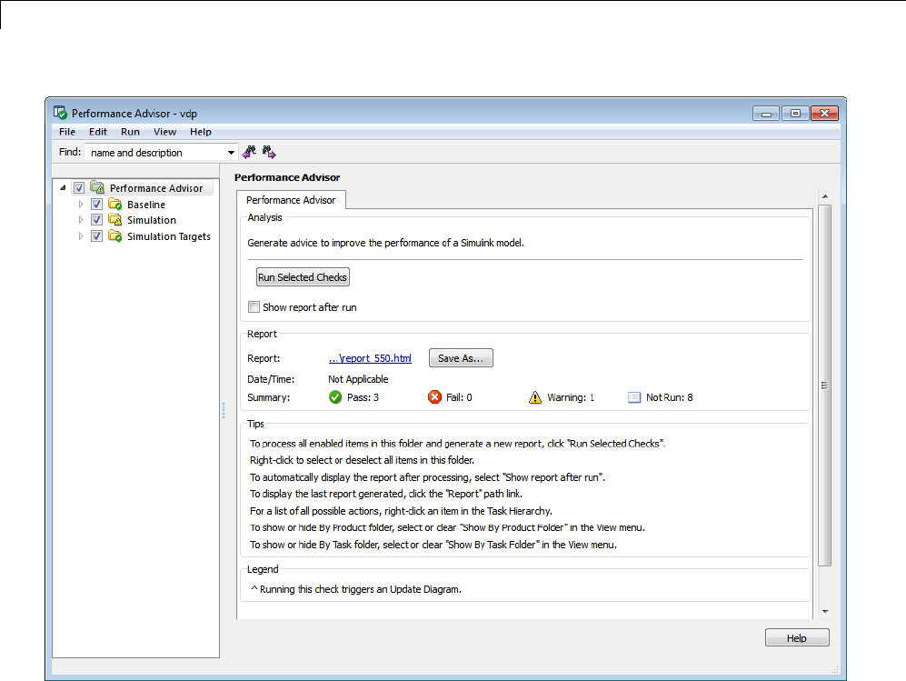
20 Performance Advisor
From the left pane, you can:
•Select by category and expand the folder to display checks related to
specific tasks, such as creating a baseline for future checks or checks based
on Simulation actions.
•Select some or all of the checks using the check boxes or context menus
associated with the checks, then run an individual check or all selected
checks in a folder.
20-4

Consult the Performance Advisor
To find checks and folders, enter text in the Find field and click the Find
Next button ( ). The Performance Advisor searches check names and
folder names for the text.
After running checks, the Performance Advisor displays the results in the
right pane. Additionally, the Performance Advisor generates an HTML report
of the check results. You can optionally view this report in a separate browser
window by clicking the Show report after run check box in the right pane
before the check has run.
The right pane is contextual. It changes depending on your actions. From
the right pane:
When you
select a...
The right pane displays a Performance Advisor
tab with...
Folder Analysis pane, containing:
•Run Selected Checks button — Click to run the
selected checks in the folderoritssubfolders.
•Show report after run check box — Select to display
an HTML report of the check results after the check
has run.
Tips and Legends sections, containing brief descriptions
on using the checks.
Check Analysis pane, containing:
•Input Parameters section — Before running checks,
specify how you want checks to run (for more
information, see “Run Performance Advisor Checks”
on page 20-8).
•Result section — Display results after check run.
Action pane, containing:
•Modify button — Click this button to perform
recommended actions.
•Result section — Display results after performing
recommended actions.
20-5

20 Performance Advisor
Performance Advisor Workflow
Your expected workflow when using Performance Advisor is:
1When you determine that the performance of a model is slower than
expected, use Performance Advisor to help identify and resolve bottlenecks.
2Have Performance Advisor
aCreate a baseline against it will compare measurements.
bRunthechecksyouselected.
cMake suggested changes.
dRun the checks again.
•If performance is improved, you can stop.
•If performance is worse than the baseline data, Performance Advisor
reinstates the model to the settings it had before the check was run.
Create Baseline
Create a baseline before running checks in Performance Advisor. A baseline
is a set of simulation measurements against which Performance Advisor
measure check results.
To create the baseline, in the Performance Advisor:
1Before creating the baseline, you need to verify and possibly set
configuration parameters to enable data logging using the Structured
with time format. To set configuration parameters, in the model, select
Simulation > Model Configuration Parameters.
2In the Configuration Parameters dialog box:
•Set Data Import/Export > Format to Structure with time.
•Set up signal logging. For an easy example, select the Data
Import/Export > States or Output check box.
•Click the Configure Signals to Log button to select the signals to log.
20-6

Consult the Performance Advisor
Note Select only the signals you are most interested in. Minimizing the
number of signals you want to log can help performance. Selecting too
many signals might cause the Performance Advisor to run for a longer
time.
3Click OK.
4Run the model once and check that the simulation runtime is not too long.
5If the Performance Advisor is not started, start it now.
6In the left pane, select Create Baseline.
7In the right pane, in the Input Parameters section:
•In Stop Time, enter a stop time for the simulation for the baseline
creation. By default, if the model stop time is less than 10, Performance
Advisor uses that value as the stop time. Otherwise, it uses 10. You
should avoid entering a large stop time because the simulation might
be too large.
•Click the Click to view baseline signals and set their tolerances
check box to see and change the baseline signal tolerance. Performance
Advisor calculates a default tolerance for the model based on the solver
setting.
After the Performance Advisor runs the check, it starts the Simulation
Data Inspector. With this tool, you can compare signals and adjust
tolerance levels. For more information, see “Inspect Signal Data with
Simulation Data Inspector” on page 17-2.
For more information on input parameters, see “Run Performance Advisor
Checks” on page 20-8.
8In the right pane, click Run This Check.
Upon successful creation of a baseline, a message like the following is
displayed in the Analysis Result section:
20-7
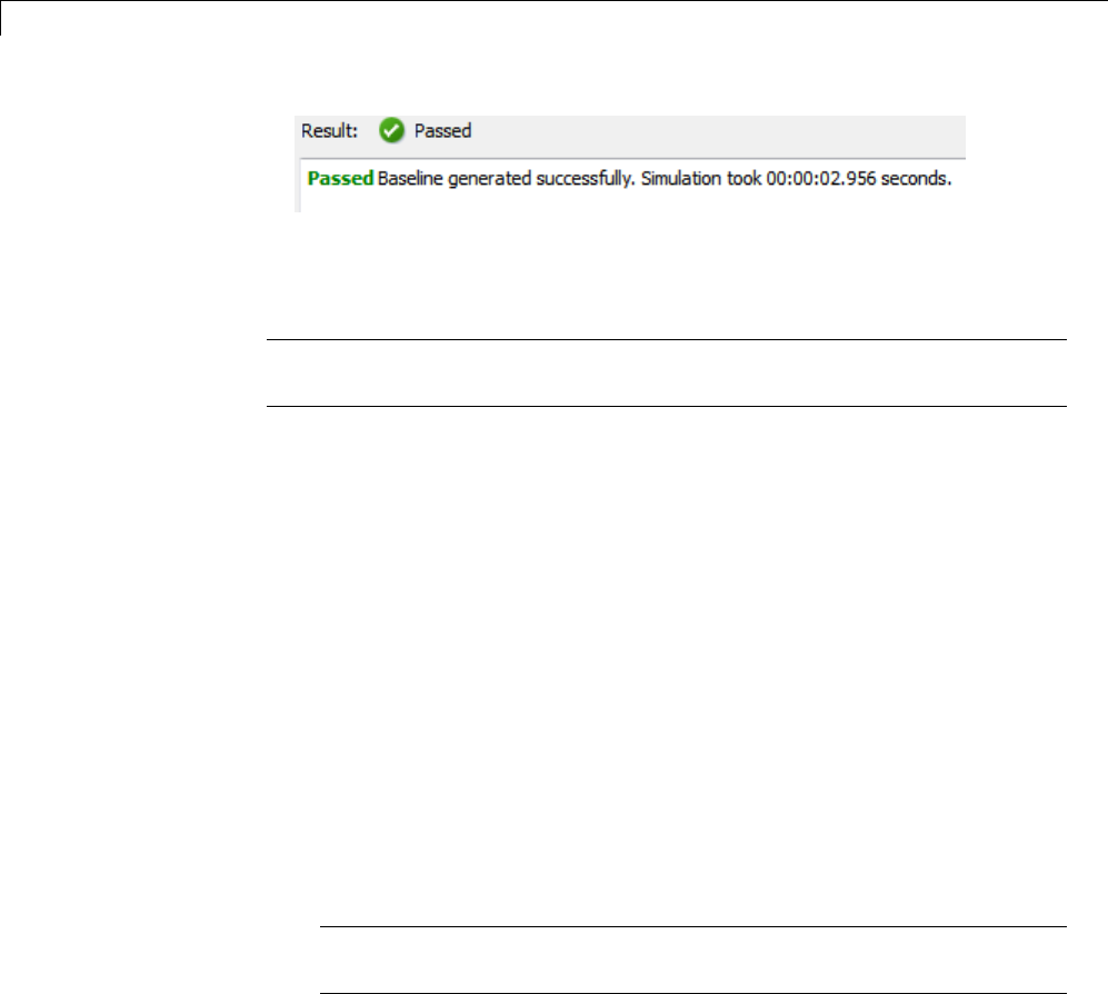
20 Performance Advisor
Observe that Performance Advisor has filled the Stop Time parameter
with the stop time of the model.
Note Alternatively, you can create the baseline when you run your selected
Performance Advisor checks.
You can now run Performance Advisor checks (see “Run Performance Advisor
Checks” on page 20-8).
Run Performance Advisor Checks
This topic assumes that you have created a baseline. If you have not yet done
so, see “Create Baseline” on page 20-6.
1Select checks to run:
•Click a folder, such as Simulation or Simulation Targets,todisplay
checks related to specific tasks.
•In a folder, select some or all of the checks using the check boxes or
context menus associated with the checks, and then run an individual
check or all selected checks. By default, the first time you run, all checks
are selected.
Tip If you are unsure of which checks apply, you can select and run all
checks, then clear the checks you are not interested in.
–To select an individual check, in the right pane, select the check. The
right pane updates with information particular to this check.
–To run all selected checks in a folder, in the left pane, select the folder
(forexample,Simulation).
20-8

Consult the Performance Advisor
–To select all selected checks for all the categories, in the left pane,
select Performance Advisor. Performance Advisor creates the
baseline, even if it has already been created, and runs the selected
checks.
•To find checks and folders, enter text in the Find field and click the
Find Next button ( ). The Performance Advisor searches in check
names, folder names, and analysis descriptions for the text.
The right pane changes depending on your selection in the left pane.
2In the right pane, specify input parameters for checks to run.
Input
Parameter
Description
Take action
based on
advice
automatically — Default. Allow Performance Advisor
to make the change for you.
manually — Make the recommended changes yourself
or review the changes first. This option allows you to
review the recommended change first. You then have
the option of making the change yourself, or clicking a
modify button that allows Performance Advisor to make
changes for you.
Validate
and revert
changes
if time of
simulation
increases
Select this check box to have Performance Advisor rerun
the simulation and verify that the change made based
on the advice improves simulation time. If the change
does not improve simulation time, Performance Advisor
reverts the changes.
Clear this check box if you do not want Performance
Advisor to run the simulation and verify the results.
20-9

20 Performance Advisor
Input
Parameter
Description
Validate
and revert
changes if
degree of
accuracy is
greater than
tolerance
Select this check box to have Performance Advisor rerun
the simulation and verify that after the change, the
model results are still within tolerance. If the result
is outside tolerance, Performance Advisor reverts the
changes.
Note If you select only this check box, Performance
Advisor compares just the signal to see that it is within
tolerance.
Clear this check box if you do not want Performance
Advisor to rerun the simulation and verify that the
results are within tolerance.
Quick
estimation
of model
build time
Click this check box to allow Performance Advisor to use
the number of blocks of a referenced model to estimate
model build time. Performance Advisor performs this
quick estimate as follows:
1Search the model for referenced models that do not
refer to other referenced models.
2Calculate the average number of blocks in each of the
referenced models that do not refer to other referenced
models.
3Of the list of referenced models that do not refer to
others, select a referenced model whose number of
blocks is closest to the calculated average.
4Build this model to obtain the build time.
5Based on the number of blocks and the build time for
this referenced model, estimate the build time for all
other referenced models.
6Based on these build times, estimate the parallel build
time for the top model.
3To run a check, in the right pane, click the Run This Check button.
Alternatively, in the menu bar, select Run > Run Selected Checks.
20-10

Consult the Performance Advisor
After running checks, the Performance Advisor displays the results in
the right pane. Additionally, the Performance Advisor generates an
HTML report of the current check results in a file with a name like
model_name\report_#.html
You can optionally view this report in a separate browser window by clicking
the Report link in the right pane of the folder node.
Note When you open the Performance Advisor for a model that you have
previously checked, the Performance Advisor initially displays the check
results generated the last time you checked the model. If you recheck the
model, the new results replace the previous results in the Performance
Advisor window.
After you run your checks, you can:
•“View and Save Performance Advisor Reports” on page 20-11
•“Understand Performance Advisor Analysis Results” on page 20-14
View and Save Performance Advisor Reports
When the Performance Advisor runs checks, it generates an HTML report
of check results.
View Performance Advisor Reports
You can access any report by selecting a folder and clicking the link in the
Report box.
Tip While you can fix warnings and failures through Performance Advisor
reports, use the Performance Advisor window for interactive fixing.
Performance Advisor reports are best for viewing a summary of checks.
As you run checks, the Performance Advisor updates the reports with the
latest information for each check in the folder. A message appears in the
report when you run the checks at different times. Time stamps indicate
20-11
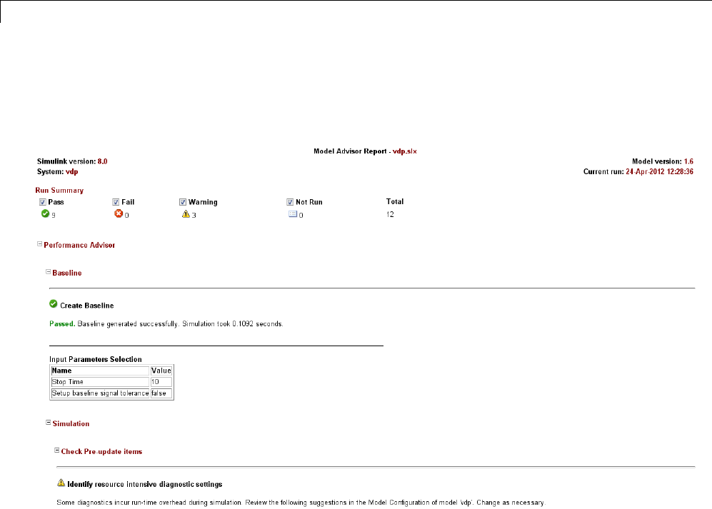
20 Performance Advisor
when checks have been run. The time of the current run appears at the top
right of the report. Checks that occurred during previous runs have a time
stamp following the check name.
You can manipulate the report to show only what you are interested in
viewing as follows:
•The check boxes next to the Run Summary status allow you to view only
the checks with the status that you are interested in viewing. For example,
you can remove the checks that have not run by clearing the check box
next to the Not Run status.
Some checks have input parameters specified in the right pane of the
Performance Advisor. For example, Identify resource intensive
diagnostic settings has several input parameters. When you run checks
with input parameters, the Performance Advisor displays the values of the
input parameters in the HTML report:
20-12
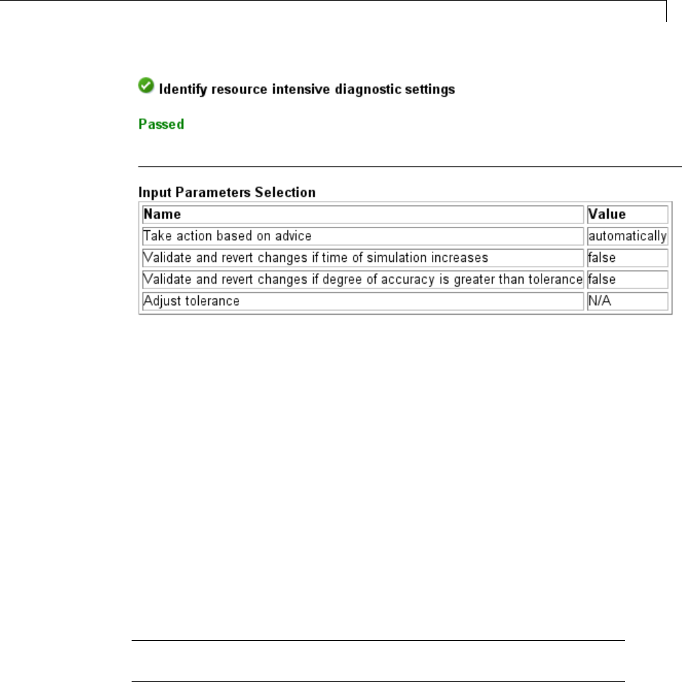
Consult the Performance Advisor
Save Performance Advisor Reports
You can archive a Performance Advisor report by saving it to a new location.
To save a report:
1In the Performance Advisor window, navigate to the folder that contains
the report you want to save.
2Select the folder that you want. The right pane of the Performance Advisor
window displays information about that folder, including a Report box.
3In the Report box, click Save As. A save as dialog box opens.
4In the save as dialog box, navigate to the location where you want to save
the report, and click Save. The Performance Advisor saves the report and
its image graphics to the new location. Performance Advisor does not save
its action results to a report.
Note If you rerun the Performance Advisor, the report is updated in the
working folder, not in the save location.
20-13
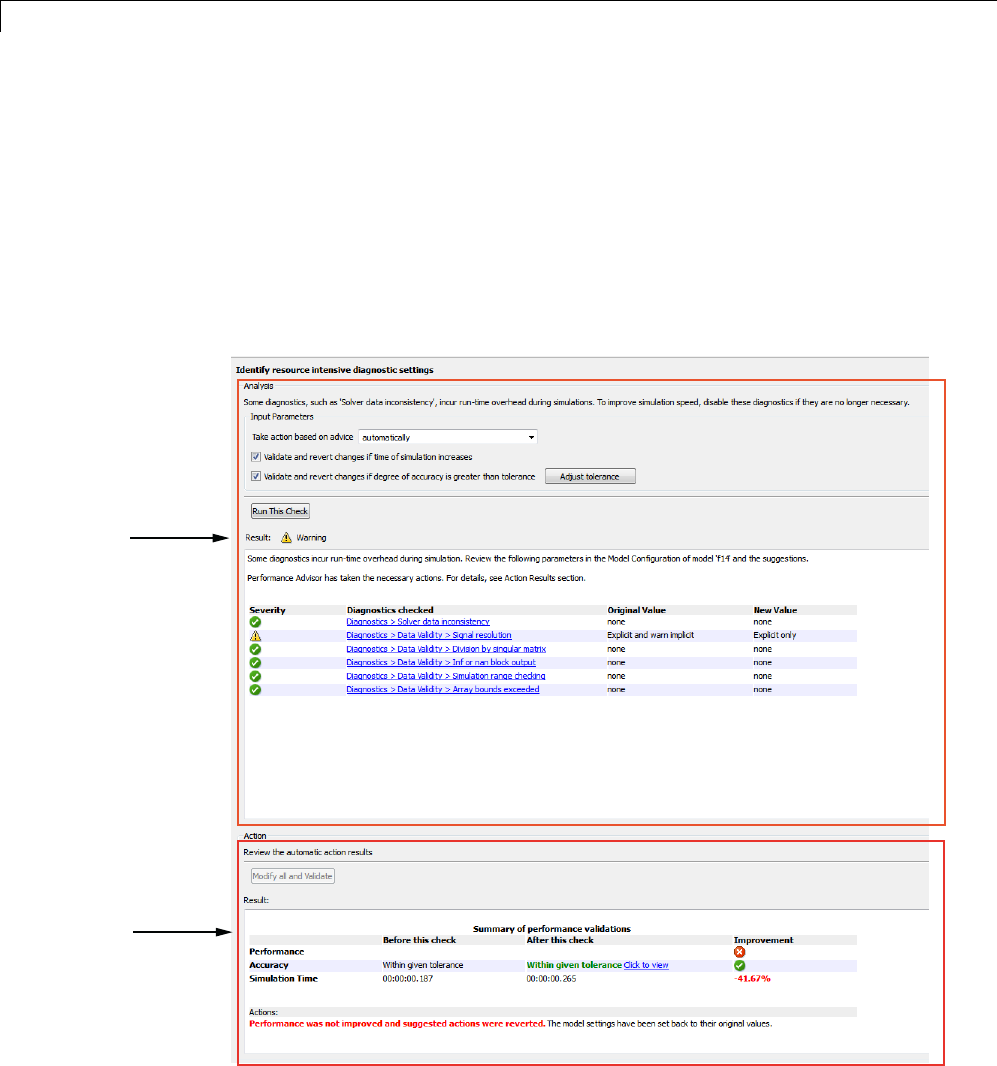
20 Performance Advisor
You can find the full path to the report in the title bar of the report window.
Typically, the report is in the working folder with a structure like the following
slprj/modeladvisor/com_2emathworks_2eSimulink_2ePerformanceAdvisor_2ePerformanceAdvisor_/
model_name/report_xxx.html
Understand Performance Advisor Analysis Results
After the Performance Advisor runs checks, it updates the right pane of the
GUI to reflect the results, for example:
Analysis
Action
20-14

Consult the Performance Advisor
To view the results of a check, in the left pane, select the check that you
ran. The right pane updates with the results of the check. This pane has
the following sections:
Section Description
Analysis Input section contains the input parameters that control the
actions.
Result section contains a description of the check and the
advice action to change the model.
Action Result section lists the status of the check, action taken or
recommended, and a summary of the checks in a table.
•If you set the Take action based on advice parameter to
automatically, Performance Advisorhasmadethechange
foryou. Youcanclickthelinksonthetabletoevaluate
the changes.
•If you Take action based on advice parameter to
manually. Performance Advisor has not made the change
for you. To make the changes yourself, click the links and
make the recommended changes.
Tip The modify button action changes depending on the
Input Parameter settings. It can only make recommended
changes (Modify all), or it can make recommended changes
and verify (Modify all and validate).
•Action section lists a summary of the actions that
Performance Advisor took based on recommendations listed
in the Result section of the Analysis section. If the tool also
performed validation actions, this section lists the results
in a summary table. If performance has not improved,
Performance Advisor reinstates the model to the settings it
had before the check was run.
When you are done, see “Fix a Warning” on page 20-16.
20-15
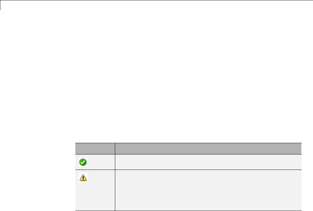
20 Performance Advisor
Fix a Warning
The top of the Analysis Result section displays text that describes actions
that Performance Advisor suggests. Based on your settings in the Input
Parameters section.
•If you set the Take action based on advice parameter to automatically,
Performance Advisor has made the recommended changes for you.
•If you set the Take action based on advice parameter to manually,you
can perform the change yourself, or have Performance Advisor make the
change for you by clicking the Modify button.
The bottom part of the Analysis Result section contains a table that lists the
results of the checks.
Severity Description
The model setting is optimal.
The model setting is suboptimal. You can choose to fix
the reported issue, or move on to the next check. For best
performance, make the recommended change. For more
information on why a specific check does not pass, see the
check documentation.
For a description of the actions that Performance Advisor takes, see “Review
the Actions Taken” on page 20-16.
Review the Actions Taken
The Action Result section contains a summary of the actions that Performance
Advisor took based on Input Parameters setting. If the tool also performed
validation actions, this section lists the results in a summary table.
20-16
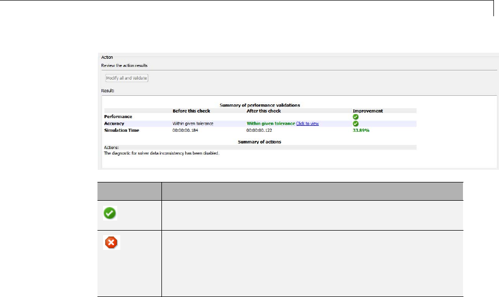
Consult the Performance Advisor
Severity Description
The actions succeeded. The tableliststhepercentageof
improvement.
The actions failed. For example, if Performance Advisor
cannot make a recommended change, it flags this as failed. It
also flags a check as failed if performance was not improved
and reinstates the model to the settings it had before the
check was run.
Save Your Model
Performance Advisor does not automatically save your model after it makes
changes. When you are satisfied with the changes to your model from
Performance Advisor, save the model.
Performance Advisor Limitations
When you use the Performance Advisor to check systems, the following
limitations apply:
•If you rename a system, you must restart the Performance Advisor to check
that system.
•Use Performance Advisor on top models. Performance Advisor does not
traverse referenced models or library links.
•Remember to save your model after Performance Advisor makes changes to
the model. Performance Advisor does not save the model.
20-17

20 Performance Advisor
For limitations that apply to specific checks, see the Limitations section
within the documentation of each check.
20-18

21
Simulink Debugger
•“Introduction to the Debugger” on page 21-2
•“Debugger Graphical User Interface” on page 21-3
•“Debugger Command-Line Interface” on page 21-10
•“Debugger Online Help” on page 21-12
•“Start the Simulink Debugger” on page 21-13
•“Start a Simulation” on page 21-15
•“Run a Simulation Step by Step” on page 21-17
•“Set Breakpoints” on page 21-22
•“Display Information About the Simulation” on page 21-28
•“Display Information About the Model” on page 21-33

21 Simulink®Debugger
Introduction to the Debugger
With the debugger, you run your simulation method by method. You can
stop after each method to examine the execution results. In this way, you
can pinpoint problems in your model to specific blocks, parameters, or
interconnections.
Note Methods are functions that the Simulink software uses to solve a model
at each time step during the simulation. Blocks are made up of multiple
methods. “Block execution” in this documentation is shorthand for “block
methods execution.” Block diagram execution is a multi-step operation that
requires execution of the different block methods in all the blocks in a diagram
at various points during the process of solving a model at each time step
during simulation, as specified by the simulation loop.
The debugger has both a graphical and a command-line user interface. The
graphical interface allows you to access the most commonly used features
of the debugger. The command-line interface gives you access to all of the
capabilitiesinthedebugger. Ifyoucanuseeithertoperformatask,the
documentation shows you first how to use the graphical interface, then the
command-line interface.
21-2
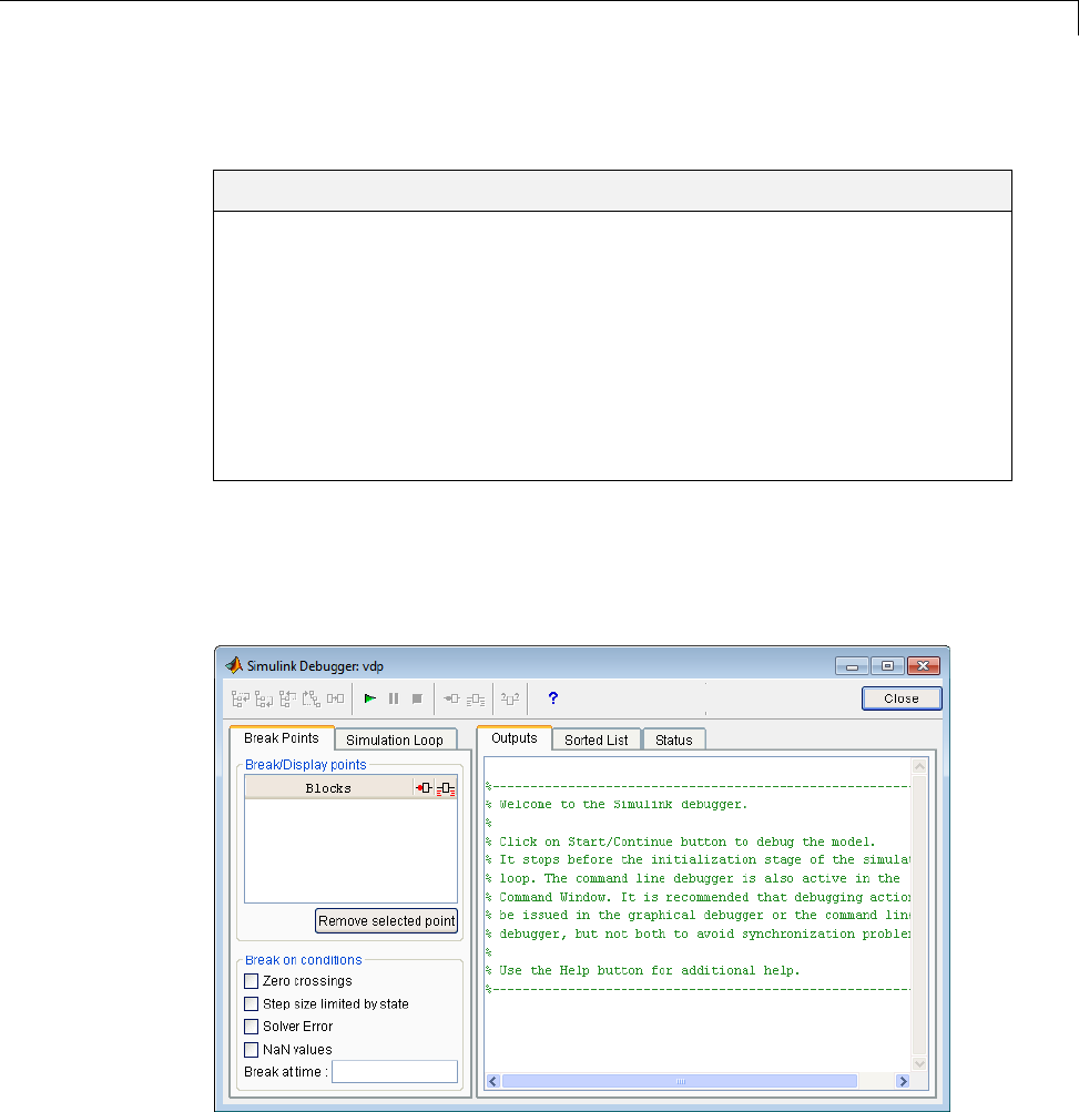
Debugger Graphical User Interface
Debugger Graphical User Interface
In this section...
“Displaying the Graphical Interface” on page 21-3
“Toolbar” on page 21-4
“Breakpoints Pane” on page 21-5
“Simulation Loop Pane” on page 21-6
“Outputs Pane” on page 21-7
“Sorted List Pane” on page 21-8
“Status Pane” on page 21-9
Displaying the Graphical Interface
Select Debug Model from a model window Simulation > Debug menu to
display the debugger graphical interface.
21-3
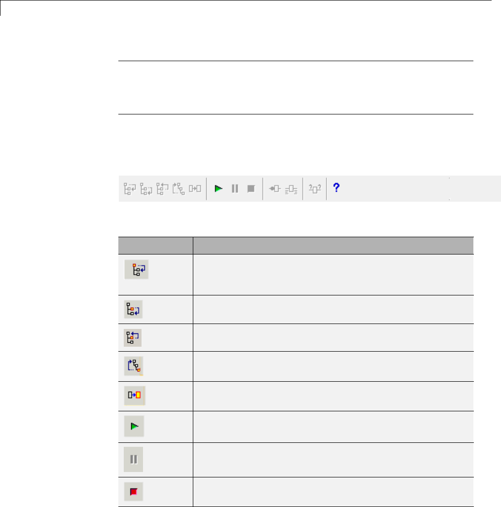
21 Simulink®Debugger
Note The debugger graphical user interface does not display state or solver
information. The command line interface does provide this information. See
“Display System States” on page 21-31 and “Display Solver Information” on
page 21-32.
Toolbar
The debugger toolbar appears at the top of the debugger window.
From left to right, the toolbar contains the following command buttons:
Button Purpose
Step into the next method (see “Stepping Commands” on
page 21-19 for more information on this command, and the
following stepping commands).
Step over the next method.
Step out of the current method.
Step to the first method at the start of next time step.
Step to the next block method.
Start or continue the simulation.
Pause the simulation.
Stop the simulation.
21-4
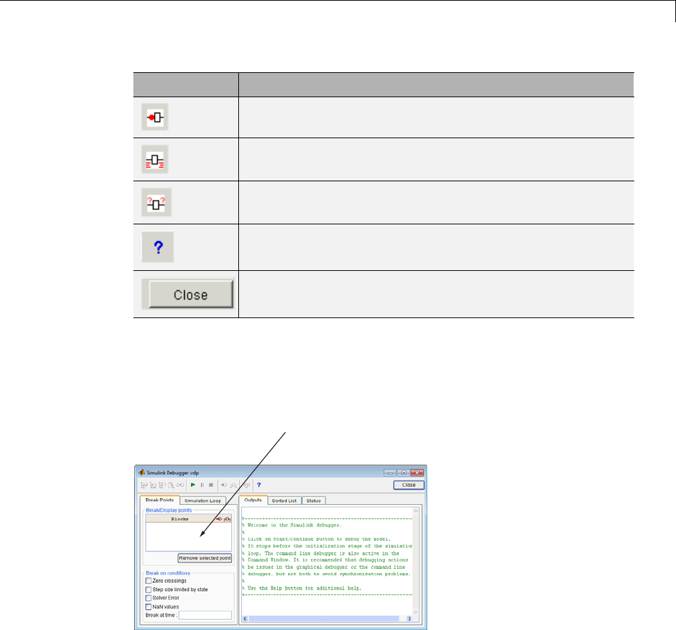
Debugger Graphical User Interface
Button Purpose
Break before the selected block.
Display inputs and outputs of the selected block when
executed (same as trace gcb).
Display the current inputs and outputs of selected block
(same as probe gcb).
Display help for the debugger.
Close the debugger.
Breakpoints Pane
To display the Breakpoints pane, select the Break Points tab on the
debugger window.
Breakpoint pane
The Breakpoints pane allows you to specify block methods or conditions at
which to stop a simulation. See “Set Breakpoints” on page 21-22 for more
information.
21-5
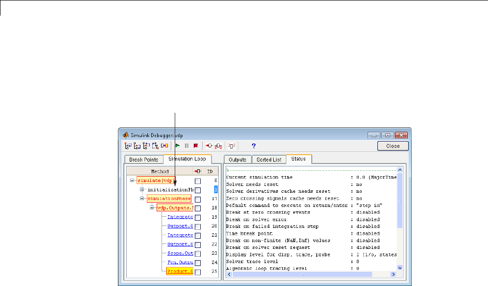
21 Simulink®Debugger
Simulation Loop Pane
To display the Simulation Loop pane, select the Simulation Loop tab on
the debugger window.
Simulation loop pane
The Simulation Loop pane contains three columns:
•Method
•Breakpoints
•ID
Method Column
The Method column lists the methods that have been called thus far in the
simulation as a method tree with expandable/collapsible nodes. Each node
of the tree represents a method that calls other methods. Expanding a node
shows the methods that the block method calls. Clicking a block method name
highlights the corresponding block in the model diagram.
Whenever the simulation stops, the debugger highlights the name of the
method where the simulation has stopped as well as the methods that invoked
it. The highlighted method names indicate the current state of the method
call stack.
21-6
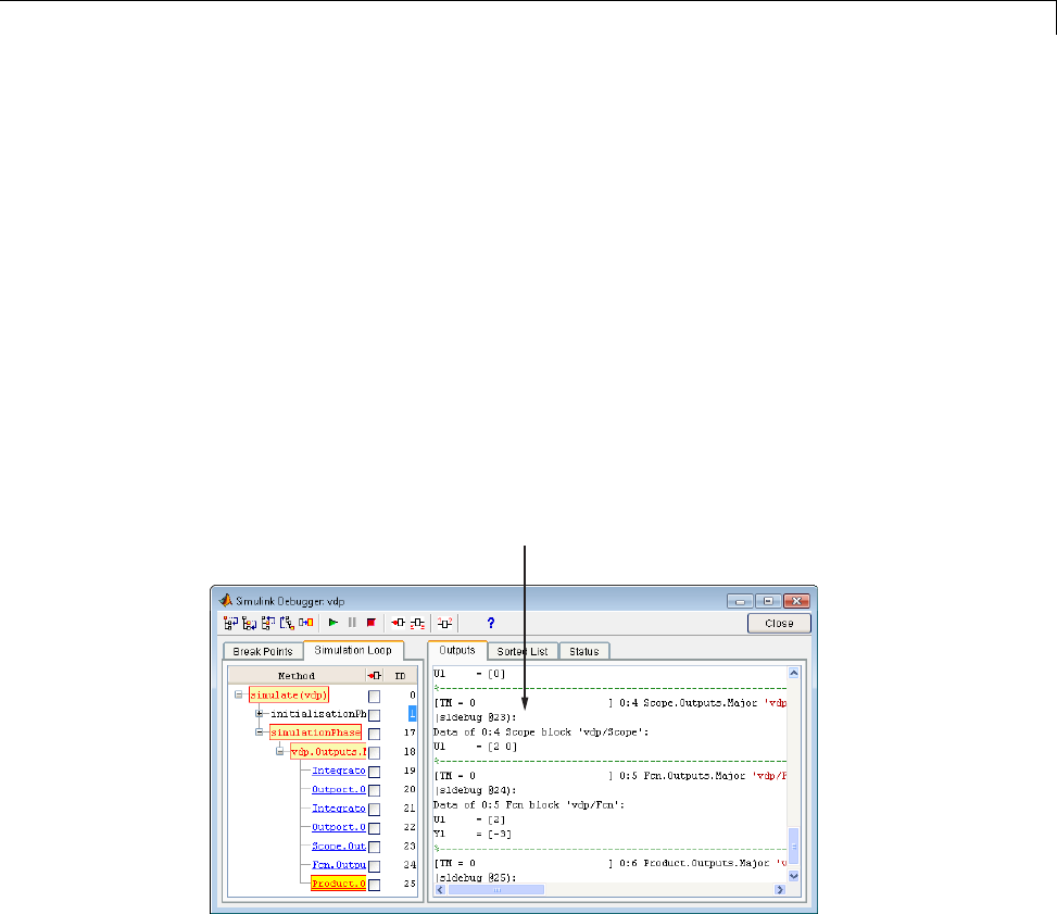
Debugger Graphical User Interface
Breakpoints Column
The breakpoints column consists of check boxes. Selecting a check box sets a
breakpoint at the method whose name appears to the left of the check box.
See “Setting Breakpoints from the Simulation Loop Pane” on page 21-24
for more information.
ID Column
The ID column lists the IDs of the methods listed in the Methods column.
See “Method ID” on page 21-10 for more information.
Outputs Pane
To display the Outputs pane, select the Outputs tab on the debugger
window.
Output pane
The Outputs pane displays the same debugger output that would appear in the
MATLAB command window if the debugger were running in command-line
mode. The output includes the debugger command prompt and the inputs,
outputs, and states of the block at whose method the simulation is currently
paused (see “Block Data Output” on page 21-18). The command prompt
displays current simulation time and the name and index of the method in
which the debugger is currently stopped (see “Block ID” on page 21-10).
21-7
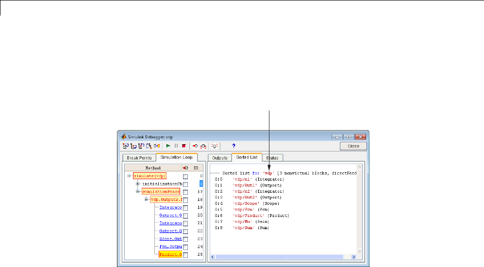
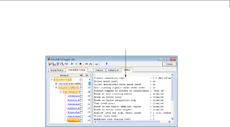
Debugger Graphical User Interface
Status Pane
To display the Status pane, select the Status tab on the debugger window.
Status pane
The Status pane displays the values of various debugger options and other
status information.
21-9

21 Simulink®Debugger
Debugger Command-Line Interface
In this section...
“Controlling the Debugger” on page 21-10
“Method ID” on page 21-10
“Block ID” on page 21-10
“Accessing the MATLAB Workspace” on page 21-11
Controlling the Debugger
In command-line mode, you control the debugger by entering commands at the
debugger command line in the MATLAB Command Window. The debugger
accepts abbreviations for debugger commands. See sldebug to access a list of
command abbreviations and repeatable commands.
Note You can repeat some commands by entering an empty command (i.e.,
by pressing the Enter key) at the command line.
Method ID
Some of the Simulink software commands and messages use method IDs
to refer to methods. A method ID is an integer assigned to a method the
first time the method is invoked. The debugger assigns method indexes
sequentially, starting with 0.
Block ID
Some of the debugger commands and messages use block IDs to refer to
blocks. Block IDs are assigned to blocks while generating the model’s sorted
lists during the compilation phase of the simulation. A block ID has the form
sysIdx:blkIdx,wheresysIdx is an integer identifying the system that
contains the block (either the root system or a nonvirtual subsystem) and
blkIdx is the position of the block in the system’s sorted list. For example,
the block ID0:1 refers to the first block in the model’s root system. The slist
command shows the block ID for each debugged block in the model.
21-10

Debugger Command-Line Interface
Accessing the MATLAB Workspace
You can enter any MATLAB expression at the sldebug prompt. For example,
suppose you are at a breakpoint and you are logging time and output of your
model as tout andyout. The following command creates a plot.
(sldebug ...) plot(tout, yout)
You cannot display the value of a workspace variable whose name is partially
or entirely the same as that of a debugger command by entering it at the
debugger command prompt. You can, however, use the eval command to
work around this problem. For example, use eval('s') to determine the
value of srather then s(tep) the simulation.
21-11
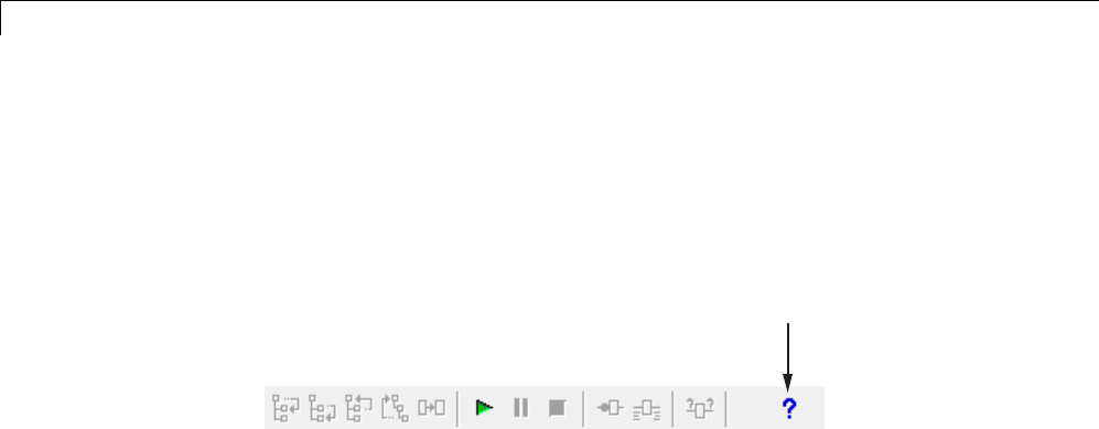
21 Simulink®Debugger
Debugger Online Help
You can get online help on using the debugger by clicking the Help button on
the debugger toolbar. Clicking the Help button displays help for the debugger
in the MATLAB product Help browser.
Help button
In command-line mode, you can get a brief description of the debugger
commands by typing help at the debug prompt.
21-12

Start the Simulink®Debugger
Start the Simulink Debugger
You can start the debugger from either a Simulink model window or from the
MATLAB Command Window.
In this section...
“Starting from a Model Window” on page 21-13
“Starting from the Command Window” on page 21-13
Starting from a Model Window
1In a model window, select Simulation>Debug>DebugModel>.
The debugger graphical user interface opens. See “Debugger Graphical
User Interface” on page 21-3.
2Continue selecting toolbar buttons.
Note When running the debugger in graphical user interface (GUI) mode,
you must explicitly start the simulation. For more information, see“Start a
Simulation” on page 21-15.
Starting from the Command Window
1In the MATLAB Command Window, enter either
•the sim command. For example, enter
sim('vdp', 'StopTime', '10', 'debug', 'on')
•or the sldebug command. For example, enter
sldebug 'vdp'
In both cases, the example model vdp loads into memory, starts the
simulation, and stops the simulation at the first block in the model
execution list.
21-13

21 Simulink®Debugger
2Continue entering debugger commands.
21-14
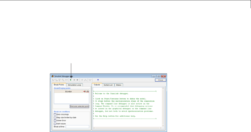
Start a Simulation
Start a Simulation
To start the simulation, click the Start/Continue button on the debugger
toolbar.
Start/Continue button
The simulation starts and stops at the first simulation method that is to be
executed. It displays the name of the method in its Simulation Loop pane.
At this point, you can
•Set breakpoints.
•Run the simulation step by step.
•Continue the simulation to the next breakpoint or end.
•Examine data.
•Perform other debugging tasks.
21-15
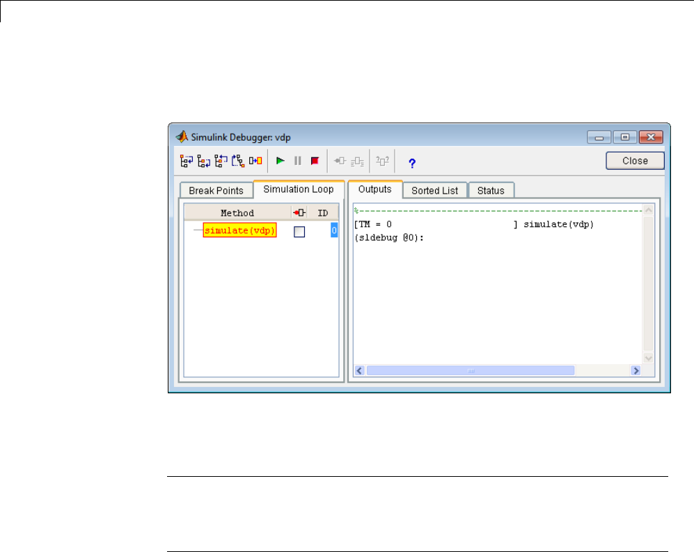
21 Simulink®Debugger
The debugger displays the name of the method in the Simulation Loop pane,
as shown in the following figure:
The following sections explain how to use the debugger controls to perform
these debugging tasks.
Note When you start the debugger in GUI mode, the debugger command-line
interface is also active in the MATLAB Command Window. However, to
prevent synchronization errors between the graphical and command-line
interfaces, you should avoid using the command-line interface.
21-16

Run a Simulation Step by Step
Run a Simulation Step by Step
In this section...
“Introduction” on page 21-17
“Block Data Output” on page 21-18
“Stepping Commands” on page 21-19
“Continuing a Simulation” on page 21-20
“Running a Simulation Nonstop” on page 21-20
Introduction
The debugger provides various commands that let you advance a simulation
from the method where it is currently suspended (the next method) by various
increments (see “Stepping Commands” on page 21-19). For example, you
can advance the simulation
•Into or over the next method
•Out of the current method
•To the top of the simulation loop.
After each advance, the debugger displays information that enables you to
determine the point to which the simulation has advanced and the results of
advancing the simulation to that point.
For example, in GUI mode, after each step command, the debugger highlights
the current method call stack in the Simulation Loop pane. The call stack
comprises the next method and the methods that invoked the next method
either directly or indirectly. The debugger highlights the call stack by
highlighting the names of the methods that make up the call stack in the
Simulation Loop pane.
21-17
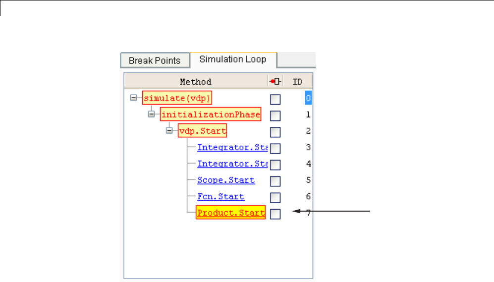
21 Simulink®Debugger
Next method
In command-line mode, you can use the where command to display the
method call stack.
Block Data Output
After executing a block method, the debugger prints any or all of the following
block data in the debugger Output panel (in GUI mode) or, if in command
line mode, the MATLAB Command Window:
•Un = v
where vis the current value of the block’s nth input.
•Yn = v
where visthecurrentvalueoftheblock’snth output.
•CSTATE = v
where vis the value of the block’s continuous state vector.
•DSTATE = v
21-18
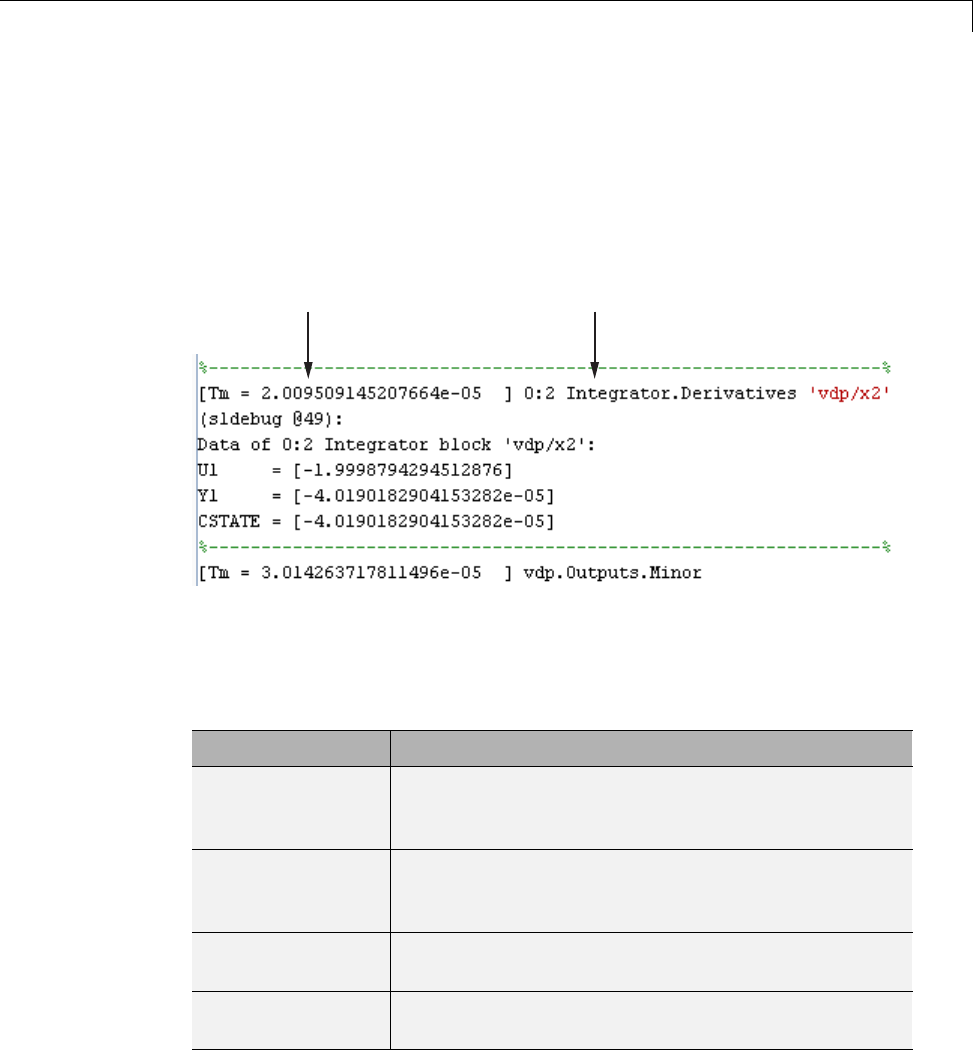
Run a Simulation Step by Step
where vis the value of the block’s discrete state vector.
The debugger also displays the current time, the ID and name of the next
method to be executed, and the name of the block to which the method applies
in the MATLAB Command Window. The following example illustrates typical
debugger outputs after a step command.
Current time Next method
Stepping Commands
Command-line mode provides the following commands for advancing a
simulation incrementally:
This command... Advances the simulation...
step [in into] Into the next method, stopping at the first method
in the next method or, if the next method does not
contain any methods, at the end of the next method
step over To the method that follows the next method, executing
all methods invoked directly or indirectly by the next
method
step out To the end of the current method, executing any
remaining methods invoked by the current method
step top To the first method of the next time step (i.e., the top
of the simulation loop)
21-19
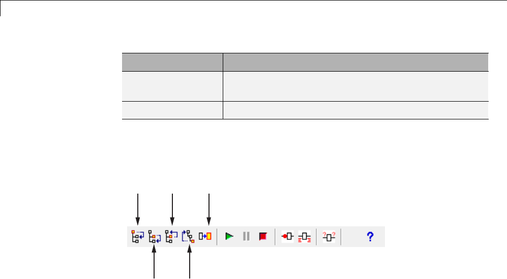
21 Simulink®Debugger
This command... Advances the simulation...
step blockmth To the next block method to be executed, executing all
intervening model- and system-level methods
next Same as step over
Buttons in the debugger toolbar allowyoutoaccessthesecommandsinGUI
mode.
Step
Step
out
Next block
method
Step
over
Step
top
Clicking a button has the same effect as entering the corresponding command
at the debugger command line.
Continuing a Simulation
In GUI mode, the Stop button turns red when the debugger suspends
the simulation for any reason. To continue the simulation, click the
Start/Continue button. In command-line mode, enter continue to continue
the simulation. By default, the debugger runs the simulation to the next
breakpoint (see “Set Breakpoints” on page 21-22) or to the end of the
simulation, whichever comes first.
Running a Simulation Nonstop
The run command lets you run a simulation to the end of the simulation,
skipping any intervening breakpoints. At the end of the simulation, the
debugger returns you to the command line. To continue debugging a model,
you must restart the debugger.
21-20

Run a Simulation Step by Step
Note The GUI mode does not provide a graphical version of the run command.
To run the simulation to the end, you must first clear all breakpoints and
then click the Start/Continue button.
21-21

21 Simulink®Debugger
Set Breakpoints
In this section...
“About Breakpoints” on page 21-22
“Setting Unconditional Breakpoints” on page 21-22
“Setting Conditional Breakpoints” on page 21-25
About Breakpoints
The debugger allows you to define stopping points called breakpoints in a
simulation. You can then run a simulation from breakpoint to breakpoint,
using the debugger continue command. The debugger lets you define two
types of breakpoints: unconditional and conditional. An unconditional
breakpoint occurs whenever a simulation reaches a method that you specified
previously. A conditional breakpoint occurs when a condition that you
specified in advance arises in the simulation.
Breakpoints are useful when you know that a problem occurs at a certain
point in your program or when a certain condition occurs. By defining
an appropriate breakpoint and running the simulation via the continue
command, you can skip immediately to the point in the simulation where the
problem occurs.
Setting Unconditional Breakpoints
You can set unconditional breakpoints from the:
•Debugger toolbar
•Simulation Loop pane
•MATLAB product Command Window (command-line mode only)
Setting Breakpoints from the Debugger Toolbar
To set a breakpoint on a block’s methods, select the block and then click
the Breakpoint button on the debugger toolbar. If you set a break point
on a block, the debugger stops at any method that the execution reaches in
the block.
21-22
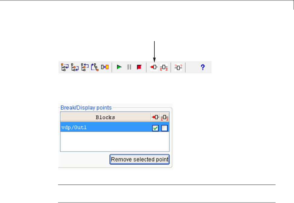
Set Breakpoints
Breakpoint
The debugger displays the name of the selected block in the Break/Display
points panel of the Breakpoints pane.
Note Clicking the Breakpoint button on the toolbar sets breakpoints on the
invocations of a block’s methods in major time steps.
You can temporarily disable the breakpoints on a block by deselecting the
checkboxinthebreakpointscolumnofthepanel.Toclearthebreakpointson
a block and remove its entry from the panel,
1Select the entry.
2Click the Remove selected point buttononthepanel.
21-23
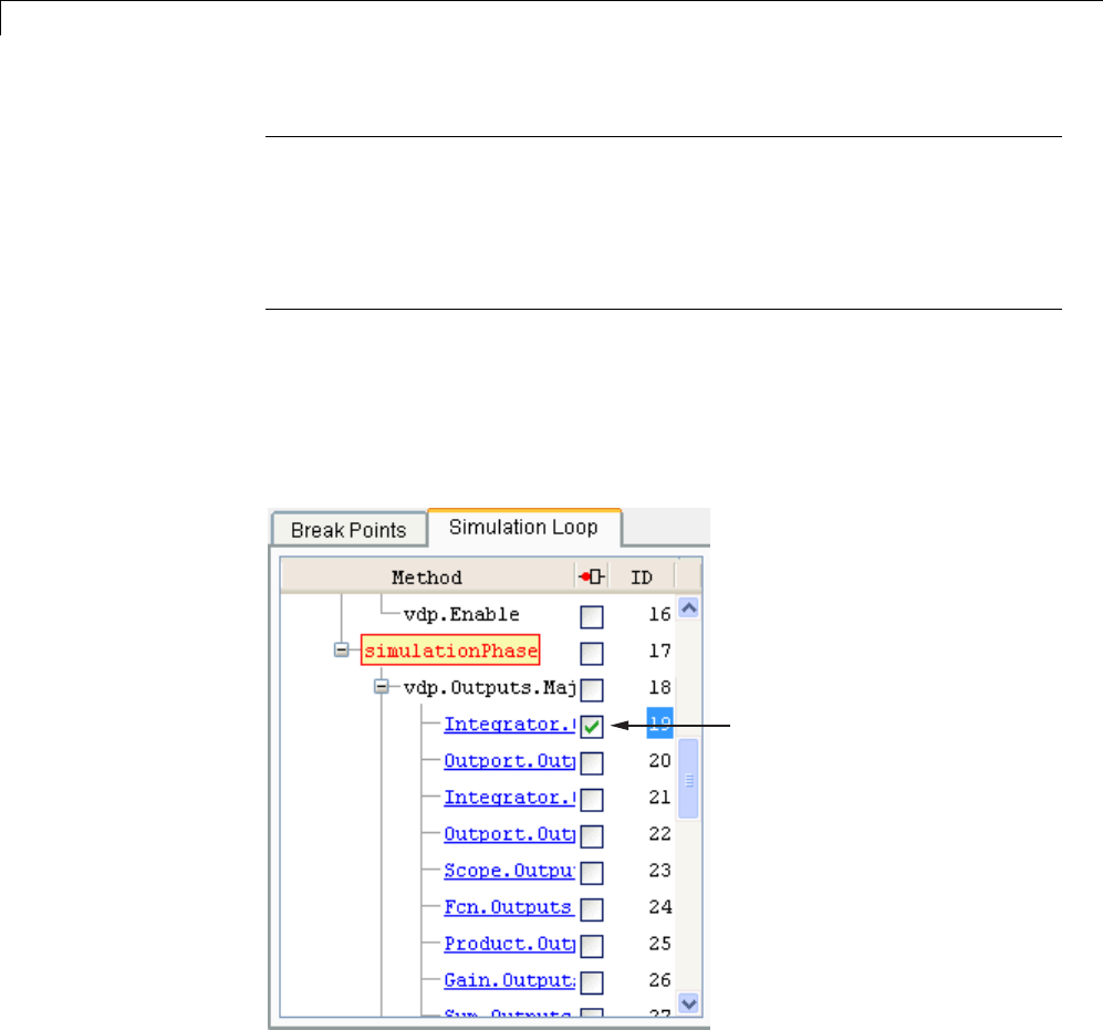
21 Simulink®Debugger
Note Youcannotsetabreakpointonavirtual block. A virtual block is
purely graphical: it indicates a grouping or relationship among a model’s
computational blocks. The debugger warns you if you try to set a breakpoint
on a virtual block. You can get a listing of a model’s nonvirtual blocks, using
the slist command (see “Displaying a Model’s Nonvirtual Blocks” on page
21-35).
Setting Breakpoints from the Simulation Loop Pane
To set a breakpoint at a particular invocation of a method displayed in the
Simulation Loop pane, select the check box next to the method’s name in
the breakpoint column of the pane.
Breakpoint
To clear the breakpoint, deselect the check box.
21-24
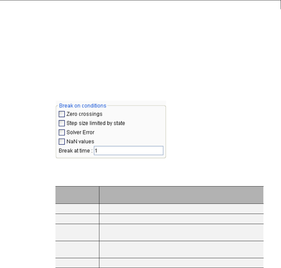
Set Breakpoints
Setting Breakpoints from the Command Window
In command-line mode, use the break and bafter commands to set
breakpoints before or after a specified method, respectively. Use the clear
command to clear breakpoints.
Setting Conditional Breakpoints
You can use either the Break on conditions controls group on the debugger
Breakpoints pane
or the following commands (in command-line mode) to set conditional
breakpoints.
This
command... Causes the Simulation to Stop...
tbreak [t] At a simulation time step
ebreak At a recoverable error in the model
nanbreak At the occurrence of an underflow or overflow (NaN)or
infinite (Inf)value
xbreak When the simulation reaches the state that determines
the simulation step size
zcbreak When a zero crossing occurs between simulation time steps
Setting Breakpoints at Time Steps
To set a breakpoint at a time step, enter a time in the debugger Break at
time field (GUI mode) or enter the time using the tbreak command. This
21-25

21 Simulink®Debugger
causes the debugger to stop the simulation at the Outputs.Major method of
the model at the first time step that follows the specified time. For example,
starting vdp in debug mode and entering the commands
tbreak 2
continue
causes the debugger to halt the simulation at the vdp.Outputs.Major method
of time step 2.078 as indicated by the output of the continue command.
%----------------------------------------------------------------%
[Tm = 2.034340153847549 ] vdp.Outputs.Minor
(sldebug @37):
Breaking on Nonfinite Values
Selecting the debugger NaN values option or entering the nanbreak
command causes the simulation to stop when a computed value is infinite or
outside the range of values that is supported by the machine running the
simulation. Thisoptionisusefulforpinpointing computational errors in
a model.
Breaking on Step-Size Limiting Steps
Selecting the Step size limited by state option or entering the xbreak
command causes the debugger to stop the simulation when the model uses a
variable-step solver and the solver encounters a state that limits the size of
the steps that it can take. This command is useful in debugging models that
appear to require an excessive number of simulation time steps to solve.
Breaking at Zero Crossings
Selecting the Zero crossings option or entering the zcbreak command
causes the simulation to halt when a nonsampled zero crossing is detected in
a model that includes blocks where zero crossings can arise. After halting,
the ID, type, and name of the block in which the zero crossing was detected is
displayed. The block ID (s:b:p) consists of a system index s, block index b,
and port index pseparated by colons (see “Block ID” on page 21-10).
21-26

Set Breakpoints
For example, setting a zero-crossing break at the start of execution of the
zeroxing example model,
>> sldebug zeroxing
%--------------------------------------------------------------
%
[TM = 0 ] zeroxing.Simulate
(sldebug @0): >> zcbreak
Break at zero crossing events : enabled
and continuing the simulation
(sldebug @0): >> continue
results in a zero-crossing break at
Interrupting model execution before running mdlOutputs at the left post of
(major time step just before) zero crossing event detected at the following location:
6[-0] 0:5:2 Saturate 'zeroxing/Saturation'
%----------------------------------------------------------------%
[TzL= 0.3435011087932808 ] zeroxing.Outputs.Major
(sldebug @16): >>
If a model does not include blocks capable of producing nonsampled zero
crossings, the command prints a message advising you of this fact.
Breaking on Solver Errors
Selecting the debugger Solver Errors option or entering the ebreak
command causes the simulation to stop if the solver detects a recoverable error
in the model. If you do not set or disable this breakpoint, the solver recovers
from the error and proceeds with the simulation without notifying you.
21-27
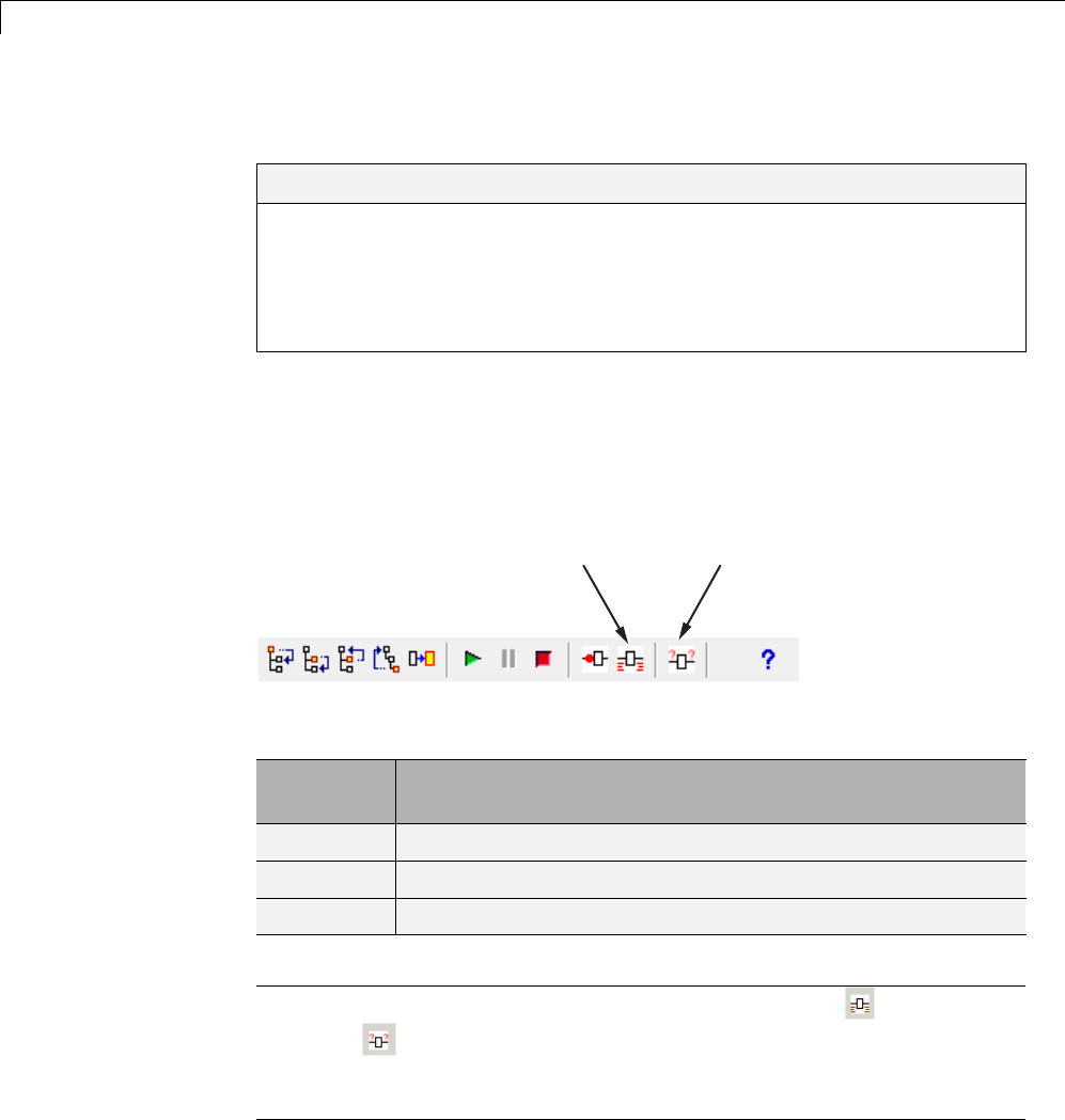
21 Simulink®Debugger
Display Information About the Simulation
In this section...
“Display Block I/O” on page 21-28
“Display Algebraic Loop Information” on page 21-30
“Display System States” on page 21-31
“Display Solver Information” on page 21-32
Display Block I/O
The debugger allows you to display block I/O by clicking the appropriate
buttons on the debugger toolbar
Watch
block I/O
Display
block I/O
or by entering the appropriate debugger command.
This
command... Displays a Blocks I/O...
probe Immediately
disp At every breakpoint any time execution stops
trace Whenever the block executes
Note The two debugger toolbar buttons, Watch Block I/O ( )andDisplay
Block I/O ( ) correspond, respectively, to trace gcb and probe gcb.The
probe and disp commands do not have a one-to-one correspondence with
the debugger toolbar buttons.
21-28

Display Information About the Simulation
Displaying I/O of a Selected Block
To display the I/O of a block, select the block and click in GUI mode or
enter the probe command in command-line mode. In the following table,
the probe gcb command has a corresponding toolbar button. The other
commands do not.
Command Description
probe Enter or exit probe mode. Typing any command causes
the debugger to exit probe mode.
probe gcb Display I/O of selected block. Same as .
probe s:b Print the I/O of the block specified by system number s
and block number b.
The debugger prints the current inputs, outputs, and states of the selected
block in the debugger Outputs pane (GUI mode) or the Command Window of
the MATLAB product.
The probe command is useful when you need to examine the I/O of a block
whose I/O is not otherwise displayed. For example, suppose you are using the
step command to run a model method by method. Each time you step the
simulation, the debugger displays the inputs and outputs of the current block.
The probe command lets you examine the I/O of other blocks as well.
Displaying Block I/O Automatically at Breakpoints
The disp command causes the debugger to display a specified block’s inputs
and outputs whenever it halts the simulation. You can specify a block by
entering its block index and entering gcb as the disp command argument.
You can remove any block from the debugger list of display points, using the
undisp command. For example, to remove block 0:0,enterundisp 0:0.
Note Automatic display of block I/O at breakpoints is not available in the
debugger GUI mode.
21-29

21 Simulink®Debugger
The disp command is useful when you need to monitor the I/O of a specific
block or set of blocks as you step through a simulation. Using the disp
command, you can specify the blocks you want to monitor and the debugger
will then redisplay the I/O of those blocks on every step. Note that the
debugger always displays the I/O of the current block when you step through
a model block by block, using the step command. You do not need to use the
disp command if you are interested in watching only the I/O of the current
block.
Watching Block I/O
To watch a block, select the block and click inthedebuggertoolbaror
enter the trace command. In GUI mode, if a breakpoint exists on the block,
you can set a watch on it as well by selecting the check box for the block in
the watch column of the Break/Display points pane. In command-line
mode, you can also specify the block by specifying its block index in the trace
command. You can remove a block from the debugger list of trace points
using the untrace command.
The debugger displays a watched block’s I/O whenever the block executes.
Watching a block allows you obtain a complete record of the block’s I/O
without having to stop the simulation.
Display Algebraic Loop Information
The atrace command causes the debugger to display information about a
model’s algebraic loops (see “Algebraic Loops” on page 3-39) each time they
are solved. The command takes a single argument that specifies the amount
of information to display.
This
command... Displays for each algebraic loop...
atrace 0 No information
atrace 1 The loop variable solution, the number of iterations
required to solve the loop, and the estimated solution error
atrace 2 Same as level 1
atrace 3 Level 2 plus the Jacobian matrix used to solve the loop
atrace 4 Level 3 plus intermediate solutions of the loop variable
21-30

Display Information About the Simulation
Display System States
The states debug command lists the current values of the system states in
the MATLAB Command Window. For example, the following sequence of
commands shows the states of the bouncing ball example (sldemo_bounce)
after its first, second, and third time steps. However, before entering the
debugger, open the Configuration Parameters dialog box, clear the Block
reduction check box on the Optimization pane, and clear the Signal storage
reuse check box on the Optimization > Signals and Parameters pane.
sldebug sldemo_bounce
%----------------------------------------------------------------%
[TM = 0 ] simulate(sldemo_bounce)
(sldebug @0): >> step top
%----------------------------------------------------------------%
[TM = 0 ] sldemo_bounce.Outputs.Major
(sldebug @16): >> next
%----------------------------------------------------------------%
[TM = 0 ] sldemo_bounce.Update
(sldebug @23): >> states
Continuous States:
Idx Value (system:block:element Name 'BlockName')
0 10 (0:4:0 CSTATE 'sldemo_bounce/Second-Order Integrator')
1. 15 (0:4:1)
(sldebug @23): >> next
%----------------------------------------------------------------%
[Tm = 0 ] solverPhase
(sldebug @26): >> states
Continuous States:
Idx Value (system:block:element Name 'BlockName')
0 10 (0:4:0 CSTATE 'sldemo_bounce/Second-Order Integrator')
1. 15 (0:4:1)
(sldebug @26): >> next
%----------------------------------------------------------------%
[TM = 0.01 ] sldemo_bounce.Outputs.Major
(sldebug @16): >> states
21-31

21 Simulink®Debugger
Continuous States:
Idx Value (system:block:element Name 'BlockName')
0 10.1495095 (0:4:0 CSTATE 'sldemo_bounce/Second-Order Integrator')
1. 14.9019 (0:4:1)
Display Solver Information
The strace command allows you to pinpoint problems in solving a models
differential equations that can slow down simulation performance. Executing
this command causes the debugger to display solver-related information at
the command line of the MATLAB product when you run or step through
a simulation. The information includes the sizes of the steps taken by the
solver, the estimated integration error resulting from the step size, whether
a step size succeeded (i.e., met the accuracy requirements that the model
specifies), the times at which solver resets occur, etc. If you are concerned
about the time required to simulate your model, this information can help you
to decide whether the solver you have chosen is the culprit and hence whether
choosing another solver might shorten the time required to solve the model.
21-32

Display Information About the Model
Display Information About the Model
In this section...
“Display Model’s Sorted Lists” on page 21-33
“Display a Block” on page 21-34
Display Model’s Sorted Lists
In GUI mode, the debugger Sorted List pane displays lists of blocks for
a models root system and each nonvirtual subsystem. Each list lists the
blocks that the subsystems contains sorted according to their computational
dependencies, alphabetical order, and other block sorting rules. In
command-line mode, you can use the slist command to display a model’s
sorted lists.
---- Sorted list for 'vdp' [9 nonvirtual blocks, directFeed=0]
0:0 'vdp/x1' (Integrator)
0:1 'vdp/Out1' (Outport)
0:2 'vdp/x2' (Integrator)
0:3 'vdp/Out2' (Outport)
0:4 'vdp/Scope' (Scope)
0:5 'vdp/Fcn' (Fcn)
0:6 'vdp/Product' (Product)
0:7 'vdp/Mu' (Gain)
0:8 'vdp/Sum' (Sum)
These displays include the block index for each command. You can use them
to determine the block IDs of the models blocks. Some debugger commands
accept block IDs as arguments.
Identifying Blocks in Algebraic Loops
If a block belongs to an algebraic list, the slist command displays an
algebraic loop identifier in the entry for the block in the sorted list. The
identifier has the form
algId=s#n
21-33

21 Simulink®Debugger
where sis the index of the subsystem containing the algebraic loop and nis
the index of the algebraic loop in the subsystem. For example, the following
entry for an Integrator block indicates that it participates in the first algebraic
loop at the root level of the model.
0:1 'test/ss/I1' (Integrator, tid=0) [algId=0#1, discontinuity]
You can use the debugger ashow command to highlight the blocks and lines
that make up an algebraic loop. See “Displaying Algebraic Loops” on page
21-36 for more information.
Display a Block
To determine the block in a models diagram that corresponds to a particular
index, enter bshow s:b at the command prompt, where s:b is the block index.
The bshow command opens the system containing the block (if necessary) and
selects the block in the systems window.
Displaying a Model’s Nonvirtual Systems
The systems command displays a list of the nonvirtual systems in the model
that you are debugging. For example, the sldemo_clutch) model contains
the following systems:
open_system('sldemo_clutch')
set_param(gcs, 'OptimizeBlockIOStorage','off')
sldebug sldemo_clutch
(sldebug @0): %----------------------------------------------------------------%
[TM = 0 ] simulate(sldemo_clutch)
(sldebug @0): >> systems
0 'sldemo_clutch'
1 'sldemo_clutch/Locked'
2 'sldemo_clutch/Unlocked'
21-34

Display Information About the Model
Note The systems command does not list subsystems that are purely
graphical. That is, subsystems that the model diagram represents as
Subsystem blocks but that are solved as part of a parent system. are
not listed. In Simulink models, the root system and triggered or enabled
subsystems are true systems. All other subsystems are virtual (that is,
graphical) and do not appear in the listing from the systems command.
Displaying a Model’s Nonvirtual Blocks
The slist command displays a list of the nonvirtual blocks in a model. The
listing groups the blocks by system. For example, the following sequence of
commands produces a list of the nonvirtual blocks in the Van der Pol (vdp)
example model.
sldebug vdp
%----------------------------------------------------------------%
[TM = 0 ] simulate(vdp)
sldebug @0): >> slist
---- Sorted list for 'vdp' [9 nonvirtual blocks, directFeed=0]
0:0 'vdp/x1' (Integrator)
0:1 'vdp/Out1' (Outport)
0:2 'vdp/x2' (Integrator)
0:3 'vdp/Out2' (Outport)
0:4 'vdp/Scope' (Scope)
0:5 'vdp/Fcn' (Fcn)
0:6 'vdp/Product' (Product)
0:7 'vdp/Mu' (Gain)
0:8 'vdp/Sum' (Sum)
Note The slist command does not list blocks that are purely graphical.
That is, blocks that indicate relationships between or groupings among
computational blocks.
21-35

21 Simulink®Debugger
Displaying Blocks with Potential Zero Crossings
The zclist command displays a list of blocks in which nonsampled zero
crossings can occur during a simulation. For example, zclist displays the
following list for the clutch sample model:
(sldebug @0): >> zclist
0 0:4:0 F HitCross 'sldemo_clutch/Friction Mode Logic/Lockup
Detection/Velocities Match'
1 0:4:1 F
2 0:10:0 F Abs 'sldemo_clutch/Friction Mode Logic/Lockup
Detection/Required Friction for Lockup/Abs'
3 0:12:0 F RelationalOperator 'sldemo_clutch/Friction Mode
Logic/Lockup Detection/Required Friction for Lockup/Relational Operator'
4 0:19:0 F Abs 'sldemo_clutch/Friction Mode Logic/Break Apart
Detection/Abs'
5 0:20:0 F RelationalOperator 'sldemo_clutch/Friction Mode
Logic/Break Apart Detection/Relational Operator'
6 2:3:0 F Signum 'sldemo_clutch/Unlocked/slip direction'
Displaying Algebraic Loops
The ashow command highlights a specified algebraic loop or the algebraic
loop that contains a specified block. To highlight a specified algebraic loop,
enter ashow s#n,wheresis the index of the system (see “Identifying Blocks
in Algebraic Loops” on page 21-33) that contains the loop and nis the index
of the loop in the system. To display the loop that contains the currently
selected block, enter ashow gcb. To show a loop that contains a specified
block, enter ashow s:b,wheres:b is the block’s index. To clear algebraic-loop
highlighting from the model diagram, enter ashow clear.
Displaying Debugger Status
In GUI mode, the debugger displays the settings of various debug options,
such as conditional breakpoints, in its Status panel. In command-line mode,
the status command displays debugger settings. For example, the following
sequence of commands displays the initial debug settings for the vdp model:
sim('vdp', 'StopTime', '10', 'debug', 'on')
%----------------------------------------------------------------%
[TM = 0 ] simulate(vdp)
(sldebug @0): >> status
21-36

Display Information About the Model
%----------------------------------------------------------------%
Current simulation time : 0.0 (MajorTimeStep)
Solver needs reset : no
Solver derivatives cache needs reset : no
Zero crossing signals cache needs reset : no
Default command to execute on return/enter : ""
Break at zero crossing events : disabled
Break on solver error : disabled
Break on failed integration step : disabled
Time break point : disabled
Break on non-finite (NaN,Inf) values : disabled
Break on solver reset request : disabled
Display level for disp, trace, probe : 1 (i/o, states)
Solver trace level : 0
Algebraic loop tracing level : 0
Animation Mode : off
Window reuse : not supported
Execution Mode : Normal
Display level for etrace : 0 (disabled)
Break points : none installed
Display points : none installed
Trace points : none installed
21-37

21 Simulink®Debugger
21-38

22
Accelerating Models
•“What Is Acceleration?” on page 22-2
•“How Acceleration Modes Work” on page 22-3
•“Code Regeneration in Accelerated Models” on page 22-7
•“Choosing a Simulation Mode” on page 22-11
•“Design Your Model for Effective Acceleration” on page 22-16
•“Perform Acceleration” on page 22-22
•“Interact with the Acceleration Modes Programmatically” on page 22-26
•“Run Accelerator Mode with the Simulink Debugger” on page 22-29
•“Capture Performance Data” on page 22-31

22 Accelerating Models
What Is Acceleration?
Acceleration is a mode of operation in the Simulink product that you can use
to speed up the execution of your model. The Simulink software includes two
modes of acceleration: Accelerator mode and the Rapid Accelerator mode.
Both modes replace the normal interpreted code with compiled target code.
Using compiled code speeds up simulation of many models, especially those
where run time is long compared to the time associated with compilation and
checking to see if the target is up to date.
The Accelerator mode works with any model, but performance decreases if a
model contains blocks that do not support acceleration. The Accelerator mode
supports the Simulink debugger and profiler. These tools assist in debugging
and determining relative performance of various parts of your model. For
more information, see “Run Accelerator Mode with the Simulink Debugger”
on page 22-29 and “Capture Performance Data” on page 22-31.
The Rapid Accelerator mode works with only those models containing blocks
that support code generation of a standalone executable. For this reason,
Rapid Accelerator mode does not support the debugger or profiler. However,
this mode generally results in faster execution than the Accelerator mode.
When used with dual-core processors, the Rapid Accelerator mode runs
Simulink and the MATLAB technical computing environment from one core
while the rapid accelerator target runs as a separate process on a second core.
For more information about the performance characteristics of the Accelerator
and Rapid Accelerator modes, and howtomeasurethedifferencein
performance, see “Comparing Performance” on page 19-5.
22-2

How Acceleration Modes Work
How Acceleration Modes Work
In this section...
“Overview” on page 22-3
“Normal Mode” on page 22-3
“Accelerator Mode” on page 22-4
“Rapid Accelerator Mode” on page 22-5
Overview
The Accelerator and Rapid Accelerator modes use portions of the Simulink
Coder product to create an executable. These modes replace the interpreted
code normally used in Simulink simulations, shortening model run time.
Although the acceleration modes use some Simulink Coder code generation
technology, you do not need the Simulink Coder software installed to
accelerate your model.
Note The code generated by the Accelerator and Rapid Accelerator modes is
suitable only for speeding the simulation of your model. You must use the
Simulink Coder product if you want to generate code for other purposes.
Normal Mode
In Normal mode, the MATLAB technical computing environment is the
foundation on which the Simulink software is built. Simulink controls the
solver and model methods used during simulation. Model methods include
such things as computation of model outputs. Normal mode runs in one
process.
22-3

22 Accelerating Models
Model
Methods
Solver
Simulink
MATLAB
One Process
Accelerator Mode
The Accelerator mode generates and links code into a C-MEX S-function.
Simulink uses this acceleration target code to perform the simulation, and the
code remains available for use in later simulations.
Simulink checks that the acceleration target code is up to date before reusing
it. As explained in “Code Regeneration in Accelerated Models” on page 22-7,
the target code regenerates if it is not up to date.
In Accelerator mode, the model methods are separate from the Simulink
software and are part of the Acceleration target code. A C-MEX S-function
API communicates with the Simulink software, and a MEX API communicates
with MATLAB. The target code executes in the same process as MATLAB
and Simulink.
22-4
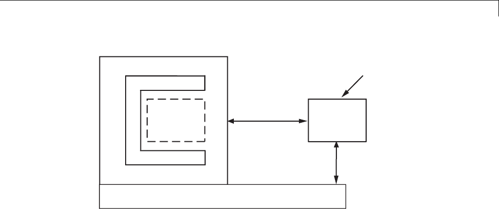
How Acceleration Modes Work
Solver
Simulink
MATLAB
Model
Methods
MEX API
Acceleration
target code
C-MEX
S-function
API
One Process
Rapid Accelerator Mode
The Rapid Accelerator mode creates a Rapid Accelerator standalone executable
from your model. This executable includes the solver and model methods,
but it resides outside of MATLAB and Simulink. It uses External mode (see
“Host/Target Communication”) to communicate with Simulink.
22-5
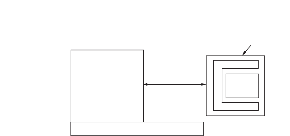
22 Accelerating Models
Simulink
MATLAB
Model
Methods
Solver
External
Mode
One Process Second Process
Rapid Accelerator
Standalone executable
MATLAB and Simulink run in one process, and if a second processing core is
available, the standalone executable runs there.
22-6

Code Regeneration in Accelerated Models
Code Regeneration in Accelerated Models
In this section...
“Structural Changes That Cause Rebuilds” on page 22-7
“Determining If the Simulation Will Rebuild” on page 22-7
Structural Changes That Cause Rebuilds
Changing the structure of your model causes the Rapid Accelerator mode
to regenerate the standalone executable, and for the Accelerator mode to
regenerate the target code and update (overwrite) the existing MEX-file.
Examples of model structure changes that result in a rebuild include:
•Changing the solver type, for example from Variable-step to Fixed-step
•Adding or deleting blocks or connections between blocks
•Changing the values of nontunable block parameters, for example, the
Seed parameter of the Random Number block
•Changing the number of inputs or outputs of blocks, even if the connectivity
is vectorized
•Changing the number of states in the model
•Selecting a different function in the Trigonometric Function block
•Changing signs used in a Sum block
•Adding a Target Language Compiler (TLC) file to inline an S-function
•Changing the sim command output argument when using Rapid
Accelerator mode
•Changing solver parameters such as stop time or rel tol when using
Rapid Accelerator mode
Determining If the Simulation Will Rebuild
The Accelerator and Rapid Accelerator modes use a checksum to determine if
the model has changed, indicating that the code should be regenerated. The
22-7

22 Accelerating Models
checksum is an array of four integers computed using an MD5 checksum
algorithm based on attributes of the model and the blocks it contains.
Use the Simulink.BlockDiagram.getChecksum command to obtain the
checksum for your model. For example:
cs1 = Simulink.BlockDiagram.getChecksum('myModel');
Obtain a second checksum after you have altered your model. The code
regenerates if the new checksum does not match the previous checksum. You
can use the information in the checksum to determine why the simulation
target rebuilt. For a detailed explanation of this procedure, see the example
model slAccelDemoWhyRebuild.
Parameter Handling in Rapid Accelerator Mode
In model rebuilds, Rapid Accelerator Mode handles block diagram and
run-time parameters differently than other parameters. You can change
some block diagram parameters during simulation without causing a rebuild.
These block diagram parameters include the following:
Block Diagram Parameters That Do Not Require Rapid
Accelerator Rebuild
Solver Parameters Loading and Logging Parameters
AbsTol Decimation
ConsecutiveZCsStepRelTol FinalStateName
ExtrapolationOrder InitialState
InitialStep LimitDataPoints
MaxConsecutiveMinStep LoadExternalInput
MaxConsecutiveZCs LoadInitialState
MaxNumMinSteps MaxDataPoints
MaxOrder OutputOption
MaxStep OutputSaveName
MinStep SaveFinalState
22-8

Code Regeneration in Accelerated Models
Block Diagram Parameters That Do Not Require Rapid
Accelerator Rebuild
NumberNwtonIterations SaveFormat
OutputTimes SaveOutput
Refine SaveState
RelTol SaveTime
SolverName SignalLogging
StartTime SignalLoggingName
StopTime StateSaveName
ZCDetectionTol TimeSaveName
For run-time parameters that you change graphically via the block diagram
or programmatically with the set_param command, you will need to
recompile the model. Recompilation might cause parts of the model to rebuild.
Alternatively, you can programmatically change tunable run-time parameters
without rebuilding parts of the model:
1Collect the run-time parameters in a run-time parameter structure
while building a rapid accelerator target executable using the
Simulink.BlockDiagram.buildRapidAcceleratorTarget function.
2To change the parameters, use the
Simulink.BlockDiagram.modifyTunableParameters function.
3To specify the modified parameters to the sim command, use the
RapidAcceleratorParameterSets and RapidAcceleratorUpToDateCheck
parameters.
For more information, see “sim in parfor with Rapid Accelerator Mode” on
page 15-9.
All other parameter changes might necessitate a rebuild of the model.
22-9

22 Accelerating Models
Parameter Changes: Passed Directly to
sim command
Passed Graphically
via Block Diagram
or via set_param
command
Run-time Rebuild not required Rebuild might be
required
Block diagram
(solver and logging
parameters)
Rebuild not required Rebuild not required
Other Rebuild might be
required
Rebuild might be
required
22-10

Choosing a Simulation Mode
Choosing a Simulation Mode
In this section...
“Simulation Mode Tradeoffs” on page 22-11
“Comparing Modes” on page 22-12
“Decision Tree” on page 22-14
Simulation Mode Tradeoffs
In general, you must trade off simulation speed against flexibility when
choosing either Accelerator mode or Rapid Accelerator mode instead of
Normal mode.
Speed
Flexibility
Rapid
Accelerator mode
Normal
mode
Accelerator mode
. Monte Carlo
. Scopes and viewers
(only from menu)
. Tune parameters
. C code
. Debugger
. MATLAB file support
. Scopes and viewers
. Scopes and viewers
from command line
. Tune parameters
. C code and interpreted
(where necessary)
. Debugger
. MATLAB file support
. Scopes and viewers
. Scopes and viewers
from command line
. Run time diagnostics
. Tune parameters
. Interpreted code
. Algebraic loops
22-11

22 Accelerating Models
Normal mode offers the greatest flexibility for making model adjustments and
displaying results, but it runs the slowest. Rapid Accelerator mode runs the
fastest, but this mode does not support the debugger or profiler, and works
only with those models for which C code is available for all of the blocks in
the model. In addition, Rapid Accelerator mode does not support 3-D signals.
If your model has 3-D signals, use Normal or Accelerator mode instead.
Accelerator mode lies between these two in performance and in interaction
with your model.
Note An exception to this rule occurs when you run multiple simulations,
each of which executes in less than one second in Normal mode. For example:
for i=1:100
sim(model); % executes in less than one second in Normal mode
end
For this set of conditions, you will typically obtain the best performance by
simulating the model in Normal mode.
Tip To gain additional flexibility, consider using model referencing to
componentize your model. If the top-level model uses Normal mode, then you
cansimulateareferencedmodelinadifferentsimulationmodethanyouuse
for other portions of a model. During the model development process, you
can choose different simulation modes for different portions of a model. For
details, see “Referenced Model Simulation Modes” on page 6-21.
Comparing Modes
The following table compares the characteristics of Normal mode, Accelerator
mode, and Rapid Accelerator mode.
22-12

Choosing a Simulation Mode
Then use this mode...
If you want to... Normal Accelerator Rapid
Accelerator
Performance
Run your model in a separate address space
Efficiently run batch and Monte Carlo
simulations
Model Adjustment
Change model parameters such as solver type,
stop time without rebuilding
Change block tunable parameters such as gain
Model Requirement
Accelerate your model even if C code is not used
for all blocks
Support MATLAB S-Function blocks
Permit algebraic loops in your model
Have your model work with the debugger or
profiler
Have your model include C++ code
Data Display
Use scopes and signal viewers See “Behavior
ofScopes
and Viewers
with Rapid
Accelerator
Mode” on
page 22-18
Use scopes and signal viewers when running
your model from the command line
22-13

22 Accelerating Models
Note Scopes and viewers do not update if you run your model from the
command line in Rapid Accelerator mode.
Decision Tree
The following decision tree can help you select between Normal mode,
Accelerator mode, or Rapid Accelerator mode.
See“ComparingPerformance”onpage19-5tounderstandhoweffectivethe
accelerator modes will be in improving the performance of your model.
22-14

Choosing a Simulation Mode
Use the debugger
or profiler?
Use
Accelerator mode
Use scopes
from the
command line?
Yes No
Pause simulation or make
simple changes without
rebuilding?
No
Yes
Use Rapid
Accelerator mode
Yes No
Begin
Is C code available
for all blocks used
in model?
YesNo
MATLAB S-function
support?
No
Yes
22-15

22 Accelerating Models
Design Your Model for Effective Acceleration
In this section...
“Select Blocks for Accelerator Mode” on page 22-16
“Select Blocks for Rapid Accelerator Mode” on page 22-17
“Control S-Function Execution” on page 22-17
“Accelerator and Rapid Accelerator Mode Data Type Considerations” on
page 22-18
“Behavior of Scopes and Viewers with Rapid Accelerator Mode” on page
22-18
“Factors Inhibiting Acceleration” on page 22-19
Select Blocks for Accelerator Mode
The Accelerator simulation mode runs the following blocks as if you were
running Normal mode because these blocks do not generate code for the
accelerator build. Consequently, if your model contains a high percentage
of these blocks, the Accelerator mode may not increase performance
significantly. All of these Simulink blocks use interpreted code.
•Display
•From File
•From Workspace
•Inport (root level only)
•Interpreted MATLAB Function
•MATLAB Function
•Outport (root level only)
•Scope
•To File
•To Workspace
•Transport Delay
22-16

Design Your Model for Effective Acceleration
•Variable Transport Delay
•XY Graph
Note In some instances, Normal mode output might not precisely match the
output from Accelerator mode because of slight differences in the numerical
precision between the interpreted and compiled versions of a model.
Select Blocks for Rapid Accelerator Mode
Blocks that do not support code generation (such as SimEvents) or blocks
that generate code only for a specific target (such as vxWorks), cannot be
simulated in Rapid Accelerator mode.
Additionally, Rapid Accelerator mode does not work if your model contains
any of the following blocks:
•Interpreted MATLAB Function
•Device driver S-functions, such as blocks from the xPC Target product, or
those targeting Freescale™ MPC555
Note In some instances, Normal mode output might not precisely match
the output from Rapid Accelerator mode because of slight differences in the
numerical precision between the interpreted and compiled versions of a model.
Control S-Function Execution
Inlining S-functions using the Target Language Compiler increases
performance with the Accelerator mode by eliminating unnecessary calls to
the Simulink application program interface (API). By default, however, the
Accelerator mode ignores an inlining TLC file for an S-function, even though
thefileexists. TheRapidAcceleratormodealwaysusestheTLCfileifone
is available.
A device driver S-Function block written to access specific hardware registers
on an I/O board is one example of why this behavior was chosen as the
default. Because the Simulink software runs on the host system rather than
22-17

22 Accelerating Models
the target, it cannot access the targets I/O registers and so would fail when
attempting to do so.
To direct the Accelerator mode to use the TLC file instead of the
S-function MEX-file, specify SS_OPTION_USE_TLC_WITH_ACCELERATOR in the
mdlInitializeSizes function of the S-function, as in this example:
static void mdlInitializeSizes(SimStruct *S)
{
/* Code deleted */
ssSetOptions(S, SS_OPTION_USE_TLC_WITH_ACCELERATOR);
}
Accelerator and Rapid Accelerator Mode Data Type
Considerations
•Accelerator mode supports fixed-point signals and vectors up to 128 bits.
•Rapid Accelerator mode does not support fixed-point signals or vectors
greater than 32 bits.
•Rapid Accelerator mode supports fixed-point parameters up to 128 bits.
•Rapid Accelerator mode supports fixed-point root inputs up to 32 bits
•Rapid Accelerator mode supports root inputs of Enumerated data type
•Rapid Accelerator mode does not support fixed-point data for the From
Workspace block.
•Rapid Accelerator mode supports bus objects as parameters.
•The Accelerator mode and Rapid Accelerator mode store integers as
compactly as possible.
•Simulink Fixed Point does not collect min, max, or overflow data in the
Accelerator or Rapid Accelerator modes.
Behavior of Scopes and Viewers with Rapid
Accelerator Mode
Running the simulation from the command line or the menu determines the
behavior of scopes and viewers in Rapid Accelerator mode.
22-18

Design Your Model for Effective Acceleration
Scope or
Viewer Type
Simulation Run from
Menu
Simulation Run from
Command Line
Simulink Scope
blocks
Same support as Normal
mode
•Logging is supported
•Scope window is not
updated
Simulink signal
viewer scopes
Graphics are updated, but
logging is not supported
Not supported
Other signal
viewer scopes
Support limited to that
available in External mode
Not supported
Signal logging Not supported Not supported
Multirate signal
viewers
Not supported Not supported
Stateflow Chart
blocks
Same support for chart
animation as Normal mode
Not supported
Rapid Accelerator mode does not support multirate signal viewers such as
the DSP System Toolbox spectrum scope or the Communications System
Toolbox™ scatterplot, signal trajectory, or eye diagram scopes.
Note Although scopes and viewers do not update when you run Rapid
Accelerator mode from the command line, they do update when you use
the menu. “Run Acceleration Mode from the User Interface” on page 22-23
shows how to run Rapid Accelerator mode from the menu. “Interact with the
Acceleration Modes Programmatically” on page 22-26 shows how to run the
simulation from the command line.
Factors Inhibiting Acceleration
You cannot use the Accelerator or Rapid Accelerator mode if your model:
•Passes array parameters to MATLAB S-functions that are not numeric,
logical, or character arrays, are sparse arrays, or that have more than
two dimensions
•Uses Fcn blocks containing trigonometric functions having complex inputs
22-19

22 Accelerating Models
Rapid Accelerator mode does not support targets written in C++.
For Rapid Accelerator mode, model parameters must be one of these data
types:
•boolean
•uint8 or int8
•uint16 or int16
•uint32 or int32
•single or double
•fixed-point
•Enumerated
Reserved Keywords
Certain words are reserved for use by the Simulink Coder code language and
by Accelerator mode and Rapid Accelerator mode. These keywords must not
appear as function or variable names on a subsystem, or as exported global
signal names. Using the reserved keywords results in the Simulink software
reporting an error, and the model cannot be compiled or run.
The keywords reserved for the Simulink Coder product are listed in
“Configure Generated Identifiers”. Additional keywords that apply only to
the Accelerator and Rapid accelerator modes are:
muDoubleScalarAbs muDoubleScalarCos muDoubleScalarMod
muDoubleScalarAcos muDoubleScalarCosh muDoubleScalarPower
muDoubleScalarAcosh muDoubleScalarExp muDoubleScalarRound
muDoubleScalarAsin muDoubleScalarFloor muDoubleScalarSign
muDoubleScalarAsinh muDoubleScalarHypot muDoubleScalarSin
muDoubleScalarAtan, muDoubleScalarLog muDoubleScalarSinh
muDoubleScalarAtan2 muDoubleScalarLog10 muDoubleScalarSqrt
22-20

Design Your Model for Effective Acceleration
muDoubleScalarAtanh muDoubleScalarMax muDoubleScalarTan
muDoubleScalarCeil muDoubleScalarMin muDoubleScalarTanh
22-21
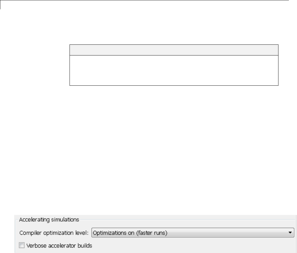
22 Accelerating Models
Perform Acceleration
In this section...
“Customize the Build Process” on page 22-22
“Run Acceleration Mode from the User Interface” on page 22-23
“Making Run-Time Changes” on page 22-25
Customize the Build Process
Compiler optimizations are off by default. This results in faster build times,
but slower simulation times. You can optimize the build process toward a
faster simulation.
1From the Simulation menu, select Model Configuration Parameters.
2In the left pane of the Configuration Parameters dialog box, select
Optimization, and then from the Compiler optimization level
drop-down list, select Optimizations on (faster runs).
Code generation takes longer with this option, but the model simulation
runs faster.
3Select Verbose accelerator builds to display progress information using
code generation, and to see the compiler options in use.
Changing the Name of the Generated File Location
By default, the Accelerator mode places the generated code in a subfolder
of the working folder called slprj/accel/modelname (for example,
slprj/accel/f14), and places a compiled MEX-file in the current working
folder. To change the name of the folder into which the Accelerator Mode
writes generated code:
22-22

Perform Acceleration
1In the Simulink editor window, select File > Simulink Preferences.
The Simulink Preferences window appears.
2In the Simulink Preferences window, navigate to the Simulation cache
folder parameter.
3Enter the absolute or relative path to your subfolder and click Apply.
Run Acceleration Mode from the User Interface
To accelerate a model, first open it, and then from the Simulation > Mode
menu, select either Accelerator or Rapid Accelerator.Thenstartthe
simulation.
The following example shows how to accelerate the already opened f14 model
using the Accelerator mode:
1From the Simulation > Mode menu, select Accelerator.
Alternatively, you can select Accelerator from the model editor’s toolbar.
22-23
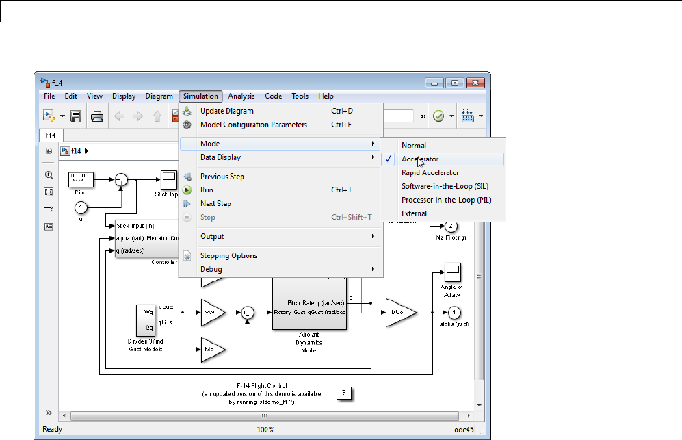
22 Accelerating Models
2From the Simulation menu, select Run.
The Accelerator and Rapid Accelerator modes first check to see if code
was previously compiled for your model. If code was created previously,
the Accelerator or Rapid Acceleratormoderunsthemodel. Ifcodewas
not previously built, they first generate and compile the C code, and then
run the model.
For an explanation of why these modes rebuild your model, see “Code
Regeneration in Accelerated Models” on page 22-7.
The Accelerator mode places the generated code in a subfolder of the working
folder called slprj/accel/modelname (for example, slprj/accel/f14), and
places a compiled MEX-file in the current working folder. If you want to
change this path, see “Changing the Name of the Generated File Location” on
page 22-22.
22-24

Perform Acceleration
The Rapid Accelerator mode places the generated code in a subfolder
of the working folder called slprj/raccel/modelname (for example,
slprj/raccel/f14).
Note The warnings that blocks generate during simulation (such as
divide-by-zero and integer overflow) are not displayed when your model runs
in Accelerator or Rapid Accelerator mode.
Making Run-Time Changes
A feature of the Accelerator and Rapid Accelerator modes is that simple
adjustments (such as changing the value of a Gain or Constant block) can
be made to the model while the simulation is still running. More complex
changes (for example, changing from a sin to tan function) are not allowed
during run time.
The Simulink software issues a warning if you attempt to make a change
that is not permitted. The absence of a warning indicates that the change
was accepted. The warning does not stop the current simulation, and the
simulation continues with the previous values. If you wish to alter the model
in ways that are not permitted during run time, you must first stop the
simulation, make the change, and then restart the simulation.
In general, simple model changes are more likely to result in code regeneration
when in Rapid Accelerator mode thanwheninAcceleratormode. For
instance, changing the stop time in Rapid Accelerator mode causes code to
regenerate, but does not cause Accelerator mode to regenerate code.
22-25

22 Accelerating Models
Interact with the Acceleration Modes Programmatically
In this section...
“Why Interact Programmatically?” on page 22-26
“Build Accelerator Mode MEX-files” on page 22-26
“Control Simulation” on page 22-26
“Simulate Your Model” on page 22-27
“Customize the Acceleration Build Process” on page 22-28
Why Interact Programmatically?
You can build an accelerated model, select the simulation mode, and run the
simulation from the command prompt or from MATLAB script. With this
flexibility, you can create Accelerator mode MEX-files in batch mode, allowing
you to build the C code and executable before running the simulations. When
you use the Accelerator mode interactively at a later time, it will not be
necessary to generate or compile MEX-files at the start of the accelerated
simulations.
Build Accelerator Mode MEX-files
With the accelbuild command, you can build the Accelerator mode MEX-file
without actually simulating the model. For example, to build an Accelerator
mode simulation of myModel:
accelbuild myModel
Control Simulation
You can control the simulation mode from the command line prompt by using
the set_param command:
set_param('modelname','SimulationMode','mode')
The simulation mode can be normal,accelerator,rapid,orexternal.
For example, to simulate your model with the Accelerator mode, you would
use:
22-26

Interact with the Acceleration Modes Programmatically
set_param('myModel','SimulationMode','accelerator')
However, a preferable method is to specify the simulation mode within the
sim command:
simOut = sim('myModel', 'SimulationMode', 'accelerator');
You can use gcs (“get current system”) to set parameters for the currently
active model (that is, the active model window) rather than modelname if you
do not wish to explicitly specify the model name.
For example, to simulate the currently opened system in the Rapid Accelerator
mode, you would use:
simOut = sim(gcs,'SimulationMode','rapid');
Simulate Your Model
You can use set_param to configure the model parameters (such as the
simulation mode and the stop time), and use the sim command to start the
simulation:
sim('modelname', 'ReturnWorkspaceOutputs', 'on');
However, the preferred method is to configure model parameters directly
using the sim command, as shown in the previous section.
You can substitute gcs for modelname if you do not want to explicitly specify
the model name.
Unless target code has already been generated, the sim command first builds
the executable and then runs the simulation. However, if the target code
has already been generated and no significant changes have been made to
the model (see “Code Regeneration in Accelerated Models” on page 22-7
for a description), the sim command executes the generated code without
regenerating the code. This process lets you run your model after making
simple changes without having to wait for the model to rebuild.
22-27

22 Accelerating Models
Simulation Example
The following sequence shows how to programmatically simulate myModel in
Rapid Accelerator mode for 10,000 seconds.
First open myModel, and then type the following in the Command Window:
simOut = sim('myModel', 'SimulationMode', 'rapid'...
'StopTime', '10000');
Use the sim command again to resimulate after making a change to your
model. If the change is minor (adjusting the gain of a gain block, for instance),
the simulation runs without regenerating code.
Customize the Acceleration Build Process
You can programmatically control the Accelerator mode and Rapid Accelerator
mode build process and the amount of information displayed during the build
process. See “Customize the Build Process” on page 22-22 for details on why
doing so might be advantageous.
Controlling the Build Process
Use the SimCompilerOptimization parameter to control the acceleration
build process. The permitted values are on or off. The default is off.
Enter the following at the command prompt to turn on compiler optimization:
set_param('myModel', 'SimCompilerOptimization', 'on')
Controlling Verbosity During Code Generation
Use the AccelVerboseBuild parameter to display progress information
during code generation. The permitted values are on or off. The default is
off.
Enter the following at the command prompt to turn on verbose build:
set_param('myModel', 'AccelVerboseBuild', 'on')
22-28

Run Accelerator Mode with the Simulink®Debugger
Run Accelerator Mode with the Simulink Debugger
In this section...
“Advantages of Using Accelerator Mode with the Debugger” on page 22-29
“How to Run the Debugger” on page 22-29
“When to Switch Back to Normal Mode” on page 22-30
Advantages of Using Accelerator Mode with the
Debugger
The Accelerator mode can shorten the length of your debugging sessions if
you have large and complex models. For example, you can use the Accelerator
mode to simulate a large model and quickly reach a distant break point.
For more information, see “Run Accelerator Mode with the Simulink
Debugger” on page 22-29.
Note You cannot use the Rapid Accelerator mode with the debugger.
How to Run the Debugger
To run your model in the Accelerator mode with the debugger:
1From the Simulation > Mode menu, select Accelerator.
2At the command prompt, enter:
sldebug modelname
3At the debugger prompt, set a time break:
tbreak 10000
continue
4Once you reach the breakpoint, use the debugger command emode (execution
mode) to toggle between Accelerator and Normal mode.
22-29

22 Accelerating Models
When to Switch Back to Normal Mode
Youmustswitcht
oNormalmodetostepthroughthesimulationbyblocks,
and when you want to use the following debug commands:
•trace
•break
•zcbreak
•nanbreak
22-30

Capture Performance Data
Capture Performance Data
In this section...
“What Is the Profiler?” on page 22-31
“HowtheProfilerWorks”onpage22-31
“Enabling the Profiler” on page 22-33
“How to Save Simulink Profiler Results” on page 22-36
What Is the Profiler?
The profiler captures data while your model runs and identifies the parts of
your model requiring the most time to simulate. You use this information to
decide where to focus your model optimization efforts.
Note You cannot use the Rapid Accelerator mode with the Profiler.
Performance data showing the time spent executing each function in your
model is placed in a report called the simulation profile.
How the Profiler Works
The following pseudocode summarizes the execution model on which the
Profiler is based.
Sim()
ModelInitialize().
ModelExecute()
for t = tStart to tEnd
Output()
Update()
Integrate()
Compute states from derivs by repeatedly calling:
MinorOutput()
MinorDeriv()
Locate any zero crossings by repeatedly calling:
MinorOutput()
22-31

22 Accelerating Models
MinorZeroCrossings()
EndIntegrate
Set time t = tNew.
EndModelExecute
ModelTerminate
EndSim
According to this conceptual model, your model is executed by invoking the
following functions zero, one, or more times, depending on the function and
the model.
Function Purpose Level
sim Simulate the model. This
top-level function invokes the
other functions required to
simulate the model. The time
spent in this function is the total
time required to simulate the
model.
System
ModelInitialize Set up the model for simulation. System
ModelExecute Execute the model by invoking
the output, update, integrate,
etc., functions for each block at
each time step from the start to
the end of simulation.
System
Output Compute the outputs of a block at
the current time step.
Block
Update Update a block’s state at the
current time step.
Block
Integrate Compute a block’s continuous
states by integrating the state
derivatives at the current time
step.
Block
MinorOutput Compute a block’s output at a
minor time step.
Block
22-32

Capture Performance Data
Function Purpose Level
MinorDeriv Compute a block’s state
derivatives at a minor time
step.
Block
MinorZeroCrossings Compute a block’s zero-crossing
values at a minor time step.
Block
ModelTerminate Free memory and perform any
other end-of-simulation cleanup.
System
Nonvirtual Subsystem Compute the output of a
nonvirtual subsystem at the
current time step by invoking
the output, update, integrate,
etc., functions for each block
that it contains. The time
spent in this function is the
time required to execute the
nonvirtual subsystem.
Block
The Profiler measures the time required to execute each invocation of these
functions and generates a report at the end of the model that describes how
much time was spent in each function.
Enabling the Profiler
To profile a model, open the model and select Show Profiler Report from
the Analysis > Performance Tools menu. Then start the simulation.
When the simulation finishes, the Simulink code generates and displays the
simulation profile for the model in the Help browser.
22-33
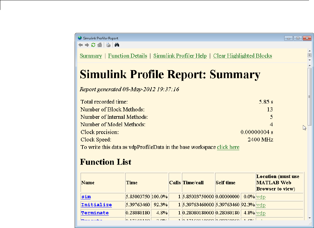
22 Accelerating Models
22-34

Capture Performance Data
Summary Section
Thesummaryfiledisplaysthefollowingperformancetotals.
Item Description
Total Recorded Time Totaltimerequiredtosimulatethemodel
Number of Block Methods Total number of invocations of block-level
functions (e.g., Output())
Number of Internal
Methods
Total number of invocations of system-level
functions (e.g., ModelExecute)
Number of Nonvirtual
Subsystem Methods
Total number of invocations of nonvirtual
subsystem functions
Clock Precision Precision of the profiler’s time measurement
The summary section then shows summary profiles for each function invoked
to simulate the model. For each function listed, the summary profile specifies
the following information.
Item Description
Name Name of function. This item is a hyperlink. Clicking it
displays a detailed profile of this function.
Time Total time spent executing all invocations of this function
as an absolute value and as a percentage of the total
simulation time
Calls Number of times this function was invoked
Time/Call Average time required for each invocation of this function,
including the time spent in functions invoked by this
function
22-35

22 Accelerating Models
Item Description
Self Time Average time required to execute this function, excluding
time spent in functions called by this function
Location Specifies the block or model executed for which this
function is invoked. This item is a hyperlink. Clicking it
highlights the corresponding icon in the model diagram.
The link works only if you are viewing the profile in the
Help browser.
Detailed Profile Section
This section contains detailed profiles for each function invoked to simulate
the model. Each detailed profile contains all the information shown in the
summary profile for the function. In addition, the detailed profile displays the
function (parent function) that invoked the profiled function and the functions
(child functions) invoked by the profiled function. Clicking the name of the
parent or a child function takes you to the detailed profile for that function.
Note Enabling the Profiler on a parent model does not enable profiling for
referenced models. You must enable profiling separately for each submodel.
Profiling occurs only if the submodel executes in Normal mode. See “Normal
Mode” on page 6-21 for more information.
How to Save Simulink Profiler Results
YoucansavetheProfilerreporttoavariableintheMATLABworkspace,and
subsequently, to a mat file. At a later time, you can regenerate and review
the report.
To save the Profiler report for a model vdp to the variable profile1 and to the
data file report1.mat, complete the following steps:
1In the Simulink Profiler Report window, click click here. Simulink
saves the report data to the variable vdpProfileData.
2Navigate to the MATLAB command window.
22-36

Capture Performance Data
3To review the report, at the command line enter:
slprofreport(vdpProfileData)
4Tosavethedatatoavariablenamedprofile1 in the base workspace, enter:
profile1 = vdpProfileData;
5Tosavethedatatoamat file named report1,enter:
save report1 profile1
To view the report at a later time, from the MATLAB command window, enter:
% Load the mat file and recreate the profile1 object
load report1
% Recreate the html report from the object
slprofreport(profile1);
22-37

22 Accelerating Models
22-38

Managing Blocks
•Chapter 23, “Working with Blocks”
•Chapter 24, “Working with Block Parameters”
•Chapter 25, “Working with Lookup Tables”
•Chapter 26, “Working with Block Masks”
•Chapter 27, “Creating Custom Blocks”
•Chapter 28, “Working with Block Libraries”
•Chapter 29, “Using the MATLAB Function Block”
•Chapter 30, “Design Considerations for C/C++ Code Generation”
•Chapter 31, “Functions Supported for Code Generation”
•Chapter 32, “System Objects Supported for Code Generation”
•Chapter 33, “Defining MATLAB Variables for C/C++ Code
Generation”
•Chapter 34, “Defining Data for Code Generation”
•Chapter 35, “Code Generation for Variable-Size Data”
•Chapter 36, “Code Generation for MATLAB Structures”
•Chapter 37, “Code Generation for Enumerated Data”
•Chapter 38, “Code Generation for MATLAB Classes”
•Chapter 39, “Code Generation for Function Handles”
•Chapter 40, “Defining Functions for Code Generation”
•Chapter 41, “Calling Functions for Code Generation”
•Chapter 42, “Generating Efficient and Reusable Code”

23
Working with Blocks
•“About Blocks” on page 23-2
•“Add Blocks” on page 23-4
•“Edit Blocks” on page 23-9
•“Set Block Properties” on page 23-15
•“Change the Appearance of a Block” on page 23-22
•“Display Port Values” on page 23-29
•“Control and Displaying the Sorted Order” on page 23-35
•“Access Block Data During Simulation” on page 23-53
•“Configure a Block for Code Generation” on page 23-57

23 Working with Blocks
About Blocks
In this section...
“What Are Blocks?” on page 23-2
“Block Tool Tips” on page 23-2
“Virtual Blocks” on page 23-2
What Are Blocks?
Blocks are the elements from which the Simulink software builds models.
You can model virtually any dynamic system by creating and interconnecting
blocks in appropriate ways. This section discusses how to use blocks to build
models of dynamic systems. Most blocks contain fields called block parameters
thatyoucanusetoentervaluesthatcustomize the behavior of the block. Be
careful not to confuse block parameters with Simulink parameters, which are
objects of type simulink.parameter that exist in the base workspace. See
“About Block Parameters” on page 24-2 and “Set Block Parameters” on page
24-4 for information about setting and changing block parameters.
Block Tool Tips
Information about a block is displayed in a tool tip when you hover the mouse
pointer over the block in the diagram view. To disable this feature, or control
what information the tool tip displays, select Display > Blocks > Tool Tip
Options in the Simulink Editor.
Virtual Blocks
When creating models, you need to be aware that Simulink blocks fall into two
basic categories: nonvirtual blocks and virtual blocks. Nonvirtual blocks play
an active role in the simulation of a system. If you add or remove a nonvirtual
block, you change the model’s behavior. Virtual blocks, by contrast, play no
active role in the simulation; they help organize a model graphically. Some
Simulink blocks are virtual in some circumstances and nonvirtual in others.
Such blocks are called conditionally virtual blocks. The following table lists
Simulink virtual and conditionally virtual blocks.
23-2

About Blocks
Block Name Condition Under Which Block Is Virtual
Bus Assignment Virtual if input bus is virtual.
Bus Creator Virtual if output bus is virtual.
Bus Selector Virtual if input bus is virtual.
Demux Always virtual.
Enable Virtual unless connected directly to an Outport
block.
From Always virtual.
Goto Always virtual.
Goto Tag Visibility Always virtual.
Ground Always virtual.
Inport Virtual unless the block resides in a conditionally
executed or atomic subsystem and has a direct
connection to an Outport block.
Mux Always virtual.
Outport Virtual when the block resides within any
subsystem block (conditional or not), and does not
reside in the root (top-level) Simulink window.
Selector Virtual only when Number of input dimensions
specifies 1and Index Option specifies Select
all,Index vector (dialog),orStarting index
(dialog).
Signal Specification Always virtual.
Subsystem Virtual unless the block is conditionally executed or
the Treat as atomic unit check box is selected.
You can check if a block is virtual with the
IsSubsystemVirtual block property. See
“Block-Specific Parameters”.
Terminator Always virtual.
Trigger Virtual when the output port is not present.
23-3

23 Working with Blocks
Add Blocks
In this section...
“Ways to Add Blocks” on page 23-4
“Add Blocks by Browsing or Searching with the Library Browser” on page
23-5
“Copy Blocks from a Model” on page 23-5
“Add Frequently Used Blocks” on page 23-6
“Add Blocks Programmatically” on page 23-8
Ways to Add Blocks
You can add blocks to a model in several ways.
Method When to Use
Browse or search libraries with the
Library Browser
•You are not sure which block to
add.
•You do not have a familiar model
from which to copy blocks.
Copy blocks from a model •You know where in a model a
blockisthatyouwanttocopy.
•You want to replicate many of the
parameter settings of an existing
block.
23-4

Add Blocks
Method When to Use
Use the Most Frequently Used
Blocks pane or context menu
•You want to add a block that you
have used frequently and recently.
•You are working on multiple
models that share several of the
same blocks.
•You do not have a familiar model
from which to copy similar blocks.
Add blocks programmatically with
the add_block function
•Youwanttoreplicatemostofthe
parameter settings of a block.
•You are working on multiple
models that share several of the
same blocks.
Add Blocks by Browsing or Searching with the
Library Browser
To browse or search for a block from a block library installed on your system,
use the Library Browser. You can browse a list of block libraries or search for
blocks whose names include the search string you specify.
When you find the block you want, select that block in the Library Browser
and drag the block into your model. See “Populate a Model” on page 4-4 for
more information.
Copy Blocks from a Model
To copy a block from a model in the Simulink Editor:
1Select the block that you want to copy from a model.
2Choose Edit > Copy.
3In the model window in which you want to place the copied block, choose
Edit > Paste.
You can copy a block:
23-5

23 Working with Blocks
•Within the same model window
•Between multiple systems open in one Simulink Editor instance
•Between systems open in multiple Simulink Editor instances
When you copy a block, the parameters use default values.
For details, see “Copy Blocks Between Windows” on page 23-10.
Add Frequently Used Blocks
When using the same block repeatedly, you can save time by using the Most
Frequently Used Blocks feature in the Library Browser or Model Editor.
Selecting Your Most Frequently Used Blocks From the Library
Browser
Open the Most Frequently Used Blocks pane with the third tab in the
Library Browser.
23-6
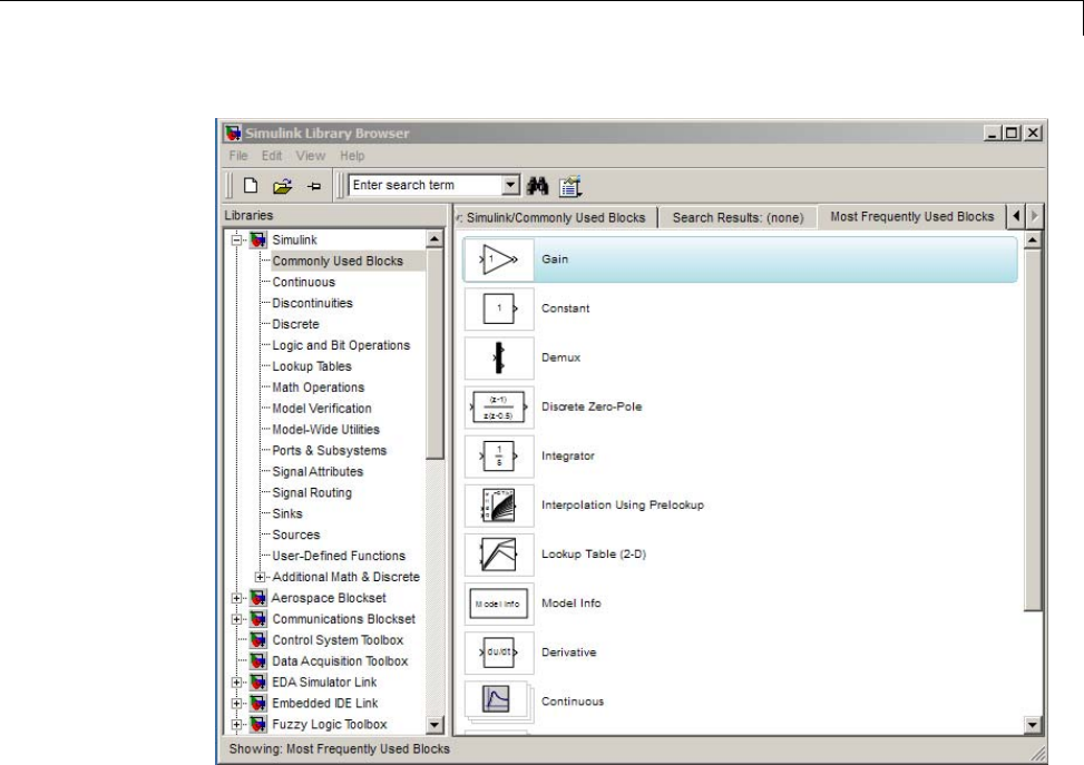
Add Blocks
To add a block to a model, select the block from the list and do either one of
the following from the Library Browser:
•Drag the block into your model.
•Right-click the block, and from the context menu select Add to
<model_name>.
Select Most Frequently Used Blocks from the Model Editor
In the Simulink Editor, you can view a list of your most frequently used
blocks. Right-click anywhere in the model except with the cursor directly on a
block or signal. In the context menu, select Most Frequently Used Blocks.
23-7

23 Working with Blocks
What Blocks Appear in the Most Frequently Used Blocks Lists
The Most Frequently Used Blocks pane lists blocks that you have added most
often, with the most frequently used block at the top. The list reflects your
ongoing modeling activity. For example, if you add several Gain blocks, the
Gain block appears in the list if the list:
•Does not already include the Gain block
•Has less than 25 blocks
•Has 25 blocks, but you added more Gain blocks than the number of
instances of the least frequently used block in the list
The list displays blocks that you rename as instances of the library block. For
example, if you rename several Gain blocks to be MyGain1,MyGain2,andso
on, those blocks count as Gain blocks.
When you close and reopen the Library Browser, the list reflects the blocks
that you added up through the previous session. The list updates only when
the Library Browser is open.
The list does not reflect blocks that you:
•Add programmatically
•Include in subsystems
If you add a subsystem that uses a specific type of block repeatedly, the list
does not reflect that activity.
The list in the Model Editor is the same as the Library Browser list, except
that the Model Editor list includes only five blocks.
Add Blocks Programmatically
To add a block programmatically, use the add_block function.
The add_block function copies the parameter values of the source block to
the new block. You can use add_block to specify values for parameters
of the new block.
23-8

Edit Blocks
Edit Blocks
In this section...
“Copy Blocks in a Model” on page 23-9
“Copy Blocks Between Windows” on page 23-10
“Move Blocks” on page 23-11
“Delete Blocks” on page 23-13
“Comment Out Blocks” on page 23-14
Copy Blocks in a Model
To copy a blocks in a model:
1In the Simulink Editor, select the block.
2Press right mouse button.
3Drag the block to a new location and release the mouse button.
You can also do this by using the Ctrl key:
1In the Simulink Editor, press and hold the Ctrl key.
2Select the block with the left mouse button.
3Drag the block to a new location and release the mouse button.
Copies of blocks have the same parameter values as the original blocks.
Sequence numbers are added to the new block names.
Note Simulink sorts block names alphabetically when generating names for
copies pasted into a model. This action can cause the names of pasted blocks to
be out of order. For example, suppose you copy a row of 16 gain blocks named
Gain,Gain1,Gain2...Gain15 and paste them into the model. The names of the
pasted blocks occur in the following order: Gain16,Gain17,Gain18...Gain31.
23-9

23 Working with Blocks
Copy Blocks Between Windows
As you build your model, you often copy blocks from Simulink block libraries
or other libraries or models into your model window. To do this:
1Open the appropriate block library or model window.
2Drag the block to copy into the target model window. To drag a block,
position the cursor over the block, then press and hold down the mouse
button. Move the cursor into the target window, then release the mouse
button.
You can also drag blocks from the Simulink Library Browser into a model
window. See “Browse Block Libraries” on page 4-4 for more information.
Note The names of Sum, Mux, Demux, Bus Creator, and Bus Selector blocks
are hidden when you copy them from the Simulink block library to a model.
This is done to avoid unnecessarily cluttering the model diagram. (The shapes
of these blocks clearly indicate their respective functions.)
You can also copy blocks by using the Simulink Editor:
1Select the block you want to copy.
2Select Edit > Copy.
3Make thetargetmodelwindowtheactivewindow.
4Choose Edit > Paste.
Simulink assigns a name to each copied block. If it is the first block of its type
in the model, its name is the same as its name in the source window. For
example, if you copy the Gain block from the Math library into your model
window, the name of the new block is Gain. If your model already contains
a block named Gain, Simulink adds a sequence number to the block name
(for example, Gain1,Gain2). You can rename blocks; see “Manipulate Block
Names” on page 23-26.
23-10

Edit Blocks
When you copy a block, the new block inherits all the original block’s
parameter values.
Formorewaystoaddblocks,see“AddBlocks”onpage23-4.
add blocks
Move Blocks
To move a single block from one place to another in a model window, drag the
block to a new location. Simulink automatically repositions lines connected to
the moved block.
To move more than one block, including connecting lines:
1Select the blocks and lines. For information about how to select more than
one block, see “Select Multiple Objects” on page 4-6.
2Drag the objects to their new location and release the mouse button.
To move a block, disconnecting lines:
1Select the block.
2Press the Shift key, then drag the block to its new location and release
the mouse button.
You can also move a block by selecting the block and pressing the arrow keys.
You cannot move a block between:
•Multiple systems open in one Simulink Editor instance
•Systems open in multiple Simulink Editor instances
If you drag a block between Simulink Editor instances, the block is copied
to the target Simulink Editor model window.
23-11
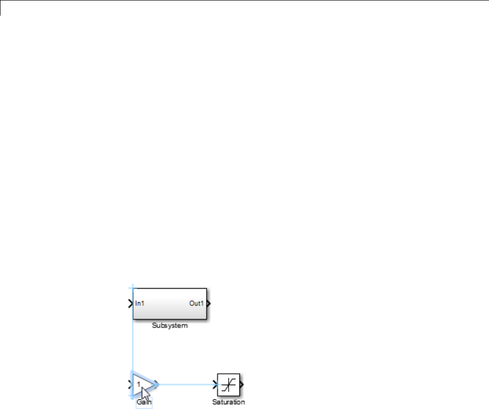
23 Working with Blocks
Align Blocks
You can manually align blocks. You can also use commands that align a
group of blocks automatically (see “Align, Distribute, and Resize Groups of
Blocks” on page 4-22 for details).
Smart Guides. You can enable smart guides to help you align blocks and
lines. When you move a block, smart guides appear to indicate when the
block ports, center, or edges are aligned with the ports, centers, and edges of
other blocks in the same diagram.
To display smart guides, in the Simulink Editor, select View > Smart
Guides. The setting applies to all open instances of the Simulink Editor.
For example, the following figure shows a snapshot of a Gain block that
you drag from one position in a diagramtoanother. Thebluesmartguides
indicate that if you drop the Gain block at this position, its left edge is aligned
with the left edge of the Subsystem block and its output port is aligned with
the input port of the Saturation block.
When you drag a block, one of its alignment features, for example, a port,
may match more than one alignment feature of another block. In this case,
Simulink displays a line for one of the features, using the following precedence
order: ports, centers, edges. For example, in the following drag-and-drop
snapshot, the Gain block center aligns with the Subsystem block center
and the Gain block output port aligns with the Saturation block input port.
23-12
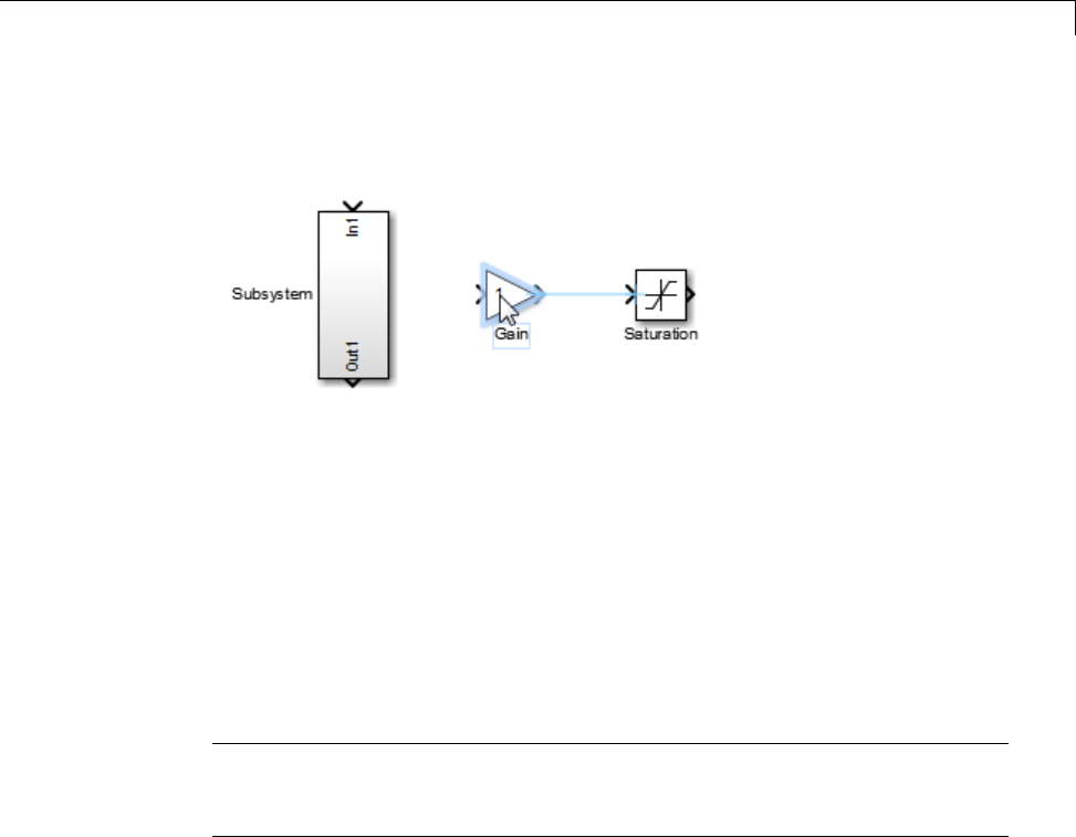
Edit Blocks
However, because ports take precedence over centers, Simulink draws a guide
only for the ports.
Position Blocks Programmatically
You can position (and resize) a block programmatically, using its Position
parameter. For example, the following command
set_param(gcb, 'Position', [5 5 20 20]);
moves the currently selected block to a location 5points down and 5points to
the right of the top left corner of the block diagram and sets the block’s height
and width to 20 points, respectively.
Note The maximum size of a block diagram’s height and width is 32767
points. An error message appears if you try to move or resize a block to a
position that exceeds the diagram’s boundaries.
Delete Blocks
Todeleteoneormoreblocks,selecttheblockstobedeletedandpressthe
Delete or Backspace key.
As an alternative, you can select Edit > ClearClear or Edit > Cut.
The Cut command writes the blocks into the clipboard, which enables you to
paste them into a model. Using the Delete or Backspace key or the Clear
command does not enable you to paste the block later.
To replace a deleted block, use the Edit > Undo command.
23-13

23 Working with Blocks
Comment Out Blocks
Comment out blocks in your model if you want to exclude them during
simulation. To exclude a block, right-click the selected block and select
Comment out.
Commenting out blocks may be useful for several tasks, such as:
•Incrementally testing parts of a model under development
•Debugging a model without having to delete and restore blocks between
simulation runs
•Testing and verifying the effects of certain model blocks on simulation
results
•Improving simulation performance
23-14

Set Block Properties
Set Block Properties
For each block in a model, you can set general block properties, such as:
•A description of the block
•The block’s order of execution
•A block annotation
•Blockcallbackfunctions
Block Properties Dialog Box
To set these block properties, open the Block Properties dialog box.
1In the Simulink Editor, select the block.
2Select Diagram > Properties.
The Block Properties dialog box opens, with the General tab open. For
example:
23-15
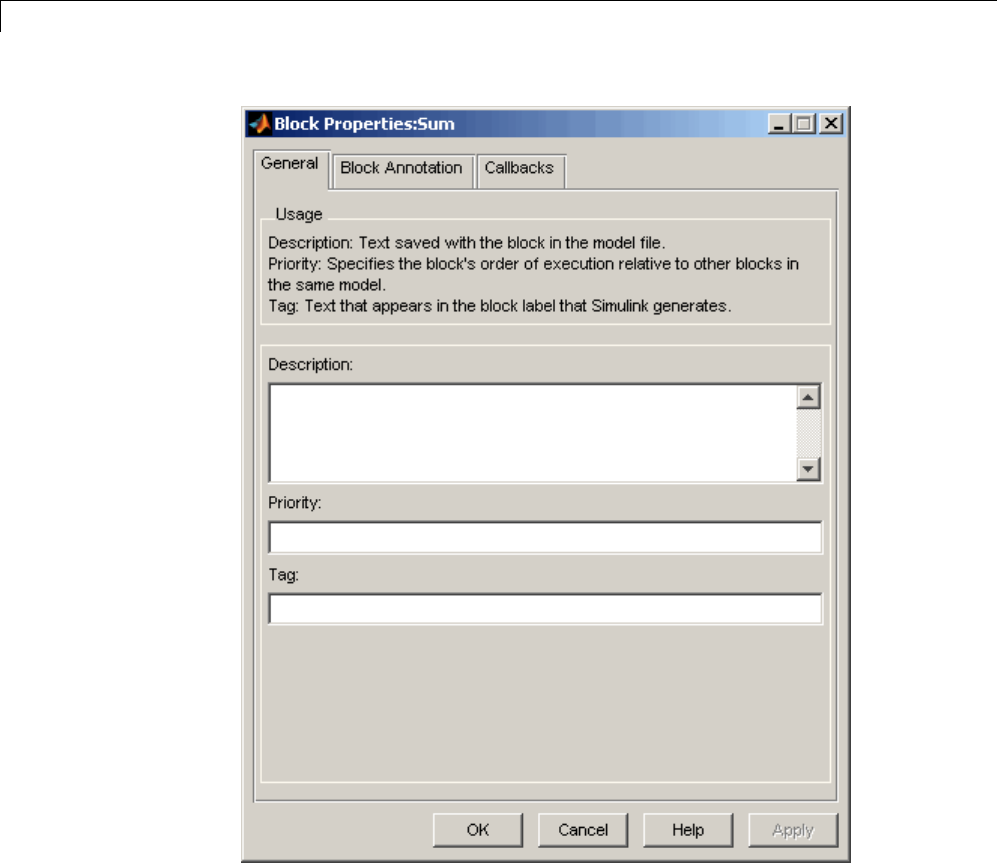
23 Working with Blocks
General Block Properties
Description
Enter a brief description of the purpose of the block or any other descriptive
information.
23-16

Set Block Properties
Priority
Specify the execution priority of this block relative to other blocks in the
model. For more information, see “Assign Block Priorities” on page 23-47.
Tag
You can use a tag to create your own block-specific label for a block. Specify
text that Simulink assigns to the block’s Tag parameter and saves with the
block in the model.
Block Annotation Properties
Use the Block Annotation tab to display the values of selected block
parameters in an annotation that appears beneath the block’s icon.
23-17
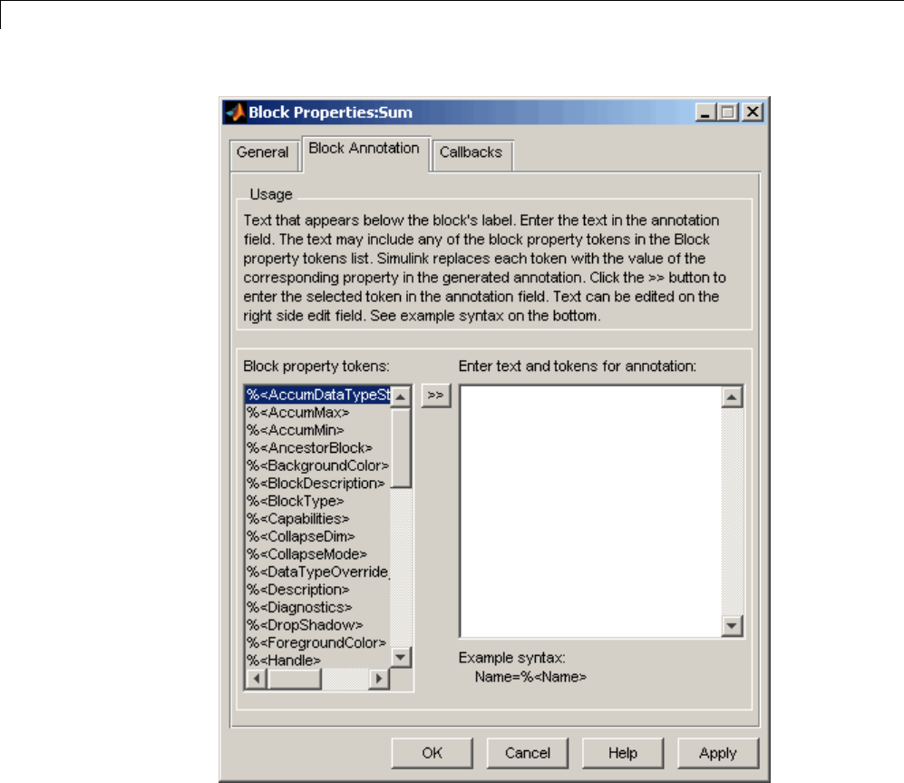
23 Working with Blocks
Enter the text of the annotation in the text field that appears on the right
side of the pane. The text can include any of the block property tokens that
appear in the list on the left side of the pane. A block property token is simply
the name of a block parameter preceded by %< and followed by >.When
displaying the annotation, Simulink replaces the tokens with the values of
the corresponding block parameters. For example, suppose that you enter the
following text and tokens for a Product block:
23-18

Set Block Properties
Multiplication = %<Multiplication>
Sample time = %<SampleTime>
In the Simulink Editor model window, the annotation appears as follows:
The block property token list on the left side of the pane lists all the
parameters that are valid for the currently selected block (see “Common Block
Parameters” and “Block-Specific Parameters”). To add one of the listed tokens
to the text field on the right side of the pane, select the token and then click
the button between the list and the text field.
You can also create block annotations programmatically. See “Create Block
Annotations Programmatically” on page 23-21.
Block Callbacks
Use the Callbacks tab to specify implementations for a block’s callbacks (see
“Callback Functions” on page 4-54).
23-19
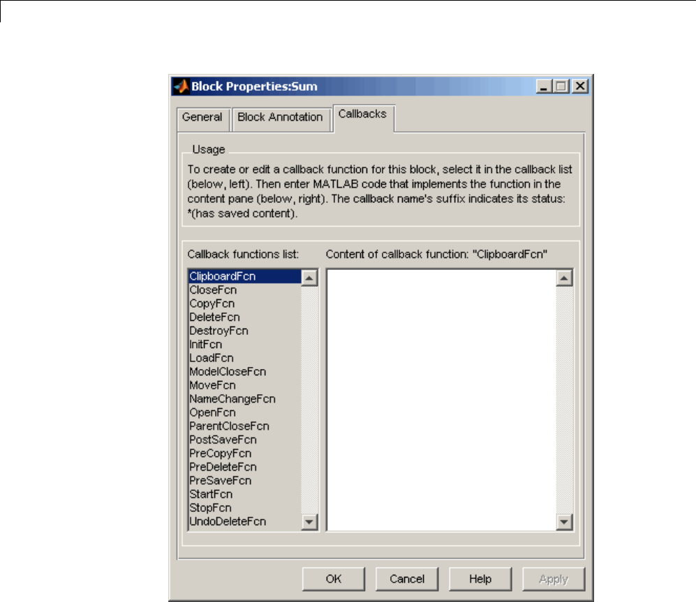
23 Working with Blocks
To specify an implementation for a callback, select the callback in the callback
list on the left side of the pane. Then enter MATLAB commands that
implement the callback in the right-hand field. Click OK or Apply to save the
change. Simulink appends an asterisk to the name of the saved callback to
indicate that it has been implemented.
23-20

Set Block Properties
Create Block Annotations Programmatically
You can use a block’s AttributesFormatString parameter to display selected
block parameters beneath the block as an “attributes format string,” which is
astringthatsp
ecifies values of the block’s attributes (parameters). “Common
Block Parameters” and “Block-Specific Parameters” describe the parameters
that a block canhave. UsetheSimulinkset_param function to set this
parameter to the desired attributes format string.
The attributes format string can be any text string that has embedded
parameter names. An embedded parameter name is a parameter name
preceded by %<andfollowedby>, for example, %<priority>. Simulink
displays the attributes format string beneath the block’s icon, replacing
each parameter name with the corresponding parameter value. You can use
line-feed characters (\n) to display each parameter on a separate line. For
example, enter the following at the MATLAB command prompt:
The Gain block displays the following block annotation:
If a parameter’s value is not a string or an integer, Simulink displays N/S
(not supported) for the parameter’s value. If the parameter name is invalid,
Simulink displays ??? as the parameter value.
23-21

23 Working with Blocks
Change the Appearance of a Block
In this section...
“Change a Block Orientation” on page 23-22
“Resize a Block” on page 23-24
“Displaying Parameters Beneath a Block” on page 23-25
“Drop Shadows” on page 23-25
“Manipulate Block Names” on page 23-26
“Specify Block Color” on page 23-28
Change a Block Orientation
By default, a block is oriented so that its input ports are on the left, and its
output ports are on the right. You can change the orientation of a block by
rotating it 90 degrees around its center or by flipping it 180 degrees around
its horizontal or vertical axis.
•“How to Rotate a Block” on page 23-22
•“How to Flip a Block” on page 23-24
How to Rotate a Block
You can rotate a block 90 degrees by selecting one of these commands from
the Diagram menu:
•Rotate & Flip > Clockwise (or Ctrl+R)
•Rotate & Flip > Counterclockwise
A rotation command effectively moves a block’s ports from its sides to its top
and bottom or from its top and bottom to its size, depending on the initial
orientation of the block. The final positions of the block ports depend on the
block’s port rotation type.
23-22
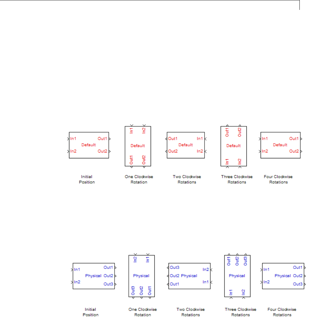
Change the Appearance of a Block
Port Rotation Type. After rotating a block clockwise, Simulink may,
depending on the block, reposition the block’s ports to maintain a left-to-right
port numbering order for ports along the top and bottom of the block and a
top-to-bottom port numbering order for ports along the left and right sides
of the block. A block whose ports are reordered after a clockwise rotation is
said to have a default port rotation type. This policy helps to maintain the
left-right and top-down block diagram orientation convention used in control
system modeling applications. All nonmasked blocks and all masked blocks
by default have the default rotation policy. The following figure shows the
effect of using the Rotate & FlipClockwise command on a block with the
default rotation policy.
A masked block can optionally specify that its ports not be reordered after a
clockwise rotation (see “Port Rotation”). Such a block is said to have a physical
port rotation type. This policy facilitates layout of diagrams in mechanical
and hydraulic systems modeling and other applications where diagrams do
not have a preferred orientation. The following figure shows the effect of
clockwise rotation on a block with a physical port rotation type
23-23
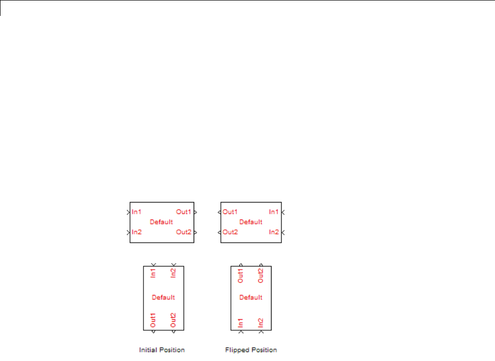
23 Working with Blocks
How to Flip a Block
Simulink provides a set of commands that allow you to flip a block 180 degrees
about its horizontal or vertical axis. The commands effectively move a block’s
input and output ports to opposite sides of the block or reverse the ordering of
the ports, depending on the block’s port rotation type.
A block with the default rotation type has one flip command:
Diagram > Rotate & Flip > Flip Block (Ctr+I). This command effectively
moves the block’s input and output ports to the side of the block opposite to
the side on which they are initially located, i.e., from the left to the right side
or from the top to the bottom side.
Resize a Block
To change the size of a block, select it, then drag any of its selection handles.
While you hold down the mouse button, a dotted rectangle shows the new
block size. When you release the mouse button, the block is resized.
For example, the following figure below shows a Signal Generator block
being resized. The lower-right handle was selected and dragged to the cursor
position. When the mouse button is released, the block takes its new size.
23-24

Change the Appearance of a Block
Tip Usethemodeleditor’sresizeblockscommandstomakeoneblockthe
same size as another (see “Align, Distribute, and Resize Groups of Blocks”
on page 4-22).
Displaying Parameters Beneath a Block
YoucancauseSimulinktodisplayoneormoreofablock’sparameters
beneath the block. Specify the parameters to be displayed by using one of the
following approaches:
•Enter an attributes format string in the Attributes format string field of
the block’s Properties dialog box (see “Set Block Properties” on page 23-15)
•Set the value of the block’s AttributesFormatString property to the
format string, using set_param
Drop Shadows
By default, blocks appear with a drop shadow.
To increase the depth of a block drop shadow:
1Select the block.
2Select Diagram > Format > Block Shadow.
For example, in this model, the Constant1 block has the Block Shadow
option enabled, and the Constant2 block uses the default drop shadow.
23-25
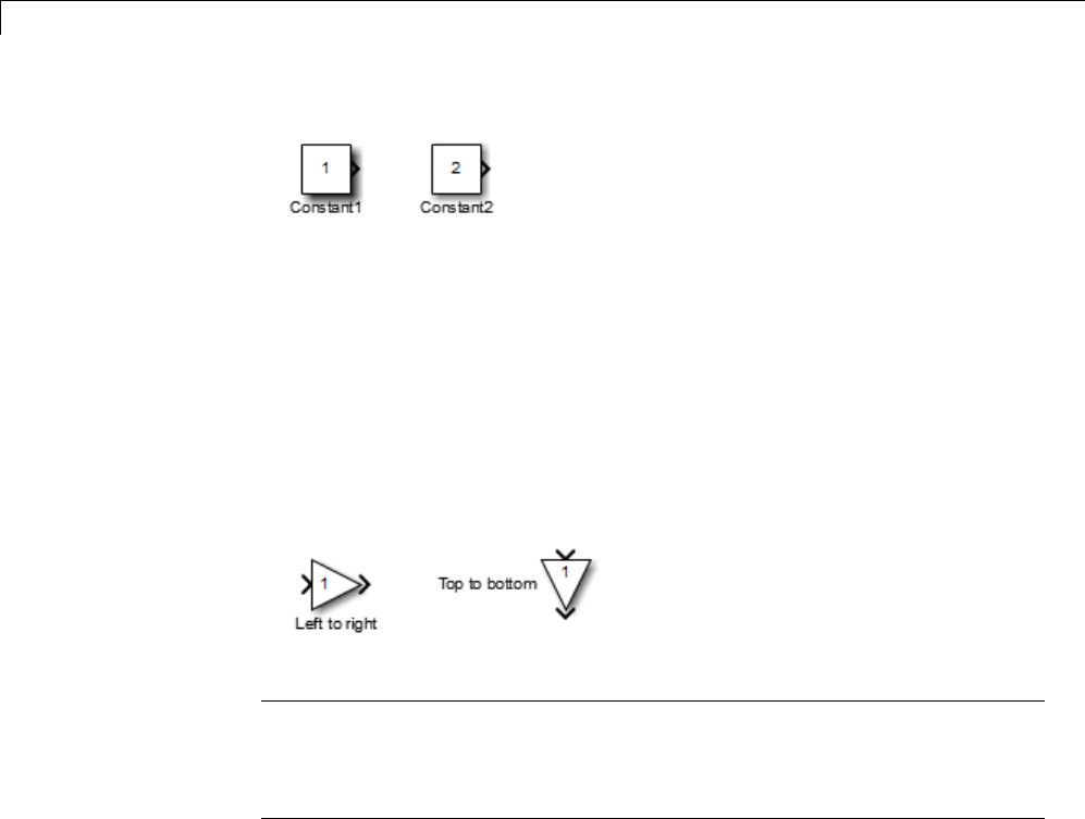
23 Working with Blocks
To remove the default drop shadows for all blocks, select File > Simulink
Preferences > Editor Defaults > Use classic diagram theme.
Manipulate Block Names
All block names in a model must be unique and must contain at least one
character. By default, block names appear below blocks whose ports are on
the sides, and to the left of blocks whose ports are on the top and bottom, as
the following figure shows:
Note Simulink commands interprets a forward slash (/) as a block path
delimiter. For example, the path vdp/Mu designates a block named Mu in the
model named vdp. Therefore, avoid using forward slashes (/) in block names
to avoid causing Simulink to interpret the names as paths.
ChangeBlockNames
You can edit a block name in one of these ways:
•To replace the block name, click the block name, select the entire name,
and then enter the new name.
•To insert characters, click between two characters to position the insertion
point, then insert text.
•To replace characters, drag the mouse to select a range of text to replace,
then enter the new text.
23-26

Change the Appearance of a Block
When you click the pointer anywhere else in the model or take any other
action, the name is accepted or rejected. If you try to change the name of a
block to a name that already exists, Simulink displays an error message.
Note If you change the name of a library block, all links to that block become
unresolved.
Change Font of Block Name
To modify the font used in a block name by selecting the block, then choosing
the Font Style menu item from the Diagram > Format menu.
1Select the block name.
2Select Diagram > Format > Font Style.
The Select Font dialog box opens.
3Select a font and specify other font characteristics, such as the font size.
Note Changing the block name font also changes the font of any text that
appears inside the block.
This procedure also changes the font of any text that appears inside the block.
Change the Location of a Block Name
To change the location of the name of a selected block, use one of these
approaches:
•Dragtheblocknametotheoppositesideoftheblock.
•Choose Diagram > Rotate & Flip > Flip Block Name. This command
changes the location of the block name to the opposite side of the block.
For more information about block orientation, see “How to Rotate a Block” on
page 23-22.
23-27

23 Working with Blocks
Hide a Block Name
By default the Simulink Editor displays the names of blocks (except for a few
blocks, such as the Bus Creator block). To hide the name of a selected block,
clear the Diagram > Format > Show Block Name menu option.
Specify Block Color
See “Specify Block Diagram Colors” on page 4-8 for information on how to
set the color of a block.
23-28
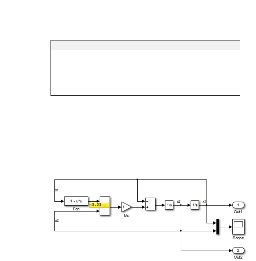
Display Port Values
Display Port Values
In this section...
“Port Value Data Tips” on page 23-29
“Display Value for a Port” on page 23-30
“Control the Port Value Display” on page 23-31
“Displayed Value When No Data Is Available” on page 23-32
“Port Value Display Limitations” on page 23-33
Port Value Data Tips
Signals can be data signals or non-data signals. For many blocks with data
signals, Simulink can display port values (block output) as data tips on the
block diagram while a simulation is running. The following model shows a
port value data tip for the Fcn block, displaying an output value of 3.03.
Displaying port value data tips can be helpful during interactive debugging of
a model. The data tips do not persist when you save a model, so do not rely on
data tips as a form of built-in documentation for the model.
23-29

23 Working with Blocks
In some cases, data signals are not accessible for display. In those cases, a
label such as wait might be displayed for optimized signals, or action might
be displayed for an action subsystem.
Note The port value display feature has limitations for models with:
•Accelerated modes
•Signal storage reuse
•Signals with some complex data types, such as bus signals
See“PortValueDisplayLimitations”onpage23-33.
Display Value for a Port
To display a data tip that shows the value of a port:
1In the Simulink Editor model window, select a port.
2Specify when the port value appears.
•To display the port value when you click on a port, select Display >
Data Display in Simulation > Show Value Label of Selected Port.
The data tip remains until you remove it.
•To display the port value when you hover the cursor over the port, select
Display > Data Display in Simulation > Show Value Labels
When Hovering. When you move the cursor away from the port, the
data tip disappears.
•To toggle between displaying and hiding the port value, select Display >
Data Display in Simulation > Toggle Value Labels When Clicked.
Reselecting that block turns off the display. If you select a block with
this port value display method, then change the display method to Show
When Hovering, the port value for that block continues to display.
To remove the all displayed port value data tips, select Display > Data
Display in Simulation > Remove All Value Labels.
23-30

Display Port Values
Control the Port Value Display
To specify port value display formatting and how frequently the display
updates:
1In the Simulink Editor model window, select a port.
2Select Display > Data Display in Simulation > Options.TheValue
Label Display Options dialog box opens.
3In the Value Label Display Options dialog box, select the appropriate
option.
Port Value Data Tip Display
Characteristic
What You Specify
When to display the port value Choose Show When Hovering,
Toggle When Clicked,orRemove
All. For details, see “Display Value
for a Port” on page 23-30.
Text size To increase the size of the output
display text, move the Font size
slider to the right.
23-31

23 Working with Blocks
Port Value Data Tip Display
Characteristic
What You Specify
Floating point data format Choose a floating point format from
the Floating point list.
Fixed-point data format Choose a fixed-point format from the
Fix point list.
Refresh interval (rate at which
Simulink updates the output
display)
The refresh rate is approximate and
is independent of simulation time.
To increase the interval, move the
Approximate refresh interval:
1.0 slider to the right.
Number of elements in port value
display
To change the number of elements
to display in the port value display,
move the Maximum number of
elements per label: 3 slider to the
left or right. This setting affects the
number of elements displayed for
vector or matrix signals with signal
widths greater than 1. This setting
does not affect scalar signals.
Displayed Value When No Data Is Available
Simulink displays an empty box when you toggle or hover on a block,
indicating that no port value is available. You see the empty box if you did
not run the simulation.
Also, if you toggle or hover on a block that Simulink optimizes out of a
simulation (such as a virtual subsystem block), the model displays a wait
string before displaying the port value during simulation.
To prevent the optimization delay of the port value display, designate
the signal as a test point. This enables the port value display to update
immediately.
23-32

Display Port Values
Port Value Display Limitations
Performance
Enabling the hovering option, or toggling at least one block, slows down the
simulation.
Accelerated Modes
Port values display as follows.
Accelerated
Mode
Port Values...
Accelerator Display as in Normal mode. See “Port Value Data Tips”
on page 23-29.
Rapid
Accelerator
Do not display. The limitation exists whether the model
itself specifies accelerated simulation or the model is
subordinate to a model that specifies accelerated simulation.
For more information, see “Rapid Simulations”.
Signal Storage Reuse
Invoking the port value displays the text optimized when the software cannot
determine the signal value, if you:
•Select Show When Hovering or Toggle When Clicked.
•Enable the Configuration Parameters > Optimization > Signals and
Parameters > Signal storage reuse parameter.
Disabling signal storage reuse increases the amount of memory used during
simulation.
Signal Data Types
Simulink displays the port value for ports connected to most kinds of signals,
including signals with built-in data types (such as double,int32,orBoolean),
DYNAMICALLY_TYPED, and several other data types. However, Simulink does
not display data for signals with some complex data types, such as bus
23-33

23 Working with Blocks
signals. In addition, the software shows the floating and fixed-point formats
for only non-complex signal value displays.
23-34

Control and Displaying the Sorted Order
Control and Displaying the Sorted Order
In this section...
“What Is Sorted Order?” on page 23-35
“Display the Sorted Order” on page 23-35
“Sorted Order Notation” on page 23-36
“How Simulink Determines the Sorted Order” on page 23-45
“Assign Block Priorities” on page 23-47
“Rules for Block Priorities” on page 23-48
“Block Priority Violations” on page 23-51
What Is Sorted Order?
During the updating phase of simulation, Simulink determines the order in
which to invoke the block methods during simulation. This block invocation
ordering is the sorted order.
You cannot set this order, but you can assign priorities to nonvirtual blocks to
indicate to Simulink their execution order relative to other blocks. Simulink
always honors block priority settings, unless there is a conflict with data
dependencies. To confirm the results of priorities that you have set, or to
debug your model, display and review the sorted order of your nonvirtual
blocks and subsystems.
Note For more information about block methods and execution, see:
•“Block Methods” on page 3-16
•“Conditional Execution Behavior” on page 7-32
Display the Sorted Order
To display the sorted order of the vdp model:
23-35
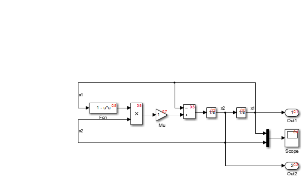
23 Working with Blocks
1Open the van der Pol equation model:
vdp
2In the model window, select Format > Block Displays > Sorted Order.
Simulink displays a notation in the top-right corner of each nonvirtual block
and each nonvirtual subsystem. These numbers indicate the order in which
the blocks execute. The first block to execute has a sorted order of 0.
For example, in the van der Pol equation model, the Integrator block with the
sorted order 0:0 executes first. The Out1 block, with the sorted order 0:1,
executes second. Similarly, the remaining blocks execute in numeric order
from 0:2 to 0:8.
You can save the sorted order setting with your model. To display the sorted
order when you reopen the model, select Simulation > Update diagram.
Sorted Order Notation
The sorted order notation varies depending on the type of block. The following
table summarizes the different formats of sorted order notation. Each format
is described in detail in the sections that follows the table.
23-36

Control and Displaying the Sorted Order
Block Type Sorted Order Notation Description
“Nonvirtual
Blocks” on page
23-38
s:b•sis the system index of the model or
subsystem. For root-level models, sis
always 0.
•bspecifies the block position within the
sorted order for the designated execution
context.
“Nonvirtual
Subsystems” on
page 23-39
s:b{si}•sis the system index of the model or
subsystem.
•bspecifies the block position within the
sorted order for the designated execution
context.
•siis the subsystem index.
“Virtual Blocks
and Subsystems”
on page 23-41
Not applicable Virtual blocks do not execute.
One initiator:
s:F{si}
•sis the system index of the model or
subsystem.
•Findicates a function-call subsystem.
•siis the subsystem index.
“Function-Call
Subsystems” on
page 23-42
Twoormoreinitiators:
•s:F{si} when the initiators
all execute at the same
level of the model hierarchy
•M:F{si}, when the initiators
execute at different levels
of the model hierarchy
•sis the system index of the initiators.
•Findicates a function-call subsystem.
•siis the subsystem index.
•Mindicates that the initiators execute at
different levels of the model hierarchy.
23-37

23 Working with Blocks
Block Type Sorted Order Notation Description
“Function-Call
Split Blocks” on
page 23-44
s:Bb•sis a system index of the model or
subsystem.
•Bindicates a branch of the function-call
signal.
•bspecifies the index of each subsystem
connected to each branch of the given
function-call signal.
“Bus-Capable
Blocks” on page
23-45
s:B •sis a system index of the model or
subsystem.
•Bindicates a bus-capable block.
•“Nonvirtual Blocks” on page 23-38
•“Nonvirtual Subsystems” on page 23-39
•“Virtual Blocks and Subsystems” on page 23-41
•“Function-Call Subsystems” on page 23-42
•“Function-Call Split Blocks” on page 23-44
•“Bus-Capable Blocks” on page 23-45
Nonvirtual Blocks
In the van der Pol equation model, all the nonvirtual blocks in the model have
a sorted order. The system index for the top-level model is 0,andtheblock
execution order ranges from 0to 8.
23-38
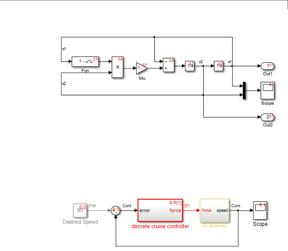
Control and Displaying the Sorted Order
Nonvirtual Subsystems
The following model contains an atomic, nonvirtual subsystem named
Discrete Cruise Controller.
When you enable the sorted order display for the root-level system, Simulink
displays the sorted order of the blocks.
The Scope block in this model has the lowest sorted order, but its input
depends on the output of the Car Dynamics subsystem. The Car Dynamics
subsystem is virtual, so it does not have a sorted order and does not execute
as an atomic unit. However, the blocks within the subsystem execute at the
root level, so the Integrator block in the Car Dynamics subsystem executes
first. The Integrator block sends its output to the Scope block in the root-level
model, which executes second.
23-39

23 Working with Blocks
The Discrete Cruise Controller subsystem has a sorted order of 0:5{1}:
•0indicates that this atomic subsystem is part of the root level of
the hierarchal system comprised oftheprimarysystemandthetwo
subsystems.
•5indicates that the atomic subsystem is the sixth block that Simulink
executes relative to the blocks within the root level.
•{1} represents the subsystem index. This index does not indicate the
relative order in which the atomic subsystem runs.
The sorted order of each block inside the Discrete Cruise Controller subsystem
has the form 1:b,where:
•1is the system index for that subsystem.
•bis the block position in the execution order. In the Discrete Cruise
Controller subsystem, the sorted order ranges from 0to 8.
23-40
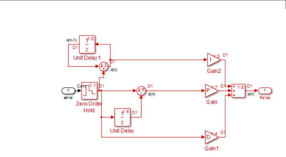
Control and Displaying the Sorted Order
Virtual Blocks and Subsystems
Virtual blocks, such as the Mux block, exist only graphically and do not
execute. Consequently, they are not part of the sorted order and do not
display any sorted order notation.
Virtual subsystems do not execute as a unit, and like a virtual block, are not
part of the sorted order. The blocks inside the virtual subsystem are part of
the root-level system sorted order, and therefore share the system index.
In the model in “Nonvirtual Subsystems” on page 23-39, the virtual subsystem
Car Dynamics does not have a sorted order. However, the blocks inside
the subsystem have a sorted order in the execution context of the root-level
model. The blocks have the same system index as the root-level model. The
Integrator block inside the Car Dynamics subsystem has a sorted order of
0:0, indicating that the Integrator block is the first block executed in the
context of the top-level model.
23-41
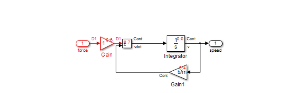
23 Working with Blocks
Function-Call Subsystems
Single Initiator. For each function-call subsystem or model attached to a
single initiator, Simulink assigns the block position F. The function-call
subsystem (or model) executes when the initiator invokes the function-call
subsystem (or model) and, therefore, does not have a sorted order independent
of its initiator. Specifically, for a subsystem that connects to one initiator,
Simulink uses the notation s:F{si},wheresis the index of the system that
contains the initiator.
For example, the sorted order for the ThresholdCalculation subsystem is
1:F{2}:
•1is the index of the system that contains the initiator, in this case, the
ShiftLogic Stateflow chart.
•Findicates that this function-call subsystem connects to one initiator.
•2is thesystemindexfortheThresholdCalculation subsystem.
23-42
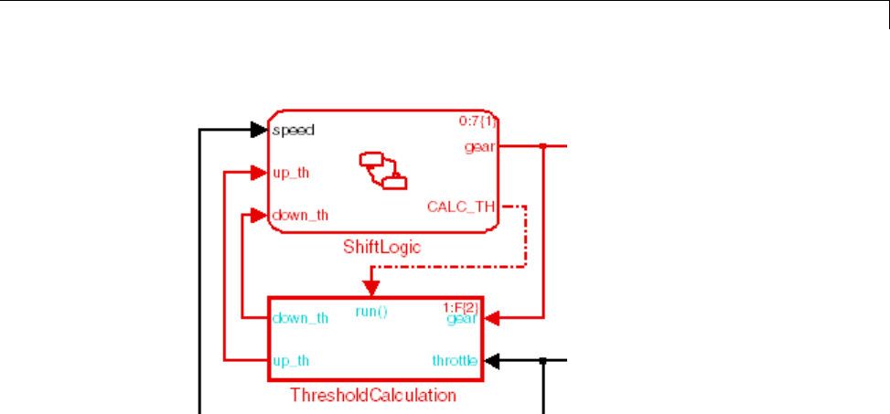
Control and Displaying the Sorted Order
Multiple Initiators. For a function-call subsystem that connects to more
than one initiator, the sorted order notation depends on the execution context
of the initiators:
•If the initiators all execute at the same level of the model hierarchy, the
notation is s:F{si}.
•If the initiators execute at different levels of the model hierarchy, the
notation is M:F{si}
For example, open the sl_subsysm_fcncall6 model. The f subsystem has
three initiators, two from the Stateflow chart, Chart1, and one from the
Stateflow chart, Chart.
Because Chart1 has a system index of 2and Chart has a system index of
1, the initiators execute at different levels in the model hierarchy. The
Function-Call Subsystem f has a sorted order notation of M:F{3}.
23-43
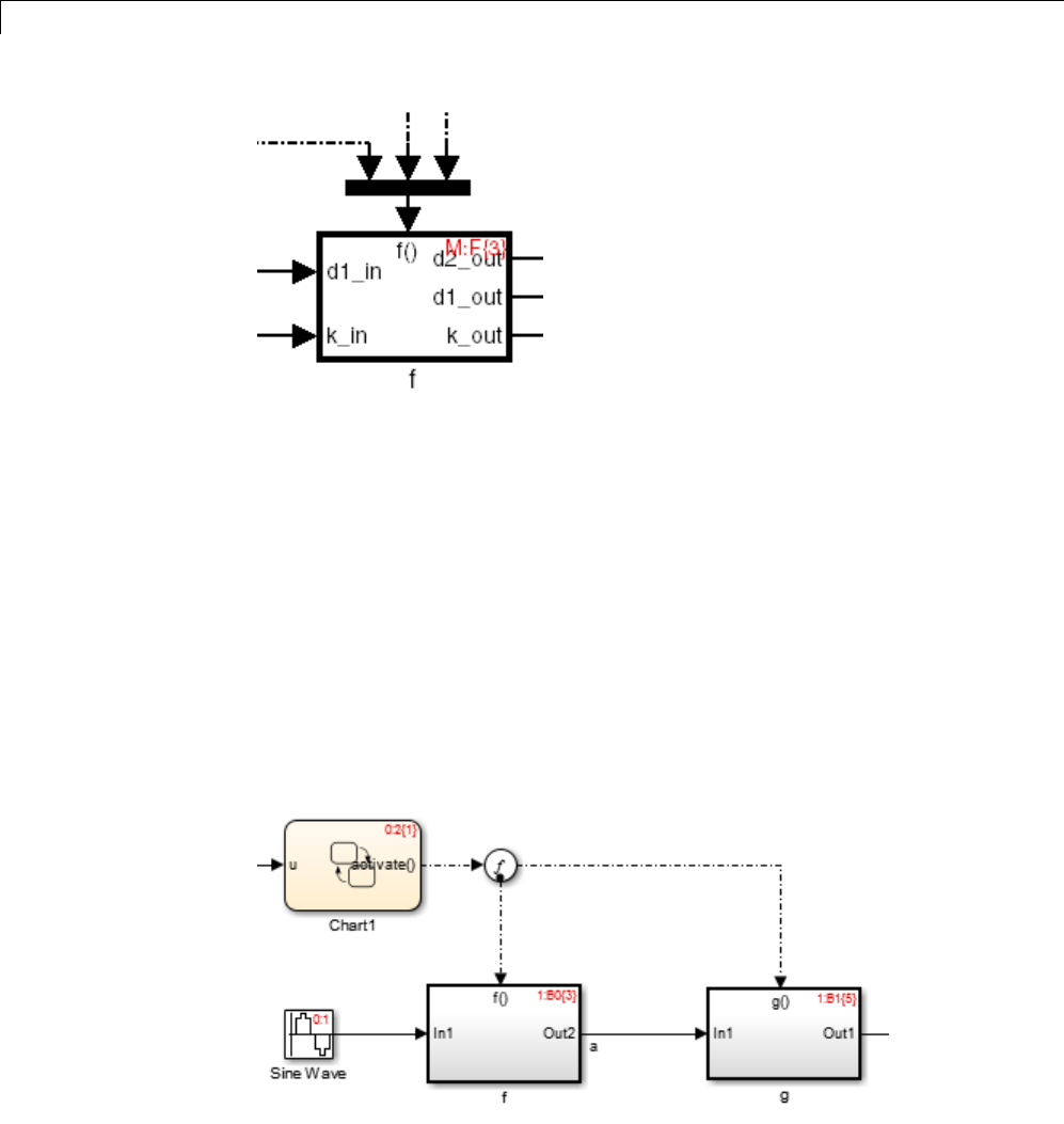
23 Working with Blocks
Function-Call Split Blocks
When a function-call signal is branched using a Function-Call Split block,
Simulink displays the order in which subsystems (or models) that connect to
the branches execute when the initiator invokes the function call. Simulink
uses the notation s:Bb to indicate this order, where B stands for branch. The
block position branges from 0to one less than the total number of subsystems
(or models) that connect to branches (B0,B1, etc.). When the function-call is
invoked, the subsystems execute in ascending order based on this number.
For example, open the sl_subsys_fcncall11 model and display the sorted
order. The sorted order indicates that the subsystem f (B0)executesbefore
the subsystem g (B1).
23-44
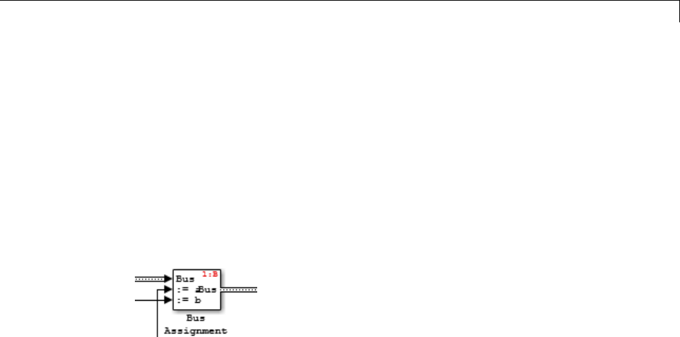
Control and Displaying the Sorted Order
Bus-Capable Blocks
A bus-capable block does not execute as a unit and therefore does not have
a unique sorted order. Such a block displays its sorted order as s:B where
Bstands for bus.
For example, open the sldemo_bus_arrays model and display the sorted
order. Open the For Each Subsystem to see that the sorted order for the
Bus Assignment block appears as 1:B.
For more information, see “Bus-Capable Blocks” on page 48-19.
How Simulink Determines the Sorted Order
Direct-Feedthrough Ports Impact on Sorted Order
To ensure that the sorted order reflects data dependencies among blocks,
Simulink categorizes block input ports according to the dependency of the
block outputs on the block input ports. An input port whose current value
determines the current value of one of the block outputs is a direct-feedthrough
port. Examples of blocks that have direct-feedthrough ports include:
•Gain
•Product
•Sum
Examples of blocks that have non-direct-feedthrough inputs:
•Integrator — Output is a function of its state.
•Constant — Does not have an input.
23-45
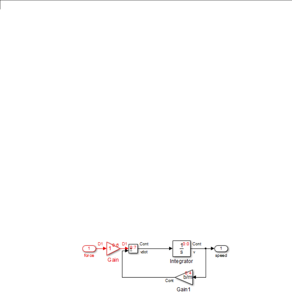
23 Working with Blocks
•Memory — Output depends on its input from the previous time step.
Rules for Sorting Blocks
To sort blocks, Simulink uses the following rules:
•If a block drives the direct-feedthrough port of another block, the block
must appear in the sorted order ahead of the block that it drives.
This rule ensures that the direct-feedthrough inputs to blocks are valid
when Simulink invokes block methods that require current inputs.
•Blocks that do not have direct-feedthrough inputs can appear anywhere
in the sorted order as long as they precede any direct-feedthrough blocks
that they drive.
Placing all blocks that do not have direct-feedthrough ports at the
beginning of the sorted order satisfies this rule. This arrangement allows
Simulink to ignore these blocks during the sorting process.
Applying these rules results in the sorted order. Blocks without
direct-feedthrough ports appear at the beginning of the list in no particular
order. These blocks are followed by blocks with direct-feedthrough ports
arranged such that they can supply valid inputs to the blocks which they drive.
The following model, from “Nonvirtual Subsystems” on page 23-39, illustrates
this result. The following blocks do not have direct-feedthrough and therefore
appear at the beginning of the sorted order of the root-level system:
•Integrator block in the Car Dynamics virtual subsystem
•Speed block in the root-level model
23-46
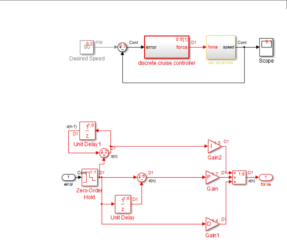
Control and Displaying the Sorted Order
Inside the Discrete Cruise Controller subsystem, all the Gain blocks, which
have direct-feedthrough ports, run before the Sum block that they drive.
Assign Block Priorities
You can assign a priority to a nonvirtualblockortoanentiresubsystem.
Higher priority blocks appear before lower priority blocks in the sorted order.
The lower the number, the higher the priority.
•“Assigning Block Priorities Programmatically” on page 23-48
•“Assigning Block Priorities Interactively” on page 23-48
23-47

23 Working with Blocks
Assigning Block Priorities Programmatically
To set priorities programmatically, use the command:
set_param(b,'Priority','n')
where
•bis the block path.
•nis any valid integer. (Negative integers and 0 are valid priority values.)
Assigning Block Priorities Interactively
To set the priority of a block or subsystem interactively:
1Right-click the block and select Properties.
2On the General tab, in the Priority field, enter the priority.
Rules for Block Priorities
Simulink honors the block priorities that you specify unless they violate data
dependencies. (“Block Priority Violations” on page 23-51 describes situations
that cause block property violations.)
In assessing priority assignments, Simulink attempts to create a sorted order
such that the priorities for the individual blocks within the root-level system
or within a nonvirtual subsystem are honored relative to one another.
Three rules pertain to priorities:
•“Priorities Are Relative” on page 23-48
•“Priorities Are Hierarchical” on page 23-50
•“Lack of Priority May Not Result in Low Priority” on page 23-51
Priorities Are Relative
Priorities are relative; the priority of a block is relative to the priority of the
blocks within the same system or subsystem.
23-48
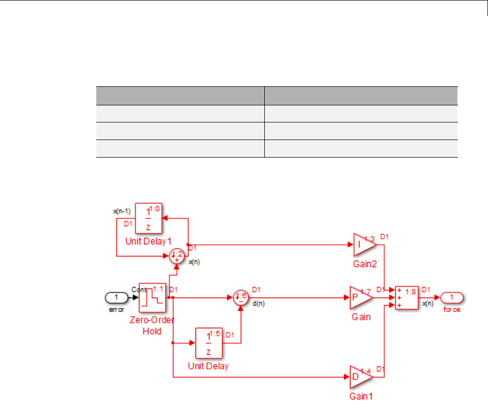
Control and Displaying the Sorted Order
For example, suppose you set the following priorities in the Discrete Cruise
Controller subsystem in the model in “Nonvirtual Subsystems” on page 23-39.
Block Priority
Gain 3
Gain1 2
Gain2 1
After updating the diagram, the sorted order for the Gain blocks is as follows.
The sorted order values of the Gain, Gain1, and Gain2 blocks reflect the
respective priorities assigned: Gain2 has highest priority and executes
before Gain1 and Gain; Gain1 has second priority and executes after Gain2;
and Gain executes after Gain1. Simulink takes into account the assigned
priorities relative to the other blocks in that subsystem.
The Gain blocks are not the first, second, and third blocks to execute. Nor
do they have consecutive sorted orders. The sorted order values do not
23-49
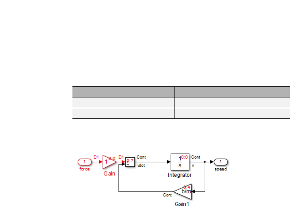
23 Working with Blocks
necessarily correspond to the priority values. Simulink arranges the blocks so
that their priorities are honored relative to each other.
Priorities Are Hierarchical
In the Car Dynamics virtual subsystem, suppose you set the priorities of
theGainblocksasfollows.
Block Priority
Gain 2
Gain1 1
After updating the diagram, the sorted order for the Gain blocks is as
illustrated. With these priorities, Gain1alwaysexecutesbeforeGain.
You can set a priority of 1to one block in each of the two subsystems because
of the hierarchal nature of the subsystems within a model. Simulink never
compares the priorities of the blocks in one subsystem to the priorities of
blocks in any other subsystem.
For example, consider this model again.
23-50
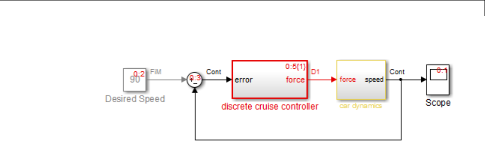
Control and Displaying the Sorted Order
The blocks within the Car Dynamics virtual subsystem are part of the
root-level system hierarchy and are part of the root-level sorted order. The
Discrete Cruise Controller subsystem has an independent sorted order with
the blocks arranged consecutively from 1:0 to 1:7.
Lack of Priority May Not Result in Low Priority
A lack of priority does not necessarily result in a low priority (higher sorting
order) for a given block. Blocks that do not have direct-feedthrough ports
executebeforeblocksthathavedirect-feedthrough ports, regardless of their
priority.
If a model has two atomic subsystems, A and B, you can assign priorities of
1and 2respectively to A and B. This priority causes all the blocks in A to
execute before any of the blocks in B. The blocks within an atomic subsystem
execute as a single unit, so the subsystem has its own system index and its
own sorted order.
Block Priority Violations
Simulink software honors the block priorities that you specify unless they
violate data dependencies. If Simulink is unable to honor a block priority, it
displays a Block Priority Violation diagnostic message.
As an example:
1Open the sldemo_bounce model.
Notice that the output of the Memory block provides the input to the
Coefficient of Restitution Gain block.
23-51

23 Working with Blocks
2Set the priority of the Coefficient of Restitution block to 1,andsetthe
priority of the Memory block to 2.
Setting these priorities specifies that the Coefficient of Restitution block
execute before the Memory block. However, the Coefficient of Restitution
block depends on the output of the Memory block, so the priorities you just
set violate the data dependencies.
3In the model window, enable sorted order by selecting Format > Block
displays > Sorted Order.
4Select Simulation > Update Diagram.
The block priority violation warning appears in the MATLAB Command
Window. The warning includes the priority for the respective blocks:
Warning: Unable to honor user-specified priorities.
'sldemo_bounce/Memory' (pri=[2]) has to execute
before 'sldemo_bounce/Coefficient of Restitution'
(pri=[1]) to satisfy data dependencies
5Remove the priorities from the Coefficient of Restitution and Memory
blocks and update the diagram again to see the correct sorted order.
23-52

Access Block Data During Simulation
Access Block Data During Simulation
In this section...
“About Block Run-Time Objects” on page 23-53
“Access a Run-Time Object” on page 23-53
“Listen for Method Execution Events” on page 23-54
“Synchronizing Run-Time Objects and Simulink Execution” on page 23-55
About Block Run-Time Objects
Simulink provides an application programming interface, called the block
run-time interface, that enables programmatic access to block data, such
as block inputs and outputs, parameters, states, and work vectors, while a
simulation is running. You can use this interface to access block run-time
data from the MATLAB command line, the Simulink Debugger, and from
Level-2 MATLAB S-functions (see “Write Level-2 MATLAB S-Functions” in
the online Simulink documentation).
Note You can use this interface even when the model is paused or is running
or paused in the debugger.
The block run-time interface consists of a set of Simulink data object classes
(see “Data Objects” on page 43-37) whose instances provide data about
the blocks in a running model. In particular, the interface associates an
instance of Simulink.RunTimeBlock, called the block’s run-time object, with
each nonvirtual block in the running model. A run-time object’s methods
and properties provide access to run-time data about the block’s I/O ports,
parameters, sample times, and states.
Access a Run-Time Object
Every nonvirtual block in a running model has a RuntimeObject parameter
whose value, while the simulation is running, is a handle for the blocks’
run-time object. This allows you to use get_param to obtain a block’s run-time
object. For example, the following statement
23-53

23 Working with Blocks
rto = get_param(gcb,'RuntimeObject');
returns the run-time object of the currently selected block.
Note Virtual blocks (see “Virtual Blocks” on page 23-2) do not have run-time
objects. Blocks eliminated during model compilation as an optimization also
do not have run-time objects (see “Block reduction”). A run-time object exists
only while the model containing the block is running or paused. If the model
is stopped, get_param returns an empty handle. When you stop or pause a
model, all existing handles for run-time objects become empty.
Listen for Method Execution Events
One application for the block run-time API is to collect diagnostic data at
key points during simulation, such as the value of block states before or
after blocks compute their outputs or derivatives. The block run-time API
provides an event-listener mechanism that facilitates such applications. For
more information, see the documentation for the add_exec_event_listener
command. For an example of using method execution events, enter
sldemo_msfcn_lms
at the MATLAB command line. This Simulink model contains the S-function
adapt_lms.m, which performs a system identification to determine the
coefficients of an FIR filter. The S-function’s PostPropagationSetup method
initializes the block run-time object’s DWork vector such that the second
vector stores the filter coefficients calculated at each time step.
In the Simulink model, double-clicking on the annotation below the S-function
block executes its OpenFcn. This function first opens a figure for plotting the
FIR filter coefficients. It then executes the function add_adapt_coef_plot.m
to add a PostOutputs method execution event to the S-function’s block
run-time object using the following lines of code.
% Get the full path to the S-function block
blk = 'sldemo_msfcn_lms/LMS Adaptive';
% Attach the event-listener function to the S-function
h = add_exec_event_listener(blk, ...
23-54

Access Block Data During Simulation
'PostOutputs', @plot_adapt_coefs);
The function plot_adapt_coefs.m is registered as an event listener that is
executed after every call to the S-function’s Outputs method. The function
accesses the block run-time object’s DWork vector and plots the filter
coefficients calculated in the Outputs method. The calling syntax used in
plot_adapt_coefs.m follows the standard needed for any listener. The first
inputargumentistheS-function’sblock run-time object, and the second
argument is a structure of event data, as shown below.
function plot_adapt_coefs(block, eventData)
% The figure's handle is stored in the block's UserData
hFig = get_param(block.BlockHandle,'UserData');
tAxis = findobj(hFig, 'Type','axes');
tAxis = tAxis(2);
tLines = findobj(tAxis, 'Type','Line');
% The filter coefficients are stored in the block run-time
% object's second DWork vector.
est = block.Dwork(2).Data;
set(tLines(3),'YData',est);
Synchronizing Run-Time Objects and Simulink
Execution
You can use run-time objects to obtain the value of a block output and display
in the MATLAB Command Window by entering the following commands.
rto = get_param(gcb,'RuntimeObject')
rto.OutputPort(1).Data
However, the displayed data may not be thetrueblockoutputiftherun-time
object is not synchronized with the Simulink execution. Simulink only
ensures the run-time object and Simulink execution are synchronized when
the run-time object is used either within a Level-2 MATLAB S-function or
in an event listener callback. When called from the MATLAB Command
Window, the run-time object can return incorrect output data if other blocks
in the model are allowed to share memory.
23-55

23 Working with Blocks
To ensure the Data field contains the correct block output, open the
Configuration Parameters dialog box, and then clear the Signal storage
reuse check box on the Optimization >Signals and Parameters pane
(see “Signal storage reuse”).
23-56

Configure a Block for Code Generation
Configure a Block for Code Generation
Use the State Attributes pane of a Block Parameters dialog box to specify
Simulink Coder code generation options for blocks with discrete states. See
“States” in the Simulink Coder documentation.
23-57

23 Working with Blocks
23-58


24 Working with Block Parameters
About Block Parameters
Most Simulink blocks have attributes whose values you can specify to
customize the block. Some attributes are common to all Simulink blocks, such
as a block’s name and foreground color. Other attributes are specific to a
block, such as the gain of a Gain block. Simulink associates a block parameter
with each user-specifiable attribute of a block. Block parameters fall into
two categories. A mathematical parameter is a parameter used to compute
the value of a block’s output, such as a Gain block’s Gain parameter. All
other parameters are configuration parameters,suchasaGainblock’sName
parameter.
A parameterized block effectively represents a family of similar blocks. For
example, when creating a model, you can set the Constant value parameter
of each instance of the Constant block separately so that each instance
behaves differently. Because it allows each standard block to represent a
family of blocks, block parameterization greatly increases the modeling power
of the standard Simulink libraries.
You specify a block attribute value by setting its associated block parameter.
For example, to set the foreground color of a block to red, you set the value
of its foreground color parameter to the string 'red'.Youcansetthevalue
programmatically, using the set_param command, or by using the block
parameters dialog box. See “Common Block Parameters” and “Block-Specific
Parameters” for the names, usages, and valid settings for Simulink block
parameters.
You can use MATLAB expressions to specify block parameter values.
The expressions can include the names of workspace variables. Simulink
evaluates the expressions before running a simulation, resolving any names
to values as described in “Symbol Resolution” on page 4-76. Do not confuse
Simulink block parameters with Simulink parameter objects. See “Block
Parameters” on page 3-9 and Simulink.Parameter for more information.
Atunable parameter is a block parameter whose value can be changed during
simulation without recompiling the model. In general, you can change the
values of mathematical parameters, but not configuration parameters. If a
parameter is not tunable and simulation is running, the dialog box control
that sets the parameter value is disabled.
24-2

About Block Parameters
If you change a tunable parameter value programmatically while simulation
is running, Simulink pauses the simulation, makes the change, then resumes
the simulation after the change is complete. Tunable parameter changes take
effect at the start of the next time step after simulation resumes.
You can use the Inline parameters check box on the
Optimization > Signals and Parameters pane of the Configuration
Parameters dialog box to specify that all parameters in your model are
nontunable except for those that you specify. This action can speed
up execution of large models and enable generation of faster code from
your model. See “Optimization Pane: Signals and Parameters” for more
information.
You can separately define each MATLAB variable intended for use in block
parameter expressions. However, this technique has several disadvantages,
such as cluttering the base workspace and providing no convenient way to
group related parameters. To avoid these disadvantages, you can combine
numeric base workspace variables into a MATLAB structure, then:
•Dereference the structure fields to provide values used in block parameter
expressions
•Pass a whole structure as an argument to a masked subsystem or a
referenced model
•Set the structure to be tunable or nontunable as you could a separately
defined variable
A structure used for any of these purposed can contain only numeric data. See
“Structure Parameters” on page24-16formoreinformation.
24-3

24 Working with Block Parameters
Set Block Parameters
You can use the Simulink set_param command to set the value of any
Simulink block parameter. In addition, you can set many block parameters
via Simulink dialog boxes and menus. These include:
•Format menu
The Simulink Editor’s Diagram > Format menu allows you to specify
attributes of the currently selected block that are visible on the model’s
block diagram, such as the block’s name and color (see “Change the
Appearance of a Block” on page 23-22 for more information).
•Block Properties dialog box
Specifies various attributes that are common to all blocks (see “Set Block
Properties” on page 23-15 for more information).
•Block Parameter dialog box
Everyblockhasadialogboxthatallows you to specify values for attributes
thatarespecifictothattypeofblock. See “Display a Block Parameter
Dialog Box” on page 24-4 for information on displaying a block’s parameter
dialog box.
•Model Explorer
TheModelExplorerallowsyoutoquicklyfindoneormoreblocksandset
their properties, thus facilitating global changes to a model, for example,
changing the gain of all of a model’s Gain blocks. See “Model Explorer
Overview” on page 9-2 for more information.
Display a Block Parameter Dialog Box
To display a block’s parameter dialog box, double-click the block in the
model or library window. You can also display a block’s parameter dialog
box by selecting the block in the model’s block diagram and choosing Block
Parameters from the Simulink Editor’s Diagram menu or from the block’s
context (right-click) menu.
24-4

Set Block Parameters
Note Double-clicking a block to display its parameter dialog box works for all
blocks with parameter dialog boxes except for Subsystem blocks and the Model
block. You must use the Simulink Editor’s Diagram menu or the block’s
context menu to display a Subsystem or Model block’s parameter dialog box.
24-5

24 Working with Block Parameters
Specify Parameter Values
In this section...
“About Parameter Values” on page 24-6
“Use Workspace Variables in Parameter Expressions” on page 24-6
“Resolve Variable References in Block Parameter Expressions” on page 24-7
“Use Parameter Objects to Specify Parameter Values” on page 24-7
“Determine Parameter Data Types” on page 24-7
About Parameter Values
Many block parameters, including mathematical parameters, accept MATLAB
expression strings as values. When Simulink compiles a model, for example,
at the start of a simulation or when you update the model, Simulink sets the
compiled values of the parameters to the result of evaluating the expressions.
Use Workspace Variables in Parameter Expressions
Block parameter expressions can include variables defined in the model’s
mask and model workspaces and in the MATLAB workspace. Using a
workspace variable facilitates updating a model that sets multiple block
parameterstothesamevalue,i.e.,itallowsyoutoupdatemultipleparameters
by setting the value of a single workspace variable. For more information,
see “Symbol Resolution” on page 4-76 and “Numeric Values with Symbols”
on page 4-78.
Using a workspace variable also allows you to change the value of a parameter
during simulation without having to open a block’s parameter dialog box. For
more information, see “Tunable Parameters” on page 24-13.
Note IfyouhaveaSimulinkCoderlicense,andyouplantogeneratecode
from a model, you can use workspace variables to specify the name, data type,
scope, volatility, tunability, and other attributes of variables used to represent
the parameter in the generated code. For more information, see “Parameters”
in the Simulink Coder documentation.
24-6

Specify Parameter Values
Resolve Variable References in Block Parameter
Expressions
When evaluating a block parameter expression that contains a variable,
Simulink by default searches the workspace hierarchy. If the variable is
not defined in any workspace, Simulink halts compilation of the model
and displays an error message. See “Symbol Resolution” on page 4-76 and
“Numeric Values with Symbols” on page 4-78 for more information.
Use Parameter Objects to Specify Parameter Values
You can use Simulink.Parameter objects in parameter expressions
to specify parameter values. For example, Kand 2*K are both valid
parameter expressions where Kis a workspace variable that references a
Simulink.Parameter object. In both cases, Simulink uses the parameter
object’s Value property as the value of K. See “Symbol Resolution” on page
4-76 and “Numeric Values with Symbols” on page 4-78for more information.
Using parameter objects to specify parameters can facilitate tuning
parameters in some applications. See “Using a Parameter Object to Specify
a Parameter As Noninlined” on page 24-15 and “Parameterize Model
References” on page 6-52 for more information.
Note Do not use expressions of the form p.Value where pis a parameter
object in block parameter expressions. Such expressions cause evaluation
errors when Simulink compiles the model.
Determine Parameter Data Types
When Simulink compiles a model, each of the model’s blocks determines a
data type for storing the values of its parameters whose values are specified
by MATLAB parameter expressions.
Most blocks use internal rules to determine the data type assigned to a
specific parameter. Exceptions include the Gain block, whose parameter
dialog box allows you to specify the data type assigned to the compiled value
of its Gain parameter. You can configure your model to check whether the
data type assigned to a parameter can accommodate the parameter value
specified by the model (see “Data Validity Diagnostics Overview”).
24-7

24 Working with Block Parameters
Obtain Parameter Information
You can use get_param to find the system and block parameter values for
your model. See “Model Parameters” and “Common Block Parameters” for
arguments get_param accepts.
The model’s signal attributes and parameter expressions must be evaluated
before some parameters are properly reported. This evaluation occurs during
the simulation compilation phase. Alternatively, you can compile your
model without first running it, and then obtain parameter information. For
instance, to access the port width, data types, and dimensions of the blocks in
your model, enter the following at the command prompt:
modelname([],[],[],'compile')
q=get_param(gcb,'PortHandles');
get_param(q.Inport,'CompiledPortDataType')
get_param(q.Inport,'CompiledPortWidth')
get_param(q.Inport,'CompiledPortDimensions')
modelname([],[],[],'term')
24-8

Check Parameter Values
Check Parameter Values
In this section...
“About Value Checking” on page 24-9
“Blocks That Perform Parameter Range Checking” on page 24-9
“Specify Ranges for Parameters” on page 24-10
“Perform Parameter Range Checking” on page 24-11
About Value Checking
Many blocks perform range checking of their mathematical parameters.
Generally, blocks that allow you to enter minimum and maximum values
check to ensure that the values of applicable parameters lie within the
specified range.
Blocks That Perform Parameter Range Checking
The following blocks perform range checking for their parameters:
Block Parameters Checked
Constant Constant value
Data Store Memory Initial value
Gain Gain
Interpolation Using Prelookup Table data
1-D Lookup Table Table data
2-D Lookup Table Table data
n-D Lookup Table Table data
Relay Output when on
Output when off
Repeating Sequence Interpolated Vector of output values
24-9

24 Working with Block Parameters
Block Parameters Checked
Repeating Sequence Stair Vector of output values
Saturation Upper limit
Lower limit
Specify Ranges for Parameters
In general, use the Output minimum and Output maximum parameters
that appear on a block parameter dialog box to specify a range of valid values
for the block parameters. The following exceptions apply:
•For the Gain block, use the Parameter minimum and Parameter
maximum fields to specify a range for the Gain parameter.
•For the Data Store Memory block, use the Minimum and Maximum fields
to specify a range for the Initial value parameter.
When specifying minimum and maximum values that constitute a range,
enter only expressions that evaluate to a finite, scalar, real number with
double data type. The default values for the minimum and maximum are []
(unspecified). The scalar values that you specify are subject to expansion, for
example, when the block parameters that Simulink checks are nonscalar (see
“Scalar Expansion of Inputs and Parameters” on page 47-38).
Note You cannot specify the minimum or maximum value as NaN,inf,or
inf.
Specifying Ranges for Complex Numbers
When you specify a minimum or maximum value for a parameter that is a
complex number, the specified minimum and maximum apply separately
to the real part and to the imaginary part of the complex number. If the
value of either part of the number is less than the minimum, or greater than
the maximum, the complex number is outside the specified range. No range
checking occurs against any combination of the real and imaginary parts,
such as (sqrt(a^2+b^2))
24-10

Check Parameter Values
Perform Parameter Range Checking
You can initiate parameter range checking in the following ways:
•When you click the OK or Apply button on a block parameter dialog box,
the block performs range checking for its parameters. However, the block
checks only the parameters that it can readily evaluate. For example, the
block does not check parameters that use an undefined workspace variable.
•In the Simulink Editor, when you start a simulation or select
Simulation > Update Diagram, Simulink performs parameter range
checking for all blocks in that model.
Simulink performs parameter range checking by comparing the values of
applicable block parameters with both thespecifiedrange(see“Specify
Ranges for Parameters” on page 24-10) and the block data type. That is,
Simulink performs the following check:
DataTypeMin MinValue VALUE MaxValue DataTypeMax
where
•DataTypeMin is the minimum value representable by the block data type.
•MinValue is the minimum value the block should output, specified by, e.g.,
Output minimum.
•VALUE is the numeric value of a block parameter.
•MaxValue is the maximum value the block should output, specified by, e.g.,
Output maximum.
•DataTypeMax is the maximum value representable by the block data type.
When Simulink detects a parameter value that violates the check, it displays
an error message. For example, consider a model that contains a Constant
block whose
•Constant value parameter specifies the variable const,whichyouhave
yettodefineinaworkspace.
•Output minimum and Output maximum parameters are set to 2and
8, respectively.
24-11
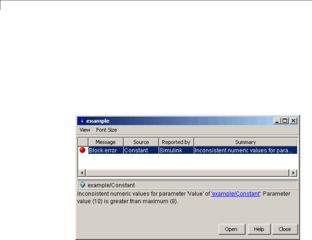
24 Working with Block Parameters
•Output data type parameter is set to uint8.
In this situation, Simulink does not perform parameter range checking when
you click the OK button on the Constant block dialog box because the variable
const is undefined. But suppose you define its value by entering
const = 10
at the MATLAB prompt, and then you update the diagram (see “Update a
Block Diagram” on page 1-25). Simulink displays the following error message:
24-12

Tunable Parameters
Tunable Parameters
In this section...
“About Tunable Parameters” on page 24-13
“Tune a Block Parameter” on page 24-13
About Tunable Parameters
Simulink lets you change the values of many block parameters during
simulation. Such parameters are called tunable parameters.Ingeneral,
only parameters that represent mathematical variables, such as the Gain
parameter of the Gain block, are tunable. Parameters that specify the
appearance or structure of a block, e.g., the number of inputs of a Sum block,
or when it is evaluated, e.g., a block’s sampletimeorpriority,arenottunable.
You can tell whether a particular parameter is tunable by examining its edit
control in the block’s dialog box or Model Explorer during simulation. If the
control is disabled, the parameter is nontunable. You cannot tune inline
parameters. See “Inline Parameters” on page 24-14 for more information.
Tune a Block Parameter
You can use a block’s dialog box or the Model Explorer to modify the tunable
parameters of any block. To use the block’s parameter dialog box, open the
block’s parameter dialog box, change the value displayed in the dialog box,
and click the dialog box’s OK or Apply button.
You can also tune a parameter at the MATLAB command line, using either
the set_param commandorbyassigninganewvaluetotheMATLAB
workspace variable that specifies the parameter’s value. In either case, you
must update the model’s block diagram for the change to take effect (see
“Update a Block Diagram” on page 1-25).
24-13

24 Working with Block Parameters
Inline Parameters
In this section...
“About Inlined Parameters” on page 24-14
“Specify Some Parameters as Noninline” on page 24-14
About Inlined Parameters
The Inline parameters option (see “Inline parameters” ) controls how
mathematical block parameters appear in code generated from the model.
When this optimization is off (the default), a model’s mathematical block
parameters appear as variables in the generated code. As a result, you can
tune the parameters both during simulation and when executing the code.
When Inline parameters is selected, the parameters appear in the generated
code as inlined numeric constants. This reduces the generated code’s memory
and processing requirements. However, because the inlined parameters
appear as constants in the generated code, you cannot tune them during
code execution. To ensure that simulation and generated code execution
fully correspond, Simulink prevents you from changing the values of block
parameters during simulation when Inline parameters is selected.
Note Simulink ignores tunable parameter specifications in the Model
Parameter Configuration dialog box if the model is a referenced model or
contains any Model blocks. Do not use this dialog box to override the inline
parameters optimization for selected parameters to permit them to be tuned.
Instead, see “Parameterize Model References” on page 6-52 for alternate
techniques. If you define tunable parameters using Simulink.Parameter
objects, you can tune the top model and reference model parameters.
Specify Some Parameters as Noninline
Suppose that you want to take advantage of the Inline parameters
optimization while retaining the ability to tune some of your model
parameters. You can do this by declaring some parameters as noninline,
using either the “Model Parameter Configuration Dialog Box” or a
24-14

Inline Parameters
Simulink.Parameter object. In either case, you must use a workspace
variable to specify the value of the parameter.
If you have a Simulink Coder license, when compiling a model with the inline
parameters option on, Simulink checks to ensure that the data types of the
workspace variables used to specify the model’s noninline parameters are
compatible with code generation. If not, Simulink halts the compilation and
displays an error. For more information, see “Tunable Workspace Parameter
Data Type Considerations”.
Note The documentation for the Simulink Coder refers to workspace
variables used to specify the value of noninline parameters as tunable
workspace parameters. In this context, the term parameter refers to a
workspacevariableusedtospecifyaparameter as opposed to the parameter
itself.
Using a Parameter Object to Specify a Parameter As
Noninlined
If you use a parameter object to specify a parameter’s value (see “Use
Parameter Objects to Specify Parameter Values” on page 24-7), you can
also use the object to specify the parameter as noninlined. To do this, set
the parameter object’s CoderInfo.StorageClass property to any value but
'Auto' (the default).
K=Simulink.Parameter;
K.CoderInfo.StorageClass = 'SimulinkGlobal';
If you set the CoderInfo.StorageClass property to any value other than
Auto, you should not include the parameter in the tunable parameters table
in the Model Parameter Configuration dialog box.
Note Simulink halts model compilation and displays an error message if
it detects a conflict between the properties of a parameter as specified by
a parameter object and the properties of the parameter as specified in the
Model Parameter Configuration dialog box.
24-15

24 Working with Block Parameters
Structure Parameters
In this section...
“About Structure Parameters” on page 24-16
“Define Structure Parameters” on page 24-17
“Referencing Structure Parameters” on page 24-17
“Structure Parameter Arguments” on page 24-18
“Tunable Structure Parameters” on page 24-19
“Parameter Structure Limitations” on page 24-20
About Structure Parameters
Separately defining all base workspace variables used in block parameter
expressions can clutter the base workspace and result in very long lists of
arguments to subsystems and referenced models. The technique provides no
waytoconvenientlygrouprelatedbaseworkspace variables, or to configure
generatedcodetoreflectthevariables’relationships.
To minimize the disadvantages of separately defining workspace variables
used by block parameters, you can group numeric variables by specifying their
names and values as the fields of a MATLAB structure in the base workspace.
A MATLAB structure that Simulink uses in block parameter expressions is
called a structure parameter. You can use structure parameters to:
•Simplify and modularize the base workspace by using multiple structures
to group related variables and to prevent name conflicts
•Dereference the structure in block parameter expressions to provide values
from structure fields rather than separate variables
•Pass all the fields in a structure to a subsystem or referenced model with a
single argument.
•Improve generated code to use structures rather multiple separate
variables
For information about creating and using MATLAB structures, see Structures
in the MATLAB documentation. You can use all the techniques described
24-16

Structure Parameters
there to manipulate structure parameters. This section assumes that you
know those techniques, and provides only information that is specific to
Simulink.
For information on structure parameters in the context of generated code for
a model, see “Structure Parameters and Generated Code”. For an example
of how to convert a model that uses unstructured workspace variables to a
model that uses structure parameters, see sldemo_applyVarStruct.
Define Structure Parameters
Defining a structure parameter is syntactically the same as defining any
MATLAB structure, as described in Structures. Every field in a MATLAB
structure that functions as a structure parameter must have a numeric data
type, even if Simulink never uses the field. Different fields can have different
numeric types.
In structure parameters, numeric types include enumerated types, by virtue
of their underlying integers. The value of a structure parameter field, can
be a real or complex scalar, vector, or multidimensional array. However, a
structure that contains any multidimensional array cannot be tuned. See
“Tunable Structure Parameters” on page 24-19.
MATLAB structures, including those used as structure parameters, can
have substructures to any depth. Structures and substructures at any level
behave identically, so the following instructions refer only to structures unless
substructures are specifically the point.
Referencing Structure Parameters
You can use MATLAB syntax, as described in Structures, to dereference a
structure parameter field anywhere in a block parameter expression that
a MATLAB variable can appear. You cannot specify a structure name in
a mathematical block parameter expression, because that would pass a
structure rather than a number. For example, suppose you have defined
the following parameter structure:
A /* Root structure
|__x /* Numeric field
|__y /* Numeric field
24-17
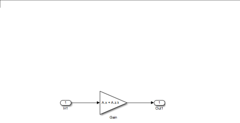
24 Working with Block Parameters
|__z /* Substructure
|__ m /* Numeric field
|__ n /* Numeric field
|__ k /* Numeric field
Given this structure, you can specify an individual field, such as A.x,ina
block parameter expression, thereby passing only xto the block. The effect
is exactly the same as if xwere a separate base workspace variable whose
valuewasthesameasthevalueofA.x. Similarly, you could reference A.z.m,
A.z.n, etc. The next figure shows an example that uses a Gain block:
The Gain block’s Gain parameter is the value of A.x + A.z.k, a numeric
expression. You could not reference Aor A.z to provide a Gain parameter
value, because neither resolves to a numeric value.
Structure Parameter Arguments
You can use a parameter structure field as a masked subsystem or model
reference argument by referencing the field, as described in the previous
section, in Subsystem block mask, or Model block. For example, suppose you
have defined the parameter structure used in the previous example:
A /* Root structure
|__x /* Numeric field
|__y /* Numeric field
|__z /* Substructure
|__ m /* Numeric field
|__ n /* Numeric field
|__ k /* Numeric field
You could then:
24-18

Structure Parameters
1Use a whole structure parameter as a masked subsystem argument or a
referenced model argument by referencing the structure’s name
2Dereference the structure as needed in the subsystem mask code, the
subsystem itself, or the referenced model.
For example, you could pass A, providing access to everything in the
root structure, or A.z, providing access only to that substructure. The
dereferencing syntax for arguments is the same as in any other context, as
described in Structures.
When you pass a structure parameter to a referenced model, the structure
definitions must be identical in the parent model and the submodel, including
any unused fields. See “Systems and Subsystems” on page 3-11, “Masking”,
and “Using Model Arguments” on page 6-53 more information about passing
and using arguments.
Tunable Structure Parameters
Declare a structure parameter to be tunable using one of the following
techniques.
•Clear Model Configuration Parameters > Optimization > Signals
and Parameters > Inline parameters. See “Inline parameters” for more
information.
•Set Inline parameters, and then specify the parameter structure as
tunable in the Model Parameter Configuration Dialog Box.
•Associate a Simulink.Parameter object with the structure parameter,
and specify the object’s storage class as anything other than Auto.Inthe
following example, the structure parameter myStruct is associated with a
Simulink.Parameter object.
myStruct = Simulink.Parameter;
myStruct.Value = [1 2 3];
myStruct.CoderInfo.StorageClass = 'ExportedGlobal';
A tunable structure parameter can contain a nontunable numeric field (like
a multidimensional array) without affecting the tunability of the rest of the
structure. You cannot define individual substructures or fields within a
24-19

24 Working with Block Parameters
structure parameter to be tunable. Only the name of the root level of the
structure appears in the Model Configuration Parameter dialog box, and only
the root can have a Simulink.Parameter object assigned to it.
For more information about tunability, see “Inline Parameters” on page 24-14
and “Tunable Parameters” on page 24-13. For simplicity, those sections
mention only separately defined base workspace variables, but all of the
information applies without change to tunable structure parameters.
Parameter Structure Limitations
•You cannot define individual substructures or fields within a structure
parameter as tunable.
•Tunable structure parameters do not support context sensitivity.
24-20

25
Working with Lookup
Tables
•“About Lookup Table Blocks” on page 25-2
•“Anatomy of a Lookup Table” on page 25-4
•“Lookup Tables Block Library” on page 25-5
•“Guidelines for Choosing a Lookup Table” on page 25-7
•“Enter Breakpoints and Table Data” on page 25-11
•“Characteristics of Lookup Table Data” on page 25-18
•“Methods for Estimating Missing Points” on page 25-23
•“Edit Existing LookupTables” on page 25-28
•“Create a Logarithm Lookup Table” on page 25-63
•“Prelookup and Interpolation Blocks” on page 25-66
•“Optimize Generated Code for Lookup Table Blocks” on page 25-67
•“UpdateLookupTableBlockstoNewVersions”onpage25-71
•“Lookup Table Glossary” on page 25-77
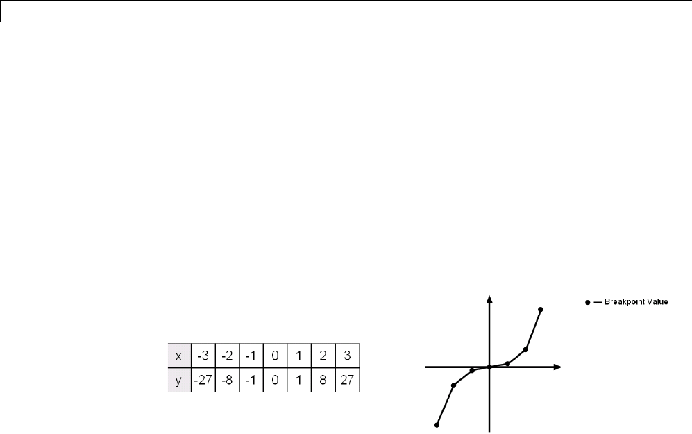
25 Working with Lookup Tables
About Lookup Table Blocks
Alookup table block uses an array of data to map input values to output
values, approximating a mathematical function. Given input values, Simulink
performs a “lookup” operation to retrieve the corresponding output values
from the table. If the lookup table does not define the input values, the block
estimates the output values based on nearby table values.
The following example illustrates a one-dimensional lookup table that
approximates the function y=x3. The lookup table defines its output (y)data
discretely over the input (x)range[-3, 3]. The following table and graph
illustrate the input/output relationship:
An input of -2 enables the table to look up and retrieve the corresponding
output value (-8). Likewise, the lookup table outputs 27 in response to an
input of 3.
When the lookup table block encounters an input that does not match any
of the table’s xvalues, it can interpolate or extrapolate the answer. For
instance, the lookup table does not define an input value of -1.5; however, the
block can linearly interpolate the nearest data points (-2, -8) and (-1, -1) to
estimate and return a value of -4.5.
25-2
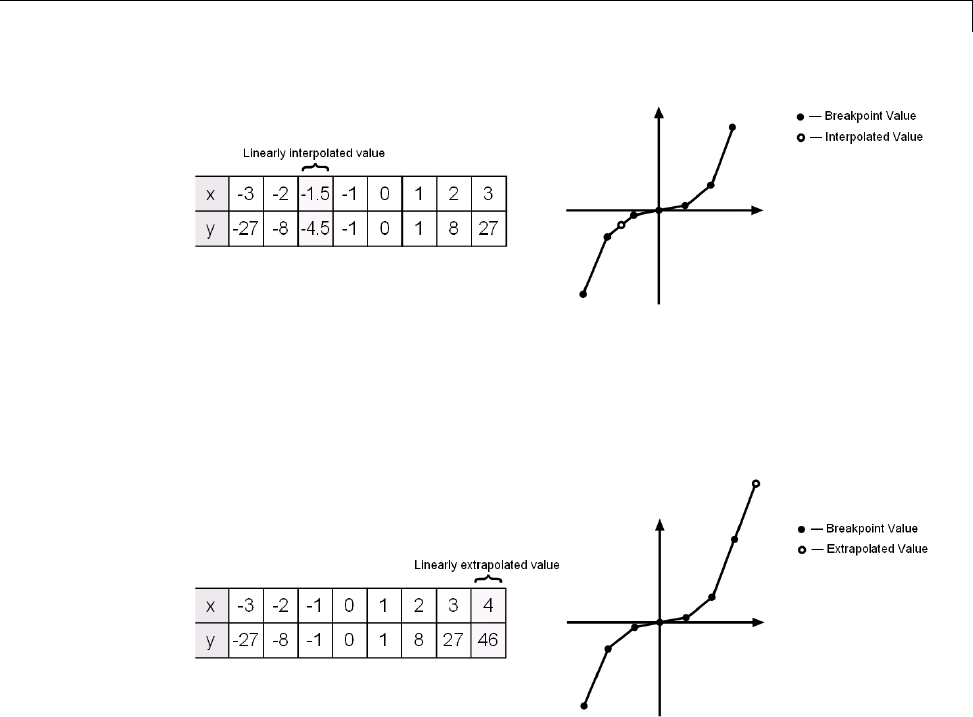
About Lookup Table Blocks
Similarly, although the lookup table does not include data for xvalues beyond
the range of [-3, 3], the block can extrapolate values using a pair of data
points at either end of the table. Given an input value of 4, the lookup
table block linearly extrapolates the nearest data points (2, 8) and (3, 27) to
estimate an output value of 46.
Since table lookups and simple estimations can be faster than mathematical
function evaluations, using lookup table blocks might result in speed
gains when simulating a model. Consider using lookup tables in lieu of
mathematical function evaluations when:
•An analytical expression is expensive to compute.
•No analytical expression exists, but the relationship has been determined
empirically.
Simulink provides a broad assortment of lookup table blocks, each geared
for a particular type of application. The sections that follow outline the
different offerings, suggest how to choosethelookuptablebestsuitedtoyour
application, and explain how to interact with the various lookup table blocks.
25-3
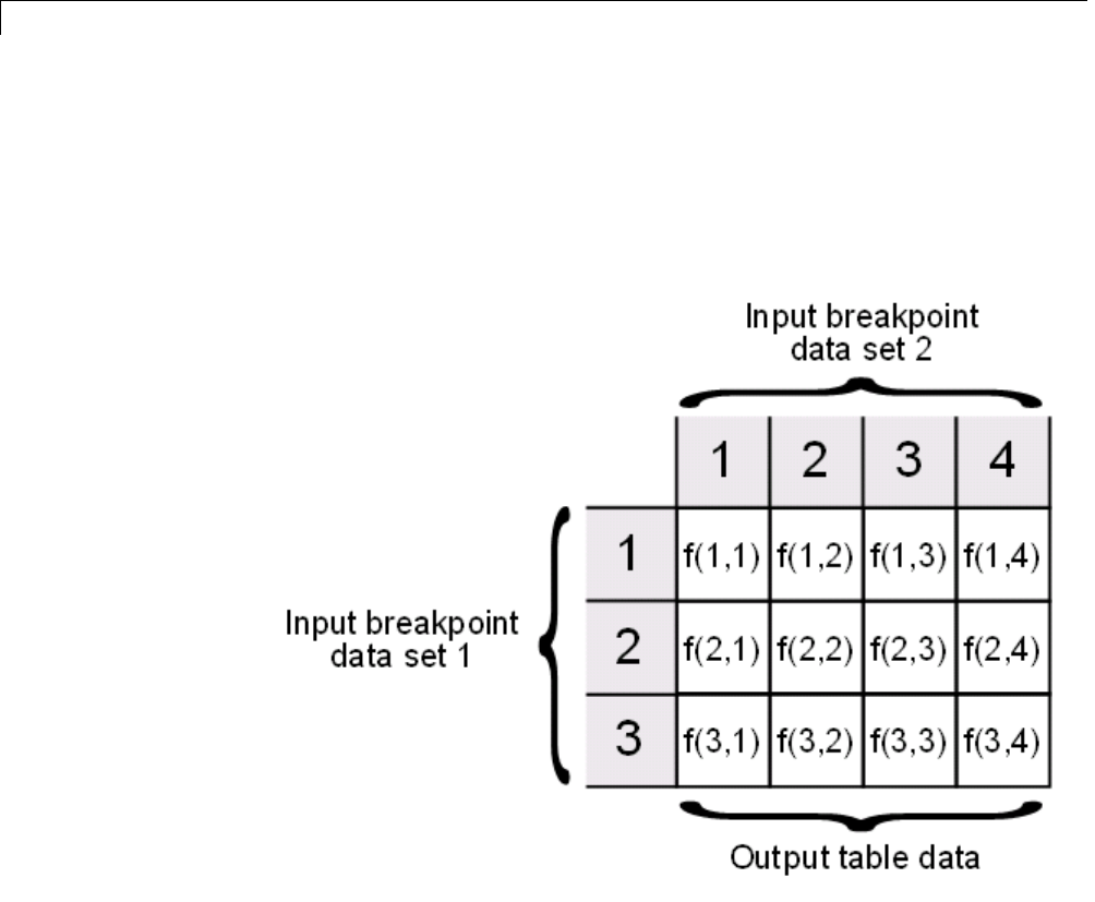
25 Working with Lookup Tables
Anatomy of a Lookup Table
The following figure illustrates the anatomy of a two-dimensional lookup
table. Vectors or breakpoint data sets and an array, referred to as table data,
constitute the lookup table.
Each breakpoint data set is an index of input values for a particular
dimension of the lookup table. The array of table data serves as a sampled
representation of a function evaluated at the breakpoint values. Lookup table
blocks use breakpoint data sets to relate a table’s input values to the output
values that it returns.
25-4
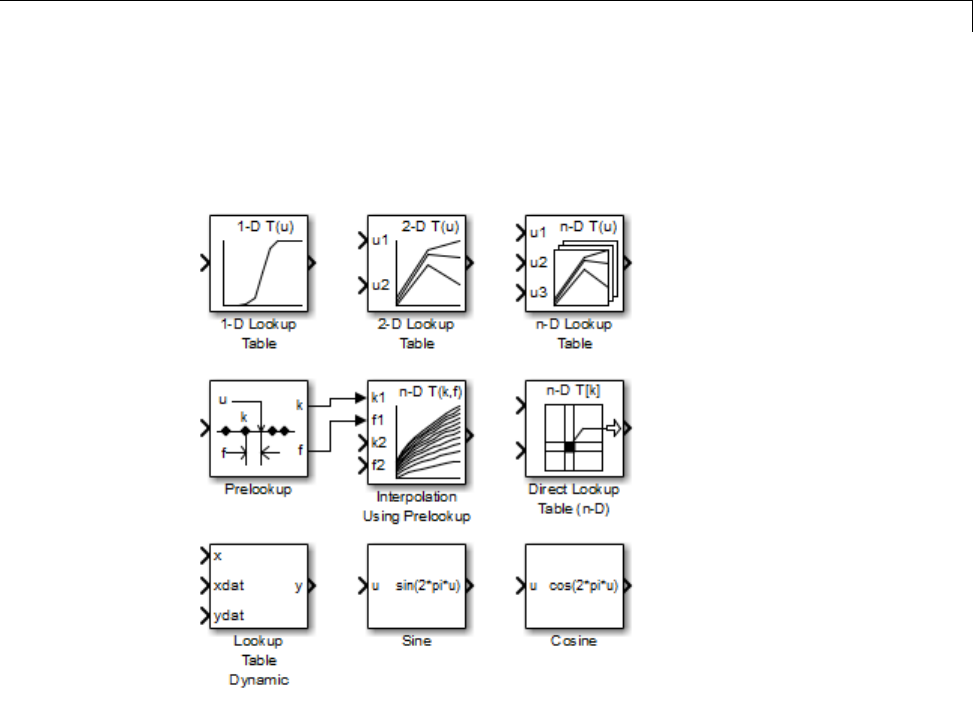
Lookup Tables Block Library
Lookup Tables Block Library
Several lookup table blocks appear in the Lookup Tables block library.
25-5

25 Working with Lookup Tables
The following table summarizes the purpose of each block in the library.
Block Name Description
1-D Lookup Table Approximate a one-dimensional function.
2-D Lookup Table Approximate a two-dimensional function.
n-D Lookup Table Approximate an N-dimensional function.
Prelookup Compute index and fraction for Interpolation Using Prelookup block.
Interpolation Using
Prelookup
Use precalculated index and fraction values to accelerate approximation
of N-dimensional function.
Direct Lookup Table
(n-D)
Index into an N-dimensional table to retrieve the corresponding outputs.
Lookup Table
Dynamic
Approximate a one-dimensional function using a dynamically specified
table.
Sine Use a fixed-point lookup table to approximate the sine wave function.
Cosine Use a fixed-point lookup table to approximate the cosine wave function.
25-6

Guidelines for Choosing a Lookup Table
Guidelines for Choosing a Lookup Table
In this section...
“Data Set Dimensionality” on page 25-7
“Data Set Numeric and Data Types” on page 25-7
“Data Accuracy and Smoothness” on page 25-8
“Dynamics of Table Inputs” on page 25-8
“Efficiency of Performance” on page 25-8
“Summary of Lookup Table Block Features” on page 25-10
Data Set Dimensionality
In some cases, the dimensions of your data set dictate which of the lookup
tableblocksisrightforyourapplication. If you are approximating a
one-dimensional function, consider using either the 1-D Lookup Table or
Lookup Table Dynamic block. If you are approximating a two-dimensional
function, consider the 2-D Lookup Table block. Blocks such as the n-D Lookup
Table and Direct Lookup Table (n-D) allow you to approximate a function of
Nvariables.
Data Set Numeric and Data Types
The numeric and data types of your data set influence the decision of which
lookup table block is most appropriate. Although all lookup table blocks
support real numbers, the Direct Lookup Table (n-D), 1-D Lookup Table, 2-D
Lookup Table, and n-D Lookup Table blocks also support complex table data.
All lookup table blocks support integer and fixed-point data in addition to
double and single data types.
Note For the Direct Lookup Table (n-D) block, fixed-point types are
supported for the table data, output port, and optional table input port.
25-7

25 Working with Lookup Tables
Data Accuracy and Smoothness
The desired accuracy and smoothness of the data returned by a lookup table
determine which of the blocks you should use. Most blocks provide options
to perform interpolation and extrapolation, improving the accuracy of values
that fall between or outside of the table data, respectively. For instance, the
Lookup Table Dynamic block performs linear interpolation and extrapolation,
while the n-D Lookup Table block performs either linear or cubic spline
interpolation and extrapolation. In contrast, the Direct Lookup Table (n-D)
block performs table lookups without any interpolation or extrapolation. You
can achieve a mix of interpolation and extrapolation methods by using the
Prelookup block with the Interpolation Using Prelookup block.
Dynamics of Table Inputs
The dynamicsofthelookuptableinputsimpactwhichofthelookuptable
blocks is ideal for your application. The blocks use a variety of index search
methods to relate the lookup table inputs to the table’s breakpoint data
sets. Most of the lookup table blocks offer a binary search algorithm, which
performs well if the inputs change significantly from one time step to the next.
The 1-D Lookup Table, 2-D Lookup Table, n-D Lookup Table, and Prelookup
blocks offer a linear search algorithm. Using this algorithm with the option
that resumes searching from the previous result performs well if the inputs
change slowly. Some lookup table blocks also provide a search algorithm that
works best for breakpoint data sets composed of evenly spaced breakpoints.
You can achieve a mix of index search methods by using the Prelookup block
with the Interpolation Using Prelookup block.
Efficiency of Performance
When the efficiency with which lookup tables operate is important, consider
using the Prelookup block with the Interpolation Using Prelookup block.
These blocks separate the table lookup process into two components — an
index search that relates inputs to the table data, followed by an interpolation
and extrapolation stage that computes outputs. These blocks enable you to
perform a single index search and then reuse the results to look up data in
multiple tables. Also, the Interpolation Using Prelookup block can perform
sub-table selection, where the block interpolates a portion of the table data
instead of the entire table. For example, if your 3-D table data constitutes a
stack of 2-D tables to be interpolated, you can specify a selection port input to
select one or more of the 2-D tables from the stack for interpolation. A full 3-D
25-8

Guidelines for Choosing a Lookup Table
interpolation has 7 sub-interpolations but a 2-D interpolation requires only 3
sub-interpolations. As a result, significant speed improvements are possible
when some dimensions of a table are used for data stacking and not intended
for interpolation. These features make table lookup operations more efficient,
reducing computational effort and simulation time.
25-9

25 Working with Lookup Tables
Summary of Lookup Table Block Features
Use the following table to identify features that correspond to particular
lookup table blocks, then select the block that best meets your requirements.
Feature
1-D
Lookup
Table
2-D
Lookup
Table
Lookup
Table
Dynamic
n-D
Lookup
Table
Direct
Lookup
Table (n-D)
Prelookup Interp.
Using
Prelookup
Interpolation Methods
Flat •••••••
Linear •••• ••
Cubic spline •• •
Extrapolation Methods
Clip •••••••
Linear •••• ••
Cubic spline •• •
Numeric & Data Type Support
Complex •• ••
Double, Single •••••••
Integer •••••••
Fixed point •••••••
Index Search Methods
Binary •••• •
Linear •• • •
Evenly spaced
points •• •••
Start at
previous index •• • •
Miscellaneous
Sub-table
selection ••
Dynamic
breakpoint data •
Dynamic table
data •••
Input range
checking •• ••••
25-10

Enter Breakpoints and Table Data
Enter Breakpoints and Table Data
In this section...
“Entering Data in a Block Parameter Dialog Box” on page 25-11
“Entering Data in the Lookup Table Editor” on page 25-13
“Entering Data Using Inports of the Lookup Table Dynamic Block” on
page 25-16
Entering Data in a Block Parameter Dialog Box
Use the following procedure to populate a 1-D Lookup Table block using the
parameter dialog box. In this example, the lookup table approximates the
function y=x3over the range [-3, 3].
1Copy a 1-D Lookup Table block from the Lookup Tables block library to a
Simulink model.
2In the model window, double-click the 1-D Lookup Table block.
25-11
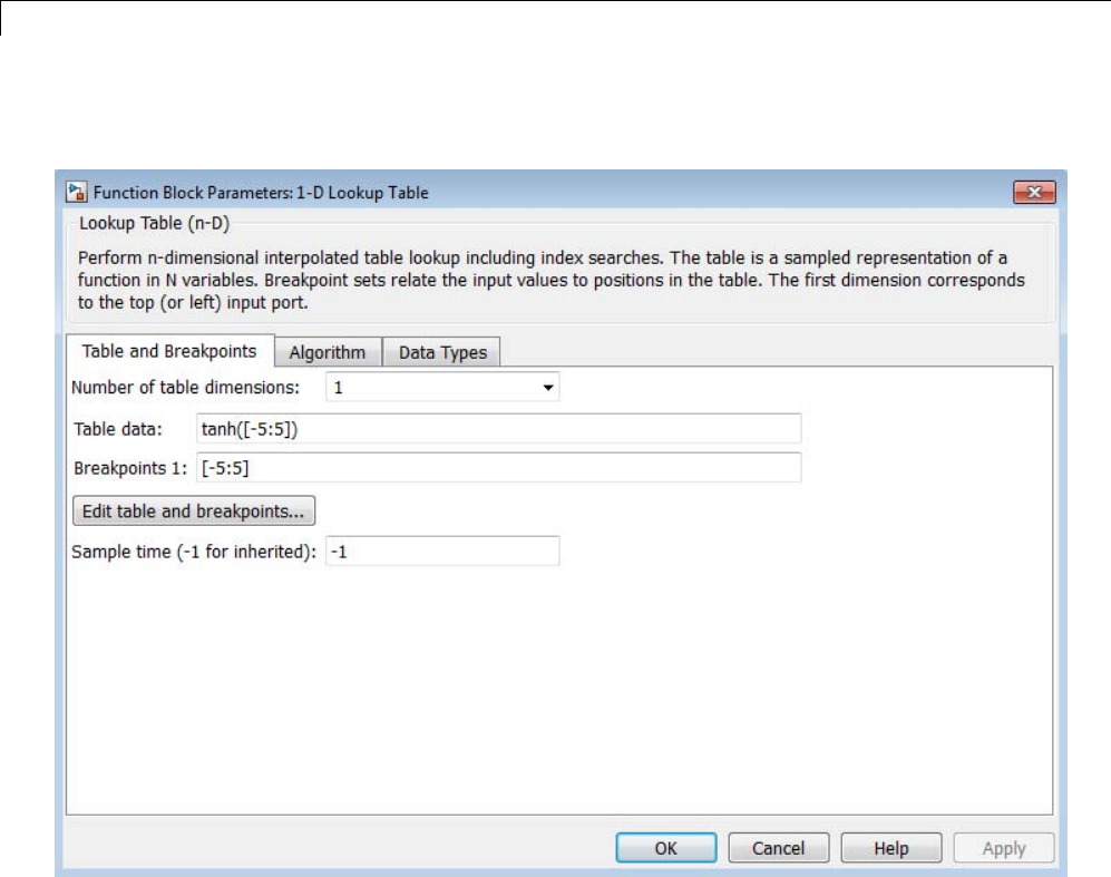
25 Working with Lookup Tables
The block parameter dialog box appears.
The dialog box displays the default values for the block.
3Enter the table dimensions, table data, and breakpoint data set in the
specified fields of the dialog box:
•In the Number of table dimensions field, enter 1.
•In the Table data field, enter [-27 -8 -1 0 1 8 27].
•In the Breakpoints 1 field, enter [-3:3].
•Click Apply.
25-12
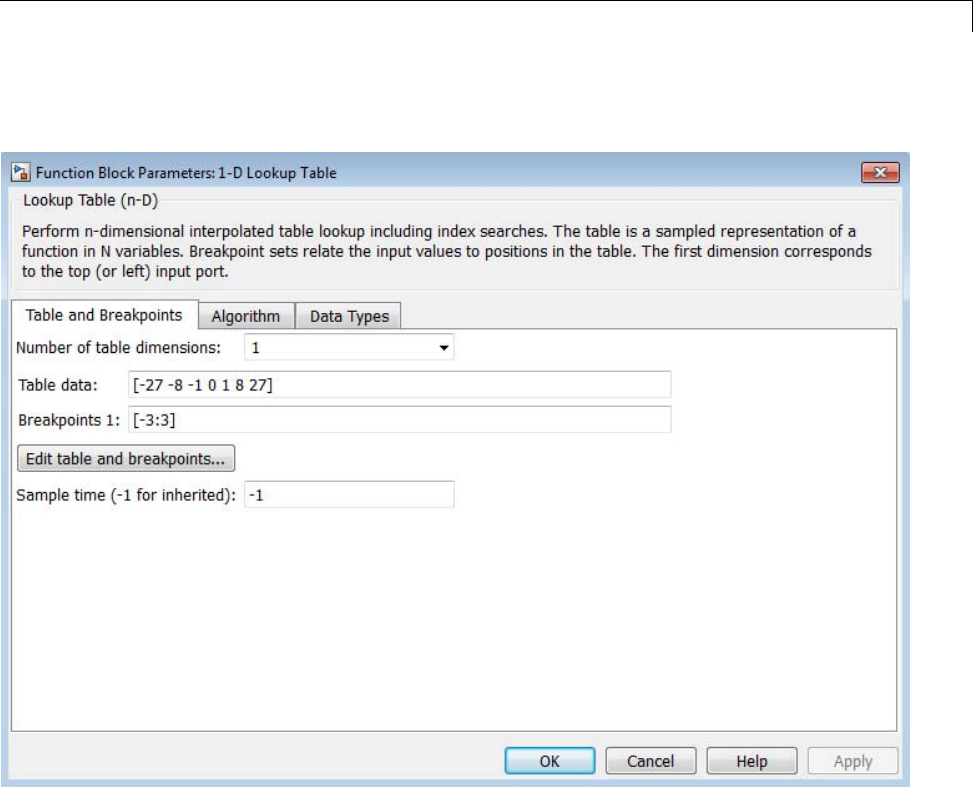
Enter Breakpoints and Table Data
The block dialog box looks something like this:
4Click OK to apply the changes and close the dialog box.
Entering Data in the Lookup Table Editor
Use the following procedure to populate a 2-D Lookup Table block using the
Lookup Table Editor. In this example, the lookup table approximates the
function z=x2+y2over the input ranges x=[0,2]and y=[0,2].
1Copy a 2-D Lookup Table block from the Lookup Tables block library to a
Simulink model.
25-13
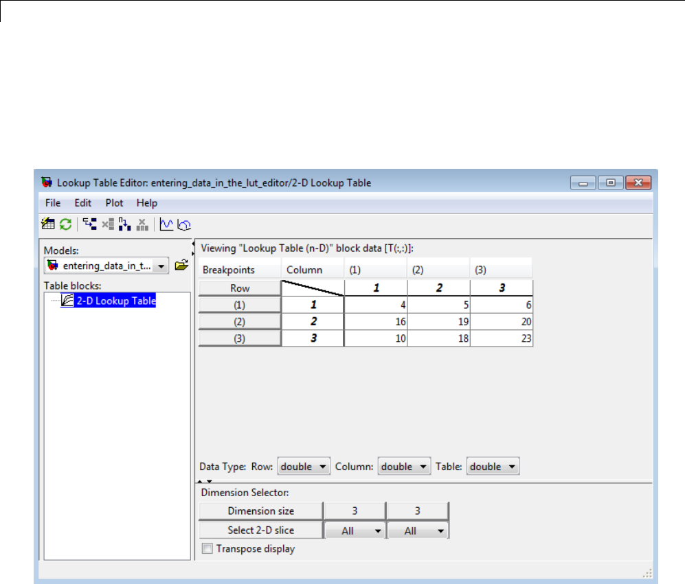
25 Working with Lookup Tables
2Open the Lookup Table Editor by selecting Lookup Table Editor from
the Simulink Edit menu or by clicking Edit table and breakpoints on
thedialogboxofthe2-DLookupTableblock.
The Lookup Table Editor appears.
It displays the default data for the 2-D Lookup Table block.
3Under Viewing "Lookup Table (n-D)" block data,enterthebreakpoint
data sets and table data in the appropriate cells. To change the default
data, double-click a cell, enter the new value, and then press Enter or click
outside the field to confirm the change:
25-14
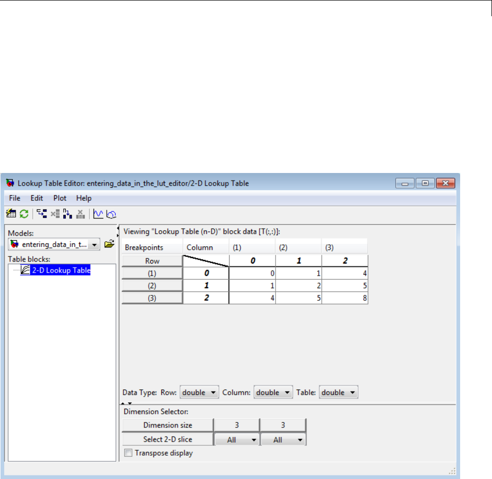
Enter Breakpoints and Table Data
•In the cells associated with the Row Breakpoints, enter each of the
values [0 1 2].
•In the cells associated with the Column Breakpoints, enter each of
the values [0 1 2].
•Inthetabledatacells,enterthevaluesinthearray[0 1 4; 1 2 5;
458]
.
The Lookup Table Editor should look like this:
4In the Lookup Table Editor, select File > Update Block Data to update
the data in the 2-D Lookup Table block.
5Close the Lookup Table Editor.
25-15

25 Working with Lookup Tables
Entering Data Using Inports of the Lookup Table
Dynamic Block
Use the following procedure to populate a Lookup Table Dynamic block using
that block’s inports. In this example, the lookup table approximates the
function y=3x2over the range [0, 10].
1Copy a Lookup Table Dynamic block from the Lookup Tables block library
to a Simulink model.
2Copy the blocks needed to implement the equation y=3x2to the Simulink
model:
•One Constant block to define the input range, from the Sources library
•One Math Function block to square the input range, from the Math
Operations library
•One Gain block to multiply the signal by 3, also from the Math
Operations library
3Assign the following parameter values to the Constant, Math Function, and
Gain blocks using their dialog boxes:
Block Parameter Value
Constant Constant value 0:10
Math Function Function square
Gain Gain 3
4Input the breakpoint data set to the Lookup Table Dynamic block by
connecting the outport of the Constant block to the inport of the Lookup
Table Dynamic block labeled xdat. This signal is the input breakpoint
data set for x.
5Input the table data to the Lookup Table Dynamic block by branching
the output signal from the Constant block and connecting it to the Math
Function block. Then connect the Math Function block to the Gain block.
Finally, connect the Gain block to the inport of the Lookup Table Dynamic
block labeled ydat. This signal is the table data for y.
25-16
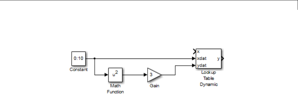
Enter Breakpoints and Table Data
The model should look something like this:
25-17
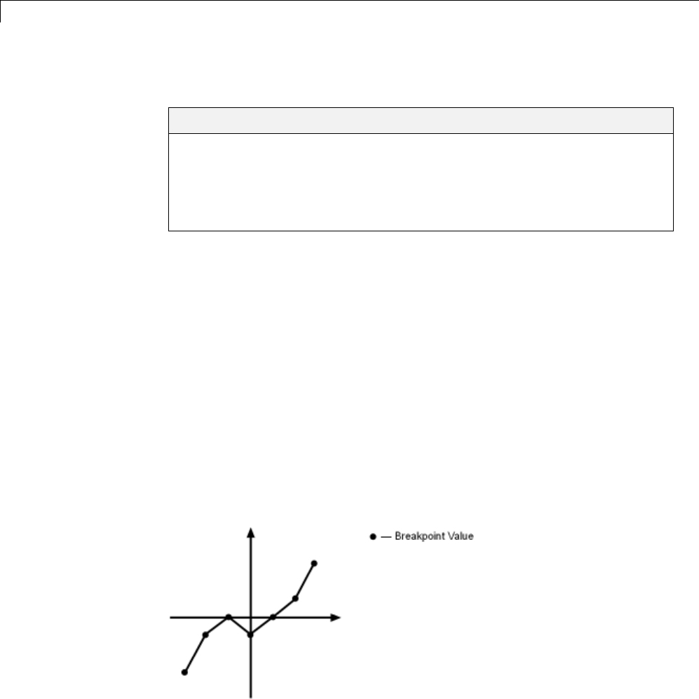
25 Working with Lookup Tables
Characteristics of Lookup Table Data
In this section...
“Sizes of Breakpoint Data Sets and Table Data” on page 25-18
“Monotonicity of Breakpoint Data Sets” on page 25-19
“Representation of Discontinuities in Lookup Tables” on page 25-20
“Formulation of Evenly Spaced Breakpoints” on page 25-22
Sizes of Breakpoint Data Sets and Table Data
The following constraints apply to the sizes of breakpoint data sets and table
data associated with lookup table blocks:
•The memory limitations of your system constrain the overall size of a
lookup table.
•Lookup tables must use consistent dimensions so that the overall size of
the table data reflects the size of each breakpoint data set.
To illustrate the second constraint, consider the following vectors of input and
output values that create the relationship in the plot.
Vector of input values: [-3 -2 -1 0 1 2 3]
Vector of output values: [-3 -1 0 -1 0 1 3]
In this example, the input and output data are the same size (1-by-7), making
the data consistently dimensioned for a 1-D lookup table.
25-18

Characteristics of Lookup Table Data
The following input and output values define the 2-D lookup table that is
graphically shown.
Row index input values: [1 2 3]
Column index input values: [1 2 3 4]
Table data: [11 12 13 14; 21 22 23 24; 31 32 33 34]
In this example, the sizes of the vectors representing the row and column
indices are 1-by-3 and 1-by-4, respectively. Consequently, the output table
must be of size 3-by-4 for consistent dimensions.
Monotonicity of Breakpoint Data Sets
The first stage of a table lookup operation involves relating inputs to the
breakpoint data sets. The search algorithm requires that input breakpoint
sets be monotonically increasing, that is, each successive element is equal to
or greater than its preceding element. For example, the vector
A=[00.511.92222.13]
repeats the value 2while all other elements are increasingly larger than their
predecessors; hence, Ais monotonically increasing.
For lookup tables with data types other than double or single, the search
algorithm requires an additional constraint due to quantization effects. In
such cases, the input breakpoint data sets must be strictly monotonically
increasing, that is, each successive element must be greater than its preceding
element. Consider the vector
B = [0 0.5 1 1.9 2 2.1 2.17 3]
25-19
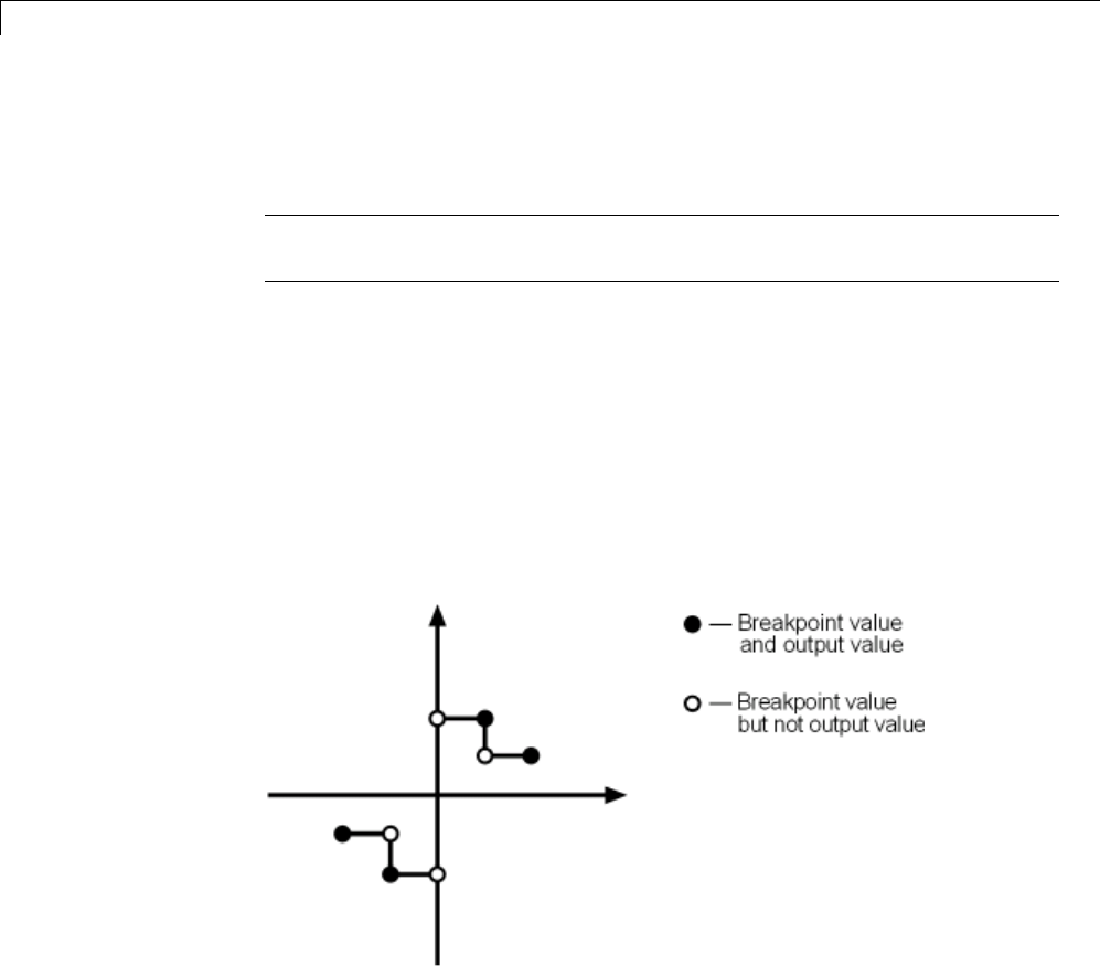
25 Working with Lookup Tables
in which each successive element is greater than its preceding element,
making Bstrictly monotonically increasing.
Note Although a breakpoint data set is strictly monotonic in double format,
it might not be so after conversion to a fixed-point data type.
Representation of Discontinuities in Lookup Tables
You can represent discontinuities in lookup tables that have monotonically
increasing breakpoint data sets. To create a discontinuity, repeat an input
value in the breakpoint data set with different output values in the table data.
For example, these vectors of input (x) and output (y) values associated with a
1-D lookup table create the step transitions depicted in the plot that follows.
Vector of input values: [-2 -1 -1 0 0 1 1 2]
Vector of output values: [-1 -1 -2 -2 2 2 1 1]
This example has discontinuities at x= –1, 0, and +1.
When there are two output values for a given input value, the block chooses
the output according to these rules:
25-20
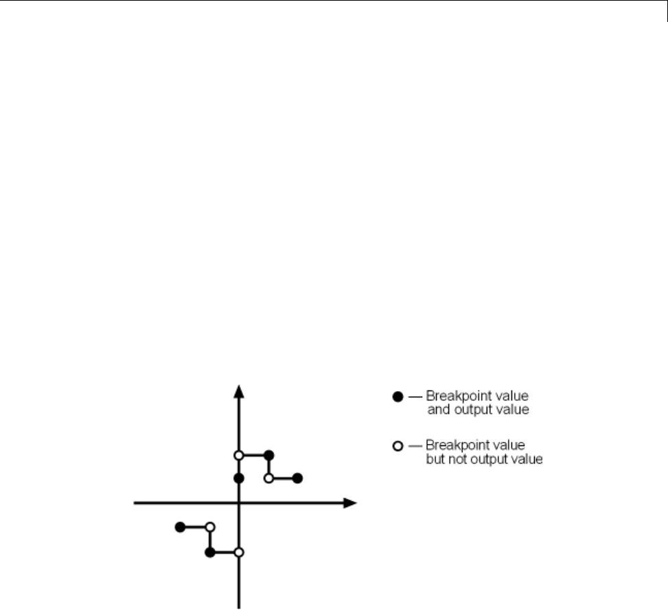
Characteristics of Lookup Table Data
•If the input signal is less than zero, the block returns the output value
associated with the last occurrence of the input value in the breakpoint data
set. In this example, if the input is –1, yis –2, marked with a solid circle.
•If the input signal is greater than zero, the block returns the output value
associated with the first occurrence of the input value in the breakpoint
data set. In this example, if the input is 1, yis 2, marked with a solid circle.
•If the input signal is zero and there are two output values specified at
the origin, the block returns the average of those output values. In this
example, if the input is 0, yis 0, the average of the two output values –2
and 2 specified at x=0.
When there are three points specified at the origin, the block generates the
output associated with the middle point. The following example demonstrates
this special rule.
Vector of input values: [-2 -1 -1 0 0 0 1 1 2]
Vector of output values: [-1 -1 -2 -2 1 2 2 1 1]
In this example, three points define the discontinuity at the origin. When the
input is 0, yis1,thevalueofthemiddlepoint.
You can apply this same method to create discontinuities in breakpoint data
sets associated with multidimensional lookup tables.
25-21

25 Working with Lookup Tables
Formulation of Evenly Spaced Breakpoints
You can represent evenly spaced breakpointsinadatasetbyusingone
of these methods.
Formulation Example When to Use This
Formulation
[first_value:spacing:last_value] [10:10:200] The lookup table does
not use double or
single.
first_value + spacing *
[0:(last_value-first_value)/spacing]
1 + (0.02 *
[0:450])
The lookup table uses
double or single.
Because floating-point data types cannot precisely represent some numbers,
the second formulation works better for double and single. For example,
use 1 + (0.02 * [0:450]) instead of [1:0.02:10]. For a list of lookup table
blocks that support evenly spaced breakpoints, see “Summary of Lookup
Table Block Features” on page 25-10.
Among other advantages, evenly spaced breakpoints can make the generated
code division-free and reduce memory usage. For more information, see:
•fixpt_evenspace_cleanup in the Simulink documentation
•“Effects of Spacing on Speed, Error, and Memory Usage” in the Simulink
Fixed Point documentation
•“Identify questionable fixed-point operations” in the Simulink Coder
documentation
Tip Do not use the MATLAB linspace function to define evenly spaced
breakpoints. Simulink uses a tighter tolerance to check whether a breakpoint
set has even spacing. If you use linspace to define breakpoints for your
lookup table, Simulink considers the breakpoints to be unevenly spaced.
25-22

Methods for Estimating Missing Points
Methods for Estimating Missing Points
In this section...
“About Estimating Missing Points” on page 25-23
“Interpolation Methods” on page 25-23
“Extrapolation Methods” on page 25-24
“Rounding Methods” on page 25-25
“Example Output for Lookup Methods” on page 25-26
About Estimating Missing Points
The second stage of a table lookup operation involves generating outputs that
correspond to the supplied inputs. If the inputs match the values of indices
specified in breakpoint data sets, the block outputs the corresponding values.
However, if the inputs fail to match index values in the breakpoint data sets,
Simulink estimates the output. In the block parameter dialog box, you can
specify how to compute the output in this situation. The available lookup
methods are described in the following sections.
Interpolation Methods
When an input falls between breakpoint values, the block interpolates the
output value using neighboring breakpoints. Most lookup table blocks have
the following interpolation methods available:
•Flat — Disables interpolation and uses the rounding operation titled Use
Input Below. For more information, see “Rounding Methods” on page
25-25.
•Linear — Fits a line between the adjacent breakpoints, and returns the
point on that line corresponding to the input.
•Cubic spline — Fits a cubic spline to the adjacent breakpoints, and
returns the point on that spline corresponding to the input.
25-23

25 Working with Lookup Tables
Note The Lookup Table Dynamic block does not let you select an
interpolation method. The Interpolation-Extrapolation option in the
Lookup Method field of the block parameter dialog box performs linear
interpolation.
Each interpolation method includes a trade-off between computation time
and the smoothness of the result. Although rounding is quickest, it is the
least smooth. Linear interpolation is slower than rounding but generates
smoother results, except at breakpoints where the slope changes. Cubic spline
interpolation is the slowest method but produces the smoothest results.
Extrapolation Methods
When an input falls outside the range of a breakpoint data set, the block
extrapolates the output value from a pair of values at the end of the
breakpoint data set. Most lookup table blocks have the following extrapolation
methods available:
•Clip — Disables extrapolation and returns the table data corresponding to
the end of the breakpoint data set range.
•Linear — Fits a line between the first or last pair of breakpoints, depending
if the input is less than the first or greater than the last breakpoint,
respectively. This method returns the point on that line corresponding
to the input.
•Cubic spline — Fits a cubic spline to the firstorlastpairofbreakpoints,
depending if the input is less than the first or greater than the last
breakpoint, respectively. This method returns the point on that spline
corresponding to the input.
Note The Lookup Table Dynamic block does not let you select an
extrapolation method. The Interpolation-Extrapolation option in the
Lookup Method field of the block parameter dialog box performs linear
extrapolation.
25-24

Methods for Estimating Missing Points
In addition to these methods, some lookup table blocks, such as the
n-D Lookup Table block, allow you to select an action to perform when
encountering situations that require extrapolation. For instance, you can
specify that Simulink generate either a warning or an error when the lookup
table inputs are outside the ranges of the breakpoint data sets. To specify
such an action, select it from the Diagnostic for out-of-range input list
on the block parameter dialog box.
Rounding Methods
If an input falls between breakpoint values or outside the range of a
breakpoint data set and you do not specify interpolation or extrapolation,
the block rounds the value to an adjacent breakpoint and returns the
corresponding output value. For example, the Lookup Table Dynamic block
lets you select one of the following rounding methods:
•Use Input Nearest — Returns the output value corresponding to the
nearest input value.
•Use Input Below — Returns the output value corresponding to the
breakpoint value that is immediately less than the input value. If no
breakpoint value exists below the input value, it returns the breakpoint
valuenearesttheinputvalue.
•Use Input Above — Returns the output value corresponding to the
breakpoint value that is immediately greater than the input value. If no
breakpoint value exists above the input value, it returns the breakpoint
valuenearesttheinputvalue.
25-25
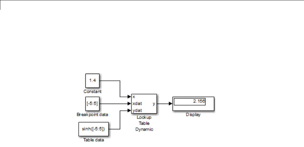
25 Working with Lookup Tables
Example Output for Lookup Methods
Inthefollowingmodel,theLookupTable Dynamic block accepts a vector
of breakpoint data given by [-5:5] and a vector of table data given by
sinh([-5:5]).
25-26

Methods for Estimating Missing Points
The Lookup Table Dynamic block outputs the following values when using the
specified lookup methods and inputs.
Lookup Method Input Output Comment
1.4 2.156 N/A
Interpolation-
Extrapolation 5.2 83.59 N/A
1.4 2.156 N/A
Interpolation-
Use End Values
5.2 74.2 The block uses the value
for sinh(5.0).
1.4 3.627 Theblockusesthevalue
for sinh(2.0).
Use Input Above
5.2 74.2 Theblockusesthevalue
for sinh(5.0).
1.4 1.175 The block uses the value
for sinh(1.0).
Use Input Below
-5.2 -74.2Theblockusesthevalue
for sinh(-5.0).
Use Input Nearest 1.4 1.175 Theblockusesthevalue
for sinh(1.0).
25-27

25 Working with Lookup Tables
Edit Existing LookupTables
In this section...
“WhentoUsetheLookupTableEditor”onpage25-28
“Layout of the Lookup Table Editor” on page 25-28
“Browsing Lookup Table Blocks” on page 25-29
“Editing Table Values” on page 25-30
“Working with Table Data of Standard Format” on page 25-32
“Working with Table Data of Nonstandard Format” on page 25-36
“Importing Data from an Excel Spreadsheet” on page 25-53
“Adding and Removing Rows and Columns in a Table” on page 25-55
“Displaying N-Dimensional Tables in the Editor” on page 25-56
“Plotting Lookup Tables” on page 25-57
“Editing Custom Lookup Table Blocks” on page 25-61
When to Use the Lookup Table Editor
Use the Lookup Table Editor to inspect and change the table elements of any
lookup table block in a model, including custom blocks that you create using
the Simulink Mask Editor (see “Editing Custom Lookup Table Blocks” on
page 25-61). You can also use a block parameter dialog box to edit a table.
However, you must open the subsystem containing the block first and then its
parameter dialog box. With the Lookup Table Editor, you can skip these steps.
Tip You cannot use the Lookup Table Editor to change the dimensions of a
lookup table. You must use the block parameter dialog box for this purpose.
Layout of the Lookup Table Editor
To open the editor, select Lookup Table Editor from the Simulink Edit
menu. The editor appears.
25-28
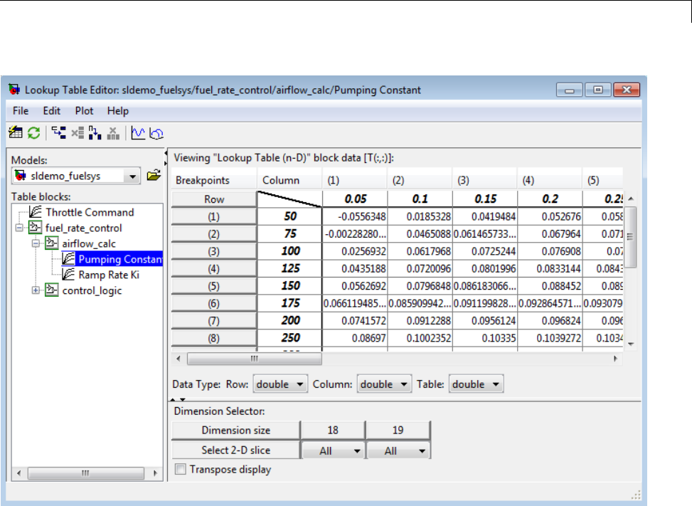
Edit Existing LookupTables
The editor contains two panes and a toolbar.
•Use the left pane to browse and select lookup table blocks in any open
model (see “Browsing Lookup Table Blocks” on page 25-29).
•Usetherightpanetoeditthelookuptableoftheselectedblock(see
“Editing Table Values” on page 25-30).
•Use the toolbar for one-click access to frequently-used commands in the
editor. Each toolbar button has a tooltip that explains its function.
Browsing Lookup Table Blocks
The Models list in the upper-left corner of the Lookup Table Editor lists
the names of all models open in the current MATLAB session. To browse
25-29
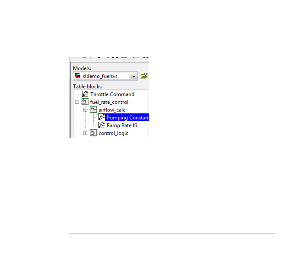
25 Working with Lookup Tables
lookup table blocks for any open models, select the model name from the list.
A tree-structured view of lookup table blocks for the selected model appears in
the Table blocks field beneath the Models list.
The tree view initially lists all lookup table blocks that reside at the model
root level. It also displays any subsystems that contain lookup table blocks.
Clicking the expand button (+) to the left of the subsystem name expands
the tree to show lookup table blocks in that subsystem. The expanded view
also shows any subsystems in the expanded subsystem. You can continue
expanding subsystem nodes to display lookup table blocks at any level in
the model hierarchy.
Clicking any lookup table block in the tree view displays the lookup table
for that block in the right pane, so that you can edit the table (see “Editing
Table Values” on page 25-30).
Note Ifyouwanttobrowsethelookuptableblocksinamodelthatisnot
currently open, you can tell the Lookup Table Editor to open the model. To
do this, select File > Open Model in the editor.
Editing Table Values
In the Viewing “Lookup Table (n-D)” block data table view of the Lookup
Table Editor, you can edit the lookup table of the block currently selected in
theadjacenttreeview.
25-30
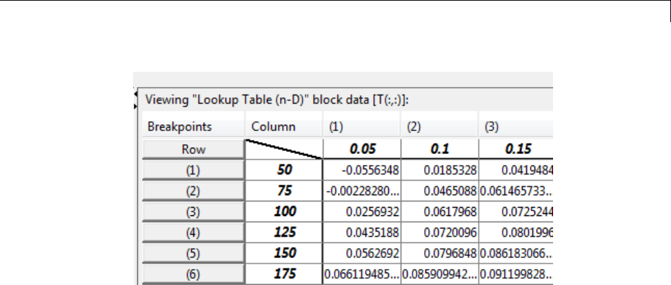
Edit Existing LookupTables
Thetableviewdisplaystheentiretableifitisone-ortwo-dimensionalora
two-dimensional slice of the table if the table has more than two dimensions
(see “Displaying N-Dimensional Tables in the Editor” on page 25-56). To
change any value that appears, double-click the value. The Lookup Table
Editor replaces the value with an edit field containing the value. Edit the
value and then press Enter or click outside the field to confirm the change.
In the Data Type below the table, you can specify the data type by row or
column, or for the entire table. By default, the data type is double. To change
thedatatype,selectthepop-upindexlistforthetableelementforwhich
youwanttochangethedatatype.
The Lookup Table Editor records your changes by maintaining a copy
ofthetable. Toupdatethecopythatthelookuptableblockmaintains,
select File > Update Block Data in the Lookup Table Editor. To restore
the Lookup Table Editor’s copy to the values stored in the block, select
File > Reload Block Data.
25-31
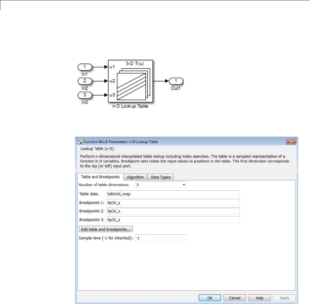
25 Working with Lookup Tables
Working with Table Data of Standard Format
Suppose that you specify a 3-D lookup table in your n-D Lookup Table block.
You use workspace variables to define the breakpoint and table data:
25-32

Edit Existing LookupTables
ThetabledatausesthedefaultSimulinkformat:
table3d_map(:,:,1) =
1234
5678
table3d_map(:,:,2) =
11 12 13 14
15 16 17 18
table3d_map(:,:,3) =
111 112 113 114
115 116 117 118
The breakpoint sets have the following values:
bp3d_y =
400 6400
bp3d_x =
0102030
bp3d_z =
01020
25-33
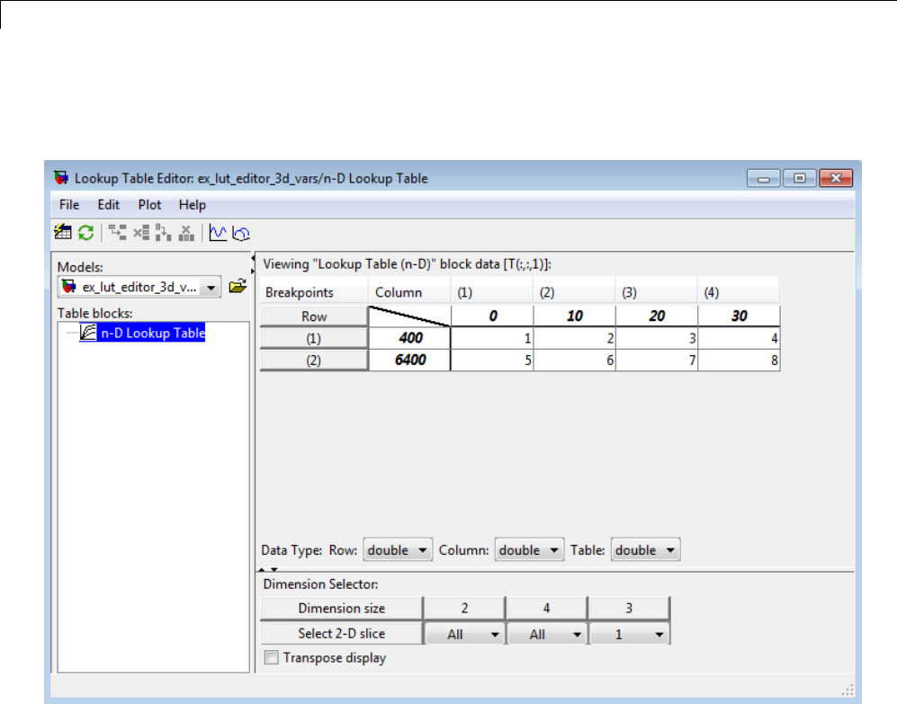
25 Working with Lookup Tables
When you click Edit table and breakpoints to open the Lookup Table
Editor, you see:
25-34
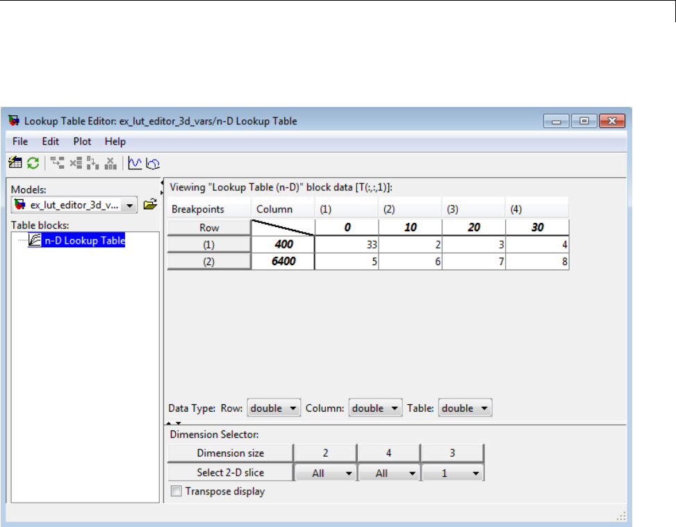
Edit Existing LookupTables
Suppose that you change a value in the Lookup Table Editor as follows:
When you select File > Update Block Data, you can propagate the change
to table3d_map, the workspace variable that contains the table data for the
n-D Lookup Table block. To propagate the change, click Yes in the pop-up
window that asks if you want to overwrite the workspace variable:
25-35
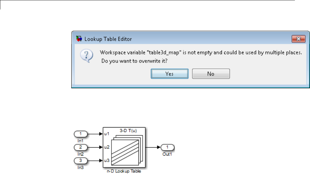
25 Working with Lookup Tables
Working with Table Data of Nonstandard Format
Suppose that you specify a 3-D lookup table in your n-D Lookup Table block.
25-36
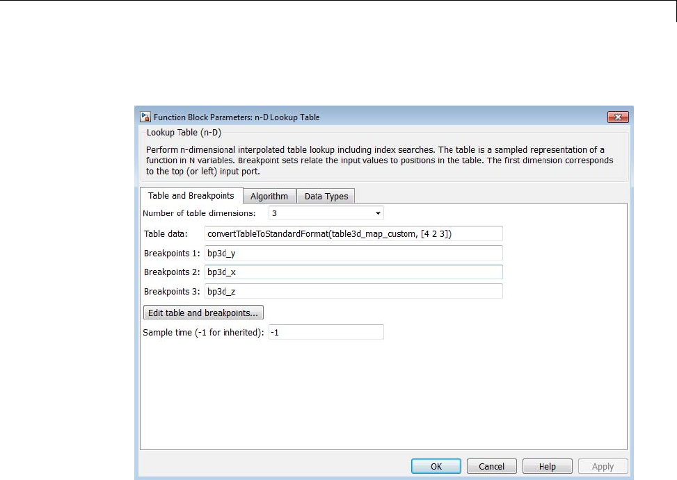
Edit Existing LookupTables
You use workspace variables to define the breakpoint and table data:
The table data uses a nonstandard format for representing 3-D table data that
differs from the default Simulink format:
table3d_map_custom =
1234
5678
11 12 13 14
15 16 17 18
111 112 113 114
115 116 117 118
TheexpressionintheTable data field converts the table data from a
nonstandard format to the default Simulink format.
25-37

25 Working with Lookup Tables
The breakpoint sets have the following values:
bp3d_y =
400 6400
bp3d_x =
0102030
bp3d_z =
01020
25-38
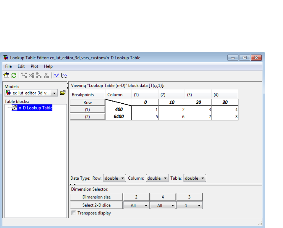
Edit Existing LookupTables
When you click Edit table and breakpoints to open the Lookup Table
Editor, you see:
25-39
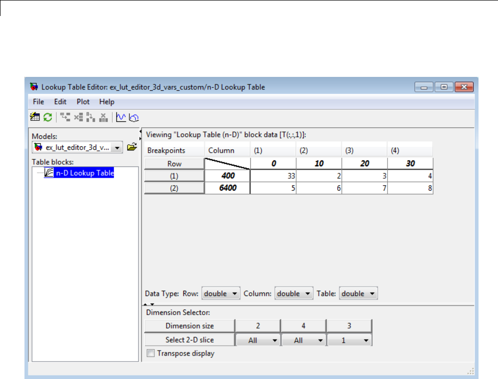
25 Working with Lookup Tables
Suppose that you change a value in the Lookup Table Editor as follows:
When you select File > Update Block Data, you cannot propagate the
change to table3d_map_custom, the workspace variable that contains the
nonstandard table data for the n-D Lookup Table block. To propagate the
change, you must register a customization function that resides on the
MATLAB search path. For details, see “Example of Propagating a Change for
Table Data of Nonstandard Format” on page 25-45.
25-40

Edit Existing LookupTables
How to Propagate Changes in the Lookup Table Editor to
Workspace Variables of Nonstandard Format
Step Task Reference
1Register a customization
function for the Lookup Table
Editor.
“How to Register a
Customization Function for
the Lookup Table Editor” on
page 25-41
2Select the appropriate responses
when prompted in the Lookup
Table Editor.
“How to Respond to Prompts
in the Lookup Table Editor” on
page 25-45
How to Register a Customization Function for the Lookup Table
Editor
To register a customization function for the Lookup Table Editor:
1In MATLAB, create a file named sl_customization.m to register your
customization:
function sl_customization(cm)
cm.LookupTableEditorCustomizer.getTableConvertToCustomInfoFcnHandle{end+1} = ...
@myConversionInfoFunction;
end
The string myConversionInfoFunction represents a function name of
your choice.
2In your sl_customization.m file, define a function that returns a blkInfo
object.
function blkInfo = myConversionInfoFunction(blk, tableStr)
blkInfo.allowTableConvertLocal = false;
blkInfo.tableWorkSpaceVarName = '';
blkInfo.tableConvertFcnHandle = [];
25-41

25 Working with Lookup Tables
% Directions for converting table data of block type 1
if strcmp(get_param(blk, 'BlockType'), 'block_type_1')
blkInfo.allowTableConvertLocal = true;
blkInfo.tableWorkSpaceVarName = 'variable_name_1';
end
% Directions for converting table data of block type 2
if strcmp(get_param(blk, 'BlockType'), 'block_type_2')
blkInfo.allowTableConvertLocal = true;
blkInfo.tableWorkSpaceVarName = 'variable_name_2';
end
......
% Directions for converting table data of block type N
if strcmp(get_param(blk, 'BlockType'), 'block_type_N')
blkInfo.allowTableConvertLocal = true;
blkInfo.tableWorkSpaceVarName = 'variable_name_N';
end
if blkInfo.allowTableConvertLocal
blkInfo.tableConvertFcnHandle = @myConvertTableDataFcn;
end
end
For each type of lookup table block that contains nonstandard table data,
specify the following three properties:
•allowTableConvertLocal — tells the Lookup Table Editor if table data
conversion is allowed for a block
•tableWorkSpaceVarName — specifies the name of the workspace variable
that has a nonstandard table format
•tableConvertFcnHandle —specifiesthehandlefortheconversion
function
25-42

Edit Existing LookupTables
Tip You can specify more restrictive if conditions in this function. For
example, to specify that table data conversion occur for a block with a given
name, you can use:
if strcmp(strrep(blk,sprintf('\n'), ' '), 'full_block_path')
blkInfo.allowTableConvertLocal = true;
blkInfo.tableWorkSpaceVarName = 'variable_name';
end
When the allowTableConvertLocal property is true:
•The table data for that block can be converted to the nonstandard format
of the workspace variable whose name matches tableWorkSpaceVarName.
•The function that converts table data corresponds to the handle that
tableConvertFcnHandle specifies.
You can use any alphanumeric name for the conversion function. The
string myConvertTableDataFcn represents a function name of your
choice.
3In your sl_customization.m file, define the function that converts table
data from the Lookup Table Editor format to the nonstandard format of
your workspace variable.
4Verify that your sl_customization.m file is complete.
5Put sl_customization.m on the MATLAB search path.
Note You can have multiple files with the name sl_customization.m
on the search path.
6At the MATLAB prompt, enter the following command to refresh all
Simulink customizations.
sl_refresh_customizations
25-43

25 Working with Lookup Tables
What Happens When Multiple Customization Functions Exist
If you have multiple sl_customization.m files on the search path, the
following happens:
•At the start of a MATLAB session, Simulink loads each customization file
on the path and executes the function at the top. Executing each function
establishes the customizations for that session.
•When you select File > Update Block Data in the Lookup Table Editor,
the editor checks the list of function handles in the cell array for
cm.LookupTableEditorCustomizer.getTableConvertToCustomInfoFcnHandle.
If the cell array... Changes in the Lookup Table
Editor...
Is empty Cannot propagate to workspace
variables with nonstandard format
Contains one or more function
handles
Can propagate to workspace
variables with nonstandard format,
depending on the value of the
allowTableConvertLocal property
•The allowTableConvertLocal property controls whether or not table data
for a block is converted from the standard format in the Lookup Table
Editor to a nonstandard format in a workspace variable.
If a customization function
specifies this block property to
be...
Then table data is...
true Converted to the nonstandard
format in the workspace variable
false Not converted to the nonstandard
format in the workspace variable
true, but another customization
function specifies the property to
be false
Not converted and the Lookup
Table Editor issues an error
25-44

Edit Existing LookupTables
How to Respond to Prompts in the Lookup Table Editor
When you select File > Update Block Data in the Lookup Table Editor,
several prompts appear. Click Yes when asked if you want to:
•Overwrite workspace variables for breakpoint data
•Overwrite workspace variables for table data
Example of Propagating a Change for Table Data of
Nonstandard Format
Suppose that you want to propagate a change from the Lookup Table Editor
to the workspace variable table3d_map_custom, which uses a nonstandard
format. Follow these steps:
1Create a file named sl_customization.m with the following contents:
function sl_customization(cm)
cm.LookupTableEditorCustomizer.getTableConvertToCustomInfoFcnHandle{end+1} = ...
@myGetTableConvertInfoFcn;
end
In this file:
•The sl_customization function takes a single argument cm,whichis
the handle to a customization manager object.
•The handle @myGetTableConvertInfoFcn is added
to the list of function handles in the cell array for
cm.LookupTableEditorCustomizer.getTableConvertToCustomInfoFcnHandle.
You can use any alphanumeric name for the function whose handle
youaddtothecellarray. Inthisexample,thefunctionnameis
myGetTableConvertInfoFcn.
2In your sl_customization.m file, define the myGetTableConvertInfoFcn
function.
function blkInfo = myGetTableConvertInfoFcn(blk, tableStr)
25-45

25 Working with Lookup Tables
blkInfo.allowTableConvertLocal = false;
blkInfo.tableWorkSpaceVarName = '';
blkInfo.tableConvertFcnHandle = [];
% Convert table data for n-D Lookup Table blocks
if strcmp(get_param(blk, 'BlockType'), 'Lookup_n-D')
blkInfo.allowTableConvertLocal = true;
blkInfo.tableWorkSpaceVarName = 'table3d_map_custom';
end
% Convert table data for Interpolation Using Prelookup blocks
if strcmp(get_param(blk, 'BlockType'), 'Interpolation_n-D')
blkInfo.allowTableConvertLocal = true;
blkInfo.tableWorkSpaceVarName = 'table4d_map_custom';
end
% Convert table data for Direct Lookup Table (n-D) blocks
if strcmp(get_param(blk, 'BlockType'), 'LookupNDDirect')
blkInfo.allowTableConvertLocal = true;
blkInfo.tableWorkSpaceVarName = 'table4d_map_custom';
end
if blkInfo.allowTableConvertLocal
blkInfo.tableConvertFcnHandle = @myConvertTableFcn;
end
end
The myGetTableConvertInfoFcn function returns the blkInfo object,
which contains three fields:
•allowTableConvertLocal — tells the Lookup Table Editor if table data
conversion is allowed for a block
•tableWorkSpaceVarName — specifies the name of the workspace variable
that has a nonstandard table format
•tableConvertFcnHandle —specifiesthehandlefortheconversion
function
When the allowTableConvertLocal property is true:
25-46

Edit Existing LookupTables
•The table data for that block is converted to the nonstandard format of
the workspace variable whose name matches tableWorkSpaceVarName.
•The function that converts table data corresponds to the handle that
tableConvertFcnHandle specifies.
You can use any alphanumeric name for the conversion function. In this
example, the function name is myConvertTableFcn.
3In your sl_customization.m file, define the myConvertTableFcn function,
which includes a separate function call to convertTable_3D.Anexampleof
an implementation is shown below:
% This function converts LUT block table from Simulink format to
% nonstandard format used in workspace variable (for 1D to 4D table)
function cMap = myConvertTableFcn(data)
mapDim = size(data);
numDim = length(mapDim);
if numDim < 3
cMap = data;
elseif numDim == 3
cMap = convertTable_3D(data);
else % numDim == 4 , currently only supports up to 4D
for i = 1:mapDim(numDim)
dataSub = data(:,:,:,i);
iStart = (i-1)*mapDim(1)*mapDim(3) + 1;
iEnd = i*mapDim(1)*mapDim(3);
cMap(iStart:iEnd,:) = convertTable_3D(dataSub);
end
end
end
% This function converts LUT block table from Simulink format to
% nonstandard format used in workspace variable (for 3D table)
function cMap = convertTable_3D(data)
% figure out the row and column number of the 3D table data
mapDim = size(data);
25-47

25 Working with Lookup Tables
numCol = mapDim(2);
numRow = mapDim(1)*mapDim(3);
cMap = zeros(numRow, numCol);
for i = 1:mapDim(3)
rowBegin = (i-1)*mapDim(1)+1;
rowEnd = i*mapDim(1);
cMap(rowBegin:rowEnd, :) = data(:,:,i);
end
end
4Verify that your sl_customization.m file is complete:
function sl_customization(cm)
cm.LookupTableEditorCustomizer.getTableConvertToCustomInfoFcnHandle{end+1} = ...
@myGetTableConvertInfoFcn;
% This function converts LUT block table from Simulink format to
% nonstandard format used in workspace variable (for 1D to 4D table)
function cMap = myConvertTableFcn(data)
mapDim = size(data);
numDim = length(mapDim);
if numDim < 3
cMap = data;
elseif numDim == 3
cMap = convertTable_3D(data);
else % numDim == 4 , currently only supports up to 4D
for i = 1:mapDim(numDim)
dataSub = data(:,:,:,i);
iStart = (i-1)*mapDim(1)*mapDim(3) + 1;
iEnd = i*mapDim(1)*mapDim(3);
cMap(iStart:iEnd,:) = convertTable_3D(dataSub);
end
end
25-48

Edit Existing LookupTables
end
% This function converts LUT block table from Simulink format to
% nonstandard format used in workspace variable (for 3D table)
function cMap = convertTable_3D(data)
% figure out the row and column number of the 3D table data
mapDim = size(data);
numCol = mapDim(2);
numRow = mapDim(1)*mapDim(3);
cMap = zeros(numRow, numCol);
for i = 1:mapDim(3)
rowBegin = (i-1)*mapDim(1)+1;
rowEnd = i*mapDim(1);
cMap(rowBegin:rowEnd, :) = data(:,:,i);
end
end
function blkInfo = myGetTableConvertInfoFcn(blk, tableStr)
blkInfo.allowTableConvertLocal = false;
blkInfo.tableWorkSpaceVarName = '';
blkInfo.tableConvertFcnHandle = [];
% Convert table data for n-D Lookup Table blocks
if strcmp(get_param(blk, 'BlockType'), 'Lookup_n-D')
blkInfo.allowTableConvertLocal = true;
blkInfo.tableWorkSpaceVarName = 'table3d_map_custom';
end
% Convert table data for Interpolation Using Prelookup blocks
if strcmp(get_param(blk, 'BlockType'), 'Interpolation_n-D')
blkInfo.allowTableConvertLocal = true;
blkInfo.tableWorkSpaceVarName = 'table4d_map_custom';
end
% Convert table data for Direct Lookup Table (n-D) blocks
25-49
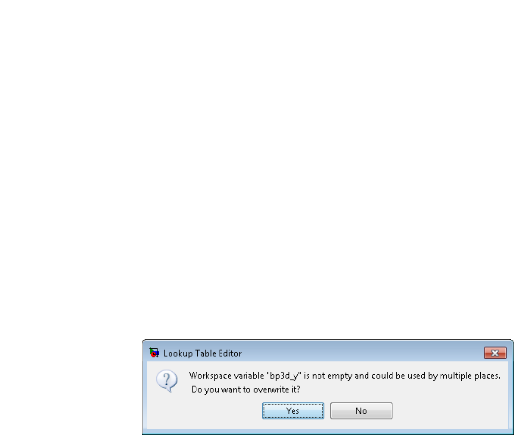
25 Working with Lookup Tables
if strcmp(get_param(blk, 'BlockType'), 'LookupNDDirect')
blkInfo.allowTableConvertLocal = true;
blkInfo.tableWorkSpaceVarName = 'table4d_map_custom';
end
if blkInfo.allowTableConvertLocal
blkInfo.tableConvertFcnHandle = @myConvertTableFcn;
end
end
end
5Put sl_customization.m on the MATLAB search path.
6At the MATLAB prompt, enter the following command to refresh all
Simulink customizations.
sl_refresh_customizations
7IntheLookupTableEditor,selectFile > Update Block Data.Several
pop-up windows appear:
aClick Yes to overwrite the workspace variable bp3d_y.
bClick Yes to overwrite the workspace variable bp3d_x.
25-50
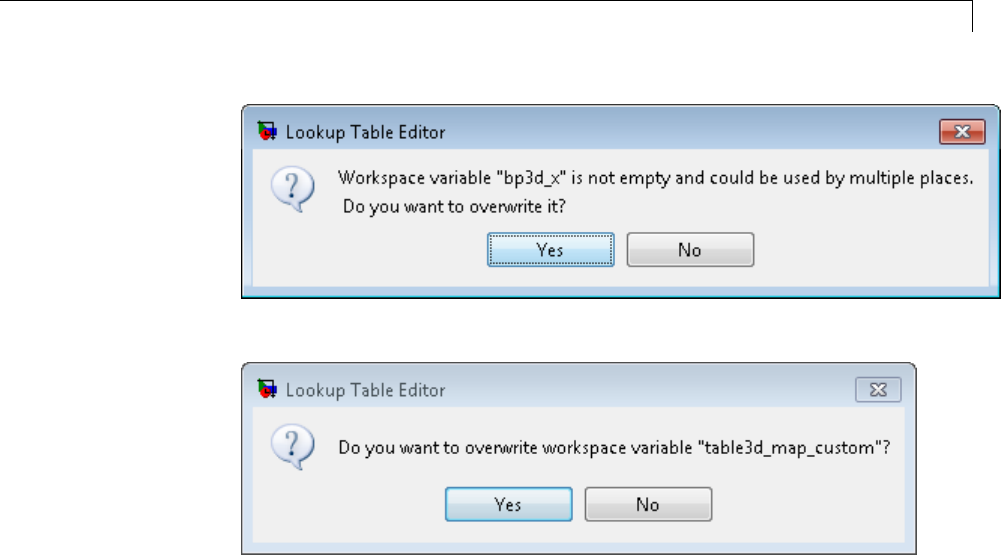
Edit Existing LookupTables
cClick Yes to overwrite the workspace variable table3d_map_custom.
8If you check the value of table3d_map_custom in the base workspace, you
now see:
table3d_map_custom =
33234
5678
11 12 13 14
15 16 17 18
111 112 113 114
115 116 117 118
ThechangethatyoumaketothetabledataintheLookupTableEditor
propagates to the workspace variable.
25-51
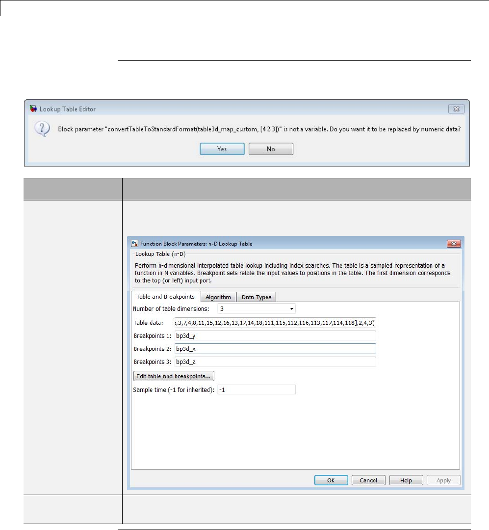
25 Working with Lookup Tables
Note If you click No to the question of whether to overwrite the workspace
variable table3d_map_custom, you get another question:
If you click... Then...
Yes The block dialog box replaces the expression in the Table data field with
numeric data.
No Your Lookup Table Editor changes for the table data do not appear in
the block dialog box.
25-52

Edit Existing LookupTables
Importing Data from an Excel Spreadsheet
If you have table data in a Microsoft Excel spreadsheet, you can import the
data into the Lookup Table Editor.
How to Import Data from the Spreadsheet
To import data into the Lookup Table Editor:
1Save the Excel file in a folder on the MATLAB path.
2Open the model that contains a lookup table block.
3Save the model with a different name.
4Open the Model Properties dialog box, for example, by selecting
File > Model Properties.
5Click the Callbacks tab and enter code for the model post-load function.
For a 2-D lookup table, the commands look something like this:
%%% BEGIN NEW CODE %%%
% Import the data from Excel for a lookup table
data = xlsread('name_of_spreadsheet','sheet_name');
% Row indices for lookup table
breakpoints1 = data(2:end,1)';
% Column indices for lookup table
breakpoints2 = data(1,2:end);
% Output values for lookup table
table_data = data(2:end,2:end);
%%% END NEW CODE %%%
For more information about using xlsread, see the MATLAB
documentation.
6Save the model again.
25-53

25 Working with Lookup Tables
Example of Importing Data from an Excel Spreadsheet
Suppose that you have table data in an Excel spreadsheet named
airflow_tables.xls and you want to import the data into the Lookup Table
Editor.
1Save airflow_tables.xls inafolderontheMATLABpath. Enterthe
following command at the MATLAB prompt and replace destination with
alocationthatisonthesearchpath:
copyfile((docpath(fullfile(docroot,'toolbox','simulink','examples','airflow_tables.xls'))),...
'destination','f')
For example, C:\MyFiles\airflow_tables.xls might be a valid value
for destination.
2Open the sldemo_fuelsys model, which contains a lookup table block
named Pumping Constant.
3Save the model with a different name, such as my_fuelsys.
4Open the Model Properties dialog box, for example, by selecting
File > Model Properties.
5Click the Callbacks tab and add the following commands under the
existing code for the post-load function:
%%% BEGIN NEW CODE %%%
% Import the data from Excel for a lookup table
data = xlsread('airflow_tables', 'Pumping Constant');
% Row indices for Pumping Constant data
SpeedVect = data(2:end,1)';
% Column indices for Pumping Constant data
PressVect = data(1,2:end);
% Output values for Pumping Constant data
PumpCon = data(2:end,2:end);
%%% END NEW CODE %%%
6Save the model again.
Whenever you open my_fuelsys, Simulink imports the table data for the
Pumping Constant block from the Excel spreadsheet.
25-54
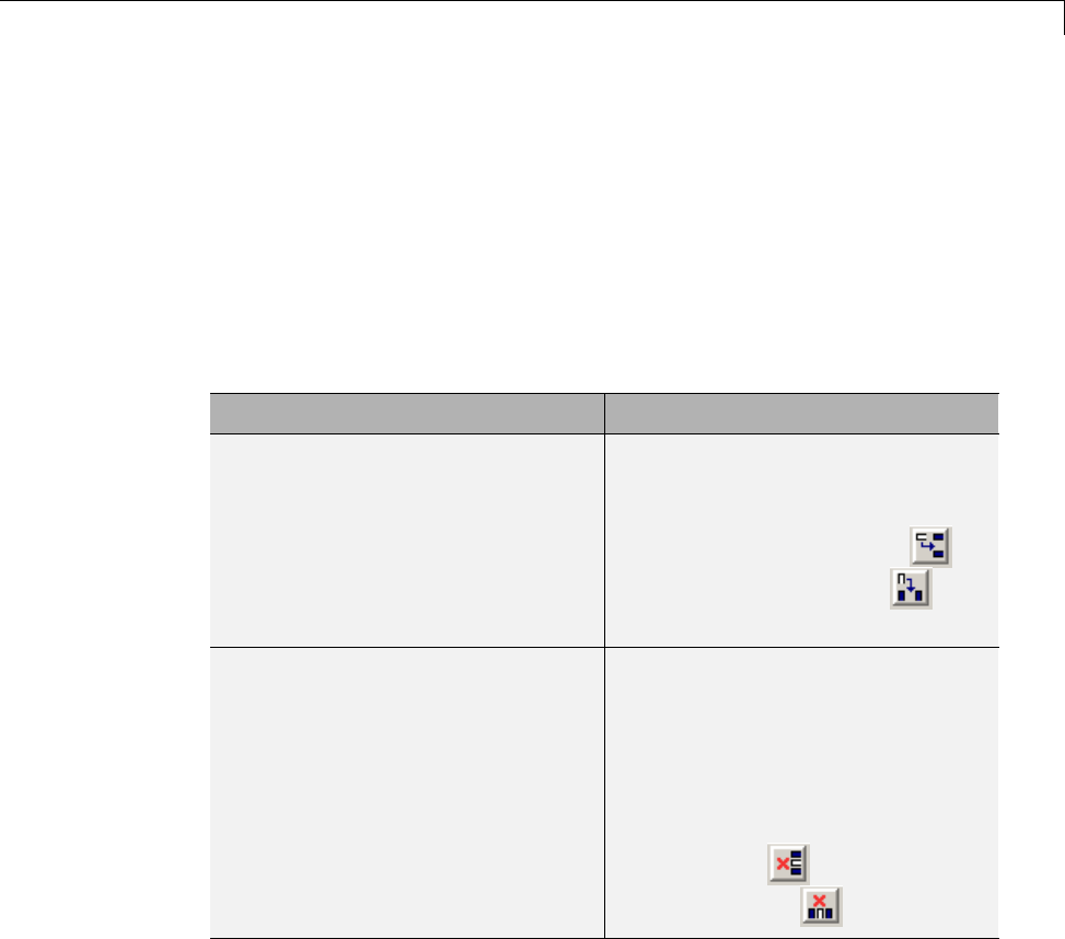
Edit Existing LookupTables
Adding and RemovingRowsandColumnsinaTable
In the Lookup Table Editor, you can add and remove rows or columns of a
table in the following cases:
•Tables that are one- or two-dimensional
•Tables defined only by breakpoints (that are inherently one-dimensional)
In those cases, follow these instructions to add or remove columns of a table
in the Lookup Table Editor.
To perform this action: Use one of these methods:
Add a row or column to a table that
appears in the table view
•Select Edit > Add Row or
Edit > Add Column in the
editor.
•Click the Add Row button or
the Add Column button in
the toolbar.
Remove a row or column from the
table that appears in the table view
•Highlight the row or column
to removeandthenselect
Edit > Remove Row(s) or
Edit > Remove Column(s) in
the editor.
•Highlight the row or column to
remove and then click the Remove
Row button or the Remove
Column button in the toolbar.
The menu items and toolbar buttons for adding and removing rows and
columns are not available for any other cases. To add or remove a row or
column for a table with more than two dimensions, you must use the block
parameter dialog box.
25-55
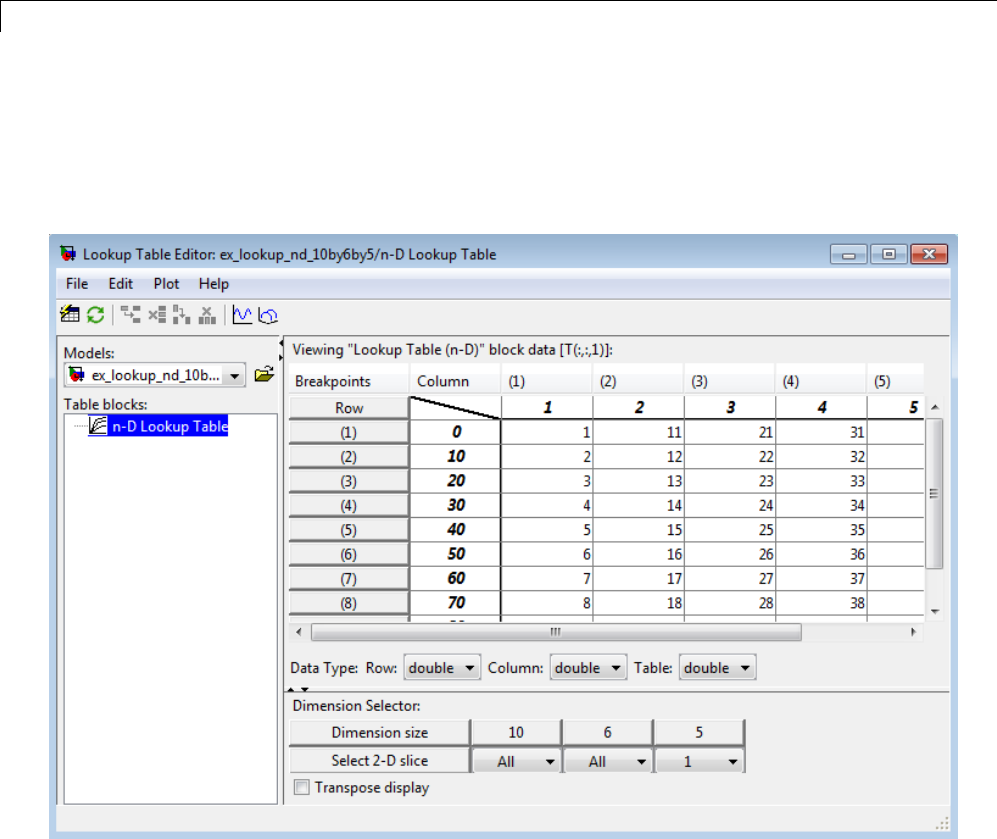
25 Working with Lookup Tables
Displaying N-Dimensional Tables in the Editor
If the lookup table of the block currently selected in the Lookup Table
Editor’s tree view has more than two dimensions, the table view displays a
two-dimensional slice of the lookup table.
The Dimension Selector specifies which slice currently appears and lets you
select another slice. The selector consists of a 2-by-Narray of controls, where N
is the number of dimensions in the lookup table. Each column corresponds
to a dimension of the lookup table. The first column corresponds to the first
dimension of the table, the second column to the second dimension of the
table, and so on. The Dimension size row of the selector array displays the
size of each dimension. The Select 2-D slice row specifies which dimensions
25-56
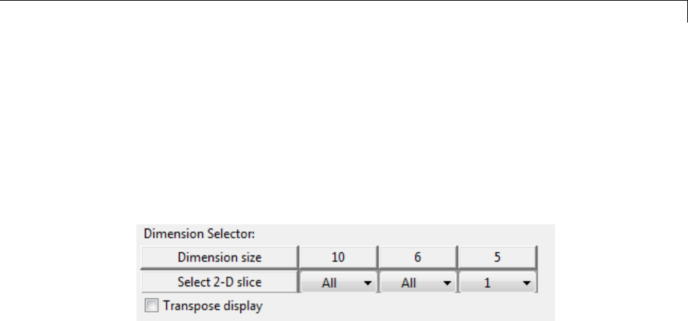
Edit Existing LookupTables
of the table correspond to the row and column axes of the slice and the indices
that select the slice from the remaining dimensions.
To select another slice of the table, specify the row and column axes of the
slice in the first two columns of the Select 2-D slice row. Then select the
indices of the slice from the pop-up index lists in the remaining columns.
For example, the following selector displays slice (:,:,1) of a 3-D lookup table.
To transpose the table display, select the Transpose display check box.
Plotting Lookup Tables
To display a linear or mesh plot of the table or table slice in the Lookup Table
Editor, select Plot > Linear or Plot > Mesh.
25-57
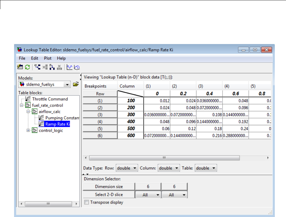
25 Working with Lookup Tables
Suppose that you have the following lookup table open:
25-58
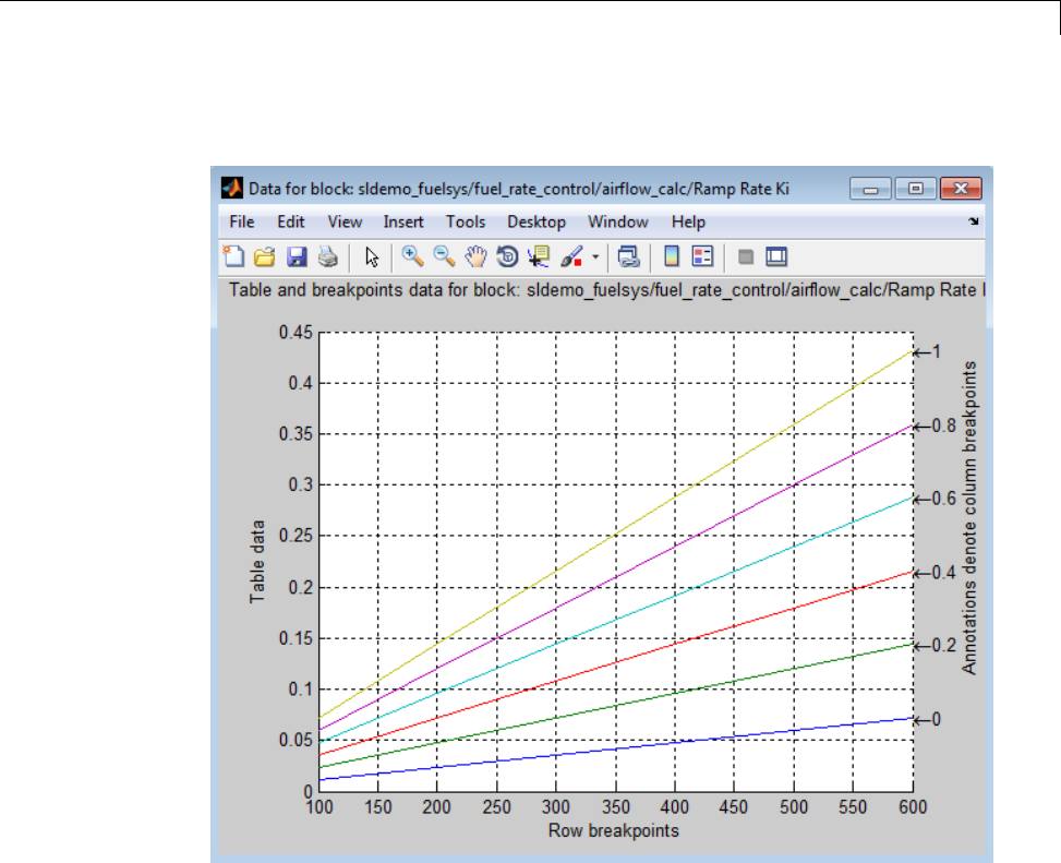
Edit Existing LookupTables
A linear plot of the table looks something like this:
25-59
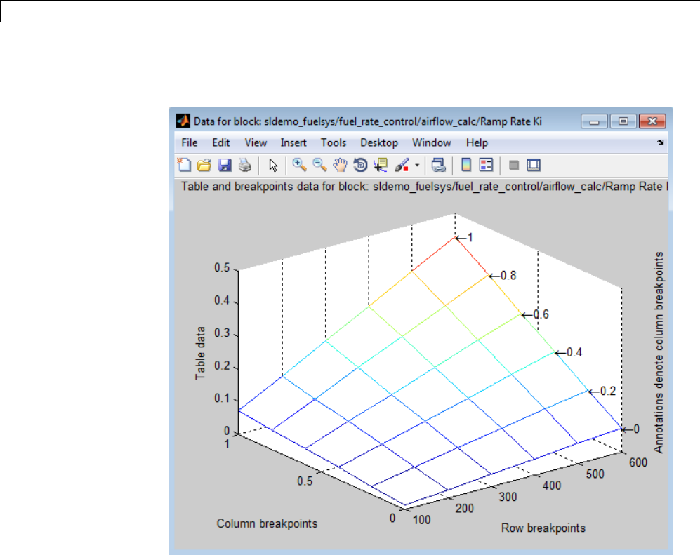
25 Working with Lookup Tables
A mesh plot of the table looks something like this:
25-60
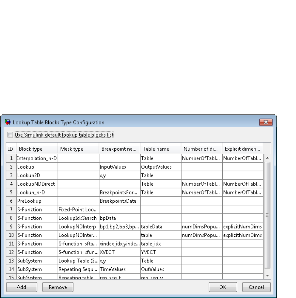
Edit Existing LookupTables
Editing Custom Lookup Table Blocks
You can use the Lookup Table Editor to edit custom lookup table blocks that
you or others have created. To do this, you must first configure the Lookup
Table Editor to recognize the custom lookup table blocks in your model. After
you configure the Lookup Table Editor to recognize custom blocks, you can
edit them as if they were standard blocks.
To configure the Lookup Table Editor to recognize custom blocks, select
File > Configure. The Lookup Table Blocks Type Configuration dialog box
appears.
By default, the dialog box displays a table of the lookup table block types
that the Lookup Table Editor currently recognizes. This table includes the
25-61

25 Working with Lookup Tables
standard blocks. Each row of the table displays key attributes of a lookup
table block type.
Adding a Custom Lookup Table Block Type
To add a custom block to the list of recognized types:
1Click Add on the dialog box.
A new row appears at the bottom of the block type table.
2Enter information for the custom block in the new row under these
headings.
Field Name Description
Block type Block type of the custom block. The block
type is the value of the block’s BlockType
parameter.
Mask type Mask type of the custom block. The mask
type is the value of the block’s MaskType
parameter.
Breakpoint name Names of the block parameters that store
the breakpoints.
Table name Name of the block parameter that stores the
table data.
Number of dimensions Leave empty.
Explicit dimensions Leave empty.
3Click OK.
Removing Custom Lookup Table Block Types
To remove a custom lookup table block type from the list that the Lookup
Table Editor recognizes, select the custom entry in the table of the Lookup
Table Blocks Type Configuration dialog box. Then click Remove.
To remove all custom lookup table block types, select the Use Simulink
default lookup table blocks list check box at the top of the dialog box.
25-62

Create a Logarithm Lookup Table
Create a Logarithm Lookup Table
Supposeyouwanttoapproximatethecommonlogarithm(base10)overthe
input range [1, 10] without performing an expensive computation. You can
perform this approximation using a lookup table block as described in the
following procedure.
1Copy the following blocks to a Simulink model:
•One Constant block to input the signal, from the Sources library
•Onen-DLookupTableblocktoapproximatethecommonlogarithm,
from the Lookup Tables library
•OneDisplayblocktodisplaytheoutput,fromtheSinkslibrary
2Assign the table data and breakpoint data set to the n-D Lookup Table
block:
aIn the Number of table dimensions field, enter 1.
bIn the Table data field, enter
[0 .301 .477 .602 .699 .778 .845 .903 .954 1].
cIn the Breakpoints 1 field, enter [1:10].
dClick Apply.
25-63
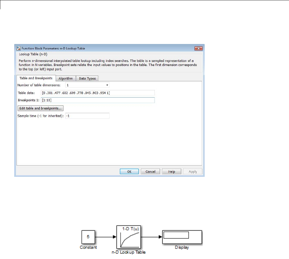
25 Working with Lookup Tables
The dialog box looks something like this:
3Double-click the Constant block to open the parameter dialog box, and
change the Constant value parameter to 5.ClickOK to apply the changes
and close the dialog box.
4Connect the blocks as follows.
5Startsimulation.
25-64

Create a Logarithm Lookup Table
The following behavior applies to the n-D Lookup Table block.
Example of Block BehaviorValue of the
Constant Block
Action by the n-D
Lookup Table Block Input Value Output Value
Equals a breakpoint Returns the
corresponding output
value
50.699
Falls between
breakpoints
Linearly interpolates
the output value
using neighboring
breakpoints
7.5 0.874
Falls outside the range
of the breakpoint data
set
Linearly extrapolates
the output value from
a pair of values at the
end of the breakpoint
data set
10.5 1.023
For the n-D Lookup Table block, the default settings for Interpolation
method and Extrapolation method are both Linear.
25-65

25 Working with Lookup Tables
Prelookup and Interpolation Blocks
The following examples show the benefits of using Prelookup and
Interpolation Using Prelookup blocks.
Action Benefit Example
Use an index search to
relate inputs to table data,
followed by an interpolation
and extrapolation stage that
computes outputs
Enables reuse of index search
results to lookupdatain
multiple tables, which reduces
simulation time
To open the model, type
sldemo_bpcheck at the
command prompt.
Lowers memory required to
store:
•Breakpoint data that uses a
smaller type than the input
signal
•Table data that uses a
smaller type than the
output signal
To open the model, type
sldemo_interp_memory at the
command prompt.
Provides easier sharing of:
•Breakpoint data among
Prelookup blocks
•Table data among
Interpolation Using
Prelookup blocks
To open the model, type
fxpdemo_lookup_shared_param
at the command prompt.
Setbreakpointandtabledata
types explicitly
Enables reuse of utility
functions in the generated
code
To open the model, type
fxpdemo_prelookup_utilfcn
at the command prompt.
Set the data type for
intermediate results explicitly
Enables use of higher precision
for internal computations than
for table data or output data
To open the model, type
fxpdemo_interp_precision
at the command prompt.
25-66

Optimize Generated Code for Lookup Table Blocks
Optimize Generated Code for Lookup Table Blocks
In this section...
“Remove Code That Checks for Out-of-Range Inputs” on page 25-67
“Optimize Breakpoint Spacing in Lookup Tables” on page 25-69
Remove Code That Checks for Out-of-Range Inputs
By default, generated code for the following lookup table blocks include
conditional statements that check for out-of-range breakpoint or index inputs:
•1-D Lookup Table
•2-D Lookup Table
•n-D Lookup Table
•Prelookup
•Interpolation Using Prelookup
To generate code that is more efficient, you can remove the conditional
statements that protect against out-of-range input values.
Block Check Box to Select
1-D Lookup Table
2-D Lookup Table
n-D Lookup Table
Prelookup
Remove protection against out-of-range
input in generated code
Interpolation Using
Prelookup
Remove protection against out-of-range
index in generated code
Selecting the check box on the block dialog box improves code efficiency
because there are fewer statements to execute. However, if you are generating
code for safety-critical applications, you should not remove the range-checking
code.
25-67

25 Working with Lookup Tables
To verify the usage of the check box, run the following Model Advisor checks
and perform the recommended actions.
Model Advisor Check When to Run the Check
By Product >Embedded Coder >
Identify lookup table blocks that
generate expensive out-of-range
checking code
For code efficiency
By Product >Simulink
Verification and Validation
>Modeling Standards >
DO-178C/DO-331 Checks >
Check usage of lookup table
blocks
For safety-critical applications
For more information about the Model Advisor, see “Consult the Model
Advisor” on page 4-81 in the Simulink documentation.
25-68

Optimize Generated Code for Lookup Table Blocks
Optimize Breakpoint Spacing in Lookup Tables
When breakpoints in a lookup table are tunable, the spacing does not affect
efficiency or memory usage of the generated code. When breakpoints are not
tunable, the type of spacing can affect the following factors.
Factor
Even Power of 2
Spaced Data Evenly Spaced Data
Unevenly Spaced
Data
Execution speed The execution speed
is the fastest. The
position search and
interpolation are
the same as for
evenly-spaced data.
However, to increase
speed a bit more for
fixed-point types, a
bit shift replaces the
position search, and a
bit mask replaces the
interpolation.
The execution speed
is faster than that for
unevenly-spaced data
because the position
search is faster and
the interpolation uses
a simple division.
The execution speed
is the slowest of the
different spacings
because the position
search is slower, and
the interpolation
requires more
operations.
Error The errorcanbe
larger than that for
unevenly-spaced
data because
approximating
afunc
tion with
nonuniform curvature
requires more points
to achieve the same
accuracy.
The errorcanbe
larger than that for
unevenly-spaced
data because
approximating
afunc
tion with
nonuniform curvature
requires more points
to achieve the same
accuracy.
The errorcanbe
smallerbecause
approximating
afunct
ion with
nonuniform curvature
requires fewer points
to achieve the same
accuracy.
ROM usage Uses less command
ROM, but more data
ROM.
Uses less command
ROM, but more data
ROM.
Uses more command
ROM, but less data
ROM.
RAM usage Not significant. Not significant. Not significant.
25-69

25 Working with Lookup Tables
Follow these guidelines:
•For fixed-point data types, use breakpoints with even, power-of-2 spacing.
•For non-fixed-point data types, use breakpoints with even spacing.
To identify opportunities for improving code efficiency in lookup table blocks,
run the following Model Advisor checks and perform the recommended
actions:
•By Product > Embedded Coder > Identify questionable fixed-point
operations
•By Product > Embedded Coder > Identify blocks that generate
expensive saturation and rounding code
For more information about the Model Advisor, see “Consult the Model
Advisor” on page 4-81 in the Simulink documentation.
25-70

Update Lookup Table Blocks to New Versions
Update Lookup Table Blocks to New Versions
In this section...
“Comparison of Blocks with Current Versions” on page 25-71
“Compatibility of Models with Older Versions of Lookup Table Blocks” on
page 25-72
“How to Update Your Model” on page 25-73
“What to Expect from the Model Advisor Check” on page 25-74
Comparison of Blocks with Current Versions
In R2011a, the following lookup table blocks were replaced with newer
versions in the Simulink library:
Block Changes Enhancements
Lookup
Table
•Block renamed as 1-D
Lookup Table
•Icon changed
•Default integer rounding mode changed from
Floor to Simplest
•Support for the following features:
-Specification of parameter data types different
from input or output signal types
-Reduced memory use and faster code execution
for nontunable breakpoints with even spacing
-Cubic-spline interpolation and extrapolation
-Table data with complex values
-Fixed-point data types with word lengths up
to 128 bits
-Specification of data types for fraction and
intermediate results
-Specification of index search method
-Specification of diagnostic for out-of-range
inputs
25-71

25 Working with Lookup Tables
Block Changes Enhancements
Lookup
Table
(2-D)
•Block renamed as 2-D
Lookup Table
•Icon changed
•Default integer rounding mode changed from
Floor to Simplest
•Support for the following features:
-Specification of parameter data types different
from input or output signal types
-Reduced memory use and faster code execution
for nontunable breakpoints with even spacing
-Cubic-spline interpolation and extrapolation
-Table data with complex values
-Fixed-point data types with word lengths up
to 128 bits
-Specification of data types for fraction and
intermediate results
-Specification of index search method
-Specification of diagnostic for out-of-range
inputs
•Check box for Require all inputs to have the
same data type now selected by default
Lookup
Table
(n-D)
•Block renamed as n-D
Lookup Table
•Icon changed
•Default integer rounding mode changed from
Floor to Simplest
Compatibility of Models with Older Versions of
Lookup Table Blocks
When you load existing models that contain the Lookup Table, Lookup Table
(2-D), and Lookup Table (n-D) blocks, those versions of the blocks appear. The
current versions of the lookup table blocks appear only when you drag the
blocks from the Simulink Library Browser into new models.
25-72

Update Lookup Table Blocks to New Versions
If you use the add_block function to add the Lookup Table, Lookup Table
(2-D), or Lookup Table (n-D) blocks to a model, those versions of the blocks
appear. If you want to add the current versions of the blocks to your model,
change the source block path for add_block:
Block Old Block Path New Block Path
Lookup Table simulink/Lookup Tables/Lookup
Table
simulink/Lookup Tables/1-D
Lookup Table
Lookup Table (2-D) simulink/Lookup Tables/Lookup
Table (2-D)
simulink/Lookup Tables/2-D
Lookup Table
Lookup Table (n-D) simulink/Lookup Tables/Lookup
Table (n-D)
simulink/Lookup Tables/n-D
Lookup Table
How to Update Your Model
To update your model to use current versions of the lookup table blocks,
follow these steps:
Step Action Reason
1Run this Model Advisor check: By
Product >Simulink >Check model,
local libraries, and referenced models
for known upgrade issues requiring
compiletimeinformation.
Identify blocks that do not have compatible
settings with the 1-D Lookup Table and
2-D Lookup Table blocks.
2For each block that does not have
compatible settings:
•Decide how to address each warning.
•Adjust block parameters as needed.
Modify each Lookup Table or Lookup Table
(2-D) block to ensure compatibility with
the current versions.
3Repeat steps 1 and 2 until you are satisfied
with the results of the Model Advisor
check.
Ensure that block replacement works for
theentiremodel.
4Run the slupdate function on your model. Perform block replacement with the 1-D
Lookup Table and 2-D Lookup Table
blocks.
25-73
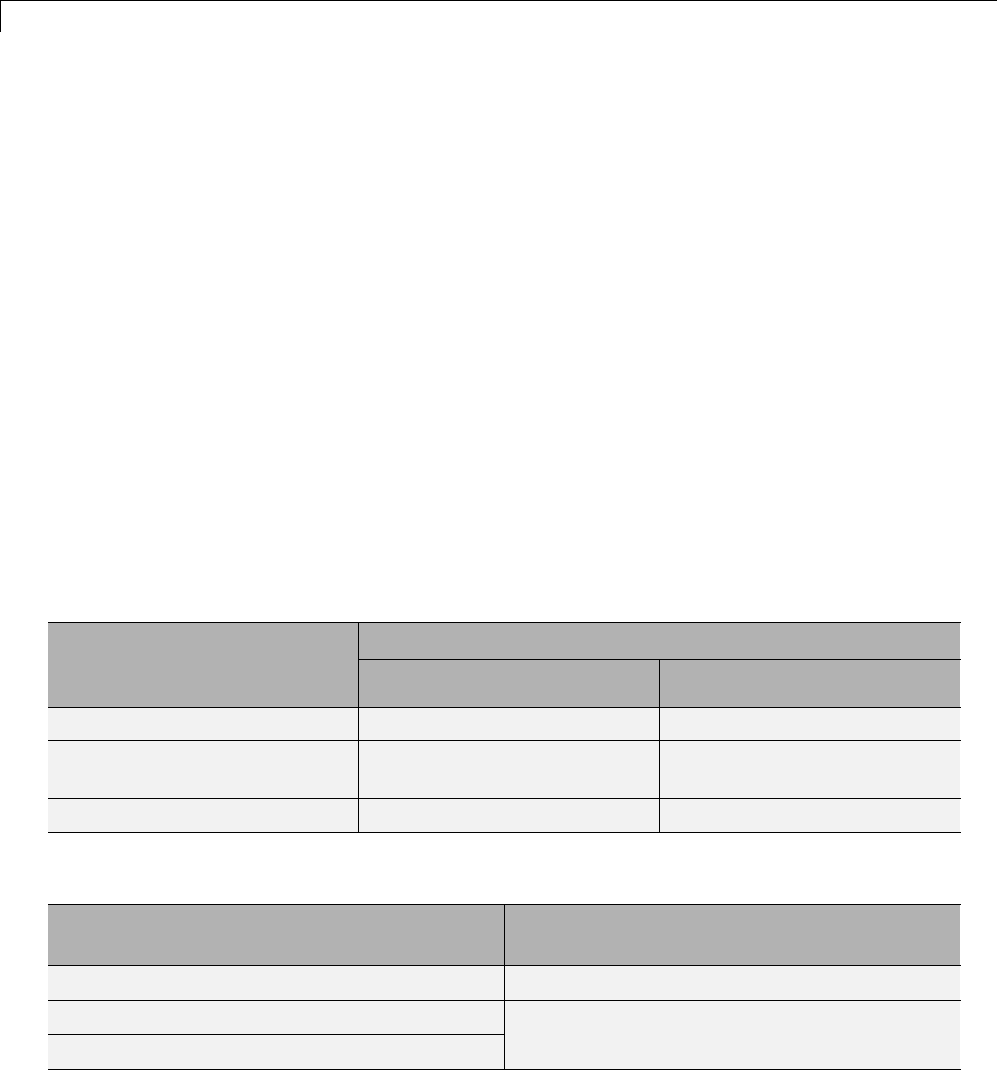
25 Working with Lookup Tables
After block replacement, the block names that appear in the model remain
the same. However, the block icons matchtheonesforthe1-DLookupTable
and 2-D Lookup Table blocks. For more information about the Model Advisor,
see “Consult the Model Advisor” on page 4-81 in the Simulink documentation.
What to Expect from the Model Advisor Check
The Model Advisor check groups all Lookup Table and Lookup Table (2-D)
blocks into three categories:
•Blocks that have compatible settings with the 1-D Lookup Table and 2-D
Lookup Table blocks
•Blocks that have incompatible settings with the 1-D Lookup Table and 2-D
Lookup Table blocks
•Blocks that have repeated breakpoints
Blocks with Compatible Settings
When a block has compatible parameter settings, automatic block replacement
can occur without backward incompatibilities.
Parameter Settings After Automatic Block Replacement
Lookup Method in the
Lookup Table or Lookup
Table (2-D) Block Interpolation Extrapolation
Interpolation-Extrapolation Linear Linear
Interpolation-Use End
Values
Linear Clip
Use Input Below Flat Not applicable
Depending on breakpoint spacing, one of two index search methods can apply.
Breakpoint Spacing in the Lookup Table
or Lookup Table (2-D) Block
Index Search Method After Automatic
Block Replacement
Not evenly spaced Binary search
Evenly spaced and tunable
Evenly spaced and not tunable
A prompt appears, asking you to select Binary
search or Evenly spaced points.
25-74

Update Lookup Table Blocks to New Versions
Blocks with Incompatible Settings
When a block has incompatible parameter settings, the Model Advisor shows
a warning and a recommended action, if applicable.
•If you perform the recommended action, you can avoid incompatibility
during block replacement.
•If you use automatic block replacement without performing the
recommended action, you might see numerical differences in your results.
Incompatibility Warning Recommended Action What Happens for
Automatic Block
Replacement
The Lookup Method is Use
Input Nearest or Use Input
Above. The replacement block
does not support these lookup
methods.
Change the lookup method to
one of the following options:
•Interpolation -
Extrapolation
•Interpolation - Use End
Values
•Use Input Below
The Lookup Method
is Interpolation -
Extrapolation,butthe
input and output are not the
same floating-point type. The
replacement block supports
linear extrapolation only when
all inputs and outputs are the
same floating-point type.
Change the extrapolation
method or the port data types
of the block.
The Lookup Method changes
to Interpolation - Use End
Values.
In the replacement block, this
setting corresponds to:
•Interpolation set to
Linear
•Extrapolation set to Clip
You also see a message that
explains possible numerical
differences.
The block uses small
fixed-point word lengths,
so that interpolation uses
only one rounding operation.
The replacement block uses
two rounding operations for
interpolation.
None You see a message that
explains possible numerical
differences.
25-75

25 Working with Lookup Tables
Blocks with Repeated Breakpoints
When a block has repeated breakpoints, the Model Advisor recommends that
you change the breakpoint data and rerun the check. You cannot perform
automatic block replacement for blocks with repeated breakpoints.
25-76

Lookup Table Glossary
Lookup Table Glossary
The following table summarizes the terminology used to describe lookup
tables in the Simulink user interface and documentation.
Term Meaning
breakpoint Asingleeleme
nt of a breakpoint
data set. A breakpoint represents
aparticularinput value to which a
corresponding output value in the
table data is mapped.
breakpoint data set Avectorofi
nput values that indexes
aparticula
r dimension of a lookup
table. A lookup table uses breakpoint
data sets torelateitsinputvaluesto
the output values that it returns.
extrapolation A process for estimating values that
lie beyond the range of known data
points.
interpolation A process for estimating values that
lie between known data points.
lookup table An array of data that maps input
valuestooutputvalues,thereby
approximating a mathematical
function. Given a set of input values,
a“loo
kup” operation retrieves the
corresponding output values from
the table. If the lookup table does
not explicitly define the input
values, Simulink can estimate an
output value using interpolation,
extrapolation, or rounding.
monotonically increasing The elements of a set are ordered
such that each successive element is
greaterthanorequaltoitspreceding
element.
25-77

25 Working with Lookup Tables
Term Meaning
rounding A process for approximating a value
by altering its digits according to a
known rule.
strictly monotonically increasing The elements of a set are ordered
such that each successive element is
greater than its preceding element.
table data Anarraythatservesasasampled
representation of a function
evaluated at a lookup table’s
breakpoint values. A lookup table
uses breakpoint data sets to index
the table data, ultimately returning
an output value.
25-78

26
Working with Block Masks
•“Block Masks” on page 26-2
•“How Mask Parameters Work” on page 26-4
•“Mask Code Execution” on page 26-7
•“Mask Terminology” on page 26-11
•“Mask a Block” on page 26-12
•“Draw Mask Icon” on page 26-15
•“Create Mask Documentation” on page 26-17
•“Initialize Mask” on page 26-19
•“Best Practices for Masking” on page 26-22
•“Considerations for Masking Model Blocks” on page 26-23
•“Masks on Blocks in User Libraries” on page 26-25
•“Promote Underlying Block Parameters to Mask” on page 26-27
•“Create Custom Interface for Simulink Blocks” on page 26-31
•“Rules for Promoting Parameters” on page 26-36
•“Mask Blocks and Promote Parameters” on page 26-38
•“Operate on Existing Masks” on page 26-42
•“Calculate Values Used Under the Mask” on page 26-46
•“Control Masks Programmatically” on page 26-49
•“Create Dynamic Mask Dialog Boxes” on page 26-56
•“Create Dynamic Masked Subsystems” on page 26-61
•“How Do I Debug Masks That Use MATLAB Code?” on page 26-67

26 Working with Block Masks
Block Masks
In this section...
“What Are Masks?” on page 26-2
“When to Use Masks?” on page 26-2
What Are Masks?
Masks are custom interfaces you can apply to Simulink blocks. A mask hides
the user interface of the block, and instead displays a custom dialog to control
specific parameters of the masked block.
When you mask a block, you change only the interface to the block, not its
underlying characteristics. Masking a nonatomic subsystem does not make it
act as an atomic subsystem, and masking a virtual block does not convert it
to a nonvirtual block.
Note You cannot save a mask separately from the block that it masks. You
canalsonotcreateanisolatedmaskdefinitionandapplyittomorethan
one block.
The mask icon and Mask Parameters dialog box are analogous to the block
icon and block Parameters dialog, respectively.
When you set mask parameter values, the mask can use the values to
dynamically change the mask icon and dialog box and to calculate values to
be used under the mask. A mask on a subsystem can dynamically change the
subsystem to reflect mask parameter values.
When to Use Masks?
Masks are useful for customizing block interfaces, encapsulating logic, and
providing restricted access to data.
26-2

Block Masks
Masks are comparable to subsystems, in that they both simplify the graphical
appearance of a model. However, subsystems do not offer an interface for
users to interact with underlying block parameters.
Consider masking a Simulink block when you want to
•display a meaningful dynamic icon that reflects values within a block
•define customized parameters whose names reflect the purpose of a block
•provide a dialog box that lets users access only select parameters of the
underlying blocks
•provide users customized documentation that is specific to the masked block
26-3

26 Working with Block Masks
How Mask Parameters Work
A masked block is a custom interface to underlying blocks that are governed
by block parameters. Mask parameters are the links to these underlying
block parameters.
Mask parameters are defined in the mask workspace, while block parameters
may be defined in the model or base workspace.
You can provide access to one or more underlying block parameters by
defining the corresponding number of mask parameters. Mask parameters
appear in the Mask Parameters dialog box as editable fields. Simulink
applies the value of a mask parameter to the value of the corresponding block
parameter during simulation.
Consider the Mask Parameters dialog box of model masking_example.
This dialog contains fields for mask parameters Slope and Intercept,both
defined in the Mask Editor.
26-4
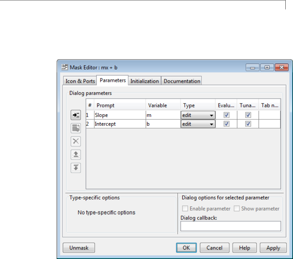
How Mask Parameters Work
Slope corresponds to mask workspace variable m,andIntercept,tomask
workspace variable b. Moreover, variable names mand bcorrespond to the
Gain and Constant value parameters of the underlying blocks.
In the Mask Parameters dialog box, when you set Slope and Intercept
to 5and 2, respectively, Simulink assigns these values to mask workspace
variables mand b.
Before simulation begins, Simulink searches up the workspace hierarchy,
looking in the mask workspace first, for values to resolve the Gain parameter
26-5

26 Working with Block Masks
mand Constant value parameter b. Since variables mand bare defined in
the mask workspace, Simulink applies their values to the block parameters.
Without a mask for the same subsystem, no mask workspace would exist. In
that case, Simulink would continue searching up the workspace hierarchy for
definitions of mand b.
26-6

Mask Code Execution
Mask Code Execution
In this section...
“Mask Code Placement” on page 26-7
“Drawing Command Execution” on page 26-7
“Initialization Command Execution” on page 26-8
“Callback Code Execution” on page 26-9
Mask Code Placement
YoucanuseMATLABcodetoinitializeamaskaswellastodrawmaskicons.
Since the location of code affects model performance, place your code to reflect
the functionality you need.
Purpose Placement in Mask
Editor
Programmatic
Specification
Initialize the mask Initialization pane MaskInitialization
parameter
Draw mask icon Icon & Ports pane MaskDisplay
parameter
Callback code for mask
parameters
Parameters pane MaskCallbacks
parameter
Drawing Command Execution
Place MATLAB code for drawing mask icons in the Icon Drawing
Commands section of the Icon & Ports pane. Simulink executes these
commands sequentially to redraw the mask icon in the following cases:
•The drawing commands are dependent on mask parameters and the values
of these mask parameters change.
•The block’s appearance is altered due to rotation or other changes.
26-7

26 Working with Block Masks
Note If you place MATLAB code for drawing mask icons in the Initialization
pane, model performance is affected, because Simulink redraws the icon each
time the masked block is evaluated in the model.
Initialization Command Execution
When you open a model, Simulink locates visible masked blocks that reside at
the top level of the model or in an open subsystem. Simulink only executes the
initialization commands for these visible masked blocks if they meet either
of the following conditions:
•The masked block has icon drawing commands.
Note Simulink does not initialize masked blocks that do not have icon
drawing commands, even if they have initialization commands.
•The masked subsystem belongs to a library and has the Allow library
blocktomodifyitscontentsparameter enabled.
Simulink initializes masked blocks that are not initially visible when you
open the subsystem or model that contains these blocks.
When you load a model into memory without displaying it graphically, no
initialization commands initially run for any masked blocks. See “Load a
Model” on page 1-7 and load_system for information about loading a model
without displaying it.
Initialization commands for all masked blocks in a model that have drawing
commands run when you:
•Update the diagram
•Start simulation
•Start code generation
Initialization commands for an individual masked block run when you:
26-8

Mask Code Execution
•Change any of the parameters that define the mask, such as MaskDisplay
and MaskInitialization,byusingtheMaskEditororset_param.
•Rotate or flip the masked block, if the icon depends on initialization
commands.
•Cause the icon to be drawn or redrawn, and the icon drawing depends
on initialization code.
•Change the value of a mask parameter by using the block dialog box or
set_param.
•Copy the masked block within the same model or between different models.
Callback Code Execution
Simulink executes the callback commands in the following cases:
•YouopentheMaskParametersdialog box. Callback commands execute
sequentially, starting with the top mask dialog box parameter.
•You modify a parameter value in the Mask Parameters dialog box and
then change the cursor’s focus (that is, you press the Tab key or click into
another field in the dialog box).
Note When you modify the parameter value by using the set_param
command, the callback commands do not execute.
•You modify the parameter value, either in the Mask Parameters dialog
box or using set_param, and then apply the change by clicking Apply or
OK. Mask initialization commands execute after callback commands (See
“Initialization Pane”).
•You hover over a masked block to see the data tip for the block, when the
data tip contains parameter names and values. The callback executes
againwhentheblockdatatipdisappears.
Note Callback commands do not execute if the Mask Parameters dialog
box is open when the block data tip appears.
26-9

26 Working with Block Masks
•Update a diagram (for example, by pressing Ctrl+D or by selecting
Simulation > Update diagram in the Simulink Editor).
26-10

Mask Terminology
Mask Terminology
Term Description
Mask icon The masked block icon generated using drawing
commands. This icon may be static or change
dynamically with underlying block parameter
values.
Mask parameters Parameters defined in the Mask Editor that link
to underlying block parameters. Setting a mask
parameter sets the corresponding block parameter.
Mask initialization
code
MATLAB code that initializes a masked block or
reflects current parameter values.
Mask callback code MATLAB code that runs when the value of a mask
parameter changes. Use callback code to modify
a mask dialog box to reflect current parameter
values.
Mask
documentation
Description and usage information for a masked
block defined in the Mask Editor.
Mask dialog A dialog box that contains fields for setting
mask parameter values and provides mask
documentation.
Mask workspace Masks that define mask parameters or contain
initialization code have a mask workspace. This
workspace stores mask parameters and temporary
values used by the mask.
26-11

26 Working with Block Masks
Mask a Block
This example shows how to create a block mask and define its parameters.
Create mask
1Open the model subsystem_example. Alternately, execute the following
command in MATLAB:
open_system([docroot '/toolbox/simulink/ug/examples/masking/subsystem_ex
a
This model contains a Subsystem block that models the equation for a
line: y=mx+b.
2Double-click the subsystem block to open it.
Notice that this subsystem contains the following blocks that are controlled
by parameters.
•Gain block, named Slope, with parameter m
•Constant block, named Intercept, with parameter b
3Return to the top-level model, right-click the subsystem block, and select
Mask > Create Mask.
The Mask Editor appears.
Define mask parameters
Define parameters to control the underlying blocks.
1In the Mask Editor, click the Parameters tab.
2In the Dialog parameters pane, click the Add parameter icon.
3In the row that appears, specify the parameters as follows.
26-12
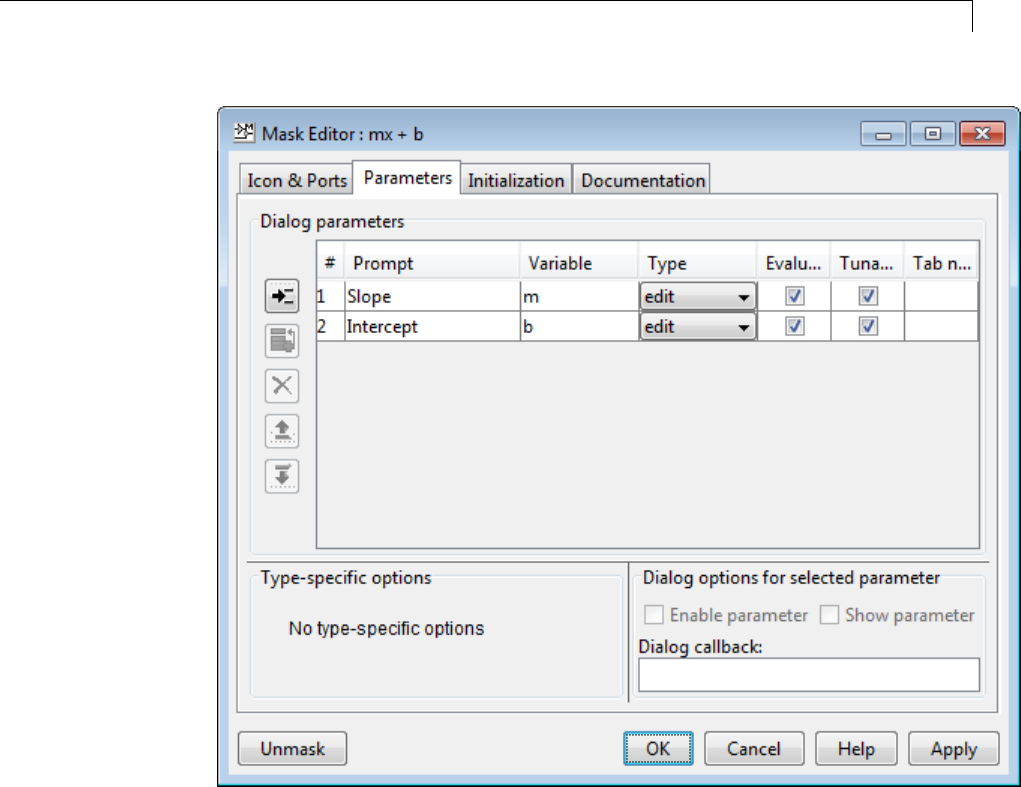
Mask a Block
4Click Apply.
Set mask parameter values
Provide values to the parameters.
1Double-click the mask to view the mask parameter dialog.
2Set Slope and Intercept as 5and 2, respectively.
To control the underlying blocks, change these parameters.
26-13

26 Working with Block Masks
3Click OK.
26-14

Draw Mask Icon
Draw Mask Icon
Thisexampleshowshowtousedrawingcommandstocreateamaskicon. You
can create icons that update when you change the mask parameters, thereby
reflecting the purpose of the block.
Draw static icon
A static mask icon remains unchanged, independent of the value of the mask
parameters.
1Right-click the masked block that requires the icon and select Mask > Edit
Mask.
The Mask Editor appears.
2In the Icons & Ports tab, enter the following command in the Icon
Drawing commands pane:
% Use specified image as mask icon
image(imread('engine.jpg'))
The image file must be on the MATLAB path.
Note For more examples of drawing command syntax, explore the
Command drop-down list in the Examples of drawing commands pane.
Draw dynamic icon
A dynamic icon changes with the values of the mask parameters. Use it to
represent the purpose of the masked block.
1Right-click the masked block that requires the icon and select Mask > Edit
Mask.
The Mask Editor appears.
2In the Icons & Ports tab, enter the following command in the Icon
Drawing commands pane:
26-15

26 Working with Block Masks
pos = get_param(gcb, 'Position');
width = pos(3) - pos(1);
x = [0, width];
y = m*x + b;
plot(x,y)
3Under Options,setIcon Units to Pixels.
The drop-down lists under Options allow you to specify icon frame
visibility, icon transparency, drawing context, icon rotation, and port
rotation.
4Click Apply.
Note If Simulink cannot evaluate all commands in the Icon Drawing
commands pane to generate an icon, three question marks (???)
appear on the mask.
See model masking_example to view the icon generated.
Additional examples
See model slexMaskDisplayAndInitializationExample for more examples
of icon drawing commands. This model shows how to draw:
•astaticmask
•a dynamic shape mask
•adynamictextmask
•an image mask
26-16

Create Mask Documentation
Create Mask Documentation
This example shows how to create mask documentation for display in the
Mask Parameters dialog box.
1Right-click the masked block to document and select Mask > Edit Mask.
The Mask Editor appears.
2In the Documentation tab, enter the following information:
•Mask type:Th
e name of the mask. This name appears at the top of the
Mask Parameters dialog box. Newlines are not permitted.
•Mask description: A summary of what the mask does. This description
appears below the mask name, and it contain newlines as well as spaces.
•Mask help:Additional mask information that appears when you click
Help in the Mask Parameters dialog box. You can use plain text, HTML
and graphics, URLs, and web or eval commands.
26-17
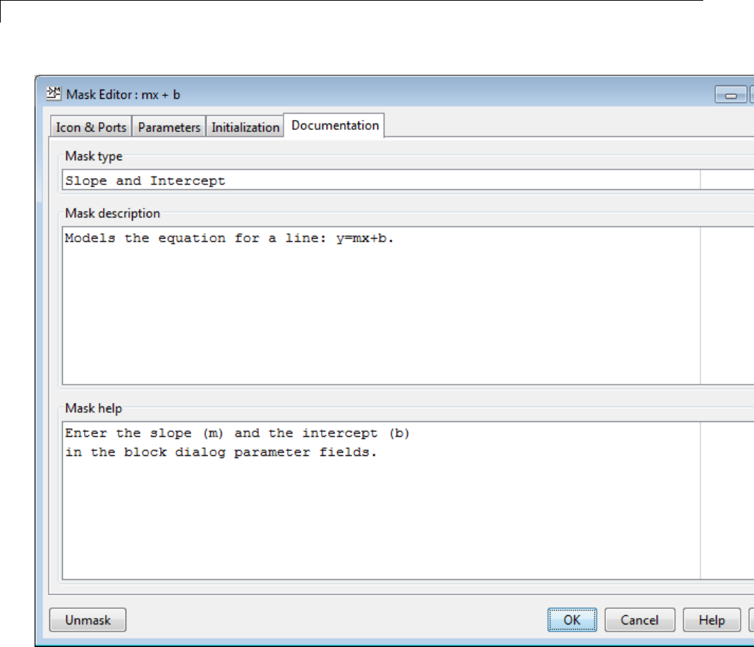
26 Working with Block Masks
26-18

Initialize Mask
Initialize Mask
The initialization code is MATLAB code that you specify and that Simulink
runs to initialize the masked subsystem at critical times, such as model
loading and the start of a simulation run (see “Initialization Command
Execution” on page 26-8). You can use the initialization code to set the initial
values of the mask parameters.
The masked subsystem initialization code can refer only to variables in its
local workspace.
When you reference the block within, or copy the block into, a model, the
Mask Parameters dialog box displays the specified default values. You cannot
use mask initialization code to change mask parameter default values in a
library block or any other block.
Mask Editor Initialization Pane
Use the Mask Editor Initialization pane to enter MATLAB commands that
initialize a masked block. Reference information about the Initialization
pane appears in “Initialization Pane”.
The Initialization pane has two sections:
•Dialog variables list
•Initialization commands edit area
26-19
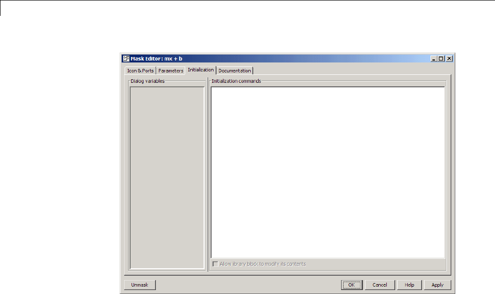
26 Working with Block Masks
Dialog variables
The Dialog variables list displays the names of the variables associated
with the mask parameters of the subsystem (that is, the parameters defined
in the Parameters pane).
You can copy the name of a parameter from this list and paste it into the
adjacent Initialization commands field, using the Simulink keyboard copy
and paste commands.
You can also use the list to change the names of mask parameter variables.
To change a name, double-click the name in the list. An edit field containing
the existing name appears. Edit the existing name and press Enter or click
outside the edit field to confirm your changes.
26-20

Initialize Mask
Initialization Commands
Enter the initialization commands in this field. You can enter any valid
MATLAB expression, consisting of MATLAB functions and scripts, operators,
and variables defined in the mask workspace. Initialization commands cannot
access base workspace variables.
Terminate initialization commands with a semicolon to avoid echoing results
to the MATLAB Command Window.
For information on debugging initialization commands, see “Initialization
Command Limitations” on page 26-21and “How Do I Debug Masks That Use
MATLAB Code?” on page 26-67.
Initialization Command Limitations
Mask initialization commands must observe the following rules:
•Do not use initialization code to create dynamic mask dialog boxes (that
is, dialog boxes whose appearance or control settings change depending on
changes made to other control settings). Instead, use the mask callbacks
that are specifically for this purpose. For more information, see “Create
Dynamic Mask Dialog Boxes” on page 26-56.
•Avoid using set_param commands on blocks residing in another masked
subsystem that you are initializing. Tryingtosetparametersofblocksin
lower-level masked subsystems can trigger unresolvable symbol errors if
lower-level masked subsystems reference symbols defined by higher-level
masked subsystems. Suppose, for example, a masked subsystem A contains
masked subsystem B, which contains Gain block C, whose Gain parameter
references a variable defined by B. Suppose also that subsystem A has
initialization code that contains the following command:
set_param([gcb '/B/C'], 'SampleTime', '-1');
Simulating or updating a model containing A causes an unresolvable
symbol error.
26-21

26 Working with Block Masks
Best Practices for Masking
These examples show best practices for masking Simulink blocks. There are
also some examples that show practices to avoid.
In this section...
“Use These Best Practices” on page 26-22
“Avoid These Practices” on page 26-22
Use These Best Practices
•Set mask parameters
•Group parameters under tabs
•Promote mask parameters
•Sequence mask callbacks
•Define mask display and initialization
•Create dynamic mask dialog boxes
•Use self-modifying library masks
•Use handle graphics in masking
Avoid These Practices
•Unsafe mask callbacks
•Unsafe nested mask callbacks
26-22

Considerations for Masking Model Blocks
Considerations for Masking Model Blocks
In this section...
“Referenced Model Name” on page 26-23
“Variable Workspace” on page 26-24
Referenced Model Name
Youcanuseamaskparametertospecifythenameofamodelreferencedby
•a masked Model block, or
•a Model block in a masked subsystem
In these cases, the mask parameter should receive the name of the reference
model literally, without being evaluated, because Simulink updates model
reference targets before mask parameters.
Use one of the following approaches to obtain the literal name of the
referenced model:
•Restricted model names: In the Parameters pane of the Mask Editor,
select the parameter that stores the referenced model name. Set its Type
to popup and clear the check box for Evaluate.
With this approach, users can only select a model name from a drop-down
list in the Mask Parameters dialog box. Further, since the Evaluate option
is cleared, the name is provided literally and not numerically evaluated.
•Unrestricted model names: In the Parameters pane of the Mask
Editor, select the parameter that stores the referenced model name. Set its
Type to edit and clear the check box for Evaluate.
With this approach, users can type the model name in the Mask Parameters
dialog box. However, since the Evaluate option is cleared, the name is
provided literally and not numerically evaluated.
See “Control Types” for more information about Pop-Up and Edit controls.
26-23

26 Working with Block Masks
Variable Workspace
When you mask a Model block that references another model, the referenced
model cannot access the mask workspace of the Model block.
Therefore, variables used by the referenced model must resolve either to
workspaces defined by the referenced model or to the base workspace.
26-24

MasksonBlocksinUserLibraries
MasksonBlocksinUserLibraries
In this section...
“About Masks and User-Defined Libraries” on page 26-25
“Masking a Block for Inclusion in a User Library” on page 26-25
“Masking a Block that Resides in a User Library” on page 26-25
“Masking a Block Copied from a User Library” on page 26-26
About Masks and User-Defined Libraries
You can mask a block that will be included in a user library or already
resides in a user library, or you can mask an instance of a user library block
that you have copied into a model. For example, a user library block might
provide the capabilities that a model needs, but its native interface might be
inappropriate or unhelpful in the context of the particular model. Masking
the block could give it a more appropriate user interface.
Masking a Block for Inclusion in a User Library
You can create a custom block by encapsulating a block diagram that defines
the block’s behavior in a masked subsystem and then placing the masked
subsystem in a library. You can also apply a mask to any other type of block
that supports masking, then include the block in a library.
Masking a block that will later be included in a library requires no special
provisions. Create the block and its mask as described in this chapter, and
include the block in the library as described in “Create Block Libraries” on
page 28-20.
Masking a Block that Resides in a User Library
Creating or changing a library block mask immediately changes the block
interface in all models that access the block using a library reference, but has
no effect on instances of the block that already exist as separate copies.
To apply or change a library block mask, open the library that contains the
block. Apply, change, or remove a mask as you could if the block did not
26-25

26 Working with Block Masks
reside in a library. In addition, you can specify non-default values for block
mask parameters. When the block is referenced within or copied into a model,
the specified default values appear on the block’s Mask Parameters dialog
box. By default, edit fields have a value of zero, check boxes are cleared,
and drop-down lists select the first item in the list. To change the default
for any field:
1Fill in the desired default values or change check box or drop-down list
settings
2Click Apply or OK to save the changed values into the library block mask.
Be sure to save the library after changing the mask of any block that it
contains. Additional information relating to masked library blocks appears in
“Create Block Libraries” on page 28-20.
Masking a Block Copied from a User Library
A block that was copied from a user library, as distinct from a block accessed
by using a library reference, has no special status with respect to masking.
You can add a mask to the copied block, or change or remove any mask that it
already has.
26-26
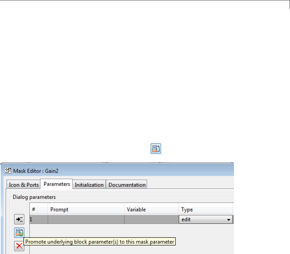
Promote Underlying Block Parameters to Mask
Promote Underlying Block Parameters to Mask
This example shows to promote the parameters of underlying blocks to the
mask. See model slexMaskParameterPromotionExample for more examples
of parameter promotion.
1Right-click a block or subsystem in your model and select Mask > Create
Mask.
The Mask Editor appears.
2Select the Parameters pane.
3Choose one or more parameters for promotion.
aCreate a new mask parameter. Click Add Parameter.
bClick the Promote button.
The Promoted parameter selector dialog box opens.
26-27
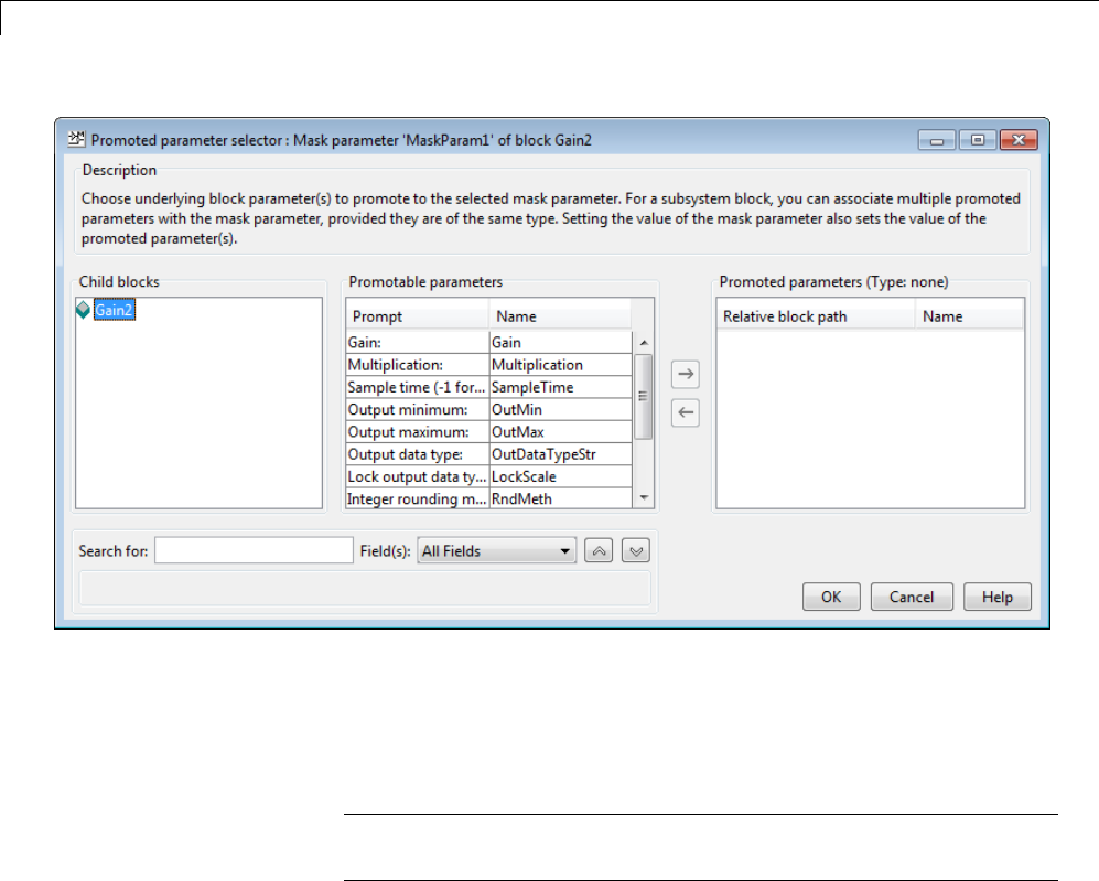
26 Working with Block Masks
cChoose underlying block parameters to promote to the currently selected
mask parameter.
•Select a parameter in the Promotable parameters table and click
the right arrow button to add to the Promoted parameters list.
Tip View the tooltips on promotable parameters to see key fields
such as Type.
•When masking a subsystem, you can use the Child blocks list or the
Search box to find underlying block parameters to promote.
•(Optional) When masking a subsystem, you can associate multiple
promoted parameters with the currently selected mask parameter,
provided they are of the same type.
For example, you can promote multiple Gain parameters in a
subsystem to a single prompt on your mask.
dClick OK to return to the Mask Editor.
26-28
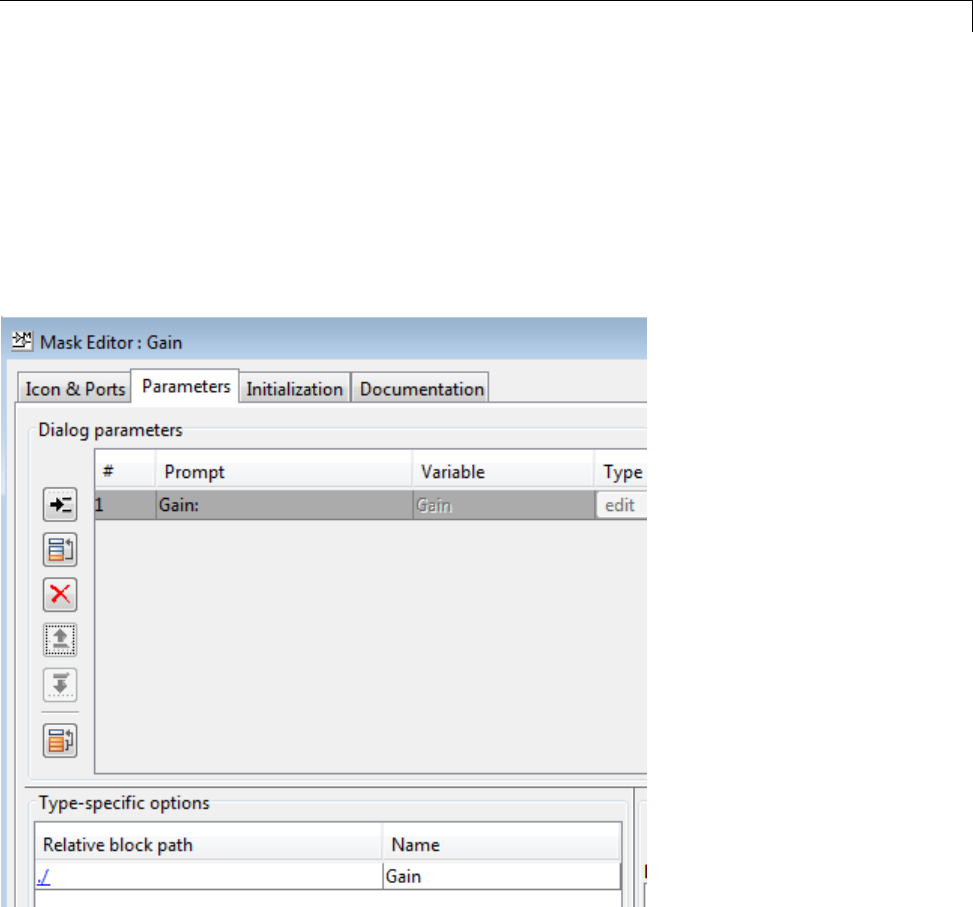
Promote Underlying Block Parameters to Mask
4Observe that the Type field is now disabled because you have promoted
a parameter to this mask parameter. Type is always disabled. Variable
is also disabled if you are directly masking a built-in block and not a
subsystem.
The Relative block path table shows you the location of the underlying
original block (where .means self ). Click the link under Relative
block path to open the underlying block.
5Edit the prompt names for the mask, if desired. You cannot edit the
variable names of built-in block parameters. See “Rules for Promoting
Parameters” on page 26-36.
6Repeat step 3 to add mask parameters and add or edit additional promoted
parameters.
26-29

26 Working with Block Masks
Tip If you want to promote many parameters from a built-in block, click
Promote All .
The Promote All button is only available for block masks, not subsystem
masks.
All the parameters appear in the Mask Editor. To remove any unwanted
parameters, use the Delete Parameter button.
7Click OK to finish editing the mask.
Now whenever you set a mask parameter, you also set the value of the
underlyingpromotedparameters.
26-30

Create Custom Interface for Simulink®Blocks
Create Custom Interface for Simulink Blocks
This example shows how to mask the Gain block and promote only the Gain
parameter to the mask, while hiding the other options and adding custom
parameters.
1Right-click a Gain block in your model and select Mask > Create Mask.
The Mask Editor appears.
2Select the Parameters pane.
3Create a new mask parameter. Click Add Parameter.
4Click the Promote button. .
The Promoted parameter selector dialog box opens.
5Select the Gain parameter in the Promotable parameters table and click
the right-arrow button to add to the Promoted parameters list.
26-31
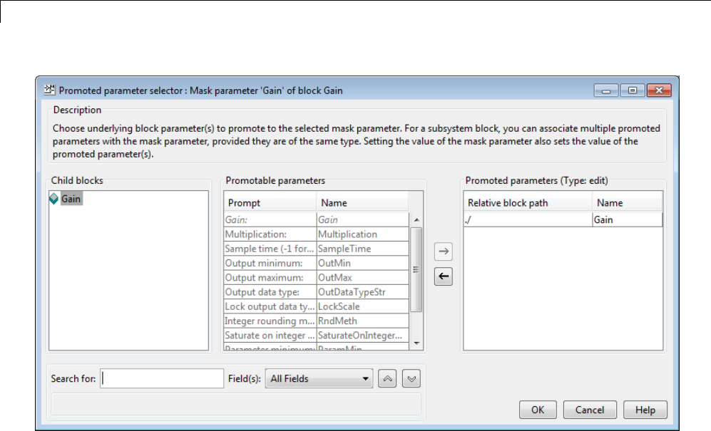
26 Working with Block Masks
6Click OK to return to the Mask Editor.
7Observe that fields such as Variable and Type are now disabled because
you have promoted a built-in parameter to this mask parameter, and
the Relative block path table shows you the location of the underlying
original block (where ./ means self ). Click the link in the Relative
block path table to open the underlying Gain block.
8(Optional) Add custom mask parameters by clicking Add Parameter.For
example, you can add an edit box to capture company notes.
26-32
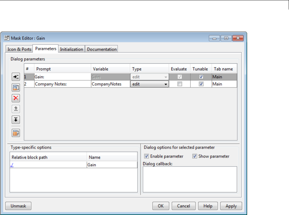
Create Custom Interface for Simulink®Blocks
9Click OKto finish creating the mask.
10 Double-click the Gain block. The new mask opens, showing only the
promoted Gain parameter and custom parameter.
26-33
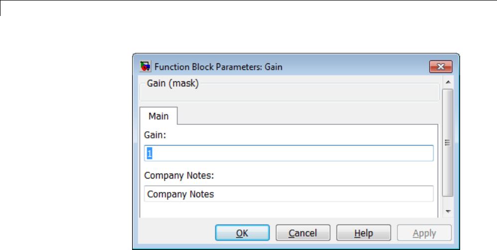
26 Working with Block Masks
11 Look under the mask to see the underlying Gain block dialog box. You can
see that the Gain parameter is now disabled because you have promoted
it to the mask.
26-34
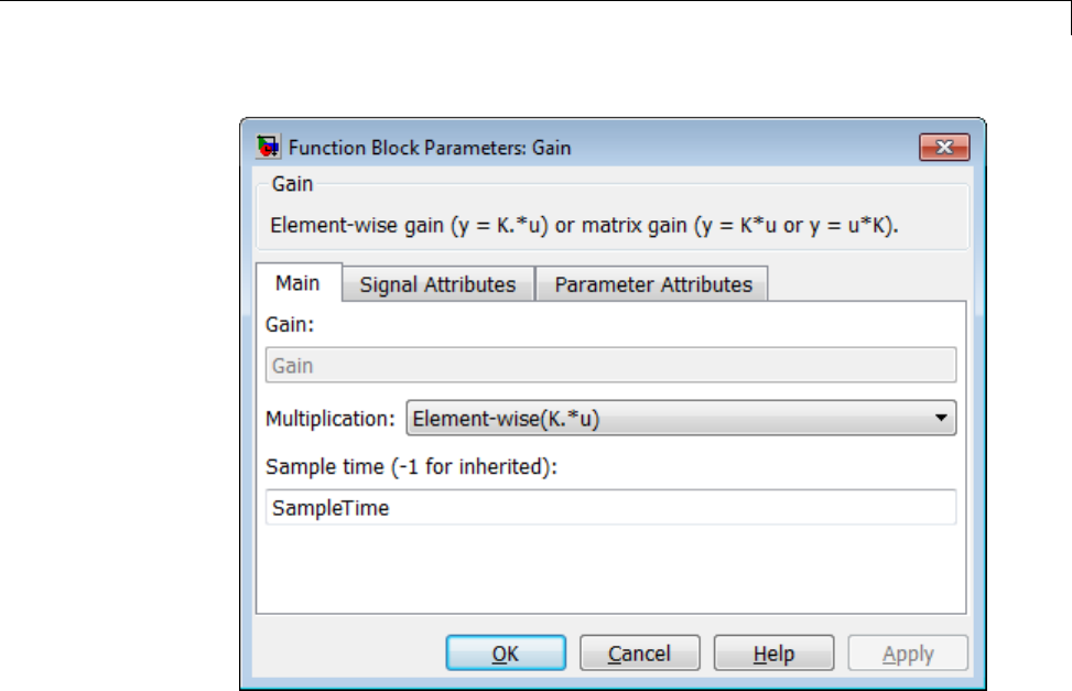
Create Custom Interface for Simulink®Blocks
26-35

26 Working with Block Masks
Rules for Promoting Parameters
In this section...
“General Rules” on page 26-36
“Promotion from directly masked block” on page 26-36
“Promotion from child blocks within subsystems” on page 26-37
“Links created from masked blocks” on page 26-37
General Rules
•Youcannotmaskblocksthatalreadyhavemasks. Forexample,some
Simulink blocks like the Ramp and Chirp Signal in the Sources library
cannot be masked.
•Some parameters with certain attributes cannot be promoted, and if you
try, an error message appears.
•After you promote a parameter to the mask, the following rule apply.
-The parameter is disabled on the block dialog box. If you try to directly
edit promoted parameters, either in the dialog or at the command line,
an error message appears.
-You cannot promote the same parameter again to a different mask
parameter.
-The mask parameter inherits the Evaluate property from the parameter
promoted to it, and you cannot change it. Any mismatch between the
Evaluate property of the mask parameter and the promoted parameter
results in an error message.
Promotion from directly masked block
•The mask parameter must have the same variable name as that of
the parameter promoted to it. You cannot change the promoted mask
parameter variable names because they are strictly inherited from the
underlying built-in block parameter.
26-36

Rules for Promoting Parameters
•The mask tries to retain the dynamic dialog behavior, if any, of the
promoted parameter. You can specify your own dynamic dialog behavior of
the mask parameter. If you do, the mask first executes the dynamic dialog
callback of the promoted parameter, followed by the user-specified dynamic
dialog callback of the mask parameter.
•You cannot promote multiple parameters to a single mask parameter.
Promotion from child blocks within subsystems
•You can associate multiple parameters provided they are of the same type.
If the parameter is of type popup or DataType then the options must also be
the same for them to be promoted together. The Evaluate property among
theparameterstobepromotedtogethermustbesimilar.
Tip View the tooltips on promotable parameters to see key fields such as
Type and Evaluate.
•If a child block is masked, you cannot promote the underlying block dialog
parameters.
•For child blocks, you cannot view or promote parameters from inside a
masked block.
•For child blocks, you cannot view or promote parameters from inside a
linked block.
Links created from masked blocks
•The underneath block dialog opens completely disabled for the links of
masked blocks. You can edit values only from the mask dialog.
•If the mask author decides not to promote a parameter, its value in the
linked blocks is tied to the library value for that parameter as specified in
the library.
26-37

26 Working with Block Masks
Mask Blocks and Promote Parameters
In this section...
“Mask Built-In Blocks Directly and Within Subsystems” on page 26-38
“Create Custom Interface for Multiple Parameters in Subsystem” on page
26-38
Mask Built-In Blocks Directly and Within Subsystems
You can directly mask built-in blocks with the Mask Editor to provide custom
icons and dialog boxes. In the Mask Editor, you can choose to promote any
underlying parameter of any block to the mask. For subsystems, you can
choose to promote parameters from any child blocks. For a subsystem
block, you can associate a single mask parameter with multiple promoted
parameters if they are of the same type. Changing the value of the mask
parameter also sets the value of the associated promoted parameters.
You can use masking in the following use cases:
•You can directly mask a built-in block to simplify the interface and add
custom parameters.
•You can promote multiple parameters from child blocks to a single mask
parameter for a subsystem block.
•You can promote all parameters for a directly masked built-in block, and
then choose a subset of the parameters to keep in the mask.
Create Custom Interface for Multiple Parameters in
Subsystem
You can promote multiple parameters from child blocks to a single mask
parameter for a subsystem block. This enables you to use a simplified single
setting in the mask to set multiple child block parameters (of the same type)
in the subsystem.
The following example demonstrates this capability. It recreates the functions
of the Ramp block by using other blocks in a subsystem, and then masking
the subsystem to create a simplified custom interface.
26-38
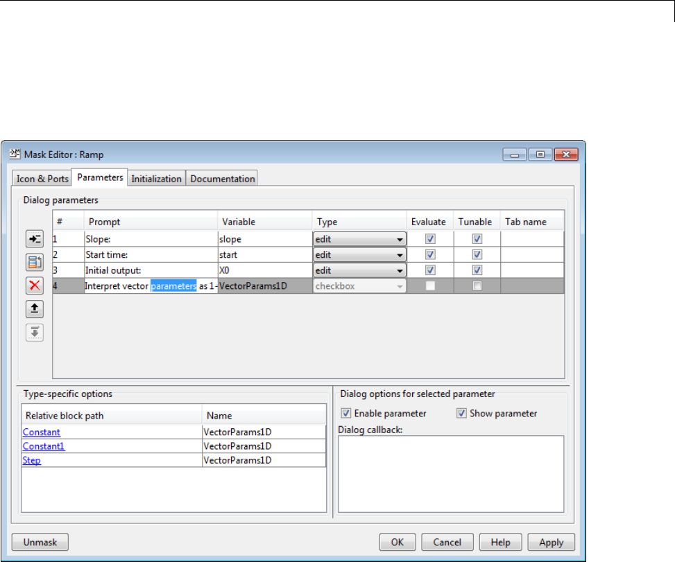
Mask Blocks and Promote Parameters
The Mask Editor contains a selection of promoted parameters from underlying
blocks within the subsystem. The selected parameter has three underlying
parametersofthesametypepromoted to the same mask parameter.
The Promoted parameter selector dialog shown next demonstrates how to
specify this setup. Three parameters of the same type, from different child
blocks, are added to the Promoted parameters listtopromotetothe
currently selected mask parameter.
26-39
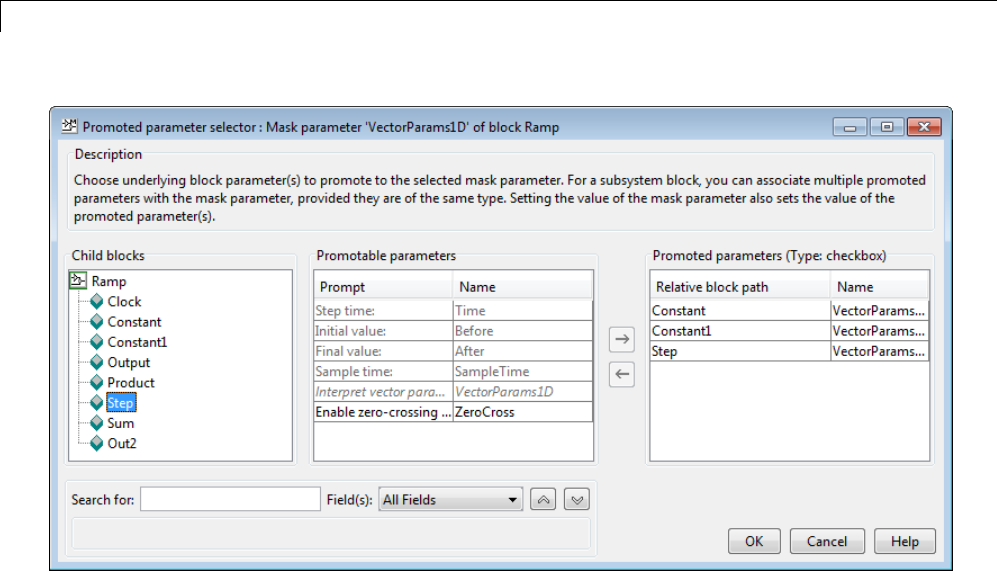
26 Working with Block Masks
The mask shows the four parameters specified in the Mask Editor.
26-40
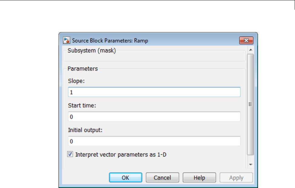
Mask Blocks and Promote Parameters
When you select the Interpret vector parameters as 1-D check box on
the mask, you also set the underlying promoted parameters in the three
child blocks.
26-41

26 Working with Block Masks
Operate on Existing Masks
In this section...
“Change a Block Mask” on page 26-42
“View Mask Parameters” on page 26-42
“Look Under Block Mask” on page 26-43
“Remove and Cache Mask” on page 26-43
“Restore Cached Mask” on page 26-45
“Permanently Delete Mask” on page 26-45
Change a Block Mask
You can change an existing mask by reopening the Mask Editor and using the
same techniques that you used to create the mask:
1Select the masked block.
2Select Mask > Edit Mask.
The Mask Editor reopens, showing the existing mask definition. Change the
mask as needed. After you change a mask, be sure to save the model before
closing it, or the changes will be lost.
View Mask Parameters
To display a masked block’s Mask Parameters dialog box, double-click
the block. Alternatively, right-click the block and select Mask > Mask
Parameters.
To display the Block Parameters dialog box that double-clicking would
display if no mask existed, right-click the masked block and select Block
Parameters (BlockType).
26-42

Operate on Existing Masks
Look Under Block Mask
To see the block diagram under a masked Subsystem block, built-in block,
or the model referenced by a masked Model block, right-click the block and
select Mask > Look Under Mask.
Remove and Cache Mask
To remove a mask from a block and cache it for possible restoration later:
1Right-click the block.
2Select Mask > Edit Mask.
The Mask Editor opens and displays the existing mask, for example:
26-43
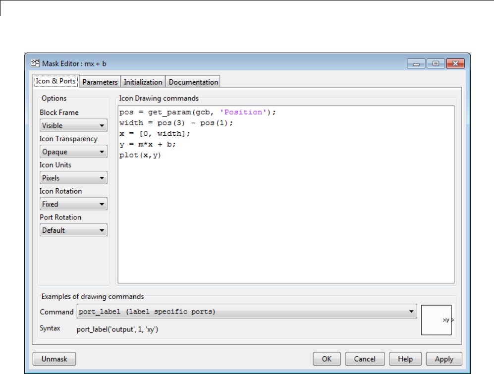
26 Working with Block Masks
3Click Unmask in the lower left corner of the Mask Editor.
The Mask Editor removes the mask from the block, saves the mask in a cache
for possible restoration, then closes. The editor caches masks separately for
each block, so removing a mask from one block has no effect on a mask cached
for any other block. Closing the Mask Editor has no effect on cached masks.
When you have removed and cached a mask, you can later restore it, as
described in “Restore Cached Mask” on page 26-45, or delete it, as described
in “Permanently Delete Mask” on page 26-45. The removed cached mask has
no further effect unless you restore it.
26-44

Operate on Existing Masks
Restore Cached Mask
As long as a model remains open, you can restore a mask that you removed as
described in “Remove and Cache Mask” on page 26-43.
1Right-click theblock.
2Select Mask > Create Mask.
The Mask Editor reopens, showing the cached masked definition.
3Modify the definition if needed, using the techniques in “Mask a Block” on
page 26-12
4Click Apply or OK to restore the mask, including any changes that you
made.
If you made any changes, be sure to save the model before closing it, or the
changes will be lost.
Permanently Delete Mask
To delete a mask permanently, first remove it as described in “Remove and
Cache Mask” on page 26-43, then save and close the model. You do not need
to close the model immediately after removing a mask that you intend to
delete. The removed mask remains in the cache and has no further effect
unless you restore it.
26-45
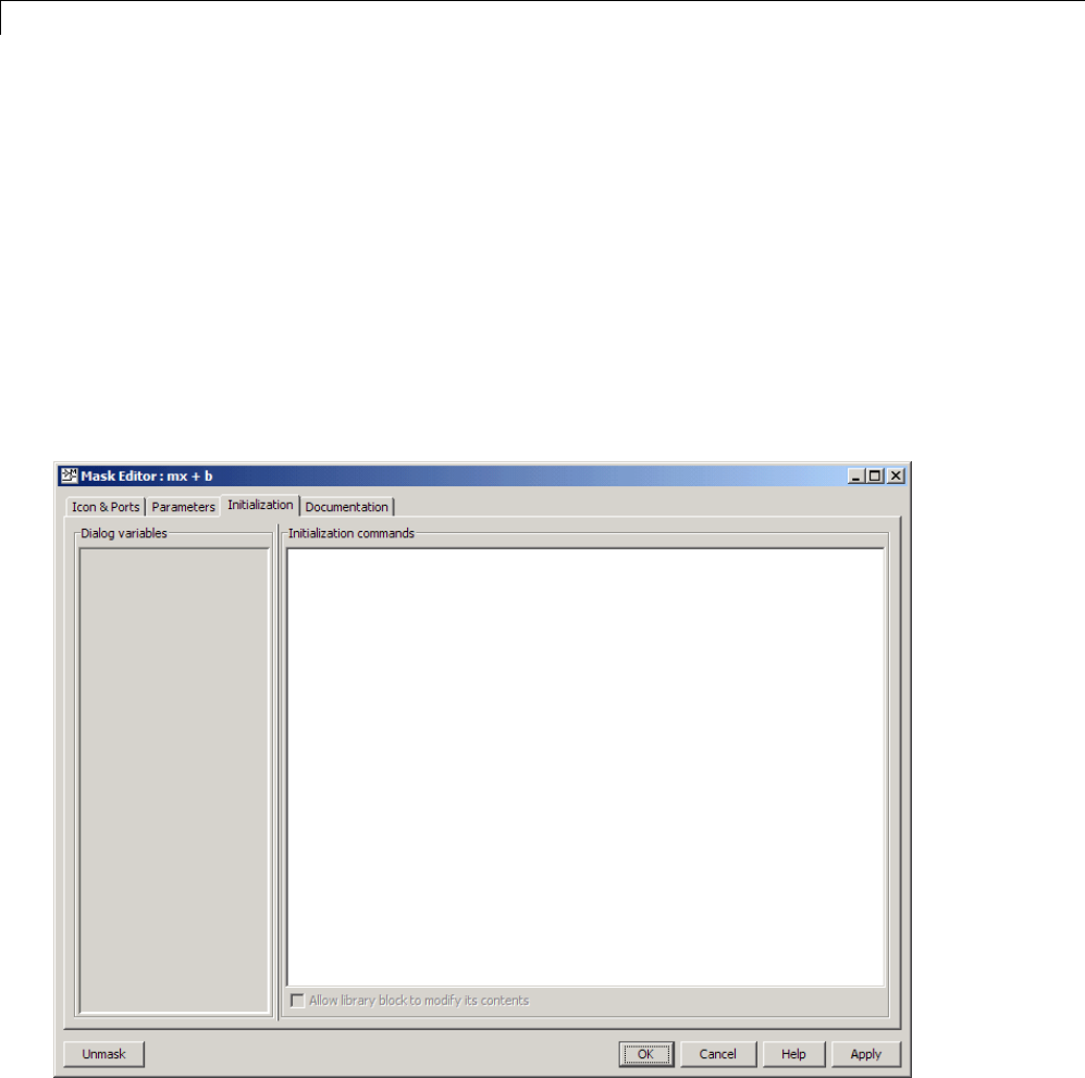
26 Working with Block Masks
CalculateValuesUsedUndertheMask
The masking_example assigns the values input using the Mask Parameters
dialog box directly to block parameters underneath the mask, as described in
“How Mask Parameters Work” on page 26-4. The assignment occurs because
the block parameter and the mask parameter have the same name, so the
search that always occurs when a block parameter needs a value finds the
mask parameter value automatically, as described in “Symbol Resolution”
on page 4-76.
You can use the Mask Editor to insert any desired calculation between a value
in the Mask Parameters dialog box and an underlying block parameter:
26-46
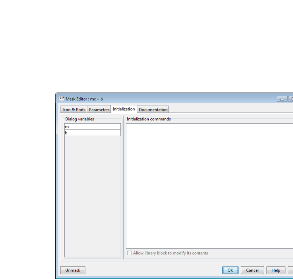
Calculate Values Used Under the Mask
See the “Initialization Pane” reference for reference information about all
Initialization pane capabilities. This section shows you how to use it for
calculating block parameter values.
To calculate a value for a block parameter, first break the link between the
mask and block parameters by giving them different names. To facilitate
such changes, the Dialog variables subpane lists all mask parameters. The
Initialization pane looks like this:
You cannot use mask initialization code to change mask parameter default
values in a library block or any other block.
26-47

26 Working with Block Masks
You can use the initialization code for a masked block to link mask parameters
indirectly to block parameters. In this approach, the initialization code
creates variables in the mask workspace whose values are functions of the
mask parameters and that appear in expressions that set the values of
parameters of blocks concealed by the mask.
If you need both the string entered and the evaluated value, clear the
Evaluate option. To get the value of a base workspace variable entered as
the literal value of the mask parameter, use the MATLAB evalin command
in the mask initialization code. For example, suppose the user enters the
string 'gain' as the literal value of the mask parameter kwhere gain is the
name of a base workspace variable. To obtain the value of the base workspace
variable, use the following command in the initialization code for the mask:
value = evalin('base', k)
These values are stored in variables in the mask workspace.Amasked
block can access variables in its mask workspace. A workspace is associated
with each masked subsystem that you create. The current values of the
subsystem’s parameters are stored in the workspace as well as any variables
created by the block’s initialization code and parameter callbacks.
Tip To use a masked subsystem in a referenced model that uses model
arguments, do not create in the mask workspace a variable that derives
its value from a mask parameter. Instead, use blocks under the masked
subsystem to perform the calculations for the mask workspace variable.
26-48

Control Masks Programmatically
Control Masks Programmatically
In this section...
“Use Simulink.Mask and Simulink.MaskParameter” on page 26-49
“Use get_param and set_param” on page 26-50
“Predefined Masked Dialog Box Parameters” on page 26-52
“Notes on Mask Parameter Storage” on page 26-54
Use Simulink.Mask and Simulink.MaskParameter
Use instances of Simulink.Mask and Simulink.MaskParameter to perform
the following mask operations:
•Create, copy, and delete masks
•Create, edit, and delete mask parameters
•Determine the block that owns the mask
•Get workspace variables defined for a mask
In this example, the variable pmask stores the mask object obtained using
Simulink.Mask.get.
pmask = Simulink.Mask.get(gcbh);
pmask =
Simulink.Mask handle
Package: Simulink
Properties:
Type: ''
Description: ''
Help: ''
Initialization: ''
SelfModifiable: 'off'
Display: 'fprintf('myMask')'
IconFrame: 'on'
26-49

26 Working with Block Masks
IconOpaque: 'on'
RunInitForIconRedraw: 'off'
IconRotate: 'none'
PortRotate: 'default'
IconUnits: 'autoscale'
Parameters: []
In this example, the variable aparam stores a mask parameter and is used to set
the properties of the mask parameter using Simulink.MaskParameter.set.
aparam = pmask.Parameters(1);
aparam =
Simulink.MaskParameter handle
Package: Simulink
Properties:
Type: 'edit'
TypeOptions: {0x1 cell}
Name: 'Myparam'
Prompt: ''
Value: '[]'
Evaluate: 'on'
Tunable: 'on'
Enabled: 'on'
Visible: 'on'
ToolTip: 'on'
Callback: ''
Alias: ''
TabName: ''
aparam.set('Name','MyParam');
For more examples, see Simulink.Mask and Simulink.MaskParameter.
Use get_param and set_param
The Simulink software defines a set of masked block parameters that
define the current state of the masked block dialog box. You can use the
26-50

Control Masks Programmatically
Mask Editor to inspect and set many of these parameters. The get_param
and set_param commands also let you inspect and set mask dialog box
parameters. The set_param command allows you to set parameters that
change the appearance of a dialog box while the dialog box is open. This
ability to change the appearance of the dialog box while the dialog box is open
allows you to create dynamic masked dialog box.
For example, you can use the set_param command in mask callback functions
to be invoked when a user changes the values of user-defined parameters.
The callback functions, in turn, can use set_param commands to change the
values of predefined parameters of the masked block dialog box, and hence its
state. For example, the callback function can hide, show, enable, or disable a
user-defined parameter control.
Use the 'mask' option of the open_system command to open the Mask
Parameters dialog box for a block at the MATLAB command line or in a
MATLAB program.
You can customize every feature of the Mask Parameters dialog box, including
which parameters appear on the dialog box, the order in which they appear,
parameter prompts, the controls used to edit the parameters, and the
parametercallbacks(codeusedtoprocess parameter values entered by the
user).
However, changing the mask parameter value with set_param does not
change the value of the underlying block variable. You cannot use get_param
or set_param to access the value of the underlying variable, because it is
hidden by the mask.
The set_param and get_param commands are insensitive to case differences
in mask variable names. For example, suppose a model named MyModel
contains a masked subsystem named Athat defines a mask variable named
Volume. Then, the following line of code returns the value of the Volume
parameter.
get_param('MyModel/A', 'voLUME')
However, case does matter when using a mask variable as the value of a
block parameter inside the masked subsystem. For example, suppose a
Gain block inside the masked subsystem Aspecifies VOLUME as the value of
26-51

26 Working with Block Masks
its Gain parameter. This variable name does not resolve in the masked
subsystem’sworkspace,asitcontainsamaskvariablenamedVolume.If
the base workspace does not contain a variable named VOLUME,simulating
MyModel produces an error.
Predefined Masked Dialog Box Parameters
The following predefined parameters are associated with masked dialog boxes.
MaskCallbacks
The value of this parameter is a cell array of strings that specify callback
expressions for the user-defined parameter controls for the dialog box. The
first cell defines the callback for the first parameter control, the second for
the second parameter control, etc. The callbacks can be any valid MATLAB
expressions, including expressions that invoke MATLAB commands. This
capability means that you can implement complex callbacks as MATLAB
program files.
You can use either the Mask Editor or the MATLAB command line to specify
mask callbacks. To use the Mask Editor to enter a callback for a parameter,
enter the callback in the Callback field for the parameter.
The easiest way to set callbacks for a mask dialog box at the MATLAB
command is to first select the corresponding masked dialog box in a model
or library window and then to issue a set_param command at the MATLAB
command line. For example, the following code
set_param(gcb,'MaskCallbacks',{'parm1_callback', '',...
'parm3_callback'});
defines callbacks for the first and third parameters of the masked dialog box
for the currently selected block. To save the callback settings, save the model
or library containing the masked block.
MaskDescription
The value of this parameter is a string specifying the description of this block.
You can change a masked block’s description dynamically by setting this
parameter in a mask callback.
26-52

Control Masks Programmatically
MaskDisplay
The value of this parameter is string that specifies the MATLAB code for
the block icon.
MaskEnables
The value of this parameter is a cell array of strings that define the enabled
state of the user-defined parameter controls for this dialog box. The first cell
defines the enabled state of the control for the first parameter, the second for
the second parameter, etc. A value of 'on' indicates that the corresponding
control is enabled for user input; a value of 'off' indicates that the control
is disabled.
You can enable or disable user input dynamically by setting this parameter in
a callback. For example, the following command in a callback
set_param(gcb,'MaskEnables',{'on','on','off'});
disables the third control of the dialog box of the currently open masked block.
Disabled controls are colored gray to indicate visually that they are disabled.
MaskInitialization
The value of this parameter is string that specifies the initialization
commands for the mask workspace.
MaskPrompts
The value of this parameter is a cell array of strings that specify prompts
for user-defined parameters. The first cell defines the prompt for the first
parameter, the second for the second parameter, and so on.
MaskType
The value of this parameter is the mask type of the block associated with
this dialog box.
26-53

26 Working with Block Masks
MaskValues
The value of this parameter is a cell array of strings that specify the values of
user-defined parameters for this dialog box. The first cell defines the value for
the first parameter, the second for the second parameter, and so on.
MaskVisibilities
The value of this parameter is a cell array of strings that specify the visibility
of the user-defined parameter controls for this dialog box. The first cell
defines the visibility of the control for the first parameter, the second for
the second parameter, etc. A value of 'on' indicates that the corresponding
control is visible; a value of 'off' indicates that the control is hidden.
You can hide or show user-defined parameter controls dynamically by setting
this parameter in the callback for a control. For example, the following
command in a callback
set_param(gcb,'MaskVisibilities',{'on','off','on'});
would hide the control for the currently selected block’s second user-defined
mask parameter. Simulink expands or shrinks a dialog box to show or hide a
control, respectively.
Note For a full list of predefined masked block parameters see the Mask
Parameters reference page.
Notes on Mask Parameter Storage
1The MaskPromptString parameter stores the Prompt field values for all
mask dialog box parameters as a string, with individual values separated
by vertical bars (|), for example:
"Slope:|Intercept:"
2The MaskStyleString parameter stores the Type field values for all mask
dialog box parameters as a string, with individual values separated by
commas. The Popup strings values appear after the popup type, as shown
in this example:
26-54

Control Masks Programmatically
"edit,checkbox,popup(red|blue|green)"
3The MaskValueString parameter stores the values of all mask dialog box
parameters as a string, with individual values separated by a vertical
bar (|). Theorderofthevaluesisthesameastheorderinwhichthe
parameters appear on the dialog box, for example:
"2|5"
4The MaskVariables parameter stores the Variable field values for all
mask dialog box parameters as a string, with individual assignments
separated by semicolons. A sequence number indicates the prompt that is
associated with a variable. A special character preceding the sequence
number indicates whether the parameter value is evaluated or used
literally. An at-sign (@) indicates evaluation; an ampersand (&)indicates
literal usage. For example:
"a=@1;b=&2;"
This string defines two Variable field values:
•The value entered in the first parameter field is evaluated in the
MATLAB workspace, and the result is assigned to variable ain the
mask workspace.
•The value entered in the second parameter field is not evaluated, but is
assigned literally to variable bin the mask workspace.
Note You cannot set the MaskVariables parameter from the mask
initialization code.
26-55

26 Working with Block Masks
Create Dynamic Mask Dialog Boxes
In this section...
“About Dynamic Masked Dialog Boxes” on page 26-56
“Show parameter” on page 26-57
“Enable parameter” on page 26-57
“Setting Masked Block Dialog Box Parameters” on page 26-57
“Setting Nested Masked Block Parameters” on page 26-59
About Dynamic Masked Dialog Boxes
You can create dialogs for masked blocks whose appearance changes in
response to user input. Features of masked dialog boxes that can change in
this way include
•Visibility of parameter controls
Changing a parameter can cause the control for another parameter to
appear or disappear. The dialog expands or shrinks when a control appears
or disappears, respectively.
•Enabled state of parameter controls
Changing a parameter can cause the control for another parameter to be
enabled or disabled for input. A disabled control is grayed to indicate
visually that it is disabled.
•Parameter values
Changing a mask dialog box parameter can cause related mask dialog box
parameters to be set to appropriate values.
Creating a dynamic masked dialog box entails using the Mask Editor in
combination with the set_param command. Specifically, you use the Mask
Editor to define parameters of the dialog box, both static and dynamic.
For each dynamic parameter, you enter a callback function that defines
how the dialog box responds to changes to that parameter (see “Callback
Code Execution” on page 26-9). The callback function can in turn use the
set_param command to set mask dialog box parameters that affect the
26-56

Create Dynamic Mask Dialog Boxes
appearance and settings of other controls on the dialog box (see “Setting
Masked Block Dialog Box Parameters” on page 26-57). Finally, you save the
model or library containing the masked subsystem to complete the creation
of the dynamic masked dialog box.
Show parameter
The selected parameter appears on the Mask Parameters dialog box only if
this option is checked (the default).
Enable parameter
Clearing this option grays the prompt of the selected parameter and disables
the edit control of the prompt.
Setting Masked Block Dialog Box Parameters
The following example creates a mask dialog box with two parameters. The
first parameter is a pop-up menu that selects one of three gain values: 2,5,or
User-defined. The selection in this pop-up menu determines the visibility of
an edit field for specifying the gain.
1Mask a subsystem: Right-click the block and select Mask > Create Mask.
2Select the Parameters pane on the Mask Editor.
3Add a parameter.
•Enter Gain: in the Prompt field
•Enter gain in the Variable field
•Select popup in the Type field
•Uncheck Evaluate to use the literal value from the pop-up menu options.
4Enter the following three values in the Popups (one per line) field:
2
5
User-defined
5Enter the following code in the Dialog callback field:
26-57

26 Working with Block Masks
% Get the mask parameter values. This is a cell
% array of strings.
maskStr = get_param(gcb,'MaskValues');
% The pop-up menu is the first mask parameter.
% Check the value selected in the pop-up
if strcmp(maskStr{1}(1),'U'),
% Set the visibility of both parameters on when
% User-defined is selected in the pop-up.
set_param(gcb,'MaskVisibilities',{'on';'on'}),
else
% Turn off the visibility of the Value field
% when User-defined is not selected.
set_param(gcb,'MaskVisibilities',{'on';'off'}),
% Set the string in the Values field equal to the
% string selected in the Gain pop-up menu.
maskStr{2}=maskStr{1};
set_param(gcb,'MaskValues',maskStr);
end
6Add a second parameter.
•Enter Value: in the Prompt field
•Enter val in the Variable field
•Uncheck Show parameter in the Dialog options for selected
parameter group. This step turns the visibility of this parameter off,
by default.
7Select Apply on the Mask Editor. The Mask Editor now looks like this
when the gain parameter is selected and comments are removed from the
mask callback code:
26-58
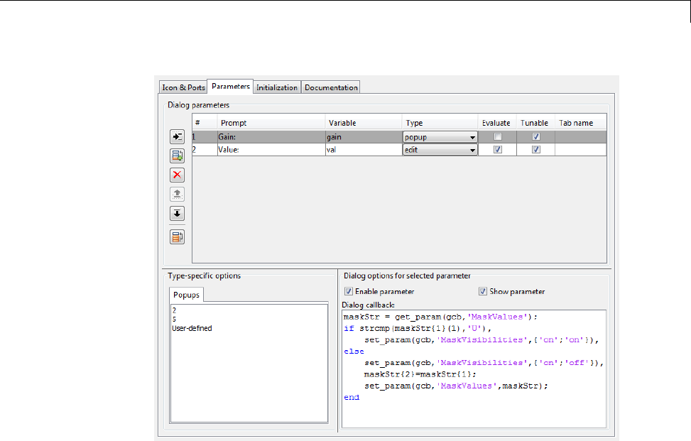
Create Dynamic Mask Dialog Boxes
Double-clicking on the new masked subsystem opens the Mask Parameters
dialog box. Selecting 2or 5for the Gain parameter hides the Value
parameter, while selecting User-defined makes the Value parameter
visible. Note that any blocks in the masked subsystem that need the gain
value should reference the mask variable val as the set_param in the else
code assures that val contains the current value of the gain when 2or 5is
selected in the popup.
Setting Nested Masked Block Parameters
Avoid using set_param commands to set parameters of blocks residing in
masked subsystems that reside in the masked subsystem being initialized.
Trying to set parameters of blocks in lower-level masked subsystems can
trigger unresolvable symbol errors if lower-level masked subsystems reference
symbols defined by higher-level masked subsystems. Suppose, for example,
a masked subsystem A contains masked subsystem B, which contains Gain
26-59

26 Working with Block Masks
block C, whose Gain parameter references a variable defined by B. Suppose
also that subsystem A’s initialization code contains the command
set_param([gcb '/B/C'], 'SampleTime', '-1');
Simulating or updating a model containing A causes an unresolvable symbol
error.
26-60

Create Dynamic Masked Subsystems
Create Dynamic Masked Subsystems
In this section...
“Allow library block to modify its contents” on page 26-61
“Create Self-Modifying Masks for Library Blocks” on page 26-61
“Evaluate Blocks Under Self-Modifying Mask” on page 26-65
Allow library block to modify its contents
This check box is enabled only if the masked subsystem resides in a library.
Checking this option allows the block initialization code to modify the
contents of the masked subsystem (that is, it lets the code add or delete blocks
and set the parameters of those blocks). Otherwise, an error is generated
when a masked library block tries to modify its contents in any way. To set
this option at the MATLAB prompt, select the self-modifying block and enter
the following command.
set_param(gcb, 'MaskSelfModifiable', 'on');
Then save the block.
Create Self-Modifying Masks for Library Blocks
You can create masked library blocks that can modify their structural
contents. These self-modifying masks allow you to:
•Modify the contents of a masked subsystem based on parameters in the
Mask Parameters dialog box or when the subsystem is initially dragged
from the library into a new model.
•Vary the number of ports on a multiport S-Function block that resides
in a library.
Creating Self-Modifying Masks Using the Mask Editor
To create a self-modifying mask using the Mask Editor:
1Unlock the library (see “Modify and Lock Libraries” on page 28-21).
26-61

26 Working with Block Masks
2Right-click the block in the library.
3Select Mask > Edit Mask. The Mask Editor opens.
4In the Mask Editor’s Initialization pane, select the Allow library block
to modify its contents option.
5Enter the code that modifies the masked subsystem in the mask’s
Initialization pane.
Note Do not enter code that structurally modifies the masked subsystem
in a dialog parameter callback (see “Mask Code Placement” on page 26-7).
Doing so triggers an error when a user edits the parameter.
6Click Apply to apply the change or OK to apply the change and dismiss
the Mask Editor.
7Lock the library.
Creating Self-Modifying Masks from the Command Line
To create a self-modifying mask from the command line:
1Unlock the library using the following command:
set_param(gcs,'Lock','off')
2Specify that the block is self-modifyingbyusingthefollowingcommand:
set_param(block_name,'MaskSelfModifiable','on')
where block_name isthefullpathtotheblockinthelibrary.
Self-Modifying Mask Example
The library selfModifying_example contains a masked subsystem that
modifies its number of input ports based on a selection made in the
subsystem’s Mask Parameters dialog box.
26-62
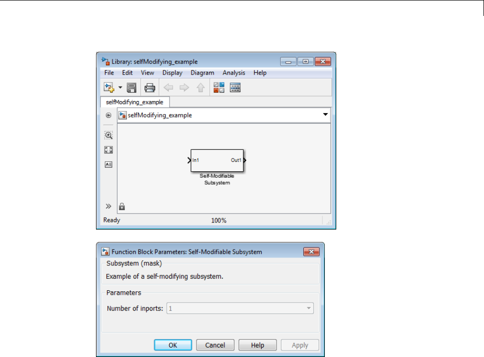
Create Dynamic Masked Subsystems
Right-click the subsystem then select Mask > Edit Mask.TheMaskEditor
opens. The Mask Editor Parameters pane defines one mask parameter
variable numIn that stores the value for the Number of inports option. This
Mask Parameters dialog box callback adds or removes Input ports inside the
masked subsystem based on the selection made in the Number of inports
list.
26-63
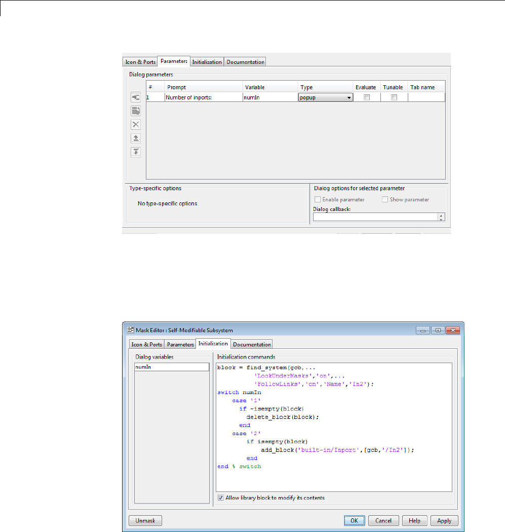
26 Working with Block Masks
To allow the dialog box callback to function properly, the Allow library
block to modify its contents option on the Mask Editor Initialization
pane is selected. If this option were not selected, copies of the library block
could not modify their structural contents and changing the selection in the
Number of inports list would produce an error.
26-64

Create Dynamic Masked Subsystems
Evaluate Blocks Under Self-Modifying Mask
This example shows how to force Simulink to evaluate blocks inside
self-modifying masks.
Simulink evaluates elements of models containing masks in the following
order:
1Mask Parameters dialog box
2Mask initialization code
3Blocks or masked subsystems under the mask
Consider the following case:
AblocknamedmyBlock inside subsystem mySubsys masked by a
self-modifying mask depends on mask parameter myParam to update itself.
myParam is exposed to the user through the Mask Parameters dialog
box. mySubsys is updated through MATLAB code written in the Mask
Initialization pane.
In this model, the sequenceofupdatesisasfollows:
1AusermakesmodifiesmyParam through the Mask Parameters dialog box.
2The mask initialization code receives this change and modifies mySubsys
under the mask.
3myBlock, which lies under mySubsys, modifies itself based on the change
to myParam.
In this sequence, myBlock, which lies under mySubsys, will not be evaluated
when the mask initialization code executes. Instead, only the masked
subsystem mySubsys is evaluated at that time and gets updated. Meanwhile,
myBlock, which needs to change, remains unmodified.
You can force Simulink to evaluate such blocks earlier by using the
Simulink.Mask.eval method in the masked subsystem’s initialization code:
26-65

26 Working with Block Masks
Simulink.Block.eval(mySubsys/myBlock);
26-66

How Do I Debug Masks That Use MATLAB®Code?
How Do I Debug Masks That Use MATLAB Code?
In this section...
“Code Written in Mask Editor” on page 26-67
“Code Written Using MATLAB Editor/Debugger” on page 26-67
Code Written in Mask Editor
Debug initialization commands and parameter callbacks entered directly into
the Mask Editor in one of the following ways:
•Remove the terminating semicolon from a command to echo its results to
the MATLAB Command Window.
•Place a keyboard commandinthecodetostopexecutionandgivecontrol
to the keyboard.
Code Written Using MATLAB Editor/Debugger
Note You cannot debug icon drawing commands using the MATLAB
Editor/Debugger. Use the syntax examples provided in the Mask Editor’s
Icons & Ports pane to help solve errors in the icon drawing commands.
Debug initialization commands and parameter callbacks written in files using
the MATLAB Editor/Debugger in the same way that you would with any
other MATLAB program file.
When debugging initialization commands, you can view the contents of the
mask workspace. However, when debugging parameter callbacks, you can
only access the base workspace of the block. If you need the value of a mask
parameter, use get_param.
26-67

26 Working with Block Masks
26-68


27 Creating Custom Blocks
When to Create Custom Blocks
Custom blocks expand the modeling functionality provided with the Simulink
product. Use a custom block to:
•Model behaviors that are not provided with a Simulink built-in solution.
•Buildmoreadvancedmodels.
•Encapsulate model components into a library block that you can copy into
multiple models.
•Provide custom graphical user interfaces or analysis routines.
27-2

Types of Custom Blocks
Types of Custom Blocks
In this section...
“MATLAB Function Blocks” on page 27-3
“Subsystem Blocks” on page 27-4
“S-Function Blocks” on page 27-4
MATLAB Function Blocks
A MATLAB Function block allows you to use the MATLAB language to define
custom functionality. These blocks are a good starting point for creating a
custom block if:
•You have an existing MATLAB function that models the custom
functionality.
•You find it easier to model custom functionality using a MATLAB function
than using a Simulink block diagram.
•The custom functionality does not include continuous or discrete dynamic
states.
You can create a custom block from a MATLAB function using one of the
following types of MATLAB function blocks.
•The Fcn block allows you to use a MATLAB expression to define a
single-input, single-output (SISO) block.
•The Interpreted MATLAB Function block allows you to use a MATLAB
function to define a SISO block.
•The MATLAB Function block allows you to define a custom block with
multiple inputs and outputs that you can deploy to an embedded processor.
Each of these blocks has advantages in particular modeling applications. For
example, you can generate code from models containing MATLAB Function
blocks while you cannot generate code for models containing an Fcn block.
27-3

27 Creating Custom Blocks
Subsystem Blocks
Subsystem blocks allow you to build a Simulink diagram to define custom
functionality. These blocks serve as a good starting point for creating a
custom block if:
•You have an existing Simulink diagram that models custom functionality.
•You find it easier to model custom functionality using a graphical
representation rather than using hand-written code.
•The custom functionality is a function of continuous or discrete system
states.
•You can model the custom functionality using existing Simulink blocks.
Once you have a Simulink subsystem that models the required behavior, you
can convertitintoacustomblockby:
1Masking the block to hide the block contents and provide a custom block
dialog.
2Placing the block in a library to prohibit modifications and allow for easily
updating copies of the block.
For more information, see “Libraries” and “Masking”.
S-Function Blocks
S-function blocks allow you to write MATLAB, C, or C++ code to define
custom functionality. These blocks serve as a good starting point for creating
a custom block if:
•You have existing MATLAB, C, or C++ code that models custom
functionality.
•You need to model continuous or discrete dynamic states or other system
behaviors that require access to the S-function API.
•You cannot model the custom functionality using existing Simulink blocks.
You can create a custom block from an S-function using one of the following
types of S-function blocks.
27-4

Types of Custom Blocks
•The Level-2 MATLAB S-Function block allows you to write your S-function
using the MATLAB language. (See“Write Level-2 MATLAB S-Functions”).
You can debug a MATLAB S-function during a simulation using the
MATLAB debugger.
•The S-Function block allows you to write your S-function in C or C++, or to
incorporate existing code into your model using a C MEX wrapper. (See
“C/C++ S-Functions”.)
•The S-Function Builder block assists you in creating a new C MEX
S-function or a wrapper function to incorporate legacy C or C++ code. (See
“C/C++ S-Functions”.)
•The Legacy Code Tool transforms existing C or C++ functions into C MEX
S-functions. (See “Integrate C Functions Using Legacy Code Tool”.)
The S-function target in the Simulink Coder product automatically generates
a C MEX S-function from a graphical subsystem. If you want to build your
custom block in a Simulink subsystem, but implement the final version of
the block in an S-function, you can use the S-function target to convert
the subsystem to an S-function. See “Generated S-Function Block” in
the Simulink Coder User’s Guide for details and limitations on using the
S-function target.
ComparingMATLABS-Functionsto MATLAB Functions for Code
Generation
MATLAB S-functions and MATLAB functions for code generation have some
fundamental differences.
•The Simulink Coder product can generate code for both MATLAB
S-functions and MATLAB functions for code generation. However,
MATLAB S-functions require a Target Language Compiler (TLC) file for
code generation. MATLAB functions for code generation do not require
aTLC-file.
•MATLAB S-functions can use any MATLAB function while MATLAB
functions for code generation are a subset of the MATLAB language. For a
list of supported functions for code generation, see “Functions Supported
for Code Generation — Alphabetical List” on page 31-2.
•MATLAB S-functions can model discrete and continuous state dynamics
while MATLAB functions for code generation cannot model state dynamics.
27-5

27 Creating Custom Blocks
Using S-Function Blocks to Incorporate Legacy Code
Each S-function block allows you to incorporate legacy code into your model,
as follows.
•A MATLAB S-function accesses legacy code through its TLC-file. Therefore,
the legacy code is available only in the generated code, not during
simulation.
•A C MEX S-functions directly calls legacy C or C++ code.
•The S-Function Builder generates a wrapper function that calls the legacy
CorC++code.
•The Legacy Code Tool generates a C MEX S-function to call the legacy C
or C++ code, which is optimized for embedded systems. See “Integrate C
Functions Using Legacy Code Tool” for more information.
See “Integration Options” in the Simulink Coder User’s Guide for more
information.
See “S-Functions Incorporate Legacy C Code” in the Simulink Developing
S-Functions for an example.
27-6

Comparison of Custom Block Functionality
Comparison of Custom Block Functionality
In this section...
“Custom Block Considerations” on page 27-7
“Modeling Requirements” on page 27-10
“Speed and Code Generation Requirements” on page 27-13
Custom Block Considerations
When creating a custom block, you may want to consider the following.
•Does the custom block need multiple input and output ports?
•Does the block need to model continuous or discrete state behavior?
•Will the block inputs and outputs have various data attributes, such as
data types or complexity?
•How important is the affect of the custom block on the speed of updating
the Simulink diagram or simulating the Simulink model?
•Do you need to generate code for a model containing the custom block?
The following two tables provide an overview of how each custom block
type addresses the previous questions. More detailed information for each
consideration follows these two tables.
Modeling Requirements
Custom Block
Type
Supports Multiple
Inputs and Outputs
Models State
Dynamics
Supports Various Data
Attributes
Subsystem Yes, including bus
signals.
Yes. Yes, including all data types,
numeric types, and dimensions
supported by the Simulink
software. Also supports
frame-based signals.
Fcn No. Must have a single
vector input and scalar
output.
No. Supports only real scalar
signals with a data type of
double or single.
27-7

27 Creating Custom Blocks
Modeling Requirements (Continued)
Custom Block
Type
Supports Multiple
Inputs and Outputs
Models State
Dynamics
Supports Various Data
Attributes
Interpreted
MATLAB Function
No. Must have a
single vector input and
output.
No. Supports only n-D, real, or
complex signals with a data
type of double.
MATLAB Function Yes, including bus
signals.
No. Yes, including all data types,
numeric types, and dimensions
supported by the Simulink
software. Also supports
frame-based signals.
Level-2 MATLAB
S-function
Yes. Yes, including
limited access
to other
S-function
APIs.
Yes, including all data types,
numeric types, and dimensions
supported by the Simulink
software. Also supports
frame-based signals.
CMEXS-function Yes, including bus
signals if using the
Legacy Code Tool to
generate the S-function.
Yes, including
full access to
all S-function
APIs.
Yes, including all data types,
numeric types, and dimensions
supported by the Simulink
software. Also supports
frame-based signals.
Speed and Code Generation Requirements
Custom Block
Type
Speed of Updating
the Diagram
Simulation Overhead Code Generation
Support
Subsystem Proportional to the
complexity of the
subsystem. For
library blocks, can
be slower the first
Proportional to the
complexity of the
subsystem. Library
Natively supported.
27-8

Comparison of Custom Block Functionality
Speed and Code Generation Requirements (Continued)
Custom Block
Type
Speed of Updating
the Diagram
Simulation Overhead Code Generation
Support
time the library is
loaded.
blocks introduce no
additional overhead.
Fcn Very fast. Minimal, but these
blocks also provide
limited functionality.
Natively supported.
Interpreted
MATLAB Function
Fast. High and incurred
when calling out to the
MATLAB interpreter.
These calls add overhead
that should be avoided
if simulation speed is a
concern.
Not supported.
MATLAB Function Can be slower if code
must be generated to
update the diagram.
Minimal if the MATLAB
interpreter is not called.
Simulation speed is
equivalent to C MEX
S-functions when the
MATLAB interpreter is
not called.
Natively supported,
with exceptions. See
“Code Generation” on
page 27-16 for more
information.
Level-2 MATLAB
S-function
Can be slower if the
S-function overrides
methods executed
when updating the
diagram.
Higher than for
Interpreted MATLAB
Function blocks
because the MATLAB
interpreter is called for
every S-function method
used. Very flexible, but
very costly.
MATLAB S-functions
initialized as a
SimViewingDevice
do not generate code.
Otherwise, MATLAB
S-functions require
aTLC-fileforcode
generation.
C MEX S-function Can be slower if the
S-function overrides
methods executed
Minimal, but
proportional to the
complexity of the
Might require a
TLC-file.
27-9

27 Creating Custom Blocks
Speed and Code Generation Requirements (Continued)
Custom Block
Type
Speed of Updating
the Diagram
Simulation Overhead Code Generation
Support
when updating the
diagram.
algorithm and the
efficiency of the code.
Modeling Requirements
Multiple Input and Output Ports
The following types of custom blocks support multiple input and output ports.
Custom
Block Type
Multiple Input and Output Port Support
Subsystem Supports multiple input and output ports, including bus
signals. In addition, you can modify the number of input
and output ports based on user-defined parameters. See
“Self-Modifying Linked Subsystems” on page 28-7 for more
information.
Fcn,
Interpreted
MATLAB
Function
Supports only a single input and a single output port. You
must use a Mux block to combine the inputs and a Demux
block to separate the outputs if you need to pass multiple
signals into or out of these blocks.
MATLAB
Function
Supports multiple input and output ports, including bus
signals. See “How Structure Inputs and Outputs Interface
with Bus Signals” on page 29-81 for more information.
S-function
(MATLAB or
CMEX)
Supports multiple input and output ports. In addition, you
can modify the number of input and output ports based on
user-defined parameters. S-functions generated using the
Legacy Code Tool also accept Simulink bus signals. See
“Integrate C Functions Using Legacy Code Tool” for more
information.
27-10

Comparison of Custom Block Functionality
State Behavior and the S-Function API
Simulink blocks communicate with the Simulink engine through the
S-function API, a set of methods that fully specifies the behavior of blocks.
Each custom block type accesses a different sets of the S-function APIs, as
follows.
Custom
Block Type
S-Function API Support
Subsystem Communicates directly with the engine. You can model
state behaviors using appropriate blocks from the
Continuous and Discrete Simulink block libraries.
Fcn,
Interpreted
MATLAB
Function,
MATLAB
Function
All create an mdlOutputs method to calculate the value
of the outputs given the value of the inputs. You cannot
access any other S-function API methods using one of these
blocks and, therefore, cannot model state behavior.
MATLAB
S-function
Accesses a larger subset of the S-function APIs, including
the methods needed to model continuous and discrete
states. For a list of supported methods, see “Level-2
MATLAB S-Function Callback Methods” in “Writing
S-Functions”.
CMEX
S-function
Accesses the complete set of S-function APIs.
Data Attribute Support
All custom block types support real scalar inputs and outputs with a data
type of double.
27-11

27 Creating Custom Blocks
Custom
Block Type
Data Attribute Support
Subsystem Supports any data type supported by the Simulink
software, including fixed-point types. Also supports
complex, 2-D, n-D, and frame-based signals.
Fcn Supports only double or single data types. In addition, the
input and output cannot be complex and the output must
be a scalar signal. Does not support frame-based signals.
Interpreted
MATLAB
Function
Supports 2-D, n-D, and complex signals, but the signal
must have a data type of double. Does not support
frame-based signals.
MATLAB
Function
Supports any data type supported by the Simulink
software, including fixed-point types. Also supports
complex, 2-D, n-D, and frame-based signals.
S-function
(MATLAB or
CMEX)
Supports any data type supported by the Simulink
software, including fixed-point types. Also supports
complex, 2-D, n-D, and frame-based signals.
27-12

Comparison of Custom Block Functionality
Speed and Code Generation Requirements
Updating the Simulink Diagram
The Simulink software updates the diagram before every simulation and
whenever requested by the user. Every block introduces some overhead into
the “update diagram” process.
Custom
Block Type
Speed of Updating the Diagram
Subsystem The speed is proportional to the complexity of the
algorithm implemented in the subsystem. If the subsystem
is contained in a library, some cost is incurred when the
Simulink software loads any unloaded libraries the first
time the diagram is updated orreadiedforsimulation.
If all referenced library blocks remain unchanged, the
Simulink software does not subsequently reload the library
and compiling the model becomes faster than if the model
did not use libraries.
Fcn,
Interpreted
MATLAB
Function
Does not incur greater update cost than other Simulink
blocks.
MATLAB
Function
Performs simulation through code generation, so these
blocks might take a significant amount of time when first
updated. However, because code generation is incremental,
if the block and the signals connected to it have not
changed, Simulink does not repeatedly update the block.
S-function
(MATLAB or
CMEX)
Incurs greater costs than other Simulink blocks only if it
overrides methods executed when updating the diagram.
If these methods become complex, they can contribute
significantly to the time it takestoupdatethediagram.
For a list of methods executed when updating the diagram,
see the process view in “Simulink Engine Interaction with
C S-Functions”. When updating the diagram, the Simulink
software invokes all relevant methods in the model
initialization phase up to, but not including, mdlStart.
27-13

27 Creating Custom Blocks
Simulation Overhead
For most applications, any of the custom block types provide acceptable
simulation performance. Use the Simulink profiler to obtain an indication
of the actual performance. See “Capture Performance Data” on page 22-31
for more information.
You can break simulation performance into two categories. The interface
costisthetimeittakestomovedatafromtheSimulinkengineintothe
block. Thealgorithmcostisthetimeneeded to perform the algorithm that
the block implements.
Custom
Block Type
Simulation Overhead
Subsystem If included in a library, introduces no interface or algorithm
costs beyond what would normally be incurred if the block
existed as a regular subsystem in the model.
Fcn Has the least simulation overhead. The block is tightly
integrated with the Simulink engine and implements
a rudimentary expression language that is efficiently
interpreted.
Interpreted
MATLAB
Function
Has a higher interface cost than most blocks and the same
algorithm cost as a MATLAB function.
When block data (such as inputs and outputs) is accessed
or returned from an Interpreted MATLAB Function block,
theSimulinkenginepackagesthisdataintoMATLAB
arrays. This packaging takes additional time and causes a
temporary increase in memory during communication. If
you pass large amounts of data across this interface, such
as, frames or arrays, this overhead can be substantial.
Once the data has been converted, the MATLAB
interpreter executes the algorithm. As a result, the
algorithm cost is the same as for MATLAB function.
Efficient code can be competitive with C code if MATLAB is
able to optimize it, or if the code uses the highly optimized
MATLAB library functions.
27-14

Comparison of Custom Block Functionality
Custom
Block Type
Simulation Overhead
MATLAB
Function
Performs simulation through code generation and so incurs
the same interface cost as standard blocks.
The algorithm cost of this block is harder to analyze
because of the block’s implementation. On average, a
function for this block and a MATLAB function run at
about the same speed. To further reduce the algorithm
cost, you can disable debugging for all the MATLAB
Function blocks in your model.
If the MATLAB Function block uses simulation-only
capabilities to call out to the MATLAB interpreter,
it incurs all the costs that a MATLAB S-function or
Interpreted MATLAB Function block incur. Calling out
to the MATLAB interpreter from a MATLAB Function
block produces a warning to prevent you from doing so
unintentionally.
MATLAB
S-function
Incurs the same algorithm costs as the Interpreted
MATLAB Function block, but with a slightly higher
interface cost. Because MATLAB S-functions can handle
multiple inputs and outputs, the packaging is more
complicated than for the Interpreted MATLAB Function
block. In addition, the Simulink engine calls the MATLAB
interpreter for each block method you implement whereas
for the Interpreted MATLAB Function block, it calls the
MATLAB interpreter only for the mdlOutputs method.
CMEX
S-function
Simulates via the compiled code and so incurs the same
interface cost as standard blocks. The algorithm cost
depends on the complexity of the S-function.
27-15

27 Creating Custom Blocks
Code Generation
Not all custom block types support code generation with Simulink Coder.
Custom
Block Type
Code Generation Support
Subsystem Supports code generation.
Fcn Supports code generation.
Interpreted
MATLAB
Function
Does not support code generation.
MATLAB
Function
Supports code generation. However, if your MATLAB
Function block calls out to the MATLAB interpreter, it
will build with the Simulink Coder product only if the
calls to the MATLAB interpreter do not affect the block
outputs. Under this condition, the Simulink Coder product
omits these calls from the generated C code. This feature
allows you to leave visualization code in place, even when
generating embedded code.
MATLAB
S-function
Generates code only if you implement the algorithm using a
Target Language Compiler (TLC) function. In accelerated
and external mode simulations, you can choose to execute
the S-function in interpretive mode by calling back to the
MATLAB interpreter without implementing the algorithm
in TLC. If the MATLAB S-function is a SimViewingDevice,
the Simulink Coder product automatically omits the block
during code generation.
CMEX
S-function
Supports code generation. For noninlined S-functions, the
Simulink Coder product uses the C MEX function during
code generation. However, you must write a TLC-file for
the S-function if you need to either inline the S-function
or create a wrapper for hand-written code. See “Insert
S-Function Code” in the Simulink Coder User’s Guide for
more information.
27-16

Expanding Custom Block Functionality
Expanding Custom Block Functionality
You can expand the functionality of any custom block using callbacks and
Handle Graphics.
Block callbacks perform user-defined actions at specific points in the
simulation. For example, the callback can load data into the MATLAB
workspace before the simulation or generate a graph of simulation data at the
end of the simulation. You can assign block callbacks to any of the custom
block types. For a list of available callbacks and more information on how to
use them, see “Create Block Callback Functions” on page 4-58.
GUIDE, the MATLAB graphical user interface development environment,
provides tools for easily creating custom user interfaces. See “GUI Building”
for more information on using GUIDE.
27-17

27 Creating Custom Blocks
Create a Custom Block
In this section...
“How to Design a Custom Block” on page 27-18
“Defining Custom Block Behavior” on page 27-20
“Deciding on a Custom Block Type” on page 27-21
“Placing Custom Blocks in a Library” on page 27-27
“Adding a Graphical User Interface to a Custom Block” on page 27-28
“Adding Block Functionality Using Block Callbacks” on page 27-37
How to Design a Custom Block
In general, use the following process to design a custom block:
1“Defining Custom Block Behavior” on page 27-20
2“Deciding on a Custom Block Type” on page 27-21
3“Placing Custom Blocks in a Library” on page 27-27
4“Adding a Graphical User Interface to a Custom Block” on page 27-28
Suppose you want to create a customized saturation block that limits the
upper and lower bounds of a signal based on either a block parameter or the
value of an input signal. In a second version of the block, you want the option
to plot the saturation limits after the simulation is finished. The following
tutorial steps you through designing these blocks. The library customsat_lib
contains the two versions of the customized saturation block.
27-18
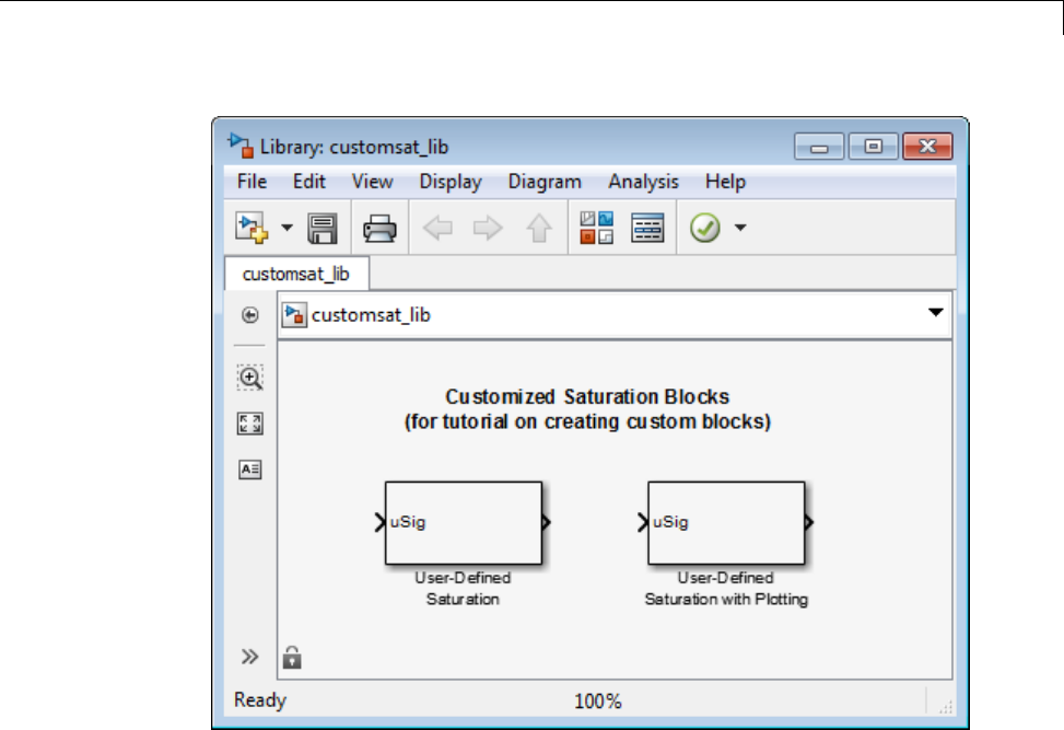
Create a Custom Block
The example model sldemo_customsat uses the basic version of the block.
27-19
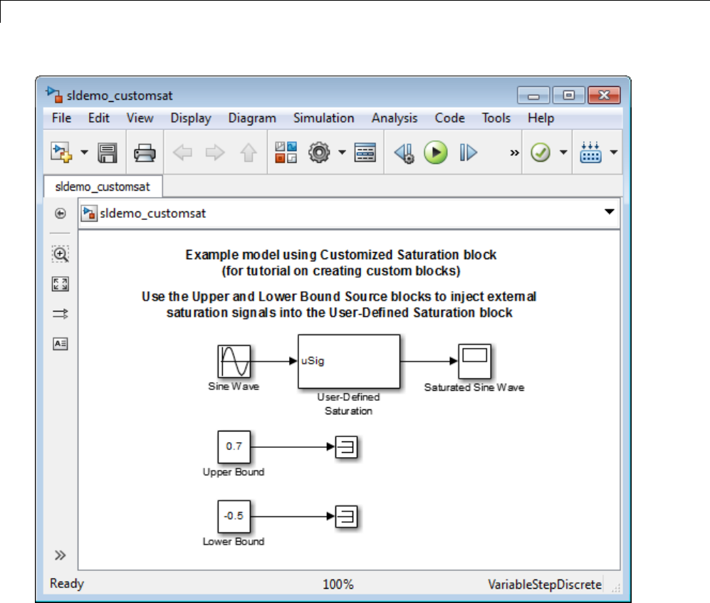
27 Creating Custom Blocks
Defining Custom Block Behavior
Begin by defining the features and limitations of your custom block. In this
example, the block supports the following features:
•Turning on and off the upper or lower saturation limit.
•Setting the upper and/or lower limits via a block parameters.
27-20

Create a Custom Block
•Setting the upper and/or lower limits using an input signal.
It also has the following restrictions:
•The input signal under saturation must be a scalar.
•The input signal and saturation limits must all have a data type of double.
•Code generation is not required.
Deciding on a Custom Block Type
Based on the custom block features, the implementation needs to support
the following:
•Multiple input ports
•A relatively simple algorithm
•No continuous or discrete system states
Therefore, this tutorial implements the custom block using a Level-2 MATLAB
S-function. MATLAB S-functions support multiple inputs and, because
the algorithm is simple, do not have significant overhead when updating
the diagram or simulating the model. See “Comparison of Custom Block
Functionality” on page 27-7 for a description of the different functionality
provided by MATLAB S-functions as compared to other types of custom blocks.
Parameterizing the MATLAB S-Function
Begin by defining the S-function parameters. This example requires four
parameters:
•The first parameter indicates how the upper saturation limit is set. The
limitcanbeoff,setviaablockparameter,orsetviaaninputsignal.
•The second parameter is the value of the upper saturation limit. This value
is used only if the upper saturation limit is set via a block parameter. In the
event this parameter is used, you should be able to change the parameter
value during the simulation, i.e., the parameter is tunable.
•The third parameter indicates how the lower saturation limit is set. The
limitcanbeoff,setviaablockparameter,orsetviaaninputsignal.
27-21

27 Creating Custom Blocks
•The fourth parameter is the value of the lower saturation limit. This value
is used only if the lower saturation limit is set via a block parameter. As
with the upper saturation limit, this parameter is tunable when in use.
The first and third S-function parameters represent modes that must be
translated into values the S-function can recognize. Therefore, define the
following values for the upper and lower saturation limit modes:
•1indicates that the saturation limit is off.
•2indicates that the saturation limit is set via a block parameter.
•3indicates that the saturation limit is set via an input signal.
Writing the MATLAB S-Function
After you define the S-function parameters and functionality, write the
S-function. The template msfuntmpl.m provides a starting point for writing a
Level-2 MATLAB S-function. You can find a completed version of the custom
saturation block in the file custom_sat.m. Savethisfiletoyourworking
folder before continuing with this tutorial.
This S-function modifies the S-function template as follows:
•The setup function initializes the number of input ports based on the
values entered for the upper and lower saturation limit modes. If the limits
are set via input signals, the method adds input ports to the block. The
setup method then indicates there are four S-function parameters and sets
the parameter tunability. Finally, the method registers the S-function
methods used during simulation.
function setup(block)
% The Simulink engine passes an instance of the Simulink.MSFcnRunTimeBlock
% class to the setup method in the input argument "block". This is known as
% the S-function block's run-time object.
% Register original number of input ports based on the S-function
% parameter values
try % Wrap in a try/catch, in case no S-function parameters are entered
27-22

Create a Custom Block
lowMode = block.DialogPrm(1).Data;
upMode = block.DialogPrm(3).Data;
numInPorts = 1 + isequal(lowMode,3) + isequal(upMode,3);
catch
numInPorts=1;
end % try/catch
block.NumInputPorts = numInPorts;
block.NumOutputPorts = 1;
% Setup port properties to be inherited or dynamic
block.SetPreCompInpPortInfoToDynamic;
block.SetPreCompOutPortInfoToDynamic;
% Override input port properties
block.InputPort(1).DatatypeID = 0; % double
block.InputPort(1).Complexity = 'Real';
% Override output port properties
block.OutputPort(1).DatatypeID = 0; % double
block.OutputPort(1).Complexity = 'Real';
% Register parameters. In order:
% -- If the upper bound is off (1) or on and set via a block parameter (2)
% or input signal (3)
% -- The upper limit value. Should be empty if the upper limit is off or
% set via an input signal
% -- If the lower bound is off (1) or on and set via a block parameter (2)
% or input signal (3)
% -- The lower limit value. Should be empty if the lower limit is off or
% set via an input signal
block.NumDialogPrms = 4;
block.DialogPrmsTunable = {'Nontunable','Tunable','Nontunable', ...
'Tunable'};
% Register continuous sample times [0 offset]
block.SampleTimes = [0 0];
%% -----------------------------------------------------------------
%% Options
%% -----------------------------------------------------------------
27-23

27 Creating Custom Blocks
% Specify if Accelerator should use TLC or call back into
% MATLAB script
block.SetAccelRunOnTLC(false);
%% -----------------------------------------------------------------
%% Register methods called during update diagram/compilation
%% -----------------------------------------------------------------
block.RegBlockMethod('CheckParameters', @CheckPrms);
block.RegBlockMethod('ProcessParameters', @ProcessPrms);
block.RegBlockMethod('PostPropagationSetup', @DoPostPropSetup);
block.RegBlockMethod('Outputs', @Outputs);
block.RegBlockMethod('Terminate', @Terminate);
%end setup function
•The CheckParameters method verifies the values entered into the Level-2
MATLAB S-Function block.
function CheckPrms(block)
lowMode = block.DialogPrm(1).Data;
lowVal = block.DialogPrm(2).Data;
upMode = block.DialogPrm(3).Data;
upVal = block.DialogPrm(4).Data;
% The first and third dialog parameters must have values of 1-3
if ~any(upMode == [1 2 3]);
error('The first dialog parameter must be a value of 1, 2, or 3');
end
if ~any(lowMode == [1 2 3]);
error('The first dialog parameter must be a value of 1, 2, or 3');
end
% If the upper or lower bound is specified via a dialog, make sure there
% is a specified bound. Also, check that the value is of type double
if isequal(upMode,2),
if isempty(upVal),
error('Enter a value for the upper saturation limit.');
end
27-24

Create a Custom Block
if ~strcmp(class(upVal), 'double')
error('The upper saturation limit must be of type double.');
end
end
if isequal(lowMode,2),
if isempty(lowVal),
error('Enter a value for the lower saturation limit.');
end
if ~strcmp(class(lowVal), 'double')
error('The lower saturation limit must be of type double.');
end
end
% If a lower and upper limit are specified, make sure the specified
% limits are compatible.
if isequal(upMode,2) && isequal(lowMode,2),
if lowVal >= upVal,
error('The lower bound must be less than the upper bound.');
end
end
%end CheckPrms function
•The ProcessParameters and PostPropagationSetup methods handle
the S-function parameter tuning.
function ProcessPrms(block)
%% Update run time parameters
block.AutoUpdateRuntimePrms;
%end ProcessPrms function
function DoPostPropSetup(block)
%% Register all tunable parameters as runtime parameters.
block.AutoRegRuntimePrms;
27-25

27 Creating Custom Blocks
%end DoPostPropSetup function
•The Outputs method calculates the block’s output based on the S-function
parameter settings and any input signals.
function Outputs(block)
lowMode = block.DialogPrm(1).Data;
upMode = block.DialogPrm(3).Data;
sigVal = block.InputPort(1).Data;
lowPortNum = 2; % Initialize potential input number for lower saturation limit
% Check upper saturation limit
if isequal(upMode,2), % Set via a block parameter
upVal = block.RuntimePrm(2).Data;
elseif isequal(upMode,3), % Set via an input port
upVal = block.InputPort(2).Data;
lowPortNum = 3; % Move lower boundary down one port number
else
upVal = inf;
end
% Check lower saturation limit
if isequal(lowMode,2), % Set via a block parameter
lowVal = block.RuntimePrm(1).Data;
elseif isequal(lowMode,3), % Set via an input port
lowVal = block.InputPort(lowPortNum).Data;
else
lowVal = -inf;
end
% Assign new value to signal
if sigVal > upVal,
sigVal = upVal;
elseif sigVal < lowVal,
sigVal=lowVal;
end
block.OutputPort(1).Data = sigVal;
27-26
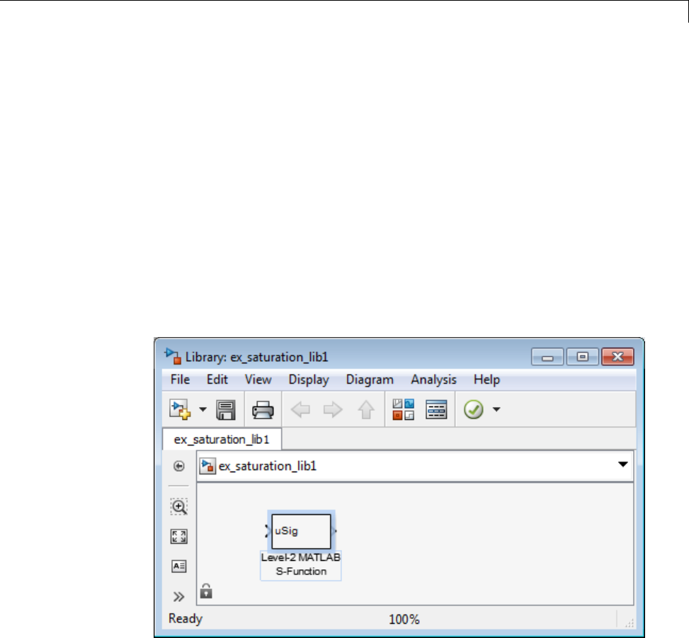
Create a Custom Block
%end Outputs function
Placing Custom Blocks in a Library
Libraries allow you to share your custom blocks with other users, easily
update the functionality of copies of the custom block, and collect blocks for
a particular project into a single location. This example places the custom
saturation block into a library as follows:
1In the Simulink Library Browser window, select File >New >Library.A
new library window opens.
2From the User-Defined Functions library, drag a new Level-2 MATLAB
S-Function block into your new library. Save your library with the filename
saturation_lib.
3Double-click the block to open its Function Block Parameters dialog box.
4In the S-function name box, enter the name of the S-function. For
example, enter custom_sat.IntheParameters box enter the following
default values 2,-1,2,1.
27-27
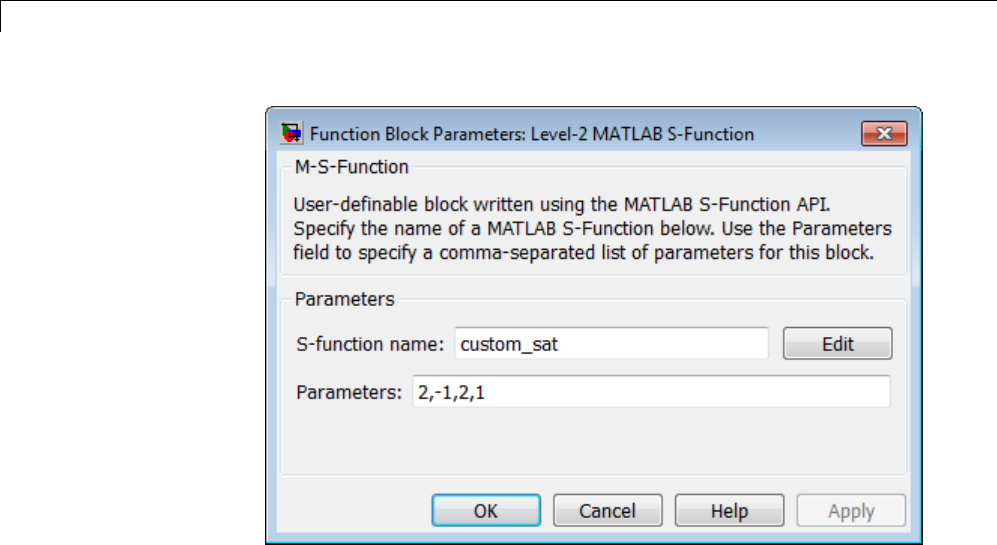
27 Creating Custom Blocks
5Click OK. The parameters changes you entered are saved and the dialog
box closes.
At this point, you have created a custom saturation block that you can share
with other users. You can make the block easier to use by adding a customized
graphical user interface.
Adding a Graphical User Interface to a Custom Block
You can create a simple block dialog for the custom saturation block using
the provided masking capabilities. Masking the block also allows you to
add port labels to indicate which ports corresponds to the input signal and
the saturation limits.
To mask the block:
1Open the custom library you created, saturation_lib.Right-click
the custom saturation block, and from the context menu, select
Diagram > Mask→Create Mask . The Mask Editor opens.
27-28
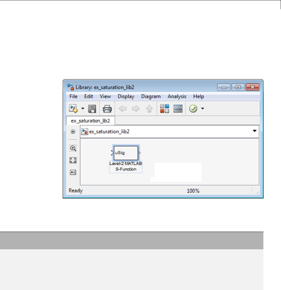
Create a Custom Block
2On the Icon & Ports pane and in the Icons Drawing commands box,
enter the following.
port_label('input',1,'uSig')
This command labels the default port as the input signal under saturation.
3On the Parameters pane, add four parameters corresponding to the four
S-function parameters. For each new parameter, click the Add parameter
button, and set up each of the parameter properties as follows.
Prompt Variable Type Tunable Popups Action for Dialog
Callback
Upper
boundary:
upMode popup No No limit | Enter limit as
parameter | Limit using
input signal
'upperbound_callback'
Upper
limit:
upVal edit Yes N/A 'upperparam_callback'
27-29

27 Creating Custom Blocks
Prompt Variable Type Tunable Popups Action for Dialog
Callback
Lower
boundary:
lowMode popup No No limit | Enter limit as
parameter | Limit using
input signal
'lowerbound_callback'
Lower
limit:
lowVal edit Yes N/A 'lowerparam_callback'
The dialog callback is invoked using the action string in the following
command:
customsat_callback(action,gcb)
The MATLAB script customsat_callback.m contains the mask parameter
callbacks. If you are stepping through this tutorial, open this file and save
it to your working folder. This MATLAB script described in detail later,
has two input arguments. The first input argument is a string indicating
which mask parameter invoked the callback. The second input argument is
thehandletotheassociatedLevel-2MATLABS-Functionblock.
The following figure shows the final Parameters pane in the Mask Editor.
27-30
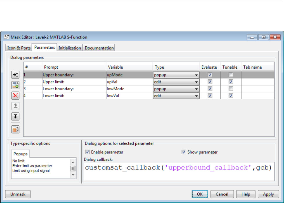
Create a Custom Block
4On the Mask Editor’s Initialization pane, select the check box Allow
library block to modify its contents. This setting allows the S-function
to change the number of ports on the block.
27-31
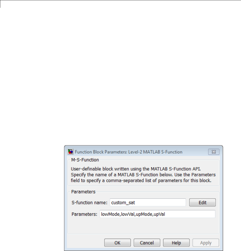
27 Creating Custom Blocks
5On the Documentation pane:
•Enter Customized Saturation into the Mask type field.
•Enter the following into the Mask description field.
Limit the input signal to an upper and lower saturation value
set either through a block parameter or input signal.
6On the Mask Editor dialog box, click OK to complete the mask parameters
dialog.
7To map the S-function parameters to the mask parameters, right-click the
Level-2 MATLAB S-Function block and select Mask > Look Under Mask.
The Function Block Parameters dialog box opens.
8Change the entry in the Parameters field as follows.
lowMode,lowVal,upMode,upVal
The following figure shows the new Block Parameters dialog.
27-32
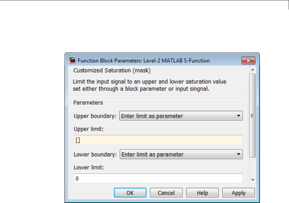
Create a Custom Block
9Click OK . Double-clicking the new version of the customized saturation
block opens the mask parameter dialog box shown in the following figure.
To create a more complicated graphical user interface, place a Handle
Graphics user interface on top of the masked block. The block’s OpenFcn
would invoke the Handle Graphics user interface, which uses calls to
set_param to modify the S-function block’s parameters based on settings
in the user interface.
Writing the Mask Callback
The function customsat_callback.m contains the mask callback code for the
custom saturation block mask parameter dialog box. This function invokes
local functions corresponding to each mask parameter through a call to feval.
The following local function controls the visibility of the upper saturation
limit’s field based on the selection for the upper saturation limit’s mode. The
callback begins by obtaining values for all mask parameters using a call to
27-33

27 Creating Custom Blocks
get_param with the property name MaskValues. If the callback needed the
value of only one mask parameter, it could call get_param with the specific
maskparametername,forexample,get_param(block,'upMode').Because
this example needs two of the mask parameter values, it uses the MaskValues
property to reduce the calls to get_param.
The callback then obtains the visibilities of the mask parameters using a call
to get_param with the property name MaskVisbilities. This call returns
a cell array of strings indicating the visibility of each mask parameter. The
callback alters the values for the mask visibilities based on the selection for
the upper saturation limit’s mode and then updates the port label string.
The callback finally uses the set_param commandtoupdatetheblock’s
MaskDisplay property to label the block’s input ports.
function customsat_callback(action,block)
% CUSTOMSAT_CALLBACK contains callbacks for custom saturation block
% Copyright 2003-2007 The MathWorks, Inc.
%% Use function handle to call appropriate callback
feval(action,block)
%% Upper bound callback
function upperbound_callback(block)
vals = get_param(block,'MaskValues');
vis = get_param(block,'MaskVisibilities');
portStr = {'port_label(''input'',1,''uSig'')'};
switch vals{1}
case 'No limit'
set_param(block,'MaskVisibilities',[vis(1);{'off'};vis(3:4)]);
case 'Enter limit as parameter'
set_param(block,'MaskVisibilities',[vis(1);{'on'};vis(3:4)]);
case 'Limit using input signal'
set_param(block,'MaskVisibilities',[vis(1);{'off'};vis(3:4)]);
portStr = [portStr;{'port_label(''input'',2,''up'')'}];
end
if strcmp(vals{3},'Limit using input signal'),
portStr = [portStr;{['port_label(''input'',',num2str(length(portStr)+1), ...
27-34

Create a Custom Block
',''low'')']}];
end
set_param(block,'MaskDisplay',char(portStr));
The final call to set_param invokes the setup function in the MATLAB
S-function custom_sat.m. Therefore, the setup function can be modified to
set the number of input ports based on the mask parameter values instead of
on the S-function parameter values. This change to the setup function keeps
the number of ports on the Level-2 MATLAB S-Function block consistent with
the values shown in the mask parameter dialog box.
The modified MATLAB S-function custom_sat_final.m contains the
following new setup function. If you are stepping through this tutorial, open
the file and save it to your working folder.
%% Function: setup ===================================================
function setup(block)
% Register original number of ports based on settings in Mask Dialog
ud = getPortVisibility(block);
numInPorts=1+isequal(ud(1),3) + isequal(ud(2),3);
block.NumInputPorts = numInPorts;
block.NumOutputPorts = 1;
% Setup port properties to be inherited or dynamic
block.SetPreCompInpPortInfoToDynamic;
block.SetPreCompOutPortInfoToDynamic;
% Override input port properties
block.InputPort(1).DatatypeID = 0; % double
block.InputPort(1).Complexity = 'Real';
% Override output port properties
block.OutputPort(1).DatatypeID = 0; % double
block.OutputPort(1).Complexity = 'Real';
% Register parameters. In order:
% -- If the upper bound is off (1) or on and set via a block parameter (2)
% or input signal (3)
27-35

27 Creating Custom Blocks
% -- The upper limit value. Should be empty if the upper limit is off or
% set via an input signal
% -- If the lower bound is off (1) or on and set via a block parameter (2)
% or input signal (3)
% -- The lower limit value. Should be empty if the lower limit is off or
% set via an input signal
block.NumDialogPrms = 4;
block.DialogPrmsTunable = {'Nontunable','Tunable','Nontunable','Tunable'};
% Register continuous sample times [0 offset]
block.SampleTimes = [0 0];
%% -----------------------------------------------------------------
%% Options
%% -----------------------------------------------------------------
% Specify if Accelerator should use TLC or call back into
% MATLAB script
block.SetAccelRunOnTLC(false);
%% -----------------------------------------------------------------
%% Register methods called during update diagram/compilation
%% -----------------------------------------------------------------
block.RegBlockMethod('CheckParameters', @CheckPrms);
block.RegBlockMethod('ProcessParameters', @ProcessPrms);
block.RegBlockMethod('PostPropagationSetup', @DoPostPropSetup);
block.RegBlockMethod('Outputs', @Outputs);
block.RegBlockMethod('Terminate', @Terminate);
%endfunction
The getPortVisibility local function in custom_sat_final.m uses the
saturation limit modes to construct a flag that is passed back to the setup
function. The setup function uses this flag to determine the necessary
number of input ports.
%% Function: Get Port Visibilities =======================================
function ud = getPortVisibility(block)
ud=[00];
27-36

Create a Custom Block
vals = get_param(block.BlockHandle,'MaskValues');
switch vals{1}
case 'No limit'
ud(2) = 1;
case 'Enter limit as parameter'
ud(2) = 2;
case 'Limit using input signal'
ud(2) = 3;
end
switch vals{3}
case 'No limit'
ud(1) = 1;
case 'Enter limit as parameter'
ud(1) = 2;
case 'Limit using input signal'
ud(1) = 3;
end
Adding Block Functionality Using Block Callbacks
The User-Defined Saturation with Plotting block in customsat_lib uses block
callbacks to add functionality to the original custom saturation block. This
block provides an option to plot the saturation limits when the simulation
ends. The following steps show how to modify the original custom saturation
block to create this new block.
1Add a check box to the mask parameter dialog box to toggle the plotting
option on and off.
aRight-click the Level-2 MATLAB S-Function block in saturation_lib
and select Edit Mask.
bOn the Mask Editor Parameters pane, add a fifth mask parameter
with the following properties.
Prompt Variable
Type Tunable
Popups Action for Dialog
Callback
Plot
saturation
limits
plotcheckcheckbox
No NA customsat_callback('plotsaturatio
n
27-37
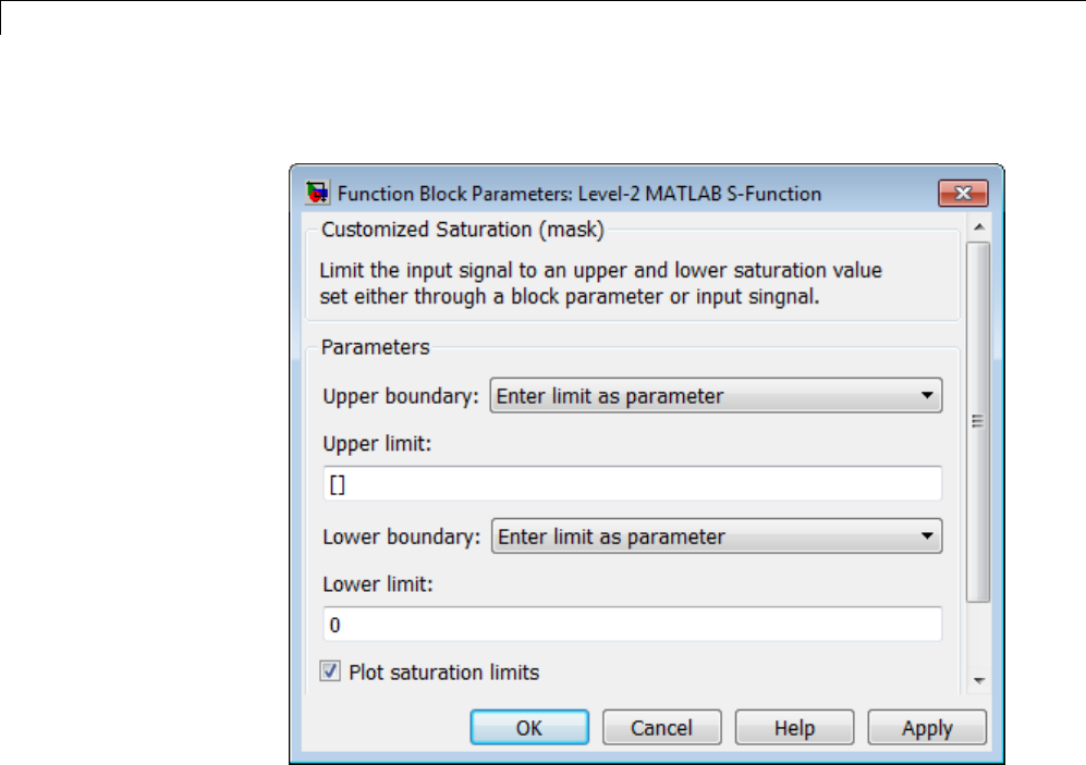
27 Creating Custom Blocks
cClick OK.
2Write a callback for the new check box. The callback initializes a
structure to store the saturation limit values during simulation in the
Level-2 MATLAB S-Function block UserData. The MATLAB script
customsat_plotcallback.m contains this new callback, as well as modified
versions of the previous callbacks to handle the new mask parameter. If
you are following through this example, open customsat_plotcallback.m
and copy its local functions over the previous local functions in
customsat_callback.m.
%% Plotting checkbox callback
function plotsaturation(block)
% Reinitialize the block's userdata
vals = get_param(block,'MaskValues');
27-38

Create a Custom Block
ud = struct('time',[],'upBound',[],'upVal',[],'lowBound',[],'lowVal',[]);
if strcmp(vals{1},'No limit'),
ud.upBound = 'off';
else
ud.upBound = 'on';
end
if strcmp(vals{3},'No limit'),
ud.lowBound = 'off';
else
ud.lowBound = 'on';
end
set_param(gcb,'UserData',ud);
3Update the MATLAB S-function Outputs method to store the
saturation limits, if applicable, as done in the new MATLAB S-function
custom_sat_plot.m. If you are following through this example, copy the
Outputs method in custom_sat_plot.m over the original Outputs method
in custom_sat_final.m
%% Function: Outputs ===================================================
function Outputs(block)
lowMode = block.DialogPrm(1).Data;
upMode = block.DialogPrm(3).Data;
sigVal = block.InputPort(1).Data;
vals = get_param(block.BlockHandle,'MaskValues');
plotFlag = vals{5};
lowPortNum = 2;
% Check upper saturation limit
if isequal(upMode,2)
upVal = block.RuntimePrm(2).Data;
elseif isequal(upMode,3)
upVal = block.InputPort(2).Data;
lowPortNum = 3; % Move lower boundary down one port number
else
upVal = inf;
27-39

27 Creating Custom Blocks
end
% Check lower saturation limit
if isequal(lowMode,2),
lowVal = block.RuntimePrm(1).Data;
elseif isequal(lowMode,3)
lowVal = block.InputPort(lowPortNum).Data;
else
lowVal = -inf;
end
% Use userdata to store limits, if plotFlag is on
if strcmp(plotFlag,'on');
ud = get_param(block.BlockHandle,'UserData');
ud.lowVal = [ud.lowVal;lowVal];
ud.upVal = [ud.upVal;upVal];
ud.time = [ud.time;block.CurrentTime];
set_param(block.BlockHandle,'UserData',ud)
end
% Assign new value to signal
if sigVal > upVal,
sigVal = upVal;
elseif sigVal < lowVal,
sigVal=lowVal;
end
block.OutputPort(1).Data = sigVal;
%endfunction
4Write the function plotsat.m to plot the saturation limits. This function
takes the handle to the Level-2 MATLAB S-Function block and uses this
handle to retrieve the block’s UserData. If you are following through this
tutorial, save plotsat.m to your working folder.
function plotSat(block)
% PLOTSAT contains the plotting routine for custom_sat_plot
% This routine is called by the S-function block's StopFcn.
27-40

Create a Custom Block
ud = get_param(block,'UserData');
fig=[];
if ~isempty(ud.time)
if strcmp(ud.upBound,'on')
fig = figure;
plot(ud.time,ud.upVal,'r');
hold on
end
if strcmp(ud.lowBound,'on')
if isempty(fig),
fig = figure;
end
plot(ud.time,ud.lowVal,'b');
end
if ~isempty(fig)
title('Upper bound in red. Lower bound in blue.')
end
% Reinitialize userdata
ud.upVal=[];
ud.lowVal=[];
ud.time = [];
set_param(block,'UserData',ud);
end
5Right-click the Level-2 MATLAB S-Function block and select Properties.
The Block Properties dialog box opens. On the Callbacks pane, modify
the StopFcn to call the plotting callback as shown in the following figure,
then click OK.
27-41
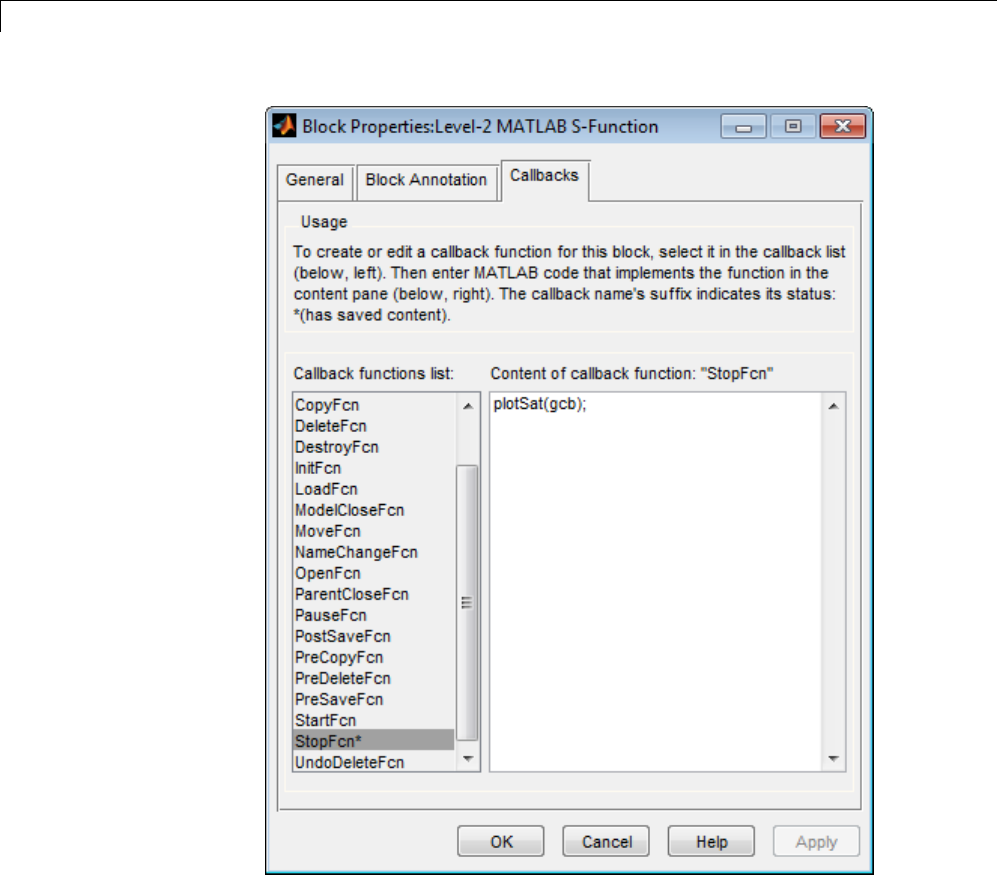
27 Creating Custom Blocks
27-42

Custom Block Examples
Custom Block Examples
In this section...
“Creating Custom Blocks from Masked Library Blocks” on page 27-43
“Creating Custom Blocks from MATLAB Functions” on page 27-43
“Creating Custom Blocks from S-Functions” on page 27-44
Creating Custom Blocks from Masked Library Blocks
The Additional Math and Discrete Simulink library is a group of custom
blocks created by extending the functionality of built-in Simulink blocks. The
Additional Discrete library contains a number of masked blocks that extend
the functionality of the standard Unit Delay block. See “Libraries” for more
general information on Simulink libraries.
Creating Custom Blocks from MATLAB Functions
The Simulink product provides a number of examples that show how to
incorporate MATLAB functions into a custom block.
•The Single Hydraulic Cylinder Simulation, sldemo_hydcyl,usesaFcn
block to model the control valve flow. In addition, the Control Valve Flow
block is a library link to one of a number of custom blocks in the library
hydlib.
•The Radar Tracking Model, sldemo_radar, uses an Interpreted MATLAB
Function block to model an extended Kalman filter. The MATLAB
function aero_extkalman.m implements the Kalman filter found inside the
Radar Kalman Filter subsystem. In this example, the MATLAB function
requires three inputs, which are bundled together using a Mux block in
the Simulink model.
•The Spiral Galaxy Formation example, sldemo_eml_galaxy, uses several
MATLAB Function blocks to construct two galaxies and calculate the
effects of gravity as these two galaxies nearly collide. The example also
uses MATLAB Function blocks to plot the simulation results using a subset
of MATLAB functions not supported for code generation. However, because
these MATLAB Function blocks have no outputs, the Simulink Coder
product optimizes them away during code generation.
27-43

27 Creating Custom Blocks
Creating Custom Blocks from S-Functions
The Simulink model sfundemos contains various examples of MATLAB and C
MEX S-functions. For more information on writing MATLAB S-functions, see
“Write Level-2 MATLAB S-Functions”. For more information on writing C
MEX S-functions, see “C/C++ S-Functions”. For a list of available S-function
examples, see “S-Function Examples” in Writing S-Functions.
27-44


28 Working with Block Libraries
About Block Libraries and Linked Blocks
Block Libraries
Ablock library is a collection of blocks that serve as prototypes for instances
of blocks in a Simulink model.
Simulink comes with two built-in block libraries: the Simulink block library
and the Simulink Coder block library. The latter is included with Simulink to
support sharing models that contain Simulink Coder blocks. Many additional
MathWorks products and associated block libraries are available. You cannot
change a built-in block library in any way.
Benefits of Block Libraries
Block libraries are a useful componentization technique for:
•Providing frequently-used, and seldom changed, modeling utilities
•Reusing components repeatedly in a model or in multiple models
For additional information about how libraries compare to other Simulink
componentization techniques, see “Componentization Guidelines” on page
12-17.
Library Browser
Simulink provides a Library Browser that you can use to display block
libraries, search for blocks by name, and copy library blocks into models.
All installed libraries appear in the Library Browser when you open it. See
“Populate a Model” on page 4-4 for information about how to use the Simulink
Library Browser.
Linked Blocks
When you copy a block from a library into a model, Simulink creates a linked
block in the model, and connects it to the library block using a library link.
The library block is the prototype block, and the linked block in the model is
an instance of the library block. The linked block appearance and behavior
28-2

About Block Libraries and Linked Blocks
are the same as the library block. For most purposes, you can ignore the
underlying link and just think of a linked block as a clone of the library block.
Copying a block from a library to another library or model does not always
create a linked block. Library blocks that support linking include subsystems,
masked blocks, and charts. However, the block author can choose not to make
the copy a linked blockbymodifyingtheCopyFcn,asdonebytheSimulink
Subsystem block.
28-3

28 Working with Block Libraries
Create and Work with Linked Blocks
In this section...
“About Linked Blocks” on page 28-4
“Create a Linked Block” on page 28-4
“Update a Linked Block” on page 28-5
“Modify Linked Blocks” on page 28-6
“Find a Linked Block’s Prototype” on page 28-7
“FindLinkedBlocksinaModel”onpage28-7
About Linked Blocks
Alinked block is an instance of a library block and contains a link to that
library block that serves as the block type’s prototype. The link consists of
the path of the library block that serves as the instance’s prototype. The link
allows the linked block to update whenever the corresponding prototype in the
library changes (“Update a Linked Block” on page 28-5). This ensures that
your model always uses the latest version of the block.
Note The data tip for a linked block shows the name of the library block it
references (see “Block Tool Tips” on page 23-2).
You can change the values of a linked block’s parameters (including in an
existing mask). You cannot add a new mask for linked blocks or edit the mask
setup, that is, add or remove mask parameters or change mask behavior.
Also, you cannot set callback parameters for a linked block. If the linked
block’s prototype is a subsystem, you can make nonstructural changes to the
contents of the linked subsystem (see “Modify Linked Blocks” on page 28-6).
Create a Linked Block
To create a linked block in a model or another library:
28-4

Create and Work with Linked Blocks
1Open your model.
2Open the Simulink Library Browser (see “Copy Blocks to Your Model” on
page 4-4), or another library.
3Use the Library Browser to find the library block that serves as a prototype
of the block you want to create (see “Browse Block Libraries” on page 4-4
and “Search Block Libraries” on page 4-5).
4Drag the library block from the Library Browser’s Library pane and drop
it into your model.
Update a Linked Block
Simulink updates out-of-date linked blocks in a model or library when you:
•Load the model or library.
•Run the simulation.
•Use the find_system command.
•Query the LinkStatus parameter of a block, using the get_param command
(see “Check and Set Link Status Programmatically” on page 28-16 ).
Note Querying the StaticLinkStatus parameter of a block does not
update any out-of-date linked blocks.
•Save changes to a library block, then Simulink automatically refreshes all
links to the block in open Model Editor windows.
When you edit a library block (in the Model Editor or at the command line),
then Simulink indicates stale links whichareopenintheModelEditorby
displaying the linked blocks grayed out. Simulink refreshes any stale links
to edited blocks when you activate the Model Editor window, even if you
have not saved the library yet.
To manually refresh links:
•Select Simulation > Update Diagram (or press Ctrl+D).
28-5

28 Working with Block Libraries
•Select Diagram > Refresh Blocks (or press Ctrl+K) to refresh links.
•Select Go To Library Link.
Modify Linked Blocks
You cannot make structural changes to linked blocks, such as adding or
deleting lines or blocks to the block diagram of a masked subsystem. If you
want to make such changes, you must disable the linked block’s link to its
library prototype (see “Disable Links to Library Blocks” on page 28-11 ).
Parameterized Links
If you change parameter values inside a linked block, you create a
parameterized link. You can change the values of any masked subsystem
linked block parameter that does not alter the block’s structure, e.g., by
adding or deleting lines, blocks, or ports. An example of a nonstructural
change is a change to the value of a mathematical block parameter, such
as the Gain parameter of the Gain block. A linked subsystem block whose
parametervaluesofinnerblocksdiffer from their corresponding library
blocks is called a parameterized link. Changing the top-level mask values
does not create a parameterized link.
When saving a model containing a parameterized link, Simulink saves the
changes to the local copy of the subsystem together with the path to the
library copy in the model’s file. When you reopen the system, Simulink copies
the library block into the loaded model and applies the saved changes.
Tip To determine whether a linked block’s parameter values differ from those
of its library prototype, open the linked block’s block diagram in an editor
window. The linked block’s library link indicator (if displayed) changes to a
red arrow and the title bar of the editor window displaying the subsystem
displays “Parameterized Link” if the linked block’s parameter values differ
from the library block’s parameter values.
See “Display Library Links” on page 28-8.
28-6

Create and Work with Linked Blocks
Self-Modifying Linked Subsystems
Simulink allows linked subsystems to change their own structural contents
without disabling the link. This allows you to create masked subsystems that
modify their structural contents based on mask parameter dialog box values.
FindaLinkedBlock’sPrototype
To find the source library and the prototype of a linked block, right-click the
linked block and select Library Link > Go To Library Link.
Alternatively, select the linked block and select Diagram > Library Link
>GoToLibraryLink.
If the library is open, Simulink selects and highlights the library block
and makes the source library the active window. If the library is not open,
Simulink first opens it and then selects the library block.
Find Linked Blocks in a Model
Use the libinfo command to get information about the linked blocks in the
model and which library blocks they link to. The ReferenceBlock property
gives the path of the library block to which a block links.
28-7

28 Working with Block Libraries
Work with Library Links
In this section...
“Display Library Links” on page 28-8
“Lock Links to Blocks in a Library” on page 28-9
“Disable Links to Library Blocks” on page 28-11
“Restore Disabled or Parameterized Links” on page 28-12
“Check and Set Link Status Programmatically” on page 28-16
“Break a Link to a Library Block” on page 28-18
“Fix Unresolved Library Links” on page 28-19
Display Library Links
A model can have a block linked to a library block, or it can have a local
instance of a block that is not linked. To enable the display of library links:
1In the Model Editor window, select Display > Library Links and from
the submenu, select one of these options:
aNone —displaysnolinks
bDisabled — displays only disabled links (the default for new models)
cUser Defined — displays only links to user libraries
dAll — displays all links
2Observe the library link indicators.
The library link indicator is a badge in the bottom left corner of each block.
You can right-click the link badge to access link menu options.
28-8
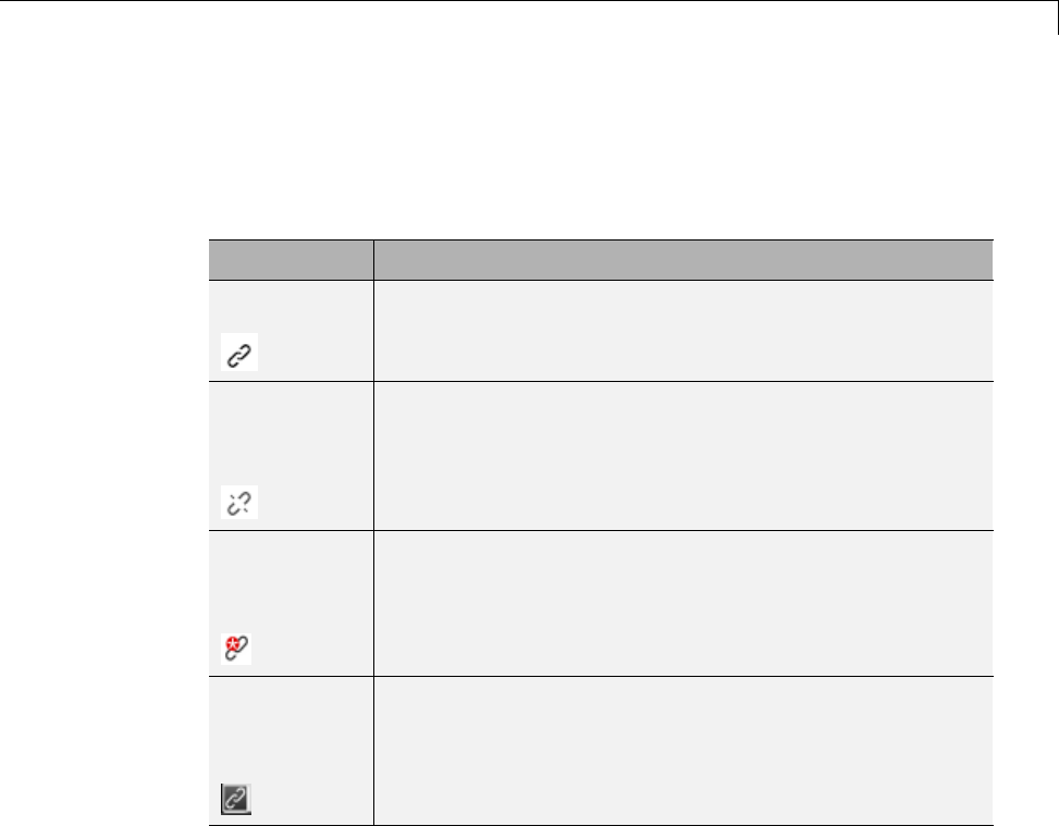
Work with Library Links
The color and icon of the link badge indicates the status of the link. If you
open a linked block, the Model Editor displays the same link badge at bottom
left. You can right-click the link badge in the corner of the canvas to access
link options such as Go To Library Block.
Link Badge Status
Black links Active link
Grey
separated
links
Inactive link
Black links
with a red
star icon
Active and modified (parameterized link)
White
links, black
background
Locked link
Lock Links to Blocks in a Library
You can lock links to a library. Lockable library links enable control of end
user editing, to prevent unintentional disabling of these links. This ensures
robust usage of mature stable libraries.
To lock links to a library, either:
•In your library window, select Diagram > Lock Links To Library.
•At the command line, use the LockLinksToLibrary property:
28-9
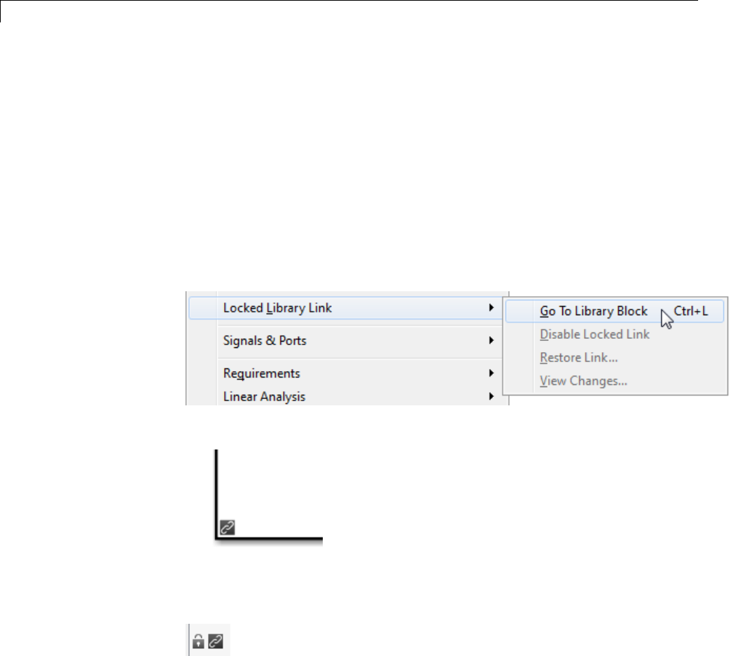
28 Working with Block Libraries
set_param('MyModelName', 'LockLinksToLibrary', 'on')
where MyModelName is the library file.
When you copy a block to a model from a library with locked links:
•The link is locked.
•You cannot disable locked links from the Model Editor.
If you select Diagram or right-click the linked block, you see the Library
Link menu has changed to Locked Library Link, and the only enabled
option is now Go To Library Block.
•If you display library links, the locked link icon has a black background.
•If you open a locked link, the window title is Locked Link: blockname.
The bottom left corner shows a lock icon and a link badge.
•You cannot edit locked link contents. If you try to make a structural
change to a locked link (such as editing the diagram), you see a message
stating that you cannot modify the link because it is either locked or inside
another locked link.
28-10

Work with Library Links
-The mask and block parameter dialogs are disabled for blocks inside
locked links. For a resolved linked block with a mask, its parameter
dialog is always disabled.
-You cannot parameterize locked links in the Model Editor.
•You can disable locked links only from the command line as follows:
set_param(gcb, 'LinkStatus', 'inactive')
To unlock links to a library:
•In your library window, select Diagram > Unlock Links To Library
•At the command line:
set_param('MyModelName', 'LockLinksToLibrary', 'off')
The status of a link (locked or not) is determined by the library state when
you copy the block. If you copy a block from a library with locked links, the
link is locked. If you later unlock the library links, any existing linked
blocks do not change to unlocked links until you refresh links.
If you use sublibraries as an organizational tool, when you lock links to a
library, you might want also to lock links to any sublibraries.
Disable Links to Library Blocks
To make a structural change to a linked block, you need to disable the link
between the block and the library block that serves as its prototype.
You cannot disable locked links from the Model Editor. See “Lock Links to
Blocks in a Library” on page 28-9.
28-11

28 Working with Block Libraries
Note When you use the Model Editor to make a structural change (such as
editing the diagram) to a block with an active library link, Simulink offers
to disable the library link for you (unless the link is locked). If you accept,
Simulink disables the link and allows you to make changes to the subsystem
block.
Do not use set_param to make a structural change to an active link; the result
of this type of change is undefined.
To disable a link:
1In the Model Editor window, right-click a linked block and select Library
Link > Disable Link.
2Alternatively, select a linked block and select the menu item
Diagram > Library Link > Disable Link.
The library link is disabled and the library link indicator changes to gray.
When a library block is disabled and it is within another library block (a
child of a parent library block), the model also disables the parent block
containing the child block.
Todisablealinkfromthecommand-line,settheLinkStatus property to
inactive as follows:
set_param(gcb, 'LinkStatus', 'inactive')
Restore Disabled or Parameterized Links
After you make changes to a disabled linked block, you may want to restore
its link to the library block and resolve any differences between the two
blocks. The Links Tool helps you with this task.
1In the Model Editor window, select a linked block with a disabled library
link.
2From the Diagram menu (or right-click context menu), select Library
Link > Resolve Link.
28-12
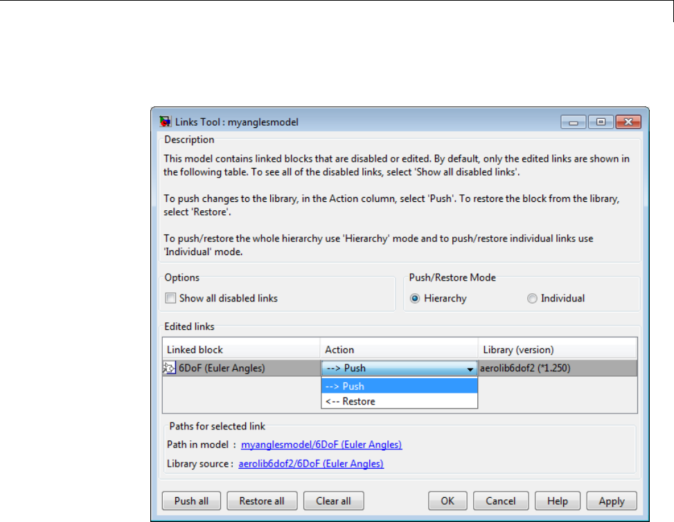
Work with Library Links
The Links Tool window opens.
The Edited links table has the following columns:
•Linked block — List of linked blocks. The list of links includes library
links with structural changes (disabled links), parameterized library
links (edited links), and library links that were actively chosen to be
resolved.
•Action — Select an action to perform on the linked block or library.
•Library — List of library names and version numbers.
3Select the check box Show all disabled links if you want to view disabled
links as well as parameterized links.
28-13

28 Working with Block Libraries
4Under Push/Restore Mode, choose a mode of action:
•If you want to act on individual links, select Individual.
•If you want to act on the whole link hierarchy, leave the default setting
on Hierarchy. See “Pushing or Restoring Link Hierarchies” on page
28-15.
5From the Linked block list, select a block name.
The Links Tool updates the Paths for selected link panel with links to
the linked block in the model and in the library.
6From the Action list, select Push or Restore for the currently selected
block.
Action Choice Links Tool Action
Push The Links Tool looks for all changes in the link
hierarchy and pushes all links with changes to their
libraries.
Push replaces the version of the block in the library
with the version in the model.
Restore The Links Tool looks for all disabled or edited links
in the link hierarchy and restores them all with
their corresponding library blocks.
Restore replaces the version of the block in the
modelwiththeversioninthelibrary.
Push Individual In Individual mode, the disabled or edited block is
pushed to the library, preserving the changes inside
it without acting on the hierarchy. All other links
are unaffected.
Restore
Inidividual
In Individual mode, the disabled or edited block is
restored from the library, and all other links are
unaffected.
Toselectthesameactionforall linked blocks, click Push all,Restore
all,orClear all.
28-14

Work with Library Links
7When you click OK or Apply, the Links Tool performs the push or restore
actions you selected in the edited links table.
After resolving a link, the versions in the library and the linked block now
match.
Note Changes you push to the library are not saved until you actively
save the library.
If a linked block name has a cautionary icon before it, the model has
other instances of this block linked from the same library block, and they
have different changes. Choose one of the instances to push changes to the
library block and restore links to the other blocks , or choose to restore all of
them with the library version.
PushingorRestoringLinkHierarchies
Caution Be cautious using Push or Restore in hierarchy mode if you have a
large hierarchy of edited and disabled links. Ensure that you want to push or
restore the whole hierarchy of links.
Pushing a hierarchy of disabled links affects the disabled links inside and
outside in the hierarchy for a given link. If you push changes from a disabled
link in the middle of a hierarchy, the inside links are pushed and the outside
links are restored if without changes. This operation does not affect outside
(parent) links with changes unless you also explicitly selected them for push.
The Links Tool starts from the lowest links (the deepest inside) and then
moves upward in the hierarchy.
Some simple examples:
1Link A contains link B and both have changes.
•Push A. The Links Tool pushes both A and B.
•Push B. The Links Tool pushes B and not A.
28-15

28 Working with Block Libraries
2Link A contains link B. A has no changes, and B has changes.
•Push B. The Links Tool pushes B and restores A. When parent links
are unmodified, they are restored.
If you have a hierarchy of parameterized links, the Links Tool can manipulate
only the top level.
Check and Set Link Status Programmatically
All blocks have a LinkStatus parameter and a StaticLinkStatus parameter
that indicate whether the block is a linked block.
Use get_param(gcb, 'StaticLinkStatus') to query the link status without
updating out-of-date linked blocks.
Use get_param and set_param to query and set the LinkStatus, which can
have the following values.
Get LinkStatus
Value Description
none Block is not a linked block.
resolved Resolved link.
unresolved Unresolved link.
implicit Block resides in library block and is itself not a link to
a library block. For example, suppose that A is a link
to a subsystem in a library that contains a Gain block.
Further, suppose that you open A and select the Gain
block. Then, get_param(gcb, 'LinkStatus') returns
implicit.
inactive Disabled link.
28-16

Work with Library Links
Set LinkStatus
Value Description
none Breaks link. Use none to break a link, e.g.,
set_param(gcb, 'LinkStatus', 'none')
inactive Disables link. Use Inactive to disable a link, e.g.,
set_param(gcb, 'LinkStatus', 'inactive')
restore Restores an inactive or disabled link to a library block
and discardsanychangesmadetothelocalcopyof
the library block. For example, set_param(gcb,
'LinkStatus', 'restore') replaces the selected block
with a link to a library block of the same type, discarding
any changes in the local copy of the library block.
This is equivalent to Restore Individual in the Links
Tool.
propagate Pushes any changes made to the disabled link to the
library block and re-establishes its link.
This is equivalent to Push Individual in the Links
Tool.
restoreHierarchy Restores all disabled links in the hierarchy with their
corresponding library blocks. This is equivalent to
Restore in hierarchy mode in the Links Tool.
propagateHierarchy
Pushes all links with changes in the hierarchy to their
libraries. This is equivalent to Push in hierarchy mode in
the Links Tool. See “Restore Disabled or Parameterized
Links” on page 28-12.
Note Using get_param to query a block’s LinkStatus also resolves any
out-of-date block links. Use get_param to update library links in a model
programmatically. Querying the StaticLinkStatus property does not resolve
any out-of-date links. Query the StaticLinkStatus property when the call to
get_param is in the callback of a child block querying the link status of its
parent.
28-17

28 Working with Block Libraries
If you call get_param on a block inside a library link, Simulink resolves the
link if necessary. This operation may involve loading part of the library and
executing callbacks.
Break a Link to a Library Block
You can break the link between a linked block and its library block to cause
the linked block to become a simple copy of the library block, unlinked to the
library block. Changes to the library block no longer affect the block. Breaking
links to library blocks may enable you to transport a masked subsystem model
as a standalone model, without the libraries (see “Masking”).
To break the link between a linked block and its library block, you can use
any of the following actions.
•Disable the link, then right-click the block and choose Library
Link > Break Link .
•At the command line, change the value of the LinkStatus parameter to
'none' using this command:
set_param(gcb, 'LinkStatus', 'none')
•Right-click and drag to copy a block, and you see an offer to break links,
unless the parent library has LockLinksToLibrary set to on. If your copied
block will be a locked link, then you do not see the option to break links.
To copy and break links to multiple blocks simultaneously, select multiple
blocks and then drag. Any locked links are ignored and not broken.
•When saving the model, you can break links by supplying arguments to
the save_system command. See save_system.
Note Breaking library links in a model does not guarantee that you can run
the model standalone, especially if the model includes blocks from third-party
libraries or optional Simulink blocksets. It is possible that a library block
invokes functions supplied with the library and hence can run only if the
library is installed on the system running the model. Further, breaking a
link can cause a model to fail when you install a new version of the library
on a system.
28-18

Work with Library Links
For example, suppose a block invokes a function that is supplied with the
library. Now suppose that a new version of the library eliminates the function.
Running a model with an unlinked copy of the block results in invocation of
a now nonexistent function, causing the simulation to fail. To avoid such
problems, you should generally avoid breaking links to libraries.
Fix Unresolved Library Links
If Simulink is unable to find either the library block or the source library on
your MATLAB path when it attempts to update the linked block, the link
becomes unresolved. Simulink issues an error message and displays these
blocks using red dashed lines. The error message is
Failed to find block "source-block-name"
in library "source-library-name"
referenced by block
"linked-block-path".
The unresolved linked block appears like this (colored red).
To fix a bad link, you must do one of the following:
•Delete the unresolved block and copy the library block back into your model.
•Add the folder that contains the required library to the MATLAB path
and select either Diagram > Update Diagram or Diagram > Refresh
Blocks.
•Double-click the unresolved block to open its dialog box (see the Bad
Link block reference page). On the dialog box that appears, correct the
pathname in the Source block field and click OK.
28-19

28 Working with Block Libraries
Create Block Libraries
In this section...
“Create a Library” on page 28-20
“Create a Sublibrary” on page 28-21
“Modify and Lock Libraries” on page 28-21
“Make Backward-Compatible Changes to Libraries” on page 28-22
Create a Library
You can create your own block library and add it to the Simulink Library
Browser (see “Add Libraries to the Library Browser” on page 28-32). To
create a library:
1Select Library from the New submenu of the File menu.
Simulink creates a model file for storing the new library and displays the
file in a new model editor window.
Tip You can also use the new_system command to create the library and
the open_system command to open the new library.
2Drag blocks from models or other libraries into the new library.
Note If you want to be able to create links in models to a block in the
library, you may need to provide a mask (see “Masking”) for the block. You
can also provide a mask for a subsystem in a library, but you do not need to
have a mask to create links to it in models.
3Save the library’s file under a new name.
28-20

Create Block Libraries
Create a Sublibrary
If your library contains many blocks, consider grouping the blocks into a
hierarchy of sublibraries. Creating a sublibrary entails inserting a reference
in the Simulink model file of one library to the model file of another library.
The referenced file is called a sublibrary of the parent (i.e., referencing)
library. The sublibraryissaidtobeincludedbyreferenceintheparent
library.
To include a library in another library as a sublibrary:
1Open the parent library.
2Add a Subsystem block to the parent library.
3Delete the subsystem’s default input and output ports.
4Create a mask for the subsystem that displays text or an image that
conveys thesublibrary’spurpose.
5Set the subsystem’s OpenFcn parameter to the name of the sublibrary’s
model file.
6Save the parent library.
Modify and Lock Libraries
Whenyouopenalibrary,itisautomatically locked and you cannot modify its
contents. To unlock the library, select Diagram > Unlock Library.
When you close the library window, Simulink locks the library.
Locking a library prevents a user from inadvertently modifying a library, for
example, by moving a block in the library or adding or deleting a block from
the library. If you attempt to modify a locked library, Simulink displays a
dialog box that allows you to unlock the library and make the change.
To unlock a block library from the MATLAB command line, use the following
command:
set_param('library_name', 'Lock', 'off');
28-21

28 Working with Block Libraries
You must then relock the library from the MATLAB command line to prevent
further changes. Use the following command to relock a block library:
set_param('library_name', 'Lock', 'on');
If you want to control end user editing of linked blocks and prevent
unintentional disabling of links, you can lock links to a library. See “Lock
Links to Blocks in a Library” on page 28-9.
When you save a library, Simulink checks file permissions and offers to try to
make the library writable if necessary.
Make Backward-Compatible Changes to Libraries
Simulink provides the following features to facilitate making changes to
library blocks without invalidating models that use the library blocks.
Forwarding Tables
You can create forwarding tables for libraries to specify how to update links
in models to reflect changes in the parameters. Use the Forwarding Table to
map old library blocks to new library blocks. For example, if you rename or
move a block in a library, you can use a forwarding table to enable Simulink
to update models that link to the block.
After you specify the forwarding table entry in a library, any links to old
library blocks will be updated when you load a model containing links to
old blocks. Library authors can use the forwarding tables to automatically
transform old links into updated links without any loss of functionality and
data. Use the forwarding table to solve compatibility issues with models
containing old links that cannot load in the current version of Simulink.
Library authors do not need to run slupdate to upgrade old links, and can
reduce maintenance of legacy blocks.
To set up a forwarding table for a library,
1Select Diagram > Unlock Library.
2Select File > Library Properties > Library Properties. The Library
Properties dialog box opens.
28-22
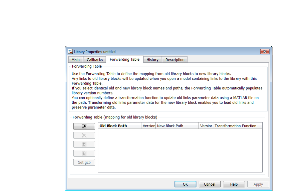
Create Block Libraries
3Select the Forwarding Table tab.
4Define the mapping from old library blocks to new library blocks.
aClick the Add New Entry button. A new row appears in the table.
bEnter values in Old Block Path and New Block Path columns.
Click GCB to get the path of the currently selected block.
If you select identical old and new library block names and paths, the
Forwarding Table automatically populates library version numbers
in the Version columns. The LibraryVersion property is the model
version of the library at the time the link was created.
c(Optional ) You can define a transformation function to update old link
parameter data using a MATLAB file on the path. Specify the function
in the Transformation Function column. Transforming old link
parameter data for the new library block enables you to load old links
and preserve parameter data.
28-23

28 Working with Block Libraries
If you do not want to specify a transformation function, do not edit
the field. When you save the library, the column will display No
Transformation.
5Click OK to apply changes and close the dialog box.
After specifying the forwarding table mapping, when you open a model
containing links to the library, links to old library blocks will be updated.
To view an example of a forwarding table:
1Enter
open_system('simulink')
2Select File > Library Properties > Library Properties
3Click the Forwarding Table tab.
4View how the forwarding table specifies the mapping of old blocks to new
blocks. You cannot make changes because the library is locked. Do not edit
the forwarding table for your Simulink library.
28-24
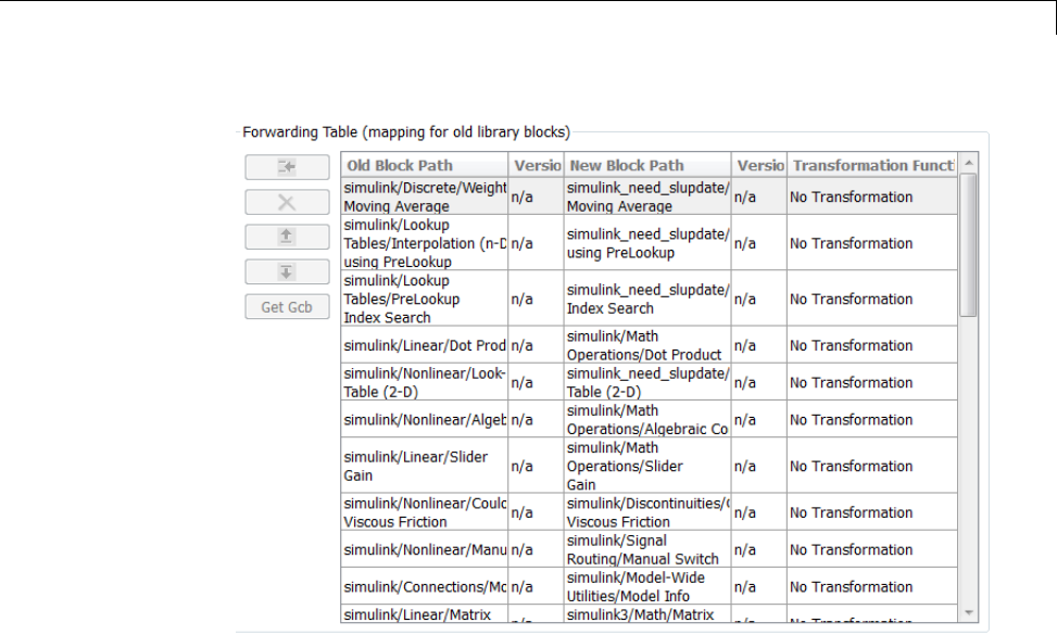
Create Block Libraries
5Click OK to close the dialog
The following example shows a forwarding table that defines:
•A block with the same name moving to a different library (Constant A)
•A block changing name in the same library (Block X to Block Y)
•A block changing name, moving library, and applying a transformation
function (Gain A to Gain B)
•A block with three version updates (Block A) using a transformation
function. When you select identical old and new library block names and
paths, the Forwarding Table automatically populates version numbers
in the Version columns. If this is the first entry with identical names,
version starts at 0, and the new version number is set to the ModelVersion
of the library. For subsequent entries, the first version is set to the
previous entry’s new version, and the new version is set to the current
ModelVersion of the library.
28-25
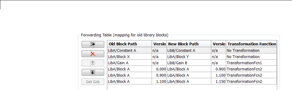
28 Working with Block Libraries
At the command line you can create a simple forwarding table specifying
the old locations and new locations of blocks that have moved within the
library or to another library. You associate a forwarding table with a library
by setting its ForwardingTable parameter to a cell array of two-element
cell arrays, each of which specifies the old and new path of a block that has
moved. For example, the following command creates a forwarding table and
assigns it to a library named Lib1.
set_param('Lib1', 'ForwardingTable', {{'Lib1/A', 'Lib2/A'}
{'Lib1/B', 'Lib1/C'}});
The forwarding table specifies that block A has moved from Lib1 to Lib2. and
that block B is now named C. Suppose that you open a model that contains
links to Lib1/A and Lib1/B. Simulink updates the link to Lib1/A to refer
to Lib2/A and the link to Lib1/B to refer to Lib1/C. The changes become
permanent when you subsequently save the model.
Writing Transformation Functions. You can use transformation functions
to add or remove parameters and define parameter values. Transforming old
link parameter data for the new library block enables you to load old links
and preserve parameter data that differs from library values. Define your
transformation function using a MATLAB file on the path, then specify the
function in the Forwarding Table Transformation Function column.
The transformation function in your MATLAB file must be like the following:
function outData = TransformationFcn(inData)
where inData is a structure with fields ForwardingTableEntry and
InstanceData,andForwardingTableEntry is a structure with fields
__slOldName__,__slNewName__,__slOldVersion__ ,__slNewVersion__.
28-26

Create Block Libraries
This general transformation function can have many local functions defined
in it. The function calls the appropriate local functions based on old block
names and versions. Use this to combine many local functions into a single
transformation function, to avoid having many transformation functions on
the MATLAB path.
InstanceData and NewInstanceData are structures with fields Name and
Value. Instance data means the names and values of parameters that are
different from the library values.
outData is a structure with fields NewInstanceData and NewBlockPath.
The following example code shows how to define a transformation function
that adds a parameter with value uint8 to update a Compare To Constant
block:
function [outData] = TransformationCompConstBlk(inData)
% Example transformation Function for old 'Compare To Const' block.
%
% If instanceData of old 'Compare To Const' block does not have
% the 'OutDataTypestr' parameter,
% add the parameter with value 'uint8'.
%
% In the Simulink library the 'ForwardingTableEntry' would be of type:
% ||__slOldName__||A||__slNewName__||B||__slTransformationFcn__||TX
%
% Exact entry is:
% ||__slOldName__||fixpt_lib_4/Logic & Comparison/Compare\nTo Constant||__slNewName__||
% simulink/Logic and Bit\nOperations/Compare\nTo Constant||__slTransformationFcn__||TransformationCompConst
B
%
%
outData.NewBlockPath = '';
outData.NewInstanceData = [];
instanceData = inData.InstanceData;
% Get the field type 'Name' from instanceData
[ParameterNames{1:length(instanceData)}] = instanceData.Name;
if (~ismember('OutDataTypeStr',ParameterNames))
28-27

28 Working with Block Libraries
% OutDataTypeStr parameter is not present in old link. Add it and set value uint8
instanceData(end+1).Name = 'OutDataTypeStr';
instanceData(end).Value = 'uint8';
end
outData.NewInstanceData = instanceData;
Creating Aliases for Mask Parameters
Simulink lets you create aliases, i.e., alternate names, for a mask’s
parameters. A model can then refer to the mask parameter by either its
name or its alias. This allows you to change the name of a mask parameter
in a library block without having to recreate links to the block in existing
models (see “Using Mask Parameter Aliases to Create Backward-Compatible
Parameter Name Changes” on page 28-28).
To create aliases for a masked block’s mask parameters, use the set_param
command to set the block’s MaskVarAliases parameter to a cell array that
specifies the names of the aliases in the same order as the mask names
appear in the block’s MaskVariables parameter.
Using Mask Parameter Aliases to Create Backward-Compatible
Parameter Name Changes. Thefollowingexampleillustratestheuse
of mask parameter aliases to create backward-compatible parameter name
changes.
1Create a new library. File >New >Library
2Open the model masking_example described in “How Mask Parameters
Work” on page 26-4. Drag the masked block named mx+b into your new
library and rename it to Line.
3Right-clicktheblockandselectProperties. In the Block Properties dialog,
select the Block Annotation tab. In the Enter text and tokens for
annotation box, enter
m = %<m>
b = %<b>
The block displays the value of its mand bparameters,
28-28

Create Block Libraries
4Right-click the block, and select Mask > Mask Parameters.IntheBlock
Parameter dialog, enter 0.5 for the Slope and 0for the Intercept.
5Save the new library with the filename mylibrary.
6Create a new Simulink model. File >New >Model.
7From the mylibrary window, drag an instance of the Line block to your
new model. Rename the instance LineA.
8Right-clicktheblockandselectMask > Mask Parameters.IntheBlock
Parameters dialog, change the value Slope to -0.5. and change the value
Intercept.to30. Select Display>LibraryLinks>UserDefined.
9Add a Scope and Clock block to your model and connect them to your block.
Save the new model with the filename mymodel.
10 From the Simulation menu, select Model Configuration Parameters.
From the Type list, select Fixed-step.FromtheSolver list, select
discrete (no continuous states.IntheFixed-step size box, enter
0.1. Simulate model.
Note that the model simulates without error.
11 Save and close mymodel.
12 Open mylibrary.
13 Edit mask. Right-click block, select Edit mask. In the Mask Editor dialog,
•Select the Parameters tab. In the Dialog parameters section and
Variable column, change the variable m to slope and bto intercept.
•Select the Icon & Ports tab. In the Icon Drawing commends box, change
the variable mto slope and bto intercept.
14 Right-click the Line block, select Properties. In the Block Properties
dialog, .
•Select the Block Annotation tab . In the Enter text and tokens of
annotation box, rename the mparameter to slope and the bparameter
to intercept.
28-29

28 Working with Block Libraries
15 Click Ok and save mylibrary.
16 Reopen mymodel.
Note that LineA icon has reverted to theappearanceofitslibrarymaster
(i.e., mylib/Line) and that its annotation displays question marks for the
values of mand b. These changes reflect the parameter name changes in
the library block. In particular, Simulink cannot find any parameters
named mand bin the library block and hence does not know what to do
with the instance values for those parameters. As a result, LineA reverts
to the default values for the slope and intercept parameters, thereby
inadvertently changing the behavior of the model. The following steps show
how to use parameter aliases to avoid this inadvertent change of behavior.
17 Close mymodel.
18 In the Library: mylibrary window, select the Line block.
19 Execute the following command at the MATLAB command line.
set_param(gcb, 'MaskVarAliases',{'m', 'b'})
This specifies that mand bare aliases for the Line block slope and
intercept parameters.
20 Reopen mymodel.
Note that LineA appearance, not the annotation, now reflects the value of
the slope parameter under its original name, i.e., m. Thisisbecausewhen
Simulink opened the model, it found that mis an alias for slope and assigned
the value of mstored in the model file to the LineA slope parameter.
21 Change LineA block annotation property to reflect LineA parameter name
changes, replace
m = %<m>
b = %<b>
with
m = %<slope>
b = %<intercept>
28-30

Create Block Libraries
LineA now appears with m = -0.5 and b = 30.
Note that LineA annotation shows that, thanks to parameter aliasing,
Simulink has correctly applied the parameter values stored for LineA in
the mymodels file to the block renamed parameters.
28-31

28 Working with Block Libraries
Add Libraries to the Library Browser
In this section...
“Display a Library in the Library Browser” on page 28-32
“Example of a Minimal slblocks.m File” on page 28-32
“Add More Descriptive Information in slblocks.m” on page 28-33
Display a Library in the Library Browser
1Create a folder in the MATLAB path for the top-level library and its
sublibraries.
You must store each top-level library that you want to appear in the
Library Browser in its own folder on the MATLAB path. Two top-level
libraries cannot exist in the same folder.
2Create or copy the top-level library and its sublibraries into the folder you
created in the MATLAB path.
3In the folder for the top-level library, include a slblocks.m file.
The approach you use to create the slblocks.m file depends on your
requirements for describing the library:
•If a minimal slblocks.m file meets your needs, then create a new
slblocks.m file, based on the example below
•If you want to describe the library more fully, consider copying an
existing slblocks.m file to use as a template, editing the copy to describe
your library (see below).
Example of a Minimal slblocks.m File
To display a library in the Library Browser, at a minimum you must include
these lines (adjusted to describe your library; comments are not required) in
the slblocks.m file.
function blkStruct = slblocks
%S
pecify that the product should appear in the library browser
28-32

Add Libraries to the Library Browser
% and be cached in its repository
Browser.Library = 'mylib';
Browser.Name = 'My Library';
blkStruct.Browser = Browser;
Add More Descriptive Information in slblocks.m
You can review other descriptive information you may wish to include in
your slblocks.m file by examining the comments in the Simulink library
slblocks.m file: matlabroot/toolbox/simulink/blocks/slblocks.m.
28-33

28 Working with Block Libraries
28-34

29
Using the MATLAB
Function Block
•“Integrate MATLAB Algorithm in Model” on page 29-4
•“What Is a MATLAB Function Block?” on page 29-6
•“Why Use MATLAB Function Blocks?” on page 29-8
•“Create Model That Uses MATLAB Function Block” on page 29-9
•“Code Generation Readiness Tool” on page 29-16
•“Check Code Using the Code Generation Readiness Tool” on page 29-22
•“Debugging a MATLAB Function Block” on page 29-23
•“MATLAB Function Block Editor” on page 29-33
•“MATLAB Function Reports” on page 29-51
•“Type Function Arguments” on page 29-64
•“Size Function Arguments” on page 29-72
•“Add Parameter Arguments” on page 29-75
•“Resolve Signal Objects for Output Data” on page 29-76
•“Types of Structures in MATLAB Function Blocks” on page 29-78
•“Attach Bus Signals to MATLAB Function Blocks” on page 29-79
•“How Structure Inputs and Outputs Interface with Bus Signals” on page
29-81
•“Rules for Defining Structures in MATLAB Function Blocks” on page 29-82
•“Index Substructures and Fields” on page 29-83

29 Using the MATLAB Function Block
•“Create Structures in MATLAB Function Blocks” on page 29-84
•“Assign Values to Structures and Fields” on page 29-86
•“Initialize a Matrix Using a Non-Tunable Structure Parameter” on page
29-88
•“Define and Use Structure Parameters” on page 29-91
•“Limitations of Structures and Buses in MATLAB Function Blocks” on
page 29-93
•“What Is Variable-Size Data?” on page 29-94
•“How MATLAB Function Blocks Implement Variable-Size Data” on page
29-95
•“Enable Support for Variable-Size Data” on page 29-96
•“Declare Variable-Size Inputs and Outputs” on page 29-97
•“Filter a Variable-Size Signal” on page 29-98
•“Enumerated Types Supported in MATLAB Function Blocks” on page
29-105
•“Define Enumerated Data Types for MATLAB Function Blocks” on page
29-106
•“Add Inputs, Outputs, and Parameters as Enumerated Data” on page
29-107
•“Basic Approach for Adding Enumerated Data to MATLAB Function
Blocks” on page 29-109
•“Instantiate Enumerated Data in MATLAB Function Blocks” on page
29-110
•“Control an LED Display” on page 29-111
•“Operations on Enumerated Data” on page 29-115
•“Using Enumerated Data in MATLAB Function Blocks” on page 29-116
•“Share Data Globally” on page 29-117
•“Add Frame-Based Signals” on page 29-126
•“Create Custom Block Libraries” on page 29-132
29-2

•“Use Traceability in MATLAB Function Blocks” on page 29-151
•“Include MATLAB Code as Comments in Generated Code” on page 29-156
•“Enhance Code Readability for MATLAB Function Blocks” on page 29-162
•“Speed Up Simulation with Basic Linear Algebra Subprograms” on page
29-171
•“Control Run-Time Checks” on page 29-173
•“Track Object Using MATLAB Code” on page 29-175
•“Filter Audio Signal Using MATLAB Code” on page 29-203
29-3
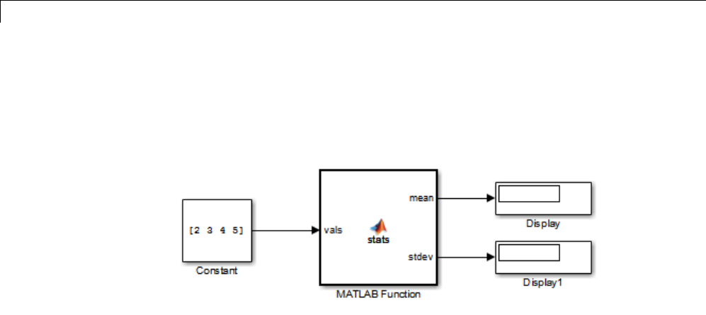
29 Using the MATLAB Function Block
Integrate MATLAB Algorithm in Model
Here is an example of a Simulink model that contains a MATLAB Function
block:
The MATLAB Function block contains the following algorithm:
function [mean,stdev] = stats(vals)
% #codegen
% calculates a statistical mean and a standard
% deviation for the values in vals.
len = length(vals);
mean = avg(vals,len);
stdev = sqrt(sum(((vals-avg(vals,len)).^2))/len);
plot(vals,'-+');
function mean = avg(array,size)
mean = sum(array)/size;
You will build this model in “Create Model That Uses MATLAB Function
Block” on page 29-9.
Defining Local Variables for Code Generation
If you intend to generate code from the MATLAB algorithm in a MATLAB
Function block, you must explicitly assign the class, size, and complexity of
local variables before using them in operations or returning them as outputs
(see “Data Definition for Code Generation” on page 34-2. In the example
29-4

Integrate MATLAB®Algorithm in Model
function stats, the local variable len is defined before being used to calculate
mean and standard deviation:
len = length(vals);
Generally, once you assign properties to a variable, you cannot redefine
its class, size, or complexity elsewhere in the function body, but there are
exceptions (see “Reassignment of Variable Properties” on page 33-9).
29-5

29 Using the MATLAB Function Block
WhatIsaMATLABFunctionBlock?
The MATLAB Function block allows you to add MATLAB functions to
Simulink models for deployment to desktop and embedded processors. This
capability is useful for coding algorithms that are better stated in the textual
language of the MATLAB software than in the graphical language of the
Simulink product. From the MATLAB Function block, you can generate
readable, efficient, and compact C/C++ code for deployment to desktop and
embedded applications. .
Calling Functions in MATLAB Function Blocks
MATLAB Function blocks can call any of the following types of functions:
•Local functions
Local functions are defined in the body of the MATLAB Function block. In
the preceding example, avg is a local function. See “Call Local Functions”
on page 41-9.
•MATLAB toolbox functions that support code generation
From MATLAB Function blocks, you can call toolbox functions that support
code generation. When you build your model with Simulink Coder, these
functions generate C code that is optimized to meet the memory and
performance requirements of desktop andembeddedenvironments.Inthe
preceding example, length,sqrt,andsum are examples of toolbox functions
that support code generation. See “Call Supported Toolbox Functions”
on page 41-10. For a complete list of supported functions, see “Functions
Supported for Code Generation — Alphabetical List” on page 31-2.
•MATLAB functions that do not support code generation
From MATLAB Function blocks, you can also call extrinsic functions.
These are functions on the MATLAB path that the compiler dispatches
to MATLAB software for execution because the target language does not
support them. These functions do not generate code; theyexecuteonlyin
the MATLAB workspace during simulation of the model. The Simulink
Coder software attempts to compile all MATLAB functions unless you
explicitly declare them to be extrinsic by using coder.extrinsic.See
“Declaring MATLAB Functions as Extrinsic Functions” on page 41-12.
29-6

What Is a MATLAB Function Block?
The code generation software detects calls to many common visualization
functions, such as plot,disp,andfigure. For MEX code generation, it
automatically calls out to MATLAB for these functions. For standalone
code generation, it does not generate code for these visualization functions.
This capability removes the requirement to declare these functions
extrinsic using the coder.extrinsic function.
See “Resolution of Function Calls in MATLAB Generated Code” on page
41-2.
29-7

29 Using the MATLAB Function Block
Why Use MATLAB Function Blocks?
MATLAB Function blocks provide the following capabilities:
•Allow you to build MATLAB functions into embeddable
applications — MATLAB Function blocks support a subset of MATLAB
toolbox functions that generate efficient C/C++ code (see “Functions
Supported for Code Generation”). With this support, you can use Simulink
Coder to generate embeddable C code from MATLAB Function blocks that
implement a variety of sophisticated mathematical applications. In this
way, you can build executables that harness MATLAB functionality, but
run outside the MATLAB environment.
•Inherit properties from Simulink input and output signals —By
default, both the size and type of input and output signals to a MATLAB
Function block are inherited from Simulink signals. You can also choose to
specify the size and type of inputs and outputs explicitly in the Ports and
Data Manager (see “Ports and Data Manager” on page 29-37) or in the
Model Explorer (see “Model Explorer Overview” on page 9-2).
29-8
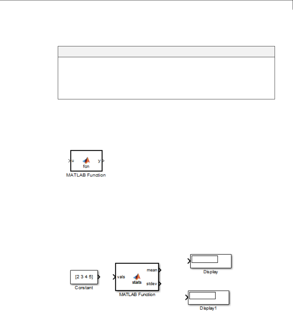
Create Model That Uses MATLAB Function Block
Create Model That Uses MATLAB Function Block
In this section...
“Adding a MATLAB Function Block to a Model” on page 29-9
“Programming the MATLAB Function Block” on page 29-10
“Building the Function and Checking for Errors” on page 29-12
“Defining Inputs and Outputs” on page 29-14
Adding a MATLAB Function Block to a Model
1Create a new model with the Simulink product and add a MATLAB
Function block to it from the User-Defined Function library:
2Add the following Source and Sink blocks to the model:
•From the Sources library, add a Constant block to the left of the
MATLAB Function block and set its value to the vector [2 3 4 5].
•From the Sinks library, add two Display blocks to the right of the
MATLAB Function block.
The model should now have the following appearance:
29-9
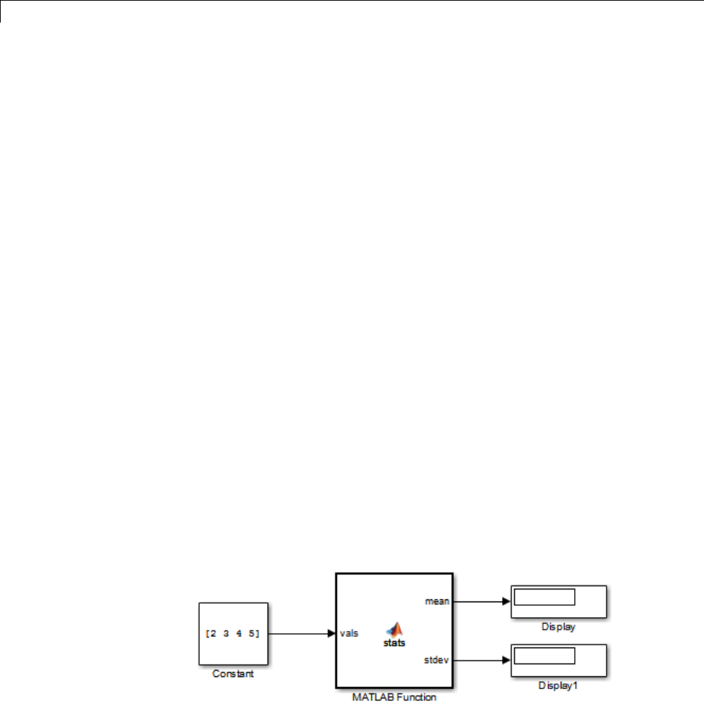
29 Using the MATLAB Function Block
3In the Simulink Editor, select File > Save As and save the model as
call_stats_block1.
Programming the MATLAB Function Block
The following exercise shows you how to program the block to calculate the
mean and standard deviation for a vector of values:
1Open the call_stats_block1 model that you saved at the end of “Adding
a MATLAB Function Block to a Model” on page 29-9. Double-click the
MATLAB Function block fcn to open it for editing.
A default function signature appears, along with the %#codegen directive.
The directive indicates that you intend to generate code from this algorithm
and turns on appropriate error checking (see “Compilation Directive
%#codegen” on page 41-8.
2Edit the function header line as follows:
function [mean,stdev] = stats(vals)
%#codegen
The function stats calculates a statistical mean and standard deviation
for the values in the vector vals. The function header declares vals as an
argument to the stats function, with mean and stdev as return values.
3Save the model as call_stats_block2.
4Complete the connections to the MATLAB Function block as shown.
29-10

Create Model That Uses MATLAB Function Block
5In the MATLAB Function Block Editor, enter a line space after the function
header and add the following code:
% calculates a statistical mean and a standard
% deviation for the values in vals.
len = length(vals);
mean = avg(vals,len);
stdev = sqrt(sum(((vals-avg(vals,len)).^2))/len);
plot(vals,'-+');
function mean = avg(array,size)
mean = sum(array)/size;
More about length
The function length is an example of a toolbox function that supports code
generation. When you simulate this model, C code is generated for this
function in the simulation application.
More about len
The class, size, and complexity of local variable len matches the output of
the toolbox function length, which returns a real scalar of type double.
By default, implicitly declared local variables like len are temporary. They
come into existence only when the function is called and cease to exist
when the function is exited. To make implicitly declared variables persist
between function calls, see “Define and Initialize Persistent Variables” on
page 33-10.
More about plot
The function plot is not supported for code generation. The code generation
software detects calls to many common visualization functions, such as
plot,disp,andfigure. For MEX code generation, it automatically calls
out to MATLAB for these functions. For standalone code generation, it does
not generate code for these visualization functions.
6Save the model as call_stats_block2.
29-11

29 Using the MATLAB Function Block
Building the Function and Checking for Errors
After programming a MATLAB Function block in a Simulink model, you can
build the function and test for errors. This section describes the steps:
1Set up your compiler.
2Build the function.
3Locate and fix errors.
Setting Up Your Compiler
Before building your MATLAB Function block, you must set up your
C compiler by running the mex -setup command, as described in the
documentation for mex. You must run this command even if you use the
default C compiler that comes with the MATLAB product for Microsoft
Windows platforms. You can also use mex to choose and configure a different
C compiler, as described in “Build MEX-Files”.
Supported Compilers for Simulation Builds. To view a list of compilers
for building models containing MATLAB Function blocks for simulation:
1Navigate to the Supported and Compatible Compilers Web page.
2Select your platform.
3In the table for Simulink and related products, find the compilers checked
in the column titled Simulink for MATLAB Function blocks.
Supported Compilers for Code Generation. To generate code for models
that contain MATLAB Function blocks, you can use any of the C compilers
supported by Simulink software for code generation with Simulink Coder.
For a list of these compilers:
1Navigate to the Supported and Compatible Compilers Web page.
2Select your platform.
3In the table for Simulink and related products, find the compilers checked
in the column titled Simulink Coder.
29-12

Create Model That Uses MATLAB Function Block
HowtoGenerateCodefortheMATLABFunctionBlock
1Open the call_stats_block2 modelthatyousavedattheendof
“Programming the MATLAB Function Block” on page 29-10.
2Double-click its MATLAB Function block stats to open it for editing.
3In the MATLAB Function Block Editor, select Build Model > Build to
compile and build the example model.
If no errors occur, the Simulation Diagnostics window displays a
message indicating success. Otherwise, this window helps you locate
errors, as described in “How to Locate and Fix Errors” on page 29-13.
How to Locate and Fix Errors
If errors occur during the build process, the Simulation Diagnostics window
lists the errors with links to the offending code.
The following exercise shows how to locate and fix an error in a MATLAB
Function block.
1In the stats function, change the local function avg to a fictitious local
function aug and then compile again to see the following messages in
window:
The Simulation Diagnostics window displays each detected error with a
red button.
2Click the first error line to display its diagnostic message in the bottom
error window.
The message also links to a report about compile-time type information for
variables and expressions in your MATLAB functions. This information
helps you diagnose error messages and understand type propagation rules.
For more information about the report, see “MATLAB Function Reports”
on page 29-51.
3In the diagnostic message for the selected error, click the blue link after
the function name to display the offending code.
29-13

29 Using the MATLAB Function Block
The offending line appears highlighted in the MATLAB Function Block
editor:
4Correct the error by changing aug back to avg and recompile.
Defining Inputs and Outputs
In the stats function header for the MATLAB Function block you defined in
“Programming the MATLAB Function Block” on page 29-10, the function
argument vals is an input, and mean and stdev are outputs. By default,
function inputs and outputs inherit their data type and size from the signals
attached to their ports. In this topic, you examine input and output data for
the MATLAB Function block to verify that it inherits the correct type and size.
1Open the call_stats_block2 modelthatyousavedattheendof
“Programming the MATLAB Function Block” on page 29-10. Double-click
the MATLAB Function block stats to open it for editing.
2In the MATLAB Function Block editor, select Edit Data.
The Ports and Data Manager opens to help you define arguments for
MATLAB Function blocks.
The left pane displays the argument vals and the return values mean and
stdev that you have already created for the MATLAB Function block.
Notice that vals is assigned a Scope of Input, which is short for Input
from Simulink.mean and stdev are assigned the Scope of Output,which
is short for Output to Simulink.
3In the left pane of the Ports and Data Manager, click anywhere in the
row for vals to highlight it.
The right pane displays the Data properties dialog box for vals.By
default, the class, size, and complexity of input and output arguments
are inherited from the signals attached to each input or output port.
Inheritance is specified by setting Size to -1,Complexityto Inherited,
and Type to Inherit: Same as Simulink.
The actual inherited values for size and type are set during compilation
of the model, and are reported in the Compiled Type and Compiled
Size columns of the left pane.
29-14

Create Model That Uses MATLAB Function Block
You can specify the type of an input or output argument by selecting a type
in the Type field of the Data properties dialog box, for example, double.
You can also specify the size of an input or output argument by entering an
expression in the Size field. For example, you can enter [2 3] in the Size
field to specify vals as a 2-by-3 matrix. See “Type Function Arguments”
on page 29-64 and “Size Function Arguments” on page 29-72 for more
information on the expressions that you can enter for type and size.
Note The default first index for any arrays that you add to a MATLAB
Function block function is 1, just as it would be in MATLAB.
For more information, see “Ports and Data Manager” on page 29-37).
29-15

29 Using the MATLAB Function Block
Code Generation Readiness Tool
In this section...
“What Information Does the Code Generation Readiness Tool Provide?” on
page 29-16
“Summary Tab” on page 29-17
“Code Structure Tab” on page 29-18
“See Also” on page 29-21
What Information Does the Code Generation
Readiness Tool Provide?
The code generation readiness tool screens MATLAB code for features and
functions that are not supported for code generation. The tool provides a
report that lists the source files that contain unsupported features and
functions. The report also provides an indication of how much work you
must do to make the MATLAB code suitable for code generation. The tool
might not detect all code generation issues. Under certain circumstances, it
might report false errors. Because the tool might not detect all issues, or
might report false errors, generate a MEX function to verify that your code is
suitable for code generation before generating C code.
29-16
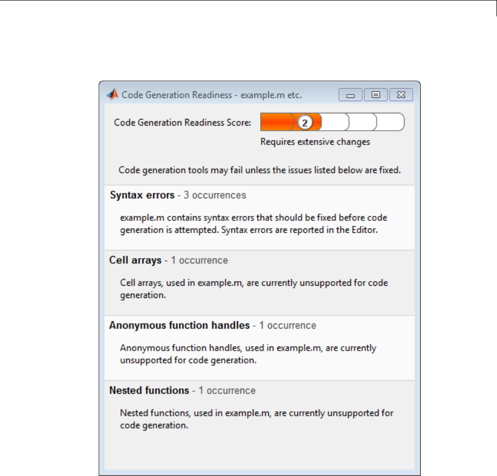
Code Generation Readiness Tool
Summary Tab
The Summary tab provides a Code Generation Readiness Score which
ranges from 1to 5.Ascoreof1indicates that the tool has detected issues that
requireextensivechangestotheMATLABcodetomakeitsuitableforcode
generation. A score of 5indicates that the tool has not detected any code
generation issues; the code is ready to use with no or minimal changes.
29-17
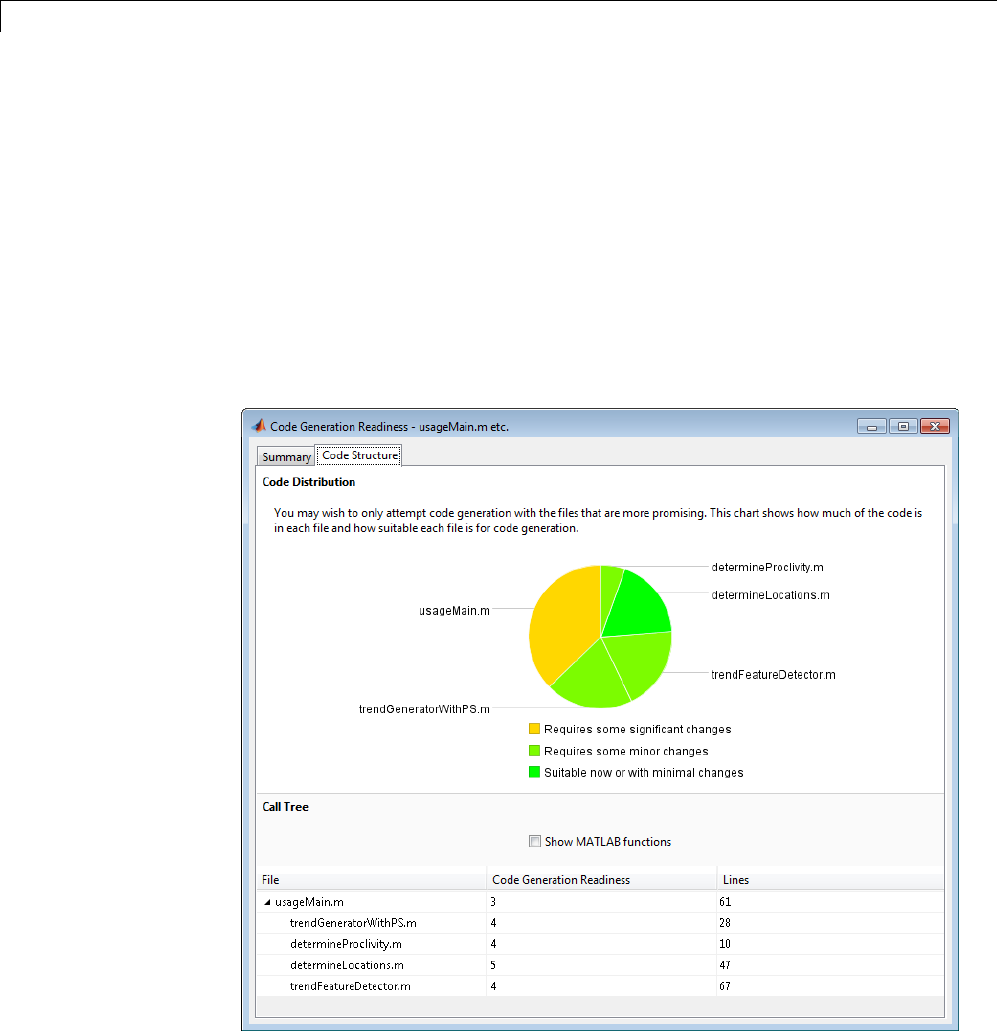
29 Using the MATLAB Function Block
On this tab, the tool also provides information about:
•MATLAB syntax issues. These issues are reported in the MATLAB editor.
Use the code analyzer to learn more about the issues and how to fix them.
•Unsupported MATLAB function calls.
•Unsupported MATLAB language features, such as recursion, cell arrays,
nested functions, and function handles.
•Unsupported data types.
Code Structure Tab
29-18

Code Generation Readiness Tool
Ifthecodethatyouarecheckingcalls other MATLAB functions, or you
are checking multiple entry-point functions, the tool displays the Code
Structure Tab.
This tab provides information about the relative size of each file and how
suitable each file is for code generation.
Code Distribution
The Code Distribution pane provides a pie chart that shows the relative
sizes of the files and how suitable each file is for code generation. This
information is useful during the planning phase of a project for estimation
and scheduling purposes. If the report indicates that there are multiple files
not yet suitable for code generation, consider fixing files that require minor
changes before addressing files with significant issues.
Call Tree
The Call Tree pane provides information on the nesting of function calls. For
each called function, the report provides a Code Generation Readiness
score which ranges from 1to 5.Ascoreof1indicates that the tool has detected
issues that require extensive changes to the MATLAB code to make it suitable
for code generation. A score of 5indicates that the tool has not detected any
code generation issues; the code is ready to use with no or minimal changes.
The report also lists the number of lines of code in each file.
Show MATLAB Functions. If you select Show MATLAB Functions,the
report also lists all the MATLAB functions called by your function code.
For each of these MATLAB functions, if the function is supported for code
generation, the report sets Code Generation Readiness to Yes.
29-19
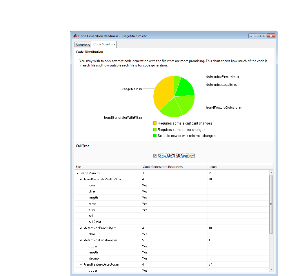
29 Using the MATLAB Function Block
29-20


29 Using the MATLAB Function Block
Check Code Using the Code Generation Readiness Tool
In this section...
“Run Code Generation Readiness Tool at the Command Line” on page 29-22
“Run the Code Generation Readiness Tool From the Current Folder
Browser” on page 29-22
Run Code Generation Readiness Tool at the
Command Line
1Navigate to the folder that contains the file that you want to check for
code generation readiness.
2At the MATLAB command prompt, enter:
coder.screener('filename')
The Code Generation Readiness tool opens for the file named filename,
provides a code generation readiness score, and lists issues that must be
fixed prior to code generation.
Run the Code Generation Readiness Tool From the
Current Folder Browser
1In the current folder browser, right-click the file that you want to check for
code generation readiness.
2From the context menu, select Check Code Generation Readiness.
The Code Generation Readiness tool opens for the selected file and
provides a code generation readiness score and lists issues that must be
fixed prior to code generation.
29-22

Debugging a MATLAB Function Block
Debugging a MATLAB Function Block
In this section...
“How Debugging Affects Simulation Speed” on page 29-23
“Enabling and Disabling Debugging” on page 29-23
“Debugging the Function in Simulation” on page 29-23
“Watching Function Variables During Simulation” on page 29-27
“Checking for Data Range Violations” on page 29-29
“Debugging Tools” on page 29-29
How Debugging Affects Simulation Speed
Debugging a MATLAB Function block slows simulation. For maximum
simulation speed, disable debugging as described in “Enabling and Disabling
Debugging” on page 29-23.
Enabling and Disabling Debugging
There are two levels of debugging available when using MATLAB Function
blocks, model level debugging and block level debugging.
Disable debugging for an entire model by clearing the Enable
debugging/animation check box in the Simulation Target pane in the
Configuration Parameters dialog. Disable debugging for an individual
MATLAB Function block by clicking Breakpoints > Enable Debugging in
the MATLAB Function Block Editor. If Enable Debugging is unavailable,
then the Simulation Target pane in the Configuration Parameters dialog is
controlling debugging.
Debugging the Function in Simulation
In “Create Model That Uses MATLAB Function Block” on page 29-9, you
created an example model with a MATLAB Function block that calculates the
mean and standard deviation for a set of input values.
To debug the MATLAB Function in this model:
29-23
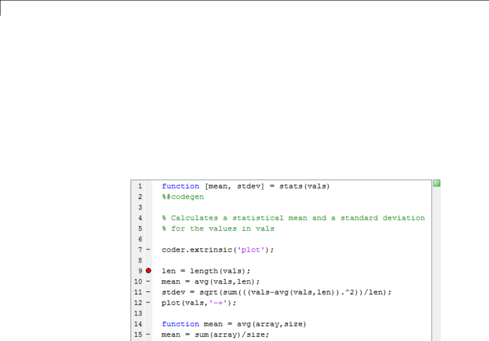
29 Using the MATLAB Function Block
1Open thecall_stats_block2 model and double-click its MATLAB
Function block stats to open it for editing.
2In the MATLAB Function Block Editor, click the dash (-) character in
the left margin of the line:
len = length(vals);
A small red ball appears in the margin of this line, indicating that you
have set a breakpoint.
29-24
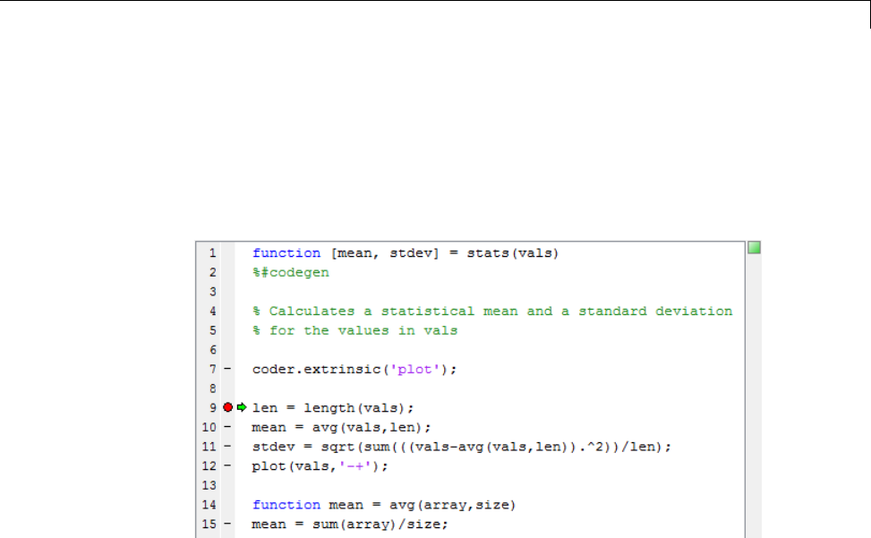
Debugging a MATLAB Function Block
3Begin simulating the model:
If you get any errors or warnings, make corrections before you try to
simulate again. Otherwise, simulation pauses when execution reaches
the breakpoint you set. This is indicated by a small green arrow in the
left margin.
4Select Step to advance execution.
The execution arrow advances to the next line of stats, which calls the
local function avg.
5Select Step In.
Execution advances to enter the local function avg. Onceyouareinalocal
function, you can use the Step or Step In commands to advance execution.
If the local function calls another local function, use the Step In icon to
enter it. If you want to execute the remaining lines of the local function,
use Step Out.
6Select Step to execute the only line in the local function avg. When the
local function avg finishes executing, a green arrow pointing down under
its last line appears.
7Select Step again to return to the function stats.
29-25
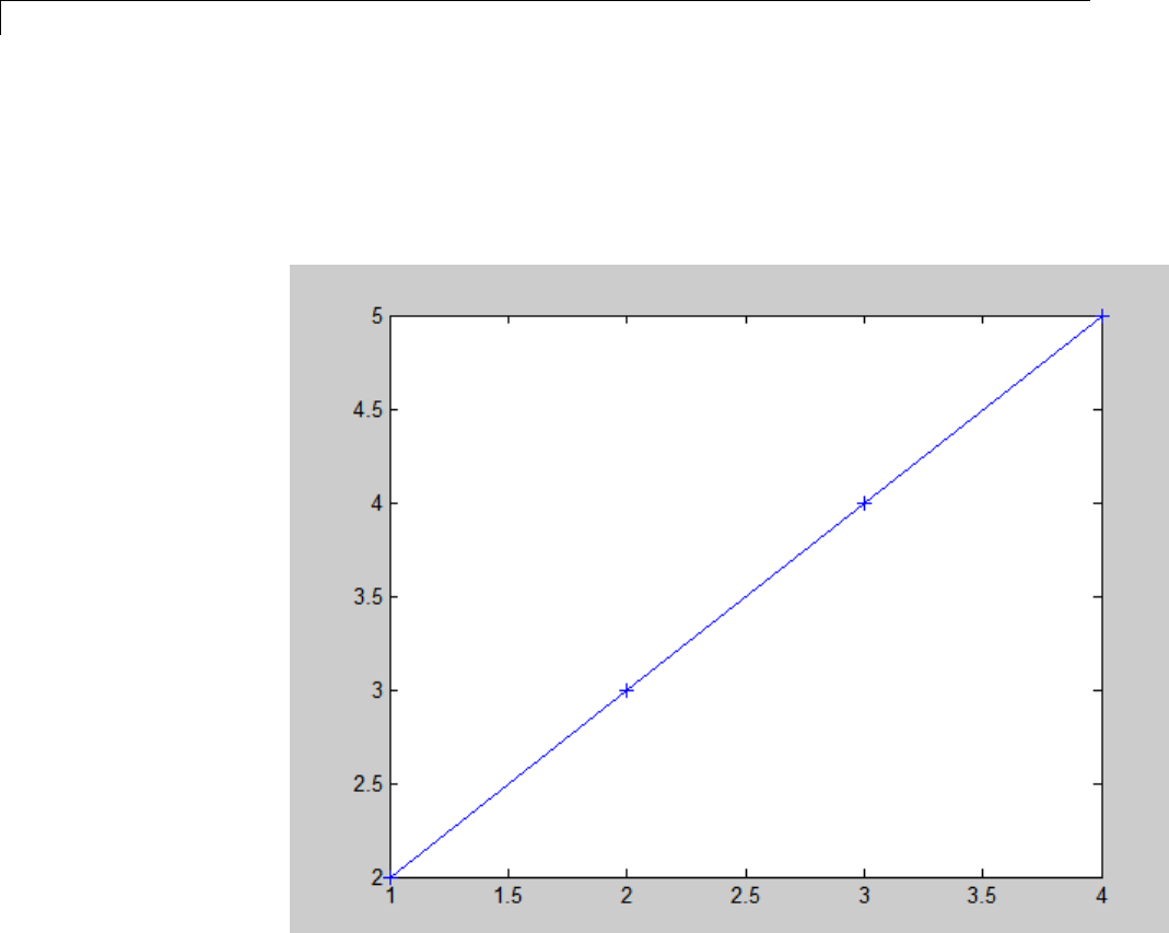
29 Using the MATLAB Function Block
Execution advances to the line after the call to the local function avg.
8Step again twice to calculate the stdev and to execute the plot function.
The plot function executes in MATLAB:
In the MATLAB Function Block Editor, a green arrow points down under
the last line of code, indicating the completion of the function stats.
9Select Continue to continue execution of the model.
The computed values of mean and stdev now appear in the Display blocks.
29-26
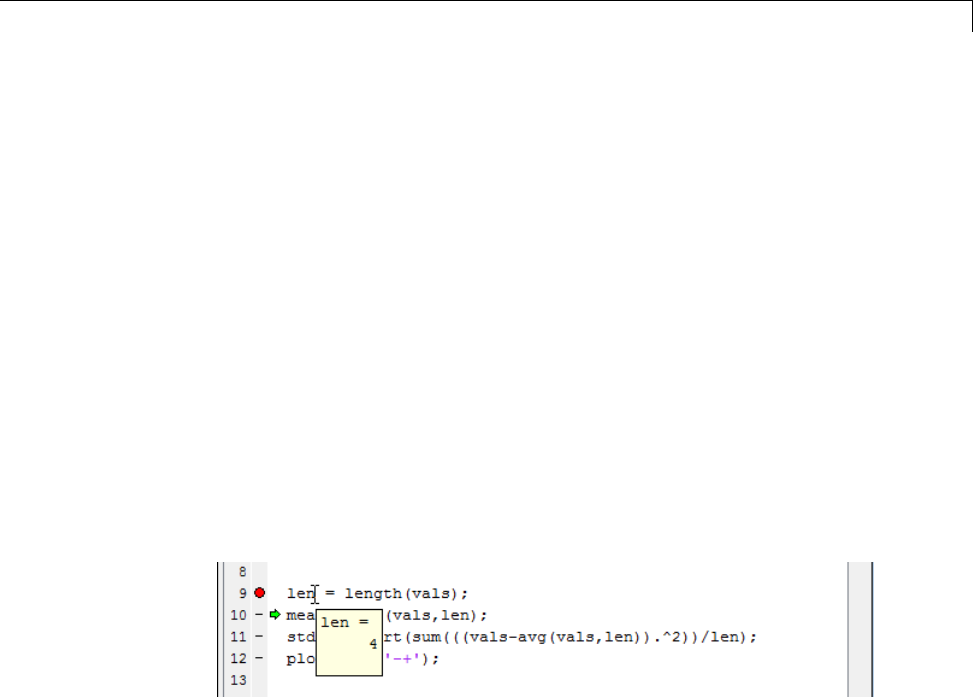
Debugging a MATLAB Function Block
10 In the MATLAB Function Block Editor, select Quit Debugging to stop
simulation.
Watching Function Variables During Simulation
While you simulate a MATLAB Function block, you can use several tools to
keep track of variable values in the function.
Watching with the Interactive Display
To display the value of a variable in the function of a MATLAB Function
block during simulation:
1In the MATLAB Function Block Editor, place the mouse cursor over the
variable text and observe the pop-up display.
For example, to watch the variable len during simulation, place the mouse
cursor over the text len in the code. The value of len appears adjacent to
the cursor, as shown:
Watching with the Command Line Debugger
You can report the values for a function variable with the Command Line
Debugger utility in the MATLAB window during simulation. When you reach
abrea
kpoint, the Command Line Debugger prompt, debug>>, appears. At
this prompt, you can see the value of a variable defined for the MATLAB
Function block by entering its name:
debug>> stdev
1.1180
debug>>
29-27

29 Using the MATLAB Function Block
The Command Line Debugger also provides the following commands during
simulation:
Command Description
ctrl-c Quit debugging and terminate simulation.
dbcont Continue execution to next breakpoint.
dbquit Quit debugging and terminate simulation.
dbstep
[in|out]
Advance to next program step after a breakpoint is
encountered. Step over or step into/out of a MATLAB local
function.
help Display help for command line debugging.
print <var> Display the value of the variable var in the current scope. If
var is a vector or matrix, you can also index into var.For
example, var(1,2).
save Saves all variables in the current scope to the specified file.
Follows the syntax of the MATLAB save command. To
retrieve variables to the MATLAB base workspace, use load
command after simulation has been ended.
<var> Equivalent to "print <var>" if variable is in the current
scope.
who Display the variables in the current scope.
whos Display the size and class (type) of all variables in the
current scope.
You can issue any other MATLAB command at the debug>> prompt, but the
results are executed in the workspace of the MATLAB Function block. To
issueacommandintheMATLABbaseworkspaceatthedebug>> prompt, use
the evalin command with the first argument 'base' followed by the second
argument command string, for example, evalin('base','whos').Toreturn
to the MATLAB base workspace, use the dbquit command.
29-28

Debugging a MATLAB Function Block
Watching with MATLAB
You can display the execution result of a MATLAB Function block line by
omitting the terminating semicolon. If you do, execution results for the line
are echoed to the MATLAB window during simulation.
Display Size Limits
The MATLAB Function Block Editor does not display the contents of matrices
that have more than two dimensions or more than 200 elements. For matrices
that exceed these limits, the MATLAB Function Block Editor displays the
shape and base type only.
Checking for Data Range Violations
When you enable debugging, MATLAB Function blocks automatically check
input and output data for data range violations when the values enter or
leave the blocks.
Specifying a Range
To specify a range for input and output data, follow these steps:
1In the Ports and Data Manager, select the input or output of interest.
The data properties dialog box opens.
2In the data properties dialog box, select the General tab and enter a limit
range, as described in “Setting General Properties” on page 29-44.
Debugging Tools
Use the following tools during a MATLAB Function block debugging session:
29-29
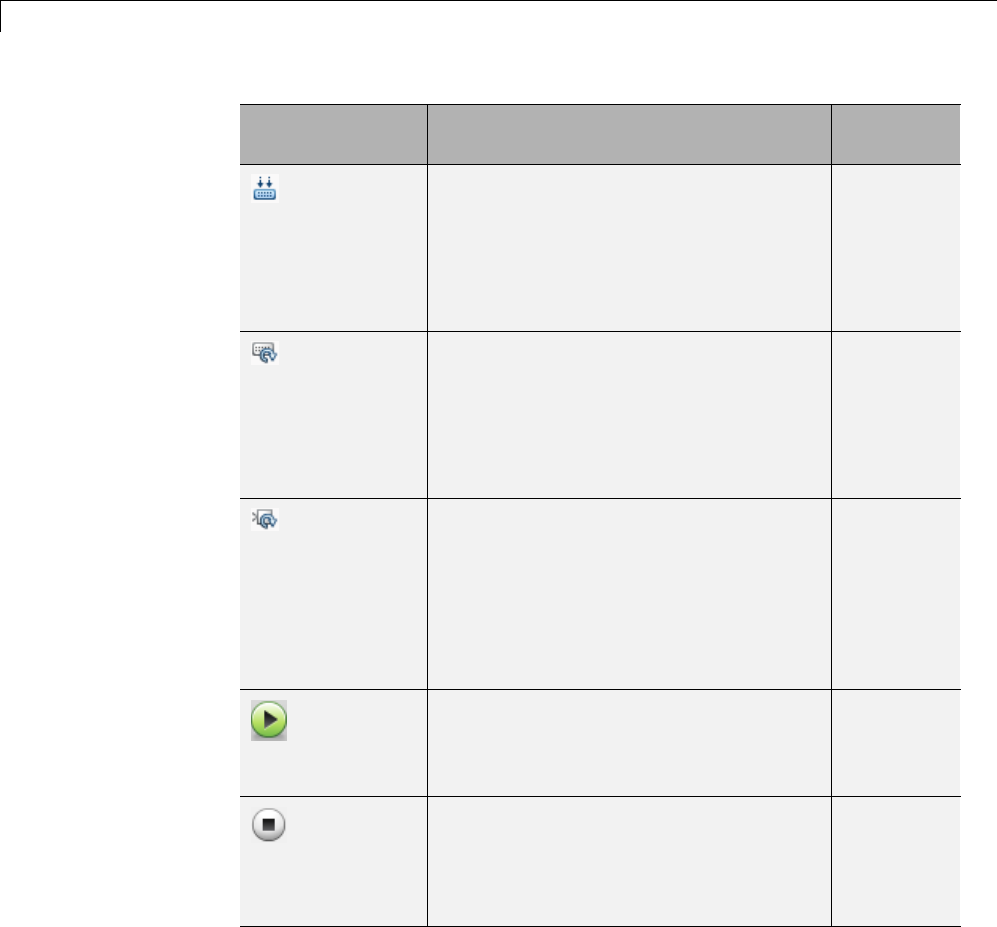
29 Using the MATLAB Function Block
Tool Button Description
Shortcut
Key
Build
Access this tool from the Editor tab by
selecting Build Model > Build.
Check for errors and build a simulation
application (if no errors are found) for the
model containing this MATLAB Function
block.
Ctrl+B
Update
Diagram
Access this tool from the Editor tab
by selecting Build Model > Update
Diagram.
Check for errors based on the latest
changes you make to the MATLAB
Function block.
Ctrl+D
Update Ports
Access this tool from the Editor tab by
selecting Build Model > Update Ports.
Updates the ports of the MATLAB
Function block with the latest changes
made to the function argument and
return values without closing the
MATLAB Function Block Editor.
Ctrl+Shift+A
Run Model
Start simulation of the model containing
the MATLAB Function block. If execution
is paused at a breakpoint, continues
debugging.
F5
Stop Model
Stop simulation of the model containing
the MATLAB Function block.
Alternatively, from the Editor tab,
select Quit Debugging if execution is
paused at a breakpoint.
Shift+F5
29-30
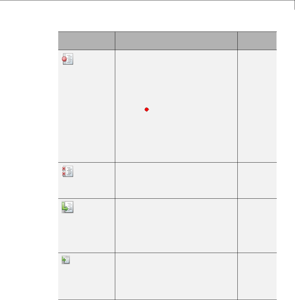
Debugging a MATLAB Function Block
Tool Button Description
Shortcut
Key
Set/Clear
Access this tool by selecting
Breakpoints > Set/Clear.
Set a new breakpoint or clear an existing
breakpoint for the selected line of code
in the MATLAB Function block. The
presence of the text cursor or highlighted
text selects the line. A breakpoint
indicator appears in the on the selected
line.
Alternatively, click the hyphen character
(-) next to the line number. A breakpoint
indicator appears in place of the hyphen.
Click the breakpoint indicator to clear
the breakpoint.
F12
Clear All
Access this tool by selecting
Breakpoints > Clear All.
Clear all existing breakpoints in the
MATLAB Function block code.
None
Step
Step through the execution of the next
line of code in the MATLAB Function
block. This tool steps past function calls
and does not enter called functions for
line-by-line execution. You can use this
tool only after execution has stopped at a
breakpoint.
F10
Step In
Step through the execution of the next
line of code in the MATLAB Function
block. If the line calls a local function,
step into the first line of the local
function. You can use this tool only after
execution has stopped at a breakpoint.
F11
29-31

29 Using the MATLAB Function Block
Tool Button Description
Shortcut
Key
Step Out
Step out of line-by-line execution of the
current function or local function. If in
a local function, the debugger continues
to the line following the call to this local
function. You can use this tool only after
execution has stopped at a breakpoint.
Shift+F11
Continue
Continue debugging after a pause, such
as stopping at a breakpoint. You can use
this tool only after execution has stopped
at a breakpoint.
F5
Quit Debugging
Exit debug mode. You can use this tool
only after execution has stopped at a
breakpoint.
Shift+F5
29-32
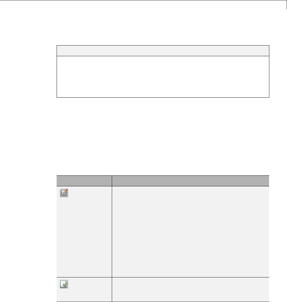
MATLAB Function Block Editor
MATLAB Function Block Editor
In this section...
“Customizing the MATLAB Function Block Editor” on page 29-33
“MATLAB Function Block Editor Tools” on page 29-33
“Editing and Debugging MATLAB Function Block Code” on page 29-34
“Ports and Data Manager” on page 29-37
Customizing the MATLAB Function Block Editor
Use the toolbar icons to customize the appearance of the MATLAB Function
Block Editor in the same manner as the MATLAB editor. See “Adjust Desktop
Appearance”.
MATLAB Function Block Editor Tools
Use the following tools to work with the MATLAB Function block:
Tool Button Description
Edit Data
OpensthePortsandDataManagerdialogtoaddor
modify arguments for the current MATLAB Function
block (see “Ports and Data Manager” on page 29-37).
View Report
Opens the MATLAB Function report for the MATLAB
Function block. For more information, see “MATLAB
Function Reports” on page 29-51.
29-33
29 Using the MATLAB Function Block
Tool Button Description
Simulation
Target
Opens the Simulation Target pane in the
Configuration Parameters dialog to enable
debugging or include custom code. See “Enabling
and Disabling Debugging” on page 29-23 for more
information on debugging
Go To Diagram
Displays the MATLAB function in its native diagram
without closing the editor.
See “Defining Inputs and Outputs” on page 29-14 for an example of defining
an input argument for a MATLAB Function block.
Editing and Debugging MATLAB Function Block Code
Commenting Out a Block of Code
To comment out a block of code in the MATLAB Function Block Editor:
1Highlight the text that you would like to comment out.
2Hold the mouse over the highlighted text and then right-click and select
Comment from the context menu. (Alternatively, select a Comment tool
from the Editor tab.
Note To uncomment a block of code, follow the same steps, but select
Uncomment instead of Comment.
Manual Indenting
To indent a block of code manually:
1Highlight the text that you would like to indent.
2Select one of the Indent tools on the Editor tab:
29-34

MATLAB Function Block Editor
Tool Description
Applies smart indenting to selected
text.
Move selected text right one indent
level.
Move selected text left one indent
level.
Opening a Selection
You can open a local function, function, file, or variable from within a file in
the MATLAB Function Block Editor.
To open a selection:
1Position the cursor in the name of the item you would like to open.
2Right-click and select Open <selection> from the context menu.
The Editor chooses the appropriate tool to open the selection. For more
information, refer to “Opening Files and Functions in the Command Window”.
Note IfyouopenaMATLABFunctionblockinputoroutputparameter,the
Ports and Data Manager opens with the selected parameter highlighted. You
can use the Ports and Data Manager to modify parameter attributes. For
more information, refer to “Ports and Data Manager” on page 29-37.
Evaluating a Selection
You can use the Evaluate a Selection menu option to report the value for
a MATLAB function variable or equation in the MATLAB window during
simulation.
To evaluate a selection:
1Highlight the variable or equation that you would like to evaluate.
29-35

29 Using the MATLAB Function Block
2Hold the mouse over the highlighted text and then right-click and select
Evaluate Selection from the context menu. (Alternatively, select
Evaluate Selection from the Text menu).
When you reach a breakpoint, the MATLAB command Window displays the
value of the variable or equation at the Command Line Debugger prompt.
debug>> stdev
1.1180
debug>>
Note You cannot evaluate a selection while MATLAB is busy, for example,
running a MATLAB file.
Setting Data Scope
To set the data scope of a MATLAB Function block input parameter:
1Highlight the input parameter that you would like to modify.
2Hold the mouse over the highlighted text and then right-click and select
Data Scope for <selection> from the context menu.
3Select:
•Input if your input data is provided by the Simulink model via an input
port to the MATLAB Function block.
•Parameter if your input is a variable of the same name in the MATLAB
or model workspace or in the workspace of a masked subsystem
containing this block.
For more information, refer to “Setting General Properties” on page 29-44.
29-36

MATLAB Function Block Editor
Ports and Data Manager
The Ports and Data Manager provides a convenient method for defining
objects and modifying their properties in a MATLAB Function block that
is open and has focus.
The Ports and Data Manager provides the same data definition capabilities
for individual MATLAB Function blocks. as the Model Explorer provides
across the model hierarchy (see “Model Explorer Overview” on page 9-2).
Ports and Data Manager Dialog Box
The Ports and Data Manager dialog box allows you to add and define data
arguments, input triggers, and function call outputs for MATLAB Function
blocks. Using this dialog, you can also modify properties for the MATLAB
Function block and the objects it contains.
The dialog box consists of two panes:
•The Contents (left) pane lists the objects that have been defined for the
MATLAB Function block.
•The Dialog (right) pane displays fields for modifying the properties of the
selectedobject.
Properties vary according to the scope and type of the object. Therefore, the
Ports and Data Manager properties dialogs are dynamic, displaying only the
property fields that are relevant for the object you add or modify.
When you first open the dialog box, it displays the properties of the MATLAB
Function block.
Opening the Ports and Data Manager
To open the Ports and Data Manager from the MATLAB Function Block
Editor, select Edit Data on the Editor tab. The Ports and Data Manager
appears for the MATLAB Function block that is open and has focus.
Ports and Data Manager Tools
The following tools are specific to the Ports and Data Manager:
29-37

29 Using the MATLAB Function Block
Tool Button Description
Go to Block
Editor
Displays the MATLAB function in the MATLAB
Function Block Editor.
Show Block
Dialog
Displays the default MATLAB function properties (see
“MATLAB Function Block Properties” on page 29-38).
Use this button to return to the settings used by the
block after viewing data associated with the block
arguments.
MATLAB Function Block Properties
This section describes each property of a MATLAB Function block.
Name. Name of the MATLAB Function block, following the same naming
conventions as for Simulink blocks (see “Manipulate Block Names” on page
23-26).
Update method. Method for activating the MATLAB Function block. You
can choose from the following update methods:
Update
Method
Description
Inherited
(default)
Input from the Simulink model activates the MATLAB
Function block.
If you define an input trigger, the MATLAB Function block
executes in response to a Simulink signal or function-call
event on the trigger port. If you do not define an input trigger,
the MATLAB Function block implicitly inherits triggers
from the model. These implicit events are the sample times
(discrete or continuous) of the signals that provide inputs to
the chart.
If you define data inputs, the MATLAB Function block
samples at the rate of the fastest data input. If you do not
29-38

MATLAB Function Block Editor
Update
Method
Description
define data inputs, the MATLAB Function block samples as
defined by its parent subsystem’s execution behavior.
Discrete The MATLAB Function block is sampled at the rate you
specify as the block’s Sample Time property. An implicit
event is generated at regular time intervals corresponding to
the specified rate. The sample time is in the same units as
the Simulink simulation time. Note that other blocks in the
model can have different sample times.
Continuous The Simulink software wakes up (samples) the MATLAB
Function block at each step in the simulation, as well as at
intermediate time points that can be requested by the solver.
This method is consistent with the continuous method.
Saturate on integer overflow. Option that determines how the MATLAB
Function block handles overflow conditions during integer operations:
Setting Action When Overflow Occurs
Enabled
(default)
Saturates an integer by setting it to the maximum positive or
negative value allowed by the word size. Matches MATLAB
behavior.
Disabled In simulation mode, generates a run-time error. For Simulink
Coder code generation, the behavior depends on your C
language compiler.
Note The Saturate on integer overflow option is relevant only for integer
arithmetic. It has no effect on fixed-point or double-precision arithmetic.
When you enable Saturate on integer overflow, MATLAB adds additional
checks during code generation to detect integer overflow or underflow.
Therefore, it is more efficient to disable this option if you are sure that integer
overflow and underflow will not occur in your MATLAB Function block code.
29-39

29 Using the MATLAB Function Block
Evenwhenyoudisablethisoption,thecodeforasimulationtargetchecksfor
integer overflow and underflow. If either condition occurs, simulation stops
and an error is generated. If you enable debugging for the MATLAB Function
block, the debugger displays the error and lets you examine the data.
If you did not enable debugging, the block generates a run-time error:
Overflow detected. Enable debugging for more information.
Note that the code generated by Simulink Coder does not check for integer
overflow or underflow and, therefore, may produce unpredictable results
when Saturate on integer overflow is disabled. In this situation, it is
recommended that you simulate first to test for overflow and underflow before
generating code.
Lock Editor. Option for locking the MATLAB Function Block Editor. When
enabled, this option prevents users from making changes to the MATLAB
Function block.
Treat these inherited Simulinksignaltypesasfiobjects.
Setting that determines whether to treat inherited fixed-point and integer
signals as Fixed-Point Toolbox™ fi objects (“Ways to Construct fi Objects”).
•When you select Fixed-point, the MATLAB Function block treats all
fixed-point inputs as Fixed-Point Toolbox fi objects.
•When you select Fixed-point & Integer, the MATLAB Function block
treats all fixed-point and integer inputs as Fixed-Point Toolbox fi objects.
MATLAB Function block fimath. Setting that defines fimath properties
for the MATLAB Function block. The block associates the fimath properties
you specify with the following objects:
•All fixed-point and integer input signals to the MATLAB Function block
that you choose to treat as fi objects.
•All fi and fimath objects constructed in the MATLAB Function block.
You can select one of the following options for the MATLAB Function block
fimath.
29-40

MATLAB Function Block Editor
Setting Description
Same as
MATLAB
When you select this option, the block uses the same fimath properties as
the current default fimath. The edit box appears dimmed and displays the
current global fimath in read-only form.
29-41

29 Using the MATLAB Function Block
Setting Description
Specify other When you select this option, you can specify your own fimath object in the
edit box. You can do so in one of two ways:
•Constructing the fimath object inside the edit box.
•Constructing the fimath object in the MATLAB or model workspace and
then entering its variable name in the edit box. If you use this option
andplantoshareyourmodelwithothers,makesureyoudefinethe
variable in the model workspace. See “Sharing Models with Fixed-Point
MATLAB Function Blocks”.
For more information on fimath objects, see “fimath Object Construction”.
Description. Description of the MATLAB Function block.
Document link. Link to documentation for the MATLAB Function block. To
document a MATLAB Function block, set the Document link property to a
Web URL address or MATLAB expression that displays documentation in a
suitable format (for example, an HTML file or text in the MATLAB Command
Window). The MATLAB Function block evaluates the expression when you
click the blue Document link text.
Adding Data to a MATLAB Function Block
You can define data arguments for MATLAB Function blocks using the
following methods:
Method For Defining Reference
Define data directly in
the MATLAB Function
block code
Input and output data See “Defining Inputs
and Outputs” on page
29-14.
Use the Ports and Data
Manager
Input, output, and
parameter data in the
MATLAB Function
See “Defining Data in
the Ports and Data
29-42
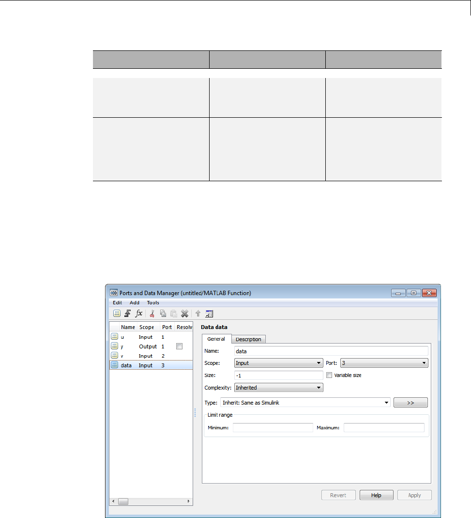
MATLAB Function Block Editor
Method For Defining Reference
block that is open and
has focus
Manager” on page
29-43.
Use the Model Explorer Input, output, and
parameter data in
MATLAB Function
blocks at all levels of
the model hierarchy
See “Model Explorer
Overview” on page 9-2
Defining Data in the Ports and Data Manager. To add a data argument
and modify its properties, follow these steps:
1In the Ports and Data Manager, select Add > Data
The Ports and Data Manager adds a default definition of the data to the
MATLAB Function block.
29-43

29 Using the MATLAB Function Block
2Modify data properties.
3Return to the MATLAB Function block properties at any time by selecting
Tools > Block Dialog.
Setting General Properties. You can set the following properties in the
General tab:
Property Description
Name Name of the data argument, following the same naming conventions used
in MATLAB.
Scope Where data resides in memory, relative to its parent. Scope determines the
range of functionality of the data argument. You can set scope to one of the
following values:
•Parameter— Specifies that the source for thisdataisavariableofthe
same name in the MATLAB or model workspace or in the workspace of
a masked subsystem containing this block. If a variable of the same
name exists in more than one of the workspaces visible to the block, the
variableclosesttotheblockintheworkspace hierarchy is used (see “Model
Workspaces” on page 4-67).
•Input— Data provided by the model via an input port to the MATLAB
Function block.
•Output— Data provided by the MATLAB Function block via an output
port to the model.
•Data Store Memory— Data provided by a Data Store Memory block in
the model.
For more information, see “Defining Inputs and Outputs” on page 29-14 and
“Add Parameter Arguments” on page 29-75.
Port Index of the port associated with the data argument. This property applies
only to input and output data.
29-44

MATLAB Function Block Editor
Property Description
Tunable Indicates whether the parameter used as the source of this data item is
tunable(see“TunableParameters”onpage 3-9). This property applies only
to parameter data. Clear this option if the parameter must be a constant
expression, such as for MATLAB toolbox functions supported for code
generation (see “Functions Supported for Code Generation — Alphabetical
List” on page 31-2).
Data must
resolve to
Simulink
signal object
Specifies that the data argument must resolve to a Simulink signal object.
This property applies only to output data. See “Symbol Resolution” on page
4-76 for more information.
Size Sizeofthedataargument.SizecanbeascalarvalueoraMATLABvectorof
values. Size defaults to –1, which means that it is inherited, as described in
“Inheriting Argument Sizes from Simulink” on page 29-72. This property does
not apply to Data Store Memory data. For more details, see “Size Function
Arguments” on page 29-72.
Variable Size Indicates whether the size of this data item is variable. This property does
not apply to Data Store Memory data.
Complexity Indicates real or complex data arguments. You can set complexity to one of
the following values:
•Off— Data argument is a real number
•On— Data argument is a complex number
•Inherited— Data argument inherits complexity based on its scope. Input
and output data inherit complexity from the Simulink signals connected
to them; parameter data inherits complexity from the parameter to which
it is bound.
Sampling
mode
Specifies how an output signal propagates through a model. This property
applies only to data with scope equal to Output. You can set sampling mode
to one of the following values:
•Sample based: Propagate the signal sample by sample (default)
•Frame based: Propagate the signal in batches of samples
29-45
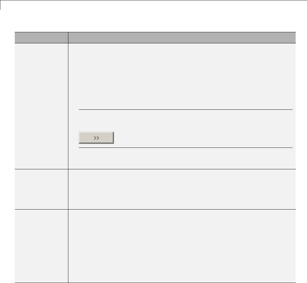
29 Using the MATLAB Function Block
Property Description
Type Type of data object. You can specify the data type by:
•Selecting a built-in type from the Type drop down list.
•Entering an expression in the Type field that evaluates to a data type (see
“Data Types” on page 43-2).
•Using the Data Type Assistant to specify a data Mode,thenspecifying
the data type based on that mode.
Note To display the Data Type Assistant, click the Show data type
assistant button:
For more information, see “Specifying Argument Types” on page 29-64.
Lock data type
setting against
changes by
the fixed-point
tools
Specify whether you want to prevent replacement of the current data
type with a type chosen by the Fixed-Point Tool or Fixed-Point Advisor.
The default setting allows replacement. See Scaling for instructions on
autoscaling fixed-point data.
Limit range Specify the range of acceptable values for input or output data. The MATLAB
Function block uses this range to validate the input or output as it enters or
leaves the block. You can enter an expression or parameter that evaluates to
a numeric scalar value.
•Minimum — The smallest value allowed for the data item during
simulation. The default value is -inf.
•Maximum — The largest value allowed for the data item during
simulation. The default value is inf.
Setting Description Properties. You can set the following properties on the
Description tab:
29-46

MATLAB Function Block Editor
Property Description
Save final
value
to base
workspace
The MATLAB Function block assigns the value of the data
argument to a variable of the same name in the MATLAB
base workspace at the end of simulation.
Description Description of the data argument.
Document
link
Link to documentation for the data argument. You can enter
a Web URL address or a MATLAB command that displays
documentation in a suitable format, such as an HTML file or
text in the MATLAB Command Window. When you click
the blue text, Document link, displayed at the bottom of
the Data properties dialog, the MATLAB Function block
evaluates the link and displays the documentation.
Adding Input Triggers to a MATLAB Function Block
An input trigger is an event on the input port that causes the MATLAB
Function block to execute. See “Triggered Subsystems” on page 7-20.
You can define the following types of triggers in MATLAB Function blocks:
•Rising
•Falling
•Either (rising or falling)
•Function call
For a description of each trigger type, see “Setting Input Trigger Properties”
on page 29-48.
Use the Ports and Data Manager to add input triggers to a MATLAB Function
block that is open and has focus. To add an input trigger and modify its
properties, follow these steps:
1In the Ports and Data Manager, select Add > Input Trigger.
29-47

29 Using the MATLAB Function Block
The Ports and Data Manager adds a default definition of the new input
trigger to the MATLAB Function block and displays the Trigger properties
dialog.
2Modify trigger properties.
3Return to the MATLAB Function block properties at any time by selecting
Tools > Block Dialog.
The Trigger Properties Dialog. The Trigger properties dialog in the Ports
and Data Manager allows you to set and modify the properties of input
triggers in MATLAB Function blocks.
To open the Trigger properties dialog, select an input trigger in the Contents
pane.
Setting Input Trigger Properties. You can set the following properties in
the Trigger properties dialog:
Property Description
Name Name of the input trigger, following the same naming
conventions used in MATLAB.
Port Index of the port associated with the input trigger. The
default value is 1.
Trigger Type of event that triggers execution of the MATLAB
Function block. You can select one of the following types
of triggers:
•Rising (default) — Triggers execution of the MATLAB
Function block when the control signal rises from a
negative or zero value to a positive value (or zero if the
initial value is negative).
•Falling— Triggers execution of the MATLAB Function
block when the control signal falls from a positive or zero
value to a negative value (or zero if the initial value is
positive).
•Either— Triggers execution of the MATLAB Function
block when the control signal is either rising or falling.
29-48

MATLAB Function Block Editor
Property Description
•Function call— Triggers execution of the MATLAB
Function block from a block that outputs function-call
events, or from an S-function
Description Description of the input trigger.
Document
link
Link to documentation for the input trigger. You can
enter a Web URL address or a MATLAB command that
displays documentation in a suitable format, such as an
HTML file or text in the MATLAB Command Window.
When you click the blue text that reads Document link
displayed at the bottom of the Trigger properties dialog,
the MATLAB Function block evaluates the link and
displays the documentation.
Adding Function Call Outputs to a MATLAB Function Block
A function call output is an event on the output port of a MATLAB Function
block that causes a function-call subsystem in the Simulink model to execute.
A function-call subsystem is a subsystem that another block can invoke
directly during a simulation. See “Function-Call Subsystems” on page 7-30.
Use the Ports and Data Manager to add and modify function call outputs to a
MATLAB Function block that is open and has focus. To add a function call
output and modify its properties, follow these steps:
1In the Ports and Data Manager, select Add > Function Call Output.
The Ports and Data Manager adds a default definition of the new function
call output to the MATLAB Function block and displays the Function Call
properties dialog.
2Modify function call output properties.
3Return to the MATLAB Function block properties at any time by selecting
Tools > Block Dialog.
29-49

29 Using the MATLAB Function Block
The Function Call Properties Dialog. The Function Call properties dialog
in the Ports and Data Manager allows you to edit the properties of function
call outputs in MATLAB Function blocks.
To open the Function Call properties dialog, select a function call output
in the Contents pane.
Setting Function Call Output Properties. You can set the following
properties in the Function Call properties dialog:
Property Description
Name Name of the function call output, following the same naming
conventions used in MATLAB.
Port Index of the port associated with the function call output.
Function call output ports are numbered sequentially after
input and output ports.
Description Description of the function call output.
Document
link
Link to documentation for the function call output. You
can enter a Web URL address or a MATLAB command
that displays documentation in a suitable format, such as
an HTML file or text in the MATLAB Command Window.
When you click Document link displayed at the bottom of
the Function Call properties dialog, the MATLAB Function
block evaluates the link and displays the documentation.
29-50

MATLAB Function Reports
MATLAB Function Reports
In this section...
“About MATLAB Function Reports” on page 29-51
“Location of MATLAB Function Reports” on page 29-51
“Opening MATLAB Function Reports” on page 29-52
“Description of MATLAB Function Reports” on page 29-52
“Viewing Your MATLAB Function Code” on page 29-52
“Viewing Call Stack Information” on page 29-54
“Viewing the Compilation Summary Information” on page 29-54
“Viewing Error and Warning Messages” on page 29-54
“Viewing Variables in Your MATLAB Code” on page 29-56
“Keyboard Shortcuts for the MATLAB Function Report” on page 29-61
“Report Limitations” on page 29-62
About MATLAB Function Reports
Whenever you build a Simulink model that contains MATLAB Function
blocks, Simulink automatically generates a report in HTML format for each
MATLAB Function block in your model. The report helps you debug your
MATLAB functions and verify that they aresuitableforcodegeneration.
The report provides links to your MATLAB functions and compile-time type
information for the variables and expressions in these functions. If your model
fails to build, this information simplifies finding sources of error messages
and aids understanding of type propagation rules.
Note If you have a Stateflow license, there is one report for each Stateflow
chart, regardless of the number of MATLAB functions it contains.
Location of MATLAB Function Reports
The code generation software provides a report for each MATLAB Function
block in the model model_name at the following location:
29-51

29 Using the MATLAB Function Block
slprj/_sfprj/
model_name/_self/
sfun/html/
Opening MATLAB Function Reports
Useoneofthefollowingmethods:
•In the MATLAB Function Block Editor, select View Report.
•In the Simulation Diagnostics window, select the report link if
compilation errors occur.
Description of MATLAB Function Reports
When you build the MATLAB function, the code generation software
generates an HTML report. The report provides the following information,
as applicable:
•MATLAB code information, including a list of all functions and their
compilation status
•Call stack information, providing information on the nesting of function
calls
•Summary of compilation results, including type of target and number of
warnings or errors
•List of all error and warning messages
•List of all variables in your MATLAB function
ViewingYourMATLABFunctionCode
To view your MATLAB function code, click the MATLAB code tab. The report
displaystheMATLABcodeforthefunction highlighted in the list on this tab.
The MATLAB code tab provides:
•A list of the MATLAB functions that have been compiled. The report
displays icons next to each function name to indicate whether compilation
was successful:
-Errors in function.
29-52

MATLAB Function Reports
-Warnings in function.
-Successful compilation, no errors or warnings.
•A filter control that you can use to sort your functions by:
-Size
-Complexity
-Class
Viewing Local Functions
The report annotates the local function with the name of the parent function
in the list of functions on the MATLAB code tab.
For example, if the MATLAB function fcn1 contains the local function subfcn
and fcn2 contains the local function subfcn2, the report displays:
fcn1 > subfcn1
fcn2 > subfcn2
Viewing Specializations
If your MATLAB function calls the same function with different types of
inputs, the report numbers each of these specializations in the list of
functions on the MATLAB code tab.
For example, if the function fcn calls the function subfcn with different
types of inputs:
function y = fcn(u) %#codegen
% Specializations
y = y + subfcn(single(u));
y = y + subfcn(double(u));
The report numbers the specializations in the list of functions.
fcn > subfcn > 1
fcn > subfcn > 2
29-53

29 Using the MATLAB Function Block
ViewingCallStackInformation
The report provides call stack information:
•On the Call stack tab.
•In the list of Callers.
If a function is called from more than one function, this list provides details
of each call site. Otherwise, the list is disabled.
Viewing Call Stack Information on the Call Stack Tab
To view call stack information, click the Call stack tab. The call stack lists
the functions in the order that the top-level function calls them. It also lists
the local functions that each function calls.
Viewing Function Call Sites in the Callers List
If a function is called from more than one function, this list provides details
of each call site. To navigate between call sites, select a call site from the
Callers list. If the function is not called more than once, this list is disabled.
Viewing the Compilation Summary Information
To view a summary of the compilation results, including type of target and
number of errors or warnings, click the Summary tab.
Viewing Error and Warning Messages
The report provides information about errors and warnings. If errors occur
during simulation of a Simulink model, simulation stops. If warnings occur,
but no errors, simulation of the model continues.
The report provides information about warnings and errors by listing all
errors and warnings in chronological order in the All Messages tab.
29-54
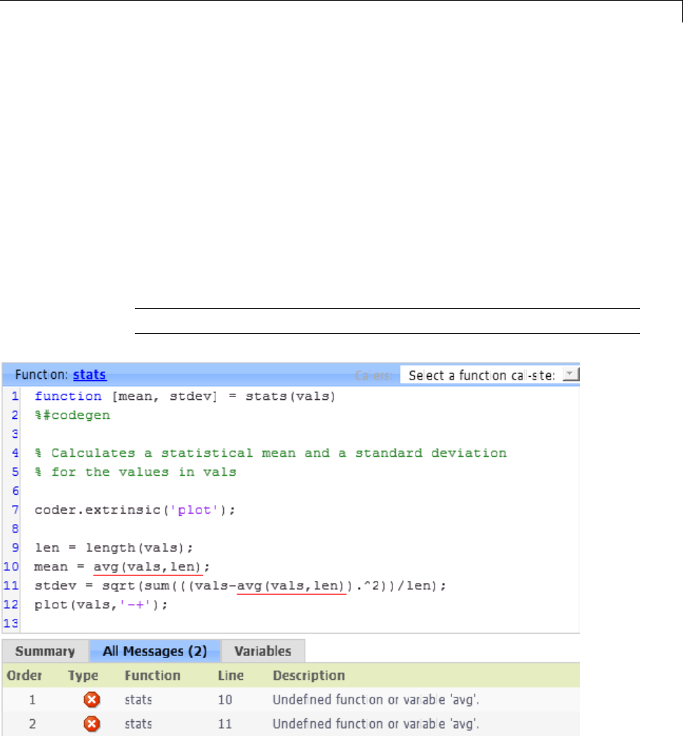
MATLAB Function Reports
Viewing Errors and Warnings in the All Messages Tab
If errors or warnings occurred during compilation, click the All Messages tab
to view a complete list of these messages. The report lists the messages in
the order that the compiler detects them. It is best practice to address the
first message in the list, because often subsequent errors and warnings are
related to the first message.
To locate the offending line of code for an error or warning in the list, click
the message in the list. The report highlights errors in the list and MATLAB
code in red and warnings in orange. Click the blue line number next to the
offendinglineofcodeintheMATLABcodepanetogototheerrorinthe
source file.
Note You can fix errors only in the source file.
29-55

29 Using the MATLAB Function Block
Viewing Error and Warning Information in Your MATLAB Code
If errors or warnings occurred during compilation, the report underlines them
in your MATLAB code. The report underlines errors in red and warnings in
orange. To learn more about a particular error or warning, place your pointer
over the underlined text.
Viewing Variables in Your MATLAB Code
Thereportprovidescompile-timetypeinformationforthevariablesand
expressions in your MATLAB code, including name, type, size, complexity,
and class. It also provides type information for fixed-point data types,
including word length and fraction length. You can use this type information
to find sources of error messages and to understand type propagation rules.
You can view information about the variables in your MATLAB code:
•On the Variables tab, view the list
•In your MATLAB code, place your pointer over the variable name
Viewing Variables in the Variables Tab
To view a list of all the variables in your MATLAB function, click the
Variables tab. The report displays a complete list of variables in the order
that they appear in the function selected on the MATLAB code tab. Clicking
a variable in the list highlights all instances of that variable, and scrolls the
MATLAB code pane so that you can view the first instance.
The report provides the following information about each variable, as
applicable.
•Order
•Name
•Type
•Size
•Complexity
•Class
29-56
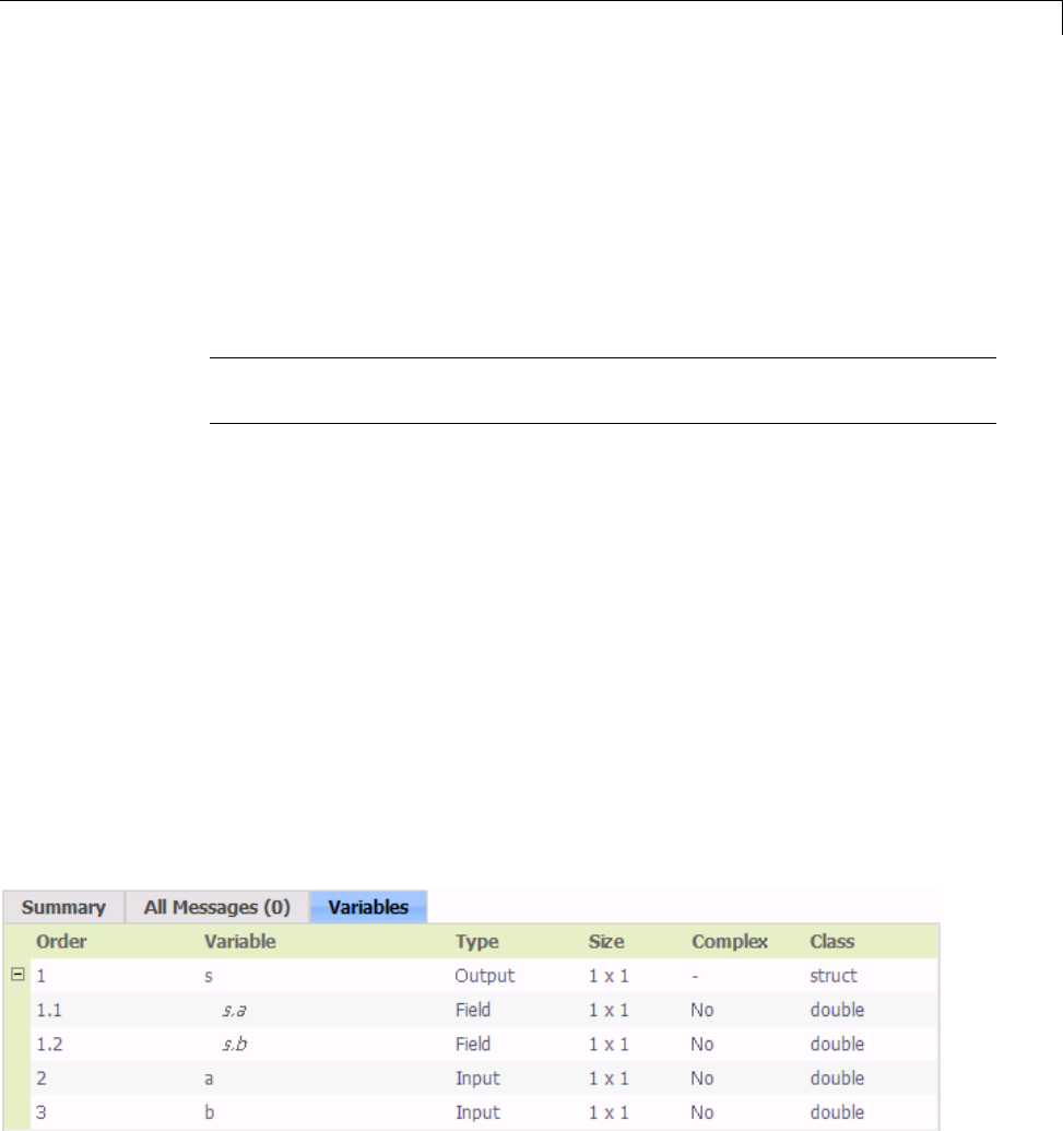
MATLAB Function Reports
•DataTypeMode (DT mode) — for fixed-point data types only. For more
information, see “DataTypeMode”.
•Signed — sign information for built-in data types, signedness information
for fixed-point data types
•Word length (WL) — for fixed-point data types only
•Fraction length (FL) — for fixed-point data types only
Note For more information on viewing fixed-point data types, see “Create
and Use Fixed-Point Code Generation Reports”.
It only displays a column if at least one variable in the code has information
in that column. For example, if the code does not contain any fixed-point data
types, the report does not display the DT mode,WL or FL columns.
Sorting Variables in the Variables Tab. By default, the report lists the
variables in the order that they appear in the selected function.
You can sort the variables by clicking the column headings on the Variables
tab. To sort the variables by multiple columns, hold down the Shift key when
clicking the column headings.
To restore the list to the original order, click the Order column heading.
Viewing Structures on the Variables Tab. You can expand structures
listed on the Variables tab to display the field properties.
29-57
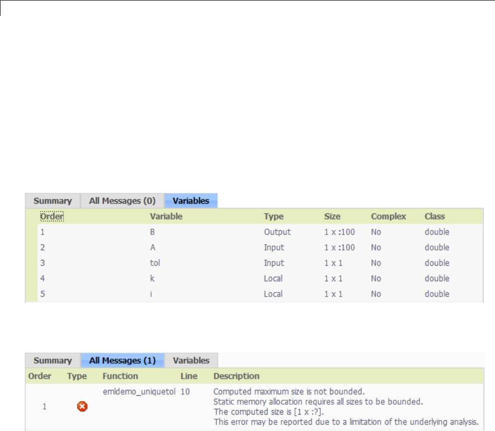
29 Using the MATLAB Function Block
If you sort the variables by type, size, complexity or class, a structure and its
fields might not appear sequentially in the list. To restore the list to the
original order, click the Order column heading.
Viewing Information About Variable-Size Arrays in the Variables
Tab. For variable-size arrays, the Size field includes information on the
computed maximum size of the array. The size of each array dimension that
varies is prefixed with a colon :.
In the following report, variable Ais variable-size. Its maximum computed
size is 1×100.
If the code generation software cannot compute the maximum size of a
variable-size array, the report displays the size as :?.
If you declare a variable-size array and then subsequently fix the dimensions
of this array in the code, the report appends *to the size of the variable. In
the generated C code, this variable appears as a variable-size array, but the
size of its dimensions do not change during execution.
29-58
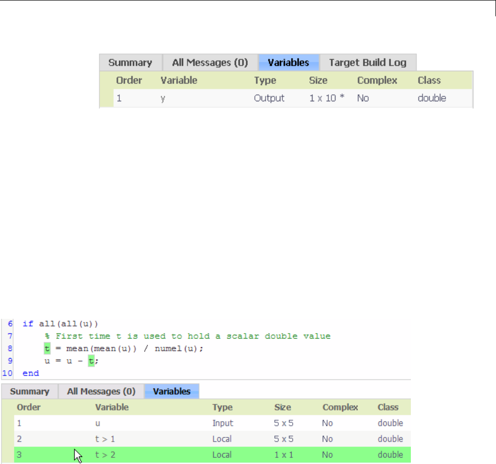
MATLAB Function Reports
For more information on how to use the size information for variable-sized
arrays, see “Variable-Size Data Definition for Code Generation”.
Viewing Renamed Variables in the Variables Tab. If your MATLAB
function reuses a variable with different size, type, or complexity, the code
generation software attempts to create separate, uniquely named variables
in the generated code. For more information, see “Reuse the Same Variable
with Different Properties”. The report numbers the renamed variables in
the list on the Variables tab. When you place your pointeroverarenamed
variable, the report highlights only the instances of this variable that share
the same data type, size, and complexity.
For example, suppose your code uses the variable tin a for-loop to hold a
scalar double, and reuses it outside the for-loop to hold a 5x5 matrix. The
report displays two variables, t>1 and t>2 in the list on the Variables tab.
29-59
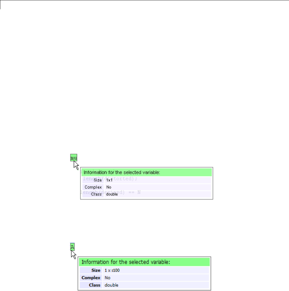
29 Using the MATLAB Function Block
Viewing Simulation Minimum and Maximum Values in the Variables
Tab. If you have a Simulink Fixed Point license, and you simulate your
modelusingtheFixed-PointToolsetuptologtheminimumandmaximum
values, you can view these values in the MATLAB Function Report. For
more information, see “Log Simulation Minimum and Maximum Values for a
MATLAB Function Block”.
Viewing Information About Variables and Expressions in Your
MATLAB Function Code
To view information about a particular variable or expression in your
MATLAB function code, on the MATLAB code pane, place your pointer
over the variable name or expression. The report highlights variables and
expressions in different colors:
Green, when the variable has data type information at this location
in the code.
For variable-size arrays, the Size field includes information on the computed
maximumsizeofthearray. Thesizeof each array dimension that varies is
prefixed with a colon :. Here the array Ais variable-sized with a maximum
computed size of 1 x 100.
29-60
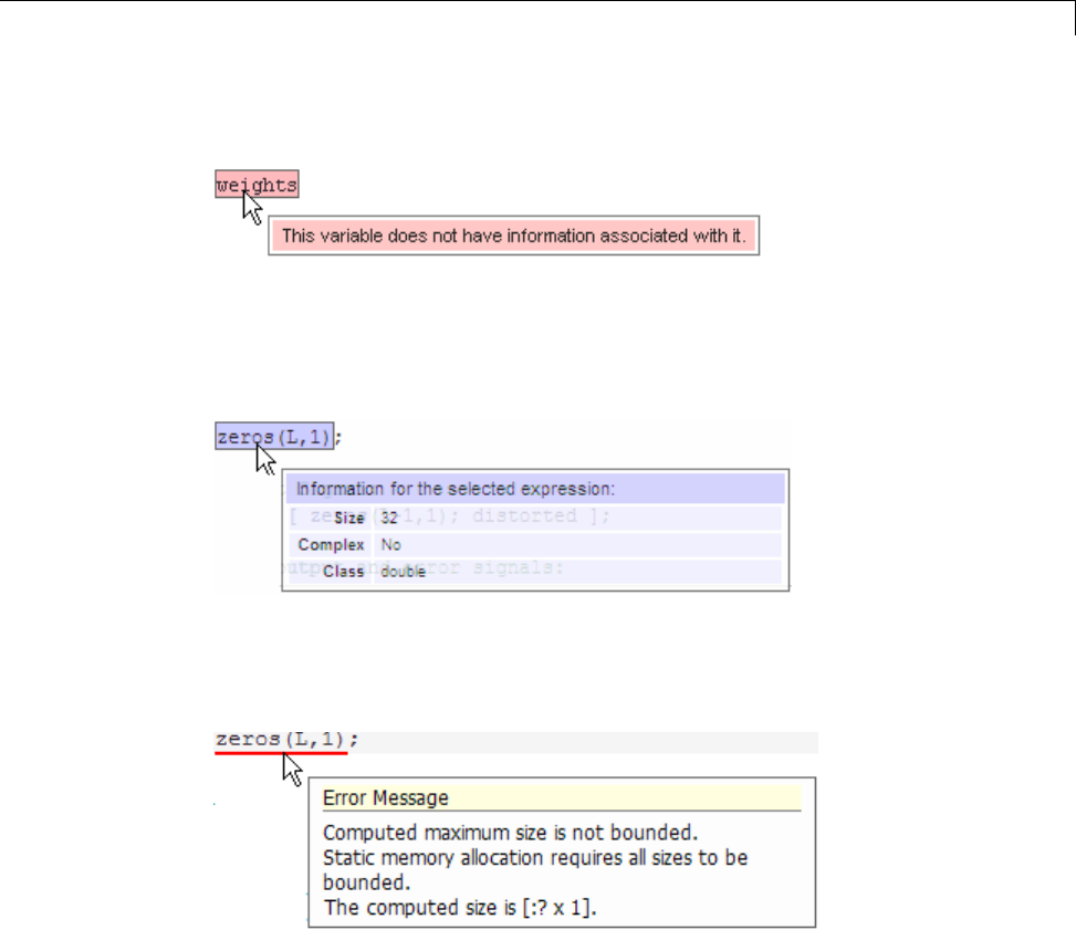
MATLAB Function Reports
Pink, when the variable has no data type information.
Purple, information about expressions. You can also view information
about expressions in your MATLAB code. On the MATLAB code pane, place
your pointer over an expression . The report highlights expressions in purple
and provides more detailed information.
Red, when there is error information for an expression. If the code
generation software cannot compute the maximum size of a variable-size
array, the report underlines the variable name and provides error information.
Keyboard Shortcuts for the MATLAB Function Report
You can use the following keyboard shortcuts to navigate between the
different panes in the MATLAB Function report. Once you have selected a
pane, use the Tab key to advance through data in that pane.
29-61

29 Using the MATLAB Function Block
To select: Use:
MATLAB Code Tab Ctrl+m
Call Stack Tab Ctrl+k
MATLAB Code Pane Ctrl+w
Summary Tab Ctrl+s
All Messages Tab Ctrl+a
Variables Tab Ctrl+v
Report Limitations
The report displays information about the variables and expressions in your
MATLAB code with the following limitations:
varargin and varargout
The report does not support varargin and varargout arrays.
Loop Unrolling
The report does not display full information for unrolled loops. It displays
data types of one arbitrary iteration.
Dead Code
The report does not display information about any dead code.
Structures
The report does not provide complete information about structures.
•On the MATLAB code pane, the report does not provide information about
all structure fields in the struct() constructor.
•On the MATLAB code pane, if a structure has a nonscalar field, and an
expression accesses an element of this field, the report does not provide
information for the field.
29-62

MATLAB Function Reports
Column Headings on Variables Tab
If you scroll through the list of variables, the report does not display the
column headings on the Variables tab.
Multiline Matrices
On the MATLAB code pane, the report does not support selection of
multiline matrices. It supports only selection of individual lines at a time.
For example, if you place your pointer over the following matrix, you cannot
select the entire matrix.
out1 = [1 2 3;
4 5 6];
The report does support selection of single line matrices.
out1 = [1 2 3; 4 5 6];
29-63

29 Using the MATLAB Function Block
Type Function Arguments
In this section...
“About Function Arguments” on page 29-64
“Specifying Argument Types” on page 29-64
“Inheriting Argument Data Types” on page 29-66
“Built-In Data Types for Arguments” on page 29-67
“Specifying Argument Types with Expressions” on page 29-68
“Specifying Simulink®Fixed Point™ Data Properties” on page 29-68
About Function Arguments
You create function arguments for a MATLAB Function block by entering
them in its function header in the MATLAB Function Block Editor. When you
define arguments, the Simulink software creates corresponding ports on the
MATLAB Function block that you can attach to signals. You can select a data
type mode for each argument that you define for a MATLAB Function block.
Each data type mode presents its own set of options for selecting a data type.
By default, the data type mode for MATLAB Function block function
arguments is Inherited. This means that the function argument inherits
its data type from the incoming or outgoing signal. To override the default
type, you first choose a data type mode and then select a data type based
on the mode.
Specifying Argument Types
To specify the type of a MATLAB Function block function argument:
1From the MATLAB Function Block Editor, select Edit Data to open the
Ports and Data Manager.
29-64

Type Function Arguments
2In the left pane, select the argument of interest.
3In the Data properties dialog box (right pane), click the Show data type
assistant button to display the Data Type Assistant. Then, choose
an option from the Mode drop-down menu.
The Data properties dialog box changes dynamically to display additional
fields for specifying the data type associated with the mode.
4Based on the mode you select, specify a desired data type:
Mode What to Specify
Inherit (default) You cannot specify a value. The data type is inherited from previously-defined
data, based on the scope you selected for the MATLAB Function block
function argument:
•If scope is Input, data type is inherited from the input signal on the
designated port.
•If scope is Output, data type is inherited from the output signal on the
designated port.
•If scope is Parameter, data type is inherited from the associated
parameter, which can be defined in the Simulink masked subsystem or
the MATLAB workspace.
See “Inheriting Argument Data Types” on page 29-66.
Built in Select from the drop-down list of supported data types, as described in
“Built-In Data Types for Arguments” on page 29-67.
Fixed point Specify the fixed-point data properties as described in “Specifying Simulink®
Fixed Point™ Data Properties” on page 29-68.
Expression Enter an expression that evaluates to a data type, as described in “Specifying
Argument Types with Expressions” on page 29-68.
29-65

29 Using the MATLAB Function Block
Mode What to Specify
Bus Object In the Bus object field, enter the name of a Simulink.Bus object to define
the properties of a MATLAB structure. You must define the bus object in
the base workspace. See “How Structure Inputs and Outputs Interface with
Bus Signals” on page 29-81.
Note You can click the Edit button to create or modify Simulink.Bus
objects using the Simulink Bus Editor (see “Manage Bus Objects with the
Bus Editor” on page 48-24).
Enumerated In the Enumerated field, enter the name of a Simulink.IntEnumType object
that you define in the base workspace. See “Enumerated Types Supported in
MATLAB Function Blocks” on page 29-105 and “Define Enumerated Data
Types for MATLAB Function Blocks” on page 29-106.
Inheriting Argument Data Types
MATLAB Function block function arguments can inherit their data types,
including fixed point types, from the signals to which they are connected. ,
and set data type mode using one of these methods:
1Select the argument of interest in the Ports and Data Manager
2In the Data properties dialog, select Inherit: Same as Simulink from
the Type drop-down menu.
See “Built-In Data Types for Arguments” on page 29-67 for a list of supported
data types.
Note An argument can also inherit its complexity (whether its value is a
real or complex number) from the signal that is connected to it. To inherit
complexity, set the Complexity field on the Data properties dialog to
Inherited.
29-66

Type Function Arguments
After you build the model, the Compiled Type column of the Ports and
Data Manager gives the actual type inherited from Simulink in the compiled
simulation application.
The inherited type of output data is inferred from diagram actions that store
values in the specified output. In the preceding example, the variables
mean and stdev are computed from operations with double operands, which
yield results of type double. If the expected type matches the inferred type,
inheritance is successful. In all other cases, a mismatch occurs during build
time.
Note Library MATLAB Function blocks can have inherited data types,
sizes, and complexities like ordinary MATLAB Function blocks. However,
all instances of the library block in a given model must have inputs with
the same properties.
Built-In Data Types for Arguments
When you select Built-in for Data type mode,theData properties dialog
displays a Data type field that provides a drop-down list of supported data
types. You can also choose a data type from the Data Type column in the
Ports and Data Manager. The supported data types are:
Data Type Description
double 64-bit double-precision floating point
single 32-bit single-precision floating point
int32 32-bit signed integer
int16 16-bit signed integer
int8 8-bit signed integer
uint32 32-bit unsigned integer
uint16 16-bit unsigned integer
uint8 8-bit unsigned integer
boolean Boolean (1 = true;0=false)
29-67

29 Using the MATLAB Function Block
Specifying Argument Types with Expressions
You can specify the types of MATLAB Function block function arguments as
expressions in the Ports and Data Manager.
1Select <data type expression> from the Type drop-down menu of the
Data properties dialog.
2In the Type field, replace “<data type expression>”withanexpression
that evaluates to a data type. The following expressions are allowed:
•Alias type from the MATLAB workspace, as described in “Creating
aDataTypeAlias”.
•fixdt function to create a Simulink.NumericType object describing a
fixed-point or floating-point data type
•type operator, to base the type on previously defined data
Specifying Simulink Fixed Point Data Properties
MATLAB Function blocks can represent signals and parameter values
as fixed-point numbers. To simulate models that use fixed-point data in
MATLAB Function blocks, you must install the Simulink Fixed Point product
on your system.
You can set the following fixed-point properties:
Signedness. Select whether you want the fixed-point data to be Signed
or Unsigned. Signed data can represent positive and negative quantities.
Unsigned data represents positive values only. The default is Signed.
Word length. Specify the size (in bits) of the word that will hold the
quantized integer. Large word sizes represent large quantities with greater
precision than small word sizes. Word length can be any integer between 0
and 128 bits. The default is 16.
Scaling. Specify the method for scaling your fixed point data to avoid
overflow conditions and minimize quantization errors. You can select the
following scaling modes:
29-68
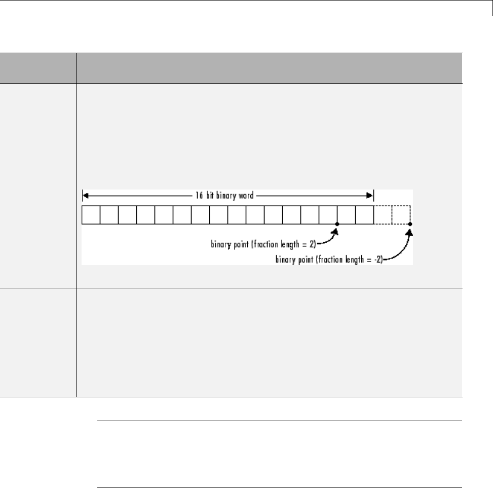
Type Function Arguments
Scaling
Mode
Description
Binary
point
(default)
If you select this mode, the Data Type Assistant displays the Fraction Length
field, specifying the binary point location.
Binary points can be positive or negative integers. A positive integer moves the
binary point left of the rightmost bit by that amount. For example, an entry of 2
sets the binary point in front of the second bit from the right. A negative integer
moves the binary point further right of the rightmost bit by that amount, as
in this example:
The default is 0.
Slope and
bias
If you select this mode, the Data Type Assistant displays fields for entering
the Slope and Bias.
•Slope can be any positive real number. The default is 1.0.
•Bias can be any real number. The default value is 0.0.
Youcanenterslopeandbiasasexpressionsthatcontainparametersdefined
in the MATLAB workspace.
Note You should use binary-point scaling whenever possible to simplify
the implementation of fixed-point data in generated code. Operations with
fixed-point data using binary-point scaling are performed with simple bit
shifts and eliminate the expensive code implementations required for separate
slope and bias values.
Data type override. Specify whether the data type override setting is
Inherit (default) or Off.
29-69

29 Using the MATLAB Function Block
Calculate Best-Precision Scaling. The Simulink software can automatically
calculate “best-precision” values for both Binary point and Slope and
bias scaling, based on the Limit range properties you specify on the Value
Attributes tab.
To automatically calculate best precision scaling values:
1Specify Minimum,Maximum, or both Limit range properties.
2Click Calculate Best-Precision Scaling.
The Simulink software calculates the scaling values, then displays them in
either the Fraction Length,orSlope and Bias fields.
Note The Limit range properties do not apply to Constant or Parameter
scopes. Therefore, Simulink cannot calculate best-precision scaling for these
scopes.
Fixed-point Details. You can view the following Fixed-point details:
Fixed-point Detail Description
Representable maximum The maximum number that can be
represented by the chosen data type,
sign, word length and fraction length
(or data type, sign, slope and bias).
Maximum The maximum value specified on the
Value Attributes tab.
Minimum The minimum value specified on the
Value Attributes tab.
Representable minimum The minimum number that can be
represented by the chosen data type,
sign, word length and fraction length
(or data type, sign, slope and bias).
Precision The precision for the given word
length and fraction length (or slope
and bias).
29-70

Type Function Arguments
Lock data type setting against changes by the fixed-point tools.
Specify whether you want to prevent replacement of the current data
type with a type chosen by the Fixed-Point Tool or Fixed-Point Advisor.
The default setting allows replacement. For instructions on autoscaling
fixed-point data, see “Scaling”.
Using Data Type Override with the MATLAB Function Block
If you set the Data Type Override mode to Double or Single in Simulink,
the MATLAB Function block sets the type of all inherited input signals and
parameters to fi double or fi single objects respectively (see “MATLAB
Function Block with Data Type Override” for more information). You must
check the data types of your inherited input signals and parameters and
use the Ports and Data Manager (see “Ports and Data Manager” on page
29-37) to set explicit types for any inputs that should not be fixed-point. Some
operations, such as sin, are not applicable to fixed-point objects.
Note If you do not set the correct input types explicitly, you may encounter
compilation problems after setting Data Type Override.
How Do I Set Data Type Override?
To set Data Type Override, follow these steps:
1From the Simulink Analysis menu, select Fixed-Point Tool.
2Set the value of the Data type override parameter to Double or Single.
29-71

29 Using the MATLAB Function Block
Size Function Arguments
In this section...
“Specifying Argument Size” on page 29-72
“Inheriting Argument Sizes from Simulink” on page 29-72
“Specifying Argument Sizes with Expressions” on page 29-73
Specifying Argument Size
Toexamineorspecifythesizeofan argument, follow these steps:
1From the MATLAB Function Block Editor, select Edit Data.
2Enter the size of the argument in the Size field of the Data properties
dialog, located in the General pane.
Note The default value is -1, indicating that size is inherited, as described
in “Inheriting Argument Sizes from Simulink” on page 29-72.
Inheriting Argument Sizes from Simulink
Size defaults to -1, which means that the data argument inherits its size from
Simulink based on its scope:
For Scope Inherits Size
InputFrom the Simulink input signal connected to the argument.
Output From the Simulink output signal connected to the argument.
Parameter From the Simulink or MATLAB parameter to which it is
bound. See “Add Parameter Arguments” on page 29-75.
After you compile the model, the Compiled Size column in the Contents
pane displays the actual size used in the compiled simulation application.
The size of an output argument is the size of the value that is assigned to it. If
the expected size in the Simulink model does not match, a mismatch error
occurs during compilation of the model.
29-72

Size Function Arguments
Note No arguments with inherited sizes are allowed for MATLAB Function
blocks in a library.
Specifying Argument Sizes with Expressions
ThesizeofadataargumentcanbeascalarvalueoraMATLABvectorof
values.
To specify size as a scalar, set the Size fieldto1orleaveitblank.Tospecify
Size as a vector, enter an array of up to two dimensions in [row column]
format where
•Number of dimensions equals the length of the vector.
•Size of each dimension corresponds to the value of each element of the
vector.
For example, a value of [2 4] defines a 2-by-4 matrix. To define a row vector
of size 5, set the Size field to [1 5]. To define a column vector of size 6, set
the Size field to [6 1] or just 6. You can enter a MATLAB expression for
each [row column] element in the Size field. Each expression can use one
or more of the following elements:
•Numeric constants
•Arithmetic operators, restricted to +,-,*,and/
•Parameters defined in the MATLAB Workspace or the parent Simulink
masked subsystem
•Calls to the MATLAB functions min,max,andsize
The following examples are valid expressions for Size:
k+1
size(x)
min(size(y),k)
In these examples, k,x,andyare variables of scope Parameter.
29-73

29 Using the MATLAB Function Block
Once you build the model, the Compiled Size column displays the actual size
used in the compiled simulation application.
29-74

Add Parameter Arguments
Add Parameter Arguments
Parameter arguments for MATLAB Function blocks do not take their
values from signals in the Simulink model. Instead, their values come from
parameters defined in a parent Simulink masked subsystem or variables
defined in the MATLAB base workspace. Using parameters allows you to pass
read-only constants in the Simulink model to the MATLAB Function block.
To add a parameter argument to a function for a MATLAB Function block.
1In the MATLAB Function Block Editor, add an argument to the function
header of the MATLAB Function block.
The name of the argument must be identical to the name of the masked
subsystem parameter or MATLAB variable that you want to pass to the
MATLAB Function block. For information on declaring parameters for
masked subsystems, see “How Mask Parameters Work” on page 26-4.
2Bring focus to the MATLAB Function block.
The new argument appears as an input port in the Simulink diagram.
3In the MATLAB Function Block Editor, select Edit Data.
4Select the new argument.
5Set Scope to Parameter.
6Examine the MATLAB Function block.
The input port no longer appears for the parameter argument.
Note Parameter arguments appear as arguments in the function header
of the MATLAB Function block to maintain MATLAB consistency. As a
result, you can test functions in a MATLAB Function block by copying and
pasting them to MATLAB.
29-75

29 Using the MATLAB Function Block
Resolve Signal Objects for Output Data
In this section...
“Implicit Signal Resolution” on page 29-76
“Eliminating Warnings for Implicit Signal Resolution in the Model” on
page 29-76
“Disabling Implicit Signal Resolution for a MATLAB Function Block” on
page 29-77
“Forcing Explicit Signal Resolution for an Output Data Signal” on page
29-77
Implicit Signal Resolution
MATLAB Function blocks participate in signal resolution with Simulink
signal objects. By default, output data from MATLAB Function blocks become
associated with Simulink signal objects of the same name during a process
called implicit signal resolution, as described in Simulink.Signal.
By default, implicit signal resolution generates a warning when you update
the chart in the Simulink model. The following sections show you how to
manage implicit signal resolution at various levels of the model hierarchy.
See “Symbol Resolution” on page 4-76 and “Explicit and Implicit Symbol
Resolution” on page 4-80 for more information.
Eliminating Warnings for Implicit Signal Resolution
in the Model
To enable implicit signal resolution for all signals in a model, but eliminate
the attendant warnings, follow these steps:
1In the Simulink Model Editor, select Simulation > Model Configuration
Parameters.
The Configuration Parameters dialog appears.
2In the left pane of the Configuration Parameters dialog, under Diagnostics,
select Data Validity.
29-76

Resolve Signal Objects for Output Data
Data Validity configuration parameters appear in the right pane.
3In the Signal resolution field, select Explicit and implicit.
Disabling Implicit Signal Resolution for a MATLAB
Function Block
To disable implicit signal resolution for a MATLAB Function block in your
model, follow these steps:
1Right-click the MATLAB Function block and select Block Parameters
(Subsystem) in the context menu.
The Block Parameters dialog opens.
2In the Permit hierarchical resolution field, select ExplicitOnly or None,
and click OK.
Forcing Explicit Signal Resolution for an Output Data
Signal
To force signal resolution for an output signal in a MATLAB Function block,
follow these steps:
1In the Simulink model, right-click the signal line connected to the output
that you want to resolve and select Properties from the context menu.
2In the Signal Properties dialog, enter a name for the signal that corresponds
to the signal object.
3Select the Signal name must resolve to Simulink signal object check
box and click OK.
29-77

29 Using the MATLAB Function Block
Types of Structures in MATLAB Function Blocks
In MATLAB Function blocks, you can define structure data as inputs or
outputs that interact with bus signals. MATLAB Function blocks also support
arrays of buses (for more information, see “Combine Buses into an Array
of Buses” on page 48-77). You can also define structures inside MATLAB
functions that are not part of MATLAB Function blocks (see “Structure
Definition for Code Generation” on page 36-2.
The following table summarizes how to create different types of structures in
MATLAB Function blocks:
Scope How to Create Details
Input Create structure data with scope of
Input.
Output Create structure data with scope of
Output.
You can create structure
data as inputs or outputs
in the top-level MATLAB
function for interfacing
to other environments.
See “Create Structures
in MATLAB Function
Blocks” on page 29-84.
Local Create a local variable implicitly in
a MATLAB function.
See “Define Scalar
Structures for Code
Generation” on page
36-4.
Persistent Declare a variable to be persistent
in a MATLAB function.
See “Make Structures
Persistent” on page 36-9.
Parameter Create structure data with scope of
Parameter
See “Define and Use
Structure Parameters”
on page 29-91.
Structures in MATLAB Function blocks can contain fields of any type and
size, including muxed signals, buses, and arrays of structures.
29-78
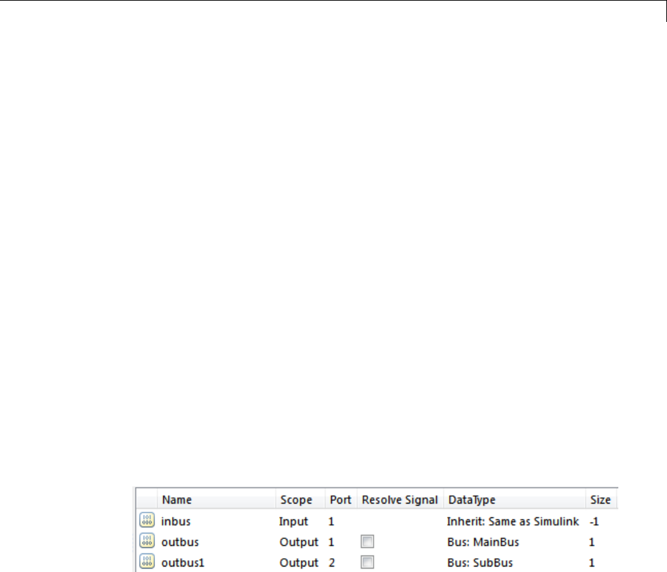
Attach Bus Signals to MATLAB Function Blocks
Attach Bus Signals to MATLAB Function Blocks
For an example of how to use structures in a MATLAB Function block, open
the model emldemo_bus_struct.
In this model, a MATLAB Function block receives a bus signal using the
structure inbus at input port 1 and outputs two bus signals from the
structures outbus at output port 1 and outbus1 at output port 2. The input
signal comes from the Bus Creator block MainBusCreator, which bundles
signals ele1,ele2,andele3.Thesignalele3 is the output of another
Bus Creator block SubBusCreator, which bundles the signals a1 and a2.
The structure outbus connects to a Bus Selector block BusSelector1;the
structure outbus1 connects to another Bus Selector block BusSelector3.
To explore the MATLAB function fcn, double-click the MATLAB Function
block. Notice that the code implicitly defines a local structure variable
mystruct using the struct function, and uses this local structure variable to
initialize the value of the first output outbus. It initializes the second output
outbus1 to the value of field ele3 of structure inbus.
Structure Definitions in Example
Here are the definitions of the structures in the MATLAB Function block in
the example, as they appear in the Ports and Data Manager:
Bus Objects Define Structure Inputs and Outputs
Each structure input and output must be defined by a Simulink.Bus object
in the base workspace (see “Create Structures in MATLAB Function Blocks”
on page 29-84). This means that the structure shares the same properties as
the bus object, including number, name, type, and sequence of fields. In this
example, the following bus objects define the structure inputs and outputs:
29-79
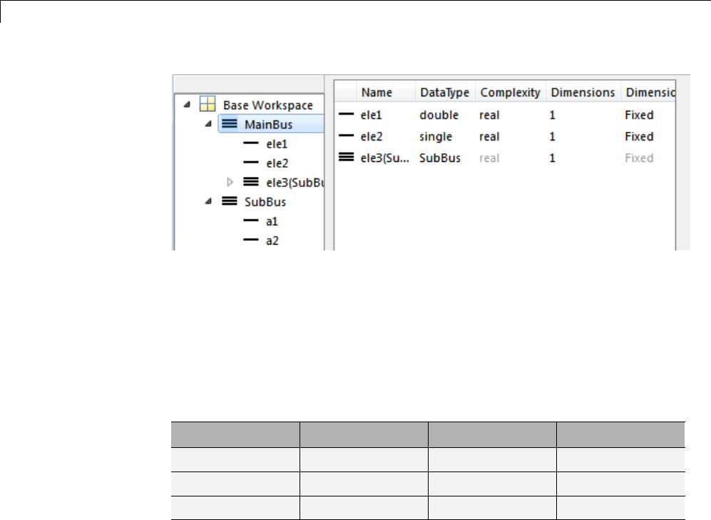
29 Using the MATLAB Function Block
The Simulink.Bus object MainBus defines structure input inbus and
structure output outbus.TheSimulink.Bus object SubBus defines structure
output outbus1. Based on these definitions, inbus and outbus have the
same properties as MainBus and, therefore, reference their fields by the same
namesasthefieldsinMainBus, using dot notation (see “Index Substructures
and Fields” on page 29-83). Similarly, outbus1 references its fields by the
same names as the fields in SubBus. Here are the field references for each
structure in this example:
Structure First Field Second Field Third Field
inbus inbus.ele1 inbus.ele2 inbus.ele3
outbus outbus.ele1 outbus.ele2 outbus.ele3
outbus1 outbus1.a1 outbus1.a2 —
To learn how to define structures in MATLAB Function blocks, see “Create
Structures in MATLAB Function Blocks” on page 29-84.
29-80

How Structure Inputs and Outputs Interface with Bus Signals
How Structure Inputs and Outputs Interface with Bus
Signals
Buses in a Simulink model appear inside the MATLAB Function block as
structures; structure outputs from the MATLAB Function block appear as
buses in Simulink models. When you create structure inputs, the MATLAB
Function block determines the type, size, and complexity of the structure from
the input signal. When you create structure outputs, you must define their
type, size, and complexity in the MATLAB function.
You connect structure inputs and outputs from MATLAB Function blocks
to any bus signal, including:
•Blocks that output bus signals — such as Bus Creator blocks
•Blocks that accept bus signals as input — such as Bus Selector and Gain
blocks
•S-Function blocks
•Other MATLAB Function blocks
Working with Virtual and Nonvirtual Buses
MATLAB Function blocks supports nonvirtual buses only (see “Virtual and
Nonvirtual Buses” on page 48-10). When models that contain MATLAB
Function block inputs and outputs are built, hidden converter blocks are used
to convert bus signals for code generation from MATLAB, as follows:
•Converts incoming virtual bus signals to nonvirtual buses for inputs to
structures in MATLAB Function blocks
•Converts outgoing nonvirtual bus signals from MATLAB Function blocks
to virtual bus signals
29-81

29 Using the MATLAB Function Block
Rules for Defining Structures in MATLAB Function Blocks
Follow these rules when defining structures in MATLAB Function blocks:
•For each structure input or output in a MATLAB Function block, you must
define a Simulink.Bus object in the base workspace to specify its type. For
more information, see Simulink.Bus.
•MATLAB Function blocks support nonvirtual buses only (see “Working
with Virtual and Nonvirtual Buses” on page 29-81).
29-82

Index Substructures and Fields
Index Substructures and Fields
As in MATLAB, you index substructures and fields structures in MATLAB
Function blocks by using dot notation. However, for code generation from
MATLAB, you must reference field values individually (see “Structure
Definition for Code Generation” on page 36-2).
For example, in the emldemo_bus_struct model described in “Attach Bus
Signals to MATLAB Function Blocks” on page 29-79, the MATLAB function
uses dot notation to index fields and substructures:
function [outbus, outbus1] = fcn(inbus)
%#codegen
substruct.a1 = inbus.ele3.a1;
substruct.a2 = int8([1 2;3 4]);
mystruct = struct('ele1',20.5,'ele2',single(100),
'ele3',substruct);
outbus = mystruct;
outbus.ele3.a2 = 2*(substruct.a2);
outbus1 = inbus.ele3;
The following table shows how the code generation software resolves symbols
in dot notation for indexing elements of the structures in this example:
Dot Notation Symbol Resolution
substruct.a1 Field a1 of local structure substruct
inbus.ele3.a1 Value of field a1 of field ele3, a substructure of
structure inputinbus
inbus.ele3.a2(1,1) Value in row 1, column 1 of field a2 of field ele3,
a substructure of structure input inbus
29-83

29 Using the MATLAB Function Block
Create Structures in MATLAB Function Blocks
Here is the workflow for creating a structure in a MATLAB Function block:
1Decide on the type (or scope) of the structure (see “Types of Structures in
MATLAB Function Blocks” on page 29-78).
2Based on the scope, follow these guidelines for creating the structure:
For Structure
Scope:
Follow These Steps:
Input 1Create a Simulink.Bus object in the base workspace to define the structure
input.
2Add data to the MATLAB Function block, as described in “Adding Data
to a MATLAB Function Block” on page 29-42. The data should have the
following properties
•Scope =Input
•Type =Bus: <object name>
For <object name>,enterthenameoftheSimulink.Bus object that
defines the structure input
See “Rules for Defining Structures in MATLAB Function Blocks” on page 29-82.
Output 1Create aSimulink.Bus object in the base workspace to define the structure
output.
2Add data to the MATLAB Function block with the following properties:
•Scope =Output
•Type =Bus: <object name>
For <object name>,enterthenameoftheSimulink.Bus object that
defines the structure output
3Define and initialize the output structure implicitly as a variable in
the MATLAB function, as described in “Structure Definition for Code
Generation” on page 36-2.
4Make sure the number, type, and size of fields in the output structure
variable definition match the properties of the Simulink.Bus object.
29-84

Create Structures in MATLAB Function Blocks
For Structure
Scope:
Follow These Steps:
Local Define the structure implicitly as a local variable in the MATLAB function,
as described in “Structure Definition for Code Generation” on page 36-2. By
default, local variables in MATLAB Function blocks are temporary.
Persistent Define the structure implicitly as a persistent variable in the MATLAB
function, as described in “Make Structures Persistent” on page 36-9.
Parameter 1Create a structure variable in the base workspace.
2Add data to the MATLAB Function block with the following properties:
•Name = same name as the structure variable you created in step 1.
•Scope =Parameter
See “Define and Use Structure Parameters” on page 29-91.
29-85

29 Using the MATLAB Function Block
Assign Values to Structures and Fields
You can assign values to any structure, substructure, or field in a MATLAB
Function block. Here are the guidelines:
Operation Conditions
Assign one structure to another
structure
Youmustdefineeachstructurewith
the same number, type, and size
of fields, either as Simulink.Bus
objects in the base workspace
or locally as implicit structure
declarations (see “Create Structures
in MATLAB Function Blocks” on
page 29-84).
Assign one structure to a
substructure of a different structure
and vice versa
You must define the structure with
the same number, type, and size of
fields as the substructure, either as
Simulink.Bus objects in the base
workspace or locally as implicit
structure declarations.
Assign an element of one structure
to an element of another structure
The elements must have the same
type and size.
For example, the following table presents valid and invalid structure
assignments based on the specifications for the model described in “Attach
Bus Signals to MATLAB Function Blocks” on page 29-79:
Assignment Valid or
Invalid?
Rationale
outbus =mystruct;Valid Both outbus and mystruct have the same number,
type, and size of fields. The structure outbus
is defined by the Simulink.Bus object MainBus
and mystruct is defined locally to match the field
properties of MainBus.
outbus =inbus;Valid Both outbus and inbus are defined by the same
Simulink.Bus object, MainBus.
29-86

Assign Values to Structures and Fields
Assignment Valid or
Invalid?
Rationale
outbus1 =inbus.ele3;Valid Both outbus1 and inbus.ele3 havethesametype
and size because each is defined by the Simulink.Bus
object SubBus.
outbus1 =inbus;Invalid The structure outbus1 is defined by a different
Simulink.Bus object than the structure inbus.
29-87
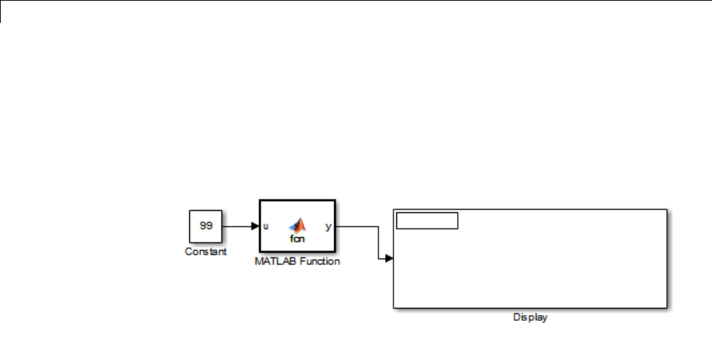
29 Using the MATLAB Function Block
Initialize a Matrix Using a Non-Tunable Structure
Parameter
The following simple example uses a non-tunable structure parameter input
to initialize a matrix output. The model looks like this:
This model defines a structure variable pin its pre-load callback function, as
follows:
29-88
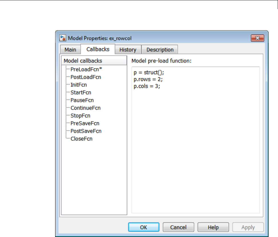
Initialize a Matrix Using a Non-Tunable Structure Parameter
The structure phas two fields, rows and cols, which specify the dimensions
of a matrix. The MATLAB Function block uses a constant input uto initialize
the matrix output y.Hereisthecode:
function y = fcn(u, p)
y = zeros(p.rows,p.cols) + u;
Running the model initializes each element of the 2-by-3 matrix yto 99, the
value of u:
29-89
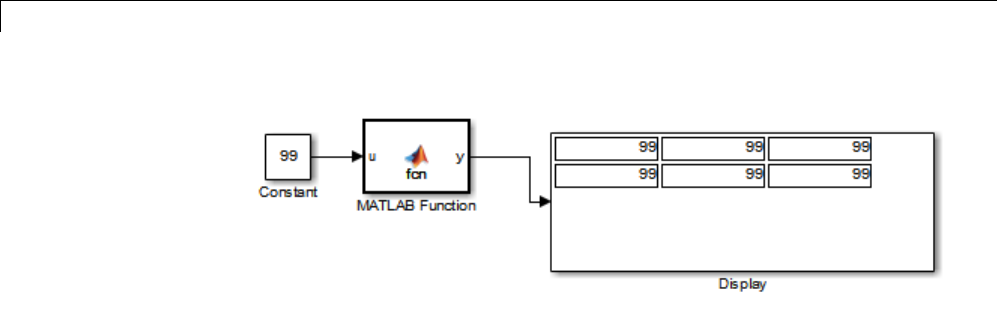
29 Using the MATLAB Function Block
29-90

Define and Use Structure Parameters
Define and Use Structure Parameters
In this section...
“Defining Structure Parameters” on page 29-91
“FIMATH Properties of Non-Tunable Structure Parameters” on page 29-91
Defining Structure Parameters
To define structure parameters in MATLAB Function blocks, follow these
steps:
1Define and initialize a structure variable
A common method is to create a structure in the base workspace. For other
methods, see “Structure Parameters” on page 24-16.
2In the Ports and Data Manager, add data in the MATLAB Function block
with the following properties:
Property What to Specify
Name Enter same name as the structure variable you defined
in the base workspace
Scope Select Parameter
Tunable Leave checked if you want to change (tune) the value
of the parameter during simulation; otherwise, clear
to make the parameter non-tunable and preserve the
initial value during simulation
Type Select Inherit: Same as Simulink
3Click Apply.
FIMATH Properties of Non-Tunable Structure
Parameters
FIMATH properties for non-tunable structure parameters containing
fixed-point values are based on the initial values of the structure. They do not
come from the FIMATH properties specified for fixed-point input signals to
29-91

29 Using the MATLAB Function Block
the parent MATLAB Function block. (These FIMATH properties appear in
the properties dialog box for MATLAB Function blocks.)
29-92

Limitations of Structures and Buses in MATLAB Function Blocks
Limitations of Structures and Buses in MATLAB Function
Blocks
•Structures in MATLAB Function blocks support a subset of the operations
available for MATLAB structures (see “Structures”).
•You cannot use variable-size data with arrays of buses (see “Array of Buses
Limitations” on page 48-81).
29-93

29 Using the MATLAB Function Block
What Is Variable-Size Data?
Variable-size data is data whose size may change at run time. By contrast,
fixed-size data is data whose size is known and locked at compile time, and
therefore cannot change at run time.
29-94

How MATLAB Function Blocks Implement Variable-Size Data
How MATLAB Function Blocks Implement Variable-Size
Data
You can define variable-size arrays and matrices as inputs, outputs, and
local data in MATLAB Function blocks. However, the block must be able to
determine the upper bounds of variable-size data at compile time.
.Formoreinfo
rmation about using variable-size data in Simulink, see
“Variable-Size Signal Basics” on page 49-2.
29-95

29 Using the MATLAB Function Block
Enable Support for Variable-Size Data
Support for variable-size data is enabled by default for MATLAB Function
blocks. To modify this property for individual blocks:
1In the MATLAB Function Block Editor, select Edit Data.
2Select or clear the check box Support variable-size arrays.
29-96

Declare Variable-Size Inputs and Outputs
Declare Variable-Size Inputs and Outputs
1In the MATLAB Function Block Editor, select Edit Data.
2Select Add > Data
3Select the Variable size check box.
4Set Scope as either Input or Output.
5Enter size:
For: What to Specify
Input Enter -1 to inherit size from Simulink or specify the explicit
size and upper bound. For example, enter [2 4] to specify
a 2-D matrix where the upper bounds are 2 for the first
dimension and 4 for the second.
Output Specify the explicit size and upper bound.
29-97

29 Using the MATLAB Function Block
Filter a Variable-Size Signal
In this section...
“About the Example” on page 29-98
“Simulink Model” on page 29-98
“Source Signal” on page 29-99
“MATLAB Function Block: uniquify” on page 29-99
“MATLAB Function Block: avg” on page 29-101
“Variable-Size Results” on page 29-102
About the Example
Thefollowingexampleappearsthroughoutthissectiontoillustratehow
MATLAB Function blocks exchange variable-size data with other Simulink
blocks. The model uses a variable-size vector to store the values of a white
noise signal. The size of the vector may vary at run time as the signal values
get pruned by functions that:
•Filter out signal values that are not unique within a specified tolerance
of each other
•Average every two signal values and output only the resulting means
Simulink Model
Open the example model by typing emldemo_process_signal at the MATLAB
command prompt. The model contains the following blocks:
Simulink Block Description
Band-Limited White Noise Generates a set of normally
distributed random values as the
source of the white noise signal.
MATLAB Function uniquify Filters out signal values that are
not unique to within a specified
tolerance of each other.
29-98
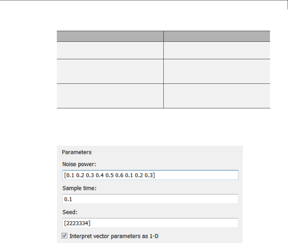
Filter a Variable-Size Signal
Simulink Block Description
MATLAB Function avg Outputs the average of a specified
number of unique signal values.
Unique values Scope that displays the unique signal
values output from the uniquify
function.
Average values Scope that displays the average
signal values output from the avg
function.
Source Signal
The band-limited white noise signal has these properties:
The size of the noise power value defines the size of the matrix that holds the
signal values — in this case, a 1-by-9 vector of double values.
MATLAB Function Block: uniquify
This block filters out signal values that are not within a tolerance of 0.2 of
each other. Here is the code:
function y = uniquify(u) %#codegen
29-99

29 Using the MATLAB Function Block
y = uniquetol(u,0.2);
The uniquify function calls an external MATLAB function uniquetol to
filter the signal values. uniquify passes the 1-by-9 vector of white noise
signal values as the first argument and the tolerance value as the second
argument. Here is the code for uniquetol:
function B = uniquetol(A,tol) %#codegen
A = sort(A);
coder.varsize('B',[1 100]);
B = A(1);
k=1;
for i = 2:length(A)
if abs(A(k) - A(i)) > tol
B = [B A(i)];
k=i;
end
end
uniquetol returns the filtered values of Ain an output vector Bso that
abs(B(i) - B(j)) > tol for all iand j. Every time Simulink samples the
Band-Limited White Noise block, it generates a different set of random values
for A.Asaresult,uniquetol may produce a different number of output
signals in Beach time it is called. To allow Bto accommodate a variable
number of elements, uniquetol declares it as variable-size data with an
explicit upper bound:
coder.varsize('B',[1 100]);
In this statement, coder.varsize declares Bas a vector whose first dimension
is fixed at 1 and whose second dimension can grow to a maximum size of 100.
Accordingly, output yof the uniquify block must also be variable sized so it
can pass the values returned from uniquetol to the Unique values scope.
Here are the properties of y:
29-100
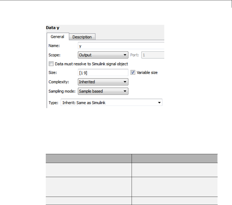
Filter a Variable-Size Signal
For variable-size outputs, you must specify an explicit size and upper bound,
shown here as [1 9].
MATLAB Function Block: avg
This block averages signal values filtered by the uniquify block as follows:
If number of signal values: The MATLAB Function block:
> 1 and divisible by 2 Averages every consecutive pair of
values
>1butnot divisible by 2 Drops the first (smallest) value and
average the remaining consecutive
pairs
=1 Returns the value unchanged
The avg function outputs the results to the Average values scope. Here
is the code:
function y = avg(u) %#codegen
if numel(u) == 1
y=u;
else
29-101
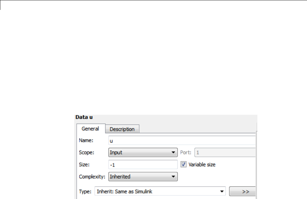
29 Using the MATLAB Function Block
k = numel(u)/2;
if k ~= floor(k)
u = u(2:numel(u));
end
y = nway(u,2);
end
Both input uand output yof avg are declared as variable-size vectors because
the number of elements varies depending on how the uniquify function block
filters the signal values. Input uinherits its size from the output of uniquify.
The avg function calls an external MATLAB function nway to calculate the
average of every two consecutive signal values. Here is the code for nway:
function B = nway(A,n) %#codegen
assert(n>=1 && n<=numel(A));
B = zeros(1,numel(A)/n);
k=1;
for i = 1 : numel(A)/n
B(i) = mean(A(k + (0:n-1)));
k=k+n;
end
Variable-Size Results
Simulating the model produces the following results:
29-102
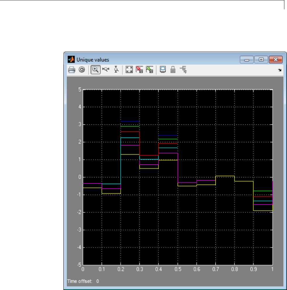
Filter a Variable-Size Signal
•The uniquify block outputs a variable number of signal values each time
it executes:
•The avg block outputs a variable number of signal values each time it
executes — approximately half the number of the unique values:
29-103
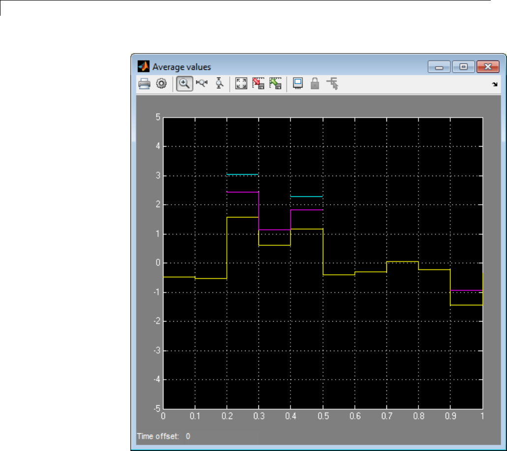
29 Using the MATLAB Function Block
29-104

Enumerated Types Supported in MATLAB Function Blocks
Enumerated Types Supported in MATLAB Function Blocks
Enumerated data is data that has a finite set of values. An enumerated data
type is a user-defined type whose values belong to a predefined set of symbols,
also called enumerated values. Each enumerated value consists of a name
and an underlying numeric value.
Like other Simulink blocks, MATLAB Function blocks support an
integer-based enumerated type derived from the class Simulink.IntEnumType.
The instances of the class represent the values that comprise the enumerated
type. The allowable values for an enumerated type must be 32-bit integers,
but do not need to be consecutive.
For example, the following MATLAB script defines an integer-based
enumerated data type named PrimaryColors:
classdef(Enumeration) PrimaryColors < Simulink.IntEnumType
enumeration
Red(1),
Blue(4),
Yellow(8)
end
end
PrimaryColors is restricted to three enumerated values:
Enumerated Value Enumerated Name Underlying Numeric
Value
Red(1) Red 1
Blue(4) Blue 4
Yellow(8) Yellow 8
You can exchange enumerated data between MATLAB Function blocks and
other Simulink blocks in a model as long as the enumerated type definition is
based on the Simulink.IntEnumType class.
For comprehensive information about enumerated data support in Simulink,
see “Enumerations” on page 43-6.
29-105

29 Using the MATLAB Function Block
Define Enumerated Data Types for MATLAB Function Blocks
You define enumerated data types for MATLAB Function blocks in the same
way as for other Simulink blocks:
1Create a class definition file.
2Define enumerated values in an enumeration section.
3Optionally override default methods in a methods section.
4SavetheMATLABfileontheMATLABpath.
29-106

Add Inputs, Outputs, and Parameters as Enumerated Data
Add Inputs, Outputs, and Parameters as Enumerated Data
You can add inputs, outputs, and parameters as enumerated data, according
to these guidelines:
For: Do This:
Inputs Inherit from the enumerated type of the connected Simulink
signal or specify the enumerated type explicitly.
Outputs Always specify the enumerated type explicitly.
Parameters For tunable parameters, specify the enumerated type
explicitly.
For non-tunable parameters, derive properties from an
enumerated parameter in a parent Simulink masked
subsystem or enumerated variable defined in the MATLAB
base workspace.
To add enumerated data to a MATLAB Function block:
1In the MATLAB Function Block Editor, select Edit Data.
2In the Ports and Data Manager, select Add > Data.
3In the Name field, enter a name for the enumerated data.
Forparameters,thenamemustmatchtheenumeratedmaskedparameter
or workspace variable name.
4In the Type field, specify an enumerated type.
To specify an explicit enumerated type:
aSelect Enum:<class name> from the drop-down menu in the Type field.
bReplace <class name> with the name of an enumerated data type that
you defined in a MATLAB file on the MATLAB path.
For example, you can enter Enum:led in the Type field. (See “Define
Enumerated Data Types for MATLAB Function Blocks” on page 29-106.)
29-107
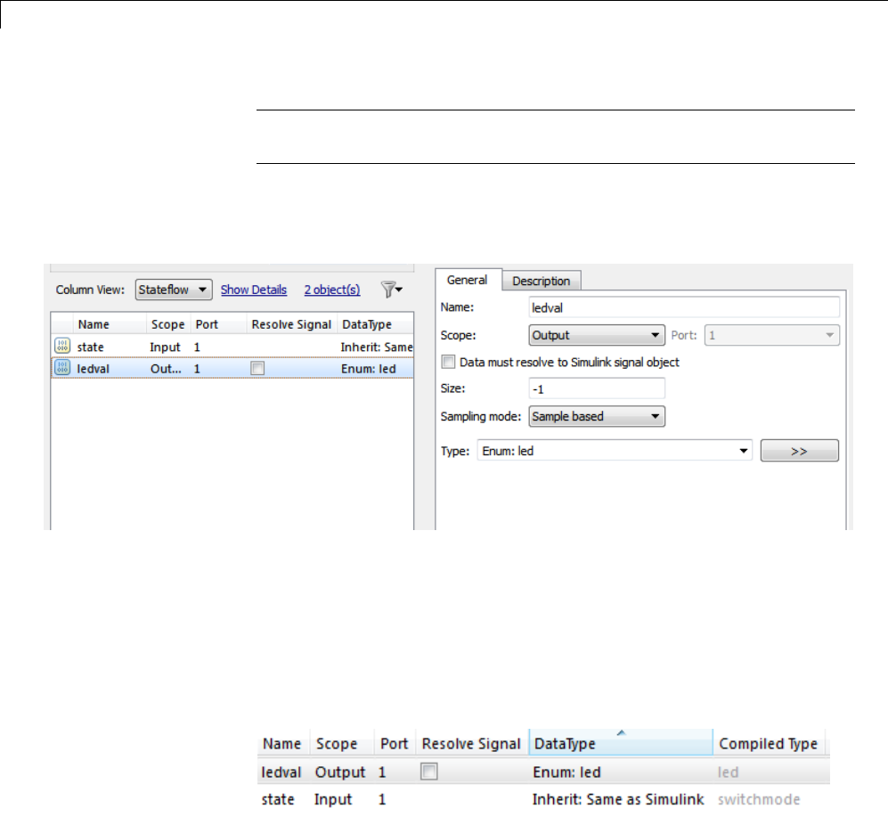
29 Using the MATLAB Function Block
Note The Complexity field disappears when you select Enum:<class
name> because enumerated data types do not support complex values.
For example, the following output ledval has an explicit enumerated
type, led:
To inherit the enumerated type from a connected Simulink signal (for
inputs only):
aSelect Inherit:Same as Simulink from the drop-down menu in the
Type field.
For example, the following input state inherits its enumerated type
switchmode from a Simulink signal:
5Click Apply.
29-108

Basic Approach for Adding Enumerated Data to MATLAB Function Blocks
Basic Approach for Adding Enumerated Data to MATLAB
Function Blocks
Here is the basic workflow for using enumerated data in MATLAB Function
blocks:
Step Action How?
1
Define an enumerated data
type that inherits from
Simulink.IntEnumType.
See “Define Enumerated Data
Types for MATLAB Function
Blocks” on page 29-106.
2
Add the enumerated data to your
MATLAB Function block.
See “Add Inputs, Outputs, and
Parameters as Enumerated
Data” on page 29-107.
3
Instantiate the enumerated type
in your MATLAB Function block.
See “Instantiate Enumerated
Data in MATLAB Function
Blocks” on page 29-110.
4
Simulate and/or generate code. See “Enumerations”.
29-109

29 Using the MATLAB Function Block
Instantiate Enumerated Data in MATLAB Function Blocks
To instantiate an enumerated type in a MATLAB Function block, use dot
notation to specify ClassName.EnumName. For example, the following MATLAB
function checkState instantiates the enumerated types myMode and myLED
from “Control an LED Display” on page 29-111. The dot notation appears
highlighted in the code.
function led = checkState(state)
%#codegen
if state == myMode.ON
led = myLED.GREEN;
else
led = myLED.RED;
end
29-110

Control an LED Display
Control an LED Display
In this section...
“About the Example” on page 29-111
“Class Definition: switchmode” on page 29-111
“Class Definition: led” on page 29-112
“Simulink Model” on page 29-112
“MATLAB Function Block: checkState” on page 29-113
“How the Model Displays Enumerated Data” on page 29-114
About the Example
The following example illustrates how MATLAB Function blocks exchange
enumerated data with other Simulink blocks. This simple model uses
enumerated data to represent the modes of a device that controls the colors
of an LED display. The MATLAB Function block receives an enumerated
data input representing the mode and, in turn, outputs enumerated data
representing the color to be displayed by the LED.
This example uses two enumerated types: switchmode to represent the set
of allowable modes and led to represent the set of allowable colors. Both
type definitions inherit from the built-in type Simulink.IntEnumType and
must reside on the MATLAB path.
Class Definition: switchmode
Here is the class definition of the switchmode enumerated data type:
classdef(Enumeration) switchmode < Simulink.IntEnumType
enumeration
OFF(0)
ON(1)
end
end
This definition must reside on the MATLAB path in a MATLAB file with the
same name as the class, switchmode.m.
29-111

29 Using the MATLAB Function Block
Class Definition: led
Here is the class definition of the led enumerated data type:
classdef(Enumeration) led < Simulink.IntEnumType
enumeration
GREEN(1),
RED(8),
end
end
This definition must reside on the MATLAB path in a file called led.m.The
set of allowable values do not need to be consecutive integers.
Simulink Model
Open the example model by typing emldemo_led_switch at the MATLAB
command prompt. The model contains the following blocks:
Simulink Block Description
Step Provides source of the on/off signal.
Outputs an initial value of 0 (off)
and at 10 seconds steps up to a value
of 1 (on).
Data Type Conversion from double
to int32
Converts the Step signal of type
double to type int32.
Data Type Conversion from int32 to
enumerated type switchmode
Converts the value of type int32 to
the enumerated type switchmode.
IntheDataTypeConversionblock,
you specify the enumerated data
type using the prefix Enum: followed
by the type name. You cannot set a
minimum or maximum value for a
signal of an enumerated type; leave
these fields at the default value [].
For this example, the Data Type
Conversion block parameters have
these settings:
•Output minimum: []
29-112

Control an LED Display
Simulink Block Description
•Output maximum: []
•Output data type:
Enum:switchmode
For more information about
specifying enumerated types in
Simulink models, see “Specify an
Enumerated Data Type” on page
43-26.
MATLAB Function checkState Evaluates enumerated data input
state to determine the color to
output as enumerated data ledval.
See “MATLAB Function Block:
checkState” on page 29-113.
Display Displays the enumerated value of
output led.
MATLAB Function Block: checkState
The function checkState in the MATLAB Function block uses enumerated
data to activate an LED display, based on the state of a device. It lights a
greenLEDdisplaytoindicatetheONstateandlightsaredLEDdisplayto
indicate the OFF state.
function ledval = checkState(state)
%#codegen
if state == switchmode.ON
ledval = led.GREEN;
else
ledval = led.RED;
end
The input state inherits its enumerated type switchmode from the Simulink
step signal; the enumerated type of output ledval is explicitly declared as
Enum:led:
29-113

29 Using the MATLAB Function Block
Explicit enumerated type declarations must include the prefix Enum:.For
more information, see “Define Enumerated Data Types for MATLAB Function
Blocks” on page 29-106.
How the Model Displays Enumerated Data
Wherever possible, Simulink displays the name of an enumerated value,
not its underlying integer. For instance, Display blocks display the name of
enumerated values. In this example, when the model simulates for less than
10 seconds, the step signal is 0, resulting in a red LED display to signify
the off state.
Similarly, if the model simulates for 10 seconds or more, the step signal is 1,
resultinginagreenLEDdisplaytosignifytheonstate.
Simulink scope blocks work differently. For more information, see
“Enumerations and Scopes” on page 44-25.
29-114

Operations on Enumerated Data
Operations on Enumerated Data
Simulink software prevents enumerated values from being used as
numeric values in mathematical computation (see “Enumerated Values in
Computation” on page 44-19).
The code generation software supports the following enumerated data
operations:
•Assignment (=)
•Relational operations (==, ~=, <, >, <=, >=, )
•Cast
•Indexing
For more information, see “Enumerated Data”.
29-115

29 Using the MATLAB Function Block
UsingEnumeratedDatainMATLABFunctionBlocks
In this section...
“When to Use Enumerated Data” on page 29-116
“Limitations of Enumerated Types” on page 29-116
When to Use Enumerated Data
You can use enumerated types to represent program states and to control
program logic, especially when you need to restrict data to a finite set of
values and refer to these values by name. Even though you can sometimes
achieve these goals by using integers or strings, enumerated types offer the
following advantages:
•Provide more readable code than integers
•Allow more robust error checking than integers or strings
For example, if you mistype the name of an element in the enumerated
type, the code generation software alerts you that the element does not
belong to the set of allowable values.
•Produce more efficient code than strings
For example, comparisons of enumerated values execute faster than
comparisons of strings.
Limitations of Enumerated Types
EnumeratedtypesinMATLABFunctionblocks are subject to the limitations
imposed by the code generation software. See “Enumerated Data Definition
for Code Generation” on page 37-2.
29-116

Share Data Globally
Share Data Globally
In this section...
“When Do You Need to Use Global Data?” on page 29-117
“Using Global Data with the MATLAB Function Block” on page 29-117
“Choosing How to Store Global Data” on page 29-118
“How to Use Data Store Memory Blocks” on page 29-120
“How to Use Simulink.Signal Objects” on page 29-122
“Using Data Store Diagnostics to Detect Memory Access Issues” on page
29-124
“Limitations of Using Shared Data in MATLAB Function Blocks” on page
29-125
When Do You Need to Use Global Data?
You might need to use global data with a MATLAB Function block if:
•You have multiple MATLAB functions that use global variables and you
want to call these functions from MATLAB Function blocks.
•You have an existing model that uses a large amount of global data and
you are adding a MATLAB Function block to this model, and you want to
avoid cluttering your model with additional inputs and outputs.
•You want to scope the visibility of data to parts of the model.
UsingGlobalDatawiththeMATLABFunctionBlock
In Simulink, you store global data using data store memory. You
implement data store memory using either Data Store Memory blocks or
Simulink.Signal objects. (For more information, see “About Data Stores” on
page 46-2.) How you store global data depends on how many global variables
you are using and the scope of these variables. For more information, see
“Choosing How to Store Global Data” on page 29-118.
29-117

29 Using the MATLAB Function Block
How MATLAB Globals Relate to Data Store Memory
In MATLAB functions in Simulink, global declarations are not mapped
to the MATLAB global workspace. Instead, you register global data with
the MATLAB Function block to map the data to data store memory. This
difference allows global data in MATLAB functions to inter-operate with the
Simulink solver and to provide diagnostics if they are misused.
A global variable resolves hierarchically to the closest data store memory
withthesamenameinthemodel. Thesameglobalvariableoccurringin
two different MATLAB Function blocks might resolve to different data store
memory depending on the hierarchy of your model. You can use this ability to
scope the visibility of data to a subsystem.
How to Use Globals with the MATLAB Function Block
TouseglobaldatainyourMATLABFunctionblock,orinanycodethatthis
block calls, you must:
1Declare a global variable in your MATLAB Function block, or in any code
that is called by the MATLAB Function block.
2RegisteraDataStoreMemoryblockorSimulink.Signal object that has
thesamenameastheglobalvariablewiththeMATLABFunctionblock.
For more information, see “How to Use Data Store Memory Blocks” on page
29-120 and “How to Use Simulink.Signal Objects” on page 29-122.
Choosing How to Store Global Data
The following table summarizes whether to use Data Store Memory blocks
or Simulink.Signal objects.
29-118

Share Data Globally
If you want to: Use: For more
information:
Use a small number
of global variables in
a single model that
does not use model
reference.
Data Store Memory
blocks.
Note Using Data Store
Memory blocks scopes
the data to the model.
“How to Use Data Store
Memory Blocks” on
page 29-120
Usealargenumber
of global variables in
a single model that
does not use model
reference.
Simulink.Signal
objects defined in the
model workspace.
Simulink.Signal
objects offer these
advantages:
•You do not have to
add numerous Data
Store Memory blocks
to your model.
•You can load the
Simulink.Signal
objects in from a
MAT-file.
“How to Use
Simulink.Signal
Objects” on page 29-122
Share data between
multiple models
(including referenced
models).
Simulink.Signal
objects defined in the
base workspace
Note If you use
Data Store Memory
blocks as well as
Simulink.Signal,
note that using Data
Store Memory blocks
scopes the data to the
model.
“How to Use
Simulink.Signal
Objects” on page 29-122
29-119

29 Using the MATLAB Function Block
How to Use Data Store Memory Blocks
1Add a MATLAB Function block to your model.
2Double-click the MATLAB Function block to open its editor.
3Declare a global variable in the MATLAB Function block code, or in any
MATLAB file that the MATLAB Function block code calls. For example:
global A;
4Add a Data Store Memory block to your model and set the following:
aSet the Data store name to match the name of the global variable in
your MATLAB Function block code.
bSet Data type to an explicit data type.
The data type cannot be auto.
cSet Signaltypeto real.
The signal type cannot be complex or auto.
dSpecify an Initial value.
The initial value of the Data Store Memory block cannot be unspecified.
5Register the variable to the MATLAB Function block.
aIn the Ports and Data Manager, add data with the same name as the
globalvariable.
bSet theScope of the data to Data Store Memory.
For more information on using the Ports and Data Manager, see “Ports and
Data Manager” on page 29-37.
29-120

Share Data Globally
Example: Using Data Store Memory with the MATLAB Function
Block
This simple model demonstrates how a MATLAB Function block uses the
global data stored in Data Store Memory block A.
1
2Double-click the MATLAB Function block to open the MATLAB Function
Block Editor.
The MATLAB Function block modifies the value of global data Aeach time
it executes.
function y=fcn
%#codegen
global A;
A = A+1;
y=A;
3In the MATLAB Function Block Editor, select Edit Data.
4In the Ports and Data Manager, select the data Ain the left pane.
The Ports and Data Manager displays the data attributes in the right pane.
Note that Ahas a scope of Data Store Memory.
5In the model, double-click the Data Store Memory block A.
The Block Parameters dialog box opens. Note that Ahas an initial value
of 25.
6Simulate the model.
29-121

29 Using the MATLAB Function Block
The MATLAB Function block reads the initial value of global data stored in
Aand updates the value of Aeach time it executes.
How to Use Simulink.Signal Objects
1Create a Simulink.Signal object in the model workspace.
Tip Create a Simulink.Signal objectinthebaseworkspacetousethe
global data with multiple models.
aIn the Model Explorer, navigate to model_name > Model Workspace in
the Model Hierarchy pane.
bSelect Add > Simulink Signal.
cEnsure that these settings apply to the Simulink.Signal object:
iSet Data type to an explicit data type.
The data type cannot be auto.
ii Set Dimensions to be fully specified.
The signal dimensions cannot be -1 or inherited.
iii Set Complexity to real.
iv Set Sample mode to Sample based.
vSpecify an Initial value.
The initial value of the signal cannot be unspecified.
2Register the Simulink.Signal object to the MATLAB Function block.
aIn the Ports and Data Manager, add data with the same name as the
Simulink.Signal object you created in the model (or base) workspace.
bSet the Scope of the data to Data Store Memory.
3Declare a global variable with the same name in the code for your MATLAB
Function block.
29-122
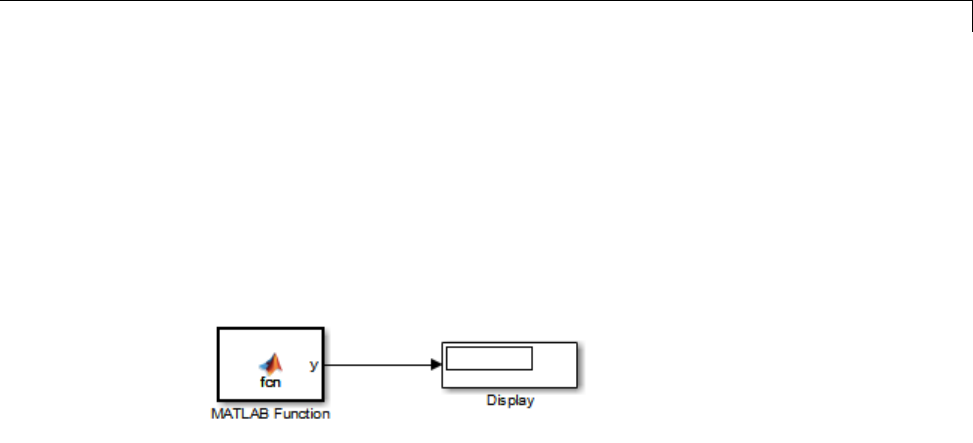
Share Data Globally
global Sig;
For more information on using the Ports and Data Manager, see “Ports and
Data Manager” on page 29-37.
Example: Using a Simulink.Signal Object with a MATLAB
Function Block
1Open the simulink_signal_local model. At the MATLAB command
line, enter:
addpath(fullfile(docroot, 'toolbox', 'simulink', 'examples'))
simulink_signal_local
2Double-click the MATLAB Function block to open its editor.
The MATLAB Function block modifies the value of global data Aeach time
it executes.
functiony=fcn
%#codegen
global A;
A = A+1;
y=A;
3From the MATLAB Function Block Editor menu, select Edit Data.
4In the Ports and Data Manager, select the data Ain the left pane.
The Ports and Data Manager displays the data attributes in the right pane.
Note that Ahas a scope of Data Store Memory.
5From the model menu, select View > Model Explorer.
29-123

29 Using the MATLAB Function Block
6IntheleftpaneoftheModelExplorer,select the model workspace for the
simulink_signal_local model.
The Contents pane displays the data in the model workspace.
7Click the Simulink.Signal object A.
The right pane displays attributes for A, including.
Attribute Value
Data type double
Complexity real
Dimensions 1
Sample mode Sample based
Initial value 5
8Simulate the model.
The MATLAB Function block reads the initial value of global data stored in
Aand updates the value of Aeach time it executes.
Using Data Store Diagnostics to Detect Memory
Access Issues
You can configure your model to provide run-time and compile-time
diagnostics for avoiding problems with data stores. Diagnostics are available
in the Configuration Parameters dialog box and the parameters dialog box for
the Data Store Memory block. These diagnostics are available for Data Store
Memory blocks only, not for Simulink.Signal objects. For more information
on using data store diagnostics, see “Data Store Diagnostics” on page 46-38.
Note If you pass data store memory arrays to functions, optimizations such
as A=foo(A) might result in the code generation software marking the entire
contents of the array as read or written even though only some elements
were accessed.
29-124

Share Data Globally
Limitations of Using Shared Data in MATLAB Function
Blocks
ThereisnoDataStoreMemorysupportfor:
•MATLAB structures
•Variable-sized data
29-125

29 Using the MATLAB Function Block
Add Frame-Based Signals
In this section...
“About Frame-Based Signals” on page 29-126
“Supported Types for Frame-Based Data” on page 29-126
“Adding Frame-Based Data in MATLAB Function Blocks” on page 29-127
“Examples of Frame-Based Signals in MATLAB Function Blocks” on page
29-128
About Frame-Based Signals
MATLAB Function blocks can input and output frame-based signals in
Simulink models. A frame of data is a collection of sequential samples from a
single channel or multiple channels. To generate frame-based signals, you
must have an available DSP System Toolbox license. For more information
about using frame-based signals, see “What Is Frame-Based Processing?”.
MATLAB Function blocks automatically convert incoming frame-based
signals as follows:
•Converts single-channel frame-based signals to MATLAB column vectors
•Converts multichannel frame-based signals to two-dimensional MATLAB
matrices
An M-by-N frame-based signal represents M consecutive samples from each of
N independent channels. N-Dimensional signals are not supported for frames.
To convert matrix or vector data to a frame-based output, use the data
property called Sampling mode to specify that your output is a frame-based
signal for downstream processing.
Supported Types for Frame-Based Data
MATLAB Function blocks accept frame-based signals of any data type except
bus objects. For a list of supported types, see “Supported Variable Types” on
page 33-18.
29-126

Add Frame-Based Signals
Adding Frame-BasedDatainMATLABFunctionBlocks
To add frame-based data to a MATLAB Function block, follow these steps:
1Add an input or output, as described in “Adding Data to a MATLAB
Function Block” on page 29-42.
2If your data is an output, set Sampling mode to Frame based.
Note If your data is an input, Sampling mode is not an option.
Note For more information on how to set data properties, see “Defining
Data in the Ports and Data Manager” on page 29-43.
29-127
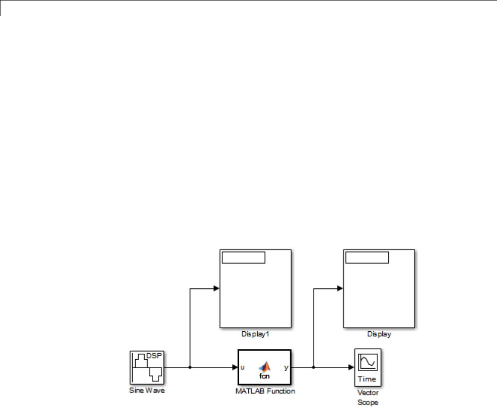
29 Using the MATLAB Function Block
Examples of Frame-Based Signals in MATLAB
Function Blocks
This topic presents examples of how to work with frame-based signals in
MATLAB Function blocks.
•“Multiplying a Frame-Based Signal by a Constant Value” on page 29-128
•“Adding a Channel to a Frame-Based Signal” on page 29-129
Multiplying a Frame-Based Signal by a Constant Value
In the following example, a MATLAB Function block multiplies all the
signal values in a frame-based single-channel input by a constant value and
outputs the result as a frame. The input signal is a sine wave that contains
5 samples per frame.
The MATLAB Function block contains the following code:
function y = fcn(u)
y = u*3;
Input uand output yinherit size, complexity, and data type from the input
sine wave signal, a 5-by-1 vector of signed, generalized fixed-point values.
For yto output a frame of data, you must explicitly set Sampling mode to
Frame based (see “Adding Frame-Based Data in MATLAB Function Blocks”
29-128
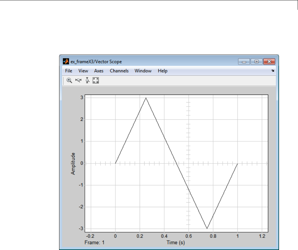
Add Frame-Based Signals
on page 29-127). When you simulate this model, the MATLAB Function block
multiplies each input signal by 3 and outputs the result as a frame.
Adding a Channel to a Frame-Based Signal
In the following example, a MATLAB Function block adds a channel to a
frame-based single-channel input and outputs the multichannel result. The
input signal is a sine wave that contains 8 samples per frame.
29-129
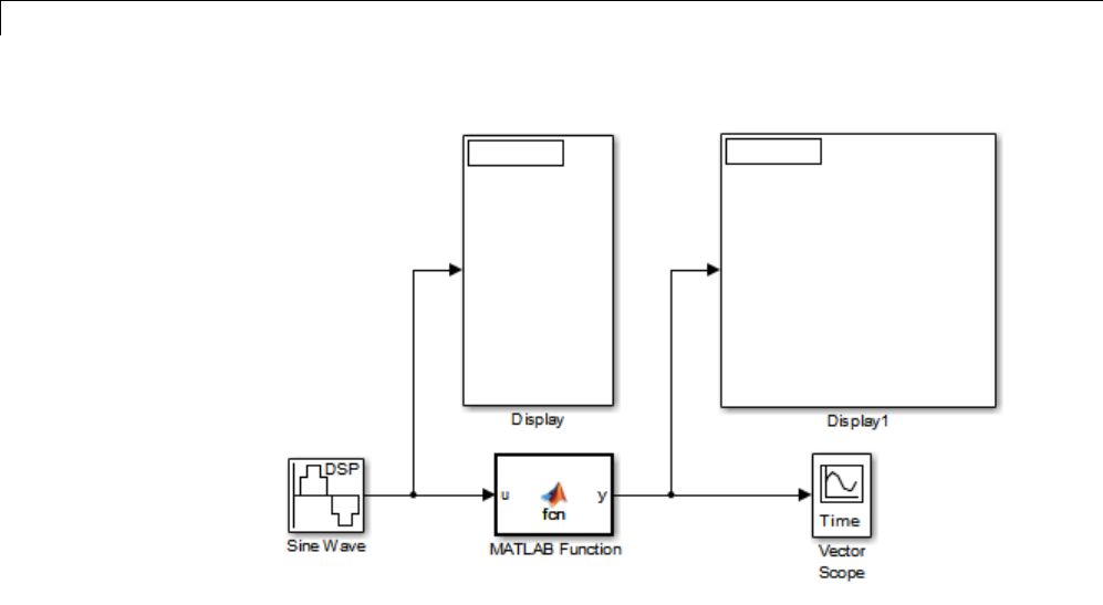
29 Using the MATLAB Function Block
The MATLAB Function block contains the following code:
function y = fcn(u)
a = [0;4;0;-4;0;4;0;-4];
y=[ua];
Input uand output yinherit size, complexity, and data type from the input
sine wave signal, an 8-by-1 vector of signed, generalized fixed-point values.
For yto output a frame of data, you must explicitly set Sampling mode to
Frame based (see “Adding Frame-Based Data in MATLAB Function Blocks”
on page 29-127). Local variable adefines a second column on the matrix
which will be output as a frame and interpreted as a second channel by
downstream blocks. When you simulate this model, the MATLAB Function
block outputs the new multichannel signal.
29-130
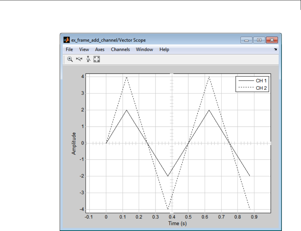
Add Frame-Based Signals
29-131

29 Using the MATLAB Function Block
Create Custom Block Libraries
In this section...
“When to Use MATLAB Function Block Libraries” on page 29-132
“How to Create Custom MATLAB Function Block Libraries” on page 29-132
“Example: Creating a Custom Signal Processing Filter Block Library” on
page 29-133
“Code Reuse with Library Blocks” on page 29-145
“Debugging MATLAB Function Library Blocks” on page 29-149
“Properties You Can Specialize Across Instances of Library Blocks” on
page 29-150
When to Use MATLAB Function Block Libraries
In Simulink, you can create your own block libraries as a way to reuse the
functionality of blocks or subsystems in one or more models. If you want to
reuse a set of MATLAB algorithms in Simulink models, you can encapsulate
your MATLAB code in a MATLAB Function block library.
As with other Simulink block libraries, you can specialize each instance of
MATLAB Function library blocks in your model to use different data types,
sample times, and other properties. Library instances that inherit the same
properties can reuse generated code (see “Code Reuse with Library Blocks”
on page 29-145).
For more information about Simulink block libraries, see “About Block
Libraries and Linked Blocks” on page 28-2.
How to Create Custom MATLAB Function Block
Libraries
Here is a basic workflow for creating custom block libraries with MATLAB
Function blocks. To work through these steps with an example, see “Example:
Creating a Custom Signal Processing Filter Block Library” on page 29-133.
29-132

Create Custom Block Libraries
1Add polymorphic MATLAB code to MATLAB Function blocks in a Simulink
model.
Polymorphic code is code that can process data with different properties,
such as type, size, and complexity.
2Configure the blocks to inherit the properties you want to specialize.
For a list of properties you can specialize, see “Properties You Can
Specialize Across Instances of Library Blocks” on page 29-150.
3Optionally, customize your library code using masking.
4Add instances of MATLAB Function library blocks to a Simulink model.
Example: Creating a Custom Signal Processing Filter
Block Library
•“What You Will Learn” on page 29-133
•“About the Filter Algorithms” on page 29-134
•“Step 1: Add the Filter Algorithms to MATLAB Function Library Blocks”
on page 29-134
•“Step 2: Configure Blocks to Inherit Properties You Want to Specialize”
on page 29-135
•“Step 3: Customize Your Library Using Masking” on page 29-136
•“Step 4: Add Instances of MATLAB Library Blocks to a Simulink Model”
on page 29-141
What You Will Learn
This simple example takes you through the workflow described in “How to
Create Custom MATLAB Function Block Libraries” on page 29-132 to show
you how to:
•Create a library of signal processing filter algorithms using MATLAB
Function blocks
•Customize one of the library blocks using mask parameters
29-133

29 Using the MATLAB Function Block
•Convert one of the filter algorithms to source-protected P-code that you can
call from a MATLAB Function library block
About the Filter Algorithms
The MATLAB filter algorithms are:
my_fft. Performs a discrete Fourier transform on an input signal. The input
can be a vector, matrix, or multidimensional array whose length is a power
of 2.
my_conv. Convolves two input vector signals. Outputs a subsection of the
convolution with a size specified by a mask parameter, Shape.
my_sobel. Convolves a 2D input matrix with a Sobel edge detection filter.
Step 1: Add the Filter Algorithms to MATLAB Function Library
Blocks
1In Simulink, create a library model by selecting File>New>Library
2Drag three MATLAB Function blocks into the model from the User-Defined
Functions section of the Simulink Library Browser and name them:
•my_fft_filter
•my_conv_filter
•my_sobel_filter
3Save the library model as my_filter_lib.
4Open the MATLAB Function block named my_fft_filter,replacethe
template code with the following code, and save the block:
function y = my_fft(x)
y = fft(x);
5Replace the template code in my_conv_filter block with the following
code and save the block:
29-134

Create Custom Block Libraries
function c = my_conv(a, b)
c = conv(a, b);
6Replace the template code in my_sobel_filter block with the following
code and save the block:
function y = my_sobel(u)
%% "my_sobel_filter" is a MATLAB function
%% on the MATLAB path.
y = my_sobel_filter(u);
The my_sobel function acts as a wrapper that calls a MATLAB function,
my_sobel_filter, on the code generation path. my_sobel_filter
implements the algorithm that convolves a 2D input matrix with a
Sobel edge detection filter. By calling the function rather than inlining
the code directly in the MATLAB Function block, you can reuse the
algorithm both as MATLAB code and in a Simulink model. You will create
my_sobel_filter next.
7In the same folder where you created my_filter_lib, create a new
MATLAB function my_sobel_filter with the following code:
function y = my_sobel_filter(u)
% Sobel edge detection filter
h = [1 2 1;...
0 0 0;...
-1 -2 -1];
y = abs(conv2(u, h));
Save the file as my_sobel_filter.m.
Step 2: Configure Blocks to Inherit Properties You Want to
Specialize
In this example, the data in the signal processing filter algorithms must
inherit size, type, and complexity from the Simulink model. By default, data
29-135

29 Using the MATLAB Function Block
in MATLAB Function blocks inherit these properties. To explicitly configure
data to inherit properties:
1Open a MATLAB Function block and select Edit Data.
2In the left pane of the Ports and Data Manager, select the data of interest.
3In the right pane, configure the data to inherit properties from Simulink:
To Inherit What to Specify
Size Enter -1 in Size field
Complexity Select Inherited from the
Complexity menu
Type Select Inherit: Same as Simulink
fromtheTypemenu
For example, if you open the MATLAB Function block my_fft_filter and look
at the properties of input xin the Ports and Data Manager, you see that size,
type, and complexity are inherited by default.
Note If your design has specific requirements or constraints, you can enter
values for any of these properties, rather than inherit them from Simulink.
For example, if your algorithm is not supposed to work with complex inputs,
set Complexity to Off.
See Also.
•“Ports and Data Manager” on page 29-37
•“Inheriting Argument Data Types” on page 29-66
Step 3: Customize Your Library Using Masking
In this exercise you will modify the convolution filter my_conv to use a custom
parameter shape that specifies what subsection of the convolution to output.
To customize this algorithm for your library, place the my_conv_filter block
under a masked subsystem and define shape as a mask parameter.
29-136
Create Custom Block Libraries
1Convert the block to a masked subsystem:
aRight-click the my_conv_filter block and select Subsystem & Model
Reference > Create Subsystem from Selection.
The my_conv_filter block changes to a subsystem block.
bChangethenameofthesubsystemtomy_conv_filter.
cRight-click the my_conv_filter subsystem and select Mask > Create
Mask from the context menu.
The Mask Editor appears with the Icon & Ports pane open.
dIn the Icons & Ports pane, add the following icon drawing commands:
disp('my_conv');
port_label('output', 1, 'c');
port_label('input', 1, 'a');
port_label('input', 2, 'b');
eSelect the Parameters tab and add a dialog parameter by selecting the
Add Parameter icon:
fAssign the following properties to the new dialog parameter:
Property What to Specify
Prompt Type Shape
Variable Type shape
29-137
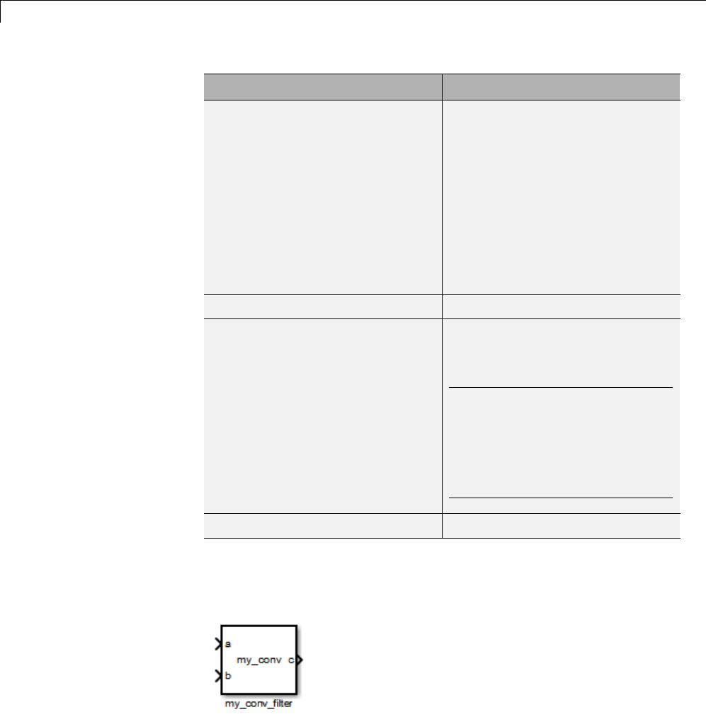
29 Using the MATLAB Function Block
Property What to Specify
Type •Select popup
•Enter type-specific options,
each on a separate line:
–full
–same
–valid
•Check Enable parameter
•Check Show parameter
Evaluate Check the box
Tunable Clear the box
Note In this example, the shape
parameter is not tunable. If in
your own application you want
to change the value of a mask
parameter during simulation,
check this box.
Tab name Leave blank
aClick OK.
Your subsystem should now look like this:
2Set subsystem properties for code reuse:
29-138
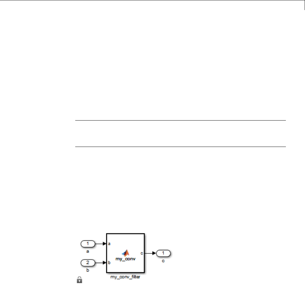
Create Custom Block Libraries
aRight-click the my_conv_filter subsystem and select Block Parameters
(Subsystem) from the context menu.
bIn the subsystem parameters dialog box, select the Treat as atomic
unit check box.
The dialog box expands to display new fields.
cTo generate a reusable function, select the Code Generation tab and in
the Function packaging field, select Reusable function from the
drop-down menu.
Note This is an optional step, required for this example. If you leave the
default setting of Auto, the code generation software uses an internal
rule to determine whether to inline the function or not.
dClick OK.
3Define the shape parameter in the MATLAB Function my_conv:
aRight-click the my_conv_filter subsystem and select Mask > Look
Under Mask from the context menu.
The block diagram under the masked subsystem opens, containing the
my_conv_filter block:
bChange the names of the port blocks to match the data names as follows:
29-139

29 Using the MATLAB Function Block
Change: To:
In1 a
In2 b
Out1 c
cDouble-click the my_conv_filter block to open the MATLAB Function
Block Editor.
dIn the MATLAB Function Block Editor, select Edit Data.
eIn the Ports and Data Manager, select Add > Data.
A new data element appears selected, along with its properties dialog.
fEnter the following properties:
Property What To Specify
Name Enter shape.
Scope Select Parameter.
Tunable Clear the box.
gLeave Size,Complexity,andType as inherited (the defaults), as
described in “Step 2: Configure Blocks to Inherit Properties You Want to
Specialize” on page 29-135.
hClick Apply, close the Ports and Data Manager, and return to the
MATLAB Function Block Editor.
4Use the shape parameter to determine the size of the convolution to output:
aIn the MATLAB Function Block Editor, modify the my_conv function
to call conv with the right shape:
function c = my_conv(a, b, shape)
if shape == 1
c = conv(a, b, 'full');
elseif shape == 2
c = conv(a, b, 'same');
else
c = conv(a, b, 'valid');
29-140

Create Custom Block Libraries
end
bSave your changes and close the MATLAB Function Block Editor.
See Also.
•“Masking”
Step 4: Add Instances of MATLAB Library Blocks to a Simulink
Model
In this exercise, you will add specialized instances of the my_conv_filter
library block to a simple test model.
1Open a new Simulink model.
For purposes of this exercise, set the following configuration parameters for
simulation:
Pane Section What to Specify
Solver Solver options •Select Fixed-Step
for Type
•Select discrete
(no continuous
states) for Solver
•Enter 1for
Fixed-step size
Data Import/Export Save options Structure for Format
2Drag two instances of the my_conv_filter block from the my_filter_lib
library into the model.
3Add Constant, Outport, and Display blocks. Your model should look
something like this:
29-141
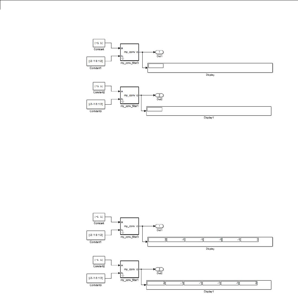
29 Using the MATLAB Function Block
Both library instances share the same size, type, and complexity for inputs
aand brespectively.
4Double-click each library instance.
The shape parameter defaults to full for both instances.
5Simulate the model.
Each library instance outputs the same result, the full 2D convolution:
6Specialize the second instance, my_conv_filter1 by setting the value of its
shape parameter to same.
29-142
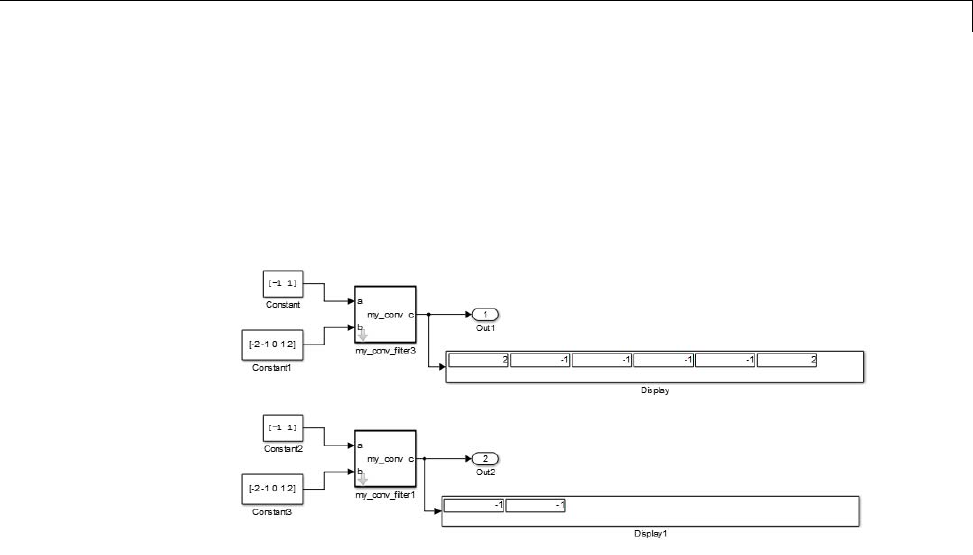
Create Custom Block Libraries
7Now simulate the model again.
This time, the outputs have different sizes: my_conv_filter3 outputs the
full 2D convolution, while my_conv_filter1 displays the central part of the
convolution as a 1-by-2 vector, the same size as a:
8Now, add a third instance by copying my_conv_filter1. Specialize the new
instance, my_conv_filter2, so that it does not inherit the same size inputs
asthefirsttwoinstances:
29-143
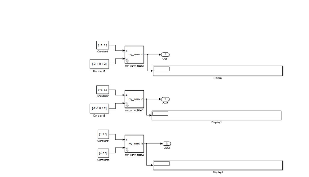
29 Using the MATLAB Function Block
9Simulate the model again.
This time, my_conv_filter1 and my_conv_filter2 each display the central
part of the convolution, but the output sizes are different because each
matches a different sized input a.
29-144
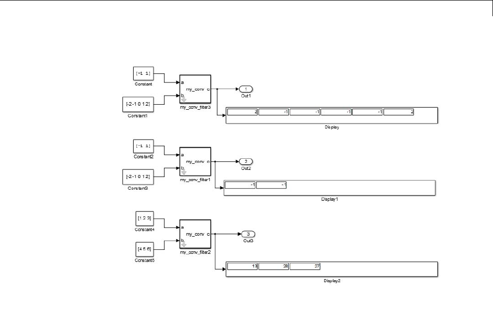
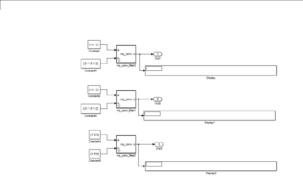
29 Using the MATLAB Function Block
In this model, the library instances my_conv_filter and my_conv_filter1
inherit the same size, type, and complexity for each respective input. For
each instance, input aisa1-by-2vectorandinputbisa1-by-5vector. By
comparison, the inputs of my_conv_filter2 inherit different respective sizes;
both are 1-by-3 vectors.
In addition, each library instance has a mask parameter called shape that
determines what subsection of the convolution to output. Assume that the
valueofshapeisthesameforeachinstance.
To generate code for this example, follow these steps:
1Enable code reuse for the library block:
aIn the library, right-click the MATLAB Function block my_conv_filter
and select Block Parameters (Subsystem) from the context menu.
bIn the Function Block Parameters dialog box, set these parameters:
•Select the Treat as atomic unit check box.
29-146

Create Custom Block Libraries
•In the Function packaging field, select Reusable function from
the drop-down menu.
2Configure the model for code generation.
For purposes of this exercise, set the following configuration parameters:
Pane Section What to Specify
Code Generation Target selection Enter ert.tlc for
System target file
Code Generation >
Report
Select Create code
generation report
check box.
3Build the model.
If you build this model, the generated C code reuses logic for the
my_conv_filter and my_conv_filter1 library instances because they
inherit the same input properties:
/*
* Output and update for atomic system:
* '<Root>/my_conv_filter'
* '<Root>/my_conv_filter1'
*/
void sp_algorithm_tes_my_conv_filter(const real32_T rtu_a[2], const real32_T
rtu_b[5], rtB_my_conv_filter_sp_algorithm *localB)
{
int32_T jA;
int32_T jA_0;
real32_T s;
int32_T jC;
/* MATLAB Function Block: '<S1>/my_conv_filter' */
/* MATLAB Function 'my_conv_filter/my_conv_filter': '<S4>:1' */
/* '<S4>:1:4' */
for (jC = 0; jC < 6; jC++) {
if (5 < jC + 2) {
29-147

29 Using the MATLAB Function Block
jA=jC-4;
} else {
jA = 0;
}
if (2 < jC + 1) {
jA_0 = 2;
} else {
jA_0 = jC + 1;
}
s = 0.0F;
while (jA + 1 <= jA_0) {
s += rtu_b[jC - jA] * rtu_a[jA];
jA++;
}
localB->c[jC] = s;
}
/* end of MATLAB Function Block: '<S1>/my_conv_filter' */
}
However, a separate function is generated for my_conv_filter2:
/* Output and update for atomic system: '<Root>/my_conv_filter2' */
void sp_algorithm_te_my_conv_filter2(const real_T rtu_a[3], const real_T rtu_b[3],
rtB_my_conv_filter_sp_algorit_h *localB)
{
int32_T jA;
int32_T jA_0;
real_T s;
int32_T jC;
/* MATLAB Function Block: '<S3>/my_conv_filter' */
/* MATLAB Function 'my_conv_filter/my_conv_filter': '<S6>:1' */
/* '<S6>:1:4' */
for (jC = 0; jC < 5; jC++) {
if (3 < jC + 2) {
29-148

Create Custom Block Libraries
jA=jC-2;
} else {
jA = 0;
}
if (3 < jC + 1) {
jA_0 = 3;
} else {
jA_0 = jC + 1;
}
s = 0.0;
while (jA + 1 <= jA_0) {
s += rtu_b[jC - jA] * rtu_a[jA];
jA++;
}
localB->c[jC] = s;
}
/* end of MATLAB Function Block: '<S3>/my_conv_filter' */
}
Note Generating C code for this model requires a Simulink Coder or
Embedded Coder license.
Debugging MATLAB Function Library Blocks
You debug MATLAB Function library blocks the same way you debug any
MATLAB Function block. However, when you add a breakpoint in a library
block, the breakpoint is shared by all instances. As you continue execution,
the debugger stops at the breakpoint in each instance.
29-149

29 Using the MATLAB Function Block
For more information, see “Debugging a MATLAB Function Block” on page
29-23
Properties You Can Specialize Across Instances of
Library Blocks
You can specialize instances of MATLAB Function library blocks by allowing
them to inherit any of the following properties from Simulink:
Property Inherits by
Default?
How to Specify Inheritance
Type Yes Set data type property to Inherit: Same
as Simulink.
Size Yes Set data size property to -1.
Complexity Yes Set data complexity property to Inherited.
Limit range No Specify minimum and maximum values as
Simulink parameters.
For example, if minimum value = aParam
and maximum value = aParam +3,
different instances of a MATLAB Function
library block can resolve to different
aParam parameters defined in their parent
mask subsystems.
Sampling mode
(input)
Yes MATLAB Function block input ports
always inherit sampling mode
Data type
override mode
for fixed-point
data
Yes Set data type override property to Inherit.
Sample time
(block)
Yes Set block sample time property to -1.
29-150

Use Traceability in MATLAB Function Blocks
Use Traceability in MATLAB Function Blocks
In this section...
“Extent of Traceability in MATLAB Function Blocks” on page 29-151
“Traceability Requirements” on page 29-151
“Basic Workflow for Using Traceability” on page 29-152
“Tutorial: Using Traceability in a MATLAB Function Block” on page 29-153
Extent of Traceability in MATLAB Function Blocks
Like other Simulink blocks, MATLAB Function blocks support bidirectional
traceability, but extend navigation to lines of source code. That is, you can
navigate between a line of generated code and its corresponding line of source
code. In other Simulink blocks, you can navigate between a line of generated
code and its corresponding object.
In addition, you can select to include the source code as comments in
the generated code. When you select this option, the MATLAB source
code appears immediately after the associated traceability tag. For more
information, see “Include MATLAB Code as Comments in Generated Code”
on page 29-156.
For information about how traceability works in Simulink blocks, see “About
Code Tracing”.
Traceability Requirements
To enable traceability comments in your code, you must have a license for
Embedded Coder software. These comments appear only in code that you
generate for an Embedded Real-Time (ERT)target.
Note Traceability is not supported for MATLAB files that you call from
a MATLAB Function block.
29-151

29 Using the MATLAB Function Block
Basic Workflow for Using Traceability
The workflow for using traceability is described in “Trace Model Objects to
Generated Code”. Here are the basic steps:
1Open the MATLAB Function block in your Simulink model.
2Define your system target file to be an Embedded Real-Time (ERT)target.
aIn the model, select Simulation > Model Configuration Parameters.
bIn the Code Generation pane, enter ert.tlc for the system target file.
3Enable traceability options.
aIn the Code Generation > Report pane, select Create code
generation report.
This action automatically selects the Open report automatically and
Code-to-model options.
bSelect Model-to-code.
This action automatically selects all options in the Traceability Report
Contents section.
4Generate the source code and header files for your model.
5Trace a line of code:
To Trace: Do This:
Line of source code to line of
generated code
Right-click in a line in your
source code and select Code
Generation > Navigate to Code
from the context menu
Line of generated code to line of
source code
Clickahyperlinkinthetraceability
comment in your generated code
To learn how to complete each step in this workflow, see “Tutorial: Using
Traceability in a MATLAB Function Block” on page 29-153
29-152

Use Traceability in MATLAB Function Blocks
Tutorial: Using Traceability in a MATLAB Function
Block
This example shows how to trace between source code and generated code in a
MATLAB Function block in the eml_fire model. Follow these steps:
1Type eml_fire at the MATLAB prompt.
2In the Simulink model window, double-click the flame block to open the
MATLAB Function Block Editor.
3In the Simulink model window, select Simulation > Model
Configuration Parameters.
4In the Code Generation pane,gototheTarget selection section and
enter ert.tlc for the system target file. Then click Apply.
Note Traceability comments appear hyperlinked in generated code only
for embedded real-time (ert)targets.
5In the Code Generation > Report pane, select the Create code
generation report option.
This action automatically selects the Open report automatically and
Code-to-model options.
6Select the Model-to-code option in the Navigation section. Then click
Apply.
This action automatically selects all options in the Traceability Report
Contents section.
Note For large models that contain over 1000 blocks, disable the
Model-to-code option to speed up code generation.
29-153

29 Using the MATLAB Function Block
7Go to the Code Generation > Interface pane. In the Software
environment section, select the continuous time option. Then click
Apply.
Note Because this example model contains a block with a continuous
sample time, you must perform this step before generating code.
8In the Code Generation pane, click Build in the lower right corner.
This action generates source code and header files for the eml_fire
model that contains the flame block. After the code generation process is
complete, the code generation report appears automatically.
9Click the eml_fire.c hyperlink in the report.
10 Scroll down through the code to see the traceability comments, which
appear as links inside /*...*/ brackets, as in this example.
for (b_x = 0; b_x < 256; b_x++) {
/* '<S2>:1:19' */
/* '<S2>:1:21' */
yb = loopVar_i + 2;
/* '<S2>:1:22' */
xb = b_x - 1;
Note The line numbers shown above may differ from the numbers that
appear in your code generation report.
11 Click the <S2>:1:19 hyperlink in this traceability comment:
/* '<S2>:1:19'*/
Line 19 of the function appears highlighted in the MATLAB Function
Block Editor.
29-154

Use Traceability in MATLAB Function Blocks
12 You can also trace a line in a MATLAB function to a line of generated
code. For example, right-click in line 21 of your function and select Code
Generation > Navigate to Code from the context menu.
The code location for line 21 appears highlighted in eml_fire.c.
29-155

29 Using the MATLAB Function Block
Include MATLAB Code as Comments in Generated Code
If you have a Simulink Coder license, you can include MATLAB source code
as comments in the code generated for a MATLAB Function block. Including
this information in the generated code enables you to:
•Correlate the generated code with your source code.
•Understand how the generated code implements your algorithm.
•Evaluate the quality of the generated code.
When you select this option, the generated code includes:
•The source code as a comment immediately after the traceability tag. When
you enable traceability and generate code for ERT targets (requires an
Embedded Coder license), the traceability tags are hyperlinks to the source
code. For more information on traceability for the MATLAB Function
block,see“UseTraceabilityinMATLAB Function Blocks” on page 29-151.
For examples and information on the location of the comments in the
generated code, see “Location of Comments in Generated Code” on page
29-157.
•The function help text in the function body in the generated code. The
function help text is the first comment after the MATLAB function
signature. It provides information about the capabilities of the function
and how to use it.
Note With an Embedded Coder license, you can also include the
function help text in the function banner of the generated code. For more
information, see “Including MATLAB Function Help Text in the Function
Banner” on page 29-160.
How to Include MATLAB Code as Comments in the
Generated Code
To include MATLAB source code as comments in the code generated for
a MATLAB Function block:
29-156

Include MATLAB®Code as Comments in Generated Code
1In the model, select Simulation > Model Configuration Parameters.
2In the Code Generation > Comments pane, select MATLAB source
code as comments and click Apply.
Location of Comments in Generated Code
The automatically generated comments containing the source code appear
after the traceability tag in the generated code as follows.
Straight-Line Source Code
The comment containing the source code precedes the generated code that
implements the source code statement. This comment appears after any
comments that you add that precede the generated code. The comments are
separated from the generated code because the statements are assigned to
function outputs.
MATLAB Code.
function [x y] = straightline(r,theta)
%#codegen
% Convert polar to Cartesian
x = r * cos(theta);
y = r * sin(theta);
Commented C Code.
/* MATLAB Function 'straightline': '<S1>:1' */
/* Convert polar to Cartesian */
/* '<S1>:1:4' x = r * cos(theta); */
/* '<S1>:1:5' y = r * sin(theta); */
straightline0_Y.x = straightline0_U.r * cos(straightline0_U.theta);
/* Outport: '<Root>/y' incorporates:
* Inport: '<Root>/r'
* Inport: '<Root>/theta'
* MATLAB Function Block: '<Root>/straightline'
*/
straightline0_Y.y = straightline0_U.r * sin(straightline0_U.theta);
29-157

29 Using the MATLAB Function Block
If Statements
The comment for the if statement immediately precedes the code that
implements the statement. This comment appears after any comments that
you add that precede the generated code. The comments for the elseif and
else clauses appear immediately after the code that implements the clause,
and before the code generated for statements in the clause.
MATLAB Code.
function y = ifstmt(u,v)
%#codegen
if u > v
y=v+10;
elseif u == v
y=u*2;
else
y=v-10;
end
Commented C Code.
/* MATLAB Function 'MLFcn': '<S1>:1' */
/* '<S1>:1:3' ifu>v*/
if (MLFcn_U.u > MLFcn_U.v) {
/* Outport: '<Root>/y' */
/* '<S1>:1:4' y=v+10;*/
MLFcn_Y.y = MLFcn_U.v + 10.0;
} else if (MLFcn_U.u == MLFcn_U.v) {
/* Outport: '<Root>/y' */
/* '<S1>:1:5' elseif u == v */
/* '<S1>:1:6' y=u*2;*/
MLFcn_Y.y = MLFcn_U.u * 2.0;
} else {
/* Outport: '<Root>/y' */
/* '<S1>:1:7' else */
/* '<S1>:1:8' y = v - 10; */
MLFcn_Y.y = MLFcn_U.v - 10.0;
29-158

Include MATLAB®Code as Comments in Generated Code
For Statements
The comment for the for statement header immediately precedes the
generated code that implements the header. This comment appears after any
comments that you add that precede the generated code.
MATLAB Code.
function y = forstmt(u)
%#codegen
y=0;
for i=1:u
y=y+1;
end
Commented C Code.
/* MATLAB Function 'MLFcn': '<S1>:1' */
/* '<S1>:1:3' y = 0; */
rtb_y = 0.0;
/* '<S1>:1:5' for i=1:u */
for (i = 1.0; i <= MLFcn_U.u; i++) {
/* '<S1>:1:6' y=y+1;*/
rtb_y++;
While Statements
The comment for the while statement header immediately precedes the
generated code that implements the statement header. This comment appears
after any comments that you add that precede the generated code.
Switch Statements
The comment for the switch statement header immediately precedes the
generated code that implements the statement header. This comment
appears after any comments that you add that precede the generated code.
The comments for the case and otherwise clauses appear immediately after
the generated code that implements the clause, and before the code generated
for statements in the clause.
29-159

29 Using the MATLAB Function Block
Including MATLABFunctionHelpTextintheFunction
Banner
You can include the function help text in the function banner of the code
generated for a MATLAB Function block. The function help text is the first
comment after the MATLAB function signature. It provides information
about the capabilities of the function and how to use it.
1In the model, select Simulation > Model Configuration Parameters.
2In the Code Generation > Comments pane, select MATLAB function
help text and click Apply.
Note If the function is inlined, the function help text is also inlined.
Therefore, the help text for inlined functions appears in the function body in
the generated code even when this option is selected.
LimitationsofMATLABSourceCodeasComments
The MATLAB Function block has the following limitations for including
MATLAB source code as comments.
•You cannot include MATLAB source code as comments for:
-MathWorks toolbox functions
-P-code
-Simulation targets
-StateflowTruth Table blocks
•The appearance or location of comments can vary depending on the
following conditions:
-Comments might still appear in the generated code even if the
implementation code is eliminated, for example, due to constant folding.
-Comments might be eliminated from the generated code if a complete
function or code block is eliminated.
-For certain optimizations, the comments might be separated from the
generated code.
29-160

Include MATLAB®Code as Comments in Generated Code
-The generated code always includes legally required comments from the
MATLAB source code, even if you do not choose to include source code
comments in the generated code.
29-161

29 Using the MATLAB Function Block
Enhance Code Readability for MATLAB Function Blocks
In this section...
“Requirements for Using Readability Optimizations” on page 29-162
“Converting If-Elseif-Else Code to Switch-Case Statements” on page 29-162
“Example of Converting Code for If-Elseif-Else Decision Logic to
Switch-Case Statements” on page 29-165
Requirements for Using Readability Optimizations
To use readability optimizations in your code, you must have an Embedded
Coder license. These optimizations appear only in code that you generate for
an embedded real-time (ert)target.
Note These optimizations do not apply to MATLAB files that you call from
the MATLAB Function block.
For more information, see “Target” and “Control Code Style” in the Embedded
Coder documentation.
Converting If-Elseif-Else Code to Switch-Case
Statements
When you generate code for embedded real-time targets, you can choose to
convert if-elseif-else decision logic to switch-case statements. This
conversion can enhance readability of the code.
For example, when a MATLAB Function block contains a long list of
conditions, the switch-case structure:
•Reduces the use of parentheses and braces
•Minimizes repetition in the generated code
29-162

Enhance Code Readability for MATLAB Function Blocks
How to Convert If-Elseif-Else Code to Switch-Case Statements
The following procedure describes how to convert generated code for the
MATLAB Function block from if-elseif-else to switch-case statements.
Step Task Reference
1Verify that your block follows the
rules for conversion.
“Verifying the Contents of the
Block” on page 29-167
2Enable the conversion. “Enabling the Conversion” on
page 29-168
3Generate code for your model.“GeneratingCodeforYour
Model” on page 29-169
Rules for Conversion
For the conversion to occur, the following rules must hold. LHS and RHS
refer to the left-hand side and right-hand side of a condition, respectively.
Construct Rules to Follow
MATLAB Function
block
Must have two or more unique conditions, in addition
to a default.
For more information, see “How the Conversion
Handles Duplicate Conditions” on page 29-164.
Must test equality only.Each condition
Must use the same variable or expression for the LHS.
Note You can reverse the LHS and RHS.
29-163

29 Using the MATLAB Function Block
Construct Rules to Follow
Must be a single variable or expression, not a
compound statement.
Cannot be a constant.
Must have an integer or enumerated data type.
Each LHS
Cannot have any side effects on simulation.
For example, the LHS can read from but not write to
global variables.
Must be a constant.
Each RHS
Must have an integer or enumerated data type.
How the Conversion Handles Duplicate Conditions
If a MATLAB Function block has duplicate conditions, the conversion
preserves only the first condition. The generated code discards all other
instances of duplicate conditions.
After removal of duplicates, two or more unique conditions must exist.
Otherwise, no conversion occurs and the generated code contains all instances
of duplicate conditions.
The following examples show how the conversion handles duplicate conditions.
Example of Generated Code Code After Conversion
if (x == 1) {
block1
} else if (x == 2) {
block2
} else if (x == 1) { // duplicate
block3
} else if (x == 3) {
block4
} else if (x == 1) { // duplicate
block5
} else {
switch (x) {
case 1:
block1; break;
case 2:
block2; break;
case 3:
block4; break;
default:
block6; break;
29-164
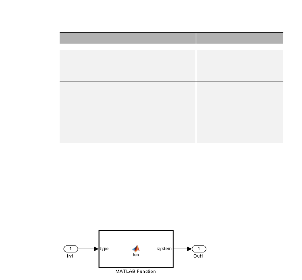
Enhance Code Readability for MATLAB Function Blocks
Example of Generated Code Code After Conversion
block6
}
}
if (x == 1) {
block1
} else if (x == 1) { // duplicate
block2
} else {
block3
}
No change, because only one
unique condition exists
Example of Converting Code for If-Elseif-Else Decision
Logic to Switch-Case Statements
Suppose that you have the following model with a MATLAB Function block.
Assume that the output data type is double and the input data type is
Controller, an enumerated type that you define. (For more information,
see “Define Enumerated Data Types for MATLAB Function Blocks” on page
29-106.)
29-165

29 Using the MATLAB Function Block
The block contains the following code:
function system = fcn(type)
%#codegen
if (type == Controller.P)
system = 0;
elseif (type == Controller.I)
system = 1;
elseif (type == Controller.PD)
system = 2;
elseif (type == Controller.PI)
system = 3;
elseif (type == Controller.PID)
system = 4;
else
system = 10;
end
The enumerated type definition in Controller.m is:
classdef(Enumeration) Controller < Simulink.IntEnumType
enumeration
P(0)
I(1)
PD(2)
PI(3)
PID(4)
UNKNOWN(10)
end
end
If you generate code for an embedded real-time target using default settings,
you see something like this:
if (if_to_switch_eml_blocks_U.In1 == P) {
/* '<S1>:1:4' */
/* '<S1>:1:5' */
if_to_switch_eml_blocks_Y.Out1 = 0.0;
} else if (if_to_switch_eml_blocks_U.In1 == I) {
/* '<S1>:1:6' */
29-166

Enhance Code Readability for MATLAB Function Blocks
/* '<S1>:1:7' */
if_to_switch_eml_blocks_Y.Out1 = 1.0;
} else if (if_to_switch_eml_blocks_U.In1 == PD) {
/* '<S1>:1:8' */
/* '<S1>:1:9' */
if_to_switch_eml_blocks_Y.Out1 = 2.0;
} else if (if_to_switch_eml_blocks_U.In1 == PI) {
/* '<S1>:1:10' */
/* '<S1>:1:11' */
if_to_switch_eml_blocks_Y.Out1 = 3.0;
} else if (if_to_switch_eml_blocks_U.In1 == PID) {
/* '<S1>:1:12' */
/* '<S1>:1:13' */
if_to_switch_eml_blocks_Y.Out1 = 4.0;
}else{
/* '<S1>:1:15' */
if_to_switch_eml_blocks_Y.Out1 = 10.0;
}
The LHS variable if_to_switch_eml_blocks_U.In1 appears multiple times
in the generated code.
Note By default, variables that appear in the block do not retain their names
in the generated code. Modified identifiersguaranteethatnonamingconflicts
occur.
Traceability comments appear between each set of /* and */ markers. To
learn more about traceability, see “Use Traceability in MATLAB Function
Blocks” on page 29-151.
Verifying the Contents of the Block
Check that the block follows all the rules in “Rules for Conversion” on page
29-163.
29-167

29 Using the MATLAB Function Block
Construct How the Construct Follows the Rules
MATLAB
Function block
Five unique conditions exist, in addition to the default:
•(type == Controller.P)
•(type == Controller.I)
•(type == Controller.PD)
•(type == Controller.PI)
•(type == Controller.PID)
Each condition Each condition:
•Tests equality
•UsesthesameinputfortheLHS
Each LHS Each LHS:
•Contains a single variable
•Is the input to the block and therefore not a constant
•Is of enumerated type Controller,whichyoudefinein
Controller.m on the MATLAB path
•Hasnosideeffectsonsimulation
Each RHS Each RHS:
•Is an enumerated value and therefore a constant
•Is of enumerated type Controller
Enabling the Conversion
1Open the Configuration Parameters dialog box.
2In the Code Generation pane, select ert.tlc for the System target file.
This step specifies an embedded real-time target for your model.
29-168

Enhance Code Readability for MATLAB Function Blocks
3In the Code Generation > Code Style pane, select the Convert
if-elseif-else patterns to switch-case statements check box.
Tip This conversion works on a per-model basis. If you select this check
box, the conversion applies to:
•All MATLAB Function blocks in a model
•MATLAB functions in all Stateflow charts of that model
•Flow graphs in all Stateflow charts of that model
For more information, see “Enhancing Readability of Code for Flow
Graphs” in the Stateflow documentation.
Generating Code for Your Model
In the Code Generation pane of the Configuration Parameters dialog box,
click Build in the lower right corner.
ThecodefortheMATLABFunctionblockusesswitch-case statements
instead of if-elseif-else code:
switch (if_to_switch_eml_blocks_U.In1) {
case P:
/* '<S1>:1:4' */
/* '<S1>:1:5' */
if_to_switch_eml_blocks_Y.Out1 = 0.0;
break;
case I:
/* '<S1>:1:6' */
/* '<S1>:1:7' */
if_to_switch_eml_blocks_Y.Out1 = 1.0;
break;
case PD:
/* '<S1>:1:8' */
/* '<S1>:1:9' */
29-169

29 Using the MATLAB Function Block
if_to_switch_eml_blocks_Y.Out1 = 2.0;
break;
case PI:
/* '<S1>:1:10' */
/* '<S1>:1:11' */
if_to_switch_eml_blocks_Y.Out1 = 3.0;
break;
case PID:
/* '<S1>:1:12' */
/* '<S1>:1:13' */
if_to_switch_eml_blocks_Y.Out1 = 4.0;
break;
default:
/* '<S1>:1:15' */
if_to_switch_eml_blocks_Y.Out1 = 10.0;
break;
}
The switch-case statements provide the following benefits to enhance
readability:
•The code reduces the use of parentheses and braces.
•The LHS variable if_to_switch_eml_blocks_U.In1 appears only once,
minimizing repetition in the code.
29-170

Speed Up Simulation with Basic Linear Algebra Subprograms
Speed Up Simulation with Basic Linear Algebra
Subprograms
In this section...
“How MATLAB Function Blocks Use the BasicLinearAlgebraSubprograms
(BLAS) Library” on page 29-171
“When to Disable BLAS Library Support” on page 29-171
“How to Disable BLAS Library Support” on page 29-172
“Supported Compilers” on page 29-172
How MATLAB Function Blocks Use the Basic Linear
Algebra Subprograms (BLAS) Library
The Basic Linear Algebra Subprograms (BLAS) Library is a library of
external linear algebra routines optimized for fast computation of low-level
matrix operations. By default, MATLAB Function blocks call BLAS library
routines to speed simulation whenever possible, except in these cases:
•Your C/C++ compiler does not support the BLAS library
•The size of the matrix is below a minimum threshold
MATLAB for code generation uses a heuristic to evaluate matrix size
against the overhead of calling an external library.
•When you are generating C/C++ code for MATLAB functions using
Simulink Coder.
Simulink Coder uses BLAS only for simulation.
When to Disable BLAS Library Support
Consider disabling BLAS library support for MATLAB Function blocks when:
•You want your simulation results to more closely agree with code generated
by Simulink Coder for your MATLAB Function block.
•You are executing code on a 64-bit platform and the number of elements
in a matrix exceeds 32 bits.
29-171

29 Using the MATLAB Function Block
In this case, automatic truncation to a 32-bit matrix size occurs.
•Your platform does not provide a robust implementation of BLAS routines.
How to Disable BLAS Library Support
MATLAB Function blocks enable BLAS library support by default, but you
can disable this feature explicitly for all MATLAB Function blocks in your
Simulink model. Follow these steps:
1Open your MATLAB Function block.
2In the MATLAB Function Block Editor, select Simulation Target.
The Configuration Parameters dialog box opens with Simulation Target
selected.
3Clear the Use BLAS library for faster simulation check box and click
Apply.
Supported Compilers
MATLAB Function blocks use the BLAS library on all C compilers except:
•Watcom
•Intel
•Borland
The default MATLAB compiler for Windows, 32–bit platforms, lcc,supports
the BLAS library. To install a different C compiler, use the mex -setup
command, as described in “Build MEX-Files”.
29-172

Control Run-Time Checks
Control Run-Time Checks
In this section...
“Types of Run-Time Checks” on page 29-173
“When to Disable Run-Time Checks” on page 29-173
“How to Disable Run-Time Checks” on page 29-174
TypesofRun-TimeChecks
In simulation, the code generated for your MATLAB Function block includes
the following run-time checks:
•Memory integrity checks
These checks detect violations of memory integrity in code generated for
MATLAB Function blocks and stop execution with a diagnostic message.
Caution For safety, these checks are enabled by default. Without memory
integrity checks, violations result in unpredictable behavior.
•Responsiveness checks in code generated for MATLAB Function blocks
These checks enable periodic checks for Ctrl+C breaks in the generated
code. Enabling responsiveness checks also enables graphics refreshing.
Caution For safety, these checks are enabled by default. Without these
checks, the only way to end a long-running execution might be to terminate
MATLAB.
When to Disable Run-Time Checks
Generally, generating code with run-time checks enabled results in more lines
of generated code and slower simulation than generating code with the checks
29-173

29 Using the MATLAB Function Block
disabled. Disabling run-time checks usually results in streamlined generated
code and faster simulation, with these caveats:
Consider disabling: Only if:
Memoryintegritychecks Youaresurethatyourcodeis
safe and that all array bounds and
dimension checking is unnecessary.
Responsiveness checks You are sure that you will not need
to stop execution of your application
using Ctrl+C.
How to Disable Run-Time Checks
MATLAB Function blocks enable run-time checks by default, but you can
disable them explicitly for all MATLAB Function blocks in your Simulink
model. Follow these steps:
1Open your MATLAB Function block.
2In the MATLAB Function Block Editor, select Simulation Target.
The Configuration Parameters dialog box opens with Simulation Target
selected.
3Clear the Ensure memory integrity or Ensure responsiveness check
boxes, as applicable, and click Apply.
29-174

Track Object Using MATLAB®Code
Track Object Using MATLAB Code
In this section...
“Learning Objectives” on page 29-175
“Tutorial Prerequisites” on page 29-176
“Example: The Kalman Filter” on page 29-176
“Files for the Tutorial” on page 29-179
“Tutorial Steps” on page 29-181
“Best Practices Used in This Tutorial” on page 29-201
“Key Points to Remember” on page 29-201
“Where to Learn More” on page 29-201
Learning Objectives
In this tutorial, you will learn how to:
•Use the MATLAB Function block to add MATLAB functions to Simulink
models for modeling, simulation, and deployment to embedded processors.
This capability is useful for coding algorithms that are better stated in the
textual language of MATLAB than in the graphical language of Simulink.
•Use coder.extrinsic to call MATLAB code from a MATLAB Function
block.
This capability allows you to do rapid prototyping. You can call existing
MATLAB code from Simulink without having to make this code suitable
for code generation.
•Check that existing MATLAB code is suitable for code generation before
generating code.
You must prepare your code before generating code.
•Specify variable-size inputs when generating code.
29-175

29 Using the MATLAB Function Block
Tutorial Prerequisites
•“What You Need to Know” on page 29-176
•“Required Products” on page 29-176
What You Need to Know
To complete this tutorial, you should have basic familiarity with MATLAB
software. You should also understand how to create and simulate a basic
Simulink model.
Required Products
To complete this tutorial, you must install the following products:
•MATLAB
•MATLAB Coder
•Simulink
•Simulink Coder
•Ccompil
er
For a list of supported compilers, see .
You must set up the C compiler before generating C code. See “Setting Up
Your C Compiler” on page 29-182.
For instructions on installing MathWorks products, see the MATLAB
installation documentation for your platform. If you have installed MATLAB
and want to check which other MathWorks products are installed, enter ver
in the MATLAB Command Window.
Example: TheKalmanFilter
•“Description” on page 29-177
•“Algorithm” on page 29-177
•“Filtering Process” on page 29-178
29-176

Track Object Using MATLAB®Code
•“Reference” on page 29-179
Description
This section describes the example used by the tutorial. You do not have to be
familiar with the algorithm to complete the tutorial.
The example for this tutorial uses a Kalman filter to estimate the position
of an object moving in a two-dimensional space from a series of noisy inputs
based on past positions. The position vector has two components, xand y,
indicating its horizontal and vertical coordinates.
Kalman filters have a wide range of applications, including control, signal
and image processing; radar and sonar; and financial modeling. They are
recursive filters that estimate the state of a linear dynamic system from a
series of incomplete or noisy measurements. The Kalman filter algorithm
relies on the state-space representation of filters and uses a set of variables
stored in the state vector to characterize completely the behavior of the
system. It updates the state vector linearly and recursively using a state
transition matrix and a process noise estimate.
Algorithm
This section describes the algorithm of the Kalman filter and is implemented
in the MATLAB version of the filter supplied with this tutorial.
The algorithm predicts the position of a moving object based on its past
positions using a Kalman filter estimator. It estimates the present position
by updating the Kalman state vector, which includes the position (xand y),
velocity (Vx and Vy), and acceleration (Ax and Ay)ofthemovingobject. The
Kalman state vector, x_est, is a persistent variable.
% Initial conditions
persistent x_est p_est
if isempty(x_est)
x_est = zeros(6, 1);
p_est = zeros(6, 6);
end
x_est is initialized to an empty 6x1 column vector and updated each time
the filter is used.
29-177

29 Using the MATLAB Function Block
The Kalman filter uses the laws of motion to estimate the new state:
XX Vxdt
YY Vydt
Vx Vx Ax dt
Vy Vy Ay dt
=+
=+
=+
=+
0
0
0
0
.
.
.
.
These laws of motion are captured in the state transition matrix A,whichisa
matrix that contains the coefficient values of x,y,Vx,Vy,Ax,andAy.
% Initialize state transition matrix
dt=1;
A=[ 1 0 dt 0 0 0;...
010dt00;...
0 0 1 0 dt 0;...
0 0 0 1 0 dt;...
0 0 0 0 1 0 ;...
000001];
Filtering Process
The filtering process has two phases:
•Predicted state and covariance
The Kalman filter uses the previously estimated state, x_est, to predict the
current state, x_prd. The predicted state and covariance are calculated in:
% Predicted state and covariance
x_prd = A * x_est;
p_prd = A * p_est * A' + Q;
•Estimation
The filter also uses the current measurement, z, and the predicted state,
x_prd,toestima
te a more accurate approximation of the current state. The
estimated state and covariance are calculated in:
% Measurement matrix
H=[100000;010000];
Q = eye(6);
R = 1000 * eye(2);
29-178

Track Object Using MATLAB®Code
% Estimation
S=H*p_prd'*H'+R;
B = H * p_prd';
klm_gain = (S \ B)';
% Estimated state and covariance
x_est = x_prd + klm_gain * (z - H * x_prd);
p_est = p_prd - klm_gain * H * p_prd;
% Compute the estimated measurements
y = H * x_est;
Reference
Haykin, Simon. Adaptive Filter Theory. Upper Saddle River, NJ:
Prentice-Hall, Inc., 1996.
Files for the Tutorial
•“About the Tutorial Files” on page 29-179
•“Location of Files” on page 29-180
•“Names and Descriptions of Files” on page 29-180
About the Tutorial Files
The tutorial uses the following files:
•Simulink model files for each step of the tutorial.
•ExampleMATLABcodefilesfor each step of the tutorial.
Throughout this tutorial, you work with Simulink models that call
MATLAB files containing a Kalman filter algorithm.
•A MAT-file that contains example input data.
•A MATLAB file for plotting.
29-179

29 Using the MATLAB Function Block
Location of Files
The tutorial files are available in the following folder:
docroot\toolbox\simulink\examples\kalman.Torunthe
tutorial, you must copy these files to a local folder. For instructions, see
“Copying Files Locally” on page 29-181.
Names and Descriptions of Files
Type Name Description
ex_kalman01 Baseline MATLAB implementation of a
scalar Kalman filter.
ex_kalman02 Version of the original algorithm suitable
for code generation.
ex_kalman03 Version of Kalman filter suitable for code
generation and for use with frame-based
and packet-based inputs.
MATLAB
function
files
ex_kalman04 Disabled inlining for code generation.
ex_kalman00 Simulink model without a MATLAB
Function block.
ex_kalman11 Complete Simulink model with a
MATLAB Function block for scalar
Kalman filter.
ex_kalman22 Simulink model with a MATLAB Function
block for a Kalman filter that accepts
fixed-size (frame-based) inputs.
ex_kalman33 Simulink model with a MATLAB Function
block for a Kalman filter that accepts
variable-size (packet-based) inputs.
Simulink
model
files
ex_kalman44 Simulink model to call ex_kalman04.m,
which has inlining disabled.
MATLAB
data file
position Contains the input data used by the
algorithm.
Plot files plot_trajectory Plots the trajectory of the object and the
Kalman filter estimated position.
29-180

Track Object Using MATLAB®Code
Tutorial Steps
•“Copying Files Locally” on page 29-181
•“Setting Up Your C Compiler” on page 29-182
•“About the ex_kalman00 Model” on page 29-182
•“Adding a MATLAB Function Block to Your Model” on page 29-184
•“Checking the ex_kalman11 Model” on page 29-186
•“Simulating the ex_kalman11 Model” on page 29-187
•“Modifying the Filter to Accept a Fixed-Size Input” on page 29-189
•“Using the Filter to Accept a Variable-Size Input” on page 29-194
•“Debugging the MATLAB Function Block” on page 29-196
•“Generating C Code” on page 29-198
Copying Files Locally
Copy the tutorial files to a local working folder:
1Create a local solutions folder, for example,
c:\simulink\kalman\solutions.
2Change to the docroot\toolbox\simulink\examples folder. At the
MATLAB command line, enter:
cd(fullfile(docroot, 'toolbox', 'simulink', 'examples'))
3Copy the contents of the kalman subfoldertoyourlocalsolutions folder,
specifyingthefullpathnameofthesolutions folder:
copyfile('kalman', 'solutions')
For example:
copyfile('kalman', 'c:\simulink\kalman\solutions')
Your solutions folder now contains a complete set of solutions for the
tutorial. If you do not want to perform the steps for each task in the
tutorial, you can view the solutions to see how the code should look.
29-181

29 Using the MATLAB Function Block
4Create a local work folder, for example, c:\simulink\kalman\work.
5Copy the following files from your solutions folder to your work folder.
•ex_kalman01
•ex_kalman00
•position
•plot_trajectory
Your work folder now contains all the files that you need to get started
with the tutorial.
Setting Up Your C Compiler
Before generating code for your Simulink model, you must set up your C
compiler. For many platforms, MathWorks supplies a default compiler with
MATLAB. If your installation does not include a default compiler, for a list
of supported compilers for the current releaseofMATLAB,seeandinstalla
compiler that is suitable for your platform.
To set up a compiler:
1At the MATLAB command line, enter:
mex -setup
2Enter yto see the list of installed compilers.
3Select a supported compiler.
4Enter yto verify your choice.
About the ex_kalman00 Model
First, examine the ex_kalman00 model supplied with the tutorial to
understand the problem that you are trying to solve using the Kalman filter.
1Open the ex_kalman00 model in Simulink:
aSet your MATLAB current folder to the folder that contains your working
files for this tutorial. At the MATLAB command line, enter:
29-182

Track Object Using MATLAB®Code
cd work
where work is the full path name of the folder containing your files. See
“Using the Current Folder Browser” for more information.
bAt the MATLAB command line, enter:
ex_kalman00
This model is an incomplete model to demonstrate how to integrate
MATLAB code with Simulink. The complete model is ex_kalman11,
which is also supplied with this tutorial.
InitFcn Model Callback Function. The model uses this callback function to:
•Load position data from a MAT-file.
•Set up data used by the Index generator block, which provides the second
input to the Selector block.
To view this callback:
1Select File > Model Properties > Model Properties.
2Select the Callbacks tab.
3Select InitFcn in the Model callbacks pane.
The callback appears.
load position.mat;
[R,C]=size(position);
idx=(1:C)';
t=idx-1;
Source Blocks. The model uses two Source blocks to provide position data
and a scalar index to a Selector block.
Selector Block. The model uses a Selector block that selects elements of its
input signal and generates an output signal based on its index input and its
Index Option settings. By changing the configuration of this block, you
can generate different size signals.
29-183

29 Using the MATLAB Function Block
To view the Selector block settings, double-click the Selector block to view the
function block parameters.
In this model, the Index Option for the first port is Select all and for
the second port is Index vector (port).Becausetheinputisa2x310
position matrix, and the index data increments from 1to 310,theSelector
block simply outputs one 2x1 output at each sample time.
MATLAB Function Block. The model uses a MATLAB Function block to
plot the trajectory of the object and the Kalman filter estimated position.
This function:
•First declares the figure,hold,andplot_trajectory functions as
extrinsic because these MATLAB visualization functions are not supported
for code generation. When you call an unsupported MATLAB function, you
must declare it to be extrinsic so MATLAB can execute it, but does not
try to generate code for it.
•Creates a figure window and holds it for the duration of the simulation.
Otherwise a new figure window appears for each sample time.
•Calls the plot_trajectory function, which plots the trajectory of the
object and the Kalman filter estimated position.
Simulation Stop Time. The simulation stop time is 309,becausetheinput
to the filter is a vector containing 310 elements and Simulink uses zero-based
indexing.
Adding a MATLAB Function Block to Your Model
To modify the model and code yourself, work through the exercises in this
section. Otherwise, open the supplied model ex_kalman11 in your solutions
subfolder to see the modified model.
For the purposes of this tutorial, you add the MATLAB Function block to
the ex_kalman00.mdl model supplied with the tutorial. You would have to
develop your own test bench starting with an empty Simulink model.
29-184

Track Object Using MATLAB®Code
Adding the MATLAB Function Block. To add a MATLAB Function block
to the ex_kalman00 model:
1Open ex_kalman00 in Simulink.
ex_kalman00
2Add a MATLAB Function block to the model:
aAt the MATLAB command line, type simulink to open the Simulink
Library Browser.
bFrom the list of Simulink libraries, select the User-Defined Functions
library.
cClick the MATLAB Function block and drag it into the ex_kalman00
model. Place the block just above the red text annotation that reads
Place MATLAB Function Block here.
dDelete the red text annotations from the model.
eSave the model in the current folder as ex_kalman11.
Calling Your MATLAB Code from the MATLAB Function Block. To call
your MATLAB code from the MATLAB Function block:
1Double-click the MATLAB Function block to open the MATLAB Function
Block Editor.
2Delete the default code displayed in the editor.
3Copy the following code to the MATLAB Function block.
function y = kalman(u)
%#codegen
y = ex_kalman01(u);
4Save the model.
29-185
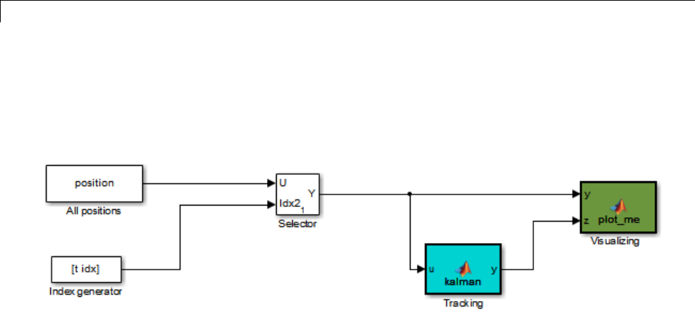
29 Using the MATLAB Function Block
Connecting the MATLAB Function Block Input and Output.
1Connect the MATLAB Function block input and output so that your model
looks like this.
See “Connect Blocks” on page 4-12 for more information.
2Save the model.
You are now ready to check your model for errors, as described in “Checking
the ex_kalman11 Model” on page 29-186.
Checking the ex_kalman11 Model
To check the model:
1In the Simulink model window, select Simulation > Update Diagram.
Simulink checks the model and generates a warning telling you to add
the %#codegen compilation directive to the ex_kalman01 file. Adding this
directive indicates that the file is intended for code generation and turns
on code generation error checking.
2Open ex_kalman01 file and add the %#codegen compilation directive after
the function declaration.
function y = ex_kalman01(z) %#codegen
3Modify the function name to ex_kalman02 and save the file as
ex_kalman02.m.
29-186

Track Object Using MATLAB®Code
4Modify the model to call ex_kalman02 byupdatingthecodeintheMATLAB
Function block.
function y = kalman(u)
%#codegen
y = ex_kalman02(u);
5Save the model and update diagram again.
This time the model updates successfully.
You are now ready to simulate your model, as described in “Simulating the
ex_kalman11 Model” on page 29-187.
Simulating the ex_kalman11 Model
To simulate the model:
1In the Simulink model window, select Simulation > Run.
As Simulink runs the model, it plots the trajectory of the object in blue and
the Kalman filter estimated position in green. Initially, you see that it
takes a short time for the estimated position to converge with the actual
position of the object. Then three sudden shifts in position occur—each time
the Kalman filter readjusts and tracks the object after a few iterations.
29-187
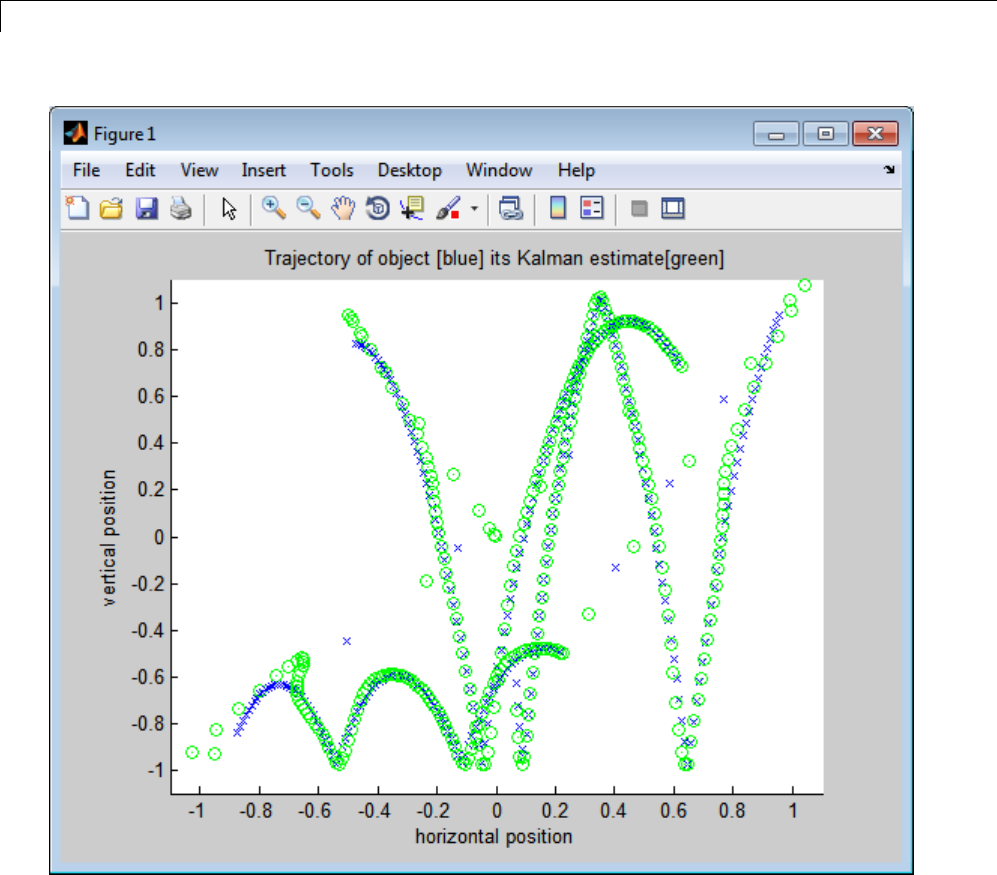

Track Object Using MATLAB®Code
Modifying the Filter to Accept a Fixed-Size Input
The filter you have worked on so far in this tutorial uses a simple batch
process that accepts one input at a time, so you must call the function
repeatedly for each input. In this part of the tutorial, you learn how to modify
the algorithm to accept a fixed-sized input, which makes the algorithm
suitable for frame-based processing. You then modify the model to provide
the input as fixed-size frames of data and call the filter passing in the data
one frame at a time.
Modifying Your MATLAB Code. Tomodifythecodeyourself, work through
the exercises in this section. Otherwise, open the supplied file ex_kalman03.m
in your solutions subfolder to see the modified algorithm.
You can now modify the algorithm to process a vector containing more than
one input. You need to find the length of the vector and call the filter code for
each element in the vector in turn. You do this by calling the filter algorithm
in a for-loop.
1Open ex_kalman02.m in the MATLAB Editor. At the MATLAB command
line, enter:
edit ex_kalman02.m
2Add a for-loop around the filter code.
aBefore the comment:
% Predicted state and covariance
insert:
for i=1:size(z,2)
bAfter:
% Compute the estimated measurements
y = H * x_est;
insert:
end
29-189

29 Using the MATLAB Function Block
cSelectthecodebetweenthefor-statement and the end statement,
right-click to open the context menu and select Smart Indent to indent
the code.
Your filter code should now look like this:
for i=1:size(z,2)
% Predicted state and covariance
x_prd = A * x_est;
p_prd = A * p_est * A' + Q;
% Estimation
S = H * p_prd' * H' + R;
B = H * p_prd';
klm_gain = (S \ B)';
% Estimated state and covariance
x_est = x_prd + klm_gain * (z - H * x_prd);
p_est = p_prd - klm_gain * H * p_prd;
% Compute the estimated measurements
y = H * x_est;
end
3Modify the line that calculates the estimated state and covariance to use
the ith element of input z.
Change:
x_est = x_prd + klm_gain * (z - H * x_prd);
to:
x_est = x_prd + klm_gain * (z(1:2,i) - H * x_prd);
4Modify the line that computes the estimated measurements to append the
result to the ith element of the output y.
Change:
y = H * x_est;
29-190

Track Object Using MATLAB®Code
to:
y(:,i) =H*x_est;
Thecodeanalyzermessageindicator in the top right turns orange to
indicate that the code analyzer has detected warnings. The code analyzer
underlines the offending code in orange and places a orange marker to
the right.
5Move your pointer over the orange marker to view the error information.
The code analyzer detects that ymust be fully defined before subscripting
it and that you cannot grow variables through indexing in generated code.
6To address this warning, preallocate memory for the output y,whichisthe
same size as the input z. Add this code before the for-loop.
% Pre-allocate output signal:
y=zeros(size(z));
Theorangemarkerdisappearsandthecodeanalyzermessageindicatorin
the top right edge of the code turns green, which indicates that you have
fixed all the errors and warnings detected by the code analyzer.
Why Preallocate the Outputs?
You must preallocate outputs here because the code generation does not
support increasing the size of an array over time. Repeatedly expanding
thesizeofanarrayovertimecanadverselyaffecttheperformanceofyour
program. See “Preallocating Memory”.
7Change the function name to ex_kalman03 and save the file as
ex_kalman03.m in the current folder.
You are ready to begin the next task in the tutorial, “Modifying Your Model
to Call the Updated Algorithm” on page 29-191.
Modifying Your Model to Call the Updated Algorithm. To modify the
model yourself, work through the exercises in this section. Otherwise, open
the supplied model ex_kalman22.mdl in your solutions subfolder to see the
modified model.
29-191

29 Using the MATLAB Function Block
Next, update your model to provide the input as fixed-size frames of data and
call ex_kalman03 passing in the data one frame at a time.
1Open ex_kalman11 model in Simulink.
ex_kalman11
2Double-click the MATLAB Function block to open the MATLAB Function
Block Editor.
3Replace the code that calls ex_kalman02 with a call to ex_kalman03.
function y = kalman(u)
%#codegen
y = ex_kalman03(u);
4Close the editor.
5Modify the InitFcn callback:
aSelect File > Model Properties > Model Properties.
The Model Properties dialog box opens.
bIn this dialog box, select the Callbacks tab.
cSelect InitFcn in the Model callbacks pane.
dReplace the existing callback with:
load position.mat;
[R,C]=size(position);
FRAME_SIZE=5;
idx=(1:FRAME_SIZE:C)';
LEN=length(idx);
t=(1:LEN)'-1;
This callback sets the frame size to 5, and the index to increment by 5.
eClick Apply and close the Model Properties dialog box.
6Update the Selector block to use the correct indices.
aDouble-click the Selector block to view the function block parameters.
29-192

Track Object Using MATLAB®Code
The Function Block Parameters dialog box opens.
bSet the second Index Option to Starting index (port).
cSet the Output Size for the second input to FRAME_SIZE,clickApply
and close the dialog box.
Now, the Index Option for the first port is Select all and for the second
port is Starting index (port). Because the index increments by 5each
sample time, and the output size is 5, the Selector block outputs a 2x5
output at each sample time.
7Change the model simulation stop time to 61.Nowtheframesizeis5,so
the simulation completes in a fifth of the sample times.
aIn the Simulink model window, select Simulation > Model
Configuration Parameters.
bIn the left pane of the Configuration Parameters dialog box, select
Solver.
cIn the right pane, set Stop time to 61.
dClick Apply and close the dialog box.
8Save the model as ex_kalman22.mdl.
Testing Your Modified Algorithm. To simulate the model:
1In the Simulink model window, select Simulation > Run.
As Simulink runs the model, it plots the trajectory of the object in blue and
the Kalman filter estimated position in green as before when you used
the batch filter.
2The simulation stops.
You have proved that your algorithm accepts a fixed-size signal. You are now
ready for the next task, “Using the Filter to Accept a Variable-Size Input”
on page 29-194.
29-193

29 Using the MATLAB Function Block
Using the Filter to Accept a Variable-Size Input
In this part of the tutorial, you learn how to specify variable-size data in
your Simulink model. Then you test your Kalman filter algorithm with
variable-size inputs and see that the algorithm is suitable for processing
packetsofdataofvaryingsize. Formore information on using variable-size
data in Simulink, see “Variable-Size Signal Basics” on page 49-2.
Updating the Model to Use Variable-Size Inputs. To modify the model
yourself, work through the exercises in this section. Otherwise, open the
supplied model ex_kalman33.mdl in your solutions subfolder to see the
modified model.
1Open ex_kalman22.mdl in Simulink.
ex_kalman22
2Modify the InitFcn callback:
aSelect File > Model Properties > Model Properties.
The Model Properties dialog box opens.
bSelect the Callbacks tab.
cSelect InitFcn in the Model callbacks pane.
dReplace the existing callback with:
load position.mat;
idx=[ 1 1 ;2 3 ;4 6 ;7 10 ;11 15 ;16 30 ;
31 70 ;71 100 ;101 200 ;201 250 ;251 310];
LEN=length(idx);
t=(0:1:LEN-1)';
This callback sets up indexing to generate eleven different size inputs.
It specifies the start and end indices for each sample time. The first
sample time uses only the first element, the second sample time uses
thesecondandthirdelements,andsoon. Thelargestsample,101 to
200, contains 100 elements.
eClick Apply and close the Model Properties dialog box.
3Update the Selector block to use the correct indices.
29-194

Track Object Using MATLAB®Code
aDouble-click the Selector block to view the function block parameters.
The Function Block Parameters dialog box opens.
bSet the second Index Option to Starting and ending indices
(port),thenclickApply and close the dialog box.
This setting means that the input to the index port specifies the start
and end indices for the input at each sample time. Because the index
input specifies different starting and ending indices at each sample
time, the Selector block outputs a variable-size signal as the simulation
progresses.
4Use the Ports and Data Manager to set the MATLAB Function input x
and output yas variable-size data.
aDouble-click the MATLAB Function block to open the MATLAB Function
Block Editor.
bFrom the editor menu, select Edit Data.
cIn the Ports and Data Manager left pane, select the input u.
The Ports and Data Manager displays information about uin the right
pane.
dOn the General tab, select the Variable size check box and click Apply.
eIn the left pane, select the output y.
fOn the General tab:
iSet the Size of yto [2 100] to specify a 2-D matrix where the upper
bounds are 2for the first dimension and 100 for the second, which is
the maximum size input specified in the InitFcn callback.
ii Select the Variable size check box.
iii Click Apply.
gClose the Ports and Data Manager.
5Now do the same for the other MATLAB Function block. Use the Ports and
Data Manager to set the Visualizing block inputs yand zas variable-size
data.
29-195

29 Using the MATLAB Function Block
aDouble-click the Visualizing block to open the MATLAB Function Block
Editor.
bFrom the editor menu, select Edit Data.
cIn the Ports and Data Manager left pane, select the input y.
dOn the General tab, select the Variable size check box and click Apply.
eIn the left pane, select the input z.
fOn the General tab, select the Variable size check box and click Apply.
gClose the Ports and Data Manager.
6Change the model simulation stop time to 10. This time, the filter processes
one of the eleven different size inputs each sample time.
7Save the model as ex_kalman33.mdl.
Testing Your Modified Model. To simulate the model:
1In the Simulink model window, select Simulation > Run.
As Simulink runs the model, it plots the trajectory of the object in blue and
the Kalman filter estimated position in green as before.
Note that the signal lines between the Selector block and the Tracking and
Visualization blocks change to show that these signals are variable-size.
2The simulation stops.
You have successfully created an algorithm that accepts variable-size inputs.
Next, you learn how to debug your MATLAB Function block, as described in
“Debugging the MATLAB Function Block” on page 29-196.
Debugging the MATLAB Function Block
You can debug your MATLAB Function block just like you can debug a
function in MATLAB.
1Double-click the MATLAB Function block that calls the Kalman filter to
open the MATLAB Function Block Editor.
29-196

Track Object Using MATLAB®Code
2In the editor, click the dash (-) character in the left margin of the line:
y = kalman03(u);
A small red ball appears in the margin of this line, indicating that you
have set a breakpoint.
3In the Simulink model window, select Simulation > Run.
The simulation pauses when execution reaches the breakpoint and a small
green arrow appears in the left margin.
4Place the pointer over the variable u.
The value of uappears adjacent to the pointer.
5From the MATLAB Function Block Editor menu, select Step In.
The kalman03.m file opens in the editor and you can now step through this
code using Step,Step In,andStep Out.
6Select Step Out.
The kalman03.m file closes and the MATLAB Function block code reappears
in the editor.
7Place the pointer over the output variable y.
You can now see the value of y.
8Click the red ball to remove the breakpoint.
9From the MATLAB Function Block Editor menu, select Quit Debugging.
10 Close the editor.
11 Close the figure window.
Now you are ready for the next task, “Generating C Code” on page 29-198.
29-197

29 Using the MATLAB Function Block
Generating C Code
You have proved that your algorithm works in Simulink. Next you generate
codeforyourmodel.
Note Before generating code, you must check that your MATLAB code is
suitable for code generation. If you call your MATLAB code as an extrinsic
function, you must remove extrinsic calls before generating code.
1Rename the MATLAB Function block to Tracking.Torenamethe
block, double-click the annotation MATLAB Function below the MATLAB
Function block and replace the text with Tracking.
When you generate code for the MATLAB Function block, Simulink Coder
uses the name of the block in the generated code. It is good practice to use
a meaningful name.
2Before generating code, ensure that Simulink Coder creates a code
generation report. This HTML report provides easy access to the list of
generated files with a summary of the configuration settings used to
generate the code.
aIn the Simulink model window, select Simulation > Model
Configuration Parameters.
The Configuration Parameters dialog box opens.
bIn the left pane of the Configuration Parameters dialog box, select
Report under Code Generation.
cIn the right pane, select Create code generation report.
The Open report automatically option is also selected.
dClick Apply and close the Configuration Parameters dialog box.
eSave your model.
3To generate code for the Tracking block:
aIn your model, select the Tracking block.
29-198

Track Object Using MATLAB®Code
bIn the Simulink model window, select Code > C/C++ Code > Build
Selected Subsystem.
4The Simulink software generates an error informing you that it cannot log
variable-size signals as arrays. You need to change the format of data
saved to the MATLAB workspace. To change this format:
•In the Simulink model window, select Simulation > Model
Configuration Parameters.
The Configuration Parameters dialog box opens.
•In the left pane of the Configuration Parameters dialog box, select Data
Import/Export.
•In the right pane, under Save to workspace options,setFormat
to Structure with time.
The logged data is now a structure that has two fields: a time field and a
signals field, enabling Simulink to log variable-size signals.
•Click Apply and close the Configuration Parameters dialog box.
•Save your model.
5Repeat step 3to generate code for the Tracking block.
The Simulink Coder software generates C code for the block and launches
the code generation report.
For more information on using the code generation report, see “Reports
for Code Generation”.
6In the left pane of the code generation report, click the Tracking.c link
to view the generated C code. Note that in the code generated for the
MATLAB Function block, Tracking, there is no code for the ex_kalman03
function because inlining is enabled by default.
7Modify your filter algorithm to disable inlining:
aIn ex_kalman03.m, after the function declaration, add:
coder.inline('never');
29-199

29 Using the MATLAB Function Block
bChange the function name to ex_kalman04 and save the file as
ex_kalman04.m in the current folder.
cIn your ex_kalman33 model, double-click the Tracking block.
The MATLAB Function Block Editor opens.
dModifythecalltothefilteralgorithmtocallex_kalman04.
function y = kalman(u)
%#codegen
y = ex_kalman04(u);
eSave the model as ex_kalman44.mdl.
8Generate code for the updated model.
aSelect the Tracking block.
bIn the model window, select Code > C/C++Code > Build Selected
Subsystem.
The Build code for Subsystem dialog box appears.
cClick the Build button.
The Simulink Coder software generates C code for the block and
launches the code generation report.
dIntheleftpaneofthecodegeneration report, click the Tracking.c link
to view the generated C code.
This time the ex_kalman04 function has code because you disabled
inlining.
/* Forward declaration for local functions */
static void Tracking_ex_kalman04(const real_T z_data[620], const int32_T
z_sizes[2], real_T y_data[620], int32_T y_sizes[2]);
/* Function for MATLAB Function Block: '<Root>/Tracking' */
static void Tracking_ex_kalman04(const real_T z_data[620], const int32_T 48
z_sizes[2], real_T y_data[620], int32_T y_sizes[2])
29-200

Track Object Using MATLAB®Code
Best Practices Used in This Tutorial
Best Practice — Saving Incremental Code Updates
Save your code before making modifications. This practice provides a fallback
in case of error and a baseline for testing and validation. Use a consistent
file naming convention. For example, add a two-digit suffix to the file name
for each file inasequence.
Key Points to Remember
•Back up your MATLAB code before you modify it.
•Decide on a naming convention for your files and save interim versions
frequently. For example, this tutorial uses a two-digit suffix to differentiate
the various versions of the filter algorithm.
•For simulation purposes, before generating code, call your MATLAB code
using coder.extrinsic to check that your algorithm is suitable for use in
Simulink. This practice provides these benefits:
-You do not have to make the MATLAB code suitable for code generation.
-You can debug your MATLAB code in MATLAB while calling it from
Simulink.
•Create a Simulink Coder code generation report. This HTML report
provides easy access to the list of generated files with a summary of the
configuration settings used to generate the code.
Where to Learn More
•“Next Steps” on page 29-202
•“Product Help” on page 29-202
29-201

29 Using the MATLAB Function Block
Next Steps
To: See:
Learn how to generate C code from your
MATLAB code using codegen
“C Code Generation at the Command Line”
Learn more about code generation from
MATLAB
“Getting Started with Simulink Coder”
Use variable-size data “Variable-Size Data Definition for Code
Generation” on page 35-3
Speed up fixed-point MATLAB code See “Fixed-Point Code Acceleration and
Generation Workflow”.
Integrate custom C code into generated code “Custom C/C++ Code Integration”
Integrate custom C code into a MATLAB
function
coder.ceval
Generate HDL from MATLAB code www.mathworks.com/products/slhdlcoder
Product Help
MathWorks product documentation is available online from the Open Help
Browser button on the MATLAB toolstrip.
For: See:
Code generation from MATLAB code “When to Generate Code from
MATLAB Algorithms” on page 30-2
A list of functions that are suitable
for code generation
“Functions Supported for Code
Generation — Alphabetical List” on
page 31-2
29-202

Filter Audio Signal Using MATLAB®Code
Filter Audio Signal Using MATLAB Code
In this section...
“Learning Objectives” on page 29-203
“Tutorial Prerequisites” on page 29-203
“Example: The LMS Filter” on page 29-204
“Files for the Tutorial” on page 29-207
“Tutorial Steps” on page 29-208
Learning Objectives
In this tutorial, you will learn how to:
•Use the MATLAB Function block to add MATLAB functions to Simulink
models for modeling, simulation, and deployment to embedded processors.
This capability is useful for coding algorithms that are better stated in the
textual language of MATLAB than in the graphical language of Simulink.
For more information, see “What Is a MATLAB Function Block?” on page
29-6 and “Create Model That Uses MATLAB Function Block” on page 29-9.
•Use coder.extrinsic to call MATLAB code from a MATLAB Function
block.
This capability allows you to call existing MATLAB code from Simulink
without first having to make this code suitable for code generation, allowing
for rapid prototyping.
•Check that existing MATLAB code is suitable for code generation.
•Convert a MATLAB algorithm from batch processing to streaming.
•Use persistent variables in code that is suitable for code generation.
You need to make the filter weights persistent so that the filter algorithm
does not reset their values each time it runs.
Tutorial Prerequisites
•“What You Need to Know” on page 29-204
29-203

29 Using the MATLAB Function Block
•“Required Products” on page 29-204
What You Need to Know
To work through this tutorial, you should have basic familiarity with
MATLAB software. You should also understand how to create a basic
Simulink model and how to simulate that model. For more information, see
“Start the Simulink Software” and “Simulink User Interface”.
Required Products
To complete this tutorial, you must install the following products:
•MATLAB
•MATLAB Coder
•Simulink
•Simulink Coder
•DSP System Toolbox
Note If you do not have a DSP System Toolbox license, see “Track Object
Using MATLAB Code” on page 29-175.
•Ccompiler
For a list of supported compilers, see .
For instructions on installing MathWorks products, refer to the installation
documentation. If you have installed MATLAB and want to check which other
MathWorks products are installed, enter ver in the MATLAB Command
Window. For instructions on installing and setting up a C compiler, see
“Setting Up the C/C++ Compiler”.
Example: The LMS Filter
•“Description” on page 29-205
•“Algorithm” on page 29-205
29-204

Filter Audio Signal Using MATLAB®Code
•“Filtering Process” on page 29-206
•“Reference” on page 29-207
Description
A least mean squares (LMS) filter is an adaptive filter that adjusts its transfer
function according to an optimizing algorithm. You provide the filter with
an example of the desired signal together with the input signal. The filter
then calculates the filter weights, or coefficients, that produce the least mean
squares of the error between the output signal and the desired signal.
This example uses an LMS filter to remove the noise in a music recording.
There are two inputs. The first input is the distorted signal: the music
recording plus the filtered noise. The second input is the desired signal: the
unfiltered noise. The filter works to eliminate the difference between the
output signal and the desired signal and outputs the difference, which, in this
case, is the clean music recording. When you start the simulation, you hear
both the noise and the music. Over time, the adaptive filter removes the noise
so you hear only the music.
Algorithm
This example uses the least mean squares (LMS) algorithm to remove noise
from an input signal. The LMS algorithm computes the filtered output, filter
error, and filter weights given the distorted and desired signals.
At the start of the tutorial, the LMS algorithm uses a batch process to filter
theaudioinput.ThisalgorithmissuitableforMATLAB,whereyouarelikely
to load in the entire signal and process it all at once. However, a batch process
is not suitable for processing a signal in real time. As you work through the
tutorial, you refine the design of the filter to convert the algorithm from
batch-based to stream-based processing.
The baseline function signature for the algorithm is:
function [ signal_out, err, weights ] = ...
lms_01(signal_in, desired)
The filtering is performed in the following loop:
for n = 1:SignalLength
29-205

29 Using the MATLAB Function Block
% Compute the output sample using convolution:
signal_out(n,ch) = weights' * signal_in(n:n+FilterLength-1,ch);
% Update the filter coefficients:
err(n,ch) = desired(n,ch) - signal_out(n,ch) ;
weights = weights + mu*err(n,ch)*signal_in(n:n+FilterLength-1,ch);
end
where SignalLength is the length of the input signal, FilterLength is the
filter length, and mu is the adaptation step size.
What Is the Adaptation Step Size?
LMS algorithms have a step size that determines the amount of correction
to apply as the filter adapts from one iteration to the next. Choosing the
appropriate step size requires experience in adaptive filter design. A step
sizethatistoosmallincreasesthetimeforthefiltertoconverge. Filter
convergence is the process where the error signal (the difference between the
output signal and the desired signal) approaches an equilibrium state over
time. A step size that is too large might cause the adapting filter to overshoot
the equilibrium and become unstable. Generally, smaller step sizes improve
the stability of the filter at the expense of the time it takes to adapt.
Filtering Process
The filtering process has three phases:
•Convolution
The convolution for the filter is performed in:
signal_out(n,ch) = weights' * signal_in(n:n+FilterLength-1,ch);
What Is Convolution?
Convolution is the mathematical foundation of filtering. In signal
processing, convolving two vectors or matrices is equivalent to filtering one
of the inputs by the other. In this implementation of the LMS filter, the
convolution operation is the vector dot product between the filter weights
and a subset of the distorted input signal.
•Calculation of error
29-206

Filter Audio Signal Using MATLAB®Code
The error is the difference between the desired signal and the output signal:
err(n,ch) = desired(n,ch) - signal_out(n,ch);
•Adaptation
The new value of the filter weights is the old value of the filter weights plus
a correction factor that is based on the error signal, the distorted signal,
and the adaptation step size:
weights = weights + mu*err(n,ch)*signal_in(n:n+FilterLength-1,ch);
Reference
Haykin, Simon. Adaptive Filter Theory. Upper Saddle River, NJ:
Prentice-Hall, Inc., 1996.
Files for the Tutorial
•“About the Tutorial Files” on page 29-207
•“Location of Files” on page 29-207
•“Names and Descriptions of Files” on page 29-208
About the Tutorial Files
The tutorial uses the following files:
•Simulink model files for each step of the tutorial.
•MATLAB code files for each step of the example.
Throughout this tutorial, you work with Simulink models that call
MATLAB files that contain a simple least mean squares (LMS) filter
algorithm.
Location of Files
The tutorial files are available in the following folder:
docroot\toolbox\simulink\examples\lms. Torunthetutorial,
you must copy these files to a local folder. For instructions, see “Copying
Files Locally” on page 29-209.
29-207

29 Using the MATLAB Function Block
Names and Descriptions of Files
Type Name Description
lms_01 Baseline MATLAB implementation
of batch filter. Not suitable for code
generation.
lms_02 Filter modified from batch to streaming.
lms_03 Frame-based streaming filter with Reset
and Adapt controls.
lms_04 Frame-based streaming filter with Reset
and Adapt controls. Suitable for code
generation.
lms_05 Disabled inlining for code generation.
MATLAB
files
lms_06 Demonstrates use of coder.nullcopy.
acoustic_environment Simulink model that provides an overview
of the acoustic environment.
noise_cancel_00 Simulink model without a MATLAB
Function block.
noise_cancel_01 Complete noise_cancel_00 model
including a MATLAB Function block.
noise_cancel_02 Simulink model for use with lms_02.m.
noise_cancel_03 Simulink model for use with lms_03.m.
noise_cancel_04 Simulink model for use with lms_04.m.
noise_cancel_05 Simulink model for use with lms_05.m.
noise_cancel_06 Simulink model for use with lms_06.m.
Simulink
model
files
design_templates Simulink model containing Adapt and
Reset controls.
Tutorial Steps
•“Copying Files Locally” on page 29-209
29-208

Filter Audio Signal Using MATLAB®Code
•“Setting Up Your C Compiler” on page 29-210
•“Running the acoustic_environment Model” on page 29-210
•“Adding a MATLAB Function Block to Your Model” on page 29-211
•“Calling Your MATLAB Code As an Extrinsic Function for Rapid
Prototyping” on page 29-212
•“Simulating the noise_cancel_01 Model” on page 29-216
•“Modifying the Filter to Use Streaming” on page 29-218
•“Adding Adapt and Reset Controls” on page 29-223
•“Generating Code” on page 29-228
•“Optimizing the LMS Filter Algorithm” on page 29-233
Copying Files Locally
Copy the tutorial files to a local folder:
1Create a local solutions folder, for example, c:\test\lms\solutions.
2Change to the docroot\toolbox\simulink\examples folder. At the
MATLAB command line, enter:
cd(fullfile(docroot, 'toolbox', 'simulink', 'examples'))
3Copy the contents of the lms subfolder to your solutions folder, specifying
the full path name of the solutions folder:
copyfile('lms', 'solutions')
Your solutions folder now contains a complete set of solutions for the
tutorial. If you do not want to perform the steps for each task, you can view
the supplied solution to see how the code should look.
4Create a local work folder, for example, c:\test\lms\work.
5Copy the following files from your solutions folder to your work folder.
•lms_01
•lms_02
29-209

29 Using the MATLAB Function Block
•noise_cancel_00
•acoustic_environment
•design_templates
Your work folder now contains all the files that you need to get started.
You are now ready to set up your C compiler.
Setting Up Your C Compiler
Before generating code for your Simulink model, you must set up your C
compiler. For most platforms, MathWorkssuppliesadefaultcompilerwith
MATLAB. If your installation does not include a default compiler, for a list
of supported compilers for the current releaseofMATLAB,seeandinstalla
compiler that is suitable for your platform.
To install a compiler:
1At the MATLAB command line, enter:
mex -setup
2Enter yto see the list of installed compilers.
3Select a supported compiler.
4Enter yto verify your choice.
Running the acoustic_environment Model
Run the acoustic_environment model supplied with the tutorial to
understand the problem that you are trying to solve using the LMS filter.
This model adds band-limited white noise to an audio signal and outputs the
resulting signal to a speaker.
To simulate the model:
1Open the acoustic_environment model in Simulink:
29-210

Filter Audio Signal Using MATLAB®Code
aSet your MATLAB current folder to the folder that contains your working
files for this tutorial. At the MATLAB command line, enter:
cd work
where work is the full path name of the folder containing your files. See
“Using the Current Folder Browser” for more information.
bAt the MATLAB command line, enter:
acoustic_environment
2Ensure that your speakers are on.
3To simulate the model, from the Simulink model window, select
Simulation > Run.
As Simulink runs the model, you hear the audio signal distorted by noise.
4While the simulation is running, double-click the Manual Switch to select
the audio source.
Now you hear the desired audio input without any noise.
The goal of this tutorial is to use a MATLAB LMS filter algorithm to remove
thenoisefromthenoisyaudiosignal. YoudothisbyaddingaMATLAB
Function block to the model and calling the MATLAB code from this block.
To learn how, see “Adding a MATLAB Function Block to Your Model” on
page 29-211.
Adding a MATLAB Function Block to Your Model
To modify the model and code yourself, work through the exercises in this
section. Otherwise, open the supplied model noise_cancel_01 in your
solutions subfolder to see the modified model.
For the purposes of this tutorial, you add the MATLAB Function block to the
noise_cancel_00 model supplied with the tutorial. In practice, you would
have to develop your own test bench starting with an empty Simulink model.
To add a MATLAB Function block to the noise_cancel_00 model:
29-211

29 Using the MATLAB Function Block
1Open noise_cancel_00 in Simulink.
noise_cancel_00
2Add a MATLAB Function block to the model:
aAt the MATLAB command line, type simulink to open the Simulink
Library Browser.
bFrom the list of Simulink libraries, select the User-Defined Functions
library.
cClick the MATLAB Function block and drag it into the noise_cancel_00
model. Place the block just above the red text annotation Place MATLAB
Function Block here.
dDelete the red text annotations from the model.
eSave the model in the current folder as noise_cancel_01.
Calling Your MATLAB Code As an Extrinsic Function for Rapid
Prototyping
In this part of the tutorial, you use the coder.extrinsic function to call your
MATLAB code from the MATLAB Function block for rapid prototyping.
WhyCallMATLABCodeAsanExtrinsicFunction?. Calling MATLAB
code as an extrinsic function provides these benefits:
•For rapid prototyping, you do not have to make the MATLAB code suitable
for code generation.
•Using coder.extrinsic enables you to debug your MATLAB code in
MATLAB. You can add one or more breakpoints in the lms_01.m file, and
then start the simulation in Simulink. When the MATLAB interpreter
encounters a breakpoint, it temporarily halts execution so that you can
inspect the MATLAB workspace and view the current values of all variables
in memory. For more information about debugging MATLAB code, see
“Ways to Debug MATLAB Files”.
How to Call MATLAB Code As an Extrinsic Function. To call your
MATLAB code from the MATLAB Function block:
29-212

Filter Audio Signal Using MATLAB®Code
1Double-click the MATLAB Function block to open the MATLAB Function
Block Editor.
2Delete the default code displayed in the MATLAB Function Block Editor.
3Copy the following code to the MATLAB Function block.
function [ Signal_Out, Weights ] = LMS(Noise_In, Signal_In) %#codegen
% Extrinsic:
coder.extrinsic('lms_01');
% Compute LMS:
[ ~, Signal_Out, Weights ] = lms_01(Noise_In, Signal_In);
end
Why Use the Tilde (~) Operator?
Because the LMS function does not use the first output from lms_01,replace
this output with the MATLAB ~operator. MATLAB ignores inputs and
outputs specified by ~. This syntax helps avoid confusion in your program
code and unnecessary clutter in your workspace, and allows you to reuse
existing algorithms without modification.
4Save the model.
The lms_01 function inputs Noise_In and Signal_In now appear as input
ports to the block and the function outputs Signal_Out and Weights
appear as output ports.
Connecting the MATLAB Function Block Inputs and Outputs.
1Connect the MATLAB Function block inputs and outputs so that your
model looks like this.
29-213
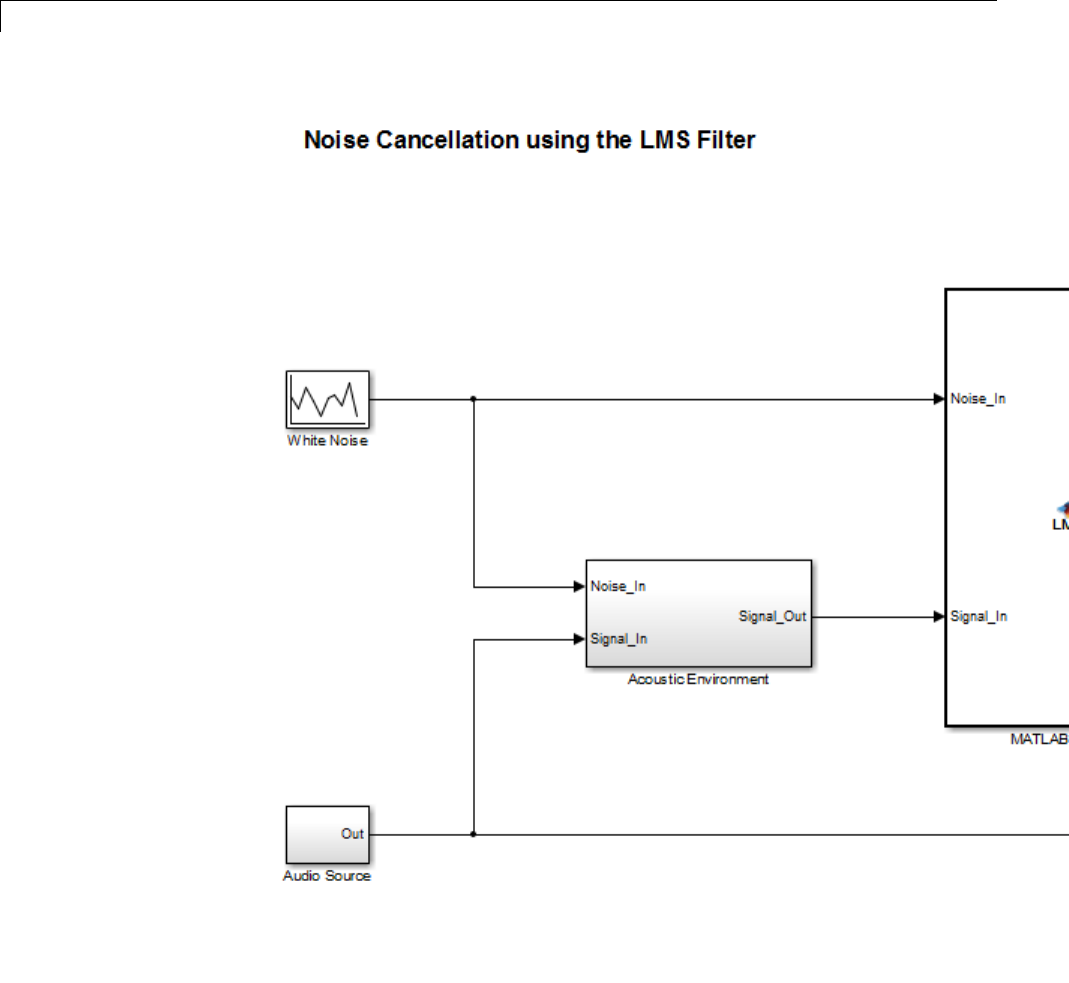

Filter Audio Signal Using MATLAB®Code
2In the MATLAB Function block code, preallocate the outputs by adding the
following code after the extrinsic call:
% Outputs:
Signal_Out = zeros(size(Signal_In));
Weights = zeros(32,1);
ThesizeofWeights is set to match the Numerator coefficients of the Digital
Filter in the Acoustic Environment subsystem.
Why Preallocate the Outputs?
For code generation, you must assign variables explicitly to have a
specific class, size, and complexity before using them in operations or
returning them as outputs in MATLAB functions. For more information,
see “Expected Differences in Behavior After Compiling MATLAB Code”
on page 30-9.
3Save the model.
You are now ready to check your model for errors.
Checking the noise_cancel_01 Model.
1In the Simulink model window, select Simulation > Update Diagram.
Simulink fails to update diagram.
Because the Analysis and Visualization block expects to receive a
frame-based signal from the LMS filter, you must configure the MATLAB
Function block Signal_Out output parameter to be frame-based rather
than sample-based.
aDouble-click the MATLAB Function block to open the MATLAB Function
Block Editor.
bSelect Edit Data to open the Ports and Data Manager.
cSelect the signal called Signal_Out from the list in the left pane.
dOn the General tab, change the Sampling mode from Sample based
to Frame based.
29-215

29 Using the MATLAB Function Block
eClick the Apply button and close the Ports and Data Manager and the
MATLAB Function Block Editor.
fSave the model.
2Check the model again; select Simulation > Update Diagram in the
Simulink model window.
Simulink updates diagram successfully. You are ready for the next task,
“Simulating the noise_cancel_01 Model” on page 29-216
Simulating the noise_cancel_01 Model
To simulate the model:
1Ensure that you can see the Time Domain plots.
To view the plots, in the noise_cancel_01 model, open the Analysis and
Visualization block and then open the Time Domain block.
2In the Simulink model window, select Simulation > Run .
As Simulink runs the model, you see and hear outputs. Initially, you hear
the audio signal distorted by noise. Then the filter attenuates the noise
gradually, until you hear only the music playing with very little noise
remaining. After two seconds, you hear the distorted noisy signal again
and the filter attenuates the noise again. This cycle repeats continuously.
29-216
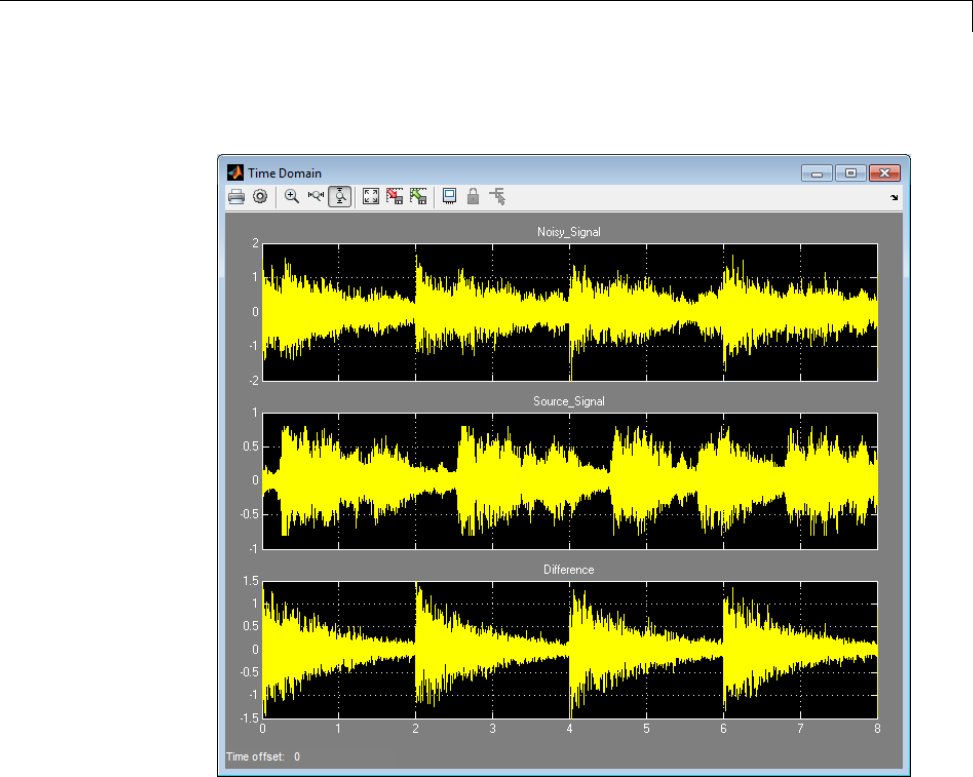
Filter Audio Signal Using MATLAB®Code
MATLAB displays the following plot showing this cycle.
3Stop the simulation.
Why Does the Filter Reset Every 2 Seconds?
The filter resets every 2 seconds because the model uses 16384 samples per
frame and a sampling rate of 8192,sothe16384 samples represent 2 seconds
of audio.
To see the model configuration:
29-217

29 Using the MATLAB Function Block
1Double-click the White Noise subsystem and note that it uses a Sample
time of 1/Fs and Samples per frame of FrameSize.Themusic in the
Audio Source subsystem also uses these values.
2FrameSize is set in the model InitFcn callback. To view this callback:
aRight-click inside the model window and select Model Properties from
the context menu.
bSelect the Callbacks tab.
cSelect InitFcn in the Model callbacks pane.
Note that FrameSize = 16*1024,whichis16384.
3Fs is set in the model PostLoadFcn callback. To view this callback, select
PostLoadFcn in the Model callbacks pane:
The following MATLAB commands set up Fs:
data = load('handel.mat');
music = data.y;
Fs = data.Fs;
Modifying the Filter to Use Streaming
•“What Is Streaming?” on page 29-218
•“Why Use Streaming?” on page 29-219
•“Viewing the Modified MATLAB Code” on page 29-219
•“Summary of Changes to the Filter Algorithm” on page 29-220
•“Modifying Your Model to Call the Updated Algorithm” on page 29-221
•“Simulating the Streaming Algorithm” on page 29-222
What Is Streaming?. A streaming filter is called repeatedly to process
fixed-size chunks of input data, or frames, until it has processed the entire
input signal. The frame size can be as small as a single sample, in which case
the filter would be operating in a sample-based mode, or up to a few thousand
samples, for frame-based processing.
29-218

Filter Audio Signal Using MATLAB®Code
Why Use Streaming?. The design of the filter algorithm in lms_01 has
the following disadvantages:
•The algorithm does not use memory efficiently.
Preallocating a fixed amount of memory for each input signal for the
lifetime of the program means more memory is allocated than is in use.
•You must know the size of the input signal at the time you call the function.
If the input signal is arriving in real time or as a stream of samples, you
would have to wait to accumulate the entire signal before you could pass
it,asabatch,tothefilter.
•The signal size is limited to a maximum size.
In an embedded application, the filter is likely to be processing a continuous
input stream. As a result, the input signal can be substantially longer than
the maximum length that a filter working in batch mode could possibly
handle. To make the filter work for any signal length, it must run in real
time. One solution is to convert the filter from batch-based processing to
stream-based processing.
Viewing the Modified MATLAB Code. Theconversiontostreaming
involves:
•Introducing a first-in, first-out (FIFO) queue
The FIFO queue acts as a temporary storage buffer, which holds a small
number of samples from the input data stream. The number of samples
held by the FIFO queue must be exactly the same as the number of samples
in the filter’s impulse response, so that the function can perform the
convolution operation between the filter coefficients and the input signal.
•Making the FIFO queue and the filter weights persistent
The filter is called repeatedly until it has processed the entire input signal.
Therefore, the FIFO queue and filter weights need to persist so that the
adaptation process does not have to start over again after each subsequent
call to the function.
Open the supplied file lms_02.m in your work subfoldertoseethemodified
algorithm.
29-219

29 Using the MATLAB Function Block
Summary of Changes to the Filter Algorithm. Note the following
important changes to the filter algorithm:
•The filter weights and the FIFO queue are declared as persistent:
persistent weights;
persistent fifo;
•The FIFO queue is initialized:
fifo = zeros(FilterLength,ChannelCount);
•The FIFO queue is used in the filter update loop:
% For each channel:
for ch = 1:ChannelCount
% For each sample time:
for n = 1:FrameSize
% Update the FIFO shift register:
fifo(1:FilterLength-1,ch) = fifo(2:FilterLength,ch);
fifo(FilterLength,ch) = signal_in(n,ch);
% Compute the output sample using convolution:
signal_out(n,ch) = weights' * fifo(:,ch);
% Update the filter coefficients:
err(n,ch) = desired(n,ch) - signal_out(n,ch) ;
weights = weights + mu*err(n,ch)*fifo(:,ch);
end
end
•You cannot output a persistent variable. Therefore, a new variable,
weights_out, is used to output the filter weights:
function [ signal_out, err, weights_out ] = ...
lms_02(distorted, desired)
weights_out = weights;
29-220

Filter Audio Signal Using MATLAB®Code
Modifying Your Model to Call the Updated Algorithm. To modify the
model yourself, work through the exercises in this section. Otherwise, open
the supplied model noise_cancel_02 in your solutions subfolder to see the
modified model.
1In the noise_cancel_01 model, double-click the MATLAB Function block
to open the MATLAB Function Block Editor.
2Modify the MATLAB Function block code to call lms_02.
aModify the extrinsic call.
% Extrinsic:
coder.extrinsic('lms_02');
bModifythecalltothefilteralgorithm.
% Compute LMS:
[ ~, Signal_Out, Weights ] = lms_02(Noise_In, Signal_In);
Modified MATLAB Function Block Code
Your MATLAB Function block code should now look like this:
function [ Signal_Out, Weights ] = LMS(Noise_In, Signal_In)
% Extrinsic:
coder.extrinsic('lms_02');
% Outputs:
Signal_Out = zeros(size(Signal_In));
Weights = zeros(32,1);
% Compute LMS:
[ ~, Signal_Out, Weights ] = lms_02(Noise_In, Signal_In);
end
3Change the frame size from 16384 to 64, which represents a more realistic
value.
aRight-click inside the model window and select Model Properties from
the context menu.
bSelect the Callbacks tab.
cIn the Model callbacks list, select InitFcn.
29-221

29 Using the MATLAB Function Block
dChange the value of FrameSize to 64.
eClick Apply and close the dialog box.
4Save your model as noise_cancel_02.
Simulating the Streaming Algorithm. To simulate the model:
1Ensure that you can see the Time Domain plots.
2Start the simulation.
As Simulink runs the model, you see and hear outputs. Initially, you hear
the audio signal distorted by noise. Then, during the first few seconds,
the filter attenuates the noise gradually, until you hear only the music
playing with very little noise remaining. MATLAB displays the following
plot showing filter convergence after only a few seconds.
29-222
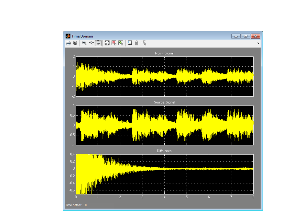
Filter Audio Signal Using MATLAB®Code
3Stop the simulation.
The filter algorithm is now suitable for Simulink. You are ready to elaborate
your model to use Adapt and Reset controls.
Adding Adapt and Reset Controls
•“Why Add Adapt and Reset Controls?” on page 29-224
•“Modifying Your MATLAB Code” on page 29-224
•“Modifying Your Model to Use Reset and Adapt Controls” on page 29-225
•“Simulating the Model with Adapt and Reset Controls” on page 29-227
29-223

29 Using the MATLAB Function Block
Why Add Adapt and Reset Controls?. In this part of the tutorial, you add
Adapt and Reset controls to your filter. Using these controls, you can turn the
filtering on and off. When Adapt is enabled, the filter continuously updates
the filter weights. When Adapt is disabled, the filter weights remain at their
current values. If Reset is set, the filter resets the filter weights.
Modifying Your MATLAB Code. Tomodifythecodeyourself, work through
the exercises in this section. Otherwise, open the supplied file lms_03.m in
your solutions subfolder to see the modified algorithm.
To modify your filter code:
1Open lms_02.m.
2In the Set up section, replace
if ( isempty(weights) )
with
if ( reset || isempty(weights) )
3In the filter loop, update the filter coefficients only if Adapt is ON.
if adapt
weights = weights + mu*err(n,ch)*fifo(:,ch);
end
4Change the function signature to use the Adapt and Reset inputs and
change the function name to lms_03.
function [ signal_out, err, weights_out ] = ...
lms_03(signal_in, desired, reset, adapt)
5Save the file in the current folder as lms_03.m:
Summary of Changes to the Filter Algorithm
Note the following important changes to the filter algorithm:
•The new input parameter reset is used to determine if it is necessary to
reset the filter coefficients:
29-224

Filter Audio Signal Using MATLAB®Code
if ( reset || isempty(weights) )
% Filter coefficients:
weights = zeros(L,1);
% FIFO Shift Register:
fifo = zeros(L,1);
end
•The new parameter adapt is used to control whether the filter coefficients
are updated or not.
if adapt
weights = weights + mu*err(n)*fifo;
end
Modifying Your Model to Use Reset and Adapt Controls. To modify
the model yourself, work through the exercises in this section. Otherwise,
open the supplied model noise_cancel_03 in your solutions subfolder to
see the modified model.
1Open the noise_cancel_02 model.
2Double-click the MATLAB Function block to open the MATLAB Function
Block Editor.
3Modify the MATLAB Function block code:
aUpdate the function declaration.
function [ Signal_Out, Weights ] = ...
LMS(Adapt, Reset, Noise_In, Signal_In )
bUpdate the extrinsic call.
coder.extrinsic('lms_03');
cUpdatethecalltotheLMSalgorithm.
% Compute LMS:
[ ~, Signal_Out, Weights ] = ...
lms_03(Noise_In, Signal_In, Reset, Adapt);
dClose the MATLAB Function Block Editor.
29-225
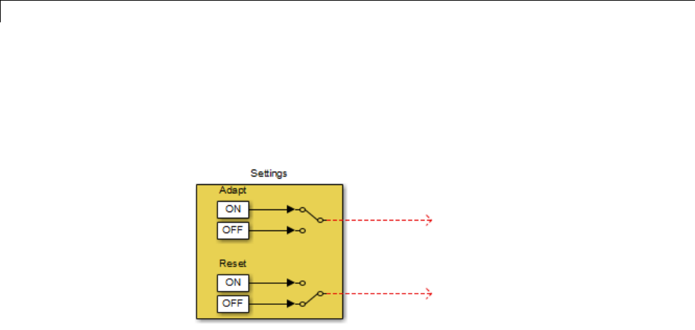
29 Using the MATLAB Function Block
The lms_03 function inputs Reset and Adapt now appear as input ports
to the MATLAB Function block.
4Open the design_templates model.
5Copy the Settings block from this model to your noise_cancel_02 model:
aFrom the design_templates model menu, select Edit > Select All.
bSelect Edit > Copy.
cFrom the noise_cancel_02 model menu, select Edit > Paste.
6Connect the Adapt and Reset outputs of the Settings subsystem to the
corresponding inputs on the MATLAB Function block. Your model should
now appear as follows.
29-226
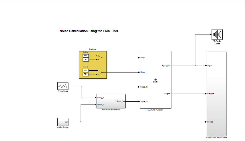
Filter Audio Signal Using MATLAB®Code
7Save the model as noise_cancel_03.
Simulating the Model with Adapt and Reset Controls. To simulate the
model and see the effect of the Adapt and Reset controls:
1In the noise_cancel_03 model, view the Convergence scope:
aDouble-click the Analysis and Visualization subsystem.
bDouble-click the Convergence scope.
2In the Simulink model window, select Simulation > Run.
Simulink runs the model as before. While the model is running, toggle
the Adapt and Reset controls and view the Convergence scope to see their
effect on the filter.
The filter converges when Adapt is ON and Reset is OFF, then resets when
you toggleReset. The results might look something like this:
29-227
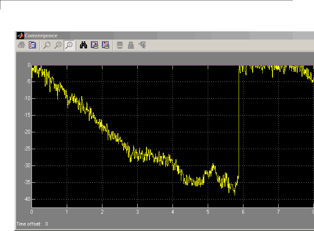
29 Using the MATLAB Function Block
3Stop the simulation.
Generating Code
You have proved that your algorithm works in Simulink. Next you generate
code for your model. Before generating code, you must ensure that your
MATLAB code is suitable for code generation. For code generation, you must
remove the extrinsic call to your code.
29-228

Filter Audio Signal Using MATLAB®Code
Making Your Code Suitable for Code Generation. To modify the model
and code yourself, work through the exercises in this section. Otherwise, open
the supplied model noise_cancel_04 and file lms_04.m in your solutions
subfolder to see the modifications.
1Rename the MATLAB Function block to LMS_Filter. Select the annotation
MATLAB Function below the MATLAB Function block and replace the text
with LMS_Filter.
When you generate code for the MATLAB Function block, Simulink Coder
uses the name of the block in the generated code. It is good practice to use
a meaningful name.
2In your noise_cancel_03 model, double-click the MATLAB Function block.
The MATLAB Function Block Editor opens.
3Delete the extrinsic declaration.
% Extrinsic:
coder.extrinsic('lms_03');
4Delete the preallocation of outputs.
% Outputs:
Signal_Out = zeros(size(Signal_In));
Weights = zeros(32,1);
5Modifythecalltothefilteralgorithm.
% Compute LMS:
[ ~, Signal_Out, Weights ] = ...
lms_04(Noise_In, Signal_In, Reset, Adapt);
6Save the model as noise_cancel_04.
7Open lms_03.m
aModifythefunctionnametolms_04.
bTurn on error checking specific tocodegenerationbyaddingthe
%#codegen compilation directive after the function declaration.
29-229

29 Using the MATLAB Function Block
function [ signal_out, err, weights_out ] = ...
lms_04(signal_in, desired, reset, adapt) %#codegen
The code analyzer message indicator in the top right turns red to
indicate that the code analyzer has detected code generation issues.
The code analyzer underlines the offending code in red and places a red
marker to the right of it.
8Move your pointer over the first red marker to view the error information.
The code analyzer detects that code generation requires signal_out to be
fully defined before subscripting it and does not support growth of variable
size data through indexing.
9Move your pointer over the second red marker and note that the code
analyzer detects the same errors for err.
10 To address these errors, preallocate the outputs signal_out and err.Add
this code after the filter setup.
% Output Arguments:
% Pre-allocate output and error signals:
signal_out = zeros(FrameSize,ChannelCount);
err = zeros(FrameSize,ChannelCount);
Why Preallocate the Outputs?
You must preallocate outputs here because code generation does not
support increasing the size of an array over time. Repeatedly expanding
thesizeofanarrayovertimecanadverselyaffecttheperformanceofyour
program. See “Preallocating Memory”.
The red error markers for the two lines of code disappear. The code
analyzer message indicator in the top right edge of the code turns green,
which indicates that you have fixed all the errors and warnings detected
bythecodeanalyzer.
11 Savethefileaslms_04.m.
29-230
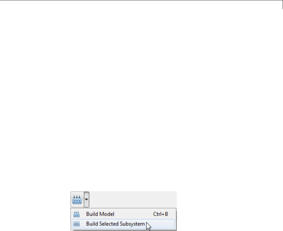
Filter Audio Signal Using MATLAB®Code
Generating Code for noise_cancel_04.
1Before generating code, ensure that Simulink Coder creates a code
generation report. This HTML report provides easy access to the list of
generated files with a summary of the configuration settings used to
generate the code.
aIn the Simulink model window, select Simulation > Model
Configuration Parameters.
bIn the left pane of the Configuration Parameters dialog box, select Code
Generation > Report.
cIn the right pane, select Create code generation report.
The Launch report automatically option is also selected.
dClick Apply and close the Configuration Parameters dialog box.
eSave your model.
2To generate code for the LMS Filter subsystem:
aIn your model, select the LMS Filter subsystem.
bFrom the Build Model tool menu, select Build Selected Subsystem.
The Build code for subsystem dialog box appears. Click the Build
button.
The Simulink Coder software generates C code for the subsystem and
launches the code generation report.
For more information on using the code generation report, see .
cIn the left pane of the code generation report, click the LMS_Filter.c
link to view the generated C code. Note that the lms_04 function has
no code because inlining is enabled by default.
29-231

29 Using the MATLAB Function Block
3Modify your filter algorithm to disable inlining:
aIn lms_04.m, after the function declaration, add:
coder.inline('never')
bChange the function name to lms_05 and save the file as lms_05.m in
the current folder.
cIn your noise_cancel_04 model, double-click the MATLAB Function
block.
The MATLAB Function Block Editor opens.
dModifythecalltothefilteralgorithmtocalllms_05.
% Compute LMS:
[ ~, Signal_Out, Weights ] = ...
lms_05(Noise_In, Signal_In, Reset, Adapt);
eSave the model as noise_cancel_05.
4Generate code for the updated model.
aIn the model, select the LMS Filter subsystem.
bFrom the Build Model tool menu, select Build Selected Subsystem.
The Build code for subsystem dialog box appears.
c
dClick the Build button.
The Simulink Coder software generates C code for the subsystem and
launches the code generation report.
eIn the left pane of the code generation report, click the LMS_Filter.c
link to view the generated C code.
This time the lms_05 function has code because you disabled inlining.
29-232

Filter Audio Signal Using MATLAB®Code
/* Forward declaration for local functions */
static void LMS_Filter_lms_05 ...
(const real_T signal_in[64],const real_T ...
desired[64], real_T reset, real_T adapt, ...
real_T signal_out[64], ...
real_T err[64], real_T weights_out[32]);
/* Function for MATLAB Function Block: 'root/LMS_Filter' */
static void LMS_Filter_lms_05 ...
(const real_T signal_in[64], const real_T ...
desired[64], real_T reset, real_T adapt, ...
real_T signal_out[64], ...
real_T err[64], real_T weights_out[32])
Optimizing the LMS Filter Algorithm
This part of the tutorial demonstrates when and how to preallocate memory
for a variable without incurring the overhead of initializing memory in the
generated code.
In lms_05.m, the MATLAB code not only declares signal_out and err to
be a FrameSize-by-ChannelCount vector of real doubles, but also initializes
each element of signal_out and err to zero. These signals are initialized to
zero in the generated C code.
MATLAB Code Generated C Code
%Pre-
allocate output and error signals:
signal_out = zeros(FrameSize,ChannelCount);
err = zeros(FrameSize,ChannelCount);
/* Pre-allocate output and error
signals: */
79 for (i = 0; i < 64; i++) {
80 signal_out[i] = 0.0;
81 err[i] = 0.0;
82 }
This forced initialization is unnecessary because both signal_out and err
are explicitly initialized in the MATLAB code before they are read.
29-233

29 Using the MATLAB Function Block
Note You should not use coder.nullcopy when declaring the variables
weights and fifo because these variables need to be initialized in the
generated code. Neither variable is explicitly initialized in the MATLAB code
before they are read.
Use coder.nullcopy in the declaration of signal_out and err to eliminate
the unnecessary initialization of memory in the generated code:
1In lms_05.m, preallocate signal_out and err using coder.nullcopy:
% Pre-allocate output and error signals:
signal_out = coder.nullcopy(zeros(FrameSize, ChannelCount));
err = coder.nullcopy(zeros(FrameSize, ChannelCount));
Caution After declaring a variable with coder.nullcopy,youmust
explicitly initialize the variable in your MATLAB code before reading it.
Otherwise, you might get unpredictable results.
2Change the function name to lms_06 and save the file as lms_06.m in the
current folder.
3In your noise_cancel_05 model, double-click the MATLAB Function block.
The MATLAB Function Block Editor opens.
4Modifythecalltothefilteralgorithm.
% Compute LMS:
[ ~, Signal_Out, Weights ] = ...
lms_06(Noise_In, Signal_In, Reset, Adapt);
5Save the model as noise_cancel_06.
Generate code for the updated model.
1Select the LMS Filter subsystem.
29-234

Filter Audio Signal Using MATLAB®Code
2From the Build Model tool menu, select BuildSelectedSubsystem.
The Build code for subsystem dialog box appears. Click the Build
button.
The Simulink Coder software and generates C code for the subsystem and
launches the code generation report.
3In the left pane of the code generation report, click the LMS_Filter.c link
to view the generated C code.
In the generated C code, this time there is no initialization to zero of
signal_out and err.
29-235

29 Using the MATLAB Function Block
29-236

30
Design Considerations for
C/C++ Code Generation
•“When to Generate Code from MATLAB Algorithms” on page 30-2
•“Which Code Generation Feature to Use” on page 30-4
•“Prerequisites for C/C++ Code Generation from MATLAB” on page 30-6
•“MATLAB Code Design Considerations for Code Generation” on page 30-7
•“Expected Differences in Behavior After Compiling MATLAB Code” on
page 30-9
•“MATLAB Language Features Supported for C/C++ Code Generation” on
page 30-13

30 Design Considerations for C/C++ Code Generation
When to Generate Code from MATLAB Algorithms
Generating code from MATLAB algorithms for desktop and embedded
systems allows you to perform your software design, implementation, and
testing completely within the MATLAB workspace. You can:
•Verify that your algorithms aresuitableforcodegeneration
•Generate efficient, readable, and compact C/C++ code automatically, which
eliminates the need to manually translate your MATLAB algorithms and
minimizes the risk of introducing errors in the code.
•Modify your design in MATLAB code to take into account the specific
requirements of desktop and embedded applications, such as data type
management, memory use, and speed.
•Test the generated code and easily verify that your modified algorithms are
functionally equivalent to your original MATLAB algorithms.
•Generate MEX functions to:
-Accelerate MATLAB algorithms in certain applications.
-Speed up fixed-point MATLAB code.
•Generate hardware description language (HDL) from MATLAB code.
When Not to Generate Code from MATLAB Algorithms
Do not generate code from MATLAB algorithms for the following applications.
Use the recommended MathWorks product instead.
To: Use:
Deploy an application that uses
handle graphics
MATLAB Compiler™
Use Java MATLAB Builder™ JA
Use toolbox functions that do not
support code generation
Toolbox functions that you rewrite for
desktop and embedded applications
Deploy MATLAB based GUI
applications on a supported
MATLAB host
MATLAB Compiler
30-2

When to Generate Code from MATLAB®Algorithms
To: Use:
Deploy web-based or Windows
applications
•MATLAB Builder NE
•MATLAB Builder JA
Interface C code with MATLAB MATLAB mex function
30-3

30 Design Considerations for C/C++ Code Generation
Which Code Generation Feature to Use
To... Use... Required Product To Explore Further...
Generate MEX
functions for verifying
generated code
codegen function MATLAB Coder Try this in “MEX
Function Generation
at the Command
Line”.
MATLAB Coder user
interface
MATLAB Coder Try this in “C Code
Generation Using the
Project Interface”.
Produce readable,
efficient, and compact
code from MATLAB
algorithms for
deployment to desktop
and embedded
systems.
codegen function MATLAB Coder Try this in “C Code
Generation at the
Command Line”.
MATLAB Coder user
interface
MATLAB CoderGenerate MEX
functions to accelerate
MATLAB algorithms codegen function MATLAB Coder
See “Accelerate
MATLAB
Algorithms”.
Integrate MATLAB
code into Simulink
MATLAB Function
block
Simulink Try this in “Track
Object Using
MATLAB Code” on
page 29-175.
Speed up fixed-point
MATLAB code
fiaccel function Fixed-Point Toolbox Learn more in “Code
Acceleration and
Code Generation from
MATLAB”.
Integrate custom C
code into MATLAB
and generate efficient,
readable code
codegen function MATLAB Coder Learn more in
“Custom C/C++ Code
Integration”.
30-4

Which Code Generation Feature to Use
To... Use... Required Product To Explore Further...
Integrate custom
Ccodeintocode
generated from
MATLAB
coder.ceval function MATLAB Coder Learn more in
coder.ceval.
Generate HDL from
MATLAB code
MATLAB Function
block
Simulink and
HDL Coder
Learn more at
www.mathworks.com/
products/slhdlcoder.
30-5

30 Design Considerations for C/C++ Code Generation
Prerequisites for C/C++ Code Generation from MATLAB
To generate C/C++ or MEX code from MATLAB algorithms, you must install
the following software:
•MATLAB Coder product
•C/C++ compiler
30-6

MATLAB®Code Design Considerations for Code Generation
MATLAB Code Design Considerations for Code Generation
When writing MATLAB code that you want to convert into efficient,
standalone C/C++ code, you must consider the following:
•Data types
C and C++ use static typing. To determine the types of your variables before
use, MATLAB Coder requires a complete assignment to each variable.
•Array sizing
Variable-size arrays and matrices are supported for code generation. You
can define inputs, outputs, and local variables in MATLAB functions to
representdatathatvariesinsizeatruntime.
•Memory
You can choose whether the generated code uses static or dynamic memory
allocation.
With dynamic memory allocation, you potentially use less memory at the
expenseoftimetomanagethememory. Withstaticmemory,yougetbest
speed performance, but with higher memory usage. Most MATLAB code
takes advantage of the dynamic sizing features in MATLAB, therefore
dynamic memory allocation typically enables you to generate code from
existing MATLAB code without modifying it much. Dynamic memory
allocation also allows some programs to compile even when upper bounds
cannot be found.
Static allocation reduces the memory footprint of the generated code, and
therefore is suitable for applications where there is a limited amount of
available memory, such as embedded applications.
•Speed
Because embedded applications must run in real time, the code must be
fast enough to meet the required clock rate.
To improve the speed of the generated code:
-Choose a suitable C/C++ compiler. The default compiler that MathWorks
supplies with MATLAB for Windows 32-bit platforms is not a good
compiler for performance.
-Consider disabling run-time checks.
30-7

30 Design Considerations for C/C++ Code Generation
By default, for safety, the code generated for your MATLAB code
contains memory integrity checks and responsiveness checks. Generally,
these checks result in more generated code and slower simulation.
Disabling run-time checks usually results in streamlined generated code
and faster simulation. Disable these checks only if you have verified that
array bounds and dimension checking is unnecessary.
See Also
•“Data Definition Basics”
•“Variable-Size Data”
•“Bounded Versus Unbounded Variable-Size Data” on page 35-4
30-8

Expected Differences in Behavior After Compiling MATLAB®Code
Expected Differences in Behavior After Compiling MATLAB
Code
In this section...
“Why Are There Differences?” on page 30-9
“Character Size” on page 30-9
“Order of Evaluation in Expressions” on page 30-9
“Termination Behavior” on page 30-10
“Size of Variable-Size N-D Arrays” on page 30-10
“SizeofEmptyArrays”onpage30-11
“Floating-Point Numerical Results” on page 30-11
“NaN and Infinity Patterns” on page 30-12
“Code Generation Target” on page 30-12
“MATLAB Class Initial Values” on page 30-12
“Variable-Size Support for Code Generation” on page 30-12
Why Are There Differences?
To convert MATLAB code to C/C++ code that works efficiently, the code
generation process introduces optimizations that intentionally cause the
generatedcodetobehavedifferently— and sometimes produce different
results — from the original source code. This section describes these
differences.
Character Size
MATLAB supports 16-bit characters, but the generated code represents
characters in 8 bits, the standard size for most embedded languages like C.
See “Code Generation for Characters” on page 34-6.
Order of Evaluation in Expressions
Generated code does not enforce order of evaluation in expressions. For most
expressions, order of evaluation is not significant. However, for expressions
30-9

30 Design Considerations for C/C++ Code Generation
with side effects, the generated code may produce the side effects in different
order from the original MATLAB code. Expressions that produce side effects
include those that:
•Modify persistent or global variables
•Display data to the screen
•Write data to files
•Modify the properties of handle class objects
In addition, the generated code does not enforce order of evaluation of logical
operators that do not short circuit.
For more predictable results, it is good coding practice to split expressions
that depend on the order of evaluation into multiple statements. For example,
rewrite:
A = f1() + f2();
as
A = f1();
A = A + f2();
so that the generated code calls f1 before f2.
Termination Behavior
Generated code does not match the termination behavior of MATLAB source
code. For example, optimizations remove infinite loops from generated code if
they have no side effects. As a result, the generated code may terminate even
though the corresponding MATLAB code does not.
Size of Variable-Size N-D Arrays
For variable-size N-D arrays, the size function might return a different
result in generated code than in MATLAB source code. The size function
sometimes returns trailing ones (singleton dimensions) in generated code, but
always drops trailing ones in MATLAB. For example, for an N-D array Xwith
dimensions [4211],size(X) might return [4 2 1 1] in generated code,
30-10

Expected Differences in Behavior After Compiling MATLAB®Code
but always returns [4 2] in MATLAB. See “Incompatibility with MATLAB in
Determining Size of Variable-Size N-D Arrays” on page 35-26.
Size of Empty Arrays
The size of an empty array in generated code might be different from its size
in MATLAB source code. See “Incompatibility with MATLAB in Determining
Size of Empty Arrays” on page 35-27.
Floating-Point Numerical Results
The generated code might not produce the same floating-point numerical
results as MATLAB in the following situations:
When computer hardware uses extended precision registers
Results vary depending on how the C/C++ compiler allocates extended
precision floating-point registers. Computation results might not match
MATLAB calculations because of different compiler optimization settings or
different code surrounding the floating-point calculations.
For certain advanced library functions
The generated code might use different algorithms to implement certain
advanced library functions, such as fft,svd,eig,mldivide,andmrdivide.
For example, the generated code uses a simpler algorithm to implement
svd to accommodate a smaller footprint. Results might also vary according
to matrix properties. For example, MATLAB might detect symmetric or
Hermitian matrices at run time and switch to specialized algorithms that
perform computations faster than implementations in the generated code.
For implementation of BLAS library functions
For implementations of BLAS library functions. Generated C/C++ code uses
reference implementations of BLAS functions, which may produce different
results from platform-specific BLAS implementations in MATLAB.
30-11

30 Design Considerations for C/C++ Code Generation
NaN and Infinity Patterns
The generated code might not produceexactlythesamepatternofNaN and inf
values as MATLAB code when these values are mathematically meaningless.
For example, if MATLAB output contains a NaN, output from the generated
code should also contain a NaN, but not necessarily in the same place.
Code Generation Target
The coder.target function returns different values in MATLAB than in the
generated code. The intent is to help you determine whether your function
is executing in MATLAB or has been compiled for a simulation or code
generation target. See .
MATLAB Class Initial Values
MATLAB computes class initial values at class loading time before code
generation. The code generation software uses the value that MATLAB
computed, it does not recompute the initial value. If the initialization uses
a function call to compute the initial value, the code generation software
does not execute this function. If the function modifies a global state, for
example, a persistent variable, code generation software might provide a
different initial value than MATLAB. For more information, see “Defining
Class Properties for Code Generation” on page 38-5.
Variable-Size Support for Code Generation
For incompatibilities with MATLAB in variable-size support for code
generation, see:
•“Incompatibility with MATLAB for Scalar Expansion”
•“Incompatibility with MATLAB in Determining Size of Variable-Size N-D
Arrays”
•“Incompatibility with MATLAB in Determining Size of Empty Arrays”
•“Incompatibility with MATLAB in Vector-Vector Indexing”
•“Incompatibility with MATLAB in Matrix Indexing Operations for Code
Generation”
30-12

MATLAB®Language Features Supported for C/C++ Code Generation
MATLAB Language Features Supported for C/C++ Code
Generation
MATLAB supports the following language features in generated code:
•N-dimensional arrays
•Matrix operations, including deletion of rows and columns
•Variable-sized data (see “Variable-Size Data Definition for Code
Generation” on page 35-3)
•Subscripting (see “Incompatibility with MATLAB in Matrix Indexing
Operations for Code Generation” on page 35-29)
•Complex numbers (see “Code Generation for Complex Data” on page 34-4)
•Numericclasses(see“SupportedVariableTypes”onpage33-18)
•Double-precision, single-precision, and integer math
•Fixed-point arithmetic (see “Code Acceleration and Code Generation from
MATLAB”)
•Program control statements if,switch,for,andwhile
•All arithmetic, relational, and logical operators
•Local functions
•Persistent variables (see “Define and Initialize Persistent Variables” on
page 33-10)
•Global variables.
•Structures
•Characters (see “Code Generation for Characters” on page 34-6)
•Function handles
•Frames (see “Add Frame-Based Signals” on page 29-126)
•Variable length input and output argument lists
•Subset of MATLAB toolbox functions
•MATLAB classes
30-13

30 Design Considerations for C/C++ Code Generation
•Ability to call functions (see “Resolution of Function Calls in MATLAB
Generated Code” on page 41-2)
MATLAB Language Features Not Supported for C/C++
Code Generation
MATLAB does not support the following features in generated code:
•Anonymous functions
•Cell arrays
•Java
•Nested functions
•Recursion
•Sparse matrices
•try/catch statements
30-14


31 Functions Supported for Code Generation
Functions Supported for Code Generation — Alphabetical
List
You can generate efficient C/C++ code for a subset of MATLAB and toolbox
functions that you call from MATLAB code. In generated code, each supported
function has the same name, arguments, and functionality as its MATLAB or
toolbox counterparts. However, to generate code for these functions, you must
adhere to certain limitations when calling them from your MATLAB source
code. These limitations appear in the list below.
To find supported functions by MATLAB category or toolbox, see “Functions
Supported for Code Generation — Categorical List” on page 31-54.
Note For more information on code generation for fixed-point algorithms,
refer to “Code Acceleration and Code Generation from MATLAB”.
Function Product Remarks/Limitations
abs MATLAB —
abs Fixed-Point
Toolbox
—
acos MATLAB •Generates an error during simulation and
returns NaN in generated code when the
input value xis real, but the output should
be complex. To get the complex result,
make the input value complex by passing in
complex(x).
acosd MATLAB —
acosh MATLAB •Generates an error during simulation and
returns NaN in generated code when the
input value xis real, but the output should
be complex. To get the complex result,
make the input value complex by passing in
complex(x).
acot MATLAB —
31-2

Functions Supported for Code Generation — Alphabetical List
Function Product Remarks/Limitations
acotd MATLAB —
acoth MATLAB —
acsc MATLAB —
acscd MATLAB —
acsch MATLAB —
add Fixed-Point
Toolbox
—
all MATLAB —
all Fixed-Point
Toolbox
—
and MATLAB —
angle MATLAB —
any MATLAB —
any Fixed-Point
Toolbox
—
asec MATLAB —
asecd MATLAB —
asech MATLAB —
asin MATLAB •Generates an error during simulation and
returns NaN in generated code when the
input value xis real, but the output should
be complex. To get the complex result,
make the input value complex by passing in
complex(x).
asind MATLAB —
asinh MATLAB —
assert MATLAB •Generates specified error messages at compile
time only if all input arguments are constants
or depend on constants. Otherwise, generates
specified error messages at run time.
31-3

31 Functions Supported for Code Generation
Function Product Remarks/Limitations
atan MATLAB —
atan2 MATLAB —
atan2d MATLAB —
atand MATLAB —
atanh MATLAB •Generates an error during simulation and
returns NaN in generated code when the
input value xis real, but the output should
be complex. To get the complex result,
make the input value complex by passing in
complex(x).
barthannwin Signal Processing
Toolbox™
•Does not support variable-size inputs.
•Window length must be a constant.
Expressions or variables are allowed if their
values do not change.
•Requires DSP System Toolbox license to
generate code.
bartlett Signal Processing
Toolbox
•Does not support variable-size inputs.
•Window length must be a constant.
Expressions or variables are allowed if their
values do not change.
•Requires DSP System Toolbox license to
generate code.
besselap Signal Processing
Toolbox
•Does not support variable-size inputs.
•Filter order must be a constant. Expressions
or variables are allowed if their values do not
change.
•Requires DSP System Toolbox license to
generate code.
beta MATLAB —
betainc MATLAB —
31-4

Functions Supported for Code Generation — Alphabetical List
Function Product Remarks/Limitations
betaln MATLAB —
bi2de Communications
System Toolbox
•Requires a Communications System Toolbox
licensetogeneratecode.
bin2dec MATLAB •Does not match MATLAB when the input is
empty.
bitand MATLAB •Does not support floating-point inputs. The
arguments must belong to an unsigned
integer class.
bitand Fixed-Point
Toolbox
•Not supported for slope-bias scaled fi objects.
bitandreduce Fixed-Point
Toolbox
—
bitcmp MATLAB •Does not support floating-point input for the
first argument. The first argument must
belong to an unsigned integer class.
bitcmp Fixed-Point
Toolbox
—
bitconcat Fixed-Point
Toolbox
—
bitget MATLAB •Does not support floating-point input for the
first argument. The first argument must
belong to an unsigned integer class.
bitget Fixed-Point
Toolbox
—
bitmax MATLAB —
bitor MATLAB •Does not support floating-point inputs. The
arguments must belong to an unsigned
integer class.
bitor Fixed-Point
Toolbox
•Not supported for slope-bias scaled fi objects.
31-5

31 Functions Supported for Code Generation
Function Product Remarks/Limitations
bitorreduce Fixed-Point
Toolbox
—
bitreplicate Fixed-Point
Toolbox
—
bitrevorder Signal Processing
Toolbox
•Does not support variable-size inputs.
•Computation performed at run time.
•Requires DSP System Toolbox license to
generate code.
bitrol Fixed-Point
Toolbox
—
bitror Fixed-Point
Toolbox
—
bitset MATLAB •Does not support floating-point input for the
first argument. The first argument must
belong to an unsigned integer class.
bitset Fixed-Point
Toolbox
—
bitshift MATLAB •Does not support floating-point input for the
first argument. The first argument must
belong to an unsigned integer class.
bitshift Fixed-Point
Toolbox
—
bitsliceget Fixed-Point
Toolbox
—
bitsll Fixed-Point
Toolbox
—
bitsra Fixed-Point
Toolbox
—
bitsrl Fixed-Point
Toolbox
—
31-6

Functions Supported for Code Generation — Alphabetical List
Function Product Remarks/Limitations
bitxor MATLAB •Does not support floating-point inputs. The
arguments must belong to an unsigned
integer class.
bitxor Fixed-Point
Toolbox
•Not supported for slope-bias scaled fi objects.
bitxorreduce Fixed-Point
Toolbox
—
blackman Signal Processing
Toolbox
•Does not support variable-size inputs.
•Window length must be a constant.
Expressions or variables are allowed if their
values do not change.
•Requires DSP System Toolbox license to
generate code.
blackmanharris Signal Processing
Toolbox
•Does not support variable-size inputs.
•Window length must be a constant.
Expressions or variables are allowed if their
values do not change.
•Requires DSP System Toolbox license to
generate code.
blanks MATLAB —
blkdiag MATLAB —
bohmanwin Signal Processing
Toolbox
•Does not support variable-size inputs.
•Window length must be a constant.
Expressions or variables are allowed if their
values do not change.
•Requires DSP System Toolbox license to
generate code.
bsxfun MATLAB —
31-7

31 Functions Supported for Code Generation
Function Product Remarks/Limitations
buttap Signal Processing
Toolbox
•Does not support variable-size inputs.
•Filter order must be a constant. Expressions
or variables are allowed if their values do not
change.
•Requires DSP System Toolbox license to
generate code.
butter Signal Processing
Toolbox
•Does not support variable-size inputs.
•Filter coefficients must be constants.
Expressions or variables are allowed if their
values do not change.
•Requires DSP System Toolbox license to
generate code.
buttord Signal Processing
Toolbox
•Does not support variable-size inputs.
•All inputs must be constants. Expressions or
variables are allowed if their values do not
change.
•Requires DSP System Toolbox license to
generate code.
bwlookup Image Processing
Toolbox™
•For best results, specify an input image of
class logical.
bwmorph Image Processing
Toolbox
•The text string specifying the operation must
be a constant and, for best results, specify an
input image of class logical.
cart2pol MATLAB —
cart2sph MATLAB —
cast MATLAB —
cat MATLAB —
ceil MATLAB —
31-8

Functions Supported for Code Generation — Alphabetical List
Function Product Remarks/Limitations
ceil Fixed-Point
Toolbox
—
cfirpm Signal Processing
Toolbox
•Does not support variable-size inputs.
•All inputs must be constants. Expressions or
variables are allowed if their values do not
change.
•Requires DSP System Toolbox license to
generate code.
char MATLAB —
cheb1ap Signal Processing
Toolbox
•Does not support variable-size inputs.
•All inputs must be constants. Expressions or
variables are allowed if their values do not
change.
•Requires DSP System Toolbox license to
generate code.
cheb1ord Signal Processing
Toolbox
•Does not support variable-size inputs.
•All inputs must be constants. Expressions or
variables are allowed if their values do not
change.
•Requires DSP System Toolbox license to
generate code.
cheb2ap Signal Processing
Toolbox
•Does not support variable-size inputs.
•All inputs must be constants. Expressions or
variables are allowed if their values do not
change.
•Requires DSP System Toolbox license to
generate code.
31-9

31 Functions Supported for Code Generation
Function Product Remarks/Limitations
cheb2ord Signal Processing
Toolbox
•Does not support variable-size inputs.
•All inputs must be constants. Expressions or
variables are allowed if their values do not
change.
•Requires DSP System Toolbox license to
generate code.
chebwin Signal Processing
Toolbox
•Does not support variable-size inputs.
•All inputs must be constants. Expressions or
variables are allowed if their values do not
change.
•Requires DSP System Toolbox license to
generate code.
cheby1 Signal Processing
Toolbox
•Does not support variable-size inputs.
•All inputs must be constants. Expressions or
variables are allowed if their values do not
change.
•Requires DSP System Toolbox license to
generate code.
cheby2 Signal Processing
Toolbox
•Does not support variable-size inputs.
•All inputs must be constants. Expressions or
variables are allowed if their values do not
change.
•Requires DSP System Toolbox license to
generate code.
31-10

Functions Supported for Code Generation — Alphabetical List
Function Product Remarks/Limitations
chol MATLAB •When there are two output arguments, either
make the input matrix variable-size in both
dimensions, or, if the input matrix must
be fixed size, copy the input matrix to a
variable-size matrix before calling chol.
coder.varsize('B');
B=A;
[B,p] = chol(B);
circshift MATLAB —
class MATLAB —
compan MATLAB —
complex MATLAB —
complex Fixed-Point
Toolbox
—
cond MATLAB —
conj MATLAB —
conj Fixed-Point
Toolbox
—
conv MATLAB —
conv Fixed-Point
Toolbox
•Variable-sized inputs are only supported
when the SumMode property of the governing
fimath is set to Specify precision or Keep
LSB.
•For variable-sized signals, you may see
different results between MATLAB and the
generated code.
-In generated code, the output for
variable-sized signals is always computed
using the SumMode property of the
governing fimath.
31-11

31 Functions Supported for Code Generation
Function Product Remarks/Limitations
-In MATLAB, the output for variable-sized
signalsiscomputedusingtheSumMode
property of the governing fimath when
both inputs are nonscalar. However, if
either input is a scalar, MATLAB computes
the output using the ProductMode of the
governing fimath.
conv2 MATLAB —
convergent Fixed-Point
Toolbox
—
convn MATLAB —
cordicabs Fixed-Point
Toolbox
•Variable-size signals are not supported.
cordicangle Fixed-Point
Toolbox
•Variable-size signals are not supported.
cordicatan2 Fixed-Point
Toolbox
•Variable-size signals are not supported.
cordiccart2pol Fixed-Point
Toolbox
•Variable-size signals are not supported.
cordiccexp Fixed-Point
Toolbox
•Variable-size signals are not supported.
cordiccos Fixed-Point
Toolbox
•Variable-size signals are not supported.
cordicpol2cart Fixed-Point
Toolbox
•Variable-size signals are not supported.
cordicrotate Fixed-Point
Toolbox
•Variable-size signals are not supported.
cordicsin Fixed-Point
Toolbox
•Variable-size signals are not supported.
cordicsincos Fixed-Point
Toolbox
•Variable-size signals are not supported.
31-12

Functions Supported for Code Generation — Alphabetical List
Function Product Remarks/Limitations
corrcoef MATLAB •Row-vector input is only supported when the
first two inputs are vectors and nonscalar.
cos MATLAB —
cosd MATLAB —
cosh MATLAB —
cot MATLAB —
cotd MATLAB —
coth MATLAB —
cov MATLAB —
cross MATLAB •If supplied, dim must be a constant.
csc MATLAB —
cscd MATLAB —
csch MATLAB —
ctranspose MATLAB —
ctranspose Fixed-Point
Toolbox
—
cumprod MATLAB •Logical inputs are not supported. Cast input
to double first.
cumsum MATLAB •Logical inputs are not supported. Cast input
to double first.
cumtrapz MATLAB —
dct Signal Processing
Toolbox
•Does not support variable-size inputs.
•Requires DSP System Toolbox license to
generate code.
•Length of transform dimension must
be a power of two. If specified, the pad
or truncation value must be constant.
Expressions or variables are allowed if their
values do not change.
31-13

31 Functions Supported for Code Generation
Function Product Remarks/Limitations
de2bi Communications
System Toolbox
•Requires a Communications System Toolbox
licensetogeneratecode.
deal MATLAB —
deblank MATLAB •Supports only inputs from the char class.
•Input values must be in the range 0-127.
dec2bin MATLAB •If input dis double,dmust be less than 2^52.
•If input dis single,dmust be less than 2^23.
•Unless you specify input nto be constant and
nis large enough that the output has a fixed
number of columns regardless of the input
values, this function requires variable-sizing
support. Without variable-sizing support, n
must be at least 52 for double,23 for single,
16 for char,32 for int32,16 for int16,and
so on.
dec2hex MATLAB •If input dis double,dmust be less than 2^52.
•If input dis single,dmust be less than 2^23.
•Unless you specify input nto be constant and
nis large enough that the output has a fixed
number of columns regardless of the input
values, this function requires variable-sizing
support. Without variable-sizing support, n
must be at least 13 for double,6for single,4
for char,8for int32,4for int16,andsoon.
deconv MATLAB —
del2 MATLAB —
det MATLAB —
31-14

Functions Supported for Code Generation — Alphabetical List
Function Product Remarks/Limitations
detrend MATLAB •If supplied and not empty, the input argument
bp must satisfy the following requirements:
-Be real
-Be sorted in ascending order
-Restrict elements to integers in the interval
[1, n-2],wherenis the number of
elements in a column of input argument X
, or the number of elements in Xwhen Xis
arowvector
-Contain all unique values
diag MATLAB •If supplied, the argument representing the
order of the diagonal matrix must be a real
and scalar integer value.
diag Fixed-Point
Toolbox
•If supplied, the index, k,mustbearealand
scalar integer value that is not a fi object.
diff MATLAB •If supplied, the arguments representing
the number of times to apply diff and
the dimension along which to calculate the
difference must be constants.
disp Fixed-Point
Toolbox
—
divide Fixed-Point
Toolbox
•Any non-fi input must be constant; that is,
its value must be known at compile time so
that it can be cast to a fi object.
•Complex and imaginary divisors are not
supported.
•The syntax T.divide(a,b) is not supported.
dot MATLAB —
double MATLAB —
double Fixed-Point
Toolbox
—
31-15

31 Functions Supported for Code Generation
Function Product Remarks/Limitations
downsample Signal Processing
Toolbox
•Does not support variable-size inputs.
dpss Signal Processing
Toolbox
•Does not support variable-size inputs.
•All inputs must be constants. Expressions or
variables are allowed if their values do not
change.
•Requires DSP System Toolbox license to
generate code.
eig MATLAB •QZ algorithm used in all cases, whereas
MATLAB might use different algorithms
for different inputs. Consequently, Vmight
represent a different basis of eigenvectors,
and the eigenvalues in Dmight not be in the
same order as in MATLAB.
•With one input, [V,D] = eig(A),theresults
will be similar to those obtained using [V,D]
= eig(A,eye(size(A)),'qz') in MATLAB,
except that for code generation, the columns
of Vare normalized.
•Options 'balance','nobalance' are not
supported for the standard eigenvalue
problem, and 'chol' is not supported for the
symmetric generalized eigenvalue problem.
•Outputs are always of complex type.
ellip Signal Processing
Toolbox
•Does not support variable-size inputs.
•Inputs must be constant. Expressions or
variables are allowed if their values do not
change.
•Requires DSP System Toolbox license to
generate code.
31-16

Functions Supported for Code Generation — Alphabetical List
Function Product Remarks/Limitations
ellipap Signal Processing
Toolbox
•Does not support variable-size inputs.
•All inputs must be constants. Expressions or
variables are allowed if their values do not
change.
•Requires DSP System Toolbox license to
generate code.
ellipke MATLAB —
ellipord Signal Processing
Toolbox
•Does not support variable-size inputs.
•All inputs must be constants. Expressions or
variables are allowed if their values do not
change.
•Requires DSP System Toolbox license to
generate code.
end Fixed-Point
Toolbox
—
epipolarLine Computer Vision
System Toolbox
—
eps MATLAB —
eps Fixed-Point
Toolbox
•Supported for scalar fixed-point signals only.
•Supported for scalar, vector, and matrix, fi
single and fi double signals.
eq MATLAB —
eq Fixed-Point
Toolbox
•Not supported for fixed-point signals with
different biases.
erf MATLAB —
erfc MATLAB —
erfcinv MATLAB —
erfcx MATLAB —
erfinv MATLAB —
31-17

31 Functions Supported for Code Generation
Function Product Remarks/Limitations
error MATLAB •This is an extrinsic call.
estimate
Fundamental
Matrix
Computer Vision
System Toolbox
—
estimateUncalibratedRectification
Computer Vision
System Toolbox
—
exp MATLAB —
expint MATLAB —
expm MATLAB —
expm1 MATLAB —
extractFeatures Computer Vision
System Toolbox
—
eye MATLAB •Dimensions must be real, nonnegative,
integers.
factor MATLAB •For double precision input, the maximum
value of Ais 2^32-1.
•For single precision input, the maximum
value of Ais 2^24-1.
factorial MATLAB —
false MATLAB •Dimensions must be real, nonnegative,
integers.
fft MATLAB •Length of input vector must be a power of 2.
fft2 MATLAB •Length of input matrix dimensions must each
be a power of 2.
fftn MATLAB •Length of input matrix dimensions must each
be a power of 2.
fftshift MATLAB —
31-18

Functions Supported for Code Generation — Alphabetical List
Function Product Remarks/Limitations
fi Fixed-Point
Toolbox
•Usetocreateafixed-pointconstantor
variable.
•The default constructor syntax without any
input arguments is not supported.
•The syntax
fi('PropertyName',PropertyValue...)
is not supported. To use property
name/property value pairs, you must first
specify the value vof the fi object as in
fi(v,'PropertyName',PropertyValue...).
•Works for all input values when complete
numerictype information of the fi object is
provided.
•Works only for constant input values (value of
input must be known at compile time) when
complete numerictype information of the fi
object is not specified.
•numerictype object information must be
available for non-fixed-point Simulink inputs.
filter MATLAB —
filter Fixed-Point
Toolbox
•Variable-sized inputs are only supported
when the SumMode property of the governing
fimath is set to Specify precision or Keep
LSB.
filter2 MATLAB —
filtfilt Signal Processing
Toolbox
•Does not support variable-size inputs.
•Filter coefficients must be constants.
Expressions or variables are allowed if their
values do not change.
•Requires DSP System Toolbox license to
generate code.
31-19

31 Functions Supported for Code Generation
Function Product Remarks/Limitations
fimath Fixed-Point
Toolbox
•Fixed-point signals coming in to a MATLAB
Function block from Simulink are assigned
the fimath object defined in the MATLAB
Function dialog in the Model Explorer.
•Use to create fimath objects in generated
code.
find MATLAB •Issues an error if a variable-sized input
becomes a row vector at run time.
Note This limitation does not apply when
the input is scalar or a variable-length row
vector.
•For variable-sized inputs, the shape of empty
outputs, 0-by-0, 0-by-1, or 1-by-0, depends on
the upper bounds of the size of the input. The
output might not match MATLAB when the
input array is a scalar or [] at run time. If
the input is a variable-length row vector, the
size of an empty output is 1-by-0, otherwise it
is 0-by-1.
fir1 Signal Processing
Toolbox
•Does not support variable-size inputs.
•All inputs must be constants. Expressions or
variables are allowed if their values do not
change.
•Requires DSP System Toolbox license to
generate code.
31-20

Functions Supported for Code Generation — Alphabetical List
Function Product Remarks/Limitations
fir2 Signal Processing
Toolbox
•Does not support variable-size inputs.
•All inputs must be constants. Expressions or
variables are allowed if their values do not
change.
•Requires DSP System Toolbox license to
generate code.
fircls Signal Processing
Toolbox
•Does not support variable-size inputs.
•All inputs must be constants. Expressions or
variables are allowed if their values do not
change.
•Requires DSP System Toolbox license to
generate code.
fircls1 Signal Processing
Toolbox
•Does not support variable-size inputs.
•All inputs must be constants. Expressions or
variables are allowed if their values do not
change.
•Requires DSP System Toolbox license to
generate code.
firls Signal Processing
Toolbox
•Does not support variable-size inputs.
•All inputs must be constants. Expressions or
variables are allowed if their values do not
change.
•Requires DSP System Toolbox license to
generate code.
firpm Signal Processing
Toolbox
•Does not support variable-size inputs.
•All inputs must be constants. Expressions or
variables are allowed if their values do not
change.
•Requires DSP System Toolbox license to
generate code.
31-21

31 Functions Supported for Code Generation
Function Product Remarks/Limitations
firpmord Signal Processing
Toolbox
•Does not support variable-size inputs.
•All inputs must be constants. Expressions or
variables are allowed if their values do not
change.
•Requires DSP System Toolbox license to
generate code.
firrcos Signal Processing
Toolbox
•Does not support variable-size inputs.
•All inputs must be constants. Expressions or
variables are allowed if their values do not
change.
•Requires DSP System Toolbox license to
generate code.
fix MATLAB —
fix Fixed-Point
Toolbox
—
flattopwin Signal Processing
Toolbox
•Does not support variable-size inputs.
•All inputs must be constants. Expressions or
variables are allowed if their values do not
change.
•Requires DSP System Toolbox license to
generate code.
flipdim MATLAB —
fliplr MATLAB —
flipud MATLAB —
floor MATLAB —
floor Fixed-Point
Toolbox
—
freqspace MATLAB —
31-22

Functions Supported for Code Generation — Alphabetical List
Function Product Remarks/Limitations
freqz Signal Processing
Toolbox
•Does not support variable-size inputs.
•freqz with no output arguments produces a
plot only when the function call terminates
in a semicolon. See “freqz With No Output
Arguments”.
•Requires DSP System Toolbox license to
generate code.
fspecial Image Processing
Toolbox
All inputs must be constants at compilation
time. Expressions or variables are allowed if
their values do not change.
full MATLAB —
fzero MATLAB •The first argument must be a function handle.
Does not support structure, inline function, or
string inputs for the first argument.
•Supports up to three output arguments. Does
not support the fourth output argument (the
output structure).
•Only supports the TolX and FunValCheck
fields of an options input structure. Ignores
all other options in an options input
structure. You cannot use the optimset
function to create the options structure.
Create this structure directly, for example,
opt.TolX = tol;
opt.FunValCheck = 'on';
The input structure field names must match
exactly.
gamma MATLAB —
gammainc MATLAB —
gammaln MATLAB —
31-23

31 Functions Supported for Code Generation
Function Product Remarks/Limitations
gaussfir Signal Processing
Toolbox
•Does not support variable-size inputs.
•All inputs must be constant. Expressions or
variables are allowed if their values do not
change.
•Requires DSP System Toolbox license to
generate code.
gausswin Signal Processing
Toolbox
•Does not support variable-size inputs.
•All inputs must be constant. Expressions or
variables are allowed if their values do not
change.
•Requires DSP System Toolbox license to
generate code.
gcd MATLAB —
ge MATLAB —
ge Fixed-Point
Toolbox
•Not supported for fixed-point signals with
different biases.
get Fixed-Point
Toolbox
•The syntax structure = get(o) is not
supported.
getlsb Fixed-Point
Toolbox
—
getmsb Fixed-Point
Toolbox
—
gradient MATLAB —
gt MATLAB —
gt Fixed-Point
Toolbox
•Not supported for fixed-point signals with
different biases.
hadamard MATLAB —
31-24

Functions Supported for Code Generation — Alphabetical List
Function Product Remarks/Limitations
hamming Signal Processing
Toolbox
•Does not support variable-size inputs.
•All inputs must be constant. Expressions or
variables are allowed if their values do not
change.
•Requires DSP System Toolbox license to
generate code.
hankel MATLAB —
hann Signal Processing
Toolbox
•Does not support variable-size inputs.
•All inputs must be constant. Expressions or
variables are allowed if their values do not
change.
•Requires DSP System Toolbox license to
generate code.
hex2dec MATLAB —
hex2num MATLAB •For n = hex2num(S),size(S,2) <=
length(num2hex(0))
hilb MATLAB —
hist MATLAB •Histogram bar plotting not supported; call
with at least one output argument.
•If supplied, the second argument xmust be a
scalar constant.
•Inputs must be real.
histc MATLAB •The output of a variable-size array that
becomes a column vector at run time is a
column-vector, not a row-vector.
horzcat Fixed-Point
Toolbox
—
hypot MATLAB —
31-25

31 Functions Supported for Code Generation
Function Product Remarks/Limitations
idct Signal Processing
Toolbox
•Does not support variable-size inputs.
•Length of transform dimension must
be a power of two. If specified, the pad
or truncation value must be constant.
Expressions or variables are allowed if their
values do not change.
•Requires DSP System Toolbox license to
generate code.
idivide MATLAB •For efficient generated code, MATLAB rules
for divide by zero are supported only for the
'round' option.
ifft MATLAB •Length of input vector must be a power of 2.
•Output of ifft block is always complex.
•Does not support the 'symmetric' option.
ifft2 MATLAB •Length of input matrix dimensions must each
be a power of 2.
•Does not support the 'symmetric' option.
ifftn MATLAB •Length of input matrix dimensions must each
be a power of 2.
•Does not support the 'symmetric' option.
ifftshift MATLAB —
imag MATLAB —
imag Fixed-Point
Toolbox
—
ind2sub MATLAB •The first argument should be a valid size
vector. Size vectors for arrays with more than
intmax elements are not supported.
inf MATLAB •Dimensions must be real, nonnegative,
integers.
int8,int16,int32 MATLAB —
31-26

Functions Supported for Code Generation — Alphabetical List
Function Product Remarks/Limitations
int8,int16,int32 Fixed-Point
Toolbox
—
integralImage Computer Vision
System Toolbox
—
interp1 MATLAB •Supports only linear and nearest
interpolation methods.
•Does not handle evenly spaced Xindices
separately.
•Xmust be strictly monotonically increasing
or strictly monotonically decreasing; does not
reorder indices.
interp2 MATLAB •Supports only 5 <= nargin <= 7.
•XI and YI must be the same size.
•Supports only 'linear' and 'nearest'
methods.
•For best performance, supply Xand Yas
vectors.
•When the Xor Yinputs are not vectors,
interp2 references only the first row of Xand
first column of Y. Supports "plaid" input for X
and Ybut does not verify that the input data
is "plaid".
•Xand Ymust contain monotonically
increasing values. If your application provides
monotonically decreasing values, first use
fliplr and flipud to change X,Y,andZto
monotonically increasing form before calling
interp2.
31-27

31 Functions Supported for Code Generation
Function Product Remarks/Limitations
intersect MATLAB •When rows is not specified:
-Inputs must be row vectors.
-If a vector is variable-sized, its first
dimension must have a fixed length of 1.
-The input [] is not supported. Use a 1-by-0
input, for example zeros(1,0), to represent
the empty set.
-Empty outputs are always row vectors,
1-by-0, never 0-by-0.
•When rows is specified, outputs ia and ib are
always column vectors. If these outputs are
empty, they are 0-by-1, never 0-by-0, even if
the output cis 0-by-0.
•Inputs must already be sorted in ascending
order. The first output is always sorted in
ascending order.
•Complex inputs must be single or double.
intfilt Signal Processing
Toolbox
•Does not support variable-size inputs.
•All inputs must be constant. Expressions or
variables are allowed if their values do not
change.
•Requires DSP System Toolbox license to
generate code.
intmax MATLAB —
intmin MATLAB —
inv MATLAB Singular matrix inputs can produce nonfinite
values that differ from MATLAB results.
invhilb MATLAB —
ipermute MATLAB —
isa MATLAB —
31-28

Functions Supported for Code Generation — Alphabetical List
Function Product Remarks/Limitations
iscell MATLAB —
ischar MATLAB —
iscolumn MATLAB —
iscolumn Fixed-Point
Toolbox
—
isdeployed MATLAB
Compiler
•Returns true and false as appropriate for
MEX and SIM targets
•Returns false for all other targets
isempty MATLAB —
isempty Fixed-Point
Toolbox
—
isEpipoleInImage Computer Vision
System Toolbox
—
isequal MATLAB —
isequal Fixed-Point
Toolbox
—
isequaln MATLAB —
isfi Fixed-Point
Toolbox
—
isfield MATLAB •Does not support cell input for second
argument
isfimath Fixed-Point
Toolbox
—
isfimathlocal Fixed-Point
Toolbox
—
isfinite MATLAB —
isfinite Fixed-Point
Toolbox
—
isfloat MATLAB —
31-29

31 Functions Supported for Code Generation
Function Product Remarks/Limitations
isinf MATLAB —
isinf Fixed-Point
Toolbox
—
isinteger MATLAB —
isletter MATLAB •Input values from the char class must be in
the range 0-127
islogical MATLAB —
ismatrix MATLAB —
ismcc MATLAB
Compiler
•Returns true and false as appropriate for
MEX and SIM targets.
•Returnsfalseforallothertargets.
ismember MATLAB •The second input, S,mustbesortedin
ascending order.
•Complex inputs must be single or double.
isnan MATLAB —
isnan Fixed-Point
Toolbox
—
isnumeric MATLAB —
isnumeric Fixed-Point
Toolbox
—
isnumerictype Fixed-Point
Toolbox
—
isprime MATLAB •For double precision input, the maximum
value of Ais 2^32-1.
•For single precision input, the maximum
value of Ais 2^24-1.
isreal MATLAB —
isreal Fixed-Point
Toolbox
—
31-30

Functions Supported for Code Generation — Alphabetical List
Function Product Remarks/Limitations
isrow MATLAB —
isrow Fixed-Point
Toolbox
—
isscalar MATLAB —
isscalar Fixed-Point
Toolbox
—
issigned Fixed-Point
Toolbox
—
issorted MATLAB —
isspace MATLAB •Input values from the char class must be in
the range 0-127
issparse MATLAB —
isstrprop MATLAB
•Supports only inputs from char and integer
classes.
•Input values must be in the range 0-127.
isstruct MATLAB —
istrellis Communications
System Toolbox
•Requires a Communications System Toolbox
licensetogeneratecode.
isvector MATLAB —
isvector Fixed-Point
Toolbox
—
kaiser Signal Processing
Toolbox
•Does not support variable-size inputs.
•All inputs must be constant. Expressions or
variables are allowed if their values do not
change.
•Requires DSP System Toolbox license to
generate code.
31-31

31 Functions Supported for Code Generation
Function Product Remarks/Limitations
kaiserord Signal Processing
Toolbox
•Does not support variable-size inputs.
•Computation performed at run time.
•Requires DSP System Toolbox license to
generate code.
kron MATLAB —
label2rgb Image Processing
Toolbox
Referring to the standard syntax:
RGB = label2rgb(L, map, zerocolor, order)
•Submit at least two input arguments: the
label matrix, L,andthecolormapmatrix,map.
•map must be an n-by-3,double, colormap
matrix. You cannot use a string containing
the name of a MATLAB colormap function or
a function handle of a colormap function.
•If you set the boundary color zerocolor to the
same color as one of the regions, label2rgb
will not issue a warning.
•If you supply a value for order,itmustbe
'noshuffle'.
lcm MATLAB —
ldivide MATLAB —
le MATLAB —
le Fixed-Point
Toolbox
•Not supported for fixed-point signals with
different biases.
length MATLAB —
length Fixed-Point
Toolbox
—
31-32

Functions Supported for Code Generation — Alphabetical List
Function Product Remarks/Limitations
levinson Signal Processing
Toolbox
•Does not support variable-size inputs.
•If specified, the order of recursion must be
a constant. Expressions or variables are
allowed if their values do not change.
•Requires DSP System Toolbox license to
generate code.
lineToBorderPoints Computer Vision
System Toolbox
—
linsolve MATLAB •The option structure must be a constant.
•Supports only a scalar option structure input.
It does not support arrays of option structures.
•Only optimizes these cases:
-UT
-LT
-UHESS =true (the TRANSA can be either
true or false)
-SYM =true and POSDEF =true
All other options are equivalent to using
mldivide.
linspace MATLAB —
log MATLAB •Generates an error during simulation and
returns NaN in generated code when the
input value xis real, but the output should
be complex. To get the complex result,
make the input value complex by passing in
complex(x).
log2 MATLAB —
log10 MATLAB —
log1p MATLAB —
logical MATLAB —
31-33

31 Functions Supported for Code Generation
Function Product Remarks/Limitations
logical Fixed-Point
Toolbox
—
logspace MATLAB —
lower MATLAB
•Supports only char inputs.
•Input values must be in the range 0-127.
lowerbound Fixed-Point
Toolbox
—
lsb Fixed-Point
Toolbox
•Supported for scalar fixed-point signals only.
•Supported for scalar, vector, and matrix, fi
single and double signals.
lt MATLAB —
lt Fixed-Point
Toolbox
•Not supported for fixed-point signals with
different biases.
lu MATLAB —
magic MATLAB —
matchFeatures Computer Vision
System Toolbox
—
max MATLAB —
max Fixed-Point
Toolbox
—
maxflat Signal Processing
Toolbox
•Does not support variable-size inputs.
•Inputs must be constant. Expressions or
variables are allowed if their values do not
change.
•Requires DSP System Toolbox license to
generate code.
mean MATLAB —
31-34

Functions Supported for Code Generation — Alphabetical List
Function Product Remarks/Limitations
mean Fixed-Point
Toolbox
—
median MATLAB —
median Fixed-Point
Toolbox
—
meshgrid MATLAB —
min MATLAB —
min Fixed-Point
Toolbox
—
minus MATLAB —
minus Fixed-Point
Toolbox
•Any non-fi input must be constant; that is,
its value must be known at compile time so
that it can be cast to a fi object.
mldivide MATLAB —
mod MATLAB •Performs all arithmetic in the output class.
Hence, results might not match MATLAB due
to different rounding errors.
mode MATLAB •Does not support third output argument C
(cell array)
mpower MATLAB —
mpower Fixed-Point
Toolbox
•The exponent input, k, must be constant; that
is, its value must be known at compile time.
•Variable-sized inputs are only supported
when the SumMode property of the governing
fimath is set to Specify precision or Keep
LSB.
•For variable-sized signals, you may see
different results between MATLAB and the
generated code.
-In generated code, the output for
variable-sized signals is always computed
31-35

31 Functions Supported for Code Generation
Function Product Remarks/Limitations
using the SumMode property of the
governing fimath.
-In MATLAB, the output for variable-sized
signalsiscomputedusingtheSumMode
property of the governing fimath when
both inputs are nonscalar. However, if
either input is a scalar, MATLAB computes
the output using the ProductMode of the
governing fimath.
mpy Fixed-Point
Toolbox
•When you provide complex inputs to the
mpy function inside a MATLAB Function
block, you must declare the input as complex
before running the simulation. To do so, go
to the Ports and data manager and set
the Complexity parameter for all known
complex inputs to On.
mrdivide MATLAB —
mrdivide Fixed-Point
Toolbox
—
mtimes MATLAB —
mtimes Fixed-Point
Toolbox
•Any non-fi input must be constant; that is,
its value must be known at compile time so
that it can be cast to a fi object.
•Variable-sized inputs are only supported
when the SumMode property of the governing
fimath is set to Specify precision or Keep
LSB.
•For variable-sized signals, you may see
different results between MATLAB and the
generated code.
-In generated code, the output for
variable-sized signals is always computed
using the SumMode property of the
governing fimath.
31-36

Functions Supported for Code Generation — Alphabetical List
Function Product Remarks/Limitations
-In MATLAB, the output for variable-sized
signalsiscomputedusingtheSumMode
property of the governing fimath when
both inputs are nonscalar. However, if
either input is a scalar, MATLAB computes
the output using the ProductMode of the
governing fimath.
NaN or nan MATLAB •Dimensions must be real, nonnegative,
integers.
nargchk MATLAB •Output structure does not include stack
information.
nargin MATLAB —
nargout MATLAB •For a function with no output arguments,
returns 1if called without a terminating
semicolon.
Note This behavior also affects extrinsic calls
with no terminating semicolon. nargout is 1for
the called function in MATLAB.
nargoutchk MATLAB •Output structure does not include stack
information.
nchoosek MATLAB —
ndgrid MATLAB —
ndims MATLAB —
ndims Fixed-Point
Toolbox
—
ne MATLAB —
ne Fixed-Point
Toolbox
•Not supported for fixed-point signals with
different biases.
31-37

31 Functions Supported for Code Generation
Function Product Remarks/Limitations
nearest Fixed-Point
Toolbox
—
nextpow2 MATLAB —
nnz MATLAB —
nonzeros MATLAB —
norm MATLAB —
normest MATLAB —
not MATLAB —
nthroot MATLAB —
null MATLAB •Might return a different basis than MATLAB
•Does not support rational basis option (second
input)
num2hex MATLAB —
numberofelements Fixed-Point
Toolbox
•Returns the number of elements of fi objects
in the generated code (works the same as
numel for fi objects in generated code).
numel MATLAB •Returns the number of elements of fi objects
in the generated code, rather than always
returning 1.
numerictype Fixed-Point
Toolbox
•Fixed-point signals coming in to a MATLAB
Function block from Simulink are assigned a
numerictype object that is populated with the
signal’s data type and scaling information.
•Returns the data type when the input is a
non-fixed-point signal.
•Usetocreatenumerictype objects in the
generated code.
31-38

Functions Supported for Code Generation — Alphabetical List
Function Product Remarks/Limitations
nuttallwin Signal Processing
Toolbox
•Does not support variable-size inputs.
•All inputs must be constant. Expressions or
variables are allowed if their values do not
change.
•Requires DSP System Toolbox license to
generate code.
ones MATLAB •Dimensions must be real, nonnegative,
integers.
or MATLAB —
orth MATLAB •Might return a different basis than MATLAB
parzenwin Signal Processing
Toolbox
•Does not support variable-size inputs.
•All inputs must be constant. Expressions or
variables are allowed if their values do not
change.
•Requires DSP System Toolbox license to
generate code.
pascal MATLAB —
permute MATLAB —
permute Fixed-Point
Toolbox
—
pi MATLAB —
pinv MATLAB —
planerot MATLAB —
plus MATLAB —
plus Fixed-Point
Toolbox
•Any non-fi input must be constant; that is,
its value must be known at compile time so
that it can be cast to a fi object.
pol2cart MATLAB —
31-39

31 Functions Supported for Code Generation
Function Product Remarks/Limitations
poly MATLAB •Does not discard nonfinite input values
•Complex input always produces complex
output
poly2trellis Communications
System Toolbox
•Requires a Communications System Toolbox
licensetogeneratecode.
polyfit MATLAB —
polyval MATLAB —
pow2 Fixed-Point
Toolbox
—
power MATLAB •Generates an error during simulation and
returns NaN in generated code when both X
and Yare real, but power(X,Y) is complex.
To get the complex result, make the input
value Xcomplexbypassingincomplex(X).
For example, power(complex(X),Y).
•Generates an error during simulation and
returns NaN in generated code when both X
and Yare real, but X.^Yis complex. To get
thecomplexresult,maketheinputvalueX
complexbyusingcomplex(X). For example,
complex(X).^Y.
power Fixed-Point
Toolbox
•The exponent input, k, must be constant; that
is, its value must be known at compile time.
primes MATLAB —
prod MATLAB —
qr MATLAB —
quad2d MATLAB
•Generates a warning if the size of the internal
storage arrays is not large enough. If a
warning occurs, a possible workaround is to
divide the region of integration into pieces
and sum the integrals over each piece.
31-40

Functions Supported for Code Generation — Alphabetical List
Function Product Remarks/Limitations
quadgk MATLAB —
quatconj Aerospace
Toolbox
—
quatdivide Aerospace
Toolbox
—
quatinv Aerospace
Toolbox
—
quatmod Aerospace
Toolbox
—
quatmultiply Aerospace
Toolbox
—
quatnorm Aerospace
Toolbox
—
quatnormalize Aerospace
Toolbox
—
rand MATLAB —
randi MATLAB —
randn MATLAB —
randperm MATLAB —
range Fixed-Point
Toolbox
—
rank MATLAB —
rcond MATLAB —
rcosfir Communications
System Toolbox
•Requires a Communications System Toolbox
licensetogeneratecode.
rdivide MATLAB —
31-41

31 Functions Supported for Code Generation
Function Product Remarks/Limitations
rdivide Fixed-Point
Toolbox
—
real MATLAB —
real Fixed-Point
Toolbox
—
reallog MATLAB —
realmax MATLAB —
realmax Fixed-Point
Toolbox
—
realmin MATLAB —
realmin Fixed-Point
Toolbox
—
realpow MATLAB —
realsqrt MATLAB —
rectwin Signal Processing
Toolbox
•Does not support variable-size inputs.
•All inputs must be constant. Expressions or
variables are allowed if their values do not
change.
•Requires DSP System Toolbox license to
generate code.
reinterpretcast Fixed-Point
Toolbox
—
rem MATLAB •Performs all arithmetic in the output class.
Hence, results might not match MATLAB due
to different rounding errors.
repmat MATLAB —
repmat Fixed-Point
Toolbox
—
31-42

Functions Supported for Code Generation — Alphabetical List
Function Product Remarks/Limitations
resample Signal Processing
Toolbox
•Does not support variable-size inputs.
•The upsampling and downsampling factors
must be specified as constants. Expressions
or variables are allowed if their values do not
change.
•Requires DSP System Toolbox license to
generate code.
rescale Fixed-Point
Toolbox
—
reshape MATLAB —
reshape Fixed-Point
Toolbox
—
rng MATLAB •For library and executable code generation
targets, and for MEX targets when extrinsic
calls are disabled, supports only the
'default' input and these generator inputs:
-'twister'
-'v4'
-'v5normal'
For these targets, the output of s=rng in the
generated code differs from the MATLAB
output. You cannot return the output of
s=rng from the generated code and pass it to
rng in MATLAB.
•For MEX targets, if extrinsic calls are
enabled, you cannot access the data in the
structure returned by rng.
31-43

31 Functions Supported for Code Generation
Function Product Remarks/Limitations
roots MATLAB •Output is always variable size
•Output is always complex
•Roots may not be in the same order as
MATLAB
•Roots of poorly conditioned polynomials may
not match MATLAB
rosser MATLAB —
rot90 MATLAB —
round MATLAB —
round Fixed-Point
Toolbox
—
rsf2csf MATLAB —
schur MATLAB Might sometimes return a different Schur
decomposition in generated code than in
MATLAB.
sec MATLAB —
secd MATLAB —
sech MATLAB —
setdiff MATLAB •When rows is not specified:
-Inputs must be row vectors.
-If a vector is variable-sized, its first
dimension must have a fixed length of 1.
-The input [] is not supported. Use a 1-by-0
input, for example, zeros(1,0) to represent
the empty set.
-Empty outputs are always row vectors,
1-by-0, never 0-by-0.
31-44

Functions Supported for Code Generation — Alphabetical List
Function Product Remarks/Limitations
•When rows is specified, output iis always
a column vector. If iis empty, it is 0-by-1,
never 0-by-0, even if the output cis 0-by-0.
•Inputs must already be sorted in ascending
order. The first output is always sorted in
ascending order.
•Complex inputs must be single or double.
setxor MATLAB •When rows is not specified:
-Inputs must be row vectors.
-If a vector is variable-sized, its first
dimension must have a fixed length of 1.
-The input [] is not supported. Use a 1-by-0
input, such as zeros(1,0), to represent the
empty set.
-Empty outputs are always row vectors,
1-by-0, never 0-by-0.
•When rows is specified, outputs ia and ib are
always column vectors. If these outputs are
empty, they are 0-by-1, never 0-by-0, even if
the output cis 0-by-0.
•Inputs must already be sorted in ascending
order. The first output is always sorted in
ascending order.
•Complex inputs must be single or double.
sfi Fixed-Point
Toolbox
—
31-45

31 Functions Supported for Code Generation
Function Product Remarks/Limitations
sgolay Signal Processing
Toolbox
•Does not support variable-size inputs.
•All inputs must be constant. Expressions or
variables are allowed if their values do not
change.
•Requires DSP System Toolbox license to
generate code.
shiftdim MATLAB Second argument must be a constant.
sign MATLAB —
sign Fixed-Point
Toolbox
—
sin MATLAB —
sind MATLAB —
single MATLAB —
single Fixed-Point
Toolbox
—
sinh MATLAB —
size MATLAB —
size Fixed-Point
Toolbox
—
sort MATLAB —
sort Fixed-Point
Toolbox
—
sortrows MATLAB —
sosfilt Signal Processing
Toolbox •Does not support variable-size inputs.
•Computation performed at run time.
•Requires DSP System Toolbox license to
generate code.
sph2cart MATLAB —
31-46

Functions Supported for Code Generation — Alphabetical List
Function Product Remarks/Limitations
squeeze MATLAB —
sqrt MATLAB •Generates an error during simulation and
returns NaN in generated code when the
input value xis real, but the output should
be complex. To get the complex result,
make the input value complex by passing in
complex(x).
sqrt Fixed-Point
Toolbox
•Complex and [Slope Bias] inputs error out.
•Negative inputs yield a 0 result.
sqrtm MATLAB —
std MATLAB —
storedInteger Fixed-Point
Toolbox
—
storedIntegerToDouble Fixed-Point
Toolbox
—
str2func MATLAB •String must be constant/known at compile
time
strcmp MATLAB •Arguments must be computable at compile
time.
strcmpi MATLAB •Input values from the char class must be in
the range 0-127.
strjust MATLAB —
strncmp MATLAB —
strncmpi MATLAB •Input values from the char class must be in
the range 0-127.
strtok MATLAB —
strtrim MATLAB •Supports only inputs from the char class.
•Input values must be in the range 0-127.
struct MATLAB —
31-47

31 Functions Supported for Code Generation
Function Product Remarks/Limitations
structfun MATLAB •Does not support the ErrorHandler option.
•The number of outputs must be less than or
equal to three.
sub Fixed-Point
Toolbox
—
sub2ind MATLAB •The first argument should be a valid size
vector. Size vectors for arrays with more than
intmax elements are not supported.
subsasgn Fixed-Point
Toolbox
—
subspace MATLAB —
subsref Fixed-Point
Toolbox
—
sum MATLAB —
sum Fixed-Point
Toolbox
•Variable-sized inputs are only supported
when the SumMode property of the governing
fimath is set to Specify precision or Keep
LSB.
svd MATLAB Uses a different SVD implementation than
MATLAB. As the singular value decomposition
is not unique, left and right singular vectors
might differ from those computed by MATLAB.
swapbytes MATLAB Inheritance of the class of the input to swapbytes
in a MATLAB Function block is supported only
when the class of the input is double.For
non-double inputs, the input port data types
must be specified, not inherited.
tan MATLAB —
tand MATLAB —
tanh MATLAB —
31-48

Functions Supported for Code Generation — Alphabetical List
Function Product Remarks/Limitations
taylorwin Signal Processing
Toolbox
•Does not support variable-size inputs.
•Inputs must be constant
•Requires DSP System Toolbox license to
generate code.
times MATLAB —
times Fixed-Point
Toolbox
•Any non-fi input must be constant; that is,
its value must be known at compile time so
that it can be cast to a fi object.
•When you provide complex inputs to the
times function inside a MATLAB Function
block, you must declare the input as complex
before running the simulation. To do so, go
to the Ports and data manager and set
the Complexity parameter for all known
complex inputs to On.
toeplitz MATLAB —
trace MATLAB —
trapz MATLAB —
transpose MATLAB —
transpose Fixed-Point
Toolbox
—
triang Signal Processing
Toolbox
•Does not support variable-size inputs.
•All inputs must be constant. Expressions or
variables are allowed if their values do not
change.
•Requires DSP System Toolbox license to
generate code.
tril MATLAB •If supplied, the argument representing the
order of the diagonal matrix must be a real
and scalar integer value.
31-49

31 Functions Supported for Code Generation
Function Product Remarks/Limitations
tril Fixed-Point
Toolbox
•If supplied, the index, k,mustbearealand
scalar integer value that is not a fi object.
triu MATLAB •If supplied, the argument representing the
order of the diagonal matrix must be a real
and scalar integer value.
triu Fixed-Point
Toolbox
•If supplied, the index, k,mustbearealand
scalar integer value that is not a fi object.
true MATLAB •Dimensions must be real, nonnegative,
integers.
tukeywin Signal Processing
Toolbox
•Does not support variable-size inputs.
•All inputs must be constant. Expressions or
variables are allowed if their values do not
change.
•Requires DSP System Toolbox license to
generate code.
typecast MATLAB •Value of string input argument type must be
lower case
•You might receive a size error when you use
typecast with inheritance of input port data
types in MATLAB Function blocks. To avoid
this error, specify the block’s input port data
types explicitly.
ufi Fixed-Point
Toolbox
—
uint8,uint16,uint32 MATLAB —
uint8,uint16,uint32 Fixed-Point
Toolbox
—
uminus MATLAB —
uminus Fixed-Point
Toolbox
—
31-50

Functions Supported for Code Generation — Alphabetical List
Function Product Remarks/Limitations
union MATLAB •When rows is not specified:
-Inputs must be row vectors.
-If a vector is variable-sized, its first
dimension must have a fixed length of 1.
-The input [] is not supported. Use a 1-by-0
input, such as zeros(1,0) to represent the
empty set.
-Empty outputs are always row vectors,
1-by-0, never 0-by-0.
•When rows is specified, outputs ia and ib are
always column vectors. If these outputs are
empty, they are 0-by-1, never 0-by-0, even if
the output cis 0-by-0.
•Inputs must already be sorted in ascending
order. The first output is always sorted in
ascending order.
•Complex inputs must be single or double.
unique MATLAB •When rows is not specified:
-The first input must be a row vector.
-If the vector is variable-sized, its first
dimension must have a fixed length of 1.
-The input [] is not supported. Use a 1-by-0
input, such as zeros(1,0), to represent the
empty set.
-Empty outputs are always row vectors,
1-by-0, never 0-by-0.
•When rows is specified, outputs mand nare
always column vectors. If these outputs are
empty, they are 0-by-1, never 0-by-0, even if
the output bis 0-by-0.
•Complex inputs must be single or double.
31-51

31 Functions Supported for Code Generation
Function Product Remarks/Limitations
unwrap MATLAB •Row vector input is only supported when the
first two inputs are vectors and nonscalar
•Performs all arithmetic in the output class.
Hence, results might not match MATLAB due
to different rounding errors
upfirdn Signal Processing
Toolbox
•Does not support variable-size inputs.
•Filter coefficients, upsampling factor, and
downsampling factor must be constants.
Expressions or variables are allowed if their
values do not change.
•Requires DSP System Toolbox license to
generate code
uplus MATLAB —
uplus Fixed-Point
Toolbox
—
upper MATLAB
•Supports only char inputs.
•Input values must be in the range 0-127.
upperbound Fixed-Point
Toolbox
—
upsample Signal Processing
Toolbox
•Does not support variable-size inputs.
•Either declare input nas constant, or use the
assert function in the calling function to set
upper bounds for n. For example,
assert(n<10)
vander MATLAB —
var MATLAB —
31-52

Functions Supported for Code Generation — Alphabetical List
Function Product Remarks/Limitations
vertcat Fixed-Point
Toolbox
—
wilkinson MATLAB —
xcorr Signal Processing
Toolbox
•Does not support variable-size inputs.
•DoesnotsupportthecasewhereAisamatrix
•Does not support partial (abbreviated) strings
of biased, unbiased, coeff, or none
•Computation performed at run time.
•Requires DSP System Toolbox license to
generate code
xor MATLAB —
yulewalk Signal Processing
Toolbox
•Does not support variable-size inputs.
•If specified, the order of recursion must be
a constant. Expressions or variables are
allowed if their values do not change.
•Requires DSP System Toolbox license to
generate code.
zeros MATLAB •Dimensions must be real, nonnegative,
integers.
zp2tf MATLAB —
31-53

31 Functions Supported for Code Generation
Functions Supported for Code Generation — Categorical
List
In this section...
“Aerospace Toolbox Functions” on page 31-55
“Arithmetic Operator Functions” on page 31-55
“Bit-Wise Operation Functions” on page 31-56
“Casting Functions” on page 31-56
“Communications System Toolbox Functions” on page 31-57
“Complex Number Functions” on page 31-57
“Computer Vision System Toolbox Functions” on page 31-58
“Data Type Functions” on page 31-59
“Derivative and Integral Functions” on page 31-59
“Discrete Math Functions” on page 31-60
“Error Handling Functions” on page 31-60
“Exponential Functions” on page 31-60
“Filtering and Convolution Functions” on page 31-61
“Fixed-Point Toolbox Functions” on page 31-61
“Histogram Functions” on page 31-70
“Image Processing Toolbox Functions” on page 31-70
“Input and Output Functions” on page 31-71
“Interpolation and Computational Geometry” on page 31-71
“Linear Algebra” on page 31-71
“Logical Operator Functions” on page 31-72
“MATLAB Compiler Functions” on page 31-72
“Matrix and Array Functions” on page 31-73
“Nonlinear Numerical Methods” on page 31-77
“Polynomial Functions” on page 31-77
31-54

Functions Supported for Code Generation — Categorical List
In this section...
“Relational Operator Functions” on page 31-77
“Rounding and Remainder Functions” on page 31-78
“Set Functions” on page 31-78
“Signal Processing Functions in MATLAB” on page 31-79
“Signal Processing Toolbox Functions” on page 31-79
“Special Values” on page 31-84
“Specialized Math” on page 31-84
“Statistical Functions” on page 31-85
“String Functions” on page 31-85
“Structure Functions” on page 31-86
“Trigonometric Functions” on page 31-86
Aerospace Toolbox Functions
Function Description
quatconj Calculate conjugate of quaternion
quatdivide Divide quaternion by another quaternion
quatinv Calculate inverse of quaternion
quatmod Calculate modulus of quaternion
quatmultiply Calculate product of two quaternions
quatnorm Calculate norm of quaternion
quatnormalize Normalize quaternion
Arithmetic Operator Functions
See Arithmetic Operators for detailed descriptions of the following operator
equivalent functions.
31-55

31 Functions Supported for Code Generation
Function Description
ctranspose Complex conjugate transpose (')
idivide Integer division with rounding option
isa Determine if input is object of given class
ldivide Left array divide
minus Minus (-)
mldivide Left matrix divide (\)
mpower Equivalent of array power operator (.^)
mrdivide Right matrix divide
mtimes Matrix multiply (*)
plus Plus (+)
power Array power
rdivide Right array divide
times Array multiply
transpose Matrix transpose (')
uminus Unary minus (-)
uplus Unary plus (+)
Bit-Wise Operation Functions
Function Description
swapbytes Swap byte ordering
Casting Functions
Data Type Description
cast Cast variable to different data type
char Create character array (string)
31-56

Functions Supported for Code Generation — Categorical List
Data Type Description
class Query class of object argument
double Convert to double-precision floating point
int8,int16,int32 Convert to signed integer data type
logical Convert to Boolean true or false data type
single Convert to single-precision floating point
typecast Convert data types without changing underlying data
uint8,uint16,
uint32
Convert to unsigned integer data type
Communications System Toolbox Functions
Function Remarks/Limitations
bi2de —
de2bi —
istrellis —
poly2trellis —
rcosfir —
Complex Number Functions
Function Description
complex Construct complex data from real and imaginary components
conj Return the conjugate of a complex number
imag Return the imaginary part of a complex number
isnumeric Return true for numeric arrays
isreal Return false (0) for a complex number
isscalar Return true if array is a scalar
31-57

31 Functions Supported for Code Generation
Function Description
real Return the real part of a complex number
unwrap Correct phase angles to produce smoother phase plots
Computer Vision System Toolbox Functions
Function Description
epipolarLine Compute epipolar lines for stereo images
estimateFundamentalMatrix Estimate fundamental matrix from corresponding
points in stereo image
estimateUncalibratedRectification Uncalibrated stereo rectification
extractFeatures Extractinterestpointdescriptors
integralImage Compute integral image
isEpipoleInImage Determine whether image contains epipole
vision.KalmanFilter Kalman filter for object tracking
31-58

Functions Supported for Code Generation — Categorical List
Function Description
lineToBorderPoints Intersection points of lines in image and image
border
matchFeatures Find matching image features
Data Type Functions
Function Description
deal Distribute inputs to outputs
iscell Determine whether input is cell array
nargchk Validate number of input arguments
nargoutchk Validate number of output arguments
str2func Construct function handle from function name string
structfun Apply function to each field of scalar structure
Derivative and Integral Functions
Function Description
cumtrapz Cumulative trapezoidal numerical integration
del2 Discrete Laplacian
diff Differences and approximate derivatives
gradient Numerical gradient
trapz Trapezoidal numerical integration
31-59

31 Functions Supported for Code Generation
Discrete Math Functions
Function Description
factor Return a row vector containing the prime factors of n
gcd Return an array containing the greatest common divisors of the
corresponding elements of integer arrays
isprime Array elements that are prime numbers
lcm Least common multiple of corresponding elements in arrays
nchoosek Binomial coefficient or all combinations
primes Generate list of prime numbers
Error Handling Functions
FunctionDescription
assert Generate error when condition is violated
error Display message and abort function
Exponential Functions
Function Description
exp Exponential
expmMatrix exponential
expm1 Compute exp(x)-1 accurately for small values of x
factorial Factorial function
log Natural logarithm
log2 Base 2 logarithm and dissect floating-point numbers into exponent and
mantissa
log10 Common (base 10) logarithm
log1p Compute log(1+x) accurately for small values of x
31-60

Functions Supported for Code Generation — Categorical List
Function Description
nextpow2 Next higher power of 2
nthroot Real nth root of real numbers
reallog Natural logarithm for nonnegative real arrays
realpow Array power for real-only output
realsqrt Square root for nonnegative real arrays
sqrt Square root
Filtering and Convolution Functions
Function Description
conv Convolution and polynomial multiplication
conv2 2-D convolution
convn N-D convolution
deconv Deconvolution and polynomial division
detrend Remove linear trends
filter 1-D digital filter
filter2 2-D digital filter
Fixed-Point Toolbox Functions
In addition to any function-specific limitations listed in the table, the following
general limitations always apply to the use of Fixed-Point Toolbox functions
in generated code or with fiaccel:
•fipref and quantizer objects are not supported.
•Word lengths greater than 128 bits are not supported.
•You cannot change the fimath or numerictype of a given fi variable after
that variable has been created.
•The boolean value of the DataTypeMode and DataType properties are not
supported.
31-61

31 Functions Supported for Code Generation
•For all SumMode property settings other than FullPrecision,the
CastBeforeSum property must be set to true.
•The numel function returns the number of elements of fi objects in the
generated code.
•You can use parallel for (parfor) loops in code compiled with fiaccel,but
those loops are treated like regular for loops.
•When you compile code containing fi objects with nontrivial slope and bias
scaling, you may see different results in generated code than you achieve
by running the same code in MATLAB.
•All general limitations of C/C++ code generated from MATLAB apply. See
“MATLAB Language Features Not Supported for C/C++ Code Generation”
for more information.
Function Remarks/Limitations
abs N/A
add N/A
all N/A
any N/A
bitand Not supported for slope-bias scaled fi objects.
bitandreduce N/A
bitcmp N/A
bitconcat N/A
bitget N/A
bitor Not supported for slope-bias scaled fi objects.
bitorreduce N/A
bitreplicate N/A
bitrol N/A
bitror N/A
bitset N/A
bitshift N/A
31-62

Functions Supported for Code Generation — Categorical List
Function Remarks/Limitations
bitsliceget N/A
bitsll N/A
bitsra N/A
bitsrl N/A
bitxor Not supported for slope-bias scaled fi objects.
bitxorreduce N/A
ceil N/A
complex N/A
conj N/A
conv •Variable-sized inputs are only supported when the SumMode
property of the governing fimath is set to Specify precision or
Keep LSB.
•For variable-sized signals, you may see different results between
generated code and MATLAB.
-In the generated code, the output for variable-sized signals is
always computed using the SumMode property of the governing
fimath.
-In MATLAB, the output for variable-sized signals is computed
using the SumMode property of the governing fimath when both
inputs are nonscalar. However, if either input is a scalar,
MATLAB computes the output using the ProductMode of the
governing fimath.
convergent N/A
cordicabs Variable-size signals are not supported.
cordicangle Variable-size signals are not supported.
cordicatan2 Variable-size signals are not supported.
cordiccart2pol Variable-size signals are not supported.
cordiccexp Variable-size signals are not supported.
cordiccos Variable-size signals are not supported.
31-63

31 Functions Supported for Code Generation
Function Remarks/Limitations
cordicpol2cart Variable-size signals are not supported.
cordicrotate Variable-size signals are not supported.
cordicsin Variable-size signals are not supported.
cordicsincos Variable-size signals are not supported.
ctranspose N/A
diag If supplied, the index, k, must be a real and scalar integer value that
is not a fi object.
disp N/A
divide •Any non-fi input must be constant; that is, its value must be
known at compile time so that it can be cast to a fi object.
•Complex and imaginary divisors are not supported.
•Code generation in MATLAB does not support the syntax
T.divide(a,b).
double N/A
end N/A
eps •Supported for scalar fixed-point signals only.
•Supported for scalar, vector, and matrix, fi single and fi double
signals.
eq Not supported for fixed-point signals with different biases.
fi •The default constructor syntax without any input arguments is
not supported.
•If the numerictype is not fully specified, the input to fi must be
aconstant,afi, a single, or a built-in integer value. If the input
is a built-in double value, it must be a constant. This limitation
allows fi to autoscale its fraction length based on the known data
type of the input.
•numerictype object information must be available for
nonfixed-point Simulink inputs.
31-64

Functions Supported for Code Generation — Categorical List
Function Remarks/Limitations
filter •Variable-sized inputs are only supported when the SumMode
property of the governing fimath is set to Specify precision or
Keep LSB.
fimath •Fixed-point signals coming in to a MATLAB Function block from
Simulink are assigned a fimath object. You define this object in
the MATLAB Function block dialog in the Model Explorer.
•Usetocreatefimath objects in the generated code.
fix N/A
floor N/A
ge Not supported for fixed-point signals with different biases.
get The syntax structure = get(o) is not supported.
getlsb N/A
getmsb N/A
gt Not supported for fixed-point signals with different biases.
horzcat N/A
imag N/A
int8,int16,int32 N/A
iscolumn N/A
isempty N/A
isequal N/A
isfi N/A
isfimath N/A
isfimathlocal N/A
isfinite N/A
isinf N/A
isnan N/A
isnumeric N/A
31-65

31 Functions Supported for Code Generation
Function Remarks/Limitations
isnumerictype N/A
isreal N/A
isrow N/A
isscalar N/A
issigned N/A
isvector N/A
le Not supported for fixed-point signals with different biases.
length N/A
logical N/A
lowerbound N/A
lsb •Supported for scalar fixed-point signals only.
•Supported for scalar, vector, and matrix, fi single and double
signals.
lt Not supported for fixed-point signals with different biases.
max N/A
mean N/A
median N/A
min N/A
minus Any non-fi input must be constant; that is, its value must be known
atcompiletimesothatitcanbecasttoafi object.
31-66

Functions Supported for Code Generation — Categorical List
Function Remarks/Limitations
mpower •The exponent input, k, must be constant; that is, its value must be
known at compile time.
•Variable-sized inputs are only supported when the SumMode
property of the governing fimath is set to Specify precision or
Keep LSB.
•For variable-sized signals, you may see different results between
the generated code and MATLAB.
-In the generated code, the output for variable-sized signals is
always computed using the SumMode property of the governing
fimath.
-In MATLAB, the output for variable-sized signals is computed
using the SumMode property of the governing fimath when
the first input, a, is nonscalar. However, when ais a scalar,
MATLAB computes the output using the ProductMode of the
governing fimath.
mpy When you provide complex inputs to the mpy function inside of a
MATLAB Function block, you must declare the input as complex
before running the simulation. To do so, go to the Ports and data
manager and set the Complexity parameter for all known complex
inputs to On.
mrdivide N/A
mtimes •Any non-fi input must be constant; that is, its value must be
known at compile time so that it can be cast to a fi object.
•Variable-sized inputs are only supported when the SumMode
property of the governing fimath is set to Specify precision or
Keep LSB.
•For variable-sized signals, you may see different results between
the generated code and MATLAB.
-In the generated code, the output for variable-sized signals is
always computed using the SumMode property of the governing
fimath.
-In MATLAB, the output for variable-sized signals is computed
using the SumMode property of the governing fimath when both
31-67

31 Functions Supported for Code Generation
Function Remarks/Limitations
inputs are nonscalar. However, if either input is a scalar,
MATLAB computes the output using the ProductMode of the
governing fimath.
ndims N/A
ne Not supported for fixed-point signals with different biases.
nearest N/A
numberofelements numberofelements and numel bothworkthesameasMATLAB
numel for fi objects in the generated code.
numerictype •Fixed-point signals coming in to a MATLAB Function block from
Simulink are assigned a numerictype object that is populated
with the signal’s data type and scaling information.
•Returns the data type when the input is a nonfixed-point signal.
•Usetocreatenumerictype objects in generated code.
permute N/A
plus Any non-fi input must be constant; that is, its value must be known
atcompiletimesothatitcanbecasttoafi object.
pow2 N/A
power The exponent input, k,mustbeconstant;thatis,itsvaluemustbe
known at compile time.
range N/A
rdivide N/A
real N/A
realmax N/A
realmin N/A
reinterpretcast N/A
repmat N/A
rescale N/A
reshape N/A
31-68

Functions Supported for Code Generation — Categorical List
Function Remarks/Limitations
round N/A
sfi N/A
sign N/A
single N/A
size N/A
sort N/A
sqrt •Complex and [Slope Bias] inputs error out.
•Negative inputs yield a 0 result.
storedInteger N/A
storedIntegerToDouble N/A
sub N/A
subsasgn N/A
subsref N/A
sum Variable-sized inputs are only supported when the SumMode property
of the governing fimath is set to Specify precision or Keep LSB.
times •Any non-fi input must be constant; that is, its value must be
known at compile time so that it can be cast to a fi object.
•When you provide complex inputs to the times function inside of a
MATLAB Function block, you must declare the input as complex
before running the simulation. To do so, go to the Ports and
data manager and set the Complexity parameter for all known
complex inputs to On.
transpose N/A
tril If supplied, the index, k, must be a real and scalar integer value that
is not a fi object.
triu If supplied, the index, k, must be a real and scalar integer value that
is not a fi object.
ufi N/A
uint8,uint16,uint32 N/A
31-69

31 Functions Supported for Code Generation
Function Remarks/Limitations
uminus N/A
uplus N/A
upperbound N/A
vertcat N/A
Histogram Functions
Function Description
hist Non-graphical histogram
histc Histogram count
Image Processing Toolbox Functions
You must have the MATLAB Coder software installed to generate C/C++ code
from MATLAB for these functions.
Function Remarks/Limitations
bwlookup Forbestresults,specifyaninputimageofclasslogical.
bwmorph The text string specifying the operation must be a constant and, for
best results, specify an input image of class logical.
fspecial All inputs must be constants at compilation time. Expressions or
variables are allowed if their values do not change.
label2rgb Referring to the standard syntax:
RGB = label2rgb(L, map, zerocolor, order)
•Submit at least two input arguments: the label matrix, L,andthe
colormap matrix, map.
•map must be an n-by-3,double, colormap matrix. You cannot use
a string containing the name of a MATLAB colormap function or a
function handle of a colormap function.
31-70

Functions Supported for Code Generation — Categorical List
Function Remarks/Limitations
•If you set the boundary color zerocolor to the same color as one of
the regions, label2rgb will not issue a warning.
•If you supply a value for order,itmustbe'noshuffle'.
Input and Output Functions
Function Description
nargin Return the number of input arguments a user has supplied
nargout Return the number of output return values a user has requested
Interpolation and Computational Geometry
Function Description
cart2polTransform Cartesian coordinates to polar or cylindrical
cart2sphTransform Cartesian coordinates to spherical
interp11-D data interpolation (table lookup)
interp2 2-D data interpolation (table lookup)
meshgrid Generate Xand Yarrays for 3-D plots
pol2cart Transform polar or cylindrical coordinates to Cartesian
sph2cart Transform spherical coordinates to Cartesian
Linear Algebra
Function Description
linsolve Solve linear system of equations
null Null space
31-71

31 Functions Supported for Code Generation
Function Description
orth Range space of matrix
rsf2csf Convert real Schur form to complex Schur form
schur Schur decomposition
sqrtm Matrix square root
Logical Operator Functions
Function Description
and Logical AND (&&)
bitand Bitwise AND
bitcmp Bitwise complement
bitget Bit at specified position
bitor Bitwise OR
bitset Set bit at specified position
bitshift Shift bits specified number of places
bitxor Bitwise XOR
not Logical NOT (~)
or Logical OR (||)
xor Logical exclusive-OR
MATLAB Compiler Functions
Function Description
isdeployed Determine whether code is running in deployed or MATLAB mode
ismcc Test if code is running during compilation process (using mcc)
31-72

Functions Supported for Code Generation — Categorical List
Matrix and Array Functions
Function Description
abs Return absolute value and complex magnitude of an array
all Test if all elements are nonzero
angle Phase angle
any Test for any nonzero elements
blkdiag Construct block diagonal matrix from input arguments
bsxfun Applies element-by-element binary operation to two arrays with
singleton expansion enabled
cat Concatenate arrays along specified dimension
circshift Shift array circularly
compan Companion matrix
cond Condition number of a matrix with respect to inversion
cov Covariance matrix
cross Vector cross product
cumprod Cumulative product of array elements
cumsum Cumulative sum of array elements
detMatrix determinant
diag Return a matrix formed around the specified diagonal vector and the
specified diagonal (0, 1, 2,...) it occupies
diff Differences and approximate derivatives
dot Vector dot product
eig Eigenvalues and eigenvectors
eye Identity matrix
false Return an array of 0s for the specified dimensions
find Find indices and values of nonzero elements
flipdim Flip array along specified dimension
fliplr Flip matrix left to right
31-73

31 Functions Supported for Code Generation
Function Description
flipud Flip matrix up to down
full Convert sparse matrix to full matrix
hadamard Hadamard matrix
hankel Hankel matrix
hilb Hilbert matrix
ind2sub Subscripts from linear index
inv Inverse of a square matrix
invhilb Inverse of Hilbert matrix
ipermute Inverse permute dimensions of array
iscolumn True if input is a column vector
isempty Determine whether array is empty
isequal Test arrays for equality
isequaln Test arrays for equality, treating NaNs as equal
isfinite Detect finite elements of an array
isfloat Determine if input is floating-point array
isinf Detect infinite elements of an array
isinteger Determine if input is integer array
islogical Determine if input is logical array
ismatrix True if input is a matrix
isnan Detect NaN elements of an array
isrow True if input is a row vector
issparse Determine whether input is sparse
isvector Determine whether input is vector
kron Kronecker tensor product
length Return the length of a matrix
linspace Generate linearly spaced vectors
31-74

Functions Supported for Code Generation — Categorical List
Function Description
logspace Generate logarithmically spaced vectors
lu Matrix factorization
magic Magic square
max Maximum elements of a matrix
min Minimum elements of a matrix
ndgrid Generate arrays for N-D functions and interpolation
ndims Number of dimensions
nnz Number of nonzero matrix elements
nonzeros Nonzero matrix elements
norm Vector and matrix norms
normest 2-norm estimate
numel Number of elements in array or subscripted array
ones Createamatrixofall1s
pascal Pascal matrix
permute Rearrange dimensions of array
pinv Pseudoinverse of a matrix
planerot Givens plane rotation
prod Product of array element
qr Orthogonal-triangular decomposition
rand Uniformly distributed pseudorandom numbers
randi Uniformly distributed pseudorandom integers
randn Normally distributed random numbers
randperm Random permutation
rank Rank of matrix
rcond Matrix reciprocal condition number estimate
repmat Replicate and tile an array
31-75

31 Functions Supported for Code Generation
Function Description
reshape Reshape one array into the dimensions of another
rng Control random number generation
rosser Classic symmetric eigenvalue test problem
rot90 Rotate matrix 90 degrees
shiftdim Shift dimensions
sign Signum function
size Returnthesizeofamatrix
sort Sort elements in ascending or descending order
sortrows Sort rows in ascending order
squeeze Remove singleton dimensions
sub2ind Single index from subscripts
subspace Angle between two subspaces
sum Sum of matrix elements
toeplitz Toeplitz matrix
trace Sum of diagonal elements
tril Extract lower triangular part
triu Extract upper triangular part
true Return an array of logical (Boolean) 1s for the specified dimensions
vander Vandermonde matrix
wilkinson Wilkinson’s eigenvalue test matrix
zeros Create a matrix of all zeros
31-76

Functions Supported for Code Generation — Categorical List
Nonlinear Numerical Methods
Function Description
fzero Find root of continuous function of one variable
quad2d Numerically evaluate double integral over planar region
quadgk Numerically evaluate integral, adaptive Gauss-Kronrod quadrature
Polynomial Functions
Function Description
poly Polynomial with specified roots
polyfit Polynomial curve fitting
polyval Polynomial evaluation
roots Polynomial roots
Relational Operator Functions
Function Description
eq Equal (==)
ge Greater than or equal to (>=)
gt Greater than (>)
le Less than or equal to (<=)
lt Less than (<)
ne Not equal (~=)
31-77

31 Functions Supported for Code Generation
Rounding and Remainder Functions
Function Description
ceil Round toward plus infinity
ceil Round toward positive infinity
convergent Round toward nearest integer with ties rounding to nearest even integer
fix Round towardzero
fix Round toward zero
floor Round toward minus infinity
floor Round toward negative infinity
mod Modulus (signed remainder after division)
nearest Round toward nearest integer with ties rounding toward positive infinity
rem Remainder after division
round Round toward nearest integer
round Roundfi object toward nearest integer or round input data using
quantizer object
Set Functions
Function Description
intersect Find set intersection of two vectors
ismember Array elements that are members of set
issorted Determine whether set elements are in sorted order
setdiff Find set difference of two vectors
setxor Find set exclusive OR of two vectors
union Find set union of two vectors
unique Find unique elements of vector
31-78

Functions Supported for Code Generation — Categorical List
Signal Processing Functions in MATLAB
Function Description
chol Cholesky factorization
conv Convolution and polynomial multiplication
fft Discrete Fourier transform
fft2 2-D discrete Fourier transform
fftn N-D discrete Fourier transform
fftshift Shift zero-frequency component to center of spectrum
filter Filter a data sequence using a digital filter that works for both real and
complex inputs
freqspace Frequency spacing for frequency response
ifft Inverse discrete Fourier transform
ifft2 2-D inverse discrete Fourier transform
ifftn N-D inverse discrete Fourier transform
ifftshift Inverse discrete Fourier transform shift
svd Singular value decomposition
zp2tf Convert zero-pole-gain filter parameters to transfer function form
Signal Processing Toolbox Functions
All of these functions require a DSP System Toolbox license to generate code.
These functions do not support variable-size inputs, you must define the size
and type of the function inputs. For more information, see “Specifying Inputs
in Code Generation from MATLAB ”.
Note Many Signal Processing Toolbox functions require constant inputs in
generated code. To specify a constant input for codegen,usecoder.Constant.
31-79

31 Functions Supported for Code Generation
Function Remarks/Limitations
barthannwin Window length must be a constant. Expressions or variables are
allowed if their values do not change.
bartlett Window length must be a constant. Expressions or variables are
allowed if their values do not change.
besselap Filter order must be a constant. Expressions or variables are allowed if
their values do not change.
bitrevorder —
blackman Window length must be a constant. Expressions or variables are
allowed if their values do not change.
blackmanharris Window length must be a constant. Expressions or variables are
allowed if their values do not change.
bohmanwin Window length must be a constant. Expressions or variables are
allowed if their values do not change.
buttap Filter order must be a constant. Expressions or variables are allowed if
their values do not change.
butter Filter coefficients must be constants. Expressions or variables are
allowed if their values do not change.
buttord All inputs must be constants. Expressions or variables are allowed if
their values do not change.
cfirpm All inputs must be constants. Expressions or variables are allowed if
their values do not change.
cheb1ap All inputs must be constants. Expressions or variables are allowed if
their values do not change.
cheb2ap All inputs must be constants. Expressions or variables are allowed if
their values do not change.
cheb1ord All inputs must be constants. Expressions or variables are allowed if
their values do not change.
cheb2ord All inputs must be constants. Expressions or variables are allowed if
their values do not change.
chebwin All inputs must be constants. Expressions or variables are allowed if
their values do not change.
31-80

Functions Supported for Code Generation — Categorical List
Function Remarks/Limitations
cheby1 All Inputs must be constants. Expressions or variables are allowed if
their values do not change.
cheby2 All inputs must be constants. Expressions or variables are allowed if
their values do not change.
dct Length of transform dimension must be a power of two. If specified, the
pad or truncation value must be constant. Expressions or variables are
allowed if their values do not change.
downsample —
dpss All inputs must be constants. Expressions or variables are allowed if
their values do not change.
ellip Inputs must be constant. Expressions or variables are allowed if their
values do not change.
ellipap All inputs must be constants. Expressions or variables are allowed if
their values do not change.
ellipord All inputs must be constants. Expressions or variables are allowed if
their values do not change.
filtfilt Filter coefficients must be constants. Expressions or variables are
allowed if their values do not change.
fir1 All inputs must be constants. Expressions or variables are allowed if
their values do not change.
fir2 All inputs must be constants. Expressions or variables are allowed if
their values do not change.
fircls All inputs must be constants. Expressions or variables are allowed if
their values do not change.
fircls1 All inputs must be constants. Expressions or variables are allowed if
their values do not change.
firls All inputs must be constants. Expressions or variables are allowed if
their values do not change.
firpm All inputs must be constants. Expressions or variables are allowed if
their values do not change.
31-81

31 Functions Supported for Code Generation
Function Remarks/Limitations
firpmord All inputs must be constants. Expressions or variables are allowed if
their values do not change.
firrcos All inputs must be constants. Expressions or variables are allowed if
their values do not change.
flattopwin All inputs must be constants. Expressions or variables are allowed if
their values do not change.
freqz freqz with no output arguments produces a plot only when the function
call terminates in a semicolon. See “freqz With No Output Arguments”.
gaussfir All inputs must be constant. Expressions or variables are allowed if
their values do not change.
gausswin All inputs must be constant. Expressions or variables are allowed if
their values do not change.
hamming All inputs must be constant. Expressions or variables are allowed if
their values do not change.
hann All inputs must be constant. Expressions or variables are allowed if
their values do not change.
idct Length of transform dimension must be a power of two. If specified, the
pad or truncation value must be constant. Expressions or variables are
allowed if their values do not change.
intfilt All inputs must be constant. Expressions or variables are allowed if
their values do not change.
kaiser All inputs must be constant. Expressions or variables are allowed if
their values do not change.
kaiserord —
levinson If specified, the order of recursion must be a constant. Expressions or
variables are allowed if their values do not change.
maxflat All inputs must be constant. Expressions or variables are allowed if
their values do not change.
nuttallwin All inputs must be constant. Expressions or variables are allowed if
their values do not change.
31-82

Functions Supported for Code Generation — Categorical List
Function Remarks/Limitations
parzenwin All inputs must be constant. Expressions or variables are allowed if
their values do not change.
rectwin All inputs must be constant. Expressions or variables are allowed if
their values do not change.
resample The upsampling and downsampling factors must be specified as
constants. Expressions or variables are allowed if their values do not
change.
sgolay All inputs must be constant. Expressions or variables are allowed if
their values do not change.
sosfilt —
taylorwin All inputs must be constant. Expressions or variables are allowed if
their values do not change.
triang All inputs must be constant. Expressions or variables are allowed if
their values do not change.
tukeywin All inputs must be constant. Expressions or variables are allowed if
their values do not change.
upfirdn •Filter coefficients, upsampling factor, and downsampling factor must
be constants. Expressions or variables are allowed if their values
do not change.
•Variable-size inputs are not supported.
upsample Either declare input nas constant, or use the assert function in the
calling function to set upper bounds for n. For example,
assert(n<10)
xcorr —
yulewalk If specified, the order of recursion must be a constant. Expressions or
variables are allowed if their values do not change.
31-83

31 Functions Supported for Code Generation
Special Values
Symbol Description
eps Floating-point relative accuracy
inf IEEE®arithmetic representation for positive infinity
intmax Largest possible value of specified integer type
intmin Smallest possible value of specified integer type
NaN or nan Not a number
pi Ratio of the circumference to the diameter for a circle
realmax Largest positive floating-point number
realmin Smallest positive floating-point number
Specialized Math
Symbol Description
beta Beta function
betainc Incomplete beta function
betaln Logarithm of beta function
ellipke Complete elliptic integrals of first and second kind
erf Error function
erfc Complementary error function
erfcinv Inverse of complementary error function
erfcx Scaled complementary error function
erfinv Inverse error function
expint Exponential integral
gamma Gamma function
gammainc Incomplete gamma function
gammaln Logarithm of the gamma function
31-84

Functions Supported for Code Generation — Categorical List
Statistical Functions
Function Description
corrcoef Correlation coefficients
mean Average or mean value of array
median Median value of array
mode Most frequent values in array
std Standard deviation
var Variance
String Functions
Function Description
bin2dec Convert binary number string to decimal number
bitmax Maximum double-precision floating-point integer
blanks Create string of blank characters
char Create character array (string)
deblank Strip trailing blanks from end of string
dec2bin Convert decimal to binary number in string
dec2hex Convert decimal to hexadecimal number in string
hex2dec Convert hexadecimal number string to decimal number
hex2num Convert hexadecimal number string to double-precision number
ischar True for character array (string)
isletter Array elements that are alphabetic letters
isspace Array elements that are space characters
isstrprop Determine whether string is of specified category
lower Convert string to lowercase
num2hex Convert singles and doubles to IEEE hexadecimal strings
31-85

31 Functions Supported for Code Generation
Function Description
strcmp Compare strings (case sensitive)
strcmpi Compare strings (case insensitive)
strjust Justify character array
strncmp Compare first n characters of strings (case sensitive)
strncmpi Compare first n characters of strings (case insensitive)
strtok Selected parts of string
strtrim Remove leading and trailing white space from string
upper Convert string to uppercase
Structure Functions
Function Description
isfield Determine whether input is structure array field
struct Create structure
isstruct Determine whether input is a structure
Trigonometric Functions
Function Description
acos Inverse cosine
acosd Inverse cosine; result in degrees
acosh Inverse hyperbolic cosine
acot Inverse cotangent; result in radians
acotd Inverse cotangent; result in degrees
acoth Inverse hyperbolic cotangent
acsc Inverse cosecant; result in radians
acscd Inverse cosecant; result in degrees
31-86

Functions Supported for Code Generation — Categorical List
Function Description
acsch Inverse cosecant and inverse hyperbolic cosecant
asec Inverse secant; result in radians
asecd Inverse secant; result in degrees
asech Inverse hyperbolic secant
asin Inverse sine
asinh Inverse hyperbolic sine
atan Inverse tangent
atan2 Four quadrant inverse tangent
atan2d Four-quadrant inverse tangent, result in degrees
atand Inverse tangent; result in degrees
atanh Inverse hyperbolic tangent
cos Cosine
cosd Cosine; result in degrees
cosh Hyperbolic cosine
cot Cotangent; result in radians
cotd Cotangent; result in degrees
coth Hyperbolic cotangent
csc Cosecant; result in radians
cscd Cosecant; result in degrees
csch Hyperbolic cosecant
hypot Square root of sum of squares
sec Secant; result in radians
secd Secant; result in degrees
sech Hyperbolic secant
sin Sine
sind Sine; result in degrees
31-87

31 Functions Supported for Code Generation
Function Description
sinh Hyperbolic sine
tan Tangent
tand Tangent; result in degrees
tanh Hyperbolic tangent
31-88

32
System Objects Supported
for Code Generation

32 System Objects Supported for Code Generation
System Objects Supported for Code Generation
In this section...
“Code Generation for System Objects” on page 32-2
“Computer Vision System Toolbox System Objects” on page 32-2
“Communications System Toolbox System Objects” on page 32-7
“DSP System Toolbox System Objects” on page 32-13
Code Generation for System Objects
You can generate C/C++ code for a subset of System objects provided by
Communications System Toolbox, DSP System Toolbox, and Computer Vision
System Toolbox. To use these System objects, you need to install the requisite
toolbox.
System objects are MATLAB object-oriented implementations of algorithms.
They extend MATLAB by enabling you to model dynamic systems represented
by time-varying algorithms. System objects are well integrated into the
MATLAB language, regardless of whether you are writing simple functions,
working interactively in the command window, or creating large applications.
In contrast to MATLAB functions, System objects automatically manage
state information, data indexing, and buffering, which is particularly useful
for iterative computations or stream data processing. This enables efficient
processing of long data sets. For general information on MATLAB objects,
see “Begin Using Object-Oriented Programming”.
Computer Vision System Toolbox System Objects
If you install Computer Vision System Toolbox software, you can generate
C/C++ code for the following Computer Vision System Toolbox System objects.
For more information on how to use these System objects, see “Use System
Objects in MATLAB Code Generation”.
32-2

System Objects Supported for Code Generation
Supported Computer Vision System Toolbox System Objects
Object Description
Analysis & Enhancement
vision.BoundaryTracer Trace object boundaries in binary images
vision.ContrastAdjuster Adjust image contrast by linear scaling
vision.Deinterlacer Remove motion artifacts by deinterlacing input
video signal
vision.EdgeDetector Find edges of objects in images
vision.ForegroundDetector Detect foreground using Gaussian Mixture
Models. This object supports tunable properties
in code generation.
vision.HistogramEqualizer Enhance contrast of images using histogram
equalization
vision.TemplateMatcher Perform template matching by shifting
template over image
Conversions
vision.Autothresholder Convert intensity image to binary image
vision.ChromaResampler Downsample or upsample chrominance
components of images
vision.ColorSpaceConverter Convert color information between color spaces
vision.DemosaicInterpolator Demosaic Bayer’s format images
vision.GammaCorrector Apply or remove gamma correction from
images or video streams
vision.ImageComplementer Compute complement of pixel values in binary,
intensity, or RGB images
vision.ImageDataTypeConverter Convert and scale input image to specified
output data type
Feature Detection, Extraction, and Matching
32-3

32 System Objects Supported for Code Generation
Supported Computer Vision System Toolbox System Objects (Continued)
Object Description
vision.CornerDetector Corner metric matrix and corner detector.
This object supports tunable properties in code
generation.
Filtering
vision.Convolver Compute 2-D discrete convolution of two input
matrices
vision.ImageFilter Perform 2-D FIR filtering of input matrix
vision.MedianFilter 2D median filtering
Geometric Transformations
vision.GeometricRotator Rotate image by specified angle
vision.GeometricScaler Enlarge or shrink image size
vision.GeometricShearer Shift rows or columns of image by linearly
varying offset
vision.GeometricTransformer Apply projective or affine transformation to an
image
vision.GeometricTransformEstimator Estimate geometric transformation from
matching point pairs
vision.GeometricTranslator Translate image in two-dimensional plane
using displacement vector
Morphological Operations
vision.ConnectedComponentLabeler Label and count the connected regions in a
binary image
vision.MorphologicalClose Perform morphological closing on image
vision.MorphologicalDilate Perform morphological dilation on an image
vision.MorphologicalErode Perform morphological erosion on an image
32-4

System Objects Supported for Code Generation
Supported Computer Vision System Toolbox System Objects (Continued)
Object Description
vision.MorphologicalOpen Perform morphological opening on an image
Object Detection
vision.HistogramBasedTracker Track object invideobasedonhistogram. This
object supports tunable properties in code
generation.
Sinks
vision.DeployableVideoPlayer Send video data to computer screen
vision.VideoFileWriter Write video frames and audio samples to
multimedia file
Sources
vision.VideoFileReader Read video frames and audio samples from
compressed multimedia file
Statistics
vision.Autocorrelator Compute 2-D autocorrelation of input matrix
vision.BlobAnalysis Compute statistics for connected regions in a
binary image
vision.Crosscorrelator Compute 2-D cross-correlation of two input
matrices
vision.Histogram Generate histogram of each input matrix. This
object has no tunable properties.
vision.LocalMaximaFinder Find local maxima in matrices
vision.Maximum Find maximum values in input or sequence of
inputs
32-5

32 System Objects Supported for Code Generation
Supported Computer Vision System Toolbox System Objects (Continued)
Object Description
vision.Mean Find mean value of input or sequence of inputs
vision.Median Find median values in an input
vision.Minimum Find minimum values in input or sequence of
inputs
vision.PSNR Compute peak signal-to-noise ratio (PSNR)
between images
vision.StandardDeviation Find standard deviation of input or sequence
of inputs
vision.Variance Find variance values in an input or sequence
of inputs
Text & Graphics
vision.AlphaBlender Combine images, overlay images, or highlight
selected pixels
vision.MarkerInserter Draw markers on output image
vision.ShapeInserter Draw rectangles, lines, polygons, or circles on
images
vision.TextInserter Draw text on image or video stream
Transforms
vision.DCT Compute 2-D discrete cosine transform
vision.FFT Two-dimensional discrete Fourier transform
vision.HoughLines Find Cartesian coordinates of lines that are
described by rho and theta pairs
vision.HoughTransform Find lines in images via Hough transform
vision.IDCT Compute 2-D inverse discrete cosine transform
vision.IFFT Two–dimensional inverse discrete Fourier
transform
vision.Pyramid Perform Gaussian pyramid decomposition
32-6

System Objects Supported for Code Generation
Supported Computer Vision System Toolbox System Objects (Continued)
Object Description
Utilities
vision.ImagePadder Pad or crop input image along its rows,
columns, or both
Communications System Toolbox System Objects
If you install Communications System Toolbox software, you can generate
C/C++ code for the following Communications System Toolbox System objects.
For information on how to use these System objects, see “Code Generation
with System Objects”.
Supported Communications System Toolbox System Objects
Object Description
Source Coding
comm.DifferentialDecoder Decode binary signal using differential decoding
comm.DifferentialEncoder Encode binary signal using differential coding
Channels
comm.AWGNChannel Add white Gaussian noise to input signal
comm.LTEMIMOChannel Filter input signal through LTE MIMO multipath
fading channel
comm.MIMOChannel Filter input signal through MIMO multipath fading
channel
comm.BinarySymmetricChannel Introduce binary errors
Equalizers
comm.MLSEEqualizer Equalize using maximum likelihood sequence
estimation
Filters
comm.IntegrateAndDumpFilter Integrate discrete-time signal with periodic resets
32-7

32 System Objects Supported for Code Generation
Supported Communications System Toolbox System Objects (Continued)
Object Description
Measurements
comm.ACPR Measure adjacent channel power ratio
comm.CCDF Measure complementary cumulative distribution
function
comm.EVM Measure error vector magnitude
comm.MER Measure modulation error ratio
Sources
comm.BarkerCode Generate Barker code
comm.HadamardCode Generate Hadamard code
comm.KasamiSequence Generate a Kasami sequence
comm.OVSFCode Generate OVSF code
comm.PNSequence Generate a pseudo-noise (PN) sequence
comm.WalshCode Generate Walsh code from orthogonal set of codes
Error Detection and Correction – Block Coding
comm.BCHDecoder Decode data using BCH decoder
comm.BCHEncoder Encode data using BCH encoder
comm.LDPCDecoder Decode binary low-density parity-check code
comm.LDPCEncoder Encode binary low-density parity-check code
comm.RSDecoder Decode data using Reed-Solomon decoder
comm.RSEncoder Encode data using Reed-Solomon encoder
Error Detection and Correction – Convolutional Coding
comm.ConvolutionalEncoder Convolutionally encode binary data
comm.ViterbiDecoder Decode convolutionally encoded data using Viterbi
algorithm
Error Detection and Correction – Cyclic Redundancy Check Coding
32-8

System Objects Supported for Code Generation
Supported Communications System Toolbox System Objects (Continued)
Object Description
comm.CRCDetector Detect errors in input data using cyclic redundancy
code
comm.CRCGenerator Generate cyclic redundancy code bits and append to
input data
comm.HDLCRCGenerator Generate CRC code bits and append to input data,
optimized for HDL code generation
comm.TurboDecoder Decode input signal using parallel concatenated
decoding scheme
comm.TurboEncoder Encode input signal using parallel concatenated
encoding scheme
Interleavers – Block
comm.AlgebraicDeinterleaver Deinterleave input symbols using algebraically
derived permutation vector
comm.AlgebraicInterleaver Permute input symbols using an algebraically
derived permutation vector
comm.BlockDeinterleaver Deinterleave input symbols using permutation
vector
comm.BlockInterleaver Permute input symbols using a permutation vector
comm.MatrixDeinterleaver Deinterleave input symbols using permutation
matrix
comm.MatrixInterleaver Permute input symbols using permutation matrix
comm.MatrixHelicalScanDeinterleaver Deinterleave input symbols by filling a matrix along
diagonals
comm.MatrixHelicalScanInterleaver Permute input symbols by selecting matrix elements
along diagonals
Interleavers – Convolutional
comm.ConvolutionalDeinterleaver Restore ordering of symbols using shift registers
comm.ConvolutionalInterleaver Permute input symbols using shift registers
32-9

32 System Objects Supported for Code Generation
Supported Communications System Toolbox System Objects (Continued)
Object Description
comm.HelicalDeinterleaver Restore ordering of symbols using a helical array
comm.HelicalInterleaver Permute input symbols using a helical array
comm.MultiplexedDeinterleaver Restore ordering of symbols using a set of shift
registers with specified delays
comm.MultiplexedInterleaver Permute input symbols using a set of shift registers
with specified delays
MIMO
comm.OSTBCCombiner Combine inputs using orthogonal space-time block
code
comm.OSTBCEncoder Encode input message using orthogonal space-time
block code
Digital Baseband Modulation – Phase
comm.BPSKDemodulator Demodulate using binary PSK method
comm.BPSKModulator Modulate using binary PSK method
comm.DBPSKModulator Modulate using differential binary PSK method
comm.DPSKDemodulator Demodulate using M-ary DPSK method
comm.DPSKModulator Modulate using M-ary DPSK method
comm.DQPSKDemodulator Demodulate using differential quadrature PSK
method
comm.DQPSKModulator Modulate using differential quadrature PSK method
comm.DBPSKDemodulator Demodulate using M-ary DPSK method
comm.QPSKDemodulator Demodulate using quadrature PSK method
comm.QPSKModulator Modulate using quadrature PSK method
comm.PSKDemodulator Demodulate using M-ary PSK method
comm.PSKModulator Modulate using M-ary PSK method
comm.OQPSKDemodulator Demodulate offset quadrature PSK modulated data
32-10

System Objects Supported for Code Generation
Supported Communications System Toolbox System Objects (Continued)
Object Description
comm.OQPSKModulator Modulate using offset quadrature PSK method
Digital Baseband Modulation – Amplitude
comm.GeneralQAMDemodulator Demodulate using arbitrary QAM constellation.
This object has no tunable properties in code
generation.
comm.GeneralQAMModulator Modulate using arbitrary QAM constellation
comm.PAMDemodulator Demodulate using M-ary PAM method
comm.PAMModulator Modulate using M-ary PAM method
comm.RectangularQAMDemodulator Demodulate using rectangular QAM method
comm.RectangularQAMModulator Modulate using rectangular QAM method
Digital Baseband Modulation – Frequency
comm.FSKDemodulator Demodulate using M-ary FSK method
comm.FSKModulator Modulate using M-ary FSK method
Digital Baseband Modulation – Trelllis Coded
comm.GeneralQAMTCMDemodulator Demodulate convolutionally encoded data mapped
to arbitrary QAM constellation
comm.GeneralQAMTCMModulator Convolutionally encode binary data and map using
arbitrary QAM constellation
comm.PSKTCMDemodulator Demodulate convolutionally encoded data mapped
to M-ary PSK constellation
comm.PSKTCMModulator Convolutionally encode binary data and map using
M-ary PSK constellation
comm.RectangularQAMTCMDemodulator Demodulate convolutionally encoded data mapped
to rectangular QAM constellation
comm.RectangularQAMTCMModulator Convolutionally encode binary data and map using
rectangular QAM constellation
Digital Baseband Modulation – Continuous Phase
32-11

32 System Objects Supported for Code Generation
Supported Communications System Toolbox System Objects (Continued)
Object Description
comm.CPFSKDemodulator Demodulate using CPFSK method and Viterbi
algorithm
comm.CPFSKModulator Modulate using CPFSK method
comm.CPMDemodulator Demodulate using CPM method and Viterbi
algorithm
comm.CPMModulator Modulate using CPM method
comm.GMSKDemodulator Demodulate using GMSK method and the Viterbi
algorithm
comm.GMSKModulator Modulate using GMSK method
comm.MSKDemodulator Demodulate using MSK method and the Viterbi
algorithm
comm.MSKModulator Modulate using MSK method
RF Impairments
comm.MemorylessNonlinearity Apply memoryless nonlinearity to input signal
comm.PhaseFrequencyOffset Apply phase and frequency offsets to input signal.
The PhaseOffset property of this object is not
tunable in code generation.
comm.PhaseNoise Apply phase noise to complex baseband signal
comm.ThermalNoise Add receiver thermal noise
Synchronization – Timing Phase
comm.EarlyLateGateTimingSynchronizer Recover symbol timing phase using early-late gate
method
comm.GardnerTimingSynchronizer Recover symbol timing phase using Gardner’s
method
comm.GMSKTimingSynchronizer Recover symbol timing phase using fourth-order
nonlinearity method
comm.MSKTimingSynchronizer Recover symbol timing phase using fourth-order
nonlinearity method
32-12

System Objects Supported for Code Generation
Supported Communications System Toolbox System Objects (Continued)
Object Description
comm.MuellerMullerTimingSynchronizer Recover symbol timing phase using Mueller-Muller
method
Synchronization Utilities
comm.CPMCarrierPhaseSynchronizer Recover carrier phase of baseband CPM signal
comm.DiscreteTimeVCO Generate variable frequency sinusoid
Converters
comm.BitToInteger Convert vector of bits to vector of integers
comm.IntegerToBit Convert vector of integers to vector of bits
Sequence Operators
comm.Descrambler Descramble input signal
comm.GoldSequence Generate Gold sequence
comm.Scrambler Scramble input signal
DSP System Toolbox System Objects
If you install DSP System Toolbox software, you can generate C/C++ code for
the following DSP System Toolbox System objects. For information on how to
use these System objects, see “Code Generation with System Objects”.
Supported DSP System Toolbox System Objects
Object Description
Estimation
dsp.BurgAREstimator Compute estimate of autoregressive model parameters
using Burg method
32-13

32 System Objects Supported for Code Generation
Supported DSP System Toolbox System Objects (Continued)
Object Description
dsp.BurgSpectrumEstimator Compute parametric spectral estimate using Burg
method
dsp.CepstralToLPC Convert cepstral coefficients to linear prediction
coefficients
dsp.LevinsonSolver Solve linear system of equations using
Levinson-Durbin recursion
dsp.LPCToAutocorrelation Convert linear prediction coefficients to autocorrelation
coefficients
dsp.LPCToCepstral Convert linear prediction coefficients to cepstral
coefficients
dsp.LPCToLSF Convert linear prediction coefficients to line spectral
frequencies
dsp.LPCToLSP Convert linear prediction coefficients to line spectral
pairs
dsp.LPCToRC Convert linear prediction coefficients to reflection
coefficients
dsp.LSFToLPC Convert line spectral frequencies to linear prediction
coefficients
dsp.LSPToLPC Convert line spectral pairs to linear prediction
coefficients
dsp.RCToAutocorrelation Convert reflection coefficients to autocorrelation
coefficients
dsp.RCToLPC Convert reflection coefficients to linear prediction
coefficients
Filters
dsp.AllpoleFilter IIR Filter with no zeros. Only the Denominator
property is tunable for code generation.
dsp.BiquadFilter Model biquadratic IIR (SOS) filters
32-14

System Objects Supported for Code Generation
Supported DSP System Toolbox System Objects (Continued)
Object Description
dsp.CICDecimator Decimate input using Cascaded Integrator-Comb filter
dsp.CICInterpolator Interpolate signal using Cascaded Integrator-Comb
filter
dsp.DigitalFilter Filter each channel of input over time using
discrete-time filter implementations. The SOSMatrix
and ScaleValues properties at not supported for code
generation.
dsp.FIRDecimator Filter and downsample input signals
dsp.FIRFilter Static or time-varying FIR filter. Only the Numerator
property is tunable for code generation.
dsp.FIRInterpolator Upsample and filter input signals
dsp.FIRRateConverter Upsample, filter and downsample input signals
dsp.IIRFilter Infinite Impulse Response (IIR) filter. Only the
Numerator and Denominator properties are tunable
for code generation.
dsp.LMSFilter Compute output, error, and weights using LMS
adaptive algorithm
Math Operations
dsp.ArrayVectorAdder Add vector to array along specified dimension
dsp.ArrayVectorDivider Divide array by vector along specified dimension
dsp.ArrayVectorMultiplier Multiply array by vector along specified dimension
dsp.ArrayVectorSubtractor Subtract vector from array along specified dimension
dsp.CumulativeProduct Compute cumulative product of channel, column, or
row elements
dsp.CumulativeSum Compute cumulative sum of channel, column, or row
elements
32-15

32 System Objects Supported for Code Generation
Supported DSP System Toolbox System Objects (Continued)
Object Description
dsp.LDLFactor Factor square Hermitian positive definite matrices
into lower, upper, and diagonal components
dsp.LevinsonSolver Solve linear system of equations using
Levinson-Durbin recursion
dsp.LowerTriangularSolver Solve LX = B for X when L is lower triangular matrix
dsp.LUFactor Factor square matrix into lower and upper triangular
matrices
dsp.Normalizer Normalize input
dsp.UpperTriangularSolver Solve UX = B for X when U is upper triangular matrix
Quantizers
dsp.ScalarQuantizerDecoder Convert each index value into quantized output value
dsp.ScalarQuantizerEncoder Perform scalar quantization encoding
dsp.VectorQuantizerDecoder Find vector quantizer codeword for given index value
dsp.VectorQuantizerEncoder Perform vector quantization encoding
Signal Management
dsp.Counter Count up or down through specified range of numbers
dsp.DelayLine Rebuffer sequence of inputs with one-sample shift
Signal Operations
dsp.Convolver Compute convolution of two inputs
dsp.Delay Delay input by specified number of samples or frames
dsp.Interpolator Interpolate values of real input samples
dsp.NCO Generate real or complex sinusoidal signals
dsp.PeakFinder Determine extrema (maxima or minima) in input
signal
dsp.PhaseUnwrapper Unwrap signal phase
32-16

System Objects Supported for Code Generation
Supported DSP System Toolbox System Objects (Continued)
Object Description
dsp.VariableFractionalDelay Delay input by time-varying fractional number of
sample periods
dsp.VariableIntegerDelay Delay input by time-varying integer number of sample
periods
dsp.Window Generate or apply window function. This object has no
tunable properties for code generation.
dsp.ZeroCrossingDetector Calculate number of zero crossings of a signal
Sinks
dsp.AudioPlayer Write audio data to computer’s audio device
dsp.AudioFileWriter Write audio file
dsp.UDPSender Send UDP packets to the network
Sources
dsp.AudioFileReader Read audio samples from an audio file
dsp.AudioRecorder Read audio data from computer’s audio device
dsp.SignalSource Import variable from workspace
dsp.SineWave Generate discrete sine wave. This object has no
tunable properties for code generation.
dsp.UDPReceiver Receive UDP packets from the network
Statistics
dsp.Autocorrelator Compute autocorrelation of vector inputs
dsp.Crosscorrelator Compute cross-correlation of two inputs
dsp.Histogram Output histogram of an input or sequence of inputs.
This object has no tunable properties for code
generation.
dsp.Maximum Compute maximum value in input
dsp.Mean Compute average or mean value in input
32-17

32 System Objects Supported for Code Generation
Supported DSP System Toolbox System Objects (Continued)
Object Description
dsp.Median Compute median value in input
dsp.Minimum Compute minimum value in input
dsp.RMS Compute root-mean-square of vector elements
dsp.StandardDeviation Compute standard deviation of vector elements
dsp.Variance Compute variance of input or sequence of inputs
Transforms
dsp.AnalyticSignal Compute analytic signals of discrete-time inputs
dsp.DCT Compute discrete cosine transform (DCT) of input
dsp.FFT Compute fast Fourier transform (FFT) of input
dsp.IDCT Compute inverse discrete cosine transform (IDCT) of
input
dsp.IFFT Compute inverse fast Fourier transform (IFFT) of
input
32-18

33
Defining MATLAB
Variables for C/C++ Code
Generation
•“Variables Definition for Code Generation” on page 33-2
•“Best Practices for Defining Variables for C/C++ Code Generation” on page
33-3
•“Eliminate Redundant Copies of Variables in Generated Code” on page 33-7
•“Reassignment of Variable Properties” on page 33-9
•“Define and Initialize Persistent Variables” on page 33-10
•“Reuse the Same Variable with Different Properties” on page 33-11
•“Avoid Overflows in for-Loops” on page 33-16
•“Supported Variable Types” on page 33-18

33 Defining MATLAB®Variables for C/C++ Code Generation
Variables Definition for Code Generation
In the MATLAB language, variables can change their properties dynamically
atruntimesoyoucanusethesamevariabletoholdavalueofanyclass,size,
or complexity. For example, the following code works in MATLAB:
function x = foo(c) %#codegen
if(c>0)
x=0;
else
x=[123];
end
disp(x);
end
However, statically-typed languages like C must be able to determine variable
properties at compile time. Therefore, for C/C++ code generation, you must
explicitly define the class, size, and complexity of variables in MATLAB
source code before using them. For example, rewrite the above source code
with a definition for x:
function x = foo(c) %#codegen
x = zeros(1,3);
if(c>0)
x=0;
else
x=[123];
end
disp(x);
end
For more information, see “Best Practices for Defining Variables for C/C++
Code Generation” on page 33-3.
33-2

Best Practices for Defining Variables for C/C++ Code Generation
Best Practices for Defining Variables for C/C++ Code
Generation
In this section...
“Define Variables By Assignment Before Using Them” on page 33-3
“Use Caution When Reassigning Variables” on page 33-6
“Use Type Cast Operators in Variable Definitions” on page 33-6
“Define Matrices Before Assigning Indexed Variables” on page 33-6
Define Variables By Assignment Before Using Them
For C/C++ code generation, you should explicitly and unambiguously define
the class, size, and complexity of variables before using them in operations or
returning them as outputs. Define variables by assignment, but note that the
assignment copies not only the value, but also the size, class, and complexity
represented by that value to the new variable. For example:
Assignment: Defines:
a = 14.7; aas a real double scalar.
b=a; bwith properties of a(real double
scalar).
c = zeros(5,2); casareal5-by-2arrayofdoubles.
d=[12345;67890]; dasareal5-by-2arrayofdoubles.
y = int16(3); yas a real 16-bit integer scalar.
Define properties this way so that the variable is defined on all execution
paths during C/C++ code generation (see Defining a Variable for Multiple
Execution Paths on page 33-4).
The data that you assign to a variable can be a scalar, matrix, or structure. If
your variable is a structure, define the properties of each field explicitly (see
Defining All Fields in a Structure on page 33-5).
33-3

33 Defining MATLAB®Variables for C/C++ Code Generation
Initializing the new variable to the value of the assigned data sometimes
results in redundant copies in the generated code. To avoid redundant
copies, you can define variables without initializing their values by using the
coder.nullcopy construct as described in “Eliminate Redundant Copies of
Variables in Generated Code” on page 33-7.
Whenyoudefinevariables,theyarelocalbydefault;theydonotpersist
between function calls. To make variables persistent, see “Define and
Initialize Persistent Variables” on page 33-10.
Defining a Variable for Multiple Execution Paths
Consider the following MATLAB code:
...
if c > 0
x=11;
end
% Later in your code ...
if c > 0
use(x);
end
...
Here, xis assigned only if c>0andusedonlywhenc>0.Thiscode
works in MATLAB, but generates a compilation error during code generation
because it detects that xis undefined on some execution paths (when c<=0),.
To make this code suitable for code generation, define xbefore using it:
x=0;
...
if c > 0
x=11;
end
% Later in your code ...
if c > 0
use(x);
end
...
33-4

Best Practices for Defining Variables for C/C++ Code Generation
Defining All Fields in a Structure
Consider the following MATLAB code:
...
if c > 0
s.a = 11;
disp(s);
else
s.a = 12;
s.b = 12;
end
% Try to use s
use(s);
...
Here, the first part of the if statement uses only the field a,andtheelse
clause uses fields aand b. This code works in MATLAB, but generates a
compilation error during C/C++ code generation because it detects a structure
type mismatch. To prevent this error, do not add fields to a structure after
you perform certain operations on the structure. For more information, see
“Structure Definition for Code Generation” on page 36-2.
To make this code suitable for C/C++ code generation, define all fields of
sbefore using it.
...
% Define all fields in structure s
s = struct( a ,0, b , 0);
if c > 0
s.a = 11;
disp(s);
else
s.a = 12;
s.b = 12;
end
%Uses
use(s);
...
33-5

33 Defining MATLAB®Variables for C/C++ Code Generation
Use Caution When Reassigning Variables
In general, you should adhere to the "one variable/one type" rule for C/C++
code generation; that is, each variable must have a specific class, size and
complexity. Generally, if you reassign variable properties after the initial
assignment, you get a compilation error during code generation, but there
are exceptions, as described in “Reassignment of Variable Properties” on
page 33-9.
UseTypeCastOperators in Variable Definitions
By default, constants are of type double. To define variables of other types,
you can use type cast operators in variable definitions. For example, the
following code defines variable yas an integer:
...
x = 15; % x is of type double by default.
y = uint8(x); % z has the value of x, but cast to uint8.
...
Define Matrices Before Assigning Indexed Variables
When generating C/C++ code from MATLAB, you cannot grow a variable by
writing into an element beyond its current size. Such indexing operations
produce run-time errors. You must define the matrix first before assigning
values to any of its elements.
For example, the following initial assignment is not allowed for code
generation:
g(3,2) = 14.6; % Not allowed for creating g
% OK for assigning value once created
For more information about indexing matrices, see “Incompatibility with
MATLAB in Matrix Indexing Operations for Code Generation” on page 35-29.
33-6

Eliminate Redundant Copies of Variables in Generated Code
Eliminate Redundant Copies of Variables in Generated
Code
In this section...
“When Redundant Copies Occur” on page 33-7
“How to Eliminate Redundant Copies by Defining Uninitialized Variables”
on page 33-7
“Defining Uninitialized Variables” on page 33-8
When Redundant Copies Occur
During C/C++ code generation, MATLAB checks for statements that attempt
to access uninitialized memory. If it detects execution paths where a variable
is used but is potentially not defined, it generates a compile-time error. To
prevent these errors, define all variables by assignment before using them in
operations or returning them as function outputs.
Note, however, that variable assignments not only copy the properties of the
assigned data to the new variable, but also initialize the new variable to the
assigned value. This forced initialization sometimes results in redundant
copies in C/C++ code. To eliminate redundant copies, define uninitialized
variables by using the coder.nullcopy function, as described in “How to
Eliminate Redundant Copies by Defining Uninitialized Variables” on page
33-7.
How to Eliminate Redundant Copies by Defining
Uninitialized Variables
1Define the variable with coder.nullcopy.
2Initializethevariablebeforereadingit.
When the uninitialized variable is an array, you must initialize all of its
elements before passing the array as an input to a function or operator
— even if the function or operator does not read from the uninitialized
portion of the array.
33-7

33 Defining MATLAB®Variables for C/C++ Code Generation
What happens if you access uninitialized data?
Uninitialized memory contains arbitrary values. Therefore, accessing
uninitialized data may lead to segmentation violations or nondeterministic
program behavior (different runs of the same program may yield
inconsistent results).
Defining Uninitialized Variables
In the following code, the assignment statement X = zeros(1,N) not only
defines Xto be a 1-by-5 vector of real doubles, but also initializes each element
of Xto zero.
function X = fcn %#codegen
N=5;
X = zeros(1,N);
fori=1:N
if mod(i,2) == 0
X(i) = i;
else
X(i) = 0;
end
end
This forced initialization creates an extra copy in the generated code. To
eliminate this overhead, use coder.nullcopy in the definition of X:
function X = fcn2 %#codegen
N=5;
X = coder.nullcopy(zeros(1,N));
fori=1:N
if mod(i,2) == 0
X(i) = i;
else
X(i) = 0;
end
end
33-8

Reassignment of Variable Properties
Reassignment of Variable Properties
For C/C++ code generation, there are certain variables that you can reassign
after the initial assignment with a value of different class, size, or complexity:
Dynamically sized variables
A variable can hold values that have the same class and complexity but
different sizes. If the size of the initial assignment is not constant, the
variable is dynamically sized in generated code. For more information, see
“Variable-Size Data”.
Variables reused in the code for different purposes
You can reassign the type (class, size, andcomplexity)ofavariableafterthe
initial assignment if each occurrence of the variable can have only one type.
In this case, the variable is renamed in the generated code to create multiple
independent variables. For more information, see “Reuse the Same Variable
with Different Properties” on page 33-11.
33-9

33 Defining MATLAB®Variables for C/C++ Code Generation
Define and Initialize Persistent Variables
Persistent variables are local to the function in which they are defined,
but they retain their values in memory between calls to the function. To
define persistent variables for C/C++ code generation, use the persistent
statement, as in this example:
persistent PROD_X;
The definition should appear at the top of the function body, after the
header and comments, but before the first use of the variable. During code
generation, the value of the persistent variable is initialized to an empty
matrix by default. You can assign your own value after the definition by using
the isempty statement, as in this example:
function findProduct(inputvalue) %#codegen
persistent PROD_X
if isempty(PROD_X)
PROD_X = 1;
end
PROD_X = PROD_X * inputvalue;
end
33-10

Reuse the Same Variable with Different Properties
Reuse the Same Variable with Different Properties
In this section...
“When You Can Reuse the Same Variable with Different Properties” on
page 33-11
“When You Cannot Reuse Variables” on page 33-12
“Limitations of Variable Reuse” on page 33-14
When You Can Reuse the Same Variable with
Different Properties
You can reuse (reassign) an input, output, or local variable with different
class, size, or complexity if MATLAB can unambiguously determine the
properties of each occurrence of this variable during C/C++ code generation.
If so, MATLAB creates separate uniquely named local variables in the
generated code. You can view these renamed variables in the code generation
report (see “Viewing Variables in Your MATLAB Code” on page 29-56).
A common example of variable reuse is in if-elseif-else or switch-case
statements. For example, the following function example1 first uses the
variable tin an if statement, where it holds a scalar double, then reuses t
outside the if statement to hold a vector of doubles.
function y = example1(u) %#codegen
if all(all(u>0))
% First, t is used to hold a scalar double value
t = mean(mean(u)) / numel(u);
u=u-t;
end
% t is reused to hold a vector of doubles
t = find(u > 0);
y = sum(u(t(2:end-1)));
To compile this example and see how MATLAB renames the reused variable t,
see Variable Reuse in an if Statement on page 33-12.
33-11

33 Defining MATLAB®Variables for C/C++ Code Generation
When You Cannot Reuse Variables
You cannot reuse (reassign) variables if it is not possible to determine the
class, size, and complexity of an occurrence of a variable unambiguously
during code generation. In this case, variables cannot be renamed and a
compilation error occurs.
For example, the following example2 function assigns a fixed-point value to
xin the if statement and reuses xto store a matrix of doubles in the else
clause. It then uses xafter the if-else statement. This function generates a
compilation error because after the if-else statement, variable xcan have
different properties depending on which if-else clause executes.
function y = example2(use_fixpoint, data) %#codegen
if use_fixpoint
% x is fixed-point
x = fi(data, 1, 12, 3);
else
% x is a matrix of doubles
x = data;
end
% When x is reused here, it is not possible to determine its
% class, size, and complexity
t = sum(sum(x));
y=t>0;
end
Variable Reuse in an if Statement
To see how MATLAB renames a reused variable t:
1Create a MATLAB file example1.m containing the following code.
function y = example1(u) %#codegen
if all(all(u>0))
% First, t is used to hold a scalar double value
t = mean(mean(u)) / numel(u);
u=u-t;
end
% t is reused to hold a vector of doubles
t = find(u > 0);
33-12
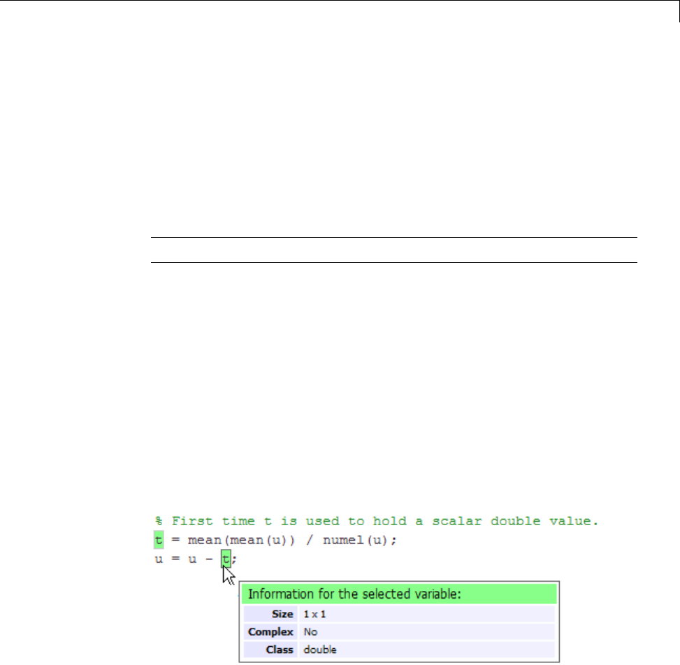
Reuse the Same Variable with Different Properties
y = sum(u(t(2:end-1)));
end
2Compile example1.
For example, to generate a MEX function, enter:
codegen -o example1x -report example1.m -args {ones(5,5)}
Note codegen requires a MATLAB Coder license.
When the compilation is complete, codegen generates a MEX function,
example1x in the current folder, and provides a link to the code generation
report.
3Open the code generation report.
4IntheMATLABcodepaneofthecodegeneration report, place your pointer
over the variable tinside the if statement.
The code generation report highlights both instances of tin the if
statement because they share the same class, size, and complexity. It
displays the data type information for tat this point in the code. Here,
tis a scalar double.
5In the MATLAB code pane of the report, place your pointer over the
variable toutside the for-loop.
33-13
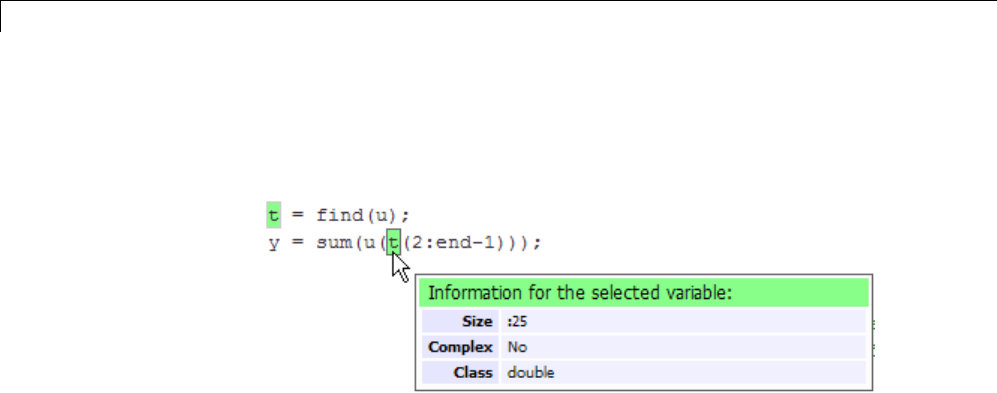
33 Defining MATLAB®Variables for C/C++ Code Generation
This time, the report highlights both instances of toutside the if
statement. The report indicates that tmightholdupto25 doubles. The size
of tis :25, that is, a column vector containing a maximum of 25 doubles.
6Click the Variables tab to view the list of variables used in example1.
The report displays a list of all the variables in example1.Therearetwo
uniquely named local variables t>1 and t>2.
7In the list of variables, place your pointer over t>1.
The code generation report highlights both instances of tin the if
statement.
8In the list of variables, place your pointer over t>2
The code generation report highlights both instances of toutside the if
statement.
Limitations of Variable Reuse
The following variables cannot be renamed in generated code:
•Persistent variables.
•Global variables.
•Variables passed to C code using coder.ref,coder.rref,coder.wref.
•Variables whose size is set using coder.varsize.
•Variables whose names are controlled using coder.cstructname.
•The index variable of a for-loop when it is used inside the loop body.
33-14

Reuse the Same Variable with Different Properties
•The block outputs of a MATLAB Function block in a Simulink model.
•Chart-owned variables of a MATLAB function in a Stateflow chart.
33-15

33 Defining MATLAB®Variables for C/C++ Code Generation
Avoid Overflows in for-Loops
When memory integrity checks are enabled, if the code generation software
detects that a loop variable might overflow on the last iteration of the
for-loop, it reports an error.
To avoid this error, use the workarounds provided in the following table.
Loop conditions causing the
error
Workaround
•The loop counter increments by 1
•The end value equals the
maximum value of the integer
type
•The loop is not covering the full
range of the integer type
Rewritetheloopsothattheend
valueisnotequaltothemaximum
value of the integer type. For
example, replace:
N=intmax('int16')
for k=N-10:N
with:
for k=1:10
•The loop counter decrements by 1
•The end value equals the
minimum value of the integer
type
•The loop is not covering the full
range of the integer type
Rewritetheloopsothattheend
value is not equal to the minimum
value of the integer type. For
example, replace:
N=intmin('int32')
for k=N+10:-1:N
with:
for k=10:-1:1
33-16

Avoid Overflows in for-Loops
Loop conditions causing the
error
Workaround
•The loop counter increments or
decrements by 1
•The start value equals the
minimum or maximum value of
the integer type
•The end value equals the
maximum or minimum value of
the integer type
The loop covers the full range of the
integer type.
Rewrite the loop casting the type
of the loop counter start, step, and
endvaluestoabiggerintegerorto
double For example, rewrite:
M= intmin('int16');
N= intmax('int16');
for k=M:N
% Loop body
end
to
M= intmin('int16');
N= intmax('int16');
for k=int32(M):int32(N)
% Loop body
end
•The loop counter increments or
decrements by a value not equal
to 1
•On last loop iteration, the loop
variable value is not equal to the
end value
Note The software error checking
might be too conservative and report
the possibility of an infinite under
these circumstances even though an
infinite loop would never occur.
Rewritetheloopsothattheloop
variable on the last loop iteration is
equal to the end value.
33-17

33 Defining MATLAB®Variables for C/C++ Code Generation
Supported Variable Types
You can use the following data types for C/C++ code generation from
MATLAB:
Type Description
char Character array (string)
complex Complex data. Cast function takes real and imaginary
components
double Double-precision floating point
int8,int16,int32 Signed integer
logical Boolean true or false
single Single-precision floating point
struct Structure
uint8,uint16,
uint32
Unsigned integer
Fixed-point See “Fixed-Point Data Types”.
33-18


34 Defining Data for Code Generation
Data Definition for Code Generation
To generate efficient standalone code, you must define the following types
and classes of data differently than you normally would when running your
code in the MATLAB environment:
Data What’s Different More Information
Complex numbers •Complexity of
variables must be set
at time of assignment
and before first use
•Expressions
containing a complex
number or variable
always evaluate to a
complex result, even
if the result is zero
Note Because
MATLAB does not
support complex
integer arithmetic,
you cannot generate
code for functions that
use complex integer
arithmetic
“Code Generation for
Complex Data” on page
34-4
Characters Restricted to 8 bits of
precision
“Code Generation for
Characters” on page
34-6
34-2

Data Definition for Code Generation
Data What’s Different More Information
Enumerated data •Supports
integer-based
enumerated types
only
•Restricted use in
switch statements
and for-loops
“Enumerated Data”
Function handles •Function handles
must be scalar values
•Same bound variable
cannot reference
different function
handles
•Cannot pass function
handles to or from
primary or extrinsic
functions
•Cannot view function
handles from the
debugger
“Function Handles”
34-3

34 Defining Data for Code Generation
Code Generation for Complex Data
In this section...
“Restrictions When Defining Complex Variables” on page 34-4
“Expressions Containing Complex Operands Yield Complex Results” on
page 34-5
Restrictions When Defining Complex Variables
For code generation, you must set the complexity of variables at the time of
assignment, either by assigning a complex constant or using the complex
function, as in these examples:
x = 5 + 6i; % x is a complex number by assignment.
y = 7 + 8j; % y is a complex number by assignment.
x = complex(5,6); % x is the complex number 5 + 6i.
Once you set the type and size of a variable, you cannot cast it to another
type or size. In the following example, the variable xis defined as complex
and stays complex:
x = 1 + 2i; % Defines x as a complex variable.
y = int16(x); % Real and imaginary parts of y are int16.
x = 3; % x now has the value 3 + 0i.
Mismatches can also occur when you assign a real operand the complex result
of an operation:
z = 3; % Sets type of z to double (real)
z = 3 + 2i; % ERROR: cannot recast z to complex
As a workaround, set the complexity of the operand to match the result
of the operation:
m = complex(3); % Sets m to complex variable of value 3 + 0i
m = 5 + 6.7i; % Assigns a complex result to a complex number
34-4

Code Generation for Complex Data
Expressions Containing Complex Operands Yield
Complex Results
In general, expressions that contain one or more complex operands always
produce a complex result in generated code, even if the value of the result is
zero. Consider the following example:
x=2+3i;
y=2-3i;
z=x+y; %zis4+0i.
In MATLAB, this code generates the real result z=4. However, during
code generation, the types for xand yare known, but their values are not.
Because either or both operands in this expression are complex, zis defined
as a complex variable requiring storage for both a real and an imaginary
part. This means that zequals the complex result 4+0iin generated code,
not 4as in MATLAB code.
There are two exceptions to this behavior:
•Functions that take complex arguments, but produce real results
y = real(x); % y is the real part of the complex number x.
y = imag(x); % y is the real-valued imaginary part of x.
y = isreal(x); % y is false (0) for a complex number x.
•Functions that take real arguments, but produce complex results:
z = complex(x,y); % z is a complex number for a real x and y.
34-5

34 Defining Data for Code Generation
Code Generation for Characters
The complete set of Unicode®characters is not supported for code generation.
Characters are restricted to 8 bits of precision in generated code. Because
many mathematical operations require more than 8 bits of precision, it is
recommended that you do not perform arithmetic with characters if you
intend to generate code from your MATLAB algorithm.
34-6

35
Code Generation for
Variable-Size Data
•“What Is Variable-Size Data?” on page 35-2
•“Variable-Size Data Definition for Code Generation” on page 35-3
•“Bounded Versus Unbounded Variable-Size Data” on page 35-4
•“Control Memory Allocation of Variable-Size Data” on page 35-5
•“Specify Variable-Size Data Without Dynamic Memory Allocation” on page
35-6
•“Variable-Size Data in Code Generation Reports” on page 35-10
•“Define Variable-Size Data for Code Generation” on page 35-12
•“C Code Interface for Arrays” on page 35-19
•“Troubleshooting Issues with Variable-Size Data” on page 35-20
•“Incompatibilities with MATLAB in Variable-Size Support for Code
Generation” on page 35-24
•“Restrictions on Variable Sizing in Toolbox Functions Supported for Code
Generation” on page 35-31

35 Code Generation for Variable-Size Data
What Is Variable-Size Data?
Variable-size data is data whose size can change at run time. By contrast,
fixed-size data is data whose size is known and locked at compile time and,
therefore, cannot change at run time.
For example, in the following MATLAB function nway,Bis a variable-size
array; its length is not known at compile time.
function B = nway(A,n)
% Compute average of every N elements of A and put them in B.
if ((mod(numel(A),n) == 0) && (n>=1 && n<=numel(A)))
B = ones(1,numel(A)/n);
k=1;
for i = 1 : numel(A)/n
B(i) = mean(A(k + (0:n-1)));
k=k+n;
end
else
error('n <= 0 or does not divide number of elements evenly');
end
35-2

Variable-Size Data Definition for Code Generation
Variable-Size Data Definition for Code Generation
In the MATLAB language, all data can vary in size. By contrast, the
semantics of generated code constrains the class, complexity, and shape of
every expression, variable, and structure field. Therefore, for code generation,
you must use each variable consistently. Each variable must:
•Be either complex or real (determined at first assignment)
•Have a consistent shape
For fixed-size data, the shape is the same as the size returned in MATLAB.
For example, if size(A) == [4 5], the shape of variable Ais 4 x 5.
For variable-size data, the shape can be abstract. That is, one or more
dimensions can be unknown (such as 4x? or ?x?).
By default, the compiler detects code logic that attempts to change these fixed
attributes after initial assignments, and flags these occurrences as errors
during code generation. However, you can override this behavior by defining
variables or structure fields as variable-size data. You can then generate
standalone code for bounded and unbounded variable-size data.
For more information, see “Bounded Versus Unbounded Variable-Size Data”
on page 35-4
35-3

35 Code Generation for Variable-Size Data
Bounded Versus Unbounded Variable-Size Data
You can generate code for bounded and unbounded variable-size data.
Bounded variable-size data has fixed upper bounds; this data can be allocated
statically on the stack or dynamically on the heap. Unbounded variable-size
data does not have fixed upper bounds; this data must be allocated on the
heap. If you use unbounded data, you must use dynamic memory allocation
so that the compiler:
•Does not check for upper bounds
•Allocates memory on the heap instead of the stack
You can control the memory allocation of variable-size data. For more
information, see “Control Memory Allocation of Variable-Size Data” on page
35-5.
35-4

Control Memory Allocation of Variable-Size Data
Control Memory Allocation of Variable-Size Data
All data whose size exceeds the dynamic memory allocation threshold is
allocated on the heap. The default dynamic memory allocation threshold is
64 kilobytes. All data whose size is less than this threshold is allocated on
the stack.
Dynamic memory allocation is an expensive operation; the performance
cost may be too high for small data sets. If you use small variable-size data
sets or data that does not change size at run time, disable dynamic memory
allocation. See .
. You can control memory allocation for individual variables by specifying
upper bounds. See “Specifying Upper Bounds for Variable-Size Data” on page
35-6.
35-5

35 Code Generation for Variable-Size Data
Specify Variable-Size Data Without Dynamic Memory
Allocation
In this section...
“Fixing Upper Bounds Errors” on page 35-6
“Specifying Upper Bounds for Variable-Size Data” on page 35-6
Fixing Upper Bounds Errors
If MATLAB cannot determine or compute the upper bound, you must specify
an upper bound. See “Specifying Upper Bounds for Variable-Size Data” on
page 35-6 and “Diagnosing and Fixing Errors in Detecting Upper Bounds”
on page 35-22
Specifying Upper Bounds for Variable-Size Data
•“When to Specify Upper Bounds for Variable-Size Data” on page 35-6
•“Specifying Upper Bounds on the Command Line for Variable-Size Inputs”
on page 35-6
•“Specifying Unknown Upper Bounds for Variable-Size Inputs” on page 35-7
•“Specifying Upper Bounds for Local Variable-Size Data” on page 35-7
•“Using a Matrix Constructor with Nonconstant Dimensions” on page 35-8
When to Specify Upper Bounds for Variable-Size Data
When using static allocation on the stack during code generation, MATLAB
must be able to determine upper bounds for variable-size data. Specify the
upper bounds explicitly for variable-size data from external sources, such
as inputs and outputs.
Specifying Upper Bounds on the Command Line for
Variable-Size Inputs
Use the coder.typeof construct with the -args option on the codegen
command line (requires a MATLAB Coder license). For example:
35-6

Specify Variable-Size Data Without Dynamic Memory Allocation
codegen foo -args {coder.typeof(double(0),[3 100],1)}
This command specifies that the input to function foo is a matrix of real
doubles with two variable dimensions. The upper bound for the first
dimension is 3; the upper bound for the second dimension is 100. For a
detailed explanation of this syntax, see .
Specifying Unknown Upper Bounds for Variable-Size Inputs
If you use dynamic memory allocation, you can specify that you don’t know
the upper bounds of inputs. To specify an unknown upper bound, use the
infinity constant Inf in place of a numeric value. For example:
codegen foo -args {coder.typeof(double(0), [1 Inf])}
In this example, the input to function foo is a vector of real doubles without
an upper bound.
Specifying Upper Bounds for Local Variable-Size Data
When using static allocation, MATLAB uses a sophisticated analysis to
calculate the upper bounds of local data at compile time. However, when the
analysis fails to detect an upper bound or calculates an upper bound that is
not precise enough for your application, you need to specify upper bounds
explicitly for local variables.
You do not need to specify upper bounds when using dynamic allocation on
the heap. In this case, MATLAB assumes all variable-size data is unbounded
and does not attempt to determine upper bounds.
Constraining the Value of a Variable That Specifies Dimensions of
Variable-Size Data. Use the assert function with relational operators to
constrain the value of variables that specify the dimensions of variable-size
data. For example:
function y = dim_need_bound(n) %#codegen
assert (n <= 5);
L= ones(n,n);
M = zeros(n,n);
M = [L; M];
y=M;
35-7

35 Code Generation for Variable-Size Data
This assert statement constrains input nto a maximum size of 5, defining L
and Mas variable-sized matrices with upper bounds of 5 for each dimension.
Specifying the Upper Bounds for All Instances of a Local Variable.
Use the coder.varsize function to specify the upper bounds for all instances
of a local variable in a function. For example:
function Y = example_bounds1(u) %#codegen
Y=[12345];
coder.varsize('Y', [1 10]);
if (u > 0)
Y = [Y Y+u];
else
Y = [Y Y*u];
end
The second argument of coder.varsize specifies the upper bound for each
instance of the variable specified in the first argument. In this example, the
argument [1 10] indicates that for every instance of Y:
•First dimension is fixed at size 1
•Second dimension can grow to an upper bound of 10
By default, coder.varsize assumes dimensions of 1 are fixed size. For more
information, see the coder.varsize reference page.
Using a Matrix Constructor with Nonconstant Dimensions
You can define a variable-size matrix by using a constructor with nonconstant
dimensions. For example:
function y = var_by_assign(u) %#codegen
if (u > 0)
y = ones(3,u);
else
y = zeros(3,1);
end
If you are not using dynamic memory allocation, you must also add an assert
statement to provide upper bounds for the dimensions. For example:
35-8

Specify Variable-Size Data Without Dynamic Memory Allocation
function y = var_by_assign(u) %#codegen
assert (u < 20);
if (u > 0)
y = ones(3,u);
else
y = zeros(3,1);
end
35-9

35 Code Generation for Variable-Size Data
Variable-Size Data in Code Generation Reports
In this section...
“What Reports Tell You About Size” on page 35-10
“How Size Appears in Code Generation Reports” on page 35-11
“How to Generate a Code Generation Report” on page 35-11
What Reports Tell You About Size
Code generation reports:
•Differentiate fixed-size from variable-size data
•Identify variable-size data with unknown upper bounds
•Identify variable-size data with fixed dimensions
If you define a variable-size array and then subsequently fix the dimensions
of this array in the code, the report appends *to the size of the variable. In
the generated C code, this variable appears as a variable-size array, but
the size of its dimensions does not change during execution.
•Provide guidance on how to fix size mismatch and upper bounds errors.
35-10
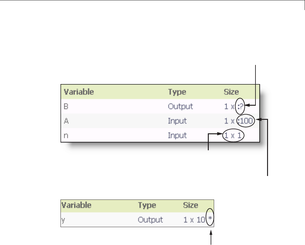
Variable-Size Data in Code Generation Reports
How Size Appears in Code Generation Reports
:? means variable size,
unknown upper bound
No colon prefix (:)
means fixed size
:100 means variable size,
upper bound = 100
* means that you declared y as variable size,
but subsequently fixed its dimensions
How to Generate a Code Generation Report
35-11

35 Code Generation for Variable-Size Data
Define Variable-Size Data for Code Generation
In this section...
“When to Define Variable-Size Data Explicitly” on page 35-12
“Using a Matrix Constructor with Nonconstant Dimensions” on page 35-13
“Inferring Variable Size from Multiple Assignments” on page 35-13
“Defining Variable-Size Data Explicitly Using coder.varsize” on page 35-14
When to Define Variable-Size Data Explicitly
For code generation, you must assign variables to have a specific class,
size, and complexity before using them in operations or returning them as
outputs. Generally, you cannot reassign variable properties after the initial
assignment. Therefore, attempts to grow a variable or structure field after
assigning it a fixed size might cause a compilation error. In these cases, you
must explicitly define the data as variable sized using one of these methods:
Method See
Assign the data from a variable-size
matrix constructor such as
•ones
•zeros
•repmat
“Using a Matrix Constructor with
Nonconstant Dimensions” on page
35-13
Assign multiple, constant sizes
to the same variable before using
(reading) the variable.
“Inferring Variable Size from
Multiple Assignments” on page
35-13
Define all instances of a variable to
be variable sized
“Defining Variable-Size Data
Explicitly Using coder.varsize” on
page 35-14
35-12

Define Variable-Size Data for Code Generation
Using a Matrix Constructor with Nonconstant
Dimensions
You can define a variable-size matrix by using a constructor with nonconstant
dimensions. Forexample:
function y = var_by_assign(u) %#codegen
if (u > 0)
y = ones(3,u);
else
y = zeros(3,1);
end
Inferring Variable Size from Multiple Assignments
You can define variable-size data by assigning multiple, constant sizes to the
same variable before you use (read) the variable in your code. When MATLAB
uses static allocation on the stack for code generation, it infers the upper
bounds from the largest size specified for each dimension. When you assign
thesames
ize to a given dimension across all assignments, MATLAB assumes
that the dimension is fixed at that size. The assignments can specify different
shapes as well as sizes.
When dynamic memory allocation is used, MATLAB does not check for upper
bounds; it assumes all variable-size data is unbounded.
Inferring Upper Bounds from Multiple Definitions with Different
Shapes
function y = var_by_multiassign(u) %#codegen
if (u > 0)
y=on
es(3,4,5);
else
y=ze
ros(3,1);
end
When static allocation is used, this function infers that yis a matrix with
three dimensions, where:
•First dimension is fixed at size 3
35-13
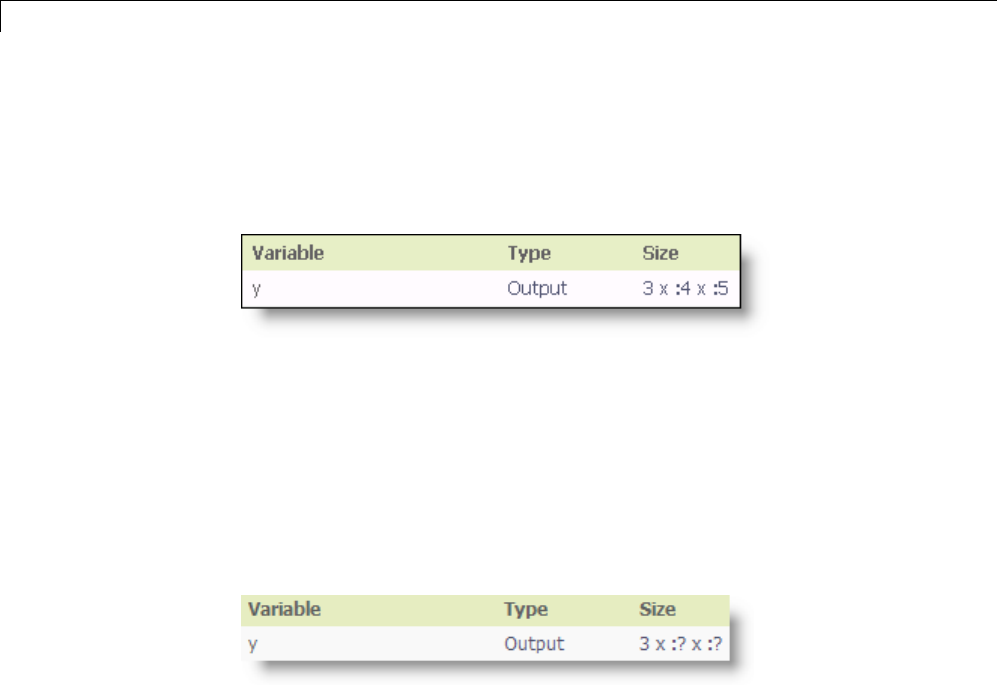
35 Code Generation for Variable-Size Data
•Second dimension is variablewithanupperboundof4
•Third dimension is variable with an upper bound of 5
The code generation report represents the size of matrix ylike this:
When dynamic allocation is used, the function analyzes the dimensions of
ydifferently:
•First dimension is fixed at size 3
•Second and third dimensions are unbounded
In this case, the code generation report represents the size of matrix ylike
this:
Defining Variable-Size Data Explicitly Using
coder.varsize
Use the function coder.varsize to define one or more variables or structure
fields as variable-size data. Optionally, you can also specify which dimensions
vary along with their upper bounds (see “Specifying Which Dimensions Vary”
on page 35-15). For example:
•Define Bas a variable-size 2-by-2 matrix, where each dimension has an
upper bound of 64:
coder.varsize('B', [64 64]);
•Define Bas a variable-size matrix:
35-14

Define Variable-Size Data for Code Generation
coder.varsize('B');
When you supply only the first argument, coder.varsize assumes all
dimensions of Bcan vary and that the upper bound is size(B).
For more information, see the coder.varsize reference page.
Specifying Which Dimensions Vary
You can use the function coder.varsize to specify which dimensions vary.
For example, the following statement defines Bas a row vector whose first
dimension is fixed at 2, but whose second dimension can grow to an upper
bound of 16:
coder.varsize('B', [2, 16], [0 1])
The third argument specifies which dimensions vary. This argument must be
a logical vector or a double vector containing only zeros and ones. Dimensions
that correspond to zeros or false have fixed size; dimensions that correspond
to ones or true vary in size. coder.varsize usually treats dimensions of size
1 as fixed (see “Defining Variable-Size Matrices with Singleton Dimensions”
on page 35-16).
For more information about the syntax, see the coder.varsize reference
page.
Allowing a Variable to Grow After Defining Fixed Dimensions
Function var_by_if defines matrix Ywith fixed 2-by-2 dimensions before first
use (where the statement Y=Y+ureads from Y). However, coder.varsize
defines Yas a variable-size matrix, allowing it to change size based on decision
logic in the else clause:
function Y = var_by_if(u) %#codegen
if (u > 0)
Y = zeros(2,2);
coder.varsize('Y');
if (u < 10)
Y=Y+u;
end
else
35-15

35 Code Generation for Variable-Size Data
Y = zeros(5,5);
end
Without coder.varsize, MATLAB infers Yto be a fixed-size, 2-by-2 matrix
and generates a size mismatch error during code generation.
Defining Variable-Size Matrices with Singleton Dimensions
A singleton dimension is any dimension for which size(A,dim) = 1. Singleton
dimensions are fixed in size when:
•You specify a dimension with an upper bound of 1 in coder.varsize
expressions.
For example, in this function, Ybehaves like a vector with one variable-size
dimension:
function Y = dim_singleton(u) %#codegen
Y=[12];
coder.varsize('Y', [1 10]);
if (u > 0)
Y = [Y 3];
else
Y = [Y u];
end
•You initialize variable-size data with singleton dimensions using matrix
constructor expressions or matrix functions.
For example, in this function, both Xand Ybehave like vectors where only
their second dimensions are variable sized:
function [X,Y] = dim_singleton_vects(u) %#codegen
Y = ones(1,3);
X=[14];
coder.varsize('Y','X');
if (u > 0)
Y = [Y u];
else
X = [X u];
end
35-16

Define Variable-Size Data for Code Generation
You can override this behavior by using coder.varsize to specify explicitly
that singleton dimensions vary. For example:
function Y = dim_singleton_vary(u) %#codegen
Y=[12];
coder.varsize('Y', [1 10], [1 1]);
if (u > 0)
Y = [Y Y+u];
else
Y = [Y Y*u];
end
In this example, the third argument of coder.varsize is a vector of ones,
indicating that each dimension of Yvaries in size. For more information, see
the coder.varsize reference page.
Defining Variable-Size Structure Fields
To define structure fields as variable-size arrays, use colon (:)astheindex
expression. The colon (:) indicates that all elements of the array are variable
sized. For example:
function y=struct_example() %#codegen
d = struct('values', zeros(1,0), 'color', 0);
data = repmat(d, [3 3]);
coder.varsize('data(:).values');
for i = 1:numel(data)
data(i).color = rand-0.5;
data(i).values = 1:i;
end
y=0;
for i = 1:numel(data)
if data(i).color > 0
y = y + sum(data(i).values);
end;
end
35-17

35 Code Generation for Variable-Size Data
The expression coder.varsize('data(:).values') defines the field values
inside each element of matrix data to be variable sized.
Here are other examples:
•coder.varsize('data.A(:).B')
In this example, data is a scalar variable that contains matrix A.Each
element of matrix Acontains a variable-size field B.
•coder.varsize('data(:).A(:).B')
This expression defines field Binside each element of matrix Ainside each
element of matrix data to be variable sized.
35-18

C Code Interface for Arrays
C Code Interface for Arrays
C Code Interface for Statically Allocated Arrays
In generated code, MATLAB contains two pieces of information about
statically allocated arrays: the maximum size of the array and its actual size.
Forexample,considertheMATLABfunctionuniquetol:
function B = uniquetol(A, tol) %#codegen
A = sort(A);
coder.varsize('B');
B = A(1);
k=1;
for i = 2:length(A)
if abs(A(k) - A(i)) > tol
B = [B A(i)];
k=i;
end
end
Generate code for uniquetol specifying that input Ais a variable-size real
double vector whose first dimension is fixed at 1 and second dimension can
vary up to 100 elements.
In the generated code, the function declaration is:
TherearetwopiecesofinformationaboutA:
•real_T A_data[100]: the maximum size of input A(where 100 is the
maximum size specified using coder.typeof).
•int32_T_A_sizes[2]: the actual size of the input.
35-19

35 Code Generation for Variable-Size Data
Troubleshooting Issues with Variable-Size Data
In this section...
“Diagnosing and Fixing Size Mismatch Errors” on page 35-20
“Diagnosing and Fixing Errors in Detecting Upper Bounds” on page 35-22
Diagnosing and Fixing Size Mismatch Errors
Check your code for these issues:
Assigning Variable-Size Matrices to Fixed-Size Matrices
You cannot assign variable-size matrices to fixed-size matrices in generated
code. Consider this example:
function Y = example_mismatch1(n) %#codegen
assert(n<10);
B = ones(n,n);
A = magic(3);
A(1) = mean(A(:));
if (n == 3)
A=B;
end
Y=A;
Compiling this function produces this error:
??? Dimension 1 is fixed on the left-hand side
but varies on the right ...
There are several ways to fix this error:
•Allow matrix Ato grow by adding the coder.varsize construct:
function Y = example_mismatch1_fix1(n) %#codegen
coder.varsize('A');
assert(n<10);
B = ones(n,n);
A = magic(3);
35-20

Troubleshooting Issues with Variable-Size Data
A(1) = mean(A(:));
if (n == 3)
A=B;
end
Y=A;
•Explicitly restrict the size of matrix Bto 3-by-3 by modifying the assert
statement:
function Y = example_mismatch1_fix2(n) %#codegen
coder.varsize('A');
assert(n==3)
B = ones(n,n);
A = magic(3);
A(1) = mean(A(:));
if (n == 3)
A=B;
end
Y=A;
•Use explicit indexing to make BthesamesizeasA:
function Y = example_mismatch1_fix3(n) %#codegen
assert(n<10);
B = ones(n,n);
A = magic(3);
A(1) = mean(A(:));
if (n == 3)
A = B(1:3, 1:3);
end
Y=A;
Empty Matrix Reshaped to Match Variable-Size Specification
If you assign an empty matrix [] to variable-size data, MATLAB might
silently reshape the data in generated code to match a coder.varsize
specification. For example:
function Y = test(u) %#codegen
Y = [];
coder.varsize(`Y', [1 10]);
35-21

35 Code Generation for Variable-Size Data
If u < 0
Y=[Yu];
end
In this example, coder.varsize defines Yas a column vector of up to 10
elements, so its first dimension is fixed at size 1. The statement Y=[]
designates the first dimension of Yas 0, creating a mismatch. The right
hand side of the assignment is an empty matrix and the left hand side is a
variable-size vector. In this case, MATLAB reshapes the empty matrix Y=
[] in generated code to Y = zeros(1,0) so it matches the coder.varsize
specification.
Performing Binary Operations on Fixed and Variable-Size Operands
You cannot perform binary operations on operands of different sizes.
Operands have different sizes if one has fixed dimensions and the other has
variable dimensions. For example:
function z = mismatch_operands(n) %#codegen
assert(n>=3 && n<10);
x = ones(n,n);
y = magic(3);
z=x+y;
When you compile this function, you get an error because yhas fixed
dimensions (3 x 3), but xhas variable dimensions. Fix this problem by using
explicit indexing to make xthesamesizeasy:
function z = mismatch_operands_fix(n) %#codegen
assert(n>=3 && n<10);
x = ones(n,n);
y = magic(3);
z=x(1:3,1:3) +y;
Diagnosing and Fixing Errors in Detecting Upper
Bounds
Check your code for these issues:
35-22

Troubleshooting Issues with Variable-Size Data
Using Nonconstant Dimensions in a Matrix Constructor
You can define variable-size data by assigning a variable to a matrix with
nonconstant dimensions. For example:
function y = dims_vary(u) %#codegen
if (u > 0)
y = ones(3,u);
else
y = zeros(3,1);
end
However, compiling this function generates an error because you did not
specify an upper bound for u.
To fix the problem, add an assert statement before the first use of u:
function y = dims_vary_fix(u) %#codegen
assert (u < 20);
if (u > 0)
y = ones(3,u);
else
y = zeros(3,1);
end
35-23

35 Code Generation for Variable-Size Data
Incompatibilities with MATLAB in Variable-Size Support
for Code Generation
In this section...
“Incompatibility with MATLAB for Scalar Expansion” on page 35-24
“Incompatibility with MATLAB in Determining Size of Variable-Size N-D
Arrays” on page 35-26
“Incompatibility with MATLAB in Determining Size of Empty Arrays” on
page 35-27
“Incompatibility with MATLAB in Vector-Vector Indexing” on page 35-28
“Incompatibility with MATLAB in Matrix Indexing Operations for Code
Generation” on page 35-29
“Dynamic Memory Allocation Not Supported for MATLAB Function Blocks”
on page 35-30
Incompatibility with MATLAB for Scalar Expansion
Scalar expansion is a method of converting scalar data to match the
dimensions of vector or matrix data. Except for some matrix operators,
MATLAB arithmetic operators work on corresponding elements of arrays with
equal dimensions. For vectors and rectangular arrays, both operands must be
the same size unless one is a scalar. If one operand is a scalar and the other is
not, MATLAB applies the scalar to every element of the other operand—this
property is known as scalar expansion.
During code generation, the standard MATLAB scalar expansion rules
apply except when operating on two variable-size expressions. In this case,
both operands must be the same size. The generated code does not perform
scalar expansion even if one of the variable-size expressions turns out to be
scalar at run time. Instead, it generates a size mismatch error at run time
for MEX functions. For non-MEX builds, there is no run-time error checking;
the generated code will have unspecified behavior.
For example, in the following function, zis scalar for the switch statement
case 0 and case 1. MATLAB applies scalar expansion when evaluating
y(:) = z; for these two cases.
35-24
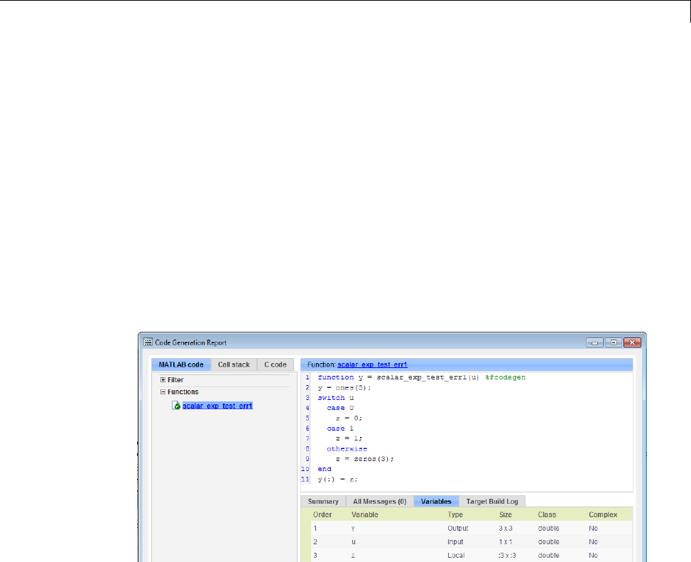
Incompatibilities with MATLAB®in Variable-Size Support for Code Generation
function y = scalar_exp_test_err1(u) %#codegen
for the otherwise case of the switch function.y = ones(3);
switch u
case 0
z=0;
case 1
z=1;
otherwise
z = zeros(3);
end
y(:) = z;
When you generate code for this function, the code generation software
determines that zis variable size with an upper bound of 3.
If you run the MEX function with uequal to zero or one, even though zis
scalar at run time, the generated code does not perform scalar expansion
and a run-time error occurs.
scalar_exp_test_err1_mex(0)
Sizes mismatch: 9 ~= 1.
Error in scalar_exp_test_err1 (line 11)
y(:) = z;
35-25

35 Code Generation for Variable-Size Data
Workaround
Use indexing to force zto be a scalar value:
function y = scalar_exp_test_err1(u) %#codegen
y = ones(3);
switch u
case 0
z=0;
case 1
z=1;
otherwise
z = zeros(3);
end
y(:) = z(1);
Incompatibility with MATLAB in Determining Size of
Variable-Size N-D Arrays
For variable-size N-D arrays, the size function can return a different result in
generated code than in MATLAB. In generated code, size(A) always returns
a fixed-length output because it does not drop trailing singleton dimensions
of variable-size N-D arrays. By contrast, size(A) in MATLAB returns a
variable-length output because it drops trailing singleton dimensions.
For example, if the shape of array Ais :?x:?x:? and size(A,3)==1,size(A)
returns:
•Three-element vector in generated code
•Two-element vector in MATLAB code
Workarounds
If your application requires generated code to return the same size of
variable-size N-D arrays as MATLAB code, consider one of these workarounds:
•Use the two-argument form of size.
For example, size(A,n) always returns the same answer in generated code
and MATLAB code.
35-26

Incompatibilities with MATLAB®in Variable-Size Support for Code Generation
•Rewrite size(A):
B = size(A);
X = B(1:ndims(A));
This version returns Xwith a variable-length output. However, you cannot
pass a variable-size Xto matrix constructors such as zeros that require a
fixed-size argument.
Incompatibility with MATLAB in Determining Size of
Empty Arrays
The size of an empty array in generated code might be different from its size
in MATLAB source code. The size might be 1x0 or 0x1 in generated code,
but 0x0 in MATLAB. Therefore, you should not write code that relies on the
specific size of empty matrices.
For example, consider the following code:
function y = foo(n) %#codegen
x = [];
i=0;
while (i<10)
x=[5,x];
i=i+1;
end
if n > 0
x=[];
end
y=size(x);
end
Concatenation requires its operands to match on the size of the dimension
that is not being concatenated. In the preceding concatenation the scalar
value has size 1x1 and xhas size 0x0. Tosupportthisusecase,thecode
generation software determines the size for xas [1 x :?].Becausethere
is another assignment x=[]after the concatenation, the size of xin the
generated code is 1x0 instead of 0x0.
35-27

35 Code Generation for Variable-Size Data
Workaround
If your application checks whether a matrix is empty, use one of these
workarounds:
•Rewriteyourcodetousetheisempty function instead of the size function.
•Instead of using x=[] to create empty arrays, create empty arrays of a
specific size using zeros. For example:
function y = test_empty(n) %#codegen
x = zeros(1,0);
i=0;
while (i<10)
x=[5,x];
i=i+1;
end
if n > 0
x = zeros(1,0);
end
y=size(x);
end
Incompatibility with MATLAB in Vector-Vector
Indexing
In vector-vector indexing, you use one vector as an index into another vector.
When either vector is variable sized, you might get a run-time error during
code generation. ConsidertheindexexpressionA(B). The general rule for
indexing is that size(A(B)) == size(B). However, when both Aand Bare
vectors, MATLAB applies a special rule: use the orientation of A as the
orientation of the output. For example, if size(A) == [1 5] and size(B) ==
[3 1],thensize(A(B)) == [1 3].
In this situation, if the code generation software detects that both Aand Bare
vectors at compile time, it applies the special rule and gives the same result
as MATLAB. However, if either Aor Bis a variable-size matrix (has shape
?x?) at compile time, the code generation software applies only the general
indexing rule. Then, if both Aand Bbecome vectors at run time, the code
generation software reports a run-time error when you run the MEX function.
For non-MEX builds, there is no run-time error checking; the generated code
35-28

Incompatibilities with MATLAB®in Variable-Size Support for Code Generation
will have unspecified behavior. It is best practice to generate and test a MEX
function before generating C code.
Workaround
Force your data to be a vector by using the colon operator for indexing:
A(B(:)). For example, suppose your code intentionally toggles between
vectors and regular matrices at run time. You can do an explicit check for
vector-vector indexing:
...
if isvector(A) && isvector(B)
C = A(:);
D = C(B(:));
else
D = A(B);
end
...
The indexing in the first branch specifies that Cand B(:) are compile-time
vectors. As a result, the code generation software applies the standard
vector-vector indexing rule.
Incompatibility with MATLAB in Matrix Indexing
Operations for Code Generation
The following limitations apply to matrix indexing operations for code
generation:
•Initialization of the following style:
for i = 1:10
M(i) = 5;
end
In this case, the size of Mchanges as the loop is executed. Code generation
does not support increasing the size of an array over time.
For code generation, preallocate Mas highlighted in the following code.
M=zeros(1,10);
35-29

35 Code Generation for Variable-Size Data
for i = 1:10
M(i) = 5;
end
•M(i:j) where iand jchange in a loop
During code generation, memory is never dynamically allocated for the size
of the expressions that change as the program executes. To implement this
behavior, use for-loops as shown in the following example:
...
M = ones(10,10);
for i=1:10
for j = i:10
M(i,j) = 2 * M(i,j);
end
end
...
Note The matrix Mmust be defined before entering the loop, as shown in
the highlighted code.
Dynamic Memory Allocation Not Supported for
MATLAB Function Blocks
Youcannotusedynamicmemoryallocationforvariable-sizedatainMATLAB
Function blocks. Use bounded instead of unbounded variable-size data.
35-30

Restrictions on Variable Sizing in Toolbox Functions Supported for Code Generation
Restrictions on Variable Sizing in Toolbox Functions
Supported for Code Generation
In this section...
“Common Restrictions” on page 35-31
“Toolbox Functions with Variable Sizing Restrictions” on page 35-32
Common Restrictions
The following common restrictions apply to multiple toolbox functions, but
only for code generation. To determine which of these restrictions apply to
specific library functions, see the table in “Toolbox Functions with Variable
Sizing Restrictions” on page 35-32.
Variable-length vector restriction
Inputs to the library function must be variable-length vectors or fixed-size
vectors. A variable-length vector is a variable-size array that has the shape
1x:n or :nx1 (one dimension is variable sized and the other is fixed at size 1).
Other shapes are not permitted, even if they are vectors at run time.
Automatic dimension restriction
When the function selects the working dimension automatically, it bases the
selection on the upper bounds for the dimension sizes. In the case of the sum
function, sum(X) selects its working dimension automatically, while sum(X,
dim) uses dim as the explicit working dimension.
For example, if Xis a variable-size matrix with dimensions 1x:3x:5,sum(x)
behaves like sum(X,2) in generated code. In MATLAB, it behaves like
sum(X,2) provided size(X,2) is not 1. In MATLAB, when size(X,2) is 1,
sum(X) behaves like sum(X,3). Consequently, you get a run-time error if an
automatically selected working dimension assumes a length of 1 at run time.
To avoid the issue, specify the intended working dimension explicitly as
aco
nstant value.
35-31

35 Code Generation for Variable-Size Data
Array-to-vector restriction
The function issues an error when a variable-size array that is not a
variable-length vector assumes the shape of a vector at run time. To avoid
the issue, specify the input explicitly as a variable-length vector instead of
a variable-size array.
Array-to-scalar restriction
The function issues an error if a variable-size array assumes a scalar value at
run time. To avoid this issue, specify all scalars as fixed size.
Toolbox Functions with Variable Sizing Restrictions
The following restrictions apply to specific toolbox functions, but only for
code generation.
Function Restrictions with Variable-Size Data
all
•See “Automatic dimension restriction” on page
35-31.
•An error occurs if you pass the first argument a
variable-size matrix that is 0-by-0 at run time.
any
•See “Automatic dimension restriction” on page
35-31.
•An error occurs if you pass the first argument a
variable-size matrix that is 0-by-0 at run time.
bsxfun
•Dimensions expand only where one input array
or the other has a fixed length of 1.
cat
•Dimension argument must be a constant.
•An error occurs if variable-size inputs are
empty at run time.
35-32

Restrictions on Variable Sizing in Toolbox Functions Supported for Code Generation
Function Restrictions with Variable-Size Data
conv
•See “Variable-length vector restriction” on page
35-31.
•Input vectors must have the same orientation,
either both row vectors or both column vectors.
cov
•For cov(X), see“Array-to-vector restriction” on
page 35-32.
cross
•Variable-size array inputs that become vectors
at run time must have the same orientation.
deconv
•For both arguments, see“Variable-length vector
restriction” on page 35-31.
detrend
•Forfirstargumentforrowvectorsonly,see
“Array-to-vector restriction” on page 35-32 .
diag
•See “Array-to-vector restriction” on page 35-32 .
diff
•See “Automatic dimension restriction” on page
35-31.
•Length of the working dimension must be
greater than the difference order input when
the input is variable sized. For example, if the
input is a variable-size matrix that is 3-by-5 at
run time, diff(x,2,1) works but diff(x,5,1)
generates a run-time error.
fft
•See “Automatic dimension restriction” on page
35-31.
35-33

35 Code Generation for Variable-Size Data
Function Restrictions with Variable-Size Data
filter
•For first and second arguments, see
“Variable-length vector restriction” on page
35-31.
•See “Automatic dimension restriction” on page
35-31.
hist
•For second argument, see“Variable-length
vector restriction” on page 35-31.
•For second input argument, see“Array-to-scalar
restriction” on page 35-32.
histc
•See “Automatic dimension restriction” on page
35-31.
ifft
•See “Automatic dimension restriction” on page
35-31.
ind2sub
•First input (the size vector input) must be fixed
size.
interp1
•For the Yinput and xi input, see“Array-to-vector
restriction” on page 35-32.
•Yinput can become a column vector dynamically.
•A run-time error occurs if Yinput is not a
variable-length vector and becomes a row vector
at run time.
ipermute
•Order input must be fixed size.
issorted
•For optional rows input, see “Variable-length
vector restriction” on page 35-31.
35-34

Restrictions on Variable Sizing in Toolbox Functions Supported for Code Generation
Function Restrictions with Variable-Size Data
magic
•Argument must be a constant.
•Output can be fixed-size matrices only.
max
•See “Automatic dimension restriction” on page
35-31.
mean
•See “Automatic dimension restriction” on page
35-31.
•An error occurs if you pass as the first argument
a variable-size matrix that is 0-by-0 at run time.
median
•See “Automatic dimension restriction” on page
35-31.
•An error occurs if you pass as the first argument
a variable-size matrix that is 0-by-0 at run time.
min
•See “Automatic dimension restriction” on page
35-31.
mode
•See “Automatic dimension restriction” on page
35-31.
•An error occurs if you pass as the first argument
a variable-size matrix that is 0-by-0 at run time.
35-35

35 Code Generation for Variable-Size Data
Function Restrictions with Variable-Size Data
mtimes
•When an input is variable sized, MATLAB
determines whether to generate code for a
general matrix*matrix multiplication or a
scalar*matrix multiplication, based on whether
one of the arguments is a fixed-size scalar. If
neither argument is a fixed-size scalar, the
inner dimensions of the two arguments must
agree even if a variable-size matrix input
happens to be a scalar at run time.
nchoosek
•Inputs must be fixed sized.
•Second input must be a constant for static
allocation..
•You cannot create a variable-size array by
passing in a variable k.
permute
•Order input must be fixed size.
planerot
•Inputmustbeafixed-size,two-elementcolumn
vector. Itcannotbeavariable-size array that
takes on the size 2-by-1 at run time.
poly
•See “Variable-length vector restriction” on page
35-31.
polyfit
•For first and second arguments, see
“Variable-length vector restriction” on page
35-31.
prod
•See “Automatic dimension restriction” on page
35-31.
•An error occurs if you pass as the first argument
a variable-size matrix that is 0-by-0 at run time.
35-36

Restrictions on Variable Sizing in Toolbox Functions Supported for Code Generation
Function Restrictions with Variable-Size Data
rand
•For an upper-bounded variable N,rand(1,N)
produces a variable-length vector of 1x:M where
Mis the upper bound on N.
•For an upper-bounded variable N,rand([1,N])
may produce a variable-length vector of :1x:M
where Mis the upper bound on N.
randn
•For an upper-bounded variable N,randn(1,N)
produces a variable-length vector of 1x:M where
Mis the upper bound on N.
•For an upper-bounded variable N,randn([1,N])
may produce a variable-length vector of :1x:M
where Mis the upper bound on N.
reshape
•When the input is a variable-size empty array,
the maximum dimension size of the output
array (also empty) cannot be larger than that
of the input.
roots
•See “Variable-length vector restriction” on page
35-31.
shiftdim
•If you do not supply the second argument, the
number of shifts is determined at compilation
time by the upper bounds of the dimension
sizes. Consequently, at run time the number of
shifts is always constant.
•An error occurs if the dimension that is shifted
to the first dimension has length 1 at run
time. To avoid the error, supply the number of
shifts as the second input argument (must be a
constant).
35-37

35 Code Generation for Variable-Size Data
Function Restrictions with Variable-Size Data
•First input argument must always have the
same number of dimensions when you supply a
positive number of shifts.
std
•See “Automatic dimension restriction” on page
35-31.
•An error occurs if you pass a variable-size
matrix with 0-by-0 dimensions at run time.
sub2ind
•First input (the size vector input) must be fixed
size.
sum
•See “Automatic dimension restriction” on page
35-31.
•An error occurs if you pass as the first argument
a variable-size matrix that is 0-by-0 at run time.
trapz
•See “Automatic dimension restriction” on page
35-31.
•An error occurs if you pass as the first argument
a variable-size matrix that is 0-by-0 at run time.
typecast
•See “Variable-length vector restriction” on page
35-31 on first argument.
var
•See “Automatic dimension restriction” on page
35-31.
•An error occurs if you pass a variable-size
matrix with 0-by-0 dimensions at run time.
35-38

36
Code Generation for
MATLAB Structures
•“Structure Definition for Code Generation” on page 36-2
•“Structure Operations Allowed for Code Generation” on page 36-3
•“Define Scalar Structures for Code Generation” on page 36-4
•“Define Arrays of Structures for Code Generation” on page 36-7
•“Make Structures Persistent” on page 36-9
•“Index Substructures and Fields” on page 36-10
•“Assign Values to Structures and Fields” on page 36-12
•“Pass Large Structures as Input Parameters” on page 36-13

36 Code Generation for MATLAB Structures
Structure Definition for Code Generation
To generate efficient standalone code for structures, you must define and use
structures differently than you normally would when running your code in
the MATLAB environment:
What’s Different More Information
Use a restricted set of operations. “Structure Operations Allowed for
Code Generation” on page 36-3
Observe restrictions on properties
and values of scalar structures.
“Define Scalar Structures for Code
Generation” on page 36-4
Make structures uniform in arrays. “Define Arrays of Structures for
Code Generation” on page 36-7
Reference structure fields
individually during indexing.
“Index Substructures and Fields” on
page 29-83
Avoid type mismatch when assigning
values to structures and fields.
“Assign Values to Structures and
Fields” on page 29-86
36-2

Structure Operations Allowed for Code Generation
Structure Operations Allowed for Code Generation
To generate efficient standalone code for MATLAB structures, you are
restricted to the following operations:
•Define structures as local and persistent variables by assignment and
using the struct function
•Index structure fields using dot notation
•Define primary function inputs as structures
•Pass structures to local functions
36-3

36 Code Generation for MATLAB Structures
Define Scalar Structures for Code Generation
In this section...
“Restrictions When Using struct” on page 36-4
“Restrictions When Defining Scalar Structures by Assignment” on page 36-4
“Adding Fields in Consistent Order on Each Control Flow Path” on page
36-4
“Restriction on Adding New Fields After First Use” on page 36-5
Restrictions When Using struct
When you use the struct function to create scalar structures for code
generation, the following restrictions apply:
•Field arguments must be scalar values.
•You cannot create structures of cell arrays.
Restrictions When Defining Scalar Structures by
Assignment
When you define a scalar structure by assigning a variable to a preexisting
structure, you do not need to define the variable before the assignment.
However, if you already defined that variable, it must have the same class,
size, and complexity as the structureyouassigntoit. Inthefollowing
example, pis defined as a structure that has the same properties as the
predefined structure S:
...
S = struct('a', 0, 'b', 1, 'c', 2);
p=S;
...
Adding Fields in Consistent Order on Each Control
Flow Path
When you create a structure, you must add fields in the same order on each
control flow path. For example, the following code generates a compiler
36-4

Define Scalar Structures for Code Generation
error because it adds the fields of structure xin a different order in each
if statement clause:
function y = fcn(u) %#codegen
if u > 0
x.a = 10;
x.b = 20;
else
x.b = 30; % Generates an error (on variable x)
x.a = 40;
end
y = x.a + x.b;
In this example, the assignment to x.a comes before x.b in the first if
statement clause, but the assignments appear in reverse order in the else
clause. Here is the corrected code:
function y = fcn(u) %#codegen
if u > 0
x.a = 10;
x.b = 20;
else
x.a = 40;
x.b = 30;
end
y = x.a + x.b;
Restriction on Adding New Fields After First Use
You cannot add fields to a structure after you perform any of the following
operations on the structure:
•Reading from the structure
•Indexing into the structure array
•Passing the structure to a function
For example, consider this code:
...
x.c = 10; % Defines structure and creates field c
36-5

36 Code Generation for MATLAB Structures
y = x; % Reads from structure
x.d = 20; % Generates an error
...
In this example, the attempt to add a new field dafter reading from structure
xgenerates an error.
This restriction extends across the structure hierarchy. For example, you
cannot add a field to a structure after operating on one of its fields or nested
structures, as in this example:
function y = fcn(u) %#codegen
x.c = 10;
y = x.c;
x.d = 20; % Generates an error
In this example, the attempt to add a new field dto structure xafter reading
from the structure’s field cgenerates an error.
36-6

Define Arrays of Structures for Code Generation
Define Arrays of Structures for Code Generation
In this section...
“Ensuring Consistency of Fields” on page 36-7
“Using repmat to Define an Array of Structures with Consistent Field
Properties” on page 36-7
“Defining an Array of Structures Using Concatenation” on page 36-8
Ensuring Consistency of Fields
When you create an array of MATLAB structures with the intent of
generating code, you must be sure that each structure field in the array has
the same size, type, and complexity.
Using repmat to Define an Array of Structures with
Consistent Field Properties
You can create an array of structures from a scalar structure by using the
MATLAB repmat function, which replicates and tiles an existing scalar
structure:
1Create a scalar structure, as described in “Define Scalar Structures for
Code Generation” on page 36-4.
2Call repmat, passing the scalar structure and the dimensions of the array.
3Assign values to each structure using standard array indexing and
structure dot notation.
For example, the following code creates X, a 1-by-3 array of scalar structures.
Each element of the array is defined by the structure s, which has two fields,
aand b:
...
s.a = 0;
s.b = 0;
X = repmat(s,1,3);
X(1).a = 1;
36-7

36 Code Generation for MATLAB Structures
X(2).a = 2;
X(3).a = 3;
X(1).b = 4;
X(2).b = 5;
X(3).b = 6;
...
Defining an Array of Structures Using Concatenation
To create a small array of structures, you can use the concatenation operator,
square brackets ( []), to join one or more structures into an array (see
“Concatenating Matrices”). For code generation, all the structures that you
concatenate must have the same size, class, and complexity.
For example, the following code uses concatenation and a local function to
create the elements of a 1-by-3 structure array:
...
W = [ sab(1,2) sab(2,3) sab(4,5) ];
function s = sab(a,b)
s.a = a;
s.b = b;
...
36-8

Make Structures Persistent
Make Structures Persistent
To make structures persist, you define them to be persistent variables and
initialize them with the isempty statement, as described in “Define and
Initialize Persistent Variables” on page 33-10.
For example, the following function defines structure Xto be persistent and
initializes its fields aand b:
function f(u) %#codegen
persistent X
if isempty(X)
X.a = 1;
X.b = 2;
end
36-9

36 Code Generation for MATLAB Structures
Index Substructures and Fields
Use these guidelines when indexing substructures and fields for code
generation:
Reference substructure field values individually using dot notation
For example, the following MATLAB code uses dot notation to index fields
and substructures:
...
substruct1.a1 = 15.2;
substruct1.a2 = int8([1 2;3 4]);
mystruct = struct('ele1',20.5,'ele2',single(100),
'ele3',substruct1);
substruct2 = mystruct;
substruct2.ele3.a2 = 2*(substruct1.a2);
...
The generated code indexes elements of the structures in this example by
resolving symbols as follows:
Dot Notation Symbol Resolution
substruct1.a1 Field a1 of local structure substruct1
substruct2.ele3.a1 Value of field a1 of field ele3, a substructure of local structure
substruct2
substruct2.ele3.a2(1,1) Value in row 1, column 1 of field a2 of field ele3, a substructure
of local structure substruct2
Reference field values individually in structure arrays
To reference the value of a field in a structure array, you must index into the
array to the structure of interest and then reference that structure’s field
individually using dot notation, as in this example:
...
36-10

Index Substructures and Fields
y = X(1).a % Extracts the value of field a
% of the first structure in array X
...
To reference all the values of a particular field for each structure in an array,
use this notation in a for loop,asinthisexample:
...
s.a = 0;
s.b = 0;
X = repmat(s,1,5);
fori=1:5
X(i).a = i;
X(i).b = i+1;
end
This example uses the repmat function to define an array of structures, each
with two fields aand bas defined by s. See “Define Arrays of Structures for
Code Generation” on page 36-7 for more information.
Do not reference fields dynamically
You cannot reference fields in a structure by using dynamic names, which
express the field as a variable expression that MATLAB evaluates at run time
(see “Generate Field Names from Variables”).
36-11

36 Code Generation for MATLAB Structures
Assign Values to Structures and Fields
Use these guidelines when assigning values to a structure, substructure,
or field for code generation:
Field properties must be consistent across structure-to-structure
assignments
If: Then:
Assigning one structure to another
structure.
Define each structure with the same
number, type, and size of fields.
Assigning one structure to a
substructure of a different structure
and vice versa.
Define the structure with the same
number, type, and size of fields as
the substructure.
Assigning an element of one
structuretoanelementofanother
structure.
The elements must have the same
type and size.
Do not use field values as constants
The values stored in the fields of a structure are not treated as constant values
in generated code. Therefore, you cannot use field values to set the size or
class of other data. For example, the following code generates a compiler error:
...
Y.a = 3;
X = zeros(Y.a); % Generates an error
In this example, even though you set field aof structure Yto the value 3, Y.a
is not a constant in generated code and, therefore, it is not a valid argument
to pass to the function zeros.
Do not assign mxArrays to structures
You cannot assign mxArrays to structure elements; convert mxArrays to
known types before code generation (see “Working with mxArrays” on page
41-17).
36-12

Pass Large Structures as Input Parameters
Pass Large Structures as Input Parameters
If you generate a MEX function for a MATLAB function that takes a large
structure as an input parameter, for example, a structure containing fields
that are matrices, the MEX function might fail to load. This load failure
occurs because, when you generate a MEX function from a MATLAB function
that has input parameters, the code generation software allocates memory for
these input parameters on the stack. To avoid this issue, pass the structure
by reference to the MATLAB function. For example, if the original function
signature is:
y = foo(a, S)
where Sis the structure input, rewrite the function to:
[y, S] = foo(a, S)
36-13

36 Code Generation for MATLAB Structures
36-14

37
Code Generation for
Enumerated Data
•“Enumerated Data Definition for Code Generation” on page 37-2
•“Enumerated Types Supported for Code Generation” on page 37-3
•“When to Use Enumerated Data for Code Generation” on page 37-4
•“Generate Code for Enumerated Data from MATLAB Function Blocks”
on page 37-5
•“Define Enumerated Data for Code Generation” on page 37-6
•“Instantiate Enumerated Types for Code Generation” on page 37-8
•“Operations on Enumerated Data Allowed for Code Generation” on page
37-9
•“Include Enumerated Data in ControlFlowStatements”onpage37-12
•“Customize Enumerated Types Based on Simulink.IntEnumType” on page
37-18
•“Control Names of Enumerated Type Values in Generated Code” on page
37-19
•“Change and Reload Enumerated Data Types” on page 37-21
•“Restrictions on Use of Enumerated Data in for-Loops” on page 37-22
•“Toolbox Functions That Support Enumerated Types for Code Generation”
on page 37-23

37 Code Generation for Enumerated Data
Enumerated Data Definition for Code Generation
To generate efficient standalone code for enumerated data, you must define
and use enumerated types differently than you normally would when running
your code in the MATLAB environment:
What’s Different More Information
Supports integer-based enumerated
types only
“Enumerated Types Supported in
MATLAB Function Blocks” on page
29-105
Each enumerated data type must
be defined in a separate file on the
MATLAB path
“Define Enumerated Data Types for
MATLAB Function Blocks” on page
29-106
Restricted set of operations “Operations on Enumerated Data”
on page 29-115
Restricted use in for-loops “Restrictions on Use of Enumerated
Data in for-Loops” on page 37-22
37-2

Enumerated Types Supported for Code Generation
Enumerated Types Supported for Code Generation
Enumerated Type Based on Simulink.IntEnumType
This enumerated data type is based on the built-in type
Simulink.IntEnumType, which is available with a Simulink
license. Use this enumerated type when exchanging enumerated data with
Simulink blocks and Stateflow charts.
Syntax
classdef(Enumeration) type_name < Simulink.IntEnumType
Example
classdef(Enumeration) myMode < Simulink.IntEnumType
enumeration
OFF(0)
ON(1)
end
end
How to Use
Here are the basic guidelines for using enumerated data based on
Simulink.IntEnumType:
Application What to Do
When exchanging
enumerated data with
Simulink blocks
Define enumerated data in MATLAB
Function blocks in Simulink models.
Requires Simulink software.
When exchanging
enumerated data with
Stateflow charts
Define enumerated data in MATLAB
functions in Stateflow charts. Requires
Simulink and Stateflow software.
See “About Simulink Enumerations” on page 44-2 for more information about
enumerated types based on Simulink.IntEnumType
37-3

37 Code Generation for Enumerated Data
When to Use Enumerated Data for Code Generation
You can use enumerated types to represent program states and to control
program logic, especially when you need to restrict data to a finite set of
values and refer to these values by name. Even though you can sometimes
achieve these goals by using integers or strings, enumerated types offer the
following advantages:
•Provide more readable code than integers
•Allow more robust error checking than integers or strings
For example, if you mistype the name of an element in the enumerated
type, you get a compile-time error that the element does not belong to the
set of allowable values.
•Produce more efficient code than strings
For example, comparisons of enumerated values execute faster than
comparisons of strings.
37-4

Generate Code for Enumerated Data from MATLAB Function Blocks
Generate Code for Enumerated Data from MATLAB
Function Blocks
Step Action How?
1
Define an enumerated data
type that inherits from
Simulink.IntEnumType.
See “Define Enumerated Data
Types for MATLAB Function
Blocks” on page 29-106
2
Add the enumerated data to your
MATLAB Function block.
See “Add Inputs, Outputs, and
Parameters as Enumerated
Data” on page 29-107
3
Instantiate the enumerated type
in your MATLAB Function block.
See “Instantiate Enumerated
Data in MATLAB Function
Blocks” on page 29-110
4
Simulate and/or generate code. See “Enumerations”
This workflow requires the following licenses:
•Simulink (for simulation)
•MATLAB Coder and Simulink Coder (for code generation)
37-5

37 Code Generation for Enumerated Data
Define Enumerated Data for Code Generation
Follow these steps to define enumerated data for code generation from
MATLAB algorithms:
1Create a class definition file.
In the MATLAB Command Window, select File>New>Class.
2Enter the class definition as follows:
classdef(Enumeration) EnumTypeName < int32
For example, the following code defines an enumerated type called sysMode:
classdef(Enumeration) sysMode < int32
...
end
EnumTypeName is a case-sensitive string that must be unique among data
type names and workspace variable names. It must inherit from the
built-in type int32.
3Define enumerated values in an enumeration section as follows:
classdef(Enumeration) EnumTypeName < int32
enumeration
EnumName(N)
...
end
end
For example, the following code defines a set of two values for enumerated
type sysMode:
classdef(Enumeration) sysMode < int32
enumeration
OFF(0)
ON(1)
end
end
37-6

Define Enumerated Data for Code Generation
An enumerated type can define any number of values. Each enumerated
value consists of a string EnumName and an underlying integer N.Each
EnumName must be unique within its type, but can also appear in other
enumerated types. The underlying integers need not be either consecutive
or ordered, nor must they be unique within the type or across types.
4SavethefileontheMATLABpath.
The name of the file must match the name of the enumerated data type.
The match is case sensitive.
To add a folder to the MATLAB search path, type addpath pathname at
the MATLAB command prompt. For more information, see “Using the
MATLAB Search Path”, addpath,andsavepath.
For examples of enumerated data type definitions, see “Define Enumerated
Data for Code Generation” on page 37-6.
Naming Enumerated Types for Code Generation
You must use a unique name for each enumerated data type. The name of an
enumerated data type cannot match the name of a toolbox function supported
for code generation, or another data type or a variable in the MATLAB base
workspace. Otherwise, a name conflict occurs.
For example, you cannot name an enumerated data type mode because
MATLAB for code generation provides a toolbox function of the same name.
For a list of toolbox functions supported for code generation, see “Functions
Supported for Code Generation — Alphabetical List” on page 31-2.
37-7

37 Code Generation for Enumerated Data
Instantiate Enumerated Types for Code Generation
To instantiate an enumerated type for code generation from MATLAB
algorithms, use dot notation to specify ClassName.EnumName. For an example,
see “Include Enumerated Data in Control Flow Statements” on page 37-12.
37-8

Operations on Enumerated Data Allowed for Code Generation
Operations on Enumerated Data Allowed for Code
Generation
To generate efficient standalone code for enumerated data, you are restricted
to the following operations. The examples are based on the definitions of the
enumeration type LEDcolor described in .
Assignment Operator, =
Example Result
xon = LEDcolor.GREEN
xoff = LEDcolor.RED
xon =
GREEN
xoff =
RED
Relational Operators, < > <= >= == ~=
Example Result
xon == xoff ans =
0
xon <= xoff ans =
1
xon > xoff ans =
0
37-9

37 Code Generation for Enumerated Data
Cast Operation
Example Result
double(LEDcolor.RED) ans =
2
z=2
y = LEDcolor(z)
z=
2
y=
RED
IndexingOperation
Example Result
m = [1 2]
n = LEDcolor(m)
p = n(LEDcolor.GREEN)
m=
12
n=
GREEN RED
p=
GREEN
37-10

Operations on Enumerated Data Allowed for Code Generation
Control Flow Statements: if, switch, while
Statement Example Executable
Example
if
if state == sysMode.ON
led = LEDcolor.GREEN;
else
led = LEDcolor.RED;
end
“if Statement with
Enumerated Data
Types” on page
37-12
switch
switch button
case VCRButton.Stop
state = VCRState.Stop;
case VCRButton.PlayOrPause
state = VCRState.Play;
case VCRButton.Next
state = VCRState.Forward;
case VCRButton.Previous
state = VCRState.Rewind;
otherwise
state = VCRState.Stop;
end
“switch Statement
with Enumerated
Data Types” on
page 37-13
while
while state ~= State.Ready
switch state
case State.Standby
initialize();
state = State.Boot;
case State.Boot
boot();
state = State.Ready;
end
end
“while Statement
with Enumerated
Data Types” on
page 37-16
37-11

37 Code Generation for Enumerated Data
Include Enumerated Data in Control Flow Statements
The following control statements work with enumerated operands in
generated code. However, there are restrictions (see “Restrictions on Use of
Enumerated Data in for-Loops” on page 37-22).
if Statement with Enumerated Data Types
This example is based on the definition of the enumeration types LEDcolor
and sysMode. The function displayState uses these enumerated data types
to activate an LED display.
Class Definition: sysMode
classdef(Enumeration) sysMode < int32
enumeration
OFF(0)
ON(1)
end
end
This definition must reside on the MATLAB path in a file with the same
name as the class, sysMode.m.
Class Definition: LEDcolor
classdef(Enumeration) LEDcolor < int32
enumeration
GREEN(1),
RED(2),
end
end
This definition must reside on the MATLAB path in a file called LEDcolor.m.
MATLAB Function: displayState
This function uses enumerated data to activate an LED display, based on the
state of a device. It lights a green LED display to indicate the ON state and
lights a red LED display to indicate the OFF state.
37-12

Include Enumerated Data in Control Flow Statements
function led = displayState(state)
%#codegen
if state == sysMode.ON
led = LEDcolor.GREEN;
else
led = LEDcolor.RED;
end
Build and Test a MEX Function for displayState
1Generate a MEX function for displayState.Usethe-args option to pass
one of the allowable values for the enumerated data input as a sample
value.
codegen displayState -args {sysMode.ON}
2Test the function. For example,
displayState(sysMode.OFF)
You should get the following result:
ans =
RED
switch Statement with Enumerated Data Types
This example is based on the definition of the enumeration types VCRState
and VCRButton. The function VCR uses these enumerated data types to set
the state of the VCR.
Class Definition: VCRState
classdef(Enumeration) VCRState < int32
enumeration
Stop(0),
Pause(1),
Play(2),
Forward(3),
37-13

37 Code Generation for Enumerated Data
Rewind(4)
end
end
This definition must reside on the MATLAB path in a file with the same
name as the class, VCRState.m.
Class Definition: VCRButton
classdef(Enumeration) VCRButton < int32
enumeration
Stop(1),
PlayOrPause(2),
Next(3),
Previous(4)
end
end
This definition must reside on the MATLAB path in a file with the same name
as the class, VCRButton.m.
MATLAB Function: VCR
This function uses enumerated data to set the state of a VCR, based on the
initial state of the VCR and the state of the VCR button.
function s = VCR(button)
%#codegen
persistent state
if isempty(state)
state = VCRState.Stop;
end
switch state
case {VCRState.Stop, VCRState.Forward, VCRState.Rewind}
state = handleDefault(button);
case VCRState.Play
switch button
37-14

Include Enumerated Data in Control Flow Statements
case VCRButton.PlayOrPause, state = VCRState.Pause;
otherwise, state = handleDefault(button);
end
case VCRState.Pause
switch button
case VCRButton.PlayOrPause, state = VCRState.Play;
otherwise, state = handleDefault(button);
end
end
s = state;
function state = handleDefault(button)
switch button
case VCRButton.Stop, state = VCRState.Stop;
case VCRButton.PlayOrPause, state = VCRState.Play;
case VCRButton.Next, state = VCRState.Forward;
case VCRButton.Previous, state = VCRState.Rewind;
otherwise, state = VCRState.Stop;
end
Build and Test a MEX Function for VCR
1Generate a MEX function for VCR.Usethe-args option to pass one of the
allowable values for the enumerated data input as a sample value.
codegen -args {VCRButton.Stop} VCR
2Test the function. For example,
s = VCR(VCRButton.Stop)
You should get the following result:
s=
Stop
37-15

37 Code Generation for Enumerated Data
while Statement with Enumerated Data Types
This example is based on the definition of the enumeration type State.The
function Setup uses this enumerated data type to set the state of a device.
Class Definition: State
classdef(Enumeration) State < int32
enumeration
Standby(0),
Boot(1),
Ready(2)
end
end
This definition must reside on the MATLAB path in a file with the same
name as the class, State.m.
MATLAB Function: Setup
The following function Setup uses enumerated data to set the state of a device.
function s = Setup(initState)
%#codegen
state = initState;
if isempty(state)
state = State.Standby;
end
while state ~= State.Ready
switch state
case State.Standby
initialize();
state = State.Boot;
case State.Boot
boot();
state = State.Ready;
end
end
37-16

Include Enumerated Data in Control Flow Statements
s = state;
function initialize()
% Perform initialization.
function boot()
% Boot the device.
Build and Test a MEX Executable for Setup
1Generate a MEX executable for Setup.Usethe-args option to pass one of
the allowable values for the enumerated data input as a sample value.
codegen Setup -args {State.Standby}
2Test the function. For example,
s = Setup(State.Standby)
You should get the following result:
s=
Ready
37-17

37 Code Generation for Enumerated Data
Customize Enumerated Types Based on
Simulink.IntEnumType
You can customize a Simulink enumerated type by using the same techniques
that work with MATLAB classes, as described in Modifying Superclass
Methods and Properties. For more information, see “Customize Simulink
Enumeration” on page 44-4.
37-18

Control Names of Enumerated Type Values in Generated Code
Control Names of Enumerated Type Values in Generated
Code
This example shows how to control the name of enumerated type values in
code generated by MATLAB Coder. (Requires a MATLAB Coder license.)
The example uses the enumerated data type definitions and function
displayState described in “Include Enumerated Data in Control Flow
Statements” on page 37-12.
1Generate a library for the function displayState that takes one input
of enumerated data type sysMode.
codegen -config:lib -report displayState -args {sysMode.ON}
codegen generates a C static library with the default name, displayState,
and supporting files in the default folder, codegen/lib/displayState.
2Click the View Report link.
3In the report, on the CCodetab, click the link to the
displayState_types.h file.
The report displays the header file containing the enumerated data type
definition.
typedef enum LEDcolor
{
LEDcolor_GREEN = 1,
LEDcolor_RED
} LEDcolor;
The enumerated value names include the class name prefix LEDcolor_.
4Modify the definition of LEDcolor to override the
addClassNameToEnumNames method. Set the return value to false instead
of true so that the enumerated value names in the generated code do not
contain the class prefix.
classdef(Enumeration) LEDcolor < int32
enumeration
GREEN(1),
37-19

37 Code Generation for Enumerated Data
RED(2),
end
methods(Static)
function y=addClassNameToEnumNames()
y=false;
end
end
end
5Clear existing class instances:
clear classes
6Generate code again.
codegen -config:lib -report displayState -args {sysMode.ON}
7Open the code generation report and lookattheenumeratedtypedefinition
in displayState_types.h.
typedef enum LEDcolor
{
GREEN = 1,
RED
} LEDcolor;
This time the enumerated value names do not include the class name prefix.
For more information, see:
•codegen
•“Include Enumerated Data in Control Flow Statements” on page 37-12 for
a description of the example function displayState and its enumerated
type definitions
37-20

ChangeandReloadEnumeratedDataTypes
ChangeandReloadEnumeratedDataTypes
You can change the definition of an enumerated data type by editing and
saving the file that contains the definition. You do not need to inform
MATLAB that a class definition has changed. MATLAB automatically reads
the modified definition when you save the file. However, the class definition
changes do not take full effect if any class instances (enumerated values) exist
that reflect the previous class definition. Such instances might exist in the
base workspace or might be cached. The following table explains options for
removing instances of an enumerated data type from the base workspace
and cache.
If In Base Workspace... If In Cache...
Do one of the following:
•Locate and delete specific obsolete
instances.
•Delete the classes from the
workspace by using the clear
classes command. For more
information, see clear.
•Clear MEX functions that are
caching instances of the class.
37-21

37 Code Generation for Enumerated Data
Restrictions on Use of Enumerated Data in for-Loops
Do not use enumerated data as the loop counter variable in for-
loops
To iterate over a range of enumerated data with consecutive values, you can
cast the enumerated data to int32 in the loop counter.
For example, suppose you define an enumerated type ColorCodes as follows:
classdef(Enumeration) ColorCodes < int32
enumeration
Red(1),
Blue(2),
Green(3)
Yellow(4)
Purple(5)
end
end
Because the enumerated values are consecutive, you can use ColorCodes
data in a for-loop like this:
...
for i = int32(ColorCodes.Red):int32(ColorCodes.Purple)
c = ColorCodes(i);
...
end
37-22

Toolbox Functions That Support Enumerated Types for Code Generation
Toolbox Functions That Support Enumerated Types for
Code Generation
The following MATLAB toolbox functions support enumerated types for code
generation:
•cast
•cat
•circshift
•flipdim
•fliplr
•flipud
•histc
•ipermute
•isequal
•isequaln
•isfinite
•isinf
•isnan
•issorted
•length
•permute
•repmat
•reshape
•rot90
•shiftdim
•sort
•sortrows
37-23

37 Code Generation for Enumerated Data
•squeeze
37-24

38
Code Generation for
MATLAB Classes
•“MATLAB Classes Definition for Code Generation” on page 38-2
•“Classes That Support Code Generation” on page 38-8
•“Memory Allocation Requirements” on page 38-9
•“Generate Code for MATLAB Value Classes” on page 38-10
•“Generate Code for MATLAB Handle Classes and System Objects” on
page 38-16
•“MATLAB Classes in Code Generation Reports” on page 38-19
•“Troubleshooting Issues with MATLAB Classes” on page 38-22

38 Code Generation for MATLAB Classes
MATLAB Classes Definition for Code Generation
To generate efficient standalone code for MATLAB classes, you must use
classes differently than you normally would when running your code in the
MATLAB environment.
What’s Different More Information
Class must be in a single file.
Because of this limitation, there is
no code generation support for a
class definition that uses an @-folder.
“Creating a Single, Self-Contained
Class Definition File”
Restricted set of language features. “Language Limitations” on page 38-2
Restricted set of code generation
features.
“Code Generation Features Not
Compatible with Classes” on page
38-4
Definition of class properties. “Defining Class Properties for Code
Generation” on page 38-5
Useofhandleclasses. “GenerateCodeforMATLABHandle
Classes and System Objects” on page
38-16
Calls to base class constructor. “Calls to Base Class Constructor” on
page 38-6
Language Limitations
Although code generation support is provided for common features of classes
such as properties and methods, there are a number of advanced features
which are not supported, such as:
•Events
•Listeners
•Arrays of objects
•Recursive data structures
-Linked lists
38-2

MATLAB®Classes Definition for Code Generation
-Trees
-Graphs
•Overloadable operators subsref,subsassign,andsubsindex
In MATLAB, classes can define their own versions of the subsref,
subsassign,andsubsindex methods. Code generation does not support
classes that have their own definitions of these methods.
•The empty method
In MATLAB, all classes have a built-in static method, empty, which creates
an empty array of the class. Code generation does not support this method.
•ThefollowingMATLABhandleclassmethods:
-addlistener
-delete
-eq
-findobj
-findprop
-ge
-gt
-isvalid
-le
-lt
-ne
-notify
•Diamond inheritance. If classes Band Cboth inherit from the same class
and class Dinherits from both class Band C, you cannot generate code
for class D.
38-3

38 Code Generation for MATLAB Classes
Code Generation Features Not Compatible with
Classes
•You can generate code for entry-point MATLAB functions that use classes,
but you cannot generate code directly for a MATLAB class.
For example, ifClassNameA is a class definition, you cannot generate code
by executing:
codegen ClassNameA
•If an entry-point MATLAB function has an input or output that is a
MATLAB class, you cannot generate code for this function.
For example, if function foo takes one input, a, that is a MATLAB object,
you cannot generate code for foo by executing:
codegen foo -args {a}
•You cannot generate code for a value class that has a set.prop method.
For example, you cannot generate code for the following Square class
because of the set.side method.
classdef Square < Shape %#codegen
properties
side;
end
methods
function obj = Square(side)
obj = obj@Shape(side^2);
obj.side = side;
end
function set.side(obj,value)
obj.side = value;
obj.area = value^2;
end
end
end
To generate code for this class, modify the class definition to remove the
set.side method.
38-4

MATLAB®Classes Definition for Code Generation
•You cannot use to declare a class or method as extrinsic.
•You cannot pass a MATLAB class to the function.
•If you use classes in code in the MATLAB Function block, you cannot use
the debugger to view class information.
Defining Class Properties for Code Generation
For code generation, you must define class properties differently than you
normally would when running your code in the MATLAB environment:
•If a class has a property of handle type, set the property in the class
constructor. For System objects, you can also use the setupImpl method.
•After defining a property, do not assign it an incompatible type. Do not use
a property before attempting to grow it.
When you define class properties for code generation, consider the same
factors that you take into account when defining variables. In the MATLAB
language, variables can change their class, size, or complexity dynamically
atruntimesoyoucanusethesamevariabletoholdavalueofanyclass,
size, or complexity. C and C++ use static typing. Before using variables,
to determine their type, the code generation software requires a complete
assignment to each variable. Similarly, before using any properties, you
must explicitly define the class, size, and complexity of all properties.
•Initial values:
-If the property has no explicit initial value, the code generation software
assumes that it is undefined at the beginning of the constructor. The
code generation software does not assign an empty matrix as the default.
-If the property has no initial value and the code generation software
cannot determine that the property is assigned on all paths prior to first
use, the software generates a compilation error.
-For System objects, if a nontunable property is a structure, you must
completely assign the structure. You cannot do partial assignment
using subscripting.
For example, for a nontunable property, you can use the following
assignment:
mySystemObject.nonTunableProperty=struct('fieldA','a','fieldB','b');
38-5

38 Code Generation for MATLAB Classes
You cannot use the following partial assignments:
mySystemObject.nonTunableProperty.fieldA = a;
mySystemObject.nonTunableProperty.fieldB = b;
-If dynamic memory allocation is enabled, code generation supports
variable-size properties for handle classes. Without dynamic memory
allocation, you cannot generate code for handle classes that have
variable-size properties.
-coder.varsize is not supported for any class properties.
•MATLAB computes class initial values at class loading time before code
generation. If you use persistent variables in MATLAB class property
initialization, the value of the persistent variable computed when the class
loads belongs to MATLAB; it is not the value used at code generation
time. If you use coder.target in MATLAB class property initialization,
coder.target is always ''.
Calls to Base Class Constructor
If a class constructor contains a call to the constructor of the base class, the
call to the base class constructor must be before any for,if,return,switch
or while statements.
For example, if you define a class Bbased on class A:
classdef B < A
methods
function obj = B(varargin)
if nargin == 0
a=1;
b=2;
elseif nargin == 1
a = varargin{1};
b=1;
elseif nargin == 2
a = varargin{1};
b = varargin{2};
end
obj = obj@A(a,b);
38-6

MATLAB®Classes Definition for Code Generation
end
end
end
Because the class definition for Buses an if statement before calling the base
class constructor for A, you cannot generate code for function callB:
function [y1,y2] = callB
x=B;
y1 = x.p1;
y2 = x.p2;
end
However, you can generate code for callB if you define class Bas:
classdef B < A
methods
function obj = NewB(varargin)
[a,b] = getaandb(varargin{:});
obj = obj@A(a,b);
end
end
end
function [a,b] = getaandb(varargin)
if nargin == 0
a=1;
b=2;
elseif nargin == 1
a = varargin{1};
b=1;
elseif nargin == 2
a = varargin{1};
b = varargin{2};
end
end
38-7

38 Code Generation for MATLAB Classes
Classes That Support Code Generation
You can generate code for MATLAB value and handle classes and user-defined
System objects. Your class can have multiple methods and properties and can
inherit from multiple classes.
To generate code for: Example:
Value classes “Generate Code for MATLAB Value
Classes” on page 38-10
Handle classes including
user-defined System objects
“Generate Code for MATLAB Handle
Classes and System Objects” on page
38-16
For more information, see:
•“Classes in the MATLAB Language”
•“MATLAB Classes Definition for Code Generation” on page 38-2
38-8

Memory Allocation Requirements
Memory Allocation Requirements
When you create a handle object, you must assign the object to a persistent
variable or to a property of another MATLAB object that must also be a
persistent variable. The assignment must be in an if-isempty clause. After
assignment, you can copy the object to a local variable, pass it to or return
it from another function. For more information, see “Generate Code for
MATLAB Handle Classes and System Objects” on page 38-16.
38-9

38 Code Generation for MATLAB Classes
Generate Code for MATLAB Value Classes
This example shows how to generate code for a MATLAB value class and then
view the generated code in the code generation report.
1In a writable folder, create a MATLAB value class, Shape.Savethecode
as Shape.m.
classdef Shape
% SHAPE Create a shape at coordinates
% centerX and centerY
properties
centerX;
centerY;
end
properties (Dependent = true)
area;
end
methods
function out = get.area(obj)
out = obj.getarea();
end
function obj = Shape(centerX,centerY)
obj.centerX = centerX;
obj.centerY = centerY;
end
end
methods(Abstract = true)
getarea(obj);
end
methods(Static)
function d = distanceBetweenShapes(shape1,shape2)
xDist = abs(shape1.centerX - shape2.centerX);
yDist = abs(shape1.centerY - shape2.centerY);
d = sqrt(xDist^2 + yDist^2);
end
end
end
38-10

Generate Code for MATLAB®Value Classes
2In the same folder, create a class, Square,thatisasubclassofShape.Save
thecodeasSquare.m.
classdef Square < Shape
% Create a Square at coordinates center X and center Y
% with sides of length of side
properties
side;
end
methods
function obj = Square(side,centerX,centerY)
obj@Shape(centerX,centerY);
obj.side = side;
end
function Area = getarea(obj)
Area = obj.side^2;
end
end
end
3In the same folder, create a class, Rhombus, that is a subclass of Shape.
SavethecodeasRhombus.m.
classdef Rhombus < Shape
properties
diag1;
diag2;
end
methods
function obj = Rhombus(diag1,diag2,centerX,centerY)
obj@Shape(centerX,centerY);
obj.diag1 = diag1;
obj.diag2 = diag2;
end
function Area = getarea(obj)
Area = 0.5*obj.diag1*obj.diag2;
end
end
end
4Write a function that uses this class.
38-11

38 Code Generation for MATLAB Classes
function [TotalArea, Distance] = use_shape
%#codegen
s = Square(2,1,2);
r = Rhombus(3,4,7,10);
TotalArea = s.area + r.area;
Distance = Shape.distanceBetweenShapes(s,r);
5Generate a static library for use_shape and generate a code generation
report.
codegen -config:lib -report use_shape
codegen generates a C static library with the default name, use_shape,
and supporting files in the default folder, codegen/lib/use_shape.
6Click the View report link.
7In the report, on the MATLAB code tab, click the link to the Rhombus class.
The report displays the class definition of the Rhombus class and highlights
the class constructor. On the Variables tab, it provides details of all the
variables used in the class. If a variable is a MATLAB object, by default,
the report displays the object without displaying its properties, as shown
for obj>1. To view the complete list of properties, expand the list as shown
for obj>2.
38-12
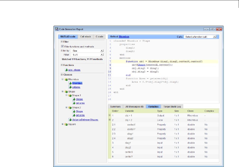
Generate Code for MATLAB®Value Classes
8At the top right side of the report, expand the Calls list.
The Calls list shows that there is a call to the Rhombus constructor from
use_shape and that this constructor calls the Shape constructor.
38-13
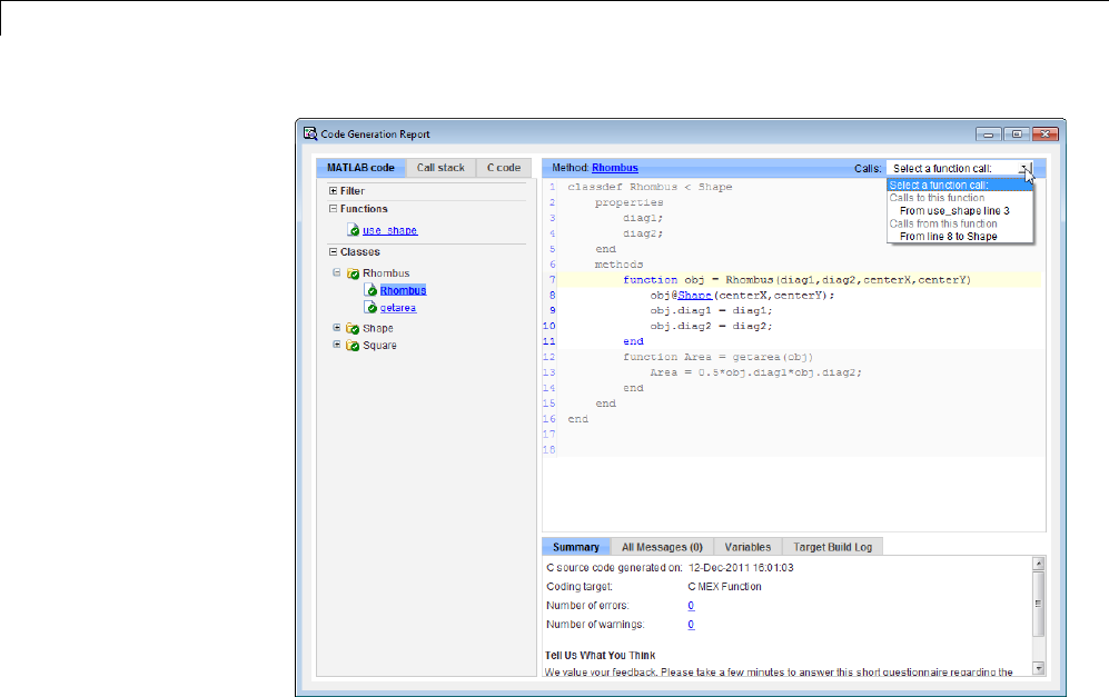
38 Code Generation for MATLAB Classes
9The constructor for the Rhombus class calls the Shape method of the base
Shape class: obj@Shape. In the report, click the Shape link in this call.
38-14
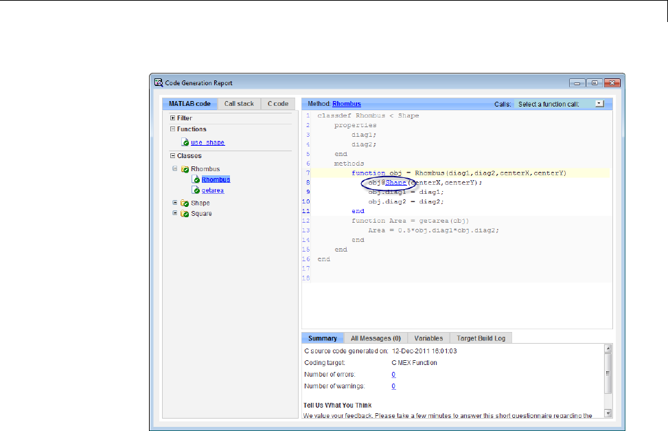
Generate Code for MATLAB®Value Classes
The link takes you to the Shape method in the Shape class definition.
38-15

38 Code Generation for MATLAB Classes
Generate Code for MATLAB Handle Classes and System
Objects
This example shows how to generate code for a user-defined System object
and then view the generated code in the code generation report. When you
create a System or handle object, you must assign the object to a persistent
variable or to a property of another MATLAB object that must also be a
persistent variable. The assignment must be in an if-isempty clause. After
assignment, you can copy the object to a local variable, pass it to or return it
from another function.
1In a writable folder, create a System object, AddOne,whichsubclassesfrom
matlab.System.SavethecodeasAddOne.m.
classdef AddOne < matlab.System
% ADDONE Compute an output value that increments the input by one
methods (Access=protected)
% stepImpl method is called by the step method
function y = stepImpl(~,x)
y = x+1;
end
end
end
2Write a function that uses this System object.
function y = testAddOne(x)
%#codegen
persistent p;
if isempty(p)
p = AddOne();
end
y = p.step(x);
end
For code generation, you must immediately assign a System object to a
persistent variable in an if isempty clause as in this example.
3Generate a MEX function for this code.
38-16
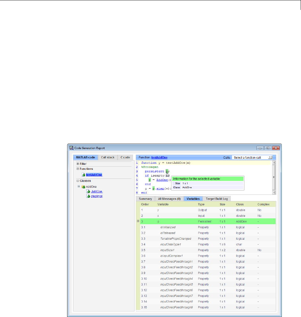
Generate Code for MATLAB®Handle Classes and System Objects
codegen -report testAddOne -args {0}
The -report option instructs codegen to generate a code generation report,
even if no errors or warnings occur. The -args option specifies that the
testAddOne function takes one scalar double input.
>> codegen -report testAddOne -args {0}
Code generation successful: View report
4Click the View report link.
5In the report, on the MATLAB Code tab Functions panel, click
testAddOne,thenclicktheVariables tab. You can view information about
the variable pon this tab.
6To view the class definition, on the Classes panel, click AddOne.
38-17
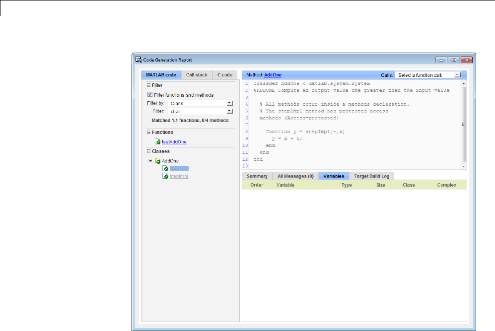
38 Code Generation for MATLAB Classes
38-18

MATLAB®Classes in Code Generation Reports
MATLAB Classes in Code Generation Reports
What Reports Tell You About Classes
Code generation reports:
•Provide a hierarchical tree of the classes used in your MATLAB code.
•Display a list of methods for each class in the MATLAB code tab.
•Display the objects used in your MATLAB code together with their
properties on the Variables tab.
•Provide a filter so that you can sort methods by class, size, and complexity.
•List the set of calls from and to the selected method in the Calls list.
How Classes Appear in Code Generation Reports
IntheMATLABCodeTab
The report displays an alphabetical hierarchical list of the classes used in the
your MATLAB code. For each class, you can:
•Expand the class information to view the class methods.
•View a class method by clicking its name. The report displays the methods
in the context of the full class definition.
•Filter the methods by size, complexity, and class by using the Filter
functions and methods option.
Default Constructors. If a class has a default constructor, the report
displays the constructor in italics.
Specializations. If the same class is specialized into multiple different
classes, the report differentiates the specializations by grouping each one
under a single node in the tree. The report associates the class definition
functions and static methods with the primary node. It associates the
instance-specific methods with the corresponding specialized node.
For example, consider a base class, Shape that has two specialized subclasses,
Rhombus and Square.TheShape class has an abstract method, getarea,
38-19
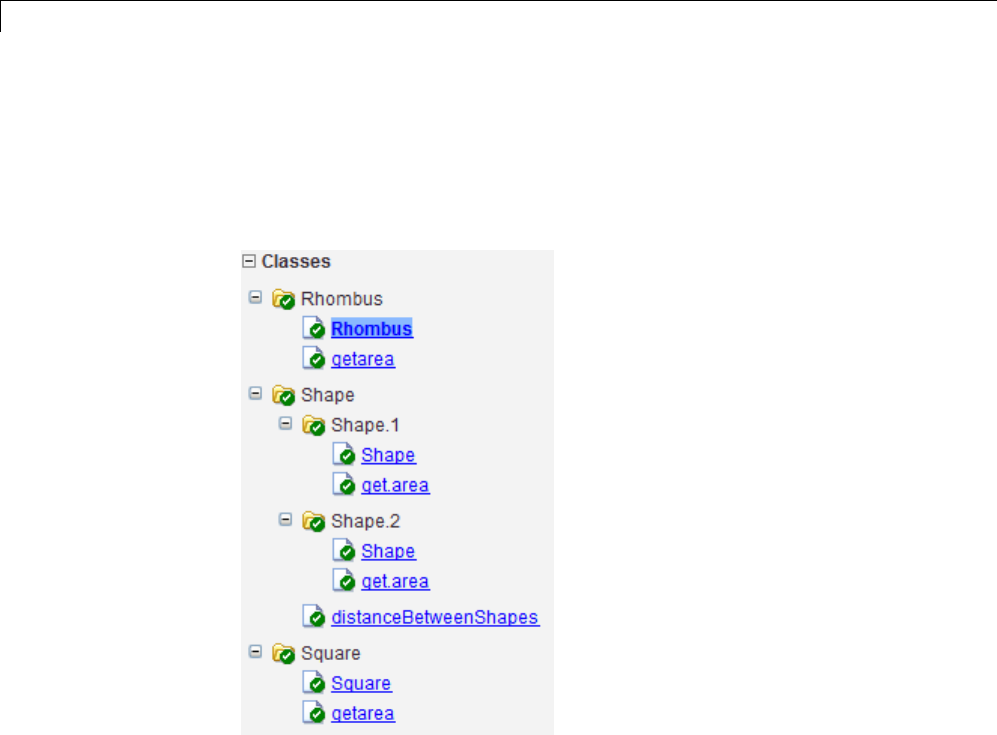
38 Code Generation for MATLAB Classes
and a static method, distanceBetweenShapes. The code generation report,
displays a node for the specialized Rhombus and Square classes with their
constructors and getarea method. It displays a node for the Shape class and
its associated static method, distanceBetweenShapes, and two instances of
the Shape class, Shape1 and Shape2.
Packages. If you define classes as part of a package, the report displays
the package in the list of classes. You can expand the package to view the
classes that it contains. For more information about packages, see “Packages
Create Namespaces”.
In the Variables Tab
The report displays all the objects in the selected function or class. By default,
for classes that have properties, the list of properties is collapsed. Click the
+symbolnexttotheobjectnametoopenthelist.
The report displays the properties using just the base property name, not the
fully qualified name. For example, if your code uses variable obj1 that is a
38-20

MATLAB®Classes in Code Generation Reports
MATLAB object with property prop1, then the report displays the property as
prop1 not obj1.prop1.WhenyousorttheVariables column, the sort order
is based on the fully qualified property name.
In the Call Stack
The call stack lists the functions and methods in the order that the top-level
function calls them. It also lists the local functions that each function calls.
How to Generate a Code Generation Report
Add the -report option to your codegen command (requires a MATLAB
Coder license)
38-21

38 Code Generation for MATLAB Classes
Troubleshooting Issues with MATLAB Classes
Class class does not have a property with name name
If a MATLAB class has a method, mymethod, that returns a handle class
with a property, myprop, you cannot generate code for the following type of
assignment:
obj.mymethod().myprop=...
For example, consider the following classes:
classdef MyClass < handle
properties
myprop
end
methods
function this = MyClass
this.myprop = MyClass2;
end
function y = mymethod(this)
y = this.myprop;
end
end
end
classdef MyClass2 < handle
properties
aa
end
end
You cannot generate code for function foo.
function foo
persistent h
if isempty(h)
h = MyClass;
end
38-22

Troubleshooting Issues with MATLAB®Classes
h.mymethod().aa = 12;
In this function, h.mymethod() returns a handle object of type MyClass2.In
MATLAB, the assignment h.mymethod().aa = 12; changes the property of
that object. Code generation does not support this assignment.
Workaround
Rewrite the code to return the object and then assign a value to a property
of the object.
function foo
persistent h
if isempty(h)
h = MyClass;
end
b=h.mymethod();
b.aa=12;
38-23

38 Code Generation for MATLAB Classes
38-24


39 Code Generation for Function Handles
Function Handles Definition for Code Generation
You can use function handles to invoke functions indirectly and parameterize
operations that you repeat frequently. You can perform the following
operations with function handles:
•Define handles that reference user-defined functions and built-in functions
supported for code generation (see “Functions Supported for Code
Generation — Alphabetical List” on page 31-2)
Note You cannot define handles that reference extrinsic MATLAB
functions.
•Define function handles as scalar values
•Pass function handles as arguments to other functions (excluding extrinsic
functions)
To generate efficient standalone code for enumerated data, you are restricted
to using a subset of the operations you can perform with function handles in
MATLAB, as described in “Function Handle Limitations for Code Generation”
on page 39-5
39-2

Define and Pass Function Handles for Code Generation
Define and Pass Function Handles for Code Generation
The following code example shows how to define and call function handles for
code generation. You can copy the example to a MATLAB Function block
in Simulink or MATLAB function in Stateflow. To convert this function to
a MEX function using codegen, uncomment the two calls to the assert
function, highlighted below:
function addval(m)
%#codegen
% Define class and size of primary input m
% Uncomment next two lines to build MEX function with codegen
% assert(isa(m,'double'));
% assert(all (size(m) == [3 3]));
% Pass function handle to addone
% to add one to each element of m
m = map(@addone, m);
disp(m);
% Pass function handle to addtwo
% to add two to each element of m
m = map(@addtwo, m);
disp(m);
function y = map(f,m)
y=m;
for i = 1:numel(y)
y(i) = f(y(i));
end
function y = addone(u)
y=u+1;
function y = addtwo(u)
y=u+2;
This code passes function handles @addone and @addtwo to the function map
which increments each element of the matrix mby the amount prescribed
39-3

39 Code Generation for Function Handles
by the referenced function. Note that map stores the function handle in the
input variable fand then uses fto invoke the function — in this case addone
first and then addtwo.
If you have MATLAB Coder, you can use the function codegen to convert the
function addval to a MEX executable that you can run in MATLAB. Follow
these steps:
1At the MATLAB command prompt, issue this command:
codegen addval
2Define and initialize a 3-by-3 matrix by typing a command like this at
the MATLAB prompt:
m = zeros(3)
3Execute the function by typing this command:
addval(m)
You should see the following result:
000
000
000
111
111
111
333
333
333
For more information, see “MEX Function Generation at the Command Line”.
39-4

Function Handle Limitations for Code Generation
Function Handle Limitations for Code Generation
Function handles must be scalar values.
You cannot store function handles in matrices or structures.
You cannot use the same bound variable to reference different
function handles.
After you bind a variable to a specific function, you cannot use the same
variable to reference two different function handles, as in this example
%Incorrect code
...
x = @plus;
x = @minus;
...
This code produces a compilation error.
You cannot pass function handles to or from extrinsic functions.
You cannot pass function handles to or from feval and other extrinsic
MATLAB functions. For more information, see “Declaring MATLAB
Functions as Extrinsic Functions” on page 41-12
You cannot pass function handles to or from primary functions.
You cannot pass function handles as inputs to or outputs from primary
functions. For example, consider this function:
function x = plotFcn(fhandle, data)
assert(isa(fhandle,'function_handle') && isa(data,'double'));
plot(data, fhandle(data));
x = fhandle(data);
In this example, the function plotFcn receives a function handle and its
data as primary inputs. plotFcn attempts to call the function referenced by
39-5

39 Code Generation for Function Handles
the fhandle with the input data and plot the results. However, this code
generates a compilation error, indicating that the function isa does not
recognize 'function_handle' as a class name when called inside a MATLAB
function to specify properties of primary inputs.
You cannot view function handles from the debugger
You cannot display or watch function handles from the debugger. They
appear as empty matrices.
39-6

40
Defining Functions for Code
Generation
•“Specify Variable Numbers of Arguments” on page 40-2
•“Supported Index Expressions” on page 40-3
•“Apply Operations to a Variable Number of Arguments” on page 40-4
•“Implement Wrapper Functions” on page 40-7
•“Pass Property/Value Pairs” on page 40-8
•“Variable Length Argument Lists for Code Generation” on page 40-10

40 Defining Functions for Code Generation
Specify Variable Numbers of Arguments
You can use varargin and varargout for passing and returning variable
numbers of parameters to MATLAB functions called from a top-level function.
Common applications of varargin and varargout for code generation are to:
•“Apply Operations to a Variable Number of Arguments” on page 40-4
•“Implement Wrapper Functions” on page 40-7
•“Pass Property/Value Pairs” on page 40-8
Code generation relies on loop unrolling to produce simple and efficient code
for varargin and varargout. This technique permits most common uses of
varargin and varargout, but not all (see “Variable Length Argument Lists
for Code Generation” on page 40-10). This following sections explain how to
code effectively using these constructs.
For more information about using varargin and varargout in MATLAB
functions, see Passing Variable Numbers of Arguments.
40-2

Supported Index Expressions
Supported Index Expressions
In MATLAB, varargin and varargout are cell arrays. Generated code does
not support cell arrays, but does allow you to use the most common syntax
—curlybraces{} — for indexing into varargin and varargout arrays, as
in this example:
%#codegen
function [x,y,z] = fcn(a,b,c)
[x,y,z] = subfcn(a,b,c);
function varargout = subfcn(varargin)
for i = 1:length(varargin)
varargout{i} = varargin{i};
end
You can use the following index expressions. The exp arguments must be
constant expressions or depend on a loop index variable.
Expression Description
varargin{exp}Read the value of element
exp
varargin{exp1:exp2}Read the values of elements
exp1 through exp2
varargin
(read only)
varargin{:} Read the values of all
elements
varargout
(readandwrite)
varargout{exp}Read or write the value of
element exp
Note The use of () is not supported for indexing into varargin and
varargout arrays.
40-3

40 Defining Functions for Code Generation
Apply Operations to a Variable Number of Arguments
You can use varargin and varargout in for-loops to apply operations to
a variable number of arguments. To index into varargin and varargout
arrays in generated code, the value of the loop index variable must be known
at compile time. Therefore, during code generation, the compiler attempts
to automatically unroll these for-loops. Unrolling eliminates the loop logic
by creating a separate copy of the loop body in the generated code for each
iteration. Within each iteration, the loop index variable becomes a constant.
For example, the following function automatically unrolls its for-loop in the
generated code:
%#codegen
function [cmlen,cmwth,cmhgt] = conv_2_metric(inlen,inwth,inhgt)
[cmlen,cmwth,cmhgt] = inch_2_cm(inlen,inwth,inhgt);
function varargout = inch_2_cm(varargin)
for i = 1:length(varargin)
varargout{i} = varargin{i} * 2.54;
end
When to Force Loop Unrolling
To automatically unroll for-loops containing varargin and varargout
expressions, the relationship between the loop index expression and the index
variable must be determined at compile time.
In the following example, the function fcn cannot detect a logical relationship
between the index expression jand the index variable i:
%#codegen
function [x,y,z] = fcn(a,b,c)
[x,y,z] = subfcn(a,b,c);
function varargout = subfcn(varargin)
j=0;
for i = 1:length(varargin)
j = j+1;
varargout{j} = varargin{j};
40-4

Apply Operations to a Variable Number of Arguments
end
As a result, the function does not unroll the loop and generates a compilation
error:
Nonconstant expression or empty matrix.
This expression must be constant because
its value determines the size or class of some expression.
To fix the problem, you can force loop unrolling by wrapping the loop header
in the function coder.unroll,asfollows:
%#codegen
function [x,y,z] = fcn(a,b,c)
[x,y,z] = subfcn(a,b,c);
function varargout = subfcn(varargin)
j=0;
for i = coder.unroll(1:length(varargin))
j=j+1;
varargout{j} = varargin{j};
end;
Using Variable Numbers of Arguments in a for-Loop
The following example multiplies a variable number of input dimensions in
inches by 2.54 to convert them to centimeters:
%#codegen
function [cmlen,cmwth,cmhgt] = conv_2_metric(inlen,inwth,inhgt)
[cmlen,cmwth,cmhgt] = inch_2_cm(inlen,inwth,inhgt);
function varargout = inch_2_cm(varargin)
for i = 1:length(varargin)
varargout{i} = varargin{i} * 2.54;
end
40-5

40 Defining Functions for Code Generation
Key Points About the Example
•varargin and varargout appear in the local function inch_2_cm,notin
the top-level function conv_2_metric.
•The index into varargin and varargout is a for-loop variable
For more information, see “Variable Length Argument Lists for Code
Generation” on page 40-10.
40-6

Implement Wrapper Functions
Implement Wrapper Functions
You can use varargin and varargout to write wrapper functions that accept
any number of inputs and pass them directly to another function.
Passing Variable Numbers of Arguments from One
Function to Another
The following example passes a variable number of inputs to different
optimization functions, based on a specified input method:
%#codegen
function answer = fcn(method,a,b,c)
answer = optimize(method,a,b,c);
function answer = optimize(method,varargin)
if strcmp(method,'simple')
answer = simple_optimization(varargin{:});
else
answer = complex_optimization(varargin{:});
end
...
Key Points About the Example
•You can use {:} to read all elements of varargin and pass them to another
function.
•You can mix variable and fixed numbers of arguments.
For more information, see “Variable Length Argument Lists for Code
Generation” on page 40-10.
40-7

40 Defining Functions for Code Generation
Pass Property/Value Pairs
You can use varargin to pass property/value pairs in functions. However,
for code generation, you must take precautions to avoid type mismatch errors
when evaluating varargin array elements in a for-loop:
If Do This:
You assign varargin array elements
to local variables in the for-loop
Verify that for all pairs, the size,
type, and complexity are the same
for each property and the same for
each value
Properties or values have different
sizes, types, or complexity
Do not assign varargin array
elements to local variables in a
for-loop; reference the elements
directly
For example, in the following function test1, the sizes of the property strings
and numeric values are not the same in each pair:
%#codegen
function test1
v = create_value('size', 18, 'rgb', [240 9 44]);
end
function v = create_value(varargin)
v = new_value();
for i = 1 : 2 : length(varargin)
name = varargin{i};
value = varargin{i+1};
switch name
case 'size'
v = set_size(v, value);
case 'rgb'
v = set_color(v, value);
otherwise
end
end
end
40-8

Pass Property/Value Pairs
...
Generated code determines the size, type, and complexity of a local variable
based on its first assignment. In this example, the first assignments occur
in the first iteration of the for-loop:
•Defines local variable name with size equal to 4
•Defines local variable value with a size of scalar
However, in the second iteration, the size of the property string changes to
3 and the size of the numeric value changes to a vector, resulting in a type
mismatch error. To avoid such errors, reference varargin array values
directly, not through local variables, as highlighted in this code:
%#codegen
function test1
v = create_value('size', 18, 'rgb', [240 9 44]);
end
function v = create_value(varargin)
v = new_value();
for i = 1 : 2 : length(varargin)
switch varargin{i}
case 'size'
v = set_size(v, varargin{i+1});
case 'rgb'
v = set_color(v, varargin{i+1});
otherwise
end
end
end
...
40-9

40 Defining Functions for Code Generation
Variable Length Argument Lists for Code Generation
Do not use varargin or varargout in top-level functions
You cannot use varargin or varargout as arguments to top-level functions.
Atop-level function is:
•The function called by Simulink in a MATLAB Function block or by
Stateflow in a MATLAB function.
•The function that you provide on the command line to codegen
For example, the following code generates compilation errors:
%#codegen
function varargout = inch_2_cm(varargin)
for i = 1:length(varargin)
varargout{i} = varargin{i} * 2.54;
end
To fix the problem, write a top-level function that specifies a fixed number of
inputs and outputs and then call inch_2_cm as an external function or local
function,asinthisexample:
%#codegen
function [cmL, cmW, cmH] = conv_2_metric(inL, inW, inH)
[cmL, cmW, cmH] = inch_2_cm(inL, inW, inH);
function varargout = inch_2_cm(varargin)
for i = 1:length(varargin)
varargout{i} = varargin{i} * 2.54;
end
Use curly braces {} to index into the argument list
For code generation, you can use curly braces {}, but not parentheses (),
to index into varargin and varargout arrays. For more information, see
“Supported Index Expressions” on page 40-3.
40-10

Variable Length Argument Lists for Code Generation
Verify that indices can be computed at compile time
If you use an expression to index into varargin or varargout,makesurethat
thevalueoftheexpressioncanbecomputed at compile time. For examples,
see “Apply Operations to a Variable Number of Arguments” on page 40-4.
Do not write to varargin
Generated code treats varargin as a read-only variable. If you want to write
to any of the input arguments, copy the values into a local variable.
40-11

40 Defining Functions for Code Generation
40-12

41
Calling Functions for Code
Generation
•“Resolution of Function Calls in MATLAB Generated Code” on page 41-2
•“Resolution of Files Types on Code Generation Path” on page 41-6
•“Compilation Directive %#codegen” on page 41-8
•“Call Local Functions” on page 41-9
•“Call Supported Toolbox Functions” on page 41-10
•“Call MATLAB Functions” on page 41-11

41 Calling Functions for Code Generation
Resolution of Function Calls in MATLAB Generated Code
From a MATLAB function, you can call local functions, supported toolbox
functions, and other MATLAB functions. MATLAB resolves function names
for code generation as follows:
41-2
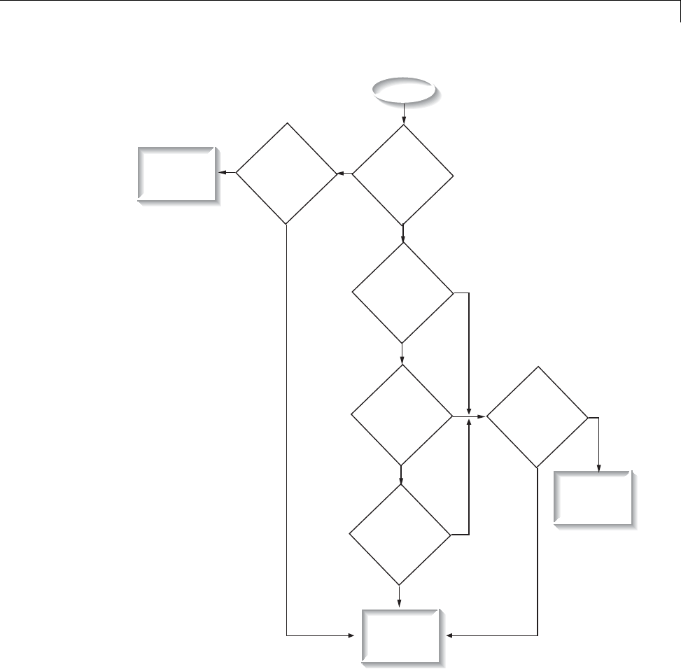
Resolution of Function Calls in MATLAB®Generated Code
Subfunction?
Function
on the code
generation
path?
Function
on
MATLAB
path?
Extrinsic
function?
Function
on
MATLAB
path?
Yes
Yes
Dispatch to
MATLAB
for execution
at runtime
No
No
No
Yes
Suitable
for code
generation?
Yes
Yes
Yes
Generate
C code
Start
Generate error
No
No
No
41-3

41 Calling Functions for Code Generation
Key Points About Resolving Function Calls
The diagram illustrates key points about how MATLAB resolves function
calls for code generation:
•Searches two paths, the code generation path and the MATLAB path
See“CompileP
ath Search Order” on page 41-4.
•Attempts to compile all functions unless the code generation software
determines that it should not compile them or you explicitly declare them
to be extrinsic.
An extrinsic function is a function on the MATLAB path that the compiler
dispatches to MATLAB software for execution because the target language
does not support the function. MATLAB does not generate code for extrinsic
functions. You declare functions to be extrinsic by using the construct
coder.extrinsic, as described in “Declaring MATLAB Functions as
Extrinsic Functions” on page 41-12.
Thecodeg
eneration software detects calls to many common visualization
functions, such as plot,disp,andfigure. For MEX code generation, it
automatically calls out to MATLAB for these functions. For standalone
code generation, it does not generate code for these visualization functions.
This capability removes the requirement to declare these functions
extrinsic using the coder.extrinsic function.
•Resolves file type based on precedence rules described in “Resolution of
Files Types on Code Generation Path” on page 41-6
CompilePathSearchOrder
During code generation, function calls are resolved on two paths:
1Code generation path
MATLAB searches this path first during code generation. The code
generation path contains the toolbox functions supported for code
generation.
2MATLAB path
If the function is not on the code generation path, MATLAB searches this
path.
41-4

Resolution of Function Calls in MATLAB®Generated Code
MATLAB applies the same dispatcher rules when searching each path (see
“Function Precedence Order”).
When to Use the Code Generation Path
Use the code generation path to override a MATLAB function with a
customized version. A file on the code generation path always shadows a file
of the same name on the MATLAB path.
41-5

41 Calling Functions for Code Generation
Resolution of Files Types on Code Generation Path
MATLAB uses the following precedence rules for code generation:
41-6
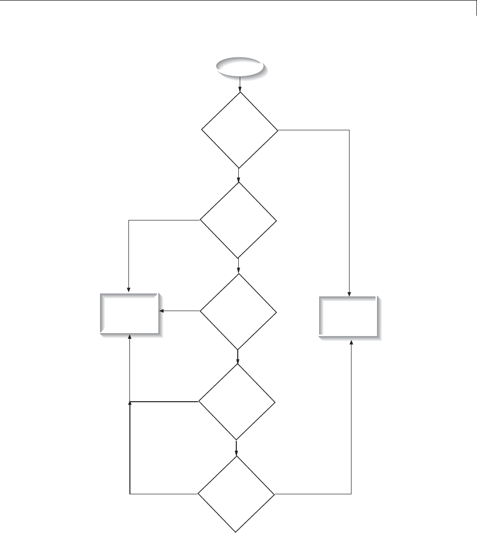
Resolution of Files Types on Code Generation Path
MEX-file?
MDL-file?
P-file?
M-file and
MEX-file in same
directory?
Yes
No
No
No
Yes
M-file?
Yes
Yes
Start
No
Compile
M-file
Generate
error
Yes
No
41-7

41 Calling Functions for Code Generation
Compilation Directive %#codegen
Add the %#codegen directive(orpragma)toyourfunctiontoindicatethatyou
intend to generate code for the MATLAB algorithm. Adding this directive
instructs the MATLAB code analyzer to help you diagnose and fix violations
that would result in errors during code generation.
41-8

Call Local Functions
Call Local Functions
Local functions are functions defined in the body of MATLAB function. They
work the same way for code generation as they do when executing your
algorithm in the MATLAB environment.
The following example illustrates how to define and call a local function mean:
function [mean, stdev] = stats(vals)
%#codegen
% Calculates a statistical mean and a standard
% deviation for the values in vals.
len = length(vals);
mean = avg(vals, len);
stdev = sqrt(sum(((vals-avg(vals,len)).^2))/len);
plot(vals,'-+');
function mean = avg(array,size)
mean = sum(array)/size;
41-9

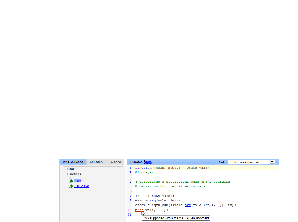
Call MATLAB®Functions
Call MATLAB Functions
The code generation software attempts to generate code for all functions, even
if they are not supported for C code generation. The software detects calls
to many common visualization functions, such as plot,disp,andfigure.
For MEX code generation, it automatically calls out to MATLAB for these
functions. For standalone code generation, it does not generate code for them.
Forexample,youmightwanttocallplot to visualize your results in the
MATLAB environment. If you generate a MEX function from a function that
calls plot and then run the generated MEX function, the code generation
software dispatches calls to the plot function to MATLAB. If you generate a
library or executable, the generated code does not contain calls to the plot
function. The code generation report highlights calls from your MATLAB
code to extrinsic functions so that it is easy to determine which functions are
supported only in the MATLAB environment.
For unsupported functions other than common visualization functions, you
must declare the functions (like pause)tobeextrinsic(see“Resolution
of Function Calls in MATLAB Generated Code” on page 41-2). Extrinsic
functions are not compiled, but instead executed in MATLAB during
simulation (see “How MATLAB Resolves Extrinsic Functions During
Simulation” on page 41-16).
There are two ways to declare a function to be extrinsic:
•Use the coder.extrinsic construct in main functions or local functions
(see “Declaring MATLAB Functions as Extrinsic Functions” on page 41-12).
41-11

41 Calling Functions for Code Generation
•Call the function indirectly using feval (see “Calling MATLAB Functions
Using feval” on page 41-16).
Declaring MATLAB Functions as Extrinsic Functions
To declare a MATLAB function to be extrinsic, add the coder.extrinsic
construct at the top of the main function or a local function:
coder.extrinsic('function_name_1', ... , 'function_name_n');
Declaring Extrinsic Functions
The following code declares the MATLAB patch function extrinsic in the
local function create_plot:
function c = pythagoras(a,b,color) %#codegen
% Calculates the hypotenuse of a right triangle
% and displays the triangle.
c = sqrt(a^2 + b^2);
create_plot(a, b, color);
function create_plot(a, b, color)
%Declare patch and axis as extrinsic
coder.extrinsic('patch');
x = [0;a;a];
y = [0;0;b];
patch(x, y, color);
axis('equal');
The code generation software detects that axis is not supported for code
generation and automatically treats it as an extrinsic function. The compiler
does not generate code for patch and axis, but instead dispatches them to
MATLAB for execution.
To test the function, follow these steps:
41-12
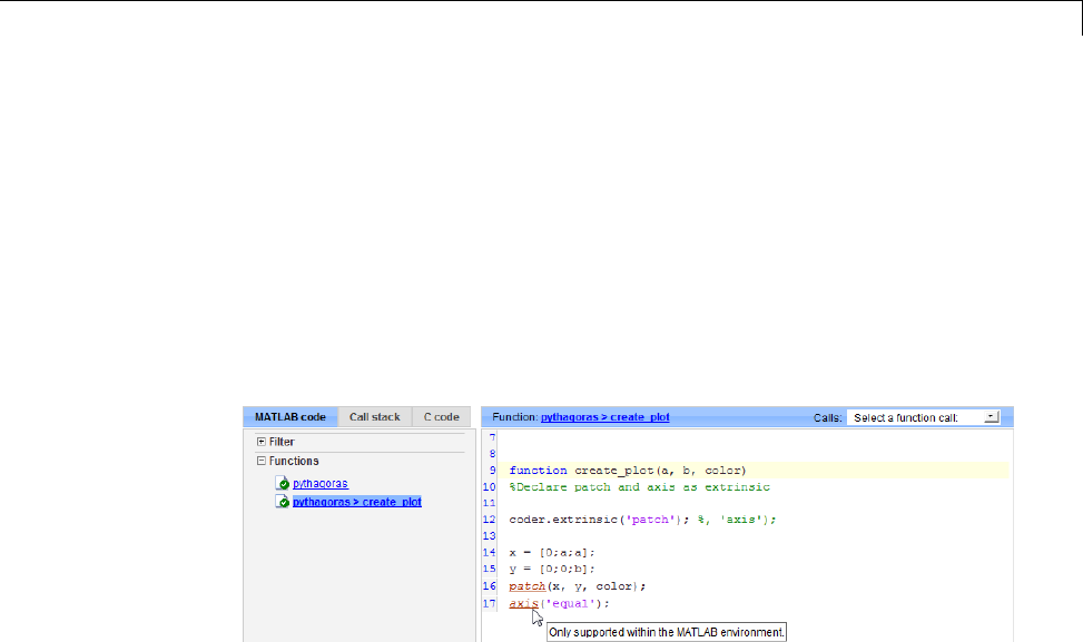
Call MATLAB®Functions
1Convert pythagoras to a MEX function by executing this command at
the MATLAB prompt:
codegen -report pythagoras -args {1, 1, [.3 .3 .3]}
2Click the link to the code generation report and then, in the report, view
theMATLABcodeforcreate_plot.
The report highlights the patch and axis functions to indicate that they
are supported only within the MATLAB environment.
3Run the MEX function by executing this command:
pythagoras_mex(3, 4, [1.0 0.0 0.0]);
MATLAB displays a plot of the right triangle as a red patch object:
41-13
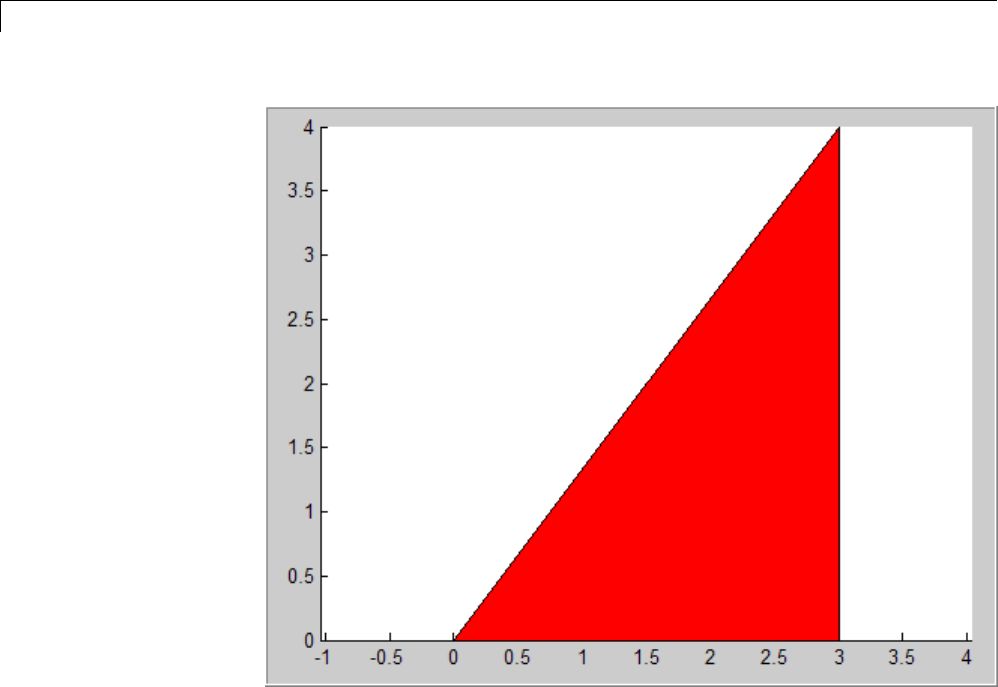
41 Calling Functions for Code Generation
When to Use the coder.extrinsic Construct
Use the coder.extrinsic construct to:
•Call MATLAB functions that produce no output — such as pause —during
simulation, without generating unnecessary code (see “How MATLAB
Resolves Extrinsic Functions During Simulation” on page 41-16).
•Make your code self-documenting and easier to debug. You can scan the
source code for coder.extrinsic statements to isolate calls to MATLAB
functions, which can potentially create and propagate mxArrays (see
“Working with mxArrays” on page 41-17).
•Save typing. With one coder.extrinsic statement, each subsequent
function call is extrinsic, as long as the call and the statement are in the
samescope(see“ScopeofExtrinsicFunctionDeclarations”onpage41-15).
41-14

Call MATLAB®Functions
•Declare the MATLAB function(s) extrinsic throughout the calling function
scope (see “Scope of Extrinsic Function Declarations” on page 41-15). To
narrow the scope, use feval (see “Calling MATLAB Functions Using feval”
on page 41-16).
Rules for Extrinsic Function Declarations
Observe the following rules when declaring functions extrinsic for code
generation:
•Declare the function extrinsic before you call it.
•Do not use the extrinsic declaration in conditional statements.
Scope of Extrinsic Function Declarations
The coder.extrinsic construct has function scope. For example, consider
the following code:
function y = foo %#codegen
coder.extrinsic('rat','min');
[N D] = rat(pi);
y=0;
y = min(N, D);
In this example, rat and min as treated as extrinsic every time they are
called in the main function foo. There are two ways to narrow the scope of
an extrinsic declaration inside the main function:
•Declare the MATLAB function extrinsic in a local function, as in this
example:
function y = foo %#codegen
coder.extrinsic('rat');
[N D] = rat(pi);
y=0;
y = mymin(N, D);
function y = mymin(a,b)
coder.extrinsic('min');
y = min(a,b);
41-15

41 Calling Functions for Code Generation
Here, the function rat is extrinsic every time it is called inside the main
function foo, but the function min is extrinsic only when called inside the
local function mymin.
•Call the MATLAB function using feval, as described in “Calling MATLAB
Functions Using feval” on page 41-16.
Calling MATLAB Functions Using feval
The function feval is automatically interpreted as an extrinsic function
during code generation. Therefore, you can use feval to conveniently call
functions that you want to execute in the MATLAB environment, rather than
compiled to generated code.
Consider the following example:
function y = foo
coder.extrinsic('rat');
[N D] = rat(pi);
y=0;
y = feval('min', N, D);
Because feval is extrinsic, the statement feval('min', N, D) is evaluated
by MATLAB — not compiled — which has the same effect as declaring the
function min extrinsic for just this one call. By contrast, the function rat is
extrinsic throughout the function foo.
How MATLAB Resolves Extrinsic Functions During
Simulation
MATLAB resolves calls to extrinsic functions — functions that do not support
code generation — as follows:
41-16
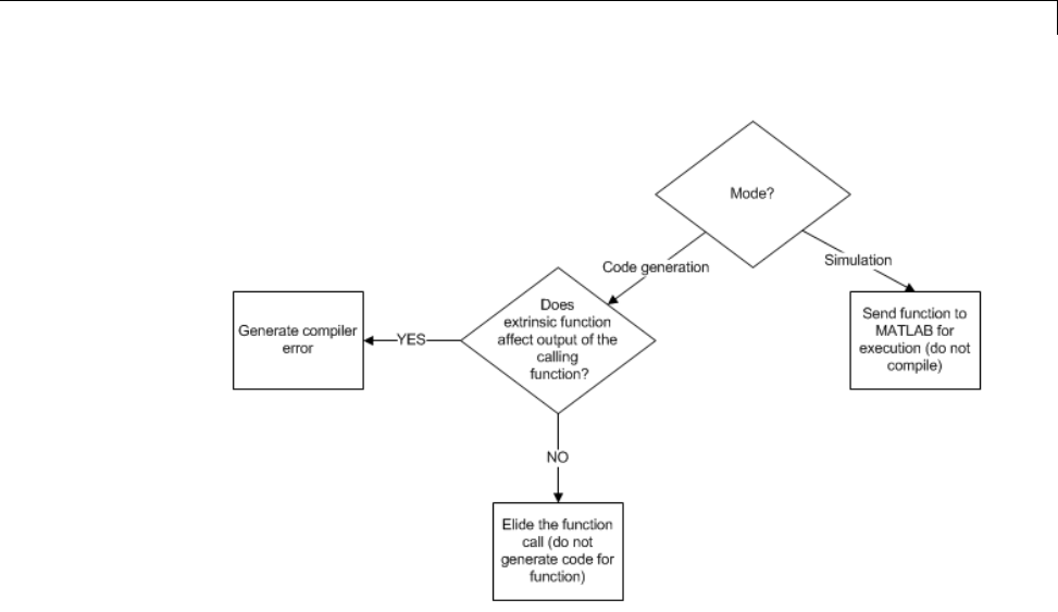
Call MATLAB®Functions
During simulation, MATLAB generates code for the call to an extrinsic
function, but does not generate the function’s internal code. Therefore, you
can run the simulation only on platforms where you install MATLAB software.
During code generation, MATLAB attempts to determine whether the
extrinsic function affects the output of the function in which it is called — for
example by returning mxArrays to an output variable (see “Working with
mxArrays” on page 41-17). Provided that there is no change to the output,
MATLAB proceeds with code generation, but excludes the extrinsic function
from the generated code. Otherwise, MATLAB issues a compiler error.
Working with mxArrays
The output of an extrinsic function is an mxArray — also called a MATLAB
array. The only valid operations for mxArrays are:
•Storing mxArrays in variables
•Passing mxArrays to functions and returning them from functions
•Converting mxArrays to known types at run time
41-17

41 Calling Functions for Code Generation
To use mxArrays returned by extrinsic functions in other operations, you must
first convert them to known types, as described in “Converting mxArrays to
Known Types” on page 41-18.
Converting mxArrays to Known Types
To convert anmxArray to a known type, assign the mxArray to a variable
whose type is defined. At run time, the mxArray is converted to the type of the
variable assigned to it. However, if the data in the mxArray is not consistent
withthetypeofthevariable, you get a run-time error.
For example, consider this code:
function y = foo %#codegen
coder.extrinsic('rat');
[N D] = rat(pi);
y = min(N, D);
Here, the top-level function foo calls the extrinsic MATLAB function rat,
which returns two mxArrays representing the numerator Nand denominator
Dof the rational fraction approximation of pi. Although you can pass these
mxArrays to another MATLAB function — in this case, min — you cannot
assign the mxArray returned by min to the output y.
If you run this function foo in a MATLAB Function block in a Simulink
model, the code generates the following error during simulation:
Function output 'y' cannot be of MATLAB type.
To fix this problem, define ytobethetypeandsizeofthevaluethatyou
expect min to return — in this case, a scalar double — as follows:
function y = foo %#codegen
coder.extrinsic('rat');
[N D] = rat(pi);
y = 0; % Define y as a scalar of type double
y = min(N,D);
41-18

Call MATLAB®Functions
Restrictions on Extrinsic Functions for Code
Generation
The full MATLAB run-time environment is not supported during code
generation. Therefore, the following restrictions apply when calling MATLAB
functions extrinsically:
•MATLAB functions that inspect the caller or write to the caller’s workspace
do not work during code generation. Such functions include:
-dbstack
-evalin
-assignin
•The MATLAB debugger cannot inspect variables defined in extrinsic
functions.
•Functions in generated code may produce unpredictable results if your
extrinsic function performs any of the following actions at run time:
-Change folders
-Change the MATLAB path
-Delete or add MATLAB files
-Change warning states
-Change MATLAB preferences
-Change Simulink parameters
LimitonFunctionArguments
You can call functions with up to 64 inputs and 64 outputs.
41-19

41 Calling Functions for Code Generation
41-20


42 Generating Efficient and Reusable Code
Unroll for-Loops
Unrolling for-loops eliminates the loop logic by creating a separate copy of the
loop body in the generated code for each iteration. Within each iteration, the
loop index variable becomes a constant. By unrolling short loops with known
bounds at compile time, MATLAB generates highly optimized code with no
branches.
You can also force loop unrolling for individual functions by wrapping the loop
header in a coder.unroll function. For more information, see coder.unroll.
42-2

Inline Functions
Inline Functions
MATLAB uses internal heuristics to determine whether or not to inline
functions in the generated code. You can use the coder.inline directive to
fine-tune these heuristics for individual functions. See coder.inline.
42-3

42 Generating Efficient and Reusable Code
Eliminate Redundant Copies of Function Inputs
You can reduce the number of copies in your generated code by writing
functions that use the same variable as both an input and an output. For
example:
function A = foo( A, B ) %#codegen
A=A*B;
end
This coding practice uses a reference parameter optimization. When a
variable acts as both input and output, MATLAB passes the variable by
reference in the generated code instead of redundantly copying the input to a
temporary variable. For example, input Aabove is passed by reference in the
generated code because it also acts as an output for function foo:
...
/* Function Definitions */
void foo(real_T *A, real_T B)
{
*A *= B;
}
...
The reference parameter optimization reduces memory usage and improves
run-time performance, especially when the variable passed by reference is
a large data structure. To achieve these benefits at the call site, call the
function with the same variable as both input and output.
By contrast, suppose you rewrite function foo without using this optimization:
function y = foo2( A, B ) %#codegen
y=A*B;
end
In this case, MATLAB generates code that passes the inputs by value and
returns the value of the output:
...
/* Function Definitions */
real_T foo2(real_T A, real_T B)
42-4

Eliminate Redundant Copies of Function Inputs
{
return A * B;
}
...
42-5

42 Generating Efficient and Reusable Code
Generate Reusable Code
With MATLAB, you can generate reusable code in the following ways:
•Write reusable functions using standard MATLAB function file names
which you can call from different locations, for example, in a Simulink
model or MATLAB function library.
•Compile external functions on the MATLAB path and integrate them into
generated C code for embedded targets.
See “Resolution of Function Calls in MATLAB Generated Code” on page 41-2.
Common applications include:
•Overriding generated library function with a custom implementation
•Implementing a reusable library on top of standard library functions that
canbeusedwithSimulink
•Swapping between different implementations of the same function
42-6


43
Working with Data
•“Data Types” on page 43-2
•“Data Objects” on page 43-37
•“Define Level-2 Data Classes” on page 43-53
•“Supported Property Types” on page 43-58
•“Upgrade Level-1 Data Classes” on page 43-59
•“Infrastructure for Extending Simulink Data Classes” on page 43-61
•“Define Level-1 Data Classes” on page 43-63
•“Associating User Data with Blocks” on page 43-80
•“Design Minimum and Maximum” on page 43-81

43 Working with Data
Data Types
In this section...
“About Data Types” on page 43-2
“Data Types Supported by Simulink” on page 43-3
“Fixed-Point Data” on page 43-4
“Enumerations” on page 43-6
“Bus Objects” on page 43-6
“Block Support for Data and Numeric Signal Types” on page 43-7
“Create Signals of a Specific Data Type” on page 43-7
“Specify Block Output Data Types” on page 43-8
“Specify Data Types Using Data Type Assistant” on page 43-15
“Display Port Data Types” on page 43-27
“Data Type Propagation” on page 43-28
“Data Typing Rules” on page 43-28
“Typecast Signals” on page 43-29
“Validate a Floating-Point Embedded Model” on page 43-29
“Validate a Single-Precision Model” on page 43-30
About Data Types
The term data type refers to the way in which a computer represents numbers
in memory. A data type determines the amount of storage allocated to a
number, the method used to encode the number’s value as a pattern of
binary digits, and the operations available for manipulating the type. Most
computers provide a choice of data types for representing numbers, each with
specific advantages in the areas of precision, dynamic range, performance,
and memory usage. To optimize performance, you can specify the data types
of variables used in the MATLAB technical computing environment. The
Simulink software builds on this capability by allowing you to specify the data
types of Simulink signals and block parameters.
43-2

Data Types
The ability to specify the data types of a model’s signals and block parameters
is particularly useful in real-time control applications. For example, it allows
a Simulink model to specify the optimal data types to use to represent
signals and block parameters in code generated from a model by automatic
code-generation tools, such as the Simulink Coder product. By choosing the
most appropriate data types for your model’s signals and parameters, you
can dramatically increase performance and decrease the size of the code
generated from the model.
Simulink performs extensive checking before and during a simulation to
ensure that your model is typesafe, that is, that code generated from the model
will not overflow or underflow and thus produce incorrect results. Simulink
models that use the default data type (double) are inherently typesafe. Thus,
if you never plan to generate code from your model or use a nondefault data
type in your models, you can skip the remainder of this section.
On the other hand, if you plan to generate code from your models and use
nondefault data types, read the remainder of this section carefully, especially
the section on data type rules (see “Data Typing Rules” on page 43-28). In
that way, you can avoid introducing data type errors that prevent your model
from running to completion or simulating at all.
Data Types Supported by Simulink
Simulink supports all built-in MATLAB data types except int64 and uint64.
The term built-in data type refers to data types defined by MATLAB itself as
opposed to data types defined by MATLAB users. Unless otherwise specified,
the term data type in the Simulink documentation refers to built-in data
types. The following table lists the built-in MATLAB data types supported
by Simulink.
Name Description
double Double-precision floating point
single Single-precision floating point
int8 Signed 8-bit integer
uint8 Unsigned 8-bit integer
int16 Signed 16-bit integer
43-3

43 Working with Data
Name Description
uint16 Unsigned 16-bit integer
int32 Signed 32-bit integer
uint32 Unsigned 32-bit integer
Besides the built-in types, Simulink defines a boolean (1 or 0) type, instances
of which are represented internally by uint8 values.
Several blocks support bus objects (Simulink.Bus)asdatatypes. See“Bus
Objects” on page 43-6.
Many Simulink blocks also support fixed-point data types. For more
information on the data types supported by a specific block for parameter and
input and output values, in the Simulink documentation see the Data Type
Support section of the reference page for that bock. If the documentation for
a block does not specify a data type, the block inputs or outputs only data of
type double.
To view a table that summarizes the data types supported by the blocks in
the Simulink block libraries, execute the following command at the MATLAB
command line:
showblockdatatypetable
Fixed-Point Data
The Simulink software allows you to create models that use fixed-point
numbers to represent signals and parameter values. Use of fixed-point
data can reduce the memory requirements and increase the speed of code
generated from a model.
To execute a model that uses fixed-point numbers, you must have the
Simulink Fixed Point product installed on your system. Specifically, you must
have the product to:
•Update a Simulink diagram (Ctrl+D) containing fixed-point data types
•Run a model containing fixed-point data types
•Generate code from a model containing fixed-point data types
43-4

Data Types
•Log the minimum and maximum values produced by a simulation
•Automatically scale the output of a model using the autoscaling tool
If the Simulink Fixed Point product is not installed on your system, you can
execute a fixed-point model as a floating-point model by enabling automatic
conversion of fixed-point data to floating-point data during simulation. See
“Overriding Fixed-Point Specifications” on page 43-5 for details.
If you do not have the Simulink Fixed Point product installed and do not
enable automatic conversion of fixed-point to floating-point data, an error
occurs if you try to execute a fixed-point model.
Note You do not need the Simulink Fixed Point product to edit a model
containing fixed-point blocks, or to use the Data Type Assistant to specify
fixed-point data types, as described in “Specifying a Fixed-Point Data Type”
on page 43-19.
Overriding Fixed-Point Specifications
Most of the functionality in the Fixed-Point Tool is for use with the Simulink
Fixed Point software. However, even if you do not have Simulink Fixed Point
software, you can configure data type override settings to simulate a model
that specifies fixed-point data types. In this mode, the Simulink software
temporarily overrides fixed-point data types with floating-point data types
when simulating the model.
Note If you use fi objects or embedded numeric data types in your model or
workspace, you might introduce fixed-point data types into your model. You
can set fipref to prevent the checkout of a Fixed-Point Toolbox license.
To simulate a model without using Simulink Fixed Point:
1In the Model Hierarchy pane, select the root model.
2In the Simulink Editor, select Analysis > Fixed-Point Tool.
43-5

43 Working with Data
The Fixed-Point Tool opens.
3In the section Settings for selected system:
•Set Fixed-point instrumentation mode to Force off.
•Set Data type override to Double or Single.
•Set Data type override applies to All numeric types.
4If you use fi objects or embedded numeric data types in your model, set
the fipref DataTypeOverride property to TrueDoubles or TrueSingles
(to be consistent with the model-wide data type override setting) and the
DataTypeOverrideAppliesTo property to All numeric types.
For example, at the MATLAB command line, enter:
p = fipref('DataTypeOverride', 'TrueDoubles', ...
'DataTypeOverrideAppliesTo', 'AllNumericTypes');
Enumerations
An enumeration isauser-defineddatatypewithafixedsetofnamesthat
represent a single type of value. When the data type of an entity is an
enumeration, the value of the entity must be one of the values defined that
enumeration. For information about enumerations, see “Data Types”. Do not
confuse enumerations with enumerated property types (see “Enumerated
Property Types” on page 43-76).
Bus Objects
Abusobject(Simulink.Bus) specifies the architectural properties of a bus, as
distinct from the values of the signals it contains. For example, a bus object
can specify the number of elements in a bus, the order of those elements,
whether and how elements are nested, and the data types of constituent
signals; but not the signal values.
You can specify a bus object as a data type for the following blocks:
•Bus Creator
•Constant
•Data Store Memory
43-6

Data Types
•Inport
•Outport
•Signal Specification
You can specify a bus object as a data type for the following classes:
•Simulink.BusElement
•Simulink.Parameter
•Simulink.Signal
See “Specify a Bus Object Data Type” on page 43-26 for information about
how to specify a bus object as a data type for blocks and classes.
Block Support for Data and Numeric Signal Types
All Simulink blocks accept signals of type double by default. Some blocks
prefer boolean input and others support multiple data types on their inputs.
For more information on the data types supported by a specific block for
parameter and input and output values, in the Simulink documentation see
the Data Type Support section of the reference page for that bock. If the
documentation for a block does not specifyadatatype,theblockinputsor
outputs only data of type double.
Create Signals of a Specific Data Type
You can introduce a signal of a specific data type into a model in any of the
following ways:
•Load signal data of the desired type from the MATLAB workspace into your
model via a root-level Inport block or a From Workspace block.
•Create a Constant block in your model and set its parameter to the desired
type.
•Use a Data Type Conversion block to convert a signal to the desired data
type.
43-7
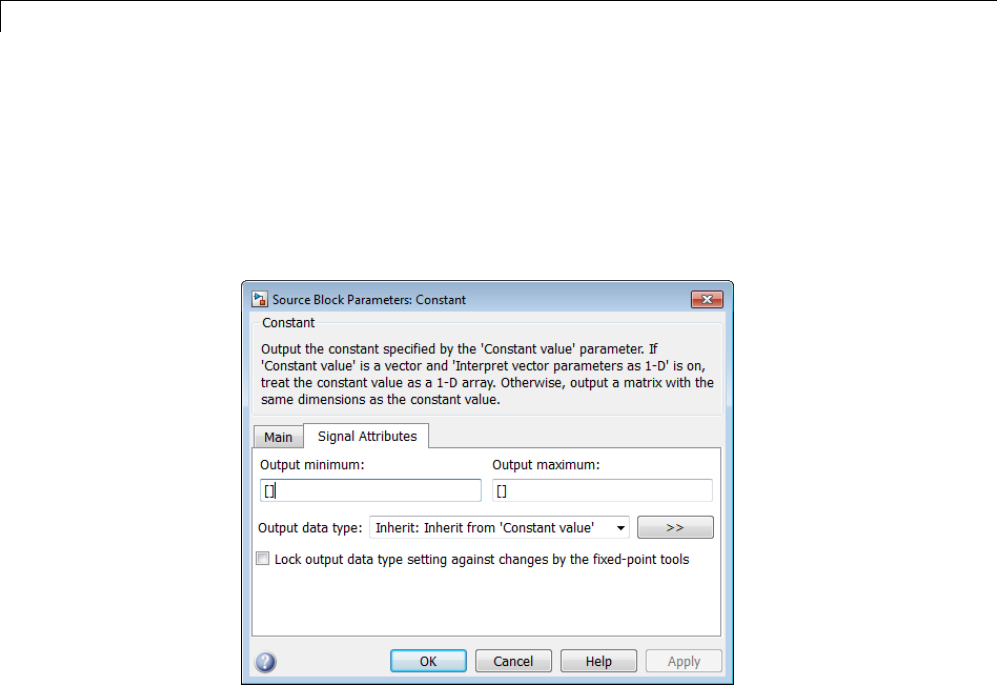
43 Working with Data
Specify Block Output Data Types
Simulink blocks determine the data type of their outputs by default. Many
blocks allow you to override the default type and explicitly specify an output
data type, using a block parameter that is typically named Output data
type. For example, the Output data type parameter appears on the Signal
Attributes pane of the Constant block dialog box.
43-8

Data Types
See the following topics for more information:
For Information About... See...
Valid data type values that you can
specify
“Entering Valid Data Type Values”
on page 43-9
An assistant that helps you specify
valid data type values
“Specify Data Types Using Data
Type Assistant” on page 43-15
Specifying valid data type values for
multiple blocks simultaneously
“Using the Model Explorer for Batch
Editing” on page 43-12
Entering Valid Data Type Values
In general, you can specify the output data type as any of the following:
•A rule that inherits a data type (see “Data Type Inheritance Rules” on
page 43-10)
•The name of a built-in data type (see “Built-In Data Types” on page 43-11)
•An expression that evaluates to a data type (see “Data Type Expressions”
on page 43-11)
Valid data type values vary among blocks. You can use the pull-down menu
associated with a block data type parameter to view the data types that a
particular block supports. For example, the Data type pull-down menu on
the Data Store Memory block dialog box lists the data types that it supports,
as shown here.
43-9
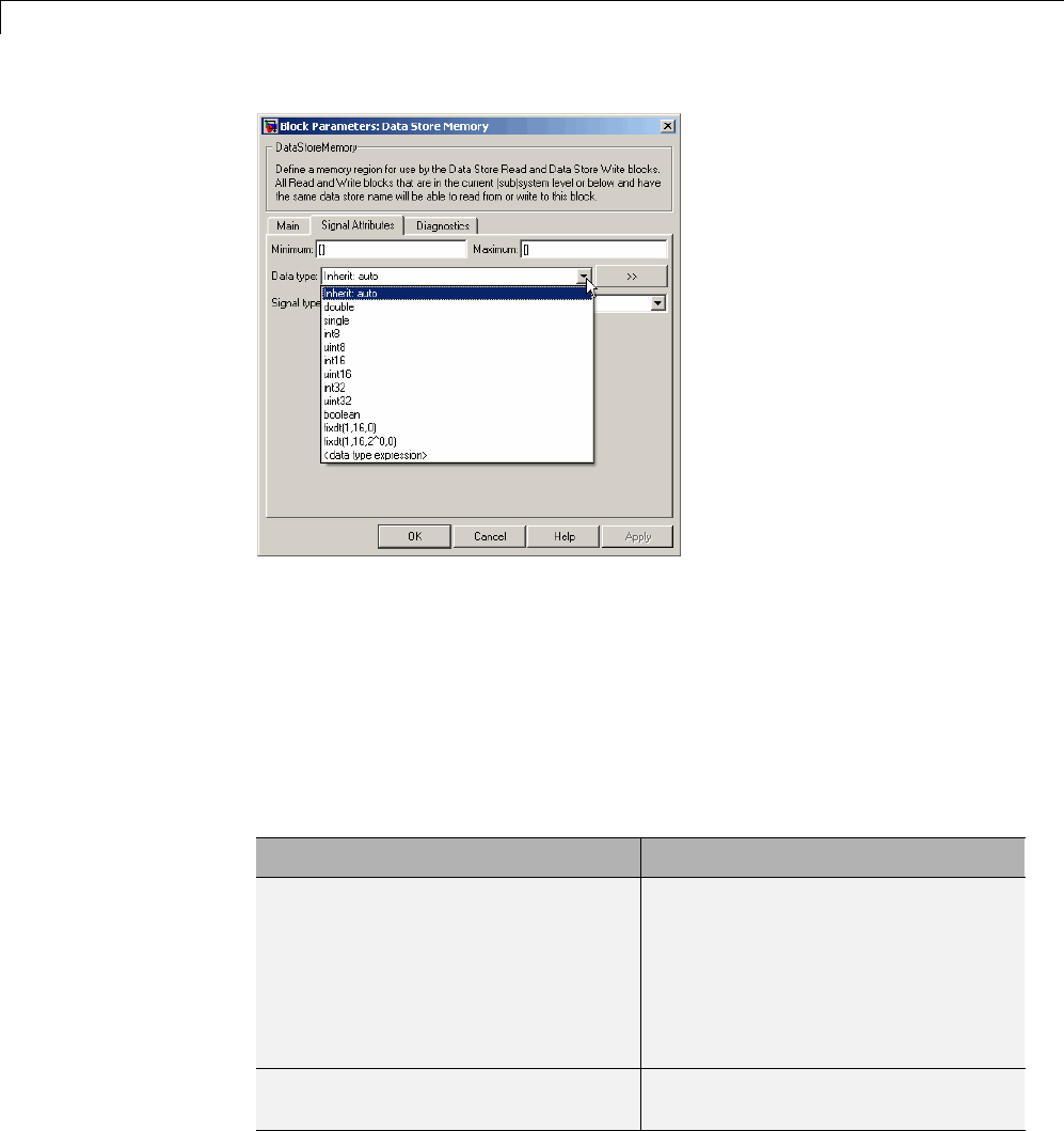
43 Working with Data
For more information about the data types that a specific block supports, see
the documentation for the block in the Simulink documentation.
Data Type Inheritance Rules. Blocks can inherit data types from a variety
of sources, including signals to which they are connected and particular block
parameters. You can specify the valueofadatatypeparameterasarule
that determines how the output signal inherits its data type. To view the
inheritance rules that a block supports, use the data type pull-down menu on
the block dialog box. The following table lists typical rules that you can select.
Inheritance Rule Description
Inherit: Inherit via back
propagation
Simulink automatically determines
the output data type of the block
during data type propagation (see
“Data Type Propagation” on page
43-28). In this case, the block uses
the data type of a downstream block
or signal object.
Inherit: Same as input Theblockusesthedatatypeofits
sole input signal for its output signal.
43-10

Data Types
Inheritance Rule Description
Inherit: Same as first input Theblockusesthedatatypeof
its first input signal for its output
signal.
Inherit: Same as second input Theblockusesthedatatypeofits
second input signal for its output
signal.
Inherit: Inherit via internal
rule
The block uses an internal rule to
determine its output data type. The
internal rule chooses a data type
that optimizes the accuracy and
precision of the block output signal.
Built-In Data Types. You can specify the value of a data type parameter as
thenameofabuilt-indata type, for example, single or boolean.Toviewthe
built-in data types that a block supports, use the data type pull-down menu on
the block dialog box. See “Data Types Supported by Simulink” on page 43-3
for a list of all built-in data types that are supported.
Data Type Expressions. You can specify the value of a data type parameter
as an expression that evaluates to a numeric data type object. Simply enter
theexpressioninthedatatypefieldontheblockdialogbox.Ingeneral,enter
one of the following expressions:
•fixdt Command
Specify the value of a data type parameter as a command that invokes the
fixdt function. This function allows you to create a Simulink.NumericType
object that describes a fixed-point or floating-point data type. See the
documentation for the fixdt function for more information.
•Data Type Object Name
Specify the value of a data type parameter as the name of a data object
that represents a data type. Simulink data objects that you instantiate
from classes, such as Simulink.NumericType and Simulink.AliasType,
simplify the task of making model-wide changes to output data types and
allow you to use custom aliases for data types. See “Data Objects” on page
43-37 for more information about Simulink data objects.
43-11
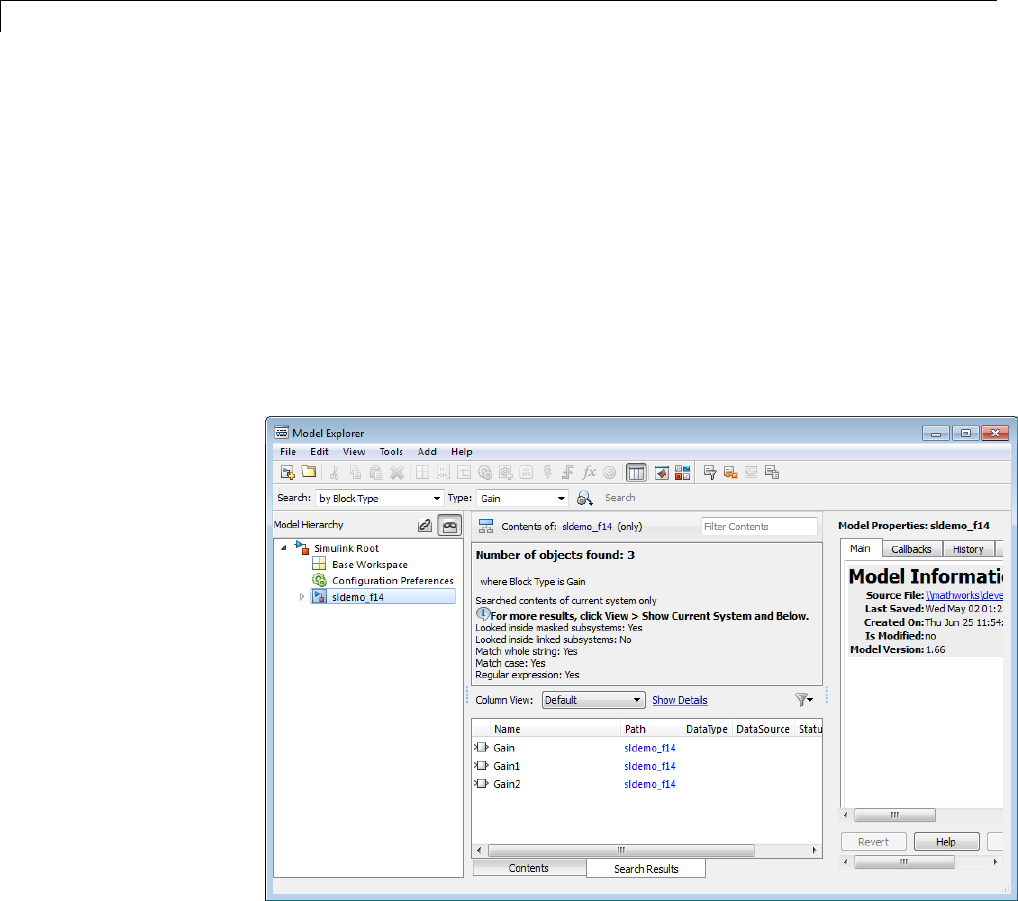
43 Working with Data
UsingtheModelExplorerforBatchEditing
UsingtheModelExplorer(see“ModelExplorer Overview” on page 9-2), you
can assign the same output data type to multiple blocks simultaneously.
For example, the sldemo_f14 model that comes with the Simulink product
contains numerous Gain blocks. Suppose you want to specify the Output
data type parameter of all the Gain blocks in the model as single.Youcan
achieve this task as follows:
1Use the Model Explorer search bar (see “Search Using Model Explorer” on
page 9-63) to identify all blocks in the sldemo_f14 model of type Gain.
The Model Explorer Contents pane lists all Gain blocks in the model.
2In the Model Explorer Contents pane, select all the Gain blocks whose
Output data type parameter you want to specify.
Model Explorer highlights the rows corresponding to your selections.
43-12
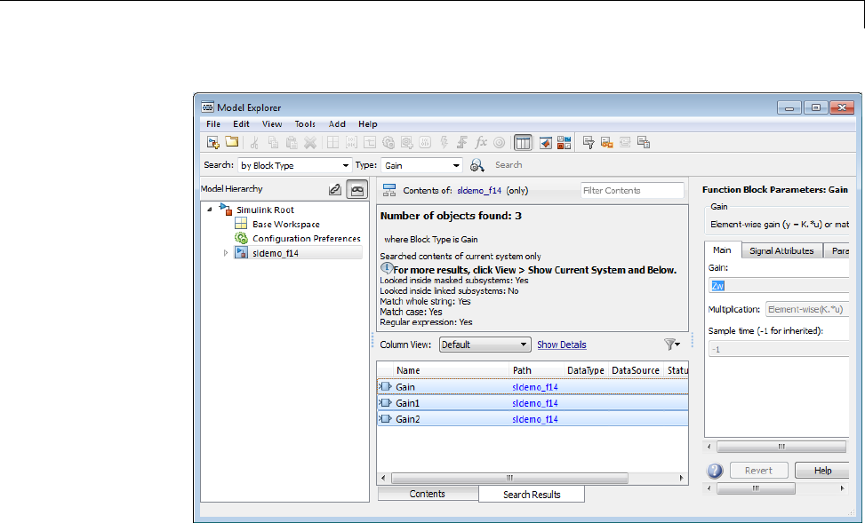
Data Types
3In the Model Explorer Contents pane, click the data type associated with
one of the selected Gain blocks.
Model Explorer displays a pull-down menu with valid data type options.
43-13
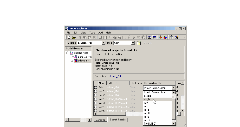
43 Working with Data
4In the pull-down menu, enter or select the desired data type, for example,
single.
Model Explorer specifies the data type of all selected items as single.
43-14
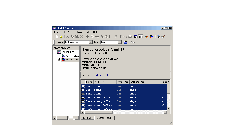
Data Types
Specify Data Types Using Data Type Assistant
The Data Type Assistant is an interactive graphical tool that simplifies
the task of specifying data types for blocks and data objects. The assistant
appears on block and object dialog boxes, adjacent to parameters that provide
data type control, such as the Output data type parameter. For example,
it appears on the Signal Attributes pane of the Constant block dialog box
shown here.
43-15
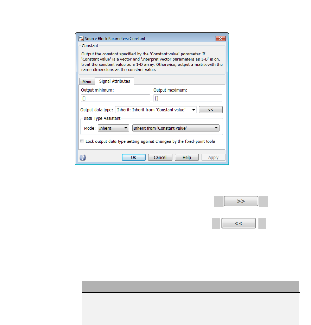
43 Working with Data
You can selectively show or hide the Data Type Assistant by clicking the
applicable button:
•Click the Show data type assistant button to display
the assistant.
•Click the Hide data type assistant button to hide a
visible assistant.
Use theData Type Assistant to specify a data type as follows:
1In theMode field, select the category of data type that you want to specify.
In general, the options include the following:
Mode Description
Inherit Inheritance rules for data types
Built in Built-in data types
Fixed point Fixed-point data types
43-16
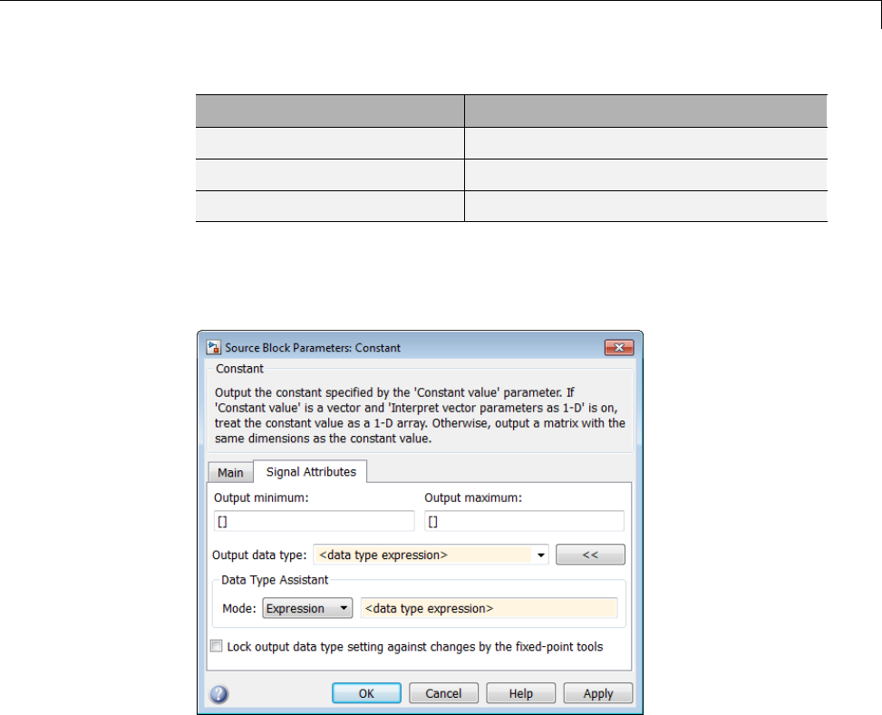
Data Types
Mode Description
Enumerated Enumerated data types
Bus object Bus object data types
Expression Expressionsthatevaluatetodatatypes
The assistant changes dynamically to display different options that
correspond to the selected mode. For example, setting Mode to Expression
causes the Constant block dialog box to appear as follows.
2In the field that is to the right of the Mode field, select or enter a data type.
For example, suppose that you designate the variable myDataType
as an alias for a single data type. You create an instance of the
Simulink.AliasType class and set its BaseType property by entering the
following commands:
myDataType = Simulink.AliasType
myDataType.BaseType = 'single'
43-17
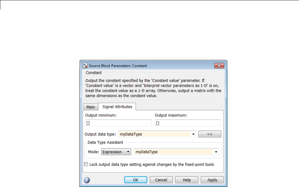
43 Working with Data
Youcanusethisdatatypeobjecttospecifytheoutputdatatypeofa
Constant block. Enter the data type alias name, myDataType,asthevalue
of the expression in the assistant.
3Click the OK or Apply button to apply your changes.
The assistant uses the data type that you specified to populate the
associated data type parameter in the block or object dialog box. In the
following example, the Output data type parameter of the Constant block
specifies the same expression that you entered using the assistant.
43-18
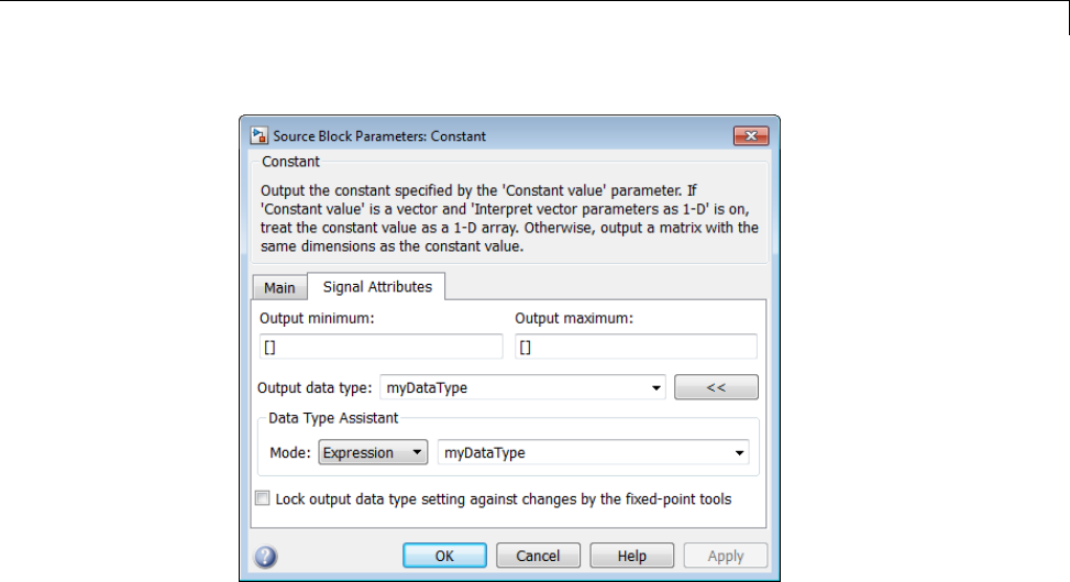
Data Types
For more information about the data types that you can specify using the
Data Type Assistant, see “Entering Valid Data Type Values” on page
43-9. For details about specifying fixed-point data types, see “Specifying
Fixed-Point Data Types with the Data Type Assistant”.
Specifying a Fixed-Point Data Type
When the Data Type Assistant Mode is Fixed point,theDataType
Assistant displays fields for specifying information about your fixed-point
data type. For a detailed discussion about fixed-point data, see “Fixed-Point
Basics”. For example, the next figure shows the Block Parameters dialog box
for a Gain block, with the Signal Attributes tab selected and a fixed-point
data type specified.
43-19
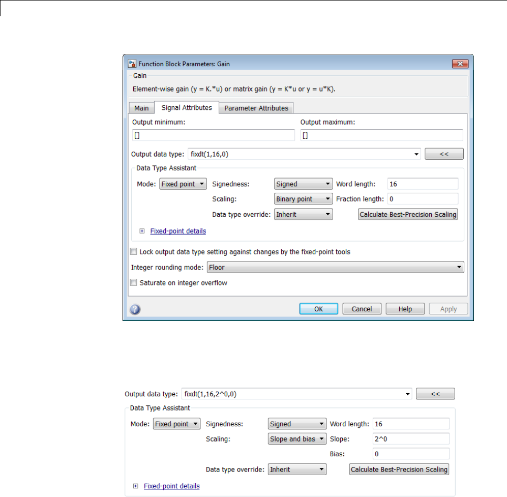
43 Working with Data
If the Scaling is Slope and bias rather than Binary point,theDataType
Assistant displays a Slope field and a Bias field rather than a Fraction
length field:
You can use the Data Type Assistant to set these fixed-point properties:
43-20
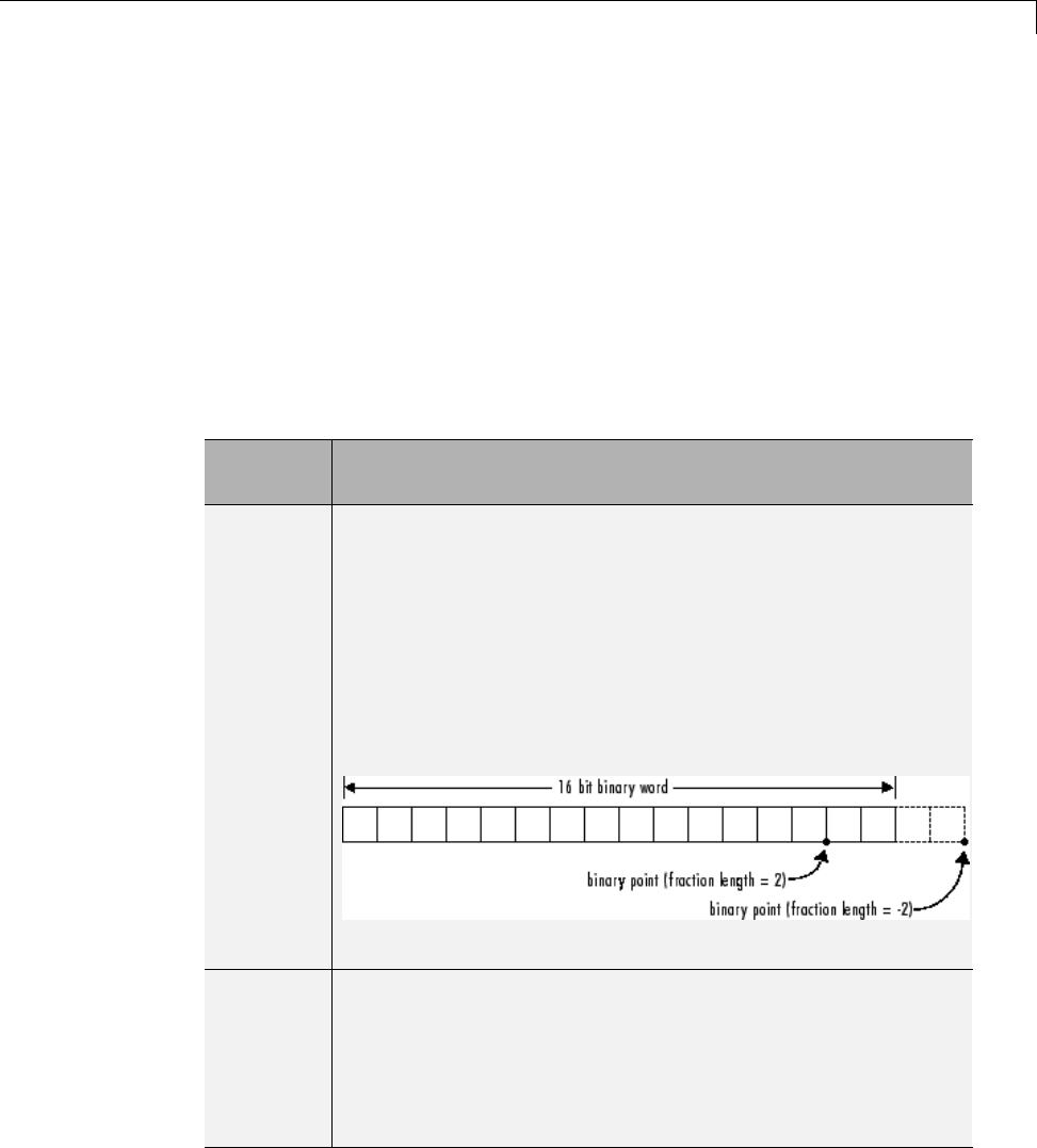
Data Types
Signedness. Specify whether you want the fixed-point data to be Signed
or Unsigned. Signed data can represent positive and negative values, but
unsigned data represents positive values only. The default setting is Signed.
Word length. Specify the bit size of the word that will hold the quantized
integer. Large word sizes represent large values with greater precision than
small word sizes. Word length can be any integer between 0 and 32. The
default bit size is 16.
Scaling. Specify the method for scaling your fixed-point data to avoid
overflow conditions and minimize quantization errors. The default method is
Binary point scaling. You can select one of two scaling modes:
Scaling
Mode
Description
Binary
point
If you select this mode, the Data Type Assistant displays
the Fraction Length field, which specifies the binary point
location.
Binary points can be positive or negative integers. A positive
integer moves the binary point left of the rightmost bit by
that amount. For example, an entry of 2 sets the binary point
in front of the second bit from the right. A negative integer
moves the binary point further right of the rightmost bit by
that amount, as in this example:
The default binary point is 0.
Slope
and bias
If you select this mode, the Data Type Assistant displays fields
for entering the Slope and Bias.
Slope can be any positive real number, and the default slope
is 1.0. Bias can be any real number, and the default bias is
0.0. You can enter slope and bias as expressions that contain
parameters you define in the MATLAB workspace.
43-21

43 Working with Data
Note Use binary-point scaling whenever possible to simplify the
implementation of fixed-point data in generated code. Operations with
fixed-point data using binary-point scaling are performed with simple bit
shifts and eliminate expensive code implementations, which are required
for separate slope and bias values.
For more information about fixed-point scaling, see “Scaling”.
Data type override. When the Mode is Built in or Fixed point,youcan
use the Data type override option to specify whether you want this data
type to inherit or ignore the data type override setting specified for its context,
that is, for the block, Simulink.Signal object or Stateflow chart in Simulink
that is using the signal. The default behavior is Inherit.
Data Type Override Mode Description
Inherit (default) Inherits the data type override
setting from its context, that is, from
the block, Simulink.Signal object
or Stateflow chart in Simulink that
is using the signal.
Off Ignores the data type override
setting of its context and uses the
fixed-point data type specified for
the signal.
The ability to turn off data type override for an individual data type provides
greater control over the data types in your model when you apply data type
override. For example, you can use this option to ensure that data types meet
the requirements of downstream blocks regardless of the data type override
setting.
Calculate Best-Precision Scaling. Click this button to calculate
best-precision values for both Binary point and Slope and bias scaling,
based on the specified minimum and maximum values. The Simulink software
displays the scaling values in the Fraction Length field or the Slope and
Bias fields.For more information, see “Constant Scaling for Best Precision”.
43-22
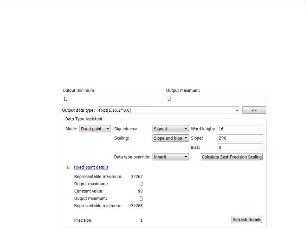
Data Types
Showing Fixed-Point Details. When you specify a fixed-point data type,
you can use the Fixed-point details subpane to see information about the
fixed-point data type that is currently displayed in the Data Type Assistant.
To see the subpane, click the expander next to Fixed-point details in the
Data Type Assistant. The Fixed-point details subpane appears at the
bottom of the Data Type Assistant:
The rows labeled Output minimum and Output maximum show the same
values that appear in the corresponding Output minimum and Output
maximum fields above the Data Type Assistant. The names of these fields
may differ from those shown. For example, a fixed-point block parameter
would show Parameter minimum and Parameter maximum,andthe
corresponding Fixed-point details rows would be labeled accordingly. See
“Signal Ranges” on page 47-44 and “Check Parameter Values” on page 24-9
for more information.
The rows labeled Representable minimum,Representable maximum,and
Precision always appear. These rows show the minimum value, maximum
value, and precision that can be represented by the fixed-point data type
43-23
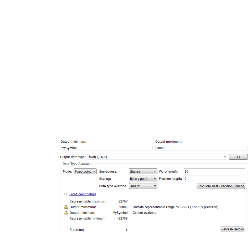
43 Working with Data
currently displayed in the Data Type Assistant. For information about these
three quantities, see “Fixed-Point Basics”.
The values displayed by the Fixed-point details subpane do not
automatically update if you click Calculate Best-Precision Scaling,or
change the range limits, the values that define the fixed-point data type,
or anything elsewhere in the model. To update the values shown in the
Fixed-point details subpane, click Refresh Details.TheDataType
Assistant then updates or recalculates all values and displays the results.
Clicking Refresh Details does not change anything in the model, it only
changes the display. Click OK or Apply to put the displayed values into
effect. If the value of a field cannot be known without first compiling the
model, the Fixed-point details subpaneshowsthevalueasUnknown.
If any errors occur when you click Refresh Details,theFixed-point details
subpane shows an error flag on the left of the applicable row, and a description
of the error on the right. For example, the next figure shows two errors:
The row labeled Output minimum shows the error Cannot evaluate because
evaluating the expression MySymbol,specifiedintheOutput minimum
field, did not return an appropriate numeric value. When an expression does
not evaluate successfully, the Fixed-point details subpane displays the
43-24
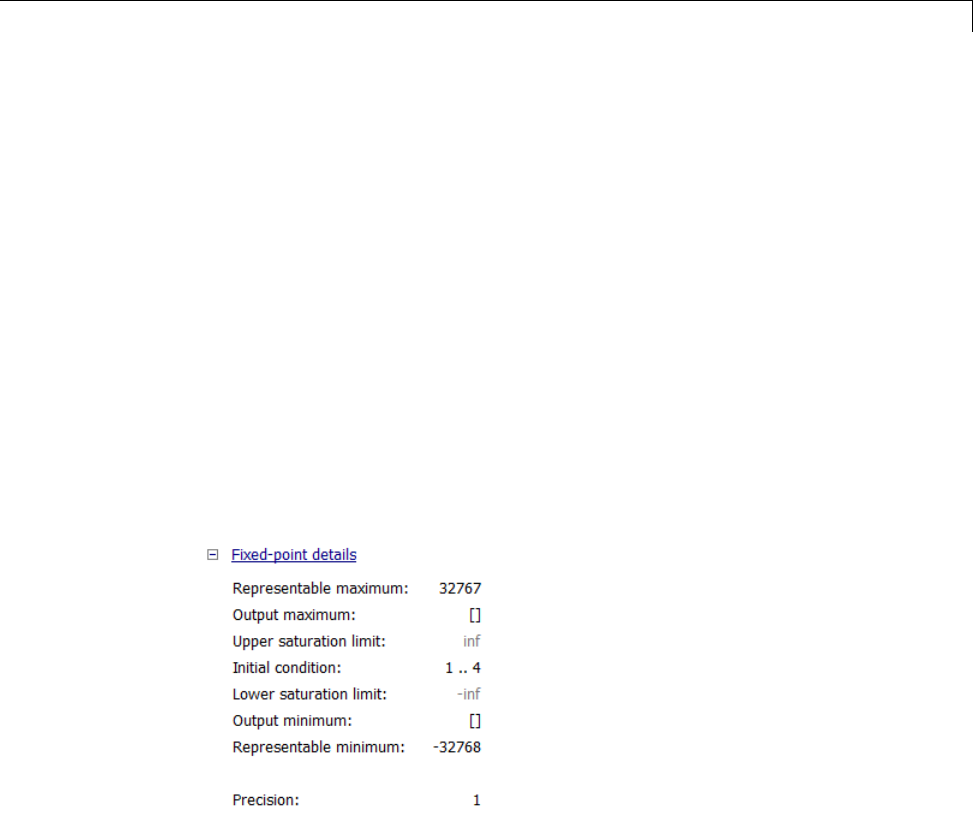
Data Types
unevaluated expression (truncating to 10 characters if necessary to save
space) in place of the unavailable value.
To correct the error in this case, you would need to define MySymbol in an
accessible workspace to provide an appropriate numeric value. After you
clicked Refresh Details,thevalueofMySymbol would appear in place of
its unevaluated text, and the error indicator and error description would
disappear.
To correct the error shown for Output maximum, you would need to decrease
Output maximum, increase Word length, or decrease Fraction length (or
some combination of these changes) sufficiently to allow the fixed-point data
type to represent the maximum value that it could have.
Other values relevant to a particular block can also appear in the Fixed-point
details subpane. For example, on a Discrete-Time Integrator block’s Signal
Attributes tab, the subpane could look like this:
Note that the values displayed for Upper saturation limit and Lower
saturation limit are greyed out. This appearance indicates that the
corresponding parameters are not currently used by the block. The greyed-out
values can be ignored.
Note also that Initial condition displays the value 1..4. The actual value
isavectorormatrixwhosesmallestelementis1and largest element is 4.To
conserve space, the Fixed-point details subpane shows only the smallest
and largest element of a vector or matrix. An ellipsis (..) replaces the omitted
values. The underlying definition of the vector or matrix is unaffected.
43-25
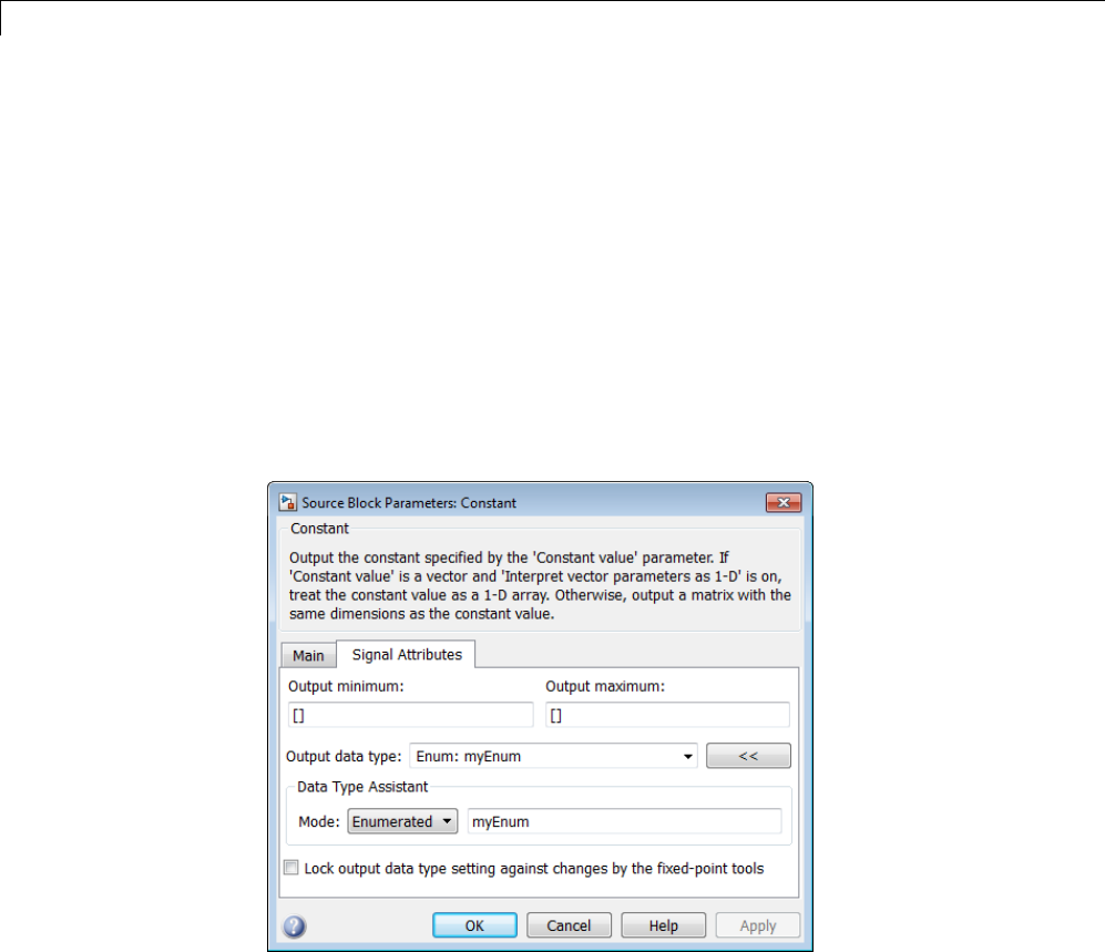
43 Working with Data
Lock output data type setting against changes by the fixed-point
tools. Select this check box to prevent replacement of the current data type
with a type that the Fixed-Point Tool or Fixed-Point Advisor chooses. For
instructions on autoscaling fixed-point data, see “Scaling”.
SpecifyanEnumeratedDataType
You can specify an enumerated data type by selecting the Enum: <class
name> option and specify an enumerated object.
In the Data Type Assistant,youcanusetheMode parameter to specify a
busasadataobjectforablock. SelecttheEnumerated option and specify
an enumerated object.
For details about enumerated data types, see “Data Types”.
Specify a Bus Object Data Type
The blocks listed in the section called “Bus Objects” on page 43-6 support
your specifying a bus object as a data type. For those blocks, in the Data
type parameter, select the Bus: <object name> option and specify a bus
43-26
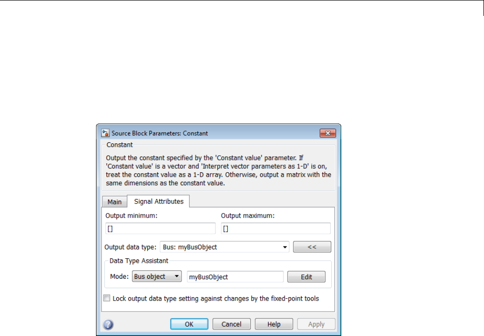
Data Types
object. You cannot use the Expression option to specify a bus object as a
data type for a block.
In the Data Type Assistant,youcanusetheMode parameter to specify a
busasadataobjectforablock.SelecttheBus option and specify a bus object.
You can specify a bus object as the data type for data objects such as
Simulink.Signal,Simulink.Parameter,andSimulink.BusElement.Inthe
Model Explorer, in Properties dialog box for a data object, in the Data type
parameter, select the Bus: <object name> option and specify a bus object.
You can also use the Expression option to specify a bus object.
For more information on specifying a bus object data type, see “Associating
Bus Objects with Simulink Blocks” on page 48-21
Display Port Data Types
In the Simulink Editor, select Display > Signals & Ports > Port Data
Types. The port data type display is not automatically updated when you
changethedatatypeofadiagramelement. Torefreshthedisplay,press
Ctrl+D.
43-27

43 Working with Data
Data Type Propagation
Whenever you start a simulation, enable display of port data types, or refresh
theportdatatypedisplay,theSimulink software performs a processing step
called data type propagation. This step involves determining the types of
signals whose type is not otherwise specified and checking the types of signals
and input ports to ensure that they do not conflict. If type conflicts arise, an
error dialog is displayed that specifies the signal and port whose data types
conflict. The signal path that creates the type conflict is also highlighted.
Note You can insert typecasting (data type conversion) blocks in your model
to resolve type conflicts. See “Typecast Signals” on page 43-29 for more
information.
Data Typing Rules
Observing the following rules can help you to create models that are typesafe
and, therefore, execute without error:
•Signal data types generally do not affect parameter data types, and vice
versa.
A significant exception to this rule is the Constant block, whose output data
type is determined by the data type of its parameter.
•If the output of a block is a function of an input and a parameter, and the
input and parameter differ in type, the Simulink software converts the
parametertotheinputtypebeforecomputingtheoutput.
•In general, a block outputs the data type that appears at its inputs.
Significant exceptions include Constant blocks and Data Type Conversion
blocks, whose output data types are determined by block parameters.
•Virtual blocks accept signals of any type on their inputs.
Examples of virtual blocks include Mux and Demux blocks and
unconditionally executed subsystems.
•The elements of a signal array connected to a port of a nonvirtual block
must be of the same data type.
43-28

Data Types
•The signals connected to the input data ports of a nonvirtual block cannot
differ in type.
•Control ports (for example, Enable and Trigger ports) accept any data type.
•Solver blocks accept only double signals.
•Connecting a non-double signal to a block disables zero-crossing detection
for that block.
Typecast Signals
An error is displayed whenever it detects that a signal is connected to a block
that does not accept the signal’s data type. If you want to create such a
connection, you must explicitly typecast (convert) the signal to a type that the
block does accept. You can use the Data Type Conversion block to perform
such conversions.
Validate a Floating-Point Embedded Model
Youcanusedatatypeoverridemodetoswitchthedatatypesinyourmodel.
This capability allows you to maintain one model but simulate and generate
code for multiple data types, and also validate the numerical behavior for
each type. For example, if you implement an algorithm using double-precision
data types and want to check whether the algorithm is also suitable for
single-precision use, you can apply a data type override to floating-point data
types to replace all doubles with singles without affecting any other data
types in your model.
Apply a Data Type Override to Floating-Point Data Types
To apply a data type override, you must specify the data type that you want to
apply and the data type that you want to replace.
You can set a data type override using one of the following methods. In these
examples, both methods change all floating-point data types to single.
From the Command Line. For example:
set_param(gcs, 'DataTypeOverride', 'Single');
set_param(gcs, 'DataTypeOverrideAppliesTo','Floating-point');
Using the Fixed-Point Tool. For example:
43-29

43 Working with Data
1In the Simulink Editor, select Analysis > Fixed-Point Tool.
The Fixed-Point Tool opens.
2Select View > Show Settings for Selected System.
3In the Fixed-Point Tool right pane, under Settings for selected system:
aSet Data type override to Single.
bSet Data type override applies to Floating-point.
For more information on data type override settings, see fxptdlg.
Validate a Single-Precision Model
This tutorial uses the ex_single_validation model to show how you can
use data type overrides. It proves that an algorithm, which implements
double-precision data types, is also suitable for single-precision embedded use.
43-30
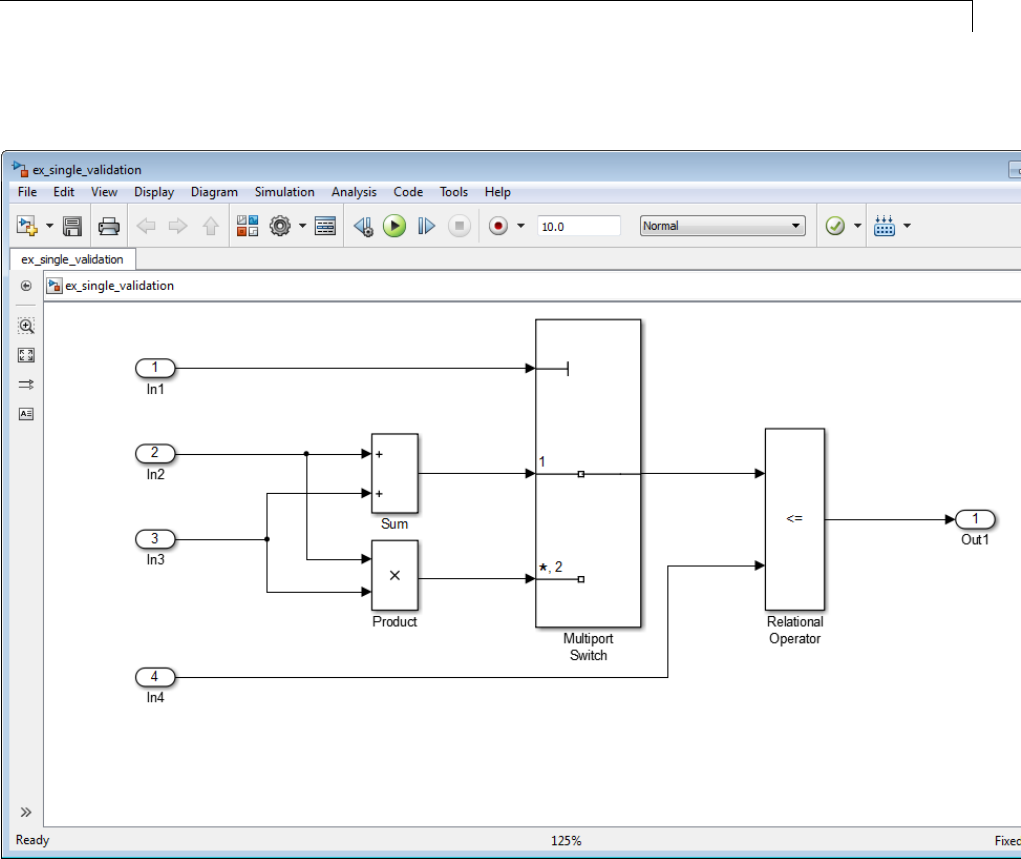
Data Types
About the Model
•The inputs In2 and In3 are double-precision inputs to the Sum and Product
blocks.
•The outputs of the Sum and Product blocks are data inputs to the Multiport
Switch block.
•The input In1 is the control input to the Multiport Switch block. The value
of this control input determines which of its other inputs, the sum of In2
43-31

43 Working with Data
and In3 or the product of In2 and In3, passes to the output port. Because
In1 is a control input, its data type is int8.
•The Relational Operator block compares the output of the Multiport Switch
block to In4, and outputs a Boolean signal.
About the Procedure
In this tutorial, you follow these steps:
1“Generate Code for the Double-Precision Model” on page 43-33
First generate code for the double-precision model to act as a reference
against which you compare the code generated for the single-precision
model.
2“Convert the Model to Single Precision” on page 43-34
Use the Fixed-Point Tool to convert all floating-point data types in the
model to singles. When you apply the data type override, you do not want to
affect the data type of the integer input In1, which acts as a control input.
Changing the data type of In1 might change the behavior of the system.
Applying the data type override only to floating-point data types ensures
that integer data types are not overridden. Similarly, you do not want to
override the logical Boolean output of the Relational Operator block. Data
type overrides never apply to Boolean data types, so this output data type
remains unchanged.
3“Generate Code for the Single-Precision Model” on page 43-35
Finally, you generate code for this single-precision model and verify that
this code is suitable for single-precision embedded use.
Running the Tutorial
Open the Model.
1Open the ex_single_validation model. At the MATLAB command line,
enter:
43-32

Data Types
addpath(fullfile(docroot,'toolbox','simulink','examples'))
ex_single_validation
Generate Code for the Double-Precision Model.
1In the Simulink Editor, select Simulation > Model Configuration
Parameters.
The Configuration Parameters dialog box opens.
2From the Code Generation node, select Report.
On the Report pane, verify that Create code generation report and
Launch report automatically are selected so that the Simulink Coder
software creates a code generation report.
3In the Simulink Editor, select Code>C/C++Code>BuildModel.
Simulink Coder generates code and displays the code generation report.
4Examine the generated code.
aIn the left pane of the report, click the ex_single_validation.h link.
The report displays the header file in the right pane.
In the code that defines external inputs and outputs for root inports and
outports, the input In1 has the type int8_T, all the remaining inputs
are double-precision real_T, and the output Out1 is boolean_T.
/* External inputs (root inport signals with auto storage) */
typedef struct {
int8_T In1;
real_T In2;
real_T In3;
real_T In4;
} ExternalInputs_ex_single_valida;
typedef struct {
boolean_T Out1;
} ExternalOutputs_ex_single_valid;
43-33

43 Working with Data
bIn the left pane of the report, click the ex_single_validation.c link.
The report displays the C code in therightpane. Thecodeforthe
double-precision model contains only double-precision operations.
real_T rtb_MultiportSwitch;
if (ex_single_validation_U.In1 == 1) {
rtb_MultiportSwitch = ex_single_validation_U.In2 +
ex_single_validation_U.In3;
}else{
rtb_MultiportSwitch = ex_single_validation_U.In2 *
ex_single_validation_U.In3;
}
ex_single_validation_Y.Out1 = (rtb_MultiportSwitch <=
ex_single_validation_U.In4);
Convert the Model to Single Precision.
1In the Simulink Editor, select Analysis > Fixed-Point Tool.
The Fixed-Point Tool opens.
2Select View > Show Settings for Selected System.
3In the Fixed-Point Tool right pane, under Settings for selected system:
aSet Data type override to Single.
bSet Data type override applies to Floating-point.
cClick Apply.
4From the Fixed-Point Tool menu, select Collect > Start Simulation.
The simulation runs. The data type override replaces all the floating-point
(double) data types in the model with single data types, but does not
affect the integer or Boolean data types.
43-34
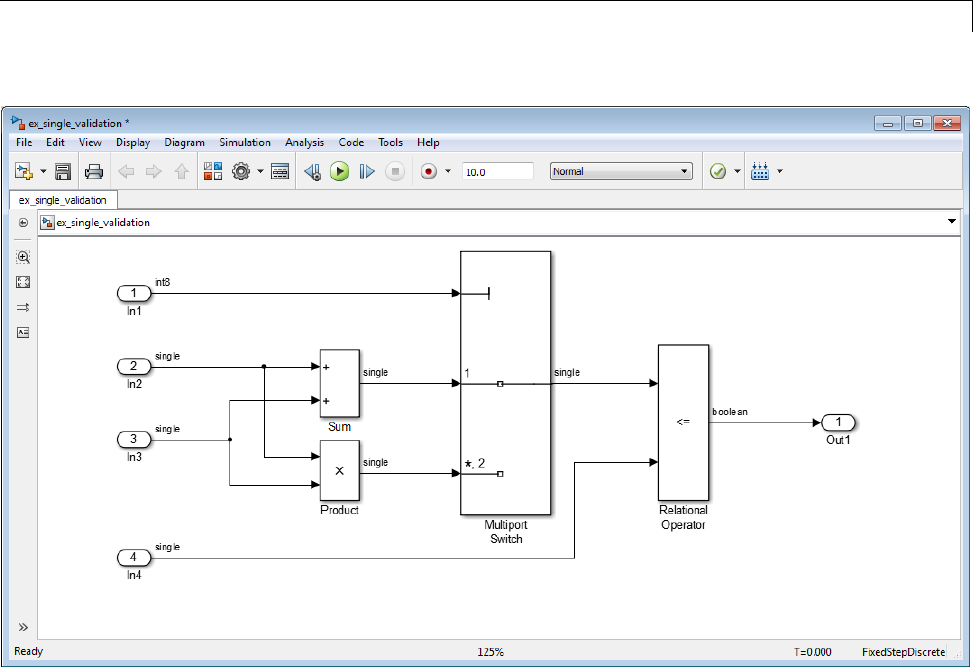
Data Types
Generate Code for the Single-Precision Model.
1In the Simulink Editor, select Code>C/C++Code>BuildModel.
Simulink Coder generates code and displays the code generation report.
2Examine the generated code.
aIn the left pane of the report, click the ex_single_validation.h link.
The report displays the header file in the right pane.
In the code that defines external inputs, the inputs In2,In3,andIn4
are now single-precision real32_T,whereasIn1 is still int8_T,and
Out1 is still boolean_T.
/* External inputs (root inport signals with auto storage) */
43-35

43 Working with Data
typedef struct {
int8_T In1;
real32_T In2;
real32_T In3;
real32_T In4;
} ExternalInputs_ex_single_valida;
typedef struct {
boolean_T Out1;
} ExternalOutputs_ex_single_valid;
bIn the left pane of the report, click the ex_single_validation.c link.
The report displays the C code in the right pane.
real32_T rtb_MultiportSwitch;
if (ex_single_validation_U.In1 == 1) {
rtb_MultiportSwitch = ex_single_validation_U.In2 +
ex_single_validation_U.In3;
}else{
rtb_MultiportSwitch = ex_single_validation_U.In2 *
ex_single_validation_U.In3;
}
ex_single_validation_Y.Out1 = (rtb_MultiportSwitch <=
ex_single_validation_U.In4);
The code for the single-precision model contains only single-precision
operations. Therefore, this code is suitable for single-precision embedded
use.
43-36

Data Objects
Data Objects
In this section...
“About Data Object Classes” on page 43-37
“About Data Object Methods” on page 43-38
“Using the Model Explorer to Create Data Objects” on page 43-40
“About Object Properties” on page 43-42
“Changing Object Properties” on page 43-42
“Handle Versus Value Classes” on page 43-44
“Comparing Data Objects” on page 43-46
“Saving and Loading Data Objects” on page 43-46
“Using Data Objects in Simulink Models” on page 43-46
“Creating Persistent Data Objects” on page 43-47
“Data Object Wizard” on page 43-47
About Data Object Classes
You can create entities called data objects that specify values, data types,
tunability, value ranges, and other key attributes of block outputs and
parameters. You can create various types of data objects and assign them to
workspace variables. You can use the variables in Simulink dialog boxes to
specify parameter and signal attributes. This allows you to make model-wide
changes to parameter and signal specifications simply by changing the
values of a few variables. With Simulink objects you can parameterize the
specification of a model’s data attributes.
Note This section uses the term data to refer generically to signals and
parameters.
The Simulink software uses objects called data classes to define the properties
of specific types of data objects. The classes also define functions, called
methods, for creating and manipulating instances of particular types of
43-37

43 Working with Data
objects. A set of built-in classes are provided for specifying specific types
of attributes. Some MathWorks products based on Simulink, such as the
Simulink Coder product, also provide classes for specifying data attributes
specific to their applications. See the documentation for those products for
information on the classes they provide. You can also create subclasses of
some of these built-in classes to specify attributes specific to your applications
(see “Define Level-1 Data Classes” on page 43-63).
Memory structures called packages areusedtostorethecodeanddatathat
implement data classes. The classes provided by the Simulink software reside
in the Simulink package. Classes provided by products based on Simulink
reside in packages provided by those products. You can create your own
packages for storing the classes that you define.
Class Naming Convention
Simulink uses dot notation to name classes:
PACKAGE.CLASS
where CLASS is the name of the class and PACKAGE is the name of the
packagetowhichtheclassbelongs,forexample,Simulink.Parameter.This
notation allows you to create and reference identically named classes that
belong to different packages. In this notation, the name of the package is
said to qualify the name of the class.
Note Class and package names are case sensitive. You cannot, for example,
use A.B and a.b interchangeably to refer to the same class.
About Data Object Methods
Data classes define functions, called methods, for creating and manipulating
the objects that they define. A class may define any of the following kinds
of methods.
Dynamic Methods
A dynamic method is a method whose identity depends on its name and the
class of an object specified implicitly or explicitly as its first argument. You
43-38

Data Objects
can use either function or dot notation to specify this object, which must be
an instance of the class that defines the method or an instance of a subclass
of the class that defines the method. For example, suppose class Adefines a
method called setName that assigns a name to an instance of A.Further,
suppose the MATLAB workspace contains an instance of A assigned to the
variable obj. Then, you can use either of the following statements to assign
the name 'foo' to obj:
obj.setName('foo');
setName(obj, 'foo');
Aclassmaydefineasetofmethodshavingthesamenameasamethod
defined by one of its super classes. In this case, the method defined by the
subclass overrides the behavior of the method defined by the parent class.
The Simulink software determines which method to invoke at runtime from
theclassoftheobjectthatyouspecifyasitsfirstorimplicitargument.Hence,
the term dynamic method.
Note Most Simulink data object methods are dynamic methods. Unless
the documentation for a method specifies otherwise, you can assume that a
method is a dynamic method.
Static Methods
A static method is a method whose identity depends only on its name and
hence cannot change at runtime. To invoke a static method, use its fully
qualified name, which includes the name of the class that defines it followed
by the name of the method itself. For example, Simulink.ModelAdvisor class
defines a static method named getModelAdvisor. The fully qualified name
of this static method is Simulink.ModelAdvisor.getModelAdvisor.The
following example illustrates invocation of a static method.
ma = Simulink.ModelAdvisor.getModelAdvisor('vdp');
Constructors
Every data class defines a method for creating instances of that class. The
name of the method is the same as the name of the class. For example, the
43-39

43 Working with Data
name of the Simulink.Parameter class’s constructor is Simulink.Parameter.
The constructors defined by Simulink data classes take no arguments.
The value returned by a constructor depends on whether its class is a handle
class or a value class. The constructor for a handle class returns a handle
to the instance that it creates if the class of the instance is a handle class;
otherwise, it returns the instance itself (see “Handle Versus Value Classes”
on page 43-44).
Using the Model Explorer to Create Data Objects
You can use the Model Explorer (see “Model Explorer Overview” on page
9-2) as well as MATLAB commands to create data objects. To use the Model
Explorer,
1Select the workspace in which you want to create the object in the Model
Explorer Model Hierarchy pane.
Only Simulink.Parameter and Simulink.Signal objects for which the
storage class is set to Auto canresideinamodelworkspace. Youmust
create all other Simulink data objects in the base MATLAB workspace
to ensure the objects are unique within the global Simulink context and
accessible to all models.
Note Subclasses of Simulink.Parameter and Simulink.Signal classes,
including mpt.Parameter and mpt.Signal objects (Embedded Coder
license required), can reside in a model workspace only if their storage
class is set to Auto.
43-40
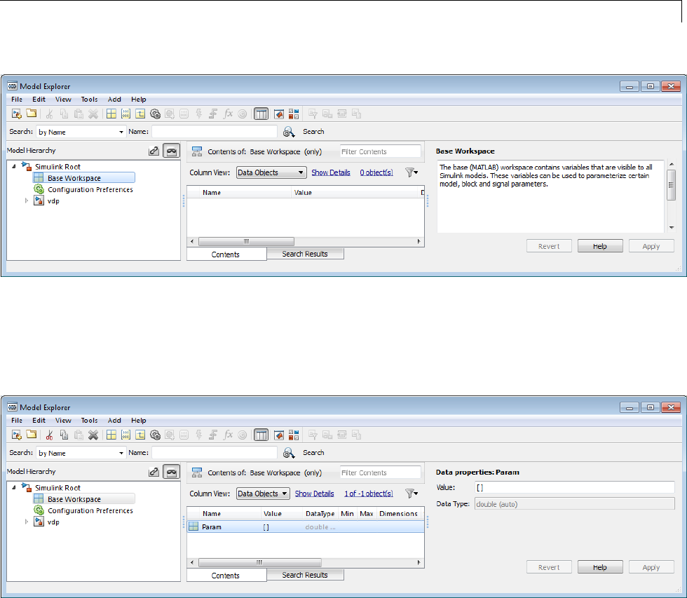
Data Objects
2Selectthetypeoftheobjectthatyou want to create (for example, Simulink
Parameter or Simulink Signal) from the Model Explorer’s Add menu or
from its toolbar. The Simulink software creates the object, assigns it to a
variable in the selected workspace, and displays its properties in the Model
Explorer’s Contents and Dialog panes.
If the type of object you want to create does not appear on the Add menu,
select Find Custom fromthemenu. TheMATLABpathissearchedfor
all data object classes derived from Simulink class on the MATLAB path,
including types that you have created, and displays the result in a dialog
box.
43-41
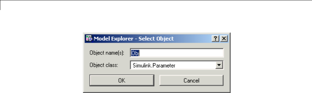
43 Working with Data
3Select the type of object (or objects) that you want to create from the
Object class list and enter the names of the workspace variables to which
youwanttheobjectstobeassignedintheObject name(s) field. Simulink
creates the specified objects and displays them in the Model Explorer’s
Contents pane.
About Object Properties
Object properties are variables associated with an object that specify
properties of the entity that the object represents, for example, the size of a
data type. The object’s class defines the names, value types, default values,
and valid value ranges of the object’s properties.
Changing Object Properties
You can use either the Model Explorer (see “Using the Model Explorer to
Change an Object’s Properties” on page 43-42) or MATLAB commands to
change a data object’s properties (see “Use MATLAB Commands to Change
Workspace Data” on page 4-71).
Using the Model Explorer to Change an Object’s Properties
To use the Model Explorer to change an object’s properties, select the
workspace that contains the object in the Model Explorer’s Model Hierarchy
pane. Then select the object in the Model Explorer’s Contents pane.
43-42

Data Objects
The Model Explorer displays the object’s property dialog box in its Dialog
pane (if the pane is visible).
You can configure the Model Explorer to display some or all of the properties
of an object in the Contents pane (see “Model Explorer: Contents Pane” on
page 9-19). To edit a property, click its value in the Contents or Dialog pane.
The value is replaced by a control that allows you to change the value.
UsingMATLABCommandstoChangeanObject’sProperties
You can also use MATLAB commands to get and set data object properties.
Use the following dot notation in MATLAB commands and programs to get
andsetadataobject’sproperties:
VALUE = OBJ.PROPERTY;
OBJ.PROPERTY = VALUE;
where OBJ is a variable that references either the object if it is an instance
of a value class or a handle to the object if the object is an instance of a
handle class (see “Handle Versus Value Classes” on page 43-44), PROPERTY
is the property’s name, and VALUE is the property’s value. For example, the
following MATLAB code creates a data type alias object (i.e., an instance of
Simulink.AliasType)andsetsitsbasetypetouint8:
gain= Simulink.AliasType;
gain.BaseType = 'uint8';
You can use dot notation recursively to get and set the properties of objects
that are values of other object’s properties, e.g.,
gain.CoderInfo.StorageClass = 'ExportedGlobal';
43-43

43 Working with Data
Handle Versus Value Classes
Simulink data object classes fall into two categories: value classes and handle
classes.
About Value Classes
The constructor for a value class (see “Constructors” on page 43-39) returns
an instance of the class and the instance is permanently associated with the
MATLAB variable to which it is initially assigned. Reassigning or passing the
variable to a function causes MATLAB to create and assign or pass a copy
of the original object.
For example,Simulink.NumericType is a value class. Executing the following
statements
>> x = Simulink.NumericType;
>> y = x;
creates two instances of class Simulink.NumericType in the workspace, one
assigned to the variable xand the other to y.
About Handle Classes
The constructor for a handle class returns a handle object. The handle can be
assigned to multiple variables or passed to functions without causing a copy
of the original object to be created. For example, Simulink.Parameter class
is a handle class. Executing
>> x = Simulink.Parameter;
>> y = x;
creates only one instance of Simulink.Parameter class in the MATLAB
workspace. Variables x and y both refer to the instance via its handle.
A program can modify an instance of a handle class by modifying any variable
that references it, e.g., continuing the previous example,
>> x.Description = 'input gain';
>> y.Description
ans =
43-44

Data Objects
input gain
Most Simulink data object classes are value classes. Exceptions include
Simulink.Signal and Simulink.Parameter class.
You can determine whether a variable is assigned to an instance of a class
or to a handle to that class by evaluating it at the MATLAB command line.
MATLAB appends the text (handle) to the name of the object class in the
value display, e.g.,
>> gain = Simulink.Parameter
gain =
Simulink.Parameter (handle)
Value: []
CoderInfo: [1x1 Simulink.ParamCoderInfo]
Description: ''
DataType: 'auto'
Min: []
Max: []
DocUnits: ''
Complexity: 'real'
Dimensions: [0 0]
Copying Handle Classes
Use the copy method of a handle class to create copies of instances of that
class. For example, Simulink.ConfigSet is a handle class that represents
model configuration sets. The following code creates a copy of the current
model’s active configuration set and attaches it to the model as an alternate
configuration geared to model development.
activeConfig = getActiveConfigSet(gcs);
develConfig = activeConfig.copy;
develConfig.Name = 'develConfig';
attachConfigSet(gcs, develConfig);
43-45

43 Working with Data
Comparing Data Objects
Simulink data objects provide a method, named isContentEqual,that
determines whether object property values are equal. This method compares
the property values of one object with those belonging to another object and
returns true (1) if all of the values are the same or false (0)otherwise. For
example, the following code instantiates two signal objects (A and B) and
specifies values for particular properties.
A = Simulink.Signal;
B = Simulink.Signal;
A.DataType = 'int8';
B.DataType = 'int8';
A.InitialValue = '1.5';
B.InitialValue = '1.5';
Afterward,usetheisContentEqual method to verify that the object
properties of A and B are equal.
>> result = A.isContentEqual(B)
result =
1
Saving and Loading Data Objects
You can use the save command to save data objects in a MAT-file and the
load command to restore them to the MATLAB workspace in the same or a
later session. Definitions of the classes of saved objects must exist on the
MATLAB path for them to be restored. If the class of a saved object acquires
new properties after the object is saved, Simulink adds the new properties to
the restored version of the object. If the class loses properties after the object
is saved, only the properties that remain are restored.
Using Data Objects in Simulink Models
You canusedataobjectsinSimulinkmodelsasparametersandsignals.
Using data objects as parameters and signals allows you to specify simulation
and code generation options on an object-by-object basis.
43-46

Data Objects
Creating Persistent Data Objects
To create parameter and signal objects that persist across Simulink sessions,
first write a script that creates objects (see “Define Level-2 Data Classes” on
page 43-53) or at the command line and save them in a MAT-file (see “Saving
and Loading Data Objects” on page 43-46). Then use either the script or a
load command asthePreLoadFcn callback routine for the model that uses
the objects. For example, suppose you save the data objects in a file named
data_objects.mat and the model to which they apply is open and active.
Then, entering the following command
set_param(gcs, 'PreLoadFcn', 'load data_objects');
at the MATLAB command line sets load data_objects as the model’s
preload function. This in turn causes the data objects to be loaded into the
model workspace whenever you open the model.
Data Object Wizard
The Data Object Wizard allows you to determine quickly which model data
are not associated with data objects and to create and associate data objects
with the data.
To use the wizard to create data objects:
1In the Simulink Editor, select Code > DataObjects > Data Object
Wizard.
43-47
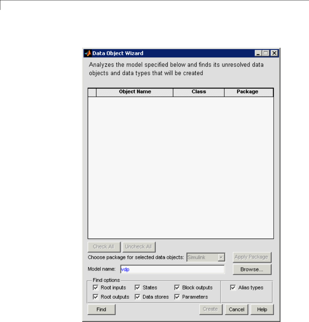
43 Working with Data
The Data Object Wizard appears.
43-48

Data Objects
2Enter, if necessary, the name of the model you want to search in the
wizard’s Model name field.
By default the wizard displays the name of the model from which you
opened the wizard. You can enter the name of another model in this field.
If the model is not open, thewizardopensthemodel.
3In Find options, uncheck any of the data object types that you want the
search to ignore.
The search options include:
Option Description
Root
inputs
Named signals from root-level input ports
Root
outputs
Named signals from root-level output ports
States States associated with any instances of the following
discrete block types:
Discrete Filter
Discrete State-Space
Discrete-Time Integrator
Discrete Transfer Fcn
Discrete Zero-Pole
Memory
PID Controller
PID Controller (2DOF)
Unit Delay
Data stores Data stores (see “About Data Stores” on page 46-2 )
Block
outputs
Named signals emitted by non-root-level blocks.
43-49

43 Working with Data
Option Description
Parameters •Parameters of any instances of the following block
types:
Constant
Gain
Relay
•Stateflow data with a Scope of Parameter.
For more information, see “Sharing Simulink
Parameters with Charts” in the Stateflow
documentation.
Alias types Data whose data type is a registered custom data type.
This option applies only if you are generating code from
the model. See “Create Data Objects with Data Object
Wizard” in the Embedded Coder documentation for more
information.
4Click the wizard’s Find button.
43-50
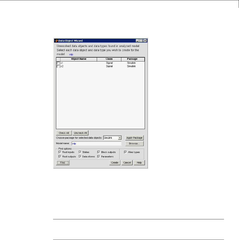
Data Objects
The wizard displays the search results in the data objects table.
5Check the data for which you want the wizard to create data objects.
6If you want the wizard to use data object classes from a package other than
the Simulink standard class package to create the data objects, select the
package from the Choose package for selected data objects list and
then select Apply Package to confirm your choice.
Note User-defined packages that you add to the Data Object Wizard
must contain a Simulink.Signal subclass named Signal and a
Simulink.Parameter subclass named Parameter.
7Click Create.
43-51

43 Working with Data
The wizard creates data objects of the appropriate class for the data
selected in the search results table.
Note Use the Model Explorer to view and edit the created data objects.
43-52

Define Level-2 Data Classes
Define Level-2 Data Classes
Note The Data Class Designer, which is used to define level-1 data classes,
is disabled by default. To learn why you should switch to level-2 data classes,
see “Infrastructure for Extending Simulink Data Classes” on page 43-61
To use the Data Class Designer, see “DefineLevel-1DataClasses”onpage
43-63.
This example shows how to use level-2 data class infrastructure to create
subclasses of Simulink data classes.
Use MATLAB class syntax to create a data class in a package, and, optionally,
assign properties to the data class and define custom storage classes.
Define data class
1Create a package folder +mypkg and add its parent folder to the MATLAB
path.
2Create class folders @Parameter and @Signal inside +mypkg.
Note Simulink requires data classes to be defined inside +Package/@Class
folders.
3In the @Parameter folder, create a MATLAB file Parameter.m and open it
for editing.
4Define a data class that is a subclass of Simulink.Parameter using
MATLAB class syntax.
classdef Parameter < Simulink.Parameter
end % classdef
Optional: Add properties to data class
43-53

43 Working with Data
The properties and end keywords enclose a property definition block.
See “Supported Property Types” on page 43-58.
classdef Parameter < Simulink.Parameter
properties % Unconstrained property type
Prop1 = [];
end
properties(PropertyType = 'logical scalar')
Prop2 = false;
end
properties(PropertyType = 'char')
Prop3 = '';
end
properties(PropertyType = 'char', AllowedValues = {'red'; 'green'; 'blue'}
Prop4 = 'red';
end
end % classdef
Note The MATLAB editor will not recognize the attributes PropertyType
and AllowedValues, because they are only defined for Simulink data classes.
You can suppress mlint warnings about these unrecognized attributes by
right-clicking the attribute in the MATLAB editor and selecting Suppress.
Optional: Add initialization code to data class
You can add a constructor within your data class to perform initialization
activities when the class is instantiated.
In this example, the constructor initializes the value of object obj based on
an optional input argument.
classdef Parameter < Simulink.Parameter
methods
function obj = Parameter(optionalValue)
43-54

Define Level-2 Data Classes
if (nargin == 1)
obj.Value = optionalValue;
end
end
end % methods
end % classdef
Optional: Define custom storage classes
Use the setupCoderInfo method to configure the CoderInfo object of your
class. Then, create a call to the useLocalCustomStorageClasses method and
launch the Custom Storage Class Designer.
1In the constructor within your data class, call the
useLocalCustomStorageClasses method.
classdef Parameter < Simulink.Parameter
methods
function setupCoderInfo(obj)
useLocalCustomStorageClasses(obj, 'mypkg');
obj.CoderInfo.StorageClass = 'Custom';
end
end % methods
end % classdef
2Launch the Custom Storage Class Designer for your package.
cscdesigner('mypkg')
3Define custom storage classes. “Use Custom Storage Class Designer”.
Optional: Define custom attributes for custom storage classes
1Create a MATLAB file myCustomAttribs.m and open it for editing.
2Define a subclass of Simulink.CustomStorageClassAttributes MATLAB
class syntax.
classdef CSCAttributes < Simulink.CustomStorageClassAttributes
properties(PropertyType = 'char')
43-55

43 Working with Data
AlternateName = '';
end
end % classdef
3Override the default implementation of the getInstanceSpecificProps
method.
Note This is an optional step. By default, you can set all custom attributes
to be instance-specific in the Custom Storage Class designer so that
they are modifiable for each data object. However, you can limit which
properties are allowed to be instance-specific.
classdef CSCAttributes < Simulink.CustomStorageClassAttributes
properties(PropertyType = 'char')
AlternateName = '';
end % properties
properties(PropertyType = 'logical scalar')
IsAlternateNameInstanceSpecific = true;
end
methods
function props = getInstanceSpecificProps(obj)
if obj.IsAlternateNameInstanceSpecific
props = findprop(obj, 'AlternateName');
end
end
end % methods
end % classdef
Alternate way of defining level-2 data classes
1Locate the +SimulinkDemos data class package on the MATLAB path.
Note The +SimulinkDemos folder is at
matlabroot/toolbox/simulink/simdemos/dataclasses
43-56

Define Level-2 Data Classes
This package contains predefined data classes.
2Copy the folder to the location where you want to define your data classes.
3Rename the folder +mypkg and add its parent folder to the MATLAB path.
4Modify the data class definitions as desired.
43-57

43 Working with Data
Supported Property Types
If you add properties to a subclass of Simulink.Parameter,Simulink.Signal,
or Simulink.CustomStorageClassAttributes, you can specify the following
property types.
Property Type Syntax
Double number properties(PropertyType =
'double scalar')
int32 number properties(PropertyType =
'int32 scalar')
Logical number properties(PropertyType =
'logical scalar')
String (char) properties(PropertyType =
'char')
String with limited set of allowed
values
properties(PropertyType =
'char', AllowedValues = {'a',
'b', 'c'})
43-58

Upgrade Level-1 Data Classes
Upgrade Level-1 Data Classes
Run the following utility function while specifying the destination folder for
the upgraded classes.
Note Property types defined in level-1 data classes that are
not subclasses of Simulink.Parameter,Simulink.Signal,or
Simulink.CustomStorageClassAttributes are not preserved during an
upgrade. Only subclasses of these three classes will preserve attributes
PropertyType and AllowedValues.
1This command upgrades all your level-1 data class packages. You cannot
upgrade selected data packages.
Simulink.data.upgradeClasses('C:\myLevel2Classes')
Here, C:\myLevel2Classes is the destination folderforyourlevel-2data
classes.
Note Do not place your upgraded level-2 classes and their equivalent
level-1 classes in the same folder.
Simulink.data.upgradeClasses uses the packagedefn.mat file in your
level-1 class packages for the upgrade and creates level-2 classes in the
specified destination folder. Then, Simulink.data.upgradeClasses adds
the folder to top of the MATLAB path and saves the path.
Note If Simulink.data.upgradeClasses cannot save the MATLAB path
because of restricted access, a warning appears. In this case, manually
add the folder to the top of the MATLAB path and save the path using
savepath.
43-59

43 Working with Data
2You can change the location of the level-2 package folders after they have
been generated. However, you will need to update your MATLAB path so
that MATLAB can find these package folders.
3Retain your level-1 classes on the MATLAB path until you have resaved all
of your models and MAT-files that contain level-1 data class objects. Any
models or MAT-files that contain level-1 data classes will continue to work
while your level-1 data classes are on the MATLAB path.
Note You cannot use both level-1 and level-2 data classes at the same
time. Level-2 classes need to be above the level-1 classes on the MATLAB
path so that they are found by MATLAB.
43-60

Infrastructure for Extending Simulink Data Classes
Infrastructure for Extending Simulink Data Classes
In this section...
“Disadvantages of Level-1 Data Class Infrastructure” on page 43-61
“Features of Level-2 Data Class Infrastructure” on page 43-61
“Other Differences between Level-1 and Level-2 Data Classes” on page 43-62
Previously, you could only use the Data Class Designer to create user-defined
subclasses of Simulink data classes such as Simulink.Parameter or
Simulink.Signal.
The Data Class Designer, which is based on level-1 data class infrastructure,
allows you to create, modify, or delete user-defined packages containing
user-defined subclasses.
In a future release, support for level-1 data class infrastructure is being
removed.
In R2012a, a replacement called level-2 data class infrastructure is being
introduced. This infrastructure will allow you to extend Simulink data classes
using MATLAB class syntax.
Disadvantages of Level-1 Data Class Infrastructure
•The syntax for defining data classes using this infrastructure is not
documented.
•The infrastructure offers limited capability for defining data classes:
-You cannot add methods to your data classes.
-You cannot add private or protected properties to your data classes.
•The data classes are only defined in P-code.
Features of Level-2 Data Class Infrastructure
•Ability to upgrade data classes you defined using level-1 data class
infrastructure. See “Upgrade Level-1 Data Classes” on page 43-59.
43-61

43 Working with Data
•Complete flexibility in defining your data classes, which can now have their
own methods and private properties.
•Simplified mechanism for defining custom storage classes for your data
classes.
•Ability to define data classes as readable MATLAB code, not P-code. With
class definitions in MATLAB code, it is easier to understand how these
classes work, to integrate code using configuration management, and to
perform peer code reviews.
•Strict matching for properties, methods, and enumeration property values.
See the detailed example “Define Level-2 Data Classes” on page 43-53.
Other Differences between Level-1 and Level-2 Data
Classes
Level-1 data class infrastructure offers the following capabilities, which are
not supported in the level-2 infrastructure.
•The infrastructure permits partial property matching and does not enforce
case sensitivity. For example, after creating a Simulink.Parameter data
object
a = Simulink.Parameter;
you could set the property Value of the data object by using the following
command.
a.value = 5;
•You can add a data class property that is already included in the superclass.
•You can add a data class property with the same name as the class.
43-62

Define Level-1 Data Classes
Define Level-1 Data Classes
Support for level-1 data class infrastructure will be removed in a future
release. Use level-2 data classes instead. See “Define Level-2 Data Classes”
on page 43-53.
Note The Data Class Designer, which is used to define level-1 data classes,
is disabled by default.
To use the Data Class Designer, run the following commands to enable level-1
data class infrastructure.
sldataclasssetup (1)
savepath
In this section...
“About Packages and Data Classes” on page 43-63
“Define Level-1 Data Classes” on page 43-64
“Working with Classes” on page 43-67
“Enumerated Property Types” on page 43-76
“Enabling Custom Storage Classes” on page 43-79
About Packages and Data Classes
Simulink packages and data classes are introduced in “About Data Object
Classes” on page 43-37 and, if you have a Simulink Coder license, in“Data
Representation”. Simulink resources include several built-in packages and
data classes. You can add user-definedpackagesanddataclasseswiththe
Simulink Data Class Designer, which can:
•Create and delete user-defined packages that can hold user-defined
subclasses.
•Create, change, and delete user-defined subclasses of some Simulink
classes.
43-63

43 Working with Data
•Add and delete user-defined subclasses contained within user-defined
packages.
•Define enumerated property types (not data types) for use by classes in a
package.
•Enable defining custom storage classes for classes that have an appropriate
parent class.
Simulink stores all package and data class definitions as P-files. You can view
any package or data class in the Data Class Designer, but you cannot use the
Designer to change a built-in package or data class. If you create or change
user-defined packages and data classes, do so only in the Data Class Designer.
Do not try to circumvent the Data Class Designer and directly modify any
package or data class definition. An unrecoverable error could result.
Appropriately configured packagesanddataclassescandefinecustom
storage classes, which specify how data is declared, stored, and represented
in generated code. Some built-in packages and data classes define built-in
customstorageclasses. YoucanusetheDataClassDesignertoenablea
user-defined package and data classtohavecustomstorageclasses,as
described in “Enabling Custom Storage Classes” on page 43-79.
Custom storage classes are defined and stored in different files than packages
and data classes use, and different rules apply to changing them. See “Apply
Custom Storage Classes” in the Embedded Coder documentation for complete
information about custom storage classes.
Define Level-1 Data Classes
This example shows how to use level-1 data class infrastructure to create
subclasses of Simulink data classes.
43-64

Define Level-1 Data Classes
Note The Data Class Designer is disabled by default.
To use the Data Class Designer, run the following commands to enable level-1
data class infrastructure.
sldataclasssetup (1)
savepath
Use the Data Class Designer to create a data class in a package, and,
optionally, define custom storage classes.
Create a package
1Open the Simulink Data Class Designer.
sldataclassdesigner
The Data Class Designer loads all packages that exist on the MATLAB
path.
2Click New next to the Package name field, name your package, and click
OK.
3In the Parent directory field, enter the path to the directory for storing
the new package.
Note Do not create class package directories under matlabroot.Packages
in these directories are treated as built-in and will not be visible in the
Data Class Designer.
4Add the parent directory to the MATLAB path.
Define a data class
1In the Classes tab, click New next to the Class name field, name your
class, and click OK.
43-65
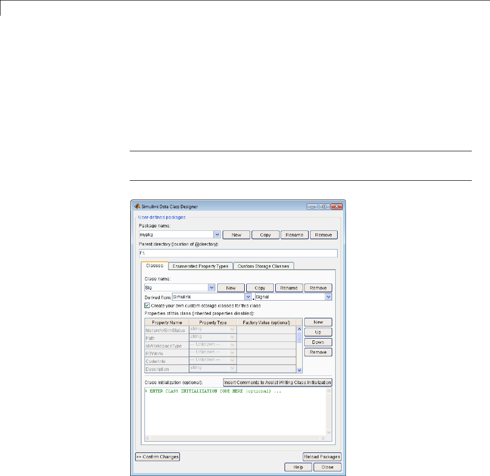
43 Working with Data
2Specify the parent class using the Derived from menus. Select
Simulink.Signal or Simulink.Parameter.
3Select the option to Create your own custom storage classes for this
class.
At least one class in your package must have this option selected.
Note If you do not select this option, your new class inherits the CSCs of
the parent class.
Inthefigureabove,anewpackagemypkg contains a new class called sig
derived from Simulink.Signal. The option to Create your own custom
storage classes for this class is selected.
43-66

Define Level-1 Data Classes
4Add other derived classes to your package and associate CSCs with them.
Register the package
1Click Confirm Changes.
2In the Confirm changes pane, select the package you created.
Note User-defined packages that you plan to add to the Data Object
Wizard must contain a Simulink.Signal subclass named Signal and a
Simulink.Parameter subclass named Parameter.
3Click Write Selected.
The package directories and files, including the CSC registration file, are
written out to the parent directory.
4Click Close.
Optional: Define custom storage classes
Define custom storage classes. See “Use Custom Storage Class Designer”.
Working with Classes
You can use the Simulink Data Class Designer to create and manage
user-defined classes. To view the Data Class Designer, choose Tools > Data
Class Designer from the Simulink menu. When opened, the designer first
scans the MATLAB path and loads any packages that it finds. The Data Class
Designer looks like this when no package is currently selected:
43-67
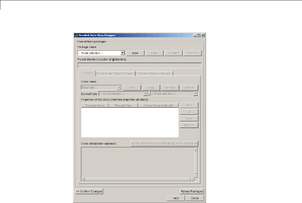
43 Working with Data
You can use the three tabs in the Data Class Designer, and a few other
designer capabilities, to select an existing class, create a new class, copy,
rename, or delete a class, and specify various class properties, as described
in this section. The rest of the designer manages packages, as described in
“Working with Classes” on page 43-67.
Creating a Data Object Class
To create a class within the currently selected package:
43-68

Define Level-1 Data Classes
1In the Simulink Editor, select Code>DataObjects>DesignData
Classes.
The Data Class Designer dialog box appears.
The designer initially scans the MATLAB path and loads any packages
that it finds.
2Selectthenameofthepackageinwhich you want to create the class from
the Package name list.
Do not create a class in any of the Simulink built-in packages, i.e., packages
in matlabroot/toolbox/simulink, or any folder under matlabroot.
3Click the New button on the Classes pane of the Data Class Designer
dialog box.
4Enter the name of the new class in the Class name field on the Classes
pane.
Note The name of the new class must be unique in the package to which
the new class belongs. Class names are case sensitive. For example, Signal
and signal is considered to be names of different classes.
5Press Enter or click OK on the Classes pane to create the specified class
in memory.
6Select a parent class for the new class (see “Specifying a Parent for a Class”
on page 43-71).
7Optionally enable custom storage classes for the class (see “Enabling
Custom Storage Classes” on page 43-79).
8Define the properties of the new class (see “Defining Class Properties”
on page 43-72).
9If necessary, create initialization code for the new class (see “Creating
Initialization Code” on page 43-74).
43-69
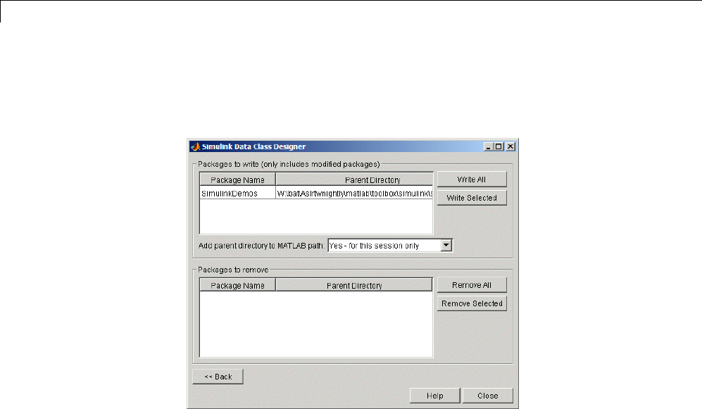
43 Working with Data
10 Click Confirm Changes.
Simulink displays the Confirm Changes pane.
11 Click Write All or select the package containing the new class definition
and click Write Selected to save the new class definition.
Copying a class
To copy a class, select the class in the Classes pane and click Copy.The
Simulink software creates a copy of the class under a slightly different name.
Edit the name, if desired, click Confirm Changes,andclickWrite All or,
after selecting the appropriate package, Write Selected to save the new class.
Renaming a class
To rename a class, select the class in the Classes pane and click Rename.
The Class name field becomes editable. Edit the field to reflect the new
name. Save the package containing the renamed class, using the Confirm
changes pane.
43-70
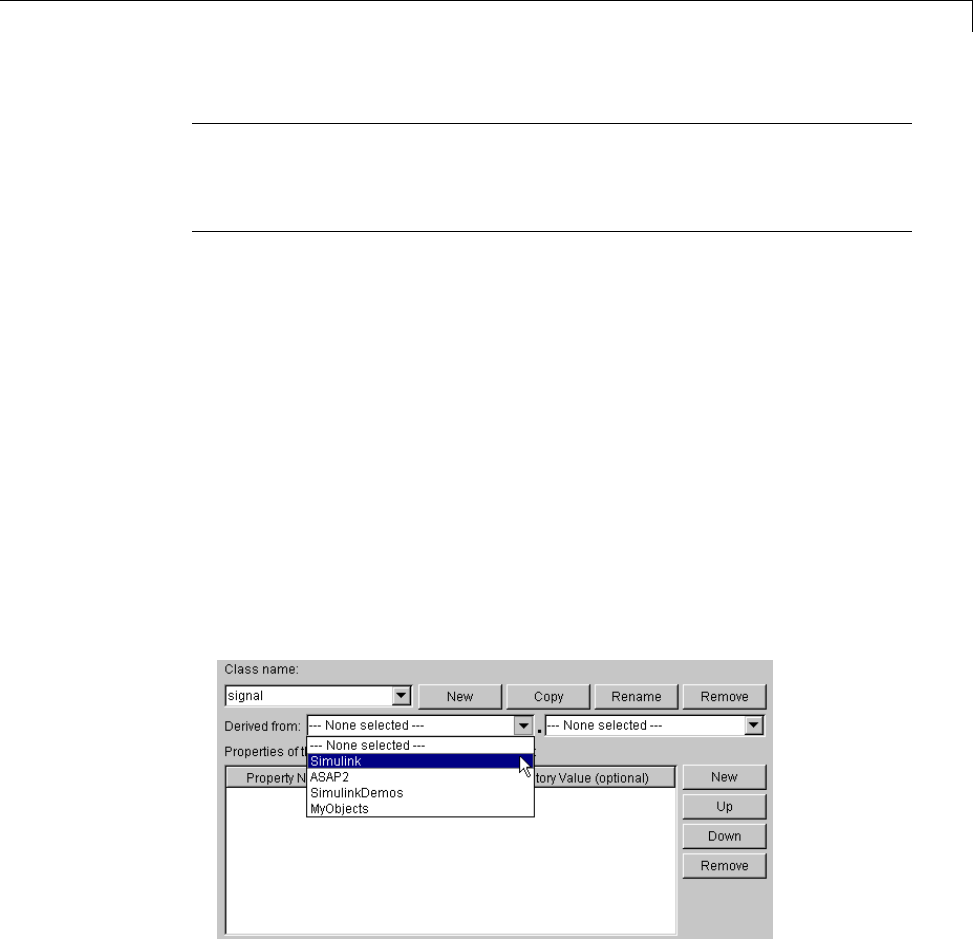
Define Level-1 Data Classes
Note You cannot modify an instantiated Simulink data class. If you try
to modify a class that has already been instantiated during the current
MATLAB session, an error message informs you that you need to restart
MATLAB if you want to modify this package.
Removing a class from a package
To remove a class definition from the currently selected package, select the
class in the Classes pane and click Remove. Theclassisremovedfromthe
in-memory definition of the class. Save the package that formerly contained
the class.
Specifying a Parent for a Class
To specify a parent for a class:
1Select the name of the class from the Class name field on the Classes
pane.
2Selectthepackagenameoftheparentclassfromtheleft-handDerived
from list box.
43-71
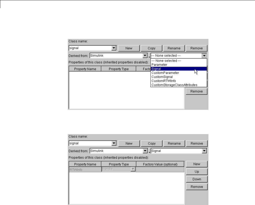
43 Working with Data
3Select the parent class from the right-hand Derived from list.
The properties of the selected class derived from the parent class are
displayed in the Properties of this class field.
The inherited properties are grayed to indicate that they cannot be
redefined by the child class.
4Save the package containing the class.
Defining Class Properties
To add a property to a class:
43-72
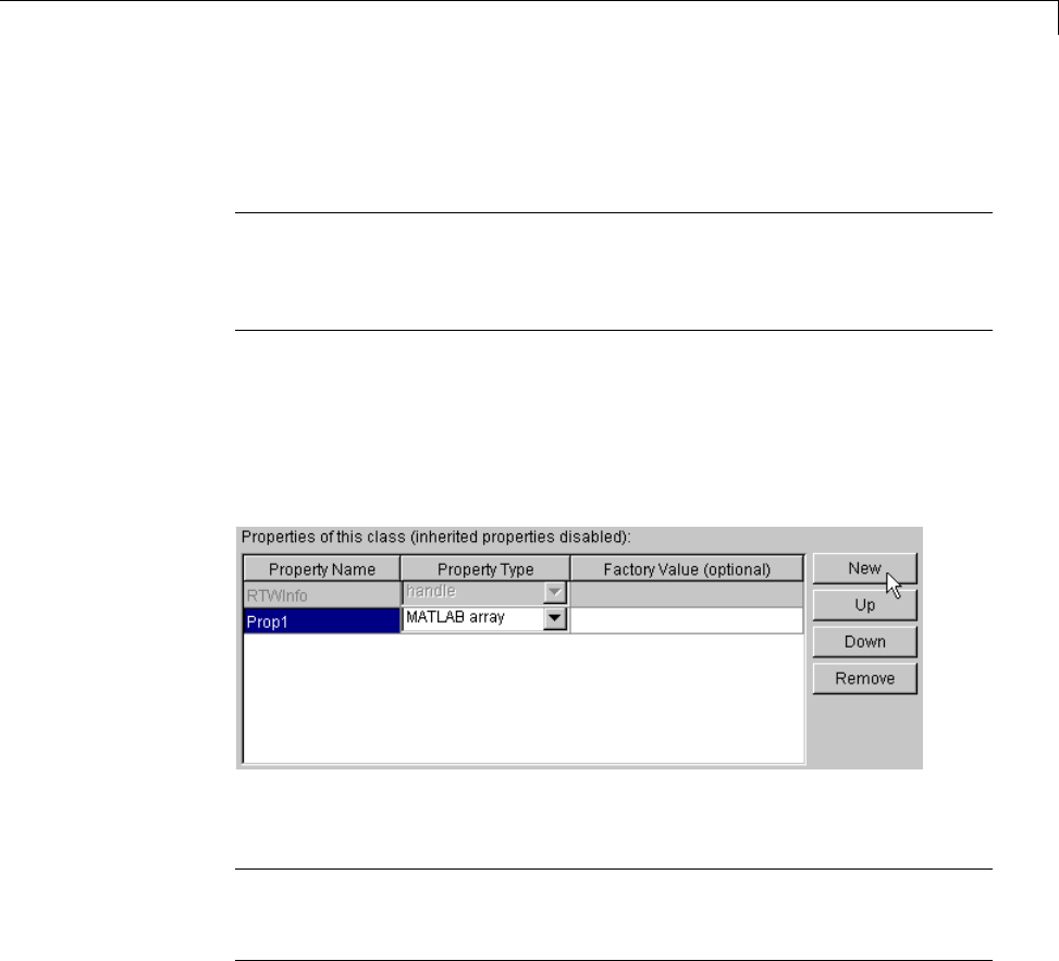
Define Level-1 Data Classes
1Select the name of the class from the Class name field on the Classes
pane.
Note You cannot modify an instantiated Simulink data class. If you try
to modify a class that has already been instantiated during the current
MATLAB session, an error message informs you that you need to restart
MATLAB if you want to modify this package.
2Click the New button next to the Properties of this class field on the
Classes pane.
A property is created with a default name and value and displays the
property in the Properties of this class field.
3Enter a name for the new property in the Property Name column.
Note Thepropertynamemustbeuniqueto the class. Unlike class names,
property names are not case sensitive. For example, Value and value are
treated as referring to the same property.
4Select the data type of the property from the Property Type list.
The list includes built-in property types and any enumerated property types
that you have defined (see “Enumerated Property Types” on page 43-76).
43-73

43 Working with Data
5If you want the property to have a default value, enter the default value in
the Factory Value column.
The default value is the value the property has when an instance of the
associated class is created. The initialization code for the class can override
this value (see “Creating Initialization Code” on page 43-74 for more
information).
The following rules apply to entering factory values for properties:
•Do not use quotation marks when entering the value of a string property.
The value that you enter is treated as a literal string.
•The value of a MATLAB array property can be any expression that
evaluates to an array, cell array, structure, or object. Enter the
expression exactly as you would enter the value on the command line,
for example, [01;10]. The expression that you enter is evaluated to
check its validity. A warning is displayed if evaluating the expression
results in an error. Regardless of whether an evaluation error occurs,
Simulink stores the expression as the factory value of the property. This
is because an expression that is invalid at define time might be valid
at run-time.
•You can enter any expression that evaluates to a numeric value as the
value of a double or int32 property. The expression is evaluated and
the result stored as the property’s factory value.
6Save the package containing the class with new or changed properties.
Creating Initialization Code
You can specify code to be executed when the Simulink software creates an
instance of a data object class. To specify initialization code for a class, select
the class from the Class name field of the Data Class Designer and enter
the initialization code in the Class initialization field.
The Data Class Designer inserts the code that you enter in the Class
initialization field in the class instantiation function of the corresponding
class. This function is invoked when an instance of this class is created.
43-74

Define Level-1 Data Classes
Note Do not include function definitions of the form shown below in the
initialization code. The following example only illustrates how the Data
Class Designer considers a class instantiation function.
function h = ClassName(varargin)
where his the handle to the object that is created and varargin is a cell array
that contains the function’s input arguments.
By entering the appropriate code in the Data Class Designer,youcancause
the instantiation function to perform such initialization operations as
•Error checking
•Loading information from data files
•Overriding factory values
•Initializing properties to user-specified values
For example, suppose you want to let a user initialize the ParamName property
of instances of a class named MyPackage.Parameter. The user does this by
passingtheinitialvalueoftheParamName property to the class constructor:
Kp = MyPackage.Parameter('Kp');
The following code in the instantiation function would perform the required
initialization:
switch nargin
case 0
% No input arguments - no action
case 1
% One input argument
h.ParamName = varargin{1};
otherwise
warning('Invalid number of input arguments');
end
43-75
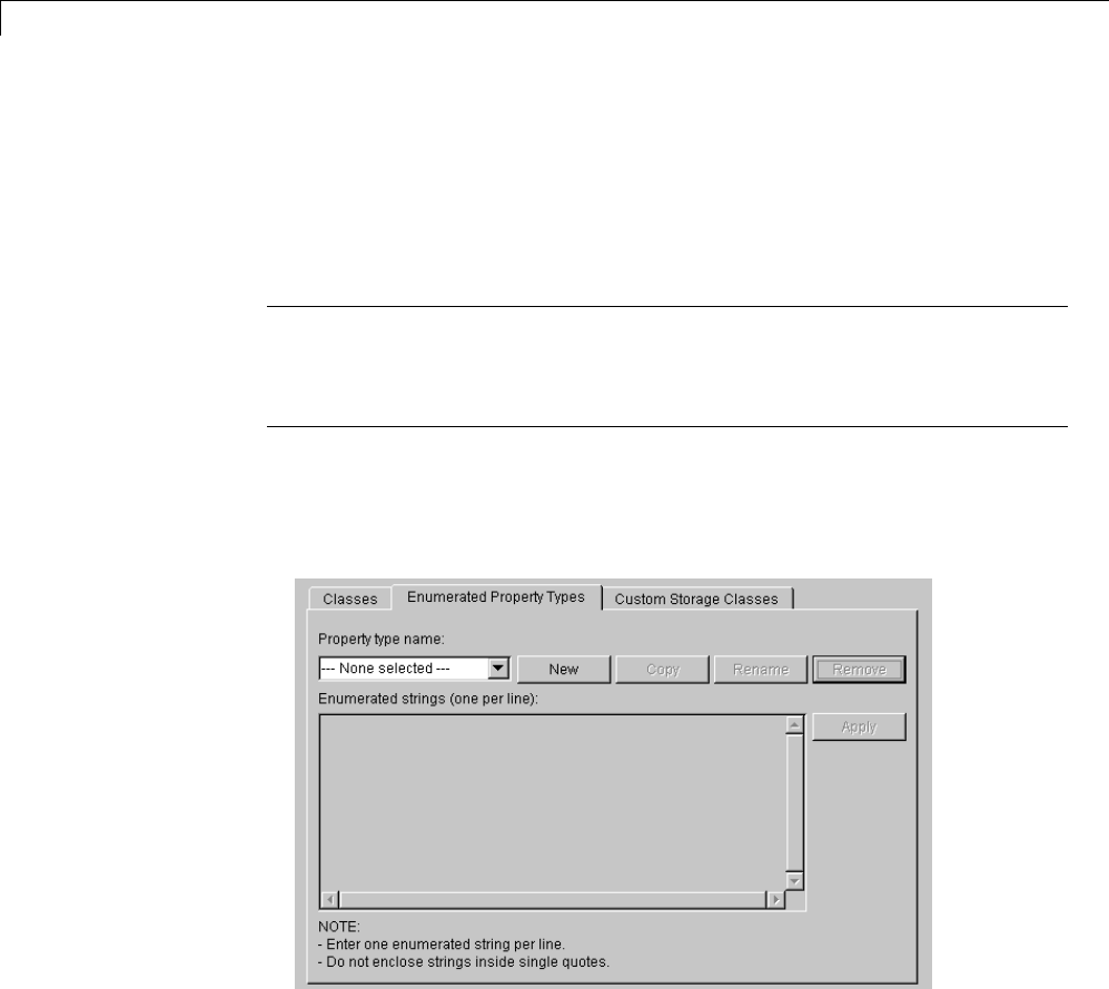
43 Working with Data
Enumerated Property Types
An enumerated property type is a property type whose value must be one of
aspecifiedseto
fvalues,forexample,red,blue,orgreen. An enumerated
property type is valid only in the package that defines it, but must be globally
unique throughout all packages.
Note Do not confuse an enumerated property type with an enumeration.
For informationonenumerations,see“UseEnumeratedDatainSimulink
Models” on page 44-10. The Data Class Designer cannot be used for defining
enumerations.
To create an enumerated property type:
1Select the Enumerated Property Types tab of the Data Class Designer.
43-76

Define Level-1 Data Classes
2Click the New button next to the Property type name field.
An enumerated property type is created with a default name.
3Change the default name in the Property type name field to the desired
name for the property.
The currently selected package defines an enumerated property type and
the type can be referenced only in the package that defines it. However,
the name of the enumerated property type must be globally unique. There
cannot be any other built-in or user-defined enumerated property type with
thesamename. Anerrorisdisplayedifyouenterthenameofanexisting
built-in or user-defined enumerated property type.
4Click the OK button.
The new property is created in memory and the Enumerated strings field
on the Enumerated Property Types pane is enabled .
5Enter the permissible values for the enumerated property type
Enumerated strings field, one per line.
43-77
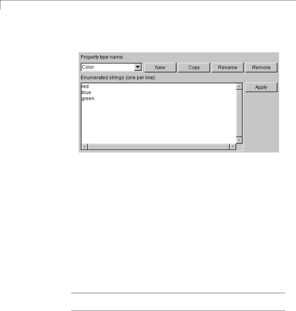
43 Working with Data
For example, the following Enumerated strings field shows the
permissible values for an enumerated property type named Color.
6Click Apply to save the changes in memory.
7Click Confirm changes.ThenclickWrite all to save this change.
You can also use the Enumerated Property Type pane to copy, rename,
and remove enumerated property types.
•Click the Copy button to copy the currently selected property type. A new
property that has a new name, but has the same value set as the original
property is created.
•Click the Rename button to rename the currently selected property type.
The Property name field becomes editable. Edit the field to reflect the
new name.
•Click the Remove button to remove the currently selected property.
Always save the package containing the modified enumerated property type.
Note You must restart the MATLAB software if you modify, add, or remove
enumerated property types from a class you have already instantiated.
43-78

Define Level-1 Data Classes
Enabling Custom Storage Classes
If you select Simulink.Signal or Simulink.Parameter as the parent of a
user-defined class, the Simulink Data Class Designer displays a check box
labeled Create your own custom storage classes for this class.Youcan
ignore this option if you do not intend to use Embedded Coder to generate
code from models that reference this data object class.
Otherwise, select this check box to cause Simulink Data Class Designer
to create custom storage classes for this data object class. The Data Class
Designer also provides a tab labeled Custom Storage Classes, but this tab
is now obsolete.
43-79

43 Working with Data
Associating User Data with Blocks
You can use the set_param command to associate your own data with a block.
For example, the following command associates the value of the variable
mydata with the currently selected block.
set_param(gcb, 'UserData', mydata)
The value of mydata can be any MATLAB data type, including arrays,
structures, objects, and Simulink data objects.
Use get_param to retrieve the user data associated with a block.
get_param(gcb, 'UserData')
The following command saves the user data associated with a block in the
model file of the model containing the block.
set_param(gcb, 'UserDataPersistent', 'on');
Note If persistent UserData for a block contains any Simulink data objects,
the directories containing the definitions for the classes of those objects must
be on the MATLAB path when you open the model containing the block.
43-80

Design Minimum and Maximum
Design Minimum and Maximum
In this section...
“Use of Design Minimum and Maximum” on page 43-81
“Valid Values for Design Minimum and Maximum” on page 43-81
Use of Design Minimum and Maximum
You can specify the design minimum and maximum for model data such as
blocks and data objects. Simulink uses the design minimum and maximum as
follows.
•To define a valid range for Simulink parameters and signals and use it in
range-checking
•To calculate best-precision scaling for fixed-point data types
•To calculate derived minimum and maximum for model data for which
design minimum and maximum are not specified
Valid Values for Design Minimum and Maximum
Simulink no longer allows you to specify the design minimum and maximum
as -Inf/Inf. The default design minimum or maximum is [].
Previously, you could specify the design minimum and maximum as -Inf/Inf.
However, this specification is ambiguous.
It may imply that the design minimum and maximum are explicitly specified;
in other words, it may imply that the parameter or signal can have any value.
It may also imply that the design minimum and maximum are unspecified.
While this ambiguity may not have a significant effect on range-checking,
it could affect the calculation of derived minimum and maximum or the
checking of data type validity.
Note Simulink generates an error or warning when you specify the design
minimum and maximum as -Inf/Inf.
43-81

43 Working with Data
Avoiding Specifying Infinite Design Minimum or Maximum
There are three sources for the warning Simulink generates if the design
minimum and/or maximum are set to -Inf/Inf. Each source requires a
different solution.
1MATLAB code
aUse error handling tools such as dbstop and lastwarn to locate the
MATLAB code that is setting the design minimum and maximum to
-Inf/Inf.
bEither remove these lines of code from the MATLAB file or replace
instances of -Inf and Inf with [].
2MAT-file: Resave the MAT-file
3SLX file: Resave the SLX file
43-82


44 Enumerations and Modeling
About Simulink Enumerations
Simulink enumerations are built on enumerations defined for the
MATLAB language. They are subclasses of the abstract superclass
Simulink.IntEnumType, and inherit from that superclass the capabilities
necessary to be used in the Simulink environment.
Before you begin to use enumerations in a modeling context, you should
understand information provided in “Enumerations”.
The following examples show how to use enumerations in Simulink and
Stateflow:
Example Shows How To Use...
Data Typing in Simulink Data types in Simulink, including
enumerated data types
Modeling a CD Player/Radio Using
Enumerated Data Types
Enumerated data types in a
Simulink model that contains a
Stateflow chart
For information on using enumerations in Stateflow, see “Enumerated Data”.
44-2

Define Simulink®Enumerations
Define Simulink Enumerations
In this section...
“Workflow to Define a Simulink Enumeration” on page 44-3
“Create Simulink Enumeration Class” on page 44-3
“Customize Simulink Enumeration” on page 44-4
“Save Enumeration in a MATLAB File” on page 44-7
“Change and Reload Enumerations” on page 44-7
“Import Enumerations Defined Externally to MATLAB” on page 44-8
Workflow to Define a Simulink Enumeration
1Create a class definition.
2Optionally, customize the enumeration.
3Optionally, save the enumeration in a MATLAB file.
Create Simulink Enumeration Class
To create a Simulink enumeration class, in the class definition:
•Define the class as a subclass of Simulink.IntEnumType
•Add an enumeration block that specifies enumeration values with
underlying integer values
Consider the following example:
classdef BasicColors < Simulink.IntEnumType
enumeration
Red(0)
Yellow(1)
Blue(2)
end
end
44-3

44 Enumerations and Modeling
The first line defines an integer-based enumeration that is derived from
built-in class Simulink.IntEnumType. The enumeration is integer-based
because IntEnumType is derived from int32.
The enumeration section specifies threeenumeratedvalues.
Enumerated Value Enumerated Name Underlying Integer
Red(0) Red 0
Yellow(1) Yellow 1
Blue(2) Blue 2
When defining an enumeration class for use in the Simulink environment,
consider the following:
•The name of the enumeration class must be unique among data type names
and base workspace variable names, and is case-sensitive.
•Underlying integer values in the enumeration section need not be unique
within the class and across types.
•Often, the underlying integers of a set of enumerated values are consecutive
and monotonically increasing, but they need not be either consecutive or
ordered.
•For simulation, an underlying integer can be any int32 value. Use the
MATLAB functions intmin and intmax to get the limits.
•For code generation, every underlyingintegervaluemustberepresentable
as an integer on the target hardware, which may impose different limits.
See“Target”and“HardwareImplementationPane”formoreinformation.
For more information on superclasses, see “Converting to Superclass Value”.
Customize Simulink Enumeration
About Simulink Enumeration Customizations
You can customize a Simulink enumeration by using the same techniques
that work with MATLAB classes, as described in “Modifying Superclass
Methods and Properties”.
44-4

Define Simulink®Enumerations
A primary source of customization are the methods associated with an
enumeration.
Inherited Methods
Enumeration class definitions can include an optional methods section.
Simulink enumerated classes inherit the following static methods from
the superclass Simulink.IntEnumType. For more information about these
methods, see Simulink.defineIntEnumType.
Default Method Description Default Value
Returned or
Specified
Usage Context
getDescription Returns a description
of the enumeration.
'' Code generation
getHeaderFile Specifies the file
in which the
enumeration is
defined for code
generation.
'' Code generation
addClassNameToEnumNames Specifies whether the
class name becomes
a prefix in generated
code.
false —prefixisnot
used
Code generation
Overriding Inherited Methods
You can override the inherited methods to customize the behavior of an
enumeration. To override a method, include a customized version of the
method in the methods section in the enumerated class definition. If you do
not want to override the inherited methods, omit the methods section.
Specifying a Default Enumerated Value
Simulink software and related generated code use an enumeration’s default
value for ground-value initialization of enumerated data when you provide no
other initial value. For example, an enumerated signal inside a conditionally
executed subsystem that has not yet executed has the enumeration’s default
value. Generated code uses an enumeration’s default value if a safe cast
44-5

44 Enumerations and Modeling
fails, as described in “Type Casting for Enumerations” in the Simulink Coder
documentation.
Unless you specify otherwise, the default value for an enumeration is the first
value in the enumeration class definition. To specify a different default value,
add your own getDefaultValue method to the methods section. The following
code shows a shell for the getDefaultValue method:
function retVal = getDefaultValue()
% GETDEFAULTVALUE Returns the default enumerated value.
% This value must be an instance of the enumerated class.
% If this method is not defined, the first enumeration is used.
retVal = ThisClass.EnumName;
end
To customize this method, provide a value for ThisClass.EnumName that
specifies the desired default.
•ThisClass must be the name of the class within which the method exists.
•EnumName must be the name of an enumerated value defined in that class.
For example:
classdef BasicColors < Simulink.IntEnumType
enumeration
Red(0)
Yellow(1)
Blue(2)
end
methods (Static)
function retVal = getDefaultValue()
retVal = BasicColors.Blue;
end
end
end
This example defines the default as BasicColors.Blue. If this method does
not appear, the default value would be BasicColors.Red, because that is the
first value listed in the enumerated class definition.
44-6

Define Simulink®Enumerations
The seemingly redundant specification of ThisClass inside the definition of
that same class is necessary because getDefaultValue returns an instance
of the default enumerated value, not just the name of the value. The
method, therefore, needs a complete specification of what to instantiate. See
“Instantiate Enumerations” on page 44-15 for more information.
SaveEnumerationinaMATLABFile
You can define an enumeration within a MATLAB file.
•The name of the definition file must match the name of the enumeration
exactly, including case. For example, the definition of enumeration
BasicColors must reside in a file named BasicColors.m.Otherwise,
MATLAB will not find the definition.
•You must define each class definition in a separate file.
•Save each definition file on the MATLAB search path. MATLAB searches
thepathtofindadefinitionwhennecessary.
To add a file or folder to the MATLAB search path, type addpath pathname
at the MATLAB command prompt. For more information, see “Using the
MATLAB Search Path”, addpath,andsavepath.
•You do not need to execute an enumeration class definition to use the
enumeration. The only requirement, as indicated in the preceding bullet, is
thatthedefinitionfilebeontheMATLABsearchpath.
Change and Reload Enumerations
You can change the definition of an enumeration by editing and saving the
file that contains the definition. You do not need to inform MATLAB that a
class definition has changed. MATLAB automatically reads the modified
definition when you save the file. However, the class definition changes do
not take full effect if any class instances (enumerated values) exist that
reflect the previous class definition. Such instances might exist in the base
workspace or might be cached.
The following table explains options for removing instances of an enumeration
from the base workspace and cache.
44-7

44 Enumerations and Modeling
If In Base Workspace... If In Cache...
Do one of the following:
•Locate and delete specific obsolete
instances.
•Delete everything from the
workspace by using the clear
command.
•Delete obsolete instances by
closing all models that you
updated or simulated while the
previous class definition was in
effect.
•Clear functions and close models
that are caching instances of the
class.
For more information about applying enumeration changes, see “Modifying
and Reloading Classes”.
Import Enumerations Defined Externally to MATLAB
If you have enumerations defined externally to MATLAB—for example,
in a data dictionary, that you want to import for use within the Simulink
environment, you can do so programmatically with calls to the function
Simulink.defineIntEnumType. This function defines an enumeration that
you can use in MATLAB as if it is defined by a class definition file. In addition
to specifying the enumeration class name and values, each function call can
specify:
•String that describes the enumeration class.
•Which of the enumeration values is the default.
For code generation, you can specify:
•Header file in which the enumeration is defined for generated code.
•Whether the code generator applies the class name as a prefix to
enumeration members—for example, BasicColors_Red or Red.
As an example, consider the following class definition:
classdef BasicColors < Simulink.IntEnumType
enumeration
Red(0)
44-8

Define Simulink®Enumerations
Yellow(1)
Blue(2)
end
methods (Static = true)
function retVal = getDescription()
retVal = 'Basic colors...';
end
function retVal = getDefaultValue()
retVal = BasicColors.Blue;
end
function retVal = getHeaderFile()
retVal = 'mybasiccolors.h';
end
function retVal = addClassNameToEnumNames()
retVal = true;
end
end
end
The following function call defines the same class for use in MATLAB:
Simulink.defineIntEnumType('BasicColors', ...
{'Red', 'Yellow', 'Blue'}, [0;1;2],...
'Description', 'Basic colors', ...
'DefaultValue', 'Blue', ...
'HeaderFile', 'mybasiccolors.h', ...
'DataScope', 'Imported', ...
'AddClassNameToEnumNames', true);
44-9

44 Enumerations and Modeling
Use Enumerated Data in Simulink Models
In this section...
“Simulate with Enumerations” on page 44-10
“Specify Enumerations as Data Types” on page 44-12
“Get Information About Enumerations” on page 44-13
“Enumeration Value Display” on page 44-13
“Instantiate Enumerations” on page 44-15
“Enumerated Values in Computation” on page 44-19
Simulate with Enumerations
Consider the following enumeration class definition—BasicColors with
enumerated values Red,Yellow,andBlue,withBlue as the default value:
classdef BasicColors < Simulink.IntEnumType
enumeration
Red(0)
Yellow(1)
Blue(2)
end
methods (Static)
function retVal = getDefaultValue()
retVal = BasicColors.Blue;
end
end
end
Once this class definition is known to MATLAB, you can use the enumeration
in Simulink and Stateflow models. Information specific to enumerations in
Stateflow appears in “Enumerated Data”. The following Simulink model
uses the enumeration defined above:
44-10
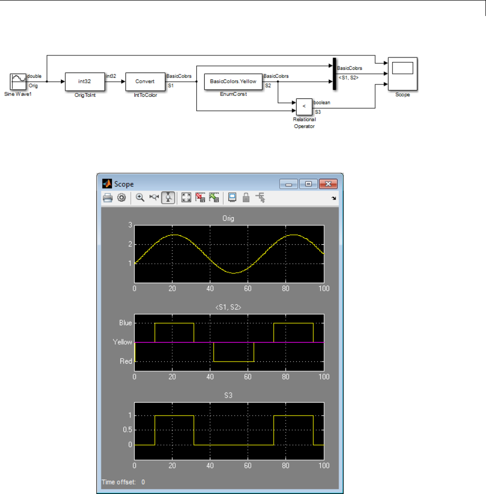
Use Enumerated Data in Simulink®Models
The output of the model looks like this:
The Data Type Conversion block OrigToInt specifies an Output data type
of int32 and Integer rounding mode: Floor,sotheblockconvertsthe
44-11

44 Enumerations and Modeling
Sine Wave block output, which appears in the top graph of the Scope display,
to a cycle of integers: 1,2,1,0,1,2,1. The Data Type Conversion block
IntToColor uses these values to select colors from the enumerated type
BasicColors by referencing their underlying integers.
The result is a cycle of colors: Yellow,Blue,Yellow,Red,Yellow,Blue,
Yellow, as shown in the middle graph. The Enumerated Constant block
EnumConst outputs Yellow, which appears in the second graph as a straight
line. The Relational Operator block compares the constant Yellow to each
value in the cycle of colors. It outputs 1(true)whenYellow is less than the
current color, and 0(false) otherwise, as shown in the third graph.
The sort order used by the comparison is the numeric order of the underlying
integers of the compared values, not the lexical order in which the enumerated
values appear in the enumerated class definition. In this example the two
orders are the same, but they need not be. See “Specify Enumerations as Data
Types” on page 44-12 and “Enumerated Values in Computation” on page
44-19 for more information.
Specify Enumerations as Data Types
Once you define an enumeration, you can use it much like any other data
type. Becauseanenumerationisaclassratherthananinstance,youmust
use the prefix ? or Enum: when specifying the enumeration as a data type.
You must use the prefix ?in the MATLAB Command Window. However, you
can use either prefix in a Simulink model. Enum: has the same effect as the
?prefix, but Enum: is preferred because it is more self-explanatory in the
context of a graphical user interface.
Depending on the context, type Enum: followed by the name of an
enumeration, or select Enum: <class name> from a menu (for example, for
the Output data type block parameter) , and replace <class name>.
To use the Data Type Assistant, set the Mode to Enumerated,thenenterthe
name of the enumeration. For example, in the previous model, the Data Type
Conversion block IntToColor, which outputs a signal of type BasicColors,
has the following output signal specification:
44-12
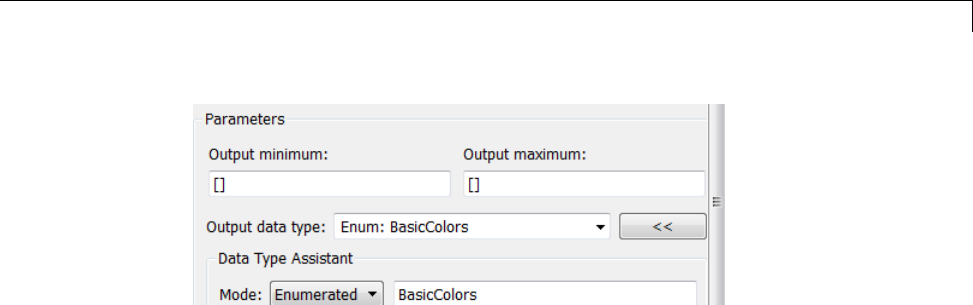
Use Enumerated Data in Simulink®Models
You cannot set a minimum or maximum value for a signal defined as an
enumeration, because the concepts of minimum and maximum are not
relevant to the purpose of enumerations. If you change the minimum or
maximum for a signal of an enumeration from the default value of [], an error
occurs when you update the model. See “Enumerated Values in Computation”
on page 44-19 for more information.
Get Information About Enumerations
Use the enumeration function to:
•Return an array that contains all enumeration values for an enumeration
class in the MATLAB Command Window
•Get the enumeration values programmatically
•Provide the values to a Simulink block parameter that accepts an array or
vector of enumerated values, such as the Case conditions parameter of
the Switch Case block
See the enumeration function for details.
Enumeration Value Display
Wherever possible, Simulink software displays enumeration values by name,
not by the underlying integer value. However, the underlying integers can
affect value display in Scope and Floating Scope blocks.
44-13

44 Enumerations and Modeling
Block... Affect on Value Display...
Scope When displaying an enumerated signal, the names
of the enumerated values appear as labels on the Y
axis. The names appear in the order given by their
underlying integers, with the lowest value at the
bottom.
Floating Scope When displaying signals that are of the same
enumeration, names appear on the Y axis as they
would for a Scope block. If the Floating Scope block
displays mixed data types, no names appear, and
any enumerated values are represented by their
underlying integers.
Enumerated Values with Non-Unique Integers
More than one value in an enumeration can have the same underlying integer
value, as described in “Specify Enumerations as Data Types” on page 44-12.
When this occurs, the value on an axis of Scope block output or in Display
block output always is the first value listed in the enumerated class definition
that has the shared underlying integer. For example:
44-14
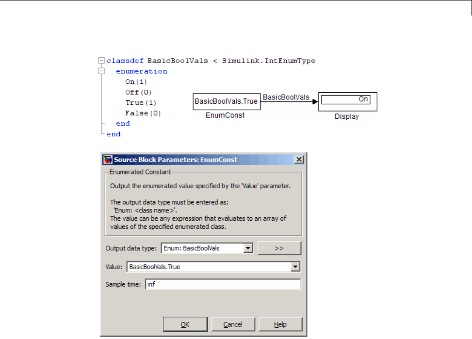
Use Enumerated Data in Simulink®Models
Although the Enumerated Constant block outputs True,bothOn and True
have the same underlying integer, and On is defined first in the class definition
enumeration section. Therefore, the Display block shows On. Similarly, a
Scope axis would show only On,neverTrue, no matter which of the two values
is input to the Scope block.
Instantiate Enumerations
Before you can use an enumeration, you must instantiate it. You can
instantiate an enumeration in MATLAB, in a Simulink model, or in a
Stateflow chart. The syntax is the same in all contexts.
44-15
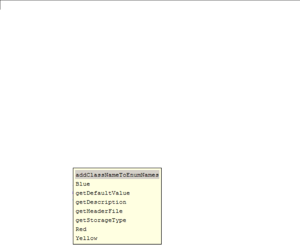
44 Enumerations and Modeling
Instantiating Enumerations in MATLAB
To instantiate an enumeration in MATLAB, enter ClassName.EnumName in the
MATLAB Command Window. The instance is created in the base workspace.
For example, if BasicColors is defined as in “Create Simulink Enumeration
Class” on page 44-3, you can type:
bcy = BasicColors.Yellow
bcy =
Yellow
Tab completion works for enumerations. For example, if you enter:
bcy = BasicColors.<tab>
MATLAB displays the elements andmethodsofBasicColors in alphabetical
order:
Double-clickanelementormethodtoinsertitatthepositionwhereyou
pressed <tab>. See “Tab Completion” for more information.
Casting Enumerations in MATLAB
In MATLAB, you can cast directly from an integer to an enumerated value:
bcb = BasicColors(2)
bcb =
44-16
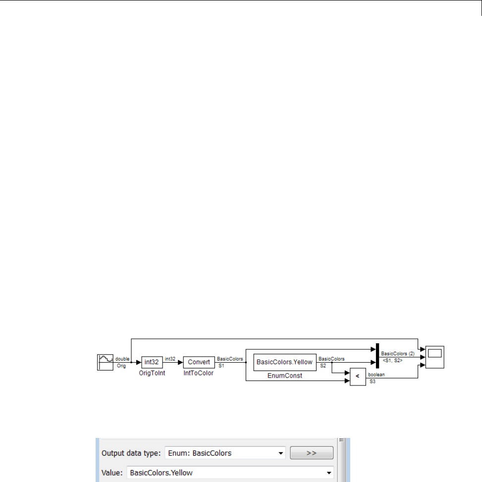
Use Enumerated Data in Simulink®Models
Blue
You can also cast from an enumerated value to its underlying integer:
>> bci = int32(bcb)
bci =
2
In either case, MATLAB returns the result of the cast in a 1x1 array of the
relevant data type.
Although casting is possible, use of enumeration values is not robust in
cases where enumeration values and the integer equivalents defined for an
enumeration class might change.
Instantiating Enumerations in Simulink (or Stateflow)
To instantiate an enumeration in a Simulink model, you can enter
ClassName.EnumName as a value in a dialog box. For example, consider the
following model:
The Enumerated Constant block EnumConst, which outputs the enumerated
value Yellow, defines that value as follows:
You can enter any valid MATLAB expression that evaluates to an
enumerated value, including arrays and workspace variables. For example,
you could enter BasicColors(1), or if you had previously executed
44-17
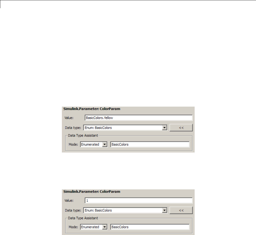
44 Enumerations and Modeling
bcy = BasicColors.Yellow in the MATLAB Command Window, you
could enter bcy. As another example, you could enter an array, such
as[BasicColors.Red, BasicColors.Yellow, BasicColors.Blue] .
You can use a Constant block to output enumerated values. However, that
block displays parameters that do not apply to enumerated types, such as
Output Minimum and Output Maximum.
If you create a Simulink.Parameter object as an enumeration, you must
specify the Value parameter as an enumeration member and the Data type
with the Enum: or ? prefix, as explained in “Specify Enumerations as Data
Types” on page 44-12.
You cannot specify the integer value of an enumeration member for the
Value parameter. See “Enumerated Values in Computation” on page 44-19
for more information. Thus, the following fails even though the integer value
for BasicColors.Yellow is 1.
The same syntax and considerations apply in Stateflow. See “Enumerated
Data” for more information.
44-18

Use Enumerated Data in Simulink®Models
Enumerated Values in Computation
By design, Simulink prevents enumerated values from being used as numeric
values in mathematical computation, even though an enumerated class is a
subclass of the MATLAB int32 class. Thus, an enumerated type does not
function as a numeric type despite the existence of its underlying integers.
For example, you cannot input an enumerated signal directly to a Gain block.
You can use a Data Type Conversion block to convert in either direction
between an integer type and an enumerated type, or between two enumerated
types. That is, you can use a Data Type Conversion block to convert an
enumerated signal to an integer signal (consisting of the underlying integers
of the enumerated signal values) and input the resulting integer signal to
aGainblock
. See “Casting Enumerated Signals” on page 44-19 for more
information.
Enumerated types in Simulink are intended to represent program states
and control program logic in blocks like the Relational Operator block and
the Switch block. When a Simulink block compares enumerated values, the
values compared must be of the same enumerated type. The block compares
enumerated values based on their underlying integers, not their order in the
enumerated class definition.
When a block like the Switch block or Multiport Switch block selects among
multiple data signals, and any data signal is of an enumerated type, all the
data signals must be of that same enumerated type. When a block inputs
both control and data signals, as Switch and Multiport Switch do, the control
signal type need not match the data signal type.
Casting Enumerated Signals
You can use a Data Type Conversion block to cast an enumerated signal to
asig
nal of any numeric type, provided that the underlying integers of all
enumerated values input to the block are within the range of the numeric
type. Otherwise, an error occurs during simulation.
Similarly, you can use a Data Type Conversion block to cast a signal of any
integer type to an enumerated signal, provided that every value input to the
Data Type Conversion block is the underlying integer of some value in the
enumerated type. Otherwise, an error occurs during simulation.
44-19
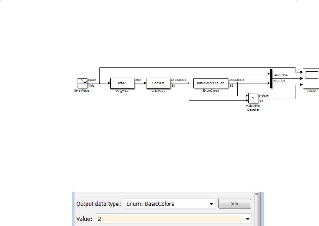
44 Enumerations and Modeling
You cannot use a Data Type Conversion block to cast a numeric signal of any
non-integer data type to an enumerated type. For example, the model used in
“Simulate with Enumerations” on page 44-10 needed two Data Conversion
blocks to convert a sine wave to enumerated values.
The first block casts double to int32, and the second block casts int32
to BasicColors. You cannot cast a complex signal to an enumerated type
regardless of the data types of its real and imaginary parts.
Casting Enumerated Block Parameters
You cannot cast a block parameter of any numeric data type to an enumerated
data type. For example, suppose that an Enumerated Constant block specifies
aValue of 2and an Output data type of Enum: BasicColors:
An error occurs because the specifications implicitly cast a double value
to an enumerated type. The error occurs even though the numeric value
corresponds arithmetically to one of the enumerated values in the enumerated
type.
You cannot cast a block parameter of an enumeration to any other data type.
For example, suppose that a Constant block specifies a Constant value of
BasicColors.Blue and an Output data type of int32.
44-20
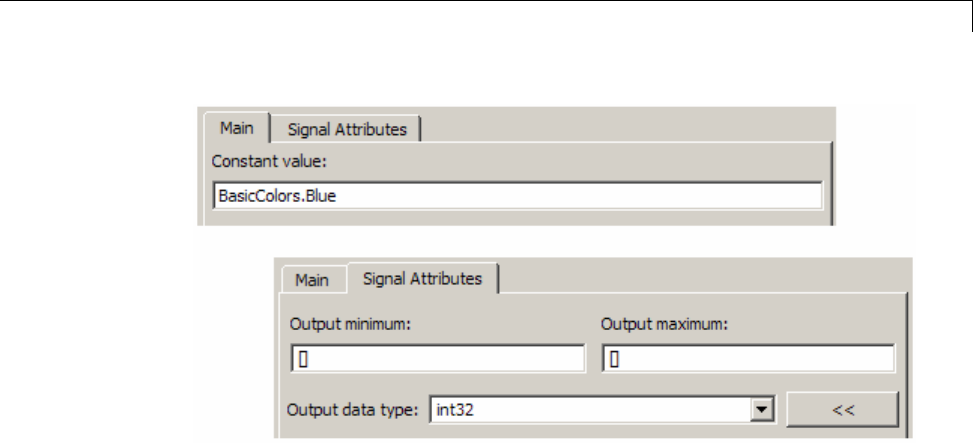
Use Enumerated Data in Simulink®Models
An error occurs because the specifications implicitly cast an enumerated value
to a numeric type. The error occurs even though the enumerated value’s
underlying integer is a valid int32.
44-21

44 Enumerations and Modeling
Simulink Constructs that Support Enumerations
In this section...
“Overview” on page 44-22
“Block Support” on page 44-22
“Class Support” on page 44-24
“Logging Enumerated Data” on page 44-24
“Importing Enumerated Data” on page 44-24
Overview
In general, all Simulink tools and constructs support enumerated types for
which the support makes sense given the purpose of enumerated types: to
represent program states and to control program logic. The Simulink Editor,
Simulink Debugger, Port Value Displays, referenced models, subsystems,
masks, buses, data logging, and most other Simulink capabilities support
enumerated types without imposing any special requirements.
Enumerated types are not intended for mathematical computation, so no
block that computes a numeric output (as distinct from passing a numeric
input through to the output) supports enumerated types. Thus an enumerated
type is not considered to be a numeric type, even though an enumerated value
has an underlying integer. See “Enumerated Values in Computation” on page
44-19 for more information.
Most capabilities that do not support enumerated types obviously could not
support them. Therefore, the Simulink documentation usually mentions
enumerated type nonsupport only where necessary to prevent a misconception
or describe an exception. See “Simulink Enumeration Limitations” on page
44-25 for information about certain constructs that could support enumerated
types but do not.
Block Support
The following Simulink blocks support enumerated types:
•Constant (but Enumerated Constant is preferable)
44-22

Simulink®Constructs that Support Enumerations
•Data Type Conversion
•Data Type Conversion Inherited
•Data Type Duplicate
•Display
•MATLAB Function
•Enumerated Constant
•Floating Scope
•From File
•From Workspace
•Inport
•Interval Test
•Interval Test Dynamic
•Multiport Switch
•Outport
•Probe (input only)
•Relational Operator
•Relay (output only)
•Repeating Sequence Stair
•Scope
•Signal Specification
•Switch
•Switch Case
•To File
•To Workspace
All members of the following categories of Simulink blocks support
enumerated types:
44-23

44 Enumerations and Modeling
•Bus-capable blocks (see “Bus-Capable Blocks” on page 48-19)
•Pass-through blocks:
-With state, like the Data Store Memory and Unit Delay blocks.
-Without state, like the Mux block.
Many Simulink blocks in addition to those named above support enumerated
types, but they either belong to one of the categories listed above, or are rarely
used with enumerated types. The Data Type Support section of each block
reference page describes all data types that the block supports.
Class Support
The following Simulink classes support enumerated types:
•Simulink.Signal
•Simulink.Parameter
•Simulink.AliasType
•Simulink.BusElement
Logging Enumerated Data
Root-level outports, To Workspace blocks, and Scope blocks can all export
enumerated values. Signal and State logging work with enumerated data in
the same way as with any other data. All logging formats are supported. The
From File block does not support enumerated data. Use the From Workspace
block instead, combined with some technique for transferring data between a
file and a workspace. See “Export Runtime Information” for more information.
Importing Enumerated Data
Root-level inports and From Workspace blocks can output enumerated signals
during simulation. Data must be provided in a Structure,Structure with
Time,orTimeSeries object. No interpolation occurs for enumerated values
between the specified simulation times. From File blocks produce only data
of type double, so they do not support enumerated types. See “Import Data”
for more information.
44-24

Simulink®Enumeration Limitations
Simulink Enumeration Limitations
In this section...
“Enumerations and Scopes” on page 44-25
“Enumerated Types for Switch Blocks” on page 44-25
“Nonsupport of Enumerations” on page 44-25
Enumerations and Scopes
When a Scope block displays an enumerated signal, the vertical axis displays
the names of the enumerated values only if the scope was open during
simulation. If you open the Scope block for the first time before any simulation
has occurred, or between simulations, the block displays only numeric values.
When simulation begins, enumerated names replace the numeric values, and
thereafter appear whenever the Scope block is opened.
When a Floating Scope block displays multiple signals, the names of
enumerated values appear on the Y axis only if all signals are of the same
enumerated type. If the Floating Scope block displays more than one type
of enumerated signal, or any numeric signal, no names appear, and any
enumerated values are represented by their underlying integers.
Enumerated Types for Switch Blocks
The control input of a Switch block can be of any data type supported
by Simulink software. However, the u2 ~=0 mode is not supported for
enumerations. If the control input has an enumeration, choose one of the
following methods to specify the criteria for passing the first input:
•Select u2 >= Threshold or u2 > Threshold and specify a threshold value
of the same enumerated type as the control input.
•Use a Relational Operator block to do the comparison and then feed the
Boolean result of this comparison into the control port of the Switch block.
Nonsupport of Enumerations
The following limitations exist when using enumerated data types with
Simulink:
44-25

44 Enumerations and Modeling
•Packages cannot contain enumeration class definitions.
•You cannot define enumerations by using a GUI like the Data Class
designer.
•The If Action block might support enumerations, but currently does not
do so.
•Generated code does not support logging enumerated data.
•Custom Stateflow targets do not support enumerated types.
•HDL Coder does not support enumerations.
44-26

45
Importing and Exporting
Simulation Data
•“Using Simulation Data” on page 45-3
•“Export Simulation Data” on page 45-4
•“Data Format for Exported Simulation Data” on page 45-8
•“Limit Amount of Exported Data” on page 45-14
•“Control Samples to Export for Variable-Step Solvers” on page 45-16
•“Export Signal Data Using Signal Logging” on page 45-19
•“Configure a Signal for Signal Logging” on page 45-21
•“View Signal Logging Configuration” on page 45-27
•“Enable Signal Logging for a Model” on page 45-34
•“Override Signal Logging Settings” on page 45-41
•“Access Signal Logging Data” on page 45-53
•“Techniques for Importing Signal Data” on page 45-61
•“Import Data to Model a Continuous Plant” on page 45-67
•“Import Data to Test a Discrete Algorithm” on page 45-70
•“Import Data for an Input Test Case” on page 45-71
•“Import Signal Logging Data” on page 45-75
•“Import Data to Root-Level Input Ports” on page 45-77
•“Import and Map Data to Root-Level Inports” on page 45-81
•“Import MATLAB timeseries Data” on page 45-98

45 Importing and Exporting Simulation Data
•“Import Structures of timeseries Objects for Buses” on page 45-100
•“Import Simulink.Timeseries and Simulink.TsArray Data” on page 45-104
•“Import Data Arrays” on page 45-105
•“Import MATLAB Time Expression Data” on page 45-107
•“Import Data Structures” on page 45-108
•“Import and Export States” on page 45-113
45-2

Using Simulation Data
Using Simulation Data
Working with Simulation Data
During simulation, you can:
•Import input signal and initial state data from a workspace or file.
•Export output signal and state data to a workspace or file.
Exporting (logging) simulation data provides a baseline for analyzing
and debugging a model. Use standard or custom MATLAB functions to
generate simulated system input signals and to graph, analyze, or otherwise
postprocess the system outputs.
Also, import data into a model for testing and analysis.
45-3

45 Importing and Exporting Simulation Data
Export Simulation Data
In this section...
“Simulation Data” on page 45-4
“Approaches for Exporting Signal Data” on page 45-4
“Enable Simulation Data Export” on page 45-6
“View Logged Simulation Data With the Simulation Data Inspector” on
page 45-7
Simulation Data
Simulation data can include any combination of signal, time, output, state,
and data store logging data.
Exporting simulation data involves saving signal values to the MATLAB
workspace during simulation for later retrieval and postprocessing. Exporting
data is also known as “data logging” or “saving simulation data.”
You can also import the exported data to use as input for simulating a model.
Approaches for Exporting Signal Data
Exporting simulation data very often involves exporting signal data. You can
use a variety of approaches for exporting signal data.
Export Approach Usage Documentation
Connect a signal to a Scope
block or viewer.
If you use a Scope block
for viewing results during
simulation, consider also using
theScopeblocktoexportdata.
Document in the diagram the
workspace variables used to
store signal data.
Save output at a sample rate
other than the base sample
rate.
Scope
45-4

Export Simulation Data
Export Approach Usage Documentation
Scopes store data and can be
memory intensive.
Connect a signal to a To File
block.
Consider using a To File block
for exporting large amounts of
data.
Document in the diagram the
workspace variables used to
store signal data.
Save output at a sample rate
other than the base sample
rate.
Use the MAT-file only after
the simulation has completed.
To File
Connect a signal to a To
Workspace block.
Document in the diagram the
workspace variables used to
store signal data.
Save output at a sample rate
other than the base sample
rate.
To Workspace
Connect a signal to a root-level
Outport block.
Consider using this approach
for logging data in a top-level
model, if the model already
includes an Outport block.
Outport
Set the signal logging
properties for a signal.
Use signal logging to avoid
adding blocks.
Log signals based on individual
signal rates.
Data is available only when
simulation is paused or
completed.
“Export Signal Data Using
Signal Logging” on page 45-19
45-5

45 Importing and Exporting Simulation Data
Export Approach Usage Documentation
Configure Simulink to export
time, state, and output data.
Consider exporting this data
to capture information about
the simulation as a whole.
Outputs and states are logged
at the base sample rate of the
model.
“Data Format for Exported
Simulation Data” on page 45-8
“Limit Amount of Exported
Data” on page 45-14
“Control Samples to Export for
Variable-Step Solvers” on page
45-16
Log a data store. Log a data store to share data
throughout a model hierarchy,
capturing the order of all data
store writes.
“Log Data Stores” on page
46-26
Use the sim command
to log simulation data
programmatically.
Use sim to export to one data
object the time, states, and
signal simulation data.
Select the Return as single
object parameter when
simulating the model using
the sim command inside a
function or a parfor loop.
sim
Enable Simulation Data Export
To export the states and root-level outputs of a model to the MATLAB base
workspace during simulation of the model, use one of these interfaces:
•Configuration Parameters > Data Import/Export pane (for details,
see “Data Import/Export Pane”)
•sim command
In both approaches, specify:
•The kinds of simulation data that you want to export:
-Signal logging
-Time
45-6

Export Simulation Data
-Output
-State or final state
-Data store
Each kind of simulation data export has an associated default variable.
You can specify your own variables for the exported data.
•The characteristics of the logged data, including:
-“Data Format for Exported Simulation Data” on page 45-8
-“Limit Amount of Exported Data” on page 45-14
-“Control Samples to Export for Variable-Step Solvers” on page 45-16
View Logged Simulation Data With the Simulation
Data Inspector
To inspect exported simulation data interactively, consider using the
Simulation Data Inspector tool.
The Simulation Data Inspector has some limitations on the kinds of logged
data that it displays. See “Limitations of the Simulation Data Inspector
Tool” on page 17-54.
45-7

45 Importing and Exporting Simulation Data
Data Format for Exported Simulation Data
In this section...
“Data Format for Block-Based Exported Data” on page 45-8
“Data Format for Model-Based Exported Data” on page 45-8
“Signal Logging Format” on page 45-8
“Logged Data Store Format” on page 45-9
“State and Output Data Format” on page 45-9
Data Format for Block-Based Exported Data
You can use the Scope, To File, or To Workspace blocks to export simulation
data. Eachoftheseblockshasaparameterthatyouusetospecifythedata
format.
Data Format for Model-Based Exported Data
The data format for model-based exporting of simulation data specifies how
Simulink stores the exported data.
Simulink uses different data formats, depending on the kind of data that
you export. For details, see:
•“Signal Logging Format” on page 45-8
•“Logged Data Store Format” on page 45-9
•“State and Output Data Format” on page 45-9
Signal Logging Format
Use the Dataset format for signal logging data in new models. Select the
format using the Configuration Parameters > Data Import/Export >
Signal logging format parameter.
For details, see “Specify the Signal Logging Data Format” on page 45-34.
45-8

Data Format for Exported Simulation Data
For backwards compatibility, Simulink supports the ModelDataLogs format
for signal logging. The ModelDataLogs format will be removed in a future
release. For details, see “ Migrate from ModelDataLogs to Dataset Format” on
page 45-35.
LoggedDataStoreFormat
When you log data store data, Simulink uses a
Simulink.SimulationData.Dataset object.
For details, see “Accessing Data Store Logging Data” on page 46-29.
State and Output Data Format
For exported state, final state, and output data, use one of the following
formats:
•“Array” on page 45-9
•“Structure with Time” on page 45-10
•“Structure” on page 45-12
•“Per-Port Structure” on page 45-12
Array
If you select this Array option, Simulink saves the states and outputs of a
model in a state and output array, respectively.
The state matrix has the name specified in the Save to workspace area (for
example, xout). Each row of the state matrix corresponds to a time sample of
the states of a model. Each column corresponds to an element of a state. For
example, suppose that your model has two continuous states, each of which
is a two-element vector. Then the first two elements of each row of the state
matrix contains a time sample of the first state vector. The last two elements
of each row contain a time sample of the second state vector.
The model output matrix has the name specified in the Save to workspace
area (for example, yout). Each column corresponds to a model output port,
and each row to the outputs at a specific time.
45-9

45 Importing and Exporting Simulation Data
Note Use array format to save your model outputs and states only if the
outputs are:
•Either all scalars or all vectors (or all matrices for states)
•Eitherallrealorallcomplex
•All of the same data type
Use the Structure or Structure with time output formats (see “Structure
with Time” on page 45-10) if your model outputs and states do not meet
these conditions.
Structure with Time
If you select this format, Simulink saves the model states and outputs in
structures that have their names specified in the Save to workspace area.
By default, the structures are xout for states and yout for output.
The structure used to save outputs has two top-level fields:
•time
Contains a vector of the simulation times.
•signals
Contains an array of substructures, each of which corresponds to a model
output port.
Each substructure has four fields:
•values
Contains the outputs for the corresponding output port.
-If the outputs are scalars or vectors, the values field is a matrix
each of whose rows represents an output at the time specified by the
corresponding elementofthetimevector.
45-10

Data Format for Exported Simulation Data
-If the outputs are matrix (2-D) values, the values field is a 3-D array of
dimensions M-by-N-by-T where M-by-N is the dimensions of the output
signal and Tis the number of output samples.
-If T=1, MATLAB drops the last dimension. Therefore, the values
field is an M-by-N matrix.
•dimensions
Specifies the dimensions of the output signal.
•label
Specifies the label of the signal connected to the output port or the type of
state (continuous or discrete).
•blockName
Specifies the name of the corresponding output port or block with states.
•inReferencedModel
Contains a value of 1if the signals field records the final state of a block
that resides in the submodel. Otherwise, the value is false (0).
Thefollowingexampleshowsthestructure-with-time format for a
nonreferenced model.
>> xout.signals(1)
ans =
values: [296206x1 double]
dimensions: 1
label: 'CSTATE'
blockName: 'vdp/x1'
inReferencedModel: 0
The structure used to save states has a similar organization. The states
structure has two top-level fields:
•time
The time field contains a vector of the simulation times.
45-11

45 Importing and Exporting Simulation Data
•signals
The field contains an array of substructures, each of which corresponds to
one of the states of the model.
Each signals structure has four fields: values,dimensions,label,and
blockName.Thevalues field contains time samples of a state of the block
specified by the blockName field. The label field for built-in blocks indicates
the type of state: either CSTATE (continuous state) or DSTATE (discrete state).
For S-Function blocks, the label containswhatevernameisassignedtothe
state by the S-Function block.
The time samples of a state are stored in the values field as a matrix of
values. Each row corresponds to a time sample. Each element of a row
corresponds to an element of the state. If the state is a matrix, the matrix
is stored in the values array in column-major order. For example, suppose
that the model includes a 2-by-2 matrix state and that 51 samples of the state
are logged during a simulation run.
The values field for this state would contain a 51-by-4 matrix. Each row
corresponds to a time sample of the state, and the first two elements of each
row correspond to the first column of the sample. The last two elements
correspond to the second column of the sample.
Note Simulink can read back simulation data saved to the MATLAB
workspace in the Structure with time output format. See “Examples of
Specifying Signal and Time Data” on page 45-111 for more information.
Structure
This format is the same as for Structure with time output format, except
that Simulink does not store simulation times in the time field of the saved
structure.
Per-Port Structure
This format consists of a separate structure-with-time or
structure-without-time for each output port. Each output data structure
has only one signals field. To specify this option, enter the names of
45-12

Data Format for Exported Simulation Data
the structures in the Output text field as a comma-separated list, out1,
out2,..., outN,whereout1 is the data for your model’s first port, out2
for the second input port, and so on.
45-13

45 Importing and Exporting Simulation Data
Limit Amount of Exported Data
In this section...
“Decimation” on page 45-14
“Limit Data Points to Last” on page 45-14
Decimation
To skip samples when exporting data, apply a decimation factor. For example,
a decimation factor of 2 saves every other sample.
The approach you use to specify a decimation factor depends on the kind
of logging data.
Kind of Data How to Specify
Signal logging Right-click the signal. In the Signal
Properties dialog box, select the
Decimation parameter.
Data store logging From the block parameters dialog
box for that block, open the Logging
tab. Apply a decimation factor using
the Decimation parameter.
State and output Enter a value in the field to the right
of the Decimation label.
Limit Data Points to Last
To limit the number of samples saved to be only the most recent samples, set
the Limit Data Points to Last parameter.
The approach you use depends on the kind of logging data.
45-14

LimitAmountofExportedData
Kind of Data How to Specify
Signal logging Right-click the signal. In the
Signal Properties dialog box, select
the Limit Data Points to Last
parameter.
Data store logging From the block parameters dialog
box for that block, open the Logging
tab. Select the Limit Data Points
to Last parameter.
State and output Enter a value in the field to the right
of the Limit Data Points to Last
label.
45-15

45 Importing and Exporting Simulation Data
Control Samples to Export for Variable-Step Solvers
In this section...
“Output Options” on page 45-16
“Refine Output” on page 45-16
“Produce Additional Output” on page 45-17
“Produce Specified Output Only” on page 45-18
Output Options
Use the Output options list on the Data Import/Export configuration pane
to control how much output the simulation generates when your model uses a
variable-step solver. Consider using one or more of these options:
•Refine output
•Produce additional output
•Produce specified output only
For details, see “Data Import/Export Pane”.
Refine Output
The Refine output option provides additional output points when the
simulation output is too coarse. This parameter provides an integer number
of output points between time steps. For example, a refine factor of 2 provides
output midway between the time steps as well as at the steps. The default
refine factor is 1.
Suppose that a sample simulation generates output at these times:
0, 2.5, 5, 8.5, 10
Choosing Refine output and specifying a refine factor of 2 generates output
at these times:
0, 1.25, 2.5, 3.75, 5, 6.75, 8.5, 9.25, 10
45-16

Control Samples to Export for Variable-Step Solvers
To get smoother output more efficiently, change the refine factor instead
of reducing the step size. When the refine factor is changed, the solvers
generate additional points by evaluating a continuous extension formula at
those points. This option changes the simulation step size so that time steps
coincide with the times that you have specified for additional output.
The refine factor applies to variable-step solvers and is most useful when you
are using ode45.Theode45 solver is capable of taking large steps. However,
when you graph simulation output, the output from this solver sometimes is
not sufficiently smooth. In such cases, run the simulation again with a larger
refine factor. A value of 4 should provide much smoother results.
Note This option helps the solver locate zero crossings, although it does not
ensure that Simulink detects all zero crossings (see “Zero-Crossing Detection”
on page 3-23).
Produce Additional Output
The Produce additional output choice enables you to specify directly those
additional times at which the solver generates output. When you select this
option, an Output times field is displayed on the Data Import/Export pane.
In this field, enter a MATLAB expression that evaluates to an additional
time or a vector of additional times. The solver produces hit times at the
output times you have specified, in addition to the times it needs to accurately
simulate the model.
Suppose that a sample simulation generates output at these times:
0, 2.5, 5, 8.5, 10
Choosing the Produce additional output option and specifying [0:10]
generates output at these times:
0, 1, 2, 3, 4, 5, 6, 7, 8, 9, 10
and perhaps at additional times, depending on the step size chosen by the
variable-step solver.
45-17

45 Importing and Exporting Simulation Data
Note This option helps the solver locate zero crossings, although it does not
ensure that Simulink detects all zero crossings (see “Zero-Crossing Detection”
on page 3-23).
Produce Specified Output Only
The Produce specified output only choice provides simulation output
only at the simulation start time, simulation stop time, and the specified
output times.
Suppose that a sample simulation generates output at these times:
0, 2.5, 5, 8.5, 10
Choosing the Produce specified output only option and specifying [0:10]
generates output at these times:
0, 1, 2, 3, 4, 5, 6, 7, 8, 9, 10
This option changes the simulation step size so that time steps coincide with
the times that you have specified for producing output. The solver may hit
other time steps to accurately simulate the model, however the output will not
include these points. This option is useful when you are comparing different
simulationstoensurethatthesimulationsproduceoutputatthesametimes.
Note This option helps the solver locate zero crossings, although it does not
ensure that Simulink detects all zero crossings (see “Zero-Crossing Detection”
on page 3-23).
45-18

Export Signal Data Using Signal Logging
Export Signal Data Using Signal Logging
In this section...
“Signal Logging” on page 45-19
“Signal Logging Workflow” on page 45-19
“Signal Logging Limitations” on page 45-20
Signal Logging
Use signal logging to capture signal data from a simulation. To enable signal
logging, set the signal logging property for individual signals and enable signal
logging for a model. For details, see “Configure a Signal for Signal Logging”
on page 45-21 and “Enable Signal Logging for a Model” on page 45-34.
For a summary of other approaches to capture signal data, see “Export
Simulation Data” on page 45-4.
Signal Logging Workflow
Signal logging involves this general workflow:
1Configure individual signals for signal logging, including controlling how
much output the simulation generates. See “Configure a Signal for Signal
Logging” on page 45-21.
2(Optional) Review the signal logging configuration for a model. See “View
Signal Logging Configuration” on page 45-27.
3Enable signal logging globally for a model. See “Enable Signal Logging
for a Model” on page 45-34.
4Specify the format for the logged signal data. See “Specify the Signal
Logging Data Format” on page 45-34.
5(Optional) Specify a name for the signal logging data. See “Specify Logging
Name” on page 45-23.
6(Optional) Specify which samples to export for models with variable-step
solvers. See “Limit the Data Logged for a Signal” on page 45-25.
45-19

45 Importing and Exporting Simulation Data
7(Optional) Configure the model to display signal logging data in the
Simulation Data Inspector. See “View Logged Signal Data with the
Simulation Data Inspector” on page 45-54.
8(Optional) Override the signal logging property settings in the model or
referenced models. See “Override Signal Logging Settings” on page 45-41.
9Simulate the model.
10 Access the signal logging data. See “Access Signal Logging Data” on page
45-53.
Signal Logging Limitations
•Rapid Accelerator mode does not support signal logging. For more
information, see “Behavior of Scopes and Viewers with Rapid Accelerator
Mode” on page 22-18.
Top-model software-in-the-loop (SIL) and processor-in-the-loop (PIL)
simulation modes support signal logging. For a description of limitations
of signal logging using SIL and PIL modes, see “Internal Signal Logging
Support” in the Embedded Coder documentation.
•YoucannotloglocaldatainStateflowTruthTableblocks.
45-20
Configure a Signal for Signal Logging
Configure a Signal for Signal Logging
In this section...
“Enable Logging for a Signal” on page 45-21
“Specify Logging Name” on page 45-23
“Limit the Data Logged for a Signal” on page 45-25
Enable Logging for a Signal
Enable logging for a signal with one of the following techniques:
•“Signal Properties Dialog Box” on page 45-21
•“Model Explorer” on page 45-22
•“Programmatic Interface” on page 45-22
You can use the Model Explorer to enable signal logging for several signals
at once, compared to opening the Signal Properties dialog box repeatedly for
each signal that you want to log. However, the Model Explorer:
•Does not display unnamed signals
•Might need to be reconfigured to display the DataLogging property (which
sets up logging for a signal)
A signal for which you enable signal logging is a logged signal.Bydefault,
Simulink displays a logged signal indicator ( ) for each logged signal.
Signal Properties Dialog Box
1In the Simulink Editor, right-click the signal.
2From the context menu, select Signal Properties.
3In the Signal Properties dialog box, in the Logging and accessibility
tab, select Log signal.
45-21

45 Importing and Exporting Simulation Data
Model Explorer
Note The only signals that Model Explorer displays are named signals. See
“Signal Names” on page 47-19.
1In the Model Explorer Model Hierarchy pane, select the node that
contains the signal for which you want to enable signal logging.
2If the Contents pane does not display the DataLogging property, set
the Column view to Signals or add the DataLogging property to the
current view. For details about column views, see “Control Model Explorer
Contents Using Views” on page 9-26.
3Enable the DataLogging property for one or more signals.
Programmatic Interface
To enable signal logging programmatically for selected blocks, use the outport
DataLogging property. Set this property using the set_param command.
For example:
1At the MATLAB Command Window, open a model. Type
vdp
2Get the port handles of the signal to log. For example, for the Mu block
outport signal.
ph = get_param('vdp/Mu','PortHandles')
3Enable signal logging for the desired outport signal.
set_param(ph.Outport(1),'DataLogging','on')
The logged signal indicator appears.
Logging Referenced Model Signals
You can log any logged signal in a referenced model. Use the Signal Logging
Selector to configure signal logging for a model reference hierarchy. For
45-22

Configure a Signal for Signal Logging
details, see “Models with Model Referencing: Overriding Signal Logging
Settings” on page 45-45.
If you use the ModelDataLogs signal logging format, then you can also use
test points to log data in referenced models (but not for a top-level model). For
information about test points, see “Designating a Signal as a Test Point” on
page 47-58. However, MathWorks recommends using the Dataset format for
signal logging. For a description of the benefits of using the Dataset format,
see “Signal logging format”. The Dataset format supports using test points for
logging in referenced models for signals that you configure for signal logging.
Specify Logging Name
You can specify a name, called the logging name, to the object that Simulink
uses to store logging data for a signal. Specifying a logging name can be
useful for signals that are unnamed or that share a duplicate name with
another signal in the model hierarchy. Specifying logging names, rather than
using the logging names that Simulink generates, can make the logged data
easier to analyze.
Note The logging name is for a specific signal. The logging name is distinct
from the signal logging name, which is the name for the object containing
all the logged signal data for a model. The default signal logging name is
logsout. For details about the signal logging name, see “Specify a Name for
the Signal Logging Data” on page 45-40.
To specify a logging name, use one of the following approaches:
•“Using the Signal Properties DialogBoxtoSpecifyaLoggingName”on
page 45-24
•“Using the Model Explorer to Specify a Logging Name” on page 45-24
•“Programmatically Specifying a Logging Name” on page 45-24
If you do not specify a custom logging name, Simulink uses the signal name.
If the signal does not have a name, the action Simulink takes depends on the
signal logging format:
45-23

45 Importing and Exporting Simulation Data
•Dataset — Uses a blank name
•ModelDataLogs — Generates a default name that is composed of the block
name and port number. For example, if the block name is MyBlock and the
signal being logged is the first output of this block, Simulink generates the
name SL_MyBlock1.
Using the Signal Properties Dialog Box to Specify a Logging
Name
1In the Simulink Editor, right-click the signal.
2From the context menu, select Signal Properties.
3Specify the logging name:
aIn the Signal Properties dialog box, select the Logging and
accessibility tab.
bFrom the Logging name list, select Custom.
cEnter the logging name in the adjacent text field.
Using the Model Explorer to Specify a Logging Name
1In the Model Explorer Model Hierarchy pane, select the node that
contains the signal for which you want to specify a logging name.
2If the Contents pane does not display the LoggingName property, add the
LoggingName property to the current view. For details about column views,
see “Control Model Explorer Contents Using Views” on page 9-26.
3Enter a logging name for one or more signals using the LoggingName
column.
Programmatically Specifying a Logging Name
Enable signal logging programmatically for selected blocks with the outport
DataLogging property. Set this property using the set_param command.
1At the MATLAB Command Window, open a model. For example, type:
45-24

Configure a Signal for Signal Logging
vdp
2Get the port handles of the signal to log. For example, for the Mu block
outport signal:
ph = get_param('vdp/Mu','PortHandles');
3Enable signal logging for the desired outport signal:
set_param(ph.Outport(1),'DataLogging','on');
The logged signal indicator appears.
4Issue commands that use the DataLoggingNameMode and DataLoggingName
parameters. For example:
set_param(ph.Outport(1),'DataLoggingNameMode','Custom');
set_param(ph.Outport(1),'DataLoggingName','x2_log');
Limit the Data Logged for a Signal
You can limit the amount of data logged for a signal by:
•Specifying a decimation factor
•Limiting the number of samples saved to be only the most recent samples
For details, see “Limit Amount of Exported Data” on page 45-14.
To limit data logged for a signal, use either the Signal Properties dialog box or
the Model Explorer. The following two sections describe how to use each of
these interfaces.
Using the Signal Properties Dialog Box to Limit the Amount of
Data Logged
1In the Simulink Editor, right-click the signal.
2From the context menu, select Signal Properties.
3In the Signal Properties dialog box, click the Logging and accessibility
tab. Then select one or both of these options:
45-25

45 Importing and Exporting Simulation Data
•Limitdatapointstolast
•Decimation
Using the Model Explorer to Limit Data Logged
1In the Model Explorer Model Hierarchy pane, select the node that
contains the signal for which you want to limit the amount of data logged.
2If the Contents pane does not display the DataLoggingDecimation
property or the DataLoggingLimitDataPoints property, add one or both of
those properties to the current view. For details about column views, see
“Control Model Explorer Contents Using Views” on page 9-26.
3To specify a decimation factor, edit the Decimation and DecimateData
properties. To limit the number of samples logged, edit the
LimitDataPoints property.
45-26

View Signal Logging Configuration
View Signal Logging Configuration
In this section...
“Approaches for Viewing the Signal Logging Configuration” on page 45-27
“Use Simulink Editor to View Signal Logging Configuration” on page 45-28
“Use Signal Logging Selector to View Signal Logging Configuration” on
page 45-30
“Use Model Explorer to View Signal Logging Configuration” on page 45-32
Approaches for Viewing the Signal Logging
Configuration
Signal Logging
Configuration Viewing
Approach
Usage Documentation
In the Simulink Editor, view
signal logging indicators.
Consider using this approach
for models with few signals
configured for signal logging
and the model hierarchy is
shallow.
This approach avoids leaving
the Simulink Editor.
YouneedtoopentheSignal
Properties dialog box for each
signal.
“Use Simulink Editor to View
Signal Logging Configuration”
on page 45-28
Use the Signal Logging
Selector.
Consider using for models
with deep hierarchies.
View a model that has signal
logging override settings for
some signals.
View the configuration as
part of specifying a subset of
“Use Signal Logging Selector
to View Signal Logging
Configuration” on page 45-30
45-27

45 Importing and Exporting Simulation Data
Signal Logging
Configuration Viewing
Approach
Usage Documentation
signals to log from all signals
configured for signal logging.
View signal logging
configuration without
displaying the signal logging
indicators in the model.
View signal logging
configuration information
such as decimation and output
options in one window.
Use the Model Explorer. View signal logging
configuration in the context
of other model component
properties.
You may need to adjust the
column view to display signal
logging properties.
“Use Model Explorer to View
Signal Logging Configuration”
on page 45-32
Use Simulink Editor to View Signal Logging
Configuration
By default, Simulink Editor displays an indicator on each signal that is set up
to log signal data. To view the signal logging setting for a signal:
1Right-click the signal, and from the context menu, select Signal
Properties.
2Select the Logging and accessibility tab.
45-28
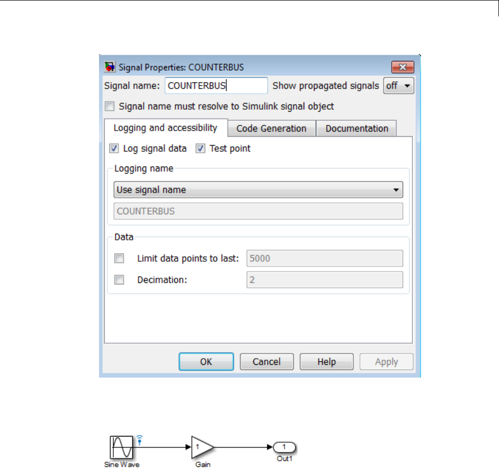
View Signal Logging Configuration
For example, in the following model the output of the Sine Wave block is
logged:
Ifyouusethecommand-lineinterfaceto override logging for a signal, the
Simulink Editor continues to display the sign logging indicator for that
signal in the Simulink Editor. When you simulate the model, Simulink
displays a red signal logging indicator for all signals configured to be logged,
45-29
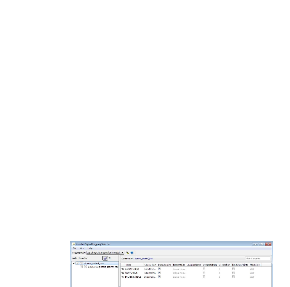
45 Importing and Exporting Simulation Data
reflecting any overrides. For details about configuring a signal for logging, see
“Configure a Signal for Signal Logging” on page 45-21.
A logged signal can also be a test point. See “Test Points” on page 47-58 for
information about test points.
To turn the display of logging indicators off, clear Display > Signals &
Ports > Testpoint & Logging Indicators.
Use Signal Logging Selector to View Signal Logging
Configuration
1Open the model for which you want to view the signal logging configuration.
2Open the Signal Logging Selector, using one of the following approaches:
•In the Configuration Parameters > Data Import/Export pane, in
the Signals area, select the Configure Signals to Log button.
If necessary, select Signal logging to enable the Configure Signals
to Log button.
•For a model that includes a Model block, you can also use the following
approach:
aIn the Simulink Editor, right-click a Model block.
bIn the context-menu, select Log Referenced Signals.
3In the Model Hierarchy pane, select the model node for which you want
to view the signal logging configuration. For example:
To expand a node in the Model Hierarchy pane, right-click that the arrow
to the left of the node.
45-30
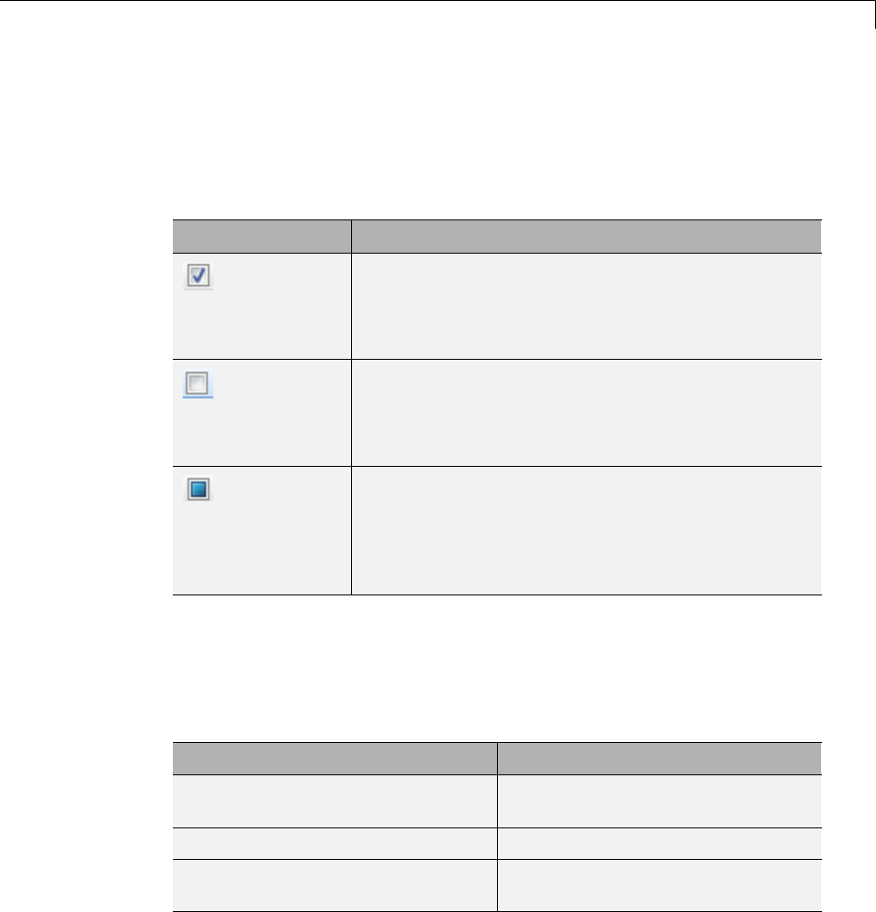
View Signal Logging Configuration
If there are no logged signals for a node, the Contents pane is empty.
If you open the Signal Logging Selector for a model that uses model
referencing, then in the Model Hierarchy pane, the check box to the left of a
model node indicates the override configuration of the node.
Check Box Signal Logging Configuration
For the top-level model node, logs all logged signals in
the top model.
For a Model block node, logs all logged signals in the
model reference hierarchy for that block.
For the top-level model node, disables logging for all
logged signals in the top model.
For a Model block node, logs disables logging for all
signals in the model reference hierarchy for that block.
For the top-level model node, logs all logged signals
that have the DataLogging setting enabled.
For a Model block node, logs all logged signals in the
model reference hierarchy for that block that have the
DataLogging setting enabled.
Viewing the Signal Logging Configuration for Subsystems,
Masked Subsystems, and Linked Libraries
The following table describes default Model Hierarchy pane display of
subsystems, masked subsystems, and linked library nodes.
Node Display Default
Subsystem Displays all that include logged
signals
Masked subsystem Does not display
Linked library Displays all that include logged
signals
45-31

45 Importing and Exporting Simulation Data
You can control how the Model Hierarchy pane displays subsystems,
masked subsystems, and linked libraries. To do control how , use icons
at the top of the Model Hierarchy pane or use the View menu, using
thesameapproachasyouuseintheModel Explorer. For details, see
“Displaying Linked Library Subsystems” on page 9-13 and “Displaying
Masked Subsystems” on page 9-14.
•To display all subsystems, including subsystems that do not include logged
signals, select the icon or View > Show All Subsystems.This
subsystem setting also applies to masked subsystems, if you specify to
display masked subsystems.
•To display masked subsystems with logged signals, use the icon or
View > Show Masked Subsystems
•To display linked libraries, use the icon or View > Show Library
Links
Filtering Signal Logging Selector Contents
To find a specific signal or property value for a signal, use the Filter
Contents edit box. Use the same approach as you use in the Model Explorer;
for details, see “Filtering Contents” on page 9-48.
Highlighting a Block in a Model
TousetheModelHierarchypanetohighlight a block in model, right-click the
block or signal and select Highlight block in model.
Use Model Explorer to View Signal Logging
Configuration
1Open the model for which you want to view the signal logging configuration.
Select the top-level model in a model reference hierarchy gives you to access
to logging configuration information for referenced models.
2In the Contents pane, set Column View to the Signals view.
45-32
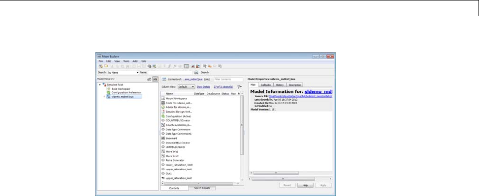

45 Importing and Exporting Simulation Data
Enable Signal Logging for a Model
In this section...
“Enable and Disable Logging Globally for a Model” on page 45-34
“Specify the Signal Logging Data Format” on page 45-34
“Specify a Name for the Signal Logging Data” on page 45-40
Enable and Disable Logging Globally for a Model
You enable or disable logging globally for logged signals in a model. By
default, signal logging is enabled. Simulink logs signals only if the Signal
logging parameter is checked. If the option is not checked, Simulink ignores
the signal logging settings for individual signals.
To disable signal logging, use one of these approaches:
•Clear the Configuration Parameters > Data Import/Export > Signal
logging parameter.
•Use the SignalLogging parameter. For example:
set_param(bdroot, 'SignalLogging', 'off')
Selecting a Subset of Signals to Log
You can select a subset of signals to log for a model that has:
•Signal logging enabled
•Logged signals
For details, see “Override Signal Logging Settings” on page 45-41.
Specify the Signal Logging Data Format
The signal logging format determines how Simulink stores the logged signal
data. You can store the data using either the Dataset or ModelDataLogs
format.
45-34

Enable Signal Logging for a Model
Set the Signal Logging Format
To set the signal logging format, use either of these approaches:
•Set the Configuration Parameters > Data Import/Export > Signal
logging format parameter to either Dataset (default) or ModelDataLogs.
•Use the SignalLoggingSaveFormat parameter, with a value of Dataset or
ModelDataLogs. For example:
set_param(bdroot, 'SignalLoggingSaveFormat', 'Dataset')
Use the Dataset Format for Signal Logging in New Models
Use the Dataset format for signal logging for new models. The ModelDataLogs
format is supported for backwards compatibility. The ModelDataLogs format
will be removed in a future release.
The Dataset format:
•Uses MATLAB timeseries objects to store logged data , which allows you
to work with logging data in MATLAB without a Simulink license. For
example, to manipulate the logged data, you can use MATLAB timeseries
methods such as filter,detrend,andresample.
•Supports logging multiple data values for a given time step, which can be
important for Iterator subsystem and Stateflow signal logging.
•Provides an easy to analyze format for logged signal data for models with
deep hierarchies, bus signals, and signals with duplicate or invalid names.
•Avoids the limitations of the ModelDataLogs format, which Bug Report
495436 describes.
When you specify the Dataset format, Simulink stores the data using a
Simulink.SimulationData.Dataset object.
Migrate from ModelDataLogs to Dataset Format
The ModelDataLogs logging format is supported for backwards compatibility.
The ModelDataLogs format will be removed in a future release. To enable
existing models that use ModelDataLogs format to continue to work in future
releases, migrate those models to use Dataset format.
45-35

45 Importing and Exporting Simulation Data
UsetheUpgradeAdvisortoupgradeamodeltouseDataset format, using
one of these approaches:
•In the Simulink Editor, select Analysis > Model Advisor > Upgrade
Advisor
•From the MATLAB command line, use the upgradeadvisor function.
If you have already logged signal data in the ModelDataLogs format, you can
use the Simulink.ModelDataLogs.convertToDataset function to update the
ModelDataLogs signal logging dataset to use Dataset format. For example, to
update the older_model_dataset from ModelDataLogs format to Dataset
format:
new_dataset = logsout.convertToDataset('older_model_dataset')
Depending upon your particular circumstances, converting a model from
using ModelDataLogs format to using Dataset format may require that you
make some modifications to your existing models and to code in callbacks,
functions, scripts, or tests. The following table identifies possible issues
that you may need to address after converting to Dataset format. The table
provides solutions for each issue.
Possible Issue After
Conversion to Dataset
Format
Solution
Code in existing callbacks,
functions, scripts,
or tests that used
the ModelDataLogs
programmatic interface
to access data may result in
an error.
Check for code that uses ModelDataLogs
format access methods. Update that code to
use Dataset format access methods.
For example, suppose existing code includes
the following line:
logsout.('Subsystem Name').X.data
ReplacethatcodewithaDataset access
method:
logsout.get('x').Values.Data
or
45-36

Enable Signal Logging for a Model
Possible Issue After
Conversion to Dataset
Format
Solution
logsout.getElement('x').Values.Data
Logging bus signals requires
aconfiguration parameter
change.
Logging buses in Dataset format requires
that Configuration Parameters >
Diagnostics > Connectivity > Mux
blocks used to create bus signals be set
to error.
To configure a model for proper bus usage,
run the Upgrade Advisor with the Check
for proper bus usage check.
Mux block signal names are
lost.
The Dataset format treats Mux block signals
as a vector.
If you need to identify signals by
signal names, replace Mux blocks
with a Bus Creator blocks. Set
Configuration Parameters >
Diagnostics > Connectivity > Mux
blocks used to create bus signals to
error.
Signal Viewer cannot be
used for signal logging.
If you use the Dataset format for signal
logging, then Simulink does not log the
signals configured to be logged in the Signal
Viewer. Explicitly mark the signal for signal
logging by using the Signal Properties dialog
box. To access the Signal Properties dialog
box, right-click a signal and from the context
menu, select Properties.
45-37

45 Importing and Exporting Simulation Data
Possible Issue After
Conversion to Dataset
Format
Solution
The unpack method
generates an error.
The unpack method, which is supported
for Simulink.ModelDataLogs
and Simulink.SubsysDataLogs
objects, is not supported for
Simulink.SimulationData.Dataset
objects.
For example, if the logged data has three
fields: x,y,andz, then:
•For ModelDataLogs format data, the
mlog.unpack method creates three
variables in the base workspace.
•For Dataset format data, access methods
by names. For example:
x = logsout.get('x').Values
The ModelDataLogs and
Dataset formats have
different naming rules for
unnamed signals.
If necessary, add signal names.
•In ModelDataLogs format, for an unnamed
signal coming from a block, Simulink
assigns a name in this form:
SL_BlockName+<portIndex>
For example, SL_Gain1.
•In Dataset format, elements do not need a
name, so Simulink leaves the signal name
empty.
•For both ModelDataLogs and Dataset
formats, Simulink assigns the same name
to unnamed signals that come from Bus
Selector blocks.
45-38

Enable Signal Logging for a Model
Possible Issue After
Conversion to Dataset
Format
Solution
Test points in referenced
models are not logged.
Consider enabling signal logging for test
points in a referenced model.
Running or updating a
model that uses model
referencing might return
asignalloggingformat
inconsistency error.
Follow the approach described in “Model
Reference Signal Logging Format
Consistency” on page 45-39.
Model Reference Signal Logging Format Consistency
If signal logging is enabled for a top model, then the signal logging format for
the non-protected referenced models must be the same as the signal logging
format for the top model.
Simulink performs signal logging format consistency checking during model
update or when you run a simulation. Simulink does not report inconsistencies
during code generation for model reference simulation target code.
If Simulink reports a signal logging format inconsistency, then use one of the
following approaches:
•Use the Upgrade Advisor (with the upgradeadvisor function) to upgrade a
model to use Dataset format.
•Use the Simulink.SimulationData.updateDatasetFormatLogging
function to convert a model and its referenced models to use Dataset
format for signal logging.
•Turn off signal logging for the model, including for all referenced models,
by clearing the Configuration Parameters > Data Import/Export >
Signal logging parameter check box.
•Disable logging for all signals in this top-level Model block.
1Select the Configuration Parameters > Data Import/Export >
Configure Signals to Log button.
45-39

45 Importing and Exporting Simulation Data
2In the Signal Logging Selector dialog box, in the Model Hierarchy
pane, clear the check box for the top Model block in the model reference
hierarchy that generated the error.
Specify a Name for the Signal Logging Data
You use the signal logging name to access the signal logging data. The default
name for the signal logging data is logsout. Specifying a signal logging name
can make it easier to identify the source of the logged data. For example, you
could specify the signal logging name car_logsout to identify the data as
being the signal logging data for the car model.
To specify a different signal logging name, use either of these approaches:
•In the edit box next to the Configuration Parameters > Data
Import/Export > Signal logging parameter, enter the signal logging
name.
•Use the SignalLoggingName parameter, specifying a signal logging name.
For example:
set_param(bdroot, 'SignalLoggingName', 'heater_model_signals')
45-40

Override Signal Logging Settings
Override Signal Logging Settings
In this section...
“Benefits of Overriding Signal Logging Settings” on page 45-41
“Two Interfaces for Overriding Signal Logging Settings” on page 45-41
“Scope of Signal Logging Setting Overrides” on page 45-42
“Signal Logging Selector” on page 45-42
“Command-Line Interface for Overriding Signal Logging Settings” on page
45-48
Benefits of Overriding Signal Logging Settings
As you develop a model, you may want to override the signal logging settings
for a specific simulation run. You can override signal logging properties
without changing the model in the Simulink Editor. Override signal logging
properties to reduce memory overhead and to facilitate the analysis of
simulation logging results.
Overriding signal logging propertiesisusefulwhenyouwantto:
•Focus on only a few logged signals by disabling logging for most of the
logged signals
•Exclude a few signals from the signal logging output
•Override specific signal logging properties, such as decimation, for a signal
•Collect only what you need when running multiple test vectors
Two Interfaces for Overriding Signal Logging Settings
Use either of two interfaces to override signal logging settings:
•“Signal Logging Selector” on page 45-42
•“Command-Line Interface for Overriding Signal Logging Settings” on
page 45-48
45-41

45 Importing and Exporting Simulation Data
You can use a combination of the two interfaces. The Signal Logging Selector
creates Simulink.SimulationData.ModelLoggingInfo objects when saving
the override settings. The command-line interface has properties whose
names correspond to the Signal Logging Selector interface. For example, the
Simulink.SimulationData.ModelDataLoggingInfo class has a LoggingMode
property, which corresponds to the Logging Mode parameter in the Signal
Logging Selector.
Scope of Signal Logging Setting Overrides
When you override signal logging settings, Simulink uses those override
settings when you simulate the model.
Simulink saves in the model the signal logging override configuration that
you specify. However, Simulink does not change the signal logging settings in
the Signal Properties dialog box for each signal in the model.
In the Signal Logging Selector, if you override some signal logging settings,
and then set the Logging Mode to Log all signals as specified in
model, the logging settings defined in the model appear in the Signal Logging
Selector. The override settings are greyed out, indicating that you cannot
override these settings. To reactivate the override settings, set Logging
Mode to Override signals.
If you close and reopen the model, the logging setting overrides that you made
are in effect, if logging mode is set to override signals for that model. When
the model displays the signal logging indicators, it displays the indicators for
all logged signals, including logged signals that you have overridden.
To use the signal logging settings that the model defines, set the logging mode
to use the logging settings defined in the model. That setting causes all logged
signals to be included in the signal logging data, ignoring any overrides.
Using the Signal Logging Selector to override logging for a specific signal does
not affect the signal logging indicator for that signal.
Signal Logging Selector
1Open the Signal Logging Selector, using one of the following approaches:
45-42
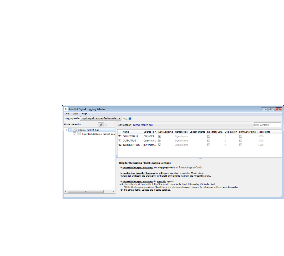
Override Signal Logging Settings
•In the Configuration Parameters > Data Import/Export pane, in
the Signals area, select the Configure Signals to Log button.
If necessary, select Signal logging to enable the Configure Signals
to Log button.
•For a model that includes a Model block, you can also use the following
approach:
aIn the Simulink Editor, right-click a Model block.
bIn the context-menu, select Log Referenced Signals.
2Set Logging Mode to Override signals.
Note The Override signals setting affects all levels of the model
hierarchy. This setting can result in turning off logging for any signal
throughout the hierarchy, based on existing settings. To review settings,
select the appropriate node in the Model Hierarchy pane.
3View the node containing the logged signals that you want to override. If
necessary, expand nodes or configuretheModelHierarchypanetodisplay
masked subsystems. See “Use Signal Logging Selector to View Signal
Logging Configuration” on page 45-30.
45-43

45 Importing and Exporting Simulation Data
4Override signal logging settings. Use one of the following approaches,
depending on whether or not your model uses model referencing:
•“Models Without Model Referencing: Overriding Signal Logging
Settings” on page 45-44
•“Models with Model Referencing: Overriding Signal Logging Settings”
on page 45-45
Note To open the Configuration Parameters > Data Import/Export
pane from the Signal Logging Selector, use the button.
Models Without Model Referencing: Overriding Signal Logging
Settings
If your model does not use model referencing (that is, the model does not
include any Model blocks), override signal logging settings using the following
procedure.
1Open the Signal Logging Selector. In the Configuration Parameters >
Data Import/Export pane, in the Signals area, select the Configure
Signals to Log button.
•If necessary, select Signal logging to enable the Configure Signals
to Log button.
45-44

Override Signal Logging Settings
2Set Logging Mode to Override signals.
3View the node containing the logged signals that you want to override. If
necessary, expand nodes or configure the Model Hierarchy pane to display
masked subsystems. See “Use Signal Logging Selector to View Signal
Logging Configuration” on page 45-30.
4In the Contents pane table, select the signal whose logging settings you
want to override.
5Override logging settings:
•To disable logging for a signal, clear the DataLogging check box for that
signal.
•To override other signal logging settings (for example, decimation),
ensure that the DataLogging check box is selected. Then, edit values in
the appropriate columns.
Models with Model Referencing: Overriding Signal Logging
Settings
If your model uses model referencing (that is, the model includes at least one
Model block), override signal logging settings using the one or more of the
following procedures:
•“Enable Logging for All Logged Signals” on page 45-46
45-45
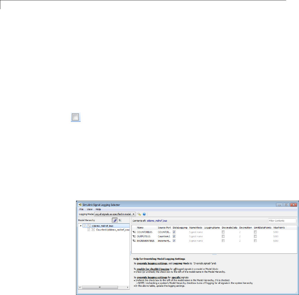
45 Importing and Exporting Simulation Data
•“Disable Logging for All Logged Signals in a Model Node” on page 45-47
•“Override Signal Logging for a Subset of Signals” on page 45-47
•“Override Other Signal Logging Properties” on page 45-48
Enable Logging for All Logged Signals. By default, Simulink logs all the
logged signals in a model, including the logged signals throughout model
reference hierarchies.
If logging is disabled for any logged signals in the top-level model or in the
top-level Model block in a model reference hierarchy, then in the Model
Hierarchy pane, the check box to the left of that node is either ) or empty
().
To enable logging of all logged signals for a node:
1Perform the steps 1–3 in “Signal Logging Selector” on page 45-42.
2Open the Signal Logging Selector. In the Configuration Parameters >
Data Import/Export pane, in the Signals area, select the Configure
Signals to Log button.
•If necessary, select Signal logging to enable the Configure Signals
to Log button.
45-46

Override Signal Logging Settings
3Set Logging Mode to Override signals.
4View the node containing the logged signals that you want to override. If
necessary, expand nodes or configuretheModelHierarchypanetodisplay
masked subsystems. See “Use Signal Logging Selector to View Signal
Logging Configuration” on page 45-30.
5In the Model Hierarchy pane, select the check box to the left of the node,
so that the check box has a check mark ( ).
•For the top-level model, logging is enabled for all logged signals in the
top-level model, but not for logged signals in model reference hierarchies.
•For a Model block at the top of a model referencing hierarchy, logging
is enabled for the whole model reference hierarchy for the selected
referenced model.
Disable Logging for All Logged Signals in a Model Node. If signal
logging is enabled for any signals in a model node, then in the Model
Hierarchy pane, the check box to the left of the node is either checked ( )
or solid blue ( ).
To disable logging for all logged signals in a node of a model:
1Perform the steps 1–3 in “Signal Logging Selector” on page 45-42.
2In the Model Hierarchy pane, clear the check box to the left of the node,
so that the check box is empty ( ).
•For the top-level model, logging is disabled for all logged signals in the
top-level model, but not for logged signals in model reference hierarchies.
•For a Model block at the top of a model referencing hierarchy, logging
is disabled for the whole model reference hierarchy for the selected
reference model.
Override Signal Logging for a Subset of Signals. To log some, but not
all, logged signals in a model node:
1Perform the steps 1–3 in “Signal Logging Selector” on page 45-42.
45-47

45 Importing and Exporting Simulation Data
2In the Model Hierarchy pane, ensure that the check box for the top-level
model or Model block is either solid blue or . Click the check box to
cycle through different states.
3In the Contents pane table, for the signals that you want to log, select the
check box in the DataLogging column.
To enable logging for multiple signals, hold the Shift or Ctrl key and
select a range of signals or individual signals. Select the check box in the
DataLogging column of one of the highlighted signals.
Override Other Signal Logging Properties. In addition to overriding the
setting for the DataLogging property for a signal, you can override other
signal logging properties, such as decimation.
1Perform the steps 1–3 in “Signal Logging Selector” on page 45-42.
2In the Model Hierarchy pane, ensure that the check box for the top-level
model or Model block is solid blue or . Click the check box to cycle
through different states.
3In the Contents pane table, for the signals for which you want to override
logging properties, enable logging by selecting the check box in the
DataLogging column.
To enable logging for multiple signals, hold the Shift or Ctrl key and
select a range of signals or individual signals. Select the check box in the
DataLogging column of one of the highlighted signals.
4In the Contents pane table, modify the settings for properties, such as
DecimateData and Decimation.
Command-Line Interface for Overriding Signal
Logging Settings
The command-line interface for overriding signal logging settings includes:
•The DataLoggingOverride model parameter — Use to view or set signal
logging override values for a model
•The following classes:
45-48
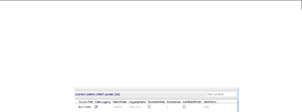
Override Signal Logging Settings
-Simulink.SimulationData.ModelLoggingInfo —Specifysignal
logging override settings for a model. This class corresponds to the
overall Signal Logging Selector interface.
-Simulink.SimulationData.SignalLoggingInfo — Override settings
for a specific signal. This class corresponds to a row in the logging
property table in the Signal Logging Selector:
-Simulink.SimulationData.LoggingInfo — Overrides for signal logging
settings such as decimation. This class corresponds to the editable
columns in a row in the logging property table in the Signal Logging
Selector.
To query a model for its signal logging override status, use the
DataLoggingOverride parameter. To configure signal logging from the
command line, use methods and properties of the three classes listed above.
The following sections describe how to use the command-line interface to
perform some common signal logging configuration tasks. The examples use
the sldemo_mdlref_bus model.
•“Create a Model Logging Information Object” on page 45-49
•“Specify Which Models to Log” on page 45-50
•“Log a Subset of Signals” on page 45-52
•“Override Other Signal Logging Properties” on page 45-52
Create a Model Logging Information Object
To use the command-line interface for overriding signal logging settings,
create a Simulink.SimulationData.ModelLoggingInfo object. For example,
use the following command to create the model logging override object for the
sldemo_mdlref_bus model and automatically add each logged signal in the
model to that object:
mi = Simulink.SimulationData.ModelLoggingInfo.createFromModel(...
45-49

45 Importing and Exporting Simulation Data
'sldemo_mdlref_bus')
mi =
Simulink.SimulationData.ModelLoggingInfo
Package: Simulink.SimulationData
Properties:
Model: 'sldemo_mdlref_bus'
LoggingMode: 'OverrideSignals'
LogAsSpecifiedByModels: {}
Signals: [1x4 Simulink.SimulationData.SignalLoggingInfo]
Methods
You can control the kinds of systems from which to include logged signals. By
default, the Simulink.SimulationData.ModelLoggingInfo object includes
logged signals from:
•Libraries
•Masked subsystems
•Referenced models
•Active variants
As an alternative, you can use the
Simulink.SimulationData.ModelLoggingInfo constructor and
specify a Simulink.SimulationData.SignalLoggingInfo object for
each signal. To ensure that you specified valid signal logging settings
for a model, use the verifySignalAndModelPaths method with the
Simulink.SimulationData.ModelLoggingInfo object for the model.
Specify Which Models to Log
Use the LoggingMode property of a
Simulink.SimulationData.ModelLoggingInfo object to specify whether to
use the signal logging settings as specified in the model and all referenced
models, or to override those settings.
45-50

Override Signal Logging Settings
You can control whether a top-level model and referenced models use override
signal logging settings or use the signal logging settings specified by the
model, as described in the Simulink.SimulationData.ModelLoggingInfo
documentation.
The following example shows how to log all signals as specified in the top
model and all referenced models. The signal logging output is stored in
topOut.
sldemo_mdlref_bus;
mi = Simulink.SimulationData.ModelLoggingInfo...
('sldemo_mdlref_bus');
mi.LoggingMode = 'LogAllAsSpecifiedInModel'
mi =
Simulink.SimulationData.ModelLoggingInfo
Package: Simulink.SimulationData
Properties:
Model: 'sldemo_mdlref_bus'
LoggingMode: 'LogAllAsSpecifiedInModel'
LogAsSpecifiedByModels: {}
Signals: []
Methods
set_param(sldemo_mdlref_bus, 'DataLoggingOverride', mi);
Thefollowingexampleshowshowtologonlysignalsinthetopmodel:
mi = Simulink.SimulationData.ModelLoggingInfo...
('sldemo_mdlref_bus');
mi.LoggingMode = 'OverrideSignals';
mi = mi.setLogAsSpecifiedInModel('sldemo_mdlref_bus', true);
set_param(sldemo_mdlref_bus, 'DataLoggingOverride', mi);
45-51

45 Importing and Exporting Simulation Data
Log a Subset of Signals
To specify a subset of logged signals to log, use the findSignal method with a
Simulink.SimulationData.ModelLoggingInfo object. For example, to log
only one signal from the referenced model instance referenced by :
sldemo_mdlref_bus;
mi = Simulink.SimulationData.ModelLoggingInfo.createFromModel(...
'sldemo_mdlref_bus');
pos = mi.findSignal({'sldemo_mdlref_bus/CounterA' ...
'sldemo_mdlref_counter_bus/Bus Creator'}, 1)
pos =
4
for idx=1:length(mi.Signals)
mi.Signals(idx).LoggingInfo.DataLogging = (idx == pos);
end
set_param(sldemo_mdlref_bus, 'DataLoggingOverride', mi);
Override Other Signal Logging Properties
In addition to overriding the setting for the DataLogging property for a signal,
you can override other signal logging properties, such as decimation.
Use Simulink.SimulationData.LoggingInfo properties to override signal
logging properties. The following example shows how to set the decimation
override settings.
mi = Simulink.SimulationData.ModelLoggingInfo.createFromModel...
('sldemo_mdlref_bus');
pos = mi.findSignal({'sldemo_mdlref_bus/CounterA' ...
'sldemo_mdlref_counter_bus/Bus Creator'}, 1);
mi.Signals(pos).LoggingInfo.DecimateData = true;
mi.Signals(pos).LoggingInfo.Decimation = 2;
45-52

Access Signal Logging Data
Access Signal Logging Data
In this section...
“View Signal Logging Data” on page 45-53
“Signal Logging Object” on page 45-54
“View Logged Signal Data with the Simulation Data Inspector” on page
45-54
“Programmatically Access Logged Signal Data Saved in Dataset Format” on
page 45-55
“Programmatically Access Logged Signal Data Saved in ModelDataLogs
Format” on page 45-57
View Signal Logging Data
To generate signal logging data, simulate the model. You can view the
signal logging data for a paused or completed simulation, using one of these
interfaces:
•The Simulation Data Inspector
•MATLAB commands
To access signal logging data programmatically, the approach you use
depends on the signal logging data format (Dataset or ModelDataLogs). For
details, see:
•“Programmatically Access Logged Signal Data Saved in Dataset Format”
on page 45-55
•“Programmatically Access Logged Signal Data Saved in ModelDataLogs
Format” on page 45-57
45-53

45 Importing and Exporting Simulation Data
Note If you do not see logging data for a signal that you configured in the
model for signal logging, check the logging configuration using the Signal
Logging Selector. Use the Signal Logging Selector to enable logging for a
signal whose logging is overridden. For details, see “View Signal Logging
Configuration” on page 45-27 and “Override Signal Logging Settings” on
page 45-41.
Signal Logging Object
Simulink saves signal logging data in a signal logging object, which you access
with a MATLAB workspace variable.
The type of the signal logging object depends on the signal logging format that
you choose. For details, see “Specify the Signal Logging Data Format” on
page 45-34.
•Dataset format — Uses a Simulink.SimulationData.Dataset object
•ModelDataLogs format — Uses a Simulink.ModelDataLogs object
The default name of the signal logging variable is logsout. You can change
the signal logging name. For details, see “Specify a Name for the Signal
Logging Data” on page 45-40.
View Logged Signal Data with the Simulation Data
Inspector
You can use the Simulation Data Inspector to view logged signal data.
To view logged signal data with the Simulation Data Inspector, in the
Simulink Editor, use one of the following approaches:
•To display logged signals whenever a simulation ends or you pause a
simulation, select Simulation > Model Configuration Parameters >
Inspect signals when simulation is stopped/paused.
•To launch the Simulation Data Inspector tool to display the data
immediately, select Simulation > Output > Simulation Data
Inspector.
45-54

Access Signal Logging Data
For additional information about using the Simulation Data Inspector, see
“Inspect Signal Data with Simulation Data Inspector” on page 17-2.
Programmatically Access Logged Signal Data Saved
in Dataset Format
When you use the default Dataset signal logging format, Simulink
saves the logging data in a Simulink.SimulationData.Dataset
object. For information on extracting signal data from
that object, see Simulink.SimulationData.Dataset.
The Simulink.SimulationData.Dataset object contains
Simulink.SimulationData.Signal objects for each logged signal.
For bus signals, the Simulink.SimulationData.Signal object consists of a
structure of MATLAB timeseries objects.
The Simulink.SimulationData.Dataset classprovidestwomethodsfor
accessing signal logging data.
Name Description
get
The getElement method shares the
same syntax and behavior as the get
method.
Get element or collection of elements
from the dataset, based on index,
name, or block path.
getLength Get number of elements in the
dataset.
For examples of accessing signal logging data that uses the Dataset format,
see Simulink.SimulationData.Dataset.
Example of Accessing Dataset Format Signal Logging Data
The sldemo_mdlref_bus model illustrates how to access signal logging data.
Accessing Data for Signals with a Duplicate Name
For a model with signals with multiple signals that have the same signal
name, the signal logging data includes a Simulink.SimulationData.Signal
45-55

45 Importing and Exporting Simulation Data
object for each signal that has a duplicate name. Simulink sorts the data for
those signals based on the model hierarchy, in top-down order.
To access a specific signal that has a duplicate name, use one of these
approaches:
•Visually inspect the Simulink.SimulationData.Signal objects to find the
data for the specific signal.
•Use the Simulink.SimulationData.Dataset.getElement method,
specifying the blockpath for the source block of the signal.
•Create a script to iterate through the signals with a duplicate signal name,
using the Simulink.SimulationData.Dataset.getElement method with
an index argument.
•Usethefollowingapproach,ifthesignalswithaduplicatenamedonot
appear in multiple instances of a referenced model in Normal mode:
1In the model, right-click the signal.
2In the context menu, select Properties.
3In the Signal Properties dialog box, set Logging name to Custom and
specify a different name than the signal name.
4Simulate the model and use the
Simulink.SimulationData.Dataset.getElement method with a
name argument.
Handling Newline Characters in Signal Logging Data
To handle newline characters in logging names in signal logging data that
uses Dataset format, use a sprintf command within a getElement call.
For example:
topOut.getElement(sprintf('INCREMENT\nBUS'))
45-56

Access Signal Logging Data
Programmatically Access Logged Signal Data Saved
in ModelDataLogs Format
Note The ModelDataLogs signal logging format is supported for backward
compatibility. For new models, use the Dataset format.
When you use theModelDataLogs signal logging format, Simulink saves
the logging data in a Simulink.ModelDataLogs object. For information on
extracting signal data from that object, see Simulink.ModelDataLogs.The
Simulink.ModelDataLogs object contains signal data objects to capture signal
logging information for specific model elements.
Model Element Signal Data Object
Top-level or referenced model Simulink.ModelDataLogs
Subsystem in a model Simulink.SubsysDataLogs
Scope block in a model Simulink.ScopeDataLogs
Signal other than a bus or Mux
signal
Simulink.Timeseries
Bus signal or Mux signal Simulink.TsArray
Virtual Signals
Avirtual signal is a signal that graphically represents other signals or
parts of other signals. Virtual signals have no functional or mathematical
significance. For more information, see “Virtual Signals” on page 47-11.
The nonvirtual components of a virtual signal are called regions.Avirtual
signalcancontainthesameregionmorethanonce. Forexample,ifthesame
nonvirtual signal is connected to two input ports of a block, the block outputs
a virtual signal that has two regions.
When you use the ModelDataLogs signal logging format, the log of a virtual
signal that contains duplicate regions includes all of the regions, even though
the data in each is the same. Logged virtual signal regions appear in the log
in a Simulink.TsputArray object. The log gives the duplicate regions unique
names, using the syntax: <signal_name>_reg<#counter>.
45-57

45 Importing and Exporting Simulation Data
Bus Signals
You can log bus signals. When you use ModelDataLogs signal logging format,
Simulink stores each logged bus signal data in a separate Simulink.TsArray
object.
The hierarchy of a bus signal is preserved in the logged signal data. The
logged name of a signal in a virtual bus derives from the name of the source
signal. The logged name of a signal in a nonvirtual bus derives from the
applicable bus object, and can differ from the name of the source signal. See
“Composite Signals” for information about those capabilities.
Handling Spaces and Newlines in Logged Names
Signal names in data logs can have spaces or newlines in their names when:
•The signal is named and the name includes a space or newline character.
•The signal is unnamed and originates in a block whose name includes a
space or newline character.
•The signal exists in a subsystem or referenced model, and the name of
the subsystem, Model block, or of any superior block, includes a space or
newline character.
Thefollowingthreeexamplesshowasignalwhosenamecontainsaspace,a
signal whose name contains a newline, and an unnamed signal that originates
in a block whose name contains a newline:
45-58
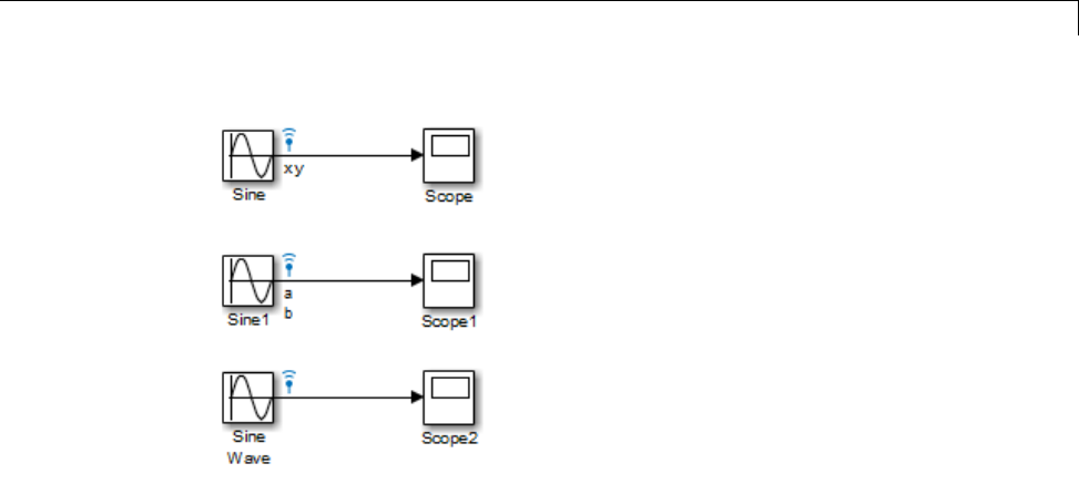
Access Signal Logging Data
The following example shows how to handle spaces or new lines in logged
names, if a model uses:
•ModelDataLogs for the signal logging format
•The default of logsout for the signal logging data
logsout =
Simulink.ModelDataLogs (model_name):
Name Elements Simulink Class
('x y') 1 Timeseries
('a
b') 1 Timeseries
('SL_Sine
Wave1') 1 Timeseries
You cannot access any of the Simulink.Timeseries objectsinthislogusing
TAB name completion or by typing the name to MATLAB. This syntax is
not recognized because the space or newline in each name appears to the
MATLABparserasaseparatorbetweenidentifiers.Forexample:
>> logsout.x y
??? logsout.x y
45-59

45 Importing and Exporting Simulation Data
|
Error: Unexpected MATLAB expression.
To reference a Simulink.Timeseries object whose name contains a space,
enclose the element containing the space in single quotes:
>> logsout.('x y')
Name: 'x y'
BlockPath: 'model_name/Sine'
PortIndex: 1
SignalName: 'x y'
ParentName: 'x y'
TimeInfo: [1x1 Simulink.TimeInfo]
Time: [51x1 double]
Data: [51x1 double]
To reference a Simulink.Timeseries objectwhosenamecontainsanewline,
concatenate to construct the element containing the newline:
>> cr=sprintf('\n')
>> logsout.(['a' cr 'b'])
Thesametechniquesworkwhenaspaceornewlineinadatalogderives
from the name of:
•An unnamed logged signal’s originating block
•A subsystem or Model block that contains any logged signal
•Any block that is superior to such a block in the model hierarchy
This code can reference logged data for the signal:
>> logsout.(['SL_Sine' cr 'Wave1'])
For names with multiple spaces, newlines, or both, repeat and combine the
two techniques as needed to specify the intended name to MATLAB.
Note You cannot use these techniques for TAB name completion.
45-60

Techniques for Importing Signal Data
Techniques for Importing Signal Data
In this section...
“Signal Data Import Techniques Summary” on page 45-61
“Comparison of Techniques” on page 45-62
“Time and Signal Values for Imported Data” on page 45-64
Signal Data Import Techniques Summary
Simulink provides several techniques for importing signal data into a model.
Signal Data Import
Technique
Description
Root-level
Inport,Trigger,
Enable, or
Function-Call
Subsystem block
Supplies external inputs from the MATLAB (base),
model, or mask workspace. Specify the external
inputs in the Configuration Parameters > Data
Import/Export > Input parameter or as a sim
command argument.
To import and map signal and bus data to
root-level inports at the same time, you can use the
Inport Mapping tool. For details, see “Import and
Map Data to Root-Level Inports” on page 45-81.
For an example, see “Import Data to Root-Level
Input Ports” on page 45-77.
From File block Reads data from a MAT-file and outputs the data
as a signal.
45-61

45 Importing and Exporting Simulation Data
Signal Data Import
Technique
Description
From Workspace block Reads data from the MATLAB (base), model, or
mask workspace and outputs the data as a signal.
For an example, see “Use From Workspace Block
to Import an Input Test Case” on page 45-72.
Signal Builder block Provides a graphical interface for creating and
generating interchangeable groups of signals.
For examples, see “Use Signal Builder Block to
Import an Input Test Case” on page 45-73 and
“Import Signal Data”.
Each of these techniques:
•Uses blocks to represent the signal data inport sources visually
•Supports data interpolation and extrapolation, which support the use of
incomplete sets of signal data
•Supports zero-crossing detection
Comparison of Techniques
Each technique is well-suited to meet one or more of the following modeling
considerations.
Modeling Consideration Suggested Technique
Purpose of importing signal data
To perform local, temporary testing
by importing a small set of signal
data
•From File block
•From Workspace block
•Signal Builder block
•Root-level Inport, Trigger, Enable,
or Function-Call Subsystem block
To test a model to be used as a
referenced model
Root-level Inport, Trigger, Enable,
or Function-Call Subsystem block
45-62

Techniques for Importing Signal Data
Modeling Consideration Suggested Technique
To verify a model using multiple test
cases
Signal Builder block, using signal
groups.
If the Simulink Verification and
Validation software is installed,
in signal groups you can use the
Verification Manager to enable or
disable individual Model Verification
blocks. For details, see “Enable and
Disable Model Verification Blocks
Using the Verification Manager”.
To perform local, temporary testing
by importing a small set of signal
data
Depending on the modeling goal,
as discussed in “Time and Signal
Values for Imported Data” on page
45-64, choose from the following
techniques:
•From File block
•From Workspace block
•Signal Builder block
•Root-level Inport, Trigger, Enable,
or Function-Call Subsystem block
Signal data
Very large dataset From File block, which incrementally
loads the data
Data exported using a To File block From File block
Data exported using a To Workspace
block
From Workspace block
Excel spreadsheet Signal Builder block, which can
import Excel spreadsheet data
directly into Simulink
Variable-size signals From Workspace block
Data storage
45-63

45 Importing and Exporting Simulation Data
Modeling Consideration Suggested Technique
In a block Signal Builder block
Inthebaseormodelworkspace •From Workspace block
•Root-level Inport, Trigger, Enable,
or Function-Call Subsystem block
In a MAT-file separate from the
model file
From File block
Time and Signal Values for Imported Data
Depending on your model development or testing goal, the approach for
specifying time and signal values can vary. Each of these guidelines applies to
one or more of the signal data import techniques (From File, From Workspace,
Signal Builder, and root-level Inport or Trigger blocks).
Modeling
Goal
Time and Signal Values Additional Notes
Import data
representing
a continuous
plant
Specify a time vector and
signal values extracted
a continuous plan (for
example, data that you
acquire experimentally
or from the results of a
previous simulation).
Useanyofthedataformats
listed in “Input Data”
on page 45-77. Here are
recommended formats for
the following imported data
sources:
•Another simulation —
Dataset
•An equation — MATLAB
time expression
In the Inport block
parameters dialog box,
select Interpolate data.
To ensure that the
Simulink variable time
solver executes at the
times that you specify
in the imported data,
set the Configuration
Parameters >
Data Import/Export >
Output options parameter
to Produce additional
output.
45-64

Techniques for Importing Signal Data
Modeling
Goal
Time and Signal Values Additional Notes
•Experimental data —
MATLAB timeseries,
data array, or structure
For details, see “Specify
Time Data” on page 45-110.
For an example of using
a structure to specify the
time and signal values, see
“Import Data to Model a
Continuous Plant” on page
45-67.
Test a discrete
algorithm
Use a structure, with an
empty time vector.
Specify signal values, but
no time vector. (One signal
value is read at each time
step, using the sample time
of the source block.)
For an example of using
a structure to specify the
signal values, see “Import
Data to Test a Discrete
Algorithm” on page 45-70.
In the Inport block
parameters dialog box,
clear Interpolate data.
Create an
input test case
(An input
test case
is typically
composed of
steps and
ramps, with
discontinuities.)
Specify a time vector and
signal values, but specify
only the time steps at points
wheretheshapeofthe
output jumps.
For details about specifying
a time vector, see “Specify
Time Data” on page 45-110.
Useanyoftheinputdata
formats described in “Input
Select the Interpolate
data parameter.
For the input, consider
using a From Workspace,
From File, or Signal Builder
block, which trigger
a zero-crossing at the
discontinuities.
For examples of using a
From Workspace block and
45-65

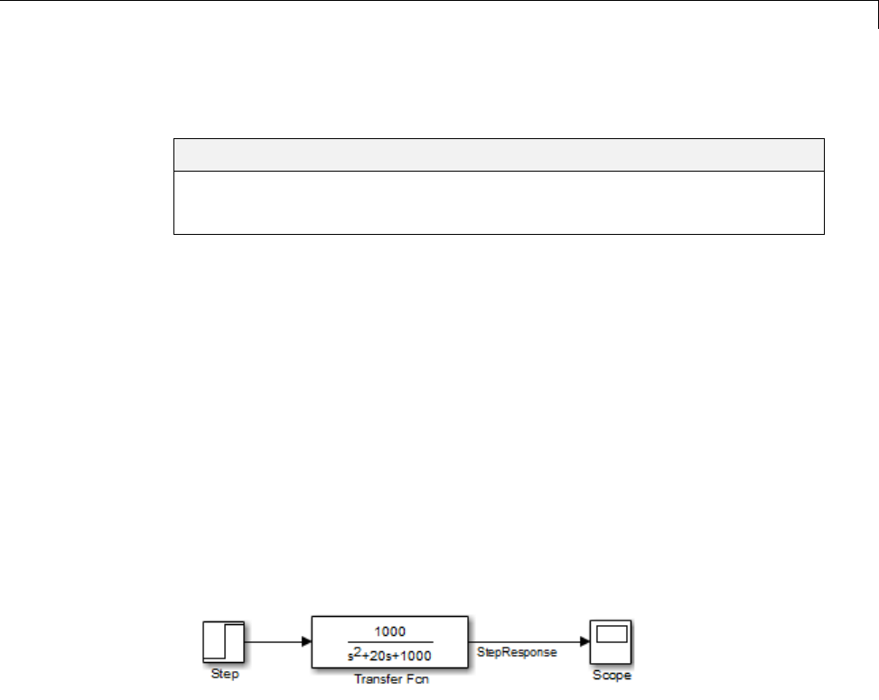
Import Data to Model a Continuous Plant
Import Data to Model a Continuous Plant
In this section...
“Share Simulation Data Across Models” on page 45-67
“Example of Importing Data to Model a Continuous Plant” on page 45-67
Share Simulation Data Across Models
When reusing data from a variable step size simulation for simulation in
another model, the second simulation must read the data at the same time
stepsasthefirstsimulation.
The following example illustrates how to reuse signal logging data from the
simulation of one model in a second model. For more information, see “Import
Signal Logging Data” on page 45-75.
Example of Importing Data to Model a Continuous
Plant
1Open the ex_data_import_continuous model.
This model uses the ode15s solver and produces continuous signals.
2To use the output of this model as input to the simulation of another model,
log the signal that you want to reuse. Select the Signal Properties >
Log signal data.
45-67
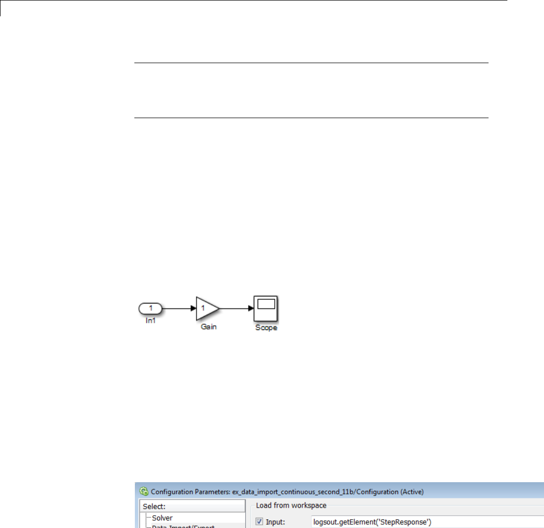
45 Importing and Exporting Simulation Data
Note To enable signal logging, you must select the Configuration
Parameters > Data Import/Export > Signal logging parameter. This
model has Signal logging enabled, and has the Signal logging format
parameter set to Dataset.
3Simulate the model.
Simulating the model saves a variable-step signal to the workspace,
using the logsout variable. The signal logging ouput is a
Simulink.SimulationData.Dataset object.
Use the Simulink.SimulationData.Dataset.getElement method to
access the logged data. The logging data for individual signals is stored in
Simulink.SimulationData.Signal objects. For this model, there is one
logged signal: StepResponse.
4Open a second model, named ex_data_import_continuous_second.
You can configure this second model to simulate using the logged data from
the first model. In this example, the second model uses a root-level Inport
block to import the logged data. The Inport block has the Interpolate
data option selected.
5In the second model, select the Configuration Parameters > Data
Import/Export > Input parameter.
Use the Simulink.SimulationData.Signal.getElement method to specify
the StepResponse signal element, as shown below:
45-68

Import Data to Model a Continuous Plant
6Specify that for the second model, the Simulink solver runs at the time
steps specified in the saved data (u). In the Data Import/Export pane, set
the Output options parameter to Produce additional output and the
Output times parameter to:
logsout.getElement('StepResponse').Values.Time
7Simulate the second model.
Note Simulink does not feed minor time-step data through root input ports.
Fordetailsaboutminortimesteps,see“MinorTimeSteps”onpage3-23.
45-69

45 Importing and Exporting Simulation Data
Import Data to Test a Discrete Algorithm
In this section...
“Specify a Signal-Only Structure” on page 45-70
“Example of Importing Data to Test a Discrete Algorithm” on page 45-70
Specify a Signal-Only Structure
To import data for a discrete signal, specify a signal-only structure as the
input value. Do not specify a time vector.
Example of Importing Data to Test a Discrete
Algorithm
1Set the sample time for the Inport, Trigger, or From Workspace block.
2For the data that you want to import, specify a structure variable that does
not include a time vector. For example, for the variable called import_var:
import_var.time = [];
import_var.signals.values = [0; 1; 5; 8; 10];
import_var.signals.dimension = 1;
The input for the first time step is read from the first element of an input
port value array. The value for the second time step is read from the second
element of the value array, and so on.
For detailsabouthowtospecifythesignalvalueanddimensiondata,see
“Specify Signal Data” on page 45-109.
3In the block parameters dialog box for the block that imports the data, clear
the Interpolate data parameter.
4If you are using a From Workspace block to import data, set the Form
output after final data value by parameter to a value other than
Extrapolation.
45-70

Import Data for an Input Test Case
Import Data for an Input Test Case
In this section...
“Guidelines for Importing a Test Case” on page 45-71
“Example of Test Case Data” on page 45-71
“Use From Workspace Block to Import an Input Test Case” on page 45-72
“Use Signal Builder Block to Import an Input Test Case” on page 45-73
Guidelines for Importing a Test Case
Typically when importing a test case in Simulink, you want to:
•Create a signal that has ramps and steps. In other words, the signal has
one or more discontinuities.
•Create the signal using the fewest points possible.
•Have the Simulink solver execute at the specified discontinuities.
To import this signal in Simulink, use a From Workspace, From File, or
Signal Builder block, all of which support zero-crossing detection.
Example of Test Case Data
The following is an example of test case data:
45-71
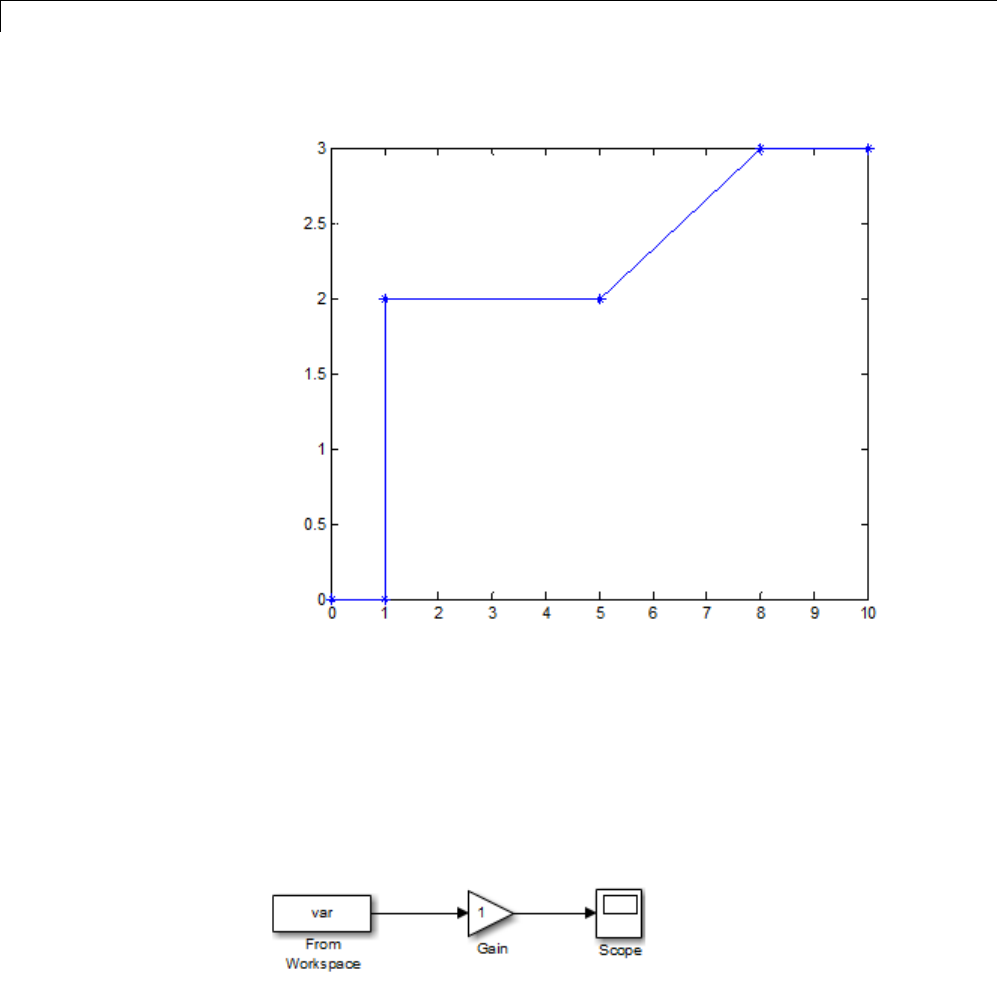
45 Importing and Exporting Simulation Data
The following two examples use this test case data.
Use From Workspace Block to Import an Input Test
Case
1Open the model ex_data_import_test_case_from_workspace.
2Enable zero-crossing detection. In the From Workspace block dialog, select
Enable zero-crossing detection.
45-72
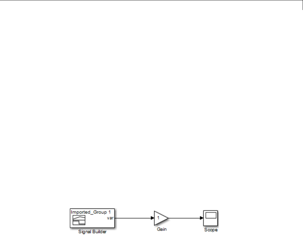
Import Data for an Input Test Case
3Create a signal structure for the test case. At each discontinuity, enter a
duplicate entry in the time vector. As described in the From Workspace
block documentation, this generates a zero-crossing and forces the
variable-stepsolvertotakeatime step at this exact time.
Define the var structure representing the test case:
var.time = [0 1 1 5 5 8 8 10];
var.signals.values = [0 0 2 2 2 3 3 3]';
var.signals.dimensions = 1;
4Toimportthetestcasestructure,inthe From Workspace block dialog, in
the Data parameter, specify var.
5Simulate the model. The Scope block reflects the test case data.
Use Signal Builder Block to Import an Input Test Case
As an alternative to using a From Workspace block, you can use a Signal
Builder block to either create a signal interactively or to import a signal from
aMAT-file.
1Open the ex_data_import_signal_builder model.
2Create a structure and save it in a MAT-file:
var.time = [0 1 1 5 5 8 8 10];
var.signals.values = [0 0 2 2 2 3 3 3]';
var.signals.dimensions = 1;
var.signals.label = 'var';
save var.mat var
3Double-click the Signal Builder block to open its dialog box.
4Select File > Import From File menu item, and select the var.mat file.
45-73

45 Importing and Exporting Simulation Data
5In the Select parameter, select Replace existing dataset.IntheData
to Import section, select the Select All check box. Confirm the selection
and click OK.
The Signal Builder block display reflects the test case data.
For a detailed example that shows how to use a Signal Builder block as the
input source for your model and to import your own signal data to the model,
see “Import Signal Data”.
45-74
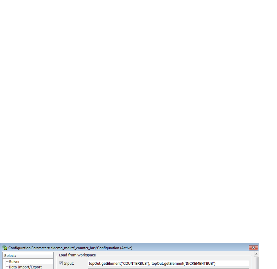
Import Signal Logging Data
Import Signal Logging Data
You can log signal data from a simulation, and then import that data into a
model. For more information about signal logging, see “Export Signal Data
Using Signal Logging” on page 45-19.
The imported signal logging data provides the input for simulating the model.
You can use imported signal logging data to perform standalone simulation
of a referenced model.
1Set the Configuration Parameters > Data Import/Export > Signal
logging format parameter to Dataset.
2Use the default signal logging output variable, logsout,orspecifya
variable using the Configuration Parameters > Data Import/Export >
Signal logging edit box.
3Simulate the parent model.
The signal logging output is a Simulink.SimulationData.Dataset object.
4Use the Simulink.SimulationData.Dataset.getElement method to
access the logged data. The logging data for individual signals is stored in
Simulink.SimulationData.Signal objects.
5For the referenced model that you want to simulate standalone, use the
Simulink.SimulationData.Signal.getElement method to specify signal
elements for the Configuration Parameters > Data Import/Export >
Input parameter.
For example:
6Simulate the referenced model.
For an example of loading logged signal data into a model:
45-75

45 Importing and Exporting Simulation Data
1Open the sldemo_mdlref_bus model.
2In the right corner of the model, double-click the left question mark block.
3See the “Logging Model Reference Signals” and “Loading Data” sections.
45-76

Import Data to Root-Level Input Ports
Import Data to Root-Level Input Ports
In this section...
“Root-Level Input Ports” on page 45-77
“Enable Data Import” on page 45-77
“Input Data” on page 45-77
“Import Bus Data” on page 45-80
Root-Level Input Ports
You can import data from a workspace and apply it to a root-level:
•Enable block
•Inport block
•Trigger block that has an edge-based (rising, falling, or either) trigger type
You can also import data from a workspace and apply it to a From Workspace
block. For details, see the From Workspace documentation and “Import Data
for an Input Test Case” on page 45-71.
Enable Data Import
To enable data import:
1Select the Configuration Parameters > Data Import/Export > Input
parameter.
2Enter an external input specification in the adjacent edit box and click
Apply.
For details, see “Input Data” on page 45-77.
Input Data
UsetheConfiguration Parameters > Data Import/Export > Input
parameter to import data from a workspace and apply it to the root-level
input ports of a model during a simulation run.
45-77

45 Importing and Exporting Simulation Data
Simulink linearly interpolates or extrapolates input values as necessary
if you select the Interpolate data option for the corresponding Inport or
Trigger block.
Note The use of the Input box is independent of the setting of the Format
list on the Data Import/Export pane.
Simulink resolves symbols used in the external input specification as
described in “Symbol Resolution” on page 4-76. See the documentation of
the sim command for some data import capabilities that are available only
for programmatic simulation.
Forms of Input Data
The input data can take any of the following forms:
•MATLAB timeseries — For details, see the following sections:
-“Import MATLAB timeseries Data” on page 45-98
-“Import Structures of timeseries Objects for Buses” on page 45-100
•Array — See “Import Data Arrays” on page 45-105.
•Simulink.SimulationData.Signal —Fordetails,see“ImportSignal
Logging Data” on page 45-75
•Structure — See “Import Data Structures” on page 45-108.
•Empty matrix — Use an empty matrix for ports for which you want to use
ground values, without having to create data structures.
•Time expression — See “Import MATLAB Time Expression Data” on page
45-107.
•Simulnk.Timeseries and Simulink.TsArray —See“Import
Simulink.Timeseries and Simulink.TsArray Data” on page 45-104.
Input Expressions
In the Input box, specify one of the following expressions:
45-78

Import Data to Root-Level Input Ports
•A MATLAB function (expressed as a string) that specifies the input u=
UT(t) at each simulation time step
•A table of input values versus time for all input ports UT = [T, U1, ...
Un],whereT = [t1, ..., tm]'
•A structure array containing data for all input ports
•A comma-separated list of tables. For details, see “Comma-Separated Lists
for the Input Parameter” on page 45-79
Comma-Separated Lists for the Input Parameter. Each table corresponds
to a specific input port. Each variable orexpressioninthelistshouldevaluate
to the appropriate object that corresponds to one of the root-level input ports
of the model, with the first item corresponding to the first root-level input
port, the second to the second root-level input port, and so on.
For an Enable or Trigger block, the signal driving the enable or trigger port
must be the last item in the comma-separated list. If you have both an enable
and a trigger port, then specify the enable port as the next-to-last item in the
list, and the trigger port as the last item.
You can load data for a subset of root-level Inport ports, without having to
create data structures for the ports for which you want to use ground values.
For information about ground values, see “Initialize Signals and Discrete
States” on page 47-51.
Using partial specification of ports simplifies the specification of external data
to input. You can use partial specification to omit an array of buses signal
from the external data to input (you cannot load array of buses data into a
root-level Inport block).
Use an empty matrix to specify ground values for a port. For example, to load
data for input ports in1 and in3, and to use ground values for port in2,enter
the following in the Input parameter:
in1, [], in3
45-79

45 Importing and Exporting Simulation Data
Import Bus Data
To import bus data to root input ports, use a structure of MATLAB
timeseries objects. For details, see “Import Structures of timeseries Objects
for Buses” on page 45-100.
To import an array of buses from a port, you can specify an empty matrix
for that port in a comma-separated list of tables. The empty matrix uses
the ground values for the bus signal.
For example, to load data for input ports in1 and in3, and to use ground
values for port in2, enter the following in the Input parameter:
in1, [], in3
45-80
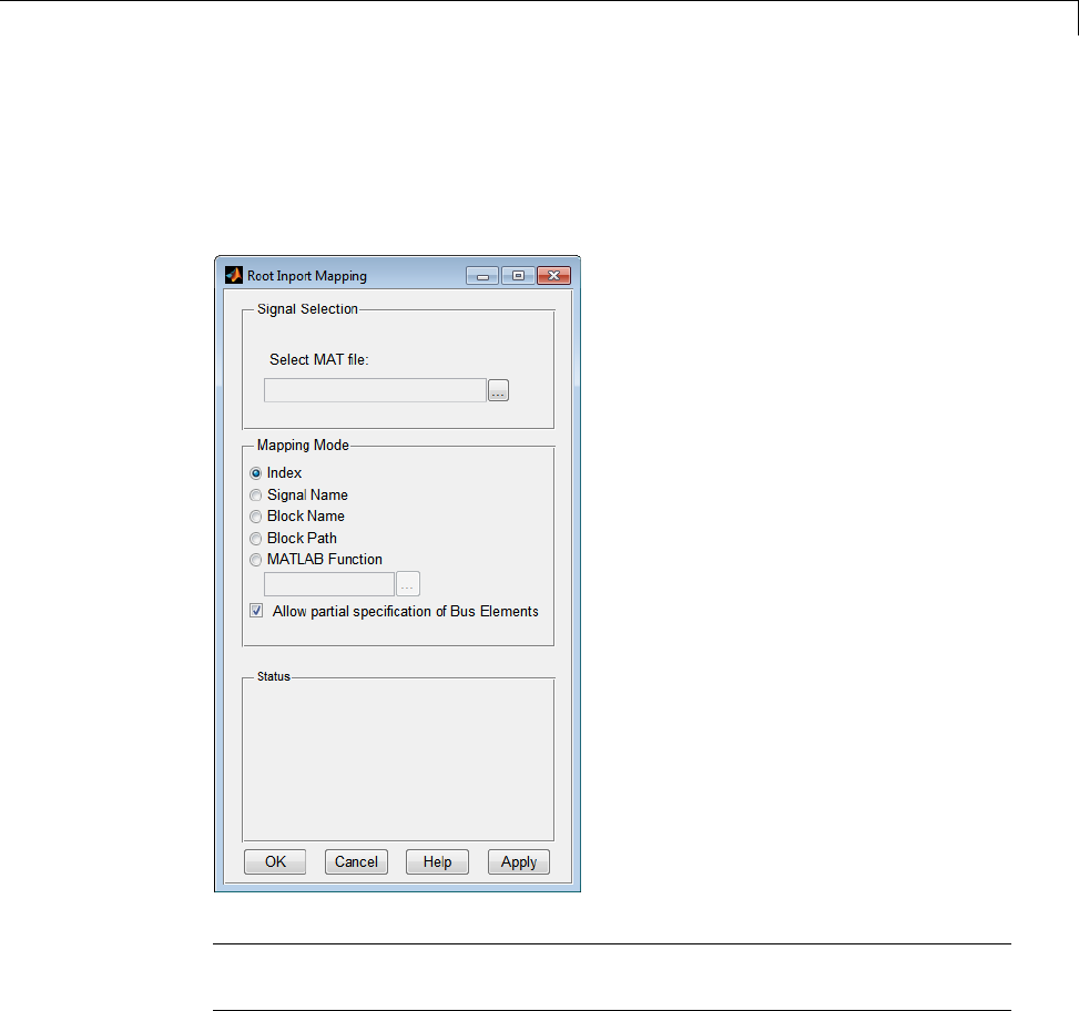
Import and Map Data to Root-Level Inports
Import and Map Data to Root-Level Inports
To import and map signal and bus data to root-level inports at the same time,
use the Root Inport Mapping tool.
Note You cannot use this dialog box to map data that already exists in the
MATLAB workspace. Use this dialog box to import the data, then map it.
Use the tool to map data to root-level inports in one of the following ways:
•Index — Assigns sequential index numbers, starting at 1, to the data in
the MAT-file and maps this data to the corresponding inport.
45-81

45 Importing and Exporting Simulation Data
-If there is more data than inports, the tool maps remaining data to
enable and trigger inports, in that order.
-If the data is not in the form of a dataset, the tool processes the data in
the order in which they are passed or parsed from the data file. This
process is the order in which they appear in the file.
•Signal Name — Assigns data to ports according to the name of the signal
ontheport.Ifthetoolfindsadataelementwhosenamematchesthename
of a signal at a port, it maps the data to the corresponding port.
•Block Name — Assigns data to ports according to the name of the
root-inport block. If the tool finds a data element whose name matches the
name of a root-inport block, it maps the data to the corresponding port.
•Block Path — Assigns data to ports according to the block path of the
root-inport block. If the tool finds a data element whose block path matches
the block path of a root-inport block, it maps the data to the corresponding
port.
•MATLAB Function — Applies mappings according to the definitions in
the custom file.
To use this tool:
•Identify the signals you want to import and map to the model root-level
inports.
•Create a MAT-file that contains the signal or bus data that you want to
import into your model and map to the root-level inports of your model (see
“MAT-File for Import and Mapping” on page 45-83).
•Determine how you want to map data (for example, by signal index or
signal name).
To map data using one of the standard map formats, see:
•“Import and Map Signal Data” on page 45-85
•“Import and Map Bus Data” on page 45-89
If you prefer to create a custom mapping file function to map data to root-level
inports, see “Create Custom Mapping File Function” on page 45-95.
45-82

Import and Map Data to Root-Level Inports
Notes:
•You cannot start or access the Root Inport Mapping tool while the model is
running or paused. The tool is available only when the model is stopped.
•If you do not click OK on the dialog box to close the tool, closing the model
also closes the tool.
MAT-File for Import and Mapping
The Root Inport Mapping dialog box requires a MAT-file that contains data
with one of the following data types or formats.
Data Formats Index
Mapping
Signal
Name
Mapping
Block
Name
Mapping
Block
Path
Mapping
Custom
Mapping
Simulink.SimulationData.-
Dataset
XXXXX
timeseries (MATLAB and
Simulink)
XXX
X(onlyfor
Simulink
timeseries)
X
Simulink.SimulationData.-
Signal
XXXXX
Structure with Time, Structure
without Time
X
TsArray XXX
Data Array X
Time Expression X
For example, a signal data MAT-file with three signals (signal1,signal2,and
signal3) with block path specified might have workspace variables that look
like the following. This file has signals that have signal names, block names,
block paths, and index values. This means that you can map the data using
Index,Signal Name,Block Name,orBlock Path mapping mode. If there are
corresponding root-level inports with corresponding indices, signal names, or
block paths, the tool maps the signal to those ports.
signal1 =
45-83

45 Importing and Exporting Simulation Data
Simulink.SimulationData.Signal
Package: Simulink.SimulationData
Properties:
Name: 'signalGain5'
BlockPath: [1x1 Simulink.SimulationData.BlockPath]
PortType: 'outport'
PortIndex: 1
Values: [1x1 timeseries]
Methods, Superclasses
>> signal2
signal2 =
Simulink.SimulationData.Signal
Package: Simulink.SimulationData
Properties:
Name: 'signalGain10'
BlockPath: [1x1 Simulink.SimulationData.BlockPath]
PortType: 'outport'
PortIndex: 1
Values: [1x1 timeseries]
Methods, Superclasses
>> signal3
signal3 =
Simulink.SimulationData.Signal
Package: Simulink.SimulationData
Properties:
Name: 'signalGain15'
BlockPath: [1x1 Simulink.SimulationData.BlockPath]
PortType: 'outport'
PortIndex: 1
Values: [1x1 timeseries]
45-84

Import and Map Data to Root-Level Inports
Methods, Superclasses
Notes:
•The tool can load only one Simulink.SimulationData.Dataset data set
per MAT-file. If the MAT-file has multiple data sets of this type, the tool
loads the first data set listed alphabetically.
•The number of signals with the formats structures with and without time
, data arrays, and time expressions must be the same as the number of
model inports, enable ports, and trigger ports.
Import and Map Signal Data
1Create a MAT-file that contains the signal data you want to import and
map.
2Open a model.
3Start the Configuration Parameters dialog box for the model.
4Navigate to the Data Import/Export pane.
5In the Load from workspace section, click Edit Input.
The Root Inport Mapping dialog box is displayed.
6In the Select MAT file parameter, specify the MAT-file that contains the
signaldatabyclickingthebrowserbuttontobrowsetothefile.
A load MAT-file window pops up.
7Click Yes to load the MAT-file in the workspace.
8In the Mapping Mode section, select how you want the imported data to
map to the root-level inports:
•Index
•Signal Name
•Block Name
45-85
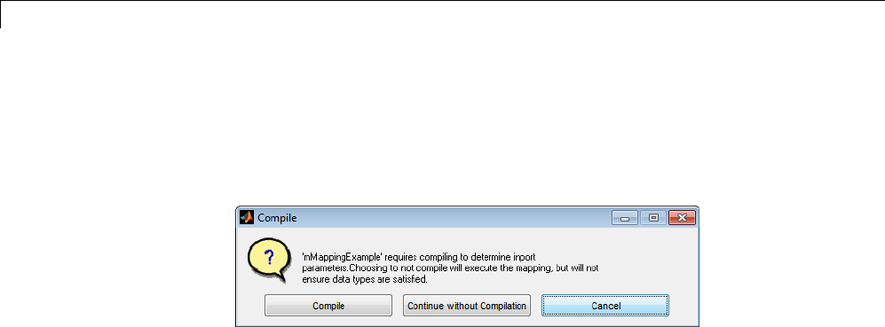
45 Importing and Exporting Simulation Data
•Block Path
•MATLAB Function
9Click Apply. A Compile dialog pops up, for example:
10 Select one of the following:
•Compile — Maps the imported data to the root-level inport and compiles
the model to check data types of root-level inports and imported data.
•Continue without Compilation — Maps the imported data to the
root-level inport, but does not compile the model. Selecting this option
might not check root-level inports, data, and data types.
•Cancel — Cancels the import. You can choose another MAT-file to
import.
TheresultsofthemappingaredisplayedintheStatusarea.
45-86
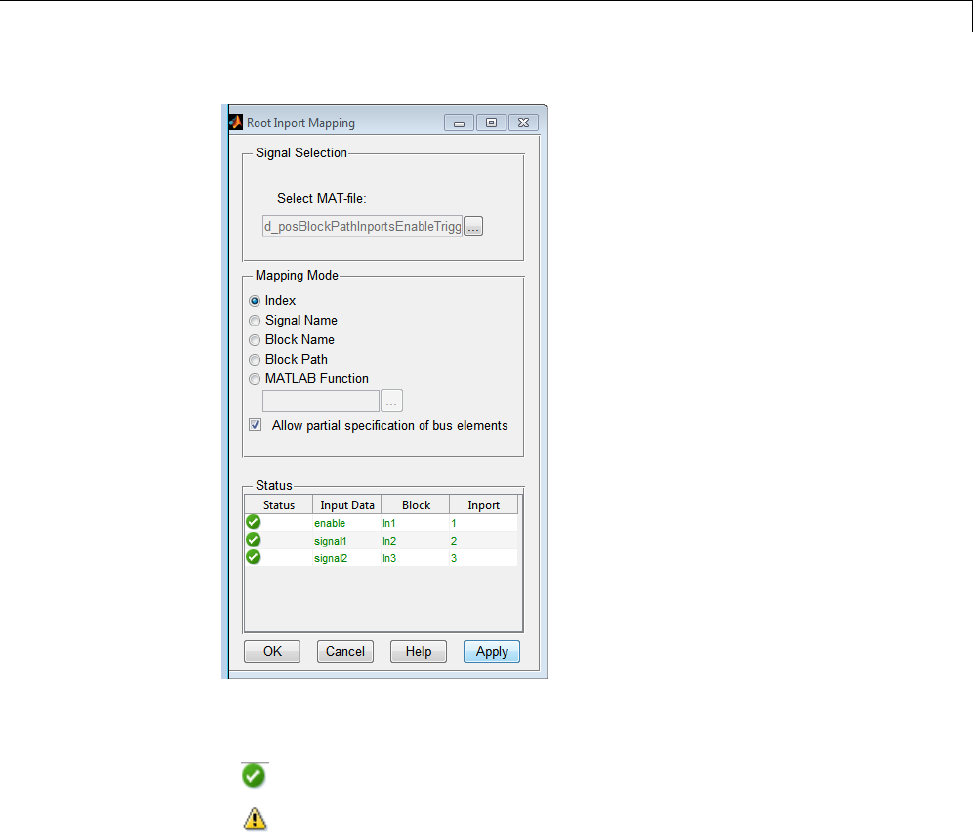
Import and Map Data to Root-Level Inports
The Status area of the tool lists the input data and the status of the
mapping:
•— Successful mapping of data to root-level inports.
•— Potential issue with mapping of data to root-level inports. The tool
might not know if all the data types match. If you choose to Continue
without Compilation as the action, the Status area might show all
data with this warning icon. To inspect the data and compare it to the
root-level inport, click anywhere in thedataline.TheComparisonTool
is displayed with the columns in the left-right order of field name, input
data, and root-level inport. Use this tool to evaluate your next action.
You might want to edit the data in the MAT-file, or you might want to
edit the root-level inport.
45-87
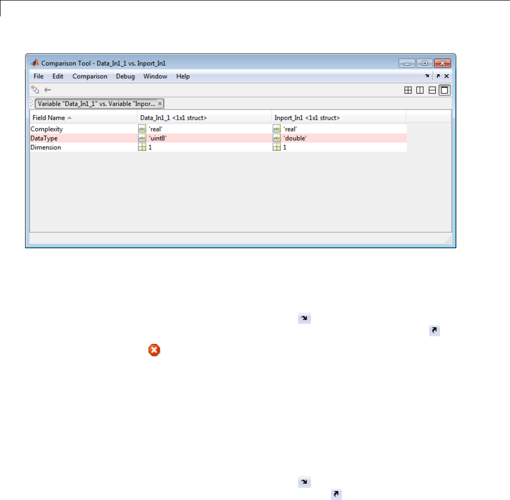
45 Importing and Exporting Simulation Data
For more information on the Comparison Tool, see “Comparing Files
and Folders”.
By default, each time you click a data line, an independent Comparison
Tool window is displayed. To dock all Comparison Tool windows in one
window, click the Dock button ( ). To view each Comparison Tool
window as a stand-alone window, click the Undock button ( ).
•— Issue with mapping of data to root-level inports. To inspect the
data and compare it to the root-level inport, click anywhere in the data
line. The Comparison Tool is displayed with the columns in the left-right
order field name, input data, and root-level inport. The Comparison Tool
is displayed with the columns in the left-right order field name, input
data, and root-level inport. Use this tool to evaluate your next action.
You might want to edit the data in the MAT-file, or you might want to
edit the root-level inport.
By default, each time you click a data line, an independent Comparison
Tool window is displayed. To dock all Comparison Tool windows in one
window, click the Dock button ( ). To view each Comparison Tool
individually, click the Undock button ( ).
For more information on the Comparison Tool, see “Comparing Files
and Folders”.
45-88

Import and Map Data to Root-Level Inports
11 Click OK.
12 If there are no mismatches with the data, in the Data Import/Export
pane of the Configuration Parameters dialog box, observe that the Input
parameter is now selected. In addition, the text box now contains the
imported data variables.
If there are root-level input ports that have not been mapped, the Root
Inport Mapping tool maps those ports as empty ([]).
To inspect the imported data, connect the output to a scope, simulate the
model, and observe the data. Optionally, to inspect the imported data, log
the signals and use the Simulink Data Inspector tool to observe the data.
13 Optionally, if you are satisfied with the data and mapping, in the Preload
tab, enter a load function to load the signal data MAT-file. This step
replaces steps 5 and 6 so that you do not need to manually load the signal
data MAT-file. For example, to load a MAT-file d_signal_data.mat,type:
load d_signal_data.mat;
14 Save and close the model.
Import and Map Bus Data
This topic assumes that you are familiar with bus objects and how to create
them. For more information, see “Bus Objects” on page 48-20.
1In the MATLAB workspace, create a bus object for the bus data you want
to import and map.
2Save that bus object definition to a MAT-file, for example d_myBusObj.mat.
3Create a MAT-file that contains the bus data you want to import for the
bus object.
4Open a model.
45-89
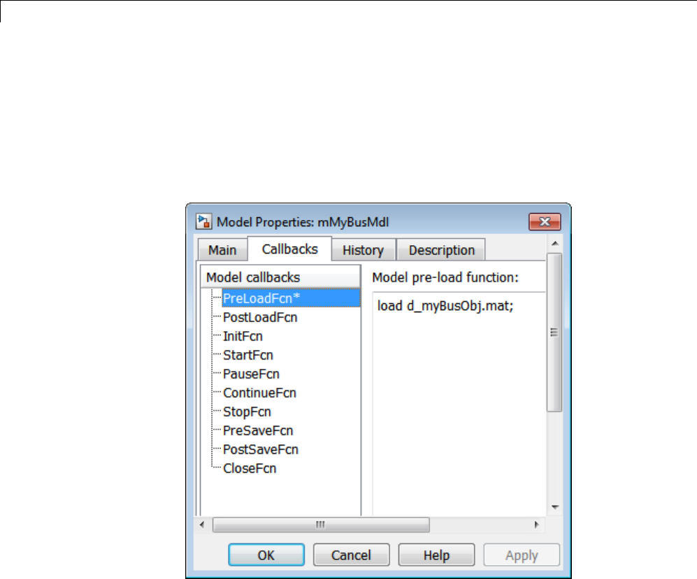
45 Importing and Exporting Simulation Data
5In the Simulink Editor, select File > Model Properties > Model
Properties.
The Model Properties dialog box is displayed.
6In the Callbacks tab, enter a load function to load the bus object definition.
For example, to load a bus object from d_myBusObj.mat:
7Start the Configuration Parameters dialog box for the model
8Navigate to the Data Import/Export pane.
9In the Load from workspace section, click Edit Input.
The Root Inport Mapping dialog box is displayed.
45-90
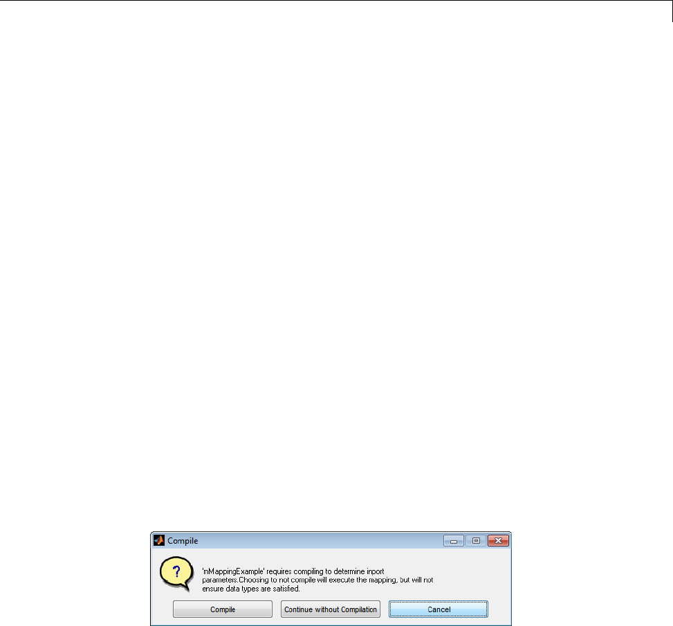
Import and Map Data to Root-Level Inports
10 In the Select MAT file parameter, specify the MAT file that contains the
signal data in one of the following ways:
•Enter the full path to the file.
•Clickthebrowserbuttontobrowsetothefile.
A load MAT file window pops up.
11 Click Yes to load the MAT-file.
12 In the Mapping Mode section, select how you want the imported data to
map to the root-level inports:
•Index
•Signal Name
•Block Name
•Block Path
•MATLAB Function
13 If you import bus data, optionally select the Allow partial specification
of bus elements check box. Selecting this check box allows you to import
bus data that is only partially defined in the MAT-file. If you clear this
check box and import incompletely specified bus data, the tool cannot
properly map the partially specified bus data to root-level inports.
14 Click Apply. A Compile dialog pops up, for example:
15 Select one of the following:
•Compile — Maps the imported data to the root-level inport and compiles
the model to check data types of root-level inports and imported data.
45-91
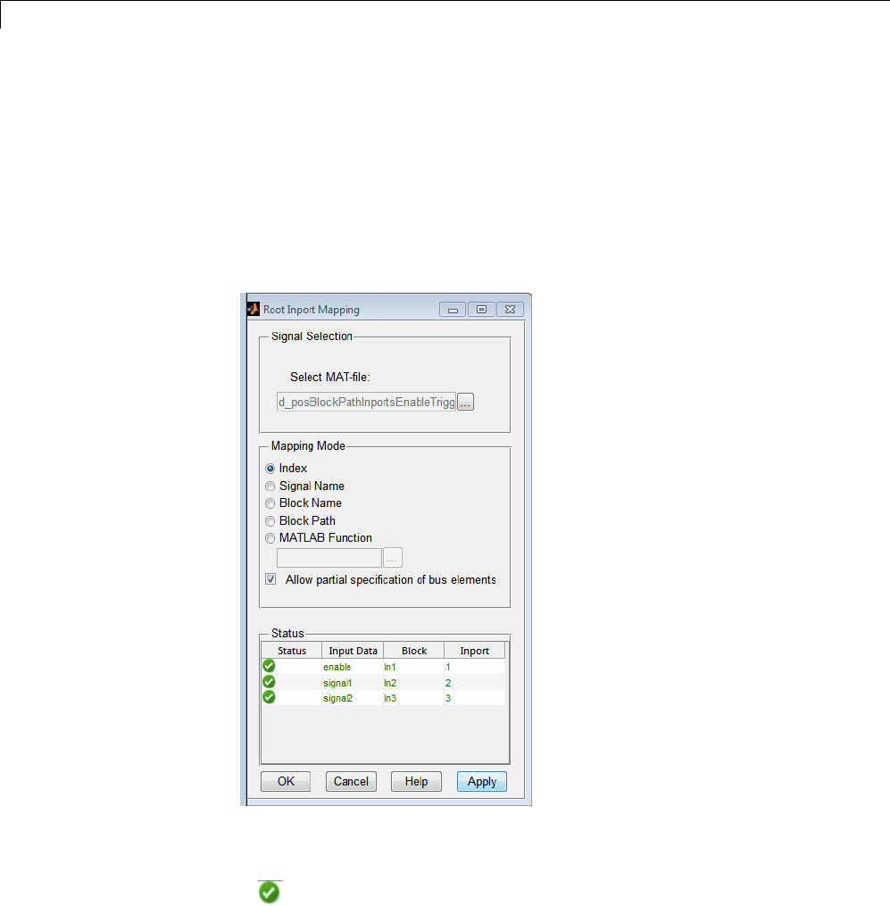
45 Importing and Exporting Simulation Data
•Continue without Compilation — Maps the imported data to the
root-level inport, but does not compile the model. Selecting this option
might not check root-level inports, data, and data types.
•Cancel — Cancels the import. You can choose another MAT-file to
import.
The results of the mapping are displayed in the Status area. If the contents
of the imported file cannot be matched with the Mapping Mode
The Status area of the tool lists the input data and the status of the
mapping:
•— Successful mapping of data to root-level inports.
45-92
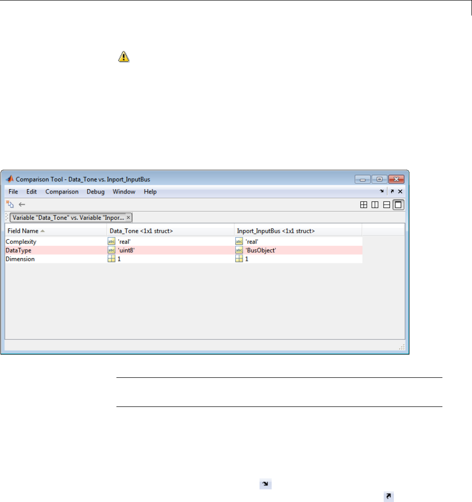
Import and Map Data to Root-Level Inports
•— Potential issue with mapping of data to root-level inports. The tool
might not know if all the data types match. If you choose to Continue
without Compilation as the action, the Status area might show all
data with this warning icon. To inspect the data and compare it to the
root-level inport, click anywhere in thedataline.TheComparisonTool
is displayed with the columns in the left-right order of field name, input
data, and root-level inport. Use this tool to evaluate your next action.
You might want to edit the data in the MAT-file, or you might want to
edit the root-level inputs.
Note When the input is a bus, click the levels of the bus object to drill
down to the individual elements in the bus.
For more information on the Comparison Tool, see “Comparing Files
and Folders”.
By default, each time you click a data line, an independent Comparison
Tool window is displayed. To dock all Comparison Tool windows in one
window, click the Dock button ( ). To view each Comparison Tool
window as a stand-alone window, click the Undock button ( ).
45-93

45 Importing and Exporting Simulation Data
•— Issue with mapping of data to root-level inports. To inspect the
data and compare it to the root-level inport, click anywhere in the data
line. The Comparison Tool is displayed with the columns in the left-right
order of field name, input data, and root-level inport. Use this tool
to evaluate your next action. You might want to edit the data in the
MAT-file, or you might want to edit the root-level inport.
Note When the input is a bus, click the levels of the bus object to drill
down to the individual elements in the bus.
For more information on the Comparison Tool, see “Comparing Files
and Folders”.
By default, each time you click a data line, an independent Comparison
Tool window is displayed. To dock all Comparison Tool windows in one
window, click the Dock button ( ). To view each Comparison Tool
window as a stand-alone window, click the Undock button ( ).
16 Click OK.
17 If there are no mismatches with the data, in the Data Import/Export
pane of the Configuration Parameters dialog box, observe that the Input
parameter is now selected. In addition, the text box now contains the
imported bus data variables.
18 Optionally, if you are satisfied with the data and mapping, in the Preload
tab, enter a load function to load the signal data MAT-file. This step
replaces steps 5 and 6 so that you do not need to manually load the signal
data MAT-file. For example, to load a MAT-file d_bus_data.mat,enter
type:
load d_bus_data.mat;
19 Save and close the model.
45-94

Import and Map Data to Root-Level Inports
If there are root-level input ports that have not been mapped, the Root Inport
Mapping tool maps those ports as empty ([]).
To inspect the imported data, connect the output to a scope, simulate the
model, and observe the data.
Create Custom Mapping File Function
Create a custom mapping file function if you do not want to rely on one of
the existing tool mapping modes to map your data to root-level input ports.
You might want to create a custom mapping file function if your signal data
contains a common prefix that is not contained in your model. You also might
want to create a custom mapping file function to explicitly map a signal.
This custom mapping file function might be useful if you want to map by
block name but the data contains a signal whose name does not match one of
the block names.
See the following files in matlabroot\help\toolbox\simulink\example
for an example:
•BlockNameIgnorePrefixMap.m — Custom mapping file function that
ignores the prefix of a signal name when importing.
•BlockNameIgnorePrefixData.mat —MAT-fileofsignaldatatobe
imported.
•ex_BlockNameIgnorePrefixExample — Model file into which you can
import and map data.
Follow these guidelines to create a custom mapping file function:
1Create a MATLAB function with the following input parameters:
•Model name
•Signal names specified as a cell array of strings
•Signals specified as a cellarrayofsignaldata
2In this function, call the getRootInportMap function to create a
variable that contains the mapping object (for an example, see
BlockNameIgnorePrefixMap.m).
45-95

45 Importing and Exporting Simulation Data
3Save and close the MATLAB function file.
4Add the path for the new function to the MATLAB path.
If there are root-level input ports that have not been mapped, the Root Inport
Mapping tool maps those ports as empty ([]).
To use the custom mapping file function, in the Input Mapping Tool:
1Open the model for which you want to import data (for example,
ex_BlockNameIgnorePrefixExample).
2Start the Configuration Parameters dialog box for the model.
3Navigate to the Data Import/Export pane.
4In the Load from workspace section, click Edit Input.
The Root Inport Mapping dialog box is displayed.
5In the Select MAT file parameter, specify the MAT-file that contains
the signal data by clicking the browser button to browse to the file (for
example, BlockNameIgnorePrefixData.mat).
A load MAT-file window pops up.
6Click Yes to load the MAT-file in the workspace.
7From the Mapping Mode list, click MATLAB Function.
8In the MATLAB Function parameter, specify the MATLAB function file
(for example, BlockNameIgnorePrefixMap.m) with the browser button.
Tip The Root Inport Mapping tool parses your custom code. The tool might
perform operations such as reordering output alphabetically and verifying
that data types are consistent.
9Click Apply. The Compile dialog box is displayed, for example:
45-96
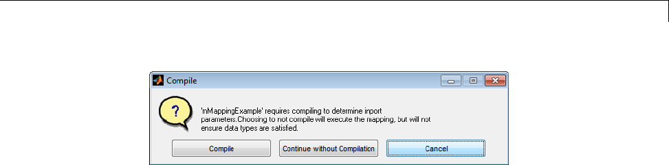
Import and Map Data to Root-Level Inports
10 Click Compile.
The software compiles the model and updates the Root Inport Mapping
dialog box.
11 Click OK.
12 In the Data Import/Export pane of the Configuration Parameters dialog
box, observe that the Input parameter is now selected. In addition, the text
box now contains the imported signal data variables. Optionally, to inspect
the imported data, log the signals and use the Simulink Data Inspector tool
to observe the data.
13 Optionally, if you are satisfied with the data and mapping, in the Preload
tab, enter a load function to load the signal data MAT-file. This step
replaces steps 5 and 6 so that you do not need to manually load the signal
data MAT-file. For example, to load a MAT-file d_signal_data.mat,enter
type:
load d_signal_data.mat;
14 Save and close the model.
45-97

45 Importing and Exporting Simulation Data
Import MATLAB timeseries Data
In this section...
“Specify Time Dimension” on page 45-98
“Models with Multiple Root Inport Blocks” on page 45-99
A root-level Inport, Enable, Trigger, and From Workspace block can import
data specified by a MATLAB timeseries object residing in a workspace.
Specify Time Dimension
When you create a MATLAB timeseries object to import data to Simulink,
the time dimension depends on the dimension and type of signal data:
•If the signal is a scalar or a 1D vector, then time is first.
Below is an example of a timeseries constructor for a scalar signal. Time
is aligned with the first dimension.
t = (0:10)';
ts = timeseries(sin(t)), t);
•If the signal dimension is 2D (including row and column vectors) or greater,
then time is last.
Below is an example of a timeseries constructor for a matrix signal. Time
is aligned with the last dimension.
t=0;
ts = timeseries([1 2; 3 4], t);
•If the signal is a 2D row vector, and there is only one time step, then
you need align time with the last dimension. Use the following in the
constructor:
'InterpretSingleRowDataAs3D', true
For example:
t=0;
ts = timeseries([1 2], t, 'InterpretSingleRowDataAs3D', true);
45-98

Import MATLAB®timeseries Data
Models with Multiple Root Inport Blocks
If you use a MATLABtimeseries object for a root Inport block in a model
that has multiple root Inport blocks, convert all of the other root Inport
block data that uses Simulink.TsArray or Simulink.Timeseries objects to
MATLAB timeseries objects or a structure of MATLABtimeseries objects.
You can use the Simulink.Timeseries.convertToMATLABTimeseries
method to convert a Simulink.Timeseries object to a MATLAB timeseries
object. For example, if sim_ts is a Simulink.Timeseries object, then the
following line converts sim_ts to a MATLAB timeseries object:
ts = sim_ts.convertToMATLABTimeseries;
45-99

45 Importing and Exporting Simulation Data
Import Structures of timeseries Objects for Buses
In this section...
“Define Structure of MATLAB timeseries Objects for a Bus Signal” on
page 45-100
“Convert Simulink.TsArray Objects” on page 45-100
“Use a Structure of MATLAB timeseries Objects to Import Bus Signals”
on page 45-101
Define Structure of MATLAB timeseries Objects for a
Bus Signal
A root-level input port defined by a bus object (see Simulink.Bus)canimport
data from a structure of MATLAB timeseries objects that represent the
bus elements for which you do not want to use the ground values. The bus
elements that you do not include in the structure use ground values.
The structure of MATLAB timeseries objects must match the bus elements
in terms of:
•Hierarchy
•The name of the structure field (The name property of the timeseries
object does not need to match the bus element name.)
•Data type
•Dimensions
•Complexity
Theorderofthestructurefieldsdoesnot have to match the order of the bus
elements.
Convert Simulink.TsArray Objects
If you are using logged data from a model whose Configuration
Parameters > Data Import/Export > Signal logging format parameter
is set to ModelDataLogs format instead of the default Dataset format,
consider converting the data to use a structure of MATLAB timeseries
45-100

Import Structures of timeseries Objects for Buses
objects. The ModelDataLogs format is supported for backwards compatibility.
The ModelDataLogs format will be removed in a future release.
You can create a structure of MATLAB timeseries objects from a
Simulink.TsArray object. For example, if tsa is a Simulink.TsArray object:
input = Simulink.SimulationData.createStructOfTimeseries(tsa);
Note If you use a structure of MATLAB timeseries objects for a root Inport
block in a model that has multiple root Inport blocks, all the root Inport blocks
must use MATLAB timeseries objects. Convert any root Inport block data
that uses Simulink.TsArray or Simulink.Timeseries objectstobeMATLAB
timeseries objects.
Use a Structure of MATLAB timeseries Objects to
Import Bus Signals
Use the following procedure to set up a model to import bus data to a root
Inport block or Trigger blocks.
The examples in this procedure assume you have a model that is set up as
follows:
•The TopBusObject bus object has two elements:
-c
-s1, which is a sub-bus that has two elements: aand b.
•The model has two root Inport blocks: In1 and In2.
-The In1 Inport block imports non-bus data.
-The In2 Inport block imports bus data of type TopBusObject.
45-101

45 Importing and Exporting Simulation Data
1Create a MATLAB timeseries object for each root Inport or Trigger block
forwhichyouwanttoimportnon-busdata.
For example:
N = 10;
Ts = 1;
t1 = ((0:N)* Ts)';
d1 = sin(t1);
in1 = timeseries(d1,t1)
2Create a structure of MATLAB timeseries objects, with one timeseries
object for each leaf bus element for which you do not want to use ground
values.
For example, to specify non-ground values for all the elements in the s2 bus:
in2.c = timeseries(d1,t1);
in2.s1.a = timeseries(d2,t2);
in2.s1.b = timerseries(d3,t3);
The MATLAB timeseries objects that you create must match the
corresponding bus element in terms of:
•Hierarchy
•Name
•Data type
•Dimensions
•Complexity
The name of the structure field must match the bus element name. The
Name property of the MATLAB timeseries object does not need to match
the bus element name.
The order of the structure fields does not matter.
To determine the number of MATLAB timeseries objects and data type,
complexity, and dimensions needed for creating a structure of timeseries
objects from a bus, you can use the Simulink.Bus.getNumLeafBusElements
and Simulink.Bus.getLeafBusElements methods. For
45-102
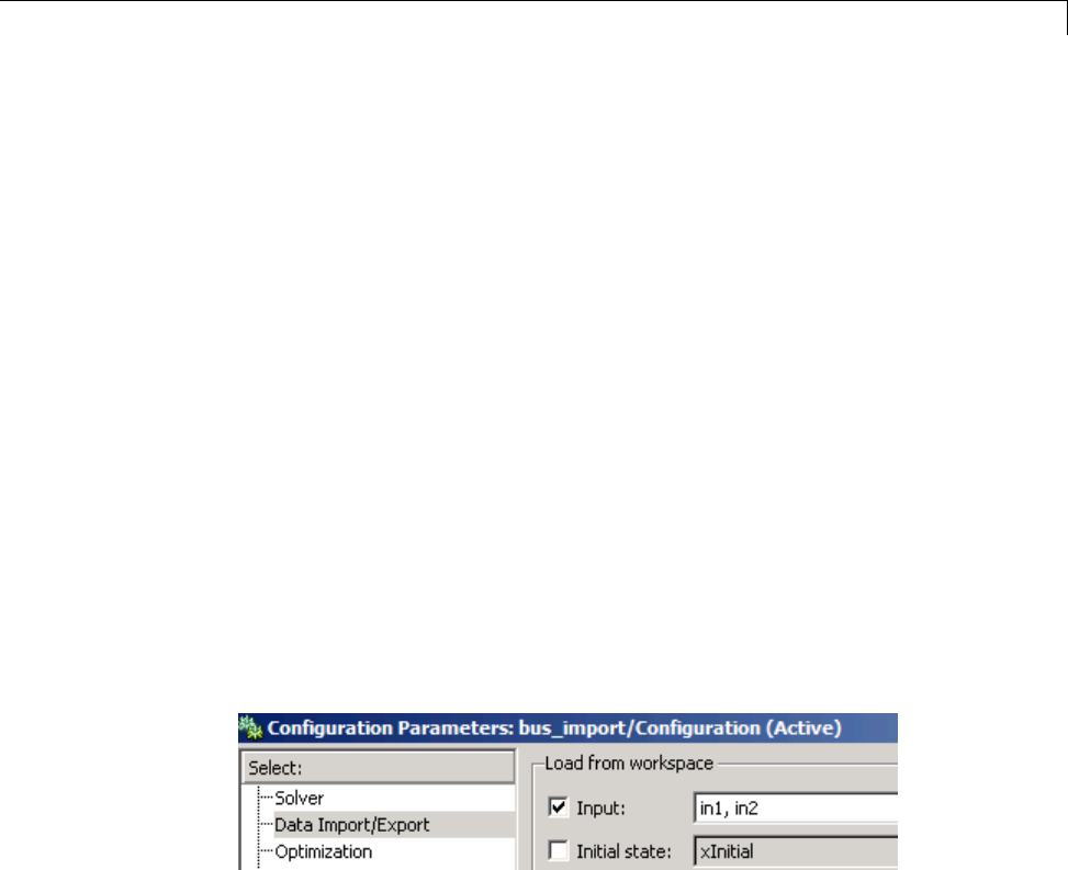
Import Structures of timeseries Objects for Buses
example, you could use these methods in conjunction with the
Simulink.SimulationData.createStructOfTimeseries utility (where
MyBus is a bus object):
num_el = MyBus.getNumLeafBusElements;
el_list = MyBus.getLeafBusElements;
To create a structure of MATLABtimeseries objects from a bus object
and a cell array of timeseries or Simulink.Timeseries objects, use the
Simulink.SimulationData.createStructOfTimeseries utility. For
example:
input = ...
Simulink.SimulationData.createStructOfTimeseries('MyBus',...
{ts1,ts2,ts3});
3In the Configuration Parameters > Import/Export pane, select
the Input parameter and enter a comma-separated list of MATLAB
timeseries objects and structures of MATLAB timeseries objects.
For example, the in1 timeseries object and the in2 structure of
timeseries objects.
45-103

45 Importing and Exporting Simulation Data
Import Simulink.Timeseries and Simulink.TsArray Data
In this section...
“Use MATLAB Timeseries for New Models” on page 45-104
“Simulink.TsArray Data” on page 45-104
Use MATLAB Timeseries for New Models
For new models, have root-level Inport block or Trigger blocks import
MATLAB timeseries data.
However, you can import existing Simulink.Timeseries object data.
Importing Simulink.Timeseries objects allows you to import data logged by
a previous simulation run that used the ModelDataLogs format for signal
logging (see “Export Signal Data Using Signal Logging” on page 45-19).
Simulink.TsArray Data
Objects of the Simulink.TsArray class have a variable number of properties.
The first property, called Name, specifies the log name of the logged
signal. The remaining properties reference logs for the elements of the
logged signal: Simulink.Timeseries objects for elementary signals and
Simulink.TsArrayobjects for mux or bus signals. The name of each property
isthelognameofthecorrespondingsignal.
45-104

Import Data Arrays
Import Data Arrays
In this section...
“Data Array Format” on page 45-105
“Specify the Input Expression” on page 45-105
Data Array Format
This import format consists of a real (noncomplex) matrix of data type
double. The first column of the matrix must be a vector of times in ascending
order. The remaining columns specify input values. In particular, each
column represents the input for a different Inport or Trigger block signal
(in sequential order) and each row is the input value for the corresponding
time point. For a Trigger block, the signal driving the trigger port must be
the last data item.
The total number of columns of the input matrix must equal n+1,wherenis
the total number of signals entering the model’s input ports.
Specify the Input Expression
The default input expression for a model is [t,u] and the default input
format is Array.Soifyoudefinetand uin the MATLAB workspace, you
need only select the Input option to input data from the model workspace.
For example, suppose that a model has two input ports, In1 that accepts two
signals, and In2 that accepts one signal. Also, suppose that the MATLAB
workspace defines tand uas follows:
N = 10;
Ts = 0.1
t = (0:N)* Ts';
u = [sin(t), cos(t), 4*cos(t)];
When the simulation runs, the signals sin(t) and cos(t) will be assigned to
In1 and the signal 4*cos(t) will be assigned to In2.
45-105

45 Importing and Exporting Simulation Data
Note The array input format allows you to load only real (noncomplex) scalar
or vector data of type double. Use the structure format to input complex data,
matrix (2-D) data, and/or data types other than double.
45-106

Import MATLAB®Time Expression Data
Import MATLAB Time Expression Data
Specify the Input Expression
You can use a MATLAB time expression to import data from a workspace.
To use a time expression, enter the expression as a string (i.e., enclosed in
single quotes) in the Input field of the Data Import/Export pane. The time
expression can be any MATLAB expression that evaluates to a row vector
equal in length to the number of signals entering the input ports of the model.
For example, suppose that a model has one vector Inport that accepts two
signals. Furthermore, suppose that timefcn is a user-defined function that
returns a row vector two elements long. The following are valid input time
expressions for such a model:
'[3*sin(t), cos(2*t)]'
'4*timefcn(w*t)+7'
The expression is evaluated at each step of the simulation, applying the
resulting values to the model’s input ports. Note that the Simulink software
defines the variable twhen it runs the simulation. Also, you can omit the
time variable in expressions for functions of one variable. For example, the
expression sin is interpreted as sin(t).
45-107

45 Importing and Exporting Simulation Data
Import Data Structures
In this section...
“Data Structures” on page 45-108
“One Structure for All Ports or a Structure for Each Port” on page 45-109
“Specify Signal Data” on page 45-109
“Specify Time Data” on page 45-110
“Examples of Specifying Signal and Time Data” on page 45-111
Data Structures
The Simulink software can read data from the workspace in the form of a
structure, whose name you specify in the Configuration Parameters >
Data Import/Export > Input parameter.
For information about defining MATLAB structures, see “Create a Structure
Array” in the MATLAB documentation.
The structure always includes a signals substructure, which contains a values
field and a dimensions field. For details about the signal data, see “Specify
Signal Data” on page 45-109. Depending on the modeling task that you want
to perform, the structure can also include a time field.
You can specify structures for the model as a whole or on a per-port basis. For
information about specifying per-port structures for the Input parameter, see
“One Structure for All Ports or a Structure for Each Port” on page 45-109.
The form of a structure that you use depends on whether you are importing
data for discrete signals (the signal is defined at evenly-spaced values of time)
or continuous signals (the signal is defined for all values of time). For discrete
signals, use a structure that has an empty time vector. For continuous
signals, the approach that you use depends on whether the data represents
a smooth curve or a curve that has discontinuities (jumps) over its range.
For details, see:
•“Import Data to Test a Discrete Algorithm” on page 45-70
45-108

Import Data Structures
•“Import Data to Model a Continuous Plant” on page 45-67
•“Import Data for an Input Test Case” on page 45-71
For both discrete and continuous signals, specify a signals field, which
contains an array of substructures, each of which corresponds to a model
input port. For details, see “Specify Signal Data” on page 45-109.
For continuous signals, you may want to specify a time field, which contains a
time vector. See “Time and Signal Values for Imported Data” on page 45-64.
One Structure for All Ports or a Structure for Each Port
You can specify one structure to provide input to all root-level input ports in a
model, or you can specify a separated structure for each port.
The per-port structure format consists of a separate structure-with-time
or structure-without-time for each port. Each port’s input data structure
has only one signals field. To specify this option, enter the names of the
structures in the Input text field as a comma-separated list, in1, in2,...,
inN,wherein1 is the data for your model’s first port, in2 for the second input
port, and so on.
The rest of the section about importing structure data focuses on specifying
one structure for all ports.
Specify Signal Data
Each signals substructure must contain two fields: values and dimensions.
The Values Field
The values field must contain an array of inputs for the corresponding input
port. If you specify a time vector, each input must correspond to a time value
specified in the time field.
If the inputs for a port are scalar or vector values, the values field must be
an M-by-N array. If you specify a time vector, Mmust be the number of time
points specified by the time field and Nis the length of each vector value.
45-109

45 Importing and Exporting Simulation Data
If the inputs for a port are matrices (2-D arrays), the values field must be an
M-by-N-by-T array where Mand Nare the dimensions of each matrix input
and Tis the number of time points. For example, suppose that you want
to input 51 time samples of a 4-by-5 matrix signal into one of your model’s
input ports. Then, the corresponding dimensions field of the workspace
structure must equal [4 5] and the values array must have the dimensions
4-by-5-by-51.
The Dimensions Field
The dimensions field specifies the dimensionsoftheinput. Ifeachinputis
a scalar or vector (1-D array) value, the dimensions field must be a scalar
value that specifies the length of the vector (1 for a scalar). If each input is a
matrix (2-D array), the dimensions field must be a two-element vector whose
first element specifies the number of rows in the matrix and whose second
element specifies the number of columns.
Note You must set the Port dimensions parameter of the Inport or
theTriggerblocktobethesamevalueasthedimensions field of the
corresponding input structure. If the values differ, an error message is
displayed when you try to simulate the model.
Specify Time Data
You can specify a time vector as part of the data structure to import. The
“Time and Signal Values for Imported Data” on page 45-64 section indicates
when you may want to add a time vector.
The following table provides recommendations for how to specify time values,
based on the kind of signal data you want to import.
45-110
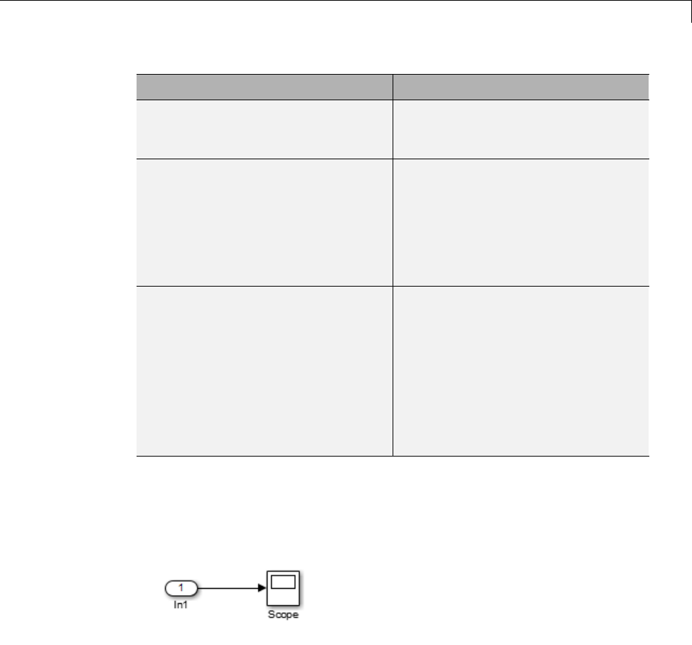
Import Data Structures
Signal Data Time Data Recommendation
Inport or Trigger block with a
discrete sample time
Do not specify a time vector.
Simulink reads one signal value at
each time step.
Evenly-spaced discrete signals Consider using an expression in the
following form:
TimeVector = Ts * (0:N);
where Ts is the time step and Nis
the number of time steps.
Unevenly-spaced values Use any valid MATLAB array
expression; for example, [1:5 5:10]
or (161015).
If the root-level input port is from
a From Workspace, From File, or
Signal Builder block, which support
zero-crossing detection, you can
specify a zero-crossing time by using
a duplicate time entry.
Examples of Specifying Signal and Time Data
In the first example, consider the following model that has a single input port:
1Create an input structure for loading 11 time samples of a two-element
signal vector of type int8 into the model:
N=10
Ts = 0.1
a.time = (0:N)*Ts';
45-111
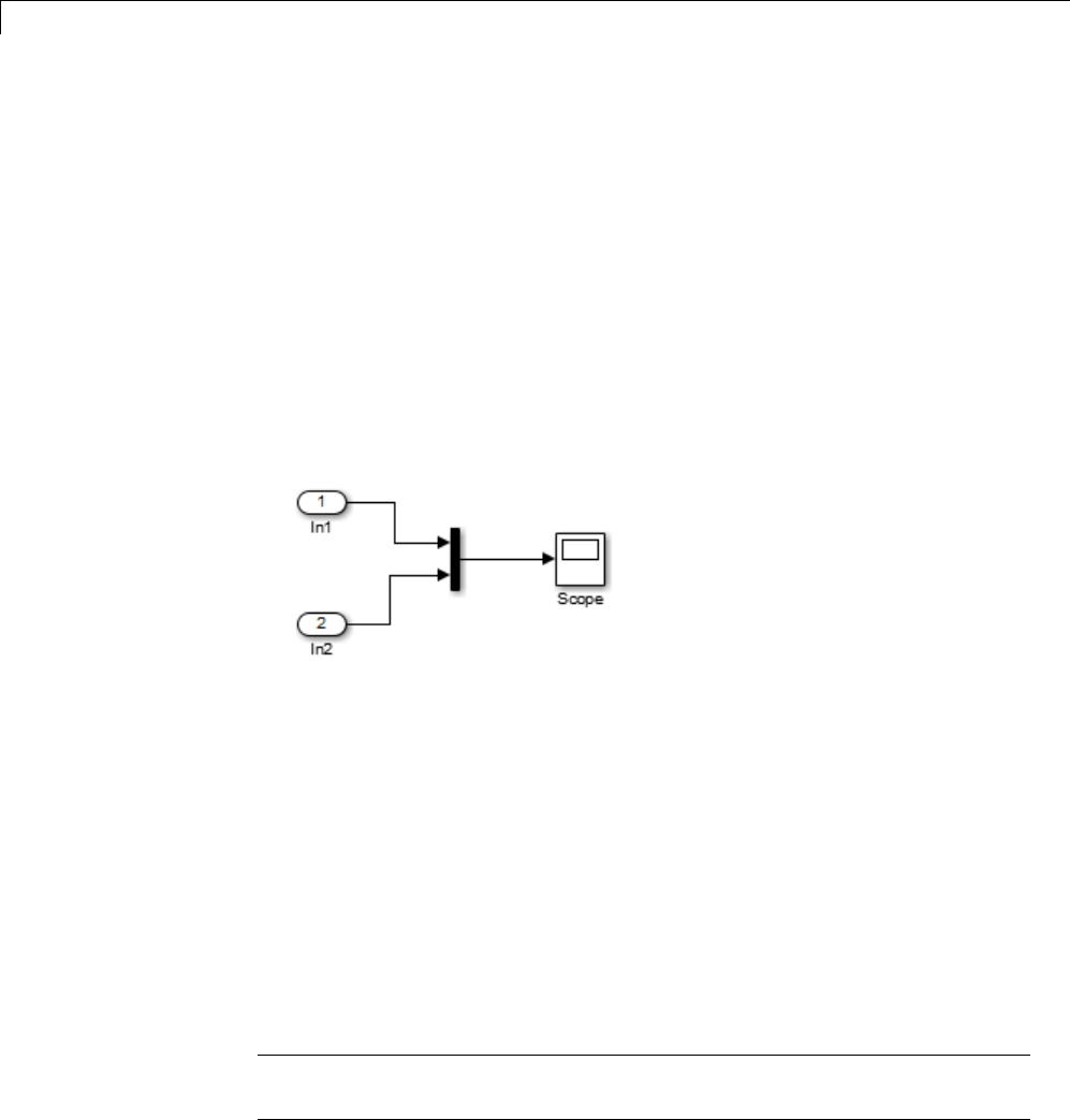
45 Importing and Exporting Simulation Data
c1 = int8([0:1:10]');
c2 = int8([0:10:100]');
a.signals(1).values = [c1 c2];
a.signals(1).dimensions = 2;
2In the Configuration Parameters > Data Import/Export > Input
parameter edit box, specify the variable a.
3In the Inport block dialog box, in the Signal Attributes tab, set Port
dimensions to 2and Data type to int8.
As another example, consider a model that has two inputs:
Suppose that you want to input a sine wave into the first port and a cosine
wave into the second port. To do this, define a structure, a,asfollows,inthe
MATLAB workspace:
a.time = (0:0.1:1)';
a.signals(1).values = sin(a.time);
a.signals(1).dimensions = 1;
a.signals(2).values = cos(a.time);
a.signals(2).dimensions = 1;
Enter the structure name (a)intheConfiguration Parameters > Data
Import/Export > Input parameter edit box.
Note Note that in this model you do not need to specify the dimension and
data type, because the default values are 1and double.
45-112

Import and Export States
Import and Export States
In this section...
“State Information” on page 45-113
“Save State Information” on page 45-113
“Import Initial States” on page 45-118
“Import and Export State Information for Referenced Models” on page
45-120
State Information
Some blocks maintain state information that Simulink uses for calculating
values during simulation. For example, the state information for a Unit
Delay block is the output signal value from the previous simulation step,
which the block uses for calculating the output signal value for the current
simulation step.
Youcanusesavedstateinformationtocaptureaknownstate. Someexamples
of uses of saved state information include:
•Stopping a simulation for a model and using the saved state information as
inputwhenyourestartthesimulation.
•Simulating one model and using the saved state information as input for
the simulation of another model that builds on the results of the first model.
Save State Information
You can save state information by either:
•Saving the final state of a simulation, using the SimState
•Saving partial state information at the end of a simulation or for each
simulation step, using a structure, structure with time, or array
SimState provides complete state information. However, use of SimState
has some limitations, such as:
•You can use only the Normal or the Accelerator mode of simulation.
45-113

45 Importing and Exporting Simulation Data
•SimState does not support code generation, including Model Reference
in accelerated modes.
To ensure that SimState meets your modeling requirements, see “Limitations
of the SimState” on page 14-38.
When you save final states without the SimState, you save only logged states
— the continuous and discrete states of blocks — which are a subset of the
complete simulation state of the model. However, if you use a structure or
structure with time, you may find that the state information is easier to read
than if you use a SimState.
For more information, see:
•“Save Complete State Information with SimState” on page 45-114
•“Save Partial Final State Information” on page 45-114
Save Complete State Information with SimState
To save complete state information, save the SimState for a simulation.
1Select the Configuration Parameters > Data Import/Export > Final
states check box.
2Also in the Data Import/Export pane, select the Save complete SimState
in final state parameter.
3In the edit box adjacent to the Save complete SimState in final state
parameter, enter a variable name for the SimState.
4Simulate the model.
For more information about using the SimState,see“SaveandRestore
Simulation State as SimState” on page 14-32.
Save Partial Final State Information
To save just the logged states (the continuous and discrete states of blocks):
45-114

Import and Export States
1Select the Configuration Parameters > Data Import/Export > Final
states check box.
2In the Final states edit box, you can specify a different variable for the
stateinformation,ifyoudonotwanttousethedefaultxFinal variable.
3Also in the Data Import/Export pane, set the Format parameter to
Structure or Structure with time. For details, see “Format for Saved
State Information” on page 45-115
4Simulate the model.
For details about examining the saved state information, see
Save State Information For Each Simulation Step
You can save state information for logged states for each simulation step
during a simulation. That level of state information can be helpful for
debugging.
1Select the Configuration Parameters > Data Import/Export > States
check box.
2In the States edit box, you can specify a different variable for the state
information, if you do not want to use the default xout variable.
3Also in the Data Import/Export pane, set the Format parameter to
Structure or Structure with time, unless you need to use array format
for compatibility with a legacy model. For details, see “Format for Saved
State Information” on page 45-115.
4Simulate the model.
Format for Saved State Information
IfyoudonotusetheSimState for saving state information, then use
Configuration Parameters > Data Import/Export > Format to specify
thedataformatforthesavedstateinformation.
You can set Format to:
45-115

45 Importing and Exporting Simulation Data
•Array (default)
•Structure
•Structure with time
The Structure and Structure with time formats are easier to read and
consistent across simulations. Also, these two formats are useful when using
state information to initialize a model for simulation, allowing you to:
•Associate initial state values directly with the full path name to the
states. This association eliminates errors that can occur if Simulink
reorders the states, but the order of the initial state array does not change
correspondingly.
•Assign a different data type to the initial value of each state.
•Initialize only a subset of the states.
The Array option for the Configuration Parameters > Data
Import/Export > Format option supports compatibility with models
developed in earlier releases, when Simulink supported only the array format
for saving state information.
The array format reflects the order of signals. The order of saved state
information can change between simulations when you change any of the
following:
•The model (even without changing the signal
•The simulation mode
•The code generation mode
Examine State Information Saved Without the SimState
If you enable the Configuration Parameters > Data Import/Export >
Final states or States parameters, Simulink saves the state information in
the format that you specify with the Format parameter. The default variable
for Final state information is xFinal, and the variable for state information
for States information is xout.
45-116

Import and Export States
If a model has no states saved, then xFinal and xout are empty variables.
To determine whether a model has states saved, use the isempty(xout)
command.
For example, suppose that you saved final state information in a structure
with time format, and use the default xFinal variable for the saved state
information.
To find the simulation time and number of states, at the MATLAB command
line, type
xFinal
xFinal =
time: 20
signals: [1x2 struct]
In this case, the simulation time is 20 and there are two states. To examine
the first state, type
xFinal.signals(1)
ans =
values: 2.0108
dimensions: 1
label: 'CSTATE'
blockName: 'vdp/x1'
stateName: ''
inReferencedModel: 0
The values and blockName fields of first state structure shows that the final
value for the output signal of the x1 block was 2.018.
Note If you write a script to analyze state information, use a combination
of label and blockName values to uniquely identify a specific state. Do not
rely on the order of the states.
45-117

45 Importing and Exporting Simulation Data
Import Initial States
To import states, enable Configuration Parameters > Data
Import/Export > Initial state and specify a variable that contains the
initial state values. For example, you could specify a variable that contains
state information saved from a previous simulation.
You can import state information to initialize a simulation:
1Enable Configuration Parameters > Data Import/Export > Initial
state.
2In the Initial state edit box, enter the name of the variable for the state
information that you want to use for initialization. You can create your own
state information in MATLAB or you can use state information saved from
a previous simulation. For details about using saved state information, see
“Import Saved State Information” on page 45-118.
The initial values that the variable specifies override the initial state
values that the blocks in the model specify in initial condition parameters.
Import Saved State Information
You can import saved state information as the initial state.
1Enable Configuration Parameters > Data Import/Export > Initial
state.
2In the Initial state edit box, enter the name of the variable in the Final
statesedit box. The state information that Simulink loads depends on the
setting of Configuration Parameters > Data Import/Export > Save
complete SimState in final state.
45-118

Import and Export States
Setting for the “Save complete
SimState in final state”
parameter
State Information
Enabled Complete state information. For
details, see “Save and Restore
Simulation State as SimState” on
page 14-32.
Cleared State information for logged states
(the continuous and discrete states
of blocks), in the format specified
in Configuration Parameters >
Data Import/Export > Format.
For details, see “Format for Saved
State Information” on page 45-115.
For example, the following commands create an initial state structure that
initialize the x2 state of the vdp model. The x1 state is not initialized in the
structure. Therefore, during simulation, Simulink uses the value in the
Integrator block associated with the state.
% Open the vdp model
vdp
% Use getInitialState to obtain an initial state structure
states = Simulink.BlockDiagram.getInitialState('vdp');
% Set the initial value of the signals structure element
% associated with x2 to 2.
states.signals(2).values = 2;
% Remove the signals structure element associated with x1
states.signals(1) = [];
To use the states variable, for the vdp model, enable the Configuration
Parameters > Data Import/Export > Initial state option (in the Load
from workspace area). Enter states into the associated edit field. When
you run the model, note that both states have the initial value of 2. The initial
45-119

45 Importing and Exporting Simulation Data
value of the x2 state is assigned in the states structure, while the initial
value of the x1 state is assigned in its Integrator block.
Import and Export State Information for Referenced
Models
Saved State Information
When Simulink saves states from a referenced model in the
structure-with-time format, Simulink adds a Boolean subfield (named
inReferencedModel)tothesignals field of the saved data structure. The
value of this additional field is true (1)ifthesignals field records the final
state of a block that resides in the submodel, and a 0otherwise. For example:
>> xout.signals(1)
ans =
values: [101x1 double]
dimensions: 1
label: 'DSTATE'
blockName: [1x66 char]
inReferencedModel: 1
If the signals field records a submodel state, its blockName subfield contains
a compound path of a top model path and a submodel path. The top model
path is the path from the model root to the Model block that references the
submodel. The submodel path is the path from the submodel root to the block
whose state the signals field records. The compound path uses a | character
to separate the top and submodel paths. For example:
>> xout.signals(1).blockName
ans =
sldemo_mdlref_basic/CounterA|sldemo_mdlref_counter/Previous Output
45-120

Import and Export States
State Initialization
Use the structure or structure with time format to initialize the states of a top
model and the models that it references.
45-121

45 Importing and Exporting Simulation Data
45-122

46
Working with Data Stores
•“About Data Stores” on page 46-2
•“Data Stores with Data Store Memory Blocks” on page 46-8
•“Data Stores with Signal Objects” on page 46-12
•“Access Data Stores with Simulink Blocks” on page 46-14
•“Data Store Examples” on page 46-23
•“Log Data Stores” on page 46-26
•“Order Data Store Access” on page 46-31
•“Data Store Diagnostics” on page 46-38
•“Data Stores and Software Verification” on page 46-46

46 Working with Data Stores
About Data Stores
In this section...
“Local and Global Data Stores” on page 46-2
“When to Use a Data Store” on page 46-3
“Create Data Stores” on page 46-3
“Access Data Stores” on page 46-4
“Configure Data Stores” on page 46-5
“Data Stores with Buses and Arrays of Buses” on page 46-5
Local and Global Data Stores
Adata store is a repository to which you can write data, and from which you
can read data, without having to connect an input or output signal directly to
the data store. Data stores are accessible across model levels, so subsystems
and referenced models can use data stores to share data without using I/O
ports. You can define two types of data stores:
•Alocal data store is accessible from anywhere in the model hierarchy that
is at or below the level at which you define the data store, except from
referenced models. You can define a local data store graphically in a model
or by creating a model workspace signal object (Simulink.Signal).
•Aglobal data store is accessible from throughout the model hierarchy,
including from referenced models. Define a global data stores only in the
MATLAB base workspace, using a signal object. The only type of data store
that a referenced model can access is a global data store.
In general, locate a data store at the lowest level in the model that allows
access to the data store by all the parts of the model that need that access.
Some examples of local and global data stores appear in “Data Store
Examples” on page 46-23.
For information about using referenced models, see “Model Reference”.
46-2

About Data Stores
Customized Data Store Access Functions in Generated Code
Embedded Coder provides a custom storage class that you can use to specify
customized data store access functions in generated code. See “Apply Custom
Storage Classes” and “GetSet Custom Storage Classes”.
When to Use a Data Store
Data stores can be useful when multiple signals at different levels of a model
need the same global values, and connecting all the signals explicitly would
clutter the model unacceptably or take too long to be feasible. Data stores are
analogous to global variables in programs, and have similar advantages and
disadvantages, such as making verification more difficult. See “Data Stores
and Software Verification” on page 46-46 for more information.
In some cases, you may be able to use a simpler technique, Goto blocks and
From blocks, to obtain results similar to those provided by data stores. The
principal disadvantage of data Goto/From links is that they generally are not
accessible across nonvirtual subsystem boundaries, while an appropriately
configured data store can be accessed anywhere. See the Goto and From block
reference pages for more information about Goto/From links.
Create Data Stores
To create a data store, you create a Data Store Memory block or a
Simulink.Signal object. The block or signal object represents the data store
and specifies its properties. Every data store must have a unique name.
•A Data Store Memory block implements a local data store. See “Data
Stores with Data Store Memory Blocks” on page 46-8.
•ASimulink.Signal object can act as a local or global data store. See “Data
Stores with Signal Objects” on page 46-12.
Data stores implemented with Data Store Memory blocks:
•Support data store initialization
•Provide control of data store scope and options at specific levels in the
model hierarchy
•Requireablocktorepresentthedatastore
46-3

46 Working with Data Stores
•Cannot be accessed within referenced models
•Cannot be in a subsystem that a For Each Subsystem block represents.
Data stores implemented with Simulink.Signal objects:
•Provide model-wide control of data store scope and options
•Do not require a block to represent the data store
•Can be accessed in referenced models, if the data store is global
Be careful not to equate local data stores with Data Store Memory blocks,
and global data stores with Simulink.Signal objects. Either technique can
define a local data store, and a signal object can define either a local or a
global data store.
Access Data Stores
Towriteasignaltoadatastore,useaDataStoreWriteblock,whichinputs
the value of a signal and writes that value to the data store.
To read a signal from a data store, use a Data Store Read block, which reads
the value in the data store and outputs that value as a signal.
For Data Store Write and Data Store Read blocks, to identify the data store to
be read from or written to, specify the data store name as a block parameter.
See “Access Data Stores with Simulink Blocks” on page 46-14 for more
information.
Data Store Logging
You can log the values of a local or global data store data variable for all the
steps in a simulation. See “Log Data Stores” on page 46-26.
46-4

About Data Stores
Configure Data Stores
Note To use buses and arrays of buses with data stores, perform both the
following procedure and “Setting Up a Model to Use Data Stores with Buses
and Arrays of Buses” on page 46-6.
The following is a general workflow for configuring data stores. You can
perform the tasks in a different order, or separately from the rest, depending
on how you use data stores.
1Whereapplicable,planyouruseofdatastorestominimizetheireffecton
software verification. For more information, see “Data Stores and Software
Verification” on page 46-46.
2Create data stores using the techniques described in “Data Stores with
Data Store Memory Blocks” on page 46-8 or “Data Stores with Signal
Objects” on page 46-12. For greater reliability, consider assigning rather
than inheriting data store attributes, as described in “Specifying Data
Store Memory Block Attributes” on page 46-8.
3Add to the model Data Store Write and Data Store Read blocks to write
to and read from the data stores, as described in “Access Data Stores with
Simulink Blocks” on page 46-14.
4Configure the model and the blocks that access each data store to avoid
concurrency failures when reading and writing the data store, as described
in “Order Data Store Access” on page 46-31.
5Apply the techniques described in “Data Store Diagnostics” on page 46-38
as needed to prevent data store errors, or to diagnose them if they occur
during simulation.
6If you intend to generate code for your model, see “Data Stores” in the
Simulink Coder documentation.
Data Stores with Buses and Arrays of Buses
Benefits of using data stores with buses and arrays of buses include:
46-5

46 Working with Data Stores
•Simplifying the model layout by associating multiple signals with a single
data store
•Producing generated code that represents the data in the store data as
structures that reflect the bus hierarchy
•Writing to and reading from data stores without creating data copies,
which results in more efficient data access
You cannot use a bus or array of buses that contains:
•Variable-dimension signals
•Frame-based signals
Setting Up a Model to Use Data Stores with Buses and Arrays
of Buses
This procedure applies to local and global data stores, and to data stores
defined with a Data Store Memory block or a Simulink.Signal object. Before
performing the procedure, you must understand how to use data stores in a
model, as described in “Configure Data Stores” on page 46-5.
To use buses and arrays of buses with data stores:
1Use the Bus Editor to define a bus object whose properties match the bus
data that you want to write to and read from a data store. For details, see
“Manage Bus Objects with the Bus Editor” on page 48-24.
2Add a data store (using a Data Store Memory block or a Simulink.Signal
object) for storing the bus data.
3Specifythebusobjectasthedatatypeof the data store. For details, see
“Specify a Bus Object Data Type” on page 43-26.
4In the Model Configuration Parameters > Diagnostics > Data
Validity pane, set the Muxblocksusedtocreatebusdiagnostic to
error. For details, see “Mux blocks used to create bus signals”.
If you receive error messages relating to Mux blocks, identify any Mux
blocks in the model that create virtual buses. Use the Analysis > Model
46-6

About Data Stores
Advisor > Simulink > Check for proper bus usage check. For details,
see “Check for proper bus usage”.
5If you use a MATLAB structure for the initial value of the data store,
then in the Model Configuration Parameters > Diagnostics >
Data Validity pane, set the Underspecified initialization detection
diagnostic to error. For details, see “Specify Initial Conditions for Bus
Signals” on page 48-65 and “Underspecified initialization detection”.
6(Optional) Select individual bus elements to write to or read from a data
store. For details, see “Accessing Specific Bus and Matrix Elements” on
page 46-16.
46-7

46 Working with Data Stores
Data Stores with Data Store Memory Blocks
In this section...
“Creating the Data Store” on page 46-8
“Specifying Data Store Memory Block Attributes” on page 46-8
Creating the Data Store
To use a Data Store Memory block to define a data store, drag an instance of
the block into the model at the topmost level from which you want the data
store to be visible. The result is a local data store, which is not accessible
within referenced models.
•To define a data store that is visible at every level within a given model,
except within Model blocks, drag the Data Store Memory block into the
root level of the model.
•To define a data store that is visible only within a particular subsystem
and the subsystems that it contains, but not within Model blocks, drag the
Data Store Memory block into the subsystem.
OnceyouhaveaddedtheDataStoreMemory block, use its parameters dialog
box to define the data store’s properties. The Data store name property
specifies the name to of the data store that the Data Store Write and Data
Store Read blocks access. See Data Store Memory documentation for details.
You can specify data store properties beyond those definable with Data Store
Memory block parameters by selecting the Data store name must resolve
to Simulink signal object option and using a signal object as the data store
name. See “Specifying Attributes Using a Signal Object” on page 46-9 for
details.
Specifying Data Store Memory Block Attributes
A Data Store Memory block can inherit three data attributes from its
corresponding Data Store Read and Data Store Write blocks. The inheritable
attributes are:
•Data type
46-8
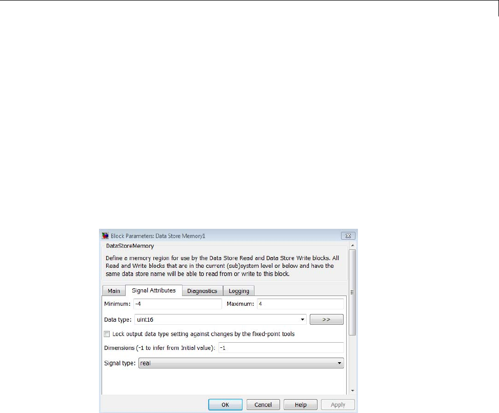
Data Stores with Data Store Memory Blocks
•Complexity
•Sample time
However, allowing these attributes to be inherited can cause unexpected
results that can be difficult to debug. To prevent such errors, use the Data
Store Memory block dialog or a Simulink.Signal object to specify the
attributes explicitly.
Specifying Attributes Using Block Parameters
YoucanusetheDataStoreMemoryblockdialogboxtospecifythedatatype
and complexity of a data store. In the next figure, the dialog box sets the
Data type to uint16 and the Signal type to real.
Specifying Attributes Using a Signal Object
You can use a Simulink.Signal object to specify data store attributes. To
establish an implicit data store, as described in “Data Stores with Signal
Objects” on page 46-12, use the same general approach as when you explicitly
associate a data object with aDataStoreMemoryblock.
The next figure shows a Data Store Memory block named Athat specifies
resolution to a Simulink.Signal object, named A.Touseasignalobjectforthe
46-9
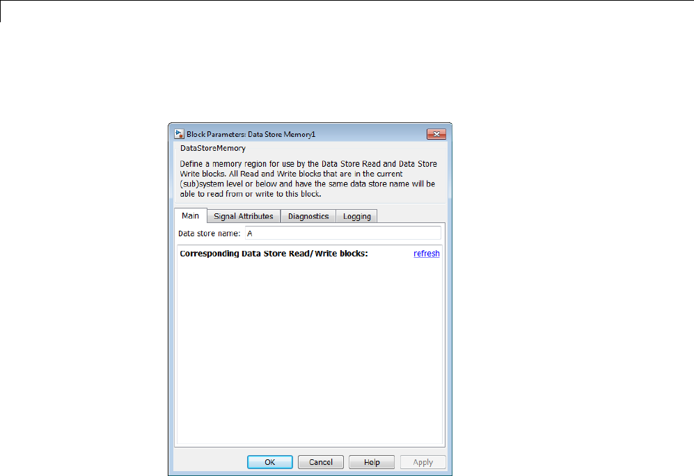
46 Working with Data Stores
data store, select the Data store name must resolve to Simulink signal
object parameter and set Data store name to the name of the signal object.
The signal object specifies values for all three data attributes that the data
store would otherwise inherit: DataType,Complexity,andSampleTime.
In this example, the Simulink.Signal object Amight have the following
properties:
A=
Simulink.Signal (handle)
CoderInfo: [1x1 Simulink.SignalCoderInfo]
Description: ''
DataType: 'auto'
Min:[]
Max:[]
DocUnits: ''
Dimensions: 1
46-10

Data Stores with Data Store Memory Blocks
DimensionsMode: 'auto'
Complexity: 'auto'
SampleTime: -1
SamplingMode: 'auto'
InitialValue: ''
46-11

46 Working with Data Stores
Data Stores with Signal Objects
In this section...
“Creating the Data Store” on page 46-12
“Local and Global Data Stores” on page 46-12
“Specifying Signal Object Data Store Attributes” on page 46-12
Creating the Data Store
To use a Simulink.Signal objecttodefineadatastorewithoutusingaData
Store Memory block, create the signal object in a workspace that is visible
to every component that needs to access the data store. The name of the
associated data store is the name of the signal object. You can use this name
in Data Store Read and Data Store Write blocks, just as if it were the Data
store name of a Data Store Memory block. Simulink creates an associated
data store when you use the signal object for data storage.
Local and Global Data Stores
You can use a Simulink.Signal object to define either a local or a global
data store.
•If you define the object in the MATLAB base workspace, the result is a
global data store, which is accessible in every model within Simulink,
including all referenced models.
•If you create the object in a model workspace, the result is a local data store,
which is accessible at every level in a model except any referenced models.
Specifying Signal Object Data Store Attributes
Data store attributes that a signal object does not define have the same
default values that they do in a Data Store Memory block. The parameter
values of a signal object used as a data store have different requirements,
depending on whether the data store is global or local.
•For a local data store, for each parameter listed in the following table, you
can either set value explicitly or you can have the data store inherit the
value from the Data Store Write and Data Store Read blocks.
46-12

Data Stores with Signal Objects
•The following table describes the parameter requirements for global data
stores.
Parameter Global Data Store Value
DataType Must be set explicitly
Complexity Must be set explicitly
Dimensions Must be set explicitly
SampleTime Can be set or inherited
SamplingMode Must be 'Sample based'
For a local data store defined using aDataStoreMemoryblockthatusesa
signal object for the Data store name parameter, you can select the Data
store must resolve to Simulink signal object parameter for compile-time
checking. The Data store must resolve to Simulink signal object
parameter causes Simulink to display an error and stop compilation if
Simulink cannot find the signal object or if the signal object properties are
inconsistent with the signal object properties.
Once you have created the object, set the properties of the signal object to the
values that you want the corresponding data store properties to have. For
example, the following commands define a data store named Error in the
MATLAB base workspace:
Error = Simulink.Signal;
Error.Description = 'Use to signal that subsystem output is invalid';
Error.DataType = 'boolean';
Error.Complexity = 'real';
Error.Dimensions = 1;
Error.SamplingMode='Sample based';
Error.SampleTime = 0.1;
46-13
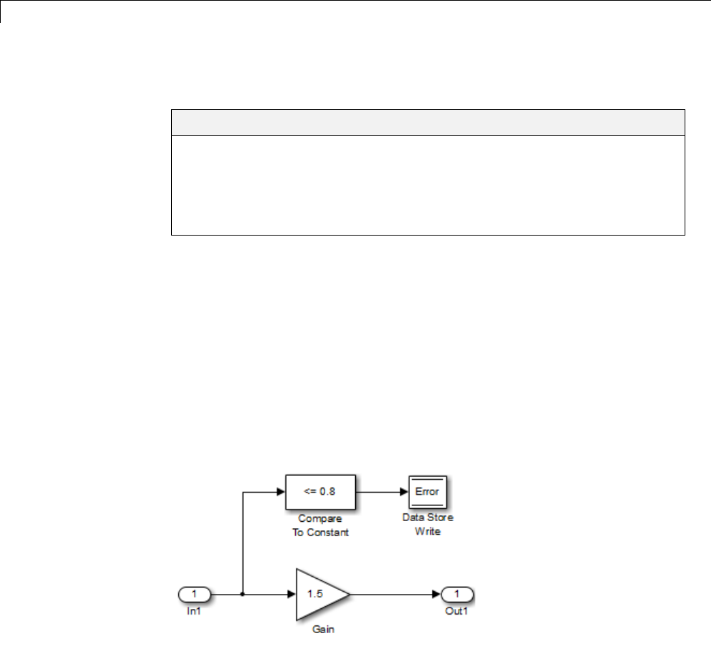
46 Working with Data Stores
Access Data Stores with Simulink Blocks
In this section...
“Writing to a Data Store” on page 46-14
“Reading from a Data Store” on page 46-14
“Accessing a Global Data Store” on page 46-15
“Accessing Specific Bus and Matrix Elements” on page 46-16
Writing to a Data Store
To set the value of a data store at each time step:
1Create an instance of a Data Store Write block at the level of your model
that computes the value.
2Set the Data Store Write block Data store name parameter to the name of
the data store to which you want it to write data.
3Connect the output of the block that computes the value to the input of
the Data Store Write block.
Reading from a Data Store
Togetthevalueofadatastoreateachtimestep:
46-14
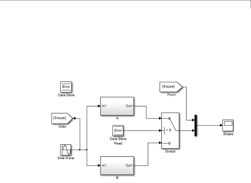
Access Data Stores with Simulink®Blocks
1Create an instance of a Data Store Read block at the level of your model
that needs the value.
2Set the Data Store Read block Data store name parameter to the name of
the data store from which you want it to read.
3Connect the output of the Data Store Read block to the input of the block
that needs the data store value.
AccessingaGlobalDataStore
When connected to a global data store (one that is defined by a signal object
in the MATLAB workspace), a Data Store Read or Data Store Write block
displays the word global abovethedatastorename.
46-15
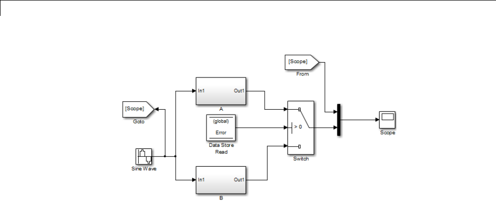
46 Working with Data Stores
Accessing Specific Bus and Matrix Elements
Selecting Specific Bus or Matrix Elements
By default, a model writes and reads all bus and matrix elements to and
fromadatastore.
To select specific bus or matrix elements to write to or read from a data store,
use the Element Assignment pane of the Data Store Write block and the
Element Selection pane of the Data Store Read block . Selecting specific
bus or matrix elements offers the following benefits:
•Reducing the number of blocks in the model. For example, you can
eliminate a Data Store Read and Bus Selector block pair or a Data Store
Write and Bus Assignment block pair for each specific bus element that
you want to access).
•Faster simulation of models with large buses and arrays of buses.
46-16
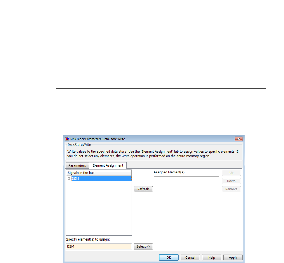
Access Data Stores with Simulink®Blocks
Writing Specific Elements to a Data Store
Note The following procedure describes how to use the Data Store Write
block interface to write specific elements to a data store. You can also perform
this task at the command line, using the DataStoreElements parameter to
specify elements. For details, see “Specification using the command line” on
page 46-22.
To assign specific bus or matrix elements to write to a data store:
1Select the Data Store Write block and in the parameters dialog box, select
the Element Assignment pane. For example, suppose you are using a
bus with a data store named DSM:
2Expand all the elements in the Signals in the bus list.
46-17
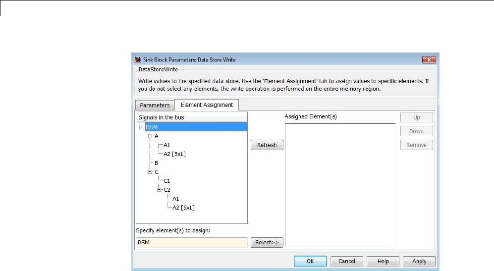
46 Working with Data Stores
3Specify the elements that you want to write to the data store. For example:
•In the Signals in the bus list, click B.ThenclickSelect>> to select
the element B.
•To write all the elements of A2 (in the Asubbus), select A2[5x1].Then
click Select>>.
•To write the second element of A2 in the C2 subbus, select the A2[5x1]
element. In the Specify element(s) to assign text box, edit the text
to say DSM.C.C2.A2(2,1).
46-18
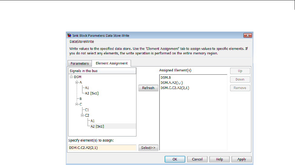
Access Data Stores with Simulink®Blocks
For more examples, see “Specifying Elements to Assign or Select” on page
46-20.
4(Optional) Reorder the assigned elements, which changes the order of the
ports of the Data Store Write block.
•To reorder an assigned element, in the Assigned element(s) list, select
the element that you want to move, and click Up or Down.
•To remove an assigned element, click Remove.
5To apply the assigned elements, click OK.
The Data Store Write block has a port for each assigned element. The
names of the selected elements that correspond to each port appear in the
block icon. If you assign several signals, these additions may diminish the
readability of the model. To improve readability, you can expand the size of
the block or create multiple Data Store Write blocks.
46-19

46 Working with Data Stores
Reading Specific Elements from a Data Store
Reading specific elements from a data store involves very similar steps as
described in “Writing Specific Elements to a Data Store” on page 46-17. The
Data Store Read block differs slightly from the Data Store Write block. A
Data Store Read block has:
•An Element Selection pane instead of an Element Assignment pane
•ASelected element(s) list instead of an Assigned element(s) list
Specifying Elements to Assign or Select
Use MATLAB matrix element syntax to specifyspecificelements. Fordetails
about specifying matrices in MATLAB, see “Creating and Concatenating
Matrices”.
Note To select matrix elements, you cannot use dynamic indexing with the
Element Assignment and Element Selection panes of Data Store Read
and Bus Assignment block pairs or Data Store Write and Bus Selector block
pairs. You can, however, use a MATLAB Function block for dynamic indexing.
Valid element specifications. The following table shows examples of valid
syntax for specifying elements to assign or select. These examples use the A2
subbus of the Abus, as shown in the bus hierarchy used in “Writing Specific
Elements to a Data Store” on page 46-17.
46-20
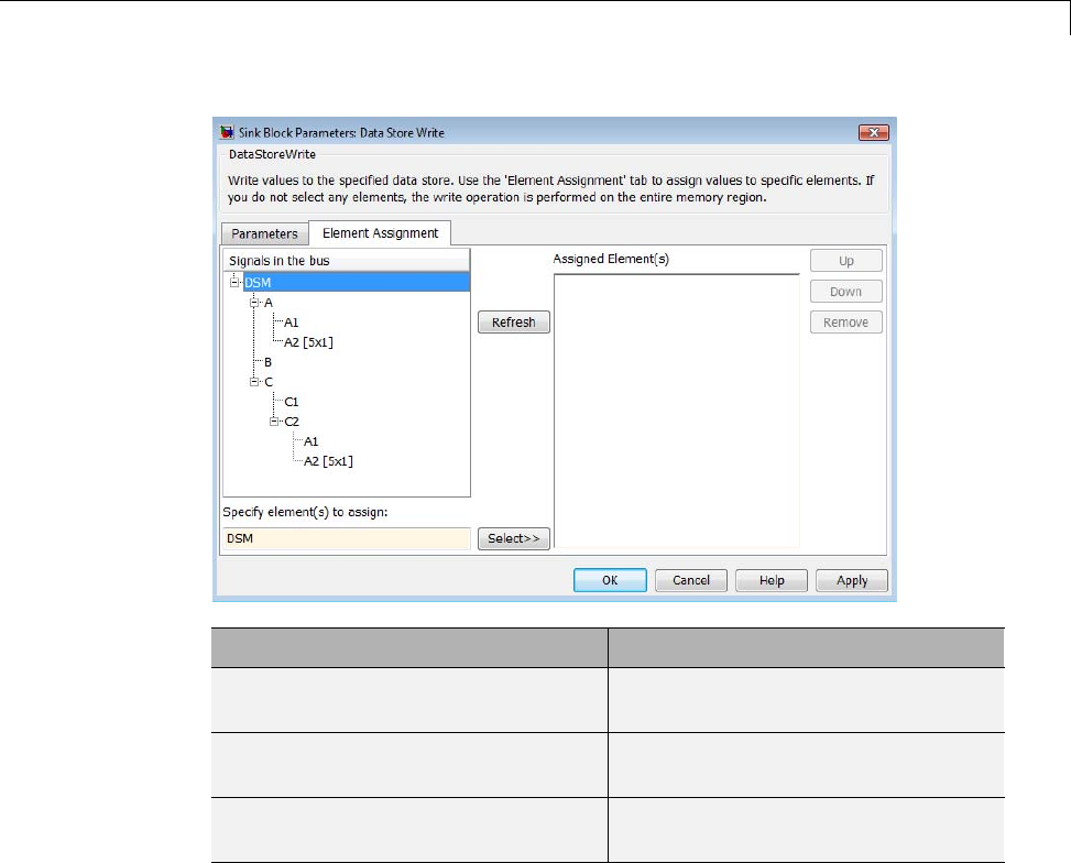
Access Data Stores with Simulink®Blocks
Valid Syntax Description
DSM.A.A2(:,:) Selects all elements in every
dimension
DSM.A.A2([1,3,5],1) Selects the first, third, and fifth
elements
DSM.A.A2(2:5,1) Selects the second through the fifth
element
Invalid element specifications. Thefollowingtableshowsexamplesof
invalid syntax for specifying elements to assign or select. These examples use
the A2 subbus of the Abus,asshowninthebushierarchyusedin“Writing
Specific Elements to a Data Store” on page 46-17.
46-21

46 Working with Data Stores
Invalid Syntax Reason the Syntax Is Invalid
DSM.A.A2(:) You must specify a colon for each
dimension. For the bus hierarchy
used in these examples, you must
use two colons.
DSM.A.A2(2:end,1) You cannot use the end operator.
DSM.A.A2(idx,1) You cannot use variables to specify
indices. Consider using a MATLAB
Function block.
DSM.A.A2(-1,1) The dimension –1 is not within the
valid dimension bounds.
Specification using the command line. To set the elements to write to
or read from, use the DataStoreElements parameter. Use a pound sign
(#) to delimit multiple elements. For example, select the Data Store Write
or Data Store Read block for which you want to specify elements and enter
acommandsuchas:
set_param(gcb, 'DataStoreElements', 'DSM.A#DSM.B#DSM.C(3,4)')
This specification results in the block now having three ports corresponding
to the elements that you specified.
46-22

Data Store Examples
Data Store Examples
In this section...
“Overview” on page 46-23
“Local Data Store Example” on page 46-23
“Global Data Store Example” on page 46-24
Overview
The following examples illustrate techniques for defining and accessing data
stores. See “Order Data Store Access” on page 46-31 for techniques that
control data store access over time, such as ensuring that a given data store is
always written before it is read. See “Data Store Diagnostics” on page 46-38
for techniques you can use to help detect and correct potential data store
errors without needing to run any simulations.
Note In addition to the following examples, see the sldemo_mdlref_dsm
model, which shows how to use global data stores to share data among
referenced models.
Local Data Store Example
The following model illustrates creation and access of a local data store, which
is visible only in a model or particular subsystem.
46-23
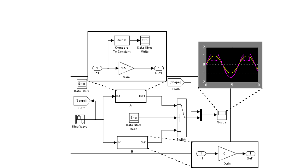
46 Working with Data Stores
This model uses a data store to permit subsystem A to signal that its output
is invalid. If subsystem A’s output is invalid, the model uses the output
of subsystem B.
Global Data Store Example
The following model replaces the subsystems of the previous example with
functionally identical submodels to illustrate use of a global data store to
share data in a model reference hierarchy.
46-24
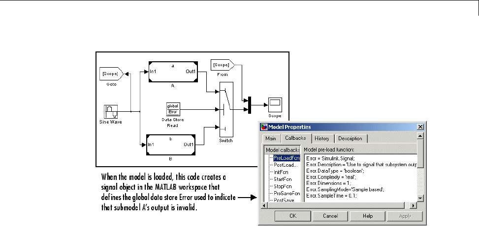
Data Store Examples
In this example, the top model uses a signal object in the MATLAB workspace
to define the error data store. This is necessary because data stores are
visible across model boundaries only if they are defined by signal objects
in the MATLAB workspace.
46-25

46 Working with Data Stores
Log Data Stores
In this section...
“Logging Local and Global Data Store Values” on page 46-26
“Supported Data Types, Dimensions, and Complexity for Logging Data
Stores” on page 46-26
“Data Store Logging Limitations” on page 46-27
“Logging Data Stores Created with a Data Store Memory Block” on page
46-27
“Logging Icon for the Data Store Memory Block” on page 46-28
“Logging Data Stores Created with a Simulink.Signal Object” on page 46-28
“Accessing Data Store Logging Data” on page 46-29
Logging Local and Global Data Store Values
You can log the values of a local or global data store data variable for all the
steps in a simulation. Two common uses of data store logging are for:
•Model debugging – view the order of all data store writes
•Confirming a model modification – use the logged data to establish a
baseline for comparing results for identifying the impact of a model
modification
To see an example of logging a global data store, see the sldemo_mdlref_dsm
model.
Supported Data Types, Dimensions, and Complexity
for Logging Data Stores
You can log data stores that use the following data types:
•All built-in data types
•Enumerated data types
•Fixed-point data types
46-26

Log Data Stores
You can log data stores that use any dimension level or complexity.
Data Store Logging Limitations
Limitations for using data store logging in a model are:
•To log data for a data store memory:
-Simulate the top-level model in Normal mode.
-For local data stores, the model containing the Data Store Memory block
must be in model reference Normal mode.
-Any block in a referenced model that writes to the data store memory
must be executed in model reference Normal mode.
•If you set the Model Configuration Parameters > Solver > Tasking
mode for periodic sample times parameter to MultiTasking,thenyou
cannot log Data Store Memory blocks that use asynchronous sample times
or hybrid sample times (that is, sample times resulting from when different
data sources for the data store have different sample times).
For details about viewing information about sample times, see “View
Sample Time Information” on page 5-9.
•You cannot log data stores that use custom data types.
Logging Data Stores Created with a Data Store
Memory Block
To log a local data store that you create with a Data Store Memory block:
1In the Block Parameters dialog box for the Data Store Memory block that
you want to log, select the Logging pane.
2Select the Log signal data check box.
3Optionally, specify limits for the amount of data logged, using the
Minimum and Maximum parameters.
4Enable data store logging with the Model Configuration
Parameters > Data Import/Export > Data stores parameter.
5Simulate the model.
46-27

46 Working with Data Stores
Logging Icon for the Data Store Memory Block
When you enable logging for a model, and you configure a local data store for
logging, the Data Store Memory block displays a blue icon. If you do not
enable logging for the model, then the icon is gray.
Logging Data Stores Created with a Simulink.Signal
Object
You can create local and global data stores using a Simulink.Signal object.
See “Data Stores with Signal Objects” on page 46-12 for details.
To log a data store that you create with a Simulink.Signal object:
1Create a Simulink.Signal object in a workspace that is visible to every
component that needs to access the data store, as described in “Data Stores
with Signal Objects” on page 46-12.
2Use the name of the Simulink.Signal object in the Data store name
block parameters of the Data Store Read and Data Store Write blocks that
you want to write to and read from the data store.
3From the MATLAB command line, set DataLogging (which is a property of
the LoggingInfo property of Simulink.Signal)to1.
For example, if you use a Simulink.Signal object called
DataStoreSignalObject to create a data store, use the following command:
DataStoreSignalObject.LoggingInfo.DataLogging = 1
4Optionally, specify limits for the amount of data logged, using the following
properties, which are properties of the LoggingInfo property of the
Simulink.Signal object: Decimation,LimitDataPoints,andMaxPoints.
5Enable data store logging with the Model Configuration
Parameters > Data Import/Export > Data stores parameter.
46-28

Log Data Stores
6Simulate the model.
Accessing Data Store Logging Data
The following Simulink classes represent data from data store logging and
provide methods for accessing that data:
Class Description
Simulink.SimulationData.BlockPath Represents a fully specified Simulink block
path; use for capturing the full model reference
hierarchy
Simulink.SimulationData.Dataset Stores logged data elements and provides
searching capabilities; use to group
Simulink.SimulationData.Element objects
in a single object
Simulink.SimulationData.DataStoreMemory Stores logging information from a data store
during simulation
Viewing Data Store Data
To view data store logging data from the command line, view the output data
set in the base workspace. The default variable for the data store logging
data set is dsmout.
The sldemo_mdlref_dsm model illustrates approaches for viewing data store
logging data.
Accessing Elements in the Data Store Logging Data
To find an element in the data store logging data, based on
the Name or BlockType property, use the getElement method of
Simulink.SimulationData.Dataset. For example:
dsmout.getElement('RefSignalVal')
ans =
Simulink.SimulationData.DataStoreMemory
Package: Simulink.SimulationData
46-29

46 Working with Data Stores
Properties:
Name: 'RefSignalVal'
Blockpath: [1x1 Simulink.SimulationData.BlockPath]
Scope: 'local'
DSMWriterBlockPaths: [1x2 Simulinkl.SimulationData.BlockPath]
DSMWriters: [101x1 uint32]
Values: 101x1 timeseries]
To access an element by index, use the
Simulink.SimulationData.Dataset.getElement method.
46-30

Order Data Store Access
Order Data Store Access
In this section...
“About Data Store Access Order” on page 46-31
“Ordering Access Using Function Call Subsystems” on page 46-31
“Ordering Access Using Block Priorities” on page 46-35
About Data Store Access Order
To obtain correct results from data stores, you must control the order of
execution of the data store’s reads and writes. If a data store’s read occurs
before its write, latency is introduced into the algorithm: the read obtains the
value that was computed and stored in the previous time step, rather than
the value computed and stored in the current time step.
Such latency may cause the system to behave other than as designed, and
in some cases may destabilize the system. Even if these problems do not
occur, an uncontrolled access order could change from one release of Simulink
to the next.
This section describes several strategies for explicitly controlling the order
of execution of a data store’s reads and writes. See “Data Store Diagnostics”
on page 46-38 for techniques you can use to detect and correct potential data
store errors without running simulations.
Ordering Access Using Function Call Subsystems
You can use function call subsystems to control the execution order of model
components that access data stores. The next figure shows this technique:
46-31
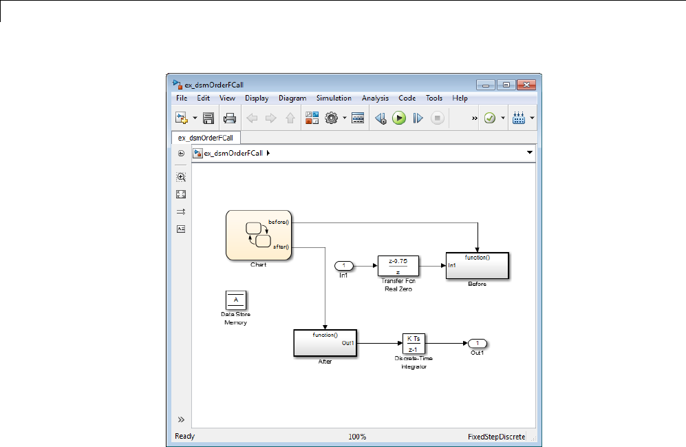
46 Working with Data Stores
46-32
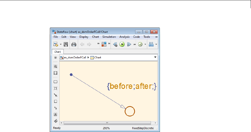
Order Data Store Access
46-33

46 Working with Data Stores
46-34
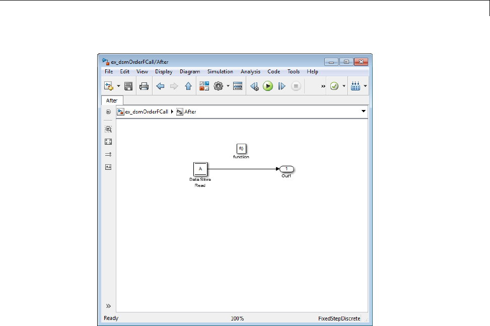
Order Data Store Access
The subsystem Before contains the Data Store Write, and the Stateflow
chart calls that subsystem before it calls the subsystem After, which contains
the Data Store Read.
Ordering Access Using Block Priorities
You can embed data store reads and writes inside atomic subsystems or
Model blocks whose priorities specify their relative execution order. The next
figure shows this technique:
46-35
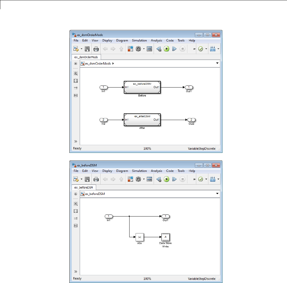
46 Working with Data Stores
46-36
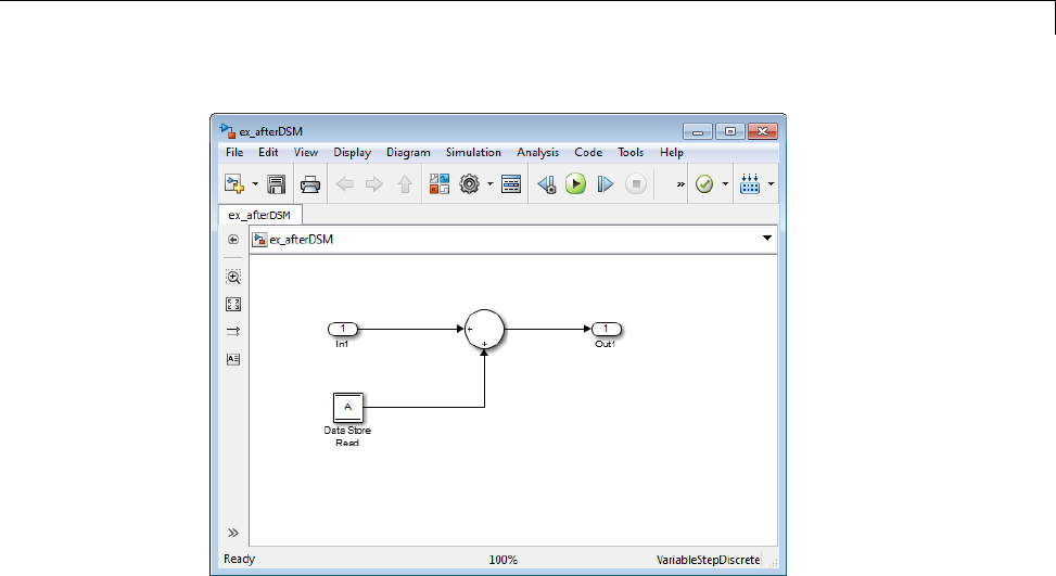
Order Data Store Access
The Model block beforeDSM has a lower priority then afterDSM,soitis
guaranteed to execute first. Since beforeDSM is atomic, all of its operations,
including the Data Store Write, will execute prior to afterDSM and all of its
operations, including the Data Store Read.
46-37

46 Working with Data Stores
Data Store Diagnostics
In this section...
“About Data Store Diagnostics” on page 46-38
“Detecting Access Order Errors” on page 46-38
“Detecting Multitasking Access Errors” on page 46-41
“Detecting Duplicate Name Errors” on page 46-43
“Data Store Diagnostics in the Model Advisor” on page 46-45
About Data Store Diagnostics
Simulink provides various run-time and compile-time diagnostics that you
can use to help avoid problems with data stores. Diagnostics are available in
the Model Configuration Parameters dialog box and the Data Store Memory
block’s parameters dialog box. The Simulink Model Advisor provides support
by listing cases where data store errors are more likely because diagnostics
are disabled.
Detecting Access Order Errors
You can use data store run-time diagnostics to detect unintended sequences of
data store reads and writes that occur during simulation. You can apply these
diagnostics to all data stores, or allow each Data Store Memory block to set
its own value. The diagnostics are:
•Detect read before write: Detect when a data store is read from before
writtentowithinagiventimestep
•Detect write after read: Detect when a data store is written to after
being read from within a given time step
•Detect write after write: Detect when a data store is written to multiple
times within a given time step
These diagnostics appear in the Model Configuration Parameters >
Diagnostics > Data Validity > Data Store Memory Block pane, where
each can have one of the following values:
46-38

Data Store Diagnostics
•Disable all — Disables this diagnostic for all data stores accessed by
the model.
•Enable all as warnings — Displays the diagnostic as a warning in the
MATLAB Command Window.
•Enable all as errors — Halts the simulation and displays the diagnostic
in an error dialog box.
•Use local settings — Allow each Data Store Memory block to set its own
value for this diagnostic (default).
The same diagnostics also appear in each Data Store Memory block
parameters dialog box Diagnostics tab. You can set each diagnostic to none,
warning,orerror. The value specified by an individual block takes effect only
if the corresponding configuration parameter is Use local settings.See
“Diagnostics Pane: Data Validity” and the Data Store Memory documentation
for more information.
Themostconservativetechniqueistosetalldatastore
diagnostics to Enable all as errors in Model Configuration
Parameters > Diagnostics > Data Validity > Data Store Memory
Block. However, this setting is not best in all cases, because it can flag
intended behavior as erroneous. For example, the next figure shows a model
that uses block priorities to force the Data Store Read block to execute before
the Data Store Write block:
46-39
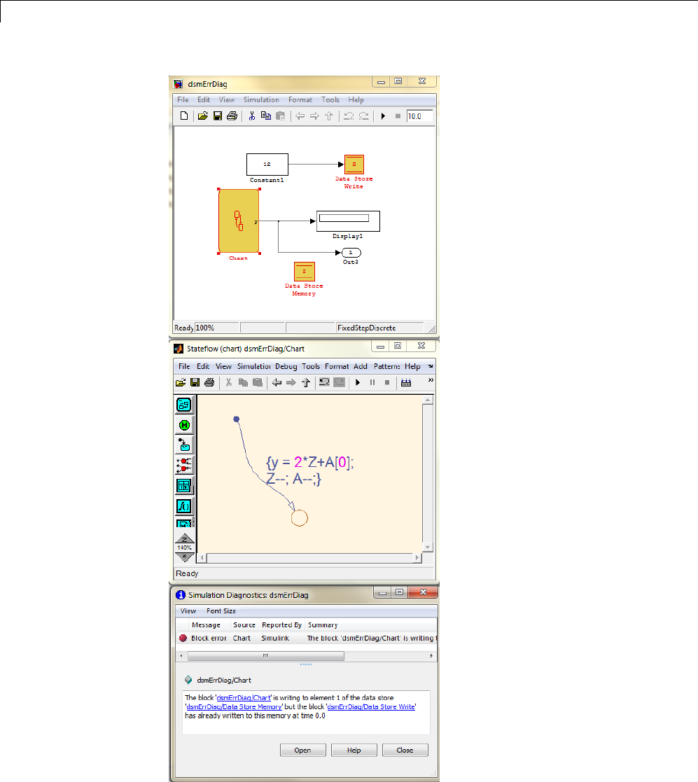
46 Working with Data Stores
46-40

Data Store Diagnostics
An error occurred during simulation because the data store Ais read from the
Stateflow chart before the Data Store Write updates it. If the associated
delay is intended, you can suppress the error by setting the global parameter
Detect read before write to Use local settings, then setting that
parametertodisableintheDataStoreWrite block. If you use this technique,
be sure to set the parameter to error in all other Data Store Write blocks
aside from those which are to be intentionally excluded from the diagnostic.
Data Store Diagnostics and the MATLAB Function Block
Diagnostics might be more conservative for data store memory used by
MATLAB Function blocks. For example, if you pass arrays of data store
memory to MATLAB functions, optimizations such as A=foo(A) might result
in MATLAB marking the entire contents of the array as read or written, even
though only some elements were accessed.
Detecting Multitasking Access Errors
Data integrity may be compromised if a data store is read from in one task
and written to in another task. For example, suppose that:
1Ataskiswritingtoadatastore.
2A second task interrupts the first task.
3The second task reads from that data store.
If the first task had only partly updated the data store when the second
task interrupted, the resulting data in the data store is inconsistent. For
example, if the value is a vector, some ofitselementsmayhavebeenwritten
in the current time step, while the rest were written in the previous step. If
the value is a multi-word, it may be left in an inconsistent state that is not
even partly correct.
Unless you are certain that task preemption cannot cause data integrity
problems, set the compile-time diagnostic Model Configuration
Parameters > Diagnostics > Data Validity > Data Store Memory Block
> Multitask Data Store to warning (the default) or error.Thisdiagnostic
flags any case of a data store that is read from and written to in different
46-41
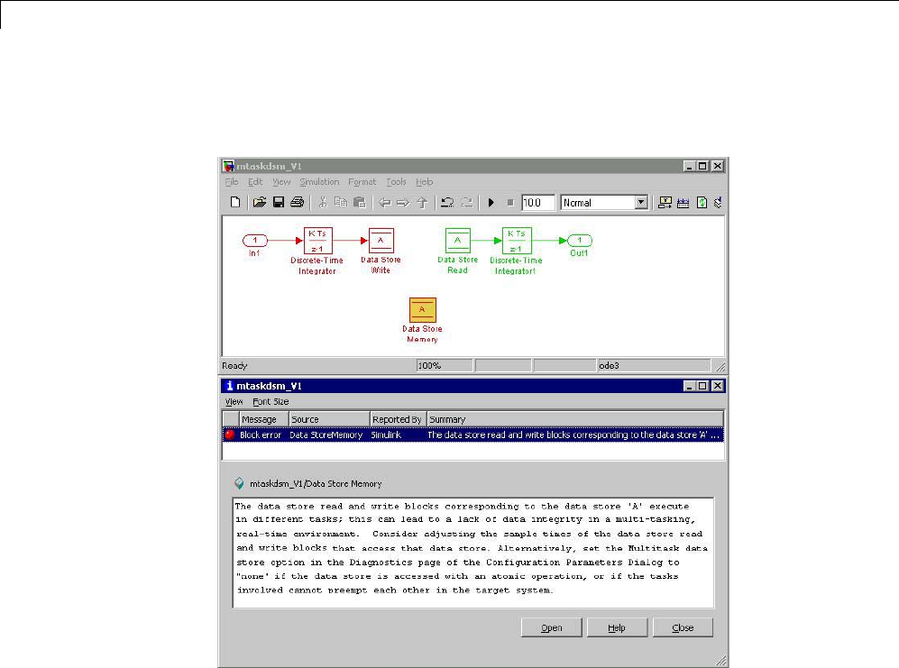
46 Working with Data Stores
tasks. The next figure illustrates a problem detected by setting Multitask
Data Store to error:
Since the data store Ais written to in the fast task and read from in the
slow task, an error is reported, with suggested remedy. This diagnostic
is applicable even in the case that a data store read or write is inside of
a conditional subsystem. Simulink correctly identifies the task that the
block is executing within, and uses that task for the purpose of evaluating
the diagnostic.
The next figure shows one solution to the problem shown above: place a rate
transition block after the data store read, which previously accessed the data
store at the slower rate.
46-42
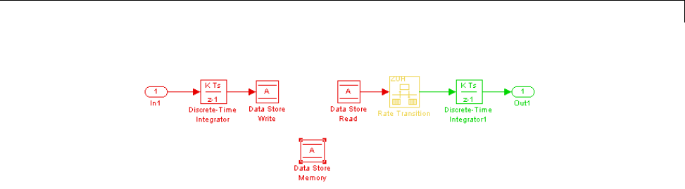
Data Store Diagnostics
With this change, the data store write can continue to occur at the faster
rate. This may be important if that data store must be read at that faster
rate elsewhere in the model.
The Multitask Data Store diagnostic also applies to data store reads and
writes in referenced models. If two different child models execute a data
store’s reads and writes in differing tasks, the error will be detected when
Simulink compiles their common parent model.
DetectingDuplicateNameErrors
Data store errors can occur due to duplicate uses of a data store name within
a model. For instance, data store shadowing occurs when two or mote data
store memories in different nested scopes have the same data store name. In
this situation, the data store memory referenced by a data store read or write
block at a low level may not be the intended store.
To prevent errors caused by duplicate data store names, set the compile-time
diagnostic Model Configuration Parameters > Diagnostics > Data
Validity > Data Store Memory Block > Duplicate Data Store Names to
warning or error. By default, the value of the diagnostic is none, suppressing
duplicate name detection. The next figure shows a problem detected by
setting Duplicate Data Store Names to error:
46-43
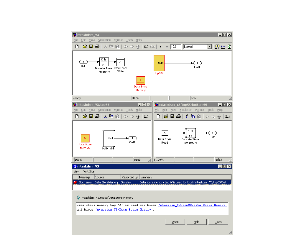
46 Working with Data Stores
The data store read at the bottom level of a subsystem hierarchy refers to a
data store named A,andtwoDataStoreMemoryblocksinthesamemodel
have that name, so an error is reported. This diagnostic guards against
assuming that the data store read refers to the Data Store Memory block in
the top level of the model. The read actually refers to the Data Store Memory
block at the intermediate level, which is closer in scope to the Data Store
Read block.
46-44

Data Store Diagnostics
Data Store Diagnostics in the Model Advisor
The Model Advisor provides several diagnostics that you can use with data
stores. See these sections for information about Model Advisor diagnostics for
data stores:
“Check Data Store Memory blocks for multitasking, strong typing, and
shadowing issues”
“Check data store block sample times for modeling errors”
“Check if read/write diagnostics are enabled for data store blocks”
46-45

46 Working with Data Stores
Data Stores and Software Verification
Data stores can have significant effects on software verification, especially in
the area of data coupling and control. Models and subsystems that use only
inports and outports to pass data result in clean, well-specified, and easily
verifiable interfaces in the generated code.
Data stores, like any type of global data, make verification more difficult. If
your development process includes software verification, consider planning
for the effect of data stores early in the design process.
For more information, see RTCA DO-331, “Model-Based Development and
Verification Supplement to DO-178C and DO-278A,” Section MB.6.3.3.b.
46-46


47
Working with Signals
•“Signal Basics” on page 47-2
•“Signal Types” on page 47-8
•“Virtual Signals” on page 47-11
•“Signal Values” on page 47-15
•“Signal Names and Labels” on page 47-19
•“Signal Label Propagation” on page 47-24
•“Signal Dimensions” on page 47-34
•“Determine Output Signal Dimensions” on page 47-36
•“Display Signal Sources and Destinations” on page 47-41
•“Signal Ranges” on page 47-44
•“Initialize Signals and Discrete States” on page 47-51
•“Test Points” on page 47-58
•“Display Signal Attributes” on page 47-61
•“Signal Groups” on page 47-66

47 Working with Signals
Signal Basics
In this section...
“About Signals” on page 47-2
“Creating Signals” on page 47-3
“Signal Line Styles” on page 47-4
“Signal Properties” on page 47-5
“Testing Signals” on page 47-6
About Signals
Asignal is a time varying quantity that has values at all points in time. You
can specify a wide range of signal attributes, including:
•Signal name
•Data type (for example, 8-bit, 16-bit, or 32-bit integer)
•Numeric type (real or complex)
•Dimensionality (one-dimensional, two-dimensional, or multidimensional
array)
Many blocks can accept or output signals of any data or numeric type and
dimensionality. Other blocks impose restrictions on the attributes of the
signals that they can handle.
In Simulink, signals are the outputs of dynamic systems represented by blocks
in a Simulink diagram and by the diagram itself. The lines in a block diagram
represent mathematical relationships among the signals defined by the block
diagram. For example, a line connecting the output of block A to the input of
block B indicates that the signal output of B depends on the signal output of A.
Simulink block diagrams represent signals with lines that have an arrowhead.
The source of the signal corresponds to the block that writes to the signal
during evaluation of its block methods (equations). The destinations of the
signal are blocks that read the signal during the evaluation of the block
methods (equations).
47-2

Signal Basics
Note Simulink signals do not travel along the lines that connect blocks
in the same way that electrical signals travel along a wire. This analogy
is misleading because it suggests that a block diagram represents physical
connections between blocks, which is not the case. Simulink signals are
mathematical, not physical, entities, and the lines in a block diagram
represent mathematical, not physical, relationships among blocks.
Creating Signals
Create a signal by adding a source block to your model. For example, you can
create a signal that varies sinusoidally with time, by dragging an instance
of the Sine block from the Simulink Sources library into your model. See
“Sources” for information about blocks that create signals in a model.
You can also use the Signal & Scope Manager to create signals in your model,
without using blocks. See “Signal and Scope Manager” on page 16-23 for
more information.
47-3
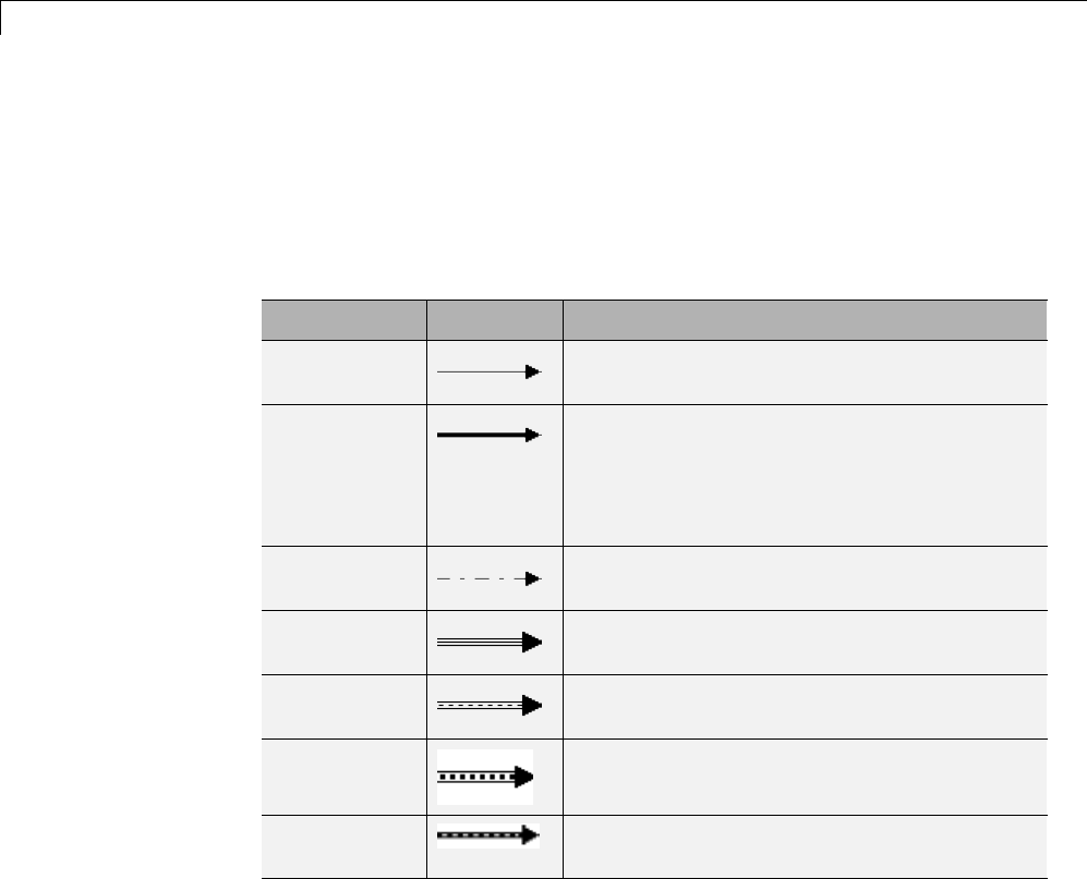
47 Working with Signals
Signal Line Styles
A Simulink model can include many different types of signals. For details, see
“Signal Types” on page 47-8.
Simulink uses a variety of line styles to display different types of signals in the
model window. Assorted line styles help you to differentiate the signal types.
Signal Type Line Style Description
Scalar and
Nonscalar
Simulink uses a thin, solid line to represent
scalar and nonscalar signals.
Nonscalar
(optional)
When you enable the Wide nonscalar lines
option, Simulink uses a thick, solid line to
represent nonscalar signals. For information
about line display options, see “Display Signal
Attributes” on page 47-61.
Control signal Simulink uses a thin, dash-dot line to
represent control signals.
Virtual Bus Simulink uses a triple line with a solid core to
represent virtual signal buses.
Nonvirtual
Bus
Simulinkusesatriplelinewithadottedcore
to represent nonvirtual signal buses.
Array of
Buses
Simulinkusesaheavytriplelinewitha
dotted core to represent array of bus signals.
Variable-Size Simulink uses a solid wide line with a white
dotted core to represent a variable-size signal.
Other than using the Wide nonscalar lines option to display nonscalar
signals as thick, solid lines, you cannot customize or control the line style of
signals. See “Wide Nonscalar Lines” on page 47-65 for more information
about this option.
As you construct a block diagram, Simulink uses a thin, solid line to represent
all signal types. After you update or start simulation of the block diagram,
Simulink redraws the lines, using the specified line styles.
47-4
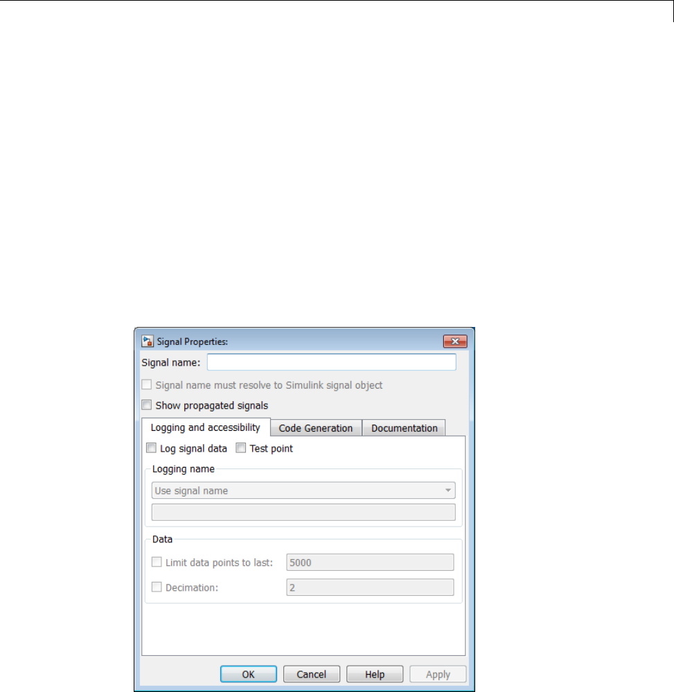
Signal Basics
Signal Properties
Specifying Signal Properties
Use the Signal Properties dialog box to specify properties for:
•Signal names and labels
•Signal logging
•Simulink Coder to use to generate code
•Documentation of the signal
To open the Signal Properties dialog box, right-click a signal and choose
Properties.
47-5

47 Working with Signals
Displaying Signal Attributes in the Model
Displaying signal attributes in the model diagram can make the model easier
to understand at a glance. For example, in the Simulink Model Editor, use the
Display > Signals & Ports menu to include in the model layout information
about signal attributes, such as:
•Port data types
•Design ranges
•Signal dimensions
•Signal resolution
For details, see “Display Signal Attributes” on page 47-61.
Display Signal Source and Destination
To highlight a signal and its source or destination blocks:
•Right-click a signal.
•In the context menu, select either Highlight Signal to Source or
Highlight Signal to Destination.
For details, see“Display Signal Sources and Destinations” on page 47-41.
Testing Signals
You can perform the following kinds of tests on signals:
•“Minimum and Maximum Values” on page 47-6
•“Connection Validation” on page 47-7
Minimum and Maximum Values
For many Simulink blocks, you can specify a range of valid values for the
output signals. Simulink provides a diagnostic for detecting when blocks
generate signals that exceed their specified ranges during simulation. For
details, see “Signal Ranges” on page 47-44.
47-6

Signal Basics
Connection Validation
Many Simulink blocks have limitations on the types of signals that they
accept. Before simulating a model, Simulink checks all blocks to ensure that
the blocks can accommodate the types of signals ouput by the ports to which
the blocks connect. If any incompatibilities exist, Simulink reports an error
and terminates the simulation.
To detect signal compatibility errors before running a simulation, update the
diagram. In the Simulink Editor, select Simulation > Update Diagram.
Signal Groups
The Signal Builder block displays interchangeable groups of signal sources.
Use the Signal Builder to create or edit groups of signals and to switch the
groups into and out of a model.
Signal groups can greatly facilitate testing a model, especially when you use
them in conjunction with Simulink Assertion blocks and the Model Coverage
Tool in the Simulink Verification and Validation product.
For details, see “Signal Groups” on page 47-66.
47-7

47 Working with Signals
Signal Types
In this section...
“Summary of Signal Types” on page 47-8
“Control Signals” on page 47-9
“Composite (Bus) Signals” on page 47-9
Summary of Signal Types
You can use many different kinds of signals in a model. The following table
summarizes the signal types, and links to sections that describe each type
in detail.
Signal Type Description
Array of buses An array whose elements are buses. See “Combine
BusesintoanArrayofBuses”onpage48-77.
Bus (Composite) A Simulink composite signal made up of other signals,
optionally including other bus signals. See “Composite
(Bus) Signals” on page 47-9.
Control Signal used by one block to initiate execution of
another block. For example, a signal that executes
a function-call or action subsystem. For details, see
“Control Signals” on page 47-9.
Nonvirtual Signal that occupies its own storage. A nonvirtual bus
reads inputs and writes outputs by accessing copies of
the component signals.
Mux A virtual vector created with a Mux block. See “Mux
Signals” on page 47-11.
Variable-Size Signalwhosesize(thenumberofelementsina
dimension), in addition to its values, can change during
a model simulation.
Virtual Signal that represents another signal or set of signals. A
virtual signal is used for graphical purposes and has no
functional effect. See “Virtual Signals” on page 47-11.
47-8
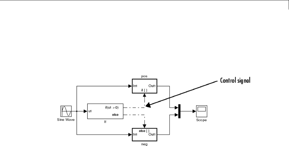
Signal Types
Control Signals
Acontrol signal is a signal used by one block to initiate execution of another
block. For example, a signal that executes a function-call or action subsystem
is a control signal. When you update or simulate a block diagram, Simulink
uses a dash-dot pattern to redraw lines representing the control signals.
Composite (Bus) Signals
You can group multiple signals into a hierarchical composite signal, called a
bus,rou
te the bus from block to block, and extract constituent signals from
the bus where needed. When you have many parallel signals, buses can
simplify the appearance of a model and help to clarify generated code. A bus
can be either virtual or nonvirtual.
For example, if you open and simulate the Bus Signal example model, the
bus1,bus2,andmain_bus signals are bus signals. These virtual bus signals
use thetriplelinestyle.
47-9
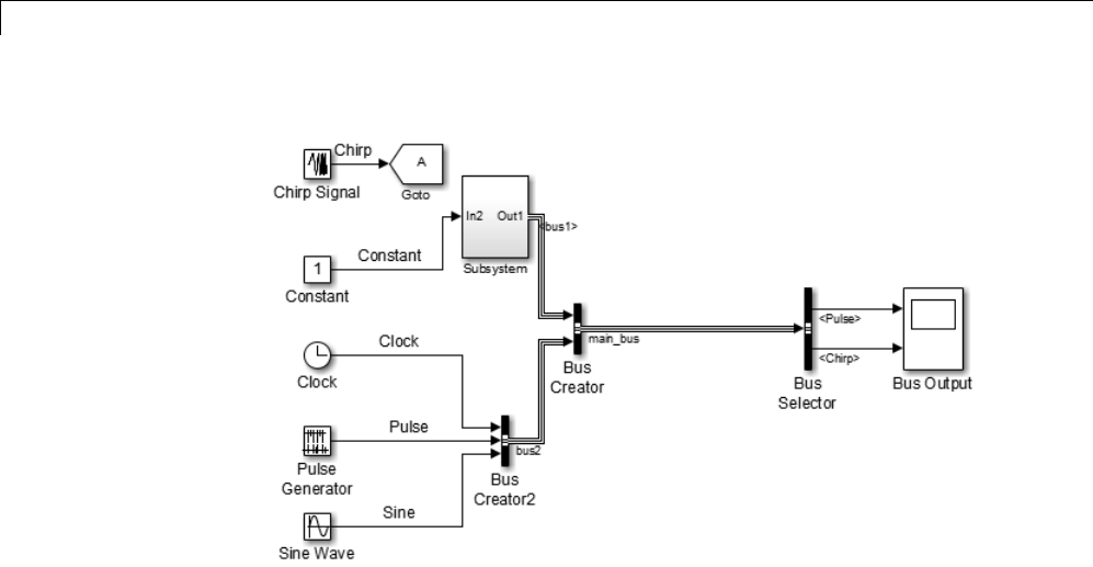

Virtual Signals
Virtual Signals
In this section...
“About Virtual Signals” on page 47-11
“Mux Signals” on page 47-11
About Virtual Signals
Avirtual signal is a signal that graphically represents other signals or
parts of other signals. Virtual signals are purely graphical entities; they
have no mathematical or physical significance. Simulink ignores them when
simulating a model, and they do not exist in generated code. Some blocks,
such as the Mux block, always generate virtual signals. Others, such as Bus
Creator, can generate either virtual or nonvirtual signals.
The nonvirtual components of a virtual signal are called regions.Avirtual
signalcancontainthesameregionmorethanonce. Forexample,ifthesame
nonvirtual signal is connected to two input ports of a Mux block, the block
outputs a virtual signal that has two regions. The regions behave as they
would if they had originated in two different nonvirtual signals, even though
the resulting behavior duplicates information.
Bus signals can also be virtual or nonvirtual. For details, see “Types of
Simulink Buses” on page 48-3.
Mux Signals
A Simulink mux is a virtual signal that graphically combines two or more
scalar or vector signals into one signal line. A Simulink mux is not a hardware
multiplexer, which combines multiple data streams into a single channel. A
Simulink mux does not combine signals in any functional sense: it exists only
virtually, and its only purpose is to simplify the visual appearance of a model.
Using a mux has no effect on simulation or generated code.
You can use a mux anywhere that you could use an ordinary (contiguous)
vector. For example, you can perform calculations on a mux. The computation
affects each constituent value in the mux just as if the values existed in a
contiguous vector, and the result is a contiguous vector, not a mux. Using a
47-11

47 Working with Signals
mux to perform computations on multiple vectors avoids the overhead of
copying the separate values to contiguous storage.
The Simulink documentation refers, sometimes interchangeably, to “muxes”,
“vectors”, and “wide signals”, and all three terms appear in Simulink GUI
labels and API names. This terminology can be confusing, because most
vector signals, which are also called wide signals, are nonvirtual and hence
are not muxes. To avoid confusion, reserve the term “mux” to refer specifically
to a virtual vector.
Amuxisavirtual vector signal. The constituent signals of a mux retain
their separate existence in every way, except visually. You can also combine
scalar and vector signals into a nonvirtual vector signal, by using a Vector
Concatenate block. The signal output by a Vector Concatenate block is an
ordinary contiguous vector, inheriting no special properties from the fact that
it was created from separate signals.
To create a composite signal whose constituent signals retain their identities
and can have different data types, use a Bus Creator block rather than a Mux
block. For details, see “About CompositeSignals”onpage48-2.Althoughyou
can use a Mux block to create a composite signal in some cases, MathWorks
discourages this practice. See “Avoid Mux/Bus Mixtures” on page 48-95 for
more information.
Using Muxes
The Signal Routing library provides two virtual blocks for implementing
muxes:
Mux
Combine several input signals into a mux (virtual vector) signal
Demux
Extract and output the values in a mux (virtual vector) signal
To implement a mux signal:
1Select a Mux and Demux block from the Signal Routing library.
2Set the Mux block Number of inputs and the Demux block Number of
outputs block parameters to the desired values.
47-12
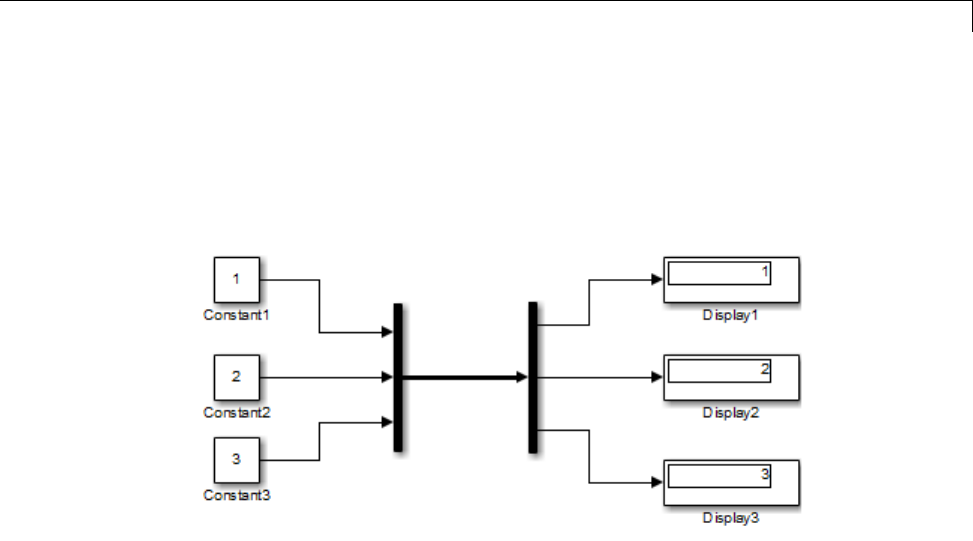
Virtual Signals
3Connect the Mux, Demux, and other blocks as needed to implement the
desired signal.
The next figure shows three signals that are input to a Mux block, transmitted
as a mux signal to a Demux block, and output as separate signals.
The Mux and Demux blocks are the left and right vertical bars, respectively.
To reduce visual complexity, neither block displays a name. In this example,
the line connecting the blocks, representing the mux signal, is wide
because the model has been built with Display > Signals & Ports > Wide
Nonscalar Lines option enabled. See “Display Signal Attributes” on page
47-61 for details.
Signals input to a Mux block can be any combination of scalars, vectors, and
muxes. The signals in the output mux appear in the order in which they were
input to the Mux block. You can use multiple Mux blocks to create a mux in
several stages, but the result is flat, not hierarchical, just as if the constituent
signals had been combined using a single mux block.
The values in all signals input to a Mux block must have the same data type.
If a Demux block attempts to output more values than exist in the input
signal, an error occurs. A Demux block can output fewer values than exist in
the input mux, and can group the values it outputs into different scalars and
vectors than were input to the Mux block. However, the Demux block cannot
rearrange the order of those values. For details, see Demux.
47-13


Signal Values
Signal Values
In this section...
“Signal Data Types” on page 47-15
“Signal Dimensions, Size, and Width” on page 47-15
“Complex Signals” on page 47-16
“Initializing Signal Values” on page 47-16
“Viewing Signal Values” on page 47-17
“Displaying Signal Values in Model Diagrams” on page 47-17
“Exporting Signal Data” on page 47-18
Signal Data Types
Data type refers to the format used to represent signal values internally. By
default, the data type of Simulink signals is double. You can create signals of
other data types. Simulink signals support the same range of data types as
MATLAB.See“DataTypes”onpage43-2formoreinformation.
Signal Dimensions, Size, and Width
Simulink blocks can output one-dimensional, two-dimensional, or
multidimensional signals. The Simulink user interface and documentation
generally refer to 1-D signals as vectors and 2-D or multidimensional signals
as matrices. A one-element array is frequently referred to as a scalar.
The size of a signal refers to the number of elements that a signal contains.
The size of a matrix (2-D) signal is generally expressed as M-by-N, where M is
the number of columns and N is the number of rows making up the signal.
The size of a vector signal is referred to as the width of the signal.
For more information, see “Signal Dimensions” on page 47-34.
47-15

47 Working with Signals
Complex Signals
The values of signals can be complex numbers or real numbers. A signal whose
values are complex numbers is a complex signal. Create a complex-valued
signal using one of the following approaches:
•Load complex-valued signal data from the MATLAB workspace into the
model via a root-level Inport block.
•Create a Constantblockinyourmodelandsetitsvaluetoacomplex
number.
•Create real signals corresponding to the real and imaginary parts of a
complex signal, then combine the parts into a complex signal, using the
Real-Imag to Complex conversion block.
Manipulate complex signals via blocks that accept them. If you are not sure
whether a block accepts complex signals, see the documentation for the block.
Initializing Signal Values
If a signal does not have an explicit initial value, the initial value that
Simulink uses depends on the data type of the signal.
Signal Data Type Default Initial Value
Numeric (other than fixed-point) Zero
Fixed-point Ground value
Boolean False
Enumerated Default value
You can specify the non-default initial values of signals for Simulink to use at
the beginning of simulation.
•For any signal, you can define a signal object (Simulink.Signal), and use
that signal object to specify an initial value for the signal.
•For some blocks, such as Outport, Data Store Memory, and Memory, you
can use either a signal object or a block parameter, or both, to specify the
initial value of a block state or output.
47-16

Signal Values
For details, see “Initialize Signals and Discrete States” on page 47-51.
ViewingSignalValues
You can use either blocks or the signal viewers (such as the Signal & Scope
Manager) to display the values of signals during a simulation. For example,
you can use either the Scope block or the Signal & Scope Manager to graph
time-varying signals on an oscilloscope-like display during simulation. For
general information about options for viewing signal values, see “View
Simulation Results” on page 16-2. For detailed information about:
•Blocks that you can use to display signals in a model, see “Sinks”
•Signal viewers, see “Signal Viewer Tasks” on page 16-6
•The Signal & Scope Manager, see “Signal and Scope Manager” on page
16-23
•Test points, which are signals that Simulink guarantees to be observable
when using a Floating Scope block in a model, see “Test Points” on page
47-58.
Displaying Signal Values in Model Diagrams
To include graphical displays of signal values in a model diagram, use one
of the following approaches:
•“Display Data Tips During Simulation” on page 47-17
•“Display Signal Value After Simulation” on page 47-18
Display Data Tips During Simulation
For many blocks, Simulink can display block output (port values) as data tips
on the block diagram while a simulation is running.
1In the Simulink Editor, select Display > Data Display in Simulation.
2From the submenu, select either Show Value Labels When Hovering or
Show Value Labels When Clicked.
3To change display options, use the Options submenu.
47-17

47 Working with Signals
For details, see “Display Port Values” on page 23-29.
Display Signal Value After Simulation
To display, below a specific signal, the signal value after simulation:
1Right-click the signal.
2In the context menu, select Show Value Label of Selected Port.
ExportingSignalData
You can save signal values to the MATLAB workspace during simulation, for
later retrieval and postprocessing. For a summary of different approaches,
see “Approaches for Exporting Signal Data” on page 45-4.
47-18

Signal Names and Labels
Signal Names and Labels
In this section...
“Signal Names” on page 47-19
“Signal Labels” on page 47-22
Signal Names
You can name a signal. The signal name appears below a signal, displayed as
a signal label (for details, see “Signal Labels” on page 47-22).
Choosing a Signal Name
The syntactic requirements for a signal name depend on how the name is
used. The most common cases are:
•The signal is named so that it can be resolved to a Simulink.Signal object.
(See Simulink.Signal.) The signal name must then be a legal MATLAB
identifier. Such an identifier starts with an alphabetic character, followed
by alphanumeric or underscore characters up to the length given by the
function namelengthmax.
•Thesignalhasanamesothesignalcan be identified and referenced by
name in a data log. (See “Export Signal Data Using Signal Logging” on
page 45-19.) Such a signal name can contain space and newline characters.
These can improve readability but sometimes require special handling
techniques, as described in “Handling Spaces and Newlines in Logged
Names” on page 45-58.
•The signal name exists only to clarify the diagram, and has no
computational significance. Such a signal name can contain anything and
never needs special handling.
•The signal is an element of a bus object. Use a valid C language identifier
for the signal name.
•Inputs to a Bus Creator block must have unique names. If there are
duplicate names, the Bus Creator block appends (signal#) to all input
signal names, where #is the input port index.
47-19

47 Working with Signals
Making every signal name a legal MATLAB identifier handles a wide range
of model configurations. Unexpected requirements may require going back
and changing signal names to follow a more restrictive syntax. You can
use the function isvarname to determine whether a signal name is a legal
MATLAB identifier.
To name a signal, use one of the following approaches:
•“Assign a name from the Simulink block diagram” on page 47-20
•“Assign a Name in the Signal Properties Dialog Box” on page 47-20
•“Assign a name from the MATLAB Command Window” on page 47-21
Assign a name from the Simulink block diagram
1Double-click a signal.
An edit box appears next to the signal.
Note When you create a signal label, take care to double-click the line. If
you click in an unoccupied area close to the line, you will create a model
annotation instead.
2Enter the desired name, then click somewhere outside the edit box.
The signal now has the specified name. A label that shows the name
appears at the location where you entered it.
For a named multibranched signal, you can put a duplicate label on any
branch of the signal by double-clicking the branch.
Assign a Name in the Signal Properties Dialog Box
1Right-click a signal and from the context menu, choose Properties.
A Signal Properties dialog box opens.
47-20

Signal Names and Labels
2In the Signal Name field, enter a name. Click OK or Apply.
A label showing the name appears on every branch of the signal.
Assign a name from the MATLAB Command Window
You can also use the MATLAB Command Window to set the name parameter
of the port or line that represents the signal:
1Selectthesourceblockforthelineorport.
2IntheMATLABCommandWindow,typecodesimilartothefollowing:
p = get_param(gcb, 'PortHandles')
l = get_param(p.Outport, 'Line')
set_param(l, 'Name', 's9')
Change the Name of a Signal
To change the name of a signal:
1Double-click a signal line.
An editing box opens around the label.
2Change the text and then click away from the label.
All labels update to reflect the change.
Alternatively, you can edit the name in the Signal Properties > Signal
name field.
Remove a Signal Name
To remove a signal name, delete all characters in the name, in any label on
the signal or in the Signal Properties > Signal name field.
To delete a label without deleting the signal name, click near the edge of the
label to select its surrounding box, then press Delete.
47-21

47 Working with Signals
Signal Labels
Asignallabelistext that appears next to the line representing a signal. The
signal label displays the signal name. Simulink creates a label for a signal
when you assign it a name. For details, see“Signal Names” on page 47-19 .
Move Signal Labels
Labels can appear above or below horizontal lines or line segments, and left or
right of vertical lines or line segments. Labels can appear at either end, at the
center, or in any combination of these locations.
To move a signal label, drag the label to a new location on the line. When
you release the mouse button, the label fixes its position near the line. You
cannot drag a label away from its signal, but only to a different location
adjacent tothesignal.
Edit Signal Labels
To edit an existing signal label, select it:
•To replace the label, click the label, double-clickordragthecursortoselect
the entire label, then enter the new label.
•To insert characters, click between two characters to position the insertion
point, then insert text.
•To replace characters, drag the mouse to select a range of text to replace,
then enter the new text.
Change the Font of a Signal Label
To change the font of a signal label:
1Select the signal.
2Click Diagram > Format > Font Style.
3Select a font from the Select Font dialog box.
47-22

Signal Names and Labels
Copy Signal Labels
To copy a signal label, hold down the Ctrl key while dragging the label to
another location on the line. When you release the mouse button, the label
appears in both the original and the new locations.
Delete Signal Labels
To delete all occurrences of a signal label, delete all the characters in the
label. When you click outside the label, the labels are deleted. To delete a
single occurrence of the label, hold down the Shift key while you select the
label, then press the Delete or Backspace key.
Show Propagated Signal Labels
You can have Simulink pass a signal name to downstream connection blocks.
Examples of connection blocks that support signal label propagation include
the Subsystem and Signal Specification blocks.
For details, see “Signal Label Propagation” on page 47-24.
47-23
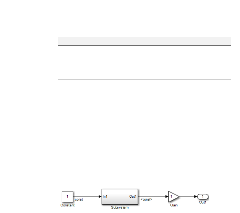
47 Working with Signals
Signal Label Propagation
In this section...
“Propagated Signal Labels” on page 47-24
“Blocks That Support Signal Label Propagation” on page 47-25
“Display Propagated Signal Labels” on page 47-25
“How Simulink Propagates Signal Labels” on page 47-26
Propagated Signal Labels
When you enable the display of signal label propagation for output signals
of the blocks listed in “Blocks That Support Signal Label Propagation” on
page 47-25:
•If there is a user-specified signal name that Simulink can propagate, the
propagated signal label includes the name in angle brackets (for example,
<sig1>).
•Ifthereisnosignalnametopropagate,Simulinkdisplaysanemptyset
of angle brackets (<>) for the label.
For example, in the following model, the output signal from the Subsystem
block is configured for signal label propagation. The propagated signal label
(<const>) is based on the name of the upstream output signal of the Constant
block (const).
For more information on how Simulink creates propagated signal labels, see
“How Simulink Propagates Signal Labels” on page 47-26.
47-24

Signal Label Propagation
Blocks That Support Signal Label Propagation
You can use signal label propagation with output signals for several
connection blocks, which route signals through the model without changing
the data. Connection blocks perform no signal transformation.
Also, Model blocks support signal label propagation.
The connection blocks that support signal label propagation are:
•Enable
•From
•Function Call Split
•Goto
•Inport (subsystem only; not root inports)
•Signal Specification
•Subsystem (through subsystem Inport and Outport blocks)
•Trigger
•Two-Way Connection (a Simscape block)
The Bus Creator and Bus Selector blocks do not support signal label
propagation. However, if you want to view the hierarchy for any bus signal,
use the Signal Hierarchy Viewer.
The Signal Properties dialog box for a signal indicates whether that signal
supports signal label propagation. The Show propagated signals parameter
is available only for blocks that support signal label propagation. For details,
see “Display Propagated Signal Labels” on page 47-25.
Display Propagated Signal Labels
To display a propagated signal label:
1Set Model Configuration Parameters > Diagnostics >
Connectivity > Mux blocks used to create bus signals to error.
47-25
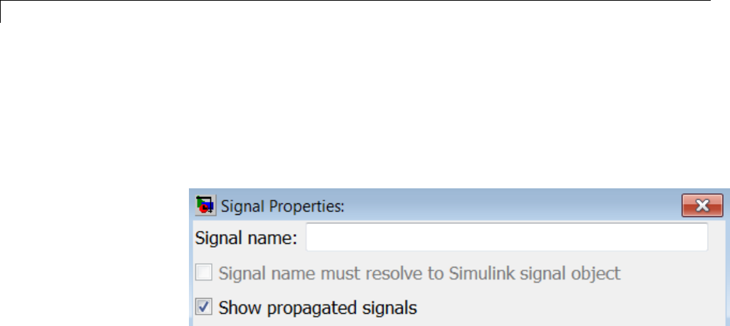
47 Working with Signals
2Right-click the signal for which you want to display a propagated signal
label.
The Signal Properties dialog box opens.
3Select Show propagated signals.
The Show propagated signals parameter is available only for output
signals from blocks that support signal label propagation.
If a signal already has a label, then an alternative approach for displaying
apropagatedsignallabelis:
1Click the signal label.
2Remove the label text.
3In the signal label text box, enter an angle bracket (<).
4Click outside the signal label.
Simulink displays the propagated signal label.
How Simulink Propagates Signal Labels
Understanding how Simulink propagates signal labels helps you to:
•Anticipate the scope of the signal label propagation, from source to final
destination
•Configure your model to display signal labels for the signals that you want
47-26

Signal Label Propagation
For output signals from supported blocks,youcanchoosetohaveSimulink
display propagated signal labels. For a list of supported blocks, see “Blocks
That Support Signal Label Propagation” on page 47-25.
In general, Simulink performs signal label propagation consistently:
•For different modeling constructs (for example, non-bus and bus signals,
virtual and nonvirtual buses, subsystem and model variants, model
referencing, and libraries)
•In models with or without hidden blocks, which Simulink inserts in certain
casestoenablesimulation
•At model load, edit, update, and simulation times
For information about some special cases, see:
•“Processing for Referenced Models” on page 47-31
•“Processing for Variants and Configurable Subsystems” on page 47-33
General Signal Label Propagation Processing
In general, when you enable signal label propagation for an output signal of a
block (for example, BlockA), Simulink performs the following processing to
find the source signal name to propagate:
1Checks the block whose output signal connects to BlockA, and if necessary,
continues checking upstream blocks, working backward from the closest
block to the farthest block.
2Stops when it encounters a block that either:
•Supports signal label propagation and has a signal name
•Does not support signal label propagation
3Obtains the signal name, if any, of the output signal for the block at which
Simulink stops.
4Uses that signal name for the propagated signal label of any output signals
of downstream blocks for which you enable signal label propagation.
47-27
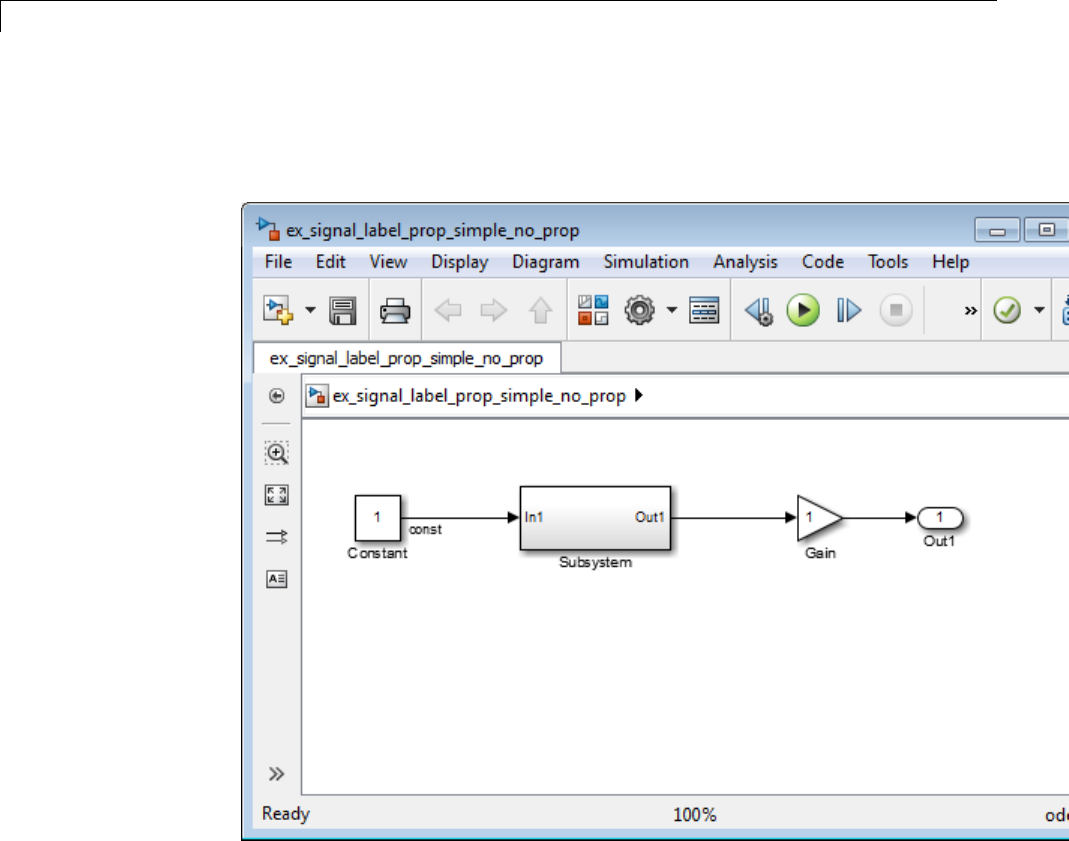
47 Working with Signals
For example, in the following model, suppose that you enable signal label
propagation for the output signal for the Subsystem block (that is, the signal
connected to the Out1 port).
47-28
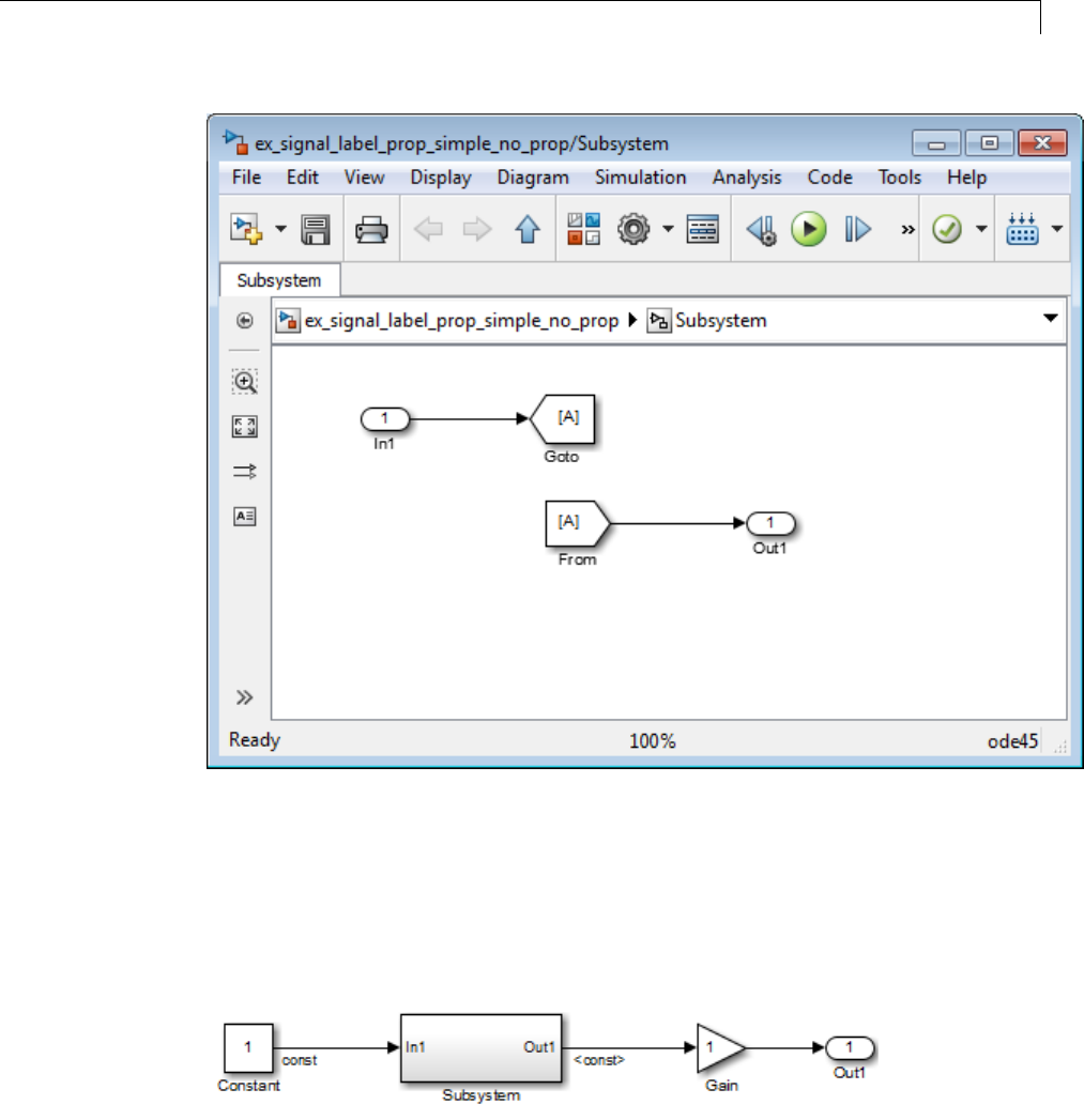
Signal Label Propagation
Simulink checks inside the subsystem, checks upstream from the From and
GoTo blocks (which support signal label propagation and do not have a name),
and then checks farther upstream, to the Constant block, which does not
support signal label propagation.
Simulink uses the signal name of the Constant block output signal, const.
The propagated signal label for the Subsystem output signal is <const>.
47-29
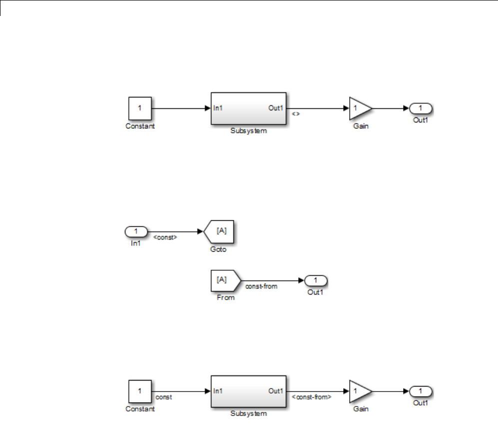
47 Working with Signals
If the output signal from the Constant block did not have a signal name, then
the propagated signal label would be an empty set of angle brackets (<>).
Suppose that in the Subsystem block you enable signal label propagation
for the output signal from the In1 block, and you use the Signal Properties
dialog box to specify the signal name const-from for the output signal of the
From block, as shown below.
The propagated signal label for the Subsystem output signal changes
to <const-from>, because that is the first named signal that Simulink
encounters in its signal label propagation processing.
In the following model, the signal label propagation for the output signal of
the Subsystem block uses the signal name bus1,whichisthenameofthe
output bus signal of the Bus Creator block. The propagated signal label does
not include the names of the bus element signals (aand b).
47-30
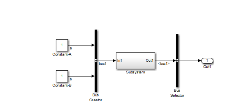
Signal Label Propagation
Processing for Referenced Models
To enable signal label propagation for referenced models, in addition to
the steps described in “Display Propagated Signal Labels” on page 47-25,
enable the Model Configuration Parameters > Model Referencing >
Propagate all signal labels out of the model parameter.
If you make a change inside a referenced model that affects signal label
propagation, the propagated signal labels outside of the referenced model
do not reflect those changes until after you update the diagram or simulate
the model.
For example, the model ex_signal_label_prop_model_ref has a referenced
model that includes an output signal from the In1 block that has a signal
name of input_1.
If you enable signal label propagation for the signal from the Out1 port of the
Model block, that signal does not reflect the name input_1 until after you
update the diagram or simulate the model.
47-31
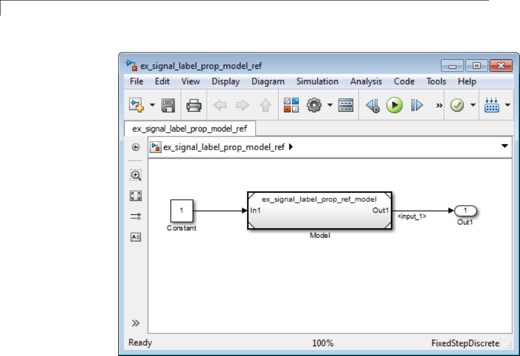
47 Working with Signals
47-32
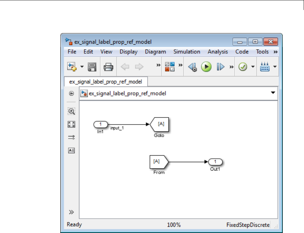
Signal Label Propagation
Processing for Variants and Configurable Subsystems
Simulink updates the propagated signal label (if enabled) for the output
signal of the Subsystem or Model block, when both of these conditions occur:
•The output signals for model reference variants have different signal
names.
•You change the active variant model or variant subsystem.
For Subsystem blocks, the signal label updates at edit time. For Model blocks,
the update occurs when you update diagram or simulate the model.
47-33

47 Working with Signals
Signal Dimensions
In this section...
“About Signal Dimensions” on page 47-34
“Simulink Blocks that Support Multidimensional Signals” on page 47-35
About Signal Dimensions
Simulink blocks can output one-dimensional, two-dimensional, or
multidimensional signals. The Simulink user interface and documentation
generally refer to 1-D signals as vectors and 2-D or multidimensional signals
as matrices. A one-element array is frequently referred to as a scalar.A
row vector is a 2-D array that has one row. A column vector is a 2-D array
that has one column.
•A one-dimensional (1-D) signal consists of a series of one-dimensional
arrays output at a frequency of one array (vector) per simulation time step.
•A two-dimensional (2-D) signal consists of a series of two-dimensional
arrays output at a frequency of one 2-D array (matrix) per block sample
time.
•A multidimensional signal consists of a series of multidimensional
(two or more dimensions) arrays output at a frequency of one array
per block sample time. You can specify multidimensional arrays with
any valid MATLAB multidimensional expression, such as [4 3]. See
“Multidimensional Arrays” for information on multidimensional arrays.
Simulink blocks vary in the dimensionality of the signals they can accept or
output. Some blocks can accept or output signals of any dimension. Some
can accept or output only scalar or vector signals. To determine the signal
dimensionality of a particular block, see the block documentation. See
“Determine Output Signal Dimensions” on page 47-36 for information on
what determines the dimensions of output signals for blocks that can output
nonscalar signals.
47-34

Signal Dimensions
Note Simulink does not support dynamic signal dimensions during a
simulation. That is, the dimension of a signal must remain constant while a
simulation is executing. However, you can change the size of a signal during a
simulation. See “Variable-Size Signal Basics” on page 49-2.
Simulink Blocks that Support Multidimensional
Signals
The Simulink Block Data Type Support table includes a column identifying
the blocks with multi-dimension signal support.
1In the Simulink editor, from the Help menu, click Simulink > Block
Data Types & Code Generation Support > All Tables.
A separate window with the Simulink Block Data Type Support table opens.
2In the Block column, locate the name of a Simulink block. Columns to the
right are data types or features. An a Xin a column indicates support
for that feature.
Simulink supports signals with up to 32 dimensions. Do not use signals with
more than 32 dimensions.
47-35

47 Working with Signals
Determine Output Signal Dimensions
In this section...
“About Signal Dimensions” on page 47-36
“Determining the Output Dimensions of Source Blocks” on page 47-36
“Determining the Output Dimensions of Nonsource Blocks” on page 47-37
“Signal and Parameter Dimension Rules” on page 47-37
“Scalar Expansion of Inputs and Parameters” on page 47-38
About Signal Dimensions
If a block can emit nonscalar signals, thedimensionsofthesignalsthatthe
block outputs depend on the block parameters, if the block is a source block;
otherwise, the output dimensions depend on the dimensions of the block input
and parameters.
Determining the Output Dimensions of Source Blocks
Asource block is a block that has no inputs. Examples of source blocks include
the Constant block and the Sine Wave block. See “Sources” for a complete
listing of Simulink source blocks. The output dimensions of a source block
are the same as those of its output value parameters if the block’s Interpret
vector parameters as 1-D parameter is off (that is, not selected in the
block parameter dialog box). If the Interpret vector parameters as 1-D
parameter is on, the output dimensions equal the output value parameter
dimensions unless the parameter dimensions are N-by-1 or 1-by-N. In the
latter case, the block outputs a vector signal of width N.
As an example of how a source block’s output value parameter(s)
and Interpret vector parameters as 1-D parameter determine the
dimensionality of its output, consider the Constant block. This block outputs
a constant signal equal to its Constant value parameter. The following table
illustrates how the dimensionality of the Constant value parameter and the
setting of the Interpret vector parameters as 1-D parameter determine
the dimensionality of the block’s output.
47-36

Determine Output Signal Dimensions
Constant Value
Interpret vector
parameters as 1-D Output
scalar off one-element array
scalar on one-element array
1-by-N matrix off 1-by-N matrix
1-by-N matrix on N-element vector
N-by-1 matrix off N-by-1 matrix
N-by-1 matrix on N-element vector
M-by-N matrix off M-by-N matrix
M-by-N matrix on M-by-N matrix
Simulink source blocks allow you to specify the dimensions of the signals
that they output. You can therefore use them to introduce signals of various
dimensions into your model.
Determining the Output Dimensions of Nonsource
Blocks
If a block has inputs, the dimensions of its outputs are, after scalar expansion,
the same as those of its inputs. (All inputs must have the same dimensions,
as discussed in “Signal and Parameter Dimension Rules” on page 47-37).
Signal and Parameter Dimension Rules
When creating a Simulink model, you must observe the following rules
regarding signal and parameter dimensions.
Input Signal Dimension Rule
All nonscalar inputs to a block must have the same dimensions.
A block can have a mix of scalar and nonscalarinputsaslongasallthe
nonscalar inputs have the same dimensions. Simulink expands the scalar
inputs to have the same dimensions as the nonscalar inputs (see “Scalar
Expansion of Inputs” on page 47-39) thus preserving the general rule.
47-37

47 Working with Signals
Block Parameter Dimension Rule
In general, a block’s parameters musthavethesamedimensionsasthe
corresponding inputs.
Two seeming exceptions exist to this general rule:
•A block can have scalar parameters corresponding to nonscalar inputs.
In this case, Simulink expands a scalar parameter to have the same
dimensions as the corresponding input (see “Scalar Expansion of
Parameters” on page 47-39) thus preserving the general rule.
•If an input is a vector, the corresponding parameter can be either an N-by-1
or a 1-by-N matrix. In this case, Simulink applies the N matrix elements to
the corresponding elements of the input vector. This exception allows use
of MATLAB row or column vectors, which are actually 1-by-N or N-by-1
matrices, respectively, to specify parameters that apply to vector inputs.
Vector or Matrix Input Conversion Rules
Simulink converts vectors to row or column matrices and row or column
matrices to vectors under the following circumstances:
•If a vector signal is connected to an input that requires a matrix, Simulink
converts the vector to a one-row or one-column matrix.
•If a one-column or one-row matrix is connected to an input that requires a
vector, Simulink converts the matrix to a vector.
•If the inputs to a block consist of a mixture of vectors and matrices and
the matrix inputs all have one column or one row, Simulink converts the
vectors to matrices having one column or one row, respectively.
Note You can configure Simulink to display a warning or error message if a
vector or matrix conversion occurs during a simulation. See “Vector/matrix
block input conversion” for more information.
Scalar Expansion of Inputs and Parameters
Scalar expansion is the conversion of a scalar value into a nonscalar array
of the same dimensions. Many Simulink blocks support scalar expansion of
47-38
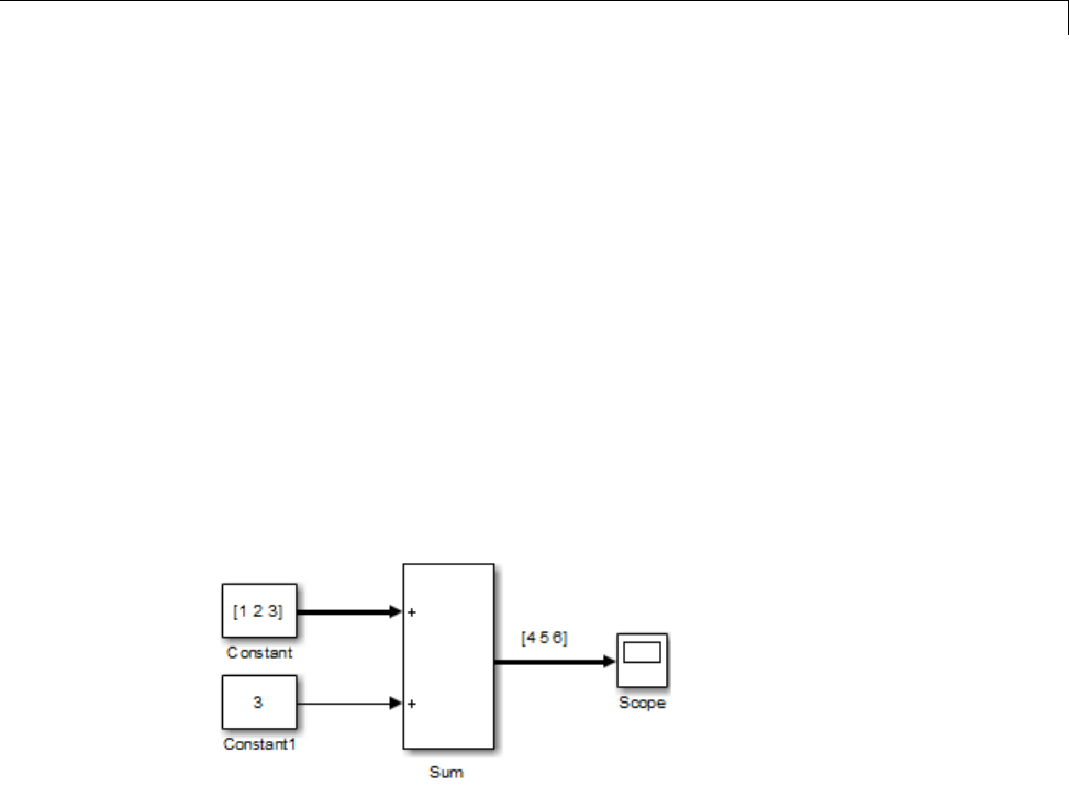
Determine Output Signal Dimensions
inputs and parameters. Block-specific descriptions indicate whether Simulink
applies scalar expansion to a block’s inputs and parameters.
Scalar Expansion of Inputs
Scalar expansion of inputs refers to the expansion of scalar inputs to match
the dimensions of other nonscalar inputs or nonscalar parameters. When the
input to a block is a mix of scalar and nonscalar signals, Simulink expands
the scalar inputs into nonscalar signals having the same dimensions as the
other nonscalar inputs. The elements of an expanded signal equal the value of
the scalar from which the signal was expanded.
The following model illustrates scalar expansion of inputs. This model adds
scalar and vector inputs. The input from block Constant1 is scalar expanded
to match the size of the vector input from the Constant block. The input
is expanded to the vector [3 3 3].
When a block’s output is a function of a parameter and the parameter is
nonscalar, Simulink expands a scalar input to match the dimensions of the
parameter. For example, Simulink expandsascalarinputtoaGainblockto
match the dimensions of a nonscalar gain parameter.
Scalar Expansion of Parameters
If a block has a nonscalar input and a corresponding parameter is a scalar,
Simulink expands the scalar parameter to have the same number of elements
as the input. Each element of the expanded parameter equals the value of
the original scalar. Simulink then applies each element of the expanded
parameter to the corresponding input element.
47-39

47 Working with Signals
This example shows that a scalar parameter (the Gain) is expanded to a
vector of identically valued elements to match the size of the block input, a
three-element vector.
47-40

Display Signal Sources and Destinations
Display Signal Sources and Destinations
In this section...
“About Signal Highlighting” on page 47-41
“Highlighting Signal Sources” on page 47-41
“Highlighting Signal Destinations” on page 47-42
“Removing Highlighting” on page 47-43
“Resolving Incomplete Highlighting to Library Blocks” on page 47-43
About Signal Highlighting
You can highlight a signal and its source or destination block(s), then
remove the highlighting once it has served its purpose. Signal highlighting
crosses subsystem boundaries, allowing you to trace a signal across multiple
subsystem levels. Highlighting does not cross the boundary into or out of a
referenced model. If a signal is composite, all source or destination blocks are
highlighted. (See “About Composite Signals” on page 48-2.)
Highlighting Signal Sources
To display the source block(s) of a signal, select the Highlight Signal to
Source option from the context menu for the signal. This option highlights:
•All branches of the signal anywhere in the model
•All virtual blocks through which the signal passes
•The nonvirtual block(s) that write the value of the signal
47-41
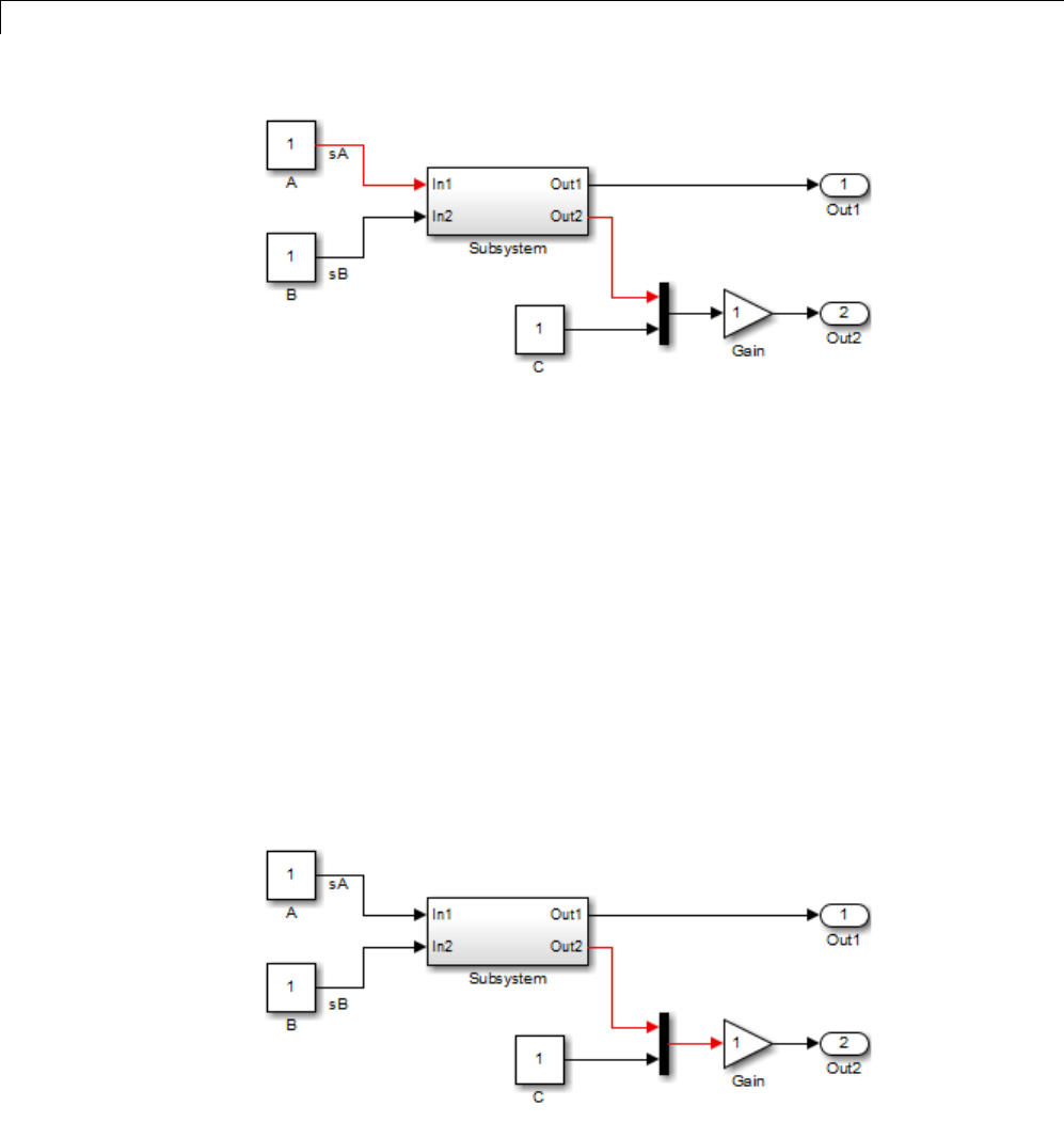
47 Working with Signals
Highlighting Signal Destinations
To display the destination blocks of a signal, select the Highlight Signal
to Destination option from the context menu for the signal. This option
highlights:
•All branches of the signal anywhere in the model
•All virtual blocks through which the signal passes
•The nonvirtual block(s) that read the value of the signal
•The signal and destination block for all blocks that are duplicates of the
inport block for the line that you select
In this example, the selected signal highlights the Gain block as the
destination block.
47-42
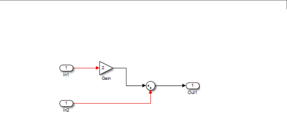
Display Signal Sources and Destinations
In the next example, selecting the signal from In2 and choosing the Highlight
Signal to Destination option highlights the signal and destination block for
In2 and In1, because In1 and In2 are duplicate inport blocks.
Removing Highlighting
To remove all highlighting, select Remove Highlighting from the model’s
context menu, or select Display > Remove Highlighting.
Resolving Incomplete Highlighting to Library Blocks
If the path from a source block or to a destination block includes an unresolved
reference to a library block, the highlighting options highlight the path from
or to the library block, respectively. Todisplaythecompletepath,firstupdate
the diagram (for example, by pressing Ctrl+D).Theupdateofthediagram
resolves all library references and displays the complete path to a destination
block or from a source block.
47-43

47 Working with Signals
Signal Ranges
In this section...
“About Signal Ranges” on page 47-44
“Blocks That Allow Signal Range Specification” on page 47-44
“Specifying Ranges for Signals” on page 47-45
“Checking for Signal Range Errors” on page 47-46
About Signal Ranges
Many Simulink blocks allow you to specify a range of valid values for their
output signals. Simulink provides a diagnostic that you can enable to detect
when blocks generate signals that exceed their specified ranges during
simulation. See the sections that follow for more information.
Blocks That Allow Signal Range Specification
The following blocks allow you to specify ranges for their output signals:
•Abs
•Constant
•Data Store Memory
•Data Type Conversion
•Difference
•Discrete Derivative
•Discrete-Time Integrator
•Gain
•Inport
•Interpolation Using Prelookup
•1-D Lookup Table
•2-D Lookup Table
47-44

Signal Ranges
•n-D Lookup Table
•Math Function
•MinMax
•Multiport Switch
•Outport
•Product, Divide, Product of Elements
•Relay
•Repeating Sequence Interpolated
•Repeating Sequence Stair
•Saturation
•Saturation Dynamic
•Signal Specification
•Sum, Add, Subtract, Sum of Elements
•Switch
Specifying Ranges for Signals
In general, use the Output minimum and Output maximum parameters
that appear on a block parameter dialog box to specify a range of valid values
for the block output signal. Exceptions include the Data Store Memory, Inport,
Outport, and Signal Specification blocks, for which you use their Minimum
and Maximum parameters to specify a signal range. See “Blocks That Allow
Signal Range Specification” on page 47-44 for a list of applicable blocks.
When specifying minimum and maximum values that constitute a range,
enter only expressions that evaluate to a scalar, real number with double data
type. The default values for the minimum and maximum are [] (unspecified).
The scalar values that you specify are subject to expansion, for example,
when the block inputs are nonscalar or bus signals (see “Scalar Expansion of
Inputs and Parameters” on page 47-38).
47-45

47 Working with Signals
Note You cannot specify the minimum or maximum value as NaN,inf,or
-inf.
Specifying Ranges for Complex Numbers
When you specify an Output minimum and/or Output maximum for a
signal that is a complex number, the specified minimum and maximum
values apply separately to the real part and to the imaginary part of the
complex number. If the value of either part of the number is less than the
minimum, or greater than the maximum, the complex number is outside the
specified range. No range checking occurs against any combination of the real
and imaginary parts, such as (sqrt(a^2+b^2))
Checking for Signal Range Errors
Simulink provides a diagnostic named Simulation range checking,which
you can enable to detect when signals exceed their specified ranges during
simulation. When enabled, Simulink compares the signal values that a block
outputswithboththespecifiedrange(see “Specifying Ranges for Signals”
on page 47-45) and the block data type. That is, Simulink performs the
following check:
DataTypeMin MinValue VALUE MaxValue DataTypeMax
where
•DataTypeMin is the minimum value representable by the block data type.
•MinValue is the minimum value the block should output, specified by, e.g.,
Output minimum.
•VALUE is the signal value that the block outputs.
•MaxValue is the maximum value the block should output, specified by, e.g.,
Output maximum.
•DataTypeMax is the maximum value representable by the block data type.
47-46
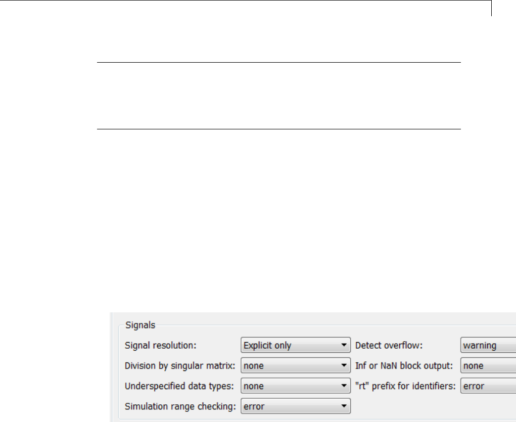
Signal Ranges
Note It is possible to overspecify how a block handles signals that exceed
particular ranges. For example, you can specify values (other than the default
values) for both signal range parameters and enable the Saturate on integer
overflow parameter. In this case, Simulink displays a warning message that
advises you to disable the Saturate on integer overflow parameter.
Enabling Simulation Range Checking
To enable the Simulation range checking diagnostic:
1In your model window, select Simulation > Model Configuration
Parameters.
Simulink displays the Configuration Parameters dialog box.
2In the Select tree on the left side of the Configuration Parameters dialog
box, click the Diagnostics > Data Validity category. On the right side
under Signals,settheSimulation range checking diagnostic to error
or warning.
3Click OK to apply your changes and close the Configuration Parameters
dialog box.
See“Simulationrangechecking”formoreinformation.
Simulating Models with Simulation Range Checking
To check for signal range errors or warnings:
47-47
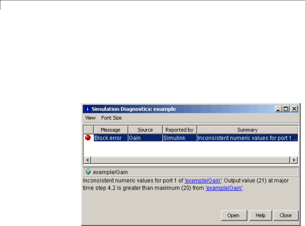
47 Working with Signals
1Enable the Simulation range checking diagnostic for your model (see
“Enabling Simulation Range Checking” on page 47-47).
2In your model window, select Simulation > Run to simulate the model.
Simulink simulates your model and performs signal range checking. If a
signal exceeds its specified range when the Simulation range checking
diagnostic specifies error, Simulink stops the simulation and displays
an error message:
Otherwise, if a signal exceeds its specified range when the Simulation
range checking diagnostic specifies warning, Simulink displays a
warning message in the MATLAB Command Window:
Warning: Inconsistent numeric values for port 1
of 'example/Gain': Output value (21) at major
time step 4.2 is greater than maximum (20) from
'example/Gain'.
Each message identifies the block whose output signal exceeds its specified
range, and the time step at which this violation occurs.
47-48
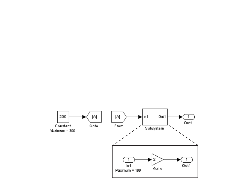
Signal Ranges
Signal Range Propagation for Virtual Blocks
Some virtual blocks (see “Virtual Blocks” on page 23-2) allow you to specify
ranges for their output signals, for example, the Inport and Outport blocks.
When the Simulation range checking diagnostic is enabled for a model
that contains such blocks, the signal range of the virtual block propagates
backward to the first instance of a nonvirtual block whose output signal it
receives. If the nonvirtual block specifies different values for its own range,
Simulink performs signal range checking with the tightest range possible.
That is, Simulink checks the signal using the larger minimum value and
the smaller maximum value.
For example, consider the following model:
In this model, the Constant block specifies its Output maximum parameter
as 300, and that of the Inport block is set to 100. Suppose you enable the
Simulation range checking diagnostic and simulate the model. The
Inport block back propagates its maximum value to the nonvirtual block that
precedes it, i.e., the Constant block. Simulink then uses the smaller of the
two maximum values to check the signal that the Constant block outputs.
Because the Constant block outputs a signal whose value (200) exceeds the
tightest range, Simulink displays the following error message:
47-49
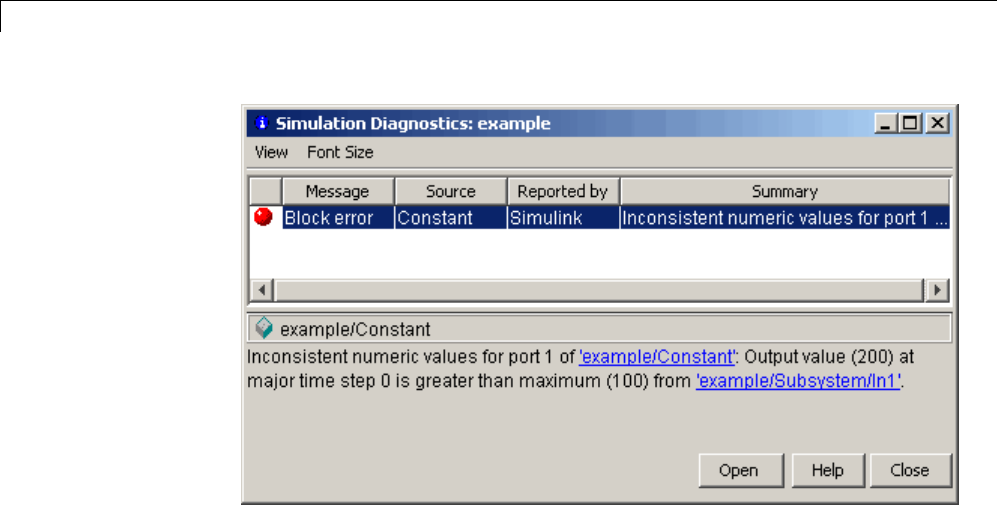
47 Working with Signals
47-50

Initialize Signals and Discrete States
Initialize Signals and Discrete States
In this section...
“About Initialization” on page 47-51
“Using Block Parameters to Initialize Signals and Discrete States” on
page 47-52
“Using Signal Objects to Initialize Signals and Discrete States” on page
47-52
“Using Signal Objects to Tune Initial Values” on page 47-53
“Example: Using a Signal Object to Initialize a Subsystem Output” on
page 47-55
“Initialization Behavior Summary for Signal Objects” on page 47-56
About Initialization
Note For information about initializing bus signals, see “Specify Initial
Conditions for Bus Signals” on page 48-65.
Simulink allows you to specify the initial values of signals and discrete states,
i.e., the values of the signals and discrete states at the Start time of the
simulation. You can use signal objectstospecifytheinitialvaluesofany
signal or discrete state in a model. In addition, for some blocks, e.g., Outport,
Data Store Memory, or Memory, you can use either a signal object or a block
parameter or both to specify the initial value of a block state or output. In
such cases, Simulink checks to ensure that the values specified by the signal
object and the parameter are consistent.
When you specify a signal object for signal or discrete state initialization, or
a variable as the value of a block parameter, Simulink resolves the name
that you specify to an appropriate object or variable, as described in “Symbol
Resolution” on page 4-76.
A given signal can be associated with at most one signal object under any
circumstances. The signal can refer to the object more that once, but every
47-51
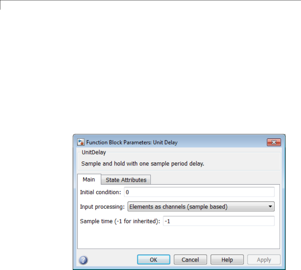
47 Working with Signals
reference must resolve to exactly the same object. A different signal object
that has exactly the same properties will not meet the requirement for
uniqueness. A compile-time error occurs if a model associates more than one
signal object with any signal. For more information, see Simulink.Signal
and the Merge block.
Using Block Parameters to Initialize Signals and
Discrete States
For blocks that have an initial value or initial condition parameter, you can
use that parameter to initialize a signal. For example, the following Block
Parameters dialog box initializes the signal for a Unit Delay block with an
initial condition of 0.
Using Signal Objects to Initialize Signals and Discrete
States
To use a signal object to specify an initial value:
47-52

Initialize Signals and Discrete States
1Create the signal object in the MATLAB workspace, as explained in “Data
Objects” on page 43-37.
Thenameofthesignalobjectmustbethesameasthenameofthesignal
or discrete state that the object is initializing.
Note Consider also setting the Signal name must resolve to Simulink
signal object option in the Signal Properties dialog box. This setting
ensures consistency between signal objects in the MATLAB workspace and
the signals that appear in your model.
2Set the signal object’s storage class to a value other than 'Auto' or
'SimulinkGlobal'.
3Set the signal object’s Initial value property to the initial value of the
signal or state. For details on what you can specify, see the description
of Simulink.Signal.
If you can also use a block parameter to set the initial value of the signal or
state, you should set the parameter either to null ([])ortothesamevalue
as the initial value of the signal object. If you set the parameter value to
null, Simulink uses the value specified by the signal object to initialize
the signal or state. If you set the parameter to any other value, Simulink
compares the parameter value to the signal object value and displays an
error if they differ.
UsingSignalObjectstoTuneInitialValues
Simulink allows you to use signal objects as an alternative to parameter
objects (see ) to tune the initial values of block outputs and states that can be
specified via a tunable parameter. To use a signal object to tune an initial
value,createasignalobjectwiththesamenameasthesignalorstateand
set the signal object’s initial value to an expression that includes a variable
defined in the MATLAB workspace. You can then tune the initial value
by changing the value of the corresponding workspace variable during the
simulation.
For example, suppose you want to tune the initial value of a Memory
block state named M1. Todothis,youmightcreateasignalobjectnamed
47-53

47 Working with Signals
M1, set its storage class to 'ExportedGlobal', set its initial value to K
(M1.InitialValue='K'), where Kis a workspace variable in the MATLAB
workspace, and set the corresponding initial condition parameter of the
Memory block to [] to avoid consistency errors. You could then change the
initial value of the Memory block’s state any time during the simulation by
changing the value of Kat the MATLAB command line and updating the
block diagram (e.g., by typing Ctrl+D).
Note To be tunable via a signal object, a signal or state’s corresponding
initial condition parameter must be tunable, e.g., the inline parameter
optimization for the model containing the signal or state must be off or the
parameter must be declared tunable in the Model Parameter Configuration
dialog box. For more information, see “Tunable Parameters” on page 3-9 and
“Tunable Parameters” on page 24-13.
47-54
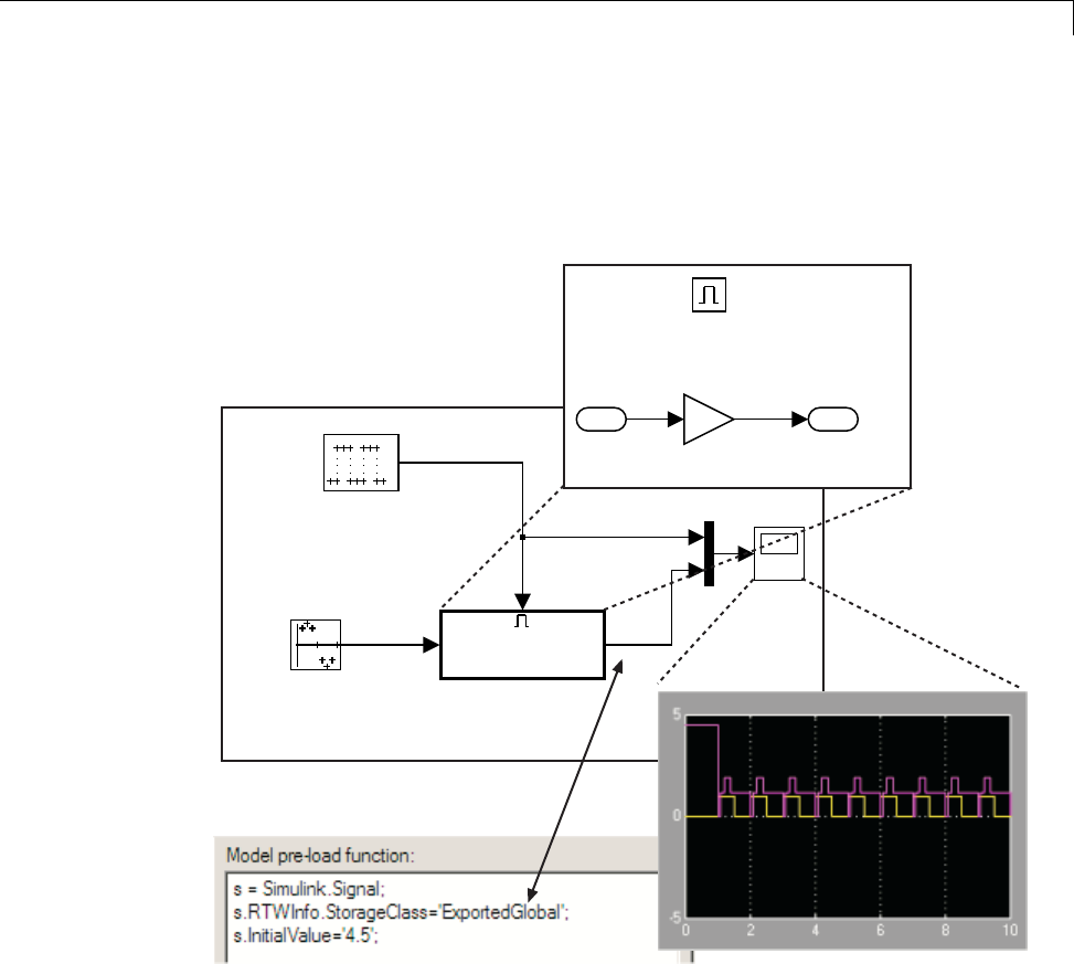
Initialize Signals and Discrete States
Example: Using a Signal Object to Initialize a
Subsystem Output
The following example shows a signal object specifying the initial output of
an enabled subsystem.
Sine Wave
Amplitude = 1
Period = 10 samples
Ts = 0.1
Scope
In1 Out1
Enabled
Subsystem
Enable
Ts = 0.1
Phase Delay = 10 samples
e
s
1
Out1
Initial Output = []
2
Gain
Enable
1
In1
Signal sis initialized to 4.5. To avoid a consistency error, the initial value of
the enabled subsystem’s Outport block must be [] or 4.5.
If you need a signal object and its initial value setting to persist across
Simulink sessions, see “Creating Persistent Data Objects” on page 43-47.
47-55
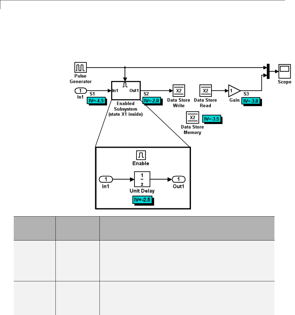
47 Working with Signals
Initialization Behavior Summary for Signal Objects
The following model and table show different types of signals and discrete
states that you can initialize and the simulation behavior that results for each.
Signal or
Discrete
State
Description Behavior
S1 Root inport •Initialized to S1.InitialValue.
•If you use the Data Import/Export pane of the Configuration
Parameters dialog to specify values for the root inputs, the
initial value is overwritten and may differ at each time step.
Otherwise, the value remains constant.
X1 Unit Delay
block — Block
with a discrete
•Initialized to X1.InitialValue.
•Simulink checks whether X1.InitialValue matches the
initial condition specified for the block and displays an error
if a mismatch occurs.
47-56

Initialize Signals and Discrete States
Signal or
Discrete
State
Description Behavior
state that
has an initial
condition
•At first write, the output equals X1.InitialValue and the
state equals S1.
•At each time step after the first write, the output equals the
state and the state is updated to equal S1.
•If the block is inside an enabled subsystem, you can use the
initial value as a reset value if the subsystem’s Enable block
parameter States when enabling is set to reset.
X2 Data Store
Memory block
•Data type work (DWork) vector initialized to
X2.InitialValue. For information on work vectors, see
“DWork Vector Basics”.
•Simulink checks whether X2.InitialValue matches the
initial condition specified for the block, and displays an error
if a mismatch occurs.
•Data Store Write blocks overwrite the value.
S2 Output of
an enabled
subsystem
•Initialized to S2.InitialValue or the value of the Outport
block. If multiple initial values are specified for the same
signal, all initial values must be the same.
•The first write occurs when the subsystem is enabled. The
block feeding the subsystem output sets the value.
•Theinitialvalueisalsousedasaresetvalueifthe
subsystem’s Enable block parameter States when enabling
or Outport block parameter Output when disabled is set
to reset.
S3 Persistent
signals
•Initialized to S3.InitialValue.
•Theoutputvalueisresetbytheblockateachtimestep.
•Affects code generation only. For simulation, setting the
initial value for S3 is irrelevant because the values are
overwritten at the model’s simulation start time.
47-57

47 Working with Signals
Test Points
In this section...
“What Is a Test Point?” on page 47-58
“Designating a Signal as a Test Point” on page 47-58
“Displaying Test Point Indicators” on page 47-60
What Is a Test Point?
Atest point is a signal that Simulink guarantees to be observable when using
a Floating Scope block in a model. Simulink allows you to designate any
signal in a model as a test point.
Designating a signal as a test point exempts the signal from model
optimizations, such as signal storage reuse (see “Signal storage reuse”) and
block reduction (see “Implement logic signals as Boolean data (vs. double)”).
These optimizations render signals inaccessible and hence unobservable
during simulation.
Signals designated as test points will not have algebraic loops minimized,
even if Minimize algebraic loop occurrences is selected (for more
information about algebraic loops, see “Algebraic Loops” on page 3-39).
Test points are primarily intended for use when generating code from a model
with Simulink Coder. For more information about test points in the context
of code generation, see “Signals with Test Points”.
Marking a signal as a test point has no impact on signal logging that uses the
Dataset logging format. For information about logging signals, see “Export
Signal Data Using Signal Logging” on page 45-19.
Designating a Signal as a Test Point
To specify that a signal whose storage class is Auto is a test point, open the
signal’s Signal Properties dialog box and select Logging and accessibility
>Testpoint. The signal is now a test point. Selecting or clearing this option
has no effect unless the signal’s storage class is Auto.
47-58

Test Points
Any signal whose storage class is not Auto is automatically a test point,
regardless of the setting of Signal Properties > Logging and accessibility
>Testpoint. You can specify a non-Auto signal storage class in three ways:
•In the Signal Properties dialog box, select the Code Generation tab,
and then set Storage class to anything other than Auto.
•Resolve the signal to a base workspace Simulink.Signal object that
specifies a storage class other than Auto.
•Embed a signal object that specifies a storage class other than Auto on
the port where the signal originates.
Using a base workspace signal object to specify that a signal is a test point can
be convenient, because it allows you to control testpointing without having
to change the model itself. Assigning storage class SimulinkGlobal has
exactly the same effect as assigning storage class Auto and selecting Signal
Properties > Logging and accessibility > Test point.
Model Referencing Limitation
Simulink might not log all signals configured for signal logging in a referenced
model, if all of these conditions exist:
•The referenced model sets the Model Configuration Parameters > Data
Import/Export > Signal logging format parameter to ModelDataLogs.
•The referenced model uses a library and you make a change that affects
the set of test points in a library, or that changes the set of models that
a library references.
To ensure proper signal logging for the referenced model:
1Open the referenced model.
2Perform an update diagram on the referenced model (for example, by
pressing Ctrl+D).
3Save the referenced model.
47-59
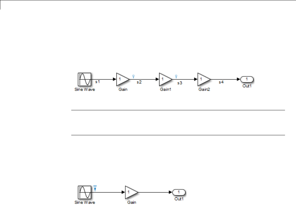
47 Working with Signals
Displaying Test Point Indicators
By default, Simulink displays an indicator on each signal whose Signal
Properties > Testpointoption is enabled. For example, in the following
model signals s2and s3 are test points:
Note Simulink does not display an indicator on a signal that is specified
as a test point by a Simulink.Signal object, because such a specification
is external to the graphical model.
A signal that is a test point can also be logged. See “Export Signal Data Using
Signal Logging” on page 45-19 for information about signal logging. The
appearance of the indicator changes to indicate signals for which logging
is also enabled.
To turn display of test point indicators on or off, in the Simulink Editor, select
or clearDisplay > Signals & Ports > Testpoint & Logging Indicators.
47-60

Display Signal Attributes
Display Signal Attributes
In this section...
“Ports & Signals Menu” on page 47-61
“Port Data Types” on page 47-62
“Design Ranges” on page 47-62
“Signal Dimensions” on page 47-63
“Signal to Object Resolution Indicator” on page 47-64
“Wide Nonscalar Lines” on page 47-65
Ports&SignalsMenu
The Display > Signals & Ports submenu of the Simulink Editor offers the
following options for displaying signal properties on the block diagram:
•Linearization Indicators
•Port Data Types (See “Port Data Types” on page 47-62)
•Design Ranges (See “Design Ranges” on page 47-62)
•Signal Dimensions (See “Signal Dimensions” on page 47-63)
•Storage Class
•Testpoint/Logging Indicators
•Signal Resolution Indicators (See “Signal to Object Resolution Indicator” on
page 47-64)
•Viewer Indicators
•Wide Nonscalar Lines (See “Wide Nonscalar Lines” on page 47-65)
In addition, you can display sample time information. If you first select
Display > Sample Time, a submenu provides the choices of Colors,
Annotations and All.TheColors option allows the block diagram signal
lines and blocks to be color-coded based on the sample time types and relative
rates. The Annotations option provides black codes on the signal lines
which indicate the type of sample time. All causes both the colors and the
47-61
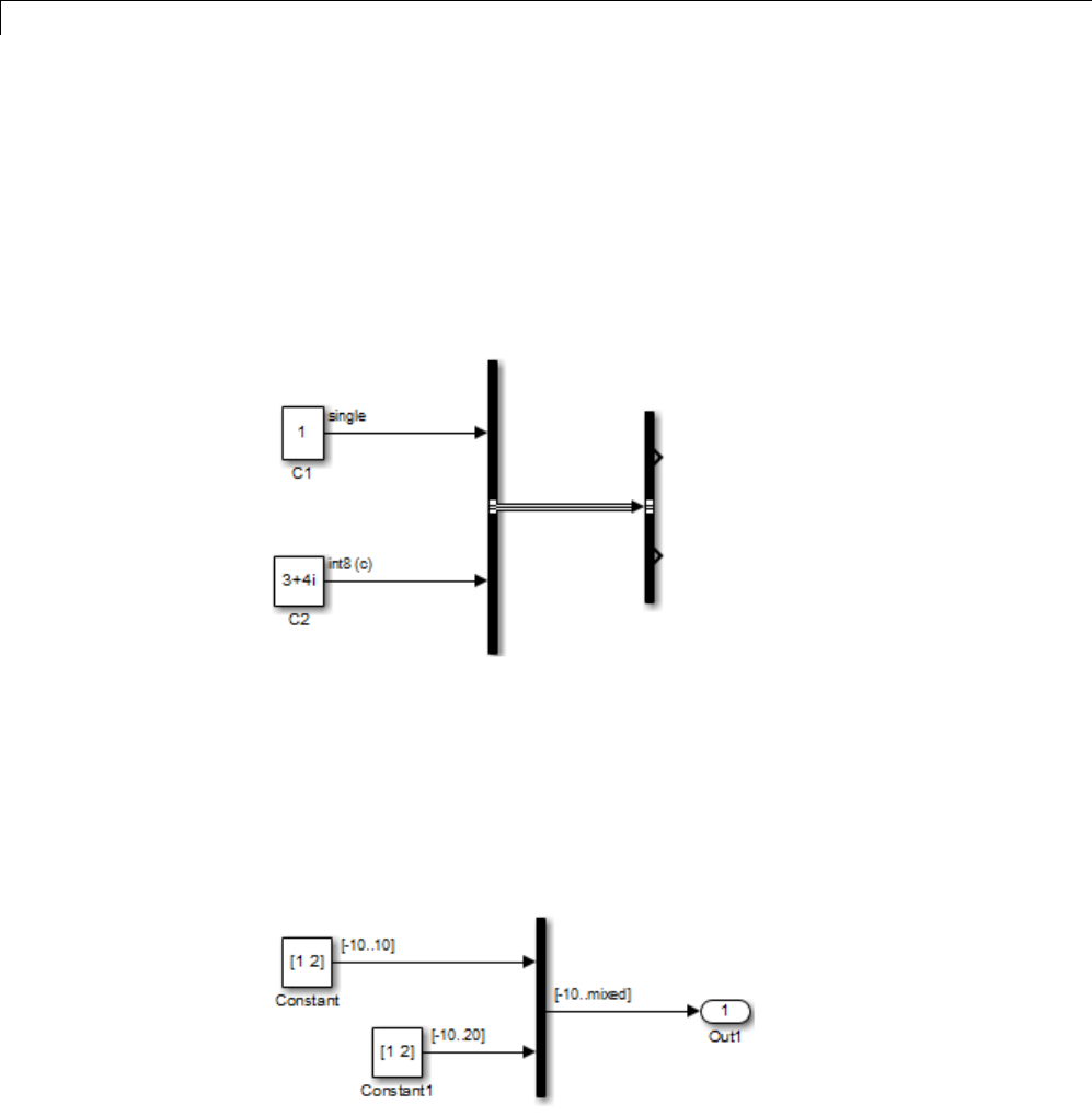
47 Working with Signals
annotations to display. All of these options cause a Sample Time Legend to
appear. The legend contains a description of the type of sample time and the
sample time rate. If Colors is turned ’on’, color codes also appear in the
legend. The same is true if Annotations are turned ’on’.
Port Data Types
Displays the data type of a signal next to the output port that emits the signal.
The notation (c) following the data type of a signal indicates that the signal
is complex.
Design Ranges
Displays the compiled design range of a signal next to the output port that
emits the signal. The ranges are computed during an update diagram.
47-62
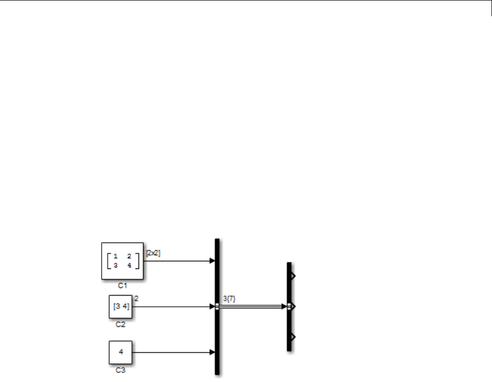
Display Signal Attributes
Ranges are displayed in the format [min..max]. In the above example,
the design range at the output port of the Mux block is displayed as
[-10..mixed], because the two signals the Mux block combines have the
same design minimum but different design maximums.
You can also use command-line parameters CompiledPortDesignMin and
CompiledPortDesignMax to access the design minimum and maximum of port
signals, respectively, at compile time. For more information, see “Common
Block Parameters”.
Signal Dimensions
Display the dimensions of nonscalar signals next to the line that carries the
signal.
The format of the display depends on whether the line represents a single
signal or a bus. If the line represents a single vector signal, Simulink displays
the width of the signal. If the line represents a single matrix signal, Simulink
displays its dimensions as [N1xN2]where Niisthesizeoftheith dimension
ofthesignal. Ifthelinerepresentsabuscarryingsignalsofthesamedata
type, Simulink displays N{M} where Nis the number of signals carried by the
bus and Mis the total number of signal elements carried by the bus. If the
bus carries signals of different data types, Simulink displays only the total
number of signal elements {M}.
47-63
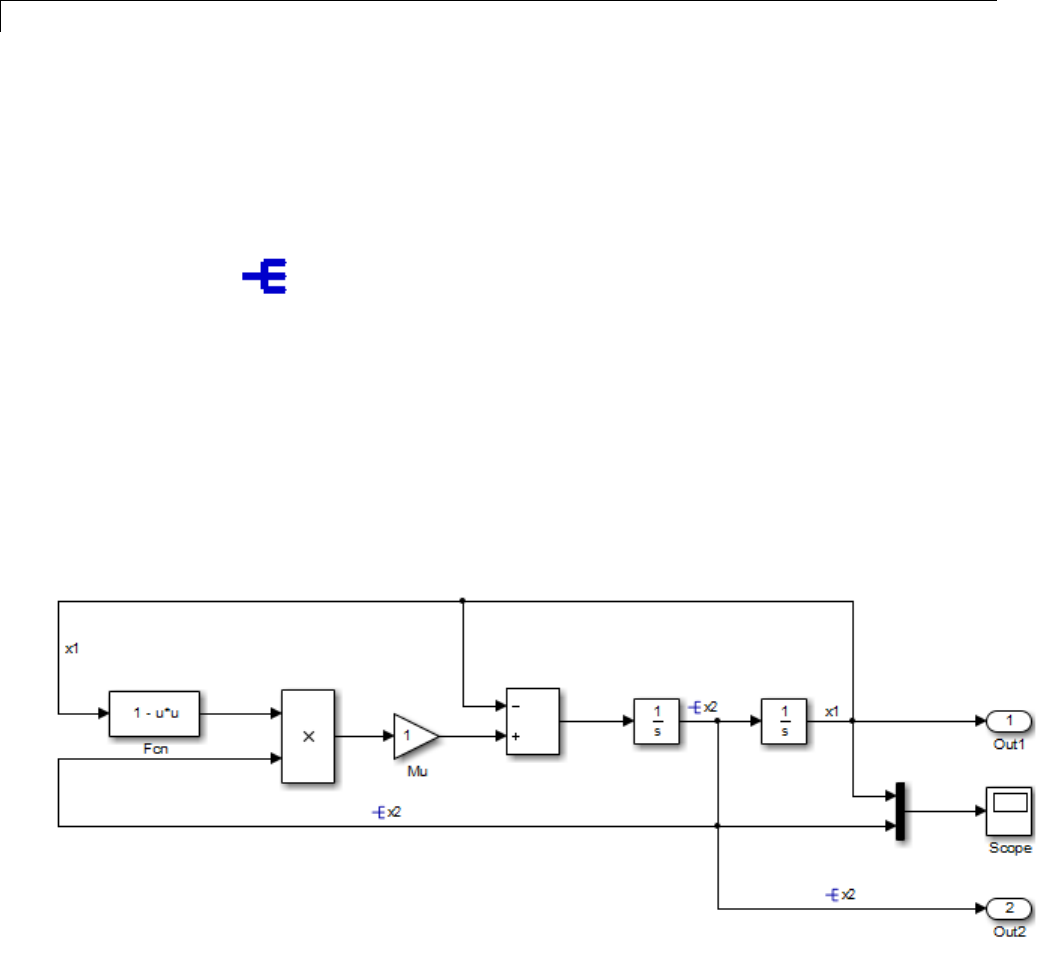
47 Working with Signals
Signal to Object Resolution Indicator
The Simulink Editor by default graphically indicates signals that must resolve
to signal objects. For any labeled signal whose Signal name must resolve
to signal objectproperty is enabled, a signal resolution icon appears to the
left of the signal name. The icon looks like this:
A signal resolution icon indicates only that a signal’s Signal name must
resolve to signal object property is enabled. The icon does not indicate
whether the signal is actually resolved, and does not appear on a signal that
is implicitly resolved without its Signal name must resolve to signal
object property being enabled.
Where multiple labels exist, each label displays a signal resolution icon. No
icon appears on an unlabeled branch. In the next figure, signal x2 must
resolvetoasignalobject,soasignalresolution icon appears to the left of
thesignalnameineachlabel:
To suppress the display of signal resolution icons, in the model window
deselect Display > Signals & Ports > Signal to Object Resolution
Indicator, which is selected by default. To restore signal resolution icons,
47-64
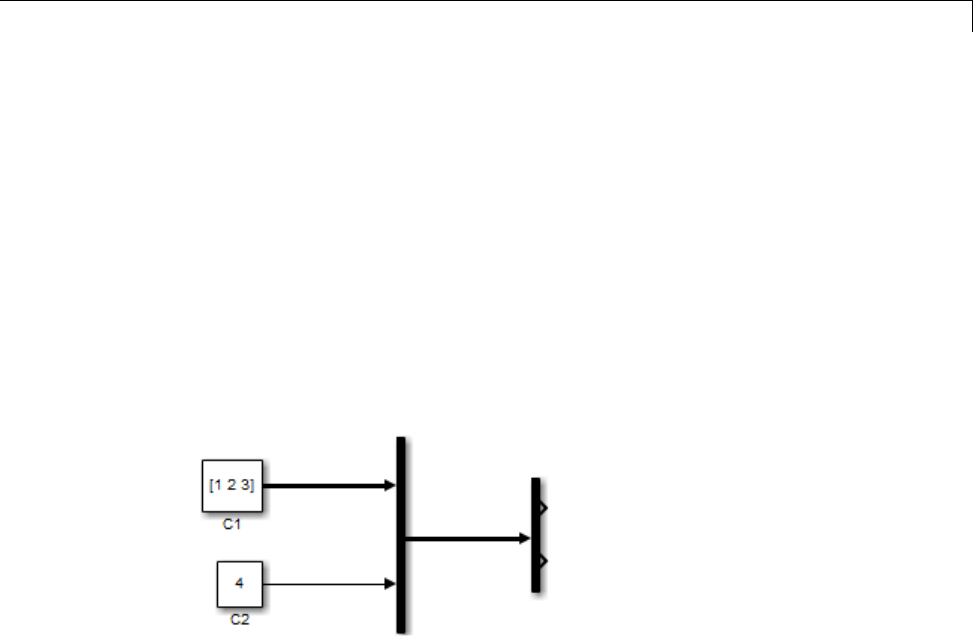
Display Signal Attributes
reselect Signal to Object Resolution Indicator. Individual signals cannot
be set to show or hide signal resolution indicators independently of the setting
for the whole model. For additional information, see:
•“Symbol Resolution” on page 4-76
•“Initialize Signals and Discrete States” on page 47-51
•Simulink.Signal
Wide Nonscalar Lines
Draws lines that carry vector or matrix signals wider than lines that carry
scalar signals.
See “About Composite Signals” on page 48-2 for more information about
vector and matrix signals.
47-65

47 Working with Signals
Signal Groups
In this section...
“About Signal Groups” on page 47-66
“Signal Builder Window” on page 47-66
“Creating Signal Group Sets” on page 47-72
“Editing Waveforms” on page 47-102
“Signal Builder Time Range” on page 47-108
“Exporting Signal Group Data” on page 47-109
“Printing, Exporting, and Copying Waveforms” on page 47-109
“Simulating with Signal Groups” on page 47-110
“Simulation Options Dialog Box” on page 47-111
About Signal Groups
The Signal Builder block displays and allows you to create or edit
interchangeable groups of signal sources and quickly switch the groups into
and out of a model.
Signal groups can greatly facilitate testing a model, especially when
you use them with conjunction with Simulink Assertion blocks and the
Model Coverage Tool from the Simulink Verification and Validation. For
a description of the Model Coverage Tool, see “Model Coverage Collection
Workflow”.
Model Configuration Parameter Solver pane settings can affect the Signal
Builder block output. See “Solvers” on page 3-21 for a description of how
solvers affect simulation.
Signal Builder Window
The Signal Builder block window allows you to define the shape of the signals
(waveform) output by the block. You can specify any waveform that is
piecewise linear.
47-66

Signal Groups
To open the window, double-click the block. The Signal Builder window
appears.
Group Panes
Help Area Signal Name Waveform Selection Status Area
List of Groups
The Signal Builder window allows you to create and modify signal groups
represented by a Signal Builder block. The Signal Builder window includes
the following controls.
47-67

47 Working with Signals
Group Pane
Displays the set of interchangeable signal source groups represented by the
block. Thepaneforeachgroupdisplaysaneditablerepresentationofeach
waveform in the group. The name of the group appears at the top of the pane.
Only one pane is visible at a time. To display a group that is not visible,
from the list, select the group name. The block outputs the group of signals
whosepaneiscurrentlyvisible. Each pane occupies a pane in the Signal
Builder block dialog box.
Signal Axes
The signals appear on separate axes that share a common time range (see
“Signal Builder Time Range” on page 47-108). This presentation allows you
to compare the relative timing of changesineachsignal. TheSignalBuilder
automatically scales the range of eachaxistoaccommodatethesignalthat
it displays. Use the Signal Builder Axes menu to change the time (T) and
amplitude (Y) ranges of the selected axis.
Signal List
Displays the names and visibility (see “Editing Signals” on page 47-69) of the
signals that belong to the currently selected signal group. Clicking an entry
in the list selects the signal. Double-clicking a signal entry in the list hides or
displays the waveform on the group pane.
Selection Status Area
Displays the name of the currently selected signal and the index of the
currently selected waveform segment or point.
Waveform Coordinates
Displays the coordinates of the currently selected waveform segment or point.
You can change the coordinates by editing the displayed values (see “Editing
Waveforms” on page 47-102).
Name
Name of the currently selected signal. You can change the name of a signal by
editing this field (see “Renaming a Signal” on page 47-72).
47-68

Signal Groups
Index
Index of the currently selected signal. The index indicates the output port at
which the signal appears. An index of 1 indicates the topmost output port, 2
indicates the second port from the top, and so on. You can change the index of
a signal by editing this field (see “Changing a Signal Index” on page 47-72).
Help Area
Displays context-sensitive tips on using Signal Builder window features.
Editing Signal Groups
The Signal Builder window allows you to create, rename, move, then delete
signal groups from the set of groups represented by a Signal Builder block.
Creating and Deleting Signal Groups. To create a signal group, copy an
existing signal group, then modify it to suit your needs. To copy an existing
signal group, select the group from the list, then select Copy from the Signal
Builder Group menu. To delete a group, select the group from the list, and
select Delete from the Group menu.
Renaming Signal Groups. To rename a signal group, select the group
from the list, then select Rename from the Signal Builder Group menu. A
dialog box appears. Edit the existing name in the dialog box or enter a new
name. Click OK.
Moving Signal Groups. To reposition a group in the stack of group panes,
selectthepaneandthenselectMove Down from the Signal Builder Group
menu to move the group lower in the stack or Move Up to move the pane
higher in the stack.
Editing Signals
The Signal Builder window allows you to create, cut and paste, hide, and
delete signals from signal groups.
47-69
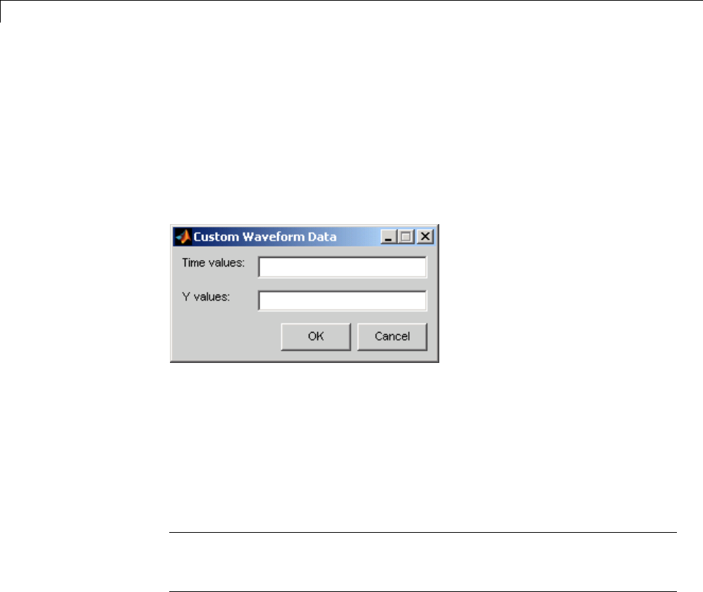
47 Working with Signals
Creating Signals. To create a signal in the currently selected signal group,
select New from the Signal Builder Signal menu. A menu of waveforms
appears. The menu includes a set of standard waveforms (Constant,Step,
and so on) and a Custom waveform option. Select one of the waveforms. If
you select a standard waveform, the Signal Builder adds a signal with that
waveform to the currently selected group.
If you select Custom, a custom waveform dialog box appears.
The dialog box allows you to add a custom piecewise linear waveform to the
groups defined by the Signal Builder block. Enter the custom waveform
time coordinates in the Time values field and the corresponding signal
amplitudes in the Y values field. The entries in either field can be any
MATLAB expression that evaluates to a vector. The resulting vectors must
be of equal length. Click OK. The Signal Builder adds a signal having the
specified shape to the currently selected group.
Note Signal Builder returns a warning if you add a custom waveform with
a large number of data points (100,000,000 or more). You can then cancel
the action.
Defining Signal Output. To specify the type of output to use for sending
test signals:
1In the Signal Builder window, select Signal > Output.
A list of output options appears.
2From the list, select:
47-70

Signal Groups
•Ports
Default. Sends individual signals fromtheblock.Anoutputportnamed
Signal Nappears for each Signal N.
•Bus
Sends single, virtual, nonhierarchical bus of signals from the block.
Tip
•You cannot use the Bus option to create a bus of non-virtual signals. An
output port named Bus appears.
•The Bus option enables you to change your model layout without having
to reroute Signal Builder block signals. Use the Bus Selector block to
select the signals from this bus.
•IfyoucreateaSignalBuilderblockwiththeSignal&ScopeManager
or with the Create & Connect Generator context menu option from
a signal line context menu, you cannot define signal output. In these
cases, the block sends individual signals.
Copying and Pasting Signals. To copy a signal from one group and paste it
into another group as a new signal:
1Select the signal you want to copy.
2Select Copy from the Signal Builder Edit menu or click the corresponding
buttononthetoolbar.
3Select the group into which you want to paste the signal.
4Select Paste from the Signal Builder Edit menu or click the corresponding
buttononthetoolbar.
To copy a signal from one axis and paste it into another axis to replace its
signal:
1Select the signal you want to copy.
47-71

47 Working with Signals
2Select Copy from the Signal Builder Edit menu or click the corresponding
buttononthetoolbar.
3Select the signal on the axes that you want to replace.
4Select Paste from the Signal Builder Edit menu or click the corresponding
buttononthetoolbar.
Deleting Signals. To delete a signal, select the signal and choose Delete or
Cut from the Signal Builder Edit menu. As a result, Signal Builder deletes
the signal from the current group. Because each signal group must contain
the same number of signals, Signal Builder also deletes all signals sharing
thesameindexintheothergroups.
Renaming a Signal. To rename a signal, select the signal and choose
Rename from the Signal Builder Signal menu. A dialog box appears with
an edit field that displays the current name of the signal. Edit or replace the
current name with a new name. Click OK.Oreditthesignalnameinthe
Name field in the lower-left corner of the Signal Builder window.
Changing a Signal Index. To change a signal index, select the signal and
choose Change Index from the Signal Builder Signal menu. A dialog box
appears with an edit field containing the existing index of the signal. Edit the
field and select OK. Or select an index from the Index list in the lower-left
corner of the Signal Builder window.
Hiding Signals. By default, the Signal Builder window displays the group
waveforms in the group pane. To hide a waveform, select the waveform and
then select Hide from the Signal Builder Signal menu. To redisplay a hidden
waveform, select the Group pane, then select Show from the Signal Builder
Signal menu to display a menu of hidden signals. Select the signal from
the menu. Alternatively, you can hide and redisplay a hidden waveform by
double-clicking its name in the Signal Builder signal list (see “Signal List”
on page 47-68).
Creating Signal Group Sets
You can create signal groups in the Signal Builder block by:
•“Creating Signal Group Sets Manually” on page 47-73
47-72
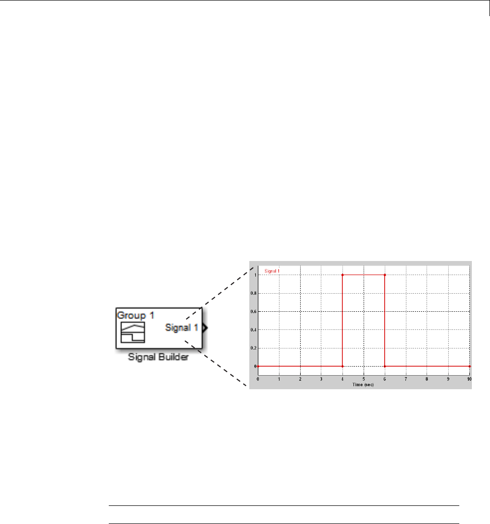
Signal Groups
•“Importing Signal Group Sets” on page 47-74
•“Importing Data with Custom Formats” on page 47-100
You can also use the signalbuilder function to populate the Signal Builder
block.
Creating Signal Group Sets Manually
This topic describes how to create signal group sets manually. If you have
signal data files, such as those from test cases, consider importing this data
as described in “Importing Signal Group Sets” on page 47-74.
To create an interchangeable set of signal groups:
1Drag an instance of the Signal Builder block from the Simulink Sources
library and drop it into your model.
By default, the block represents a single signal group containing a single
signal source that outputs a square wave pulse.
2Use the block signal editor (see “Signal Builder Window” on page 47-66) to
create additional signal groups, add signals to the signal groups, modify
existing signals and signal groups, and select the signal group that the
block outputs.
Note Each signal group must contain the same number of signals.
47-73

47 Working with Signals
3Connect the output of the block to your diagram.
The block displays an output port for each signal that the block can output.
You can create as many Signal Builder blocks as you like in a model, each
representing a distinct set of interchangeable groups of signal sources. When
a group has multiple signals, the signals might have different end times.
However, Signal Builder block requires the end times of signals within a
group to match. If a mismatch occurs, Signal Builder block matches the end
times by holding the last value of the signal with the smaller end time.
See “Simulating with Signal Groups” on page 47-110 for information on using
signal groups in a model.
Importing Signal Group Sets
The topics in this section describe how to import signal data into the Signal
Builder block. You should already have a signal data file whose contents you
want to import. For example, you might have signal data from previously run
test cases. See “Importing Signal Groups from Existing Data Sets” on page
47-74 for a description of the data formats that the Signal Builder
block accepts. The procedures in the following topics use the file
matlabroot\help\toolbox\simulink\ug\examples\signals\3Grp_3Sig.xls.
See “Data Import and Logging Workflow” for a description of the Signal
Builder block in a simulation workflow.
Importing Signal Groups from Existing Data Sets. You might have
existing signal data sets that you want to enter into the Signal Builder block.
The File > Import from File command on the Signal Builder window starts
the Import File dialog box. This dialog box is modal, which means that focus
cannot change to another MATLAB window while the dialog box is running.
If you want to see changes in the Signal Builder window after you import
data, do one of the following:
•Close the Import File dialog box.
•Set up the Import File dialog box and Signal Builder window side by side.
47-74

Signal Groups
Note You cannot undo the results of importing a signal data file. In addition,
you cannot undo the last action performed before opening the Import File
dialog box. When you close the Import File dialog box, the Undo last edit
and Redo last edit buttons on the Signal Builder window are grayed out.
These buttons are grayed out regardless of whether you imported a data file.
The Import File dialog box accepts the following appropriately formatted
file types:
•Microsoft Excel (.xls,.xlsx)
•Comma-separated value (CSV) text files (.csv)
•MAT-files (.mat)
Note Signal Builder block uses the xlsread function. See the xlsread
documentation for information on supported platforms.
You can import your data set file only if it is appropriately formatted.
For Microsoft Excel spreadsheets:
•The Signal Builder block interprets the first row as signal name. If you
do not specify a signal name, the Signal Builder block assigns a default
one with the format Imported_Signal #,where#increments with each
additional unnamed signal.
•The Signal Builder block interprets the first column as time. In this
column, the time values must increase.
•The Signal Builder block interprets the remaining columns as signals.
•If there are multiple sheets:
-Each sheet must have the same number of signals (columns).
-Eachsheetmusthavethesamesetofsignalnames(ifany).
-Each column on each sheet must have the same number of rows.
47-75
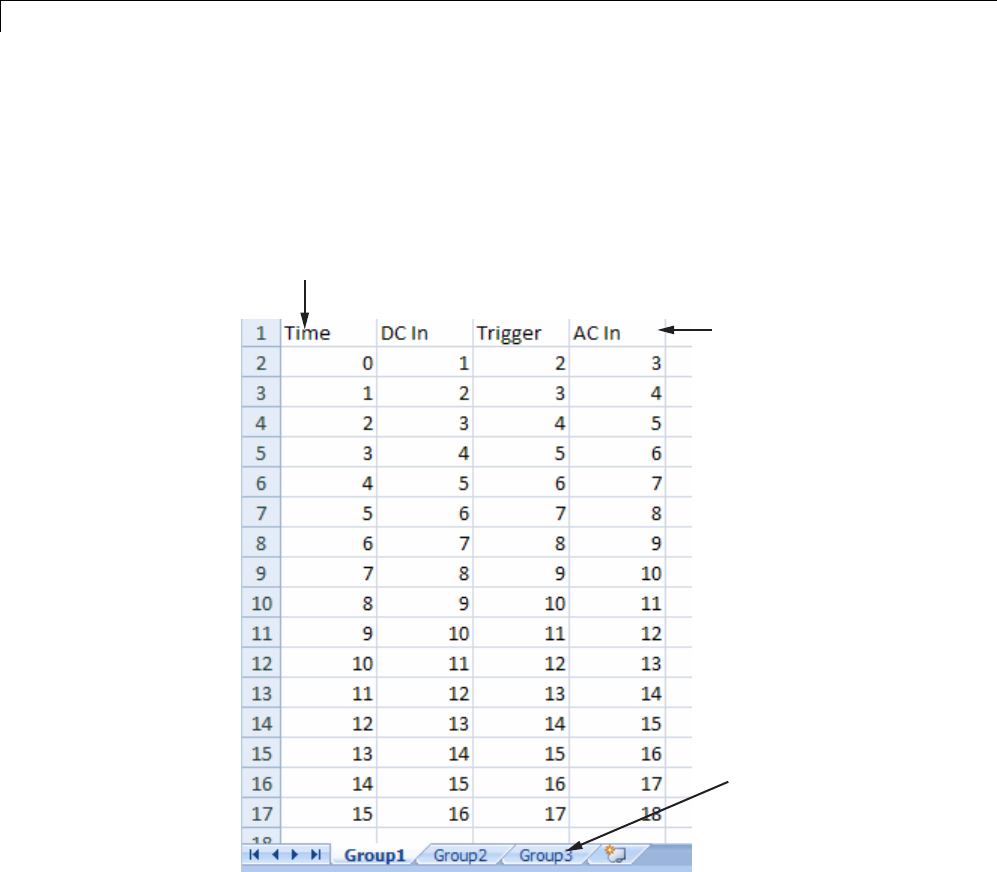
47 Working with Signals
•Signal Builder block interprets each worksheet as a signal group.
This example contains an acceptably formatted Microsoft Excel spreadsheet.
It has three worksheets named Group1, Group2, and Group3, representing
three signal groups.
Signal names (optional)
Worksheets - equivalent
to signal group
Time must be first column
For CSV text files:
•Each file contains only numbers. Do not name signals in a CSV file.
•The Signal Builder block interprets the first column as time. In this
column, the time values must increase.
•The Signal Builder block interprets the remaining columns as signals.
47-76

Signal Groups
•Each column must have the same number of entries.
•The Signal Builder block interprets each file as one signal group.
•The Signal Builder block assigns a default signal name to each signal with
the format Imported_Signal #,where#increments with each additional
signal.
This example contains an acceptably formatted CSV file. The contents
represent one signal group.
0,0,0,5,0
1,0,1,5,0
2,0,1,5,0
3,0,1,5,0
4,5,1,5,0
5,5,1,5,0
6,5,1,5,0
7,0,1,5,0
8,0,1,5,1
9,0,1,5,1
10,0,1,5,0
For MAT-files:
•The Signal Builder block supports data store logging that the
Simulink.SimulationData.Dataset object represents and interprets this
data as a single group.
•The Signal Builder block supports Simulink output saved as a structure
with time.
•The Signal Builder block supports the Signal Builder data format. This
format is a group of cell arrays that must be labeled:
-time
-data
-sigName
-groupName
sigName and groupName are optional.
47-77

47 Working with Signals
•For backwards compatibility, the Signal Builder block supports logged
data from the Simulink.ModelDataLogs object and interprets this data as
a single group. The ModelDataLogs format will be removed in a future
release.
•Signal Builder block does not support:
-Simulink output as only a structure
-Simulink output as only an array
Note Signal Builder returns a warning if you import a large number of data
points (100,000,000 or more). You can then cancel the action.
This example contains an acceptably logged MATLAB workspace. Use the
MATLAB workspace Save command to save the variables to a MAT-file.
Import this file to the Signal Builder block.
Signal Builder Block Import File Dialog Box. The Signal Builder Import
File dialog box allows you to import existing signal data files into the Signal
Builder block.
47-78
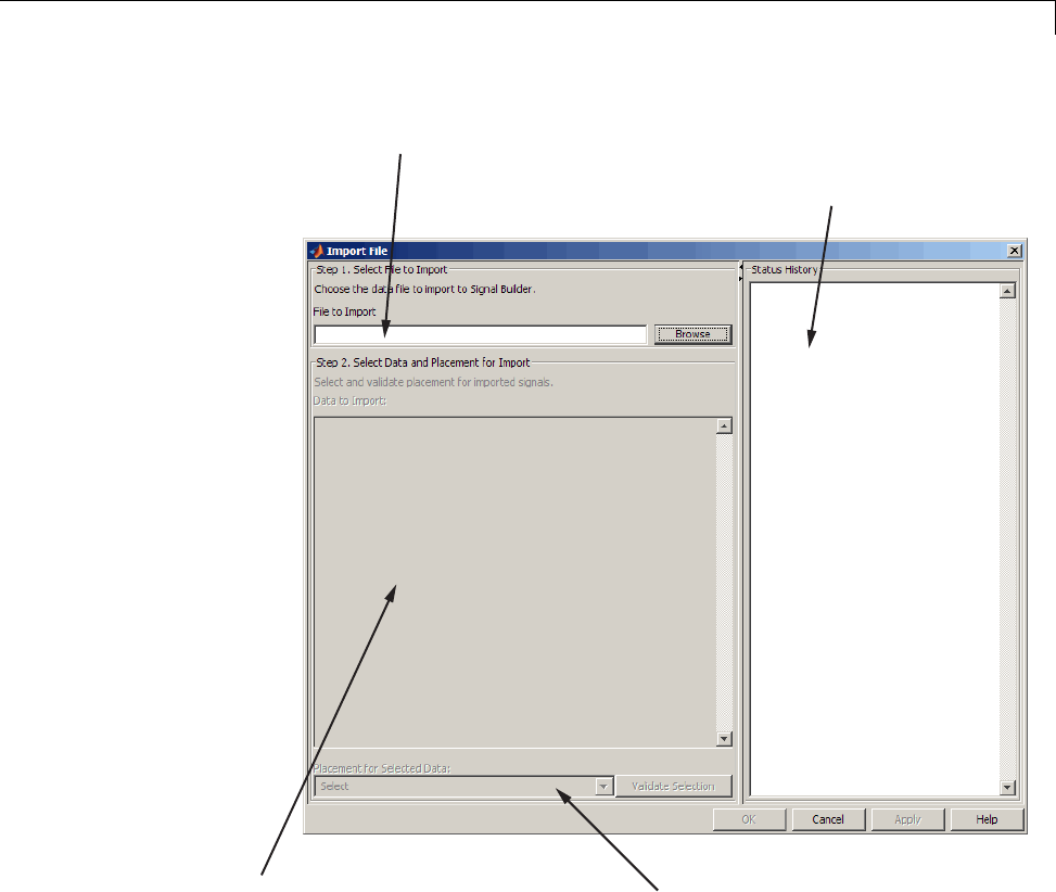
Signal Groups
Signal data file to import
Tree view of signal data file contents Drop-down list of import actions
for signal data
Repository of data import
status messages
Replacing All Signal Data with Selected Data. Simulink software creates
a default Signal Builder block with one signal. To replace this signal and all
other signal data that the block might display:
1Create a model and drag a Signal Builder block into that model.
2Double-click the block.
47-79
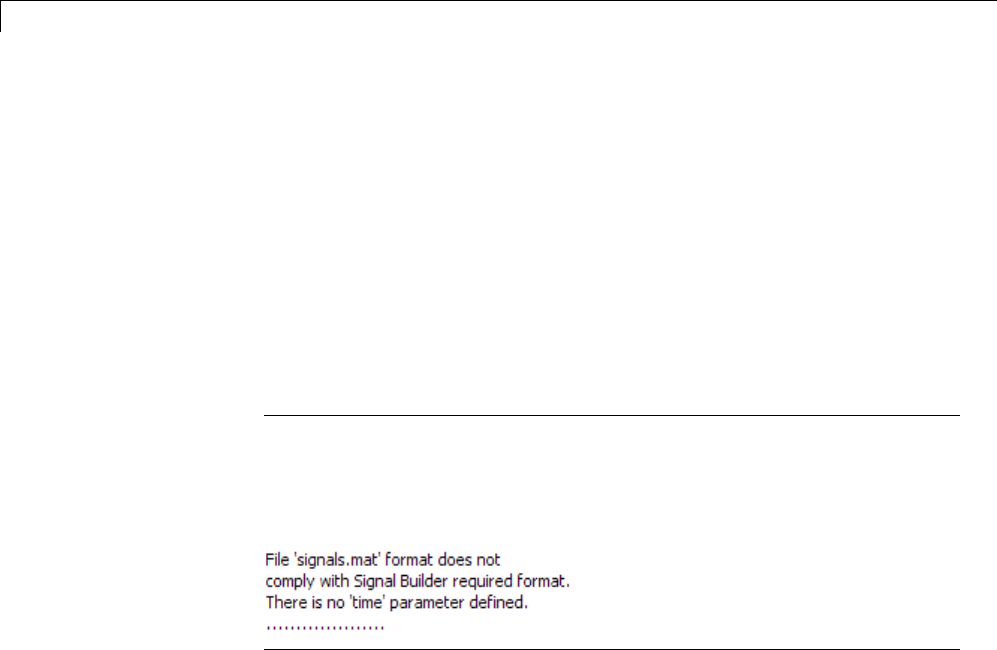
47 Working with Signals
The Signal Builder window appears with its default Signal 1.
3In the Signal Builder window, select File > Import from File.
The Import File dialog box appears.
4In the File to Import field, enter a signal data file name or click Browse.
Thefilebrowserappears.
5If you select the file browser, navigate to and select a signal data file. For
example, select 3Grp_3Sig.xls.
Note If you try to import an improperly formatted data file, an error
message pops up. When you click to dismiss this window, the Status
History pane displays a more detailed error message (if there is one).
For example:
The Data to Import pane contains the signal data from the file. Click the
expander to display all the signals.
47-80
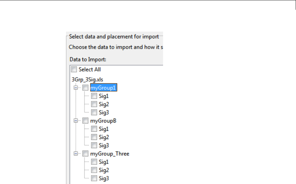
Signal Groups
6Select the signals you want to import. To import all the signals, click
Select All.
7From the Placement for Selected Data list, select the action to take on
the signal data. For example, select Replace existing dataset.
The Confirm Selection button is activated. Validate your signal selection
before the Signal Builder block performs the specified action. If the signal
data selection is not appropriate, Confirm Selection remains grayed out.
For example, Confirm Selection remains grayed out if the number of
signals you select is not the same as the number of signals in the Signal
Builder group that you want to replace.
8ClicktheConfirm Selection button.
If the requested action is a valid one, the Status History pane displays
messages to indicate the status. For example:
47-81
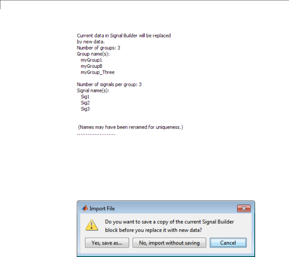
47 Working with Signals
The confirmation also enables the OK and Apply buttons.
9If you are satisfied with the status message, click Apply to replace the
existing signal data with the contents of this file.
When selecting Replace existing dataset, the software gives you the
opportunity to save the existing contents of the Signal Builder block.
10 Click a button, as follows:
47-82

Signal Groups
To... Click...
Save the contents of the Signal
Builder block before replacing it
with the new signal data.
Note This selection prompts you
to save the Signal Builder block
in a model name of your choice.
ThesoftwaresavesonlytheSignal
Builder block and no other model
content.
Yes, save as
Replace the contents of the Signal
Builder block without saving them
first.
No, import without saving
Stop the replacement process. Cancel
For this example, select No, import without saving to replace the
contents of the Signal Builder block.
11 The Signal Builder block updates with the new signal data. Click OK to
close the Import File dialog box and inspect the Signal Builder block.
47-83
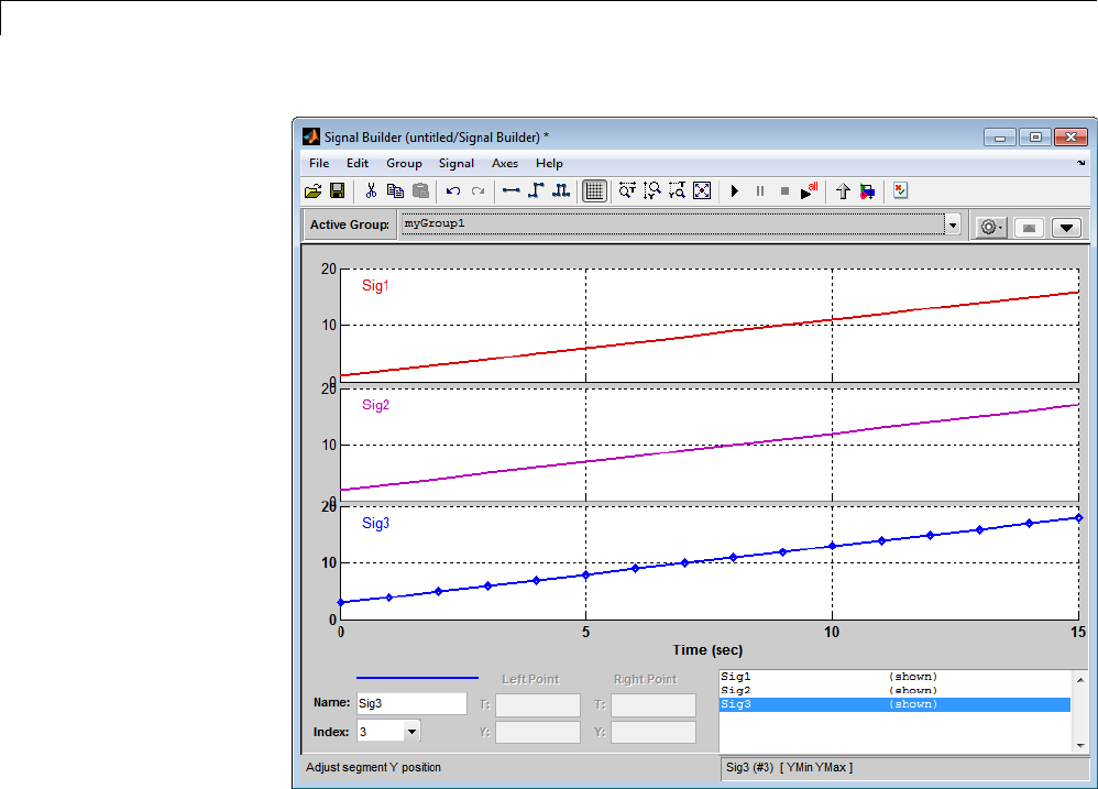
47 Working with Signals
12 Click OK.
13 Inspect the updated Signal Builder window to confirm that your signal
data is intact.
14 Close the Signal Builder window and save and close the model. For
example, save the model as signalbuilder1.
47-84

Signal Groups
Appending Selected Signals to All Existing Signal Groups. You can
import signals from a signal data file and append selected signals to the end of
all existing signal groups. If the signal names to be appended are not unique,
the software renames them by incrementing each name by 1 or higher until
it is a unique signal name. For example, if the block and data file contain
signals named thermostat, the software renames the imported signal to
thermostat1 upon appending. If you add another signal named thermostat,
the software names that latest version thermostat2.
This topic uses signalbuilder1 from the procedure in “Replacing All Signal
Data with Selected Data” on page 47-79.
1In the MATLAB Command Window, type signalbuilder1.
2Double-click the Signal Builder block.
The Signal Builder window appears.
3In the Signal Builder window, select File > Import from File.
The Import File dialog box appears.
4In the File to Import field, enter a signal data file name or click Browse.
The file browser is displayed.
5If you select the file browser, navigate to and select a signal data file. For
example, select 3Grp_3Sig.xls.
Note If you try to import an improperly formatted signal data file, an
error message pops up. When you click to dismiss this window, the Status
History pane displays an error message. For example:
47-85

47 Working with Signals
The Data to Import pane contains the signal data from the file. Click the
expander to display all the signals.
6Select the signals you want to import. In this example, there are three
groups, myGroup1, myGroupB, and myGroup_Three. Select all the signals
in myGroup1.
7From the Placement for Selected Data list, select the action to take on
the signal data. For example, select Append selected signals to all
groups.
The Confirm Selection button is activated. Validate your signal selection
before the Signal Builder block performs the specified action. If the signal
data selection is not appropriate, Confirm Selection remains grayed out.
For example, Confirm Selection remains grayed out if the number of
signals you select is not the same as the number of signals in the Signal
Builder group that you want to replace.
8Click the Confirm Selection button.
If the requested action is a valid one, the Status History pane displays
messagestoindicatethestate. Forexample:
47-86
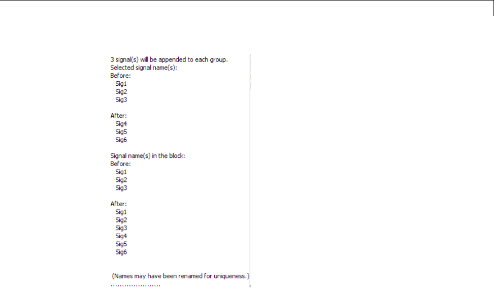
Signal Groups
The confirmation also enables the OK and Apply buttons.
Observe the Before and After headings for the signals. These sections
indicate the names of the block and imported data signals before and after
the append action.
9If you are satisfied with the status message, click Apply to append the
selected signals to all the signal groups in the Signal Builder block.
10 The Signal Builder block updates with the new signal data. Click OK to
close the Import File dialog box and inspect the Signal Builder block.
47-87
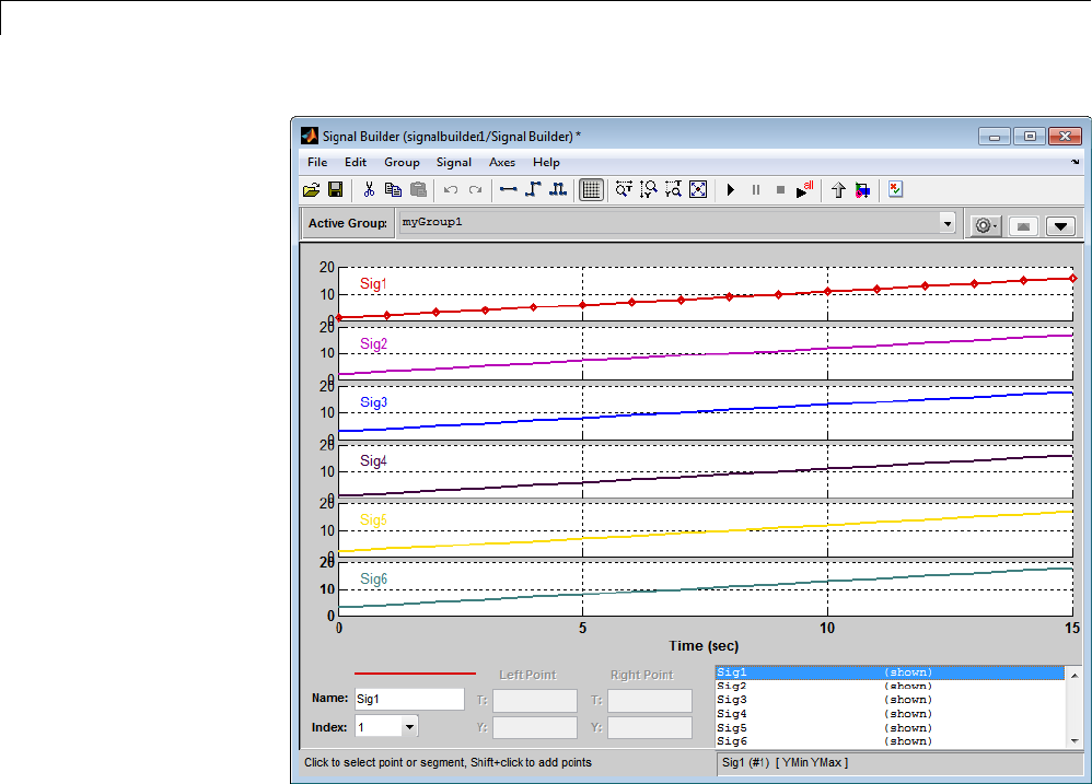
47 Working with Signals
11 Click OK.
12 Inspect the updated Signal Builder window to confirm that your signal
data is intact. Notice that the software has renamed the signals Sig1, Sig2,
and Sig3 from the signal data file to Sig4, Sig5, and Sig6 in the Signal
Builder block.
13 Close the Signal Builder window and save and close the model. For
example, save the model as signalbuilder2.
47-88

Signal Groups
Appending Selected Signals to Sequential Existing Signal Groups.
You can append signals, in the order in which they are selected, to the end
of sequential signal groups. This statement means that you select the same
number of signals as there are signal groups, and sequentially append each
signal to a different group. The software renames each appended signal to
thenameofthelastappendedsignal.
This topic uses signalbuilder1 from the procedure in “Replacing All Signal
Data with Selected Data” on page 47-79.
1In the MATLAB Command Window, type signalbuilder1.
2Double-click the Signal Builder block.
The Signal Builder window appears.
3Note how many groups exist in the Signal Builder block. For example,
this Signal Builder block has three groups, myGroup1, myGroupB, and
myGroup_Three.
47-89
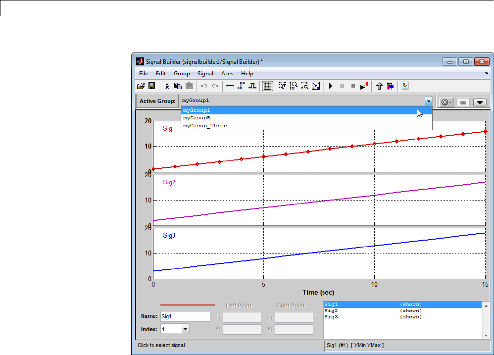
47 Working with Signals
4Double-click the block.
The Import File dialog box appears.
5In the File to Import field, enter a signal data file name or click Browse.
The file browser appears.
6If you select the file browser, navigate to and select a signal data file. For
example, select 3Grp_3Sig.xls.
47-90
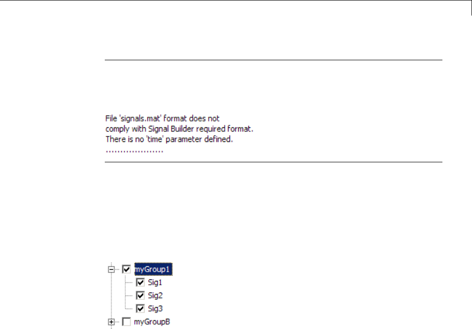
Signal Groups
Note If you try to import an improperly formatted signal data file, an
error message popup window. When you click to dismiss this window, the
Status History pane displays an error message. For example:
The Data to Import pane contains the signal data from the file. Click the
expander to display all the signals.
7Select the signals you want to import. In this example, there are three
groups, myGroup1, myGroupB, and myGroup_Three. Select all the signals
in myGroup1.
8From the Placement for Selected Data list, select the action to take
on the signal data. For example, select Append selected signals to
different groups (in order).
The Confirm Selection button is activated. Validate your signal selection
before the Signal Builder block performs the specified action.
9Click the Confirm Selection button.
If the requested action is a valid one, the Status History pane displays
messagestoindicatethestate. Forexample:
47-91

47 Working with Signals
The confirmation also enables the OK and Apply buttons.
10 If you are satisfied with the status message, click Apply to append the
signals.
The Signal Builder block updates with the new signal data. Click OK to
close the Import File dialog box and inspect the three groups of the Signal
Builder block.
The topmost signal group, myGroup1, shows all signals by default,
including the new Sig4.
47-92
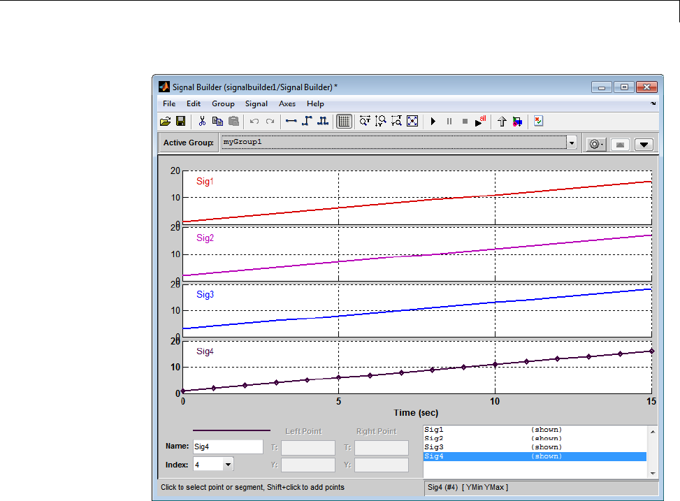
Signal Groups
11 Click another group name, for example, myGroupB. Notice that Sig4 exists
for the group, hidden by default.
47-93
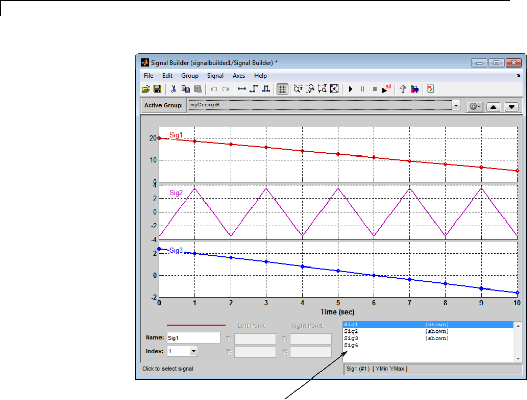
47 Working with Signals
Sig4 appears in signal list, but does not appear in group pane
12 To show Sig4 on this pane, double-click Sig4 in the Selection Status area of
the pane. The graph is updated to reflect Sig4.
47-94
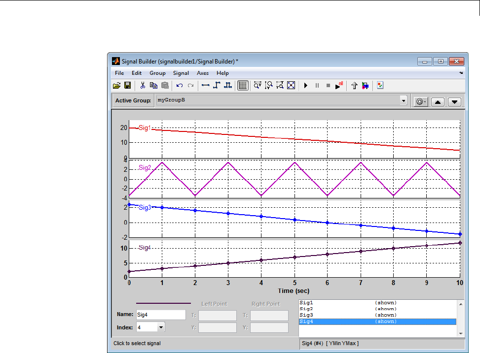
Signal Groups
13 Close the Signal Builder window and save and close the model. For
example, save the model as signalbuilder3.
Appending Signal Groups to Existing Groups. You can append one
or more signal groups to the end of the list of existing signal groups. If the
block already has a signal group with the same name as the one you are
adding, the software increments the group name by 1 or higher until it is
unique before adding it. For example, if the block and data file contain groups
namedMyGroup1, the software renames the imported group to MyGroup2 upon
appending. If you add another group named MyGroup1, the software names
thatlatestversionMyGroup3.
47-95
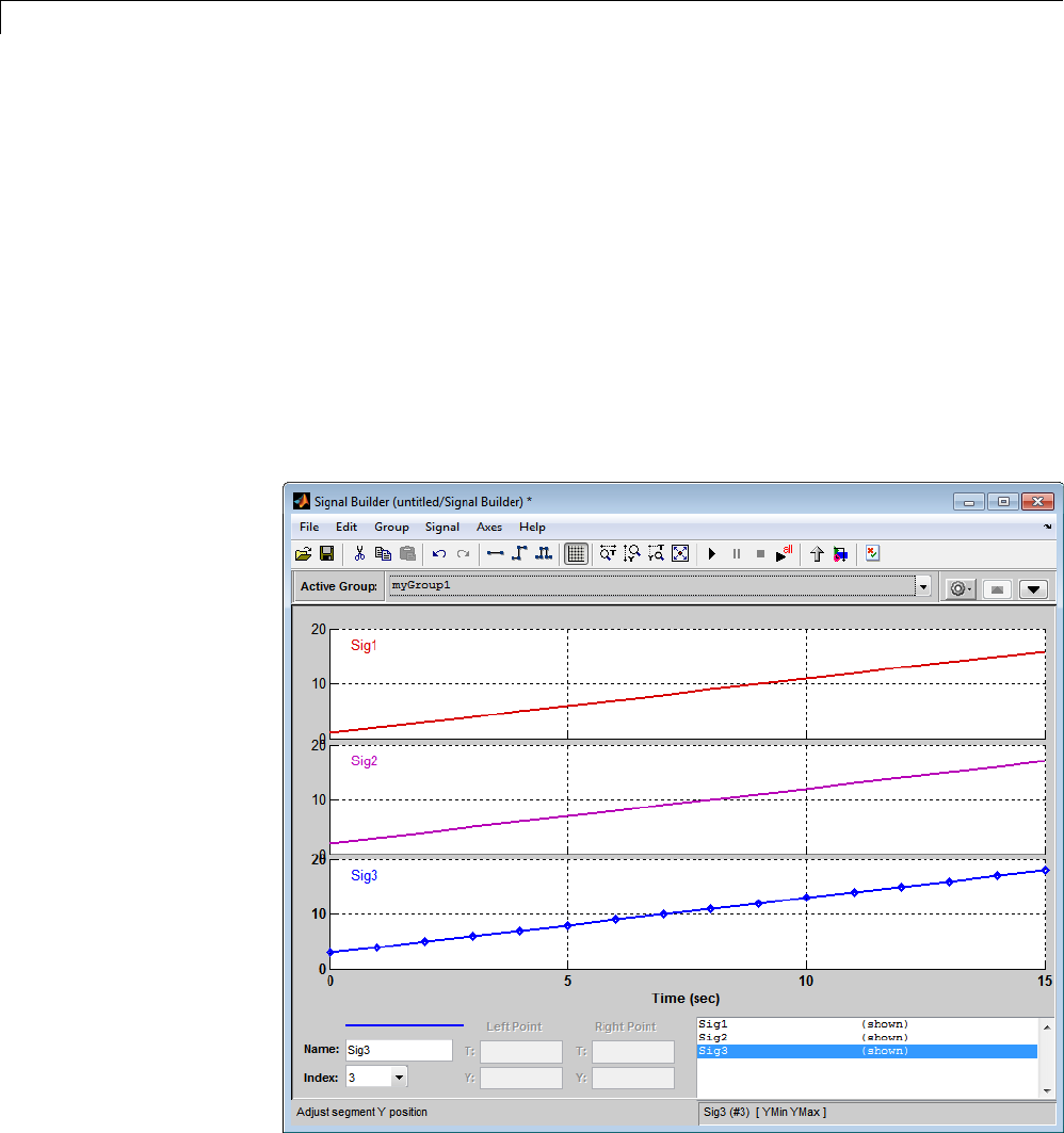
47 Working with Signals
This topic uses signalbuilder1 from the procedure in “Replacing All Signal
Data with Selected Data” on page 47-79.
1In the MATLAB Command Window, type signalbuilder1.
2Double-click the Signal Builder block.
The Signal Builder window appears.
3Note how many groups exist in the Signal Builder block, and how many
signals exist in each group. The Signal Builder block requires that all
groups have the same number of signals. For example, this Signal Builder
block has three groups, myGroup1, myGroupB, and myGroup_Three.
Three signals exist in each group.
47-96
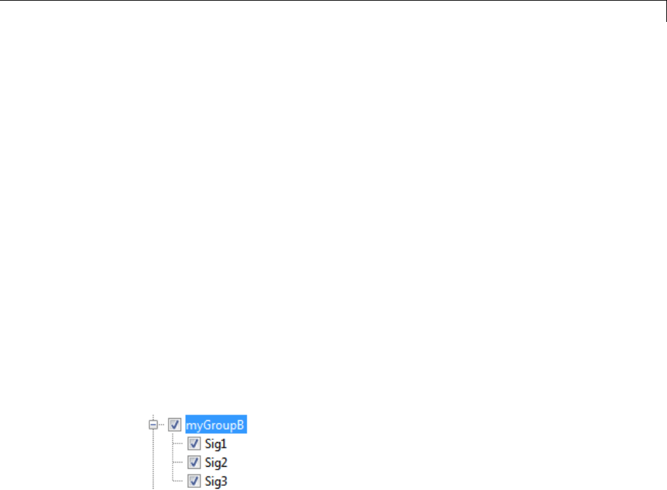
Signal Groups
4Double-click the block.
The Import File dialog box appears.
5In the File to Import text field, enter a signal data file name or click
Browse.
Thefilebrowserappears.
6If you select the file browser, navigate to and select a signal data file. For
example, select 3Grp_3Sig.xls.
The Data to Import pane contains the signal data from the file. Click the
expander to display all the signals.
7Evaluate the number of signals in the groups of this data file. If the number
of signals in each group equals the number of signals in the groups that
exist in the block, you can append one of these groups to the block.
8Select the group you want to import. In this example, there are three
groups, myGroup1, myGroupB, and myGroup_Three. Select myGroupB.
9From the Placement for Selected Data list, select the action to take on
the signal group. For example, select Append groups.
The Confirm Selection button is activated. Validate your signal selection
before the Signal Builder block performs the specified action.
10 Click the Confirm Selection button.
If the requested action is a valid one, the Status History pane displays
messagestoindicatethestate. Forexample:
47-97
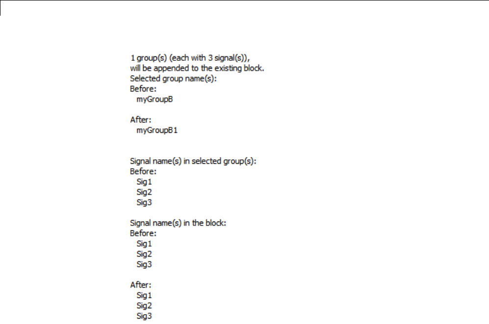
47 Working with Signals
The confirmation also enables the OK and Apply buttons.
11 If you are satisfied with the status message, click Apply to append the
signals.
The Signal Builder block updates with the new signal data. Click OK
to close the Import File dialog box and inspect the groups of the Signal
Builder block.
Notice the addition of the new signal group as the last pane. Because there
is already a signal group named myGroupB, the software automatically
increments the new signal group name by 1.
47-98
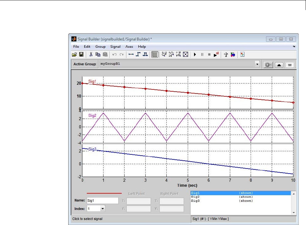
Signal Groups
12 Close the Signal Builder window and save and close the model. For
example, save the model as signalbuilder4.
Appending Signals with the Same Name to Existing Signal Groups.
If you append a signal whose name is the same as a signal that exists in
the Signal Builder block, the software increments the name of the appended
signal by 1. The software repeats incrementing until the appended signal
name is unique. For example:
1Assume your Signal Builder block has a signal group, myGroup1,withthe
signals Sig1, Sig2, and Sig3.
2Append a signal named Sig1 to myGroup1.
47-99
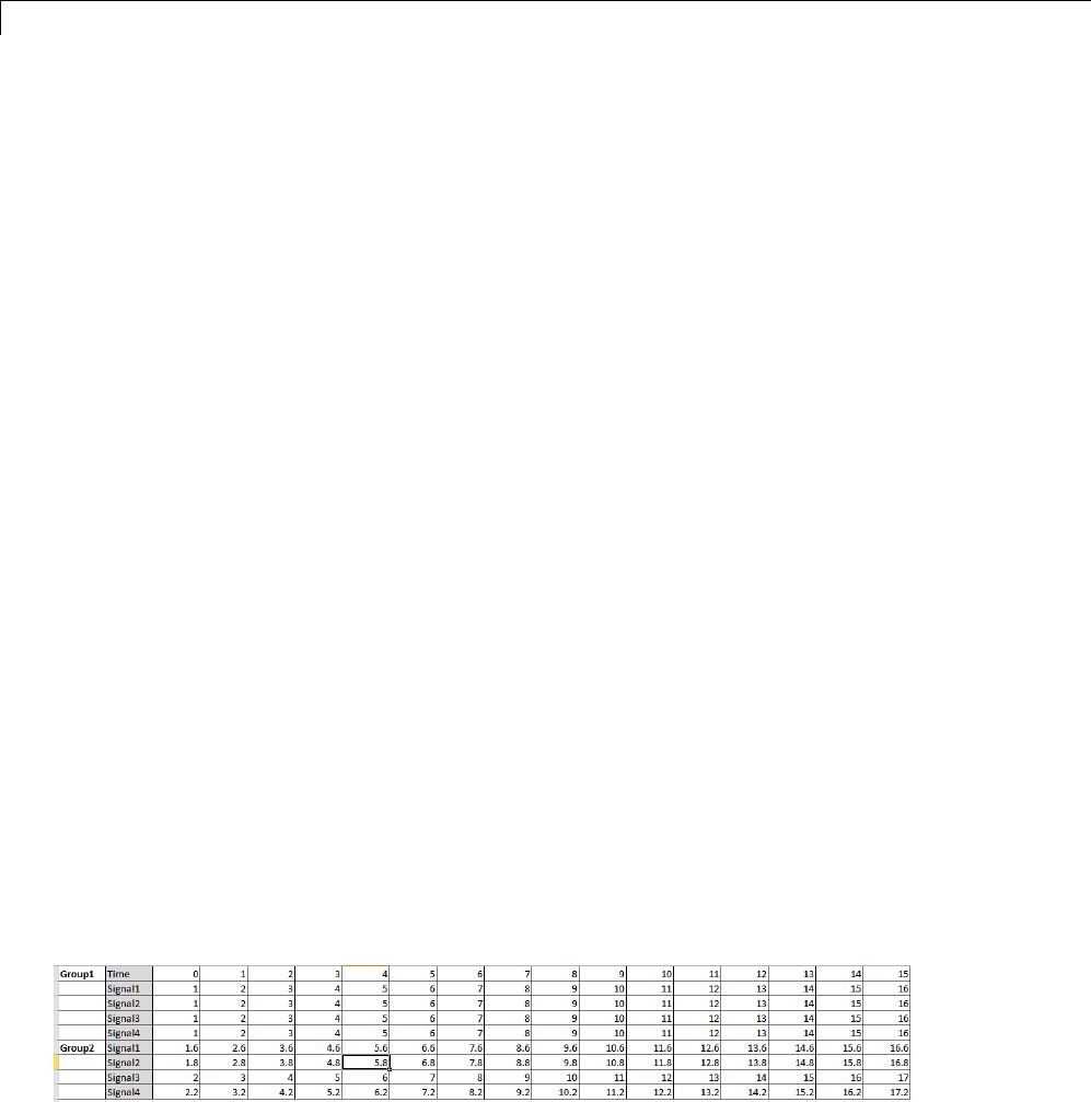
47 Working with Signals
3Observe that the software increments Sig1 to Sig4 before appending it
to myGroup1.
Appending a Group of Signals with Different Signal Names. If you
append a signal group whose signal names differ from those that exist in the
Signal Builder block, the software changes the names of the existing signals
to be the same as the appended signals. For example,
1Assume your Signal Builder block has a signal group, myGroup1,withthe
signals Sig1, Sig2, and Sig3.
2Append a signal group named myGroup2 whose signal names are SigA,
SigB, and SigC.
3Observe that the software:
•Appends myGroup2.
•Renames the signals in myGroup1 to be the same as those in myGroup2.
Importing Data with Custom Formats
This topic describes how to import signal data formatted in a custom format.
You should already have a signal data from a file whose contents you want to
import. See “Importing Signal Groups from Existing Data Sets” on page 47-74
for a description of the data formats that the Signal Builder block accepts. If
your data is not formatted using one of these data formats, use the following
workflow to import the custom formatted data. This workflow uses the
following files, located in matlabroot\help\toolbox\simulink\examples,
as examples:
•SigBldCustomFile.xls — Signal data Microsoft Excel file using a format
that Signal Builder block does not accept, for example:
•createSignalBuilderSupportedFormat.m — Custom MATLAB function
that uses xlsread to read Microsoft Excel spreadsheets. This example
47-100

Signal Groups
function reformats the custom data, in a format that the Signal Builder
block supports, as follows:
-grpNames — Cell array that contains group name strings with number of
rows = 1, number of columns = number of groups.
-sigNames — Cell array that contains signal name strings with number
of rows = 1, columns = number of signals.
-time — Cell array that contains time data with number of rows =
number of signals, columns = number of groups.
-data — Cell array that contains signal data with number of rows =
number of signals, columns = number of groups.
Signal Builder has the following requirements for this custom function:
-Number of signals in each group must be the same.
-Signal names in each group must be the same.
-Number of data points in each signal must be the same.
-Each element in the time and data cell array holds a matrix of real
numbers. This matrix can be [1xN]or[Nx1], where Nis the number of
data points in every signal.
1Identify the format of your custom signal data, for example:
SigBldCustomFile.xls
2Create a custom MATLAB function that:
aUses a MATLAB I/O function, such as xlsread,to
read your custom formatted signal data. For example,
createSignalBuilderSupportedFormat.m.
bFormats the custom formatted signal data to one that the Signal Builder
block accepts, for example, a MAT-file.
3Use your custom MATLAB function to write your custom formatted signal
data to a file that Signal Builder block accepts. For example:
createSignalBuilderSupportedFormat('SigBldCustomFile.xls', 'OutputData.mat')
47-101

47 Working with Signals
4Import the reformatted signal data file, OutputData.mat, into the Signal
Builder block (see “Importing Signal Group Sets” on page 47-74).
Editing Waveforms
The Signal Builder window allows you to change the shape, color, and line
style and thickness of the waveforms output by a group.
Reshaping a Waveform
The Signal Builder window allows you tochangethewaveformbyselecting
and dragging its line segments and points with the mouse or arrow keys or
by editing the coordinates of segments or points.
47-102
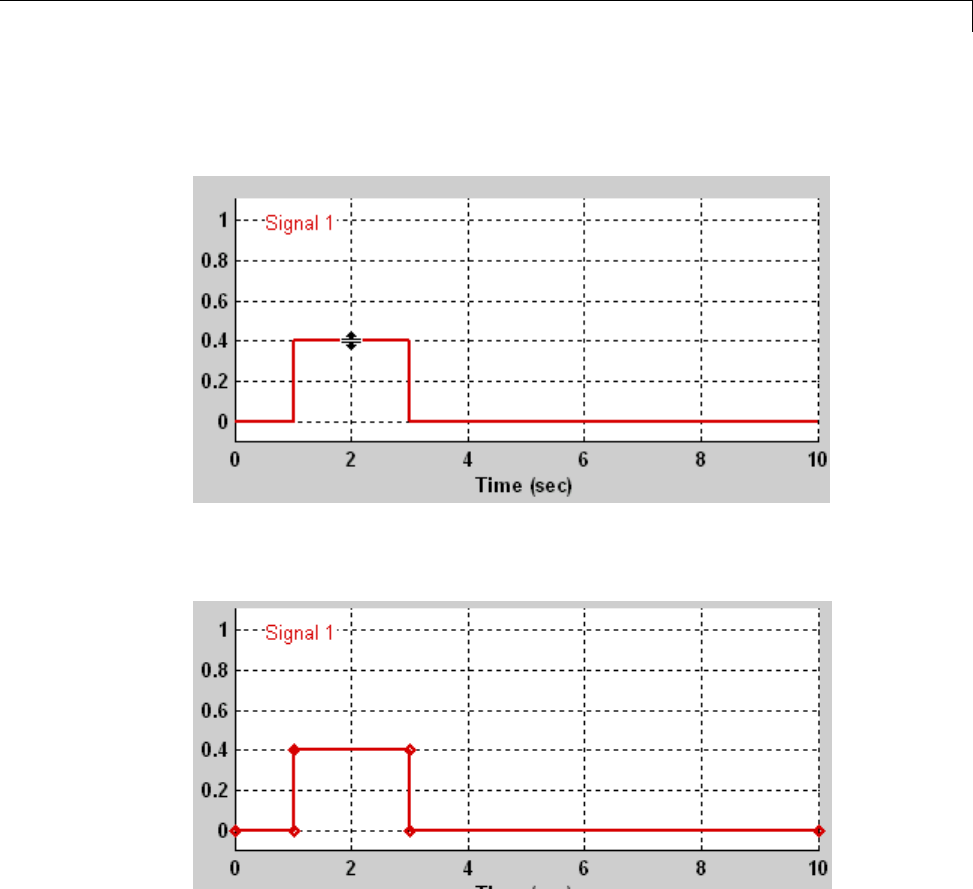
Signal Groups
Selecting a Waveform. To select a waveform, left-click the mouse on any
point on the waveform.
The Signal Builder displays the waveform points to indicate that the
waveform is selected.
To deselect a waveform, left-click any point on the waveform axis that is not
on the waveform itself or press the Esc key.
47-103
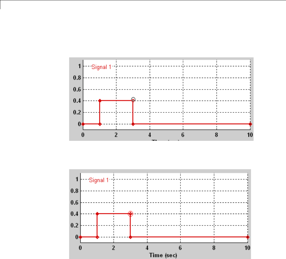
47 Working with Signals
Selecting Points. To select a point of a waveform, first select the waveform.
Then position the mouse cursor over the point. The cursor changes shape to
indicate that it is over a point.
Left-click the point with the mouse. The Signal Builder draws a circle around
the point to indicate your selection.
To deselect the point, press the Esc key.
47-104
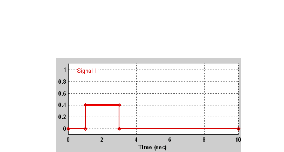
Signal Groups
Selecting Segments. To select a line segment, first select the waveform that
contains it. Then left-click the segment. The Signal Builder thickens the
segment to indicate that it is selected.
To deselect the segment, press the Esc key.
Moving Waveforms. To move a waveform, select it and use the arrow keys
on your keyboard to move the waveform in the desired direction. Each key
stroke moves the waveform to the next location on the snap grid (see “Snap
Grid” on page 47-106) or by 0.1 inches if the snap grid is not enabled.
47-105
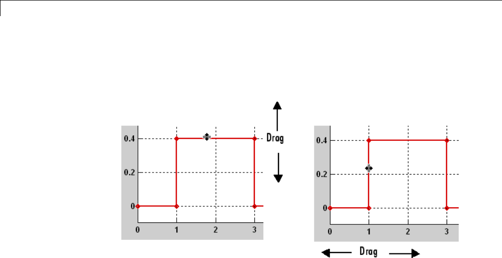
47 Working with Signals
Dragging Segments. To drag a line segment to a new location, position the
mouse cursor over the line segment. The mouse cursor changes shape to show
the direction in which you can drag the segment.
Press the left mouse button and drag the segment in the direction indicated
to the desired location. You can also use the arrow keys on your keyboard
to move the selected line segment.
Dragging points. To drag a point along the signal amplitude (vertical) axis,
move the mouse cursor over the point. The cursor changes shape to a circle to
indicate that you can drag the point. Drag the point parallel to the y-axis to
the desired location. To drag the point alongthetime(horizontal)axis,press
the Shift keywhiledraggingthepoint. Youcanalsousethearrowkeyson
your keyboard to move the selected point.
Snap Grid. Each waveform axis contains an invisible snap grid that
facilitates precise positioning of waveform points. The origin of the snap grid
coincides with the origin of the waveform axis. When you drop a point or
segment that you have been dragging, the Signal Builder moves the point or
the segment points to the nearest point or points on the grid, respectively.
The Signal Builder Axes menu allows you to specify the grid horizontal
(time) axis and vertical (amplitude) axis spacing independently. The finer the
spacing, the more freedom you have in placing points but the harder it is to
position points precisely. By default, the grid spacing is 0, which means that
you can place points anywhere on the grid; i.e., the grid is effectively off. Use
the Axes menu to select the spacing that you prefer.
47-106

Signal Groups
Inserting and Deleting points. To insert a point, first select the waveform.
Then hold down the Shift key and left-click the waveform at the point where
youwanttoinsertthepoint. Todeleteapoint,selectthepointandpress
the Del key.
Editing Point Coordinates. To change the coordinates of a point, first select
the point. The Signal Builder displays the current coordinates of the point
in the Left Point edit fields at the bottom of the Signal Builder window. To
change the amplitude of the selected point, edit or replace the value in the
Yfield with the new value and press Enter.TheSignalBuildermovesthe
point to its new location. Similarly edit the value in the Tfield to change
thetimeoftheselectedpoint.
Editing Segment Coordinates. To change the coordinates of a segment,
first select the segment. The Signal Builder displays the current coordinates
of the endpoints of the segment in the Left Point and Right Point edit fields
at the bottom of the Signal Builder window. To change a coordinate, edit the
value in its corresponding edit field and press Enter.
Changing the Color of a Waveform
To change the color of a waveform, select the waveform and then select Color
from the Signal Builder Signal menu. The Signal Builder displays the
MATLAB color chooser. Choose a new color for the waveform. Click OK.
Changing a Waveform Line Style and Thickness
The Signal Builder can display a waveform as a solid, dashed, or dotted line.
It uses a solid line by default. To change the line style of a waveform, select
the waveform, then select Line Style from the Signal Builder Signal menu.
A menu of line styles pops up. Select a line style from the menu.
Tochangethelinethicknessofawaveform, select the waveform, then select
Line Width from the Signal menu. A dialog box appears with the line
current thickness. Edit the thickness value and click OK.
47-107
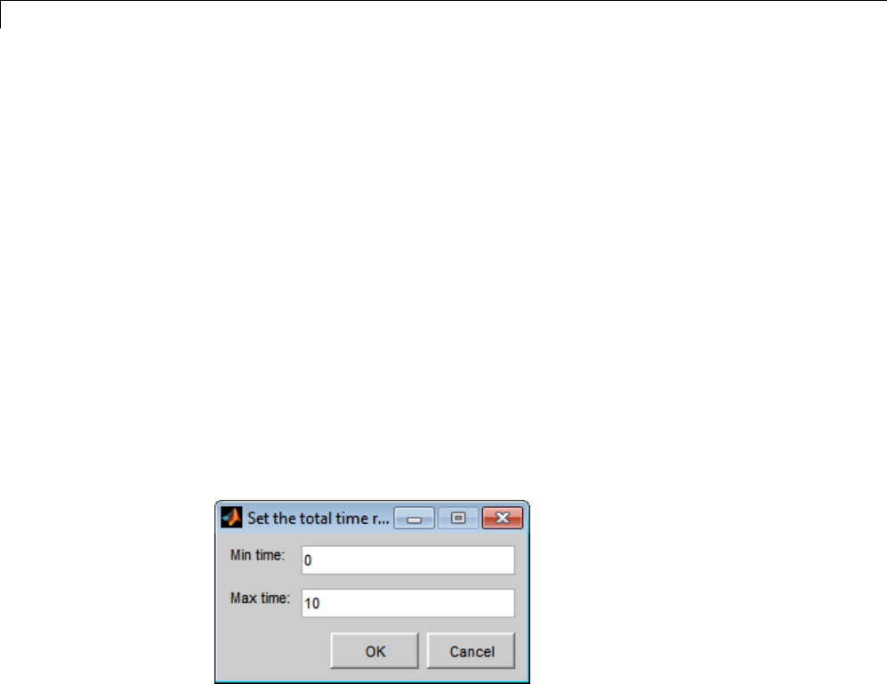
47 Working with Signals
Signal Builder Time Range
The Signal Builder time range determines the span of time over which its
output is explicitly defined. By default, the time range runs from 0 to 10
seconds. You can change both the beginning and ending times of a block time
range(see“Cha
nging a Signal Builder Time Range” on page 47-108).
If the simulation starts before the start time of a block time range, the
block extrapolates its initial output from its first two defined outputs. If the
simulation runs beyond the block time range, the block by default outputs
values extrapolated from the last defined signal values for the remainder of
the simulation. The Signal Builder Simulation Options dialog box allows
you to specify other final output options (see “Signal values after final time”
on page 47-111 for more information).
Changing a Signal Builder Time Range
To change the time range, select Change Time Range from the Signal
Builder Axes menu. A dialog box appears.
Edit the Min time and Max time fields as necessary to reflect the beginning
and ending times of the new time range, respectively. Click OK.
47-108
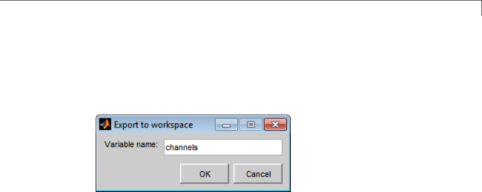
Signal Groups
Exporting SignalGroupData
To export the data that define a Signal Builder block signal groups to the
MATLAB workspace, select Export to Workspace from the block File
menu. A dialog box appears.
The Signal Builder exports the data by default to a workspace variable named
channels.Toexporttoadifferentlynamedvariable,enterthevariablename
in the Variable name field. Click OK. The Signal Builder exports the data to
the workspace as the value of the specified variable.
The exported data is an array of structures. The structure xData and yData
fields contain the coordinate points defining signals in the currently selected
signal group. You can access the coordinate values defining signals associated
with other signal groups from the structure allXData and allYData fields.
Printing, Exporting, and Copying Waveforms
The Signal Builder window allows you to print, export, and copy the
waveforms visible in the active signal group.
To print the waveforms to a printer, select Print from the block File menu.
You can also export the waveforms to other destinations by using the Export
option from the block File menu. From this submenu, select one of the
following destinations:
•To File — Converts the current view to a graphics file.
Select the format of the graphics file from the Save as type drop-down list
on the resulting Export dialog box.
•To Figure — Converts the current view to a MATLAB figure window.
47-109

47 Working with Signals
To copy the waveforms to the system clipboard for pasting into other
applications, select Copy Figure To Clipboard from the block Edit menu.
Simulating with Signal Groups
You can use standard simulation commands to run models containing Signal
Builder blocks or you can use the Run or Run all command in the Signal
Builder window (see “Running All Signal Groups” on page 47-110).
If you want to capture inputs and outputs that the Run all command
generates, consider using the SystemTest™ software.
Activating a Signal Group
During a simulation, a Signal Builder block always outputs the active signal
group. Theactivesignalgroupisthegroup selected in the Signal Builder
window for that block, if the dialog box is open. Otherwise, the active group is
the group that was selected when the dialog box was last closed. To activate a
group, open the group Signal Builder window and select the group.
Running Different Signal Groups in Succession
The Signal Builder toolbar includes the standard Simulink buttons for
running a simulation. This facilitates running several different signal groups
in succession. For example, you can open the dialog box, select a group, run a
simulation, select another group, run a simulation, etc., all from the Signal
Builder window.
Running All Signal Groups
To run all the signal groups defined by a Signal Builder block, open the block
dialog box and click the Run all button
from the Signal Builder toolbar. The Run all command runs a series of
simulations, one for each signal group defined by the block. If you installed
Simulink Verification and Validation on your system and are using the Model
Coverage Tool, the Run all command configures the tool to collect and save
coverage data for each simulation in the MATLAB workspace and display a
47-110
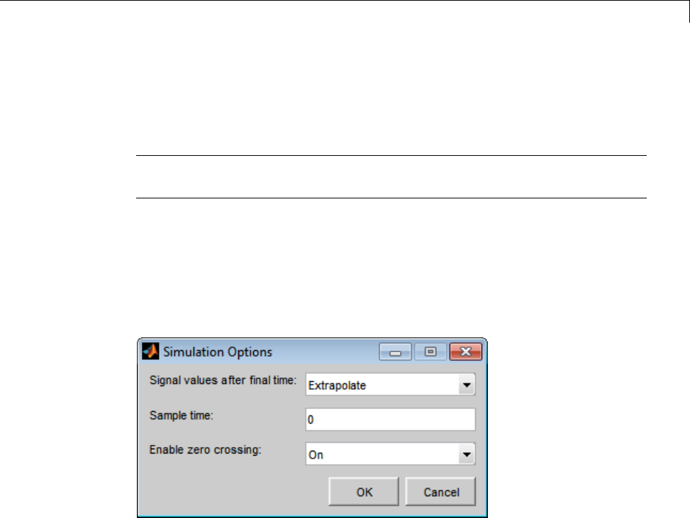
Signal Groups
report of the combined coverage results at the end of the last simulation.
This allows you to quickly determine how well a set of signal groups tests
your model.
Note To stop a series of simulations started by the Run all command, enter
Ctrl+C at the MATLAB command line.
Simulation Options Dialog Box
The Simulation Options dialog box allows you to specify simulation options
pertaining to the Signal Builder. To display the dialog box, select Simulation
Options from the File menu of the Signal Builder window. The dialog box
appears.
The dialog box allows you to specify the following options.
Signal values after final time
The setting of this control determines the output of the Signal Builder block if
asim
ulation runs longer than the period defined by the block. The options are
•Hold final value
47-111
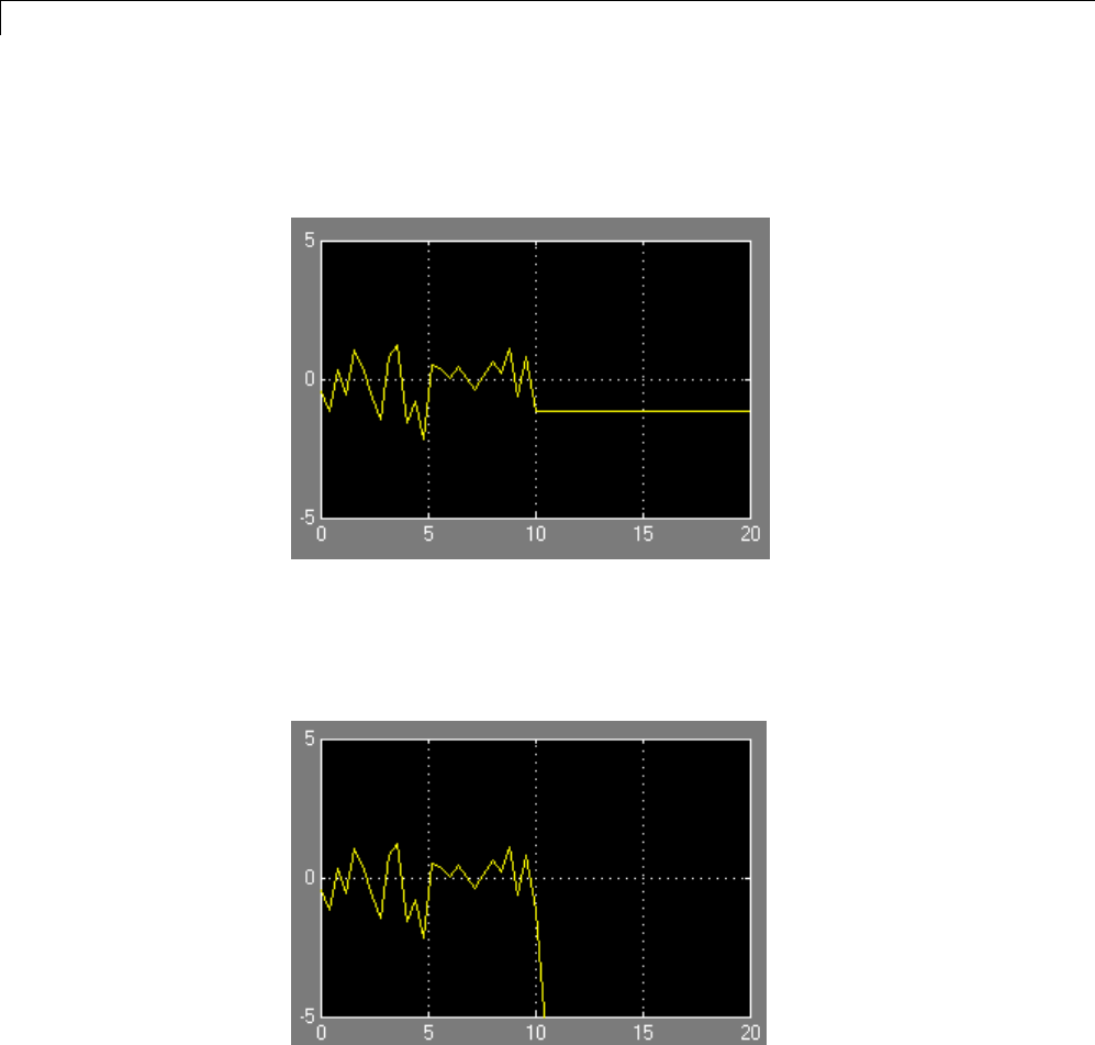
47 Working with Signals
Selecting this option causes the Signal Builder block to output the last
defined value of each signal in the currently active group for the remainder
of the simulation.
•Extrapolate
Selecting this option causes the Signal Builder block to output values
extrapolated from the last defined value of each signal in the currently
active group for the remainder of the simulation.
•Set to zero
47-112

Signal Groups
Selecting this option causes the Signal Builder block to output zero for the
remainder of the simulation.
Sample time
Determines whether the Signal Builder block outputs a continuous (the
default) or a discrete signal. If you want the block to output a continuous
signal, enter 0 in this field. For example, the following display shows
the output of a Signal Builder block set to output a continuous Gaussian
waveform over a period of 10 seconds.
47-113
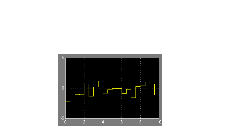
47 Working with Signals
Ifyouwanttheblocktooutputadiscretesignal,enterthesampletimeof
the signal in this field. The following example shows the output of a Signal
Builder block set to emit a discrete Gaussian waveform having a 0.5 second
sample time.
Enable zero crossing
Specifies whether the Signal Builder block detects zero-crossing events
(enabled by default). For more information, see “Zero-Crossing Detection”
on page 3-23.
47-114

48
Using Composite Signals
•“About Composite Signals” on page 48-2
•“Virtual and Nonvirtual Buses” on page 48-10
•“Create and Access a Bus” on page 48-15
•“Nest Buses” on page 48-17
•“Bus-Capable Blocks” on page 48-19
•“Bus Objects” on page 48-20
•“Bus Object API” on page 48-23
•“Manage Bus Objects with the Bus Editor” on page 48-24
•“Store and Load Bus Objects” on page 48-46
•“Map Bus Objects to Models” on page 48-48
•“Filter Displayed Bus Objects” on page 48-49
•“Customize Bus Object Import and Export” on page 48-55
•“Connect Buses to Inports and Outports” on page 48-61
•“Specify Initial Conditions for Bus Signals” on page 48-65
•“Combine Buses into an Array of Buses” on page 48-77
•“Bus Data Crossing Model Reference Boundaries” on page 48-93
•“Buses and Libraries” on page 48-94
•“Avoid Mux/Bus Mixtures” on page 48-95
•“Buses in Generated Code” on page 48-105
•“Composite Signal Limitations” on page 48-106

48 Using Composite Signals
About Composite Signals
In this section...
“Composite Signal Terminology” on page 48-2
“Types of Simulink Buses” on page 48-3
“View Information about Buses” on page 48-3
“Buses and Muxes” on page 48-7
“Bus Objects” on page 48-8
“Bus Code” on page 48-8
Composite Signal Terminology
Acomposite signal is a signal that is composed of other signals. The
constituent signals originate separately and join to form the composite signal.
They can then be extracted from the composite signal downstream and
used as if they had never been joined. Composite signals can reduce visual
complexity in models by grouping signals that run in parallel over some or all
of their courses, and can serve various other purposes.
A Simulink composite signal is called a bus signal,orjustabus.ASimulink
bus is analogous to a bundle of wires held together by tie wraps. Simulink
implementsabusasaname-basedhierarchical structure. A Simulink bus
should not be confused with a hardware bus, like the bus in the backplane
of many computers. It is more like a programmatic structure defined in a
language like C.
The signals that constitute a bus are called elements. The constituent signals
retain their separate identities within the bus and can be of any type or types,
including other buses nested to any level. The elements of a bus can be any
of the following:
•Mixed data type signals (e.g. double, integer, fixed point)
•Mixture of scalar and vector elements
•Busesaselements
•N-D signals
48-2

About Composite Signals
•Mixture of Real and Complex signals
Some requirements and limitations apply when you connect buses to blocks or
to nonvirtual subsystems. See “Bus-Capable Blocks” on page 48-19, “Connect
Buses to Inports and Outports” on page 48-61, and “Composite Signal
Limitations” on page 48-106 for more information.
TypesofSimulinkBuses
A bus can be either virtual or nonvirtual. Both virtual and nonvirtual
buses provide the same visual simplification, but their implementations are
different.
•Virtual buses exist only graphically. They have no functional effects and
do not appear in generated code; only the constituent signals appear. See
“Virtual Signals” on page 47-11 for details. Simulink implements virtual
buses with pointers, so virtual buses add no data copying overhead and
do not affect performance.
•Nonvirtual buses may have functional effects. They appear as structures in
generated code, which can simplify the code and clarify its correspondence
with the model. Simulink implements nonvirtual buses by copying data
from the source signals to the bus, which can affect performance.
The two types of buses are interchangeable for many purposes, but some
situations require a nonvirtual bus. See “Virtual and Nonvirtual Buses” on
page 48-10 for more information.
View Information about Buses
To view information about buses, use one of the following approaches:
•Use the Signal Hierarchy Viewer to interactively display bus hierarchy
(for bus signals)
•FromtheMATLABcommandline,displaythetypeandhierarchyofa
bus signal in a compiled model. For details, see “CompiledBusType and
SignalHierarchy Parameters” on page 48-6.
48-3
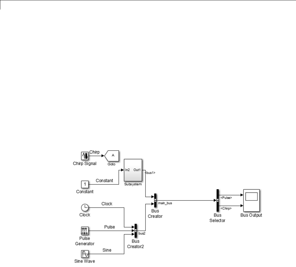
48 Using Composite Signals
Signal Hierarchy Viewer
Use the Signal Hierarchy Viewer to interactively display information about
a signal. For a bus signal, the Signal Hierarchy Viewer displays the bus
hierarchy.
1Check that the Configuration Parameters > Diagnostics >
Connectivity > Mux blocks used to create bus signals parameter
is set to error.
2Right-click a signal line.
3Select the Signal Hierarchy option. The Signal Hierarchy Viewer dialog
box appears.
For example, open the busdemo model.
Right-click the main_bus signal (output signal for the Bus Creator block), and
select Signal Hierarchy. The following information appears:
48-4
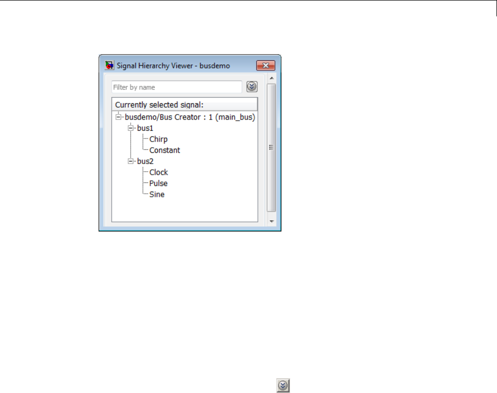
About Composite Signals
Each Signal Hierarchy Viewer is associated with a specific model. If you edit
a model while the associated Signal Hierarchy Viewer is open, the Signal
Hierarchy Viewer reflects those updates.
You can also open the Signal Hierarchy Viewer in the Simulink Model Editor.
1Select View > Signal Hierarchy.
2Select a signal
To filter the displayed signals, click the Options button on the right-hand
side of the Filter by name edit box ( ).
•To use MATLAB regular expressions for filtering signal names, select
Enable regular expression. For example, entering r$ in the Filter by
name edit box displays all signals whose names end with a lowercase r
(and their immediate parents). For details, see “Regular Expressions”.
•To use a flat list format to display the list of filtered signals, based on the
search text in the Filter by name edit box, select Show filtered results
as a flat list. The flat list format uses dot notation to reflect the hierarchy
of bus signals. The following is an example of a flat list format for a filtered
set of nested bus signals.
48-5
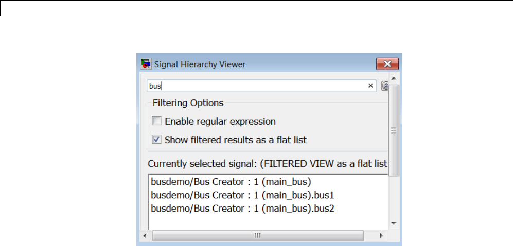
48 Using Composite Signals
CompiledBusType and SignalHierarchy Parameters
To get information about the type and hierarchy of a bus signal in a compiled
model, use these parameters with the get_param command:
•CompiledBusType — For a compiled model, returns information about
whether the signal connected to a port is a bus, and if so, whether the
signal is a virtual or nonvirtual bus.
•SignalHierarchy — If the signal is a bus, returns the name and hierarchy
of the signals in the bus.
Before you use these commands:
1In the Configuration Parameters > Diagnostics > Connectivity
pane, set the Mux blocks used to create bus signals diagnostic to error.
2Update the diagram or simulate the model.
For example, if you open and simulate the busdemo model, the model looks
as shown below:
48-6
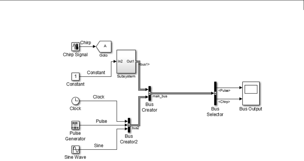
About Composite Signals
The following code illustrates how you can use the SignalHierarchy and
CompiledBusType parameters:
mdl = 'busdemo';
open_system(mdl)
% Obtain the handle a port
ph = get_param([mdl '/Bus Creator'], 'PortHandles');
% SignalHierarchy is available at edit time
sh = get_param(ph.Outport, 'SignalHierarchy')
% Compile the model
busdemo([],[],[],'compile');
bt = get_param(ph.Outport, 'CompiledBusType')
% Terminate the model
busdemo([],[],[],'term');
BusesandMuxes
If allsignalsinabusarethesametype,youmaybeabletouseacontiguous
vectororavirtualvector(mux)instead of a bus. For more information, see
“Mux Signals” on page 47-11. In some cases, muxes and virtual buses can be
treated interchangeably; implicit type conversion occurs when needed.
48-7

48 Using Composite Signals
Do not mix muxes and buses in new applications.
One way that such a mux/bus mixture occurs is when you use a Mux block
to create a virtual bus, such as a Mux block that outputs to a Bus Selector.
This kind of mixture does not support strong type checking and increases
the likelihood of run-time errors. MathWorks discourages treating muxes
and buses interchangeably. Mux/bus mixtures may become unsupported
in the future. Simulink generates a warning for this kind of mux/bus
mixture when you load a model created in a release prior to R2010a. For
new models, Simulink generates an error. Do not create such mux/bus
mixtures in new applications, and consider upgrading existing applications
to avoid such mixtures. The Configuration Parameters > Diagnostics
> Connectivity pane provides diagnostics that report cases where muxes
and virtual buses are used interchangeably, and includes capabilities that you
can use to upgrade a model to eliminate such mixtures. See “Avoid Mux/Bus
Mixtures” on page 48-95 for details.
Another way for a mux/bus mixture to occur is when a virtual bus signal is
treated as a mux, such as a bus signal that inputs directly to a Gain block. To
detect such mixtures, in the Configuration Parameters > Diagnostics
> Connectivity pane, set the Bus signal treated as vector diagnostic
to warning or error.
Bus Objects
Abuscanhaveanassociatedbus object, which can both provide and validate
bus properties. A bus object is an instance of class Simulink.Bus that is
defined in the base workspace. The object defines the structure of the bus
and the properties of its elements, such as nesting, data type, and size. Bus
objects are optional for virtual buses and required for nonvirtual buses. See
“Bus Objects” on page 48-20 for more information. You can create bus objects
programmatically or by using the Simulink Bus Editor, which facilitates bus
object creation and management. See “Manage Bus Objects with the Bus
Editor” on page 48-24 for more information.
Bus Code
The various techniques for defining buses are essentially equivalent for
simulation, but the techniques used can make a significant difference in the
efficiency, size, and readability of generated code. If you intend to generate
48-8

About Composite Signals
production code for a model that uses buses, see “Buses” for information about
the best techniques to use.
48-9

48 Using Composite Signals
Virtual and Nonvirtual Buses
In this section...
“Virtual and Nonvirtual Buses” on page 48-10
“Choosing Between Virtual and Nonvirtual Buses” on page 48-11
“Creating Nonvirtual Buses” on page 48-12
“Nonvirtual Bus Sample Times” on page 48-13
“Automatic Bus Conversion” on page 48-13
“Explicit Bus Conversion” on page 48-13
Virtual and Nonvirtual Buses
Abussignalcanbevirtual, meaning that it is just a graphical convenience
that has no functional effect, or nonvirtual, meaning that the signal occupies
its own storage.
Bus Storage
During simulation:
•A block connected to a virtual bus reads inputs and writes outputs by
accessing the memory allocated to the component signals. These signals
are typically noncontiguous, and no intermediate memory exists.
•A block connected to a nonvirtual bus reads inputs and writes outputs by
accessing copies of the component signals. The copies are maintained in a
contiguous area of memory allocated to the bus.
Compared with nonvirtual buses, virtual buses reduce memory requirements
because they do not require a separate contiguous storage block, and execute
faster because they do not require copying data to and from that block.
A nonvirtual bus is represented by a structure in generated code, which can
be helpful when tracing the correspondence between the model and the code.
48-10
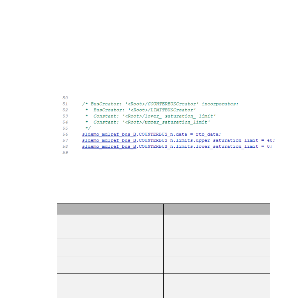
Virtual and Nonvirtual Buses
Simulation Results and Generated Code
For a virtual bus, simulation results and generated code are exactly the same
as if the bus did not exist, which functionally it does not.
Generated code for a nonvirtual busrepresentsthebusdatawithastructure.
The use of a structure in the generated code can be helpful when tracing the
correspondence between the model and the code. For example, below is the
generated code for Bus Creator block in the sldemo_mdlref_bus model.
Choosing Between Virtual and Nonvirtual Buses
Whether to use a virtual or nonvirtual bus depends on your modeling goal.
Frequently, model contain both virtual and nonvirtual buses.
Modeling Goal Type of Bus
Use bus signals within a functional
units, such as within a referenced
model
Virtual
Use signals with different sample
rates in a bus
Virtual (required)
Have bus data packaged as data
structures in the generated code
Nonvirtual
Have bus data cross model reference,
MATLAB Function block, or
Stateflow chart boundaries
Nonvirtual
48-11

48 Using Composite Signals
Not all blocks can accept buses. See “Bus-Capable Blocks” on page 48-19 for
more about which blocks can handle which types of buses. Virtual buses
are the default except where nonvirtual buses are explicitly required. See
“Connect Buses to Inports and Outports” on page 48-61 for more information.
For additional guidelines for generated code for buses, see “About Buses and
Code Generation”.
Creating Nonvirtual Buses
Bus signals do not specify whether they are virtual or nonvirtual; they inherit
that specification from the block in which they originate. Every block that
creates or requires a nonvirtual bus must have an associated bus object.
Those blocks are:
•Bus Creator
•Inport
•Outport
•Constant
•Data Store Memory
Tospecifythatabusisnonvirtual:
1Associate the block with a bus object, as described in “Associating Bus
Objects with Simulink Blocks” on page 48-21.
2For the block that creates the bus, open the Block Parameters dialog box.
3Set Data type to Bus: <object name> and replace <object name> with
the bus object name.
4For any Bus Creator, Inport, or Outport blocks that have an associated bus
object, enable the Enable output as nonvirtual bus parameter.
5Click OK or Apply.
The Signal Attributes parameter is applicable only to root Inport and
Outport blocks, and does not appear in the parameters of a subsystem
Inport or Outport block. In a root Outport block, setting Signal Attributes
48-12

Virtual and Nonvirtual Buses
> Output as nonvirtual bus in parent model specifies that the bus
emerging in the parent model is nonvirtual. The bus that is input to the root
Outport can be virtual or nonvirtual.
Nonvirtual Bus Sample Times
All signals in a nonvirtual bus must have the same sample time, even if the
elements of the associated bus object specify inherited sample times. Any bus
operation that would result in a nonvirtual bus that violates this requirement
generates an error.
All buses and signals input to a Bus Creator block that outputs a nonvirtual
bus must therefore have the same sample time. You can use a Rate Transition
block to change the sample time of an individual signal, or of all signals in a
bus, to allow the signal or bus to be included in a nonvirtual bus.
Automatic Bus Conversion
When updating a diagram prior to simulation or code generation, the Simulink
software automatically converts virtual buses to nonvirtual buses where the
conversion is possible and prevents an error. For example, referenced models
and Stateflow charts require any bus connected to them to be nonvirtual.
The conversion consists of inserting hidden Signal Conversion blocks into the
model where needed.
The source block of any virtual bus that is converted to a nonvirtual bus,
whether explicitly or automatically, must specify a bus object, as described
in “Bus Objects” on page 48-20. Conversion to a nonvirtual bus fails if no
busobjectisspecified,andtheSimulink software posts an error message
describing the problem.
Explicit Bus Conversion
You can eliminate the need for the automatic conversion by using one of these
approaches:
•Specify a nonvirtual bus in the block where the bus originates. For
example, if you use a Bus Creator block to create a bus, then to specify a
48-13

48 Using Composite Signals
nonvirtual bus, set the Bus Creator block Data type parameter to use a
Simulink.Bus object.
•Manually insert a Signal Conversion block. Using a Signal Conversion
block can reduce memory usage, support modeling constructs such as
Model blocks that require that input buses be nonvirtual, and reduce
generated code. For details, see the Signal Conversion documentation.
48-14
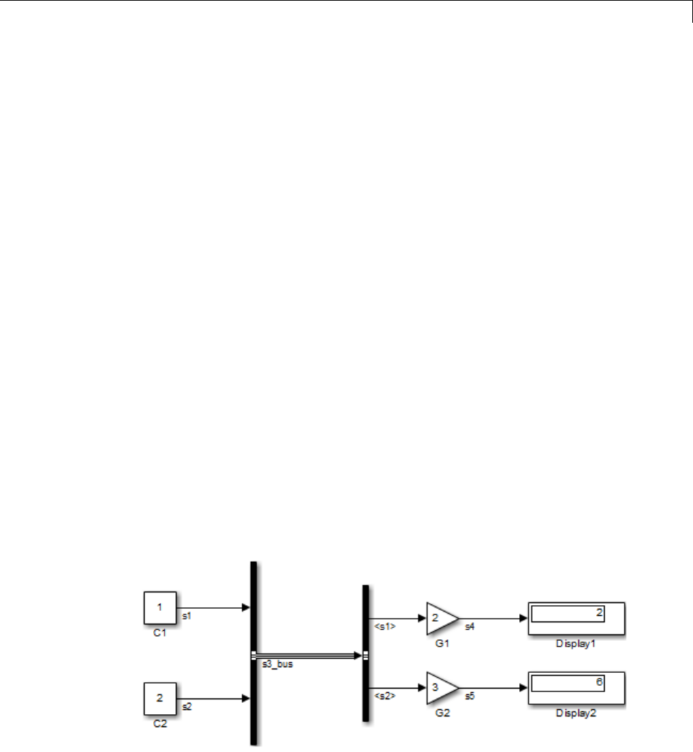
Create and Access a Bus
Create and Access a Bus
The Signal Routing library provides three blocks that you can use for
implementing buses:
Bus Creator
Create a bus that contains specified elements
Bus Assignment
Replace specified bus elements
Bus Selector
Select elements from a bus
Each of these blocks is virtual or nonvirtual depending on whether the bus
that it processes is virtual or nonvirtual. The Simulink software chooses the
block type, and changes it automatically if the bus type changes.
To create and access a bus signal that has default properties:
1Clone a Bus Creator and Bus Selector block from the Signal Routing library.
2Connect the Bus Creator, Bus Selector, and other blocks as needed to
implement the desired bus.
The next figure shows two signals (s1 and s2)thatareinputtoaBusCreator
block, transmitted as a bus signal (s3_bus) to a Bus Selector block, and
output as separate signals.
48-15
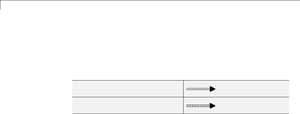
48 Using Composite Signals
The Bus Creator and Bus Selector blocks are the left and right vertical bars,
respectively. Consistent with the goal of reducing visual complexity, neither
block displays a name. The line connecting the blocks (s3_bus), representing
the bus signal, is tripled because the model has been built, and the middle
line is solid because the bus is virtual. The line would be dashed if the bus
were nonvirtual:
Virtual Bus
Nonvirtual Bus
See “Signal Line Styles” on page 47-4 for more about the graphical appearance
of signals. You can also display other signal characteristics graphically, as
described under “Display Signal Attributes” on page 47-61.
Simulink automatically labels the output signals of the Bus Selector block
to reflect the name of the selected bus elements (for example, in the above
model, s1 and s2).
For more information about creating and accessing buses, see the reference
documentation for the Bus Creator, Bus Selector, and Bus Assignment blocks.
48-16
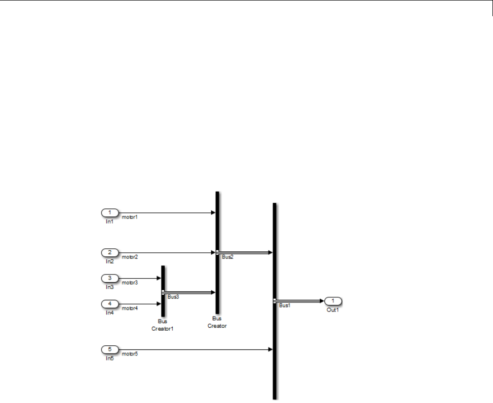
Nest Buses
Nest Buses
You can nest buses to any depth. To create a nested bus, use a Bus Creator
block. If one of the inputs to the Bus Creator block is a bus, then the output is
a nested bus. To select a signal within a nested bus, use a Bus Selector block.
For example, in the next model, the Bus3 bussignalcombinestwosignals,
motor3 and motor4.TheBus2 signal combines the Bus3 bus signal and the
motor1 and motor2 signals. The Bus1 signal combines the Bus2 bus signal
and the motor5 signal.
All of the signals retain their separate identities, just as if no bus creation
and selection occurred. You can use Bus Selector blocks to select individual
signals from a nested bus.
The Simulink software automatically handles most of the complexities
involved. For example, you can specify to have Simulink repair broken
selections in the Bus Selector and Bus Assignment block parameter dialog
boxes due to upstream bus hierarchy changes. To enable these automatic
repairs, in theConfiguration Parameters > Diagnostics > Connectivity
48-17

48 Using Composite Signals
pane, set the Repair bus selections diagnostic to Warn and repair.The
repairs occur when you update a model. Tosavetherepairs,savethemodel.
Circular Bus Definitions
The ability to nest a bus as an element of another bus creates the possibility of
a loop of Bus Creator blocks, Bus Selector blocks, and bus-capable blocks that
inadvertently includes a bus as an element of itself. The resulting circular
definition cannot be resolved and therefore causes an error.
The error message that appears specifies the location at which the Simulink
software determined that the circular structure exists. The error is not really
at any one location: the structure as a whole is in error. Nonetheless, the
location cited in the error message can be useful for beginning to trace the
definition cycle; its structure may not be obvious on visual inspection.
1Begin by selecting a signal line associated with the location cited in the
error message.
2Choose Highlight to Signal to Source or Highlight Signal to
Destination from the signal’s context menu. (See “Display Signal Sources
and Destinations” on page 47-41 for more information.)
3Continue choosing signals and highlighting their sources and destinations
until the cycle becomes clear.
4Restructure the model as needed to eliminate the circular bus definition.
Because the problem is a circular definition rather than a circular
computation, the cycle cannot be broken by inserting additional blocks, in the
way that an algebraic loop can be broken by inserting a Unit Delay block.
No alternative exists but to restructurethemodeltoeliminatethecircular
bus definition.
48-18

Bus-Capable Blocks
Bus-Capable Blocks
Buses are not intended to support computation performed directly on the bus.
Therefore, only a small subset of blocks, called bus-capable blocks,canprocess
buses directly. All virtual blocks are bus-capable. The following nonvirtual
blocks are also bus-capable:
•Memory
•Merge
•Multiport Switch
•Rate Transition
•Switch
•Unit Delay
•Zero-Order Hold
All signals in a nonvirtual bus input to a bus-capable block must have the
same sample time, even if the elements of the associated bus object specify
inherited sample times. You can use a Rate Transition block to change the
sample time of an individual signal, or of all signals in a bus.
Some bus-capable blocks impose other constraints on bus propagation through
them. See the documentation for specific blocks for more information.
You can sometimes connect a virtual bus to a block that is not bus-capable
without generating an error, but such a connection intermixes buses and
muxes, which MathWorks discourages. See “Avoid Mux/Bus Mixtures” on
page 48-95 for details.
48-19

48 Using Composite Signals
Bus Objects
In this section...
“About Bus Objects” on page 48-20
“Bus Object Capabilities” on page 48-21
“Associating Bus Objects with Simulink Blocks” on page 48-21
About Bus Objects
The properties that you specify for a bus signal by using Bus Creator block
parameters are inherited by all downstream blocks that use the bus. Using
Bus Creator block parameters is adequate for defining virtual buses and
performing limited error checking. However, to define a nonvirtual bus, or
to perform complete error checking on any bus, use a bus object to specify
additional information.
Creating a bus object establishes a composite data type whose name is the
name of the bus object and whose properties are given by the object. A bus
object specifies only the architectural properties of a bus, as distinct from
the values of the signals it contains. For example, a bus object can specify
the number of elements in a bus, the order of those elements, whether and
how elements are nested, and the data types of constituent signals; but not
the signal values.
A bus object is analogous to a structure definition in C: it defines the members
of the bus but does not create a bus. A bus object is an instance of class
Simulink.Bus that is defined in the base workspace. A bus object serves as
the root of an ordered hierarchy of bus elements, which are instances of class
Simulink.BusElement. Each element completely specifies the properties of
one signal in a bus: its name, data type, dimensionality, etc. The order of the
elements contained in the bus object defines the order of the signals in the bus.
Referenced models, Stateflow charts, and MATLAB Function blocks that
input and output buses require those buses to be defined with bus objects.
Inport and Outport blocks can use bus objects to specify the structure of the
bus passing through them. Root inport blocks use bus objects to specify
the structure of the bus. Root outport blocks use bus objects to check the
48-20

Bus Objects
structure of the incoming bus and to specify the structure of the bus in the
parent model, if any.
Bus Object Capabilities
You can associate a bus object with several blocks. For details, see
“Associating Bus Objects with Simulink Blocks” on page 48-21.
When a bus object governs a signal output by a block, the signal is a bus
that has exactly the properties specified by the object. When a bus object
governs a signal input by a block, the signal must be a bus that has exactly
the properties specified by the object; any variance causes an error.
A bus object can also specify properties that were not defined by constituent
signals,butwerelefttobeinherited.Aproperty specification in a bus object
can either validate or provide the corresponding property in the bus. If the
bus specifies a different property, an error occurs. If the bus does not specify
theproperty,butleavesittobeinherited, the bus inherits the property from
the bus object. Note again that such inheritance never includes signal values.
You can use the Simulink Bus Editor to create and manage bus objects, as
described in “Manage Bus Objects with the Bus Editor” on page 48-24, or you
can use the Simulink API, as described in “Bus Object API” on page 48-23.
After you create a bus object and specify its attributes, you can associate it
with any block that needs to use the bus definition that the object provides.
Associating Bus Objects with Simulink Blocks
You can associate a bus object with the following blocks:
•Bus Creator
•Data Store Memory
•Data Store Read
•Data Store Write
•From File
•From Workspace
•Inport
48-21

48 Using Composite Signals
•Outport
•Permute Dimensions
•Probe
•Reshape
•Signal Conversion
•Signal Specification
In the Block Parameters dialog box for the block that you want to associate
with a bus, set Data type to Bus: <object name> and replace <object
name> with the bus object name.
Note Do not set the minimum and maximum values for bus data on blocks
with bus object data type. Simulink ignores these settings. Instead, set the
minimumandmaximumvaluesforbuselementsofthebusobjectspecifiedas
thedatatype. Thevaluesshouldbefiniterealdoublescalar.
For information on the Minimum and Maximum properties of a bus element,
see Simulink.BusElement.
48-22

Bus Object API
Bus Object API
The Simulink software provides all Bus Editor capabilities programmatically.
Many of these capabilities, like importing and exporting MATLAB code files
and MAT-files, are not specific to bus objects, and are described elsewhere in
the MATLAB and Simulink documentation.
The classes that implement bus objects are:
Simulink.Bus
Specify the properties of a signal bus
Simulink.BusElement
Describe an element of a signal bus
The functions that create and save bus objects are:
Simulink.Bus.createObject
Create bus objects for blocks, optionally saving them in a MATLAB file
in a specified format
Simulink.Bus.cellToObject
Convert a cell array containing bus information to bus objects in the
base workspace
Simulink.Bus.objectToCell
Convert bus objects in the base workspace to a cell array containing
bus information
Simulink.Bus.save
Export specified bus objects or all bus objects from the base workspace
to a MATLAB file in a specified format
Simulink.Bus.createMATLABStruct
Create MATLAB structure with same hierarchy, names, and attributes
as the bus signal
In addition, when you use Simulink.SubSystem.convertToModelReference
to convert an atomic subsystem to a referenced model, you can save any bus
objects created during the conversion to a MATLAB file.
48-23

48 Using Composite Signals
Manage Bus Objects with the Bus Editor
In this section...
“Introduction” on page 48-24
“Open the Bus Editor” on page 48-25
“Display Bus Objects” on page 48-26
“Create Bus Objects” on page 48-29
“Create Bus Elements” on page 48-32
“Nest Bus Definitions” on page 48-35
“Change Bus Entities” on page 48-38
“Export Bus Objects” on page 48-42
“Import Bus Objects” on page 48-44
“Close the Bus Editor” on page 48-44
Introduction
The Simulink Bus Editor is a tool similar to the Model Explorer, but is
customized for use with bus objects. You can use the Simulink Bus Editor to:
•Create new bus objects and elements
•Navigate, change, and nest bus objects
•Import existing bus objects from a MATLAB code file or MAT-file
•Export bus objects to a MATLAB code file or MAT-file
For a description of bus objects and their use, see “Bus Objects” on page 48-20.
Base Workspace Bus Objects
All bus objects exist in the MATLAB base workspace. Bus Editor actions
take effect in the base workspace immediately, and can be used by Simulink
models as soon as each action is complete. The Bus Editor does not have a
workspace of its own: it acts only on the base workspace. Bus Editor actions
do not directly affect bus object definitions in saved MATLAB code files or
48-24
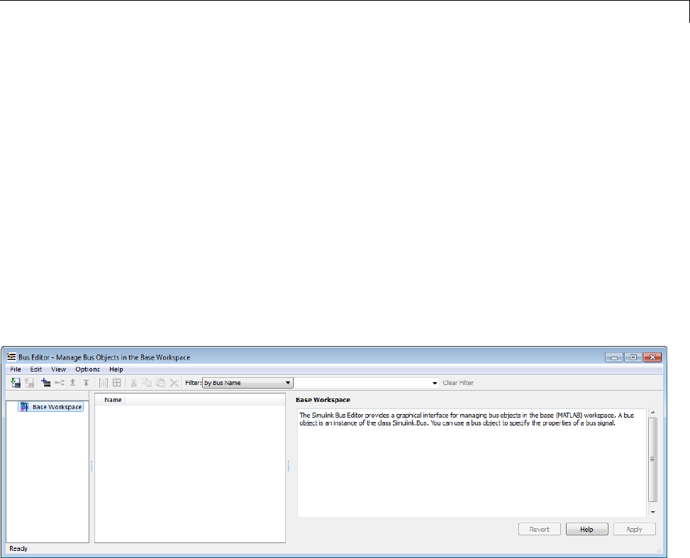
Manage Bus Objects with the Bus Editor
MAT-files. To save changed bus object definitions, export them from the base
workspaceintoMATLABcodefilesorMAT-files, as described in “Export
Bus Objects” on page 48-42.
Open the Bus Editor
You can open the Bus Editor in any of these ways:
•In the Simulink Editor, select Edit > Bus Editor.
•In a bus object’s dialog box in the Model Explorer, click the Launch Bus
Editor button.
•Enter buseditor at the command line of the MATLAB software.
If no bus objects exist, the Bus Editor looks like the one shown here:
Bus Editor Commands
The Bus Editor provides menu choices that you can use to execute all Bus
Editor commands. The editor also provides toolbar icons and keyboard
shortcuts for all commonly used commands, including the standard MATLAB
shortcuts for Cut, Copy, Paste, and Delete. The Toolbar Tip for each icon
describes the command, and the menu entry for each command shows any
shortcut. The icons for commands that are specific to the Bus Editor are:
48-25
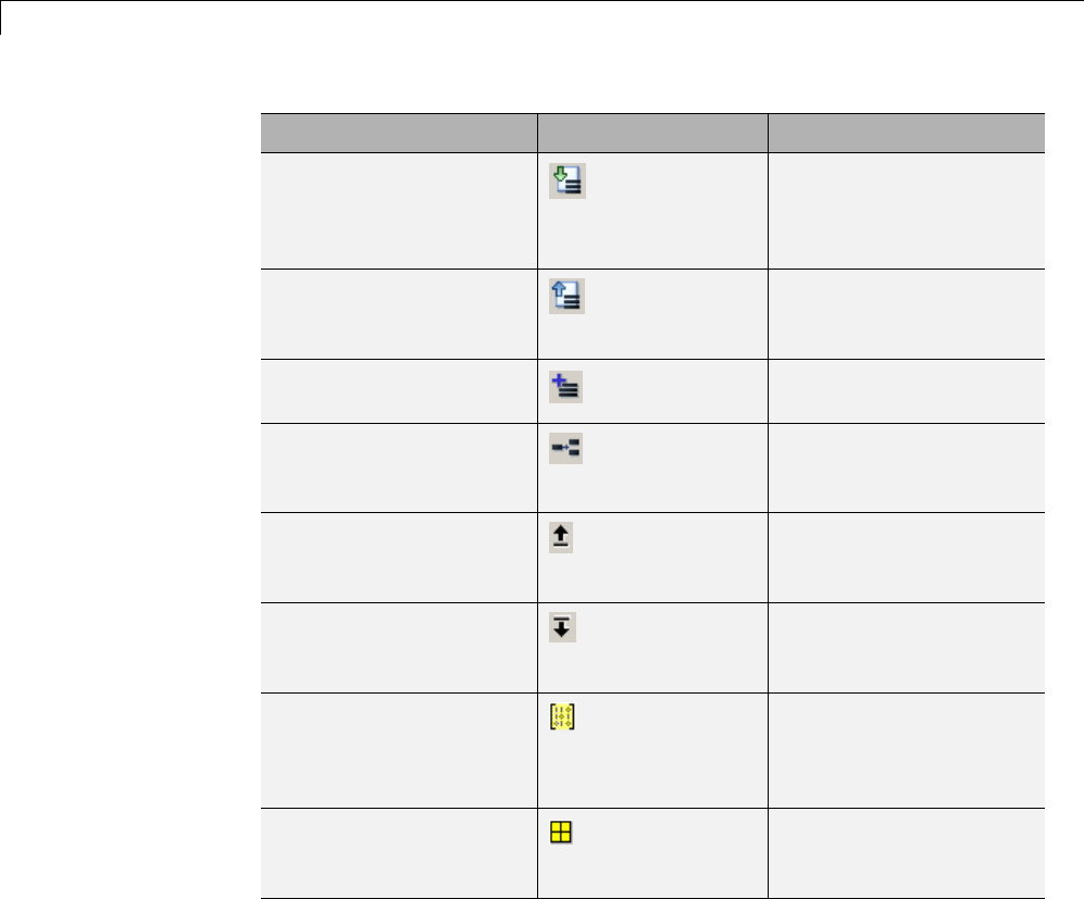
48 Using Composite Signals
Command Icon Description
Import Import the contents of
aMATLABcodefileor
MAT-file into the base
workspace.
Export Export all bus objects and
elements to a MATLAB
code file or MAT-file.
Create Create a new bus object
in the base workspace.
Insert Add a bus element below
the currently selected
bus entity.
Move Up Move the selected
element up in the list of
a bus object’s elements.
Move Down Move the selected
element down in the list
of bus object elements.
Create/Edit a
Simulink.Parameter
object
Create or edit a
Simulink.Parameter
object for the selected bus
object.
Create a MATLAB
structure
Create a MATLAB
structure for the selected
bus object.
You can use toolbar icons and keyboard shortcuts instead of menu commands
whenever you prefer.
Display Bus Objects
The Bus Editor is similar to the Model Explorer (which can display bus objects
but cannot edit them) and uses the same three panes to display bus objects:
48-26

Manage Bus Objects with the Bus Editor
•Hierarchy pane (left) — Displays the bus objects defined in the base
workspace
•Contents pane (center) — Displays the elements of the bus object selected
in the Hierarchy pane
•Dialog pane (right) — Displays for editing the current selection in the
Contents or Hierarchy pane
Items that appear in the Hierarchy pane or the Contents pane have Context
menus that provide immediate access to the capabilities most likely to be
useful with that item. The contents of an item’s Context menu depend on the
item and the current state within the Bus Editor. All Context menu options
are also available from the menu bar and/or the toolbar. Right-click any item
intheHierarchyorContentspanetoseeitsContextmenu.
Hierarchy Pane
If no bus objects exist in the base workspace, the Hierarchy pane shows only
Base Workspace, which is the root of the hierarchy of bus objects. The Bus
Editor then looks as shown in the previous figure. As you create or import
bus objects, they appear in the Hierarchy Pane as nodes subordinate to Base
Workspace. The bus objects appear in alphabetical order. The next figure
showstheBusEditorwithtwobusobjects,control and main, defined in
the base workspace:
48-27
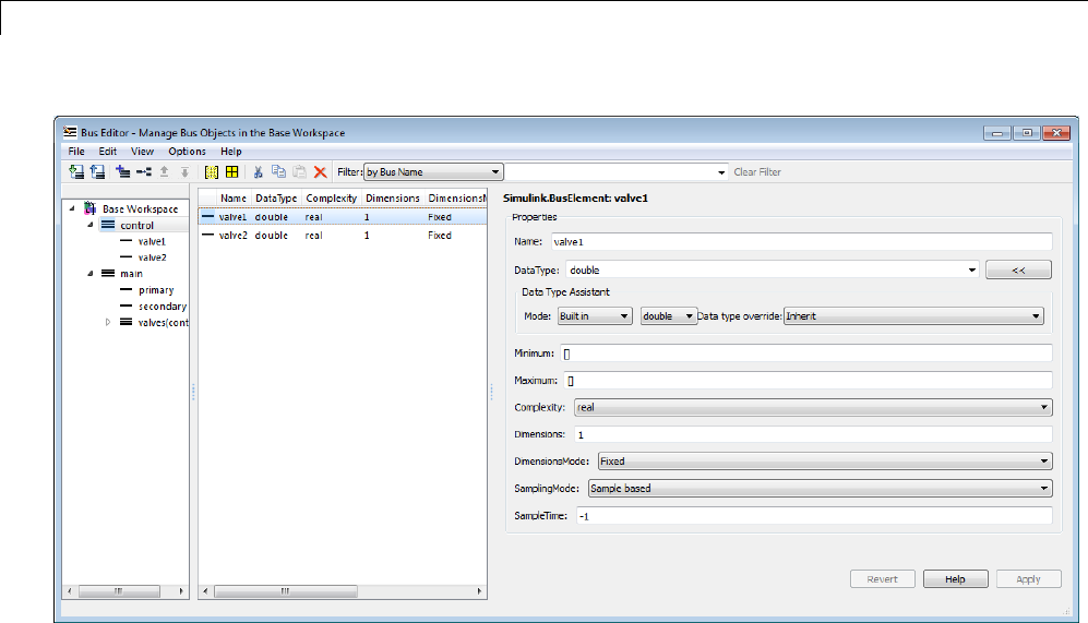
48 Using Composite Signals
The Hierarchy pane displays each bus object as an expandable node. The root
of the node displays the name of the bus object, and (if the bus contains any
elements) a button for expanding and collapsing the node. Expanding a bus
node displays named subnodes that represent the bus’s top-level elements.
In the preceding figure, both bus objects are fully expanded , and control is
selected.
Contents Pane
Selecting any top-level bus object in the Hierarchy Pane displays the object’s
elements in the Contents pane. In the previous figure, the elements of bus
object control,valve1 and valve2, appear. Each element’s properties
appear to the right of the element’s name. These properties are editable, and
you can edit the properties of multiple elements in one operation, as described
in “Editing in the Contents Pane” on page 48-39.
Dialog Pane
When a bus object is selected in the Hierarchy pane, or a bus object or element
is selected in the Contents pane, the properties of the selected item appear in
48-28

Manage Bus Objects with the Bus Editor
the Dialog pane. In the previous figure, valve1 is selected in the Contents
pane, so the Dialog pane shows its properties. These properties are editable,
and changes can be reverted or applied using the buttons below the Dialog
pane, as described in “Editing in the Dialog Pane” on page 48-41.
Filter Boxes
By default, the Bus Editor displays all bus objects that exist in the base
workspace. Where a model contains large numbers of bus objects, seeing them
all at the same time can be inconvenient. To facilitate working efficiently with
large collections of bus objects, you can use the Filter boxes, to the right of
the iconic tools in the toolbar, to show a selected subset of bus objects. See
“Filter Displayed Bus Objects” on page 48-49 for details.
Create Bus Objects
TousetheBusEditortocreateanewbusobjectinthebaseworkspace:
1Choose File > Add Bus.
A new bus object with a default name and properties is created immediately
inthebaseworkspace. Theobjectappears in the Hierarchy pane, and its
default properties appear in the Dialog pane:
48-29
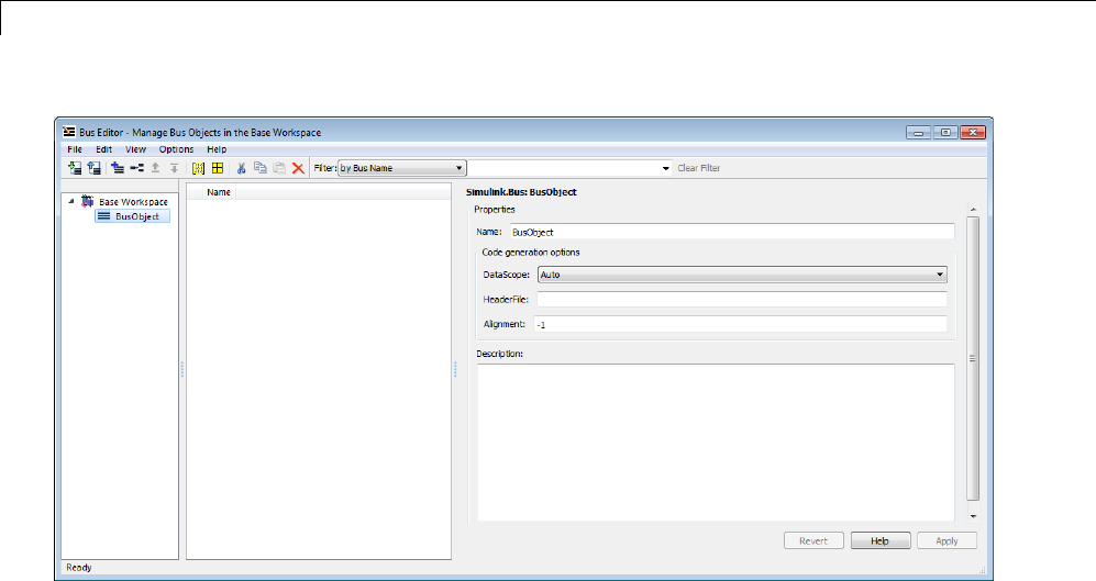
48 Using Composite Signals
2To specify the bus object name and other properties, in the Dialog pane:
aSpecify the Name of the of the new bus object (or you can retain the
default name). The name must be unique in the base workspace. See
“Choosing a Signal Name” on page 47-19 for guidelines for signal names.
bOptionally, specify a C Header file that defines a user-defined type
corresponding to this bus object. This header file has no effect on
Simulink simulation; it is used only by Simulink Coder software to
generate code.
cOptionally, specify a Description that provides information about the
bus object to human readers. This description has no effect on Simulink
simulation; it exists only for human convenience.
3Click Apply.
The properties of the bus object on the base workspace change as specified.
If you rename BusObject to main, the Bus Editor looks like this:
48-30
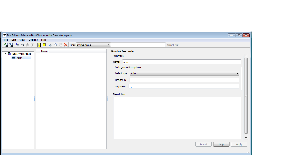
Manage Bus Objects with the Bus Editor
You can use Add Bus atanytimetocreateanewbusobjectinthebase
workspace, then set the name and properties of the object as needed. You
can intersperse creating bus objects and specifying their properties in any
order. The hierarchy pane reorders as needed to display all bus objects in
alphabetical order. If you add an additional bus object named control,the
Bus Editor looks like this:
48-31

48 Using Composite Signals
You can also use capabilities outside the Bus Editor to create new bus objects.
Such objects do not appear in the Bus Editor until the next time its window is
selected.
Create Bus Elements
Every bus element belongs to a specific bus. To create a new bus element:
1In the Hierarchy pane, select the entity below which to create the new
element. The entity can be a bus or a bus element. The new element
will belong to the selected bus object, or to the bus object that contains
the selected element. The previous figure shows the control bus object
selected.
2Choose File > Add/Insert BusElement.
A new bus element with a default name and properties is created
immediately in the applicable bus object. The object appears in the
Hierarchy pane immediately below the previously selected entity, and its
default properties appear in the Dialog pane:
48-32
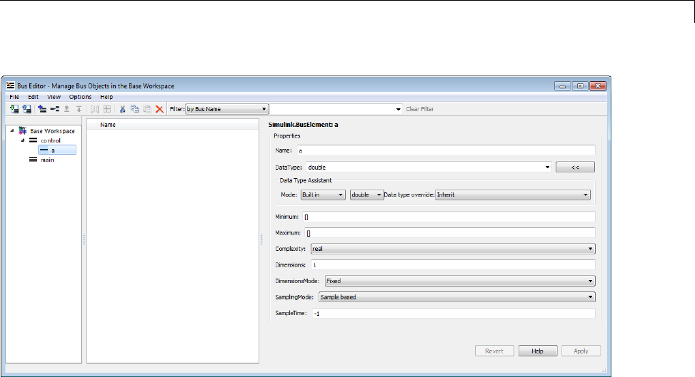
Manage Bus Objects with the Bus Editor
3To specify the bus element name and other properties, in the Dialog pane:
aSpecify the Name of the of the new bus element (or you can retain the
default name). The name must be unique among the elements of the bus
object. See “Signal Names” on page 47-19 for guidelines for signal names.
bSpecify the other properties of the element. The properties must match
the properties of the corresponding signal within the bus exactly, and
can be anything that a legal signal might have. The Data Type Assistant
appears in the Dialog pane to help specify the element’s data type. You
can specify any available data type, including a user-defined data type.
4Click Apply.
The properties of the bus element of the bus object in the base workspace
change as specified. If you rename the new element ato valve1,theBus
Editor looks like this:
48-33
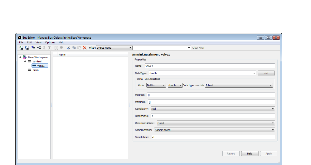
48 Using Composite Signals
You can use Add/Insert BusElement at any time to create a new bus
element in any bus object. You can intersperse creating bus objects and
specifying their properties in any order. The order of the other bus elements
in the bus object does not change when a new element is added. If you add
element valve2 to control,andsecondary and primary to main,theBus
Editor looks like this:
48-34
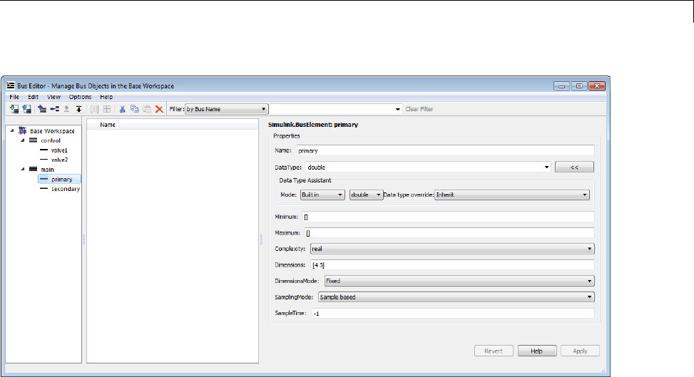
Manage Bus Objects with the Bus Editor
You can also use capabilities outside the Bus Editor to add new bus elements
to a bus object. Such an addition changes an existing bus object, so any new
bus element appears immediately in the Bus Editor.
Nest Bus Definitions
As described in “Nest Buses” on page 48-17, any signal in a bus can be
another bus, which can in turn contain subordinate buses, and so on to any
depth. Describing nested buses with bus objects requires nesting the bus
definitions that the objects provide.
Every bus object inherently defines a data type whose properties are those
specified by the object. To nest one bus definition in another, you assign to an
element of one bus object a data type that is defined by another bus object.
The element then represents a nested bus whose structure is given by the
bus object that provides its data type.
A data type defined by a bus object is called a bus type.Nestingbusesby
assigning bus types to elements, rather than by subordinating the bus objects
that define the types, allows the same bus definition to be used conveniently
48-35
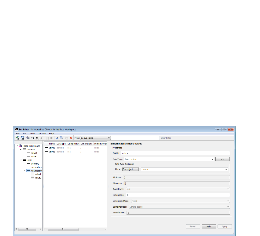
48 Using Composite Signals
in multiple contexts without unwanted interactions. To specify that an
element of a bus object represents a nested bus definition:
1Create a bus element to represent the nested bus definition, in the
appropriate position under the containing bus object, and give the element
the desired name. (You can also use an existing element.)
2Use the Dialog pane to set the data type of the element to the name of a bus
object. The Data Type Assistant shows the names of all available bus types.
(Youcanalsospecifyanonexistentbustypeanddefinetheobjectlater.)
In the preceding figure, if you add to bus object main a third element named
valves,setthedatatypeofvalves to be control (the name of the other
defined bus object) and expand the new element valves,theBusEditorlooks
like this:
The bus object main shown in the Bus Editor now defines the same structure
used by the bus signal main in the next figure:
48-36
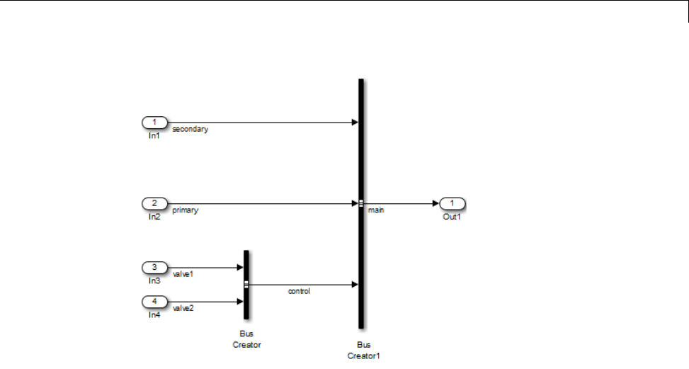
Manage Bus Objects with the Bus Editor
The distinction between a bus object and the bus type that it defines can
be useful for initially understanding how nested bus objects work and how
the Bus Editor handles them. In other contexts, the distinction is mostly an
implementation detail, and describing bus objects themselves as being nested
is more convenient. The rest of this chapter follows that convention.
You can nest a bus object in as many different bus objects as desired, and as
manytimesinthesamebusobjectasdesired.Youcannestbusobjectstoany
depth, but you cannot define a circular structure by directly or indirectly
nesting a bus object within itself.
If you try to define a circular structure, the Bus Editor posts a warning and
sets the data type of the element that would have completed the cycle to
double.ClickOK to dismiss the Notice and continue using the editor.
You can use the Hierarchy pane to explore nested bus objects by expanding
the objects, but you cannot change any property of a bus object anywhere that
it appears in nested form. To change the properties of a nested bus object,
you must change the source object, which is accessible at the top level in
the Hierarchy pane. You can jump from a nested bus object to its source
48-37

48 Using Composite Signals
object by selecting the nested object and choosing Go to ’element’from its
Context menu.
Change Bus Entities
You can use the Bus Editor to change and delete existing bus objects and
elements at any time. All three panes allow you to change the entities that
they display. Changes that create, reorder, or delete entities take effect
immediately in the base workspace. Changes to properties take effect when
you apply them, or can be canceled, leaving the properties unchanged. The
Bus Editor does not provide an Undo capability.
The Bus Editor provides comprehensive GUI capabilities for changing bus
entities. You can Cut, Copy, and Paste within and between panes in any way
that has a legal result. The Hierarchy and Dialog panes provide a Context
menu for the current selection. Pasting a Copied entity always creates a
copy, as distinct from a pointer to the original. The Bus Editor automatically
changes names when needed to avoid duplication.
Changes made outside the bus editor can affect the information on display
within it. Any change to an existing bus object or bus element is visible
immediately in the editor. Any change that creates or deletes a bus object
becomes visible in the bus editor next time its window is selected.
Editing in the Hierarchy pane
You can select the root node Base Workspace and perform various
operations, like export, cut, copy, paste, and delete. The operation
simultaneously affects all bus objects displayed in the Hierarchy pane, but
does not affect any that are invisible because a filter is in effect. See “Filter
Displayed Bus Objects” on page 48-49 for details.
As you use the Bus Editor, the Hierarchy pane automatically reorders the bus
objects it displays to maintain alphabetical order. This behavior cannot be
changed. However, the elements under a bus object can appear in any order.
To change that order, cut and paste elements as needed, or move elements up
and down as follows:
1Select the element to be moved.
48-38

Manage Bus Objects with the Bus Editor
2Choose Edit > Move Element Up or Edit > Move Element Down.
You cannot Paste one bus object under another to create a nested bus object
specification. To specify a nested bus, you must change the data type of a
buselementtobethetypeofanexisting bus object, as described in “Nest
Buses” on page 48-17.
Editing in the Contents Pane
Selecting any top-level bus object in the Hierarchy pane displays the object’s
elements in the Contents pane. Each element’s properties appear to the right
of the element’s name, and can be edited. To change a property displayed in
the Contents pane, click the value, enter a new value, then press Return.
Choose View > Dialog View to hide the Dialog pane to provide more room
to display properties in the Contents pane. Choose the command again to
redisplay the Dialog pane.
You can use the mouse and keyboard to select multiple elements in the
Contents pane. The selected entities need not be contiguous. You can then
perform any operation that you could on a single entity selected in the pane,
including operations performed with the Context menu. Clicking and editing
a value in any selected element changes that value in them all.
The next figure shows the Bus Editor with Dialog View enabled, two
elements selected in the Contents pane, and the DataType property selected
for editing in the second element:
48-39
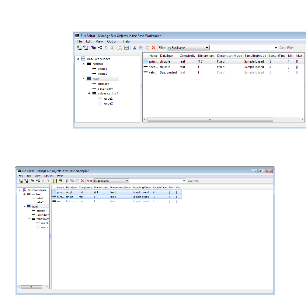
48 Using Composite Signals
If you change the value of DataType to single and press Return, the value
changes for both elements. The effect is the same no matter which element
you edit in a multiple selection:
48-40
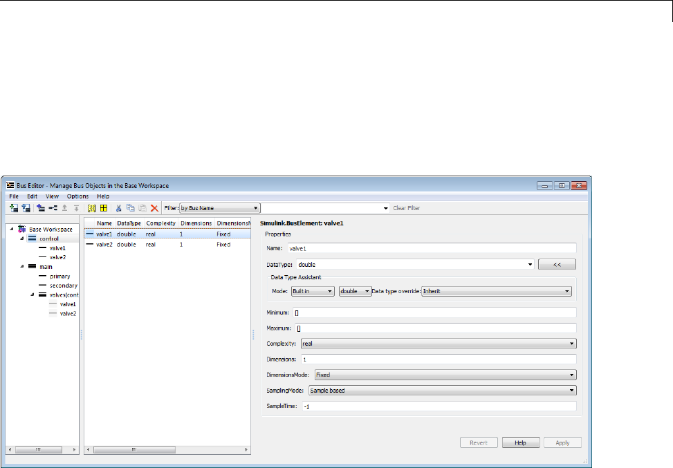
Manage Bus Objects with the Bus Editor
Editing in the Dialog Pane
When a bus object is selected in the Hierarchy pane, or a bus object or element
is selected in the Contents pane, the properties of the selected item appear in
the Dialog pane. In the next figure, valve1 is selected in the Contents pane,
so the Dialog pane shows its properties:
The properties shown in the Dialog paneareeditable,andthepaneincludes
theDataTypeAssistant. ClickApply to save changes, or Revert to cancel
them and restore the values that existed before any unapplied changes. You
can edit only one element at a time in the Dialog pane. If multiple entities are
selected in the Contents pane, all fields in the Dialog pane are grayed out:
48-41
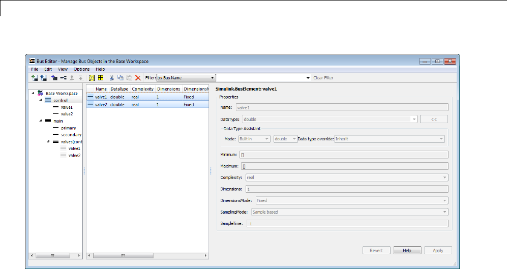
48 Using Composite Signals
If you use the Dialog pane to change any property of a bus entity, then
navigate elsewhere without clicking either Apply or Revert, a query box
appears by default. The query box asks whether to apply changes, ignore
changes, or continue as if the navigationhadnotbeentried.Youcansuppress
this query for future operations by checking Never ask me again in the box,
or by selecting Options > Auto Apply/Ignore Dialog Changes.
If you suppress the query, and thereafter navigate away from a change
without clicking Apply or Revert, the Bus Editor automatically applies or
discards changes, depending on which action you most recently chose in the
box. You can re-enable the query box for future operations by deselecting
Options > Auto Apply/Ignore Dialog Changes.
Export Bus Objects
Like all base workspace objects, bus objects are not saved with a model that
uses them, but exist separately in a MATLAB code file or MAT-file. You can
use the Bus Editor to export some or all bus objects to either type of file.
48-42

Manage Bus Objects with the Bus Editor
•If you export bus objects to a MATLAB code file, the Bus Editor asks
whether to store them in object format or cell format (the default). Specify
the desired format.
•If exporting would overwrite an existing MATLAB code file or MAT-file, a
confirmation dialog box appears. Confirm the export or cancel it and try
a different filename.
To export all bus objects from thebaseworkspacetoafile:
1In the Bus Editor, choose File > Export to File.
The Export dialog box appears.
2Specify the desired name and format of the export file.
3Click Save.
All bus objects, and nothing else, are exported to the specified file in the
specified format.
To export only selected bus objects from the base workspace to a file:
1Select a bus object in the Hierarchy pane, or one or more bus objects in the
Contents pane.
2Right-click to display the Context menu.
3Choose Export to File to export only the selected bus objects, or Export
with Related Bus Objects to File to also export any nested bus objects
used by the selected objects.
4Use the Export dialog box to export the selected bus object(s).
Clicking the Export icon in the toolbar is equivalent to choosing File >
Export, which exports all bus objects whether or not any are selected.
CustomizingBusObjectExport
You can customize bus object export by providing a custom function that
writes the exported objects to something other than the default destination,
a MATLAB code file or MAT-file stored in the file system. For example, the
48-43

48 Using Composite Signals
exported bus objects could be saved as records in a corporate database. See
“Customize Bus Object Import and Export” on page 48-55 for details.
Import Bus Objects
You can use the Bus Editor to import the definitions in a MATLAB code file
or MAT-file to the base workspace. Importing the file imports the complete
contents of the file, not just any bus objects that it contains. If you import
a file not exported by the Bus Editor, be careful that it does not contain
unwanted definitions previously exported from the base workspace or created
programmatically.
To import bus objects from a file to the base workspace:
1Choose File > Import into Base Workspace.
2UsetheOpenFiledialogboxtonavigatetoandimportthedesiredfile.
Before importing the file, the Bus Editor posts a warning that importing the
file will overwrite any variable in the base workspace that has the same name
as an entity in the file. Click Yes or No as appropriate. The imported bus
objects appear immediately in the editor. You can also use capabilities outside
the Bus Editor to import bus objects. Such objects do not appear in the Bus
Editor until the next time its window becomes the current window.
CustomizingBusObjectImport
You can customize bus object import by providing a custom function that
imports the objects from something other than the default source, a MATLAB
code file or MAT-file stored in the file system. For example, the bus objects
could be retrieved from records in a corporate database. See “Customize Bus
Object Import and Export” on page 48-55 for details.
Close the Bus Editor
To close the Bus Editor, choose File > Close. Closing the Bus Editor neither
saves nor discards changes to bus objects, which remain unaffected in the
base workspace. However, if you also close MATLAB without saving changes
to bus objects, the changes will be lost. To save bus objects without saving
other base workspace contents, use the techniques described in “Export Bus
48-44

Manage Bus Objects with the Bus Editor
Objects” on page 48-42. You can also save bus objects using any MATLAB
technique that saves the contents of the base workspace, but the resulting file
will contain everything in the base workspace, not just bus objects.
You can configure the Bus Editor so that closing it posts a reminder to save
bus objects. To enable the reminder, select Options > Always Warn Before
Closing. When this option is selected and you try to close the Bus Editor,
a reminder appears that asks whether the editor should save bus objects
before closing. Click Yes to save bus objects and close, No to close without
saving bus objects, or Cancel to dismiss the reminder and continue in the
Bus Editor. You can disable the reminder by deselecting Options > Always
Warn Before Closing.
48-45

48 Using Composite Signals
Store and Load Bus Objects
In this section...
“MATLAB Code Files” on page 48-46
“MATLAB Data Files (MAT-Files)” on page 48-47
“Database or Other External Source Files” on page 48-47
You can store bus object objects in a variety formats.
Format When to Use
MATLAB code file For traceability and model
differencing using MATLAB
code
MATLAB data file (MAT-file) For faster bus loading and saving
Database or other external data
source
For comparing bus interface
information with design documents
stored in an external data source.
MATLABCodeFiles
You can read and save bus data with MATLAB code files.
To save all bus objects (instances of the Simulnk.Bus class) in the MATLAB
base workspacetoaMATLABcodefile,useone of the following approaches:
•Use the Bus Editor (see “Export Bus Objects” on page 48-42 and “Import
Bus Objects” on page 48-44).
•From the MATLAB command line, use the Simulink.Bus.save command.
To save variables from the base workspace to a MATLAB code file, use the
Simulink.saveVars command. The file containing the variables is formatted
to be easily understood and editable. Running the file restores the saved
variables to the base workspace.
For traceability, consider using a clearlynamedseparatefileforeachmodel.
48-46

Store and Load Bus Objects
MATLAB Data Files(MAT-Files)
You can load bus objects in MATLAB data files (MAT-files), using one of the
following approaches:
•Use the Bus Editor (see “Export Bus Objects” on page 48-42 and “Import
Bus Objects” on page 48-44).
•From the MATLAB command line, use the load command.
Loading large data from MAT-files is faster than loading from MATLAB code
files.
Database or Other External Source Files
You can capture bus interface information in a database or other external
source, and use scripts and Database Toolbox™ functionality to read that
information into MATLAB.
You can usesl_customization.m to customize the Bus Editor to import bus
data from a database or other external source. For details, see “Customize
Bus ObjectImportandExport”onpage48-55.
48-47

48 Using Composite Signals
Map Bus Objects to Models
As models become complex, you need to keep track of which models use which
bus objects. From any model or bus object, you should be able to tell what
component it needs or is needed by.
A model must load all of its bus objects before you execute the model. For
automation and consistency across models, it is important to map bus objects
to models.
•By identifying all of the bus objects a model needs, you can ensure that
those objects are loaded before model execution.
•By identifying all models that use a bus object, you can ensure that changes
to a bus object do not cause unexpected changes in any of the models that
use that bus object.
To map bus objects to models, consider:
•Using Simulink Projects. For details, see “Project Management”
•Capturing the mapping information in an external data source, such as
a database.
Use a Rigorous Naming Convention
Using a rigorous and standard naming convention for bus mapping
information is a straightforward approach. For example, consider the model
and data required for an actuator control function. You could name the
model Actuator and name the input and output ports Actuator_bus_in and
Actuator_bus_out, respectively. This naming convention makes it clear to
what models a particular bus object is related, and vice versa.
Note that this approach can cause issues if the output from one model
reference is fed directly to another model reference. In this case, the naming
mismatch results in an error.
48-48
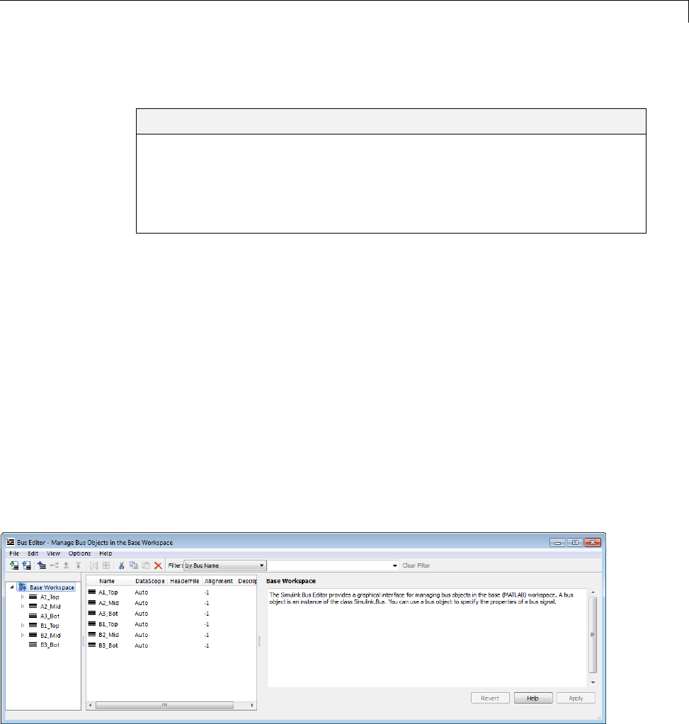
Filter Displayed Bus Objects
Filter Displayed Bus Objects
In this section...
“Filter by Name” on page 48-50
“Filter by Relationship” on page 48-51
“Change Filtered Objects” on page 48-53
“Clear the Filter” on page 48-54
By default, the Bus Editor displays all bus objects that exist in the base
workspace, always in alphabetical order. When a model contains large
numbers of bus objects, seeing them all at the same time can be inconvenient.
To facilitate working efficiently with large collections of bus objects, you can
set the Bus Editor to display only bus objects that:
•Have names that match a given string or regular expression
•Have a specified relationship to a bus object specified by name
To set a filter, you specify values in the Filter boxes to the right of the tools in
the toolbar. The left Filter box specifies the type of filtering. This box always
appears, and is called the Filter Type box. Depending on the specified type
of filtering, one or two boxes appear to the right of the Filter Type box. The
next figure includes the Filter boxes (near the top of the dialog box) and
shows that six bus objects exist in the Base Workspace:
48-49
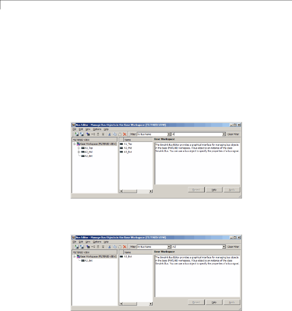
48 Using Composite Signals
The bus objects shown form two disjoint hierarchies. A1_Top is the parent of
A2_Mid,whichistheparentofA3_Bot. Similarly, B1_Top >B2_Mid >B3_Bot.
See “Nest Buses” on page 48-17 for information about bus object hierarchies.
Filter by Name
To filter bus objects by name, set the Filter Type box to by Bus Name (which
isthedefault). TherightFilter box is the Object Name box. Type any
MATLAB regular expression (which can just be a string) into the Object
Name box. As you type, the Bus Editor updates dynamically to show only bus
objects whose names match the expression you have typed. The comparison is
case-sensitive. For example, entering Adisplays:
Note that FILTERED VIEW appears in three locations, as shown in the
preceding figure. This indicator appears whenever any filter is in effect.
Entering the additional character 3into the Object Name box displays:
48-50
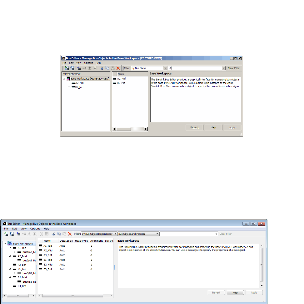
Filter Displayed Bus Objects
In a MATLAB regular expression, the metacharacter dot (.) matches any
character, so entering .2 displays:
See “Regular Expressions” for complete information about MATLAB regular
expression syntax.
Filter by Relationship
To filter bus objects by relationship, set the Filter Type box to by Bus
Object Dependency.AthirdFilter box, called the Relationship box,
appears between the Filter Type box and the Object Name box. You may
have to widen the Bus Editor to see all three boxes:
In the Relationship box,selectthetypeofrelationshiptodisplay. The
options are:
48-51
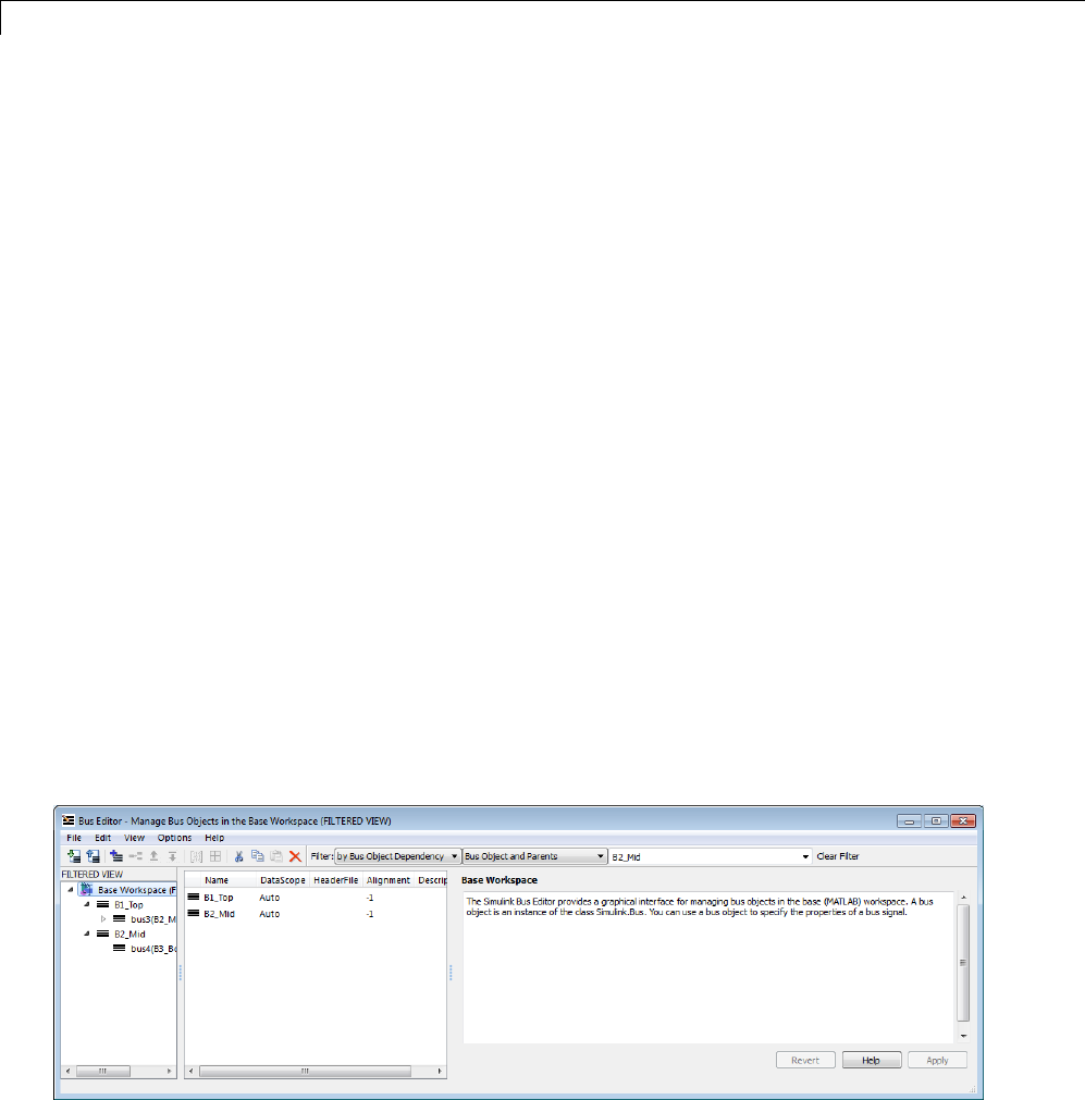
48 Using Composite Signals
•Bus Object and Parents — Show a specified bus object and all superior
bus objects in the hierarchy (default)
•Bus Object and Dependents — Show a specified bus object and all
subordinate bus objects in the hierarchy
•Bus Object and Related Objects — Show a specified bus object and all
superior and subordinate bus objects
In the Object Name box, specify a bus object by name. You can use the
list to select any existing bus object name, or you can type a name. As you
type, the editor:
•Dynamically completes the field to indicate the first bus object that
alphabetically matches what you have typed.
•Updates the display panes to show only that object and any objects that
have the specified relationship to it.
When filtering by relationship, you must enter a string, not a regular
expression, in the Object Name box. The match is case-sensitive. For
example, assuming that A1_Top is the parent of A2_Mid,whichistheparent
of A3_Bot (as previously described) if you enter B2 (or any leftmost substring
that matches only B2_Mid)intheObject Name box, the Bus Editor displays
the following for each of the three choices of relationship type:
Bus Object and Parents
Bus Object and Dependents
48-52
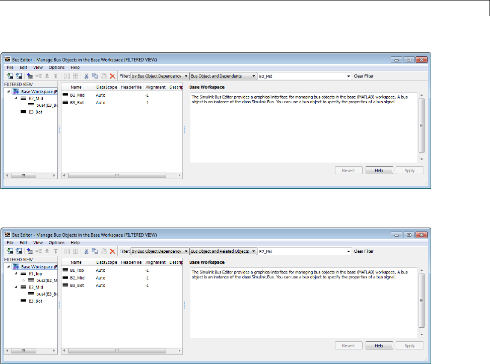
Filter Displayed Bus Objects
Bus Object and Related Objects
Note that FILTERED VIEW appears in each the preceding figures, as it does
when any filter is in effect.
Change Filtered Objects
You can work with any bus object that is visible in a filtered display exactly
as you could in an unfiltered display. Ifyouchangethenameordependency
of an object so that it no longer passes the current filter, the object vanishes
from the display. Conversely, if some activity outside the Bus Editor changes
afilteredobjectsothatitpassesthecurrent filter, the object immediately
becomes visible.
48-53
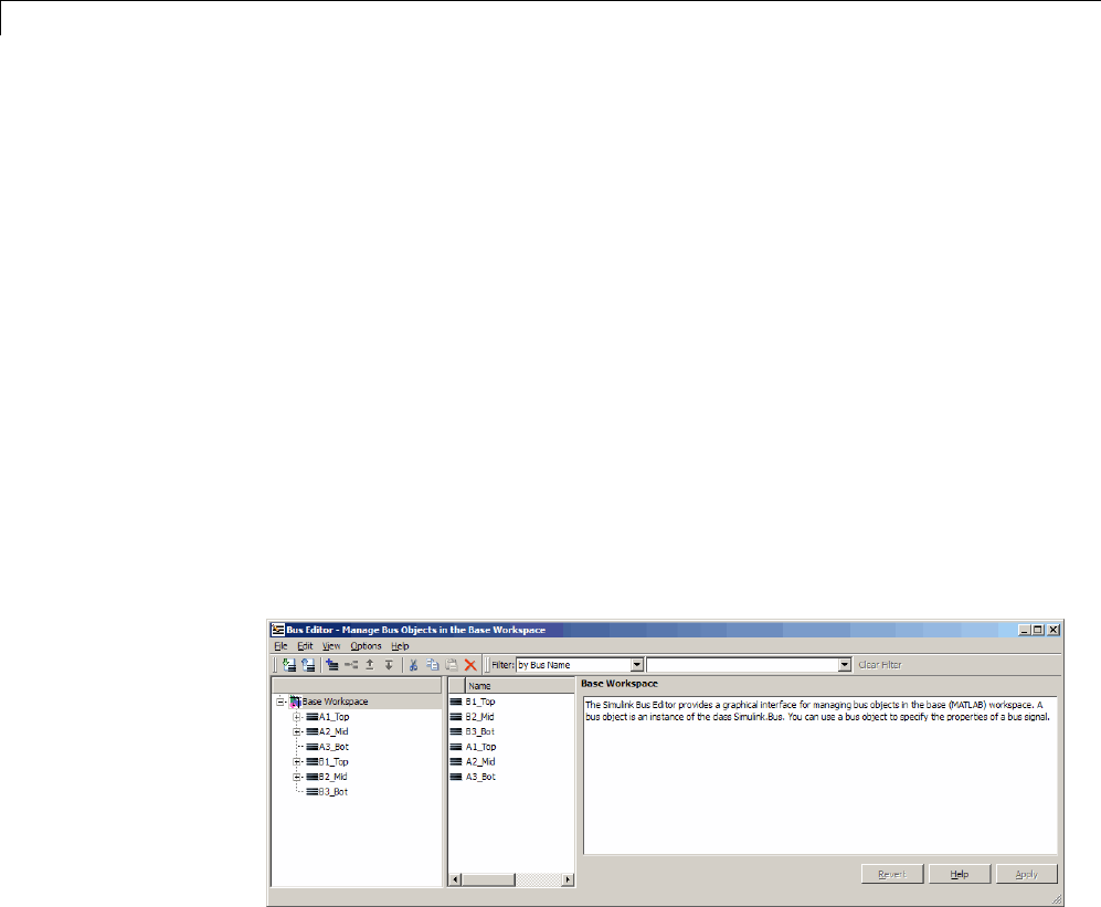
48 Using Composite Signals
A new bus object created within the Bus Editor with a filter in effect may or
may not appear, depending on the filter. If you create a new bus object but do
not see it in the editor, check the filter. The new object (whose name always
begins with BusObject) may exist but be invisible. Bus objects created or
imported using capabilities outside the Bus Editor are not visible until the
Bus Editor window is next selected, regardless of whether a filter is in effect.
Operations performed on the root node Base Workspace in the Hierarchy
pane, such as exporting bus objects, affect only visible objects. An object that
is invisible because a filter is in effect is unaffected by the operation. If you
want to export all existing bus objects, be sure to clear any filter that may be
in effect before performing the export.
Clear the Filter
To clear any filter currently in effect, click the Clear Filter button at the
right of the Filter subpane, or press the F5 key. The subpane reverts to its
default state, in which all bus objects appear:
If you jump from a nested bus object to its source object by selecting the
nested object and choosing Go to ’element’from its Context menu, and the
source object is invisible due to a filter, the Bus Editor automatically clears
the filter and selects the source object. Jumping to an object that is already
visible leaves the filter unchanged.
48-54

Customize Bus Object Import and Export
Customize Bus Object Import and Export
In this section...
“Prerequisites for Customization” on page 48-56
“Writing a Bus Object Import Function” on page 48-56
“Writing a Bus Object Export Function” on page 48-57
“Registering Customizations” on page 48-58
“Changing Customizations” on page 48-59
You can use the Bus Editor to import bus objects to the base workspace, as
described in “Import Bus Objects” on page 48-44, and to export bus objects
from the base workspace, as described in “Export Bus Objects” on page 48-42.
By default, the Bus Editor can import bus objects only from a MATLAB code
file or MAT-file, and can export bus objects only to a MATLAB code file or
MAT-file, with the files stored somewhere that is accessible using an ordinary
Open or Save dialog.
Alternatively, you can customize the Bus Editor’s import and export
commands by writing MATLAB functions that provide the desired capabilities,
and registering these functions using the Simulink Customization Manager.
When a custom bus object import or export function exists, and you use the
Bus Editor to import or export bus objects, the editor calls the custom import
or export function rather than using its default capabilities.
A customized import or export function can have any desired effect and
use any available technique. For example, rather than storing bus objects
in MATLAB code files or MAT-files in the file system, you could provide
customized functions that store the objects as records in a corporate database,
perhaps in a format that also meets other corporate data management
requirements.
This section describes techniques for designing and implementing a
custom bus object import or export function, and for using the Simulink
Customization Manager to register such a custom function. The registration
process establishes the custom import and export functions as callbacks for
the Bus Editor Import to Base Workspace and Export to File commands,
replacing the default capabilities of the editor.
48-55

48 Using Composite Signals
CustomizingtheBusEditor’simportandexport capabilities has no effect on
any MATLAB or Simulink API function: it affects only the behavior of the
Bus Editor. You can customize bus object import, export, or both. You can
establish, change, and cancel import or export customization at any time.
Canceling import or export customization restores the default Bus Editor
capabilities for that operation without affecting the other.
Prerequisites for Customization
To perform bus object import or export customization, you must understand:
•The MATLAB language and programming techniques that you will need.
•Simulink bus object syntax. See “About Bus Objects” on page 48-20,
Simulink.Bus,Simulink.BusElement, and “Nest Bus Definitions” on
page 48-35.
•The proprietary format into which you will translate bus objects, and all
techniques necessary to access the facility that stores the objects.
•Any platform-specific techniques needed to obtain data from the user, such
as the name of the location in which to store or access bus objects.
The rest of the information that you will need, including all necessary
information about the Simulink Customization Manager appears in this
section. For complete information about the Customization Manager, see
“Simulink Environment Customization”.
Writing a Bus Object Import Function
A callback function that customizes bus import can use any MATLAB
programming construct or technique. The function can take zero or more
arguments, which can be anything that the function needs to perform its task.
You can use functions, global variables, or any other MATLAB technique to
provide argument values. The function can also poll the user for information,
such as a designation of where to obtain bus object information. The general
algorithm of a custom bus object import function is:
1Obtain bus object information from the local repository.
2Translate each bus object definition to a Simulink bus object.
48-56

Customize Bus Object Import and Export
3Save each bus object to the MATLAB base workspace.
An example of the syntactic shell of an import callback function is:
function myImportCallBack
disp('Custom import was called!');
Although this function does not import any bus objects, it is syntactically
valid and could be registered with the Simulink Customization Manager.
A real import function would somehow obtain a designation of where to
obtain the bus object(s) to import; convert each one to a Simulink bus object;
and store the object in the base workspace. The additional logic needed
is enterprise-specific.
Writing a Bus Object Export Function
A callback function that customizes bus export can use any MATLAB
programming construct or technique. The function must take one argument,
and can take zero or more additional arguments, which can be anything
that the function needs to perform its task. When the Bus Editor calls
the function, the value of the first argument is a cell array containing the
namesofallbusobjectsselectedwithin the editor to be exported. You can
use functions, global variables, or any other MATLAB technique to provide
values for any additional arguments. The general algorithm of a customized
export function is:
1Iterate over the list of object names in the first argument.
2Obtain the bus object corresponding to each name.
3Translate the bus object to the proprietary syntax.
4Save the translated bus object in the local repository.
An example of the syntactic shell of such an export callback function is:
function myExportCallBack(selectedBusObjects)
disp('Custom export was called!');
for idx = 1:length(selectedBusObjects)
disp([selectedBusObjects{idx} ' was selected for export.']);
end
48-57

48 Using Composite Signals
Although this function does notexportanybusobjects,itissyntacticallyvalid
and could be registered. It accepts a cell array of bus object names, iterates
over them, and prints each name. A real export function would use each name
to retrieve the corresponding bus object from the base workspace; convert the
object to proprietary format; and store the converted object somewhere. The
additional logic needed is enterprise-specific.
Registering Customizations
To customize bus object import or export, you provide a customization
registration function that inputs and configures the Customization Manager
whenever you start the Simulink software or subsequently refresh Simulink
customizations. The steps for using a customization registration function are:
1Create a file named sl_customization.m to contain the customization
registration function (or use an existing customization file).
2At the top of the file, create a function named sl_customization that
takes a single argument (or use the customization function in an existing
file). When the function is invoked, the value of this argument will be
the Customization Manager.
3Configure the sl_customization function to set importCallbackFcn and
exportCallbackFcn to be function handles that specify your customized
busobjectimportandexportfunctions.
4If sl_customization.m is a new customization file, put it anywhere on the
MATLAB search path. Two frequently-used locations are matlabroot and
the current working directory; or you may want to extend the search path.
A simple example of a customization registration function is:
function sl_customization(cm)
disp('My customization file was loaded.');
cm.BusEditorCustomizer.importCallbackFcn = @myImportCallBack;
cm.BusEditorCustomizer.exportCallbackFcn = @(x)myExportCallBack(x);
When the Simulink software starts up, it traverses the MATLAB search path
looking for files named sl_customization.m. The software loads each such
file that it finds (not just the first file) and executes the sl_customization
function at its top, establishing the customizations that the function specifies.
48-58

Customize Bus Object Import and Export
Executing the previous customization function will display a message (which
an actual function probably would not) and establish that the Bus Editor uses
a function named myImportCallBack() to import bus objects, and a function
named myExportCallBack(x) to export bus objects.
The function corresponding to a handle that appears in a callback registration
need not be defined when the registration occurs, but it must be defined when
the Bus Editor later calls the function. The same latitude and requirement
applies to any functions or global variables used to provide the values of any
additional arguments.
Other functions can also exist in the sl_customization.m file. However, the
Simulink software ignores files named sl_customization.m except when
it starts up or refreshes customizations, so any changes to functions in
the customization file will be ignored until one of those events occurs. By
contrast, changes to other MATLAB code files on the MATLAB path take
effect immediately.
Changing Customizations
You can change the handles established in the sl_customization function by
changing the function to specify the changed handles, saving the function,
then refreshing customizations by executing:
sl_refresh_customizations
The Simulink software then traverses the MATLAB path and reloads all
sl_customization.m files that it finds, executing the first function in each
one, just as it did on Simulink startup.
You can revert to default import or export behavior by setting the appropriate
BusEditorCustomizer element to [] in the sl_customization function,
then refreshing customizations. Alternatively, you can eliminate both
customizations in one operation by executing:
cm.BusEditorCustomizer.clear
where cm was previously set to a customization manager object (see
“Registering Customizations” on page 48-58).
48-59

48 Using Composite Signals
Changes to the import and export callback functions themselves, as distinct
from changes to the handles that register them as customizations, take
effect immediately unless they are in the sl_customization.m file itself, in
which case they take effect next time you refresh customizations. Keeping
the callback functions in separate files usually provides more flexible and
modular results.
48-60

Connect Buses to Inports and Outports
Connect Buses to Inports and Outports
In this section...
“Connect Buses to Root Level Inports” on page 48-61
“Connect Buses to Root Level Outports” on page 48-61
“Connect Buses to Nonvirtual Inports” on page 48-61
“Connect Buses to Model, Stateflow, and MATLAB Function Blocks” on
page 48-64
“Connect Multi-Rate Buses to Referenced Models” on page 48-64
Connect Buses to Root Level Inports
If you want a root level Inport of a model to produce a bus signal, in the Inport
block parameters dialog box, set Data type to Bus: <object name> and
replace <object name> with the name of the bus object name that defines
the bus that the Inport produces. See “Bus Objects” on page 48-20 for more
information.
Connect Buses to Root Level Outports
A root level Outport of a model can accept a virtual bus only if all elements of
the bus have the same data type. The Outport block automatically unifies the
bus to a vector having the same number of elements as the bus, and outputs
that vector.
If you want a root level Outport of a model to accept a bus signal that contains
mixed types, in the Outport block parameters dialog box, set Data type to
Bus: <object name> and replace <object name> with the name of the bus
object name that defines the bus that the Inport produces. If the bus signal
is virtual, it will be converted to nonvirtual, as described in “Automatic Bus
Conversion” on page 48-13. See “Bus Objects” on page 48-20 more information.
Connect Buses to Nonvirtual Inports
By default, an Inport block is a virtual block and accepts a bus as input.
However, an Inport block is nonvirtual if it resides in a conditionally executed
or atomic subsystem, or a referenced model, and it or any of its components
48-61
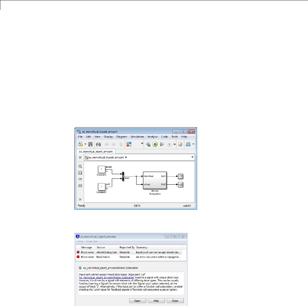
48 Using Composite Signals
is directly connected to an output of the subsystem or model. In such a case,
the Inport block can accept a bus only if all elements of the bus have the
same data type.
If the components are of differing data types, attempting to simulate the
model causes the Simulink software to halt the simulation and display an
error message. You can avoid this problem, without changing the semantics of
your model, by inserting a Signal Conversion block between the Inport block
and the Outport block to which it was originally connected.
For example, the following model, which includes an atomic subsystem, does
not simulate.
Starting the simulation generates the following error messages:
Opening the subsystem reveals that in this model, the Inport block labeled
nonvirtual is nonvirtual because it resides in an atomic subsystem and one
48-62
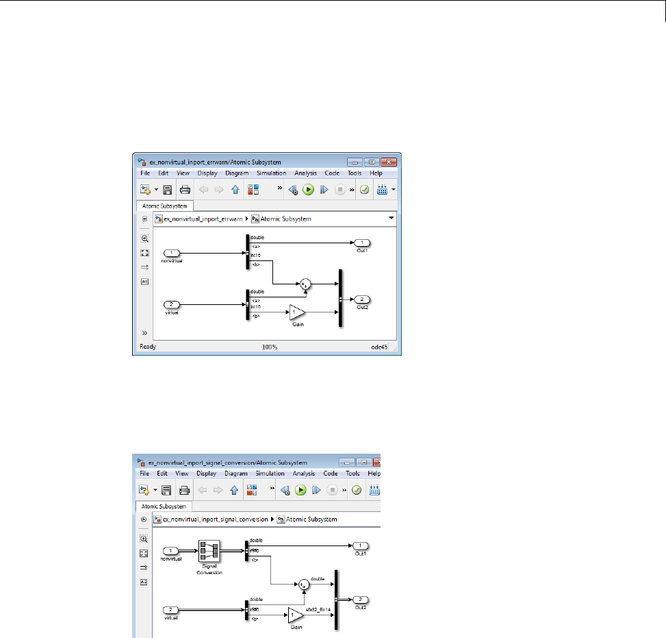
Connect Buses to Inports and Outports
of its components (labeled a) is directly connected to one of the subsystem’s
outputs. Further, the bus (bus1) connected to the subsystem’s inputs has
components of differing data types. As a result, you cannot simulate this
model.
To break the direct connection to the subsystem’s output, insert a Signal
Conversion block. Set the Signal Conversion block Output parameter to
Signal copy. Inserting the Signal Conversion block enables the Simulink
software to simulate the model.
48-63

48 Using Composite Signals
Connect Buses to Model, Stateflow, and MATLAB
Function Blocks
Referenced models, Stateflow charts, and MATLAB Function blocks require
anybusconnectedtothemtobenonvirtual.Toprovideforthisrequirement,
where possible the Simulink software automatically converts any virtual
bus connected to a Model block or Stateflow chart to a nonvirtual bus. See
“Automatic Bus Conversion” on page 48-13 for details.
Connect Multi-Rate Buses to Referenced Models
In a model that uses a fixed-rate solver, referenced models can input only
single-rate buses. However, you can input the signals in a multi-rate bus to a
referenced model by inserting blocks into the parent and referenced model as
follows:
1In the parent model: Insert a Rate Transition block to convert the
multi-rate bus to a single-rate bus. The Rate Transition block must specify
arateinitsBlock Parameters > Output port sample time field unless
one of the following is true:
•The Configuration Parameters > Solver pane specifies a rate:
–Periodic sample time constraint is Specified
–Sample time properties contains the specified rate.
•The Inport that accepts the bus in the referenced model specifies a rate
in its Block Properties > Signal Attributes > Sample time field.
2In the referenced model: Use a Bus Selector block to pick out signals
of interest, and use Rate Transition blocks to convert the signals to the
desired rates.
48-64

Specify Initial Conditions for Bus Signals
Specify Initial Conditions for Bus Signals
In this section...
“Bus Signal Initialization” on page 48-65
“Create Initial Condition (IC) Structures” on page 48-67
“Three Ways to Initialize Bus Signals Using Block Parameters” on page
48-72
“Setting Diagnostics to Support Bus Signal Initialization” on page 48-76
Bus Signal Initialization
Bus signal initialization is a special kind of signal initialization. For general
information about initializing signals, see “Initialize Signals and Discrete
States” on page 47-51.
Bus signal initialization specifies the bus element values that Simulink uses
for the first execution of a block that uses that bus signal. By default, the
initial value for a bus element is the ground value (represented by 0). Bus
initialization, as described in this section, involves specifying nonzero initial
conditions (ICs).
You can use bus signal initialization features to:
•Specify initial conditions for signals that have different data types
•Apply a different initial condition for each signal in the bus
•Specify initial conditions for a subset of signals in a bus without specifying
initial conditions for all the signals
•Use the same initial conditions for multiple blocks, signals, or models
Blocks that Support Bus Signal Initialization
You can initialize bus signal values that input to a block, if that block meets
both of these conditions:
•It has an initial value or initial condition block parameter
•It supports bus signals
48-65

48 Using Composite Signals
The following blocks support bus signal initialization:
•Data Store Memory
•Memory
•Merge
•Outport (when the block is inside a conditionally executed context)
•Rate Transition
•Unit Delay
For example, the Unit Delay block is a bus-capable block and the Block
Parameters dialog box for the Unit Delay block has an Initial conditions
parameter.
Initialization Is Not Supported for Bus Signals with
Variable-Size or Frame-Based Elements
You cannot initialize a bus that has:
•Variable-size signals
•Frame-based signals
Workflow for Initializing Bus Signals Using Initial Condition
Structures
You need to set up your model properly to use initial condition structures to
initialize bus signals. The general workflow involves the tasks listed in the
following table. You can vary the order of the tasks, but before you update the
diagram or run a simulation, you need to ensure your model is set up properly.
48-66

Specify Initial Conditions for Bus Signals
Task Documentation
Define an IC structure “Create Initial Condition (IC)
Structures” on page 48-67
Use an IC structure to specify a
nonzero initial condition.
“Three Ways to Initialize Bus
Signals Using Block Parameters” on
page 48-72
Set Configuration Parameters dialog
box diagnostics
“Setting Diagnostics to Support Bus
Signal Initialization” on page 48-76
Create Initial Condition (IC) Structures
You can create partial or full IC structures to represent initial values for a
bus signal. Create an IC structure by either:
•Defining a MATLAB structure in the MATLAB base or Simulink model
workspace
•Specifying an expression that evaluatestoastructurefortheinitial
condition parameter in the Block Parameters dialog boxforablockthat
supports bus signal initialization
For information about defining MATLAB structures, see “Create a Structure
Array” in the MATLAB documentation.
Full and Partial IC Structures
A full IC structure provides an initial value for every element of a bus signal.
This IC structure mirrors the bus hierarchy and reflects the attributes of
the bus elements.
A partial IC structure provides initial values for a subset of the elements of
a bus signal. If you use a partial IC structure, during simulation, Simulink
creates a full IC structure to represent all of the bus signal elements,
assigning the respective ground value to each element for which the partial
IC structure does not explicitly assign a value.
Specifying partial structures for block parameter values can be useful during
the iterative process of creating a model. Partial structures enable you
48-67

48 Using Composite Signals
to focus on a subset of signals in a bus. When you use partial structures,
Simulink initializes unspecified signals implicitly.
Specifying full structures during code generation offers these advantages:
•Generates more readable code
•Supports a modeling style that explicitly initializes all signals
Match IC Structure Values to Corresponding Bus Element Data
Characteristics
The field that you specify in an IC structure must match the following data
attributes of the bus element exactly:
•Name
•Data type
•Dimension
•Complexity
For example, if you define a bus element to be a real [2x2] double array, then
in the IC structure, define the value to initialize that bus element to be a
real [2x2] double array.
You must explicitly specify fields in the IC structure for every bus element
that has an enumerated (enum)datatype.
When you define a partial IC structure:
•Include only fields that are in the bus.
•You can omit fields that are in the bus.
•Make the field in the IC structure correspond to the nesting level of the
bus element.
•Within the same nesting level in both the structure and the bus, you
can specify the structure fields in a different order than the order of the
elements in the bus.
48-68

Specify Initial Conditions for Bus Signals
Note The value of an IC structure must lie within the design minimum and
maximum range of the corresponding bus element. Simulink performs this
range checking during an update diagram and when you run the model.
Examples of Partial Structures
Suppose you have a bus, Top, composed of three elements: A,B,andC,with
these characteristics:
•Ais a nested bus, with two signal elements.
•Bis a single signal.
•Cis a nested bus that includes bus Aas a nested bus.
The following model, busic_example includes the nested Top bus. The screen
capture below shows the model after it has been updated.
48-69
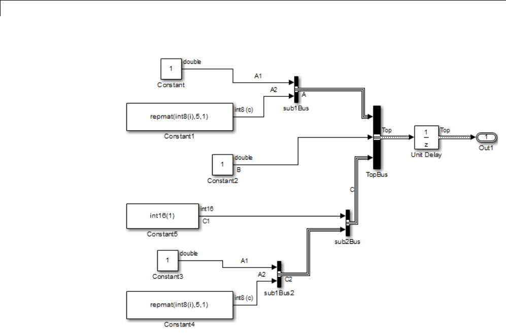
48 Using Composite Signals
The following diagram summarizes the Top bus hierarchy and the data type,
dimension, and complexity of the bus elements .
Top
A (sub1)
A1 (double)
A2 (int8, 5x1, complex)
B (double)
C (sub2)
C1 (int16)
C2 (sub1)
A1 (double)
A2 (int8, 5x1, complex)
48-70

Specify Initial Conditions for Bus Signals
Valid partial IC structures. In the following examples, Kis an IC structure
specified for the initial value of the Unit Delay block. The IC structure
corresponds to the Top bus in the busic_example model.
The following table shows valid initial condition specifications.
Valid Syntax Description
K.A.A1 = 3 Bus element Top.A.A1 is double; the
corresponding structure field is 3,whichisa
double.
K = struct('C',struct('C1',int16(4))) Matching data types can require you to
cast types. Bus element Top.C.C1 is int16.
The corresponding structure field explicitly
specifies int16(4).
K = struct('B',3,'A',struct('A1',4)) Bus element Top.B and Top.A are at the
same nesting level in the bus. For bus
elements at the same nesting level, the order of
corresponding structure fields does not matter.
Invalid partial IC structures. In the following examples, Kis an IC structure
specified for the initial value of the Unit Delay block. The IC structure
corresponds to the Top bus in the busic_example model.
These three initial condition specifications are not valid:
Invalid Syntax Reason the Syntax Is Invalid
K.A.A2 = 3 Value data type, dimension, and complexity do
not match. Top.A.A2 is an int8,butK.A.A2 is
a double; Top.A.A2 is 5x1,butK.A.A2 is 1x1;
Top.A.A2 is complex, but K.A.A2 is real.
K.C.C2 = 3 You cannot use a scalar to initialize IC
substructures.
K = struct('B',3,'X',4) You cannot specify fields that are not in the
bus (Xdoes not exist in the bus).
48-71

48 Using Composite Signals
Creating Full IC Structures Using
Simulink.Bus.createMATLABStruct
Use the Simulink.Bus.createMATLABStruct function to streamline the
process of creating a full MATLAB initial condition structure with the same
hierarchy, names, and data attributes as a bus signal. This function fills
all the elements that you do not specify with the ground values for those
elements.
You can use several different kinds of input with the
Simulink.Bus.createMATLABStruct function, including
•Abusobjectname
•An array of port handles
You can invoke the Simulink.Bus.createMATLABStruct function from the
Bus Editor, using one of these approaches:
•Select the File > Create a MATLAB structure menu item.
•Select the bus object for which you want to create a full MATLAB structure
and click the Create a MATLAB structure icon ( ) from the toolbar.
You can then edit the MATLAB structure in the MATLAB Editor.
See the Simulink.Bus.createMATLABStruct documentation for details.
Using Model Advisor to Check for Partial Structures
To detect when structure parameters are not consistent in shape (hierarchy
and names) with the associated bus signal, in the Model Editor, use the
Tools > Model Advisor > By Product > Simulink “Check for partial
structure parameter usage with bus signals” check. This check identifies
partial IC structures.
Three Ways to Initialize Bus Signals Using Block
Parameters
You initialize a bus signal by setting the initial condition parameter for a
block that receives a bus signal as input and that supports bus initialization
(see “Blocks that Support Bus Signal Initialization” on page 48-65).
48-72

Specify Initial Conditions for Bus Signals
For example, the Block Parameters dialog box for the Unit Delay block has
an Initial conditions parameter.
For a block that supports bus signal initialization, you can replace the default
value of 0with:
•A MATLAB structure that explicitly defines the initial conditions for the
bus signal.
For example, in the Initial conditions parameter of the Unit Delay block,
you could type in a structure such as shown below:
48-73
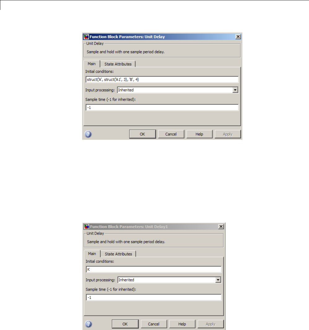
48 Using Composite Signals
•A MATLAB variable that you define as an IC structure with the
appropriate values.
For example, you could define the following partial structure in the base
workspace:
K = struct('A', struct('A1', 3), 'B', 4);
You can then specify the Kstructure as the Initial conditions parameter
of the Unit Delay block:
48-74
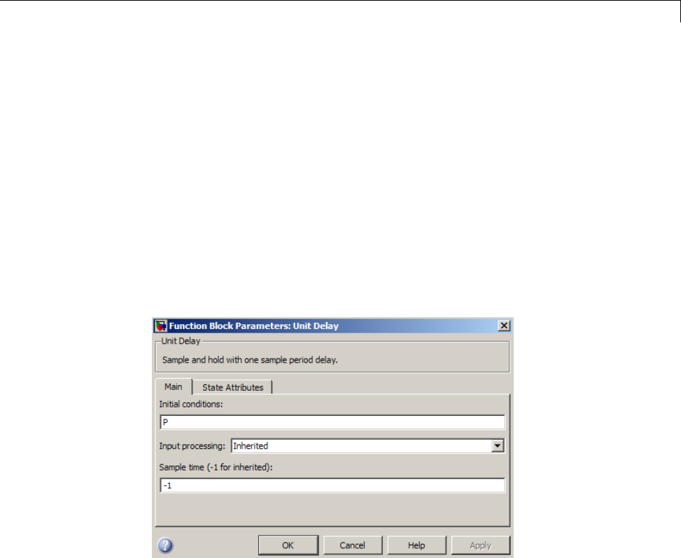
Specify Initial Conditions for Bus Signals
•ASimulink.Parameter object that uses an IC structure for the Value
property
For example, you could define the partial structure Pinthebaseworkspace
(reflecting the busic model discussed in the previous section):
P = Simulink.Parameter;
P.Datatype = 'Bus: Top';
P.Value = Simulink.Bus.createMATLABStruct('Top');
P.Value.A.A1 = 3;
P.Value.B = 5;
You can then specify the Pstructure as the Initial conditions parameter
of the Unit Delay block:
All three approaches require that you define an IC structure (see “Create
Initial Condition (IC) Structures” on page 48-67). You cannot specify a
nonzero scalar value or any other type of value other than 0,anICstructure,
or Simulink.Parameter object to initialize a bus signal.
Defining an IC structure as a MATLAB variable, rather than specifying
the IC structure directly in the block parameters dialog box offers several
advantages, including:
•Reuse of the IC structure for multiple blocks
48-75

48 Using Composite Signals
•Using the IC structure as a tunable parameter during simulation
You can tune the value of a Simulink.Parameter object during simulation.
Setting Diagnostics to Support Bus Signal
Initialization
To enable bus signal initialization, before you start a simulation, set the
following two Configuration Parameterdiagnosticsasindicated:
•In the Configuration Parameters > Diagnostics > Connectivity
pane, set “Mux blocks used to create bus signals” to error.
•Configuration Parameters > Diagnostics > Data Validity pane, set
“Underspecified initialization detection” to simplified.
The documentation for these diagnostics explains how convert your model to
handle error messages the diagnostics generate.
48-76

Combine Buses into an Array of Buses
Combine Buses into an Array of Buses
In this section...
“What Is an Array of Buses?” on page 48-77
“Benefits of an Array of Buses” on page 48-79
“Blocks That Support Arrays of Buses” on page 48-80
“Array of Buses Limitations” on page 48-81
“Define an Array of Buses” on page 48-83
“Using an Array of Buses in a Model” on page 48-86
“Generated Code for an Array of Buses” on page 48-89
“Convert a Model to Use an Array of Buses” on page 48-90
What Is an Array of Buses?
An array of buses is an array whose elements are buses. Each element in an
array of buses must be nonvirtual and must have the same bus type. (That
is, each bus object has the same signal name, hierarchy, and attributes for
its bus elements.)
An example of using an array of buses is to model a multi-channel
communication system. You can model all the channels using the same bus
object, although each of the channels could have a different value.
Using arrays of buses involves:
•Using a bus object as a data type (See “Specify a Bus Object Data Type”
on page 43-26.)
•Working with arrays (See “Create Numeric Arrays”)
To see an example of a model that uses an array of buses, open the
sldemo_bus_arrays model. In this example, the nonvirtual bus input signals
connect to a Concatenate block that creates an array of bus signals. When you
update the diagram, the model looks like the following figure:
48-77
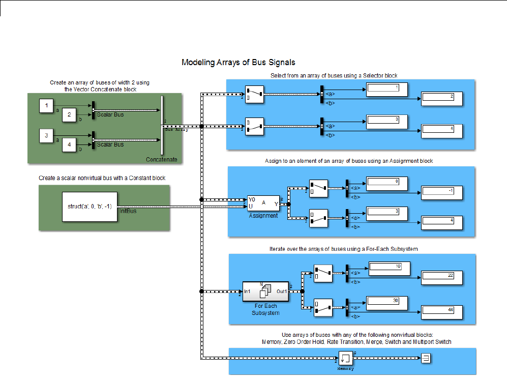
48 Using Composite Signals
The model uses the array of buses with:
•An Assignment block, to assign a bus in the array
•AForE
ach Subsystem block, to perform iterative processing over each
bus in the array
•AMem
ory block, to output the array of buses input from the previous time
step
For additional background about when to use arrays of buses, see:
•“Benefits of an Array of Buses” on page 48-79
48-78

Combine Buses into an Array of Buses
•“Blocks That Support Arrays of Buses” on page 48-80
•“Array of Buses Limitations” on page 48-81
For details about working with an array of buses, see:
•“DefineanArrayofBuses”onpage48-83
•“Using an Array of Buses in a Model” on page 48-86
•“Generated Code for an Array of Buses” on page 48-89
For information about converting an existing model, see “Convert a Model to
Use an Array of Buses” on page 48-90.
Benefits of an Array of Buses
Using an array of buses allows you to replace buses of arrays and buses of
identical buses. Using an array of buses provides these benefits:
•Represents structured data compactly
-Reduces model complexity
-Reduces maintenance by centralizing algorithms used for processing
multiple buses
•Streamlines iterative processing of multiple buses of the same type, for
example, by using a For Each Subsystem with the array of buses
•Makesiteasierforyoutochangethe number of buses, without your
having to restructure the rest of the model or make updates in multiple
places in the model
•Allows models to use built-in blocks, such as the Assignment or Selector
blocks, to manipulate arrays of buses just like arrays of any other type,
rather than your creating custom S-functions to manage packing and
unpacking structure signals
•Supports using the combined bus data across subsystem boundaries, model
reference boundaries, and into or out of a MATLAB Function block
•Allows you to keep all the logic in the Simulink model, rather than splitting
the logic between C code and the Simulink model
48-79

48 Using Composite Signals
-Supports integrated consistency and correctness checking, maintaining
metadata in the model, and avoids your keeping track of model
components in two different environments
•Generated code has an array of C structures that you can integrate with
legacy C code that uses arrays of structures:
-Makes it easier to index into an array for Simulink computations, using
afor loop on indexed structures
Blocks That Support Arrays of Buses
The following blocks support arrays of buses:
•Virtual blocks (see “Virtual Blocks” on page 23-2)
•These nonvirtual blocks:
-Data Store Memory
-Data Store Read
-Data Store Write
-Merge
-Multiport Switch
-Rate Transition
-Switch
-Zero-Order Hold
•Assignment
•MATLAB Function
•Matrix Concatenate
•Selector
•Signal Conversion
•Vector Concatenate
•Width
•Two-Way Connection (a Simscape block)
48-80

Combine Buses into an Array of Buses
For requirements for using some of these blocks with arrays of buses, see
“Block Limitations” on page 48-82.
Using Arrays of Buses with Bus-Related Blocks
To select a signal within an array of buses:
1UseaSelectorblocktofindtheappropriatebuswithinthevector.
2Use a Bus Selector block to select the signal.
To assign to a signal within an array of buses:
1UseaBusAssignmentblocktoassigntoabuselement.
2Use the Assignment block to assign the bus to the vector.
Bus Selector and Bus Assignment blocks can only accept scalar buses, no
arrays of buses.
A Bus Creator block can accept an array of buses as input, but cannot have
array of buses as output.
Array of Buses Limitations
Bus Limitations
The buses combined into an array must all:
•Be nonvirtual
•Have the same bus type (that is, same name, hierarchies, and attributes
for the bus elements)
•Have no variable-size signals or frame-based signals
Structure Parameter Limitations
The following limitations apply to using structure parameters with an array
of buses.
48-81

48 Using Composite Signals
You can use:
•0as an initial condition for an array of buses
•Ascalarstruct that represents the same hierarchy and names as the
array of buses
You cannot use:
•Partial structures
•An array of structures
•A structure parameter for an array of buses that has an element that is
an array of buses
For more information, see “Specify Initial Conditions for Bus Signals” on
page 48-65.
Set Strict Bus Handling Diagnostic to Error
Before you run simulation on a model that uses an array of buses, in the
Configuration Parameters > Diagnostics > Connectivity pane, set
Muxblocksusedtocreatebussignalsto error.
Block Limitations
The following table describes the block parameter setting limitations for
blocks that support arrays of buses. This information is also in the reference
pages for each of these blocks.
For limitations for bus-related blocks, see “Using Arrays of Buses with
Bus-Related Blocks” on page 48-81.
48-82

Combine Buses into an Array of Buses
Block Block Parameters Limitations
Memory Initial condition — Only this parameter
(which may be, but does not have to be, a
structure) is scalar-expanded to match the
dimensions of the array of buses.
Merge •Allow unequal port widths —Clearthis
parameter.
•Number of inputs —Settoavalueof2or
greater.
•Initial condition — Only this parameter
(which may be, but does not have to be, a
structure) is scalar-expanded to match the
dimensions of the array.
Multiport Switch Number of data ports — Set to a value of 2
or greater.
Signal Conversion Output —SettoSignal copy.
Switch Threshold — Specify a scalar threshold.
Simulink Feature Limitations
You cannot:
•Loganarrayofbusessignal
•Import data from or export data to an array of buses.
Stateflow Limitations
Stateflow action language does not support arrays of buses.
Define an Array of Buses
For information about the kinds of buses that you can combine into an array
of buses, see “Bus Limitations” on page 48-81.
48-83

48 Using Composite Signals
Using a Concatenate Block to Define an Array of Buses
To define an array of buses, use a Concatenate block. The table describes
the array of buses input requirements and output for each of the Vector
Concatenate and the Matrix Concatenate versions of the Concatenate block.
Block Bus Signal Input
Requirement
Output
Vector
Concatenate
Vectors, row vectors, or
columns vectors
If any of the inputs are row or
column vectors, row or column
vector
Matrix
Concatenate
Signals of any
dimensionality (scalars,
vectors, and matrices)
Trailing dimensions are
assumedtobe1forlower
dimensionality inputs.
Concatenation is on the
dimension that you specify with
the Concatenate dimension
parameter.
To use a Concatenate block to define an array of buses, see “How to Define
an Array of Buses” on page 48-84.
Note Do not use a Mux block or a Bus Creator block to define an array of
buses. Instead, use a Bus Creator block to create scalar bus signals.
How to Define an Array of Buses
1Define one bus object to use for all the bus signals that you want to combine
into an array of buses. For information about defining bus objects, see
“Create Bus Objects” on page 48-29.
The sldemo_bus_arrays model defines an sldemo_bus_arrays_busobject
bus object, which the Bus Creator blocks use for the input bus signals
(Scalar Bus)forthearrayofbuses.
2Add a Vector Concatenate or Matrix Concatenate block to the model and
open the block parameters dialog box for the block.
48-84

Combine Buses into an Array of Buses
The sldemo_bus_arrays_busobject model uses a Vector Concatenate
block, because the inputs are scalars.
3Set the Number of inputs parametertobethenumberofbusesthatyou
want to be in the array of buses.
The block icon displays the number of input ports that you specify.
4Set the Mode parametertomatchthetypeoftheinputbusdata.
In the sldemo_bus_arrays model, the input bus data is scalar, so the
Mode setting is Vector.
5If you use a Matrix Concatenation block, set the Concatenate dimension
parameter to specify the output dimension along which to concatenate the
input arrays. Enter one of the following values:
•1to concatenate input arrays vertically
•2to concatenate input arrays horizontally
•A higher dimension than 2, to perform multidimensional concatenation
on the inputs
6Connect the buses that you want to be in the array of buses to the
Concatenate block.
Signal Line Style for an Array of Buses
After you create an array of buses and update the diagram, the line style for
the array of buses signal is a thicker version of the signal line style for a
nonvirtual bus signal.
For example, in the sldemo_bus_arrays model, the Scalar Bus signal is a
nonvirtual bus signal, and the Bus Array output signal of the Concatenate
block is an array of buses signal.
48-85
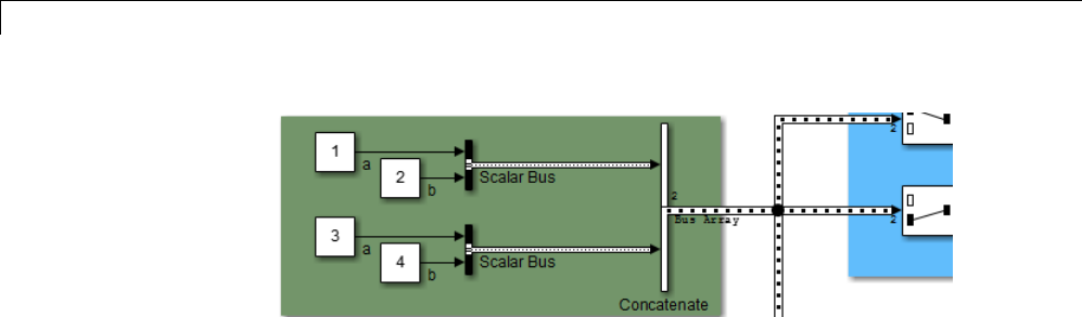
48 Using Composite Signals
Using an Array of Buses in a Model
A General Workflow for Using an Array of Buses in a Model
Setting up a model to use an array of buses usually involves basic tasks
similar to these:
1Define the array of buses, as described in “Define an Array of Buses” on
page 48-83.
2Add a subsystem for performing iterative processing on each element
of the array of buses. For example, use a For Each Subsystem block or
an Iterator block. See “Performing Iterative Processing with an Array of
Buses” on page 48-87.
3Connect the array of buses signal from the Concatenate block to the
iterative processing subsystem that you set up in step 2.
4Model yourscalaralgorithmwithintheiterative processing subsystem
(for example, a For Each subsystem). Operate on the array first (using
Selector and Assignment blocks), and then use the Bus Selector and Bus
Assignment blocks to select elements from, or assign elements to, a scalar
bus within the subsystem.
This simplified picture reflects the general workflow described above.
48-86
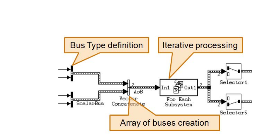
Combine Buses into an Array of Buses
Performing Iterative Processing with an Array of Buses
You can perform iterative processing on the bus signal data of an array of
buses using blocks such as a For Each Subsystem block, a While Iterator
Subsystem block, or a For Iterator Subsystem block. You can use one of these
blocks to perform the same kind of processing on each bus in the array of
buses, or a selected subset of buses in the array of buses.
Assigning Into an Array of Buses
Use an Assignment block to assign values to specified elements in a bus array.
For example, in the sldemo_bus_arrays model, the Assignment block assigns
the value to the first element of the array of buses. The block parameters
dialog box looks like the following graphic:
48-87

48 Using Composite Signals
To assign bus elements within a bus signal, use the Bus Assignment block.
The input for the Bus Assignment block must be a scalar bus signal.
Selecting Bus Elements from an Array of Buses
Use a Selector block to select elements of an array of buses. The input array
of buses can be of any dimensionality.
The output bus signal of the Selector block is a selected or reordered set of
elements from the input array of buses.
For example, the sldemo_bus_arrays model uses Selector blocks to select
elements from the array of buses signal that the Assignment and For Each
Subsystem blocks outputs. The block parameters dialog box for the Selector
block that selects the first element looks like the following graphic:
48-88
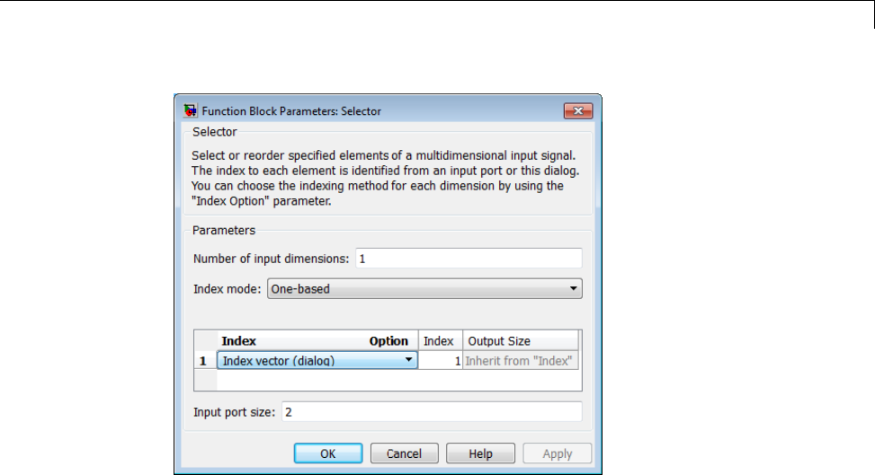
Combine Buses into an Array of Buses
To select bus elements within a bus signal, use the Bus Selector block. The
input for the Bus Selector block must be a scalar bus signal.
Generated Code for an Array of Buses
When you generate code for a model that includes an array of buses, a typedef
that represents the underlying bus type appears in the *_types.h file.
Code generation produces an array of C structures that you can integrate
with legacy C code that uses arrays of structures. As necessary, code for bus
variables (arrays) are generated in the following structures:
•Block IO
•States
•External inputs
•External outputs
Here is a simplified example of some generated code for an array of buses.
48-89

48 Using Composite Signals
Convert a Model to Use an Array of Buses
There are several reasons to convert a model to use an array of buses (see
“Benefits of an Array of Buses” on page 48-79). For example:
•The model was developed before Simulink supported arrays of buses
(introduced in R2010b), and the model contains many subsystems that
perform the same kind of processing.
•The model that has grown in complexity.
General Workflow for Converting a Model to Use an Array
of Buses
This section presents a general guide to converting a model that contains
buses to a model that uses an array of buses. The method that you use
depends on your model. For details about these techniques, see “Combine
Buses into an Array of Buses” on page 48-77.
This workflow refers to a stylized example model. The example shows the
original modeling pattern and a new modeling pattern that uses an array
of buses.
48-90
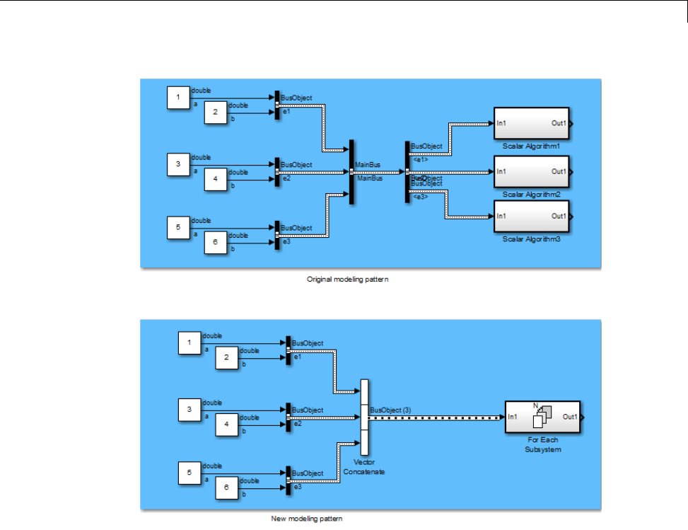
Combine Buses into an Array of Buses
In the original modeling pattern:
•The target bus signal to be converted is named MainBus, and it has three
elements, each of type BusObject.
•The ScalarAlgorithm1,ScalarAlgorithm2,andScalarAlgorithm3
subsystems encapsulate the algorithms that operate on each of the bus
elements. The subsystems all have the same content.
•A Bus Selector block picks out each element of MainBus to drive the
subsystems.
The construction in the original modeling pattern is inefficient for two reasons:
48-91

48 Using Composite Signals
•A copy of the subsystem that encapsulates the algorithm is made for each
element of the bus that is to be processed.
•Adding another element to MainBus involves changing the bus object
definition and the Bus Selector block, and adding a new subsystem. Each
of these changes is a potential source of error.
To convert the original modeling pattern to use an array of buses:
1Identify the target bus and associated algorithm that you want to convert.
Typically, the target bus signal is a bus of buses, where each element bus
signal is of the same type.
•The bus that you convert must be a nonvirtual bus. You can convert a
virtual bus to a nonvirtual bus if all elements of the target bus have the
same sample time (or if the sample time is inherited).
•The target bus cannot have variable-dimensioned and frame-based
elements.
2Use a Vector Concatenate or Matrix Concatenate block to convert the
original bus of buses signal to an array of buses.
In the example, the new modeling pattern uses a Vector Concatenate block
to replace the Bus Creator block that creates the MainBus signal. The
output of the Vector Concatenate block is an array of buses, where the type
of the bus signal is BusObject. The new model eliminates the wrapper
bus signal (MainBus).
3Replace all identical copies of the algorithm subsystem with a single
For-Each subsystem that encapsulates the scalar algorithm. Connect the
array of buses signal to the For-Each subsystem.
The new model eliminates the Bus Selector blocks that separate out the
elements of the MainBus signal in the original model.
4Configure the For Each Subsystem block to iterate over the input array of
buses signal and concatenate the output bus signal.
For limitations, see the For Each Subsystem block documentation; for
example, the scalar algorithm within the For-Each subsystem cannot have
continuous states.
48-92

Bus Data Crossing Model Reference Boundaries
Bus Data Crossing Model Reference Boundaries
A model reference boundary refers to the boundary between a model that
contains a Model block and the referenced model. If you have bus data in a
model that is passed to a Model block, then that data crosses the boundary to
the referenced model.
To have bus data cross model reference boundaries:
1Use a nonvirtual bus (required). Using a nonvirtual bus provides a
well-defined data interface for code generation.
Use a bus object (Simulink.Bus) to define the bus. For details, see
“Creating Nonvirtual Buses” on page 48-12.
2Consider stripping out unneeded data from bus objects crossing model
reference boundaries.
In large models, bus objects can become quite large and have several levels
of hierarchy. Often referenced models need some, but not all, of the data
contained in large buses. Passing unneeded data across model reference
boundaries impacts performance negatively. The interface definition for a
model should specify exactly what data the model uses.
48-93

48 Using Composite Signals
Buses and Libraries
When you define a library block, the block can input, process, and output
buses just as an ordinary subsystem can. MathWorks recommends not
using Bus Selector blocks in library blocks, because such use complicates
changing the library blocks and increases the likelihood of errors. When a
Bus Selector block appears in a library block, the following considerations
and recommendations apply:
•You cannot change a Bus Selector block directly within a library. To change
the Bus Selector block, copy the library block that uses it to a model, edit
the Bus Selector block within the context of the model, then copy the
changed library block back to the library.
•The Inport that feeds the Bus Selector block should have an associated bus
object, as described in “Bus Objects” on page 48-20. This bus object must
be stored in a MATLAB code file or MAT-file, and imported into the base
workspace of any model that subsequently uses the library block.
•Any model that uses the library block containing the Bus Selector should
set Configuration Parameters > Connectivity > Element name
mismatch to error. This setting minimizes the possibility of consistency
errors at the interface to the library block.
See “Block Libraries” for information about creating block libraries and
copying library blocks to and from them.
48-94

Avoid Mux/Bus Mixtures
Avoid Mux/Bus Mixtures
In this section...
“Introduction” on page 48-95
“Using Diagnostics for Mux/Bus Mixtures” on page 48-96
“Using the Model Advisor for Mux/Bus Mixtures” on page 48-100
“Correcting Buses Used as Muxes” on page 48-101
“Bus to Vector Block Compatibility Issues” on page 48-103
“Avoiding Mux/Bus Mixtures When Developing Models” on page 48-104
Introduction
You can use muxes and virtual buses interchangeably in a model if all
constituent signals have the same attributes and the model has no nested
buses. You can implement such a signal as either a mux or a virtual bus, and
the Simulink software by default automatically converts between the two
formatsasneeded. See“MuxSignals” on page 47-11 for information about
muxes.
Do not mix muxes and buses in new applications.
One way that such a mux/bus mixture occurs is when you use a Mux block
to create a virtual bus, such as a Mux block that outputs to a Bus Selector.
This kind of mixture does not support strong type checking and increases
the likelihood of run-time errors. MathWorks discourages treating muxes
and buses interchangeably. Mux/bus mixtures may become unsupported
in the future. Simulink generates a warning for this kind of mux/bus
mixture when you load a model created in a release prior to R2010a. For
new models, Simulink generates an error. Do not create such mux/bus
mixtures in new applications, and consider upgrading existing applications to
avoid such mixtures. The Configuration Parameters > Diagnostics >
Connectivity pane provides diagnostics that report cases where muxes and
virtual buses are used interchangeably, and includes capabilities that you can
use to upgrade a model to eliminate such mixtures. See “Using Diagnostics for
Mux/Bus Mixtures” on page 48-96 and “Using the Model Advisor for Mux/Bus
Mixtures” on page 48-100 for details.
48-95

48 Using Composite Signals
Another way for a mux/bus mixture to occur is when a virtual bus signal is
treated as a mux, such as a bus signal that inputs directly to a Gain block. To
detect such mixtures, in the Configuration Parameters > Diagnostics
> Connectivity pane, set the Bus signal treated as vector diagnostic
to warning or error.
Note Do not confuse muxes used as bus elements, which is legal and causes
no problems, with mux/bus mixtures. A mux/bus mixture occurs only when
some blocks treat a signal as a mux, while other blocks treat that same signal
as a bus.
Using Diagnostics for Mux/Bus Mixtures
The Configuration Parameters > Diagnostics > Connectivity pane
provides the following diagnostics to detect mux/bus mixtures.
Diagnostic Description
Mux blocks used to create bus
signals
Detect and correct muxes that are
used as buses
Bus signal treated as vector Detect and correct buses that are
used as muxes (vectors)
Non-bus signals treated as bus
signals
Detect when Simulink implicitly
converts a non-bus signal to a bus
signal
You can use these diagnostics as described in this section, or you can use the
Model Advisor to perform the some of these checks and also to obtain advice
about corrections, as described in “Consult the Model Advisor” on page 4-81.
For complete information about the Connectivity pane, see “Connectivity
Diagnostics Overview”.
Mux blocks used to create bus signals
To detect and correct muxes that are used as buses, in the Configuration
Parameters > Diagnostics > Connectivity pane:
1Set Mux blocks used to create bus signals to warning or error.
48-96
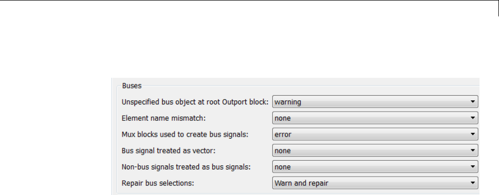
Avoid Mux/Bus Mixtures
2Set Bus signal treated as vector to none.
3Click OK or Apply.
4Build the model.
5Replace blocks as needed to correct any cases of Mux blocks used to create
buses. You can use the slreplace_mux function to replace all such Mux
blocks in a single operation.
For complete information about this option, see the reference documentation
for “Mux blocks used to create bus signals”.
Bus signal treated as vector
To detect and correct buses that are used as if they were muxes (vectors):
1Correct any cases of Mux blocks used to create buses as described in “Mux
blocks used to create bus signals” on page 48-96.
2In the Configuration Parameters > Diagnostics > Connectivity
pane, set Muxblocksusedtocreatebussignalsto error.
3Inthesamepane,setBus signal treated as vector to warning or error.
48-97
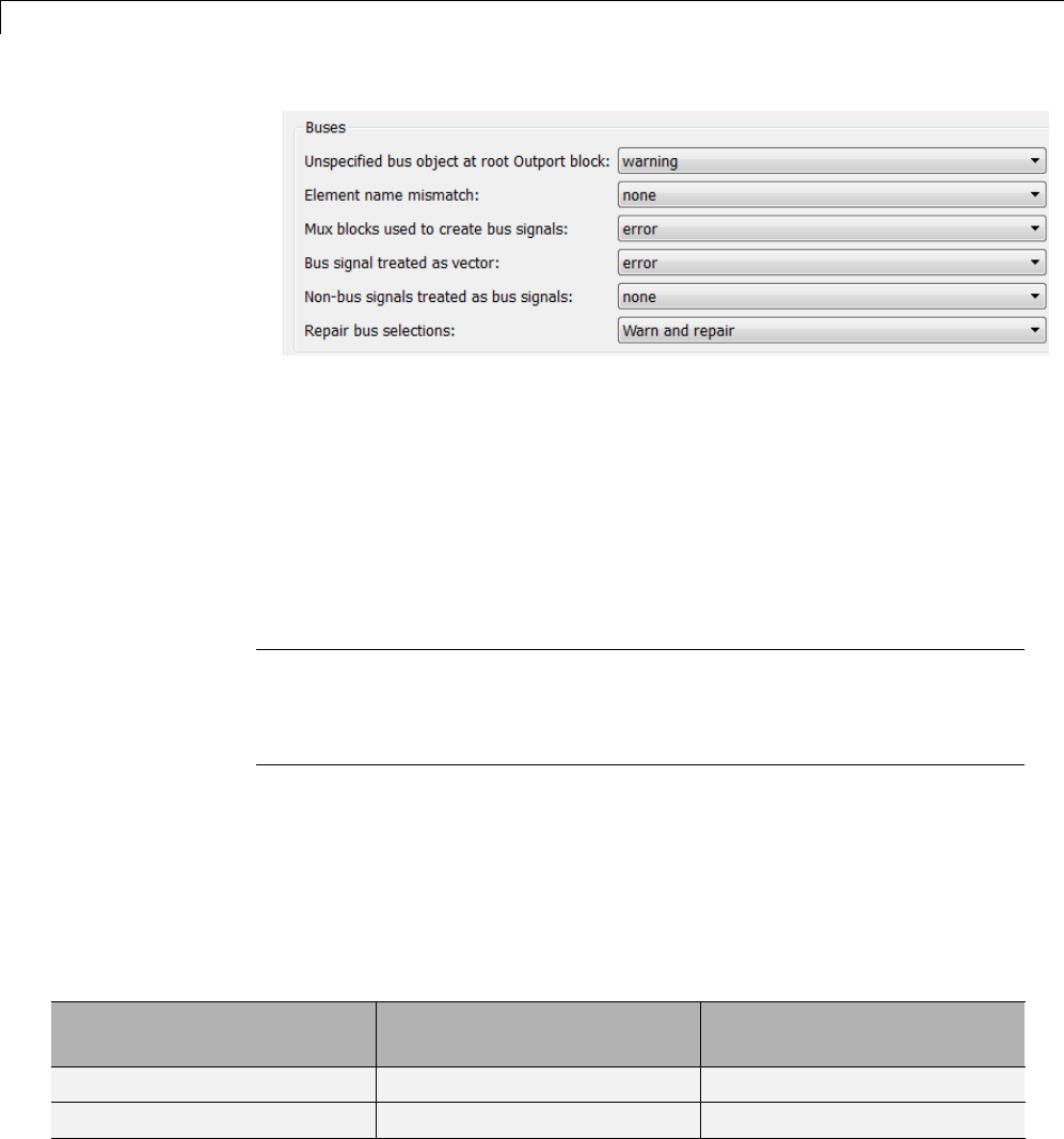
48 Using Composite Signals
4Click OK or Apply.
5Build the model.
6Correct the model where needed as described under “Correcting Buses
Used as Muxes” on page 48-101.
For complete information about this option, see the reference documentation
for “Bus signal treated as vector”.
Note Bus signal treated as vector is disabled unless you set Mux blocks
used to create bus signals to error. Setting Bus signal treated as vector
to error has no effect unless you have previously corrected all cases of Mux
blocks used to create buses.
Equivalent Parameter Values
Due to the requirement that Mux blocks used to create bus signals be
error before Bus signal treated as vector is enabled, one parameter,
StrictBusMsg, can specify all permutations of the two controls. The
parametercanhaveoneoffivevalues.Thefollowingtableshowsthesevalues
and the equivalent GUI control settings:
Value of StrictBusMsg
(API)
Mux blocks used to create
bus signals (GUI)
Bus signal treated as vector
(GUI)
None none none
Warning warning none
48-98

Avoid Mux/Bus Mixtures
Value of StrictBusMsg
(API)
Mux blocks used to create
bus signals (GUI)
Bus signal treated as vector
(GUI)
ErrorLevel1 error none
WarnOnBusTreatedAsVector error warning
ErrorOnBusTreatedAsVector error error
Non-bus signals treated as bus signals
Detect when Simulink implicitly converts a non-bus signal to a bus signal:
1Correct any cases of Mux blocks used to create buses as described in “Mux
blocks used to create bus signals” on page 48-96.
2In the Configuration Parameters > Diagnostics > Connectivity
pane, set Muxblocksusedtocreatebussignalsto error.
3Inthesamepane,setNon-bus signals treated as bus signals to
warning or error.
4Click OK or Apply.
5Build the model.
6Correct the model where needed as described under “Correcting Buses
Used as Muxes” on page 48-101.
For complete information about this option, see the reference documentation
for “Non-bus signals treated as bus signals”.
48-99

48 Using Composite Signals
UsingtheModelAdvisorforMux/BusMixtures
The Model Advisor provides a convenient way to both run the diagnostics for
mux/busmixturesandobtainadviceabout corrections. To use the Model
Advisor to detect and correct mux/bus mixtures:
1Set Configuration Parameters > Diagnostics > Connectivity > Buses
> Mux blocks used to create bus signals to none.
2Click OK or Apply.
3Select and run the Model Advisor check Simulink > Check for proper
bus usage.
The Model Advisor reports any cases of Mux blocks used to create bus
signals.
4Follow the Model Advisor’s suggestions to correct any errors reported by
the check. You can use the slreplace_mux function to replace all such
errors in a single operation.
5Set Configuration Parameters > Diagnostics > Connectivity > Buses
>Muxblocks used to create bus signals to error.
6Set Configuration Parameters > Diagnostics > Connectivity > Bus
signal treated as vector to none.
48-100
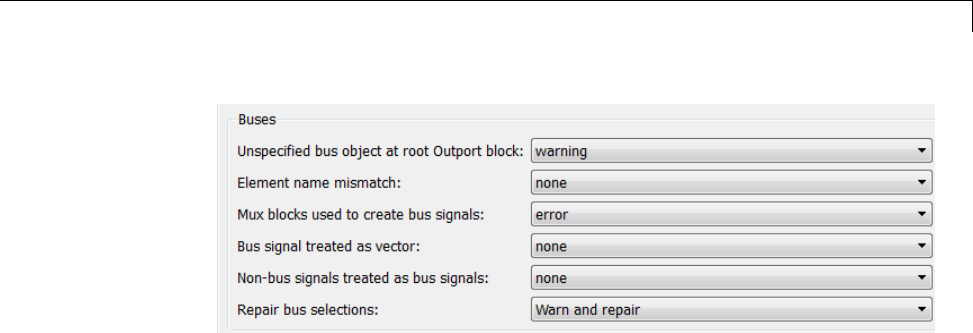
Avoid Mux/Bus Mixtures
7Click OK or Apply.
8Again run the Model Advisor check Simulink > Check for proper bus
usage.
The Model Advisor reports any cases of bus signals treated as muxes
(vectors).
9Follow the Model Advisor’s suggestions and the information in “Correcting
Buses Used as Muxes” on page 48-101 to correct any errors discovered
by the check.
Instructions for using the Model Advisor appear in “Consult the Model
Advisor” on page 4-81.
Correcting Buses Used as Muxes
Whenyoudiscoverabussignalusedasamux,oneansweristoreorganizethe
model by replacing blocks so that the mixture no longer occurs. Where that is
undesirable or unfeasible, the Simulink software provides two capabilities to
address the problem:
•The Bus to Vector block (Signal Attributes library), which you can insert
into any bus used implicitly as a mux to explicitly convert the bus to a
mux (vector).
•The Simulink.BlockDiagram.addBusToVector function, which
automatically inserts Bus to Vector blocks wherever needed.
48-101
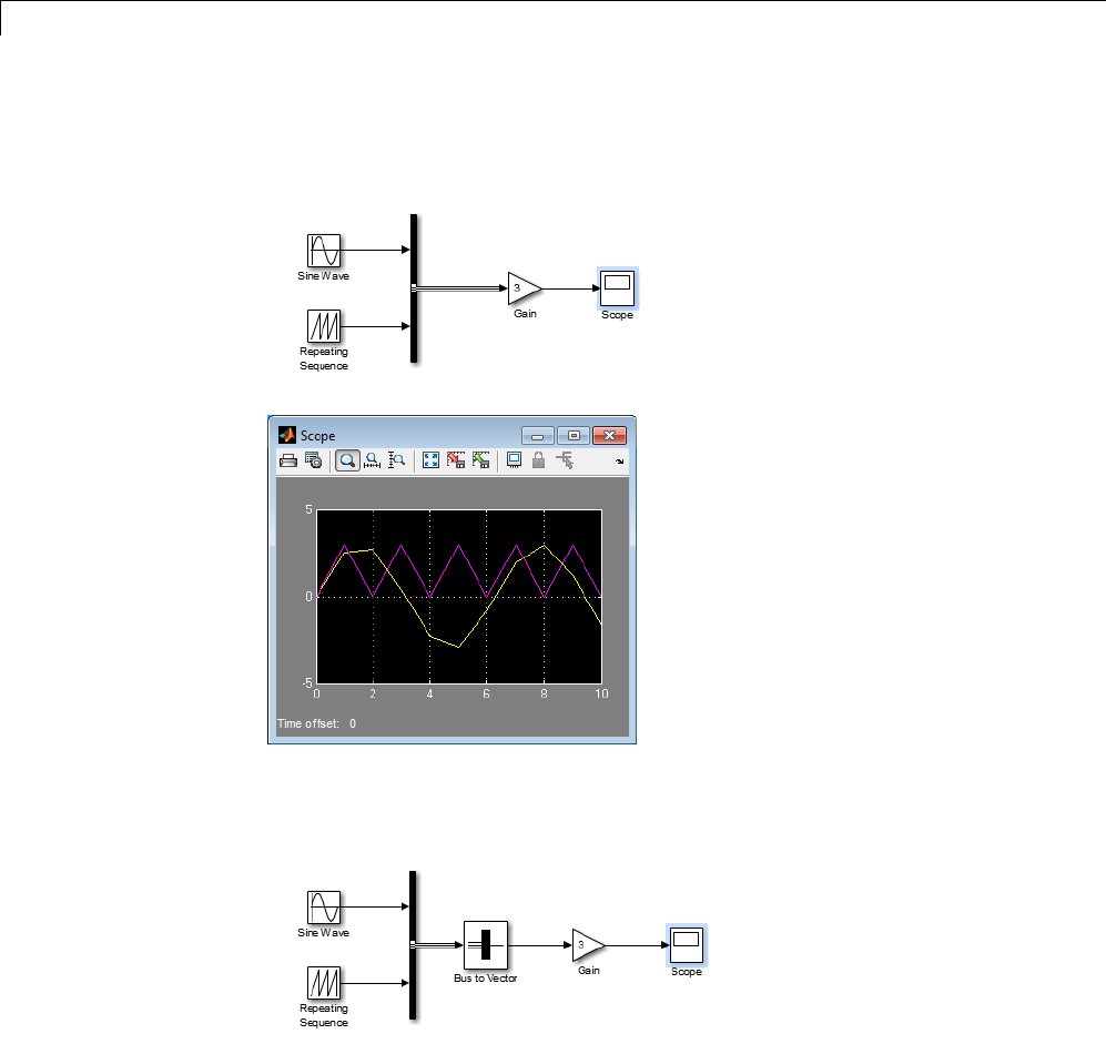
48 Using Composite Signals
For example, this model uses a bus as a mux by inputting the bus to a Gain
block. The Scope block shows the results.
This figure shows the same model, rebuilt after inserting a Bus to Vector
block into the bus.
48-102
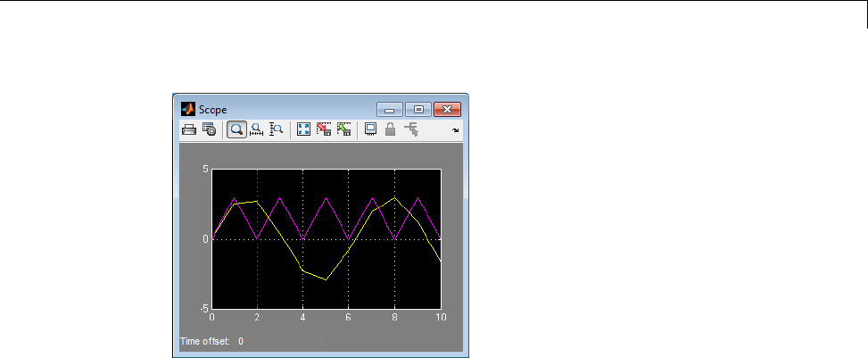
Avoid Mux/Bus Mixtures
Note that the results of simulation are the same in either case. The Bus to
Vector block is virtual, and never affects simulation results, code generation,
or performance. For more information, see the reference documentation for
the Bus to Vector block and the Simulink.BlockDiagram.addBusToVector
function.
Bus to Vector Block Compatibility Issues
If you use Save As to save a model in a version of the Simulink product before
R2007a (V6.6), the following is done:
•Set the StrictBusMsg parameter to error if its value is
WarnOnBusTreatedAsVector or ErrorOnBusTreatedAsVector.
•Replace each Bus to Vector block in the model with a null subsystem that
outputs nothing.
The resulting model specifies strong type checking for Mux blocks used to
create buses. Before you can use the model, you must reconnect or otherwise
correct each signal that contained a Bus to Vector block but is now interrupted
by a null subsystem.
In R2010a, if you load a model created in a prior release, you may get warning
messages that you did not get before. To avoid getting Mux block-related
warnings for existing models that you want to load in R2010a, use the
slreplace_mux function to substitute Bus Creator blocks for any Mux blocks
used to create buses signals.
48-103

48 Using Composite Signals
Avoiding Mux/Bus Mixtures When Developing
Models
MathWorks discourages the use of mux/bus mixtures, and may cease to
support them at some future time. MathWorks, therefore, recommends
upgrading existing models to eliminate any mux/bus mixtures, and
permanently setting Mux blocks used to create bus signals and Bus
signal treatedasvectorto error in all new models and all existing models
that may undergo further development.
Note The Bus to Vector block is intended only for use in existing models to
facilitate the elimination of implicit conversion of buses into muxes. New
models and new parts of existing models should avoid mux/bus mixtures, and
should not useBustoVectorblocksforanypurpose.
48-104

Buses in Generated Code
Buses in Generated Code
If you have a Simulink Coder license, the various techniques for defining
buses are essentially equivalent for simulation, but the techniques used
can make a significant difference in the efficiency, size, and readability of
generated code. For example, a nonvirtual bus appears as a structure in
generated code, and only one copy exists of any algorithm that uses the bus.
The use of a structure in the generated code can be helpful when tracing the
correspondence between the model and the code. For example, below is the
generated code for Bus Creator block in the sldemo_mdlref_bus model.
A virtual bus does not appear as a structure or any other coherent unit in
generated code, and a separate copy of any algorithm that manipulates the
bus exists for each element.
Using buses properly results in efficient code and visually clean models. If you
intend to generate production code for a model that uses buses, see “Buses”
for information about the best techniques to use.
48-105

48 Using Composite Signals
Composite Signal Limitations
•Buses that contain signals of enumerated data types cannot pass through
a block that requires a nonzero scalar initial value (such as a Unit Delay
block).
•Root level bus outputs cannot be logged using the Configuration
Parameters > Data Import/Export > Save to Workspace > Output
option. Use standard signal logging instead, as described in “Export Signal
Data Using Signal Logging” on page 45-19.
•Inputs to a Bus Creator block must have unique names. If there are
duplicate names, the Bus Creator block appends (signal#) to all input
signal names, where #is the input port index.
48-106

49
Working with Variable-Size
Signals
•“Variable-Size Signal Basics” on page 49-2
•“Simulink Models Using Variable-Size Signals” on page 49-6
•“S-Functions Using Variable-Size Signals” on page 49-20
•“Simulink Block Support for Variable-Size Signals” on page 49-23
•“Variable-Size Signal Limitations” on page 49-26

49 Working with Variable-Size Signals
Variable-Size Signal Basics
In this section...
“About Variable-Size Signals” on page 49-2
“Creating Variable-Size Signals” on page 49-2
“How Variable-Size Signals Propagate” on page 49-3
“Empty Signals” on page 49-4
“Subsystem Initialization of Variable-Size Signals” on page 49-4
About Variable-Size Signals
A Simulink signal can be a scalar, vector (1-D), matrix (2-D), or N-D. For
information about these types of signals, see “Signal Basics” on page 47-2 in
the Simulink User’s Guide.
A Simulink variable-size signal is a signal whose size (the number of
elements in a dimension), in addition to its values, can change during a model
simulation. However, during a simulation, the number of dimensions cannot
change. This capability allows you to model systems with varying resources,
constraints, and environments.
Creating Variable-Size Signals
You can create variable-size signals in your Simulink model by using:
•Switch or Multiport Switch blocks with different input ports having
fixed-size signals with different sizes. The output is a variable-size signal.
•AselectorblockandtheStarting and ending indices (port) indexing
option. The index port signal can specify different subregions of the
input data signal which produce an output signal of variable size as the
simulation progresses.
•The S-function block with the output port configured for a variable-size
signal. The output includes not only the values but also the dimension
of the signal.
49-2
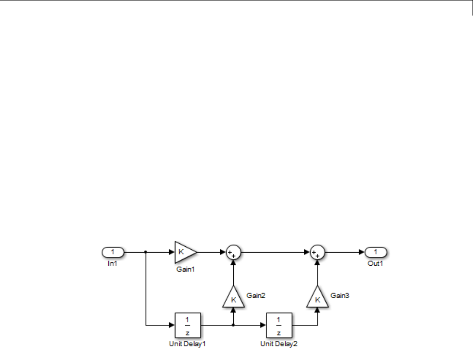
Variable-Size Signal Basics
How Variable-Size Signals Propagate
In the Simulink environment, variable-size signals can change their size
during model execution in one of two ways:
•At every step of model execution.
Various blocks in the model modify the sizes of the signals during execution
of the output method.
•Only during initialization of conditionally executed subsystems.
Size changes occur during distinct mode-switching events in subsystems
such as Action, Enable, and Function-Call subsystems.
You can see the key difference by considering a Discrete 2-Tap Filter block
with states.
Discrete 2-Tap Filter
Assume that the input signal dimension to this filter changes from 4 to 1
during simulation. It is ambiguous when and how the states of the Unit
Delay blocks should adapt from 4 to 1 to continue processing the input. To
ensure consistency, both Unit Delay blocks must change their state behavior
synchronously. To prevent ambiguity, Simulink generally disallows blocks
whose number of states depends on input signal sizes in contexts where signal
sizes change at any point during execution.
In contrast, consider the same Discrete 2-Tap Filter block in a Function-Call
subsystem. Assume that this subsystem is using the second way to propagate
variable-size signals. In this case, the size of the input signal changes from
49-3

49 Working with Variable-Size Signals
4 to 1 only at the initialization of the subsystem. At initialization, the
subsystem resets all of its states (including the states of the two Unit Delay
blocks) to their initial values. Resetting the subsystem ensures no ambiguity
on the assignment of states to the input signal of the filter.
“Mode-Dependent Variable-Size Signals” on page 49-14 shows how you can
use the two ways of propagating variable-size signals in a complementary
fashion to model complex systems.
Empty Signals
An empty signal is a signal with a length of 0. For example, signals with
size [0],[0x3],[2x0],and[2x0x3] are all empty signals. Simulink allows
empty signals with variable-size signals and supports most element-wise
operations. However, Simulink does not support empty signals for blocks that
modify signal dimensions. Unsupported blocks include Reshape, Permute,
and Sum along a specified dimension.
Subsystem Initialization of Variable-Size Signals
The initial signal size from an Outport block in a conditionally executed
subsystem varies depending on the parameters you select.
If you set the Propagate sizes of variable-size signals parameter in the
parent subsystem to During execution,theInitial output parameter for
the Output block must not exceed the maximum size of the input port. If the
Initial output parameter value is:
Initial output parameter Initial output signal size
A nonscalar matrix The initial output signal size is
thesizeoftheInitial output
parameter.
Ascalar The initial output signal size is a
scalar.
The default [] The initial output size is an empty
signal (dimensions are all zeros).
49-4

Variable-Size Signal Basics
If you set the Propagate sizes of variable-size signals parameter in the
parent subsystem to Only when enabling,theInitial output parameter for
the Output block must be a scalar value.
•When size is repropagated for the input of the Outport block, the initial
output value is set using scalar expansion from the scalar parameter value.
•If the Initial output parameter is the default value [], Simulink treats
the initial output as a grounded value.
•If the model does not activate the parent subsystem at start time (t=0),
the current size of the subsystem output corresponding to the Outport
block is set to maximum size.
•When its parent subsystem repropagates signal sizes, the values of the
subsystem variable-size output signals are also reset to their initial output
parameter values.
49-5

49 Working with Variable-Size Signals
Simulink Models Using Variable-Size Signals
In this section...
“Variable-Size Signal Generation and Operations” on page 49-6
“Variable-Size Signal Length Adaptation” on page 49-10
“Mode-Dependent Variable-Size Signals” on page 49-14
Variable-Size Signal Generation and Operations
This example model shows how to create a variable-size signal from multiple
fixed-size signals and from a single data signal. It also shows some of the
operations you can apply to variable-size signals.
For a complete list of blocks that support variable-size signals, see “Simulink
Block Support for Variable-Size Signals” on page 49-23.
1In the MATLAB Command Window, type
sldemo_varsize_basic
2In the Simulink Editor, select Display > Signals & Ports > Signal
Dimensions. Run a simulation or press Ctrl-D.
The Simulink editor displays the signal dimensions and line styles. See
“Signal Basics” on page 47-2 for an interpretation of signal line styles.
49-6
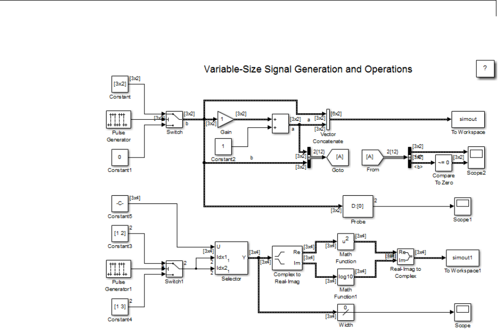
Simulink Models Using Variable-Size Signals
Creating a Variable-Size Signal from Fixed-Size Signals
Onewaytocreateavariable-sizesignalistousetheSwitchblock.Theinput
signals to the Switch block can differ in their number of dimensions and in
their size.
49-7
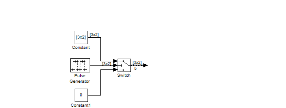
49 Working with Variable-Size Signals
Output from the Switch block is a 2-D variable-size signal with a maximum
size of 3x2.WhenyouselecttheAllow different data input sizes
parameter on the Switch block, Simulink does not expand the scalar value
from the Constant1 block.
Saving Variable-Size Signal Data
You could add a To Workspace block to the output from the Switch block.
Since the model already has a To Workspace block, the second To Workspace
block would save data to a signal array named simout2 The values field logs
the actual signal values. If logged signal data is smaller than the maximum
size, values are padded with NaNs or appropriate values. To obtain these
signal values, type:
simout2.signals.values
ans(:,:,1) =
1-1
-2 2
-3 3
ans(:,:,2) =
1-1
-2 2
49-8

Simulink Models Using Variable-Size Signals
-3 3
ans(:,:,3) =
0NaN
NaN NaN
NaN NaN
The valueDimensions field logs the dimensions of a variable-size signal. To
obtain the dimensions, type:
simout2.signals.valueDimensions
Thesignaldimensionsforthefirstthreetimestepsareshown.
ans =
32
32
11
Creating a Variable-Size Signal from a Single Data Signal
The data signal (Constant5) is a 3x4 matrix. The Pulse Generator represents
a control signal that selects a starting and ending index value ( [1 2] or [1
3]). The Selector block then uses the index values to select different parts of
the data signal at each time step and output a variable-size signal.
49-9
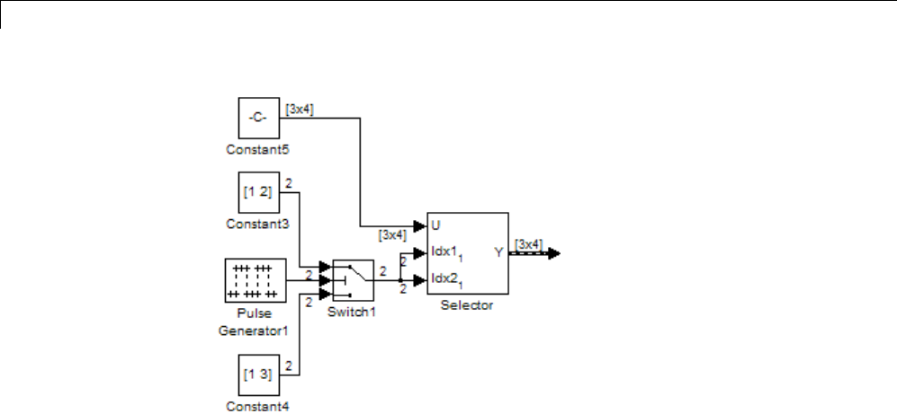
49 Working with Variable-Size Signals
Viewing Changes in Signal Size
The output from the Selector block is either a 2x2 or 3x3 matrix. Because the
maximum dimension for a variable-size signal is the 3x4 matrix from the data
signal, the logged output signals are padded with NaNs.
Use the Probe or Width blocks to inspect the current dimensions and width
of a variable-size signal. In addition, you can display variable-size signals
on Scope blocks and save variable-size signals to the workspace using the
To Workspace block.
Processing Variable-Size Signals
The remainder of the model shows various operations that are possible with
variable-size signals. Operations include using the Gain block, the Sum block,
theMathFunctionblock,theMatrixConcatenate block. You can connect
variable-size signals with the From, Goto, Bus Assignment, Bus Creator, and
Bus Selector blocks.
Variable-Size Signal Length Adaptation
This example model corresponds to a hypothetical system where the model
adapts the length of a signal over time. Length adaptation is based on the
value of a control signal. When the control signal falls within one of three
49-10
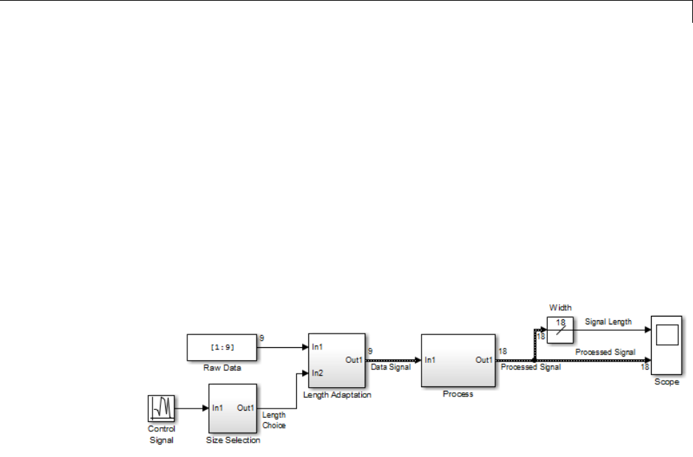
Simulink Models Using Variable-Size Signals
predefined ranges, the fixed-size raw data signal changes to a variable-size
data signal.
The variable-size signal connects to a processing block, where blocks that
support variable-size signals operate on it. A MATLAB Function block with
both input and output signals of variable size allow more flexibility than other
blocks supporting variable-size signals. See “Simulink Block Support for
Variable-Size Signals” on page 49-23.
To open the example model, in the MATLAB® Command Window, type:
sldemo_varsize_dataLengthAdapt
Creating a Variable-Size Signal by Adapting the Length of a
Data Signal
This model generates a data signal and converts the signal to a variable-size
signal. The size of the signal depends on the value of a control signal. The
raw data signal is a column vector with values from 1to 9.
[1:9].'
ans =
1
2
3
4
5
6
7
49-11
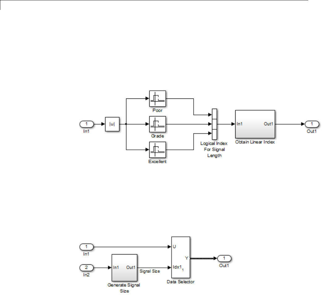
49 Working with Variable-Size Signals
8
9
The Size Selection subsystem determines the quality of the data signal and
outputs a quality value ( 1, 2, or 3). This value helps to select the length of the
data signal in the Length Adaptation subsystem.
IntheLengthAdaptationsubsystem,the Signal Size subsystem generates an
index based on the quality value from the Size Selection subsystem (In2). The
Data Selector block uses the starting and ending indices to adapt the length
of the data signal (In1) and output a variable-size signal.
49-12
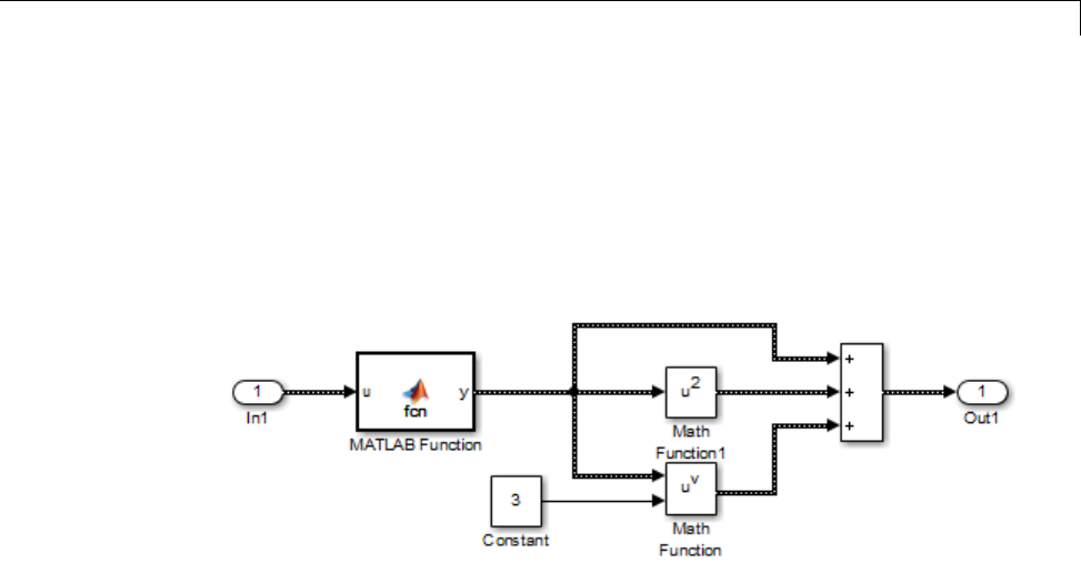
Simulink Models Using Variable-Size Signals
Processing a Variable-Size Signal
The center section of the model processes the variable-size signal. The
MATLAB Function block adds zeros between the data values in a way that
is similar to upsampling a signal. The dimension of the signal changes from
9to 18. The Math Function blocks shows various manipulations you can
do with variable-size signals.
Visualizing a Variable-Size Signal
The right section of the model determines the signal width (size) and uses a
scope to visualize the width and the processed data signal.
49-13
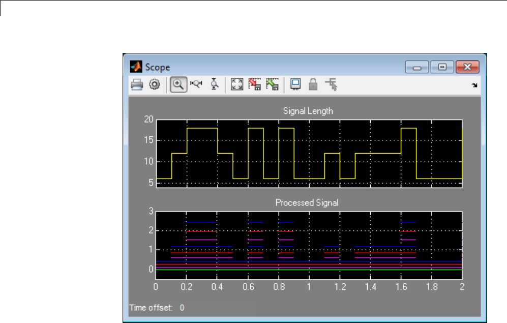
49 Working with Variable-Size Signals
Mode-Dependent Variable-Size Signals
This example model represents a system that has three operation modes. For
each mode, the data signal to process has a different size.
The Process subsystem in this model receives a variable-size signal where the
size of the signal depends on the operation mode of the system. For each
mode change, the Stateflow chart, Mode Control Logic, detects when the data
signal size changes. It then generates a function call to reset the blocks in
the Process subsystem.
To open the model, In the MATLAB Command Window, type:
sldemo_varsize_multimode
49-14
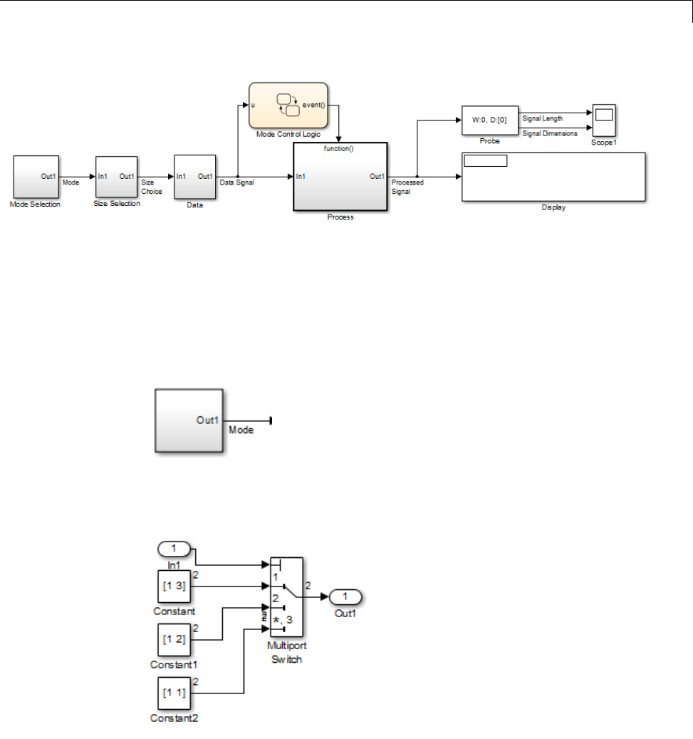
Simulink Models Using Variable-Size Signals
Creating a Variable-Size Signal Based on Mode
The Mode Selection subsystem determines the mode for processing a data
signal and outputs a mode value ( 1, 2, or 3). This value helps to select the
length of the data signal using the Size Selection and Data subsystems.
The Size Selection subsystem creates an index value from the mode value. In
this example, the index values are [1 3],[1 2],and[1 1].
49-15
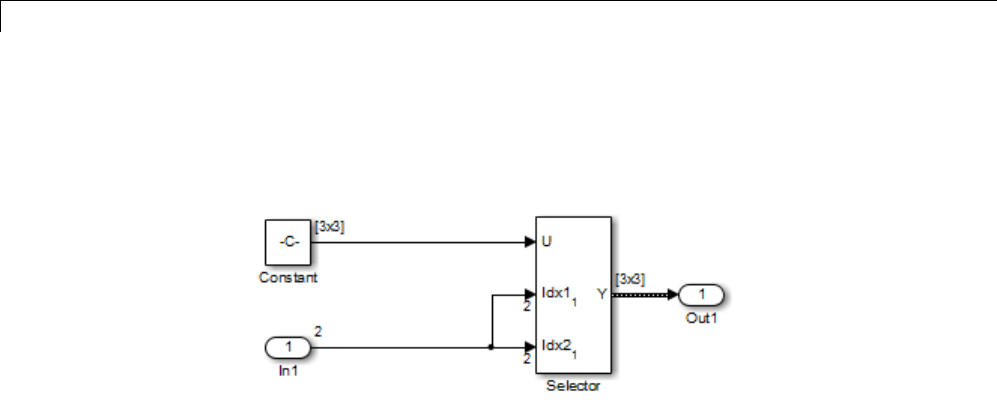
49 Working with Variable-Size Signals
The Data subsystem takes a data signal (Constant block) and selects part of
the data signal dependent on the mode. Theoutputisavariable-sizesignal
with a matrix size of 3x3,2x2,and1x1.
The dimensions of the raw data signal (Constant block) is a 3x3.After
connecting a To Workspace block to a signal line, you can view the signal in
the MATLAB Command Window by typing:
simout.signals.values
ans(:,:,1) =
147
258
369
The variable-size signal generated from the Data subsystem is also a 3x3
matrix. For shorter signals, the matrix is padded with NaNs.
simout.signals.values
ans(:,:,1) =
1NaNNaN
NaN NaN NaN
NaN NaN NaN
ans(:,:,2) =
49-16
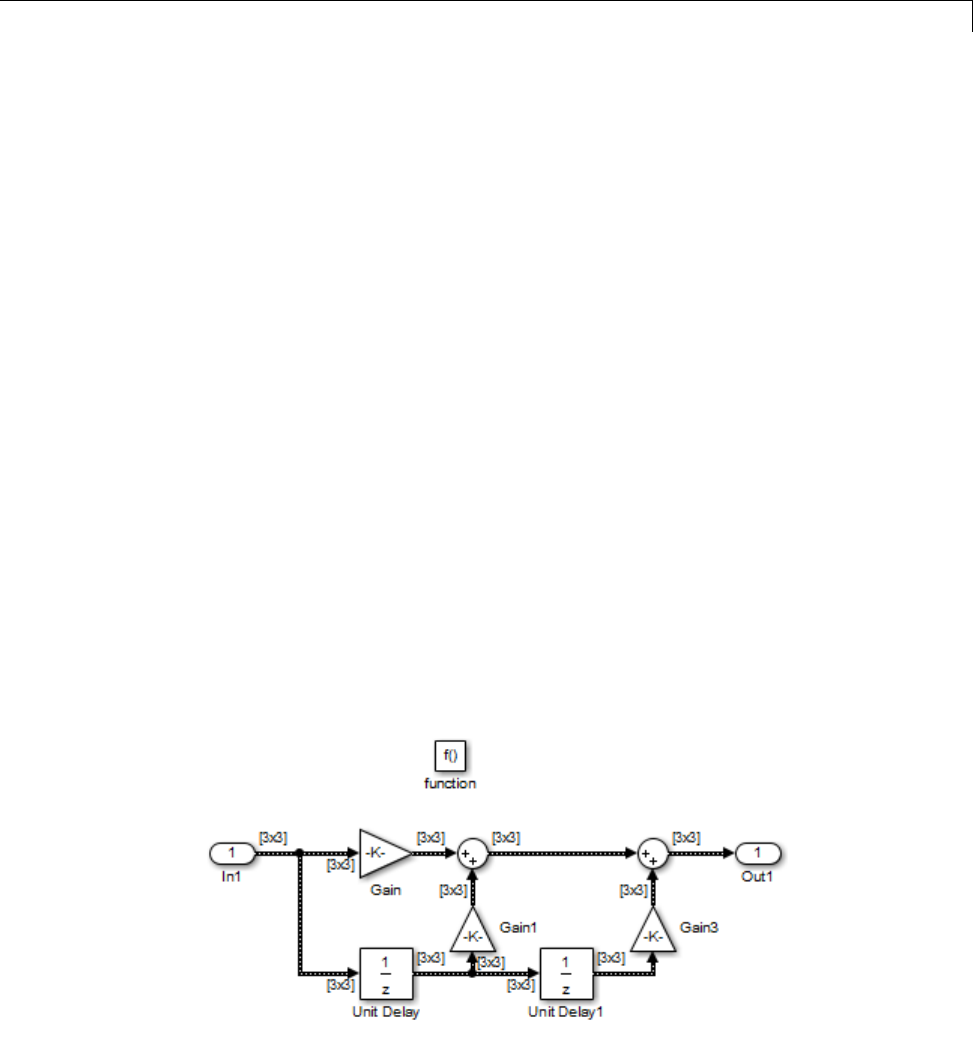
Simulink Models Using Variable-Size Signals
14NaN
25NaN
NaN NaN NaN
ans(:,:,3) =
147
258
369
Processing a Variable-Size Signal with a Conditionally
Executed Subsystem
Because the Process subsystem contains a Delay block, the subsystem resets
and repropagates the signal at each time step. This model uses a Stateflow
chart to detect a signal size change and reset the Process subsystem.
In the function block dialog, and from the Propagate sizes of variable-size
signals list, choose Only when enabling. When the model enables this
subsystem, selecting this option directs the Simulink software to propagate
sizes for variable-size signals inside the conditionally executed subsystem.
Signal sizes can change only when they transition from disabled to enabled.
For an explanation of handling signal-size changes with blocks containing
states, see “How Variable-Size Signals Propagate” on page 49-3.
49-17
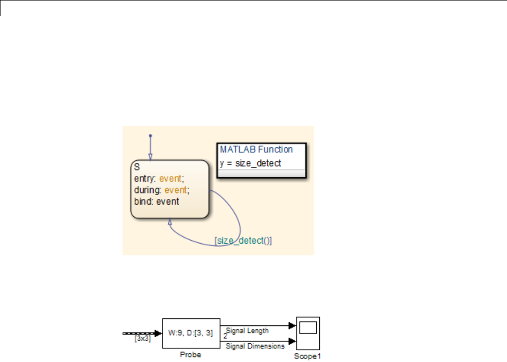
49 Working with Variable-Size Signals
The Stateflow chart determines if there is a change in the size of the signal.
The function size_detect calculates the width of the variable-size signal at
each time step, and compares the current width to the previous width. If
there is a change in signal size, the chart outputs a function-call output event
that resets and repropagates the signal sizes within the Process subsystem.
Visualizing Data
Use the Probe block to visualize signal size and signal dimension.
Since the signals are nxnmatrices, the signal dimension lines overlap in
the Scope display.
49-18
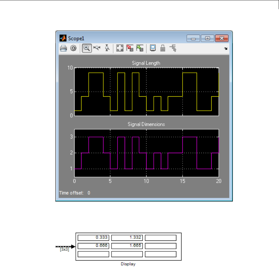
Simulink Models Using Variable-Size Signals
You can use a Display block and the Simulink Debugger to visualize signal
values at each time step.
49-19
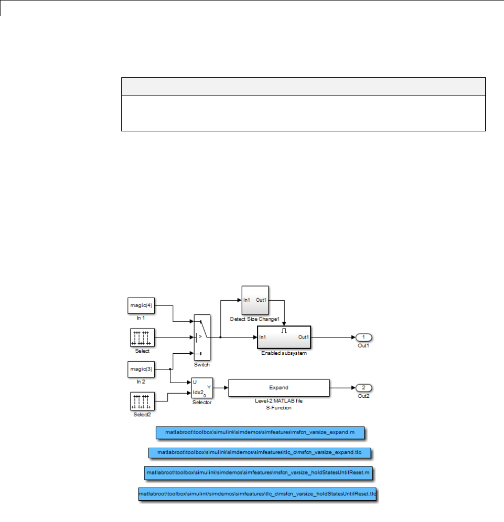
49 Working with Variable-Size Signals
S-Functions Using Variable-Size Signals
In this section...
“Level-2 MATLAB S-Function with Variable-Size Signals” on page 49-20
“C S-Function with Variable-Size Signals” on page 49-21
Level-2 MATLAB S-Function with Variable-Size Signals
Both Level-2 MATLAB S-Functions and C S-Functions support variable-size
signals when you set the DimensionMode for the output port to Variable.
You also need to consider the current dimension of the input and output
signals in the input and output update methods.
To open this example model, in the MATLAB Command Window, type:
msfcndemo_varsize
49-20
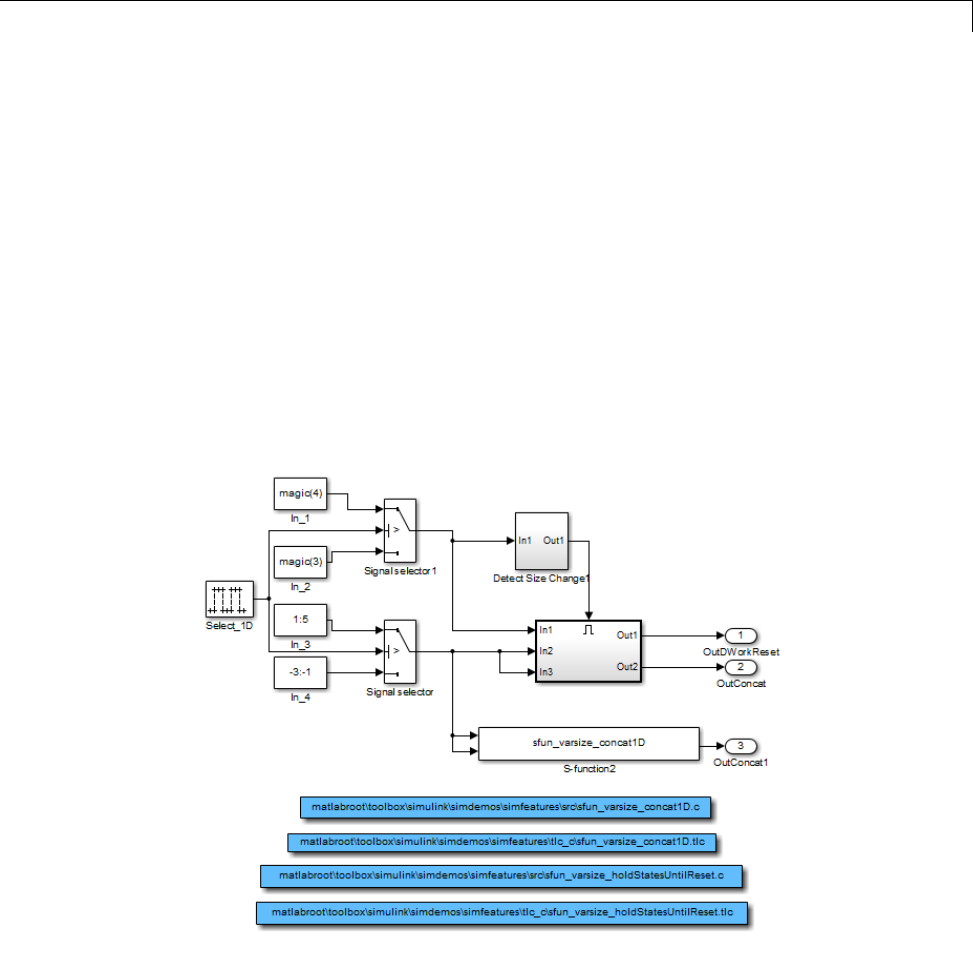
S-Functions Using Variable-Size Signals
The Enabled subsystem includes a Level-2 MATLAB S-Function which shows
how to implement a block that holds its states until reset. Because this block
contains states and delays the input signal, the input size can change only
when a reset occurs.
The Expand block is a Level-2 MATLAB S-Function that takes a scalar input
and outputs a vector of length indicated by its input value. The output is
by 1:n where nis the input value.
C S-Function with Variable-Size Signals
To open this example model, in the MATLAB Command Window, type:
sfcndemo_varsize
The enabled subsystems have two S-Functions:
49-21

49 Working with Variable-Size Signals
•sfun_varsize_holdStatesUntilReset is a C S-Function that has states and
requires its DWorks vector to reset whenever the sizes of the input signal
changes.
•sfun_varsize_concat1D is a C S-function that implements the concatenation
of two unoriented vectors. You can use this function within an enabled
subsystem by itself.
49-22

Simulink®Block Support for Variable-Size Signals
Simulink Block Support for Variable-Size Signals
In this section...
“Simulink Block Data Type Support” on page 49-23
“Conditionally Executed Subsystem Blocks” on page 49-23
“Switching Blocks” on page 49-24
Simulink Block Data Type Support
The Simulink Block Data Type Support table includes a complete list of blocks
that support variable-size signals.
To view the table:
1Open a Simulink model.
2Select Help > Simulink > Block Data Ty[es & Code Generation
Support > Simulink.
An Xin the Variable-Size Support column indicates support for that block.
Tip You can also view the table by entering showblockdatatypetable at
the command prompt.
Conditionally Executed Subsystem Blocks
Control port blocks are in conditionally executed subsystems. You can set
the Propagate sizes of variable-size signals parameter for these blocks
to During exection,Only when execution is resumed (Action Port), and
Only when enabling (Enable and Trigger or Function-Call).
49-23
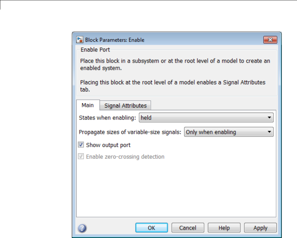
49 Working with Variable-Size Signals
•Action Port
•Enable
•Trigger — Trigger type set to function-call
Switching Blocks
Switching blocks support variable-size signals by allowing input signals with
different sizes and propagating the size of the input signal to the output
49-24
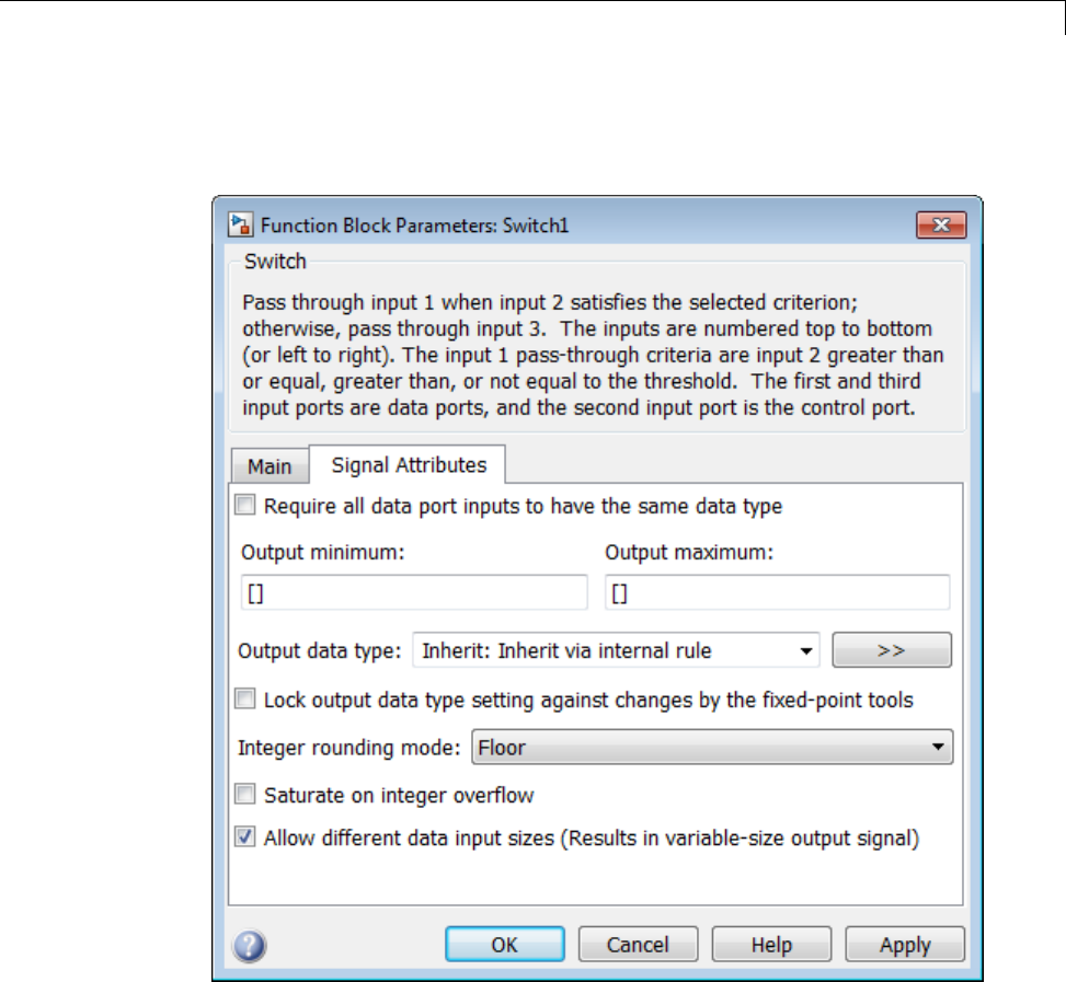
Simulink®Block Support for Variable-Size Signals
signal. You can set the Allow different data input sizes parameter for
these blocks on the Signal Attributes pane to either on or off.
•Switch
•Multiport Switch
•Manual Switch
49-25

49 Working with Variable-Size Signals
Variable-Size Signal Limitations
The following table is a list of known limitations and workarounds.
Limitation Workaround
Array format logging does not
support variable-size signals.
Use a Structureor Structure With
Time format for logging variable-size
signals.
Right-click signal logging does not
support variable-size signals.
Use a To Workspace block (with
Structure or Structure With Time
format) or a root Outport block for
logging variable-size signals.
Aframe-ba
sed variable-size signal
cannot change the frame length (first
dimension size), but it can change
the second dimension size (number
of channels). Using frame-based
signals requires DSP System Toolbox
software.
Use the Frame Conversion block to
convert a signal into sample-based
signal.
Variable-size signals must have a
discrete sample time.
—
A scalar signal (width equals 1)
cannot be a variable-size signal
because the maximum size is 1.
—
Embedded Coder does not support
variable-size signals with ERT
S-functions, custom storage classes,
function prototype control, the
AUTOSAR, C++ interface, and the
ERT reusable code interface.
—
49-26

Variable-Size Signal Limitations
Limitation Workaround
Simulink does not support
variable-size parameter or DWork
vectors.
—
Rapid accelerator mode does not
support models having root-level
input ports with variable-size
signals.
—
49-27

49 Working with Variable-Size Signals
49-28


50 Customizing the Simulink®User Interface
Add Items to Model Editor Menus
In this section...
“About Adding Items” on page 50-2
“Code for Adding Menu Items” on page 50-2
“Define Menu Items” on page 50-4
“Register Menu Customizations” on page 50-10
“Callback Info Object” on page 50-11
“Debugging Custom Menu Callbacks” on page 50-11
“Menu Tags” on page 50-11
About Adding Items
You can add commands and submenus to the following menu locations for the
Simulink Editor and Stateflow Editor:
•The end of top-level menus
•The menu bar
•The beginning or end of a context menu
Toaddanitemtoaneditormenu:
•For each item, create a function, called a schema function, that defines the
item (see “Define Menu Items” on page 50-4).
•Register the menu customizations with the Simulink customization
manager at startup, e.g., in an sl_customization.m file on the MATLAB
path (see “Register Menu Customizations” on page 50-10).
•Create callback functions that implement the commands triggered by the
items that you add to the menus.
Code for Adding Menu Items
The following sl_customization.m file adds four items to the Simulink
Editor’s Tools menu.
50-2

Add Items to Model Editor Menus
function sl_customization(cm)
%% Register custom menu function.
cm.addCustomMenuFcn('Simulink:ToolsMenu', @getMyMenuItems);
end
%% Define the custom menu function.
function schemaFcns = getMyMenuItems(callbackInfo)
schemaFcns = {@getItem1,...
@getItem2,...
{@getItem3,3}... %% Pass 3 as user data to getItem3.
@getItem4};
end
%% Define the schema function for first menu item.
function schema = getItem1(callbackInfo)
schema = sl_action_schema;
schema.label = 'Item One';
schema.userdata = 'item one';
schema.callback = @myCallback1;
end
function myCallback1(callbackInfo)
disp(['Callback for item ' callbackInfo.userdata ' was called']);
end
function schema = getItem2(callbackInfo)
% Make a submenu label 'Item Two' with
% the menu item above three times.
schema = sl_container_schema;
schema.label = 'Item Two';
schema.childrenFcns = {@getItem1, @getItem1, @getItem1};
end
function schema = getItem3(callbackInfo)
% Create a menu item whose label is
% 'Item Three: 3', with the 3 being passed
% from getMyItems above.
schema = sl_action_schema;
50-3

50 Customizing the Simulink®User Interface
schema.label = ['Item Three: ' num2str(callbackInfo.userdata)];
end
function myToggleCallback(callbackInfo)
if strcmp(get_param(gcs, 'ScreenColor'), 'red') == 0
set_param(gcs, 'ScreenColor', 'red');
else
set_param(gcs, 'ScreenColor', 'white');
end
end
%% Define the schema function for a toggle menu item.
function schema = getItem4(callbackInfo)
schema = sl_toggle_schema;
schema.label = 'Red Screen';
if strcmp(get_param(gcs, 'ScreenColor'), 'red') == 1
schema.checked = 'checked';
else
schema.checked = 'unchecked';
end
schema.callback = @myToggleCallback;
end
Define Menu Items
You define a menu item by creating a function that returns an object, called
aschema object, that specifies the information needed to create the menu
item. The menu item that you define may trigger a custom action or display a
custom submenu. See the following sections for more information.
•“Defining Menu Items That Trigger Custom Commands” on page 50-4
•“Defining Custom Submenus” on page 50-8
Defining Menu Items That Trigger Custom Commands
To define an item that triggers a custom command, your schema function
must accept a callback info object (see “Callback Info Object” on page 50-11)
and create and return an action schema object (see “Action Schema Object”
on page 50-5) that specifies the item’s label and a function, called a callback,
50-4

Add Items to Model Editor Menus
to be invoked when the user selects the item. For example, the following
schema function defines a menu item that displays a message when selected
by the user.
function schema = getItem1(callbackInfo)
%% Create an instance of an action schema.
schema = sl_action_schema;
%% Specify the menu item's label.
schema.label = 'My Item 1';
schema.userdata = 'item1';
%% Specify the menu item's callback function.
schema.callback = @myCallback1;
end
function myCallback1(callbackInfo)
disp(['Callback for item ' callbackInfo.userdata
' was called']);
end
Action Schema Object. This object specifies information about menu items
that trigger commands that you define, including the label that appears on
the menu item and the function to be invoked when the user selects the menu
item. Use the function sl_action_schema to create instances of this object
in your schema functions. Its properties include
•tag
Optional string that identifies this action, for example, so that it can be
referenced by a filter function.
•label
String specifying the label that appears on a menu item that triggers
this action.
•state
50-5

50 Customizing the Simulink®User Interface
Property that specifies the state of this action. Valid values are 'Enabled'
(the default), 'Disabled',and'Hidden'.
•statustip
String specifying text to appear in the editor’s status bar when the user
selects the menu item that triggers this action.
•userdata
Data that you specify. May be of any type.
•accelerator
String specifying a keyboard shortcut that a user may use to trigger this
action. The string must be of the form 'Ctrl+K',whereKis the shortcut
key. For example, 'Ctrl+T' specifies that the user may invoke this action
by holding down the Ctrl key and pressing the Tkey.
•callback
String specifying a MATLAB expression to be evaluated or a handle to a
function to be invoked when a user selects the menu item that triggers this
action. This function must accept one argument: a callback info object.
•autoDisableWhen
Property that controls when a menu item is automatically disabled.
Setting When Menu Items Are Disabled
'Locked' (default) When the active editor is
locked or when the model is busy
'Busy' Only if the model is busy
'Never' Never
Toggle Schema Object. This object specifies information about a menu
item that toggles some object on or off. Use the function sl_toggle_schema to
create instances of this object in your schema functions. Its properties include
•tag
Optional string that identifies this toggle action, for example, so that it can
be referenced by a filter function.
50-6

Add Items to Model Editor Menus
•label
String specifying the label that appears on a menu item that triggers this
toggle action.
•checked
Specify whether the menu item displays a check mark. Valid values are
'unchecked' (default) and 'checked'
•state
String that specifies the state of this toggle action. Valid values are
'Enabled' (default), 'Disabled',and'Hidden'.
•statustip
String specifying text to appear in the editor’s status bar when the user
selects the menu item that triggers this toggle action.
•userdata
Data that you specify. May be of any type.
•accelerator
String specifying a keyboard shortcut that a user may use to trigger this
action. The string must be of the form 'Ctrl+K',whereKis the shortcut
key. For example, 'Ctrl+T' specifies that the user may invoke this action
by holding down the Ctrl key and pressing the Tkey.
•callback
String specifying a MATLAB expression to be evaluated or a handle to a
function to be invoked when a user selects the menu item that triggers this
action. This function must accept one argument: a callback info object.
•autoDisableWhen
Property that controls when a menu item is automatically disabled.
Setting When Menu Items Are Disabled
'Locked' (default) When the active editor is
locked or when the model is busy
'Busy' Only if the model is busy
'Never' Never
50-7

50 Customizing the Simulink®User Interface
Defining Custom Submenus
To define a submenu, create a schema function that accepts a callback
info object and returns a container schema object (see “Container Schema
Object” on page 50-8) that specifies the schemas that define the items on the
submenu. For example, the following schema function defines a submenu that
contains three instances of the menu item defined in the example in “Defining
Menu Items That Trigger Custom Commands” on page 50-4.
function schema = getItem2( callbackInfo )
schema = sl_container_schema;
schema.label = 'Item Two';
schema.childrenFcns = {@getItem1, @getItem1, @getItem1};
end
Container Schema Object. A container schema object specifies a submenu’s
label and its contents. Use the function sl_container_schema to create
instancesofthisobjectinyourschema functions. Properties of the object
include
•tag
Optional string that identifies this submenu.
•label
String specifying the submenu’s label.
•state
String that specifies the state of this submenu. Valid values are 'Enabled'
(the default), 'Disabled',and'Hidden'.
•statustip
String specifying text to appear in the editor’s status bar when the user
selectsthissubmenu.
•childrenFcns
Cell array that specifies the contents of the submenu. Each entry in the
cell array can be
-A pointer to a schema function that defines an item on the submenu (see
“Define Menu Items” on page 50-4)
50-8

Add Items to Model Editor Menus
-A two-element cell array whose first element is a pointer to a schema
function that defines an item entry and whose second element is data to
be inserted as user data in the callback info object (see “Callback Info
Object” on page 50-11) passed to the schema function
-'separator', which causes a separator to appear between the item
defined by the preceding entry in the cell array and the item defined
in the following entry. The case is ignored for this entry (for example,
'SEPARATOR' and 'Separator' are both valid entries). A separator is
also suppressed if it appears at the beginning or end of the submenu and
separators that would appear successively are combined into a single
separator (for example, as a result of an item being hidden).
For example, the following cell array specifies two submenu entries:
{@getItem1, 'separator', {@getItem2, 1}}
In this example, a 1 is passed to getItem2 via a callback info object.
•generateFcn
Pointer to a function that returns a cell array defining the contents of the
submenu. The cell array must have the same format as that specified for
the container schema objects childrenFcns property.
Note The generateFcn property takes precedence over the childrenFcns
property. If you set both, the childrenFcns property is ignored and the cell
array returned by the generateFcn is used to create the submenu.
•userdata
Data of any type that is passed to generateFcn.
•autoDisableWhen
Property that controls when a menu item is automatically disabled.
50-9

50 Customizing the Simulink®User Interface
Setting When Menu Items Are Disabled
'Locked' (default) When the active editor is
locked or when the model is busy
'Busy' Only if the model is busy
'Never' Never
Register Menu Customizations
You must register custom items to be included on a Simulink menu with the
customization manager. Use the sl_customization.m file for a Simulink
installation (see “Registering Customizations” on page 50-27) to perform this
task.Inparticular,foreachmenuthatyouwanttocustomize,yoursystem’s
sl_customization function must invoke the customization manager’s
addCustomMenuFcn method (see “Customization Manager” on page 50-27).
Each invocation should pass the tag of the menu (see “Menu Tags” on page
50-11) to be customized and a custom menu function that specifies the items
to be added to the menu (see “Creating the Custom Menu Function” on page
50-10) . For example, the following sl_customization function adds custom
items to the Simulink Tools menu.
function sl_customization(cm)
%% Register custom menu function.
cm.addCustomMenuFcn('Simulink:ToolsMenu', @getMyItems);
Creating the Custom Menu Function
The custom menu function returns a cell array of schema functions that define
custom items that you want to appear on the model editor menus (see “Define
Menu Items” on page 50-4 ). The custom menu function returns a cell array
similar to that returned by the generateFcn function.
Your custom menu function should accept a callback info object (see “Callback
Info Object” on page 50-11) and return a cell array that lists the schema
functions. Each element of the cell array can be either a handle to a schema
function or a two-element cell array whose first element is a handle to a
schema function and whose second element is user-defined data to be passed
to the schema function. For example, the following custom menu function
returns a cell array that lists three schema functions.
50-10

Add Items to Model Editor Menus
function schemas = getMyItems(callbackInfo)
schemas = {@getItem1, ...
@getItem2, ...
{@getItem3,3} }; % Pass 3 as userdata to getItem3.
end
Callback Info Object
Instances of these objects are passed to menu customization functions.
Properties of these objects include
•uiObject
Handle to the owner of the menu for which this is the callback. The owner
can be the Simulink Editor or the Stateflow Editor.
•model
Handle to the model being displayed in the editor window.
•userdata
User data. The value of this field can be any type of data.
Debugging Custom Menu Callbacks
On systems using the Microsoft Windows operating system, selecting a
custom menu item whose callback contains a breakpoint can cause the mouse
to become unresponsive or the menu to remain open and on top of other
windows. To fix these problems, use the MATLAB code debugger keyboard
commands to continue execution of the callback.
Menu Tags
A menu tag is a string that identifies a Simulink Editor or the Stateflow
Editor menu bar or menu. You need to know a menu’s tag to add custom
items to it (see “Register Menu Customizations” on page 50-10). You can
configure the editor to display all (see “Displaying Menu Tags” on page 50-13)
but the following tags:
50-11

50 Customizing the Simulink®User Interface
Tag Add...
Simulink tags
Simulink:MenuBar Menu to Simulink Editor’s menu bar
Simulink:PreContextMenu Item to the beginning of Simulink Editor’s
context menu
Simulink:PostContextMenu Item to the end of Simulink Editor’s
context menu
Simulink:FileMenu Item near the end of the Simulink Editor’s
File menu, but before the Exit MATLAB
item
Simulink:EditMenu Item to the end of the Simulink Editor’s
Edit menu
Simulink:ViewMenu Item to the end of the Simulink Editor’s
View menu
Simulink:DisplayMenu Item to the end of the Simulink Editor’s
Display menu
Simulink:DiagramMenu Item to the end of the Simulink Editor’s
Diagram menu
Simulink:SimulationMenu Item to the end of the Simulink Editor’s
Simulation menu
Simulink:AnalysisMenu Item to the end of the Simulink Editor’s
Analysis menu
Simulink:CodeMenu Item to the end of the Simulink Editor’s
Code menu
Simulink:ToolsMenu Item to the end of the Simulink Editor’s
Tools menu
Simulink:HelpMenu Item to the end of Simulink Editor’s Help
menu
Stateflow tags
Stateflow:MenuBar Menu to Stateflow Editor’s menu bar
Stateflow:PreContextMenu Item to the beginning of Stateflow Editor’s
context menu.
50-12

Add Items to Model Editor Menus
Tag Add...
Stateflow:ContextMenu Items to the end of Stateflow Editor’s
context menu.
Stateflow:FileMenu Item near the end of the Stateflow Editor’s
File menu, but before the Exit MATLAB
item
Stateflow:EditMenu Item to the end of Stateflow Editor’s Edit
menu
Stateflow:ViewMenu Item to the end of the Stateflow Editor’s
View menu
Stateflow:DisplayMenu Item to the end of the Stateflow Editor’s
Display menu
Stateflow:ChartMenu Item to the end of the Stateflow Editor’s
Chart menu
Stateflow:SimulationMenu Item to the end of the Stateflow Editor’s
Simulation menu
Stateflow:AnalysisMenu Item to the end of the Stateflow Editor’s
Analysis menu
Stateflow:CodeMenu Item to the end of the Stateflow Editor’s
Code menu
Stateflow:ToolsMenu Item to the end of the Stateflow Editor’s
Tools menu
Stateflow:HelpMenu Item to the end of the Stateflow Editor’s
Help menu
Displaying Menu Tags
You can configure the Simulink and Stateflow software to display the tag
for a menu item next to the item’s label, allowing you to determine at a
glance the tag for a menu. The Simulink:TagName customizations appear
only if the current editor is the Simulink Editor. The Stateflow:TagName
customizations appear only if the current editor is the Stateflow Editor.
50-13
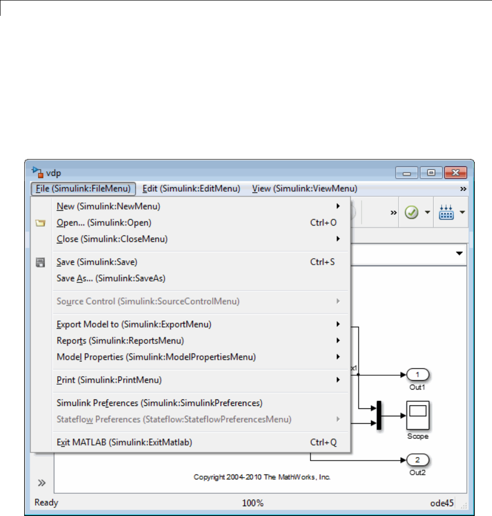
50 Customizing the Simulink®User Interface
To configure the editor to display menu tags, at the MATLAB command line,
set the customization manager’s showWidgetIdAsToolTip property to true.
For example:
cm = sl_customization_manager;
cm.showWidgetIdAsToolTip=true;
The tag of each menu item appears next to the item’s label on the menu:
50-14

Add Items to Model Editor Menus
To turn off tag display, enter the following command at the command line:
cm.showWidgetIdAsToolTip=false;
Note Some menu items may not work while menu tag display is enabled. To
ensure that all items work, turn off menu tag display before using the menus.
Simulink and Stateflow Editor Menu Customization
Use the same general procedures to customize Stateflow Editor menus as you
use for Simulink Editor. The addition of custom menu functions to the ends
of top-level menus depends on the active editor:
•Menus bound to Simulink:FileMenu only appear when the Simulink
Editor is active.
•Menus bound to Stateflow:FileMenu only appear when the Stateflow
Editor is active.
•To have a menu to appear in both of the editors, call addCustomMenuFcn
twice, once for each tag. Check that the code works in both editors.
50-15

50 Customizing the Simulink®User Interface
Disable and Hide Model Editor Menu Items
In this section...
“About Disabling and Hiding Model Editor Menu Items” on page 50-16
“Example: Disabling the New Model Command on the Simulink Editor’s
File Menu” on page 50-16
“Creating a Filter Function” on page 50-16
“Registering a Filter Function” on page 50-17
About Disabling and Hiding Model Editor Menu Items
You can disable or hide items that appear on the Simulink model editor
menus. To disable or hide a menu item, you must:
•Create a filter function that disables or hides the menu item (see “Creating
a Filter Function” on page 50-16).
•Register the filter function with the customization manager (see
“Registering a Filter Function” on page 50-17).
For more information on Model Editor menu items, see:
Example: Disabling the New Model Command on
the Simulink Editor’s File Menu
function sl_customization(cm)
cm.addCustomFilterFcn('Simulink:NewModel',@myFilter);
end
function state = myFilter(callbackInfo)
state = 'Disabled';
end
Creating a Filter Function
Your filter function must accept a callback info object and return a string that
specifies the state that you want to assign to the menu item. Valid states are
50-16

Disable and Hide Model Editor Menu Items
•'Hidden'
•'Disabled'
•'Enabled'
Your filter function may have to compete with other filter functions and with
Simulink itself to assign a state to an item. Who succeeds depends on the
strength of the state that each assigns to the item. 'Hidden' is the strongest
state. If any filter function or Simulink assigns 'Hidden' to the item, it is
hidden. 'Enabled' is the weakest state. For an item to be enabled, all filter
functions and the Simulink or Stateflow products must assign 'Enabled'to
the item. The 'Disabled' state is of middling strength. It overrides
'Enabled' but is itself overridden by 'Hidden'. For example, if any filter
function or Simulink or Stateflow assigns 'Disabled' to a menu item and
none assigns 'Hidden' to the item, the item is disabled.
Note The Simulink software does not allow you to filter some menu items,
for example, the Exit MATLAB item on the Simulink File menu. An error
message is displayed if you attempt to filter a menu item that you are not
allowed to filter.
Registering a Filter Function
Use the customization manager’s addCustomFilterFcn method to register a
filter function. The addCustomFilterFcn method takes two arguments: a tag
that identifies the menu or menu item tobefiltered(see“DisplayingMenu
Tags” on page 50-13) and a pointer to the filter function itself. For example,
the following code registers a filter function for the New Model item on the
Simulink File menu.
function sl_customization(cm)
cm.addCustomFilterFcn('Simulink:NewModel',@myFilter);
end
50-17

50 Customizing the Simulink®User Interface
Disable and Hide Dialog Box Controls
In this section...
“About Disabling and Hiding Controls” on page 50-18
“Disable a Button on a Dialog Box” on page 50-19
“Write Control Customization Callback Functions” on page 50-20
“Dialog Box Methods” on page 50-20
“Dialog Box and Widget IDs” on page 50-21
“Register Control Customization Callback Functions” on page 50-22
About Disabling and Hiding Controls
The Simulink product includes a customization API that allows you to disable
and hide controls (also referred to as widgets), such as text fields and buttons,
on most of its dialog boxes. The customization API allows you to disable or
hide controls on an entire class of dialog boxes, for example, parameter dialog
boxes via a single method call.
Before attempting to customize a Simulink dialog box or class of dialog
boxes, you must first ensure that the dialog box or class of dialog boxes is
customizable. Any dialog box that appears in the dialog pane of Model
Explorer is customizable. In addition, any dialog box that has dialog and
widgetIDsiscustomizable. Todetermine whether a standalone dialog box
(i.e., one that does not appear in Model Explorer) is customizable, open the
dialog box, enable dialog and widget ID display (see “Dialog Box and Widget
IDs” on page 50-21), and position the mouse over a widget. If a widget ID
appears, the dialog box is customizable.
Once you have determined that a dialog box or class of dialog boxes is
customizable, you must write MATLAB code to customize the dialog boxes.
This entails writing callback functions that disable or hide controls for a
specific dialog box or class of dialog boxes (see “Write Control Customization
Callback Functions” on page 50-20) and registering the callback functions
via an object called the customization manager (see “Register Control
Customization Callback Functions” on page 50-22). Simulink then invokes
50-18

Disable and Hide Dialog Box Controls
the callback functions to disable or hide the controls whenever a user opens
the dialog boxes.
For more information on Dialog Box controls, see:
Disable a Button on a Dialog Box
The following sl_customization.m file disables the Build button on the
Code Generation pane of the Configuration Parameters dialog box for any
model whose name contains “engine.”
function sl_customization(cm)
% Disable for standalone Configuration Parameters dialog box.
cm.addDlgPreOpenFcn('Simulink.ConfigSet',@disableRTWBuildButton)
% Disable for Configuration Parameters dialog box that appears in
% the Model Explorer.
cm.addDlgPreOpenFcn('Simulink.RTWCC',@disableRTWBuildButton)
end
function disableRTWBuildButton(dialogH)
hSrc = dialogH.getSource; % Simulink.RTWCC
hModel = hSrc.getModel;
modelName = get_param(hModel, 'Name');
if ~isempty(strfind(modelName, 'engine'))
% Takes a cell array of widget Factory ID.
dialogH.disableWidgets({'Simulink.RTWCC.Build'})
end
end
To test this customization:
1Put the preceding sl_customization.m file on the path.
2Register the customization by entering sl_refresh_customizations at
the command line or by restarting the MATLAB software (see “Registering
Customizations” on page 50-27).
50-19

50 Customizing the Simulink®User Interface
3Open the sldemo_engine model, for example, by entering the command
sldemo_engine at the command line.
Write Control Customization Callback Functions
A callback function for disabling or hiding controls on a dialog box should
accept one argument: a handle to the dialog box object that contains the
controls you want to disable or hide. The dialog box object provides methods
that the callback function can use to disable or hide the controls that the
dialog box contains.
The dialog box object also provides access to objects containing information
about the current model. Your callback function can use these objects to
determine whether to disable or hide controls. For example, the following
callback function uses these objects to disable the Build buttonontheCode
Generation pane of the Configuration Parameters dialog box displayed in
Model Explorer for any model whose name contains “engine.”
function disableRTWBuildButton(dialogH)
hSrc = dialogH.getSource; % Simulink.RTWCC
hModel = hSrc.getModel;
modelName = get_param(hModel, 'Name');
if ~isempty(strfind(modelName, 'engine'))
% Takes a cell array of widget Factory ID.
dialogH.disableWidgets({'Simulink.RTWCC.Build'})
end
Dialog Box Methods
Dialog box objects provide the following methods for enabling, disabling, and
hiding controls:
•disableWidgets(widgetIDs)
•hideWidgets(widgetIDs)
where widgetIDs is a cell array of widget identifiers (see “Dialog Box and
Widget IDs” on page 50-21) that specify the widgets to be disabled or hidden.
50-20

Disable and Hide Dialog Box Controls
Dialog Box and Widget IDs
Dialog box and widget IDs are strings that identify a control on a Simulink
dialog box. To determine the dialog box and widget ID for a particular control,
execute the following code at the command line:
cm = sl_customization_manager;
cm.showWidgetIdAsToolTip = true
Then, open the dialog box that contains the control and move the mouse
cursor over the control to display a tooltip listing the dialog box and the widget
IDs for the control. For example, moving the cursor over the Start time field
on the Solverpane of the Configuration Parameters dialog box reveals that
the dialog box ID for the Solver pane is Simulink.SolverCC and the widget
ID for the Start time field is Simulink.SolverCC.StartTime.
50-21
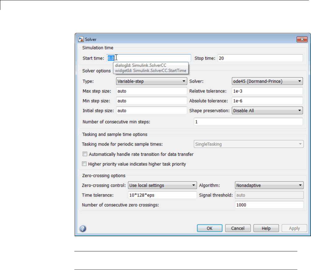
50 Customizing the Simulink®User Interface
Note The tooltip displays “not customizable” for controls that are not
customizable.
Register Control Customization Callback Functions
To register control customization callback functions for a particular
installation of the Simulink product, include code in the installation’s
sl_customization.m file (see “Registering Customizations” on page 50-27)
that invokes the customization manager’s addDlgPreOpenFcn on the callbacks.
50-22

Disable and Hide Dialog Box Controls
The addDlgPreOpenFcn takes two arguments. The first argument is a dialog
box ID (see “Dialog Box and Widget IDs” on page 50-21) and the second
is a pointer to the callback function to be registered. Invoking this method
causes the registered function to be invoked for each dialog box of the type
specified by the dialog box ID. The function is invoked before the dialog box
is opened, allowing the function to perform the customizations before they
become visible to the user.
The following example registers a callback that disables the Build button on
the Code Generation pane of the Configuration Parameters dialog box (see
“Write Control Customization Callback Functions” on page 50-20).
function sl_customization(cm)
% Disable for standalone Configuration Parameters dialog box.
cm.addDlgPreOpenFcn('Simulink.ConfigSet',@disableRTWBuildButton)
% Disable for Configuration Parameters dialog box that appears in
% the Model Explorer
cm.addDlgPreOpenFcn('Simulink.RTWCC',@disableRTWBuildButton)
end
Note Registering a customization callback causes the Simulink software to
invoke the callback for every instance of the class of dialog boxes specified by
the method’s dialog box ID argument. This allows you to use a single callback
to disable or hide a control for an entire class of dialog boxes. In particular,
you can use a single callback to disableorhidethecontrolforaparameter
that is common to most built-in blocks. This is because most built-in block
dialog boxes are instances of the same dialog box super class.
50-23

50 Customizing the Simulink®User Interface
Customize the Library Browser
In this section...
“Reorder Libraries” on page 50-24
“Disable and Hide Libraries” on page 50-24
“Customize the Library Browser Menu” on page 50-25
Reorder Libraries
The order in which a library appears in the Library Browser is determined
by its name and its sort priority. Libraries appear in the Library Browser’s
tree view in ascending order of priority, with all blocks having the same
priority sorted alphabetically. The Simulink library has a sort priority of
-1 by default; all other libraries, a sort priority of 0. This guarantees that
the Simulink library is by default the first library displayed in the Library
Browser. You can reorder libraries by changing their sort priorities. To
change library sort priorities, insert a line of code of the following form in an
sl_customization.m file (see “Registering Customizations” on page 50-27)
on the MATLAB path:
cm.LibraryBrowserCustomizer.applyOrder( {'LIBNAME1', PRIORITY1, ...
'LIBNAME2, 'PRIORITY2, ...
.
.
'LIBNAMEN', PRIORITYN} );
where LIBNAMEn is the name of the library or its model file and PRIORITYn is
an integer indicating the library’s sort priority. For example, the following
code moves the Simulink Extras library to the top of the Library Browser’s
tree view.
cm.LibraryBrowserCustomizer.applyOrder( {'Simulink Extras', -2} );
Disable and Hide Libraries
To disableorhidelibraries,sublibraries, or library blocks, insert code
of the following form in an sl_customization.m file (see “Registering
Customizations” on page 50-27) on the MATLAB path:
50-24

Customize the Library Browser
cm.LibraryBrowserCustomizer.applyFilter( {'PATH1', 'STATE1', ...
'PATH2', 'STATE2', ...
.
.
'PATHN', 'STATEN'} );
where PATHn is the path of the library, sublibrary, or block to be disabled or
hidden and 'STATEn' is 'Disabled' or 'Hidden'. For example, the following
code hides the Simulink Sources sublibrary and disables the Sinks sublibrary.
cm.LibraryBrowserCustomizer.applyFilter({'Simulink/Sources','Hidden'});
cm.LibraryBrowserCustomizer.applyFilter({'Simulink/Sinks','Disabled'});
Customize the Library Browser Menu
You can perform the same kinds of customizations to the Library Browser
menu as you can to the model and Stateflow editor menus. Simply use the
corresponding Library Browser menu tags to perform the customizations.
•LibraryBrowser:FileMenu
•LibraryBrowser:EditMenu
•LibraryBrowser:ViewMenu
•LibraryBrowser:HelpMenu
For example, the following code adds a menu item to the Library Browser’s
file menu:
%Menu customization:
% Add items to the Library Browser File menu
cm.addCustomMenuFcn('LibraryBrowser:FileMenu',@getMyMenuItems)
%% Define the custom menu function.
function schemaFcns = getMyMenuItems(callbackInfo)
schemaFcns = {@myBasic};
end
%% Define the schema function for first menu item.
function schema = myBasic(callbackInfo)
disp('1');
50-25

50 Customizing the Simulink®User Interface
schema = sl_action_schema;
schema.label = 'Display 1';
schema.userdata = 'item one';
schema.tag = 'LibraryBrowser:ItemOne';
end
50-26

Registering Customizations
Registering Customizations
In this section...
“About Registering User Interface Customizations” on page 50-27
“Customization Manager” on page 50-27
About Registering User Interface Customizations
YoumustregisteryouruserinterfacecustomizationsusingaMATLAB
function called sl_customization.m.ThisislocatedontheMATLABpathof
the Simulink installation that you want to customize. The sl_customization
function should accept one argument: ahandletoacustomizationmanager
object. For example:
function sl_customization(cm)
The customization manager object includes methods for registering menu
and control customizations (see “Customization Manager” on page 50-27).
Your instance of the sl_customization function should use these methods to
register customizations specific to your application. For more information, see
the following sections on performing customizations.
•“Add Items to Model Editor Menus” on page 50-2
•“Disable and Hide Model Editor Menu Items” on page 50-16
•“Disable and Hide Dialog Box Controls” on page 50-18
The sl_customization.m file is read when the Simulink software starts. If
you subsequently change the sl_customization.m file, you must restart
the Simulink software or enter the following command at the command line
to effect the changes:
sl_refresh_customizations
Customization Manager
The customization manager includes the following methods:
50-27

50 Customizing the Simulink®User Interface
•addCustomMenuFcn(stdMenuTag, menuSpecsFcn)
Adds the menus specified by menuSpecsFcn to the end of the
standard Simulink menu specified by stdMenuTag.ThestdMenuTag
argument is a string that specifies the menu to be customized. For
example, the stdMenuTag for the Simulink editor’s Tools menu is
'Simulink:ToolsMenu' (see “Displaying Menu Tags” on page 50-13 for
more information). The menuSpecsFcn argument is a handle to a function
that returns a list of functions that specify the items to be added to the
specified menu. See “Add Items to Model Editor Menus” on page 50-2 for
more information.
•addCustomFilterFcn(stdMenuItemID, filterFcn)
Adds a custom filter function specified by filterFcn for the standard
Simulink model editor menu item specified by stdMenuItemID.The
stdMenuItemID argument is a string that identifies the menu item. For
example, the ID for the New Model item on the Simulink editor’s File
menu is 'Simulink:NewModel' (see “Displaying Menu Tags” on page 50-13
for more information) . The filterFcn argument is a pointer to a function
that hides or disables the specifiedmenuitem. See“DisableandHide
Model Editor Menu Items” on page 50-16 for more information.
50-28

51
PrintFrame Editor
•“PrintFrame Editor Overview” on page 51-2
•“Design the Print Frame” on page 51-8
•“SpecifythePrintFramePageSetup”onpage51-9
•“Create Borders (Rows and Cells)” on page 51-11
•“Add Information to Cells” on page 51-14
•“Change Information in Cells” on page 51-18
•“Save and Open Print Frames” on page 51-22
•“Print Block Diagrams with Print Frames” on page 51-23
•“CreateandUseaPrintFrame”onpage51-26

51 PrintFrame Editor
PrintFrame Editor Overview
In this section...
“About the Print Frame Editor” on page 51-2
“What PrintFrames Are” on page 51-3
“Start the PrintFrame Editor” on page 51-6
“Help for the PrintFrame Editor” on page 51-7
“Close the PrintFrame Editor” on page 51-7
“Print Frame Process” on page 51-7
About the Print Frame Editor
The PrintFrame Editor is a graphical user interface you use to create and edit
print frames for block diagrams created with the Simulink software and the
Stateflow product. This chapter outlines the PrintFrame Editor, accessible
with the frameedit command.
The following figure describes the general layout of the PrintFrame Editor.
51-2
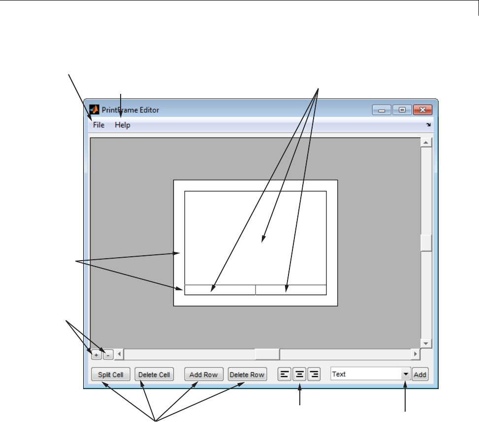
PrintFrame Editor Overview
Use the file menu for page setup, and
saving and opening print frames.
Get help for the PrintFrame Editor.
Change the information in a cell, and resize, add,
and remove cells.
Add and
remove
rows.
Zoom in or
out on
selected
cell.
Use these buttons to create and edit borders
Use these
buttons to
align
information
within a
cell.
Use the list box and
button to add information
in cells, such as text or
the date.
What PrintFrames Are
Print frames are borders containing information relevant to the block
diagram, for example, the name of the block diagram. After creating a print
51-3

51 PrintFrame Editor
frame, you can use the Simulink software or the Stateflow product to print a
block diagram with a print frame.
This illustration shows an example of a print frame with the major elements
labeled.
51-4
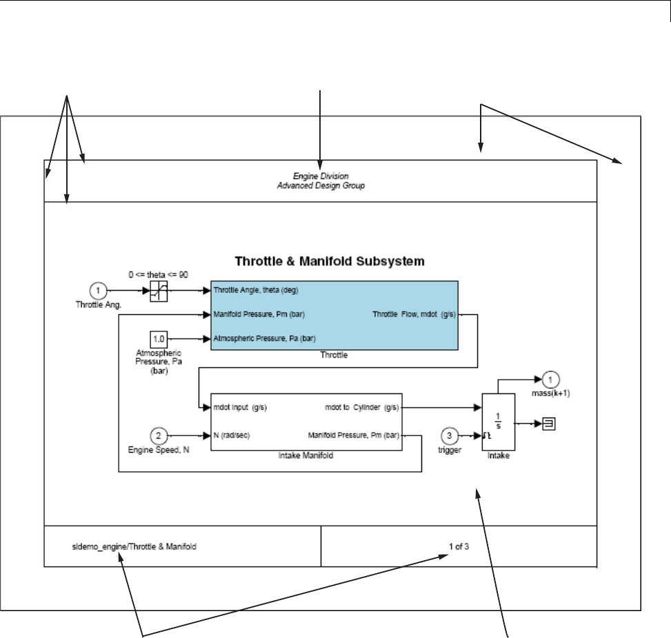
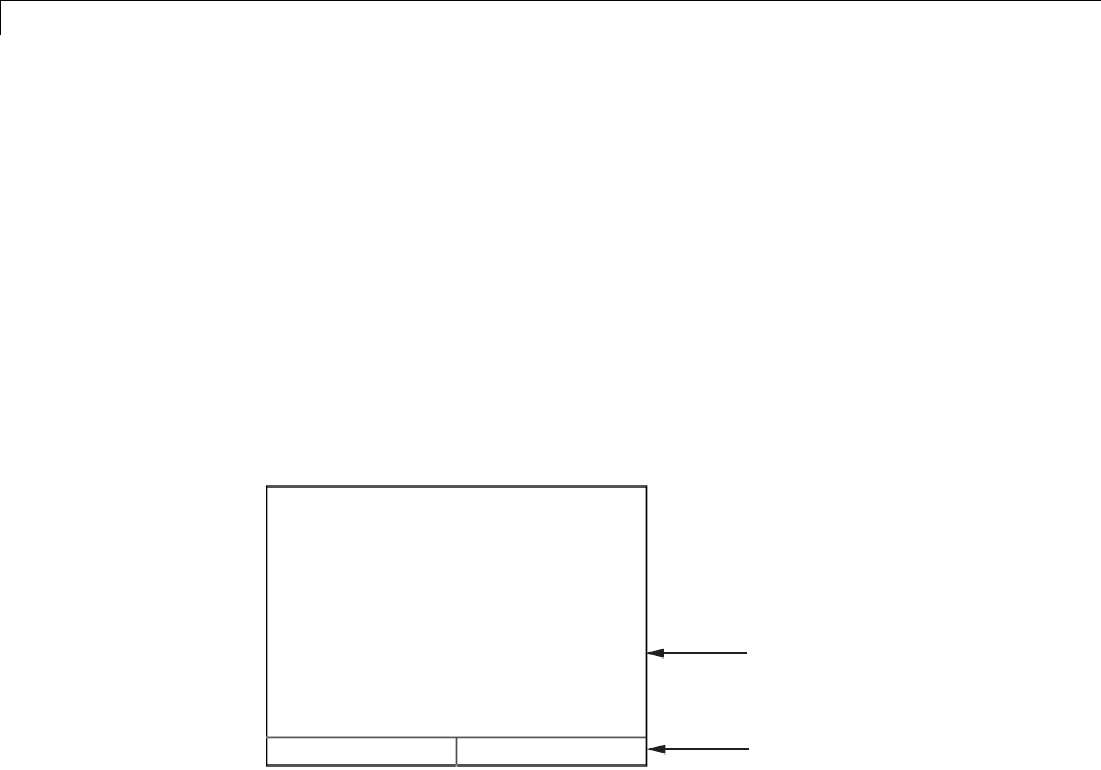
51 PrintFrame Editor
Start the PrintFrame Editor
Type frameeditat the MATLAB prompt. The PrintFrame Editor window
appears. The PrintFrame Editor window opens with the default print
frame.
You can use frameedit filename to open the PrintFrame Editor window
with the specified file name, where filename is a figure file you previously
created and saved using frameedit.
Default Print Frame
The default print frame has two rows. The top row consists of one cell and
the bottom row has two cells.
Top row
Bottom row
You can add information entries to these cells. You can also add new rows
and cells and add information in them, or change entries to different ones.
Zooming In and Out
While using the PrintFrame Editor, you might need to zoom in on an area
to better see the information or cell.
1Clickintheareayouwanttozoominon.
This selects a cell.
2Click the zoom in button.
51-6

PrintFrame Editor Overview
The area is magnified.
3Click the zoom in button repeatedly to continue zooming in.
To zoom out, reducing magnification in an area, click the zoom out button.
Click the zoom out button repeatedly to continue zooming out.
Help for the PrintFrame Editor
Select PrintFrame Editor Help from the Help menu in the PrintFrame
Editor window to access this online help.
Close the PrintFrame Editor
To close the PrintFrame Editor window, click the close box in the upper
right corner, or select Close from the File menu.
Print Frame Process
These are the basic steps for creating and using print frames:
•“Design the Print Frame” on page 51-8
•“SpecifythePrintFramePageSetup”onpage51-9
•“Create Borders (Rows and Cells)” on page 51-11
•“Add Information to Cells” on page 51-14
•“Change Information in Cells” on page 51-18
•“Save and Open Print Frames” on page 51-22
•“Print Block Diagrams with Print Frames” on page 51-23
Seealsothe“CreateandUseaPrintFrame”onpage51-26.
51-7

51 PrintFrame Editor
Design the Print Frame
In this section...
“Before You Begin” on page 51-8
“Variable and Static Information” on page 51-8
“Single Use or Multiple Use Print Frames” on page 51-8
Before You Begin
Before you create a print frame using the PrintFrame Editor, consider
thetypeofinformationyouwanttoincludeinitandhowyouwantthe
information to appear. You might want to make a sketch of how you want the
print frame to look, and note the wording you want to use.
Variable and Static Information
In a print frame, you can include variable and static information. Variable
information is automatically supplied at the time of printing, for example,
the date the block diagram is being printed. Static information always
prints exactly as you entered it, for example, the name and address of your
organization.
Single Use or Multiple Use Print Frames
Youcandesignaprintframeforoneparticular block diagram, or you can
design a more generic print frame for printing with different block diagrams.
51-8
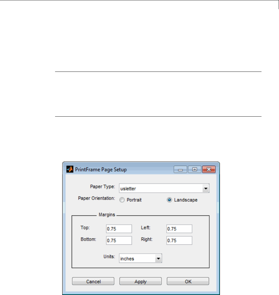
Specify the Print Frame Page Setup
Specify the Print Frame Page Setup
After you have an idea of the design of your print frame, specify the page
setup for the print frame.
Note Always begin creating a new print frame with PrintFrame Page
Setup. If, instead, you begin by creating borders and adding information, and
then later change the page setup, you might have to correct the borders and
placement of the information. For example, if you add information to cells and
then change the page setup paper orientation from landscape to portrait, the
information you added might not fit in the cells, given the new orientation.
1In the PrintFrame Editor window, select Page Setup from the File
menu.
The PrintFrame Page Setup dialog box appears.
51-9

51 PrintFrame Editor
2In the dialog box, specify:
•Paper Type – for example, usletter
•Paper Orientation –portraitorlandscape
•Margins for the print frame and the Units in which to specify the
margins
3Click Apply to see the effects of the changes you made. Then click OK to
close the dialog box.
51-10

Create Borders (Rows and Cells)
Create Borders (Rows and Cells)
In this section...
“First Steps” on page 51-11
“Add and Remove Rows” on page 51-11
“Add and Remove Cells” on page 51-12
“Resize Rows and Cells” on page 51-12
“Print Frame Size” on page 51-12
First Steps
Onceyouhavesetupthepage,usethePrintFrameEditortospecifyborders
(cells) in which the block diagram and information will be placed.
Important Always specify the PrintFrame page setup before creating borders
and adding information (see “Specify thePrintFramePageSetup”onpage
51-9). Otherwise, you might have to correct the borders and placement of the
information. For example, if you add information to cells and then change
the paper orientation from landscape to portrait, the information you added
might not fit in the cells, given the new orientation.
Add and Remove Rows
You can add and remove rows in a print frame.
1Click within an existing row to select it. If a row consists of multiple cells,
click in any of the cells in the row to select that row.
When a row is selected, handles appear on all four corners. If handles
appear on only two corners, you clicked on and only selected the line, not
the row.
51-11

51 PrintFrame Editor
2Click the add row button to create a new row.
The new row appears above the row you selected.
3To remove a row, select the row and click the delete row button.
Add and Remove Cells
You can create multiple cells within a row.
1Select the row in which you want multiple cells.
2Click the split cell button.
The row splits into two cells. If the row already consists of more than one
cell, the selected cell splits into two cells.
3To remove a cell, select the cell and click the delete cell button.
Resize Rows and Cells
You can change the dimensions of a row or cell.
1Click on the line you want to move.
A handle appears on both ends of the line.
2Drag the line to the new location.
For example, to make a row taller, click on the top line that forms the row.
Then drag the line up and the height of the row increases.
PrintFrameSize
Note that the overall size of the print frame is based on the options you specify
using the page setup feature. Therefore, when you change the dimensions
51-12

Create Borders (Rows and Cells)
of one row or cell, the dimensions of the row or cell next to it change in an
inverse direction. For example, if you drag the top line of a row to make it
taller, the row above it becomes shorter by the same amount.
To change the overall dimensions of theprintframe,usethepagesetup
feature. See “Specify the Print Frame Page Setup” on page 51-9.
51-13
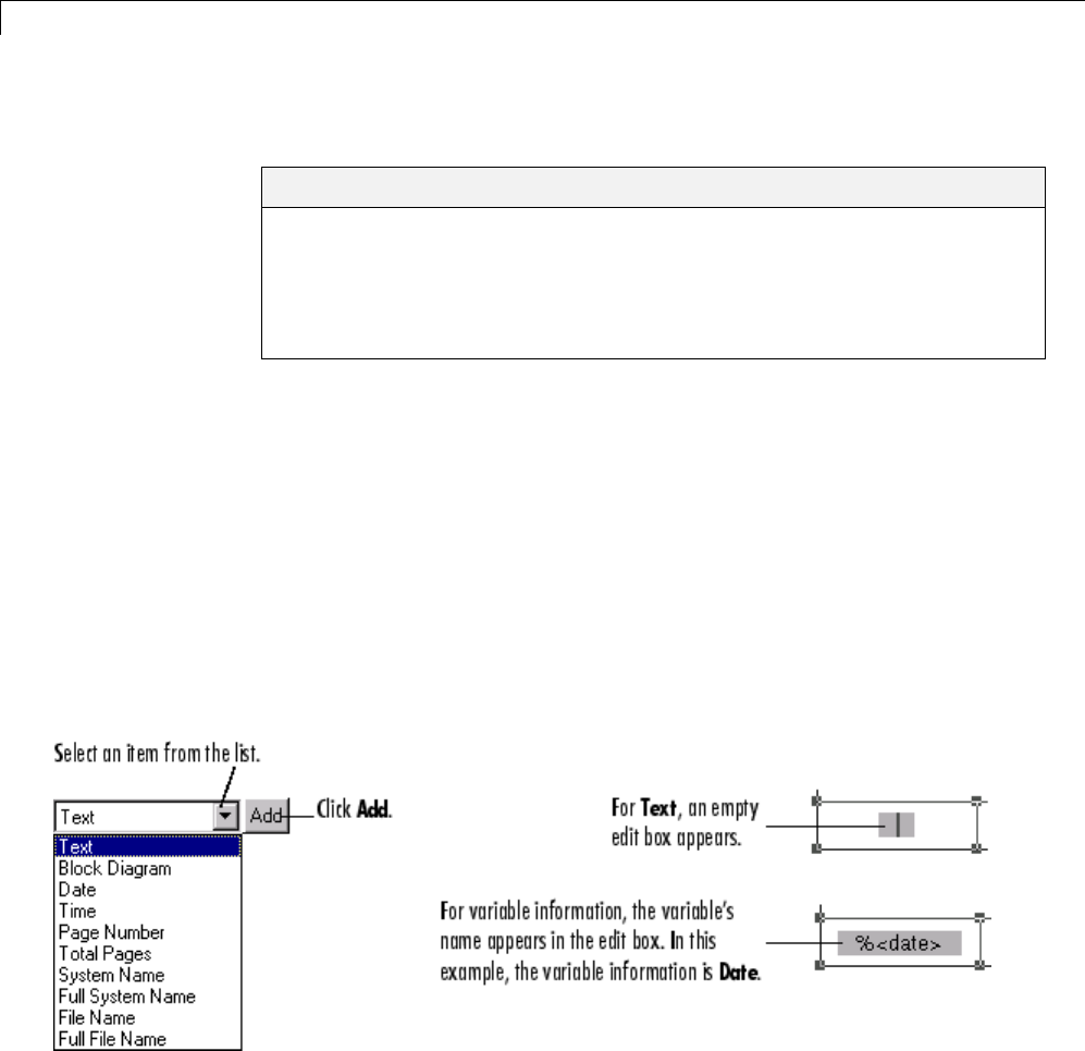
51 PrintFrame Editor
Add Information to Cells
In this section...
“Adding Information to Cells” on page 51-14
“Text Information” on page 51-15
“Variable Information” on page 51-15
“Multiple Entries in a Cell” on page 51-16
Adding Information to Cells
Use the following steps to add information to cells.
1Select the cell where you want to add information.
2From the list box, select the type of information you want to add.
3Click the Add button.
An edit box containing that information appears in the cell. (The edit boxes
for your platform might look slightly different from those in the figure
below.)
4Click outside of the edit box to end editing mode.
51-14

Add Information to Cells
Note If you click the Add button and nothing happens, it might be because
you did not select a cell first.
Text Information
For Text, type the text you want to include in that cell, for example, the name
of your organization. Press the Enter key if you want to type additional
text on a new line. Note that you can type special characters, for example,
superscripts and subscripts, Greek letters, and mathematical symbols. For
special characters, use embedded TeX sequences (see the text command
String property (in Text Properties of the online documentation) for a list
of allowable sequences). Click outside of the edit box when you are finished
to end editing mode.
Variable Information
All of the items in the information list box, except for the Text item, are
for adding variable information, which is supplied at the time of printing.
When you print a block diagram with a print frame that contains variable
information, the information for that particular block diagram prints in
those fields.
Types of Variable Information
The variable entries you can include are:
•Block Diagram — This entry indicates where the block diagram is to be
printed. Block Diagram is a mandatory entry. If Block Diagram is not
in one of the cells, you cannot save the print frame and therefore cannot
print a block diagram with it.
•Date — The date that the block diagram and print frame are printed, in
dd-mmm-yyyy format, for example, 05-Dec.-1997.
•Time — The time that the block diagram and print frame are printed, in
hh:mm format, for example, 14:22.
•Page Number — The page of the block diagram being printed.
•Total Pages — The total number of pages being printed for the block
diagram, which depends on the printing options specified.
51-15

51 PrintFrame Editor
•System Name — The name of the block diagram being printed.
•Full System Name — The name of the block diagram being printed,
including its position from the root system through the current system, for
example, engine/Throttle & Manifold.
•File Name — The file name of the block diagram, for example,
sldemo_engine.mdl.
•Full File Name — The full path and file
name for the block diagram, for example,
\\matlab\toolbox\simulink\simdemos\automotive\sldemo_engine.mdl.
Note: Adding the system name or file name does not mean that you can
then specify a file name for the Simulink software or the Stateflow product
in the PrintFrame Editor. It means that when you print a block diagram
and specify that it print with a print frame, the system name or file name of
the Simulink software or the Stateflow product block diagram is printed in
the specified cell of the print frame.
Format for Variable Information
When you add a variable entry, a percent sign, %, is automatically included
to identify the entry as variable informationratherthanatextstring. In
addition, the type of entry, for example, page, appears in angle brackets,
< >. The entry consists of the entire string, for example, %<page>,forPage
Number.
Multiple Entries in a Cell
You can include multiple entries in one cell.
1Select the cell.
2Add another item from the list box.
The new entry is added after the last entry in that cell.
Youcanalsotypedescriptivetexttoanyofthevariableentrieswithoutusing
the Text item in the information list box.
51-16

Add Information to Cells
1Double-click in the cell.
An edit box appears around the entry.
2Type text in the edit box before or after the entry.
3Click anywhere outside of the edit box to end editing mode.
Note You cannot include multiple entries or text in the cell that contains the
block diagram entry. %<blockdiagram> must be the only information in that
cell. If there is any other information in that cell, you cannot save the print
frame and therefore cannot print it with a block diagram.
51-17
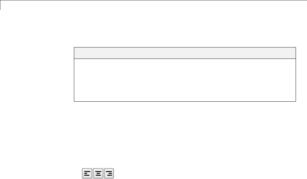
51 PrintFrame Editor
ChangeInformationinCells
In this section...
“Align the Information in a Cell” on page 51-18
“EditTextStrings”onpage51-18
“Remove and Copy Entries” on page 51-19
“Change the Font Characteristics” on page 51-20
AligntheInformationinaCell
To align the information within a cell:
1Click within the cell to select it.
2Click on one of the Align buttons for left, center, or right alignment.
The information aligns within the cell.
Alignment does not apply to the cell that contains the %<blockdiagram>
entry. The block diagram is automatically scaled and centered to fit in that
cellatthetimeofprinting.
Edit Text Strings
You can change text you typed in a cell:
1Double-click the information you want to edit.
An edit box appears around all of the information in that cell.
2Click at the start of the text you want to change and drag to the end of
thetexttobechanged.
This highlights the text.
3Type the replacement text.
51-18

Change Information in Cells
It automatically replaces the highlighted text.
4Click anywhere outside of the edit box to end editing mode.
Note Be careful not to edit the text of a variable entry, because then the
variable information will not print. For example, if you accidentally remove
the %from the %<page> entry, the text <page> will print instead of the actual
page number.
Remove and Copy Entries
You can cut, copy, paste, or delete an entry:
1Double-click the information you want to remove or copy.
An edit box appears around all of the information in that cell.
2Click at the start of the entry you want to edit and drag to the end of that
entry. This highlights the entry.
Forvariableinformation,besuretoincludetheentirestring,forexample,
%<page>.
Note that for computers running the Microsoft Windows operating system,
you can select all of the entries in a cell by right-clicking the information
and choosing Select All from the pop-up menu.
3Use the standard editing techniques for your platform to cut, copy, or delete
the highlighted information.
•For computers running the Microsoft Windows operating system,
right-click in the edit box and select Cut,Copy,orDelete from the
pop-up menu.
•For UNIX based systems, highlighting the information automatically
copies it to the clipboard. If you want to remove it, press the Delete key.
If you make a mistake, use your platform’s standard undo technique. For
example, for computers running the Microsoft Windows operating system,
right-click in the edit box and select Undo from the pop-up menu.
51-19
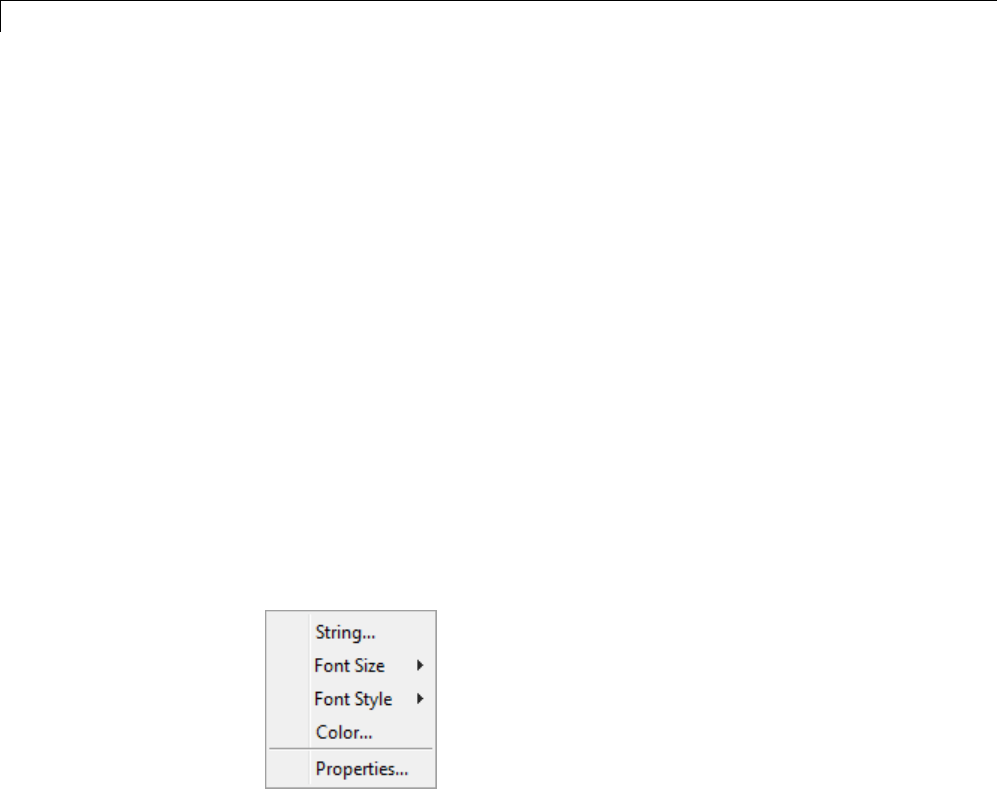
51 PrintFrame Editor
4If you cut or copied the information to the clipboard and want to paste it,
double-click the entry where you want to paste it and position the cursor at
the new location in that edit box. Then use the standard paste technique
for your platform.
•For computers running the Microsoft Windows operating system,
right-click at the new location and select Paste from the pop-up menu.
•For UNIX based systems, click at the new location and then click the
middle mouse button.
5Click somewhere outside of the edit box to end editing mode.
Change the Font Characteristics
You can change the font characteristics for the information in any cell.
Specifically, you can specify the font size, style, color, and family.
1Right-click the information in the cell.
The information in the cell is selectedandthepop-upmenuforchanging
font characteristics appears.
If this pop-up menu does not appear, it is because you were in edit mode.
To get the font pop-up menu, click somewhere outside of the edit box
surrounding the information and then right-click.
2Select an item from the pop-up menu. Choose Properties if you want to
change the font family or if you want to change multiple characteristics
at once.
Note that you can also select String from the pop-up menu, which allows
you to edit the text string.
51-20

Change Information in Cells
3Select the new font characteristic(s) for that cell. For example, for Font
Size, select the new size from its pop-up menu.
Note that changing the font characteristics for the %<blockdiagram> entry
is not relevant and does nothing.
51-21

51 PrintFrame Editor
Save and Open Print Frames
In this section...
“Save a Print Frame” on page 51-22
“Open a Print Frame” on page 51-22
Save a Print Frame
Youmustsaveaprintframetoprintablockdiagramwiththatprintframe.
To save a print frame:
1Select Save As from the File menu.
The Save As dialog box appears.
2Type a name for the print frame in the File name edit box.
3Click the Save button.
The print frame is saved as a figure file, which has the .fig extension. A
figure file is a binary file used for print frames.
Open a Print Frame
You can open a saved print frame in the PrintFrame Editor, make changes
to it, and save it under the same or a different name. To open an existing
print frame:
1Select Open from the File menu.
2Select the print frame you want to open.
All print frames are figure files.
Alternatively, you can open a print frame from the MATLAB prompt. Type
frameedit filename and the PrintFrame Editor opens with the print frame
file you specified.
51-22

Print Block Diagrams with Print Frames
Print Block Diagrams with Print Frames
When using the Simulink software or Stateflow product, you can print a block
diagram with the print frame.
1Select File>Print>Print.
The Print Model dialog box appears. The dialog box shown below is for
computers running the Microsoft Windows operating system. The dialog
box for your platform might look slightly different.
51-23
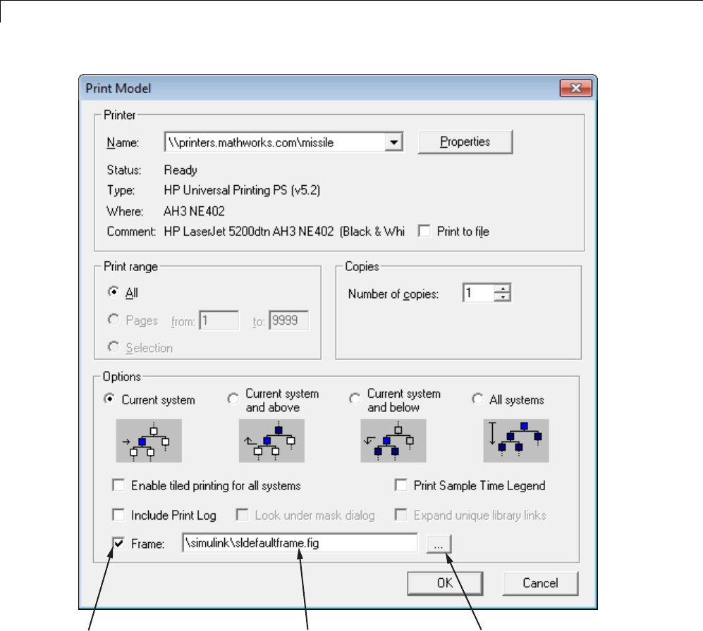
51 PrintFrame Editor
Check this box to print
the block diagram with a
print frame.
Type the path and filename
of the print frame you want
the block diagram to print with,
click the ... button
and then select the print
frame file.
or
In the Print Model dialog box:
1Select the Frame check box.
51-24

Print Block Diagrams with Print Frames
2Supply the file name for the print frame you want to use. Either type the
path and file name directly in the edit box, or click the ... button and select
theprintframefileyousavedusingthePrintFrameEditor.
Note that the default print frame file name, sldefaultframe.fig,appears
in the file name edit box until you specify a different file name.
3Specify other printing options in the Print dialog box. For example,
for computers running the Microsoft Windows operating system, specify
options under Properties.
Note Specify the paper orientation for printing the way you normally
would. The paper orientation you specified in the PrintFrame Editor’s
PrintFrame Page Setup dialog box is not the same as the paper
orientation used for printing. For example, assume you specified a
landscape-oriented print frame in thePrintFrameEditor. Ifyouwantthe
printed page to have a landscape orientation, you must specify that at
the time of printing. For example, for computers running the Microsoft
Windows operating system, click the Properties button in the Print
Model dialog box, and for Page Setup,specifytheOrientation as
Landscape.
4Click OK in the Print dialog box.
The block diagram prints with the print frame you specified.
Seealsotheexample,“PrinttheBlock Diagram with the Print Frame” on
page 51-30.
51-25

51 PrintFrame Editor
Create and Use a Print Frame
In this section...
“About the Example” on page 51-26
“Create the Print Frame” on page 51-27
“Print the Block Diagram with the Print Frame” on page 51-30
About the Example
This example uses a Simulink model of an engine. It involves two parts —
first creating a print frame, and then printing the engine model with that
print frame. The result looks similar to the figure below.
51-26
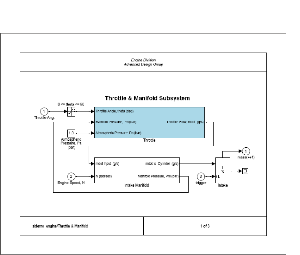
CreateandUseaPrintFrame
Create the Print Frame
1At the MATLAB prompt, type frameedit.
The PrintFrame Editor window appears.
2Set up the page:
aSelect Page Setup from the File menu.
51-27

51 PrintFrame Editor
The PrintFrame Page Setup dialog box opens.
bFor Paper Type, select a size that is appropriate for your printer.
cFor this example, keep the Paper Orientation as Landscape and
the Margins set to 0.75 inches.
dClick the OK button.
The dialog box closes. The print frame you see in the PrintFrame
Editor window will reflect your changes.
3Add the information entries %<blockdiagram>,%<fullsystem>,and
%<page>.
aClick within the upper row in the print frame.
bFrom the bottom right list box, select Block Diagram,thenclickAdd.
The %<blockdiagram> appears in the row.
cClick within the lower left cell in the print frame.
dFrom the bottom right list box, select Full System Name,thenclick
Add.The
%<fullsystem> appears in the cell.
eClick within the lower right cell in the print frame.
fFrom the bottom right list box, select Page Number,thenclickAdd.
The %<page> appears in the cell.
4Add a row at the top.
aClick within the upper row in the print frame, the row that contains
the %<blockdiagram> entry.
Be sure that handles appear on all four corners of the row.
bClick the add row button.
A new row appears at the top, above the row you selected.
5Make the new row shorter.
aClick on the horizontal line that separates the top row (the row you just
added) from the row beneath it (the row containing the %<blockdiagram>
entry).
51-28

CreateandUseaPrintFrame
Be sure that only two handles appear, one at each end of the line. If you
see four handles in either row, click directly on the horizontal line and
the other two handles disappear.
bDrag the line up until the top row is about the same height as the row
at the bottom of the print frame.
6Add information in the top row.
aClick anywhere within the top row (the row you just added).
bSelect Text from the information list box.
cClick the Add button.
An edit box appears in the cell.
dType Engine Division,presstheEnter keytoadvancethecursorto
the next line, and then type Advanced Design Group.
Click the zoom in button if you need to magnify the entry.
eClick outside of the edit box to end editing mode.
7In the left cell of the bottom row, align the information on the left.
aClick the zoom out button if you need to.
bClick within the left cell of the bottom row to select it.
cClick the left alignment button.
The entry moves to the left.
8Make the information in the top row appear in italics.
aRight-click on the entry in the row.
bSelect Font Style from the pop-up menu.
If the pop-up menu for font properties does not appear, you are in
editing mode. Click outside of the edit box to end editing mode and then
right-click the text to access the pop-up menu.
cFrom the Font Style pop-up menu, select italic.
51-29
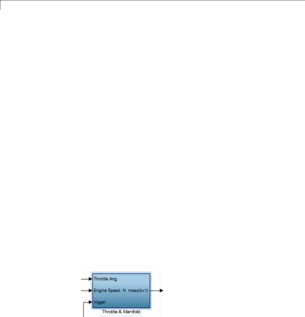
51 PrintFrame Editor
The entry in the cell appears in italics and the information will appear in
italics when the print frame is printed with a Simulink diagram.
9Add the total number of pages to the right cell in the bottom row.
aClick within the cell to select it.
bAdd the total pages entry: select Total Pages from the information
list box and click the Add button.
The %<npages> entry appears after the %<page> entry. If you need to,
zoom in to see the entry.
cAdd the text of after the page number entry. Click the cursor after
the %<page> entry, and then type of (type a space before and after
the word).
The information in the cell now is: %<page> of %<npages>.
10 Save the print frame: select Save As from the File menu. In the Save
Frame dialog box, type engdivl for the File name.ClicktheSave button.
Theprintframeissavedasafigurefile.
11 You can close the PrintFrame Editor window by clicking the close box.
Print the Block Diagram with the Print Frame
1To view the Simulink engine model, type sldemo_engine at the MATLAB
prompt.
The engine model appears in a Simulink window.
2Double-clicktheThrottle&Manifoldblock.
51-30
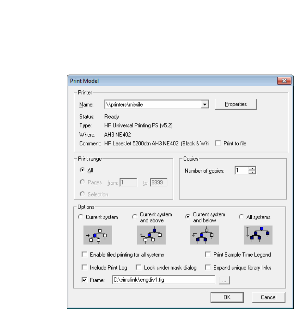
CreateandUseaPrintFrame
The Throttle & Manifold subsystem opens in a new window.
3In the Throttle & Manifold window, select File>Print >Print.
The Print Model dialog box opens.
4Click the Properties button, and set the page orientation to landscape.
51-31

51 PrintFrame Editor
5In the Print Model dialog box, under Options, select Current system
and below.
This specifies that the Throttle & Manifold block diagram and its
subsystems will print.
6Check the Frame check box.
7Specify the print frame to use.
aClick the ... button.
bIn the FrameFileSelectiondialog box, find the file name of the print
frame you just created, engdivl.fig, and select it.
cClick the Open button.
The path and file name appear in the Frame edit box.
8Click OK in the Print Model dialog box.
The Throttle & Manifold block diagram prints with the print frame; it
should look similar to the figure shown at the start of this example.
In addition, the Throttle block diagram and the Intake Manifold block
diagram print because you specified printing of the current system and its
subsystems. These block diagrams also print with the engdivl print frame,
but note that their variable information in the print frame is different.
51-32


52
About Run on Target
Hardware Feature

52 About Run on Target Hardware Feature
About Run on Target Hardware Feature
RunonTargetHardwareis a feature of the Simulink product that runs a
Simulink model on target hardware.
At the time of publication, Simulink software supports the following target
hardware:
•Arduino Mega 2560 and Arduino Uno
•BeagleBoard Xm, BeagleBoard Bx, and BeagleBoard Cx
•LEGO™ MINDSTORMS®NXT
•PandaBoard
To use this feature, open a Simulink model, and select Tools >Run on
Target Hardware.
To start using Run on Target Hardware, first use the Target Installer to
install support for your target hardware. The Target Installer guides you
through the process of getting a support package, installing a target,and
in some cases, replacing the firmware on your target hardware. To use
Target Installer, open a Simulink model, and select Tools >RunonTarget
Hardware >Install/Update Support Package.
You can have the Target Installer download a support package from
MathWorks.com, or use a support package in a local folder. The Target
Installer uses the support package to install a target, which provides the
software tools and features required for a specific type of target hardware,
including:
•A Simulink block library
•A pane in the Configuration Parameters dialog
•Third-party software
•Examples
For detailed information about using the Target Installer with your hardware,
see:
52-2

About Run on Target Hardware Feature
•“Install Support for Arduino Hardware” on page 53-2
•“Install Support for BeagleBoard Hardware” on page 54-2
•“Install Support for LEGO MINDSTORMS NXT Hardware” on page 55-2
•“Install Support for PandaBoard Hardware” on page 56-2
After installing the appropriate target,youcanrunamodelonyourtarget
hardware using the following menu items under Tools >RunonTarget
Hardware:
•Prepare to Run — Before using this menu item, create a backup
copy of your model. Clicking Prepare to Run changes the model
Configuration Parameters and opens the Run on Target Hardware pane
in the Configuration Parameters dialog. IntheRunonTargetHardware
pane, set the Target hardware parameter, and then save the changes to
your model.
•Run — This menu item appears after you have prepared the model to
run. Clicking Run creates an executable file from the model and runs
it on the target hardware.
•Options — This menu item opens the Run on Target Hardware pane in the
model Configuration Parameters dialog. You can use this pane to specify
thetargethardwareandconfigureoptional settings, such as External mode.
52-3

52 About Run on Target Hardware Feature
52-4

53
Work with Arduino
Hardware
•“Install Support for Arduino Hardware” on page 53-2
•“Open Block Libraries for Arduino Hardware” on page 53-10
•“Run Model on Arduino Hardware” on page 53-13
•“Tune and Monitor Models Running on Arduino Mega 2560 Hardware” on
page 53-15
•“Use Serial Communications with Arduino Hardware” on page 53-19
•“Detect and Fix Task Overruns on Arduino Hardware” on page 53-22
•“Troubleshoot Running Models on Arduino Hardware” on page 53-24
•“Configure Host COM Port Manually” on page 53-26

53 Work with Arduino®Hardware
Install Support for Arduino Hardware
This topic shows how to add support for Arduino®hardware to the Simulink
product. After you complete this process, you can run Simulink models on
your Arduino hardware.
The installation process adds the following items to your host computer:
•Third-party software development tools, such as the Arduino software
•A Simulink block library for configuring and accessing Arduino sensors,
actuators, and communication interfaces
•Examples for getting started and learning about specific features
To check for updates, repeat this process when a new version of MATLAB
software is released. You can also check for updates between releases.
Note You can use this software on host computers running versions of 32-bit
or 64-bit Windows that Simulink software supports.
To install support for Arduino hardware:
1Start Target Installer using one of the following methods:
•In a MATLAB Command Window, enter targetinstaller.
•In a model, click the Tools menu, and select Run on Target Hardware >
Install/Update Support Package.
2Choosetogetthesupportpackagefrom the Internet or from a folder.
Note Thetimerequiredtodownloadingthesupportpackageandthird-party
software varies depending on the bandwidth and speed of your Internet
connection.
53-2

Install Support for Arduino®Hardware
Internet: This option is selected by default. Target Installer downloads and
installs the support package and third-party software from the Internet.
Folder: Target Installer gets the support package and third-party software
installers from the specified folder. If the third-party software installers are
not available, Target Installer downloads and installs those from the Internet.
You must have write privileges for this folder. Having write privileges for the
default folder is typically not an issue. If you change to a new folder for which
you do not have write permissions, such as a shared folder on a network,
Target Installer generates an error message.
To solve this issue, copy the support package to a folder for which you have
writeprivileges,andpointTargetInstallertothatsamefolder. Forexample,
copy the support package to C:\MATLAB\Targets\version\downloads.If
they are available, also copy the third-party software installers associated
with the support package.
To locate the support package in a folder, search for a filename that begins with
arduino and ends with .zip. For example: arduinouno_r2012a_v1_0.zip
53-3
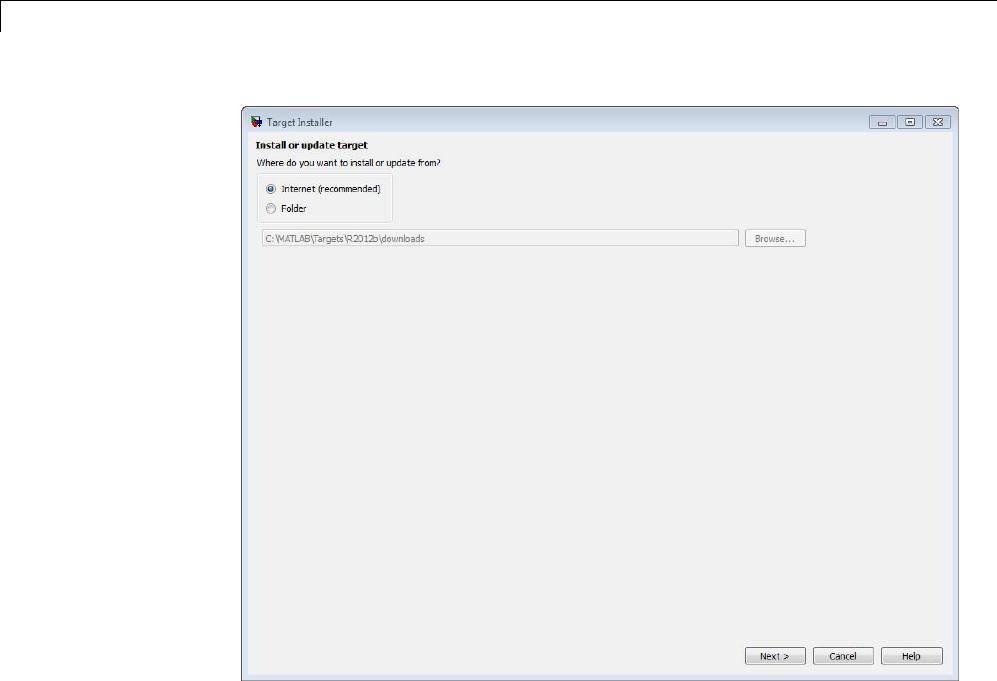
53 Work with Arduino®Hardware
3Select the Install check box for either Arduino target, and click Next.(To
install another target, run Target Installer again later on.)
The Installation folder parameter specifies where Target Installer puts the
target files. You must have write privileges for this folder.
53-4
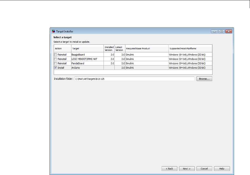
Install Support for Arduino®Hardware
4Target Installer confirms that you are installing the target, and lists
third-party software it will install.
Review the information, including the license agreements, and click Install.
53-5
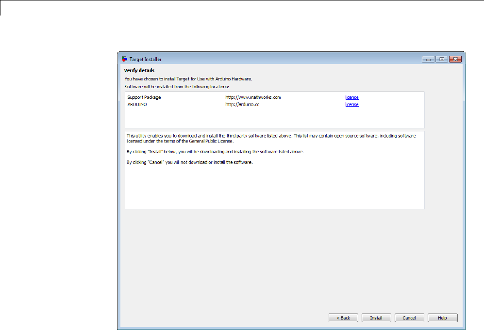
53 Work with Arduino®Hardware
Target Installer displays a progress bar while it downloads and installs the
third-party software.
53-6
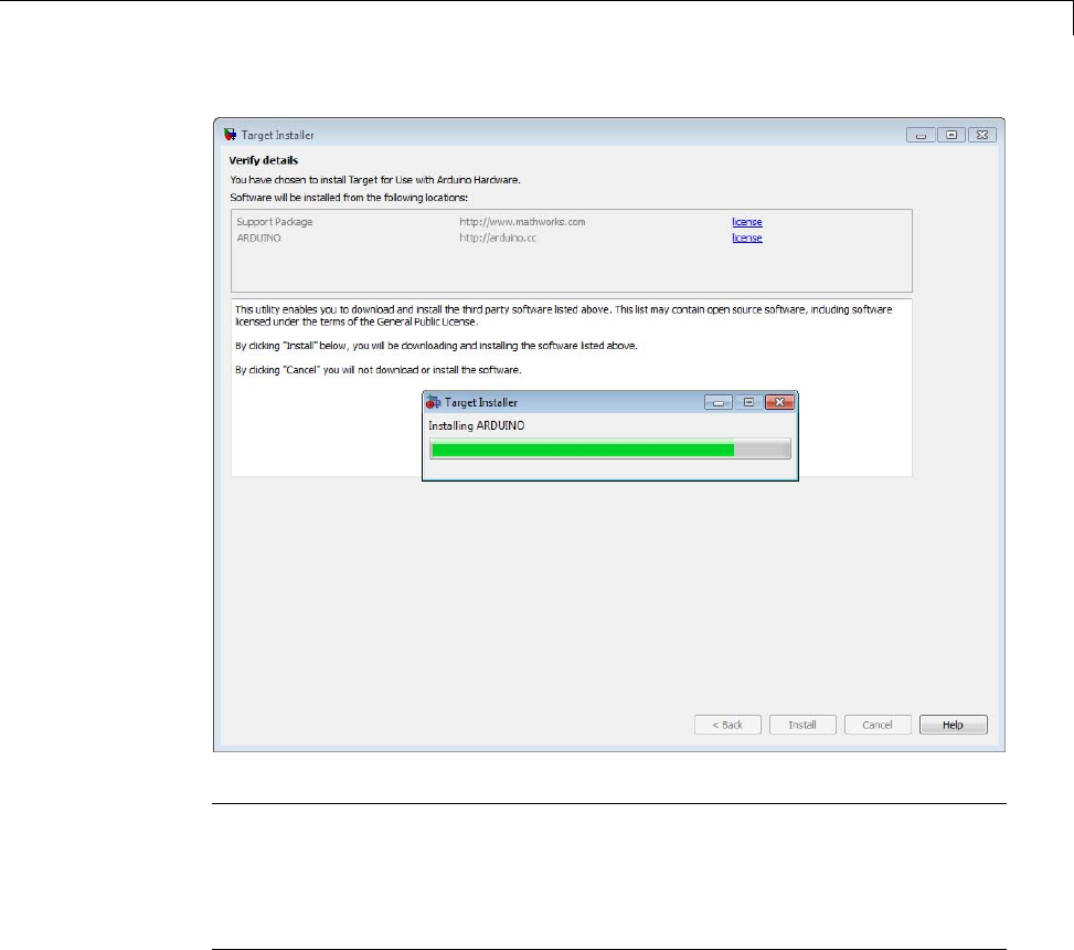
Install Support for Arduino®Hardware
Note If you installed the target previously, Target Installer may remove
files from that installation before installing the current target. If Target
Installer cannot remove those files automatically, it instructs you to delete
the files manually. Close the MATLAB software before removing the files.
Then, restart MATLAB software and run Target Installer again.
5To view target examples, leave the Launch target examples checkbox
selected and click Finish.
53-7
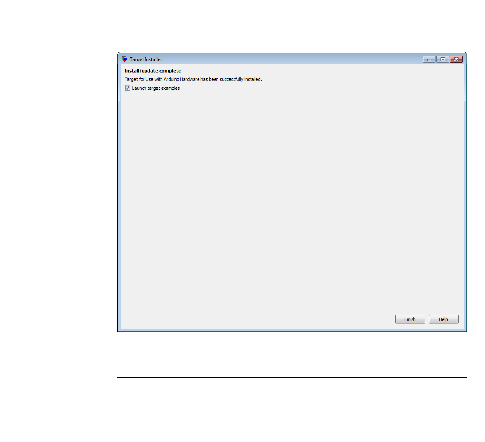
53 Work with Arduino®Hardware
The Help that opens displays the appropriate examples for your hardware.
Note To reopen the examples later, enter the following text in a MATLAB
Command Window:
demo simulink 'Target for Use with Arduino'
53-8
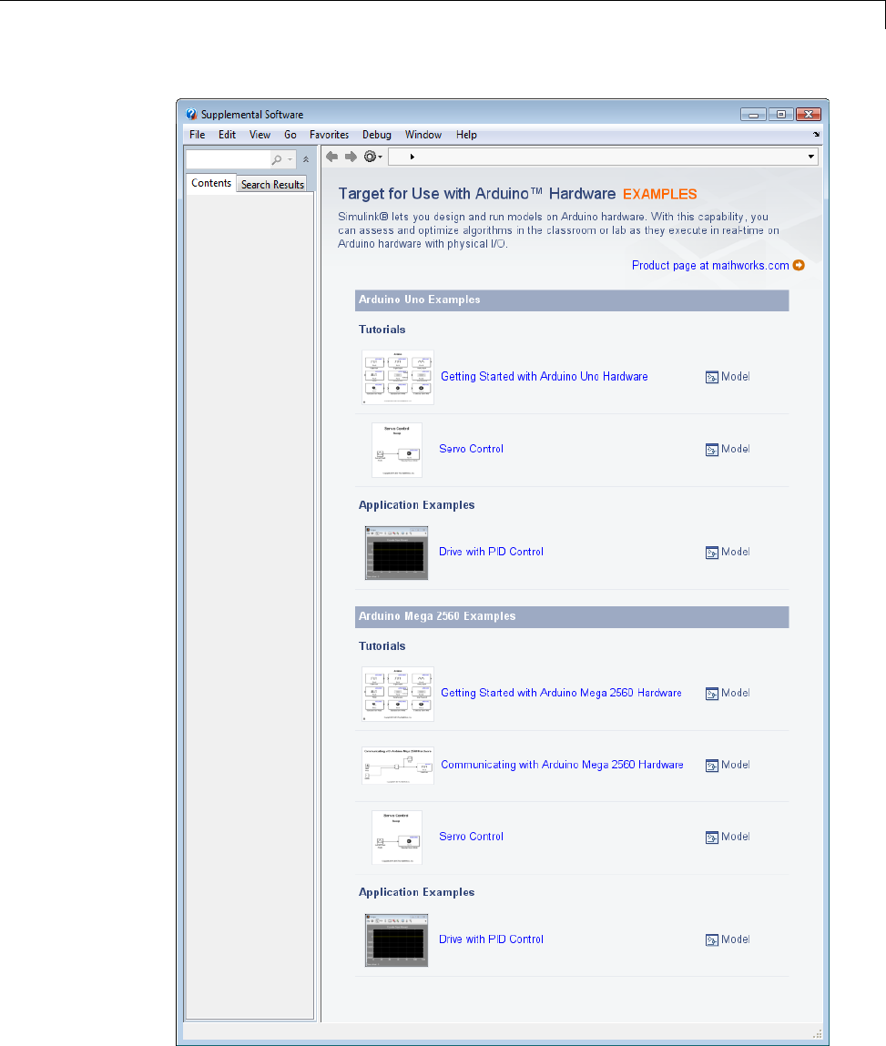
Install Support for Arduino®Hardware
53-9

53 Work with Arduino®Hardware
Open Block Libraries for Arduino Hardware
You can open the block libraries for your Arduino hardware from the
MATLAB Command Window or from the Simulink Library Browser.
The blocks in these block libraries provide support for various peripherals
available on the Arduino hardware.
From the Command Line
AfterinstallingsupportforyourArduino hardware, you can open its block
library from the MATLAB Command Window.
After installing support for Arduino hardware, enter:
arduinolib
The software opens the corresponding block library.
53-10
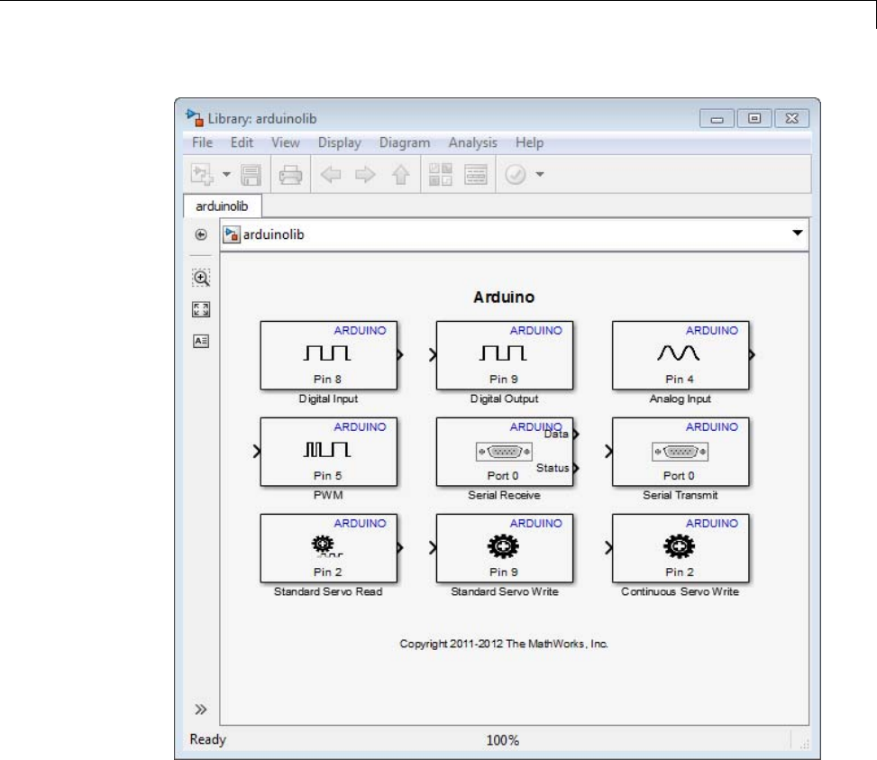
Open Block Libraries for Arduino®Hardware
From the Simulink Library Browser
To open the block library from the Simulink Library Browser:
Enter simulink in the MATLAB Command Window, or click the following
icon on the MATLAB toolbar.
53-11
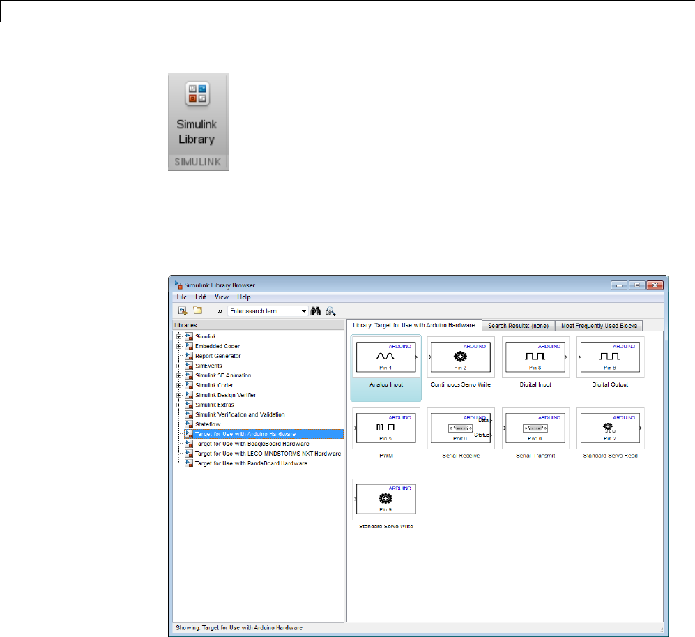
53 Work with Arduino®Hardware
In the Simulink Library Browser, click Target for Use with Arduino
Hardware.
Simulink Library Browser displays the corresponding block library.
53-12

Run Model on Arduino®Hardware
Run Model on Arduino Hardware
You can prepare, configure, and run a model on your Arduino hardware.
Before starting:
•Connect your Arduino hardware to the host computer using a USB cable.
•Create or open a Simulink model located on a local drive or a mapped
network drive that has a drive letter assigned to it.
The software generates an error message if the location of the model
contains a UNC path. For example, \\server-00\user$\MATLAB\
To prepare and run the model:
1Use File >Save As to create a working copy of your model. Keep the original
model as a backup copy.
2Click the Tools menu in the model, and select Run on Target Hardware >
Prepare toRun. This action changes the model Configuration Parameters.
3In the Run on Target Hardware pane that opens, set the Target hardware
parameter to Arduino Mega 2560 or Arduino Uno.
4If your model contains one or more Model blocks, configure the submodels as
described in “Prepare Models That Use Model Reference” on page 53-14.
5Click the Tools menu, and select Run on Target Hardware >Run.
This action automatically downloads and runs your model on the Arduino
hardware.
The lower left corner of the model window displays status while Simulink
software prepares, downloads, and runs the model on the target hardware.
To stop a model running on Arduino hardware, you can:
•Disconnect the power from the hardware. When you reconnect the power,
the model will start running again.
•Run a new or updated model on the hardware. This action automatically
stops and erases the previous model running on the Arduino hardware.
53-13

53 Work with Arduino®Hardware
To restart the model running on the Arduino hardware, press the RESET
buttonontheboard.
Prepare Models That Use Model Reference
You can use Model blocks to include one model in another. Each instance of a
Model block represents a reference to another model, called a referenced model
or submodel. The model that contains a referenced model is its parent model.
When you run the parent model on your target hardware, the submodel
effectively replaces the Model block that references it. For more information,
see “Overview of Model Referencing” on page 6-2
When you run a model on target hardware, the parent model and the
submodels must have the same Configuration Parameter settings.
If your model contains Model blocks, perform the following steps for each
Model block:
1Open the model associated with the Model block.
2Click the Tools menu, and select Run on Target Hardware >Prepare
to Run.
3Apply the same Configuration Parameters settings to the submodel as you
applied to the parent model.
If the model and Model blocks have different settings, the software generates
an error when you try to run the model on the target hardware.
See Also
•“Create the Simple Model”
•“Troubleshoot Running Models on Arduino Hardware” on page 53-24
•“Configure Host COM Port Manually” on page 53-26
•“Tune and Monitor Models Running on Arduino Mega 2560 Hardware” on
page 53-15
•“Overview of Model Referencing” on page 6-2
53-14

Tune and Monitor Models Running on Arduino®Mega 2560 Hardware
Tune and Monitor Models Running on Arduino Mega 2560
Hardware
In this section...
“About External Mode” on page 53-15
“Run Your Model in External Mode” on page 53-16
“Stop External Mode” on page 53-18
About External Mode
You can use External mode to tune parameters in, and monitor data from,
your model while it is running on the Arduino Mega 2560 hardware. This
capability is not available with Arduino Uno hardware.
External mode enables you to tune model parameters and evaluate the effects
of different parameter values on the model results in real-time, in order to
find the optimal values to achieve the desired performance. This process
is calledparameter tuning.
External mode accelerates parameter tuning because you do not have to
re-run the model each time you change parameters. External mode also lets
you develop and validate your model using the actual data and hardware for
which it is designed. This software-hardware interaction is not available
solelybysimulatingamodel.
The following list provides an overview of the parameter tuning process with
External mode:
•In the model on your host computer, you enable External mode in the
Configuration Parameters.
•In the model on your host computer, you configure Simulink software to
run your model on the target hardware.
•You use the model on the host computer as a user interface for interacting
with the model running on the target hardware:
53-15

53 Work with Arduino®Hardware
-Whenyouopenblocksandapplynewparametervaluesonthehost
computer, External mode updates the corresponding values in the model
running on the target hardware.
-If your model contains blocks for viewing data, such as Scope or Display
blocks, External mode sends the corresponding data from the target
hardware to those blocks on the host computer.
•You determine the optimal parameter settings by adjusting parameter
values on the host computer and observing data/outputs from the target
hardware.
When you have finished tuning a model, you can disable External mode and
run the tuned model on your hardware.
Some limitations apply while you are using External mode:
•Do not configure Serial Receive or Serial Transmit blocks in your model to
use serial port 0. External mode uses serial port 0.
•Do not use the following Arduino®servo blocks: Standard Servo Read,
Standard Servo Write, and Continuous Servo Write.
Run Your Model in External Mode
Before starting:
•Connect your Arduino Mega 2560 hardware to the host computer using a
USB cable.
•Create or open a Simulink model located on a local drive or a mapped
network drive that has a drive letter assigned to it.
The software generates an error message if the location of the model
contains a UNC path. For example, \\server-00\user$\MATLAB\
To prepare and run the model:
1Open your Simulink model.
2Review the value of the Simulation stop time parameter, located on
the model toolbar, as shown here.
53-16

Tune and Monitor Models Running on Arduino®Mega 2560 Hardware
•To run the model for an indefinite period, enter inf.
•To run the model for a finite period, enter a number of seconds. For
example, entering 120 runs the model on the Arduino hardware for
2 minutes.
3Click the Tools menu, and select Run on Target Hardware >Options.
4In the Run on Target Hardware pane that opens, select the Enable
External mode checkbox.
5Click OK, and then save the changes to your model.
6Click the Tools menu, and select Run on Target Hardware >Run.
The lower left corner of the model window displays status while Simulink
software prepares, downloads, and runs the model on the target hardware.
7While the model is running in External mode, you can change tunable
parameter values in the model on your host computer and observe the
corresponding changes in the model running on the hardware.
If your model contains blocks from the Simulink Sinks block library,
the sinkblocksinthemodelonyourhostcomputerdisplaythevalues
generated by the model running on the hardware.
If your model does not contain a sink block to which External mode can
send data, the MATLAB Command Window displays a “No data has been
selected for uploading” warning. You can disregard this warning, or you
can add a sink block to the model and rerun your model.
When you have finished tuning and monitoring your model, you can disable
External mode.
To deploy model to your hardware without using External mode. See “Run
Model on Arduino Hardware” on page 53-13:
53-17

53 Work with Arduino®Hardware
Note External mode increases the processing burden of the model running
on the hardware. If the software reports an overrun, you can apply the
solutions described in “Detect and Fix Task Overruns on Arduino Hardware”
on page 53-22.
Stop External Mode
To stop the model running in External mode, click the black square Stop
button located on the model toolbar, as shown here.
This action stops the process for the model running on the Arduino hardware,
and stops the model simulation running on your host computer.
If the Simulation stop time parameter is set to a specific number of seconds,
External mode stops when that period has elapsed.
To disable External mode:
1Click the Tools menu, and select Run on Target Hardware >Options.
2In the Run on Target Hardware pane that opens, clear the Enable
External mode checkbox.
3Click OK, and then save the changes to your model.
53-18

Use Serial Communications with Arduino®Hardware
Use Serial Communications with Arduino Hardware
In this section...
“Hardware” on page 53-19
“Transmit Serial Data” on page 53-20
“Receive Serial Data” on page 53-21
Arduino hardware has serial ports, also known as UARTs, that can
communicate with other devices that have serial interfaces.
Hardware
The Arduino Uno board has one serial port, serial port 0, connected to:
•The digital pins marked TX 1 (transmit) and RX 0 (receive).
•The USB port, through a serial-to-USB converter.
The Arduino Mega 2560 board has four serial ports:
•Serial port 0 is connected to Communication pins marked TX0 1 (transmit)
and RX0 0 (receive). Serial port 0 is also connected to the USB port through
a converter.
•Serial port 1 is connected to Communication pins marked TX1 18 (transmit)
and RX1 19 (receive).
•Serial port 2 is connected to Communication pins marked TX2 16 (transmit)
and RX2 17 (receive).
•Serial port 3 is connected to Communication pins marked TX3 14(transmit)
and RX3 15 (receive).
You can use serial port 0 to communicate with other devices that have serial
ports, or to communicate with a computer over the USB port.
Each serial port supports one Serial Transmit and one Serial Receive block,
one block per pin.
53-19

53 Work with Arduino®Hardware
If you intend to use External mode with Arduino Mega 2560 hardware, use
serial ports 1 through 3 for serial communications. Serial port 0 is not
available for serial communications because it is connected to the USB port,
whichExternalmodeusestocommunicatewiththehostcomputer. This
restriction does not apply to Arduino Uno hardware, because External mode is
not supported. For more information, see “Tune and Monitor Models Running
on Arduino Mega 2560 Hardware” on page 53-15.
Serial communications are not supported in models that also use the Arduino
Standard Servo Read, Standard Servo Write, and Continuous Servo Write
blocks.
Warning Only connect serial port pins to devices that use 5 Volt TTL
logic. Do not connect these pins to an RS-232 serial interface, such
as the DE-9M connector on a computer, without limiting the voltage.
The RS-232 standard allows higher voltages that can damage your
hardware. For details, read the documentation for your Arduino
hardware.
Transmit Serial Data
To transmit data through a serial port or USB port on the Arduino hardware:
1Add the Arduino Serial Transmit block to your model.
2Connect a data source to the block input on the Serial Transmit block.
If the data type is not uint8, use a Data Type Conversion block to convert
it to uint8.
3In the Arduino Serial Transmit block, select a Port number.
4Click the Tools menu in the model, and select Run on Target Hardware
>Options.
In the Configuration Parameters dialog that opens, on the Run on Target
Hardware pane, set the baud rate for the serial port you selected in the
Arduino Serial Transmit block.
5Connect the appropriate digital transmit pin to the hardware that receives
the data.
53-20

Use Serial Communications with Arduino®Hardware
6Run the model, as described in “Run Model on Arduino Hardware” on
page 53-13.
7If your model uses the Arduino USB port (Serial port 0) to transmit data to
a device that is not your host computer, reconnect the USB cable to that
device and press the RESET button.
Receive Serial Data
To receive data through a serial port or USB port on the Arduino hardware:
1Add the Arduino Serial Receive block to your model.
2On the Arduino Serial Receive block, connect the Data block output to
a block that uses the data.
3Open the Arduino Serial Receive block and specify the Port number.
4Click the Tools menu in the model, and select Run on Target Hardware
>Options.
In the Configuration Parameters dialog that opens, on the Run on Target
Hardware pane, set the baud rate for the serial port you selected in the
Arduino Serial Receive block.
5Connect the digital receive pin to the hardware that transmits the data.
6Run the model, as described in “Run Model on Arduino Hardware” on
page 53-13.
7If your model uses the Arduino USB port (Serial port 0) to receive data
from a device that is not your host computer, reconnect the USB cable to
that device and press the RESET button.
53-21

53 Work with Arduino®Hardware
Detect and Fix Task Overruns on Arduino Hardware
You can configure a Simulink model running on the target hardware to detect
and notify you when a task overrun occurs. A task overrun occurs if the target
hardware is still performing one instance of a task when the next instance
of that task is scheduled to begin. You can fix overruns by decreasing the
frequency with which tasks are scheduled to run, and/or by reducing the
number of tasks defined by your model.
To enable overrun detection:
1Click the Tools menu in the model, and select Run on Target Hardware
and Options.
2In the Run on Target Hardware pane that opens, select the Enable
overrun detection check box.
3Use the Digital output to set on overrun parameter to specify the pin
number of a digital output.
4Click OK.
To create a visual overrun indicator for your board, connect an appropriate
resistor in series with an LED between the GND and the hardware pin specified
by the Digital output to set on overrun parameter. Orient the LED so the
longer leg (positive) is connected to the digital output pin.
When a task overrun occurs:
•The state of the digital output pin specified by the Digital output to set
on overrun parameter changes from low (0 Volts) to high (5 Volts).
•The model continues running, but the effective sample time will be longer
than specified.
To fix an overrun condition, reduce the processing burden of the model by
applying one or more of the following solutions:
•Increase the sample times for the model. For example, increase the values
of the Sample time parameters in all of your data source blocks.
53-22

Detect and Fix Task Overruns on Arduino®Hardware
•Simplify the model.
If you are using External mode, and the preceding solutions do not fix the task
overrun condition, consider clearing the Enable External mode checkbox
in the Run on Target Hardware pane. External mode adds a lightweight
server to the model running on the target hardware. This server increases
the processing burden upon the target hardware, which can contribute to a
task overrun condition.
53-23

53 Work with Arduino®Hardware
Troubleshoot Running Models on Arduino Hardware
In this section...
“Block Produces Zeros in Simulation” on page 53-24
““Could not automatically set host COM port”” on page 53-24
Block Produces Zeros in Simulation
If you simulate a model on your host computer without running it on your
target hardware, input blocks produce zeros, and output blocks do nothing.
This is the expected behavior.
For example, if you select Simulation >Run in a model that contains a
Digital Input block and a Digital Output block:
•The block output on the Digital Input block produces zeros.
•The Digital Output block does nothing.
To solve this issue, run your model on the target hardware as described in:
•“Run Model on Arduino Hardware” on page 53-13
•“Run Your Model in External Mode” on page 53-16
“Could not automatically set host COM port”
If you try to run a model on your Arduino hardware and Simulink generates
an error message similar to this one: “The call to realtime_make_rtw_hook,
during the entry hook generated the following error: Could not automatically
set host COM port for your Arduino hardware. This may be due to a
disconnected or unrecognized board. If the board is not connected to your host
computer, connect it and let the operating system install the board driver.”
Resolve Connection Issues
To resolve connection issues:
1Verify that your Arduino hardware is powered on and connected to your
host computer.
53-24

Troubleshoot Running Models on Arduino®Hardware
2Try running the model again on your Arduino hardware.
Resolve Driver Issues
If you get the error message while your board is powered on and connected to
your host computer, resolve any issues with Arduino drivers in Windows:
1In the Windows Start menu, select Devices and Printers.
2If you find an Unknown Device under Other Devices or COM Ports,
double click the Unknown Device.
3In the Unknown Device Properties dialog box that opens, click the
Hardware tab, and click Properties.
4In the Unknown device Properties dialog box that opens, click Update
Driver.
5In the Update Driver Software - Unknown Device dialog box that
opens, click Browse my computer for driver software.
6Select the Include subfolders checkbox and click Browse.
7Navigate to the Installation folder that Target Installer
used when you installed support for your Arduino hardware,
and then click Next. By default, this folder location is
C:\MATLAB\Targets\releasenumber\arduino-version. For example:
C:\MATLAB\Targets\R2012a\arduino-1.0.
8If prompted by Windows Security, choose Install this driver software
anyway, and let Windows complete the process of installing the driver.
9Try running the model again on your Arduino hardware.
If you get the error message after resolving issues with Arduino drivers, set
thehostCOMportandbaudratemanually. ThedriversforsomeArduino
board revisions do not identify the board as an Arduino device in Windows. In
that case, set the COM port number and Serial 0 baud rate manually, as
described in “Configure Host COM Port Manually” on page 53-26
53-25

53 Work with Arduino®Hardware
Configure Host COM Port Manually
Simulink software automatically detects the COM port settings of the
USB connection between your host computer and the Arduino hardware.
Optionally, you can also configure these settings manually.
To configure the COM port settings manually:
1Click the Tools menu in the model, and select Run on Target Hardware
>Options.
2In the Run on Target Hardware pane, change the SethostCOMport
parameter to Manually and leave the Configuration Parameters dialog
open.
3Open Devices and Printers in Windows.
4Double-click Arduino Uno or Arduino Mega 2560 device.
5In the device properties dialog, click the Hardware tab, and then click the
Properties button.
6Click the Port Settings tab.
For example, the following image shows an Arduino device in Devices and
Printers, the Hardware tab, and the Port Settings tab.
53-26
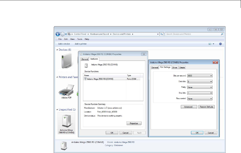
Configure Host COM Port Manually
7In Configuration Parameters, update COM port number and Serial 0
baud rate to match the Arduino device in Windows.
53-27
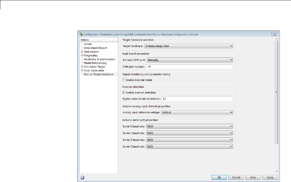
53 Work with Arduino®Hardware
8Click OK and save the model.
53-28

54
Work with BeagleBoard
Hardware
•“Install Support for BeagleBoard Hardware” on page 54-2
•“Replace Firmware on BeagleBoard Hardware” on page 54-9
•“Choose the Type of Serial Cable” on page 54-24
•“Connect to Serial Port on BeagleBoard Hardware” on page 54-25
•“Configure Network Connection with BeagleBoard Hardware” on page
54-30
•“Get IP Address of BeagleBoard Hardware” on page 54-34
•“Open Block Library for BeagleBoard Hardware” on page 54-36
•“Run Model on BeagleBoard Hardware” on page 54-39
•“Tune and Monitor Model Running on BeagleBoard Hardware” on page
54-42
•“Detect and Fix Task Overruns on BeagleBoard Hardware” on page 54-46

54 Work with BeagleBoard Hardware
Install Support for BeagleBoard Hardware
This topic shows how to add support for BeagleBoard hardware to the
Simulink product.
After you complete this process, and replace the firmware on the BeagleBoard
hardware, you can run a Simulink model on your BeagleBoard hardware, as
described in “Run Model on BeagleBoard Hardware” on page 54-39.
This process downloads and installs the following items on your host
computer:
•Third-party software development tools
•A Simulink block library called Target for Use with BeagleBoard
Hardware.
•Examples
For convenience, this document occasionally refers to BeagleBoard hardware
as a “board” or as “target hardware”.
Note You can only use this target on a host computer running a version of
32-bit or 64-bit Windows that Simulink software supports.
Repeatthisprocesseverysixmonthsorsotoupdatetothelatestversion
of the target.
1Open the Install or update target screen in the Target Installer using one
of the following methods:
•In a model, select Tools > Run on Target Hardware > Install/Update
Support Package.
•In a MATLAB Command Window, enter targetinstaller.
2Choosetogetthesupportpackagefrom the Internet or from a folder.
54-2

Install Support for BeagleBoard Hardware
Note The file size of the support package and other downloads is over 1 GB.
Downloading the support package and third-party software can take a while.
Internet: This option is selected by default. Target Installer downloads and
install the support package and third-party software from the Internet.
Folder: Target Installer gets the support package and third-party software
installers from the folder specified. If the third-party software installers are
not available, Target Installer downloads and installs those from the Internet.
You must have write privileges for this folder. If you use the default folder,
having write privileges is typically not an issue. If you change to a new folder
for which you do not have write permissions, such as a shared folder on a
network, the Target Installer generates an error message.
To solve this issue, copy the support package to a folder for which you have
writeprivileges,andpointTargetInstallertothatsamefolder. Forexample,
copy the support package to C:\MATLAB\Targets\version\downloads.If
the third-party software installers associated with the support package are
available, also copy these.
To locate the support package in a folder, search for a filename
that begins with beagleboard and ends with .zip. For example:
beagleboard_r2012a_v1_0.zip
54-3

54 Work with BeagleBoard Hardware
3Select the BeagleBoard check box, and click Next.
The Installation folder parameter tells Target Installer where to install the
support package and the third-party software.
54-4
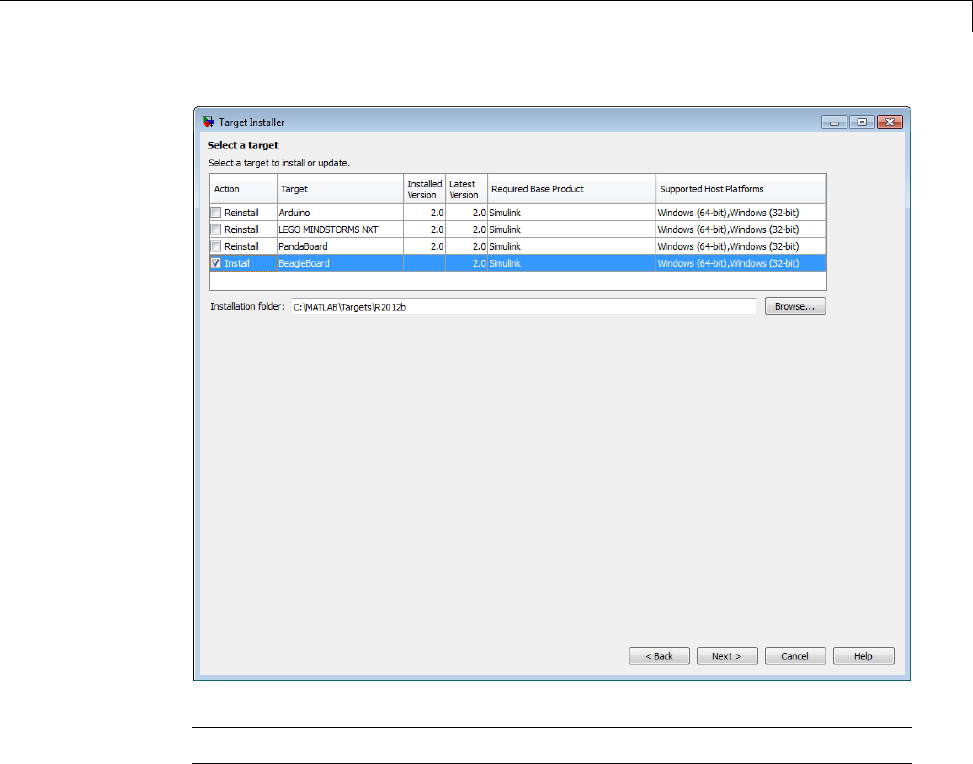
Install Support for BeagleBoard Hardware
Note You must have write privileges for the Installation folder.
4Target Installer confirms that you are installing the target, and lists
third-party software it will install.
Review the information, including the license agreements, and click Install.
54-5
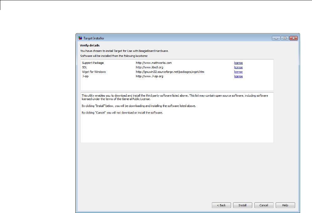
54 Work with BeagleBoard Hardware
Target Installer displays a progress bar while it downloads and installs the
third-party software.
54-6

Install Support for BeagleBoard Hardware
Note If you installed the target previously, Target Installer removes the
files from that installation before installing the current target. If Target
Installer cannot remove those files automatically, it instructs you to delete
the files manually. Close the MATLAB software before removing the files.
Then, restart MATLAB software and run Target Installer again.
5To replace the factory-installed firmware on the BeagleBoard hardware
with Ubuntu®Linux, as described in “Replace Firmware on BeagleBoard
Hardware” on page 54-9.
54-7

54 Work with BeagleBoard Hardware
54-8

Replace Firmware on BeagleBoard Hardware
Replace Firmware on BeagleBoard Hardware
This topic shows how to replace the firmware on the BeagleBoard hardware
(the “board”) with Ubuntu Linux firmware that can run Simulink models.
Before replacing the firmware, install the target, as described in “Install
Support for BeagleBoard Hardware” on page 54-2.
After replacing the firmware, you can run a Simulink model on the
BeagleBoard hardware, as described in “Run Model on BeagleBoard
Hardware” on page 54-39.
The following steps provide an overview of the firmware replacement process:
1The Target Installer locates a firmware image on your host computer or
downloads new one.
2The Target Installer uses the host computer to write the firmware image
to a microSD or SD memory card.
3You transfer the microSD or SD memory card to the BeagleBoard hardware.
4The Target Installer applies the IP settings you choose to the firmware on
the BeagleBoard hardware.
Note Target Installer does not use the BeagleBoard hardware to write the
firmware image to the memory card.
To replace the firmware on your BeagleBoard hardware:
1Open the Update firmware screen in the Target Installer using one of the
following methods:
•Click Continue in the Install/update complete screen of the Target
Installer.
•In a model, select Tools > Run on Target Hardware > Update
firmware.
54-9
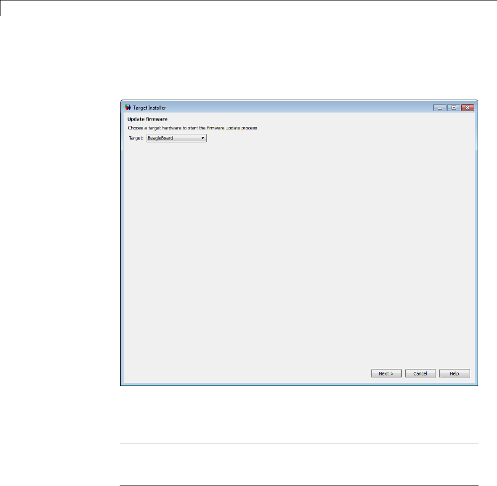
54 Work with BeagleBoard Hardware
•In a MATLAB Command Window, enter targetupdater.
2Choose the BeagleBoard option and click Next.
3Choose your board version and click Next. This action enables the Target
Installer to display instructions that are specific to your hardware.
Note The images in this topic only apply to the BeagleBoard xM hardware.
If you are using the BeagleBoard Bx or Cx hardware, refer to the images in
the Target Installer.
54-10
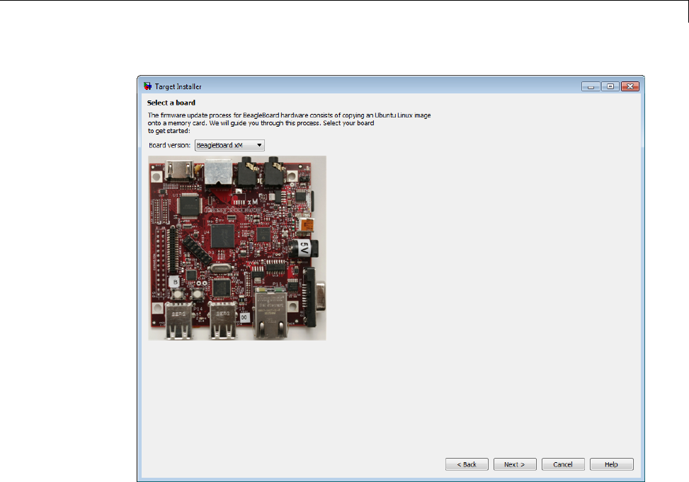
Replace Firmware on BeagleBoard Hardware
4Make the connections shown and click Next.
54-11
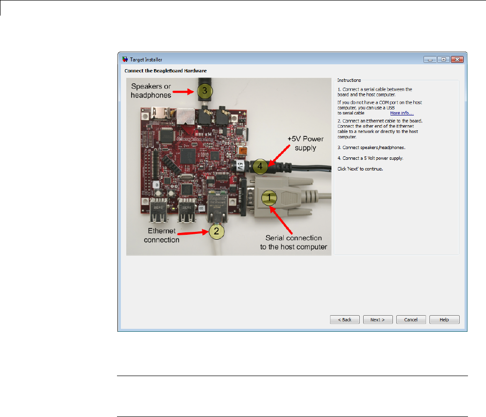
54 Work with BeagleBoard Hardware
5Choose to get the firmware image from the Internet or from a folder.
Note Thefilesizeofthefirmwareimageisapproximately1GB.Depending
on your connection, downloading the firmware can take from 2 to 60 minutes,
or more.
Internet: This option is selected by default. When you click Download,
Target Installer checks the Download folder for a valid firmware image:
•If a firmware image is not present, Target Installer downloads a firmware
image from the Internet, and saves it to the download folder.
54-12

Replace Firmware on BeagleBoard Hardware
•If a firmware image is present, Target Installer uses the firmware image
already present in the download folder, and does not download a new
firmware image from the Internet.
Folder:WhenyouclickDownload, Target Installer checks the Download
folder for a valid firmware image:
•If a firmware image is not present, Target Installer displays an error
message that the image file is missing. To solve this issue, copy the
firmware image from another location to the download folder, or choose
the Internet option instead.
•If a firmware image is present, Target Installer continues the firmware
installation process.
You must have write privileges for the download folder. If you use the default
download folder, having write privileges is typically not an issue. If you
change to a new download folder for which you do not have write permissions,
such as a shared folder on a network, the Target Installer generates an
error message: “Error: Download the firmware. The download folder is not
writable. Choose a folder for which you have write permissions”.
Tosolvethisissue,copythefirmwareimagetoafolderforwhichyouhave
write privileges. For example, copy the firmware image from the shared
folder on the network to the C:\Users\username\AppData\Local\Temp
folder. Then, update the Download location to the same folder, and click
Download again.
To locate the firmware image in a folder, search for a
filename that begins with beagleboard_ubuntu. For example:
beagleboard_ubuntu_11_04_r4_12_08_2011.img.7z
54-13
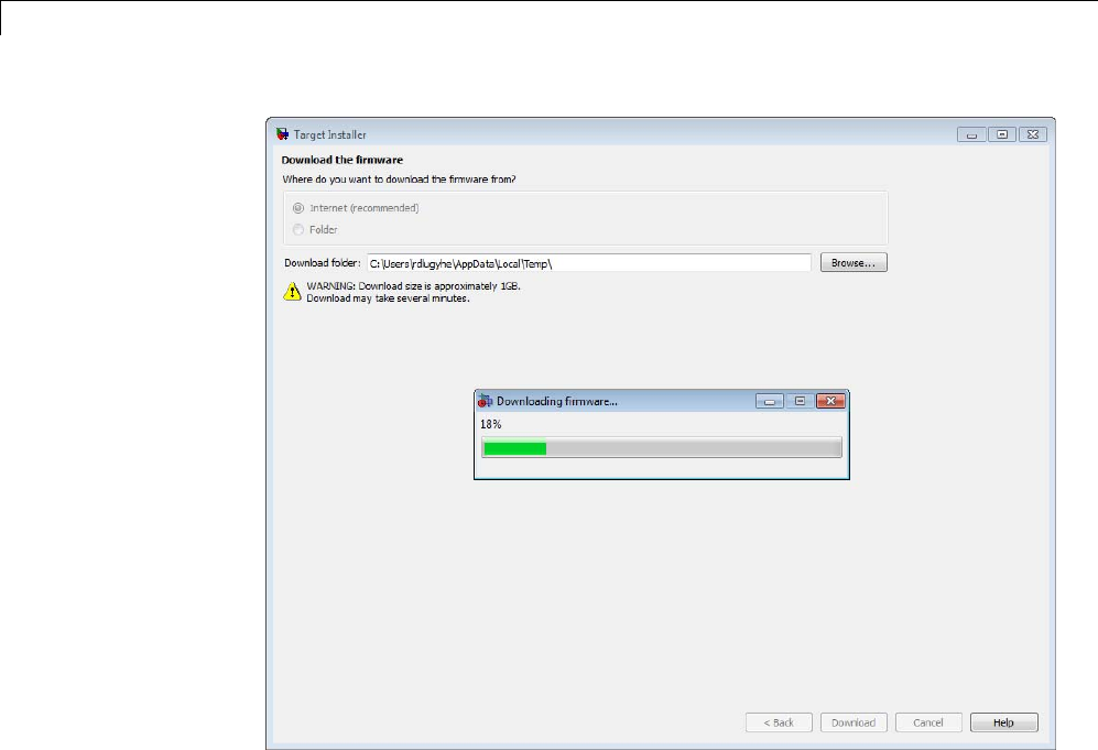
54 Work with BeagleBoard Hardware
6Insert the microSD or SD memory card into a media card reader connected to
your host computer. Windows assigns a drive letter to the memory card.
7Target Installer does not automatically detect the drive letter of the memory
card. It displays a drive letter for each device with removable storage.
•If only one drive letter is available, click Next.
•If no drive letters are available, check that the memory card is fully
inserted, and click Refresh.
•If multiple drive letters are available, open the Windows Start menu,
choose Computer, and look for the memory card under Devices with
Removable Storage.
54-14
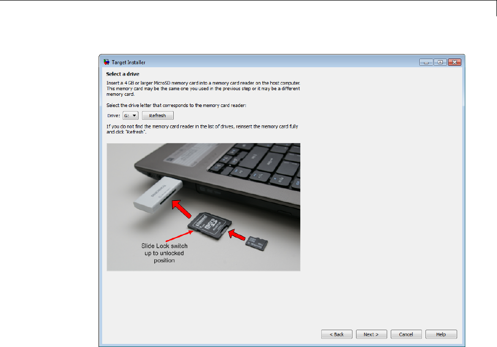
Replace Firmware on BeagleBoard Hardware
8Click Write. Target Installer overwrites all previous data on the memory
card with the firmware. This process takes several minutes to complete.
54-15
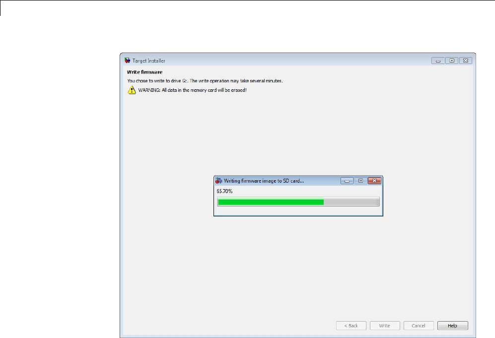
54 Work with BeagleBoard Hardware
9Get the COM port of the serial connection in Windows. From the Windows
Start menu, choose search programs and files for “Device Manager”. Open
Device Manager, expand Ports (COM & LPT), and identify the COM port of
the serial connection to the BeagleBoard hardware.
For example, the following image shows a DB9 serial port called
“Communications Port” using COM1, and a USB-to-serial adapter called
“Prolific USB-to-Serial Comm Port” using COM6.
54-16
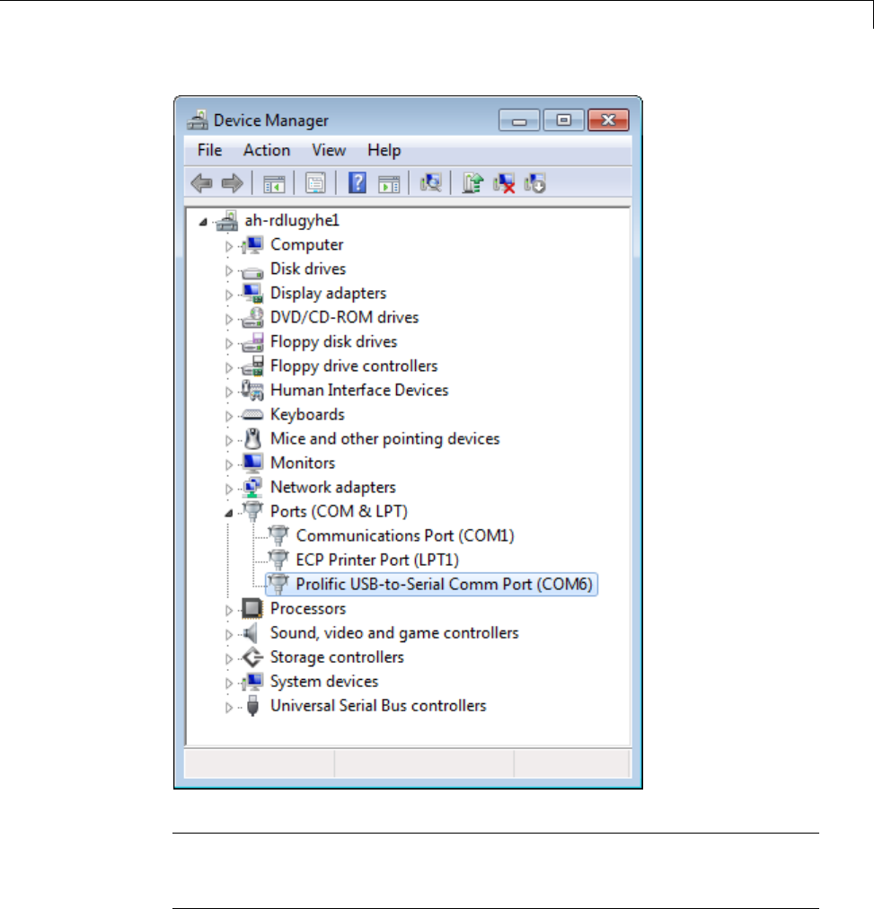
Replace Firmware on BeagleBoard Hardware
Note Some USB-to-serial adapters do not appear in the list of serial
connections immediately after you install the software drivers. To solve this
issue, disconnect/reconnect the adapter, or reboot your host computer.
54-17
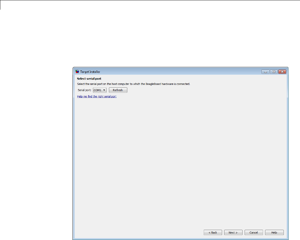
54 Work with BeagleBoard Hardware
10 Target Installer does not automatically choose the COM port of the serial
connection. After you get the COM port of the serial connection from Windows
Device Manager, return to Target Installer, set Serial port to the COM port,
and click Next.
11 Insert the memory card into the BeagleBoard hardware, and follow the
instructions for resetting your board:
•For the BeagleBoard xM hardware, press and release the RESET button.
•For the BeagleBoard Bx/Cx hardware,holddowntheUSERbuttonwhile
you press and release the RESET button.
Click Next. When the Target Installer detects a reset, it displays progress
booting the board.
54-18

Replace Firmware on BeagleBoard Hardware
If the Target Installer does not display any progress, click Back.Onthe
Select serial port screen. Verify that you selected the correct COM port, and
close any other applications, such as PuTTY, that might using the serial
connection.
12 If your board is connected to a network with DHCP services, such as an office
LAN or a home network connected to the Internet, select Automatically get
IP address, give the board a unique name, and click Configure.DHCPis
a network service that automatically configures the IP settings of Ethernet
devices connected to a network.
If your board is directly connected to an Ethernet port on your computer, or
connected to an isolated network without DHCP services, select Manually
enter IP address, give the board a unique name, enter static IP settings
for the board, and click Configure.
54-19

54 Work with BeagleBoard Hardware
To enter static IP settings for your board, follow these guidelines:
•The value of the subnet mask must be the same for all devices on the
network.
•The value of the IP address must be unique for each device on the network.
For example, if the Ethernet port on your host computer has a network mask
of 255.255.255.0 and a static IP address of 192.168.1.1,set:
•Network mask to use the same network mask value, 255.255.255.0.
•IP address to an unused IP address, between 192.168.1.2 and
192.168.1.254.
When you click Configure, the Target Installer opens a serial connection
and applies the settings to the board.
54-20
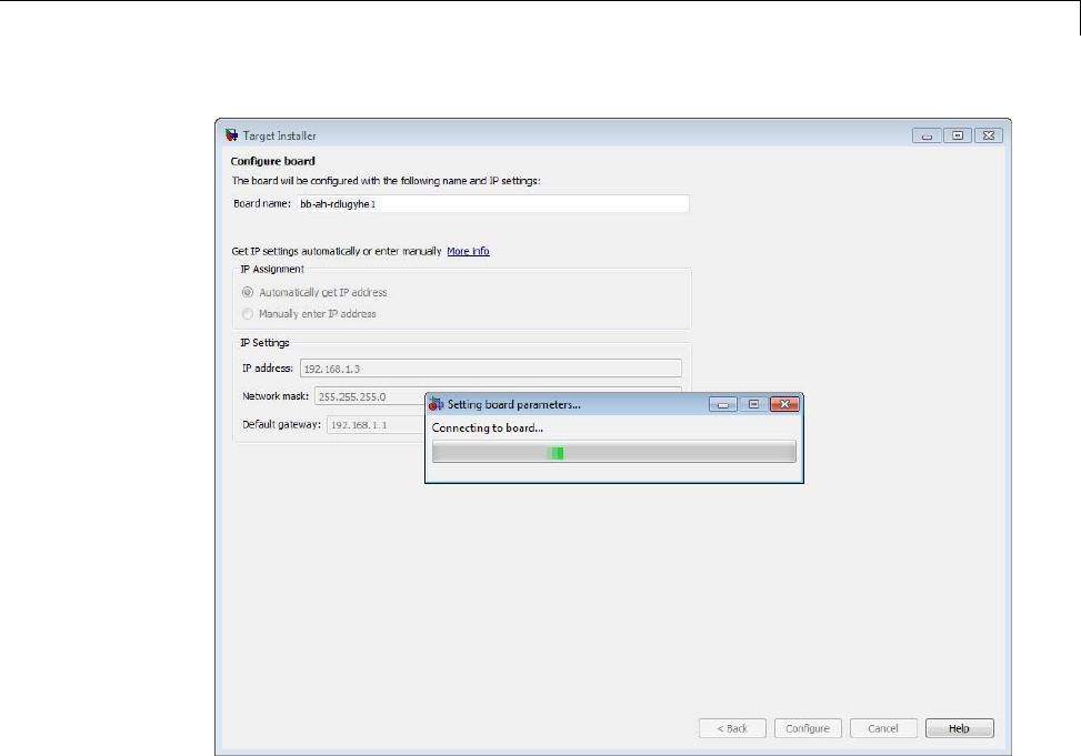
Replace Firmware on BeagleBoard Hardware
13 Make a note of the board information. Then, click Next.
54-21
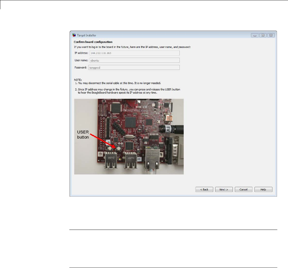
54 Work with BeagleBoard Hardware
14 Click Finish.IfLaunch target examples is enabled, the Target Installer
opens the example page for BeagleBoard hardware.
Note To reopen the examples later, enter the following text in a MATLAB
Command Window:
demo simulink 'Target for Use with Beagleboard'
54-22

Replace Firmware on BeagleBoard Hardware
54-23

54 Work with BeagleBoard Hardware
ChoosetheTypeofSerialCable
This topic shows you how to choose a serial cable for connecting your host
computer to the BeagleBoard hardware.
Two types of cables are available for this purpose:
•DB9 null modem M/F cable
•USB to DB9 male adapter cable
DB9 null modem M/F cable:
•If your host computer has a DB9 male serial connector similar to the one in
the following image, you can use a DB9 null modem M/F cable.
•To find the appropriate cable online, search for “DB9 low profile null
modem M-F cable”.
USB to DB9 male adapter cable:
•If your host computer has a USB port, you can use a USB to DB9 male
adapter cable.
•Tofindtheappropriatecableonline,search for "USB to RS-232 DB9 Serial
Adapter”.
•Some USB-to-serial adapters do not appear in the list of serial connections
immediately after you install the software drivers. To solve this issue,
disconnect and reconnect the adapter, or reboot your host computer.
•To avoid issues with the software/driver quality, we recommend choosing
an adapter that has good customer feedback ratings, or using the DB9 null
modem M/F cable instead.
54-24

Connect to Serial Port on BeagleBoard Hardware
Connect to Serial Port on BeagleBoard Hardware
This topic shows you how to configure and open a command line session with
the target hardware.
This is an optional task that you can use to:
•View the standard output while the board boots.
•Get or set the IP address, as described in “Get IP Address of BeagleBoard
Hardware” on page 54-34 topic.
To open a serial connection to your board:
1Connect a serial cable from your host computer to the female DB9 connector
on the board.
2Identify the COM port for your serial connection. In Windows 7, use the
“search programs and files” feature in the Start menu to find “Device
Manager”. Open Device Manager, and expand Ports (COM & LPT) to see
the list of serial connections.
For example, the following image shows that the DB9 serial port called
“Communications Port” uses COM1. Similarly, the image shows that the
USB-to-serial adapter called “Prolific USB-to-Serial Comm Port” uses
COM6.
54-25

54 Work with BeagleBoard Hardware
Note If you have trouble locating the COM port number, search the
Windows “Help and Support” for “Device Manager”.
3In the MATLAB Command Window, start PuTTY by entering:
54-26

Connect to Serial Port on BeagleBoard Hardware
h = beagle;
system(['"' fullfile(h.PutilsFolder, 'putty.exe') '" -serial &'], '-runAsAdmin');
4In the PuTTY dialog box that opens, select the Serial category.
5Set the following values:
•Serial line to connect to: If you are using your computer’s built-in
serial port, try COM1. Otherwise, use the Device Manager in Windows to
determine the COM port number.
•Speed (baud):115200
54-27

54 Work with BeagleBoard Hardware
•Flow control:None
6In the PuTTY dialog box, select the Session category.
7Set the Connection type parameter to Serial, enter a new name for
Saved Sessions,clickSave,andclickOpen.
54-28

Connect to Serial Port on BeagleBoard Hardware
Note Do not save the serial settings to Default Settings.TheDefault
Settings must remain configured to use SSH in order to run your Simulink
model on the BeagleBoard hardware. Otherwise, trying to run the model
on BeagleBoard hardware produces an error message similar to this one:
>> [status, message] = h.connect()
Error using linkfoundation.util.beagleboard/connect (line 125)
SSH connection to host 144.212.110.44 failed:
FATAL ERROR: Network error: Connection refused
8When a terminal window opens, press the Enter key on your keyboard.
The terminal window displays the Linux command line.
9When you are finished, enter logout on the Linux command line, and close
PuTTY to end the serial connection.
See Also
•“Get IP Address of BeagleBoard Hardware” on page 54-34
•For more information about PuTTY, see:
http://www.chiark.greenend.org.uk/~sgtatham/putty/
54-29

54 Work with BeagleBoard Hardware
Configure Network Connection with BeagleBoard
Hardware
You can configure the IP settings of the BeagleBoard hardware by running
Linux shell commands directly on the BeagleBoard hardware (the “board”).
To inspect and reconfigure the IP settings on a board that already has the new
firmware, follow the procedure in this section that starts with “To configure
the board to use DHCP or static IP settings”.
To configure the IP settings while you are replacing the firmware on your
BeagleBoard hardware, see “Replace Firmware on BeagleBoard Hardware”
on page 54-9.
You may need to reconfigure the IP settings if your board:
•Has unknown IP settings.
•Is unreachable using a network connection.
•Is being moved to a network or direct Ethernet connection that uses static
IP settings.
•Is being moved from a network that used static IP settings to one that
uses DHCP services.
When you complete the procedure in this topic, the board should be able to
communicate over the network to which it is connected.
Before starting the procedure in this topic, it helps to understand the
conditions under which networks use DHCP or static IP settings:
•If your board is connected to a network with DHCP services, such as an
office LAN or a home network connected to the Internet, configure the
board to use DHCP services. DHCP is a network service that automatically
configures the IP settings of Ethernet devices connected to a network.
•If your board is directly connected to an Ethernet port on your computer,
or connected to an isolated network without DHCP services, configure
the board to use static IP settings.
54-30

Configure Network Connection with BeagleBoard Hardware
To configure the board to use DHCP or static IP settings:
1Open a serial command line session, as described in “Connect to Serial Port
on BeagleBoard Hardware” on page 54-25
Alternatively, if your board is connected to a monitor, keyboard, and mouse,
you can log in to the Ubuntu desktop and open a terminal window.
2Display the contents of the /etc/network/interfaces file. Enter:
cat /etc/network/interfaces
If the board is configured to use DHCP services (the default configuration),
dhcp appears at the end of the following line:
iface eth0 inet dhcp
If the board is configured to use static IP settings, static appears at the
end of the following line:
iface eth0 inet static
3Create a backup of the /etc/network/interfaces file. Enter:
sudo cp /etc/network/interfaces /etc/network/interfaces.backup
Enter the root password when prompted (default: temppwd).
4Change the permissions of /etc/network/interfaces so you can edit the
file. Enter:
sudo chmod 777 /etc/network/interfaces
Enter the root password when prompted (default: temppwd).
5Edit interfaces using a simple editor called nano. Enter:
nano interfaces
6Editthelastwordoflinethatstartswithiface eth0 inet.
TouseDHCPservices,editthelinetosay:
54-31

54 Work with BeagleBoard Hardware
iface eth0 inet dhcp
TousestaticIPsettings,editthelinetosay:
iface eth0 inet static
7For static IP settings, add lines for address,netmask,andgateway.For
example:
iface eth0 inet static
address 192.168.1.2
netmask 255.255.255.0
gateway 192.168.1.1
Note For static IP settings:
•The value of the subnet mask must be the same for all devices on the
network.
•The value of the IP address must be unique for each device on the
network.
For example, if the Ethernet port on your host computer has a network
mask of 255.255.255.0 and a static IP address of 192.168.1.1,set:
•netmask to use the same network mask value, 255.255.255.0.
•address to an unused IP address, between 192.168.1.2 and
192.168.1.254.
8Tell nano to exit and save the changes:
Press Ctrl+x.
Enter Yto save the modified buffer.
For “File Name to Write: interfaces”, press Enter.
The nano editor confirms that it “Wrote # lines” and returns control to
the command line.
9Restore the original file permissions. Enter:
54-32

Configure Network Connection with BeagleBoard Hardware
sudo chmod u=rw,g=r,o=r interfaces
Enter the root password when prompted. (default: temppwd)
10 Test the IP settings by logging in to the board over a telnet session.
Note You can use the ifconfig command to temporarily change the IP
settings. Rebooting the board removes the ifconfig settings and restores the
/etc/network/interfaces settings.
To change the IP settings temporarily, open a Linux command line, and enter
ifconfig, the device id, a valid IP address, netmask, and the appropriate
network mask. For example:
ifconfig eth0 192.168.45.12 netmask 255.255.255.0
Related
Examples
•“Run Model on BeagleBoard Hardware” on page 54-39
•“Get IP Address of BeagleBoard Hardware” on page 54-34
54-33

54 Work with BeagleBoard Hardware
Get IP Address of BeagleBoard Hardware
You can get the IP address of the BeagleBoard hardware (the “board”) by
listening to the audio output, or by using the Linux command line. This is
an optional task that you can use to:
•Preparing a model to run on a board that is different from the previous
one you used.
•Opening a telnet session with a board whose IP settings you do not know.
•Configuring the UDP Send block.
When you prepare a model to run on a board, your model Configuration
Parameters reuse the IP settings of the previous board you used. If you are
working with a different board on the same network, get the IP address of the
your new board, and update the Host name parameter in the Configuration
Parameters. For more information, see “Run Model on BeagleBoard
Hardware” on page 54-39.
If Ethernet port on the BeagleBoard hardware board has an IP address, the
audio output on the board can read the IP address out loud. For example the
board can say “My IP address is one hundred and forty four point two one two
pointoneonezeropointtwozerosix.”
To listen your board’s IP address using headphones or speakers:
1Plug headphones or speakers into the AUDIO OUT jack on the board.
2Press the USER button on the board.
3Write down the IP address as the board reads it out over the headphones
or speakers.
The Linux command line on the board can provide the IP address of the
Ethernet port.
To get your board’s IP address command line session:
1Open a serial command line session on your board, as described in “Connect
to Serial Port on BeagleBoard Hardware” on page 54-25.
54-34

Get IP Address of BeagleBoard Hardware
If your board is connected to a monitor, keyboard, and mouse, you can also
log in to the Ubuntu desktop and open a terminal window.
2At the Linux command line, enter ifconfig.
3Locate the IP address following inet addr in the command line output.
For example, locate inet addr:144.212.110.206 on line 9 of the following
output:
omap login: ubuntu
Password:
Last login: Wed Nov 23 15:40:36 EST 2011 from ah-rdlugyhe1.dhcp.mathworks.com on pts/1
Welcome to Ubuntu 11.04 (GNU/Linux 3.0.4-x3 armv7l)
* Documentation: https://help.ubuntu.com/
ubuntu@omap:~$ ifconfig
eth0 Link encap:Ethernet HWaddr d2:a7:db:b3:c4:81
inet addr:144.212.110.206 Bcast:144.212.110.255 Mask:255.255.255.0
inet6 addr: fe80::d0a7:dbff:feb3:c481/64 Scope:Link
UP BROADCAST RUNNING MULTICAST MTU:1488 Metric:1
RX packets:125537 errors:0 dropped:0 overruns:0 frame:0
TX packets:76 errors:0 dropped:0 overruns:0 carrier:0
collisions:0 txqueuelen:1000
RX bytes:18103491 (18.1 MB) TX bytes:7670 (7.6 KB)
lo Link encap:Local Loopback
inet addr:127.0.0.1 Mask:255.0.0.0
inet6 addr: ::1/128 Scope:Host
UP LOOPBACK RUNNING MTU:16436 Metric:1
RX packets:4 errors:0 dropped:0 overruns:0 frame:0
TX packets:4 errors:0 dropped:0 overruns:0 carrier:0
collisions:0 txqueuelen:0
RX bytes:240 (240.0 B) TX bytes:240 (240.0 B)
ubuntu@omap:~$
Related
Examples
•“Connect to Serial Port on BeagleBoard Hardware” on page 54-25
•“Run Model on BeagleBoard Hardware” on page 54-39
•“Configure Network Connection with BeagleBoard Hardware” on page
54-30
54-35

54 Work with BeagleBoard Hardware
Open Block Library for BeagleBoard Hardware
This block library provides support for protocols and APIs available on
BeagleBoard hardware (the “board”).
To open the block library from the MATLAB Command Window, enter:
beagleboardlib
The following block library opens.
54-36
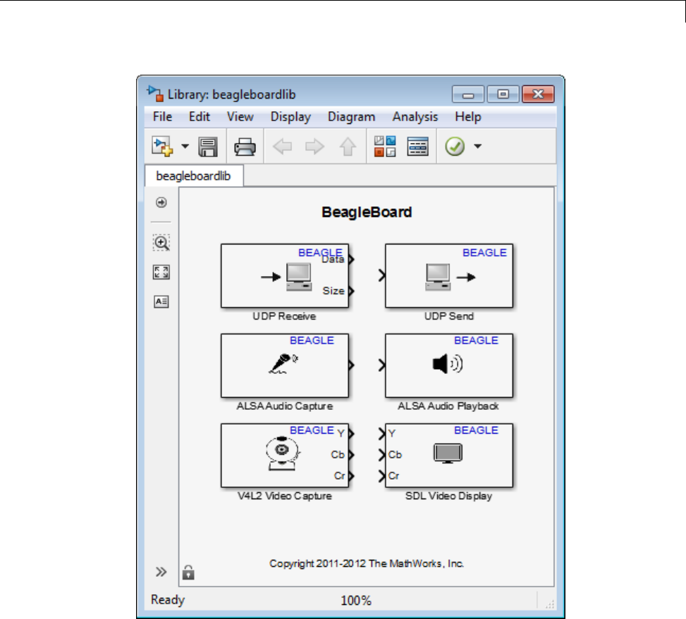
Open Block Library for BeagleBoard Hardware
To open the block library from the Simulink Library Browser:
1Open the Simulink Library Browser by entering simulink in the MATLAB
Command Window, or by clicking the following icon on the MATLAB toolbar.
54-37
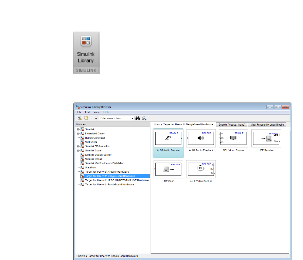
54 Work with BeagleBoard Hardware
2In the Simulink Library Browser, click Target for Use with BeagleBoard
Hardware.
54-38

Run Model on BeagleBoard Hardware
Run Model on BeagleBoard Hardware
This example shows how to prepare, configure, and run a simple model on
your BeagleBoard hardware (the “board”).
Before starting this procedure:
•Connect your board to the network and to a power supply.
•Create or open a Simulink model.
To prepare and run the model:
1Use File > Save As to create a working copy of your model. Keep the original
model as a backup copy.
2In your model, select ToolsRun on Target HardwarePrepare to Run.
This action changes the model Configuration Parameters.
3In the Run on Target Hardware pane that opens, set the Target hardware
parameter to BeagleBoard.
4If you have changed boards since the last time you updated the firmware or
ran a model, update the Host name,User name,andPassword parameters.
5Select Tools > Run on Target Hardware > Run. This action automatically
downloads and runs your model on the board.
Note Pressing RESET or cycling the power on the BeagleBoard hardware
during this step can cause the ssh utility to hang.
Warning Avoid using the RESET button to stop a running model
and reboot the board. Doing so can corrupt operating system and
program files. To fix corrupt files, replace the firmware as described
in “Replace Firmware on BeagleBoard Hardware” on page 54-9.
Running a new or updated model on the board:
•Automatically stops a running model with the same name.
54-39

54 Work with BeagleBoard Hardware
•Does not stop running models that have other names.
To stop a model running on the board, enter the following commands in the
MATLAB Command Window:
h=beagle;
h.stop('modelName');
For example, to stop the sumdiff model, enter:
h=beagle;
h.stop('sumdiff');
To restart a model that was previously running on the board, or to run
multiple instances of a model, enter the following commands in the MATLAB
Command Window:
h=beagle;
h.run('modelName');
Note You do not need to enter h=beagle; multiple times if a previous
instance of his available in the MATLAB Workspace.
Forexample,torestartthesumdiffmodel you stopped in the previous
example, enter:
h.run('sumdiff');
Prepare Models That Use Model Reference
You can include one model in another by using Model blocks. Each instance
of a Model block represents a reference to another model, called a referenced
model or submodel. The model that contains a referenced model is its parent
model. When you run parent model on your target hardware, the submodel
effectively replaces the Model block that references it. For more information,
see “Overview of Model Referencing” on page 6-2.
To run on target hardware, the parent model and the submodels must have
the same Configuration Parameter settings.
54-40

Run Model on BeagleBoard Hardware
For each Model block:
•Select Tools > Run on Target Hardware > Prepare to Run.
•Apply the same Configuration Parameters settings to the submodel as you
applied to the parent model.
If the model and Model blocks have different settings, the software generates
an error when you try to run the model on the target hardware.
See Also
•“Create the Simple Model”
•“Configure Network Connection with BeagleBoard Hardware” on page
54-30
•“Tune and Monitor Model Running on BeagleBoard Hardware” on page
54-42
•“Overview of Model Referencing” on page 6-2
54-41

54 Work with BeagleBoard Hardware
Tune and Monitor Model Running on BeagleBoard
Hardware
In this section...
“About External Mode” on page 54-42
“Run Your Simulink Model in External Mode” on page 54-43
“Stop External Mode” on page 54-45
About External Mode
You can use External mode to tune parameters and monitor a model running
on your target hardware.
External mode enables you to tune model parameters and evaluate the effects
of different parameter values on model results in real-time, in order to find
the optimal values to achieve desired performance. This process is called
parameter tuning.
External mode accelerates parameter tuning because you do not have to
re-run the model each time you change parameters.Externalmodealsolets
you develop and validate your model using the actual data and hardware for
which it is designed. This software-hardware interaction is not available
solely by simulating a model.
The following list provides an overview of the parameter tuning process with
External mode:
•In the model on your host computer, you enable External mode in the
Configuration Parameters.
•In the model on your host computer, you tell Simulink software to run
your model on the target hardware.
•Simulink software runs the model on the target hardware.
•You use the model on the host computer as a user interface for interacting
with the model running on the target hardware:
54-42
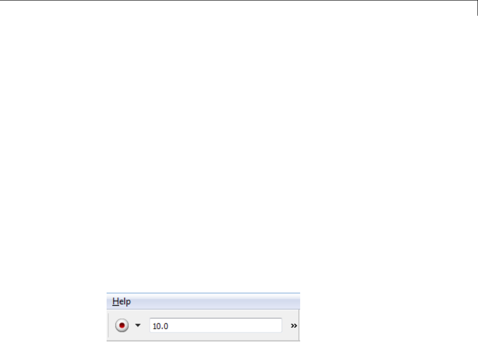
Tune and Monitor Model Running on BeagleBoard Hardware
-When open blocks and apply new parameter values on the host computer,
External mode updates the corresponding values on target hardware.
-If your model contains blocks for viewing data, such as Scope or Display
blocks, External mode sends the corresponding data from the target
hardware to those blocks on the host computer.
•You determine the optimal parameter values by adjusting parameter values
on the host computer and observing data/outputs from the target hardware.
•When you are finished, you save the new parameter values, disable
External mode, and save the model.
Run Your Simulink Model in External Mode
1Create a network connection between the BeagleBoard hardware and your
host computer. See “Configure Network Connection with BeagleBoard
Hardware” on page 54-30
2In the model, set the Simulation stop time parameter, located on the
model toolbar, as shown here.
•To run the model for an indefinite period, enter inf.
•To run the model for a finite period, enter a number of seconds. For
example, entering 120 runsthemodelonthehardwarefor2minutes.
3Select Tools > Run on Target Hardware > Options.
4In the Run on Target Hardware pane that opens, select Enable External
mode.
5ClickOK, and then save the changes your model.
6In your model, select Tools > Run on Target Hardware > Run.
After several minutes, Simulink starts running your model on the board.
54-43

54 Work with BeagleBoard Hardware
7While the model is running in External mode, you can change parameter
values in the model on your host computer and observe the corresponding
changes in the model running on the hardware.
If your model contains blocks from the Simulink Sinks block library,
the sink blocks in the model on your host computer display the values
generated by the model running on the hardware.
If your model does not contain a sink block to which External mode can
send data, the MATLAB Command Window displays a warning message.
For example:
Warning: No data has been selected for uploading.
> In C:\Program Files (x86)\MATLAB\R2012a Student1\toolbox\
realtime\realtime\+realtime\extModeAutoConnect.p>
extModeAutoConnect at 17
In C:\Program Files (x86)\MATLAB\R2012a Student1\toolbox\
realtime\realtime\sl_customization.p>myRunCallback at 149
You can disregard this warning, or you can add a sink block to the model.
Note To use External mode with the Run on Target Hardware feature, only
use the External mode settings described in this topic.
If you have Simulink Coder or Embedded Coder software, do not use other
External mode-related items that appear that in the Tools menu or the
Configuration Parameters dialog.
Note External mode increases the processing burden of the model running
on the board. If the software reports an overrun, clear the Enable External
mode checkbox in the Run on Target Hardware pane.
Note If you have the Embedded Coder or Simulink Coder products, you can
use External mode with a model that contains Model blocks (uses the “Model
reference”).
54-44

Tune and Monitor Model Running on BeagleBoard Hardware
Stop External Mode
To stop the model running in External mode, click the Stop button located
on the model toolbar, as shown here.
This action stops the process for the model running on the BeagleBoard
hardware, and stops the model simulation running on your host computer.
If it is set to a finite period, the Simulation stop time parameter stops
External mode when the period elapses.
54-45

54 Work with BeagleBoard Hardware
Detect and Fix Task Overruns on BeagleBoard Hardware
You can configure a model running on the target hardware to detect and
notify you of when task overrun occurs.
Standard scheduling works well when a processor is moderately loaded but
may fail if the processor becomes overloaded. When a task is required to
perform extra processing and takes longer than normal to execute, it may
be scheduled to execute before a previous instance of the same task has
completed. The result is a task overrun.
To enable overrun detection:
1In your model, click Tools > Run on Target Hardware > Options.
2In the Run on Target Hardware pane that opens, select the Enable
overrun detection check box.
3Click OK.
When a task overrun occurs, the command prompt on the host machine
repeatedly prints an “Overrun” error message, such as “Overrun — rate for
subrate task 1 is too fast”, until the model stops.
To fix an overrun condition:
•Simplify the model.
•Increasethesampletimesforthemodelandtheblocksinit. Forexample,
changetheSample time parameter in all of your data source blocks, such
as blocks for input devices, from 0.1 to 0.2.
Note External mode increases the processing burden of the model running
on your board. If the software reports an overrun, clear the Enable External
mode checkbox in the Run on Target Hardware pane.
54-46

55
Work with LEGO
MINDSTORMS NXT
Hardware
•“Install Support for LEGO MINDSTORMS NXT Hardware” on page 55-2
•“Replace Firmware on NXT Brick” on page 55-7
•“Open Block Library for LEGO MINDSTORMS NXT Hardware” on page
55-11
•“Run Model on NXT Brick” on page 55-14
•“Tune Parameters and Monitor Data in a Model Running on NXT Brick” on
page 55-16
•“Detect and Fix Task Overruns on NXT Brick” on page 55-22
•“ExchangeDataBetweenTwoNXTBricks”onpage55-23
•“Set Up A Bluetooth Connection” on page 55-31

55 Work with LEGO®MINDSTORMS®NXT Hardware
Install Support for LEGO MINDSTORMS NXT Hardware
This example shows how to add support for LEGO MINDSTORMS NXT
hardware to the Simulink product.
This process downloads and installs:
•Third-party software development tools on your host computer.
•A Simulink block library called Target for Use with LEGO
MINDSTORMS NXT Hardware.
•Examples
For convenience, this document occasionally refers to LEGO MINDSTORMS
NXT hardware as an “NXT brick” or as “target hardware”.
Note You can only use this target on a host computer running 32-bit or
64-bit version of Windows that Simulink supports.
Repeat this process every six months or so to update the third-party tools, the
block library, or firmware to the latest versions.
1Open the Install or update target screen in the Target Installer using one
of the following methods:
•In a model, select Tools >Run on Target Hardware >Install/Update
Support Package.
•In a MATLAB Command Window, enter targetinstaller.
2Target Installer prompts “Where do you want to install or update from?”
Keep the default, Internet,andclickNext.
55-2
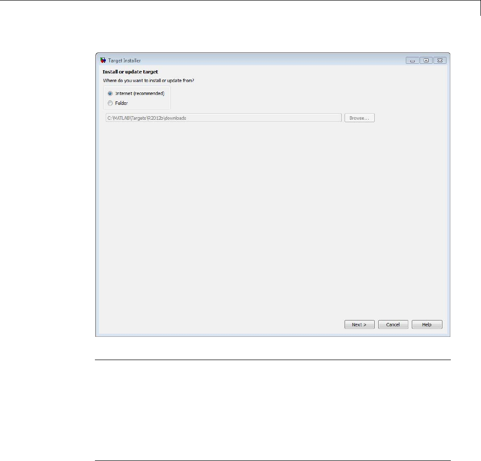
Install Support for LEGO®MINDSTORMS®NXT Hardware
Note If you choose the Folder option, place the support package zip file in a
folder for which you have write privileges. Otherwise, the Target Installer
cannot complete the installation process.
If the support package in a read-only folder, copy the support package
zip file to a writable folder before continuing. For example, copy
legomindstormsnxt_r20*.zip from a read-only network drive to the
C:\MATLAB\Targets\R20*\downloads folder on your host computer.
55-3
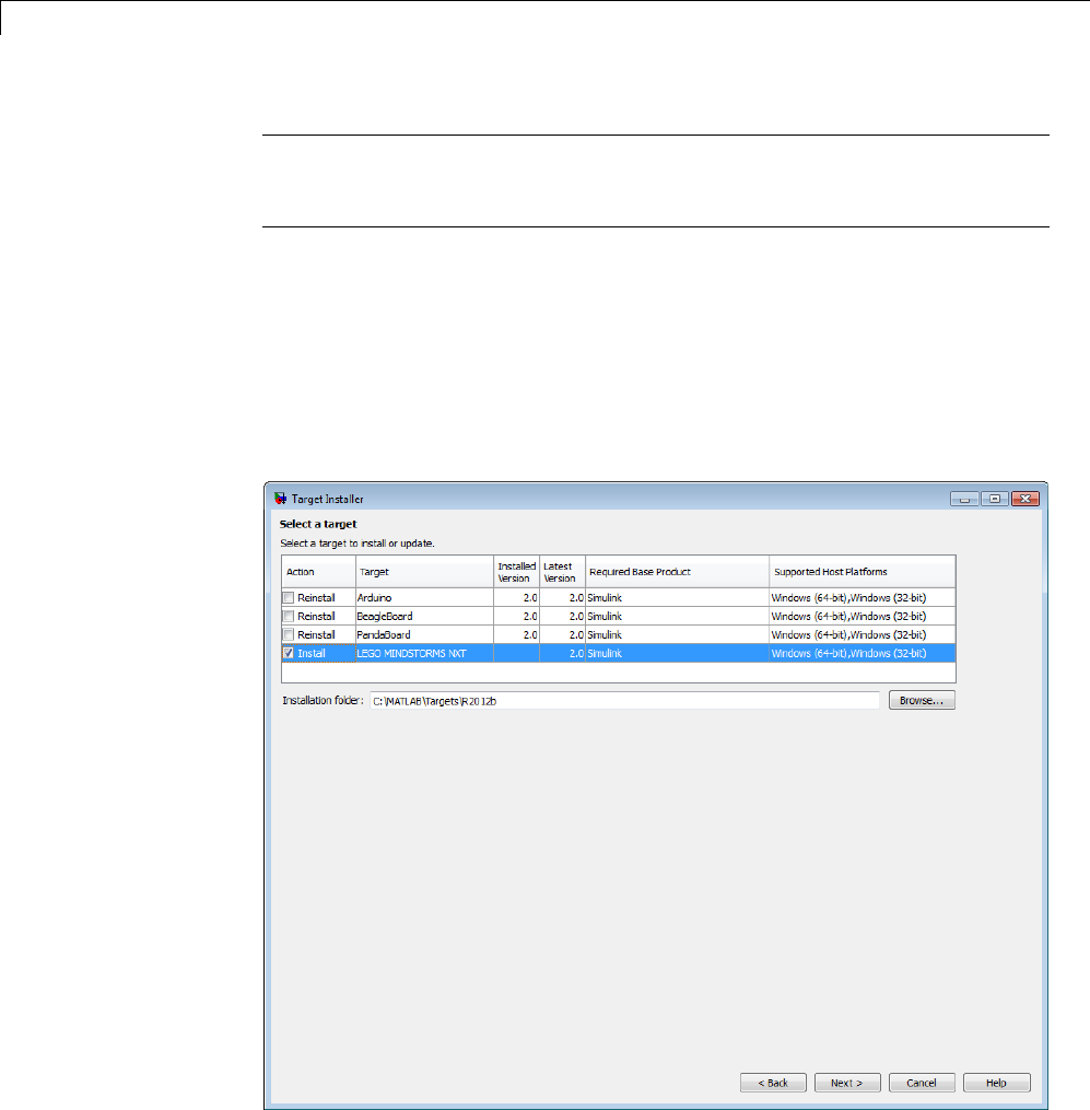
55 Work with LEGO®MINDSTORMS®NXT Hardware
Note If you are choosing the Folder option because you do not have Internet
access, the support package folder must also contain installers for the
required third-party software.
3Select the LEGO MINDSTORMS NXT checkbox and click Next.
The Installation folder parameter tells Target Installer where to install the
support package and the third-party software. Set the Installation folder
parameter to a local hard drive. Do not use a mapped network drive because
doing so causes the Cygwin installation to fail during the target installation
process.
55-4
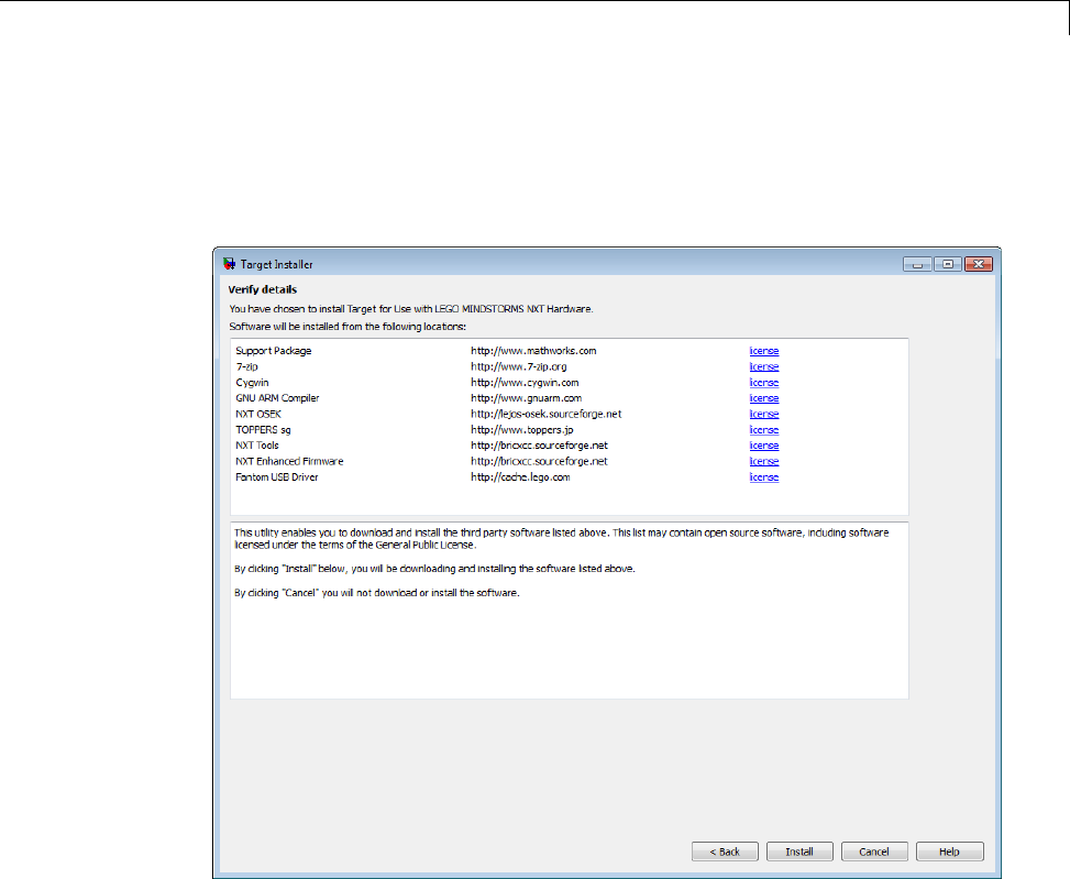
Install Support for LEGO®MINDSTORMS®NXT Hardware
4Target Installer states that you have chosen to install the support package for
LEGO MINDSTORMS NXT and lists third-party software it will install.
Review the information, and click Install.
Target Installer displays a progress bar while it downloads and installs the
third-party software.
55-5
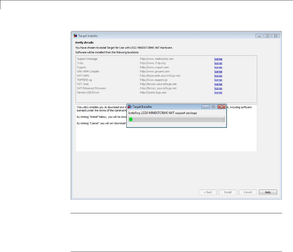
55 Work with LEGO®MINDSTORMS®NXT Hardware
Note If you installed the target previously, Target Installer removes the
files from that installation before installing the current target. If Target
Installer cannot remove those files automatically, it instructs you to delete
the files manually. Close the MATLAB software before removing the files.
Then, restart MATLAB software and run Target Installer again.
5The Target Installer finishes installing the target and displays the following
screen.
If your NXT brick still has its factory-installed firmware, click Continue >
and complete the process described in “Replace Firmware on NXT Brick” on
page 55-7. Otherwise, click Close.
55-6

Replace Firmware on NXT Brick
Replace Firmware on NXT Brick
This topic shows how to replace the firmware on the NXT brick with enhanced
firmware that can run Simulink models. The enhanced firmware can run
When you complete this process, and install the target for use with LEGO
MINDSTORMS NXT hardware, you can run a Simulink model on NXT brick,
as described in “Run Model on NXT Brick” on page 55-14.
Repeatthisprocesseverysixmonthsorsotoreplacethefirmwarewiththe
latest version.
Warning This process completely erases the memory on the NXT
brick.
1Open the Update firmware screen in the Target Installer using one of the
following methods:
•Click Continue > in the Install/update complete screen of the Target
Installer.
•In a model, select Tools >Run on Target Hardware >Update
firmware.
•In a MATLAB Command Window, enter targetupdater.
2Choose LEGO MINDSTORMS NXT and click Next.
55-7
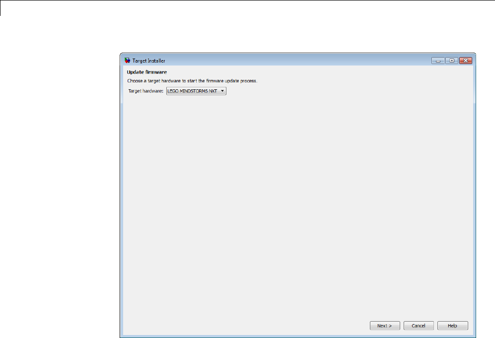
55 Work with LEGO®MINDSTORMS®NXT Hardware
3Connect the NXT brick to your host computer with a USB cable.
Turn the NXT brick on by pressing its orange button.
Enter a unique name for the Name your LEGO MINDSTORMS NXT
parameter, and click Next.
55-8
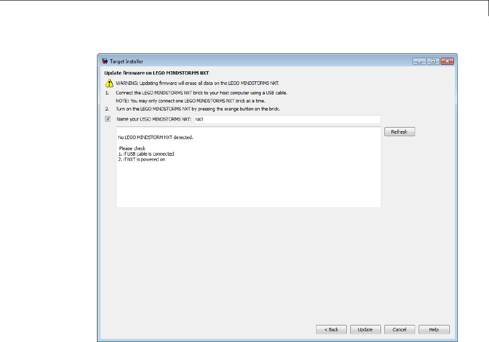
Replace Firmware on NXT Brick
During the firmware update, the NXT brick emits a faint ticking sound and
the LCD goes blank. The USB connection to the host computer can disconnect
and reconnect multiple times.
When the firmware process is complete, the NXT brick displays the default
screen including My Files.
4ClickFinish and review the examples.
55-9
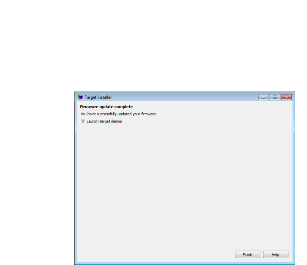
55 Work with LEGO®MINDSTORMS®NXT Hardware
Note To reopen the examples later, enter the following text in a MATLAB
Command Window:
demo simulink 'Target for Use with LEGO'
55-10

Open Block Library for LEGO®MINDSTORMS®NXT Hardware
Open Block Library for LEGO MINDSTORMS NXT Hardware
The block library for LEGO MINDSTORMS NXT hardware is a collection
of blocks that provides drivers for LEGO MINDSTORMS NXT sensors and
hardware.
TherearetwowaystoopentheblocklibraryforLEGOMINDSTORMS
NXT hardware:
•The MATLAB Command Window. This approach is quick, but doesn’t
display the other Simulink block libraries that are available.
•The Simulink Library Browser. This approach takes a few more steps, but
displays all of the Simulink block libraries that are available.
1In the MATLAB Command Window, enter:
legonxtlib
The block library for LEGO MINDSTORMS NXT hardware opens.
55-11
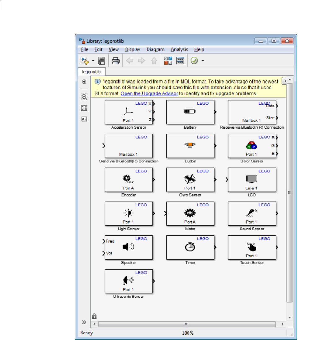
55 Work with LEGO®MINDSTORMS®NXT Hardware
55-12
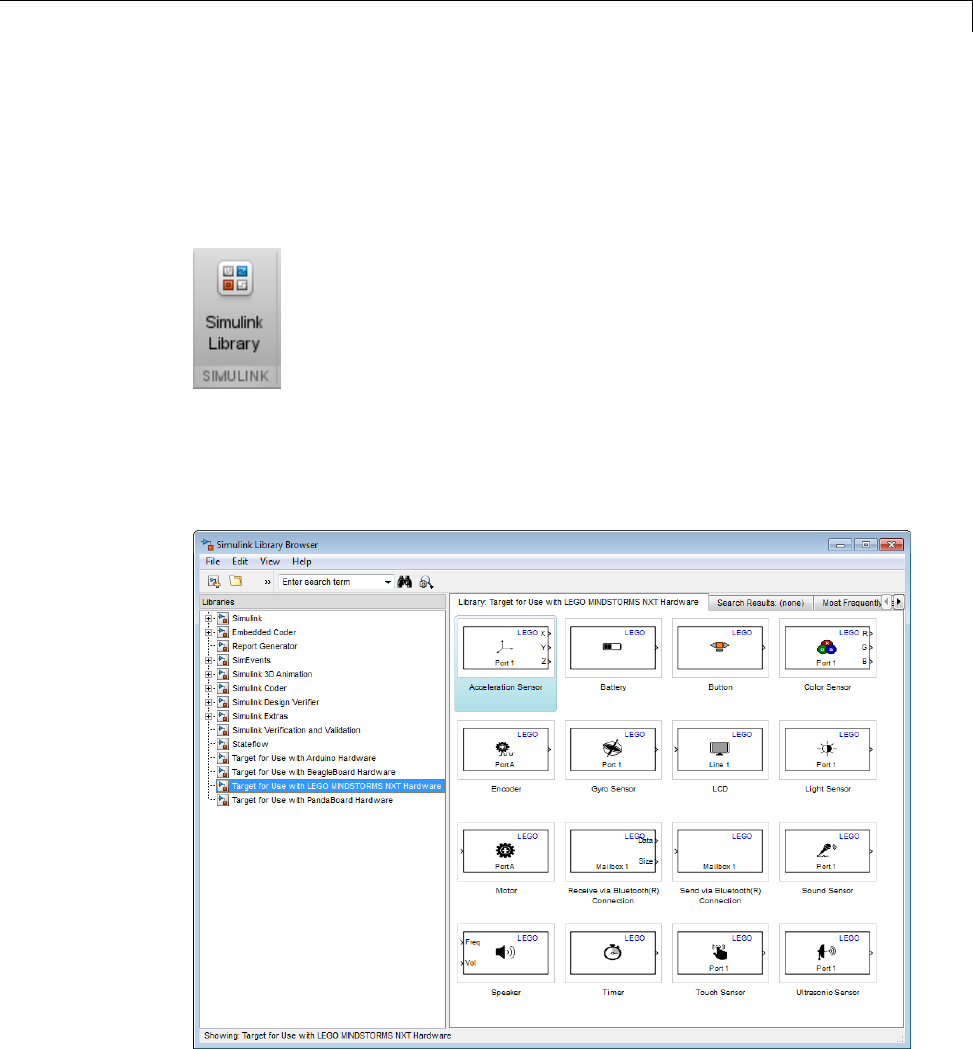
Open Block Library for LEGO®MINDSTORMS®NXT Hardware
2In the MATLAB Command Window, enter:
simulink
Or, in the MATLAB Toolbar, click the following icon.
Simulink Library Browser opens.
3In the Simulink Library Browser, click Target for Use with LEGO
MINDSTORMSNXTHardware.
55-13

55 Work with LEGO®MINDSTORMS®NXT Hardware
Run Model on NXT Brick
This topic shows how to configure and run a model on NXT brick.
Before starting this procedure, create or open a Simulink model.
1Connect your NXT brick to the host computer using a USB cable or a
Bluetooth®device. Simulink software uses this connection to download the
model to the NXT hardware when you run the model.
For more information about using a Bluetooth device, see “Set Up A Bluetooth
Connection” on page 55-31.
2Use File >Save As to create a working copy of your model. Keep the original
model as a backup copy.
3In your model, select Tools >Run on Target Hardware >Prepare to
Run. This action changes the model Configuration Parameters.
4In the Run on Target Hardware pane that opens, set the Target hardware
parameter to LEGO MINDSTORMS NXT.
5Set the Connection type parameter to USB connection or Bluetooth
connection.
6TurntheNXTbrickonbypressingtheorangebutton. TheLCDdisplays
LEGO and MINDSTORMS splash screens, and then My Files.
Note The NXT brick automatically powers down after several minutes of
inactivity. If this happens, turn the power back on.
7Select Tools >Run on Target Hardware >Run. This action automatically
downloads and runs your model on the NXT brick.
When the NXT hardware starts running the model, the LCD displays “I am
running ...”, or it displays the input values and labels of any LCD blocks
in the model.
55-14

Run Model on NXT Brick
Note To restart a model while it is running, press the left-arrow button
on the NXT brick.
Torestartamodelthatisstopped,usethe orange button on the NXT brick to
select My Files > Software Files, and then select your model.
To stop the model, press the grey button on the NXT brick.
Prepare Models That Use Model Reference
You can include one model in another by using Model blocks. Each instance
of a Model block represents a reference to another model, called a referenced
model or submodel. The model that contains a referenced model is its parent
model. When you run parent model on your target hardware, the submodel
effectively replaces the Model block that references it. For more information,
see “Overview of Model Referencing” on page 6-2.
To run on target hardware, the parent model and the submodels must have
the same Configuration Parameter settings.
For each Model block:
•Select Tools >Run on Target Hardware >Prepare to Run.
•Apply the same Configuration Parameters settings to the submodel as you
applied to the parent model.
If the model and Model blocks have different settings, the software generates
an error when you try to run the model on the target hardware.
55-15

55 Work with LEGO®MINDSTORMS®NXT Hardware
Tune Parameters and Monitor Data in a Model Running
on NXT Brick
In this section...
“About External Mode” on page 55-16
“Run Your Simulink Model in External Mode” on page 55-17
“Stop External Mode” on page 55-18
“Set COM Port Number Manually” on page 55-19
About External Mode
This topic explains how the External mode feature enables you to tune
parameters and monitor data in a model running on your target hardware.
When you enable External mode and choose the Run command, Simulink
embeds light-weight client/server code in your model and then runs your
model on the target hardware. If you tune parameters in the model on your
host computer, External mode updates the corresponding parameter values
in the model running on the target hardware. You can use sink blocks, such
as Display or Scope blocks, to monitor data from the model running on the
target hardware. External mode sends data from the sink blocks on the target
hardware to the corresponding sink blocks on your host computer, where
you canvieworlogthedata.
External mode accelerates parameter tuning. When you develop an algorithm,
you must typically try a range of parameter values in order to find the optimal
settings. Without External mode, you must re-run the model on the target
hardware to evaluate the effects of each change. With External mode, you
can adjust parameter values, monitor data, and evaluate the results until you
find the optimal value, without re-running the model.
External mode increases the processing burden of the model running on the
NXT brick. If the model running on the hardware reports an overrun, you can
disable External mode or fix the issue as described in “Detect and Fix Task
Overruns on NXT Brick” on page 55-22.
55-16
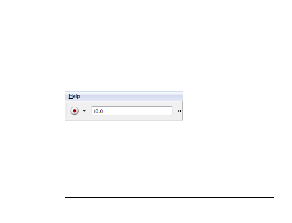
Tune Parameters and Monitor Data in a Model Running on NXT Brick
Run Your Simulink Model in External Mode
Before running your model in External mode, set up a Bluetooth connection
between the NXT hardware and your Windows computer, as described in “Set
Up A Bluetooth Connection” on page 55-31
1In the model, set the Simulation stop time parameter, located on the
model toolbar, as shown here.
•To run the model for an indefinite period, enter inf.
•To run the model for a finite period, enter a number of seconds. For
example, entering 120 runsthemodelonthehardwarefor2minutes.
2Select Tools >Run on Target Hardware >Options.
3In the Run on Target Hardware pane that opens, select Enable External
mode.
Note This action disables the Enable communication between two
NXT bricks parameter. External mode requires exclusive use of the
Bluetooth device on the NXT brick.
4Click OK, and then save the changes your model.
5In your model, select Tools >Run on Target Hardware >Run.
After several minutes, Simulink starts running your model on the NXT
brick.
6While the model is running in External mode, you can change parameter
values in the model on your host computer and observe the corresponding
changes in the model running on the hardware.
55-17

55 Work with LEGO®MINDSTORMS®NXT Hardware
If your model contains blocks from the Simulink Sinks block library,
the sink blocks in the model on your host computer display the values
generated by the model running on the hardware.
If your model does not contain a sink block to which External mode can
send data, the MATLAB Command Window displays an error message.
For example:
Warning: No data has been selected for uploading.
> In C:\Program Files (x86)\MATLAB\R2012a Student1\toolbox\
realtime\realtime\+realtime\extModeAutoConnect.p>
extModeAutoConnect at 17
In C:\Program Files (x86)\MATLAB\R2012a Student1\toolbox\
realtime\realtime\sl_customization.p>myRunCallback at 149
You can disregard this warning, or you can add a sink block to the model.
Note To use External mode with the Run on Target Hardware feature, only
use the External mode settings described in this topic.
If you have Simulink Coder or Embedded Coder software, do not use other
External mode-related items that appear that in the Tools menu or the
Configuration Parameters dialog.
Note If you have the Embedded Coder or Simulink Coder products, you can
use External mode with a model that contains Model blocks (uses the “Model
reference”).
Stop External Mode
To stop the model running in External mode, click the Stop button located
on the model toolbar, as shown here.
55-18
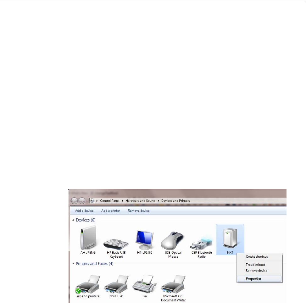
Tune Parameters and Monitor Data in a Model Running on NXT Brick
This action turns off the power of the NXT brick, and stops the model
simulation running on your host computer.
If it is set to a finite period, the Simulation stop time parameter stops
External mode when the period elapses.
Set COM Port Number Manually
By default, Run on Target Hardware automatically gets the COM port
number of the NXT brick when you use External mode. However, you have
the option of setting the COM port number manually.
1In Windows, locate the NXT brick under Control Panel >Hardware and
Sound >Devices and Printers.
The NXT brick uses the name you assigned to it during the firmware update
process. By default, that name is “NXT”. If you changed that name during
the firmware update, the Windows device label shows that new name.
2Right-click the NTX brick and select Properties.
3In the Properties dialog box, select the Hardware tab and make a note of
the COM port number.
55-19
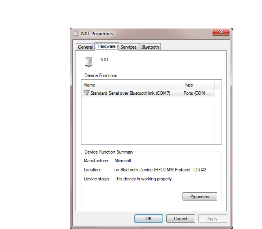
55 Work with LEGO®MINDSTORMS®NXT Hardware
4In your model, select the Tools >Run on Target Hardware >Options
menu item.
5In the Run on Target Hardware pane that opens, change the Set host
COM port parameter to Manually.
55-20

Tune Parameters and Monitor Data in a Model Running on NXT Brick
6In the COM port number parameter, enter the COM port number you
noted earlier.
55-21

55 Work with LEGO®MINDSTORMS®NXT Hardware
Detect and Fix Task Overruns on NXT Brick
You can configure a model running on the target hardware to detect and
notify you of when task overrun occurs.
Standard scheduling works well when a processor is moderately loaded but
may fail if the processor becomes overloaded. When a task is required to
perform extra processing and takes longer than normal to execute, it may
be scheduled to execute before a previous instance of the same task has
completed. The result is a task overrun.
To enable overrun detection:
1In your model, click Tools,Run on Target Hardware and Options.
2In the Run on Target Hardware pane that opens, select the Enable
overrun detection check box.
3Click OK.
When a task overrun occurs, the LCD on the NXT brick displays an “Overrun!”
error message until you stop the model.
To fix an overrun condition:
•Simplify the model.
•Increasethesampletimesforthemodelandtheblocksinit. Forexample,
change the Sample time parameter in all of your data sources, such as
the sensor blocks, from 0.1 to 0.2.
Note External mode increases the processing burden of the model running
on the NXT brick. If the software reports an overrun, clear the Enable
External mode checkbox in the Run on Target Hardware pane.
55-22

Exchange Data Between Two NXT Bricks
Exchange Data Between Two NXT Bricks
In this section...
“Tips for Use Bluetooth Blocks” on page 55-23
“Add Bluetooth Blocks to your Models” on page 55-23
“Configure Bluetooth Slave” on page 55-27
“Configure Bluetooth Master” on page 55-28
This topic explains how to exchange data between two separate NXT
Intelligent Bricks (“NXT bricks”) over a Bluetooth connection.
If, instead, you are looking for information about exchanging data between
your host computer and an NXT brick, see “Tune Parameters and Monitor
Data in a Model Running on NXT Brick” on page 55-16.
Tips for Use Bluetooth Blocks
Here are some tips for using the Send via Bluetooth Connection block and
Receive via Bluetooth Connection block:
•Use two separate models, one for each NXT brick.
•You can only use the Bluetooth blocks for connecting two NXT bricks.
•For each Send via Bluetooth Connection block in one model, use a
corresponding Receive via Bluetooth Connection block in the other model.
Set the Mailbox parameterinbothblockstothesamenumber.
•For each Receive via Bluetooth Connection block in a model, use a unique
Mailbox number.
•A model can contain no more than five Receive via Bluetooth Connection
blocks.
Add Bluetooth Blocks to your Models
Add Bluetooth blocks to your models and configure them:
1Open legonxtlib.
55-23
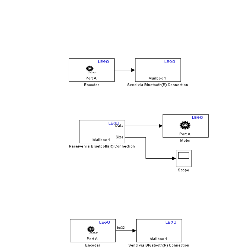
55 Work with LEGO®MINDSTORMS®NXT Hardware
2Open two models. One for each NXT brick.
3Add a Send via Bluetooth Connection block to a model, and connect it to
the data source, as shown in the following example.
4Add a Receive via Bluetooth Connection block to the other model, and
connect it to the data sinks, as shown in the following example.
5In the model that contains the Send via Bluetooth Connection block, select
the Display >Signals & Ports >Port Data Types menu item. Then,
select Simulation >Update Diagram Ctrl+D. Observe the data type
that appears above the connector attached to the Send via Bluetooth
Connection block. For example “int32” in the following example.
55-24

Exchange Data Between Two NXT Bricks
6Open the Receive via Bluetooth Connection block in the other model. Apply
thedatatypefromtheprevioussteptotheData type parameter in the
Receive via Bluetooth Connection block.
7In the model that contains the Send via Bluetooth Connection block, select
the Display >Signals & Ports >Signal Dimensions menu item. Then,
select Simulation >Update Diagram Ctrl+D.
•If the signal dimensions are greater than 1, the connector attached to
the Send via Bluetooth Connection block displays the signal dimension.
Multiply the signal dimensions to get the value you will apply to the
Message size parameter. For example, if the signal dimensions are
2x10, the set Message size to 10.
•If the signal is one-dimensional, the connector attached to the Send via
Bluetooth Connection block does not display a signal dimension. For a
one-dimensional signal, set Message size to 1.
8In the model that contains the Receive via Bluetooth Connection
block, apply the signal dimension from the previous step to the Signal
dimension parameter in the Receive via Bluetooth Connection block.
55-25
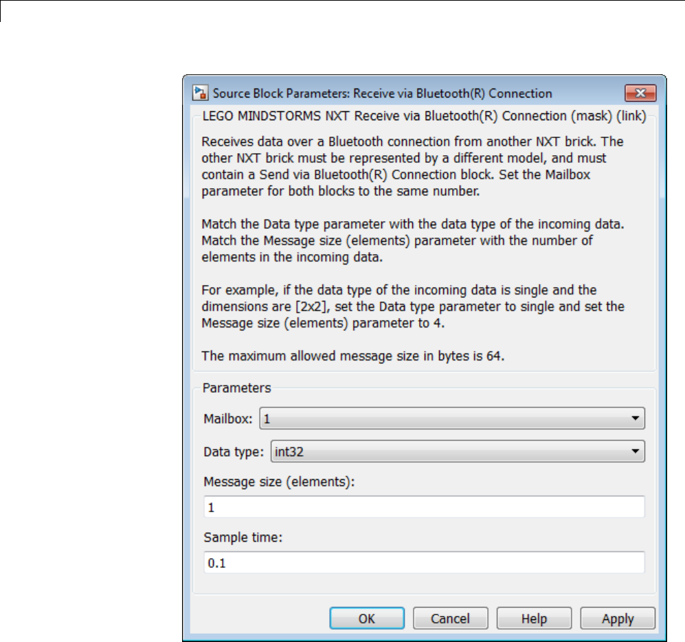
55 Work with LEGO®MINDSTORMS®NXT Hardware
9Save all of your changes and leave the models open.
55-26

Exchange Data Between Two NXT Bricks
Configure Bluetooth Slave
Using your models, configure the NXT brick to operate as a slave Bluetooth
node. You can make this choice arbitrarily, without regard to which device
is sending or receiving data.
To configure an NXT brick as a slave Bluetooth node:
1Open one model and select Tools >Run on Target Hardware >Options.
2In the Run on Target Hardware pane that opens, select the Enable
communication between two NXT bricks check box, and set Bluetooth
mode to Slave.
Note This action disables the External mode parameter. Enabling
communication between two NXT bricks requires exclusive use of the
Bluetooth device on the NXT brick.
55-27
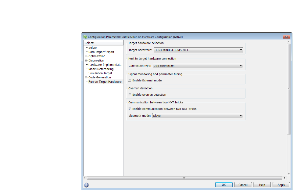
55 Work with LEGO®MINDSTORMS®NXT Hardware
3Click OK. This saves and closes the Configuration Parameters.
4In your model, select Tools >Run on Target Hardware >Run to run
your model on the NXT brick.
This process can take a couple of minutes. When the download completes,
the NXT brick automatically runs the application.
5When Simulink software finishes downloading the application to the slave
NXT brick, the LCD displays “Waiting...”.
Observe the number on the second line of the LCD. The first 12 digits of
this number are the Slave Bluetooth address,whichyouwilluseasyou
configure the Bluetooth master in the next procedure.
Configure Bluetooth Master
Configure the other NXT brick as a master Bluetooth node:
55-28
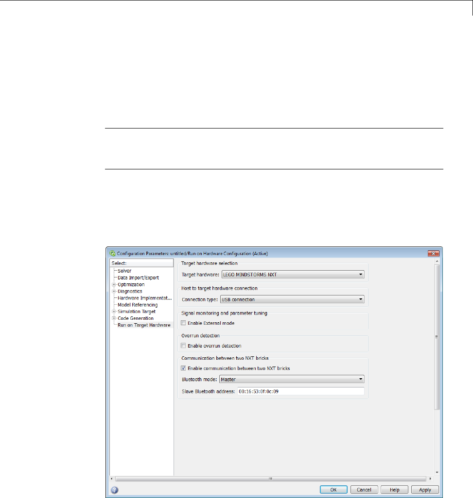
Exchange Data Between Two NXT Bricks
1Open one model and select Tools >Run on Target Hardware >Options.
2In the Run on Target Hardware pane that opens, select the Enable
communication between two NXT bricks check box, and set Bluetooth
mode to Master.
Note This action disables the External mode parameter. Enabling
communication between two NXT bricks requires exclusive use of the
Bluetooth device on the NXT brick.
3Enter the 12-digit Slave Bluetooth address, inserting a colon between
each pair of digits. For example, if the slave NXT brick displays
00165312926900,enter00:16:53:12:92:69. Disregard the last two digits,
00.
4Click OK. This saves and closes the Configuration Parameters.
55-29

55 Work with LEGO®MINDSTORMS®NXT Hardware
5In your model, select Tools >Run on Target Hardware >Run to run
your model on the NXT brick.
This process can take a couple of minutes. When the download completes,
the NXT brick automatically runs the application and connects to the
Bluetooth slave.
6On the Bluetooth master, turn the wheel back and forth. Observe the
direction and speed of the wheel on the Bluetooth slave.
55-30

Set Up A Bluetooth Connection
Set Up A Bluetooth Connection
This topic shows you how to set up a Bluetooth connection between your
Windows host computer and the NXT hardware.
You may need to create a Bluetooth connection between your Windows host
computer and the NXT hardware for either of these purposes:
•To enable External mode, as described in “Tune Parameters and Monitor
Data in a Model Running on NXT Brick” on page 55-16.
•To download the model to the NXT hardware. You do so by setting the
Connection type to Bluetooth connection, as described in “Run Model
on NXT Brick” on page 55-14.
This procedure requires a Bluetooth device on your host computer that is
compatible with the NTX’s built-in Bluetooth device. Details for adding a
Bluetooth device vary from one of version of Windows to another. If needed,
search Microsoft help for additional information.
Note Some Bluetooth devices do not support connections with the NXT brick.
For this reason, MathWorks recommends using the 9847 Bluetooth Dongle
specified on the LEGO MINDSTORMS NXT Web site.
Set up a Bluetooth on your Windows host:
1Connect a supported Bluetooth dongle to your Windows host computer. Let
Windows automatically find and install the appropriate drivers.
2Turn the NXT brick on, and verify that the small Bluetooth icon is visible in
the upper-left corner of the LCD. The icon looks like a capital-B composed
of two triangles.
If the Bluetooth symbol is not visible, press the right arrow on the NXT
brick four times. Then, select Bluetooth >On/Off >On.
3In Windows 7, open Control Panel >Devices and Printers to check
whether the NXT brick has already been added to Devices.
55-31
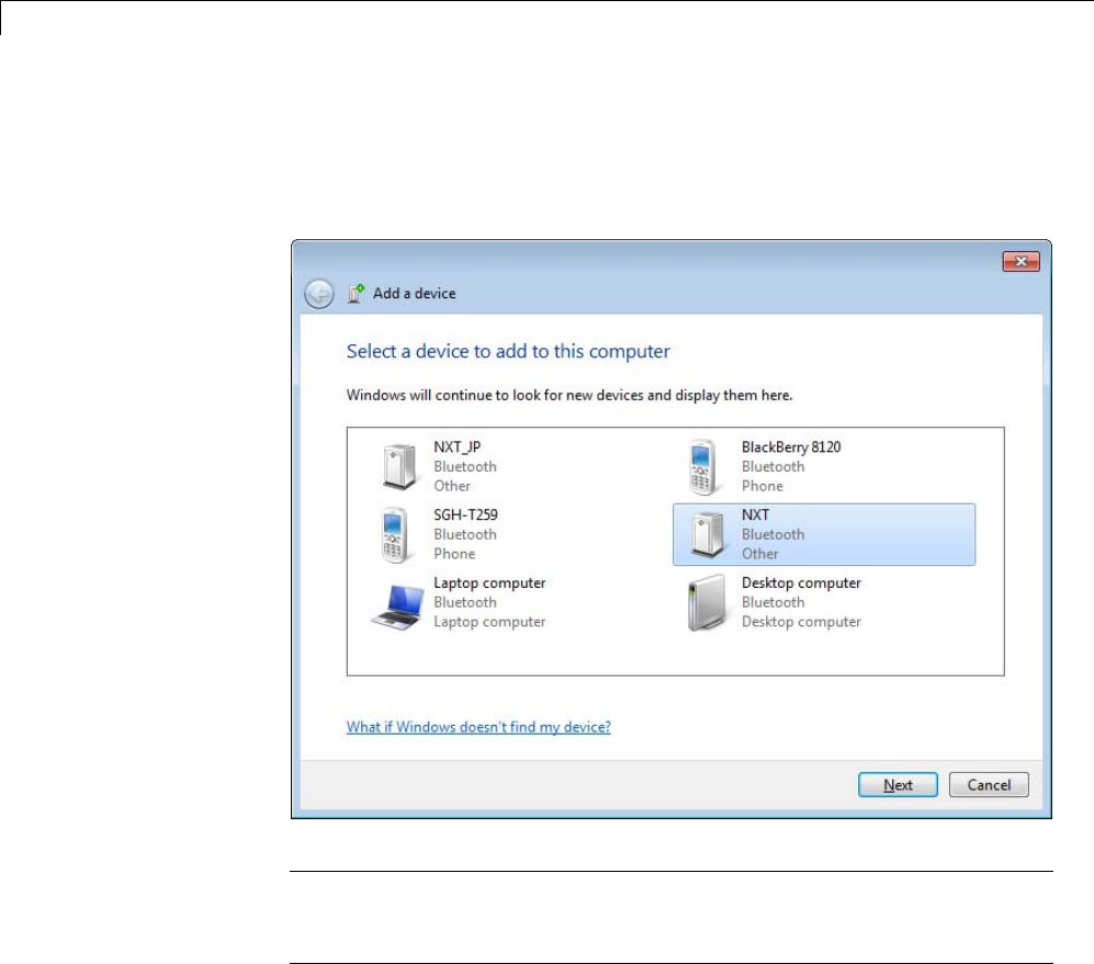
55 Work with LEGO®MINDSTORMS®NXT Hardware
4If the NXT brick is not among the devices, click Add a device.
5In the Add a device wizard that opens, select your NXT Bluetooth device,
and click Next.
Note All of the NXT bricks operating within Bluetooth range appear in
the list of devices. To avoid confusion, assign a unique name to your NXT
brick, as described in “Replace Firmware on NXT Brick” on page 55-7.
6When the LCD on the NXT brick displays the default passkey, 1234,
promptly press the orange button on the NXT brick.
55-32
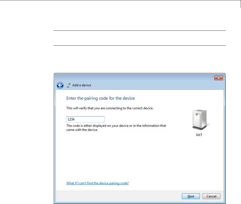
Set Up A Bluetooth Connection
Note If the NXT times out during this step, return to Windows, select the
NXT Bluetooth device, and click Next.
7In the Add a device dialog box, enter the passkey, 1234,asthepairing
code. Click Next.
8When you see confirmation that the device has been added, click Close.
The next time you turn on both devices, the Bluetooth connection between
your host computer and the NXT brick will be available.
55-33
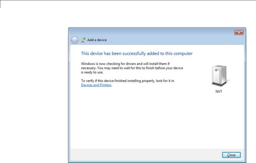
55 Work with LEGO®MINDSTORMS®NXT Hardware
If you have trouble with the Bluetooth connection, try removing the device
from Devices and Printers and repeating this process.
55-34

56
Work with PandaBoard
Hardware
•“Install Support for PandaBoard Hardware” on page 56-2
•“Replace Firmware on PandaBoard Hardware” on page 56-9
•“Choose the Type of Serial Cable” on page 56-22
•“Connect to Serial Port on PandaBoard Hardware” on page 56-23
•“Configure Network Connection with PandaBoard Hardware” on page 56-28
•“Get IP Address of PandaBoard Hardware” on page 56-32
•“Open Block Library for PandaBoard Hardware” on page 56-35
•“Run Model on PandaBoard Hardware” on page 56-38
•“Tune and Monitor Model Running on PandaBoard Hardware” on page
56-41
•“Detect and Fix Task Overruns on PandaBoard Hardware” on page 56-45
•“Access the Linux Desktop Directly Using Desktop Computer Peripherals”
on page 56-46
•“Access the Linux Desktop Remotely Using VNC” on page 56-48
•“Configure Wi-Fi on PandaBoard Hardware” on page 56-50

56 Work with PandaBoard Hardware
Install Support for PandaBoard Hardware
You can add support for PandaBoard hardware to Simulink product, using
the following process. After you complete this process, and replace the
firmware on the PandaBoard hardware, you can run a Simulink model on
your PandaBoard hardware, as described in “Run Model on PandaBoard
Hardware” on page 56-38.
Using this installation process, you download and install the following items
on your host computer:
•Third-party software development tools
•A Simulink block library called Target for Use with PandaBoard Hardware.
•Examples
For convenience, these instructions occasionally refer to PandaBoard
hardware as a “board” or as “target hardware”.
Note You can use this target only on a host computer running a version of
32-bit or 64-bit Windows that Simulink software supports.
1Open the Install or update target screen in the Target Installer, using
one of the following methods:
•In a model, select Tools > Run on Target Hardware > Install/Update
Support Package.
•In a MATLAB Command Window, enter targetinstaller.
2Choose whether to get the support package from the Internet or from a folder.
Note The file size of the support package and other downloads is over 1 GB.
Downloading the support package and third-party software can take a while.
56-2

Install Support for PandaBoard Hardware
Internet: This option is selected by default. Target Installer downloads and
install the support package and third-party software from the Internet.
Folder: Target Installer gets the support package from the folder specified. If
you choose Folder, you must have write privileges for the folder specified.
•Installing from the default folder — If you use the default folder, having
write privileges is typically not an issue.
•Installing from the folder without write permission — You may want to
install from a different folder for which you do not have write permissions,
such as a shared folder on a network. If so, Target Installer generates
an error message.
To resolve this issue, copy the support package to a folder for which you have
write privileges, and point Target Installer to that same folder. For example,
copy the support package to C:\MATLAB\Targets\version\downloads.
To locate the support package in a folder, search for a filename
that begins with pandaboard and ends with .zip. For example:
pandaboard_r2012a_v1_0.zip
56-3

56 Work with PandaBoard Hardware
3Select the PandaBoard check box, and click Next.
The Installation folder parameter specifies where Target Installer puts
the target files.
56-4

Install Support for PandaBoard Hardware
Note You must have write privileges for the Installation folder.
4Target Installer confirms that you are installing the target, and lists
third-party software it will install.
Review the information, including the license agreements, and click Install.
56-5

56 Work with PandaBoard Hardware
Target Installer displays a progress bar while it downloads and installs the
third-party software.
56-6
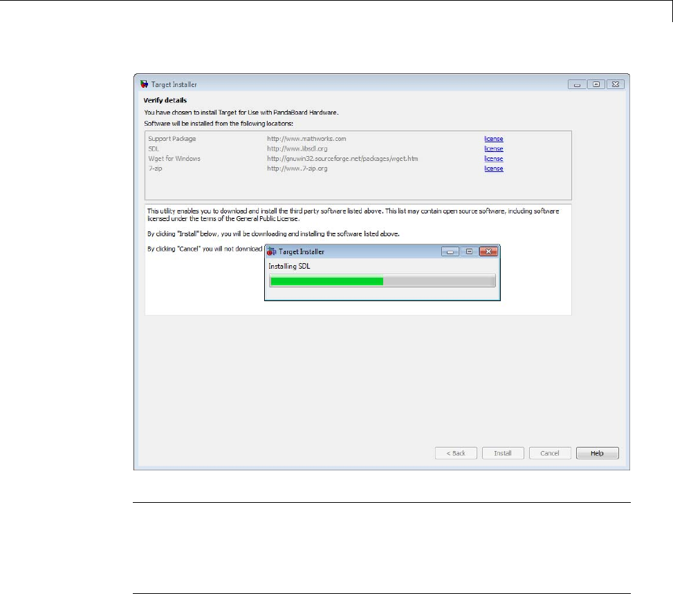
Install Support for PandaBoard Hardware
Note If you installed the target previously, Target Installer removes the
files from that installation before installing the current target. If Target
Installer cannot remove those files automatically, it instructs you to delete
the files manually. Close the MATLAB software before removing the files.
Then, restart MATLAB software and run Target Installer again.
5Click Continue to replace the factory-installed firmware on the PandaBoard
hardware with Ubuntu Linux, as described in “Replace Firmware on
PandaBoard Hardware” on page 56-9.
56-7
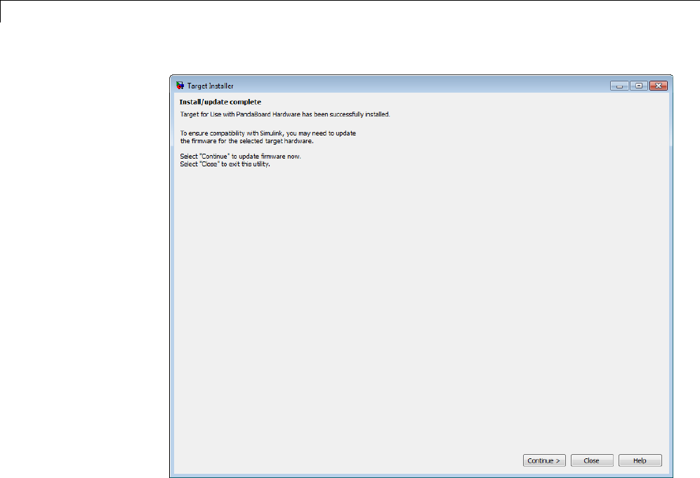
56 Work with PandaBoard Hardware
56-8

Replace Firmware on PandaBoard Hardware
Replace Firmware on PandaBoard Hardware
This topic shows how to replace the firmware on the PandaBoard hardware
(the “board”) with a Linaro.org build of Ubuntu Linux firmware that can
run Simulink models.
Before replacing the firmware, install the target, as described in “Install
Support for PandaBoard Hardware” on page 56-2.
After replacing the firmware, you can run a Simulink model on the
PandaBoard hardware, as described in “Run Model on PandaBoard
Hardware” on page 56-38.
The following steps provide an overview of the firmware replacement process:
1The Target Installer locates a firmware image on your host computer or
downloads new one.
2The Target Installer uses the host computer to write the firmware image
to a microSD or SD memory card.
3You transfer the microSD or SD memory card to the PandaBoard hardware.
4The Target Installer applies the IP settings you choose to the firmware on
the PandaBoard hardware.
Note Target Installer does not use the PandaBoard hardware to write the
firmware image to the memory card.
To replace the firmware on your PandaBoard hardware:
1Open the Update firmware screen in the Target Installer using one of the
following methods:
•Click Continue in the Install/update complete screen of the Target
Installer.
•In a model, select Tools > Run on Target Hardware > Update
firmware.
56-9
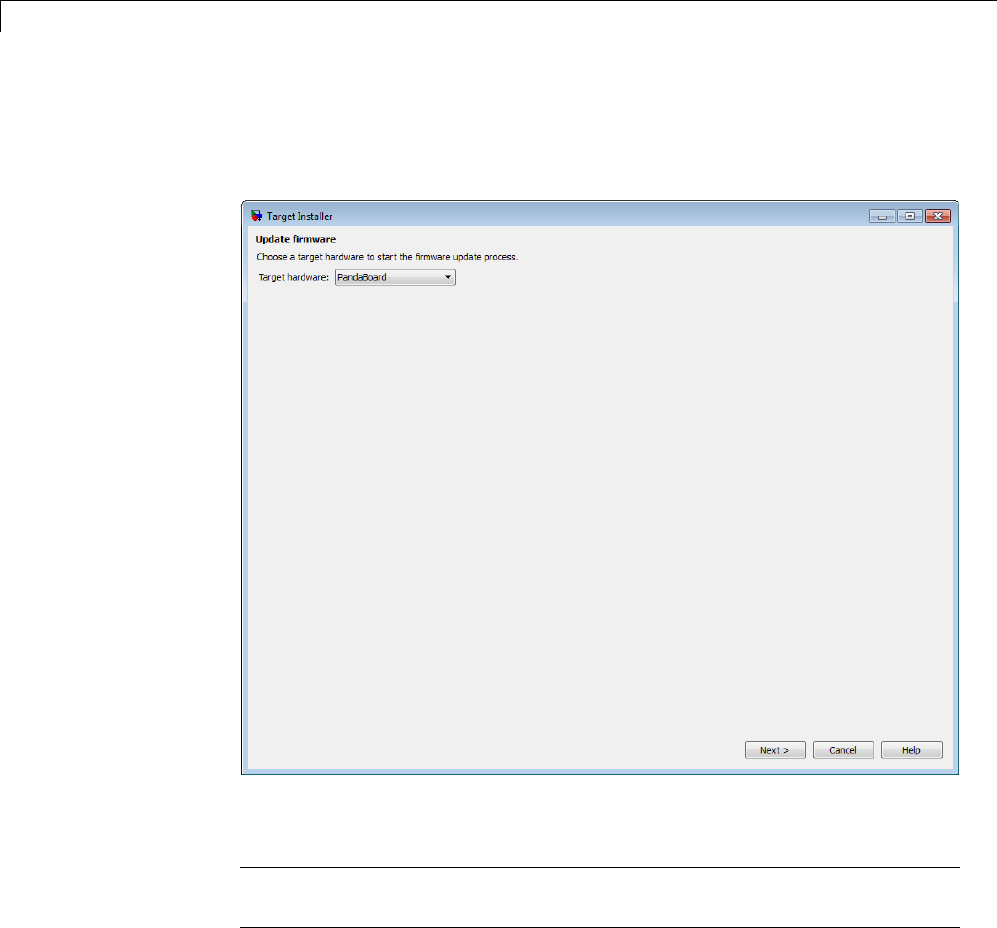
56 Work with PandaBoard Hardware
•In a MATLAB Command Window, enter targetupdater.
2Choose the PandaBoard option and click Next.
3Make the connections shown and click Next.
Note For “3. Speakers or headphones”, use the lower jack (closest to the
board).
56-10
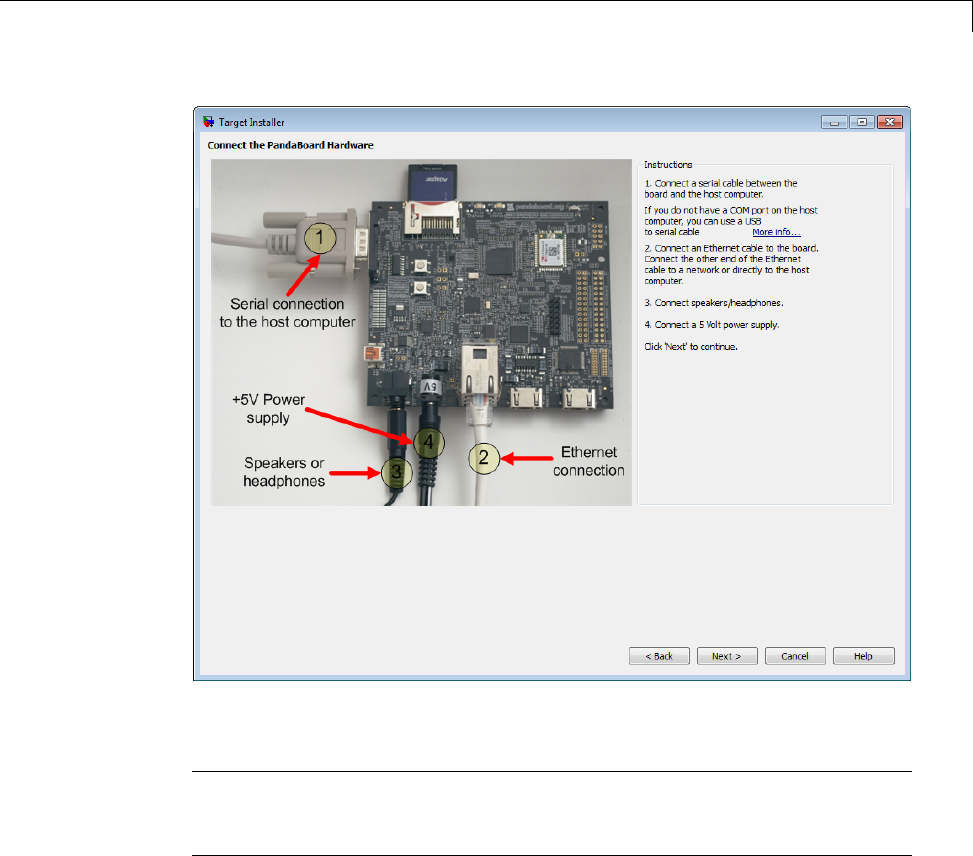
Replace Firmware on PandaBoard Hardware
4Choose to get the firmware image from the Internet or from a folder.
Note Thefilesizeofthefirmwareimageisapproximately1GB.Depending
on your connection, downloading the firmware can take from 2 to 60 minutes,
or more.
Internet: This option is selected by default. When you click Download,
Target Installer checks the Download folder for a valid firmware image:
•If a firmware image is not present, Target Installer downloads a firmware
image from the Internet, and saves it to the download folder.
56-11

56 Work with PandaBoard Hardware
•If a firmware image is present, Target Installer uses the firmware image
already present in the download folder, and does not download a new
firmware image from the Internet.
Folder:WhenyouclickDownload, Target Installer checks the Download
folder for a valid firmware image:
•If a firmware image is not present, Target Installer displays an error
message that the image file is missing. To solve this issue, copy the
firmware image from another location to the download folder, or choose
the Internet option instead.
•If a firmware image is present, Target Installer continues the firmware
installation process.
You must have write privileges for the download folder. If you use the default
download folder, having write privileges is typically not an issue. If you
change to a new download folder for which you do not have write permissions,
such as a shared folder on a network, the Target Installer generates an
error message: “Error: Download the firmware. The download folder is not
writable. Choose a folder for which you have write permissions”.
Tosolvethisissue,copythefirmwareimagetoafolderforwhichyouhave
write privileges. For example, copy the firmware image from the shared
folder on the network to the C:\Users\username\AppData\Local\Temp
folder. Then, update the Download location to the same folder, and click
Download again.
Tolocatethefirmwareimageinafolder, search for a filename that
begins with pandaboard and ends with .img or .7z . For example:
pandaboard_ubuntu_11_10_3_1_1_04_14_2012.img
56-12
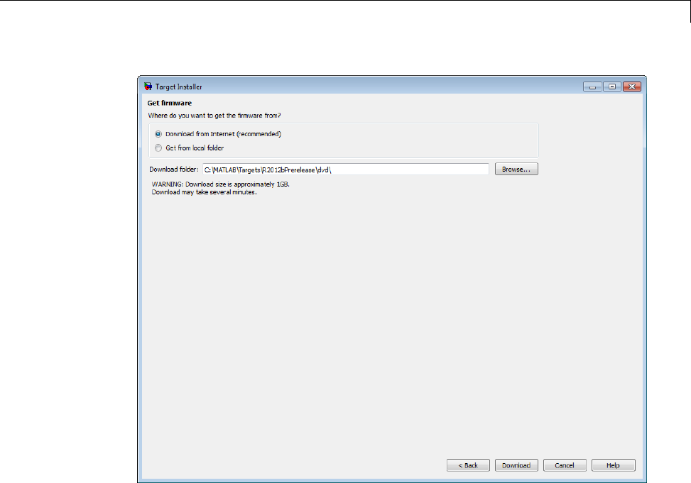
Replace Firmware on PandaBoard Hardware
5Insert the microSD or SD memory card into a media card reader connected to
your host computer. Windows assigns a drive letter to the memory card.
6Target Installer does not automatically detect the drive letter of the memory
card. It displays a drive letter for each device with removable storage.
•If only one drive letter is available, click Next.
•If no drive letters are available, check that the memory card is fully
inserted, and click Refresh.
•If multiple drive letters are available, open the Windows Start menu,
choose Computer, and look for the memory card under Devices with
Removable Storage.
56-13
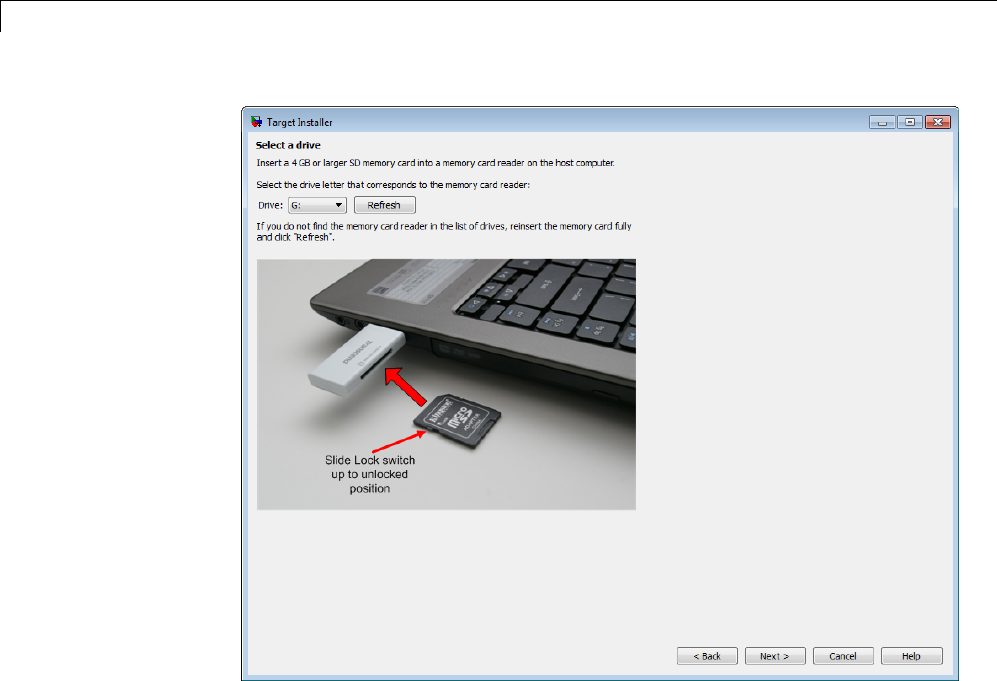
56 Work with PandaBoard Hardware
7Click Write. Target Installer overwrites all previous data on the memory
card with the firmware. This process takes several minutes to complete.
56-14

Replace Firmware on PandaBoard Hardware
8Get the COM port of the serial connection in Windows. From the Windows
Start menu, choose search programs and files for “Device Manager”. Open
Device Manager, expand Ports (COM & LPT), and identify the COM port of
the serial connection to the PandaBoard hardware.
For example, the following image shows a DB9 serial port called
“Communications Port” using COM1, and a USB-to-serial adapter called
“Prolific USB-to-Serial Comm Port” using COM6.
56-15
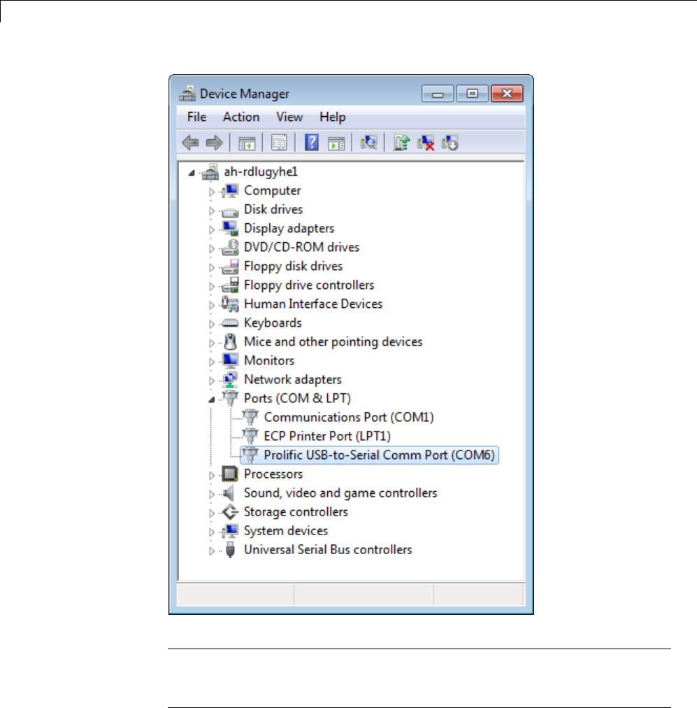
56 Work with PandaBoard Hardware
Note Some USB-to-serial adapters do not appear in the list of serial
connections immediately after you install the software drivers. To solve this
issue, disconnect/reconnect the adapter, or reboot your host computer.
56-16

Replace Firmware on PandaBoard Hardware
9Target Installer does not automatically choose the COM port of the serial
connection. After you get the COM port of the serial connection from Windows
Device Manager, return to Target Installer, set Serial port to the COM port,
and click Next.
10 Press and release the RESET button. Then, insert the memory card into
the PandaBoard hardware.
Click Next. When the Target Installer detects a reset, it displays progress
booting the board.
If the Target Installer does not display any progress, click <Back.Onthe
Select serial port screen. Verify that you selected the correct COM port, and
close any other applications, such as PuTTY, that might using the serial
connection.
56-17
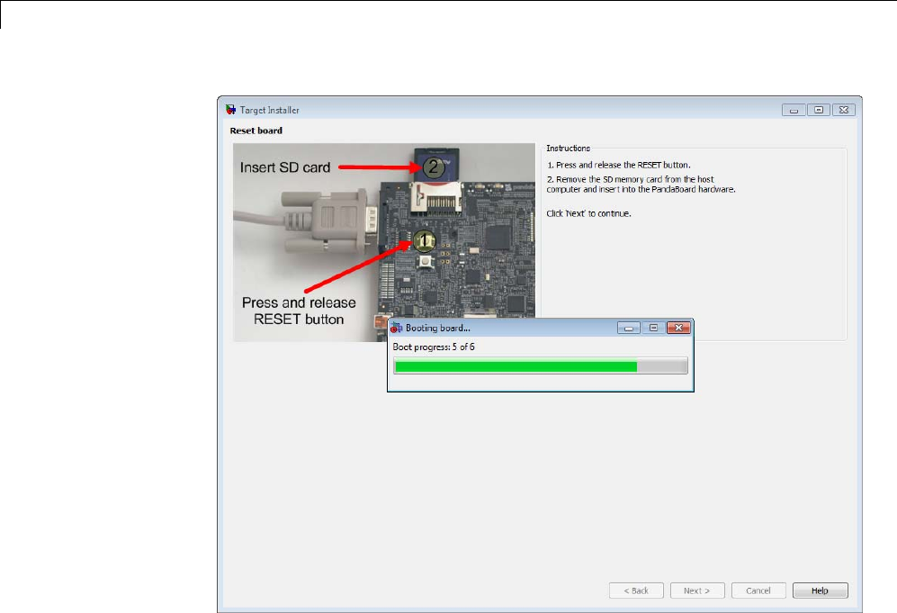
56 Work with PandaBoard Hardware
11 If your board is connected to a network with DHCP services, such as an office
LAN or a home network connected to the Internet, select Automatically get
IP address, give the board a unique name, and click Configure.DHCPis
anetwo
rk service that automatically configures the IP settings of Ethernet
devices connected to a network.
If your board is directly connected to an Ethernet port on your computer, or
connected to an isolated network without DHCP services, select Manually
enterIPaddress, give the board a unique name, enter static IP settings
for the board, and click Configure.
To enter static IP settings for your board, follow these guidelines:
•The value of the subnet mask must be the same for all devices on the
network.
56-18
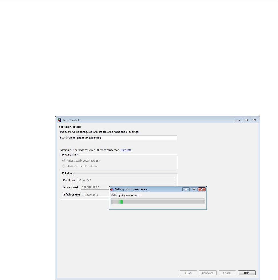
Replace Firmware on PandaBoard Hardware
•The value of the IP address must be unique for each device on the network.
For example, if the Ethernet port on your host computer has a network mask
of 255.255.255.0 and a static IP address of 192.168.1.1,set:
•Network mask to use the same network mask value, 255.255.255.0.
•IP address to an unused IP address, between 192.168.1.2 and
192.168.1.254.
When you click Configure, the Target Installer opens a serial connection
and applies the settings to the board.
12 Make a note of the values for IP address,User name,andPassword.
Then, click Next.
56-19
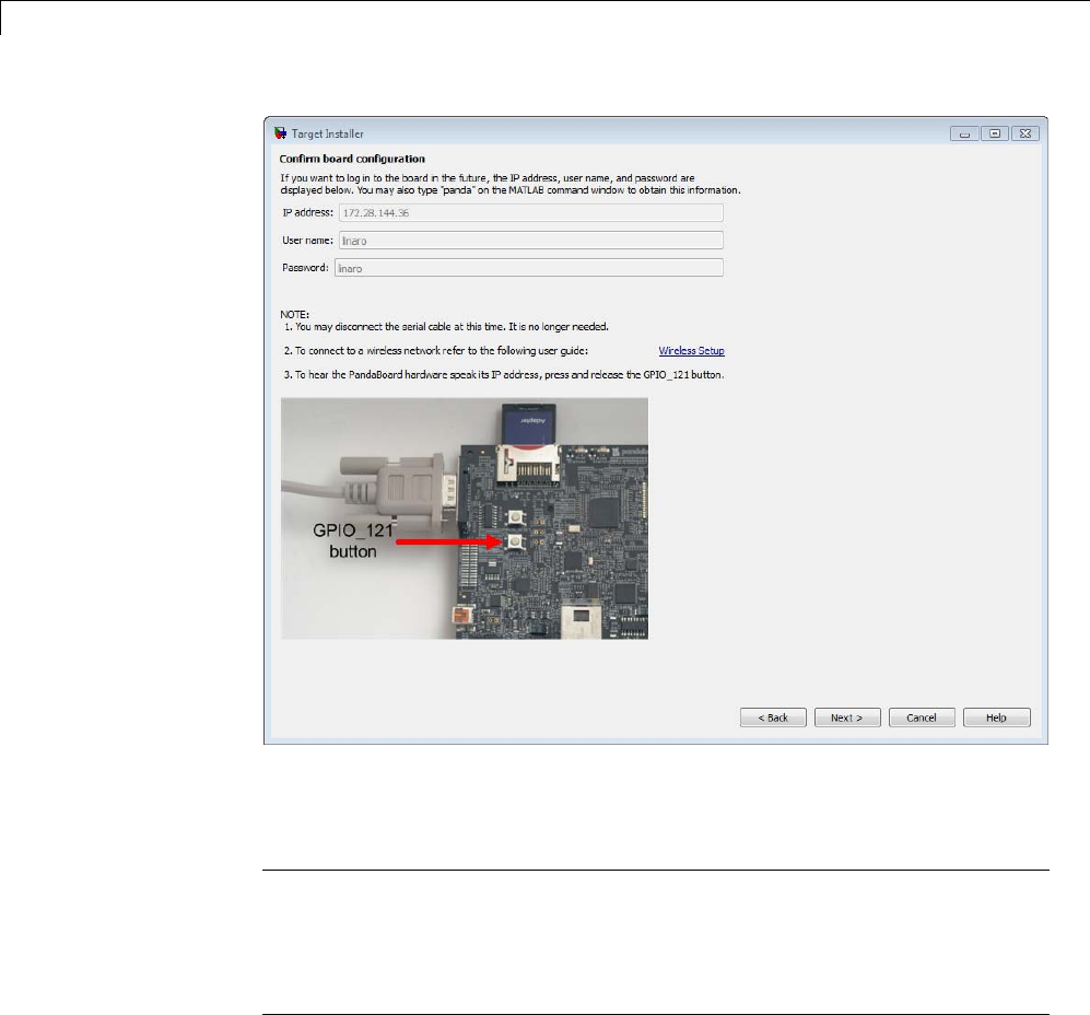
56 Work with PandaBoard Hardware
13 Click Finish.IfLaunch target examples is enabled, the Target Installer
opens the example page for PandaBoard hardware.
Note To reopen the examples later, enter the following text in a MATLAB
Command Window:
demo simulink 'Target for Use with Pandaboard'
56-20
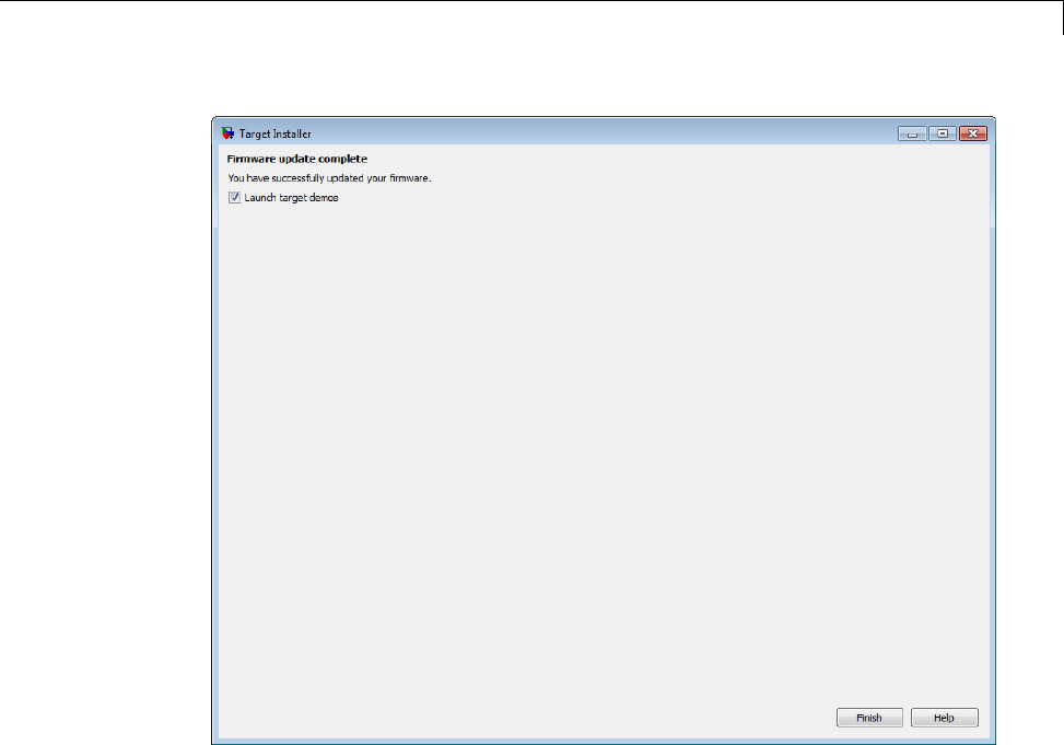
Replace Firmware on PandaBoard Hardware
56-21

56 Work with PandaBoard Hardware
ChoosetheTypeofSerialCable
This topic shows you how to choose a serial cable for connecting your host
computer to the PandaBoard hardware.
Two types of cables are available for this purpose:
•DB9 null modem M/F cable
•USB to DB9 male adapter cable
DB9 null modem M/F cable:
•If your host computer has a DB9 male serial connector similar to the one in
the following image, you can use a DB9 null modem M/F cable.
•To find the appropriate cable online, search for “DB9 low profile null
modem M-F cable”.
USB to DB9 male adapter cable:
•If your host computer has a USB port, you can use a USB to DB9 male
adapter cable.
•Tofindtheappropriatecableonline,search for "USB to RS-232 DB9 Serial
Adapter”.
•Some USB-to-serial adapters do not appear in the list of serial connections
immediately after you install the software drivers. To solve this issue,
disconnect and reconnect the adapter, or reboot your host computer.
•To avoid issues with the software/driver quality, we recommend choosing
an adapter that has good customer feedback ratings, or using the DB9 null
modem M/F cable instead.
56-22

Connect to Serial Port on PandaBoard Hardware
Connect to Serial Port on PandaBoard Hardware
This topic shows you how to configure and open a command line session with
the target hardware.
This is an optional task that you can use to:
•View the standard output while the board boots.
•Get or set the IP address, as described in “Get IP Address of PandaBoard
Hardware” on page 56-32 topic.
To open a serial connection to your board:
1Connect a serial cable from your host computer to the female DB9 connector
on the board.
2Identify the COM port for your serial connection. In Windows 7, use the
“search programs and files” feature in the Start menu to find “Device
Manager”. Open Device Manager, and expand Ports (COM & LPT) to see
the list of serial connections.
For example, the following image shows that the DB9 serial port called
“Communications Port” uses COM1. Similarly, the image shows that the
USB-to-serial adapter called “Prolific USB-to-Serial Comm Port” uses
COM6.
56-23
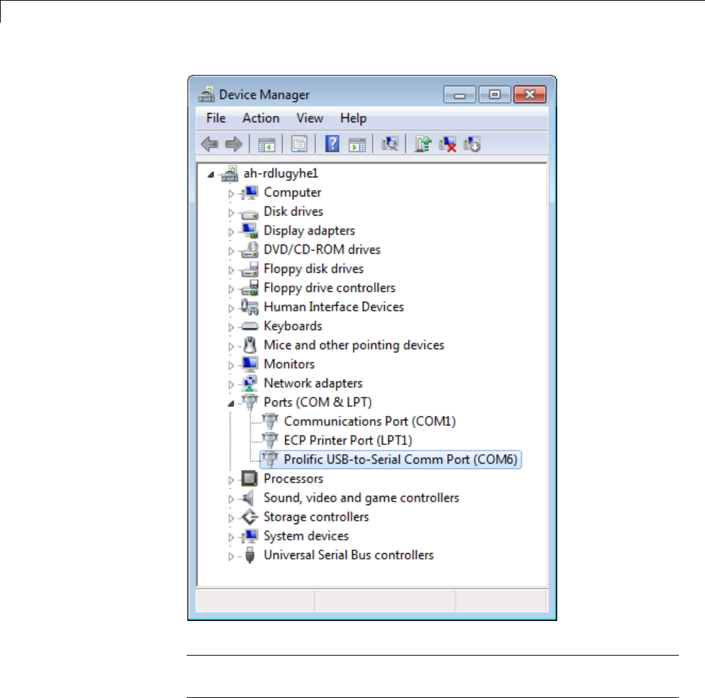
56 Work with PandaBoard Hardware
Note If you have trouble locating the COM port number, search the
Windows “Help and Support” for “Device Manager”.
3In the MATLAB Command Window, start PuTTY by entering:
56-24
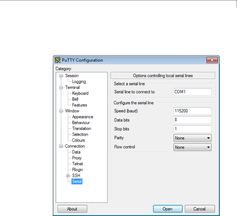
Connect to Serial Port on PandaBoard Hardware
h = panda;
system(['"' fullfile(h.PutilsFolder, 'putty.exe') '" -serial &'], '-runAsAdmin');
4In the PuTTY dialog box that opens, select the Serial category.
5Set the following values:
•Serial line to connect to: If you are using your computer’s built-in
serial port, try COM1. Otherwise, use the Device Manager in Windows to
determine the COM port number.
•Speed (baud):115200
56-25
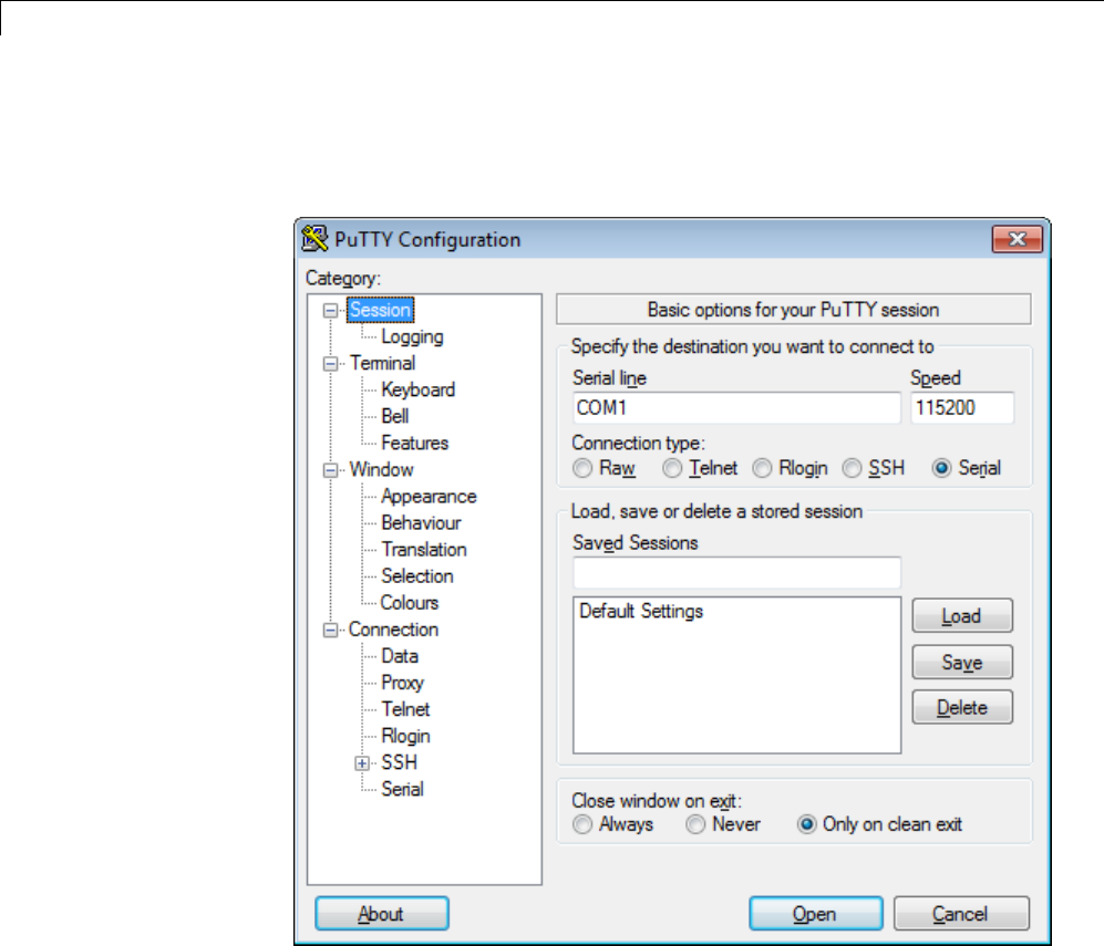
56 Work with PandaBoard Hardware
•Flow control:None
6In the PuTTY dialog box, select the Session category.
7Set the Connection type parameter to Serial, enter a new name for
Saved Sessions,clickSave,andclickOpen.
56-26

Connect to Serial Port on PandaBoard Hardware
Note Do not save the serial settings to Default Settings.TheDefault
Settings must remain configured to use SSH in order to run your Simulink
model on the BeagleBoard hardware. Otherwise, trying to run the model
on BeagleBoard hardware produces an error message similar to this one:
>> [status, message] = h.connect()
Error using linkfoundation.util.pandaboard/connect (line 125)
SSH connection to host 144.212.110.44 failed:
FATAL ERROR: Network error: Connection refused
8When a terminal window opens, press the Enter key on your keyboard.
The terminal window displays the Linux command line.
9When you are finished, enter logout on the Linux command line, and close
PuTTY to end the serial connection.
See Also
•“Get IP Address of PandaBoard Hardware” on page 56-32
•For more information about PuTTY, see:
http://www.chiark.greenend.org.uk/~sgtatham/putty/
56-27

56 Work with PandaBoard Hardware
Configure Network Connection with PandaBoard
Hardware
You can configure the IP settings of the PandaBoard hardware by running
Linux shell commands directly on the PandaBoard hardware (the “board”).
To inspect and reconfigure the IP settings on a board that already has the new
firmware, follow the procedure in this section that starts with “To configure
the board to use DHCP or static IP settings”.
To configure the IP settings while you are replacing the firmware on your
PandaBoard hardware, see “Replace Firmware on PandaBoard Hardware”
on page 56-9.
You may need to reconfigure the IP settings if your board:
•Has unknown IP settings.
•Is unreachable using a network connection.
•Is being moved to a network or direct Ethernet connection that uses static
IP settings.
•Is being moved from a network that used static IP settings to one that
uses DHCP services.
When you complete the procedure in this topic, the board should be able to
communicate over the network to which it is connected.
Before starting the procedure in this topic, it helps to understand the
conditions under which networks use DHCP or static IP settings:
•If your board is connected to a network with DHCP services, such as an
office LAN or a home network connected to the Internet, configure the
board to use DHCP services. DHCP is a network service that automatically
configures the IP settings of Ethernet devices connected to a network.
•If your board is directly connected to an Ethernet port on your computer,
or connected to an isolated network without DHCP services, configure
the board to use static IP settings.
56-28

Configure Network Connection with PandaBoard Hardware
To configure the board to use DHCP or static IP settings:
1Open a serial command line session, as described in “Connect to Serial Port
on PandaBoard Hardware” on page 56-23
Alternatively, you can use a terminal window after accessing the Linux
desktopasdescribedin:
•“Access the Linux Desktop Directly Using Desktop Computer
Peripherals” on page 56-46
•“Access the Linux Desktop Remotely Using VNC” on page 56-48
2Display the contents of the /etc/network/interfaces file. Enter:
cat /etc/network/interfaces
If the board is configured to use DHCP services (the default configuration),
dhcp appears at the end of the following line:
iface eth0 inet dhcp
If the board is configured to use static IP settings, static appears at the
end of the following line:
iface eth0 inet static
3Create a backup of the /etc/network/interfaces file. Enter:
sudo cp /etc/network/interfaces /etc/network/interfaces.backup
If prompted, enter the root password (default: linaro).
4Change the permissions of /etc/network/interfaces so you can edit the
file. Enter:
sudo chmod 777 /etc/network/interfaces
If prompted, enter the root password (default: linaro).
5Edit interfaces using a simple editor called nano. Enter:
nano /etc/network/interfaces
56-29

56 Work with PandaBoard Hardware
6Editthelastwordoflinethatstartswithiface eth0 inet.
TouseDHCPservices,editthelinetosay:
iface eth0 inet dhcp
TousestaticIPsettings,editthelinetosay:
iface eth0 inet static
7For static IP settings, add lines for address,netmask,andgateway.For
example:
iface eth0 inet static
address 192.168.1.2
netmask 255.255.255.0
gateway 192.168.1.1
Note For static IP settings:
•The value of the subnet mask must be the same for all devices on the
network.
•The value of the IP address must be unique for each device on the
network.
For example, if the Ethernet port on your host computer has a network
mask of 255.255.255.0 and a static IP address of 192.168.1.1,set:
•netmask to use the same network mask value, 255.255.255.0.
•address to an unused IP address, between 192.168.1.2 and
192.168.1.254.
8Tell nano to exit and save the changes:
Press Ctrl+x.
Enter Yto save the modified buffer.
For “File Name to Write: interfaces”, press Enter.
56-30

Configure Network Connection with PandaBoard Hardware
The nano editor confirms that it “Wrote # lines” and returns control to
the command line.
9Restore the original file permissions. Enter:
sudo chmod u=rw,g=r,o=r /etc/network/interfaces
If prompted, enter the root password (default: linaro).
10 Test the IP settings by logging in to the board over a telnet session.
Note You can use the ifconfig command to temporarily change the IP
settings. Rebooting the board removes the ifconfig settings and restores the
/etc/network/interfaces settings.
To change the IP settings temporarily, open a Linux command line, and enter
ifconfig, the device id, a valid IP address, netmask, and the appropriate
network mask. For example:
ifconfig eth0 192.168.45.12 netmask 255.255.255.0
Related
Examples
•“Run Model on PandaBoard Hardware” on page 56-38
•“Get IP Address of PandaBoard Hardware” on page 56-32
56-31

56 Work with PandaBoard Hardware
Get IP Address of PandaBoard Hardware
You can get the IP address of the PandaBoard hardware (the “board”) by
listening to the audio output, or by using the Linux command line. This is
an optional task that you can use to:
•Preparing a model to run on a board that is different from the previous
one you used.
•Opening a telnet session with a board whose IP settings you do not know.
•Configuring the UDP Send block.
When you prepare a model to run on a board, your model Configuration
Parameters reuse the IP settings of the previous board you used. If you are
working with a different board on the same network, get the IP address of the
your new board, and update the Host name parameter in the Configuration
Parameters. For more information, see “Run Model on PandaBoard
Hardware” on page 56-38.
If Ethernet port on the PandaBoard hardware board has an IP address, the
audio output on the board can read the IP address out loud. For example the
board can say “My IP address is one hundred and forty four point two one two
pointoneonezeropointtwozerosix.”
To listen your board’s IP address using headphones or speakers:
1Plug headphones or speakers into the AUDIO OUT jack on the board.
2Press the GPIO_121 button on the board.
56-32
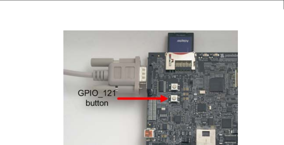
Get IP Address of PandaBoard Hardware
3Write down the IP address as the board reads it out over the headphones
or speakers.
The Linux command line on the board can provide the IP address of the
Ethernet port.
To get your board’s IP address using a command line session:
1Open a serial command line session on your board, as described in “Connect
to Serial Port on PandaBoard Hardware” on page 56-23.
Alternatively, you can use a terminal window after accessing the Linux
desktopasdescribedin:
•“Access the Linux Desktop Directly Using Desktop Computer
Peripherals” on page 56-46
•“Access the Linux Desktop Remotely Using VNC” on page 56-48
2At the Linux command line, enter ifconfig.
3Locate the IP address following inet addr in the command line output.
For example, locate inet addr:172.28.144.36 on line 3 of the following
output:
56-33

56 Work with PandaBoard Hardware
root@panda-ah-rdlugyhe1:~# ifconfig
eth0 Link encap:Ethernet HWaddr 0a:40:27:be:3b:0a
inet addr:172.28.144.36 Bcast:172.28.144.255 Mask:255.255.255.0
inet6 addr: fe80::840:27ff:febe:3b0a/64 Scope:Link
UP BROADCAST RUNNING MULTICAST MTU:1488 Metric:1
RX packets:15137 errors:0 dropped:0 overruns:0 frame:0
TX packets:1080 errors:0 dropped:0 overruns:0 carrier:0
collisions:0 txqueuelen:1000
RX bytes:5118973 (5.1 MB) TX bytes:144806 (144.8 KB)
lo Link encap:Local Loopback
inet addr:127.0.0.1 Mask:255.0.0.0
inet6 addr: ::1/128 Scope:Host
UP LOOPBACK RUNNING MTU:16436 Metric:1
RX packets:0 errors:0 dropped:0 overruns:0 frame:0
TX packets:0 errors:0 dropped:0 overruns:0 carrier:0
collisions:0 txqueuelen:0
RX bytes:0 (0.0 B) TX bytes:0 (0.0 B)
wlan0 Link encap:Ethernet HWaddr 0a:00:27:be:3b:0a
UP BROADCAST MULTICAST MTU:1500 Metric:1
RX packets:0 errors:0 dropped:0 overruns:0 frame:0
TX packets:0 errors:0 dropped:0 overruns:0 carrier:0
collisions:0 txqueuelen:1000
RX bytes:0 (0.0 B) TX bytes:0 (0.0 B)
root@panda-ah-rdlugyhe1:~#
Related
Examples
•“Connect to Serial Port on PandaBoard Hardware” on page 56-23
•“Run Model on PandaBoard Hardware” on page 56-38
•“Get IP Address of PandaBoard Hardware” on page 56-32
56-34

Open Block Library for PandaBoard Hardware
Open Block Library for PandaBoard Hardware
This block library provides support for protocols and APIs available on
PandaBoard hardware (the “board”).
To open the block library from the MATLAB Command Window, enter:
pandaboardlib
The following block library opens.
56-35
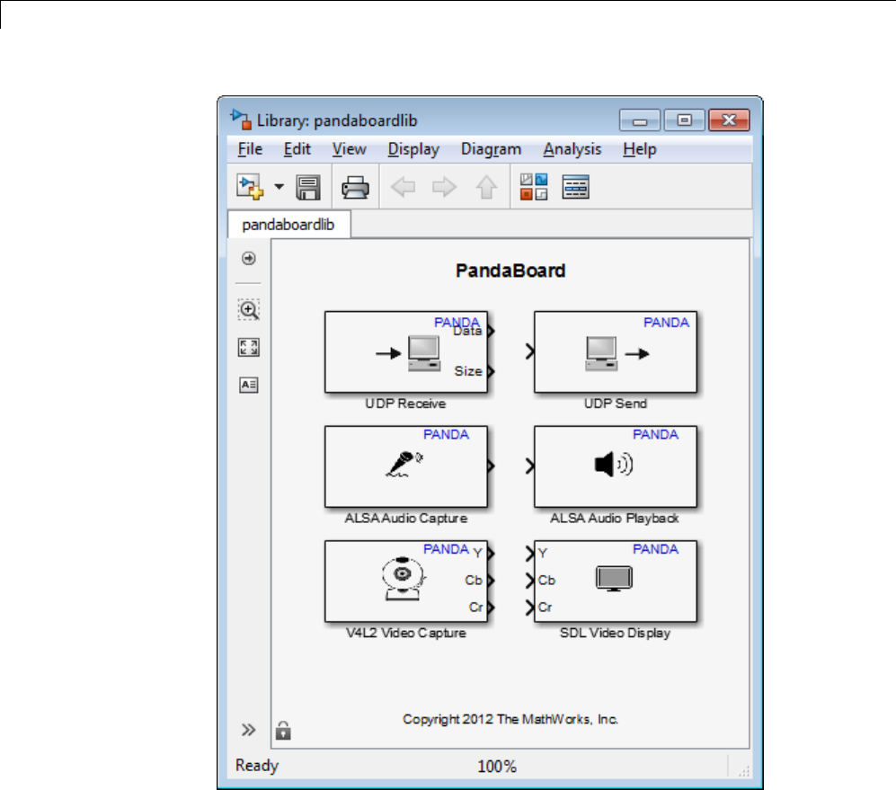
56 Work with PandaBoard Hardware
To open the block library from the Simulink Library Browser:
1Open the Simulink Library Browser by entering simulink in the MATLAB
Command Window, or by clicking the following icon on the MATLAB toolbar.
56-36
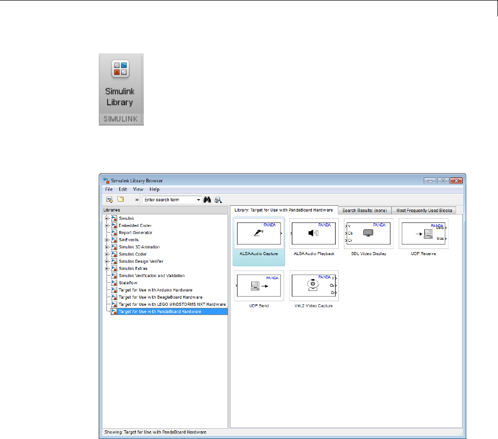
Open Block Library for PandaBoard Hardware
2In the Simulink Library Browser, click Target for Use with PandaBoard
Hardware.
56-37

56 Work with PandaBoard Hardware
Run Model on PandaBoard Hardware
This example shows how to prepare, configure, and run a simple model on
your PandaBoard hardware (the “board”).
Before starting this procedure:
•Connect your board to the network and to a power supply.
•Create or open a Simulink model.
To prepare and run the model:
1Use File > Save As to create a working copy of your model. Keep the original
model as a backup copy.
2In your model, select Tools > Run on Target Hardware > Prepare to
Run.Thisa
ction changes the model Configuration Parameters.
3In the Run on Target Hardware pane that opens, set the Target hardware
parameter to PandaBoard.
4If you have changed boards since the last time you updated the firmware or
ran a model, update the Host name,User name,andPassword parameters.
5Select Tools > Run on Target Hardware > Run. This action automatically
downloads and runs your model on the board.
Note Pressing RESET or cycling the power on the PandaBoard hardware
during this step can cause the ssh utility to hang.
Warning Avoid using the RESET button to stop a running model
and reboot the board. Doing so can corrupt operating system and
program files. To fix corrupt files, replace the firmware as described
in “Replace Firmware on PandaBoard Hardware” on page 56-9.
Running a new or updated model on the board:
•Automatically stops a running model with the same name.
56-38

Run Model on PandaBoard Hardware
•Does not stop running models that have other names.
To stop a model running on the board, enter the following commands in the
MATLAB Command Window:
h=panda;
h.stop('modelName');
For example, to stop the sumdiff model, enter:
h=panda;
h.stop('sumdiff');
To restart a model that was previously running on the board, or to run
multiple instances of a model, enter the following commands in the MATLAB
Command Window:
h=panda;
h.run('modelName');
Note You do not need to enter h=panda; multiple times if a previous instance
of his available in the MATLAB Workspace.
Forexample,torestartthesumdiffmodel you stopped in the previous
example, enter:
h.run('sumdiff');
Prepare Models That Use Model Reference
You can include one model in another by using Model blocks. Each instance
of a Model block represents a reference to another model, called a referenced
model or submodel. The model that contains a referenced model is its parent
model. When you run parent model on your target hardware, the submodel
effectively replaces the Model block that references it. For more information,
see “Overview of Model Referencing” on page 6-2.
To run on target hardware, the parent model and the submodels must have
the same Configuration Parameter settings.
56-39

56 Work with PandaBoard Hardware
For each Model block:
•Select Tools > Run on Target Hardware > Prepare to Run.
•Apply the same Configuration Parameters settings to the submodel as you
applied to the parent model.
If the model and Model blocks have different settings, the software generates
an error when you try to run the model on the target hardware.
See Also
•“Create the Simple Model”
•“Configure Network Connection with PandaBoard Hardware” on page 56-28
•“Tune and Monitor Model Running on PandaBoard Hardware” on page
56-41
•“Overview of Model Referencing” on page 6-2
56-40

Tune and Monitor Model Running on PandaBoard Hardware
Tune and Monitor Model Running on PandaBoard
Hardware
In this section...
“About External Mode” on page 56-41
“Run Your Simulink Model in External Mode” on page 56-42
“Stop External Mode” on page 56-44
About External Mode
You can use External mode to tune parameters and monitor a model running
on your target hardware.
External mode enables you to tune model parameters and evaluate the effects
of different parameter values on model results in real-time, in order to find
the optimal values to achieve desired performance. This process is called
parameter tuning.
External mode accelerates parameter tuning because you do not have to
re-run the model each time you change parameters.Externalmodealsolets
you develop and validate your model using the actual data and hardware for
which it is designed. This software-hardware interaction is not available
solely by simulating a model.
The following list provides an overview of the parameter tuning process with
External mode:
•In the model on your host computer, you enable External mode in the
Configuration Parameters.
•In the model on your host computer, you tell Simulink software to run
your model on the target hardware.
•Simulink software runs the model on the target hardware.
•You use the model on the host computer as a user interface for interacting
with the model running on the target hardware:
56-41
56 Work with PandaBoard Hardware
-When open blocks and apply new parameter values on the host computer,
External mode updates the corresponding values on target hardware.
-If your model contains blocks for viewing data, such as Scope or Display
blocks, External mode sends the corresponding data from the target
hardware to those blocks on the host computer.
•You determine the optimal parameter values by adjusting parameter values
on the host computer and observing data/outputs from the target hardware.
•When you are finished, you save the new parameter values, disable
External mode, and save the model.
Run Your Simulink Model in External Mode
1Create a network connection between the PandaBoard hardware and your
host computer. See “Configure Network Connection with PandaBoard
Hardware” on page 56-28
2In the model, set the Simulation stop time parameter, located on the
model toolbar, as shown here.
•To run the model for an indefinite period, enter inf.
•To run the model for a finite period, enter a number of seconds. For
example, entering 120 runsthemodelonthehardwarefor2minutes.
3Select Tools > Run on Target Hardware > Options.
4In the Run on Target Hardware pane that opens, select Enable External
mode.
5ClickOK, and then save the changes your model.
6In your model, select Tools > Run on Target Hardware > Run.
After several minutes, Simulink starts running your model on the board.
56-42

Tune and Monitor Model Running on PandaBoard Hardware
7While the model is running in External mode, you can change parameter
values in the model on your host computer and observe the corresponding
changes in the model running on the hardware.
If your model contains blocks from the Simulink Sinks block library,
the sink blocks in the model on your host computer display the values
generated by the model running on the hardware.
If your model does not contain a sink block to which External mode can
send data, the MATLAB Command Window displays a warning message.
For example:
Warning: No data has been selected for uploading.
> In C:\Program Files (x86)\MATLAB\R2012a Student1\toolbox\
realtime\realtime\+realtime\extModeAutoConnect.p>
extModeAutoConnect at 17
In C:\Program Files (x86)\MATLAB\R2012a Student1\toolbox\
realtime\realtime\sl_customization.p>myRunCallback at 149
You can disregard this warning, or you can add a sink block to the model.
Note To use External mode with the Run on Target Hardware feature, only
use the External mode settings described in this topic.
If you have Simulink Coder or Embedded Coder software, do not use other
External mode-related items that appear that in the Tools menu or the
Configuration Parameters dialog.
Note External mode increases the processing burden of the model running
on the board. If the software reports an overrun, clear the Enable External
mode checkbox in the Run on Target Hardware pane.
Note If you have the Embedded Coder or Simulink Coder products, you can
use External mode with a model that contains Model blocks (uses the “Model
reference”).
56-43

56 Work with PandaBoard Hardware
Stop External Mode
To stop the model running in External mode, click the Stop button located
on the model toolbar, as shown here.
This action stops the process for the model running on the PandaBoard
hardware, and stops the model simulation running on your host computer.
If it is set to a finite period, the Simulation stop time parameter stops
External mode when the period elapses.
56-44

Detect and Fix Task Overruns on PandaBoard Hardware
Detect and Fix Task Overruns on PandaBoard Hardware
You can configure a model running on the target hardware to detect and
notify you of when task overrun occurs.
Standard scheduling works well when a processor is moderately loaded but
may fail if the processor becomes overloaded. When a task is required to
perform extra processing and takes longer than normal to execute, it may
be scheduled to execute before a previous instance of the same task has
completed. The result is a task overrun.
To enable overrun detection:
1In your model, click Tools > Run on Target Hardware > Options.
2In the Run on Target Hardware pane that opens, select the Enable
overrun detection check box.
3Click OK.
When a task overrun occurs, the command prompt on the host machine
repeatedly prints an “Overrun” error message, such as “Overrun — rate for
subrate task 1 is too fast”, until the model stops.
To fix an overrun condition:
•Simplify the model.
•Increasethesampletimesforthemodelandtheblocksinit. Forexample,
changetheSample time parameter in all of your data source blocks, such
as blocks for input devices, from 0.1 to 0.2.
Note External mode increases the processing burden of the model running
on your board. If the software reports an overrun, clear the Enable External
mode checkbox in the Run on Target Hardware pane.
56-45
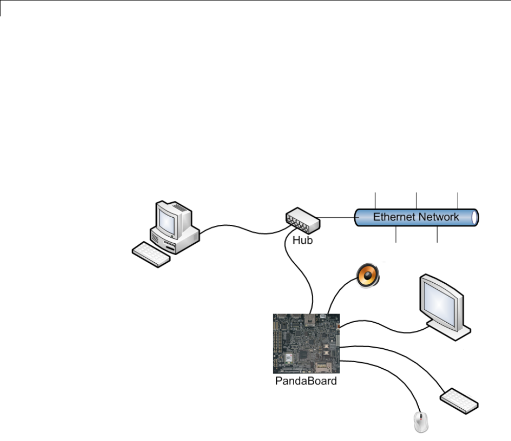
56 Work with PandaBoard Hardware
Access the Linux Desktop Directly Using Desktop Computer
Peripherals
You can access the Linux desktop on the PandaBoard hardware using
hardware peripherals such as a monitor, keyboard, and mouse.
You can use this approach to connect the PandaBoard hardware to a wireless
network, as described in “Configure Wi-Fi on PandaBoard Hardware” on
page 56-50.
If you do not have hardware peripherals, you can access the Linux desktop as
described in “Access the Linux Desktop Remotely Using VNC” on page 56-48.
To connect to the PandaBoard hardware to the hardware peripherals:
1Connect a computer monitor to the HDMI output, labelled P2 on the
PandaBoard hardware.
56-46

Access the Linux®Desktop Directly Using Desktop Computer Peripherals
2Connect the USB keyboard and USB mouse to the USB ports on the
PandaBoard hardware.
Note To connect additional USB devices, use a powered USB hub.
3You can connect computer speakers to the lower of the two 3.5 mm audio
connectors, labelled J16 on the PandaBoard hardware.
4You can connect a network cable to the Ethernet port.
5Connect the PandaBoard hardware to the power supply.
6Log in to the Linux desktop using the username and password. The default
user name and password is linaro.
56-47

56 Work with PandaBoard Hardware
Access the Linux Desktop Remotely Using VNC
You can remotely access the Linux desktop on the PandaBoard hardware
from another computer. This capability uses a client-server graphical desktop
sharing system called Virtual Network Computing (VNC).
The PandaBoard firmware distributed by MathWorks has a built-in VNC
server called x11vnc. To remotely interact with the PandaBoard hardware,
youcanrunaVNCclientonaremotecomputer,openaVNCconnectionwith
x11vnc on the PandaBoard hardware.
To open a VNC session from MATLAB:
1Create a physical network connection between your host computer and
the PandaBoard hardware.
2In the MATLAB Command Window, enter:
h = panda
h.connect
h.execute('export DISPLAY=:0.0; xhost +; x11vnc&', true)
h.execute('pidof x11vnc', true);
The MATLAB Command Window displays the status of the VNC server
running on the PandaBoard hardware. For example:
h=
realtime.internal.LinuxServices
Package: realtime.internal
Properties:
HostName: '172.28.144.36'
UserName: 'linaro'
Password: 'linaro'
BuildDir: '/home/linaro'
PutilsFolder: 'C:\Program Files\MATLAB\R2012b\toolbox\idelink\foundation\hostapps'
Methods
56-48

Access the Linux®Desktop Remotely Using VNC
ans =
0
access control disabled, clients can connect from any host
ans =
0
>>
3Open the VNC viewer and connect to the HostName IP address of the
PandaBoard.
56-49

56 Work with PandaBoard Hardware
Configure Wi-Fi on PandaBoard Hardware
PandaBoard has built-in 802.11b/g/n wireless networking.
To configure the PandaBoard hardware for wireless network connection, use
the Network Manager in the Linux desktop:
1Access the Linux desktop running on the PandaBoard hardware as
described in either of the following topics:
•“Access the Linux Desktop Directly Using Desktop Computer
Peripherals” on page 56-46
•“Access the Linux Desktop Remotely Using VNC” on page 56-48
2On the Linux desktop, open the Network manager, and select a wireless
network.
56-50

Configure Wi-Fi™ on PandaBoard Hardware
3If prompted, enter the wireless network password, and click Connect.
56-51

56 Work with PandaBoard Hardware
56-52

A
Examples
Use this list to find examples in the documentation.

AExamples
Simulink Basics
“Update a Block Diagram” on page 1-25
“Update a Block Diagram” on page 1-25
“Update a Block Diagram” on page 1-25
“Diagram Positioning and Sizing” on page 1-31
“Add Items to Model Editor Menus” on page 50-2
“Disable and Hide Model Editor Menu Items” on page 50-16
“Disable and Hide Dialog Box Controls” on page 50-18
A-2


AExamples
Creating a Model
“Create a Model Template” on page 4-2
“Create Annotations Programmatically” on page 4-34
“Create a Subsystem by Grouping Existing Blocks” on page 4-37
“Discretize Blocks from the Simulink Model” on page 4-135
“Enabled Subsystems” on page 7-4
“Enabled Subsystems” on page 7-4
“Triggered Subsystems” on page 7-20
“Triggered Subsystems” on page 7-20
“Triggered and Enabled Subsystems” on page 7-24
“Triggered and Enabled Subsystems” on page 7-24
“Conditional Execution Behavior” on page 7-32
“Conditional Execution Behavior” on page 7-32
“Data Store Examples” on page 46-23
A-4


Code Generation for Variable-Size Data
Code Generation for Variable-Size Data
“Constraining the Value of a Variable That Specifies Dimensions of
Variable-Size Data” on page 35-7
“Specifying the Upper Bounds for All Instances of a Local Variable” on
page 35-8
“Inferring Upper Bounds from Multiple Definitions with Different Shapes”
on page 35-13
A-11

AExamples
Code Generation for Structures
“Adding Fields in Consistent Order on Each Control Flow Path” on page
36-4
“Using repmat to Define an Array of Structures with Consistent Field
Properties” on page 36-7
“Defining an Array of Structures Using Concatenation” on page 36-8
“Make Structures Persistent” on page 36-9
A-12


Index
IndexSymbols and Numerics
%51-16
<>51-16
A
Abs block
zero crossings 3-35
absolute tolerance
definition 14-22
simulation accuracy 19-11
accelbuild command
building Accelerator MEX-file 22-26
Acceleration
code regeneration 22-7
compilation overhead 19-5
debugger advantages 22-29
decision tree 22-14
designing for 22-16
how to run debugger with 22-29
inhibiting 22-19
numerical precision 22-17
verses normal mode 22-17
trade-offs 22-11
Accelerator
description 22-2
determining why it rebuilds 22-7
how it works 22-3
making run time changes 22-25
Simulink blocks whose performance is not
improved by 22-16
switching back to normal mode 22-30
using with Simulink debugger 22-29
Accelerator and Rapid Accelerator
choosing between 22-11
comparing 22-11
Accelerator mode
keywords 22-20
Accelerators
customizing build process 22-22
interacting programmatically 22-26
running 22-23
Action Port block
in subsystem 4-45
activating
configuration references 10-21
Adams-Bashforth-Moulton PECE solver 14-19
Add button 51-14
adding
cells 51-12
rows 51-11
text to cells 51-14
variable information to cells 51-14
Algebraic loop diagnostic 3-43
algebraic loop solver
limitations 3-50
line-search algorithm 3-50
operations 3-49
trust-region algorithm 3-50
algebraic loops
artificial
atomic subsystems causing 3-55
bundled signals causing 3-57
eliminating using Simulink 3-68
problems caused by 3-43
avoiding discontinuities in 3-51
changing block priorities effect on 3-54
definition 3-40
direct feedthrough blocks 3-39
displaying 3-43 to 3-45
highlighting 21-36
identifying blocks in 21-33
mathematical definition of 3-41
physical meaning of 3-42
problems caused by 3-43
simulation speed 19-3
using Algebraic Constraint blocks to
remove 3-54
using IC blocks to remove 3-54
aligning
Index-1

Index
information in cells 51-18
aligning blocks 23-12
annotations
changing font 4-26
creating 4-23
definition 4-23
deleting 4-27
editing 4-25
moving 4-24
using symbols and Greek letters in 4-32
using TeX formatting commands in 4-32
using to document models 12-7
arguments
limit on number for code generation from
MATLAB 41-19
artificial algebraic loops
atomic subsystems causing 3-55
bundled signals causing 3-57
Assignment block
and For Iterator block 4-51
associating
bus objects
with model entities 48-21
asynchronous sample time 5-18
atomic subsystem 3-12
attaching
configuration references 10-18
to additional models 10-38
attributes format string 4-21
AttributesFormatString block
parameter 23-21
avoiding
mux/bus mixtures 48-104
B
Backlash block
zero crossings 3-35
backpropagating sample time 5-31
Backspace key
deleting blocks 23-13
deleting labels 47-23
Band-Limited White Noise block
simulation speed 19-3
block
simulation terminated or suspended 14-5
block callback parameters 4-58
block callbacks
adding custom functionality 27-37
Block data tips 23-2
block diagram
updating 1-25
block diagram entry 51-15
block diagrams
printing 1-28
block libraries
adding to Library Browser 28-32
creating 28-20
locking 28-21
modifying 28-21
searching 4-5
block methods
invoking 23-35
block names
changing location 23-27
copied blocks 23-10
editing 23-26
flipping location 23-27
generated for copied blocks 23-10
hiding and showing 23-28
location 23-26
rules 23-26
block parameters
about 24-1
displaying beneath a block 23-47
modifying during simulation 14-31
scalar expansion 47-38
setting 24-4
block priorities
assigning 23-47
Index-2

Index
effect on algebraic loops 3-54
rules 23-48
Block Properties dialog box 23-15
blocks
aligning 23-12
assigning priorities 23-47
associating user data with 43-80
autoconnecting 4-12
bus-capable 48-19
callback routines 4-54
changing font 23-27
changing font names 23-27
changing location of names 23-27
checking connections 3-18
connecting automatically 4-12
connecting manually 4-15
copying from Library Browser 4-5
copying into models 23-10
custom, Simulink 27-2
categories 27-3
code generation requirements 27-8
designing 27-18
examples 27-43
incorporating legacy code 27-6
modeling requirements 27-7
simulation requirements 27-8
tutorial 27-18
using block callbacks 27-37
using MATLAB functions 27-3
using S-functions 27-4
using Subsystems 27-4
deleting 23-13
disconnecting 4-21
displaying sorted order on 23-35
drop shadows 23-25
duplicating 23-9
grouping to create subsystem 4-37
hiding block names 23-28
input ports with direct feedthrough 3-39
invoking methods 23-35
moving between windows 23-11
moving in a model 23-11
names
editing 23-26
orientation 23-22
resizing 23-24
reversing signal flow through 12-8
rotating 23-22
rules for priorities 23-48
showing block names 23-28
updating 3-18
<>blocks 23-26
See also block names
borders
creating 51-11
important note about 51-11
bounding box
grouping blocks for subsystem 4-37
selecting objects 4-6
branch lines 4-16
Break Library Link menu item 28-18
breaking links to library block 28-18
breakpoints
setting 21-22
setting at end of block 21-25
setting at timesteps 21-25
setting on nonfinite values 21-26
setting on step-size-limiting steps 21-26
setting on zero crossings 21-26
Browser 9-80
building models
tips 12-6
Bus Editor 48-20
opening 48-25
bus objects
associating
with model entities 48-21
creating
with the API 48-23
with the Bus Editor 48-29
Index-3

Index
using 48-20
bus signals
created by Mux blocks 48-96
used as vectors 48-97
Bus to Vector block
backward compatibility 48-103
bus-capable blocks 48-19
sorted order and 23-45
buses 48-61
connecting to inports 48-61
mixing with muxes 48-95
nesting 48-17
busses used as muxes
correcting 48-101
C
C compiler
set up for code generation 29-210
set up for code generation from
MATLAB 29-182
C/C++ code generation for supported
functions 31-1
callback routines 4-54
callback routines, referencing mask parameters
in 4-59
callback tracing 4-55
cells
adding 51-12
adding text to 51-15
adding variable information to 51-15
changing information in 51-18
deleting 51-12
resizing 51-12
selecting 51-11
splitting 51-12
center alignment button 51-18
changing
fonts 51-20
information in cells 51-18
values using configuration references 10-23
10-39
characters, special 51-15
classes
enumerated 44-1
Clear menu item 23-13
Clipboard block callback parameter 4-59
Clock block
example 18-3
CloseFcn block callback parameter 4-59
CloseFcn model callback parameter 4-56
closing PrintFrame Editor 51-7
code generation for MATLAB
comparing to MATLAB S-functions 27-5
code generation from MATLAB
benefits of 30-2
best practices for working with
variables 33-3
calling local functions 41-9
calling MATLAB functions 41-11
calling MATLAB functions using feval 41-16
characters 34-6
communications system toolbox System
objects 32-7
compilation directive %#codegen 41-8
computer vision system toolbox System
objects 32-2
converting mxArrays to known types 41-18
declaring MATLAB functions as extrinsic
functions 41-12
defining persistent variables 33-10
defining variables 33-2
defining variables by assignment 33-3
dsp system toolbox System objects 32-13
eliminating redundant copies of function
inputs 42-4
eliminating redundant copies of uninitialized
variables 33-7
how it resolves function calls 41-2
initializing persistent variables 33-10
Index-4

Index
inlining functions 42-3
limit on number of function arguments 41-19
pragma 41-8
resolving extrinsic function calls during
simulation 41-16
resolving extrinsic function calls in generated
code 41-17
rules for defining uninitialized variables 33-7
setting properties of indexed variables 33-6
supported toolbox functions 41-10
unrolling for-loops 42-2
using type cast operators in variable
definitions 33-6
variables, complex 34-4
when not to use 30-2
when to use 30-2
which features to use 30-4
working with mxArrays 41-17
Code Generation from MATLAB
C compiler set up 29-182 29-210
getting started tutorial prerequisites 29-176
29-203
coder.extrinsic 41-12
using to debug MATLAB code 29-212
coder.nullcopy
uninitialized variables 33-7
color of text 51-20
colors for sample times 5-31
command line debugger for MATLAB Function
block 29-27
commands
undoing 1-21
communications system toolbox System objects
supported for code generation from
MATLAB 32-7
CompareToConstantblock
zero crossings 3-35
CompareToZeroblock
zero crossings 3-35
compiled sample time 5-20
Compiled Size property for MATLAB Function
block variables 29-72
compilers
supported for MATLAB Function blocks
(code generation) 29-12
supported for MATLAB Function blocks
(simulation) 29-12
composite signals 48-2
computer vision system toolbox System objects
supported for code generation from
MATLAB 32-2
conditional execution behavior 7-32
conditionally executed subsystem 3-11
conditionally executed subsystems 7-2
configurable subsystem 4-129
Configuration Parameters dialog box
increasing Accelerator performance 19-9
configuration references
activating 10-21
and building models 10-25
and generating code 10-25
attaching 10-18
to additional models 10-38
changing values with 10-23 10-39
creating 10-18
limitations 10-31
obtaining handles 10-40
obtaining values with 10-39
configuration sets
copying 10-36
reading from an M-file 10-36
referencing 10-18
using 10-12
connecting
buses to inports 48-61
buses to root-level inports 48-61
connecting blocks 4-15
ConnectionCallback
port callback parameters 4-63
constant sample time 5-16
Index-5

Index
ContinueFcn model callback parameter 4-56
4-59
continuous sample time 5-15
control flow diagrams
do-while 4-49
for 4-50
if-else 4-44
switch 4-46
while 4-47
control flow subsystem 7-2
control input 7-2
control signal 7-2
Control System Toolbox
linearization 18-6
controlling run-time checks
MATLAB Function block 29-173
Copy menu item 23-10
CopyFcn block callback parameter 4-59
copying
blocks 23-10
configuration sets 10-36
signal labels 47-23
copying information among cells 51-19
correcting
buses used as muxes 48-101
Created model parameter 4-119
creating
bus objects
with the API 48-23
with the Bus Editor 48-29
configuration references 10-18
custom Simulink blocks 27-2
freestanding configuration sets 10-36
creating print frames 51-7
Creator model parameter 4-119
custom blocks
creating 27-2
Customizing Accelerator Build
AccelVerboseBuild 22-28
SimCompilerOptimization 22-28
Cut menu item 23-11
D
data
enumerated 44-1
data range checking
MATLAB Function blocks 29-29
data types
displaying 43-27
enumerated 44-1
propagation definition 43-28
specifying 43-8
data types of MATLAB Function variables 29-67
data, adding to MATLAB Function blocks 29-42
date entry 51-15
Dead Zone block
zero crossings 3-35
debugger
highlighting algebraic loops using 3-45
running incrementally 21-17
setting breakpoints 21-22
setting breakpoints at time steps 21-25
setting breakpoints at zero crossings 21-26
setting breakpoints on nonfinite values 21-26
setting breakpoints on step-size-limiting
steps 21-26
skipping breakpoints 21-20
starting 21-10
stepping by time steps 21-20
debugging
breakpoints in MATLAB Function block
function 29-24
display variable values in MATLAB Function
block function 29-27
displaying MATLAB Function block
variables in MATLAB 29-27
MATLAB Function block example 29-23
MATLAB Function block function 29-23
Index-6

Index
operations for debugging MATLAB
functions 29-29
stepping through MATLAB Function block
function 29-25
decimation factor
saving simulation output 45-14 to 45-15
default print frame 51-6
defining uninitialized variables
rules 33-7
defining variables
for C/C++ code generation 33-3
Delete key
deleting annotations 4-27
deleting blocks 23-13
deleting signal labels 47-23
DeleteChildFcn block callback parameter 4-60
DeleteFcn block callback parameter 4-60
deleting
cells 51-12
rows 51-11
dependency analysis 9-83 13-104
best practices 13-123
comparing manifests 13-117
editing manifests 13-114
exporting manifests 13-118
file manifests 13-120
generating manifests 13-105
viewing dependencies 9-83
Derivative block
linearization 18-9
Description model parameter 4-120
Description property
MATLAB Function blocks 29-42
design considerations
when writing MATLAB Code for code
generation 30-7
designing
custom Simulink blocks 27-18
designing print frames 51-8
DestroyFcn block callback parameter 4-60
diagnosing simulation errors 14-39
diagnostics
for mux/bus mixtures 48-96
diagonal line segments 4-17
direct feedthrough blocks 3-39
direct-feedthrough ports
sorted order and 23-45
disabled subsystem
output 7-7
disconnecting blocks 4-21
discrete blocks
in enabled subsystem 7-11
in triggered systems 7-23
discrete sample time 5-14
discrete states
initializing 47-51
discretization methods 4-126
discretizing a Simulink model 4-122
dlinmod function
extracting linear models 18-5
do-while control flow diagram 4-49
Docking Scope Viewer 16-15
Document link property
MATLAB Function blocks 29-42
drop shadows 23-25
dsp system toolbox System objects
supported for code generation from
MATLAB 32-13
duplicating blocks 23-9
E
editing
MATLAB Function block function code 29-33
mode 51-14
text in cells 51-18
editing look-up tables 25-28
editor 1-17
eliminating redundant copies of function
inputs 42-4
Index-7

Index
Enable block
creating enabled subsystems 7-5
outputting enable signal 7-10
states when enabling 7-9
zero crossings 3-35
enabled subsystems 7-4
initializing output of 47-55
setting states 7-9
ending Simulink session 1-40
enlarging display 51-6
entries for information 51-16
enumerated data types 44-1
Enumerations 44-1
error checking
MATLAB Function blocks 29-12
error tolerance 14-22
simulation accuracy 19-11
simulation speed 19-3
ErrorFcn block callback parameter 4-60
example using print frames 51-26
examples
Clock block 18-3
continuous system 12-8
converting Celsius to Fahrenheit 12-15
equilibrium point determination 18-11
linearization 18-5
multirate discrete model 5-22
Outport block 18-3
return variables 18-3
structures in a MATLAB Function
block 29-79
To Workspace block 18-3
Transfer Function block 12-9
working with frame-based signals in
MATLAB Function blocks 29-128
execution context
defined 7-34
displaying 7-36
propagating 7-34
Exit MATLAB menu item 1-40
extrinsic functions 41-12
calling in MATLAB Function block
functions 29-6
F
Fcn block
simulation speed 19-3
figure file 51-6
saving 51-22
file
.fig 51-22
opening 51-22
saving 51-22
file name
maximum length 1-9
file name entry 51-15
files
writing to 14-5
fixed in minor step 5-15
fixed-point data 43-4
properties 29-68
properties in Simulink model 43-19
fixed-step solvers
definition 3-22
Flip Block Name menu item 23-27
floating Display block 14-31
floating Scope block 14-31
font
annotations 4-26
block 23-27
block names 23-27
special characters 51-15
symbols 51-15
Font menu item
changing block name font 23-27
font size, setting for Model Explorer 9-6
font size, setting for Simulink dialog boxes 9-6
fonts, changing 51-20
for control flow diagram 4-50
Index-8

Index
For Iterator block
and Assignment block 4-51
in subsystem 4-50
output iteration number 4-51
specifying number of iterations 4-51
frame-based signals
adding frame-based data to MATLAB
Function blocks 29-127
examples of use in MATLAB Function
blocks 29-128
using in MATLAB Function blocks 29-126
frameedit
opening print frame 51-22
starting 51-6
frames 51-2
freestanding configuration sets
creating 10-36
From File block
zero crossings 3-35
From Workspace block
zero crossings 3-35
full file name entry 51-15
full system name entry 51-15
function call outputs, adding to MATLAB
Function blocks 29-49
Function-Call Split blocks
sorted order and 23-44
function-call subsystems
sorted order and 23-42
functions
limit on number of arguments for code
generation 41-19
Functions supported for C/C++ code
generation 31-1
alphabetical list 31-2
arithmetic operator functions 31-55
bit-wise operation functions 31-56
casting functions 31-56
Communications System Toolbox
functions 31-57
complex number functions 31-57
Computer Vision System Toolbox
functions 31-58
data type functions 31-59
derivative and integral functions 31-59
discrete math functions 31-60
error handling functions 31-60
exponential functions 31-60
filtering and convolution functions 31-61
Fixed-Point Toolbox functions 31-61
histogram functions 31-70
Image Processing Toolbox functions 31-70
input and output functions 31-71
interpolation and computational geometry
functions 31-71
linear algebra functions 31-71
logical operator functions 31-72
MATLAB Compiler functions 31-72
matrix/array functions 31-73
nonlinear numerical methods 31-77
polynomial functions 31-77
relational operator functions 31-77
rounding and remainder functions 31-78
set functions 31-78
signal processing functions 31-79
Signal Processing Toolbox functions 31-79
special value functions 31-84
specialized math functions 31-84
statistical functions 31-85
string functions 31-85
structure functions 31-86
trigonometric functions 31-86
Functions supported for MEX and C/C++ code
generation
categorized list 31-54
fundamental sample time 14-11
G
Generator
Index-9

Index
performing common tasks 16-21
removing 16-22
get_param command
checking simulation status 15-7
Go To Library Link menu item 28-7
Greek letters 51-15
using in annotations 4-32
grouping blocks 4-36
H
handles on selected object 4-6
held output of enabled subsystem 7-7
held states of enabled subsystem 7-9
Hide Port Labels menu item 4-42
hiding block names 23-28
hierarchy of model
advantage of subsystems 12-7
replacing virtual subsystems 3-18
highlighting
requirements in a model 9-97
Hit Crossing block
notification of zero crossings 3-37
howtodisablerun-timechecks
MATLAB Function block 29-174
hybrid systems
integrating 5-25
I
If block
connecting outputs 4-45
data input ports 4-45
data output ports 4-45
zero crossings
andDisablezerocrossingdetection
option 3-36
if-else control flow diagram 4-44
important note about print frames 51-9
importing initial states 45-118
indexed variables
setting properties for code generation from
MATLAB 33-6
information
adding to cells 51-14
copying among cells 51-19
in print frames 51-8
mandatory 51-15
multiple entries in a cell 51-16
removing 51-19
information list box 51-14
inherited sample time 5-15
inheriting MATLAB Function block variable
size 29-72
inheriting MATLAB Function variable
types 29-66
InitFcn block callback parameter 4-60
InitFcn model callback parameter 4-56
initial conditions
specifying 45-113
Initial State check box 45-118
initial states
loading 45-118
initial step size
simulation accuracy 19-11
initial values
tuning 47-53
initialization
persistent variables 33-10
inlining S-functions using the TLC
and Accelerator performance 22-17
Inport block
in subsystem 4-37
linearization 18-6
supplying input to model 45-61
inports
connecting to buses 48-61
root-level
connecting to buses 48-61
Index-10

Index
input triggers, adding to MATLAB Function
blocks 29-47
inputs
loading from a workspace 45-61
mixing vector and scalar 47-39
scalar expansion 47-38
Integer Delay blocks
use in removing algebraic loops 3-51
integer overflow and underflow
and simulation targets in MATLAB Function
blocks 29-40
in MATLAB Function blocks 29-39 to 29-40
Integrator block
example 12-8
sample time colors 5-31
simulation speed 19-3
zero crossings 3-36
Interpreted MATLAB Function block
simulation speed 19-3
invalid loops, avoiding 12-2
invalid loops, detecting 12-3
J
Jacobian matrices 14-21
K
keyboard actions summary 1-41
Keywords
acceleration 22-20
L
labeling signals 47-22
labeling subsystem ports 4-42
LastModifiedBy model parameter 4-120
LastModifiedDate model parameter 4-120
left alignment button 51-18
libinfo command 28-7
libraries 12-17
library blocks
breaking links to 28-18
finding 28-7
getting information about 28-16
Library Browser
adding libraries to 28-32
copying blocks from 4-5
library links
disabling 28-11
displaying 28-8
self-modifying 28-7
showing in Model Browser 9-82
status of 28-16
unresolved 28-19
line segments 4-17
diagonal 4-19
moving 4-18
line vertices
moving 4-20
line-search algorithm
Simulink algebraic loop solver 3-50
linear models
extracting
example 18-5
linearization 18-5
lines
branch 4-16
connecting blocks 4-12
dragging 51-12
moving 23-11
selecting 51-11
signals carried on 14-31
linked blocks
about 28-4
creating 28-4
modifying 28-6
updating 28-5
links
breaking 28-18
LinkStatus block parameter 28-16
Index-11

Index
linmod function
example 18-5
LoadFcn block callback parameter 4-60
loading from a workspace 45-61
local functions
in MATLAB Function block functions 29-6
location of block names 23-26
Lock Editor property
MATLAB Function blocks 29-40
logging signals 45-19
look-up tables, editing 25-28
Lookup Table Editor 25-28
lookup tables
blocks 25-5
components 25-4
data characteristics 25-18
data entry 25-11
definition 25-2
estimation 25-23
examples for Prelookup and Interpolation
Using Prelookup blocks 25-66
extrapolation 25-24
interpolation 25-23
rounding 25-25
selection guidelines 25-7
terminology 25-77
loops, algebraic.Seealgebraic loops
loops, avoiding invalid 12-2
loops, detecting invalid 12-3
M
magnifying display 51-6
manifest 13-120
margins 51-9
masked blocks
parameters
referencing in callbacks 4-59
showing in Model Browser 9-82
masked subsystems
showing in Model Browser 9-82
mathematical symbols 51-15
using in annotations 4-32
MATLAB
features not supported for code
generation 30-14
terminating 1-40
MATLAB file S-functions
simulation speed 19-3
MATLAB for code generation
variable types 33-18
MATLAB function block
MATLAB Function report keyboard
shortcuts 29-61
MATLAB Function block
calling MATLAB code 29-212
controlling run-time checks 29-173
how to disable run-time checks 29-174
resolving signal objects 29-76
using 29-184 29-211
when to disable run-time checks 29-173
MATLAB Function Block Editor
description 29-10
MATLAB Function block fimath
MATLAB Function blocks 29-40
MATLAB Function blocks 29-51
adding data using the Ports and Data
Manager 29-42
adding frame-based data 29-127
adding function call outputs using the Ports
and Data Manager 29-49
adding input triggers using the Ports and
Data Manager 29-47
and embedded applications 29-8
and standalone executables 29-8
breakpoints in function 29-24
built-in data types 29-67
calling extrinsic functions 29-6
calling MATLAB functions 29-6
creating model with 29-9
Index-12

Index
data range checking 29-29
debugging 29-23
debugging example 29-23
debugging function for 29-23
debugging operations 29-29
description 29-51
Description property 29-42
diagnostic errors 29-12
display variable value 29-27
displaying variable values in MATLAB 29-27
Document link property 29-42
example containing structures 29-79
example model with 29-9
example program 29-10
inherited data types and sizes 29-8
inheriting variable size 29-72
local functions 29-6
Lock Editor property 29-40
MATLAB Function Block Editor 29-10 29-33
MATLAB Function block fimath 29-40
MATLAB run-time library of functions 29-6
Name property 29-38
parameter arguments 29-75
Ports and Data Manager 29-37
Saturate on integer overflow property 29-39
setting properties 29-38
simulating function 29-23
Simulink input signal properties 29-40
sizing variables 29-72
sizing variables by expression 29-73
stepping through function 29-25
supported compilers for code
generation 29-12
supported compilers for simulation 29-12
typing variables 29-64
typing with other variables 29-68
Update method property 29-38
variable type by inheritance 29-66
variables for 29-14
why use them? 29-8
working with frame-based signals 29-126
MATLAB Function report keyboard shortcuts
MATLAB Function report 29-61
MATLAB Function reports 29-51
description 29-51
MATLAB functions
and generating code for mxArrays 41-17
calling in MATLAB Function block
functions 29-6
MATLAB run-time library functions 29-6
mdl files 1-9
Memory block
simulation speed 19-3
memory issues 12-7
Minimize algebraic loop occurrences
parameter 3-62
Minimize algebraic loop parameter 3-62
MinMax block
zero crossings 3-36
mixed continuous and discrete systems 5-25
mixing
muxes, and buses 48-95
model
editor 1-17
Model Advisor
and mux/bus mixtures 48-100
Model Browser 9-80
showing library links in 9-82
showing masked subsystems in 9-82
model callback parameters 4-55
model configuration preferences 9-11
model dependencies 9-83 13-104
best practices 13-123
comparing manifests 13-117
editing manifests 13-114
exporting manifests 13-118
file manifests 13-120
generating manifests 13-105
viewing 9-83
model dependency viewer 9-83
Index-13

Index
model discretization
configurable subsystems 4-129
discretizing a model 4-122
overview 4-122
specifying the discretization method 4-126
starting the model discretizer 4-125
Model Explorer
Apply Changes 9-71
Auto Apply/Ignore Dialog Changes 9-71
Dialog pane 9-70
font size 9-6
model file name, maximum size of 1-9
model files
mdl file 1-9
model navigation commands 4-39
model referencing 12-17
ModelCloseFcn block callback parameter 4-60
modeling strategies 12-7
modeling techniques 12-17
models
callback routines 4-54
creating 4-2
creating change histories for 4-117
creating templates 4-2
editing 1-4
highlighting requirements in 9-97
navigating 4-39
navigating to requirements documents
from 9-100
organizing and documenting 12-7
printing 1-28
properties of 4-110
saving 1-8
selecting entire 4-7
tips for building 12-6
ModelVersion model parameter 4-121
ModelVersionFormat model parameter 4-121
ModifiedBy model parameter 4-120
ModifiedByFormat model parameter 4-120
ModifiedComment model parameter 4-120
ModifiedDateFormat model parameter 4-120
ModifiedHistory> model parameter 4-120
Monte Carlo analysis 15-2
mouse actions summary 1-41
MoveFcn block callback parameter 4-61
multiple entries in a cell 51-16
multirate discrete systems
example 5-23
Mux blocks
used to create bus signals 48-96
mux/bus mixtures
and Model Advisor 48-100
avoiding 48-104
diagnostics for 48-96
muxes
correcting busses used as 48-101
mixing with buses 48-95
mxArrays
converting to known types 41-18
for code generation from MATLAB 41-17
N
Name property
MATLAB Function blocks 29-38
NameChangeFcn block callback parameter 4-61
names
blocks 23-26
copied blocks 23-10
navigating
from model to requirements documents 9-100
nesting
buses 48-17
New menu item 4-2
non-bus signals
treated as bus signals 48-99
nonvirtual buses
compared with virtual 48-10
specifying 48-12
nonvirtual subsystem 3-11
Index-14

Index
number of pages entry 51-15
numerical differentiation formula 14-21
numerical integration 3-19
O
objects
selecting more than one 4-6
selecting one 4-6
obtaining
configuration reference handles 10-40
values using configuration references 10-39
ode113 solver
hybrid systems 3-8
ode113 solver
advantages 14-19
Memory block
and simulation speed 19-3
ode15s solver
advantages 14-21
and stiff problems 19-3
hybrid systems 3-8
Memory block
and simulation speed 19-3
unstable simulation results 19-11
ode23 solver
hybrid systems 3-8
ode23s solver
advantages 14-21
simulation accuracy 19-11
ode45 solver
hybrid systems 3-8
Open menu item 1-4
OpenFcn block callback parameter
purpose 4-61
opening
print frame file 51-22
PrintFrame Editor 51-6
Subsystem block 4-38
the Bus Editor 48-25
orientation of blocks 23-22
Outport block
example 18-3
in subsystem 4-37
linearization 18-6
output
additional 45-17
between trigger events 7-23
disabled subsystem 7-7
enable signal 7-10
smoother 45-16
specifying for simulation 45-18
subsystem initial output 7-5
trajectories
viewing 18-2
trigger signal 7-23
writing to file
when written 14-5
writing to workspace
when written 14-5
output ports
Enable block 7-10
Trigger block 7-23
P
page number entry 51-15
page setup 51-9
paper orientation and type 51-9
PaperOrientation model parameter 1-31
PaperPosition model parameter 1-31
PaperPositionMode model parameter 1-31
PaperType model parameter 1-31
parameter arguments for MATLAB Function
blocks 29-75
Parameter values
checking
using get_param 24-8
parameters
block 24-1
Index-15

Index
setting values of 24-4
tunable
definition 3-9
ParentCloseFcn block callback parameter 4-61
Paste menu item 23-10
PauseFcn model callback parameter 4-56 4-61
performance
comparing Acceleration to Normal Mode 19-7
persistent variables
defining for code generation from
MATLAB 33-10
initializing for code generation from
MATLAB 33-10
ports
default port rotation 23-23
labeling in subsystem 4-42
physical port rotation 23-23
Ports and Data Manager
adding data to MATLAB Function
blocks 29-42
adding function call outputs to MATLAB
Function blocks 29-49
adding input triggers to MATLAB Function
blocks 29-47
Ports and Data Manager, MATLAB Function
Block 29-37
PostLoadFcn model callback parameter 4-56
PostSaveFcn block callback parameter 4-61
PostSaveFcn model callback parameter 4-57
PreCopyFcn block callback parameter 4-61
PreDeleteFcn block callback parameter 4-62
preferences, model configuration 9-11
PreLoadFcn model callback parameter 4-57
PreSaveFcn block callback parameter 4-62
PreSaveFcn model callback parameter 4-57
print command 1-28
print frames
defined 51-2
designing 51-8
important note about 51-9
process for creating 51-7
size of 51-12
Print menu item 1-28
PrintFrame Editor
closing 51-7
interface for 51-6
starting 51-6
printing with print frames
block diagrams 51-23
multiple use 51-8
Priority block parameter 23-47
process for creating print frames 51-7
produce additional output option 45-17
produce specified output only option 45-18
profiler
enabling 22-33
Profiler
how it works 22-31
properties
setting for MATLAB Function blocks 29-38
properties of Scope Viewer 16-16
purely discrete systems 5-22
Q
Quit MATLAB menu item 1-40
R
Random Number block
simulation speed 19-3
Rapid Accelerator
description 22-2
determining why it rebuilds 22-7
how to run 22-22
Simulink blocks not supported 22-16 to
22-17
visualization 22-18
Rapid Accelerator mode
how to run 22-22
Index-16

Index
keywords 22-20
rate transitions 5-28
reading
configuration sets from an M-file 10-36
Redo menu item 1-21
referencing
configuration sets 10-18
refine factor
smoothing output 45-16
Relational Operator block
zero crossings 3-36
relative tolerance
definition 14-22
simulation accuracy 19-11
Relay block
zero crossings 3-36
removing information 51-19
requirements
features available in Simulink 9-96
features requiring Simulink Verification and
Validation license 9-96
highlighting 9-97
in subsystems 9-97
navigating to 9-100
navigating to, from System Requirements
block 9-100
viewing details 9-99
Requirements Management Interface (RMI)
Simulink Verification and Validation license
required for 9-96
Reserved
accelerator mode keywords 22-20
reset
output of enabled subsystem 7-7
states of enabled subsystem 7-9
resizing blocks 23-24
resizing rows and cells 51-12
resolving
signal objects for MATLAB Function
blocks 29-76
return variables
example 18-3
reversing direction of signal flow 12-8
right alignment button 51-18
root-level inports
connecting to buses 48-61
Rosenbrock formula 14-21
Rotate & Flip>Clockwise menu item 23-22
Rotate & Flip>Counter-clockwise menu
item 23-22
rotating a block 23-22
rows
adding 51-11
deleting 51-11
resizing 51-12
selecting 51-11
splitting 51-12
S
sample time
backward propagating 5-31
colors 5-31
fundamental 14-11
simulation speed 19-3
Sample Time Legend 5-10
sample time propagation 5-29
saturate
on integer overflow in MATLAB Function
blocks 29-39
Saturate on integer overflow property
MATLAB Function blocks 29-39
saturation block
zero crossings
how used 3-37
Saturation block
zero crossings 3-36
Save As menu item 1-9
Save menu item 1-9
save_system command
Index-17

Index
breaking links 28-18
saving 51-22
scalar expansion 47-38
Scope block
example of a continuous system 12-9
Scope blocks and viewers
differences between 16-3
Scope Viewer 16-1
adding multiple signals to 16-8
attaching 16-6
axes 16-16
data markers 16-17
how to display 16-9
legends 16-11
limiting data 16-18
performance 16-20
performing common tasks 16-6
properties dialog 16-16
refresh 16-19
saving axes settings
gui 16-14
scroll 16-17
signal logging 16-18
simulation speed 19-4
toolbar 16-14
Scopes
using with Rapid Accelerator 22-18
Second-Order Integrator, zero crossings 3-36
Select All menu item 4-7
selecting cells, rows, and lines 51-11
Set Font dialog box 23-27
set_param command
breaking link 28-18
controlling model execution 22-26
running a simulation 14-3 15-7
setting block parameters within MATLAB
S-functions 27-33
setting simulation mode 22-26
setting breakpoints 21-22
shadowed files 12-4
Shampine, L. F. 14-21
Shape preservation
improving solver accuracy 3-23
show output port
Enable block 7-10
Trigger block 7-23
showing block names 23-28
Sign block
zero crossings 3-36
Signal Builder
snap grid 47-106
Signal Builder block
zero crossings 3-36
Signal Builder time range
about 47-108
changing 47-108
Signal Builder window 47-67
signal groups 47-66
activating 47-110
copying and pasting 47-71
creating a custom waveform in 47-70
creating a set of 47-73
creating and deleting 47-69
creating signals in 47-69
deleting 47-72
discrete 47-113
editing 47-66
exporting to workspace 47-109
final values 47-111
hiding waveforms 47-69
moving 47-69
outputting 47-70
renaming 47-69
renaming signals in 47-110
running all 47-110
simulating with 47-110
specifying final values for 47-111
specifying sample time of 47-113
time range of 47-108
signal labels
Index-18

Index
copying 47-23
creating 47-22
deleting 47-23
editing 47-22
moving 47-22
using to document models 12-7
signal logging, enabling 45-21
signal objects
resolving for MATLAB Function blocks 29-76
using to initialize signals 47-52
signal processing functions
for C/C++ code generation 31-79
signals
composite 48-2
initializing 47-51
labeling 47-22
labels 47-22
names 47-19
reversing direction of flow 12-8
virtual 47-11
signals, creating 47-3
signals, logging 45-19
sim command
comparing performance 19-7
simulating an accelerated model 22-27
syntax 15-3
simulation
accuracy 19-11
checking status of 15-7
displaying information about
algebraic loops 21-30
block execution order 21-33
block I/O 21-28
debug settings 21-36
integration 21-32
nonvirtual blocks 21-35
nonvirtual systems 21-34
system states 21-31
zero crossings 21-36
execution phase 3-19
MATLAB Function block 29-23
parameters
specifying 14-39
running incrementally 21-17
running nonstop 21-20
speed 19-3
stepping by breakpoints 21-22
stepping by time steps 21-20
unstable results 19-11
Simulation Diagnostics Viewer 14-39
simulation errors
diagnosing 14-39
Simulation Options dialog box 47-111
simulation time
compared to clock time 14-8
Simulink
custom blocks, creating 27-2
ending session 1-40
icon 1-2
starting 1-2
terminating 1-40
Simulink block library.Seeblock libraries
simulink command
starting Simulink 1-2
Simulink dialog boxes
font size 9-6
Simulink input signal properties
MATLAB Function blocks 29-40
Simulink Profiler
purpose 22-31
Simulink, printing with print frames 51-2
Simulink.BlockDiagram.getChecksum command
determining why the Accelerators rebuilds
with 22-8
size of
cells 51-12
print frame 51-9
print frame page setup 51-12
rows 51-12
text 51-20
Index-19

Index
size of block
changing 23-24
sizing MATLAB Function block variables by
expression 29-73
sizing MATLAB Function block variables by
inheritance 29-72
sizing MATLAB Function variables 29-72
smart guides 23-12
snap grid, Signal Builder 47-106
solvers
fixed-step
definition 3-22
ode113
advantages 14-19
and simulation speed 19-3
ode15s
advantages 14-21
and simulation speed 19-3
and stiff problems 19-3
simulation accuracy 19-11
ode23s
advantages 14-21
simulation accuracy 19-11
sorted order
bus-capable blocks and 23-45
direct-feedthrough ports and 23-45
displaying 23-35
Function-Call Split blocks and 23-44
function-call subsystems and 23-42
how Simulink®determines 23-45
notation 23-36
virtual blocks and 23-41
special characters 51-15
specifying
nonvirtual buses 48-12
speed of simulation 19-3
splitting rows and cells 51-12
stairs function 5-24
Start menu item 12-16
start time 14-8
StartFcn block callback parameter 4-62
StartFcn model callback parameter 4-57
starting
PrintFrame Editor 51-6
starting Simulink 1-2
starting the model discretizer 4-125
states
between trigger events 7-23
importing initial 45-118
when enabling 7-9
states, discrete
initializing 47-51
static information in cells 51-8
status
checking simulation 15-7
Step block
zero crossings 3-36
step size
simulation speed 19-3
stiff problems 14-21
stiff systems
simulation speed 19-3
stop time 14-8
StopFcn block callback parameter 4-62
StopFcn model callback parameter 4-57
style of text 51-20
subscript 51-15
subsystem
atomic 3-12
conditionally executed 3-11
initial output 7-5
nonvirtual 3-11
virtual 3-11
Subsystem block
adding to create subsystem 4-37
opening 4-38
Subsystem Examples block library 12-2
subsystem ports
labeling 4-42
subsystem sample time
Index-20

Index
sample time 5-21
subsystems 12-17
controlling access to 4-42
creating 4-36
highlighting requirements in 9-97
labeling ports 4-42
model hierarchy 12-7
opening 4-39
triggered and enabled 7-24
underlying blocks 4-38
undoing creation of 4-39
summary of mouse and keyboard actions 1-41
superscript 51-15
Switch block
zero crossings 3-36
Switch Case block
zero crossings
and Disable zero-crossing detection
option 3-36
switch control flow diagram 4-46
SwitchCase block
adding cases 4-46
connecting to Action subsystem 4-47
data input 4-46
symbols 51-15
system name entry 51-15
System Requirements block 9-100
T
terminating MATLAB 1-40
terminating Simulink 1-40
terminating Simulink session 1-40
test point icons 45-28 47-60
test points 47-58
TeX commands
using in annotations 4-32
TeX sequences 51-15
text
adding to cells 51-15
editing 51-18
editing mode 51-14
size of 51-20
special characters 51-15
style of 51-20
tic command
comparing performance 19-7
time entry 51-15
time interval
simulation speed 19-3
time range
of a Signal Builder block 47-108
tips for building models 12-6
To Workspace block
example 18-3
toc command
comparing performance 19-7
total pages entry 51-15
Transfer Fcn block
example 12-9
Transport Delay block
linearization 18-9
Trigger and Enabled Subsystem
zero crossings 3-37
Trigger block
creating triggered subsystem 7-22
outputting trigger signal 7-23
showing output port 7-23
zero crossings 3-37
triggered and enabled subsystems 7-24
triggered sample time 5-18
triggered subsystems 7-20
triggers
control signal
outputting 7-23
events 7-20
input 7-20
type parameter 7-22
trust-region algorithm
Simulink algebraic loop solver 3-50
Index-21

Index
tunable parameters
definition 3-9
tutorial
creating a customized saturation block 27-18
type cast operators
using in variable definitions 33-6
typing MATLAB Function block variables with
other variables 29-68
typing MATLAB Function variables 29-64
U
Undo menu item 1-21
UndoDeleteFcn block callback parameter 4-62
undoing commands 1-21
uninitialized variables
eliminating redundant copies in generated
code 33-7
units for margins 51-9
unstable simulation results 19-11
Update Diagram menu item
fixing bad link 28-19
out-of-date linked block 28-5
Update method property
MATLAB Function blocks 29-38
updating a block diagram 1-25
updating a diagram programmatically 15-7
user
specifying current 4-110
user data 43-80
UserData 43-80
UserDataPersistent 43-80
using
bus objects 48-20
V
variable information
adding to cells 51-15
defined 51-8
format for 51-16
variable sample time 5-17
variable types supported for code generation
from MATLAB 33-18
variables
creating for MATLAB Function blocks 29-14
eliminating redundant copies in C/C++ code
generated from MATLAB 33-7
Variables
defining by assignment for code generation
from MATLAB 33-3
defining for code generation from
MATLAB 33-2
vector length
checking 3-18
vectors
bus signals used as 48-97
vertices
moving 4-20
Viewers
using with Rapid Accelerator 22-18
Viewers and generators
when to use 16-4
viewing output trajectories 18-2
viewing sample time information
Sample Time Display 5-9
virtual blocks 23-2
sorted order and 23-41
virtual buses
compared with nonvirtual 48-10
virtual signals 47-11
virtual subsystem 3-11
visualization
Rapid Accelerator limitations 22-18
Visualizing
simulation results 16-1
W
when to disable run-time checks
Index-22

Index
MATLAB Function block 29-173
while control flow diagram 4-47
While Iterator block
changing to do-while 4-49
condition input 4-49
in subsystem 4-48
initial condition input 4-49
iterator number output 4-49
workspace
loading from 45-61
writing to
simulation terminated or
suspended 14-5
Z
zero
zero-crossing threshold 3-34
zero crossing detection 3-23
zero crossings
disabled by non-double data types 43-29
saturation block 3-37
zero-crossing
adaptive 3-33
algorithms 3-33
blocks that register 3-35
demonstrating effects 3-24
missing events 3-30
nonadaptive 3-33
preventing excessive 3-30
threshold 3-34
zero-crossing detection 3-23
zero-crossing slope method 7-5
zooming 51-6
Index-23
