Software Guide
SoftwareGuide
User Manual:
Open the PDF directly: View PDF ![]() .
.
Page Count: 25

SOFTWARE
USER GUIDE
Contents
Getting Started ................................................................................................................................ S1
Requirements ......................................................................................................................................... S1
Installation .............................................................................................................................................. S1
Windows/Mac ..................................................................................................................................... S1
Raspberry-Pi ........................................................................................................................................ S3
Repository Structure Guide ................................................................................................................... S4
Hardware ............................................................................................................................................ S4
Software .............................................................................................................................................. S4
Before Running a Protocol ................................................................................................................ S5
Initial Function Testing ........................................................................................................................... S5
Testing Light Sources .......................................................................................................................... S5
Testing Linear Actuators ..................................................................................................................... S5
Calibration Guide.................................................................................................................................... S6
Loading a Plate ....................................................................................................................................... S6
Software Structure ........................................................................................................................... S7
Structure Overview ................................................................................................................................. S7
Structure Guide ....................................................................................................................................... S8
System.py ............................................................................................................................................ S8
GUI.py ................................................................................................................................................. S9
PlateConfiguration.py ....................................................................................................................... S10
Protocol.py ........................................................................................................................................ S10
Absorbance.py .................................................................................................................................. S11
Fluorescence.py ................................................................................................................................ S11
Auxiliary.py ........................................................................................................................................ S12
Shake.py ............................................................................................................................................ S12
Kinetic.py ........................................................................................................................................... S12
Machine.py ....................................................................................................................................... S13
Arduino.py ......................................................................................................................................... S13
Spec.py .............................................................................................................................................. S14
System Level Control ...................................................................................................................... S14
GUI Level Control ........................................................................................................................... S15
Running the GUI .................................................................................................................................... S15
The Intro Screen .................................................................................................................................... S15
The Settings Screen ............................................................................................................................... S16
The Plate/Well Selection ....................................................................................................................... S17
The Protocol Selection .......................................................................................................................... S18
Kinetic Toggling ..................................................................................................................................... S19
Absorbance Settings ............................................................................................................................. S20
Fluorescence Settings ........................................................................................................................... S20
Auxiliary Settings ................................................................................................................................... S21
Review Protocol Sequence ................................................................................................................... S22

Return to Table of Contents S1
Getting Started
Requirements
The OSP software is written in Python 2.7 and utilizes the PyQt4 package to create a functional user
interface. Below is a list of all the python packages required to successfully use the OSP device.
• PyQt 4
• Seabreeze
• Numpy
• Pickle
• Platform
• Xlsxwriter
• Matplotlib
• Time
• Serial
• Warnings
In addition, the Arduino IDE will have to be installed in order to load the OSP Arduino script (provided in
this repository) on the device’s Arduino UNO board.
The installation section below will guide you through installing all python packages and any programs
required.
Installation
Windows/Mac
Installation of OSP software requirements on any Windows/Mac device is accomplished utilizing
Anaconda, which should come prepackaged with all requirements except PyQt4, Seabreeze, Pyserial and
Git. The following instructions require you to write in command line. If you have never used command
line visit the following LINK (Windows) or LINK (Mac) for a quick intro.
Step 1. Install Anaconda – Visit the following LINK to download the Anaconda software. Be sure to
download the version for Python 2.X and your specific OS environment (Windows/Mac). When
prompted whether to add Anaconda to your path select yes.
Step 2. Install Git– Visit the following LINK to download the Git software. When prompted whether to
add Git to your path select yes.

Return to Table of Contents S2
Step 3. Clone the OSP repository – Open the Terminal on your computer as an administrator. To do this,
find the Terminal application, right-click it and select Run as administrator. To clone the repository onto
your system, type the following lines of code (Make sure to use the ones specific to your OS):
Windows
cd %USERPROFILE%
git clone https://github.com/brianchowlab/OSP.git
MAC
cd ~
git clone https://github.com/brianchowlab/OSP.git
Step 4. Run the OSP installation script – In the open Terminal window type the following lines of code
and leave the window open:
Windows
.\OSP\Software\install_pc_reqs.sh
MAC
./OSP/Software/install_pc_reqs.sh
Step 5. Install Arduino IDE – Visit the following LINK to download the latest Arduino IDE.
Step 6. Upload OSP script to Arduino UNO – Using the Arduino IDE, open up the OSP Arduino script
located in the cloned repository folder OSP\Software\Arduino Files\OSP_Serial_Communication. Make
sure the Arduino is plugged into the USB hub in the OSP device and that the OSP device is connected to
your computer via USB. Click the UPLOAD button in the Arduino IDE to compile and upload the code to
the Arduino UNO.
Step 7. (ONLY WINDOWS USERS) Setting up Seabreeze Drivers – Visit the following LINK and click the
download button. Extract the .zip file to a known location. Open Device Manager on your Windows
machine. Connect your computer to the OSP device via USB. In the Device Manager’s list of devices
make sure that there is now a tab named Ocean Optics USB Devices. In that tab, there should be a
device named Ocean Optics STS (WinUSB). If this device is present you can now move on to step 9.
If for some reason, you cannot find Ocean Optics USB Devices in the Device Manager you will have to
manually set-up the drivers. To do this, in the Device Manager find the tab labeled Other Devices. In that
tab there should be a device named STS. Right-click on this device name and select Update drivers from
the drop-down menu. Next, a window will pop up asking you where the system should look for the
drivers. Select the Browse my computer for the driver software option. On the next screen click the

Return to Table of Contents S3
browse button and direct the system to the windows-driver-files folder which you downloaded &
extracted at the beginning of this step.
Step 8. Opening the user interface – In order to start utilizing the OSP device, make sure the device is
turned on and plugged into the computer via USB. In your open Terminal type the following lines of
code:
Windows
activate osp
cd “OSP\Software\Python Files”
python GUI.py
MAC
source activate osp
cd “OSP/Software/Python Files”
python GUI.py
Raspberry-Pi
The simplest way to install the OSP software on a Raspberry-Pi is downloading and installing the OSP.img
file provided. In order to do this, you will need to have a completely empty 16GB Micro SD Card. If the
card is not empty, all of its contents will be deleted in the installation of the OSP.img file. In addition, the
first 3 installation steps need to be performed on a computer/laptop with an SD card slot.
Step 1. Download & Unzip the OSP.img – Visit the following LINK and click the DISK IMAGE FILE link and
download button. Once downloaded, unzip the file to a known location.
Step 2. Download & Install the Etcher program – Visit the following LINK and download the Etcher program
for your specific operating system.
Step 3. Install the OSP.img onto the SD card – Insert your empty SD card into the computer. Start up the
Etcher software and follow the on-screen instructions in order to install the OSP.img onto the card. This
process can take up to 10 minutes.
Step 4. Update the OSP repository – Once the OSP.img file is installed, insert it into your Raspberry-Pi
(which should be connected to the turned on OSP device, touch-screen/monitor, keyboard & mouse).
Turn the Raspberry-Pi on and when it is booted open the Terminal. Type the following and close the
window when it is finished:
cd OSP
git pull origin master

Return to Table of Contents S4
Step 5. Running the User Interface – To activate the user interface, make sure the OSP device is turned
on and connected to the Raspberry-Pi via USB. Open up the Terminal and type the following:
cd “OSP/Software/Python Files”
sudo python GUI.py
Repository Structure Guide
Below you will find a detailed explanation of how the repository is structured, including folder and file
descriptions.
Hardware
All the files required for assembly of the OSP device are in this folder. The full Assembly Guide
and Parts List can be found here as a PDFs.
CAD Files
All files necessary to 3D-print custom parts for the OSP device are found here. Each part is labeled
according to its part number in the Parts List
Laser-Cut Files
All files necessary to laser-cut custom parts for the OSP device are found here. Each part is labeled
according to its part number in the Parts List
PCB Files
All files necessary to order custom-made PCB board for the OSP device are found here. Each part is
labeled according to its part number in the Parts List.
Software
All the files for installation and execution of the OSP software are in this folder. The full Software
Guide can be found here as a PDF.
Arduino Files
The main Arduino script is found in this folder.
Graphical Designer Files
All raw GUI Designer files are found in this folder. GUI graphics are derived from these files.
Python Files
Data
This directory is where all saved data from experiments are saved in the form of .xlsx files.
Images
This directory contains all the image files referenced in the GUI.

Return to Table of Contents S5
Protocols
This directory is where all protocol sequences are saved from the GUI
Screens
This directory contains the Python equivalent of the graphical files found in Software/Graphical
Files
System Settings
This directory contains the setting files such as calibrated well positions, excitation LED
wavelengths, and the number of scans to average during a measurement.
All Other Files
These rest of the files are Python scripts containing the class objects from which the GUI is
accessed. An explanation of each of these classes is provided in the next section.
Before Running a Protocol
Initial Function Testing
Once the OSP device is fully built and connected to a computer or Raspberry-Pi, it is useful to test the
functionality of the linear actuators and light sources. To do so, open up the Arduino IDE, click on the Tool
tab in the menu bar, and select the Serial Monitor from the drop-down menu. Follow the instructions
below and enter the commands to test the functionality of individual components:
Testing Light Sources
To test LED 1 type: L1;
This should result in the LED 1 turning on. To turn it off, type the same command in again.
To test LED 2 type: L2;
This should result in the LED 2 turning on. To turn it off, type the same command in again.
To test LED 3 type: L3;
This should result in the LED 3 turning on. To turn it off, type the same command in again.
To test LED 4 type: L4;
This should result in the LED 4 turning on. To turn it off, type the same command in again.
To test LED 5 type: L5;
This should result in LED 5 & LED 6 turning on. To turn them off, type the same command in again.
Testing Linear Actuators
To extend Linear Actuators type: M1500.001500.00;
This should result in both linear actuators extending to about half their limit.
To contract the linear actuators type: M1000.001000.00;
This should result in both linear actuators fully contracting.
Return to Table of Contents S6
Calibration Guide
The software provided in this repository comes with pre-loaded calibrated positions for a 24-well plate
and a 96-well plate. However, it is recommended that an initial calibration is performed after the OSP
device is built to account for any small difference
Before performing any sort of calibration, you will need to prepare the calibration lid for the specific
plate-type that is to be calibrated. Refer to the Calibration Lid Assembly at the end of the General
Assembly Guide for instructions on how to do this.
The following steps should be followed every time a calibration is performed:
Step 1. Attach fiber to photodiode – Detach the fiber from the STS spectrophotometer and screw it into
the photodiode mount.
Step 2. Adjust the iris size – As part of the Top Optics Assembly there is an iris. Using the markings on the
rim of the iris, set the size of it to 2.
Step 3. Insert plate into OSP device – Place the calibration lid onto an empty micro-well plate and insert
it into the device (refer to the next section about proper orientation).
Step 4. Initialize calibration – On the GUI press the Calibrate button and when prompted input the size
of the micro-well plate (24 or 96). The machine will begin the calibration process and alert you when it is
finished. This process takes around 3 minutes.
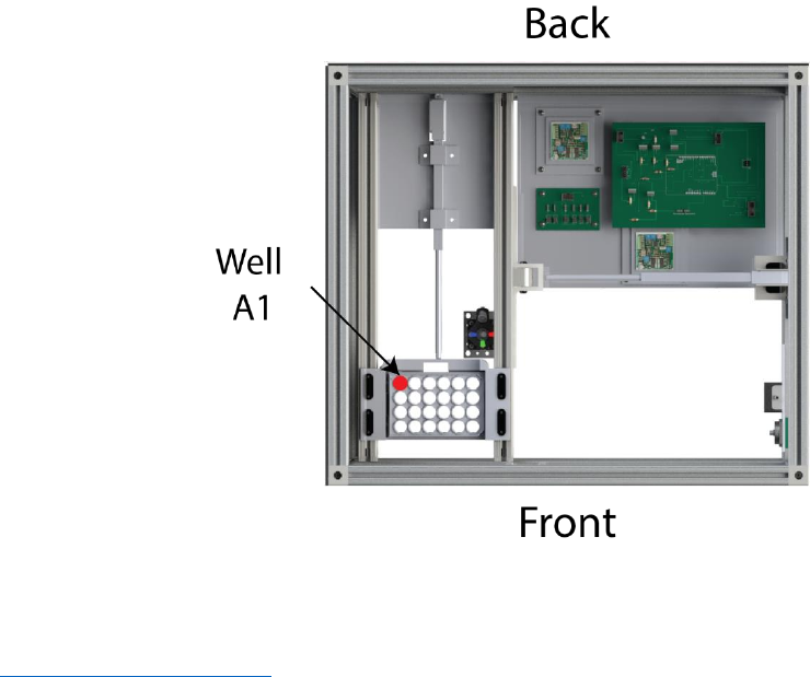
Loading a Plate
The orientation in which you load the plate is important not only for the calibration process but also for
any sort of measurement performed on the OSP device. Please refer to the below picture to ensure you
are loading the plate correctly. The plate should be held firmly in place with the attached springs.
Return to Table of Contents S7
Software Structure
The OSP software is object oriented and composed of a total of twelve class objects. The below sections
will explain the structure of the software and how information is passed between the objects.
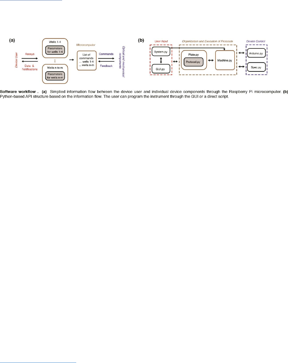
Structure Overview
The diagram below depicts the general flow of information between the 6 main software objects. The
entire structure can be divided into three separate categories based on functionality.
System.py and GUI.py are the primary classes that allow the user to interface with the plate
reader. They track and store user input. System.py is the object that contains all the vital functionality of
translating the user input into commands to change device settings. This object is responsible for loading-
in user settings (such as calibrated well coordinates and excitation led wavelengths) and for preparing the
system for execution of input protocols. The user can call this object to set-up and execute protocol
sequences from a Python script (more information about this and examples in System Level Control).
Alternatively, the user can control the device via the provided GUI (GUI.py) object. The GUI.py object (the
visual user interface) has access to all the functions and variables of the System.py object.
User input (into either the GUI.py or System.py constructs) results in the creation of a
PlateConfiguration.py object containing a list of Protocol.py objects. This combination of classes organizes
the desired sequence of protocols to be executed. The PlateConfiguration.py object contains a list of the
selected wells and a separate list of the protocols to be run. As mentioned before, the list of protocols is
a list of protocol objects (e.g. Absorbance.py is an object for an absorbance protocol and it inherits its
attributes from the Protocol.py object). Each protocol object contains all the necessary parameters
(spectrophotometer settings, excitation LED, acquisition type, etc.) for it to be executed.
The user is not limited to one PlateConfiguration.py structure. Performing separate protocols on
different sets of wells would simply require multiple PlateConfiguration.py objects to be created. For
example, to measure fluorescence from the set of wells [A1, A2, A3] using a 470nm LED and then measure
fluorescence from the set of wells [D1, D2, D3] using a 610nm LED, the system would create two
PlateConfiguration.py objects (one for each set of selected wells); the first PlateConfiguration.py object
would represent the set of wells [A1, A2, A3] and contains a single Fluorescence.py object (for the scan
with 470nm excitation), and the second PlateConfiguration.py object would represent the set of wells [D1,
D2, D3] and also contains a single Fluorescence.py object (for the scan with 610nm excitation).

Return to Table of Contents S8
Once the PlateConfiguration.py object(s) is/are created, a list of these objects is sent to the
Machine.py construct. This object is the control center of the entire software. Machine.py is responsible
for parsing through the list of PlateConfiguration.py objects and their respective Protocol.py objects. As it
parses these protocols, it sends the respective commands to the Arduino.py and Spec.py structures to
perform the necessary operations to successfully execute the inputs. In other words, Machine.py is the
object responsible for sending commands to the Arduino to tell it to move the linear actuators or to turn
on/off the LEDs or external devices (except for the detector). In addition, it extracts spectra from the
spectrophotometer and outputs the extracted data to a properly formatted Excel sheet. As a result, there
is constant bi-directional communication between the Machine.py, Arduino.py & Spec.py objects.
A more detailed description of the functions and attributes of the involved class objects are below.
Structure Guide
This section describes each Python object and the functions which are available to call from it. For syntax
details and examples of usage please refer to the System Level Control section as well as the commented
source code.
System.py
Description:
This class object’s main purpose is to track user inputs and adjust the system wide settings
accordingly. It contains all the necessary functions to add plate objects to the protocol sequence, load
calibration data, add protocols, and retrieve information about existing protocols.
Functions:
load_calibration_data() – Used to load calibrated well-position data into system.
load_settings() – Used to load the system settings from the settings file. This includes the
labeled wavelengths of the excitation LEDs.
save_settings() – Used to save system settings to the settings file.
load_well_labels() – Used to make a list of well labels when the object is made.
set_plate_type() – Creates a new plate object and sets it as either 24 or 96 well.
set_current_plate() – Used to select a plate object so that it can be edited.
get_current_plate_type() – Returns whether the current plate is 24 or 96 well.
get_plate_count() – Returns the total number of plate objects.
remove_plate_object() – Removes the plate object.
get_selected_wells() – Returns the labels of the selected wells for a specific plate object.
get_settings() – Returns a list containing the system settings.
select_wells() – Select a specified set of wells for a specific plate object.
clear_wells() – Unselect any selected wells from a specific plate object.
select_all_wells() – Select all wells for a specific plate object.
add_absorbance_protocol() – Add an absorbance protocol to a specific plate object.
add_fluorescence_protocol() – Add a fluorescence protocol to a specific plate object.
add_auxiliary_protocol() – Add an auxiliary protocol to a specific plate object.
turn_kinetic_tracking_on() – Used to mark the start of a kinetic cycle.

Return to Table of Contents S9
add_kinetic_absorbance_protocol() – Used to add an absorbance protocol to a kinetic cycle.
add_kinetic_fluorescence_protocol() – Used to add a fluorescence protocol to a kinetic cycle.
add_kinetic_auxiliary_protocol() – Used to add an auxiliary protocol to a kinetic cycle.
get_all_protocol_brief_descriptions() – Returns brief descriptions (Labels & Index) of all
protocols in a plate object.
get_all_protocol_full_description() – Returns detailed descriptions (Labels & Settings) of all
protocol in a plate object.
initialize_machine() – Opens an instance of the Machine object.
initialize_datasheet() - Creates the data output file.
start_program() – Executes the protocol sequence.
close_machine() – Closes the instance of the Machine object.
GUI.py
Description:
This object contains all the code that comes together to create the User Interface. Running this
object will bring up an instance of the GUI. For details about how to use the interface see the GUI Level
Control section. This class object has access to all the functions that are in System.py.
Functions:
move_plate_out() – Moves plate holder into position by the front door panel.
initialize_calibration() – Runs the calibration sequence
change_settings() – Used to change system settings such as excitation LED wavelengths.
update_settings() – Used to update the system settings file.
start_plate_selection() – Opens the plate selection screen of the GUI
start_well_selection() – Opens the well selection screen of the GUI
start_protocol_selection() – Opens the protocol selection menu of the GUI
load_protocol_sequence() – Loads in a saved protocol sequence from a file.
save_protocol_sequence() – Used to save the currently selected protocol sequence to a file.
add_new_plate_configuration() – Adds a new plate object and brings up well selection menu.
back_function() – Used to return to previous screen.
open_protocol() – Opens the menu for a selected protocol.
add_protocol() – Adds the protocol and its settings to the protocol sequence.
review_protocols() – Brings up the review screen of the GUI
initialize_program() – Starts the execution of the protocol sequence
reset_system() – Resets system. Clears the protocol sequence and returns to main menu.
add_items() – Function to add object to the QTreeWidget (PyQt)
get_current_item() - Function to get selected object from the QTreeWidget (PyQt)
remove_plate() – Deletes a plate object and all its protocols from the protocol sequence.
remove_protocol_selection() – Deletes a protocol object from the protocol sequence.
edit_protocol_selection() – Brings up the menu of the chosen protocol and allows editing.
update_protocol() – Sets the edits made to a protocol and updates the protocol sequence
edit_knetic_protocol_selection() – Used to edit a protocol part of a kinetic cycle
update_kinetic_protocol() - Sets into place the edits made to a protocol that is a part of a
kinetic cycle and updates the protocol sequence.
add_parent() – Function to add object to the QTreeWidget (PyQt)

Return to Table of Contents S10
add_child() – Function to add object to the QTreeWidget (PyQt)
add_subchild() – Function to add object to the QTreeWidget (PyQt)
PlateConfiguration.py
Description:
This object contains all the information about a specific plate configuration input by the user. A
plate configuration is defined as a set of wells to run specific protocols on. Each plate object contains the
following information:
(1) The plate type (24 or 96)
(2) List of protocol of objects (the protocol sequence to perform on the selected wells)
(3) List of selected wells.
(4) Overall ordering if there is more than one plate configuration input by the user.
Functions:
add_protocol() – Used to add a protocol object to the list of protocols.
get_protocol_count() – Returns the current number of protocols in the protocol list
initialize_wells() – Creates a list of well labels when the plate object is created.
get_protocol_brief_description() – Get a short description of the specified protocol.
get_protocol_full_description() – Get a detailed description of the specified protocol.
remove_protocol() – Removes a protocol from the protocol list.
get_selected_wells() – Returns the labels of the wells selected for the plate object.
get_well_status() – Returns list describing whether a well is selected or not.
clear_wells() – Used to unselect all wells.
selected_all_wells() – Used to select all wells.
select_wells() – Used to select a specified set of wells.
Protocol.py
Description:
This object is a general parent class for all possible protocols. It contains the following general
information about the selected protocol:
(1) The protocol label (Absorbance, Fluorescence, Auxiliary, or Kinetic)
(2) The plate index to which the protocol is assigned to
(3) The order number of the protocol in the protocol list of the assigned plate object.
Functions:
get_brief_description() – Returns a short description (Label & Index in protocol list) of the
protocol

Return to Table of Contents S11
Absorbance.py
Description:
This object contains all the system settings and necessary information to perform an absorbance
measurement with settings defined by the user:
(1) The exposure time.
(2) The list of steps that need be run by the machine to perform the measurement.
(3) The excel sheet layout of the measurement results.
Functions:
get_full_description() – Returns detailed description (Label & Setting Information) of protocol
get_exposure_time() – Returns exposure time of protocol
set_exposure_time() – Sets the exposure time of protocol
initialize_excel_section() – Creates the header of the protocol in the data output file.
get_dark() – Includes list of Machine.py commands to execute to perform a dark
measurement.
start() – Includes list of Machine.py commands to execute to perform an Absorbance
measurement.
Fluorescence.py
Description:
This object contains all the system settings and necessary information to perform a fluorescence
measurement with settings defined by the user:
(1) The exposure time.
(2) The list of excitation LEDs to trigger.
(3) The list of steps that need be run by the machine to perform the measurement.
(4) The excel sheet layout of the measurement results.
Functions:
get_full_description() - Returns detailed description (Label & Setting Information) of protocol
get_exposure_time() - Returns exposure time of protocol
get_led_index() – Returns a string describing which excitation LED(s) were chosen
get_wavelength() – Returns the wavelength(s) of the selected LED(s)
set_exposure_time() – Sets the exposure time of the protocol
set_excitation_source() – Sets which excitation LED(s) will be used.
initialize_excel_section() - Creates the header of the protocol in the data output file.
get_dark() – Includes list of Machine.py commands to execute to perform a dark
measurement.
start() – Includes list of Machine.py commands to execute to perform a Fluorescence
measurement.

Return to Table of Contents S12
Auxiliary.py
Description:
This object contains all the system settings and necessary information to perform a measurement
using the auxiliary port with settings defined by the user:
(1) The exposure time.
(2) The list of auxiliary ports to trigger.
(3) The list of steps that need be run by the machine to perform the measurement.
(4) The excel sheet layout of the measurement results.
Functions:
get_full_description() - Returns detailed description (Label & Setting Information) of protocol
get_duration() – Returns the duration in milliseconds
get_aux_index() – Returns which auxiliary port is being used.
set_duration() – Used to set the duration in milliseconds.
start() - Includes list of Machine.py commands to execute Auxiliary functionality.
Shake.py
Description:
This object contains all the system settings and necessary information to initialize and perform
shaking of the plate:
(1) The list of steps that need be run by the machine to perform the measurement.
Functions:
get_full_description() - Returns detailed description (Label & Setting Information) of protocol
start() - Includes list of Machine.py commands to execute Auxiliary functionality.
Kinetic.py
Description:
This object is for time-course measurements. This object represents a set of protocols which need
to be performed on each individual well. The following information is contained within this object:
(1) The order number of the object in the list of protocols of the assigned plate configuration
(2) The type of kinetic method: Interval (regular interval over specified time) or Repeat (repeated
set number of time)
(3) List of protocol of objects (the protocol sequence to perform in the Kinetic cycle)
(4) The layout of the excel sheet of the results of the kinetic cycle
Functions:
get_full_description() - Returns detailed description (Label & Setting Information) of protocol
add_protocol() - Add protocol to the Kinetic cycle.
remove_protocol() – Remove protocol from kinetic cycle.
get_protocol_count() - Returns the current number of protocols in the kinetic cycle.
get_protocol_brief_description() - Returns a short description (Label & Index in kinetic cycle) of
the selected protocol.

Return to Table of Contents S13
get_protocol_full_description() - Returns a detailed description (Label & Setting information) of
the selected protocol.
get_protocol() – Returns the selected protocol object.
initialize_excel_section_start() - Creates the header of the protocol in the data output file that
represents the start of the kinetic cycle.
initialize_excel_section_stop() - Creates the header of the protocol in the data output file that
represents the stop of the kinetic cycle.
Machine.py
Description:
This object contains all the functions to interface with the Arduino, Ocean Optics
spectrophotometer, and Excel sheet to which the resulting data is being written to. Each protocol object
contains a list of commands that the machine object needs to perform in order to execute the specific
protocol.
Functions:
Initialize_arduino() – Creates an Arduino object and begins Serial communication.
initialize_spec() – Creates a Spec object.
move_plate() – Used to move plate to specific position.
turn_led_on() – Used to turn LED on
turn_led_off() – Used to turn LED off
trigger_aux() – Used to trigger an auxiliary port.
set_exposure_time() – Used to set the exposure time of the spec.
set_scans_to_avg() – Used to set the number of scans to average on the spec.
set_boxcar_width() – Used to set the boxcar width of the spec.
calibrate() – Used to run the calibration sequence
start_program() – Used to start protocol sequence execution.
Arduino.py
Description:
This object is used to interface with the Arduino. It allows the user to write and read to and from
the Arduino’s Serial.
Functions
write() – Used to write to the Serial port of the Arduino.
read() – Used to read from the Serial port of the Arduino.
close() – Disconnects system from Arduino.

Return to Table of Contents S14
Spec.py
Description:
This object is used to interface with the Ocean Optics Spectrophotometer through their API. It
allows the user to set exposure time, boxcar width, scans to average, and to capture spectra.
Functions
For functions, see the linked Seabreeze documentation.
System Level Control
System level control of the OSP device refers to setting up and executing protocols via a manual Python
script. An example script which shows the basics of how to write a Python script to execute OSP
protocols is provided in the Python Files directory of the repository and can be opened with any text
editor. Refer to the comments in the script for details about functions and their use. The script can also
be run by typing the following lines of code in the terminal:
Windows
activate osp
cd %HOMEPROFILE%
cd “OSP\Software\Python Files”
python system_ex1.py
MAC
source activate osp
cd ~
cd “OSP/Software/Python Files”
python system_ex1.py
Return to Table of Contents S15
1
2
3
4
GUI Level Control
Running the GUI
If working from a Raspberry-Pi, the best way to initialize OSP is to use the Terminal, direct the Pi to the
‘Python Files’ directory, and run GUI.py from there. If not running on a Raspberry-Pi, simply run GUI.py
either from the Terminal (refer to the Running the User Interface steps in the Installation section).
!!! Important Note !!!: The size of the GUI has been optimized for the Raspberry-Pi Touch Screen. If you
have a high-resolution display (e.g. 4K), you may need to adjust resolution to display the GUI properly
(recommended 1280x720). Users with standard resolution displays (e.g. 1920x1080) should be fine with
their default settings and should not have to change the resolution.
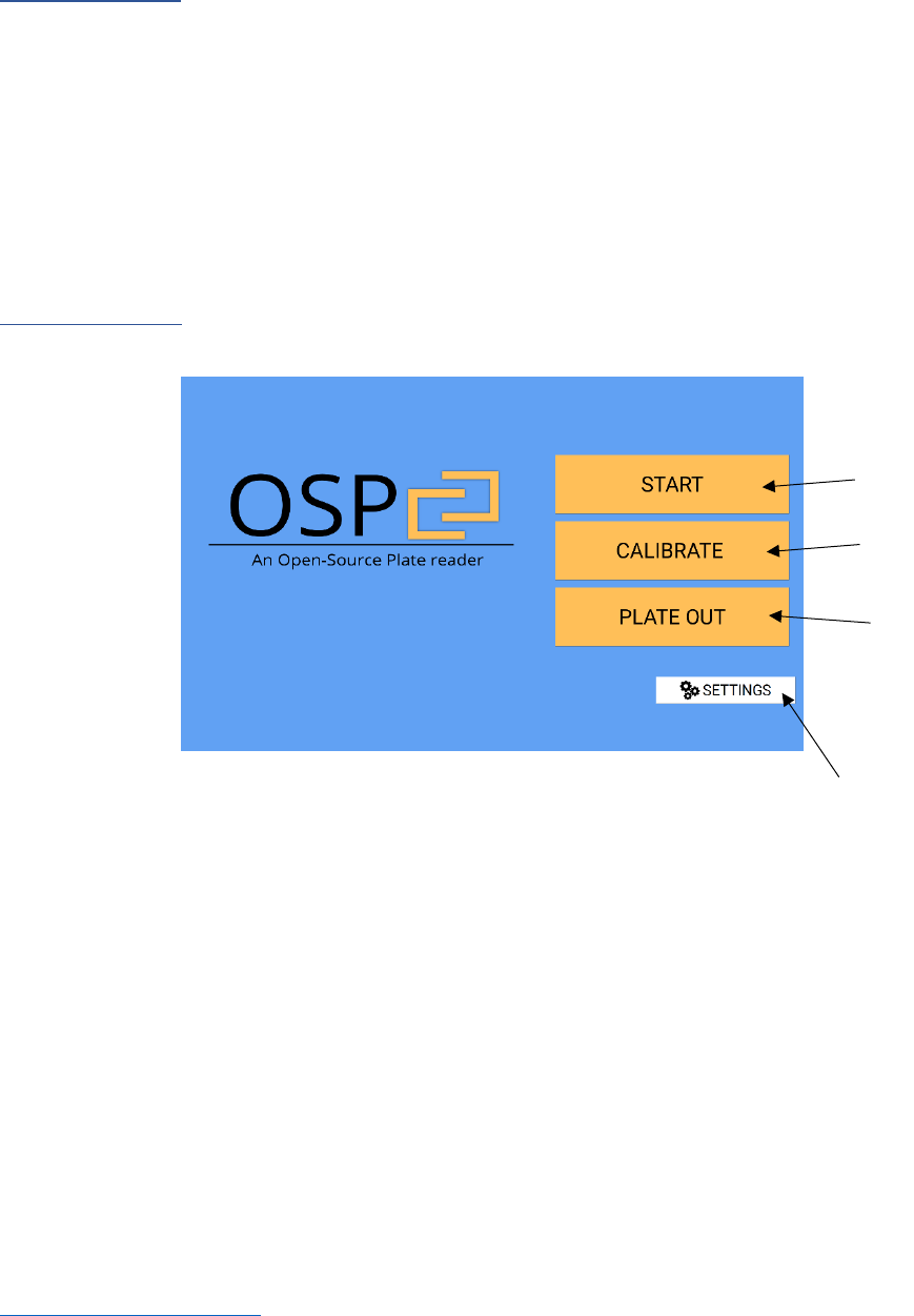
The Intro Screen
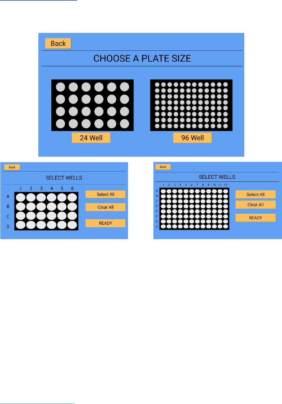
1. The START button leads to the plate selection screen, where the user can input whether they will
be using a 24-well plate or a 96-well plate for the protocol sequence.
2. The CALIBRATE button allows the user to re-calibrate the well positions in the system for either a
24-well plate or a 96-well plate. When pressed, a pop-up message shows up asking the user to
input the plate-type (24 or 96) that they wish to calibrate the positions for.
3. The PLATE OUT button allows the user to have the device move the plate holder to the edge of
the front door for plate loading and removal.
4. The SETTINGS button brings the user to the Settings Window, where they are allowed to change
specific settings of the system.
Return to Table of Contents S16
1
2
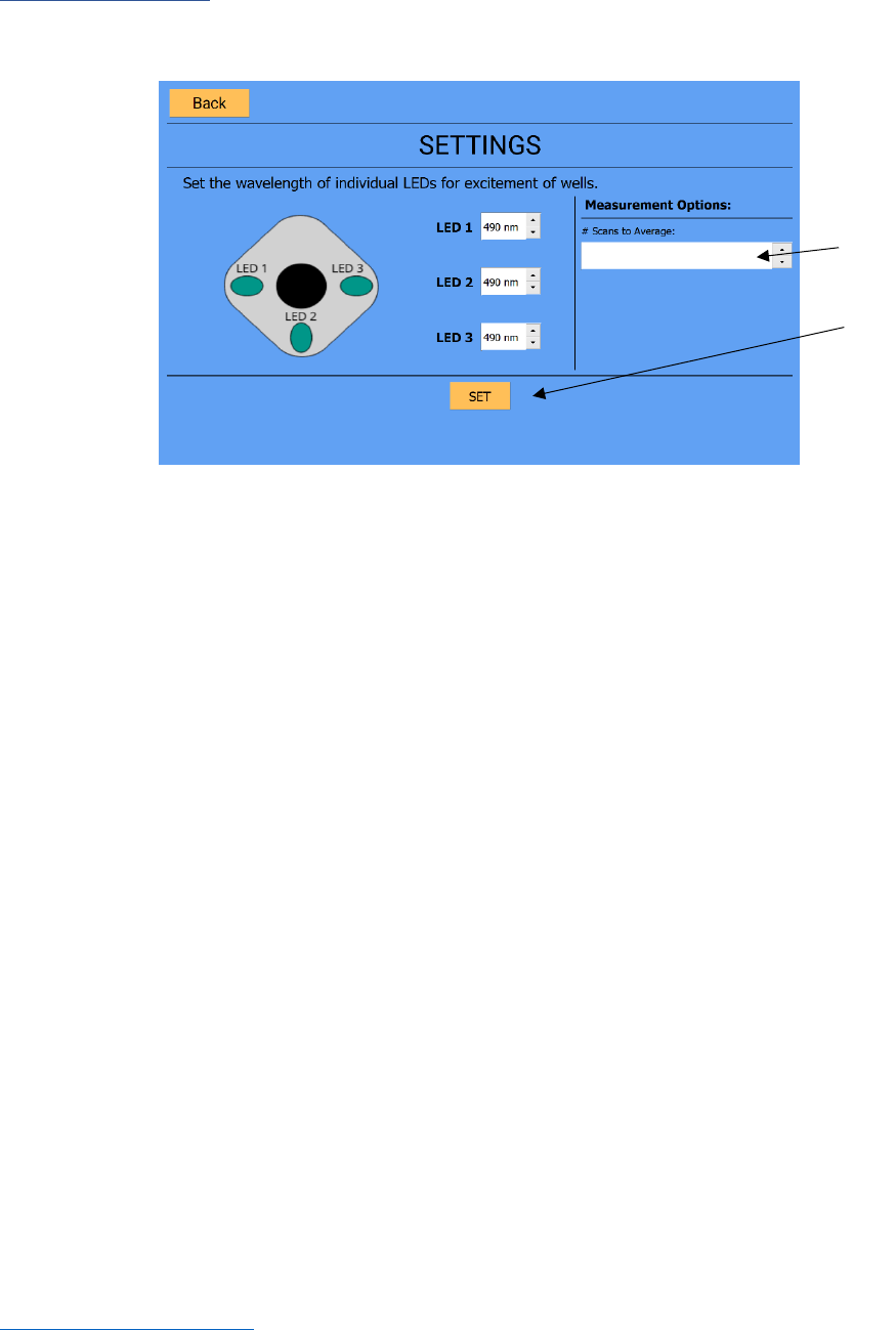
The Settings Screen
Here, the user has access to change the system settings, specifically, the LED wavelength labels and the
number of scans to average.
1. Here, the user can enter an integer to change the number of scans that the spectrophotometer
averages when performing a measurement.
2. The three LEDs correspond to the three excitation light sources. Here the user can change the
wavelengths to describe the LEDs connected to a specific LED socket position (or digital switch).
These wavelengths are then used as reference for data output.
3. Once the user clicks the SET button the displayed settings are saved to ‘…/System
Settings/savedSettings.txt’.
4. Hitting the BACK button will take the user to the home screen or the protocol selection screen
(depending on which screen was up/active before the settings were accessed).
Return to Table of Contents S17
The Plate/Well Selection
The user has the option to select which type of plate they will perform the protocol sequence on. A
protocol sequence can only be run on one type of plate. Plate selection leads the user to the well selection
window for the chosen plate type.
Click & Drag to select wells. Pressing the ‘BACK’ button will return the user to the plate selection window.
Return to Table of Contents S18
1
2
3
4
5
6
7
9
8
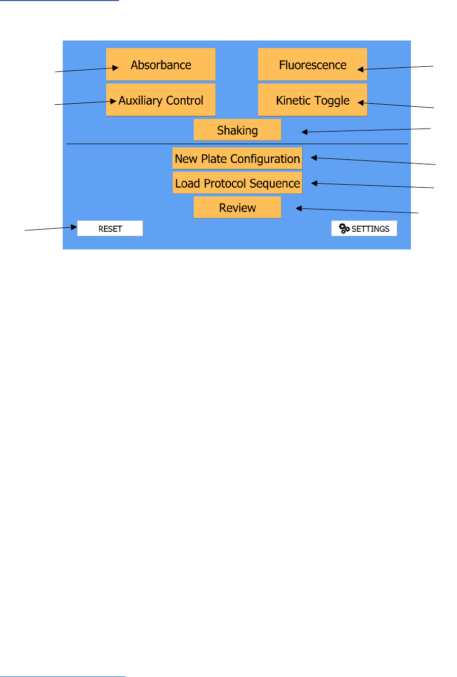
The Protocol Selection
From this screen, the user can choose to add specific protocols to their protocol sequence. Settings may
also be changed from this screen.
1. The ABSORBANCE button takes the user to the absorbance protocol settings screen. This allows
the user to set the exposure time.
2. The AUXILIARY CONTROL button takes the user to the auxiliary control settings screen. Here, the
user can choose which auxiliary port to turn on and for how long.
3. The FLUORESCENCE button takes the user to the fluorescence protocol settings screen. Here the
user chooses which excitation LED to use and sets the exposure time of the measurement.
4. The KINETIC TOGGLE switch allows the user to turn on/off a kinetic cycle (time-course).
5. The SHAKE button adds a protocol to shake the plate for 5 seconds.
6. The NEW PLATE CONFIGURATION button allows the user to create a new selection of wells for a
different protocol sequence. Going down this path creates a new PlateConfiguration.py object.
7. The LOAD PROTOCOL SEQUENCE button allows the user to load a pre-existing (custom made)
protocol sequence that has been saved to the repository. The loaded sequence will replace the
current protocol sequence.
8. The REVIEW button takes the user to the review screen where they can see the protocol sequence
resulting from their inputs, and edit any of the protocols individually or remove them.
9. The RESET button will take the user back to the main screen and clear the system of any protocols
and well selections.
Return to Table of Contents S19
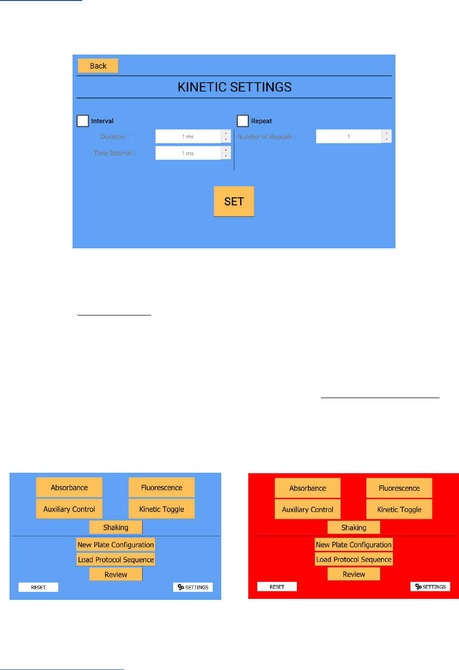
Kinetics OFF
Kinetics ON
Kinetic Toggling
“Kinetics” allows the user to iteratively perform a specific protocol for time-course measurements without
having to manually repeat the inputs. OSP allows two methods of kinetics: (1) Interval and (2) Repeat.
Note that the user can only select one method, described below:
Interval Kinetics:
This method performs a protocol or a sequence of protocols in intervals (based on the interval specified
by the user) for a specific duration (e.g. absorbance of a sample every 10 seconds for 2 minutes). The user
must ensure that the time it takes to perform the specific protocol or sequence of protocols does not
exceed the interval time.
Repeat Kinetics:
This method simply repeats a protocol or a sequence of protocols the specified number of times. Once
the SET button is pressed on the ‘Kinetic Settings’ screen, the user is taken back to the protocol selection
menu, which will then have a background that is bright red. The kinetic state is set to ON as long as the
background is red. To toggle the kinetic cycle off, press the kinetic button again and the screen will return
to its original (blue) color. The user will not be able to review the protocol or add a new plate
configuration until the kinetic cycle is turned off.
Return to Table of Contents S20
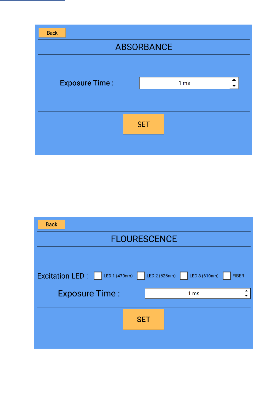
Absorbance Settings
The only tunable parameter here is exposure time. The light source for absorbance measurements by
default is the top LED light source (by default, a 430nm LED + White LED).
Fluorescence Settings
The user must specify which excitation LED to use. The wavelength of the LED is referenced from the saved
settings. The system will display a warning message if the user attempts to press the set button without
checking one LED box. Multiple LEDS can be selected.
Return to Table of Contents S21
1
2
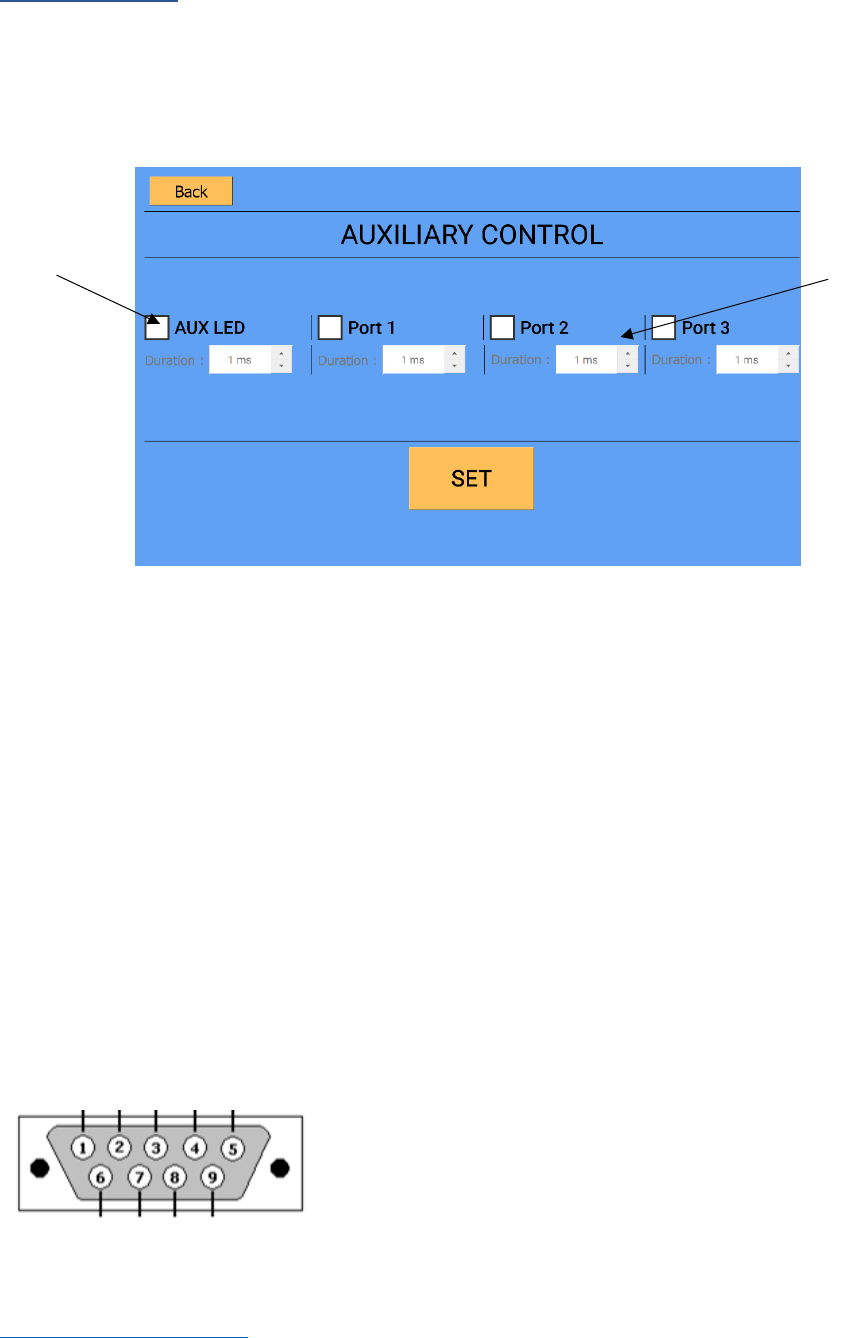
Auxiliary Settings
Here, the user can select which auxiliary port (see “Top Optical Train” Assembly) they want to turn on by
digital logic, and for what duration of time. Note that only one port can be turned on at one time. One
port is specifically for unpowered LEDs. The other three communication ports are more customizable; to
access their trigger ports, see the DB9 port pin-out diagram on the next page. By default, triggering a port
also moves the motors to position the selected well under the top auxiliary optics attachment.
1. The AUX LED PORT (LED #4) controls an extra unpowered LED of choice, and the default limiting
resistor sets the current to ~20mA (assuming a ~3V LED bias voltage). Setting the ‘duration’ sets
the amount of time this auxiliary LED is on once the well is positioned under it.
2. Any of the three generic ‘ports’ allows direct control of external electrical connections that can
be accessed through the DB9 header (see below diagram for pin-out). Each port contains two data
pins (1 IN and 1 OUT) for digital control and inputs to/from the Arduino. The user can customize
an Arduino script for automating external devices. For custom series of events where movement
under the auxiliary piece is not required, this default can be eliminated by commenting out the
movement function (machine.move_plate()) for the corresponding port number of the
Auxiliary.py script.
When accessing the auxiliary port +12V power (pin 3), the total current draw should be less than 3 amps
to ensure sufficient power for all internal components. When accessing the auxiliary port +5V power (pin
3), the total current draw should be less than 1.5 amps to prevent damage to the internal switch.
1. +5V
2. Port 2: Trigger
3. +12V
4. GND
5. Port 1: Data In
6. Port 1: Trigger
7. Port 2: Data In
8. Port 3: Trigger
9. Port 3: Data In
Return to Table of Contents S22
1
2
3
4
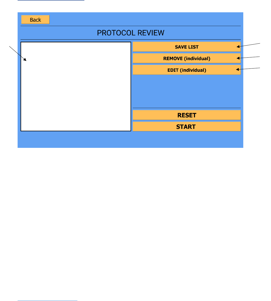
Review Protocol Sequence
1. Window displaying the selected plates & protocols in their desired order. Each selection in the
window is selectable. By highlighting one of the protocols, the user can edit/remove it.
2. The SAVE LIST button allows the user to save the current set of protocols in their order as a
‘protocol’ object. NOTE: When saving a sequence of protocols, the system saves the protocols
and all their settings in shown order, and the plate type. The loaded sequence plate type cannot
be changed unless the system is reset.
3. The REMOVE button allows the user to remove one of the protocols OR an entire plate
configuration from the protocol sequence. If a plate configuration (e.g. Plate #1) is selected, that
entire plate object and all of its assigned protocols will be deleted. NOTE: The user can only delete
one protocol or plate at a time.
4. The EDIT button allows the user to edit a single protocol or a single selection of wells. In order to
edit the selected wells, the user needs to highlight the selected wells tab.
Plate #1
Selected Wells
Protocols
Absorbance
Exposure Time: 1000 (ms)
