Solution Manual Mathematical Statistics With Applications 7th Edition Wackerly
User Manual:
Open the PDF directly: View PDF ![]() .
.
Page Count: 334 [warning: Documents this large are best viewed by clicking the View PDF Link!]

1
Chapter 1: What is Statistics?
1.1 a. Population: all generation X age US citizens (specifically, assign a ‘1’ to those who
want to start their own business and a ‘0’ to those who do not, so that the population is
the set of 1’s and 0’s). Objective: to estimate the proportion of generation X age US
citizens who want to start their own business.
b. Population: all healthy adults in the US. Objective: to estimate the true mean body
temperature
c. Population: single family dwelling units in the city. Objective: to estimate the true
mean water consumption
d. Population: all tires manufactured by the company for the specific year. Objective: to
estimate the proportion of tires with unsafe tread.
e. Population: all adult residents of the particular state. Objective: to estimate the
proportion who favor a unicameral legislature.
f. Population: times until recurrence for all people who have had a particular disease.
Objective: to estimate the true average time until recurrence.
g. Population: lifetime measurements for all resistors of this type. Objective: to estimate
the true mean lifetime (in hours).
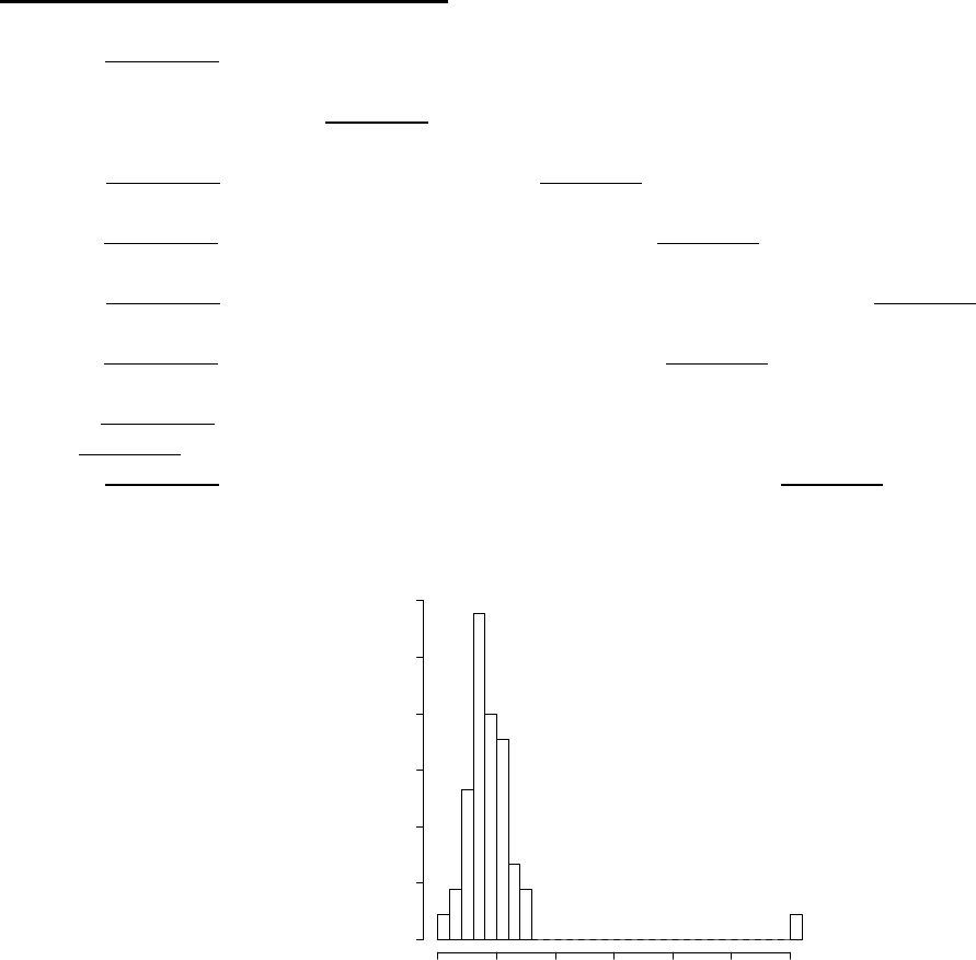
1.2 a. This histogram is above.
Histogram of wind
wind
Density
5 101520253035
0.00 0.05 0.10 0.15 0.20 0.25 0.30
b. Yes, it is quite windy there.
c. 11/45, or approx. 24.4%
d. it is not especially windy in the overall sample.
www.elsolucionario.net
2 Chapter 1: What is Statistics?
Instructor’s Solutions Manual
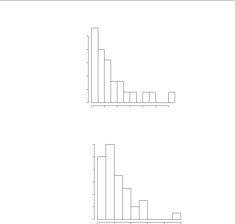
1.3 The histogram is above.
Histogram of U235
U235
Density
024681012
0.00 0.05 0.10 0.15 0.20 0.25
1.4 a. The histogram is above.
Histogram of stocks
stocks
Density
24681012
0.00 0.05 0.10 0.15 0.20 0.25 0.30
b. 18/40 = 45%
c. 29/40 = 72.5%
1.5 a. The categories with the largest grouping of students are 2.45 to 2.65 and 2.65 to 2.85.
(both have 7 students).
b. 7/30
c. 7/30 + 3/30 + 3/30 + 3/30 = 16/30
1.6 a. The modal category is 2 (quarts of milk). About 36% (9 people) of the 25 are in this
category.
b. .2 + .12 + .04 = .36
c. Note that 8% purchased 0 while 4% purchased 5. Thus, 1 – .08 – .04 = .88 purchased
between 1 and 4 quarts.
www.elsolucionario.net
Chapter 1: What is Statistics? 3
Instructor’s Solutions Manual
1.7 a. There is a possibility of bimodality in the distribution.
b. There is a dip in heights at 68 inches.
c. If all of the students are roughly the same age, the bimodality could be a result of the
men/women distributions.
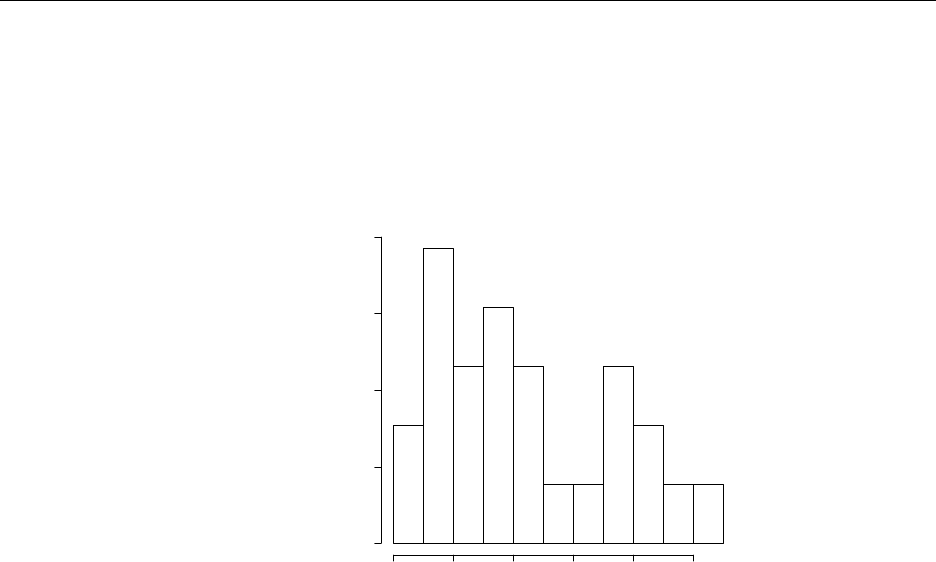
1.8 a. The histogram is above.
Histogram of AlO
AlO
Density
10 12 14 16 18 20
0.00 0.05 0.10 0.15 0.20
b. The data appears to be bimodal. Llanederyn and Caldicot have lower sample values
than the other two.
1.9 a. Note that 9.7 = 12 – 2.3 and 14.3 = 12 + 2.3. So, (9.7, 14.3) should contain
approximately 68% of the values.
b. Note that 7.4 = 12 – 2(2.3) and 16.6 = 12 + 2(2.3). So, (7.4, 16.6) should contain
approximately 95% of the values.
c. From parts (a) and (b) above, 95% - 68% = 27% lie in both (14.3. 16.6) and (7.4, 9.7).
By symmetry, 13.5% should lie in (14.3, 16.6) so that 68% + 13.5% = 81.5% are in (9.7,
16.6)
d. Since 5.1 and 18.9 represent three standard deviations away from the mean, the
proportion outside of these limits is approximately 0.
1.10 a. 14 – 17 = -3.
b. Since 68% lie within one standard deviation of the mean, 32% should lie outside. By
symmetry, 16% should lie below one standard deviation from the mean.
c. If normally distributed, approximately 16% of people would spend less than –3 hours
on the internet. Since this doesn’t make sense, the population is not normal.
1.11 a. ∑
=
n
i
c
1
= c + c + … + c = nc.
b. i
n
i
yc
∑
=1
= c(y1 + … + yn) = ∑
=
n
ii
yc
1
c.
()
∑
=
+
n
iii yx
1
= x1 + y1 + x2 + y2 + … + xn + yn = (x1 + x2 + … + xn) + (y1 + y2 + … + yn)
www.elsolucionario.net

4 Chapter 1: What is Statistics?
Instructor’s Solutions Manual
Using the above, the numerator of s2 is ∑
=
−
n
iiyy
1
2
)(=
∑
=
+−
n
iii yyyy
1
2
2)2( = ∑
=
−
n
ii
y
1
2
∑
=
+
n
iiynyy
1
2
2 Since ∑
=
=
n
ii
yyn
1
, we have ∑
=
−
n
iiyy
1
2
)( = ∑
=
−
n
iiyny
1
2
2. Let ∑
=
=
n
ii
y
n
y
1
1
to get the result.
1.12 Using the data, ∑
=
6
1ii
y = 14 and ∑
=
6
1
2
ii
y= 40. So, s2 = (40 - 142/6)/5 = 1.47. So, s = 1.21.
1.13 a. With ∑
=
45
1ii
y= 440.6 and ∑
=
45
1
2
ii
y= 5067.38, we have that
y
= 9.79 and s = 4.14.
b. k interval frequency Exp. frequency
1 5.65, 13.93 44 30.6
2 1.51, 18.07 44 42.75
3 -2.63, 22.21 44 45
1.14 a. With ∑
=
25
1ii
y= 80.63 and ∑
=
25
1
2
ii
y= 500.7459, we have that
y
= 3.23 and s = 3.17.
b.
1.15 a. With ∑
=
40
1ii
y= 175.48 and ∑
=
40
1
2
ii
y= 906.4118, we have that
y
= 4.39 and s = 1.87.
b.
1.16 a. Without the extreme value,
y
= 4.19 and s = 1.44.
b. These counts compare more favorably:
k interval frequency Exp. frequency
1 0.063, 6.397 21 17
2 -3.104, 9.564 23 23.75
3 -6.271, 12.731 25 25
k interval frequency Exp. frequency
1 2.52, 6.26 35 27.2
2 0.65, 8.13 39 38
3 -1.22, 10 39 40
k interval frequency Exp. frequency
1 2.75, 5.63 25 26.52
2 1.31, 7.07 36 37.05
3 -0.13, 8.51 39 39
www.elsolucionario.net
Chapter 1: What is Statistics? 5
Instructor’s Solutions Manual
1.17 For Ex. 1.2, range/4 = 7.35, while s = 4.14. For Ex. 1.3, range/4 = 3.04, while = s = 3.17.
For Ex. 1.4, range/4 = 2.32, while s = 1.87.
1.18 The approximation is (800–200)/4 = 150.
1.19 One standard deviation below the mean is 34 – 53 = –19. The empirical rule suggests
that 16% of all measurements should lie one standard deviation below the mean. Since
chloroform measurements cannot be negative, this population cannot be normally
distributed.
1.20 Since approximately 68% will fall between $390 ($420 – $30) to $450 ($420 + $30), the
proportion above $450 is approximately 16%.
1.21 (Similar to exercise 1.20) Having a gain of more than 20 pounds represents all
measurements greater than one standard deviation below the mean. By the empirical
rule, the proportion above this value is approximately 84%, so the manufacturer is
probably correct.
1.22 (See exercise 1.11) ∑
=
−
n
iiyy
1
)(=
∑
=
n
ii
y
1
– 0
11
=−= ∑∑ ==
n
ii
n
iiyyyn .
1.23 a. (Similar to exercise 1.20) 95 sec = 1 standard deviation above 75 sec, so this
percentage is 16% by the empirical rule.
b. (35 sec., 115 sec) represents an interval of 2 standard deviations about the mean, so
approximately 95%
c. 2 minutes = 120 sec = 2.5 standard deviations above the mean. This is unlikely.
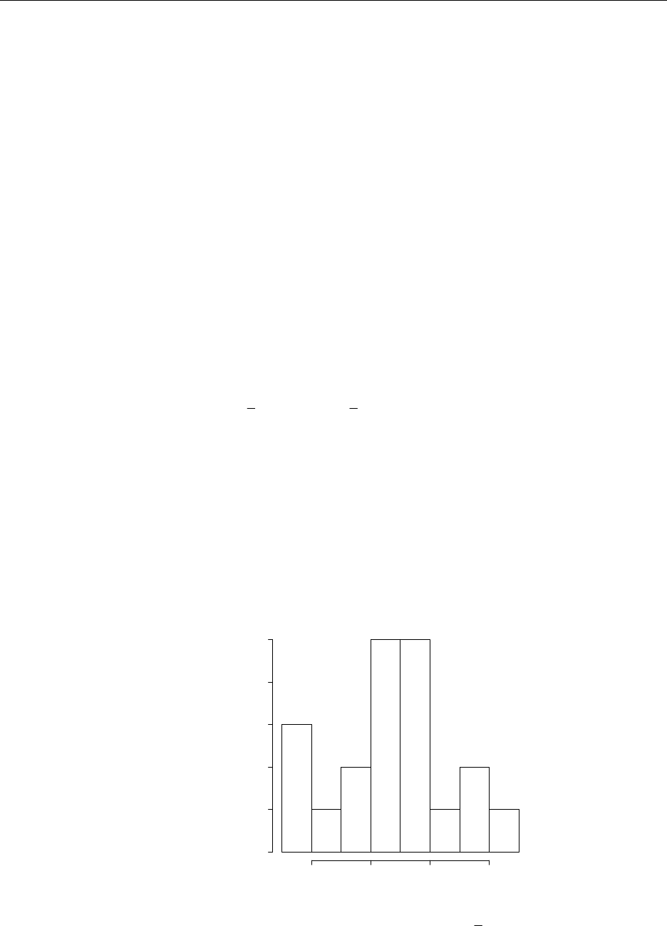
1.24 a. (112-78)/4 = 8.5
b. The histogram is above.
Histogram of hr
hr
Frequency
80 90 100 110
012345
c. With ∑
=
20
1ii
y= 1874.0 and ∑
=
20
1
2
ii
y= 117,328.0, we have that
y
= 93.7 and s = 9.55.
www.elsolucionario.net

6 Chapter 1: What is Statistics?
Instructor’s Solutions Manual
d.
1.25 a. (716-8)/4 = 177
b. The figure is omitted.
c. With ∑
=
88
1ii
y= 18,550 and ∑
=
88
1
2
ii
y= 6,198,356, we have that
y
= 210.8 and s = 162.17.
d.
1.26 For Ex. 1.12, 3/1.21 = 2.48. For Ex. 1.24, 34/9.55 = 3.56. For Ex. 1.25, 708/162.17 =
4.37. The ratio increases as the sample size increases.
1.27 (64, 80) is one standard deviation about the mean, so 68% of 340 or approx. 231 scores.
(56, 88) is two standard deviations about the mean, so 95% of 340 or 323 scores.
1.28 (Similar to 1.23) 13 mg/L is one standard deviation below the mean, so 16%.
1.29 If the empirical rule is assumed, approximately 95% of all bearing should lie in (2.98,
3.02) – this interval represents two standard deviations about the mean. So,
approximately 5% will lie outside of this interval.
1.30 If μ = 0 and σ = 1.2, we expect 34% to be between 0 and 0 + 1.2 = 1.2. Also,
approximately 95%/2 = 47.5% will lie between 0 and 2.4. So, 47.5% – 34% = 13.5%
should lie between 1.2 and 2.4.
1.31 Assuming normality, approximately 95% will lie between 40 and 80 (the standard
deviation is 10). The percent below 40 is approximately 2.5% which is relatively
unlikely.
1.32 For a sample of size n, let n′ denote the number of measurements that fall outside the
interval
y
± ks, so that (n – n′)/n is the fraction that falls inside the interval. To show this
fraction is greater than or equal to 1 – 1/k2, note that
(n – 1)s2 = ∑
∈
−
Ai iyy 2
)( +
∑
∈
−
bi iyy 2
)( , (both sums must be positive)
where
A = {i: |yi -
y
| ≥ ks} and B = {i: |yi –
y
| < ks}. We have that
∑
∈
−
Ai iyy 2
)( ≥
∑
∈Ai
sk 22 = n′k2s2, since if i is in A, |yi –
y
| ≥ ks and there are n′ elements in
A. Thus, we have that s2 ≥ k2s2n′/(n-1), or 1 ≥ k2n′/(n–1) ≥ k2n′/n. Thus, 1/k2 ≥ n′/n or
(n – n′)/n ≥ 1 – 1/k2.
k interval frequency Exp. frequency
1 84.1, 103.2 13 13.6
2 74.6, 112.8 20 19
3 65.0, 122.4 20 20
k interval frequency Exp. frequency
1 48.6, 373 63 59.84
2 -113.5, 535.1 82 83.6
3 -275.7, 697.3 87 88
www.elsolucionario.net
Chapter 1: What is Statistics? 7
Instructor’s Solutions Manual
1.33 With k =2, at least 1 – 1/4 = 75% should lie within 2 standard deviations of the mean.
The interval is (0.5, 10.5).
1.34 The point 13 is 13 – 5.5 = 7.5 units above the mean, or 7.5/2.5 = 3 standard deviations
above the mean. By Tchebysheff’s theorem, at least 1 – 1/32 = 8/9 will lie within 3
standard deviations of the mean. Thus, at most 1/9 of the values will exceed 13.
1.35 a. (172 – 108)/4 =16
b. With ∑
=
15
1ii
y= 2041 and ∑
=
15
1
2
ii
y= 281,807 we have that
y
= 136.1 and s = 17.1
c. a = 136.1 – 2(17.1) = 101.9, b = 136.1 + 2(17.1) = 170.3.
d. There are 14 observations contained in this interval, and 14/15 = 93.3%. 75% is a
lower bound.
1.36 a. The histogram is above.
0 10203040506070
ex1.36
0123456 8
b. With ∑
=
100
1ii
y= 66 and ∑
=
100
1
2
ii
y= 234 we have that
y
= 0.66 and s = 1.39.
c. Within two standard deviations: 95, within three standard deviations: 96. The
calculations agree with Tchebysheff’s theorem.
1.37 Since the lead readings must be non negative, 0 (the smallest possible value) is only 0.33
standard deviations from the mean. This indicates that the distribution is skewed.
1.38 By Tchebysheff’s theorem, at least 3/4 = 75% lie between (0, 140), at least 8/9 lie
between (0, 193), and at least 15/16 lie between (0, 246). The lower bounds are all
truncated a 0 since the measurement cannot be negative.
www.elsolucionario.net
8
Chapter 2: Probability
2.1 A = {FF}, B = {MM}, C = {MF, FM, MM}. Then, A∩B = 0/, B∩C = {MM}, BC ∩=
{MF, FM},
B
A
∪={FF,MM}, CA∪= S, CB ∪ = C.
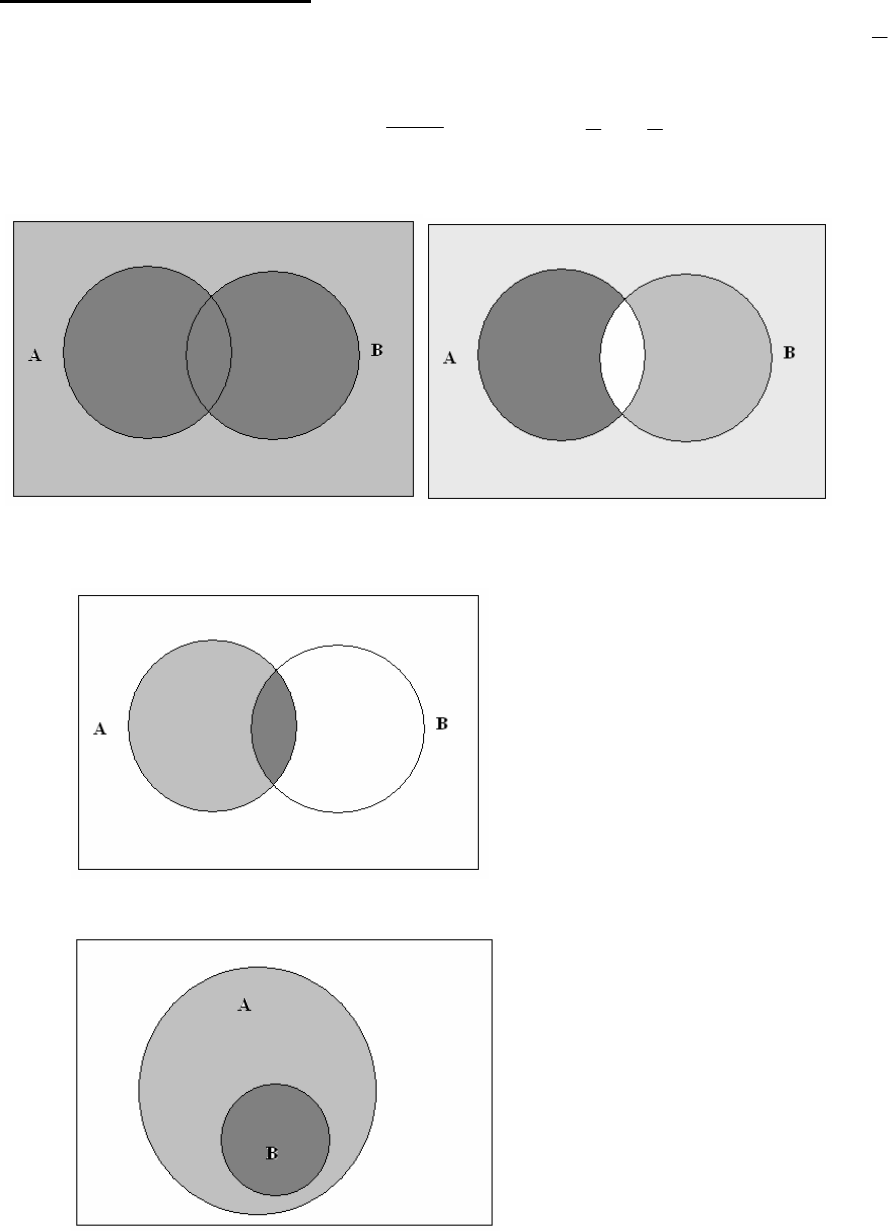
2.2 a. A∩B b.
B
A
∪ c.
B
A
∪ d. )()( BABA ∩∪∩
2.3
2.4 a.
b.
www.elsolucionario.net

Chapter 2: Probability 9
Instructor’s Solutions Manual
2.5 a. ASABBABABA =∩=∪∩=∩∪∩ )()()(.
b. AABBBABBAB =∩=∩∪∩=∩∪ )()()()(.
c. =∩∩=∩∩∩ )()()( BBABABA 0/. The result follows from part a.
d. )()( BBABAB ∩∩=∩∩ = 0/. The result follows from part b.
2.6 A = {(1,2), (2,2), (3,2), (4,2), (5,2), (6,2), (1,4), (2,4), (3,4), (4,4), (5,4), (6,4), (1,6), (2,6),
(3,6), (4,6), (5,6), (6,6)}
C= {(2,2), (2,4), (2,6), (4,2), (4,4), (4,6), (6,2), (6,4), (6,6)}
A∩B = {(2,2), (4,2), (6,2), (2,4), (4,4), (6,4), (2,6), (4,6), (6,6)}
B
A∩= {(1,2), (3,2), (5,2), (1,4), (3,4), (5,4), (1,6), (3,6), (5,6)}
B
A∪= everything but {(1,2), (1,4), (1,6), (3,2), (3,4), (3,6), (5,2), (5,4), (5,6)}
ACA =∩
2.7 A = {two males} = {M1, M2), (M1,M3), (M2,M3)}
B = {at least one female} = {(M1,W1), (M2,W1), (M3,W1), (M1,W2), (M2,W2), (M3,W2),
{W1,W2)}
B
= {no females} = A SBA
=
∪
=
∩
B
A0/ A
B
A=∩
2.8 a. 36 + 6 = 42 b. 33 c. 18
2.9 S = {A+, B+, AB+, O+, A-, B-, AB-, O-}
2.10 a. S = {A, B, AB, O}
b. P({A}) = 0.41, P({B}) = 0.10, P({AB}) = 0.04, P({O}) = 0.45.
c. P({A} or {B}) = P({A}) + P({B}) = 0.51, since the events are mutually exclusive.
2.11 a. Since P(S) = P(E1) + … + P(E5) = 1, 1 = .15 + .15 + .40 + 3P(E5). So, P(E5) = .10 and
P(E4) = .20.
b. Obviously, P(E3) + P(E4) + P(E5) = .6. Thus, they are all equal to .2
2.12 a. Let L = {left tern}, R = {right turn}, C = {continues straight}.
b. P(vehicle turns) = P(L) + P(R) = 1/3 + 1/3 = 2/3.
2.13 a. Denote the events as very likely (VL), somewhat likely (SL), unlikely (U), other (O).
b. Not equally likely: P(VL) = .24, P(SL) = .24, P(U) = .40, P(O) = .12.
c. P(at least SL) = P(SL) + P(VL) = .48.
2.14 a. P(needs glasses) = .44 + .14 = .48
b. P(needs glasses but doesn’t use them) = .14
c. P(uses glasses) = .44 + .02 = .46
2.15 a. Since the events are M.E., P(S) = P(E1) + … + P(E4) = 1. So, P(E2) = 1 – .01 – .09 –
.81 = .09.
b. P(at least one hit) = P(E1) + P(E2) + P(E3) = .19.
www.elsolucionario.net

10 Chapter 2: Probability
Instructor’s Solutions Manual
2.16 a. 1/3 b. 1/3 + 1/15 = 6/15 c. 1/3 + 1/16 = 19/48 d. 49/240
2.17 Let B = bushing defect, SH = shaft defect.
a. P(B) = .06 + .02 = .08
b. P(B or SH) = .06 + .08 + .02 = .16
c. P(exactly one defect) = .06 + .08 = .14
d. P(neither defect) = 1 – P(B or SH) = 1 – .16 = .84
2.18 a. S = {HH, TH, HT, TT}
b. if the coin is fair, all events have probability .25.
c. A = {HT, TH}, B = {HT, TH, HH}
d. P(A) = .5, P(B) = .75, P(
B
A
∩
) = P(A) = .5, P(
B
A∪) = P(B) = .75, P(
B
A∪) = 1.
2.19 a. (V1, V1), (V1, V2), (V1, V3), (V2, V1), (V2, V2), (V2, V3), (V3, V1), (V3, V2), (V3, V3)
b. if equally likely, all have probability of 1/9.
c. A = {same vendor gets both} = {(V1, V1), (V2, V2), (V3, V3)}
B = {at least one V2} = {(V1, V2), (V2, V1), (V2, V2), (V2, V3), (V3, V2)}
So, P(A) = 1/3, P(B) = 5/9, P(
B
A∪) = 7/9, P(
B
A
∩
) = 1/9.
2.20 a. P(G) = P(D1) = P(D2) = 1/3.
b. i. The probability of selecting the good prize is 1/3.
ii. She will get the other dud.
iii. She will get the good prize.
iv. Her probability of winning is now 2/3.
v. The best strategy is to switch.
2.21 P(A) = P( )()( BABA ∩∪∩ ) = P)( BA
∩
+ P)( BA∩ since these are M.E. by Ex. 2.5.
2.22 P(A) = P( )( BAB ∩∪ ) = P(B) + P)( BA∩ since these are M.E. by Ex. 2.5.
2.23 All elements in B are in A, so that when B occurs, A must also occur. However, it is
possible for A to occur and B not to occur.
2.24 From the relation in Ex. 2.22, P)( BA∩ ≥ 0, so P(B) ≤ P(A).
2.25 Unless exactly 1/2 of all cars in the lot are Volkswagens, the claim is not true.
2.26 a. Let N1, N2 denote the empty cans and W1, W2 denote the cans filled with water. Thus,
S = {N1N2, N1W2, N2W2, N1W1, N2W1, W1W2}
b. If this a merely a guess, the events are equally likely. So, P(W1W2) = 1/6.
2.27 a. S = {CC, CR, CL, RC, RR, RL, LC, LR, LL}
b. 5/9
c. 5/9
www.elsolucionario.net

Chapter 2: Probability 11
Instructor’s Solutions Manual
2.28 a. Denote the four candidates as A1, A2, A3, and M. Since order is not important, the
outcomes are {A1A2, A1A3, A1M, A2A3, A2M, A3M}.
b. assuming equally likely outcomes, all have probability 1/6.
c. P(minority hired) = P(A1M) + P(A2M) + P(A3M) = .5
2.29 a. The experiment consists of randomly selecting two jurors from a group of two women
and four men.
b. Denoting the women as w1, w2 and the men as m1, m2, m3, m4, the sample space is
w1,m1 w2,m1 m1,m2 m2,m3 m3,m4
w1,m2 w2,m2 m1,m3 m2,m4
w1,m3 w2,m3 m1,m4
w1,m4 w2,m4 w1,w2
c. P(w1,w2) = 1/15
2.30 a. Let w1 denote the first wine, w2 the second, and w3 the third. Each sample point is an
ordered triple indicating the ranking.
b. triples: (w1,w2,w3), (w1,w3,w2), (w2,w1,w3), (w2,w3,w1), (w3,w1,w2), (w3,w2,w1)
c. For each wine, there are 4 ordered triples where it is not last. So, the probability is 2/3.
2.31 a. There are four “good” systems and two “defactive” systems. If two out of the six
systems are chosen randomly, there are 15 possible unique pairs. Denoting the systems
as g1, g2, g3, g4, d1, d2, the sample space is given by S = {g1g2, g1g3, g1g4, g1d1,
g1d2, g2g3, g2g4, g2d1, g2d2, g3g4, g3d1, g3d2, g4g1, g4d1, d1d2}. Thus:
P(at least one defective) = 9/15 P(both defective) = P(d1d2) = 1/15
b. If four are defective, P(at least one defective) = 14/15. P(both defective) = 6/15.
2.32 a. Let “1” represent a customer seeking style 1, and “2” represent a customer seeking
style 2. The sample space consists of the following 16 four-tuples:
1111, 1112, 1121, 1211, 2111, 1122, 1212, 2112, 1221, 2121,
2211, 2221, 2212, 2122, 1222, 2222
b. If the styles are equally in demand, the ordering should be equally likely. So, the
probability is 1/16.
c. P(A) = P(1111) + P(2222) = 2/16.
2.33 a. Define the events: G = family income is greater than $43,318, N otherwise. The
points are E1: GGGG E2: GGGN E3: GGNG E4: GNGG
E5: NGGG E6: GGNN E7: GNGN E8: NGGN
E9: GNNG E10: NGNG E11: NNGG E12: GNNN
E13: NGNN E14: NNGN E15: NNNG E16: NNNN
b. A = {E1, E2, …, E11} B = {E6, E7, …, E11} C = {E2, E3, E4, E5}
c. If P(E) = P(N) = .5, each element in the sample space has probability 1/16. Thus,
P(A) = 11/16, P(B) = 6/16, and P(C) = 4/16.
www.elsolucionario.net

12 Chapter 2: Probability
Instructor’s Solutions Manual
2.34 a. Three patients enter the hospital and randomly choose stations 1, 2, or 3 for service.
Then, the sample space S contains the following 27 three-tuples:
111, 112, 113, 121, 122, 123, 131, 132, 133, 211, 212, 213, 221, 222, 223,
231, 232, 233, 311, 312, 313, 321, 322, 323, 331, 332, 333
b. A = {123, 132, 213, 231, 312, 321}
c. If the stations are selected at random, each sample point is equally likely. P(A) = 6/27.
2.35 The total number of flights is 6(7) = 42.
2.36 There are 3! = 6 orderings.
2.37 a. There are 6! = 720 possible itineraries.
b. In the 720 orderings, exactly 360 have Denver before San Francisco and 360 have San
Francisco before Denver. So, the probability is .5.
2.38 By the mn rule, 4(3)(4)(5) = 240.
2.39 a. By the mn rule, there are 6(6) = 36 possible roles.
b. Define the event A = {(1,6), (2,5), (3,4), (4,3), (5,2), (6,1)}. Then, P(A) = 6/36.
2.40 a. By the mn rule, the dealer must stock 5(4)(2) = 40 autos.
b. To have each of these in every one of the eight colors, he must stock 8*40 = 320
autos.
2.41 If the first digit cannot be zero, there are 9 possible values. For the remaining six, there
are 10 possible values. Thus, the total number is 9(10)(10)(10)(10)(10)(10) = 9*106.
2.42 There are three different positions to fill using ten engineers. Then, there are 10
3
P= 10!/3!
= 720 different ways to fill the positions.
2.43 ⎟
⎟
⎠
⎞
⎜
⎜
⎝
⎛
⎟
⎟
⎠
⎞
⎜
⎜
⎝
⎛
⎟
⎟
⎠
⎞
⎜
⎜
⎝
⎛
1
1
5
6
3
9 = 504 ways.
2.44 a. The number of ways the taxi needing repair can be sent to airport C is ⎟
⎟
⎠
⎞
⎜
⎜
⎝
⎛
⎟
⎟
⎠
⎞
⎜
⎜
⎝
⎛
5
5
5
8 = 56.
So, the probability is 56/504 = 1/9.
b. ⎟
⎟
⎠
⎞
⎜
⎜
⎝
⎛
⎟
⎟
⎠
⎞
⎜
⎜
⎝
⎛
4
4
2
6
3 = 45, so the probability that every airport receives one of the taxis requiring
repair is 45/504.
2.45 ⎟
⎟
⎠
⎞
⎜
⎜
⎝
⎛
1072
17 = 408,408.
www.elsolucionario.net

Chapter 2: Probability 13
Instructor’s Solutions Manual
2.46 There are ⎟
⎟
⎠
⎞
⎜
⎜
⎝
⎛
2
10 ways to chose two teams for the first game, ⎟
⎟
⎠
⎞
⎜
⎜
⎝
⎛
2
8 for second, etc. So,
there are 5
2
!10
2
2
2
4
2
6
2
8
2
10 =
⎟
⎟
⎠
⎞
⎜
⎜
⎝
⎛
⎟
⎟
⎠
⎞
⎜
⎜
⎝
⎛
⎟
⎟
⎠
⎞
⎜
⎜
⎝
⎛
⎟
⎟
⎠
⎞
⎜
⎜
⎝
⎛
⎟
⎟
⎠
⎞
⎜
⎜
⎝
⎛ = 113,400 ways to assign the ten teams to five games.
2.47 There are ⎟
⎟
⎠
⎞
⎜
⎜
⎝
⎛
2
2n ways to chose two teams for the first game, ⎟
⎟
⎠
⎞
⎜
⎜
⎝
⎛−
2
22n for second, etc. So,
following Ex. 2.46, there are n
n
2
!2 ways to assign 2n teams to n games.
2.48 Same answer: ⎟
⎟
⎠
⎞
⎜
⎜
⎝
⎛
5
8 = ⎟
⎟
⎠
⎞
⎜
⎜
⎝
⎛
3
8 = 56.
2.49 a. ⎟
⎟
⎠
⎞
⎜
⎜
⎝
⎛
2
130 = 8385.
b. There are 26*26 = 676 two-letter codes and 26(26)(26) = 17,576 three-letter codes.
Thus, 18,252 total major codes.
c. 8385 + 130 = 8515 required.
d. Yes.
2.50 Two numbers, 4 and 6, are possible for each of the three digits. So, there are 2(2)(2) = 8
potential winning three-digit numbers.
2.51 There are ⎟
⎟
⎠
⎞
⎜
⎜
⎝
⎛
3
50 = 19,600 ways to choose the 3 winners. Each of these is equally likely.
a. There are ⎟
⎟
⎠
⎞
⎜
⎜
⎝
⎛
3
4 = 4 ways for the organizers to win all of the prizes. The probability is
4/19600.
b. There are ⎟
⎟
⎠
⎞
⎜
⎜
⎝
⎛
⎟
⎟
⎠
⎞
⎜
⎜
⎝
⎛
1
46
2
4 = 276 ways the organizers can win two prizes and one of the other
46 people to win the third prize. So, the probability is 276/19600.
c. ⎟
⎟
⎠
⎞
⎜
⎜
⎝
⎛
⎟
⎟
⎠
⎞
⎜
⎜
⎝
⎛
2
46
1
4 = 4140. The probability is 4140/19600.
d. ⎟
⎟
⎠
⎞
⎜
⎜
⎝
⎛
3
46 = 15,180. The probability is 15180/19600.
2.52 The mn rule is used. The total number of experiments is 3(3)(2) = 18.
www.elsolucionario.net

14 Chapter 2: Probability
Instructor’s Solutions Manual
2.53 a. In choosing three of the five firms, order is important. So 5
3
P= 60 sample points.
b. If F3 is awarded a contract, there are 4
2
P = 12 ways the other contracts can be assigned.
Since there are 3 possible contracts, there are 3(12) = 36 total number of ways to award
F3 a contract. So, the probability is 36/60 = 0.6.
2.54 There are ⎟
⎟
⎠
⎞
⎜
⎜
⎝
⎛
4
8 = 70 ways to chose four students from eight. There are ⎟
⎟
⎠
⎞
⎜
⎜
⎝
⎛
⎟
⎟
⎠
⎞
⎜
⎜
⎝
⎛
2
5
2
3 = 30 ways
to chose exactly 2 (of the 3) undergraduates and 2 (of the 5) graduates. If each sample
point is equally likely, the probability is 30/70 = 0.7.
2.55 a. ⎟
⎟
⎠
⎞
⎜
⎜
⎝
⎛
10
90 b. ⎟
⎟
⎠
⎞
⎜
⎜
⎝
⎛
⎟
⎟
⎠
⎞
⎜
⎜
⎝
⎛
⎟
⎟
⎠
⎞
⎜
⎜
⎝
⎛
10
90
6
70
4
20 = 0.111
2.56 The student can solve all of the problems if the teacher selects 5 of the 6 problems that
the student can do. The probability is ⎟
⎟
⎠
⎞
⎜
⎜
⎝
⎛
⎟
⎟
⎠
⎞
⎜
⎜
⎝
⎛
5
10
5
6 = 0.0238.
2.57 There are ⎟
⎟
⎠
⎞
⎜
⎜
⎝
⎛
2
52 = 1326 ways to draw two cards from the deck. The probability is
4*12/1326 = 0.0362.
2.58 There are ⎟
⎟
⎠
⎞
⎜
⎜
⎝
⎛
5
52 = 2,598,960 ways to draw five cards from the deck.
a. There are ⎟
⎟
⎠
⎞
⎜
⎜
⎝
⎛
⎟
⎟
⎠
⎞
⎜
⎜
⎝
⎛
2
4
3
4 = 24 ways to draw three Aces and two Kings. So, the probability is
24/2598960.
b. There are 13(12) = 156 types of “full house” hands. From part a. above there are 24
different ways each type of full house hand can be made. So, the probability is
156*24/2598960 = 0.00144.
2.59 There are ⎟
⎟
⎠
⎞
⎜
⎜
⎝
⎛
5
52 = 2,598,960 ways to draw five cards from the deck.
a. ⎟
⎟
⎠
⎞
⎜
⎜
⎝
⎛
⎟
⎟
⎠
⎞
⎜
⎜
⎝
⎛
⎟
⎟
⎠
⎞
⎜
⎜
⎝
⎛
⎟
⎟
⎠
⎞
⎜
⎜
⎝
⎛
⎟
⎟
⎠
⎞
⎜
⎜
⎝
⎛
1
4
1
4
1
4
1
4
1
4 = 45 = 1024. So, the probability is 1024/2598960 = 0.000394.
b. There are 9 different types of “straight” hands. So, the probability is 9(45)/2598960 =
0.00355. Note that this also includes “straight flush” and “royal straight flush” hands.
2.60 a. n
n
365
)1365()363)(364(365 +− b. With n = 23, 23
365
)343()364(365
1
−= 0.507.
www.elsolucionario.net

Chapter 2: Probability 15
Instructor’s Solutions Manual
2.61 a. n
n
n365
364
365
)364()364)(364(364 =
. b. With n = 253,
253
365
364
1⎟
⎠
⎞
⎜
⎝
⎛
− = 0.5005.
2.62 The number of ways to divide the 9 motors into 3 groups of size 3 is ⎟
⎟
⎠
⎞
⎜
⎜
⎝
⎛
!3!3!3
!9 = 1680. If
both motors from a particular supplier are assigned to the first line, there are only 7
motors to be assigned: one to line 1 and three to lines 2 and 3. This can be done ⎟
⎟
⎠
⎞
⎜
⎜
⎝
⎛
!3!3!1
!7
= 140 ways. Thus, 140/1680 = 0.0833.
2.63 There are ⎟
⎟
⎠
⎞
⎜
⎜
⎝
⎛
5
8 = 56 sample points in the experiment, and only one of which results in
choosing five women. So, the probability is 1/56.
2.64
6
6
1
!6 ⎟
⎠
⎞
⎜
⎝
⎛ = 5/324.
2.65
46
6
1
6
2
!5 ⎟
⎠
⎞
⎜
⎝
⎛
⎟
⎠
⎞
⎜
⎝
⎛= 5/162.
2.66 a. After assigning an ethnic group member to each type of job, there are 16 laborers
remaining for the other jobs. Let na be the number of ways that one ethnic group can be
assigned to each type of job. Then:
⎟
⎟
⎠
⎞
⎜
⎜
⎝
⎛
⎟
⎟
⎠
⎞
⎜
⎜
⎝
⎛
=4435
16
1111
4
a
n. The probability is na/N = 0.1238.
b. It doesn’t matter how the ethnic group members are assigned to jobs type 1, 2, and 3.
Let na be the number of ways that no ethnic member gets assigned to a type 4 job. Then:
⎟
⎟
⎠
⎞
⎜
⎜
⎝
⎛
⎟
⎟
⎠
⎞
⎜
⎜
⎝
⎛
=5
16
0
4
a
n. The probability is ⎟
⎟
⎠
⎞
⎜
⎜
⎝
⎛
⎟
⎟
⎠
⎞
⎜
⎜
⎝
⎛
⎟
⎟
⎠
⎞
⎜
⎜
⎝
⎛
5
20
5
16
0
4 = 0.2817.
2.67 As shown in Example 2.13, N = 107.
a. Let A be the event that all orders go to different vendors. Then, A contains na =
10(9)(8)…(4) = 604,800 sample points. Thus, P(A) = 604,800/107 = 0.0605.
b. The 2 orders assigned to Distributor I can be chosen from the 7 in ⎟
⎟
⎠
⎞
⎜
⎜
⎝
⎛
2
7 = 21 ways.
The 3 orders assigned to Distributor II can be chosen from the remaining 5 in ⎟
⎟
⎠
⎞
⎜
⎜
⎝
⎛
3
5 =
10 ways. The final 2 orders can be assigned to the remaining 8 distributors in 82
ways. Thus, there are 21(10)(82) = 13,440 possibilities so the probability is
13440/107 = 0.001344.
www.elsolucionario.net

16 Chapter 2: Probability
Instructor’s Solutions Manual
c. Let A be the event that Distributors I, II, and III get exactly 2, 3, and 1 order(s)
respectively. Then, there is one remaining unassigned order. Thus, A contains
7
1
2
3
5
2
7⎟
⎟
⎠
⎞
⎜
⎜
⎝
⎛
⎟
⎟
⎠
⎞
⎜
⎜
⎝
⎛
⎟
⎟
⎠
⎞
⎜
⎜
⎝
⎛ = 2940 sample points and P(A) = 2940/107 = 0.00029.
2.68 a. ⎟
⎟
⎠
⎞
⎜
⎜
⎝
⎛
n
n = )!(!
!
nnn
n
− = 1. There is only one way to choose all of the items.
b. ⎟
⎟
⎠
⎞
⎜
⎜
⎝
⎛
0
n = )!0(!0
!
−n
n = 1. There is only one way to chose none of the items.
c. ⎟
⎟
⎠
⎞
⎜
⎜
⎝
⎛
r
n = )!(!
!
rnr
n
− = ))!(()!(
!
rnnrn
n
−−− = ⎟
⎟
⎠
⎞
⎜
⎜
⎝
⎛
−rn
n. There are the same number of
ways to choose r out of n objects as there are to choose n – r out of n objects.
d. ∑∑ =
−
=⎟
⎟
⎠
⎞
⎜
⎜
⎝
⎛
=
⎟
⎟
⎠
⎞
⎜
⎜
⎝
⎛
=+= n
i
iin
n
i
nn
i
n
i
n
11
11)11(2.
2.69 )!1(!
)!1(
)!1(!
!
)!1(!
)1(!
)!1()!1(
!
)!(!
!
1knk
n
knk
kn
knk
knn
knk
n
knk
n
k
n
k
n
−+
+
=
+−
+
+−
+−
=
+−−
+
−
=
⎟
⎟
⎠
⎞
⎜
⎜
⎝
⎛
−
+
⎟
⎟
⎠
⎞
⎜
⎜
⎝
⎛
2.70 From Theorem 2.3, let y1 = y2 = … = yk = 1.
2.71 a. P(A|B) = .1/.3 = 1/3. b. P(B|A) = .1/.5 = 1/5.
c. P(A|
B
A∪) = .5/(.5+.3-.1) = 5/7 d. P(A|A∩B) = 1, since A has occurred.
e. P(A∩B|
B
A∪) = .1(.5+.3-.1) = 1/7.
2.72 Note that P(A) = 0.6 and P(A|M) = .24/.4 = 0.6. So, A and M are independent. Similarly,
P(FA | ) = .24/.6 = 0.4 = P(A), so A and F are independent.
2.73 a. P(at least one R) = P(Red) 3/4. b. P(at least one r) = 3/4.
c. P(one r | Red) = .5/.75 = 2/3.
2.74 a. P(A) = 0.61, P(D) = .30. P(A∩D) = .20. Dependent.
b. P(B) = 0.30, P(D) = .30. P(B∩D) = 0.09. Independent.
c. P(C) = 0.09, P(D) = .30. P(C∩D) = 0.01. Dependent.
www.elsolucionario.net

Chapter 2: Probability 17
Instructor’s Solutions Manual
2.75 a. Given the first two cards drawn are spades, there are 11 spades left in the deck. Thus,
the probability is
⎟
⎟
⎠
⎞
⎜
⎜
⎝
⎛
⎟
⎟
⎠
⎞
⎜
⎜
⎝
⎛
3
50
3
11
= 0.0084. Note: this is also equal to P(S3S4S5|S1S2).
b. Given the first three cards drawn are spades, there are 10 spades left in the deck. Thus,
the probability is
⎟
⎟
⎠
⎞
⎜
⎜
⎝
⎛
⎟
⎟
⎠
⎞
⎜
⎜
⎝
⎛
2
49
2
10
= 0.0383. Note: this is also equal to P(S4S5|S1S2S3).
c. Given the first four cards drawn are spades, there are 9 spades left in the deck. Thus,
the probability is
⎟
⎟
⎠
⎞
⎜
⎜
⎝
⎛
⎟
⎟
⎠
⎞
⎜
⎜
⎝
⎛
1
48
1
9
= 0.1875. Note: this is also equal to P(S5|S1S2S3S4)
2.76 Define the events: U: job is unsatisfactory A: plumber A does the job
a. P(U|A) = P(A∩U)/P(A) = P(A|U)P(U)/P(A) = .5*.1/.4 = 0.125
b. From part a. above, 1 – P(U|A) = 0.875.
2.77 a. 0.40 b. 0.37 c. 0.10 d. 0.40 + 0.37 – 0.10 = 0.67
e. 1 – 0.4 = 0.6 f. 1 – 0.67 = 0.33 g. 1 – 0.10 = 0.90
h. .1/.37 = 0.27 i. 1/.4 = 0.25
2.78 1. Assume P(A|B) = P(A). Then:
P(A∩B) = P(A|B)P(B) = P(A)P(B). P(B|A) = P(B∩A)/P(A) = P(A)P(B)/P(A) = P(B).
2. Assume P(B|A) = P(B). Then:
P(A∩B) = P(B|A)P(A) = P(B)P(A). P(A|B) = P(A∩B)/P(B) = P(A)P(B)/P(B) = P(A).
3. Assume P(A∩B) = P(B)P(A). The results follow from above.
2.79 If A and B are M.E., P(A∩B) = 0. But, P(A)P(B) > 0. So they are not independent.
2.80 If
B
A⊂, P(A∩B) = P(A) ≠ P(A)P(B), unless B = S (in which case P(B) = 1).
2.81 Given P(A) < P(A|B) = P(A∩B)/P(B) = P(B|A)P(A)/P(B), solve for P(B|A) in the
inequality.
2.82 P(B|A) = P(B∩A)/P(A) = P(A)/P(A) = 1
P(A|B) = P(A∩B)/P(B) = P(A)/P(B).
www.elsolucionario.net

18 Chapter 2: Probability
Instructor’s Solutions Manual
2.83 P(ABA∪|) = P(A)/P(
B
A∪) = )()(
)(
BPAP
AP
+, since A and B are M.E. events.
2.84 Note that if P(32 AA ∩) = 0, then P(321 AAA
∩
∩
) also equals 0. The result follows from
Theorem 2.6.
2.85 P( )| BA = P(
B
A∩)/P(
B
) =
[
][]
)(
)()(1
)(
)()|(1
)(
)()|(
BP
APBP
BP
APABP
BP
APABP −
=
−
==
).(
)(
)()( AP
BP
APBP = So, BA and are independent.
P()| AB = P( )AB ∩/P(A) =
[
]
)(
)()|(1
)(
)()|(
AP
BPBAP
AP
BPBAP −
=. From the above,
BA and are independent. So P( )| AB =
[
]
).(
)(
)()(
)(
)()(1 BP
AP
BPAP
AP
BPAP ==
− So,
BA and are independent
2.86 a. No. It follows from P()BA∪ = P(A) + P(B) – P(A∩B) ≤ 1.
b. P(A∩B) ≥ 0.5
c. No.
d. P(A∩B) ≤ 0.70.
2.87 a. P(A) + P(B) – 1.
b. the smaller of P(A) and P(B).
2.88 a. Yes.
b. 0, since they could be disjoint.
c. No, since P(A∩B) cannot be larger than either of P(A) or P(B).
d. 0.3 = P(A).
2.89 a. 0, since they could be disjoint.
b. the smaller of P(A) and P(B).
2.90 a. (1/50)(1/50) = 0.0004.
b. P(at least one injury) = 1 – P(no injuries in 50 jumps) = 1 = (49/50)50 = 0.636. Your
friend is not correct.
2.91 If A and B are M.E., P()BA∪ = P(A) + P(B). This value is greater than 1 if P(A) = 0.4
and P(B) = 0.7. So they cannot be M.E. It is possible if P(A) = 0.4 and P(B) = 0.3.
2.92 a. The three tests are independent. So, the probability in question is (.05)3 = 0.000125.
b. P(at least one mistake) = 1 – P(no mistakes) = 1 – (.95)3 = 0.143.
www.elsolucionario.net

Chapter 2: Probability 19
Instructor’s Solutions Manual
2.93 Let H denote a hit and let M denote a miss. Then, she wins the game in three trials with
the events HHH, HHM, and MHH. If she begins with her right hand, the probability she
wins the game, assuming independence, is (.7)(.4)(.7) + (.7)(.4)(.3) + (.3)(.4)(.7) = 0.364.
2.94 Define the events A: device A detects smoke B: device B detects smoke
a. P()BA∪ = .95 + .90 - .88 = 0.97.
b. P(smoke is undetected) = 1 - P()BA∪ = 1 – 0.97 = 0.03.
2.95 Part a is found using the Addition Rule. Parts b and c use DeMorgan’s Laws.
a. 0.2 + 0.3 – 0.4 = 0.1
b. 1 – 0.1 = 0.9
c. 1 – 0.4 = 0.6
d. 3.
1.3.
)(
)()(
)(
)(
)|( −
=
∩−
=
∩
=BP
BAPBP
BP
BAP
BAP = 2/3.
2.96 Using the results of Ex. 2.95:
a. 0.5 + 0.2 – (0.5)(0.2) = 0.6.
b. 1 – 0.6 = 0.4.
c. 1 – 0.1 = 0.9.
2.97 a. P(current flows) = 1 – P(all three relays are open) = 1 – (.1)3 = 0.999.
b. Let A be the event that current flows and B be the event that relay 1 closed properly.
Then, P(B|A) = P(B∩A)/P(A) = P(B)/P(A) = .9/.999 = 0.9009. Note that
A
B
⊂.
2.98 Series system: P(both relays are closed) = (.9)(.9) = 0.81
Parallel system: P(at least one relay is closed) = .9 + .9 – .81 = 0.99.
2.99 Given that )( BAP ∪ = a, P(B) = b, and that A and B are independent. Thus P()BA∪ =
1 – a and P(B∩A) = bP(A). Thus, P()BA∪ = P(A) + b - bP(A) = 1 – a. Solve for P(A).
2.100 )(
))()((
)(
))((
)|( CP
CBCAP
CP
CBAP
CBAP
∩
∪
∩
=
∩∪
=∪ =
)(
)()()(
CP
CBAPCBPCAP
∩
∩
−
∩
+∩ = P(A|C) + P(B|C) + P(A∩B|C).
2.101 Let A be the event the item gets past the first inspector and B the event it gets past the
second inspector. Then, P(A) = 0.1 and P(B|A) = 0.5. Then P(A∩B) = .1(.5) = 0.05.
2.102 Define the events: I: disease I us contracted II: disease II is contracted. Then,
P(I) = 0.1, P(II) = 0.15, and P(I∩II) = 0.03.
a. P(I ∪II) = .1 + .15 – .03 = 0.22
b. P(I∩II|I ∪II) = .03/.22 = 3/22.
www.elsolucionario.net

20 Chapter 2: Probability
Instructor’s Solutions Manual
2.103 Assume that the two state lotteries are independent.
a. P(666 in CT|666 in PA) = P(666 in CT) = 0.001
b. P(666 in CT∩666 in PA) = P(666 in CT)P(666 in PA) = .001(1/8) = 0.000125.
2.104 By DeMorgan’s Law, )(1)(1)( BAPBAPBAP ∪−=∩−=∩ . Since )( BAP ∪≤
)()( BPAP +, )(BAP ∩≥ 1 – ).()( BPAP −
2.105 P(landing safely on both jumps) ≥ – 0.05 – 0.05 = 0.90.
2.106 Note that it must be also true that )()( BPAP =. Using the result in Ex. 2.104,
)( BAP ∩≥ 1 – 2 )( AP ≥ 0.98, so P(A) ≥ 0.99.
2.107 (Answers vary) Consider flipping a coin twice. Define the events:
A: observe at least one tail B: observe two heads or two tails C: observe two heads
2.108 Let U and V be two events. Then, by Ex. 2.104, )(VUP
∩
≥ 1 – ).()( VPUP − Let U =
A∩B and V = C. Then, )( CBAP
∩
∩
≥ 1 – )()( CPBAP −∩ . Apply Ex. 2.104 to
)( BAP ∩ to obtain the result.
2.109 This is similar to Ex. 2.106. Apply Ex. 2.108: 0.95 ≤ 1 – )()()( CPBPAP −− ≤
)( CBAP ∩∩ . Since the events have the same probability, 0.95 ≤ 1 )(3 AP−. Thus,
P(A) ≥ 0.9833.
2.110 Define the events:
I: item is from line I II: item is from line II N: item is not defective
Then, P(N) = P())(IIIN ∪∩ = P(N∩I) + P(N∩II) = .92(.4) + .90(.6) = 0.908.
2.111 Define the following events:
A: buyer sees the magazine ad
B: buyer sees the TV ad
C: buyer purchases the product
The following are known: P(A) = .02, P(B) = .20, P(A∩B) = .01. Thus )(BAP ∩ = .21.
Also, P(buyer sees no ad) = )( BAP ∩ = 1 )(BAP ∪
−
= 1 – 0.21 = 0.79. Finally, it is
known that )|( BACP ∪ = 0.1 and )|( BACP ∩ = 1/3. So, we can find P(C) as
P(C) = ))(())(( BACPBACP ∩∩+∪∩ = (1/3)(.21) + (.1)(.79) = 0.149.
2.112 a. P(aircraft undetected) = P(all three fail to detect) = (.02)(.02)(.02) = (.02)3.
b. P(all three detect aircraft) = (.98)3.
2.113 By independence, (.98)(.98)(.98)(.02) = (.98)3(.02).
www.elsolucionario.net

Chapter 2: Probability 21
Instructor’s Solutions Manual
2.114 Let T = {detects truth} and L = {detects lie}. The sample space is TT, TL, LT, LL. Since
one suspect is guilty, assume the guilty suspect is questioned first:
a. P(LL) = .95(.10) = 0.095 b. P(LT) = ..95(.9) = 0.885
b. P(TL) = .05(.10) = 0.005 d. 1 – (.05)(.90) = 0.955
2.115 By independence, (.75)(.75)(.75)(.75) = (.75)4.
2.116 By the complement rule, P(system works) = 1 – P(system fails) = 1 – (.01)3.
2.117 a. From the description of the problem, there is a 50% chance a car will be rejected. To
find the probability that three out of four will be rejected (i.e. the drivers chose team 2),
note that there are ⎟
⎟
⎠
⎞
⎜
⎜
⎝
⎛
3
4 = 4 ways that three of the four cars are evaluated by team 2. Each
one has probability (.5)(.5)(.5)(.5) of occurring, so the probability is 4(.5)4 = 0.25.
b. The probability that all four pass (i.e. all four are evaluated by team 1) is (.5)4 = 1/16.
2.118 If the victim is to be saved, a proper donor must be found within eight minutes. The
patient will be saved if the proper donor is found on the 1st, 2nd, 3rd, or 4th try. But, if the
donor is found on the 2nd try, that implies he/she wasn’t found on the 1st try. So, the
probability of saving the patient is found by, letting A = {correct donor is found}:
P(save) = P(A) + )()()( AAAAPAAAPAAP ++ .
By independence, this is .4 + .6(.4) + (.6)2(.4) + (.6)3(.4) = 0.8704
2.119 a. Define the events: A: obtain a sum of 3 B: do not obtain a sum of 3 or 7
Since there are 36 possible rolls, P(A) = 2/36 and P(B) = 28/36. Obtaining a sum of 3
before a sum of 7 can happen on the 1st roll, the 2nd roll, the 3rd roll, etc. Using the events
above, we can write these as A, BA, BBA, BBBA, etc. The probability of obtaining a sum
of 3 before a sum of 7 is given by P(A) + P(B)P(A) + [P(B)]2P(A) + [P(B)]3P(A) + … .
(Here, we are using the fact that the rolls are independent.) This is an infinite sum, and it
follows as a geometric series. Thus, 2/36 + (28/36)(2/36) + (28/36)2(2/26) + … = 1/4.
b. Similar to part a. Define C: obtain a sum of 4 D: do not obtain a sum of 4 or 7
Then, P(C) = 3/36 and P(D) = 27/36. The probability of obtaining a 4 before a 7 is 1/3.
2.120 Denote the events G: good refrigerator D: defective refrigerator
a. If the last defective refrigerator is found on the 4th test, this means the first defective
refrigerator was found on the 1st, 2nd, or 3rd test. So, the possibilities are DGGD, GDGD,
and GGDD. So, the probability is
(
)
(
)
(
)
3
1
4
3
5
4
6
2. The probabilities associated with the other
two events are identical to the first. So, the desired probability is 3
()()()
5
1
3
1
4
3
5
4
6
2= .
b. Here, the second defective refrigerator must be found on the 2nd, 3rd, or 4th test.
Define: A1: second defective found on 2nd test
A2: second defective found on 3rd test
A3: second defective found on 4th test
www.elsolucionario.net

22 Chapter 2: Probability
Instructor’s Solutions Manual
Clearly, P(A1) =
()()
15
1
5
1
6
2=. Also, P(A3) = 5
1 from part a. Note that A2 = {DGD, GDD}.
Thus, P(A2) = 2
()()
()
15
2
4
1
5
4
6
2=. So, P(A1) + P(A2) + P(A3) = 2/5.
c. Define: B1: second defective found on 3rd test
B2: second defective found on 4th test
Clearly, P(B1) = 1/4 and P(B2) = (3/4)(1/3) = 1/4. So, P(B1) + P(B2) = 1/2.
2.121 a. 1/n
b. 1
1
1−
−⋅nn
n = 1/n. 2
1
1
21 −−
−− ⋅⋅ nn
n
n
n = 1/n.
c. P(gain access) = P(first try) + P(second try) + P(third try) = 3/7.
2.122 Applet exercise (answers vary).
2.123 Applet exercise (answers vary).
2.124 Define the events for the voter: D: democrat R: republican F: favors issue
9/7
)4(.3.)6(.7.
)6(.7.
)()|()()|(
)()|(
)|( =
+
=
+
=RPRFPDPDFP
DPDFP
FDP
2.125 Define the events for the person: D: has the disease H: test indicates the disease
Thus, P(H|D) = .9, )|( DHP = .9, P(D) = .01, and )(DP = .99. Thus,
)()|()()|(
)()|(
)|( DPDHPDPDHP
DPDHP
HDP +
= = 1/12.
2.126 a. (.95*.01)/(.95*.01 + .1*.99) = 0.08756.
b. .99*.01/(.99*.01 + .1*.99) = 1/11.
c. Only a small percentage of the population has the disease.
d. If the specificity is .99, the positive predictive value is .5.
e. The sensitivity and specificity should be as close to 1 as possible.
2.127 a. .9*.4/(.9*.4 + .1*.6) = 0.857.
b. A larger proportion of the population has the disease, so the numerator and
denominator values are closer.
c. No; if the sensitivity is 1, the largest value for the positive predictive value is .8696.
d. Yes, by increasing the specificity.
e. The specificity is more important with tests used for rare diseases.
2.128 a. Let .)|()|( pBAPBAP == By the Law of Total Probability,
(
)
.)()()()|()()|()( pBPBPpBPBAPBPBAPAP =+=+=
Thus, A and B are independent.
b. )()()|()()|()()|()()|()( BPCPCBPCPCBPCPCAPCPCAPAP =+>+= .
www.elsolucionario.net

Chapter 2: Probability 23
Instructor’s Solutions Manual
2.129 Define the events: P: positive response M: male respondent F: female respondent
P(P|F) = .7, P(P|M) = .4, P(M) = .25. Using Bayes’ rule,
)75(.3.)25(.6.
)25(.6.
)()|()()|(
)()|(
)|( +
=
+
=FPFPPMPMPP
MPMPP
PMP = 0.4.
2.130 Define the events: C: contract lung cancer S: worked in a shipyard
Thus, P(S|C) = .22, )|( CSP = .14, and P(C) = .0004. Using Bayes’ rule,
)9996(.14.)0004(.22.
)0004(.22.
)()|()()|(
)()|(
)|( +
=
+
=CPCSPCPCSP
CPCSP
SCP = 0.0006.
2.131 The additive law of probability gives that )()()( BAPBAPBAP ∩+∩=Δ . Also, A and
B can be written as the union of two disjoint sets: )()( BABAA ∩∪= ∩ and
)()( BABAB ∩∪∩= . Thus, )()()( BAPAPBAP ∩−=∩ and
)()()( BAPBPBAP ∩−=∩ . Thus, )(2)()()( BAPBPAPBAP ∩
−
+
=
Δ
.
2.132 For i = 1, 2, 3, let Fi represent the event that the plane is found in region i and Ni be the
complement. Also Ri is the event the plane is in region i. Then P(Fi|Ri) = 1 – αi and
P(Ri) = 1/3 for all i. Then,
a. )()|()()|()()|(
)()|(
)|(
331221111
111
11 RPRNPRPRNPRPRNP
RPRNP
NRP ++
= =
3
1
3
1
3
1
1
3
1
1
++
α
α
= 2
1
1
+
α
α
.
b. Similarly, 2
1
)|(
1
12 +
=
α
NRP and c. 2
1
)|(
1
13 +
=
α
NRP .
2.133 Define the events: G: student guesses C: student is correct
)|( CGP =)2(.25.)8(.1
)8(.1
)()|()()|(
)()|(
+
=
+GPGCPGPGCP
GPGCP = 0.9412.
2.134 Define F as “failure to learn. Then, P(F|A) = .2, P(F|B) = .1, P(A) = .7, P(B) = .3. By
Bayes’ rule, P(A|F) = 14/17.
2.135 Let M = major airline, P = private airline, C = commercial airline, B = travel for business
a. P(B) = P(B|M)P(M) + P(B|P)P(P) + P(B|C)P(C) = .6(.5) + .3(.6) + .1(.9) = 0.57.
b. P(B∩P) = P(B|P)P(P) = .3(.6) = 0.18.
c. P(P|B) = P(B∩P)/P(B) = .18/.57 = 0.3158.
d. P(B|C) = 0.90.
2.136 Let A = woman’s name is selected from list 1, B = woman’s name is selected from list 2.
Thus, P(A) = 5/7, )|( ABP = 2/3, )|( ABP = 7/9.
(
)
() ()
44
30
)()|()()|(
)()|(
)|(
7
2
9
7
7
5
3
2
7
5
3
2=
+
=
+
=APABPAPABP
APABP
BAP .
www.elsolucionario.net

24 Chapter 2: Probability
Instructor’s Solutions Manual
2.137 Let A = {both balls are white}, and for i = 1, 2, … 5
Ai = both balls selected from bowl i are white. Then ∪.AAi=
Bi = bowl i is selected. Then, )(i
BP = .2 for all i.
a. P(A) = ∑)()|( iii BPBAP =
(
)
(
)
(
)
[
]
10 4
3
5
4
4
2
5
3
4
1
5
2
5
1
+
+
+
+
= 2/5.
b. Using Bayes’ rule, P(B3|A) =
50
2
50
3
= 3/20.
2.138 Define the events:
A: the player wins
Bi: a sum of i on first toss
Ck: obtain a sum of k before obtaining a 7
Now, ∑
=
∩= 12
1
)()(
ii
BAPAP . We have that )()()( 1232 BAPBAPBAP ∩=
∩
=
∩
= 0.
Also, ,)()( 36
6
77 ==∩ BPBAP 36
2
1111 )()(
=
=
∩
BPBAP .
Now,
(
)
36
3
36
3
3
1
74744 )()()()(
=
=
=
∩=∩ BPCPBCPBAP (using independence Ex. 119).
Similarly, P(C5) = P(C9) = 10
4, P(C6) = P(C8) = 11
5, and P(C10) = 9
3.
Thus, 36
1
10
396
25
86
45
2
95 )(,)()(,)()( =∩
=
∩
=
∩
=
∩=∩ BAPBAPBAPBAPBAP .
Putting all of this together, P(A) = 0.493.
2.139 From Ex. 1.112, P(Y = 0) = (.02)3 and P(Y = 3) = (.98)3. The event Y = 1 are the events
FDF, DFF, and FFD, each having probability (.02)2(.98). So, P(Y = 1) = 3(.02)2(.98).
Similarly, P(Y = 2) = 3(.02)(.98)2.
2.140 The total number of ways to select 3 from 6 refrigerators is ⎟
⎟
⎠
⎞
⎜
⎜
⎝
⎛
3
6 = 20. The total number
of ways to select y defectives and 3 – y nondefectives is ⎟
⎟
⎠
⎞
⎜
⎜
⎝
⎛
−
⎟
⎟
⎠
⎞
⎜
⎜
⎝
⎛
yy 3
42 , y = 0, 1, 2. So,
P(Y = 0) = 20
3
4
0
2⎟
⎟
⎠
⎞
⎜
⎜
⎝
⎛
⎟
⎟
⎠
⎞
⎜
⎜
⎝
⎛
= 4/20, P(Y = 1) = 4/20, and P(Y = 2) = 12/20.
2.141 The events Y = 2, Y = 3, and Y = 4 were found in Ex. 2.120 to have probabilities 1/15,
2/15, and 3/15 (respectively). The event Y = 5 can occur in four ways:
DGGGD GDGGD GGDGD GGGDD
Each of these possibilities has probability 1/15, so that P(Y = 5) = 4/15. By the
complement rule, P(Y = 6) = 5/15.
www.elsolucionario.net

Chapter 2: Probability 25
Instructor’s Solutions Manual
2.142 Each position has probability 1/4, so every ordering of two positions (from two spins) has
probability 1/16. The values for Y are 2, 3. P(Y = 2) = 16
1
2
4⎟
⎟
⎠
⎞
⎜
⎜
⎝
⎛ = 3/4. So, P(Y = 3) = 1/4.
2.143 Since )()()( ABPABPBP ∩+∩= , 1 = )|()|(
)(
)(
)(
)( BAPBAP
BP
ABP
BP
ABP +=
∩
+
∩.
2.144 a. S = {16 possibilities of drawing 0 to 4 of the sample points}
b. .21614641
4
4
3
4
2
4
1
4
0
44
==++++=
⎟
⎟
⎠
⎞
⎜
⎜
⎝
⎛
+
⎟
⎟
⎠
⎞
⎜
⎜
⎝
⎛
+
⎟
⎟
⎠
⎞
⎜
⎜
⎝
⎛
+
⎟
⎟
⎠
⎞
⎜
⎜
⎝
⎛
+
⎟
⎟
⎠
⎞
⎜
⎜
⎝
⎛
c. =∪
B
A{E1, E2, E3, E4},
=
∩
B
A{E2}, 0/=∩ BA ,
=
∪
B
A{E2, E4}.
2.145 All 18 orderings are possible, so the total number of orderings is 18!
2.146 There are ⎟
⎟
⎠
⎞
⎜
⎜
⎝
⎛
5
52 ways to draw 5 cards from the deck. For each suit, there are ⎟
⎟
⎠
⎞
⎜
⎜
⎝
⎛
5
13 ways
to select 5 cards. Since there are 4 suits, the probability is ⎟
⎟
⎠
⎞
⎜
⎜
⎝
⎛
⎟
⎟
⎠
⎞
⎜
⎜
⎝
⎛
5
52
5
13
4 = 0.00248.
2.147 The gambler will have a full house if he is dealt {two kings} or {an ace and a king}
(there are 47 cards remaining in the deck, two of which are aces and three are kings).
The probabilities of these two events are ⎟
⎟
⎠
⎞
⎜
⎜
⎝
⎛
⎟
⎟
⎠
⎞
⎜
⎜
⎝
⎛
2
47
2
3 and ⎟
⎟
⎠
⎞
⎜
⎜
⎝
⎛
⎟
⎟
⎠
⎞
⎜
⎜
⎝
⎛
⎟
⎟
⎠
⎞
⎜
⎜
⎝
⎛
2
47
1
2
1
3, respectively.
So, the probability of a full house is ⎟
⎟
⎠
⎞
⎜
⎜
⎝
⎛
⎟
⎟
⎠
⎞
⎜
⎜
⎝
⎛
2
47
2
3+⎟
⎟
⎠
⎞
⎜
⎜
⎝
⎛
⎟
⎟
⎠
⎞
⎜
⎜
⎝
⎛
⎟
⎟
⎠
⎞
⎜
⎜
⎝
⎛
2
47
1
2
1
3 = 0.0083.
2.148 Note that 495
4
12 =
⎟
⎟
⎠
⎞
⎜
⎜
⎝
⎛. P(each supplier has at least one component tested) is given by
495
2
5
1
4
1
3
1
5
2
4
1
3
1
5
1
4
2
3⎟
⎟
⎠
⎞
⎜
⎜
⎝
⎛
⎟
⎟
⎠
⎞
⎜
⎜
⎝
⎛
⎟
⎟
⎠
⎞
⎜
⎜
⎝
⎛
+
⎟
⎟
⎠
⎞
⎜
⎜
⎝
⎛
⎟
⎟
⎠
⎞
⎜
⎜
⎝
⎛
⎟
⎟
⎠
⎞
⎜
⎜
⎝
⎛
+
⎟
⎟
⎠
⎞
⎜
⎜
⎝
⎛
⎟
⎟
⎠
⎞
⎜
⎜
⎝
⎛
⎟
⎟
⎠
⎞
⎜
⎜
⎝
⎛
= 270/475 = 0.545.
2.149 Let A be the event that the person has symptom A and define B similarly. Then
a. )( BAP ∪ = )( BAP ∩ = 0.4
b. )( BAP ∪ = 1 – )( BAP ∪ = 0.6.
c. )(/)()|( BPBAPBBAP ∩=∩ = .1/.4 = 0.25
www.elsolucionario.net

26 Chapter 2: Probability
Instructor’s Solutions Manual
2.150 P(Y = 0) = 0.4, P(Y = 1) = 0.2 + 0.3 = 0.5, P(Y = 2) = 0.1.
2.151 The probability that team A wins in 5 games is p4(1 – p) and the probability that team B
wins in 5 games is p(1 – p)4. Since there are 4 ways that each team can win in 5 games,
the probability is 4[p4(1 – p) + p(1 – p)4].
2.152 Let R denote the event that the specimen turns red and N denote the event that the
specimen contains nitrates.
a. )()|()()|()( NPNRPNPNRPRP += = .95(.3) + .1(.7) = 0.355.
b. Using Bayes’ rule, P(N|R) = .95(.3)/.355 = 0.803.
2.153 Using Bayes’ rule,
)()|()()|()()|(
)()|(
)|(
332211
11
1IPIHPIPIHPIPIHP
IPIHP
HIP ++
= = 0.313.
2.154 Let Y = the number of pairs chosen. Then, the possible values are 0, 1, and 2.
a. There are ⎟
⎟
⎠
⎞
⎜
⎜
⎝
⎛
4
10 = 210 ways to choose 4 socks from 10 and there are ⎟
⎟
⎠
⎞
⎜
⎜
⎝
⎛
4
524 = 80 ways
to pick 4 non-matching socks. So, P(Y = 0) = 80/210.
b. Generalizing the above, the probability is ⎟
⎟
⎠
⎞
⎜
⎜
⎝
⎛
⎟
⎟
⎠
⎞
⎜
⎜
⎝
⎛
r
n
r
nr
2
2
2
2
2.
2.155 a. P(A) = .25 + .1 + .05 + .1 = .5
b. P(A∩B) = .1 + .05 = 0.15.
c. 0.10
d. Using the result from Ex. 2.80, 4.
15.25.25.
−
+
= 0.875.
2.156 a. i. 1 – 5686/97900 = 0.942 ii. (97900 – 43354)/97900 = 0.557
ii. 10560/14113 = 0.748 iv. (646+375+568)/11533 = 0.138
b. If the US population in 2002 was known, this could be used to divide into the total
number of deaths in 2002 to give a probability.
2.157 Let D denote death due to lung cancer and S denote being a smoker. Thus:
)8)(.|()2)(.|(10)()|()()|()( SDPSDPSPSDPSPSDPDP +=+= = 0.006. Thus,
021.0)|( =
SDP .
www.elsolucionario.net

Chapter 2: Probability 27
Instructor’s Solutions Manual
2.158 Let W denote the even that the first ball is white and B denote the event that the second
ball is black. Then:
)()|()()|(
)()|(
)|( WPWBPWPWBP
WPWBP
BWP +
= =
(
)
() ()
bwb
nbw nb
bww
nbw b
bww
nbw b
++++
+++
+++
+=nbw
w
++
2.159 Note that 0/∪= SS , and S and 0/ are disjoint. So, 1 = P(S) = P(S) + P(0/) and therefore
P(0/) = 0.
2.160 There are 10 nondefective and 2 defective tubes that have been drawn from the machine,
and number of distinct arrangements is ⎟
⎟
⎠
⎞
⎜
⎜
⎝
⎛
2
12 = 66.
a. The probability of observing the specific arrangement is 1/66.
b. There are two such arrangements that consist of “runs.” In addition to what was
given in part (a), the other is DDNNNNNNNNNNNN. Thus, the probability of two
runs is 2/66 = 1/33.
2.161 We must find P(R ≤ 3) = P(R = 3) + P(R = 2), since the minimum value for R is 2. Id the
two D’s occurs on consecutive trials (but not in positions 1 and 2 or 11 and 12), there are
9 such arrangements. The only other case is a defective in position 1 and 12, so that
(combining with Ex. 2.160 with R = 2), there are 12 possibilities. So, P(R ≤ 3) = 12/66.
2.162 There are 9! ways for the attendant to park the cars. There are 3! ways to park the
expensive cars together and there are 7 ways the expensive cars can be next to each other
in the 9 spaces. So, the probability is 7(3!)/9! = 1/12.
2.163 Let A be the event that current flows in design A and let B be defined similarly. Design A
will function if (1 or 2) & (3 or 4) operate. Design B will function if (1 & 3) or (2 & 4)
operate. Denote the event Ri = {relay i operates properly}, i = 1, 2, 3, 4. So, using
independence and the addition rule,
P(A) = )()( 4321 RRRR ∪∩∪ = (.9 + .9 – .92)(.9 + .9 – .92) = 0.9801.
P(B) = )()( 4231 RRRR
∩
∪∩ = .92 + .92 – (.92)2 = .9639.
So, design
A has the higher probability.
2.164 Using the notation from Ex. 2.163, )(/)()|( 4141 APARRPARRP
∩
∩
=
∩
.
Note that 4141 RRARR ∩=∩∩ , since the event R1 ∩ R4 represents a path for the current
to flow. The probability of this above event is .92 = .81, and the conditional probability is
in question is .81/.9801 = 0.8264.
2.165 Using the notation from Ex. 2.163, )(/)()|( 4141 BPBRRPBRRP
∩
∩
=
∩
.
=
∩
∪
∩
∩∩=∩∩ )()()( 42314141 RRRRRRBRR )()( 42341 RRRRR ∩∪
∩
∩
. The
probability of the above event is .93 + .92 - .94 = 0.8829. So, the conditional probability
in question is .8829/.9639 = 0.916.
www.elsolucionario.net

28 Chapter 2: Probability
Instructor’s Solutions Manual
2.166 There are ⎟
⎟
⎠
⎞
⎜
⎜
⎝
⎛
4
8 = 70 ways to choose the tires. If the best tire the customer has is ranked
#3, the other three tires are from ranks 4, 5, 6, 7, 8. There are ⎟
⎟
⎠
⎞
⎜
⎜
⎝
⎛
3
5 = 10 ways to select
three tires from these five, so that the probability is 10/70 = 1/7.
2.167 If Y = 1, the customer chose the best tire. There are ⎟
⎟
⎠
⎞
⎜
⎜
⎝
⎛
3
7 = 35 ways to choose the
remaining tires, so P(Y = 1) = 35/70 = .5.
If Y = 2, the customer chose the second best tire. There are ⎟
⎟
⎠
⎞
⎜
⎜
⎝
⎛
3
6 = 20 ways to choose the
remaining tires, so P(Y = 2) = 20/70 = 2/7. Using the same logic, P(Y = 4) = 4/70 and so
P(Y = 5) = 1/70.
2.168 a. The two other tires picked by the customer must have ranks 4, 5, or 6. So, there are
⎟
⎟
⎠
⎞
⎜
⎜
⎝
⎛
2
3 = 3 ways to do this. So, the probability is 3/70.
b. There are four ways the range can be 4: #1 to #5, #2 to #6, #3 to #7, and #4 to #8.
Each has probability 3/70 (as found in part a). So, P(R = 4) = 12/70.
c. Similar to parts a and b, P(R = 3) = 5/70, P(R = 5) = 18/70, P(R = 6) = 20/70, and
P(R = 7) = 15/70.
2.169 a. For each beer drinker, there are 4! = 24 ways to rank the beers. So there are 243 =
13,824 total sample points.
b. In order to achieve a combined score of 4 our less, the given beer may receive at most
one score of two and the rest being one. Consider brand A. If a beer drinker assigns a
one to A there are still 3! = 6 ways to rank the other brands. So, there are 63 ways for
brand A to be assigned all ones. Similarly, brand A can be assigned two ones and one
two in 3(3!)3 ways. Thus, some beer may earn a total rank less than or equal to four in
4[63 + 3(3!)3] = 3456 ways. So, the probability is 3456/13824 = 0.25.
2.170 There are ⎟
⎟
⎠
⎞
⎜
⎜
⎝
⎛
3
7 = 35 ways to select three names from seven. If the first name on the list is
included, the other two names can be picked ⎟
⎟
⎠
⎞
⎜
⎜
⎝
⎛
2
6 = 15 ways. So, the probability is 15/35
= 3/7.
www.elsolucionario.net

Chapter 2: Probability 29
Instructor’s Solutions Manual
2.171 It is stated that the probability that Skylab will hit someone is (unconditionally) 1/150,
without regard to where that person lives. If one wants to know the probability condition
on living in a certain area, it is not possible to determine.
2.172 Only 1)|(|( =+ BAPBAP is true for any events A and B.
2.173 Define the events: D: item is defective C: item goes through inspection
Thus P(D) = .1, P(C|D) = .6, and )|( DCP = .2. Thus,
)()|()()|(
)()|(
)|( DPDCPDPDCP
DPDCP
CDP +
= = .25.
2.174 Let A = athlete disqualified previously B = athlete disqualified next term
Then, we know 3.)(,5.)|(,15.)|( === APABPABP . To find P(B), use the law of total
probability: P(B) = .3(.5) + .7(.15) = 0.255.
2.175 Note that P(A) = P(B) = P(C) = .5. But, )(CBAP
∩
∩
= P(HH) = .25 ≠ (.5)3. So, they
are not mutually independent.
2.176 a. )]()[()])[( CBCAPCBAP
∩
∪∩=∩∪ = )()()( CBAPCBPCAP ∩∩−
∩
+
∩
)()]()()()([)()()()()()()( CPBPAPBPAPCPBPAPCPBPCPAP −
+
=
−
+=
)()( CPBAP ∩= .
b. Similar to part a above.
2.177 a. P(no injury in 50 jumps) = (49/50)50 = 0.364.
b. P(at least one injury in 50 jumps) = 1 – P(no injury in 50 jumps) = 0.636.
c. P(no injury in n jumps) = (49/50)n ≥ 0.60, so n is at most 25.
2.178 Define the events: E: person is exposed to the flu F: person gets the flu
Consider two employees, one of who is inoculated and one not. The probability of
interest is the probability that at least one contracts the flu. Consider the complement:
P(at least one gets the flu) = 1 – P(neither employee gets the flu).
For the inoculated employee: )()()( EFPEFPFP ∩+∩= = .8(.6) + 1(.4) = 0.88.
For the non-inoculated employee: )()()( EFPEFPFP ∩+∩= = .1(.6) + 1(.4) = 0.46.
So, P(at least one gets the flu) = 1 – .88(.46) = 0.5952
2.179 a. The gamblers break even if each win three times and lose three times. Considering the
possible sequences of “wins” and “losses”, there are ⎟
⎟
⎠
⎞
⎜
⎜
⎝
⎛
3
6 = 20 possible orderings. Since
each has probability
()
6
2
1, the probability of breaking even is 20
(
)
6
2
1 = 0.3125.
www.elsolucionario.net

30 Chapter 2: Probability
Instructor’s Solutions Manual
b. In order for this event to occur, the gambler Jones must have $11 at trial 9 and must
win on trial 10. So, in the nine remaining trials, seven “wins” and two “losses” must be
placed. So, there are ⎟
⎟
⎠
⎞
⎜
⎜
⎝
⎛
2
9 = 36 ways to do this. However, this includes cases where
Jones would win before the 10th trial. Now, Jones can only win the game on an even trial
(since he must gain $6). Included in the 36 possibilities, there are three ways Jones could
win on trial 6: WWWWWWWLL, WWWWWWLLW, WWWWWWLWL, and there are six
ways Jones could win on trial 8: LWWWWWWWL, WLWWWWWWL, WWLWWWWWL,
WWWLWWWWL, WWWWLWWWL, WWWWWLWWL. So, these nine cases must be
removed from the 36. So, the probability is 27
(
)
10
2
1.
2.180 a. If the patrolman starts in the center of the 16x16 square grid, there are 48 possible paths
to take. Only four of these will result in reaching the boundary. Since all possible paths
are equally likely, the probability is 4/48 = 1/47.
b. Assume the patrolman begins by walking north. There are nine possible paths that will
bring him back to the starting point: NNSS, NSNS, NSSN, NESW, NWSE, NWES, NEWS,
NSEW, NSWE. By symmetry, there are nine possible paths for each of north, south, east,
and west as the starting direction. Thus, there are 36 paths in total that result in returning
to the starting point. So, the probability is 36/48 = 9/47.
2.181 We will represent the n balls as 0’s and create the N boxes by placing bars ( | ) between
the 0’s. For example if there are 6 balls and 4 boxes, the arrangement
0|00||000
represents one ball in box 1, two balls in box 2, no balls in box 3, and three balls in box 4.
Note that six 0’s were need but only 3 bars. In general, n 0’s and N – 1 bars are needed to
represent each possible placement of n balls in N boxes. Thus, there are ⎟
⎟
⎠
⎞
⎜
⎜
⎝
⎛
−
−+
1
1
N
nN
ways to arrange the 0’s and bars. Now, if no two bars are placed next to each other, no
box will be empty. So, the N – 1 bars must be placed in the n – 1 spaces between the 0’s.
The total number of ways to do this is ⎟
⎟
⎠
⎞
⎜
⎜
⎝
⎛
−
−
1
1
N
n, so that the probability is as given in the
problem.
www.elsolucionario.net

31
Chapter 3: Discrete Random Variables and Their Probability Distributions
3.1 P(Y = 0) = P(no impurities) = .2, P(Y = 1) = P(exactly one impurity) = .7, P(Y = 2) = .1.
3.2 We know that P(HH) = P(TT) = P(HT) = P(TH) = 0.25. So, P(Y = -1) = .5, P(Y = 1) =
.25 = P(Y = 2).
3.3 p(2) = P(DD) = 1/6, p(3) = P(DGD) + P(GDD) = 2(2/4)(2/3)(1/2) = 2/6, p(4) =
P(GGDD) + P(DGGD) + P(GDGD) = 3(2/4)(1/3)(2/2) = 1/2.
3.4 Define the events: A: value 1 fails B: valve 2 fails C: valve 3 fails
)()2( CBAPYP ∩∩== = .83 = 0.512
)()())(()0( CBPAPCBAPYP ∪
=
∪∩== = .2(.2 + .2 - .22) = 0.072.
Thus, P(Y = 1) = 1 - .512 - .072 = 0.416.
3.5 There are 3! = 6 possible ways to assign the words to the pictures. Of these, one is a
perfect match, three have one match, and two have zero matches. Thus,
p(0) = 2/6, p(1) = 3/6, p(3) = 1/6.
3.6 There are ⎟
⎟
⎠
⎞
⎜
⎜
⎝
⎛
2
5 = 10 sample points, and all are equally likely: (1,2), (1,3), (1,4), (1,5),
(2,3), (2,4), (2,5), (3,4), (3,5), (4,5).
a. p(2) = .1, p(3) = .2, p(4) = .3, p(5) = .4.
b. p(3) = .1, p(4) = .1, p(5) = .2, p(6) = .2, p(7) = .2, p(8) = .1, p(9) = .1.
3.7 There are 33 = 27 ways to place the three balls into the three bowls. Let Y = # of empty
bowls. Then:
p(0) = P(no bowls are empty) = 27
6
27
!3
=
p(2) = P(2 bowls are empty) = 27
3
p(1) = P(1 bowl is empty) = 1 27
18
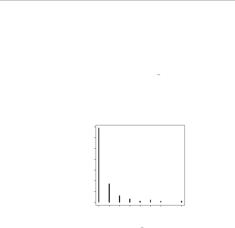
27
3
27
6
=
−
−
.
3.8 Note that the number of cells cannot be odd.
p(0) = P(no cells in the next generation) = P(the first cell dies or the first cell
splits and both die) = .1 + .9(.1)(.1) = 0.109
p(4) = P(four cells in the next generation) = P(the first cell splits and both created
cells split) = .9(.9)(.9) = 0.729.
p(2) = 1 – .109 – .729 = 0.162.
3.9 The random variable Y takes on vales 0, 1, 2, and 3.
a. Let E denote an error on a single entry and let N denote no error. There are 8 sample
points: EEE, EEN, ENE, NEE, ENN, NEN, NNE, NNN. With P(E) = .05 and P(N) = .95
and assuming independence:
P(Y = 3) = (.05)3 = 0.000125 P(Y = 2) = 3(.05)2(.95) = 0.007125
P(Y = 1) = 3(.05)2(.95) = 0.135375 P(Y = 0) = (.95)3 = 0.857375.
www.elsolucionario.net

32 Chapter 3: Discrete Random Variables and Their Probability Distributions
Instructor’s Solutions Manual
b. The graph is omitted.
c. P(Y > 1) = P(Y = 2) + P(Y = 3) = 0.00725.
3.10 Denote R as the event a rental occurs on a given day and N denotes no rental. Thus, the
sequence of interest is RR, RNR, RNNR, RNNNR, … . Consider the position immediately
following the first R: it is filled by an R with probability .2 and by an N with probability
.8. Thus, P(Y = 0) = .2, P(Y = 1) = .8(.2) = .16, P(Y = 2) = .128, … . In general,
P(Y = y) = .2(.8)y, y = 0, 1, 2, … .
3.11 There is a 1/3 chance a person has O+ blood and 2/3 they do not. Similarly, there is a
1/15 chance a person has O– blood and 14/15 chance they do not. Assuming the donors
are randomly selected, if X = # of O+ blood donors and Y = # of O– blood donors, the
probability distributions are
0 1 2 3
p(x) (2/3)3 = 8/27 3(2/3)2(1/3) = 12/27 3(2/3)(1/3)2 =6/27 (1/3)3 = 1/27
p(y) 2744/3375 196/3375 14/3375 1/3375
Note that Z = X + Y = # will type O blood. The probability a donor will have type O
blood is 1/3 + 1/15 = 6/15 = 2/5. The probability distribution for Z is
0 1 2 3
p(z) (2/5)3 = 27/125 3(2/5)2(3/5) = 54/27 3(2/5)(3/5)2 =36/125 (3/5)3 = 27/125
3.12 E(Y) = 1(.4) + 2(.3) + 3(.2) + 4(.1) = 2.0
E(1/Y) = 1(.4) + 1/2(.3) + 1/3(.2) + 1/4(.1) = 0.6417
E(Y2 – 1) = E(Y2) – 1 = [1(.4) + 22(.3) + 32(.2) + 42(.1)] – 1 = 5 – 1 = 4.
V(Y) = E(Y2) = [E(Y)]2 = 5 – 22 = 1.
3.13 E(Y) = –1(1/2) + 1(1/4) + 2(1/4) = 1/4
E(Y2) = (–1)2(1/2) + 12(1/4) + 22(1/4) = 7/4
V(Y) = 7/4 – (1/4)2 = 27/16.
Let C = cost of play, then the net winnings is Y – C. If E(Y – C) = 0, C = 1/4.
3.14 a. μ = E(Y) = 3(.03) + 4(.05) + 5(.07) + … + 13(.01) = 7.9
b. σ2 = V(Y) = E(Y2) – [E(Y)]2 = 32(.03) + 42(.05) + 52(.07) + … + 132(.01) – 7.92 = 67.14
– 62.41 = 4.73. So, σ = 2.17.
c. (μ – 2σ, μ + 2σ) = (3.56, 12.24). So, P(3.56 < Y < 12.24) = P(4 ≤ Y ≤ 12) = .05 + .07 +
.10 + .14 + .20 + .18 + .12 + .07 + .03 = 0.96.
3.15 a. p(0) = P(Y = 0) = (.48)3 = .1106, p(1) = P(Y = 1) = 3(.48)2(.52) = .3594, p(2) = P(Y =
2) = 3(.48)(.52)2 = .3894, p(3) = P(Y = 3) = (.52)3 = .1406.
b. The graph is omitted.
c. P(Y = 1) = .3594.
www.elsolucionario.net

Chapter 3: Discrete Random Variables and Their Probability Distributions 33
Instructor’s Solutions Manual
d. μ = E(Y) = 0(.1106) + 1(.3594) + 2(.3894) + 3(.1406) = 1.56,
σ2 = V(Y) = E(Y2) –[E(Y)]2 = 02(.1106) + 12(.3594) + 22(.3894) + 32(.1406) – 1.562 =
3.1824 – 2.4336 = .7488. So, σ = 0.8653.
e. (μ – 2σ, μ + 2σ) = (–.1706, 3.2906). So, P(–.1706 < Y < 3.2906) = P(0 ≤ Y ≤ 3) = 1.
3.16 As shown in Ex. 2.121, P(Y = y) = 1/n for y = 1, 2, …, n. Thus, E(Y) = ∑
=
+
=
n
y
n
ny
1
2
1
1.
∑
=
++
== n
y
nn
nyYE
1
6
)12)(1(
2
1
2)( . So,
(
)
12
1
12
)1)(1(
2
2
1
6
)12)(1( 2
)( −
−+
+
++ ==−= n
nn
n
nn
YV .
3.17 μ = E(Y) = 0(6/27) + 1(18/27) + 2(3/27) = 24/27 = .889
σ2 = V(Y) = E(Y2) –[E(Y)]2 = 02(6/27) + 12(18/27) + 22(3/27) – (24/27)2 = 30/27 –
576/729 = .321. So, σ = 0.567
For (μ – 2σ, μ + 2σ) = (–.245, 2.023). So, P(–.245 < Y < 2.023) = P(0 ≤ Y ≤ 2) = 1.
3.18 μ = E(Y) = 0(.109) + 2(.162) + 4(.729) = 3.24.
3.19 Let P be a random variable that represents the company’s profit. Then, P = C – 15 with
probability 98/100 and P = C – 15 – 1000 with probability 2/100. Then,
E(P) = (C – 15)(98/100) + (C – 15 – 1000)(2/100) = 50. Thus, C = $85.
3.20 With probability .3 the volume is 8(10)(30) = 2400. With probability .7 the volume is
8*10*40 = 3200. Then, the mean is .3(2400) + .7(3200) = 2960.
3.21 Note that E(N) = E(8πR2) = 8πE(R2). So, E(R2) = 212(.05) + 222(.20) + … + 262(.05) =
549.1. Therefore E(N) = 8π(549.1) = 13,800.388.
3.22 Note that p(y) = P(Y = y) = 1/6 for y = 1, 2, …, 6. This is similar to Ex. 3.16 with n = 6.
So, E(Y) = 3.5 and V(Y) = 2.9167.
3.23 Define G to be the gain to a person in drawing one card. The possible values for G are
$15, $5, or $–4 with probabilities 3/13, 2/13, and 9/13 respectively. So,
E(G) = 15(3/13) + 5(2/13) – 4(9/13) = 4/13 (roughly $.31).
3.24 The probability distribution for Y = number of bottles with serious flaws is:
p(y) 0 1 2
y .81 .18 .01
Thus, E(Y) = 0(.81) + 1(.18) + 2(.01) = 0.20 and V(Y) = 02(.81) + 12(.18) + 22(.01) –
(.20)2 = 0.18.
3.25 Let X1 = # of contracts assigned to firm 1; X2 = # of contracts assigned to firm 2. The
sample space for the experiment is {(I,I), (I,II), (I,III), (II,I), (II,II), (II,III), (III,I), (III,II),
(III,III)}, each with probability 1/9. So, the probability distributions for X1 and X2 are:
x1 0 1 2 x2 0 1 2
p(x1) 4/9 4/9 1/9 p(x2) 4/9 4/9 1/9
www.elsolucionario.net

34 Chapter 3: Discrete Random Variables and Their Probability Distributions
Instructor’s Solutions Manual
Thus, E(X1) = E(X2) = 2/3. The expected profit for the owner of both firms is given by
90000(2/3 + 2/3) = $120,000.
3.26 The random variable Y = daily sales can have values $0, $50,000 and $100,000.
If Y = 0, either the salesperson contacted only one customer and failed to make a sale or
the salesperson contacted two customers and failed to make both sales. Thus P(Y = 0) =
1/3(9/10) + 2/3(9/10)(9/10) = 252/300.
If Y = 2, the salesperson contacted to customers and made both sales. So, P(Y = 2) =
2/3(1/10)(1/10) = 2/300.
Therefore, P(Y = 1) = 1 – 252/300 – 2/300 = 46/300.
Then, E(Y) = 0(252/300) + 50000(46/300) + 100000(2/300) = 25000/3 (or $8333.33).
V(Y) =380,561,111 and σ = $19,507.98.
3.27 Let Y = the payout on an individual policy. Then, P(Y = 85,000) = .001, P(Y = 42,500) =
.01, and P(Y = 0) = .989. Let C represent the premium the insurance company charges.
Then, the company’s net gain/loss is given by C – Y. If E(C – Y) = 0, E(Y) = C. Thus,
E(Y) = 85000(.001) + 42500(.01) + 0(.989) = 510 = C.
3.28 Using the probability distribution found in Ex. 3.3, E(Y) = 2(1/6) + 3(2/6) + 4(3/6) =
20/6. The cost for testing and repairing is given by 2Y + 4. So, E(2Y + 4) = 2(20/6) + 4 =
64/6.
3.29 ).()()()()()()(
1111111
YEypyjpjjpjpkYPkYP
yjj
j
kkkjkkkj
=⋅=⋅=====≥ ∑∑∑∑∑∑∑∑∑ ∞
=
∞
=
∞
==
∞
=
∞
=
∞
=
∞
=
∞
=
3.30 a. The mean of X will be larger than the mean of Y.
b. E(X) = E(Y + 1) = E(Y) + 1 = μ + 1.
c. The variances of X and Y will be the same (the addition of 1 doesn’t affect variability).
d. V(X) = E[(X – E(X))2] = E[(Y + 1 – μ – 1)2] = E[(Y – μ)2] = σ2.
3.31 a. The mean of W will be larger than the mean of Y if μ > 0. If μ < 0, the mean of W will
be smaller than μ. If μ = 0, the mean of W will equal μ.
b. E(W) = E(2Y) = 2E(Y) = 2μ.
c. The variance of W will be larger than σ2, since the spread of values of W has increased.
d. V(X) = E[(X – E(X))2] = E[(2Y – 2μ)2] = 4E[(Y – μ)2] = 4σ2.
3.32 a. The mean of W will be smaller than the mean of Y if μ > 0. If μ < 0, the mean of W
will be larger than μ. If μ = 0, the mean of W will equal μ.
b. E(W) = E(Y/10) = (.1)E(Y) = (.1)μ.
c. The variance of W will be smaller than σ2, since the spread of values of W has
decreased.
d. V(X) = E[(X – E(X))2] = E[(.1Y – .1μ)2] = (.01)E[(Y – μ)2] = (.01)σ2.
www.elsolucionario.net

Chapter 3: Discrete Random Variables and Their Probability Distributions 35
Instructor’s Solutions Manual
3.33 a. .)()()()( babYaEbEaYEbaYE
+
=
+
=
+=+
μ
b. .])[(])[(])[()( 222222
σμμμ
aYEaaaYEbabaYEbaYV =−=−=−−+=+
3.34 The mean cost is E(10Y) = 10E(Y) = 10[0(.1) + 1(.5) + 2(.4)] = $13. Since V(Y) .41,
V(10Y) = 100V(Y) = 100(.41) = 41.
3.35 With FSSSB ∪= , P(B) = P(SS) + P(FS) =
(
)
(
)
4999
2000
5000
3000
4999
1999
5000
2000
+
= 0.4
P(B|first trial success) = 4999
1999 = 0.3999, which is not very different from the above.
3.36 a. The random variable Y does not have a binomial distribution. The days are not
independent.
b. This is not a binomial experiment. The number of trials is not fixed.
3.37 a. Not a binomial random variable.
b. Not a binomial random variable.
c. Binomial with n = 100, p = proportion of high school students who scored above 1026.
d. Not a binomial random variable (not discrete).
e. Not binomial, since the sample was not selected among all female HS grads.
3.38 Note that Y is binomial with n = 4, p = 1/3 = P(judge chooses formula B).
a. p(y) =
()()
yy
y
−
⎟
⎟
⎠
⎞
⎜
⎜
⎝
⎛4
3
2
3
1
4, y = 0, 1, 2, 3, 4.
b. P(Y ≥ 3) = p(3) + p(4) = 8/81 + 1/81 = 9/81 = 1/9.
c. E(Y) = 4(1/3) = 4/3.
d. V(Y) = 4(1/3)(2/3) = 8/9
3.39 Let Y = # of components failing in less than 1000 hours. Then, Y is binomial with n = 4
and p = .2.
a. P(Y = 2) = 22 )8(.2.
2
4⎟
⎟
⎠
⎞
⎜
⎜
⎝
⎛ = 0.1536.
b. The system will operate if 0, 1, or 2 components fail in less than 1000 hours. So,
P(system operates) = .4096 + .4096 + .1536 = .9728.
3.40 Let Y = # that recover from stomach disease. Then, Y is binomial with n = 20 and p = .8.
To find these probabilities, Table 1 in Appendix III will be used.
a. P(Y ≥ 10) = 1 – P(Y ≤ 9) = 1 – .001 = .999.
b. P(14 ≤ Y ≤ 18) = P(Y ≤ 18) – P(Y ≤ 13) – .931 – .087 = .844
c. P(Y ≤ 16) = .589.
3.41 Let Y = # of correct answers. Then, Y is binomial with n = 15 and p = .2. Using Table 1
in Appendix III, P(Y ≥ 10) = 1 – P(Y ≤ 9) = 1 – 1.000 = 0.000 (to three decimal places).
www.elsolucionario.net
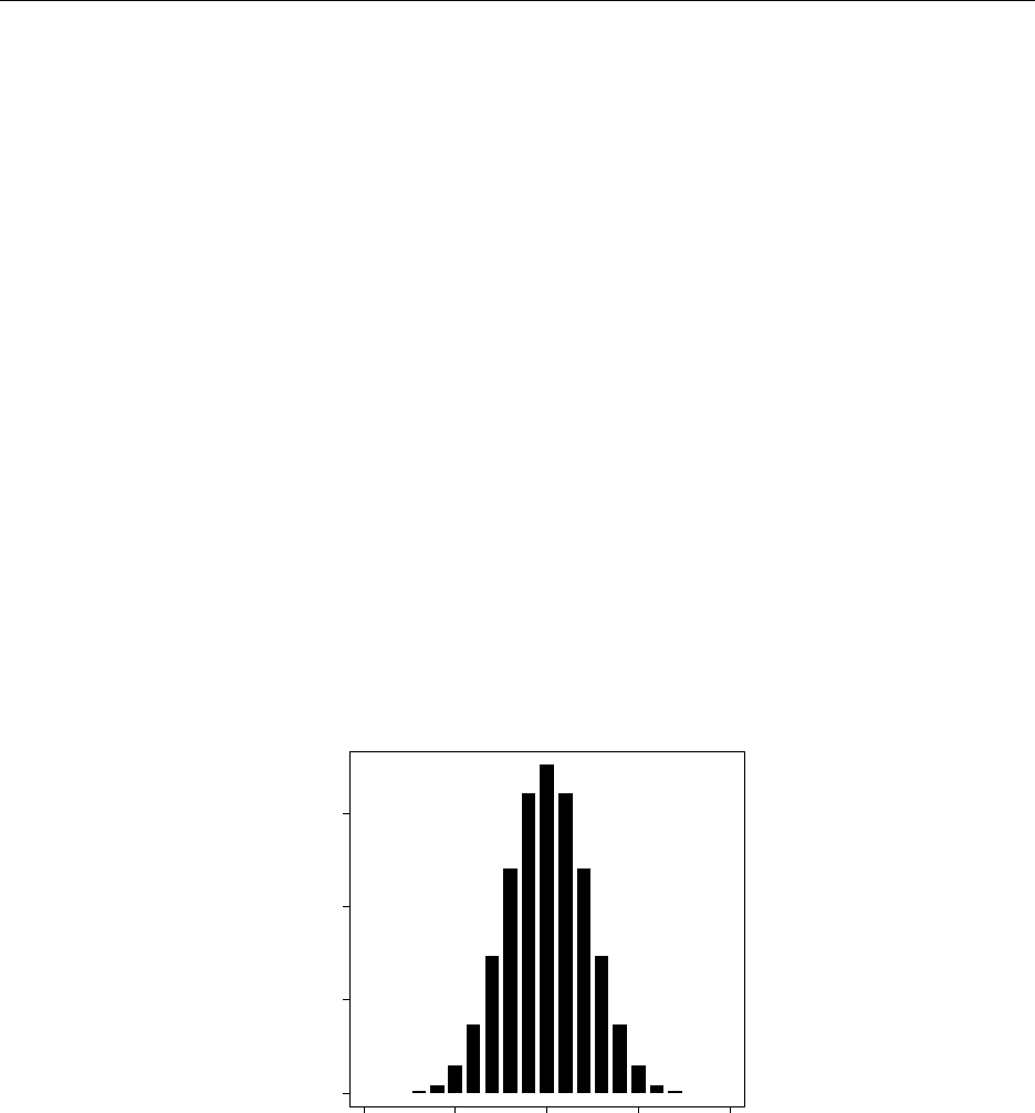
36 Chapter 3: Discrete Random Variables and Their Probability Distributions
Instructor’s Solutions Manual
3.42 a. If one answer can be eliminated on every problem, then, Y is binomial with n = 15 and
p = .25. Then, P(Y ≥ 10) = 1 – P(Y ≤ 9) = 1 – 1.000 = 0.000 (to three decimal places).
b. If two answers can be (correctly) eliminated on every problem, then, Y is binomial
with n = 15 and p = 1/3. Then, P(Y ≥ 10) = 1 – P(Y ≤ 9) = 0.0085.
3.43 Let Y = # of qualifying subscribers. Then, Y is binomial with n = 5 and p = .7.
a. P(Y = 5) = .75 = .1681
b. P(Y ≥ 4) = P(Y = 4) + P(Y = 5) = 5(.74)(.3) + .75 = .3601 + .1681 = 0.5282.
3.44 Let Y = # of successful operations. Then Y is binomial with n = 5.
a. With p = .8, P(Y = 5) = .85 = 0.328.
b. With p = .6, P(Y = 4) = 5(.64)(.4) = 0.259.
c. With p = .3, P(Y < 2) = P(Y = 1) + P(Y = 0) = 0.528.
3.45 Note that Y is binomial with n = 3 and p = .8. The alarm will function if Y = 1, 2, or 3.
Thus, P(Y ≥ 1) = 1 – P(Y = 0) = 1 – .008 = 0.992.
3.46 When p = .5, the distribution is symmetric. When p < .5, the distribution is skewed to the
left. When p > .5, the distribution is skewed to the right.
3.47 The graph is above.
0 5 10 15 20
0.00 0.05 0.10 0.15
y
p(y)
3.48 a. Let Y = # of sets that detect the missile. Then, Y has a binomial distribution with n = 5
and p = .9. Then, P(Y = 4) = 5(.9)4(.1) = 0.32805 and
P(Y ≥ 1) = 1 – P(Y = 0) = 1 – 5(.9)4(.1) = 0.32805.
b. With n radar sets, the probability of at least one diction is 1 – (.1)n. If 1 – (.1)n = .999,
n = 3.
3.49 Let Y = # of housewives preferring brand A. Thus, Y is binomial with n = 15 and p = .5.
a. Using the Appendix, P(Y ≥ 10) = 1 – P(Y ≤ 9) = 1 – .849 = 0.151.
b. P(10 or more prefer A or B) = P(6 ≤ Y ≤ 9) = 0.302.
www.elsolucionario.net

Chapter 3: Discrete Random Variables and Their Probability Distributions 37
Instructor’s Solutions Manual
3.50 The only way team A can win in exactly 5 games is to win 3 in the first 4 games and then
win the 5th game. Let Y = # of games team A wins in the first 4 games. Thus, Y has a
binomial distribution with n = 4. Thus, the desired probability is given by
P(Team A wins in 5 games) = P(Y = 3)P(Team A wins game 5)
= ppp )1(
3
43−
⎟
⎟
⎠
⎞
⎜
⎜
⎝
⎛ = )1(4 4pp −.
3.51 a. P(at least one 6 in four rolls) = 1 – P(no 6’s in four rolls) = 1 – (5/6)4 = 0.51775.
b. Note that in a single toss of two dice, P(double 6) = 1/36. Then:
P(at least one double 6 in twenty–four rolls) = 1 – P(no double 6’s in twenty–four rolls) =
= 1 – (35/36)24 = 0.4914.
3.52 Let Y = # that are tasters. Then, Y is binomial with n = 20 and p = .7.
a. P(Y ≥ 17) = 1 – P(Y ≤ 16) = 0.107.
b. P(Y < 15) = P(Y ≤ 14) = 0.584.
3.53 There is a 25% chance the offspring of the parents will develop the disease. Then, Y = #
of offspring that develop the disease is binomial with n = 3 and p =.25.
a. P(Y = 3) = (.25)3 = 0.015625.
b. P(Y = 1) = 3(.25)(.75)2 = 0.421875
c. Since the pregnancies are mutually independent, the probability is simply 25%.
3.54 a. and b. follow from simple substitution
c. the classifications of “success” and “failure” are arbitrary.
3.55 yny
n
y
yny
n
y
pp
yny
nnnn
pp
yny
nyyy
YYYE −
=
−
=
−
−−−−
−−−
=−
−
−−
=−− ∑∑ )1(
))!3(3()!3(
)!3)(2)(1(
)1(
)!(!
!)2)(1(
)}2)1({
30
= 33
3
0
3)2)(1()1(
3
)2)(1( pnnnpp
z
n
pnnn znz
n
z
−−=−
⎟
⎟
⎠
⎞
⎜
⎜
⎝
⎛−
−− −−
−
=
∑ .
Equating this to E(Y3) – 3E(Y2) + 2E(Y), it is found that
E(Y3) = .)2)(1()1(3 32 nppnnnpnn +−−−−
3.56 Using expression for the mean and variance of Y = # of successful explorations, a
binomial random variable with n = 10 and p = .1, E(Y) = 10(.1) = 1, and
V(Y) = 10(.1)(.9) = 0.9.
3.57 If Y = # of successful explorations, then 10 – Y is the number of unsuccessful
explorations. Hence, the cost C is given by C = 20,000 + 30,000Y + 15,000(10 – Y).
Therefore, E(C) = 20,000 + 30,000(1) + 15,000(10 – 1) = $185,000.
3.58 If Y is binomial with n = 4 and p = .1, E(Y) = .4 and V(Y) = .36. Thus, E(Y2) = .36 + (.4)2
= 0.52. Therefore, E(C) = 3(.52) + (.36) + 2 = 3.96.
www.elsolucionario.net

38 Chapter 3: Discrete Random Variables and Their Probability Distributions
Instructor’s Solutions Manual
3.59 If Y = # of defective motors, then Y is binomial with n = 10 and p = .08. Then, E(Y) = .8.
The seller’s expected next gain is $1000 – $200E(Y) = $840.
3.60 Let Y = # of fish that survive. Then, Y is binomial with n = 20 and p = .8.
a. P(Y = 14) = .109.
b. P(Y ≥ 10) = .999.
c. P(Y ≤ 16) = .589.
d. μ = 20(.8) = 16, σ2 = 20(.8)(.2) = 3.2.
3.61 Let Y = # with Rh+ blood. Then, Y is binomial with n = 5 and p = .8
a. 1 – P(Y = 5) = .672.
b. P(Y ≤ 4) = .672.
c. We need n for which P(Y ≥ 5) = 1 – P(Y ≤ 4) > .9. The smallest n is 8.
3.62 a. Assume independence of the three inspection events.
b. Let Y = # of plane with wing cracks that are detected. Then, Y is binomial with n = 3
and p = .9(.8)(.5) = .36. Then, P(Y ≥ 1) = 1 – P(Y = 0) = 0.737856.
3.63 a. Found by pulling in the formula for p(y) and p(y – 1) and simplifying.
b. Note that P(Y < 3) = P(Y ≤ 2) = P(Y = 2) + P(Y = 1) + P(Y = 0). Now, P(Y = 0) =
(.96)90 = .0254. Then, P(Y = 1) = )0254(.
)96(.1
04).1190( +− = .0952 and P(Y = 2) =
)0952(.
)96(.2
04).1290( +− = .1765. Thus, P(Y < 3) = .0254 + .0952 + .1765 = 0.2971
c. 1
)1( >
+−
yq
yn is equivalent to yqyppn >
−
+
)1( is equivalent to ypn >+ )1(. The
others are similar.
d. Since for y ≤ (n + 1)p, then p(y) ≥ p(y – 1) > p(y – 2) > … . Also, for y ≥ (n + 1)p, then
p(y) ≥ p(y + 1) > p(y + 2) > … . It is clear that p(y) is maximized when y is a close to
(n + 1)p as possible.
3.64 To maximize the probability distribution as a function of p, consider taking the natural
log (since ln() is a strictly increasing function, it will not change the maximum). By
taking the first derivative of ln[p(y0)] and setting it equal to 0, the maximum is found to
be y0/n.
3.65 a. E(Y/n) = E(Y)/n = np/n = p.
b. V(Y/n) = V(Y)/n2 = npq/n2 = pq/n. This quantity goes to zero as n goes to infinity.
3.66 a. 1
1
1
01
1=
−
== ∑∑ ∞
=
∞
=
−
q
pqppq
x
x
y
y (infinite sum of a geometric series)
b. .
2
1q
pq
pq
y
y=
−
−
The event Y = 1 has the highest probability for all p, 0 < p < 1.
www.elsolucionario.net

Chapter 3: Discrete Random Variables and Their Probability Distributions 39
Instructor’s Solutions Manual
3.67 (.7)4(.3) = 0.07203.
3.68 1/(.30) = 3.33.
3.69 Y is geometric with p = 1 – .41 = .59. Thus, )59(.)41(.)( 1−
=y
yp , y = 1, 2, … .
3.70 Let Y = # of holes drilled until a productive well is found.
a. P(Y = 3) = (.8)2(.2) = .128
b. P(Y > 10) = P(first 10 are not productive) = (.8)10 = .107.
3.71 a. ∑∑ ∞
=
−
∞
+=
−===>
1
1
1
1
)(
x
axa
ay
yqpqqpqaYP .
b. From part a, b
a
ba q
q
q
aYP
baYP
aYP
aYbaYP
aYbaYP ==
>
+>
=
>
>+>
=>+>
+
)(
)(
)(
),(
)|( .
c. The results in the past are not relevant to a future outcome (independent trials).
3.72 Let Y = # of tosses until the first head. P(Y ≥ 12 | Y > 10) = P(Y > 11 | Y > 10) = 1/2.
3.73 Let Y = # of accounts audited until the first with substantial errors is found.
a. P(Y = 3) = .12(.9) = .009.
b. P(Y ≥ 3) = P(Y > 2) = .12 = .01.
3.74 μ = 1/.9 = 1.1, σ = 2
9.
9.1− = .35
3.75 Let Y = # of one second intervals until the first arrival, so that p = .1
a. P(Y = 3) = (.9)2(.1) = .081.
b. P(Y ≥ 3) = P(Y > 2) = .92 = .81.
3.76 0
)7(.)( 0
y
yYP => ≥ .1. Thus, y0 ≤ )7ln(.
)1ln(. = 6.46, so y0 ≤ = 6.
3.77 P(Y = 1, 3, 5, …) = P(Y = 1) + P(Y + 3) + P(Y = 5) + … = p + q2p + q4p + … =
p[1 + q2 + q4 + …] = 2
1
1
q
p−. (Sum an infinite geometric series in
()
k
q2.)
3.78 a. (.4)4(.6) = .01536.
b. (.4)4 = .0256.
3.79 Let Y = # of people questioned before a “yes” answer is given. Then, Y has a geometric
distribution with p = P(yes) = P(smoker and “yes”) + P(nonsmoker and “yes”) = .3(.2) +
0 = .06. Thus, p(y) = .06(.94)y–1. y = 1, 2, … .
www.elsolucionario.net

40 Chapter 3: Discrete Random Variables and Their Probability Distributions
Instructor’s Solutions Manual
3.80 Let Y = # of tosses until the first 6 appears, so Y has a geometric distribution. Using the
result from Ex. 3.77,
P(B tosses first 6) = P(Y = 2, 4, 6, …) = 1 – P(Y = 1, 3, 5, …) = 1 – 2
1
1
q
p−.
Since p = 1/6, P(B tosses first 6) = 5/11. Then,
P(Y = 4 | B tosses the first 6) 11/5
)6/1()6/5(
11/5
)4( 2
=
=YP = 275/1296.
3.81 With p = 1/2, then μ = 1/(1/2) = 2.
3.82 With p = .2, then μ = 1/(.2) = 5. The 5th attempt is the expected first successful well.
3.83 Let Y = # of trials until the correct password is picked. Then, Y has a geometric
distribution with p = 1/n. P(Y = 6) =
(
)
.
5
1
1n
n
n−
3.84 E(Y) = n, V(Y) = ).1()1( 2
1−=− nnn
n
3.85 Note that .)1( 2
2
2−
−= yy
dq
dqyyq Thus, .)1(
2
2
2
2
2∑∑ ∞
=
−
∞
=
−=
y
y
y
y
dq
dqyyq Thus,
E[Y(Y–1)] = ∑∑ ∞
=
−
∞
=
−−=−
1
2
1
1)1()1(
y
y
y
yqyypqqyy = ∑
∞
=2
2
2
y
y
dq
dqpq = ⎭
⎬
⎫
⎩
⎨
⎧−−
−q
q
pq dq
d1
1
1
2
2 =
23
2
)1(
2
p
q
q
pq =
−. Use this with V(Y) = E[Y(Y–1)] + E(Y) – [E(Y)]2.
3.86 P(Y = y0) = .
1
0pq y− Like Ex. 3.64, maximize this probability by first taking the natural
log.
3.87 p
pp
yy
p
p
p
y
yy
y
ppYE −
∞
=
−
−
−
∞
=
−==−= ∑∑ 1
)ln(
1
)1(
1
1
1
1)1()/1( .
3.88 pqpqyYPyYP yy ==+=== −+ 11* )1()(, y = 0, 1, 2, … .
3.89 .11)()( 1
*−=−= p
YEYE V(Y*) = V(Y – 1) = V(Y).
3.90 Let Y = # of employees tested until three positives are found. Then, Y is negative
binomial with r = 3 and p = .4. P(Y = 10) = 73 )6(.4.
2
9⎟
⎟
⎠
⎞
⎜
⎜
⎝
⎛ = .06.
3.91 The total cost is given by 20Y. So, E(20Y) = 20E(Y) = 20 4.
3 = $50. Similarly, V(20Y) =
400V(Y) = 4500.
www.elsolucionario.net

Chapter 3: Discrete Random Variables and Their Probability Distributions 41
Instructor’s Solutions Manual
3.92 Let Y = # of trials until this first non–defective engine is found. Then, Y is geometric
with p = .9. P(Y = 2) = .9(.1) = .09.
3.93 From Ex. 3.92:
a. P(Y = 5) = 23 )1(.)9(.
2
4⎟
⎟
⎠
⎞
⎜
⎜
⎝
⎛ = .04374.
b. P(Y ≤ 5) = P(Y = 3) + P(Y = 4) + P(Y = 5) = .729 + .2187 + .04374 = .99144.
3.94 a. μ = 1/(.9) = 1.11, σ2 = (.1)/(.9)2 = .1234.
b. μ = 3/(.9) = 3.33, σ2 = 3(.1)/(.9)2 = .3704.
3.95 From Ex. 3.92 (and the memory–less property of the geometric distribution),
P(Y ≥ 4 | Y > 2) = P(Y > 3 | Y > 2) = P(Y > 1) = 1 – P(Y = 0) = .1.
3.96 a. Let Y = # of attempts until you complete your call. Thus, Y is geometric with p = .4.
Thus, P(Y = 1) = .4, P(Y = 2) = (.6).4 = .24, P(Y = 3) = (.6)2.4 = .144.
b. Let Y = # of attempts until both calls are completed. Thus, Y is negative binomial with
r = 2 and p = .4. Thus, P(Y = 4) = 3(.4)2(.6)2 = .1728.
3.97 a. Geometric probability calculation: (.8)2(.2) = .128.
b. Negative binomial probability calculation: 43 )8(.)2(.
2
6⎟
⎟
⎠
⎞
⎜
⎜
⎝
⎛ = .049.
c. The trials are independent and the probability of success is the same from trial to trial.
d. μ = 3/.2 = 15, σ2 = 3(.8)/(.04) = 60.
3.98 a. q
ry
y
qp
qp
yp
yp
ryr
ryr y
ryr
ryr y
−
−
==
−−−
−−−
−
−
−−
−1
)1(
)(
1
)!1()!1(
)!2(
)!()!1(
)!1(
b. If q
ry
y
−
−1 > 1, then yq – q > y – r or equivalently y
q
qr >
−
−
1. The 2nd result is similar.
c. If r = 7, p = .5 = q, then y
q
qr >=
−
−
=
−
−
13
5.1
5.7
1.
3.99 Define a random variable X = y trials before the before the first success, y = r – 1, r, r + 1,
… . Then, X = Y – 1, where Y has the negative binomial distribution with parameters r
and p. Thus, p(x) = ryr
ryr yqp −+
+−−
1
)!1()!1(
!, y = r – 1, r, r + 1, … .
3.100 a. yrrryr qp
r
ry
qp
r
ry
ryYPyYP ⎟
⎟
⎠
⎞
⎜
⎜
⎝
⎛
−
−+
=
⎟
⎟
⎠
⎞
⎜
⎜
⎝
⎛
−
−+
=+=== −+
1
1
1
1
)()( *, y = 0, 1, 2, … .
b. E(Y*) = E(Y) – r = r/p – r = r/q, V(Y*) = V(Y – r) = V(Y).
www.elsolucionario.net

42 Chapter 3: Discrete Random Variables and Their Probability Distributions
Instructor’s Solutions Manual
3.101 a. Note that P(Y = 11) = 65 )1(
4
10 pp −
⎟
⎟
⎠
⎞
⎜
⎜
⎝
⎛. Like Ex. 3.64 and 3.86, maximize this
probability by first taking the natural log. The maximum is 5/11.
b. In general, the maximum is r/y0.
3.102 Let Y = # of green marbles chosen in three draws. Then. P(Y = 3) = ⎟
⎟
⎠
⎞
⎜
⎜
⎝
⎛
⎟
⎟
⎠
⎞
⎜
⎜
⎝
⎛
3
10
3
5 = 1/12.
3.103 Use the hypergeometric probability distribution with N = 10, r = 4, n = 5. P(Y = 0) = 42
1.
3.104 Define the events: A: 1st four selected packets contain cocaine
B: 2nd two selected packets do not contain cocaine
Then, the desired probability is P(A∩B) = P(B|A)P(A). So,
P(A) = ⎟
⎟
⎠
⎞
⎜
⎜
⎝
⎛
⎟
⎟
⎠
⎞
⎜
⎜
⎝
⎛
4
20
4
15 = .2817 and P(B|A) = ⎟
⎟
⎠
⎞
⎜
⎜
⎝
⎛
⎟
⎟
⎠
⎞
⎜
⎜
⎝
⎛
2
16
2
5 = .0833. Thus,
P(A∩B) = .2817(.0833) = 0.0235.
3.105 a. The random variable Y follows a hypergeometric distribution. The probability of being
chosen on a trial is dependent on the outcome of previous trials.
b. P(Y ≥ 2) = P(Y = 2) + P(Y = 3) = 7143.01786.5357.
3
8
3
5
3
8
1
3
2
5
=+=+
⎟
⎟
⎠
⎞
⎜
⎜
⎝
⎛
⎟
⎟
⎠
⎞
⎜
⎜
⎝
⎛
⎟
⎟
⎠
⎞
⎜
⎜
⎝
⎛
⎟
⎟
⎠
⎞
⎜
⎜
⎝
⎛
⎟
⎟
⎠
⎞
⎜
⎜
⎝
⎛
.
c. μ = 3(5/8) = 1.875, σ2 = 3(5/8)(3/8)(5/7) = .5022, so σ = .7087.
3.106 Using the results from Ex.103, E(50Y) = 50E(Y) = 50[5
(
)
10
4] = $100. Furthermore,
V(50Y) = 2500V(Y) = 2500[5
(
)
(
)
9
5
10
6
10
4] = 1666.67.
3.107 The random variable Y follows a hypergeometric distribution with N = 6, n = 2, and r = 4.
3.108 Use the fact that P(at least one is defective) = 1 – P(none are defective). Then, we
require P(none are defective) ≤ .2. If n = 8,
P(none are defective) =
(
)
(
)
(
)
(
)
(
)
(
)
(
)
(
)
13
10
14
11
15
12
16
13
17
14
18
15
19
16
20
17 = 0.193.
3.109 Let Y = # of treated seeds selected.
a. P(Y = 4) =
⎟
⎟
⎠
⎞
⎜
⎜
⎝
⎛
⎟
⎟
⎠
⎞
⎜
⎜
⎝
⎛
⎟
⎟
⎠
⎞
⎜
⎜
⎝
⎛
4
10
0
5
4
5
= .0238
b. P(Y ≤ 3) = 1 – P(Y = 4) = 1 –
⎟
⎟
⎠
⎞
⎜
⎜
⎝
⎛
⎟
⎟
⎠
⎞
⎜
⎜
⎝
⎛
⎟
⎟
⎠
⎞
⎜
⎜
⎝
⎛
4
10
0
5
4
5
= 1 – .0238 = .9762.
c. same answer as part (b) above.
www.elsolucionario.net
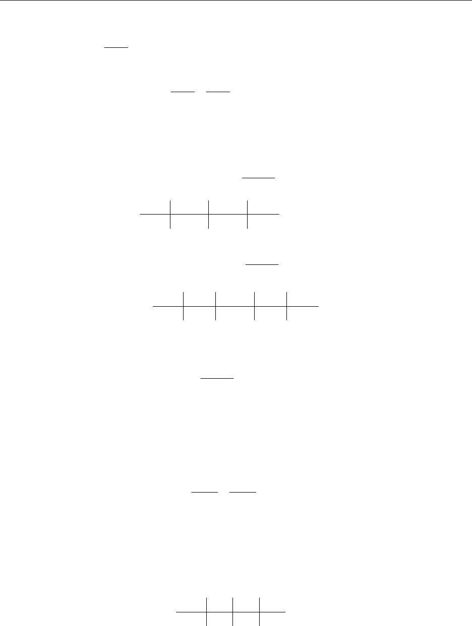
Chapter 3: Discrete Random Variables and Their Probability Distributions 43
Instructor’s Solutions Manual
3.110 a. P(Y = 1) =
⎟
⎟
⎠
⎞
⎜
⎜
⎝
⎛
⎟
⎟
⎠
⎞
⎜
⎜
⎝
⎛
⎟
⎟
⎠
⎞
⎜
⎜
⎝
⎛
3
6
1
2
2
4
= .6.
b. P(Y ≥ 1) = p(1) + p(2) =
⎟
⎟
⎠
⎞
⎜
⎜
⎝
⎛
⎟
⎟
⎠
⎞
⎜
⎜
⎝
⎛
⎟
⎟
⎠
⎞
⎜
⎜
⎝
⎛
⎟
⎟
⎠
⎞
⎜
⎜
⎝
⎛
⎟
⎟
⎠
⎞
⎜
⎜
⎝
⎛
⎟
⎟
⎠
⎞
⎜
⎜
⎝
⎛
+
3
6
2
2
1
4
3
6
1
2
2
4
= .8
c. P(Y ≤ 1) = p(0) + p(1) = .8.
3.111 a. The probability function for Y is p(y) =
⎟
⎟
⎠
⎞
⎜
⎜
⎝
⎛
⎟
⎟
⎠
⎞
⎜
⎜
⎝
⎛
−
⎟
⎟
⎠
⎞
⎜
⎜
⎝
⎛
3
10
3
82
yy , y = 0, 1, 2. In tabular form, this is
y 0 1 2
p(y) 14/30 14/30 2/30
b. The probability function for Y is p(y) =
⎟
⎟
⎠
⎞
⎜
⎜
⎝
⎛
⎟
⎟
⎠
⎞
⎜
⎜
⎝
⎛
−
⎟
⎟
⎠
⎞
⎜
⎜
⎝
⎛
3
10
3
64
yy , y = 0, 1, 2, 3. In tabular form, this is
3.112 Let Y = # of malfunctioning copiers selected. Then, Y is hypergeometric with probability
function
p(y) =
⎟
⎟
⎠
⎞
⎜
⎜
⎝
⎛
⎟
⎟
⎠
⎞
⎜
⎜
⎝
⎛
−
⎟
⎟
⎠
⎞
⎜
⎜
⎝
⎛
4
8
4
53
yy , y = 0, 1, 2, 3.
a. P(Y = 0) = p(0) = 1/14.
b. P(Y ≥ 1) = 1 – P(Y = 0) = 13/14.
3.113 The probability of an event as rare or rarer than one observed can be calculated according
to the hypergeometric distribution, Let Y = # of black members. Then, Y is
hypergeometric and P(Y ≤ 1) =
⎟
⎟
⎠
⎞
⎜
⎜
⎝
⎛
⎟
⎟
⎠
⎞
⎜
⎜
⎝
⎛
⎟
⎟
⎠
⎞
⎜
⎜
⎝
⎛
⎟
⎟
⎠
⎞
⎜
⎜
⎝
⎛
⎟
⎟
⎠
⎞
⎜
⎜
⎝
⎛
⎟
⎟
⎠
⎞
⎜
⎜
⎝
⎛
+
6
20
6
12
0
8
6
20
5
12
3
8
= .187. This is nearly 20%, so it is not
unlikely.
3.114 μ = 6(8)/20 = 2.4, σ2 6(8/20)(12/20)(14/19) = 1.061.
3.115 The probability distribution for Y is given by
y 0 1 2
p(y) 1/5 3/5 1/5
3.116 (Answers vary, but with n =100, the relative frequencies should be close to the
probabilities in the table above.)
y 0 1 2 3
p(y) 5/30 15/30 9/30 1/30
www.elsolucionario.net

44 Chapter 3: Discrete Random Variables and Their Probability Distributions
Instructor’s Solutions Manual
3.117 Let Y = # of improperly drilled gearboxes. Then, Y is hypergeometric with N = 20, n = 5,
and r = 2.
a. P(Y = 0) = .553
b. The random variable T, the total time, is given by T = 10Y + (5 – Y) = 9Y + 5. Thus,
E(T) = 9E(Y) + 5 = 9[5(2/20)] + 5 = 9.5.
V(T) = 81V(T) = 81(.355) = 28.755, σ = 5.362.
3.118 Let Y = # of aces in the hand. Then. P(Y = 4 | Y ≥ 3) = )4()3(
)4(
=+=
=
YPYP
YP . Note that Y
is a hypergeometric random variable. So,
⎟
⎟
⎠
⎞
⎜
⎜
⎝
⎛
⎟
⎟
⎠
⎞
⎜
⎜
⎝
⎛
⎟
⎟
⎠
⎞
⎜
⎜
⎝
⎛
==
5
52
2
48
3
4
)3(YP = .001736 and
⎟
⎟
⎠
⎞
⎜
⎜
⎝
⎛
⎟
⎟
⎠
⎞
⎜
⎜
⎝
⎛
⎟
⎟
⎠
⎞
⎜
⎜
⎝
⎛
==
5
52
1
48
4
4
)4(YP = .00001847. Thus, P(Y = 4 | Y ≥ 3) = .0105.
3.119 Let the event A = 2nd king is dealt on 5th card. The four possible outcomes for this event
are {KNNNK, NKNNK, NNKNK, NNNKK}, where K denotes a king and N denotes a
non–king. Each of these outcomes has probability:
(
)
(
)
(
)
(
)
(
)
48
3
49
46
50
47
51
48
52
4. Then, the desired
probability is P(A) = 4
()()
(
)
(
)
(
)
48
3
49
46
50
47
51
48
52
4 = .016.
3.120 There are N animals in this population. After taking a sample of k animals, making and
releasing them, there are N – k unmarked animals. We then choose a second sample of
size 3 from the N animals. There are ⎟
⎟
⎠
⎞
⎜
⎜
⎝
⎛
3
N ways of choosing this second sample and
there are ⎟
⎟
⎠
⎞
⎜
⎜
⎝
⎛
⎟
⎟
⎠
⎞
⎜
⎜
⎝
⎛−
12
kkN ways of finding exactly one of the originally marked animals. For
k = 4, the probability of finding just one marked animal is
P(Y = 1) = )2)(1(
)5)(4(12
3
1
4
2
4
−−
−−
⎟
⎟
⎠
⎞
⎜
⎜
⎝
⎛
⎟
⎟
⎠
⎞
⎜
⎜
⎝
⎛
⎟
⎟
⎠
⎞
⎜
⎜
⎝
⎛−
=NNN NN
N
N
.
Calculating this for various values of N, we find that the probability is largest for N = 11
or N = 12 (the same probability is found: .503).
3.121 a. P(Y = 4) = 2
!4
24−
e= .090.
b. P(Y ≥ 4) = 1 – P(Y ≤ 3) = 1 – .857 = .143 (using Table 3, Appendix III).
c. P(Y < 4) = P(Y ≤ 3) = .857.
d. P(Y ≥ 4 | Y ≥ 2) = )2(
)4(
≥
≥
YP
YP = .143/.594 = .241
www.elsolucionario.net

Chapter 3: Discrete Random Variables and Their Probability Distributions 45
Instructor’s Solutions Manual
3.122 Let Y = # of customers that arrive during the hour. Then, Y is Poisson with λ = 7.
a. P(Y ≤ 3) = .0818.
b. P(Y ≥ 2) = .9927.
c. P(Y = 5) = .1277
3.123 If p(0) = p(1),
λλ
λ
−− =ee . Thus, λ = 1. Therefore, p(2) = 1
!2
12−
e = .1839.
3.124 Using Table 3 in Appendix III, we find that if Y is Poisson with λ = 6.6, P(Y ≤ 2) = .04.
Using this value of λ, P(Y > 5) = 1 – P(Y ≤ 5) = 1 – .355 = .645.
3.125 Let S = total service time = 10Y. From Ex. 3.122, Y is Poisson with λ = 7. Therefore,
E(S) = 10E(Y) = 7 and V(S) = 100V(Y) = 700. Also,
P(S > 150) = P(Y > 15) = 1 – P(Y ≤ 15) = 1 – .998 = .002, and unlikely event.
3.126 a. Let Y = # of customers that arrive in a given two–hour time. Then, Y has a Poisson
distribution with λ = 2(7) = 14 and P(Y = 2) = 14
!2
142−
e.
b. The same answer as in part a. is found.
3.127 Let Y = # of typing errors per page. Then, Y is Poisson with λ = 4 and P(Y ≤ 4) = .6288.
3.128 Note that over a one–minute period, Y = # of cars that arrive at the toll booth is Poisson
with λ = 80/60 = 4/3. Then, P(Y ≥ 1) = 1 – P(Y = 0) = 1 – e– 4/3 = .7364.
3.129 Following the above exercise, suppose the phone call is of length t, where t is in minutes.
Then, Y = # of cars that arrive at the toll booth is Poisson with λ = 4t/3. Then, we must
find the value of t such that P(Y = 0) = 1 – e–4t/3 ≥ .4.
Therefore, t ≤ – 4
3ln(.6) = .383 minutes, or about .383(60) = 23 seconds.
3.130 Define: Y1 = # of cars through entrance I, Y2 = # of cars through entrance II. Thus, Y1 is
Poisson with λ = 3 and Y2 is Poisson with λ = 4.
Then, P(three cars arrive) = P(Y1 = 0, Y2 = 3) + P(Y1 = 1, Y2 = 2)+ P(Y1 = 2, Y2 = 1) +
+P(Y1 = 3, Y2 = 0).
By independence, P(three cars arrive) = P(Y1 = 0)P(Y2 = 3) + P(Y1 = 1)P(Y2 = 2)
+ P(Y1 = 2)P(Y2 = 1) + P(Y1 = 3)P(Y2 = 0).
Using Poisson probabilities, this is equal to 0.0521
3.131 Let the random variable Y = # of knots in the wood. Then, Y has a Poisson distribution
with λ = 1.5 and P(Y ≤ 1) = .5578.
3.132 Let the random variable Y = # of cars entering the tunnel in a two–minute period. Then,
Y has a Poisson distribution with λ = 1 and P(Y > 3) = 1 – P(Y ≤ 3) = 0.01899.
www.elsolucionario.net

46 Chapter 3: Discrete Random Variables and Their Probability Distributions
Instructor’s Solutions Manual
3.133 Let X = # of two–minute intervals with more than three cars. Therefore, X is binomial
with n = 10 and p = .01899 and P(X ≥ 1) = 1 – P(X = 0) = 1 – (1–.01899)10 = .1745.
3.134 The probabilities are similar, even with a fairly small n.
3.135 Using the Poisson approximation, λ ≈ np = 100(.03) = 3, so P(Y ≥ 1) = 1 – P(Y = 0) =
.9524.
3.136 Let Y = # of E. coli cases observed this year. Then, Y has an approximate Poisson
distribution with λ ≈ 2.4.
a. P(Y ≥ 5) = 1 – P(Y ≤ 4) = 1 – .904 = .096.
b. P(Y > 5) = 1 – P(Y ≤ 5) = 1 – .964 = .036. Since there is a small probability
associated with this event, the rate probably has charged.
3.137 Using the Poisson approximation to the binomial with λ ≈ np = 30(.2) = 6.
Then, P(Y ≤ 3) = .1512.
3.138 ∑∑ ∞
=
λ−
∞
=
λ− λ−−λ− λ==−
0
!
)1(
2
0
!
)1( 2
)]1([
yyeyy
yyeyy yy
YYE . Using the substitution z = y – 2, it is found
that E[Y(Y – 1)] = λ2. Use this with V(Y) = E[Y(Y–1)] + E(Y) – [E(Y)]2 = λ.
3.139 Note that if Y is Poisson with λ = 2, E(Y) = 2 and E(Y2) = V(Y) + [E(Y)]2 = 2 + 4 = 6. So,
E(X) = 50 – 2E(Y) – E(Y2) = 50 – 2(2) – 6 = 40.
3.140 Since Y is Poisson with λ = 2, E(C) =
()
[
]
()
1
1
!
1
1
0
!
100
2
1100100100 1
2
2
2−
∞
=
−
∞
=
=== ∑∑ −
−eeE
yy
e
yy
e
Yy
Y
.
3.141 Similar to Ex. 3.139: E(R) = E(1600 – 50Y2) = 1600 – 50(6) = $1300.
3.142 a. ...,2,1,
)!1(
!
)1(
)(
1=== λ
−
λ
λ
−λ−−
λ−
y
y
ye
y
e
yp yp
y
y
b. Note that if λ > y, p(y) > p(y – 1). If λ > y, p(y) > p(y – 1). If λ = y for some integer y,
p(y) = p(y – 1).
c. Note that for λ a non–integer, part b. implies that for y – 1 < y < λ,
p(y – 1) < p(y) > p(y + 1).
Hence, p(y) is maximized for y = largest integer less than λ. If λ is an integer, then p(y) is
maximized at both values λ – 1 and λ.
y p(y), exact binomial p(y), Poisson approximation
0 .358 .368
1 .378 .368
2 .189 .184
3 .059 .061
4 .013 .015
www.elsolucionario.net

Chapter 3: Discrete Random Variables and Their Probability Distributions 47
Instructor’s Solutions Manual
3.143 Since λ is a non–integer, p(y) is maximized at y = 5.
3.144 Observe that with λ = 6, p(5) = 1606.
!5
665 =
−
e, p(6) = 1606.
!6
666 =
−
e.
3.145 Using the binomial theorem, .)()()()(
0
ntynyt
n
y
tY qpeqpe
y
n
eEtm +=
⎟
⎟
⎠
⎞
⎜
⎜
⎝
⎛
== −
=
∑
3.146 tnt
dt
dpeqpentm 1
)()( −
+= . At t = 0, this is np = E(Y).
tnttnt
dt
dpeqpenpeqpenntm 121 )()())(1()(
2
2−− +++−= . At t = 0, this is np2(n – 1) + np.
Thus, V(Y) = np2(n – 1) + np – (np)2 = np(1 – p).
3.147 The moment–generating function is .
1
)()()(
0
1
1
t
t
y
ytty
n
y
tytY
qe
pe
qepeqpeeEtm −
==== ∑∑ ∞
=
−
=
3.148 2
)1(
)( t
t
dt
dqe
pe
tm −
=. At t = 0, this is 1/p = E(Y).
4
2
)1(
))(1(2)1(
)(
2
2
t
ttttt
dt
dqe
qeqepepeqe
tm −
−−−−
=. At t = 0, this is (1+q)/p2.
Thus, V(Y) = (1+q)/p2 – (1/p)2 = q/p2.
3.149 This is the moment–generating function for the binomial with n = 3 and p = .6.
3.150 This is the moment–generating function for the geometric with p = .3.
3.151 This is the moment–generating function for the binomial with n = 10 and p = .7, so
P(Y ≤ 5) = .1503.
3.152 This is the moment–generating function for the Poisson with λ = 6. So, μ = 6 and σ =
6 ≈ 2.45. So, P(|Y – μ| ≤ 2σ) = P(μ – 2σ ≤ Y ≤ μ + 2σ) = P(1.1 ≤ Y ≤ 10.9) =
P(2 ≤ Y ≤ 10) = .940.
3.153 a. Binomial with n = 5, p = .1
b. If m(t) is multiplied top and bottom by ½, this is a geometric mgf with p = ½.
c. Poisson with λ = 2.
3.154 a. Binomial mean and variance: μ = 1.667, σ2 = 1.111.
b. Geometric mean and variance: μ = 2, σ2 = 2.
c. Poisson mean and variance: μ = 2, σ2 = 2.
www.elsolucionario.net

48 Chapter 3: Discrete Random Variables and Their Probability Distributions
Instructor’s Solutions Manual
3.155 Differentiate to find the necessary moments:
a. E(Y) = 7/3.
b. V(Y) = E(Y2) – [E(Y)]2 = 6 – (7/3)2 = 5/9.
c. Since ).()( tY
eEtm =Y can only take on values 1, 2, and 3 with probabilities 1/6, 2/6,
and 3/6.
3.156 a. 1)1()()0( 0=== EeEm Y.
b. )3()()()()( )3(3 tmeEeEeEtm YtYttW
W==== .
c. )()()()()( 22)2( tmeeeEeEeEtm ttYtYttX
X
−−− ==== .
3.157 a. From part b. in Ex. 3.156, the results follow from differentiating to find the necessary
moments.
b. From part c. in Ex. 3.156, the results follow from differentiating to find the necessary
moments.
3.158 The mgf for W is )()()()()( )()( atmeeeEeEeEtm btYatbtbaYttW
W==== +.
3.159 From Ex. 3.158, the results follow from differentiating the mgf of W to find the necessary
moments.
3.160 a. E(Y*) = E(n – Y) = n – E(Y) = n – np = n(1 – p) = nq. V(Y*) = V(n – Y) = V(Y) = npq.
b. .)()()()()()( )()(
*
*
ntntYtntYnttY
YqpetmeeeEeEeEtm +=−==== −−
c. Based on the moment–generating function, Y* has a binomial distribution.
d. The random variable Y* = # of failures.
e. The classification of “success” and “failure” in the Bernoulli trial is arbitrary.
3.161 .)()()()()( 1
)1(
*
*t
qe
p
ttYtYttY
YtmeeeEeEeEtm −
−−− =====
3.162 Note that )(
)(
)1( )1(
)( tm tm
tr =,
[
]
()
2
2
)1()2(
)(
)()()(
)2( )( tm
tmtmtm
tr −
=. Then,
μ
=== 1
)(
)0(
)0(
)1( )1(
)0( YE
m
m
r.
[]
()
2
1
)]([)(
)0(
)0()0()0(
)2( 22
2
2
)1()2(
)0(
σ
=== −− YEYE
m
mmm
r.
3.163 Note that r(t) = 5(et – 1). Then, t
etr 5)(
)1( =and t
etr 5)(
)2( =. So,
λμ
=== 5)0(
)1(
r
and
λσ
=== 2)2( 5)( t
etr .
www.elsolucionario.net

Chapter 3: Discrete Random Variables and Their Probability Distributions 49
Instructor’s Solutions Manual
3.164 For the binomial, nyny
n
y
Yptqqpt
y
n
tEtP )()()()(
0
+=
⎟
⎟
⎠
⎞
⎜
⎜
⎝
⎛
== −
=
∑. Differentiating with
respect to t, .)()( 1
1
1npptqnptP t
n
t
dt
d=+= =
−
=
3.165 For the Poisson, )1(
00 !
)(
!
)()( −λ
∞
=
λ−
λ−
λ−
∞
=
λ−
=
λ
=
λ
== ∑∑ t
y
ty
t
y
yy
Ye
y
et
e
e
y
te
tEtP . Differentiating
with respect to t, λ=λ== =
−λ
=1
)1(
1
)()( t
t
t
dt
detPYE and 2
1
)1(2
1
)(
2
2λ=λ= =
−λ
=t
t
t
dt
detP =
E[Y(Y – 1)] = E(Y2) – E(Y). Thus, V(Y) = λ.
3.166 E[Y(Y – 1)(Y – 2)] = 3
1
)1(3
1
)(
3
3
λλ
λ
== =
−
=t
t
t
dt
detP = E(Y3) – 3E(Y2) + 2E(Y). Therefore,
E(Y3) = λ3 + 3(λ2 + λ) – 2λ = λ3 + 3λ2 + λ.
3.167 a. The value 6 lies (11–6)/3 = 5/3 standard deviations below the mean. Similarly, the
value 16 lies (16–11)/3 = 5/3 standard deviations above the mean. By Tchebysheff’s
theorem, at least 1 – 1/(5/3)2 = 64% of the distribution lies in the interval 6 to 16.
b. By Tchebysheff’s theorem, .09 = 1/k2, so k = 10/3. Since σ = 3, kσ = (10/3)3 = 10 = C.
3.168 Note that Y has a binomial distribution with n = 100 and p = 1/5 = .2
a. E(Y) = 100(.2) = 20.
b. V(Y) = 100(.2)(.8) = 16, so σ = 4.
c. The intervals are 20 ± 2(4) or (12, 28), 20 + 3(4) or (8, 32).
d. By Tchebysheff’s theorem, 1 – 1/32 or approximately 89% of the time the number of
correct answers will lie in the interval (8, 32). Since a passing score of 50 is far from
this range, receiving a passing score is very unlikely.
3.169 a. E(Y) = –1(1/18) + 0(16/18) + 1(1/18) = 0. E(Y2) = 1(1/18) + 0(16/18) + 1(1/18) = 2/18
= 1/9. Thus, V(Y) = 1/9 and σ = 1/3.
b. P(|Y – 0| ≥ 1) = P(Y = –1) + P(Y = 1) = 1/18 + 1/18 = 2/18 = 1/9. According to
Tchebysheff’s theorem, an upper bound for this probability is 1/32 = 1/9.
c. Example: let X have probability distribution p(–1) = 1/8, p(0) = 6/8, p(1) = 1/8. Then,
E(X) = 0 and V(X) = 1/4.
d. For a specified k, assign probabilities to the points –1, 0, and 1 as p(–1) = p(1) = 2
2
1
k
and p(0) = 1 – k
1.
3.170 Similar to Ex. 3.167: the interval (.48, 52) represents two standard deviations about the
mean. Thus, the lower bound for this interval is 1 – ¼ = ¾. The expected number of
coins is 400(¾) = 300.
www.elsolucionario.net

50 Chapter 3: Discrete Random Variables and Their Probability Distributions
Instructor’s Solutions Manual
3.171 Using Tchebysheff’s theorem, 5/9 = 1 – 1/k2, so k = 3/2. The interval is 100 ± (3/2)10, or
85 to 115.
3.172 From Ex. 3.115, E(Y) = 1 and V(Y) = .4. Thus, σ = .63. The interval of interest is 1 ±
2(.63), or (–.26, 2.26). Since Y can only take on values 0, 1, or 2, 100% of the values
will lie in the interval. According to Tchebysheff’s theorem, the lower bound for this
probability is 75%.
3.173 a. The binomial probabilities are p(0) = 1/8, p(1) = 3/8, p(2) = 3/8, p(3) = 1/8.
b. The graph represents a symmetric distribution.
c. E(Y) = 3(1/2) = 1.5, V(Y) = 3(1/2)(1/2) = .75. Thus, σ = .866.
d. For one standard deviation about the mean: 1.5 ± .866 or (.634, 2.366)
This traps the values 1 and 2, which represents 7/8 or 87.5% of the probability. This is
consistent with the empirical rule.
For two standard deviations about the mean: 1.5 ± 2(.866) or (–.232, 3.232)
This traps the values 0, 1, and 2, which represents 100% of the probability. This is
consistent with both the empirical rule and Tchebysheff’s theorem.
3.174 a. (Similar to Ex. 3.173) the binomial probabilities are p(0) = .729, p(1) = .243, p(2) =
.027, p(3) = .001.
b. The graph represents a skewed distribution.
c. E(Y) = 3(.1) = .3, V(Y) = 3(.1)(.9) = .27. Thus, σ = .520.
d. For one standard deviation about the mean: .3 ± .520 or (–.220, .820)
This traps the value 1, which represents 24.3% of the probability. This is not consistent
with the empirical rule.
For two standard deviations about the mean: .3 ± 2(.520) or (–.740, 1.34)
This traps the values 0 and 1, which represents 97.2% of the probability. This is
consistent with both the empirical rule and Tchebysheff’s theorem.
3.175 a. The expected value is 120(.32) = 38.4
b. The standard deviation is )68)(.32(.120 = 5.11.
c. It is quite likely, since 40 is close to the mean 38.4 (less than .32 standard deviations
away).
3.176 Let Y represent the number of students in the sample who favor banning clothes that
display gang symbols. If the teenagers are actually equally split, then E(Y) = 549(.5) =
274.5 and V(Y) = 549(.5)(.5) = 137.25. Now. Y/549 represents the proportion in the
sample who favor banning clothes that display gang symbols, so E(Y/549) = .5 and
V(Y/549) = .5(.5)/549 = .000455. Then, by Tchebysheff’s theorem,
P(Y/549 ≥ .85) ≤ P(|Y/549 – .5| ≥ .35) ≤ 1/k2,
www.elsolucionario.net

Chapter 3: Discrete Random Variables and Their Probability Distributions 51
Instructor’s Solutions Manual
where k is given by kσ = .35. From above, σ = .02134 so k = 16.4 and 1/(16.4)2 = .0037.
This is a very unlikely result. It is also unlikely using the empirical rule. We assumed
that the sample was selected randomly from the population.
3.177 For C = 50 + 3Y, E(C) = 50 + 3(10) = $80 and V(C) = 9(10) = 90, so that σ = 9.487.
Using Tchebysheff’s theorem with k = 2, we have P(|Y – 80| < 2(9.487)) ≥ .75, so that the
required interval is (80 – 2(9.487), 80 + 2(9.487)) or (61.03, 98.97).
3.178 Using the binomial, E(Y) = 1000(.1) = 100 and V(Y) = 1000(.1)(.9) = 90. Using the result
that at least 75% of the values will fall within two standard deviation of the mean, the
interval can be constructed as 100 ± 2 90 , or (81, 119).
3.179 Using Tchebysheff’s theorem, observe that
2
1
)|(|)()( k
kYPkYPkYP ≤
σ
≥
μ
−
≤
σ
≥
μ
−
=
σ
+μ≥ .
Therefore, to find P(Y ≥ 350) ≤ 1/k2, we solve 150 + k(67.081) = 350, so k = 2.98. Thus,
P(Y ≥ 350) ≤ 1/(2.98)2 = .1126, which is not highly unlikely.
3.180 Number of combinations = 26(26)(10)(10)(10)(10) = 6,760,000. Thus,
E(winnings) = 100,000(1/6,760,000) + 50,000(2/6,760,000) + 1000(10/6,760,000) =
$.031, which is much less than the price of the stamp.
3.181 Note that P(acceptance) = P(observe no defectives) = 50
0
5qp
⎟
⎟
⎠
⎞
⎜
⎜
⎝
⎛. Thus:
p = Fraction defective P(acceptance)
0 1
.10 .5905
.30 .1681
.50 .0312
1.0 0
3.182 OC curves can be constructed using points given in the tables below.
a. Similar to Ex. 3.181: P(acceptance) = 100
0
10 qp
⎟
⎟
⎠
⎞
⎜
⎜
⎝
⎛. Thus,
p 0 .05 .10 .30 .50 1
P(acceptance) 1 .599 .349 .028 .001 0
b. Here, P(acceptance) = 91100
1
10
0
10 qpqp ⎟
⎟
⎠
⎞
⎜
⎜
⎝
⎛
+
⎟
⎟
⎠
⎞
⎜
⎜
⎝
⎛. Thus,
p 0 .05 .10 .30 .50 1
P(acceptance) 1 .914 .736 .149 .01 0
www.elsolucionario.net
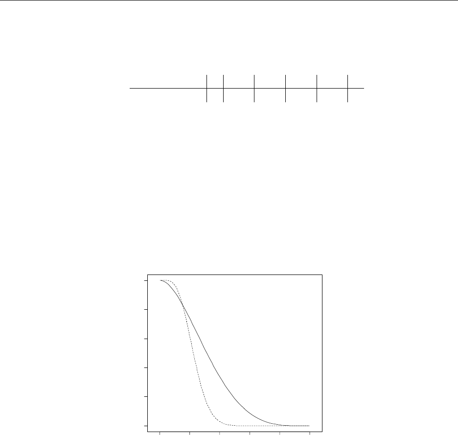
52 Chapter 3: Discrete Random Variables and Their Probability Distributions
Instructor’s Solutions Manual
c. Here, P(acceptance) = 8291100
2
10
1
10
0
10 qpqpqp ⎟
⎟
⎠
⎞
⎜
⎜
⎝
⎛
+
⎟
⎟
⎠
⎞
⎜
⎜
⎝
⎛
+
⎟
⎟
⎠
⎞
⎜
⎜
⎝
⎛. Thus,
p 0 .05 .10 .30 .50 1
P(acceptance) 1 .988 .930 .383 .055 0
3.183 Graph the two OC curves with n = 5 and a = 1 in the first case and n = 25 and a = 5 in the
second case.
a. By graphing the OC curves, it is seen that if the defectives fraction ranges from p = 0
to p = .10, the seller would want the probability of accepting in this interval to be a
high as possible. So, he would choose the second plan.
b. If the buyer wishes to be protected against accepting lots with a defective fraction
greater than .3, he would want the probability of acceptance (when p > .3) to be as
small as possible. Thus, he would also choose the second plan.
0.0 0.2 0.4 0.6 0.8 1.0
0.00.20.40.60.81.0
p
P(A)
The above graph illustrates the two OC curves. The solid lie represents the first case and the
dashed line represents the second case.
3.184 Let Y = # in the sample who favor garbage collect by contract to a private company.
Then, Y is binomial with n = 25.
a. If p = .80, P(Y ≥ 22) = 1 – P(Y ≤ 21) = 1 – .766 = .234,
b. If p = .80, P(Y = 22) = .1358.
c. There is not strong evidence to show that the commissioner is incorrect.
3.185 Let Y = # of students who choose the numbers 4, 5, or 6. Then, Y is binomial with n = 20
and p = 3/10.
a. P(Y ≥ 8) = 1 – P(Y ≤ 7) = 1 – .7723 = .2277.
b. Given the result in part a, it is not an unlikely occurrence for 8 students to choose 4, 5
or 6.
www.elsolucionario.net

Chapter 3: Discrete Random Variables and Their Probability Distributions 53
Instructor’s Solutions Manual
3.186 The total cost incurred is W = 30Y. Then,
E(W) = 30E(Y) = 30(1/.3) = 100, V(W) = 900V(Y) = 900(.7/.32) = 7000.
Using the empirical rule, we can construct a interval of three standard deviations about
the mean: 100 ± 3 7000 , or (151, 351).
3.187 Let Y = # of rolls until the player stops. Then, Y is geometric with p = 5/6.
a. P(Y = 3) = (1/6)2(5/6) = .023.
b. E(Y) = 6/5 = 1.2.
c. Let X = amount paid to player. Then, X = 2Y–1.
()
q
p
qppqEXE
x
yx
yyY
21
22)2()(
10
111
−
==== ∑∑
∞
=
∞
=
−−− , since 2q < 1. With p = 5/6,
this is $1.25.
3.188 The result follows from )0(1
)0()1(1
)1(
)2(
)1(
)1(
)1|1( =−
=
−=
−
=
≥
≥
=
≥
>
=≥> YP
YPYP
YP
YP
YP
YP
YYP .
3.189 The random variable Y = # of failures in 10,000 starts is binomial with n = 10,000 and
p = .00001. Thus, P(Y ≥ 1) = 1 – P(Y = 0) = 1 – (.9999)10000 = .09516.
Poisson approximation: 1 – e–.1 = .09516.
3.190 Answers vary, but with n = 100,
y
should be quite close to μ = 1.
3.191 Answers vary, but with n = 100, s2 should be quite close to σ2 = .4.
3.192 Note that p(1) = p(2) = … p(6) = 1/6. From Ex. 3.22, μ = 3.5 and σ2 = 2.9167. The
interval constructed of two standard deviations about the mean is (.08, 6.92) which
contains 100% of the possible values for Y.
3.193 Let Y1 = # of defectives from line I, Y2 is defined similarly. Then, both Y1 and Y2 are
binomial with n = 5 and defective probability p. In addition, Y1 + Y2 is also binomial with
n = 10 and defective probability p. Thus,
.476.0
4
10
2
5
2
5
4
10
2
5
2
5
)4(
)2()2(
)4|2(
55
3232
21
11
211 =
⎟
⎟
⎠
⎞
⎜
⎜
⎝
⎛
⎟
⎟
⎠
⎞
⎜
⎜
⎝
⎛
⎟
⎟
⎠
⎞
⎜
⎜
⎝
⎛
=
⎟
⎟
⎠
⎞
⎜
⎜
⎝
⎛
⎟
⎟
⎠
⎞
⎜
⎜
⎝
⎛
⎟
⎟
⎠
⎞
⎜
⎜
⎝
⎛
=
=+
==
==+=
qp
qpqp
YYP
YPYP
YYYP
Notice that the probability does not depend on p.
3.194 The possible outcomes of interest are:
WLLLLLLLLLL, LWLLLLLLLLL, LLWLLLLLLLL
So the desired probability is .1(.9)10 + .9(.1)(.9)9 + (.9)2(.1)(.9)8 = 3(.1)(.9)10 = .104.
www.elsolucionario.net

54 Chapter 3: Discrete Random Variables and Their Probability Distributions
Instructor’s Solutions Manual
3.195 Let Y = # of imperfections in one–square yard of weave. Then, Y is Poisson with λ = 4.
a. P(Y ≥ 1) = 1 – P(Y = 0) = 1 – e–4 = .982.
b. Let W = # of imperfections in three–square yards of weave. Then, W is Poisson with
λ = 12. P(W ≥ 1) = 1 – P(W = 0) = 1 – e–12.
3.196 For an 8–square yard bolt, let X = # of imperfections so that X is Poisson with λ = 32.
Thus, C = 10X is the cost to repair the weave and
E(C) = 10E(X) = $320 and V(C) = 100V(X) = 3200.
3.197 a. Let Y = # of samples with at least one bacteria colony. Then, Y is binomial with n = 4
and p = P(at least one bacteria colony) = 1 – P(no bacteria colonies) = 1 – e–2 = .865 (by
the Poisson). Thus, P(Y ≥ 1) = 1 – P(Y = 0) = 1 – (.135)4 = .9997.
b. Following the above, we require 1 – (.135)n = .95 or (.135)n = .05. Solving for n, we
have )135ln(.
)05ln(.
=n = 1.496, so take n = 2.
3.198 Let Y = # of neighbors for a seedling within an area of size A. Thus, Y is Poisson with λ =
A*d, where for this problem d = 4 per square meter.
a. Note that “within 1 meter” denotes an area A = π(1 m)2 = π m2. Thus, P(Y = 0) = e–4π.
b. “Within 2 meters” denotes an area A = π(2 m)2 = 4π m2. Thus,
P(Y ≤ 3) = P(Y = 0) + P(Y = 1) + P(Y = 2) + P(Y = 3) = ∑
=
−
3
0
!
)16( 16
yye
y
π
π
.
3.199 a. Using the binomial model with n = 1000 and p = 30/100,000, let λ ≈ np =
1000(30/100000) = .300 for the Poisson approximation.
b. Let Y = # of cases of IDD. P(Y ≥ 2) = 1 – P(Y = 0) – P(Y = 1) = 1 – .963 = .037.
3.200 Note that
[]
[
]
n
tt
n
tt
nt pppttpqpeq )1)1()( !3!2!3!2
3232 ++++=+++++=+ .
Expanding the above multinomial (but only showing the first three terms gives
[
]
++−++=+ −− 2
!2
21 1)1(1)(1)( 2n
t
nnnt nppnntnppeq
The coefficients agree with the first and second moments for the binomial distribution.
3.201 From Ex. 103 and 106, we have that μ = 100 and σ = 67.1666 = 40.825. Using an
interval of two standard deviations about the mean, we obtain 100 ± 2(40.825) or
(18.35, 181.65)
www.elsolucionario.net

Chapter 3: Discrete Random Variables and Their Probability Distributions 55
Instructor’s Solutions Manual
3.202 Let W = # of drivers who wish to park and W′ = # of cars, which is Poisson with mean λ.
a. Observe that
P(W = k) = !)!(!
!
)()|( n
eqp
knk
n
nWPnWkWP n
knk
knkn
λ
−
==
′
=
′
=λ−−
∞
=
∞
=∑∑
= λλ−
∞
=
−
∞
=
−
λ− λ
=λ
λ
=λ
−
⎟
⎟
⎠
⎞
⎜
⎜
⎝
⎛
λ∑∑ q
k
j
j
jk
kn
kn
knk
kee
k
p
j
q
k
p
kn
q
k
p
e!
)(
!!
)(
)!(! 0
= p
ke
k
pλ−
λ
!
)( , k = 0, 1, 2, … .
Thus, P(W = 0) = p
eλ− .
b. This is a Poisson distribution with mean λp.
3.203 Note that Y(t) has a negative binomial distribution with parameters r = k, p = e–λt.
a. E[Y(t)] = keλt, V[Y(t)] = )( 2
)1(
2
tt
e
ek eek
t
tλλ
−−=
λ−
λ− .
b. With k = 2, λ = .1, E[Y(5)] = 3.2974, V[Y(5)] = 2.139.
3.204 Let Y = # of left–turning vehicles arriving while the light is red. Then, Y is binomial with
n = 5 and p = .2. Thus, P(Y ≤ 3) = .993.
3.205 One solution: let Y = # of tosses until 3 sixes occur. Therefore, Y is negative binomial
where r = 3 and p = 1/6. Then, P(Y = 9) =
()()
0434127.
2
86
6
5
3
6
1=
⎟
⎟
⎠
⎞
⎜
⎜
⎝
⎛. Note that this
probability contains all events where a six occurs on the 9th toss. Multiplying the above
probability by 1/6 gives the probability of observing 4 sixes in 10 trials, where a six
occurs on the 9th and 10th trial: (.0424127)(1/6) = .007235.
3.206 Let Y represent the gain to the insurance company for a particular insured driver and let P
be the premium charged to the driver. Given the information, the probability distribution
for Y is given by: y p(y)
P .85
P – 2400 .15(.80) = .12
P – 7200 .15(.12) = .018
P – 12,000 .15(.08) = .012
If the expected gain is 0 (breakeven), then:
E(Y) = P(.85) + (P – 2400).12 + (P – 7200).018 + (P – 12000).012 = 0, so P = $561.60.
3.207 Use the Poisson distribution with λ = 5.
a. p(2) = .084, P(Y ≤ 2) = .125.
b. P(Y > 10) = 1 – P(Y ≤ 10) = 1 – .986 = .014, which represents an unlikely event.
www.elsolucionario.net

56 Chapter 3: Discrete Random Variables and Their Probability Distributions
Instructor’s Solutions Manual
3.208 If the general public was split 50–50 in the issue, then Y = # of people in favor of the
proposition is binomial with n = 2000 and p = .5. Thus,
E(Y) = 2000(.5) = 1000 and V(Y) = 2000(.5)(.5) = 500.
Since σ = 500 = 22.36, observe that 1373 is (1373 – 1000)/22.36 = 16.68 standard
deviations above the mean. Such a value is unlikely.
3.209 Let Y = # of contracts necessary to obtain the third sale. Then, Y is negative binomial
with r = 3, p = .3. So, P(Y < 5) = P(Y = 3) + P(Y = 4) = .33 + 3(.3)3(.7) = .0837.
3.210 In Example 3.22, λ = μ = 3 and σ2 = 3 and that σ = 3 = 1.732. Thus,
)464.6464.())732.1(2|3(|
≤
≤
−=≤− YPYP = P(Y ≤ 6) = .966. This is consistent with
the empirical rule (approximately 95%).
3.211 There are three scenarios:
• if she stocks two items, both will sell with probability 1. So, her profit is $.40.
• if she stocks three items, two will sell with probability .1 (a loss of .60) and three
will sell with probability .9. Thus, her expected profit is (–.60).1 + .60(.9) = $.48.
• if she stocks four items, two will sell with probability .1 (a loss of 1.60), three will
sell with probability .4 (a loss of .40), and four will sell with probability .5 (a gain
of .80. Thus, her expected profit is (–1.60).1 + (–.40).4 + (.80).5 = $.08
So, to maximize her expected profit, stock three items.
3.212 Note that:
()()()
()
[]
()()()()
[]
1
1
2
2
1
1
1
1
2
2
1
1
)!(!
!+−
+−−−
−− −−
−− −−
−
−
+−
+−
−
−
−
−
−
⎟
⎟
⎠
⎞
⎜
⎜
⎝
⎛
⎟
⎟
⎠
⎞
⎜
⎜
⎝
⎛
−
−
⎟
⎟
⎠
⎞
⎜
⎜
⎝
⎛
×= nN ynrN
yN rN
yN rN
yN rN
yN yr
N
r
N
r
N
r
yny n
n
N
yn
rN
y
r
. In the
first bracketed part, each quotient in parentheses has a limiting value of p. There are y
such quotients. In the second bracketed part, each quotient in parentheses has a limiting
value of 1 – p = q. There are n – y such quotients, Thus,
yny
n
N
yn
rN
y
r
qp
y
n−
⎟
⎟
⎠
⎞
⎜
⎜
⎝
⎛
⎟
⎟
⎠
⎞
⎜
⎜
⎝
⎛
−
−
⎟
⎟
⎠
⎞
⎜
⎜
⎝
⎛
⎟
⎟
⎠
⎞
⎜
⎜
⎝
⎛
→ as N → ∞
3.213 a. The probability is p(10) =
⎟
⎟
⎠
⎞
⎜
⎜
⎝
⎛
⎟
⎟
⎠
⎞
⎜
⎜
⎝
⎛
⎟
⎟
⎠
⎞
⎜
⎜
⎝
⎛
20
100
10
60
10
40
= .1192 (found by dhyper(10, 40, 60, 20) in R).
b. The binomial approximation is
(
)
1010
!10!10
!20 )6(.4. = .117, a close value to the above
(exact) answer.
www.elsolucionario.net

Chapter 3: Discrete Random Variables and Their Probability Distributions 57
Instructor’s Solutions Manual
3.214 Define: A = accident next year B = accident this year C = safe driver
Thus, P(C) = .7, P(A|C) = .1 = P(B|C), and 5.)|()|( == CBPCAP . From Bayes’ rule,
P(C|B) = )3(.5.)7(.1.
)7(.1.
)()|()()|(
)()|(
+
=
+CPCBPCPCBP
CPCBP = 7/22.
Now, we need P(A|B). Note that since ,SCC =∪ this conditional probability is equal to
)|()|()|()|()|)(( BCAPBCAPBCAPBCAPBCCAP ∩+=∩+∩=∪∩ ∩, or
)|()|()|()|()|( BCAPBCPBCAPBCPBAP ∩+∩= = 7/22(.1) + 15/22(.5) = .3727.
So, the premium should be 400(.3727) = $149.09.
3.215 a. Note that for (2), there are two possible values for N2, the number of tests performed: 1
and k + 1. If N2 = 1, all of the k people are healthy and this probability is (.95)k. Thus,
P(N2 = k + 1) = 1 – (.95)k. Thus, E(N2) = 1(.95)k + (k + 1)(1 – .95k) = 1 + k(1 – .95k).
This expectation holds for each group, so that for n groups the expected number of tests
is n[1 + k(1 – .95k)].
b. Writing the above as g(k) = k
N[1 + k(1 – .95k)], where n = k
N, we can minimize this
with respect to k. Note that g′(k) = 2
1
k + (.95k)ln(.95), a strictly decreasing function.
Since k must be an integer, it is found that g(k) is minimized at k = 5 and g(5) = .4262.
c. The expected number of tests is .4262N, compared to the N tests is (1) is used. The
savings is then N – .4262N = .5738N.
3.216 a. P(Y = n) = )1()2)(1(
)1()2)(1(
)!(
)!(
!
!+−−−
+−−−
−
−
⎟
⎟
⎠
⎞
⎜
⎜
⎝
⎛
⎟
⎟
⎠
⎞
⎜
⎜
⎝
⎛
−
−
⎟
⎟
⎠
⎞
⎜
⎜
⎝
⎛
=×= nNNNN nrrrr
nr nN
N
r
n
N
nn
rN
n
r
.
b. Since for integers a > b, ba
b
b
a
b
a
−
+
⎟
⎟
⎠
⎞
⎜
⎜
⎝
⎛
+
⎟
⎟
⎠
⎞
⎜
⎜
⎝
⎛
=1
1
, apply this result to find that
yn
ynrN
yry
ryp
ryp
−
+++−
−
+
+⋅= 1
1
)|1(
)|( 1
11
1 and yn
ynrN
yry
ryp
ryp
−
+++−
−
+
+⋅= 1
1
)|1(
)|( 21
22
2.
With r1 < r2, it follows that )|1(
)|1(
)|(
)|(
2
1
21
1ryp
ryp
ryp
ryp
+
+
>.
c. Note that from the binomial theorem, k
N
k
Ny
k
N
a∑
=⎟
⎟
⎠
⎞
⎜
⎜
⎝
⎛
=+ 1
1
0
1
)1( . So,
⎥
⎦
⎤
⎢
⎣
⎡⎟
⎟
⎠
⎞
⎜
⎜
⎝
⎛
+
⎟
⎟
⎠
⎞
⎜
⎜
⎝
⎛
+
⎟
⎟
⎠
⎞
⎜
⎜
⎝
⎛
×
⎥
⎦
⎤
⎢
⎣
⎡⎟
⎟
⎠
⎞
⎜
⎜
⎝
⎛
+
⎟
⎟
⎠
⎞
⎜
⎜
⎝
⎛
+
⎟
⎟
⎠
⎞
⎜
⎜
⎝
⎛
=++ 1121
1
1
11
1
1
11
1010
)1()1( NNNN y
N
N
y
NN
y
N
N
y
NN
aa =
www.elsolucionario.net

58 Chapter 3: Discrete Random Variables and Their Probability Distributions
Instructor’s Solutions Manual
⎥
⎦
⎤
⎢
⎣
⎡⎟
⎟
⎠
⎞
⎜
⎜
⎝
⎛
+
+
+
⎟
⎟
⎠
⎞
⎜
⎜
⎝
⎛+
+
⎟
⎟
⎠
⎞
⎜
⎜
⎝
⎛+
=+ ++ 2121
21
21
2121
10
)1( NNNN y
NN
NN
y
NNNN
a. Since these are equal, the
coefficient of every yn must be equal. In the second equality, the coefficient is
⎟
⎟
⎠
⎞
⎜
⎜
⎝
⎛+
n
NN 21 .
In the first inequality, the coefficient is given by the sum
⎟
⎟
⎠
⎞
⎜
⎜
⎝
⎛
−
⎟
⎟
⎠
⎞
⎜
⎜
⎝
⎛
=
⎟
⎟
⎠
⎞
⎜
⎜
⎝
⎛
⎟
⎟
⎠
⎞
⎜
⎜
⎝
⎛
++
⎟
⎟
⎠
⎞
⎜
⎜
⎝
⎛
−
⎟
⎟
⎠
⎞
⎜
⎜
⎝
⎛
+
⎟
⎟
⎠
⎞
⎜
⎜
⎝
⎛
⎟
⎟
⎠
⎞
⎜
⎜
⎝
⎛∑
=kn
N
k
NN
n
N
n
NN
n
NN n
k
2
0
1212121
0110 , thus the relation holds.
d. The result follows from part c above.
3.217
[]
∑∑∑ =⎟
⎟
⎠
⎞
⎜
⎜
⎝
⎛
⎟
⎟
⎠
⎞
⎜
⎜
⎝
⎛
−
−
⎟
⎟
⎠
⎞
⎜
⎜
⎝
⎛
−
−
=⎟
⎟
⎠
⎞
⎜
⎜
⎝
⎛
⎟
⎟
⎠
⎞
⎜
⎜
⎝
⎛
−
−
−−
−
=⎟
⎟
⎠
⎞
⎜
⎜
⎝
⎛
⎟
⎟
⎠
⎞
⎜
⎜
⎝
⎛
−
−
⎟
⎟
⎠
⎞
⎜
⎜
⎝
⎛
⎥
⎥
⎦
⎤
⎢
⎢
⎣
⎡
=
⎥
⎥
⎦
⎤
⎢
⎢
⎣
⎡
== n
yn
N
yn
rN
y
r
n
yn
N
yn
rN
yry r
n
yn
N
yn
rN
y
r
yrrYE
1
1
1
1
)!()!1(
)!1(
0
)( . In this sum, let x = y – 1:
()
N
nr
n
ox n
N
xn
rN
x
r
n
ox n
N
xn
rN
x
r
n
N
rr =
⎥
⎥
⎦
⎤
⎢
⎢
⎣
⎡
=
⎥
⎥
⎦
⎤
⎢
⎢
⎣
⎡∑∑ −
=⎟
⎟
⎠
⎞
⎜
⎜
⎝
⎛
−
−
⎟
⎟
⎠
⎞
⎜
⎜
⎝
⎛
−−
−
⎟
⎟
⎠
⎞
⎜
⎜
⎝
⎛−
−
=⎟
⎟
⎠
⎞
⎜
⎜
⎝
⎛
⎟
⎟
⎠
⎞
⎜
⎜
⎝
⎛
−−
−
⎟
⎟
⎠
⎞
⎜
⎜
⎝
⎛−1
1
1
1
1
11
1
.
3.218
[]
∑∑∑ =⎟
⎟
⎠
⎞
⎜
⎜
⎝
⎛
⎟
⎟
⎠
⎞
⎜
⎜
⎝
⎛
−
−
⎟
⎟
⎠
⎞
⎜
⎜
⎝
⎛
−
−
=⎟
⎟
⎠
⎞
⎜
⎜
⎝
⎛
⎟
⎟
⎠
⎞
⎜
⎜
⎝
⎛
−
−
−−−
−−
=⎟
⎟
⎠
⎞
⎜
⎜
⎝
⎛
⎟
⎟
⎠
⎞
⎜
⎜
⎝
⎛
−
−
⎟
⎟
⎠
⎞
⎜
⎜
⎝
⎛
−
⎥
⎥
⎦
⎤
⎢
⎢
⎣
⎡
−=
⎥
⎥
⎦
⎤
⎢
⎢
⎣
⎡
==− n
yn
N
yn
rN
y
r
n
yn
N
yn
rN
yryyy rrr
n
yn
N
yn
rN
y
r
yy rrYYE
2
2
2
0
)!()!2)(1(
)!2)(1(
0
)1(
)1()]1([ . In this
sum, let x = y – 2 to obtain the expectation )1(
)1()1(
−
−−
NN nnrr . From this result, the variance of
the hypergeometric distribution can also be calculated.
www.elsolucionario.net
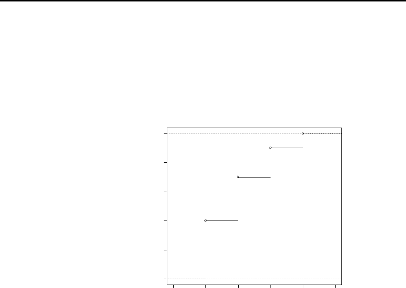
59
Chapter 4: Continuous Variables and Their Probability Distributions
4.1 a.
⎪
⎪
⎪
⎩
⎪
⎪
⎪
⎨
⎧
≥
<≤
<≤
<≤
<
=≤=
41
439.
327.
214.
10
)()(
y
y
y
y
y
yYPyF
b. The graph is above.
012345
0.00.20.40.60.81.0
y
F(y)
4.2 a. p(1) = .2, p(2) = (1/4)4/5 = .2, p(3) = (1/3)(3/4)(4/5) = 2., p(4) = .2, p(5) = .2.
b.
⎪
⎪
⎪
⎩
⎪
⎪
⎪
⎨
⎧
≥
<≤
<≤
<≤
<≤
<
=≤=
51
548.
436.
324.
212.
10
)()(
y
y
y
y
y
y
yYPyF
c. P(Y < 3) = F(2) = .4, P(Y ≤ 3) = .6, P(Y = 3) = p(3) = .2
d. No, since Y is a discrete random variable.
www.elsolucionario.net

60 Chapter 4: Continuous Variables and Their Probability Distributions
Instructor’s Solutions Manual
4.3 a. The graph is above.
01
01
y
F(y)
q = 1-p
b. It is easily shown that all three properties hold.
4.4 A binomial variable with n = 1 has the Bernoulli distribution.
4.5 For y = 2, 3, …, F(y) – F(y – 1) = P(Y ≤ y) – P(Y ≤ y – 1) = P(Y = y) = p(y). Also,
F(1) = P(Y ≤ 1) = P(Y = 1) = p(1).
4.6 a. F(i) = P(Y ≤ i) = 1 – P(Y > i) = 1 – P(1st i trials are failures) = 1 – qi.
b. It is easily shown that all three properties hold.
4.7 a. P(2 ≤ Y < 5) = P(Y ≤ 4) – P(Y ≤ 1) = .967 – .376 = 0.591
P(2 < Y < 5) = P(Y ≤ 4) – P(Y ≤ 2) = .967 – .678 = .289.
Y is a discrete variable, so they are not equal.
b. P(2 ≤ Y ≤ 5) = P(Y ≤ 5) – P(Y ≤ 1) = .994 – .376 = 0.618
P(2 < Y ≤ 5) = P(Y ≤ 5) – P(Y ≤ 2) = .994 – .678 = 0.316.
Y is a discrete variable, so they are not equal.
c. Y is not a continuous random variable, so the earlier result do not hold.
4.8 a. The constant k = 6 is required so the density function integrates to 1.
b. P(.4 ≤ Y ≤ 1) = .648.
c. Same as part b. above.
d. P(Y ≤ .4 | Y ≤ .8) = P(Y ≤ .4)/P(Y ≤ .8) = .352/.896 = 0.393.
e. Same as part d. above.
www.elsolucionario.net
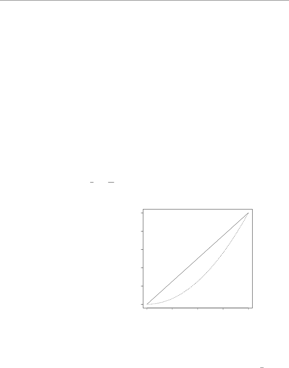
Chapter 4: Continuous Variables and Their Probability Distributions 61
Instructor’s Solutions Manual
4.9 a. Y is a discrete random variable because F(y) is not a continuous function. Also, the set
of possible values of Y represents a countable set.
b. These values are 2, 2.5, 4, 5.5, 6, and 7.
c. p(2) = 1/8, p(2.5) = 3/16 – 1/8 = 1/16, p(4) = 1/2 – 3/16 = 5/16, p(5.5) = 5/8 – 1/2 =
1/8, p(6) = 11/16 – 5/8 = 1/16, p(7) = 1 – 11/16 = 5/16.
d. P(Y ≤ 5.
φ) = F(5.
φ) = .5, so 5.
φ
= 4.
4.10 a. F(95.
φ) = ∫
φ
−
95.
0
)1(6 dyyy = .95, so 95.
φ
= 0.865.
b. Since Y is a continuous random variable, y0 = 95.
φ
= 0.865.
4.11 a.
[]
122/
2
0
2
0
2===
∫ccycydy , so c = 1/2.
b. 4
0
2
2
)()( y
y
t
y
dtdttfyF === ∫∫
∞−
, 0 ≤ y ≤ 2.
c. Solid line: f(y); dashed line: F(y)
0.0 0.5 1.0 1.5 2.0
0.0 0.2 0.4 0.6 0.8 1.0
y
d. P(1 ≤ Y ≤ 2) = F(2) – F(1) = 1 – .25 = .75.
e. Note that P(1 ≤ Y ≤ 2) = 1 – P(0 ≤ Y < 1). The region (0 ≤ y < 1) forms a triangle (in
the density graph above) with a base of 1 and a height of .5. So, P(0 ≤ Y < 1) = 2
1(1)(.5)
= .25 and P(1 ≤ Y ≤ 2) = 1 – .25 = .75.
www.elsolucionario.net

62 Chapter 4: Continuous Variables and Their Probability Distributions
Instructor’s Solutions Manual
4.12 a. F(–∞) = 0, F(∞) = 1, and F(y1) – F(y2) = 2
1
2
2yy ee −− − > 0 provided y1 > y2.
b. 2
3.
1)( 3.
φ
φ
−
−= eF = .3, so 3.
φ
= )7ln(.− = 0.5972.
c. 2
2)()( y
yeyFyf −
=
′
= for y ≥ 0 and 0 elsewhere.
d. P(Y ≥ 200) = 1 – P(Y < 200) = 1 – P(Y ≤ 200) = 1 – F(2) = e–4.
e. P(Y > 100 | Y ≤ 200) = P(100 < Y ≤ 200)/P(Y ≤ 200) = [F(2) – F(1)]/F(2) = 4
41
1−
−−
−
−
e
ee .
4.13 a. For 0 ≤ y ≤ 1, F(y) = 2/
2
0
ytdt
y
=
∫. For 1 < y ≤ 1.5, F(y) = 12/1
1
1
0
−+=+ ∫∫ ydttdt
y
= y – 1/2. Hence,
⎪
⎪
⎩
⎪
⎪
⎨
⎧
>
≤<−
≤≤
<
=
5.11
5.112/1
102/
00
)(
2
y
yy
yy
y
yF
b. P(0 ≤ Y ≤ .5) = F(.5) = 1/8.
c. P(.5 ≤ Y ≤ 1.2) = F(1.2) – F(.5) = 1.2 – 1/2 – 1/8 = .575.
4.14 a. A triangular distribution.
b. For 0 < y < 1, F(y) = 2/
2
0
ytdt
y
=
∫. For 1 ≤ y < 2, F(y) = 12)2( 2
1
1
0
2−−=−+ ∫∫ y
y
ydtttdt .
c. P(.8 ≤ Y ≤ 1.2) = F(1.2) – F(.8) = .36.
d. P(Y > 1.5 | Y > 1) = P(Y > 1.5)/P(Y > 1) = .125/.5 = .25.
4.15 a. For b ≥ 0, f (y) ≥ 0. Also,
]
1//)( 2=−== ∞
∞∞
∞− ∫∫ b
b
ybybyf .
b. F(y) = 1 – b/y, for y ≥ b, 0 elsewhere.
c. P(Y > b + c) = 1 – F(b + c) = b/(b + c).
d. Applying part c., P(Y > b + d | Y > b + c) = (b + c)/(b + d).
www.elsolucionario.net
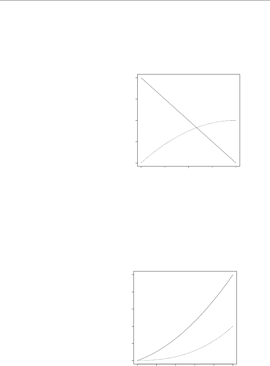
Chapter 4: Continuous Variables and Their Probability Distributions 63
Instructor’s Solutions Manual
4.16 a.
[]
122/2)2(
2
0
2
0
2==−=−
∫cyycdyyc , so c = 1/2.
b. F(y) = y – y2/4, for 0 ≤ y ≤ 2.
c. Solid line: f(y); dashed line: F(y)
0.0 0.5 1.0 1.5 2.0
0.0 0.5 1.0 1.5 2.0
y
d. P(1 ≤ Y ≤ 2) = F(2) – F(1) = 1/4.
4.17 a.
[]
12/3/)(
1
0
2
0
232 =+=+
∫ycydyycy , c = 3/2.
b. F(y) = 2/2/ 23 yy + for 0 ≤ y ≤ 1.
c. Solid line: f(y); dashed line: F(y)
0.0 0.2 0.4 0.6 0.8 1.0
0.00.51.01.52.02.5
y
www.elsolucionario.net

64 Chapter 4: Continuous Variables and Their Probability Distributions
Instructor’s Solutions Manual
d. F(–1) = 0, F(0) = 0, F(1) = 1.
e. P(Y < .5) = F(.5) = 3/16.
f. P(Y ≥ .5 | Y ≥ .25) = P(Y ≥ .5)/P(Y ≥ .25) = 104/123.
4.18 a. 12/4.)2(.2.
1
0
0
1
=+=++ ∫∫
−
cdycydy , so c = 1.2.
b.
⎪
⎪
⎩
⎪
⎪
⎨
⎧
>
≤<++
≤<−+
−≤
=
11
10)31(2.
01)1(2.
10
)( 2
y
yyy
yy
y
yF
c. Solid line: f(y); dashed line: F(y)
-1.0 -0.5 0.0 0.5 1.0
0.0 0.5 1.0 1.5
y
d. F(–1) = 0, F(0) = .2, F(1) = 1
e. P(Y > .5 | Y > .1) = P(Y > .5)/P(Y > .1) = .55/.774 = .71.
4.19 a. Differentiating F(y) with respect to y, we have
⎪
⎪
⎩
⎪
⎪
⎨
⎧
≥
<≤
<<
≤
=
40
42125.
20125.
00
)(
y
yy
y
y
yf
b. F(3) – F(1) = 7/16
c. 1 – F(1.5) = 13/16
d. 7/16/(9/16) = 7/9.
www.elsolucionario.net

Chapter 4: Continuous Variables and Their Probability Distributions 65
Instructor’s Solutions Manual
4.20 From Ex. 4.16:
]
3/2)2(5.)( 2
0
62
2
0
32 =+=−= ∫yy
dyyyYE ,
]
3/2)2(5.)( 2
0
83
2
0
22 43 =+=−= ∫yy
dyyyYE .
So, V(Y) = 2/3 – (2/3)2 = 2/9.
4.21 From Ex. 4.17:
]
708.24/17)5.1)( 1
0
38
3
1
0
23 34 ==+=+= ∫yy
dyyyYE .
]
55.4/110/3)5.1)( 1
0
410
3
1
0
342 45 =+=+=+= ∫yy
dyyyYE .
So, V(Y) = .55 – (.708)2 = .0487.
4.22 From Ex. 4.18:
∫∫ =++=
−
1
0
2
0
1
4.)2.12(.2.)( dyyyydyYE , ∫∫ =++=
−
1
0
32
0
1
22 3/3.1)2.12(.2.)( dyyydyyYE .
So, V(Y) = 1.3/3 – (.4)2 = .2733.
4.23 1. ccdyyfcdyycfcE ==== ∫∫ ∞
∞−
∞
∞−
)1()()()( .
2. )].([)()()()()]([ YgcEdyyfygcdyyfycgYcgE === ∫∫
∞
∞−
∞
∞−
3. ∫
∞
∞−
++=++ dyyfygygygYgYgYgE kk )()]()()([)]()()([ 2121 ""
= ∫∫∫ ∞
∞−
∞
∞−
∞
∞−
++ dyyfygdyyfygdyyfyg k)()()()()()( 21 "
= )].([)]([)]([ 21 YgEYgEYgE k
"
+
+
4.24 222222 )]([)]([2)(})]([)(2{})]({[)( YEYEYEYEYYEYEYEYEYV +−=+−=−=
=22 )]([)( YEYE −= σ2.
4.25 Ex. 4.19:
12/31125.125.)(
4
2
2
2
0
=+= ∫∫ dyyydyYE , .6/47125.125.)(
4
2
3
2
0
22 =+= ∫∫ dyydyyYE
So, V(Y) = 47/6 – (31/12)2 = 1.16.
4.26 a. babYaEdyybfdyyayfdyyfbaybaYE +=+=+=+=+ ∫∫∫
∞
∞−
∞
∞−
∞
∞−
μ
)()()()()()( .
b. }][{}]{[})]({[)( 2222
μμ
−=−−+=+−+=+ YaEbabaYEbaYEbaYEbaYV
= a2V(Y) = a2σ2.
www.elsolucionario.net

66 Chapter 4: Continuous Variables and Their Probability Distributions
Instructor’s Solutions Manual
4.27 First note that from Ex. 4.21, E(Y) = .708 and V(Y) = .0487. Then,
E(W) = E(5 – .5Y) = 5 – .5E(Y) = 5 – .5(.708) = $4.65.
V(W) = V(5 – .5Y) =.25V(Y) = .25(.0487) = .012.
4.28 a. By using the methods learned in this chapter, c = 105.
b. ∫=−=
1
0
43 .8/3)1(105)( dyyyYE
4.29
]
605.5.)( 61
59
2
61
59
2=== ∫y
ydyYE ,
]
3
1
61
59
3
61
59
22 36005.5.)( 3=== ∫y
dyyYE . Thus,
V(Y) = 3600 3
1 – (60)2 = 3
1.
4.30 a. ∫==
1
0
23/22)( dyyYE , ∫==
1
0
32 2/12)( dyyYE . Thus, V(Y) = 1/2 – (2/3)2 = 1/18.
b. With X = 200Y – 60, E(X) = 200(2/3) – 60 = 220/3, V(X) = 20000/9.
c. Using Tchebysheff’s theorem, a two standard deviation interval about the mean is
given by 220/3 ± 2 9/20000 or (–20.948, 167.614).
4.31
()
.4)6)(2()(
6
2
32
3=−−= ∫dyyyyYE
4.32 a.
[
]
.4.2)4()( 4
0
5
4
64
3
4
0
3
64
35=−=−= ∫y
ydyyyYE V(Y) = .64.
b. E(200Y) = 200(2.4) = $480, V(200Y) = 2002(.64) = 25,600.
c. P(200Y > 600) = P(Y > 3) = .)4(
4
3
2
64
3=−
∫dyyy 2616, or about 26% of the time the
cost will exceed $600 (fairly common).
4.33 a.
[
]
5.5)7()( 7
5
4
3
3
14
2
2
49
8
3
7
5
2
8
34=+−=−= ∫y
yydyyyYE
[
]
4.30)7()( 7
5
5
4
4
14
3
3
49
8
3
7
5
22
8
3
25=+−=−= ∫y
yydyyyYE , so V(Y) = .15.
b. Using Tchebysheff’s theorem, a two standard deviation interval about the mean is
given by 5.5 ± 2 15. or (4.725, 6.275). Since Y ≥ 5, the interval is (5, 6.275).
c. 5781.)7()5.5(
5.5
5
2
8
3=−=< ∫dyyYP , or about 58% of the time (quite common).
www.elsolucionario.net

Chapter 4: Continuous Variables and Their Probability Distributions 67
Instructor’s Solutions Manual
4.34 ∫∫∫∫∫∫∫ ∞∞∞∞∞∞
−=>=
⎟
⎟
⎠
⎞
⎜
⎜
⎝
⎛
=
⎟
⎟
⎠
⎞
⎜
⎜
⎝
⎛
==
000000
.)](1[)()()()()( dyyFdyyYPdtdyyfdyyfdtdyyyfYE
y
y
4.35 Let μ = E(Y). Then, ])[(])[( 22 aYEaYE −μ+μ−=−
= 22 )()])([(2])[( aaYEYE −μ+−μμ−−μ−
= .)( 22 a−μ+σ
The above quantity is minimized when μ = a.
4.36 This is also valid for discrete random variables –– the properties of expected values used
in the proof hold for both continuous and discrete random variables.
4.37 ∫∫∫∞−
∞∞
∞−
+==
0
0
)()()()( dyyyfdyyyfdyyyfYE . In the first integral, let w = –y, Then,
.0)()()()()(
0000
=+−=+−−= ∫∫∫∫∞∞∞∞
dyyyfdywwfdyyyfdywwfYE
4.38 a.
⎪
⎪
⎩
⎪
⎪
⎨
⎧
>
≤≤=
<
=∫
11
101
00
)(
0y
yydy
y
yF
y
b. P(a ≤ Y ≤ a + b) = F(a + b) – F(a) = a + b – a = b.
4.39 The distance Y is uniformly distributed on the interval A to B, If she is closer to A, she
has landed in the interval (A, 2
BA+). This is one half the total interval length, so the
probability is .5. If her distance to A is more than three times her distance to B, she has
landed in the interval ( 4
3AB+, B). This is one quarter the total interval length, so the
probability is .25.
4.40 The probability of landing past the midpoint is 1/2 according to the uniform distribution.
Let X = # parachutists that land past the midpoint of (A, B). Therefore, X is binomial with
n = 3 and p = 1/2. P(X = 1) = 3(1/2)3 = .375.
4.41 First find 3)(33
11
)(
2
221
2
1
12
3
1
3
2
3
12
2
12
2
2
1
2
1
θ+θθ+θ
=
θ−θ
θ−θ
=
⎥
⎦
⎤
⎢
⎣
⎡
θ−θ
=
θ−θ
=
θ
θ
θ
θ
∫y
dyyYE . Thus,
V(Y) = 12
)(
23
2
12
2
12
2
221
2
1θ−θ
=
⎟
⎟
⎠
⎞
⎜
⎜
⎝
⎛θ+θ
−
θ+θθ+θ .
www.elsolucionario.net

68 Chapter 4: Continuous Variables and Their Probability Distributions
Instructor’s Solutions Manual
4.42 The distribution function is
12
1
)( θ−θ
θ
−
=y
yF , for θ1 ≤ y ≤ θ2. For ,5.)( 5. =φF then
5.
φ = θ1 + .5(θ2 – θ1) = .5(θ2 + θ1). This is also the mean if the distribution.
4.43 Let A = πR2, where R has a uniform distribution on the interval (0, 1). Then,
E(A) = πE(R2) = 3
1
0
2π
=π∫drr
V(A) = π2V(R2) = π2[E(R4) –
2
3
1⎟
⎠
⎞
⎜
⎝
⎛] = 45
4
3
1
5
1
3
12
2
2
2
1
0
42 π
=
⎥
⎥
⎦
⎤
⎢
⎢
⎣
⎡⎟
⎠
⎞
⎜
⎝
⎛
−π=
⎥
⎥
⎦
⎤
⎢
⎢
⎣
⎡⎟
⎠
⎞
⎜
⎝
⎛
−π ∫drr .
4.44 a. Y has a uniform distribution (constant density function), so k = 1/4.
b.
⎪
⎪
⎩
⎪
⎪
⎨
⎧
>
≤≤−=
−<
=∫
−
+
21
22
20
)(
2
4
2
4
1
y
ydy
y
yF
yy
4.45 Let Y = low bid (in thousands of dollars) on the next intrastate shipping contract. Then, Y
is uniform on the interval (20, 25).
a. P(Y < 22) = 2/5 = .4
b. P(Y > 24) = 1/5 = .2.
4.46 Mean of the uniform: (25 + 20)/2 = 22.5.
4.47 The density for Y = delivery time is 4
1
)(
=
yf , 1 ≤ y ≤ 5. Also, E(Y) = 3, V(Y) = 4/3.
a. P(Y > 2) = 3/4.
b. E(C) = E(c0 + c1Y2) = c0 + c1E(Y2) = c0 + c1[V(Y) + (E(Y))2] = c0 + c1[4/3 + 9]
4.48 Let Y = location of the selected point. Then, Y has a uniform distribution on the interval
(0, 500).
a. P(475 ≤ Y ≤ 500) = 1/20
b. P(0 ≤ Y ≤ 25) = 1/20
c. P(0 < Y < 250) = 1/2.
4.49 If Y has a uniform distribution on the interval (0, 1), then P(Y > 1/4) = 3/4.
4.50 Let Y = time when the phone call comes in. Then, Y has a uniform distribution on the
interval (0, 5). The probability is P(0 < Y < 1) + P(3 < Y < 4) = .4.
4.51 Let Y = cycle time. Thus, Y has a uniform distribution on the interval (50, 70). Then,
P(Y > 65 | Y > 55) = P(Y > 65)/P(Y > 55) = .25/(.75) = 1/3.
4.52 Mean and variance of a uniform distribution: μ = 60, σ2 = (70–50)2/12 = 100/3.
www.elsolucionario.net

Chapter 4: Continuous Variables and Their Probability Distributions 69
Instructor’s Solutions Manual
4.53 Let Y = time when the defective circuit board was produced. Then, Y has an approximate
uniform distribution on the interval (0, 8).
a. P(0 < Y < 1) = 1/8.
b. P(7 < Y < 8) = 1/8
c. P(4 < Y < 5 | Y > 4) = P(4 < Y < 5)/P(Y > 4) = (1/8)/(1/2) = 1/4.
4.54 Let Y = amount of measurement error. Then, Y is uniform on the interval (–.05, .05).
a. P(–.01 < Y < .01) = .2
b. E(Y) = 0, V(Y) = (.05 + .05)2/12 = .00083.
4.55 Let Y = amount of measurement error. Then, Y is uniform on the interval (–.02, .05).
a. P(–.01 < Y < .01) = 2/7
b. E(Y) = (–.02 + .05)/2 = .015, V(Y) = (.05 + .02)2/12 = .00041.
4.56 From Example 4.7, the arrival time Y has a uniform distribution on the interval (0, 30).
Then, P(25 < Y < 30 | Y > 10) = 1/6/(2/3) = 1/4.
4.57 The volume of a sphere is given by (4/3)πr3 = (1/6)πd3, where r is the radius and d is the
diameter. Let D = diameter such that D is uniform distribution on the interval (.01, .05).
Thus, E(3
6D
π) = ddd
∫
π
05.
01.
4
1
3
6 = .0000065π. By similar logic used in Ex. 4.43, it can be
found that V(3
6D
π) = .0003525π2.
4.58 a. P(0 ≤ Z ≤ 1.2) = .5 – .1151 = .3849
b. P(–.9 ≤ Z ≤ 0) = .5 – .1841 – .3159.
c. P(.3 ≤ Z ≤ 1.56) = .3821 – .0594 = .3227.
d. P(–.2 ≤ Z ≤ .2) = 1 – 2(.4207) = .1586.
e. P(–1.56 ≤ Z ≤ –.2) = .4207 – .0594 = .3613
f. P(0 ≤ Z ≤ 1.2) = .38493. The desired probability is for a standard normal.
4.59 a. z0 = 0.
b. z0 = 1.10
c. z0 = 1.645
d. z0 = 2.576
4.60 The parameter σ must be positive, otherwise the density function could obtain a negative
value (a violation).
4.61 Since the density function is symmetric about the parameter μ, P(Y < μ) = P(Y > μ) = .5.
Thus, μ is the median of the distribution, regardless of the value of σ.
4.62 a. P(Z2 < 1) = P(–1 < Z < 1) = .6826.
b. P(Z2 < 3.84146) = P(–1.96 < Z < 1.96) = .95.
www.elsolucionario.net

70 Chapter 4: Continuous Variables and Their Probability Distributions
Instructor’s Solutions Manual
4.63 a. Note that the value 17 is (17 – 16)/1 = 1 standard deviation above the mean.
So, P(Z > 1) = .1587.
b. The same answer is obtained.
4.64 a. Note that the value 450 is (450 – 400)/20 = 2.5 standard deviations above the mean.
So, P(Z > 2.5) = .0062.
b. The probability is .00618.
c. The top scale is for the standard normal and the bottom scale is for a normal
distribution with mean 400 and standard deviation 20.
4.65 For the standard normal, P(Z > z0) = .1 if z0 = 1.28. So, y0 = 400 + 1.28(20) = $425.60.
4.66 Let Y = bearing diameter, so Y is normal with μ = 3.0005 and σ = .0010. Thus,
Fraction of scrap = P(Y > 3.002) + P(Y < 2.998) = P(Z > 1.5) + P(Z < –2.5) = .0730.
4.67 In order to minimize the scrap fraction, we need the maximum amount in the
specifications interval. Since the normal distribution is symmetric, the mean diameter
should be set to be the midpoint of the interval, or μ = 3.000 in.
4.68 The GPA 3.0 is (3.0 – 2.4)/.8 = .75 standard deviations above the mean. So, P(Z > .75) =
.2266.
4.69 The z–score for 1.9 is (1.9 – 2.4)/.8 = –.625. Thus, P(Z < –.625) = .2660.
4.70 From Ex. 4.68, the proportion of students with a GPA greater than 3.0 is .2266. Let X = #
in the sample with a GPA greater than 3.0. Thus, X is binomial with n = 3 and p = .2266.
Then, P(X = 3) = (.2266)3 = .0116.
4.71 Let Y = the measured resistance of a randomly selected wire.
a. P(.12 ≤ Y ≤ .14) = )( 005.
13.14.
005.
13.12. −−
≤
≤
ZP = P(–2 ≤ Z ≤ 2) = .9544.
b. Let X = # of wires that do not meet specifications. Then, X is binomial with n = 4 and
p = .9544. Thus, P(X = 4) = (.9544)4 = .8297.
4.72 Let Y = interest rate forecast, so Y has a normal distribution with μ = .07 and σ = .026.
a. P(Y > .11) = P(Z > 026.
07.11. −) = P(Z > 1.54) = .0618.
b. P(Y < .09) = P(Z > 026.
07.09. −) = P(Z > .77) = .7794.
4.73 Let Y = width of a bolt of fabric, so Y has a normal distribution with μ = 950 mm and σ =
10 mm.
a. P(947 ≤ Y ≤ 958) = )( 10
950958
10
950947 −−
≤
≤
ZP = P(–.3 ≤ Z ≤ .8) = .406
b. It is necessary that P(Y ≤ c) = .8531. Note that for the standard normal, we find that
P(Z ≤ z0) = .8531 when z0 = 1.05. So, c = 950 + (1.05)(10) = 960.5 mm.
www.elsolucionario.net

Chapter 4: Continuous Variables and Their Probability Distributions 71
Instructor’s Solutions Manual
4.74 Let Y = examination score, so Y has a normal distribution with μ = 78 and σ2 = 36.
a. P(Y > 72) = P(Z > –1) = .8413.
b. We seek c such that P(Y > c) = .1. For the standard normal, P(Z > z0) = .1 when z0 =
1.28. So c = 78 + (1.28)(6) = 85.68.
c. We seek c such that P(Y > c) = .281. For the standard normal, P(Z > z0) = .281 when
z0 = .58. So, c = 78 + (.58)(6) = 81.48.
d. For the standard normal, P(Z < –.67) = .25. So, the score that cuts off the lowest 25%
is given by (–.67)(6) + 78 = 73.98.
e. Similar answers are obtained.
f. P(Y > 84 | Y > 72) = P(Y > 84)/P(Y > 72) = P(Z > 1)/P(Z > –1) = .1587/.8413 = .1886.
4.75 Let Y = volume filled, so that Y is normal with mean μ and σ = .3 oz. They require that
P(Y > 8) = .01. For the standard normal, P(Z > z0) = .01 when z0 = 2.33. Therefore, it
must hold that 2.33 = (8 – μ)/.3, so μ = 7.301.
4.76 It follows that .95 = P(|Y– μ| < 1) = P(|Z| < 1/σ), so that 1/σ = 1.96 or σ = 1/1.96 = .5102.
4.77 a. Let Y = SAT math score. Then, P(Y < 550) = P(Z < .7) = 0.758.
b. If we choose the same percentile, 18 + 6(.7) = 22.2 would be comparable on the ACT
math test.
4.78 Easiest way: maximize the function lnf (y) = 2
2
2
)(
)2ln( σ
μ−
−πσ− y to obtain the maximum
at y = μ and observe that f (μ) = 1/( πσ 2).
4.79 The second derivative of f (y) is found to be
(
)
[
]
2
2
22
3
)(
2)(
2
11)( σ
−μ
σμ−−
πσ −=
′′ y
y
eyf . Setting
this equal to 0, we must have that
[
]
2
2
)(
1σ
−μ
−y = 0 (the other quantities are strictly positive).
The two solutions are y = μ + σ and μ – σ.
4.80 Observe that A = L*W = |Y|×3|Y| = 3Y2. Thus, E(A) = 3E(Y2) = 3(σ2 + μ2).
4.81 a.
]
.1)1( 0
0
=−==Γ ∞
−
∞
−
∫yy edye
b.
[]
)1()1()1()( 2
0
0
1
0
1−αΓ−α=−α+−==αΓ −−α
∞
∞
−−α
∞
−−α ∫∫ dyeyeydyey yyy .
4.82 From above we have Γ(1) = 1, so that Γ(2) = 1Γ(1) = 1, Γ(3) = 2Γ(2) = 2(1), and
generally Γ(n) = (n–1)Γ(n–1) = (n–1)! Γ(4) = 3! = 6 and Γ(7) = 6! = 720.
4.83 Applet Exercise –– the results should agree.
www.elsolucionario.net

72 Chapter 4: Continuous Variables and Their Probability Distributions
Instructor’s Solutions Manual
4.84 a. The larger the value of α, the more symmetric the density curve.
b. The location of the distribution centers are increasing with α.
c. The means of the distributions are increasing with α.
4.85 a. These are all exponential densities.
b. Yes, they are all skewed densities (decaying exponential).
c. The spread is increasing with β.
4.86 a. P(Y < 3.5) = .37412
b. P(W < 1.75) = P(Y/2 < 1.75) = P(Y < 3.5) = .37412.
c. They are identical.
4.87 a. For the gamma distribution, 05.
φ
=.70369.
b. For the χ2 distribution, 05.
φ = .35185.
c. The .05–quantile for the χ2 distribution is exactly one–half that of the .05–quantile for
the gamma distribution. It is due to the relationship stated in Ex. 4.86.
4.88 Let Y have an exponential distribution with β = 2.4.
a. P(Y > 3) = 4.2/34.2/
3
4.2
1−−
∞
=
∫edye y= .2865.
b. ∫−
=≤≤
3
2
4.2/
4.2
1
)32( dyeYP y = .1481.
4.89 a. Note that β−β−
∞
β=
∫/2/
2
1edye y = .0821, so β = .8
b. P(Y ≤ 1.7) = 8./7.1
1−
−e = .5075
4.90 Let Y = magnitude of the earthquake which is exponential with β = 2.4. Let X = # of
earthquakes that exceed 5.0 on the Richter scale. Therefore, X is binomial with n = 10
and p = P(Y > 5) = 4.2/54.2/
5
4.2
1−−
∞
=
∫edye y = .1245. Finally, the probability of interest is
P(X ≥ 1) = 1 – P(X = 0) = 1 – (.8755)10 = 1 – .2646 = .7354.
4.91 Let Y = water demand in the early afternoon. Then, Y is exponential with β = 100 cfs.
a. P(Y > 200) = 2100/
200
100
1−−
∞
=
∫edye y = .1353.
b. We require the 99th percentile of the distribution of Y:
P(Y > 99.
φ) = 100/
100/
100
199.
99.
φ−
−
∞
φ
=
∫edye y = .01. So, 99.
φ
= –100ln(.01) = 460.52 cfs.
www.elsolucionario.net

Chapter 4: Continuous Variables and Their Probability Distributions 73
Instructor’s Solutions Manual
4.92 The random variable Y has an exponential distribution with β = 10. The cost C is related
to Y by the formula C = 100 + 40Y + 3Y2. Thus,
E(C) = E(100 + 40Y + 3Y2) = 100 + 40(10) + 3E(Y2) = 100 + 400 + 3(100 + 102) = 1100.
To find V(C), note that V(C) = E(C2) – [E(C)]2. Therefore,
E(C2) = E[(100 + 40Y + 3Y2)2] = 10,000 + 2200E(Y2) + 9E(Y4) + 8000E(Y) + 240E(Y3).
E(Y) = 10 E(Y2) = 200
E(Y3) = dyey y100/
100
1
0
3−
∞
∫ = Γ(4)1003 = 6000.
E(Y4) = dyey y100/
100
1
0
4−
∞
∫ = Γ(5)1004 = 240,000.
Thus, E(C2) = 10,000 + 2200(200) + 9(240,000) + 8000(10) + 240(6000) = 4,130,000.
So, V(C) = 4,130,000 – (1100)2 = 2,920,000.
4.93 Let Y = time between fatal airplane accidents. So, Y is exponential with β = 44 days.
a. P(Y ≤ 31) = 44/3144/
31
0
44
11−− −=
∫edye y = .5057.
b. V(Y) = 442 = 1936.
4.94 Let Y = CO concentration in air samples. So, Y is exponential with β = 3.6 ppm.
a. P(Y > 9) = 6.3/96.3/
9
6.3
1−−
∞
=
∫edye y = .0821
b. P(Y > 9) = 5.2/96.3/
9
5.2
1−−
∞
=
∫edye y = .0273
4.95 a. For any k = 1, 2, 3, …
P(X = k) = P(k – 1 ≤ Y < k) = P(Y < k) – P(Y ≤ k – 1) = 1 – e–k/β – (1 – e–(k–1)/β)
= e–(k–1)/β – e–k/β.
b. P(X = k) = e–(k–1)/β – e–k/β = e–(k–1)/β – e–(k–1)/β(e1/β) = e–(k–1)/β(1 – e1/β) = [e–1/β]k–1(1 – e1/β).
Thus, X has a geometric distribution with p = 1 – e1/β.
www.elsolucionario.net

74 Chapter 4: Continuous Variables and Their Probability Distributions
Instructor’s Solutions Manual
4.96 a. The density function f (y) is in the form of a gamma density with α = 4 and β = 2.
Thus, k = 96
1
2)4(
1
4=
Γ.
b. Y has a χ2 distribution with ν = 2(4) = 8 degrees of freedom.
c. E(Y) = 4(2) = 8, V(Y) = 4(22) = 16.
d. Note that σ = 16 = 4. Thus, P(|Y – 8| < 2(4)) = P(0 < Y < 16) = .95762.
4.97 P(Y > 4) = 14/
4
4
1−−
∞
=
∫edye y = .3679.
4.98 We require the 95th percentile of the distribution of Y:
P(Y > 95.
φ) = 4/
4/
4
195.
95.
φ−
−
∞
φ
=
∫edye y = .05. So, 95.
φ
= –4ln(.05) = 11.98.
4.99 a. P(Y > 1) = 11
1
0
!
1−−
=
+=
∑−ee
yy
e = .7358.
b. The same answer is found.
4.100 a. P(X1 = 0) = 1
λ−
e and P(X2 = 0) = 2
λ−
e. Since λ2 > λ1, 2
λ−
e < 1
λ−
e.
b. The result follows from Ex. 4.100.
c. Since distribution function is a nondecreasing function, it follows from part b that
P(X1 ≤ k) = P(Y > λ1) > P(Y > λ2) = P(X2 ≤ k)
d. We say that X2 is “stochastically greater” than X1.
4.101 Let Y have a gamma distribution with α = .8, β = 2.4.
a. E(Y) = (.8)(2.4) = 1.92
b. P(Y > 3) = .21036
c. The probability found in Ex. 4.88 (a) is larger. There is greater variability with the
exponential distribution.
d. P(2 ≤ Y ≤ 3) = P(Y > 2) – P(Y > 3) = .33979 – .21036 = .12943.
4.102 Let Y have a gamma distribution with α = 1.5, β = 3.
a. P(Y > 4) = .44592.
b. We require the 95th percentile: 95.
φ
= 11.72209.
www.elsolucionario.net

Chapter 4: Continuous Variables and Their Probability Distributions 75
Instructor’s Solutions Manual
4.103 Let R denote the radius of a crater. Therefore, R is exponential w/ β = 10 and the area is
A = πR2. Thus,
E(A) = E(πR2) = πE(R2) = π(100 + 100) = 200π.
V(A) = E(A2) – [E(A)]2 = π2[E(R4) – 2002] = π2[240,000 – 2002] = 200,000π2,
where E(R4) = ∫
∞
−
0
10/4
10
1drer r = 104Γ(5) = 240.000.
4.104 Y has an exponential distribution with β = 100. Then, P(Y > 200) = e–200/100 = e–2. Let the
random variable X = # of componential that operate in the equipment for more than 200
hours. Then, X has a binomial distribution and
P(equipment operates) = P(X ≥ 2) = P(X = 2) + P(X = 3) = 32222 )()1()(3 −−− +− eee = .05.
4.105 Let the random variable Y = four–week summer rainfall totals
a. E(Y) = 1.6(2) = 3.2, V(Y) = 1.6(22) = 6.4
b. P(Y > 4) = .28955.
4.106 Let Y = response time. If μ = 4 and σ2 = 8, then it is clear that α = 2 and β = 2.
a. 2/
4
1
)( y
yeyf −
=, y > 0.
b. P(Y < 5) = 1 – .2873 = .7127.
4.107 a. Using Tchebysheff’s theorem, two standard deviations about the mean is given by
4 ± 2 8 = 4 ± 5.657 or (–1.657, 9.657), or simply (0, 9.657) since Y must be positive.
b. P(Y < 9.657) = 1 – .04662 = 0.95338.
4.108 Let Y = annual income. Then, Y has a gamma distribution with α = 20 and β = 1000.
a. E(Y) = 20(1000) = 20,000, V(Y) = 20(1000)2 = 20,000,000.
b. The standard deviation σ = 000,000,20 = 4472.14. The value 30,000 is 14.4472
000,20000,30 −
= 2.236 standard deviations above the mean. This represents a fairly extreme value.
c. P(Y > 30,000) = .02187
4.109 Let Y have a gamma distribution with α = 3 and β = 2. Then, the loss L = 30Y + 2Y2.
Then,
E(L) = E(30Y + 2Y2) = 30E(Y) + 2E(Y2) = 30(6) + 2(12 + 62) = 276,
V(
L) = E(L2) – [E(L)]2 = E(900Y2 + 120Y3 + 4Y4) – 2762.
E(Y3) = 2/
0
16
5y
ye−
∞
∫ = 480 E(Y4) = 2/
0
16
6y
ye−
∞
∫ = 5760
Thus, V(L) = 900(48) + 120(480) + 4(5760) – 2762 = 47,664.
www.elsolucionario.net

76 Chapter 4: Continuous Variables and Their Probability Distributions
Instructor’s Solutions Manual
4.110 Y has a gamma distribution with α = 3 and β = .5. Thus, E(Y) = 1.5 and V(Y) = .75.
4.111 a. )(
)(
1
)(
)(
1
/
0
1
)(
1
/1
0
)(
1
)( αΓ
α+Γββα+Γ
βαΓ
β−
∞
−α+
βαΓ
β−−α
∞
βαΓ ==== α+
ααα ∫∫ aa
yayaa aa
dyeydyeyyYE .
b. For the gamma function Γ(t), we require t > 0.
c. .)( )(
)(
)(
)1(
11αβ=== αΓ
αΓβα
αΓ
α+Γβ
YE
d. )(
)5(.
5. 5.
)()( αΓ
α+Γβ
== YEYE , α > 0.
e. )1(
1
)(
)1(
11
)()/1( −αβαΓ
α+−Γβ
−=== −
YEYE , α > 1.
)(
)5.(
)(
)5.(
5. 5.
)()/1( αΓβ
−αΓ
αΓ
α+−Γβ
−=== −
YEYE , α > .5.
)2)(1(
1
)2()2)(1(
)2(
)(
)2(
22
2
22
)()/1( −α−αβ
−αΓ−α−α
−αΓβ
αΓ
α+−Γβ
−−− === YEYE , α > 2.
4.112 The chi–square distribution with ν degrees of freedom is the same as a gamma
distribution with α = ν/2 and β = 2.
a. From Ex. 4.111, )(
)(2
2
2
)( ν
ν
Γ
+Γ
=a
aa
YE .
b. As in Ex. 4.111 with α + a > 0 and α = ν/2, it must hold that ν > –2a
c. )(
)(2
5.
2
2
1
)()( ν
+ν
Γ
Γ
== YEYE , ν > 0.
d. 2
1
)(
)1(2
1
2
2
1
)()/1( −ν
Γ
+−Γ
−=== ν
ν
−
YEYE , ν > 2.
)(2
)(
5.
2
2
1
)()/1( ν
−ν
Γ
Γ
−== YEYE , ν > 1.
)4)(2(
1
)2)(1(2
1
22
22
2
)()/1( −ν−ν
−−
−=== νν
YEYE , α > 4.
4.113 Applet exercise.
4.114 a. This is the (standard) uniform distribution.
b. The beta density with α = 1, β = 1 is symmetric.
c. The beta density with α = 1, β = 2 is skewed right.
d. The beta density with α = 2, β = 1 is skewed left.
e. Yes.
4.115 a. The means of all three distributions are .5.
b. They are all symmetric.
c. The spread decreases with larger (and equal) values of α and β.
d. The standard deviations are .2236, .1900, and .1147 respectively. The standard
deviations are decreasing which agrees with the density plots.
e. They are always symmetric when α = β.
www.elsolucionario.net

Chapter 4: Continuous Variables and Their Probability Distributions 77
Instructor’s Solutions Manual
4.116 a. All of the densities are skewed right.
b. The density obtains a more symmetric appearance.
c. They are always skewed right when α < β and α > 1 and β > 1.
4.117 a. All of the densities are skewed left.
b. The density obtains a more symmetric appearance.
c. They are always skewed right when α > β and α > 1 and β > 1.
4.118 a. All of the densities are skewed right (similar to an exponential shape).
b. The spread decreases as the value of β gets closer to 12.
c. The distribution with α = .3 and β = 4 has the highest probability.
d. The shapes are all similar.
4.119 a. All of the densities are skewed left (a mirror image of those from Ex. 4.118).
b. The spread decreases as the value of α gets closer to 12.
c. The distribution with α = 4 and β = .3 has the highest probability.
d. The shapes are all similar.
4.120 Yes, the mapping explains the mirror image.
4.121 a. These distributions exhibit a “U” shape.
b. The area beneath the curve is greater closer to “1” than “0”.
4.122 a. P(Y > .1) = .13418
b. P(Y < .1) = 1 – .13418 = .86582.
c. Values smaller than .1 have greater probability.
d. P(Y < .1) = 1 – .45176 = .54824
e. P(Y > .9) = .21951.
f. P(0.1 < Y < 0.9) = 1 – .54824 – .21951 = .23225.
g. Values of Y < .1 have the greatest probability.
4.123 a. The random variable Y follows the beta distribution with α = 4 and β = 3, so the
constant k = !2!3
!6
)3()4(
)34( =
ΓΓ
+Γ = 60.
b. We require the 95th percentile of this distribution, so it is found that 95.
φ = 0.84684.
4.124 a. P(Y > .4) =
[]
1
4.
43
1
4.
32 34)1212( yydyyy −=−
∫ = .8208.
b. P(Y > .4) = .82080.
4.125 From Ex. 4.124 and using the formulas for the mean and variance of beta random
variables, E(Y) = 3/5 and V(Y) = 1/25.
www.elsolucionario.net
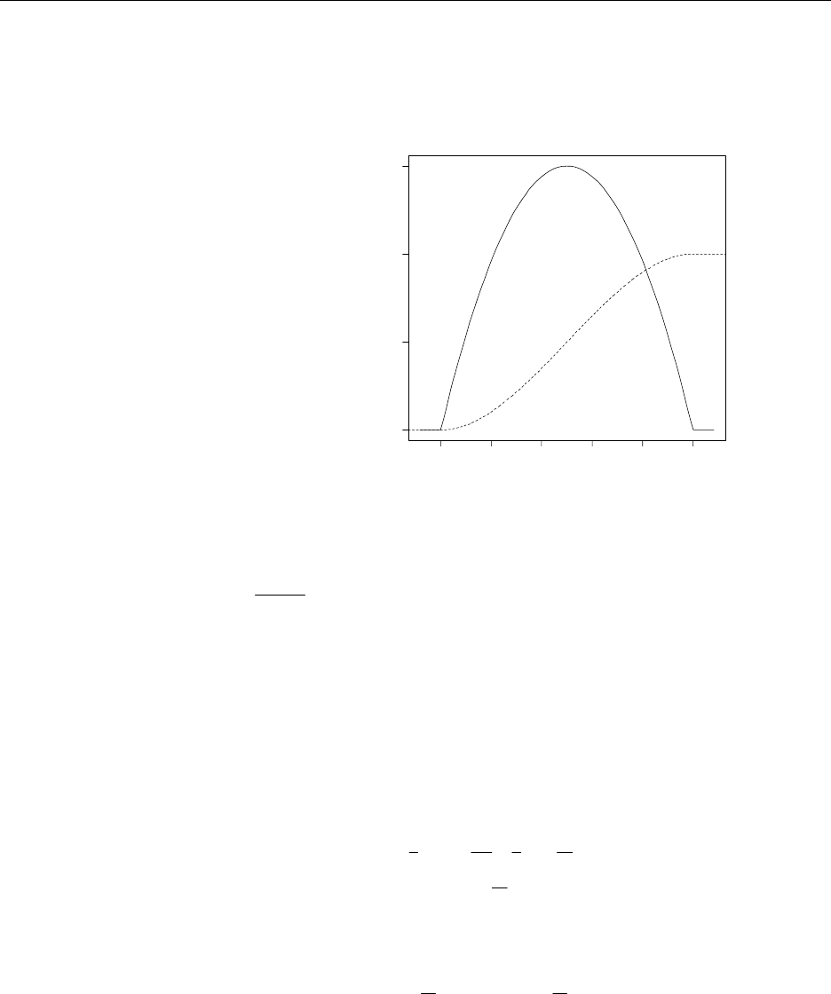
78 Chapter 4: Continuous Variables and Their Probability Distributions
Instructor’s Solutions Manual
4.126 a. ∫−=−=
y
yydtttyF
0
322 23)66()( , 0 ≤ y ≤ 1. F(y) = 0 for y < 0 and F(y) = 1 for y > 1.
b. Solid line: f(y); dashed line: F(y)
0.0 0.2 0.4 0.6 0.8 1.0
0.0 0.5 1.0 1.5
y
c. 396.25.75.092.192.1)5(.)8(.)8.5(.
=
+
−
−
=
−=≤≤ FFYP .
4.127 For α = β = 1, 10,1)1()( 1111
)1()1(
)2( ≤≤=−= −−
ΓΓ
Γyyyyf , which is the uniform distribution.
4.128 The random variable Y = weekly repair cost (in hundreds of dollars) has a beta
distribution with α = 1 and β = 3. We require the 90th percentile of this distribution:
.1.)1()1(3)( 3
9.
1
2
9.
9.
=φ−=−=φ> ∫
φ
dyyYP
Therefore, 9.
φ = 1 – (.1)1/3 = .5358. So, the budgeted cost should be $53.58.
4.129 E(C) = 10 + 20E(Y) + 4E(Y2) = 10 + 20
(
)
3
1 + 4
(
)
9
1
4*9
2
+
= 3
52
V(C) = E(C2) – [E(C)]2 = E[(10 + 20Y + 4Y2)2] –
(
)
2
3
52
E[(10 + 20Y + 4Y2)2] = 100 + 400E(Y) + 480E(Y2) + 160E(Y3) + 16E(Y4)
Using mathematical expectation, E(Y3) = 10
1 and E(Y4) = 15
1. So,
V(C) = E(C2) – [E(C)]2 = (100 + 400/3 + 480/6 + 160/10 + 16/15) – (52/3)2 = 29.96.
www.elsolucionario.net

Chapter 4: Continuous Variables and Their Probability Distributions 79
Instructor’s Solutions Manual
4.130 To find the variance σ2 = E(Y2) – μ2:
E(Y2) = )1)((
)1(
)2(
)()2(
)()(
)(
1
1
0
1
)()(
)( )1( +β+αβ+α
α+α
β++αΓ
βΓ+αΓ
βΓαΓ
β+αΓ
−β+α
βΓαΓ
β+αΓ ==−
∫dyyy
σ2 =
()
)1()(
2
)1)((
)1(
2+β+αβ+α
αβ
β+αα
+β+αβ+α
α+α =− .
4.131 This is the same beta distribution used in Ex. 4.129.
a. P(Y < .5) =
]
5.
0
2
5.
0
2)1(2 yydyy −=−
∫ = .75
b. E(Y) = 1/3, V(Y) = 1/18, so σ = 18/1 = .2357.
4.132 Let Y = proportion of weight contributed by the fine powders
a. E(Y) = .5, V(Y) = 9/(36*7) = 1/28
b. E(Y) = .5, V(Y) = 4/(16*5) = 1/20
c. E(Y) = .5, V(Y) = 1/(4*3) = 1/12
d. Case (a) will yield the most homogenous blend since the variance is the smallest.
4.133 The random variable Y has a beta distribution with α = 3, β = 5.
a. The constant 105
!4!2
!7
)5()3(
)53( === ΓΓ
+Γ
c.
b. E(Y) = 3/8.
c. V(Y) = 15/(64*9) = 5/192, so σ = .1614.
d. P(Y > .375 + 2(.1614)) = P(Y > .6978) = .02972.
4.134 a. If α = 4 and β = 7, then we must find
P(Y ≤ .7) = ∑
=
−
⎟
⎟
⎠
⎞
⎜
⎜
⎝
⎛
=10
4
10
)3(.)7(.
10
)7(.
i
ii
i
F = P(4 ≤ X ≤ 10), for the random variable X
distributed as binomial with n = 10 and p = .7. Using Table I in Appendix III, this is
.989.
b. Similarly, F(.6) = P(12 ≤ X ≤ 25), for the random variable X distributed as binomial
with n = 25 and p = .6. Using Table I in Appendix III, this is .922.
c. Similar answers are found.
4.135 a. P(Y1 = 0) = (1 – p1)n > P(Y2 = 0) = (1 – p2)n, since p1 < p2.
b. P(Y1 ≤ k) = 1 – P(Y1 ≥ k + 1) = ∫
∑−+
−
−=−
⎟
⎟
⎠
⎞
⎜
⎜
⎝
⎛
−
−−
−
+=
1
0
1
11
1),1(
)1(
1)1(1
pknk
ini
n
ki knkB
tt
pp
i
n
= 1 – P(X ≤ p1) = P(X > p1), where is X beta with parameters k + 1, n – k.
c. From part b, we see the integrands for P(Y1 ≤ k) and P(Y2 ≤ k) are identical but since
p1 < p2, the regions of integration are different. So, Y2 is “stochastically greater” than Y1.
www.elsolucionario.net

80 Chapter 4: Continuous Variables and Their Probability Distributions
Instructor’s Solutions Manual
4.136 a. Observing that the exponential distribution is a special case of the gamma distribution,
we can use the gamma moment–generating function with α = 1 and β = θ:
t
tm θ−
=1
1
)(, t < 1/θ.
b. The first two moments are found by 2
)1(
)( t
tm θ−
θ
=
′, E(Y) = θ=
′
)0(m.
3
)1(
2
)( t
tm θ−
θ
=
′′ , E(Y2) = 2
2)0( θ=
′′
m. So, V(Y) = 2θ2 – θ2 = θ2.
4.137 The mgf for U is )()()()()( )()( atmeeeEeEeEtm btYatbtbaYttU
U==== +. Thus,
)()()( atmaeatmbetm btbt
U′
+=
′. So, )()0()0( UEabmabmU=μ+
=
′
+
=
′
.
)()()()()( 22 atmeaatmabeatmabeatmebtm btbtbtbt
U′′
+
′
+
′
+=
′′ , so
)()(2)0( 2222 UEYEaabbmU=+μ+=
′′ .
Therefore, V(U) = )(2 222 YEaabb +μ+ – 2
)( μ+ ab = 22222 ])([ σ=μ− aYEa .
4.138 a. For U = Y – μ, the mgf )(tmUis given in Example 4.16. To find the mgf for Y = U + μ,
use the result in Ex. 4.137 with a = 1, b = – μ:
2/
22
)()( tt
U
t
Yetmetm σ+μμ− ==
b. 2/2 22
)()( tt
Yettm σ+μ
σ+μ=
′, so
μ
=
′
)0(
Y
m
2/22/22 2222
)()( tttt
Yeettm σ+μσ+μ σ+σ+μ=
′′ , so 22
)0( σ+μ=
′′
Y
m. Finally, V(Y) = σ2.
4.139 Using Ex. 4.137 with a = –3 and b = 4, it is trivial to see that the mgf for X is
2/9)34(4 22
)3()( ttt
Xetmetm σ+μ−
=−= .
By the uniqueness of mgfs, X is normal with mean 4 – 3μ and variance 9σ2.
4.140 a. Gamma with α = 2, β = 4
b. Exponential with β = 3.2
c. Normal with μ = –5, σ2 = 12
4.141 )( 12
12
2
1
12
)()( θ−θ −
θ
θ
θ−θ
θθ
=== ∫teee
tY tt
ty dyeEtm .
www.elsolucionario.net

Chapter 4: Continuous Variables and Their Probability Distributions 81
Instructor’s Solutions Manual
4.142 a. t
e
Y
t
tm 1
)( −
=
b. From the cited exercises, at
e
W
at
tm 1
)( −
=. From the uniqueness property of mgfs, W is
uniform on the interval (0, a).
c. The mgf for X is at
e
X
at
tm −−
−
=1
)( , which implies that X is uniform on the interval (–a, 0).
d. The mgf for V is at ee
at
e
bt
V
bttabat
etm −− +
== )(
1
)( , which implies that V is uniform on the
interval (b, b + a).
4.143 The mgf for the gamma distribution is α−
β−= )1()( ttm . Thus,
1
)1()( −α−
β−αβ=
′ttm , so )()0( YEm
=
α
β
=
′
22 )1()1()( −α−
β−αβ+α=
′′ ttm , so )()1()0( 22 YEm =αβ+α=
′′ . So,
V(Y) = .)()1( 222 αβ=αβ−αβ+α
4.144 a. The density shown is a normal distribution with μ = 0 and σ2 = 1. Thus, π= 2/1k.
b. From Ex. 4.138, the mgf is 2/
2
)( t
etm =.
c. E(Y) = 0 and V(Y) = 1.
4.145 a.
]
.)( 5
2
00
2/5
5
2
2/32/3 === ∫
ℵ−
∞−
yyyT edyeeeE
b. 1,)()(
0
1
1−>=== ∫
∞−
+tdyeeeEtm t
ytytY .
c. By using the methods with mgfs, E(Y) = –1, E(Y2) = 2, so V(Y) = 2 – (–1)2 = 1.
4.146 We require P(|Y– μ| ≤ kσ) ≥ .90 = 1 – 1/k2. Solving for k, we see that k = 3.1622. Thus,
the necessary interval is |Y– 25,000| ≤ (3.1622)(4000) or 12,351 ≤ 37,649.
4.147 We require P(|Y– μ| ≤ .1) ≥ .75 = 1 – 1/k2. Thus, k = 2. Using Tchebysheff’s inequality,
1 = kσ and so σ = 1/2.
4.148 In Exercise 4.16, μ = 2/3 and σ = 9/2 = .4714. Thus,
P(|Y – μ| ≤ 2σ) = P(|Y – 2/3| ≤ .9428) = P(–.2761 ≤ Y ≤ 1.609) = F(1.609) = .962.
Note that the negative portion of the interval in the probability statement is irrelevant
since Y is non–negative. According to Tchsebysheff’s inequality, the probability is at
least 75%. The empirical rule states that the probability is approximately 95%. The
above probability is closest to the empirical rule, even though the density function is far
from mound shaped.
www.elsolucionario.net

82 Chapter 4: Continuous Variables and Their Probability Distributions
Instructor’s Solutions Manual
4.149 For the uniform distribution on (θ1, θ2), μ = 2
21 θ+θ and σ2 = 12
)( 2
12 θ−θ . Thus,
2σ = 3
)( 12 θ−θ .
The probability of interest is
P(|Y – μ| ≤ 2σ) = P(μ – 2σ ≤ Y ≤ μ + 2σ) = P(2
21 θ+θ –3
)( 12 θ−θ ≤ Y ≤ 2
21 θ+θ +3
)( 12 θ−θ )
It is not difficult to show that the range in the last probability statement is greater than the
actual interval that Y is restricted to, so
P(2
21 θ+θ –3
)( 12 θ−θ ≤ Y ≤ 2
21 θ+θ +3
)( 12 θ−θ ) = P(θ1 ≤ Y ≤ θ2) = 1.
Note that Tchebysheff’s theorem is satisfied, but the probability is greater than what is
given by the empirical rule. The uniform is not a mound–shaped distribution.
4.150 For the exponential distribution, μ = β and σ2 = β2. Thus, 2σ = 2β. The probability of
interest is
P(|Y – μ| ≤ 2σ) = P(μ – 2σ ≤ Y ≤ μ + 2σ) = P(–β ≤ Y ≤ 3β) = P(0 ≤ Y ≤ 3β)
This is simply F(3β) = 1 – e–3β = .9502. The empirical rule and Tchebysheff’s theorem
are both valid.
4.151 From Exercise 4.92, E(C) = 1000 and V(C) = 2,920,000 so that the standard deviation is
000,920,2 = 1708.80. The value 2000 is only (2000 – 1100)/1708.8 = .53 standard
deviations above the mean. Thus, we would expect C to exceed 2000 fair often.
4.152 We require P(|L– μ| ≤ kσ) ≥ .89 = 1 – 1/k2. Solving for k, we have k = 3.015. From Ex.
4.109, μ = 276 and σ = 218.32. The interval is
|L– 276| ≤ 3.015(218.32) or (–382.23, 934.23)
Since L must be positive, the interval is (0, 934.23)
4.153 From Ex. 4.129, it is shown that E(C) = 3
52 and V(C) = 29.96, so, the standard deviation
is 96.29 = 5.474. Thus, using Tchebysheff’s theorem with k = 2, the interval is
|Y – 3
52 | ≤ 2(5.474) or (6.38, 28.28)
4.154 a. μ = 7, σ2 = 2(7) = 14.
b. Note that σ = 14 = 3.742. The value 23 is (23 – 7)/3.742 = 4.276 standard
deviations above the mean, which is unlikely.
c. With α = 3.5 and β = 2, P(Y > 23) = .00170.
www.elsolucionario.net

Chapter 4: Continuous Variables and Their Probability Distributions 83
Instructor’s Solutions Manual
4.155 The random variable Y is uniform over the interval (1, 4). Thus, 3
1
)( =yf for 1 ≤ y ≤ 4
and 0)( =yf elsewhere. The random variable C = cost of the delay is given as
⎩
⎨
⎧
≤<−+
≤≤
== 42)2(20100
21100
)( yY
y
YgC
Thus, dyydydyyfygYgECE ∫∫∫ −++===
∞
∞−
4
2
3
1
2
1
3
100 )]2(20100[)()()]([)( = $113.33.
4.156 Note that Y is a discrete random variable with probability .2 + .1 = .3 and it is continuous
with probability 1 – .3 = .7. Hence, by using Definition 4.15, we can write Y as a mixture
of two random variables X1 and X2. The random variable X1 is discrete and can assume
two values with probabilities P(X1 = 3) = .2/.3 = 2/3 and P(X1 = 6) = .1/.3 = 1/3. Thus,
E(X1) = 3(2/3) + 6(1/3) = 4. The random variable X2 is continuous and follows a gamma
distribution (as given in the problem) so that E(X2) = 2(2) = 4. Therefore,
E(Y) = .3(4) + .7(4) = 4.
4.157 a. The distribution function for X is
⎪
⎪
⎩
⎪
⎪
⎨
⎧
≥
<≤−=
<
=−−
∫
2001
20001
00
)( 100/
0
100/
100
1
x
xedxe
x
xF x
xt.
b. E(X) = )200(1353.
200
0
100/
100
1+
∫−dxex x = 86.47, where .1353 = P(Y > 200).
4.158 The distribution for V is gamma with α = 4 and β = 500. Since there is one discrete point
at 0 with probability .02, using Definition 4.15 we have that c1 = .02 and c2 = .98.
Denoting the kinetic energy as K = 2
mV2 we can solve for the expected value:
E(K)= (.98) 2
mE(V2) = (.98) 2
m{V(V) + [E(V)]2} = (.98) 2
m{4(500)2 + 20002} = 2,450,000m.
4.159 a. The distribution function has jumps at two points: y = 0 (of size .1) and y = .5 (of size
.15). So, the discrete component of F(y) is given by
⎪
⎩
⎪
⎨
⎧
≥
<≤=
<
=+
5.1
504.
00
)( 15.1.
1.
1
y
y
y
yF
The continuous component of F(y) can then by determined:
⎪
⎪
⎩
⎪
⎪
⎨
⎧
≥
<≤−
<≤
<
=
11
15.3/)14(
5.03/4
00
)(
2
2
y
yy
yy
y
yF
www.elsolucionario.net

84 Chapter 4: Continuous Variables and Their Probability Distributions
Instructor’s Solutions Manual
b. Note that c1 = .1 + .15 = .25. So, )(75.0)(25.0)( 21 yFyFyF
+
=
.
c. First, observe that ⎩
⎨
⎧
≥
<≤
=
′
=5.3/4
5.03/8
)()( 22 y
yy
yFyf . Thus,
533.3/43/8)5)(.6(.25.)(
1
5.
5.
0
2=++= ∫∫ dyydyyYE . Similarly, E(Y2) = .3604 so
that V(Y) = .076.
4.160 a. 1if1)(,0if0)(,11,)(tan)( 2
1
1
2
1
)1(
2
2>=<=≤≤−+== −
π
−
+π
∫yyFyyFyydyyF
y
y.
b. Find E(Y) directly using mathematical expectation, or observe that f (y) is symmetric
about 0 so using the result from Ex. 4.27, E(Y) = 0.
4.161 Here, μ = 70 and σ = 12 with the normal distribution. We require 9.
φ
, the 90th percentile
of the distribution of test times. Since for the standard normal distribution, P(Z < z0) = .9
for z0 = 1.28, thus
9.
φ
= 70 + 12(1.28) = 85.36.
4.162 Here, μ = 500 and σ = 50 with the normal distribution. We require 01.
φ, the 1st percentile
of the distribution of light bulb lives. For the standard normal distribution, P(Z < z0) =
.01 for z0 = –2.33, thus
01.
φ
= 500 + 50(–2.33) = 383.5
4.163 Referring to Ex. 4.66, let X = # of defective bearings. Thus, X is binomial with n = 5 and
p = P(defective) = .073. Thus,
P(X > 1) = 1 – P(X = 0) = 1 – (.927)5 = .3155.
4.164 Let Y = lifetime of a drill bit. Then, Y has a normal distribution with μ = 75 hours and
σ = 12 hours.
a. P(Y < 60) = P(Z < –1.25) = .1056
b. P(Y ≥ 60) = 1 – P(Y < 60) = 1 – .1056 = .8944.
c. P(Y > 90) = P(Z > 1.25) = .1056
4.165 The density function for Y is in the form of a gamma density with α = 2 and β = .5.
a. c = 2
)5)(.2(
1
Γ = 4.
b. E(Y) = 2(.5) = 1, V(Y) = 2(.5)2 = .5.
c. 2
)5.1(
1
)( t
tm −
=, t < 2.
www.elsolucionario.net

Chapter 4: Continuous Variables and Their Probability Distributions 85
Instructor’s Solutions Manual
4.166 In Example 4.16, the mgf is 2/
22
)( σ
=t
etm . The infinite series expansion of this is
()
(
)
(
)
"" ++++=++++= σσσσσσ
4882!3
1
3
2!2
1
2
22
664422222222 11)( tttttt
tm
Then, μ1 = coefficient of t, so μ1 = 0
μ2 = coefficient of t2/2!, so μ2 = σ2
μ3 = coefficient of t3/3!, so μ3 = 0
μ4 = coefficient of t4/4!, so μ4 = 3σ4
4.167 For the beta distribution,
E(Yk) = )(
)()(
)()(
)(
1
0
11
)()(
)(
1
0
11
)()(
)( )1()1( β+α+Γ
βΓα+Γ
βΓαΓ
β+αΓ
−β−α+
βΓαΓ
β+αΓ
−β−α
βΓαΓ
β+αΓ =−=− ∫∫ k
k
kk dyyydyyyy .
Thus, E(Yk) = )()(
)()(
β+α+ΓαΓ
α+Γβ+αΓ
kk.
4.168 Let T = length of time until the first arrival. Thus, the distribution function for T is given
by F(t) = P(T ≤ t) = 1 – P(T > t) = 1 – P[no arrivals in (0, t)] = 1 – P[N = 0 in (0, t)]
The probability P[N = 0 in (0, t)] is given by !0
)( 0t
et λ−
λ = e–λt. Thus, F(t) = 1 – e–λt and
f (t) = λe–λt, t > 0.
This is the exponential distribution with β = 1/λ.
4.169 Let Y = time between the arrival of two call, measured in hours. To find P(Y > .25), note
that λt = 10 and t = 1. So, the density function for Y is given by f (y) = 10e–10y, y > 0.
Thus, P(Y > .25) = e–10(.25) = e–2.5 = .082.
4.170 a. Similar to Ex. 4.168, the second arrival will occur after time t if either one arrival has
occurred in (0, t) or no arrivals have occurred in (0, t). Thus:
P(U > t) = P[one arrival in (0, t)] + P[no arrivals in (0, t)] = !0
)( 0t
et λ−
λ + !1
)( 1t
et λ−
λ. So,
F(t) = 1 – P(U > t) = 1 – !0
)( 0t
et λ−
λ + !1
)( 1t
et λ−
λ = 1 – t
et λ−
+λ )1(.
The density function is given by t
tetFtf λ−
λ=
′
=2
)()(, t > 0. This is a gamma density
with α = 2 and β = 1/λ.
b. Similar to part a, but let X = time until the kth arrival. Thus, P(X > t) = ∑
−
=
λλ−
1
0
!
)(
k
nnet tn . So,
F(t) = 1 – ∑
−
=
λλ−
1
0
!
)(
k
nnet tn .
www.elsolucionario.net

86 Chapter 4: Continuous Variables and Their Probability Distributions
Instructor’s Solutions Manual
The density function is given by
⎥
⎦
⎤
⎢
⎣
⎡−λ=
⎥
⎦
⎤
⎢
⎣
⎡+λ−−=
′
=∑∑∑∑ −
=
−
=
−
λλ
λ−
−
=
−
=
−
λ
λ−
λ
λ− −
−1
0
1
1
)!1(
)(
!
)(
1
0
1
1
)!1(!
)( 1
1
)()(
k
n
k
nn
t
n
t
t
k
n
k
nnt
t
n
t
tnn
nn
neeetFtf . Or,
0,)( )!1(
1>= −
λλ−− ttf ket tkk . This is a gamma density with α = k and β = 1/λ.
4.171 From Ex. 4.169, W = waiting time follow an exponential distribution with β = 1/2.
a. E(W) = 1/2, V(W) = 1/4.
b. P(at least one more customer waiting) = 1 – P(no customers waiting in three minutes)
= 1 – e–6.
4.172 Twenty seconds is 1/5 a minute. The random variable Y = time between calls follows an
exponential distribution with β = .25. Thus:
P(Y > 1/5) = ∫
∞
−− =
5/1
5/44
4edye y.
4.173 Let R = distance to the nearest neighbor. Then,
P(R > r) = P(no plants in a circle of radius r)
Since the number of plants in a area of one unit has a Poisson distribution with mean λ,
the number of plants in a area of πr2 units has a Poisson distribution with mean λπr2.
Thus,
F(r) = P(R ≤ r) = 1 – P(R > r) = 1 – .
2
r
eλπ−
So, 2
2)()( r
retFrf λπ−
λπ=
′
=, r > 0.
4.174 Let Y = interview time (in hours). The second applicant will have to wait only if the time
to interview the first applicant exceeds 15 minutes, or .25 hour. So,
P(Y > .25) = .61.2 5.
25.
2== −
∞
−
∫edye y
4.175 From Ex. 4.11, the median value will satisfy 5.2/)( 2== yyF . Thus, the median is
given by 414.12 =.
4.176 The distribution function for the exponential distribution with mean β is .1)( /β−
−= y
eyF
Thus, we require the value y such that 5.1)( /=−= β− y
eyF . Solving for y, this is βln(2).
www.elsolucionario.net
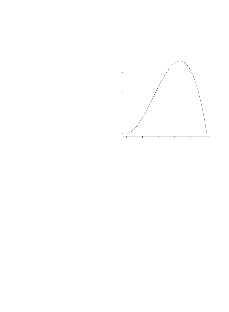
Chapter 4: Continuous Variables and Their Probability Distributions 87
Instructor’s Solutions Manual
4.177 a. 2.07944 = 3ln(2)
b. 3.35669 < 4, the mean of the gamma distribution.
c. 46.70909 < 50, the mean of the gamma distribution.
d. In all cases the median is less than the mean, indicating right skewed distributions.
4.178 The graph of this beta density is above.
0.0 0.2 0.4 0.6 0.8 1.0
0.0 0.5 1.0 1.5
y
f(y)
a. Using the relationship with binomial probabilities,
P(.1 ≤ Y ≤ .2) = 4(.2)3(.8) + (.2)4 – 4(.1)3(.9) – (.1)4 = .0235.
b. P(.1 ≤ Y ≤ .2) = .9963 – .9728 = .0235, which is the same answer as above.
c. 05.
φ = .24860, 95.
φ = .90239.
d. P(05.
φ ≤ Y ≤ 95.
φ) = .9.
4.179 Let X represent the grocer’s profit. In general, her profit (in cents) on a order of 100k
pounds of food will be X = 1000Y – 600k as long as Y < k. But, when Y ≥ k the grocer’s
profit will be X = 1000k – 600k = 400k. Define the random variable Y′ as
⎩
⎨
⎧
≥
<≤
=
′kYk
kYY
Y0
Then, we can write g(Y′) = X = 1000Y′ + 600k. The random variable Y′ has a mixed
distribution with one discrete point at k. Therefore,
3
1
2
113)()( kdyykYPkYPc
k
−==≥==
′
=∫, so that c2 = k3.
Thus, ⎩
⎨
⎧
≥
<≤
=ky
ky
yF 1
00
)(
2 and 3
3
3
0
2
3
21 )0|()( k
y
k
dtt
y
kYyYPyF =
∫
=<
′
≤≤= , 0 ≤ y < k.
Thus, from Definition 4.15,
∫−+−=+=
′
=
k
k
ydykykkkYgEcYgEcYgEXE
0
3
33
2211 3
2
)6001000(400)1()]([)]([)]([)( ,
or E(X) = 400k – 250k2. This is maximized at k = (.4)1/3 = .7368. (2nd derivative is –.)
www.elsolucionario.net

88 Chapter 4: Continuous Variables and Their Probability Distributions
Instructor’s Solutions Manual
4.180 a. Using the result of Ex. 4.99, P(Y ≤ 4) = 1 – .7619.
2
0
!
44=
∑
=
−
yy
e
y
b. A similar result is found.
4.181 The mgf for Z is 2/
)( 2
)/()()()( t
Y
tt
Zt
ZetmeeEeEtm y=σ=== σ
μ
σ
μ− −, which is a mgf for a
normal distribution with μ = 0 and σ = 1.
4.182 a. P(Y ≤ 4) = P(X ≤ ln4) = P[Z ≤ (ln4 – 4)/1] = P(Z ≤ –2.61) = .0045.
b. P(Y > 8) = P(X > ln8) = P[Z > (ln8 – 4)/1] = P(Z > –1.92) = .9726.
4.183 a. E(Y) = 112/163 ee =
+ (598.74 g), V(Y) = 22 16 4
(1)10ee
−
−.
b. With k = 2, the interval is given by E(Y) ± 2 )(YV or 598.74 ± 3,569,038.7. Since the
weights must be positive, the final interval is (0, 3,570,236.1)
c. P(Y < 598.74) = P(lnY < 6.3948) = P[Z < (6.3948 – 3)/4] = P(Z < .8487) = .8020
4.184 The mgf forY is ∫∫∫∫ ∞
−−
∞
+
∞
−
∞
+=+==
0
)1(
2
1
0
)1(
2
1
0
2
1
0
2
1
)()( dyedyedyeedyeeeEtm tyytytyytytY
Y.
This simplifies to 2
1
1
)( t
Ytm −
=. Using this, E(Y) = 0
)1(
2
02
)( =
−
==
′t
t
t
t
tm = 0.
4.185 a. 1)1()()1()()( 21 =−+=−+= ∫∫∫ ∞
∞−
∞
∞−
∞
∞−
aadyyfadyyfadyyf .
b. i. 2121 )1()()1()()()( μ−+μ=−+== ∫∫∫
∞
∞−
∞
∞−
∞
∞−
aadyyyfadyyyfadyyyfYE
ii. ))(1()()()1()()( 2
2
2
2
2
1
2
12
2
1
2
2σ+μ−+σ+μ=−+= ∫∫
∞
∞−
∞
∞−
aadyyfyadyyfyaYE . So,
V(Y) = E(Y2) – [E(Y)]2 = 2
21
2
2
2
2
2
1
2
1])1([))(1()( μ−+μ−σ+μ−+σ+μ aaaa , which
simplifies to 2
21
2
2
2
1])[1()1( μ−μ−+σ−+σ aaaa
4.186 For m = 2, dye
y
yYE yα−
∞
∫α
=/
0
2
2
)( . Let u = y2/α. Then, du
u
dy 2
α
=. Then,
2
)2/1(
)2/3(
2
)(
0
2/1/
0
22Γα
=Γα=α=
α
=∫∫
∞
−α−
∞
dueudye
y
YE uy . Using similar methods,
it can be shown that α=)( 2
YE so that ⎥
⎦
⎤
⎢
⎣
⎡π
−α=
⎥
⎦
⎤
⎢
⎣
⎡Γα
−α= 4
1
2
)2/1(
)(
2
YV , since it will
be shown in Ex. 4.196 that Γ(1/2) = π.
www.elsolucionario.net

Chapter 4: Continuous Variables and Their Probability Distributions 89
Instructor’s Solutions Manual
4.187 The density for Y = the life length of a resistor (in thousands of hours) is
.0,)( 10
210/
2>= −yyf y
ye
a. P(Y > 5) =
]
5.2
5
10/
5
10
22
10/
2−
∞
−
∞
=−=
∫−eedy y
ye y = .082.
b. Let X = # of resistors that burn out prior to 5000 hours. Thus, X is a binomial random
variable with n = 3 and p = .082. Then, P(X = 1) = 3(1 – .082)(.082)2 = .0186.
4.188 a. This is the exponential distribution with β = α.
b. Using the substitution u = ym/α in the integrals below, we find:
)/11()( /1
0
/1/1/
0
mdueudyeyYE mummym
mm+Γα=α== ∫∫
∞
−α−
∞
α
)/21()( /1
0
/2/2/1
0
2mdueudyeyYE mummym
mm+Γα=α== ∫∫
∞
−α−+
∞
α.
Thus,
)]/11()/21([)( 2/2 mmYV m+Γ++Γα= .
4.189 Since this density is symmetric about 0, so using the result from Ex. 4.27, E(Y) = 0.
Also, it is clear that V(Y) = E(Y2). Thus,
1
1
)2/)2(,2/1(
)2/)2(,2/3(
)1(
)2/)2(,2/1(
1
)( 2/)4(22
1
1
2
−
=
−
−
=−
−
=−
−
∫nnB
nB
dyyy
nB
YE n = V(Y). This
equality follows after making the substitution u = y2.
4.190 a. For the exponential distribution, β−
β
=/
1
)( t
etf and β−
−= /
1)( t
etF . Thus, r(t) = 1/β.
b. For the Weibull, α−
α
−
=/
1
)( m
my
my eyf and α−
−= /
1)( m
y
eyF . Thus, α
−
=1
)( m
my
tr , which is
an increasing function of t when m > 1.
4.191 a. G(y) = )(1
)()(
)(
)(
)|( cF
cFyF
cYP
yYcP
cYyYP −
−
=
≥
≤
≤
=≥≤ .
b. Refer to the properties of distribution functions; namely, show G(–∞) = 0, G(∞) = 1,
and for constants a and b such that a ≤ b, G(a) ≤ G(b).
c. It is given that 3/
2
1)( y
eyF −
−= . Thus, by using the result in part b above,
P(Y ≤ 4 | Y ≥ 2) = 4
2/2
2/23/4
1
1(1
2
22
−
−
−−
−=
−−− e
e
ee .
4.192 a.
()
dvevVE KTmv
KT
m)2/(
0
3
2/3
2
2
4)( −
∞
π∫
π= . To evaluate this integral, let u =
()
KT
m
v2
2 so that
dudv u
m
KT
2
12
= to obtain ππ
∞
−
π=Γ== ∫m
KT
m
KT
u
m
KT duueVE 22
0
22)2(22)( .
www.elsolucionario.net

90 Chapter 4: Continuous Variables and Their Probability Distributions
Instructor’s Solutions Manual
b.
()
dvevmVmEmVE KTmv
KT
m)2/(
0
4
2/3
2
2
2
1
2
2
12
2)()( −
∞
π∫
π== . Here, let u =
()
KT
m
v2
2 so that
dudv u
m
KT
2
12
= to obtain KTmVE KT
2
3
2
5
2
2
2
1)()( =Γ= π (here, we again used the result
from Ex. 4.196 where it is shown that Γ(1/2) = π).
4.193 For 100/
100
1
)( y
eyf −
=, we have that 100/
1)( y
eyF −
−= . Thus,
150)50|(
50
100
1100/
2/1 ==≥ ∫
∞−
−dyYYE y
ye
e.
Note that this value is 50 + 100, where 100 is the (unconditional) mean of Y. This
illustrates the memoryless property of the exponential distribution.
4.194 ∫∫∫∫ ∞
∞−
∞
∞−
+−
π
∞
∞−
−
π
∞
∞−
−
π=
⎥
⎦
⎤
⎢
⎣
⎡
⎥
⎦
⎤
⎢
⎣
⎡dxdyedxedye yxuuxuy )()2/1(
2
1
)2/1(
2
1
)2/1(
2
12222 . By changing to polar
coordinates, x2 + y2 = r2 and dxdy = rdrdθ. Thus, the desired integral becomes
∫∫
π∞
−
π=θ
2
0
1
0
)2/1(
2
12
u
ur drdre .
Note that the result proves that the standard normal density integrates to 1 with u = 1.
4.195 a. First note that W = (Z2 + 3Z)2 = Z4 + 6Z3 + 9Z2. The odd moments of the standard
normal are equal to 0, and E(Z2) = V(Z) + [E(Z)]2 = 1 + 0 = 1. Also, using the result in
Ex. 4.199, E(Z4) = 3 so that E(W) = 3 + 9(1) = 12.
b. Applying Ex. 4.198 and the result in part a:
9.1)( )( =−≥≤ w
WE
wWP ,
so that w = 120.
4.196
[]
π=π=π===Γ ∫∫∫
∞
−
π
−
∞∞
−−
2
1
0
)2/1(
2
1
)2/1(
00
2/1 2222)2/1( 22 dxedxedyey xxy (relating
the last integral to that P(Z > 0), where Z is a standard normal random variable).
4.197 a. Let y = sin2θ, so that dy = 2sinθcosθdθ. Thus,
∫∫∫
π
−β−α
π
−β−α−β−α θθ=θθ−θ=−=βα
2/
0
1212
2/
0
1222
1
0
11 cossin2)sin1(sin2)1(),( dddyyyB , using
the trig identity θ=θ− 22 cossin1.
www.elsolucionario.net

Chapter 4: Continuous Variables and Their Probability Distributions 91
Instructor’s Solutions Manual
b. Following the text, ∫∫∫∫
∞∞
−−−β−α
∞
−−β
∞
−−α ==βΓαΓ
00
11
0
1
0
1
)()( dydzezydzezdyey zyzy . Now,
use the transformation θ=θ= 2222 sin,cos rxry so that θθ= sincos4 3
rdydz .
Following this and using the result in part a, we find
∫
∞
−−β+α
βα=βΓαΓ
0
)1(2 2),()()( 2rdrerB r.
A final transformation with x = r2 gives )(),()()(
β
+
α
Γ
β
α
=
β
Γ
α
Γ
B, proving the result.
4.198 Note that
)|)((|)()(|)(|)(|)(||])([|
|)(||)(|
kYgkPdyykfdyyfygdyyfygYgE
kygkyg
>=>≥= ∫∫∫∞
>
∞
∞−
∞
>
,
Since kyg >|)(| for this integral. Therefore,
kYgEkYgP /|))((|1)|)((|
−
≥
≤
.
4.199 a. Define 2/12 2
)( yi eyyg −−
= for positive integer values of i. Observe that )()( ygyg
−
=
−
so that g(y) is an odd function. The expected value E(Z2i–1) can be written
as ∫
∞
∞−
π
−=dyygZE i)()( 2
1
12 which is thus equal to 0.
b. Now, define 2/2 2
)( yieyyh −
= for positive integer values of i. Observe that
)()( yhyh =− so that h(y) is an even function. The expected value E(Z2i) can be written
as ∫∫
∞
π
∞
∞−
π==
0
2
2
2
1
2)()()( dyyhdyyhZE i. Therefore, the integral becomes
)2/1(22)( 1
0
2/1
1
0
2/2
2
2
22+Γ=== π
∞
−−
π
∞
−
π∫∫ idwewdyeyZE iwiiyii .
In the last integral, we applied the transformation w = z2/2.
c. 1)2/1(2)2/11(2)( 1
1
1
1
2=π=+Γ= ππ
ZE
3)2/1)(2/3(2)2/12(2)( 2
1
2
1
4=π=+Γ= ππ
ZE
15)2/1)(2/3)(2/5(2)2/13(2)( 3
1
3
1
6=π=+Γ= ππ
ZE
105)2/1)(2/3)(2/5)(2/7(2)2/14(2)( 4
1
4
1
8=π=+Γ= ππ
ZE .
d. The result follows from:
(
)
)()2/1(2)2/1(2)2/1(2)12( 2
1ii
i
ij
i
i
ij
i
ij
ZEijjj =+Γ=−=−=− π
=== ∏∏∏ .
www.elsolucionario.net

92 Chapter 4: Continuous Variables and Their Probability Distributions
Instructor’s Solutions Manual
4.200 a. )()(
)()(
)(
)()(
)()(
)(
1
0
11
)()(
)( )1()( β+α+ΓαΓ
α+Γβ+αΓ
β+α+Γ
βΓα+Γ
βΓαΓ
β+αΓ
−β−α+
βΓαΓ
β+αΓ ==−= ∫aa
a
a
aa dyyyYE .
b. The value α + a must be positive in the beta density.
c. With a = 1, β+αα
β+α+ΓαΓ
α+Γβ+αΓ == )1()(
)1()(
1)(YE .
d. With a = 1/2, )2/1()(
)2/1()(
2/1 )( β+α+ΓαΓ
α+Γβ+αΓ
=YE .
e. With a = –1, 1
1
)1()(
)1()(
1)( −α
−β+α
−β+αΓαΓ
−αΓβ+αΓ
−==YE , α > 1
With a = –1/2, )2/1()(
)2/1()(
2/1 )( −β+αΓαΓ
−αΓβ+αΓ
−=YE , α > 1/2
With a = –2, )2)(1(
)2)(1(
)2()(
)2()(
2)( −α−α
−β+α−β+α
−β+αΓαΓ
−αΓβ+αΓ
−==YE , α > 2.
www.elsolucionario.net

93
Chapter 5: Multivariate Probability Distributions
5.1 a. The sample space S gives the possible values for Y1 and Y2:
S AA AB AC BA BB BC CA CB CC
(y1, y2) (2, 0) (1, 1) (1, 0) (1, 1) (0, 2) (1, 0) (1, 0) (0, 1) (0, 0)
Since each sample point is equally likely with probably 1/9, the joint distribution for Y1
and Y2 is given by
y1
0 1 2
01/92/91/9
y2 1 2/9 2/9 0
2 1/9 0 0
b. F(1, 0) = p(0, 0) + p(1, 0) = 1/9 + 2/9 = 3/9 = 1/3.
5.2 a. The sample space for the toss of three balanced coins w/ probabilities are below:
Outcome HHH HHT HTH HTT THH THT TTH TTT
(y1, y2) (3, 1) (3, 1) (2, 1) (1, 1) (2, 2) (1, 2) (1, 3) (0, –1)
probability 1/8 1/8 1/8 1/8 1/8 1/8 1/8 1/8
y1
0 1 2 3
–1 1/8 0 0 0
y2 1 0 1/8 2/8 1/8
2 0 1/8 1/8 0
3 0 1/8 0 0
b. F(2, 1) = p(0, –1) + p(1, 1) + p(2, 1) = 1/2.
5.3 Note that using material from Chapter 3, the joint probability function is given by
p(y1, y2) = P(Y1 = y1, Y2 = y2) =
⎟
⎟
⎠
⎞
⎜
⎜
⎝
⎛
⎟
⎟
⎠
⎞
⎜
⎜
⎝
⎛
−−
⎟
⎟
⎠
⎞
⎜
⎜
⎝
⎛
⎟
⎟
⎠
⎞
⎜
⎜
⎝
⎛
3
9
3
234
2121 yyyy , where 0 ≤ y1, 0 ≤ y2, and y1 + y2 ≤ 3.
In table format, this is
y1
0 1 2 3
0 0 3/84 6/84 1/84
y2 1 4/84 24/84 12/84 0
2 12/84 18/84 0 0
3 4/84 0 0 0
www.elsolucionario.net

94 Chapter 5: Multivariate Probability Distributions
Instructor’s Solutions Manual
5.4 a. All of the probabilities are at least 0 and sum to 1.
b. F(1, 2) = P(Y1 ≤ 1, Y2 ≤ 2) = 1. Every child in the experiment either survived or didn’t
and used either 0, 1, or 2 seatbelts.
5.5 a. 1065.3)3/1,2/1(
2/1
0
3/1
0
21121 ==≤≤ ∫∫ dydyyYYP .
b. 5.3)2/(
1
0
2/
0
21112
1
==≤ ∫∫
y
dydyyYYP .
5.6 a.
[]
.125.)5(.1)5.()5.(
5.
0
222
5.
0
5.
0
1
5.
1
1
5.
212121 2
2
=−===+>=>− ∫∫∫∫+
+
dyydyydydyYYPYYP y
y
b. ∫∫∫ −−=−=>−=>−=<
1
5.
22
1
5.
1
/5.
21212121 )/5.1(111)/5.(1)5.(1)5.(
2
dyydydyYYPYYPYYP
y
= 1 – [.5 + .5ln(.5)] = .8466.
5.7 a.
[]
.00426.1)5,1( 51
2
5
1
0
1
1
0
21
5
)(
21
2121 =−=
⎥
⎦
⎤
⎢
⎣
⎡
⎥
⎦
⎤
⎢
⎣
⎡
==>< −−
∞
−−
∞
+− ∫∫∫∫ eedyedyedydyeYYP yyyy
b. .8009.41)3()3( 3
3
0
21
3
0
)(
2121
2
21 =−==−<=<+ −
−
+−
∫∫ edydyeYYPYYP
y
yy
5.8 a. Since the density must integrate to 1, evaluate 14/
21
1
0
1
0
21 ==
∫∫ kdydyyky , so k = 4.
b. 2
2
2
121
00
21221121
21
4),(),( yydtdtttyYyYPyyF
yy
==≤≤= ∫∫ , 0 ≤ y1 ≤ 1, 0 ≤ y2 ≤ 1.
c. P(Y1 ≤ 1/2, Y2 ≤ 3/4) = (1/2)2(3/4)2 = 9/64.
5.9 a. Since the density must integrate to 1, evaluate 16/)1( 21
1
00
2
2
==−
∫∫ kdydyyk
y
, so k = 6.
b. Note that since Y1 ≤ Y2, the probability must be found in two parts (drawing a picture is
useful):
P(Y1 ≤ 3/4, Y2 ≥ 1/2) = ∫∫∫∫ −+−
4/3
2/1
1
12221
1
2/1
1
2/1
2
1
)1(6)1(6
y
dydyydydyy =24/64 + 7/64 = 31/64.
5.10 a. Geometrically, since Y1 and Y2 are distributed uniformly over the triangular region,
using the area formula for a triangle k = 1.
b. This probability can also be calculated using geometric considerations. The area of the
triangle specified by Y1 ≥ 3Y2 is 2/3, so this is the probability.
www.elsolucionario.net

Chapter 5: Multivariate Probability Distributions 95
Instructor’s Solutions Manual
5.11 The area of the triangular region is 1, so with a uniform distribution this is the value of
the density function. Again, using geometry (drawing a picture is again useful):
a. P(Y1 ≤ 3/4, Y2 ≤ 3/4) = 1 – P(Y1 > 3/4) – P(Y2 > 3/4) = 1 –
(
)
(
)()()
32
29
4
1
4
1
2
1
4
1
2
1
2
1=− .
b. P(Y1 – Y2 ≥ 0) = P(Y1 ≥ Y2). The region specified in this probability statement
represents 1/4 of the total region of support, so P(Y1 ≥ Y2) = 1/4.
5.12 Similar to Ex. 5.11:
a. P(Y1 ≤ 3/4, Y2 ≤ 3/4) = 1 – P(Y1 > 3/4) – P(Y2 > 3/4) = 1 –
(
)
(
)()()
8
7
4
1
4
1
2
1
4
1
4
1
2
1=− .
b. .2/12)2/1,2/1(
2/1
0
2/1
0
2121 ==≤≤ ∫∫ dydyYYP
5.13 a. 16
9
30)2/1,2/1( 12
2/1
0
2/1
1
2
21
1
== ∫∫
−
dydyyyF
y
.
b. Note that:
)2/1,2/1()2/1,2/1()1,2/1()1,2/1()2,2/1( 212121 >≤
+
≤
≤
=
≤
≤
== YYPYYPYYPFF
So, the first probability statement is simply )2/1,2/1(F from part a. The second
probability statement is found by
16
4
30)2/1,2/1( 2
1
2/1
1
0
2
2121
2
==>≤ ∫∫
−
dydyyyYYP
y
.
Thus, 16
13
16
4
16
9
)2,2/1( =+=F.
c. .65625.
32
21
32
11
1301)(1)( 12
2/1
0
1
2
212121
1
1
==−=−=≤−=> ∫∫
−
dydyyyYYPYYP
y
y
5.14 a. Since 0),( 21 ≥yyf , simply show ∫∫ =
−
1
0
2
122
2
116
1
1
y
y
dydyyy .
b. ∫∫ ==−<=<+
−
5.
0
1
122
2
11221 16/16)1()1(
1
1
y
y
dydyyyYYPYYP .
5.15 a. 21
2
1
2
21
2
11
1221 2)1,2(
2
1
1
1−−
−− −===>< ∫∫∫∫ eedydyedydyeYYP
y
y
y
y.
b. 2/1)2(
02
2121
2
1==≥ ∫∫
∞∞
−
y
ydydyeYYP .
c. 1
01
212121
2
1
)1()1( −
∞∞
+
−==+≥=≥− ∫∫ edydyeYYPYYP
y
y.
www.elsolucionario.net

96 Chapter 5: Multivariate Probability Distributions
Instructor’s Solutions Manual
5.16 a. 21
1
4/1
2/1
0
2121 )()4/1,2/1( dydyyyYYP ∫∫ +=>< = 21/64 = .328125.
b. 3/1)()1()1( 21
1
0
1
0
212121
2
=+=−≤=≤+ ∫∫
−
dydyyyYYPYYP
y
.
5.17 This can be found using integration (polar coordinates are helpful). But, note that this is
a bivariate uniform distribution over a circle of radius 1, and the probability of interest
represents 50% of the support. Thus, the probability is .50.
5.18
()
1
2
3
2
3
2
2/
1
2
1
1
2/
1
1
4
1
21
2/)(
1
11
8
1
21
2
1
2
1
2121
)1,1( −
−−
−
∞
−
∞
+−
∞∞
==
⎥
⎦
⎤
⎢
⎣
⎡
⎥
⎦
⎤
⎢
⎣
⎡
==>> ∫∫∫∫ eeedyedyeydydyeyYYP yyyy
5.19 a. The marginal probability function is given in the table below.
y1 0 1 2
p1(y1) 4/9 4/9 1/9
b. No, evaluating binomial probabilities with n = 3, p = 1/3 yields the same result.
5.20 a. The marginal probability function is given in the table below.
y2 –1 1 2 3
p2(y2) 1/8 4/8 2/8 1/8
b. 4/1)1|3( 8/4
8/1
)1(
)1,3(
21 2
21 ===== =
==
YP
YYP
YYP .
5.21 a. The marginal distribution of Y1 is hypergeometric with N = 9, n = 3, and r = 4.
b. Similar to part a, the marginal distribution of Y2 is hypergeometric with N = 9, n = 3,
and r = 3. Thus,
3/2)2|1(
3
9
1
6
2
3
3
9
0
2
2
3
1
4
)2(
)2,1(
21 2
21 =====
⎟
⎟
⎠
⎞
⎜
⎜
⎝
⎛
⎟
⎟
⎠
⎞
⎜
⎜
⎝
⎛
⎟
⎟
⎠
⎞
⎜
⎜
⎝
⎛
⎟
⎟
⎠
⎞
⎜
⎜
⎝
⎛
⎟
⎟
⎠
⎞
⎜
⎜
⎝
⎛
⎟
⎟
⎠
⎞
⎜
⎜
⎝
⎛
⎟
⎟
⎠
⎞
⎜
⎜
⎝
⎛
=
==
YP
YYP
YYP .
c. Similar to part b,
15/8)1|1()1|1(
3
9
2
6
1
3
3
9
1
4
1
2
1
3
)1(
)1,1(
2123 2
21 ========
⎟
⎟
⎠
⎞
⎜
⎜
⎝
⎛
⎟
⎟
⎠
⎞
⎜
⎜
⎝
⎛
⎟
⎟
⎠
⎞
⎜
⎜
⎝
⎛
⎟
⎟
⎠
⎞
⎜
⎜
⎝
⎛
⎟
⎟
⎠
⎞
⎜
⎜
⎝
⎛
⎟
⎟
⎠
⎞
⎜
⎜
⎝
⎛
⎟
⎟
⎠
⎞
⎜
⎜
⎝
⎛
=
==
YP
YYP
YYPYYP .
5.22 a. The marginal distributions for Y1 and Y2 are given in the margins of the table.
b. P(Y2 = 0 | Y1 = 0) = .38/.76 = .5 P(Y2 = 1 | Y1 = 0) = .14/.76 = .18
P(Y2 = 2 | Y1 = 0) = .24/.76 = .32
c. The desired probability is P(Y1 = 0 | Y2 = 0) = .38/.55 = .69.
www.elsolucionario.net

Chapter 5: Multivariate Probability Distributions 97
Instructor’s Solutions Manual
5.23 a. 10,3)( 2
2
2
2
3
2
3
1
1
122
2
≤≤−== ∫yydyyyf
y
.
b. Defined over y2 ≤ y1 ≤ 1, with the constant y2 ≥ 0.
c. First, we have 10,33)( 1
2
22
0
111
1
≤≤== ∫yydyyyf
y
. Thus,
12112 0,/1)|( yyyyyf ≤≤= . So, conditioned on Y1 = y1, we see Y2 has a uniform
distribution on the interval (0, y1). Therefore, the probability is simple:
P(Y2 > 1/2 | Y1 = 3/4) = (3/4 – 1/2)/(3/4) = 1/3.
5.24 a. 10,1)( 111 ≤≤= yyf , 10,1)( 222
≤
≤
=
yyf .
b. Since both Y1 and Y2 are uniformly distributed over the interval (0, 1), the probabilities
are the same: .2
c. 10 2≤≤ y.
d. 10,1)()|( 1121
≤
≤== yyfyyf
e. P(.3 < Y1 < .5 | Y2 = .3) = .2
f. P(.3 < Y2 < .5 | Y2 = .5) = .2
g. The answers are the same.
5.25 a. 0,)( 111
1>= −yeyf y, 0,)( 222
2>= −yeyf y. These are both exponential density
functions with β = 1.
b. .2858.)5.21()5.21( 5.21
21 =−=<<=<< −− eeYPYP
c. y2 > 0.
d. 0,)()|( 11121
1>== −yeyfyyf y.
e. 0,)()|( 22212
2>== −yeyfyyf y.
f. The answers are the same.
g. The probabilities are the same.
5.26 a. 10,2)(;10,24)( 22211
1
0
22111 ≤≤=≤≤== ∫yyyfyydyyyyf .
b. 4/12
2
4
)4/3|2/1(
2/1
0
11
1
4/3
22
2/1
0
1
4/3
2121
21 ===≥≤ ∫
∫
∫∫ dyy
dyy
dydyyy
YYP .
c. 10,2)()|( 111121
≤
≤
== yyyfyyf .
d. 10,2)()|( 222212
≤
≤
== yyyfyyf .
e. 16/92)4/3()2/1|4/3(
4/3
0
11121 ==≤==≤ ∫dyyYPYYP .
www.elsolucionario.net

98 Chapter 5: Multivariate Probability Distributions
Instructor’s Solutions Manual
5.27 a. ;10,)1(3)1(6)( 1
2
1
1
2211
1
≤≤−=−= ∫yydyyyf
y
10),1(6)1(6)( 222
0
1222
2
≤≤−=−= ∫yyydyyyf
y
.
b. .63/32
)1(3
)1(6
)4/3|2/1( 4/3
0
1
2
1
2/1
00
212
12
2
=
−
−
=≤≤
∫
∫∫
dyy
dydyy
YYP
y
c. 10,/1)|( 21221
≤
≤≤= yyyyyf .
d. 10,)1/()1(2)|( 21
2
1212 ≤≤≤−−= yyyyyyf .
e. From part d, 12/1),1(8)2/1|( 222
≤
≤
−
=yyyf . Thus, .4/1)2/1|4/3( 12
=
=≥ YYP
5.28 Referring to Ex. 5.10:
a. First, find 10),1(21)( 22
2
2
122
2
≤≤−== ∫yydyyf
y
. Then, 25.)5.( 2=≥YP .
b. First find .22,)|( 12
)1(2
1
21 2
≤
≤
=−yyyyf y Thus, 21,1)5.|( 11 ≤≤
=
yyf –– the
conditional distribution is uniform on (1, 2). Therefore, 5.)5.|5.1( 21 ==≥ YYP
5.29 Referring to Ex. 5.11:
a. 10),1(21)( 22
1
1
122
2
2
≤≤−== ∫
−
−
yydyyf
y
y
. In order to find f1(y1), notice that the limits of
integration are different for 0 ≤ y1 ≤ 1 and –1 ≤ y1 ≤ 0. For the first case:
1
1
0
211 11)(
1ydyyf
y
−== ∫
−
, for 0 ≤ y1 ≤ 1. For the second case, 1
1
0
211 11)(
1ydyyf
y
+== ∫
+
, for
–1 ≤ y1 ≤ 0. This can be written as ||1)( 111 yyf
−
=
, for –1 ≤ y1 ≤ 1.
b. The conditional distribution is ||1
1
12 1
)|( y
yyf −
=
, for 0 ≤ y1 ≤ 1 – |y1|. Thus,
3/4)4/1|( 2=yf . Then, ∫
==>
4/3
2/1
212 3/4)4/1|2/1( dyYYP = 1/3.
5.30 a. ∫∫ ==≤≥
−
4/1
0
16
3
1
2/1
2121 .2)4/1,2/1(
2
y
dydyYYP And, ∫=−=≤
4/1
0
16
7
222 .)1(2)4/1( dyyYP
Thus, 7
3
21 )4/1|2/1( =≤≥ YYP .
b. Note that 21
1
1
21 10,)|( 2yyyyf y
−
≤
≤
=−. Thus, 4/30,3/4)4/1|( 11 ≤≤
=
yyf .
Thus, ∫
==>
4/3
2/1
212 3/4)4/1|2/1( dyYYP = 1/3.
www.elsolucionario.net

Chapter 5: Multivariate Probability Distributions 99
Instructor’s Solutions Manual
5.31 a. 10,)1(2030)( 1
2
112
1
1
2
2111
1
1
≤≤−== ∫
−
−
yyydyyyyf
y
y
.
b. This marginal density must be constructed in two parts:
⎪
⎪
⎩
⎪
⎪
⎨
⎧
≤≤−=
≤≤−+=
=
∫
∫
−
+
10)1(530
01)1(1530
)(
22
2
2
1
0
1
2
21
22
2
2
1
0
1
2
21
22 2
2
yyydyyy
yyydyyy
yf y
y
.
c. 3
1
2
2
2
3
12 )1()|( −
−= yyyyf , for y1 – 1 ≤ y2 ≤ 1 – y1.
d. 32
2
2
3
2)25(.)75.|( −
=yyf , for –.25 ≤ y2 ≤ .25, so P(Y2 > 0 | Y1 = .75) = .5.
5.32 a. 10),1(126)( 11
2
122
2
2
111
1
1
≤≤−== ∫
−
yyydyyyyf
y
y
.
b. This marginal density must be constructed in two parts:
⎪
⎪
⎩
⎪
⎪
⎨
⎧
≤≤−=
≤≤=
=
∫
∫
−
21)2(26
1026
)(
2
3
22
2
0
12
2
1
2
4
2
0
12
2
1
22 2
2
yyydyyy
yydyyy
yf y
y
.
c. 12112
2
1
12 2),1/()|( yyyyyyyf
−
≤
≤
−= .
d. Using
the density found in part c, 53.4./)6.|1.1(
11
6.
22
2
1
12 ===< ∫dyyYYP
5.33 Refer to Ex. 5.15:
a. .0,)( 11
0
211
1
1
1≥== −−
∫yeydyeyf y
y
y .0,)( 2122
2
2
1≥== −
∞
−
∫yedyeyf y
y
y
b. 21
)(
21 ,)|( 21 yyeyyf yy ≥= −− .
c. 12112 0,/1)|( yyyyyf ≤≤= .
d. The density functions are different.
e. The marginal and conditional probabilities can be different.
5.34 a. Given Y1 = y1, Y2 has a uniform distribution on the interval (0, y1).
b. Since f1(y1) = 1, 0 ≤ y1 ≤ 1, f (y1, y2) = f (y2 | y1)f1(y1) = 1/y1, 0 ≤ y2 ≤ y1 ≤ 1.
c. ∫≤≤−==
1
221122
2
10),ln(/1)(
y
yydyyyf .
5.35 With Y1 = 2, the conditional distribution of Y2 is uniform on the interval (0, 2). Thus,
P(Y2 < 1 | Y1 = 2) = .5.
www.elsolucionario.net

100 Chapter 5: Multivariate Probability Distributions
Instructor’s Solutions Manual
5.36 a. 2
1
1
1
0
22111 )()( +=+= ∫ydyyyyf , 0 ≤ y1 ≤ 1. Similarly 2
1
222 )( +
=
yyf , 0 ≤ y2 ≤ 1.
b. First, 8
5
2
1
1
2/1
2
2
1
2)()( =+=≥ ∫yYP , and ∫∫ =+=≥≥
1
2/1
8
3
21
1
2/1
21
2
1
2
2
1
1)(),( dydyyyYYP .
Thus, 5
3
2
1
2
2
1
1)|( =≥≥ YYP .
c.
()
.34375.)5.|75.(
2
1
2
1
1
75.
1
2
1
1
21 =
+
+
==> ∫dyy
YYP
5.37 Calculate 2/
2
1
1
2/)(
0
8
22
221
1
)( yyy
yedyeyf −+−
∞
== ∫, y2 > 0. Thus, Y2 has an exponential
distribution with β = 2 and P(Y2 > 2) = 1 – F(2) = e–1.
5.38 This is the identical setup as in Ex. 5.34.
a. f (y1, y2) = f (y2 | y1)f1(y1) = 1/y1, 0 ≤ y2 ≤ y1 ≤ 1.
b. Note that f (y2 | 1/2) = 1/2, 0 ≤ y2 ≤ 1/2. Thus, P(Y2 < 1/4 | Y1 = 1/2) = 1/2.
c. The probability of interest is P(Y1 > 1/2 | Y2 = 1/4). So, the necessary conditional
density is f (y1 | y2) = f (y1, y2)/f2(y2) = )ln(
1
21 yy −, 0 ≤ y2 ≤ y1 ≤ 1. Thus,
P(Y1 > 1/2 | Y2 = 1/4) = ∫
1
2/1
1
4ln
1
1dy
y= 1/2.
5.39 The result follows from:
)(
),(
)(
),(
)(
),(
)|( 1211211111
11 wWP
ywYyYP
wWP
wYYyYP
wWP
wWyYP
wWyYP =
−
==
=
=
=
+
=
=
=
=
=
=== .
Since Y1 and Y2 are independent, this is
(
)
!
)(
)!(!
1211
11 )
21
(
21
1
2
1
2
1
1
1
1
)(
)()(
)|(
w
e
yw
e
y
e
w
ywy
wWP
ywYPyYP
wWyYP λ+λ−
λ−
−
λ−
λ+λ
−
λλ
=
=
−==
===
=
11
21
1
21
1
1
1
ywy
y
w−
⎟
⎟
⎠
⎞
⎜
⎜
⎝
⎛
λ+λ
λ
−
⎟
⎟
⎠
⎞
⎜
⎜
⎝
⎛
λ+λ
λ
⎟
⎟
⎠
⎞
⎜
⎜
⎝
⎛.
This is the binomial distribution with n = w and p =
21
1
λ+λ
λ
.
www.elsolucionario.net

Chapter 5: Multivariate Probability Distributions 101
Instructor’s Solutions Manual
5.40 As the Ex. 5.39 above, the result follows from:
)(
),(
)(
),(
)(
),(
)|( 1211211111
11 wWP
ywYyYP
wWP
wYYyYP
wWP
wWyYP
wWyYP =
−
==
=
=
=
+
=
=
=
=
=
=== .
Since Y1 and Y2 are independent, this is (all terms involving p1 and p2 drop out)
21
11
21
1
2
1
1
1211
11 0
0
,
)(
)()(
)|( nyw
ny
w
nn
yw
n
y
n
wWP
ywYPyYP
wWyYP ≤−≤
≤≤
⎟
⎟
⎠
⎞
⎜
⎜
⎝
⎛+
⎟
⎟
⎠
⎞
⎜
⎜
⎝
⎛
−
⎟
⎟
⎠
⎞
⎜
⎜
⎝
⎛
=
=
−==
=== .
5.41 Let Y = # of defectives in a random selection of three items. Conditioned on p, we have
=−
⎟
⎟
⎠
⎞
⎜
⎜
⎝
⎛
== −ypp
y
pyYP yy ,)1(
3
)|( 3 0, 1, 2, 3.
We are given that the proportion of defectives follows a uniform distribution on (0, 1), so
the unconditional probability that Y = 2 can be found by
∫∫∫ ∫ −=−====== −
1
0
32
1
0
1
0
1
0
132 )(3)1(3)()|2(),2()2( dpppdpppdppfpYPdppYPYP
= 1/4.
5.42 (Similar to Ex. 5.41) Let Y = # of defects per yard. Then,
()
1
2
1
0
!
00
)()|(),()( +
λ−
∞
λ
∞∞
=λ=λλλ==λλ== ∫∫∫ λ− y
y
ededfyYPdyYPyp y, y = 0, 1, 2, … .
Note that this is essentially a geometric distribution (see Ex. 3.88).
5.43 Assume ).()|( 1121 yfyyf = Then, )()()()|(),( 2211222121 yfyfyfyyfyyf
=
=
so that
Y1 and Y2 are independent. Now assume that Y1 and Y2 are independent. Then, there
exists functions g and h such that )()(),( 2121 yhygyyf
=
so that
∫∫∫∫ ×== 22112121 )()(),(1 dyyhdyygdydyyyf .
Then, the marginals for Y1 and Y2 can be defined by
∫
∫
∫
∫=
×
=
11
1
2
2211
21
11 )(
)(
)()(
)()(
)( dyyg
yg
dy
dyyhdyyg
yhyg
yf , so ∫
=
22
2
22 )(
)(
)( dyyh
yh
yf .
Thus, )()(),( 221121 yfyfyyf =. Now it is clear that
)()(/)()()(/),()|( 11222211222121 yfyfyfyfyfyyfyyf =
=
=,
provided that )( 22 yf > 0 as was to be shown.
5.44 The argument follows exactly as Ex. 5.43 with integrals replaced by sums and densities
replaced by probability mass functions.
5.45 No. Counterexample: P(Y1 = 2, Y2 = 2) = 0 ≠ P(Y1 = 2)P(Y2 = 2) = (1/9)(1/9).
5.46 No. Counterexample: P(Y1 = 3, Y2 = 1) = 1/8 ≠ P(Y1 = 3)P(Y2 = 1) = (1/8)(4/8).
www.elsolucionario.net

102 Chapter 5: Multivariate Probability Distributions
Instructor’s Solutions Manual
5.47 Dependent. For example: P(Y1 = 1, Y2 = 2) ≠ P(Y1 = 1)P(Y2 = 2).
5.48 Dependent. For example: P(Y1 = 0, Y2 = 0) ≠ P(Y1 = 0)P(Y2 = 0).
5.49 Note that 10,33)( 1
2
1
0
2111
1
≤≤== ∫yydyyyf
y
, 10],1[3)( 2
2
2
2
3
1
1122
1
≤≤−== ∫yydyyyf
y
.
Thus, )()(),( 221121 yfyfyyf ≠ so that Y1 and Y2 are dependent.
5.50 a. Note that 10,11)( 1
1
0
211 ≤≤== ∫ydyyf and 10,11)( 2
1
0
122 ≤≤== ∫ydyyf . Thus,
)()(),( 221121 yfyfyyf = so that Y1 and Y2 are independent.
b. Yes, the conditional probabilities are the same as the marginal probabilities.
5.51 a. Note that 0,)( 1
0
2
)(
11
121 >== −
∞
+−
∫yedyeyf yyy and 0,)( 2
0
1
)(
22
221 >== −
∞
+−
∫yedyeyf yyy .
Thus, )()(),( 221121 yfyfyyf = so that Y1 and Y2 are independent.
b. Yes, the conditional probabilities are the same as the marginal probabilities.
5.52 Note that ),( 21 yyf can be factored and the ranges of y1 and y2 do not depend on each
other so by Theorem 5.5 Y1 and Y2 are independent.
5.53 The ranges of y1 and y2 depend on each other so Y1 and Y2 cannot be independent.
5.54 The ranges of y1 and y2 depend on each other so Y1 and Y2 cannot be independent.
5.55 The ranges of y1 and y2 depend on each other so Y1 and Y2 cannot be independent.
5.56 The ranges of y1 and y2 depend on each other so Y1 and Y2 cannot be independent.
5.57 The ranges of y1 and y2 depend on each other so Y1 and Y2 cannot be independent.
5.58 Following Ex. 5.32, it is seen that )()(),( 221121 yfyfyyf
≠
so that Y1 and Y2 are
dependent.
5.59 The ranges of y1 and y2 depend on each other so Y1 and Y2 cannot be independent.
5.60 From Ex. 5.36, 2
1
111 )( += yyf , 0 ≤ y1 ≤ 1, and 2
1
222 )(
+
=
yyf , 0 ≤ y2 ≤ 1. But,
)()(),( 221121 yfyfyyf ≠ so Y1 and Y2 are dependent.
5.61 Note that ),( 21 yyf can be factored and the ranges of y1 and y2 do not depend on each
other so by Theorem 5.5, Y1 and Y2 are independent.
www.elsolucionario.net

Chapter 5: Multivariate Probability Distributions 103
Instructor’s Solutions Manual
5.62 Let X, Y denote the number on which person A, B flips a head on the coin, respectively.
Then, X and Y are geometric random variables and the probability that the stop on the
same number toss is:
"" +=
=
+
=
=
=
+
=
=+== )2()2()1()1()2,2()1,1( YPXPYPXPYXPYXP
= 2
2
0
2
1
2
1
11
)1(1
])1[()1()1()()( p
p
ppppppiYPiXP
k
k
ii
ii
−−
=−=−−=== ∑∑∑ ∞
=
∞
=
∞
=
−− .
5.63 6
1
02/
12
)(
2121
1
1
21
)2,( ==<> ∫∫
∞
+−
y
y
yy dydyeYYYYP and 3
2
02/
12
)(
21
1
21
)2( ==< ∫∫
∞∞
+−
y
yy dydyeYYP . So,
.4/1)2|( 2121 =<> YYYYP
5.64 4
1
1
02/
122121
1
1
1)2,( ==<> ∫∫
y
y
dydyYYYYP , 4
3
1
0
2/
0
122121
1
11)2(1)2( =−=≥−=< ∫∫
y
dydyYYPYYP .
So, .3/1)2|( 2121 =<> YYYYP
5.65 a. The marginal density for Y1 is 2
0
11
2121 )]21)(21(1[()( dyeeeyf yyyy −−−
∞
−−−α−= ∫
= .)2()21(
0
2
2
0
2
22121 ⎥
⎦
⎤
⎢
⎣
⎡−−α− ∫∫ ∞
−−−
∞
−− dyeeedyee yyyyy
= 1121 )11)(21(
0
2
yyyy eedyee −−
∞
−− =
⎥
⎦
⎤
⎢
⎣
⎡−−α−
∫,
which is the exponential density with a mean of 1.
b. By symmetry, the marginal density for Y2 is also exponential with β = 1.
c. When α = 0, then )()(),( 221121
21 yfyfeyyf yy == −− and so Y1 and Y2 are independent.
Now, suppose Y1 and Y2 are independent. Then, E(Y1Y2) = E(Y1)E(Y2) = 1. So,
=)( 21YYE ∫∫
∞
−−−
∞
−−−α−
0
21
0
21
2121 )]21)(21(1[( dydyeeeyy yyyy
= ⎥
⎦
⎤
⎢
⎣
⎡−×
⎥
⎦
⎤
⎢
⎣
⎡−α− ∫∫∫∫
∞
−−
∞
−−
∞
−−
∞
0
22
0
11
0
212
0
1
221121 )21()21( dyeeydyeeydydyeyy yyyyyy
=
(
)()
4/1111 2
1
2
1
α
−
=−−α− . This equals 1 only if α = 0.
5.66 a. Since 1)(
2
=
∞F,
[
]
)(}11)}{(1{11)(),( 1111111 yFyFyFyF
=
−
−
α
−
⋅
⋅
=
∞.
b. Similarly, it is )( 22 yF from ),( 21 yyF
c. If α = 0, )()(),( 221121 yFyFyyF =, so by Definition 5.8 they are independent.
d. If α ≠ 0, )()(),( 221121 yFyFyyF ≠, so by Definition 5.8 they are not independent.
www.elsolucionario.net

104 Chapter 5: Multivariate Probability Distributions
Instructor’s Solutions Manual
5.67 ),(),(),(),(),( 21 caFdaFcbFdbFdYcbYaP
+
−
−
=≤<≤<
)()()()()()()()( 21212121 cFaFdFaFcFbFdFbF
+
−
−
=
[
]
[
]
)()()()()()( 221221 cFdFaFcFdFbF
−
−
−
=
[]
[
]
)()()()( 2211 cFdFaFbF
−
×
−
=
)()( 21 dYcPbYaP
≤
<
×
≤
<
=.
5.68 Given that 11 2
1
11 )8(.)2(.
2
)( yy
y
yp −
⎟
⎟
⎠
⎞
⎜
⎜
⎝
⎛
=, y1 = 0, 1, 2, and 12 1
22 )7(.)3(.)( yy
yp −
=, y2 = 0, 1:
a. 1211 12
1
221121 )7(.)3(.)8(.)2(.
2
)()(),( yyyy
y
ypypyyp −−
⎟
⎟
⎠
⎞
⎜
⎜
⎝
⎛
== , y1 = 0, 1, 2 and y2 = 0, 1.
b. The probability of interest is )1,0()0,1()0,0()1( 21 pppYYP
+
+
=
≤
+
= .864.
5.69 a. 3/)(
221121
21
)9/1()()(),( yy
eyfyfyyf +−
== , y1 > 0, y2 > 0.
b. 3/1
1
0
3
4
1
0
21
3/)(
21 1)9/1()1(
2
21 −
−
+−
∫∫ −==≤+ edydyeYYP
y
yy = .0446.
5.70 With 1)()(),( 221121
=
=
yfyfyyf , 0 ≤ y1 ≤ 1, 0 ≤ y2 ≤ 1,
P(Y2 ≤ Y1 ≤ Y2 + 1/4) = 32/711
1
4/14/1
12
4/1
00
12
1
1
1
=+ ∫∫∫∫ −
y
y
y
dydydydy .
5.71 Assume uniform distributions for the call times over the 1–hour period. Then,
a. 4/1)2/1)(2/1()2/1(2/1()2/1,2/1( 2121 ==≤≤=≤≤ YPYPYYP .
b. Note that 5 minutes = 1/12 hour. To find )12/1|(| 21
≤
−
YYP , we must break the
region into three parts in the integration:
∫∫∫∫∫∫ −
+
−
+
++=≤−
1
12/11
1
12/1
12
12/11
12/1
12/1
12/1
12
12/1
0
12/1
0
1221
1
1
1
1
111)12/1|(|
y
y
y
y
dydydydydydyYYP = 23/144.
5.72 a. E(Y1) = 2(1/3) = 2/3.
b. V(Y1) = 2(1/3)(2/3) = 4/9
c. E(Y1 – Y2) = E(Y1) – E(Y2) = 0.
5.73 Use the mean of the hypergeometric: E(Y1) = 3(4)/9 = 4/3.
5.74 The marginal distributions for Y1 and Y2 are uniform on the interval (0, 1). And it was
found in Ex. 5.50 that Y1 and Y2 are independent. So:
a. E(Y1 – Y2) = E(Y1) – E(Y2) = 0.
b. E(Y1Y2) = E(Y1)E(Y2) = (1/2)(1/2) = 1/4.
c. E(Y12 + Y22) = E(Y12) + E(Y22) = (1/12 + 1/4) + (1/12 + 1/4) = 2/3
d. V(Y1Y2) = V(Y1)V(Y2) = (1/12)(1/12) = 1/144.
www.elsolucionario.net

Chapter 5: Multivariate Probability Distributions 105
Instructor’s Solutions Manual
5.75 The marginal distributions for Y1 and Y2 are exponential with β = 1. And it was found in
Ex. 5.51 that Y1 and Y2 are independent. So:
a. E(Y1 + Y2) = E(Y1) + E(Y2) = 2, V(Y1 + Y2) = V(Y1) + V(Y2) = 2.
b. ∫∫
∞∞
+
−−
=+>=>−
0
21
3
2121
2
21
)3()3( dydyeYYPYYP
y
yy =(1/2)e–3 = .0249.
c. ∫∫
∞∞
+
−−
=−>=−<−
0
12
3
2121
1
21
)3()3( dydyeYYPYYP
y
yy =(1/2)e–3 = .0249.
d. E(Y1 – Y2) = E(Y1) – E(Y2) = 0, V(Y1 – Y2) = V(Y1) + V(Y2) = 2.
e. They are equal.
5.76 From Ex. 5.52, we found that Y1 and Y2 are independent. So,
a. 3/22)(
1
0
1
2
11 == ∫dyyYE .
b. 4/22)(
1
0
1
3
1
2
1== ∫dyyYE , so 18/19/44/2)( 1
=
−
=
YV .
c. E(Y1 – Y2) = E(Y1) – E(Y2) = 0.
5.77 Following Ex. 5.27, the marginal densities can be used:
a. 2/1)1(6)(,4/1)1(3)(
1
0
2222
1
0
1
2
111 =−==−= ∫∫ dyyyYEdyyyYE .
b. 80/3)4/1(10/1)(,10/1)1(3)( 2
1
1
0
1
2
1
2
1
2
1=−==−= ∫YVdyyyYE ,
20/1)2/1(10/3)(,10/3)1(6)( 2
2
1
0
22
2
2
2
2=−==−= ∫YVdyyyYE .
c. E(Y1 – 3Y2) = E(Y1) – 3·E(Y2) = 1/4 – 3/2 = –5/4.
5.78 a. The marginal distribution for Y1 is f1(y1) = y1/2, 0 ≤ y1 ≤ 2. E(Y1) = 4/3, V(Y1) = 2/9.
b. Similarly, f2(y2) = 2(1 – y2), 0 ≤ y2 ≤ 1. So, E(Y2) = 1/3, V(Y1) = 1/18.
c. E(Y1 – Y2) = E(Y1) – E(Y2) = 4/3 – 1/3 = 1.
d. V(Y1 – Y2) = E[(Y1 – Y2)2] – [E(Y1 – Y2)]2 = E(Y12) – 2E(Y1Y2) + E(Y22) – 1.
Since E(Y1Y2) = ∫∫ =
1
0
2
2
2121 2/1
2
y
dydyyy , we have that
V(Y1 – Y2) = [2/9 + (4/3)2] – 1 + [1/18 + (1/3)2] – 1 = 1/6.
Using Tchebysheff’s theorem, two standard deviations about the mean is (.19, 1.81).
www.elsolucionario.net

106 Chapter 5: Multivariate Probability Distributions
Instructor’s Solutions Manual
5.79 Referring to Ex. 5.16, integrating the joint density over the two regions of integration:
0)(
1
0
1
0
1221
0
1
1
0
122121
11
=+= ∫∫∫∫
−
−
+yy
dydyyydydyyyYYE
5.80 From Ex. 5.36, 2
1
111 )( += yyf , 0 ≤ y1 ≤ 1, and 2
1
222 )(
+
=
yyf , 0 ≤ y2 ≤ 1. Thus,
E(Y1) = 7/12 and E(Y2) = 7/12. So, E(30Y1 + 25Y2) = 30(7/12) + 25(7/12) = 32.08.
5.81 Since Y1 and Y2 are independent, E(Y2/Y1) = E(Y2)E(1/Y1). Thus, using the marginal
densities found in Ex. 5.61,
E(Y2/Y1) = E(Y2)E(1/Y1) = 1)(2 2
1
0
1
2/
4
1
2
2/
0
2
2
112 ==
⎥
⎦
⎤
⎢
⎣
⎡∫∫ ∞
−−
∞
dyedyey yy .
5.82 The marginal densities were found in Ex. 5.34. So,
E(Y1 – Y2) = E(Y1) – E(Y2) = 1/2 – ∫−
1
0
222 )ln( dyyy = 1/2 – 1/4 = 1/4.
5.83 From Ex. 3.88 and 5.42, E(Y) = 2 – 1 = 1.
5.84 All answers use results proven for the geometric distribution and independence:
a. E(Y1) = E(Y2) = 1/p, E(Y1 – Y2) = E(Y1) – E(Y2) = 0.
b. E(Y12) = E(Y22) = (1 – p)/p2 + (1/p)2 = (2 – p)/p2. E(Y1Y2) = E(Y1)E(Y2) = 1/p2.
c. E[(Y1 – Y2)2] = E(Y12) – 2E(Y1Y2) + E(Y22) = 2(1 – p)/p2.
V(Y1 – Y2) = V(Y1) + V(Y2) = 2(1 – p)/p2.
d. Use Tchebysheff’s theorem with k = 3.
5.85 a. E(Y1) = E(Y2) = 1 (both marginal distributions are exponential with mean 1)
b. V(Y1) = V(Y2) = 1
c. E(Y1 – Y2) = E(Y1) – E(Y2) = 0.
d. E(Y1Y2) = 1 – α/4, so Cov(Y1, Y2) = – α/4.
e. V(Y1 – Y2) = V(Y1) + V(Y2) – 2Cov(Y1, Y2) = 1 + α/2. Using Tchebysheff’s theorem
with k = 2, the interval is )2/22,2/22( α+α+− .
5.86 Using the hint and Theorem 5.9:
a. E(W) = E(Z)E(2/1
1
−
Y) = 0E(2/1
1
−
Y) = 0. Also, V(W) = E(W2) – [E(W)]2 = E(W2).
Now, E(W2) = E(Z2)E(1
1
−
Y) = 1·E(1
1
−
Y) = E(1
1
−
Y) = 2
1
1−ν , ν1 > 2 (using Ex. 4.82).
b. E(U) = E(Y1)E(1
2
−
Y) = 2
2
1
−ν
ν, ν2 > 2, V(U) = E(U2) – [E(U)]2 = E(Y12)E(2
2
−
Y) –
(
)
2
2
2
1
−ν
ν
= )4)(2(
1
11 22
)2( −ν−ν
+νν –
()
2
2
2
1
−ν
ν = )4()2(
)2(2
2
2
2
2`1
−ν−ν
−ν+νν , ν2 > 4.
www.elsolucionario.net

Chapter 5: Multivariate Probability Distributions 107
Instructor’s Solutions Manual
5.87 a. E(Y1 + Y2) = E(Y1) + E(Y2) = ν1 + ν2.
b. By independence, V(Y1 + Y2) = V(Y1) + V(Y2) = 2ν1 + 2ν2.
5.88 It is clear that E(Y) = E(Y1) + E(Y2) + … + E(Y6). Using the result that Yi follows a
geometric distribution with success probability (7 – i)/6, we have
E(Y) = ∑
=−
6
17
6
ii = 1 + 6/5 + 6/4 + 6/3 + 6/2 + 6 = 14.7.
5.89 Cov(Y1, Y2) = E(Y1Y2) – E(Y1)E(Y2) = ),( 2121
12
yypyy
yy
∑
∑
– [2(1/3)]2 = 2/9 – 4/9 = –2/9.
As the value of Y1 increases, the value of Y2 tends to decrease.
5.90 From Ex. 5.3 and 5.21, E(Y1) = 4/3 and E(Y2) = 1. Thus,
E(Y1Y2) = 1)2(1)1(2)1(1 84
18
84
12
84
24
=
+
+
So, Cov(Y1, Y2) = E(Y1Y2) – E(Y1)E(Y2) = 1 – (4/3)(1) = –1/3.
5.91 From Ex. 5.76, E(Y1) = E(Y2) = 2/3. E(Y1Y2) = 21
2
2
1
0
1
0
2
1
4dydyyy
∫∫ = 4/9. So,
Cov(Y1, Y2) = E(Y1Y2) – E(Y1)E(Y2) = 4/9 – 4/9 = 0 as expected since Y1 and Y2 are
independent.
5.92 From Ex. 5.77, E(Y1) = 1/4 and E(Y2) = 1/2. E(Y1Y2) = 2122
1
00
1)1(6
2dydyyyy
y
−
∫∫ = 3/20.
So, Cov(Y1, Y2) = E(Y1Y2) – E(Y1)E(Y2) = 3/20 – 1/8 = 1/40 as expected since Y1 and Y2 are
dependent.
5.93 a. From Ex. 5.55 and 5.79, E(Y1Y2) = 0 and E(Y1) = 0. So,
Cov(Y1, Y2) = E(Y1Y2) – E(Y1)E(Y2) = 0 – 0E(Y2) = 0.
b. Y1 and Y2 are dependent.
c. Since Cov(Y1, Y2) = 0, ρ = 0.
d. If Cov(Y1, Y2) = 0, Y1 and Y2 are not necessarily independent.
5.94 a. Cov(U1, U2) = E[(Y1 + Y2)(Y1 – Y2)] – E(Y1 + Y2)E(Y1 – Y2)
= E(Y12) – E(Y22) – [E(Y1)]2 – [E(Y2)]2
= ( 2
1
2
1μ+σ ) – ( 2
2
2
2μ+σ ) – ( 2
2
2
1μ−μ ) = 2
2
2
1σ−σ .
b. Since V(U1) = V(U2) = 2
2
2
1σ+σ (Y1 and Y2 are uncorrelated), 2
2
2
1
2
2
2
1
σ+σ
σ−σ
=ρ .
c. If 2
2
2
1σ=σ , U1 and U2 are uncorrelated.
www.elsolucionario.net
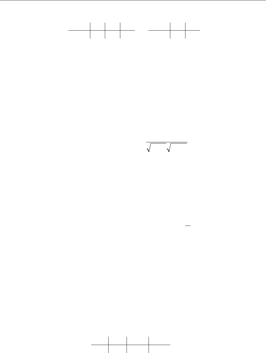
108 Chapter 5: Multivariate Probability Distributions
Instructor’s Solutions Manual
5.95 Note that the marginal distributions for Y1 and Y2 are
y1 –1 0 1 y2 0 1
p1(y1) 1/3 1/3 1/3 p2(y2)2/31/3
So, Y1 and Y2 not independent since p(–1, 0) ≠ p1(–1)p2(0). However, E(Y1) = 0 and
E(Y1Y2) = (–1)(0)1/3 + (0)(1)(1/3) + (1)(0)(1/3) = 0, so Cov(Y1, Y2) = 0.
5.96 a. Cov(Y1, Y2) = E[(Y1 – μ1)(Y2 – μ2)] = E[(Y2 – μ2)(Y1 – μ1)] = Cov(Y2, Y1).
b. Cov(Y1, Y1) = E[(Y1 – μ1)(Y1 – μ1)] = E[(Y1 – μ1)2] = V(Y1).
5.97 a. From Ex. 5.96, Cov(Y1, Y1) = V(Y1) = 2.
b. If Cov(Y1, Y2) = 7, ρ = 7/4 > 1, impossible.
c. With ρ = 1, Cov(Y1, Y2) = 1(4) = 4 (a perfect positive linear association).
d. With ρ = –1, Cov(Y1, Y2) = –1(4) = –4 (a perfect negative linear association).
5.98 Since ρ2 ≤ 1, we have that –1 ≤ ρ ≤ 1 or –1 ≤ )()(
),(Cov
21
21
YVYV
YY ≤ 1.
5.99 Since E(c) = c, Cov(c, Y) = E[(c – c)(Y – μ)] = 0.
5.100 a. E(Y1) = E(Z) = 0, E(Y2) = E(Z2) = 1.
b. E(Y1Y2) = E(Z3) = 0 (odd moments are 0).
c. Cov(Y1, Y1) = E(Z3) – E(Z)E(Z2) = 0.
d. P(Y2 > 1 | Y1 > 1) = P(Z2 > 1 | Z > 1) = 1 ≠ P(Z2 > 1). Thus, Y1 and Y2 are dependent.
5.101 a. Cov(Y1, Y2) = E(Y1Y2) – E(Y1)E(Y2) = 1 – α/4 – (1)(1) = 4
α
−
.
b. This is clear from part a.
c. We showed previously that Y1 and Y2 are independent only if α = 0. If ρ = 0, if must be
true that α = 0.
5.102 The quantity 3Y1 + 5Y2 = dollar amount spend per week. Thus:
E(3Y1 + 5Y2) = 3(40) + 5(65) = 445.
E(3Y1 + 5Y2) = 9V(Y1) + 25V(Y2) = 9(4) + 25(8) = 236.
5.103 E(3Y1 + 4Y2 – 6Y3) = 3E(Y1) + 4E(Y2) – 6E(Y3) = 3(2) + 4(–1) – 6(–4) = –22,
V(3Y1 + 4Y2 – 6Y3) = 9V(Y1) + 16V(Y2) + 36E(Y3) + 24Cov(Y1, Y2) – 36Cov(Y1, Y3) –
48Cov(Y2, Y3) = 9(4) + 16(6) + 36(8) + 24(1) – 36(–1) – 48(0) = 480.
5.104 a. Let X = Y1 + Y2. Then, the probability distribution for X is
x 1 2 3
p(x) 7/84 42/84 35/84
Thus, E(X) = 7/3 and V(X) = .3889.
b. E(Y1 + Y2) = E(Y1) + E(Y2) = 4/3 + 1 = 7/3. We have that V(Y1) = 10/18, V(Y2) = 42/84,
and Cov(Y1, Y1) = –1/3, so
www.elsolucionario.net

Chapter 5: Multivariate Probability Distributions 109
Instructor’s Solutions Manual
V(Y1 + Y2) = V(Y1) + V(Y2) + 2Cov(Y2, Y3) = 10/18 + 42/84 – 2/3 = 7/18 = .3889.
5.105 Since Y1 and Y2 are independent, V(Y1 + Y2) = V(Y1) + V(Y1) = 1/18 + 1/18 = 1/9.
5.106 V(Y1 – 3Y2) = V(Y1) + 9V(Y2) – 6Cov(Y1, Y2) = 3/80 + 9(1/20) – 6(1/40) = 27/80 = .3375.
5.107 Since E(Y1) = E(Y2) = 1/3, V(Y1) = V(Y2) = 1/18 and E(Y1Y2) = ∫∫
−
1
0
21
1
0
21
2
2dydyyy
y
= 1/12,
we have that Cov(Y1, Y1) = 1/12 – 1/9 = –1/36. Therefore,
E(Y1 + Y2) = 1/3 + 1/3 = 2/3 and V(Y1 + Y2) = 1/18 + 1/18 + 2(–1/36) = 1/18.
5.108 From Ex. 5.33, Y1 has a gamma distribution with α = 2 and β = 1, and Y2 has an
exponential distribution with β = 1. Thus, E(Y1 + Y2) = 2(1) + 1 = 3. Also, since
E(Y1Y2) = 3
0
12
0
21
1
1=
∫∫
∞
−dydyeyy
y
y, Cov(Y1, Y1) = 3 – 2(1) = 1,
V(Y1 – Y2) = 2(1)2 + 12 – 2(1) = 1.
Since a value of 4 minutes is four three standard deviations above the mean of 1 minute,
this is not likely.
5.109 We have E(Y1) = E(Y2) = 7/12. Intermediate calculations give V(Y1) = V(Y2) = 11/144.
Thus, E(Y1Y2) = 3/1)(
1
0
21
1
0
2121 =+
∫∫ dydyyyyy , Cov(Y1, Y1) = 1/3 – (7/12)2 = –1/144.
From Ex. 5.80, E(30Y1 + 25Y2) = 32.08, so
V(30Y1 + 25Y2) = 900V(Y1) + 625V(Y2) + 2(30)(25) Cov(Y1, Y1) = 106.08.
The standard deviation of 30Y1 + 25Y2 is 08.106 = 10.30. Using Tchebysheff’s
theorem with k = 2, the interval is (11.48, 52.68).
5.110 a. V(1 + 2Y1) = 4V(Y1), V(3 + 4Y2) = 16V(Y2), and Cov(1 + 2Y1, 3 + 4Y2) = 8Cov(Y1, Y2).
So, 2.
)(16)(4
),(8Cov
21
21 =ρ=
YVYV
YY .
b. V(1 + 2Y1) = 4V(Y1), V(3 – 4Y2) = 16V(Y2), and Cov(1 + 2Y1, 3 – 4Y2) = –8Cov(Y1, Y2).
So, 2.
)(16)(4
),(8Cov-
21
21 −=ρ−=
YVYV
YY .
c. V(1 – 2Y1) = 4V(Y1), V(3 – 4Y2) = 16V(Y2), and Cov(1 – 2Y1, 3 – 4Y2) = 8Cov(Y1, Y2).
So, 2.
)(16)(4
),(8Cov
21
21 =ρ=
YVYV
YY .
www.elsolucionario.net

110 Chapter 5: Multivariate Probability Distributions
Instructor’s Solutions Manual
5.111 a. V(a + bY1) = b2V(Y1), V(c + dY2) = d2V(Y2), and Cov(a + bY1, c + dY2) = bdCov(Y1, Y2).
So, 2121 ,
2
2
1
2
21
,||
)()(
),(Cov
YYWW bd
bd
YVdYVb
YYbd ρ==ρ . Provided that the constants b and d are
nonzero, || bd
bd is either 1 or –1. Thus, |||| 2121 ,, YYWW
ρ
=
ρ
.
b. Yes, the answers agree.
5.112 In Ex. 5.61, it was showed that Y1 and Y2 are independent. In addition, Y1 has a gamma
distribution with α = 2 and β = 2, and Y2 has an exponential distribution with β = 2. So,
with C = 50 + 2Y1 + 4Y2, it is clear that
E(C) = 50 + 2E(Y1) + 4E(Y2) = 50 + (2)(4) + (4)(2) = 66
V(C) = 4V(Y1) + 16V(Y2) = 4(2)(4) + 16(4) = 96.
5.113 The net daily gain is given by the random variable G = X – Y. Thus, given the
distributions for X and Y in the problem,
E(G) = E(X) – E(Y) = 50 – (4)(2) = 42
V(G) = V(G) + V(G) = 32 + 4(22) = 25.
The value $70 is (70 – 42)/5 = 7.2 standard deviations above the mean, an unlikely value.
5.114 Observe that Y1 has a gamma distribution with α = 4 and β = 1 and Y2 has an exponential
distribution with β = 2. Thus, with U = Y1 – Y2,
a. E(U) = 4(1) – 2 = 2
b. V(U) = 4(12) + 22 = 8
c. The value 0 has a z–score of (0 – 2)/ 8 = –.707, or it is –.707 standard deviations
below the mean. This is not extreme so it is likely the profit drops below 0.
5.115 Following Ex. 5.88:
a. Note that for non–negative integers a and b and i ≠ j,
P(Yi = a, Yj = b) = P(Yj = b | Yi = a)P(Yi = a)
But, P(Yj = b | Yi = a) = P(Yj = b) since the trials (i.e. die tosses) are independent ––
the experiments that generate Yi and Yj represent independent experiments via the
memoryless property. So, Yi and Yj are independent and thus Cov(Yi. Yj) = 0.
b. V(Y) = V(Y1) + … + V(Y6) = 0 + 22222 )6/1(
6/5
)6/2(
6/4
)6/3(
6/3
)6/4(
6/2
)6/5(
6/1
+
+
+
+
= 38.99.
c. From Ex. 5.88, E(Y) = 14.7. Using Tchebysheff’s theorem with k = 2, the interval is
14.7 ± 2 99.38 or (0 , 27.188)
www.elsolucionario.net

Chapter 5: Multivariate Probability Distributions 111
Instructor’s Solutions Manual
5.116 V(Y1 + Y2) = V(Y1) + V(Y2) + 2Cov(Y1, Y2), V(Y1 – Y2) = V(Y1) + V(Y2) – 2Cov(Y1, Y2).
When Y1 and Y2 are independent, Cov(Y1, Y2) = 0 so the quantities are the same.
5.117 Refer to Example 5.29 in the text. The situation here is analogous to drawing n balls
from an urn containing N balls, r1 of which are red, r2 of which are black, and N – r1 – r2
are neither red nor black. Using the argument given there, we can deduce that:
E(Y1) = np1 V(Y1) = np1(1 – p1)
(
)
1−
−
NnN where p1 = r1/N
E(Y2) = np2 V(Y2) = np2(1 – p2)
(
)
1−
−
NnN where p2 = r2/N
Now, define new random variables for i = 1, 2, …, n:
⎩
⎨
⎧
=otherwise0
femalematureaisalligatorif1 i
Ui ⎩
⎨
⎧
=otherwise0
malematureaisalligatorif1 i
Vi
Then, ∑
=
=n
ii
UY
1
1 and ∑
=
=n
ii
VY
1
2. Now, we must find Cov(Y1, Y2). Note that:
E(Y1Y2) = E⎜
⎝
⎛∑
=
n
ii
U
1
,⎟
⎠
⎞
∑
=
n
ii
V
1
= ∑
=
n
iiiVUE
1
)(+
∑
≠ji jiVUE )(.
Now, since for all i, E(Ui, Vi) = P(Ui = 1, Vi = 1) = 0 (an alligator can’t be both female
and male), we have that E(Ui, Vi) = 0 for all i. Now, for i ≠ j,
E(Ui, Vj) = P(Ui = 1, Vi = 1) = P(Ui = 1)P(Vi = 1|Ui = 1) =
(
)
21
11
21 pp
N
N
N
r
N
r
−− =.
Since there are n(n – 1) terms in
∑
≠ji jiVUE )( , we have that E(Y1Y2) = n(n – 1) 21
1pp
N
N
−.
Thus, Cov(Y1, Y2) = n(n – 1) 21
1pp
N
N
− – (np1)(np2) = 21
1
)( pp
NnNn
−
−
−.
So,
[
]
()
21
1
21 npnpE nn
Y
n
Y−=− = 21 pp
−
,
[
]
[]
),(Cov2)()( 2121
1
2
21 YYYVYVV n
n
Y
n
Y−+=− =
(
)
2
2121
)1( )( pppp
Nn nN −−+
−
−
5.118 Let Y = X1 + X2, the total sustained load on the footing.
a. Since X1 and X2 have gamma distributions and are independent, we have that
E(Y) = 50(2) + 20(2) = 140
V(Y) = 50(22) + 20(22) = 280.
b. Consider Tchebysheff’s theorem with k = 4: the corresponding interval is
140 + 4 280 or (73.07, 206.93).
So, we can say that the sustained load will exceed 206.93 kips with probability less
than 1/16.
www.elsolucionario.net

112 Chapter 5: Multivariate Probability Distributions
Instructor’s Solutions Manual
5.119 a. Using the multinomial distribution with p1 = p2 = p3 = 1/3,
P(Y1 = 3, Y2 = 1, Y3 = 2) =
(
)
6
3
1
!2!1!3
!6 = .0823.
b. E(Y1) = n/3, V(Y1) = n(1/3)(2/3) = 2n/9.
c. Cov(Y2, Y3) = –n(1/3)(1/3) = –n/9.
d. E(Y2 – Y3) = n/3 – n/3 = 0, V(Y2 – Y3) = V(Y2) + V(Y3) – 2Cov(Y2, Y3) = 2n/3.
5.120 E(C) = E(Y1) + 3E(Y2) = np1 + 3np2.
V(C) = V(Y1) + 9V(Y2) + 6Cov(Y1, Y2) = np1q1 + 9np2q2 – 6np1p2.
5.121 If N is large, the multinomial distribution is appropriate:
a. P(Y1 = 2, Y2 = 1) = 0972.)6(.)1(.)3(. 212
!2!1!2
!5 =.
b.
[
]
=− n
Y
n
Y
E21 = 21 pp −= .3 – .1 = .2
[
]
[]
),(Cov2)()( 2121
1
2
21 YYYVYVV n
n
Y
n
Y−+=− = n
pp
n
qp
n
qp 212211 2++ = .072.
5.122 Let Y1 = # of mice weighing between 80 and 100 grams, and let Y2 = # weighing over 100
grams. Thus, with X having a normal distribution with μ = 100 g. and σ = 20 g.,
p1 = P(80 ≤ X ≤ 100) = P(–1 ≤ Z ≤ 0) = .3413
p2 = P(X > 100) = P(Z > 0) = .5
a. P(Y1 = 2, Y2 = 1) = 1109.)1587(.)5(.)3413(. 112
!1!1!2
!4 =.
b. P(Y2 = 4) = 0625.)5(. 4
!0!4!0
!4 =.
5.123 Let Y1 = # of family home fires, Y2 = # of apartment fires, and Y3 = # of fires in other
types. Thus, (Y1, Y2, Y3) is multinomial with n = 4, p1 = .73, p2 = .2 and p3 = .07. Thus,
P(Y1 = 2, Y2 = 1, Y3 = 1) = 6(.73)2(.2)(.07) = .08953.
5.124 Define C = total cost = 20,000Y1 + 10,000Y2 + 2000Y3
a. E(C) = 20,000E(Y1) + 10,000E(Y2) + 2000E(Y3)
= 20,000(2.92) + 10,000(.8) + 2000(.28) = 66,960.
b. V(C) = (20,000)2V(Y1) + (10,000)2V(Y2) + (2000)2V(Y3) + covariance terms
= (20,000)2(4)(.73)(.27) + (10,000)2(4)(.8)(.2) + (2000)2(4)(.07)(.93)
+ 2[20,000(10,000)(–4)(.73)(.2) + 20,000(2000)(–4)(.73)(.07) +
10,000(2000)(–4)(.2)(.07)] = 380,401,600 – 252,192,000 = 128,209,600.
5.125 Let Y1 = # of planes with no wine cracks, Y2 = # of planes with detectable wing cracks,
and Y3 = # of planes with critical wing cracks. Therefore, (Y1, Y2, Y3) is multinomial with
n = 5, p1 = .7, p2 = .25 and p3 = .05.
a. P(Y1 = 2, Y2 = 2, Y3 = 1) = 30(.7)2(.25)2(.05) = .046.
b. The distribution of Y3 is binomial with n = 5, p3 = .05, so
www.elsolucionario.net

Chapter 5: Multivariate Probability Distributions 113
Instructor’s Solutions Manual
P(Y3 ≥ 1) = 1 – P(Y3 = 0) = 1 – (.95)5 = .2262.
5.126 Using formulas for means, variances, and covariances for the multinomial:
E(Y1) = 10(.1) = 1 V(Y1) = 10(.1)(.9) = .9
E(Y2) = 10(.05) = .5 V(Y2) = 10(.05)(.95) = .475
Cov(Y1, Y2) = –10(.1)(.05) = –.05
So,
E(Y1 + 3Y2) = 1 + 3(.5) = 2.5
V(Y1 + 3Y2) = .9 + 9(.475) + 6(–.05) = 4.875.
5.127 Y is binomial with n = 10, p = .10 + .05 = .15.
a. P(Y = 2) = 82 )85(.)15(.
2
10⎟
⎟
⎠
⎞
⎜
⎜
⎝
⎛ = .2759.
b. P(Y ≥ 1) = 1 – P(Y = 0) = 1 – (.85)10 = .8031.
5.128 The marginal distribution for Y1 is found by
∫
∞
∞−
=22111 ),()( dyyyfyf .
Making the change of variables u = (y1 – μ1)/σ1 and v = (y2 – μ2)/σ2 yields
∫
∞
∞−
⎥
⎦
⎤
⎢
⎣
⎡ρ−+
ρ−
−
ρ−πσ
=dvuvvuyf )2(
)1(2
1
exp
12
1
)( 22
2
2
1
11 .
To evaluate this, note that )1()(2 22222 ρ−+ρ−=ρ−+ uuvuvvu so that
∫
∞
∞−
−⎥
⎦
⎤
⎢
⎣
⎡ρ−
ρ−
−
ρ−πσ
=dvuveyf u2
2
2/
2
1
11 )(
)1(2
1
exp
12
1
)( 2,
So, the integral is that of a normal density with mean ρu and variance 1 – ρ2. Therefore,
2
1
2
11 2/)(
1
11 2
1
)( σμ−−
πσ
=y
eyf , –∞ < y1 < ∞,
which is a normal density with mean μ1 and standard deviation σ1. A similar procedure
will show that the marginal distribution of Y2 is normal with mean μ2 and standard
deviation σ2.
5.129 The result follows from Ex. 5.128 and defining )(/),()|( 222121 yfyyfyyf
=
, which
yields a density function of a normal distribution with mean ))(/( 22211
μ
−σσ
ρ
+
μ
y and
variance )1( 22
1ρ−σ .
5.130 a. ∑∑∑∑ ====
σ=== n
iji
n
iiji
n
i
n
jjiji baYVbaYYbaUU
11
2
11
21 )(),(Cov),(Cov , since the Yi’s are
independent. If ),(Cov 21 UU = 0, it must be true that ∑
=
n
ijiba
1
= 0 since σ2 > 0. But, it is
trivial to see if ∑
=
n
ijiba
1
= 0, ),(Cov 21 UU = 0. So, U1 and U2 are orthogonal.
www.elsolucionario.net

114 Chapter 5: Multivariate Probability Distributions
Instructor’s Solutions Manual
b. Given in the problem, ),( 21 UU has a bivariate normal distribution. Note that
E(U1) = ∑
=
μn
ii
a
1
, E(U2) = ∑
=
μn
ii
b
1
, V(U1) = ∑
=
σn
ii
a
1
2
2, and V(U2) = ∑
=
σn
ii
b
1
2
2. If they are
orthogonal, ),(Cov 21 UU = 0 and then .0
21 ,
=
ρ
UU So, they are also independent.
5.131 a. The joint distribution of Y1 and Y2 is simply the product of the marginals )( 11 yf and
)( 22 yf since they are independent. It is trivial to show that this product of density has
the form of the bivariate normal density with ρ = 0.
b. Following the result of Ex. 5.130, let a1 = a2 = b1 = 1 and b2 = –1. Thus, ∑
=
n
ijiba
1
= 0
so U1 and U2 are independent.
5.132 Following Ex. 5.130 and 5.131, U1 is normal with mean μ1 + μ2 and variance 2σ2 and U2
is normal with mean μ1 – μ2 and variance 2σ2.
5.133 From Ex. 5.27, 221 /1)|( yyyf =, 0 ≤ y1 ≤ y2 and )1(6)( 2222 yyyf
−
=
, 0 ≤ y2 ≤ 1.
a. To find )|( 221 yYYE =, note that the conditional distribution of Y1 given Y2 is uniform
on the interval (0, y2). So, )|( 221 yYYE
=
= 2
2
y.
b. To find ))|(( 21 YYEE , note that the marginal distribution is beta with α = 2 and β = 2.
So, from part a, ))|(( 21 YYEE = E(Y2/2) = 1/4. This is the same answer as in Ex. 5.77.
5.134 The z–score is (6 – 1.25)/ 5625.1 = 3.8, so the value 6 is 3.8 standard deviations above
the mean. This is not likely.
5.135 Refer to Ex. 5.41:
a. Since Y is binomial, E(Y|p) = 3p. Now p has a uniform distribution on (0, 1), thus
E(Y) = E[E(Y|p)] = E(3p) = 3(1/2) = 3/2.
b. Following part a, V(Y|p) = 3p(1 – p). Therefore,
V(p) = E[3p(1 – p)] + V(3p) = 3E(p – p2) + 9V(p)
= 3E(p) – 3[V(p) + (E(p))2] + 9V(p) = 1.25
5.136 a. For a given value of λ, Y has a Poisson distribution. Thus, E(Y | λ) = λ. Since the
marginal distribution of λ is exponential with mean 1, E(Y) = E[E(Y | λ)] = E(λ) = 1.
b. From part a, E(Y | λ) = λ and so V(Y | λ) = λ. So, V(Y) = E[V(Y | λ)] + E[V(Y | λ)] = 2
c. The value 9 is (9 – 1)/ 2 = 5.657 standard deviations above the mean (unlikely score).
5.137 Refer to Ex. 5.38: )|( 112 yYYE = = y1/2. For y1 = 3/4, )4/3|( 12
=
YYE = 3/8.
5.138 If Y = # of bacteria per cubic centimeter,
a. E(Y) = E(Y) = E[E(Y | λ)] = E(λ) = αβ.
www.elsolucionario.net

Chapter 5: Multivariate Probability Distributions 115
Instructor’s Solutions Manual
b. V(Y) = E[V(Y | λ)] + V[E(Y | λ)] = αβ + αβ2 = αβ(1+β). Thus, )1( β+αβ=σ .
5.139 a. ∑∑ ==
αβ==
⎟
⎠
⎞
⎜
⎝
⎛
== n
ii
n
iinYEYEnNTE
11
)()|(.
b.
λ
αβ
=
α
β== )()]|([)( NENTEETE . Note that this is E(N)E(Y).
5.140 Note that V(Y1) = E[V(Y1 | Y2)] + V[E(Y1 | Y2)], so E[V(Y1 | Y2)] = V(Y1) – V[E(Y1 | Y2)].
Thus, E[V(Y1 | Y2)] ≤ V(Y1).
5.141 E(Y2) = ))|(( 12 YYEE = E(Y1/2) = 2
λ
V(Y2) = E[V(Y2 | Y1)] + V[E(Y2 | Y1)] = E[12/
2
1
Y] + V[Y1/2] = (2λ2)/12 + (λ2)/2 =
2
2
3
λ
.
5.142 a. E(Y) = E[E(Y|p)] = E(np) = nE(p) = β+α
α
n.
b. V(Y) = E[V(Y | p)] + V[E(Y | p)] = E[np(1 – p)] + V(np) = nE(p – p2) + n2V(p). Now:
nE(p – p2) = β+α
α
n – )1)((
)1(
+β+αβ+α
+
α
α
n
n
2V(p) = )1()( 2
2
+β+αβ+α
αβn.
So, V(Y) = β+α
α
n – )1)((
)1(
+β+αβ+α
+
ααn + )1()( 2
2
+β+αβ+α
αβn = )1()(
)(
2+β+αβ+α
+β+α
α
βnn .
5.143 Consider the random variable y1Y2 for the fixed value of Y1. It is clear that y1Y2 has a
normal distribution with mean 0 and variance 2
1
y and the mgf for this random variable is
2/
2
1
2
21 )()( ytYty eeEtm == .
Thus,
()
1
)1(2/
2
1
2/
1
22
1
2
12121 )()]|([)()()( dyeeEYeEEeEeEtm tytYYtYYtY
tU
U∫
∞
∞−
−−
π
===== .
Note that this integral is essentially that of a normal density with mean 0 and variance
2
1
1
t−, so the necessary constant that makes the integral equal to 0 is the reciprocal of the
standard deviation. Thus,
(
)
2/1
2
1)( −
−= ttmU. Direct calculations give 0)0( =
′
U
m and
1)0( =
′′
U
m. To compare, note that E(U) = E(Y1Y2) = E(Y1)E(Y2) = 0 and V(U) = E(U2) =
E(Y12Y22) = E(Y12)E(Y22) = (1)(1) = 1.
www.elsolucionario.net

116 Chapter 5: Multivariate Probability Distributions
Instructor’s Solutions Manual
5.144
∑
∑
∑∑ ===
1212
)()()()(),()()()]()([ 221121212121
yyyy
ypypyhygyypyhygYhYgE
)]([)]([)()()()( 21222111
12
YhEYgEypyhypyg
yy
×=
∑∑ .
5.145 The probability of interest is P(Y1 + Y2 < 30), where Y1 is uniform on the interval (0, 15)
and Y2 is uniform on the interval (20, 30). Thus, we have
21
30
20
230
0
21 10
1
15
1
)30( dydyYYP
y
⎟
⎠
⎞
⎜
⎝
⎛
⎟
⎠
⎞
⎜
⎝
⎛
=<+ ∫∫
−
= 1/3.
5.146 Let (Y1, Y2) represent the coordinates of the landing point of the bomb. Since the radius
is one mile, we have that 0 ≤ 2
2
2
1yy + ≤ 1. Now,
P(target is destroyed) = P(bomb destroys everything within 1/2 of landing point)
This is given by ))(( 2
2
1
2
2
2
1≤+YYP . Since (Y1, Y2) are uniformly distributed over the unit
circle, the probability in question is simply the area of a circle with radius 1/2 divided by
the area of the unit circle, or simply 1/4.
5.147 Let Y1 = arrival time for 1st friend, 0 ≤ y1 ≤ 1, Y2 = arrival time for 2nd friend, 0 ≤ y2 ≤ 1.
Thus f (y1, y2) = 1. If friend 2 arrives 1/6 hour (10 minutes) before or after friend 1, they
will meet. We can represent this event as |Y1 – Y2| < 1/3. To find the probability of this
event, we must find:
36/11111)3/1|(| 1
1
6/5
1
6/1
21
6/5
6/1
6/1
6/1
21
6/1
0
6/1
0
221
1
1
1
1
=++=<− ∫∫∫∫∫∫ −
+
−
+
dydydydydydyYYP
y
y
y
y
.
5.148 a.
⎟
⎟
⎠
⎞
⎜
⎜
⎝
⎛
⎟
⎟
⎠
⎞
⎜
⎜
⎝
⎛
−−
⎟
⎟
⎠
⎞
⎜
⎜
⎝
⎛
⎟
⎟
⎠
⎞
⎜
⎜
⎝
⎛
=
3
9
3
234
21
2121
),( yyyy
yyp , y1 = 0, 1, 2, 3, y2 = 0, 1, 2, 3, y1 + y2 ≤ 3.
b. Y1 is hypergeometric w/ r = 4, N = 9, n = 3; Y2 is hypergeometric w/ r = 3, N = 9, n = 3
c. P(Y1 = 1 | Y2 ≥ 1) = [p(1, 1) + p(1, 2)]/[1 – p2(0)] = 9/16
5.149 a. 2
1
0
2111 33)(
1
ydyyyf
y
== ∫, 0 ≤ y1 ≤ 1, )1(3)( 2
2
2
3
1
1111
2
ydyyyf
y
−== ∫, 0 ≤ y2 ≤ 1.
b. 44/23)2/1|4/3( 21 =≤≤ YYP .
c. f(y1 | y2) = )1/(2 2
21 yy −, y2 ≤ y1 ≤ 1.
d. 12/5)2/1|4/3( 21 ==≤ YYP .
5.150 a. Note that f(y2 | y1) = f(y1, y2)/f(y1) = 1/y1, 0 ≤ y2 ≤ y1. This is the same conditional
density as seen in Ex. 5.38 and Ex. 5.137. So, E(Y2 | Y1 = y1) = y1/2.
www.elsolucionario.net

Chapter 5: Multivariate Probability Distributions 117
Instructor’s Solutions Manual
b. E(Y2) = E[E(Y2 | Y1)] = E(Y1/2) = 1
2
1
1
0
23
1dyy
y
∫ = 3/8.
c. E(Y2) = 2
2
2
1
0
2
3
2)1( dyyy −
∫ = 3/8.
5.151 a. The joint density is the product of the marginals: β+−
β
=/)(
1
21
21
2
),( yy
eyyf , y1 ≥ ∞, y2 ≥ ∞
b. 2
00
1
/)(
1
21
2
21
2
)( dydyeaYYP
aya
yy
∫∫
−
β+−
β
=≤+ = 1 –
[
]
β−
β+ /
/1 a
ea .
5.152 The joint density of (Y1, Y2) is 2
2
2
1121 )(18),( yyyyyf −= , 0 ≤ y1 ≤ 1, 0 ≤ y2 ≤ 1. Thus,
P(Y1Y2 ≤ .5) = P(Y1 ≤ .5/Y2) = 1 – P(Y1 > .5/Y2) = 1 – ∫∫ −
1
5.
1
/5.
21
2
2
2
11
2
)(18
y
dydyyyy . Using
straightforward integration, this is equal to (5 – 3ln2)/4 = .73014.
5.153 This is similar to Ex. 5.139:
a. Let N = # of eggs laid by the insect and Y = # of eggs that hatch. Given N = n, Y has a
binomial distribution with n trials and success probability p. Thus, E(Y | N = n) = np.
Since N follows as Poisson with parameter λ, E(Y) = E[E(Y | N )] = E(Np ) = λp.
b. V(Y) = E[V(Y | N)] + V[E(Y | N)] = E[Np(1 – p)] + V[Np] = λp.
5.154 The conditional distribution of Y given p is binomial with parameter p, and note that the
marginal distribution of p is beta with α = 3 and β = 2.
a. Note that dppp
y
n
dppfpyfpyfyf yny 1
1
0
2
1
0
1
0
)1(12)()|(),()( +−+ −
⎟
⎟
⎠
⎞
⎜
⎜
⎝
⎛
=== ∫∫∫ . This
integral can be evaluated by relating it to a beta density w/ α = y + 3, β = n + y + 2.
Thus,
)5(
)3()2(
12)( +Γ
+Γ+−Γ
⎟
⎟
⎠
⎞
⎜
⎜
⎝
⎛
=n
yyn
y
n
yf , y = 0, 1, 2, …, n.
b. For n = 2, E(Y | p) = 2p. Thus, E(Y) = E[E(Y|p)] = E(2p) = 2E(p) = 2(3/5) = 6/5.
5.155 a. It is easy to show that
Cov(W1, W2) = Cov(Y1 + Y2, Y1 + Y3)
= Cov(Y1, Y1) + Cov(Y1, Y3) + Cov(Y2, Y1) + Cov(Y2, Y3)
= Cov(Y1, Y1) = V(Y1) = 2ν1.
b. It follows from part a above (i.e. the variance is positive).
www.elsolucionario.net

118 Chapter 5: Multivariate Probability Distributions
Instructor’s Solutions Manual
5.156 a. Since E(Z) = E(W) = 0, Cov(Z, W) = E(ZW) = E(Z22/1−
Y) = E(Z2)E(2/1−
Y) = E(2/1−
Y).
This expectation can be found by using the result Ex. 4.112 with a = –1/2. So,
Cov(Z, W) = E(2/1−
Y) = )(2
)(
2
2
1
2
ν
ν
Γ
−
Γ
, provided ν > 1.
b. Similar to part a, Cov(Y, W) = E(YW) = E(YW) = E(Y)E(W) = 0.
c. This is clear from parts (a) and (b) above.
5.157
(
)
α
α+
+β
β
∞
α
β+βλ−−α+
∞
βαΓ+Γ
α+Γ
=λ
βαΓ+Γ
λ
=λλλ= ∫∫ )()1(
)(
)()1(
)()|()( 1
0
]/)1[(1
0y
y
d
y
e
dfypyp
y
y
, y = 0, 1, 2, … . Since
it was assumed that α was an integer, this can be written as
α
⎟
⎠
⎞
⎜
⎝
⎛
+β
⎟
⎠
⎞
⎜
⎝
⎛
+β
β
⎟
⎟
⎠
⎞
⎜
⎜
⎝
⎛−α+
=1
1
1
1
)(
y
y
y
yp , y = 0, 1, 2, … .
5.158 Note that for each Xi, E(Xi) = p and V(Xi) = pq. Then, E(Y) = ΣE(Xi) = np and V(Y) = npq.
The second result follows from the fact that the Xi are independent so therefore all
covariance expressions are 0.
5.159 For each Wi, E(Wi) = 1/p and V(Wi) = q/p2. Then, E(Y) = ΣE(Xi) = r/p and V(Y) = rq/p2.
The second result follows from the fact that the Wi are independent so therefore all
covariance expressions are 0.
5.160 The marginal probabilities can be written directly:
P(X1 = 1) = P(select ball 1 or 2) = .5 P(X1 = 0) = .5
P(X2 = 1) = P(select ball 1 or 3) = .5 P(X2 = 0) = .5
P(X3 = 1) = P(select ball 1 or 4) = .5 P(X3 = 0) = .5
Now, for i ≠ j, Xi and Xj are clearly pairwise independent since, for example,
P(X1 = 1, X2 = 1) = P(select ball 1) = .25 = P(X1 = 1)P(X2 = 1)
P(X1 = 0, X2 = 1) = P(select ball 3) = .25 = P(X1 = 0)P(X2 = 1)
However, X1, X2, and X3 are not mutually independent since
P(X1 = 1, X2 = 1, X3 = 1) = P(select ball 1) = .25 ≠ P(X1 = 1)P(X2 = 1)P(X1 = 3).
www.elsolucionario.net

Chapter 5: Multivariate Probability Distributions 119
Instructor’s Solutions Manual
5.161 21
11 )()()()()( μ−μ=
∑
−
∑
=−=− i
m
i
nXEYEXEYEXYE
mnXVYVXVYVXYV i
m
i
n//)()()()()( 2
2
2
1
11
22 σ+σ=
∑
+
∑
=+=−
5.162 Using the result from Ex. 5.65, choose two different values for α with –1 ≤ α ≤ 1.
5.163 a. The distribution functions with the exponential distribution are:
1
1)( 11
y
eyF −
−= , y1 ≥ 0; 2
1)( 22
y
eyF −
−= , y2 ≥ 0.
Then, the joint distribution function is
)])((1][1][1[),( 2121
21
yyyy eeeeyyF −−−− α−−−= .
Finally, show that ),( 21
21
2yyF
yy ∂∂
∂ gives the joint density function seen in Ex. 5.162.
b. The distribution functions with the uniform distribution on (0, 1) are:
)( 11 yF = y1, 0 ≤ y1 ≤ 1 ; )( 22 yF = y2, 0 ≤ y2 ≤ 1.
Then, the joint distribution function is
)]1)(1(1[),( 212121 yyyyyyF
−
−
α
−
=
.
c. ),( 21
21
2yyF
yy ∂∂
∂ =
[
]
)21)(21(1),( 2121 yyyyf
−
−
α
−
=
, 0 ≤ y1 ≤ 1, 0 ≤ y2 ≤ 1.
d. Choose two different values for α with –1 ≤ α ≤ 1.
5.164 a. If t1 = t2 = t3 = t, then m(t, t, t) =
(
)
)( 321 XXXt
eE ++ . This, by definition, is the mgf for the
random variable X1 + X2 + X3.
b. Similarly with t1 = t2 = t and t3 = 0, m(t, t, 0) =
(
)
)( 21 XXt
eE +.
c. We prove the continuous case here (the discrete case is similar). Let (X1, X2, X3) be
continuous random variables with joint density function ),,( 321 xxxf . Then,
∫∫∫
∞
∞−
∞
∞−
∞
∞−
=321321321 ),,(),,( 33
2211 dxdxdxxxxfeeetttm xt
xtxt .
Then,
∫∫∫
∞
∞−
∞
∞−
∞
∞−
===
++
=
∂∂∂
∂
3213213210321
321
),,(),,( 3
21
321
3
21
321 dxdxdxxxxfxxxtttm
ttt
k
kk
ttt
k
kk
kkk
.
This is easily recognized as
(
)
3
21
321
k
kk XXXE .
5.165 a. 3
21
332211
123
321 321
!!!
!
321 ),,( x
xx
xtxtxt
xxx xxx npppetttm ++
∑∑∑
=
= 33
2211
123
321 )()()( 321
!!!
!xt
xtxt
xxx xxx nepepep
∑∑∑ = n
t
tt epepep )( 3
21
321 ++ . The
final form follows from the multinomial theorem.
www.elsolucionario.net

120 Chapter 5: Multivariate Probability Distributions
Instructor’s Solutions Manual
b. The mgf for X1 can be found by evaluating m(t, 0, 0). Note that q = p2 + p3 = 1 – p1.
c. Since Cov(X1, X2) = E(X1X2) – E(X1)E(X2) and E(X1) = np1 and E(X2) = np2 since X1 and
X2 have marginal binomial distributions. To find E(X1X2), note that
21021
21
2
)1()0,,( 21 ppnnttm
tt tt −=
∂∂
∂
== .
Thus, Cov(X1, X2) = n(n – 1)p1p2 – (np1)(np2) = –np1p2.
5.166 The joint probability mass function of (Y1, Y2, Y3) is given by
⎟
⎟
⎠
⎞
⎜
⎜
⎝
⎛
⎟
⎟
⎠
⎞
⎜
⎜
⎝
⎛
⎟
⎟
⎠
⎞
⎜
⎜
⎝
⎛
⎟
⎟
⎠
⎞
⎜
⎜
⎝
⎛
=
⎟
⎟
⎠
⎞
⎜
⎜
⎝
⎛
⎟
⎟
⎠
⎞
⎜
⎜
⎝
⎛
⎟
⎟
⎠
⎞
⎜
⎜
⎝
⎛
⎟
⎟
⎠
⎞
⎜
⎜
⎝
⎛
=
n
N
y
Np
y
Np
y
Np
n
N
y
N
y
N
y
N
yyyp 3
3
2
2
1
1
3
3
2
2
1
1
321 ),,(,
where y1 + y2 + y3 = n. The marginal distribution of Y1 is hypergeometric with r = Np1, so
E(Y1) = np1, V(Y1) = np1(1–p1)
(
)
1−
−
NnN . Similarly, E(Y2) = np2, V(Y2) = np2(1–p2)
()
1−
−
NnN . It
can be shown that (using mathematical expectation and straightforward albeit messy
algebra) E(Y1Y2) = 1
21
)1( −
−N
N
ppnn . Using this, it is seen that
Cov(Y1, Y2) = 1
21
)1( −
−
N
N
ppnn – (np1)(np2) = –np1p2
()
1−
−
NnN .
(Note the similar expressions in Ex. 5.165.) Finally, it can be found that
)1)(1( 21
21
pp
pp
−−
−=ρ .
5.167 a. For this exercise, the quadratic form of interest is
22
221
22
1
2)]([)](2[)( YEtYYEtYECBtAt +−+=++ .
Since E[(tY1 – Y2)2] ≥ 0 (it is the integral of a non–negative quantity), so we must have
that CBtAt ++
2 ≥ 0. In order to satisfy this inequality, the two roots of this quadratic
must either be imaginary or equal. In terms of the discriminant, we have that
04
2≤− ACB , or
0)()(4)](2[ 2
2
2
1
2
21 ≤−− YEYEYYE .
Thus, )()()]([ 2
2
2
1
2
21 YEYEYYE ≤.
b. Let μ1 = E(Y1), μ2 = E(Y2), and define Z1 = Y1 – μ1, Z2 = Y2 – μ2. Then,
1
)()(
)]([
])[(])([
)])(([
2
2
2
1
2
21
2
22
2
11
2
2211
2≤=
μ−μ−
μ−μ−
=ρ ZEZE
ZZE
YEYE
YYE
by the result in part a.
www.elsolucionario.net

121
Chapter 6: Functions of Random Variables
6.1 The distribution function of Y is ∫−=−=
y
YyydttyF
0
2
2)1(2)( , 0 ≤ y ≤ 1.
a. 2
2
1
2
1
2
1
2
1
1)()(2)()()12()()(
1
++++ −==≤=≤−=≤= uuu
Y
u
UFYPuYPuUPuF . Thus,
11,)()( 2
1
11
≤
≤
−=
′
=−uuFuf u
UU .
b. 2
2
1
2
1
2
11
2
1
2)()(21)()()21()()(
2
++−− =−==≤=≤−=≤= uuu
Y
u
UFYPuYPuUPuF . Thus,
11,)()( 2
1
22
≤
≤
−=
′
=+uuFuf u
UU .
c. uuuFuYPuYPuUPuF YU −==≤=≤=≤= 2)()()()()( 2
3
3 Thus,
10,1)()( 1
33
≤
≤
−=
′
=uuFuf u
UU .
d. .6/1)(,3/1)(,3/1)( 321
=
=−= UEUEUE
e. .6/1)(,3/1)21(,3/1)12( 2==−−=− YEYEYE
6.2 The distribution function of Y is ∫
−
−==
y
YydttyF
1
32 )1)(2/1()2/3()( , –1 ≤ y ≤ 1.
a. )118/()3/()3/()3()()( 3
2
1
1
1−==≤=≤=≤= uuFuYPuYPuUPuF YU . Thus,
33,18/)()( 2
11 ≤≤−=
′
=uuuFuf UU .
b. ])3(1[)3(1)3()3()()( 3
2
1
2
2uuFuYPuYPuUPuF YU −−=−−=−≥=≤−=≤= .
Thus, 42,)3()()( 2
2
3
22 ≤≤−=
′
=uuuFuf UU .
c. 2/32
3)()()()()()(
3uuFuFuYuPuYPuUPuF YYU =−−=≤≤−=≤=≤= .
Thus, 10,)()( 2
3
33 ≤≤=
′
=uuuFuf UU .
6.3 The distribution function for Y is ⎪
⎩
⎪
⎨
⎧
>
≤<−
≤≤
=
5.11
5.112/1
102/
)(
2
y
yy
yy
yFY.
a. )()()410()()( 10
4
10
4++
=
≤
=
≤
−
=≤= u
Y
u
UFYPuYPuUPuF . So,
⎪
⎩
⎪
⎨
⎧
>
≤<
≤≤−
=−
+
111
116
64
)( 10
1
200
)4( 2
u
u
u
uF u
u
U, and ⎪
⎩
⎪
⎨
⎧
≤<
≤≤−
=
′
=
+
elsewhere0
116
64
)()( 10
1
100
4
u
u
uFuf
u
UU .
b. E(U) = 5.583.
c. E(10Y – 4) = 10(23/24) – 4 = 5.583.
6.4 The distribution function of Y is 4/
1)( y
YeyF −
−= , 0 ≤ y.
a. 12/)1(
3
1
3
11)()()13()()( −−
−− −==≤=≤+=≤= u
u
Y
u
UeFYPuYPuUPuF . Thus,
1,)()( 12/)1(
12
1≥=
′
=−− ueuFuf u
UU .
b. E(U) = 13.
www.elsolucionario.net
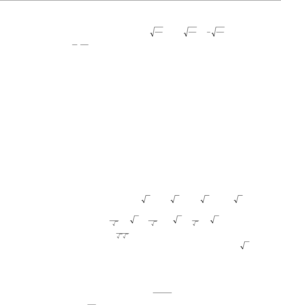
122 Chapter 6: Functions of Random Variables
Instructor’s Solutions Manual
6.5 The distribution function of Y is 4/)( yyFY
=
, 1 ≤ y ≤ 5.
2
3
4
1
2
3
2
3
2)()()32()()( −−− ==≤=≤+=≤= uu
Y
u
UFYPuYPuUPuF . Differentiating,
()
535,)()( 2/1
2
3
16
1≤≤=
′
=−
−uuFuf u
UU .
6.6 Refer to Ex. 5.10 ad 5.78. Define )()()()( 2121 uYYPuYYPuUPuFU
+
≤=
≤
−
=
≤
=
.
a. For u ≤ 0, 0)()()( 21
=
≤
−
=
≤= uYYPuUPuFU.
For 0 ≤ u < 1, ∫∫ ==≤−=≤=
+
uuy
y
UudydyuYYPuUPuF
0
2
2
2121 2/1)()()(
2
2
.
For 1 ≤ u ≤ 2, ∫∫
−
+
−−=−=≤−=≤=
u
uy
UudydyuYYPuUPuF
2
0
2
2
2121 2/)2(111)()()(
2
.
Thus, ⎪
⎩
⎪
⎨
⎧
≤≤−
<≤
=
′
=
elsewhere0
212
10
)()( yu
uu
uFuf UU .
b. E(U) = 1.
6.7 Let FZ(z) and fZ(z) denote the standard normal distribution and density functions
respectively.
a. ).()()()()()( 2uFuFuZuPuZPuUPuF ZZU −−=≤≤−=≤=≤= The
density function for U is then
0),()()()()( 1
2
1
2
1≥=−+=
′
=uufufufuFuf Z
u
Z
u
Z
u
UU .
Evaluating, we find 0)( 2/2/1
2
1≥= −−
πueuuf u
U.
b. U has a gamma distribution with α = 1/2 and β = 2 (recall that Γ(1/2) = π).
c. This is the chi–square distribution with one degree of freedom.
6.8 Let FY(y) and fY(y) denote the beta distribution and density functions respectively.
a. ).1(1)1()1()()( uFuYPuYPuUPuF YU
−
−
=
−
≥
=
≤
−=≤= The density function
for U is then 10,)1()1()()( 11
)()(
)( ≤≤−=−=
′
=−α−β
βΓαΓ
β+αΓ uuuufuFuf YUU .
b. E(U) = 1 – E(Y) = β+α
β.
c. V(U) = V(Y).
6.9 Note that this is the same density from Ex. 5.12: 2),( 21
=
yyf , 0 ≤ y1 ≤ 1, 0 ≤ y2 ≤ 1,
0 ≤ y1 + y2 ≤ 1.
a. 2
00
212121
2
2)()()()( udydyYuYPuYYPuUPuF uyu
U==−≤=≤+=≤= ∫∫
−
. Thus,
uuFuf UU 2)()( =
′
=, 0 ≤ u ≤ 1.
b. E(U) = 2/3.
c. (found in an earlier exercise in Chapter 5) E(Y1 + Y2) = 2/3.
www.elsolucionario.net

Chapter 6: Functions of Random Variables 123
Instructor’s Solutions Manual
6.10 Refer to Ex. 5.15 and Ex. 5.108.
a. u
yu
y
y
UedydyeYuYPuYYPuUPuF −
∞+
−−==+≤=≤−=≤= ∫∫ 1)()()()(
0
212121
2
2
1, so that
u
UU euFuf −
=
′
=)()(, u ≥ 0, so that U has an exponential distribution with β = 1.
b. From part a above, E(U) = 1.
6.11 It is given that fi(yi) = i
y
e−, yi ≥ 0 for i = 1, 2. Let U = (Y1 + Y2)/2.
a. ,21)2()()()( 22
2
0
2
2121
2
2
2
21
21 uu
uyu
y
yy
YY
UueedydyeYuYPuPuUPuF −−
−
−−
+−−==−≤=≤=≤= ∫∫
so that u
UU ueuFuf 2
4)()( −
=
′
=, u ≥ 0, a gamma density with α = 2 and β = 1/2.
b. From part (a), E(U) = 1, V(U) = 1/2.
6.12 Let FY(y) and fY(y) denote the gamma distribution and density functions respectively.
a. )/()()()( cuYPucYPuUPuFU
≤
=
≤
=≤= . The density function for U is then
0,)/()()( /1
))((
11 ≥==
′
=β−−α
βαΓ αueucufuFuf cu
c
Y
c
UU . Note that this is another
gamma distribution.
b. The shape parameter is the same (α), but the scale parameter is cβ.
6.13 Refer to Ex. 5.8;
∫∫
−
−−
=−≤=≤+=≤=
uyu
yy
UdydyeYuYPuYYPuUPuF
00
212121
2
21
)()()()( = uu uee −− −−1.
Thus, u
UU ueuFuf −
=
′
=)()(, u ≥ 0.
6.14 Since Y1 and Y2 are independent, so 2
2
2
1121 )(18),( yyyyyf −= , for 0 ≤ y1 ≤ 1, 0 ≤ y2 ≤ 1.
Let U = Y1Y2. Then,
∫∫ −−=>=≤=≤=≤=
11
/
21
2
2
2
11212121
2
)(181)/()/()()()(
uyu
UdydyyyyYuYPYuYPuYYPuUPuF
= 9u2 – 8u3 + 6u3lnu.
)ln1(18)()( uuuuuFuf UU +−=
′
=, 0 ≤ u ≤ 1.
6.15 Let U have a uniform distribution on (0, 1). The distribution function for U is
uuUPuFU=≤= )()(, 0 ≤ u ≤ 1. For a function G, we require G(U) = Y where Y has
distribution function FY(y) = 2
1y
e−
−, y ≥ 0. Note that
FY(y) = P(Y ≤ y) = )]([)]([))(( 11 yGFyGUPyUGP U−− =≤=≤ = u.
So it must be true that =
−)(
1yG 2
1y
e−
−= u so that G(u) = [–ln(1– u)]–1/2. Therefore, the
random variable Y = [–ln(U – 1)]–1/2 has distribution function FY(y).
www.elsolucionario.net

124 Chapter 6: Functions of Random Variables
Instructor’s Solutions Manual
6.16 Similar to Ex. 6.15. The distribution function for Y is .,1)( 2bydttbyF y
b
y
b
Y≥−== ∫−
FY(y) = P(Y ≤ y) = )]([)]([))(( 11 yGFyGUPyUGP U
−− =≤=≤ = u.
So it must be true that =
−)(
1yG y
b
−
1= u so that G(u) = u
b
−1. Therefore, the random
variable Y = b/(1 – U) has distribution function FY(y).
6.17 a. Taking the derivative of F(y), α
−α
θ
α
=1
)( y
yf , 0 ≤ y ≤ θ.
b. Following Ex. 6.15 and 6.16, let u =
(
)
α
θ
y so that y = θu1/α. Thus, the random variable
Y = θU1/α has distribution function FY(y).
c. From part (b), the transformation is y = 4 u. The values are 2.0785, 3.229, 1.5036,
1.5610, 2.403.
6.18 a. Taking the derivative of the distribution function yields 1
)( −α−α
αβ= yyf , y ≥ β.
b. Following Ex. 6.15, let
(
)
α
β
−= y
u1 so that α
−
β
=/1
)1( u
y. Thus, α−
−β= /1
)1( UY .
c. From part (b), y = 3 u−1/ . The values are 3.0087, 3.3642, 6.2446, 3.4583, 4.7904.
6.19 The distribution function for X is:
FX(x) = P(X ≤ x) = P(1/Y ≤ x) = P(Y ≥ 1/x) = 1 – FY(1/x)
= 1 –
()
[
]
()
αα β=β− xx1 , 0 < x < β–1, which is a power distribution with θ = β–1.
6.20 a. ,)()()()()( 2wwFwYPwYPwWPwF YW ==≤=≤+≤= 0 ≤ w ≤ 1.
b. ,)()()()()( 222 wwFwYPwYPwWPwF YW ==≤=≤+≤= 0 ≤ w ≤ 1.
6.21 By definition, P(X = i) = P[F(i – 1) < U ≤ F(i)] = F(i) – F(i – 1), for i = 1, 2, …, since for
any 0 ≤ a ≤ 1, P(U ≤ a) = a for any 0 ≤ a ≤ 1. From Ex. 4.5, P(Y = i) = F(i) – F(i – 1), for
i = 1, 2, … . Thus, X and Y have the same distribution.
6.22 Let U have a uniform distribution on the interval (0, 1). For a geometric distribution with
parameter p and distribution function F, define the random variable X as:
X = k if and only if F(k – 1) < U ≤ F(k), k = 1, 2, … .
Or since F(k) = 1 – qk, we have that:
X = k if and only if 1 – qk–1 < U ≤ 1 – qk, OR
X = k if and only if qk, < 1–U ≤ qk–1, OR
X = k if and only if klnq ≤ ln(1–U) ≤ (k–1)lnq, OR
X = k if and only if k–1 < [ln(1–U)]/lnq ≤ k.
6.23 a. If U = 2Y – 1, then Y = 2
1
+U. Thus, 2
1
=
du
dy and 2
1
2
1
2
1)1(2)( uu
Uuf −+ =
−
=
, –1 ≤ u ≤ 1.
b. If U = 1– 2Y , then Y = 2
1U−. Thus, 2
1
=
du
dy and 2
1
2
1
2
1)1(2)( uu
Uuf +− =
−
=
, –1 ≤ u ≤ 1.
c. If U = Y2 , then Y = U. Thus, u
du
dy
2
1
= and u
u
u
Uuuf −
=−= 1
2
1)1(2)(, 0 ≤ u ≤ 1.
www.elsolucionario.net

Chapter 6: Functions of Random Variables 125
Instructor’s Solutions Manual
6.24 If U = 3Y + 1, then Y = 3
1
−U. Thus, 3
1
=
du
dy . With 4/
4
1
)( y
Yeyf −
=, we have that
[
]
12/)1(
12
1
12/)1(
4
1
3
1
)( −−−− == uu
Ueeuf , 1 ≤ u.
6.25 Refer to Ex. 6.11. The variable of interest is U = 2
21 YY +. Fix Y2 = y2. Then, Y1 = 2u – y2
and 2
1=
du
dy . The joint density of U and Y2 is g(u, y2) = 2e–2u, u ≥ 0, y2 ≥ 0, and y2 < 2u.
Thus, u
uu
Uuedyeuf 2
2
0
2
242)( −− == ∫ for u ≥ 0.
6.26 a. Using the transformation approach, Y = U1/m so that mm
mdu
dy u/)1(
1−−
= so that the density
function for U is α−
α
=/
1
)( u
Ueuf , u ≥ 0. Note that this is the exponential distribution
with mean α.
b. ∫
∞
α−
α
==
0
/
1
// )()( dueuUEYE umkmkk =
(
)
mk
m
k/
1α+Γ , using the result from Ex. 4.111.
6.27 a. Let W=Y. The random variable Y is exponential so β−
β
=/
1
)( y
Yeyf . Then, Y = W2
and w
dw
dy 2=. Then, β−
β
=/
22
)( w
Yweyf , w ≥ 0, which is Weibull with m = 2.
b. It follows from Ex. 6.26 that E(Yk/2) =
(
)
2/
21k
kβ+Γ
6.28 If Y is uniform on the interval (0, 1), 1)(
=
ufU. Then, 2/U
eY −
= and 2/
2
1u
du
dy e−
−= .
Then, 2/
2
1
2/
2
1||1)( uu
Yeeyf −− =−= , u ≥ 0 which is exponential with mean 2.
6.29 a. With 2
2
mV
W=, m
W
V2
= and mw
dw
dv
2
1
||
=
. Then,
kTw
m
a
mbw
mw
mwa
Wewewf /2/1
2
/2
2
)/2(
2/3
)( −− == , w ≥ 0.
The above expression is in the form of a gamma density, so the constant a must be
chosen so that the density integrate to 1, or simply
2/3
2
3
2/3 ))((
1
2
kTm
a
Γ
=.
So, the density function for W is
kTw
kT
Wewwf /2/1
))((
1
2/3
2
3
)( −
Γ
=.
b. For a gamma random variable, E(W) = kT
2
3.
6.30 The density function for I is 2/1)(
=
ifI, 9 ≤ i ≤ 11. For P = 2I2, I = 2/P and
2/12/3
)2/1( −
=p
dp
di . Then, p
ppf 24
1
)(
=
, 162 ≤ p ≤ 242.
www.elsolucionario.net

126 Chapter 6: Functions of Random Variables
Instructor’s Solutions Manual
6.31 Similar to Ex. 6.25. Fix Y1 = y1. Then, U = Y2/y1, Y2 = y1U and 1
|| 2y
du
dy =. The joint
density of Y1 and U is 2/)1(
2
1
8
1
1
1
),( uy
eyuyf +−
=, y1 ≥ 0, u ≥ 0. So, the marginal
density for U is 3
1
)1(
2
0
1
2/)1(
2
1
8
1
)( u
uy
Udyeyuf +
∞
+− == ∫, u ≥ 0.
6.32 Now fY(y) = 1/4, 1 ≤ y ≤ 5. If U = 2Y2 + 3, then Y =
(
)
2/1
2
3−U and
(
)
3
2
4
1
|| −
=u
du
dy . Thus,
)3(28
1
)( −
=u
Uuf , 5 ≤ u ≤ 53.
6.33 If U = 5 – (Y/2), Y = 2(5 – U). Thus, 2|| =
du
dy and )33180(4)( 2
uuufU+−= , 4.5 ≤ u ≤ 5.
6.34 a. If U = Y2, Y = U. Thus, u
du
dy
2
1
|| = and θ−
θ
=/
1
)( u
Ueuf , u ≥ 0. This is the
exponential density with mean θ.
b. From part a, E(Y) = E(U1/2) = 2
πθ . Also, E(Y2) = E(U) = θ, so V(Y) = ]1[ 4
π
−θ .
6.35 By independence, 1),( 21 =yyf , 0 ≤ y1 ≤ 0, 0 ≤ y2 ≤ 1. Let U = Y1Y2. For a fixed value
of Y1 at y1, then y2 = u/y1. So that 1
21
ydu
dy =. So, the joint density of Y1 and U is
11 /1),( yuyg
=
, 0 ≤ y1 ≤ 0, 0 ≤ u ≤ y1.
Thus, )ln()/1()(
1
11 udyyuf
u
U−== ∫, 0 ≤ u ≤ 1.
6.36 By independence, )(
4
21
2
2
2
1
2
21
),( yy
yy eyyf +−
θ
=, y1 > 0, y2 > 0. Let U = 2
2
2
1YY +. For a fixed
value of Y1 at y1, then U = 2
2
2
1Yy + so we can write 2
12 yuy −= . Then, 2
1
2
2
1
yu
du
dy
−
= so
that the joint density of Y1 and U is
2
1
2
2
11
2
1
/
4
1),( yu
u
yuy euyg −
θ−
θ
−
==θ−
θ
/
1
2
2
u
ey , for 0 < y1 < u.
Then, θ−
θ
θ−
θ== ∫/
1
1
0
/
1
2
22
)( u
uu
Uuedyeyuf . Thus, U has a gamma distribution with α = 2.
6.37 The mass function for the Bernoulli distribution is yy ppyp −
−= 1
)1()(, y = 0, 1.
a. t
x
ty
tY
YpepypeeEtm +−=== ∑
=
1)()()(
1
0
1
1.
b. nt
n
iY
tW
WpeptmeEtm i]1[)()()(
1
+−=== ∏
=
c. Since the mgf for W is in the form of a binomial mgf with n trials and success
probability p, this is the distribution for W.
www.elsolucionario.net

Chapter 6: Functions of Random Variables 127
Instructor’s Solutions Manual
6.38 Let Y1 and Y2 have mgfs as given, and let U = a1Y1 + a2Y2. The mdf for U is
)()()()()()()( 21
)()()(
21
22112211 tamtameEeEeEeEtm YY
YtaYtatYaYa
Ut
U==== +.
6.39 The mgf for the exponential distribution with β = 1 is 1
)1()( −
−= ttm , t < 1. Thus, with
Y1 and Y2 each having this distribution and U = (Y1 + Y2)/2. Using the result from Ex.
6.38, let a1 = a2 = 1/2 so the mgf for U is .)2/1()2/()2/()( 2−
−== ttmtmtmU Note that
this is the mgf for a gamma random variable with α = 2, β = 1/2, so the density function
for U is 0,4)( 2≥= −uueuf u
U.
6.40 It has been shown that the distribution of both 2
1
Y and 2
2
Yis chi–square with ν = 1. Thus,
both have mgf 2/1
)21()( −
−= ttm , t < 1/2. With U = 2
1
Y + 2
2
Y, use the result from Ex.
6.38 with a1 = a2 = 1 so that .)21()()()( 1−
−== ttmtmtmU Note that this is the mgf for a
exponential random variable with β = 2, so the density function for U is
0,)( 2/
2
1≥= −ueuf u
U (this is also the chi–square distribution with ν = 2.)
6.41 (Special case of Theorem 6.3) The mgf for the normal distribution with parameters μ and
σ is 2/
22
)( tt
etm σ+μ
=. Since the Yi’s are independent, the mgf for U is given by
[
]
∑∑∏∏ σ+μ====
== ii i
n
ii
n
i
tYa
Ut
Ui
ii atattameEeEtm 222
11
)2/(exp)()()()(.
This is the mgf for a normal variable with mean
∑
μii
a and variance ∑
σii
a22 .
6.42 The probability of interest is P(Y2 > Y1) = P(Y2 – Y1 > 0). By Theorem 6.3, the
distribution of Y2 – Y1 is normal with μ = 4000 – 5000 = –1000 and σ2 = 4002 + 3002 =
250,000. Thus, P(Y2 – Y1 > 0) = P(Z > 000,250
)1000(0 −− ) = P(Z > 2) = .0228.
6.43 a. From Ex. 6.41,
Y
has a normal distribution with mean μ and variance σ2/n.
b. For the given values,
Y
has a normal distribution with variance σ2/n = 16/25. Thus,
the standard deviation is 4/5 so that
P(|
Y
–μ| ≤ 1) = P(–1 ≤
Y
–μ ≤ 1) = P(–1.25 ≤ Z ≤ 1.25) = .7888.
c. Similar to the above, the probabilities are .8664, .9544, .9756. So, as the sample size
increases, so does the probability that P(|
Y
–μ| ≤ 1).
6.44 The total weight of the watermelons in the packing container is given by ∑=
=n
ii
YU 1, so
by Theorem 6.3 U has a normal distribution with mean 15n and variance 4n. We require
that )()140(05. 4
15140
nn
ZPUP −
>=>= . Thus, nn
4
15140− = z.05= 1.645. Solving this
nonlinear expression for n, we see that n ≈ 8.687. Therefore, the maximum number of
watermelons that should be put in the container is 8 (note that with this value n, we have
P(U > 140) = .0002).
www.elsolucionario.net

128 Chapter 6: Functions of Random Variables
Instructor’s Solutions Manual
6.45 By Theorem 6.3 we have that U = 100 +7Y1 + 3Y2 is a normal random variable with mean
μ = 100 + 7(10) + 3(4) = 182 and variance σ2 = 49(.5)2 + 9(.2)2 = 12.61. We require a
value c such that P(U > c) = P(61.12
182−
>c
Z). So, 61.12
182−c = 2.33 and c = $190.27.
6.46 The mgf for W is 2/)/2( )21()/2()()()( n
Y
tYWt
WttmeEeEtm −β −=β=== . This is the mgf
for a chi–square variable with n degrees of freedom.
6.47 By Ex. 6.46, U = 2Y/4.2 has a chi–square distribution with ν = 7. So, by Table III,
P(Y > 33.627) = P(U > 2(33.627)/4.2) = P(U > 16.0128) = .025.
6.48 From Ex. 6.40, we know that V = 2
1
Y + 2
2
Y has a chi–square distribution with ν = 2. The
density function for V is 2/
2
1
)( v
Vevf −
=, v ≥ 0. The distribution function of U = V is
)()()()( 22 uFuVPuUPuF VU =≤=≤= , so that 2/
2
)()( u
UU ueuFuf −
=
′
=, u ≥ 0. A sharp
observer would note that this is a Weibull density with shape parameter 2 and scale 2.
6.49 The mgfs for Y1 and Y2 are, respectively, 1
1]1[)( n
t
Ypeptm +−= , 2
2]1[)( n
t
Ypeptm +−= .
Since Y1 and Y2 are independent, the mgf for Y1 + Y2 is 21
21 ]1[)()( nn
t
YY peptmtm +
+−=× .
This is the mgf of a binomial with n1 + n2 trials and success probability p.
6.50 The mgf for Y is nt
Ypeptm ]1[)( +−= . Now, define X = n –Y. The mgf for X is
nt
Y
tnYnttX
XepptmeeEeEtm ])1([)()()()( )( −+=−=== −.
This is an mgf for a binomial with n trials and “success” probability (1 – p). Note that the
random variable X = # of failures observed in the experiment.
6.51 From Ex. 6.50, the distribution of n2 – Y2 is binomial with n2 trials and “success”
probability 1 – .8 = .2. Thus, by Ex. 6.49, the distribution of Y1 + (n2 – Y2) is binomial
with n1 + n2 trials and success probability p = .2.
6.52 The mgfs for Y1 and Y2 are, respectively, )1(
1
1)( −λ
=t
e
Yetm , )1(
2
2)( −λ
=t
e
Yetm .
a. Since Y1 and Y2 are independent, the mgf for Y1 + Y2 is )1)(( 21
21 )()( −λ+λ
=× t
e
YY etmtm .
This is the mgf of a Poisson with mean λ1 + λ2.
b. From Ex. 5.39, the distribution is binomial with m trials and p = 21
1
λ+λ
λ.
6.53 The mgf for a binomial variable Yi with ni trials and success probability pi is given by
i
i
n
t
iiY epptm ]1[)( +−= . Thus, the mgf for
∑
=
=n
ii
YU 1∏+−= i
n
t
iiU i
epptm ]1[)(is .
a. Let pi = p and ni = m for all i. Here, U is binomial with m(n) trials and success
probability p.
b. Let pi = p. Here, U is binomial with
∑
=
n
ii
n
1trials and success probability p.
c. (Similar to Ex. 5.40) The cond. distribution is hypergeometric w/ r = ni, N =
∑
i
n.
d. By definition,
www.elsolucionario.net

Chapter 6: Functions of Random Variables 129
Instructor’s Solutions Manual
)|( 1
21 ∑=
=+ n
ii
YkYYP = )(
),( 21 mYP mYkYYP
i
i
=
∑
=
∑
=+ = )(
),( 3
21
mYP
kmYkYYP
i
n
ii
=
∑
−==+ ∑==)(
)()( 3
21
mYP
kmYPkYYP
i
n
ii
=
∑
−==+ ∑=
=
⎟
⎟
⎠
⎞
⎜
⎜
⎝
⎛
⎟
⎟
⎠
⎞
⎜
⎜
⎝
⎛
−
⎟
⎟
⎠
⎞
⎜
⎜
⎝
⎛+
∑
∑
=
=
m
n
km
n
k
nn
n
ii
n
ii
1
3
21
, which is hypergeometric with r = n1 + n2.
e. No, the mgf for U does not simplify into a recognizable form.
6.54 a. The mgf for U =
∑
=λ−
=
∑ii
t
e
U
n
iietmY )1(
1)(is , which is recognized as the mgf for a
Poisson w/ mean i
iλ
∑.
b. This is similar to 6.52. The distribution is binomial with m trials and p = ∑λ
λ
i
1.
c. Following the same steps as in part d of Ex. 6.53, it is easily shown that the conditional
distribution is binomial with m trials and success probability ∑λ
λ+λ
i
21 .
6.55 Let Y = Y1 + Y2. Then, by Ex. 6.52, Y is Poisson with mean 7 + 7 = 14. Thus,
P(Y ≥ 20) = 1 – P(Y ≤ 19) = .077.
6.56 Let U = total service time for two cars. Similar to Ex. 6.13, U has a gamma distribution
with α = 2, β = 1/2. Then, P(U > 1.5) = duue u
∫
∞
−
5.1
2
4 = .1991.
6.57 For each Yi, the mgf is i
ittmY
α−
β−= )1()( , t < 1/β. Since the Yi are independent, the mgf
for U = ∑=
n
ii
Y
1is ∑
β−=β−= =α−
α−
∏n
ii
itttmU1
)1()1()( .
This is the mgf for the gamma with shape parameter
∑
=α
n
ii
1 and scale parameter β.
6.58 a. The mgf for each Wi is )1(
)( t
t
qe
pe
tm −
=. The mgf for Y is
()
r
qe
pe
rt
t
tm −
=1
)]([ , which is the
mgf for the negative binomial distribution.
b. Differentiating with respect to t, we have
(
)
p
r
t
qe
pe
r
qe
pe
tt
t
t
t
rtm =×=
′=
−
−
−
=0
)1(
1
1
02
)( = E(Y).
Taking another derivative with respect to t yields
2
2
)1(2
121 )1(
0
)1(
)1)()(1()()()1(
0
)( p
qrrpr
t
qe
qeqerperpeperqe
trt
rttrtrttrt
tm ++
=
−
−−+−−
===
′′ +
−+ = E(Y2).
Thus, V(Y) = E(Y2) – [E(Y)]2 = rq/p2.
www.elsolucionario.net

130 Chapter 6: Functions of Random Variables
Instructor’s Solutions Manual
c. This is similar to Ex. 6.53. By definition,
)|( 1i
WkWP Σ= = )(
),( 1mWP
mWkWP
i
i
=
∑
=
∑
== )(
),( 2
1
mWP
kmWkWP
i
n
ii
=
∑
−== ∑==
⎟
⎟
⎠
⎞
⎜
⎜
⎝
⎛
−
−
⎟
⎟
⎠
⎞
⎜
⎜
⎝
⎛
−
−−
=
∑
−== =
∑=
1
1
2
1
)(
)()( 2
1
r
m
r
km
mWP
kmWPkWP
i
n
ii.
6.59 The mgfs for Y1 and Y2 are, respectively, 2/
1
1)21()( ν−
−= ttmY, 2/
2
2)21()( ν−
−= ttmY. Thus
the mgf for U = Y1 + Y2 = mU(t) = 2/)( 21
21 )21()()( ν+ν−
−=× ttmtm YY , which is the mgf for a
chi–square variable with ν1 + ν2 degrees of freedom.
6.60 Note that since Y1 and Y2 are independent, mW(t) = )()( 21 tmtm YY
×
. Therefore, it must be
so that mW(t)/ )()( 21 tmtm YY =. Given the mgfs for W and Y1, we can solve for )(
2tmY:
)(
2tmY = 2/)( 1
1)21(
)21(
)21( ν−ν−
ν−
ν−
−=
−
−t
t
t.
This is the mgf for a chi–squared variable with ν – ν1 degrees of freedom.
6.61 Similar to Ex. 6.60. Since Y1 and Y2 are independent, mW(t) = )()( 21 tmtm YY ×. Therefore,
it must be so that mW(t)/ )()( 21 tmtm YY
=
. Given the mgfs for W and Y1,
)(
2tmY = )1)((
)1(
)1(
1
1
−λ−λ
−λ
−λ
=t
t
t
e
e
ee
e
e.
This is the mgf for a Poisson variable with mean λ – λ1.
6.62 )()(]})(){exp[()]}()({exp[ 2121221121212211 21 ttmttmYttYttEYYtYYtE YY
+
+
=
+
+
+
=
−++
= 2
2
2
2
1
2
2
21
2
2
21
2]exp[]exp[])(exp[])(exp[ 2222 tttttt σσσσ =−+
= )()( 21 11 tmtm UU .
Since the joint mgf factors, U1 and U2 are independent.
6.63 a. The marginal distribution for U1 is 2
/
2
0
1
1
2
2
1)( dueuuf u
U
β−
∞
β
∫
== 1, 0 < u1 < 1.
b. The marginal distribution for U2 is β−
β
β−
β== ∫/
2
1
1
/
2
1
0
1
2
2
2
2
2
2)( uu
Ueudueuuf , u2 > 0. This
is a gamma density with α = 2 and scale parameter β.
c. Since the joint distribution factors into the product of the two marginal densities, they
are independent.
6.64 a. By independence, the joint distribution of Y1 and Y2 is the product of the two marginal
densities:
β+−−α−α
βαΓαΓ α+α
=/)(1
2
1
1
)()(
1
21
2121
21
1
),( yy
eyyyyf a, y1 ≥ 0, y2 ≥ 0.
With U and V as defined, we have that y1 = u1u2 and y2 = u2(1–u1). Thus, the Jacobian of
transformation J = u2 (see Example 6.14). Thus, the joint density of U1 and U2 is
www.elsolucionario.net

Chapter 6: Functions of Random Variables 131
Instructor’s Solutions Manual
2
/1
12
1
21
)()(
1
21
221
21
1
)]1([)(),( ueuuuuuuf u
a
β−−α−α
βαΓαΓ −= α+α
β−
−α+α
−α−α
βαΓαΓ −= α+α
/
1
2
1
1
1
1
)()(
12
21
21
21
1
)1( u
euuu
a, with 0 < u1 < 1, and u2 > 0.
b. 1
1
1
1
)()(
)(
/
1
0
1
1
1
1
1
)()(
1
1
21
1
1
21
21
21
1
1)1()1()( −α−α
αΓαΓ
α+αΓ
β−
−α+α
∞
β
−α−α
αΓαΓ −=−= ∫α+α uudvevuuuf a
a
a
v
U, with
0 < u1 < 1. This is the beta density as defined.
c. β−
−α+α
α+αΓβ
−α−α
αΓαΓ
β−
−α+α
βα+αα+α =−= ∫/
1
2
)(
1
1
1
0
1
1
1
1
)()(
1
/
1
2
1
2
2
21
21
21
21
1
2
21
21
2)1()( uu
Ueuduuueuuf a,
with u2 > 0. This is the gamma density as defined.
d. Since the joint distribution factors into the product of the two marginal densities, they
are independent.
6.65 a. By independence, the joint distribution of Z1 and Z2 is the product of the two marginal
densities:
2/)(
2
1
21
2
2
2
1
),( zz
ezzf +−
π
=.
With U1 = Z1 and U2 = Z1 + Z2, we have that z1 = u1 and z2 = u2 – u1. Thus, the Jacobian
of transformation is
1
11
01 =
−
=J.
Thus, the joint density of U1 and U2 is
22 2 2
121 1 122
[ ( ) ]/2 (2 2 )/2
11
12 22
(, ) uuu u uuu
fuu e e
ππ
−+− − − +
== .
b. ,1)()(,0)()(,0)()( 1121211
=
=
=
+
=
== ZVUVZZEUEZEUE
1)(),(,2)()()()( 2
12121212 ===+=+= ZEUUCovZVZVZZVUV
c. Not independent since ρ ≠ 0.
d. This is the bivariate normal distribution with μ1 = μ2 = 0, 2
1
σ = 1, 2
2
σ = 2, and ρ = 2
1.
6.66 a. Similar to Ex. 6.65, we have that y1 = u1 – u2 and y2 = u2. So, the Jacobian of
transformation is
1
10
11 =
−
=J.
Thus, by definition the joint density is as given.
b. By definition of a marginal density, the marginal density for U1 is as given.
www.elsolucionario.net

132 Chapter 6: Functions of Random Variables
Instructor’s Solutions Manual
c. If Y1 and Y2 are independent, their joint density factors into the product of the marginal
densities, so we have the given form.
6.67 a. We have that y1 = u1u2 and y2 = u2. So, the Jacobian of transformation is
2
12
10 u
uu
J== .
Thus, by definition the joint density is as given.
b. By definition of a marginal density, the marginal density for U1 is as given.
c. If Y1 and Y2 are independent, their joint density factors into the product of the marginal
densities, so we have the given form.
6.68 a. Using the result from Ex. 6.67,
3
21222121 8)(8),( uuuuuuuuf == , 0 ≤ u1 ≤ 1, 0 ≤ u2 ≤ 1.
b. The marginal density for U1 is
1
1
0
2
3
211 28)(
1uduuuufU== ∫, 0 ≤ u1 ≤ 1.
The marginal density for U1 is
3
2
1
0
1
3
212 48)(
2uduuuufU== ∫, 0 ≤ u2 ≤ 1.
The joint density factors into the product of the marginal densities, thus independence.
6.69 a. The joint density is 2
2
2
1
1
21 ),( yy
yyf
=
, y1 > 1, y2 > 1.
b. We have that y1 = u1u2 and y2 = u2(1 – u1). The Jacobian of transformation is u2. So,
2
1
3
2
2
1)1(
1
21 ),( uuu
uuf −
=
,
with limits as specified in the problem.
c. The limits may be simplified to: 1/u1 < u2, 0 < u1 < 1/2, or 1/(1–u1) < u2, 1/2 ≤ u1 ≤ 1.
d. If 0 < u1 < 1/2, then 2
1
1
2
1
3
2
2
1
1)1(2
1
2
/1
)1(
1
1)( u
uuuu
Uduuf −
∞
−== ∫.
If 1/2 ≤ u1 ≤ 1, then 2
1
1
2
1
3
2
2
1
12
1
2
)1/(1
)1(
1
1)( u
uuuu
Uduuf == ∫
∞
−
−.
e. Not independent since the joint density does not factor. Also note that the support is
not rectangular.
www.elsolucionario.net

Chapter 6: Functions of Random Variables 133
Instructor’s Solutions Manual
6.70 a. Since Y1 and Y2 are independent, their joint density is 1),( 21
=
yyf . The inverse
transformations are 2
1
21 uu
y+
= and 2
2
21 uu
y−
=. Thus the Jacobian is
2
1
2
1
2
1
2
1
2
1
=
−
=J, so that
2
1
21 ),( =uuf , with limits as specified in the problem.
b. The support is in the shape of a square with corners located (0, 0), (1, 1), (2, 0), (1, –1).
c. If 0 < u1 < 1, then 12
2
1
1
1
1
1)( uduuf
u
u
U== ∫
−
.
If 1 ≤ u1 < 2, then 12
2
2
2
1
12)(
1
1
1uduuf
u
u
U−== ∫
−
−
.
d. If –1 < u2 < 0, then 22
2
2
1
21)(
2
2
2uduuf
u
u
U+== ∫
+
−
.
If 0 ≤ u2 < 1, then 22
2
2
1
21)(
2
2
2uduuf
u
u
U−== ∫
−
.
6.71 a. The joint density of Y1 and Y2 is β+−
β
=/)(
1
21
21
2
),( yy
eyyf . The inverse transformations
are 2
21
1
1u
uu
y+
= and 2
1
1
2u
u
y+
= and the Jacobian is
2
2
1
2
2
1
2
2
2
1
2
2
)1(
)1(
1
1
)1(
1
u
u
u
u
u
u
u
u
u
J+
−
+
−
+
+
+==
So, the joint density of U1 and U2 is
2
2
1
1
2)1(
/
1
21 ),( u
u
u
euuf +
β−
β
=, u1 > 0, u2 > 0.
b. Yes, U1 and U2 are independent since the joint density factors and the support is
rectangular (Theorem 5.5).
6.72 Since the distribution function is F(y) = y for 0 ≤ y ≤ 1,
a. )1(2)(
)1( uug −= , 0 ≤ u ≤ 1.
b. Since the above is a beta density with α = 1 and β = 2, E(U1) = 1/3, V(U1) = 1/18.
6.73 Following Ex. 6.72,
a. uug 2)(
)2( =, 0 ≤ u ≤ 1.
b. Since the above is a beta density with α = 2 and β = 1, E(U2) = 2/3, V(U2) = 1/18.
6.74 Since the distribution function is F(y) = y/θ for 0 ≤ y ≤ θ,
a.
()
n
nyyG θ= /)(
)( , 0 ≤ y ≤ θ.
b. nn
nn nyyGyg θ=
′
=−/)()( 1
)()( , 0 ≤ y ≤ θ.
c. It is easily shown that E(Y(n)) =
θ
+1nn, V(Y(n)) = )2()1( 2
2
++
θ
nn n.
www.elsolucionario.net

134 Chapter 6: Functions of Random Variables
Instructor’s Solutions Manual
6.75 Following Ex. 6.74, the required probability is P(Y(n) < 10) = (10/15)5 = .1317.
6.76 Following Ex. 6.74 with f (y) = 1/θ for 0 ≤ y ≤ θ,
a. By Theorem 6.5,
(
)
(
)
n
knk yy
knk n
kn
y
k
y
knk n
kyg θ
−θ
−−θ
−
θ
−θ
−
θ−−
−−
== )(
)!()!1(
!
1
1
)!()!1(
!
)(
1
)( , 0 ≤ y ≤ θ.
b. E(Y(k)) =
()()
dydy kn
y
k
y
knk n
nk
yy
knk nn
knk −
θ
θ
θ+−Γ+Γ
+Γ
+
θ
θ
−θ
−− −= ∫∫ −1
0
)1()1(
)2(
1
0
)(
)!()!1(
!. To evaluate this
integral, apply the transformation z = θ
y and relate the resulting integral to that of a
beta density with α = k + 1 and β = n – k + 1. Thus, E(Y(k)) = θ
+1nk.
c. Using the same techniques in part b above, it can be shown that 2
)2)(1(
)1(
2
)( )( θ= ++
+
nn kk
k
YE
so that V(Y(k)) = 2
)2()1(
)1(
2θ
++
+−
nn
kkn .
d. E(Y(k) – Y(k–1)) = E(Y(k)) – E(Y(k–1)) =
θ
+1nk–
θ
+
−
1
1
n
k =
θ
+1
1
n. Note that this is constant for
all k, so that the expected order statistics are equally spaced.
6.77 a. Using Theorem 6.5, the joint density of Y(j) and Y(k) is given by
(
)
(
)
(
)
()
2
1
11
)!()!1()!1(
!
))(( 1),( θ
−
θ
−−
θθ
−
θ−−−− −−= kn
y
jk
y
y
j
y
knjkj n
kjkj k
j
k
j
yyg , 0 ≤ yj ≤ yk ≤ θ.
b. Cov(Y(j), Y(k)) = E(Y(j)Y(k)) – E(Y(j))E(Y(k)). The expectations E(Y(j)) and E(Y(k)) were
derived in Ex. 6.76. To find E(Y(j)Y(k)), let u = yj/θ and v = yk/θ and write
E(Y(j)Y(k)) = ∫∫ −−− −−θ
1
00
1)1()(
vknjkj dudvvvuvuc ,
where )!()!1()!1(
!knjkj n
c−−−−
=. Now, let w = u/v so u = wv and du = vdw. Then, the integral is
[][]
),1()1,2()1()1( 2
1
0
1
1
0
12 jkjBknkBcdwwwduuuc jkjknk −++−+θ=
⎥
⎦
⎤
⎢
⎣
⎡−
⎥
⎦
⎤
⎢
⎣
⎡−θ ∫∫ −−−+ .
Simplifying, this is 2
)2)(1(
)1( θ
++
+
nn jk . Thus, Cov(Y(j), Y(k)) = 2
)2)(1(
)1( θ
++
+
nn jk – 2
)2()1(
1
2
)1( 22 θ=θ ++
+−
+nn kn
n
jk .
c. V(Y(k) – Y(j)) = V(Y(k)) + V(Y(j)) – 2Cov(Y(j), Y(k))
= 2
)2()1(
)1(
2θ
++
+−
nn
kkn + 2
)2()1(
)1(
2θ
++
+−
nn
jjn – 2
)2()1(
)1(2
2θ
++
+−
nn
kn = 2
)2()1(
)1)((
2θ
++
++−−
nn
kknjk .
6.78 From Ex. 6.76 with θ = 1, knk
knk n
knk
knk n
kyyyyyg −−
+−ΓΓ
+Γ
−−
−− −=−= )1()1()( 1
)1()(
)1(
1
)!()!1(
!
)( .
Since 0 ≤ y ≤ 1, this is the beta density as described.
6.79 The joint density of Y(1) and Y(n) is given by (see Ex. 6.77 with j = 1, k = n),
(
)
(
)
(
)
2
1
1
2
1
1))(1( )()1()1(),( 1−
θθθθ −−=−−= n
n
n
n
y
y
nn yynnnnyyg n, 0 ≤ y1 ≤ yn ≤ θ.
Applying the transformation U = Y(1)/Y(n) and V = Y(n), we have that y1 = uv, yn = v and the
Jacobian of transformation is v. Thus,
()
(
)
12
1
2
1)1()1()()1(),( −−
θ
−
θ−−=−−= nn
n
n
nvunnvuvvnnvuf , 0 ≤ u ≤ 1, 0 ≤ v ≤ θ.
Since this joint density factors into separate functions of u and v and the support is
rectangular, thus Y(1)/Y(n) and V = Y(n) are independent.
www.elsolucionario.net

Chapter 6: Functions of Random Variables 135
Instructor’s Solutions Manual
6.80 The density and distribution function for Y are )1(6)( yyyf
−
=
and 32 23)( yyyF −= ,
respectively, for 0 ≤ y ≤ 1.
a.
()
n
nyyyG 32
)( 23)( −= , 0 ≤ y ≤ 1.
b.
()
(
)
1
322
1
32
)()( 23)1(6)66(23)()( −− −−=−−=
′
=nn
nn yyynyyyyynyGyg , 0 ≤ y ≤ 1.
c. Using the above density with n = 2, it is found that E(Y(2))=.6286.
6.81 a. With β−
β
=/
1
)( y
eyf and β−
−= /
1)( y
eyF , y ≥ 0:
[
]
β−
β
β−
β
−
β− == //
1
1
/
)1( )( ny
n
y
n
yeeenyg , y ≥ 0.
This is the exponential density with mean β/n.
b. With n = 5, β = 2, Y(1) has and exponential distribution with mean .4. Thus
P(Y(1) ≤ 3.6) = 9
1−
−e = .99988.
6.82 Note that the distribution function for the largest order statistic is
[
]
[
]
n
y
n
neyFyG β−
−== /
)( 1)()(, y ≥ 0.
It is easily shown that the median m is given by m = 5.
φ
= βln2. Now,
P(Y(m) > m) = 1 – P(Y(m) ≤ m) = 1 –
[
]
n
F)2ln(β = 1 – (.5)n.
6.83 Since F(m) = P(Y ≤ m) = .5, P(Y(m) > m) = 1 – P(Y(n) ≤ m) = 1 – )(
)( mG n = 1 – (.5)n. So,
the answer holds regardless of the continuous distribution.
6.84 The distribution function for the Weibull is α−
−= /
1)( m
y
eyF , y > 0. Thus, the
distribution function for Y(1), the smallest order statistic, is given by
[]
[
]
α−α− −=−=−−= //
)1( 11)(11)( mm ny
n
y
neeyFyG , y > 0.
This is the Weibull distribution function with shape parameter m and scale parameter α/n.
6.85 Using Theorem 6.5, the joint density of Y(1) and Y(2) is given by
2),( 21)2)(1(
=
yyg , 0 ≤ y1 ≤ y2 ≤ 1.
Thus, P(2Y(1) < Y(2)) =
1
1/ 2 1
21
02
2
y
dy dy
∫∫ = .5.
6.86 Using Theorem 6.5 with β−
β
=/
1
)( y
eyf and β−
−= /
1)( y
eyF , y ≥ 0:
a.
()
(
)
(
)( )
β
+−
β−
−
β−
−−β
−
β−
−
β−
−− −=−= β− 1
1
/
1
/
)!()!1(
!
/
1
/
)!()!1(
!
)( 11)( /kn
y
k
y
knk ne
kn
y
k
y
knk n
keeeeyg y, y ≥ 0.
b.
(
)
(
)
(
)
β−
β
+−
β−
−−
β−
β−
−
β−
−−−− −−= /
1
1
/
1
/
/
1
/
)!()!1()!1(
!
))(( 2
1),( j
kk
jj y
kn
y
jk
y
y
j
y
knjkj n
kjkj eeeeeyyg ,
0 ≤ yj ≤ yk < ∞.
www.elsolucionario.net

136 Chapter 6: Functions of Random Variables
Instructor’s Solutions Manual
6.87 For this problem, we need the distribution of Y(1) (similar to Ex. 6.72). The distribution
function of Y is
)4)(2/1(
4
)4)(2/1( 1)2/1()()( −−−− −==≤= ∫y
ytedyeyYPyF , y ≥ 4.
a.
[]
)4()4)(2/1(
2
1
1
)4)(2/1(
)1( 2)( −−−−−− == yyy eeeyg , y ≥ 4.
b. E(Y(1)) = 5.
6.88 This is somewhat of a generalization of Ex. 6.87. The distribution function of Y is
)()( 1)()( θ−−
θ
θ−− −==≤= ∫y
ytedyeyYPyF , y > θ.
a.
[]
)4()(
1
)(
)1( )( −−θ−−
−
θ−− == yny
n
yneeenyg , y > θ.
b. E(Y(1)) = θ+
n
1.
6.89 Theorem 6.5 gives the joint density of Y(1) and Y(n) is given by (also see Ex. 6.79)
2
11))(1( ))(1(),( −
−−= n
nnn yynnyyg , 0 ≤ y1 ≤ yn ≤ 1.
Using the method of transformations, let R = Y(n) – Y(1) and S = Y(1). The inverse
transformations are y1 = s and yn = r + s and Jacobian of transformation is 1. Thus, the
joint density of R and S is given by
22 )1())(1(),( −− −=−+−= nn rnnssrnnsrf , 0 ≤ s ≤ 1 – r ≤ 1.
(Note that since r = yn – y1, r ≤ 1 – y1 or equivalently r ≤ 1 – s and then s ≤ 1 – r).
The marginal density of R is then
)1()1()1()( 22
1
0
rrnndsrnnrf nn
r
R−−=−= −−
−
∫, 0 ≤ r ≤ 1.
FYI, this is a beta density with α = n – 1 and β = 2.
6.90 Since the points on the interval (0, t) at which the calls occur are uniformly distributed,
we have that F(w) = w/t, 0 ≤ w ≤ t.
a. The distribution of W(4) is 444
)4( /)]([)( twwFwG == , 0 ≤ w ≤ t. Thus P(W(4) ≤ 1) =
16/1)1(
)4( =G.
b. With t = 2, 6.14/2/4)(
2
0
4
2
0
44
)4( === ∫∫ dwwdwwWE .
6.91 With the exponential distribution with mean θ, we have θ−
θ
=/
1
)( y
eyf , θ−
−= /
1)( y
eyF ,
for y ≥ 0.
a. Using Theorem 6.5, the joint distribution of order statistics W(j) and W(j–1) is given by
(
)
(
)
(
)
θ+−
θ
−
θ−
−
θ−
−−
−−
−−
−= /)(
1
/
2
/
)!()!2(
!
1))(1(
1
2
1
1),( jjjj ww
jn
w
j
w
jnj n
jjjj eeewwg , 0 ≤ wj–1 ≤ wj < ∞.
Define the random variables S = W(j–1), Tj = W(j) – W(j–1). The inverse transformations
are wj–1 = s and wj = tj + s and Jacobian of transformation is 1. Thus, the joint density
of S and Tj is given by
www.elsolucionario.net

Chapter 6: Functions of Random Variables 137
Instructor’s Solutions Manual
()
(
)
(
)
θ+−
θ
−
θ+−
−
θ−
−− −= /)2(
1
/)(
2
/
)!()!2(
!
2
1),( jj ts
jn
st
j
s
jnj n
jeeetsf
(
)
(
)
θ+−−
−
θ−
θ
θ+−−
−− −= /)2(
2
/
1
/)1(
)!()!2(
!1
2
sjn
j
s
tjn
jnj neee j, s ≥ 0, tj ≥ 0.
The marginal density of Tj is then
()( )
dseeetf sjn
j
s
tjn
jnj n
jT j
j∫
∞
θ+−−
−
θ−
θ
θ+−−
−− −=
0
/)2(
2
/
1
/)1(
)!()!2(
!1)( 2.
Employ the change of variables θ−
=/s
eu and the above integral becomes the integral
of a scaled beta density. Evaluating this, the marginal density becomes
θ+−−
θ
+−
=/)1(
1
)( j
j
tjn
jn
jT etf , tj ≥ 0.
This is the density of an exponential distribution with mean θ/(n – j+1).
b. Observe that
))(1(...))(2())(1()1( 123121
1
−
=
−+−++−−+−−+=+−
∑rr
r
jjWWrnWWnWWnnWTjn
= W1 + W2 + … + Wr–1 + (n – r + 1)Wr = rr
r
jjUWrnW =−+
∑
=)(
1.
Hence, θ=+−= ∑=rTErnUE r
jjr 1)()1()(.
6.92 By Theorem 6.3, U will have a normal distribution with mean (1/2)(μ – 3μ) = – μ and
variance (1/4)(σ2 + 9σ2) = 2.5σ2.
6.93 By independence, the joint distribution of I and R is rrif 2),(
=
, 0 ≤ i ≤ 1 and 0 ≤ r ≤ 1.
To find the density for W, fix R= r. Then, W = I2r so I = rW / and
()
2/1
2
1−
=r
w
rdw
di for
the range 0 ≤ w ≤ r ≤ 1. Thus, wrrwf /),( = and
()
wdrwrwf w
w
−== ∫1
3
2
1
/)( , 0 ≤ w ≤ 1.
6.94 Note that Y1 and Y2 have identical gamma distributions with α = 2, β = 2. The mgf is
2
)21()( −
−= ttm , t < 1/2.
The mgf for U = (Y1 + Y2)/2 is
4
2/)( )1()2/()2/()()()( 21 −
+−==== ttmtmeEeEtm YYt
tU
U.
This is the mgf for a gamma distribution with α = 4 and β = 1, so that is the distribution
of U.
6.95 By independence, 1),( 21 =yyf , 0 ≤ y1 ≤ 0, 0 ≤ y2 ≤ 1.
a. Consider the joint distribution of U1 = Y1/Y2 and V = Y2. Fixing V at v, we can write
U1 = Y1/v. Then, Y1 = vU1 and v
du
dy =
1. The joint density of U1 and V is vvug
=
),(.
The ranges of u and v are as follows:
www.elsolucionario.net

138 Chapter 6: Functions of Random Variables
Instructor’s Solutions Manual
• if y1 ≤ y2 , then 0 ≤ u ≤ 1 and 0 ≤ v ≤ 1
• if y1 > y2 , then u has a minimum value of 1 and a maximum at 1/y2 = 1/v.
Similarly, 0 ≤ v ≤ 1
So, the marginal distribution of U1 is given by
⎪
⎪
⎩
⎪
⎪
⎨
⎧
>=
≤≤=
=
∫
∫
1
10
)(
/1
0
2
1
1
0
2
1
2
1
uvdv
uvdv
uf u
u
U.
b. Consider the joint distribution of U2 = –ln(Y1Y2) and V = Y1. Fixing V at v, we can
write U2 = –ln(vY2). Then, Y2 = ve U/
2
− and ve u
du
dy /
2−
−= . The joint density of U2
and V is vevug u/),( −
−= , with –lnv ≤ u < ∞ and 0 ≤ v ≤ 1. Or, written another way,
e–u ≤ v ≤ 1.
So, the marginal distribution of U2 is given by
u
e
u
Uuedvveuf
u
−− =−= ∫
−
1
/)(
2, 0 ≤ u.
c. Same as Ex. 6.35.
6.96 Note that P(Y1 > Y2) = P(Y1 – Y2 > 0). By Theorem 6.3, Y1 – Y2 has a normal distribution
with mean 5 – 4 = 1 and variance 1 + 3 = 4. Thus,
P(Y1 – Y2 > 0) = P(Z > –1/2) = .6915.
6.97 The probability mass functions for Y1 and Y2 are:
Note that W = Y1 + Y2 is a random variable with support (0, 1, 2, 3, 4, 5, 6, 7). Using the
hint given in the problem, the mass function for W is given by
w p(w)
0 p1(0)p2(0) = .4096(.125) = .0512
1 p1(0)p2(1) + p1(1)p2(0) = .4096(.375) + .4096(.125) = .2048
2 p1(0)p2(2) + p1(2)p2(0) + p1(1)p2(1) = .4096(.375) + .1536(.125) + .4096(.375) = .3264
3 p1(0)p2(3) + p1(3)p2(0) + p1(1)p2(2) + p1(2)p2(1) = .4096(.125) + .0256(.125) + .4096(.375)
+ .1536(.375) = .2656
4 p1(1)p2(3) + p1(3)p2(1) + p1(2)p2(2) + p1(4)p2(0) = .4096(.125) + .0256(.375) + .1536(.375)
+ .0016(.125) = .1186
5 p1(2)p2(3) + p1(3)p2(2) + p1(4)p2(1) = .1536(.125) + .0256(.375) + .0016(.375) = .0294
6 p1(4)p2(2) + p1(3)p2(3) = .0016(.375) + .0256(.125) = .0038
7 p1(4)p2(3) = .0016(.125) = .0002
Check: .0512 + .2048 + .3264 + .2656 + .1186 + .0294 + .0038 + .0002 = 1.
y1 0 1 2 3 4 y2 0 1 2 3
p1(y1) .4096 .4096 .1536 .0256 .0016 p2(y2) .125 .375 .375 .125
www.elsolucionario.net

Chapter 6: Functions of Random Variables 139
Instructor’s Solutions Manual
6.98 The joint distribution of Y1 and Y2 is )(
21
21
),( yy
eyyf +−
=, y1 > 0, y2 > 0. Let U1 = 21
1
YY Y
+,
U2 = Y2. The inverse transformations are y1 = u1u2/(1 – u1) and y2 = u2 so the Jacobian of
transformation is
2
1
2
1
1
2
1
2
)1(
1
)1(
10 u
u
u
u
u
u
J−
−
−== .
Thus, the joint distribution of U1 and U2 is
2
1
2
2121
)1(
])1/([
21 ),( u
u
uuuu
euuf −
+−−
==2
1
2
12
)1(
)1/([
u
u
uu
e−
−− , 0 ≤ u1 ≤ 1, u2 > 0.
Therefore, the marginal distribution for U1 is
2
0
)1(
)1/([
12
1
2
12
1)( dueuf u
u
uu
U∫
∞
−
−−
= = 1, 0 ≤ u1 ≤ 1.
Note that the integrand is a gamma density function with α = 1, β = 1 – u1.
6.99 This is a special case of Example 6.14 and Ex. 6.63.
6.100 Recall that by Ex. 6.81, Y(1) is exponential with mean 15/5 = 3.
a. P(Y(1) > 9) = e–3.
b. P(Y(1) < 12) = 1 – e–4.
6.101 If we let (A, B) = (–1, 1) and T = 0, the density function for X, the landing point is
2/1)(
=
xf , –1 < x < 1.
We must find the distribution of U = |X|. Therefore,
FU(u) = P(U ≤ u) = P(|X| ≤ u) = P(– u ≤ X ≤ u) = [u – (– u)]/2 = u.
So, fU(u) = F′U(u) = 1, 0 ≤ u ≤ 1. Therefore, U has a uniform distribution on (0, 1).
6.102 Define Y1 = point chosen for sentry 1 and Y2 = point chosen for sentry 2. Both points are
chosen along a one–mile stretch of highway, so assuming independent uniform
distributions on (0, 1), the joint distribution for Y1 and Y2 is
1),( 21
=
yyf , 0 ≤ y1 ≤ 1, 0 ≤ y2 ≤ 1.
The probability of interest is P(|Y1 – Y2 | < 2
1). This is most easily solved using geometric
considerations (similar to material in Chapter 5): P(|Y1 – Y2 | < 2
1) = .75 (this can easily
be found by considering the complement of the event).
6.103 The joint distribution of Y1 and Y2 is 2/)(
2
1
21
2
2
2
1
),( yy
eyyf +−
π
=. Considering the
transformations U1 = Y1/Y2 and U2 = Y2. With y1 = u1u2 and y2 = |u2|, the Jacobian of
transformation is u2 so that the joint density of U1 and U2 is
2/)]1([
2
2
1
2/])[(
2
2
1
21
2
1
2
2
2
2
2
21
),( uuuuu eueuuuf +−
π
+−
π== .
The marginal density of U1 is
2
0
2/)]1([
2
1
2
2/)]1([
2
2
1
1
2
1
2
2
2
1
2
2
1)( dueudueuuf uuuu
U∫∫
∞
+−
π
∞
∞−
+−
π== .
Using the change of variables v = 2
2
u so that dvdu v2
1
2
=
gives the integral
www.elsolucionario.net

140 Chapter 6: Functions of Random Variables
Instructor’s Solutions Manual
)1(
1
0
2/)]1([
2
1
12
1
2
1
1)( u
uv
Udveuf +π
∞
+−
π== ∫, ∞ < u1 < ∞.
The last expression above comes from noting the integrand is related an exponential
density with mean )1/(2 2
1
u+. The distribution of U1 is called the Cauchy distribution.
6.104 a. The event {Y1 = Y2} occurs if
{(Y1 = 1, Y2 = 1), (Y1 = 2, Y2 = 2), (Y1 = 3, Y2 = 3), …}
So, since the probability mass function for the geometric is given by p(y) = p(1 – p)y–1,
we can find the probability of this event by
P(Y1 = Y2) = p(1)2 + p(2)2 + p(3)2 … = ...)1()1( 42222 +−+−+ ppppp
=p
p
p
p
pp
j
j
−
=
−−
=−
∑
∞
=2)1(1
)1( 2
2
0
22 .
b. Similar to part a, the event {Y1 – Y2 = 1} = {Y1 = Y2 + 1} occurs if
{(Y1 = 2, Y2 = 1), (Y1 = 3, Y2 = 2), (Y1 = 4, Y2 =3), …}
Thus,
P(Y1 – Y2 = 1) = p(2) p(1) + p(3) p(2) + p(4) p(3) + …
=p
pp
pppppp −
−
=+−+−+− 2
)1(
...)1()1()1( 52322 .
c. Define U = Y1 – Y2. To find pU(u) = P(U = u), assume first that u > 0. Thus,
∑∑ ∞
=
−−+
∞
=
−−==+===−==
1
11
1
222121
2
22
2
)1()1()()()()(
y
yyu
y
ppppyYPyuYPuYYPuUP
= p
pp
pppppp u
x
xu
y
y
u
−
−
=−−=−− ∑∑ ∞
=
∞
=
−
2
)1(
)1()1()1()1(
1
22
1
)1(2
2
2
2.
If u < 0, proceed similarly with y2 = y1 – u to obtain u
pp
uUP u
−
−
==
−
2
)1(
)( . These two
results can be combined to yield u
pp
uUPup u
U−
−
=== 2
)1(
)()(
||
, u = 0, ±1, ±2, … .
6.105 The inverse transformation is y = 1/u – 1. Then,
(
)
11
),(
11
1
1
),(
1)1()( 2
−α−β
βα
β+α
−α
−
βα −== uuuuf B
u
uu
B
U, 0 < u < 1.
This is the beta distribution with parameters β and α.
6.106 Recall that the distribution function for a continuous random variable is monotonic
increasing and returns values on [0, 1]. Thus, the random variable U = F(Y) has support
on (0, 1) and has distribution function
uuFFuFYPuYFPuUPuFU==≤=≤=≤= −− )]([))(())(()()( 11 , 0 ≤ u ≤ 1.
The density function is 1)()(
=
′
=
uFuf UU , 0 ≤ u ≤ 1, which is the density for the uniform
distribution on (0, 1).
www.elsolucionario.net

Chapter 6: Functions of Random Variables 141
Instructor’s Solutions Manual
6.107 The density function for Y is 4
1
)(
=
yf , –1 ≤ y ≤ 3. For U = Y2, the density function for U
is given by
[
]
)()()( 2
1ufufuf u
U−+= ,
as with Example 6.4. If –1 ≤ y ≤ 3, then 0 ≤ u ≤ 9. However, if 1 ≤ u ≤ 9, )( uf − is not
positive. Therefore,
⎪
⎩
⎪
⎨
⎧
≤≤=+
<≤
=+
=
91)0(
10
)(
)(
8
1
4
1
2
1
4
1
4
1
4
1
2
1
u
u
uf
uu
uu
U.
6.108 The system will operate provided that C1 and C2 function and C3 or C4 function. That is,
defining the system as S and using set notation, we have
)()()()( 4213214321 CCCCCCCCCCS ∩
∩
∪
∩
∩
=
∪∩∩= .
At some y, the probability that a component is operational is given by 1 – F(y). Since the
components are independent, we have
)()()()( 4321421321 CCCCPCCCPCCCPSP ∩
∩
∩
−
∩
∩
+
∩∩= .
Therefore, the reliability of the system is given by
[1 – F(y)]3 + [1 – F(y)]3 – [1 – F(y)]4 = [1 – F(y)]3[1 + F(y)].
6.109 Let C3 be the production cost. Then U, the profit function (per gallon), is
⎩
⎨
⎧
−
<<−
=otherwise
32
3
2
3
1
31
CC
YCC
U.
So, U is a discrete random variable with probability mass function
P(U = C1 – C3) = ∫−
3/2
3/1
3)1(20 dyyy = .4156.
P(U = C2 – C3) = 1 – ,4156 = .5844.
6.110 a. Let X = next gap time. Then, .1)60()60( 6−
−==≤ eFXP X
b. If the next four gap times are assumed to be independent, then Y = X1 + X2 + X3 + X4
has a gamma distribution with α = 4 and β =10. Thus,
0,)( 10/3
10)4(
1
4≥= −
Γyeyyf y.
6.111 a. Let U = lnY. So, ydy
du 1
= and with fU(u) denoting the normal density function,
[
]
2
2
2
)(ln
2
11 exp)(ln)( σ
μ−
πσ −== y
y
U
y
Yyfyf , y > 0.
b. Note that E(Y) = E(eU) = mU(1) = 2/
2
σ+μ
e, where mU(t) denotes the mgf for U. Also,
E(Y2) = E(e2U) = mU(2) = 2
22 σ+μ
eso V(Y) = 2
22 σ+μ
e–
(
)()
1
222 2
2
2/ −= σσ+μσ+μ eee .
www.elsolucionario.net

142 Chapter 6: Functions of Random Variables
Instructor’s Solutions Manual
6.112 a. Let U = lnY. So, ydy
du 1
= and with fU(u) denoting the gamma density function,
1,)(ln)(ln)(ln)( /)1(1
)(
1
/)(ln1
)(
11 >=== ββ+−−α
βαΓ
β−−α
βαΓ αα yyyeyyfyf y
y
U
y
Y.
b. Similar to Ex. 6.111: E(Y) = E(eU) = mU(1) = α−
β− )1(, β < 1, where mU(t) denotes the
mgf for U.
c. E(Y2) = E(e2U) = mU(2) = α−
β− )21(, β < .5, so that V(Y) = α−
β− )21( – α−
β− 2
)1(.
6.113 a. The inverse transformations are y1 = u1/u2 and y2 = u2 so that the Jacobian of
transformation is 1/|u2|. Thus, the joint density of U1 and U2 is given by
||
1
),/(),(
2
221,21, 2121 u
uuufuuf YYUU =.
b. The marginal density is found using standard techniques.
c. If Y1 and Y2 are independent, the joint density will factor into the product of the
marginals, and this is applied to part b above.
6.114 The volume of the sphere is V = 3
3
4Rπ, or R =
(
)
3/1
4
3V
π, so that
()
3/2
3/1
4
3
3
1−
π
=v
dv
dr . Thus,
()
3/1
3/2
4
3
3
2
)( −
π
=vvfV, 0 ≤ v ≤
π
3
4.
6.115 a. Let R = distance from a randomly chosen point to the nearest particle. Therefore,
P(R > r) = P(no particles in the sphere of radius r) = P(Y = 0 for volume 3
3
4rπ).
Since Y = # of particles in a volume v has a Poisson distribution with mean λv, we have
P(R > r) = P(Y = 0) = λπ− 3
)3/4( r
e, r > 0.
Therefore, the distribution function for R is F(r) = 1 – P(R > r) = 1 – λπ− 3
)3/4( r
eand the
density function is
3
)3/4(2
4)()( r
errFrf λπ−
λπ=
′
=, r > 0.
b. Let U = R3. Then, R = U1/3 and 3/2
3
1−
=u
du
dr . Thus,
u
Ueuf )3/4(
3
4
)( λπ−
λπ
=, u > 0.
This is the exponential density with mean λπ4
3.
6.116 a. The inverse transformations are y1 = u1 + u2 and y2 = u2. The Jacobian of
transformation is 1 so that the joint density of U1 and U2 is
),(),( 221,21, 2121 uuufuuf YYUU
+
=
.
b. The marginal density is found using standard techniques.
c. If Y1 and Y2 are independent, the joint density will factor into the product of the
marginals, and this is applied to part b above.
www.elsolucionario.net

143
Chapter 7: Sampling Distributions and the Central Limit Theorem
7.1 a. – c. Answers vary.
d. The histogram exhibits a mound shape. The sample mean should be close to 3.5 = μ
e. The standard deviation should be close to σ/3 = 1.708/ 3 = .9860.
f. Very similar pictures.
7.2 a. P(
Y
= 2) = P(W = 6) = p(4, 1, 1) + p(1, 4, 1) + p(1, 1, 4) + p(3, 2, 1) + p(3, 1, 2)
= p(2, 3, 1) + p(2, 1, 3) + p(1, 3, 2)+ p(1, 2, 3) + p(2, 2, 2) = 216
10 .
b. Answers vary, but the relative frequency should be fairly close.
c. The relative frequency should be even closer than what was observed in part b.
7.3 a. The histogram should be similar in shape, but this histogram has a smaller spread.
b. Answers vary.
c. The normal curve should approximate the histogram fairly well.
7.4 a. The histogram has a right–skewed shape. It appears to follow p(y) = y/21, y = 1, …, 6.
b. From the Stat Report window, μ = 2.667, σ = 1.491.
c. Answers vary.
d. i. It has a right–skewed shape. ii. The mean is larger, but the std. dev. is smaller.
e. i. sample mean = 2.667, sample std. dev = 1.491/ 12 = .4304.
ii. The histogram is closely mound shaped.
iii. Very close indeed.
7.5 a. Answers vary.
b. Answers vary, but the means are probably not equal.
c. The sample mean values cluster around the population mean.
d. The theoretical standard deviation for the sample mean is 6.03/ 5 = 2.6967.
e. The histogram has a mound shape.
f. Yes.
7.6 The larger the sample size, the smaller the spread of the histogram. The normal curves
approximate the histograms equally well.
7.7 a. – b. Answers vary.
c. The mean should be close to the population variance
d. The sampling distribution is not mound–shaped for this case.
e. The theoretical density should fit well.
f. Yes, because the chi–square density is right–skewed.
7.8 a. σ2 = (6.03)2 = 36.3609.
b. The two histograms have similar shapes, but the histogram generated from the smaller
sample size exhibits a greater spread. The means are similar (and close to the value
found in part a). The theoretical density should fit well in both cases.
c. The histogram generated with n = 50 exhibits a mound shape. Here, the theoretical
density is chi–square with ν = 50 – 1 = 49 degrees of freedom (a large value).
www.elsolucionario.net

144 Chapter 7: Sampling Distributions and the Central Limit Theorem
Instructor’s Solutions Manual
7.9 a. P(|
Y
– μ| ≤ .3) = P(–1.2 ≤ Z ≤ 1.2) = .7698.
b. P(|
Y
– μ| ≤ .3) = P(–.3 n ≤ Z ≤ .3 n) = 1 – 2P(Z > .3 n). For n = 25, 36, 69, and
64, the probabilities are (respectively) .8664, .9284, .9642, and .9836.
c. The probabilities increase with n, which is intuitive since the variance of
Y
decreases
with n.
d. Yes, these results are consistent since the probability was less than .95 for values of n
less than 43.
7.10 a. P(|
Y
– μ| ≤ .3) = P(–.15 n ≤ Z ≤ .15 n) = 1 – 2P(Z > .15 n). For n = 9, the
probability is .3472 (a smaller value).
b. For n = 25: P(|
Y
– μ| ≤ .3) = 1 – 2P(Z > .75) = .5468
For n = 36: P(|
Y
– μ| ≤ .3) = 1 – 2P(Z > .9) = .6318
For n = 49: P(|
Y
– μ| ≤ .3) = 1 – 2P(Z > 1.05) = .7062
For n = 64: P(|
Y
– μ| ≤ .3) = 1 – 2P(Z > 1.2) = .7698
c. The probabilities increase with n.
d. The probabilities are smaller with a larger standard deviation (more diffuse density).
7.11 P(|
Y
– μ| ≤ 2) = P(–1.5 ≤ Z ≤ 1.5) = 1 – 2P(Z > 1.5) = 1 – 2(.0668) = .8664.
7.12 From Ex. 7.11, we require P(|
Y
– μ| ≤ 1) = P(–.25 n ≤ Z ≤ .25 n) = .90. This will be
solved by taking .25 n = 1.645, so n = 43.296. Hence, sample 44 trees.
7.13 Similar to Ex. 7.11: P(|
Y
– μ| ≤ .5) = P(–2.5 ≤ Z ≤ 2.5) = .9876.
7.14 Similar to Ex. 7.12: we require P(|
Y
– μ| ≤ .5) = P(– n
4.
5. ≤ Z ≤n
4.
5. ) = .95. Thus,
n
4.
5. = 1.96 so that n = 6.15. Hence, run 7 tests.
7.15 Using Theorems 6.3 and 7.1:
a. 21
)( μ−μ=−YXE .
b. nmYXV //)( 2
2
2
1σ+σ=− .
c. It is required that )1|)((| 21 ≤μ−μ−−YXP = .95. Using the result in part b for
standardization with n = m, 5.2and,2 2
2
2
1=σ=σ , we obtain n = 17.29. Thus, the two
sample sizes should be at least 18.
7.16 Following the result in Ex. 7.15 and since the two population means are equal, we find
)()1(
10
8.
10
4.
10
8.
10
4.
1
++
−≥=≥− BA YX
BA PYXP = P(Z ≥ 2.89) = .0019.
7.17 (P6
6
1
2≤
∑=ii
Z) = .57681.
7.18 )279()3( 22 ≥=≥ SPSP = .0014.
www.elsolucionario.net

Chapter 7: Sampling Distributions and the Central Limit Theorem 145
Instructor’s Solutions Manual
7.19 Given that s2 = .065 and n = 10, suppose σ2 = .04. The probability of observing a value
of s2 that is as extreme or more so is given by
P(S2 ≥ .065) = P(9S2/.04 ≥ 9(.065)/.04) = P(9S2/.04 ≥ 14.925) = .10
Thus, it is fairly unlikely, so this casts some doubt that σ2 = .04.
7.20 a. Using the fact that the chi–square distribution is a special case of the gamma
distribution, E(U) = ν, V(U) = 2ν.
b. Using Theorem 7.3 and the result from part a:
=−== −
σ
σ
−
−
σ)1()()( 1
2
1
1
22
2
2nSESE n
n
n σ2.
()
(
)
[
]
=−== −
σ
σ
−
−
σ)1(2)()( 2
1
2
1
2
1
22
2
2nSVSV n
n
n2σ4/(n – 1).
7.21 These values can be found by using percentiles from the chi–square distribution.
With σ2 = 1.4 and n = 20, 2
4.1
19 S has a chi–square distribution with 19 degrees of freedom.
a. )()( 22
1
2
1
2bSPbSP nn
σ
−
σ
−≤=≤ )( 4.1
19
2
4.1
19 bSP ≤= = .975. It must be true that
8523.32
4.1
19 =b, the 97.5%-tile of this chi–square distribution, and so b = 2.42.
b. Similarly, )()( 22
1
2
1
2aSPaSP nn
σ
−
σ
−≥=≥ = .974. Thus, 96055.8
4.1
19
=
a, the 2.5%-tile
of this chi–square distribution, and so a = .656.
c. )( 2bSaP ≤≤ = .95.
7.22 a. The corresponding gamma densities with parameters (α, β) are (5, 2), (20, 2), (40, 2),
respectively.
b. The chi–square densities become more symmetric with larger values of ν.
c. They are the same.
d. Not surprising, given the answer to part b.
7.23 a. The three probabilities are found to be .44049, .47026, and .47898, respectively.
b. As the degrees of freedom increase, so do the probabilities.
c. Since the density is becoming more symmetric, the probability is approaching .5.
7.24 a. .05097
b. .05097
c. 1 – 2(.05097) = .8806.
d. The t–distribution with 5 degrees of freedom exhibits greater variability.
7.25 a. Using Table 5, t.10 = 1.476. Using the applet, t.10 = 1.47588.
b. The value t.10 is the 90th percentile/quantile.
c. The values are 1.31042, 1.29582, 1.28865, respectively.
d. The t–distribution exhibits greater variability than the standard normal, so the
percentiles are more extreme than z.10.
e. As the degrees of freedom increase, the t–distribution approaches the standard normal
distribution.
www.elsolucionario.net

146 Chapter 7: Sampling Distributions and the Central Limit Theorem
Instructor’s Solutions Manual
7.26 From Definition 7.2,
)()( 21
21 S
gn
S
gn TPgYgP ≤≤=≤μ−≤ = .90. Thus, it must be true that 05.
1t
S
gn −= and
05.
2t
S
gn =. Thus, with n = 9 and t.05 = 1.86, SgSg 3
86.1
2
3
86.1
1,
=
−
=
.
7.27 By Definition 7.3, 2
2
2
1/SS has an F–distribution with 5 numerator and 9 denominator
degrees of freedom. Then,
a. P(2
2
2
1/SS > 2) = .17271.
b. P(2
2
2
1/SS < .5) = .23041.
c. P(2
2
2
1/SS > 2) + P(2
2
2
1/SS < .5) = .17271 + .23041 = .40312.
7.28 a. Using Table 7, F.025 = 6.23.
b. The value F.025 is the 97.5%-tile/quantile.
c. Using the applet, F.975 = .10873.
d. Using the applet, F.025 = 9.19731.
e. The relationship is 1/.10873 ≈ 9.19731.
7.29 By Definition 7.3, Y = )/()/( 2211
ν
÷
νWW has an F distribution with ν1 numerator and ν2
denominator degrees of freedom. Therefore, U = 1/Y = )/()/( 1122 ν
÷
ν
WW has an F
distribution with ν2 numerator and ν1 denominator degrees of freedom.
7.30 a. E(Z) = 0, E(Z2) = V(Z) + [E(Z)]2 = 1.
b. This is very similar to Ex. 5.86, part a. Using that result, it is clear that
i. E(T) = 0
ii. V(T) = E(T2) = νE(Z2/Y) = ν/(ν–2), ν > 2.
7.31 a. The values for F.01 are 5.99, 4.89, 4.02, 3.65, 3.48, and 3.32, respectively.
b. The values for F.01 are decreasing as the denominator degrees of freedom increase.
c. From Table 6, 2767.13
2
01. =χ .
d. 13.2767/3.32 ≈ 4. This follows from the fact that the F ratio as given in Definition 7.3
converges to W1/ ν1 as ν2 increases without bound.
7.32 a. Using the applet, t.05 = 2.01505.
b. 10.)()()( 05.05.
2
05.
2=−<+>=> tTPtTPtTP .
c. Using the applet, F.10 = 4.06042.
d. F.10 = 4.06042 = (2.01505)2 = 2
05.
t.
e. Let F = T2. Then, )()()()(10. 10.10.10.
2
10. FTPFTPFTPFFP >+−<=>=>= .
This must be equal to the expression given in part b.
7.33 Define T = ν// WZ as in Definition 7.2. Then, )//(
22 ν= WZT . Since Z2 has a chi–
square distribution with 1 degree of freedom, and Z and W are independent, T2 has an F
distribution with 1 numerator and ν denominator degrees of freedom.
www.elsolucionario.net

Chapter 7: Sampling Distributions and the Central Limit Theorem 147
Instructor’s Solutions Manual
7.34 This exercise is very similar to Ex. 5.86, part b. Using that result, is can be shown that
a. ×== ν
ν
−
ν
ν
1
2
1
2)()()( 1
21 WEWEFE
(
)
)2/( 22
2
2
1−νν=
−ν
ν, ν2 > 2.
b.
(
)
(
)
2
2
2
2
2
1
2
22
2
2
1
2)()()]([)()( −ν
−
ν
ν−=−= v
WEWEFEFEFV
=
(
)
)4)(2(
1
11
2
221
2)2( −ν−νν
ν+νν –
(
)
2
2
2
2
−ν
v
=
[
]
[
]
)4()2(/)2(2 2
2
2121
2
2−ν−νν−ν+νν , ν2 > 4.
7.35 Using the result from Ex. 7.34,
a. E(F) = 70/(70–2) = 1.029.
b. V(F) = [2(70)2(118)]/[50(68)2(66)] = .076
c. Note that the value 3 is (3 – 1.029)/ 076. = 7.15 standard deviations above this
mean. This represents and unlikely value.
7.36 We are given that 2
2
2
12σ=σ . Thus, 2/2
2
2
1=σσ and )2/( 2
2
2
1SS has an F distribution with
10 – 1 = 9 numerator and 8 – 1 = 7 denominator degrees of freedom.
a. We have P(2
2
2
1/SS ≤ b) = P()2/( 2
2
2
1SS ≤ b/2) = .95. It must be that b/2 = F.05 = 3.68,
so b = 7.36.
b. Similarly, a/2 = F.95, but we must use the relation a/2 = 1/F.05, where F.05 is the 95th
percentile of the F distribution with 7 numerator and 9 denominator degrees of
freedom (see Ex. 7.29). Thus, with F.05 = 3.29 = .304, a/2 = 2/3.29 = .608.
c. P(.608 ≤2
2
2
1/SS ≤ 7.36) = .90.
7.37 a. By Theorem 7.2, χ2 with 5 degrees of freedom.
b. By Theorem 7.3, χ2 with 4 degrees of freedom (recall that σ2 = 1).
c. Since 2
6
Y is distributed as χ2 with 1 degrees of freedom, and
∑
=−
5
1
2
)(
iiYY and 2
6
Y are
independent, the distribution of W + U is χ2 with 4 + 1 = 5 degrees of freedom.
7.38 a. By Definition 7.2, t–distribution with 5 degrees of freedom.
b. By Definition 7.2, t–distribution with 4 degrees of freedom.
c.
Y
follows a normal distribution with μ = 0, σ2 = 1/5. So, Y5 is standard normal and
()
2
5Y is chi–square with 1 degree of freedom. Therefore, 2
5Y + 2
6
Y has a chi–square
distribution with 2 degrees of freedom (the two random variables are independent). Now,
the quotient
]4/[]2/)5[(/)5(2 2
6
22
6
2UYYUYY ÷+=+
has an F-distribution with 2 numerator and 4 denominator degrees of freedom.
Note: we have assumed that
Y
and U are independent (as in Theorem 7.3).
www.elsolucionario.net
148 Chapter 7: Sampling Distributions and the Central Limit Theorem
Instructor’s Solutions Manual
7.39 a. Note that for i = 1, 2, …, k, the i
X have independent a normal distributions with mean
μi and variance σ/ni. Since θ
ˆ, a linear combination of independent normal random
variables, by Theorem 6.3 θ
ˆ has a normal distribution with mean given by
∑
=μ=++=θ k
iiikk cXcXcEE 1
11 )...()
ˆ
(
and variance
∑=
σ=++=θ k
iiikk ncXcXcVV 1
222
11 /)...()
ˆ
(.
b. For i = 1, 2, …, k, 22 /)1( σ− ii Sn follows a chi–square distribution with ni – 1 degrees
of freedom. In addition, since the 2
i
S are independent,
2
1
2
2/)1( σ−=
σ∑=
k
iii Sn
SSE
is a sum of independent chi–square variables. Thus, the above quantity is also distributed
as chi–square with degrees of freedom
∑
∑
== −=− k
ii
k
iiknn 11 .)1(
c. From part a, we have that ∑=
σ
θ−θ
k
iii nc
1
22 /
ˆ
has a standard normal distribution. Therefore, by Definition 7.2, a random variable
constructed as
∑
∑
∑=
=
=−
σ−
σ
θ−θ
k
ii
k
iii
k
iii kn
Sn
nc 1
2
1
2
1
22
/)1(
/
ˆ
= ∑=
θ−θ
k
iii nc
1
22 /MSE
ˆ
has the t–distribution with ∑=−
k
iikn
1 degrees of freedom. Here, we are assuming that θ
ˆ
and SSE are independent (similar to
Y
and S2 as in Theorem 7.3).
7.40 a. Both histograms are centered about the mean M = 16.50, but the variation is larger for
sample means of size 1.
b. For sample means of size 1, the histogram closely resembles the population. For
sample means of size 3, the histogram resembles the shape of the population but the
variability is smaller.
c. Yes, the means are very close and the standard deviations are related by a scale of 3.
d. The normal densities approximate the histograms fairly well.
e. The normal density has the best approximation for the sample size of 25.
7.41 a. For sample means of size 1, the histogram closely resembles the population. For
sample means of size 3, the histogram resembles that of a multi–modal population. The
means and standard deviations follow the result of Ex. 7.40 (c), but the normal densities
are not appropriate for either case. The normal density is better with n = 10, but it is best
with n = 25.
b. For the “U–shaped population,” the probability is greatest in the two extremes in the
distribution.
www.elsolucionario.net

Chapter 7: Sampling Distributions and the Central Limit Theorem 149
Instructor’s Solutions Manual
7.42 Let
Y
denote the sample mean strength of 100 random selected pieces of glass. Thus,
the quantity (
Y
– 14.5)/.2 has an approximate standard normal distribution.
a. P(
Y
> 14) ≈ P(Z > 2.5) = .0062.
b. We have that P(–1.96 < Z < 1.96) = .95. So, denoting the required interval as (a, b)
such that P(a <
Y
< b) = .95, we have that –1.96 = (a – 14)/.2 and 1.96 = (b – 14)/.2.
Thus, a = 13.608, b = 14.392.
7.43 Let
Y
denote the mean height and σ = 2.5 inches. By the Central Limit Theorem,
)22()()5.5.()5.|(| 5.2
)10(5
5.2
)10(5. ≤≤−=≤≤≈≤μ−≤−=≤μ− −− ZPZPYPYP = .9544.
7.44 Following Ex. 7.43, we now require
=≤≤≈≤μ−≤−=≤μ− −)()4.4.()4.|(| 5.2
5
5.2
5. nn ZPYPYP .95.
Thus, it must be true that 5.2
5n = 1.96, or n = 150.0625. So, 151 men should be sampled.
7.45 Let
Y
denote the mean wage calculated from a sample of 64 workers. Then,
0548.)60.1()()90.6( 5.
)00.790.6(8 =−≤=≤≈≤ −ZPZPYP .
7.46 With n = 40 and σ ≈ (range)/4 = (8 – 5)/4 = .75, the approximation is
.9090.)69.169.1()|(|)2.|(| 75.
)2(.40 =≤≤−=≤≈≤μ− ZPZPYP
7.47 (Similar to Ex. 7.44). Following Ex. 7.47, we require
.90.)|(|)1.|(| 75.
)1(. =≤≈≤μ− n
ZPYP
Thus, we have that 75.
)1(.n = 1.645, so n = 152.21. Therefore, 153 core samples should be
taken.
7.48 a. Although the population is not normally distributed, with n = 35 the sampling
distribution of
Y
will be approximately normal. The probability of interest is
)11()1|(| ≤μ−≤−=≤μ− YPYP .
In order to evaluate this probability, the population standard deviation σ is needed. Since
it is unknown, we will estimate its value by using the sample standard deviation s = 12 so
that the estimated standard deviation of
Y
is 12/ 35 = 2.028. Thus,
)49.49.()()11()1|(| 028.2
1
028.2
1≤≤−=≤≤−≈≤μ−≤−=≤μ− ZPZPYPYP = .3758.
b. No, the measurements are still only estimates.
7.49 With μ = 1.4 hours, σ = .7 hour, let
Y
= mean service time for n = 50 cars. Then,
)02.2()()6.1( 7.
)1416(50 >=>≈> −ZPZPYP = .0217.
7.50 We have )11()|(|)1|(| /
1<<−=<=<μ− σZPZPYP n = .6826.
www.elsolucionario.net

150 Chapter 7: Sampling Distributions and the Central Limit Theorem
Instructor’s Solutions Manual
7.51 We require )()|(|)1|(| /10
1
/10
1
/
1
nnn ZPZPYP <<−=<=<μ− σ = .99. Thus it must be
true that n/10
1 = z.005 = 2.576. So, n = 663.57, or 664 measurements should be taken.
7.52 Let
Y
denote the average resistance for the 25 resistors. With μ = 200 and σ = 10 ohms,
a. P(199 ≤
Y
≤ 202) ≈ P(–.5 ≤ Z ≤ 1) = .5328.
b. Let X = total resistance of the 25 resistors. Then,
P(X ≤ 5100) = P(
Y
≤ 204) ≈ P(Z ≤ 2) = .9772.
7.53 a. With these given values for μ and σ, note that the value 0 has a z–score of (0 – 12)/9 =
1.33. This is not considered extreme, and yet this is the smallest possible value for CO
concentration in air. So, a normal distribution is not possible for these measurements.
b.
Y
is approximately normal: )22.2()()14( 9
)1214(100 >=>≈> −ZPZPYP = .0132.
7.54 0)10()()3.1( 05.
)4.13.1(25 ≈−<=<≈< −ZPZPYP , so it is very unlikely.
7.55 a. i. We assume that we have a random sample
ii. Note that the standard deviation for the sample mean is .8/ 30 = .146. The
endpoints of the interval (1, 5) are substantially beyond 3 standard deviations
from the mean. Thus, the probability is approximately 1.
b. Let Yi denote the downtime for day i, i = 1, 2, …, 30. Then,
)14.1()()833.3()115( 8.
)4833.3(30
30
1−<=<≈<=< −
=
∑ZPZPYPYP ii = .1271.
7.56 Let Yi denote the volume for sample i, i = 1, 2, …, 30. We require
95.)()()200( 2
)4(50
50
200
50
1=<≈μ−<μ−=> μ−
=
∑ZPYPYP ii.
Thus, 05.
2
)4(50 z−=
μ− = –1.645, and then μ = 4.47.
7.57 Let Yi denote the lifetime of the ith lamp, i = 1, 2, …, 25, and the mean and standard
deviation are given as 50 and 4, respectively. The random variable of interest is
∑
=
25
1ii
Y,
which is the lifetime of the lamp system. So,
P(∑=
25
1ii
Y≥ 1300) = P(
Y
≥ 52) ≈ .0062.)5.2()( 4
)5052(25 =≥=≥ −ZPZP
7.58 For Wi = Xi – Yi, we have that E(Wi) = E(Xi) – E(Yi) = μ1 – μ2 and V(Wi) = V(Xi) – V(Yi) =
2
2
2
1σ+σ since Xi and Yi are independent. Thus, YXYXWW n
iii
n
n
ii
n−=−==
∑
∑
== 1
1
1
1)(
so )(WE = μ1 – μ2, and )(WV = n/)( 2
2
2
1σ+σ . Thus, since the Wi are independent,
)(
)(
/)(
)()(
2
2
2
1
21
WV
WEW
n
YX
Un
−
=
σ+σ
μ−μ−−
=
satisfies the conditions of Theorem 7.4 and has a limiting standard normal distribution.
www.elsolucionario.net

Chapter 7: Sampling Distributions and the Central Limit Theorem 151
Instructor’s Solutions Manual
7.59 Using the result of Ex. 7.58, we have that n = 50, σ1 = σ2 = 2 and μ1 = μ2. Let
X
denote
the mean time for operator A and let
Y
denote the mean time for operator B (both
measured in seconds) Then, operator A will get the job if
X
–
Y
< –1. This probability
is
P(
X
–
Y
< –1) ≈
(
)
)5.2(
50/)44(
1
−
<
=
<
+
−ZPZP = .0062.
7.60 Extending the result from Ex. 7.58, let
X
denote the mean measurement for soil A and
Y
the mean measurement for soil B. Then, we require
[]
[]
5.205.)(
100
02.
50
01.
05.
21 ≤=
⎥
⎦
⎤
⎢
⎣
⎡≤≈≤μ−μ−− +ZPZPYXP = .9876.
7.61 It is necessary to have
[]
[
]
90.04.)( 02.01.
05.
05.
21 02.01. =≤=
⎥
⎦
⎤
⎢
⎣
⎡≤≈≤μ−μ−− +
+
n
ZPZPYXP
nn
.
Thus, 645.1
05.
02.01.
05. ==
+z
n, so n = 50.74. Each sample size must be at least n = 51.
7.62 Let Yi represent the time required to process the ith person’s order, i = 1, 2, …, 100. We
have that μ = 2.5 minutes and σ = 2 minutes. So, since 4 hours = 240 minutes,
=−>=>≈>=> −
=
∑)5.()()4.2()240( 2
)5.24.2(100
100
1ZPZPYPYP ii.6915.
7.63 Following Ex. 7.62, consider the relationship )120( 1<
∑
=
n
ii
YP = .1 as a function of n:
Then, )()/120()120( 2
)5.2/120(
1
−
=<≈<=<
∑nn
n
iiZPnYPYP = .1. So, we have that
2
)5.2/120( −nn = –z.10 = –1.282.
Solving this nonlinear relationship (for example, this can be expressed as a quadratic
relation in n), we find that n = 55.65 so we should take a sample of 56 customers.
7.64 a. two.
b. exact: .27353, normal approximation: .27014
c. this is the continuity correction
7.65 a. exact: .91854, normal approximation: .86396.
b. the mass function does not resemble a mound–shaped distribution (n is not large here).
7.66 Since P(|Y – E(Y)| ≤ 1) = P(E(Y) – 1 ≤ Y ≤ E(Y) + 1) = P(np – 1 ≤ Y ≤ np + 1), if n = 20
and p = .1, P(1 ≤ Y ≤ 3) = .74547. Normal Approximation: .73645.
7.67 a. n = 5 (exact: ..99968, approximate: .95319), n = 10 (exact: ..99363, approximate:
.97312), n = 15 (exact: .98194, approximate: .97613), n = 20 (exact: .96786,
approximate: .96886).
b. The binomial histograms appear more mound shaped with increasing values of n. The
exact and approximate probabilities are closer for larger n values.
c. rule of thumb: n > 9(.8/.2) = 36, which is conservative since n = 20 is quite good.
www.elsolucionario.net

152 Chapter 7: Sampling Distributions and the Central Limit Theorem
Instructor’s Solutions Manual
7.68 a. The probability of interest is P(Y ≥ 29), where Y has a binomial distribution with n =
50 and p = .48. Exact: .10135, approximate: .10137.
b. The two probabilities are close. With n = 50 and p = .48, the binomial histogram is
mound shaped.
7.69 a. Probably not, since current residents would have learned their lesson.
b. (Answers vary). With b = 32, we have exact: ..03268, approximate: .03289.
7.70 a. nqpqnpqqnpqnpqp <⇔<⇔<⇔<+ /9/9/31/3 2.
b. npqpnpqpnpqnpqp <⇔<⇔<⇔<− /9/9/31/3 2.
c. Parts a and b imply that
(
)
p
q
q
p
n,max9>, and it is trivial to show that
(
)
),min(
),max(
,max qp qp
p
q
q
p= (consider the three cases where q
p
q
p
q
p
<>
=
,, .
7.71 a. n > 9.
b. n > 14, n > 14, n > 36, n > 36, n > 891, n > 8991.
7.72 Using the normal approximation, )()15( )9)(.1(.100
105.14 −
≥
≈
≥ZPYP = P(Z ≥ 1.5) = .0668.
7.73 Let Y = # the show up for a flight. Then, Y is binomial with n = 160 and p = .95. The
probability of interest is P(Y ≤ 155), which gives the probability that the airline will be
able to accommodate all passengers. Using the normal approximation, this is
8980.)27.1()()155( )05)(.95(.160
)95(.1605.155 =≤=≤≈≤ −ZPZPYP .
7.74 a. Note that calculating the exact probability is easier: with n = 1500, p = 1/410,
P(Y ≥ 1) = 1 – P(Y = 0) = 1 – (409/410)1500 = .9504.
b. Here, n = 1500, p = 1/64. So,
)()30( 0713.23
4375.235.30 −
>
≈
>ZPYP = P(Z > 1.47) = .0708.
c. The value y = 30 is (30 – 23.4375)/ 0713.23 = 1.37 standard deviations above the
mean. This does not represent an unlikely value.
7.75 Let Y = # the favor the bond issue. Then, the probability of interest is
()
()
)2.12.1(06.06.06.
64
)8(.2.
64
)8(.2.
06.06. ≤≤−=
⎟
⎠
⎞
⎜
⎝
⎛≤≤≈≤−≤−=≤− −ZPZPpPpP n
Y
n
Y = .7698.
7.76 a. We know that V(Y/n) = p(1 – p)/n. Consider n fixed and let g(p) = p(1 – p)/n. This
function is maximized at p = 1/2 (verify using standard calculus techniques).
b. It is necessary to have
(
)
95.1. =≤− pP n
Y, or approximately
(
)
95.
/
1. =≤ npq
ZP .
Thus, it must be true that npq /
1. = 1.96. Since p is unknown, replace it with the value 1/2
found in part a (this represents the “worse case scenario”) and solve for n. In so doing, it
is found that n = 96.04, so that 97 items should be sampled.
www.elsolucionario.net

Chapter 7: Sampling Distributions and the Central Limit Theorem 153
Instructor’s Solutions Manual
7.77 (Similar to Ex. 7.76). Here, we must solve npq /
15. = z.01 = 2.33. Using p = 1/2, we find
that n = 60.32, so 61 customers should be sampled.
7.78 Following Ex. 7.77: if p = .9, then
(
)
(
)
1)54.3(15. 50/)1(.9.
15. ≈≤=≤≈≤− ZPZPpP n
Y.
7.79 a. Using the normal approximation:
)67.()()5.1()2( )9)(.1(.25
5.25.1
−
≥
=
≥=≥=≥ −ZPZPYPYP = .7486.
b. Using the exact binomial probability:
729.271.1)1(1)2(
=
−=≤−=≥ YPYP .
7.80 Let Y = # in the sample that are younger than 31 years of age. Since 31 is the median
age, Y will have a binomial distribution with n = 100 and p = 1/2 (here, we are being
rather lax about the specific age of 31 in the population). Then,
0287.)9.1()()5.59()60( )5)(.5(.100
505.59 =≥
=
≥
≈
≥=≥ −ZPZPYPYP .
7.81 Let Y = # of non–conforming items in our lot. Thus, with n = 50:
a. With p = .1, P(lot is accepted) = P(Y ≤ 5) = P(Y ≤ 5.5) = )( )9)(.1(.50
)1(.505.5 −
≤ZP =
)24.( ≤ZP = .5948.
b. With p = .2 and .3, the probabilities are .0559 and .0017 respectively.
7.82 Let Y = # of disks with missing pulses. Then, Y is binomial with n = 100 and p = .2.
Thus, )38.1()()5.14()15( )8)(.2(.100
)2(.1005.14 −≥=≥≈≥=≥ −ZPZPYPYP = .9162.
7.83 a. Let Y = # that turn right. Then, Y is binomial with n = 50 and p = 1/3. Using the
applet, P(Y ≤ 15) = .36897.
b. Let Y = # that turn (left or right). Then, Y is binomial with n = 50 and p = 2/3. Using
the applet, P(Y ≥ (2/3)50) = P(Y ≥ 33.333) = P(Y ≥ 34) = .48679.
7.84 a.
(
)
21
)()(
2
22
1
11
2
2
1
1
2
2
1
1ppE n
pn
n
pn
n
YE
n
YE
n
Y
n
Y−=−=−=− .
b.
(
)
2
22
1
11
2
2
222
2
1
111
2
2
2
2
1
1
2
2
1
1)()(
n
qp
n
qp
n
qpn
n
qpn
n
YV
n
YV
n
Y
n
Y
V+=+=+=− .
7.85 It is given that p1 = .1 and p2 = .2. Using the result of Ex. 7.58, we obtain
()
8414.)4.1(1.)(
50
)8(.2.
50
)9(.1.
2
2
1
11.
21 =≤=
⎟
⎠
⎞
⎜
⎝
⎛≤≈≤−−− +ZPZPppP n
Y
n
Y.
7.86 Let Y = # of travel vouchers that are improperly documented. Then, Y has a binomial
distribution with n = 100, p = .20. Then, the probability of observing more than 30 is
)()5.30()30( )8)(.2(.100
)2(.1005.30 −
>≈>=> ZPYPYP = P(Z > 2.63) = .0043.
We conclude that the claim is probably incorrect since this probability is very small.
www.elsolucionario.net

154 Chapter 7: Sampling Distributions and the Central Limit Theorem
Instructor’s Solutions Manual
7.87 Let X = waiting time over a 2–day period. Then, X is exponential with β = 10 minutes.
Let Y = # of customers whose waiting times is greater than 10 minutes. Then, Y is
binomial with n = 100 and p is given by
1
10
10/
10
1−
∞
−== ∫edyep y = .3679.
Thus, )636.2(()50( )6321)(.3679(.1000
)3697(.10050 ≥=≥≈≥ −ZPZPYP = .0041.
7.88 Since the efficiency measurements follow a normal distribution with mean μ = 9.5
lumens and σ = .5 lumens, then
Y
= mean efficiency of eight bulbs
follows a normal distribution with mean 9.5 lumens and standard deviation .5/ 8.
Thus, )()10( 8/5.
5.910−
>=> ZPYP = P(Z > 2.83) = .0023.
7.89 Following Ex. 7.88, it is necessary that )()10( 8/5.
10 μ−
>=> ZPYP = .80, where μ denotes
the mean efficiency. Thus, 84.
2.
8/5.
10 −==
μ− z so μ = 10.15.
7.90 Denote Y = # of successful transplants. Then, Y has a binomial distribution with n = 100
and p = .65. Then, using the normal approximation to the binomial,
)15.1()()70( )35)(.65(.100
)65(.10070 >=>≈> −ZPZPYP = .1251.
7.91 Since X, Y, and W are normally distributed, so are ,X ,Y and .W In addition, by
Theorem 6.3 U follows a normal distribution such that
321 4.2.4.)(
μ
+
μ
+
μ
=
=μ UE
U
(
)
(
)
(
)
3
2
3
2
2
2
1
2
116.04.16.)(
2
nnn
UUV σ
σσ ++==σ .
7.92 The desired probability is
[]
[
]
50.6. 64/])4.6()4.6[(
06.
22 ≤=
⎥
⎦
⎤
⎢
⎣
⎡≤=>− +ZPZPYXP = .6170.
7.93 Using the mgf approach, the mgf for the exponential distribution with mean θ is
1
)1()( −
θ−= ttmY, t < 1/ θ.
The mgf for U = 2Y/ θ is
1)/2( )21()/2()()()( −θ −=θ=== ttmeEeEtm Y
YttU
U, t < 1/ 2.
This is the mgf for the chi–square distribution with 2 degrees of freedom.
7.94 Using the result from Ex. 7.93, the quantity 2Yi/20 is chi–square with 2 degrees of
freedom. Further, since the Yi are independent,
∑
=
=5
120/2
ii
YU is chi–square with 10
degrees of freedom. Thus,
(
)
)( 10
5
1
c
iiUPcYP >=>
∑
= = .05. So, it must be true that
2
05.
10 χ=
c = 18.307, or c = 183.07.
www.elsolucionario.net

Chapter 7: Sampling Distributions and the Central Limit Theorem 155
Instructor’s Solutions Manual
7.95 a. Since μ = 0 and by Definition 2, 10/S
Y
T= has a t–distribution with 9 degrees of
freedom. Also, 2
2
2
2
210
10
/
S
Y
S
Y
T== has an F–distribution with 1 numerator and 9
denominator degrees of freedom (see Ex. 7.33).
b. By Definition 3, 2
2
2
10Y
S
T=
− has an F–distribution with 9 numerator and 1
denominator degrees of freedom (see Ex. 7.29).
c. With 9 numerator and 1 denominator degrees of freedom, F.05 = 240.5. Thus,
⎟
⎠
⎞
⎜
⎝
⎛<<−=
⎟
⎟
⎠
⎞
⎜
⎜
⎝
⎛<=
⎟
⎟
⎠
⎞
⎜
⎜
⎝
⎛<= 04.4904.4924055.240
10
95. 2
2
2
2
Y
S
P
Y
S
P
Y
S
P,
so c = 49.04.
7.96 Note that Y has a beta distribution with α = 3 and β = 1. So, μ = 3/4 and σ2 = 3/80. By
the Central Limit Theorem, )63.1()()7.( 40/0375.
75.7. −>=>≈> −ZPZPYP = .9484.
7.97 a. Since the Xi are independent and identically distributed chi–square random variables
with 1 degree of freedom, if
∑
=
=n
ii
XY 1, then E(Y) = n and V(Y) = 2n. Thus, the
conditions of the Central Limit Theorem are satisfied and
n
X
n
nY
Z/2
1
2
−
=
−
=.
b. Since each Yi is normal with mean 6 and variance .2, we have that
∑=
−
=50
1
2
2.
)6(
i
i
Y
U
is chi–square with 50 degrees of freedom. For i = 1, 2, …, 50, let Ci be the cost for a
single rod, Then, Ci = 4(Yi – 6)2 and the total cost is UCT ii8.
50
1==
∑
=. By Ex. 7.97,
()( )()
)1(
100
5060
60488.48 >=
⎟
⎠
⎞
⎜
⎝
⎛−
>≈>=>=> ZPZPUPUPTP = .1587.
7.98 a. Note that since Z has a standard normal distribution, the random variable Z/c also has a
normal distribution with mean 0 and variance 1/c2 = ν/w. Thus, we can write the
conditional density of T given W = w as
∞<<∞−= ν−
ν
πtewtf wt
w,)|( )2/(
2
12.
b. Since W has a chi–square distribution with ν degrees of freedom,
(
)
2/12/
2)2/(
1
)2/(
2
1
2/
2
)()|(),( wwt
wewewfwtfwtf −−ν
νΓ
ν−
ν
πν
== .
c. Integrating over w, we obtain
www.elsolucionario.net

156 Chapter 7: Sampling Distributions and the Central Limit Theorem
Instructor’s Solutions Manual
()
()
[]
.1exp)( 1]2/)1[(
2
2)2/(
1
0
1
2/12/
2)2/(
1
0
)2/(
2
12
2/)1(2/
2dwwdwewetf tw
wwt
w−+ν
ν
νΓ
∞
πν
−−ν
νΓ
∞
ν−
ν
π+−== +νν ∫∫
Writing another way this is,
() ()
()
[]
.1exp)( 1]2/)1[(
2
/1
1
2
1
0
]2/)1[(
1
)2/(
]2/)1[(
/1 2
2/)1(
2
2/)1(
2/)1(
2dwwtf tw
t
t−+ν
ν
ν+
∞
+νΓνΓ
+νΓ
πν
ν+ +−= +ν−+ν
+ν− ∫
The integrand is that of a gamma density with shape parameter (ν+1)/2 and scale
parameter
[
]
ν+ /1/2 2
t, so it must integrate to one. Thus, the given form for )(tf is
correct.
7.99 a. Similar to Ex. 7.98. For fixed W2 = w2, F = W1/c, where c = w2ν1/ν2. To find this
conditional density of F, note that the mgf for W1 is
2/
1
1)21()( ν−
−= ttmW.
The mgf for F = W1/c is
2/
1
1)/21()/()( ν−
−== ctctmtm WF .
Since this mgf is in the form of a gamma mgf, the conditional density of F, conditioned
that W2 = w2, is gamma with shape parameter ν1 and scale parameter 2ν2/(w2ν1).
b. Since W2 has a chi–square distribution with ν2 degrees of freedom, the joint density is
()() ()
2/
2
2/
2
2
2/1)2/(
2
)2/(1)2/(
222
2
2
1
12
21
222121
2
)()|(),( ν
ν
ν
ν
νν
−−ννν−−ν
ΓΓ
==
w
wfw ewef
wfwfgwfg
=
()() ()
2/)(
2
2/
2
]1/)[2/(1]2/)[(
2
1)2/(
21
2
1
1
21
212211
2ν+ν
ν
ν
ν
νν
+νν−−ν+ν−ν
ΓΓ
fw
ewf .
c. Integrating over w2, we obtain,
()() ()
∫
∞
+νν−−ν+ν
ν+ν
ν
ν
ν
νν
−ν
ΓΓ
=
0
2
]1/)[2/(1]2/)[(
2
2/)(
2
2/
2
1)2/(
21221
21
2
1
1
21
1
2
)( dwew
f
fg fw .
The integrand can be related to a gamma density with shape parameter (ν1 + ν2)/2 and
scale parameter
()
1
21
2
1/1 −
νν+ f in order to evaluate the integral. Thus:
(
)
()()
(
)
()
2/)(
2/
2/)(
21
1)2/(
22
2
21
1
1
2
21
1
21
21
2
/1
)( ν+ν
ν
ν
ν
ν+ν−
−ν
νν
ν+ν νν+
ΓΓ
Γ
=ff
fg , f ≥ 0.
7.100 The mgf for X is
(
)
1exp)( −λ= t
Xetm .
a. The mgf for
()
λλ−= /XY is given by
(
)
λ−λ−λ=λ== λλ− tetmeeEtm t
X
ttY
Y
/
exp)/()()( .
b. Using the expansion as given, we have
(
)
[
]
(
)
"" ++=+++λ+λ−= λλ
λ
λ2/1
32
2/3
32
6
2
6
2expexp)( ttttt
Yttm .
www.elsolucionario.net
Chapter 7: Sampling Distributions and the Central Limit Theorem 157
Instructor’s Solutions Manual
As λ → ∞, all terms after the first in the series will go to zero so that the limiting form
of the mgf is
(
)
2
2
exp)( t
Ytm =
c. Since the limiting mgf is the mgf of the standard normal distribution, by Theorem 7.5
the result is proven.
7.101 Using the result in Ex. 7.100,
)1()()110( 100
100110
≤
=
≤
≈
≤−ZPZPXP = .8413.
7.102 Again use the result in Ex. 7.101,
)5.1()()45( 36
3645 ≥
=
≥
≈
≥−ZPZPYP = .0668.
7.103 Following the result in Ex. 7.101, and that X and Y are independent, the quantity
21
21 )(
λ+λ
λ
−
λ
−
−
YX
has a limiting standard normal distribution (see Ex. 7.58 as applied to the Poisson).
Therefore, the approximation is
)1()10( >
≈
>
−
ZPYXP = .1587.
7.104 The mgf for Yn is given by
[
]
n
t
Ypeptm n+−= 1)(.
Let p = λ/n and this becomes
[
]
[
]
n
t
n
n
t
nn
Yeetm n)1(11)( 1−λ+=+−= λλ .
As n → ∞, this is
(
)
1exp −λ t
e, the mgf for the Poisson with mean λ.
7.105 Let Y = # of people that suffer an adverse reaction. Then, Y is binomial with n = 1000
and p = .001. Using the result in Ex. 7.104, we let λ = 1000(.001) = 1 and evaluate
,264.736.1)1(1)2(
=
−
≈
≤
−
=
≥YPYP
using the Poisson table in Appendix 3.
www.elsolucionario.net

158
Chapter 8: Estimation
8.1 Let )
ˆ
(θ= BB . Then,
[][ ]
(
)
[]
)
ˆ
(
ˆ
2)()
ˆ
(
ˆ
))
ˆ
(
ˆ
()
ˆ
()
ˆ
(2
2
22 θ−θ×++
⎥
⎦
⎤
⎢
⎣
⎡θ−θ=+θ−θ=θ−θ=θ EEBBEEEBEEEMSE
2
)
ˆ
(BV +θ= .
8.2 a. The estimator θ
ˆ is unbiased if E(θ
ˆ) = θ. Thus, B(θ
ˆ) = 0.
b. E(θ
ˆ) = θ + 5.
8.3 a. Using Definition 8.3, B(θ
ˆ) = aθ + b – θ = (a – 1)θ + b.
b. Let ab /)
ˆ
(
ˆ*−θ=θ .
8.4 a. They are equal.
b. )
ˆ
()
ˆ
(θ>θ VMSE .
8.5 a. Note that θ=θ )
ˆ
(*
E and 2* /)
ˆ
(]/)
ˆ
[()
ˆ
(aVabVV θ=−θ=θ . Then,
2** /)
ˆ
()
ˆ
()
ˆ
(MSE aVV θ=θ=θ .
b. Note that 2
])1[()
ˆ
()
ˆ
()
ˆ
()
ˆ
(MSE baVBV +θ−+θ=θ+θ=θ . A sufficiently large value of
a will force )
ˆ
(MSE)
ˆ
(MSE *θ<θ . Example: a = 10.
c. A amply small value of a will make )
ˆ
(MSE)
ˆ
(MSE *θ>θ . Example: a = .5, b = 0.
8.6 a. θ=θ−+θ=θ−+θ=θ )1()
ˆ
()1()
ˆ
()
ˆ
(213 aaEaaEE .
b. 2
2
2
1
2
2
2
1
2
3)1()
ˆ
()1()
ˆ
()
ˆ
(σ−+σ=θ−+θ=θ aaVaVaV , since it was assumed that 1
ˆ
θ and
2
ˆ
θ are independent. To minimize )
ˆ
(3
θV, we can take the first derivative (with
respect to a), set it equal to zero, to find
2
2
2
1
2
2
σ+σ
σ
=a.
(One should verify that the second derivative test shows that this is indeed a
minimum.)
8.7 Following Ex. 8.6 but with the condition that 1
ˆ
θ and 2
ˆ
θ are not independent, we find
caaaaV )1(2)1()
ˆ
(2
2
2
1
2
3−+σ−+σ=θ .
Using the same method w/ derivatives, the minimum is found to be
c
c
a2
2
2
2
1
2
2
−σ+σ
−σ
=.
www.elsolucionario.net

Chapter 8: Estimation 159
Instructor’s Solutions Manual
8.8 a. Note that 1
ˆ
θ, 2
ˆ
θ, 3
ˆ
θ and 5
ˆ
θ are simple linear combinations of Y1, Y2, and Y3. So, it is
easily shown that all four of these estimators are unbiased. From Ex. 6.81 it was shown
that 4
ˆ
θ has an exponential distribution with mean θ/3, so this estimator is biased.
b. It is easily shown that V(1
ˆ
θ) = θ2, V(2
ˆ
θ) = θ2/2, V(3
ˆ
θ) = 5θ2/9, and V(5
ˆ
θ) = θ2/9, so
the estimator 5
ˆ
θ is unbiased and has the smallest variance.
8.9 The density is in the form of the exponential with mean θ + 1. We know that
Y
is
unbiased for the mean θ + 1, so an unbiased estimator for θ is simply
Y
– 1.
8.10 a. For the Poisson distribution, E(Y) = λ and so for the random sample, E(
Y
) = λ. Thus,
the estimator Y=λ
ˆ is unbiased.
b. The result follows from E(Y) = λ and E(Y2) = V(Y) + λ2 = 2λ2, so E(C) = 4λ + λ2.
c. Since E(
Y
) = λ and E(2
Y
) = V(
Y
) + [E(
Y
)]2 = λ2/n + λ2 = )/11(
2n+λ . Then, we
can construct an unbiased estimator )/14(
ˆ2nYY −+=θ .
8.11 The third central moment is defined as
54)(9)(])3[(])[( 2333 +−=−=μ− YEYEYEYE .
Using the unbiased estimates 2
ˆ
θand 3
ˆ
θ, it can easily be shown that 3
ˆ
θ– 9 2
ˆ
θ + 54 is an
unbiased estimator.
8.12 a. For the uniform distribution given here, E(Yi) = θ + .5. Hence, E(
Y
) = θ + .5 so that
B(
Y
) = .5.
b. Based on ,Y the unbiased estimator is
Y
– .5.
c. Note that )12/(1)( nYV = so 25.)12/(1)(MSE += nY .
8.13 a. For a random variable Y with the binomial distribution, E(Y) = np and V(Y) = npq, so
E(Y2) = npq + (np)2. Thus,
()
[]
{}
pqnnppqnpYEYEnE nn
Y
n
Y)1()()(1 22
1−=−−=−=− .
b. The unbiased estimator should have expected value npq, so consider the estimator
(
)
(
)
[
]
n
Y
n
Y
nnn−=θ −1
ˆ1.
www.elsolucionario.net

160 Chapter 8: Estimation
Instructor’s Solutions Manual
8.14 Using standard techniques, it can be shown that E(Y) =
(
)
θ
+αα
1, E(Y2) =
()
2
2θ
+αα. Also, it
is easily shown that Y(n) follows the power family with parameters nα and θ.
a. From the above,
(
)
θ==θ +αα
1
)( )()
ˆ
(nn
n
YEE , so that the estimator is biased.
b. Since α is known, the unbiased estimator is
(
)
(
)
)(
11 ˆn
n
n
n
nY
α
+α
α
+α =θ .
c. 2
)2)(1(
2
2
)(
2
)(
2
)()( )(2)(])[()( θ=θ+θ−=θ−= +α+α nn
nnnn YEYEYEYMSE .
8.15 Using standard techniques, it can be shown that E(Y) =(3/2)β, E(Y2) = 3β2. Also it is
easiliy shown that Y(1) follows the Pareto family with density function
)13(3
)1( 3)( +−
β= nn ynyg , y ≥ β.
Thus, E(Y(1)) =
(
)
β
−13
3
nn and 2
23
3
2
)1( )( β= −nn
YE .
a. With )1(
ˆY
=β ,
()
(
)
β=β−β=β −− 13
1
13
3
)
ˆ
(nnn
B.
b. Using the above, 2
)23)(13(
2
2
)1(
2
)1()1( )(2)()()
ˆ
(β=β+β−==β −− nn
YEYEYMSEMSE .
8.16 It is known that 22 /)1( σ− Sn is chi–square with n–1 degrees of freedom.
a.
[]
{}
]2/)1[(
)2/(2
1
2/2/)1(
0
2]2/)1[(
1
2/1
1
2/1
)1(
12/)1(2
2
)( −Γ
Γ
−
σ
−−
∞
−Γ
−
σ
σ
−
−
σ=== ∫−nn
n
vn
n
n
Sn
ndvevvESE n.
b. The estimator S
n
nn
)2/(2
]2/)1[(1
ˆΓ
−Γ−
=σ is unbiased for σ.
c. Since E(
Y
) = μ, the unbiased estimator of the quantity is σ− αˆ
zY .
8.17 It is given that 1
ˆ
p is unbiased, and since E(Y) = np, E(2
ˆ
p) = (np + 1)/(n+2).
a. B(2
ˆ
p) = (np + 1)/(n+2) – p = (1–2p)/(n+2).
b. Since 1
ˆ
p is unbiased, MSE( 1
ˆ
p) = V( 1
ˆ
p) = p(1–p)/n. MSE( 2
ˆ
p) = V(2
ˆ
p) + B(2
ˆ
p) =
2
2
)2(
)21()1(
+
−+−
n
ppnp .
c. Considering the inequality
npp
n
ppnp )1(
)2(
)21()1(
2
2−
+
−+− <,
this can be written as
0)48()48( 2<++−+ npnpn .
Solving for p using the quadratic formula, we have
48
1
2
1
)48(2
)48(4)48(48 2
+
+
+
+−+±+ ±== n
n
n
nnnn
p.
So, p will be close to .5.
8.18 Using standard techniques from Chapter 6, is can be shown that the density function for
Y(1) is given by
(
)
1
)1( 1)( −
θθ −= n
y
n
yg , 0 ≤ y ≤ θ.
So, E(Y(1)) = 1+
θ
n and so an unbiased estimator for θ is (n+1)Y(1).
www.elsolucionario.net

Chapter 8: Estimation 161
Instructor’s Solutions Manual
8.19 From the hint, we know that E(Y(1)) = β/n so that θ
ˆ = nY(1) is unbiased for β. Then,
MSE( θ
ˆ) = V(θ
ˆ) + B(θ
ˆ) = V(nY(1)) = n2V(Y(1)) = β2.
8.20 If Y has an exponential distribution with mean θ, then by Ex. 4.11, 2/)( πθ=YE .
a. Since Y1 and Y2 are independent, E(X) = πθ/4 so that (4/π)X is unbiased for θ.
b. Following part a, it is easily seen that E(W) = π2θ2/16, so (42/π2)W is unbiased for θ2.
8.21 Using Table 8.1, we can estimate the population mean by
y
= 11.5 and use a two–
standard–error bound of 2(3.5)/ 50 = .99. Thus, we have 11.5 ± .99.
8.22 (Similar to Ex. 8.21) The point estimate is
y
= 7.2% and a bound on the error of
estimation is 2(5.6)/ 200 = .79%.
8.23 a. The point estimate is
y
= 11.3 ppm and an error bound is 2(16.6)/ 467 = 1.54 ppm.
b. The point estimate is 46.4 – 45.1 = 1.3 and an error bound is 467
)2.10(
191
)8.9( 22
2+ = 1.7.
c. The point estimate is .78 – .61 = .17 and an error bound is 191
)39)(.61(.
467
)22)(.78(.
2+ = .08.
8.24 Note that by using a two–standard–error bound, 1001
)31)(.69(.
2 = .0292 ≈ .03. Constructing
this as an interval, this is (.66, .72). We can say that there is little doubt that the true
(population) proportion falls in this interval. Note that the value 50% is far from the
interval, so it is clear that a majority did feel that the cost of gasoline was a problem.
8.25 We estimate the difference to be 2.4 – 3.1 = –.7 with an error bound of 100
64.244.1
2+ = .404.
8.26 a. The estimate of the true population proportion who think humans should be sent to
Mars is .49 with an error bound of 1093
)51(.49.
2= .03.
b. The standard error is given by npp )
ˆ
1(
ˆ−, and this is maximized when p
ˆ= .5. So, a
conservative error bound that could be used for all sample proportions (with n = 1093) is
1093
)5(.5.
2 = .0302 (or 3% as in the above).
8.27 a. The estimate of p is the sample proportion: 592/985 = .601, and an error bound is
given by 985
)399(.601.
2 = .031.
b. The above can be expressed as the interval (.570, .632). Since this represents a clear
majority for the candidate, it appears certain that the republican will be elected.
Following Example 8.2, we can be reasonably confident by this statement.
c. The group of “likely voters” is not necessarily the same as “definite voters.”
www.elsolucionario.net

162 Chapter 8: Estimation
Instructor’s Solutions Manual
8.28 The point estimate is given by the difference of the sample proportions: .70 – .54 = .16
and an error bound is 100
)46(.54.
180
)3(.7.
2+ = .121.
8.29 a. The point estimate is the difference of the sample proportions: .45 – .51 = –.06, and an
error bound is .45(.55) .51(.49)
1001 1001
2+ = .045.
b. The above can be expressed as the interval (–.06 – .045, –.06 + .045) or (–.105, –.015).
Since the value 0 is not contained in the interval, it seems reasonable to claim that fan
support for baseball is greater at the end of the season.
8.30 The point estimate is .45 and an error bound is 1001
)55(.45.
2 = .031. Since 10% is roughly
three times the two–standard–error bound, it is not likely (assuming the sample was
indeed a randomly selected sample).
8.31 a. The point estimate is the difference of the sample proportions: .93 – .96 = –.03, and an
error bound is .93(.07) .96(.04)
200 450
2+ = .041.
b. The above can be expressed as the interval (–.071, .011). Note that the value zero is
contained in the interval, so there is reason to believe that the two pain relievers offer the
same relief potential.
8.32 With n = 20, the sample mean amount
y
= 197.1 and the standard deviation s = 90.86.
• The total accounts receivable is estimated to be 500(
y
) = 500(197.1) = 98,550.
The standard deviation of this estimate is found by 20
500)500( σ
=YV . So, this
can be estimated by 500(90.86)/ 20 = 10158.45 and an error bound is given by
2(10158.46) = 20316.9.
• With
y
= 197.1, an error bound is 2(90.86)/ 20 = 40.63. Expressed as an
interval, this is (197.1 – 40.63, 197.1 + 40.63) or (156.47, 237.73). So, it is
unlikely that the average amount exceeds $250.
8.33 The point estimate is 6/20 = .3 and an error bound is 20
)7(.3.
2 = .205. If 80% comply, and
20% fail to comply. This value lies within our error bound of the point estimate, so it is
likely.
8.34 An unbiased estimator of λ is
Y
, and since nYV /)( λ= , an unbiased estimator of the
standard error of is nY /.
8.35 Using the result of Ex. 8.34:
a. The point estimate is
y
= 20 and a bound on the error of estimation is 50/202 =
1.265.
www.elsolucionario.net

Chapter 8: Estimation 163
Instructor’s Solutions Manual
b. The point estimate is the difference of the sample mean: 20 – 23 = –3.
8.36 An unbiased estimator of θ is
Y
, and since nYV /)( θ= , an unbiased estimator of the
standard error of is nY /.
8.37 Refer to Ex. 8.36: with n = 10, an estimate of θ =
y
= 1020 and an error bound is
(
)
10/10002 = 645.1.
8.38 To find an unbiased estimator of p
p
YV 11
2
)(
−
=
, note that E(Y) = p
1 so Y is an unbiased
estimator of p
1. Further, p
p
YEYVYE 12
22
2
)]([)()( −=+= so 2
2
2)( p
YYE =+ .
Therefore, an unbiased estimate of V(Y) is 22
22 YYYY Y−+ =+ .
8.39 Using Table 6 with 4 degrees of freedom,
(
)
48773.9/271072.
≤
β
≤
YP = .90. So,
(
)
71072.
2
48773.9
2YY
P
≤
β
≤
= .90
and
()
71072.
2
48773.9
2,YY forms a 90% CI for β.
8.40 Use the fact that σ
μ−
=Y
Z has a standard normal distribution. With σ = 1:
a. The 95% CI is (Y – 1.96, Y + 1.96) since
95.)96.196.1()96.196.1( =
+
≤
μ
≤
−
=
≤
μ
−
≤− YYPYP .
b. The value Y + 1.645 is the 95% upper limit for μ since
95.)645.1()645.1(
=
+
≤
μ
=
≤
μ
−
YPYP .
c. Similarly, Y – 1.645 is the 95% lower limit for μ.
8.41 Using Table 6 with 1 degree of freedom:
a. )0009821./02389.5/()02389.5/0009821(.95. 22222 YYPYP ≤σ≤=≤σ≤= .
b. )0039321./()/0039321(.95. 2222 YPYP ≤σ=σ≤= .
c. )84146.3/()84146.3/(95. 2222 σ≤=≤σ= YPYP .
8.42 Using the results from Ex. 8.41, the square–roots of the boundaries can be taken to obtain
interval estimates σ:
a. Y/2.24 ≤ σ ≤ Y/.0313.
b. σ ≤ Y/.0627.
c. σ ≥ Y/1.96.
8.43 a. The distribution function for Y(n) is
(
)
n
y
nyG θ
=)(, 0 ≤ y ≤ θ, so the distribution function
for U is given by
=
θ
=
θ
≤
=
≤
=)()()()( )( uGuYPuUPuF nnU u, 0 ≤ y ≤ 1.
www.elsolucionario.net

164 Chapter 8: Estimation
Instructor’s Solutions Manual
b. (Similar to Example 8.5) We require the value a such that ⎟
⎟
⎠
⎞
⎜
⎜
⎝
⎛≤
θa
Y
Pn)( = FU(a) = .95.
Therefore, an = .95 so that a = (.95)1/n and the lower confidence bound is [Y(n)](.95)–1/n.
8.44 a. 2
2
0
2
2)(2
)()( θ
−
θ
=
θ
−θ
=≤= ∫yy
dt
t
yYPyF
y
Y, 0 < y < θ.
b. The distribution of U = Y/θ is given by
)1(22)()()()( 2uuuuuFuYPuUPuF YU −=−=θ=θ≤=≤= , 0 < u < 1. Since this
distribution does not depend on θ, U = Y/θ is a pivotal quantity.
c. Set P(U ≤ a) = FY(a) = 2a(1 – a) = .9 so that the quadratic expression is solved at
a = 1 – 10. = .6838 and then the 90% lower bound for θ is Y/.6838.
8.45 Following Ex. 8.44, set P(U ≥ b) = 1 – FY(b) = 1 – 2b(1 – b) = .9, thus b = 1 – 9. =
.05132 and then the 90% upper bound for θ is Y/.05132.
8.46 Let U = 2Y/θ and let mY(t) denote the mgf for the exponential distribution with mean θ.
Then:
a. 1/2 )21()/2()()()( −θ −=θ=== ttmeEeEtm Y
YttU
U. This is the mgf for the chi–square
distribution with one degree of freedom. Thus, U has this distribution, and since the
distribution does not depend on θ, U is a pivotal quantity.
b. Using Table 6 with 2 degrees of freedom, we have
(
)
90.99147.5/2102587.
=
≤
θ
≤
YP .
So,
()
102587.
2
99147.5
2,YY represents a 90% CI for θ.
c. They are equivalent.
8.47 Note that for all i, the mgf for Yi is 1
() (1 )
Y
mt t
θ
−
=− , t < 1/θ.
a. Let ∑=θ= n
ii
YU 1/2 . The mgf for U is
[
]
2/1,)21()/2()()( <−=θ== −tttmeEtm n
n
Y
tU
U.
This is the mgf for the chi–square distribution with 2n degrees of freedom. Thus, U
has this distribution, and since the distribution does not depend on θ, U is a pivotal
quantity.
b. Similar to part b in Ex. 8.46, let 2
025.
2
975. ,χχ be percentage points from the chi–square
distribution with 2n degrees of freedom such that
(
)
95./2 2
025.
1
2
975. =χ≤θ≤χ ∑=
n
ii
YP .
www.elsolucionario.net

Chapter 8: Estimation 165
Instructor’s Solutions Manual
So, ⎟
⎟
⎠
⎞
⎜
⎜
⎝
⎛
χχ
∑∑ ==
2
025.
1
2
975.
12
,
2n
ii
n
iiYY represents a 95% CI for θ.
c. The CI is ⎟
⎠
⎞
⎜
⎝
⎛
62872.5
)77.4)(7(2
,
1190.26
)77.4)(7(2 or (2.557, 11.864).
8.48 (Similar to Ex. 8.47) Note that for all i, the mgf for Yi is 2
)1()( −
β−=tmY, t < 1/β.
a. Let ∑=β= n
ii
YU 1/2 . The mgf for U is
[
]
2/1,)21()/2()()( 2<−=β== −tttmeEtm n
n
Y
tU
U.
This is the mgf for the chi–square distribution with 4n degrees of freedom. Thus, U
has this distribution, and since the distribution does not depend on θ, U is a pivotal
quantity.
b. Similar to part b in Ex. 8.46, let 2
025.
2
975. ,χχ be percentage points from the chi–square
distribution with 4n degrees of freedom such that
(
)
95./2 2
025.
1
2
975. =χ≤β≤χ ∑=
n
ii
YP .
So, ⎟
⎟
⎠
⎞
⎜
⎜
⎝
⎛
χχ
∑∑ ==
2
025.
1
2
975.
12
,
2n
ii
n
iiYY represents a 95% CI for β.
c. The CI is ⎟
⎠
⎞
⎜
⎝
⎛
59083.9
)39.5)(5(2
,
1696.34
)39.5)(5(2 or (1.577, 5.620).
8.49 a. If α = m (a known integer), then U = β
∑=/2 1
n
ii
Y still a pivotal quantity and using a
mgf approach it can be shown that U has a chi–square distribution with mn degrees of
freedom. So, the interval is
⎟
⎟
⎠
⎞
⎜
⎜
⎝
⎛
χχ α
=
α−
=∑∑
2
2/
1
2
2/1
12
,
2n
ii
n
iiYY ,
where 2
2/
2
2/1 ,αα− χχ are percentage points from the chi–square distribution with mn
degrees of freedom.
b. The quantity U = β
∑=/
1
n
ii
Y is distributed as gamma with shape parameter cn and scale
parameter 1. Since c is known, percentiles from this distribution can be calculated from
this gamma distribution (denote these as 2/2/1 ,αα−
γ
γ
) so that similar to part a, the CI is
⎟
⎟
⎠
⎞
⎜
⎜
⎝
⎛
γγ α
=
α−
=∑∑
2
2/
1
2/1
1,
n
ii
n
iiYY .
c. Following the notation in part b above, we generate the percentiles using the Applet:
www.elsolucionario.net

166 Chapter 8: Estimation
Instructor’s Solutions Manual
.975 .025
16.74205, 36.54688
γ
γ
=
=
Thus, the CI is ⎟
⎠
⎞
⎜
⎝
⎛
74205.16
)36.11(10
,
54688.36
)36.11(10 or (3.108, 6.785).
8.50 a. –.1451
b. .2251
c. Brand A has the larger proportion of failures, 22.51% greater than Brand B.
d. Brand B has the larger proportion of failures, 14.51% greater than Brand A.
e. There is no evidence that the brands have different proportions of failures, since we are
not confident that the brand difference is strictly positive or negative.
8.51 a.-f. Answers vary.
8.52 a.-c. Answers vary.
d. The proportion of intervals that capture p should be close to .95 (the confidence level).
8.53 a. i. Answers vary. ii. smaller confidence level, larger sample size, smaller value of p.
b. Answers vary.
8.54 a. The interval is not calculated because the length is zero (the standard error is zero).
b.-d. Answers vary.
e. The sample size is not large (consider the validity of the normal approximation to the
binomial).
8.55 Answers vary, but with this sample size, a normal approximation is appropriate.
8.56 a. With z.01 = 2.326, the 98% CI is 800
)55(.45.
326.245. ± or .45 ± .041.
b. Since the value .50 is not contained in the interval, there is not compelling evidence
that a majority of adults feel that movies are getting better.
8.57 With z.005 = 2.576, the 99% interval is 1001
)49(.51.
576.251. ± or .51 ± .04. We are 99%
confident that between 47% and 55% of adults in November, 2003 are baseball fans.
8.58 The parameter of interest is μ = mean number of days required for treatment. The 95%
CI is approximately
(
)
nszy /
025.
±, or 5.4 ± 1.96(3.1 500/ ) or (5.13, 5.67).
8.59 a. With z.05 = 1.645, the 90% interval is 1030
)22(.78.
645.178. ± or .78 ± .021.
b. The lower endpoint of the interval is .78 – .021 = .759, so there is evidence that the
true proportion is greater than 75%.
8.60 a. With z.005 = 2.576, the 99% interval is
(
)
130/73.576.225.98 ± or 98.25 ± .165.
www.elsolucionario.net
Chapter 8: Estimation 167
Instructor’s Solutions Manual
b. Written as an interval, the above is (98.085, 98.415). So, the “normal” body
temperature measurement of 98.6 degrees is not contained in the interval. It is possible
that the standard for “normal” is no longer valid.
8.61 With z.025 = 1.96, the 95% CI is 30
)6.17()3.24( 22
96.19.1401.167 +
±− or (15.46, 36.94).
8.62 With z.005 = 2.576, the approximate 99% CI is 41
)1.8(
34
)1.7( 22
576.23.218.24 +±− or
)02.8,02.1(−. With 99% confidence, the difference in mean molt time for normal males
versus those split from their mates is between (–1.02, 8.02).
8.63 a. With z.025 = 1.96, the 95% interval is 1000
)22(.78.
96.178. ± or .78 ± .026 or (.754, .806).
b. The margin of error reported in the article is larger than the 2.6% calculated above.
Assuming that a 95% CI was calculated, a value of p = .5 gives the margin of error 3.1%.
8.64 a. The point estimates are .35 (sample proportion of 18-34 year olds who consider
themselves patriotic) and .77 (sample proportion of 60+ year olds who consider
themselves patriotic. So, a 98% CI is given by (here, z.01 = 2.326)
340
)65)(.35(.
150
)23)(.77(.
326.235.77. +±− or .42 ± .10 or (.32, .52).
b. Since the value for the difference .6 is outside of the above CI, this is not a likely
value.
8.65 a. The 98% CI is, with z.01 = 2.326, is
100
)88(.12.)82(.18.
326.212.18. +
±− or .06 ± .117 or (–.057, .177).
b. Since the interval contains both positive and negative values, it is likely that the two
assembly lines produce the same proportion of defectives.
8.66 a. With z.05 = 1.645, the 90% CI for the mean posttest score for all BACC students is
(
)
365
03.8
645.15.18 ± or 18.5 ± .82 or (17.68, 19.32).
b. With z.025 = 1.96, the 95% CI for the difference in the mean posttest scores for BACC
and traditionally taught students is 298
)96.6(
365
)03.8( 22
96.1)5.165.18( +±− or 2.0 ± 1.14.
c. Since 0 is outside of the interval, there is evidence that the mean posttest scores are
different.
8.67 a. The 95% CI is 60
8.8
96.12.7 ± or 7.2 ± .75 or (6.45, 7.95).
www.elsolucionario.net
168 Chapter 8: Estimation
Instructor’s Solutions Manual
b. The 90% CI for the difference in the mean densities is 90
9.4
60
8.8
645.1)7.42.7( +±− or
2.5 ± .74 or (1.76, 3.24).
c. Presumably, the population is ship sightings for all summer and winter months. It is
quite possible that the days used in the sample were not randomly selected (the months
were chosen in the same year.)
8.68 a. Recall that for the multinomial, V(Yi) = npiqi and Cov(Yi,Yj) = – npipj for i ≠ j. Hence,
.2),(Cov2)()()( 212211212121 pnpqnpqnpYYYVYVYYV ++=−+=−
b. Since n
YY
pp 21
21 ˆˆ −
=− , using the result in part a we have
(
)
212211
1
21 2)
ˆˆ
(ppqpqpppV n++=− .
Thus, an approximate 95% CI is given by
(
)
212211
1
21 ˆˆ
2
ˆˆˆˆ
96.1
ˆˆ ppqpqppp n++±−
Using the supplied data, this is
()
)16)(.06(.2)84(.16.)94(.06.96.116.06. 500
1++±− = –.10 ± .04 or (–.14, –.06).
8.69 For the independent counts Y1, Y2, Y3, and Y4, the sample proportions are iii nYp /
ˆ= and
iiii nqppV /)
ˆ
(= for i = 1, 2, 3, 4. The interval of interest can be constructed as
)]
ˆˆ
()
ˆˆ
[(96.1)
ˆˆ
()
ˆˆ
(24132413 ppppVpppp −−−±−−− .
By independence, this is
]
ˆˆˆˆˆˆˆˆ
[96.1)
ˆˆ
()
ˆˆ
(22441133
1
2413 qpqpqpqppppp n+++±−−− .
Using the sample data, this is
)75(.25.)31(.69.)57(.43.)35(.65[.96.1)43.25(.)65.69(. 500
1+++±−−−
or .22 ± .34 or (–.12, .56)
8.70 As with Example 8.9, we must solve the equation B
n
pq =96.1 for n.
a. With p = .9 and B = .05, n = 139.
b. If p is unknown, use p = .5 so n = 385.
8.71 With B = 2, σ = 10, n = 4σ2/B2, so n = 100.
8.72 a. Since the true proportions are unknown, use .5 for both to compute an error bound
(here, we will use a multiple of 1.96 that correlates to a 95% CI):
1000
)5(.5.
1000
)5(.5.
96.1 + = .044.
b. Assuming that the two sample sizes are equal, solve the relation
02.645.1 )5(.5.)5(.5. =+ nn ,
so n = 3383.
www.elsolucionario.net

Chapter 8: Estimation 169
Instructor’s Solutions Manual
8.73 From the previous sample, the proportion of ‘tweens who understand and enjoy ads that
are silly in nature is .78. Using this as an estimate of p, we estimate the sample size as
02.576.2 )22(.78. =
n or n = 2847.
8.74 With B = .1 and σ = .5, n = (1.96)2σ2/B2, so n = 97. If all of the specimens were selected
from a single rainfall, the observations would not be independent.
8.75 Here, 1.645.1 2
2
2
1
2
1=+ σσ
nn , but ,25.
2
2
2
1=σ=σ n1 = n2 = n, so sample n = 136 from each
location.
8.76 For n1 = n2 = n and by using the estimates of population variances given in Ex. 8.61, we
can solve 5645.1 22 )6.17()3.24( =
+
nso that n = 98 adults must be selected from each region.
8.77 Using the estimates 54.
ˆ
,7.
ˆ21
=
=pp , the relation is 05.645.1 )46(.54.)3(.7. =
+
n so n = 497.
8.78 Here, we will use the estimates of the true proportions of defectives from Ex. 8.65. So,
with a bound B = (.2)/2 = .1, the relation is 1.96.1 )88(.12.)82(.18. =
+
nso n = 98.
8.79 a. Here, we will use the estimates of the population variances for the two groups of
students:
5.576.2 22 )96.6()03.8( =+ nn ,
so n = 2998 students from each group should be sampled.
b. For comparing the mean pretest scores, s1 = 5.59, s2 = 5.45 so 5.576.2 22 )45.5()59.5( =+ nn
and thus n = 1618 students from each group should be sampled.
c. If it is required that all four sample sizes must be equal, use n = 2998 (from part a) to
assure an interval width of 1 unit.
8.80 The 95% CI, based on a t–distribution with 21 – 1 = 20 degrees of freedom, is
26.6 ± 2.086
(
)
21/4.7 = 26.6 ± 3.37 or (23.23, 29.97).
8.81 The sample statistics are
y
= 60.8, s = 7.97. So, the 95% CI is
60.8 ± 2.262
(
)
10/97.7 = 60.8 ± 5.70 or (55.1, 66.5).
8.82 a. The 90% CI for the mean verbal SAT score for urban high school seniors is
505 ± 1.729
(
)
20/57 = 505 ± 22.04 or (482.96, 527.04).
b. Since the interval includes the score 508, it is a plausible value for the mean.
c. The 90% CI for the mean math SAT score for urban high school seniors is
www.elsolucionario.net

170 Chapter 8: Estimation
Instructor’s Solutions Manual
495 ± 1.729
(
)
20/69 = 495 ± 26.68 or (468.32, 521.68).
The interval does include the score 520, so the interval supports the stated true mean
value.
8.83 a. Using the sample–sample CI for μ1 – μ2, using an assumption of normality, we
calculate the pooled sample variance
6034.15
18
)98.3(9)92.3(9
222 == +
p
s
Thus, the 95% CI for the difference in mean compartment pressures is
14.5–11.1 ±
(
)
10
1
10
1
6034.15101.2 + = 3.4 ± 3.7 or (–.3, 7.1).
b. Similar to part a, the pooled sample variance for runners and cyclists who exercise at
80% maximal oxygen consumption is given by
3413.18
18
)95.4(9)49.3(9
222 == +
p
s.
The 90% CI for the difference in mean compartment pressures here is
12.2–11.5 ±
(
)
10
1
10
1
3413.18734.1 + = .7 ± 3.32 or (–2.62, 4.02).
c. Since both intervals contain 0, we cannot conclude that the means in either case are
different from one another.
8.84 The sample statistics are
y
= 3.781, s = .0327. So, the 95% CI, with 9 degrees of
freedom and t.025 = 2.262, is
3.781 ± 2.262
(
)
10/0327. = 3.781 ± .129 or (3.652, 3.910).
8.85 The pooled sample variance is 647.51
34
)8(19)6(15
222 == +
p
s. Then the 95% CI for μ1 – μ2 is
(
)
20
1
16
1
647.5196.11211 +±− = –1 ± 4.72 or (–5.72, 3.72)
(here, we approximate t.025 with z.025 = 1.96).
8.86 a. The sample statistics are, with n = 14,
y
= 0.896, s = .400. The 95% CI for μ = mean
price of light tuna in water, with 13 degrees of freedom and t.025 = 2.16 is
.896 ± 2.16
(
)
14/4. = .896 ± .231 or (.665, 1.127).
b. The sample statistics are, with n = 11,
y
= 1.147, s = .679. The 95% CI for μ = mean
price of light tuna in oil, with 10 degrees of freedom and t.025 = 2.228 is
1.147 ± 2.228
(
)
11/679. = 1.147 ± .456 or (.691, 1.603).
This CI has a larger width because: s is larger, n is smaller, tα/2 is bigger.
8.87 a. Following Ex. 8.86, the pooled sample variance is 291.
23
)679(.10)4(.13
222 == +
p
s. Then the
90% CI for μ1 – μ2, with 23 degrees of freedom and t.05 = 1.714 is
www.elsolucionario.net

Chapter 8: Estimation 171
Instructor’s Solutions Manual
(
)
11
1
14
1
291.714.1)147.1896(. +±− = –.251 ± .373 or (–.624, .122).
b. Based on the above interval, there is not compelling evidence that the mean prices are
different since 0 is contained inside the interval.
8.88 The sample statistics are, with n = 12,
y
= 9, s = 6.4. The 90% CI for μ = mean LC50
for DDT is, with 11 degrees of freedom and t.05 = 1.796,
9 ± 1.796
(
)
12/4.6 = 9 ± 3.32 or (5.68, 12.32).
8.89 a. For the three LC50 measurements of Diazinon,
y
= 3.57, s = 3.67. The 90% CI for
the true mean is (2.62, 9.76).
b. The pooled sample variance is 6.36
13
)57.3(2)4.6(11
222 == +
p
s. Then the 90% CI for the
difference in mean LC50 chemicals, with 15 degrees of freedom and t.025 = 1.771, is
(
)
3
1
12
1
6.36771.1)57.39( +±− = 5.43 ± 6.92 or (–1.49, 12.35).
We assumed that the sample measurements were independently drawn from normal
populations with σ1 = σ2.
8.90 a. For the 95% CI for the difference in mean verbal scores, the pooled sample variance is
5.1894
28
)45(14)42(14
222 == +
p
s and thus
446 – 534 ± 2.048
(
)
15
2
5.1894 = –88 ± 32.55 or (–120.55, –55.45).
b. For the 95% CI for the difference in mean math scores, the pooled sample variance is
5.2976
28
)52(14)57(14
222 == +
p
s and thus
548 – 517 ± 2.048
(
)
15
2
5.2976 = 31 ± 40.80 or (–9.80, 71.80).
c. At the 95% confidence level, there appears to be a difference in the two mean verbal
SAT scores achieved by the two groups. However, a difference is not seen in the math
SAT scores.
d. We assumed that the sample measurements were independently drawn from normal
populations with σ1 = σ2.
8.91 Sample statistics are:
Season sample mean sample variance sample size
spring 15.62 98.06 5
summer 72.28 582.26 4
The pooled sample variance is 57.305
7
)26.582(3)06.98(4
2== +
p
s and thus the 95% CI is
www.elsolucionario.net

172 Chapter 8: Estimation
Instructor’s Solutions Manual
15.62 – 72.28 ± 2.365
(
)
4
1
5
1
57.305 + = –56.66 ± 27.73 or (–84.39, –28.93).
It is assumed that the two random samples were independently drawn from normal
populations with equal variances.
8.92 Using the summary statistics, the pooled sample variance is 0016.
7
)002(.4)001(.3
2== +
p
s and
so the 95% CI is given by
.22 – .17 ± 2.365
(
)
5
1
4
1
0016. + = .05 ± .063 or (–.013, .113).
8.93 a. Since the two random samples are assumed to be independent and normally
distributed, the quantity
Y
X
+
2 is normally distributed with mean 2μ1 + μ2 and variance
()
2
3
4σ+ mn . Thus, is σ2 is known, then
Y
X
+
2 ± 1.96 mn 3
4+σ is a 95% CI for 2μ1 + μ2.
b. Recall that ∑=−σ n
iiXX
1
22 )()/1( has a chi–square distribution with n – 1 degrees of
freedom. Thus, ∑=−σ m
iiYY
1
22 )()]3/(1[ is chi–square with m – 1 degrees of freedom and
the sum of these is chi–square with n + m – 2 degrees of freedom. Then, by using
Definition 7.2, the quantity
mn
YX
T3
4
21
ˆ
)2(2
+σ
μ+μ−+
=, where
2
)()(
ˆ1
2
3
1
1
2
2
−+
−+−
=σ
∑
∑
==
mn
YYXX m
ii
n
ii.
Then, the 95% CI is given by mn
tYX 3
4
025. ˆ
2+σ±+ .
8.94 The pivotal quantity is T =
21
11
2121 )(
nn
p
S
YY
+
μ−μ−− , which has a t–distribution w/ n1 + n2 – 2
degrees of freedom. By selecting tα from this distribution, we have that P(T < tα) = 1 – α.
Using the same approach to derive the confidence interval, it is found that
21
11
21 nn
p
StYY +±− α
is a 100(1 – α)% upper confidence bound for μ1 – μ2.
8.95 From the sample data, n = 6 and s2 = .503. Then, 2
95.
χ = 1.145476 and 2
05.
χ = 11.0705
with 5 degrees of freedom. The 90% CI for σ2 is
(
)
145476.1
)503(.5
0705.11
)503(.5 , or (.227, 2.196). We are
90% confident that σ2 lies in this interval.
8.96 From the sample data, n = 10 and s2 = 63.5. Then, 2
95.
χ = 3.3251 and 2
05.
χ = 16.9190 with
9 degrees of freedom. The 90% CI for σ2 is
(
)
3251.3
6.571
9190.16
6.571 , or (33.79, 171.90).
www.elsolucionario.net
Chapter 8: Estimation 173
Instructor’s Solutions Manual
8.97 a. Note that
(
)
(
)
2
)1(
2
1
)1(
2
1
2
2
2
1σ>=χ>=α− α−
χ
−
α−
σ
−SnSn PP . Then, 2
1
2
)1(
α−
χ
−Sn is a 100(1–α)% upper
confidence bound for σ2.
b. Similar to part (a), it can be shown that 2
2
)1(
α
χ
−Sn is a 100(1–α)% lower confidence bound
for σ2.
8.98 The confidence interval for σ2 is
(
)
2
2/
2
2
2/1
2)1()1( ,αα− χ
−
χ
−SnSn , so since S2 > 0, the confidence interval
for σ is simply ⎟
⎠
⎞
⎜
⎝
⎛
αα− χ
−
χ
−
2
2/
2
2
2/1
2)1()1( ,SnSn .
8.99 Following Ex. 8.97 and 8.98:
a. 100(1 – α)% upper confidence bound for σ: 2
1
2
)1(
α−
χ
−Sn .
b. 100(1 – α)% lower confidence bound for σ: 2
2
)1(
α
χ
−Sn .
8.100 With n = 20, the sample variance s2 = 34854.4. From Ex. 8.99, a 99% upper confidence
bound for the standard deviation σ is, with 2
99.
χ = 7.6327,
6327.7
)4.34854(19 = 294.55.
Since this is an upper bound, it is possible that the true population standard deviation is
less than 150 hours.
8.101 With n = 6, the sample variance s2 = .0286. Then, 2
95.
χ = 1.145476 and 2
05.
χ = 11.0705
with 5 degrees of freedom and the 90% CI for σ2 is
(
)
145476.1
)0286(.5
0705.11
)0286(.5 , = (.013 .125).
8.102 With n = 5, the sample variance s2 = 144.5. Then, 2
995.
χ = .20699 and 2
005.
χ = 14.8602
with 4 degrees of freedom and the 99% CI for σ2 is
(
)
20699.
)5.144(4
8602.14
)5.144(4 , = (38.90, 2792.41).
8.103 With n = 4, the sample variance s2 = 3.67. Then, 2
95.
χ = .351846 and 2
05.
χ = 7.81473 with
3 degrees of freedom and the 99% CI for σ2 is
(
)
351846.
)67.3(3
81473.7
)67.3(3 , = (1.4, 31.3).
An assumption of independent measurements and normality was made. Since the
interval implies that the standard deviation could be larger than 5 units, it is possible that
the instrument could be off by more than two units.
8.104 The only correct interpretation is choice d.
www.elsolucionario.net
174 Chapter 8: Estimation
Instructor’s Solutions Manual
8.105 The difference of the endpoints 7.37 – 5.37 = 2.00 is equal to n
z2
2/
2σ
α = 2zα/2 25
6.
Thus, zα/2 ≈ 2.04 so that α/2 = .0207 and the confidence coefficient is 1 – 2(.0207) =
.9586.
8.106 a. Define: p1 = proportion of survivors in low water group for male parents
p2 = proportion of survivors in low nutrient group for male parents
Then, the sample estimates are 1
ˆ
p= 522/578 = .903 and 2
ˆ
p= 510/568 = .898. The 99%
CI for the difference p1 – p2 is
568
)102(.898.
578
)097(.903.
576.2898.903. +±− = .005 ± .0456 or (–.0406, .0506).
b. Define: p1 = proportion of male survivors in low water group
p2 = proportion of female survivors in low water group
Then, the sample estimates are 1
ˆ
p= 522/578 = .903 and 2
ˆ
p= 466/510 = .914. The 99%
CI for the difference p1 – p2 is
510
)086(.914.
578
)097(.903.
576.2914.903. +±− = –.011 ± .045 or (–.056, .034).
8.107 With B = .03 and α = .05, we use the sample estimates of the proportions to solve
03.96.1 )102(.898.)097(.903. =+ nn .
The solution is n = 764.8, therefore 765 seeds should be used in each environment.
8.108 If it is assumed that p = kill rate = .6, then this can be used in the sample size formula
with B = .02 to obtain (since a confidence coefficient was not specified, we are using a
multiple of 2 for the error bound)
.02 = n
)4(.6.
2.
So, n = 2400.
8.109 a. The sample proportion of unemployed workers is 25/400 = .0625, and a two–standard–
error bound is given by 400
)9375(.0625.
2 = .0242.
b. Using the same estimate of p, the true proportion of unemployed workers, gives the
relation n
)9375(.0625.
2 = .02. This is solved by n = 585.94, so 586 people should be
sampled.
8.110 For an error bound of $50 and assuming that the population standard deviation σ = 400,
the equation to be solved is
n
400
96.1 = 50.
www.elsolucionario.net

Chapter 8: Estimation 175
Instructor’s Solutions Manual
This is solved by n = 245.96, so 246 textile workers should be sampled.
8.111 Assuming that the true proportion p = .5, a confidence coefficient of .95 and desired error
of estimation B = .005 gives the relation
n
)5(.5.
96.1 = .005.
The solution is n = 38,416.
8.112 The goal is to estimate the difference of
p1 = proportion of all fraternity men favoring the proposition
p2 = proportion of all non–fraternity men favoring the proposition
A point estimate of p1 – p2 is the difference of the sample proportions:
300/500 – 64/100 = .6 – .64 = –.04.
A two–standard–error bound is
100
)36(.64.
500
)4(.6.
2+ = .106.
8.113 Following Ex. 112, assuming equal sample sizes and population proportions, the equation
that must be solved is
nn
)4(.6.)4(.6.
2+ = .05.
Here, n = 768.
8.114 The sample statistics are
y
= 795 and s = 8.34 with n = 5. The 90% CI for the mean
daily yield is
795 ± 2.132
(
)
5/34.8 = 795 ± 7.95 or (787.05, 802.85).
It was necessary to assume that the process yields follow a normal distribution and that
the measurements represent a random sample.
8.115 Following Ex. 8.114 w/ 5 – 1 = 4 degrees of freedom, 2
95.
χ = .710721 and 2
05.
χ = 9.48773.
The 90% CI for σ2 is (note that 4s2 = 278)
(
)
710721.
278
48773.9
278 , or (29.30, 391.15).
8.116 The 99% CI for μ is given by, with 15 degrees of freedom and t.005 = 2.947, is
(
)
16/25.25947.247.79 ± = 79.47 ± 18.60 or (60.87, 98.07).
We are 99% confident that the true mean long–term word memory score is contained in
the interval.
8.117 The 90% CI for the mean annual main stem growth is given by
11.3 ± 1.746
(
)
17/4.3 = 11.3 ± 1.44 or (9.86, 12.74).
8.118 The sample statistics are
y
= 3.68 and s = 1.905 with n = 6. The 90% CI for the mean
daily yield is
www.elsolucionario.net

176 Chapter 8: Estimation
Instructor’s Solutions Manual
3.68 ± 2.015
(
)
6/905.1 = 3.68 ± 1.57 or (2.11, 5.25).
8.119 Since both sample sizes are large, we can use the large sample CI for the difference of
population means:
45
8
50
10 22
96.17275 +±− = 3 ± 3.63 or (–.63, 6.63).
8.120 Here, we will assume that the two samples of test scores represent random samples from
normal distributions with σ1 = σ2. The pooled sample variance is 74.62
23
)71(13)52(10
2== +
p
s.
The 95% CI for μ1 – μ2 is given by
(
)
14
1
11
1
74.62069.26964 +±− = –5 ± 6.60 or (–11.60, 1.60).
8.121 Assume the samples of reaction times represent random sample from normal populations
with σ1 = σ2. The sample statistics are: 1
y = 1.875, 2
1
s = .696, 2
y = 2.625, 2
2
s = .839.
The pooled sample variance is 7675.
14
)839(.7)696(.7
2== +
p
s and the 90% CI for μ1 – μ2 is
1.875 – 2.625 ±
(
)
8
2
7675.761.1 = –.75 ± .77 or (–1.52, .02).
8.122 A 90% CI for μ = mean time between billing and payment receipt is, with z.05 = 1.645
(here we can use the large sample interval formula),
(
)
100/3.17645.11.39 ± = 39.1 ± 2.846 or (36.25, 41.95).
We are 90% confident that the true mean billing time is contained in the interval.
8.123 The sample proportion is 1914/2300 = .832. A 95% CI for p = proportion of all viewers
who misunderstand is
2300
)168(.832.
96.1832. ± = .832 ± .015 or (.817, .847).
8.124 The sample proportion is 278/415 = .67. A 95% CI for p = proportion of all corporate
executives who consider cash flow the most important measure of a company’s financial
health is
415
)33(.67.
96.167. ± = .67 ± .045 or (.625, .715).
8.125 a. From Definition 7.3, the following quantity has an F–distribution with n1 – 1
numerator and n2 – 1 denominator degrees of freedom:
2
1
2
2
2
2
2
1
2
)1(
1
)1(
)1(
)1(
2
2
2
22
2
1
2
11
σ
σ
×=
−
−
=
σ
−
σ
−
S
S
n
n
FSn
Sn
.
b. By choosing quantiles from the F–distribution with n1 – 1 numerator and n2 – 1
denominator degrees of freedom, we have
α
−
=
<
<
αα− 1)( 2/2/1 FFFP .
Using the above random variable gives
α−=<
σ
σ
<=<
σ
σ
×< αα−αα− 1)()( 2/
2
1
2
2
2
1
2
2
2/1
2
1
2
2
2/
2
1
2
2
2
2
2
1
2/1 F
S
S
F
S
S
PF
S
S
FP .
www.elsolucionario.net

Chapter 8: Estimation 177
Instructor’s Solutions Manual
Thus,
⎟
⎟
⎠
⎞
⎜
⎜
⎝
⎛
αα− 2/
2
1
2
2
2/1
2
1
2
2,F
S
S
F
S
S
is a 100(1 – α)% CI for 2
1
2
2/σσ .
An alternative expression is given by the following. Let 1
2,
ν
αν
F denote the upper–α critical
value from the F–distribution with ν1 numerator and ν2 denominator degrees of freedom.
Because of the relationship (see Ex. 7.29)
2
1
1
2
,
,
1
ν
αν
ν
αν =F
F,
a 100(1 – α)% CI for 2
1
2
2/σσ is also given by
⎟
⎟
⎠
⎞
⎜
⎜
⎝
⎛ν
αν
ν
αν
2
1
2
2
,
2
1
2
2
,
1
2
2
1
,
1
S
S
F
S
S
F.
8.126 Using the CI derived in Ex. 8.126, we have that 03.4
1
9
025,.9
9
025,.9 == F
F. Thus, the CI for
the ratio of the true population variances is
(
)
273.
)094(.03.4
273.
094.
03.4
1,⋅ = (.085, 1.39).
8.127 It is easy to show (e.g. using the mgf approach) that
Y
has a gamma distribution with
shape parameter 100c0 and scale parameter (.01)β. In addition the statistic U = β/Y is a
pivotal quantity since the distribution is free of β: the distribution of U is gamma with
shape parameter 100c0 and scale parameter (.01). Now, E(U) = c0 and V(U) = (.01)c0 and
by the Central Limit Theorem,
0
0
0
0
1.
/
1. c
cY
c
cU −β
=
−
has an approximate standard normal distribution. Thus,
α−≈
⎟
⎟
⎠
⎞
⎜
⎜
⎝
⎛<
−β
<− αα 1
1.
/
2/
0
0
2/ z
c
cY
zP .
Isolating the parameter β in the above inequality yields the desired result.
8.128 a. Following the notation of Section 8.8 and the assumptions given in the problem, we
know that 21 YY −is a normal variable with mean μ1 – μ2 and variance 2
2
1
1
2
1n
k
n
σσ +. Thus, the
standardized variable Z* as defined indeed has a standard normal distribution.
b. The quantities 2
1
2
11
1
)1(
σ
−
=Sn
U and 2
1
2
22
2
)1(
σ
−
=k
Sn
U have independent chi–square
distributions with n1 – 1 and n2 – 1 degrees of freedom (respectively). So, W* = U1 + U2
has a chi–square distribution with n1 + n2 – 2 degrees of freedom.
www.elsolucionario.net

178 Chapter 8: Estimation
Instructor’s Solutions Manual
c. By Definition 7.2, the quantity
)2/( 21
*
*
*
−+
=nnW
Z
T follows a t–distribution with
n1 + n2 – 2 degrees of freedom.
d. A 100(1 – α)% CI for μ1 – μ2 is given by 21
1
*
2/21 n
k
n
p
StYY +±− α, where tα/2 is the
upper–α/2 critical value from the t–distribution with n1 + n2 – 2 degrees of freedom and
*
p
S is defined in part (c).
e. If k = 1, it is equivalent to the result for σ1 = σ2.
8.129 Recall that V(S2) = 1
24
−
σ
n.
a. 2
4
)1(2
2
1
2)()( n
n
n
nSVSV σ−
−==
′.
b. The result follows from
(
)
)()()()( 22
2
1
2
1
2SVSVSVSV n
n
n
n<==
′−− since .1
1<
−
n
n
8.130 Since S2 is unbiased,
MSE(S2) = V(S2) = 1
24
−
σ
n. Similarly,
2222 )]([)()(MSE SBSVS ′
+
′
=
′ =
(
)
2
4
2
4)12(
2
22
1
)1(2
n
n
n
n
n
nσ−
−
σ− =σ−σ+ .
By considering the ratio of these two MSEs, it can be seen that 2
S′ has the smaller MSE
and thus possibly a better estimator.
8.131 Define the estimator .)(
ˆ1
22 ∑=−=σ n
iiYYc Therefore, E(2
ˆ
σ) = c(n – 1)σ2 and
V(2
ˆ
σ) = 2c2(n – 1)σ4 so that
MSE( 2
ˆ
σ) = 2c2(n – 1)σ4 + [c(n – 1)σ2 – σ2]2.
Minimizing this quantity with respect to c, we find that the smallest MSE occurs when
1
1
+
=n
c.
8.132 a. The distribution function for Y(n) is given by
cn
n
nY
y
yFyYPyF n⎟
⎠
⎞
⎜
⎝
⎛
θ
==<= )]([)()( )(
)( , 0 ≤ y ≤ θ.
b. The distribution of U = Y(n)/θ is
nc
nU uuYPuUPuF =θ≤=≤= )()()( )( , 0 ≤ u ≤ 1.
Since this distribution is free of θ, U = Y(n)/θ is a pivotal quantity. Also,
()
(
)
cn
YY kkFFnYkPnYkP nn −=θ−θ=θ≤<θ=≤θ< 1)()()(1/)( )()( .
c. i. Using the result from part b with n = 5 and c = 2.4,
.95 = 1 –
()
12
k so k = .779
www.elsolucionario.net

Chapter 8: Estimation 179
Instructor’s Solutions Manual
ii. Solving the equations .975 = 1 –
(
)
12
1
k and .025 = 1 –
(
)
12
2
k, we obtain
k1 = .73535 and k2 = .99789. Thus,
()
95.
73535.99789.
99789./73535. )5()5(
)5( =
⎟
⎟
⎠
⎞
⎜
⎜
⎝
⎛<θ<=<θ< YY
PYP .
So, ⎟
⎟
⎠
⎞
⎜
⎜
⎝
⎛
73535.
,
99789.
)5()5( YY is a 95% CI for θ.
8.133 We know that 22 )( σ=
i
SE and 1
2
22
)( −
σ
=i
n
i
SV for i = 1, 2.
a. 2
21
2
22
2
11
2
2
)()1()()1(
)( σ=
−+
−+−
=nn
SEnSEn
SE p
b.
()
2
2
2
)()1()()1(
)(
21
4
2
21
2
2
2
2
2
1
2
1
2
−+
σ
=
−+
−+−
=nn
nn
SVnSVn
SV p.
8.134 The width of the small sample CI is
(
)
n
S
t2/
2α, and from Ex. 8.16 it was derived that
]2/)1[(
)2/(2
1
)( −Γ
Γ
−
σ
=nn
n
SE . Thus,
(
)
(
)
(
)
]2/)1[(
)2/(
)1(
2/
2/3
2/ 22 −Γ
Γ
−
σ
αα =nn
nnn
SttE .
8.135 The midpoint of the CI is given by M =
(
)
2
2/
2
2
2/1
2)1()1(
2
1
αα− χ
−
χ
−+SnSn . Therefore, since E(S2) = σ2, we
have
(
)
(
)
2
11
2
)1()1()1(
2
1
2
2/
2
2/1
2
2
2/
2
2
2/1
2
)( σ≠+=+= αα−αα− χχ
σ−
χ
σ−
χ
σ− nnn
ME .
8.136 Consider the quantity .YYp− Since Y1, Y2, …, Yn, Yp are independent and identically
distributed, we have that
0)( =μ−μ=− YYE p
(
)
n
n
pnYYV 1
222 /)( +
σ=σ+σ=− .
Therefore,
n
n
pYY
Z1+
σ
−
= has a standard normal distribution. So, by Definition 7.2,
n
n
p
n
n
p
S
YY
n
Sn
YY
1
2
2
1
)1(
)1( +
+−
=
−σ
−
σ
−
has a t–distribution with n – 1 degrees of freedom. Thus, by using the same techniques as
used in Section 8.8, the prediction interval is
n
n
StY 1
2/
+
α
±,
www.elsolucionario.net

180 Chapter 8: Estimation
Instructor’s Solutions Manual
where tα/2 is the upper–α/2 critical value from the t–distribution with n – 1 degrees of
freedom.
www.elsolucionario.net

181
Chapter 9: Properties of Point Estimators and Methods of Estimation
9.1 Refer to Ex. 8.8 where the variances of the four estimators were calculated. Thus,
eff( 1
ˆ
θ,5
ˆ
θ) = 1/3 eff( 2
ˆ
θ,5
ˆ
θ) = 2/3 eff( 3
ˆ
θ,5
ˆ
θ) = 3/5.
9.2 a. The three estimators a unbiased since:
E(1
ˆ
μ) =
()
μ
=
μ
+
μ
=
+)()()( 2
1
21
2
1YEYE
μ=μ+
−
μ
−
+μ=μ 4/
)2(2
)2(
4/)
ˆ
(2n
n
E
μ==μ )()
ˆ
(3YEE .
b. The variances of the three estimators are
2
2
1
22
4
1
1)()
ˆ
(σ=σ+σ=μV
)2(4
8/16/
)2(4
)2(
16/)
ˆ
(
2
22
2
2
2
2−
σ
+σ=σ+
−
σ−
+σ=μ nn
n
V
nV /)
ˆ
(2
3σ=μ .
Thus, eff( 3
ˆ
μ,2
ˆ
μ) = )2(8
2
−n
n, eff( 3
ˆ
μ
1
ˆ
μ
) = n/2.
9.3 a. E(1
ˆ
θ) = E(
Y
) – 1/2 = θ + 1/2 – 1/2 = θ. From Section 6.7, we can find the density
function of 2
ˆ
θ = Y(n): 1
)()( −
θ−= n
nynyg , θ ≤ y ≤ θ + 1. From this, it is easily shown
that E(2
ˆ
θ) = E(Y(n)) – n/(n + 1) = θ.
b. V(1
ˆ
θ) = V(
Y
) = σ2/n = 1/(12n). With the density in part a, V(2
ˆ
θ) = V(Y(n)) = 2
)1)(2( ++ nn n.
Thus, eff( 1
ˆ
θ,2
ˆ
θ) = 2
2
)1)(2(
12
++ nn
n.
9.4 See Exercises 8.18 and 6.74. Following those, we have that V(1
ˆ
θ) = (n + 1)2V(Y(n)) =
2
2θ
+nn. Similarly, V(2
ˆ
θ) =
()
2
1
n
n+V(Y(n)) = 2
)2(
1θ
+nn . Thus, the ratio of these variances is
as given.
9.5 From Ex. 7.20, we know S2 is unbiased and V(S2) = V(2
1
ˆ
σ) = 1
24
−
σ
n. For 2
2
ˆ
σ, note that Y1 –
Y2 is normal with mean 0 and variance σ2. So, 2
2
21
2
)(
σ
−YY is chi–square with one degree of
freedom and E(2
2
ˆ
σ) = σ2, V(2
2
ˆ
σ) = 2σ4. Thus, we have that eff( 2
1
ˆ
σ,2
2
ˆ
σ) = n – 1.
9.6 Both estimators are unbiased and V(1
ˆ
λ) = λ/2 and V(2
ˆ
λ) = λ/n. The efficiency is 2/n.
9.7 The estimator 1
ˆ
θ is unbiased so MSE( 1
ˆ
θ) = V(1
ˆ
θ) = θ2. Also, 2
ˆ
θ =
Y
is unbiased for θ
(θ is the mean) and V(2
ˆ
θ) = σ2/n = θ2/n. Thus, we have that eff( 1
ˆ
θ,2
ˆ
θ) = 1/n.
www.elsolucionario.net

182 Chapter 9: Properties of Point Estimators and Methods of Estimation
Instructor’s Solutions Manual
9.8 a. It is not difficult to show that 22
21
)(ln
σμ∂
∂−=
yf , so I(μ) = σ2/n, Since V(
Y
) = σ2/n,
Y
is
an efficient estimator of μ.
b. Similarly, 22
2)(ln
λλ∂
∂−= yyp and E(–Y/λ2) = 1/λ. Thus, I(λ) = λ/n. By Ex. 9.6,
Y
is an
efficient estimator of λ.
9.9 a. X6 = 1.
b.-e. Answers vary.
9.10 a.-b. Answers vary.
9.11 a.-b. Answers vary.
c. The simulations are different but get close at n = 50.
9.12 a.-b. Answers vary.
9.13 a. Sequences are different but settle down at large n.
b. Sequences are different but settle down at large n.
9.14 a. the mean, 0.
b.-c. the variability of the estimator decreases with n.
9.15 Referring to Ex. 9.3, since both estimators are unbiased and the variances go to 0 with as
n goes to infinity the estimators are consistent.
9.16 From Ex. 9.5, V(2
2
ˆ
σ) = 2σ4 which is constant for all n. Thus, 2
2
ˆ
σ is not a consistent
estimator.
9.17 In Example 9.2, it was shown that both
X
and
Y
are consistent estimators of μ1 and μ2,
respectively. Using Theorem 9.2,
X
–
Y
is a consistent estimator of μ1 – μ2.
9.18 Note that this estimator is the pooled sample variance estimator 2
p
S with n1 = n2 = n. In
Ex. 8.133 it was shown that 2
p
S is an unbiased estimator. Also, it was shown that the
variance of 2
p
S is 12
24
21
4
−
σ
=
−+
σ
nnn . Since this quantity goes to 0 with n, the estimator
is consistent.
9.19 Given f (y), we have that E(Y) = 1+θθ and V(Y) = 2
)1)(2( +θ+θ
θ (Y has a beta distribution with
parameters α = θ and β = 1. Thus, E(
Y
) = 1+θθ and V(
Y
) = 2
)1)(2( +θ+θ
θ
n. Thus, the
conditions are satisfied for
Y
to be a consistent estimator.
www.elsolucionario.net

Chapter 9: Properties of Point Estimators and Methods of Estimation 183
Instructor’s Solutions Manual
9.20 Since E(Y) = np and V(Y) = npq, we have that E(Y/n) = p and V(Y/n) = pq/n. Thus, Y/n is
consistent since it is unbiased and its variance goes to 0 with n.
9.21 Note that this is a generalization of Ex. 9.5. The estimator 2
ˆ
σ can be written as
⎥
⎦
⎤
⎢
⎣
⎡−
++
−
+
−
+
−
=σ −
2
)(
2
)(
2
)(
2
)(
1
ˆ
2
1
2
56
2
34
2
12
2nn YYYYYY
YY
k….
There are k independent terms in the sum, each with mean σ2 and variance 2σ4.
a. From the above, E(2
ˆ
σ) = (kσ2)/k = σ2. So 2
ˆ
σ is an unbiased estimator.
b. Similarly, V(2
ˆ
σ) = k(2σ4)/k2 = 2σ4/k. Since k = n/2, V(2
ˆ
σ) goes to 0 with n and 2
ˆ
σ is
a consistent estimator.
9.22 Following Ex. 9.21, we have that the estimator λ
ˆ can be written as
⎥
⎦
⎤
⎢
⎣
⎡−
++
−
+
−
+
−
=λ −
2
)(
2
)(
2
)(
2
)(
1
ˆ
2
1
2
56
2
34
2
12 nn YYYYYY
YY
k….
For
Yi, Yi–1, we have that:
λ=
λ+λ+λ−λ+λ
=
+−
=
−−−−
2
)(2)(
2
)()()(2)(
2
])[( 222
2
11
22
1iiiiii YEYEYEYEYYE
γ=
λ+λ+λ
=
+
<
−−−
4
8122
4
)()(
4
])[( 32
2
1
22
1iiii YVYVYYV , since Yi and Yi–1 are
independent and non–negative (the calculation can be performed using the
Poisson mgf).
a. From the above, E(λ
ˆ) = (kλ)/k = λ. So λ
ˆ is an unbiased estimator of λ.
b. Similarly, V(λ
ˆ) < kγ/k2, where γ < ∞ is defined above. Since k = n/2, V(λ
ˆ) goes to 0
with n and λ
ˆ is a consistent estimator.
9.23 a. Note that for i = 1, 2, …, k,
0)( 122 =− −ii YYE 2
122
2
122 )[(2)( −− −=σ=− iiii YYEYYV .
Thus, it follows from methods used in Ex. 9.23 that 2
ˆ
σ is an unbiased estimator.
b. ])[(
4
1
])[(
4
1
)
ˆ
(2
12
1
2
122
2
2YYV
k
YYV
k
Vk
iii −=−=σ ∑=−, since the Y’s are independent and
identically distributed. Now, it is clear that ])[(])[( 4
12
2
12 YYEYYV −≤− , and when this
quantity is expanded, only moments of order 4 or less are involved. Since these were
assumed to be finite, ∞<− ])[( 4
12 YYE and so ])[(
4
1
)
ˆ
(2
12
2YYV
k
V−=σ → 0 as n → ∞.
c. This was discussed in part b.
www.elsolucionario.net

184 Chapter 9: Properties of Point Estimators and Methods of Estimation
Instructor’s Solutions Manual
9.24 a. From Chapter 6, ∑=
n
ii
Y
1
2 is chi–square with with n degrees of freedom.
b. Note that 1)( =
n
WE and nWV n/1)(
=
. Thus, as n → ∞, Wn → 1)( =
n
WE in
probability.
9.25 a. Since E(Y1) = μ, Y1 is unbiased.
b. .6826.)11()1|(| 1
=
≤
≤−=≤μ− ZPYP
c. The estimator is not consistent since the probability found in part b does not converge
to unity (here, n = 1).
9.26 a. We have that )()()( )()()(
ε
−
θ
−
ε
+
θ
=
ε
+
θ
≤
≤ε−θ nnn FFYP .
• If ε > θ, 1)(
)( =ε+θ
n
F and 0)(
)(
=
ε
−
θ
n
F. Thus, )()( ε+θ≤
≤
ε
−
θ
n
YP = 1.
• If ε < θ, 1)(
)( =ε+θ
n
F,
(
)
n
n
Fθε−θ
=ε−θ )(
)( . So,
(
)
n
n
YP θε−θ
−=ε+θ≤≤ε−θ 1)( )( .
b. The result follows from
()
[
]
11lim)(lim )( =−=ε+θ≤≤ε−θ θε−θ
∞→∞→
n
nnn YP .
9.27
()
(
)
nn
FFYPYP θ
ε
θε−θ =−−=ε−θ−ε+θ=ε+θ≤≤ε−θ=ε≤θ− 11)()()()|(| )1()1()1()1( .
But,
()
0lim =
θ
ε
∞→
n
nfor ε < θ. So, Y(1) is not consistent.
9.28
()
n
FFYPYP α
ε+β
β
−=ε−β−ε+β=ε+β≤≤ε−β=ε≤β− 1)()()()|(| )1()1()1()1( . Since
()
0lim =
α
ε+β
β
∞→
n
n for ε > 0, Y(1) is consistent.
9.29
()
n
FFYPYP α
θε−θ
−=ε−θ−ε+θ=ε+θ≤≤ε−θ=ε≤θ− 1)()()()|(| )1()1()1()1( . Since
()
0lim =
α
θε−θ
∞→
n
n for ε > 0, Y(1) is consistent.
9.30 Note that Y is beta with μ = 3/4 and σ2 = 3/5. Thus, E(
Y
) = 3/4 and V(
Y
) = 3/(5n).
Thus, V(
Y
) → 0 and
Y
converges in probability to 3/4.
9.31 Since
Y
is a mean of independent and identically distributed random variables with finite
variance,
Y
is consistent and
Y
converges in probability to E(
Y
) = E(Y) = αβ.
9.32 Notice that ∞=== ∫∫ ∞∞
22
2
22 2
2
)( dydy
y
yYE , thus V(Y) = ∞ and so the law of large
numbers does not apply.
9.33 By the law of large numbers,
X
and
Y
are consistent estimators of λ1 and λ2. By
Theorem 9.2, YXX
+ converges in probability to 21
1
λ+λ
λ. This implies that observed values of
the estimator should be close to the limiting value for large sample sizes, although the
variance of this estimator should also be taken into consideration.
www.elsolucionario.net

Chapter 9: Properties of Point Estimators and Methods of Estimation 185
Instructor’s Solutions Manual
9.34 Following Ex. 6.34, Y2 has an exponential distribution with parameter θ. Thus, E(Y2) = θ
and V(Y2) = θ2. Therefore, E(Wn) = θ and V(Wn) = θ2/n. Clearly, Wn is a consistent
estimator of θ.
9.35 a. μ=μ++μ+μ= )()( 1
n
n
YE , so n
Y is unbiased for μ.
b. ∑=σ=σ++σ+σ= n
ii
n
n
n
n
YV 1
2
1
22
2
2
1
1
22 )()( .
c. In order for n
Y to be consistent, it is required that V(n
Y) → 0 as n → ∞. Thus, it must
be true that all variances must be finite, or simply ∞<σ }{max 2
ii .
9.36 Let X1, X2, …, Xn be a sequence of Bernoulli trials with success probability p. Thus, it is
seen that ∑=
=n
ii
XY 1. Thus, by the Central Limit Theorem,
n
pq
pp
Un
n
−
=ˆ has a limiting
standard normal distribution. By Ex. 9.20, it was shown that n
p
ˆ is consistent for p, so it
makes sense that n
q
ˆ is consistent for q, and so by Theorem 9.2 nn qp ˆˆ is consistent for pq.
Define pq
qp
Wnn
n
ˆˆ
= so that Wn converges in probability to 1. By Theorem 9.3, the
quantity
n
qp
pp
W
U
nn
n
n
n
ˆˆ
ˆ−
= converges to a standard normal variable.
9.37 The likelihood function is L(p) = ii xnx pp Σ−Σ −)1( . By Theorem 9.4, ∑=
n
ii
X
1 is sufficient
for p with =Σ ),( pxg iii xnx pp Σ−Σ −)1( and h(y) = 1.
9.38 For this exercise, the likelihood function is given by
()
⎥
⎦
⎤
⎢
⎣
⎡μ+μ−
σ
−
σπ=
⎥
⎥
⎦
⎤
⎢
⎢
⎣
⎡
σ
μ−
−
σπ
=∑
∑
=
−−
=2
1
2
2
2/
2
1
2
2/ 2
2
1
exp)2(
2
)(
exp
)2(
1nyny
y
Ln
ii
nn
n
ii
nn .
a. When σ2 is known,
Y
is sufficient for μ by Theorem 9.4 with
⎟
⎟
⎠
⎞
⎜
⎜
⎝
⎛
σ
μ−μ
=μ 2
2
2
2
exp),( nyn
yg and h(y) = ⎟
⎠
⎞
⎜
⎝
⎛
σ
−
σπ ∑=
−− n
ii
nn y
1
2
2
2/
2
1
exp)2( .
b. When μ is known, use Theorem 9.4 with
⎥
⎥
⎦
⎤
⎢
⎢
⎣
⎡
σ
μ−
−σ=σμ− ∑
∑=
−
=2
1
2
2/22
1
2
2
)(
exp)(),)((
n
ii
n
n
ii
y
yg and h(y) = 2/
)2( n−
π.
c. When both μ and σ2 are unknown, the likelihood can be written in terms of the two
statistics U1 = ∑=
n
ii
Y
1 and U2 = ∑=
n
ii
Y
1
2 with h(y) = 2/
)2( n−
π. The statistics
Y
and S2
are also jointly sufficient since they can be written in terms of U1 and U2.
www.elsolucionario.net

186 Chapter 9: Properties of Point Estimators and Methods of Estimation
Instructor’s Solutions Manual
9.39 Note that by independence, ∑=
=n
ii
YU 1 has a Poisson distribution with parameter nλ.
Thus, the conditional distribution is expressed as
!
)(
!
!
)(
!
)(
),,(
)|,,(
1
11
11
u
en
y
e
u
en
y
e
uUP
yYyYP
uUyYyYP nu i
n
y
nu
n
ii
y
nn
nn
ii
λ−
λ−
Σ
λ−
=
λ−
λ
Π
λ
=
λ
λ
=
=
==
==== ∏
…
….
We have that uyi=Σ , so the above simplifies to
⎪
⎩
⎪
⎨
⎧=Σ
Π
====
otherwise0
if
!
!
)|,,( 11
uy
yn
u
uUyYyYP i
i
u
nn
….
Since the conditional distribution is free of λ, the statistic ∑=
=n
ii
YU 1 is sufficient for λ.
9.40 The likelihood is
(
)
∑
∏=
=
−θ−θ=θ n
ii
n
ii
nn yyL 1
2
1/exp2)( . By Theorem 9.4, U = ∑=
n
ii
Y
1
2 is
sufficient for θ with
(
)
θ−θ=θ −/exp),( uug n and h(y) =
∏
=
n
ii
ny
1
2.
9.41 The likelihood is
(
)
(
)
∑
∏=
−
=
−α−α=α n
i
m
i
m
n
ii
nn yymL 1
1
1/exp)( . By Theorem 9.4, U
=∑=
n
i
m
i
Y
1 is sufficient for α with
(
)
α−α=α −/exp),( uug n and h(y) =
()
1
1
−
=
∏m
n
ii
nym .
9.42 The likelihood function is L(p) = nynn
ny
npppp i−
−Σ −=− )1()1( . By Theorem 9.4,
Y
is
sufficient for p with
=
),( pyg nynn pp −
−)1( and h(y) = 1.
9.43 With θ known, the likelihood is
(
)
1
1
)(
−α
=
α− ∏
θα=α n
ii
nn yL . By Theorem 9.4, U =
∏
=
n
ii
Y
1
is sufficient for α with
(
)
1
1
),(
−α
=
α− ∏
θα=α n
ii
nn yug and h(y) = 1.
9.44 With β known, the likelihood is
(
)
)1(
1
)(
+α−
=
α∏
βα=α n
ii
nn yL . By Theorem 9.4, U =
∏=
n
ii
Y
1 is sufficient for α with
(
)
)1(
),( +α−
α
βα=α uug nn and h(y) = 1.
9.45 The likelihood function is
[
]
[
]
∑
∏∏ =
== θ−θ=θ=θ n
ii
n
ii
n
n
iiydcybayfL 1
11 )()(exp)()]([)|()(.
Thus, U = ∑=
n
ii
Yd
1)( is sufficient for θ because by Theorem 9.4 L(θ) can be factored
into, where u = ∑=
n
ii
yd
1)(,
[
]
ucaug n)(exp)]([),( θ−θ=θ and h(y) = ∏=
n
ii
yb
1)( .
9.46 The exponential distribution is in exponential form since a(β) = c(β) = 1/ β, b(y) = 1, and
d(y) = y. Thus, by Ex. 9.45, ∑=
n
ii
Y
1 is sufficient for β, and then so is
Y
.
www.elsolucionario.net

Chapter 9: Properties of Point Estimators and Methods of Estimation 187
Instructor’s Solutions Manual
9.47 We can write the density function as ]ln)1(exp[)|( yyf −α−αθ=α α. Thus, the density
has exponential form and the sufficient statistic is
()
1
ln
n
i
iY
=
∑. Since this is equivalently
expressed as
(
)
∏=
n
ii
Y
1
ln , we have no contradiction with Ex. 9.43.
9.48 We can write the density function as ]ln)1(exp[)|( yyf +α−αβ=α α. Thus, the density
has exponential form and the sufficient statistic is ∑=
n
ii
Y
1ln . Since this is equivalently
expressed as
∏
=
n
ii
Y
1
ln , we have no contradiction with Ex. 9.44.
9.49 The density for the uniform distribution on (0, θ) is θ
=θ 1
)|( yf , 0 ≤ y ≤ θ. For this
problem and several of the following problems, we will use an indicator function to
specify the support of y. This is given by, in general, for a < b,
⎩
⎨
⎧≤≤
=otherwise0
if1
)(
,
bya
yI ba .
Thus, the previously mentioned uniform distribution can be expressed as
)(
1
)|( ,0 yIyf θ
θ
=θ .
The likelihood function is given by )(
1
)(
1
)( )(,0
1,0 n
n
n
ii
nyIyIL θ
=θθ
=
θ
=θ ∏, since
)()( )(,0
1,0 n
n
iiyIyI θ
=θ=
∏. Therefore, Theorem 9.4 is satisfied with h(y) = 1 and
)(
1
),( )(,0)( n
n
nyIyg θ
θ
=θ .
(This problem could also be solved using the conditional distribution definition of
sufficiency.)
9.50 As in Ex. 9.49, we will define the uniform distribution on the interval (θ1, θ2) as
)(
)(
1
),|( 21 ,
12
21 yIyf θθ
θ−θ
=θθ .
The likelihood function, using the same logic as in Ex. 9.49, is
)()(
)(
1
)(
)(
1
),( )(,)1(,
12
1,
12
21 212121 n
n
n
ii
nyIyIyIL θθθθ
=θθ θ−θ
=
θ−θ
=θθ ∏.
So, Theorem 9.4 is satisfied with )()(
)(
1
),,,( )(,)1(,
12
21)()1( 2121 n
n
nyIyIyyg θθθθ
θ−θ
=θθ and
h(y) = 1.
9.51 Again, using the indicator notation, the density is
)()](exp[)|( ,yIyyf a∞
θ
−
−
=
θ
(it should be obvious that y < ∞ for the indicator function). The likelihood function is
www.elsolucionario.net

188 Chapter 9: Properties of Point Estimators and Methods of Estimation
Instructor’s Solutions Manual
(
)
(
)
)(exp)(exp)( )1(,
1
1,
1yInyyInyL a
n
i
n
iia
n
i∞
=
=∞
=θ+−=θ+−=θ ∑
∏
∑.
Theorem 9.4 is satisfied with
(
)
)(exp),( )1(,)1( yInyg a∞
θ
=
θ
and
(
)
∑=
−= n
iyh 1
exp)( y.
9.52 Again, using the indicator notation, the density is
)(
3
)|( ,0
3
2yI
y
yf θ
θ
=θ .
The likelihood function is )(
3
)(
3
)( )(,0
3
1
2
1,0
3
1
2
n
n
n
ii
n
n
ii
n
n
ii
n
yI
y
yI
y
Lθ
=
=θ
=
θ
=
θ
=θ
∏
∏
∏
. Then,
Theorem 9.4 is satisfied with )(),( )(,0
3
)( n
n
nyIyg θ
−
θ=θ and ∏=
=n
ii
nyh 1
2
3)( y.
9.53 Again, using the indicator notation, the density is
)(
2
)|( ,
3
2yI
y
yf ∞θ
θ
=θ .
The likelihood function is
(
)
(
)
)(2)(2)( )1(,
1
32
1,
1
32 yIyyIyL n
ii
nn
n
ii
n
ii
nn ∞θ
=
−
=∞θ
=
−∏
∏
∏
θ=θ=θ
Theorem 9.4 is satisfied with )(),( )1(,
2
)1( yIyg n∞θ
θ=θ and
(
)
∏=
−
=n
ii
nyh 1
3
2)( y.
9.54 Again, using the indicator notation, the density is
)(),|( ,0
1yIyyf θ
−αα−
αθ=θα .
The likelihood function is
()
(
)
)()(),( )(,0
1
11 ,0
1
1n
i
n
i
nn
n
ii
i
n
i
nn yIyyIyL θ
−α
=
α−
=θ
−α
=
α− ∏∏∏ θα=θα=θα .
Theorem 9.4 is satisfied with
(
)
)(),,,( )(,0
1
1
)(
1n
i
n
i
nn
n
i
n
iyIyyyg θ
−α
=
α−
=∏∏ θα=θα , h(y) = 1
so that
(
)
)(
1,n
i
n
iYY
∏= is jointly sufficient for α and θ.
9.55 Lastly, using the indicator notation, the density is
)(),|( ,
)1( yIyyf ∞β
+α−α
αβ=βα .
The likelihood function is
)()(),( )1(,
)1(
11 ,
)1(
1yIyyIyL i
n
i
nn
n
ii
i
n
i
nn ∞β
+α−
=
α
=∞β
+α−
=
α⎟
⎠
⎞
⎜
⎝
⎛
βα=
⎟
⎠
⎞
⎜
⎝
⎛
βα=βα ∏∏∏ .
Theorem 9.4 is satisfied with )(),,,( )1(,
)1(
1
)1(
1yIyyyg i
n
i
nn
i
n
i∞β
+α−
=
α
=⎟
⎠
⎞
⎜
⎝
⎛
βα=βα ∏∏ , and
h(y) = 1 so that
(
)
)1(
1,YY i
n
i
∏= is jointly sufficient for α and β.
9.56 In Ex. 9.38 (b), it was shown that ∑=μ−
n
ii
y
1
2
)( is sufficient for σ2. Since the quantity
∑=μ−=σ n
ii
ny
1
2
1
2)(
ˆ is unbiased and a function of the sufficient statistic, it is the MVUE
of σ2.
www.elsolucionario.net

Chapter 9: Properties of Point Estimators and Methods of Estimation 189
Instructor’s Solutions Manual
9.57 Note that the estimator can be written as
2
ˆ
22
2YX SS +
=σ ,
where ∑=
−−= n
ii
n
XXXS 1
2
1
1
2)(,
∑=
−−= n
ii
n
YYYS 1
2
1
1
2)( . Since both of these estimators
are the MVUE (see Example 9.8) for σ2 and E( 2
ˆ
σ) = σ2, 2
ˆ
σ is the MVUE for σ2.
9.58 From Ex. 9.34 and 9.40, ∑=
n
ii
Y
1
2 is sufficient for θ and E(Y2) = θ. Thus, the MVUE is
∑=
=θ n
ii
nY
1
2
1
ˆ.
9.59 Note that E(C) = E(3Y2) = 3E(Y2) = 3[V(Y) + (E(Y))2] = 3(λ + λ2). Now, from Ex. 9.39, it
was determined that ∑=
n
ii
Y
1 is sufficient for λ, so if an estimator can be found that is
unbiased for 3(λ + λ2) and a function of the sufficient statistic, it is the MVUE. Note that
∑=
n
ii
Y
1 is Poisson with parameter nλ, so
222 )]([)()( λ+=+= λ
n
YEYVYE , and
nnYE /)/( λ= .
Thus λ2 = )/()( 2nYEYE − so that the MVUE for 3(λ + λ2) is
[
]
(
)
[
]
n
YYYnYY 1
22 13/3 −+=+− .
9.60 a. The density can be expressed as ]ln)1exp[()|( yyf
−
θ
θ
=
θ
. Thus, the density has
exponential form and ∑=
−n
ii
y
1ln is sufficient for θ.
b. Let W = –lnY. The distribution function for W is
w
e
w
WedyyeYPwYPwWPwF wθ−−θ− −=θ−=≤−=≤−=≤= ∫−
11)(1)ln()()( 0
1, w > 0.
This is the exponential distribution function with mean 1/θ.
c. For the transformation U = 2θW, the distribution function for U is
2/
22 1)()()2()()( u
u
W
u
UeFWPuWPuUPuF −
θθ −==≤=≤θ=≤= , u > 0.
Note that this is the exponential distribution with mean 2, but this is equivalent to the
chi–square distribution with 2 degrees of freedom. Therefore, by property of independent
chi–square variables, ∑=
θn
ii
W
1
2 is chi–square with 2n degrees of freedom.
d. From Ex. 4.112, the expression for the expected value of the reciprocal of a chi–square
variable is given. Thus, it follows that
(
)
)1(2
1
22
1
2
1
1−
=
−
=
⎥
⎦
⎤
⎢
⎣
⎡θ−
=
∑nn
WE n
ii.
e. From part d, ∑∑ == −
−
=
−
n
ii
n
iiY
n
W
n
11 ln
11 is unbiased and thus the MVUE for θ.
www.elsolucionario.net

190 Chapter 9: Properties of Point Estimators and Methods of Estimation
Instructor’s Solutions Manual
9.61 It has been shown that Y(n) is sufficient for θ and E(Y(n)) =
(
)
θ
+1nn. Thus,
()
)(
1n
n
nY
+ is the
MVUE for θ.
9.62 Calculate n
nuyn dueundynyeYE 1
0
)(
)1( )()( +θ=θ+== ∫∫ ∞
−
∞
θ
θ−− . Thus, Y(1) – n
1 is the MVUE
for θ.
9.63 a. The distribution function for Y is 33 /)( θ= yyF , 0 ≤ y ≤ θ. So, the density function for
Y(n) is nnn
nnyyfyFnyf 3131
)( /3)()]([)( θ== −− , 0 ≤ y ≤ θ.
b. From part a, it can be shown that E(Y(n)) =
θ
+13
3
nn. Since Y(n) is sufficient for θ, n
n
3
13 +Y(n)
is the MVUE for θ.
9.64 a. From Ex. 9.38,
Y
is sufficient for μ. Also, since σ = 1,
Y
has a normal distribution
with mean μ and variance 1/n. Thus, 222 /1)]([)()( μ+=+= nYEYVYE . Therefore, the
MVUE for μ2 is nY /1
2−.
b. V(nY /1
2−) = V(2
Y
) = E(4
Y
) – [E(2
Y
)]2 = E(4
Y
) – [1/n + μ2]2. It can be shown that
E(4
Y
) = 4
6
32
2μ++ μ
n
n (the mgf for
Y
can be used) so that
V(nY /1
2−) = 4
6
32
2μ++ μ
n
n – – [1/n + μ2]2 = 22 /)42( nnμ+ .
9.65 a. )1()0()1()0,1()1()( 2121 ppYPYPYYPTPTE
−
=
=
=
=
=
==== .
b. )(
)1,0,1(
)(
),0,1(
)|1( 3
21
21
wWP
wYYYP
wWP
wWYYP
wWTP
n
ii
=
−===
=
=
===
===
∑
=
=
wnw
wnw
n
ii
pp
w
n
pp
w
n
pp
wWP
wYPYPYP
−
−−−
=
−
⎟
⎟
⎠
⎞
⎜
⎜
⎝
⎛
−
⎟
⎟
⎠
⎞
⎜
⎜
⎝
⎛
−
−
−
=
=
−=== ∑
)1(
)1(
1
2
)1(
)(
)1()0()1(
)1(1
3
21
= )1(
)(
−
−
nn
wnw .
c. ⎟
⎠
⎞
⎜
⎝
⎛−
⎟
⎠
⎞
⎜
⎝
⎛
−
=
⎟
⎠
⎞
⎜
⎝
⎛
−
−
=== n
W
n
W
n
n
n
Wn
n
W
WTPWTE 1
11
)|1()|( . Since T is unbiased by
part (a) above and W is sufficient for p and so also for p(1 – p), )1/()1( −− nYYn is the
MVUE for p(1 – p).
9.66 a. i. The ratio of the likelihoods is given by
ii
ii
ii
ii
ii yx
yy
xx
yny
xnx
p
p
pp
pp
pp
pp
pL
pL Σ−Σ
Σ−Σ
Σ−Σ
Σ−Σ
Σ−Σ
⎟
⎟
⎠
⎞
⎜
⎜
⎝
⎛
−
=
−
−
=
−
−
=1
)1(
)1(
)1(
)1(
)|(
)|(
y
x
www.elsolucionario.net

Chapter 9: Properties of Point Estimators and Methods of Estimation 191
Instructor’s Solutions Manual
ii. If ii yx Σ=Σ , the ratio is 1 and free of p. Otherwise, it will not be free of p.
iii. From the above, it must be that ∑=
=n
iin YYYg 1
1),,( … is the minimal sufficient
statistic for p. This is the same as in Example 9.6.
b. i. The ratio of the likelihoods is given by
()
⎥
⎦
⎤
⎢
⎣
⎡−
θ
−=
θ−θ
θ−θ
=
θ
θ∑∑
∏
∏
∏∑
∏
∑
==
=
=
==
−
==
−n
ii
n
ii
n
ii
n
ii
n
i
n
ii
n
i
n
n
i
n
ii
n
i
n
yx
y
x
yy
xx
L
L
1
2
1
2
1
1
11
2
11
21
exp
)/exp()(2
)/exp()(2
)|(
)|(
y
x
ii. The above likelihood ratio will only be free of θ if ∑∑ == =n
ii
n
iiyx 1
2
1
2, so that
∑=
n
ii
Y
1
2 is a minimal sufficient statistic for θ.
9.67 The likelihood is given by
⎥
⎥
⎦
⎤
⎢
⎢
⎣
⎡
σ
μ−
−
σπ
=σμ ∑=
2
1
2
2/
2
2
)(
exp
)2(
1
),|(
n
ii
nn
y
Ly.
The ratio of the likelihoods is
[
]
=
⎭
⎬
⎫
⎩
⎨
⎧μ−−μ−
σ
−=
σμ
σμ ∑∑ ==
n
ii
n
iiyx
L
L
1
2
1
2
22
2
)()(
2
1
exp
),|(
),|(
y
x
(
)
[
]
⎭
⎬
⎫
⎩
⎨
⎧−μ−−
σ
−∑∑∑∑
====
n
i
n
i
n
iii
n
iii yxyx
1111
22
22
2
1
exp .
This ratio is free of (μ, σ2) only if both ∑∑ == =n
ii
n
iiyx 1
2
1
2 and ∑∑ == =n
ii
n
iiyx 11 , so
∑=
n
ii
Y
1 and ∑=
n
ii
Y
1
2 form jointly minimal sufficient statistics for μ and σ2.
9.68 For unbiased estimators g1(U) and g2(U), whose values only depend on the data through
the sufficient statistic U, we have that E[g1(U) – g2(U)] = 0. Since the density for U is
complete, g1(U) – g2(U) ≡ 0 by definition so that g1(U) = g2(U). Therefore, there is only
one unbiased estimator for θ based on U, and it must also be the MVUE.
9.69 It is easy to show that μ = 2
1
+θ+θ so that μ−
−μ
=θ 1
12 . Thus, the MOM estimator is Y
Y
−
−
=θ 1
12
ˆ.
Since
Y
is a consistent estimator of μ, by the Law of Large Numbers θ
ˆ converges in
probability to θ. However, this estimator is not a function of the sufficient statistic so it
can’t be the MVUE.
9.70 Since μ = λ, the MOM estimator of λ is .
ˆ1Ym =
′
=λ
9.71 Since E(Y) = 1
μ′ = 0 and E(Y2) = 2
μ
′
= V(Y) = σ2, we have that .
ˆ1
2
1
2
2∑=
=
′
=σ n
ii
nYm
www.elsolucionario.net

192 Chapter 9: Properties of Point Estimators and Methods of Estimation
Instructor’s Solutions Manual
9.72 Here, we have that 1
μ′ = μ and 2
μ
′
= σ2 + μ2. Thus, Ym =
′
=μ 1
ˆ and 2
2
2
ˆYm −
′
=σ =
.)(
2
1
2
1
2
1
2
1∑∑ == −=− ii
n
n
ii
nYYYY
9.73 Note that our sole observation Y is hypergeometric such that E(Y) = nθ/N. Thus, the
MOM estimator of θ is nNY /
ˆ=θ .
9.74 a. First, calculate 1
μ
′ = E(Y) = dyyy
∫
θ
θ−θ
0
2
/)(2 = θ/3. Thus, the MOM estimator of θ is
.3
ˆY=θ
b. The likelihood is )(2)( 1
2
i
n
i
nn yL
∏
=
−−θθ=θ . Clearly, the likelihood can’t be factored
into a function that only depends on
Y
, so the MOM is not a sufficient statistic for θ.
9.75 The density given is a beta density with α = β = θ. Thus, 1
μ
′
= E(Y) = .5. Since this
doesn’t depend on θ, we turn to )12(2
1
2
2)( +θ
+θ
==μ′YE (see Ex. 4.200). Hence, with
∑=
=
′n
ii
nYm 1
2
1
2, the MOM estimator of θ is 14
21
2
2
ˆ−
′
′
−
=θ m
m.
9.76 Note that 1
μ′ = E(Y) = 1/p. Thus, the MOM estimator of p is ./1
ˆYp
=
9.77 Here, 1
μ′ = E(Y) = θ
2
3. So, the MOM estimator of θ is .
ˆ3
2Y=θ
9.78 For Y following the given power family distribution,
1
3
3
0
3
0
1
1
33)( +α α
+α
α−α−α =α=α= ∫+α
y
dyyYE .
Thus, the MOM estimator of θ is Y
Y
−
=θ 3
ˆ.
9.79 For Y following the given Pareto distribution,
)1/()( 1
1−ααβ=αβ=αβ= ∞
β
+α−
α
∞
β
α−α +α−
∫y
dyyYE .
The mean is not defined if α < 1. Thus, a generalized MOM estimator for α cannot be
expressed.
9.80 a. The MLE is easily found to be .
ˆY=λ
b. E(λ
ˆ) = λ, V(λ
ˆ) = λ/n.
c. Since λ
ˆ is unbiased and has a variance that goes to 0 with increasing n, it is consistent.
d. By the invariance property, the MLE for P(Y = 0) is exp(– λ
ˆ).
www.elsolucionario.net

Chapter 9: Properties of Point Estimators and Methods of Estimation 193
Instructor’s Solutions Manual
9.81 The MLE is θ
ˆ = .Y By the invariance property of MLEs, the MLE of θ2 is .
2
Y
9.82 The likelihood function is
(
)
(
)
∑
∏=
−
=
−θ−θ=θ n
i
r
i
r
n
ii
nn yyrL 1
1
1/exp)( .
a. By Theorem 9.4, a sufficient statistic for θ is ∑=
n
i
r
i
Y
1.
b. The log–likelihood is
(
)
∑
∏=
=θ−−++θ−=θ n
i
r
i
n
iiyyrrnnL 1
1/ln)1(lnln)(ln .
By taking a derivative w.r.t. θ and equating to 0, we find ∑=
=θ n
i
r
i
nY
1
1
ˆ.
c. Note that θ
ˆ is a function of the sufficient statistic. Since it is easily shown that
θ=)( r
YE , θ
ˆ is then unbiased and the MVUE for θ.
9.83 a. The likelihood function is n
L−
+θ=θ )12()(. Let γ = γ(θ)= 2θ + 1. Then, the
likelihood can be expressed as n
L−
γ=γ)( . The likelihood is maximized for small values
of γ. The smallest value that can safely maximize the likelihood (see Example 9.16)
without violating the support is .
ˆ)( n
Y
=
γ Thus, by the invariance property of MLEs,
(
)
1
ˆ)(
2
1−=θ n
Y.
b. Since V(Y) = 12
)12( 2
+θ . By the invariance principle, the MLE is
(
)
.12/
2
)( n
Y
9.84 This exercise is a special case of Ex. 9.85, so we will refer to those results.
a. The MLE is 2/
ˆY=θ , so the maximum likelihood estimate is 2/y = 63.
b. E(θ
ˆ) = θ, V(θ
ˆ) = V( 2/Y) = θ2/6.
c. The bound on the error of estimation is 6/)130(2)
ˆ
(2 2
=θV = 106.14.
d. Note that V(Y) = 2θ2 = 2(130)2. Thus, the MLE for V(Y) = 2
)
ˆ
(2 θ.
9.85 a. For α > 0 known the likelihood function is
(
)
(
)
∑
∏=
−α
=
αθ−
θαΓ
=θ n
ii
n
ii
nn yyL 1
1
1/exp
)]([
1
)(.
The log–likelihood is then
(
)
∑
∏=
=θ−−α+θα−αΓ−=θ n
ii
n
iiyynnL 1
1/ln)1(ln)](ln[)(ln
so that
∑=
θθ+θα−=θ n
ii
d
dynL 1
2
//)(ln .
Equating this to 0 and solving for θ, we find the MLE of θ to be
YY
n
ii
nα
=
α==θ ∑1
1
1
ˆ.
b. Since E(Y) = αθ and V(Y) = αθ2, E(θ
ˆ) = θ, V(θ
ˆ) = )/(
2αθ n.
c. Since
Y
is a consistent estimator of μ = αθ, it is clear that θ
ˆ must be consistent for θ.
www.elsolucionario.net

194 Chapter 9: Properties of Point Estimators and Methods of Estimation
Instructor’s Solutions Manual
d. From the likelihood function, it is seen from Theorem 9.4 that U = ∑=
n
ii
Y
1 is a
sufficient statistic for θ. Since the gamma distribution is in the exponential family of
distributions, U is also the minimal sufficient statistic.
e. Note that U has a gamma distribution with shape parameter nα and scale parameter θ.
The distribution of 2U/θ is chi–square with 2nα degrees of freedom. With n = 5, α = 2,
2U/θ is chi–square with 20 degrees of freedom. So, with 2
95.
χ = 10.8508, 2
05.
χ = 31.4104,
a 90% CI for θ is ⎟
⎟
⎠
⎞
⎜
⎜
⎝
⎛∑∑ ==
8508.10
2
,
4104.31
211
n
ii
n
iiYY .
9.86 First, similar to Example 9.15, the MLEs of μ1 and μ2 are X=μ1
ˆ and Y=μ2
ˆ. To
estimate σ2, the likelihood is
⎪
⎭
⎪
⎬
⎫
⎪
⎩
⎪
⎨
⎧
⎥
⎥
⎦
⎤
⎢
⎢
⎣
⎡⎟
⎠
⎞
⎜
⎝
⎛
σ
μ−
−
⎟
⎠
⎞
⎜
⎝
⎛
σ
μ−
−
σπ
=σ ∑∑
==
++
m
i
n
i
ii
nmnm
yx
L11
2
2
2
1
2
1
2/)(
2exp
)2(
1
)( .
The log–likelihood is
(
)()
[
]
∑∑
==
σμ−−μ−−σ+−=σ m
i
n
iii yxnmKL 11
2
2
2
1
2
1
2
2
ln)()(ln
By differentiating and setting this quantity equal to 0, we obtain
(
)
(
)
nm
yx
m
i
n
iii
+
μ−−μ−
=σ
∑
∑
==11
2
2
2
1
2
ˆ.
As in Example 9.15, the MLEs of μ1 and μ2 can be used in the above to arrive at the MLE
for σ2:
(
)
(
)
nm
YYXX
m
i
n
iii
+
−−−
=σ
∑
∑
==11
22
2
ˆ.
9.87 Let Y1 = # of candidates favoring candidate A, Y2 = # of candidate favoring candidate B,
and Y3 = # of candidates favoring candidate C. Then, (Y1, Y2, Y3) is trinomial with
parameters (p1, p2, p3) and sample size n. Thus, the likelihood L(p1, p2) is simply the
probability mass function for the trinomial (recall that (p3 = 1– p1 – p2):
3
21
321 )1(),( 2121
!!!
!
21
y
yy
nnn nppppppL −−=
This can easily be jointly maximized with respect to p1 and p2 to obtain the MLEs
nYp /
ˆ11 =, nYp /
ˆ22 =, and so nYp /
ˆ33
=
.
For the given data, we have 1
ˆ
p = .30, 2
ˆ
p = .38, and 3
ˆ
p = .32. Thus, the point estimate
of p1 – p2 is .30 – .38 = –.08. From Theorem 5.13, we have that V(Yi) = npiqi and
Cov(Yi,Yj) = – npipj. A two–standard–deviation error bound can be found by
nppnqpnqpppCovpVpVppV /2//2)
ˆ
,
ˆ
(2)
ˆ
()
ˆ
(2)
ˆˆ
(2 212211212121 ++=−+=− .
This can be estimated by using the MLEs found above. By plugging in the estimates,
error bound of .1641 is obtained.
www.elsolucionario.net

Chapter 9: Properties of Point Estimators and Methods of Estimation 195
Instructor’s Solutions Manual
9.88 The likelihood function is
(
)
θ
=
∏
+θ=θ n
ii
nyL 1
)1()( . The MLE is ∑=
−=θ n
ii
Yn 1ln/
ˆ. This
is a different estimator that the MOM estimator from Ex. 9.69, however note that the
MLE is a function of the sufficient statistic.
9.89 Note that the likelihood is simply the mass function for Y:
(
)
yy
ypppL −
−= 22 )1()( . By
the ML criteria, we choose the value of p that maximizes the likelihood. If Y = 0, L(p) is
maximized at p = .25. If Y = 2, L(p) is maximized at p = .75. But, if Y = 1, L(p) has the
same value at both p = .25 and p = .75; that is, L(.25) = L(.75) for y = 1. Thus, for this
instance the MLE is not unique.
9.90 Under the hypothesis that pW = pM = p, then Y = # of people in the sample who favor the
issue is binomial with success probability p and n = 200. Thus, by Example 9.14, the
MLE for p is nYp /
ˆ= and the sample estimate is 55/200.
9.91 Refer to Ex. 9.83 and Example 9.16. Let γ = 2θ. Then, the MLE for γ is )(
ˆn
Y=γ and by
the invariance principle the MLE for θ is 2/
ˆ)(n
Y=θ .
9.92 a. Following the hint, the MLE of θ is )(
ˆn
Y=θ .
b. From Ex. 9.63, nn
nnyyf 313
)( /3)( θ= −, 0 ≤ y ≤ θ. The distribution of T = Y(n)/θ is
13
3)( −
=n
Tnttf , 0 ≤ t ≤ 1.
Since this distribution doesn’t depend on θ, T is a pivotal quantity.
c. (Similar to Ex. 8.132) Constants a and b can be found to satisfy P(a < T < b) = 1 – α
such that P(T < a) = P(T > b) = α/2. Using the density function from part b, these are
given by )3/(1
)2/( n
aα= and )3/(1
)2/1( n
bα−= . So, we have
1 – α = P(a < Y(n)/θ < b) =
(
)
aYbYP nn // )()(
<
θ
<
.
Thus, ⎟
⎟
⎠
⎞
⎜
⎜
⎝
⎛
αα− )3/(1
)(
)3/(1
)(
)2/(
,
)2/1( n
n
n
nYY is a (1 – α)100% CI for θ.
9.93 a. Following the hint, the MLE for θ is )1(
ˆY=θ .
b. Since F(y | θ) = 1 – 2θ2y–2, the density function for Y(1) is easily found to be
)12(2
)1( 2)( +−
θ= nn ynyg , y > θ.
If we consider the distribution of T = θ/Y(1), the density function of T can be found to be
12
2)( −
=n
Tnttf , 0 < t < 1.
c. (Similar to Ex. 9.92) Constants a and b can be found to satisfy P(a < T < b) = 1 – α
such that P(T < a) = P(T > b) = α/2. Using the density function from part b, these are
given by )2/(1
)2/( n
aα= and )2/(1
)2/1( n
bα−= . So, we have
www.elsolucionario.net

196 Chapter 9: Properties of Point Estimators and Methods of Estimation
Instructor’s Solutions Manual
1 – α = P(a < θ/Y(1) < b) =
(
)
)1()1( bYaYP
<
θ
<
.
Thus,
[
]
)1(
)2/(1
)1(
)2/(1 )2/1(,)2/( YY nn α−α is a (1 – α)100% CI for θ.
9.94 Let β = t(θ) so that θ = )(
1β
−
t. If the likelihood is maximized at θ
ˆ, then L(θ
ˆ) ≥ L(θ) for
all θ. Define β
ˆ = t(θ
ˆ) and denote the likelihood as a function of β as L1(β) = L()(
1β
−
t).
Then, for any β,
)
ˆ
())
ˆ
(()
ˆ
()())(()( 1
11
1β=β=θ≤θ=β=β −− LtLLLtLL .
So, the MLE of β is β
ˆ and so the MLE of t(θ) is t(θ
ˆ).
9.95 The quantity to be estimated is R = p/(1 – p). Since nYp /
ˆ
=
is the MLE of p, by the
invariance principle the MLE for R is ).
ˆ
1/(
ˆ
ˆppR −=
9.96 From Ex. 9.15, the MLE for σ2 was found to be ∑=−=σ n
ii
nYY
1
2
1
2)(
ˆ. By the invariance
property, the MLE for σ is ∑=−=σ=σ n
ii
nYY
1
2
1
2)(
ˆˆ .
9.97 a. Since p/1
1=μ′, the MOM estimator for p is ./1/1
ˆ1Ymp =
′
=
b. The likelihood function is ny
ni
pppL −Σ
−= )1()( and the log–likelihood is
)1ln()(ln)(ln 1pnypnpL n
ii−−+= ∑=.
Differentiating, we have
)()(ln 1
1
1∑=
−−−= n
ii
pp
n
dp
dnypL .
Equating this to 0 and solving for p, we obtain the MLE ,/1
ˆYp = which is the same as
the MOM estimator found in part a.
9.98 Since )1ln()1(ln)|(ln pyppyp
−
−+= ,
)1/()1(/1)|(ln pyppyp
dp
d
−
−
−=
22 )1/()1(/1)|(ln
2
2pyppyp
dp
d−−−−= .
Then,
[]
[
]
)1(
1
)1/()1(/1)|(ln 2
22
2
2
pp
pYpEpYpE dp
d
−
=−−−−−=− .
Therefore, the approximate (limiting) variance of the MLE (as given in Ex. 9.97) is given
by
n
pp
pV )1(
)
ˆ
(
2−
≈.
www.elsolucionario.net
Chapter 9: Properties of Point Estimators and Methods of Estimation 197
Instructor’s Solutions Manual
9.99 From Ex. 9.18, the MLE for t(p) = p is nYp /
ˆ
=
and with
[
]
)1(
1
)|(ln
2
2
pp
dp
dpYpE −
=− , a
100(1 – α)% CI for p is npp
zp )
ˆ
1(
ˆ
2/
ˆ−
α
±. This is the same CI for p derived in Section 8.6.
9.100 In Ex. 9.81, it was shown that 2
Y
is the MLE of t(θ) = θ2. It is easily found that for the
exponential distribution with mean θ,
[
]
2
1
)|(ln
2
2
θ
=θ− YfE dp
d.
Thus, since θ=θ
θ2)(t
d
d, we have an approximate (large sample) 100(1 – α)% CI for θ as
⎟
⎟
⎠
⎞
⎜
⎜
⎝
⎛
±=
⎟
⎟
⎠
⎞
⎜
⎜
⎝
⎛θ
±α
θ=θ
θ
αn
Y
zY
n
zY 2
2/
2
ˆ
1
2
2/
22)2(
2
.
9.101 From Ex. 9.80, the MLE for t(λ) = exp(–λ) is t(λ
ˆ) = exp(– λ
ˆ) = exp(–
Y
). It is easily
found that for the Poisson distribution with mean λ,
[
]
λ
=λ− 1
)|(ln
2
2YpE dp
d.
Thus, since )exp()(
λ
−−=λ
λt
d
d, we have an approximate 100(1 – α)% CI for λ as
n
YY
zY
n
zY
Y
)2exp(
)exp(
)2exp(
)exp( 2/
1
2/
−
±−=
λ−
±− α
=λ
λ
α.
9.102 With n = 30 and
y
= 4.4, the maximum likelihood estimate of p is 1/(4.4) = .2273 and an
approximate 90% CI for p is
30
)7727(.)2273(.
96.12273.
)
ˆ
1(
ˆ
ˆ
22
025. ±=
−
±n
pp
zp = .2273 ± .0715 or (.1558, .2988).
9.103 The Rayleigh distribution is a special case of the (Weibull) distribution from Ex. 9.82.
Also see Example 9.7
a. From Ex. 9.82 with r = 2, ∑=
=θ n
ii
nY
1
2
1.
ˆ
b. It is easily found that for the Rayleigh distribution with parameter θ,
3
2
2
21
)|(ln
2
2
θ
−
θ
=θ Y
Yf
dp
d.
Since E(Y2) = θ,
[]
2
1
)|(ln
2
2
θ
=θ− YfE dp
d and so V( θ
ˆ) ≈ θ2/n.
9.104 a. MOM: 1)(
1+θ==μ′YE , so 11
ˆ11 −=−
′
=θ Ym .
b. MLE: )1(2
ˆY=θ , the first order statistic.
www.elsolucionario.net

198 Chapter 9: Properties of Point Estimators and Methods of Estimation
Instructor’s Solutions Manual
c. The estimator 1
ˆ
θ is unbiased since E(1
ˆ
θ) = E(
Y
) – 1 = θ + 1 – 1 = θ. The distribution
of Y(1) is )(
)1( )( θ−−
=yn
neyg , y > θ. So, E(Y(1)) = E(2
ˆ
θ) =
θ
+
n
1. Thus, 2
ˆ
θ is not unbiased
but n
Y1
)1(
*
2
ˆ−=θ is unbiased for θ.
The efficiency of 1
ˆ1−=θ Y relative to n
Y1
)1(
*
2
ˆ−=θ is given by
n
n
n
n
YV
YV
YV
YV
V
V1
1
1
)1(
1
)1(
1
*
2
*
21
2
)(
)(
)1(
)(
)
ˆ
(
)
ˆ
(
)
ˆ
,
ˆ
(eff ===
−
−
=
θ
θ
=θθ .
9.105 From Ex. 9.38, we must solve
n
yy
n
d
Ld ii 2
4
2
22
2)(
2
2
)(
2
ln ˆ
so,0 μ−Σ
σ
μ−Σ
σ
−
σ=σ=+= .
9.106 Following the method used in Ex. 9.65, construct the random variable T such that
T = 1 if Y1 = 0 and T = 0 otherwise
Then, E(T) = P(T = 1) = P(Y1 = 0) = exp(–λ). So, T is unbiased for exp(–λ). Now, we
know that W = ∑=
n
ii
Y
1 is sufficient for λ, and so it is also sufficient for exp(–λ).
Recalling that W has a Poisson distribution with mean nλ,
)(
),0(
)|0()|1()|( 1
1wWP
wWYP
wWYPwWTPwWTE =
==
========
=
(
)
(
)
()
w
n
w
n
n
w
n
n
n
ii
w
w
e
ee
wWP
wYPYP 1
!
)(
!
])1[(
)1(
2
11
)(
)0( −==
=
==
λ
λ−
λ−
λ−−λ−
=
∑
.
Thus, the MVUE is
()
i
Y
n
Σ
−1
1. Note that in the above we used the result that ∑=
n
ii
Y
2 is
Poisson with mean (n–1)λ.
9.107 The MLE of θ is .
ˆY=θ By the invariance principle for MLEs, the MLE of )(tF is
)./exp()(
ˆYttF −=
9.108 a. E(V) = P(Y1 > t) = 1 – F(t) = exp(–t/θ). Thus, V is unbiased for exp(–t/θ).
b. Recall that U has a gamma distribution with shape parameter n and scale parameter θ.
Also, U – Y1 = ∑=
n
ii
Y
2 is gamma with shape parameter n – 1 and scale parameter θ, and
since Y1 and U – Y1 are independent,
(
)
θ−−
−
θ−Γ
θ−
θ−=− −
/)(
2
1
)1(
1
/
1
11
1
1
1)(),( yu
n
n
yeyueyuyf n, 0 ≤ y1 ≤ u < ∞.
Next, apply the transformation z = u – y1 such that u = z + y1 to get the joint distribution
θ−−
θ−Γ −= /2
1
)1(
1
1)(),( un
neyuuyf n, 0 ≤ y1 ≤ u < ∞.
Now, we have
2
1
1
1
1)(
1
)(
),(
)|( −
−−
⎟
⎠
⎞
⎜
⎝
⎛−
== n
nyu
u
n
uf
uyf
uyf , 0 ≤ y1 ≤ u < ∞.
www.elsolucionario.net

Chapter 9: Properties of Point Estimators and Methods of Estimation 199
Instructor’s Solutions Manual
c. 1
2
1
1
2
1
1
11
1
)(
1
)|()|( dy
u
y
u
n
dyyu
u
n
uUtYPUVE u
t
n
u
t
n
n∫∫
−
−
−⎟
⎠
⎞
⎜
⎝
⎛−
⎟
⎠
⎞
⎜
⎝
⎛−
=−
⎟
⎠
⎞
⎜
⎝
⎛−
==>=
=
1
1
111
−
−
⎟
⎠
⎞
⎜
⎝
⎛−=
⎟
⎠
⎞
⎜
⎝
⎛−−
n
u
t
n
u
t
u
y.
So, the MVUE is
1
1
−
⎟
⎠
⎞
⎜
⎝
⎛−
n
U
t.
9.109 Let Y1, Y2, …, Yn represent the (independent) values drawn on each of the n draws. Then,
the probability mass function for each Yi is
P(Yi = k) = N
1, k = 1, 2, …, N.
a. Since 2
1
2
)1(
1
1
1
1)()( +
+
== ======μ′∑∑ N
N
NN
N
kN
N
kkkYkPYE , the MOM estimator of N
is Y
N=
+
2
1
ˆ1 or 12
ˆ1−= YN .
b. First,
(
)
NYENE N=−=−= +121)(2)
ˆ
(2
1
1, so 1
ˆ
N is unbiased. Now, since
6
)12)(1(
6
)12)(1(
1
1
22 )( ++++
==== ∑NN
NNNN
N
N
kkYE , we have that V(Y) = 12
)1)(1( −+ NN . Thus,
()
n
N
n
NN
YVNV 3
1
12
)1)(1(
1
2
4)(4)
ˆ
(−
−+ === .
9.110 a. Following Ex. 9.109, the likelihood is
)(}),,2,1{()( )(
1
1
1NyINyINL n
N
n
ii
Nnn ≤=∈= ∏=….
In order to maximize L, N should be chosen as small as possible subject to the constraint
that y(n) ≤ N. Thus )(2
ˆn
YN =.
b. Since
(
)
n
N
k
nn kYPkYPkYPkNP =≤≤=≤=≤ )()()()
ˆ
(1)(2 , so
(
)
n
N
k
kNP 1
2)1
ˆ
(−
=−≤
and
() ()
])1([)
ˆ
(1
2
nnn
n
N
k
n
N
kkkNkNP −−=−== −
−. So,
∑∑ =
++−
=
−−−−−=−−= N
k
nnnn
N
k
nnn kkkNkkkNNE 1
11
1
2])1()1([])1([)
ˆ
(
[
]
∑=
+− −−= N
k
nnn kNN 1
1)1(.
Consider ∑=−++++=−
N
k
nnnnn Nk
1)1(210)1( …. For large N, this is approximately
the area beneath the curve f (x) = xn from x = 0 to x = N, or .)1( 1
0
1
1
+
=
+
=≈− ∫
∑n
N
Nn
N
k
nn
dxxk
Thus, NNNNE nn
n
N
nn n
11
1
2][)
ˆ
(1
++
+− =−≈ + and )(
1
2
1
3ˆˆ n
n
n
n
nYNN ++ == is approximately
unbiased for N.
c. )
ˆ
(2
NV is given, so
(
)
)2(
2
2
1
3
2
)
ˆ
()
ˆ
(+
+== nn N
n
nNVNV .
www.elsolucionario.net

200 Chapter 9: Properties of Point Estimators and Methods of Estimation
Instructor’s Solutions Manual
d. Note that, for n > 1,
(
)
22
2
3
11
3
2
)1(
3
)2(
)
ˆ
(
)
ˆ
(1N
n
N
N
n
nn
NV
NV −== +
−+ > 1,
since for large N,
(
)
11 2
1≈− N
9.111 The (approximately) unbiased estimate of N is 252)210(
ˆ5
6
)(
1
3=== +n
n
nYN and an
approximate error bound is given by
)7(5
)252(
)2(
3
2
222)
ˆ
(2 ≈≈ +nn N
NV = 85.192.
9.112 a. (Refer to Section 9.3.) By the Central Limit Theorem, n
Y
/λ
λ− converges to a standard
normal variable. Also, λ/Y converges in probability to 1 by the Law of Large Numbers,
as does λ/Y. So, the quantity
λ
λ
λ−
=
/
/
Y
n
Y
Wn = nY
Y
/
λ−
converges to a standard normal distribution.
b. By part a, an approximate (1 – α)100% CI for λ is nYzY /
2/α
±.
www.elsolucionario.net

201
Chapter 10: Hypothesis Testing
10.1 See Definition 10.1.
10.2 Note that Y is binomial with parameters n = 20 and p.
a. If the experimenter concludes that less than 80% of insomniacs respond to the drug
when actually the drug induces sleep in 80% of insomniacs, a type I error has
occurred.
b. α = P(reject H0 | H0 true) = P(Y ≤ 12 | p = .8) = .032 (using Appendix III).
c. If the experimenter does not reject the hypothesis that 80% of insomniacs respond to
the drug when actually the drug induces sleep in fewer than 80% of insomniacs, a
type II error has occurred.
d. β(.6) = P(fail to reject H0 | Ha true) = P(Y > 12 | p = .6) = 1 – P(Y ≤ 12 | p = .6) = .416.
e. β(.4) = P(fail to reject H0 | Ha true) = P(Y > 12 | p = .4) = .021.
10.3 a. Using the Binomial Table, P(Y ≤ 11 | p = .8) = .011, so c = 11.
b. β(.6) = P(fail to reject H0 | Ha true) = P(Y > 11 | p = .6) = 1 – P(Y ≤ 11 | p = .6) = .596.
c. β(.4) = P(fail to reject H0 | Ha true) = P(Y > 11 | p = .4) = .057.
10.4 The parameter p = proportion of ledger sheets with errors.
a. If it is concluded that the proportion of ledger sheets with errors is larger than .05,
when actually the proportion is equal to .05, a type I error occurred.
b. By the proposed scheme, H0 will be rejected under the following scenarios (let E =
error, N = no error):
Sheet 1 Sheet 2 Sheet 3
N N .
N E N
E N N
E E N
With p = .05, α = P(NN) + P(NEN) + P(ENN) + P(EEN) = (.95)2 + 2(.05)(.95)2 +
(.05)2(.95) = .995125.
c. If it is concluded that p = .05, but in fact p > .05, a type II error occurred.
d. β(pa) = P(fail to reject H0 | Ha true) = P(EEE, NEE, or ENE | pa) = .)1(2 32 aaa ppp +−
10.5 Under H0, Y1 and Y2 are uniform on the interval (0, 1). From Example 6.3, the
distribution of U = Y1 + Y2 is
⎩
⎨
⎧
≤<−
≤≤
=212
10
)( uu
uu
ug
Test 1: P(Y1 > .95) = .05 = α.
Test 2: α = .05 = P(U > c) = ∫−
2
)2(
c
duu = 2 = 2c + .5c2. Solving the quadratic gives
the plausible solution of c = 1.684.
www.elsolucionario.net

202 Chapter 10: Hypothesis Testing
Instructor’s Solutions Manual
10.6 The test statistic Y is binomial with n = 36.
a. α = P(reject H0 | H0 true) = P(|Y – 18| ≥ 4 | p = .5) = P(Y ≤ 14) + P(Y ≥ 22) = .243.
b. β = P(fail to reject H0 | Ha true) = P(|Y – 18| ≤ 3 | p = .7) = P(15 ≤ Y ≤ 21| p = .7) =
.09155.
10.7 a. False, H0 is not a statement involving a random quantity.
b. False, for the same reason as part a.
c. True.
d. True.
e. False, this is given by α.
f. i. True.
ii. True.
iii. False, β and α behave inversely to each other.
10.8 Let Y1 and Y2 have binomial distributions with parameters n = 15 and p.
a. α = P(reject H0 in stage 1 | H0 true) + P(reject H0 in stage 2 | H0 true)
),6()4()3,6()4( 121
3
0
11211 iYYYPYPYYYPYP i≤≥++≥=≤≥++≥= ∑=
)()6()4( 12
3
0
1iYPiYPYP i≤−≥+≥= ∑= = .0989 (calculated with p = .10).
Using
R, this is found by:
> 1 - pbinom(3,15,.1)+sum((1-pbinom(5-0:3,15,.1))*dbinom(0:3,15,.1))
[1] 0.0988643
b. Similar to part a with p = .3: α = .9321.
c. β = P(fail to reject H0 | p = .3)
= )()5()5,( 1
3
0221
3
01iYPiYPYYiYP ii =−==≤+= ∑∑ == = .0679.
10.9 a. The simulation is performed with a known p = .5, so rejecting H0 is a type I error.
b.-e. Answers vary.
f. This is because of part a.
g.-h. Answers vary.
10.10 a. An error is the rejection of H0 (type I).
b. Here, the error is failing to reject H0 (type II).
c. H0 is rejected more frequently the further the true value of p is from .5.
d. Similar to part c.
10.11 a. The error is failing to reject H0 (type II).
b.-d. Answers vary.
10.12 Since β and α behave inversely to each other, the simulated value for β should be smaller
for α = .10 than for α = .05.
10.13 The simulated values of β and α should be closer to the nominal levels specified in the
simulation.
www.elsolucionario.net

Chapter 10: Hypothesis Testing 203
Instructor’s Solutions Manual
10.14 a. The smallest value for the test statistic is –.75. Therefore, since the RR is {z < –.84},
the null hypothesis will never be rejected. The value of n is far too small for this large–
sample test.
b. Answers vary.
c. H0 is rejected when p
ˆ = 0.00. P(Y = 0 | p = .1) = .349 > .20.
d. Answers vary, but n should be large enough.
10.15 a. Answers vary.
b. Answers vary.
10.16 a. Incorrect decision (type I error).
b. Answers vary.
c. The simulated rejection (error) rate is .000, not close to α = .05.
10.17 a. H0: μ1 = μ2, Ha: μ1 > μ2.
b. Reject if Z > 2.326, where Z is given in Example 10.7 (D0 = 0).
c. z = .075.
d. Fail to reject H0 – not enough evidence to conclude the mean distance for breaststroke
is larger than individual medley.
e. The sample variances used in the test statistic were too large to be able to detect a
difference.
10.18 H0: μ = 13.20, Ha: μ < 13.20. Using the large sample test for a mean, z = –2.53, and with
α = .01, –z.01 = –2.326. So, H0 is rejected: there is evidence that the company is paying
substandard wages.
10.19 H0: μ = 130, Ha: μ < 130. Using the large sample test for a mean, z = 40/1.2
1306.128 −= – 4.22 and
with –z.05 = –1.645, H0 is rejected: there is evidence that the mean output voltage is less
than 130.
10.20 H0: μ ≥ 64, Ha: μ < 64. Using the large sample test for a mean, z = –1.77, and w/ α = .01,
–z.01 = –2.326. So, H0 is not rejected: there is not enough evidence to conclude the
manufacturer’s claim is false.
10.21 Using the large–sample test for two means, we obtain z = 3.65. With α = .01, the test
rejects if |z| > 2.576. So, we can reject the hypothesis that the soils have equal mean
shear strengths.
10.22 a. The mean pretest scores should probably be equal, so letting μ1 and μ2 denote the mean
pretest scores for the two groups, H0: μ1 = μ2, Ha: μ1 ≠ μ2.
b. This is a two–tailed alternative: reject if |z| > zα/2.
c. With α = .01, z.005 = 2.576. The computed test statistic is z = 1.675, so we fail to reject
H0: we cannot conclude the there is a difference in the pretest mean scores.
www.elsolucionario.net

204 Chapter 10: Hypothesis Testing
Instructor’s Solutions Manual
10.23 a.-b. Let μ1 and μ2 denote the mean distances. Since there is no prior knowledge, we will
perform the test H0: μ1 – μ2 = 0 vs. Ha: μ1 – μ2 ≠ 0, which is a two–tailed test.
c. The computed test statistic is z = –.954, which does not lead to a rejection with α = .10:
there is not enough evidence to conclude the mean distances are different.
10.24 Let p = proportion of overweight children and adolescents. Then, H0: p = .15, Ha: p < .15
and the computed large sample test statistic for a proportion is z = –.56. This does not
lead to a rejection at the α = .05 level.
10.25 Let p = proportion of adults who always vote in presidential elections. Then, H0: p = .67,
Ha: p ≠ .67 and the large sample test statistic for a proportion is |z| = 1.105. With z.005 =
2.576, the null hypothesis cannot be rejected: there is not enough evidence to conclude
the reported percentage is false.
10.26 Let p = proportion of Americans with brown eyes. Then, H0: p = .45, Ha: p ≠ .45 and the
large sample test statistic for a proportion is z = –.90. We fail to reject H0.
10.27 Define: p1 = proportion of English–fluent Riverside students
p2 = proportion of English–fluent Palm Springs students.
To test H0: p1 – p2 = 0, versus Ha: p1 – p2 ≠ 0, we can use the large–sample test statistic
2
22
1
11
21 ˆˆ
n
qp
n
qp
pp
Z+
−
=.
However, this depends on the (unknown) values p1 and p2. Under H0, p1 = p2 = p (i.e.
they are samples from the same binomial distribution), so we can “pool” the samples to
estimate p:
21
21
21
2211 ˆˆ
ˆnn
YY
nn
pnpn
pp+
+
=
+
+
=.
So, the test statistic becomes
()
21
11
21
ˆˆ
ˆˆ
nn
ppqp
pp
Z+
−
=.
Here, the value of the test statistic is z = –.1202, so a significant difference cannot be
supported.
10.28 a. (Similar to 10.27) Using the large–sample test derived in Ex. 10.27, the computed test
statistic is z = –2.254. Using a two–sided alternative, z.025 = 1.96 and since |z| > 1.96, we
can conclude there is a significant difference between the proportions.
b. Advertisers should consider targeting females.
www.elsolucionario.net

Chapter 10: Hypothesis Testing 205
Instructor’s Solutions Manual
10.29 Note that color A is preferred over B and C if it has the highest probability of being
purchased. Thus, let p = probability customer selects color A. To determine if A is
preferred, consider the test H0: p = 1/3, Ha: p > 1/3. With p
ˆ = 400/1000 = .4, the test
statistic is z = 4.472. This rejects H0 with α = .01, so we can safely conclude that color A
is preferred (note that it was assumed that “the first 1000 washers sold” is a random
sample).
10.30 Let p
ˆ = sample percentage preferring the product. With α = .05, we reject H0 if
645.1
100/)8(.2.
2.
ˆ−<
−
p.
Solving for p
ˆ, the solution is p
ˆ < .1342.
10.31 The assumptions are: (1) a random sample (2) a (limiting) normal distribution for the
pivotal quantity (3) known population variance (or sample estimate can be used for large
n).
10.32 Let p = proportion of U.S. adults who feel the environment quality is fair or poor. To test
H0: p = .50 vs. Ha: p > 50, we have that p
ˆ = .54 so the large–sample test statistic is z =
2.605 and with z.05 = 1.645, we reject H0 and conclude that there is sufficient evidence to
conclude that a majority of the nation’s adults think the quality of the environment is fair
or poor.
10.33 (Similar to Ex. 10.27) Define:
p1 = proportion of Republicans strongly in favor of the death penalty
p2 = proportion of Democrats strongly in favor of the death penalty
To test H0: p1 – p2 = 0 vs. Ha: p1 – p2 > 0, we can use the large–sample test derived in Ex.
10.27 with 20.
ˆ
and,17.
ˆ
,23.
ˆ21
=
== p
ppp . Thus, z = 1.50 and for z.05 = 1.645, we fail
to reject H0: there is not enough evidence to support the researcher’s belief.
10.34 Let μ = mean length of stay in hospitals. Then, for H0: μ = 5, Ha: μ > 5, the large sample
test statistic is z = 2.89. With α = .05, z.05 = 1.645 so we can reject H0 and support the
agency’s hypothesis.
10.35 (Similar to Ex. 10.27) Define:
p1 = proportion of currently working homeless men
p2 = proportion of currently working domiciled men
The hypotheses of interest are H0: p1 – p2 = 0, Ha: p1 – p2 < 0, and we can use the large–
sample test derived in Ex. 10.27 with 355.
ˆ
and,38.
ˆ
,30.
ˆ21
=
=
=
p
ppp . Thus, z = –1.48
and for –z.01 = –2.326, we fail to reject H0: there is not enough evidence to support the
claim that the proportion of working homeless men is less than the proportion of working
domiciled men.
10.36 (similar to Ex. 10.27) Define:
www.elsolucionario.net

206 Chapter 10: Hypothesis Testing
Instructor’s Solutions Manual
p1 = proportion favoring complete protection
p2 = proportion desiring destruction of nuisance alligators
Using the large–sample test for H0: p1 – p2 = 0 versus Ha: p1 – p2 ≠ 0, z = – 4.88. This
value leads to a rejections at the α = .01 level so we conclude that there is a difference.
10.37 With H0: μ = 130, this is rejected if 645.1
/
130 −<= σ
−
n
y
z, or if n
yσ
−
<
645.1
130 = 129.45. If
μ = 128, then )()128|45.129( 40/1.2
12845.129 −
>==μ>=β ZPYP = P(Z > 4.37) = .0000317.
10.38 With H0: μ ≥ 64, this is rejected if 326.2
/
64 −<= σ
−
n
y
z, or if n
yσ
−
<
326.2
64 = 61.36. If μ =
60, then )()60|36.61( 50/8
6036.61 −
>==μ>=β ZPYP = P(Z > 1.2) = .1151.
10.39 In Ex. 10.30, we found the rejection region to be: { p
ˆ < .1342}. For p = .15, the type II
error rate is
(
)
)4424.()15.|1342.
ˆ
(100/)85(.15.
15.1342.
−
>
=
>
=
=
>=β −ZPZPppP = .6700.
10.40 Refer to Ex. 10.33. The null and alternative tests were H0: p1 – p2 = 0 vs. Ha: p1 – p2 > 0.
We must find a common sample size n such that α = P(reject H0 | H0 true) = .05 and β =
P(fail to reject H0 | Ha true) ≤ .20. For α = .05, we use the test statistic
n
qp
n
qp
pp
Z
2211
0
ˆˆ 21
+
−−
= such that we reject H0 if Z ≥ z.05 = 1.645. In other words,
Reject H0 if: n
qp
n
qp
pp 2211
645.1
ˆˆ 21 +≥− .
For β, we fix it at the largest acceptable value so P(21 ˆˆ pp
−
≤ c | p1 – p2 = .1) = .20 for
some c, or simply
Fail to reject H0 if:
n
qp
n
qp
pp
2211
1.
ˆˆ 21
+
−
−
= –.84, where –.84 = z.20.
Let n
qp
n
qp
pp 2211
645.1
ˆˆ 21 +=− and substitute this in the above statement to obtain
–.84 =
n
qp
n
qp
n
qp
n
qp
n
qp
n
qp
22112211
2211 1.
645.1
1.645.1
+
−=
+
−+ , or simply 2.485 =
n
qp
n
qp 2211
1.
+.
Using the hint, we set p1 = p2 = .5 as a “worse case scenario” and find that
2.485 =
[]
nn 11
)5(.5.
1.
+.
The solution is n = 308.76, so the common sample size for the researcher’s test should be
n = 309.
10.41 Refer to Ex. 10.34. The rejection region, written in terms of
y
, is
{
}
{
}
228.5645.1
500/1.3
5>⇔>
−y
y.
Then, β = P(228.5≤y | μ = 5.5) =
(
)
500/1.3
5.5228.5 −
≤
ZP = P(Z ≤ 1.96) = .025.
www.elsolucionario.net

Chapter 10: Hypothesis Testing 207
Instructor’s Solutions Manual
10.42 Using the sample size formula given in this section, we have
37.607
2
0
22
)(
)( == μ−μ
σ+ βα
a
zz
n,
so a sample size of 608 will provide the desired levels.
10.43 Let μ1 and μ2 denote the mean dexterity scores for those students who did and did not
(respectively) participate in sports.
a. For H0: μ1 – μ2 = 0 vs. Ha: μ1 – μ2 > 0 with α = .05, the rejection region is {z > 1.645}
and the computed test statistic is
49.
68.3119.32
37
)56.4(
37
)34.4( 22 =
+
−
=z.
Thus H0 is not rejected: there is insufficient evidence to indicate the mean dexterity
score for students participating in sports is larger.
b. The rejection region, written in terms of the sample means, is
702.1645.1 37
)56.4(
37
)34.4(
21
22 =+>−YY .
Then,
(
)
.1056.)25.1()3|702.1(
21
ˆ
3703.1
2121 =−<=≤==μ−μ≤−=β −
σ−ZPZPYYP YY
10.44 We require
()
⎟
⎠
⎞
⎜
⎝
⎛>==μ−μ>−=α σ+σ
−
n
c
ZPcYYP /
0
2121 2
2
2
1
)0|(, so that 2
2
2
1σ+σ
α=nc
z. Also,
⎟
⎠
⎞
⎜
⎝
⎛≤==μ−μ≤−=β σ+σ
−
2
2
2
1
)3(
2121 )3|( nc
ZPcYYP , so that 2
2
2
1
)3(
σ+σ
−
β=− nc
z. By eliminating c
in these two expressions, we have nn zz 2
2
2
1
2
2
2
13σ+σ
β
σ+σ
α−= . Solving for n, we have
66.47
2
222
3
])56.4()34.4[()645.1(2 == +
n.
A sample size of 48 will provide the required levels of α and β.
10.45 The 99% CI is 155.22.576.243.165.1 35
)22(.
30
)26(. 22 ±=+±− or (.065, .375). Since the
interval does not contain 0, the null hypothesis should be rejected (same conclusion as
Ex. 10.21).
10.46 The rejection region is α
θ
>
σ
θ−θ z
ˆ
ˆ0, which is equivalent to θ
ασ−θ<θ ˆ
0ˆ
ˆz. The left–hand
side is the 100(1 – α)% lower confidence bound for θ.
10.47 (Refer to Ex. 10.32) The 95% lower confidence bound is 1060
)46(.54.
645.154. − = .5148.
Since the value p = .50 is less than this lower bound, it does not represent a plausible
value for p. This is equivalent to stating that the hypothesis H0: p = .50 should be
rejected.
www.elsolucionario.net
208 Chapter 10: Hypothesis Testing
Instructor’s Solutions Manual
10.48 (Similar to Ex. 10.46) The rejection region is α
θ
−<
σ
θ−θ z
ˆ
ˆ0, which is equivalent to
θ
ασ+θ>θ ˆ
0ˆ
ˆz. The left–hand side is the 100(1 – α)% upper confidence bound for θ.
10.49 (Refer to Ex. 10.19) The upper bound is
(
)
40
1.2
645.16.128
+
= 129.146. Since this bound
is less than the hypothesized value of 130, H0 should be rejected as in Ex. 10.19.
10.50 Let μ = mean occupancy rate. To test H0: μ ≥ .6, Ha: μ < .6, the computed test statistic is
99.1
120/11.
6.58. −== −
z. The p–value is given by P(Z < –1.99) = .0233. Since this is less
than the significance level of .10, H0 is rejected.
10.51 To test H0: μ1 – μ2 = 0 vs. Ha: μ1 – μ2 ≠ 0, where μ1, μ2 represent the two mean reading
test scores for the two methods, the computed test statistic is
.58.1
7174
50
10
50
922 =
+
−
=z
The p–value is given by 1142.)58.1(2)58.1|(|
=
>
=
>ZPZP , and since this is larger
than α = .05, we fail to reject H0.
10.52 The null and alternative hypotheses are H0: p1 – p2 = 0 vs. Ha: p1 – p2 > 0, where p1 and
p2 correspond to normal cell rates for cells treated with .6 and .7 (respectively)
concentrations of actinomycin D.
a. Using the sample proportions .786 and .329, the test statistic is (refer to Ex. 10.27)
70
2
)443)(.557(.
329.786. −
=z = 5.443. The p–value is P(Z > 5.443) ≈ 0.
b. Since the p–value is less than .05, we can reject H0 and conclude that the normal cell
rate is lower for cells exposed to the higher actinomycin D concentration.
10.53 a. The hypothesis of interest is H0: μ1 = 3.8, Ha: μ1 < 3.8, where μ1 represents the mean
drop in FVC for men on the physical fitness program. With z = –.996, we have p–value
= P(Z < –1) = .1587.
b. With α = .05, H0 cannot be rejected.
c. Similarly, we have H0: μ2 = 3.1, Ha: μ2 < 3.1. The computed test statistic is z = –1.826
so that the p–value is P(Z < –1.83) = .0336.
d. Since α = .05 is greater than the p–value, we can reject the null hypothesis and
conclude that the mean drop in FVC for women is less than 3.1.
10.54 a. The hypotheses are H0: p = .85, Ha: p > .85, where p = proportion of right–handed
executives of large corporations. The computed test statistic is z = 5.34, and with α = .01,
z.01 = 2.326. So, we reject H0 and conclude that the proportion of right–handed
executives at large corporations is greater than 85%
www.elsolucionario.net

Chapter 10: Hypothesis Testing 209
Instructor’s Solutions Manual
b. Since p–value = P(Z > 5.34) < .000001, we can safely reject H0 for any significance
level of .000001 or more. This represents strong evidence against H0.
10.55 To test H0: p = .05, Ha: p < .05, with p
ˆ = 45/1124 = .040, the computed test statistic is z
= –1.538. Thus, p–value = P(Z < –1.538) = .0616 and we fail to reject H0 with α = .01.
There is not enough evidence to conclude that the proportion of bad checks has decreased
from 5%.
10.56 To test H0: μ1 – μ2 = 0 vs. Ha: μ1 – μ2 > 0, where μ1, μ2 represent the two mean recovery
times for treatments {no supplement} and {500 mg Vitamin C}, respectively. The
computed test statistic is 35/])2.1()9.2[(
8.59.6
22 +
−
=z = 2.074. Thus, p–value = P(Z > 2.074) =
.0192 and so the company can reject the null hypothesis at the .05 significance level
conclude the Vitamin C reduces the mean recovery times.
10.57 Let p = proportion who renew. Then, the hypotheses are H0: p = .60, Ha: p ≠ .60. The
sample proportion is p
ˆ = 108/200 = .54, and so the computed test statistic is z = –1.732.
The p–value is given by )732.1(2
−
<
ZP = .0836.
10.58 The null and alternative hypotheses are H0: p1 – p2 = 0 vs. Ha: p1 – p2 > 0, where p1 and
p2 correspond to, respectively, the proportions associated with groups A and B. Using
the test statistic from Ex. 10.27, its computed value is 858.2
50
2
)4(.6.
46.74.
=
=
−
z. Thus, p–value
= P(Z > 2.858) = .0021. With α = .05, we reject H0 and conclude that a greater fraction
feel that a female model used in an ad increases the perceived cost of the automobile.
10.59 a.-d. Answers vary.
10.60 a.-d. Answers vary.
10.61 If the sample size is small, the test is only appropriate if the random sample was selected
from a normal population. Furthermore, if the population is not normal and σ is
unknown, the estimate s should only be used when the sample size is large.
10.62 For the test statistic to follow a t–distribution, the random sample should be drawn from a
normal population. However, the test does work satisfactorily for similar populations
that possess mound–shaped distributions.
10.63 The sample statistics are
y
= 795, s = 8.337.
a. The hypotheses to be tested are H0: μ = 800, Ha: μ < 800, and the computed test
statistic is 5/337.8
800795−
=t = –1.341. With 5 – 1 = 4 degrees of freedom, –t.05 = –2.132 so
we fail to reject H0 and conclude that there is not enough evidence to conclude that
the process has a lower mean yield.
b. From Table 5, we find that p–value > .10 since –t.10 = –1.533.
c. Using the Applet, p–value = .1255.
www.elsolucionario.net

210 Chapter 10: Hypothesis Testing
Instructor’s Solutions Manual
d. The conclusion is the same.
10.64 The hypotheses to be tested are H0: μ = 7, Ha: μ ≠ 7, where μ = mean beverage volume.
a. The computed test statistic is 10/12.
71.7 −
=t = 2.64 and with 10 –1 = 9 degrees of
freedom, we find that t.025 = 2.262. So the null hypothesis could be rejected if α = .05
(recall that this is a two–tailed test).
b. Using the Applet, 2P(T > 2.64) = 2(.01346) = .02692.
c. Reject H0.
10.65 The sample statistics are
y
= 39.556, s = 7.138.
a. To test H0: μ = 45, Ha: μ < 45, where μ = mean cost, the computed test statistic is t =
–3.24. With 18 – 1 = 17 degrees of freedom, we find that –t.005 = –2.898, so the p–
value must be less than .005.
b. Using the Applet, P(T < –3.24) = .00241.
c. Since t.025 = 2.110, the 95% CI is 39.556 ±
(
)
18
138.7
11.2 or (36.006, 43.106).
10.66 The sample statistics are
y
= 89.855, s = 14.904.
a. To test H0: μ = 100, Ha: μ < 100, where μ = mean DL reading for current smokers, the
computed test statistic is t = –3.05. With 20 – 1 = 19 degrees of freedom, we find that
–t.01 = –2.539, so we reject H0 and conclude that the mean DL reading is less than
100.
b. Using Appendix 5, –t.005 = –2.861, so p–value < .005.
c. Using the Applet, P(T < –3.05) = .00329.
10.67 Let μ = mean calorie content. Then, we require H0: μ = 280, Ha: μ > 280.
a. The computed test statistic is 10/54
280358−
=
t = 4.568. With 10 – 1 = 9 degrees of freedom,
t.01 = 2.821 so H0 can be rejected: it is apparent that the mean calorie content is
greater than advertised.
b. The 99% lower confidence bound is 10
54
821.2358
−
= 309.83 cal.
c. Since the value 280 is below the lower confidence bound, it is unlikely that μ = 280
(same conclusion).
10.68 The random samples are drawn independently from two normal populations with
common variance.
10.69 The hypotheses are H0: μ1 – μ2 = 0 vs. Ha: μ1 – μ2 ≠ 0.
a. The computed test statistic is, where 74.62
23
)71(13)52(10
2== +
p
s, is given by
⎟
⎠
⎞
⎜
⎝
⎛+
−
=
14
1
11
1
74.62
6964
t = –1.57.
i. With 11 + 14 – 2 = 23 degrees of freedom, –t.10 = –1.319 and –t.05 = –1.714.
Thus, since we have a two–sided alternative, .10 < p–value < .20.
ii. Using the Applet, 2P(T < –1.57) = 2(.06504) = .13008.
www.elsolucionario.net

Chapter 10: Hypothesis Testing 211
Instructor’s Solutions Manual
b. We assumed that the two samples were selected independently from normal
populations with common variance.
c. Fail to reject H0.
10.70 a. The hypotheses are H0: μ1 – μ2 = 0 vs. Ha: μ1 – μ2 > 0. The computed test statistic is t =
2.97 (here, 0001444.
2=
p
s). With 21 degrees of freedom, t.05 = 1.721 so we reject H0.
b. For this problem, the hypotheses are H0: μ1 – μ2 = .01 vs. Ha: μ1 – μ2 > .01. Then,
()
⎟
⎠
⎞
⎜
⎝
⎛+
−−
=
12
1
9
1
01.026.041.
2
p
s
t = .989 and p–value > .10. Using the Applet, P(T > .989) = .16696.
10.71 a. The summary statistics are: 1
y = 97.856, 2
1
s = .3403, 2
y = 98.489, 2
2
s = .3011. To
test: H0: μ1 – μ2 = 0 vs. Ha: μ1 – μ2 ≠ 0, t = -2.3724 with 16 degrees of freedom. We have
that –t.01 = –2.583, –t.025 = –2.12, so .02 < p–value < .05.
b. Using the Applet, 2P(T < –2.3724) = 2(.01527) = .03054.
R output:
> t.test(temp~sex,var.equal=T)
Two Sample t-test
data: temp by sex
t = -2.3724, df = 16, p-value = 0.03055
alternative hypothesis: true difference in means is not equal to 0
95 percent confidence interval:
-1.19925448 -0.06741219
sample estimates:
mean in group 1 mean in group 2
97.85556 98.48889
10.72 To test: H0: μ1 – μ2 = 0 vs. Ha: μ1 – μ2 ≠ 0, t = 1.655 with 38 degrees of freedom. Since
we have that α = .05, t.025 ≈ z.025 = 1.96 so fail to reject H0 and p–value = 2P(T > 1.655) =
2(.05308) = .10616.
10.73 a. To test: H0: μ1 – μ2 = 0 vs. Ha: μ1 – μ2 ≠ 0, t = 1.92 with 18 degrees of freedom. Since
we have that α = .05, t.025 = 2.101 so fail to reject H0 and p–value = 2P(T > 1.92) =
2(.03542) = .07084.
b. To test: H0: μ1 – μ2 = 0 vs. Ha: μ1 – μ2 ≠ 0, t = .365 with 18 degrees of freedom. Since
we have that α = .05, t.025 = 2.101 so fail to reject H0 and p–value = 2P(T > .365) =
2(.35968) = .71936.
10.74 The hypotheses are H0: μ = 6 vs. Ha: μ < 6 and the computed test statistic is t = 1.62 with
11 degrees of freedom (note that here
y
= 9, so H0 could never be rejected). With α =
.05, the critical value is –t.05 = –1.796 so fail to reject H0.
www.elsolucionario.net

212 Chapter 10: Hypothesis Testing
Instructor’s Solutions Manual
10.75 Define μ = mean trap weight. The sample statistics are
y
= 28.935, s = 9.507. To test
H0: μ = 30.31 vs. Ha: μ < 30.31, t = –.647 with 19 degrees of freedom. With α = .05, the
critical value is –t.05 = –1.729 so fail to reject H0: we cannot conclude that the mean trap
weight has decreased. R output:
> t.test(lobster,mu=30.31, alt="less")
One Sample t-test
data: lobster
t = -0.6468, df = 19, p-value = 0.2628
alternative hypothesis: true mean is less than 30.31
95 percent confidence interval:
-Inf 32.61098
10.76 a. To test H0: μ1 – μ2 = 0 vs. Ha: μ1 – μ2 > 0, where μ1, μ2 represent mean plaque
measurements for the control and antiplaque groups, respectively.
b. The pooled sample variance is 1024.
12
)32(.6)32(.6
222 == +
p
s and the computed test statistic
is 806.2
7
2
1024.
78.26.1 ==
⎟
⎠
⎞
⎜
⎝
⎛
−
t with 12 degrees of freedom. Since α = .05, t.05 = 1.782 and H0 is
rejected: there is evidence that the antiplaque rinse reduces the mean plaque
measurement.
c. With t.01 = 2.681 and t.005 = 3.005, .005 < p–value < .01 (exact: .00793).
10.77 a. To test: H0: μ1 – μ2 = 0 vs. Ha: μ1 – μ2 ≠ 0, where μ1, μ2 are the mean verbal SAT
scores for students intending to major in engineering and language (respectively), the
pooled sample variance is 5.1894
28
)45(14)42(14
222 == +
p
s and the computed test statistic is
54.5
15
2
5.1894
534446 −==
⎟
⎠
⎞
⎜
⎝
⎛
−
t with 28 degrees of freedom. Since –t.005 = –2.763, we can reject H0
and p–value < .01 (exact: 6.35375e-06).
b. Yes, the CI approach agrees.
c. To test: H0: μ1 – μ2 = 0 vs. Ha: μ1 – μ2 ≠ 0, where μ1, μ2 are the mean math SAT scores
for students intending to major in engineering and language (respectively), the pooled
sample variance is 5.2976
28
)52(14)57(14
222 == +
p
s and the computed test statistic is
56.1
15
2
5.2976
517548 ==
⎟
⎠
⎞
⎜
⎝
⎛
−
t with 28 degrees of freedom. From Table 5, .10 < p–value < .20
(exact: 0.1299926).
d. Yes, the CI approach agrees.
www.elsolucionario.net

Chapter 10: Hypothesis Testing 213
Instructor’s Solutions Manual
10.78 a. We can find P(Y > 1000) = P(Z > 40
8001000−) = P(Z > 5) ≈ 0, so it is very unlikely that the
force is greater than 1000 lbs.
b. Since n = 40, the large–sample test for a mean can be used: H0: μ = 800 vs. Ha: μ > 800
and the test statistic is 40/2350
800825−
=z = 3.262. With p–value = P(Z > 3.262) < .00135, we
reject H0.
c. Note that if σ = 40, σ2 = 1600. To test: H0: σ2 = 1600 vs. Ha: σ2 > 1600. The test
statistic is 1600
)2350(39
2=χ = 57.281. With 40 – 1 = 39 degrees of freedom (approximated
with 40 degrees of freedom in Table 6), 2
05.
χ = 55.7585. So, we can reject H0 and
conclude there is sufficient evidence that σ exceeds 40.
10.79 a. The hypotheses are: H0: σ2 = .01 vs. Ha: σ2 > .01. The test statistic is 01.
)018(.7
2=χ =
12.6 with 7 degrees of freedom. With α = .05, 2
05.
χ = 14.07 so we fail to reject H0. We
must assume the random sample of carton weights were drawn from a normal population.
b. i. Using Table 6, .05 < p–value < .10.
ii. Using the Applet, P(χ2 > 12.6) = .08248.
10.80 The two random samples must be independently drawn from normal populations.
10.81 For this exercise, refer to Ex. 8.125.
a. The rejection region is
{}
(
)
{
}
1
2/,
2
2
2
12/,
2
2
2
1
2
1
1
2
−
ν
αν
ν
αν <∪> FSSFSS . If the reciprocal is
taken in the second inequality, we have 1
22/,
2
1
2
2
ν
αν
>FSS .
b.
(
)
(
)
(
)
α=>+>=> ν
αν
ν
αν
ν
αν 2
1
1
22/,
2
1
2
22/,
2
2
2
12/,
22 FSSPFSSPFSSP L
S
SL , by part a.
10.82 a. Let 2
1
σ, 2
2
σ denote the variances for compartment pressure for resting runners and
cyclists, respectively. To test H0:2
1
σ = 2
2
σ vs. Ha:2
1
σ ≠ 2
2
σ, the computed test statistic is
F = (3.98)2/(3.92)2 = 1.03. With α = .05, 9
025,.9
F = 4.03 and we fail to reject H0.
b. i. From Table 7, p–value > .1.
ii. Using the Applet, 2P(F > 1.03) = 2(.4828) = .9656.
c. Let 2
1
σ, 2
2
σ denote the population variances for compartment pressure for 80%
maximal O2 consumption for runners and cyclists, respectively. To test H0:2
1
σ = 2
2
σ vs.
Ha:2
1
σ ≠ 2
2
σ, the computed test statistic is F = (16.9)2/(4.67)2 = 13.096 and we reject H0:
the is sufficient evidence to claim a difference in variability.
d. i. From Table 7, p–value < .005.
ii. Using the Applet, 2P(F > 13.096) = 2(.00036) = .00072.
www.elsolucionario.net

214 Chapter 10: Hypothesis Testing
Instructor’s Solutions Manual
10.83 a. The manager of the dairy is concerned with determining if there is a difference in the
two variances, so a two–sided alternative should be used.
b. The salesman for company A would prefer Ha:2
1
σ < 2
2
σ, since if this hypothesis is
accepted, the manager would choose company A’s machine (since it has a smaller
variance).
c. For similar logic used in part b, the salesman for company B would prefer Ha:2
1
σ > 2
2
σ.
10.84 Let 2
1
σ, 2
2
σ denote the variances for measurements corresponding to 95% ethanol and
20% bleach, respectively. The desired hypothesis test is H0:2
1
σ = 2
2
σ vs. Ha:2
1
σ ≠ 2
2
σ and
the computed test statistic is F =
(
)
17143.78095.2 = 16.222.
a. i. With 14 numerator and 14 denominator degrees of freedom, we can approximate
the critical value in Table 7 by 15
005,.14
F = 4.25, so p–value < .01 (two–tailed test).
ii. Using the Applet, 2P(F > 16.222) ≈ 0.
b. We would reject H0 and conclude the variances are different.
10.85 Since (.7)2 = .49, the hypotheses are: H0: σ2 = .49 vs. Ha: σ2 > .49. The sample variance
s2 = 3.667 so the computed test statistic is 49.
)667.3(3
2=χ = 22.45 with 3 degrees of freedom.
Since 2
05.
χ = 12.831, p–value < .005 (exact: .00010).
10.86 The hypotheses are: H0: σ2 = 100 vs. Ha: σ2 > 100. The computed test statistic is
100
)144(19
2=χ = 27.36. With α = .01, 2
01.
χ = 36.1908 so we fail to reject H0: there is not
enough evidence to conclude the variability for the new test is higher than the standard.
10.87 Refer to Ex. 10.87. Here, the test statistic is (.017)2/(.006)2 = 8.03 and the critical value
is 9
05,.12
F = 2.80. Thus, we can support the claim that the variance in measurements of
DDT levels for juveniles is greater than it is for nestlings.
10.88 Refer to Ex. 10.2. Table 1 in Appendix III is used to find the binomial probabilities.
a. power(.4) = P(Y ≤ 12 | p = .4) = .979. b. power(.5) = P(Y ≤ 12 | p = .5) = .86
c. power(.6) = P(Y ≤ 12 | p = .6) = .584. d. power(.7) = P(Y ≤ 12 | p = .7) = .228
www.elsolucionario.net
Chapter 10: Hypothesis Testing 215
Instructor’s Solutions Manual
e. The power function is above.
0.10.20.30.40.50.60.70.8
0.0 0.2 0.4 0.6 0.8 1.0
p
power
10.89 Refer to Ex. 10.5: Y1 ~ Unif(θ, θ + 1).
a. θ = .1, so Y1 ~ Unif(.1, 1.1) and power(.1) = P(Y1 > .95) = ∫1.1
95. dy = .15
b. θ = .4: power(.4) = P(Y > .95) = .45
c. θ = .7: power(.7) = P(Y > .95) = .75
d. θ = 1: power(1) = P(Y > .95) = 1
e. The power function is above.
0.20.40.60.81.01.2
0.2 0.4 0.6 0.8 1.0
θ
power
10.90 Following Ex. 10.5, the distribution function for Test 2, where U = Y1 + Y2, is
www.elsolucionario.net
216 Chapter 10: Hypothesis Testing
Instructor’s Solutions Manual
⎪
⎪
⎩
⎪
⎪
⎨
⎧
>
≤<−−
≤≤
<
=
21
2115.2
105.
00
)( 2
2
u
uuu
uu
u
uFU .
The test rejects when U > 1.684. The power function is given by:
)2684.12()684.1()(power 2121 θ−>
θ
−
+
=
>
+
=
θθYYPYYP
)2684.1(
θ
−
>
=
UP = 1 – FU(1.684 – 2θ).
a. power(.1) = 1 – FU(1.483) = .133 power(.4) = 1 – FU(.884) = .609
power(.7) = 1 – FU(.284) = .960 power(1) = 1 – FU(–.316) = 1.
b. The power function is above.
0.0 0.2 0.4 0.6 0.8 1.0
0.2 0.4 0.6 0.8 1.0
θ
power
c. Test 2 is a more powerful test.
10.91 Refer to Example 10.23 in the text. The hypotheses are H0: μ = 7 vs. Ha: μ > 7.
a. The uniformly most powerful test is identically the Z–test from Section 10.3. The
rejection region is: reject if 20/5
7
−
=Y
Z > z.05 = 1.645, or equivalently, reject if
82.7725.645.1 =+>Y.
b. The power function is: power(μ) =
(
)
20/5
82.7
)|82.7( μ−
>=μ> ZPYP . Thus:
power(7.5) = )5.7|82.7( >YP = P(Z > .64) = .2611.
power(8.0) = )0.8|82.7( >YP = P(Z > –.36) = .6406.
power(8.5) = )5.8|82.7( >YP = P(Z > –1.36) = .9131
power(9.0) = )0.9|82.7( >YP = P(Z > –2.36) = .9909.
www.elsolucionario.net
Chapter 10: Hypothesis Testing 217
Instructor’s Solutions Manual
c. The power function is above.
7.0 7.5 8.0 8.5 9.0 9.5 10.0
0.2 0.4 0.6 0.8 1.0
μ
power
10.92 Following Ex. 10.91, we require power(8) =
(
)
n
ZPYP /5
882.7
)8|82.7( −
>=> = .80. Thus,
n/5
882.7 − = z.80 = –.84. The solution is n = 108.89, or 109 observations must be taken.
10.93 Using the sample size formula from the end of Section 10.4, we have 2
2
)510(
)25()96.196.1(
−
+
=n =
15.3664, so 16 observations should be taken.
10.94 The most powerful test for H0: σ2 = 2
0
σ vs. Ha: σ2 = 2
1
σ, 2
1
σ > 2
0
σ, is based on the
likelihood ratio:
.)(
2
exp
)(
)(
1
2
2
1
2
0
2
0
2
1
0
1
2
1
2
0ky
L
Ln
ii
n
<
⎥
⎥
⎦
⎤
⎢
⎢
⎣
⎡
⎟
⎟
⎠
⎞
⎜
⎜
⎝
⎛μ−
σσ
σ−σ
−
⎟
⎟
⎠
⎞
⎜
⎜
⎝
⎛
σ
σ
=
σ
σ∑=
This simplifies to
cknyT n
ii=
σ−σ
σσ
⎥
⎦
⎤
⎢
⎣
⎡−
⎟
⎟
⎠
⎞
⎜
⎜
⎝
⎛
σ
σ
>μ−= ∑=2
0
2
1
2
1
2
0
0
1
1
22
lnln)(,
which is to say we should reject if the statistic T is large. To find a rejection region of
size α, note that
2
0
1
2
2
0
)(
σ
μ−
=
σ
∑=
n
ii
Y
T has a chi–square distribution with n degrees of freedom. Thus, the
most powerful test is equivalent to the chi–square test, and this test is UMP since the RR
is the same for any 2
1
σ > 2
0
σ.
10.95 a. To test H0: θ = θ0 vs. Ha: θ = θa, θ0 < θa, the best test is
.
11
exp
)(
)( 4
1
0
12
0
0ky
L
L
ii
a
a
a
<
⎥
⎦
⎤
⎢
⎣
⎡
⎟
⎟
⎠
⎞
⎜
⎜
⎝
⎛
θ
−
θ
−
⎟
⎟
⎠
⎞
⎜
⎜
⎝
⎛
θ
θ
=
θ
θ∑=
www.elsolucionario.net
218 Chapter 10: Hypothesis Testing
Instructor’s Solutions Manual
This simplifies to
ckyT
a
a
ii=
⎥
⎦
⎤
⎢
⎣
⎡
θ
−
θ
⎟
⎟
⎠
⎞
⎜
⎜
⎝
⎛
θ
θ
>=
−
=
∑
1
0
12
0
4
1
11
ln ,
so H0 should be rejected if T is large. Under H0, Y has a gamma distribution with a shape
parameter of 3 and scale parameter θ0. Likewise, T is gamma with shape parameter of 12
and scale parameter θ0, and 2T/θ0 is chi–square with 24 degrees of freedom. The critical
region can be written as
1
00
4
1
0
2
2
2c
c
Y
Tii=
θ
>
θ
=
θ
∑=,
where c1 will be chosen (from the chi–square distribution) so that the test is of size α.
b. Since the critical region doesn’t depend on any specific θa < θ0, the test is UMP.
10.96 a. The power function is given by power(θ) = .5.1
1
5.
1
∫θ−θ −=θ dyy The power function is
graphed below.
0246810
0.0 0.2 0.4 0.6 0.8 1.0
θ
power
b. To test H0: θ = 1 vs. Ha: θ = θa, 1 < θa, the likelihood ratio is
.
1
)(
)1(
1k
y
L
L
a
a
a
<
θ
=
θ−θ
This simplifies to
c
k
ya
a
=
⎟
⎟
⎠
⎞
⎜
⎜
⎝
⎛
θ
>−θ 1
1
1,
where c is chosen so that the test is of size α. This is given by
α=−===θ≥ ∫cdycYP c1)1|( 1,
so that c = 1 – α. Since the RR does not depend on a specific θa > 1, it is UMP.
www.elsolucionario.net

Chapter 10: Hypothesis Testing 219
Instructor’s Solutions Manual
10.97 Note that (N1, N2, N3) is trinomial (multinomial with k = 3) with cell probabilities as
given in the table.
a. The likelihood function is simply the probability mass function for the trinomial:
[]
3
2
12
2
321
)1()1(2)( n
n
n
nnn
n
Lθ−θ−θθ
⎟
⎟
⎠
⎞
⎜
⎜
⎝
⎛
=θ , 0 < θ < 1, n = n1 + n2 + n3.
b. Using part a, the best test for testing H0: θ = θ0 vs. Ha: θ = θa, θ0 < θa, is
.
1
1
)(
)( 3221 2
0
2
00 k
L
Lnn
a
nn
aa
<
⎟
⎟
⎠
⎞
⎜
⎜
⎝
⎛
θ−
θ−
⎟
⎟
⎠
⎞
⎜
⎜
⎝
⎛
θ
θ
=
θ
θ++
Since we have that n2 + 2n3 = 2n – (2n1 + n2), the RR can be specified for certain
values of S = 2N1 + N2. Specifically, the log–likelihood ratio is
,ln
1
1
ln)2(ln 00 ksns
aa
<
⎟
⎟
⎠
⎞
⎜
⎜
⎝
⎛
θ−
θ−
−+
⎟
⎟
⎠
⎞
⎜
⎜
⎝
⎛
θ
θ
or equivalently
cnks
a
a
a
=
⎥
⎦
⎤
⎢
⎣
⎡
⎟
⎟
⎠
⎞
⎜
⎜
⎝
⎛
θ−θ
θ−θ
×
⎥
⎦
⎤
⎢
⎣
⎡
⎟
⎟
⎠
⎞
⎜
⎜
⎝
⎛
θ−
θ−
−>
−1
0
00
)1(
)1(
ln
1
1
ln2ln .
So, the rejection region is given by
{
}
cNNS >
+
=
21
2.
c. To find a size α rejection region, the distribution of (N1, N2, N3) is specified and with
S = 2N1 + N2, a null distribution for S can be found and a critical value specified such
that P(S ≥ c | θ0) = α.
d. Since the RR doesn’t depend on a specific θa > θ0, it is a UMP test.
10.98 The density function that for the Weibull with shape parameter m and scale parameter θ.
a. The best test for testing H0: θ = θ0 vs. Ha: θ = θa, where θ0 < θa, is
,
11
exp
)(
)(
1
00
0ky
L
Ln
i
m
i
a
n
a
a
<
⎥
⎦
⎤
⎢
⎣
⎡
⎟
⎟
⎠
⎞
⎜
⎜
⎝
⎛
θ
−
θ
−
⎟
⎟
⎠
⎞
⎜
⎜
⎝
⎛
θ
θ
=
θ
θ∑=
This simplifies to
.
11
lnln
1
0
0
1cnky
aa
n
i
m
i=
⎥
⎦
⎤
⎢
⎣
⎡
θ
−
θ
×
⎥
⎦
⎤
⎢
⎣
⎡
⎟
⎟
⎠
⎞
⎜
⎜
⎝
⎛
θ
θ
+−>
−
=
∑
So, the RR has the form
{
}
cYT m
i
m
i>= ∑=1, where c is chosen so the RR is of size α.
To do so, note that the distribution of Ym is exponential so that under H0,
00
1
0
2
2
2
θ
>
θ
=
θ
∑=c
Y
Tn
i
m
i
is chi–square with 2n degrees of freedom. So, the critical value can be selected from
the chi–square distribution and this does not depend on the specific θa > θ0, so the test
is UMP.
www.elsolucionario.net

220 Chapter 10: Hypothesis Testing
Instructor’s Solutions Manual
b. When H0 is true, T/50 is chi–square with 2n degrees of freedom. Thus, 2
05.
χ can be
selected from this distribution so that the RR is {T/50 > 2
05.
χ} and the test is of size α
= .05. If Ha is true, T/200 is chi–square with 2n degrees of freedom. Thus, we
require
05.)()400|200/()400|50/( 2
05.
4
1
22
05.
4
1
2
05. =χ≤χ==θχ≤==θχ≤=β PTPTP .
Thus, we have that 2
95.
2
05.
4
1χ=χ . From Table 6 in Appendix III, it is found that the
degrees of freedom necessary for this equality is 12 = 2n, so n = 6.
10.99 a. The best test is
()
[]
,exp
)(
)(
0
00 kn
L
L
a
T
aa
<λ−λ
⎟
⎟
⎠
⎞
⎜
⎜
⎝
⎛
λ
λ
=
λ
λ
where ∑=
=n
ii
YT 1. This simplifies to
(
)
()
c
nk
T
a
a=
λλ
λ−λ−
>/ln
ln
0
0,
and c is chosen so that the test is of size α.
b. Since under H0 ∑=
=n
ii
YT 1 is Poisson with mean nλ, c can be selected such that
P(T > c | λ = λ0) = α.
c. Since this critical value does not depend on the specific λa > λ0, so the test is UMP.
d. It is easily seen that the UMP test is: reject if T < k′.
10.100 Since X and Y are independent, the likelihood function is the product of all marginal
mass function. The best test is given by
()
()
.)2/3exp(4
)32/exp(3
)22exp(2
3
2
2
1
1
0knm
nm
nm
L
Li
i
i
i
ii y
x
y
x
yx <+−=
−−
−−
=Σ
Σ
Σ
Σ
Σ+Σ
This simplifies to
,)3/2ln()4(ln 11 kyx n
ii
m
ii′
<+ ∑∑ ==
and k′ is chosen so that the test is of size α.
10.101 a. To test H0: θ = θ0 vs. Ha: θ = θa, where θa < θ0, the best test is
.
11
exp
)(
)(
1
00
0ky
L
Ln
ii
a
n
a
a
<
⎥
⎥
⎦
⎤
⎢
⎢
⎣
⎡
⎟
⎟
⎠
⎞
⎜
⎜
⎝
⎛
θ
−
θ
−
⎟
⎟
⎠
⎞
⎜
⎜
⎝
⎛
θ
θ
=
θ
θ∑=
Equivalently, this is
www.elsolucionario.net

Chapter 10: Hypothesis Testing 221
Instructor’s Solutions Manual
ckny
aa
n
ii=
⎥
⎦
⎤
⎢
⎣
⎡
θ
−
θ
×
⎥
⎥
⎦
⎤
⎢
⎢
⎣
⎡+
⎟
⎟
⎠
⎞
⎜
⎜
⎝
⎛
θ
θ
<
−
=
∑
1
0
0
1
11
lnln ,
and c is chosen so that the test is of size α (the chi–square distribution can be used – see
Ex. 10.95).
b. Since the RR does not depend on a specific value of θa < θ0, it is a UMP test.
10.102 a. The likelihood function is the product of the mass functions:
ii yny pppL Σ−Σ −= )1()(.
i. It follows that the likelihood ratio is
n
a
y
a
a
yn
a
y
a
yn
y
ap
p
pp
pp
pp
pp
pL
pL i
i
i
i
i
⎟
⎟
⎠
⎞
⎜
⎜
⎝
⎛
−
−
⎟
⎟
⎠
⎞
⎜
⎜
⎝
⎛
−
−
=
−
−
=
Σ
Σ−
Σ
Σ−
Σ
1
1
)1(
)1(
)1(
)1(
)(
)( 0
0
0000 .
ii. Simplifying the above, the test rejects when
.ln
1
1
ln
)1(
)1(
ln 0
0
0
1k
p
p
n
pp
pp
y
aa
a
n
ii<
⎟
⎟
⎠
⎞
⎜
⎜
⎝
⎛
−
−
+
⎟
⎟
⎠
⎞
⎜
⎜
⎝
⎛
−
−
∑=
Equivalently, this is
.
)1(
)1(
ln
1
1
lnln
1
0
00
1c
pp
pp
p
p
nky
a
a
a
n
ii=
⎥
⎥
⎦
⎤
⎢
⎢
⎣
⎡
⎟
⎟
⎠
⎞
⎜
⎜
⎝
⎛
−
−
×
⎥
⎥
⎦
⎤
⎢
⎢
⎣
⎡
⎟
⎟
⎠
⎞
⎜
⎜
⎝
⎛
−
−
−>
−
=
∑
iii. The rejection region is of the form { ∑=
n
ii
y
1 > c}.
b. For a size α test, the critical value c is such that α=>
∑=)|( 0
1pcYP n
ii. Under H0,
∑=
n
ii
Y
1 is binomial with parameters n and p0.
c. Since the critical value can be specified without regard to a specific value of pa, this is
the UMP test.
10.103 Refer to Section 6.7 and 9.7 for this problem.
a. The likelihood function is )()( )(,0 n
nyIL θ
−
θ=θ . To test H0: θ = θ0 vs. Ha: θ = θa,
where θa < θ0, the best test is
.
)(
)(
)(
)(
)(,0
)(,0
0
00k
yI
yI
L
L
n
n
n
a
aa
<
⎟
⎟
⎠
⎞
⎜
⎜
⎝
⎛
θ
θ
=
θ
θ
θ
θ
So, the test only depends on the value of the largest order statistic Y(n), and the test
rejects whenever Y(n) is small. The density function for Y(n) is nn
nnyyg −− θ= 1
)(, for
0 ≤ y ≤ θ. For a size α test, select c such that
www.elsolucionario.net

222 Chapter 10: Hypothesis Testing
Instructor’s Solutions Manual
,)|(
0
0
0
1
0)( n
n
cnn
nc
dynycYP θ
=θ=θ=θ<=α ∫−−
so c = θ0α1/n. So, the RR is {Y(n) < θ0α1/n}.
b. Since the RR does not depend on the specific value of θa < θ0, it is UMP.
10.104 Refer to Ex. 10.103.
a. As in Ex. 10.103, the test can be based on Y(n). In the case, the rejection region is of
the form {Y(n) > c}. For a size α test select c such that
,1)|(
0
0
1
0)(
0
n
n
c
nn
n
c
dynycYP θ
−=θ=θ=θ>=α ∫
θ
−−
so c = θ0(1 – α)1/n.
b. As in Ex. 10.103, the test is UMP.
c. It is not unique. Another interval for the RR can be selected so that it is of size α
and the power is the same as in part a and independent of the interval. Example:
choose the rejection region ),0(),(where),,(),( 00 θ⊂
∞
θ
∪
=
babaC . Then,
n
nn
n
ab
bYaP
0
0)( )|( θ
−
=θ<<=α ,
The power of this test is given by
,1)1()|()|( 00
0)()( +
θ
θ
−α=
θ
θ−θ
+
θ
−
=θθ>+θ<< n
a
n
n
a
nn
a
n
a
nn
anan
ab
YPbYaP
which is independent of the interval (a, b) and has the same power as in part a.
10.105 The hypotheses are H0: σ2 = 2
0
σ vs. Ha: σ2 > 2
0
σ. The null hypothesis specifies
}:{ 2
0
22
0σ=σσ=Ω , so in this restricted space the MLEs are 2
0
,
ˆσ=μ y. For the
unrestricted space Ω, the MLEs are ,
ˆy
=
μ
while
⎥
⎦
⎤
⎢
⎣
⎡−σ=σ ∑=
n
iiyy
n1
22
0
2)(
1
,max
ˆ.
The likelihood ratio statistic is
⎥
⎥
⎦
⎤
⎢
⎢
⎣
⎡
σ
−
+
σ
−
−
⎟
⎟
⎠
⎞
⎜
⎜
⎝
⎛
σ
σ
=
Ω
Ω
=λ ∑∑ ==
2
1
2
2
0
1
2
2/
2
0
2
0
ˆ
2
)(
2
)(
exp
ˆ
)
ˆ
(
)
ˆ
(n
ii
n
ii
nyyyy
L
L.
If 2
ˆ
σ = 2
0
σ, λ = 1. If 2
ˆ
σ > 2
0
σ,
⎥
⎥
⎦
⎤
⎢
⎢
⎣
⎡+
σ
−
−
⎟
⎟
⎠
⎞
⎜
⎜
⎝
⎛
σ
−
=
Ω
Ω
=λ ∑∑ ==
2
2
)(
exp
)(
)
ˆ
(
)
ˆ
(
2
0
1
2
2/
2
0
1
2
0n
yy
n
yy
L
Ln
ii
n
n
ii,
and H0 is rejected when λ ≤ k. This test is a function of the chi–square test statistic
2
0
22 /)1( σ−=χ Sn and since the function is monotonically decreasing function of χ2,
the test λ ≤ k is equivalent to χ2 ≥ c, where c is chosen so that the test is of size α.
www.elsolucionario.net

Chapter 10: Hypothesis Testing 223
Instructor’s Solutions Manual
10.106 The hypothesis of interest is H0: p1 = p2 = p3 = p4 = p. The likelihood function is
ii y
i
y
i
ii
pp
y
L−
=−
⎟
⎟
⎠
⎞
⎜
⎜
⎝
⎛
=∏200
4
1)1(
200
)( p.
Under H0, it is easy to verify that the MLE of p is 800/
ˆ4
1
∑=
=ii
yp . For the
unrestricted space, 200/
ˆii yp = for i = 1, 2, 3, 4. Then, the likelihood ratio statistic is
∏=
−
Σ−Σ
⎟
⎠
⎞
⎜
⎝
⎛−
⎟
⎠
⎞
⎜
⎝
⎛
⎟
⎠
⎞
⎜
⎝
⎛Σ
−
⎟
⎠
⎞
⎜
⎝
⎛Σ
=λ
4
1
200
800
200
1
200
800
1
800
i
y
i
y
i
y
i
y
i
ii
ii
yy
yy
.
Since the sample sizes are large, Theorem 10.2 can be applied so that λ− ln2 is
approximately distributed as chi–square with 3 degrees of freedom and we reject H0 if
81.7ln2 2
05. =χ>λ− . For the data in this exercise, y1 = 76, y2 = 53, y3 = 59, and y4 = 48.
Thus, λ− ln2 = 10.54 and we reject H0: the fraction of voters favoring candidate A is
not the sample in all four wards.
10.107 Let X1, …, Xn and Y1, …, Ym denote the two samples. Under H0, the quantity
2
0
2
2
2
1
2
0
11
22 )1()1(
)()(
σ
−+−
=
σ
−+−
=∑∑
== SmSn
YYXX
V
n
i
n
iii
has a chi–square distribution with n + m – 2 degrees of freedom. If Ha is true, then both
2
1
S and 2
2
S will tend to be larger than 2
0
σ. Under H0, the maximized likelihood is
()
VL nn 2
1
0
2/
0exp
1
)2(
1
)
ˆ
(−
σπ
=Ω .
In the unrestricted space, the likelihood is either maximized at σ0 or σa. For the former,
the likelihood ratio will be equal to 1. But, for k < 1, )
ˆ
(
)
ˆ
(0
Ω
Ω
L
L < k only if a
σ=σ
ˆ. In this
case,
(
)
[
]
()
[
]
2
2
0
2
2
01expexp
)
ˆ
(
)
ˆ
(
2
1
0
2
1
2
1
0
0
aa VVV
L
Ln
a
n
a
σ
σ
σ
σ−−
⎟
⎟
⎠
⎞
⎜
⎜
⎝
⎛
σ
σ
=+−
⎟
⎟
⎠
⎞
⎜
⎜
⎝
⎛
σ
σ
=
Ω
Ω
=λ ,
which is a decreasing function of V. Thus, we reject H0 if V is too large, and the
rejection region is {V > 2
α
χ}.
10.108 The likelihood is the product of all n = n1 + n2 + n3 normal densities:
(
)
(
)
()
{
}
∑∑∑ =σ
μ−
=σ
μ−
=σ
μ−
σσσ
π−−−=Θ 3
3
3
2
2
2
1
1
1
3
3
2
2
1
11
2
2
1
1
2
2
1
1
2
2
11
)2(
1exp)( n
i
w
n
i
y
n
i
xiii
n
nn
n
L
a. Under Ha (unrestricted), the MLEs for the parameters are:
2
3
2
2
1
2
1
2
1321 ˆ
,
ˆ
,)(
ˆ
,
ˆ
,
ˆ
,
ˆ1
1σσ−=σ=μ=μ=μ ∑=
n
ii
nXXWYX defined similarly.
Under H0, 22
3
2
2
2
1σ=σ=σ=σ and the MLEs are
www.elsolucionario.net

224 Chapter 10: Hypothesis Testing
Instructor’s Solutions Manual
n
nnn
WYX 2
33
2
22
2
11
2
321
ˆˆˆ
ˆ
,
ˆ
,
ˆ
,
ˆσ+σ+σ
=σ=μ=μ=μ .
By defining the LRT, it is found to be equal to
(
)
(
)
(
)
()
2/
2
2/
2
3
2/
2
2
2/
2
1
ˆ
ˆˆˆ 321
n
nnn
σ
σσσ
=λ .
b. For large values of n1, n2, and n3, the quantity
λ
−
ln2 is approximately chi–square
with 3–1=2 degrees of freedom. So, the rejection region is: 99.5ln2 2
05. =χ>λ− .
10.109 The likelihood function is
(
)
[
]
2
1
1
1
21
//exp
1
)( θ+θ−
θθ
=Θ ∑∑ ==
n
ii
m
ii
nm yxL .
a. Under Ha (unrestricted), the MLEs for the parameters are:
YX =θ=θ 21 ˆ
,
ˆ.
Under H0, θ=θ=θ 21 and the MLE is
)/()(
ˆnmYnXm ++=θ .
By defining the LRT, it is found to be equal to
()
nm
nm YnXm
nmYX
+
+
+
=λ
b. Since 1
1/2 θ
∑=
m
ii
X is chi–square with 2m degrees of freedom and 2
1/2 θ
∑=
n
ii
Y is
chi–square with 2n degrees of freedom, the distribution of the quantity under H0
(
)
()
Y
X
n
Y
m
X
Fn
ii
m
ii
=
θ
θ
=∑
∑
=
=
2
/2
2
/2
1
1
has an F–distribution with 2m numerator and 2n denominator degrees of freedom.
This test can be seen to be equivalent to the LRT in part a by writing
()
[
]
[
]
[]
[]
n
nmn
nmm
m
nmF n
nmm
n
nmY YnXm
m
nmX YnXm
nm
nm YnXm
nm F
YX −
++
−
++
−
+
+
−
+
+
+
+
+++===λ )(
)()( .
So, λ is small if F is too large or too small. Thus, the rejection region is equivalent
to F > c1 and F < c2, where c1 and c2 are chosen so that the test is of size α.
10.110 This is easily proven by using Theorem 9.4: write the likelihood function as a function
of the sufficient statistic, so therefore the LRT must also only be a function of the
sufficient statistic.
10.111 a. Under H0, the likelihood is maximized at θ0. Under the alternative (unrestricted)
hypothesis, the likelihood is maximized at either θ0 or θa. Thus, )()
ˆ
(00 θ=Ω LL and
)}(),(max{)
ˆ
(0a
LLL θθ=Ω . Thus,
})()(,1max{
1
)}(),(max{
)(
)
ˆ
(
)
ˆ
(
00
00
θθ
=
θθ
θ
=
Ω
Ω
=λ LLLL
L
L
L
aa
.
www.elsolucionario.net

Chapter 10: Hypothesis Testing 225
Instructor’s Solutions Manual
b. Since })()(,1min{
})()(,1max{
1
0
0
a
a
LL
LL θθ=
θθ , we have λ < k < 1 if and only if
.)()( 0kLL a
<
θ
θ
c. The results are consistent with the Neyman–Pearson lemma.
10.112 Denote the samples as ,,,and,,, 21 11 nn YYXX …… where n = n1 + n2.
Under Ha (unrestricted), the MLEs for the parameters are:
(
)
∑∑
==
−+−=σ=μ=μ 12
11
22
1
2
21 )()(
ˆ
,
ˆ
,
ˆn
i
n
iii
nYYXXYX .
Under H0, μ=μ=μ 21 and the MLEs are
(
)
∑∑
==
+μ−+μ−=σ=μ 12
21
11
22
1
2
0)
ˆ
()
ˆ
(
ˆ
,
ˆn
i
n
iii
nn
YnXn YX .
By defining the LRT, it is found to be equal to
k
n
≤
⎟
⎟
⎠
⎞
⎜
⎜
⎝
⎛
σ
σ
=λ
2/
2
0
2
ˆ
ˆ, or equivalently reject if k′
≥
⎟
⎟
⎠
⎞
⎜
⎜
⎝
⎛
σ
σ
2
2
0
ˆ
ˆ.
Now, write
2
1
1
2
1
2
1
2)
ˆ
()()
ˆ
()
ˆ
(111 μ−+−=μ−+−=μ− ∑∑∑ === XnXXXXXX n
ii
n
ii
n
ii,
2
2
1
2
1
2
1
2)
ˆ
()()
ˆ
()
ˆ
(222 μ−+−=μ−+−=μ− ∑∑∑ === YnYYYYYY n
ii
n
ii
n
ii,
and since YX n
n
n
n21
ˆ+=μ , and alternative expression for 2
0
ˆ
σ is
∑∑
== −+−+−
12
21
11
222 )()()(
n
i
n
in
nn
ii YXYYXX .
Thus, the LRT rejects for large values of
⎟
⎟
⎠
⎞
⎜
⎜
⎝
⎛
−+−
−
+∑∑
==
12
21
11
22
2
)()(
)(
1n
i
n
iii
n
nn
YYXX
YX .
Now, we are only concerned with μ1 > μ2 in Ha, so we could only reject if
Y
X
−> 0.
Thus, the test is equivalent to rejecting if ∑∑
==
−+−
−
12
11
22 )()(
n
i
n
iii YYXX
YX is large.
This is equivalent to the two–sample t test statistic (σ2 unknown) except for the
constants that do not depend on the data.
10.113 Following Ex. 10.112, the LRT rejects for large values of
⎟
⎟
⎠
⎞
⎜
⎜
⎝
⎛
−+−
−
+∑∑
==
12
21
11
22
2
)()(
)(
1n
i
n
iii
n
nn
YYXX
YX .
Equivalently, the test rejects for large values of
∑∑
==
−+−
−
12
11
22 )()(
n
i
n
iii YYXX
YX .
www.elsolucionario.net

226 Chapter 10: Hypothesis Testing
Instructor’s Solutions Manual
This is equivalent to the two–sample t test statistic (σ2 unknown) except for the
constants that do not depend on the data.
10.114 Using the sample notation 321 331221111 ,,,,,,,, nnn YYYYYY ……… , with n = n1 + n2 + n3, we
have that under Ha (unrestricted hypothesis), the MLEs for the parameters are:
⎟
⎠
⎞
⎜
⎝
⎛−=σ=μ=μ=μ ∑∑
==
3
1
2
1
1
2
332211 )(
ˆ
,
ˆ
,
ˆ
,
ˆi
n
jiij
n
iYYYYY .
Under H0, μ=μ=μ=μ 321 so the MLEs are
⎟
⎠
⎞
⎜
⎝
⎛μ−=σ==μ ∑∑∑∑ ==
++
==
3
1
2
1
1
2
0
3
11
1)
ˆ
(
ˆ
,
ˆ332211
i
n
jij
nn
YnYnYn
i
n
jij
n
ii YY .
Similar to Ex. 10.112, ny defining the LRT, it is found to be equal to
k
n
≤
⎟
⎟
⎠
⎞
⎜
⎜
⎝
⎛
σ
σ
=λ
2/
2
0
2
ˆ
ˆ, or equivalently reject if k′
≥
⎟
⎟
⎠
⎞
⎜
⎜
⎝
⎛
σ
σ
2
2
0
ˆ
ˆ.
In order to show that this test is equivalent to and exact F test, we refer to results and
notation given in Section 13.3 of the text. In particular,
2
ˆ
σn = SSE
2
0
ˆ
σn = TSS = SST + SSE
Then, we have that the LRT rejects when
,1
MSE
MST
1
SSE
SST
1
SSE
SSTSSE
SSE
TSS
3
2
3
2kF nn ′
≥+++=+=
+
=−−
where the statistic )3SSE/(
2SST/
MSE
MST
n-
F== has an F–distribution with 2 numerator and
n–3 denominator degrees of freedom under H0. The LRT rejects when the statistic F is
large and so the tests are equivalent,
10.115 a. True
b. False: H0 is not a statement regarding a random quantity.
c. False: “large” is a relative quantity
d. True
e. False: power is computed for specific values in Ha
f. False: it must be true that p–value ≤ α
g. False: the UMP test has the highest power against all other α–level tests.
h. False: it always holds that λ ≤ 1.
i. True.
10.116 From Ex. 10.6, we have that
power(p) = 1 – β(p) = 1 – P(|Y – 18| ≤ 3 | p) = 1 – P(15 ≤ Y ≤ 21 | p).
Thus,
power(.2) = .9975 power(.3) = .9084 power(.4) = .5266
power(.5) = .2430
power(.6) = .9975 power(.7) = .9084 power(.8) = .5266
www.elsolucionario.net
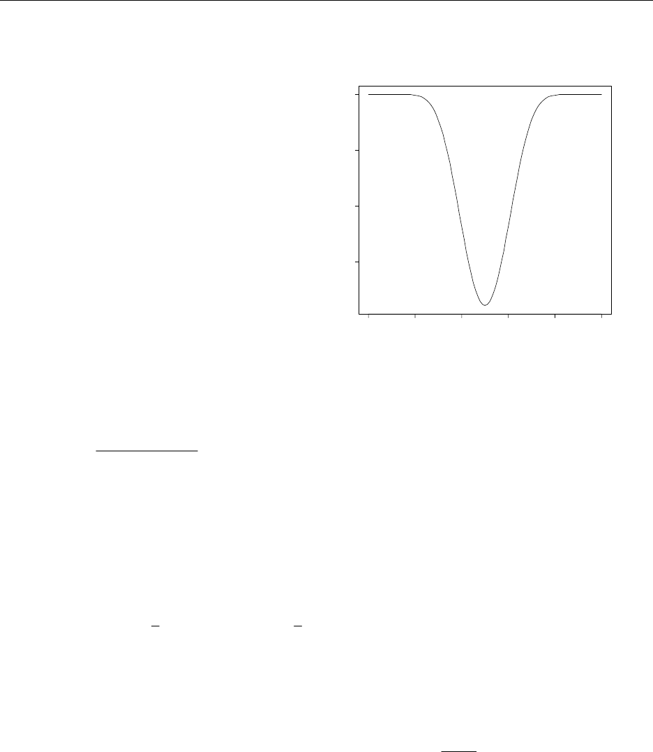
Chapter 10: Hypothesis Testing 227
Instructor’s Solutions Manual
A graph of the power function is above.
0.00.20.40.60.81.0
0.4 0.6 0.8 1.0
p
power
10.117 a. The hypotheses are H0: μ1 – μ2 = 0 vs. Ha: μ1 – μ2 ≠ 0, where μ1 = mean nitrogen
density for chemical compounds and μ2 = mean nitrogen density for air. Then,
000001064.
17
)000574(.8)00131(.9
222 == +
p
s and |t| = 22.17 with 17 degrees of freedom. The p–
value is far less than 2(.005) = .01 so H0 should be rejected.
b. The 95% CI for μ1 – μ2 is (–.01151, –.00951).
c. Since the CI do not contain 0, there is evidence that the mean densities are different.
d. The two approaches agree.
10.118 The hypotheses are H0: μ1 – μ2 = 0 vs. Ha: μ1 – μ2 < 0, where μ1 = mean alcohol blood
level for sea level and μ2 = mean alcohol blood level for 12,000 feet. The sample
statistics are 1
y = .10, s1 = .0219, 2
y = .1383, s2 = .0232. The computed value of the
test statistic is t = –2.945 and with 10 degrees of freedom, –t.10 = –1.383 so H0 should be
rejected.
10.119 a. The hypotheses are H0: p = .20, Ha: p > .20.
b. Let Y = # who prefer brand A. The significance level is
α = P(Y ≥ 92 | p = .20) = P(Y > 91.5 | p = .20) ≈ P(Z > 8
805.91 −) = P(Z > 1.44) = .0749.
10.120 Let μ = mean daily chemical production.
a. H0: μ = 1100, Ha: μ < 1100.
b. With .05 significance level, we can reject H0 if Z < –1.645.
c. For this large sample test, Z = –1.90 and we reject H0: there is evidence that
suggests there has been a drop in mean daily production.
10.121 The hypotheses are H0: μ1 – μ2 = 0 vs. Ha: μ1 – μ2 ≠ 0, where μ1, μ2 are the mean
breaking distances. For this large–sample test, the computed test statistic is
www.elsolucionario.net

228 Chapter 10: Hypothesis Testing
Instructor’s Solutions Manual
64
87
64
102
109118
||
+
−
=z = 5.24. Since p–value ≈ 2P(Z > 5.24) is approximately 0, we can reject
the null hypothesis: the mean braking distances are different.
10.122 a. To test H0:2
1
σ = 2
2
σ vs. Ha:2
1
σ > 2
2
σ, where 2
1
σ, 2
2
σ represent the population
variances for the two lines, the test statistic is F = (92,000)/(37,000) = 2.486 with 49
numerator and 49 denominator degrees of freedom. So, with F.05 = 1.607 we can reject
the null hypothesis.
b. p–value = P(F > 2.486) = .0009
Using R:
> 1-pf(2.486,49,49)
[1] 0.0009072082
10.123 a. Our test is H0:2
1
σ = 2
2
σ vs. Ha:2
1
σ ≠ 2
2
σ, where 2
1
σ, 2
2
σ represent the population
variances for the two suppliers. The computed test statistic is F = (.273)/(.094) = 2.904
with 9 numerator and 9 denominator degrees of freedom. With α = .05, F.05 = 3.18 so
H0 is not rejected: we cannot conclude that the variances are different.
b. The 90% CI is given by
(
)
32511.3
)094(.9
919.16
)094(.9 , = (.050, .254). We are 90% confident that the
true variance for Supplier B is between .050 and .254.
10.124 The hypotheses are H0: μ1 – μ2 = 0 vs. Ha: μ1 – μ2 ≠ 0, where μ1, μ2 are the mean
strengths for the two materials. Then, 0033.
2=
p
s and t =
⎟
⎠
⎞
⎜
⎝
⎛
−
9
2
0033.
978.237.1 = 9.568 with 17
degrees of freedom. With α = .10, the critical value is t.05 = 1.746 and so H0 is rejected.
10.125 a. The hypotheses are H0: μA – μB = 0 vs. Ha: μA – μB ≠ 0, where μA, μB are the mean
efficiencies for the two types of heaters. The two sample means are 73.125, 77.667,
and 017.10
2=
p
s. The computed test statistic is
⎟
⎠
⎞
⎜
⎝
⎛+
−
6
1
8
1
017.10
667.77125.73 = –2.657 with 12 degrees of
freedom. Since p–value = 2P(T > 2.657), we obtain .02 < p–value < .05 from Table 5
in Appendix III.
b. The 90% CI for μA – μB is
(
)
6
1
8
1
017.10782.1667.77125.73 +±− = –4.542 ± 3.046 or (–7.588, –1.496).
Thus, we are 90% confident that the difference in mean efficiencies is between –7.588
and –1.496.
10.126 a. 3
2
3
1
2
2
1
2
1
)()()()
ˆ
()
ˆ
(2
3
2
2
2
1n
a
n
a
n
a
WVaYVaXVaVSE ++σ=++=θ=θ .
b. Since θ
ˆ is a linear combination of normal random variables, θ
ˆ is normally
distributed with mean θ and standard deviation given in part a.
www.elsolucionario.net

Chapter 10: Hypothesis Testing 229
Instructor’s Solutions Manual
c. The quantity 22
321 /)( σ++ p
Snnn is chi–square with n1+n2+n3 – 3 degrees of freedom
and by Definition 7.2, T has a t–distribution with n1+n2+n3 – 3 degrees of freedom.
d. A 100(1 – α)% CI for θ is 3
2
3
1
2
2
1
2
1
2/
ˆn
a
n
a
n
a
p
st ++±θ α, where tα/2 is the upper–α/2 critical
value from the t–distribution with n1+n2+n3 – 3 degrees of freedom.
e. Under H0, the quantity
3
2
3
1
2
2
1
2
1
)
ˆ
(0
n
a
n
a
n
a
p
s
t++
θ−θ
= has a t–distribution with n1+n2+n3 – 3
degrees of freedom. Thus, the rejection region is: |t| > tα/2.
10.127 Let P = X + Y – W. Then, P has a normal distribution with mean μ1 + μ2 – μ3 and
variance (1 + a + b)σ2. Further, WYXP −+= is normal with mean μ1 + μ2 – μ3 and
variance (1 + a + b)σ2/n. Therefore,
nba
P
Z/)1(
)( 321
++σ
μ−μ+μ−
=
is standard normal. Next, the quantities
2
1
2
2
1
2
2
1
2)(
,
)(
,
)(
σ
−
σ
−
σ
−∑∑∑ ===
b
WW
a
YYXX n
ii
n
ii
n
ii
have independent chi–square distributions, each with n – 1 degrees of freedom. So,
their sum is chi–square with 3n – 3 degrees of freedom. Therefore, by Definition 7.2,
we can build a random variable that follows a t–distribution (under H0) by
nbaS
kP
T
p/)1( ++
−
=,
where
(
)
)33()()()( 1
2
1
1
2
1
1
22 −−+−+−= ∑∑∑ === nWWYYXXS n
ii
b
n
ii
a
n
iiP . For the test,
we reject if |t| > t.025, where t.025 is the upper .024 critical value from the t–distribution
with 3n – 3 degrees of freedom.
10.128 The point of this exercise is to perform a “two–sample” test for means, but information
will be garnered from three samples – that is, the common variance will be estimated
using three samples. From Section 10.3, we have the standard normal quantity
21
11
21 )(
nn
YX
Z+σ
μ−μ−−
=.
As in Ex. 10.127,
(
)
2
1
2
1
2
1
2321 )()()( σ−+−+− ∑∑∑ ===
n
ii
n
ii
n
iiWWYYXX has a chi–
square distribution with n1+n2+n3 – 3 degrees of freedom. So, define the statistic
(
)
)3()()()( 321
1
2
1
2
1
22 321 −++−+−+−= ∑∑∑ === nnnWWYYXXS n
ii
n
ii
n
iiP
www.elsolucionario.net

230 Chapter 10: Hypothesis Testing
Instructor’s Solutions Manual
and thus the quantity
21
11
21 )(
nn
P
S
YX
T+
μ−μ−−
= has a t–distribution with n1+n2+n3 – 3
degrees of freedom.
For the data given in this exercise, we have H0: μ1 – μ2 = 0 vs. Ha: μ1 – μ2 ≠ 0 and with
sP = 10, the computed test statistic is |t| =
10
2
10
5060− = 2.326 with 27 degrees of freedom.
Since t.025 = 2.052, the null hypothesis is rejected.
10.129 The likelihood function is ∑=
−θθ−−θ=Θ n
ii
nyL 1121 ]/)(exp[)( . The MLE for θ2 is
)1(2
ˆY=θ . To find the MLE of θ1, we maximize the log–likelihood function to obtain
)
ˆ
(
ˆ
12
1
1∑=θ−=θ n
ii
nY. Under H0, the MLEs for θ1 and θ2 are (respectively) θ1,0 and
)1(2
ˆY=θ as before. Thus, the LRT is
⎥
⎥
⎦
⎤
⎢
⎢
⎣
⎡
θ
−
+
θ
−
−
⎟
⎟
⎠
⎞
⎜
⎜
⎝
⎛
θ
θ
=
Ω
Ω
=λ ∑∑ ==
1
1)1(
0,1
1)1(
0,1
1
0
ˆ
)()(
exp
ˆ
)
ˆ
(
)
ˆ
(n
ii
n
ii
nyyyy
L
L
⎥
⎥
⎦
⎤
⎢
⎢
⎣
⎡+
θ
−
−
⎟
⎟
⎠
⎞
⎜
⎜
⎝
⎛
θ
−
=∑∑ == n
yy
n
yy n
ii
n
n
ii
0,1
1)1(
0,1
1)1( )(
exp
)( .
Values of λ ≤ k reject the null hypothesis.
10.130 Following Ex. 10.129, the MLEs are )
ˆ
(
ˆ
12
1
1∑=θ−=θ n
ii
nY and )1(2
ˆY=θ . Under H0, the
MLEs for θ2 and θ1 are (respectively) θ2,0 and )(
ˆ
10,2
1
0,1 ∑=θ−=θ n
ii
nY. Thus, the LRT is
given by
n
n
ii
n
ii
n
ii
n
ii
n
y
yyyyy
L
L
⎥
⎥
⎦
⎤
⎢
⎢
⎣
⎡
θ−
−
=
⎥
⎥
⎦
⎤
⎢
⎢
⎣
⎡
θ
−
+
θ
θ−
−
⎟
⎟
⎠
⎞
⎜
⎜
⎝
⎛
θ
θ
=
Ω
Ω
=λ ∑
∑∑∑
=
===
10,2
1)1(
1
1)1(
0,1
10,2
0,1
1
0
)(
)(
ˆ
)(
ˆ
)(
exp
ˆ
ˆ
)
ˆ
(
)
ˆ
(.
Values of λ ≤ k reject the null hypothesis.
www.elsolucionario.net
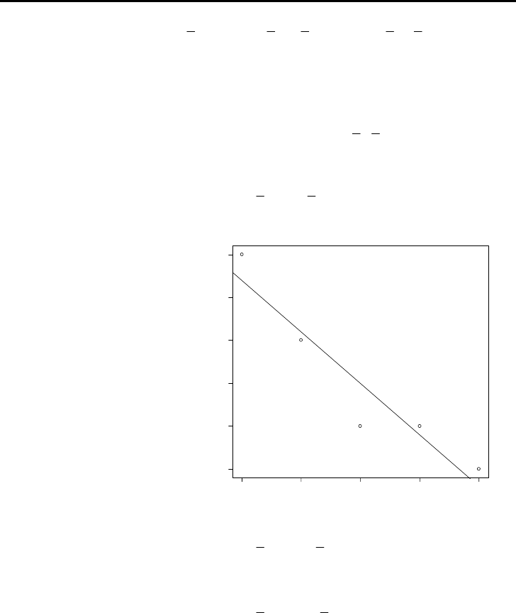
231
Chapter 11: Linear Models and Estimation by Least Squares
11.1 Using the hint, .
ˆ
)
ˆ
(
ˆˆ
)(
ˆ1110 yxxyxxy =β+β−=β+β=
11.2 a. slope = 0, intercept = 1. SSE = 6.
b. The line with a negative slope should exhibit a better fit.
c. SSE decreases when the slope changes from .8 to .7. The line is pivoting around the
point (0, 1), and this is consistent with (
y
x
, ) from part Ex. 11.1.
d. The best fit is: y = 1.000 + 0.700x.
11.3 The summary statistics are:
x
= 0,
y
= 1.5, Sxy = –6, Sxx = 10. Thus, y
ˆ = 1.5 – .6x.
The graph is above.
-2 -1 0 1 2
0.5 1.0 1.5 2.0 2.5 3.0
p11.3x
p11.3y
11.4 The summary statistics are:
x
= 72,
y
= 72.1, Sxy = 54,243, Sxx = 54,714. Thus, y
ˆ =
0.72 + 0.99x. When x = 100, the best estimate of y is y
ˆ = 0.72 + 0.99(100) = 99.72.
11.5 The summary statistics are:
x
= 4.5,
y
= 43.3625, Sxy = 203.35, Sxx = 42. Thus, y
ˆ =
21.575 + 4.842x. Since the slope is positive, this suggests an increase in median prices
over time. Also, the expected annual increase is $4,842.
11.6 a. intercept = 43.362, SSE = 1002.839.
b. the data show an increasing trend, so a line with a negative slope would not fit well.
c. Answers vary.
d. Answers vary.
e. (4.5, 43.3625)
f. The sum of the areas is the SSE.
11.7 a. The relationship appears to be proportional to x2.
b. No.
c. No, it is the best linear model.
www.elsolucionario.net
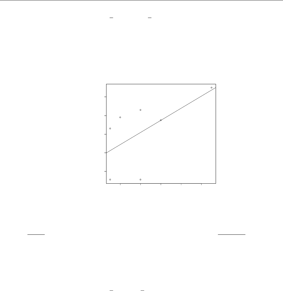
232 Chapter 11: Linear Models and Estimation by Least Squares
Instructor’s Solutions Manual
11.8 The summary statistics are:
x
= 15.505,
y
= 9.448, Sxy = 1546.459, Sxx = 2359.929.
Thus, y
ˆ = –0.712 + 0.655x. When x = 12, the best estimate of y is y
ˆ = –.712 +
0.655(12) = 7.148.
11.9 a. See part c.
b. y
ˆ = –15.45 + 65.17x.
c. The graph is above.
1.61.82.02.22.4
60 80 100 120 140
p11.9x
p11.9y
d. When x = 1.9, the best estimate of y is y
ˆ = –15.45 + 65.17(1.9) = 108.373.
11.10 0)(2)(2
SSE 2
11
11
1
=β−−=β−−=
β∑∑ == i
n
iiiii
n
iixyxxxy
d
d, so ∑
∑
=
=
=β n
ii
n
iii
x
yx
1
2
1
1
ˆ.
11.11 Since ∑=
n
iii yx
1 = 134,542 and ∑=
n
ii
x
1
2 = 53,514, 1
ˆ
β = 2.514.
11.12 The summary statistics are:
x
= 20.4,
y
= 12.94, Sxy = –425.571, Sxx = 1859.2.
a. The least squares line is: y
ˆ = 17.609 – 0.229x.
www.elsolucionario.net
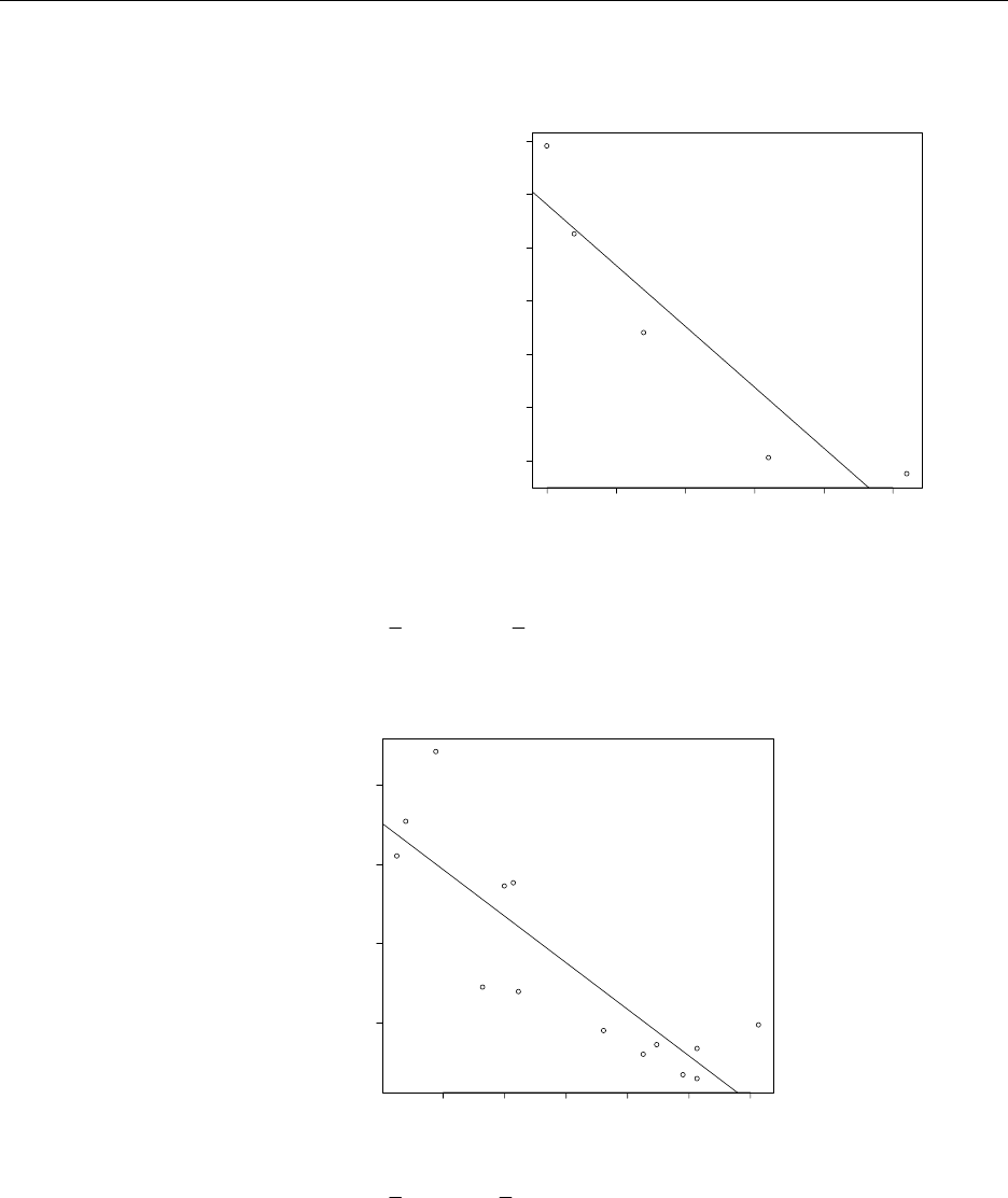
Chapter 11: Linear Models and Estimation by Least Squares 233
Instructor’s Solutions Manual
b. The line provides a reasonable fit.
0 1020304050
8 101214161820
p11.12x
p11.12y
c. When x = 20, the best estimate of y is y
ˆ = 17.609 – 0.229(20) = 13.029 lbs.
11.13 The summary statistics are:
x
= 6.177,
y
= 270.5, Sxy = –5830.04, Sxx = 198.29.
a. The least squares line is: y
ˆ = 452.119 – 29.402x.
b. The graph is above.
24681012
200 300 400 500
p11.13x
p11.13y
11.14 The summary statistics are:
x
= .325,
y
= .755, Sxy = –.27125, Sxx = .20625
a. The least squares line is: y
ˆ = 1.182 – 1.315x.
www.elsolucionario.net
234 Chapter 11: Linear Models and Estimation by Least Squares
Instructor’s Solutions Manual
0.1 0.2 0.3 0.4 0.5
0.4 0.5 0.6 0.7 0.8 0.9 1.0
p11.14x
p11.14y
b. The graph is above. The line provides a reasonable fit to the data.
11.15 a. SSE ))()](
ˆ
[)
ˆˆ
(1
22
1
1
2
1
10∑∑∑ === −=−β−−=β−β−= n
iii
n
iii
n
iiyyxxyyxy
+ ∑∑ == −−β−−β n
iii
n
iixxyyxx 1
1
1
22
1))((
ˆ
2)(
ˆ
∑=−= n
iiyy
1
2
)(+ xyxy SS 11 ˆ
2
ˆβ−β = yy
Sxy
S
1
ˆ
β− .
b. Since xyyy SS 1
ˆ
SSE β−= ,
xxxyxyyy SSSS /)(SSE
ˆ
SSE 2
1+=β+= . But, Sxx > 0 and (Sxy)2 ≥ 0. So,
SSE ≥
yy
S.
11.16 The summary statistics are:
x
= 60,
y
= 27, Sxy = –1900, Sxx = 6000.
a. The least squares line is: y
ˆ = 46.0 –.31667x.
b. The graph is above.
30 40 50 60 70 80 90
15 20 25 30 35 40
p11.16x
p11.16y
www.elsolucionario.net
Chapter 11: Linear Models and Estimation by Least Squares 235
Instructor’s Solutions Manual
c. Using the result in Ex. 11.15(a), SSE = yy
Sxy
S
1
ˆ
β− = 792 – (–.31667)(–1900) =
190.327. So, s2 = 190.327/10 = 19.033.
11.17 a. With Syy = 1002.8388 and Sxy = 203.35, SSE = 1002.8388 – 4.842(203.35) = 18.286.
So, s2 = 18.286/6 = 3.048.
b. The fitted line is y
ˆ = 43.35 + 2.42x*. The same answer for SSE (and thus s2) is
found.
11.18 a. For Ex. 11.8, Syy = 1101.1686 and Sxy = 1546.459, SSE = 1101.1686 –
.6552528(1546.459) = 87.84701. So, s2 = 87.84701/8 = 10.98.
b. Using the coding xxx ii −=
*, the fitted line is y
ˆ = 9.448 + .655x*. The same answer
for s2 is found.
11.19 The summary statistics are:
x
= 16,
y
= 10.6, Sxy = 152.0, Sxx = 320.
a. The least squares line is: y
ˆ = 3.00 + 4.75x.
b. The graph is above.
10 15 20
6 8 10 12 14 16
p11.19x
p11.19y
c. s2 = 5.025.
11.20 The likelihood function is given by,
(
)
n
Kπσ= 2,
()
⎥
⎦
⎤
⎢
⎣
⎡β−β−
σ
−=ββ ∑=
n
iii xyKL 1
2
10
2
10 2
1
exp),(, so that
()
∑=β−β−
σ
−=ββ n
iii xyKL 1
2
10
2
10 2
1
ln),(ln .
Note that maximizing the likelihood (or equivalently the log–likelihood) with respect to
β0 and β1 is identical to minimizing the positive quantity
(
)
∑=β−β−
n
iii xy
1
2
10 . This is
the least–squares criterion, so the estimators will be the same.
www.elsolucionario.net

236 Chapter 11: Linear Models and Estimation by Least Squares
Instructor’s Solutions Manual
11.21 Using the results of this section and Theorem 5.12,
)
ˆ
(0)
ˆ
,
ˆ
(Cov)
ˆ
,(Cov)
ˆ
,
ˆ
(Cov)
ˆ
,
ˆ
(Cov 11111110 β−=ββ−β=ββ−=ββ VxxYxY .
Thus, )
ˆ
,
ˆ
(Cov 10 ββ = xx
Sx /
2
σ− . Note that if ∑=
n
ii
x
1= 0,
x
= 0 so )
ˆ
,
ˆ
(Cov 10 ββ = 0.
11.22 From Ex. 11.20, let θ = σ2 so that the log–likelihood is
()
∑=β−β−
θ
−θ−π−=θ n
iii
nn xyL 1
2
10
22 2
1
ln)2ln()(ln .
Thus,
()
∑=
θβ−β−
θ
+
θ
−=θ n
iii
d
dxy
n
L1
2
10
2
2
1
2
)(ln .
The MLE is
(
)
∑=β−β−=σ=θ n
iii
nxy
1
2
10
1
2
ˆ
ˆ, but since β0 and β1 are unknown, we can
insert their MLEs from Ex. 11.20 to obtain:
(
)
SSE
ˆˆ
ˆ1
1
2
10
1
2
n
n
iii
nxy =β−β−=σ ∑=.
11.23 From Ex. 11.3, it is found that Syy = 4.0
a. Since SSE = 4 – (–.6)(–6) = .4, s2 = .4/3 = .1333. To test H0: β1 = 0 vs. Ha: β1 ≠ 0,
)1(.1333.
|6.|
|| −
=t = 5.20 with 3 degrees of freedom. Since t.025 = 3.182, we can reject H0.
b. Since t.005 = 5.841 and t.01 = 4.541, .01 < p–value < .02.
Using the Applet, 2P(T > 5.20) = 2(.00691) = .01382.
c. –.6 ± 3.182 1.1333. = –.6 ± .367 or (–.967, –.233).
11.24 To test H0: β1 = 0 vs. Ha: β1 ≠ 0, SSE = 61,667.66 and s2 =5138.97. Then,
)005043(.97.5139
|402.29|
|| −
=t = 5.775 with 12 degrees of freedom.
a. From Table 5, P(|T| > 3.055) = 2(.005) = .01 > p–value.
b. Using the Applet, 2P(T > 5.775) = .00008.
c. Reject H0.
11.25 From Ex. 11.19, to test H0: β1 = 0 vs. Ha: β1 ≠ 0, s2 = 5.025 and Sxx = 320. Then,
320/025.5
|475.|
|| =t = 3.791 with 8 degrees of freedom.
a. From Table 5, P(|T| > 3.355) = 2(.005) = .01 > p–value.
b. Using the Applet, 2P(T > 3.791) = 2(.00265) = .0053.
c. Reject H0.
d. We cannot assume the linear trend continues – the number of errors could level off
at some point.
e. A 95% CI for β1: .475 ± 2.306 320/025.5 = .475 ± .289 or (.186, .764). We are
95% confident that the expected change in number of errors for an hour increase of
lost sleep is between (.186, .764).
11.26 The summary statistics are:
x
= 53.9,
y
= 7.1, Sxy = 198.94, Sxx = 1680.69, Syy = 23.6.
a. The least squares line is: y
ˆ = 0.72 + 0.118x.
www.elsolucionario.net

Chapter 11: Linear Models and Estimation by Least Squares 237
Instructor’s Solutions Manual
b. SSE = 23.6 – .118(198.94) = .125 so s2 = .013. A 95% CI for β1 is 0.118 ±
2.776 00059.013. = 0.118 ± .008.
c. When x = 0, E(Y) = β0 + β1(0) = β0. So, to test H0: β0 = 0 vs. Ha: β0 ≠ 0, the test
statistic is 895.1013.
|72.|
|| =t= 4.587 with 4 degrees of freedom. Since t.005 = 4.604 and
t.01 = 3.747, we know that .01 < p–value < .02.
d. Using the Applet, 2P(T > 4.587) = 2(.00506) = .01012.
e. Reject H0.
11.27 Assuming that the error terms are independent and normally distributed with 0 mean
and constant variance σ2:
a. We know that
ii
ii
c
Zσ
β−β
=0,
ˆ
has a standard normal distribution under H0.
Furthermore, 22 /)2( σ−= SnV has a chi–square distribution with n – 2 degrees of
freedom. Therefore, by Definition 7.2,
ii
ii
cSnV
Z0,
ˆ
)2/(
β−β
=
−
has a t–distribution with n – 2 degrees of freedom under H0 for i = 1, 2.
b. Using the pivotal quantity expressed above, the result follows from the material in
Section 8.8.
11.28 Restricting to Ω0, the likelihood function is
⎥
⎦
⎤
⎢
⎣
⎡β−
σ
−=Ω ∑=
σπ
n
ii
yL nn 1
2
0
2
)2(
1
0)(
2
1
exp)( 2/ .
It is not difficult to verify that the MLEs for β0 and σ2 under the restricted space are
Y
and ∑=−
n
ii
nYY
1
2
1)( (respectively). The MLEs have already been found for the
unrestricted space so that the LRT simplifies to
2/
2/
1
2
1
2
0SSE
)(
)
ˆ
(
)
ˆ
(
)
ˆ
(n
yy
n
n
ii
n
iii
S
yy
yy
L
L⎟
⎟
⎠
⎞
⎜
⎜
⎝
⎛
=
⎟
⎟
⎠
⎞
⎜
⎜
⎝
⎛
−
−
=
Ω
Ω
=λ ∑
∑
=
=.
So, we reject if λ ≤ k, or equivalently if
kk
Sn
yy ′
=≥ −/2
SSE .
Using the result from 11.15,
)2(
1
)2(
ˆ
1
SSE
ˆ
1
SSE
ˆ
SSE 2
2
1
11
−
+=
−
β
+=
β
+=
β+
n
T
Sn
S
SS xx
xyxy .
So, we see that λ is small whenever
11
1
ˆ
cS
Tβ
= is large in magnitude, where
xx
S
c1
11 =.
This is the usual t–test statistic, so the result has been proven.
www.elsolucionario.net

238 Chapter 11: Linear Models and Estimation by Least Squares
Instructor’s Solutions Manual
11.29 Let 1
ˆ
β and 1
ˆ
γ be the least–squares estimators for the linear models Yi = β0 + β1xi + εi
and Wi = γ0 + γ1ci + εi as defined in the problem Then, we have that:
• E(1
ˆ
β – 1
ˆ
γ
) = β1 – γ1
• V(1
ˆ
β – 1
ˆ
γ
) =
(
)
ccxx SS 11
2+σ , where ∑=−= m
iicc ccS 1
2
)(
• 1
ˆ
β – 1
ˆ
γ
follows a normal distribution, so that under H0, β1 – γ1 = 0 so that
()
ccxx SS
Z11
11 ˆ
ˆ
+σ
γ−β
= is standard normal
• Let V = SSEY + SSEW = ∑∑ == −+− m
iii
n
iii WWYY 1
22
1)
ˆ
()
ˆ
( . Then, 2
/σV has a
chi–square distribution with n + m – 4 degrees of freedom
• By Definition 7.2 we can build a random variable with a t–distribution (under
H0):
()
ccxx SS
S
mnV
Z
T11
11 ˆ
ˆ
)4/( +
γ−β
=
−+
=, where S = (SSEY + SSEW)/(n + m – 4).
H0 is rejected in favor of Ha for large values of |T|.
11.30 a. For the first experiment, the computed test statistic for H0: β1 = 0 vs. Ha: β1 ≠ 0 is t1 =
(.155)/(.0202) = 7.67 with 29 degrees of freedom. For the second experiment, the
computed test statistic is t2 = (.190)/(.0193) = 9.84 with 9 degrees of freedom. Both of
these values reject the null hypothesis at α = .05, so we can conclude that the slopes are
significantly different from 0.
b. Using the result from Ex. 11.29, 1026.)41131/()86.104.2( =
−
+
+
=
S. We can
extract the values of Sxx and Scc from the given values of V(1
ˆ
β):
2
1)0202(.
29/04.2
)
ˆ
(
)2/( =
β
−
=V
nSSE
SY
xx = 172.397,
so similarly Scc = 554.825. So, to test equality for the slope parameters, the computed
test statistic is
()
825.554
1
397.172
1
1024.
|190.155.|
|| +
−
=t = 1.25
with 38 degrees of freedom. Since t.025 ≈ z.025 = 1.96, we fail to reject H0: we cannot
conclude that the slopes are different.
11.31 Here, R is used to fit the regression model:
> x <- c(19.1, 38.2, 57.3, 76.2, 95, 114, 131, 150, 170)
> y <- c(.095, .174, .256, .348, .429, .500, .580, .651, .722)
> summary(lm(y~x))
Call:
lm(formula = y ~ x)
www.elsolucionario.net

Chapter 11: Linear Models and Estimation by Least Squares 239
Instructor’s Solutions Manual
Residuals:
Min 1Q Median 3Q Max
-1.333e-02 -4.278e-03 -2.314e-05 8.056e-03 9.811e-03
Coefficients:
Estimate Std. Error t value Pr(>|t|)
(Intercept) 1.875e-02 6.129e-03 3.059 0.0183 *
x 4.215e-03 5.771e-05 73.040 2.37e-11 ***
---
Signif. codes: 0 '***' 0.001 '**' 0.01 '*' 0.05 '.' 0.1 ' ' 1
Residual standard error: 0.008376 on 7 degrees of freedom
Multiple R-Squared: 0.9987, Adjusted R-squared: 0.9985
F-statistic: 5335 on 1 and 7 DF, p-value: 2.372e-11
From the output, the fitted model is y
ˆ = .01875 + .004215x. To test H0: β1 = 0 against
Ha: β1 ≠ 0, note that the p–value is quite small indicating a very significant test statistic.
Thus, H0 is rejected and we can conclude that peak current increases as nickel
concentrations increase (note that this is a one–sided alternative, so the p–value is
actually 2.37e-11 divided by 2).
11.32 a. From Ex. 11.5, 1
ˆ
β = 4.8417 and Sxx = 42. From Ex. 11.15, s2 = 3.0476 so to test H0:
β1 = 0 vs. Ha: β1 > 0, the required test statistic is t = 17.97 with 6 degrees of freedom.
Since t.01 = 3.143, H0 is rejected: there is evidence of an increase.
b. The 99% CI for β1 is 4.84 ± 1.00 or (3.84, 5.84).
11.33 Using the coded x’s from 11.18, *
1
ˆ
β = .655 and s2 = 10.97. Since Sxx =
()
∑=
10
1
2
*
ii
x=
2360.2388, the computed test statistic is
2388.2360
97.10
655.
|| =t = 9.62 with 8 degrees of
freedom. Since t.025 = 2.306, we can conclude that there is evidence of a linear
relationship.
11.34 a. Since t.005 = 3.355, we have that p–value < 2(.005) = .01.
b. Using the Applet, 2P(T < 9.61) = 2(.00001) = .00002.
11.35 With a0 = 1 and a1 = x*, the result follows since
(
)
2
2*2*2
1
2
1
2
*2*
1
2
1
*
10
2)(2)(1
)
ˆˆ
(σ
+−+−
=σ
−+⋅
=β+β ∑∑ ==
xx
n
ii
n
xx
n
ii
n
S
xxxxxnx
S
xxxx
xV
2
2*
2
2*
1)(1
)( σ
⎥
⎦
⎤
⎢
⎣
⎡−
+=σ
−+
=
xxxx
xx
n
S
xx
nS
xxS .
www.elsolucionario.net
240 Chapter 11: Linear Models and Estimation by Least Squares
Instructor’s Solutions Manual
This is minimized when 0)( 2* =− xx , so .
*xx =
11.36 From Ex. 11.13 and 11.24, when x* = 5, y
ˆ = 452.119 – 29.402(5) = 305.11 so that
V(
Y
ˆ) is estimated to be 402.98. Thus, a 90% CI for E(Y) is 305.11 ± 1.782 98.402 =
305.11 ± 35.773.
11.37 From Ex. 11.8 and 11.18, when x* = 12, y
ˆ = 7.15 so that V(
Y
ˆ) is estimated to be
⎥
⎦
⎤
⎢
⎣
⎡−
+929.2359
)504.1512(
1.97.10
2
= 1.154 Thus, a 95% CI for E(Y) is 7.15 ± 2.306 154.1 =
7.15 ± 2.477 or (4.67, 9.63).
11.38 Refer to Ex. 11.3 and 11.23, where s2 = .1333, y
ˆ = 1.5 – .6x, Sxx = 10 and
x
= 0.
• When x* = 0, the 90% CI for E(Y) is 1.5 ± 2.353 )(1333. 5
1 or (1.12, 1.88).
• When x* = –2, the 90% CI for E(Y) is 2.7 ± 2.353 )(1333. 10
4
5
1+ or (2.03, 3.37).
• When x* = 2, the 90% CI for E(Y) is .3 ± 2.353 )(1333. 10
4
5
1+ or (–.37, .97).
On the graph, note the interval lengths.
-2 -1 0 1 2
-101234
p11.3x
p11.3y
11.39 Refer to Ex. 11.16. When x* = 65, y
ˆ = 25.395 and a 95% CI for E(Y) is
25.395 ± 2.228 ⎥
⎦
⎤
⎢
⎣
⎡−
+6000
)6065(
12
1
033.19
2
or 25.395 ± 2.875.
11.40 Refer to Ex. 11.14. When x* = .3, y
ˆ = .7878 and with SSE = .0155, Sxx = .20625, and
x
= .325, the 90% CI for E(Y) is .7878 ± 1.86 ⎥
⎦
⎤
⎢
⎣
⎡−
+20625.
)325.3(.
10
1
8
0155. 2
or (.76, .81).
www.elsolucionario.net

Chapter 11: Linear Models and Estimation by Least Squares 241
Instructor’s Solutions Manual
11.41 a. Using xY 10 ˆˆ β−=β and 1
ˆ
β as estimators, we have xy xY μβ+β−=μ 11 ˆˆ
ˆ so that
)(
ˆ
ˆ1xy xY μ−β−=μ .
b. Calculate
(
)
xx
x
xx S
x
nS
x
n
xy xVxYVV 2
22 )(
1
22
1
2)()
ˆ
()()()
ˆ
(μ−
σσ +σ=μ−+=βμ−+=μ .
From Ex. 11.4, s2 = 7.1057 and Sxx = 54,714 so that )7274(99.1.72
ˆ−
+
=
μ
y = 74.08
and the variance of this estimate is calculated to be
[
]
714,54
)7274(
10
12
1057.7 −
+ = .711. The
two–standard deviation error bound is 2 711. = 1.69.
11.42 Similar to Ex. 11.35, the variance is minimized when .
*xx =
11.43 Refer to Ex. 11.5 and 11.17. When x = 9 (year 1980), y
ˆ = 65.15 and the 95% PI is
(
)
42
)5.49(
8
12
105.3447.215.65 −
++± = 65.15 ± 5.42 or (59.73, 70.57).
11.44 For the year 1981, x = 10. So, y
ˆ = 69.99 and the 95% PI is
(
)
42
)5.410(
8
12
105.3447.299.69 −
++± = 69.99 ± 5.80.
For the year 1982, x = 11. So, y
ˆ = 74.83 and the 95% PI is
(
)
42
)5.411(
8
12
105.3447.283.74 −
++± = 74.83 ± 6.24.
Notice how the intervals get wider the further the prediction is from the mean. For the
year 1988, this is far beyond the limits of experimentation. So, the linear relationship
may not hold (note that the intervals for 1980, 1981 and 1982 are also outside of the
limits, so caveat emptor).
11.45 From Ex. 11.8 and 11.18 (also see 11.37), when x* = 12, y
ˆ = 7.15 so that the 95% PI is
7.15 ± ⎥
⎦
⎤
⎢
⎣
⎡−
++ 929.2359
)504.1512(
10
1
197.10306.2
2
= 7.15 ± 8.03 or (–.86, 15.18).
11.46 From 11.16 and 11.39, when x* = 65, y
ˆ = 25.395 so that the 95% PI is given by
25.395 ± ⎥
⎦
⎤
⎢
⎣
⎡−
++ 6000
)6065(
12
1
1033.19228.2
2
= 25.395 ± 10.136.
11.47 From Ex. 11.14, when x* = .6, y
ˆ = .3933 so that the 95% PI is given by
.3933 ± ⎥
⎦
⎤
⎢
⎣
⎡−
++ 20625.
)325.6(.
10
1
100194.306.2
2
= .3933 ± .12 or (.27, .51).
11.48 The summary statistics are Sxx = 380.5, Sxy = 2556.0, and Syy = 19,263.6. Thus, r = .944.
To test H0: ρ = 0 vs. Ha: ρ > 0, t = 8.0923 with 8 degrees of freedom. From Table 7, we
find that p–value < .005.
www.elsolucionario.net

242 Chapter 11: Linear Models and Estimation by Least Squares
Instructor’s Solutions Manual
11.49 a. r2 behaves inversely to SSE, since r2 = 1 – SSE/Syy.
b. The best model has r2 = .817, so r = .90388 (since the slope is positive, r is as well).
11.50 a. r2 increases as the fit improves.
b. For the best model, r2 = .982 and so r = .99096.
c. The scatterplot in this example exhibits a smaller error variance about the line.
11.51 The summary statistics are Sxx = 2359.929, Sxy = 1546.459, and Syy = 1101.1686. Thus,
r = .9593. To test H0: ρ = 0 vs. Ha: ρ ≠ 0, |t| = 9.608 with 8 degrees of freedom. From
Table 7, we see that p–value < 2(.005) = .01 so we can reject the null hypothesis that the
correlation is 0.
11.52 a. Since the slope of the line is negative, 61.
2−=−= rr = –.781.
b. This is given by r2, so 61%.
c. To test H0: ρ = 0 vs. Ha: ρ < 0, 2
)781.(1
12781.
−−
−
=t = –4.33 with 12 degrees of freedom.
Since – t.05 = –1.782, we can reject H0 and conclude that plant density decreases with
increasing altitude.
11.53 a. This is given by r2 = (.8261)2 = .68244, or 68.244%.
b. Same answer as part a.
c. To test H0: ρ = 0 vs. Ha: ρ > 0, 2
)8261(.1
88261.
−
=t = 4.146 with 8 degrees of freedom. Since
t.01 = 2.896, we can reject H0 and conclude that heights and weights are positively
correlated for the football players.
d. p–value = P(T > 4.146) = .00161.
11.54 a. The MOM estimators for 2
X
σ and 2
Y
σ were given in Ex. 9.72.
b. By substituting the MOM estimators, the MOM estimator for ρ is identical to r, the
MLE.
11.55 Since xxxy SS /
ˆ1=β and yyxx SSr /
ˆ1
β= , we have that the usual t–test statistic is:
2
1
1
1
1
1
1
2
/
ˆ
1
2
ˆ
/
ˆ
2
ˆ
/
ˆ
r
nr
SS
nSS
SS
nS
SS
T
yyxy
yyxx
xyyy
xx
xx −
−
=
β−
−β
=
β−
−β
=
β
=.
11.56 Here, r = .8.
a. For n = 5, t = 2.309 with 3 degrees of freedom. Since t.05 = 2.353, fail to reject H0.
b. For n = 12, t = 4.2164 with 10 degrees of freedom. Here, t.05 = 1.812, reject H0.
c. For part a, p–value = P(T > 2.309) = .05209. For part (b), p–value = .00089.
d. Different conclusions: note the 2−n term in the numerator of the test statistic.
e. The larger sample size in part b caused the computed test statistic to be more
extreme. Also, the degrees of freedom were larger.
www.elsolucionario.net
Chapter 11: Linear Models and Estimation by Least Squares 243
Instructor’s Solutions Manual
11.57 a. The sample correlation r determines the sign.
b. Both r and n determine the magnitude of |t|.
11.58 For the test H0: ρ = 0 vs. Ha: ρ > 0, we reject if t = 2
1
2
r
r
−≥ t.05 = 2.92. The smallest value
of r that would lead to a rejection of H0 is the solution to the equation
2
2
92.2 1rr −= .
Numerically, this is found to be r = .9000.
11.59 For the test H0: ρ = 0 vs. Ha: ρ < 0, we reject if t = 2
1
18
r
r
−≤ –t.05 = –1.734. The largest
value of r that would lead to a rejection of H0 is the solution to the equation
2
18
734.1 1rr −= −.
Numerically, this is found to be r = –.3783.
11.60 Recall the approximate normal distribution of
(
)
r
r
−
+
1
1
2
1ln given on page 606. Therefore,
for sample correlations r1 and r2, each being calculated from independent samples of
size n1 and n2 (respectively) and drawn from bivariate normal populations with
correlations coefficients ρ1 and ρ2 (respectively), we have that
(
)
(
)
(
)
(
)
[
]
3
1
3
1
1
1
2
1
1
1
2
1
1
1
2
1
1
1
2
1
21
2
2
1
1
2
2
1
1lnlnlnln
−−
ρ−
ρ+
ρ−
ρ+
−
+
−
+
+
−−−
=
nn
r
r
r
r
Z
is approximately standard normal for large n1 and n2.
Thus, to test H0: ρ1 = ρ2 vs. Ha: ρ1 ≠ ρ2 with r1 = .9593, n1 = 10, r2 = .85, n2 = 20, the
computed test statistic is
(
)
(
)
52.1
lnln
17
1
7
1
15.
85.1
2
1
0407.
9593.1
2
1=
+
−
=z.
Since the rejection region is all values |z| > 1.96 for α = .05, we fail to reject H0.
11.61 Refer to Example 11.10 and the results given there. The 90% PI is
234.
)457.15.1(
6
12
1)045(.132.2979. −
++± = .979 ± .104 or (.875, 1.083).
11.62 Using the calculations from Example 11.11, we have yyxx
xy
SS
S
r= = .9904. The
proportion of variation described is r2 = (.9904)2 = .9809.
11.63 a. Observe that lnE(Y) = lnα0 – α1x. Thus, the logarithm of the expected value of Y is
linearly related to x. So, we can use the linear model
wi = β0 + β1xi + εi,
where wi = lnyi, β0 = lnα0 and β1= – α1. In the above, note that we are assuming an
additive error term that is in effect after the transformation. Using the method of least
squares, the summary statistics are:
www.elsolucionario.net

244 Chapter 11: Linear Models and Estimation by Least Squares
Instructor’s Solutions Manual
x
= 5.5, 2
xΣ= 385, w = 3.5505, Sxw = –.7825, Sxx = 82.5, and Sww = .008448.
Thus, 1
ˆ
β = –.0095, 0
ˆ
β = 3.603 and 1
ˆ
α
= –(–.0095) = .0095, 0
ˆ
α
= exp(3.603) = 36.70.
Therefore, the prediction equation is x
ey 0095.
70.36
ˆ−
=.
b. To find a CI for α0, we first must find a CI for β0 and then merely transform the
endpoints of the interval. First, we calculate the SSE using SSE = Sww – 1
ˆ
βSxw =
.008448 – (–.0095)(–.782481) = .0010265 and so s2 = (.0010265)/8 = .0001283 Using
the methods given in Section 11.5, the 90% CI for β0 is
3.6027 ± 1.86
()
5.82(10
385
0001283. or (3.5883, 3.6171). So the 90% CI for α0 is given by
(
)
6171.35883.3 ,ee = (36.17, 37.23).
11.64 This is similar to Ex. 11.63. Note that lnE(Y) = –α01
α
x and ln[–lnE(Y)] = lnα0 + α1lnx.
So, we would expect that ln(–lny) to be linear in lnx. Define wi = ln(–lnyi), ti = lnxi, β0 =
lnα0, β1= α1. So, we now have the familiar linear model
wi = β0 + β1ti + εi
(again, we are assuming an additive error term that is in effect after the transformation).
The methods of least squares can be used to estimate the parameters. The summary
statistics are t = –1.12805, w = –1.4616, Stw = 3.6828, and Stt = 1.51548
So, 1
ˆ
β = 2.4142, 0
ˆ
β = 1.2617 and thus 1
ˆ
α
= 2.4142 and 0
ˆ
α
= exp(1.2617) = 3.5315.
This fitted model is
(
)
4142.2
5315.3exp
ˆxy −= .
11.65 If y is related to t according to y = 1 – e–βt, then –ln(1 – y) = βt. Thus, let wi = –ln(1 – yi)
and we have the linear model wi = βti + εi
(again assuming an additive error term). This is the “no–intercept” model described in
Ex. 11.10 and the least squares estimator for β is given to be ∑
∑
=
=
=β n
ii
n
iii
t
wt
1
2
1
ˆ. Now, using
similar methods from Section 11.4, note that ∑=
σ
=β n
ii
t
V
1
2
2
)
ˆ
( and 2
1
2
2
)
ˆ
(
SSE
σ
−
=
σ
∑=
n
iiww
is chi–square with n – 1 degrees of freedom. So, by Definition 7.2, the quantity
∑=
β−β
=n
ii
tS
T
1
2
/
ˆ,
where S = SSE/(n – 1) , has a t–distribution with n – 1 degrees of freedom.
A 100(1 – α)% CI for β is
www.elsolucionario.net

Chapter 11: Linear Models and Estimation by Least Squares 245
Instructor’s Solutions Manual
∑=
α
±β n
ii
t
St
1
2
2/
1
ˆ,
and tα/2 is the upper– α/2 critical value from the t–distribution with n – 1 degrees of
freedom.
11.66 Using the matrix notation from this section,
⎥
⎥
⎥
⎥
⎥
⎥
⎦
⎤
⎢
⎢
⎢
⎢
⎢
⎢
⎣
⎡
−
−
=
21
11
01
11
21
X
⎥
⎥
⎥
⎥
⎥
⎥
⎦
⎤
⎢
⎢
⎢
⎢
⎢
⎢
⎣
⎡
=
5.
1
1
2
3
Y ⎥
⎦
⎤
⎢
⎣
⎡
−
=
′6
5.7
YX ⎥
⎦
⎤
⎢
⎣
⎡
=
′100
05
XX .
Thus, ⎥
⎦
⎤
⎢
⎣
⎡
−
=
⎥
⎦
⎤
⎢
⎣
⎡
−
⎥
⎦
⎤
⎢
⎣
⎡
=
⎥
⎦
⎤
⎢
⎣
⎡
−
⎥
⎦
⎤
⎢
⎣
⎡
=
−
6.
5.1
6
5.7
1.0
02.
6
5.7
100
05
ˆ
1
β so that xy 6.5.1
ˆ−
=
.
11.67
⎥
⎥
⎥
⎥
⎥
⎥
⎦
⎤
⎢
⎢
⎢
⎢
⎢
⎢
⎣
⎡−
=
31
21
11
01
11
X
⎥
⎥
⎥
⎥
⎥
⎥
⎦
⎤
⎢
⎢
⎢
⎢
⎢
⎢
⎣
⎡
=
5.
1
1
2
3
Y ⎥
⎦
⎤
⎢
⎣
⎡
=
′5.1
5.7
YX ⎥
⎦
⎤
⎢
⎣
⎡
=
′155
55
XX
The student should verify that ⎥
⎦
⎤
⎢
⎣
⎡
−
−
=
′−
1.1.
1.3.
)( 1
XX so that ⎥
⎦
⎤
⎢
⎣
⎡
−
=6.
1.2
ˆ
β. Not that the
slope is the same as in Ex. 11.66, but the y–intercept is different. Since
X
X
′ is not a
diagonal matrix (as in Ex. 11.66), computing the inverse is a bit more tedious.
11.68
⎥
⎥
⎥
⎥
⎥
⎥
⎥
⎥
⎥
⎦
⎤
⎢
⎢
⎢
⎢
⎢
⎢
⎢
⎢
⎢
⎣
⎡
−
−
−
=
931
421
111
001
111
421
931
X
⎥
⎥
⎥
⎥
⎥
⎥
⎥
⎥
⎥
⎦
⎤
⎢
⎢
⎢
⎢
⎢
⎢
⎢
⎢
⎢
⎣
⎡
−
−
=
0
0
1
1
0
0
1
Y
⎥
⎥
⎥
⎦
⎤
⎢
⎢
⎢
⎣
⎡−
=
′
8
4
1
YX
⎥
⎥
⎥
⎦
⎤
⎢
⎢
⎢
⎣
⎡
=
′
196028
0280
2807
XX .
The student should verify (either using Appendix I or a computer),
www.elsolucionario.net
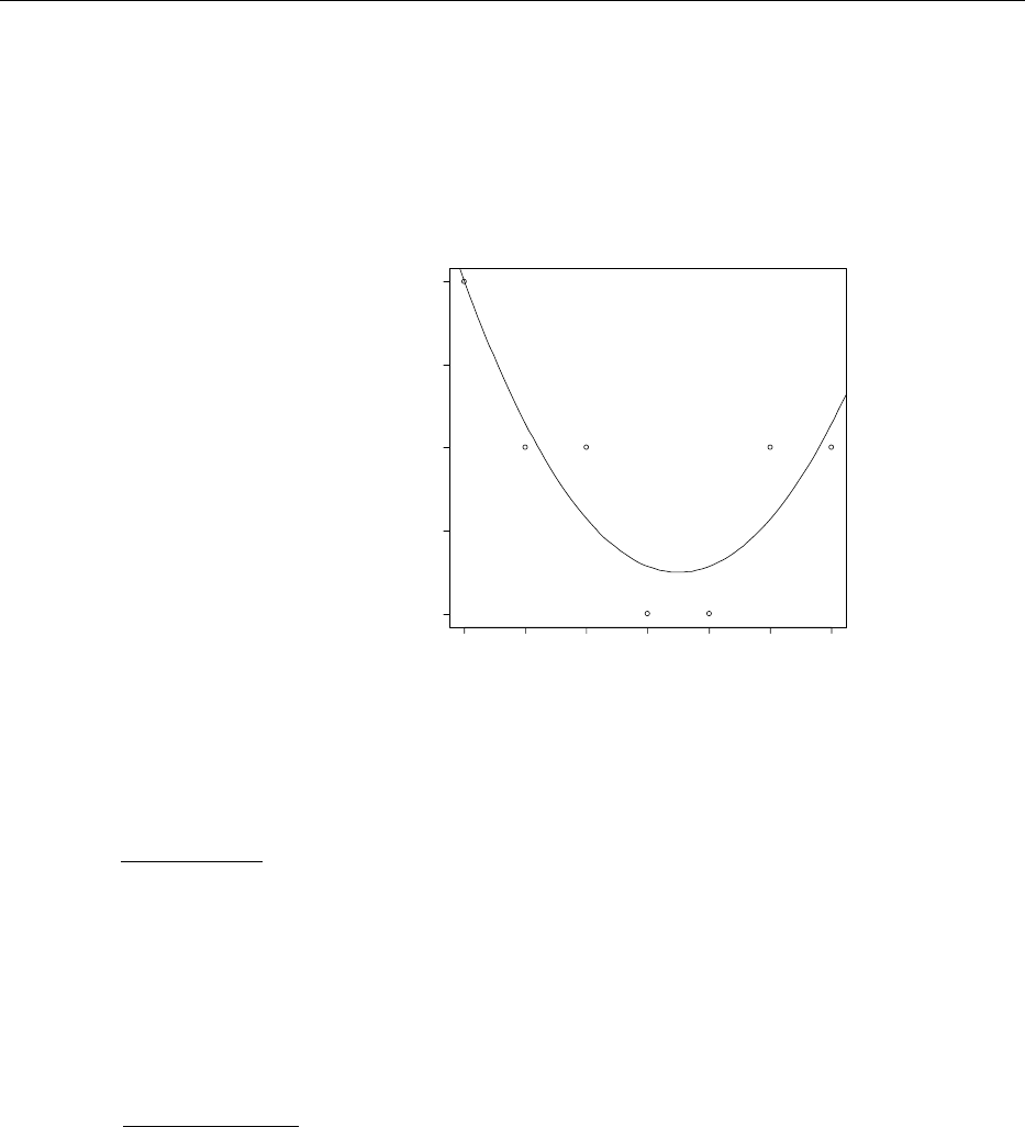
246 Chapter 11: Linear Models and Estimation by Least Squares
Instructor’s Solutions Manual
⎥
⎥
⎥
⎦
⎤
⎢
⎢
⎢
⎣
⎡
−
−
=
′−
011905.004762.
0035714.0
04762.03333.
)( 1
XX so that
⎥
⎥
⎥
⎦
⎤
⎢
⎢
⎢
⎣
⎡
−
−
=
142859.
142857.
714285.
ˆ
β and the fitted
model is 2
142859.142857.714285.
ˆxxy +−−= .
The graphed curve is above.
-3 -2 -1 0 1 2 3
-1.0 -0.5 0.0 0.5 1.0
p11.68x
p11.68y
11.69 For this problem, R will be used.
> x <- c(-7, -5, -3, -1, 1, 3, 5, 7)
> y <- c(18.5,22.6,27.2,31.2,33.0,44.9,49.4,35.0)
a. Linear model:
> lm(y~x)
Call:
lm(formula = y ~ x)
Coefficients:
(Intercept) x
32.725 1.812 xy 812.1725.32
ˆ+
=
←
b. Quadratic model
> lm(y~x+I(x^2))
Call:
lm(formula = y ~ x + I(x^2))
Coefficients:
(Intercept) x I(x^2)
35.5625 1.8119 -0.1351 2
1351.8119.15625.35
ˆxxy −+=←
11.70 a. The student should verify that 817,105
=
′
YY , ⎥
⎦
⎤
⎢
⎣
⎡
=
′106155
721
YX , and ⎥
⎦
⎤
⎢
⎣
⎡
=991392.
719805.
ˆ
β.
So, SSE = 105,817 – 105,760.155 = 56.845 and s2 = 56.845/8 = 7.105625.
www.elsolucionario.net
Chapter 11: Linear Models and Estimation by Least Squares 247
Instructor’s Solutions Manual
b. Using the coding as specified, the data are:
*
i
x –62 –60 –63 –45 –25 40 –36 169 –13 95
i
y 9 14 7 29 45 109 40 238 60 70
The student should verify that ⎥
⎦
⎤
⎢
⎣
⎡
=54243
721
'* YX , ⎥
⎦
⎤
⎢
⎣
⎡
=714,540
010
*'* XX and
⎥
⎦
⎤
⎢
⎣
⎡
=991392.
1.72.
ˆ
β. So, SSE = 105,817 – 105,760.155 = 56.845 (same answer as part a).
11.71 Note that the vector a is composed of k 0’s and one 1. Thus,
ii EEE β=
′
=
′
=
′
=β βββ a(aa )
ˆ
)
ˆ
()
ˆ
(
21212 )()()
ˆ
)
ˆ
()
ˆ
(σ=
′′
σ=
′
σ
′
=
′
=
′
=β −− iii cEVV aaaaa(aa XXXXββ
11.72 Following Ex. 11.69, more detail with the R output is given by:
> summary(lm(y~x+I(x^2)))
Call:
lm(formula = y ~ x + I(x^2))
Residuals:
1 2 3 4 5 6 7 8
2.242 -0.525 -1.711 -2.415 -4.239 5.118 8.156 -6.625
Coefficients:
Estimate Std. Error t value Pr(>|t|)
(Intercept) 35.5625 3.1224 11.390 9.13e-05 ***
x 1.8119 0.4481 4.044 0.00988 **
I(x^2) -0.1351 0.1120 -1.206 0.28167
---
Signif. codes: 0 '***' 0.001 '**' 0.01 '*' 0.05 '.' 0.1 ' ' 1
Residual standard error: 5.808 on 5 degrees of freedom
Multiple R-Squared: 0.7808, Adjusted R-squared: 0.6931
F-statistic: 8.904 on 2 and 5 DF, p-value: 0.0225
a. To test H0: β2 = 0 vs. Ha: β2 ≠ 0, the computed test statistic is t = –1.206 and p–value
= .28167. Thus, H0 would not be rejected (no quadratic effect).
b. From the output, it is presented that )
ˆ
(2
βV = .1120. So, with 5 degrees of
freedom, t.05 = 3.365 so a 90% for β2 is –.1351 ± (3.365)(.1120) = –.1351 ± .3769 or
(–.512, .2418). Note that this interval contains 0, agreeing with part a.
11.73 If the minimum value is to occur at x0 = 1, then this implies β1 + 2β2 = 0. To test this
claim, let a′ = [0 1 2] for the hypothesis H0: β1 + 2β2 = 0 vs. Ha: β1 + 2β2 ≠ 0. From
www.elsolucionario.net
248 Chapter 11: Linear Models and Estimation by Least Squares
Instructor’s Solutions Manual
Ex. 11.68, we have that 21 ˆ
2
ˆβ+β = .142861, s2 = .14285 and we calculate aa 1
)( −
′′ XX =
.083334. So, the computed value of the test statistic is )083334(.14285.
|142861.|
|| =t = 1.31 with 4
degrees of freedom. Since t.025 = 2.776, H0 is not rejected.
11.74 a. Each transformation is defined, for each factor, by subtracting the midpoint (the
mean) and dividing by one–half the range.
b. Using the matrix definitions of X and Y, we have that
⎥
⎥
⎥
⎥
⎥
⎥
⎦
⎤
⎢
⎢
⎢
⎢
⎢
⎢
⎣
⎡
−
−
−
−
=
′
4.20
6.2
4.19
2.50
338
YX
⎥
⎥
⎥
⎥
⎥
⎥
⎦
⎤
⎢
⎢
⎢
⎢
⎢
⎢
⎣
⎡
=
′
160000
016000
001600
000160
000016
XX so that
⎥
⎥
⎥
⎥
⎥
⎥
⎦
⎤
⎢
⎢
⎢
⎢
⎢
⎢
⎣
⎡
−
−
−
−
=
275.1
1625.
2125.1
1375
.3
125.21
ˆ
β.
The fitted model is 4321 275.11625.2125.11375.3125.21
ˆxxxxy
−
−
−
−
=.
c. First, note that SSE =
Y
Y
′ – YXβ′′
ˆ = 7446.52 – 7347.7075 = 98.8125 so that s2 =
98.8125/(16 – 5) = 8.98. Further, tests of H0: βi = 0 vs. H0: βi ≠ 0 for i = 1, 2, 3, 4, are
based on the statistic 98.8
ˆ
4
ˆi
ii
i
ics
tβ
=
β
= and H0 is rejected if |ti| > t.005 = 3.106. The
four computed test statistics are t1 = –4.19, t2 = –1.62, t3 = –.22 and t4 = –1.70. Thus,
only the first hypothesis involving the first temperature factor is significant.
11.75 With the four given factor levels, we have a′ = [1 –1 1 –1 1] and so aa 1
)( −
′′ XX =
5/16. The estimate of the mean of Y at this setting is
9375.21275.11625.2125.11375.3125.21
ˆ
=
−
+
−
+
=y
and the 90% confidence interval (based on 11 degrees of freedom) is
01.39375.2116/596.8796.19375.21 ±=± or (18.93, 24.95).
11.76 First, we calculate s2 = SSE/(n – k –1) = 1107.01/11 = 100.637.
a. To test H0: β2 = 0 vs. H0: β2 < 0, we use the t–test with c22 = 8.1·10–4:
)00081(.637.100
92.
−
=t = –3.222.
With 11 degrees of freedom, –t.05 = –1.796 so we reject H0: there is sufficient
evidence that β2 < 0.
b. (Similar to Ex. 11.75) With the three given levels, we have a′ = [1 914 65 6] and
so aa 1
)( −
′′ XX = 92.76617. The estimate of the mean of Y at this setting is
9812.39)6(56.11)65(92.)914(0092.83.38
ˆ
=
+
−
−
=y
and the 95% CI based on 11 degrees of freedom is
www.elsolucionario.net

Chapter 11: Linear Models and Estimation by Least Squares 249
Instructor’s Solutions Manual
76617.92637.100201.29812.39 ± = 39.9812 ± 212.664.
11.77 Following Ex. 11.76, the 95% PI is 76617.93637.100201.29812.39 ± = 39.9812 ±
213.807.
11.78 From Ex. 11.69, the fitted model is 2
1351.8119.15625.35
ˆxxy −+= . For the year
2004, x = 9 and the predicted sales is y
ˆ = 35.5625 + 1.8119(9) –.135(92) = 40.9346.
With we have a′ = [1 9 81] and so aa 1
)( −
′′ XX = 1.94643. The 98% PI for Lexus sales
in 2004 is then
94643.11)808.5(365.39346.40 +± = 40.9346 ± 33.5475.
11.79 For the given levels, y
ˆ = 21.9375, aa 1
)( −
′′ XX = .3135, and s2 = 8.98. The 90% PI
based on 11 degrees of freedom is )3135.1(98.8796.19375.21 +± = 21.9375 ± 6.17
or (15.77, 28.11).
11.80 Following Ex. 11.31, Syy = .3748 and SSE = yy
Sxy
S
1
ˆ
β− = .3748 – (.004215)(88.8) =
.000508. Therefore, the F–test is given by 7/000508.
1/)000508.3748(. −
=F = 5157.57 with 1
numerator and 7 denominator degrees of freedom. Clearly, p–value < .005 so reject H0.
11.81 From Definition 7.2, let Z ~ Nor(0, 1) and W ~ 2
ν
χ, and let Z and W be independent.
Then, ν
=/W
Z
T has the t–distribution with ν degrees of freedom. But, since Z2 ~ 2
1
χ,
by Definition 7.3, F = T2 has a F–distribution with 1 numerator and ν denominator
degrees of freedom. Now, specific to this problem, note that if k = 1, SSER = Syy. So,
the reduced model F–test simplifies to
2
2
2
1
1
/
ˆ
)2/(
)
ˆ
(T
Ss
nSSE
SSS
F
xx
C
xyyyyy =
β
=
−
β−−
=.
11.82 a. To test H0: β1 = β2 = β3 = 0 vs. Ha: at least one βi ≠ 0, the F–statistic is
11
/
01.1107
3/)01.110746.10965(
−
=F = 32.653,
with 3 numerator and 11 denominator degrees of freedom. From Table 7, we see that
p–value < .005, so there is evidence that at least one predictor variable contributes.
b. The coefficient of determination is 899.
46.10965
01.1107
1
2=−=R, so 89.9% of the
variation in percent yield (Y) is explained by the model.
11.83 a. To test H0: β2 = β3 = 0 vs. Ha: at least one βi ≠ 0, the reduced model F–test is
www.elsolucionario.net

250 Chapter 11: Linear Models and Estimation by Least Squares
Instructor’s Solutions Manual
(5470.07 1107.01) / 2 21.677
1107.01/11
F
−
==,
with 2 numerator and 11 denominator degrees of freedom. Since F.05 = 3.98, we can
reject H0.
b. We must find the value of SSER such that (SSE 1107.01) / 2
1107.01/11
R
−
= 3.98. The solution
is SSER = 1908.08
11.84 a. The result follows from
F
kn
kS
S
S
k
kn
R
R
k
kn yy
yy
yy =
+−
−
=
⎟
⎟
⎠
⎞
⎜
⎜
⎝
⎛−
+−
=
⎟
⎟
⎠
⎞
⎜
⎜
⎝
⎛
−
+−
])1(SSE/[
SSE)/(
/SSE
/SSE1
)1(
1
)1(
2
2
.
b. The form is F = T2.
11.85 Here, n = 15, k = 4.
a. Using the result from Ex. 11.84, F = ⎟
⎠
⎞
⎜
⎝
⎛
−942.1
942.
4
10 = 40.603 with 4 numerator and
10 denominator degrees of freedom. From Table 7, it is clear that p–value < .005,
so we can safely conclude that at least one of the variables contributes to predicting
the selling price.
b. Since yy
SR /SSE1
2−= , SSE = 16382.2(1 – .942) = 950.1676.
11.86 To test H0: β2 = β3 = β4 = 0 vs. Ha: at least one βi ≠ 0, the reduced–model F–test is
10
/
1676.950
3/)16.9501553(
−
=F= 2.115,
with 3 numerator and 10 denominator degrees of freedom. Since F.05 = 3.71, we fail to
reject H0 and conclude that these variables should be dropped from the model.
11.87 a. The F–statistic, using the result in Ex. 11.84, is ⎟
⎠
⎞
⎜
⎝
⎛
=1.
9.
4
2
F = 4.5 with 4 numerator
and 2 denominator degrees of freedom. Since F.1 = 9.24, we fail to reject H0.
b. Since k is large with respect to n, this makes the computed F–statistic small.
c. The F–statistic, using the result in Ex. 11.84, is ⎟
⎠
⎞
⎜
⎝
⎛
=85.
15.
3
40
F = 2.353 with 3
numerator and 40 denominator degrees of freedom. Since F.1 = 2.23, we can reject H0.
d. Since k is small with respect to n, this makes the computed F–statistic large.
11.88 a. False; there are 15 degrees of freedom for SSE.
b. False; the fit (R2) cannot improve when independent variables are removed.
c. True
www.elsolucionario.net

Chapter 11: Linear Models and Estimation by Least Squares 251
Instructor’s Solutions Manual
d. False; not necessarily, since the degrees of freedom associated with each SSE is
different.
e. True.
f. False; Model III is not a reduction of Model I (note the x1x2 term).
11.89 a. True.
b. False; not necessarily, since Model III is not a reduction of Model I (note the x1x2
term).
c. False; for the same reason in part (b).
11.90 Refer to Ex. 11.69 and 11.72.
a. We have that SSER = 217.7112 and SSEC = 168.636. For H0: β2 = 0 vs. Ha: β2 ≠ 0,
the reduced model F–test is 5
/
636.168
636.1687112.217
−
=F = 1.455 with 1 numerator and
5 denominator degrees of freedom. With F.05 = 6.61, we fail to reject H0.
b. Referring to the R output given in Ex. 11.72, the F–statistic is F = 8.904 and the p–
value for the test is .0225. This leads to a rejection at the α = .05 level.
11.91 The hypothesis of interest is H0: β1 = β4 = 0 vs. Ha: at least one βi ≠ 0, i = 1, 4. From
Ex. 11.74, we have SSEC = 98.8125. To find SSER, we fit the linear regression model
with just x2 and x3 so that
⎥
⎥
⎥
⎦
⎤
⎢
⎢
⎢
⎣
⎡
−
−=
′
6.2
4.19
338
YX
⎥
⎥
⎥
⎦
⎤
⎢
⎢
⎢
⎣
⎡
=
′−
16/100
016/10
0016/1
)( 1
XX
and so SSER = 7446.52 – 7164.195 = 282.325. The reduced–model F–test is
11
/
8125.98
2/)8125.98325.282(
−
=F = 10.21,
with 2 numerator and 11 denominator degrees of freedom. Thus, since F.05 = 3.98, we
can reject H0 can conclude that either T1 or T2 (or both) affect the yield.
11.92 To test H0: β3 = β4 = β5 = 0 vs. Ha: at least one βi ≠ 0, the reduced–model F–test is
18
/
177.152
3/)177.152134.465(
−
=F = 12.34,
with 3 numerator and 18 denominator degrees of freedom. Since F.005 = 5.92, we have
that p–value < .005.
11.93 Refer to Example. 11.19. For the reduced model, s2 = 326.623/8 = 40.83. Then,
⎥
⎥
⎥
⎦
⎤
⎢
⎢
⎢
⎣
⎡
=
′−
17/200
017/20
0011/1
)( 1
XX , a′ = [1 1 –1].
www.elsolucionario.net

252 Chapter 11: Linear Models and Estimation by Least Squares
Instructor’s Solutions Manual
So, β
ˆ
ˆa′
=y = 93.73 + 4 – 7.35 = 90.38 and aa 1
)( −
′′ XX = .3262. The 95% CI for E(Y)
is )3262(.83.40306.238.90 ± = 90.38 ± 8.42 or (81.96, 98.80).
11.94 From Example 11.19, tests of H0: βi = 0 vs. H0: βi ≠ 0 for i = 3, 4, 5, are based on the
statistic
ii
i
ics
tβ
=ˆ with 5 degrees of freedom and H0 is rejected if |ti| > t.01 = 4.032.
The three computed test statistics are |t3| = .58, |t4| = 3.05, |t5| = 2.53. Therefore, none of
the three parameters are significantly different from 0.
11.95 a. The summary statistics are:
x
= –268.28,
y
= .6826, Sxy = –15.728, Sxx = 297.716,
and Syy = .9732. Thus, y
ˆ = –13.54 – 0.053x.
b. First, SSE = .9732 – (–.053)(–15.728) = .14225, so s2 = .14225/8 = .01778. The test
statistic is
716.297
01778.
053.
−
=t = –6.86 and H0 is rejected at the α = .01 level.
c. With x = –273, y
ˆ = –13.54 – .053(–273) = .929. The 95% PI is
716.297
)28.268273(
10
12
101778.306.2929. −
++± = .929 ± .33.
11.96 Here, R will be used to fit the model:
> x <- c(.499, .558, .604, .441, .550, .528, .418, .480, .406, .467)
> y <- c(11.14,12.74,13.13,11.51,12.38,12.60,11.13,11.70,11.02,11.41)
> summary(lm(y~x))
Call:
lm(formula = y ~ x)
Residuals:
Min 1Q Median 3Q Max
-0.77823 -0.07102 0.08181 0.16435 0.36771
Coefficients:
Estimate Std. Error t value Pr(>|t|)
(Intercept) 6.5143 0.8528 7.639 6.08e-05 ***
x 10.8294 1.7093 6.336 0.000224 ***
---
Signif. codes: 0 '***' 0.001 '**' 0.01 '*' 0.05 '.' 0.1 ' ' 1
Residual standard error: 0.3321 on 8 degrees of freedom
Multiple R-Squared: 0.8338, Adjusted R-squared: 0.813
F-statistic: 40.14 on 1 and 8 DF, p-value: 0.0002241
a. The fitted model is y
ˆ = 6.5143 + 10.8294x.
b. The test H0: β1 = 0 vs. Ha: β1 ≠ 0 has a p–value of .000224, so H0 is rejected.
c. It is found that s = .3321 and Sxx = .0378. So, with x = .59, y
ˆ = 6.5143 +
10.8294(.59) = 12.902. The 90% CI for E(Y) is
12.902 0378.
)4951.59(.
10
12
)3321(.860.1 −
+± = 12.902 ± .36.
www.elsolucionario.net

Chapter 11: Linear Models and Estimation by Least Squares 253
Instructor’s Solutions Manual
11.97 a. Using the matrix notation,
⎥
⎥
⎥
⎥
⎥
⎥
⎥
⎥
⎥
⎦
⎤
⎢
⎢
⎢
⎢
⎢
⎢
⎢
⎢
⎢
⎣
⎡
−
−−
−
−−
−
−−
=
1531
1021
1311
0401
1311
1021
1531
X,
⎥
⎥
⎥
⎥
⎥
⎥
⎥
⎥
⎥
⎦
⎤
⎢
⎢
⎢
⎢
⎢
⎢
⎢
⎢
⎢
⎣
⎡
=
3
3
2
1
0
0
1
Y,
⎥
⎥
⎥
⎥
⎦
⎤
⎢
⎢
⎢
⎢
⎣
⎡
−
=
′
3
10
14
10
YX ,
⎥
⎥
⎥
⎥
⎦
⎤
⎢
⎢
⎢
⎢
⎣
⎡
=
′−
6/1000
084/100
0028/10
0007/1
)( 1
XX .
So, the fitted model is found to be y
ˆ = 1.4825 + .5x1 + .1190x2 – .5x3.
b. The predicted value is y
ˆ = 1.4825 + .5 – .357 + .5 = 2.0715. The observed value at
these levels was y = 2. The predicted value was based on a model fit (using all of the
data) and the latter is an observed response.
c. First, note that SSE = 24 – 23.9757 = .0243 so s2 = .0243/3 = .008. The test statistic
is )6/1(008.
5.
ˆ3−
β== ii
cs
t = –13.7 which leads to a rejection of the null hypothesis.
d. Here, a′ = [1 1 –3 –1] and so aa 1
)( −
′′ XX = .45238. So, the 95% CI for E(Y) is
45238.008.182.30715.2 ± = 2.0715 ± .19 or (1.88, 2.26).
e. The prediction interval is 45238.1008.182.30715.2 +± = 2.0715 ± .34 or (1.73,
2.41).
11.98 Symmetric spacing about the origin creates a diagonal X′X matrix which is very easy to
invert.
11.99 Since
xx
S
V2
1)
ˆ
(σ
=β , this will be minimized when ∑=−= n
iixx xxS 1
2
)( is as large as
possible. This occurs when the xi are as far away from
x
as possible. If –9 ≤ x ≤ 9,
chose n/2 at x = –9 and n/2 at x = 9.
11.100 Based on the minimization strategy in Ex. 11.99, the values of x are: –9, –9, –9, –9, –9,
9, 9, 9, 9, 9. Thus ∑∑ == =−= 10
1
2
10
1
2
)( ii
iixx xxxS = 810. If equal spacing is employed,
the values of x are: –9, –7, –5, –3, –1, 1, 3, 5, 7, 9. Thus, ∑∑ == =−= 10
1
2
10
1
2
)( ii
iixx xxxS
= 330. The relative efficiency is the ratio of the variances, or 330/810 = 11/27.
11.101 Here, R will be used to fit the model:
> x1 <- c(0,0,0,0,0,1,1,1,1,1)
> x2 <- c(-2,-1,0,1,2,-2,-1,0,1,2)
> y <- c(8,9,9.1,10.2,10.4,10,10.3,12.2,12.6,13.9)
www.elsolucionario.net
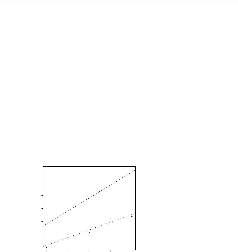
254 Chapter 11: Linear Models and Estimation by Least Squares
Instructor’s Solutions Manual
> summary(lm(y~x1+x2+I(x1*x2)))
Call:
lm(formula = y ~ x1 + x2 + I(x1 * x2))
Residuals:
Min 1Q Median 3Q Max
-0.4900 -0.1925 -0.0300 0.2500 0.4000
Coefficients:
Estimate Std. Error t value Pr(>|t|)
(Intercept) 9.3400 0.1561 59.834 1.46e-09 ***
x1 2.4600 0.2208 11.144 3.11e-05 ***
x2 0.6000 0.1104 5.436 0.00161 **
I(x1 * x2) 0.4100 0.1561 2.627 0.03924 *
---
Signif. codes: 0 '***' 0.001 '**' 0.01 '*' 0.05 '.' 0.1 ' ' 1
Residual standard error: 0.349 on 6 degrees of freedom
Multiple R-Squared: 0.9754, Adjusted R-squared: 0.963
F-statistic: 79.15 on 3 and 6 DF, p-value: 3.244e-05
a. The fitted model is y
ˆ = 9.34 + 2.46x1 + .6x2 + .41x1x2.
b. For bacteria type A, x1 = 0 so y
ˆ = 9.34 + .6x2 (dotted line)
For bacteria type B, x1 = 1 so y
ˆ = 11.80 + 1.01 x2 (solid line)
-2 -1 0 1 2
8 9 10 11 12 13 14
x2
y
x
x
x
x
x
c. For bacteria A, x1 = 0, x2 = 0, so y
ˆ = 9.34. For bacteria B, x1 = 1, x2 = 0, so y
ˆ =
11.80. The observed growths were 9.1 and 12.2, respectively.
d. The rates are different if the parameter β3 is nonzero. So, H0: β3 = 0 vs. Ha: β3 ≠ 0
has a p–value = .03924 (R output above) and H0 is rejected.
e. With x1 = 1, x2 = 1, so y
ˆ = 12.81. With s = .349 and aa 1
)( −
′′ XX = .3, the 90% CI
is 12.81 ± .37.
f. The 90% PI is 12.81 ± .78.
www.elsolucionario.net

Chapter 11: Linear Models and Estimation by Least Squares 255
Instructor’s Solutions Manual
11.102 The reduced model F statistic is 195
/
9.783
2/)9.78323.795(
−
=F = 1.41 with 2 numerator and
195 denominator degrees of freedom. Since F.05 ≈ 3.00, we fail to reject H0: salary is
not dependent on gender.
11.103 Define 1 as a column vector of n 1’s. Then Y1
′
=
n
y1. We must solve for the vector x
such that βxˆ
′
=y. Using the matrix definition of β
ˆ, we have
Y1YXXXx ′
=
′′′
=−
n
y1
1
)(
YY1YYXXXx ′′
=
′′′′ −
n
1
1
)(
which implies
1XXXx ′
=
′′′ −
n
1
1
)(
X1XXXXx ′
=
′′′ −
n
1
1
)(
so that
X1x
′
=
′
n
1.
That is, ]1[ 21 k
xxx …=
′
x.
11.104 Here, we will use the coding 15
65
1
−
=
P
x and 100
200
2
−
=
T
x. Then, the levels are x1 = –1, 1
and x2 = –1, 0, 1.
a.
⎥
⎥
⎥
⎥
⎥
⎥
⎥
⎥
⎦
⎤
⎢
⎢
⎢
⎢
⎢
⎢
⎢
⎢
⎣
⎡
=
28
23
22
26
23
21
Y
⎥
⎥
⎥
⎥
⎥
⎥
⎥
⎥
⎦
⎤
⎢
⎢
⎢
⎢
⎢
⎢
⎢
⎢
⎣
⎡
−
−
−
−
−−
=
1111
0011
1111
1111
0011
1111
X
⎥
⎥
⎥
⎥
⎦
⎤
⎢
⎢
⎢
⎢
⎣
⎡
=
′
97
11
3
143
YX
⎥
⎥
⎥
⎥
⎦
⎤
⎢
⎢
⎢
⎢
⎣
⎡
−
−
=
′−
75.005.
025.00
001667.0
5.005.
)( 1
XX
So, the fitted model is y
ˆ = 23 + .5x1 + 2.75x2 + 2
2
25.1 x.
b. The hypothesis of interest is H0: β3 = 0 vs. Ha: β3 ≠ 0 and the test statistic is (verify
that SSE = 1 so that s2 = .5) )75(.5.
|25.1|
|| =t = 2.040 with 2 degrees of freedom. Since t.025 =
4.303, we fail to reject H0.
c. To test H0: β2 = β3 = 0 vs. Ha: at least one βi ≠ 0, i = 2, 3, the reduced model must be
fitted. It can be verified that SSER = 33.33 so that the reduced model F–test is F =
32.33 with 2 numerator and 2 denominator degrees of freedom. It is easily seen that H0
should be rejected; temperature does affect yield.
11.105 a. xx
yy
xx
yy
yyxx
xy
xx
xy
S
S
S
S
SS
S
S
Sr===β1
ˆ.
www.elsolucionario.net
256 Chapter 11: Linear Models and Estimation by Least Squares
Instructor’s Solutions Manual
b. The conditional distribution of Yi, given Xi = xi, is (see Chapter 5) normal with mean
)( xiy x
x
yμ−ρ+μ σ
σ and variance )1( 22 ρ−σy. Redefine β1 = x
y
σ
σ
ρ, β0 = xy μβ−μ 1. So,
if ρ = 0, β1 = 0. So, using the usual t–statistic to test β1 = 0, we have
yy
xx
Sn
xx Sr
Sn
SS
T
xx )1(
)2(
ˆ
ˆ
/
ˆ
2
1
1
2
SSE
11
−
−β
=
β
=
β
=
−
.
c. By part a, xx
yy
S
S
r=β1
ˆ and the statistic has the form as shown. Note that the
distribution only depends on n – 2 and not the particular value xi. So, the distribution is
the same unconditionally.
11.106 The summary statistics are Sxx = 66.54, Sxy = 71.12, and Syy = 93.979. Thus, r = .8994.
To test H0: ρ = 0 vs. Ha: ρ ≠ 0, |t| = 5.04 with 6 degrees of freedom. From Table 7, we
see that p–value < 2(.005) = .01 so we can reject the null hypothesis that the correlation
is 0.
11.107 The summary statistics are Sxx = 153.875, Sxy = 12.8, and Syy = 1.34.
a. Thus, r = .89.
b. To test H0: ρ = 0 vs. Ha: ρ ≠ 0, |t| = 4.78 with 6 degrees of freedom. From Table 7,
we see that p–value < 2(.005) = .01 so we can reject the null hypothesis that the
correlation is 0.
11.108 a.-c. Answers vary.
www.elsolucionario.net

257
Chapter 12: Considerations in Designing Experiments
12.1 (See Example 12.1) Let n1 =
(
)
(
)
90
533
21
1+σ+σ
σ=n = 33.75 or 34 and n2 = 90 − 34 = 56.
12.2 (See Ex. 12.1). If n1 = 34 and n2 = 56, then
7111.
56
25
34
9
21 =+=σ −YY
In order to achieve this same bound with equal sample sizes, we must have
9
n+25
n=.7111
The solution is n = 47.8 or 48. Thus, it is necessary to have n1 = n2 = 48 so that the
same amount of information is implied.
12.3 The length of a 95% CI is twice the margin of error:
2(1.96) 9
n1+25
n2,
and this is required to be equal to two. In Ex. 12.1, we found n1 = (3/8)n and n1 =
(5/8)n, so substituting these values into the above and equating it to two, the solution is
found to be n = 245.9. Thus, n1 = 93 and n2 = 154.
12.4 (Similar to Ex. 12.3) Here, the equation to solve is
2(1.96) 9
n1+25
n1 = 2.
The solution is n1 = 130.6 or 131, and the total sample size required is 131 + 131 = 262.
12.5 Refer to Section 12.2. The variance of the slope estimate is minimized (maximum
information) when Sxx is as large as possible. This occurs when the data are as far away
from
x
as possible. So, with n = 6, three rats should receive x = 2 units and three rats
should receive x = 5 units.
12.6 When σ is known, a 95% CI for β is given by
xx
S
z
σ
±β α2/1
ˆ.
Under the two methods, we calculate that Sxx = 13.5 for Method 1 and Sxx = 6.3 for
Method 2. Thus, Method 2 will produce the longer interval. By computing the ratio of
the margins of error for the two methods (Method 2 to Method 1), we obtain 3.6 5.13 =
1.464; thus Method 2 produces an interval that is 1.464 times as large as Method 1.
Under Method 2, suppose we take n measurements at each of the six dose levels. It is
not difficult to show that now Sxx = 6.3n. So, in order for the intervals to be equivalent,
we must have that 6.3n = 13.5, and so n = 2.14. So, roughly twice as many observations
are required.
12.7 Although it was assumed that the response variable Y is truly linear over the range of x,
the experimenter has no way to verify this using Method 2. By assigning a few points
at x = 3.5, the experimenter could check for curvature in the response function.
www.elsolucionario.net
258 Chapter 12: Considerations in Designing Experiments
Instructor’s Solutions Manual
12.8 Checking for true linearity and constant error variance cannot be performed if the data
points are spread out as far as possible.
12.9 a. Each half of the iron ore sample should be reasonably similar, and assuming the two
methods are similar, the data pairs should be positively correlated.
b. Either analysis compares means. However, the paired analysis requires fewer ore
samples and reduces the sample−to−sample variability.
12.10 The sample statistics are: d = −.0217, s
D
2 = .0008967.
a. To test H0: μD = 0 vs. Ha: μD ≠ 0, the test statistic is |t| = 60008967.
0217.− = 1.773 with 5
degrees of freedom. Since t.025 = 2.571, H0 is not rejected.
b. From Table 5, .10 < p−value < .20.
c. The 95% CI is 6
0008967.
571.20217. ±− = −.0217 ± .0314.
12.11 Recall that
(
)
21
2
2
2
1
12)( σρσ+σ+σ= n
DVar given in this section.
a. This occurs when ρ > 0.
b. This occurs when ρ = 0.
c. This occurs when ρ < 0.
d. If the samples are negatively correlated, a matched−pairs experiment should not be
performed. Otherwise, if it is possible, the matched−pairs experiment will have an
associated variance that is equal or less than the variance associated with the
independent samples experiment.
12.12 a. There are 2n − 2 degrees of freedom for error.
b. There are n − 1 degrees of freedom for error.
c. n Independent samples Matched−pairs
5 d.f. = 8, t.025 = 2.306 d.f. = 4, t.025 = 2.776
10 d.f. = 18, t.025 = 2.101 d.f. = 9, t.025 = 2.262
30 d.f. = 58, t.025 = 1.96 d.f. = 29, t.025 = 2.045
d. Since more observations are required for the independent samples design, this
increases the degrees of freedom for error and thus shrinks the critical values used in
confidence intervals and hypothesis tests.
12.13 A matched−pairs experiment is preferred since there could exist sample−to−sample
variability when using independent samples (one person could be more prone to plaque
buildup than another).
12.14 The sample statistics are: d = −.333, s
D
2 = 5.466. To test H0: μD = 0 vs. Ha: μD < 0, the
test statistic is t = 6466.5
333.− = −.35 with 5 degrees of freedom. From Table 5, p−value > .1
so H0 is not rejected.
www.elsolucionario.net
Chapter 12: Considerations in Designing Experiments 259
Instructor’s Solutions Manual
12.15 a. The sample statistics are: d = 1.5, s
D
2 = 2.571. To test H0: μD = 0 vs. Ha: μD ≠ 0, the
test statistic is |t| = 8571.2
5.1 = 2.65 with 7 degrees of freedom. Since t.025 = 2.365, H0 is
rejected.
b. Notice that each technician’s score is similar under both design A and B, but the
technician’s scores are not similar in general (some are high and some are low). Thus,
pairing is important to screen out the variability among technicians.
c. We assumed that the population of differences follows a normal distribution, and that
the sample used in the analysis was randomly selected.
12.16 The sample statistics are: d = −3.88, s
D
2 = 8.427.
a. To test H0: μD = 0 vs. Ha: μD < 0, the test statistic is t = 15427.8
88.3
− = −5.176 with 14
degrees of freedom. From Table 5, it is seen that p−value < .005, so H0 is rejected
when α = .01.
b. A 95% CI is 15/427.8145.288.3 ±− = −3.88 ± 1.608.
c. Using the Initial Reading data,
y
= 36.926 and s2 = 40.889. A 95% CI for the mean
muck depth is 15/889.40145.2926.36 ± = 36.926 ± 3.541.
d. Using the Later Reading data,
y
= 33.046 and s2 = 35.517. A 95% CI for the mean
much depth is 15/517.35145.2046.33 ± = 33.046 ± 3.301.
e. For parts a and b, we assumed that the population of differences follows a normal
distribution, and that the sample used in the analysis was randomly selected. For
parts c and d, we assumed that the individual samples were randomly selected from
two normal populations.
12.17 a. iijiiij EUEYE
μ
=
ε
+
+
μ= )()()(.
b. Each Y1j involves the sum of a uniform and a normal random variable, and this
convolution does not result in a normal random variable.
c. ),(Cov),(Cov 221121 jjjjjj UUYY
ε
+
+
μ
ε
+
+μ= = ),(Cov 21
μ
μ
+ ),(Cov jj UU +
),(Cov 21 jj εε = 0 + V(Uj) + 0 = 1/3.
d. Observe that jjjjj YYD 212121
ε
−
ε
+
μ
−
μ
=
−= . Since the random errors are
independent and follow a normal distribution, Dj is a normal random variable. Further,
for j ≠ j′, 0),(Cov =
′
jj DD since the two random variables are comprised of constants
and independent normal variables. Thus, Dj and j
D′ are independent (recall that if two
normal random variables are uncorrelated, they are also independent − but this is not
true in general).
e. Provided that the distribution of Uj has a mean of zero and finite variance, the result
will hold.
12.18 Use Table 12 and see Section 12.4 of the text.
12.19 Use Table 12 and see Section 12.4 of the text.
www.elsolucionario.net

260 Chapter 12: Considerations in Designing Experiments
Instructor’s Solutions Manual
12.20 a. There are six treatments. One example would be the first catalyst and the first
temperature setting.
b. After assigning the n experimental units to the treatments, the experimental units are
numbered from 1 to n. Then, a random number table is used to select numbers until all
experimental units have been selected.
12.21 Randomization avoids the possibility of bias introduced by a nonrandom selection of
sample elements. Also, it provides a probabilistic basis for the selection of a sample.
12.22 Factors are independent experimental variables that the experimenter can control.
12.23 A treatment is a specific combination of factor levels used in an experiment.
12.24 Yes. Suppose that a plant biologist is comparing three soil types used for planting,
where the response is the yield of a crop planted in the different soil types. Then, “soil
type” is a factor variable. But, if the biologist is comparing the yields of different
greenhouses, but each greenhouse used different soil types, then “soil type” is a
nuisance variable.
12.25 Increases accuracy of the experiment: 1) selection of treatments, 2) choice of number of
experimental units assigned to each treatment.
Decreases the impact of extraneous sources of variability: randomization; assigning
treatments to experimental units.
12.26 There is a possibility of significant rat−to−rat variation. By applying all four dosages to
tissue samples extracted from the same rat, the experimental error is reduced. This
design is an example of a randomized block design.
12.27 In the Latin square design, each treatment appears in each row and each column exactly
once. So, the design is:
12.28 A CI could be constructed for the specific population parameter, and the width of the CI
gives the quantity of information.
12.29 A random sample of size n is a sample that was randomly selected from all possible
(unique) samples of size n (constructed of observations from the population of interest)
and each sample had an equal chance of being selected.
12.30 From Section 12.5, the choice of factor levels and the allocation of the experimental
units to the treatments, as well as the total number of experimental units being used,
affect the total quantity of information. Randomization and blocking can control these
factors.
BAC
CBA
ACB
www.elsolucionario.net

Chapter 12: Considerations in Designing Experiments 261
Instructor’s Solutions Manual
12.31 Given the model proposed in this exercise, we have the following:
a. iiijiiij EPEYE
μ
=
+
+
μ
=
ε
++μ= 00)()()(.
b. Obviously, ii
YE μ=)( . Also,
[
]
[
]
22
111 )()()()( σ+σ=ε+== P
n
iji
n
ij
n
iVPVYVYV ,
since Pi and εij are independent for all i, j.
c. From part b, 2121 )()()( μ−μ=−= YEYEDE . Now, to find V(D ), note that
[
]
∑∑∑ === ε+ε+μ−μ== n
jj
n
jj
n
n
jj
nDD 12
11
1
21
1
1.
Thus, since the εij are independent,
[
]
∑∑ == ε+ε= n
jj
n
jj
nVVDV 12
11
1)()()( 2 = n/2 2
σ.
Further, since D is a linear combination of normal random variables, it is also
normally distributed.
12.32 From Exercise 12.31, clearly n
D
/2
)(
2
21
σ
μ−μ− has a standard normal distribution. In
addition, since D1, …, Dn are independent normal random variables with mean μ1 − μ2
and variance 2σ2, the quantity
2
1
2
2
2
2
)(
2
)1(
σ
−
=
σ
−
=∑=
n
ii
DDD
Sn
W
is chi−square with ν = n − 1 degrees of freedom. Therefore, by Definition 7.2 and
under H0: μ1 − μ2 = 0,
nS
D
W
Z
D// =
ν
has a t−distribution with n − 1 degrees of freedom.
12.33 Using similar methods as in Ex. 12.31, we find that for this model,
[]
[
]
2
1
22
1
12121
1222)()()()()( 2σ>σ+σ=ε+ε++= ∑=n
P
n
n
jjjjj
nVVPVPVDV .
Thus, the variance is larger with the completely randomized design, since the unwanted
variation due to pairing is not eliminated.
12.34 The sample statistics are: d = −.062727, s
D
2 = .012862.
a. We expect the observations to be positively correlated since (assuming the people
are honest) jobs that are estimated to take a long time actually take a long time when
processed. Similar for jobs that are estimated to take a small amount of processor
time.
b. To test H0: μD = 0 vs. Ha: μD < 0, the test statistic is t = 11012862.
0627272.− = −1.834 with 10
degrees of freedom. Since −t.10 = −1.362, H0 is rejected: there is evidence that the
customers tend to underestimate the processor time.
c. From Table 5, we have that .025 < p−value < .05.
d. A 90% CI for 21
μ
−μ=μD, is 11/012862.812.1062727. ±− = −.063 ± .062 or
(−.125, −.001).
www.elsolucionario.net
262 Chapter 12: Considerations in Designing Experiments
Instructor’s Solutions Manual
12.35 The sample statistics are: d = −1.58, s
D
2 = .667.
a. To test H0: μD = 0 vs. Ha: μD ≠ 0, the test statistic is |t| = 1.58
.667 5
− = 4.326 with 4
degrees of freedom. From Table 5, we can see that .01 < p−value < .025, so H0
would be rejected for any α ≥ .025.
b. A 95% CI is given by 5/667.776.258.1 ±− = −1.58 ± 1.014 or (−2.594, −.566).
c. We will use the estimate of the variance of paired differences. Also, since the
required sample will (probably) be large, we will use the critical value from the
standard normal distribution. Our requirement is then:
nn
zD667.
96.12. 2
025. ≈
σ
=.
The solution is n = 64.059, or 65 observations (pairs) are necessary.
12.36 The sample statistics are: d = 106.9, s
D
2 = 1364.989.
a. Each subject is presented each sign in random order. If the subject’s reaction time is
(in general) high, both responses should be high. If the subject’s reaction time is (in
general) low. both responses should be low. Because of the subject−to−subject
variability, the matched pairs design can eliminate this extraneous source of
variation.
b. To test H0: μD = 0 vs. Ha: μD ≠ 0, the test statistic is |t| = 10/989.1364
0.106 = 9.15 with 9
degrees of freedom. Since t.025 = 2.262, H0 is rejected.
c. From Table 5, we see that p−value < 2(.005) = .01.
d. The 95% CI is given by 10/989.1364262.29.106 ± = 106.9 ± 26.428 or (80.472,
133.328).
12.37 There are nk1 points at x = −1, nk2 at x = 0, and nk3 points at x = 1. The design matrix X
can be expressed as
⎥
⎥
⎥
⎥
⎥
⎥
⎥
⎥
⎥
⎥
⎥
⎥
⎥
⎥
⎥
⎥
⎥
⎦
⎤
⎢
⎢
⎢
⎢
⎢
⎢
⎢
⎢
⎢
⎢
⎢
⎢
⎢
⎢
⎢
⎢
⎢
⎣
⎡
−
−
−
=
111
111
111
001
001
001
111
111
111
###
###
###
X; thus AXX n
aba
bab
ab
n
kknkknkkn
kknkknkkn
kknkknn
=
⎥
⎥
⎥
⎦
⎤
⎢
⎢
⎢
⎣
⎡
=
⎥
⎥
⎥
⎦
⎤
⎢
⎢
⎢
⎣
⎡
+−+
−+−
+−
=
′
1
)()()(
)()()(
)()(
311331
133113
3113
,
where a = k1 + k3 and b = k3 − k1.
www.elsolucionario.net

Chapter 12: Considerations in Designing Experiments 263
Instructor’s Solutions Manual
Now, the goal is to minimize 22
2
2)
ˆ
(cV σ=β , where c22 is the (3, 3) element of (X′X)−1.
To calculate (X′X)−1, note that it can be expressed as
⎥
⎥
⎥
⎦
⎤
⎢
⎢
⎢
⎣
⎡
−−−
−−
−−
=
−
222
2
2222
10
0
)det(
1
bababab
babaa
abba
nA
A, and (the student should verify) the
determinant of A simplifies to det(A) = 4k1k2k3. Hence,
⎟
⎟
⎠
⎞
⎜
⎜
⎝
⎛−−+
σ
=
−
σ=β
321
2
1331
2
321
2
2
24
)(
4
)
ˆ
(kkk
kkkk
nkknk
ba
V.
We must minimize
[
]
[]
321
31
321
3131
321
31
2
1331
321
2
1331
4
4
4
1)(
4
4)(
4
)(
kkk
kk
kkk
kkkk
kkk
kkkkkk
kkk
kkkk
Q−
−−+
=
−+−+
=
−−+
=
3131
31
231
31
1
1
4
1
4kkkk
kk
kkk
kk
−−
−
+
=−
+
=.
So, with
3131
31
1
1
4kkkk
kk
Q−−
−
+
=, we can differentiate this with respect to k1 and k3
and set these equal to zero. The two equations are:
2
31
2
3
2
31
2
1
)1(4
(*))1(4
kkk
kkk
−−=
−−= .
Since k1, k2, and k3 are all positive, k1 = k3 by symmetry of the above equations and
therefore by (*), 2
1
2
1)21(4 kk −= so that k1 = k3 = .25. Thus, k2 = .50.
www.elsolucionario.net

264
Chapter 13: The Analysis of Variance
13.1 The summary statistics are: 1
y = 1.875, 2
1
s = .6964286, 2
y = 2.625, 2
2
s = .8392857, and
n1 = n2 = 8. The desired test is: H0: μ1 = μ2 vs. Ha: μ1 ≠ μ2, where μ1, μ2 represent the
mean reaction times for Stimulus 1 and 2 respectively.
a. SST = 4(1.875 – 2.625)2 = 2.25, SSE = 7(.696428) + 7(.8392857) = 10.75. Thus,
MST = 2.25/1 = 2.25 and MSE = 10.75/14 = .7679. The test statistic F = 2.25/.7679
= 2.93 with 1 numerator and 14 denominator degrees of freedom. Since F.05 = 4.60,
we fail to reject H0: the stimuli are not significantly different.
b. Using the Applet, p–value = P(F > 2.93) = .109.
c. Note that 2
p
s = MSE = .7679. So, the two–sample t–test statistic is |t| =
⎟
⎠
⎞
⎜
⎝
⎛
−
8
2
7679.
625.2875.1 =
1.712 with 14 degrees of freedom. Since t.025 = 2.145, we fail to reject H0. The two
tests are equivalent, and since F = T2, note that 2.93 ≈ (1.712)2 (roundoff error).
d. We assumed that the two random samples were selected independently from normal
populations with equal variances.
13.2 Refer to Ex. 10.77. The summary statistics are: 1
y = 446, 2
1
s = 42, 2
y = 534, 2
2
s = 45,
and n1 = n2 = 15.
a. SST = 7.5(446 – 534)2 = 58,080, SSE = 14(42) + 14(45) = 1218. So, MST = 58,080
and MSE = 1218/28 = 1894.5. The test statistic F = 58,080/1894.5 = 30.64 with 1
numerator and 28 denominator degrees of freedom. Clearly, p–value < .005.
b. Using the Applet, p–value = P(F > 30.64) = .00001.
c. In Ex. 10.77, t = –5.54. Observe that (–5.54)2 ≈ 30.64 (roundoff error).
d. We assumed that the two random samples were selected independently from normal
populations with equal variances.
13.3 See Section 13.3 of the text.
13.4 For the four groups of students, the sample variances are: 2
1
s = 66.6667, 2
2
s = 50.6192,
2
3
s = 91.7667, 2
4
s = 33.5833 with n1 = 6, n2 = 7, n3 = 6, n4 = 4. Then, SSE = 5(66.6667)
+ 6(50.6192) + 5(91.7667) + 3(33.5833) = 1196.6321, which is identical to the prior
result.
13.5 Since W has a chi–square distribution with r degrees of freedom, the mgf is given by
2/
)21()()( rtW
WteEtm −
−== .
Now, W = U + V, where U and V are independent random variables and V is chi–square
with s degrees of freedom. So,
2/2/)( )21()21)(()()()()()( rstUtVtUVUttW
WtteEeEeEeEeEtm −−+ −=−==== .
Therefore, 2/)(
2/
2/
)21(
)21(
)21(
)()( sr
s
r
tU
Ut
t
t
eEtm −−
−
−
−=
−
−
== . Since this is the mgf for a chi–
square random variable with r – s degrees of freedom, where r > s, by the Uniqueness
Property for mgfs U has this distribution.
www.elsolucionario.net

Chapter 13: The Analysis of Variance 265
Instructor’s Solutions Manual
13.6 a. Recall that by Theorem 7.3, 22 /)1( σ− ii Sn is chi–square with ni – 1 degrees of
freedom. Since the samples are independent, by Ex. 6.59, ∑=σ−=σ k
iii Sn
1
222 /)1(/SSE
is chi–square with n – k degrees of freedom.
b. If H0 is true, all of the observations are identically distributed since it was already
assumed that the samples were drawn independently from normal populations with
common variance. Thus, under H0, we can combine all of the samples to form an
estimator for the common mean,
Y
, and an estimator for the common variance, given by
TSS/(n – 1). By Theorem 7.3, TSS/σ2 is chi–square with n – 1 degrees of freedom.
c. The result follows from Ex. 13.5: let W = TSS/σ2 where r = n – 1 and let V = SSE/σ2
where s = n – k. Now, SSE/σ2 is distributed as chi–square with n – k degrees of freedom
and TSS/σ2 is distributed as chi–square under H0. Thus, U = SST/σ2 is chi–square under
H0 with n – 1 – (n – k) = k – 1 degrees of freedom.
d. Since SSE and TSS are independent, by Definition 7.3
(
)
()
MSE
MST
)(SSE
)1(SST
2
2
=
−σ
−σ
=kn
k
F
has an F–distribution with k – 1 numerator and n – k denominator degrees of freedom.
13.7 We will use R to solve this problem:
> waste <- c(1.65, 1.72, 1.5, 1.37, 1.6, 1.7, 1.85, 1.46, 2.05, 1.8,
1.4, 1.75, 1.38, 1.65, 1.55, 2.1, 1.95, 1.65, 1.88, 2)
> plant <- c(rep("A",5), rep("B",5), rep("C",5), rep("D",5))
> plant <- factor(plant) # change plant to a factor variable
> summary(aov(waste~plant))
Df Sum Sq Mean Sq F value Pr(>F)
plant 3 0.46489 0.15496 5.2002 0.01068 *
Residuals 16 0.47680 0.02980
---
Signif. codes: 0 '***' 0.001 '**' 0.01 '*' 0.05 '.' 0.1 ' ' 1
a. The F statistic is given by F = MST/MSE = .15496/.0298 = 5.2002 (given in the
ANOVA table above) with 3 numerator and 16 denominator degrees of freedom.
Since F.05 = 3.24, we can reject H0: μ1 = μ2 = μ3 = μ4 and conclude that at least one of
the plant means are different.
b. The p–value is given in the ANOVA table: p–value = .01068.
13.8 Similar to Ex. 13.7, R will be used to solve the problem:
> salary <- c(49.3, 49.9, 48.5, 68.5, 54.0, 81.8, 71.2, 62.9, 69.0,
69.0, 66.9, 57.3, 57.7, 46.2, 52.2)
> type <- factor(c(rep("public",5), rep("private",5), rep("church",5)))
a. This is a completely randomized, one–way layout (this is sampled data, not a
designed experiment).
b. To test H0: μ1 = μ2 = μ3, the ANOVA table is given below (using R):
www.elsolucionario.net

266 Chapter 13: The Analysis of Variance
Instructor’s Solutions Manual
> summary(aov(salary~type))
Df Sum Sq Mean Sq F value Pr(>F)
type 2 834.98 417.49 7.1234 0.009133 **
Residuals 12 703.29 58.61
---
Signif. codes: 0 '***' 0.001 '**' 0.01 '*' 0.05 '.' 0.1 ' ' 1
From the output, F = MST/MSE = 7.1234 with 3 numerator and 12 denominator degrees
of freedom. From Table 7, .005 < p–value < .01.
c. From the output, p-value = .009133.
13.9 The test to be conducted is H0: μ1 = μ2 = μ3 = μ4, where μi is the mean strength for the ith
mix of concrete, i = 1, 2, 3, 4. The alternative hypothesis at least one of the equalities
does not hold.
a. The summary statistics are: TSS = .035, SST = .015, and so SSE = .035 – .015 = .020.
The mean squares are MST = .015/3 = .005 and MSE = .020/8 = .0025, so the F
statistic is given by F = .005/.0025 = 2.00, with 3 numerator and 8 denominator
degrees of freedom. Since F.05 = 4.07, we fail to reject H0: there is not enough
evidence to reject the claim that the concrete mixes have equal mean strengths.
b. Using the Applet, p–value = P(F > 2) = .19266. The ANOVA table is below.
Source d.f SS MS
F p–value
Treatments 3 .015 .005 2.00 .19266
Error 8 .020 .0025
Total 11 .035
13.10 The test to be conducted is H0: μ1 = μ2 = μ3, where μi is the mean score where the ith
method was applied, i = 1, 2, 3. The alternative hypothesis at least one of the equalities
does not hold
a. The summary statistics are: TSS = 1140.5455, SST = 641.8788, and so SSE =
1140.5455 – 641.8788 = 498.6667. The mean squares are MST = 641.8788/2 =
320.939 and MSE = 498.6667/8 = 62.333, so the F statistic is given by F =
320.939/62.333 = 5.148, with 2 numerator and 8 denominator degrees of freedom.
By Table 7, .025 < p–value < .05.
b. Using the Applet, p–value = P(F > 5.148) = .03655. The ANOVA table is below.
Source d.f SS MS F p–value
Treatments 2 641.8788 320.939 5.148 .03655
Error 8 498.6667 62.333
Total 10 1140.5455
c. With α = .05, we would reject H0: at least one of the methods has a different mean
score.
www.elsolucionario.net

Chapter 13: The Analysis of Variance 267
Instructor’s Solutions Manual
13.11 Since the three sample sizes are equal,
(
)
321
3
1yyyy
+
+
=
= 3
1(.93 + 1.21 + .92) = 1.02.
Thus, SST = 2
3
1
2
3
1
1)02.1(14)( −=− ∑∑ == ii
iiyyyn = .7588. Now, recall that the
“standard error of the mean” is given by ns / , so SSE can be found by
SSE = 13[14(.04)2 + 14(.03)2 + 14(.04)2] = .7462.
Thus, the mean squares are MST = .7588/2 = .3794 and MSE = .7462/39 = .019133, so
that the F statistic is F = .3794/.019133 = 19.83 with 2 numerator and 39 denominator
degrees of freedom. From Table 7, it is seen that p–value < .005, so at the .05
significance level we reject the null hypothesis that the mean bone densities are equal.
13.12 The test to be conducted is H0: μ1 = μ2 = μ3, where μi is the mean percentage of Carbon
14 where the ith concentration of acetonitrile was applied, i = 1, 2, 3. The alternative
hypothesis at least one of the equalities does not hold
a. The summary statistics are: TSS = 235.219, SST = 174.106, and so SSE = 235.219 –
174.106 = 61.113. The mean squares are MST = 174.106/2 = 87.053 and MSE =
235.219/33 = 1.852, so the F statistic is given by F = 87.053/1.852 = 47.007, with 2
numerator and 33 denominator degrees of freedom. Since F.01 ≈ 5.39, we reject H0:
at least one of the mean percentages is different and p–value < .005. The ANOVA
table is below.
Source d.f SS MS F p–value
Treatments 2 174.106 87.053 47.007 < .005
Error 33 61.113 1.852
Total 35 235.219
b. We must assume that the independent measurements from low, medium, and high
concentrations of acetonitrile are normally distributed with common variance.
13.13 The grand mean is 165
)24.6(18)88.4(102)59.4(45 ++
=y = 4.949. So,
SST = 45(4.59 – 4.949)2 + 102(4.88 – 4.949)2 + 18(6.24 – 4.949)2 = 36.286.
SSE =
∑=−
3
1
2
)1(
ii
sn = 44(.70)2 + 101(.64)2 + 17(.90)2 = 76.6996.
The F statistic is F = 162/6996.76
2/286.36
MSE
MST = = 38.316 with 2 numerator and 162 denominator
degrees of freedom. From Table 7, p–value < .005 so we can reject the null hypothesis of
equal mean maneuver times. The ANOVA table is below.
Source d.f SS MS
F p–value
Treatments 2 36.286 18.143 38.316 < .005
Error 162 76.6996 .4735
Total 164 112.9856
13.14 The grand mean is 3
041.022.032. ++
=y = 0.0317. So,
SST = 10[(.032 – .0317)2 + (.022 – .0317)2 + (.041 – .0317)2 = .001867.
SSE =
∑=−
3
1
2
)1(
ii
sn = 9[(.014)2 + (.008)2 + (.017)2] = .004941.
www.elsolucionario.net

268 Chapter 13: The Analysis of Variance
Instructor’s Solutions Manual
The F statistic is F = 4.94 with 2 numerator and 27 denominator degrees of freedom.
Since F.05 = 3.35, we can reject H0 and conclude that the mean chemical levels are
different.
13.15 We will use R to solve this problem:
> oxygen <- c(5.9, 6.1, 6.3, 6.1, 6.0, 6.3, 6.6, 6.4, 6.4, 6.5, 4.8,
4.3, 5.0, 4.7, 5.1, 6.0, 6.2, 6.1, 5.8)
> location <- factor(c(1,1,1,1,1,2,2,2,2,2,3,3,3,3,3,4,4,4,4))
> summary(aov(oxygen~location))
Df Sum Sq Mean Sq F value Pr(>F)
location 3 7.8361 2.6120 63.656 9.195e-09 ***
Residuals 15 0.6155 0.0410
---
Signif. codes: 0 '***' 0.001 '**' 0.01 '*' 0.05 '.' 0.1 ' ' 1
>
The null hypothesis is H0: μ1 = μ2 = μ3 = μ4, where μi is the mean dissolved O2 in location
i, i = 1, 2, 3, 4. Since the p–value is quite small, we can reject H0 and conclude the mean
dissolved O2 levels differ.
13.16 The ANOVA table is below:
Source d.f SS MS
F p–value
Treatments 3 67.475 22.4917 .87 > .1
Error 36 935.5 25.9861
Total 39 1002.975
With 3 numerator and 36 denominator degrees of freedom, we fail to reject with α = .05:
there is not enough evidence to conclude a difference in the four age groups.
13.17 i
n
ji
n
n
ji
n
n
jij
n
i
i
i
i
i
i
iYEYE μ=μ=τ+μ== ∑∑∑ ===
•1
1
1
1
1
1)()()(
2
1
1
1
1
1)()()( 22 σ=ε== ∑∑ ==
•i
i
i
i
in
n
jij
n
n
jij
n
iVYVYV .
13.18 Using the results from Ex. 13.17,
iiiiiiii YYE ′′′
•
′
•τ−τ=τ+μ−τ+μ=μ−μ=− )()(
(
)
2
11
)()()( σ+=+=− ′
•
′
••
′
•ii nn
iiii YVYVYYV
13.19 a. Recall that μi = μ + τi for i = 1, …, k. If all τi’s = 0, then all μi’s = μ. Conversely, if
k
μ==μ=μ …
21 , we have that k
τ
+
μ
=
=
τ
+
μ
=
τ
+
μ
…
21 and k
τ
==τ=
τ
…
21 .
Since it was assumed that ∑=τ
k
ii
1 = 0, all τi’s = 0. Thus, the null hypotheses are
equivalent.
b. Consider μi = μ + τi and μi′ = μ + τi′. If μi ≠ μi′, then μ + τi ≠ μ + τi′ and thus τi ≠ τi′.
Since ∑=τ
k
ii
1 = 0, at least one τi ≠ 0 (actually, there must be at least two). Conversely, let
www.elsolucionario.net

Chapter 13: The Analysis of Variance 269
Instructor’s Solutions Manual
τi ≠ 0. Since ∑=τ
k
ii
1 = 0, there must be at least one i′ such that τi ≠ τi′. With μi = μ + τi
and μi′ = μ + τi′, it must be so that μi ≠ μi′. Thus, the alternative hypotheses are equivalent.
13.20 a. First, note that 1
y = 75.67 and 2
1
s = 66.67. Then, with n1 = 6, a 95% CI is given by
6/67.66571.267.75 ± = 75.67 ± 8.57 or (67.10, 84.24).
b. The interval computed above is longer than the one in Example 13.3.
c. When only the first sample was used to estimate σ2, there were only 5 degrees of
freedom for error. However, when all four samples were used, there were 14 degrees of
freedom for error. Since the critical value t.025 is larger in the above, the CI is wider.
13.21 a. The 95% CI would be given by
41
11
14025.41 nn
styy +±− ,
where 2
)1()1(
14 41
2
44
2
11 −+
−+−
=nn
snsn
s = 7.366. Since t.025 = 2.306 based on 8 degrees of freedom,
the 95% CI is 4
1
6
1
)366.7(306.208.12 +±− = –12.08 ± 10.96 or (–23.04, –1.12).
b. The CI computed above is longer.
c. The interval computed in Example 13.4 was based on 19 degrees of freedom, and the
critical value t.025 was smaller.
13.22 a. Based on Ex. 13.20 and 13.21, we would expect the CIs to be shorter when all of the
data in the one–way layout is used.
b. If the estimate of σ2 using only one sample is much smaller than the pooled estimate
(MSE) – so that the difference in degrees of freedom is offset – the CI width using just
one sample could be shorter.
13.23 From Ex. 13.7, the four sample means are (again, using R):
> tapply(waste,plant,mean)
A B C D
1.568 1.772 1.546 1.916
>
a. In the above, the sample mean for plant A is 1.568 and from Ex. 13.7, MSE = .0298
with 16 degrees of freedom. Thus, a 95% CI for the mean amount of polluting
effluent per gallon for plant A is
±568.1 5/0298.12.2 = 1.568 ± .164 or (1.404, 1.732).
There is evidence that the plant is exceeding the limit since values larger than 1.5
lb/gal are contained in the CI.
b. A 95% CI for the difference in mean polluting effluent for plants A and D is
(
)
5
2
0298.12.2916.1568.1 ±− = –.348 ± .231 or (–.579, –.117).
Since 0 is not contained in the CI, there is evidence that the means differ for the two
plants.
www.elsolucionario.net

270 Chapter 13: The Analysis of Variance
Instructor’s Solutions Manual
13.24 From Ex. 13.8, the three sample means are (again, using R):
> tapply(salary,type,mean)
church private public
56.06 70.78 54.04
Also, MSE = 58.61 based on 12 degrees of freedom. A 98% CI for the difference in
mean starting salaries for assistant professors at public and private/independent
universities is
(
)
5
2
61.58681.278.7004.54 ±− = –16.74 ± 12.98 or (–29.72, –3.76).
13.25 The 95% CI is given by 14/2)1383(.96.121.193. ±− = –.28 ± .102 or (–.382, –.178)
(note that the degrees of freedom for error is large, so 1.96 is used). There is evidence
that the mean densities for the two groups are different since the CI does not contain 0.
13.26 Refer to Ex. 13.9. MSE = .0025 with 8 degrees of freedom.
a. 90% CI for μA: 2.25 ± 1.86 3/0025. = 2.25 ± .05 or (2.20, 2.30).
b. 95% CI for μA – μB: 2.25 – 2.166 ± 2.306
(
)
3
2
0025. = .084 ± .091 or (–.007, .175).
13.27 Refer to Ex. 13.10. MSE = 62.233 with 8 degrees of freedom.
a. 95% CI for μA: 76 ± 2.306 5/333.62 = 76 ± 8.142 or (67.868, 84.142).
b. 95% CI for μB: 66.33 ± 2.306 3/333.62 = 66.33 ± 10.51 or (55.82, 76.84).
c. 95% CI for μA – μB: 76 – 66.33 ± 2.306
(
)
3
1
5
1
333.62 + = 9.667 ± 13.295.
13.28 Refer to Ex. 13.12. MSE = 1.852 with 33 degrees of freedom
a. 23.965 ± 1.96 12/852.1 = 23.962 ± .77.
b. 23.965 – 20.463 ± 1.645
(
)
12
2
852.1 = 3.502 ± .914.
13.29 Refer to Ex. 13.13. MSE = .4735 with 162 degrees of freedom.
a. 6.24 ± 1.96 18/4735. = 6.24 ± .318.
b. 4.59 – 4.58 ± 1.96
(
)
102
1
45
1
4735. + = –.29 ± .241.
c. Probably not, since the sample was only selected from one town and driving habits
can vary from town to town.
13.30 The ANOVA table for these data is below.
Source d.f SS MS
F p–value
Treatments 3 36.7497 12.2499 4.88 < .05
Error 24 60.2822 2.5118
Total 27 97.0319
a. Since F.05 = 3.01 with 3 numerator and 24 denominator degrees of freedom, we reject
the hypothesis that the mean wear levels are equal for the four treatments.
www.elsolucionario.net

Chapter 13: The Analysis of Variance 271
Instructor’s Solutions Manual
b. With 2
y = 14.093 and 3
y = 12.429, a 99% CI for the difference in the means is
(
)
7
2
5118.2797.2429.12093.14 ±− = 1.664 ± 2.3695.
c. A 90% CI for the mean wear with treatment A is
()
7
1
5118.2711.1986.11 ± = 11.986 ± 1.025 or (10.961, 13.011).
13.31 The ANOVA table for these data is below.
Source d.f SS MS
F p–value
Treatments 3 18.1875 2.7292 1.32 > .1
Error 12 24.75 2.0625
Total 15 32.9375
a. Since F.05 = 3.49 with 3 numerator and 12 denominator degrees of freedom, we fail to
reject the hypothesis that the mean amounts are equal.
b. The methods of interest are 1 and 4. So, with 1
y = 2 and 4
y = 4, a 95% CI for the
difference in the mean levels is
()
4
2
0625.2052.242 ±− = –2 ± 2.21 or (–.21, 4.21).
13.32 Refer to Ex. 13.14. MSE = .000183 with 27 degrees of freedom. A 95% CI for the mean
residue from DDT is 10/000183.052.2041. ± = .041 ± .009 or (.032, .050).
13.33 Refer to Ex. 13.15. MSE = .041 with 15 degrees of freedom. A 95% CI for the
difference in mean O2 content for midstream and adjacent locations is
6.44 – 4.78
(
)
5
2
041.131.2± = 1.66 ± .273 or (1.39, 1.93).
13.34 The estimator for 421
2
1)(
μ
−
μ
+μ=θ is 421
2
1)(
ˆyyy −+=θ . So,
(
)
4
2
2
2
1
2
4
1
)
ˆ
(nnn
Vσσσ ++=θ .
A 95% CI for θ is given by
(
)
421
1
4
1
4
1
025.421
2
1MSE)( nnn
tyyy ++±−+ . Using the
supplied data, this is found to be .235 ± .255.
13.35 Refer to Ex. 13.16. MSE = 25.986 with 36 degrees of freedom.
a. A 90% CI for the difference in mean heart rate increase for the 1st and 4th groups is
(
)
10
2
986.25645.12.289.30 ±− = 2.7 ± 3.75.
b. A 90% CI for the 2nd group is
10/986.25645.15.27 ± = 27.5 ± 2.652 or (24.85, 30.15).
13.36 See Sections 12.3 and 13.7.
13.37 a. μ=β+τ+μ=β+τ+μ= ∑∑∑∑∑∑ ======
b
jj
k
ii
bk
k
i
b
jji
bk
k
i
b
jij
bk kbbkYE 11
1
11
1
11
1()()( .
b. The parameter μ represents the overall mean.
www.elsolucionario.net

272 Chapter 13: The Analysis of Variance
Instructor’s Solutions Manual
13.38 We have that:
∑∑ ==
•ε+β+τ+μ== b
jijji
b
b
jij
b
iYY 1
1
1
1)(
∑∑∑ === ε+τ+μ=ε+β+τ+μ= b
jij
b
i
b
jij
b
b
jj
b
i1
1
1
1
1
1.
Thus: ii
b
jij
b
ii EYE μ=τ+μ=ε+τ+μ= ∑=
•)()( 1
1, so •i
Y is an unbiased estimator.
2
1
1
1)()( 2σ=ε= ∑=
•b
b
jij
b
iVYV .
13.39 Refer to Ex. 13.38.
a. iiiiii YYE ′′
•
′
•τ−τ=τ+μ−τ+μ=− )()(.
b. 2
2
)()()( σ=+=− •
′
••
′
•b
iiii YVYVYYV , since •
′
•ii YY and are independent.
13.40 Similar to Ex. 13.38, we have that
∑∑ ==
•ε+β+τ+μ== k
iijji
k
k
iij
k
jYY 1
1
1
1)(
∑∑∑ === ε+β+μ=ε+β+τ+μ= k
iij
k
j
k
iij
k
j
k
ii
k1
1
1
1
1
1.
a. jjj
YE μ=β+μ=
•)( , 2
1
1
1)()( 2σ=ε= ∑=
•k
k
iij
k
jVYV .
b. jjjjjj YYE ′′′
•• β−β=β+μ−β+μ=− )()( .
c. 2
2
)()()( σ=+=− ′
••
′
•• k
jjjj YVYVYYV , since jj YY ′
•• and are independent.
13.41 The sums of squares are Total SS = 1.7419, SST = .0014, SSB = 1.7382, and SSE =
.0023. The ANOVA table is given below:
Source d.f SS MS
F
Program 5 1.7382 .3476 772.4
Treatments 1 .0014 .0014 3.11
Error 5 .0023 .00045
Total 11 1.7419
a. To test H0: μ1 = μ2, the F–statistic is F = 3.11 with 1 numerator and 5 denominator
degrees of freedom. Since F.05 = 6.61, we fail to reject the hypothesis that the mean
CPU times are equal. This is the same result as Ex. 12.10(b).
b. From Table 7, p–value > .10.
c. Using the Applet, p–value = P(F > 3.11) = .1381.
d. Ignoring the round–off error, 2
D
s = 2MSE.
13.42 Using the formulas from this section, TSS = 674 – 588 = 86, SSB = 4
283620 222 ++ – CM = 32,
SST = 3
1821 22 ++… – CM = 42. Thus, SSE = 86 – 32 – 42 = 12. The remaining calculations
are given in the ANOVA table below.
www.elsolucionario.net

Chapter 13: The Analysis of Variance 273
Instructor’s Solutions Manual
Source d.f SS MS F
Treatments 3 42 14 7
Blocks 2 32 16
Error 6 12 2
Total 11 86
The F–statistic is F = 7 with 3 and 6 degrees of freedom. With α = .05, F.05 = 4.76 so we
can reject the hypothesis that the mean resistances are equal. Also, .01 < p–value < .025
from Table 7.
13.43 Since the four chemicals (the treatment) were applied to three different materials, the
material type could add unwanted variation to the analysis. So, material type was treated
as a blocking variable.
13.44 Here, R will be used to analyze the data. We will use the letters A, B, C, and D to denote
the location and the numbers 1, 2, 3, 4, and 5 to denote the company.
> rate <- c(736, 745, 668, 1065, 1202, 836, 725, 618, 869, 1172, 1492,
1384,1214, 1502, 1682, 996, 884, 802, 1571, 1272)
> location <- factor(c(rep(“A”,5),rep(“B”,5),rep(“C”,5),rep(“D”,5)))
> company <- factor(c(1:5,1:5,1:5,1:5))
> summary(aov(rate ~ company + location))
Df Sum Sq Mean Sq F value Pr(>F)
company 4 731309 182827 12.204 0.0003432 ***
location 3 1176270 392090 26.173 1.499e-05 ***
Residuals 12 179769 14981
---
Signif. codes: 0 '***' 0.001 '**' 0.01 '*' 0.05 '.' 0.1 ' ' 1
a. This is a randomized block design (applied to sampled data).
b. The F–statistic is F = 26.173 with a p–value of .00001499. Thus, we can safely
conclude that there is a difference in mean premiums.
c. The F–statistic is F = 12.204 with a p–value of .0003432. Thus, we can safely
conclude that there is a difference in the locations.
d. See parts b and c above.
13.45 The treatment of interest is the soil preparation and the location is a blocking variable.
The summary statistics are:
CM = (162)2/12 = 2187, TSS = 2298 – CM = 111, SST = 8900/4 – CM = 38,
SSB = 6746/3 – CM = 61.67. The ANOVA table is below.
Source d.f SS MS
F
Treatments 2 38 19 10.05
Blocks 3 61.67 20.56 10.88
Error 6 11.33 1.89
Total 11 111
www.elsolucionario.net

274 Chapter 13: The Analysis of Variance
Instructor’s Solutions Manual
a. The F–statistic for soil preparations is F = 10.05 with 2 numerator and 6 denominator
degrees of freedom. From Table 7, p–value < .025 so we can reject the null
hypothesis that the mean growth is equal for all soil preparations.
b. The F–statistic for the locations is F = 10.88 with 3 numerator and 6 denominator
degrees of freedom. Here, p–value < .01 so we can reject the null hypothesis that the
mean growth is equal for all locations.
13.46 The ANOVA table is below.
Source d.f SS MS
F
Treatments 4 .452 .113 8.37
Blocks 3 1.052 .3507 25.97
Error 12 .162 .0135
Total 19 1.666
a. To test for a difference in the varieties, the F–statistic is F = 8.37 with 4 numerator
and 12 denominator degrees of freedom. From Table 7, p–value < .005 so we would
reject the null hypothesis at α = .05.
b. The F–statistic for blocks is 25.97 with 3 numerator and 12 denominator degrees of
freedom. Since F.05 = 3.49, we reject the hypothesis of no difference between blocks.
13.47 Using a randomized block design with locations as blocks, the ANOVA table is below.
Source d.f SS MS
F
Treatments 3 8.1875 2.729 1.40
Blocks 3 7.1875 2.396 1.23
Error 9 17.5625 1.95139
Total 15 32.9375
With 3 numerator and 9 denominator degrees of freedom, F.05 = 3.86. Thus, neither the
treatment effect nor the blocking effect is significant.
13.48 Note that there are 2bk observations. So, let yijl denote the lth observation in the jth block
receiving the ith treatment. Therefore, with CM =
(
)
bk
y
lji ijl
2
2
,,
∑ ,
TSS = ∑lji ijl
y
,,
2 – CM with 2bk – 1 degrees of freedom,
SST = b
y
ii
2
2
∑•• – CM with k – 1 degrees of freedom,
SSB = k
y
jj
2
2
∑•• , with b – 1 degrees of freedom, and
SSE = TSS – SST – SSB with 2bk – b – k – 1 degrees of freedom.
www.elsolucionario.net

Chapter 13: The Analysis of Variance 275
Instructor’s Solutions Manual
13.49 Using a randomized block design with ingots as blocks, the ANOVA table is below.
Source d.f SS MS
F
Treatments 2 131.901 65.9505 6.36
Blocks 6 268.90 44.8167
Error 12 124.459 10.3716
Total 20 524.65
To test for a difference in the mean pressures for the three bonding agents, the F–statistic
is F = 6.36 with 2 numerator and 12 denominator degrees of freedom. Since F.05 = 3.89,
we can reject H0.
13.50 Here, R will be used to analyze the data. The carriers are the treatment levels and the
blocking variable is the shipment.
> time <- c(15.2,14.3, 14.7, 15.1, 14.0, 16.9, 16.4, 15.9, 16.7, 15.6,
17.1, 16.1, 15.7, 17.0, 15.5) # data is entered going down columns
> carrier <- factor(c(rep("I",5),rep("II",5),rep("III",5)))
> shipment <- factor(c(1:5,1:5,1:5))
> summary(aov(time ~ carrier + shipment))
Df Sum Sq Mean Sq F value Pr(>F)
carrier 2 8.8573 4.4287 83.823 4.303e-06 ***
shipment 4 3.9773 0.9943 18.820 0.000393 ***
Residuals 8 0.4227 0.0528
---
Signif. codes: 0 '***' 0.001 '**' 0.01 '*' 0.05 '.' 0.1 ' ' 1
>
To test for a difference in mean delivery times for the carriers, from the output we have
the F–statistic F = 83.823 with 2 numerator and 8 denominator degrees of freedom.
Since the p–value is quite small, we can conclude there is a difference in mean delivery
times between carriers.
A randomized block design was used because different size/weight shipments can also
affect the delivery time. In the experiment, shipment type was blocked.
13.51 Some preliminary results are necessary in order to obtain the solution (see Ex. 13.37–40):
(1) 2222 )()]([)()( jiijijij YEYVYE β+τ+μ+σ=+=
(2) With ∑
=
•• ji ij
bk YY ,
1, μ=
•• )(YE , 2
1
)( σ=
•• bk
YV , 22
1
2)( μ+σ=
•• bk
YE
(3) With ∑
=
•iij
k
jYY 1, jj
YE β+μ=
•)( , 2
1
)( σ=
•k
j
YV , 22
1
2)()( j
k
j
YE β+μ+σ=
•
(4) With ∑
=
•jij
b
iYY 1, ii
YE τ+μ=
•)(, 2
1
)( σ=
•b
i
YV , 22
1
2)()( i
b
i
YE τ+μ+σ=
•
a.
[]
(
)
(
)
[
]
∑∑ •••••• −
−
=−
−
=ii
iiYkEYE
k
b
YYE
k
b
E222
1
)(
1
)MST(
∑∑ τ
−
+σ=
⎥
⎦
⎤
⎢
⎣
⎡
⎟
⎟
⎠
⎞
⎜
⎜
⎝
⎛μ+
σ
−
⎟
⎟
⎠
⎞
⎜
⎜
⎝
⎛τ+μτ+μ+
σ
−
=ii
iii k
b
bk
k
bk
b222
2
22
2
1
2
1.
www.elsolucionario.net

276 Chapter 13: The Analysis of Variance
Instructor’s Solutions Manual
b.
[]
(
)
(
)
[
]
∑∑ •••••• −
−
=−
−
=jj
jjYbEYE
b
k
YYE
b
k
E222
1
)(
1
)MSB(
∑∑ β
−
+σ=
⎥
⎦
⎤
⎢
⎣
⎡
⎟
⎟
⎠
⎞
⎜
⎜
⎝
⎛μ+
σ
−
⎟
⎟
⎠
⎞
⎜
⎜
⎝
⎛β+μβ+μ+
σ
−
=jj
jjj b
k
bk
b
kb
k222
2
22
2
1
2
1.
c. Recall that TSS = 2
,
2
••
−
∑YbkY
ji ij . Thus,
E(TSS) =
()
∑∑∑ β+τ+σ−=
⎟
⎟
⎠
⎞
⎜
⎜
⎝
⎛μ+
σ
−β+τ+μ+σ jj
ii
ji ji kbbk
bk
bk 2222
2
,
2222 )1( .
Therefore, since E(SSE) = E(TSS) – E(SST) – E(SSB), we have that
E(SSE) = E(TSS) – (k – 1)E(MST) – (b – 1)E(MSB) = (bk – k – b + 1)σ2.
Finally, since 1
SSE
MST +−−
=bkbk , E(MST) = σ2.
13.52 From Ex. 13.41, recall that MSE = .00045 with 5 degrees of freedom and b = 6. Thus, a
95% CI for the difference in mean CPU times for the two computers is
(
)
6
2
00045.571.2575.1553.1 ±− = –.022 ± .031 or (–.053, .009).
This is the same interval computed in Ex. 12.10(c).
13.53 From Ex. 13.42, MSE = 2 with 6 degrees of freedom and b = 3. Thus, the 95% CI is
(
)
3
2
2447.257 ±− = 2 ± 2.83.
13.54 From Ex. 13.45, MSE = 1.89 with 6 degrees of freedom and b = 4. Thus, the 90% CI is
(
)
4
2
89.1943.15.1216 ±− = 3.5 ± 1.89 or (1.61, 5.39).
13.55 From Ex. 13.46, MSE = .0135 with 12 degrees of freedom and b = 4. The 95% CI is
(
)
4
2
0135.179.2544.2689.2 ±− = .145 ± .179.
13.56 From Ex. 13.47, MSE = 1.95139 with 9 degrees of freedom and b = 4. The 95% CI is
(
)
4
2
95139.1262.22 ± = 2 ± 2.23.
This differs very little from the CI computed in Ex. 13.31(b) (without blocking).
13.57 From Ex. 13.49, MSE = 10.3716 with 12 degrees of freedom and b = 7. The 99% CI is
(
)
7
2
3716.10055.39.751.71 ±− = –4.8 ± 5.259.
13.58 Refer to Ex. 13.9. We require an error bound of no more than .02, so we need n such that
(
)
02.2 2
2≤σ n,
The best estimate of σ2 is MSE = .0025, so using this in the above we find that n ≥ 50.
So the entire number of observations needed for the experiment is 4n ≥ 4(50) = 200.
www.elsolucionario.net

Chapter 13: The Analysis of Variance 277
Instructor’s Solutions Manual
13.59 Following Ex. 13.27(a), we require 102 2≤
σ
A
n, where 2 ≈ t.025. Estimating σ2 with MSE
= 62.333, the solution is nA ≥ 2.49, so at least 3 observations are necessary.
13.60 Following Ex. 13.27(c), we require
(
)
202 2
2≤σ n where 2 ≈ t.025. Estimating σ2 with
MSE = 62.333, the solution is n ≥ 1.24, so at least 2 observations are necessary. The total
number of observations that are necessary is 3n ≥ 6.
13.61 Following Ex. 13.45, we must find b, the number of locations (blocks), such that
(
)
12 2
2≤σ b,
where 2 ≈ t.025. Estimating σ2 with MSE = 1.89, the solution is b ≥ 15.12, so at least 16
locations must be used. The total number of locations needed in the experiment is at least
3(16) = 48.
13.62 Following Ex. 13.55, we must find b, the number of locations (blocks), such that
(
)
5.2 2
2≤σ b,
where 2 ≈ t.025. Estimating σ2 with MSE = 1.95139, the solution is b ≥ 62.44, so at least
63 locations are needed.
13.63 The CI lengths also depend on the sample sizes i
n and i
n′, and since these are not equal,
the intervals differ in length.
13.64 a. From Example 13.9, t.00417 = 2.9439. A 99.166% CI for μ1 – μ2 is
7
1
6
1
)937.7(9439.243.7867.75 +±− = –2.76 ± 13.00.
b. The ratio is 97154.
)00.13(2
)63.12(2 =.
c. The ratios are equivalent (save roundoff error).
d. If we divide the CI length for μ1 – μ3 (or equivalently the margin of error) found in Ex.
13.9 by the ratio given in part b above, a 99.166% CI for μ1 – μ3 can be found to be
4.84 ± 13.11/.97154 = 4.84 ± 13.49.
13.65 Refer to Ex. 13.13. Since there are three intervals, each should have confidence
coefficient 1 – .05/3 = .9833. Since MSE = .4735 with 162 degrees of freedom, a critical
value from the standard normal distribution can be used. So, since α = 1 – .9833 = .0167,
we require zα/2 = z.00833 = 2.39. Thus, for pairs (i, j) of (1, 2), (1, 3) and (2, 3), the CIs are
(
)
()
()
420.36.1or4735.39.236.1:)3,2(
459.65.1or4735.39.265.1:)3,1(
294.29.0or4735.39.229.0:)2,1(
18
1
102
1
18
1
45
1
102
1
45
1
±−+±−
±−+±−
±−+±−
.
The simultaneous coverage rate is at least 95%. Note that only the interval for (1, 2)
contains 0, suggesting that μ1 and μ2 could be equal.
www.elsolucionario.net

278 Chapter 13: The Analysis of Variance
Instructor’s Solutions Manual
13.66 In this case there are three pairwise comparisons to be made. Thus, the Bonferroni
technique should be used with m = 3.
13.67 Refer to Ex. 13.45. There are three intervals to construct, so with α = .10, each CI should
have confidence coefficient 1 – .10/3 = .9667. Since MSE = 1.89 with 6 degrees of
freedom, we require t.0167 from this t–distribution. As a conservative approach, we will
use t.01 = 3.143 since t.0167 is not available in Table 5 (thus, the simultaneous coverage
rate is at least 94%). The intervals all have half width
(
)
4
2
89.1143.3 = 3.06 so that the
intervals are:
(1, 2): –3.5 ± 3.06 or (–6.56, –.44)
(1, 3): .5 ± 3.06 or (–2.56, 3.56)
(2, 3): 4.0 ± 3.06 or (.94, 7.06)
13.68 Following Ex. 13.47, MSE = 1.95139 with 9 degrees of freedom. For an overall
confidence level of 95% with 3 intervals, we require t.025/3 = t.0083. By approximating this
with t.01, the half width of each interval is
(
)
4
2
95139.1821.2 = 2.79. The intervals are:
(1, 4): –2 ± 2.79 or (–4.79, .79)
(2, 4): –1 ± 2.79 or (–3.79, 1.79)
(3, 4): –.75 ± 2.79 or (–3.54, 2.04)
13.69 a. β0 + β3 is the mean response to treatment A in block III.
b. β3 is the difference in mean responses to chemicals A and D in block III.
13.70 a. The complete model is Y = β0 + β1x1 + β2x2 + ε, where
⎩
⎨
⎧
=otherwise0
methodif1
1
A
x , ⎩
⎨
⎧
=otherwise0
methodif1
2
B
x.
Then, we have
⎥
⎥
⎥
⎥
⎥
⎥
⎥
⎥
⎥
⎥
⎥
⎥
⎥
⎥
⎥
⎦
⎤
⎢
⎢
⎢
⎢
⎢
⎢
⎢
⎢
⎢
⎢
⎢
⎢
⎢
⎢
⎢
⎣
⎡
=
87
95
79
71
74
54
80
68
76
83
73
Y
⎥
⎥
⎥
⎥
⎥
⎥
⎥
⎥
⎥
⎥
⎥
⎥
⎥
⎥
⎥
⎦
⎤
⎢
⎢
⎢
⎢
⎢
⎢
⎢
⎢
⎢
⎢
⎢
⎢
⎢
⎢
⎢
⎣
⎡
=
001
001
001
101
101
101
011
011
011
011
011
X
⎥
⎥
⎥
⎦
⎤
⎢
⎢
⎢
⎣
⎡
=
′
303
055
3511
XX
⎥
⎥
⎥
⎦
⎤
⎢
⎢
⎢
⎣
⎡
−=
67.20
11
87
ˆ
β
www.elsolucionario.net
Chapter 13: The Analysis of Variance 279
Instructor’s Solutions Manual
Thus, SSEc = YXβYY ′′
−
′ˆ = 65,286 – 54,787.33 = 498.67 with 11 – 3 = 8 degrees of
freedom. The reduced model is Y = β0 + ε, so that X is simply a column vector of eleven
1’s and 11
1
1
)( =
′−
XX . Thus, y=β
ˆ = 76.3636. Thus, SSER = 65,286 – 64,145.455 =
1140.5455. Thus, to test H0: β1 = β2 = 0, the reduced model F–test statistic is
8
/
67.498
2/)67.4985455.1140(
−
=F = 5.15
with 2 numerator and 8 denominator degrees of freedom. Since F.05 = 4.46, we reject H0.
b. The hypotheses of interest are H0: μA – μB = 0 versus a two–tailed alternative. Since
MSE = SSEc/8 = 62.333, the test statistic is
⎟
⎠
⎞
⎜
⎝
⎛+
−
=
3
1
5
1
333.62
33.6676
|| t = 1.68.
Since t.025 = 2.306, the null hypothesis is not rejected: there is not a significant difference
between the two mean levels.
c. For part a, from Table 7 we have .025 < p–value < .05. For part b, from Table 5 we
have 2(.05) < p–value < 2(.10) or .10 < p–value < .20.
13.71 The complete model is Y = β0 + β1x1 + β2x2 + β3x3 + β4x4 + β5x5 +ε, where x1 and x2 are
dummy variables for blocks and x3, x4, x5 are dummy variables for treatments. Then,
⎥
⎥
⎥
⎥
⎥
⎥
⎥
⎥
⎥
⎥
⎥
⎥
⎥
⎥
⎥
⎥
⎥
⎦
⎤
⎢
⎢
⎢
⎢
⎢
⎢
⎢
⎢
⎢
⎢
⎢
⎢
⎢
⎢
⎢
⎢
⎢
⎣
⎡
=
8
9
4
7
6
13
8
9
4
8
3
5
Y
⎥
⎥
⎥
⎥
⎥
⎥
⎥
⎥
⎥
⎥
⎥
⎥
⎥
⎥
⎥
⎥
⎥
⎦
⎤
⎢
⎢
⎢
⎢
⎢
⎢
⎢
⎢
⎢
⎢
⎢
⎢
⎢
⎢
⎢
⎢
⎢
⎣
⎡
=
000001
100001
010001
001001
000101
100101
010101
001101
00001
1
100011
010011
001011
X
⎥
⎥
⎥
⎥
⎥
⎥
⎥
⎥
⎦
⎤
⎢
⎢
⎢
⎢
⎢
⎢
⎢
⎢
⎣
⎡
=
′
300113
030113
003113
111404
111044
3334412
XX
⎥
⎥
⎥
⎥
⎥
⎥
⎥
⎥
⎦
⎤
⎢
⎢
⎢
⎢
⎢
⎢
⎢
⎢
⎣
⎡
−
−
=
4
1
1
2
2
6
ˆ
β
Thus, SSEc = 674 – 662 = 12 with 12 – 6 = 6 degrees of freedom. The reduced model is
Y = β0 + β1x1 + β2x2 + ε, where x1 and x2 are as defined in the complete model. Then,
⎥
⎥
⎥
⎦
⎤
⎢
⎢
⎢
⎣
⎡
−
−
−−
=
′−
5.25.25.
25.5.25.
25.25.25.
)( 1
XX ,
⎥
⎥
⎥
⎦
⎤
⎢
⎢
⎢
⎣
⎡
−
=
2
2
7
ˆ
β
so that SSER = 674 – 620 = 54 with 12 – 3 = 9 degrees of freedom. The reduced model
F–test statistic is 6/12
3/)1254( −
=F = 7 with 3 numerator and 6 denominator degrees of
freedom. Since F.05 = 4.76, H0 is rejected: the treatment means are different.
www.elsolucionario.net

280 Chapter 13: The Analysis of Variance
Instructor’s Solutions Manual
13.72 (Similar to Ex. 13.71). The full model is Y = β0 + β1x1 + β2x2 + β3x3 + β4x4 + β5x5 +ε,
where x1, x2, and x3 are dummy variables for blocks and x4 and x5 are dummy variables
for treatments. It can be shown that SSEc = 2298 – 2286.6667 = 11.3333 with 12 – 6 = 6
degrees of freedom. The reduced model is Y = β0 + β4x4 + β5x5 +ε, and SSER = 2298 –
2225 = 73 with 12 – 3 = 9 degrees of freedom. Then, the reduced model F–test statistic
is 6/3333.11
3/)3333.1173( −
=F = 10.88 with 3 numerator and 6 denominator degrees of freedom.
Since Since F.05 = 4.76, H0 is rejected: there is a difference due to location.
13.73 See Section 13.8. The experimental units within each block should be as homogenous as
possible.
13.74 a. For the CRD, experimental units are randomly assigned to treatments.
b. For the RBD, experimental units are randomly assigned the k treatments within each
block.
13.75 a. Experimental units are the patches of skin, while the three people act as blocks.
b. Here, MST = 1.18/2 = .59 and MSE = 2.24/4 = .56. Thus, to test for a difference in
treatment means, calculate F = .59/.56 = 1.05 with 2 numerator and 4 denominator
degrees of freedom. Since F.05 = 6.94, we cannot conclude there is a difference.
13.76 Refer to Ex. 13.9. We have that CM = 58.08, TSS = .035, and SST = .015. Then, SSB =
4
)9.8()6.8()9.8( 222 ++ – CM = .015 with 2 degrees of freedom. The ANOVA table is below:
Source d.f SS MS
F
Treatments 3 .015 .00500 6.00
Blocks 2 .015 .00750 9.00
Error 6 .005 .000833
Total 11 .035
a. To test for a “sand” effect, this is determined by an F–test for blocks. From the
ANOVA table F = 9.00 with 2 numerator and 6 denominator degrees of freedom.
Since F.05 = 5.14, we can conclude that the type of sand is important.
b. To test for a “concrete type” effect, from the ANOVA table F = 6.00 with 3
numerator and 6 denominator degrees of freedom. Since F.05 = 4.76, we can conclude
that the type of concrete mix used is important.
c. Compare the sizes of SSE from Ex. 13.9 and what was calculated here. Since the
experimental error was estimated to be much larger in Ex. 13.9 (by ignoring a block
effect), the test for treatment effect was not significant.
13.77 Refer to Ex. 13.76
a. A 95% CI is given by
(
)
3
2
000833.447.2166.225.2 ±− = .084 ± .06 or (.024, .144).
b. Since the SSE has been reduced by accounting for a block effect, the precision has
been improved.
www.elsolucionario.net

Chapter 13: The Analysis of Variance 281
Instructor’s Solutions Manual
13.78 a. This is not a randomized block design. There are 9 treatments (one level of drug 1 and
one level of drug 2). Since both drugs are factors, there could be interaction present.
b. The second design is similar to the first, except that there are two patients assigned to
each treatment in a completely randomized design.
13.79 a. We require 102 1≤σ n, so that n ≥ 16.
b. With 16 patients assigned to each of the 9 treatments, there are 16(9) – 9 = 135 degrees
of freedom left for error.
c. The half width, using t.025 ≈ 2, is given by 16
1
16
1
)20(2 + = 14.14.
13.80 In this experiment, the car model is the treatment and the gasoline brand is the block.
Here, we will use R to analyze the data:
> distance <- c(22.4, 20.8, 21.5, 17.0, 19.4, 18.7, 19.2, 20.2, 21.2)
> model <- factor(c("A","A","A","B","B","B","C","C","C"))
> gasoline <- factor(c("X","Y","Z","X","Y","Z","X","Y","Z"))
> summary(aov(distance ~ model + gasoline))
Df Sum Sq Mean Sq F value Pr(>F)
model 2 15.4689 7.7344 6.1986 0.05951 .
gasoline 2 1.3422 0.6711 0.5378 0.62105
Residuals 4 4.9911 1.2478
---
Signif. codes: 0 '***' 0.001 '**' 0.01 '*' 0.05 '.' 0.1 ' ' 1
a. To test for a car model effect, the F–test statistic is F = 6.1986 and by the p–value
this is not significant at the α = .05 level.
b. To test for a gasoline brand effect, the F–test statistic is F = .5378. With a p–value of
.62105, this is not significant and so gasoline brand does not affect gas mileage.
13.81 Following Ex. 13.81, the R output is
> summary(aov(distance~model))
Df Sum Sq Mean Sq F value Pr(>F)
model 2 15.4689 7.7344 7.3274 0.02451 *
Residuals 6 6.3333 1.0556
---
Signif. codes: 0 '***' 0.001 '**' 0.01 '*' 0.05 '.' 0.1 ' ' 1
a. To test for a car model effect, the F–test statistic is F = 6.1986 with p–value = .02451.
Thus, with α = .05, we can conclude that the car model has an effect on gas mileage.
b. In the RBD, SSE was reduced (somewhat) but 2 degrees of freedom were lost. Thus
MSE is larger in the RBD than in the CRD.
c. The CRD randomly assigns treatments to experimental units. In the RBD, treatments
are randomly assigned to experimental units within each block, and this is not the
same randomization procedure as a CRD.
13.82 a. This is a completely randomized design.
b. The sums of squares are: TSS = 183.059, SST = 117.642, and SSE = 183.059 –
117.642 = 65.417. The ANOVA table is given below
www.elsolucionario.net

282 Chapter 13: The Analysis of Variance
Instructor’s Solutions Manual
Source d.f SS MS
F
Treatments 3 117.642 39.214 7.79
Error 13 65.417 5.032
Total 16 183.059
To test for equality in mean travel times, the F–test statistic is F = 7.79 with 3 numerator
and 13 denominator degrees of freedom. With F.01 = 5.74, we can reject the hypothesis
that the mean travel times are equal.
c. With 1
y = 26.75 and 3
y = 32.4, a 95% CI for the difference in means is
(
)
5
1
4
1
032.5160.24.3275.26 +±− = –5.65 ± 3.25 or (–8.90, –2.40).
13.83 This is a RBD with digitalis as the treatment and dogs are blocks.
a. TSS = 703,681.667, SST = 524,177.167, SSB = 173,415, and SSE = 6089.5. The
ANOVA table is below.
Source d.f SS MS F
Treatments 2 524,177.167 262,088.58 258.237
Blocks 3 173,415 57,805.00 56.95
Error 6 6,089.5 1,014.9167
Total 11 703,681.667
b. There are 6 degrees of freedom for SSE.
c. To test for a digitalis effect, the F–test has F = 258.237 with 2 numerator and 6
denominator degrees of freedom. From Table 7, p–value < .005 so this is significant.
d. To test for a dog effect, the F–test has F = 56.95 with 3 numerator and 6 denominator
degrees of freedom. From Table 7, p–value < .005 so this is significant.
e. The standard deviation of the difference between the mean calcium uptake for two
levels of digitalis is
(
)
4
1
4
111 9167.1014 +=+ ji nn
s = 22.527.
f. The CI is given by )53.22(447.25.140225.1165
±
−
= –237.25 ± 55.13.
13.84 We require
()
202 2
2≤σ b. From Ex. 13.83, we can estimate σ2 with MSE = 1014.9167
so that the solution is b ≥ 20.3. Thus, at least 21 replications are required.
13.85 The design is completely randomized with five treatments, containing 4, 7, 6, 5, and 5
measurements respectively.
a. The analysis is as follows:
CM = (20.6)2/27 = 15.717
TSS = 17,500 – CM = 1.783
SST = 5
)4.2(
4
)5.2( 22 ++… – CM = 1.212, d.f. = 4
SSE = 1.783 – 1.212 = .571, d.f. = 22.
To test for difference in mean reaction times, F = 22/571.
4/212.1 = 11.68 with 4 numerator
and 22 denominator degrees of freedom. From Table 7, p–value < .005.
www.elsolucionario.net

Chapter 13: The Analysis of Variance 283
Instructor’s Solutions Manual
b. The hypothesis is H0: μA – μD = 0 versus a two–tailed alternative. The test statistic is
⎟
⎠
⎞
⎜
⎝
⎛+
−
=
5
1
4
1
02596.
920.625.
|| t = 2.73.
The critical value (based on 22 degrees of freedom) is t.025 = 2.074. Thus, H0 is
rejected. From Table 5, 2(.005) < p–value < 2(.01).
13.86 This is a RBD with people as blocks and stimuli as treatments. The ANOVA table is
below.
Source d.f SS MS
F
Treatments 4 .787 .197 27.7
Blocks 3 .140 .047
Error 12 .085 .0071
Total 19 1.012
To test for a difference in the mean reaction times, the test statistic is F = 27.7 with 4
numerator and 12 denominator degrees of freedom. With F.05 = 3.25, we can reject the
null hypothesis that the mean reaction times are equal.
13.87 Each interval should have confidence coefficient 1 – .05/4 = .9875 ≈ .99. Thus, with 12
degrees of freedom, we will use the critical value t.005 = 3.055 so that the intervals have a
half width given by
(
)
4
2
0135.055.3 = .251. Thus, the intervals for the differences in
means for the varieties are
μA – μD: .320 ± .251 μB – μD: .145 ± .251
μC – μD: .023 ± .251 μE – μD: –.124 ± .251
13.88 ∑∑∑∑ == ••••
== −+−+−+−=−= b
j
k
ijjiiij
b
j
k
iij YYYYYYYYYY 11
2
11
2)()(TSS
∑∑
== •••• +−−+−+−= b
j
k
ijiijji YYYYYYYY
11
2
)( ← expand as shown
+−+−= ∑∑∑∑ ==
•
==
•
b
j
k
ij
b
j
k
iiYYYY 11
2
11
2)()( ∑∑
== •• +−−
b
j
k
ijiij YYYY
11
2
)(
+ cross terms ( = C)
+−+−= ∑∑ =•
=•
b
jj
k
iiYYkYYb 1
2
1
2)()( ∑∑
== •• +−−
b
j
k
ijiij YYYY
11
2
)( + C
SSESSBSST ++= + C.
So, it is only left to show that the cross terms are 0. They are expressed as
)3(.)()(2
)2()()(2
)1()()(2
11
11
11
∑∑
∑∑
∑∑
==
•••
==
•••
==
••
+−−−+
+−−−+
−−=
k
i
b
jjiiji
b
j
k
ijiijj
b
j
k
iij
YYYYYY
YYYYYY
YYYYC
Part (1) is equal to zero since
(
)
ijij
bk
b
ijij
k
b
jijij
bk
iji
k
b
jjYYYYYY Σ−Σ=Σ−Σ=− ∑∑ == •1
1
11
1)( = 0.
www.elsolucionario.net

284 Chapter 13: The Analysis of Variance
Instructor’s Solutions Manual
Part (2) is equal to zero since
(
)
∑∑
==
•• Σ+Σ−Σ−=+−−
k
i
k
iijij
bk
iji
k
ijj
b
ijjiij YYYYYYYY
11
111
)(
0
11
=
Σ
+
Σ
−
Σ
−
Σ
=
ijij
b
ijiijij
b
iji YYYY .
A similar expansion will shown that part (3) is also equal to 0, proving the result.
13.89 a. We have that ij
Y and ji
Y′are normally distributed. Thus, they are independent if their
covariance is equal to 0 (recall that this only holds for the normal distribution). Thus,
),(Cov),(Cov),(Cov jijijjjijiijjijiij YY ′′′′′
ε
+βε+β
=
ε
+
β
+
τ
+
μ
ε
+
β
+
τ
+
μ=
),(Cov),(Cov),(Cov),(Cov jiijjijjijjj ′′′′ εε
+
β
ε
+
ε
β
+
β
β= = 0,
by independence specified in the model. The result is similar for ij
Y and ji
Y′′ .
b. ),(Cov),(Cov),(Cov jijijjjijiijjijiij YY ′′′′ ε+βε
+
β
=
ε
+
β
+
τ
+
μ
ε
+
β
+
τ+μ=
2
)( Bj
Vσ=β= , by independence of the other terms.
c. When 2
B
σ = 0, ),(Cov jiij YY ′= 0.
13.90 a. From the model description, it is clear that E(Yij) = μ + τi and V(Yij) = 22
ε
σ+σB.
b. Note that •i
Y is the mean of b independent observations in a block. Thus,
=
•)( i
YEE(Yij) = μ + τi (unbiased) and )()()( 22
11 ε• σ+σ== B
b
ij
b
iYVYV .
c. From part b above, iiiiii YYE ′′
•
′
•τ−τ=τ+μ−τ+μ=− )()(.
d. ⎥
⎦
⎤
⎢
⎣
⎡⎟
⎠
⎞
⎜
⎝
⎛ε+β+τ+μ−ε+β+τ+μ=− ∑∑∑∑ =′
=
′
==
•
′
•
b
iji
b
jji
b
iij
b
jjiii bbbb
VYYV 1111
1111
)(
[
]
[
]
b
V
b
V
b
bb
Vb
iji
b
iij
b
iji
b
iij
2
1
2
1
2
11
2
1111 ε
=′
== ′
=
σ
=ε+ε=
⎥
⎦
⎤
⎢
⎣
⎡ε−ε= ∑∑∑∑ .
13.91 First, ∑∑∑∑ ====
•ε+β+μ=ε+β+τ+μ=ε+β+τ+μ= k
iij
k
j
k
iij
k
k
iji
k
k
iijji
k
j
Y1
1
1
1
1
1
1
1)(.
a. Using the above, μ=
•)( j
YE and 2
1
2
1
1)()()( 2ε
=
•σ+σ=ε+β= ∑k
B
k
iij
k
jj VVYV .
b.
()
∑=
−
ετ+σ= k
ii
kb
E1
2
1
2
)MST( as calculated in Ex. 13.51, since the block effects cancel
here as well.
c. 22
1
2
1
)(
)MSB( B
b
jjk
b
YY
kEE σ+σ=
⎥
⎥
⎦
⎤
⎢
⎢
⎣
⎡
−
−
=ε
=•
∑
d. 2
)MSE( ε
σ=E, using a similar derivation in Ex. 13.51(c).
www.elsolucionario.net
Chapter 13: The Analysis of Variance 285
Instructor’s Solutions Manual
13.92 a. MSE
ˆ2=σε.
b.
k
B
MSE-MSB
ˆ2=σ . By Ex. 13.91, this estimator is unbiased.
13.93 a. The vector AY can be displayed as
⎥
⎥
⎥
⎥
⎥
⎥
⎦
⎤
⎢
⎢
⎢
⎢
⎢
⎢
⎣
⎡
=
⎥
⎥
⎥
⎥
⎥
⎥
⎥
⎥
⎥
⎥
⎥
⎦
⎤
⎢
⎢
⎢
⎢
⎢
⎢
⎢
⎢
⎢
⎢
⎢
⎣
⎡
−
−−+++
⋅
−+
−
=
−
−
∑
1
2
1
121
321
21
)1(
)1((
32
2
2
n
nn
ii
U
U
U
Yn
nn
YnYYY
YYY
YY n
Y
…
AY
Then, ∑∑ −
== +=
′′
=
′
=1
1
2
1
2n
ii
n
iiUYnY AYAYYY .
b. Write Li = ∑=
n
jjijYa
1, a linear function of Y1, …, Yn. Two such linear functions, say Li
and Lk are pairwise orthogonal if and only if ∑=
n
jkjij aa
1= 0 and so Li and Lk are
independent (see Chapter 5). Let L1, L2, …, Ln be the n linear functions in AY. The
constants aij, j = 1, 2, …, n are the elements of the ith row of the matrix A. Moreover, if
any two rows of the matrix A are multiplied together, the result is zero (try it!). Thus, L1,
L2, …, Ln are independent linear functions of Y1, …, Yn.
c. ∑∑∑∑ −
=
−
=== =−+=−=− 1
1
2
1
1
22
1
2
1
2
)( n
ii
n
ii
n
ii
n
iiUYnUYnYnYYY . Since Ui is
independent of Yn for i = 1, 2, …, n – 1, ∑=−
n
iiYY
1
2
)( and
Y
are independent.
d. Define
21
2
2
2
1
2
2
1
2
2
1
2)(
)()()( XX
Yn
YYYYYY
W
n
ii
n
ii
n
ii+=
σ
μ−
+
σ
−
=
σ
μ−+−
=
σ
μ−
=∑∑∑ === .
Now, W is chi–square with n degrees of freedom, and X2 is chi–square with 1 degree of
freedom since 2
2
2/Z
n
Y
X=
⎟
⎟
⎠
⎞
⎜
⎜
⎝
⎛
σ
μ−
=. Since X1 and X2 are independent (from part c), we
can use moment generating functions to show that
2/12/ )21)(()()()()21( 121
−− −===− ttmtmtmtmt XXXW
n.
Thus, 2/)1(
)21()(
1
−−
−= n
Xttm and this is seen to be the mgf for the chi–square distribution
with n – 1 degrees of freedom, proving the result.
www.elsolucionario.net

286 Chapter 13: The Analysis of Variance
Instructor’s Solutions Manual
13.94 a. From Section 13.3, SSE can be written as ∑=−= k
iii Sn
1
2
)1(SSE . From Ex. 13.93,
each i
Y is independent of ∑=−= i
n
jiiji YYS 1
22 )( . Therefore, since the k samples are
independent, k
YY ,,
1… are independent of SSE.
b. Note that SST = ∑=−
k
iii YYn
1
2
)( , and
Y
can be written as
n
Yn
Y
k
iii
∑=
=1.
Since SST can be expressed as a function of only k
YY ,,
1…, by part (a) above we have
that SST and SSE are independent. The distribution of MSE
MST
=
F was derived in Ex.
13.6.
www.elsolucionario.net

287
Chapter 14: Analysis of Categorical Data
14.1 a. H0: p1 = .41, p2 = .10, p3 = .04, p4 = .45 vs. Ha: not H0. The observed and expected
counts are:
A B AB O
observed 89 18 12 81
expected 200(.41) = 82 200(.10) = 20 200(.04) = 8 200(.45) = 90
The chi–square statistic is 90
)9081(
8
)812(
20
)2018(
82
)8289(
22222 −−−− +++=X= 3.696 with 4 –1 = 3
degrees of freedom. Since 2
05.
χ = 7.81473, we fail to reject H0; there is not enough
evidence to conclude the proportions differ.
b. Using the Applet, p–value = P(χ2 > 3.696) = .29622.
14.2 a. H0: p1 = .60, p2 = .05, p3 = .35 vs. Ha: not H0. The observed and expected counts are:
admitted unconditionally admitted conditionally refused
observed 329 43 128
expected 500(.60) = 300 500(.05) = 25 500(.35) = 175
The chi–square test statistic is 175
)175128(
25
)2543(
300
)300329(
2222 −−− ++=X= 28.386 with 3 – 1 = 2
degrees of freedom. Since 2
05.
χ = 7.37776, we can reject H0 and conclude that the current
admission rates differ from the previous records.
b. Using the Applet, p–value = P(χ2 > 28.386) = .00010.
14.3 The null hypothesis is H0: p1 = p2 = p3 = p4 = 4
1 vs. Ha: not H0. The observed and
expected counts are:
lane 1 2 3 4
observed 294 276 238 192
expected 250 250 250 250
The chi–square statistic is 250
)250192()250238()250276()250294(
22222 −+−+−+−
=X= 24.48 with 4 –1 = 3
degrees of freedom. Since 2
05.
χ = 7.81473, we reject H0 and conclude that the lanes are
not preferred equally. From Table 6, p–value < .005.
Note that R can be used by:
> lanes <- c(294,276,238,192)
> chisq.test(lanes,p = c(.25,.25,.25,.25)) # p is not necessary here
Chi-squared test for given probabilities
data: lanes
X-squared = 24.48, df = 3, p-value = 1.983e-05
www.elsolucionario.net

288 Chapter 14: Analysis of Categorical Data
Instructor’s Solutions Manual
14.4 The null hypothesis is H0: p1 = p2 = … = p7 = 7
1 vs. Ha: not H0. The observed and
expected counts are:
SU M T W R F SA
observed 24 36 27 26 32 26 29
expected 28.571 28.571 28.571 28.571 28.571 28.571 28.571
The chi–square statistic is 571.28
)571.2829()571.2836()571.2824(
2222 −++−+−
=…
X= 24.48 with 7 –1 = 6
degrees of freedom. Since 2
05.
χ = 12.5916, we can reject the null hypothesis and conclude
that there is evidence of a difference in percentages of heart attacks for the days of the
week
14.5 a. Let p = proportion of heart attacks on Mondays. Then, H0: p = 7
1 vs. Ha: p > 7
1. Then,
p
ˆ= 36/200 = .18 and from Section 8.3, the test statistic is
200
)7/6)(7/1(
7/118. −
=z = 1.50.
Since z.05 = 1.645, we fail to reject H0.
b. The test was suggested by the data, and this is known as “data snooping” or “data
dredging.” We should always apply the scientific method: first form a hypothesis and
then collect data to test the hypothesis.
c. Monday has often been referred to as the most stressful workday of the week: it is the
day that is farthest from the weekend, and this realization gets to some people.
14.6 a. jijiji npnpnEnEnnE
−
=
−=− )()()(.
b. Define the sample proportions nnp ii /
ˆ
=
and nnp jj /
ˆ
=
. Then, ji pp ˆˆ − is unbiased
for pi – pj from part a above.
c. jijjiijijiji pnppnppnpnnnVnVnnV 2)1()1(),(Cov2)()()( +
−
+
−
=
−
+=− .
d.
(
)
jijjii
n
ji
n
ji ppppppnnVppV 2)1()1()()
ˆˆ
(11
2
+
−
+
−
=
−=− .
e. A consistent estimator is one that is unbiased and whose variance tends to 0 as the
sample size increases. Thus, ji pp ˆˆ
−
is a consistent estimator.
f. Given the information in the problem and for large n, the quantity
ji pp
jiji
n
pppp
Z
ˆˆ
)(
ˆˆ
−
σ
−
−
−
=
is approx. normally distributed, where
(
)
jijjii
n
pp pppppp
ji 2)1()1(
1
ˆˆ +−+−=σ −.
Now, since ji pp ˆ
and
ˆ are consistent estimators,
(
)
()
jijjii
n
jijjii
n
pp
pp
npppppp
pppppp
W
ji
ji
ˆˆ
2)
ˆ
1(
ˆ
)
ˆ
1(
ˆ
2)1()1(
ˆ1
1
ˆˆ
ˆˆ
+−+−
+−+−
=
σ
σ
=
−
−
www.elsolucionario.net

Chapter 14: Analysis of Categorical Data 289
Instructor’s Solutions Manual
tends to 1 (see Chapter 9). Therefore, the quantity
()
jijjii
n
jiji
pp
pp
pp
jiji
nn pppppp
pppppppp
WZ
ji
ji
ji ˆˆ
2)
ˆ
1(
ˆ
)
ˆ
1(
ˆ
)(
ˆˆ
ˆ
)(
ˆˆ
1
ˆˆ
ˆˆ
ˆˆ +−+−
−−−
=
⎟
⎟
⎠
⎞
⎜
⎜
⎝
⎛
σ
σ
σ
−−−
=
−
−
−
has a limiting standard normal distribution by Slutsky’s Theorem. The expression for the
confidence interval follows directly from the above.
14.7 From Ex. 14.3, 294.
ˆ1=p and 192.
ˆ4
=
p. A 95% (large sample) CI for p1 – p4 is
1000
)192)(.294(.2)808(.192.)706(.294.
96.1192.294. ++
±− = .102 ± .043 or (.059, .145).
There is evidence that a greater proportion use the “slow” lane since the CI does not
contain 0.
14.8 The hypotheses are H0: ratio is 9:3:3:1 vs. Ha: not H0. The observed and expected counts
are:
category 1 (RY) 2 (WY) 3 (RG) 4 (WG)
observed 56 19 17 8
expected 56.25 18.75 18.75 6.25
The chi–square statistic is 25.6
)25.68(
75.18
)75.1817(
75.18
)75.1819(
25.56
)25.5656(
22222 −−−− +++=X= .658 with 3
degrees of freedom. Since 2
05.
χ = 7.81473, we fail to reject H0: there is not enough
evidence to conclude the ratio is not 9:3:3:1.
14.9 a. From Ex. 14.8, 56.
ˆ1=p and 17.
ˆ3
=
p. A 95% (large sample) CI for p1 – p3 is
100
)17)(.56(.2)83(.17.)44(.56.
96.117.56. ++
±− = .39 ± .149 or (.241, .539).
b. There are three intervals to construct: p1 – p2, p1 – p3, and p1 – p4. So that the
simultaneous confidence coefficient is at least 95%, each interval should have confidence
coefficient 1 – (.05/3) = .98333. Thus, we require the critical value z.00833 = 2.39. The
three intervals are
100
)19)(.56(.2)81(.19.)44(.56.
39.219.56. ++
±− = .37 ± .187
100
)17)(.56(.2)83(.17.)44(.56.
39.217.56. ++
±− = .39 ± .182
100
)08)(.56(.2)92(.08.)44(.56.
39.208.56. ++
±− = .48 ± .153.
www.elsolucionario.net

290 Chapter 14: Analysis of Categorical Data
Instructor’s Solutions Manual
14.10 The hypotheses of interest are H0: p1 = .5, p2 = .2, p3 = .2, p4 = .1 vs. Ha: not H0. The
observed and expected counts are:
defect 1 2 3 4
observed 48 18 21 13
expected 50 20 20 10
It is found that X2 = 1.23 with 3 degrees of freedom. Since 2
05.
χ = 7.81473, we fail to
reject H0; there is not enough evidence to conclude the proportions differ.
14.11 This is similar to Example 14.2. The hypotheses are H0: Y is Poisson(λ) vs. Ha: not H0.
Using
y
to estimate λ, calculate iii fyy
Σ
=
400
1 = 2.44. The expected cell counts are
estimated as !
)44.2exp()44.2(
400
ˆ
)(
ˆ
i
i
y
y
ii pnnE −
== . However, after Y = 7, the expected cell
count drops below 5. So, the final group will be compiled as {Y ≥ 7}. The observed and
(estimated) expected cell counts are below:
# of colonies ni i
p
ˆ )(
ˆi
nE
0 56 .087 34.86
1 104 .2127 85.07
2 80 .2595 103.73
3 62 .2110 84.41
4 42 .1287 51.49
5 27 .0628 25.13
6 9 .0255 10.22
7 or more 20 400 – 394.96 = 5.04
The chi–square statistic is 04.5
)04.520(
86.34
)86.3456(
222 −− ++= …X = 69.42 with 8 – 2 = 6 degrees of
freedom. Since 2
05.
χ = 12.59, we can reject H0 and conclude that the observations do not
follow a Poisson distribution.
14.12 This is similar to Ex. 14.11. First, iii fyy
Σ
=
414
1 = 0.48309. The observed and
(estimated) expected cell counts are below; here, we collapsed cells into {Y ≥ 3}:
# of accidents ni i
p
ˆ )(
ˆi
nE
0 296 .6169 255.38
1 74 .298 123.38
2 26 .072 29.80
3 18 .0131 5.44
Then, 44.5
)44.518(
38.255
)38.255296(
222 −− ++= …X = 55.71 with 4 – 2 = 2 degrees of freedom. Since
2
05.
χ = 5.99, we can reject the claim that this is a sample from a Poisson distribution.
www.elsolucionario.net

Chapter 14: Analysis of Categorical Data 291
Instructor’s Solutions Manual
14.13 The contingency table with observed and expected counts is below.
All facts known Some facts withheld Not sure Total
Democrat 42
(53.48)
309
(284.378)
31
(44.142)
382
Republican 64
(49.84)
246
(265.022)
46
(41.138)
356
Other 20
(22.68)
115
(120.60)
27
(18.72)
162
Total 126 670 104 900
a. The chi–square statistic is 72.18
)72.1827(
378.284
)378.284309(
48.53
)48.5342(
2222 −−− +++= …X = 18.711 with
degrees of freedom (3–1)(3–1) = 4. Since 2
05.
χ = 9.48773, we can reject H0 and
conclude that there is a dependence between part affiliation and opinion about a
possible cover up.
b. From Table 6, p–value < .005.
c. Using the Applet, p–value = P(χ2 > 18.711) = .00090.
d. The p–value is approximate since the distribution of the test statistic is only
approximately distributed as chi–square.
14.14 R will be used to answer this problem:
> p14.14 <- matrix(c(24,35,5,11,10,8),byrow=T,nrow=2)
> chisq.test(p14.14)
Pearson's Chi-squared test
data: p14.14
X-squared = 7.267, df = 2, p-value = 0.02642
a. In the above, X2 = 7.267 with a p–value = .02642. Thus with α = .05, we can
conclude that there is evidence of a dependence between attachment patterns and
hours spent in child care.
b. See part a above.
14.15 a.
[]
[
]
(
)
∑∑∑∑∑∑ ======
+−
=
−
=
−
=c
j
r
iji
n
cr
n
crn
ij
c
j
r
i
n
cr
n
cr
ij
c
j
r
iij
ijij
cr
n
n
n
nE
nEn
X
jijiij
ji
ji
11
2
2
2
11
2
11
2
2
)
ˆ
(
)
ˆ
(
⎥
⎥
⎦
⎤
⎢
⎢
⎣
⎡+−= ∑∑ ∑∑∑∑ == ====
c
j
r
i
c
j
r
i
jiij
c
j
r
iji
ij
n
cr
n
n
cr
n
n11 11
2
11
2
2
(
)
(
)
⎥
⎥
⎦
⎤
⎢
⎢
⎣
⎡⋅
+−=
⎥
⎥
⎦
⎤
⎢
⎢
⎣
⎡
+−= ∑∑
∑∑
∑∑ ==
==
== 2
11
2
2
11
11
2
22 n
nn
cr
n
n
n
cr
cr
n
nc
j
r
iji
ij
c
jj
r
ii
c
j
r
iji
ij
⎥
⎥
⎦
⎤
⎢
⎢
⎣
⎡−= ∑∑
== 1
11
2
c
j
r
iji
ij
cr
n
n.
www.elsolucionario.net

292 Chapter 14: Analysis of Categorical Data
Instructor’s Solutions Manual
b. When every entry is multiplied by the same constant k, then
()
⎥
⎥
⎦
⎤
⎢
⎢
⎣
⎡−=
⎥
⎥
⎦
⎤
⎢
⎢
⎣
⎡−= ∑∑∑∑ ==== 11 11
2
11
2
2c
j
r
iji
ij
c
j
r
iji
ij
cr
n
kn
kckr
kn
knX .
Thus, X2 will be increased by a factor of k.
14.16 The contingency table with observed and expected counts is below.
Church attendance Bush Democrat Total
More than … 89
(73.636)
53
(68.364)
142
Once / week 87
(80.378)
68
(74.622)
155
Once / month 93
(92.306)
85
(85.695)
178
Once / year 114
(128.604)
134
(119.400)
248
Seldom / never 22
(30.077)
36
(27.923)
58
Total 405 376 781
The chi–square statistic is 923.27
)923.2736(
636.73
)636.7389(
222 −− ++= …X = 15.7525 with (5 – 1)(2 – 1) =
4 degrees of freedom. Since 2
05.
χ = 9.48773, we can conclude that there is evidence of a
dependence between frequency of church attendance and choice of presidential
candidate.
b. Let p = proportion of individuals who report attending church at least once a week.
To estimate this parameter, we use 781
68875389
ˆ+++
=
p = .3803. A 95% CI for p is
781
)6197(.3803.
96.13803. ± = .3803 ± .0340.
14.17 R will be used to solve this problem:
Part a:
> p14.17a <- matrix(c(4,0,0,15,12,3,2,7,7,2,3,5),byrow=T,nrow=4)
> chisq.test(p14.17a)
Pearson's Chi-squared test
data: p14.17a
X-squared = 19.0434, df = 6, p-value = 0.004091
Warning message:
Chi-squared approximation may be incorrect in: chisq.test(p14.17a)
Part b:
> p14.17b <- matrix(c(19,6,2,19,41,27,3,7,31,0,3,3),byrow=T,nrow=4)
> chisq.test(p14.17b)
www.elsolucionario.net

Chapter 14: Analysis of Categorical Data 293
Instructor’s Solutions Manual
Pearson's Chi-squared test
data: p14.17b
X-squared = 60.139, df = 6, p-value = 4.218e-11
Warning message:
Chi-squared approximation may be incorrect in: chisq.test(p14.17b)
a. Using the first output, X2 = 19.0434 with a p–value of .004091. Thus we can
conclude at α = .01 that the variables are dependent.
b. Using the second output, X2 = 60.139 with a p–value of approximately 0. Thus we
can conclude at α = .01 that the variables are dependent.
c. Some of the expected cell counts are less than 5, so the chi–square approximation
may be invalid (note the warning message in both outputs).
14.18 The contingency table with observed and expected counts is below.
16–34 35–54 55+ Total
Low violence 8
(13.16)
12
(13.67)
21
(14.17)
41
High violence 18
(12.84)
15
(13.33)
7
(13.83)
40
Total 26 27 28 81
The chi–square statistic is 83.13
)83.137(
16.13
)16.138(
222 −− ++= …X= 11.18 with 2 degrees of freedom.
Since 2
05.
χ = 5.99, we can conclude that there is evidence that the two classifications are
dependent.
14.19 The contingency table with the observed and expected counts is below.
No Yes Total
Negative 166
(151.689)
1
(15.311)
167
Positive 260
(274.311)
42
(27.689)
302
Total 426 43 469
a. Here, 689.26
)689.2642(
689.151
)689.151166(
222 −− ++= …X = 22.8705 with 1 degree of freedom. Since
2
05.
χ = 3.84, H0 is rejected and we can conclude that the complications are dependent
on the outcome of the initial ECG.
b. From Table 6, p–value < .005.
14.20 We can rearrange the data into a 22
×
contingency table by just considering the type A
and B defects:
www.elsolucionario.net

294 Chapter 14: Analysis of Categorical Data
Instructor’s Solutions Manual
B
B
Total
A 48
(45.54)
18
(20.46)
66
A 21
(23.46)
13
(10.54)
34
Total 69 31 100
Then, X2 = 1.26 with 1 degree of freedom. Since 2
05.
χ = 3.84, we fail to reject H0: there is
not enough evidence to prove dependence of the defects.
14.21 Note that all the three examples have n = 50. The tests proceed as in previous exercises.
For all cases, the critical value is 2
05.
χ = 3.84
a. 20 (13.44) 4 (10.56) X2 = 13.99, reject H0: species segregate
8 (14.56) 18 (11.44)
b. 4 (10.56) 20 (13.44) X2 = 13.99, reject H0: species overly mixed
18 (11.44) 18 (14.56)
c. 20 (18.24) 4 (5.76) X2 = 1.36, fail to reject H0
18 (19.76) 8 (6.24)
14.22 a. The contingency table with the observed and expected counts is:
Treated Untreated Total
Improved 117
(95.5)
74
(95.5)
191
Not Improved 83
(104.5)
126
(104.5)
209
Total 200 200 400
5.104
)5.104126(
5.95
)5.95117(
222 −− ++= …X = 18.53 with 1 degree of freedom. Since 2
05.
χ = 3.84, we
reject H0; there is evidence that the serum is effective.
b. Let p1 = probability that a treated patient improves and let p2 = probability that an
untreated patient improves. The hypotheses are H0: p1 – p2 = 0 vs. Ha: p1 – p2 ≠ 0. Using
the procedure from Section 10.3 (derived in Ex. 10.27), we have 1
ˆ
p = 117/200 = .585, 2
ˆ
p
= 74/200 = .37, and the “pooled” estimator 400
74117
ˆ+
=
p = .4775, the test statistic is
()
()
200
211
21
)5225(.4775.
37.585.
ˆˆ
ˆˆ
21
−
=
+
−
=
nn
qp
pp
z = 4.3.
Since the rejection region is |z| > 1.96, we soundly reject H0. Note that z2 = X2.
c. From Table 6, p–value < .005.
www.elsolucionario.net

Chapter 14: Analysis of Categorical Data 295
Instructor’s Solutions Manual
14.23 To test H0: p1 – p2 = 0 vs. Ha: p1 – p2 ≠ 0, the test statistic is
()
21
11
21
ˆˆ
ˆˆ
nn
qp
pp
Z+
−
=,
from Section 10.3. This is equivalent to
()
qpnn
ppnn
qp
pp
Z
nn ˆˆ
)(
)
ˆˆ
(
ˆˆ
)
ˆˆ
(
21
2
2121
11
2
21
2
21 +
−
=
+
−
=.
However, note that
21
2211
21
21 ˆˆ
ˆnn
pnpn
nn
YY
p+
+
=
+
+
=.
Now, consider the X2 test from Ex. 14.22. The hypotheses were H0: independence of
classification vs. Ha: dependence of classification. If H0 is true, then p1 = p2 (serum has
no affect). Denote the contingency table as
Treated Untreated Total
Improved n11 = 11 ˆ
pn n12 = 22 ˆ
pn n11 + n12
Not Improved n21 = 11 ˆ
qn n22 = 22 ˆ
qn n21 + n22
Total n11 + n21 = n1 n12 + n22 = n2 n1 + n2 = n
The expected counts are found as follows. pnnE nn
nnyy
nn
nnnn ˆ
)(
ˆ1
))(())((
11 21
211121
21
21111211 === +
++
+
++ .
So similarly, qnnE ˆ
)(
ˆ121 =, pnnE ˆ
)(
ˆ212 =, and qnnE ˆ
)(
ˆ222 =. Then, the X2 statistic can
be expressed as
qn
qqn
pn
ppn
qn
qqn
pn
ppn
Xˆ
)
ˆˆ
(
ˆ
)
ˆˆ
(
ˆ
)
ˆˆ
(
ˆ
)
ˆˆ
(
2
2
2
2
2
2
2
2
2
2
1
2
1
2
1
1
2
1
2
1
2−
+
−
+
−
+
−
=
q
ppn
p
ppn
q
ppn
p
ppn
ˆ
)]
ˆ
1()
ˆ
1[(
ˆ
)
ˆˆ
(
ˆ
)]
ˆ
1()
ˆ
1[(
ˆ
)
ˆˆ
(2
22
2
22
2
11
2
11 −−−
+
−
+
−−−
+
−
=
However, by combining terms, this is equal to qp
ppn
qp
ppn
Xˆˆ
)
ˆˆ
(
ˆˆ
)
ˆˆ
(2
22
2
11
2−
+
−
=. By
substituting the expression for p
ˆ above in the numerator, this simplifies to
2
21
221122212
2
21
221112111
2ˆˆˆˆ
ˆˆ
ˆˆˆˆ
ˆˆ ⎟
⎟
⎠
⎞
⎜
⎜
⎝
⎛
+
−−+
+
⎟
⎟
⎠
⎞
⎜
⎜
⎝
⎛
+
−−+
=nn
pnpnpnpn
qp
n
nn
pnpnpnpn
qp
n
X
2
21
2
2121
)(
ˆˆ
)
ˆˆ
(Z
nnqp
ppnn =
+
−
= from above. Thus, the tests are equivalent.
14.24 a. R output follows.
> p14.24 <- matrix(c(40,56,68,84,160,144,132,116),byrow=T,nrow=2)
> chisq.test(p14.24)
Pearson's Chi-squared test
data: p14.24
X-squared = 24.3104, df = 3, p-value = 2.152e-05 <–- reject H0
www.elsolucionario.net

296 Chapter 14: Analysis of Categorical Data
Instructor’s Solutions Manual
b. Denote the samples as 1, 2, 3, and 4. Then, the sample proportions that provide
parental support for the four groups are ,28.200/56
ˆ
,20.200/40
ˆ21 =
=
=
=
pp
42.800/84
ˆ
,34.200/68
ˆ43
=
=== pp .
i. A 95% CI for p1 – p4 is 200
)58(.42.
200
)80(.20.
96.142.20. +±− = –.22 ± .088.
ii. With 6 confidence intervals, each interval should have confidence coefficient
1 – (.05/6) = .991667. Thus, we require the critical value z.004167 = 2.638. The six
intervals are:
p1 – p2: –.08 ± .112
p1 – p3: –.14 ± .116 (*)
p1 – p4: –.22 ± .119 (*)
p2 – p3: –.06 ± .122
p2 – p4: –.14 ± .124 (*)
p3 – p4: –.08 ± .128
iii. By considering the intervals that do not contain 0, these are noted by (*).
14.25 a. Three populations (income categories) are under investigation. In each population,
members are classified as one out of the four education levels, thus creating the
multinomial.
b. X2 = 19.1723 with 6 degrees of freedom, and p-value = 0.003882 so reject H0.
c. The sample proportions are:
• at least an undergraduate degree and marginally rich: 55/100 = .55
• at least an undergraduate degree and super rich: 66/100.66
The 95% CI is
100
)34(.66.
100
)45(.55.
96.166.55. +±− = –.11 ± .135.
14.26 a. Constructing the data using a contingency table, we have
Machine Number Defectives Nondefectives
1 16 384
2 24 376
3 9 391
In the chi–square test, X2 = 7.19 with 2 degrees of freedom. Since 2
05.
χ = 5.99, we can
reject the claim that the machines produce the same proportion of defectives.
b. The hypothesis of interest is H0: p1 = p2 = p3 = p against an alternative that at least one
equality is not correct. The likelihood function is
ii n
i
n
i
ii
pp
n
L−
=−
⎟
⎟
⎠
⎞
⎜
⎜
⎝
⎛
=∏400
3
1)1(
400
)( p.
www.elsolucionario.net

Chapter 14: Analysis of Categorical Data 297
Instructor’s Solutions Manual
In Ω, the MLE of pi is 400/
ˆii np =, i = 1, 2, 3. In Ω0, the MLE of p is 1200/
ˆi
np Σ= .
Then,
∏=
−
Σ−Σ
⎟
⎠
⎞
⎜
⎝
⎛−
⎟
⎠
⎞
⎜
⎝
⎛
⎟
⎠
⎞
⎜
⎝
⎛Σ
−
⎟
⎠
⎞
⎜
⎝
⎛Σ
=λ
3
1
400
1200
400
1
400
1200
1
1200
i
n
i
y
i
y
i
n
i
ii
ii
nn
nn
.
Using the large sample properties, –2lnλ = –2(–3.689) = 7.378 with 2 degrees of
freedom. Again, since 2
05.
χ = 5.99, we can reject the claim that the machines produce the
same proportion of defectives.
14.27 This exercise is similar to the others. Here, X2 = 38.429 with 6 degrees of freedom.
Since 2
05.
χ = 12.59, we can conclude that age and probability of finding nodules are
dependent.
14.28 a. The chi–square statistic is X2 = 10.2716 with 1 degree of freedom. Since 2
05.
χ = 3.84,
we can conclude that the proportions in the two plants are different.
b. The 95% lower bound is
100
)49(.51.
100
)27(.73.
645.151.73. +−− = .22 – .11 = .11.
Since the lower bound is greater than 0, this gives evidence that the proportion at the
plant with active worker participation is greater.
c. No. The chi–square test in (a) only detects a difference in proportions (equivalent to a
two–tailed alternative).
14.29 The contingency table with observed and expected counts is below.
City A City B Nonurban 1 Nonurban 2 Total
w/ lung disease 34
(28.75)
42
(28.75)
21
(28.75)
18
(28.75)
115
w/o lung disease 366
(371.25)
358
(371.25)
379
(371.25)
382
(371.25)
1485
Total 400 400 400 400 1600
a. Using the above, it is found that X2 = 14.19 with 3 degrees of freedom and since 2
05.
χ
= 7.81, we can conclude that there is a difference in the proportions of lung disease
for the four locations.
b. It is known that cigarette smoking contributes to lung disease. If more smokers live
in urban areas (which is possibly true), this could confound our results. Thus,
smokers should probably be excluded from the study.
www.elsolucionario.net

298 Chapter 14: Analysis of Categorical Data
Instructor’s Solutions Manual
14.30 The CI is 400
)895(.105.
400
)915(.085.
96.1105.085. +±− = –.02 ± .041.
14.31 The contingency table with observed and expected counts is below.
RI CO CA FL Total
Participate 46
(63.62)
63
(78.63)
108
(97.88)
121
(97.88)
338
Don’t participate 149
(131.38)
178
(162.37)
192
(202.12)
179
(202.12)
698
Total 195 241 300 300 1036
Here, X2 = 21.51 with 3 degrees of freedom. Since 2
01.
χ = 11.3449, we can conclude that
there is a difference in participation rates for the states.
14.32 See Section 5.9 of the text.
14.33 This is similar to the previous exercises. Here, X2 = 6.18 with 2 degrees of freedom.
From Table 6, we find that .025 < p–value < .05, so there is sufficient evidence that the
attitudes are not independent of status.
14.34 R will be used here.
> p14.34a <- matrix(c(43,48,9,44,53,3),byrow=T,nrow=2)
> chisq.test(p14.34a)
Pearson's Chi-squared test
data: p14.34a
X-squared = 3.259, df = 2, p-value = 0.1960
>
> p14.34b <- matrix(c(4,42,41,13,3,48,35,14),byrow=T,nrow=2)
> chisq.test(p14.34b)
Pearson's Chi-squared test
data: p14.34b
X-squared = 1.0536, df = 3, p-value = 0.7883
Warning message:
Chi-squared approximation may be incorrect in: chisq.test(p14.34b)
a. For those drivers who rate themselves, the p–value for the test is .1960, so there is not
enough evidence to conclude a dependence on gender and driver ratings.
b. For those drivers who rate others, the p–value for the test is .7883, so there is not
enough evidence to conclude a dependence on gender and driver ratings.
c. Note in part b, the software is warning that two cells have expected counts that are
less than 5, so the chi–square approximation may not be valid.
www.elsolucionario.net

Chapter 14: Analysis of Categorical Data 299
Instructor’s Solutions Manual
14.35 R:
> p14.35 <- matrix(c(49,43,34,31,57,62),byrow=T,nrow=2)
> p14.35
[,1] [,2] [,3]
[1,] 49 43 34
[2,] 31 57 62
> chisq.test(p14.35)
Pearson's Chi-squared test
data: p14.35
X-squared = 12.1818, df = 2, p-value = 0.002263
In the above, the test statistic is significant at the .05 significance level, so we can
conclude that the susceptibility to colds is affected by the number of relationships that
people have.
14.36 R:
> p14.36 <- matrix(c(13,14,7,4,12,9,14,3),byrow=T,nrow=2)
> chisq.test(p14.36)
Pearson's Chi-squared test
data: p14.36
X-squared = 3.6031, df = 3, p-value = 0.3076
Warning message:
Chi-squared approximation may be incorrect in: chisq.test(p14.36)
a. From the above, we fail to reject the hypothesis that position played and knee injury
type are independent.
b. From the above, p–value = .3076.
c. From the above, p–value = .3076.
14.37 The hypotheses are H0: Y is binomial(4, p) vs. Ha: Y isn’t binomial(4, p). The probability
mass function is
(
)
yy
yppyYPyp −
−=== 44 )1()()( , y = 0, 1, 2, 3, 4.
Similar to Example 14.2, we can estimate p by using the MLE (see Chapter 10; think of
this as an experiment with 400 trials):
400
)9(4)21(3)42(2)17(1)11(0
trialsofnumber
successesofnumber
ˆ++++
==p = .5
So, the expected counts are
(
)
(
)
4444 )5(.)5(.)5(.)(
ˆ
100)(
ˆi
ii
ii ipnE === −, i = 0, …, 4. The
observed and expected cell counts are below.
0 1 2 3 4
ni 11 17 42 21 9
)(
ˆi
nE 6.25 25 37.5 21 6.25
Thus, X2 = 8.56 with 5 – 1 – 1 = 3 degrees of freedom and the critical value is 2
05.
χ = 7.81.
Thus, we can reject H0 and conclude the data does not follow as binomial.
www.elsolucionario.net

300 Chapter 14: Analysis of Categorical Data
Instructor’s Solutions Manual
14.38 a. The likelihood function is
[]
i
y
n
n
y
Li
Π
θ
θ−−=θ
Σ
−
)1ln()1()(.
So,
(
)
∑=
θ+θ−−=θ n
ii
ynkL 1
ln)]1ln[ln()(ln where k is a quantity that does not depend
on θ. By taking a derivative and setting this expression equal to 0, this yields
0
1
)1ln(1
1
1=
θ
+
θ−
⎟
⎠
⎞
⎜
⎝
⎛
θ− ∑=
n
ii
y
n,
or equivalently
)
ˆ
1ln()
ˆ
1(
ˆ
θ−θ−−
θ
=Y.
b. The hypotheses are H0: data follow as logarithmic series vs. Ha: not H0. From the
table, 675
)29(7)57(3)146(2)359(1 ++++
=…
y = 2.105. Thus, to estimate θ, we must solve the
nonlinear equation )
ˆ
1ln()
ˆ
1(
ˆ
105.2 θ−θ−−
θ
=, or equivalently we must find the root of
.0
ˆ
)
ˆ
1ln()
ˆ
1(105.2 =θ+θ−θ−
By getting some help from R,
> uniroot(function(x) x + 2.101*(1-x)*log(1-x),c(.0001,.9999))
$root
[1] 0.7375882
Thus, we will use θ
ˆ = .7376. The probabilities are estimated as
)7376.1ln(
7376.
)1(
ˆ−
−=p = .5513, )7376.1ln(2
)7376(. 2
)2(
ˆ−
−=p = .2033, 1000.)3(
ˆ=p,
0553.)4(
ˆ=p, 0326.)5(
ˆ=p, 0201.)6(
ˆ
=
p, 0374.),8,7(
ˆ
=
…p (by subtraction)
The expected counts are obtained by multiplying these estimated probabilities by the total
sample size of 675. The expected counts are
Here, X2 = 5.1708 with 7 – 1 – 1 = 5 degrees of freedom. Since 2
05.
χ = 11.07, we fail to
reject H0.
1 2 3 4 5 6 7+
)(
ˆi
nE 372.1275 137.2275 67.5000 37.3275 22.005 13.5675 25.245
www.elsolucionario.net

Chapter 14: Analysis of Categorical Data 301
Instructor’s Solutions Manual
14.39 Consider row i as a single cell with ri observations falling in the cell. Then, r1, r2, … rr
follow a multinomial distribution so that the likelihood function is
(
)
r
r
r
r
rr
nrrr pppL …
21
21 21
)( =p.
so that
∑=
+= r
jjj prkL 1ln)(ln p,
where k does not involve any parameters and this is subject to ∑=
r
jj
p
1 = 1. Because of
this restriction, we can substitute ∑−
=
−= 1
1
1r
jjr pp and ∑−
=
−= 1
1
r
jjr rnr . Thus,
(
)
(
)
∑∑∑ −
=
−
=
−
=−−++= 1
1
1
1
1
11lnln)(ln r
jj
r
jj
r
jjj prnprkL p.
Thus, the n – 1 equations to solve are
()
0
1
ln
1
1
1
1=
−
−
−=
∂
∂
∑
∑
−
=
−
=
r
jj
r
jj
i
i
ip
rn
p
r
p
L,
or equivalently
(
)
(
)
∑∑ −
=
−
=−=− 1
1
1
1
1r
jji
r
jji rnppr , i = 1, 2, …, r – 1. (*)
In order to solve these simultaneously, add them together to obtain
(
)
(
)
∑∑∑∑ −
=
−
=
−
=
−
=−=− 1
1
1
1
1
1
1
11r
jj
r
ii
r
jj
r
iirnppr
Thus, ∑∑ −
=
−
==1
1
1
1
r
ii
r
iipnr and so ∑∑ −
=
−
==1
1
1
1
1ˆr
ii
n
r
iirp . Substituting this into (*) above
yields the desired result.
14.40 a. The model specifies a trinomial distribution with p1 = p2, p2 = 2p(1 – p), p3 = (1 – p)2.
Hence, the likelihood function is
3
21
321
2
2
!!!
!)1()]1(2[)( n
nn
nnn npppppL −−= .
The student should verify that the MLE for p is n
nn
p2
221
ˆ+
=. Using the given data, p
ˆ = .5
and the (estimated) expected cell counts are )(
ˆ1
nE = 100(.5)2 = 25, )(
ˆ2
nE = 50, and
)(
ˆ3
nE = 25. Using these, we find that X2 = 4 with 3 – 1 – 1 = 1 degree of freedom.
Thus, since 2
05.
χ = 3.84 we reject H0: there is evidence that the model is incorrect.
b. If the model specifies p = .5, it is not necessary to find the MLE as above. Thus, X2
will have 3 – 1 = 2 degrees of freedom. The computed test statistic has the same value as
in part a, but since 2
05.
χ = 5.99, H0 is not rejected in this case.
www.elsolucionario.net

302 Chapter 14: Analysis of Categorical Data
Instructor’s Solutions Manual
14.41 The problem describes a multinomial experiment with k = 4 cells. Under H0, the four cell
probabilities are p1 = p/2, p2 = p2/2 + pq, p3 = q/2, and p4 = q2/2, but p = 1 – q. To obtain
an estimate of p, the likelihood function is
4
3
21 )2/()2/()2/()2/( 22 n
n
nn qqpqppCL += ,
where C is the multinomial coefficient. By substituting q = 1 – p, this simplifies to
43
221 2
)1()2( nn
nnn ppCpL +
+−−= .
By taking logarithms, a first derivative, and setting the expression equal to 0, we obtain
0)(2)4243()22( 214321
2
4321 =+++++−+++ nnpnnnnpnnnn
(after some algebra). So, the MLE for p is the root of this quadratic equation. Using the
supplied data and the quadratic formula, the valid solution is 6080
760,941,16960
ˆ−
=p = .9155.
Now, the estimated cell probabilities and estimated expected cell counts can be found by:
i
p
ˆ )(
ˆi
nE ni
45775.2/
ˆ=p 915.50 880
qpp ˆˆ
2/
ˆ2+ = .49643 992.86 1032
04225.2/
ˆ=q 84.50 80
00357.2/
ˆ2=q 7.14 8
Then, X2 = 3.26 with 4 – 1 – 1 = 2 degrees of freedom. Since 2
05.
χ = 5.99, the
hypothesized model cannot be rejected.
14.42 Recall that from the description of the problem, it is required that 1
1
*
1== ∑∑ ==
k
ii
k
iipp .
The likelihood function is given by (multiplication of two multinomial mass functions)
(
)
j
jm
j
k
j
n
jppCL *
1
∏=
=,
where C are the multinomial coefficients. Now under H0, this simplifies to
∏
=
+
=k
j
mn
jjj
pCL 1
0.
This is a special case of Ex. 14.39, so the MLEs are mn
mn
iii
p+
+
=
ˆ and the estimated expected
counts are )(
ˆi
nE =
(
)
mn
mn
i
ii
npn +
+
=
ˆ and )(
ˆi
mE =
(
)
mn
mn
iii
mpm +
+
=
ˆ for i = 1, …, k. The chi–
square test statistic is given by
()
[]
() ()
[]
()
∑∑ =
+
+
+
+
=
+
+
+
+−
+
−
=k
jmn
mn
mn
mn
i
k
jmn
mn
mn
mn
i
ii
ii
ii
ii
m
mm
n
nn
X1
2
1
2
2
which has a chi–square distribution with 2k – 2 – (k – 1) = k – 1 degrees of freedom.
Two degrees of freedom are lost due the two conditions first mentioned in the solution of
this problem, and k – 1 degrees of freedom are lost in the estimation of cell probabilities.
Hence, a rejection region will be based on k – 1 degrees of freedom in the chi–square
distribution.
www.elsolucionario.net

Chapter 14: Analysis of Categorical Data 303
Instructor’s Solutions Manual
14.43 In this exercise there are 4 binomial experiments, one at each of the four dosage levels.
So, with i = 1, 2, 3, 4, and pi represents the binomial (success probability) parameter for
dosage i, we have that pi = 1 + βi. Thus, in order to estimate β, we form the likelihood
function (product of four binomial mass functions):
iiii nn
ii
nn
ii
i
n
Kii
n
L−
=
−
=ββ+
⎟
⎟
⎠
⎞
⎜
⎜
⎝
⎛
=β−β+
⎟
⎟
⎠
⎞
⎜
⎜
⎝
⎛
=β ∏∏ 1000
4
1
1000
4
1)1(
1000
)()1(
1000
)( ,
where K is a constant that does not involve β. Then,
∑∑ == −
β
+
β+
=
β
β4
1
4
1)1000(
1
1
)(
ii
i
in
i
in
d
dL .
By equating this to 0, we obtain a nonlinear function of β that must be solved numerically
(to find the root). Below is the R code that does the job; note that in the association of β
with probability and the dose levels, β must be contained in (–.25, 0):
> mle <- function(x)
+ {
+ ni <- c(820,650,310,50)
+ i <- 1:4
+ temp <- sum(1000-ni)
+ return(sum(i*ni/(1+i*x))+temp/x)
+ }
>
> uniroot(mle, c(-.2499,-.0001)) <– guessed range for the parameter
$root
[1] -0.2320990
Thus, we take 232.
ˆ−=β and so: 232.1
ˆ1
−
=
p = .768
)232.(21
ˆ2
−
+
=
p = .536,
)232.(31
ˆ3
−
+
=
p = .304
)232.(41
ˆ4
−
+
=
p = .072.
The observed and (estimated) expected cell counts are
The chi–square test statistic is X2 = 74.8 with 8 – 4 – 1 = 3 degrees of freedom (see note
below). Since 2
05.
χ = 7.81, we can soundly reject the claim that p = 1 + βD.
Note: there are 8 cells, but 5 restrictions: • pi + qi = 1 for i = 1, 2, 3, 4
• estimation of β.
Dosage 1 2 3 4
Survived 820
(768)
650
(536)
320
(304)
50
(72)
Died 180
(232)
350
(464)
690
(696)
950
(928)
www.elsolucionario.net

304
Chapter 15: Nonparametric Statistics
15.1 Let Y have a binomial distribution with n = 25 and p = .5. For the two–tailed sign test,
the test rejects for extreme values (either too large or too small) of the test statistic whose
null distribution is the same as Y. So, Table 1 in Appendix III can be used to define
rejection regions that correspond to various significant levels. Thus:
Rejection region α
Y ≤ 6 or Y ≥ 19 P(Y ≤ 6) + P(Y ≥ 19) = .014
Y ≤ 7 or Y ≥ 18 P(Y ≤ 7) + P(Y ≥ 18) = .044
Y ≤ 8 or Y ≥ 17 P(Y ≤ 8) + P(Y ≥ 17) = .108
15.2 Let p = P(blood levels are elevated after training). We will test H0: p = .5 vs Ha: p > .5.
a. Since m = 15, so p–value = P(M ≥ 15) =
(
)
(
)
(
)
1717
16
1717
16
1717
15 5.5.5. ++ = 0.0012.
b. Reject H0.
c. P(M ≥ 15) = P(M > 14.5) ≈ P(Z > 2.91) = .0018, which is very close to part a.
15.3 Let p = P(recovery rate for A exceeds B). We will test H0: p = .5 vs Ha: p ≠ .5. The data
are:
Hospital A B Sign(A – B)
1 75.0 85.4 –
2 69.8 83.1 –
3 85.7 80.2 +
4 74.0 74.5 –
5 69.0 70.0 –
6 83.3 81.5 +
7 68.9 75.4 –
8 77.8 79.2 –
9 72.2 85.4 –
10 77.4 80.4 –
a. From the above, m = 2 so the p–value is given by 2P(M ≤ 2) = .110. Thus, in order to
reject H0, it would have been necessary that the significance level α ≥ .110. Since this
is fairly large, H0 would probably not be rejected.
b. The t–test has a normality assumption that may not be appropriate for these data.
Also, since the sample size is relatively small, a large–sample test couldn’t be used
either.
15.4 a. Let p = P(school A exceeds school B in test score). For H0: p = .5 vs Ha: p ≠ .5, the
test statistic is M = # of times school A exceeds school B in test score. From the table,
we find m = 7. So, the p–value = 2P(M ≥ 7) = 2P(M ≤ 3) = 2(.172) = .344. With α = .05,
we fail to reject H0.
b. For the one–tailed test, H0: p = .5 vs Ha: p > .5. Here, the p–value = P(M ≥ 7) = .173
so we would still fail to reject H0.
www.elsolucionario.net

Chapter 15: Nonparametric Statistics 305
Instructor’s Solutions Manual
15.5 Let p = P(judge favors mixture B). For H0: p = .5 vs Ha: p ≠ .5, the test statistic is M = #
of judges favoring mixture B. Since the observed value is m = 2, p–value = 2P(M ≤ 2) =
2(.055) = .11. Thus, H0 is not rejected at the α = .05 level.
15.6 a. Let p = P(high elevation exceeds low elevation). For H0: p = .5 vs Ha: p > .5, the test
statistic is M = # of nights where high elevation exceeds low elevation. Since the
observed value is m = 9, p–value = P(M ≥ 9) = .011. Thus, the data favors Ha.
b. Extreme temperatures, such as the minimum temperatures in this example, often have
skewed distributions, making the assumptions of the t–test invalid.
15.7 a. Let p = P(response for stimulus 1 is greater that for stimulus 2). The hypotheses are
H0: p = .5 vs Ha: p > .5, and the test statistic is M = # of times response for stimulus 1
exceeds stimulus 2. If it is required that α ≤ .05, note that
P(M ≤ 1) + P(M ≥ 8) = .04,
where M is binomial(n = 9, p = .5) under H0. Our rejection region is the set {0, 1, 8, 9}.
From the table, m = 2 so we fail to reject H0.
b. The proper test is the paired t–test. So, with H0: μ1 – μ2 = 0 vs. Ha: μ1 – μ2 ≠ 0, the
summary statistics are d = –1.022 and 2
D
s = 3.467, the computed test statistic is
9
467.3
022.1
|| −
=t= 1.65 with 8 degrees of freedom. Since t.025 = 2.306, we fail to reject H0.
15.8 Let p = P(B exceeds A). For H0: p = .5 vs Ha: p ≠ .5, the test statistic is M = # of
technicians for which B exceeds A with n = 7 (since one tied pair is deleted). The
observed value of M is 1, so the p–value = 2P(M ≤ 1) = .125, so H0 is not rejected.
15.9 a. Since two pairs are tied, n = 10. Let p = P(before exceeds after) so that H0: p = .5 vs
Ha: p > .5. From the table, m = 9 so the p–value is P(M ≥ 9) = .011. Thus, H0 is not
rejected with α = .01.
b. Since the observations are counts (and thus integers), the paired t–test would be
inappropriate due to its normal assumption.
15.10 There are n ranks to be assigned. Thus, T+ + T– = sum of all ranks = =
∑=
n
ii
1n(n+1)/2
(see Appendix I).
15.11 From Ex. 15.10, T– = n(n+1)/2 – T+. If T+ > n(n+1)/4, it must be so that T– < n(n+1)/4.
Therefore, since T = min(T+, T–), T = T–.
15.12 a. Define di to be the difference between the math score and the art score for the ith
student, i = 1, 2, …, 15. Then, T+ = 14 and T– = 106. So, T = 14 and from Table 9, since
14 < 16, p–value < .01. Thus H0 is rejected.
b. H0: identical population distributions for math and art scores vs. Ha: population
distributions differ by location.
www.elsolucionario.net

306 Chapter 15: Nonparametric Statistics
Instructor’s Solutions Manual
15.13 Define di to be the difference between school A and school B. The differences, along
with the ranks of |di| are given below.
Then, T+ = 49 and T– = 6 so T = 6. Indexing n = 10 in Table 9, .02 < T < .05 so H0 would
be rejected if α = .05. This is a different decision from Ex. 15.4
15.14 Using the data from Ex. 15.6, T– = 1 and T+ = 54, so T = 1. From Table 9, p–value < .005
for this one–tailed test and thus H0 is rejected.
15.15 Here, R is used:
> x <- c(126,117,115,118,118,128,125,120)
> y <- c(130,118,125,120,121,125,130,120)
> wilcox.test(x,y,paired=T,alt="less",correct=F)
Wilcoxon signed rank test
data: x and y
V = 3.5, p-value = 0.0377
alternative hypothesis: true mu is less than 0
The test statistic is T = 3.5 so H0 is rejected with α = .05.
15.16 a. The sign test statistic is m = 8. Thus, p–value = 2P(M ≥ 8) = .226 (computed using a
binomial with n = 11 and p = .5). H0 should not be rejected.
b. For the Wilcoxon signed–rank test, T+ = 51.5 and T– = 14.5 with n = 11. With α = .05,
the rejection region is {T ≤ 11} so H0 is not rejected.
15.17 From the sample, T+ = 44 and T– = 11 with n = 10 (two ties). With T = 11, we reject H0
with α = .05 using Table 9.
15.18 Using the data from Ex. 12.16:
di 3 6.1 2 4 2.5 8.9 .8 4.2 9.8 3.3 2.3 3.7 2.5 –1.8 7.5
|di| 3 6.1 2 4 2.5 8.9 .8 4.2 9.8 3.3 2.3 3.7 2.5 1.8 7.5
rank 7 12 3 10 5.5 14 1 11 15 8 4 9 5.5 2 13
Thus, T+ = 118 and T– = 2 with n = 15. From Table 9, since T– < 16, p–value < .005 (a
one–tailed test) so H0 is rejected.
15.19 Recall for a continuous random variable Y, the median ξ is a value such that P(Y > ξ) =
P(Y < ξ) = .5. It is desired to test H0: ξ = ξ0 vs. Ha: ξ ≠ ξ0.
1 2 3 4 5 6 7 8 9 10
di 285–41512–279–313
rank |di| 13 4 3 9 7 1 5 6 2 8
www.elsolucionario.net

Chapter 15: Nonparametric Statistics 307
Instructor’s Solutions Manual
a. Define Di = Yi – ξ0 and let M = # of negative differences. Very large or very small
values of M (compared against a binomial distribution with p = .5) lead to a rejection.
b. As in part a, define Di = Yi – ξ0 and rank the Di according to their absolute values
according to the Wilcoxon signed–rank test.
15.20 Using the results in Ex. 15.19, we have H0: ξ = 15,000 vs. Ha: ξ > 15,000 The differences
di = yi – 15000 are:
di –200 1900 3000 4100 –1800 3500 5000 4200 100 1500
|di| 200 1900 3000 4100 1800 3500 5000 4200 100 1500
rank 2 5 6 8 4 7 10 9 1 3
a. With the sign test, m = 2, p–value = P(M ≤ 2) = .055 (n = 10) so H0 is rejected.
b. T+ = 49 and T– = 6 so T = 6. From Table 9, .01 < p–value < .025 so H0 is rejected.
15.21 a. U = 4(7) + )5)(4(
2
1 – 34 = 4. Thus, the p–value = P(U ≤ 4) = .0364
b. U = 5(9) + )6)(5(
2
1 – 25 = 35. Thus, the p–value = P(U ≥ 35) = P(U ≤ 10) = .0559.
c. U = 3(6) + )4)(3(
2
1 – 23 = 1. Thus, p–value = 2P(U ≤ 1) = 2(.0238) = .0476
15.22 To test: H0: the distributions of ampakine CX–516 are equal for the two groups
Ha: the distributions of ampakine CX–516 differ by a shift in location
The samples of ranks are:
Thus,
U = 100 + 10(11)/2 – 108 = 47. By Table 8,
p–value = 2P(U ≤ 47) > 2P(U ≤ 39) = 2(.2179) = .4358.
Thus, there is not enough evidence to conclude that the population distributions of
ampakine CX–516 are different for the two age groups.
15.23 The hypotheses to be tested are:
H0: the population distributions for plastics 1 and 2 are equal
Ha: the populations distributions differ by location
The data (with ranks in parentheses) are:
Plastic 1 15.3 (2) 18.7 (6) 22.3 (10) 17.6 (4) 19.1 (7) 14.8 (1)
Plastic 2 21.2 (9) 22.4 (11) 18.3 (5) 19.3 (8) 17.1 (3) 27.7 (12)
By Table 8 with n1 = n2 = 6, P(U ≤ 7) = .0465 so α = 2(.0465) = .093. The two possible
values for U are UA = A
W−+ 2
)7(6
36 = 27 and UB = B
W−+ 2
)7(6
36 = 9. So, U = 9 and
thus H0 is not rejected.
Age group
20s 20 11 7.5 14 7.5 16.5 2 18.5 3.5 7.5 WA = 108
65–70 1 16.5 7.5 14 11 14 5 11 18.5 3.5 W
B
= 102
www.elsolucionario.net

308 Chapter 15: Nonparametric Statistics
Instructor’s Solutions Manual
15.24 a. Here, UA = A
W−+ 2
)10(9
81 = 126 – 94 = 32 and UB = B
W−+ 2
)10(9
81 = 126 – 77 = 49.
Thus, U = 32 and by Table 8, p–value = 2P(U ≤ 32) = 2(.2447) = .4894.
b. By conducting the two sample t–test, we have H0: μ1 – μ2 = 0 vs. Ha: μ1 = μ2 ≠ 0. The
summary statistics are 267.8
1=y, 133.8
2
=
y, and 8675.
2=
p
s. The computed test stat.
is
⎟
⎠
⎞
⎜
⎝
⎛
=
9
2
8675.
1334.
|| t = .30 with 16 degrees of freedom. By Table 5, p–value > 2(.1) = .20 so
H0 is not rejected.
c. In part a, we are testing for a shift in distribution. In part b, we are testing for unequal
means. However, since in the t–test it is assumed that both samples were drawn from
normal populations with common variance, under H0 the two distributions are also equal.
15.25 With n1 = n2 = 15, it is found that WA = 276 and WB = 189. Note that although the actual
failure times are not given, they are not necessary:
WA = [1 + 5 + 7 + 8 + 13 + 15 + 20 + 21 + 23 + 24 + 25 + 27 + 28 + 29 + 30] = 276.
Thus, U = 354 – 276 = 69 and since E(U) = 2
21nn = 112.5 and V(U) = 581.25,
25.581
5.11269−
=
z = –1.80.
Since –1.80 < –z.05 = –1.645, we can conclude that the experimental batteries have a
longer life.
15.26 R:
> DDT <- c(16,5,21,19,10,5,8,2,7,2,4,9)
> Diaz <- c(7.8,1.6,1.3)
> wilcox.test(Diaz,DDT,correct=F)
Wilcoxon rank sum test
data: Diaz and DDT
W = 6, p-value = 0.08271
alternative hypothesis: true mu is not equal to 0
With α = .10, we can reject H0 and conclude a difference between the populations.
15.27 Calculate UA = A
W−+ 2
)5(4
)6(4 = 34 – 34 = 0 and UB = B
W−+ 2
)7(6
)6(4 = 45 – 21 = 24.
Thus, we use U = 0 and from Table 8, p–value = 2P(U ≤ 0) = 2(.0048) = .0096. So, we
would reject H0 for α ≈ .10.
15.28 Similar to previous exercises. With n1 = n2 = 12, the two possible values for U are
UA = 5.89144 2
)13(12 −+ = 132.5 and UB = 5.210144 2
)13(12 −+ = 11.5,
but since it is required to detect a shift of the “B” observations to the right of the “A”
observations, we let U = UA = 132.5. Here, we can use the large–sample approximation.
The test statistic is 300
725.132 −
=z = 3.49, and since 3.49 > z.05 = 1.645, we can reject H0 and
conclude that rats in population “B” tend to survive longer than population A.
www.elsolucionario.net

Chapter 15: Nonparametric Statistics 309
Instructor’s Solutions Manual
15.29 H0: the 4 distributions of mean leaf length are identical, vs. Ha: at least two are different.
R:
> len <-
c(5.7,6.3,6.1,6.0,5.8,6.2,6.2,5.3,5.7,6.0,5.2,5.5,5.4,5.0,6,5.6,4,5.2,
3.7,3.2,3.9,4,3.5,3.6)
> site <- factor(c(rep(1,6),rep(2,6),rep(3,6),rep(4,6)))
> kruskal.test(len~site)
Kruskal-Wallis rank sum test
data: len by site
Kruskal-Wallis chi-squared = 16.974, df = 3, p-value = 0.0007155
We reject H0 and conclude that there is a difference in at least two of the four sites.
15.30 a. This is a completely randomized design.
b. R:
> prop<-c(.33,.29,.21,.32,.23,.28,.41,.34,.39,.27,.21,.30,.26,.33,.31)
> campaign <- factor(c(rep(1,5),rep(2,5),rep(3,5)))
> kruskal.test(prop,campaign)
Kruskal-Wallis rank sum test
data: prop and campaign
Kruskal-Wallis chi-squared = 2.5491, df = 2, p-value = 0.2796
From the above, we cannot reject H0.
c. R:
> wilcox.test(prop[6:10],prop[11:15], alt="greater")
Wilcoxon rank sum test
data: prop[6:10] and prop[11:15]
W = 19, p-value = 0.1111
alternative hypothesis: true mu is greater than 0
From the above, we fail to reject H0: we cannot conclude that campaign 2 is more
successful than campaign 3.
15.31 a. The summary statistics are: TSS = 14,288.933, SST = 2586.1333, SSE = 11,702.8. To
test H0: μA = μB = μC, the test statistic is 12/8.702,11
2/1333.2586
=F= 1.33 with 2 numerator and 12
denominator degrees of freedom. Since F.05 = 3.89, we fail to reject H0. We assumed
that the three random samples were independently drawn from separate normal
populations with common variance. Life–length data is typically right skewed.
b. To test H0: the population distributions are identical for the three brands, the test
statistic is
(
)
)16(3
5
49
5
35
5
36
)16(15
122 222 −++=H = 1.22 with 2 degrees of freedom. Since 2
05.
χ =
5.99, we fail to reject H0.
www.elsolucionario.net

310 Chapter 15: Nonparametric Statistics
Instructor’s Solutions Manual
15.32 a. Using R:
> time<–c(20,6.5,21,16.5,12,18.5,9,14.5,16.5,4.5,2.5,14.5,12,18.5,9,
1,9,4.5, 6.5,2.5,12)
> strain<-factor(c(rep("Victoria",7),rep("Texas",7),rep("Russian",7)))
>
> kruskal.test(time~strain)
Kruskal-Wallis rank sum test
data: time by strain
Kruskal-Wallis chi-squared = 6.7197, df = 2, p-value = 0.03474
By the above, p–value = .03474 so there is evidence that the distributions of recovery
times are not equal.
b. R: comparing the Victoria A and Russian strains:
> wilcox.test(time[1:7],time[15:21],correct=F)
Wilcoxon rank sum test
data: time[1:7] and time[15:21]
W = 43, p-value = 0.01733
alternative hypothesis: true mu is not equal to 0
With p–value = .01733, there is sufficient evidence that the distribution of recovery times
with the two strains are different.
15.33 R:
> weight <- c(22,24,16,18,19,15,21,26,16,25,17,14,28,21,19,24,23,17,
18,13,20,21)
> temp <- factor(c(rep(38,5),rep(42,6),rep(46,6),rep(50,5)))
>
> kruskal.test(weight~temp)
Kruskal-Wallis rank sum test
data: weight by temp
Kruskal-Wallis chi-squared = 2.0404, df = 3, p-value = 0.5641
With a p–value = .5641, we fail to reject the hypothesis that the distributions of weights
are equal for the four temperatures.
15.34 The rank sums are: RA = 141, RB = 248, and RC = 76. To test H0: the distributions of
percentages of plants with weevil damage are identical for the three chemicals, the test
statistic is
(
)
)31(3
10
76
10
248
10
141
)31(30
12 22
2−++=H = 19.47. Since 2
005.
χ = 10.5966, the p–value
is less than .005 and thus we conclude that the population distributions are not equal.
www.elsolucionario.net

Chapter 15: Nonparametric Statistics 311
Instructor’s Solutions Manual
15.35 By expanding H,
∑
∑
∑∑∑
∑
∑
=
=
===
=
=
+−
+
=
⋅
+
+
⎟
⎠
⎞
⎜
⎝
⎛+
+
+
=
+
++
+
=
⎟
⎟
⎠
⎞
⎜
⎜
⎝
⎛+
++−
+
=
⎟
⎟
⎠
⎞
⎜
⎜
⎝
⎛+
+
+
−
+
=
k
i
i
i
k
i
i
i
k
i
k
ii
k
ii
i
i
k
i
i
i
i
i
i
k
iiii
n
n
R
nn
n
n
nnn
n
n
R
nn
n
n
n
R
n
n
R
nn
n
n
R
n
n
R
n
nn
nn
RRn
nn
H
1
2
1
2
111
2
1
2
2
2
1
2
2
.)1(3
)1(
12
)1(3
2
)1(12
)1(
12
)1(312
)1(
12
4
)1(
)1(
)1(
12
4
)1(
2
1
2
)1(
12
15.36 There are 15 possible pairings of ranks: The statistic H is
(
)
147
7
1
)7(32/
)7(6
12 22 −=−= ∑∑ ii RRH .
The possible pairings are below, along with the value of H for each.
Thus, the null distribution of H is (each of the above values are equally likely):
h 0 2/7 6/7 8/7 2 18/7 24/7 26/7 32/7
p(h) 1/15 2/15 2/15 2/15 2/15 1/15 2/15 2/15 1/15
pairings H
(1, 2) (3, 4) (5, 6) 32/7
(1, 2) (3, 5) (4, 6) 26/7
(1, 2) (3, 6) (5, 6) 24/7
(1, 3) (2, 4) (5, 6) 26/7
(1, 3) (2, 5) (4, 6) 18/7
(1, 3) (2, 6) (4, 5) 14/7
(1, 4) (2, 3) (5, 6) 24/7
(1, 4) (2, 5) (3, 6) 8/7
(1, 4) (2, 6) (3, 5) 6/7
(1, 5) (2, 3) (4, 6) 14/7
(1, 5) (2, 4) (3, 6) 6/7
(1, 5) (2, 6) (3, 4) 2/7
(1, 6) (2, 3) (4, 5) 8/7
(1, 6) (2, 4) (3, 5) 2/7
(1, 6) (2, 5) (3, 4) 0
www.elsolucionario.net

312 Chapter 15: Nonparametric Statistics
Instructor’s Solutions Manual
15.37 R:
> score <- c(4.8,8.1,5.0,7.9,3.9,2.2,9.2,2.6,9.4,7.4,6.8,6.6,3.6,5.3,
2.1,6.2,9.6,6.5,8.5,2.0)
> anti <- factor(c(rep("I",5),rep("II",5),rep("III",5),rep("IV",5)))
> child <- factor(c(1:5, 1:5, 1:5, 1:5))
> friedman.test(score ~ anti | child)
Friedman rank sum test
data: score and anti and child
Friedman chi-squared = 1.56, df = 3, p-value = 0.6685
a. From the above, we do not have sufficient evidence to conclude the existence of a
difference in the tastes of the antibiotics.
b. Fail to reject H0.
c. Two reasons: more children would be required and the potential for significant child
to child variability in the responses regarding the tastes.
15.38 R:
> cadmium <- c(162.1,199.8,220,194.4,204.3,218.9,153.7,199.6,210.7,
179,203.7,236.1,200.4,278.2,294.8,341.1,330.2,344.2)
> harvest <- c(rep(1,6),rep(2,6),rep(3,6))
> rate <- c(1:6,1:6,1:6)
> friedman.test(cadmium ~ rate | harvest)
Friedman rank sum test
data: cadmium and rate and harvest
Friedman chi-squared = 11.5714, df = 5, p-value = 0.04116
With α = .01 we fail to reject H0: we cannot conclude that the cadmium concentrations
are different for the six rates of sludge application.
15.39 R:
> corrosion <- c(4.6,7.2,3.4,6.2,8.4,5.6,3.7,6.1,4.9,5.2,4.2,6.4,3.5,
5.3,6.8,4.8,3.7,6.2,4.1,5.0,4.9,7.0,3.4,5.9,7.8,5.7,4.1,6.4,4.2,5.1)
> sealant <- factor(c(rep("I",10),rep("II",10),rep("III",10)))
> ingot <- factor(c(1:10,1:10,1:10))
> friedman.test(corrosion~sealant|ingot)
Friedman rank sum test
data: corrosion and sealant and ingot
Friedman chi-squared = 6.6842, df = 2, p-value = 0.03536
With α = .05, we can conclude that there is a difference in the abilities of the sealers to
prevent corrosion.
www.elsolucionario.net

Chapter 15: Nonparametric Statistics 313
Instructor’s Solutions Manual
15.40 A summary of the ranked data is
Ear A B C
1 2 3 1
2 2 3 1
3 1 3 2
4 3 2 1
5 2 1 3
6 1 3 2
7 2.5 2.5 1
8 2 3 1
9 2 3 1
10 2 3 1
Thus, RA = 19.5, RB = 26.5, and RC = 14.
To test: H0: distributions of aflatoxin levels are equal
Ha: at least two distributions differ in location
85.7)4)(10(3])14()5.26()5.19[( 222
)4)(3(10
12 =−++=
r
F with 2 degrees of freedom. From
Table 6, .01 < p–value < .025 so we can reject H0.
15.41 a. To carry out the Friedman test, we need the rank sums, Ri, for each model. These can
be found by adding the ranks given for each model. For model A, R1 = 8(15) = 120. For
model B, R2 = 4 + 2(6) + 7 + 8 + 9 + 2(14) = 68, etc. The Ri values are:
120, 68, 37, 61, 31, 87, 100, 34, 32, 62, 85, 75, 30, 71, 67
Thus, ∑2
i
R = 71,948 and then )]16)(8(3948,71[
)16)(15(8
12
−
=
r
F = 65.675 with 14 degrees
of freedom. From Table 6, we find that p–value < .005 so we soundly reject the
hypothesis that the 15 distributions are equal.
b. The highest (best) rank given to model H is lower than the lowest (worst) rank given to
model M. Thus, the value of the test statistic is m = 0. Thus, using a binomial
distribution with n = 8 and p = .5, p–value = 2P(M = 0) = 1/128.
c. For the sign test, we must know whether each judge (exclusively) preferred model H or
model M. This is not given in the problem.
15.42 H0: the probability distributions of skin irritation scores are the same for the 3 chemicals
vs. Ha: at least two of the distributions differ in location.
From the table of ranks, R1 = 15, R2 = 19, and R3 = 14. The test statistic is
75.1)4)(8(3])14()19()15[( 222
)4)(3(8
12 =−++=
r
F
with 2 degrees of freedom. Since 2
01.
χ = 9.21034, we fail to reject H0: there is not enough
evidence to conclude that the chemicals cause different degrees of irritation.
www.elsolucionario.net

314 Chapter 15: Nonparametric Statistics
Instructor’s Solutions Manual
15.43 If k = 2 and b = n, then
(
)
nRRF n
r9
2
2
2
1
2−+= . For R1 = 2n – M and R2 = n + M, then
[]
[]
2
2
1
2
4
1
2
22
22222
22
)(
4
)(
4
)225.(
2
5.4)2()44(
2
9)()2(
2
nM
n
nnMM
n
MnMn
n
nMnMnMnMn
n
nMnMn
n
Fr
−=
−−=
+−−=
−++++−=
−++−=
The Z statistic from Section 15.3 is )(
2
2
1
2
1
2
1
nM
nn
nM
Z−=
−
=. So, Z2 = Fr.
15.44 Using the hints given in the problem,
(
)
(
)
∑
∑+++−=+−= ++ 4/)1(/)1(/2 222
)1(
12
22
)1(
12 kbRkbRRRRRF ii
kk
b
ii
kk
b
r
)1(3/ 2
)1(
12
4
)1(12
2
)1(
12
22
)1(
12 +−=+−=
∑
∑+
++
+kbRbR i
kbkk
kkbkbk
k
i
kk
b.
15.45 This is similar to Ex. 15.36. We need only work about the 3! = 6 possible rank pairing.
They are listed below, with the Ri values and Fr. When b = 2 and k = 3, .24
2
2
1−Σ= ir RF
Block Block
1 2
Ri1 2
Ri
1 1 2 1 1 2
2 2 4 2 3 5
3 3 6 3 2 5
Fr = 4 Fr = 3
Block Block
1 2
Ri1 2
Ri
1 2 3 1 2 3
2 1 3 2 3 5
3 3 6 3 1 4
Fr = 3 Fr = 1
Block Block
1 2
Ri1 2
Ri
1 3 4 1 3 4
2 1 3 2 2 4
3 2 5 3 1 4
F
r
= 1 F
r
= 0
www.elsolucionario.net

Chapter 15: Nonparametric Statistics 315
Instructor’s Solutions Manual
Thus, with each value being equally likely, the null distribution is given by
P(Fr = 0) = P(Fr = 4) = 1/6 and P(Fr = 1) = P(Fr = 3) = 1/3.
15.46 Using Table 10, indexing row (5, 5):
a. P(R = 2) = P(R ≤ 2) = .008 (minimum value is 2).
b. P(R ≤ 3) = .040.
c. P(R ≤ 4) = .167.
15.47 Here, n1 = 5 (blacks hired), n2 = 8 (whites hired), and R = 6. From Table 10,
p–value = 2P(R ≤ 6) = 2(.347) = .694.
So, there is no evidence of nonrandom racial selection.
15.48 The hypotheses are H0: no contagion (randomly diseased)
Ha: contagion (not randomly diseased)
Since contagion would be indicated by a grouping of diseased trees, a small numer of
runs tends to support the alternative hypothesis. The computed test statistic is R = 5, so
with n1 = n2 = 5, p–value = .357 from Table 10. Thus, we cannot conclude there is
evidence of contagion.
15.49 a. To find P(R ≤ 11) with n1 = 11 and n2 = 23, we can rely on the normal approximation.
Since E(R) = 1
2311
)23)(11(2 +
+ = 15.88 and V(R) = 6.2607, we have (in the second step the
continuity correction is applied)
P(R ≤ 11) = P(R < 11.5) ≈ )( 2607.6
88.155.11 −
<
ZP = P(Z < –1.75) = .0401.
b. From the sequence, the observed value of R = 11. Since an unusually large or small
number of runs would imply a non–randomness of defectives, we employ a two–tailed
test. Thus, since the p–value = 2P(R ≤ 11) ≈ 2(.0401) = .0802, significance evidence for
non–randomness does not exist here.
15.50 a. The measurements are classified as A if they lie above the mean and B if they fall
below. The sequence of runs is given by
A A A A A B B B B B B A B A B A
Thus, R = 7 with n1 = n2 = 8. Now, non–random fluctuation would be implied by a small
number of runs, so by Table 10, p–value = P(R ≤ 7) = .217 so non–random fluctuation
cannot be concluded.
b. By dividing the data into equal parts, 1
y = 68.05 (first row) and 2
y = 67.29 (second
row) with 2
p
s = 7.066. For the two–sample t–test,
⎟
⎠
⎞
⎜
⎝
⎛
−
=
8
2
066.7
27.6705.68
|| t = .57 with 14 degrees
of freedom. Since t.05 = 1.761, H0 cannot be rejected.
15.51 From Ex. 15.18, let A represent school A and let B represent school B. The sequence of
runs is given by
A B A B A B B B A B B A A B A B A A
www.elsolucionario.net

316 Chapter 15: Nonparametric Statistics
Instructor’s Solutions Manual
Notice that the 9th and 10th letters and the 13th and 14th letters in the sequence represent
the two pairs of tied observations. If the tied observations were reversed in the sequence
of runs, the value of R would remain the same: R = 13. Hence the order of the tied
observations is irrelevant.
The alternative hypothesis asserts that the two distributions are not identical. Therein, a
small number of runs would be expected since most of the observations from school A
would fall below those from school B. So, a one–tailed test is employed (lower tail) so
the p–value = P(R ≤ 13) = .956. Thus, we fail to reject the null hypothesis (similar with
Ex. 15.18).
15.52 Refer to Ex. 15.25. In this exercise, n1 = 15 and n2 = 16. If the experimental batteries
have a greater mean life, we would expect that most of the observations from plant B to
be smaller than those from plant A. Consequently, the number of runs would be small.
To use the large sample test, note that E(R) = 16 and V(R) = 7.24137. Thus, since R = 15,
the approximate p–value is given by
)1858.()5.15()15(
−
<
≈
<
=
≤ZPRPRP = .4263.
Of course, the hypotheses H0: the two distributions are equal, would not be rejected.
15.53 R:
> grader <- c(9,6,7,7,5,8,2,6,1,10,9,3)
> moisture <- c(.22,.16,.17,.14,.12,.19,.10,.12,.05,.20,.16,.09)
> cor(grader,moisture,method="spearman")
[1] 0.911818
Thus, rS = .911818. To test for association with α = .05, index .025 in Table 11 so the
rejection region is |rS | > .591. Thus, we can safely conclude that the two variables are
correlated.
15.54 R:
> days <- c(30,47,26,94,67,83,36,77,43,109,56,70)
> rating <- c(4.3,3.6,4.5,2.8,3.3,2.7,4.2,3.9,3.6,2.2,3.1,2.9)
> cor.test(days,rating,method="spearman")
Spearman's rank correlation rho
data: days and rating
S = 537.44, p-value = 0.0001651
alternative hypothesis: true rho is not equal to 0
sample estimates:
rho
-0.8791607
From the above, rS = –.8791607 and the p–value for the test H0: there is no association is
given by p–value = .0001651. Thus, H0 is rejected.
15.55 R:
> rank <- c(8,5,10,3,6,1,4,7,9,2)
> score <- c(74,81,66,83,66,94,96,70,61,86)
> cor.test(rank,score,alt = "less",method="spearman")
www.elsolucionario.net

Chapter 15: Nonparametric Statistics 317
Instructor’s Solutions Manual
Spearman's rank correlation rho
data: rank and score
S = 304.4231, p-value = 0.001043
alternative hypothesis: true rho is less than 0
sample estimates:
rho
-0.8449887
a. From the above, rS = –.8449887.
b. With the p–value = .001043, we can conclude that there exists a negative association
between the interview rank and test score. Note that we only showed that the
correlation is negative and not that the association has some specified level.
15.56 R:
> rating <- c(12,7,5,19,17,12,9,18,3,8,15,4)
> distance <- c(75,165,300,15,180,240,120,60,230,200,130,130)
> cor.test(rating,distance,alt = "less",method="spearman")
Spearman's rank correlation rho
data: rating and distance
S = 455.593, p-value = 0.02107
alternative hypothesis: true rho is less than 0
sample estimates:
rho
-0.5929825
a. From the above, rS = –.5929825.
b. With the p–value = .02107, we can conclude that there exists a negative association
between rating and distance.
15.57 The ranks for the two variables of interest xi and yi corresponding the math and art,
respectively) are shown in the table below.
Student 1 2 3 4 5 6 7 8 9 10 11 12 13 14 15
R(xi) 1 3 2 4 5 7.5 7.5 9 10.5 12 13.5 6 13.5 15 10.5
R(yi) 5 11.5 1 2 3.5 8.5 3.5 13 6 15 11.5 7 10 14 8.5
Then, 22 ]120)5.1238(15[
)120(120)5.1148(15
−
−
=
S
r = .6768 (the formula simplifies as shown since the
samples of ranks are identical for both math and art). From Table 11 and with α = .10,
the rejection region is |rS | > .441 and thus we can conclude that there is a correlation
between math and art scores.
15.58 R:
> bending <- c(419,407,363,360,257,622,424,359,346,556,474,441)
> twisting <- c(227,231,200,211,182,304,384,194,158,225,305,235)
> cor.test(bending,twisting,method="spearman",alt="greater")
www.elsolucionario.net

318 Chapter 15: Nonparametric Statistics
Instructor’s Solutions Manual
Spearman's rank correlation rho
data: bending and twisting
S = 54, p-value = 0.001097
alternative hypothesis: true rho is greater than 0
sample estimates:
rho
0.8111888
a. From the above, rS = .8111888.
b. With a p–value = .001097, we can conclude that there is existence of a population
association between bending and twisting stiffness.
15.59 The data are ranked below; since there are no ties in either sample, the alternate formula
for rS will be used.
R(xi) 2 3146851079
R(yi) 2 3146851079
di 0 0000000 00
Thus, )99(10
)0()0()0[(6 222
1+++
−= …
S
r = 1 – 0 = 1.
From Table 11, note that 1 > .794 so the p–value < .005 and we soundly conclude that
there is a positive correlation between the two variables.
15.60 It is found that rS = .9394 with n = 10. From Table 11, the p–value < 2(.005) = .01 so we
can conclude that correlation is present.
15.61 a. Since all five judges rated the three products, this is a randomized block design.
b. Since the measurements are ordinal values and thus integers, the normal theory would
not apply.
c. Given the response to part b, we can employ the Friedman test. In R, this is (using the
numbers 1–5 to denote the judges):
> rating <- c(16,16,14,15,13,9,7,8,16,11,7,8,4,9,2)
> brand <- factor(c(rep("HC",5),rep("S",5),rep("EB",5)))
> judge <- c(1:5,1:5,1:5)
> friedman.test(rating ~ brand | judge)
Friedman rank sum test
data: rating and brand and judge
Friedman chi-squared = 6.4, df = 2, p-value = 0.04076
With the (approximate) p–value = .04076, we can conclude that the distributions for
rating the egg substitutes are not the same.
www.elsolucionario.net

Chapter 15: Nonparametric Statistics 319
Instructor’s Solutions Manual
15.62 Let p = P(gourmet A’s rating exceeds gourmet B’s rating for a given meal). The
hypothesis of interest is H0: p = .5 vs Ha: p ≠ .5. With M = # of meals for which A is
superior, we find that
P(M ≤ 4) + P(M ≥ 13) = 2P(M ≤ 4) = .04904.
using a binomial calculation with n = 17 (3 were ties) and p = .5. From the table, m = 8
so we fail to reject H0.
15.63 Using the Wilcoxon signed–rank test,
> A <- c(6,4,7,8,2,7,9,7,2,4,6,8,4,3,6,9,9,4,4,5)
> B <- c(8,5,4,7,3,4,9,8,5,3,9,5,2,3,8,10,8,6,3,5)
> wilcox.test(A,B,paired=T)
Wilcoxon signed rank test
data: A and B
V = 73.5, p-value = 0.9043
alternative hypothesis: true mu is not equal to 0
With the p–value = .9043, the hypothesis of equal distributions is not rejected (as in Ex.
15.63).
15.64 For the Mann–Whitney U test, WA = 126 and WB = 45. So, with n1 = n2 = 9, UA = 0 and
UB = 81. From Table 8, the lower tail of the two–tailed rejection region is {U ≤ 18} with
α = 2(.0252) = .0504. With U = 0, we soundly reject the null hypothesis and conclude
that the deaf children do differ in eye movement rate.
15.65 With n1 = n2 = 8, UA = 46.5 and UB = 17.5. From Table 8, the hypothesis of no difference
will be rejected if U ≤ 13 with α = 2(.0249) = .0498. Since our U = 17.5, we fail to reject
H0 (same as in Ex. 13.1).
15.66 a. The measurements are ordered below according to magnitude as mentioned in the
exercise (from the “outside in”):
To test H0: 22
BA σ=σ vs. Ha: 22
BA σ>σ , we use the Mann–Whitney U statistic. If Ha is
true, then the measurements for A should be assigned lower ranks. For the significance
level, we will use α = P(U ≤ 3) = .056. From the above table, the values are U1 = 17 and
U2 = 3. So, we reject H0.
b. For the two samples, 2
A
s = .00575 and 2
B
s = .00117. Thus, F = .00575/.00117 = 4.914
with 4 numerator and 3 denominator degrees of freedom. From R:
> 1 - pf(4.914,4,3)
[1] 0.1108906
Since the p–value = .1108906, H0 would not be rejected.
Instrument A B A B B B A A A
Response 1060.21 1060.24 1060.27 1060.28 1060.30 1060.32 1060.34 1060.36 1060.40
Rank 1 3 5 7 9 8 6 4 2
www.elsolucionario.net

320 Chapter 15: Nonparametric Statistics
Instructor’s Solutions Manual
15.67 First, obviously P(U ≤ 2) = P(U = 0) + P(U = 1) + P(U = 2). Denoting the five
observations from samples 1 and 2 as A and B respectively (and n1 = n2 = 5), the only
sample point associated with U = 0 is
B B B B B A A A A A
because there are no A’s preceding any of the B’s. The only sample point associated with
U = 1 is
B B B B A B A A A A
since only one A observation precedes a B observation. Finally, there are two sample
points associated with U = 2:
B B B A B B A A A A B B B B A A B A A A
Now, under the null hypothesis all of the
(
)
10
5 = 252 orderings are equally likely. Thus,
P(U ≤ 2) = 4/252 = 1/63 = .0159.
15.68 Let Y = # of positive differences and let T = the rank sum of the positive differences.
Then, we must find P(T ≤ 2) = P(T = 0) + P(T = 1) + P(T = 2). Now, consider the three
pairs of observations and the ranked differences according to magnitude. Let d1, d2, and
d3 denote the ranked differences. The possible outcomes are:
d1d2d3YT
+ + + 3 6
– + + 2 5
+ – + 2 4
+ + – 2 3
– – + 1 3
– + – 1 2
+ – – 1 1
– – – 0 0
Now, under H0 Y is binomial with n = 3 and p = P(A exceeds B) = .5. Thus,
P(T = 0) = P(T = 0, Y = 0) = P(Y = 0)P(T = 0 | Y = 0) = .125(1) = .125.
Similarly, P(T = 1) = P(T = 1, Y = 1) = P(Y = 1)P(T = 1 | Y = 1) = ..375(1/3) = .125,
since conditionally when Y = 1, there are three possible values for T (1, 2, or 3).
Finally, P(T = 2) = P(T = 2, Y = 1) = P(Y = 1)P(T = 2 | Y = 1) = ..375(1/3) = .125, using
similar logic as in the above.
Thus, P(T ≤ 2) = .125 + .125 + .125 = .375.
www.elsolucionario.net

Chapter 15: Nonparametric Statistics 321
Instructor’s Solutions Manual
15.69 a. A composite ranking of the data is:
Line 1 Line 2 Line 3
19 14 2
16 10 15
12 5 4
20 13 11
3 9 1
18 17 8
21 7 6
R1 = 109 R2 = 75 R3 = 47
Thus,
H =
[
]
154.7)22(3
7
47
7
75
7
109
)22(21
12 22 ==++
with 2 degrees of freedom. Since 2
05.
χ = 5.99147, we can reject the claim that the
population distributions are equal.
15.70 a. R:
> rating <- c(20,19,20,18,17,17,11,13,15,14,16,16,15,13,18,11,8,
12,10,14,9,10)
> supervisor <- factor(c(rep("I",5),rep("II",6),rep("III",5),
rep("IV",6)))
> kruskal.test(rating~supervisor)
Kruskal-Wallis rank sum test
data: rating by supervisor
Kruskal-Wallis chi-squared = 14.6847, df = 3, p-value = 0.002107
With a p–value = .002107, we can conclude that one or more of the supervisors tend to
receive higher ratings
b. To conduct a Mann–Whitney U test for only supervisors I and III,
> wilcox.test(rating[12:16],rating[1:5], correct=F)
Wilcoxon rank sum test
data: rating[12:16] and rating[1:5]
W = 1.5, p-value = 0.02078
alternative hypothesis: true mu is not equal to 0
Thus, with a p–value = .02078, we can conclude that the distributions of ratings for
supervisors I and III differ by location.
www.elsolucionario.net

322 Chapter 15: Nonparametric Statistics
Instructor’s Solutions Manual
15.71 Using Friedman’s test (people are blocks), R1 = 19, R2 = 21.5, R3 = 27.5 and R4 = 32. To
test H0: the distributions for the items are equal vs.
Ha: at least two of the distributions are different
the test statistic is
[
]
.21.6)5)(10(332)5.27()5.21(19 2222
)5)(4(10
12 =−+++=
r
F
With 3 degrees of freedom, 2
05.
χ = 7.81473 and so H0 is not rejected.
15.72 In R:
> perform <- c(20,25,30,37,24,16,22,25,40,26,20,18,24,27,39,41,21,25)
> group <- factor(c(1:6,1:6,1:6))
> method <- factor(c(rep("lect",6),rep("demonst",6),rep("machine",6)))
> friedman.test(perform ~ method | group)
Friedman rank sum test
data: perform and method and group
Friedman chi-squared = 4.2609, df = 2, p-value = 0.1188
With a p–value = .1188, it is unwise to reject the claim of equal teach method
effectiveness, so fail to reject H0.
15.73 Following the methods given in Section 15.9, we must obtain the probability of observing
exactly Y1 runs of S and Y2 runs of F, where Y1 + Y2 = R. The joint probability mass
functions for Y1 and Y2 is given by
(
)
(
)
()
16
8
7
1
7
1
21
21
),( −−
=yy
yyp .
(1) For the event R = 2, this will only occur if Y1 = 1 and Y2 = 1, with either the S
elements or the F elements beginning the sequence. Thus,
870,12
2
)1,1(2)2(
=
=
=
pRP .
(2) For R = 3, this will occur if Y1 = 1 and Y2 = 2 or Y1 = 2 and Y2 = 1. So,
870,12
14
)1,2()2,1()3(
=
+
=
=
ppRP .
(3) Similarly, 870,12
98
)2,2(2)4(
=
=
=pRP .
(4) Likewise, 870,12
294
)3,2()2,3()5(
=
+
=
=ppRP .
(5) In the same manor, 870,12
882
)3,3(2)6(
=
=
=
pRP .
Thus, P(R ≤ 6) = 870,12
88229498142 ++++ = .100, agreeing with the entry found in Table 10.
15.74 From Ex. 15.67, it is not difficult to see that the following pairs of events are equivalent:
{W = 15} ≡ {U = 0}, {W = 16} ≡ {U = 2}, and {W = 17} ≡ {U = 3}.
Therefore, P(W ≤ 17) = P(U ≤ 3) = .0159.
www.elsolucionario.net

Chapter 15: Nonparametric Statistics 323
Instructor’s Solutions Manual
15.75 Assume there are n1 “A” observations and n2 “B” observations, The Mann–Whitney U
statistic is defined as
∑=
=2
1
n
ii
UU ,
where Ui is the number of A observations preceding the ith B. With B(i) to be the ith B
observation in the combined sample after it is ranked from smallest to largest, and write
R[B(i)] to be the rank of the ith ordered B in the total ranking of the combined sample.
Then, Ui is the number of A observations the precede B(i). Now, we know there are (i – 1)
B’s that precede B(i), and that there are R[B(i)] – 1 A’s and B’s preceding B(i). Then,
2/)1()(])([ 22
11
)(
1)(
1
2222 +−=−=−== ∑∑∑∑ ==== nnWiBRiBRUU B
n
i
n
i
i
n
ii
n
ii
Now, let N = n1 + n2. Since WA + WB = N(N + 1)/2, so WB = N(N + 1)/2 – WA. Plugging
this expression in to the one for U yields
.
2/)1(2/)1(
2
)1(
21
2
2
2
22
112
2
221
2
221
2
1
2
2
2
2
A
nn
A
nnnnnnnn
A
nnNN
A
WnnW
WWnnNNU
−+=−=
−=−+−+=
+−−++++
+++
Thus, the two tests are equivalent.
15.76 Using the notation introduced in Ex. 15.65, note that
∑∑ == == N
ii
n
iiA XARW 11
1)(,
where
⎩
⎨
⎧
=Bzi
AzzR
X
i
ii
isamplefromisf0
samplefromisif)(
If H0 is true,
E(Xi) = R(zi)P[Xi = R(zi)] + 0·P(Xi = 0) = R(zi)N
n1
N
n
ii zRXE 1
22 )]([)( =
(
)
(
)
2
1111 (
2
2
2)]([)()]([)( N
nNn
i
N
n
i
N
n
ii zRzRzRXV −
=−= .
(
)
(
)
1
1
11
)()()](),([)()(),( −
−
==== N
n
N
n
iijjiiiiji zRzRzRXzRXPzRzRXXE .
From the above, it can be found that
[
]
.)()(),(Cov )1(
)(
2
11
−
−−
=NN
nNn
iiji zRzRXX
Therefore,
(
)
2
)1(
2
)1(
11
111 )()()( +
+
== ==== ∑∑ Nn
NN
N
n
N
ii
N
n
N
iiA zRXEWE
and
www.elsolucionario.net

324 Chapter 15: Nonparametric Statistics
Instructor’s Solutions Manual
[]
[]
[]
[]
[]
.
)]([)(
)]([)()()]([
),(Cov)()(
12
)1(
)1(
)1)(23(
24
12
)1(
6
)12)(1(
4
)1(
)1(
)(
12
)12)(1)((2
1
2
2
1
)1(
)(
6
)12)1(
)(
1
2
11
)1(
)(
1
2
)(
1
21212121
22
2
1111
2
11
2
11
2
11
2
11
++
−
−+
+
++
+++
−
−++−
==
−
−
++
−
===
−
−
=
−
=≠
=−=
−−=
⎭
⎬
⎫
⎩
⎨
⎧−−=
−−=
+=
∑∑
∑∑∑∑
∑∑
nnnn
Nn
NN
N
N
nnnn
NNNNN
NN
nNn
N
NNnNn
N
ii
N
ii
NN
nNn
NNNN
N
nNn
N
ii
N
i
N
jji
NN
nNn
N
ii
N
nNn
N
ijijiiA
zRzR
zRzRzRzR
XXXVWV
From Ex. 15.75 it was shown that U = A
nn Wnn −+ +
2
)1(
21
11 . Thus,
22
)1(
21
2111 )()( nn
A
nn WEnnUE =−+= +
12
)1( 2121
)()( ++
== nnnn
A
WVUV .
15.77 Recall that in order to obtain T, the Wilcoxon signed–rank statistic, the differences di are
calculated and ranked according to absolute magnitude. Then, using the same notation as
in Ex. 15.76,
∑=
+=N
ii
XT 1
where
⎩
⎨
⎧
=negativeisf0
positiveisif)(
i
ii
iDi
DDR
X
When H0 is true, p = P(Di > 0) = 2
1. Thus,
)()]([)()( 2
1
iiiii DRDRXPDRXE
=
=
=
2
2
1
22 )]([)]([)]([)( iiiii DRDRXPDRXE ===
2
4
1
2
2
1
2
2
1)]([)]([)]([)( iiii DRDRDRXV ===
)()()](),([)()(),( 4
1
jijjiijiji DRDRDRXDRXPDRDRXXE
=
=
=
=.
Then, Cov(Xi, Xj) = 0 so
(
)
4
)1(
2
)1(
2
1
11 2
1)()()( ++
==
+==== ∑∑ nnnn
n
ii
n
iiDRXETE
(
)
24
)12)(1(
6
)12)(1(
4
1
2
11 4
1])([)()( ++++
==
+==== ∑∑ nnnnnn
n
ii
n
iiDRXVTV .
Since +
+
−−= TT nn
2
)1( (see Ex. 15.10),
)()()( TETETE == +−
)()()( TVTVTV == +− .
www.elsolucionario.net

Chapter 15: Nonparametric Statistics 325
Instructor’s Solutions Manual
15.78 Since we use Xi to denote the rank of the ith “X” sample value and Yi to denote the rank of
the ith “Y” sample value,
2
)1(
11
+
== == ∑∑ nn
n
ii
n
iiYX and 6
)12)(1(
1
2
1
2++
== == ∑∑ nnn
n
ii
n
iiYX .
Then, define di = Xi – Yi so that
()
6
)12)(1(
1
6
)12)(1(
1
22
1
222 ++
=
++
== +−=+−= ∑∑∑ nnn
n
iii
nnn
n
iiiii
n
iiYXYYXXd
and thus
∑∑ =
++
=−= n
ii
nnn
n
iii dYX 1
2
2
1
6
)12)(1(
1.
Now, we have
(
)
(
)
() ()
.
)1(
6
1
1
2
1
2
12
)1(
1
2
2
12
)1)(1(
1
2
212
)1)(1(
4
)1(
6
)12)(1(
4
)1(
1
2
26
)12)(1(
1
2
1
2
1
2
1
2
111
22
2
2
222
222
−
−=
−=
−
=
−
−−
=
⎥
⎦
⎤
⎢
⎣
⎡−
⎥
⎦
⎤
⎢
⎣
⎡−
−
=
∑
∑
∑
∑
∑∑∑∑
∑∑∑
=
−
=
−+
=
−+
+++
+
=
++
====
===
nn
d
d
d
d
YYnXXn
YXYXn
r
n
ii
nn
n
ii
n
nnn
n
ii
n
nnn
nnnnn
nn
n
ii
n
nnn
n
i
n
iii
n
i
n
iii
n
ii
n
ii
n
iii
S
www.elsolucionario.net

326
Chapter 16: Introduction to Bayesian Methods of Inference
16.1 Refer to Table 16.1.
a. (10,30)
β
b. n = 25
c. (10,30)
β
, n = 25
d. Yes
e. Posterior for the (1, 3)
β
prior.
16.2 a.-d. Refer to Section 16.2
16.3 a.-e. Applet exercise, so answers vary.
16.4 a.-d. Applex exercise, so answers vary.
16.5 It should take more trials with a beta(10, 30) prior.
16.6 Here, yny pp
y
n
pyppyL −
−
⎟
⎟
⎠
⎞
⎜
⎜
⎝
⎛
== )1()|()|( , where y = 0, 1, …, n and 0 < p < 1. So,
11 )1(
)()(
)(
)1(),( −β−α− −
βΓαΓ
β+αΓ
×−
⎟
⎟
⎠
⎞
⎜
⎜
⎝
⎛
=pppp
y
n
pyf yny
so that
)(
)()(
)()(
)(
)1(
)()(
)(
)(
1
0
11
β+α+Γ
β+−Γα+Γ
βΓαΓ
β+αΓ
=−
βΓαΓ
β+αΓ
⎟
⎟
⎠
⎞
⎜
⎜
⎝
⎛
=∫−β+−−α+
n
yny
dppp
y
n
ym yny .
The posterior density of p is then
11* )1(
)()(
)(
)|( −β+−−α+ −
β+−Γα+Γ
β
+
α
+
Γ
=yny pp
yny
n
ypg , 0 < p < 1.
This is the identical beta density as in Example 16.1 (recall that the sum of n i.i.d.
Bernoulli random variables is binomial with n trials and success probability p).
16.7 a. The Bayes estimator is the mean of the posterior distribution, so with a beta posterior
with α = y + 1 and β = n – y + 3 in the prior, the posterior mean is
4
1
44
1
ˆ+
+
+
=
+
+
=nn
Y
n
Y
pB.
b. p
n
np
n
YE
pE B≠
+
+
=
+
+
=4
1
4
1)(
)
ˆ
(, 22 )4(
)1(
)4(
)(
)
ˆ
(+
−
=
+
=n
pnp
n
YV
pV
16.8 a. From Ex. 16.6, the Bayes estimator for p is 2
1
)|(
ˆ+
+
== n
Y
YpEpB.
b. This is the uniform distribution in the interval (0, 1).
c. We know that nYp /
ˆ= is an unbiased estimator for p. However, for the Bayes
estimator,
www.elsolucionario.net

Chapter 16: Introduction to Bayesian Methods of Inference 327
Instructor’s Solutions Manual
2
1
2
1)(
)
ˆ
(+
+
=
+
+
=n
np
n
YE
pE B and 22 )2(
)1(
)2(
)(
)
ˆ
(+
−
=
+
=n
pnp
n
YV
pV B.
Thus, 2
2
2
2
2
)2(
)21()1(
2
1
)2(
)1(
)]
ˆ
([)
ˆ
()
ˆ
(+
−+−
=
⎟
⎠
⎞
⎜
⎝
⎛−
+
+
+
+
−
=+= n
ppnp
p
n
np
n
pnp
pBpVpMSE BBB .
d. For the unbiased estimator p
ˆ, MSE( p
ˆ) = V(p
ˆ) = p(1 – p)/n. So, holding n fixed, we
must determine the values of p such that
n
pp
n
ppnp )1(
)2(
)21()1(
2
2−
<
+
−+− .
The range of values of p where this is satisfied is solved in Ex. 8.17(c).
16.9 a. Here, pppyppyL y1
)1()|()|( −
−== , where y = 1, 2, … and 0 < p < 1. So,
111 )1(
)()(
)(
)1(),( −β−α− −
βΓαΓ
β
+
α
Γ
×−= pppppyf y
so that
)(
)1()1(
)()(
)(
)1(
)()(
)(
)(
1
0
2
β+α+Γ
−β+Γ+αΓ
βΓαΓ
β+αΓ
=−
βΓαΓ
β+αΓ
=∫−+βα
y
y
dpppym y.
The posterior density of p is then
*2
()
(|) (1 )
(1)( 1)
y
y
gpy p p
y
αβ
α
β
αβ
+
−
Γ++
=−
Γ+Γ+− , 0 < p < 1.
This is a beta density with shape parameters α* = α + 1 and β* = β + y – 1.
b. The Bayes estimators are
,
1
)|(
ˆ
)1( Y
YpEpB+β+α
+α
==
,
))(1(
)1)(1(
))(1(
)1)(2(1
)|()|()]1([)2( 2
YY
YYYY
YpEYpEpp B
+β+α++β+α
−+β+α
=
+β+α++β+α
+α+
α
−
+β+α
+
α
=−=−
where the second expectation was solved using the result from Ex. 4.200. (Alternately,
the answer could be found by solving ∫−=−
1
0
*)|()1(]|)1([ dpYpgppYppE .
16.10 a. The joint density of the random sample and θ is given by the product of the marginal
densities multiplied by the gamma prior:
www.elsolucionario.net

328 Chapter 16: Introduction to Bayesian Methods of Inference
Instructor’s Solutions Manual
[]
()
⎟
⎟
⎟
⎠
⎞
⎜
⎜
⎜
⎝
⎛
+β
β
θ−
βαΓ
θ
=βθ−θ−
βαΓ
θ
=
βθ−θ
βαΓ
θ−θ=θ
∑
∑
∏
=
α
−α+
=
α
−α+
−α
α
=
1
exp
)(
/exp
)(
)/exp(
)(
1
)exp(),,,(
1
1
1
1
1
1
1
n
ii
n
n
ii
n
n
iin
y
y
yyyf …
b. ∫∑
∞
=
−α+
αθ
⎟
⎟
⎠
⎞
⎜
⎜
⎝
⎛
+β
β
θ−θ
βαΓ
=
01
1
11
exp
)(
1
),,( d
y
yym n
ii
n
n
…, but this integral resembles
that of a gamma density with shape parameter n + α and scale parameter
1
1+β
β
∑=
n
ii
y.
Thus, the solution is
α+
=
α⎟
⎟
⎠
⎞
⎜
⎜
⎝
⎛
+β
β
β+Γ
βαΓ
=∑
n
n
ii
ny
nyym 1
)(
)(
1
),,(
1
1….
c. The solution follows from parts (a) and (b) above.
d. Using the result in Ex. 4.111,
()
() ()
1
1
11
1
1
1
)1(
1
)|/1()|(
ˆ
11
1
1
**
−α+β
+
−α+
=
−α+β
+β
=
⎥
⎥
⎦
⎤
⎢
⎢
⎣
⎡−α+
+β
β
=
−αβ
=θ=μ=μ
∑∑
∑
==
−
=
nn
Y
n
Y
n
Y
EE
n
ii
n
ii
n
ii
BYY
e. The prior mean for 1/θ is )1(
1
)/1( −αβ
=θE (again by Ex. 4.111). Thus, B
μ
ˆ can be
written as
()
⎟
⎠
⎞
⎜
⎝
⎛
−α+
−α
−αβ
+
⎟
⎠
⎞
⎜
⎝
⎛
−α+
=μ 1
1
1
1
1
ˆnn
n
Y
B,
which is a weighted average of the MLE and the prior mean.
f. We know that
Y
is unbiased; thus E(
Y
) = μ = 1/θ. Therefore,
() ()
⎟
⎠
⎞
⎜
⎝
⎛
−α+
−α
−αβ
+
⎟
⎠
⎞
⎜
⎝
⎛
−α+θ
=
⎟
⎠
⎞
⎜
⎝
⎛
−α+
−α
−αβ
+
⎟
⎠
⎞
⎜
⎝
⎛
−α+
=μ 1
1
1
1
1
1
1
1
1
1
1
)()
ˆ
(nn
n
nn
n
YEE B.
Therefore, B
μ
ˆ is biased. However, it is asymptotically unbiased since
0/1)
ˆ
(→
θ
−
μ
B
E.
Also,
www.elsolucionario.net

Chapter 16: Introduction to Bayesian Methods of Inference 329
Instructor’s Solutions Manual
()
0
1
1
1
1
1
)()
ˆ
(22
2
2
2
→
−α+
θ
=
⎟
⎠
⎞
⎜
⎝
⎛
−α+
θ
=
⎟
⎠
⎞
⎜
⎝
⎛
−α+
=μ n
n
n
n
n
n
n
YVV B.
So, θ⎯→⎯μ /1
ˆp
B and thus it is consistent.
16.11 a. The joint density of U and λ is
⎥
⎦
⎤
⎢
⎣
⎡⎟
⎟
⎠
⎞
⎜
⎜
⎝
⎛
+β
β
λ−λ
βαΓ
=
βλ−λ−λ
βαΓ
=
βλ−λ
βαΓ
×
λ−λ
=λλ=λ
−α+
α
−α+
α
−α
α
1
exp
)(!
)/exp(
)(!
)/exp(
)(
1
!
)(exp)(
)()|(),(
1
1
1
n
u
n
n
u
nu
nn
gupuf
u
u
u
u
u
b. λ
⎥
⎦
⎤
⎢
⎣
⎡⎟
⎟
⎠
⎞
⎜
⎜
⎝
⎛
+β
β
λ−λ
βαΓ
=∫
∞
−α+
αd
n
u
n
um u
u
0
1
1
exp
)(!
)( , but this integral resembles that of a
gamma density with shape parameter u + α and scale parameter 1+β
β
n. Thus, the
solution is
α+
α⎟
⎟
⎠
⎞
⎜
⎜
⎝
⎛
+β
β
α+Γ
βαΓ
=
u
u
n
u
u
n
um 1
)(
)(!
)(.
c. The result follows from parts (a) and (b) above.
d. ⎟
⎟
⎠
⎞
⎜
⎜
⎝
⎛
+β
β
α+=βα=λ=λ 1
)()|(
ˆ**
n
UUE
B.
e. The prior mean for λ is E(λ) = αβ. From the above,
()
⎟
⎟
⎠
⎞
⎜
⎜
⎝
⎛
+β
αβ+
⎟
⎟
⎠
⎞
⎜
⎜
⎝
⎛
+β
β
=
⎟
⎟
⎠
⎞
⎜
⎜
⎝
⎛
+β
β
α+=λ ∑=1
1
11
ˆ
1nn
n
Y
n
Y
n
iiB ,
which is a weighted average of the MLE and the prior mean.
f. We know that
Y
is unbiased; thus E(
Y
) = λ Therefore,
⎟
⎟
⎠
⎞
⎜
⎜
⎝
⎛
+β
αβ+
⎟
⎟
⎠
⎞
⎜
⎜
⎝
⎛
+β
β
λ=
⎟
⎟
⎠
⎞
⎜
⎜
⎝
⎛
+β
αβ+
⎟
⎟
⎠
⎞
⎜
⎜
⎝
⎛
+β
β
=λ 1
1
11
1
1
)()
ˆ
(nn
n
nn
n
YEE B.
So, B
λ
ˆ is biased but it is asymptotically unbiased since
)
ˆ
(B
Eλ – λ → 0.
Also,
www.elsolucionario.net

330 Chapter 16: Introduction to Bayesian Methods of Inference
Instructor’s Solutions Manual
()
0
1
11
)()
ˆ
(2
22
→
+β
β
λ=
⎟
⎟
⎠
⎞
⎜
⎜
⎝
⎛
+β
βλ
=
⎟
⎟
⎠
⎞
⎜
⎜
⎝
⎛
+β
β
=λ n
n
n
n
nn
n
YVV B.
So, λ⎯→⎯λ p
B
ˆ and thus it is consistent.
16.12 First, it is given that W = vU = ∑=μ−
n
ii
Yv 1
2
0)( is chi–square with n degrees of freedom.
Then, the density function for U (conditioned on v) is given by
()
2/2/12/
2/
2/
12/
2/ 2)2/(
1
2)2/(
1
)()|( uvnn
n
uv
n
n
WU evu
n
euv
n
vuvfvvuf −−−
−
Γ
=
Γ
== .
a. The joint density of U and v is then
.
2
2
exp
2)()2/(
1
)/2/exp(
2)()2/(
1
)/exp(
)(
1
)2/exp(
2)2/(
1
)()|(),(
12/12/
2/
12/12/
2/
12/12/
2/
⎥
⎦
⎤
⎢
⎣
⎡⎟
⎟
⎠
⎞
⎜
⎜
⎝
⎛
+β
β
−
βαΓΓ
=
β−−
βαΓΓ
=
β−
βαΓ
×−
Γ
==
−α+−
α
−α+−
α
−α
α
−
u
vvu
n
vuvvu
n
vvuvvu
n
vgvufvuf
nn
n
nn
n
nn
n
U
b. dv
u
vvu
n
um nn
n∫
∞
−α+−
α⎥
⎦
⎤
⎢
⎣
⎡⎟
⎟
⎠
⎞
⎜
⎜
⎝
⎛
+β
β
−
βαΓΓ
=
0
12/12/
2/ 2
2
exp
2)()2/(
1
)( , but this integral
resembles that of a gamma density with shape parameter n/2 + α and scale parameter
2
2
+β
β
u. Thus, the solution is
α+
α
−
⎟
⎟
⎠
⎞
⎜
⎜
⎝
⎛
+β
β
α+Γ
βαΓΓ
=
2/
2/
12/
2
2
)2/(
2)()2/(
)(
n
n
n
u
n
n
u
um .
c. The result follows from parts (a) and (b) above.
d. Using the result in Ex. 4.111(e),
()
22
2
2
2
12/
1
)1(
1
)|/1()|(
ˆ**
22
−α+β
+β
=
⎟
⎟
⎠
⎞
⎜
⎜
⎝
⎛
β
+β
−α+
=
−αβ
==σ=σ n
UU
n
UvEUE
B.
e. The prior mean for )1(
1
/1
2
−αβ
==σ v. From the above,
()
⎟
⎠
⎞
⎜
⎝
⎛
−α+
−α
−αβ
+
⎟
⎠
⎞
⎜
⎝
⎛
−α+
=
−α+β
+β
=σ 22
)1(2
)1(
1
2222
2
ˆ2
nn
n
n
U
n
U
B.
16.13 a. (.099, .710)
b. Both probabilities are .025.
www.elsolucionario.net

Chapter 16: Introduction to Bayesian Methods of Inference 331
Instructor’s Solutions Manual
c. P(.099 < p < .710) = .95.
d.-g. Answers vary.
h. The credible intervals should decrease in width with larger sample sizes.
16.14 a.-b. Answers vary.
16.15 With y = 4, n = 25, and a beta(1, 3) prior, the posterior distribution for p is beta(5, 24).
Using R, the lower and upper endpoints of the 95% credible interval are given by:
> qbeta(.025,5,24)
[1] 0.06064291
> qbeta(.975,5,24)
[1] 0.3266527
16.16 With y = 4, n = 25, and a beta(1, 1) prior, the posterior distribution for p is beta(5, 22).
Using R, the lower and upper endpoints of the 95% credible interval are given by:
> qbeta(.025,5,22)
[1] 0.06554811
> qbeta(.975,5,22)
[1] 0.3486788
This is a wider interval than what was obtained in Ex. 16.15.
16.17 With y = 6 and a beta(10, 5) prior, the posterior distribution for p is beta(11, 10). Using
R, the lower and upper endpoints of the 80% credible interval for p are given by:
> qbeta(.10,11,10)
[1] 0.3847514
> qbeta(.90,11,10)
[1] 0.6618291
16.18 With n = 15, ∑=
n
ii
y
1 = 30.27, and a gamma(2.3, 0.4) prior, the posterior distribution for
θ is gamma(17.3, .030516). Using R, the lower and upper endpoints of the 80% credible
interval for θ are given by
> qgamma(.10,shape=17.3,scale=.0305167)
[1] 0.3731982
> qgamma(.90,shape=17.3,scale=.0305167)
[1] 0.6957321
The 80% credible interval for θ is (.3732, .6957). To create a 80% credible interval for
1/θ, the end points of the previous interval can be inverted:
.3732 < θ < .6957
1/(.3732) > 1/θ > 1/(.6957)
Since 1/(.6957) = 1.4374 and 1/(.3732) = 2.6795, the 80% credible interval for 1/θ is
(1.4374, 2.6795).
www.elsolucionario.net

332 Chapter 16: Introduction to Bayesian Methods of Inference
Instructor’s Solutions Manual
16.19 With n = 25, ∑=
n
ii
y
1 = 174, and a gamma(2, 3) prior, the posterior distribution for λ is
gamma(176, .0394739). Using R, the lower and upper endpoints of the 95% credible
interval for λ are given by
> qgamma(.025,shape=176,scale=.0394739)
[1] 5.958895
> qgamma(.975,shape=176,scale=.0394739)
[1] 8.010663
16.20 With n = 8, u = .8579, and a gamma(5, 2) prior, the posterior distribution for v is
gamma(9, 1.0764842). Using R, the lower and upper endpoints of the 90% credible
interval for v are given by
> qgamma(.05,shape=9,scale=1.0764842)
[1] 5.054338
> qgamma(.95,shape=9,scale=1.0764842)
[1] 15.53867
The 90% credible interval for v is (5.054, 15.539). Similar to Ex. 16.18, the 90% credible
interval for σ2 = 1/v is found by inverting the endpoints of the credible interval for v,
given by (.0644, .1979).
16.21 From Ex. 6.15, the posterior distribution of p is beta(5, 24). Now, we can find
)3.()( *
0
*<=Ω∈ pPpP by (in R):
> pbeta(.3,5,24)
[1] 0.9525731
Therefore, )3.()( ** ≥=Ω∈ pPpP a = 1 – .9525731 = .0474269. Since the probability
associated with H0 is much larger, our decision is to not reject H0.
16.22 From Ex. 6.16, the posterior distribution of p is beta(5, 22). We can find
)3.()( *
0
*<=Ω∈ pPpP by (in R):
> pbeta(.3,5,22)
[1] 0.9266975
Therefore, )3.()( ** ≥=Ω∈ pPpP a = 1 – .9266975 = .0733025. Since the probability
associated with H0 is much larger, our decision is to not reject H0.
16.23 From Ex. 6.17, the posterior distribution of p is beta(11, 10). Thus,
)4.()( *
0
*<=Ω∈ pPpP is given by (in R):
> pbeta(.4,11,10)
[1] 0.1275212
Therefore, )4.()( ** ≥=Ω∈ pPpP a = 1 – .1275212 = .8724788. Since the probability
associated with Ha is much larger, our decision is to reject H0.
16.24 From Ex. 16.18, the posterior distribution for θ is gamma(17.3, .0305). To test
H0: θ > .5 vs. Ha: θ ≤ .5,
we calculate )5.()( *
0
*>θ=Ω∈θ PP as:
www.elsolucionario.net

Chapter 16: Introduction to Bayesian Methods of Inference 333
Instructor’s Solutions Manual
> 1 - pgamma(.5,shape=17.3,scale=.0305)
[1] 0.5561767
Therefore, )5.()( ** ≥θ=Ω∈θ PP a = 1 – .5561767 = .4438233. The probability
associated with H0 is larger (but only marginally so), so our decision is to not reject H0.
16.25 From Ex. 16.19, the posterior distribution for λ is gamma(176, .0395). Thus,
)6()( *
0
*>λ=Ω∈λ PP is found by
> 1 - pgamma(6,shape=176,scale=.0395)
[1] 0.9700498
Therefore, )6()( ** ≤λ=Ω∈λ PP a = 1 – .9700498 = .0299502. Since the probability
associated with H0 is much larger, our decision is to not reject H0.
16.26 From Ex. 16.20, the posterior distribution for v is gamma(9, 1.0765). To test:
H0: v < 10 vs. Ha: v ≥ 10,
we calculate )10()( *
0
*<=Ω∈ vPvP as
> pgamma(10,9, 1.0765)
[1] 0.7464786
Therefore, )10()( ** ≥=Ω∈λ vPP a = 1 – .7464786 = .2535214. Since the probability
associated with H0 is larger, our decision is to not reject H0.
www.elsolucionario.net
