Solution Manual For Robotics Ling Planning And Control
User Manual:
Open the PDF directly: View PDF ![]() .
.
Page Count: 159 [warning: Documents this large are best viewed by clicking the View PDF Link!]
Luigi Villani, Giuseppe Oriolo, Bruno Siciliano
Solution Manual for
Robotics
Modelling, Planning and Control
February 6, 2009
Springer

Preface
This manual presents the solutions to all the end-of-chapter problems con-
tained in the textbook Robotics: Modelling, Planning and Control
(ISBN 978-1-84628-641-4, e-ISBN 978-1-84628-642-1) by Bruno Siciliano,
Lorenzo Sciavicco, Luigi Villani and Giuseppe Oriolo, Springer-Verlag, Lon-
don, 2009.
Solutions to analytical problems are developed by emphasizing the crucial
steps towards the solution. Some problems may be solved in different ways; the
solution reported in the manual is believed to be the most straightforward. The
solutions to several problems contain useful analytical developments which are
complementary to the theoretical derivation in the textbook.
Solutions to programming problems are accompanied by results of com-
puter implementations in Matlab R
(version 7.4) with Simulink R
.1The
code (downloadable from www.springer.com/978-1-84628-641-4) is avail-
able free of charge to those adopting this volume as a text for courses.
The software is not aimed at providing a complete toolbox, but only at
solving the end-of-chapter problems. Nonetheless, the code has been developed
in a modular fashion which should allow direct expansion to more complex
problems as well as ease of changing the problems data.
For the problems solved in Matlab, the solution is contained in a file with
.m extension, where the first letter is an s, followed by the problem number,
e.g., s4 1.m is the file to execute for solving Problem 4.1.
The problems requiring simulation of a dynamic system have been solved
in Simulink and the solution is contained in a file with .mdl extension, e.g.,
s3 21.mdl is the file to execute for solving Problem 3.21. Each problem of
this kind requires the initialization of certain variables before starting the
simulation. This is performed in a file where the first letter is an i, followed
by the problem number, e.g., i3 21.m is the initialization file for Problem
3.21.
1Matlab and Simulink are registered trademarksofTheMathWorks,Inc.
vi Preface
For both Matlab-andSimulink-based problems, the output plots of
relevant variables are obtained by executing a file where the first letter is
ap, followed by the problem number, e.g., p3 21.m is the file for plotting the
output variables of Problem 3.21.
Variable initialization and plot can be activated by double clicking respec-
tively on the upper-left block and the lower-right block in the Simulink block
diagrams.
For problems requiring the simulation of two different systems, two files
have been created where letters aand bhave been used to distinguish them,
e.g., s3 22a.mdl and s3 22b.mdl are the files for solving Problem 3.22 with
two different algorithms; accordingly, the files for plotting output variables
have been named p3 22a.m and p3 22b.m.
The above files are supplemented by other function and script files which
are needed to solve the programming problems.
All the files used to solve a given problem are collected into a folder with
the same label of the problem, e.g. Folder 321 contains the files of Problem
3.21.
Helpful comments are added to each file to describe its contents and func-
tions. A readme.txt file is also provided.
Finally, the authors wish to thank Luigi Freda for his contributions to the
software developed for the solution of some problems of Chapter 12.
Naples and Rome Luigi Villani
February 2009 Giuseppe Oriolo
Bruno Siciliano

Contents
2 Kinematics ................................................ 1
3 Differential Kinematics and Statics ........................ 19
4 Trajectory Planning ....................................... 39
5 Actuators and Sensors ..................................... 51
6 Control Architecture ...................................... 59
7Dynamics.................................................. 65
8 Motion Control ............................................ 79
9ForceControl..............................................101
10 Visual servoing ............................................111
11 Mobile Robots .............................................127
12 Motion Planning ..........................................143

2
Kinematics
Solution to Problem 2.1
Composition of rotation matrices with respect to the current frame gives
R(φ)=Rz(ϕ)Rx(ϑ)Rz (ψ).
Using the expressions of elementary rotation matrices in (2.6) and (2.8):
Rz(ϕ)=⎡
⎣
cϕ−sϕ0
sϕcϕ0
001
⎤
⎦
Rx(ϑ)=⎡
⎣10 0
0cϑ−sϑ
0sϑcϑ⎤
⎦
Rz (ϕ)=⎡
⎣cψ−sψ0
sψcψ0
001
⎤
⎦
and taking the products gives
R(φ)=⎡
⎣cϕcψ−sϕcϑsψ−cϕsψ−sϕcϑcψsϕsϑ
sϕcψ+cϕcϑsψ−sϕsψ+cϕcϑcψ−cϕsϑ
sϑsψsϑcψcϑ⎤
⎦.
As for the inverse problem, given a rotation matrix
R=⎡
⎣
r11 r12 r13
r21 r22 r23
r31 r32 r33 ⎤
⎦,

22Kinematics
the set of Euler angles ZXZ is given by
ϕ=Atan2(r13,−r23)
ϑ=Atan2
r2
31 +r2
32,r
33
ψ=Atan2(r31,r
32)
when ϑ∈(0,π). Otherwise, if ϑ∈(−π, 0) then the solution is
ϕ=Atan2(−r13,r
23)
ϑ=Atan2
−r2
31 +r2
32,r
33
ψ=Atan2(−r31,−r32).
Solution to Problem 2.2
In the case sϑ= 0, the rotation matrix in (2.18) becomes
R(φ)=⎡
⎣
cϕ+ψ−sϕ+ψ0
sϕ+ψcϕ+ψ0
001
⎤
⎦
when ϑ=0.Otherwise,ifϑ=π, then the matrix is
R(φ)=⎡
⎣−cϕ−ψ−sϕ−ψ0
−sϕ−ψcϕ−ψ0
00−1⎤
⎦.
From the elements [1,2] and [2,2] it is possible to compute only the sum or
difference of angles ϕand ψ, i.e.,
ϕ±ψ=Atan2(−r12,r
22)
where the positive sign holds for ϑ= 0 and the negative sign holds for ϑ=π.
Solution to Problem 2.3
In the case cϑ= 0, the rotation matrix in (2.21) becomes
R(φ)=⎡
⎣0sψ−ϕcψ−ϕ
0cψ−ϕ−sψ−ϕ
−10 0
⎤
⎦
when ϑ=π/2. Otherwise, if ϑ=−π/2, then the matrix is
R(φ)=⎡
⎣0−sψ+ϕ−cψ+ϕ
0cψ+ϕ−sψ+ϕ
10 0
⎤
⎦.
2 Kinematics 3
From the elements [2,2] and [2,3] it is possible to compute only the sum or
difference of angles ψand ϕ, i.e.,
ψ±ϕ=Atan2(−r23,r
22)
where the positive sign holds for ϑ=−π/2 and the negative sign holds for
ϑ=π/2.
Solution to Problem 2.4
The rotation matrix can be obtained as in (2.24)
R(ϑ, r)=Rz(α)Ry(β)Rz(ϑ)Ry(−β)Rz(−α),
where the elementary rotation matrices are given as in (2.6) and (2.7):
Rz(α)=⎡
⎣cα−sα0
sαcα0
001
⎤
⎦
Ry(β)=⎡
⎣cβ0sβ
010
−sβ0cβ⎤
⎦
Rz(ϑ)=⎡
⎣cϑ−sϑ0
sϑcϑ0
001
⎤
⎦.
Taking the first product gives
Rz(α)Ry(β)=⎡
⎣cαcβ−sαcαsβ
sαcβcαsαsβ
−sβ0cβ⎤
⎦.
The next product gives
Rz(α)Ry(β)Rz(ϑ)=⎡
⎣
cαcβcϑ−sαsϑ−cαcβsϑ−sαcϑcαsβ
sαcβcϑ+cαsϑ−sαcβsϑ+cαcϑsαsβ
−sβcϑsβsϑcβ⎤
⎦.
Then, by observing that
Ry(−β)Rz(−α)=(Rz(α)Ry(β))T,
the overall rotation matrix is
R(ϑ, r)=⎡
⎣
(s2
α+c2
αc2
β)cθ+c2
αs2
βsαcαs2
β(1 −cϑ)−cβsϑ
sαcαs2
β(1 −cϑ)+cβsϑ(s2
αc2
β+c2
α)cθ+s2
αs2
β
cαsβcβ(1 −cϑ)−sαsβsϑsαsβcβ(1 −cϑ)+cαsβsϑ
cαsβcβ(1 −cϑ)+sαsβsϑ
sαsβcβ(1 −cϑ)−cαsβsϑ
s2
βcϑ+c2
β
⎤
⎦.

42Kinematics
Recalling the relations
sα=ry
r2
x+r2
y
cα=rx
r2
x+r2
y
sβ=r2
x+r2
ycβ=rz
r2
x+r2
y+r2
z=1
and using the following identities:
s2
α+c2
αc2
β=1−r2
x
s2
αc2
β+c2
α=1−r2
y
leads to expression (2.25).
Solution to Problem 2.5
From the expression of R(ϑ, r) in (2.25), summing the elements on the diag-
onal gives
r11 +r22 +r33 =1+2cosϑ
from which the angle is
ϑ=cos−1r11 +r22 +r33 −1
2.
Then, taking suitable differences between the off-diagonal elements gives
r32 −r23 =2rxsin ϑ
r13 −r31 =2rysin ϑ
r21 −r12 =2rzsin ϑ
and thus
r=1
2sinϑ⎡
⎣r32 −r23
r13 −r31
r21 −r12 ⎤
⎦.
In the case sin ϑ=0,ifr11 +r22 +r33 =3,thenϑ= 0; this means that no
rotation has occurred and ris arbitrary. Instead, if r11 +r22 +r33 =−1, then
ϑ=πand the expression of the rotation matrix becomes
R(π, r)=⎡
⎣2r2
x−12rxry2rxrz
2rxry2r2
y−12ryrz
2rxrz2ryrz2r2
z−1⎤
⎦.

2 Kinematics 5
The three components of the unit vector can be computed by taking any row
or column; for instance, from the first column it is
rx=±r11 +1
2
ry=r12
2rx
rz=r13
2rx
.
However, if rx≈0, then the computation of ryand rzis ill-conditioned. In
that case, it is better to use another column to compute either ryor rz,and
so forth.
Solution to Problem 2.6
With reference to (2.25), the quantities cϑ,risϑand rirj(1 −cϑ)fori, j =
x, y, z can be respectively expressed as
cϑ=2cos
2(ϑ/2) −1
=2η2−1
risϑ=2risin (ϑ/2)cos (ϑ/2)
=2ηi
rirj(1 −cϑ)=2rirjsin 2(ϑ/2)
=2ij
where (2.30) and (2.31) have been used. Hence, (2.33) follows.
Solution to Problem 2.7
Start observing that
R(ϑ, r)r=RT(ϑ, r)r=r
since ris the axis of the rotation described by R. Then, since and rare
aligned, the result
R(η, )=RT(η, )=
follows directly.
Solution to Problem 2.8
By taking the expressions of the diagonal elements of the matrix in (2.33),
the following equality holds:
1
2√r11 +r22 +r33 +1=6η2+2(2
x+2
y+2
z)−2,

62Kinematics
and thus using the constraint in (2.32) gives (2.34).
By taking the expressions of the elements [2,3] and [3,2] of the matrix
in (2.33), together with the diagonal elements, the following equality holds:
1
2sgn (r32 −r23)√r11 −r22 −r33 +1= 1
2sgn (4ηx)2(2
x−2
y−2
z−η2+1),
and thus using again the constraint in (2.32) gives
1
2sgn (r32 −r23)√r11 −r22 −r33 +1=sgn(4ηx)|x|=x
where the assumption η≥0 has been exploited. A similar argument can be
worked out to derive the expressions of yand zin (2.35).
Solution to Problem 2.9
Using the expression of the rotation matrix as a function of the unit quaternion
in (2.33), the product R1R2gives rise to a rotation matrix which is a function
of {η1,1}and {η2,2}. The diagonal elements of such matrix are
r11 =2(η2
1+2
1x)−12(η2
2+2
2x)−1
+4(1x1y−η11z)(2x2y+η22z)+4(1x1z+η11y)(2x2z−η22y)
r22 =2(η2
1+2
1y)−12(η2
2+2
2y)−1
+4(1y1z−η11x)(2y2z+η22x)+4(1x1y+η11z)(2x2y−η22z)
r33 =2(η2
1+2
1z)−12(η2
2+2
2z)−1
+4(1x1z−η11y)(2x2z+η22y)+4(1y1z+η11x)(2y2z−η22x).
Then, compose these terms as follows:
r11 +r22 +r33 +1=42
1x2
2x+2
1y2
2y+2
1z2
2z
+21x2x1y2y+21x2x1z2z+21y2y1z2z)
−8η1η2(1x2x+1y2y+1z2z)
+(4η2
1−2) 2
2x+2
2y+2
2z+(4η2
2−2) 2
1x+2
1y+2
1z
+12η2
1η2
2−6η2
1−6η2
2+4.
Using the constraint in (2.32) yields
1
4(r11 +r22 +r33 +1)=(η1η2−T
12)2
which, in view of (2.34), coincides with the square of the scalar part of the
quaternion product in (2.37).
A similar argument can be pursued to show the equivalence between the
vector part of the quaternion that can be extracted from the product R1R2
using (2.33) and the vector part of the quaternion product in (2.37).
2 Kinematics 7
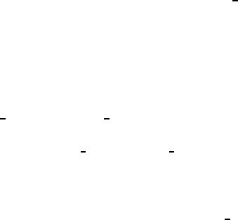
Fig. S2.1. Four-link closed-chain planar arm with frame assignment
Solution to Problem 2.10
The matrix
A0
1=⎡
⎢
⎣R0
1o0
1
0T1
⎤
⎥
⎦
can be inverted as a block-partitioned matrix. In fact, by recalling that
AD
OB
−1
=A−1−A−1DB−1
OB
−1,
expression (2.45) follows by observing that (R0
1)−1=R1
0.
Solution to Problem 2.11
Joint 4 was selected as the cut joint. The link frames can be assigned as in
Fig. S2.1. With this choice, the Denavit-Hartenberg parameters are specified
in Table S2.1.
Table S2.1. DH parameters for the four-link closed-chain planar arm
Link aiαidiϑi
1a100ϑ1
2a200ϑ2
30π/20ϑ3
1 a1 −π/20ϑ1
40 0d40
Notice that the parameters for Link 4 are all constant. For the first two revo-
lute joints, the homogeneous transformation matrix defined in (2.52) has the
82Kinematics
same structure as in (2.62), while for the third revolute joint, the homogeneous
transformation matrix is
A2
3(ϑ3)=⎡
⎢
⎣
c30s30
s30−c30
01 0 0
00 0 1
⎤
⎥
⎦.
Therefore, the coordinate transformations for the two branches of the tree are
respectively:
A0
3(q)=A0
1A1
2A2
3=⎡
⎢
⎣
c1230s123a1c1+a2c12
s1230−c123a1s1+a2s12
01 0 0
00 0 1
⎤
⎥
⎦
where q=[ϑ1ϑ2ϑ3]T,and
A0
1 (q)=⎡
⎢
⎣
c1 0−s1 a1 c1
s1 0c1 a1 s1
0−10 0
00 0 1
⎤
⎥
⎦
where q =ϑ1 . To complete, the constant homogeneous transformation for
the last link is
A3
4=⎡
⎢
⎣
100 0
010 0
001d4
000 1
⎤
⎥
⎦.
With reference to (2.60), the orientation constraints are (ϑ31 =π)
z0
3(q)=z0
1 (q)
x0T
3(q)x0
1 (q)=−1
which give
s123=−s1
c123=−c1
and thus
ϑ2+ϑ3=π−ϑ1+ϑ1 .(S2.1)
On the other hand, the position constraints are
x0T
3(q)
y0T
3(q)p0
3(q)−p0
1 (q)=0
0
which give
a1cos (ϑ2+ϑ3)+a2cos ϑ3−a1 cos (ϑ1+ϑ2+ϑ3−ϑ1 )=0
2 Kinematics 9
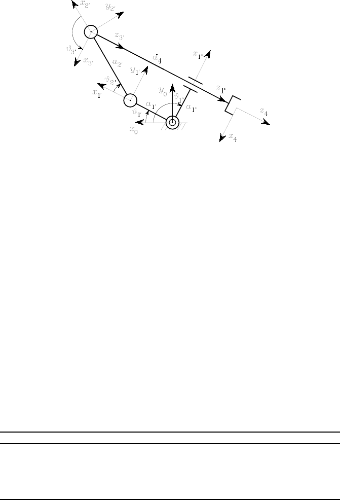
Fig. S2.2. Cylindrical arm with frame assignment
Table S2.2. DH parameters for the cylindrical arm
Link aiαidiϑi
10 0 0ϑ1
20−π/2d20
30 0d30
and, in view of (S2.1), it is
cos ϑ3=−a1 +a1cos (ϑ1 −ϑ1)
a2
.(S2.2)
The solution to (S2.2) exists for any ϑ1and ϑ1 provided that
a1+a1 ≤a2.
Further, it is
s3=±1−c2
3
with c3as in (S2.2). Therefore, it is
ϑ3=Atan2(s3,c
3)
ϑ2=π−ϑ1+ϑ1 −ϑ3.
It follows that the vector of joint variables is q=[ϑ1ϑ1 ]T.Thesejoints
are natural candidates to be the actuated joints. The arm direct kinematics
can be computed as T0
4(q)=A0
3(q)A3
4where the expressions of ϑ2and ϑ3
have to be substituted into the homogeneous transformation A0
3.
10 2 Kinematics
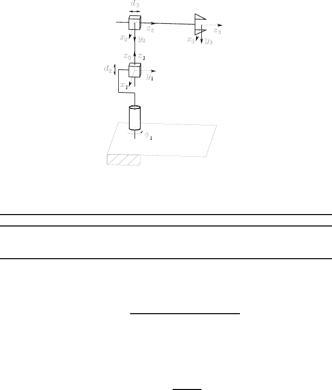
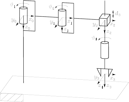
Fig. S2.3. SCARA manipulator with frame assignment
Solution to Problem 2.12
The link frames can be assigned as in Fig. S2.2. With this choice, the Denavit-
Hartenberg parameters are specified in Table S2.2.
The homogeneous transformation matrices (2.52) for the three joints are:
A0
1(ϑ1)=⎡
⎢
⎣
c1−s100
s1c100
0010
0001
⎤
⎥
⎦A1
2(d2)=⎡
⎢
⎣
1000
0010
0−10d2
0001
⎤
⎥
⎦
A2
3(d3)=⎡
⎢
⎣
100 0
010 0
001d3
000 1
⎤
⎥
⎦,
and thus the arm direct kinematics is
T0
3(q)=A0
1A1
2A2
3=⎡
⎢
⎣
c10−s1−d3s1
s10c1d3c1
0−10 d2
00 0 1
⎤
⎥
⎦
where q=[ϑ1d2d3]T.
Solution to Problem 2.13
The link frames can be assigned as in Fig. S2.3. Since the typical approach
to an object is from the top, it is reasonable to choose all the joint axes
pointing downwards. With this choice, the Denavit-Hartenberg parameters
are specified in Table S2.3.

2 Kinematics 11
Table S2.3. DH parameters for the SCARA manipulator
Link aiαidiϑi
1a100ϑ1
2a200ϑ2
300d30
4 000ϑ4
The homogeneous transformation matrices (2.52) for the four joints are:
Ai−1
i(ϑi)=⎡
⎢
⎣
ci−si0aici
sici0aisi
0010
0001
⎤
⎥
⎦i=1,2
A2
3(d3)=⎡
⎢
⎣
100 0
010 0
001d3
000 1
⎤
⎥
⎦A3
4(ϑ4)=⎡
⎢
⎣
c4−s400
s4c400
0010
0001
⎤
⎥
⎦,
and thus the manipulator direct kinematics is
T0
4(q)=A0
1A1
2A2
3A3
4=⎡
⎢
⎣
c124 −s124 0a1c1+a2c12
s124 c124 0a1s1+a2s12
001 d3
000 1
⎤
⎥
⎦(S2.3)
where q=[ϑ1ϑ2d3ϑ4]T. It is worth noticing that the direct kinematics
of this structure can be conceptually derived from that of a three-link planar
arm in which a3=0,ϑ3is replaced by ϑ4,andthezcoordinate is d3.
Solution to Problem 2.14
The torso can be modelled as an anthropomorphic arm, corresponding to the
first three DOFs. Therefore T0
3in (2.78) and (2.79) has the expression (2.66).
The constant matrices Tt
land Tt
rcan be computed in terms of the angle
βand of the lengths dland drof segments OtOland OtOr,beingOt,Oland
Orthe origins of frames t,land r, respectively. In detail:
Tt
l=Rt
lot
t,l
0T1Tt
r=Rt
rot
t,r
0T1,
where
ot
t,l =⎡
⎣dlcβ
0
dlsβ⎤
⎦ot
t,r =⎡
⎣drcβ
0
−drsβ⎤
⎦
12 2 Kinematics
are the positions of the origins of frames land rwith respect to frame tand
Rt
l=⎡
⎣
0−sβcβ
10 0
0cβsβ⎤
⎦Rt
r=⎡
⎣
0sβcβ
10 0
0cβ−sβ⎤
⎦
are the corresponding rotation matrices.
Finally, matrices Tr
rh =Tl
lh can be computed using (2.72) with (2.77) in
place of (2.73).
Solution to Problem 2.15
Consider two sets of Euler angles ZYZ:
φ1=⎡
⎣
π/2
π/2
0⎤
⎦φ2=⎡
⎣−π/2
−π/2
0⎤
⎦.
The corresponding rotation matrices are
R(φ1)=⎡
⎣0−10
001
−100
⎤
⎦R(φ2)=⎡
⎣010
001
100
⎤
⎦.
Composition of rotations with respect to the current frame gives
R(φ1)R(φ2)=⎡
⎣00−1
10 0
0−10
⎤
⎦
to which the following two sets of Euler angles correspond as for (2.19) and
(2.20):
φa=⎡
⎣π
π/2
−π/2⎤
⎦φb=⎡
⎣0
−π/2
π/2⎤
⎦.
On the other hand, composition of rotations with respect to the fixed frame
gives
R(φ2)R(φ1)=⎡
⎣001
−100
0−10
⎤
⎦
to which the following two sets of Euler angles correspond as for (2.19) and
(2.20):
φa=⎡
⎣0
π/2
−π/2⎤
⎦φb=⎡
⎣π
−π/2
π/2⎤
⎦.
2 Kinematics 13
It is evident that the two results differ, and then it is not possible to commute
the order of rotations. Notice, also, that the rotation matrix resulting from
direct sum of the two given sets of angles is
R(φ1+φ2)=I
to which the set of Euler angles φ=[0 0 0]
Tcorresponds.
Solution to Problem 2.16
In view of the approximations cos (dφ)≈1andsin(dφ)≈dφ, the elementary
rotation matrices for infinitesimal angles can be written as:
Rx(dφx)=⎡
⎣10 0
0cos(dφx)−sin (dφx)
0sin(dφx)cos(dφx)⎤
⎦≈⎡
⎣10 0
01−dφx
0dφx1⎤
⎦
Ry(dφy)=⎡
⎣cos (dφy)0sin(dφy)
010
−sin (dφy)0cos(dφy)⎤
⎦≈⎡
⎣10dφy
010
−dφy01
⎤
⎦
Rz(dφz)=⎡
⎣cos (dφz)−sin (dφz)0
sin (dφz)cos(dφz)0
001
⎤
⎦≈⎡
⎣1−dφz0
dφz10
001
⎤
⎦.
Multiplying the first two matrices gives
Rx(dφx)Ry(dφy)≈⎡
⎣10dφy
01−dφx
−dφydφx1⎤
⎦
where higher order terms have been neglected. Reversing the order of multi-
plication gives
Ry(dφy)Rx(dφx)≈⎡
⎣
10dφy
01−dφx
−dφydφx1⎤
⎦,
which shows that the rotation resulting from any two elementary rotations is
independent of the order of rotations when the angles of rotation are infinites-
imal.
Constructing the matrix of the three elementary rotations about coordi-
nate axes for infinitesimal angles gives
R(dφx,dφ
y,dφ
z)=⎡
⎣1−dφzdφy
dφz1−dφx
−dφydφx1⎤
⎦.
14 2 Kinematics
For another set of infinitesimal angles, the rotation matrix can be formally
written as
R(dφ
x,dφ
y,dφ
z)=⎡
⎣1−dφ
zdφ
y
dφ
z1−dφ
x
−dφ
ydφ
x1⎤
⎦.
Multiplying these two rotation matrices and neglecting higher order terms
gives
R(dφx,dφ
y,dφ
z)R(dφ
x,dφ
y,dφ
z)=
⎡
⎣1−(dφz+dφ
z)dφy+dφ
y
dφz+dφ
z1−(dφx+dφ
x)
−(dφy+dφ
y)dφx+dφ
x1⎤
⎦
=R(dφx+dφ
x,dφ
y+dφ
y,dφ
z+dφ
z).
Solution to Problem 2.17
In order to find the arm reachable workspace, it is worth considering all the
joint configurations giving a loss of mobility. These are the 23= 8 configura-
tions for the joint limits:
qA=⎡
⎣−π/3
−2π/3
−π/2⎤
⎦qB=⎡
⎣−π/3
−2π/3
π/2⎤
⎦qC=⎡
⎣−π/3
2π/3
−π/2⎤
⎦qD=⎡
⎣−π/3
2π/3
π/2⎤
⎦
qE=⎡
⎣π/3
−2π/3
−π/2⎤
⎦qF=⎡
⎣π/3
−2π/3
π/2⎤
⎦qG=⎡
⎣π/3
2π/3
−π/2⎤
⎦qH=⎡
⎣π/3
2π/3
π/2⎤
⎦,
the 4 configurations for ϑ2=0:
qI=⎡
⎣−π/3
0
−π/2⎤
⎦qJ=⎡
⎣−π/3
0
π/2⎤
⎦qK=⎡
⎣π/3
0
−π/2⎤
⎦qL=⎡
⎣π/3
0
π/2⎤
⎦,
the 4 configurations for ϑ3=0:
qM=⎡
⎣−π/3
−2π/3
0⎤
⎦qN=⎡
⎣−π/3
2π/3
0⎤
⎦qO=⎡
⎣
π/3
−2π/3
0⎤
⎦qP=⎡
⎣
π/3
2π/3
0⎤
⎦,
and the 2 configurations for both ϑ2=0andϑ3=0:
qQ=⎡
⎣−π/3
0
0⎤
⎦qR=⎡
⎣π/3
0
0⎤
⎦.
2 Kinematics 15
−0.5 0 0.5 1 1.5
−1
−0.5
0
0.5
1
[m]
[m]
D
H
P
R
Q
M
A
E
Fig. S2.4. Reachable workspace for a three-link planar arm
Starting from point Ain Cartesian space corresponding to qA, it is necessary
to draw all the arcs connecting such point to all other points corresponding
to configurations that differ only for one component, i.e., points B,C,E,I,
M. Repeating the procedure for each point leads to obtaining all the portions
of the requested workspace. It can be recognized that the external contour of
the area AM QRP HEDA delimits the reachable workspace, as illustrated in
Fig. S2.4.
Solution to Problem 2.18
When s3=0,thetwocasesc3=1andc3=−1 have to be considered.
In the case c3= 1, the arm is outstretched with ϑ3= 0. From (2.105)–
(2.108), it is
ϑ2,I=ϑ2,III =Atan2pWz,p2
Wx +p2
Wy(S2.4)
ϑ2,II =ϑ2,IV =Atan2pWz,−p2
Wx +p2
Wy.(S2.5)
Hence, if p2
Wx +p2
Wy >0, two different solutions exist for ϑ2. The corre-
sponding values of ϑ1are those in (2.109) or (2.110). On the other hand, if
p2
Wx +p2
Wy = 0, i.e., pWx =pWy = 0, the admissibility of the solution re-
quires that pWz =±(a2+a3). Hence, from (S2.4) and (S2.5) it is ϑ2=±π/2.
Moreover, in view of (2.109) and (2.110), an infinity of solutions exists for ϑ1.
In the case c3=−1, the arm is retracted with ϑ3=±π. From (2.105)–
(2.108), it is
ϑ2,I=ϑ2,III =Atan2(a2−a3)pWz,(a2−a3)p2
Wx +p2
Wy(S2.6)
ϑ2,II =ϑ2,IV =Atan2(a2−a3)pWz,−(a2−a3)p2
Wx +p2
Wy.(S2.7)
Hence, assuming that a2=a3,ifp2
Wx +p2
Wy >0, two different solutions
exist for ϑ2. The corresponding values of ϑ1are those in (2.109) or (2.110). On

16 2 Kinematics
the other hand, if p2
Wx +p2
Wy = 0, i.e., pWx =pWy = 0, the admissibility
of the solution requires that pWz =±|a2−a3|. Hence, from (S2.6) and (S2.7),
it is ϑ2=±π/2. As in previous case, in view of (2.109), (2.110), an infinity
of solutions exists for ϑ1. Notice that, if a2=a3,itispWx =pWy =pWz =0
necessarily. Therefore, an infinity of solutions exists both for ϑ1and ϑ2.
Solution to Problem 2.19
From the direct kinematics as in Problem 2.12, the end-effector position is
given by
px=−d3s1
py=d3c1
pz=d2.
The first joint variable can be computed from the first two equations as
ϑ1=Atan2(−px,p
y).
Then, the third joint variable can be computed by squaring and summing
those same two equations leading to
d3=p2
x+p2
y.
Finally, the second joint variables is
d2=pz.
Solution to Problem 2.20
From the direct kinematics as in Problem 2.13, the end-effector position is
given by
px=a1c1+a2c12
py=a1s1+a2s12
pz=d3.
The first two equations are the same as (2.91) and (2.92) for a three-link
planar arm. Then it is
c2=p2
x+p2
y−a2
1−a2
2
2a1a2
with −1≤c2≤1and
s2=±1−c2
2

2 Kinematics 17
where the positive sign corresponds to ϑ2∈(0,π) and the negative sign cor-
responds to ϑ2∈(−π, 0). The second joint variable is
ϑ2=Atan2(s2,c
2).
The first joint variable can be computed from
s1=(a1+a2c2)py−a2s2px
p2
x+p2
y
c1=(a1+a2c2)px+a2s2py
p2
x+p2
y
and thus
ϑ1=Atan2(s1,c
1).
The end-effector orientation can be expressed as
φ=ϑ1+ϑ2+ϑ4,
from which the fourth joint variable is
ϑ4=φ−ϑ1−ϑ2.
Finally, the third joint variable is
d3=pz.

3
Differential Kinematics and Statics
Solution to Problem 3.1
Let
R=[xyz]T
where the unit vector triplet (x,y,z) forms a right-handed frame. Then, the
product RS(ω)RTcan be written as
RS(ω)RT=⎡
⎣
xT
yT
zT⎤
⎦S(ω)[xyz]
=⎡
⎣
xTS(ω)xx
TS(ω)yx
TS(ω)z
yTS(ω)xy
TS(ω)yy
TS(ω)z
zTS(ω)xz
TS(ω)yz
TS(ω)z⎤
⎦
=⎡
⎣
xT(ω×x)xT(ω×y)xT(ω×z)
yT(ω×x)yT(ω×y)yT(ω×z)
zT(ω×x)zT(ω×y)zT(ω×z)⎤
⎦.
In view of the properties of scalar triple products, this matrix is skew-
symmetric and then
RS(ω)RT=S(ω)=⎡
⎣0−ω
zω
y
ω
z0−ω
x
−ω
yω
x0⎤
⎦(S3.1)
where the elements of the previous matrix can be written as
ω
x=zT(ω×y)=ωT(y×z)=ωTx
ω
y=xT(ω×z)=ωT(z×x)=ωTy
ω
z=yT(ω×x)=ωT(x×y)=ωTz.
20 3 Differential Kinematics and Statics
Hence, it is
ω=[ω
xω
yω
z]T
=ωT[xyz]T
=Rω.
Substituting ωin (S3.1) leads to conclude
RS(ω)RT=S(Rω).
Solution to Problem 3.2
For the cylindrical arm in Fig. 2.35, the Jacobian is
J(q)=z0×(p−p0)z1z2
z000
where the various vectors can be computed from arm direct kinematics
p0=⎡
⎣0
0
0⎤
⎦p=⎡
⎣−d3s1
d3c1
d2⎤
⎦
z0=z1=⎡
⎣
0
0
1⎤
⎦z2=⎡
⎣−s1
c1
0⎤
⎦.
Then, the expression of the geometric Jacobian is
J=⎡
⎢
⎢
⎢
⎢
⎢
⎣
−d3c10−s1
−d3s10c1
010
000
000
100
⎤
⎥
⎥
⎥
⎥
⎥
⎦
(S3.2)
which reveals that it is inherently impossible to rotate about axes xand y.
Solution to Problem 3.3
For the SCARA manipulator in Fig. 2.36, the Jacobian is
J(q)=z0×(p−p0)z1×(p−p1)z2z3×(p−p3)
z0z10z3
3 Differential Kinematics and Statics 21
where the various vectors can be computed from manipulator direct kinemat-
ics
p0=⎡
⎣0
0
0⎤
⎦p1=⎡
⎣a1c1
a1s1
0⎤
⎦p3=⎡
⎣a1c1+a2c12
a1s1+a2s12
d3⎤
⎦p=⎡
⎣a1c1+a2c12
a1s1+a2s12
d3⎤
⎦
z0=z1=z2=z3=⎡
⎣
0
0
1⎤
⎦.
Then, the expression of the geometric Jacobian is
J=⎡
⎢
⎢
⎢
⎢
⎢
⎣
−a1s1−a2s12 −a2s12 00
a1c1+a2c12 a2c12 00
0010
0000
0000
1101
⎤
⎥
⎥
⎥
⎥
⎥
⎦
which reveals that it is inherently impossible to rotate about axes xand y.
In view of this, if a four-dimensional operational space (r= 4) is of concern,
then the (4 ×4) analytical Jacobian can be extracted from Jby eliminating
rows 4 and 5, i.e.,
JA=⎡
⎢
⎣
−a1s1−a2s12 −a2s12 00
a1c1+a2c12 a2c12 00
0010
1101
⎤
⎥
⎦.(S3.3)
Solution to Problem 3.4
From the expression of the geometric Jacobian in (3.35), it is possible to
extract the analytical Jacobian by eliminating the three null rows, i.e.,
JA=⎡
⎣−a1s1−a2s12 −a3s123 −a2s12 −a3s123 −a3s123
a1c1+a2c12 +a3c123 a2c12 +a3c123 a3c123
111
⎤
⎦.
In order to compute its determinant, it is worth subtracting the second column
from the first one and the third column from the second one, respectively,
giving
J
A=⎡
⎣−a1s1−a2s12 −a3s123
a1c1a2c12 a3c123
00 1
⎤
⎦
whose determinant is
det(J
A)=a1a2s2.
22 3 Differential Kinematics and Statics
It follows that, for a1,a
2= 0, the determinant vanishes whenever
ϑ2=0 ϑ2=π,
that are the same singularities of the two-link planar arm. It may be verified
that the rank of the Jacobian does not further decrease, and thus the arm has
no other singularities.
Solution to Problem 3.5
For the spherical arm in Fig. 2.22, the Jacobian is
J(q)=z0×(p−p0)z1×(p−p1)z2
z0z10
where the various vectors can be computed from arm direct kinematics
p0=p1=⎡
⎣0
0
0⎤
⎦p=⎡
⎣c1s2d3−s1d2
s1s2d3+c1d2
c2d3⎤
⎦
z0=⎡
⎣0
0
1⎤
⎦z1=⎡
⎣−s1
c1
0⎤
⎦z2=⎡
⎣c1s2
s1s2
c2⎤
⎦.
Then, the expression of the geometric Jacobian is
J=⎡
⎢
⎢
⎢
⎢
⎢
⎣
−s1s2d3−c1d2c1c2d3c1s2
c1s2d3−s1d2s1c2d3s1s2
0−s2d3c2
0−s10
0c10
100
⎤
⎥
⎥
⎥
⎥
⎥
⎦
.
With three DOFs, it is worth considering end-effector linear velocity only,
corresponding to the first three rows of the Jacobian, i.e.,
JP=⎡
⎣−s1s2d3−c1d2c1c2d3c1s2
c1s2d3−s1d2s1c2d3s1s2
0−s2d3c2⎤
⎦
which could have been also obtained by differentiating the vector pabove
with respect to the joint variable vector q(analytical Jacobian). In order to
determine singularities of JP, its determinant has to be computed, giving
det(JP)=−d2
3s2.
This vanishes if s2= 0 and/or d3= 0. The first situation occurs whenever
ϑ2=0 ϑ2=π,
3 Differential Kinematics and Statics 23
whereas the second situation occurs whenever
d3=0,
i.e., when Frame 3 coincides with Frame 2 and thus Joint 2 velocity does not
contribute to end-effector linear velocity. Finally, it is worth observing that
both types of singularities are internal singularities.
Solution to Problem 3.6
From the geometric Jacobian in (S3.2), the Jacobian relative to end-effector
linear velocity can be extracted by considering only the first three rows, i.e.,
JP=⎡
⎣−d3c10−s1
−d3s10c1
010
⎤
⎦.
Its determinant is
det(JP)=d3
which vanishes at the singularity
d3=0.
This occurs when the end effector is located along Joint 1 axis, and thus this
singularity is conceptually similar to the shoulder singularity of an anthropo-
morphic arm.
Solution to Problem 3.7
With reference to the analytical Jacobian in (S3.3), it is worth subtracting
the second column from the first one. The modified Jacobian becomes
J
A=⎡
⎢
⎣
−a1s1−a2s12 00
a1c1a2c12 00
0010
0001
⎤
⎥
⎦,
whose determinant is
det(J
A)=a1a2s2.
For a1,a
2= 0, the determinant vanishes whenever
ϑ2=0 ϑ2=π
which are the same singularities of the two-link and three-link planar arms.
In other words, the addition of a prismatic joint to a three-link planar arm
—which makes it become a SCARA manipulator— does not introduce further
singularities.

24 3 Differential Kinematics and Statics
Solution to Problem 3.8
The singular values of Jare defined as the square roots of the eigenvalues of
the matrix JJT. On the other hand, the determinant of a matrix is given by
the product of its eigenvalues, and thus the manipulability measure in (3.56)
is given by the product of the singular values of the Jacobian matrix.
Solution to Problem 3.9
Let Rbe the radius of the circular object. The expression of the minimum
distance of the arm from the obstacle can be written as
d=min
di
(di−R)i=1,2,3, (S3.4)
where didenotes the minimum distance of Link ifrom the centre oof the
obstacle. Let then pi=[pix piy ]Tdenote the position vector of the point
along Link iwhich is closest to o.Linkilies along a line, whose equation can
be written in the parametric form
pix =xi−1+si(xi−xi−1)(S3.5)
piy =yi−1+si(yi−yi−1)(S3.6)
where (xi−1,y
i−1)and(xi,y
i) are the coordinates of the origins of Link i−1
and Link iframes, respectively; obviously, the parameter sivaries in the
range (0,1). Therefore, computation of the minimum distance is given by the
solution to a minimization problem as a function of si, i.e.,
min
si(pix −xo)2+(piy −yo)20≤si≤1
where (xo,y
o) are the coordinates of o. Using (S3.5) and (S3.6), and taking
the derivative with respect to siof the above function leads to the solution
s
i=−(xi−1−xo)(xi−xi−1)+(yi−1−yo)(yi−yi−1)
a2
i
(S3.7)
where a2
i=(xi−xi−1)2+(yi−yi−1)2. For the point pito belong to Link i,
the parameter shall be subject to the constraint
si=max
0,min{1,s
i},(S3.8)
which then allows computing pix and piy as in (S3.5), (S3.6). In sum, the
following operating procedure can be established.
Execute steps aand bfor i=1,2,3:
a. Compute s
ias in (S3.7) and sias in (S3.8).
b. Compute pias in (S3.5), and
di=(pix −xo)2+(piy −yo)2.

3 Differential Kinematics and Statics 25
To complete, compute das in (S3.4).
Solution to Problem 3.10
The problem is that to invert differential kinematics ve=J˙
qby tolerating a
finite error , i.e.,
ve−J˙
q=.
The solution can be obtained by minimizing the cost functional
g(˙
q,)= 1
2k2˙
qT˙
q+1
2T.
To cast the problem as a classic constrained optimization problem, let
w=˙
q
A=[JI].
With these positions, the above differential kinematics constraint can be
rewritten as
ve−Aw =0,
while the cost functional becomes
g(w)=1
2wTQw
where
Q=k2IO
OI
is a positive definite weighting matrix. By using the method of Lagrangian
multipliers, the modified cost functional can be written as
g(w,λ)=1
2wTQw +λT(ve−Aw)
where λis an (r×1) vector. The optimal solution is conceptually similar
to (3.50), i.e.,
w=Q−1AT(AQ−1AT)−1ve.
In view of the above expressions of w,Aand Q, the solution can be formally
written after simple algebraic manipulation as
˙
q
=JT
k2IJJT+k2I−1
ve.
It follows that the joint velocity is given by
˙
q=JTJJT+k2I−1
ve
26 3 Differential Kinematics and Statics
where
J=JT(JJT+k2I)−1
is the damped least-squares inverse of J, whereas the error is given by
=k2JJT+k2I−1
ve.
The damping factor kestablishes the relative weight between the kinematic
constraint ve=J˙
qand the minimum norm joint velocity requirement. In
the neighbourhood of a singularity, kis to be chosen large enough so as to
render differential kinematics inversion well conditioned, whereas far from
singularities, kcanbechosensmall(evenk= 0) so as to guarantee accurate
differential kinematics inversion.
Solution to Problem 3.11
From (3.6), it is
S(ω)= ˙
R(φ)RT(φ)
with R(φ) as in (2.18). Taking the required derivatives gives
S(ω)= ˙
Rz(ϕ)Ry(ϑ)Rz (ψ)RT
z (ψ)RT
y(ϑ)RT
z(ϕ)
+Rz(ϕ)˙
Ry(ϑ)Rz (ψ)RT
z (ψ)RT
y(ϑ)RT
z(ϕ)
+Rz(ϕ)Ry(ϑ)˙
Rz (ψ)RT
z (ψ)RT
y(ϑ)RT
z(ϕ).
Then, in view of (2.4), (3.8), (3.11), the previous expression can be simplified
into
S(ω)=S(˙ϕz)
+Rz(ϕ)S(˙
ϑy)RT
z(ϕ)
+Rz(ϕ)Ry(ϑ)S(˙
ψz)RT
y(ϑ)RT
z(ϕ)
=S(˙ϕz)+S(˙
ϑRz(ϕ)y)+S(˙
ψRz(ϕ)Ry(ϑ)z)
and then
ω=[zR
z(ϕ)yRz(ϕ)Ry(ϑ)z ]˙
φ
=⎡
⎣0−sϕcϕsϑ
0cϕsϕsϑ
10 cϑ⎤
⎦˙
φ.
Solution to Problem 3.12
From (2.21), the contributions to the angular velocity of the derivatives of the
three Roll–Pitch–Yaw angles can be written as:
˙
ϕ=˙ϕ⎡
⎣0
0
1⎤
⎦˙
ϑ=˙
ϑ⎡
⎣0
1
0⎤
⎦˙
ψ =˙
ψ⎡
⎣1
0
0⎤
⎦,
3 Differential Kinematics and Statics 27
where the superscripts indicate that rotations occur about axes of current
frames. Then, expressing the last two vectors with respect to the reference
frame gives
˙
ϑ=Rz(ϕ)˙
ϑ=˙
ϑ⎡
⎣−sϕ
cϕ
0⎤
⎦
˙
ψ=Rz(ϕ)Ry(ϑ)˙
ψ =˙
ψ⎡
⎣cϕcϑ
sϕcϑ
−sϑ⎤
⎦.
Summing the three contributions leads to
ω=˙
ϕ+˙
ϑ+˙
ψ
=⎡
⎣0−sϕcϕcϑ
0cϕsϕcϑ
10−sϑ⎤
⎦˙
φ,
from which it is
T(φ)=⎡
⎣0−sϕcϕcϑ
0cϕsϕcϑ
10−sϑ⎤
⎦.
The determinant of matrix Tis −cϑ, which implies that the relationship
cannot be inverted for ϑ=−π/2,π/2. These are representation singularities of
φ; notice also that solutions (2.22) and (2.23) degenerate at such singularities.
Solution to Problem 3.13
The contributions to the angular velocity of the derivatives of the three Euler
angles can be written as:
˙
ϕ=˙ϕeϕ˙
ϑ=˙
ϑe
ϑ˙
ψ =˙
ψe
ψ,
where eϕ,e
ϑand e
ψare the constant unit vectors of the axes of the current
frames, which depend on the particular triplet of Euler angles. The super-
scripts indicate that vectors are expressed in the current frames. In the case
ϕ=ϑ=ψ= 0 the current frames coincide and the three contributions can
be added, i.e.,
ω=˙
ϕ+˙
ϑ+˙
ψ =T(0)˙
φ
with T(0)=[eϕe
ϑe
ψ]. Therefore, with the choice
eϕ=⎡
⎣1
0
0⎤
⎦e
ϑ=⎡
⎣0
1
0⎤
⎦e
ψ=⎡
⎣0
0
1⎤
⎦,
i.e., for XYZ angles, it is T(0)=I.
28 3 Differential Kinematics and Statics
Fig. S3.1. Block scheme of the inverse kinematics algorithm for arm position
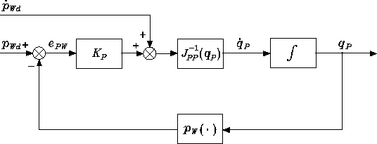
Solution to Problem 3.14
With reference to a 6-DOFs manipulator having a spherical wrist, let qP=
[q1q2q3]Tdenote the vector of joint variables determining arm position
and qO=[ϑ4ϑ5ϑ6]Tthe vector of joint variables determining wrist ori-
entation. For such manipulator, it is possible to solve inverse kinematics in
two stages; namely, first solve for qP,andthensolveforqO.
Let pd(t)andRd(t)=[nd(t)sd(t)ad(t) ] be the desired time history
of end-effector position and orientation. From (2.93), it is possible to compute
the desired time behaviour of wrist position as
pWd =pd−d6ad.
Taking time derivative of both sides gives
˙
pWd =˙
pd−d6ωd×ad
where the time derivative of the unit vector ad(constant norm) has been
expressed as ˙
ad=ωd×ad.
By using the block-partitioned form of the Jacobian in (3.42) with p=
pW, the differential kinematics equation for arm linear velocity is
˙
pW=JPP(qP)˙
qP
where JPP formally coincides with J11 evaluated for p=pW.Inviewofthis,
the joint velocity solution of kind (3.70) can be written as
˙
qP=J−1
PP(qP)( ˙
pWd +KPePW)
where ePW =pWd −pWand KPis a positive definite matrix. The resulting
block scheme is shown in Fig. S3.1.
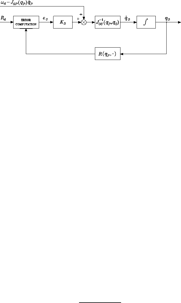
OncethetimebehaviourofqPand ˙
qPhas been computed in the first
stage, the differential kinematics equation for wrist angular velocity is
ω=JOP (qP)˙
qP+JOO(qP,qO)˙
qO
3 Differential Kinematics and Statics 29
Fig. S3.2. Block scheme of the inverse kinematics algorithm for wrist orientation
where JOP and JOO respectively denote the Jacobians J21 and J22 in (3.42)
evaluated for p=pW. In view of this, the joint velocity solution of kind (3.70)
can be written as
˙
qO=J−1
OO(qP,qO)ωd−JOP (qP)˙
qP+KOeO
where eOis the orientation error in (3.85) and KOis a positive definite matrix.
The resulting block scheme for the second stage is shown in Fig. S3.2.
It is anticipated that the two-stage algorithm leads to a computational
savings with respect to the algorithm based on the inverse of the full Jacobian.
Solution to Problem 3.15
In the case ˙
xd=0, the time derivative of the Lyapunov function is given as
in (3.77) ˙
V(e)=eTK˙
xd−eTKJA(q)JT
A(q)Ke
where the sign of the first term is indefinite, and the second term is less than
or equal to zero. This function can be upper bounded as
˙
V(e)≤|eTK˙
xd|−JT
AKe2.
In the worst case, it is necessary to take the largest value of the first term and
the smallest value of the second term, leading to
˙
V(e)≤eλmax(K)˙
xdmax −σ2
r(JA)λ2
min(K)e2,
where λmax (K)(λmin(K)) denotes the maximum (minimum) eigenvalue of K,
˙
xdmax denotes the maximum end-effector velocity, and σr(JA) denotes the
minimum singular value of JA. The quadratic term in the error prevails over
the linear term as long as
e≥˙
xdmaxλmax (K)
σ2
r(JA)λ2
min (K)

30 3 Differential Kinematics and Statics
and ˙
V(e)≤0. It follows that an upper bound on the error is given by
emax =˙
xdmax
kσ2
r(JA)
where Khas been conveniently chosen as a diagonal matrix K=kI.
Solution to Problem 3.16
The matrix product RdRTgives
RdRT=
⎡
⎣ndxnx+sdxsx+adxaxndxny+sdxsy+adxayndxnz+sdxsz+adxaz
ndynx+sdy sx+adyaxndy ny+sdysy+adyayndynz+sdysz+adyaz
ndznx+sdzsx+adz axndz ny+sdz sy+adzayndznz+sdz sz+adzaz⎤
⎦.
In view of (3.84), subtracting the element [1,2] from the element [2,1] and
equating the difference to 2rzsϑas in (2.28) gives
2rzsϑ=(ndynx−ndxny)+(sdysx−sdxsy)+(adyax−adxay),
and thus
rzsϑ=1
2(n×nd)z+(s×sd)z+(a×ad)z
where the subscripts zdenote the z-components of the relevant vectors. In a
similar way, subtracting the elements [3,1] from the respective elements [1,3]
and equating the difference to 2rysϑgives
rysϑ=1
2(n×nd)y+(s×sd)y+(a×ad)y.
Yet, subtracting the elements [2,3] from the respective elements [3,2] and
equating the difference to 2rxsϑgives
rxsϑ=1
2(n×nd)x+(s×sd)x+(a×ad)x.
In turn, grouping the previous three expressions leads to
rsin ϑ=1
2(n×nd+s×sd+a×ad)
and, in view of the definition of orientation error as in (3.83), the result in
(3.85) follows.
Solution to Problem 3.17
The expression of the orientation error from (3.85) is
eO=1
2(n×nd+s×sd+a×ad).

3 Differential Kinematics and Statics 31
Taking the time derivative of the first term on the right-hand side gives
d
dt(n×nd)= ˙
n×nd+n×˙
nd
=−S(nd)˙
n+S(n)˙
nd.
Expressing the time derivatives of the unit vectors as
˙
n=ω×n=−S(n)ω
˙
nd=ωd×nd=−S(nd)ωd
leads to d
dt(n×nd)=S(nd)S(n)ω−S(n)S(nd)ωd.
Proceeding in a similar way for the other two terms on the right-hand side of
(3.85) yields
d
dt(s×sd)=S(sd)S(s)ω−S(s)S(sd)ωd
d
dt(a×ad)=S(ad)S(a)ω−S(a)S(ad)ωd.
In turn, grouping the previous three contributions to the time derivative of
the orientation error gives
˙
eO=−1
2S(n)S(nd)+S(s)S(sd)+S(a)S(ad)ωd
+1
2S(nd)S(n)+S(sd)S(s)+S(ad)S(a)ω
and, in view of the position (3.87), the result in (3.86) follows.
Solution to Problem 3.18
It is not difficult to see that, by using the skew-symmetric operator S(·), (2.33)
can be rewritten in compact form as
R(η, )=(2η2−1)I+2T+2ηS(). (S3.9)
Computing the time derivative of (S3.9) gives
˙
R(η, )=4˙ηηI+2˙
T+2˙
T+2˙ηS()+2ηS(˙
). (S3.10)
Substituting (S3.9) and (S3.10) into (3.6) gives:
S(ω)= ˙
RRT
=4˙ηη(2η2−1)I+8˙ηηT−8˙ηη2S()
+2(2η2−1)˙
T+4˙
TT−4η˙
TS()
+2(2η2−1)˙
T+4˙
TT−4η˙
TS() (S3.11)
+2 ˙η(2η2−1)S()+4˙ηS()T−4˙ηηS()S()
+2 ˙η(2η2−1)S(˙
)+4ηS(˙
)T−4η2S(˙
)S().
32 3 Differential Kinematics and Statics
q
plot
dag(J_p(q))dp + P(q)dq_0
Jacobian pseudo-inverse
with constraint
cs(q)
sinusoidal
functions
dq_0
constraint
velocity
dqe_p
k_p(q)
direct
kinematics
K_p
[T,dp_d]
time
0.001z
z-1
unconstrained
solution
constrained
solution
+
-
[T,p_d] +
+
Fig. S3.3. Simulink block diagram of closed-loop Jacobian pseudo-inverse algo-
rithm with constraint
Next, taking the time derivative of the constraint in (2.32) gives
T˙
=˙
T=−η˙η. (S3.12)
Then, using (2.32), (S3.12) and the property S(x)S(y)=yxT−xTyI yields
the following equalities:
˙
TT=(1−η2)˙
T
˙
TT=−˙ηηT
S()S()=T−(1 −η2)I
S(˙
)S()=˙
T+˙ηηI
˙
TS()=(S(˙
)S()−˙ηηI)S()
S(˙
)T=S(˙
)(S()S()+(1−η2)I).
By virtue of the above equalities and observing that S()=0, (S3.11) be-
comes
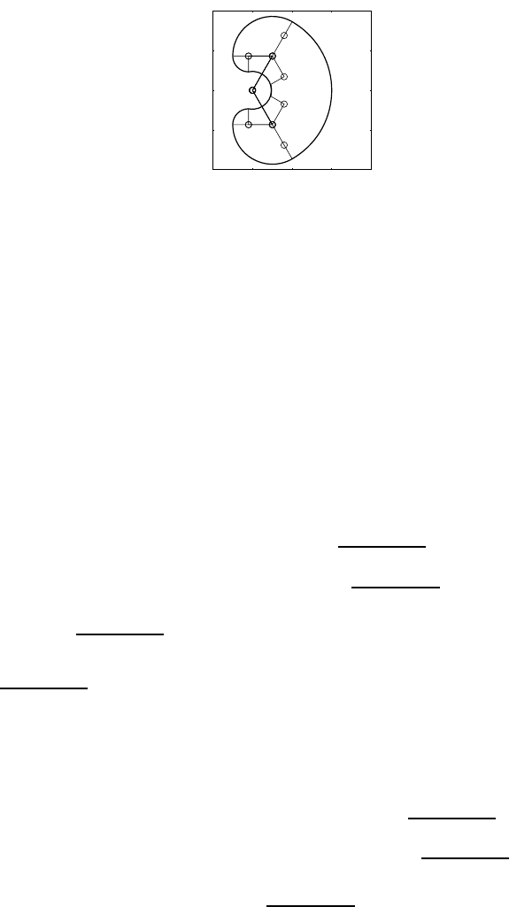
S(ω)=2(
˙
T−˙
T)+2ηS(˙
)−2˙ηS()
which, in view of the property S(S(x)y)=yxT−xyT, can be written in the
form
S(ω)=2S(S()˙
)+2ηS(˙
)−2˙ηS().
Finally, the angular velocity can be computed as
ω=2S()˙
+2η˙
−2˙η. (S3.13)
3 Differential Kinematics and Statics 33
0 0.5 1 1.5 2 2.5
−2
−1
0
1
2
[s]
[rad]
joint pos
1
2
3
0 0.5 1 1.5 2 2.5
−0.4
−0.2
0
1
2
3
[s]
[rad/s]
joint vel
0 0.5 1 1.5 2 2.5
0
1
2
3
4
5
6x 10⁻⁶
[s]
[m]
pos error norm
0 0.5 1 1.5 2 2.5
−0.1
−0.05
0
0.05
0.1
0.15
[s]
[m]
distance
Fig. S3.4. Time history of the joint positions and velocities, of the norm of end-
effector position error, and of the distance from the obstacle in the unconstrained
case
Solution to Problem 3.19
Multiplying both sides of (S3.13) by Tand using (S3.12), (2.32) yields
Tω=2ηT˙
−2˙ηT=−2˙η
and thus
˙η=−1
2Tω.
Multiplying both sides of (S3.13) by S() yields
S()ω=2S()S()˙
+2ηS()˙
,
which, by virtue of (S3.12), (2.32), (S3.13) and the property S(x)S(y)=
yxT−xTyI, can be rewritten in the form
S()ω=−2˙ηη−2(1 −η2)˙
+η(ω−2η˙
+2˙η)
=−2˙
+ηω
and thus
˙
=1
2(ηI−S()) ω.
34 3 Differential Kinematics and Statics
0 0.5 1 1.5 2 2.5
−2
−1
0
1
2
[s]
[rad]
joint pos
1
2
3
0 0.5 1 1.5 2 2.5
−5
0
5
12
3
[s]
[rad/s]
joint vel
0 0.5 1 1.5 2 2.5
0
1
2
3
4
5
6x 10⁻⁶
[s]
[m]
pos error norm
0 0.5 1 1.5 2 2.5
−0.1
−0.05
0
0.05
0.1
0.15
[s]
[m]
distance
Fig. S3.5. Time history of the joint positions and velocities, of the norm of end-
effector position error, and of the distance from the obstacle in the constrained case
Solution to Problem 3.20
Differentiating (3.96) with respect to time gives
˙
V=2(ηd−η)( ˙ηd−˙η)+2(d−)T(˙
d−˙
)
=ηT
d−ηdT−S(d)(ωd−ω)
where the quaternion propagation in (3.94), (3.95), and the property S()=
0have been exploited. The result in (3.97) follows by using (3.91) and (3.93).
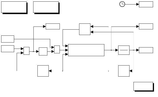
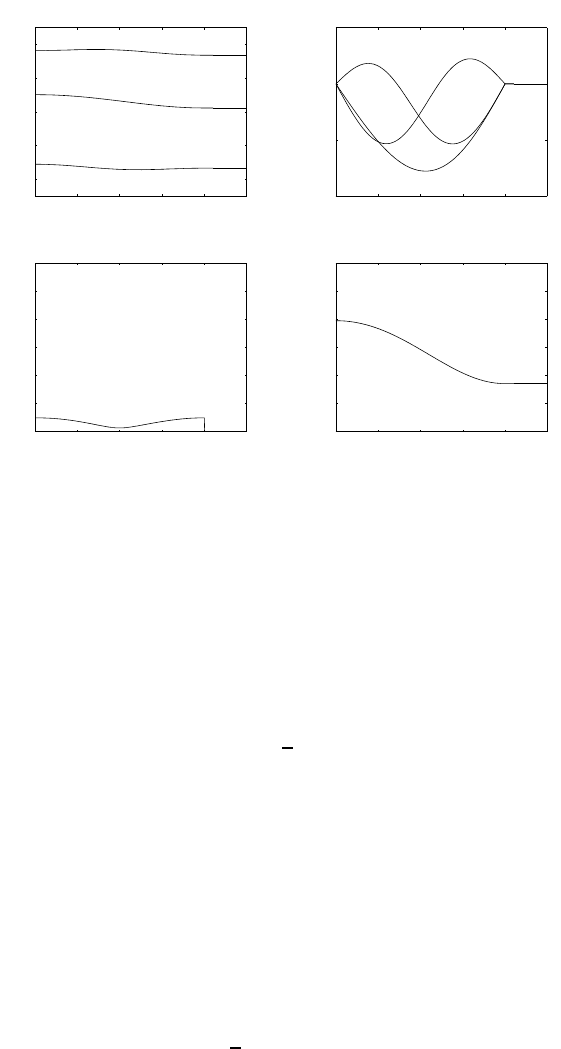
Solution to Problem 3.21
From the given pd(0), the initial posture of the arm q(0) is computed
according to the formulæ in Sect. 2.12.1 (elbow-up) with an arbitrary value
of φ, e.g., φ=π/4. The desired trajectory regards the vertical component of
end-effector position and is chosen as
pdy(t)=pdy(0) + 0.51−cos (0.5πt)pdy(2) −pdy (0)0≤t≤2
with pdy(0) = 0.2andpdy(2) = −0.2. The desired velocity is found by differ-
entiation of the above trajectory. As for the constraint, the minimum distance
of the arm from the obstacle (3.58) is computed according to the solution to
3 Differential Kinematics and Statics 35
variables
initialization
[T,dx_d]
+
-
[T,x_d]
K
e
inv(J_a(q))dx
Jacobian
inverse
+
+
k(q)
direct
kinematics
time
dq
0.001z
z-1 q
plot
cs(q)
sinusoidal
functions
Fig. S3.6. Simulink block diagram of closed-loop Jacobian inverse algorithm
Problem 3.11. Its gradient is found by numerical differentiation with a step of
10−6.
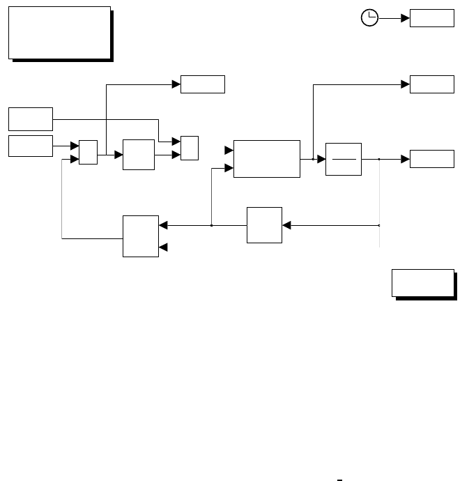
The inverse kinematics algorithm based on (3.72) is used, with the matrix
gain K=diag{500,500}and ˙
q0as in (3.55) with k0= 35. The resulting
Simulink block diagram is shown in Fig. S3.3, where both the unconstrained
case (k0= 0) and the constrained case can be run.
The files with the solution can be found in Folder 321.
The resulting joint positions and velocities, as well as the norm of end-
effector position error and the distance from the obstacle, in the two cases,
are shown in Figs. S3.4 and S3.5, respectively.
It can be recognized that the position error is small along the trajectory
and tends to zero at steady state in both cases. In the unconstrained case, the
arm is seen to collide with the obstacle (negative distance). On the other hand,
in the constrained case, large initial values of joint velocities occur which are
needed to move the arm away from the obstacle.
Solution to Problem 3.22
From the given xd(0), the initial posture of the manipulator q(0) is computed
according to the formulæ in the solution to Problem 2.20 (elbow-up). The
desired trajectory for the end-effector position is chosen as
xd(t)=xd(0) + 0.51−cos (0.5πt)xdy(2) −xdy(0)0≤t≤2
36 3 Differential Kinematics and Statics
0 0.5 1 1.5 2 2.5
−3
−2
−1
0
1
2
3
1
2
3
4
[s]
[rad]
joint pos
0 0.5 1 1.5 2 2.5
−2
−1
0
1
2
1
2
3
4
[s]
[rad/s]
joint vel
0 0.5 1 1.5 2 2.5
0
0.5
1
1.5
2x 10⁻⁶
[s]
[m]
pos error norm
0 0.5 1 1.5 2 2.5
−1.5
−1
−0.5
0
0.5
1
1.5 x 10⁻⁵
[s]
[rad]
orien error
Fig. S3.7. Time history of the joint positions and velocities, of the norm of end-
effector position error, and of the end-effector orientation error with closed-loop
Jacobian inverse algorithm
with xd(0) = [ 0.7000]
Tand xd(2) = [ 0 0.80.5π/2]
T. The de-
sired velocity is found by differentiation of the above trajectory.
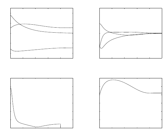
First, the inverse kinematics algorithm based on (3.70) is used where the
analytical Jacobian is given in (S3.3). The matrix gain is chosen as K=
diag{500,500,500,100}. The resulting Simulink block diagram is shown in
Fig. S3.6.
The files with the solution can be found in Folder 322.
The resulting joint positions and velocities, as well as the norm of end-
effector position error and the end-effector orientation error, are shown in
Fig. S3.7. The tracking performance is satisfactory and the errors vanish at
steady state.
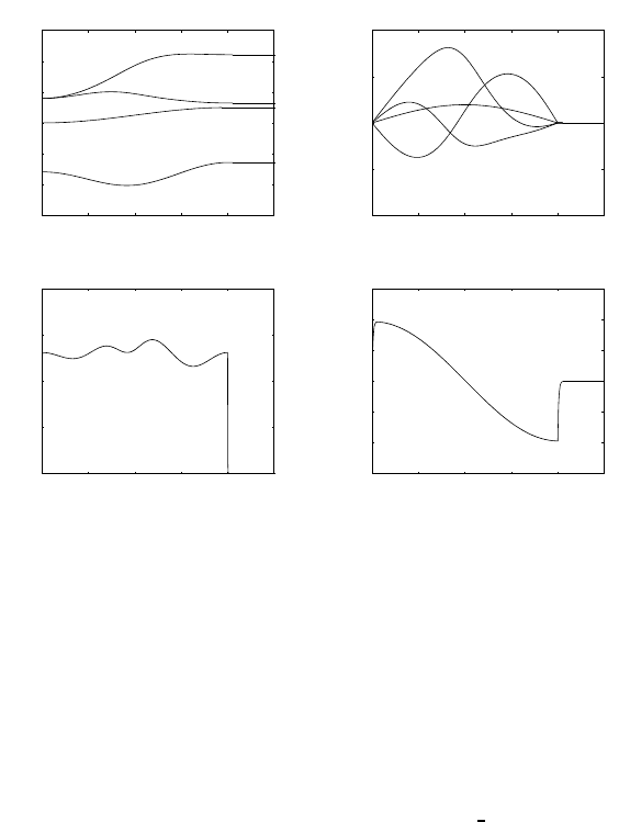
Next, the inverse kinematics algorithm based on (3.76) is used with the
same matrix gain as above. The resulting Simulink block diagram is shown
in Fig. S3.8.
The resulting joint positions and velocities, as well as the norm of end-
effector position error and the end-effector orientation error, are shown in
Fig. S3.9. It can be recognized that tracking errors slightly increase, but
steady-state performance remains satisfactory.

3 Differential Kinematics and Statics 37
variables
initialization
+
-
dqe
[T,x_d]
k(q)
direct
kinematics
time
plot
K
tr(J_a(q))Ke
Jacobian
transpose
cs(q)
sinusoidal
functions
0.001z
z-1 q
Fig. S3.8. Simulink block diagram of closed-loop Jacobian transpose algorithm
Solution to Problem 3.23
The core of the quadratic form defining the velocity manipulability ellipsoid
in (3.123) is given by the inverse of the core of the quadratic form defining
the force manipulability ellipsoid in (3.126). Let A=JJTdenote such core.
The eigenvalues λiand the eigenvectors uiof Asatisfy the equation
Aui=λiui.
Premultiplying both sides by A−1and dividing by λigives
A−1ui=1
λi
ui,
which demonstrates the notable result that the directions of the principal axes
(eigenvectors) of the force and velocity manipulability ellipsoids coincide while
their dimensions (eigenvalues) are in inverse proportion.
38 3 Differential Kinematics and Statics
0 0.5 1 1.5 2 2.5
−3
−2
−1
0
1
2
3
1
2
3
4
[s]
[rad]
joint pos
0 0.5 1 1.5 2 2.5
−2
−1
0
1
2
1
2
3
4
[s]
[rad/s]
joint vel
0 0.5 1 1.5 2 2.5
0
0.002
0.004
0.006
0.008
0.01
[s]
[m]
pos error norm
0 0.5 1 1.5 2 2.5
−6
−4
−2
0
2
4
6x 10⁻³
[s]
[rad]
orien error
Fig. S3.9. Time history of the joint positions and velocities, of the norm of end-
effector position error, and of the end-effector orientation error with closed-loop
Jacobian transpose algorithm

4
Trajectory Planning
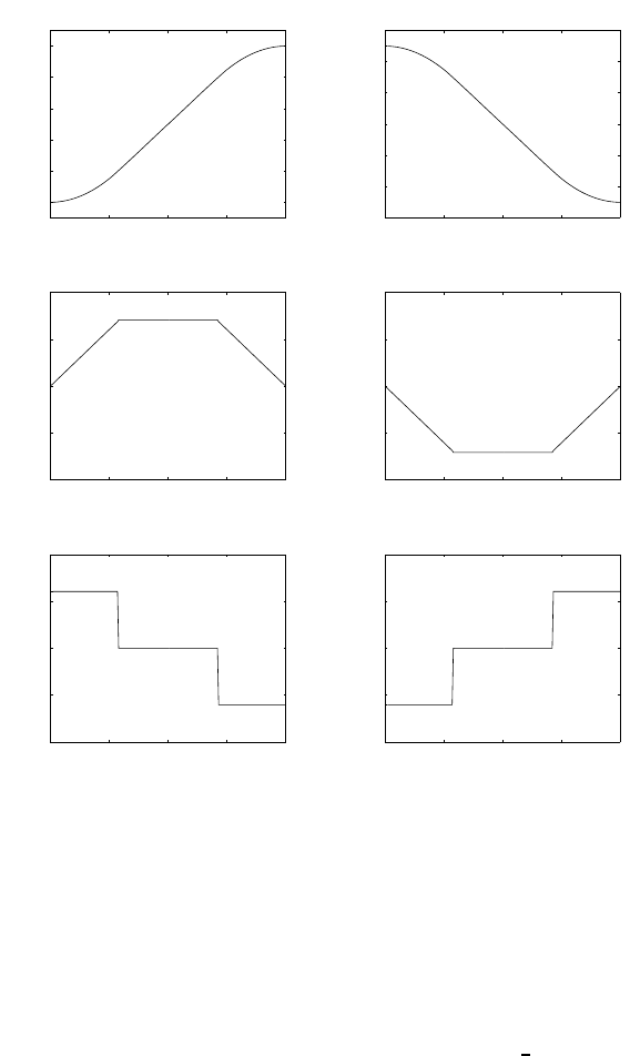
Solution to Problem 4.1
In order to satisfy initial and final constraints on position, velocity and accel-
eration, a fifth-order polynomial is needed
q(t)=a5t5+a4t4+a3t3+a2t2+a1t+a0.
The coefficients can be determined by solving the following system of linear
equations:
a0=qi
a1=˙qi
2a2=¨qi
a5t5
f+a4t4
f+a3t3
f+a2t2
f+a1tf+a0=qf
5a5t4
f+4a4t3
f+3a3t2
f+2a2tf+a1=˙qf
20a5t3
f+12a4t2
f+6a3tf+2a2=¨qf.
With the given data, the files used to compute the coefficients and to generate
the time behaviour of position, velocity and acceleration can be found in Folder
41.
The coefficients are:
a0=1 a1=0 a2=0 a3=15
4a4=−45
16 a5=9
16
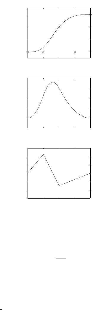
and the resulting trajectory is illustrated in Fig. S4.1.
Solution to Problem 4.2
Imposing velocity constraints yields
˙qi=0
˙qf=k(1 −cos (atf)).
40 4 Trajectory Planning
0 0.5 1 1.5 2
1
2
3
4
pos
[s]
[rad]
0 0.5 1 1.5 2
−0.5
0
0.5
1
1.5
2
2.5
vel
[s]
[rad/s]
0 0.5 1 1.5 2
−5
0
5
acc
[s]
[rad/s^2]
Fig. S4.1. Time history of position, velocity and acceleration with a fifth-order
polynomial timing law
The second equation implies that
0≤˙qf
k≤2
which is satisfied for all kas long as ˙qf= 0. In that case, it is a=2π/tf.
Then, integrating the given velocity profile gives
q(t)=k1+kt−tf
2πsin 2πt
tf,
and imposing position constraints yields the two coefficients
k1=qi
4 Trajectory Planning 41
0 0.5 1 1.5 2
0
1
2
3
pos
[s]
[rad]
0 0.5 1 1.5 2
0
1
2
3
vel
[s]
[rad/s]
0 0.5 1 1.5 2
−5
0
5
acc
[s]
[rad/s^2]
Fig. S4.2. Time history of position, velocity and acceleration with a raised cosine
timing law
k=qf−qi
tf
.
With the given data, the files used to compute the two coefficients and to
generate the time behaviour of position, velocity and acceleration can be found
in Folder 42.
The coefficients are:
k=1.5k1=0
and the resulting trajectory is illustrated in Fig. S4.2.
42 4 Trajectory Planning
0 1 2 3 4
0
1
2
3
pos
[s]
[rad]
0 1 2 3 4
−0.5
0
0.5
1
1.5
2
vel
[s]
[rad/s]
0 1 2 3 4
−3
−2
−1
0
1
2
3
acc
[s]
[rad/s^2]
Fig. S4.3. Time history of position, velocity and acceleration with two fifth-order
interpolating polynomials
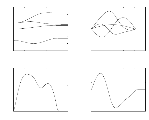
Solution to Problem 4.3
It is required to satisfy initial and final constraints on position, velocity and
acceleration (6 equations), intermediate position constraints (2 equations),
and continuity of velocity and acceleration at the intermediate point (2 equa-
tions). Therefore, with two fifth-order interpolating polynomials it is possible
to specify also velocity and acceleration at the intermediate point.
Let qmdenote the intermediate point at time tm. A viable choice is to
compute the mean velocities in the two intervals
˙qa=qm−qi
tm−ti
˙qb=qf−qm
tf−tm
,
4 Trajectory Planning 43
and then to choose velocity at the intermediate point as
˙qm=˙qa+˙qb
2.
Likewise, for acceleration it is
¨qa=˙qm−˙qi
tm−ti
¨qb=˙qf−˙qm
tf−tm
and then
¨qm=¨qa+¨qb
2.
With the given data and null initial and final velocities and accelerations, the
files used to generate the time behaviour of position, velocity and acceleration
can be found in the Folder 43.
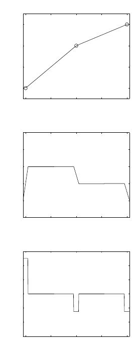
The resulting trajectory is illustrated in Fig. S4.3.
Solution to Problem 4.4
By using (4.13), (4.14), (4.23), (4.16), (4.25), the time derivative of Πk(t)in
(4.27) can be written as
˙
Πk(t)=−¨
Πk(tk)
2Δtk
(tk+1 −t)2+¨
Πk+1(tk+1)
2Δtk
(t−tk)2(S4.1)
+qk+1 −qk
Δtk
+Δtk
6¨
Πk(tk)−¨
Πk+1(tk+1)k=1,...,N +1
where q2and qN+1 are unknown. Then, using (4.15), (4.24) leads to
Δtk
6¨
Πk(tk)+Δtk+Δtk+1
3¨
Πk+1(tk+1)+ Δtk+1
6¨
Πk+2(tk+2)(S4.2)
=qk
Δtk−1
Δtk+1
+1
Δtkqk+1 +qk+2
Δtk+1
k=1,...,N
where ¨
Π1(t1)=¨qias in (4.19) and ¨
ΠN+2(tN+2)=¨qfas in (4.22).
Evaluating (S4.1) for k=1att=t1and applying (4.17), (4.18) yields
q2=qi+˙qiΔt1+¨qi
Δt2
1
3+¨
Π2(t2)Δt2
1
6.(S4.3)
Likewise, evaluating (S4.1) for k=N+1 at t=tN+2 and applying (4.20),
(4.21) yields
qN+1 =qf−˙qfΔtN+1 +¨qf
Δt2
N+1
3+¨
ΠN+1(tN+1)Δt2
N+1
6.(S4.4)
In the case N>3, substituting (S4.3) into (S4.2) for k=1,2 and (S4.4) into
(S4.2) for k=N−1,N leads to writing the linear system of Nequations into
Nunknowns given in (4.28).
44 4 Trajectory Planning
The coefficient matrix takes on the tridiagonal band structure
A=⎡
⎢
⎢
⎢
⎢
⎣
a11 a12 ... 00
a21 a22 ... 00
.
.
..
.
.....
.
..
.
.
00... a
N−1,N−1aN−1,N
00... a
N,N−1aNN
⎤
⎥
⎥
⎥
⎥
⎦
where ⎧
⎪
⎪
⎪
⎪
⎪
⎪
⎪
⎪
⎪
⎪
⎪
⎪
⎪
⎪
⎪
⎪
⎪
⎪
⎪
⎪
⎪
⎪
⎪
⎪
⎪
⎪
⎪
⎨
⎪
⎪
⎪
⎪
⎪
⎪
⎪
⎪
⎪
⎪
⎪
⎪
⎪
⎪
⎪
⎪
⎪
⎪
⎪
⎪
⎪
⎪
⎪
⎪
⎪
⎪
⎪
⎩
a11 =Δt1
2+Δt2
3+Δt2
1
6Δt2
akk =Δtk+Δtk+1
3k=2,...,N −1
aNN =ΔtN
3+ΔtN+1
2+Δt2
N+1
6ΔtN
a21 =Δt2
6−Δt2
1
6Δt2
ak,k−1=Δtk
6k=3,...,N
ak,k+1 =Δtk+1
6k=1,...,N −2
aN−1,N =ΔtN
6−Δt2
N+1
6ΔtN
which depend only on the given time intervals Δtk,k=1,...,N +1.
Further, the components of the vector bof known terms in (4.28) are:
⎧
⎪
⎪
⎪
⎪
⎪
⎪
⎪
⎪
⎪
⎪
⎪
⎪
⎪
⎪
⎪
⎪
⎪
⎪
⎪
⎨
⎪
⎪
⎪
⎪
⎪
⎪
⎪
⎪
⎪
⎪
⎪
⎪
⎪
⎪
⎪
⎪
⎪
⎪
⎪
⎩
b1=q3−qi
Δt2−1
Δt2
+1
Δt1˙qiΔt1+¨qi
Δt2
1
3−¨qi
Δt1
6
b2=1
Δt2qi+˙qiΔt1+¨qi
Δt2
1
3−1
Δt3
+1
Δt2q3+q4
Δt3
bk=qk
Δtk−1
Δtk+1
+1
Δtkqk+1 +qk+2
Δtk+1
k=3,...,N −2
bN−1=qN−1
ΔtN−1−1
ΔtN
+1
ΔtN−1qN+1
ΔtNqf−˙qfΔtN+1 +¨qf
Δt2
N+1
3
bN=qN−qf
ΔtN−1
ΔtN+1
+1
ΔtN−˙qfΔtN+1 +¨qf
Δt2
N+1
3−¨qf
ΔtN+1
6
where the values qkare given for k=1,3,...,N,N +2.

4 Trajectory Planning 45
On the other hand, in the case N= 3, the same expressions for the a’s
can be used; for the b’s, instead, b1and b3can be computed as above and b2
takes on the expression
b2=1
Δt2qi+˙qiΔt1+¨qi
Δt2
1
3−1
Δt3
+1
Δt2q3
+1
Δt3qf−˙qfΔt4+¨qf
Δt2
4
3.
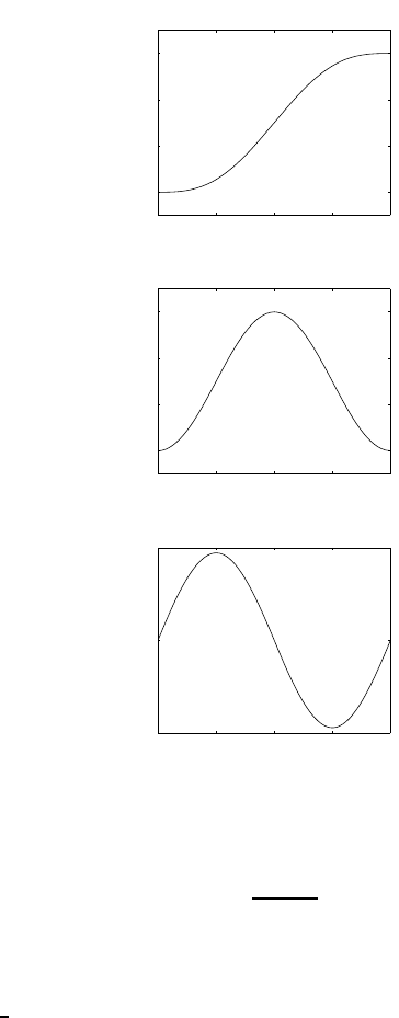
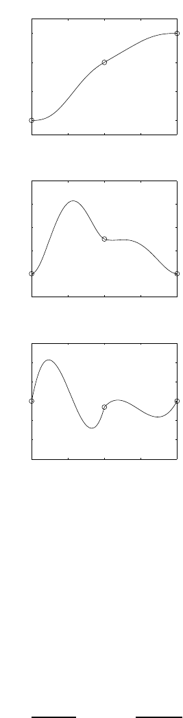
Solution to Problem 4.5
The time instants of the two virtual points are chosen as t1=1andt4=
3. With the given data, the files used to compute the matrix Aand the
vector bin (4.28), and to generate the time behaviour of position, velocity
and acceleration can be found in the Folder 45.
The matrix of coefficients is
A=⎡
⎣11/60
02/30
01/61
⎤
⎦b=⎡
⎣2
−1
−1⎤
⎦,
and the resulting trajectory is illustrated in Fig. S4.4.
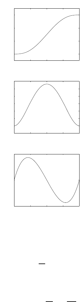
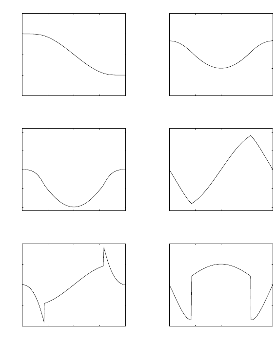
Solution to Problem 4.6
The interpolating trajectory given by a sequence of linear polynomials with
parabolic blends can be analytically described as
q(t)=⎧
⎪
⎪
⎨
⎪
⎪
⎩
ak1(t−tk)+ak0tk+Δt
k
2≤t<t
k+1 −Δt
k+1
2
bk2(t−tk)2+bk1(t−tk)+bk0tk−Δt
k
2≤t<t
k+Δt
k
2.
The velocity in the linear segments is
˙qk−1,k =⎧
⎪
⎪
⎨
⎪
⎪
⎩
˙qik=1
qk−qk−1
Δtk−1
k=2,...,N
˙qfk=N+1,
and then the coefficients of the linear polynomials are
ak0=qkak1=˙qk,k+1 k=1,...,N −1.
Imposing continuity of velocity between the linear and parabolic polynomials
at time instants (tk−Δt
k/2) and (tk+Δt
k/2) allows computing the coefficients
bk1=˙qk,k+1 +˙qk−1,k
2bk2=˙qk,k+1 −˙qk−1,k
2Δt
k
k=1,...,N.
46 4 Trajectory Planning
0 1 2 3 4
0
1
2
3
pos
[s]
[rad]
0 1 2 3 4
−0.5
0
0.5
1
1.5
2
vel
[s]
[rad/s]
0 1 2 3 4
−3
−2
−1
0
1
2
3
acc
[s]
[rad/s^2]
Fig. S4.4. Time history of position, velocity and acceleration with a cubic spline
timing law
Then, imposing continuity of position at (tk+Δt
k/2) yields
bk0=qk+(˙qk,k+1 −˙qk−1,k )Δt
k
8k=1,...,N;
it can be verified that this choice guarantees continuity of position also at
(tk−Δt
k/2).
The duration of the blend times is chosen as Δt
k=0.2fork=1,2,3.
With the given data, the files used to compute the above coefficients, and
to generate the time behaviour of position, velocity and acceleration can be
found in Folder 46.
4 Trajectory Planning 47
0 1 2 3 4
0
1
2
3
pos
[s]
[rad]
0 1 2 3 4
−0.5
0
0.5
1
1.5
2
vel
[s]
[rad/s]
0 1 2 3 4
−6
−4
−2
0
2
4
6
acc
[s]
[rad/s^2]
Fig. S4.5. Time history of position, velocity and acceleration with a timing law of
interpolating linear polynomials with parabolic blends
The coefficients are:
a10 =0 a11 =1 a20 =2 a21 =0.5
b10 =0.025 b11 =0.5b12 =2.5
b20 =1.9875 b21 =0.75 b22 =−1.25
b30 =2.9875 b31 =0.25 b32 =−1.25,
and the resulting trajectory is illustrated in Fig. S4.5.
48 4 Trajectory Planning
0 0.5 1 1.5 2
0
0.2
0.4
0.6
0.8
1
x−pos
[s]
[m]
0 0.5 1 1.5 2
−0.4
−0.2
0
0.2
0.4
0.6
y−pos
[s]
[m]
0 0.5 1 1.5 2
−1
−0.5
0
0.5
1
x−vel
[s]
[m/s]
0 0.5 1 1.5 2
−1
−0.5
0
0.5
1
y−vel
[s]
[m/s]
0 0.5 1 1.5 2
−2
−1
0
1
2
x−acc
[s]
[m/s^2]
0 0.5 1 1.5 2
−2
−1
0
1
2
y−acc
[s]
[m/s^2]
Fig. S4.6. Time history of position, velocity and acceleration of x-andy-
components along a straight path with a trapezoidal velocity profile timing law
Solution to Problem 4.7
A trapezoidal velocity profile for the path coordinate sis assigned according
to (4.8) with maximum velocity ˙sc= 1. The timing law for p(t)andits
derivatives is generated via (4.34) and (4.42).
With the given data, the files used to generate the time behaviour of
position, velocity and acceleration can be found in Folder 47.
The resulting trajectories for the x-andy-components are illustrated in
Fig. S4.6.
4 Trajectory Planning 49
0 0.5 1 1.5 2
−1
−0.5
0
0.5
1
y−pos
[s]
[m]
0 0.5 1 1.5 2
0
0.5
1
1.5
z−pos
[s]
[m]
0 0.5 1 1.5 2
−1
−0.5
0
0.5
1
y−vel
[s]
[m/s]
0 0.5 1 1.5 2
−1
−0.5
0
0.5
1
z−vel
[s]
[m/s]
0 0.5 1 1.5 2
−2
−1
0
1
2
y−acc
[s]
[m/s^2]
0 0.5 1 1.5 2
−2
−1
0
1
2
z−acc
[s]
[m/s^2]
Fig. S4.7. Time history of position, velocity and acceleration of x-andy-
components along a circular path with a trapezoidal velocity profile timing law
Solution to Problem 4.8
The unit vectors of the axes of the reference frame for the circle are chosen as
x=yy
=−zz
=−x;
notice that the choice z=−xensures that the path is executed clockwise
about axis x. From (4.39), the path representation is
p(s)=⎡
⎣0
0.5cos(2s)
1−0.5sin(2s)⎤
⎦.

50 4 Trajectory Planning
Since it is required to execute half a circle with tf= 2, the final value of the
path coordinate is sf=s(2) = π/2. Then, a trapezoidal velocity profile for
the path coordinate sis assigned according to (4.8) with maximum velocity
˙sc= 1. The timing law for p(t) and its derivatives is generated via (4.39),
(4.44).
With the given data, the files used to generate the time behaviour of
position, velocity and acceleration can be found in Folder 48.
The resulting trajectories for the y-andz-components are illustrated in
Fig. S4.7.

5
Actuators and Sensors
Solution to Problem 5.1
At steady state, (5.1)–(5.4) can be written in the time domain as
va=Raia+vg(S5.1)
vg=kvωm(S5.2)
cm=Fmωm+cr(S5.3)
cm=ktia(S5.4)
where
va=Ci(0)Gv(v
c−kiia). (S5.5)
Combining (S5.1), (S5.2), (S5.5) with ki=0andK=Ci(0)Gvgives
Kv
c=Raia+kvωm
and yet, using (S5.3) and (S5.4) with cr=0,itis
Kv
c=FmRa
kt
+kvωm.
If Fmkvkt/Ra,then
ωm≈K
kv
v
c.
If instead ki= 0, on reduction of (S5.1)–(S5.5), it is
Kv
c=Ra+Kki
ktcm+kvωm.
If KkiRa,then
cm≈kt
kiv
c−kv
Kωm.
52 5 Actuators and Sensors
variables
initialization
C_i
V'_c
G_v
T_v.s+1
k_v
+
-
-
k_t +
-
curr
omega
F_m
plot
time
1
L_a.s 1
I_m.s
R_a
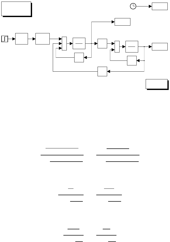
Fig. S5.1. Simulink block diagram of electric servomotor
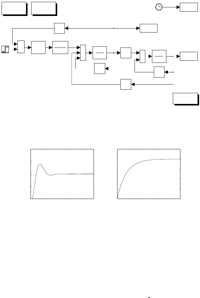
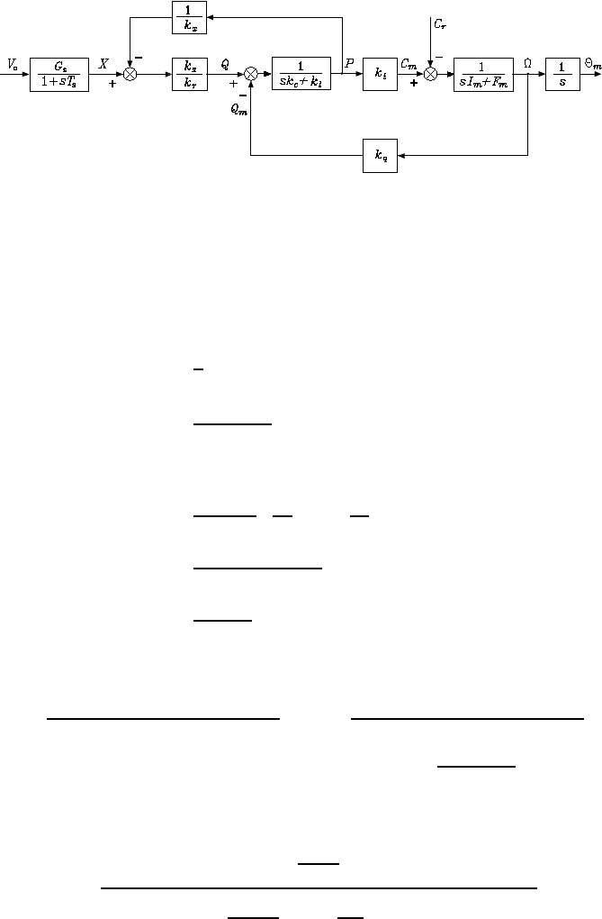
From the block scheme in Fig. 5.3, the output can be computed via the closed-
loop transfer functions; namely, the input/output and disturbance/output
transfer functions, i.e.,
Ωm=
Kkt
Ra(sIm+Fm)
1+ kvkt
Ra(sIm+Fm)
V
c−
1
sIm+Fm
1+ kvkt
Ra(sIm+Fm)
Cr.
If Fmkvkt/Ra,then
Ωm=
K
kv
1+sRaIm
kvkt
V
c−
Ra
kvkt
1+sRaIm
kvkt
Cr.
Finally, from the block scheme in Fig. 5.4, it is straightforward to compute
the output as
Ωm=
kt
kiFm
1+sIm
Fm
V
c−
1
Fm
1+sIm
Fm
Cr.
Solution to Problem 5.2
With reference to the scheme in Fig. 5.2 (ki=0andCr=0)andthegiven
data, the resulting Simulink block diagram is shown in Fig. S5.1. The servo-
5 Actuators and Sensors 53
0 0.05 0.1 0.15
−0.5
0
0.5
1
1.5
2
2.5
[s]
[A]
current
0 0.05 0.1 0.15
0
1
2
3
4
5
6
[s]
[rad/s]
velocity
Fig. S5.2. Time history of current and velocity step response for an electric servo-
motor
motor is simulated as a continuous-time system using a variable-step integra-
tion method with a maximum step size of 1 ms. Notice that the amplifier time
constant is too small to produce appreciable effects at this sampling time.
The files with the solution can be found in Folder 52.
The resulting current and velocity responses to a unit step voltage input V
c
are shown in Fig. S5.2. It can be seen that the steady-state velocity slightly
deviates from the value of 5 rad/s as in (5.7), because of the presence of
mechanical friction (Fm). This also implies that the steady-state current is
different from zero.
Solution to Problem 5.3
By closing a current loop with large loop gain, the current response is expected
to become much faster than the velocity response. Velocity plays the role of a
disturbance for the voltage-to-current closed-loop system. Hence, it is worth
choosing a PI control structure for Ci(s) in order to obtain a null steady-state
error, i.e.,
Ci(s)=KI
1+sTI
s.
With the given data, by setting Ωm= 0, the closed-loop input/output transfer
function (Tv≈0) is
Ia
V
c
=1+sTI
1+s0.2+KITI
KI
+s20.002
KI
.
Since the settling time within 1% is given by
ts=4.6
ζωn
,
either the damping ratio or the natural frequency can be imposed. Choosing
ζ=0.7withts=2msyields
KI= 21592 TI=0.000416.
54 5 Actuators and Sensors
+
-
k_t
+
-
-
k_v
velocitycurrent
curr
G_v
T_v.s+1 1
L_a.s
R_a
k_i
C_i(s)
V'_c
-
+
plot
F_m
omega
1
I_m.s
time
Fig. S5.3. Simulink block diagram of electric servomotor with current feedback
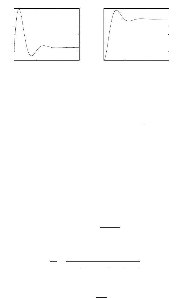
loop and PI control
0 1 2 3 4 5
x 10−3
0
0.5
1
1.5
2
[s]
[A]
current
0 0.2 0.4 0.6 0.8 1
0
5
10
15
20
25
[s]
[rad/s]
velocity
Fig. S5.4. Time history of current and velocity step response for an electric servo-
motor with current feedback loop and PI control
The resulting Simulink block diagram is shown in Fig. S5.3. The servomotor
is simulated as a continuous-time system using a variable-step integration
method. Since the current dynamics is much faster than the velocity dynamics,
the maximum step size has been chosen much smaller than in Problem 5.2, i.e.,
0.05 ms. Further, in order to make a comparison between the velocity response
in this case and the case of Problem 5.2, the block diagram in Fig. S5.3 features
a separate execution with a longer final time and a sampling time of 1 ms.
The files with the solution can be found in Folder 53.
The resulting current and velocity are shown in Fig. S5.4. The current
response goes as expected, while the velocity response is slowed down with
respect to the response in Fig. S5.2 because it is dominated by the time
constant Im/Tm.
5 Actuators and Sensors 55
Fig. S5.5. Reduction on the block scheme of a hydraulic motor with servovalve and
distributor
Solution to Problem 5.4
From this block scheme, the following relations can be found:
Θm=1
sΩm
Ωm=Cm−Cr
sIm+Fm
Cm=ktP
P=1
skc+klkx
krX−P
kx−kqΩm
=kxX−krkqΩm
1+krkl+skrkc
X=Gs
1+sTs
Vc.
Substituting (S5.6) into (S5.6), and then (S5.6) into (S5.6), yields
1+ ktkrkq
(sIm+Fm)(1 + krkl+skrkc)Ωm=ktkx
(1 + krkl+skrkc)(sIm+Fm)X
−1
sIm+Fm
Cr.
Solving for Ωm, substituting it into (S5.6), and using (S5.6) leads to
Θm=
kxGs
krkq
s(1 + sTs)1+ Fm
ktkrkq1+sIm
Fm(1 + krkl+skrkc)Vc

56 5 Actuators and Sensors
−
1+krkl+skrkc
ktkrkq
s1+ Fm
ktkrkq1+sIm
Fm(1 + krkl+skrkc)Cr.
Solution to Problem 5.5
Without loss of generality, the case of 4 bits is considered. The truth table of
the interconversion logic circuit is reported in Table S5.1.
Table S5.1. Truth table of the interconversion logic circuit from Gray-code to
binary code
Gray Code Binary Code
#x1x2x3x4y1y2y3y4
0 0000 0000
1 0001 0001
2 0011 0010
3 0010 0011
4 0110 0100
5 0111 0101
6 0101 0110
7 0100 0111
8 1100 1000
9 1101 1001
10 1111 1010
11 1110 1011
12 1010 1100
13 1011 1101
14 1001 1110
15 1000 1111
The first columns of the two codes are equal, and thus
y1=x1.
From the second column at the output, it can be recognized that y2=1when
x1=0andx2=1,orelsewhenx1=1andx2= 0, and thus
y2=¯x1x2+x1¯x2=x1⊕x2=y1⊕x2
where “⊕” is the symbol for the logical operator XOR. From the third column
at the output, it can be recognized that y3=1wheny2=0andx3=1,or
else when y2=1andx3= 0, and thus
y3=y2⊕x3.
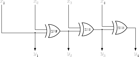
5 Actuators and Sensors 57
Fig. S5.6. Interconversion logic circuit from Gray code to binary code
Finally, from the fourth column it is
y4=y3⊕x4.
The resulting interconversion logic circuit is illustrated in Fig. S5.6 where the
conventional symbol of XOR is used.
Solution to Problem 5.6
The skew-symmetric operator is
S(rc
cs)=⎡
⎣
0−0.20
0.200.3
0−0.30
⎤
⎦,
and thus applying (5.32) gives
fc
c
μc
c=⎡
⎢
⎢
⎢
⎢
⎢
⎣
0 0 1000
0−10000
1 0 0000
00.20001
0.300.20−10
00.30100
⎤
⎥
⎥
⎥
⎥
⎥
⎦
⎡
⎢
⎢
⎢
⎢
⎢
⎣
20
0
0
0
6
0
⎤
⎥
⎥
⎥
⎥
⎥
⎦
=⎡
⎢
⎢
⎢
⎢
⎢
⎣
0
0
20
0
0
0
⎤
⎥
⎥
⎥
⎥
⎥
⎦
,
that is,
fc
c=[0 0 20]
TNμc
c=[0 0 0]
TN·m.
As can be seen, there is no resulting moment in the contact frame.
Solution to Problem 5.7
Let the end-effector frame coincide with Frame 4 in Fig. S2.3. Then, with
reference to (S2.3), the homogeneous transformation from the base frame to
the end-effector frame at q=[0 π/40.10]is
Tb
c=⎡
⎢
⎣
0.707 −0.707 0 0.854
0.707 0.707 0 0.354
0010.1
0001
⎤
⎥
⎦.
58 5 Actuators and Sensors
Using (5.35) gives
˜
pc=⎡
⎢
⎣
0.066
0.141
0.8
1
⎤
⎥
⎦
and, in view of (5.41), it is
Ω=⎡
⎣633.6 0 250
0 964 250
001
⎤
⎦
and thus from (5.40)
xI= 241.82
yI= 335.92
λ=0.8.
Hence
XI= 302.27 YI= 419.90.

6
Control Architecture
Solution to Problem 6.1
With reference to the hierarchical control architecture in Fig. 6.1, the solution
can be articulated at the task and action levels as follows.
At the task level, in order to decompose the task into a sequence of ac-
tions, the decision module shall consult the knowledge base available in the
modelling module concerning the manipulator and the environment. If the
environment is scarcely structured, the knowledge base shall be updated with
the information to be presented by the sensor module via the use of heterocep-
tive sensors, e.g., vision. Once the environment is structured, the modelling
module provides the relative location between the manipulator, the object
and the obstacle. Feasibility of the task shall be verified, and a possible se-
quence of actions is generated: approach position A, pick object, move object
while avoiding obstacle, approach position B, place object. The two approach
actions are opportune to ensure smooth pick-and-place of the object.
At the action level, the symbolic commands coming from the task level
are interpreted by the decision module which shall take the resolutions needed
to execute the given sequence of actions, that is, choice of reference frame,
motion in operational space, intermediate path or via points C,D,E,F
(see Fig. S6.1), duration of time intervals, path primitives off the obstacle,
and type of interpolating functions. By doing so, the decision module shall
consult the knowledge base available in the modelling module to verify path
feasibility. As for the approach actions, the decisions imparted to the primitive
level shall regard low values of velocities and vertical orientation of the end
effector, whereas the knowledge base shall be updated with the information
available in the sensor module via the use of range or proximity sensors.
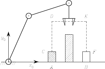
60 6 Control Architecture
Fig. S6.1. Choice of reference frame and intermediate positions for an object pick-
and-place task
Solution to Problem 6.2
With reference to the sequence of points illustrated in Fig. S6.1, the oper-
ational space motion primitives can be determined in the two cases of path
points and via points, respectively, as follows.
In the case of path points, the various points can be connected by seg-
ments. To ensure safe grasp of the object at point Cand safe release of the
object at point F, it is advisable to choose null velocity and acceleration at
each of those points. As for the intermediate points Dand E, it is sufficient
to impose null velocities. Hence, the timing law along the segments CD and
EF shall be polynomials of at least fourth order, whereas the timing law
along the segment DE shall be either a cubic polynomial or a trajectory with
trapezoidal velocity profile.
In the case of via points, the actual path in the neighbourhood of Dand
Eis of no concern, as long as it is kept at a safety distance from the obstacle.
The passage in the proximity of the two via points can be obtained by using
the same interpolating functions as for the previous case, on condition that
the generation of the timing laws along the segments DE and EF are suitably
anticipated in time. As above, null initial and final velocity and acceleration
are to be imposed.
Finally, the presence of a redundant DOFs relative to a bidimensional
position task can be exploited to keep end-effector orientation constant along
−y.
Solution to Problem 6.3
Before executing the peg-in-hole task, the end effector shall approach the hole.
It can be argued that it is difficult to guarantee exact positioning of the peg
relative to the hole; this may render the insertion phase quite critical. It is
assumed that the main cause of uncertainty regards only position, that is the
axis of the peg can be considered to be aligned with the axis of the hole during
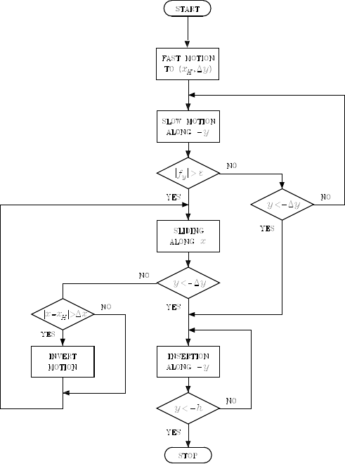
6 Control Architecture 61
Fig. S6.2. Flow chart for the execution of a peg-in-hole task
the approach to the hole; also, it is assumed that no jamming occurs during
insertion.
Choose a reference frame at the base of the arm, with axis xalong the
horizontal direction (positive from the base to the hole) and axis yalong the
positive vertical direction. A possible solution is to split the whole task into
three subtasks as follows.
At first, a fast motion towards the position (xH,Δy) shall be executed,
where xHis the estimated xcoordinate of the center of the hole and Δy is a
small distance from the estimated height of the hole (y= 0). This is meant
to avoid colliding the surface around the hole during the approach phase. A
pure motion control strategy is needed to accomplish this subtask.
Next, a slow motion along −yshall be executed, still with a pure mo-
tion control strategy. This goes on until yis below the given distance −Δy

62 6 Control Architecture
(when the peg is considered to have entered the hole), unless a contact force
fyis sensed above a threshold , due to a collision with the surface. In that
case, before proceeding with insertion, it is necessary to slide along the sur-
face in either positive or negative horizontal direction until a force below the
threshold is sensed; if the xcoordinate of end-effector position goes too far
from xH(greater than a distance Δx), then the motion shall be inverted. A
force/position control strategy is needed to accomplish this subtask where po-
sition is controlled along xand force is controlled along yto a desired pushing
force. This goes on until the peg enters the hole.
Finally, the insertion along −yis accomplished by using a force/position
control strategy where position is controlled along y, force is controlled along
x, and moment is controlled about z; moment control is needed to keep the
peg in axis with the hole during insertion.
The flow chart corresponding to the articulation of the whole task into
the above three subtasks is illustrated in Fig. S6.2.
Solution to Problem 6.4
The task can be divided into the following sequence of actions:
•command new object on conveyor,
•fast motion of end effector to a location above object to pick,
•slow motion of end effector towards object,
•pick object from conveyor,
•fast motion of object to a loading location above pallet,
•slow motion of object downwards,
•release object.
At the beginning, the end effector is moved to a home location from which
the task starts. The above sequence is iterated until the pallet is filled, and
then the end effector is taken back to the home location.
Below a PASCAL program is listed to execute the given task.
program FILL PALLET;
type point: array[1..6] of real;
const home: point=(------); {end-effector home location}
object: point=(------); {object location}
pallet: point=(------); {lower-left pallet location}
lift: -.-; {z-offset above object}
length: -.-; {object x-dimension}
width: -.-; {object y-dimension}
fast: -.-; {fast velocity}
slow: -.-; {slow velocity}
var i,j: integer;
current: point; {end-effector current location}
procedure MOVETO(var endpoint:point,velocity:real);
procedure GRASP;
procedure RELEASE;

6 Control Architecture 63
procedure NEW OBJECT;
begin
MOVETO(home,fast);
for i:=0 to 3 do
for j:= 0 to 3 do
begin
NEW OBJECT;
current:=object;
current[3]:=current[3]+lift;
MOVETO(current,fast);
MOVETO(object,slow);
GRASP;
MOVETO(current,slow);
current:=pallet;
current[1]:=current[1]+i*length;
current[2]:=current[2]+j*width;
current[3]:=current[3]+lift;
MOVETO(current,fast);
current[3]:=current[3]-lift;
MOVETO(current,slow);
RELEASE;
current[3]:=current[3]+lift;
MOVETO(current,slow);
end
MOVETO(home,fast);
end

7
Dynamics
Solution to Problem 7.1
Consider the Cartesian arm in Fig. S7.1, for which the vector of generalized
coordinates is q=[d1d2]T.
Let m1,m2be the masses of the two links and mm1,mm2the masses
of the rotors of the two joint motors. Let also Im1,Im2be the moments of
inertia about the axes of the two rotors. It is assumed that pmi=pi−1and
zmi=zi−1,fori=1,2, i.e., the motors are located on the joint axes with
centres of mass located at the origins of the respective frames.
With the choice of the frames in Fig. S7.1, it is z1=[1/√201/√2]
T.
Hence, computation of the Jacobians in (7.16), (7.18) yields
J(1)
P=⎡
⎣00
00
10
⎤
⎦J(2)
P=⎡
⎣01/√2
00
11/√2⎤
⎦.
Obviously it is J(1)
O=J(2)
O=O.
Computation of the Jacobians in (7.25), (7.26), (7.28), (7.29) respectively
yields
J(m1)
P=⎡
⎣00
00
00
⎤
⎦J(m2)
P=⎡
⎣00
00
10
⎤
⎦
J(m1)
O=⎡
⎣00
00
kr10⎤
⎦J(m2)
O=⎡
⎣0kr2/√2
00
0kr2/√2⎤
⎦
where kri is the gear reduction ratio of motor i.
From (7.32), the inertia matrix is
B=m1+mm2+k2
r1Im1+m2m2/√2
m2/√2m2+k2
r2Im2.
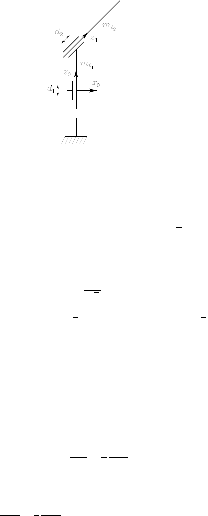
66 7 Dynamics
Fig. S7.1. Two-link Cartesian arm where Joint 2 axis forms an angle of π/4with
Joint 1 axis
Notice that Bis constant, which implies that C=O. As for the gravitational
terms, with g0=[0 0 −g]T, (7.39) gives:
g1=(m1+mm2+m2)gg
2=m2g/√2.
In the absence of friction and tip contact forces, the resulting equations of
motion are
(m1+mm2+k2
r1Im1+m2)¨
d1+m2
√2
¨
d2+(m1+mm2+m2)g=τ1
m2
√2
¨
d1+(m2+k2
r2Im2)¨
d2+m2
√2g=τ2
where τ1and τ2denote the forces applied to the two joints. It is worth pointing
out that, differently from the arm in Fig. 7.3, the dynamic model is coupled
(nonnull off-diagonal terms in the inertia matrix) and gravity acts also on the
second joint.
Solution to Problem 7.2
A natural choice for the elements of matrix Csatisfying (7.43) with hijk as
in (7.41) is
cij =
n
k=1 ∂bij
∂qk−1
2
∂bjk
∂qi˙qk.
For the two-link planar arm of Fig. 7.4, they become
c11 =
2
k=1 ∂b11
∂qk−1
2
∂b1k
∂q1˙qk=−2m2a12s2˙
ϑ2

7Dynamics 67
c12 =
2
k=1 ∂b12
∂qk−1
2
∂b2k
∂q1˙qk=−m2a12s2˙
ϑ2
c21 =
2
k=1 ∂b21
∂qk−1
2
∂b1k
∂q2˙qk=m2a12s2˙
ϑ1−1
2m2a12s2˙
ϑ2
c22 =
2
k=1 ∂b22
∂qk−1
2
∂b2k
∂q2˙qk=1
2m2a12s2˙
ϑ1.
Setting h=−m2a12s2leads to
C=2h˙
ϑ2h˙
ϑ2
−h˙
ϑ1+h
2˙
ϑ2−h
2˙
ϑ1
while the time derivative of the inertia matrix can be written as
˙
B=2h˙
ϑ2h˙
ϑ2
h˙
ϑ20.
Therefore, the matrix N(q,˙
q)= ˙
B−2Cbecomes
N(q,˙
q)=−2h˙
ϑ2−h˙
ϑ2
2h˙
ϑ1h˙
ϑ1
which clearly is not skew-symmetric. Nevertheless, it is easy to show that the
product
˙
qTN(q,˙
q)˙
q=0,
confirming that (7.49) holds even for a choice of Cso that (7.48) does not
hold.
Solution to Problem 7.3
Consider the SCARA arm in Fig. S7.1, for which the vector of generalized co-
ordinates is q=[ϑ1ϑ2d3ϑ4]Tand link frames assigned as in Fig. S2.3.
For the first two links, consider the same kinematics and dynamic parameters
of the two-link planar arm of Exmple 7.2. Moreover, links 3 and 4 can be
considered as a unique rigid body, referred as “last link”, which translates
along axis z2of the prismatic Joint 3 and rotates about axis z3of the revolute
Joint 4. Let m3denote the mass of the last link. For simplicity, it is assumed
that the centre of mass p4of the last link is located on axis z3;letI4denote
the element [3,3] of the inertia tensor of the last link relative to the centre
of mass. Also, assume that the motors of Joints 3 and 4 have negligible mass
and inertia.
Due to the additivity property, the kinetic energy of the SCARA manip-
ulator can be computed by adding the kinetic energy of the last link to the
68 7 Dynamics
kinetic energy of the two-link planar arm. Therefore, from (7.32), the inertia
matrix can be computed as
B(q)=B(q)+B(q)
where Bis the (4 ×4) matrix obtained completing the (2 ×2) inertial matrix
of the two-link planar arm of Sect. 7.3.2 with two null columns and two null
rows, while B is the contribution of the last link, which can be computed as
B(q)=m3J(4)T
PJ(4)
P+J(4)T
OR4Ii
iRT
4J(4)
O.(S7.1)
The computation of the Jacobians in (7.16), (7.17) yields
J(4)
P=⎡
⎣−a1s1−a2s12 −a2s12 00
a1c1+a2c12 a2c12 00
0010
⎤
⎦J(4)
O=⎡
⎣0000
0000
1101
⎤
⎦
Hence, from (S7.1), the nonnull elements of matrix B(q)are
b
11 =m3(a2
1+a2
2+2a1a2c2)+I4
b
12 =b
21 =m3(a2
2+a1a2c2)+I4
b
14 =b
41 =I4
b
22 =m3a2
2+I4
b
24 =b
42 =I4
b
33 =m3
b
44 =I4.
Therefore, the nonnull elements of the inertia matrix of the SCARA manipu-
lator are:
b11 =I1+m12
1+k2
r1Im1+I2+m2(a2
1+2
2+2a12c2)
+Im2+mm2a2
1+m3(a2
1+a2
2+2a1a2c2)+I4
b12 =b21 =I2+m2(2
2+a12c2)+kr2Im2+m3(a2
2+a1a2c2)+I4
b14 =b41 =I4
b22 =I2+m22
2+k2
r2Im2+m3a2
2+I4
b24 =b42 =I4
b33 =m3
b44 =I4.
The Christoffel symbols for the SCARA manipulator can be computed as
cijk =c
ijk +c
ijk
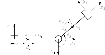
7Dynamics 69
Fig. S7.2. Two-link planar arm with a prismatic joint and a revolute joint
where c
ijk are the Christoffel symbols of the two-link planar arm of Sect. 7.3.2,
while c
ijk are those computed from the elements b
ij of B(q) as in (7.45).
The nonnull elements are:
c112 =−m2a12s2−m3a1a2s2=k
c122 =k
c211 =−k,
leading to the matrix
C(q,˙
q)=⎡
⎢
⎢
⎣
k˙
ϑ2k(˙
ϑ1+˙
ϑ2)00
−k˙
ϑ1000
0000
0000
⎤
⎥
⎥
⎦.
As for the gravitational terms, it can be easily understood that gravity con-
tributes only to Joint 3 force, which has the expression
g3=m3g.
Solution to Problem 7.4
By using the expressions of the parameters in (7.83), the equations of motion
(7.82) can be rewritten as
τ1=a2
1π1+2a1π2+π3+k2
r1π4+(a2
1+2a1a2c2+a2
2)π5
+(2a1c2+2a2)π6+π7+π8)¨
ϑ1
+(a1a2c2+a2
2)π5+(a1c2+2a2)π6+π7+kr2π8¨
ϑ2
−(2a1a2s2π5+2a1s2π6)˙
ϑ1˙
ϑ2−(a1a2s2π5+a1s2π6)˙
ϑ2
2
+(a1π1+π2+a1π5)gc1+(a2π5+π6)gc12
τ2=(a2
2π5+2a2π6+π7+k2
r2π8)¨
ϑ2
+(a1a2c2+a2
2)π5+(a1c2+2a2)π6+π7+kr2π8¨
ϑ1
+(a1a2s2π5+a1s2π6)˙
ϑ2
1
+(a2π5+π6)gc12.
70 7 Dynamics
It is then possible to find the following linear combinations between the pa-
rameters which bring the number thereof down to a minimum of 5:
π
1=a1π1+π2+a1π5=a1m1+m1C1+a1m2
π
2=a1π2+π3+k2
r1π4=a1m1C1+¯
I1+k2
r1Im1
π
3=a2π5+π6=a2m2+m2C2(S7.2)
π
4=a2π6+π7=a2m2C2+¯
I2
π
5=π8=Im2.
Accordingly, the elements of the regressor become
y
11 =a1¨
ϑ1+gc1
y
12 =¨
ϑ1
y
13 =(2a1c2+a2)¨
ϑ1+(a1c2+a2)¨
ϑ2−2a1s2˙
ϑ1˙
ϑ2−a1s2˙
ϑ2
2+gc12
y
14 =¨
ϑ1+¨
ϑ2
y
15 =¨
ϑ1+kr2¨
ϑ2(S7.3)
y
21 =0
y
22 =0
y
23 =a2¨
ϑ2+(a1c2+a2)¨
ϑ1+a1s2˙
ϑ2
1+gc12
y
24 =¨
ϑ2+¨
ϑ1
y
25 =k2
r2¨
ϑ2+kr2¨
ϑ1.
Solution to Problem 7.5
Consider the planar arm in Fig. S7.2, for which the vector of generalized
coordinates is q=[d1ϑ2]T.
Let m1,m2be the masses of the two links, 1,2the distances of the
centres of mass from the respective joint axes, and mm1,mm2the masses of
the rotors of the two joint motors. Let also I2be the inertia tensor of Link
2 about Joint 2 axis, and Im1,Im2the moments of inertia about the axes of
the two rotors. It is assumed that pmi=pi−1and zmi=zi−1,fori=1,2,
i.e., the motors are located on the joint axes with centres of mass located at
the origins of the respective frames.
With the choice of the frames in Fig. S7.2, it is z1=[0 1 0]
T,
p1=pm2=[0 0 d1]T,p2=[−2c20d1+2s2]T. Computation of
the Jacobians in (7.16), (7.18) yields
J(1)
P=⎡
⎣
00
00
10
⎤
⎦J(2)
P=⎡
⎣
02s2
00
12c2⎤
⎦,

7Dynamics 71
whereas computation of the Jacobians in (7.17), (7.19) yields
J(1)
O=⎡
⎣00
00
00
⎤
⎦J(2)
O=⎡
⎣00
01
00
⎤
⎦.
Computation of the Jacobians in (7.25), (7.26) yields
J(m1)
P=⎡
⎣
00
00
00
⎤
⎦J(m2)
P=⎡
⎣
00
00
10
⎤
⎦,
whereas computation of the Jacobians in (7.28), (7.29) yields
J(m1)
O=⎡
⎣00
00
kr10⎤
⎦J(m2)
O=⎡
⎣00
0kr2
00
⎤
⎦
where kri is the gear reduction ratio of motor i.
From (7.32), the inertia matrix is
B(q)=b11 b12(ϑ2)
b12(ϑ2)b22
b11 =m1+mm2+m2+k2
r1Im1
b12 =m22c2
b22 =I2+m22
2+k2
r2Im2
where I2=I2zz is the constant moment of inertia about Joint 2 axis.
Computation of Christoffel symbols as in (7.45) gives:
c111 =c112 =c121 =c211 =c212 =c221 =c222 =0
c122 =∂b12
∂q2−1
2
∂b22
∂q1
=−m22s2
leading to the matrix
C(q,˙
q)=0−m22s2˙
ϑ2
00
.
Computing the matrix Nin (7.47) gives
N(q,˙
q)= ˙
B(q)−2C(q,˙
q)
=0m22s2˙
ϑ2
−m22s2˙
ϑ20
which is skew-symmetric.

72 7 Dynamics
As for the gravitational terms, with g0=[−g00]
T, (7.39) gives:
g1=0
g2=m22gs2.
In the absence of friction and tip contact forces, the resulting equations of
motion are
(m1+mm2+m2+k2
r1Im1)¨
d1+m22c2¨
ϑ2−m22s2˙
ϑ2
2=τ1(S7.4)
m22c2¨
d1+(I2+m22
2+k2
r2Im2)¨
ϑ2+m22gs2=τ2(S7.5)
where τ1and τ2respectively denote the force applied to Joint 1 and the torque
applied to Joint 2.
The presence of a concentrated tip payload of mass mLalters Link 2
parameters as follows:
m
2=m2+mL
2=m22+mLa2
m
2
I
2=I2+m2(
2−2)2+mL(a2−
2)2
and the same formal dynamic model can be written as above in terms of the
new parameters.
A minimum parameterization of the dynamic model can be obtained in
terms of the following parameter vector:
π=[π
1π
2π
3]T
π
1=m1+mm2+m
2+k2
r1Im1
π
2=m
2
2
π
3=I
2+m
22
2+k2
r2Im2.
Accordingly, the elements of the regressor are
y
11 =¨
d1
y
12 =c2¨
ϑ2−s2˙
ϑ2
2
y
13 =0
y
21 =0
y
22 =c2¨
d1+gs2
y
23 =¨
ϑ2.
Solution to Problem 7.6
Let x1and x2denote the absolute angles of the two joints. The relationship
between relative and absolute angles is
x1=ϑ1x2=ϑ1+ϑ2.
7Dynamics 73
This can be formally treated as a coordinate transformation from the joint
space to the operational space of absolute angles. The analytical Jacobian
characterizing such transformation at velocity level is then
JA=10
11
,
which is always nonsingular, implying that the absolute angles constitute a
set of generalized coordinates for the system.
Therefore, the terms of the operational space dynamic model can be com-
puted according to (7.134)–(7.136). From (7.134), the inertia matrix is
BA=bA11 bA12
bA12 bA22
where, using the expressions of bij in Sect. 7.3.2, the elements in the new
coordinates are
bA11 =b11 +b22 −2b12
=I1+m12
1+k2
r1Im1+m2a2
1+(1−kr2)2Im2+mm2a2
1
bA12 =b12 −b22
=m2a12cos (x2−x1)+kr2(1 −kr2)Im2
bA22 =b22
=I2+m22
2+k2
r2Im2.
Notice that the diagonal elements are configuration-invariant; also, if kr2=1
(direct drive), then the effect of motor 2 inertia on both bA12 and bA22 vanishes.
Further, from (7.135), the velocity-dependent term is
CA˙
x=c11 −c12 c21 −c22
c21 c22
which, using the expressions of cij in Sect. 4.3.2, in the new coordinates be-
comes
CA˙
x=h˙x2
2
−h˙x2
1
where h=−m2a12sin (x2−x1). Interestingly enough, there is no Coriolis
effect; this can be explained by observing that rotation of Link 2 is represented
with reference to Frame 0 and thus is independent of rotation of Link 1.
Finally, from (7.136), the gravity term is
gA=g1−g2
g2
which, using the expressions of giin Sect. 4.3.2, in the new coordinates be-
comes
gA=(m11+mm2a1+m2a1)gcos x1
m22gcos x2.
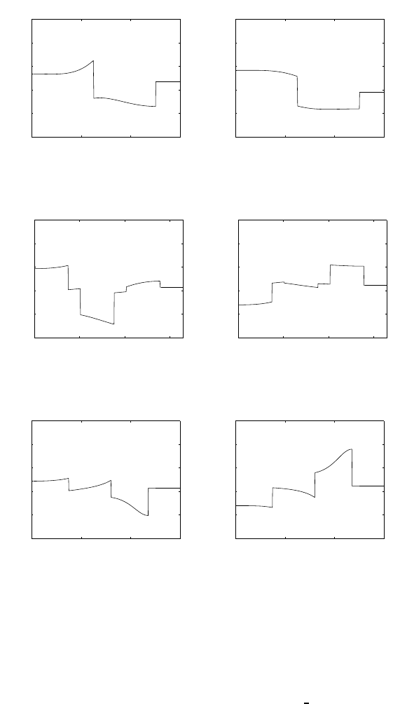
74 7 Dynamics
0 0.2 0.4 0.6
−1
−0.5
0
0.5
1
1.5 x 10⁴
[s]
[Nm]
joint 1 torque
0 0.2 0.4 0.6
−1
−0.5
0
0.5
1
1.5 x 10⁴
[s]
[Nm]
joint 2 torque
Fig. S7.3. Time history of joint torques for the first trajectory of Example 7.2
0 0.2 0.4 0.6
−1
−0.5
0
0.5
1
1.5 x 10⁴
[s]
[Nm]
joint 1 torque
0 0.2 0.4 0.6
−1
−0.5
0
0.5
1
1.5 x 10⁴
[s]
[Nm]
joint 2 torque
Fig. S7.4. Time history of joint torques for the second trajectory of Example 7.2
0 0.2 0.4 0.6
−1
−0.5
0
0.5
1
1.5 x 10⁴
[s]
[Nm]
joint 1 torque
0 0.2 0.4 0.6
−1
−0.5
0
0.5
1
1.5 x 10⁴
[s]
[Nm]
joint 2 torque
Fig. S7.5. Time history of joint torques for the third trajectory of Example 7.2
Solution to Problem 7.7
The various terms of the dynamic model are computed by using the mini-
mum parameterization in the solution to Problem 7.4. The tip forces can be
incorporated in the model as in (7.42), i.e., via the Jacobian transpose.
The files with the solution can be found in Folder 77.
The resulting torques for the three trajectories of Example 7.2 are illus-
trated in Figs. S7.3, S7.4, S7.5, respectively.
7Dynamics 75
Solution to Problem 7.8
Start by imposing the initial conditions for the velocities and accelerations:
¨
p0
0−g0
0=[g00]
Tω0
0=˙
ω0
0=0.
All quantities shall be referred to the current link frame. With the choice of
the frames as in Fig. S7.2, the following vectors are obtained:
r1
1,C1=⎡
⎣
0
C1
0⎤
⎦r1
0,1=⎡
⎣
0
d1
0⎤
⎦r2
2,C2=⎡
⎣
C2
0
0⎤
⎦r2
1,2=⎡
⎣
a2
0
0⎤
⎦
where C1and C2are both negative quantities. The rotation matrices needed
for vector transformation from one frame to another are:
R0
1=⎡
⎣−100
001
010
⎤
⎦R1
2=⎡
⎣c2−s20
s2c20
001
⎤
⎦.
Further it is assumed that the axes of rotations of the rotors coincide with
the respective joint axes, i.e., zi−1
mi=z0=[001]
Tfor i=1,2.
According to (7.107)–(7.114), the Newton-Euler algorithm requires the
execution of the following steps.
•Forward recursion: Link 1
ω1
1=0
˙
ω1
1=0
¨
p1
1=⎡
⎢
⎣−g
¨
d1
0
⎤
⎥
⎦
¨
p1
C1=⎡
⎢
⎣−g
¨
d1
0
⎤
⎥
⎦
˙
ω0
m1=⎡
⎢
⎣
0
0
kr1¨
d1
⎤
⎥
⎦.
•Forward recursion: Link 2
ω2
2=⎡
⎢
⎣
0
0
˙
ϑ2
⎤
⎥
⎦
76 7 Dynamics
˙
ω2
2=⎡
⎢
⎣
0
0
¨
ϑ2
⎤
⎥
⎦
¨
p2
2=⎡
⎢
⎣
s2¨
d1−a2˙
ϑ2
2−gc2
c2¨
d1+a2¨
ϑ2+gs2
0
⎤
⎥
⎦
¨
p2
C2=⎡
⎢
⎣
s2¨
d1−(C2+a2)˙
ϑ2
2−gc2
c2¨
d1+(C2+a2)¨
ϑ2+gs2
0
⎤
⎥
⎦
˙
ω1
m2=⎡
⎢
⎣
0
0
kr2¨
ϑ2
⎤
⎥
⎦.
•Backward recursion: Link 2
f2
2=⎡
⎢
⎣
m2s2¨
d1−m2(C2+a2)˙
ϑ2
2−m2gc2
m2c2¨
d1+m2(C2+a2)¨
ϑ2+m2gs2
0
⎤
⎥
⎦
μ2
2=⎡
⎢
⎣∗
∗
m2(C2+a2)c2¨
d1+¯
I2zz +m2(C2+a2)2¨
ϑ2+m2(C2+a2)gs2
⎤
⎥
⎦
τ2=m2(C2+a2)c2¨
d1+¯
I2zz +m2(C2+a2)2+k2
r2Im2¨
ϑ2
+m2(C2+a2)gs2,
where the components marked by the symbol ‘∗’ have not been computed,
since they are not related to the joint torque τ2.
•Backward recursion: Link 1
f1
1=⎡
⎢
⎣−m2(C2+a2)s2¨
ϑ2−m2(C2+a2)c2˙
ϑ2
2−(m1+m2)g
(m1+m2)¨
d1+m2(C2+a2)c2¨
ϑ2−m2(C2+a2)s2˙
ϑ2
2
0
⎤
⎥
⎦
τ1=(m1+m2+k2
r1Im1)¨
d1+m2(C2+a2)c2¨
ϑ2−m2(C2+a2)s2˙
ϑ2
2.
In view of the following equalities:
m1=m1+mm2m2=m22=C2+a2¯
I2zz =I2,

7Dynamics 77
the above dynamic model coincides with the model derived in (S7.4), (S7.5),
with Lagrange formulation.
Solution to Problem 7.9
In order to differentiate matrix BAin (7.130) with respect to time, it is worth
recalling the formula for the derivative of the inverse of a matrix A
d
dtA−1(t)=−A−1(t)˙
A(t)A−1(t).
Therefore, the time derivative of BAcan be expressed as
˙
BA=−BA˙
JAB−1JT
A−JAB−1˙
BB−1JT
A+JAB−1˙
JT
ABA.
As regards CA, in view of (3.62), the relation in (7.131) can be written as
CAJA˙
q=BAJAB−1C˙
q−BA˙
JA˙
q,
and using a right pseudo-inverse of JA, e.g., the one in (7.138), leads to
CA=BAJAB−1C¯
JA−BA˙
JA¯
JA.
Hence, the matrix ˙
BA−2CAcanbeexpressedas
˙
BA−2CA=¯
JT
A(˙
B−2C)¯
JA+BA˙
JA¯
JA−¯
JT
A˙
JT
ABA.
From the skew-symmetry of ˙
B−2Cit follows that the first term represents
a skew-symmetric matrix. Also, by observing that the second term on the
right-hand side is the transpose of the third term, the matrix resulting from
the difference of those terms is skew-symmetric too. It can be concluded that
the whole matrix ˙
BA−2CAis skew-symmetric.
Solution to Problem 7.10
For a given (r×1) vector of end-effector forces γA, the problem can be for-
mulated as that to find the (n×1) vector τthat satisfies the linear equation
¯
JT
Aτ=γA,(S7.6)
where ¯
JAis given in (7.138), and minimize the quadratic cost functional
g(τ)= 1
2(τ−τa)TB−1(τ−τa),
where τais an (n×1) vector of arbitrary torques.

78 7 Dynamics
This problem can be solved with the method of Lagrangian multipliers.
Consider the modified cost functional
g(τ,λ)=1
2(τ−τa)TB−1(τ−τa)+λT(γA−¯
JT
Aτ)
where λis an (r×1) vector of Lagrangian multipliers. The solution has to
satisfy the necessary conditions:
∂g
∂τT
=0∂g
∂λT
=0.
From the first condition, it is
τ=B¯
JAλ+τa,(S7.7)
while the second condition gives the constraint (S7.6). Substituting (S7.7) in
(S7.6) yields
λ=(
¯
JT
AB¯
JA)−1(γA−¯
JT
Aτa).
Then, substituting λback in (S7.7) gives
τ=B¯
JA(¯
JT
AB¯
JA)−1γA+I−B¯
JA(¯
JT
AB¯
JA)−1¯
JT
Aτa.
In view of (7.138) and (7.130), it is
¯
JA=B−1JT
A(JAB−1JT
A)−1,
and thus the above expression can be simplified into
τ=JT
A(q)γA+I−JT
A(q)¯
JT
A(q)τa
which is the sought solution. Notice that JT
Ais a right pseudo-inverse of ¯
JT
A
weighted by B−1,orelse¯
JAis a right pseudo-inverse of JAweighted by B.
Solution to Problem 7.11
For a nonredundant manipulator, the core of the dynamic manipulability el-
lipsoid is given as in (7.149) which can be written as
J−T(q)BT(q)B(q)J−1(q)=(J(q)B−1(q)B−T(q)JT(q))−1.
By analogy to the velocity manipulability ellipsoid (3.123), the dynamic ma-
nipulability measure can be defined as
w(q)=detJ(q)B−1(q)B−T(q)JT(q).
Since Jand Bare square matrices and det(B)>0 for all q,then
w(q)=|detJ(q)|
detB(q)=w(q)
detB(q)
with w(q) as in (3.56).

8
Motion Control
Solution to Problem 8.1
The transfer function of the forward path of the scheme in Fig. 5.10 is
P(s)=CP(s)M(s)=kmKP(1 + sTP)
s2(1 + sTm),
being CP(s) the transfer function of he PI position controller and
M(s)= km
s(1 + sTm).
The transfer function of the return path is
H(s)=kTP.
It follows that the closed-loop input/output transfer function is
Θm(s)
Θr(s)=P(s)
1+P(s)H(s)=
1
kTP
1+ s2(1 + sTm)
kmKPkTP(1 + sTP)
,
while the closed-loop disturbance/output transfer function is
Θm(s)
D(s)=−M(s)
1+P(s)H(s)=−
sRa
ktKPkTP(1 + sTP)
1+ s2(1 + sTm)
kmKPkTP(1 + sTP)
.
Solution to Problem 8.2
Operating by the rules for block reduction on the scheme in Fig. 5.11, it
is worth moving the input to the block kTV onto Θmand subtracting the
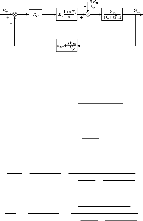
80 8 Motion Control
Fig. S8.1. Reduction on the block scheme of position and velocity feedback control
output to Θr. Then, the reduced block scheme of the system becomes that in
Fig. S8.1.
The transfer function of the forward path is then
P(s)=KPCV(s)M(s)=kmKPKV(1 + sTV)
s2(1 + sTm),
being CV(s) the transfer function of the PI velocity controller and M(s)the
transfer function of the actuator. The transfer function of the return path is
H(s)=kTP 1+skTV
KPkTP .
It follows that the closed-loop input/output transfer function with TV=Tm
is
Θm(s)
Θr(s)=P(s)
1+P(s)H(s)=
1
kTP
1+ skTV
KPkTP
+s2
kmKPkTPKV
.
The closed-loop disturbance/output transfer function is
Θ(s)
D(s)=−M(s)
1+P(s)H(s)=−
sRa
ktKPkTPKV(1 + sTm)
1+ skTV
KPkTP
+s2
kmKPkTPKV
.
Solution to Problem 8.3
First, it is worth observing that the block scheme of Fig. 8.9 has been obtained
from the scheme of Fig. 8.6 operating by the usual rules for block reduction.
In particular, the input to the block kTA has been moved onto ˙
Θm, while the
output to the same block has been moved onto the output of CA(s). Likewise,
the input to the block kTV has been moved onto Θm, while the output to the

8 Motion Control 81
Fig. S8.2. Reduction on the block scheme of position, velocity and acceleration
feedback control
same block has been moved onto the input to KP; then, the resulting two
blocks in parallel have been summed giving (kTP +skTV /KP). Solving the
inmost feedback loop gives the transfer function
sM(s)=
kt
sRaI
1+ ktkv
sRaI
=
1
kv
1+sRaI
kvkt
=km
1+sTm
,
and thus the block scheme of the system becomes that in Fig. S8.2.
Solving the inner feedback loop gives the transfer function
G(s)=
km
1+sTm
1+kmkTAKA(1 + sTA)
(1 + sTm)
=km
(1 + kmKAkTA)⎛
⎜
⎜
⎝1+
sTm1+kmKAkTA
TA
Tm
(1 + kmKAkTA)⎞
⎟
⎟
⎠
,
and thus the block scheme of the system becomes that in Fig. S8.3.
The transfer function of the forward path is then
P(s)=KPKVCA(s)G(s)
s=KPKVKA(1 + sTA)
s2G(s).
The transfer function of the return path is
H(s)=kTP 1+ skTV
KPkTP .
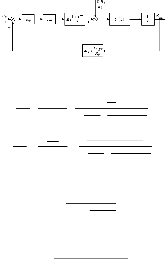
82 8 Motion Control
Fig. S8.3. Further reduction on the block scheme of position, velocity and acceler-
ation feedback control
It follows that the closed-loop input/output transfer function with TA=Tm
is
Θm(s)
Θr(s)=P(s)
1+P(s)H(s)=
1
kTP
1+ skTV
KPkTP
+s2(1 + kmKAkTA)
kmKPkTPKVKA
,
while the closed-loop disturbance/output transfer function is
Θm(s)
D(s)=−
G(s)
s
1+P(s)H(s)=−
sRa
ktKPkTPKVKA(1 + sTA)
1+ skTV
KPkTP
+s2(1 + kmKAkTA)
kmKPkTPKVKA
.
Solution to Problem 8.4
With the given data, the condition Fmkvkt/Rais verified and km=
2 rad/(V ·s), Tm=7.2s, kTP = 1. The closed-loop input/output transfer
function is
W(s)= (1 + sTP)
1+sTP+s2(1 + sTm)
kmKPkTP
.
Choosing TP=10Tm= 72 s leads to the root locus in Fig. S8.4 as a function
of the gain K=20KP.
If a damping ratio ζ=0.4 is desired, the resulting controller gain is
KP=0.0013. For such value, two complex poles (−0.062,±j0.142) and a real
pole (−0.015) are obtained. Hence, the above transfer function can be written
as
W(s)= (1 + 72s)
(1 + 5.161s+41.62s2)(1 + 66.66s).
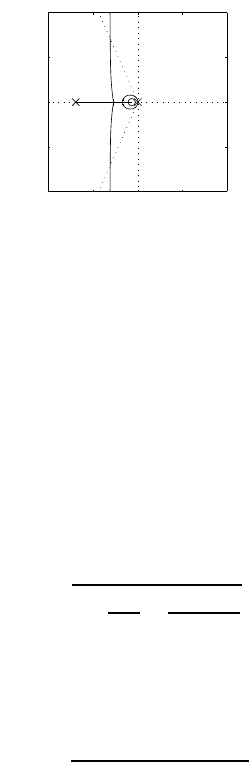
8 Motion Control 83
−0.2 −0.1 0 0.1 0.2
−0.2
−0.1
0
0.1
0.2
real axis
image axis
Fig. S8.4. Root locus for the position feedback control scheme
Correspondingly, the disturbance rejection factor is XR=0.0013, while an
estimate of the output recovery time is TR=72s.Thesevaluesrevealthe
poor disturbance rejection performance of the closed-loop system under simple
position feedback control.
Solution to Problem 8.5
With the given data, the condition Fmkvkt/Rais verified and km=
2 rad/(V·s), Tm=7.2s, kTP =1,kTV =1.ChoosingTV=Tmyields the
closed-loop input/output transfer function
W(s)= 1
1+ s
KP
+s2
2KPKV
.
With the given specifications for ζand ωn, the controller gains can be deter-
mined according to (8.30) and (8.31), giving KP=25andKV= 8, and thus
the above transfer function becomes
W(s)= 1
1+0.04s+0.0025s2
which has two complex poles (−8,±j18.33). Correspondingly, the disturbance
rejection factor is XR= 200, while an estimate of the output recovery time is
TR=7.2 s. These values reveal the good disturbance rejection performance of
the closed-loop system under position and velocity feedback control; however,
it is not possible to further decrease the output recovery time which is limited
bythetimeconstantTmof the drive system.

84 8 Motion Control
Solution to Problem 8.6
With the given data, the condition Fmkvkt/Rais verified and km=
2 rad/(V·s), Tm=7.2s, kTP =1,kTV =1,kTA =1.ChoosingTA=Tm
yields the closed-loop input/output transfer function
W(s)= 1
1+ s
KP
+s2(1 + 2KA)
2KPKVKA
.
With the given specifications for ζ,ωnand XR, the controller gains can be
determined according to (8.39), (8.40), (8.41) giving KP= 25, KV= 32,
KA=0.5, and thus the above transfer function becomes
W(s)= 1
1+0.04s+0.0025s2
which is the same transfer function of the previous problem. Remarkably,
in the case of position, velocity and acceleration feedback control, the dis-
turbance rejection performance is improved in terms of XR, although the
output recovery time TRis still the same as in the previous case. Finally,
in order to reconstruct acceleration from velocity measurement, a first-order
filter as in Fig. 8.11 can be used. With the given ζand ωn, the closed-loop
system bandwidth is ω3=26.84 rad/s, and then the filter bandwidth shall
be chosen wide enough with respect to the drive system bandwidth, e.g.,
ω3f=kf= 400 rad/s.
Solution to Problem 8.7
As for the block scheme in Fig. 8.12, where the saturation block can be ne-
glected, it is worth moving both the output of the block Tm/kmand the
output of the block 1/kmonto the input to the block kP(1 + sTP)/s;alsothe
quantities ˙
Θdand ¨
Θdcan be generated from Θdas sΘdand s2Θd, respectively.
Therefore, the reduced block scheme becomes that in Fig. S8.5.
The relationship between the desired input and the new reference input
is then
Θ
r(s)=kTP +s2Tm
km
+s
kms
KP(1 + sTP)Θd(s)
=kTP +s2(1 + sTm)
kmKP(1 + sTP)Θd(s).
As for the block scheme in Fig. 8.13, where the saturation block can be
neglected, it is worth moving both the output of the block 1/kmKVand
the output of the block kTV onto the input to the block KP;asabove,the
quantities ˙
Θdand ¨
Θdcan be generated from Θdas sΘdand s2Θd, respectively.
Therefore, the reduced block scheme becomes that in Fig. S8.6.
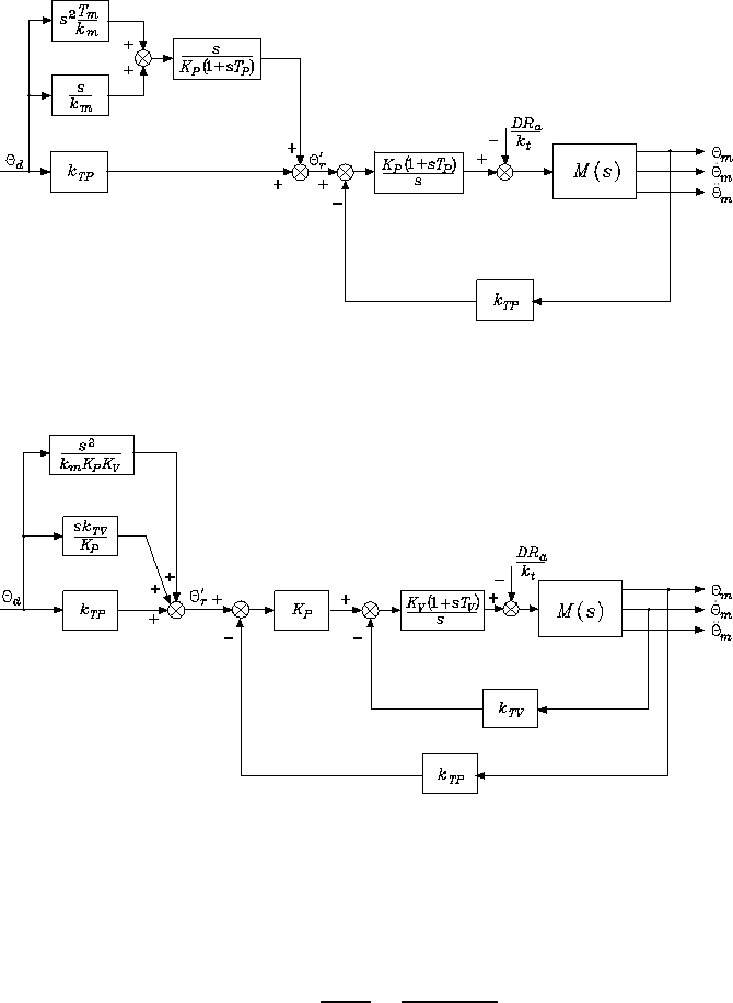
8 Motion Control 85
Fig. S8.5. Reduction on the block scheme of position feedback control with decen-
tralized feedforward compensation
Fig. S8.6. Reduction on the block scheme of position and velocity feedback control
with decentralized feedforward compensation
The relationship between the desired input and the new reference input
is then
Θ
r(s)=kTP +skTV
KP
+s2
kmKPKVΘd(s).
As for the block scheme in Fig. 8.14, where the saturation block can be
neglected, it is worth moving both the output of the block (kTA +1/kmKA)
and the output of the block kTV onto the input to the block KP; again, the
quantities ˙
Θdand ¨
Θdcan be generated from Θdas sΘdand s2Θd, respectively.
Therefore, the reduced block scheme becomes that in Fig. S8.7.
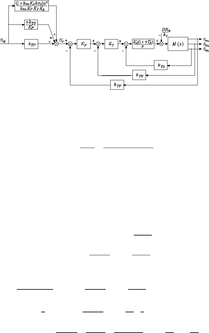
86 8 Motion Control
Fig. S8.7. Reduction on the block scheme of position, velocity and acceleration
feedback control with decentralized feedforward compensation
The relationship between the desired input and the new reference input
is then
Θ
r(s)=kTP +skTV
KP
+(1 + kmKAkTA)s2
kmKPKVKAΘd(s).
Solution to Problem 8.8
The block scheme in Fig. 8.15 is clearly equivalent to that in Fig. 8.12, since
the block KP(1 + sTP)/s can be split into two blocks in parallel, i.e., KPTP
and KP/s.
Concerning the block scheme in Fig. 8.28, it is worth considering the input
Uand the output Yof the block KV(1 + sTV)/s. By neglecting the effect of
the saturation block and setting E=kTP(Θd−Θm), the input Uis given by
U=KPE+kTV (˙
Θd−˙
Θm)+ 1
kmKV
¨
Θd
=KP1+ kTV
KPkTP
sE+1
kmKV
¨
Θd.
Then the output can be expressed (TV=Tm)as
Y=KV(1 + sTV)
sKP1+ kTV
KPkTP
sE+1
kmKV
¨
Θd
=KPKV1
s+TV1+ kTV
KPkTP
sE+1
km1
s+Tm¨
Θd
=KPKVTV+KVkTV
kTP
+KPKV
s+KVTVkTV
kTP
sE+1
km
˙
Θd+Tm
km
¨
Θd
8 Motion Control 87
corresponding to the block scheme in Fig. 8.16.
In a similar way, concerning the block scheme in Fig. 8.29, it is worth
considering the input Uand the output Yof the block KA(1 + sTA)/s.By
neglecting the effect of the saturation blocks and setting E=kTP(Θd−Θm),
the input Uis given by
U=KVKPE+kTV (˙
Θd−˙
Θm)+kTA +1
kmKA¨
Θd−kTA ¨
Θm
=KPKV+KVkTV
kTP
s+kTA
kTP
s2E+1
kmKA
¨
Θd.
Then the output can be expressed (TA=Tm)as
Y=KA1
s+TAKPKV+KVkTV
kTP
s+kTA
kTP
s2E+1
kmKA
¨
Θd
=KPKVKATA+KVkTV KA
kTP
+KPKVKA
s
+KVkTV KATA+KAkTA
kTP s+KATAkTA
kTP
s2E
+1
km
˙
Θd+Tm
km
¨
Θd
corresponding to the block scheme in Fig. 8.17.
Solution to Problem 8.9
From (8.75), the following matrix inequality can be written:
BmI≤B−1≤BMI
where all three matrices are positive definite. Setting
%
B=2
BM+Bm
I,
which is positive definite, allows writing the matrix inequality
2Bm
BM+Bm
I≤B−1%
B≤2BM
BM+Bm
I.
Subtracting the identity matrix from each term gives
−αI≤B−1%
B−I≤αI
where
α=BM−Bm
BM+Bm
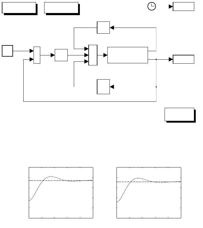
88 8 Motion Control
q_d=[pi/4 -pi/2] time
q_d=[-pi -3pi/4]
K_d
dq
g(q)
gravity
compensation
inv(B(q))(tau-tau')
arm
+
-q
q_d -
+
+
K_p
plot
Fig. S8.8. Simulink block diagram of joint space PD control with gravity compen-
sation
0 0.5 1 1.5 2 2.5
0.6
0.65
0.7
0.75
0.8
[s]
[rad]
joint 1 pos
0 0.5 1 1.5 2 2.5
−1.75
−1.7
−1.65
−1.6
−1.55
−1.5
[s]
[rad]
joint 2 pos
Fig. S8.9. Time history of the joint positions with joint space PD control with
gravity compensation for the first posture
and 0 <α<1. The matrix in the middle is lower bounded by a negative
definite diagonal matrix and upper bounded by a positive definite diagonal
matrix, where these two matrices have the same norm. Thus, it follows that
B−1%
B−I≤α.
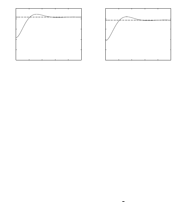
8 Motion Control 89
0 0.5 1 1.5 2 2.5
−3.35
−3.3
−3.25
−3.2
−3.15
−3.1
[s]
[rad]
joint 1 pos
0 0.5 1 1.5 2 2.5
−2.5
−2.45
−2.4
−2.35
−2.3
[s]
[rad]
joint 2 pos
Fig. S8.10. Time history of the joint positions with joint space PD control with
gravity compensation for the second posture
Solution to Problem 8.10
The control scheme in Fig. 8.20 is used with the same matrix gains as for case
F in Sect. 8.7, i.e.,
KP= 3750IK
D= 750I.
The initial arm postures for the two cases are chosen as q−[0.10.1]
T.The
various terms of the dynamic model are computed by using the minimum
parameterization in the solution to Problem 7.4.
The resulting Simulink block diagram is shown in Fig. S8.8, where both
desired postures can be assigned. The arm is simulated as a continuous-time
system using a variable-step integration method with a maximum step size of
1 ms. All the blocks of the controller are simulated as discrete-time subsystems
with the given sampling time of 1 ms.
The with the solution can be found in Folder 810.
The resulting joint positions for the two postures are shown in Figs. S8.9
and S8.10, respectively. The dashed line indicates the desired joint position,
while the solid line indicates the actual joint position. It can be seen that both
postures are reached at steady state.
Solution to Problem 8.11
With reference to the dynamic model in the solution to Problem 7.4, the
presence of a payload alters the dynamic parameters of augmented Link 2.
Since the payload is a mass mLconcentrated at the tip, the only parameter
that varies is the mass of the augmented link which becomes
m
2=m2+mL;
in fact, both the inertia first moment m2C2and inertia moment ¯
I2remain
the same because they are evaluated with respect to a frame located at the
tip. Hence, only parameters π
1and π
3in (S7.2) have to be recomputed with
the modified m
2.
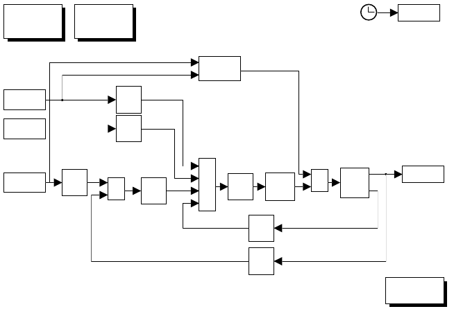
90 8 Motion Control
K_p = 5
K_v = 10
K_p = 6.25
K_v = 32
+
+
PI M
voltage-controlled
arm
k_fv
k_fa
q
[T,q_d] k_fp +
-
+
+
+
-
[T,ddq_d]
tau_d
computed torque
[T,dq_d]
plot
k_tv
k_tp
K_v
K_p
time
dq
Fig. S8.11. Simulink block diagram of joint space computed torque control with
feedforward compensation of the diagonal terms of the inertia matrix and of gravi-
tational terms, and independent joint control with position and velocity feedback
The desired trajectories for the two joints are generated via trapezoidal ve-
locity profiles with maximum velocities ˙qc1=3π/4 rad/s and ˙qc2=π/3 rad/s,
respectively.
The control scheme in Fig. 8.19 is used with feedforward compensation
of the diagonal terms of the inertia matrix and of gravitational terms. As for
the decentralized controller, the independent joint control with position and
velocity feedback in Fig. 5.11 is adopted.
Initially, the same gains for each joint servo are chosen as for case A in
Sect. 8.7, i.e., (kTP =kTV =1)
KP=5 KV= 10,
corresponding to ωn= 5 rad/s and ζ=0.5, and thus to a closed-loop band-
width ω3=6.36 rad/s. This gives a disturbance rejection factor XR= 50.
Then, by observing that the required trajectory is faster than the cor-
responding trajectory in Sect. 8.7, a larger bandwidth is imposed. Setting
ωn= 10 rad/s and ζ=0.8givesω3=10.78 rad/s. From (8.30) and (8.31), the
gains become
KP=6.25 KV=32
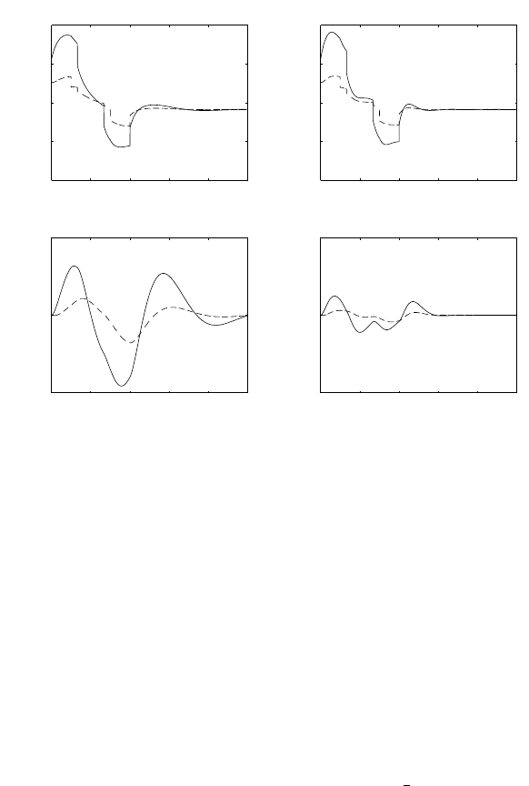
8 Motion Control 91
0 0.5 1 1.5 2 2.5
−4000
−2000
0
2000
4000
[s]
[Nm]
joint torques
0 0.5 1 1.5 2 2.5
−0.05
0
0.05
[s]
[rad]
joint pos errors
0 0.5 1 1.5 2 2.5
−4000
−2000
0
2000
4000
[s]
[Nm]
joint torques
0 0.5 1 1.5 2 2.5
−0.05
0
0.05
[s]
[rad]
joint pos errors
Fig. S8.12. Time history of the joint torques and position errors with joint space
computed torque control with feedforward compensation of the diagonal terms of
the inertia matrix and of gravitational terms, and independent joint control with
position and velocity feedback; left—first choice of servo gains, right—second choice
of servo gains
and, from (8.33), it is XR= 200, i.e., a disturbance rejection factor which is
four times as much as the previous one.
The resulting Simulink block diagram is shown in Fig. S8.11, where both
choices of servo gains can be executed. The arm is voltage-controlled as in
the scheme of Fig. 8.3 and is simulated as a continuous-time system using
a variable-step integration method with a maximum step size of 1 ms. All
the blocks of the controller are simulated as discrete-time subsystems with
the given sampling time of 1 ms; in particular, the PI block is discretized
assuming a zero-order hold on the inputs.
The files with the solution can be found in Folder 811.
The resulting joint torques and position errors are shown in Fig. S8.12.
The solid line refers to Joint 1, while the dashed line refers to Joint 2. It can
be seen that the tracking performance with the second choice of the servo
gains is considerably improved, at the expense of a sharper behaviour of joint
torques, though.
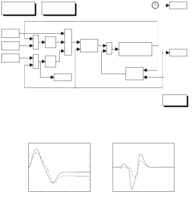
92 8 Motion Control
n(q,dq)
nonlinear
compensation
time
e
B(q)u
inertia
+
+inv(B(q))(tau-tau')
arm
q
plot
[T,q_d]
[T,ddq_d]
[T,dq_d]
+
+
+
K_d
-
+
K_p
+
-
compensated
load mass
noncompensated
load mass
dq
Fig. S8.13. Simulink block diagram of joint space inverse dynamics control
0 0.5 1 1.5 2 2.5
−0.02
−0.01
0
0.01
0.02
[s]
[rad]
joint pos errors
0 0.5 1 1.5 2 2.5
−5
0
5x 10⁻⁴
[s]
[rad]
joint pos errors
Fig. S8.14. Time history of the joint position errors with joint space inverse dy-
namics control; left—noncompensated load mass, right —compensated load mass
Solution to Problem 8.12
The modification of the dynamic model to account for the load mass and
the generation of joint trajectories are accomplished as in the solution to
Problem 8.11.
The control scheme in Fig. 8.22 is used where the matrix gains are chosen
as
KP= 100IK
D=16I
corresponding to an error dynamics for both joints characterized by ωni =
10 rad/s and ζi=0.8fori=1,2.
The resulting Simulink block diagram is shown in Fig. S8.13, where both
the noncompensated load mass case and the compensated load mass case can
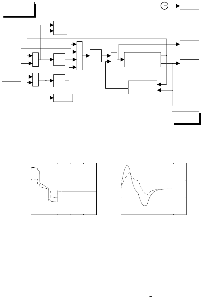
8 Motion Control 93
tau
q
B_h
constant
inertia
e
K_d
K_p
UV
robustness
+
+inv(B(q))(tau-tau')
arm
variables
initialization
time
plot
+
+
+
+
[T,ddq_d]
-
+
[T,dq_d]
[T,q_d] +
-
F_vdq+g(q)
friction and gravity
compensation
dq
Fig. S8.15. Simulink block diagram of joint space robust control
0 0.5 1 1.5 2 2.5
−4000
−2000
0
2000
4000
[s]
[Nm]
joint torques
0 0.5 1 1.5 2 2.5
−1.5
−1
−0.5
0
0.5
1
1.5 x 10⁻³
[s]
[rad]
joint pos errors
Fig. S8.16. Time history of the joint torques and position errors with joint space
robust control
be executed. The arm is torque-controlled as in the scheme of Fig. 8.4 and
is simulated as a continuous-time system using a variable-step integration
method with a maximum step size of 0.1 ms. All the blocks of the controller
are simulated as discrete-time subsystems with the given sampling time of
1ms.
The files with the solution can be found in Folder 812.
The resulting joint position errors in the two cases are shown in Fig. S8.14.
The solid line refers to Joint 1, while the dashed line refers to Joint 2. It
can be seen that the tracking performance is excellent when load mass is
compensated, while it is degraded both during transient and at steady state
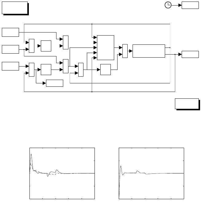
94 8 Motion Control
variables
initialization
e
[T,dq_d]
sig
dq_r
ddq_r
+
-
[T,ddq_d]
-
+
Lam Y( . )pi_h
adaptive
control
+
+
+
+
[T,q_d] +
-
Lam
plot
+
+
inv(B(q))(tau-tau')
arm
q
time
K_d
dq
Fig. S8.17. Simulink block diagram of joint space adaptive control
0 0.5 1 1.5 2 2.5
−1
−0.5
0
0.5
1x 10⁻³
[s]
[rad]
joint pos errors
0 0.5 1 1.5 2 2.5
0
5
10
15
20
[s]
[kg]
load mass estimate
Fig. S8.18. Time history of the joint position errors and of the load mass estimate
with joint space adaptive control
when the load mass is not compensated. Also, in the case of noncompensated
load mass, steady-state errors occur.
Solution to Problem 8.13
The modification of the dynamic model to account for the load mass and
the generation of joint trajectories are accomplished as in the solution to
Problem 8.11.
The control scheme in Fig. 8.23 is used with constant inertia ( %
B=¯
B)
and compensation of friction and gravity (%
n=Fv˙
q+g). The gains defining
the error dynamics are chosen as in the solution to Problem 8.12, i.e.,
KP= 100IK
D=16I;

8 Motion Control 95
furthermore, the matrix Pin (8.81) is chosen as
P=I,
and the gain ρand the thickness of the boundary layer in (8.89) are respec-
tively chosen as
ρ=70 =0.001.
The resulting Simulink block diagram is shown in Fig. S8.15. The arm
is simulated as a continuous-time system using a variable step integration
method with a maximum step size of 1 ms. All the blocks of the controller are
simulated as discrete-time subsystems with the given sampling time of 1 ms.
The files with the solution can be found in Folder 813.
The resulting joint torques and position errors are shown in Fig. S8.16.
The solid line refers to Joint 1, while the dashed line refers to Joint 2. It can be
seen that, in spite of the imperfect dynamic model compensation, the tracking
performance is satisfactory, thanks to the use of the robustness action.
Solution to Problem 8.14
A minimum parameterization of the dynamic model is obtained as in the so-
lution to Problem 7.4, with suitable modification of augmented Link 2 param-
eters as in the solution to Problem 8.11. The generation of joint trajectories
is also accomplished as in the solution to Problem 8.11.
The control scheme in Fig. 8.26 is used. In terms of the new reference
velocity and acceleration vectors in (8.92), the regressor in (S7.3) becomes
y
11 =a1¨
ϑr1+gc1
y
12 =¨
ϑr1
y
13 =(2a1c2+a2)¨
ϑr1+(a1c2+a2)¨
ϑr2−a1s2˙
ϑr1˙
ϑ2−a1s2˙
ϑ1˙
ϑr2−a1s2˙
ϑ2˙
ϑr2
+gc12
y
14 =¨
ϑr1+¨
ϑr2
y
15 =¨
ϑr1+kr2¨
ϑr2
y
21 =0
y
22 =0
y
23 =(a1c2+a2)¨
ϑr1+a2¨
ϑr2+a1s2˙
ϑ1˙
ϑr1+gc12
y
24 =¨
ϑr1+¨
ϑr2
y
25 =kr2¨
ϑr1+k2
r2¨
ϑr2.
In view of the presence of a concentrated tip load mass, the only variations
occurring on the parameters in (S7.2) are:
Δπ
1=a1mLΔπ
3=a2mL.

96 8 Motion Control
Hence, the control law in (8.98) can be formally written as
u=Y(q,˙
q,˙
qr,¨
qr)π+Fv˙
qr+mLyL+KDσ
where Yis computed as above and
yL=a1y
11 +a2y
13
a1y
21 +a2y
23 ,
being π=mLthe only unknown parameter.
The gains are chosen as
Λ=10IK
D= 10000Ikπ=0.005;
the initial estimate of πis set to 0, and the true value of mLis utilized only
to update the simulated arm model.
The resulting Simulink block diagram is shown in Fig. S8.17. The arm
is simulated as a continuous-time system using a variable-step integration
method with a maximum step size of 1 ms. All the blocks of the controller are
simulated as discrete-time subsystems with the given sampling time of 1 ms.
The files with the solution can be found in Folder 814.
The resulting joint position errors and load mass estimate are shown in
Fig. S8.18. For the joint position errors, the solid line refers to Joint 1, while
the dashed line refers to Joint 2. It can be seen that the tracking performance
is satisfactory, thanks to the adaptive action on the load mass; in this case,
the parameter estimate converges to the true value.
Solution to Problem 8.15
The modification of the dynamic model to account for the load mass is ac-
complished as in the solution to Problem 8.11.
The control scheme in Fig. 8.29 is used with the same matrix gains as for
case K in Sect. 8.7, i.e.,
KP= 16250IK
D= 3250I.
The initial tip positions for the two postures are chosen as p−[0.10.1]
T.
The resulting Simulink block diagram is shown in Fig. S8.19, where both
desired positions can be assigned. The arm is simulated as a continuous-time
system using a vaiable-step integration method with a maximum step size of
1 ms. All the blocks of the controller are simulated as discrete-time subsystems
with the given sampling time of 1 ms.
The files with the solution can be found in Folder 815.
The resulting components of tip position for the two postures are shown
in Figs. S8.20 and S8.21, respectively. The dashed line indicates the desired
tip coordinate, while the solid line indicates the actual tip coordinate. It can
be seen that both postures are reached at steady state.
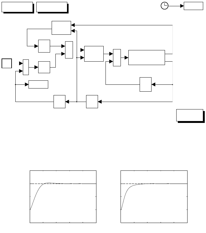
8 Motion Control 97
p_d=[0.6 -0.2]p_d=[0.5 0.5]
g(q)
gravity
compensation
+
-
p_d
-
+
J_a(q)
cs(q)
sinusoidal
functions
tr(J_a(q))
Jacobian
transpose
+
+
dq
inv(B(q))(tau-tau')
arm
K_p
K_d
k(q)
direct
kinematics
time
plot
p
q
Fig. S8.19. Simulink block diagram of operational space PD control with gravity
compensation
0 0.5 1 1.5 2 2.5
0.35
0.4
0.45
0.5
0.55
[s]
[m]
x−pos
0 0.5 1 1.5 2 2.5
0.35
0.4
0.45
0.5
0.55
[s]
[m]
y−pos
Fig. S8.20. Time history of the tip position components with operational space PD
control with gravity compensation for the first posture
Solution to Problem 8.16
The modification of the dynamic model to account for the load mass is ac-
complished as in the solution to Problem 8.11. The desired tip trajectory is
generated in terms of the path coordinate svia a trapezoidal velocity profile
with maximum velocity ˙sc=1.5.
The control scheme in Fig. 8.30 is used with the matrix gains:
KP= 100IK
D=16I.
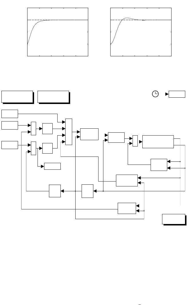
98 8 Motion Control
0 0.5 1 1.5 2 2.5
0.45
0.5
0.55
0.6
0.65
[s]
[m]
x−pos
0 0.5 1 1.5 2 2.5
−0.3
−0.25
−0.2
−0.15
[s]
[m]
y−pos
Fig. S8.21. Time history of the tip position components with operational space PD
control with gravity compensation for the second posture
[T,p_d]
[T,ddp_d]
q
dq
inv(B(q))(tau-tau')
arm
+
+
B(q)u
inertia
+
+
+
-
K_p
+
-
K_d
+
-
[T,dp_d]
compensated
load mass
noncompensated
load mass
en(q,dq)
nonlinear
compensation
inv(J_a(q))
Jacobian
inverse
plot
cs(q)
sinusoidal
functions
k(q)
direct
kinematics dJ_a(q,dq)
Jacobian
derivative
J_a(q)
analytical
Jacobian
time
Fig. S8.22. Simulink block diagram of operational space inverse dynamics control
The resulting Simulink block diagram is shown in Fig. S8.22, where both
the noncompensated load mass case and the compensated load mass case
can be executed. The arm is simulated as a continuous-time system using a
variable-step integration method with a maximum step size of 1 ms. All the
blocks of the controller are simulated as discrete-time subsystems with the
given sampling time of 1 ms.
The files with the solution can be found in Folder 816.
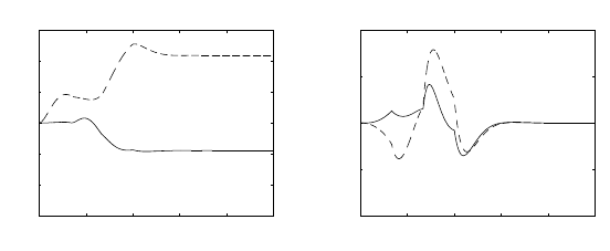
8 Motion Control 99
0 0.5 1 1.5 2 2.5
−6
−4
−2
0
2
4
6x 10⁻³
[s]
[m]
tip pos errors
0 0.5 1 1.5 2 2.5
−4
−2
0
2
4x 10⁻⁴
[s]
[m]
tip pos errors
Fig. S8.23. Time history of the components of tip position error with opera-
tional space inverse dynamics control; left—noncompensated load mass, right —
compensated load mass
The resulting components of tip position error in the two cases are shown
in Fig. S8.23. The solid line refers to xcomponent, while the dashed line refers
to ycomponent. It can be seen that the performance is excellent when the
load mass is compensated, while it is degraded both during transient and at
steady state when the load mass is not compensated.

9
Force Control
Solution to Problem 9.1
Computing the time derivative of od
d,e =RT
d(oe−od)gives
˙
od
d,e =RT
d(˙
oe−˙
od)−˙
RT
d(oe−od). (S9.1)
In view of (3.10), (3.7) and (3.11) the following equality holds
˙
RT
d=−RT
dS(ωd)=−S(RT
dωd)RT
d=−S(ωd
d)RT
d(S9.2)
which, replaced in (S9.1), gives (9.10).
To derive (9.11), consider the equality
˙
Rd
e=˙
RT
dRe+RT
d˙
Re=−S(ωd
d)Re
d+S(ωd
e)Re
d=S(ωd
d,e)Re
d,
where (S9.2), (3.10), and (3.11) have been used. It follows that (3.64) can be
rewritten as
ωd
d,e =T(φd,e)˙
φd,e
being φd,e the vector of Euler angles extracted from Rd
eand ωd
d,e the angular
velocity corresponding to ˙
Rd
e. Hence, expression (9.11) follows.
Solution to Problem 9.2
Pre-multiplying by Kboth sides of the equality
dxr,e =dxr,d −dxe,d,
and using (9.21) and (9.20) gives
he=Kdxr,d −KK−1
Phe

102 9 Force Control
and thus
(I6+KK−1
P)he=Kdxr,d ,
from which expression (9.22) follows. Equality (9.23) is obtained replac-
ing (9.22) into (9.20).
Solution to Problem 9.3
Similarly to Example 9.2, all the quantities can be referred to a base frame and
control law with force measurement (9.30), (9.31) can be adopted. To compute
the model of the contact force, in view of the geometry of the environment, it
is useful to consider also a rotated base frame with axes parallel to the axes
xcand ycof Fig. 9.16 and with the same origin of the base frame of axes x0
and y0. The corresponding rotation matrix is
Rc=1/√2−1/√2
1/√21/√2.
In the rotated base frame, the environment stiffness matrix has the simple
expression
Kc=diag{0,k
y},
corresponding to the absence of interaction forces along the direction of axis
xc(fc
e=[0 fc
y]T). The elastic force in the rotated base frame has the
expression
fc
e=Kc(oc
e−oc
r),
being oc
ethe end-effector position and oc
rthe equilibrium position of the plane
in the rotated base frame. The above expression can be rewritten in the base
frame in the form
fe=K(oe−or),
with
K=RcKcRT
c=ky1/2−1/2
−1/21/2
and or=[1 0]
T.
The impedace parameters can be set similarly to Example 9.2, on the
basis of the equations
mdx ¨xc
e+kDx ˙xc
e+kPxxc
e=kPxxc
d
mdy ¨yc
e+kDy ˙yc
e+(kPy +ky)yc
e=kyyc
r+kPyyc
d
referred to the rotated base frame, where the diagonal matrices
Mc
d=diag{mdx,m
dy}Kc
D=diag{kDx,k
Dy}Kc
P=diag{kPx,k
Py}
define an active impedance in the rotated base frame. The corresponding
impedance matrices referred to the base frame are
Md=RcMc
dRT
cKD=RcMc
dRT
cKP=RcMc
dRT
c.

9 Force Control 103
o_e
do_e
f_e
operational space
decoupled arm
u = ddo_e
environment
K(o_e−o_r)
e
f_e time
plot
variables
initialization
K_d inv(M_d)
K_p
[T,do_d]
[T,ddo_d]
[T,o_d]
Fig. S9.1. SIMULINK block diagram of impedance control.
Notice that, differently from Example 9.2, the interaction occurs along yc.
Therefore, for the unconstrained motion along xc, the behaviour is determined
by
ωnx =kPx
mdx
ζx=kDx
2√mdxkPx
,
while, for the constrained motion along axis yc, the behaviour is determined
by
ωny =&kPy +ky
mdy
ζy=kDy
2'mdy(kPy +ky).
With the choice
mdx =mdy = 100 kDx =kDy = 1600 kPx =kPy = 5000,
and the given value of environment stiffness ky, the dynamics is characterized
by
ωnx =7.07 rad/s ζx=1.13
and
ωny = 10 rad/s ζy=0.8.
The desired tip trajectory is generated in terms of the path coordinate s
via a trapezoidal velocity profile with maximum velocity ˙sc=0.5.
The resulting Simulink block diagram is shown in Fig. S9.1. The arm is
simulated as a continuous-time system using the a variable-step integration
method with a minimum step size of 1 ms. All the blocks of the controller are
simulated as discrete-time subsystems with the given sampling time of 1 ms.
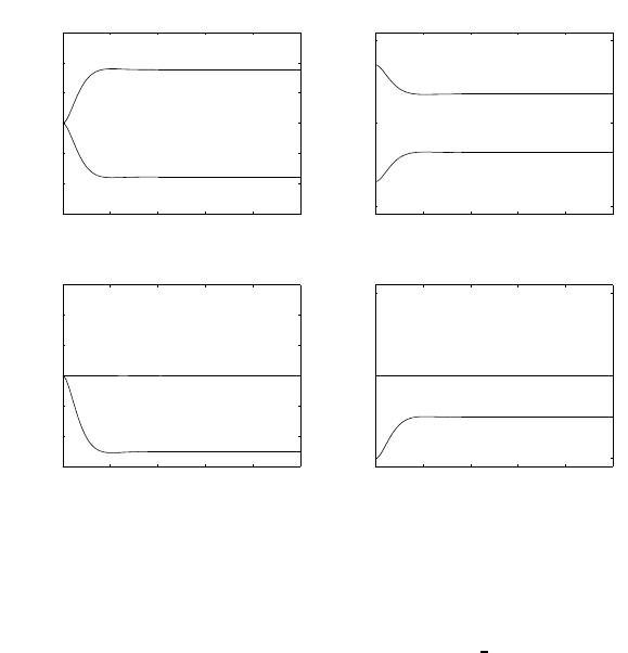
104 9 Force Control
0 0.5 1 1.5 2 2.5
−0.06
−0.04
−0.02
0
0.02
0.04
0.06
[s]
[m]
pos error
x
y
0 0.5 1 1.5 2 2.5
−500
0
500
[s]
[N]
force
x
y
0 0.5 1 1.5 2 2.5
−0.06
−0.04
−0.02
0
0.02
0.04
0.06
[s]
[m]
pos error
xc
yc
0 0.5 1 1.5 2 2.5
−500
0
500
[s]
[N]
force
xc
yc
Fig. S9.2. Time history of the tip position error and of the contact force with
impedance control. Top: components in the base frame. Bottom: components in the
rotated base frame.
The files with the solution can be found in Folder 9 3.
The resulting tip position error and contact force are shown in Fig. S9.2,
both referred to the base frame (top) and to the rotated base frame (bottom).
It can be verified that the position error keeps small during the task execution,
ensuring a bounded contact force. In particular, it can be observed that the
position error is null along the unconstrained motion direction (axis xc), where
the force is null; on the other hand, the force response along the constrained
motion direction (axis yc) remains bounded and converges to a constant value
which depends on the plane stiffness and undeformed position as well as on
the active compliance.
Solution to Problem 9.4
From the block scheme in Fig. 9.8, at the equilibrium, it is ˙
x≡0,¨
x≡0.
Then, the input to the block KPmust be null, which implies
xd+xF−xe=0.
In view of (9.21) and (9.41), it follows that
xd+CFK(xr−xe)+fd−xe=0,

9 Force Control 105
and thus the equilibrium location satisfies the equation
xe=xd+CFK(xr−xe)+fd.
Solution to Problem 9.5
The norm of vector
=he−Sfλ
with weighting matrix Wis defined as
W=√TW.(S9.3)
The vector λwhich minimizes the norm (S9.3) can computed also as the
solution of a minimization problem for the quadratic cost functional
g()=1
2TW.
The solution has to satisfy the necessary condition
∂g
∂λT
=0
which gives
−ST
fW(he−Sfλ)=0,
and thus
λ=(ST
fWSf)−1ST
fWh
e.
Solution to Problem 9.6
Taking into account that CK =KC =I6, Equation (9.70) can be rewritten
in the form
K=Sf(ST
fCSf)−1ST
fCK
which, considering the definition (9.55) of weighted pseudo-inverse with weight
C, can be rewritten as
K=SfS†
fK=PfK.
Solution to Problem 9.7
Assuming that the screwdriver can move along the slot of the screw, it is worth
choosing the constraint frame attached to the screwdriver as in Fig. S9.3.
Natural constraints can be determined first. Motion constraints describe
the impossibility to generate arbitrary linear velocities along axes yc,zcand
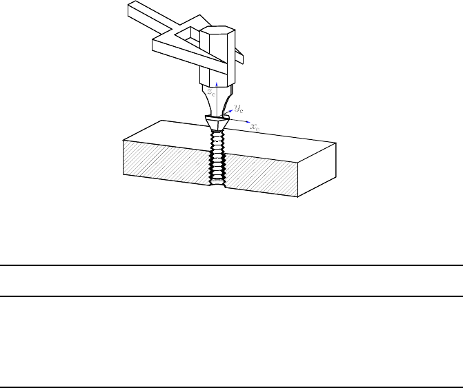
106 9 Force Control
Fig. S9.3. Driving a screw in a hole.
Table S9.1. Natural and artificial constraints for the task of Fig. S9.3.
Natural Artificial
Constraints Constraints
˙pc
yfc
y
˙pc
zfc
z
ωc
xμc
x
ωc
yμc
y
fc
x˙pc
x
μc
zωc
z
angular velocities about axes xc,yc. Force constraints describe the impossi-
bility to exert arbitrary forces along axis xcand moment about axis zc.
As a consequence, artificial constraints regard the variables not subject to
natural constraints. Hence, with reference to natural velocity constraints along
axes yc,zcand about xc,yc, it is possible to specify artificial constraints for
forces along yc,zcand moments about xc,yc. Also, with reference to natural
generalized force constraints along axis ycand about axis zc,itispossibleto
specify artificial constraints for linear velocity along xcand angular velocity
about zc. The set of constraints is summarized in Table S9.1. Notice that, in
the case of a frictionless groove, once ωc
zis specified, then ˙pc
zis determined
according to the pitch of the screw.
Solution to Problem 9.8
The control input (9.77) referred to the constraint frame, in view of the ex-
pressions of Sc
f,Sc
vand Ccin Example 9.4, can be computed as
αc
x=αν
αc
y=c2,2fλ.

9 Force Control 107
Taking into account (9.81), the control input αc
ycanbeexpressedas
αc
y=−c2,2kDλ ˙
λ+kPλ(λd−λ),
where a constant desired force λdwas considered. In view of the equalities
˙oc
y=c2,2˙
λand λ=fc
y, the equation can be rewritten in the form
αc
y=−kDλ ˙oc
y+kPλ(λd−fc
y),
showing that the the control action in the force controlled subspace consists
of a proportional force control with inner velocity loop.
Solution to Problem 9.9
The computation of Sc†
fusing the compliance matrix
Cc=c1,1c1,2
c1,2c2,2
as a weighting matrix gives
Sc†
f=(ScT
fCcSc
f)−1ScT
fCc=[c−1
2,2c1,21].
On the other hand, computing S†
fin the base frame gives
S†
f=(ST
fCSf)−1ST
fC=1
√2c1,2−c2,2
c2,2
c1,2+c2,2
c2,2,
where C=RcCcRT
c.NoticethatS†
f=Sc†
fRT
cand the same transformation
rule holds for S†
v. Also, if fc
e=[fc
xfc
y]T,then
λ=Sc†
ffc
e=S†
ffe=c1,2
c2,2
fc
x+fc
y,
independently from the frame to which S†
fand feare referred. On the other
hand, if the contact force fc
ebelongs to subspace R(Sc
f), i.e., fc
e=[0 fc
y]T,
then it is λ=fc
yindependently from the particular weighting matrix.
Analogously, the computation of Sc†
vusing the stiffness matrix
Kc=k1,1k1,2
k1,2k2,2
as a weighting matrix gives
Sc†
v=(ScT
vKcSc
v)−1ScT
vKc=[1 k−1
1,1k1,2]

108 9 Force Control
in the constraint frame, and
S†
v=1
√2k1,1−k1,2
k1,1
k1,1+k1,2
k1,1
in the base frame.
Solution to Problem 9.10
In view of the results of Example 9.4, the hybrid control law can be designed
by choosing the control inputs ανand fλaccording to (9.80) and (9.84),
respectively, with suitable control gains.
In detail, the control gains in (9.80) can be set to
kPν =16 kIν = 100,
corresponding to ωnν = 10 rad/s and ζν=0.8 for the dynamics of the velocity
error νd−ν.
The same dynamics can be imposed to the force λwith the choice
kDλ =16 kPλ = 100,
in the case that the stiffness of the environment is known.
In the case that only an estimate of the stiffness of the environment is
available, the quantity Lf=lfhas the value
lf=ˆc2,2
c2,2
and thus ˙
ˆ
λ=ˆc−1
2,2˙oc
y.
Assuming, for example, ˆc−1
2,2=4·103N/m, then lf=1.25, corresponding
to ωnλ =11.18 rad/s and ζλ=0.71 for the dynamics of the force.
The initial tip position is chosen on the plane as oe(0) = [ 1 0 ]T.The
desired velocity along axis xcis set as in Problem 9.3, while the desired force
along axis ycis set to −50 N.
The resulting Simulink block diagram is shown in Fig. S9.4. The arm
is simulated as a continuous-time system using a variable-step integration
method with a minimum step size of 1 ms. All the blocks of the controller are
simulated as discrete-time subsystems with the given sampling time of 1 ms.
The files with the solution can be found in Folder 910.
The resulting tip velocity error along xcand contact force along ycare
shown in Fig. S9.5. It can be verified that the velocity error keeps small during
task execution; also, the contact force reaches the desired value at steady state.
In Fig. S9.6, the continuous line represents the end-effector path in the base
frame, while the dashed line corresponds to the plane at rest. It can be verified
that the plane complies during the interaction.
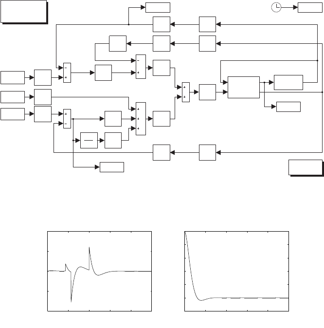
9 Force Control 109
do_e
f_eo_e
operational space
decoupled arm
u = ddo_e
environment
K’(o_e−o_r)
e_nu
timelam
o_e
plot
variables
initialization
pS_f
K_Dl
K_Pl
C’S_f
G_f
K_Pnu S_v
R_c
trR_c
pS_v
pS_v
pS_f
trR_c
trR_c
pS_v
K_Inu
[T,v_d]
[T,a_d]
K Ts
z−1
h_d
Fig. S9.4. SIMULINK block diagram of hybrid force/motion control.
0 0.5 1 1.5 2 2.5
−2
−1
0
1
2x 10⁻³
[s]
[m/s]
vel error
0 0.5 1 1.5 2 2.5
−60
−50
−40
−30
−20
−10
0
[s]
[N]
force
Fig. S9.5. Time history of the tip velocity error and of the contact force with hybrid
force/motion control.
Solution to Problem 9.11
In view of equality ˙
q=Jρ(r)˙
rand (9.63) the following equality holds
ve=J(q)˙
q=J(q)Jρ(r)˙
r=Sv(q)˙
r.
Hence, pre-multiplying both sides of the above equation by S†
vand using (9.59)
gives
ν=˙
r.
Also, it is ˙
ν=¨
r. Therefore, control law (9.95) yields the closed-loop equation
¨
r−¨
rd+KDr(˙
rd−˙
r)+KPr(rd−r)=0,
showing that tracking of a desired position rd(t)isachieved.
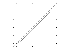
110 9 Force Control
1 1.1 1.2
0
0.05
0.1
0.15
0.2
0.25
[m]
[m]
Fig. S9.6. Tip’s path in the base frame (continous line) and undeformed contact
plane (dashed line).

10
Visual servoing
Solution to Problem 10.1
The principal moments of the region are the eigenvalues of matrix Iwhich
are
λ=1
2μ2,0+μ0,2+4μ2
1,1+(μ0,2−μ2,0)2
λ=1
2μ2,0+μ0,2−4μ2
1,1+(μ0,2−μ2,0)2
with λ≥λ>0. The principal axis (i.e., the eigenvector of I) corresponding
to λis aligned to vector
aλ=μ1,1
λ−μ2,0.
Therefore
tα=1
2μ1,1μ0,2−μ2,0+4μ2
1,1+(μ0,2−μ2,0)2,
where tα=tanα. Considering that
t2α=2tα
1−t2
α
=2μ1,1
μ2,0−μ0,2
,
Equation (10.2) follows.
Solution to Problem 10.2
The singular value decomposition of the (12 ×9) matrix Ais given by
A=UΣV T, (S10.1)
112 10 Visual servoing
where Uis a (12 ×12) orthogonal matrix, Vis a (9 ×9) orthogonal matrix
and
Σ=D0
O0D=diag{σ1,σ
2,...,σ
8}
whith σ1≥σ2≥...≥σ8>0 being the non-null singular values of matrix A,
which is of rank 8. Post-multiplying by Vboth sides of Eq. (S10.1) gives
AV =UΣ
and thus Avi=σiui,fori=1,...,8andAv9=0,beingvithe i-th
column of V, known as right eigenvector, and uithe i-th column of U,known
as left eigenvector, corresponding to σi. In sum, the right eigenvector v9,
corresponding to the null singular value of A, is a non-null solution to (10.10).
Solution to Problem 10.3
Notice that equality Tr(RcT
oUΣV T)=Tr(VTRcT
oUΣ) derives from prop-
erty Tr(AB)=Tr(BA), for square matrices Aand B.Also,sinceVTRcT
oU
is an an orthogonal matrix, all its elements have absolute value lower than or
equal to 1.
The problem of minimizing the Frobenius norm is equivalent to that of
minimizing the quantity
Rc
o−Q2
F=Tr(Rc
o−Q)T(Rc
o−Q)=3+TrQTQ−2Tr RcT
oQ,
which is minimum when Tr RcT
oQis maximum. Consider the singular value
decomposition
Q=UΣV T
where Σ=diag{σ1,σ
2,σ
3},σi>0. The following equality holds
Tr RcT
oUΣV T=TrVTRcT
oUΣ=
3
i=1
zi,iσi
where zi,i,i=1,2,3 are the diagonal elements of the orthogonal matrix
VTRcT
oU, whose absolute values are lower than or equal to 1. Thus
Tr RcT
oUΣV T≤
3
i=1
σi
and the equality holds when zi,i = 1. Hence the maximum of Tr RcT
oQis
achieved by choosing Rcas in (10.12), which ensures that VTRcT
oU=I.
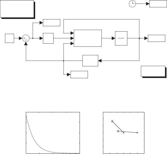
10 Visual servoing 113
xh
es
time
sh
plot
variables
initialization
s(xh)
Jacobian
inverse
inv(J_as)vs
K_s K Ts
z−1
s
Fig. S10.1. Simulink block diagram of the pose estimation algorithm based on the
inverse of image Jacobian. Case of two feature points.
0 0.01 0.02 0.03 0.04
0
0.1
0.2
0.3
0.4
[s]
error norm
−0.2 −0.1 0 0.1 0.2
−0.2
−0.1
0
0.1
0.2
0.3
image plane
Fig. S10.2. Time history of the norm of the estimation error and corresponding
paths of the feature points projections on image plane
Solution to Problem 10.4
In view of the results of Example 10.3, the Jacobian JAs, based on the feature
vector of two points, is a square (4 ×4) matrix. Hence, the pose estimation
algorithm based on the inverse of image Jacobian can be adopted.
According to (10.40) and (10.41), the following equality holds
˙
%
xc,o =%
vc
c,o =Γ(oc
c,o)L−1
sKses,
where Lsis the (4 ×4) interaction matrix of points P1and P2, obtained from
the (4 ×6) interaction matrix of a set of two points by removing the fourth
and fifth column. Also, Γ(oc
c,o)isthe(4×4) matrix
Γ(oc
c,o)=−Is
3(oc
c,o)
0T−1,
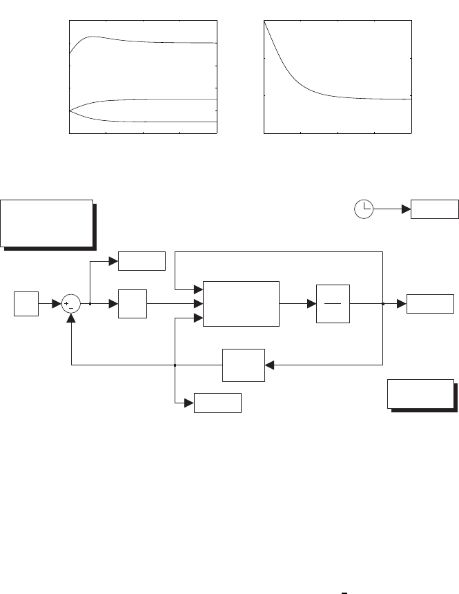
114 10 Visual servoing
0 0.01 0.02 0.03 0.04
−0.2
0
0.2
0.4
0.6
0.8
z
y
x
[s]
[m]
pos
0 0.01 0.02 0.03 0.04
−1.5
−1
−0.5
0
[s]
[rad]
orien
Fig. S10.3. Time history of camera pose estimate
xh
es
time
sh
plot
sl(xh)
variables
initialization
K_s K Ts
z−1
s
Jacobian
inverse
inv(J_asl)vs
Fig. S10.4. Simulink block diagram of the pose estimation algorithm based on the
inverse of image Jacobian. Case of two feature points.
being s3(·) is the third column of matrix S(·).
Matrix gain Kshas been chosen as Ks= 160I4. The initial estimate has
been set to ˆ
xc,o(0) = [ 0 0 0.5 0 ]. The resulting Simulink block diagram
is shown in Fig. S10.1. The Euler numerical integration method has been
adopted, with sampling time of 1 ms.
The files with the solution can be found in Folder 10 4.
The results in Fig. S10.2 show that the norm of the estimation error of
the feature parameters estends to zero asymptotically with convergence of
exponential type; moreover, due to the fact that matrix gain Kswas chosen
diagonal with equal elements, the paths of the projections of the feature points
on the image plane (between the initial positions marked with crosses and the
final positions marked with circles) are line segments.
The corresponding time histories of the components of vector %
xc,o for
position and orientation are reported in Fig. S10.3. It can be verified that, with
the chosen value of Ks, the algorithm converges in about 0.03 s, corresponding
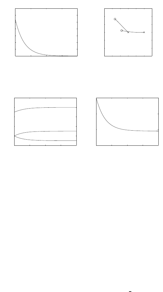
10 Visual servoing 115
0 0.01 0.02 0.03 0.04
0
0.2
0.4
0.6
0.8
1
1.2
[s]
error norm
−0.2 −0.1 0 0.1 0.2
−0.2
−0.1
0
0.1
0.2
0.3
image plane
Fig. S10.5. Time history of the norm of the estimation error and corresponding
paths of the feature points projections on image plane
0 0.01 0.02 0.03 0.04
−0.2
0
0.2
0.4
0.6
0.8
z
y
x
[s]
[m]
pos
0 0.01 0.02 0.03 0.04
−1.5
−1
−0.5
0
[s]
[rad]
orien
Fig. S10.6. Time history of camera pose estimate
to 30 iterations. The final value, namely, the estimated relative pose of the
object with respect to the camera, is ˆ
xc,o [−0.10.10.6−π/3]
T.
Solution to Problem 10.5
The solution is similar to that of Problem 10.4, but the feature parameters
are defined according to (10.28), and the interaction matrix of a line segment
is used.
Matrix gain Kshas been chosen as Ks= 160I4. The initial estimate has
been set to ˆ
xc,o =[0 0 0.5 0 ]. The feature vector of the line segment
corresponding to that of Problem 10.4 is
s=[−0.1250 0.0945 0.1668 −1.0470 ]T.
The resulting Simulink block diagram is shown in Fig. S10.4. The Euler
numerical integration method has been adopted, with sampling time of 1 ms.
The files with the solution can be found in Folder 10 5.
The results in Figs. S10.5 and S10.6 are quite similar to those of Prob-
lem 10.4. Notice that, however, the paths of the projections of the feature
points on the image plane are not perfectly linear, due to the different choice
116 10 Visual servoing
of feature vector. This is reflected also by a different time history of the z
component of the camera position during the transient. Obviously, the same
final value is achieved for the estimated relative pose of the object with respect
to the camera, namely ˆ
xc,o [−0.10.10.6−π/3]
T.
Solution to Problem 10.6
In view of the equalities pi=¯
pi+¯
pand p
i=¯
p
i+¯
p, function (10.55) can
be rewritten as
g(o)=
n
i=1 pi−o−Rp
i2=n¯
p−o−R¯
p2+
n
i=1 ¯
pi−R¯
p
i2
+2
n
i=1
(¯
p−o−R¯
p)T(¯
pi−R¯
p
i)
=n¯
p−o−R¯
p2+
n
i=1 ¯
pi−R¯
p
i2,
considering that (n
i=1 ¯
pi=(n
i=1 ¯
p
i=0. Hence, with the choice of oas
in (10.56), function (10.55) is minimum. The same result can be obtained
computing the value of owhich satisfies the necessary condition (∂g/∂o)T=
0.
Solution to Problem 10.7
Function (10.57) can be rewritten as
n
i=1 ¯
pi−R¯
p
i2=
n
i=1 ¯
pi2−2
n
i=1
¯
pT
iRT¯
pi+
n
i=1 R¯
p
i2
which is minimum when the quantity (n
i=1 ¯
pT
iRT¯
piis maximum. This quan-
tity, in view of the property aTb=Tr(ba), can be rewritten as
n
i=1
¯
pT
iRT¯
pi=
n
i=1
Tr RT¯
pi¯
pT
i=Tr(RTK),
with K=(n
i=1 ¯
pi¯
p
iT. Hence, the matrix Rwhich minimizes function (10.57)
is the matrix which maximizes the trace of RTK.
Solution to Problem 10.8
The control scheme in Fig. 10.14 is adopted, with the same matrix gains used
in control scheme Aof Sect. 10.9, namely,
KP=diag{500,500,10,10}KD=diag{500,500,10,10}.
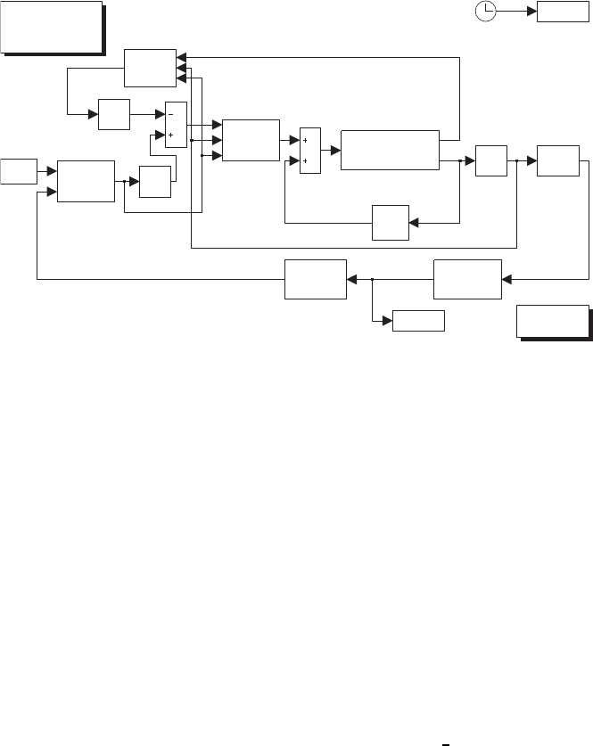
10 Visual servoing 117
dq
q
xtilde
sinusoidal
functions
cs(q)
gravity
g(q)
time
splot
estimate
J_Aq(q)
variables
initialization
features
cs x_co
SCARA arm
inv(B(q))(tau−tau’)
Jacobian
transpose
tr(J_Aq(q))
K_p
K_d
x_do
Fig. S10.7. Simulink block diagram of the position-based visual servoing scheme
of PD type with gravity compensation
The initial pose of the camera frame is xc(0) = [ 1 1 0.5π/4]
Tand the
desired pose of the object frame with respect to the camera frame has been set
to xd,o =[−0.10.10.6−π/3]
T. The various terms of the dynamic model
of the SCARA manipulator are computed as in the solution to Problem 7.3.
The pose estimation algorithm is based on the measurements of the fea-
tures of the line segment P1P2, as in the solution to Problem 10.5, using the
same matrix gain, namely, Ks= 160I4. The initial pose estimate is chosen
as ˆ
xc,o(0) = xd,o.
The resulting Simulink block diagram is shown in Fig. S10.7. The arm
is simulated as a continuous-time system using a variable-step integration
method with a maximum step size of 1 ms. All the blocks of the controller are
simulated as discrete-time subsystems with the given sampling time of 4 ms,
while the sampling time of the estimation algorithm has been set to 1 ms.
The files with the solution can be found in Folder 10 8.
The results of Figs. S10.8 and S10.9 (right) are very similar to those of
Figs. 10.18 and 10.19 (right), as expected. In fact, the two control schemes dif-
fer only for the estimation algorithms which, in both cases, have fast dynamics
with negligible effects on the control loop dynamics.
Notice that, in Fig. S10.9 (left), the time history of the feature parameters
of the line segment P1P2used by the estimation algorithm in Fig. S10.7 is
reported.
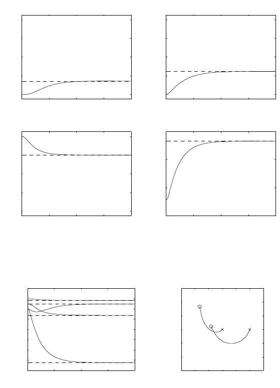
118 10 Visual servoing
0 2 4 6 8
1
1.1
1.2
1.3
1.4
[s]
[m]
x−pos
0 2 4 6 8
1
1.1
1.2
1.3
1.4
[s]
[m]
y−pos
0 2 4 6 8
0.1
0.2
0.3
0.4
0.5
[s]
[m]
z−pos
0 2 4 6 8
0.5
1
1.5
2
[s]
[rad]
alpha
Fig. S10.8. Time history of camera frame position and orientation with position-
based visual servoing scheme of PD type with gravity compensation
0 2 4 6 8
−1
−0.8
−0.6
−0.4
−0.2
0
0.2
[s]
param
−0.2 −0.1 0 0.1 0.2
−0.2
−0.1
0
0.1
0.2
0.3
image plane
Fig. S10.9. Time history of feature parameters and corresponding path of feature
points projections on image plane with position-based visual servoing scheme of PD
type with gravity compensation
Solution to Problem 10.9
The control scheme in Fig. 10.17 is adopted, with the same matrix gain used
in control scheme Bof Sect. 10.9, namely, K=I4.
The initial pose of the camera frame is xc(0) = [ 1 1 0.5π/4]
T,and
the desired pose of the object frame with respect to the camera frame has
been set to xd,o =[−0.10.10.6−π/3]
T.

10 Visual servoing 119
q
xtilde
sinusoidal
functions
cs(q)
controlled
manipulator
1
s
time
splot
estimate
variables
initialization
features
cs x_co
Jacobian
inverse
inv(J_Aq(q))
K
x_do
Fig. S10.10. Simulink block diagram of the resolved-velocity position-based visual
servoing scheme
The pose estimation algorithm is based on the measurements of the fea-
tures of the line segment P1P2, as in the solution to Problem 10.5, using the
same matrix gain, namely, Ks= 160I4. The initial pose estimate is chosen
as ˆ
xc,o(0) = xd,o.
The resulting Simulink block diagram is shown in Fig. S10.10. Notice
that the dynamics of the controlled robot manipulator is approximated by a
simple integrator. All the blocks of the controller are simulated as discrete-
time subsystems with the given sampling time of 4 ms, while the sampling
time of the estimation algorithm has been set to 1 ms.
The files with the solution can be found in Folder 10 9.
The results of Figs. S10.11 and S10.12 (right) are very similar to those
of Figs 10.20 and 10.21 (right), as expected (see also the solution to Prob-
lem 10.8).
Solution to Problem 10.10
The control scheme in Fig. 10.16 is adopted with the matrix gains
KPs =diag{300,300,150,50}KDs =diag{330,330,165,40},
which guarantee a closed-loop dynamics similar to that of control scheme Cin
Sect. 10.9. Notice that, in this case, the dynamics of the closed-loop depends
on the type of feature parameters extracted from visual measurements.
The various terms of the dynamic model of the SCARA manipulator are
computed as in the solution to Problem 7.3.
The initial pose of the camera frame is xc(0) = [ 1 1 0.5π/4]
T,and
the desired value of the feature parameters of the line segment P1P2has
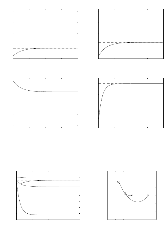
120 10 Visual servoing
0 2 4 6 8
1
1.1
1.2
1.3
1.4
[s]
[m]
x−pos
0 2 4 6 8
1
1.1
1.2
1.3
1.4
[s]
[m]
y−pos
0 2 4 6 8
0.1
0.2
0.3
0.4
0.5
[s]
[m]
z−pos
0 2 4 6 8
0.5
1
1.5
2
[s]
[rad]
alpha
Fig. S10.11. Time history of camera frame position and orientation with resolved-
velocity position-based visual servoing
0 2 4 6 8
−1
−0.8
−0.6
−0.4
−0.2
0
0.2
[s]
param
−0.2 −0.1 0 0.1 0.2
−0.2
−0.1
0
0.1
0.2
0.3
image plane
Fig. S10.12. Time history of feature parameters and corresponding path of fea-
ture points projections on image plane with resolved-velocity position-based visual
servoing
been set to sd=[−0.1250 0.0945 0.1667 −1.0472 ]T, corresponding to
the desired pose xd,o.
Matrix Ls(s,zc) has been approximated with matrix %
Ls=Ls(s,z
d),
where zdis the third component of vector xd,o.
The resulting Simulink block diagram is shown in Fig. S10.13. The arm
is simulated as a continuous-time system using a variable-step integration
method with a maximum step size of 1 ms. All the blocks of the controller are

10 Visual servoing 121
dq
q
sinusoidal
functions
cs(q)
gravity
g(q)
time
splot
J_L(s,zc,q)
features
variables
initialization
features
cs x_co
SCARA arm
inv(B(q))(tau−tau’)
Jacobian
transpose
tr(J_L(s,zc,q))
K_p
K_d
x_do
Fig. S10.13. Simulink block diagram of the image-based visual servoing scheme
of PD type with gravity compensation
simulated as discrete-time subsystems with the given sampling time of 4 ms,
while the sampling time of the estimation algorithm has been set to 1 ms.
The files with the solution can be found in Folder 10 10.
The results are shown in Figs. S10.14 and S10.15. With respect to the
results of Figs 10.22 and 10.23, it can be observed that the phenomenon of
camera retreat is mitigated.
Solution to Problem 10.11
The control scheme in Fig. 10.17 is adopted with the same matrix gain used
in control scheme Cof Sect. 10.9, namely, Ks=I4.
The initial pose of the camera frame is xc(0) = [ 1 1 0.5π/4]
T,and
the desired value of the feature parameters of the line segment P1P2has
been set to sd=[−0.1250 0.0945 0.1667 −1.0472 ]T, corresponding to
the desired pose xd,o.
Matrix Ls(s,zc) has been approximated with matrix %
Ls=Ls(s,z
d),
where zdis the third component of vector xd,o.
The resulting Simulink block diagram is shown in Fig. S10.16. Notice
that the dynamics of the controlled robot manipulator is approximated by a
simple integrator. All the blocks of the controller are simulated as discrete-
time subsystems with the given sampling time of 4 ms, while the sampling
time of the estimation algorithm has been set to 1 ms.
The files with the solution can be found in Folder 10 11.
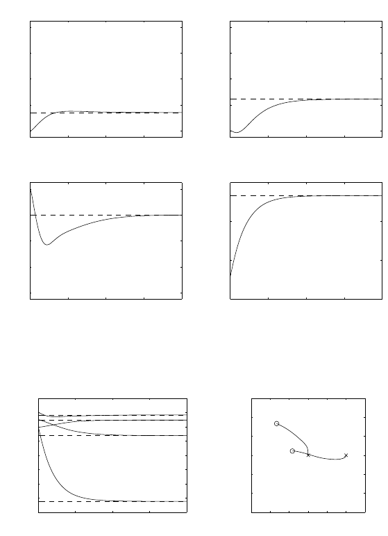
122 10 Visual servoing
0 2 4 6 8
1
1.1
1.2
1.3
1.4
[s]
[m]
x−pos
0 2 4 6 8
1
1.1
1.2
1.3
1.4
[s]
[m]
y−pos
0 2 4 6 8
0.1
0.2
0.3
0.4
0.5
[s]
[m]
z−pos
0 2 4 6 8
0.5
1
1.5
2
[s]
[rad]
alpha
Fig. S10.14. Time history of camera frame position and orientation with image-
based visual servoing scheme of PD type with gravity compensation
0 2 4 6 8
−1
−0.8
−0.6
−0.4
−0.2
0
0.2
[s]
param
−0.2 −0.1 0 0.1 0.2
−0.2
−0.1
0
0.1
0.2
0.3
image plane
Fig. S10.15. Time history of feature parameters and corresponding path of feature
points projections on image plane with image-based visual servoing scheme of PD
type with gravity compensation
The results of Figs. S10.17 and S10.18 (right), with the given choice of
the control gains, are quite similar to those of Figs 10.22 and 10.23 (right).
However, it can be noticed the absence of the phenomenon of camera retreat.
Solution to Problem 10.12
The distance dccan be computed as
dc=ncT rc
c=zcncT )
sp,
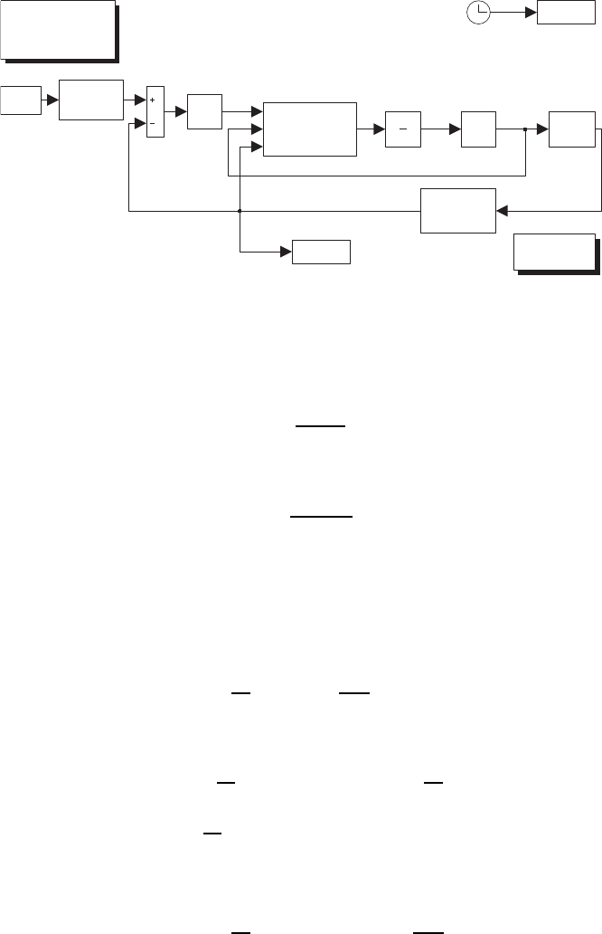
10 Visual servoing 123
q
sinusoidal
functions
cs(q)
controlled
manipulator
1
s
time
splot
features
variables
initialization
features
cs x_co
Jacobian
inverse
inv(J_L(s,zc,q))
K
x_do
Fig. S10.16. Simulink block diagram of the resolved-velocity image-based visual
servoing scheme
and thus
zc=dc
ncT )
sp
.
Analogously, the following equality can be derived
zd=dd
ndT )
sp,d
.
Hence, expression (10.94) follows directly.
In order to derive (10.95), consider that the distance dccan be computed
also as
dc=dd+ncT oc
c,d,
and thus dc
dd
=1+ncT oc
c,d
dd
.
Moreover, the following equality holds
det(H)=det
Rc
d+1
dd
oc
c,dndT =detI+1
dd
oc
c,dncT Rc
d
=det
I+1
dd
oc
c,dncT .
By direct computation, it is possible to verify the identity
det I+1
dd
oc
c,dncT =1+ncT oc
c,d
dd
,

124 10 Visual servoing
0 2 4 6 8
1
1.1
1.2
1.3
1.4
[s]
[m]
x−pos
0 2 4 6 8
1
1.1
1.2
1.3
1.4
[s]
[m]
y−pos
0 2 4 6 8
0.1
0.2
0.3
0.4
0.5
[s]
[m]
z−pos
0 2 4 6 8
0.5
1
1.5
2
[s]
[rad]
alpha
Fig. S10.17. Time history of camera frame position and orientation with resolved-
velocity image-based visual servoing
0 2 4 6 8
−1
−0.8
−0.6
−0.4
−0.2
0
0.2
[s]
param
−0.2 −0.1 0 0.1 0.2
−0.2
−0.1
0
0.1
0.2
0.3
image plane
Fig. S10.18. Time history of feature parameters and corresponding path of feature
points projections on image plane with resolved-velocity image-based visual servoing
and thus dc
dd
=det(H).

10 Visual servoing 125
Solution to Problem 10.13
Notice that
∂ep(rc
c)
∂rc
c
=zc
zdρz
⎡
⎢
⎢
⎢
⎢
⎢
⎢
⎣
−1
zc
0xc
z2
c
0−1
zc
yc
z2
c
00−1
zc
⎤
⎥
⎥
⎥
⎥
⎥
⎥
⎦
=1
zdρz⎡
⎢
⎣−10 X
0−1Y
00−1
⎤
⎥
⎦
S(rc
c)=zc⎡
⎣0−1Y
10−X
−YX 0⎤
⎦.
Hence, in view of (10.26) and (10.96), the following equalities hold
Jp=∂ep(rc
c)
∂rc
c
=1
zdρz⎡
⎢
⎣−10 X
0−1Y
00−1
⎤
⎥
⎦
Jo=−∂ep(rc
c)
∂rc
c
S(rc
c)=⎡
⎢
⎣
XY −1−X2Y
1+Y2−XY −X
−YX0
⎤
⎥
⎦.

11
Mobile Robots
Solution to Problem 11.1
Denote by (x, y) the Cartesian coordinates of a representative point on the
tricycle (e.g., the midpoint of the rear wheel axle), by φthe steering angle
of the front wheel with respect to the vehicle, and by θ0the orientation of
the vehicle with respect to the xaxis. Once the configuration of the tricycle
and of the first i−1 trailers are given, the configuration of the i-th trailer
is completely described by the its orientation θiwith respect to the xaxis.
The configuration vector for the complete vehicle is therefore obtained as q=
[xyφθ
0θ1... θ
N]T, and takes values in IR2×SO(2) ×...×SO(2)
(with SO(2) appearing N+ 2 times). Another possibility is to replace the
absolute angle θiwith the relative angle θi−θi−1to describe the orientation
of each trailer.
Solution to Problem 11.2
Add the kinematic constraints side-by-side to obtain
3˙q3+r(˙q4+˙q5+˙q6)=0
that can be integrated as
q3=−r
3(q4+q5+q6)+c,
where cis an integration constant. The kinematic constraints are then par-
tially integrable. In particular, the orientation q3of the robot is a linear func-
tion of the wheel rotation angles q4,q5,q6.
Solution to Problem 11.3
Consider a single Pfaffian constraint
aT(q)˙
q=
n
j=1
aj(q)˙qj=0.

128 11 Mobile Robots
The corresponding kinematic model is
˙
q=
n−1
j=1
gj(q)uj,
where {g1(q),...,gn−1(q)}is a basis of N(aT(q)). Without loss of generality,
assume that a1(q)= 0, and consider the following choice of input vector fields
g1=
⎡
⎢
⎢
⎢
⎢
⎢
⎢
⎢
⎢
⎢
⎣
−γ(q)a2(q)
γ(q)a1(q)
0
0
.
.
.
0
0
⎤
⎥
⎥
⎥
⎥
⎥
⎥
⎥
⎥
⎥
⎦
g2=
⎡
⎢
⎢
⎢
⎢
⎢
⎢
⎢
⎢
⎢
⎣
−γ(q)a3(q)
0
γ(q)a1(q)
0
.
.
.
0
0
⎤
⎥
⎥
⎥
⎥
⎥
⎥
⎥
⎥
⎥
⎦
... gn−1=
⎡
⎢
⎢
⎢
⎢
⎢
⎢
⎢
⎢
⎢
⎣
−γ(q)an(q)
0
0
0
.
.
.
0
γ(q)a1(q)
⎤
⎥
⎥
⎥
⎥
⎥
⎥
⎥
⎥
⎥
⎦
where γ(q)= 0. The distribution Δ=span{g1,...,gn−1}is involutive if any
Lie bracket [gi,gj] can be written as a linear combination of g1,...,gn−1.
Forexample,consider[g1,g2]. A simple computation gives
[g1,g2]=
⎡
⎢
⎢
⎢
⎢
⎢
⎢
⎢
⎢
⎢
⎢
⎢
⎢
⎢
⎣
∂(γa2)
∂q1γa3−∂(γa3)
∂q1γa2+∂(γa3)
∂q2−∂(γa2)
∂q3γa1
∂(γa1)
∂q3γa1−∂(γa1)
∂q1γa3
∂(γa1)
∂q1γa2−∂(γa1)
∂q2γa1
0
.
.
.
0
⎤
⎥
⎥
⎥
⎥
⎥
⎥
⎥
⎥
⎥
⎥
⎥
⎥
⎥
⎦
Using the integrability condition expressed by (11.9), one easily verifies that
[g1,g2]= ∂(γa3)
∂q1
g1−∂(γa2)
∂q1
g2+∂(γa1)
∂q1
a3g1+a2g2
a1
,
i.e., [g1,g2] is a linear combination of g1,g2.
A similar construction can be repeated for any Lie bracket [gi,gj]; hence,
the distribution Δis involutive under the integrability condition (11.9).
Solution to Problem 11.4
Consider a set of kPfaffian constraints
AT˙
q=0

11 Mobile Robots 129
with a constant constraint matrix AT. Then, the associated kinematic model
˙
q=
m
j=1
gjuj=Gu m=n−k(S11.1)
has constant input vector fields g1,...,gm. Its accessibility distribution ΔA
is clearly involutive, because [gi,gj] = 0 for any i,j. The controllability
condition (11.11) is hence violated, and in particular
dim ΔA(q)=m.
Therefore, the above set of Pfaffian constraints is completely integrable, i.e.,
holonomic. This obvious conclusion could have also been reached by noting
that (S11.1) is in fact a driftless linear system, and using directly the control-
lability rank condition (D.15).
Solution to Problem 11.5
Integration of the kinematic model (11.13) under the given input sequence
starting from the initial configuration q0=[x0y0θ0]Tprovides
x(4ε)=x0+εcos θ0−εcos (θ0+ε)
y(4ε)=y0+εsin θ0−εsin (θ0+ε)
θ(4ε)=θ0.
The displacement is therefore
q(4ε)−q0=⎡
⎣
εcos θ0−εcos (θ0+ε)
εsin θ0−εsin (θ0+ε)
0⎤
⎦=ε2t,
with
t=⎡
⎢
⎢
⎢
⎢
⎣
cos θ0−cos (θ0+ε)
ε
sin θ0−sin (θ0+ε)
ε
0
⎤
⎥
⎥
⎥
⎥
⎦
— compare with the expression of the displacement for a generic two-input
system as given in Appendix D.
Finally, one obtains
lim
ε→0t=⎡
⎢
⎢
⎢
⎣
−dcos θ
dθ ***θ=θ0
−dsin θ
dθ ***θ=θ0
0
⎤
⎥
⎥
⎥
⎦=⎡
⎣
sin θ0
−cos θ0
0⎤
⎦,

130 11 Mobile Robots
that coincides with the value at q0of the Lie Bracket of the two input vector
fields (see Sect. 11.2.1).
Solution to Problem 11.6
With reference to Figs. 1.13 and 11.3, denote by pR=[xRyR]T,pL=
[xLyL]Tand pM=[xMyM]Trespectively the position vector of the
right wheel centre, of the left wheel centre and of the midpoint between the
two. Since
˙xi=rω
icos θ
˙yi=rω
isin θ,
where i=R, L,oneobtains
˙xM=˙xR+˙xL
2=rcos θωR+ωL
2
˙yM=˙yR+˙yL
2=rsin θωR+ωL
2
and therefore
v=˙x2
M+˙y2
M=r(ωR+ωL)
2.
The expression of the angular velocity of the robot can be obtained by
applying the general velocity composition rule (B.4) and making use of the
skew-symmetric operator S(·):
˙
pR=˙
pL+S(ω)(pR−pL), (S11.2)
where
S(ω)=0−ω
ω0
because the motion of the robot is planar. Using the expressions of ˙
pR,˙
pL
and the fact that
pR=pL+dsin θ
−dcos θ,
Equation (S11.2) becomes
rω
Rcos θ
rω
Rsin θ=rω
Lcos θ
rω
Lsin θ+0−ω
ω0dsin θ
−dcos θ.
Squaring and adding side-by-side these two equations leads to
ω2=r2(ωR−ωL)2
d2.

11 Mobile Robots 131
Using again one of the two equations, it can be concluded that the only
solution is
ω=r(ωR−ωL)
d.
Solution to Problem 11.7
With reference to Fig. 11.4, denote by (xC,y
C) the Cartesian coordinates of
the instantaneous centre of rotation Cin the world reference frame, and by
(x
C,y
C) its coordinates in a moving frame having the origin at the centre of
the rear wheel and the xaxis aligned with the bicycle body. Simple geometry
gives x
c
y
c=0
/tan φ
and thus
xc
yc=x
y+R(θ)x
c
y
c=x−sin θ/tan φ
y+cos θ/tan φ,
where
R(θ)=cos θ−sin θ
sin θcos θ
is the (planar) rotation matrix of the moving frame with respect to the world
frame.
Since the velocity vector of a generic point Pon the robot body is tangent
to the circle centred at Cand passing through P, the modulus of the angular
velocity of the bicycle is obtained as
ωbody =vP/RP, (S11.3)
where vPis the modulus of the velocity of P,andRPis its instantaneous
radius of rotation (i.e., its radius of curvature):
RP='(xP−xC)2+(yP−yC)2.
The resulting ωbody is obviously the same for any choice of P.Inparticular,
by choosing Pas the centre of the rear wheel, one has RP=/tan φ, and thus
ωbody =˙
θ=vtan φ/,
consistently with the evolution of θpredicted by the kinematic model (11.19).
Finally, plugging this expression of ωin (S11.3) yields
vP=Rpvtan φ/.

132 11 Mobile Robots
Solution to Problem 11.8
With the configuration vector q=[xyφθ
0θ1...θ
N]Tdefined in the
solution to Problem 11.1, the N+ 2 kinematic constraints are
˙xfsin (θ0+φ)−˙yfcos (θ0+φ)=0
˙xsin θ0−˙ycos θ0=0
˙xisin θi−˙yicos θi=0 i=1,...,N,
where (xf,y
f)and(xi,y
i) are the Cartesian coordinates of the centre of the
tricycle front wheel and of the i-th trailer wheel axle midpoint, respectively
(compare with (11.15), (11.16)). Denote by the distance between the front
wheel and the rear axle of the tricycle, and by ithe hinge-to-hinge length of
the i-th trailer. It is
xf=x+cos θ0
yf=y+sin θ0
and
xi=x−
i
j=1
jcos θj
yi=y−
i
j=1
jsin θj,
so that the kinematic constraints become
˙xsin (θ0+φ)−˙ycos (θ0+φ)−˙
θ0cos φ=0
˙xsin θ0−˙ycos θ0=0
˙xsin θi−˙ycos θi+
i
j=1
˙
θjjcos (θi−θj)=0 i=1,...,N.
The null space of the constraint matrix is spanned by the two columns of
G(q)=
⎡
⎢
⎢
⎢
⎢
⎢
⎢
⎢
⎢
⎢
⎢
⎢
⎢
⎢
⎢
⎢
⎢
⎢
⎢
⎢
⎣
cos θ00
sin θ00
01
1
tan φ0
−1
1sin (θ1−θ0)0
−1
2cos (θ1−θ0)sin(θ2−θ1)0
.
.
..
.
.
−1
i+i−1
j=1 cos (θj−θj−1)sin (θi−θi−1)0
.
.
..
.
.
−1
N+N−1
j=1 cos (θj−θj−1)sin (θN−θN−1)0
⎤
⎥
⎥
⎥
⎥
⎥
⎥
⎥
⎥
⎥
⎥
⎥
⎥
⎥
⎥
⎥
⎥
⎥
⎥
⎥
⎦
=[
g1(q)g2(q)]

11 Mobile Robots 133
(compare with (11.19)). The kinematic control system is then
˙
q=g1(q)v+g2(q)ω,
where vand ωare respectively the driving velocity of the rear wheels and the
steering velocity of the tricycle.
Solution to Problem 11.9
According to (11.14), the velocity inputs of the equivalent unicycle model are
given by
v=r(ωR+ωL)
2
ω=r(ωR−ωL)
d,
where ris the wheel radius and dis the distance between the wheel centres.
Solving for ωRin the first and replacing the obtained expression in the second
yields
ωL=2v−dω
2r
ωR=2v+dω
2r.
The resulting constraints on v,ωare then
****
2v(t)−dω(t)
2r****≤ωRL
****
2v(t)+dω(t)
2r****≤ωRL,
that correspond to a rhombus-shaped admissible region in the v,ωplane.
In particular, the maximum achievable values for these velocities are easily
computed as the intercepts of the sides of the rhombus with the v,ωaxes,
i.e., ±rω
RL for the driving velocity and ±2rω
RL/d for the steering velocity.
Solution to Problem 11.10
The geometric version of the (2,4) chained form is
z
1=)v1
z
2=)v2
z
3=z2)v1
z
4=z3)v1.

134 11 Mobile Robots
Choose the geometric inputs )v1,)v2in the parameterized form (11.49), with
Δ=z1,f −z1,i and s∈[si,s
f]=[0,|Δ|]. Integrating in a recursive fashion the
second, third and fourth equations and setting z2(sf)=z2,f ,z3(sf)=z3,f
and z4(sf)=z4,f leads to a linear system in the form (11.50) where
D=⎡
⎢
⎢
⎢
⎣
|Δ|Δ2
2|Δ|3
3
sgn(Δ)Δ2
2Δ3
6sgn(Δ)Δ4
12
|Δ|3
6Δ4
24 |Δ|5
60
⎤
⎥
⎥
⎥
⎦d=⎡
⎣z2,f −z2,i
z3,f −z3,i −z2,iΔ
z4,f −z4,i −z3,iΔ−z2,i|Δ|⎤
⎦.
Solution to Problem 11.11
It is sufficient to modify (11.48) as follows:
)v1=Δ=z1,f −z1,i,
with the second input (11.49) unchanged. With this choice, z1will reach its
final desired value exactly at sf= 1. The coefficients c0,...,c
n−2in (11.49)
are computed by solving a linear system of equations that is still in the general
form (11.50). For example, in the case of the (2,3) chained form, one obtains
D=11/2
Δ/2Δ/6d=z2,f −z2,i
z3,f −z3,i −z2,iΔ.
Solution to Problem 11.12
As shown in the solution to Problem 11.11, the path planning scheme based
on parameterized inputs (scheme A in the following) must be modified by
letting
)v1=Δ=z1,f −z1,i
to obtain sf= 1 and allow a comparison with the scheme that uses interpolat-
ing polynomials of different degree (scheme B in the following). With scheme
A one has then
z1(s)=z1,i +(z1,f −z1,i)s
that coincides with the expression of z1(s) generated by scheme B. Moreover,
being
)v2=c0+c1s
for a (2,3) chained form, it is
z2(s)=z2,i +c0s+c1s2/2
and
z3(s)=z3,i +Δ,s
0
(c0σ+c1σ2/2)dσ =z3,i +Δ(c0s2/2+c1s3/6).
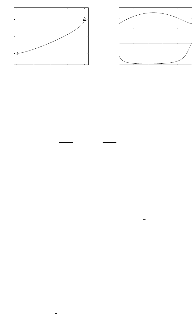
11 Mobile Robots 135
0 0.5 1 1.5 2
0
0.5
1
[m]
[m]
0 0.2 0.4 0.6 0.8 1
0
2
4
[m]
tilde v(s)
0 0.2 0.4 0.6 0.8 1
0
5
10
[rad]
tilde omega(s)
Fig. S11.1. Path planning via Cartesian polynomials; left: Cartesian path of the
unicycle for the required parking manoeuvre, right: geometric inputs along the path
Hence, z3(s) with scheme A is a cubic polynomial in s,asiswithschemeB.
However, there is a unique cubic polynomial that meets the two boundary
conditions on z3and the two boundary conditions on z2
z
3(0)
z
1(0) =z2i
z
3(1)
z
1(1) =z2f.
Hence, the expressions of z3(s) generated by the two schemes coincide. Since
z1and z3are flat outputs for a (2,3) chained form (see the end of Sect. 11.5.2),
a unique z2(s) is associated to z1(s)andz3(s). One can then conclude that
the paths in the zspace (and the associated geometric inputs) generated by
the two schemes are exactly the same.
Solution to Problem 11.13
The files with the solution can be found in Folder 11 13.Fortherequired
manoeuvre, the coefficients of the interpolating polynomials
x(s)=s3xf−(s−1)3xi+αxs2(s−1) + βxs(s−1)2
y(s)=s3yf−(s−1)3yi+αys2(s−1) + βys(s−1)2
are found to be
αx=−6βx=1
αy=−2βy=0
where ki=kf= 1. The corresponding unicycle path is shown in Fig. S11.1.
Using the flatness property of the unicycle, expressed by (11.45), (11.46)
and (11.47), File s11 13.m also generates the geometric inputs )v(s), )ω(s)
along the path, as shown in Fig. S11.1.
There are several ways to find a feasible timing law s=s(t)overthe
planned path. For example, one may simply let s=t,sothatv(t)andω(t)

136 11 Mobile Robots
coincide with )v(s)and)ω(s), respectively. However, both the inputs violate the
given bounds; in particular, the maximum value is attained by ωat 10 rad/sec.
A uniform scaling procedure with T= 10 can then be used to slow down the
trajectory and recover the feasibility of the inputs (see (11.54), (11.55)).
Solution to Problem 11.14
The (2,3) chained form is
˙z1=v1
˙z2=v2
˙z3=z2v1.
Assume that a desired state trajectory (z1d(t),z
2d(t),z
3d(t)) is given. For the
desired trajectory to be feasible, it must satisfy the equations
˙z1d=v1d
˙z2d=v2d
˙z3d=z2dv1d
for some choice of the reference inputs (v1d(t),v
2d(t)). Defining the state errors
ei=zid −zi,fori=1,2,3, and the input errors ui=vid −vi,fori=1,2,
one has the following error dynamics
˙e1=u1
˙e2=u2
˙e3=z2dv1d−z2v1=v1de2+z2du1−e2u1.
Linearization around the reference trajectory yields the time-varying system
˙
e=⎡
⎣
˙e1
˙e2
˙e3⎤
⎦=⎡
⎣
000
000
0v1d0⎤
⎦⎡
⎣
e1
e2
e3⎤
⎦+⎡
⎣
10
01
z2d0⎤
⎦u1
u2=A(t)e+B(t)u.
With the linear time-varying feedback
u1=−k1e1
u2=−k2e2−k3
v1d
e3
the closed-loop linearized error dynamics becomes
˙
e=⎡
⎢
⎣
−k100
0−k2−k3
v1d
−k1z2dv1d0
⎤
⎥
⎦e.

11 Mobile Robots 137
The characteristic polynomial of this system is constant:
p(λ)=(λ+k1)(λ2+k2λ+k3).
The eigenvalues are thus constant, and have negative real part provided that
k1,k2and k3are positive. As discussed in Sect. 11.6.1, this does not guarantee
stability in view of the time-varying nature of the linearized error dynamics,
except for the case when v1dand z2dare constant1. In this case, the linearized
error system becomes time-invariant, and therefore it is asymptotically stable
with the above choice of gains. Hence, the original error system is also asymp-
totically stable at the origin, although this result is not guaranteed to hold
globally.
Solution to Problem 11.15
With reference to the kinematic model (11.19) and Fig. 11.4, consider the
following outputs:
y1=x+cos θ+bcos (θ+φ)
y2=y+sin θ+bsin (θ+φ)
with b= 0. They represent the Cartesian coordinates of a point Pon the line
passing through the centre of the front wheel and oriented as the wheel itself,
located at a distance |b|from the contact point of the wheel with the ground.
The time derivatives of y1and y2are
˙y1
˙y2=cos θ−tan φ(sin θ+bsin (θ+φ)/)−bsin (θ+φ)
sin θ+tanφ(cos θ+bcos (θ+φ)/)bcos (θ+φ)v
ω
=T(θ, φ)v
ω.
Matrix T(θ, φ) has determinant b/cos φ, and is therefore always invertible
under the assumption that b=0and|φ(t)|≤π/2. It is then sufficient to use
the following input transformation
v
ω=T−1(θ, φ)u1
u2
to put the equations of the bicycle in the input-output linearized form:
˙y1=u1
˙y2=u2
˙
θ=sinφ(cos (θ+φ)u1+sin(θ+φ)u2)/
˙
φ=−(cos (θ+φ)sin φ/ +sin(θ+φ)/b)u1
−(sin (θ+φ)sin φ/ −cos (θ+φ)/b)u2.
1One may verify that, if the (2,3) chained form represents a unicycle under the
transformation (11.23), (11.24), constant values of v1dand z2dcorrespond to
reference trajectories over which ωdis constant and vdincreases linearly over
time (as in an Archimedean spiral).
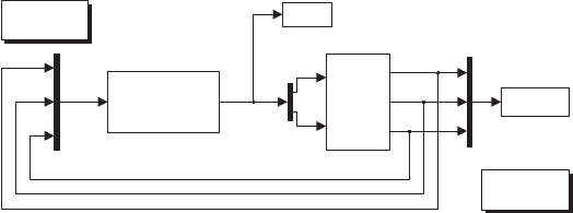
138 11 Mobile Robots
unicycle
v
omega
x
y
theta
inputs
configuration
variables
initialization
plot
Cartesian regulator
configuration inputs
Fig. S11.2. Simulink block diagram of the unicycle with the modified cartesian
regulator
At this point, a simple linear controller such as
u1=˙y1d+k1(y1d−y1)
u2=˙y2d+k2(y2d−y2),
with k1>0, k2>0, guarantees exponential convergence to zero of the Carte-
sian tracking error, with decoupled dynamics on its two components. Note
that the orientation and the steering angle, whose evolutions are governed by
the third and fourth equation, are not controlled.
Solution to Problem 11.16
First of all, note that the Cartesian regulator (11.78), (11.79) may be equiv-
alently written as
v=k1nTep(S11.4)
ω=k2γ, (S11.5)
where n=[cosθsin θ]Tis the unit vector aligned with the sagittal axis,
ep=[−x−y]Tis the Cartesian error and γ=Atan2(y, x)−θ+πis
the pointing error, i.e., the angle between nand ep(see also Fig. 11.18).
Expression (S11.5) shows that ωinduces a rotation until nand epalign, i.e.,
until the unicycle points to the origin; as a consequence, the latter will always
be reached in forward motion.
Now, redefine the steering velocity (S11.5) as follows:
ω=-k2γif nTep>0
k2(γ−sign(γ)π)ifnTep≤0. (S11.6)
With this modification, the unicycle is forced to align with epif the pointing
error is acute, and with −epotherwise. In the second case, the origin will be
reached in backward motion.
Unicycle control with the modified position regulator (S11.4), (S11.6) is
implemented by the Simulink block diagram shown in Fig. S11.2. The files
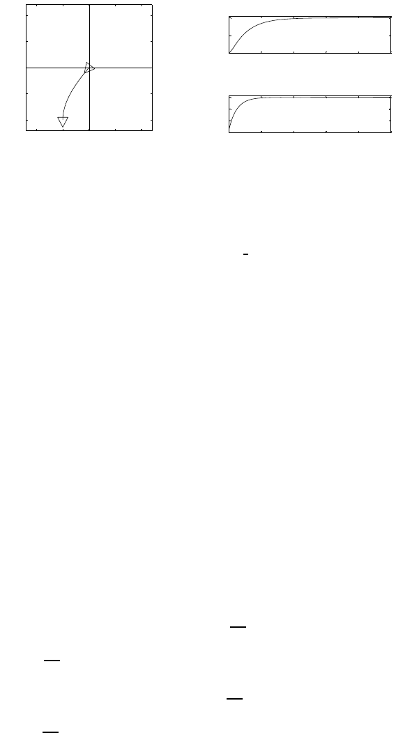
11 Mobile Robots 139
-2 -1 0 1 2
-2
-1
0
1
2
[m]
[m]
0 2 4 6 8 10
-2
-1
0
[m/s]
[s]
driving velocity
0 2 4 6 8 10
-1.5
-1
-0.5
0
[rad/s]
[s]
steering velocity
Fig. S11.3. Regulation to the origin of the Cartesian position of the unicycle with
the modified controller (S11.4), (S11.6); left: Cartesian motion of the unicycle, right:
time evolution of the velocity inputs vand ω
with the solution can be found in Folder 11 16. The unicycle is simulated
as a continuous-time system using a variable-step integration method, with
a maximum step size of 0.01 s. The controller gains can be chosen in the
initialization file.
When the initial pointing error is an acute angle, the modified and the
original position regulators produce exactly the same trajectories. For exam-
ple, this is the case of the simulation in Fig. 11.19 (left). However, in the case
of Fig. 11.19 (right), the initial pointing error is obtuse, and thus the modi-
fied position regulator leads the unicycle to the origin in backward motion, as
shown in Fig. S11.3.
Solution to Problem 11.17
Assume that the velocity inputs are constant within each sampling interval:
v(t)=vkω(t)=ωkt∈[tk,t
k+1].
Integration of the kinematic equations (11.13) of the unicycle readily provides
θ(t)=θk+ωk(t−tk)
and
x(t)=xk+vk,t−tk
0
cos (θk+ωkτ)dτ =xk+vk
ωk
(sin (θk+ωk(t−tk)) −sin θk)
=xk+vk
ωk
(sin θ(t)−sin θk)
y(t)=yk+vk,t−tk
0
sin (θk+ωkτ)dτ =yk−vk
ωk
(cos (θk+ωk(t−tk)) −cos θk)
=yk−vk
ωk
(cos θ(t)−cos θk).
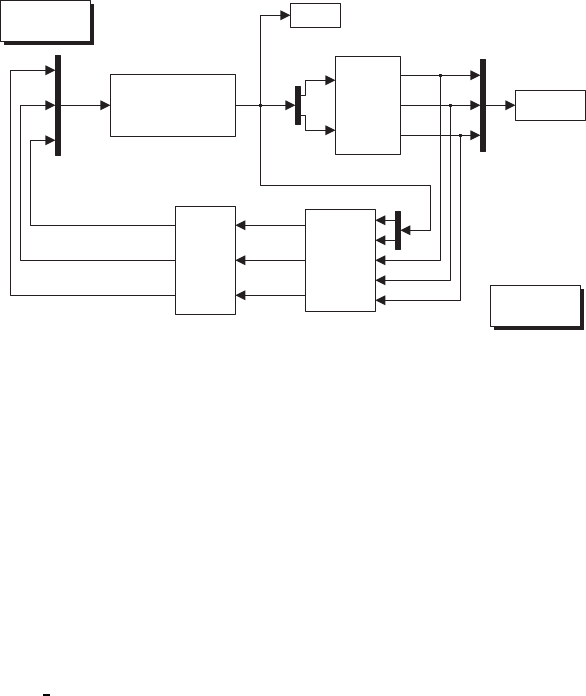
140 11 Mobile Robots
unicycle
v
omega
x
y
theta
posture regulator
polar configuration inputs
odometric localization
with Runge−Kutta
v
omega
x
y
theta
x_k
y_k
theta_k
conversion to
p
olar coordinates
x
y
theta
delta
gamma
rho
inputs
configuration
variables
initialization
plot
Fig. S11.4. Simulink block diagram of the unicycle with the posture regulator and
Runge–Kutta odometric localization
Evaluating the above expressions at t=tk+1 =tk+Tsleads to the odo-
metric prediction (11.85). Alternative proofs can be devised using geometric
arguments (the unicycle travels along an arc of circle during each sampling
interval) or resorting to a chained-form transformation.
Solution to Problem 11.18
Control of the unicycle with the posture regulator (11.81), (11.82) and Runge–
Kutta odometric localization (11.84) is implemented by the Simulink block
diagram shown in Fig. S11.4. The files with the solution can be found in
Folder 11 18. The unicycle is simulated as a continuous-time system using a
variable-step integration method, with a maximum step size of 0.01 s. The
controller gains and the duration Tsof the sampling interval for odometric
localization can be chosen in the initialization file.
The results obtained with Ts=0.01 s and Ts=0.1sareshownin
Fig. S11.5 and Fig. S11.6, respectively. The initial configuration of the unicycle
is the same of Fig. 11.20 (right). Notice how for Ts=0.1 s the low accuracy of
the odometric localization does not hinder the convergence of the unicycle to
the destination. However, a further increase of Tswill ultimately destabilize
the controlled unicycle.
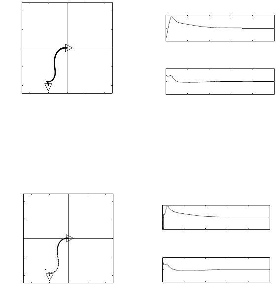
11 Mobile Robots 141
−2−1 0 1 2
−2
−1
0
1
2
[m]
[m]
0 2 4 6 8 10
−2
0
2
[m/s]
[s]
driving velocity
0 2 4 6 8 10
−10
0
10
[rad/s]
[s]
steering velocity
Fig. S11.5. Regulation to the origin of the posture of the unicycle with the con-
troller (11.81), (11.82) and odometric localization (11.84) with Ts=0.01 s; left:
Cartesian motion of the unicycle (continuous) and odometric estimate (dots), right:
time evolution of the velocity inputs vand ω
-2 -1 0 1 2
-2
-1
0
1
2
[m]
[m]
0 2 4 6 8 10
-2
0
2
[m/s]
[s]
driving velocity
0 2 4 6 8 10
-10
0
10
[rad/s]
[s]
steering velocity
Fig. S11.6. Regulation to the origin of the posture of the unicycle with the con-
troller (11.81), (11.82) and odometric localization (11.84) with Ts=0.1s;left:
Cartesian motion of the unicycle (continuous) and odometric estimate (dots), right:
time evolution of the velocity inputs vand ω

12
Motion Planning
Solution to Problem 12.1
The configuration of the mobile manipulator is q=[xyθ
0θ1... θ
6]T,
where (x, y) are the Cartesian coordinates of the contact point of the wheel
with the ground (equivalently, of the wheel centre), θ0is the orientation of the
unicycle with respect to the xaxis, and θ1,...,θ
6are the manipulator joint
variables. The configuration space is therefore C=IR
2×SO(2) ×...×SO(2)
(with SO(2) appearing 7 times), and has dimension 9.
Solution to Problem 12.2
Assume that the configuration qtakes values in the subset Qof Fig. 12.1 —
this can be obtained by computing the joint variables q1and q2modulo 2π).
Given two configurations qA=(q1,A,q
2,A), qB=(q1,B ,q
2,B)inQ, define
Δ1=min(|q1,A −q1,B |,2π−|q1,A −q1,B|)
Δ2=min(|q2,A −q2,B |,2π−|q2,A −q2,B|)
and let
d3(qA,qB)=Δ2
1+Δ2
2.
This definition of configuration space distance clearly satisfies the requirement
of the problem.
Itcanbeeasilyshownthatd3(qA,qB)coincideswithd2(qA,qB)givenby
eq. (12.2) whenever the Euclidean distance between qAand qBis not larger
than √2π.
Solution to Problem 12.3
A possible solution is shown in Fig. S12.1. In the first scene, the robot is
triangular and there is a single square obstacle, while in the second the robot
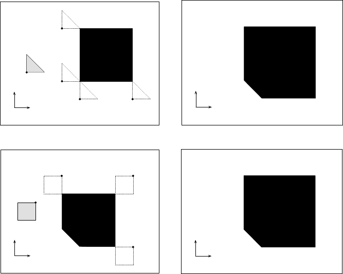
144 12 Motion Planning
B
x
yO
q
q
2
1
C
O
B
x
yO
O
q
q
2
1
C
O
Fig. S12.1. Two different scenes (above/below) that result in the same C-obstacle
region. For each scene, left:therobotB, the obstacle Oand the growing procedure
for building C-obstacles, right: the configuration space Cand the C-obstacle CO
is square and the obstacle is a pentagon. Under the assumption that the robots
can freely translate without changing their orientation, the C-obstacle region
is exactly the same for the two scenes.
Solution to Problem 12.4
The problem can be solved by visual inspection of Fig. 12.4. For example,
the following configurations of the 2R manipulator lie in the three disjoint
components of Cfree:
qa=π/4
π/2qb=4.12
π/6qc=4.12
2.88 [rad].
The manipulator posture and the position in Cfor each of these configurations
is shown in Fig. S12.2.
Solution to Problem 12.5
Consider the lists V={V1,...,V
v}and S={S1,...,S
s}of all the vertices
and sides of the given limited polygonal subset Kof IR2.Aroughsketchof
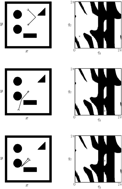
12 Motion Planning 145
Fig. S12.2. Three configurations of the 2R manipulator that lie in disjoint com-
ponents of Cfree :qa(top), qb(centre) and qc(bottom). For each of them, left:the
corresponding manipulator posture, right:thepositioninC
a naive algorithm for computing the generalized Voronoi diagram of Kis the
following.
1. Build all the equidistance curves as follows:
1a. For each vertex-vertex pair (Vi,V
j), derive the equation of the line LViVj
passing through the midpoint of the segment ViVjand orthogonal to
the segment itself.
1b. For each vertex-side pair (Vi,S
j), denote by LSjthe line containing Sj,
and derive the equation of the parabola PViSjhaving Vias focus and
LSjas directrix.
1c. For each side-side pair (Si,S
j), denote by LSiand LSjthe lines con-
taining Siand Sj, respectively, and derive the equation of the bisectrix
LSiSjof the angle formed by LSiand LSjwhich contains Siand Sj.

146 12 Motion Planning
2. For each possible pair of equidistance curves, compute the intersection
points — at most one in the case of a line/line pair, at most two for a
line/parabola or parabola/parabola pair. Each of these points is charac-
terized by the two distances from the features (vertex/vertex, line/line or
line/vertex) that generate the two intersecting equidistance curves.
3. Discard all intersection points that do not belong to K.
4. Discard all intersection points for which the two characteristic distances
are not equal.
5. For each remaining intersection point, compute its clearance, and discard
all intersection points for which the clearance is not equal to the charac-
teristic distance.
6. All the remaining intersection points are nodes of the generalized Voronoi
diagram. Its arcs are the portions of the equidistance curves that are en-
closed by these nodes.
Solution to Problem 12.6
Refer to the example shown in Fig. 12.7, and assume that the goal configu-
ration qgis moved somewhere in cell c6,sothatcs=c3and cg=c6.The
shortest channel joining csto cgis clearly {c3,c
2,c
6}. The path extraction
procedure described in Sect. 12.4.1 would produce a broken line with the fol-
lowing 4 vertices: qs, the midpoint of the common boundary between c3and
c2, the midpoint of the common boundary between c2and c6, and finally qg.
Hence, the second of the 3 edges forming the path would lie completely on the
boundary of cell c2, and in particular would go through the leftmost vertex
of the obstacle.
To solve this problem, the path extraction procedure can be modified
by including additional vertices in the path. For example, in addition to qs,
qgand the midpoints of the common boundaries in the channel, one may
include the centroids (or a generic internal point) of all the cells crossed by
the channel, with the exception of csand cg. In the above case, the resulting
free path would be a broken line with 5 vertices: qs, the midpoint of the
common boundary between c3and c2, the centroid of cell c2, the midpoint of
the common boundary between c2and c6, and finally qg.
Solution to Problem 12.7
The files with the solution can be found in Folder 12 7;runs12 7.m to ex-
ecute the program. The robot is a planar manipulator whose first two joints
are prismatic (so that the base can move arbitrarily) followed by an arbitrary
number of revolute joints. An admissible range can be specified for each joint
variable; in particular, a fixed-base manipulator is specified by setting to zero
the minimum and maximum values of the prismatic joint variables. The ob-
stacles may be line segments, circles or polygons. The user must also input
the start and goal configurations, the maximum number of configurations in
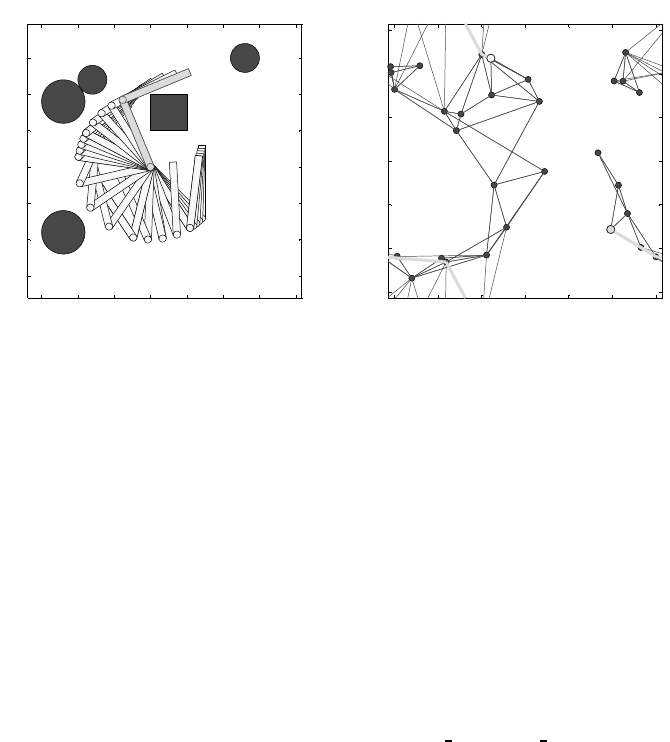
12 Motion Planning 147
-3 -2 -1 0 1 2 3
-3
-2
-1
0
1
2
3
configuration space
-1.5 -1 -0.5 0 0.5 1 1.5 2
-1.5
-1
-0.5
0
0.5
1
1.5
workspace
Fig. S12.3. Motion planning for a 2R planar manipulator via the PRM method;
left: stroboscopic motion of the robot in the workspace, right: the PRM and the
solution path (thick gray) in the configuration space
the roadmap, the maximum number of neighbours to which a new sample can
be connected, and the maximum distance between neighbours.
The solution of a specific planning problem for a 2R fixed-base ma-
nipulator is reported in Fig. S12.3. The start and goal configurations are
qs=[−π/43π/4]Tand qg=[5π/8−π/2]T[rad,rad], respectively. Note
that the configuration space, shown as a square in the figure, is correctly
treated as a two-dimensional torus in the program. In particular, the config-
uration space distance is a generalization of the definition proposed in the
solution to Problem 12.2.
Solution to Problem 12.8
The files with the solution can be found in Folder 12 8;runs12 8.m to execute
the program. The obstacles may be line segments, circles or polygons. The user
must also input the start and goal configurations, the motion primitives (the
discrete set of admissible constant values of the driving and steering velocities
within the time interval Δ), the value of Δand the maximum number of
configurations in the roadmap.
Since the unicycle cannot reach arbitrary configurations in Cfree with this
planner, the program terminates whenever a configuration is reached that is
sufficiently close to the desired goal; to this end, a user-selectable distance
threshold is used. Moreover, to bias the search towards the goal, qrand may
be set to qgoal — rather than to a random configuration — with a probability
that can be chosen arbitrarily.
The solution of a specific problem is reported in Fig. S12.4. The start and
goal configurations are qs=[−300]
Tand qg=[3 −3.50]
T[m,m,rad],
respectively. Note that the unicycle does not exactly reach qg,showningray
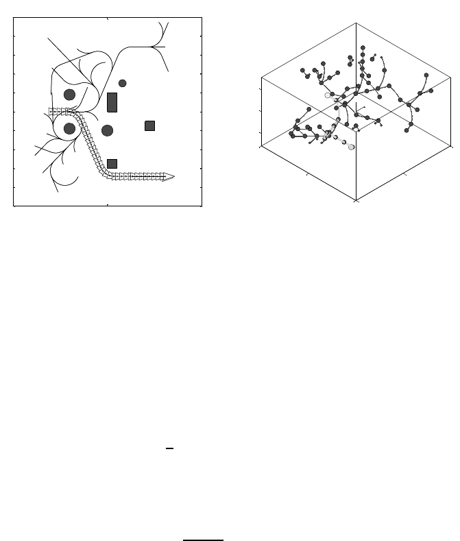
148 12 Motion Planning
-5 0 5
-5
-4
-3
-2
-1
0
1
2
3
4
5
workspace
-5
0
5 -5
0
5
-2
0
2
y
configuration space
x
T
Fig. S12.4. Motion planning for a unicycle via the RRT method; left: stroboscopic
motion of the robot and projection of the RRT on the workspace, right:theRRT
and the solution path (thick gray) in the configuration space
in the stroboscopic plot. The configuration space, shown as a parallelepiped
in the figure, is correctly treated as IR2×SO(2) in the program. In particular,
the configuration space distance is an adaptation of the definition proposed
in the solution to Problem 12.2.
Solution to Problem 12.9
Let
Ua(q)=⎧
⎨
⎩
1
2kae(q)2if e(q)≤ρ
kbe(q)if e(q)>ρ.
Continuity of the attractive force at the transition radius ρis guaranteed by
imposing
kae(q)=kb
e(q)
e(q)for e(q)=ρ,
i.e., kb=ρk
a.
Solution to Problem 12.10
Consider Fig. S12.5, and in particular the half-line that originates at qgand
passes through the centre of the obstacle. Visualize a point that travels along
this half-line, coming from the point at infinity, where the total potential is
infinity — because of the attractive potential. The total potential goes back
to infinity when the point reaches the boundary of the obstacle — because of
the repulsive potential. Therefore, there is a point on the line where Uhas a
local minimum; call this point P.
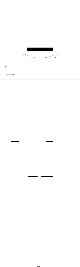
12 Motion Planning 149
R/
\4
h
?
r
Fig. S12.5. The emergence of local minima due to the superposition of attractive
and repulsive potentials
Now consider points Aand Bthat are located along the same equipoten-
tial contour of the repulsive potential Uras P. Since the attractive potential
is higher at Aand Bthan at C,Pis a local minimum also in the direction of
the line AB.Informulæ:
∂U
∂x ****P
=0 ∂U
∂y ****P
=0,
which imply that Pis a stationary point for U, i.e., the gradient of Uis zero
at P. To show that Pis indeed a local minimum, one should consider the
Hessian matrix of U⎡
⎢
⎢
⎢
⎣
∂2U
∂x2
∂U
∂x∂y
∂U
∂y∂x
∂2U
∂y2
⎤
⎥
⎥
⎥
⎦
and prove that it is positive definite in P. This can be verified by using the
analytic expression of U. Note that the elements of the diagonal are certainly
positive in Pin view of the above arguments.
Solution to Problem 12.11
Denote by (x, y) the Cartesian coordinates of the robot, by (xi,y
i)theCarte-
sian coordinates of the centre Ciof the i-th circular obstacle, and by ρiits
radius. The attractive potential is
Ua(x, y)=1
2ka(x2+y2),

150 12 Motion Planning
while the repulsive potentials (γ=2)are
Ur,i(x, y)=⎧
⎪
⎨
⎪
⎩
kr,i
21
ηi(x, y)−1
η0,i 2
if ηi(x, y)≤η0,i
0ifηi(x, y)>η
0,i,
for i=1,2,3, with ηi(x, y)='(x−xi)2+(y−yi)2−ρi. The total potential
is
Ut(x, y)=Ua(x, y)+
3
i=1
Ur,i(x, y),
while the total force is
f(x, y)=fa(x, y)+
3
i=1
fr,i(x, y)
with
fa(x, y)=−kax
y
and
fr,i(x, y)=⎧
⎪
⎪
⎪
⎨
⎪
⎪
⎪
⎩
kr,i
η2
i(x, y)1
ηi(x, y)−1
η0,i ∇ηi(x, y)ifηi(x, y)≤η0,i
0ifηi(x, y)>η
0,i.
In view of the above expression for ηi(x, y), one has
∇ηi(x, y)=⎡
⎢
⎢
⎢
⎣
x−xi
'(x−xi)2+(y−yi)2
y−yi
'(x−xi)2+(y−yi)2
⎤
⎥
⎥
⎥
⎦.
The actual numerical expressions depend on the choice of the constants ka
and kr,i ,fori=1,2,3, as well as of the obstacle range of influence η0,i.
Assuming that the ranges of influence of the obstacles do not overlap,
the saddle points of the total potential will be clearly located along the lines
that join the origin of the reference frame (the goal) with the centres of the
circular obstacles, in the ‘shadow zone’ of each obstacle. In particular, the
saddle points are found by solving the equations
−kax
y=kr,i
η2
i(x, y)1
ηi(x, y)−1
η0,i ∇ηi(x, y)i=1,2,3,
each representing the balance between the attractive force and the i-th repul-
sive force.
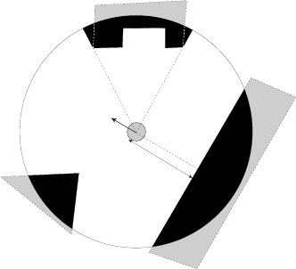
12 Motion Planning 151
ODVHUVFDQ
DUHD
URERW
n
n
n
.d
.1
.n
Fig. S12.6. On-line planning based on artificial potential fields for a circular mobile
robot equipped with a rotating laser range finder.
Solution to Problem 12.12
In principle, there are two main approaches for on-line motion planning based
on sensor data.
•The first approach is to store the data coming from the sensors in a map —
i.e., a representation of the portion of the environment that the robot has
visited so far — and use it to plan in an incremental fashion (deliberative
planning).
•The second approach is to react only to the obstacles that are currently
perceived of the robot, without any form of memory (reactive planning).
The artificial potential field technique naturally lends itself to a reactive
implementation, as briefly discussed below.
Refer to the situation shown in Fig. S12.6. The workspace obstacles O1,
O2and O3are depicted in black for the portion falling inside the laser scan
area, and in gray outside. Note how the perceived obstacle is larger than
the actual obstacle for O2, due to the fact that the laser range finder is a
visibility-based sensor.
Consider first the case of a point robot. Since the goal is known, the
attractive potential can be built as in the off-line case — this is true provided
that the robot is equipped with a localization module. To build the repulsive
potential, it is reasonable to define the range of influence η0,i of the obstacles
to be smaller than the maximum measurable range R—iftherobotdoesnot
detect the obstacle, it does not react to it. A typical choice is η0,i =R, for all
i. As seen in Sect. 12.6.2, the perceived obstacle region must be decomposed
in convex components to guarantee continuity of the repulsive potential field;
in the case of Fig. S12.6, only O2needs to undergo this procedure. At this
point, the repulsive force produced by each convex component is computed as
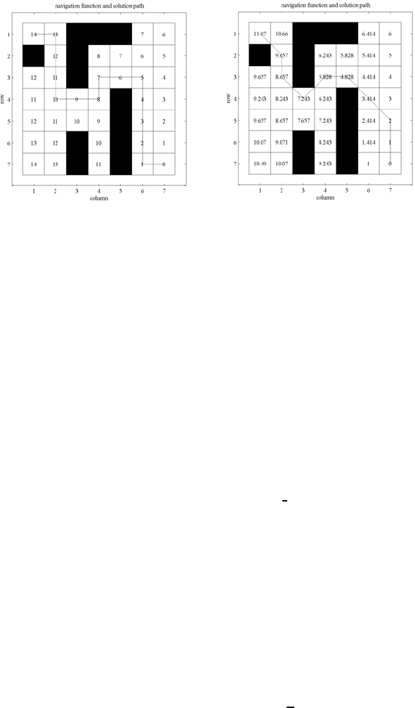
152 12 Motion Planning
Fig. S12.7. The assigned occupancy grid, the navigation function and the solution
path from cell (1,1) to cell (7,7); left: using 1-adjacency, right: using 2-adjacency
in (12.15), with ηi,∇ηidirectly obtained from the range scan profile — see
the example in Fig. S12.6.
In the case of a robot with a finite nonzero radius ρ, one simply uses ηi−ρ
in place of ηiin (12.15), and obtains ∇ηias in the point robot case.
It is easy to realize that this reactive version of the artificial potential
method behaves exactly as the off-line version, in the sense that the resulting
motion of the robot is the same. Clearly, this is true as long as the envi-
ronment is continuously scanned during the motion and the above procedure
for computing the potential field can be efficiently implemented, so as to be
executed within the duration of the motion control cycle.
Solution to Problem 12.13
The files with the solution can be found in Folder 12 13. The user is required to
input the binary gridmap representing the configuration space, the start and
goal cells, and the adjacency type (1- or 2-adjacency). The cells are assumed
to be squares with unit side. During the expansion of the wavefront that
originates at qg, the increase of the navigation function between adjacent cells
(cost-to-go) is set equal to the Euclidean distance between the cell centres.
The solution path is then found by following the steepest descent from the
goal cell.
For illustration, Fig. S12.7 shows the results obtained on a (7×7) gridmap,
with (1,1) as the start cell and (7,7) as the goal cell. The path found using
2-adjacency is shorter as expected. It is easy to realize that even when the
solution paths are in the same homotopy class — i.e., one can be continu-
ously deformed into the other — the 1-adjacency path may be longer than
the 2-adjacency path by a factor of as much as √2. On the other hand, 2-
adjacency produces paths that may graze the C-obstacles; as a consequence,
it is recommended that these are slightly enlarged before planning.

http://www.springer.com/978-1-84628-641-4
