DOX Solutions 02 DDP 2 Manual
Solutions%20Manual(%EC%8B%A4%EA%B3%84%20%EC%97%B0%EC%8A%B5%EB%AC%B8%EC%A0%9C%20%EC%86%94%EB%A3%A8%EC%85%98)
User Manual: DDP-2
Open the PDF directly: View PDF ![]() .
.
Page Count: 488 [warning: Documents this large are best viewed by clicking the View PDF Link!]
Solutions from Montgomery, D. C. (2001) Design and Analysis of Experiments, Wiley, NY
2-1
Chapter 2
Simple Comparative Experiments
Solutions
2-1 The breaking strength of a fiber is required to be at least 150 psi. Past experience has indicated that
the standard deviation of breaking strength is
V
= 3 psi. A random sample of four specimens is tested. The
results are y1=145, y2=153, y3=150 and y4=147.
(a) State the hypotheses that you think should be tested in this experiment.
H
0: P = 150 H1: P > 150
(b) Test these hypotheses using
D
= 0.05. What are your conclusions?
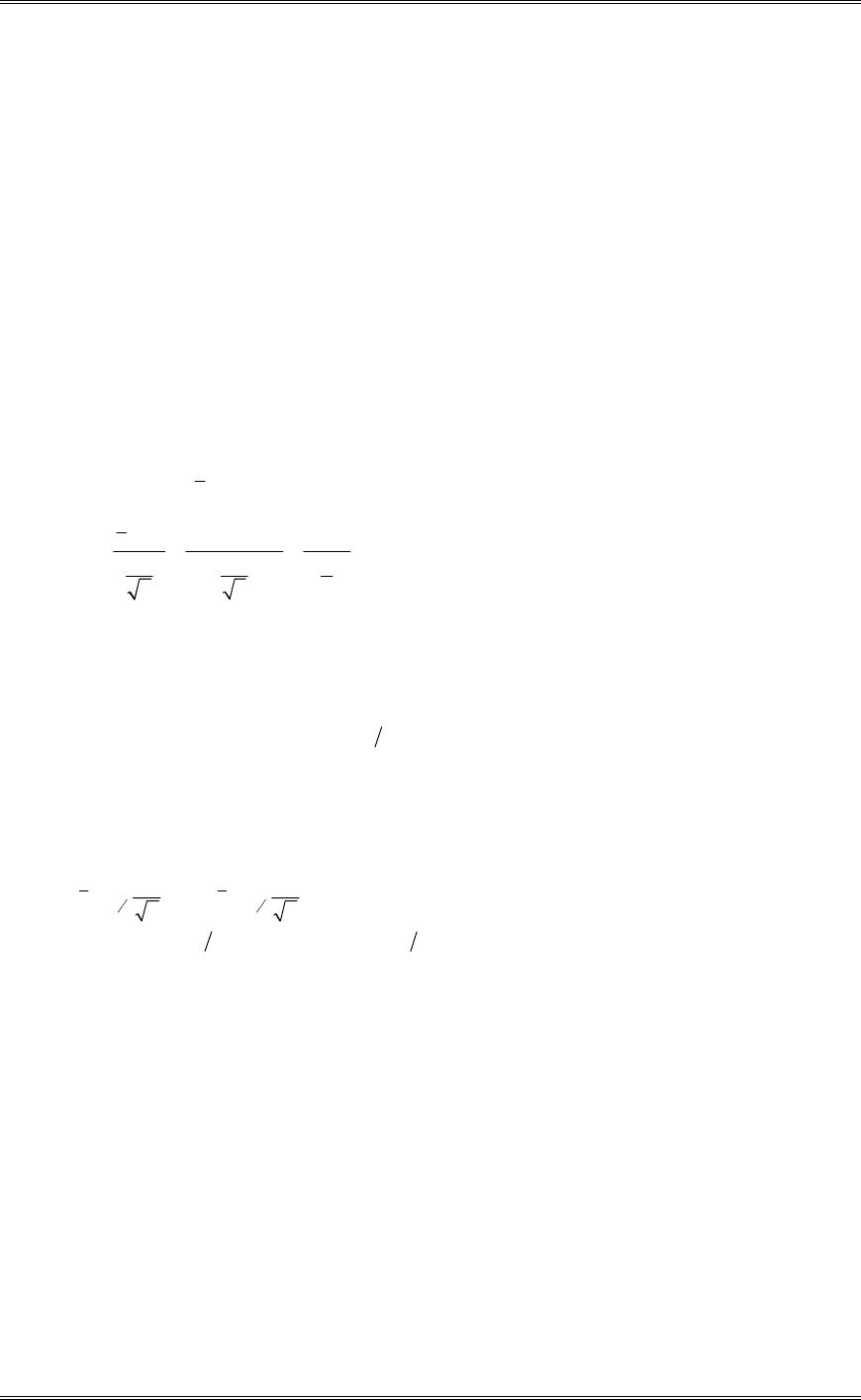
n = 4,
V
= 3, y= 1/4 (145 + 153 + 150 + 147) = 148.75
148.75 150 1.25 0.8333
33
2
4
o
o
y
z
n
P
V
Since z0.05 = 1.645, do not reject.
(c) Find the P-value for the test in part (b).
From the z-table:
>@
20140796707995032796701 ....P #
(d) Construct a 95 percent confidence interval on the mean breaking strength.
The 95% confidence interval is
2396.175.1482396.175.148
22
dd
dd
P
V
P
V
DD
n
zy
n
zy
145 81 151 69..dd
P
2-2 The viscosity of a liquid detergent is supposed to average 800 centistokes at 25qC. A random
sample of 16 batches of detergent is collected, and the average viscosity is 812. Suppose we know that the
standard deviation of viscosity is
V
= 25 centistokes.
(a) State the hypotheses that should be tested.
H
0:
P
= 800 H1:
P
z 800
(b) Test these hypotheses using
D
= 0.05. What are your conclusions?
Solutions from Montgomery, D. C. (2001) Design and Analysis of Experiments, Wiley, NY
2-2
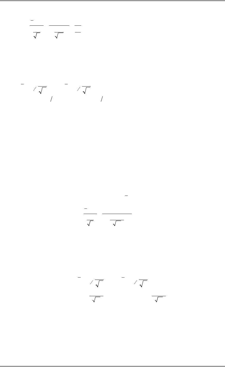
812 800 12 1.92
25 25
4
16
o
o
y
z
n
P
V
Since z
D
/2 = z0.025 = 1.96, do not reject.
(c) What is the P-value for the test? P 2 0 0274 0 0549(. ) .
(d) Find a 95 percent confidence interval on the mean.
The 95% confidence interval is
n
zy
n
zy
V
P
V
DD
22 dd
2582475799
25128122512812
425961812425961812
..
..
..
dd
dd
dd
P
P
P
2-3 The diameters of steel shafts produced by a certain manufacturing process should have a mean
diameter of 0.255 inches. The diameter is known to have a standard deviation of
V
= 0.0001 inch. A
random sample of 10 shafts has an average diameter of 0.2545 inches.
(a) Set up the appropriate hypotheses on the mean
P
.
H
0:
P
= 0.255 H1:
P
z 0.255
(b) Test these hypotheses using
D
= 0.05. What are your conclusions?
n = 10,
V
= 0.0001, y= 0.2545
0.2545 0.255 15.81
0.0001
10
o
o
y
z
n
P
V
Since z0.025 = 1.96, reject H0.
(c) Find the P-value for this test. P=2.6547x10-56
(d) Construct a 95 percent confidence interval on the mean shaft diameter.
The 95% confidence interval is
n
zy
n
zy
V
P
V
DD
22 dd
0.0001 0.0001
0.2545 1.96 0.2545 1.96
10 10
P
§· §·
dd
¨¸ ¨¸
©¹ ©¹
0 254438 0 254562..dd
P
2-4 A normally distributed random variable has an unknown mean P and a known variance
V
2 = 9. Find
the sample size required to construct a 95 percent confidence interval on the mean, that has total width of
1.0.
Solutions from Montgomery, D. C. (2001) Design and Analysis of Experiments, Wiley, NY
2-3
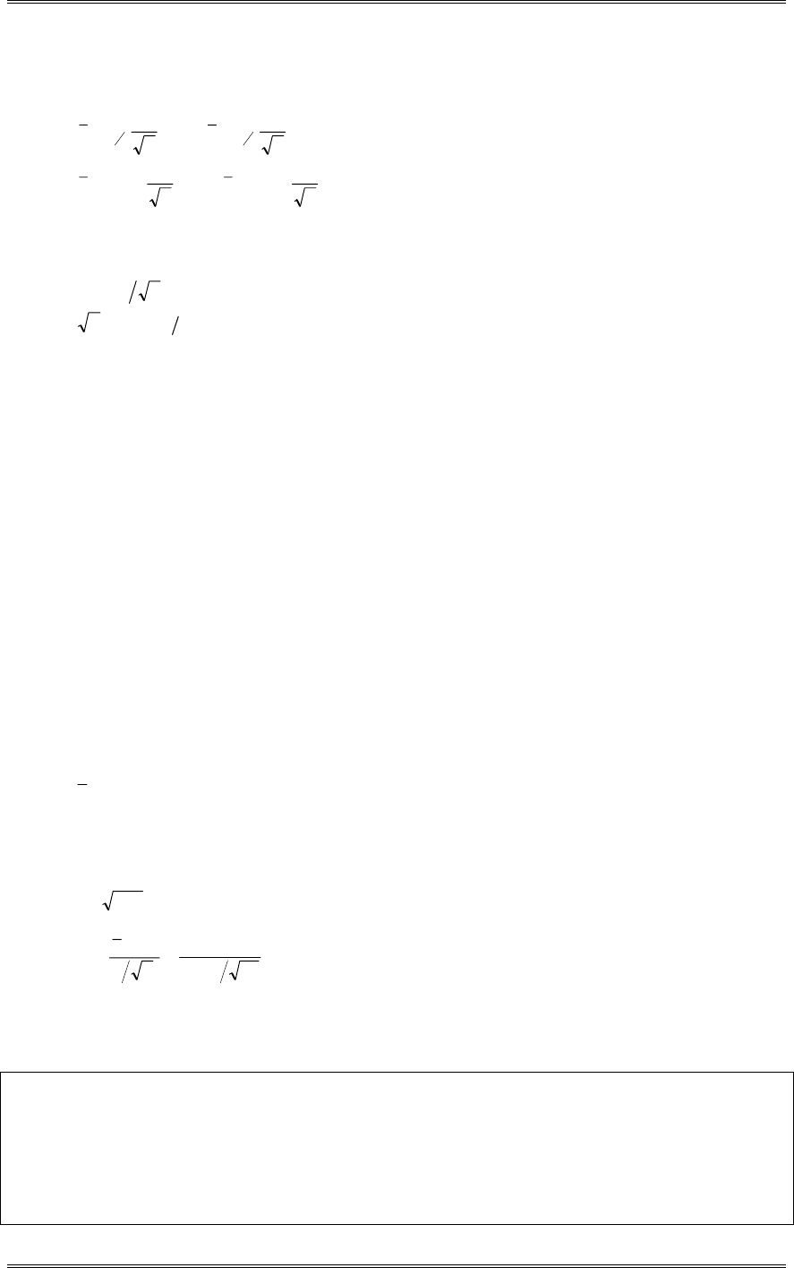
Since y a N(
P
,9), a 95% two-sided confidence interval on
P
is
yz nyz n
dd
DD
VPV
22
ynyn
dd(. ) (. )196 3196 3
P
If the total interval is to have width 1.0, then the half-interval is 0.5. Since z/2 = z0.025 = 1.96,
139301387611
7611503961
503961
2#
..n
...n
.n.
2-5 The shelf life of a carbonated beverage is of interest. Ten bottles are randomly selected and tested,
and the following results are obtained:
Days
108 138
124 163
124 159
106 134
115 139
(a) We would like to demonstrate that the mean shelf life exceeds 120 days. Set up appropriate
hypotheses for investigating this claim.
H
0:
P
= 120 H1:
P
> 120
(b) Test these hypotheses using
D
= 0.01. What are your conclusions?
y= 131
s2 = [ (108 - 131)2 + (124 - 131)2 + (124 - 131)2 + (106 - 131)2 + (115 - 131)2 + (138 - 131)2
+ (163 - 131)2 + (159 - 131)2 + (134 - 131)2 + ( 139 - 131)2 ] / (10 - 1)
s2 = 3438 / 9 = 382
s 382 19 54.
ty
sn
o
o
P
131 120
19 54 10 178
..
since t0.01,9 = 2.821; do not reject H0
Minitab Output
T-Test of the Mean
Test of mu = 120.00 vs mu > 120.00
Variable N Mean StDev SE Mean T P
Shelf Life 10 131.00 19.54 6.18 1.78 0.054
T Confidence Intervals
Solutions from Montgomery, D. C. (2001) Design and Analysis of Experiments, Wiley, NY
2-4
Variable N Mean StDev SE Mean 99.0 % CI
Shelf Life 10 131.00 19.54 6.18 ( 110.91, 151.09)
(c) Find the P-value for the test in part (b). P=0.054
(d) Construct a 99 percent confidence interval on the mean shelf life.
The 95% confidence interval is n
s
ty
n
s
ty n,n, 1
2
1
2 dd
DD P
1954 1954
131 3.250 131 3.250
10 10
P
§· §·
dd
¨¸ ¨¸
©¹ ©¹
110 91 15109..
dd
P
2-6 Consider the shelf life data in Problem 2-5. Can shelf life be described or modeled adequately by a
normal distribution? What effect would violation of this assumption have on the test procedure you used in
solving Problem 2-5?
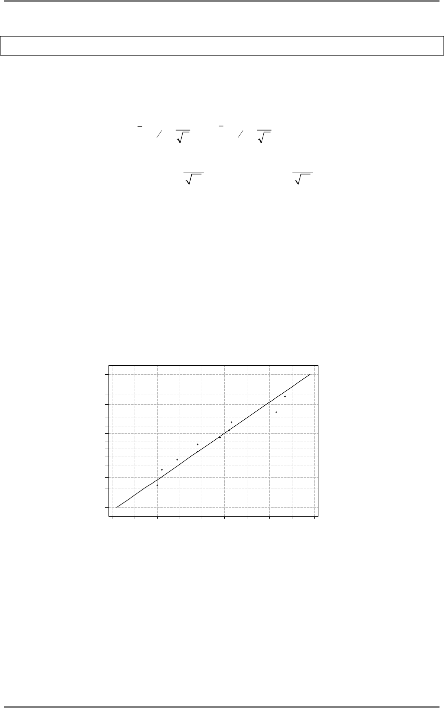
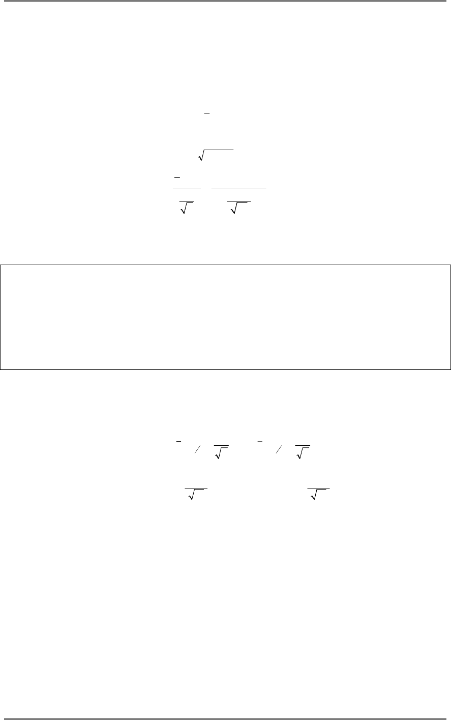
A normal probability plot, obtained from Minitab, is shown. There is no reason to doubt the adequacy of
the normality assumption. If shelf life is not normally distributed, then the impact of this on the t-test in
problem 2-5 is not too serious unless the departure from normality is severe.
1761661561461361261161069686
99
95
90
80
70
60
50
40
30
20
10
5
1
Data
Percent
1.292AD*
Goodness of Fit
Normal Probability Plot for Shelf Life
ML Estimates
Mean
StDev
131
18.5418
ML Estimates
2-7 The time to repair an electronic instrument is a normally distributed random variable measured in
hours. The repair time for 16 such instruments chosen at random are as follows:
Hours
159 280 101 212
224 379 179 264
222 362 168 250
149 260 485 170
Solutions from Montgomery, D. C. (2001) Design and Analysis of Experiments, Wiley, NY
2-5
(a) You wish to know if the mean repair time exceeds 225 hours. Set up appropriate hypotheses for
investigating this issue.
H
0:
P
= 225 H1:
P
> 225
(b) Test the hypotheses you formulated in part (a). What are your conclusions? Use
D
= 0.05.
y= 247.50
s2 =146202 / (16 - 1) = 9746.80
s 9746 8 98 73..
241.50 225 0.67
98.73
16
o
o
y
ts
n
P
since t0.05,15 = 1.753; do not reject H0
Minitab Output
T-Test of the Mean
Test of mu = 225.0 vs mu > 225.0
Variable N Mean StDev SE Mean T P
Hours 16 241.5 98.7 24.7 0.67 0.26
T Confidence Intervals
Variable N Mean StDev SE Mean 95.0 % CI
Hours 16 241.5 98.7 24.7 ( 188.9, 294.1)
(c) Find the P-value for this test. P=0.26
(d) Construct a 95 percent confidence interval on mean repair time.
The 95% confidence interval is
n
s
ty
n
s
ty n,n, 1
2
1
2 dd
DD P
98.73 98.73
241.50 2.131 241.50 2.131
16 16
P
§· §·
dd
¨¸ ¨¸
©¹ ©¹
12949188 .. dd
P
2-8 Reconsider the repair time data in Problem 2-7. Can repair time, in your opinion, be adequately
modeled by a normal distribution?
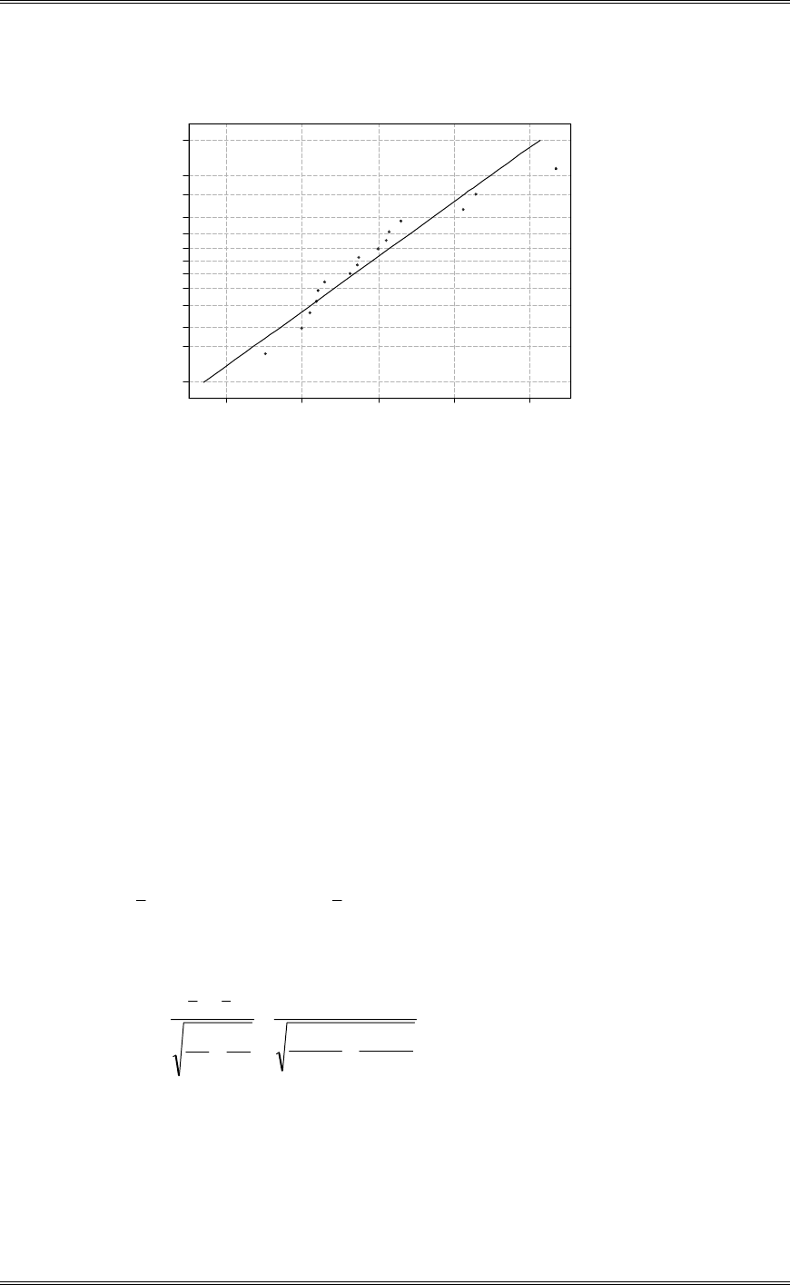
The normal probability plot below does not reveal any serious problem with the normality assumption.
Solutions from Montgomery, D. C. (2001) Design and Analysis of Experiments, Wiley, NY
2-6
45035025015050
99
95
90
80
70
60
50
40
30
20
10
5
1
Data
Percent
1.185AD*
Goodness of Fit
Normal Probability Plot for Hours
ML Estimates
Mean
StDev
241.5
95.5909
ML Estimates
2-9 Two machines are used for filling plastic bottles with a net volume of 16.0 ounces. The filling
processes can be assumed to be normal, with standard deviation of
V
1 = 0.015 and
V
2 = 0.018. The quality
engineering department suspects that both machines fill to the same net volume, whether or not this volume
is 16.0 ounces. An experiment is performed by taking a random sample from the output of each machine.
Machine 1 Machine 2
16.03 16.01 16.02 16.03
16.04 15.96 15.97 16.04
16.05 15.98 15.96 16.02
16.05 16.02 16.01 16.01
16.02 15.99 15.99 16.00
(a) State the hypotheses that should be tested in this experiment.
H
0:
P
1 =
P
2 H
1:
P
1 z
P
2
(b) Test these hypotheses using
D
=0.05. What are your conclusions?
y
n
1
1
1
16 015
0 015
10
.
.
V
y
n
2
2
2
16 005
0 018
10
.
.
V
zyy
nn
o
12
1
2
1
2
2
2
22
16 015 16 018
0 015
10
0 018
10
135
VV
..
..
.
z0.025 = 1.96; do not reject
(c) What is the P-value for the test? P=0.1770
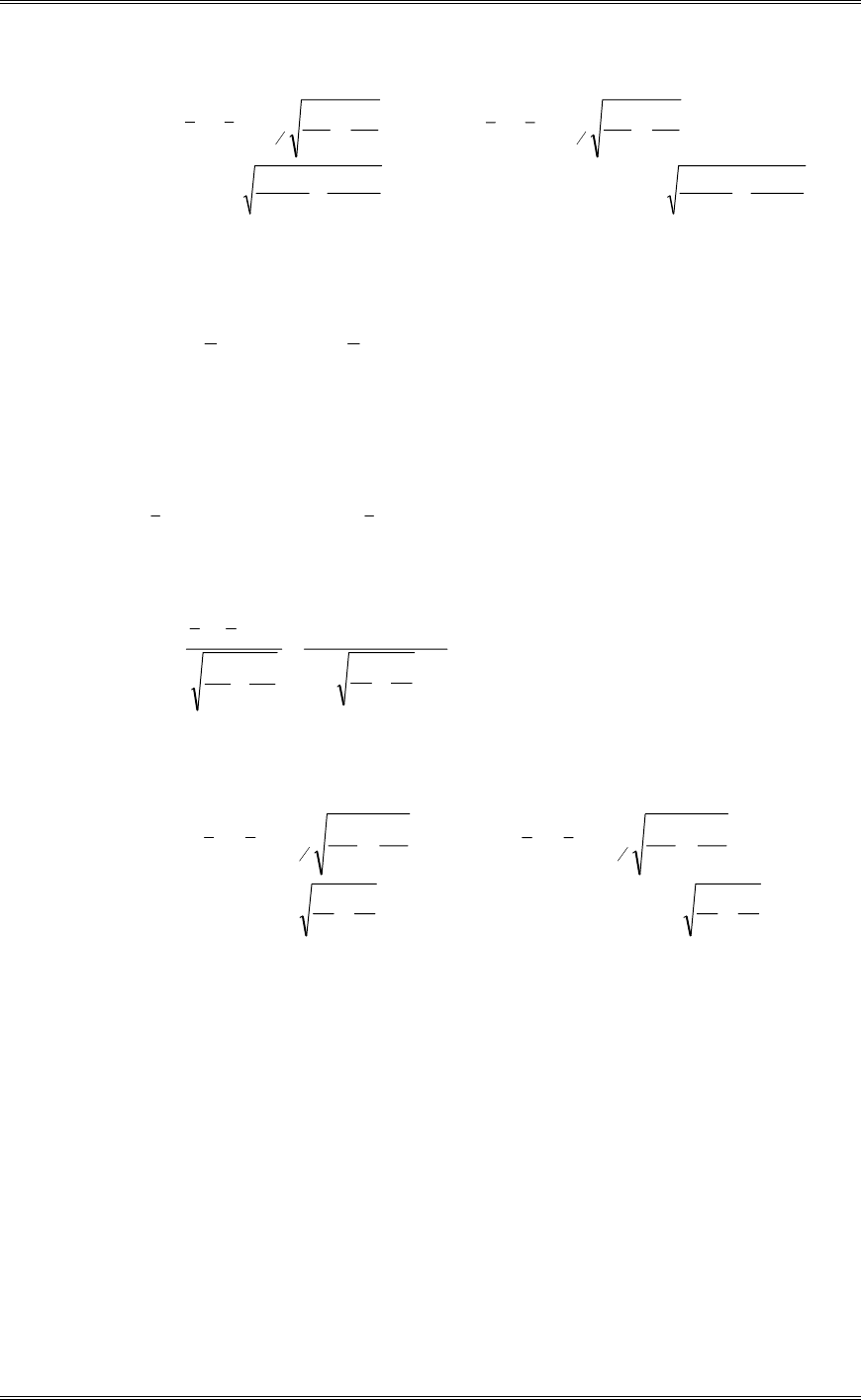
(d) Find a 95 percent confidence interval on the difference in the mean fill volume for the two machines.
Solutions from Montgomery, D. C. (2001) Design and Analysis of Experiments, Wiley, NY
2-7
The 95% confidence interval is
2
2
2
1
2
1
2121
2
2
2
1
2
1
21 22 nn
zyy
nn
zyy
VV
PP
VV
DD
dd
10
018.0
10
015.0
)6.19()005.16015.16(
10
018.0
10
015.0
)6.19()005.16015.16(
22
21
22 dd
PP
0245.00045.0 21 dd
PP
2-10 Two types of plastic are suitable for use by an electronic calculator manufacturer. The breaking
strength of this plastic is important. It is known that
V
1 =
V
2 = 1.0 psi. From random samples of n1 = 10
and n2 = 12 we obtain y1 = 162.5 and y2 = 155.0. The company will not adopt plastic 1 unless its
breaking strength exceeds that of plastic 2 by at least 10 psi. Based on the sample information, should they
use plastic 1? In answering this questions, set up and test appropriate hypotheses using
D
= 0.01.
Construct a 99 percent confidence interval on the true mean difference in breaking strength.
H
0:
P
1 -
P
2 =10 H1:
P
1 -
P
2 >10
10
1
5162
1
1
1
n
.y
V
10
1
0155
2
2
2
n
.y
V
zyy
nn
o
12
1
2
1
2
2
2
22
10 162 5 155 0 10
1
10
1
12
585
VV
.. .
z0.01 = 2.225; do not reject
The 99 percent confidence interval is
2
2
2
1
2
1
2121
2
2
2
1
2
1
21 22 nn
zyy
nn
zyy
VV
PP
VV
DD
dd
12
1
10
1
)575.2()0.1555.162(
12
1
10
1
)575.2()0.1555.162(
22
21
22 dd
PP
60.840.6 21 dd
PP
2-11 The following are the burning times of chemical flares of two different formulations. The design
engineers are interested in both the means and variance of the burning times.
Type 1 Type 2
65 82 64 56
81 67 71 69
57 59 83 74
66 75 59 82
82 70 65 79
(a) Test the hypotheses that the two variances are equal. Use
D
= 0.05.

Solutions from Montgomery, D. C. (2001) Design and Analysis of Experiments, Wiley, NY
2-8
H
H
01
2
2
2
1
2
2
2
1
:
:
VV
VV
z S
S
1
2
9 264
9 367
.
.
FS
S
0
1
2
2
2
8582
87 73 098
.
..
F002599 403
.,, . FF
09759 9
00259 9
11
403 0 248
.,,
.,, .. Do not reject.
(b) Using the results of (a), test the hypotheses that the mean burning times are equal. Use
D
= 0.05.
What is the P-value for this test?
SnSn S
nn
S
tyy
Snn
p
p
p
21 1
2
22
2
12
0
12
12
11
2
156195
18 86 775
932
11
70 4 70 2
932 1
10
1
10
0 048
()( ) ..
.
..
.
.
t002518 2 101
., . Do not reject.
From the computer output, t=0.05; do not reject. Also from the computer output P=0.96
Minitab Output
Two Sample T-Test and Confidence Interval
Two sample T for Type 1 vs Type 2
N Mean StDev SE Mean
Type 1 10 70.40 9.26 2.9
Type 2 10 70.20 9.37 3.0
95% CI for mu Type 1 - mu Type 2: ( -8.6, 9.0)
T-Test mu Type 1 = mu Type 2 (vs not =): T = 0.05 P = 0.96 DF = 18
Both use Pooled StDev = 9.32
(c) Discuss the role of the normality assumption in this problem. Check the assumption of normality for
both types of flares.
The assumption of normality is required in the theoretical development of the t-test. However, moderate
departure from normality has little impact on the performance of the t-test. The normality assumption is
more important for the test on the equality of the two variances. An indication of nonnormality would be
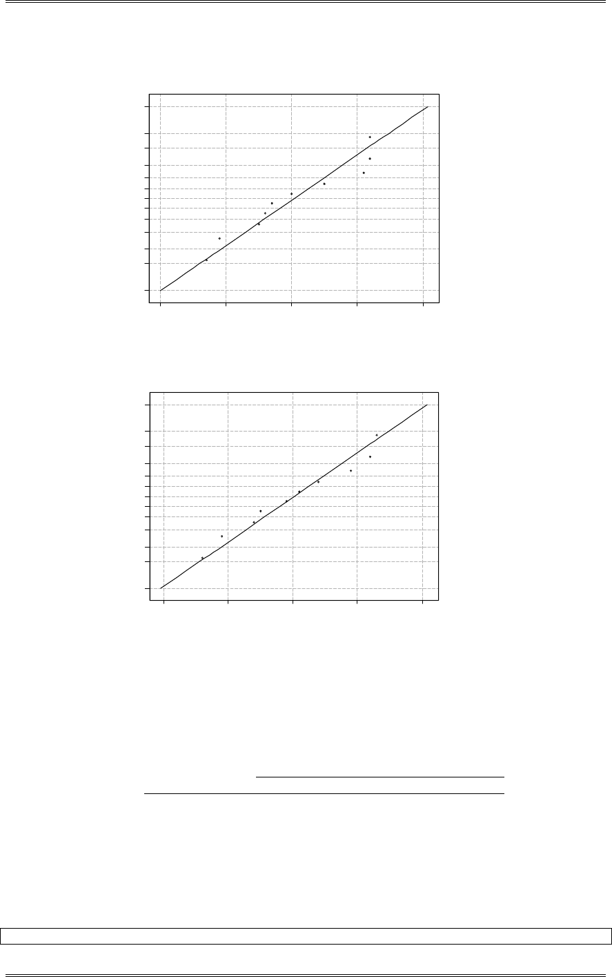
of concern here. The normal probability plots shown below indicate that burning time for both
formulations follow the normal distribution.
Solutions from Montgomery, D. C. (2001) Design and Analysis of Experiments, Wiley, NY
2-9
9080706050
99
95
90
80
70
60
50
40
30
20
10
5
1
Data
Percent
1.387AD*
Goodness of Fit
Normal Probability Plot for Type 1
ML Estimates
Mean
StDev
70.4
8.78863
ML Estimates
9080706050
99
95
90
80
70
60
50
40
30
20
10
5
1
Data
Percent
1.227AD*
Goodness of Fit
Normal Probability Plot for Type 2
ML Estimates
Mean
StDev
70.2
8.88594
ML Estimates
2-12 An article in Solid State Technology, "Orthogonal Design of Process Optimization and Its
Application to Plasma Etching" by G.Z. Yin and D.W. Jillie (May, 1987) describes an experiment to
determine the effect of C2F6 flow rate on the uniformity of the etch on a silicon wafer used in integrated
circuit manufacturing. Data for two flow rates are as follows:
C
2F6 Uniformity Observation
(SCCM) 1 2 3 4 5 6
125 2.7 4.6 2.6 3.0 3.2 3.8
200 4.6 3.4 2.9 3.5 4.1 5.1
(a) Does the C2F6 flow rate affect average etch uniformity? Use
D
= 0.05.
No, C2F6 flow rate does not affect average etch uniformity.
Minitab Output
Two Sample T-Test and Confidence Interval
Solutions from Montgomery, D. C. (2001) Design and Analysis of Experiments, Wiley, NY
2-10
Two sample T for Uniformity
Flow Rat N Mean StDev SE Mean
125 6 3.317 0.760 0.31
200 6 3.933 0.821 0.34
95% CI for mu (125) - mu (200): ( -1.63, 0.40)
T-Test mu (125) = mu (200) (vs not =): T = -1.35 P = 0.21 DF = 10
Both use Pooled StDev = 0.791
(b) What is the P-value for the test in part (a)? From the computer printout, P=0.21
(c) Does the C2F6 flow rate affect the wafer-to-wafer variability in etch uniformity? Use
D
= 0.05.
H
H
F
F
01
2
2
2
1
2
2
2
00555
0
1
505
0 5776
0 6724 086
:
:
.
.
..
.,,
VV
VV
z
Do not reject; C2F6 flow rate does not affect wafer-to-wafer variability.
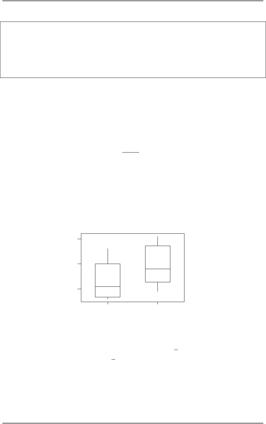
(d) Draw box plots to assist in the interpretation of the data from this experiment.
The box plots shown below indicate that there is little difference in uniformity at the two gas flow rates.
Any observed difference is not statistically significant. See the t-test in part (a).
200125
5
4
3
Flow Rate
Uniformity
2-13 A new filtering device is installed in a chemical unit. Before its installation, a random sample
yielded the following information about the percentage of impurity: y1 = 12.5, S1
2 =101.17, and n1 = 8.
After installation, a random sample yielded y2 = 10.2, S2
2 = 94.73, n2 = 9.
(a) Can you concluded that the two variances are equal? Use
D
= 0.05.

Solutions from Montgomery, D. C. (2001) Design and Analysis of Experiments, Wiley, NY
2-11
071
7394
17101
534
2
2
2
1
0
870250
2
2
2
11
2
2
2
10
.
.
.
S
S
F
.F
:H
:H
,,.
z
VV
VV
Do Not Reject. Assume that the variances are equal.
(b) Has the filtering device reduced the percentage of impurity significantly? Use
D
= 0.05.
7531
4790
9
1
8
1
899
210512
11
899
7497
298
7394191710118
2
11
15050
21
21
0
21
2
22
2
11
2
211
210
.t
.
.
..
nn
S
yy
t
.S
.
).)(().)((
nn
S)n(S)n(
S
:H
:H
,.
p
p
p
z
PP
P
P
Do not reject. There is no evidence to indicate that the new filtering device has affected the mean
2-14 Twenty observations on etch uniformity on silicon wafers are taken during a qualification
experiment for a plasma etcher. The data are as follows:
5.34 6.65 4.76 5.98 7.25
6.00 7.55 5.54 5.62 6.21
5.97 7.35 5.44 4.39 4.98
5.25 6.35 4.61 6.00 5.32
(a) Construct a 95 percent confidence interval estimate of
V
2.
22
2
22
,1 (1 ),1
22
22
2
2
11
20 1 0.88907 20 1 0.88907
32.852 8.907
0.457 1.686
nn
nS nS
DD
V
FF
V
V
dd
dd
dd
(b) Test the hypothesis that
V
2 = 1.0. Use
D
= 0.05. What are your conclusions?
H
H
0
2
1
2
1
1
:
:
V
V
z
FV
0
2
0
215019
SS .
F
002519
232 852
., .
F
097519
28 907
., .
Solutions from Montgomery, D. C. (2001) Design and Analysis of Experiments, Wiley, NY
2-12
Do not reject. There is no evidence to indicate that
V
1
21z
(c) Discuss the normality assumption and its role in this problem.
The normality assumption is much more important when analyzing variances then when analyzing means.
A moderate departure from normality could cause problems with both statistical tests and confidence
intervals. Specifically, it will cause the reported significance levels to be incorrect.
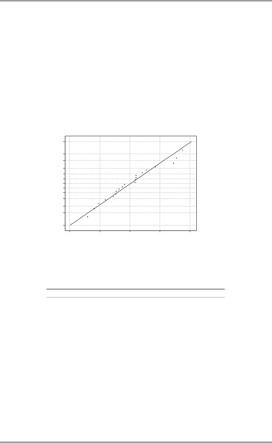
(d) Check normality by constructing a normal probability plot. What are your conclusions?
The normal probability plot indicates that there is not any serious problem with the normality assumption.
7.86.85.84.83.8
99
95
90
80
70
60
50
40
30
20
10
5
1
Data
Percent
0.835AD*
Goodness of Fit
Normal Probability Plot for Uniformity
ML Estimates
Mean
StDev
5.828
0.866560
ML Estimates
2-15 The diameter of a ball bearing was measured by 12 inspectors, each using two different kinds of
calipers. The results were:
Inspector Caliper 1 Caliper 2 Difference Difference^2
1 0.265 0.264 .001 .000001
2 0.265 0.265 .000 0
3 0.266 0.264 .002 .000004
4 0.267 0.266 .001 .000001
5 0.267 0.267 .000 0
6 0.265 0.268 -.003 .000009
7 0.267 0.264 .003 .000009
8 0.267 0.265 .002 .000004
9 0.265 0.265 .000 0
10 0.268 0.267 .001 .000001
11 0.268 0.268 .000 0
12 0.265 0.269 -.004 .000016
¦0003.
¦0 000045.
(a) Is there a significant difference between the means of the population of measurements represented by
the two samples? Use
D
= 0.05.
Solutions from Montgomery, D. C. (2001) Design and Analysis of Experiments, Wiley, NY
2-13
H
H
01 2
11 2
:
:
PP
PP
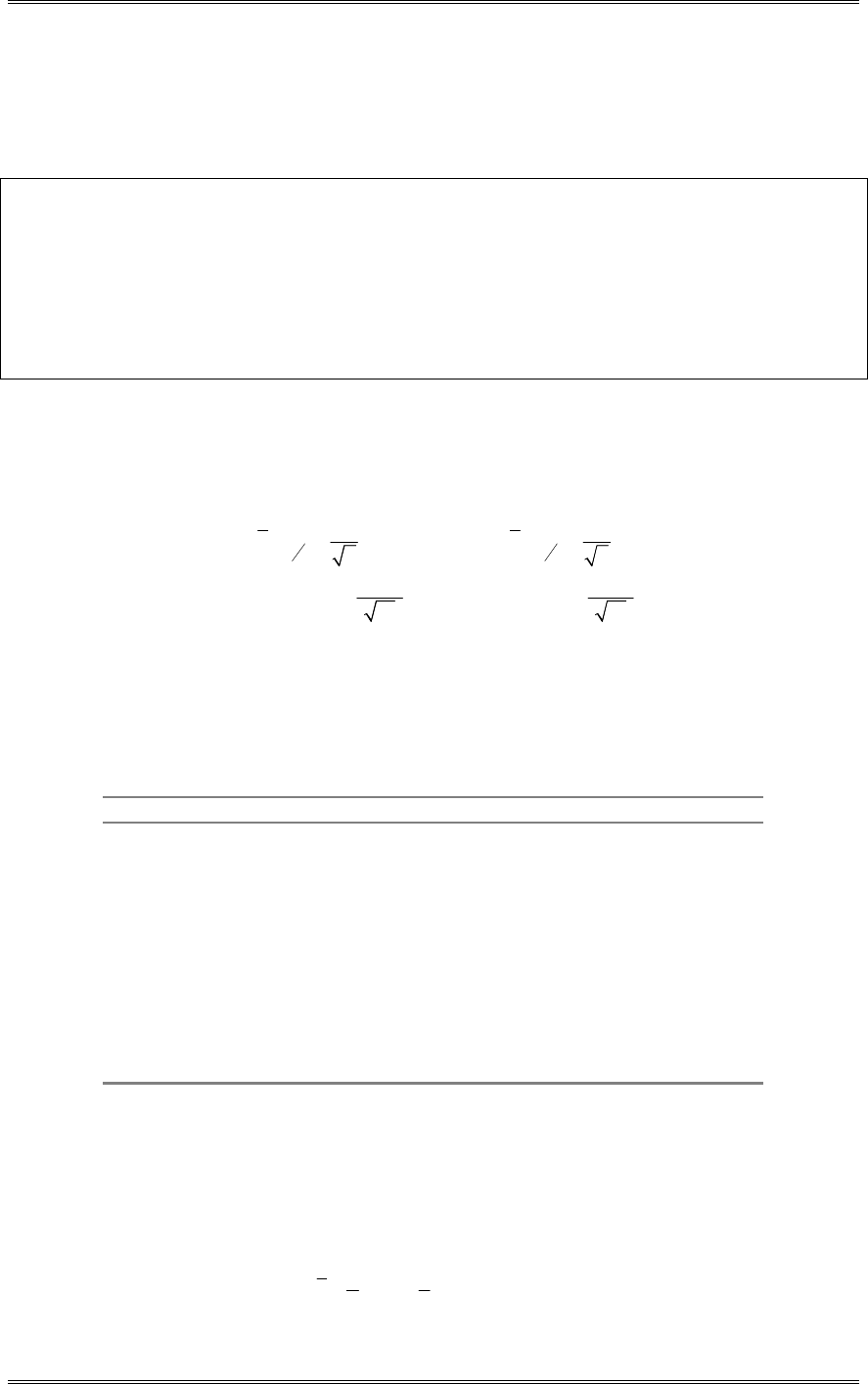
z or equivalently 0
0
1
0
z
d
d
:H
:H
P
P
Minitab Output
Paired T-Test and Confidence Interval
Paired T for Caliper 1 - Caliper 2
N Mean StDev SE Mean
Caliper 12 0.266250 0.001215 0.000351
Caliper 12 0.266000 0.001758 0.000508
Difference 12 0.000250 0.002006 0.000579
95% CI for mean difference: (-0.001024, 0.001524)
T-Test of mean difference = 0 (vs not = 0): T-Value = 0.43 P-Value = 0.674
(b) Find the P-value for the test in part (a). P=0.674
(c) Construct a 95 percent confidence interval on the difference in the mean diameter measurements for
the two types of calipers.
12
,1 ,1
22
0.002 0.002
0.00025 2.201 0.00025 2.201
12 12
0.00102 0.00152
dd
D
nn
d
d
SS
dt dt
nn
PPP
P
P
d d
dd
dd
2-16 An article in the Journal of Strain Analysis (vol.18, no. 2, 1983) compares several procedures for
predicting the shear strength for steel plate girders. Data for nine girders in the form of the ratio of
predicted to observed load for two of these procedures, the Karlsruhe and Lehigh methods, are as follows:
Girder Karlsruhe Method Lehigh Method Difference Difference^2
S1/1 1.186 1.061 0.125 0.015625
S2/1 1.151 0.992 0.159 0.025281
S3/1 1.322 1.063 0.259 0.067081
S4/1 1.339 1.062 0.277 0.076729
S5/1 1.200 1.065 0.135 0.018225
S2/1 1.402 1.178 0.224 0.050176
S2/2 1.365 1.037 0.328 0.107584
S2/3 1.537 1.086 0.451 0.203401
S2/4 1.559 1.052 0.507 0.257049
Sum = 2.465 0.821151
Average = 0.274
(a) Is there any evidence to support a claim that there is a difference in mean performance between the two
methods? Use
D
= 0.05.
H
H
01 2
11 2
:
:
PP
PP
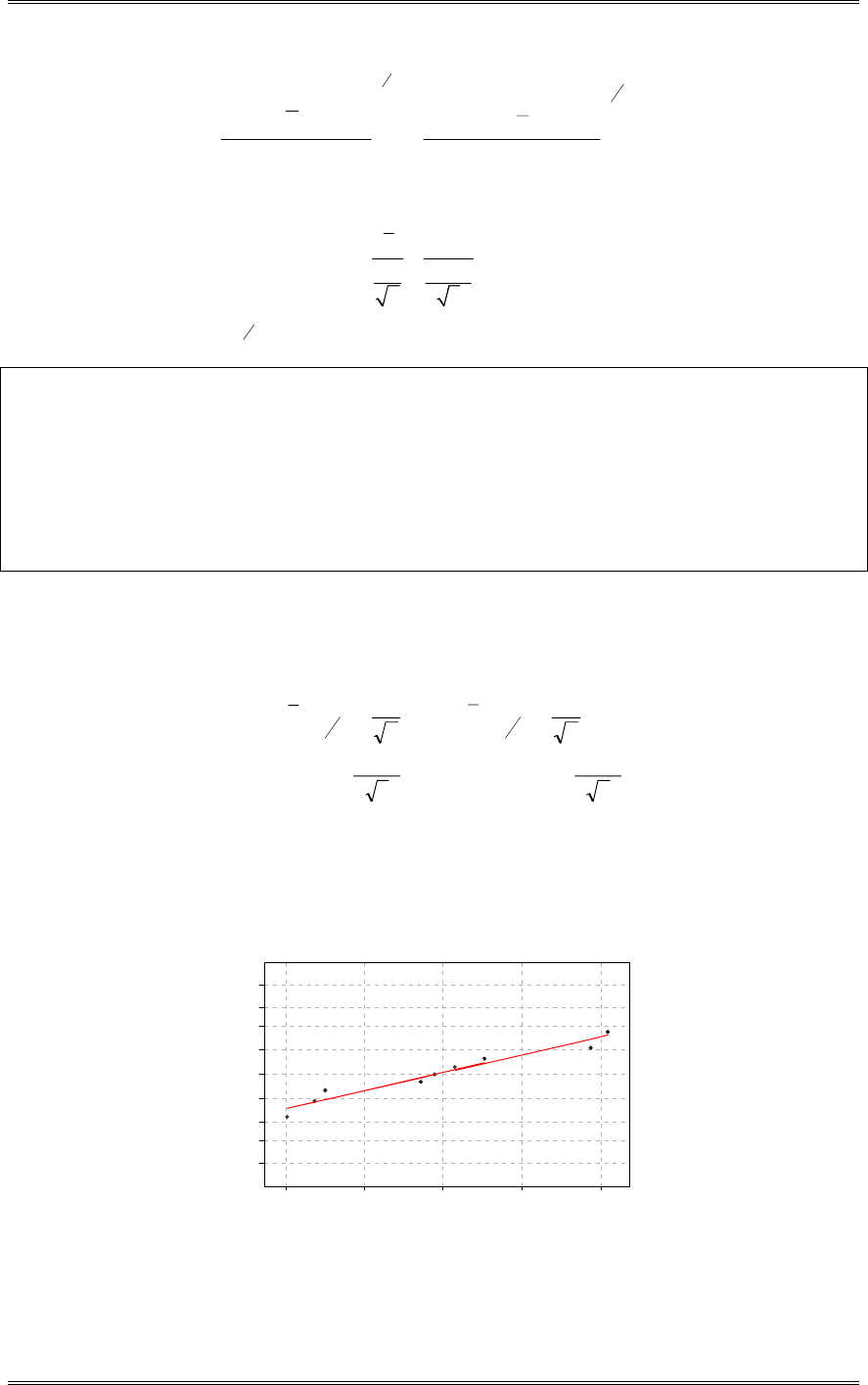
z or equivalently 0
0
1
0
z
d
d
:H
:H
P
P
1
11
2.465 0.274
9
n
i
i
dd
n
¦
Solutions from Montgomery, D. C. (2001) Design and Analysis of Experiments, Wiley, NY
2-14
12
212
22
11
11
0.821151 (2.465)
90.135
191
nn
ii
ii
d
dd
n
sn
ªº
§· ªº
«»
¨¸ «»
©¹
«»
«»
«»
«»
«»
¬¼
«»
¬¼
¦¦
0
0.274 6.08
0.135
9
d
d
tS
n
3062
90250
1
2.tt ,.
n,
D
, reject the null hypothesis.
Minitab Output
Paired T-Test and Confidence Interval
Paired T for Karlsruhe - Lehigh
N Mean StDev SE Mean
Karlsruh 9 1.3401 0.1460 0.0487
Lehigh 9 1.0662 0.0494 0.0165
Difference 9 0.2739 0.1351 0.0450
95% CI for mean difference: (0.1700, 0.3777)
T-Test of mean difference = 0 (vs not = 0): T-Value = 6.08 P-Value = 0.000
(b) What is the P-value for the test in part (a)? P=0.0002
(c) Construct a 95 percent confidence interval for the difference in mean predicted to observed load.
377770170230
9
1350
30622740
9
1350
30622740
1
2
1
2
..
.
..
.
..
n
S
td
n
S
td
d
d
d
n,
d
d
n,
dd
dd
dd
P
P
PDD
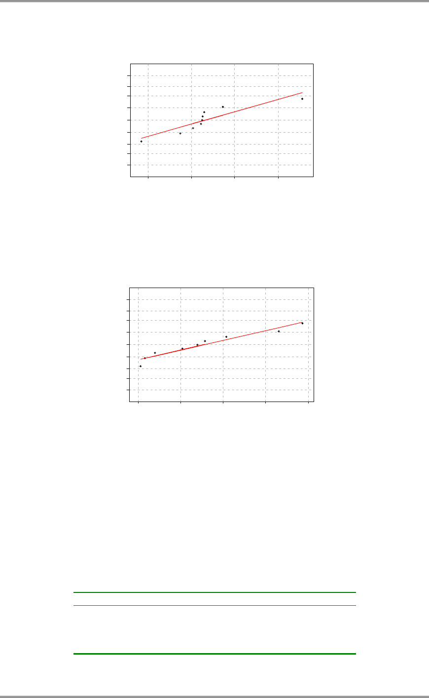
(d) Investigate the normality assumption for both samples.
P-Value: 0.537
A-Squared: 0.286
Anderson-Darling Normality Test
N: 9
St Dev : 0.146031
Av erage: 1.34011
1.551.451.351.251.15
.999
.99
.95
.80
.50
.20
.05
.01
.001
Probability
Karlsruhe
Normal Probability Plot
Solutions from Montgomery, D. C. (2001) Design and Analysis of Experiments, Wiley, NY
2-15
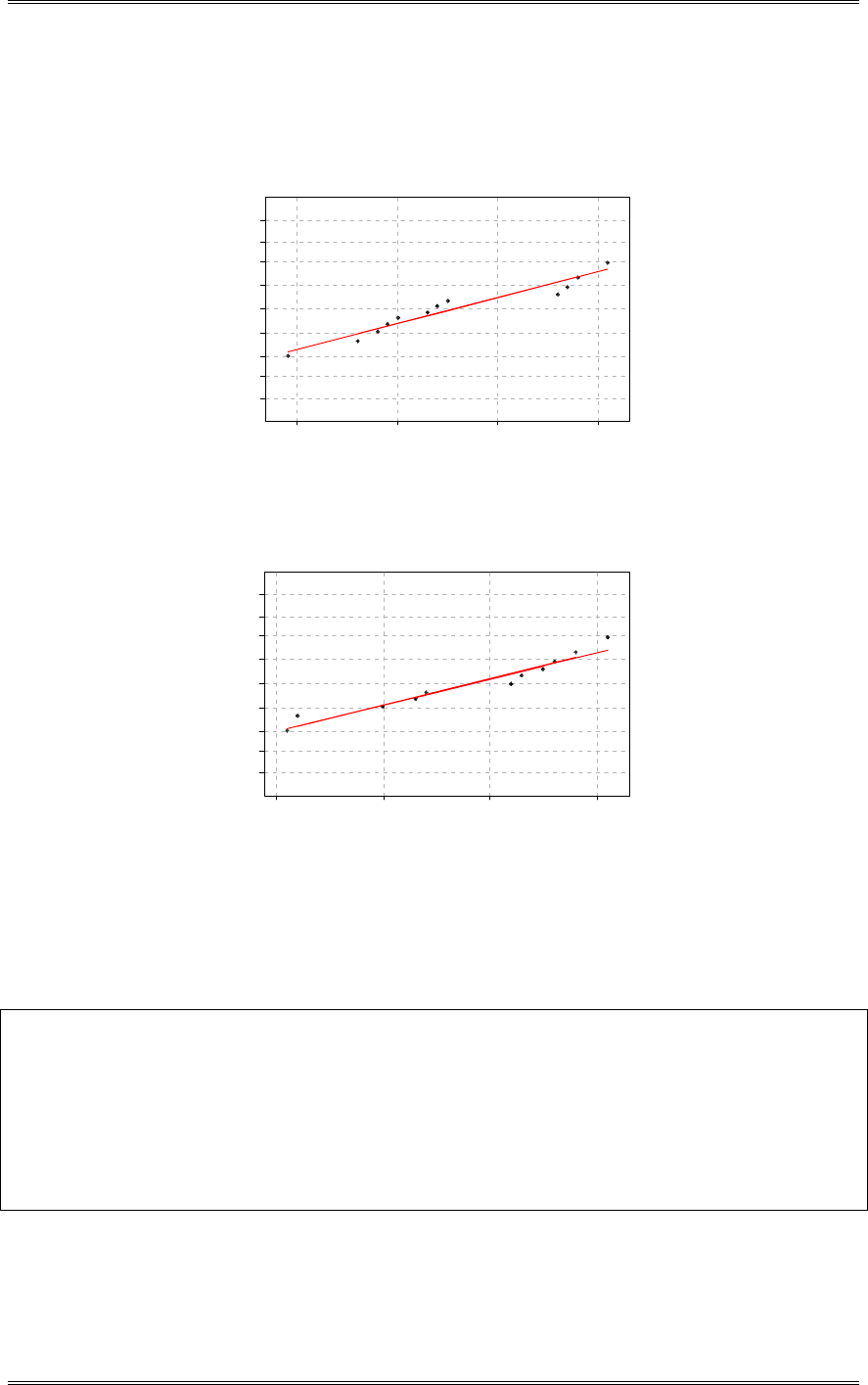
P-Value: 0.028
A-Squared: 0.772
Anderson-Darling N ormalit y Test
N: 9
StDev: 0.0493806
Av erage: 1.06622
1.151.101.051.00
.999
.99
.95
.80
.50
.20
.05
.01
.001
Probability
Lehigh
Normal Probability Plot
(e) Investigate the normality assumption for the difference in ratios for the two methods.
P-Value: 0.464
A-Squared: 0.318
Anderson-Darling Normality Test
N: 9
St D ev : 0. 135099
Av erage: 0.273889
0.520.420.320.220.12
.999
.99
.95
.80
.50
.20
.05
.01
.001
Probability
Difference
Normal Probability Plot
(f) Discuss the role of the normality assumption in the paired t-test.
As in any t-test, the assumption of normality is of only moderate importance. In the paired t-test, the
assumption of normality applies to the distribution of the differences. That is, the individual sample
measurements do not have to be normally distributed, only their difference.
2-17 The deflection temperature under load for two different formulations of ABS plastic pipe is being
studied. Two samples of 12 observations each are prepared using each formulation, and the deflection
temperatures (in qF) are reported below:
Formulation 1 Formulation 2
212 199 198 177 176 198
194 213 216 197 185 188
211 191 200 206 200 189
193 195 184 201 197 203
Solutions from Montgomery, D. C. (2001) Design and Analysis of Experiments, Wiley, NY
2-16
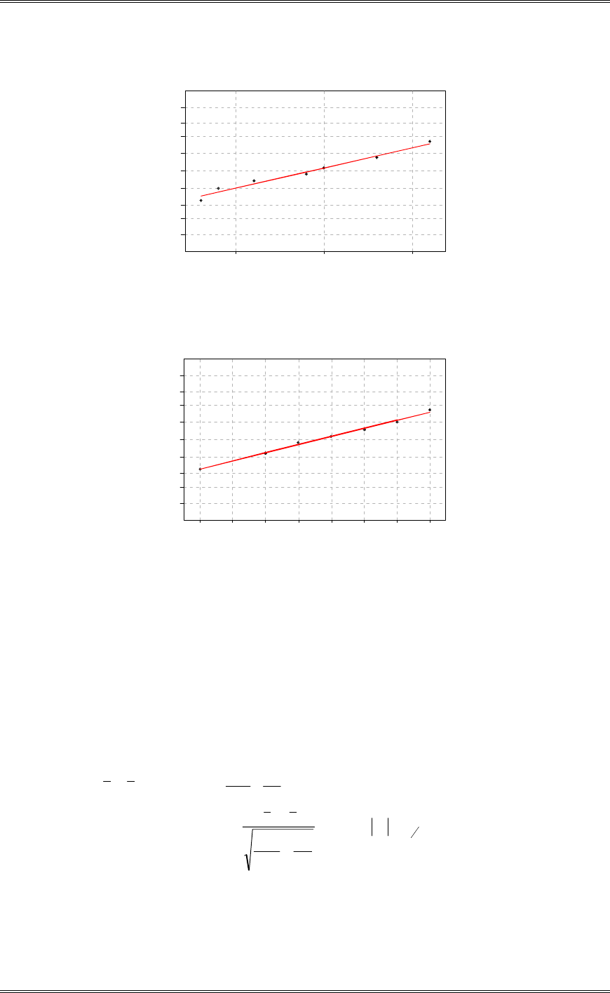
(a) Construct normal probability plots for both samples. Do these plots support assumptions of normality
and equal variance for both samples?
P-Value: 0.227
A-Squared: 0.450
Anderson-Darling Normality Test
N: 12
StDev : 10.1757
Av erage: 200.5
215205195185
.999
.99
.95
.80
.50
.20
.05
.01
.001
Probability
Form 1
Normal Probability Plot
P-Value: 0.236
A-Squared: 0.443
Anderson-Darling Normality Test
N: 12
St Dev : 9.94949
Av erage: 193.083
205195185175
.999
.99
.95
.80
.50
.20
.05
.01
.001
Probability
Form 2
Normal Probability Plot
(b) Do the data support the claim that the mean deflection temperature under load for formulation 1
exceeds that of formulation 2? Use
D
= 0.05.
Minitab Output
Two Sample T-Test and Confidence Interval
Two sample T for Form 1 vs Form 2
N Mean StDev SE Mean
Form 1 12 200.5 10.2 2.9
Form 2 12 193.08 9.95 2.9
95% CI for mu Form 1 - mu Form 2: ( -1.1, 15.9)
T-Test mu Form 1 = mu Form 2 (vs >): T = 1.81 P = 0.042 DF = 22
Both use Pooled StDev = 10.1
(c) What is the P-value for the test in part (a)? P = 0.042

Solutions from Montgomery, D. C. (2001) Design and Analysis of Experiments, Wiley, NY
2-17
2-18 Refer to the data in problem 2-17. Do the data support a claim that the mean deflection temperature
under load for formulation 1 exceeds that of formulation 2 by at least 3 qF?
Yes, formulation 1 exceeds formulation 2 by at least 3 qF.
Minitab Output
Two-Sample T-Test and CI: Form1, Form2
Two-sample T for Form1 vs Form2
N Mean StDev SE Mean
Form1 12 200.5 10.2 2.9
Form2 12 193.08 9.95 2.9r
Difference = mu Form1 - mu Form2
Estimate for difference: 7.42
95% lower bound for difference: 0.36
T-Test of difference = 3 (vs >): T-Value = 1.08 P-Value = 0.147 DF = 22
Both use Pooled StDev = 10.1
2-19 In semiconductor manufacturing, wet chemical etching is often used to remove silicon from the
backs of wafers prior to metalization. The etch rate is an important characteristic of this process. Two
different etching solutionsare being evaluated. Eight randomly selected wafers have been etched in each
solution and the observed etch rates (in mils/min) are shown below:
Solution 1 Solution 2
9.9 10.6 10.2 10.6
9.4 10.3 10.0 10.2
10.0 9.3 10.7 10.4
10.3 9.8 10.5 10.3
(a) Do the data indicate that the claim that both solutions have the same mean etch rate is valid? Use
D
=
0.05 and assume equal variances.
See the Minitab output below.
Minitab Output
Two Sample T-Test and Confidence Interval
Two sample T for Solution 1 vs Solution 2
N Mean StDev SE Mean
Solution 8 9.925 0.465 0.16
Solution 8 10.362 0.233 0.082
95% CI for mu Solution - mu Solution: ( -0.83, -0.043)
T-Test mu Solution = mu Solution (vs not =):T = -2.38 P = 0.032 DF = 14
Both use Pooled StDev = 0.368
(b) Find a 95% confidence interval on the difference in mean etch rate.
From the Minitab output, -0.83 to –0.043.
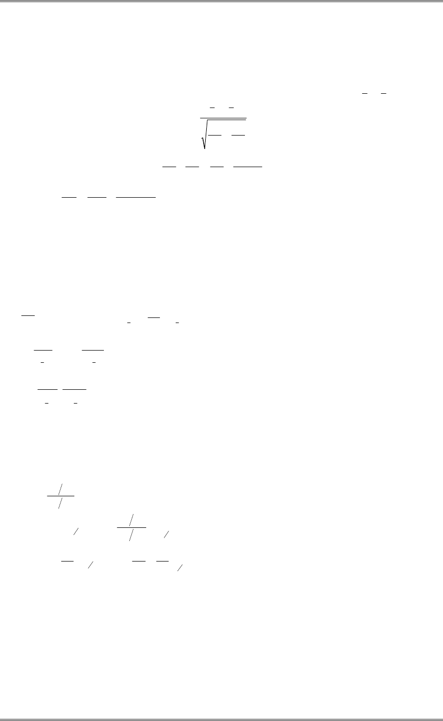
(c) Use normal probability plots to investigate the adequacy of the assumptions of normality and equal
variances.
Solutions from Montgomery, D. C. (2001) Design and Analysis of Experiments, Wiley, NY
2-18
P-Value: 0.743
A-Squared: 0.222
Anderson-Darling N ormalit y Test
N: 8
StDev: 0.465219
Av erage: 9.925
10.510.09.5
.999
.99
.95
.80
.50
.20
.05
.01
.001
Probability
Solution 1
Normal Probability Plot
P-Value: 0.919
A-Squared: 0.158
Anderson-Darling Normality Test
N: 8
St Dev : 0.232609
Av erage: 10.3625
10.710.610.510.410.310.210.110.0
.999
.99
.95
.80
.50
.20
.05
.01
.001
Probability
Solution 2
Normal Probability Plot
Both the normality and equality of variance assumptions are valid.
2-20 Two popular pain medications are being compared on the basis of the speed of absorption by the
body. Specifically, tablet 1 is claimed to be absorbed twice as fast as tablet 2. Assume that 2
1
V
and 2
2
V
are known. Develop a test statistic for
H
0: 2
P
1 =
P
2
H
1: 2
P
1 z
P
2
22
12
12 1 2
12
4
2~2,
yy N nn
VV
PP
§·
¨¸
©¹
, assuming that the data is normally distributed.
The test statistic is: zyy
nn
o
2
4
12
1
2
1
2
2
2
VV
, reject if zz
o!
D
2
2-21 Suppose we are testing
H
0:
P
1 =
P
2
H
1:
P
1 z
P
2
Solutions from Montgomery, D. C. (2001) Design and Analysis of Experiments, Wiley, NY
2-19
where 2
1
V
and 2
2
V
are known. Our sampling resources are constrained such that n1 + n2 = N. How should
we allocate the N observations between the two populations to obtain the most powerful test?
The most powerful test is attained by the n1 and n2 that maximize zo for given yy
12
.
Thus, we chose n1 and n2 to max zyy
nn
o
12
1
2
1
2
2
2
VV
, subject to n1 + n2 = N.
This is equivalent to min Lnn nNn
VV V V
1
2
1
2
2
2
1
2
1
2
2
1
, subject to n1 + n2 = N.
Now
22
12
2
2
11 1
0
dL
dn n Nn
VV
, implies that n1 / n2 =
V
1 /
V
2.
Thus n1 and n2 are assigned proportionally to the ratio of the standard deviations. This has
intuitive appeal, as it allocates more observations to the population with the greatest variability.
2-22 Develop Equation 2-46 for a 100(1 -
D
) percent confidence interval for the variance of a normal
distribution.
2
1
2~n
SS
F
V
. Thus, 22
1,1 ,1
22
21
nn
SS
P
FFD
V
½
dd
®¾
¯¿
. Therefore,
22
,1 1 ,1
22
21
nn
SS SS
P
VD
FF
½
°°
dd
®¾
°°
¯¿
,
so
22
,1 1 ,1
22
,
nn
SS SS
FF
ªº
«»
«»
¬¼
is the 100(1 -
D
)% confidence interval on
V
2.
2-23 Develop Equation 2-50 for a 100(1 -
D
) percent confidence interval for the ratio
V
1
2 / 2
2
V
, where 2
1
V
and 2
2
V
are the variances of two normal distributions.
21
22
22
1, 1
22
11
~nn
SF
S
V
V
21
22
22
22
1,1,1 22 ,1,1
21
11
1
nn nn
S
PF F
S
VD
V
½
dd
®¾
¯¿
or
21
22
222
111
1,1,1
222
,1,1
21
222
1
nn nn
SS
PF F
SS
VD
V
½
dd
®¾
¯¿
2-24 Develop an equation for finding a 100(1 -
D
) percent confidence interval on the difference in the
means of two normal distributions where 2
1
V
z 2
2
V
. Apply your equation to the portland cement
experiment data, and find a 95% confidence interval.

Solutions from Montgomery, D. C. (2001) Design and Analysis of Experiments, Wiley, NY
2-20
2
12 1 2
,
22
12
12
~
yy t
SS
nn
DX
PP
2 2
22 22
12 12
12 1 2
,,
12 12
SS SS
tyyt
nn nn
XX
PP
dd
2 2
22 22
12 12
12 1 2 12
,,
12 12
SS SS
yy t yy t
nn nn
XX
PP
dd
where
2
22
12
12
22
22
12
12
12
11
SS
nn
SS
nn
nn
X
§·
¨¸
©¹
§·§·
¨¸¨¸
©¹©¹
Using the data from Table 2-1
n
y
S
1
1
1
2
10
16 764
0100138
.
.
n
y
S
2
2
2
2
10
17 343
0 0614622
.
.
12
0.100138 0.0614622
16.764 17.343 2.110 10 10
PP
dd
0.100138 0.0614622
16.764 17.343 2.110 10 10
where 1702417
110
10
06146220
110
10
1001380
10
06146220
10
1001380
22
2
#
¸
¹
·
¨
©
§
¸
¹
·
¨
©
§
¸
¹
·
¨
©
§
.
..
..
X
12
1.426 0.889
PP
dd
This agrees with the result in Table 2-2.
2-25 Construct a data set for which the paired t-test statistic is very large, but for which the usual two-
sample or pooled t-test statistic is small. In general, describe how you created the data. Does this give you
any insight regarding how the paired t-test works?
A B delta
7.1662 8.2416 1.07541
2.3590 2.4555 0.09650
19.9977 21.1018 1.10412
0.9077 2.3401 1.43239
-15.9034 -15.0013 0.90204
-6.0722 -5.5941 0.47808

Solutions from Montgomery, D. C. (2001) Design and Analysis of Experiments, Wiley, NY
2-21
9.9501 10.6910 0.74085
-1.0944 -0.1358 0.95854
-4.6907 -3.3446 1.34615
-6.6929 -5.9303 0.76256
Minitab Output
Paired T-Test and Confidence Interval
Paired T for A - B
N Mean StDev SE Mean
A 10 0.59 10.06 3.18
B 10 1.48 10.11 3.20
Difference 10 -0.890 0.398 0.126
95% CI for mean difference: (-1.174, -0.605)
T-Test of mean difference = 0 (vs not = 0): T-Value = -7.07 P-Value = 0.000
Two Sample T-Test and Confidence Interval
Two sample T for A vs B
N Mean StDev SE Mean
A 10 0.6 10.1 3.2
B 10 1.5 10.1 3.2
95% CI for mu A - mu B: ( -10.4, 8.6)
T-Test mu A = mu B (vs not =): T = -0.20 P = 0.85 DF = 18
Both use Pooled StDev = 10.1
These two sets of data were created by making the observation for A and B moderately different within
each pair (or block), but making the observations between pairs very different. The fact that the difference
between pairs is large makes the pooled estimate of the standard deviation large and the two-sample t-test
statistic small. Therefore the fairly small difference between the means of the two treatments that is present
when they are applied to the same experimental unit cannot be detected. Generally, if the blocks are very
different, then this will occur. Blocking eliminates the variabiliy associated with the nuisance variable that
they represent.

Solutions from Montgomery, D. C. (2001) Design and Analysis of Experiments, Wiley, NY
3-1
Chapter 3
Experiments with a Single Factor: The Analysis of Variance
Solutions
3-1 The tensile strength of portland cement is being studied. Four different mixing techniques can be
used economically. The following data have been collected:
Mixing Technique Tensile Strength (lb/in2)
1 3129 3000 2865 2890
2 3200 3300 2975 3150
3 2800 2900 2985 3050
4 2600 2700 2600 2765
(a) Test the hypothesis that mixing techniques affect the strength of the cement. Use
D
= 0.05.
Design Expert Output
Response: Tensile Strengthin lb/in^2
ANOVA for Selected Factorial Model
Analysis of variance table [Partial sum of squares]
Sum of Mean F
Source Squares DF Square Value Prob > F
Model 4.897E+005 3 1.632E+005 12.73 0.0005 significant
A 4.897E+005 3 1.632E+005 12.73 0.0005
Residual 1.539E+005 12 12825.69
Lack of Fit 0.000 0
Pure Error 1.539E+005 12 12825.69
Cor Total 6.436E+005 15
The Model F-value of 12.73 implies the model is significant. There is only
a 0.05% chance that a "Model F-Value" this large could occur due to noise.
Treatment Means (Adjusted, If Necessary)
Estimated
Standard
Mean
Error
1-1 2971.00 56.63
2-2 3156.25 56.63
3-3 2933.75 56.63
4-4 2666.25 56.63
Mean
Standard t for H0
Treatment Difference DF Error Coeff=0 Prob > |t|
1 vs 2 -185.25 1 80.08 -2.31 0.0392
1 vs 3 37.25 1 80.08 0.47 0.6501
1 vs 4 304.75 1 80.08 3.81 0.0025
2 vs 3 222.50 1 80.08 2.78 0.0167
2 vs 4 490.00 1 80.08 6.12 < 0.0001
3 vs 4 267.50 1 80.08 3.34 0.0059
The F-value is 12.73 with a corresponding P-value of .0005. Mixing technique has an effect.
(b) Construct a graphical display as described in Section 3-5.3 to compare the mean tensile strengths for
the four mixing techniques. What are your conclusions?
62556
4
712825 .
.
n
MS
SE
y.i
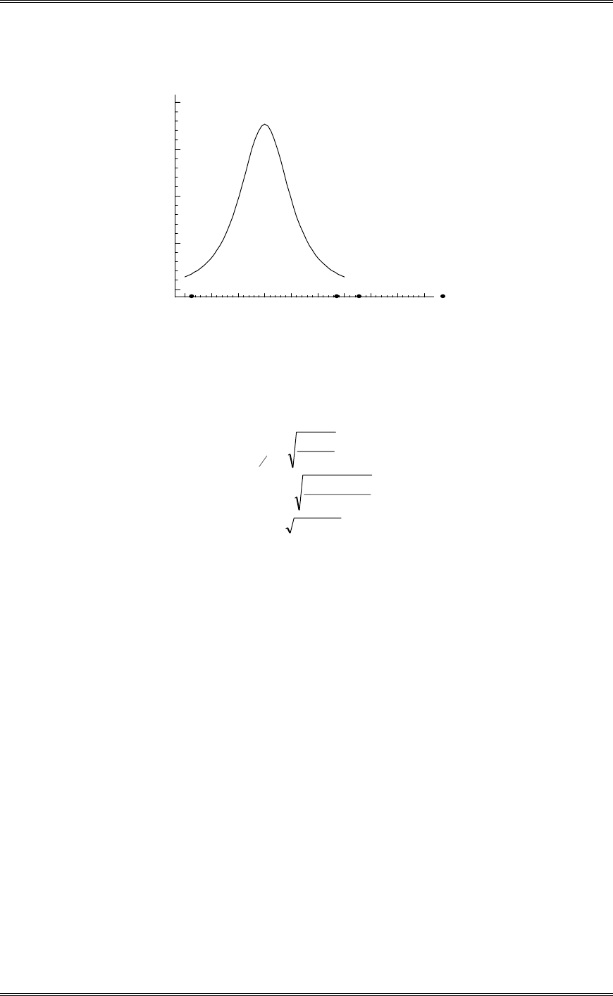
Solutions from Montgomery, D. C. (2001) Design and Analysis of Experiments, Wiley, NY
3-2
2700 2800 2900 3000 3100
Tensile Strength
Scaled t Distribution
(3) (2)(1)(4)
Based on examination of the plot, we would conclude that 1
P
and 3
P
are the same; that 4
P
differs from
1
P
and 3
P
, that 2
P
differs from 1
P
and 3
P
, and that 2
P
and 4
P
are different.
(c) Use the Fisher LSD method with
D
=0.05 to make comparisons between pairs of means.
4951748564121792
4
7128252
2
4160250
2
...LSD
).(
tLSD
n
MS
tLSD
,.
aN,
E
D
Treatment 2 vs. Treatment 4 = 3156.250 - 2666.250 = 490.000 > 174.495
Treatment 2 vs. Treatment 3 = 3156.250 - 2933.750 = 222.500 > 174.495
Treatment 2 vs. Treatment 1 = 3156.250 - 2971.000 = 185.250 > 174.495
Treatment 1 vs. Treatment 4 = 2971.000 - 2666.250 = 304.750 > 174.495
Treatment 1 vs. Treatment 3 = 2971.000 - 2933.750 = 37.250 < 174.495
Treatment 3 vs. Treatment 4 = 2933.750 - 2666.250 = 267.500 > 174.495
The Fisher LSD method is also presented in the Design-Expert computer output above. The results agree
with graphical method for this experiment.
(d) Construct a normal probability plot of the residuals. What conclusion would you draw about the
validity of the normality assumption?
There is nothing unusual about the normal probability plot of residuals.
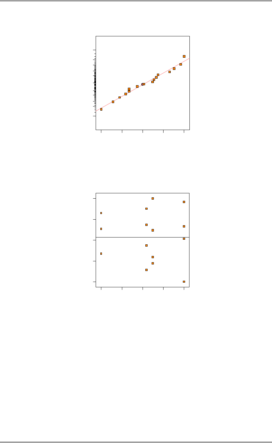
Solutions from Montgomery, D. C. (2001) Design and Analysis of Experiments, Wiley, NY
3-3
Residual
Norm al % probability
Normal plot of residuals
-181.25 -96.4375 -11.625 73.1875 158
1
5
10
20
30
50
70
80
90
95
99
(e) Plot the residuals versus the predicted tensile strength. Comment on the plot.
There is nothing unusual about this plot.
22
Predicted
Residuals
Residuals vs. Predicted
-181.25
-96.4375
-11.625
73.1875
158
2666.25 2788.75 2911.25 3033.75 3156.25
(f) Prepare a scatter plot of the results to aid the interpretation of the results of this experiment.
Design-Expert automatically generates the scatter plot. The plot below also shows the sample average for
each treatment and the 95 percent confidence interval on the treatment mean.
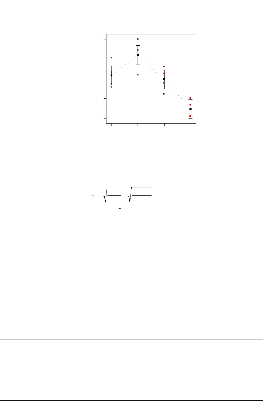
Solutions from Montgomery, D. C. (2001) Design and Analysis of Experiments, Wiley, NY
3-4
Technique
Tensile Strength
One Factor Plot
1 2 3 4
2579.01
2759.26
2939.51
3119.75
3300
22
3-2 Rework part (b) of Problem 3-1 using the Duncan's multiple range test. Does this make any
difference in your conclusions?
62556
4
712825 .
.
n
MS
SE
y.i
56218862556333124
90018262556233123
40617462556083122
0504
0503
0502
...S,rR
...S,rR
...S,rR
.i
.i
.i
y.
y.
y.
Treatment 2 vs. Treatment 4 = 3156.250 - 2666.250 = 490.000 > 188.562 (R4)
Treatment 2 vs. Treatment 3 = 3156.250 - 2933.750 = 222.500 > 182.900 (R3)
Treatment 2 vs. Treatment 1 = 3156.250 - 2971.000 = 185.250 > 174.406 (R2)
Treatment 1 vs. Treatment 4 = 2971.000 - 2666.250 = 304.750 > 182.900 (R3)
Treatment 1 vs. Treatment 3 = 2971.000 - 2933.750 = 37.250 < 174.406 (R2)
Treatment 3 vs. Treatment 4 = 2933.750 - 2666.250 = 267.500 > 174.406 (R2)
Treatment 3 and Treatment 1 are not different. All other pairs of means differ. This is the same result
obtained from the Fisher LSD method and the graphical method.
(b) Rework part (b) of Problem 3-1 using Tukey’s test with
D
= 0.05. Do you get the same conclusions
from Tukey’s test that you did from the graphical procedure and/or Duncan’s multiple range test?
Minitab Output
Tukey's pairwise comparisons
Family error rate = 0.0500
Individual error rate = 0.0117
Critical value = 4.20
Intervals for (column level mean) - (row level mean)
1 2 3
2 -423

Solutions from Montgomery, D. C. (2001) Design and Analysis of Experiments, Wiley, NY
3-5
53
3 -201 -15
275 460
4 67 252 30
543 728 505
No, the conclusions are not the same. The mean of Treatment 4 is different than the means of Treatments
1, 2, and 3. However, the mean of Treatment 2 is not different from the means of Treatments 1 and 3
according to the Tukey method, they were found to be different using the graphical method and Duncan’s
multiple range test.
(c) Explain the difference between the Tukey and Duncan procedures.
A single critical value is used for comparison with the Tukey procedure where a – 1 critical values are
used with the Duncan procedure. Tukey’s test has a type I error rate of
D
for all pairwise comparisons
where Duncan’s test type I error rate varies based on the steps between the means. Tukey’s test is more
conservative and has less power than Duncan’s test.
3-3 Reconsider the experiment in Problem 3-1. Find a 95 percent confidence interval on the mean
tensile strength of the portland cement produced by each of the four mixing techniques. Also find a 95
percent confidence interval on the difference in means for techniques 1 and 3. Does this aid in
interpreting the results of the experiment?
n
MS
ty
n
MS
ty E
aN,
.ii
E
aN,
.i dd
22
DD P
Treatment 1: 4
1282837
17922971 .r
3871232971 .r
38730946132847 1.. dd
P
Treatment 2: 3156.25r123.387
63732798633032 2.. dd
P
Treatment 3: 2933.75r123.387
13730573632810 3.. dd
P
Treatment 4: 2666.25r123.387
63727898632542 4.. dd
P
Treatment 1 - Treatment 3: n
MS
tyy
n
MS
tyy E
aN,
.j.iji
E
aN,
.j.i
22
22 dd
DD PP
4
7128252
1792752933002971 .
... r
745211245137 31 .. dd
PP
3-4 An experiment was run to determine whether four specific firing temperatures affect the density of
a certain type of brick. The experiment led to the following data:
Temperature Density
100 21.8 21.9 21.7 21.6 21.7
125 21.7 21.4 21.5 21.4
150 21.9 21.8 21.8 21.6 21.5
175 21.9 21.7 21.8 21.4

Solutions from Montgomery, D. C. (2001) Design and Analysis of Experiments, Wiley, NY
3-6
(a) Does the firing temperature affect the density of the bricks? Use
D
= 0.05.
No, firing temperature does not affect the density of the bricks. Refer to the Design-Expert output below.
Design Expert Output
Response: Density
ANOVA for Selected Factorial Model
Analysis of variance table [Partial sum of squares]
Sum of Mean F
Source Squares DF Square Value Prob > F
Model 0.16 3 0.052 2.02 0.1569 not significant
A 0.16 3 0.052 2.02 0.1569
Residual 0.36 14 0.026
Lack of Fit 0.000 0
Pure Error 0.36 14 0.026
Cor Total 0.52 17
The "Model F-value" of 2.02 implies the model is not significant relative to the noise. There is a
15.69 % chance that a "Model F-value" this large could occur due to noise.
Treatment Means (Adjusted, If Necessary)
Estimated
Standard
Mean
Error
1-100 21.74 0.072
2-125 21.50 0.080
3-150 21.72 0.072
4-175 21.70 0.080
Mean
Standard t for H0
Treatment Difference DF Error Coeff=0 Prob > |t|
1 vs 2 0.24 1 0.11 2.23 0.0425
1 vs 3 0.020 1 0.10 0.20 0.8465
1 vs 4 0.040 1 0.11 0.37 0.7156
2 vs 3 -0.22 1 0.11 -2.05 0.0601
2 vs 4 -0.20 1 0.11 -1.76 0.0996
3 vs 4 0.020 1 0.11 0.19 0.8552
(b) Is it appropriate to compare the means using Duncan’s multiple range test in this experiment?
The analysis of variance tells us that there is no difference in the treatments. There is no need to proceed
with Duncan’s multiple range test to decide which mean is difference.
(c) Analyze the residuals from this experiment. Are the analysis of variance assumptions satisfied?
There is nothing unusual about the residual plots.
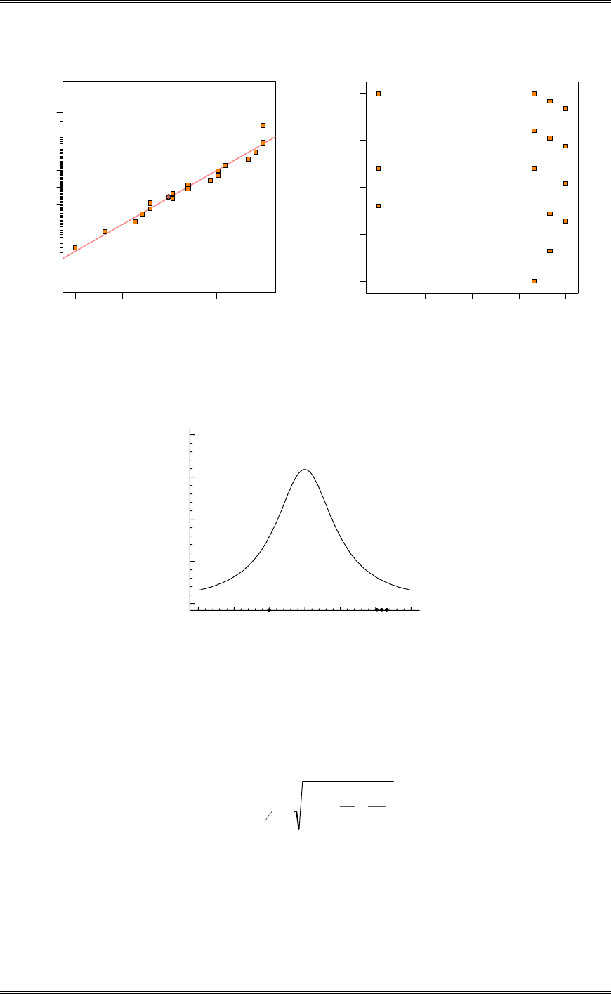
Solutions from Montgomery, D. C. (2001) Design and Analysis of Experiments, Wiley, NY
3-7
Residual
Normal % probability
Normal plot of residuals
-0.3 -0.175 -0.05 0.075 0.2
1
5
10
20
30
50
70
80
90
95
99
22
22
22
Predicted
Residuals
Residuals vs. Predicted
-0.3
-0.175
-0.05
0.075
0.2
21.50 21.56 21.62 21.68 21.74
(d) Construct a graphical display of the treatments as described in Section 3-5.3. Does this graph
adequately summarize the results of the analysis of variance in part (b). Yes.
21.2 2 1.3 2 1.4 2 1.5 2 1.6 21.7 21.8
M ean D ens ity
Scaled t Distribution
(125) (175,150,100)
3-5 Rework Part (d) of Problem 3-4 using the Fisher LSD method. What conclusions can you draw?
Explain carefully how you modified the procedure to account for unequal sample sizes.
When sample sizes are unequal, the appropriate formula for the LSD is
¸
¸
¹
·
¨
¨
©
§ ji
Enn
MStLSD
aN,
11
2
D
Treatment 1 vs. Treatment 2 = 21.74 – 21.50 = 0.24 > 0.2320
Treatment 1 vs. Treatment 3 = 21.74 – 21.72 = 0.02 < 0.2187
Treatment 1 vs. Treatment 4 = 21.74 – 21.70 = 0.04 < 0.2320
Treatment 3 vs. Treatment 2 = 21.72 – 21.50 = 0.22 < 0.2320
Treatment 4 vs. Treatment 2 = 21.70 – 21.50 = 0.20 < 0.2446
Treatment 3 vs. Treatment 4 = 21.72 – 21.70 = 0.02 < 0.2320

Solutions from Montgomery, D. C. (2001) Design and Analysis of Experiments, Wiley, NY
3-8
Treatment 1, temperature of 100, is different than Treatment 2, temperature of 125. All other pairwise
comparisons do not identify differences. Notice something very interesting has happened here. The
analysis of variance indicated that there were no differences between treatment means, yet the LSD
procedure found a difference; in fact, the Design-Expert output indicates that the P-value if slightly less
that 0.05. This illustrates a danger of using multiple comparison procedures without relying on the results
from the analysis of variance. Because we could not reject the hypothesis of equal means using the
analysis of variance, we should never have performed the Fisher LSD (or any other multiple comparison
procedure, for that matter). If you ignore the analysis of variance results and run multiple comparisons,
you will likely make type I errors.
The LSD calculations utilized Equation 3-32, which accommodates different sample sizes. Equation 3-32
simplifies to Equation 3-33 for a balanced design experiment.
3-6 A manufacturer of television sets is interested in the effect of tube conductivity of four different
types of coating for color picture tubes. The following conductivity data are obtained:
Coating Type Conductivity
1 143 141 150 146
2 152 149 137 143
3 134 136 132 127
4 129 127 132 129
(a) Is there a difference in conductivity due to coating type? Use
D
= 0.05.
Yes, there is a difference in means. Refer to the Design-Expert output below..
Design Expert Output
ANOVA for Selected Factorial Model
Analysis of variance table [Partial sum of squares]
Sum of Mean F
Source Squares DF Square Value Prob > F
Model 844.69 3 281.56 14.30 0.0003 significant
A 844.69 3 281.56 14.30 0.0003
Residual 236.25 12 19.69
Lack of Fit 0.000 0
Pure Error 236.25 12 19.69
Cor Total 1080.94 15
The Model F-value of 14.30 implies the model is significant. There is only
a 0.03% chance that a "Model F-Value" this large could occur due to noise.
Treatment Means (Adjusted, If Necessary)
Estimated
Standard
Mean
Error
1-1 145.00 2.22
2-2 145.25 2.22
3-3 132.25 2.22
4-4 129.25 2.22
Mean
Standard t for H0
Treatment Difference DF Error Coeff=0 Prob > |t|
1 vs 2 -0.25 1 3.14 -0.080 0.9378
1 vs 3 12.75 1 3.14 4.06 0.0016
1 vs 4 15.75 1 3.14 5.02 0.0003
2 vs 3 13.00 1 3.14 4.14 0.0014
2 vs 4 16.00 1 3.14 5.10 0.0003
3 vs 4 3.00 1 3.14 0.96 0.3578
(b) Estimate the overall mean and the treatment effects.
Solutions from Montgomery, D. C. (2001) Design and Analysis of Experiments, Wiley, NY
3-9
68758937513725129
68755937513725132
31257937513725145
06257937513700145
9375137162207
44
33
22
11
...yy
ˆ
...yy
ˆ
...yy
ˆ
...yy
ˆ
./
ˆ
...
...
...
...
W
W
W
W
P
(c) Compute a 95 percent interval estimate of the mean of coating type 4. Compute a 99 percent interval
estimate of the mean difference between coating types 1 and 4.
Treatment 4: 4
6919
179225129 .
.. r
08451344155124 4.. dd
P
Treatment 1 - Treatment 4:
4
69192
055325129145 .
.. r
336251646 41 .. dd
PP
(d) Test all pairs of means using the Fisher LSD method with
D
=0.05.
Refer to the Design-Expert output above. The Fisher LSD procedure is automatically included in the
output.
The means of Coating Type 2 and Coating Type 1 are not different. The means of Coating Type 3 and
Coating Type 4 are not different. However, Coating Types 1 and 2 produce higher mean conductivity that
does Coating Types 3 and 4.
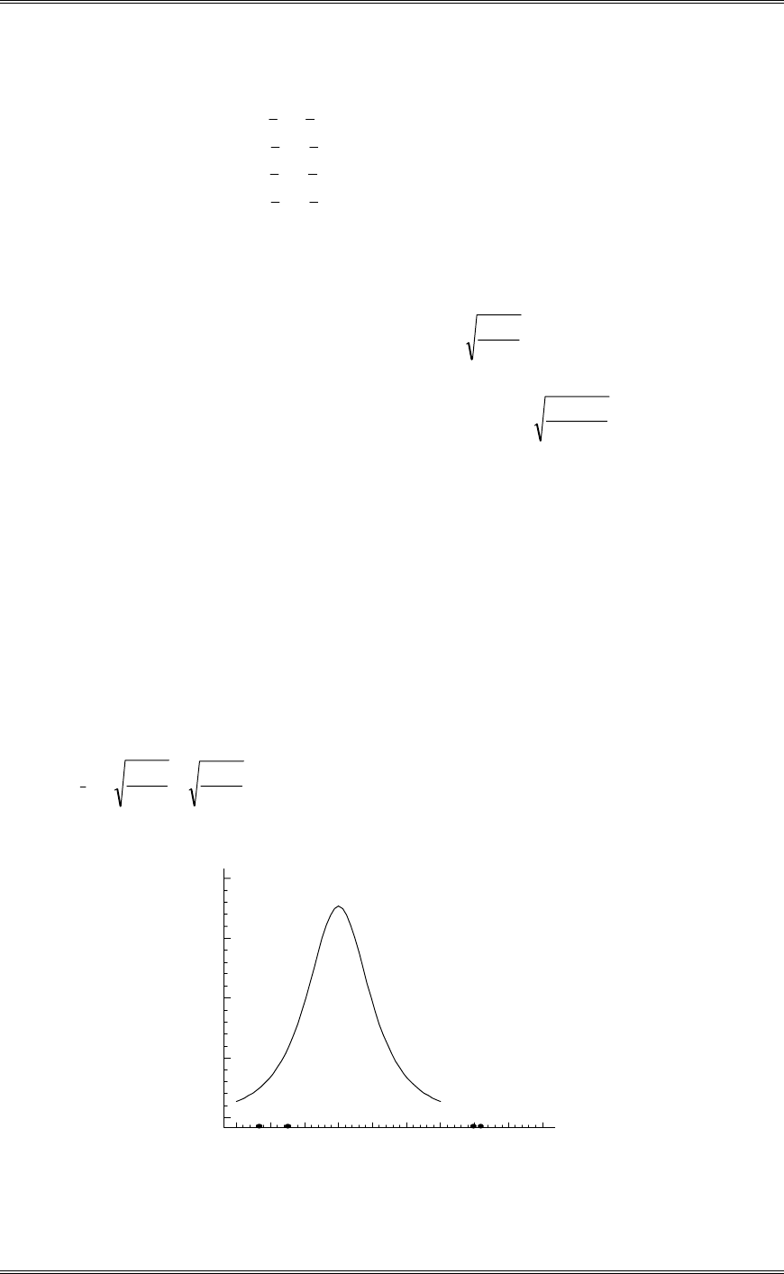
(e) Use the graphical method discussed in Section 3-5.3 to compare the means. Which coating produces
the highest conductivity?
2192
4
9616 .
.
n
MS
SE
y.i Coating types 1 and 2 produce the highest conductivity.
130 135 140 145 150
Conductivity
Scaled t Distribution
(3) (2)(1 )(4)
Solutions from Montgomery, D. C. (2001) Design and Analysis of Experiments, Wiley, NY
3-10
(f) Assuming that coating type 4 is currently in use, what are your recommendations to the
manufacturer? We wish to minimize conductivity.
Since coatings 3 and 4 do not differ, and as they both produce the lowest mean values of conductivity, use
either coating 3 or 4. As type 4 is currently being used, there is probably no need to change.
3-7 Reconsider the experiment in Problem 3-6. Analyze the residuals and draw conclusions about
model adequacy.
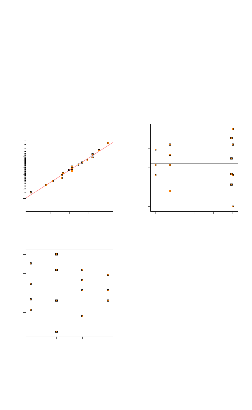
There is nothing unusual in the normal probability plot. A funnel shape is seen in the plot of residuals
versus predicted conductivity indicating a possible non-constant variance.
Residual
Normal % probability
Normal plot of residuals
-8.25 -4 .5 -0.75 36.75
1
5
10
20
30
50
70
80
90
95
99
22
Predicted
Residuals
Residuals vs. Predicted
-8.25
-4.5
-0.75
3
6.75
129.25 133.25 137.25 141.25 145.25
22
Coating Type
Residuals
Residuals vs. Coating Type
-8.25
-4.5
-0.75
3
6.75
1 2 3 4
3-8 An article in the ACI Materials Journal (Vol. 84, 1987. pp. 213-216) describes several experiments
investigating the rodding of concrete to remove entrapped air. A 3” x 6” cylinder was used, and the

Solutions from Montgomery, D. C. (2001) Design and Analysis of Experiments, Wiley, NY
3-11
number of times this rod was used is the design variable. The resulting compressive strength of the
concrete specimen is the response. The data are shown in the following table.
Rodding Level Compressive Strength
10 1530 1530 1440
15 1610 1650 1500
20 1560 1730 1530
25 1500 1490 1510
(a) Is there any difference in compressive strength due to the rodding level? Use
D
= 0.05.
There are no differences.
Design Expert Output
ANOVA for Selected Factorial Model
Analysis of variance table [Partial sum of squares]
Sum of Mean F
Source Squares DF Square Value Prob > F
Model 28633.33 3 9544.44 1.87 0.2138 not significant
A 28633.33 3 9544.44 1.87 0.2138
Residual 40933.33 8 5116.67
Lack of Fit 0.000 0
Pure Error 40933.33 8 5116.67
Cor Total 69566.67 11
The "Model F-value" of 1.87 implies the model is not significant relative to the noise. There is a
21.38 % chance that a "Model F-value" this large could occur due to noise.
Treatment Means (Adjusted, If Necessary)
Estimated Standard
Mean Error
1-10 1500.00 41.30
2-15 1586.67 41.30
3-20 1606.67 41.30
4-25 1500.00 41.30
Mean
Standard t for H0
Treatment Difference DF Error Coeff=0 Prob > |t|
1 vs 2 -86.67 1 58.40 -1.48 0.1761
1 vs 3 -106.67 1 58.40 -1.83 0.1052
1 vs 4 0.000 1 58.40 0.000 1.0000
2 vs 3 -20.00 1 58.40 -0.34 0.7408
2 vs 4 86.67 1 58.40 1.48 0.1761
3 vs 4 106.67 1 58.40 1.83 0.1052
(b) Find the P-value for the F statistic in part (a). From computer output, P=0.2138.
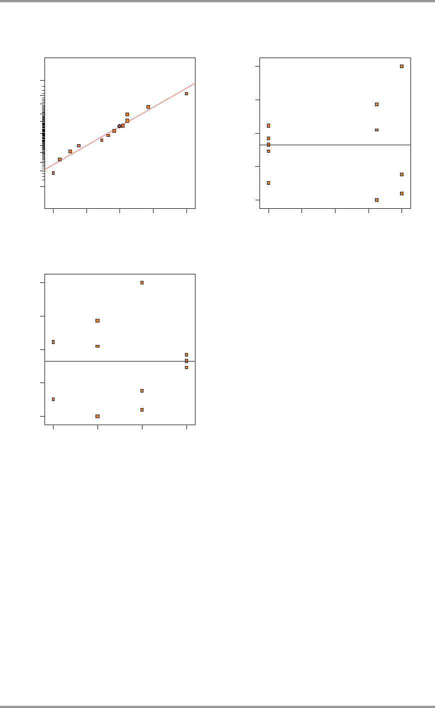
(c) Analyze the residuals from this experiment. What conclusions can you draw about the underlying
model assumptions?
There is nothing unusual about the residual plots.
Solutions from Montgomery, D. C. (2001) Design and Analysis of Experiments, Wiley, NY
3-12
Residual
Normal % probability
Normal plot of residuals
-86.6667 -34.1667 18.3333 70.8333 123.333
1
5
10
20
30
50
70
80
90
95
99
22
Predicted
Residuals
Residuals vs. Predicted
-86.6667
-34.1667
18.3333
70.8333
123.333
1500.00 1526.67 1553.33 1580.00 1606.67
22
Rodding Level
Residuals
Residuals vs. Rodding Level
-86.6667
-34.1667
18.3333
70.8333
123.333
1 2 3 4
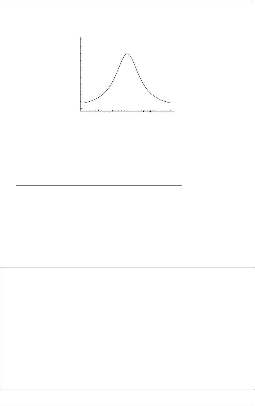
(d) Construct a graphical display to compare the treatment means as describe in Section 3-5.3.
Solutions from Montgomery, D. C. (2001) Design and Analysis of Experiments, Wiley, NY
3-13
1418 1459 1500 1541 1582 1623 1664
Mean Compressive Strength
Scaled t Distribution
(10, 25) (15) (20)
3-9 An article in Environment International (Vol. 18, No. 4, 1992) describes an experiment in which
the amount of radon released in showers was investigated. Radon enriched water was used in the
experiment and six different orifice diameters were tested in shower heads. The data from the experiment
are shown in the following table.
Orifice Dia. Radon Released (%)
0.37 80 83 83 85
0.51 75 75 79 79
0.71 74 73 76 77
1.02 67 72 74 74
1.40 62 62 67 69
1.99 60 61 64 66
(a) Does the size of the orifice affect the mean percentage of radon released? Use
D
= 0.05.
Yes. There is at least one treatment mean that is different.
Design Expert Output
Response: Radon Released in %
ANOVA for Selected Factorial Model
Analysis of variance table [Partial sum of squares]
Sum of Mean F
Source Squares DF Square Value Prob > F
Model 1133.38 5 226.68 30.85 < 0.0001 significant
A 1133.38 5 226.68 30.85 < 0.0001
Residual 132.25 18 7.35
Lack of Fit 0.000 0
Pure Error 132.25 18 7.35
Cor Total 1265.63 23
The Model F-value of 30.85 implies the model is significant. There is only
a 0.01% chance that a "Model F-Value" this large could occur due to noise.
Treatment Means (Adjusted, If Necessary)
EstimatedStandard
Mean Error
1-0.37 82.75 1.36
2-0.51 77.00 1.36
3-0.71 75.00 1.36
4-1.02 71.75 1.36
5-1.40 65.00 1.36
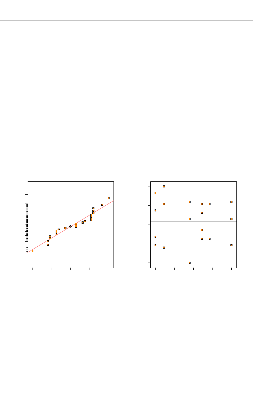
Solutions from Montgomery, D. C. (2001) Design and Analysis of Experiments, Wiley, NY
3-14
6-1.99 62.75 1.36
Mean
Standard t for H0
Treatment Difference DF Error Coeff=0 Prob > |t|
1 vs 2 5.75 1 1.92 3.00 0.0077
1 vs 3 7.75 1 1.92 4.04 0.0008
1 vs 4 11.00 1 1.92 5.74 < 0.0001
1 vs 5 17.75 1 1.92 9.26 < 0.0001
1 vs 6 20.00 1 1.92 10.43 < 0.0001
2 vs 3 2.00 1 1.92 1.04 0.3105
2 vs 4 5.25 1 1.92 2.74 0.0135
2 vs 5 12.00 1 1.92 6.26 < 0.0001
2 vs 6 14.25 1 1.92 7.43 < 0.0001
3 vs 4 3.25 1 1.92 1.70 0.1072
3 vs 5 10.00 1 1.92 5.22 < 0.0001
3 vs 6 12.25 1 1.92 6.39 < 0.0001
4 vs 5 6.75 1 1.92 3.52 0.0024
4 vs 6 9.00 1 1.92 4.70 0.0002
5 vs 6 2.25 1 1.92 1.17 0.2557
(b) Find the P-value for the F statistic in part (a). P=3.161 x 10⁻⁸
(c) Analyze the residuals from this experiment.
There is nothing unusual about the residuals.
Residual
Normal % probability
Normal plot of residuals
-4.75 -2.5625 -0.375 1.8125 4
1
5
10
20
30
50
70
80
90
95
99
22
22
22
22
22
Predicted
Residuals
Residuals vs. Predicted
-4.75
-2.5625
-0.375
1.8125
4
62.75 67.75 72.75 77.75 82.75
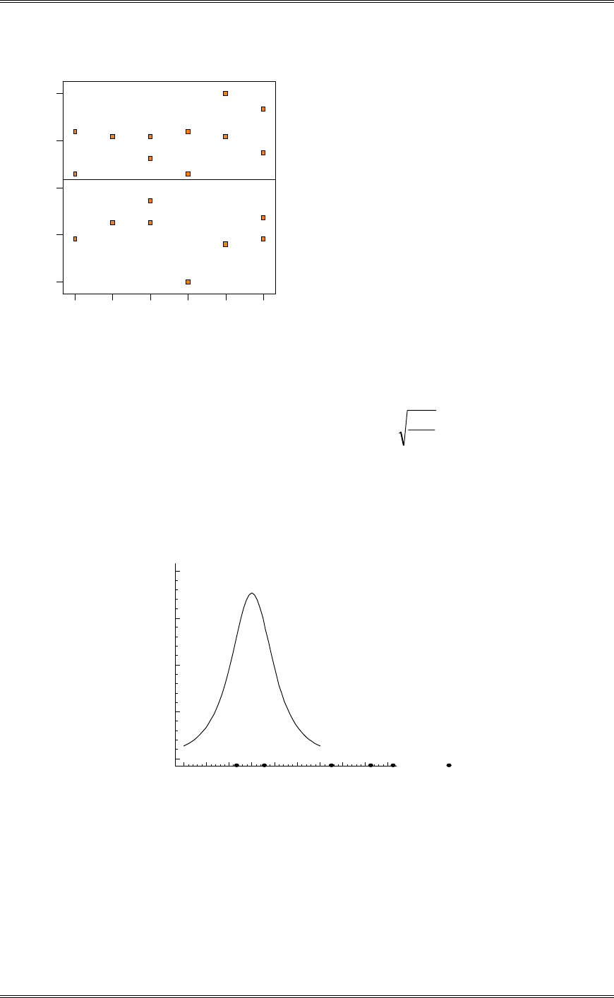
Solutions from Montgomery, D. C. (2001) Design and Analysis of Experiments, Wiley, NY
3-15
22
22
22 22
22
Orifice Diameter
Residuals
Residuals vs. Orifice Diameter
-4.75
-2.5625
-0.375
1.8125
4
123456
(d) Find a 95 percent confidence interval on the mean percent radon released when the orifice diameter is
1.40.
Treatment 5 (Orifice =1.40): 4
357
10126 .
.r
8486715262 .. dd
P
(e) Construct a graphical display to compare the treatment means as describe in Section 3-5.3. What
conclusions can you draw?
60 65 70 75 80
Conductivity
Scaled t Distribution
(6) (5) (3) (2) (1)(4)
Treatments 5 and 6 as a group differ from the other means; 2, 3, and 4 as a group differ from the other
means, 1 differs from the others.
3-10 The response time in milliseconds was determined for three different types of circuits that could be
used in an automatic valve shutoff mechanism. The results are shown in the following table.

Solutions from Montgomery, D. C. (2001) Design and Analysis of Experiments, Wiley, NY
3-16
Circuit Type Response Time
1 9 12 10 8 15
2 20 21 23 17 30
3 6 5 8 16 7
(a) Test the hypothesis that the three circuit types have the same response time. Use
D
= 0.01.
From the computer printout, F=16.08, so there is at least one circuit type that is different.
Design Expert Output
Response: Response Time in ms
ANOVA for Selected Factorial Model
Analysis of variance table [Partial sum of squares]
Sum of Mean F
Source Squares DF Square Value Prob > F
Model 543.60 2 271.80 16.08 0.0004 significant
A 543.60 2 271.80 16.08 0.0004
Residual 202.80 12 16.90
Lack of Fit 0.000 0
Pure Error 202.80 12 16.90
Cor Total 746.40 14
The Model F-value of 16.08 implies the model is significant. There is only
a 0.04% chance that a "Model F-Value" this large could occur due to noise.
Treatment Means (Adjusted, If Necessary)
Estimated
Standard
Mean
Error
1-1 10.80 1.84
2-2 22.20 1.84
3-3 8.40 1.84
Mean
Standard t for H0
Treatment Difference DF Error Coeff=0 Prob > |t|
1 vs 2 -11.40 1 2.60 -4.38 0.0009
1 vs 3 2.40 1 2.60 0.92 0.3742
2 vs 3 13.80 1 2.60 5.31 0.0002
(b) Use Tukey’s test to compare pairs of treatment means. Use
D
= 0.01.
83851
5
1690 .
n
MS
SE
y.i
045
123010.q ,,.
266904583851
0...t
1 vs. 2: ~10.8-22.2~=11.4 > 9.266
1 vs. 3: ~10.8-8.4~=2.4 < 9.266
2 vs. 3: ~22.2-8.4~=13.8 > 9.266
1 and 2 are different. 2 and 3 are different.
Notice that the results indicate that the mean of treatment 2 differs from the means of both treatments 1
and 3, and that the means for treatments 1 and 3 are the same. Notice also that the Fisher LSD procedure
(see the computer output) gives the same results.
(c) Use the graphical procedure in Section 3-5.3 to compare the treatment means. What conclusions can
you draw? How do they compare with the conclusions from part (a).
The scaled-t plot agrees with part (b). In this case, the large difference between the mean of treatment 2
and the other two treatments is very obvious.
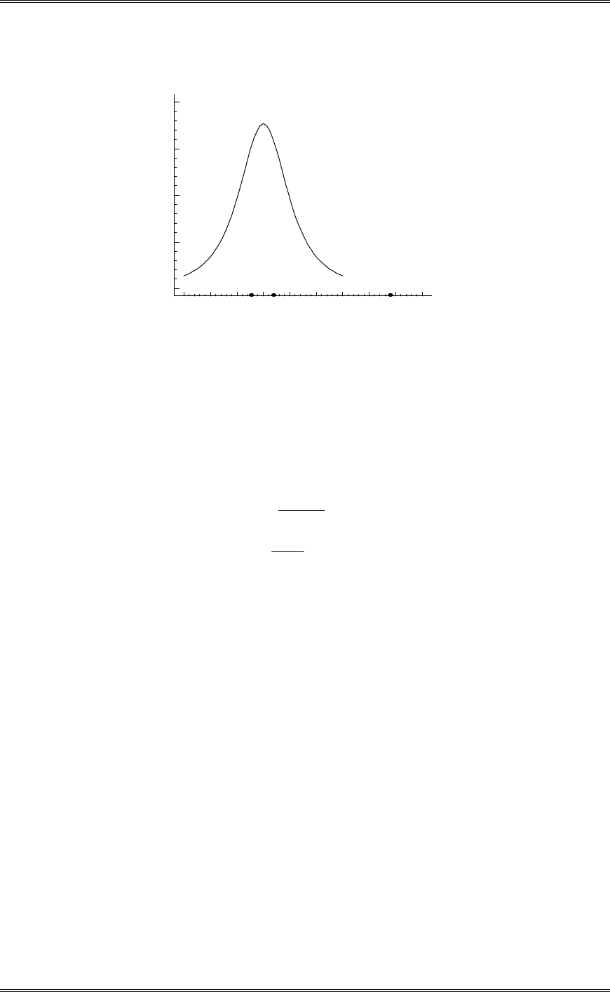
Solutions from Montgomery, D. C. (2001) Design and Analysis of Experiments, Wiley, NY
3-17
5 10152025
Tensile Strength
Scaled t Distribution
(3) (2)(1)
(d) Construct a set of orthogonal contrasts, assuming that at the outset of the experiment you suspected
the response time of circuit type 2 to be different from the other two.
01 23
11 23
11. 2.3.
1
20
20
2
54 2 111 42 126
H
H
Cy y y
C
PPP
PPP
z
2
1
1
126 529.2
56
529.2 31.31
16.9
C
C
SS
F
Type 2 differs from the average of type 1 and type 3.
(e) If you were a design engineer and you wished to minimize the response time, which circuit type
would you select?
Either type 1 or type 3 as they are not different from each other and have the lowest response time.
(f) Analyze the residuals from this experiment. Are the basic analysis of variance assumptions satisfied?
The normal probability plot has some points that do not lie along the line in the upper region. This may
indicate potential outliers in the data.
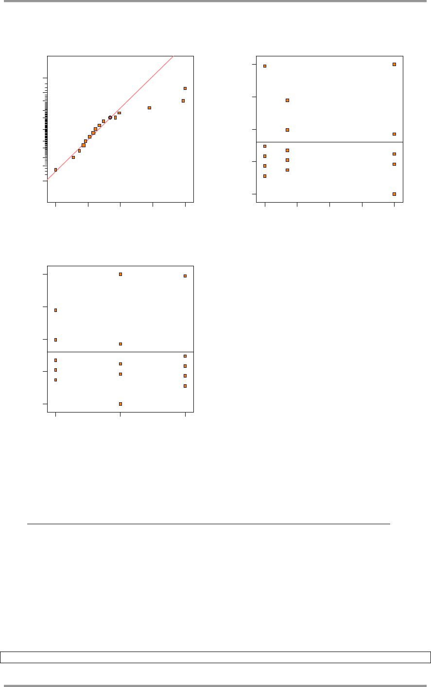
Solutions from Montgomery, D. C. (2001) Design and Analysis of Experiments, Wiley, NY
3-18
Residual
Normal % probability
Normal plot of residuals
-5.2 -1.9 5 1.3 4.55 7.8
1
5
10
20
30
50
70
80
90
95
99
Predicted
Residuals
Residuals vs. Predicted
-5.2
-1.95
1.3
4.55
7.8
8.40 11.85 15.30 18.75 22.20
Circuit Type
Residuals
Residuals vs. Circuit Type
-5.2
-1.95
1.3
4.55
7.8
123
3-11 The effective life of insulating fluids at an accelerated load of 35 kV is being studied. Test data
have been obtained for four types of fluids. The results were as follows:
Fluid Type Life (in h) at 35 kV Load
1 17.6 18.9 16.3 17.4 20.1 21.6
2 16.9 15.3 18.6 17.1 19.5 20.3
3 21.4 23.6 19.4 18.5 20.5 22.3
4 19.3 21.1 16.9 17.5 18.3 19.8
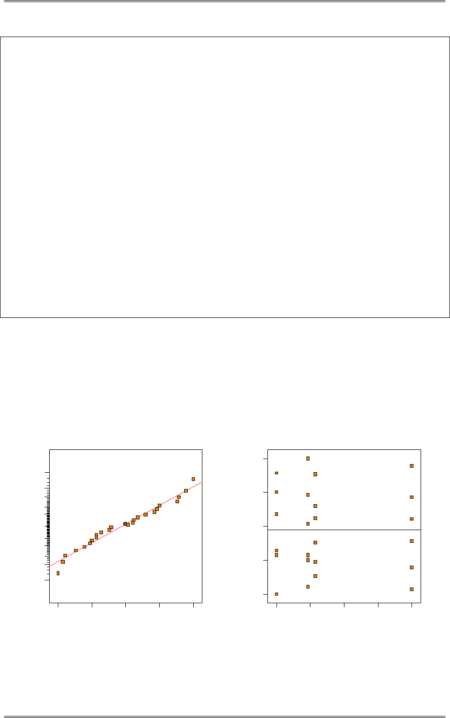
(a) Is there any indication that the fluids differ? Use D = 0.05.
At D = 0.05 there are no difference, but at since the P-value is just slightly above 0.05, there is probably a
difference in means.
Design Expert Output
Response: Life in in h
Solutions from Montgomery, D. C. (2001) Design and Analysis of Experiments, Wiley, NY
3-19
ANOVA for Selected Factorial Model
Analysis of variance table [Partial sum of squares]
Sum of Mean F
Source Squares DF Square Value Prob > F
Model 30.17 3 10.06 3.05 0.0525 not significant
A 30.16 3 10.05 3.05 0.0525
Residual 65.99 20 3.30
Lack of Fit 0.000 0
Pure Error 65.99 20 3.30
Cor Total 96.16 23
The Model F-value of 3.05 implies there is a 5.25% chance that a "Model F-Value"
this large could occur due to noise.
Treatment Means (Adjusted, If Necessary)
Estimated
Standard
Mean
Error
1-1 18.65 0.74
2-2 17.95 0.74
3-3 20.95 0.74
4-4 18.82 0.74
Mean
Standard t for H0
Treatment Difference DF Error Coeff=0 Prob > |t|
1 vs 2 0.70 1 1.05 0.67 0.5121
1 vs 3 -2.30 1 1.05 -2.19 0.0403
1 vs 4 -0.17 1 1.05 -0.16 0.8753
2 vs 3 -3.00 1 1.05 -2.86 0.0097
2 vs 4 -0.87 1 1.05 -0.83 0.4183
3 vs 4 2.13 1 1.05 2.03 0.0554
(b) Which fluid would you select, given that the objective is long life?
Treatment 3. The Fisher LSD procedure in the computer output indicates that the fluid 3 is different from
the others, and it’s average life also exceeds the average lives of the other three fluids.
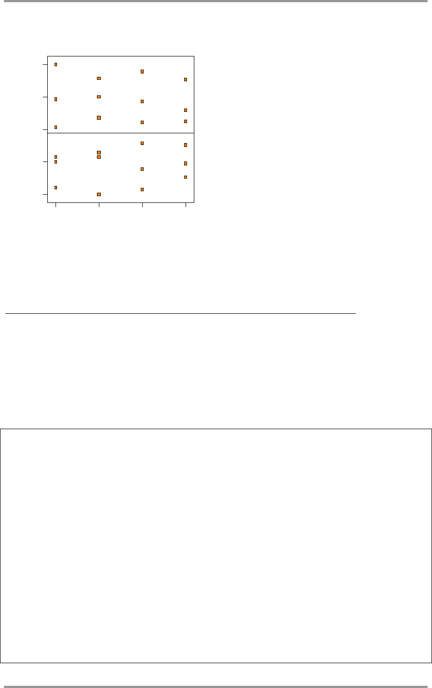
(c) Analyze the residuals from this experiment. Are the basic analysis of variance assumptions satisfied?
There is nothing unusual in the residual plots.
Residual
Normal % probability
Normal plot of residuals
-2.65 -1 .25 0.15 1.55 2.95
1
5
10
20
30
50
70
80
90
95
99
Predicted
Residuals
Residuals vs. Predicted
-2.65
-1.25
0.15
1.55
2.95
17.95 18.70 19.45 20.20 20.95
Solutions from Montgomery, D. C. (2001) Design and Analysis of Experiments, Wiley, NY
3-20
Fluid Type
Residuals
Residuals vs. Fluid Type
-2.65
-1.25
0.15
1.55
2.95
1 2 3 4
3-12 Four different designs for a digital computer circuit are being studied in order to compare the
amount of noise present. The following data have been obtained:
Circuit Design Noise Observed
1 19 20 19 30 8
2 80 61 73 56 80
3 47 26 25 35 50
4 95 46 83 78 97
(a) Is the amount of noise present the same for all four designs? Use D = 0.05.
No, at least one treatment mean is different.
Design Expert Output
Response: Noise
ANOVA for Selected Factorial Model
Analysis of variance table [Partial sum of squares]
Sum of Mean F
Source Squares DF Square Value Prob > F
Model 12042.00 3 4014.00 21.78 < 0.0001 significant
A 12042.00 3 4014.00 21.78 < 0.0001
Residual 2948.80 16 184.30
Lack of Fit 0.000 0
Pure Error 2948.80 16 184.30
Cor Total 14990.80 19
The Model F-value of 21.78 implies the model is significant. There is only
a 0.01% chance that a "Model F-Value" this large could occur due to noise.
Treatment Means (Adjusted, If Necessary)
Estimated
Standard
Mean
Error
1-1 19.20 6.07
2-2 70.00 6.07
3-3 36.60 6.07
4-4 79.80 6.07
Mean
Standard t for H0
Treatment Difference DF Error Coeff=0 Prob > |t|
1 vs 2 -50.80 1 8.59 -5.92 < 0.0001

Solutions from Montgomery, D. C. (2001) Design and Analysis of Experiments, Wiley, NY
3-21
1 vs 3 -17.40 1 8.59 -2.03 0.0597
1 vs 4 -60.60 1 8.59 -7.06 < 0.0001
2 vs 3 33.40 1 8.59 3.89 0.0013
2 vs 4 -9.80 1 8.59 -1.14 0.2705
3 vs 4 -43.20 1 8.59 -5.03 0.0001
(b) Analyze the residuals from this experiment. Are the basic analysis of variance assumptions satisfied?
There is nothing unusual about the residual plots.
Residual
Normal % probability
Normal plot of residuals
-33.8 -21.05 -8.3 4.45 17.2
1
5
10
20
30
50
70
80
90
95
99
22
22
Predicted
Residuals
Residuals vs. Predicted
-33.8
-21.05
-8.3
4.45
17.2
19.20 34.35 49.50 64.65 79.80
22
22
Circuit Design
Residuals
Residuals vs. Circuit Design
-33.8
-21.05
-8.3
4.45
17.2
1 2 3 4
(c) Which circuit design would you select for use? Low noise is best.
From the Design Expert Output, the Fisher LSD procedure comparing the difference in means identifies
Type 1 as having lower noise than Types 2 and 4. Although the LSD procedure comparing Types 1 and 3
has a P-value greater than 0.05, it is less than 0.10. Unless there are other reasons for choosing Type 3,
Type 1 would be selected.

Solutions from Montgomery, D. C. (2001) Design and Analysis of Experiments, Wiley, NY
3-22
3-13 Four chemists are asked to determine the percentage of methyl alcohol in a certain chemical
compound. Each chemist makes three determinations, and the results are the following:
Chemist Percentage of Methyl Alcohol
1 84.99 84.04 84.38
2 85.15 85.13 84.88
3 84.72 84.48 85.16
4 84.20 84.10 84.55
(a) Do chemists differ significantly? Use
D
= 0.05.
There is no significant difference at the 5% level, but chemists differ significantly at the 10% level.
Design Expert Output
Response: Methyl Alcohol in %
ANOVA for Selected Factorial Model
Analysis of variance table [Partial sum of squares]
Sum of Mean F
Source Squares DF Square Value Prob > F
Model 1.04 3 0.35 3.25 0.0813 not significant
A 1.04 3 0.35 3.25 0.0813
Residual 0.86 8 0.11
Lack of Fit 0.000 0
Pure Error 0.86 8 0.11
Cor Total 1.90 11
The Model F-value of 3.25 implies there is a 8.13% chance that a "Model F-Value"
this large could occur due to noise.
Treatment Means (Adjusted, If Necessary)
Estimated
Standard
Mean
Error
1-1 84.47 0.19
2-2 85.05 0.19
3-3 84.79 0.19
4-4 84.28 0.19
Mean
Standard t for H0
Treatment Difference DF Error Coeff=0 Prob > |t|
1 vs 2 -0.58 1 0.27 -2.18 0.0607
1 vs 3 -0.32 1 0.27 -1.18 0.2703
1 vs 4 0.19 1 0.27 0.70 0.5049
2 vs 3 0.27 1 0.27 1.00 0.3479
2 vs 4 0.77 1 0.27 2.88 0.0205
3 vs 4 0.50 1 0.27 1.88 0.0966
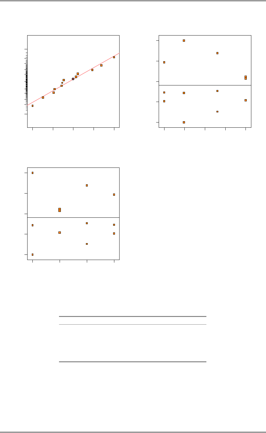
(b) Analyze the residuals from this experiment.
There is nothing unusual about the residual plots.
Solutions from Montgomery, D. C. (2001) Design and Analysis of Experiments, Wiley, NY
3-23
Residual
Normal % probability
Normal plot of residuals
-0.43 -0.1925 0.045 0.2825 0.52
1
5
10
20
30
50
70
80
90
95
99
Predicted
Residuals
Residuals vs. Predicted
-0.43
-0.1925
0.045
0.2825
0.52
84.28 84.48 84.67 84.86 85.05
Chemist
Residuals
Residuals vs. Chemist
-0.43
-0.1925
0.045
0.2825
0.52
1 2 3 4
(c) If chemist 2 is a new employee, construct a meaningful set of orthogonal contrasts that might have
been useful at the start of the experiment.
Chemists Total C1 C2 C3
1 253.41 1 -2 0
2 255.16 -3 0 0
3 254.36 1 1 -1
4 252.85 1 1 1
Contrast Totals: -4.86 0.39 -1.51

Solutions from Montgomery, D. C. (2001) Design and Analysis of Experiments, Wiley, NY
3-24
543
107270
3800
3800
23
511
0750
107270
0080
0080
63
390
1156
107270
6560
6560
123
864
3
2
3
2
2
2
1
2
1
.
.
.
F.
.
SS
.
.
.
F.
.
SS
*.
.
.
F.
.
SS
CC
CC
CC
Only contrast 1 is significant at 5%.
3-14 Three brands of batteries are under study. It is s suspected that the lives (in weeks) of the three
brands are different. Five batteries of each brand are tested with the following results:
Weeks of Life
Brand 1 Brand 2 Brand 3
100 76 108
96 80 100
92 75 96
96 84 98
92 82 100
(a) Are the lives of these brands of batteries different?
Yes, at least one of the brands is different.
Design Expert Output
Response: Life in Weeks
ANOVA for Selected Factorial Model
Analysis of variance table [Partial sum of squares]
Sum of Mean F
Source Squares DF Square Value Prob > F
Model 1196.13 2 598.07 38.34 < 0.0001 significant
A 1196.13 2 598.07 38.34 < 0.0001
Residual 187.20 12 15.60
Lack of Fit 0.000 0
Pure Error 187.20 12 15.60
Cor Total 1383.33 14
The Model F-value of 38.34 implies the model is significant. There is only
a 0.01% chance that a "Model F-Value" this large could occur due to noise.
Treatment Means (Adjusted, If Necessary)
Estimated
Standard
Mean
Error
1-1 95.20 1.77
2-2 79.40 1.77
3-3 100.40 1.77
Mean
Standard t for H0
Treatment Difference DF Error Coeff=0 Prob > |t|
1 vs 2 15.80 1 2.50 6.33 < 0.0001
1 vs 3 -5.20 1 2.50 -2.08 0.0594
2 vs 3 -21.00 1 2.50 -8.41 < 0.0001
(b) Analyze the residuals from this experiment.
There is nothing unusual about the residuals.

Solutions from Montgomery, D. C. (2001) Design and Analysis of Experiments, Wiley, NY
3-25
Residual
Normal % probability
Normal plot of residuals
-4.4 -1.4 1.6 4.6 7.6
1
5
10
20
30
50
70
80
90
95
99
2
2
2
2
22
Predicted
Residuals
Residuals vs. Predicted
-4.4
-1.4
1.6
4.6
7.6
79.40 84.65 89.90 95.15 100.40
2
2
2
2
22
Brand
Residuals
Residuals vs. Brand
-4.4
-1.4
1.6
4.6
7.6
123
(c) Construct a 95 percent interval estimate on the mean life of battery brand 2. Construct a 99 percent
interval estimate on the mean difference between the lives of battery brands 2 and 3.
n
MS
ty E
aN,
.i
r
2
D
Brand 2: 5
6015
1792479 .
.. r
84934079 .. r
2498355175 2.. dd
P
Brand 2 - Brand 3: n
MS
tyy E
aN,
.j.i
2
2
r
D
5
60152
05534100479 .
... r
3691363128 32 .. dd
PP

Solutions from Montgomery, D. C. (2001) Design and Analysis of Experiments, Wiley, NY
3-26
(d) Which brand would you select for use? If the manufacturer will replace without charge any battery
that fails in less than 85 weeks, what percentage would the company expect to replace?
Chose brand 3 for longest life. Mean life of this brand in 100.4 weeks, and the variance of life is
estimated by 15.60 (MSE). Assuming normality, then the probability of failure before 85 weeks is:
000050903
6015
410085 ..
.
.
¸
¸
¹
·
¨
¨
©
§
))
That is, about 5 out of 100,000 batteries will fail before 85 week.
3-15 Four catalysts that may affect the concentration of one component in a three component liquid
mixture are being investigated. The following concentrations are obtained:
Catalyst
1 2 3 4
58.2 56.3 50.1 52.9
57.2 54.5 54.2 49.9
58.4 57.0 55.4 50.0
55.8 55.3 51.7
54.9
(a) Do the four catalysts have the same effect on concentration?
No, their means are different.
Design Expert Output
Response: Concentration
ANOVA for Selected Factorial Model
Analysis of variance table [Partial sum of squares]
Sum of Mean F
Source Squares DF Square Value Prob > F
Model 85.68 3 28.56 9.92 0.0014 significant
A 85.68 3 28.56 9.92 0.0014
Residual 34.56 12 2.88
Lack of Fit 0.000 0
Pure Error 34.56 12 2.88
Cor Total 120.24 15
The Model F-value of 9.92 implies the model is significant. There is only
a 0.14% chance that a "Model F-Value" this large could occur due to noise.
Treatment Means (Adjusted, If Necessary)
Estimated
Standard
Mean
Error
1-1 56.90 0.76
2-2 55.77 0.85
3-3 53.23 0.98
4-4 51.13 0.85
Mean
Standard t for H0
Treatment Difference DF Error Coeff=0 Prob > |t|
1 vs 2 1.13 1 1.14 0.99 0.3426
1 vs 3 3.67 1 1.24 2.96 0.0120
1 vs 4 5.77 1 1.14 5.07 0.0003
2 vs 3 2.54 1 1.30 1.96 0.0735
2 vs 4 4.65 1 1.20 3.87 0.0022
3 vs 4 2.11 1 1.30 1.63 0.1298
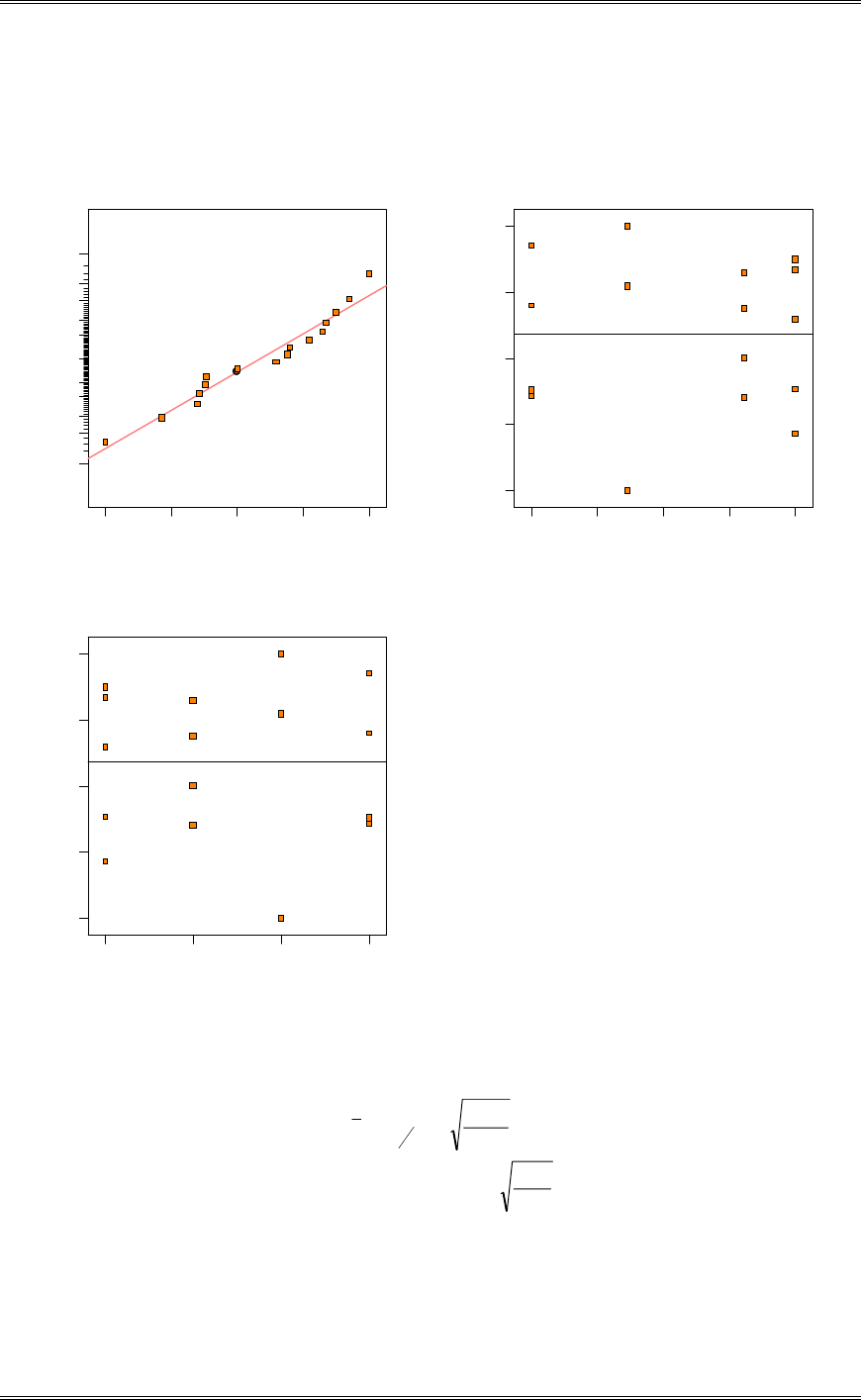
Solutions from Montgomery, D. C. (2001) Design and Analysis of Experiments, Wiley, NY
3-27
(b) Analyze the residuals from this experiment.
There is nothing unusual about the residual plots.
Residual
Normal % probability
Normal plot of residuals
-3.13333 -1.80833 -0.483333 0.841667 2.16667
1
5
10
20
30
50
70
80
90
95
99
Predicted
Residuals
Residuals vs. Predicted
-3.13333
-1.80833
-0.483333
0.841667
2.16667
51.13 52.57 54.01 55.46 56.90
Catalyst
Residuals
Residuals vs. Catalyst
-3.13333
-1.80833
-0.483333
0.841667
2.16667
1 2 3 4
(c) Construct a 99 percent confidence interval estimate of the mean response for catalyst 1.
n
MS
ty E
aN,
.i
r
2
D
Catalyst 1: 5
882
0553956 .
.. r
31862956 .. r
218659581454 1.. dd
P

Solutions from Montgomery, D. C. (2001) Design and Analysis of Experiments, Wiley, NY
3-28
3-16 An experiment was performed to investigate the effectiveness of five insulating materials. Four
samples of each material were tested at an elevated voltage level to accelerate the time to failure. The
failure times (in minutes) is shown below.
Material Failure Time (minutes)
1 110 157 194 178
2 1 2 4 18
3 880 1256 5276 4355
4 495 7040 5307 10050
5 7 5 29 2
(a) Do all five materials have the same effect on mean failure time?
No, at least one material is different.
Design Expert Output
Response: Failure Time
in Minutes
ANOVA for Selected Factorial Model
Analysis of variance table [Partial sum of squares]
Sum of Mean F
Source Squares DF Square Value Prob > F
Model 1.032E+008 4 2.580E+007 6.19 0.0038 significant
A 1.032E+008 4 2.580E+007 6.19 0.0038
Residual 6.251E+007 15 4.167E+006
Lack of Fit 0.000 0
Pure Error 6.251E+00715 4.167E+006
Cor Total 1.657E+008 19
The Model F-value of 6.19 implies the model is significant. There is only
a 0.38% chance that a "Model F-Value" this large could occur due to noise.
Treatment Means (Adjusted, If Necessary)
Estimated
Standard
Mean
Error
1-1 159.75 1020.67
2-2 6.25 1020.67
3-3 2941.75 1020.67
4-4 5723.00 1020.67
5-5 10.75 1020.67
Mean
Standard t for H0
Treatment Difference DF Error Coeff=0 Prob > |t|
1 vs 2 153.50 1 1443.44 0.11 0.9167
1 vs 3 -2782.00 1 1443.44 -1.93 0.0731
1 vs 4 -5563.25 1 1443.44 -3.85 0.0016
1 vs 5 149.00 1 1443.44 0.10 0.9192
2 vs 3 -2935.50 1 1443.44 -2.03 0.0601
2 vs 4 -5716.75 1 1443.44 -3.96 0.0013
2 vs 5 -4.50 1 1443.44 -3.118E-003 0.9976
3 vs 4 -2781.25 1 1443.44 -1.93 0.0732
3 vs 5 2931.00 1 1443.44 2.03 0.0604
4 vs 5 5712.25 1 1443.44 3.96 0.0013
(b) Plot the residuals versus the predicted response. Construct a normal probability plot of the residuals.
What information do these plots convey?
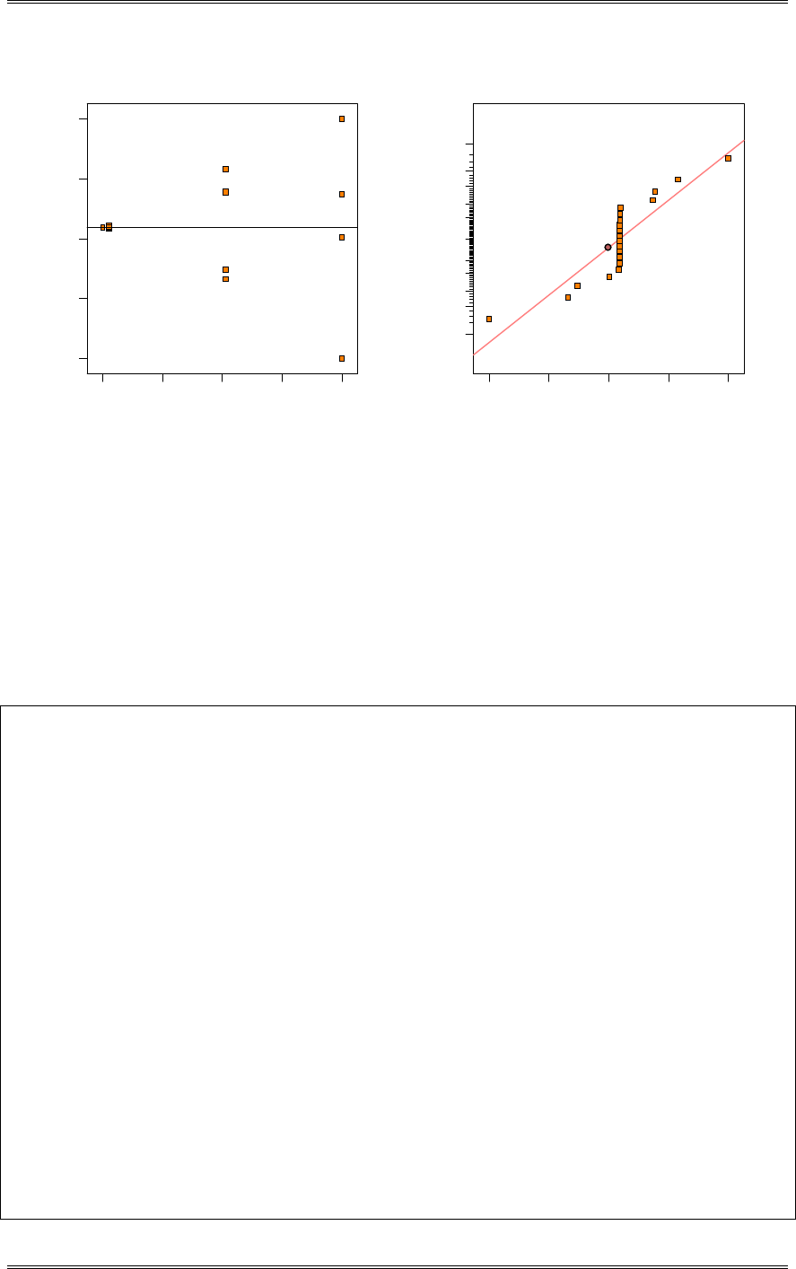
Solutions from Montgomery, D. C. (2001) Design and Analysis of Experiments, Wiley, NY
3-29
Predicted
Residuals
Residuals vs. Predicted
-5228
-2839.25
-450.5
1938.25
4327
6.25 1435.44 2864.62 4293.81 5723.00
Residual
Normal % probability
Normal plot of residuals
-5228 -2839.25 -450.5 1938.25 4327
1
5
10
20
30
50
70
80
90
95
99
The plot of residuals versus predicted has a strong outward-opening funnel shape, which indicates the
variance of the original observations is not constant. The residuals plotted in the normal probability plot
also imply that the normality assumption is not valid. A data transformation is recommended.
(c) Based on your answer to part (b) conduct another analysis of the failure time data and draw
appropriate conclusions.
A natural log transformation was applied to the failure time data. The analysis identifies that there exists
at least one difference in treatment means.
Design Expert Output
Response: Failure Time
in Minutes Transform: Natural log Constant: 0.000
ANOVA for Selected Factorial Model
Analysis of variance table [Partial sum of squares]
Sum of Mean F
Source Squares DF Square Value Prob > F
Model 165.06 4 41.26 37.66 < 0.0001 significant
A 165.06 4 41.26 37.66 < 0.0001
Residual 16.44 15 1.10
Lack of Fit 0.000 0
Pure Error 16.44 15 1.10
Cor Total 181.49 19
The Model F-value of 37.66 implies the model is significant. There is only
a 0.01% chance that a "Model F-Value" this large could occur due to noise.
Treatment Means (Adjusted, If Necessary)
Estimated
Standard
Mean
Error
1-1 5.05 0.52
2-2 1.24 0.52
3-3 7.72 0.52
4-4 8.21 0.52
5-5 1.90 0.52
Mean
Standard t for H0
Treatment Difference DF Error Coeff=0 Prob > |t|
1 vs 2 3.81 1 0.74 5.15 0.0001
1 vs 3 -2.66 1 0.74 -3.60 0.0026
1 vs 4 -3.16 1 0.74 -4.27 0.0007
1 vs 5 3.15 1 0.74 4.25 0.0007
2 vs 3 -6.47 1 0.74 -8.75 < 0.0001
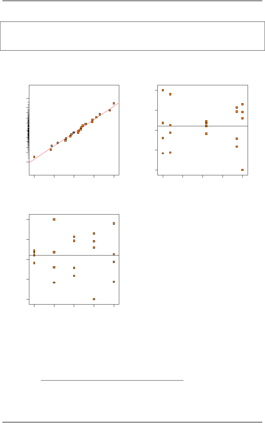
Solutions from Montgomery, D. C. (2001) Design and Analysis of Experiments, Wiley, NY
3-30
2 vs 4 -6.97 1 0.74 -9.42 < 0.0001
2 vs 5 -0.66 1 0.74 -0.89 0.3856
3 vs 4 -0.50 1 0.74 -0.67 0.5116
3 vs 5 5.81 1 0.74 7.85 < 0.0001
4 vs 5 6.31 1 0.74 8.52 < 0.0001
There is nothing unusual about the residual plots when the natural log transformation is applied.
Residual
Normal % probability
Normal plot of residuals
-2.00945 -1.09511 -0.180766 0.733576 1.64792
1
5
10
20
30
50
70
80
90
95
99
Predicted
Residuals
Residuals vs. Predicted
-2.00945
-1.09511
-0.180766
0.733576
1.64792
1.24 2.99 4.73 6.47 8.21
Ma te ri al
Residuals
Residuals vs. Material
-2.00945
-1.09511
-0.180766
0.733576
1.64792
12345
3-17 A semiconductor manufacturer has developed three different methods for reducing particle counts
on wafers. All three methods are tested on five wafers and the after-treatment particle counts obtained.
The data are shown below.
Method Count
1 31 10 21 4 1
2 62 40 24 30 35
3 58 27 120 97 68
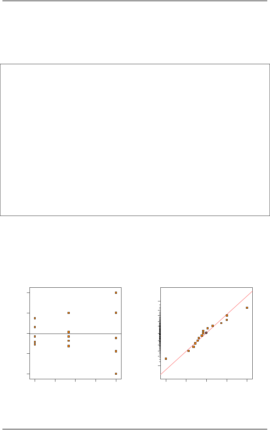
Solutions from Montgomery, D. C. (2001) Design and Analysis of Experiments, Wiley, NY
3-31
(a) Do all methods have the same effect on mean particle count?
No, at least one method has a different effect on mean particle count.
Design Expert Output
Response: Count
ANOVA for Selected Factorial Model
Analysis of variance table [Partial sum of squares]
Sum of Mean F
Source Squares DF Square Value Prob > F
Model 8963.73 2 4481.87 7.91 0.0064 significant
A 8963.73 2 4481.87 7.91 0.0064
Residual 6796.00 12 566.33
Lack of Fit 0.000 0
Pure Error 6796.00 12 566.33
Cor Total 15759.73 14
The Model F-value of 7.91 implies the model is significant. There is only
a 0.64% chance that a "Model F-Value" this large could occur due to noise.
Treatment Means (Adjusted, If Necessary)
Estimated
Standard
Mean
Error
1-1 13.40 10.64
2-2 38.20 10.64
3-3 73.00 10.64
Mean
Standard t for H0
Treatment Difference DF Error Coeff=0 Prob > |t|
1 vs 2 -24.80 1 15.05 -1.65 0.1253
1 vs 3 -59.60 1 15.05 -3.96 0.0019
2 vs 3 -34.80 1 15.05 -2.31 0.0393
(b) Plot the residuals versus the predicted response. Construct a normal probability plot of the residuals.
Are there potential concerns about the validity of the assumptions?
The plot of residuals versus predicted appears to be funnel shaped. This indicates the variance of the
original observations is not constant. The residuals plotted in the normal probability plot do not fall along
a straight line, which suggests that the normality assumption is not valid. A data transformation is
recommended.
Predicted
Residuals
Residuals vs. Predicted
-46
-22.75
0.5
23.75
47
13.40 28.30 43.20 58.10 73.00
Residual
Normal % probability
Normal plot of residuals
-46 -22.75 0.5 23.75 47
1
5
10
20
30
50
70
80
90
95
99

Solutions from Montgomery, D. C. (2001) Design and Analysis of Experiments, Wiley, NY
3-32
(c) Based on your answer to part (b) conduct another analysis of the particle count data and draw
appropriate conclusions.
For count data, a square root transformation is often very effective in resolving problems with inequality
of variance. The analysis of variance for the transformed response is shown below. The difference
between methods is much more apparent after applying the square root transformation.
Design Expert Output
Response: Count Transform: Square root Constant: 0.000
ANOVA for Selected Factorial Model
Analysis of variance table [Partial sum of squares]
Sum of Mean F
Source Squares DF Square Value Prob > F
Model 63.90 2 31.95 9.84 0.0030 significant
A 63.90 2 31.95 9.84 0.0030
Residual 38.96 12 3.25
Lack of Fit 0.000 0
Pure Error 38.96 12 3.25
Cor Total 102.86 14
The Model F-value of 9.84 implies the model is significant. There is only
a 0.30% chance that a "Model F-Value" this large could occur due to noise.
Treatment Means (Adjusted, If Necessary)
Estimated
Standard
Mean
Error
1-1 3.26 0.81
2-2 6.10 0.81
3-3 8.31 0.81
Mean
Standard t for H0
Treatment Difference DF Error Coeff=0 Prob > |t|
1 vs 2 -2.84 1 1.14 -2.49 0.0285
1 vs 3 -5.04 1 1.14 -4.42 0.0008
2 vs 3 -2.21 1 1.14 -1.94 0.0767
3-18 Consider testing the equality of the means of two normal populations, where the variances are
unknown but are assumed to be equal. The appropriate test procedure is the pooled t test. Show that the
pooled t test is equivalent to the single factor analysis of variance.
22
21
02
n
p
.. t~
n
S
yy
t assuming n1 = n2 = n
E
i
n
j
.ij
n
j
.j
n
j
.j
pMS
n
yy
n
yyyy
S{
¦¦¦¦
2222
2
11
2
1
1
2
22
1
2
11
for a=2
Furthermore,
n
y
n
yn
yy ..
i
.i
.. 22
2
2
1
2
2
21
¸
¹
·
¨
©
§
¦
, which is exactly the same as SSTreatments in a one-way
classification with a=2. Thus we have shown that
E
Treatments
MS
SS
t
2
0. In general, we know that u,u Ft 1
2
so that 221
2
0
n,
F~t . Thus the square of the test statistic from the pooled t-test is the same test statistic
that results from a single-factor analysis of variance with a=2.

Solutions from Montgomery, D. C. (2001) Design and Analysis of Experiments, Wiley, NY
3-33
3-19 Show that the variance of the linear combination ¦
a
i
.ii yc
1
is ¦
a
i
ii cn
1
22
V
.
¦¦¦¦¦¦
»
»
¼
º
«
«
¬
ª
»
»
¼
º
«
«
¬
ªii n
j
.ij
a
i
i
a
i
n
j
iji
a
i
.ii
a
i
.ii yVcyVcycVycV
11
2
11
2
11
,
2
V
ij
yV
¦
a
i
ii nc
1
22
V
3-20 In a fixed effects experiment, suppose that there are n observations for each of four treatments. Let
2
3
2
2
2
1Q,Q,Q be single-degree-of-freedom components for the orthogonal contrasts. Prove that
2
3
2
2
2
1QQQSSTreatments .
2
33433
2
224322
2
1143211
2
3
QSSyyC
QSSyyyC
QSSyyyyC
C..
C...
C....
n
)yy(
Q
n
)yyy(
Q
n
)yyyy(
Q
..
...
....
2
6
2
12
3
2
432
3
2
4322
2
2
43212
1
n
yyy
QQQ iji
.j.i.i
12
69
4
1
2
2
3
2
2
2
1
¦¦¦
¸
¸
¹
·
¨
¨
©
§
and since
¸
¸
¹
·
¨
¨
©
§ ¦¦¦
4
1
22
2
1
i
.i..
ji
.j.i yyyy , we have Treatments
..
i
.ii
...i
SS
n
y
n
y
n
yy
QQQ
¦
¦
412
312 24
1
2
4
1
22
2
3
2
2
2
1
for a=4.
3-21 Use Bartlett's test to determine if the assumption of equal variances is satisfied in Problem 3-14.
Use
D
= 0.05. Did you reach the same conclusion regarding the equality of variance by examining the
residual plots?
c
q
.30262
2
0
F
, where

Solutions from Montgomery, D. C. (2001) Design and Analysis of Experiments, Wiley, NY
3-34
aN
Sn
S
aNn
a
c
SlognSlogaNq
a
i
ii
p
a
i
i
a
i
iip
¸
¸
¹
·
¨
¨
©
§
¦
¦
¦
1
2
2
1
11
1
2
10
2
10
1
1
13
1
1
1
820
814
211
2
3
2
2
2
1
.S
.S
.S
615
315
820158141521115
315
820158141521115
2
2
.
...
S
...
S
p
p
13891
12
1
4
3
133
1
1
31515
133
1
1
1
11
.c
c
a
i
¸
¹
·
¨
©
§
¸
¸
¹
·
¨
¨
©
§
¦
1675015014317514
8208142114615315
1
10101010
1
2
10
2
10
...q
.log.log.log.logq
SlognSlogaNq
a
i
iip
¦
33860
13891
16750
3026230262
2
0.
.
.
.
c
q
.
F
499
2
4050.
,.
F
Cannot reject null hypothesis; conclude that the variance are equal. This agrees with the residual plots in
Problem 3-16.
3-22 Use the modified Levene test to determine if the assumption of equal variances is satisfied on
Problem 3-14. Use
D
= 0.05. Did you reach the same conclusion regarding the equality of variances by
examining the residual plots?
The absolute value of Battery Life – brand median is:
ij i
yy
Brand 1 Brand 2 Brand 3
4 4 8
0 0 0
4 5 4
0 4 2
4 2 0
The analysis of variance indicates that there is not a difference between the different brands and therefore
the assumption of equal variances is satisfired.
Design Expert Output
Response: Mod Levine
ANOVA for Selected Factorial Model
Analysis of variance table [Partial sum of squares]

Solutions from Montgomery, D. C. (2001) Design and Analysis of Experiments, Wiley, NY
3-35
Sum of
Mean F
Source Squares DF Square Value Prob > F
Model 0.93 2 0.47 0.070 0.9328
A 0.93 2 0.47 0.070 0.9328
Pure Error 80.00 12 6.67
Cor Total 80.93 14
3-23 Refer to Problem 3-10. If we wish to detect a maximum difference in mean response times of 10
milliseconds with a probability of at least 0.90, what sample size should be used? How would you obtain a
preliminary estimate of 2
V
?
2
2
2
2
V
)
a
nD
, use MSE from Problem 3-10 to estimate 2
V
.
n.
.
n9860
91632
10 2
2
)
Letting 050.
D
, P(accept) = 0.1 , 21
1 a
X
Trial and Error yields:
n 2
X
) P(accept)
5 12 2.22 0.17
6 15 2.43 0.09
7 18 2.62 0.04
Choose n t 6, therefore N t 18
Notice that we have used an estimate of the variance obtained from the present experiment. This indicates
that we probably didn’t use a large enough sample (n was 5 in problem 3-10) to satisfy the criteria
specified in this problem. However, the sample size was adequate to detect differences in one of the
circuit types.
When we have no prior estimate of variability, sometimes we will generate sample sizes for a range of
possible variances to see what effect this has on the size of the experiment. Often a knowledgeable expert
will be able to bound the variability in the response, by statements such as “the standard deviation is going
to be at least…” or “the standard deviation shouldn’t be larger than…”.
3-24 Refer to Problem 3-14.
(a) If we wish to detect a maximum difference in mean battery life of 0.5 percent with a probability of at
least 0.90, what sample size should be used? Discuss how you would obtain a preliminary estimate of
V
2 for answering this question.
Use the MSE from Problem 3-14.
)2
2
2
2
nD
a
V
n.
.
..n 0022440
601532
6667910050 2
2
u
)
Letting
D
005. , P(accept) = 0.1 , 21
1 a
X

Solutions from Montgomery, D. C. (2001) Design and Analysis of Experiments, Wiley, NY
3-36
Trial and Error yields:
n 2
X
) P(accept)
40 117 1.895 0.18
45 132 2.132 0.10
50 147 2.369 0.05
Choose n t 45, therefore N t 135
See the discussion from the previous problem about the estimate of variance.
(b) If the difference between brands is great enough so that the standard deviation of an observation is
increased by 25 percent, what sample size should be used if we wish to detect this with a probability
of at least 0.90?
21
1 a
X
12315
2 aN
X
050.
D
10.)accept(P d
>@
>@
n..nP.n 56250112501011101011 22
O
Trial and Error yields:
n 2
X
O P(accept)
40 117 4.84 0.13
45 132 5.13 0.11
50 147 5.40 0.10
Choose n t 50, therefore N t 150
3-25 Consider the experiment in Problem 3-16. If we wish to construct a 95 percent confidence interval
on the difference in two mean battery lives that has an accuracy of r2 weeks, how many batteries of each
brand must be tested?
050.
D
615.MS E
n
MS
twidth E
aN,.
2
0250
Trial and Error yields:
n
X
2 t width
5 12 2.179 5.44
10 27 2.05 3.62
31 90 1.99 1.996
32 93 1.99 1.96
Choose n t 31, therefore N t 93
3-26 Suppose that four normal populations have means of
P
1=50,
P
2=60,
P
3=50, and
P
4=60. How many
observations should be taken from each population so that the probability or rejecting the null hypothesis

Solutions from Montgomery, D. C. (2001) Design and Analysis of Experiments, Wiley, NY
3-37
of equal population means is at least 0.90? Assume that
D
=0.05 and that a reasonable estimate of the
error variance is 2
V
=25.
100
5555
55
4
220
4
4321
4
1
2
4321
4
1
¦
¦
i
i
i
i
ii
,,,
,,,i,
W
WWWW
P
P
WPP
n
n
n
a
ni
¦
)
V
W
)
254
100
2
2
2
050143 21 .,n,
DXX
, From the O.C. curves we can construct the following:
n ) X2 E 1-E
4 2.00 12 0.18 0.82
5 2.24 16 0.08 0.92
Therefore, select n=5
3-27 Refer to Problem 3-26.
(a) How would your answer change if a reasonable estimate of the experimental error variance were 2
V
=
36?
n.
n.
n
a
ni
69440
69440
364
100
2
2
2
¦
)
V
W
)
050143 21 .,n,
DXX
, From the O.C. curves we can construct the following:
n ) X2 E 1-E
5 1.863 16 0.24 0.76
6 2.041 20 0.15 0.85
7 2.205 24 0.09 0.91
Therefore, select n=7
(b) How would your answer change if a reasonable estimate of the experimental error variance were 2
V
=
49?
n.
n.
n
a
ni
51020
51020
494
100
2
2
2
¦
)
V
W
)
050143 21 .,n,
DXX
, From the O.C. curves we can construct the following:

Solutions from Montgomery, D. C. (2001) Design and Analysis of Experiments, Wiley, NY
3-38
n ) X2 E 1-E
7 1.890 24 0.16 0.84
8 2.020 28 0.11 0.89
9 2.142 32 0.09 0.91
Therefore, select n=9
(c) Can you draw any conclusions about the sensitivity of your answer in the particular situation about
how your estimate of
V
affects the decision about sample size?
As our estimate of variability increases the sample size must increase to ensure the same power of the test.
(d) Can you make any recommendations about how we should use this general approach to choosing n in
practice?
When we have no prior estimate of variability, sometimes we will generate sample sizes for a range of
possible variances to see what effect this has on the size of the experiment. Often a knowledgeable expert
will be able to bound the variability in the response, by statements such as “the standard deviation is going
to be at least…” or “the standard deviation shouldn’t be larger than…”.
3-28 Refer to the aluminum smelting experiment described in Section 4-2. Verify that ratio control
methods do not affect average cell voltage. Construct a normal probability plot of residuals. Plot the
residuals versus the predicted values. Is there an indication that any underlying assumptions are violated?
Design Expert Output
Response: Cell Average
ANOVA for Selected Factorial Model
Analysis of variance table [Partial sum of squares]
Sum of Mean F
Source Squares DF Square Value Prob > F
Model 2.746E-003 3 9.153E-004 0.20 0.8922 not significant
A 2.746E-003 3 9.153E-004 0.20 0.8922
Residual 0.090 20 4.481E-003
Lack of Fit 0.000 0
Pure Error 0.090 20 4.481E-003
Cor Total 0.092 23
The "Model F-value" of 0.20 implies the model is not significant relative to the noise. There is a
89.22 % chance that a "Model F-value" this large could occur due to noise.
Treatment Means (Adjusted, If Necessary)
Estimated
Standard
Mean
Error
1-1 4.86 0.027
2-2 4.83 0.027
3-3 4.85 0.027
4-4 4.84 0.027
Mean
Standard t for H0
Treatment Difference DF Error Coeff=0 Prob > |t|
1 vs 2 0.027 1 0.039 0.69 0.4981
1 vs 3 0.013 1 0.039 0.35 0.7337
1 vs 4 0.025 1 0.039 0.65 0.5251
2 vs 3 -0.013 1 0.039 -0.35 0.7337
2 vs 4 -1.667E-003 1 0.039 -0.043 0.9660
3 vs 4 0.012 1 0.039 0.30 0.7659
The following residual plots are satisfactory.
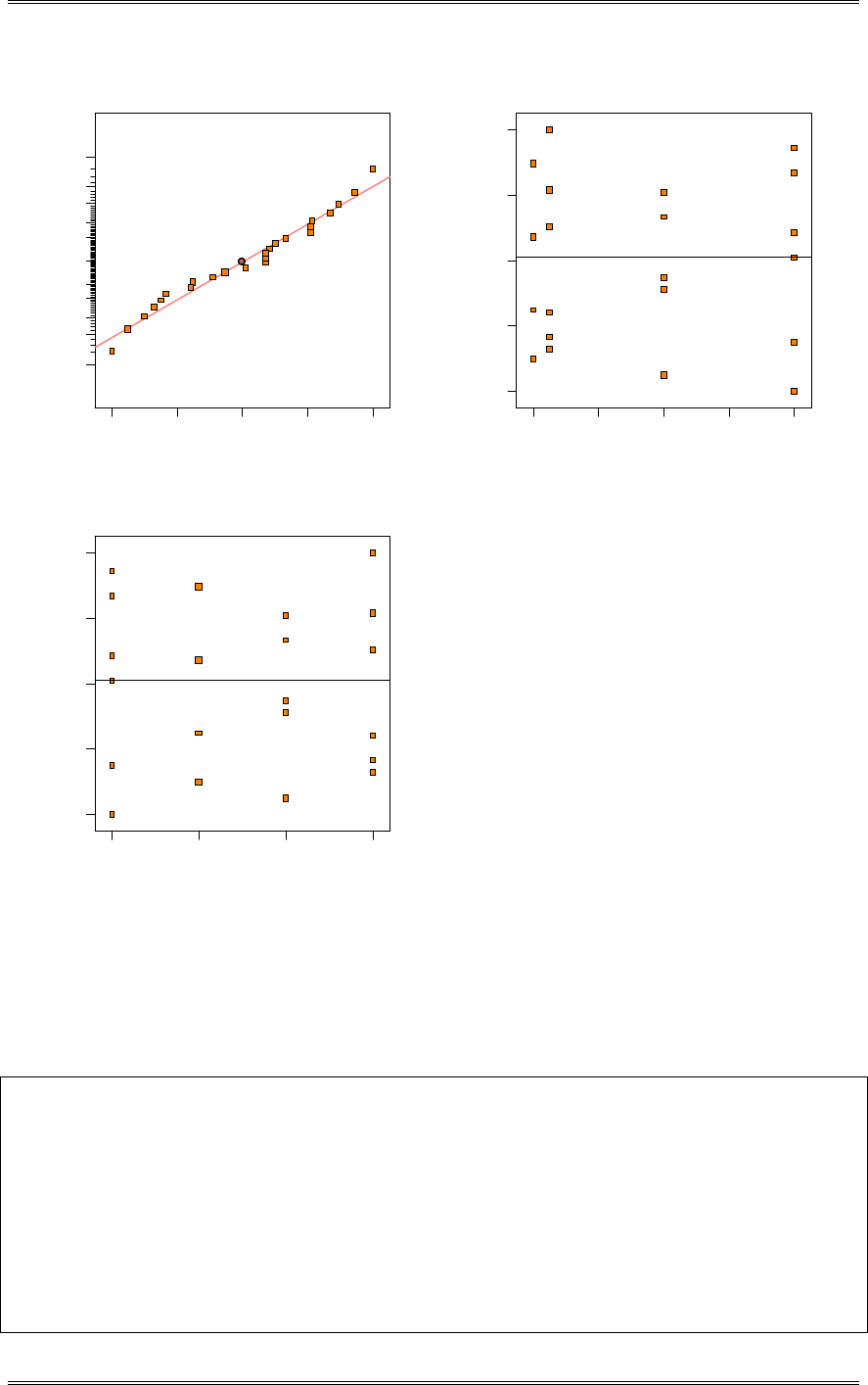
Solutions from Montgomery, D. C. (2001) Design and Analysis of Experiments, Wiley, NY
3-39
Residual
Normal % probability
Normal plot of residuals
-0.11 -0.05625 -0.0025 0.05125 0.105
1
5
10
20
30
50
70
80
90
95
99
333
22
Predicted
Residuals
Residuals vs. Predicted
-0.11
-0.05625
-0.0025
0.05125
0.105
4.833 4.840 4.847 4.853 4.860
333
22
Al g ori th m
Residuals
Residuals vs. Algorithm
-0.11
-0.05625
-0.0025
0.05125
0.105
1 2 3 4
3-29 Refer to the aluminum smelting experiment in Section 3-8. Verify the analysis of variance for pot
noise summarized in Table 3-13. Examine the usual residual plots and comment on the experimental
validity.
Design Expert Output
Response: Cell StDev Transform: Natural log Constant: 0.000
ANOVA for Selected Factorial Model
Analysis of variance table [Partial sum of squares]
Sum of Mean F
Source Squares DF Square Value Prob > F
Model 6.17 3 2.06 21.96 < 0.0001 significant
A 6.17 3 2.06 21.96 < 0.0001
Residual 1.87 20 0.094
Lack of Fit 0.000 0
Pure Error 1.87 20 0.094
Cor Total 8.04 23
The Model F-value of 21.96 implies the model is significant. There is only
a 0.01% chance that a "Model F-Value" this large could occur due to noise.
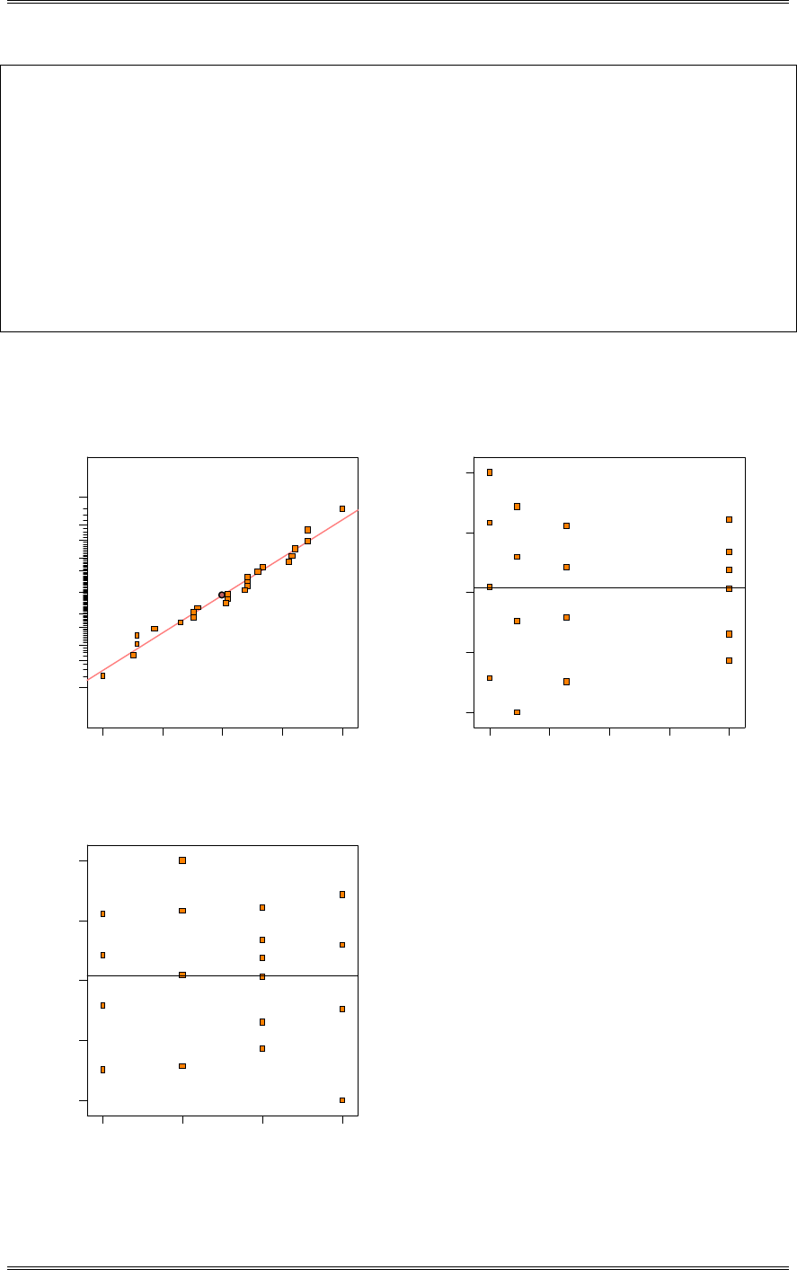
Solutions from Montgomery, D. C. (2001) Design and Analysis of Experiments, Wiley, NY
3-40
Treatment Means (Adjusted, If Necessary)
Estimated
Standard
Mean
Error
1-1 -3.09 0.12
2-2 -3.51 0.12
3-3 -2.20 0.12
4-4 -3.36 0.12
Mean
Standard t for H0
Treatment Difference DF Error Coeff=0 Prob > |t|
1 vs 2 0.42 1 0.18 2.38 0.0272
1 vs 3 -0.89 1 0.18 -5.03 < 0.0001
1 vs 4 0.27 1 0.18 1.52 0.1445
2 vs 3 -1.31 1 0.18 -7.41 < 0.0001
2 vs 4 -0.15 1 0.18 -0.86 0.3975
3 vs 4 1.16 1 0.18 6.55 < 0.0001
The following residual plots identify the residuals to be normally distributed, randomly distributed
through the range of prediction, and uniformly distributed across the different algorithms. This validates
the assumptions for the experiment.
Residual
Normal % probability
Normal plot of residuals
-0.55611 -0.288858 -0.0216069 0.245645 0.512896
1
5
10
20
30
50
70
80
90
95
99
333
2
22
2
2
22
2
Predicted
Residuals
Residuals vs. Predicted
-0.55611
-0.288858
-0.0216069
0.245645
0.512896
-3.51 -3 .18 -2.85 -2.53 -2.20
333
2
22
2
2
22
2
Al g ori th m
Residuals
Residuals vs. Algorithm
-0.55611
-0.288858
-0.0216069
0.245645
0.512896
1 2 3 4

Solutions from Montgomery, D. C. (2001) Design and Analysis of Experiments, Wiley, NY
3-41
3-30 Four different feed rates were investigated in an experiment on a CNC machine producing a
component part used in an aircraft auxiliary power unit. The manufacturing engineer in charge of the
experiment knows that a critical part dimension of interest may be affected by the feed rate. However,
prior experience has indicated that only dispersion effects are likely to be present. That is, changing the
feed rate does not affect the average dimension, but it could affect dimensional variability. The engineer
makes five production runs at each feed rate and obtains the standard deviation of the critical dimension
(in 10-3 mm). The data are shown below. Assume that all runs were made in random order.
Feed Rate Production Run
(in/min) 1 2 3 4 5
10 0.09 0.10 0.13 0.08 0.07
12 0.06 0.09 0.12 0.07 0.12
14 0.11 0.08 0.08 0.05 0.06
16 0.19 0.13 0.15 0.20 0.11
(a) Does feed rate have any effect on the standard deviation of this critical dimension?
Because the residual plots were not acceptable for the non-transformed data, a square root transformation
was applied to the standard deviations of the critical dimension. Based on the computer output below, the
feed rate has an effect on the standard deviation of the critical dimension.
Design Expert Output
Response: Run StDev Transform: Square root Constant: 0.000
ANOVA for Selected Factorial Model
Analysis of variance table [Partial sum of squares]
Sum of Mean F
Source Squares DF Square Value Prob > F
Model 0.040 3 0.013 7.05 0.0031 significant
A 0.040 3 0.013 7.05 0.0031
Residual 0.030 16 1.903E-003
Lack of Fit 0.000 0
Pure Error 0.030 16 1.903E-003
Cor Total 0.071 19
The Model F-value of 7.05 implies the model is significant. There is only
a 0.31% chance that a "Model F-Value" this large could occur due to noise.
Treatment Means (Adjusted, If Necessary)
Estimated
Standard
Mean
Error
1-10 0.30 0.020
2-12 0.30 0.020
3-14 0.27 0.020
4-16 0.39 0.020
Mean
Standard t for H0
Treatment Difference DF Error Coeff=0 Prob > |t|
1 vs 2 4.371E-003 1 0.028 0.16 0.8761
1 vs 3 0.032 1 0.028 1.15 0.2680
1 vs 4 -0.088 1 0.028 -3.18 0.0058
2 vs 3 0.027 1 0.028 0.99 0.3373
2 vs 4 -0.092 1 0.028 -3.34 0.0042
3 vs 4 -0.12 1 0.028 -4.33 0.0005
(b) Use the residuals from this experiment of investigate model adequacy. Are there any problems with
experimental validity?
The residual plots are satisfactory.
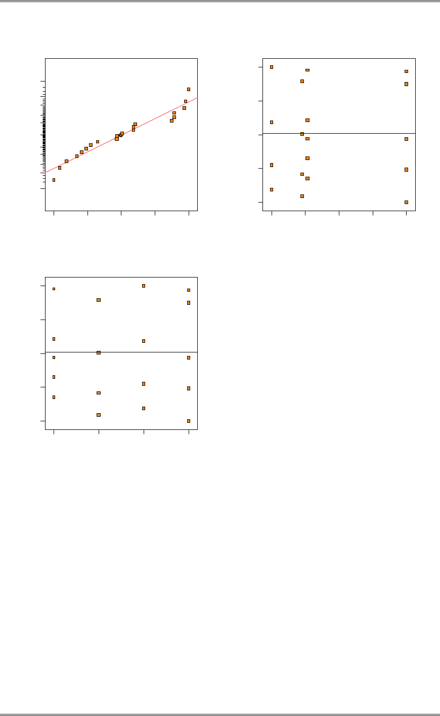
Solutions from Montgomery, D. C. (2001) Design and Analysis of Experiments, Wiley, NY
3-42
Residual
Normal % probability
Normal plot of residuals
-0.0608614 -0.0310256 -0.00118983 0.028646 0.0584817
1
5
10
20
30
50
70
80
90
95
99 22
22
Predicted
Residuals
Residuals vs. Predicted
-0.0608614
-0.0310256
-0.00118983
0.028646
0.0584817
0.27 0.30 0.33 0.36 0.39
22
22
Feed Rate
Residuals
Residuals vs. Feed Rate
-0.0608614
-0.0310256
-0.00118983
0.028646
0.0584817
1 2 3 4
3-31 Consider the data shown in Problem 3-10.
(a) Write out the least squares normal equations for this problem, and solve them for
P
and
W
i, using the
usual constraint ¸
¹
·
¨
©
§
¦
3
10
ii
ˆ
W
. Estimate 21
WW
.
P
ˆ
15 1
5
W
ˆ
2
5
W
ˆ
3
5
W
ˆ
=207
P
ˆ
5 1
5
W
ˆ
=54
P
ˆ
5 2
5
W
ˆ
=111
P
ˆ
15 3
5
W
ˆ
=42
Imposing 0
3
1
¦
i
i
ˆ
W
, therefore 8013.
ˆ
P
, 003
1.
ˆ
W
, 408
2.
ˆ
W
, 405
3.
ˆ
W

Solutions from Montgomery, D. C. (2001) Design and Analysis of Experiments, Wiley, NY
3-43
4011408003
21 ...
ˆˆ
WW
(b) Solve the equations in (a) using the constraint 0
3
W
ˆ. Are the estimators i
ˆ
W
and
P
ˆ the same as you
found in (a)? Why? Now estimate 21
WW
and compare your answer with that for (a). What
statement can you make about estimating contrasts in the i
W
?
Imposing the constraint, 0
3
W
ˆ we get the following solution to the normal equations: 408.
ˆ
P
,
402
1.
ˆ
W
, 813
2.
ˆ
W
, and 0
3
W
ˆ. These estimators are not the same as in part (a). However,
40118013402
21 ...
ˆˆ
WW
, is the same as in part (a). The contrasts are estimable.
(c) Estimate 1
WP
, 321
2
WWW
and 21
WWP
using the two solutions to the normal equations.
Compare the results obtained in each case.
Contrast Estimated from Part (a) Estimated from Part (b)
1 1
WP
10.80 10.80
2 321
2
WWW
-9.00 -9.00
3 21
WWP
19.20 24.60
Contrasts 1 and 2 are estimable, 3 is not estimable.
3-32 Apply the general regression significance test to the experiment in Example 3-1. Show that the
procedure yields the same results as the usual analysis of variance.
From Table 3-3:
376
..
y
from Example 3-1, we have:
244566562
3602450415
543
21
.
ˆ
.
ˆ
.
ˆ
.
ˆ
.
ˆ
.
ˆ
WWW
WWP
¦¦
5
1
5
1
26292
ij
ij
y, with 25 degrees of freedom.
801306
542441085668856277360492453760415
5
1
.,
..)....
y
ˆ
y
ˆ
,R
i
.i..
¦
WPWP
with 5 degrees of freedom.
20161861306292
5
1
5
1
2..,RySS
ij
ijE ¦¦
WP
with 25-5 degrees of freedom.
This is identical to the SSE found in Example 3-1.

Solutions from Montgomery, D. C. (2001) Design and Analysis of Experiments, Wiley, NY
3-44
The reduced model:
0456553760415 ..y
ˆ
R..
PP
, with 1 degree of freedom.
7647504565586130 ...R,RR
PWPPW
, with 5-1=4 degrees of freedom.
Note:
Treatment
SSR
PW
from Example 3-1.
Finally,
7614
068
94118
20
4
0.
.
.
SS
tR
F
E
PW
which is the same as computed in Example 3-1.
3-33 Use the Kruskal-Wallis test for the experiment in Problem 3-11. Are the results comparable to
those found by the usual analysis of variance?
From Design Expert Output of Problem 3-11
Response: Life in in h
ANOVA for Selected Factorial Model
Analysis of variance table [Partial sum of squares]
Sum of Mean F
Source Squares DF Square Value Prob > F
Model 30.17 3 10.06 3.05 0.0525 not significant
A 30.16 3 10.05 3.05 0.0525
Residual 65.99 20 3.30
Lack of Fit 0.000 0
Pure Error
65.99 20 3.30
Cor Total 96.16 23
>@
815124354040
12424
12
13
1
12
1
2
..N
n
R
NN
H
a
ii
.i
»
»
¼
º
«
«
¬
ª
¦
817
2
3050.
,.
F
Accept the null hypothesis; the treatments are not different. This agrees with the analysis of variance.
3-34 Use the Kruskal-Wallis test for the experiment in Problem 3-12. Compare conclusions obtained
with those from the usual analysis of variance?
From Design Expert Output of Problem 3-12
Response: Noise
ANOVA for Selected Factorial Model
Analysis of variance table [Partial sum of squares]
Sum of Mean F
Source Squares DF Square Value Prob > F
Model 12042.00 3 4014.00 21.78 < 0.0001 significant
A 12042.00 3 4014.00 21.78 < 0.0001
Residual 2948.80 16 184.30
Lack of Fit 0.000 0

Solutions from Montgomery, D. C. (2001) Design and Analysis of Experiments, Wiley, NY
3-45
Pure Error
2948.80 16 184.30
Cor Total 14990.80 19
>@
9013120362691
12020
12
13
1
12
1
2
..N
n
R
NN
H
a
ii
.i
»
»
¼
º
«
«
¬
ª
¦
8412
2
4050.
,.
F
Reject the null hypothesis because the treatments are different. This agrees with the analysis of variance.
3-35 Consider the experiment in Example 3-1. Suppose that the largest observation on tensile strength
is incorrectly recorded as 50. What effect does this have on the usual analysis of variance? What effect
does is have on the Kruskal-Wallis test?
The incorrect observation reduces the analysis of variance F0 from 14.76 to 5.44. It does not change the
value of the Kruskal-Wallis test.

Solutions from Montgomery, D. C. (2001) Design and Analysis of Experiments, Wiley, NY
4-1
Chapter 4
Randomized Blocks, Latin Squares, and Related Designs
Solutions
4-1 A chemist wishes to test the effect of four chemical agents on the strength of a particular type of
cloth. Because there might be variability from one bolt to another, the chemist decides to use a randomized
block design, with the bolts of cloth considered as blocks. She selects five bolts and applies all four
chemicals in random order to each bolt. The resulting tensile strengths follow. Analyze the data from this
experiment (use
D
= 0.05) and draw appropriate conclusions.
Bolt
Chemical 1 2 3 4 5
1 73 68 74 71 67
2 73 67 75 72 70
3 75 68 78 73 68
4 73 71 75 75 69
Design Expert Output
Response: Strength
ANOVA for Selected Factorial Model
Analysis of variance table [Partial sum of squares]
Sum of Mean F
Source Squares DF Square Value Prob > F
Block 157.00 4 39.25
Model 12.95 3 4.32 2.38 0.1211 not significant
A 12.95 3 4.32 2.38 0.1211
Residual 21.80 12 1.82
Cor Total 191.75 19
The "Model F-value" of 2.38 implies the model is not significant relative to the noise. There is a
12.11 % chance that a "Model F-value" this large could occur due to noise.
Std. Dev. 1.35 R-Squared 0.3727
Mean 71.75 Adj R-Squared 0.2158
C.V. 1.88 Pred R-Squared -0.7426
PRESS 60.56 Adeq Precision 10.558
Treatment Means (Adjusted, If Necessary)
Estimated
Standard
Mean
Error
1-1 70.60 0.60
2-2 71.40 0.60
3-3 72.40 0.60
4-4 72.60 0.60
Mean
Standard t for H0
Treatment Difference DF Error Coeff=0 Prob > |t|
1 vs 2 -0.80 1 0.85 -0.94 0.3665
1 vs 3 -1.80 1 0.85 -2.11 0.0564
1 vs 4 -2.00 1 0.85 -2.35 0.0370
2 vs 3 -1.00 1 0.85 -1.17 0.2635
2 vs 4 -1.20 1 0.85 -1.41 0.1846
3 vs 4 -0.20 1 0.85 -0.23 0.8185
There is no difference among the chemical types at
D
= 0.05 level.
4-2 Three different washing solutions are being compared to study their effectiveness in retarding
bacteria growth in five-gallon milk containers. The analysis is done in a laboratory, and only three trials

Solutions from Montgomery, D. C. (2001) Design and Analysis of Experiments, Wiley, NY
4-2
can be run on any day. Because days could represent a potential source of variability, the experimenter
decides to use a randomized block design. Observations are taken for four days, and the data are shown
here. Analyze the data from this experiment (use
D
= 0.05) and draw conclusions.
Days
Solution 1 2 3 4
1 13 22 18 39
2 16 24 17 44
3 5 4 1 22
Design Expert Output
Response: Growth
ANOVA for Selected Factorial Model
Analysis of variance table [Partial sum of squares]
Sum of Mean F
Source Squares DF Square Value Prob > F
Block 1106.92 3 368.97
Model 703.50 2 351.75 40.72 0.0003 significant
A 703.50 2 351.75 40.72 0.0003
Residual 51.83 6 8.64
Cor Total 1862.25 11
The Model F-value of 40.72 implies the model is significant. There is only
a 0.03% chance that a "Model F-Value" this large could occur due to noise.
Std. Dev. 2.94 R-Squared 0.9314
Mean 18.75 Adj R-Squared 0.9085
C.V. 15.68 Pred R-Squared 0.7255
PRESS 207.33 Adeq Precision 19.687
Treatment Means (Adjusted, If Necessary)
Estimated
Standard
Mean
Error
1-1 23.00 1.47
2-2 25.25 1.47
3-3 8.00 1.47
Mean
Standard t for H0
Treatment Difference DF Error Coeff=0 Prob > |t|
1 vs 2 -2.25 1 2.08 -1.08 0.3206
1 vs 3 15.00 1 2.08 7.22 0.0004
2 vs 3 17.25 1 2.08 8.30 0.0002
There is a difference between the means of the three solutions. The Fisher LSD procedure indicates that
solution 3 is significantly different than the other two.
4-3 Plot the mean tensile strengths observed for each chemical type in Problem 4-1 and compare them to
a scaled t distribution. What conclusions would you draw from the display?
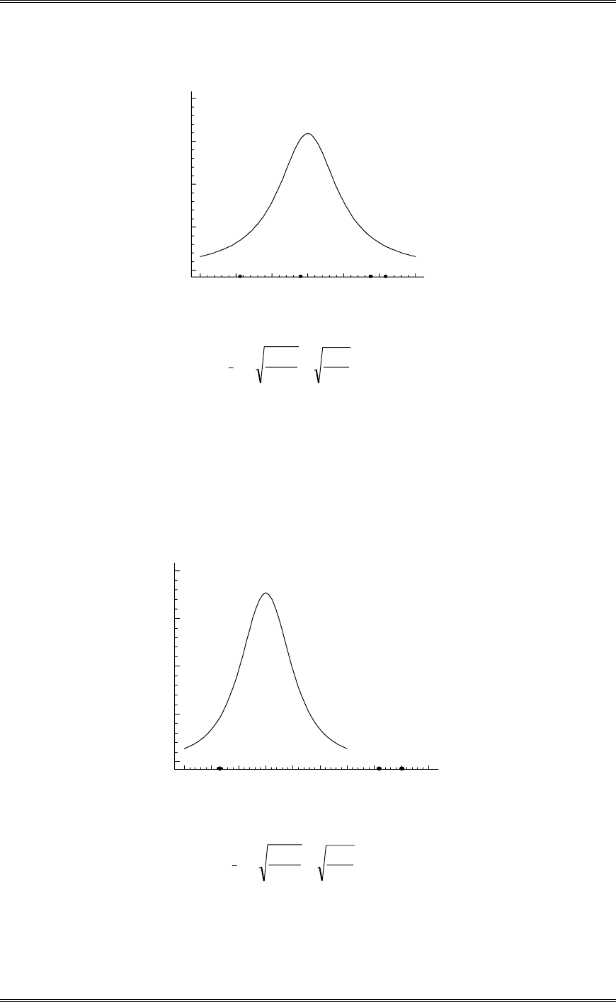
Solutions from Montgomery, D. C. (2001) Design and Analysis of Experiments, Wiley, NY
4-3
70.0 71.0 72.0 73.0
Mean Strength
Scaled t Distribution
(1) (2 )
(
3,4
)
6030
5
821 .
.
b
MS
SE
y.i
There is no obvious difference between the means. This is the same conclusion given by the analysis of
variance.
4-4 Plot the average bacteria counts for each solution in Problem 4-2 and compare them to an
appropriately scaled t distribution. What conclusions can you draw?
5 10152025
Bacteria Growth
Scaled t Distribution
(
1
)
(
2
)
(3)
471
4
648 .
.
b
MS
SE
y.i
There is no difference in mean bacteria growth between solutions 1 and 2. However, solution 3 produces
significantly lower mean bacteria growth. This is the same conclusion reached from the Fisher LSD
procedure in Problem 4-4.

Solutions from Montgomery, D. C. (2001) Design and Analysis of Experiments, Wiley, NY
4-4
4-5 An article in the Fire Safety Journal (“The Effect of Nozzle Design on the Stability and Performance
of Turbulent Water Jets,” Vol. 4, August 1981) describes an experiment in which a shape factor was
determined for several different nozzle designs at six levels of efflux velocity. Interest focused on potential
differences between nozzle designs, with velocity considered as a nuisance variable. The data are shown
below:
Jet Efflux Velocity (m/s)
Nozzle
Design 11.73 14.37 16.59 20.43 23.46 28.74
1 0.78 0.80 0.81 0.75 0.77 0.78
2 0.85 0.85 0.92 0.86 0.81 0.83
3 0.93 0.92 0.95 0.89 0.89 0.83
4 1.14 0.97 0.98 0.88 0.86 0.83
5 0.97 0.86 0.78 0.76 0.76 0.75
(a) Does nozzle design affect the shape factor? Compare nozzles with a scatter plot and with an analysis
of variance, using
D
= 0.05.
Design Expert Output
Response: Shape
ANOVA for Selected Factorial Model
Analysis of variance table [Partial sum of squares]
Sum of Mean F
Source Squares DF Square Value Prob > F
Block 0.063 5 0.013
Model 0.10 4 0.026 8.92 0.0003 significant
A 0.10 4 0.026 8.92 0.0003
Residual 0.057 20 2.865E-003
Cor Total 0.22 29
The Model F-value of 8.92 implies the model is significant. There is only
a 0.03% chance that a "Model F-Value" this large could occur due to noise.
Std. Dev. 0.054 R-Squared 0.6407
Mean 0.86 Adj R-Squared 0.5688
C.V. 6.23 Pred R-Squared 0.1916
PRESS 0.13 Adeq Precision 9.438
Treatment Means (Adjusted, If Necessary)
Estimated
Standard
Mean
Error
1-1 0.78 0.022
2-2 0.85 0.022
3-3 0.90 0.022
4-4 0.94 0.022
5-5 0.81 0.022
Mean
Standard t for H0
Treatment Difference DF Error Coeff=0 Prob > |t|
1 vs 2 -0.072 1 0.031 -2.32 0.0311
1 vs 3 -0.12 1 0.031 -3.88 0.0009
1 vs 4 -0.16 1 0.031 -5.23 < 0.0001
1 vs 5 -0.032 1 0.031 -1.02 0.3177
2 vs 3 -0.048 1 0.031 -1.56 0.1335
2 vs 4 -0.090 1 0.031 -2.91 0.0086
2 vs 5 0.040 1 0.031 1.29 0.2103
3 vs 4 -0.042 1 0.031 -1.35 0.1926
3 vs 5 0.088 1 0.031 2.86 0.0097
4 vs 5 0.13 1 0.031 4.21 0.0004
Nozzle design has a significant effect on shape factor.
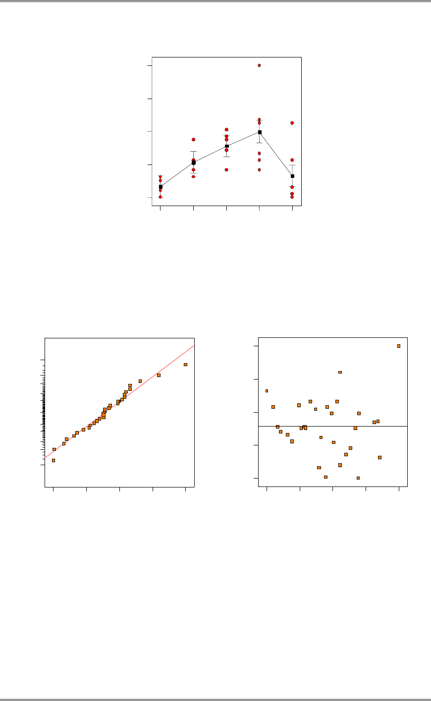
Solutions from Montgomery, D. C. (2001) Design and Analysis of Experiments, Wiley, NY
4-5
Nozzle Design
Shape
One Factor Plot
1 2 3 4 5
0.749435
0.847076
0.944718
1.04236
1.14
2
2
2
2
2
2
2
2
(b) Analyze the residual from this experiment.
The plots shown below do not give any indication of serious problems. Thre is some indication of a mild
outlier on the normal probability plot and on the plot of residualks versus the predicted velocity.
Residual
Normal % probability
Normal plot of residuals
-0.0786667 -0.0286667 0.0213333 0.0713333 0.121333
1
5
10
20
30
50
70
80
90
95
99
Predicted
Residuals
Residuals vs. Predicted
-0.0786667
-0.0286667
0.0213333
0.0713333
0.121333
0.73 0.80 0.87 0.95 1.02
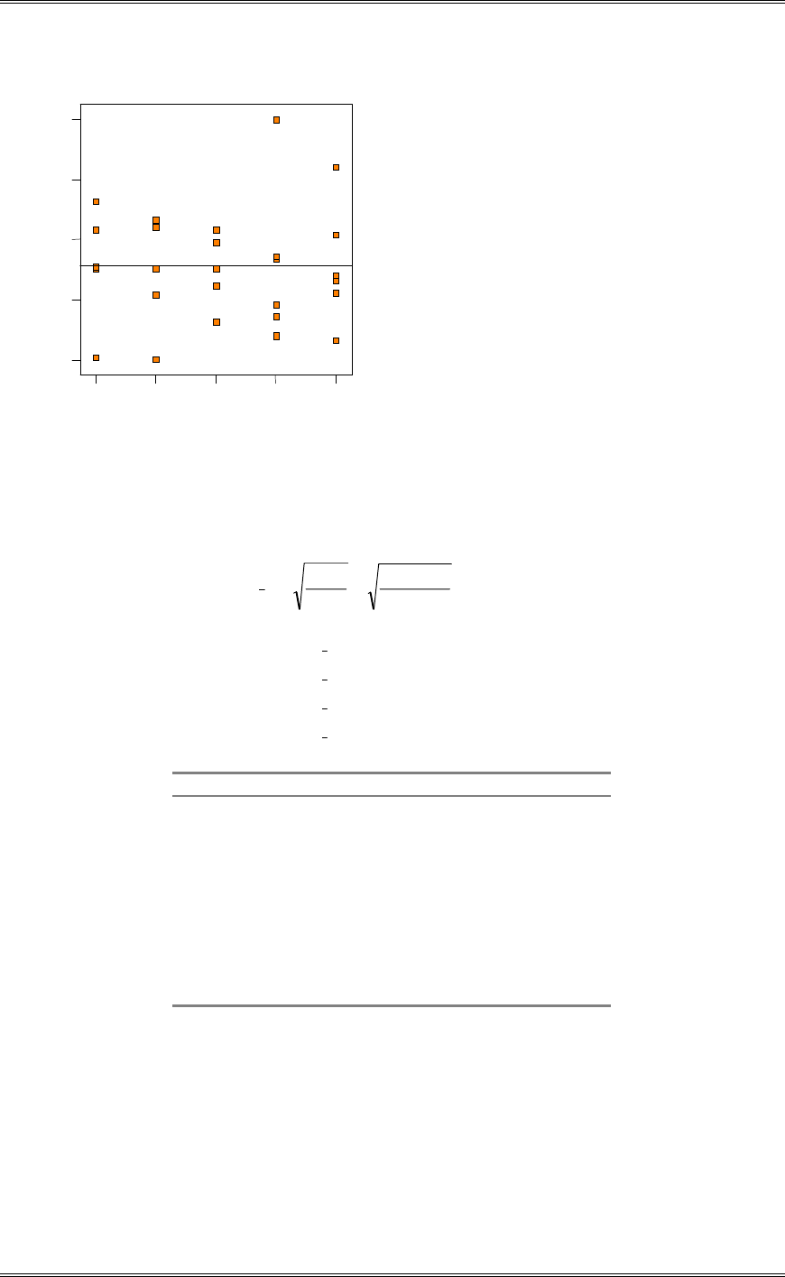
Solutions from Montgomery, D. C. (2001) Design and Analysis of Experiments, Wiley, NY
4-6
2
2
2
2
Nozzle Design
Residuals
Residuals vs. Nozzle Design
-0.0786667
-0.0286667
0.0213333
0.0713333
0.121333
1 2 3 4 5
(c) Which nozzle designs are different with respect to shape factor? Draw a graph of average shape factor
for each nozzle type and compare this to a scaled t distribution. Compare the conclusions that you
draw from this plot to those from Duncan’s multiple range test.
0218520
6
0028650 .
.
b
MS
SE
y.i
R2= r0.05(2,20) Syi.= (2.95)(0.021852)= 0.06446
R3= r0.05(3,20) Syi.= (3.10)(0.021852)= 0.06774
R4= r0.05(4,20) Syi.= (3.18)(0.021852)= 0.06949
R5= r0.05(5,20) Syi.= (3.25)(0.021852)= 0.07102
Mean Difference R
1 vs 4 0.16167 > 0.07102 different
1 vs 3 0.12000 > 0.06949 different
1 vs 2 0.07167 > 0.06774 different
1 vs 5 0.03167 < 0.06446
5 vs 4 0.13000 > 0.06949 different
5 vs 3 0.08833 > 0.06774 different
5 vs 2 0.04000 < 0.06446
2 vs 4 0.09000 > 0.06774 different
2 vs 3 0.04833 < 0.06446
3 vs 4 0.04167 < 0.06446
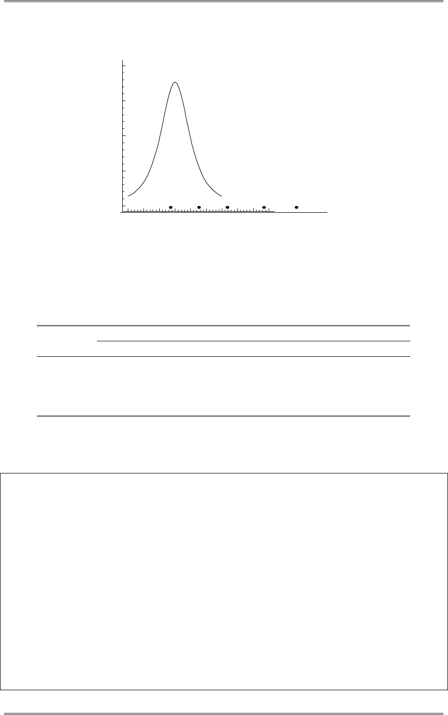
Solutions from Montgomery, D. C. (2001) Design and Analysis of Experiments, Wiley, NY
4-7
0.75 0.80 0.85 0.90 0.95
Shape Factor
Scaled t Distribution
(
2
)
(
3
)
(
4
)
(5)(1)
4-6 Consider the ratio control algorithm experiment described in Chapter 3, Section 3-8. The
experiment was actually conducted as a randomized block design, where six time periods were selected as
the blocks, and all four ratio control algorithms were tested in each time period. The average cell voltage
and the standard deviation of voltage (shown in parentheses) for each cell as follows:
Ratio Control Time Period
Algorithms 1 2 3 4 5 6
1 4.93 (0.05) 4.86 (0.04) 4.75 (0.05) 4.95 (0.06) 4.79 (0.03) 4.88 (0.05)
2 4.85 (0.04) 4.91 (0.02) 4.79 (0.03) 4.85 (0.05) 4.75 (0.03) 4.85 (0.02)
3 4.83 (0.09) 4.88 (0.13) 4.90 (0.11) 4.75 (0.15) 4.82 (0.08) 4.90 (0.12)
4 4.89 (0.03) 4.77 (0.04) 4.94 (0.05) 4.86 (0.05) 4.79 (0.03) 4.76 (0.02)
(a) Analyze the average cell voltage data. (Use
D
= 0.05.) Does the choice of ratio control algorithm
affect the cell voltage?
Design Expert Output
Response: Average
ANOVA for Selected Factorial Model
Analysis of variance table [Partial sum of squares]
Sum of Mean F
Source Squares DF Square Value Prob > F
Block 0.017 5 3.487E-003
Model 2.746E-003 3 9.153E-004 0.19 0.9014 not significant
A 2.746E-003 3 9.153E-004 0.19 0.9014
Residual 0.072 15 4.812E-003
Cor Total 0.092 23
The "Model F-value" of 0.19 implies the model is not significant relative to the noise. There is a
90.14 % chance that a "Model F-value" this large could occur due to noise.
Std. Dev. 0.069 R-Squared 0.0366
Mean 4.84 Adj R-Squared -0.1560
C.V. 1.43 Pred R-Squared -1.4662
PRESS 0.18 Adeq Precision 2.688
Treatment Means (Adjusted, If Necessary)
Estimated
Standard
Mean
Error
1-1 4.86 0.028

Solutions from Montgomery, D. C. (2001) Design and Analysis of Experiments, Wiley, NY
4-8
2-2 4.83 0.028
3-3 4.85 0.028
4-4 4.84 0.028
Mean
Standard t for H0
Treatment Difference DF Error Coeff=0 Prob > |t|
1 vs 2 0.027 1 0.040 0.67 0.5156
1 vs 3 0.013 1 0.040 0.33 0.7438
1 vs 4 0.025 1 0.040 0.62 0.5419
2 vs 3 -0.013 1 0.040 -0.33 0.7438
2 vs 4 -1.667E-003 1 0.040 -0.042 0.9674
3 vs 4 0.012 1 0.040 0.29 0.7748
The ratio control algorithm does not affect the mean cell voltage.
(b) Perform an appropriate analysis of the standard deviation of voltage. (Recall that this is called “pot
noise.”) Does the choice of ratio control algorithm affect the pot noise?
Design Expert Output
Response: StDev Transform: Natural log Constant: 0.000
ANOVA for Selected Factorial Model
Analysis of variance table [Partial sum of squares]
Sum of Mean F
Source Squares DF Square Value Prob > F
Block 0.94 5 0.19
Model 6.17 3 2.06 33.26 < 0.0001 significant
A 6.17 3 2.06 33.26 < 0.0001
Residual 0.93 15 0.062
Cor Total 8.04 23
The Model F-value of 33.26 implies the model is significant. There is only
a 0.01% chance that a "Model F-Value" this large could occur due to noise.
Std. Dev. 0.25 R-Squared 0.8693
Mean -3.04 Adj R-Squared 0.8432
C.V. -8.18 Pred R-Squared 0.6654
PRESS 2.37 Adeq Precision 12.446
Treatment Means (Adjusted, If Necessary)
Estimated
Standard
Mean
Error
1-1 -3.09 0.10
2-2 -3.51 0.10
3-3 -2.20 0.10
4-4 -3.36 0.10
Mean
Standard t for H0
Treatment Difference DF Error Coeff=0 Prob > |t|
1 vs 2 0.42 1 0.14 2.93 0.0103
1 vs 3 -0.89 1 0.14 -6.19 < 0.0001
1 vs 4 0.27 1 0.14 1.87 0.0813
2 vs 3 -1.31 1 0.14 -9.12 < 0.0001
2 vs 4 -0.15 1 0.14 -1.06 0.3042
3 vs 4 1.16 1 0.14 8.06 < 0.0001
A natural log transformatio was applied to the pot noise data. The ratio control algorithm does affect the
pot noise.
(c) Conduct any residual analyses that seem appropriate.
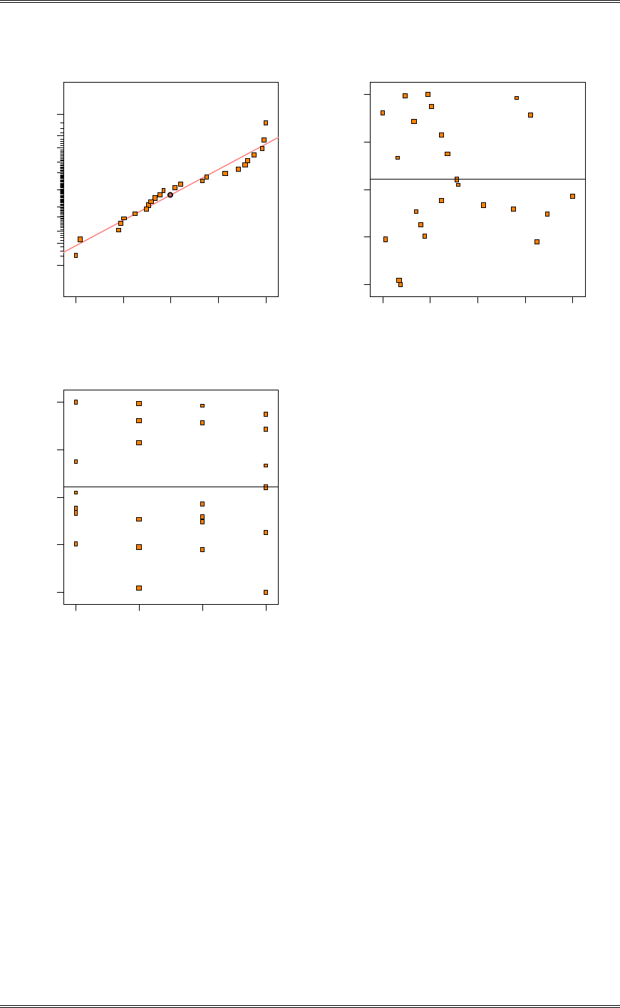
Solutions from Montgomery, D. C. (2001) Design and Analysis of Experiments, Wiley, NY
4-9
Residual
Normal % probability
Normal plot of residuals
-0.359093 -0.19708 -0.0350673 0.126945 0.288958
1
5
10
20
30
50
70
80
90
95
99
Predicted
Residuals
Residuals vs. Predicted
-0.359093
-0.19708
-0.0350673
0.126945
0.288958
-3.73 -3 .26 -2.78 -2.31 -1.84
Al g ori th m
Residuals
Residuals vs. Algorithm
-0.359093
-0.19708
-0.0350673
0.126945
0.288958
1 2 3 4
The normal probability plot shows slight deviations from normality; however, still acceptable.
(d) Which ratio control algorithm would you select if your objective is to reduce both the average cell
voltage and the pot noise?
Since the ratio control algorithm has little effect on average cell voltage, select the algorithm that
minimizes pot noise, that is algorithm #2.
4-7 An aluminum master alloy manufacturer produces grain refiners in ingot form. This company
produces the product in four furnaces. Each furnace is known to have its own unique operating
characteristics, so any experiment run in the foundry that involves more than one furnace will consider
furnace a nuisance variable. The process engineers suspect that stirring rate impacts the grain size of the
product. Each furnace can be run at four different stirring rates. A randomized block design is run for a
particular refiner and the resulting grain size data is shown below.
Furnace

Solutions from Montgomery, D. C. (2001) Design and Analysis of Experiments, Wiley, NY
4-10
Stirring Rate 1 2 3 4
5 8 4 5 6
10 14 5 6 9
15 14 6 9 2
20 17 9 3 6
(a) Is there any evidence that stirring rate impacts grain size?
Design Expert Output
Response: Grain Size
ANOVA for Selected Factorial Model
Analysis of variance table [Partial sum of squares]
Sum of Mean F
Source Squares DF Square Value Prob > F
Block 165.19 3 55.06
Model 22.19 3 7.40 0.85 0.4995 not significant
A 22.19 3 7.40 0.85 0.4995
Residual 78.06 9 8.67
Cor Total 265.44 15
The "Model F-value" of 0.85 implies the model is not significant relative to the noise. There is a
49.95 % chance that a "Model F-value" this large could occur due to noise.
Std. Dev. 2.95 R-Squared 0.2213
Mean 7.69 Adj R-Squared -0.0382
C.V. 38.31 Pred R-Squared -1.4610
PRESS 246.72 Adeq Precision 5.390
Treatment Means (Adjusted, If Necessary)
Estimated
Standard
Mean
Error
1-5 5.75 1.47
2-10 8.50 1.47
3-15 7.75 1.47
4-20 8.75 1.47
Mean
Standard t for H0
Treatment Difference DF Error Coeff=0 Prob > |t|
1 vs 2 -2.75 1 2.08 -1.32 0.2193
1 vs 3 -2.00 1 2.08 -0.96 0.3620
1 vs 4 -3.00 1 2.08 -1.44 0.1836
2 vs 3 0.75 1 2.08 0.36 0.7270
2 vs 4 -0.25 1 2.08 -0.12 0.9071
3 vs 4 -1.00 1 2.08 -0.48 0.6425
The analysis of variance shown above indicates that there is no difference in mean grain size due to the
different stirring rates.
(b) Graph the residuals from this experiment on a normal probability plot. Interpret this plot.
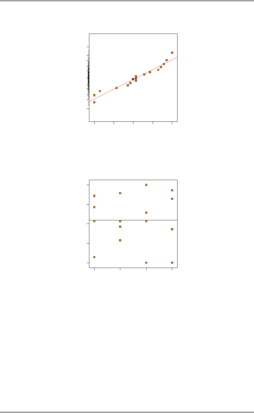
Solutions from Montgomery, D. C. (2001) Design and Analysis of Experiments, Wiley, NY
4-11
Residual
Normal % probability
Normal plot of residuals
-3.8125 -2.0625 -0.3125 1.4375 3.1875
1
5
10
20
30
50
70
80
90
95
99
The plot indicates that normality assumption is valid.
(c) Plot the residuals versus furnace and stirring rate. Does this plot convey any useful information?
Stirring Rate
Residuals
Residuals vs. Stirring Rate
-3.8125
-2.0625
-0.3125
1.4375
3.1875
1 2 3 4
The variance is consistent at different stirring rates. Not only does this validate the assumption of uniform
variance, it also identifies that the different stirring rates do not affect variance.
(d) What should the process engineers recommend concerning the choice of stirring rate and furnace for
this particular grain refiner if small grain size is desirable?
There really isn’t any effect due to the stirring rate.
4-8 Analyze the data in Problem 4-2 using the general regression significance test.
P
:
P
ˆ
12 1
4
W
ˆ
2
4
W
ˆ
3
4
W
ˆ
1
3
E
ˆ
2
3
E
ˆ
3
3
E
ˆ
4
3
E
ˆ
=225
1
W
:
P
ˆ
4 1
4
W
ˆ
1
E
ˆ
2
E
ˆ
3
E
ˆ
4
E
ˆ
=92
2
W
:
P
ˆ
4 2
4
W
ˆ
1
E
ˆ
2
E
ˆ
3
E
ˆ
4
E
ˆ
=101

Solutions from Montgomery, D. C. (2001) Design and Analysis of Experiments, Wiley, NY
4-12
3
W
:
P
ˆ
4 3
4
W
ˆ
1
E
ˆ
2
E
ˆ
3
E
ˆ
4
E
ˆ
=32
1
E
:
P
ˆ
3 1
W
ˆ
2
W
ˆ
3
W
ˆ
1
3
E
ˆ
=34
2
E
:
P
ˆ
3 1
W
ˆ
2
W
ˆ
3
W
ˆ
2
3
E
ˆ
=50
3
E
:
P
ˆ
3 1
W
ˆ
2
W
ˆ
3
W
ˆ
3
3
E
ˆ
=36
4
E
:
P
ˆ
3 1
W
ˆ
2
W
ˆ
3
W
ˆ
4
3
E
ˆ
=105
Applying the constraints ¦¦
0
ji ˆ
ˆ
EW
, we obtain:
12
225
P
ˆ, 12
51
1
W
ˆ, 12
78
2
W
ˆ, 12
129
3
W
ˆ, 12
89
1
E
ˆ, 12
25
2
E
ˆ, 12
81
3
E
ˆ, 12
195
4
E
ˆ
¸
¹
·
¨
©
§
¸
¹
·
¨
©
§
¸
¹
·
¨
©
§
¸
¹
·
¨
©
§
¸
¹
·
¨
©
§
¸
¹
·
¨
©
§
50
12
25
34
12
89
32
12
129
101
12
78
92
12
51
225
12
225
EWP
,,R
176029105
12
195
36
12
81 .
¸
¹
·
¨
©
§
¸
¹
·
¨
©
§
¦¦ 6081
2
ij
y,
¦¦ 83511760296081
2..,,RySS ijE
EWP
Model Restricted to
W
i 0:
P
:
P
ˆ
12 1
3
E
ˆ
2
3
E
ˆ
3
3
E
ˆ
4
3
E
ˆ
=225
1
E
:
P
ˆ
3 1
3
E
ˆ
=34
2
E
:
P
ˆ
3 2
3
E
ˆ
=50
3
E
:
P
ˆ
3 3
3
E
ˆ
=36
4
E
:
P
ˆ
3 4
3
E
ˆ
=105
Applying the constraint ¦ 0
j
ˆ
E
, we obtain:
12
225
P
ˆ , 1289
1/
ˆ
E
, 12
25
2
E
ˆ, 12
81
3
E
ˆ, 12
195
4
E
ˆ. Now:
675325105
12
195
36
12
81
50
12
25
34
12
89
225
12
225 .,R
¸
¹
·
¨
©
§
¸
¹
·
¨
©
§
¸
¹
·
¨
©
§
¸
¹
·
¨
©
§
¸
¹
·
¨
©
§
EP
Treatments
SS...,R,,R,R 50703675325176029
EPEWPEPW
Model Restricted to 0
j
E
:
P
:
P
ˆ
12 1
4
W
ˆ
2
4
W
ˆ
3
4
W
ˆ
=225
1
W
:
P
ˆ
4 1
4
W
ˆ
=92
2
W
:
P
ˆ
4 2
4
W
ˆ
=101
3
W
:
P
ˆ
4 3
4
W
ˆ
=32
Applying the constraint ¦ 0
i
ˆ
W
, we obtain:
12
225
P
ˆ, 12
51
1
W
ˆ, 12
78
2
W
ˆ, 12
129
3
W
ˆ
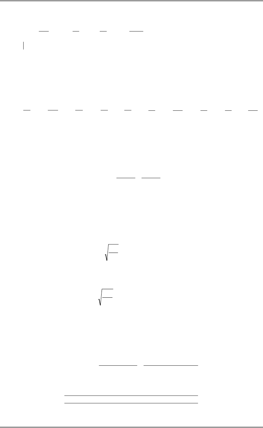
Solutions from Montgomery, D. C. (2001) Design and Analysis of Experiments, Wiley, NY
4-13
25492232
12
129
101
12
78
92
12
51
225
12
225 .,R
¸
¹
·
¨
©
§
¸
¹
·
¨
©
§
¸
¹
·
¨
©
§
¸
¹
·
¨
©
§
WP
Blocks
SS...,R,,R,R 921106254922176029
WPEWPWPE
4-9 Assuming that chemical types and bolts are fixed, estimate the model parameters Wi and Ej in
Problem 4-1.
Using Equations 4-14, Applying the constraints, we obtain:
20
35
P
ˆ, 20
23
1
W
ˆ, 20
7
2
W
ˆ, 20
13
3
W
ˆ,20
17
4
W
ˆ, 20
35
1
E
ˆ, 20
65
2
E
ˆ, 20
75
3
E
ˆ, 20
20
4
E
ˆ,20
65
5
E
ˆ
4-10 Draw an operating characteristic curve for the design in Problem 4-2. Does this test seem to be
sensitive to small differences in treatment effects?
Assuming that solution type is a fixed factor, we use the OC curve in appendix V. Calculate
6983
42
2
2
2
.
a
bii ¦¦
W
V
W
)
using MSE to estimate
V
2. We have:
21
1 a
X
63211
2 ba
X
.
If ¦ E
MS
ˆ
i
22
VW
, then:
151
13
4.
)
and 700.
#
E
If ¦ Ei MS
ˆ22 2
VW
, then:
631
23
4.
)
and 550.
#
E
, etc.
This test is not very sensitive to small differences.
4-11 Suppose that the observation for chemical type 2 and bolt 3 is missing in Problem 4-1. Analyze the
problem by estimating the missing value. Perform the exact analysis and compare the results.
y23 is missing.
2575
34
136022752824
11
32
23 .
ba
ybyay
y
ˆ
'
..
'
.
'
.
Thus, y2.=357.25, y.3=3022.25, and y..=1435.25
Source SS DF MS F0
Chemicals 12.7844 3 4.2615 2.154

Solutions from Montgomery, D. C. (2001) Design and Analysis of Experiments, Wiley, NY
4-14
Bolts 158.8875 4
Error 21.7625 11 1.9784
Total 193.4344 18
F0.10,3,11=2.66, Chemicals are not significant.
4-12 Two missing values in a randomized block. Suppose that in Problem 4-1 the observations for
chemical type 2 and bolt 3 and chemical type 4 and bolt 4 are missing.
(a) Analyze the design by iteratively estimating the missing values as described in Section 4-1.3.
12
54 32
23
'
..
'
.
'
.yyy
y
ˆ
and 12
54 44
44
'
..
'
.
'
.yyy
y
ˆ
Data is coded y-70. As an initial guess, set 0
23
y equal to the average of the observations available for
chemical 2. Thus, 50
4
2
0
23 .y . Then ,
043
12
5256584
0
44 .
.
y
ˆ
415
12
042817524
1
23 .
.
y
ˆ
632
12
41306584
1
44 .
.
y
ˆ
445
12
632717524
2
44 .
.
y
ˆ
632
12
44306584
2
44 .
.
y
ˆ
445
23 .y
ˆ ? 632
44 .y
ˆ
Design Expert Output
ANOVA for Selected Factorial Model
Analysis of variance table [Partial sum of squares]
Sum of Mean F
Source Squares DF Square Value Prob > F
Block 156.83 4 39.21
Model 9.59 3 3.20 2.08 0.1560 not significant
A 9.59 3 3.20 2.08 0.1560
Residual 18.41 12 1.53
Cor Total 184.83 19
(b) Differentiate SSE with respect to the two missing values, equate the results to zero, and solve for
estimates of the missing values. Analyze the design using these two estimates of the missing values.
¦¦¦¦ ¦ 2
20
1
2
4
1
2
5
1
2
..j..iijEyyyySS
Ryy.y.y.y.y.SSE 44234423
2
44
2
23 1073866060
From 0
4423
y
SS
y
SS EE
w
w
w
w
, we obtain:

Solutions from Montgomery, D. C. (2001) Design and Analysis of Experiments, Wiley, NY
4-15
732110
861021
4423
4423
.y
ˆ
.y
ˆ
.
.y
ˆ
.y
ˆ
.
455
23 .y
ˆ , 632
44 .y
ˆ
These quantities are almost identical to those found in part (a). The analysis of variance using these new
data does not differ substantially from part (a).
(c) Derive general formulas for estimating two missing values when the observations are in different
blocks.
ab
yyy
a
yyyy
b
yyyy
yySS kv
iu..
kv
v.iuu.
kv.k
iu.i
kviuE
2
2222
22
c
c
c
c
c
c
From 0
4423
y
SS
y
SS EE
w
w
w
w
, we obtain:
ab
y
ˆ
ab
'y'by'ay
ab
ba
y
ˆkv
..j..i
iu
»
¼
º
«
¬
ª 11
ab
y
ˆ
ab
'y'by'ay
ab
)b)(a(
y
ˆiu..v..k
kv
»
¼
º
«
¬
ª 11
whose simultaneous solution is:
>
@
>
@
>
@
>@
22
222222
11111
111111111
baba
baab'yabbab'yabbaa'y
y
ˆ..u..i
iu
>@
>@
22 111
ba
'y'by'ayab ..v..k
>@
>@
22 111
11
ba
'y'by'ayab'y'by'ay
y
ˆ..v..k..u..i
kv
(d) Derive general formulas for estimating two missing values when the observations are in the same
block. Suppose that two observations yij and ykj are missing, i
z
k (same block j).
ab
yyy
a
yyy
b
yyyy
yySS kj
ij..
kj
ijj.
kj.k
ij.i
kjijE
2222
22
c
c
c
c
From 0
4423
y
SS
y
SS EE
w
w
w
w
, we obtain
2
11
11
c
c
c
bay
ˆ
ba
yybya
y
ˆkj
..j..i
ij
2
11
11
c
c
c
bay
ˆ
ba
yybya
y
ˆij
..j..k
kj
whose simultaneous solution is:

Solutions from Montgomery, D. C. (2001) Design and Analysis of Experiments, Wiley, NY
4-16
>
@
>@
2
2
2
111
111
11
c
c
c
c
c
c
c
c
c
ba
yybyabayybyab
ba
yybya
y
ˆ..j..i..j..k..j..i
ij
>@
>@
42
2
11111
11
c
c
c
c
c
c
baba
yybyaabyybya
y
ˆ..j..i..j..k
kj
4-13 An industrial engineer is conducting an experiment on eye focus time. He is interested in the effect
of the distance of the object from the eye on the focus time. Four different distances are of interest. He has
five subjects available for the experiment. Because there may be differences among individuals, he decides
to conduct the experiment in a randomized block design. The data obtained follow. Analyze the data from
this experiment (use
D
= 0.05) and draw appropriate conclusions.
Subject
Distance (ft) 1 2 3 4 5
4 10 6 6 6 6
6 7 6 6 1 6
8 5 3 3 2 5
10 6 4 4 2 3
Design Expert Output
Response: Focus Time
ANOVA for Selected Factorial Model
Analysis of variance table [Partial sum of squares]
Sum of Mean F
Source Squares DF Square Value Prob > F
Block 36.30 4 9.07
Model 32.95 3 10.98 8.61 0.0025 significant
A 32.95 3 10.98 8.61 0.0025
Residual 15.30 12 1.27
Cor Total 84.55 19
The Model F-value of 8.61 implies the model is significant. There is only
a 0.25% chance that a "Model F-Value" this large could occur due to noise.
Std. Dev. 1.13 R-Squared 0.6829
Mean 4.85 Adj R-Squared 0.6036
C.V. 23.28 Pred R-Squared 0.1192
PRESS 42.50 Adeq Precision 10.432
Treatment Means (Adjusted, If Necessary)
Estimated
Standard
Mean
Error
1-4 6.80 0.50
2-6 5.20 0.50
3-8 3.60 0.50
4-10 3.80 0.50
Mean
Standard t for H0
Treatment Difference DF Error Coeff=0 Prob > |t|
1 vs 2 1.60 1 0.71 2.24 0.0448
1 vs 3 3.20 1 0.71 4.48 0.0008
1 vs 4 3.00 1 0.71 4.20 0.0012
2 vs 3 1.60 1 0.71 2.24 0.0448
2 vs 4 1.40 1 0.71 1.96 0.0736
3 vs 4 -0.20 1 0.71 -0.28 0.7842
Distance has a statistically significant effect on mean focus time.

Solutions from Montgomery, D. C. (2001) Design and Analysis of Experiments, Wiley, NY
4-17
4-14 The effect of five different ingredients (A, B, C, D, E) on reaction time of a chemical process is
being studied. Each batch of new material is only large enough to permit five runs to be made.
Furthermore, each runs requires approximately 1 1/2 hours, so only five runs can be made in one day. The
experimenter decides to run the experiment as a Latin square so that day and batch effects can be
systematically controlled. She obtains the data that follow. Analyze the data from this experiment (use
D
=
0.05) and draw conclusions.
Day
Batch 1 2 3 4 5
1 A=8 B=7 D=1 C=7 E=3
2 C=11 E=2 A=7 D=3 B=8
3 B=4 A=9 C=10 E=1 D=5
4 D=6 C=8 E=6 B=6 A=10
5 E=4 D=2 B=3 A=8 C=8
Minitab Output
General Linear Model
Factor Type Levels Values
Batch random 5 1 2 3 4 5
Day random 5 1 2 3 4 5
Catalyst fixed 5 A B C D E
Analysis of Variance for Time, using Adjusted SS for Tests
Source DF Seq SS Adj SS Adj MS F P
Catalyst 4 141.440 141.440 35.360 11.31 0.000
Batch 4 15.440 15.440 3.860 1.23 0.348
Day 4 12.240 12.240 3.060 0.98 0.455
Error 12 37.520 37.520 3.127
Total 24 206.640
4-15 An industrial engineer is investigating the effect of four assembly methods (A, B, C, D) on the
assembly time for a color television component. Four operators are selected for the study. Furthermore,
the engineer knows that each assembly method produces such fatigue that the time required for the last
assembly may be greater than the time required for the first, regardless of the method. That is, a trend
develops in the required assembly time. To account for this source of variability, the engineer uses the
Latin square design shown below. Analyze the data from this experiment (
D
= 0.05) draw appropriate
conclusions.
Order of
Operator
Assembly 1 2 3 4
1 C=10 D=14 A=7 B=8
2 B=7 C=18 D=11 A=8
3 A=5 B=10 C=11 D=9
4 D=10 A=10 B=12 C=14
Minitab Output
General Linear Model
Factor Type Levels Values
Order random 4 1 2 3 4
Operator random 4 1 2 3 4
Method fixed 4 A B C D
Analysis of Variance for Time, using Adjusted SS for Tests
Source DF Seq SS Adj SS Adj MS F P

Solutions from Montgomery, D. C. (2001) Design and Analysis of Experiments, Wiley, NY
4-18
Method 3 72.500 72.500 24.167 13.81 0.004
Order 3 18.500 18.500 6.167 3.52 0.089
Operator 3 51.500 51.500 17.167 9.81 0.010
Error 6 10.500 10.500 1.750
Total 15 153.000
4-16 Suppose that in Problem 4-14 the observation from batch 3 on day 4 is missing. Estimate the
missing value from Equation 4-24, and perform the analysis using this value.
y354 is missing.
>
@
>@
583
43
14622415285
12
2
354 .
pp
yyyyp
y
ˆ...
k..
.j...i
c
c
c
c
Minitab Output
General Linear Model
Factor Type Levels Values
Batch random 5 1 2 3 4 5
Day random 5 1 2 3 4 5
Catalyst fixed 5 A B C D E
Analysis of Variance for Time, using Adjusted SS for Tests
Source DF Seq SS Adj SS Adj MS F P
Catalyst 4 128.676 128.676 32.169 11.25 0.000
Batch 4 16.092 16.092 4.023 1.41 0.290
Day 4 8.764 8.764 2.191 0.77 0.567
Error 12 34.317 34.317 2.860
Total 24 187.849
4-17 Consider a p x p Latin square with rows (
D
i), columns (
E
k), and treatments (
W
j) fixed. Obtain least
squares estimates of the model parameters
D
i,
E
k,
W
j.
...
p
k
k
p
j
j
p
i
iy
ˆ
p
ˆ
p
ˆ
p
ˆ
p: ¦¦¦ 111
2
EWDPP
..i
p
k
k
p
j
jii y
ˆ
p
ˆ
p
ˆ
p
ˆ
p: ¦¦ 11
EWDPD
, p,...,,i 21
.j.
p
k
kj
p
i
ij y
ˆ
p
ˆ
p
ˆ
p
ˆ
p: ¦¦ 11
EWDPW
, p,...,,j 21
k..k
p
j
j
p
i
ik y
ˆ
p
ˆ
p
ˆ
p
ˆ
p: ¦¦
EWDPE
11
, p,...,,k 21
There are 3p+1 equations in 3p+1 unknowns. The rank of the system is 3p-2. Three side conditions are
necessary. The usual conditions imposed are: 0
111
¦¦¦
p
k
k
p
j
j
p
i
iˆ
ˆˆ
EWD
. The solution is then:
...
...
2
.. ...
ˆ
ˆ, 1, 2,...,
ii
yy
p
yyi p
P
D

Solutions from Montgomery, D. C. (2001) Design and Analysis of Experiments, Wiley, NY
4-19
.. ...
.. ...
ˆ, 1, 2,...,
ˆ, 1, 2,...,
jj
ki
yyj p
yyk p
W
E
4-18 Derive the missing value formula (Equation 4-24) for the Latin square design.
¸
¸
¹
·
¨
¨
©
§
¦¦¦¦¦ ¦ 2
22
2
2
22p
y
p
y
p
y
p
y
ySS ...k..
.j.
..i
ijkE
Let yijk be missing. Then
R
p
yy
p
yy
p
yy
p
yy
ySS ijk
...
ijk
k..
ijk
.j.
ijk
..i
ijkE
c
c
c
c
2
222
22
where R is all terms without yijk.. From 0
ijk
E
y
SS
w
w
, we obtain:
22
2
21
p
'y'y'y'yp
p
pp
y...k...j...i
ijk
, or
21
2
pp
'y'y'y'yp
y...k...j...i
ijk
4-19 Designs involving several Latin squares. [See Cochran and Cox (1957), John (1971).] The p x p
Latin square contains only p observations for each treatment. To obtain more replications the experimenter
may use several squares, say n. It is immaterial whether the squares used are the same are different. The
appropriate model is
ijkhjh)h(kj)h(ihijkh )(y
HWUEWDUP
°
°
¯
°
°
®
n,...,,h
p,...,,k
p,...,,j
p,...,,i
21
21
21
21
where yijkh is the observation on treatment j in row i and column k of the hth square. Note that
D
ih
()
and
E
kh
()
are row and column effects in the hth square, and
U
h is the effect of the hth square, and ( )
W
U
jh is the
interaction between treatments and squares.
(a) Set up the normal equations for this model, and solve for estimates of the model parameters. Assume
that appropriate side conditions on the parameters are 0
¦hh
ˆ
U
,
0
¦ihi
ˆ
D
, and
0
¦khk
ˆ
E
for each h, 0
¦jj
ˆ
W
,
0
¦jjh
ˆ
UW
for each h, and
0
¦hjh
ˆ
UW
for each j.
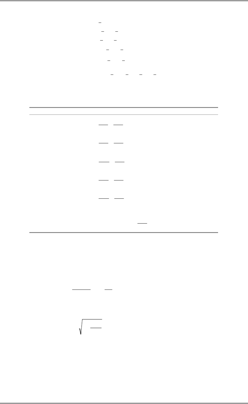
Solutions from Montgomery, D. C. (2001) Design and Analysis of Experiments, Wiley, NY
4-20
....h.....j.h.j.
jh
^
h...kh..)h(k
h...h..i)h(i
......j.j
....h...h
....
yyyy
yy
ˆ
yy
ˆ
yy
ˆ
yy
ˆ
y
ˆ
¸
¸
¹
·
¨
¨
©
§
WU
E
D
W
U
P
(b) Write down the analysis of variance table for this design.
Source SS DF
Treatments ¦2
2
2
np
y
np
y....
..j. p-1
Squares ¦2
2
2
2
np
y
p
y....h... n-1
Treatment x Squares SquaresTreatments
....
h.j. SSSS
np
y
p
y
¦2
2
2
(p-1)(n-1)
Rows ¦2
22
np
y
p
yh...h..i n(p-1)
Columns ¦2
22
np
y
p
yh...kh.. n(p-1)
Error subtraction n(p-1)(p-2)
Total 2
2
2
np
y
y....
ijkh
¦¦¦¦ np2-1
4-20 Discuss how the operating characteristics curves in the Appendix may be used with the Latin square
design.
For the fixed effects model use:
¦
¦ 2
2
2
2
2
V
W
V
W
)
j
j
p
p, 1
1 p
X
12
2 pp
X
For the random effects model use:
OV
V
W
1
2
2
p,
X
11 p
12
2 pp
X
4-21 Suppose that in Problem 4-14 the data taken on day 5 were incorrectly analyzed and had to be
discarded. Develop an appropriate analysis for the remaining data.
Two methods of analysis exist: (1) Use the general regression significance test, or (2) recognize that the
design is a Youden square. The data can be analyzed as a balanced incomplete block design with a=b=5,
r=k=4 and
O
=3. Using either approach will yield the same analysis of variance.

Solutions from Montgomery, D. C. (2001) Design and Analysis of Experiments, Wiley, NY
4-21
Minitab Output
General Linear Model
Factor Type Levels Values
Catalyst fixed 5 A B C D E
Batch random 5 1 2 3 4 5
Day random 4 1 2 3 4
Analysis of Variance for Time, using Adjusted SS for Tests
Source DF Seq SS Adj SS Adj MS F P
Catalyst 4 119.800 120.167 30.042 7.48 0.008
Batch 4 11.667 11.667 2.917 0.73 0.598
Day 3 6.950 6.950 2.317 0.58 0.646
Error 8 32.133 32.133 4.017
Total 19 170.550
4-22 The yield of a chemical process was measured using five batches of raw material, five acid
concentrations, five standing times, (A, B, C, D, E) and five catalyst concentrations (
D
,
E
,
J
,
G
,
H
). The
Graeco-Latin square that follows was used. Analyze the data from this experiment (use
D
= 0.05) and draw
conclusions.
Acid Concentration
Batch 1 2 3 4 5
1 A
D
=26 B
E
=16 C
J
=19 D
G
=16 E
H
=13
2 B
J
=18 C
G
=21 D
H
=18 E
D
=11 A
E
=21
3 C
H
=20 D
D
=12 E
E
=16 A
J
=25 B
G
=13
4 D
E
=15 E
J
=15 A
G
=22 B
H
=14 C
D
=17
5 E
G
=10 A
H
=24 B
D
=17 C
E
=17 D
J
=14
General Linear Model
Factor Type Levels Values
Time fixed 5 A B C D E
Catalyst random 5 a b c d e
Batch random 5 1 2 3 4 5
Acid random 5 1 2 3 4 5
Analysis of Variance for Yield, using Adjusted SS for Tests
Source DF Seq SS Adj SS Adj MS F P
Time 4 342.800 342.800 85.700 14.65 0.001
Catalyst 4 12.000 12.000 3.000 0.51 0.729
Batch 4 10.000 10.000 2.500 0.43 0.785
Acid 4 24.400 24.400 6.100 1.04 0.443
Error 8 46.800 46.800 5.850
Total 24 436.000
4-23 Suppose that in Problem 4-15 the engineer suspects that the workplaces used by the four operators
may represent an additional source of variation. A fourth factor, workplace (
D
,
E
,
J
,
G
) may be introduced
and another experiment conducted, yielding the Graeco-Latin square that follows. Analyze the data from
this experiment (use
D
= 0.05) and draw conclusions.
Order of
Operator
Assembly 1 2 3 4
1 C
E
=11 B
J
=10 D
G
=14 A
D
=8
2 B
D
=8 C
G
=12 A
J
=10 D
E
=12
3 A
G
=9 D
D
=11 B
E
=7 C
J
=15

Solutions from Montgomery, D. C. (2001) Design and Analysis of Experiments, Wiley, NY
4-22
4 D
J
=9 A
E
=8 C
D
=18 B
G
=6
Minitab Output
General Linear Model
Factor Type Levels Values
Method fixed 4 A B C D
Order random 4 1 2 3 4
Operator random 4 1 2 3 4
Workplac random 4 a b c d
Analysis of Variance for Time, using Adjusted SS for Tests
Source DF Seq SS Adj SS Adj MS F P
Method 3 95.500 95.500 31.833 3.47 0.167
Order 3 0.500 0.500 0.167 0.02 0.996
Operator 3 19.000 19.000 6.333 0.69 0.616
Workplac 3 7.500 7.500 2.500 0.27 0.843
Error 3 27.500 27.500 9.167
Total 15 150.000
However, there are only three degrees of freedom for error, so the test is not very sensitive.
4-24 Construct a 5 x 5 hypersquare for studying the effects of five factors. Exhibit the analysis of
variance table for this design.
Three 5 x 5 orthogonal Latin Squares are:
ABCDE
BCDEA
CDEAB
DEABC
EABCD
DEJGH
JGHDE
HDEJG
EJGHD
GHDEJ
12345
45123
23451
51234
34512
Let rows = factor 1, columns = factor 2, Latin letters = factor 3, Greek letters = factor 4 and numbers =
factor 5. The analysis of variance table is:
Source DF
Rows 4
Columns 4
Latin Letters 4
Greek Letters 4
Numbers 4
Error 4
Total 24
4-25 Consider the data in Problems 4-15 and 4-23. Suppressing the Greek letters in 4-23, analyze the data
using the method developed in Problem 4-19.
Square 1 - Operator
Batch 1 2 3 4 Row Total
1 C=10 D=14 A=7 B=8 (39)
2 B=7 C=18 D=11 A=8 (44)
3 A=5 B=10 C=11 D=9 (35)
4 D=10 A=10 B=12 C=14 (46)
(32) (52) (41) (36) 164=y…1

Solutions from Montgomery, D. C. (2001) Design and Analysis of Experiments, Wiley, NY
4-23
Square 2 - Operator
Batch 1 2 3 4 Row Total
1 C=11 B=10 D=14 A=8 (43)
2 B=8 C=12 A=10 D=12 (42)
3 A=9 D=11 B=7 C=15 (42)
4 D=9 A=8 C=18 B=6 (41)
(37) (41) (49) (41) 168=y…2
Assembly Methods Totals
A y.1..=65
B y.2..=68
C y.3..=109
D y.4..=90
Source SS DF MS F0
Assembly Methods 159.25 3 53.08 14.00*
Squares 0.50 1 0.50
A x S 8.75 3 2.92 0.77
Assembly Order (Rows) 19.00 6 3.17
Operators (columns) 70.50 6 11.75
Error 45.50 12 3.79
Total 303.50 31
Significant at 1%.
4-26 Consider the randomized block design with one missing value in Table 4-7. Analyze this data by
using the exact analysis of the missing value problem discussed in Section 4-1.4. Compare your results to
the approximate analysis of these data given in Table 4-8.
P
: 15
P
41
W
32
W
43
W
44
W
41
E
42
E
33
E
44
E
=17
W
1: 4
P
41
W
E
1
E
2
E
3
E
4 =3
W
2: 3
P
32
W
E
1
E
2
E
4 =1
W
3: 4
P
43
W
E
1
E
2
E
3
E
4 =-2
W
4: 4
P
44
W
E
1
E
2
E
3
E
4 =15
E
1: 4
P
W
1
W
2
W
3
W
4 41
E
=-4
E
2: 4
P
W
1
W
2
W
3
W
4 32
E
=-3
E
3: 3
P
W
1
W
3
W
4
43
E
=6
E
4: 4
P
W
1
W
2
W
3
W
4
44
E
=19
Applying the constraints ¦¦
0
ji ˆ
ˆ
EW
, we obtain:
36
41
P
ˆ, 36
14
1
W
ˆ, 36
24
2
W
ˆ, 36
59
3
W
ˆ,36
94
4
W
ˆ, 36
77
1
E
ˆ, 36
68
2
E
ˆ, 36
24
3
E
ˆ, 36
121
4
E
ˆ

Solutions from Montgomery, D. C. (2001) Design and Analysis of Experiments, Wiley, NY
4-24
¦¦
4
1
4
1
78138
ij
j.j.ii.. .y
ˆ
y
ˆ
y
ˆ
,,R
EWPEWP
With 7 degrees of freedom.
¦¦ 00145
2.yij ,
¦¦ 2267813800145
2...,,RySS ijE
EWP
which is identical to SSE obtained in the approximate analysis. In general, the SSE in the exact and
approximate analyses will be the same.
To test Ho:0
i
W
the reduced model is ijjij
y
HEP
. The normal equations used are:
P
: ˆ
15
P
1
ˆ
4
E
2
ˆ
4
E
3
ˆ
3
E
4
ˆ
4
E
=17
E
1: 4
P
1
ˆ
4
E
=-4
E
2: 4
P
2
ˆ
4
E
=-3
E
3: 3
P
3
ˆ
3
E
=6
E
4: 4
P
4
ˆ
4
E
=18
Applying the constraint ¦ 0
j
ˆ
E
, we obtain:
16
19
P
ˆ , 16
35
1
E
ˆ, 16
31
2
E
ˆ, 16
13
3
E
ˆ, 16
53
4
E
ˆ. Now
¦
4
1
2599
j
j.j.. .y
ˆ
y
ˆ
,R
EPEP
with 4 degrees of freedom.
Treatments
SS...,R,,R,R 5339259978138
EPEWPEPW
with 7-4=3 degrees of freedom.
EPW
,R is used to test Ho:
W
i 0.
The sum of squares for blocks is found from the reduced model ijiij
y
HWP
. The normal equations
used are:
Model Restricted to 0
j
E
:
P
: 15
P
41
W
32
W
43
W
44
W
=17
W
1: ˆ
4
P
41
W
=3
W
2: ˆ
3
P
32
W
=1
W
3: ˆ
4
P
43
W
=-2
W
4: ˆ
4
P
44
W
=15
Applying the constraint ˆ0
i
W
¦, we obtain:
13
ˆ12
P
, 1
4
ˆ12
W
, 2
9
ˆ12
W
, 3
19
ˆ12
W
, 4
32
ˆ12
W

Solutions from Montgomery, D. C. (2001) Design and Analysis of Experiments, Wiley, NY
4-25
¦
4
1
8359
i
.ii.. .y
ˆ
y
ˆ
,R
WPWP
with 4 degrees of freedom.
Blocks
SS...,R,,R,R 9578835978138
WPEWPWPE
with 7-4=3 degrees of freedom.
Source DF SS(exact) SS(approximate)
Tips 3 39.53 39.98
Blocks 3 78.95 79.53
Error 8 6.22 6.22
Total 14 125.74 125.73
Note that for the exact analysis, EBlocksTipsT SSSSSSSS z .
4-27 An engineer is studying the mileage performance characteristics of five types of gasoline additives.
In the road test he wishes to use cars as blocks; however, because of a time constraint, he must use an
incomplete block design. He runs the balanced design with the five blocks that follow. Analyze the data
from this experiment (use
D
= 0.05) and draw conclusions.
Car
Additive 1 2 3 4 5
1 17 14 13 12
2 14 14 13 10
3 14 13 14 9
4 13 11 11 12
5 11 12 10 8
There are several computer software packages that can analyze the incomplete block designs discussed in
this chapter. The Minitab General Linear Model procedure is a widely available package with this
capability. The output from this routine for Problem 4-27 follows. The adjusted sums of squares are the
appropriate sums of squares to use for testing the difference between the means of the gasoline additives.
Minitab Output
General Linear Model
Factor Type Levels Values
Additive fixed 5 1 2 3 4 5
Car random 5 1 2 3 4 5
Analysis of Variance for Mileage, using Adjusted SS for Tests
Source DF Seq SS Adj SS Adj MS F P
Additive 4 31.7000 35.7333 8.9333 9.81 0.001
Car 4 35.2333 35.2333 8.8083 9.67 0.001
Error 11 10.0167 10.0167 0.9106
Total 19 76.9500
4-28 Construct a set of orthogonal contrasts for the data in Problem 4-27. Compute the sum of squares
for each contrast.

Solutions from Montgomery, D. C. (2001) Design and Analysis of Experiments, Wiley, NY
4-26
One possible set of orthogonal contrasts is:
21540
PPPP
:H (1)
210
PP
:H (2)
540
PP
:H (3)
215430 4
PPPPP
:H (4)
The sums of squares and F-tests are:
Brand -> 1 2 3 4 5
Qi 33/4 11/4 -3/4 -14/4 -27/4 cQ
ii
¦ SS F0
(1) -1 -1 0 1 1 -85/4 30.10 39.09
(2) 1 -1 0 0 0 -22/4 4.03 5.23
(3) 0 0 0 -1 1 -13/4 1.41 1.83
(4) -1 -1 4 -1 -1 -15/4 0.19 0.25
Contrasts (1) and (2) are significant at the 1% and 5% levels, respectively.
4-29 Seven different hardwood concentrations are being studied to determine their effect on the strength
of the paper produced. However the pilot plant can only produce three runs each day. As days may differ,
the analyst uses the balanced incomplete block design that follows. Analyze this experiment (use
D
= 0.05)
and draw conclusions.
Hardwood
Days
Concentration (%) 1 2 3 4 5 6 7
2 114
120 117
4 126 120
119
6 137 114
134
8 141 129 149
10 145 150 143
12
120 118 123
14
136 130 127
There are several computer software packages that can analyze the incomplete block designs discussed in
this chapter. The Minitab General Linear Model procedure is a widely available package with this
capability. The output from this routine for Problem 4-29 follows. The adjusted sums of squares are the
appropriate sums of squares to use for testing the difference between the means of the hardwood
concentrations.
Minitab Output
General Linear Model
Factor Type Levels Values
Concentr fixed 7 2 4 6 8 10 12 14
Days random 7 1 2 3 4 5 6 7
Analysis of Variance for Strength, using Adjusted SS for Tests
Source DF Seq SS Adj SS Adj MS F P
Concentr 6 2037.62 1317.43 219.57 10.42 0.002
Days 6 394.10 394.10 65.68 3.12 0.070
Error 8 168.57 168.57 21.07
Total 20 2600.29

Solutions from Montgomery, D. C. (2001) Design and Analysis of Experiments, Wiley, NY
4-27
4-30 Analyze the data in Example 4-6 using the general regression significance test.
P
: 12
P
31
W
32
W
33
W
34
W
31
E
32
E
33
E
34
E
=870
W
1: 3
P
31
W
E
1
E
3
E
4 =218
W
2: 3
P
32
W
E
2
E
3
E
4 =214
W
3: 3
P
33
W
E
1
E
2
E
3 =216
W
4: 3
P
34
W
E
1
E
2
E
4 =222
E
1: 3
P
W
1
W
3
W
4 31
E
=221
E
2: 3
P
W
2
W
3
W
4 32
E
=207
E
3: 3
P
W
1
W
2
W
3
33
E
=224
E
4: 3
P
W
1
W
2
W
4
34
E
=218
Applying the constraints
WE
ij
¦¦ 0 , we obtain:
/
P
870 12 , /
W
198 , /
W
278 , /
W
348 ,/
W
420 8 ,
/
E
178
, /
E
231 8
, /
E
324 8
, /
E
408
with 7 degrees of freedom.
yij
263156 00
¦¦ ,.
SS y R
Eij
¦¦ 263156 00 63152 75 3 25(,,) . . .
PWE
.
To test Ho:
W
i 0 the reduced model is yij j ij
PE H
. The normal equations used are:
P
: 12
P
31
E
32
E
33
E
34
E
=870
E
1: 3
P
31
E
=221
E
2: 3
P
32
E
=207
E
3: 3
P
33
E
=224
E
4: 3
P
34
E
=218
Applying the constraint ¦ 0
j
ˆ
E
, we obtain:
12
870
P
ˆ, 6
7
1
E
ˆ, 6
21
2
E
ˆ, 6
13
3
E
ˆ, 6
1
4
E
ˆ
¦
4
1
0013063
j
j.j.. .,y
ˆ
y
ˆ
,R
EPEP
with 4 degrees of freedom.

Solutions from Montgomery, D. C. (2001) Design and Analysis of Experiments, Wiley, NY
4-28
Treatments
SS...,R,,R,R 752200631307563152
EPEWPEPW
with 7-4=3 degrees of freedom.
EPW
,R is used to test Ho:0
i
W
.
The sum of squares for blocks is found from the reduced model ijiij
y
HWP
. The normal equations
used are:
Model Restricted to 0
j
E
:
P
: 12
P
31
W
32
W
33
W
34
W
=870
W
1: 3
P
31
W
=218
W
2: 3
P
32
W
=214
W
3: 3
P
33
W
=216
W
4: 3
P
34
W
=222
The sum of squares for blocks is found as in Example 4-6. We may use the method shown above to find an
adjusted sum of squares for blocks from the reduced model, ijiij
y
HWP
.
4-31 Prove that
a
Qk a
ii
O
¦ 1
2
is the adjusted sum of squares for treatments in a BIBD.
We may use the general regression significance test to derive the computational formula for the adjusted
treatment sum of squares. We will need the following:
a
kQ
ˆi
i
O
W
, ¦
b
i
j.ij.ii ynkykQ
1
¦¦
a
i
b
j
j.j.ii.. y
ˆ
y
ˆ
y
ˆ
,,R
11
EWPEWP
and the sum of squares we need is:
¦¦¦
b
j
j.
a
i
b
j
j.j.ii.. k
y
y
ˆ
y
ˆ
y
ˆ
,R
1
2
11
EWPEPW
The normal equation for
E
is, from equation (4-35),
¦
a
i
j.jiij y
ˆ
k
ˆ
n
ˆ
k:
1
EWPE
and from this we have:
¦
a
i
iijj.j.j.jj. ˆ
ny
ˆ
kyy
ˆ
ky
1
2
WPE

Solutions from Montgomery, D. C. (2001) Design and Analysis of Experiments, Wiley, NY
4-29
therefore,
¦¦ ¦
»
»
»
»
»
¼
º
«
«
«
«
«
¬
ª
a
i
b
j
j.
a
i
iijj.
j.j.
.ii.. k
y
k
ˆ
ny
k
y
ˆ
k
k
y
y
ˆ
y
ˆ
,R
11
2
1
2
W
P
WPEPW
)adjusted(Treatments
a
i
a
i
i
a
i
a
i
j.ij.ii SS
a
Q
k
a
kQ
Qyn
k
y
ˆ
),(R i{
¸
¸
¹
·
¨
¨
©
§
¸
¹
·
¨
©
§
¸
¸
¹
·
¨
¨
©
§ ¦¦¦¦ 1
2
111
1
OO
WEPW
4-32 An experimenter wishes to compare four treatments in blocks of two runs. Find a BIBD for this
experiment with six blocks.
Treatment Block 1 Block 2 Block 3 Block 4 Block 5 Block 6
1 X X X
2 X
X X
3 X X X
4
X X X
Note that the design is formed by taking all combinations of the 4 treatments 2 at a time. The parameters of
the design are
O
= 1, a=4, b=6, k=3, and r=2
4-33 An experimenter wishes to compare eight treatments in blocks of four runs. Find a BIBD with 14
blocks and
O
= 3.
The design has parameters a=8, b=14,
O
= 3, r=2 and k=4. It may be generated from a 23 factorial design
confounded in two blocks of four observations each, with each main effect and interaction successively
confounded (7 replications) forming the 14 blocks. The design is discussed by John (1971, pg. 222) and
Cochran and Cox (1957, pg. 473). The design follows:
Blocks 1=(I) 2=a 3=b 4=ab 5=c 6=ac 7=bc 8=abc
1 X X X X
2 X X X X
3 X X
X X
4 X X X X
5 X X
X X
6
X X
X X
7 X X
X X
8
X X X X
9 X X X X
10
X X X X
11 X X X X
12 X X X X
13 X X X X
14 X X
X X

Solutions from Montgomery, D. C. (2001) Design and Analysis of Experiments, Wiley, NY
4-30
4-34 Perform the interblock analysis for the design in Problem 4-27.
The interblock analysis for Problem 4-27 uses 770
2.
ˆ
V
and 142
2.
ˆ
E
V
. A summary of the interblock,
intrablock and combined estimates is:
Parameter Intrablock Interblock Combined
W
1 2.20 -1.80 2.18
W
2 0.73 0.20 0.73
W
3 -0.20 -5.80 -0.23
W
4 -0.93 9.20 -0.88
W
5 -1.80 -1.80 -1.80
4-35 Perform the interblock analysis for the design in Problem 4-29. The interblock analysis for problem
4-29 uses 0721
2.
ˆ
V
and
>
@
>@
1219
27
607216865
1
1
2.
..
ra
bMSMS E)adj(Blocks
E
V
. A summary of
the interblock, intrablock, and combined estimates is give below
Parameter Intrablock Interblock Combined
W
1 -12.43 -11.79 -12.38
W
2 -8.57 -4.29 -7.92
W
3 2.57 -8.79 1.76
W
4 10.71 9.21 10.61
W
5 13.71 21.21 14.67
W
6 -5.14 -22.29 -6.36
W
7 -0.86 10.71 -0.03
4-36 Verify that a BIBD with the parameters a = 8, r = 8, k = 4, and b = 16 does not exist. These
conditions imply that
O
rk
a
()()1
1
83
7
24
7, which is not an integer, so a balanced design with these
parameters cannot exist.
4-37 Show that the variance of the intra block estimators {
W
i} is
2
2
1
a
)a(k
O
V
.
Note that
a
kQ
ˆi
i
O
W
, and ¦
b
j
j.ij.ii yn
k
yQ
1
1, and
¸
¸
¹
·
¨
¨
©
§ ¦¦
.i
b
j
j.ij.i
b
j
j.ij.ii yynykynkykQ
11
1
yi. contains r observations, and the quantity in the parenthesis is the sum of r(k-1) observations, not
including treatment i. Therefore,
22
2
211
VV
krkrQVkkQV ii

Solutions from Montgomery, D. C. (2001) Design and Analysis of Experiments, Wiley, NY
4-31
or
^`
>@
k
kr
kkr
k
QV i
2
2
2
1
111
1
V
V
To find
i
ˆ
V
W
, note that:
2
2
2
22 11
V
O
V
OO
W
a
kkr
k
kr
a
k
QV
a
k
ˆ
Vi
i
¸
¹
·
¨
©
§
¸
¹
·
¨
©
§
However, since
11 kra
O
, we have:
2
2
1
V
O
W
a
ak
ˆ
Vi
Furthermore, the
^`
i
ˆ
W
are not independent, this is required to show that
2
2
V
O
WW
a
k
ˆˆ
Vji
4-38 Extended incomplete block designs. Occasionally the block size obeys the relationship a < k < 2a.
An extended incomplete block design consists of a single replicate or each treatment in each block along
with an incomplete block design with k* = k-a. In the balanced case, the incomplete block design will have
parameters k* = k-a, r* = r-b, and
O
*. Write out the statistical analysis. (Hint: In the extended incomplete
block design, we have
O
= 2r-b+
O
*.)
As an example of an extended incomplete block design, suppose we have a=5 treatments, b=5 blocks and
k=9. A design could be found by running all five treatments in each block, plus a block from the balanced
incomplete block design with k* = k-a=9-5=4 and
O
*=3. The design is:
Block Complete Treatment Incomplete Treatment
1 1,2,3,4,5 2,3,4,5
2 1,2,3,4,5 1,2,4,5
3 1,2,3,4,5 1,3,4,5
4 1,2,3,4,5 1,2,3,4
5 1,2,3,4,5 1,2,3,5
Note that r=9, since the augmenting incomplete block design has r*=4, and r= r* + b = 4+5=9, and
O
= 2r-
b+
O
*=18-5+3=16. Since some treatments are repeated in each block it is possible to compute an error sum
of squares between repeat observations. The difference between this and the residual sum of squares is due
to interaction. The analysis of variance table is shown below:
Source SS DF
Treatments
(adjusted) ¦
O
a
Q
ki
2
a-1
Blocks
N
y
k
y..
j. 2
2
¦ b-1
Interaction Subtraction (a-1)(b-1)
Error [SS between repeat observations] b(k-a)
Total ¦¦ N
y
y..
ij
2
2 N-1

Solutions from Montgomery, D. C. (2001) Design and Analysis of Experiments, Wiley, NY
4-32

Solutions from Montgomery, D. C. (2001) Design and Analysis of Experiments, Wiley, NY
5-1
Chapter 5
Introduction to Factorial Designs
Solutions
5-1 The yield of a chemical process is being studied. The two most important variables are thought to
be the pressure and the temperature. Three levels of each factor are selected, and a factorial experiment
with two replicates is performed. The yield data follow:
Pressure
Temperature 200 215 230
150 90.4 90.7 90.2
90.2 90.6 90.4
160 90.1 90.5 89.9
90.3 90.6 90.1
170 90.5 90.8 90.4
90.7 90.9 90.1
(a) Analyze the data and draw conclusions. Use
D
= 0.05.
Both pressure (A) and temperature (B) are significant, the interaction is not.
Design Expert Output
Response:Surface Finish
ANOVA for Selected Factorial Model
Analysis of variance table [Partial sum of squares]
Sum of Mean F
Source Squares DF Square Value Prob > F
Model 1.14 8 0.14 8.00 0.0026 significant
A 0.77 2 0.38 21.59 0.0004
B 0.30 2 0.15 8.47 0.0085
AB 0.069 4 0.017 0.97 0.4700
Residual 0.16 9 0.018
Lack of Fit 0.000 0
Pure Error 0.16 9 0.018
Cor Total 1.30 17
The Model F-value of 8.00 implies the model is significant. There is only a 0.26% chance that a
"Model F-Value" this large could occur due to noise.
Values of "Prob > F" less than 0.0500 indicate model terms are significant.
In this case A, B are significant model terms.
Values greater than 0.1000 indicate the model terms are not significant.
If there are many insignificant model terms (not counting those required to support hierarchy),
model reduction may improve your model.
(b) Prepare appropriate residual plots and comment on the model’s adequacy.
The residuals plot show no serious deviations from the assumptions.
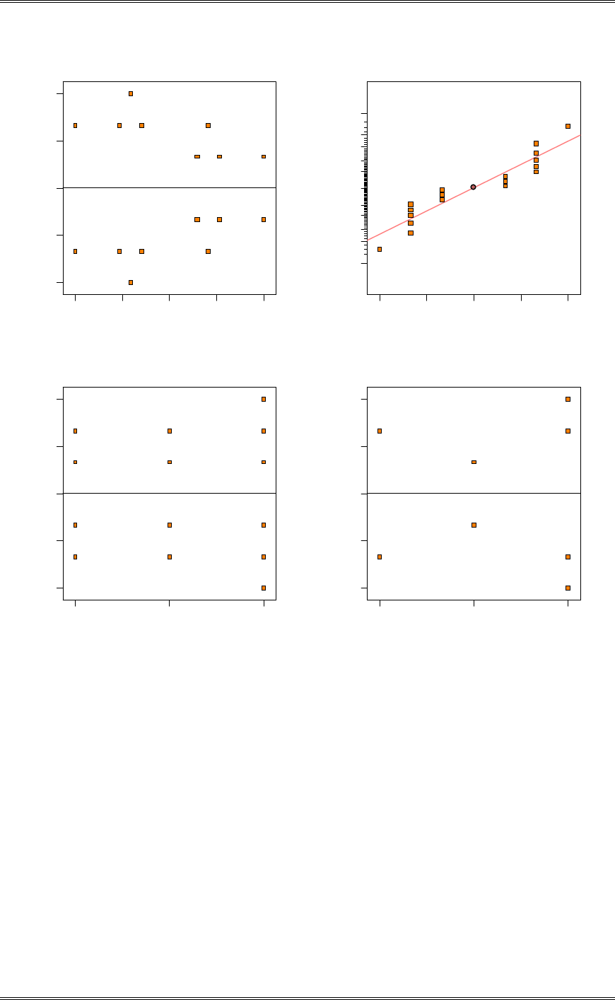
Solutions from Montgomery, D. C. (2001) Design and Analysis of Experiments, Wiley, NY
5-2
Predicted
Residuals
Residuals vs. Predicted
-0.15
-0.075
4
.26326E-014
0.075
0.15
90.00 90.21 90.43 90.64 90.85
Residual
Normal % probability
Normal plot of residuals
-0.15 -0.075 -4.26326E-014 0.075 0.15
1
5
10
20
30
50
70
80
90
95
99
22
Temperature
Residuals
Residuals vs. Temperature
-0.15
-0.075
4
.26326E-014
0.075
0.15
123
3
2
22
2
3
22
2
2
3
Pressure
Residuals
Residuals vs. Pressure
-0.15
-0.075
4
.26326E-014
0.075
0.15
123
(c) Under what conditions would you operate this process?
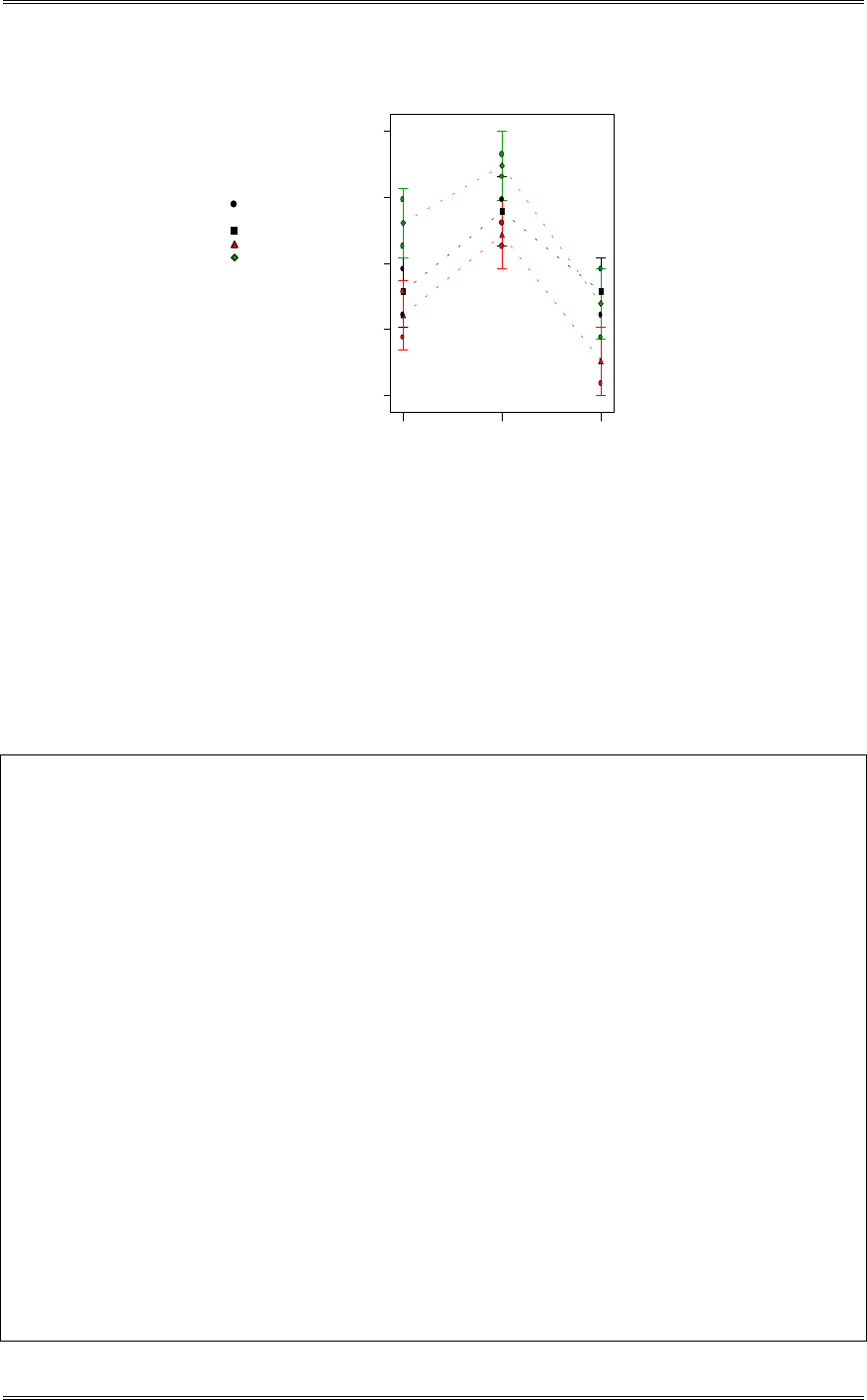
Solutions from Montgomery, D. C. (2001) Design and Analysis of Experiments, Wiley, NY
5-3
DESIGN-EXPERT Plot
Yield
X = A: Pressure
Y = B: Temperature
Design Points
B1 150
B2 160
B3 170
Tem perature
Interaction G raph
P ressure
Yield
200 215 230
89.8492
90.1371
90.425
90.7129
91.0008
2
2
2
2
2
2
Pressure set at 215 and Temperature at the high level, 170 degrees C, give the highest yield.
The standard analysis of variance treats all design factors as if they were qualitative. In this case, both
factors are quantitative, so some further analysis can be performed. In Section 5-5, we show how response
curves and surfaces can be fit to the data from a factorial experiment with at least one quantative factor.
Since both factors in this problem are quantitative and have three levels, we can fit linear and quadratic
effects of both temperature and pressure, exactly as in Example 5-5 in the text. The Design-Expert
output, including the response surface plots, now follows.
Design Expert Output
Response:Surface Finish
ANOVA for Selected Factorial Model
Analysis of variance table [Partial sum of squares]
Sum of Mean F
Source Squares DF Square Value Prob > F
Model 1.13 5 0.23 16.18 < 0.0001 significant
A 0.10 1 0.10 7.22 0.0198
B 0.067 1 0.067 4.83 0.0483
A2 0.67 1 0.67 47.74 < 0.0001
B2 0.23 1 0.23 16.72 0.0015
AB 0.061 1 0.061 4.38 0.0582
Residual 0.17 12 0.014
Lack of Fit 7.639E-003 3 2.546E-003 0.14 0.9314 not significant
Pure Error 0.16 9 0.018
Cor Total 1.30 17
The Model F-value of 16.18 implies the model is significant. There is only
a 0.01% chance that a "Model F-Value" this large could occur due to noise.
Values of "Prob > F" less than 0.0500 indicate model terms are significant.
In this case A, B, A2, B2 are significant model terms.
Values greater than 0.1000 indicate the model terms are not significant.
If there are many insignificant model terms (not counting those required to support hierarchy),
model reduction may improve your model.
Std. Dev. 0.12 R-Squared 0.8708
Mean 90.41 Adj R-Squared 0.8170
C.V. 0.13 Pred R-Squared 0.6794
PRESS 0.42 Adeq Precision 11.968
Coefficient Standard 95% CI 95% CI
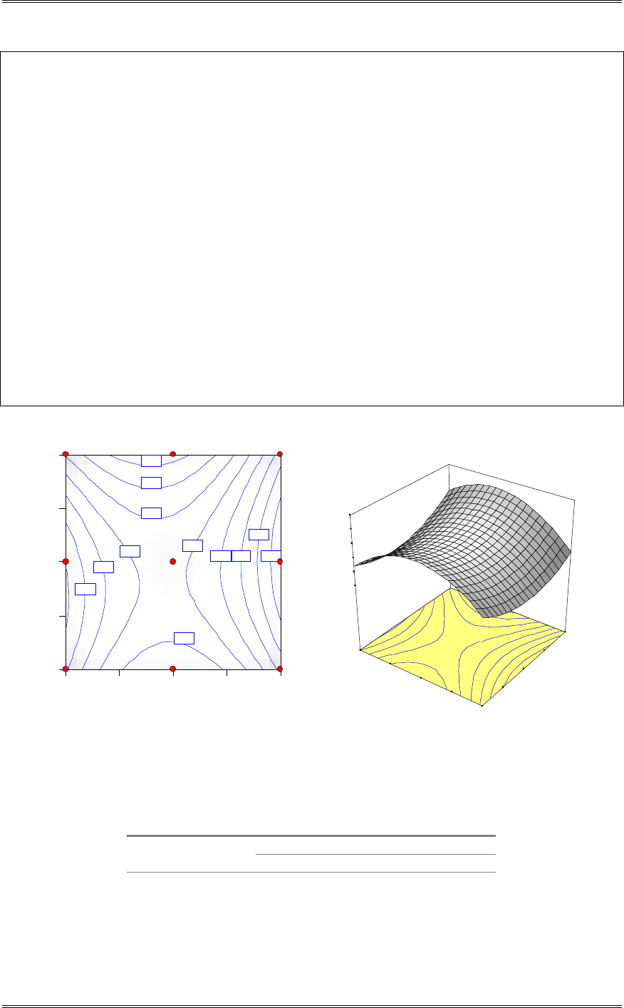
Solutions from Montgomery, D. C. (2001) Design and Analysis of Experiments, Wiley, NY
5-4
Factor Estimate DF Error Low High VIF
Intercept 90.52 1 0.062 90.39 90.66
A-Pressure -0.092 1 0.034 -0.17 -0.017 1.00
B-Temperature 0.075 1 0.034 6.594E-004 0.15 1.00
A
2 -0.41 1 0.059 -0.54 -0.28 1.00
B
2 0.24 1 0.059 0.11 0.37 1.00
AB -0.087 1 0.042 -0.18 3.548E-003 1.00
Final Equation in Terms of Coded Factors:
Yield =
+90.52
-0.092 * A
+0.075 * B
-0.41 * A2
+0.24 * B2
-0.087 * A * B
Final Equation in Terms of Actual Factors:
Yield =
+48.54630
+0.86759 * Pressure
-0.64042 * Temperature
-1.81481E-003 * Pressure2
+2.41667E-003 * Temperature2
-5.83333E-004 * Pressure * Temperature
Yie ld
A: Pressure
B: Temperature
200.00 207.50 215.00 222.50 230.00
150.00
155.00
160.00
165.00
170.00
90.1
90.2
90.3
90.3
90.4
90.4
90.5 90.5
90.6
90.6
90.7
90.8
2 2 2
2 2 2
2 2 2
90
90.2
90.4
90.6
90.8
91
Yie ld
200.00
207.50
215.00
222.50
230.00 150.00
155.00
160.00
165.00
170.00
A: Pre s s ure
B: Temperature
5-2 An engineer suspects that the surface finish of a metal part is influenced by the feed rate and the
depth of cut. She selects three feed rates and four depths of cut. She then conducts a factorial experiment
and obtains the following data:
Depth of Cut (in)
Feed Rate (in/min) 0.15 0.18 0.20 0.25
74 79 82 99
0.20 64 68 88 104
60 73 92 96
92 98 99 104
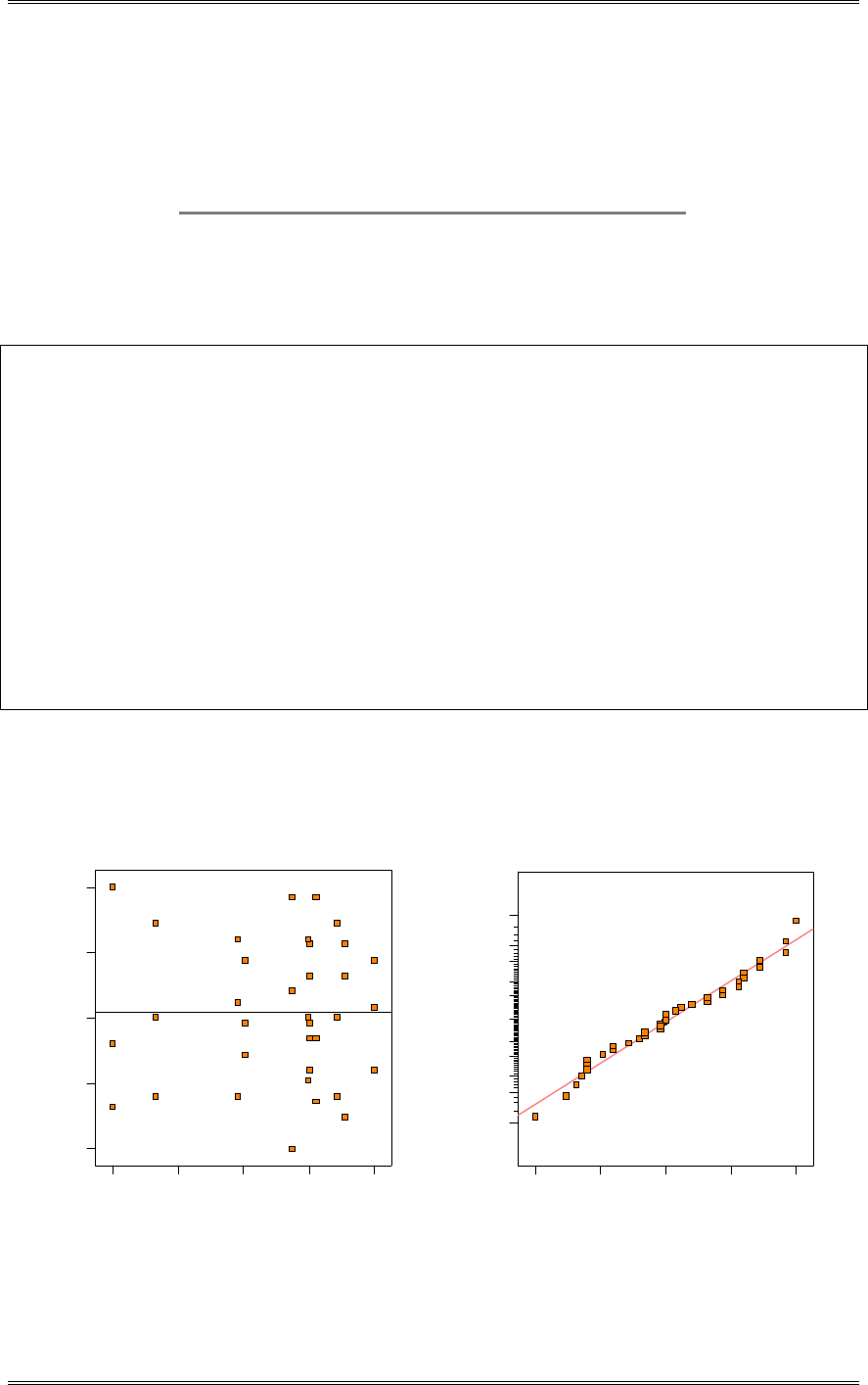
Solutions from Montgomery, D. C. (2001) Design and Analysis of Experiments, Wiley, NY
5-5
0.25 86 104 108 110
88 88 95 99
99 104 108 114
0.30 98 99 110 111
102 95 99 107
(a) Analyze the data and draw conclusions. Use
D
= 0.05.
The depth (A) and feed rate (B) are significant, as is the interaction (AB).
Design Expert Output
Response: Surface Finish
ANOVA for Selected Factorial Model
Analysis of variance table [Partial sum of squares]
Sum of Mean F
Source Squares DF Square Value Prob > F
Model 5842.67 11 531.15 18.49 < 0.0001 significant
A 2125.11 3 708.37 24.66 < 0.0001
B 3160.50 2 1580.25 55.02 < 0.0001
AB 557.06 6 92.84 3.23 0.0180
Residual 689.33 24 28.72
Lack of Fit 0.000 0
Pure Error 689.33 24 28.72
Cor Total 6532.00 35
The Model F-value of 18.49 implies the model is significant. There is only
a 0.01% chance that a "Model F-Value" this large could occur due to noise.
Values of "Prob > F" less than 0.0500 indicate model terms are significant.
In this case A, B, AB are significant model terms.
(b) Prepare appropriate residual plots and comment on the model’s adequacy.
The residual plots shown indicate nothing unusual.
Predicted
Residuals
Residuals vs. Predicted
-8.66667
-4.5
-0.333333
3.83333
8
66.00 77.17 88.33 99.50 110.67
Residual
Normal % probability
Normal plot of residuals
-8.66667 -4.5 -0.333333 3.83333 8
1
5
10
20
30
50
70
80
90
95
99
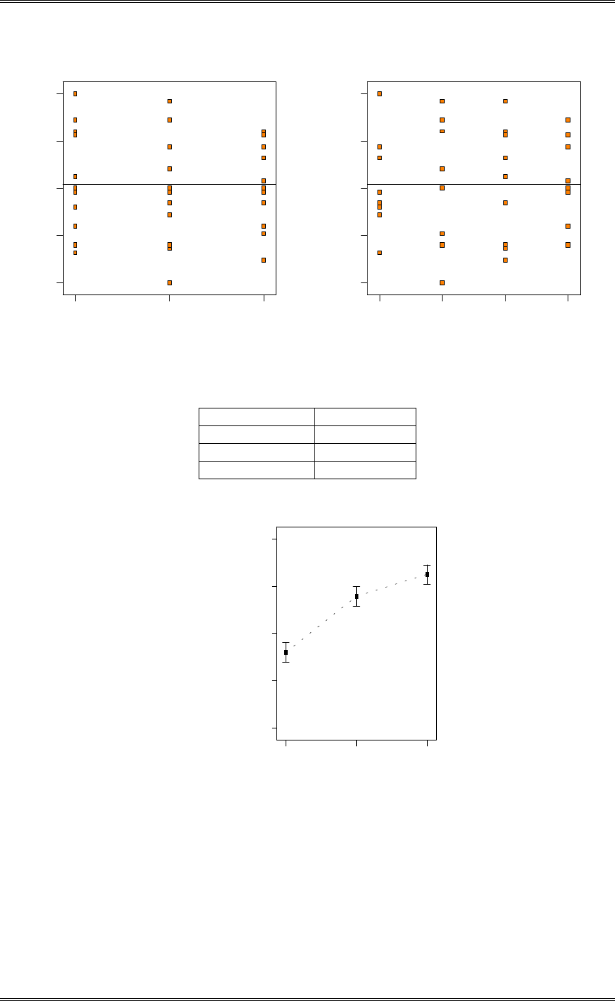
Solutions from Montgomery, D. C. (2001) Design and Analysis of Experiments, Wiley, NY
5-6
22
22
Feed Rate
Residuals
Residuals vs. Feed Rate
-8.66667
-4.5
-0.333333
3.83333
8
123
Depth of Cut
Residuals
Residuals vs. Depth of Cut
-8.66667
-4.5
-0.333333
3.83333
8
1 2 3 4
(c) Obtain point estimates of the mean surface finish at each feed rate.
Feed Rate Average
0.20 81.58
0.25 97.58
0.30 103.83
DESIGN-EXPERT Plot
Surface Finish
X = B: Feed Rate
Actual Factor
A: Depth of Cut = Average
Feed R ate
S urface Finish
O ne F actor P lot
0.20 0.25 0.30
60
73.5
87
100.5
114
W a rn in g ! F a c to r in v o lv e d in a n in te ra c tio n .
(d) Find P-values for the tests in part (a).
The P-values are given in the computer output in part (a).
5-3 For the data in Problem 5-2, compute a 95 percent interval estimate of the mean difference in
response for feed rates of 0.20 and 0.25 in/min.

Solutions from Montgomery, D. C. (2001) Design and Analysis of Experiments, Wiley, NY
5-7
We wish to find a confidence interval on
PP
12
, where
P
1 is the mean surface finish for 0.20 in/min and
P
2is the mean surface finish for 0.25 in/min.
n
MS
tyy
n
MS
tyy E
nab
E
nab
22
)1,2..2..1211,2..2..1 dd
DD PP
032.916
3
)7222.28(2
)064.2()5833.975833.81( r r
Therefore, the 95% confidence interval for
PP
12
is -16.000 r 9.032.
5-4 An article in Industrial Quality Control (1956, pp. 5-8) describes an experiment to investigate the
effect of the type of glass and the type of phosphor on the brightness of a television tube. The response
variable is the current necessary (in microamps) to obtain a specified brightness level. The data are as
follows:
Glass Phosphor Type
Type 1 2 3
280 300 290
1 290 310 285
285 295 290
230 260 220
2 235 240 225
240 235 230
(a) Is there any indication that either factor influences brightness? Use
D
= 0.05.
Both factors, phosphor type (A) and Glass type (B) influence brightness.
Design Expert Output
Response: Current in microamps
ANOVA for Selected Factorial Model
Analysis of variance table [Partial sum of squares]
Sum of Mean F
Source Squares DF Square Value Prob > F
Model 15516.67 5 3103.33 58.80 < 0.0001 significant
A 933.33 2 466.67 8.84 0.0044
B 14450.00 1 14450.00 273.79 < 0.0001
AB 133.33 2 66.67 1.26 0.3178
Residual 633.33 12 52.78
Lack of Fit 0.000 0
Pure Error 633.33 12 52.78
Cor Total16150.00 17
The Model F-value of 58.80 implies the model is significant. There is only
a 0.01% chance that a "Model F-Value" this large could occur due to noise.
Values of "Prob > F" less than 0.0500 indicate model terms are significant.
In this case A, B are significant model terms.
(b) Do the two factors interact? Use
D
= 0.05.
There is no interaction effect.
(c) Analyze the residuals from this experiment.
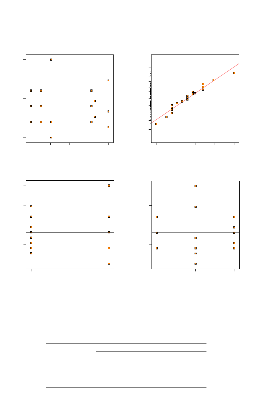
Solutions from Montgomery, D. C. (2001) Design and Analysis of Experiments, Wiley, NY
5-8
The residual plot of residuals versus phosphor content indicates a very slight inequality of variance. It is
not serious enough to be of concern, however.
22
Predicted
Residuals
Residuals vs. Predicted
-10
-3.75
2.5
8.75
15
225.00 244.17 263.33 282.50 301.67
Residual
Normal % probability
Normal plot of residuals
-10 -3.7 5 2.5 8.75 15
1
5
10
20
30
50
70
80
90
95
99
22
2
2
2
2
Glas s Type
Residuals
Residuals vs. Glass Type
-10
-3.75
2.5
8.75
15
1 2
2
22
2
Phosphor Type
Residuals
Residuals vs. Phosphor Type
-10
-3.75
2.5
8.75
15
123
5-5 Johnson and Leone (Statistics and Experimental Design in Engineering and the Physical Sciences,
Wiley 1977) describe an experiment to investigate the warping of copper plates. The two factors studies
were the temperature and the copper content of the plates. The response variable was a measure of the
amount of warping. The data were as follows:
Copper Content (%)
Temperature (°C) 40 60 80 100
50 17,20 16,21 24,22 28,27
75 12,9 18,13 17,12 27,31
100 16,12 18,21 25,23 30,23
125 21,17 23,21 23,22 29,31
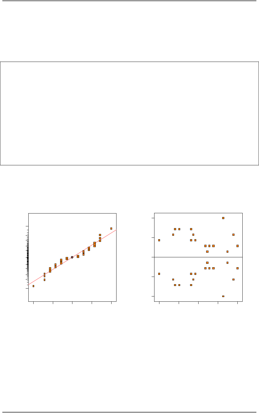
Solutions from Montgomery, D. C. (2001) Design and Analysis of Experiments, Wiley, NY
5-9
(a) Is there any indication that either factor affects the amount of warping? Is there any interaction
between the factors? Use
D
= 0.05.
Both factors, copper content (A) and temperature (B) affect warping, the interaction does not.
Design Expert Output
Response: Warping
ANOVA for Selected Factorial Model
Analysis of variance table [Partial sum of squares]
Sum of Mean F
Source Squares DF Square Value Prob > F
Model 968.22 15 64.55 9.52 < 0.0001 significant
A
698.34 3 232.78 34.33 < 0.0001
B
156.09 3 52.03 7.67 0.0021
AB
113.78 9 12.64 1.86 0.1327
Residual 108.50 16 6.78
Lack of Fit
0.000 0
Pure Error
108.50 16 6.78
Cor Total 1076.72 31
The Model F-value of 9.52 implies the model is significant. There is only
a 0.01% chance that a "Model F-Value" this large could occur due to noise.
Values of "Prob > F" less than 0.0500 indicate model terms are significant.
In this case A, B are significant model terms.
(b) Analyze the residuals from this experiment.
There is nothing unusual about the residual plots.
Residual
Normal % probability
Normal plot of residuals
-3.5 -1.75 -1.06581E-014 1.75 3.5
1
5
10
20
30
50
70
80
90
95
99
Predicted
Residuals
Residuals vs. Predicted
-3.5
-1.75
1.06581E-014
1.75
3.5
10.50 15.38 20.25 25.13 30.00
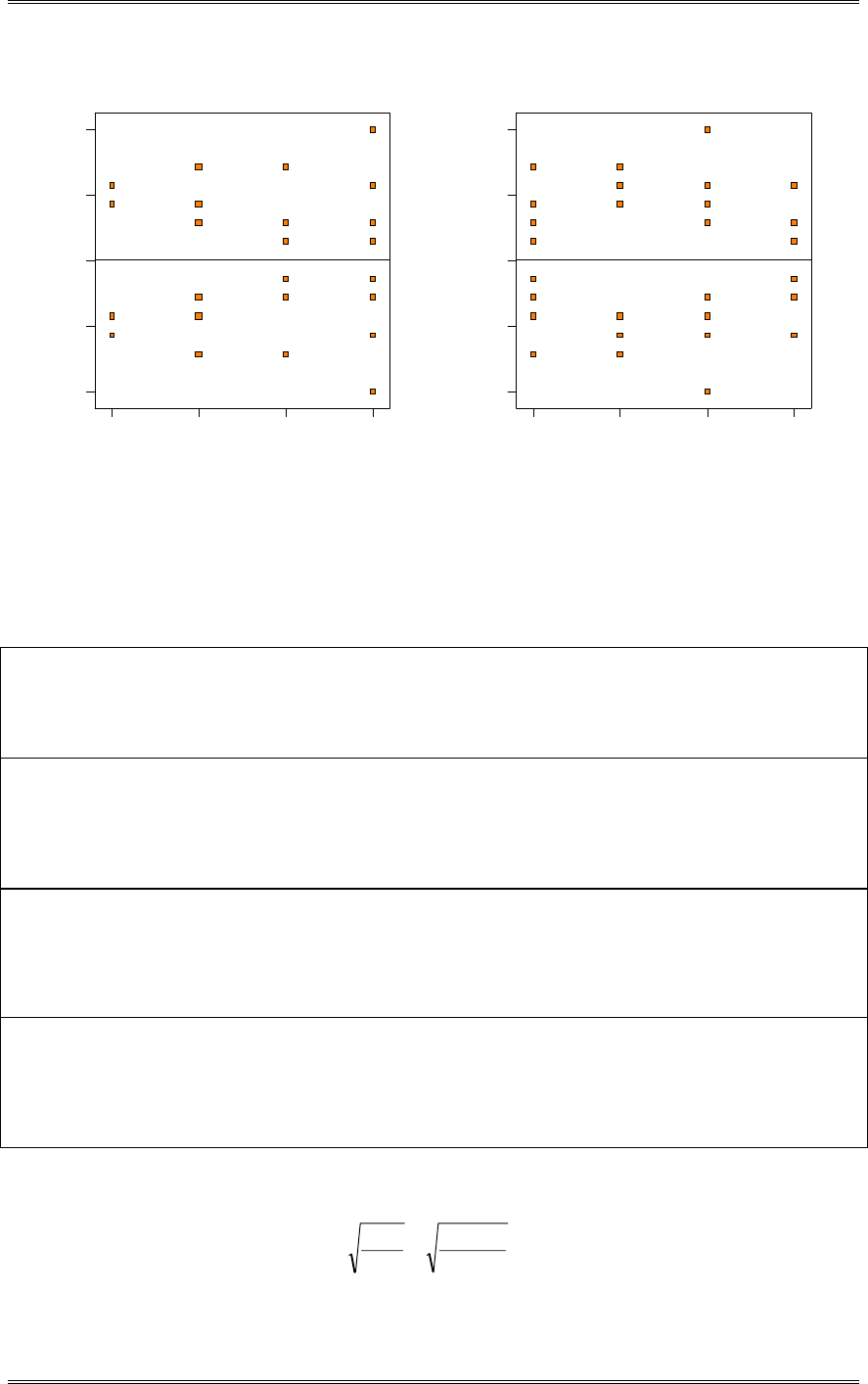
Solutions from Montgomery, D. C. (2001) Design and Analysis of Experiments, Wiley, NY
5-10
2
2
2
2
2
2
2
2
Copper Content
Residuals
Residuals vs. Copper Content
-3.5
-1.75
1.06581E-014
1.75
3.5
1 2 3 4
Temperature
Residuals
Residuals vs. Temperature
-3.5
-1.75
1.06581E-014
1.75
3.5
1 2 3 4
(c) Plot the average warping at each level of copper content and compare them to an appropriately scaled
t distribution. Describe the differences in the effects of the different levels of copper content on
warping. If low warping is desirable, what level of copper content would you specify?
Design Expert Output
Factor Name Level Low Level High Level
A Copper Content 40 40 100
B Temperature Average 50 125
Prediction SE Mean 95% CI low 95% CI high SE Pred 95% PI low 95% PI high
Warping15.50 1.84 11.60 19.40 3.19 8.74 22.26
Factor Name Level Low Level High Level
A Copper Content 60 40 100
B Temperature Average 50 125
Prediction SE Mean 95% CI low 95% CI high SE Pred 95% PI low 95% PI high
Warping18.88 1.84 14.97 22.78 3.19 12.11 25.64
Factor Name Level Low Level High Level
A Copper Content 80 40 100
B Temperature Average 50 125
Prediction SE Mean 95% CI low 95% CI high SE Pred 95% PI low 95% PI high
Warping21.00 1.84 17.10 24.90 3.19 14.24 27.76
Factor Name Level Low Level High Level
A Copper Content 100 40 100
B Temperature Average 50 125
Prediction SE Mean 95% CI low 95% CI high SE Pred 95% PI low 95% PI high
Warping28.25 1.84 24.35 32.15 3.19 21.49 35.01
Use a copper content of 40 for the lowest warping.
31
4
781256 .
.
b
MS
SE
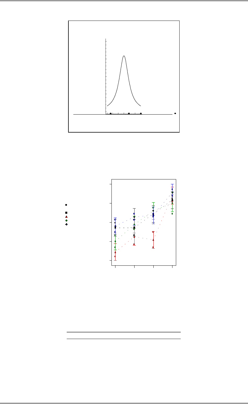
Solutions from Montgomery, D. C. (2001) Design and Analysis of Experiments, Wiley, NY
5-11
15.0 18.0 21.0 24.0 27.0
Warping
Scaled t Distribution
Cu=40 Cu=60 Cu=80 Cu=100
(d) Suppose that temperature cannot be easily controlled in the environment in which the copper plates
are to be used. Does this change your answer for part (c)?
Use a copper of content of 40. This is the same as for part (c).
DESIGN-EXPERT Plot
Warping
X = A: Copper Content
Y = B: Temperature
Design Points
B1 50
B2 75
B3 100
B4 125
Tem perature
Interaction G raph
C opper C ontent
W a rp in g
40 60 80 100
7.73979
13.9949
20.25
26.5051
32.7602
2
3
2
2
2
2
2
2
2
2
3
2
2
3
2
2
2
5-6 The factors that influence the breaking strength of a synthetic fiber are being studied. Four
production machines and three operators are chosen and a factorial experiment is run using fiber from the
same production batch. The results are as follows:
Machine
Operator 1 2 3 4
1 109 110 108 110
110 115 109 108
2 110 110 111 114
112 111 109 112
3 116 112 114 120
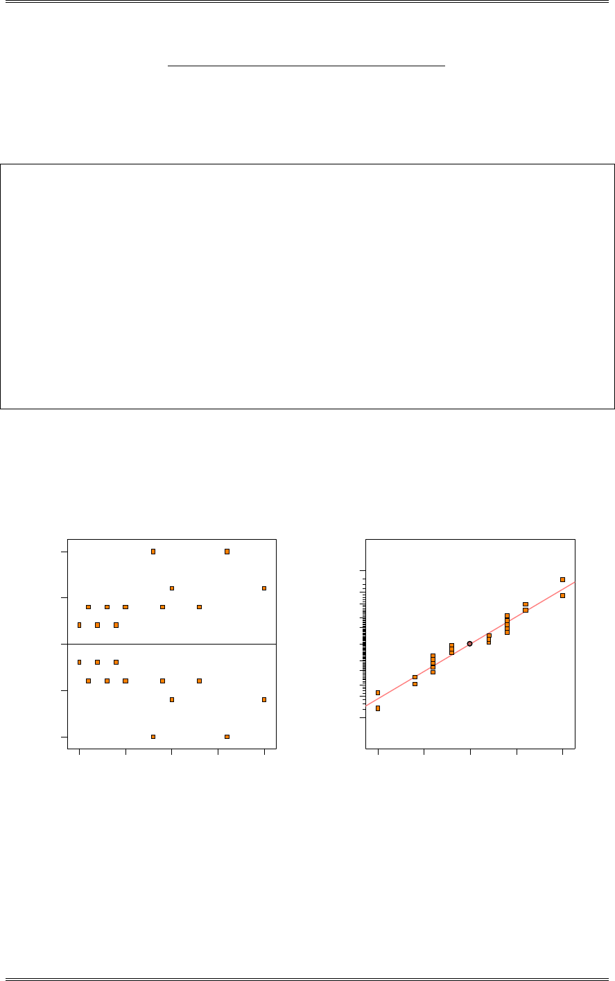
Solutions from Montgomery, D. C. (2001) Design and Analysis of Experiments, Wiley, NY
5-12
114 115 119 117
(a) Analyze the data and draw conclusions. Use
D
= 0.05.
Only the Operator (A) effect is significant.
Design Expert Output
Response:Stength
ANOVA for Selected Factorial Model
Analysis of variance table [Partial sum of squares]
Sum of
Mean F
Source Squares DF Square Value Prob > F
Model 217.46 11 19.77 5.21 0.0041 significant
A 160.33 2 80.17 21.14 0.0001
B 12.46 3 4.15 1.10 0.3888
AB 44.67 6 7.44 1.96 0.1507
Residual 45.50 12 3.79
Lack of Fit 0.000 0
Pure Error 45.50 12 3.79
Cor Total 262.96 23
The Model F-value of 5.21 implies the model is significant.
There is only a 0.41% chance that a "Model F-Value" this large could occur due to noise.
Values of "Prob > F" less than 0.0500 indicate model terms aresignificant.
In this case A are significant model terms.
(b) Prepare appropriate residual plots and comment on the model’s adequacy.
The residual plot of residuals versus predicted shows that variance increases very slightly with strength.
There is no indication of a severe problem.
Predicted
Residuals
Residuals vs. Predicted
-2.5
-1.25
7.81597E-014
1.25
2.5
108.50 111.00 113.50 116.00 118.50
Residual
Normal % probability
Normal plot of residuals
-2.5 -1.25 -7.81597E-014 1.25 2.5
1
5
10
20
30
50
70
80
90
95
99
Solutions from Montgomery, D. C. (2001) Design and Analysis of Experiments, Wiley, NY
5-13
3
3
2
2
3
3
3
3
2
2
Operator
Residuals
Residuals vs. Operator
-2.5
-1.25
7.81597E-014
1.25
2.5
1 2 3
5-7 A mechanical engineer is studying the thrust force developed by a drill press. He suspects that the
drilling speed and the feed rate of the material are the most important factors. He selects four feed rates
and uses a high and low drill speed chosen to represent the extreme operating conditions. He obtains the
following results. Analyze the data and draw conclusions. Use
D
= 0.05.
(A) Feed Rate
(B)
Drill Speed 0.015 0.030 0.045 0.060
125 2.70 2.45 2.60 2.75
2.78 2.49 2.72 2.86
200 2.83 2.85 2.86 2.94
2.86 2.80 2.87 2.88
Design Expert Output
Response: Force
ANOVA for Selected Factorial Model
Analysis of variance table [Partial sum of squares]
Sum of Mean F
Source Squares DF Square Value Prob > F
Model 0.28 7 0.040 15.53 0.0005 significant
A 0.15 1 0.15 57.01 < 0.0001
B 0.092 3 0.031 11.86 0.0026
AB 0.042 3 0.014 5.37 0.0256
Residual 0.021 8 2.600E-003
Lack of Fit 0.000 0
Pure Error 0.021 8 2.600E-003
Cor Total 0.30 15
The Model F-value of 15.53 implies the model is significant.
There is only a 0.05% chance that a "Model F-Value" this large could occur due to noise.
Values of "Prob > F" less than 0.0500 indicate model terms are significant.
In this case A, B, AB are significant model terms.
The factors speed and feed rate, as well as the interaction is important.
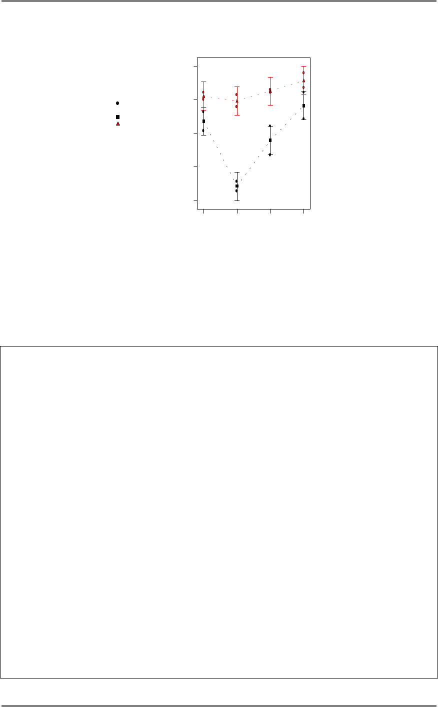
Solutions from Montgomery, D. C. (2001) Design and Analysis of Experiments, Wiley, NY
5-14
DESIGN-EXPERT Plot
Force
X = B: Feed Rate
Y = A: Drill Speed
Design Points
A1 125
A2 200
D rill S p e e d
Interaction G raph
Feed R ate
F o rc e
0.015 0.030 0.045 0.060
2.41121
2.5506
2.69
2.8294
2.96879
The standard analysis of variance treats all design factors as if they were qualitative. In this case, both
factors are quantitative, so some further analysis can be performed. In Section 5-5, we show how response
curves and surfaces can be fit to the data from a factorial experiment with at least one quantative factor.
Since both factors in this problem are quantitative and have three levels, we can fit linear and quadratic
effects of both temperature and pressure, exactly as in Example 5-5 in the text. The Design-Expert
output, including the response surface plots, now follows.
Design Expert Output
Response: Force
ANOVA for Selected Factorial Model
Analysis of variance table [Partial sum of squares]
Sum of Mean F
Source Squares DF Square Value Prob > F
Model 0.23 4 0.057 8.05 0.0027 significant
A 0.15 1 0.15 21.11 0.0008
B 0.019 1 0.019 2.74 0.1262
B2 0.058 1 0.058 8.20 0.0154
AB 1.125E-003 1 1.125E-003 0.16 0.6966
Residual 0.077 11 7.021E-003
Lack of Fit 0.056 3 0.019 7.23 0.0115 significant
Pure Error 0.021 8 2.600E-003
Cor Total 0.30 15
The Model F-value of 8.05 implies the model is significant. There is only
a 0.27% chance that a "Model F-Value" this large could occur due to noise.
Values of "Prob > F" less than 0.0500 indicate model terms are significant.
In this case A, B2 are significant model terms.
Values greater than 0.1000 indicate the model terms are not significant.
If there are many insignificant model terms (not counting those required to support hierarchy),
model reduction may improve your model.
Std. Dev. 0.084 R-Squared 0.7455
Mean 2.77 Adj R-Squared 0.6529
C.V. 3.03 Pred R-Squared 0.4651
PRESS 0.16 Adeq Precision 7.835
Coefficient Standard 95% CI 95% CI
Factor Estimate DF Error Low High VIF
Intercept 2.69 1 0.034 2.62 2.76
A-Drill Speed 0.096 1 0.021 0.050 0.14 1.00
B-Feed Rate 0.047 1 0.028 -0.015 0.11 1.00
B2 0.13 1 0.047 0.031 0.24 1.00
AB -0.011 1 0.028 -0.073 0.051 1.00
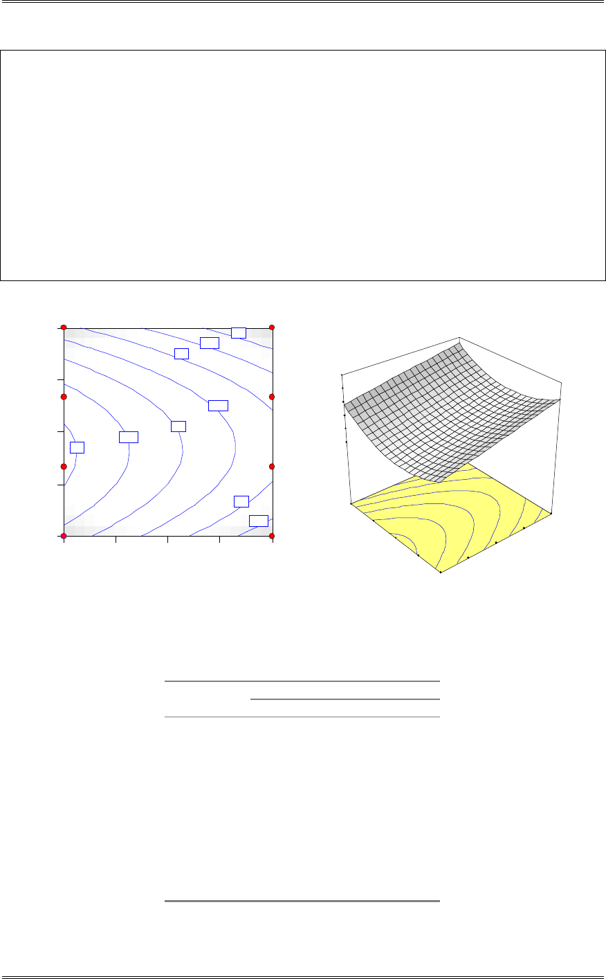
Solutions from Montgomery, D. C. (2001) Design and Analysis of Experiments, Wiley, NY
5-15
Final Equation in Terms of Coded Factors:
Force =
+2.69
+0.096 * A
+0.047 * B
+0.13 * B2
-0.011 * A * B
Final Equation in Terms of Actual Factors:
Force =
+2.48917
+3.06667E-003 * Drill Speed
-15.76667 * Feed Rate
+266.66667 * Feed Rate2
-0.013333 * Drill Speed * Feed Rate
Force
A: Drill Speed
B: Fee d R ate
125.00 143.75 162.50 181.25 200.00
0.02
0.03
0.04
0.05
0.06
2.6
2.65
2.7
2.75
2.8
2.8
2.85
2.85
2.9
2 2
2 2
2 2
2 2
2.5
2.6
2.7
2.8
2.9
3
Fo rce
125.00
143.75
162.50
181.25
200.00
0.02
0.03
0.04
0.05
0.06
A: Drill Speed
B: Fee d R ate
5-8 An experiment is conducted to study the influence of operating temperature and three types of face-
plate glass in the light output of an oscilloscope tube. The following data are collected:
Temperature
Glass Type 100 125 150
580 1090 1392
1 568 1087 1380
570 1085 1386
550 1070 1328
2 530 1035 1312
579 1000 1299
546 1045 867
3 575 1053 904
599 1066 889
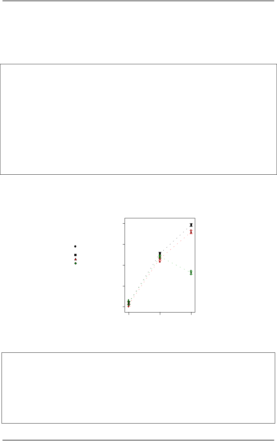
Solutions from Montgomery, D. C. (2001) Design and Analysis of Experiments, Wiley, NY
5-16
Use
D
= 0.05 in the analysis. Is there a significant interaction effect? Does glass type or temperature
affect the response? What conclusions can you draw? Use the method discussed in the text to partition
the temperature effect into its linear and quadratic components. Break the interaction down into
appropriate components.
Design Expert Output
Response: Light Output
ANOVA for Selected Factorial Model
Analysis of variance table [Partial sum of squares]
Sum of Mean F
Source Squares DF Square Value Prob > F
Model 2.412E+006 8 3.015E+005 824.77 < 0.0001 significant
A 1.509E+005 2 75432.26 206.37 < 0.0001
B
1.970E+006 2 9.852E+005 2695.26 < 0.0001
AB
2.906E+005 4 72637.93 198.73 < 0.0001
Residual 6579.33 18 365.52
Lack of Fit
0.000 0
Pure Error 6579.33 18 365.52
Cor Total 2.418E+006 26
The Model F-value of 824.77 implies the model is significant.
There is only a 0.01% chance that a "Model F-Value" this large could occur due to noise.
Values of "Prob > F" less than 0.0500 indicate model terms are significant.
In this case A, B, AB are significant model terms.
Both factors, Glass Type (A) and Temperature (B) are significant, as well as the interaction (AB). For
glass types 1 and 2 the response is fairly linear, for glass type 3, there is a quadratic effect.
DESIGN-EXPERT Plot
Light Output
X = B: Temperature
Y = A: Glass Type
Design Points
A1 1
A2 2
A3 3
G lass Type
Interaction G raph
Tem perature
L ig h t O u tp u t
100 125 150
530
748.099
966.199
1184.3
1402.4
Design Expert Output
Response: Light Output
ANOVA for Selected Factorial Model
Analysis of variance table [Partial sum of squares]
Sum of Mean F
Source Squares DF Square Value Prob > F
Model 2.412E+006 8 3.015E+005 824.77 < 0.0001 significant
A 1.509E+005 2 75432.26 206.37 < 0.0001
B 1.780E+006 1 1.780E+006 4869.13 < 0.0001
B2 1.906E+005 1 1.906E+005 521.39 < 0.0001
AB 2.262E+005 2 1.131E+005 309.39 < 0.0001
AB2 64373.93 2 32186.96 88.06 < 0.0001
Pure Error 6579.33 18 365.52

Solutions from Montgomery, D. C. (2001) Design and Analysis of Experiments, Wiley, NY
5-17
Cor Total 2.418E+006 26
The Model F-value of 824.77 implies the model is significant. There is only
a 0.01% chance that a "Model F-Value" this large could occur due to noise.
Values of "Prob > F" less than 0.0500 indicate model terms are significant.
In this case A, B, B2, AB, AB2 are significant model terms.
Values greater than 0.1000 indicate the model terms are not significant.
If there are many insignificant model terms (not counting those required to support hierarchy),
model reduction may improve your model.
Std. Dev. 19.12 R-Squared 0.9973
Mean 940.19 Adj R-Squared 0.9961
C.V. 2.03 Pred R-Squared 0.9939
PRESS 14803.50 Adeq Precision 75.466
Coefficient Standard 95% CI 95% CI
Factor Estimate DF Error Low High VIF
Intercept 1059.00 1 6.37 1045.61 1072.39
A[1] 28.33 1 9.01 9.40 47.27
A[2] -24.00 1 9.01 -42.93 -5.07
B-Temperature 314.44 1 4.51 304.98 323.91 1.00
B2 -178.22 1 7.81 -194.62 -161.82 1.00
A[1]B 92.22 1 6.37 78.83 105.61
A[2]B 65.56 1 6.37 52.17 78.94
A[1]B2 70.22 1 11.04 47.03 93.41
A[2]B2 76.22 1 11.04 53.03 99.41
Final Equation in Terms of Coded Factors:
Light Output =
+1059.00
+28.33 * A[1]
-24.00 * A[2]
+314.44 * B
-178.22 * B2
+92.22 * A[1]B
+65.56 * A[2]B
+70.22 * A[1]B2
+76.22 * A[2]B2
Final Equation in Terms of Actual Factors:
Glass Type 1
Light Output =
-3646.00000
+59.46667 * Temperature
-0.17280 * Temperature2
Glass Type 2
Light Output =
-3415.00000
+56.00000 * Temperature
-0.16320 * Temperature2
Glass Type 3
Light Output =
-7845.33333
+136.13333 * Temperature
-0.51947 * Temperature2
5-9 Consider the data in Problem 5-1. Use the method described in the text to compute the linear and
quadratic effects of pressure.
See the alternative analysis shown in Problem 5-1 part (c).

Solutions from Montgomery, D. C. (2001) Design and Analysis of Experiments, Wiley, NY
5-18
5-10 Use Duncan’s multiple range test to determine which levels of the pressure factor are significantly
different for the data in Problem 5-1.
1890
3.y .. 3790
1.y .. 6890
2.y ..
05430
23
017770 .
.
an
MS
SE
y.j.
60492
010.,r .
86493
010.,r .
2498005430604
2...R
2640005430864
3...R
2 vs. 3 = 0.50 > 0.2640 (R3)
2 vs. 1 = 0.31 > 0.2498 (R2)
1 vs. 3 = 0.19 < 0.2498 (R2)
Therefore, 2 differs from 1 and 3.
5-11 An experiment was conducted to determine if either firing temperature or furnace position affects
the baked density of a carbon anode. The data are shown below.
Temperature (°C)
Position 800 825 850
570 1063 565
1 565 1080 510
583 1043 590
528 988 526
2 547 1026 538
521 1004 532
Suppose we assume that no interaction exists. Write down the statistical model. Conduct the analysis of
variance and test hypotheses on the main effects. What conclusions can be drawn? Comment on the
model’s adequacy.
The model for the two-factor, no interaction model is ijkjiijk
y
HEWP
. Both factors, furnace
position (A) and temperature (B) are significant. The residual plots show nothing unusual.
Design Expert Output
Response: Density
ANOVA for Selected Factorial Model
Analysis of variance table [Partial sum of squares]
Sum of Mean F
Source Squares DF Square Value Prob > F
Model 9.525E+005 3 3.175E+005 718.24 < 0.0001 significant
A 7160.06 1 7160.06 16.20 0.0013
B 9.453E+005 2 4.727E+005 1069.26 < 0.0001
Residual 6188.78 14 442.06
Lack of Fit 818.11 2 409.06 0.91 0.4271 not significant
Pure Error 5370.67 12 447.56
Cor Total 9.587E+005 17
The Model F-value of 718.24 implies the model is significant.
There is only a 0.01% chance that a "Model F-Value" this large could occur due to noise.
Values of "Prob > F" less than 0.0500 indicate model terms are significant.
In this case A, B are significant model terms.
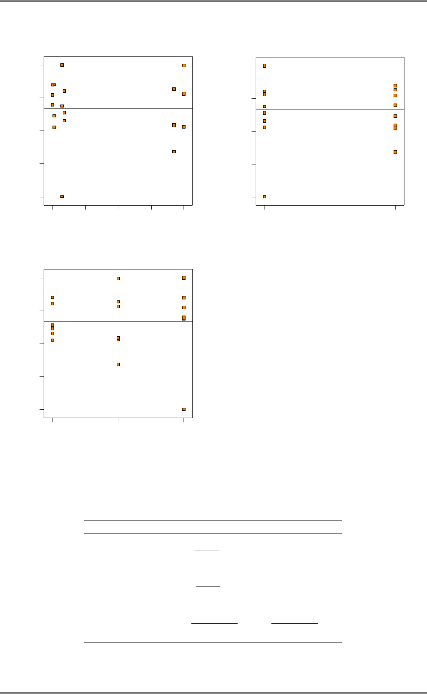
Solutions from Montgomery, D. C. (2001) Design and Analysis of Experiments, Wiley, NY
5-19
Predicted
Residuals
Residuals vs. Predicted
-53.4444
-33.4444
-13.4444
6.55556
26.5556
523.56 656.15 788.75 921.35 1053.94
Position
Residuals
Residuals vs. Position
-53.4444
-33.4444
-13.4444
6.55556
26.5556
1 2
Temperature
Residuals
Residuals vs. Temperature
-53.4444
-33.4444
-13.4444
6.55556
26.5556
123
5-12 Derive the expected mean squares for a two-factor analysis of variance with one observation per
cell, assuming that both factors are fixed.
Degrees of Freedom
¦
a
i
i
Aa
bMSE
1
2
2
1
W
V
a-1
¦
b
j
j
Bb
aMSE
1
2
2
1
E
V
b-1
¦¦
a
i
b
j
ij
AB ba
MSE
11
2
2
11
WE
V
1
11
ab
ba

Solutions from Montgomery, D. C. (2001) Design and Analysis of Experiments, Wiley, NY
5-20
5-13 Consider the following data from a two-factor factorial experiment. Analyze the data and draw
conclusions. Perform a test for nonadditivity. Use
D
= 0.05.
Column Factor
Row Factor 1 2 3 4
1 36 39 36 32
2 18 20 22 20
3 30 37 33 34
Design Expert Output
Response: data
ANOVA for Selected Factorial Model
Analysis of variance table [Partial sum of squares]
Sum of Mean F
Source Squares DF Square Value Prob > F
Model 609.42 5 121.88 25.36 0.0006 significant
A 580.50 2 290.25 60.40 0.0001
B 28.92 3 9.64 2.01 0.2147
Residual 28.83 6 4.81
Cor Total 638.25 11
The Model F-value of 25.36 implies the model is significant. There is only
a 0.06% chance that a "Model F-Value" this large could occur due to noise.
The row factor (A) is significant.
The test for nonadditivity is as follows:
2927925540513833328
540513
91667285058034
34
357
9166728505803574010014
2
2
2
11
2
...SSSSSS
.SS
..
..
SS
SSabSS
ab
y
SSSSyyyy
SS
NsidualReError
N
N
BA
a
i
b
j
..
BA..j..iij
N
»
»
¼
º
«
«
¬
ª
¸
¸
¹
·
¨
¨
©
§
»
»
¼
º
«
«
¬
ª
¸
¸
¹
·
¨
¨
©
§
¦¦
Source of Sum of Degrees of Mean
Variation Squares Freedom Square F0
Row 580.50 2 290.25 57.3780
Column 28.91667 3 9.63889 1.9054
Nonadditivity 3.54051 1 3.54051 0.6999
Error 25.29279 5 5.058558
Total 638.25 11
5-14 The shear strength of an adhesive is thought to be affected by the application pressure and
temperature. A factorial experiment is performed in which both factors are assumed to be fixed. Analyze
the data and draw conclusions. Perform a test for nonadditivity.
Temperature (°F)

Solutions from Montgomery, D. C. (2001) Design and Analysis of Experiments, Wiley, NY
5-21
Pressure (lb/in2) 250 260 270
120 9.60 11.28 9.00
130 9.69 10.10 9.57
140 8.43 11.01 9.03
150 9.98 10.44 9.80
Design Expert Output
Response: Strength
ANOVA for Selected Factorial Model
Analysis of variance table [Partial sum of squares]
Sum of Mean F
Source Squares DF Square Value Prob > F
Model 5.24 5 1.05 2.92 0.1124 not significant
A 0.58 3 0.19 0.54 0.6727
B 4.66 2 2.33 6.49 0.0316
Residual 2.15 6 0.36
Cor Total 7.39 11
The "Model F-value" of 2.92 implies the model is not significant relative to the noise.
There is a 11.24 % chance that a "Model F-value" this large could occur due to noise.
Values of "Prob > F" less than 0.0500 indicate model terms are significant.
In this case B are significant model terms.
Temperature (B) is a significant factor.
66440148948015388332
489480
6576545806917034
34
93117
6576545806917093117777415113
2
2
2
11
2
...SSSSSS
.SS
..
.
....
SS
SSabSS
ab
y
SSSSyyyy
SS
NsidualReError
N
N
BA
a
i
b
j
..
BA..j..iij
N
»
»
¼
º
«
«
¬
ª
¸
¸
¹
·
¨
¨
©
§
»
»
¼
º
«
«
¬
ª
¸
¸
¹
·
¨
¨
©
§
¦¦
Source of Sum of Degrees of Mean
Variation Squares Freedom Square F0
Row 0.5806917 3 0.1935639 0.5815
Column 4.65765 2 2.328825 6.9960
Nonadditivity 0.48948 1 0.48948 1.4704
Error 1.6644 5 0.33288
Total 7.392225 11
5-15 Consider the three-factor model
ijk
jkij
kjiijk
y
HEJWEJEWP
°
¯
°
®
c,...,,k
b,...,,j
a,...,,i
21
21
21

Solutions from Montgomery, D. C. (2001) Design and Analysis of Experiments, Wiley, NY
5-22
Notice that there is only one replicate. Assuming the factors are fixed, write down the analysis of variance
table, including the expected mean squares. What would you use as the “experimental error” in order to
test hypotheses?
Source Degrees of Freedom Expected Mean Square
A a-1
¦
a
i
i
a
bc
1
2
2
1
W
V
B b-1
¦
b
j
j
b
ac
1
2
2
1
E
V
C c-1
¦
c
k
k
c
ab
1
2
2
1
J
V
AB (a-1)(b-1)
¦¦
a
i
b
j
ij
ba
c
11
2
2
11
EW
V
BC (b-1)(c-1)
¦¦
b
j
c
k
jk
cb
a
11
2
2
11
EJ
V
Error (AC + ABC) b(a-1)(c-1)
V
2
Total abc-1
5-16 The percentage of hardwood concentration in raw pulp, the vat pressure, and the cooking time of
the pulp are being investigated for their effects on the strength of paper. Three levels of hardwood
concentration, three levels of pressure, and two cooking times are selected. A factorial experiment with
two replicates is conducted, and the following data are obtained:
Percentage Cooking Time 3.0 Hours Cooking Time 4.0 Hours
of Hardwood Pressure Pressure
Concentration 400 500 650 400 500 650
2 196.6 197.7 199.8 198.4 199.6 200.6
196.0 196.0 199.4 198.6 200.4 200.9
4 198.5 196.0 198.4 197.5 198.7 199.6
197.2 196.9 197.6 198.1 198.0 199.0
8 197.5 195.6 197.4 197.6 197.0 198.5
196.6 196.2 198.1 198.4 197.8 199.8
(a) Analyze the data and draw conclusions. Use
D
= 0.05.
Design Expert Output
Response: strength
ANOVA for Selected Factorial Model
Analysis of variance table [Partial sum of squares]
Sum of Mean F
Source Squares DF Square Value Prob > F
Model 59.73 17 3.51 9.61 < 0.0001 significant
A 7.76 2 3.88 10.62 0.0009
B 20.25 1 20.25 55.40 < 0.0001
C 19.37 2 9.69 26.50 < 0.0001
AB 2.08 2 1.04 2.85 0.0843
AC 6.09 4 1.52 4.17 0.0146
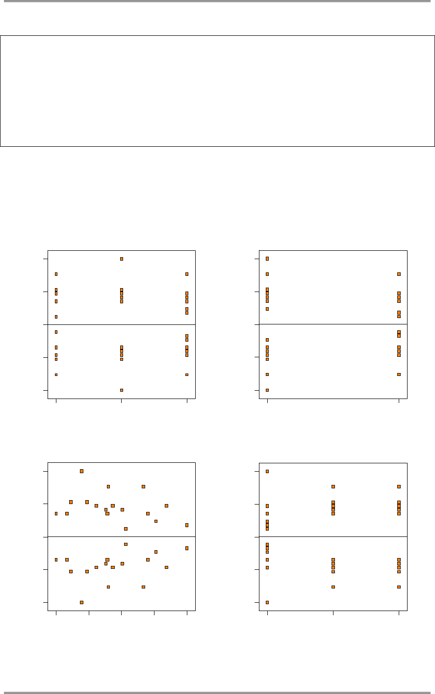
Solutions from Montgomery, D. C. (2001) Design and Analysis of Experiments, Wiley, NY
5-23
BC 2.19 2 1.10 3.00 0.0750
ABC 1.97 4 0.49 1.35 0.2903
Residual 6.58 18 0.37
Lack of Fit 0.000 0
Pure Error 6.58 18 0.37
Cor Total 66.31 35
The Model F-value of 9.61 implies the model is significant. There is only
a 0.01% chance that a "Model F-Value" this large could occur due to noise.
Values of "Prob > F" less than 0.0500 indicate model terms are significant.
In this case A, B, C, AC are significant model terms.
All three main effects, concentration (A), pressure (C) and time (B), as well as the concentration x
pressure interaction (AC) are significant at the 5% level. The concentration x time (AB) and pressure x
time interactions (BC) are significant at the 10% level.
(b) Prepare appropriate residual plots and comment on the model’s adequacy.
Pressure
Residuals
Residuals vs. Pressure
-0.85
-0.425
0
0.425
0.85
123
2
2
2
2
Cooking Time
Residuals
Residuals vs. Cooking Time
-0.85
-0.425
0
0.425
0.85
1 2
Predicted
Residuals
Residuals vs. Predicted
-0.85
-0.425
0
0.425
0.85
195.90 197.11 198.33 199.54 200.75
2
2
2
2
Hardwood
Residuals
Residuals vs. Hardwood
-0.85
-0.425
0
0.425
0.85
1 2 3
There is nothing unusual about the residual plots.
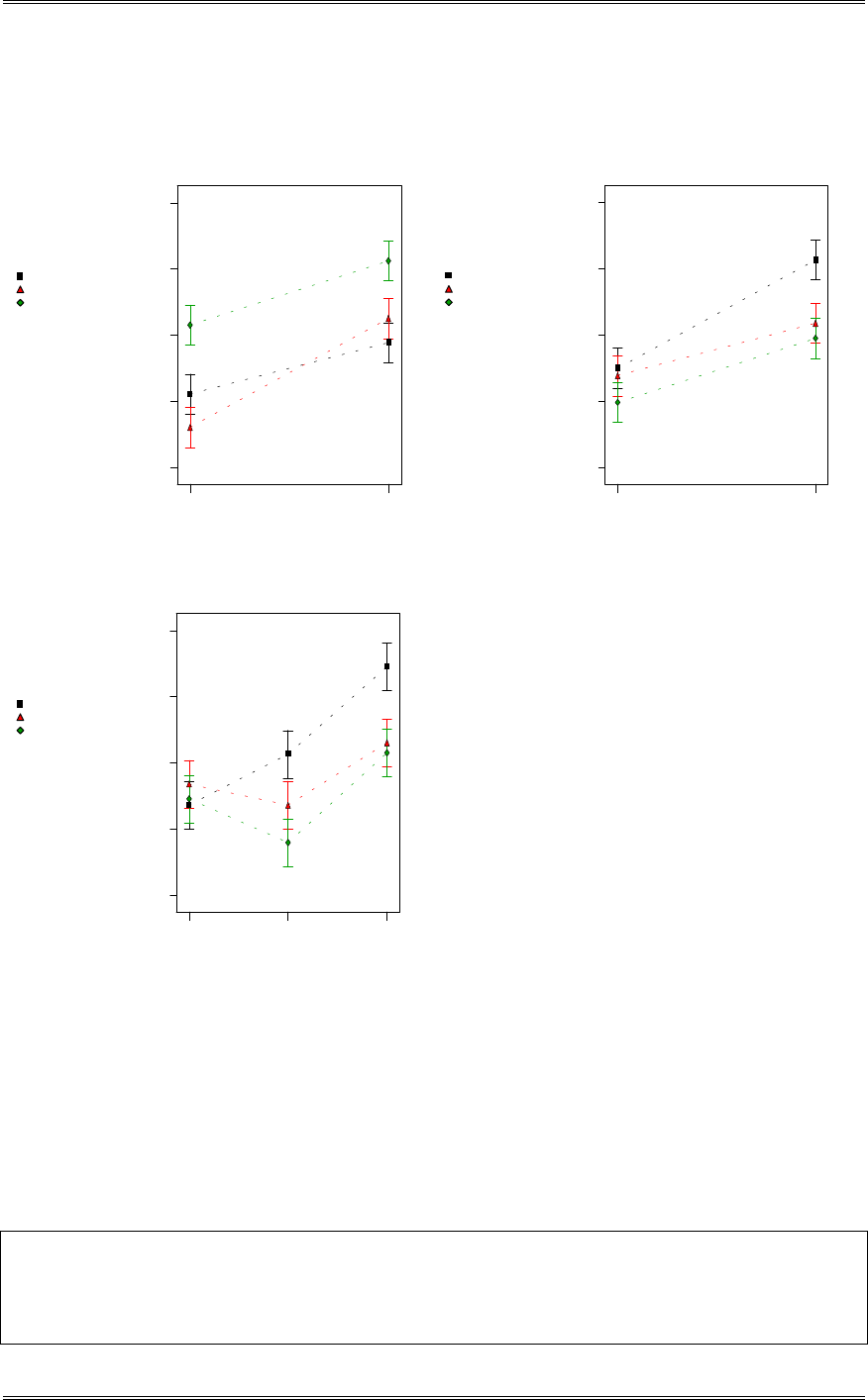
Solutions from Montgomery, D. C. (2001) Design and Analysis of Experiments, Wiley, NY
5-24
(c) Under what set of conditions would you run the process? Why?
DESIGN-EXPERT Plot
strength
X = B: Cooking Time
Y = C: Pressure
C1 400
C2 500
C3 650
Actual Factor
A: Hardwood = Average
P ressure
Interaction G raph
C ooking Tim e
strength
3 4
195.6
196.925
198.25
199.575
200.9
DESIGN-EXPERT Plot
strength
X = B: Cooking Time
Y = A: Hardwood
A1 2
A2 4
A3 8
Actual Factor
C: Pressure = Average
Hardwood
Interaction G raph
C ooking Tim e
strength
3 4
195.6
196.925
198.25
199.575
200.9
DESIGN-EXPERT Plot
strength
X = C: Pressure
Y = A: Hardwood
A1 2
A2 4
A3 8
Actual Factor
B: Cooking Time = Average
Hardwood
Interaction G raph
P ressure
strength
400 500 650
195.6
196.925
198.25
199.575
200.9
For the highest strength, run the process with the percentage of hardwood at 2, the pressure at 650, and
the time at 4 hours.
The standard analysis of variance treats all design factors as if they were qualitative. In this case, all three
factors are quantitative, so some further analysis can be performed. In Section 5-5, we show how response
curves and surfaces can be fit to the data from a factorial experiment with at least one quantative factor.
Since the factors in this problem are quantitative and two of them have three levels, we can fit linear and
quadratic. The Design-Expert output, including the response surface plots, now follows.
Design Expert Output
Response: Strength
ANOVA for Selected Factorial Model
Analysis of variance table [Partial sum of squares]
Sum of Mean F
Source Squares DF Square Value Prob > F
Model 58.02 13 4.46 11.85 < 0.0001 significant

Solutions from Montgomery, D. C. (2001) Design and Analysis of Experiments, Wiley, NY
5-25
A 7.15 1 7.15 18.98 0.0003
B 3.42 1 3.42 9.08 0.0064
C 0.22 1 0.22 0.58 0.4559
A2 1.09 1 1.09 2.88 0.1036
C2 4.43 1 4.43 11.77 0.0024
AB 1.06 1 1.06 2.81 0.1081
AC 3.39 1 3.39 9.01 0.0066
BC 0.15 1 0.15 0.40 0.5350
A2B 1.30 1 1.30 3.46 0.0763
A2C 2.19 1 2.19 5.81 0.0247
AC2 1.65 1 1.65 4.38 0.0482
BC2 2.18 1 2.18 5.78 0.0251
ABC 0.40 1 0.40 1.06 0.3136
Residual 8.29 22 0.38
Lack of Fit 1.71 4 0.43 1.17 0.3576 not significant
Pure Error 6.58 18 0.37
Cor Total 66.31 35
The Model F-value of 11.85 implies the model is significant. There is only
a 0.01% chance that a "Model F-Value" this large could occur due to noise.
Values of "Prob > F" less than 0.0500 indicate model terms are significant.
In this case A, B, C2, AC, A2C, AC2, BC2 are significant model terms.
Values greater than 0.1000 indicate the model terms are not significant.
If there are many insignificant model terms (not counting those required to support hierarchy),
model reduction may improve your model.
Std. Dev. 0.61 R-Squared 0.8750
Mean 198.06 Adj R-Squared 0.8011
C.V. 0.31 Pred R-Squared 0.6657
PRESS 22.17 Adeq Precision 14.071
Coefficient Standard 95% CI 95% CI
Factor Estimate DF Error Low High VIF
Intercept 197.21 1 0.26 196.67 197.74
A-Hardwood -0.98 1 0.23 -1.45 -0.51 3.36
B-Cooking Time 0.78 1 0.26 0.24 1.31 6.35
C-Pressure 0.19 1 0.25 -0.33 0.71 4.04
A2 0.42 1 0.25 -0.094 0.94 1.04
C2 0.79 1 0.23 0.31 1.26 1.03
AB -0.21 1 0.13 -0.47 0.050 1.06
AC -0.46 1 0.15 -0.78 -0.14 1.08
BC 0.080 1 0.13 -0.18 0.34 1.04
A2B 0.46 1 0.25 -0.053 0.98 3.96
A2C 0.73 1 0.30 0.10 1.36 3.97
AC2 0.57 1 0.27 4.979E-003 1.14 3.32
BC2 -0.55 1 0.23 -1.02 -0.075 3.30
ABC 0.15 1 0.15 -0.16 0.46 1.02
Final Equation in Terms of Coded Factors:
Strength =
+197.21
-0.98 * A
+0.78 * B
+0.19 * C
+0.42 * A2
+0.79 * C2
-0.21 * A * B
-0.46 * A * C
+0.080 * B * C
+0.46 * A2 * B
+0.73 * A2 * C
+0.57 * A * C2
-0.55 * B * C2
+0.15 * A * B * C
Final Equation in Terms of Actual Factors:

Solutions from Montgomery, D. C. (2001) Design and Analysis of Experiments, Wiley, NY
5-26
Strength =
+229.96981
+12.21654 * Hardwood
-12.97602 * Cooking Time
-0.21224 * Pressure
-0.65287 * Hardwood2
+2.34333E-004 * Pressure2
-1.60038 * Hardwood * Cooking Time
-0.023415 * Hardwood * Pressure
+0.070658 * Cooking Time * Pressure
+0.10278 * Hardwood2 * Cooking Time
+6.48026E-004 * Hardwood2 * Pressure
+1.22143E-005 * Hardwood * Pressure2
-7.00000E-005 * Cooking Time * Pressure2
+8.23308E-004 * Hardwood * Cooking Time * Pressure
Strength
A: Hardwood
C: Pressure
2.00 3.50 5.00 6.50 8. 0 0
400.00
450.00
500.00
550.00
600.00
650.00
198
198.5
198.5
199
199.5
200
200.5
2 2 2
2 2 2
2 2 2
197
197.5
198
198.5
199
199.5
200
200.5
201
201.5
Streng th
2.00
3.50
5.00
6.50
8.00 400.00
450.00
500.00
550.00
600.00
650.00
A: Hardwood
C: Pres s ure
Cooking Time: B = 4.00
5-17 The quality control department of a fabric finishing plant is studying the effect of several factors on
the dyeing of cotton-synthetic cloth used to manufacture men’s shirts. Three operators, three cycle times,
and two temperatures were selected, and three small specimens of cloth were dyed under each set of
conditions. The finished cloth was compared to a standard, and a numerical score was assigned. The
results follow. Analyze the data and draw conclusions. Comment on the model’s adequacy.
Temperature
300° 350°
Operator Operator
Cycle Time 1 2 3 1 2 3
23 27 31 24 38 34
40 24 28 32 23 36 36
25 26 29 28 35 39
36 34 33 37 34 34
50 35 38 34 39 38 36
36 39 35 35 36 31
28 35 26 26 36 28
60 24 35 27 29 37 26
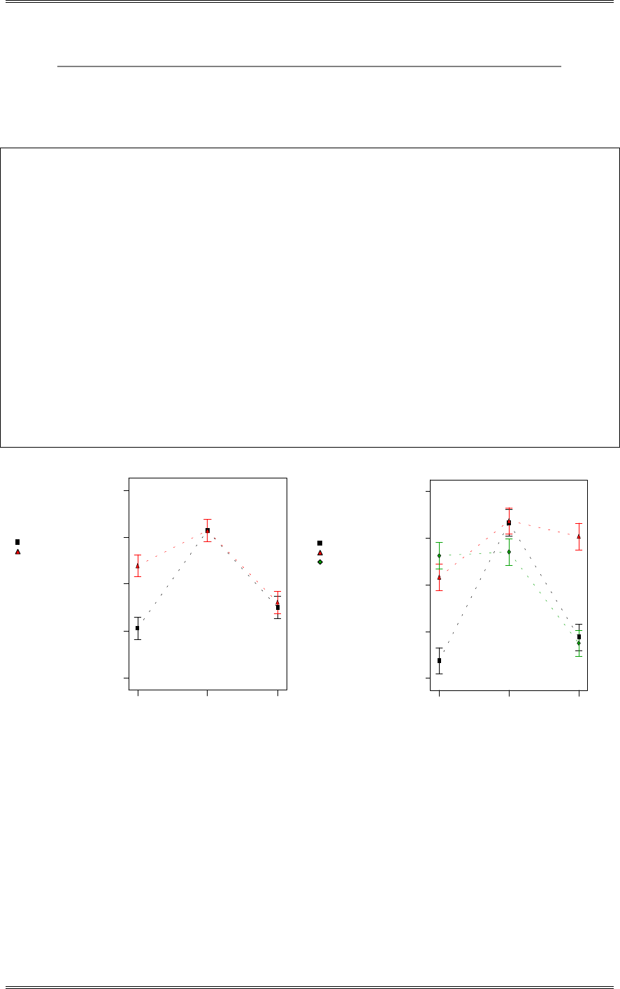
Solutions from Montgomery, D. C. (2001) Design and Analysis of Experiments, Wiley, NY
5-27
27 34 25 25 34 24
All three main effects, and the AB, AC, and ABC interactions are significant. There is nothing unusual
about the residual plots.
Design Expert Output
Response: Score
ANOVA for Selected Factorial Model
Analysis of variance table [Partial sum of squares]
Sum of
Mean F
Source Squares DF Square Value Prob > F
Model 1239.33 17 72.90 22.24 < 0.0001 significant
A
436.00 2 218.00 66.51 < 0.0001
B
261.33 2 130.67 39.86 < 0.0001
C
50.07 1 50.07 15.28 0.0004
AB
355.67 4 88.92 27.13 < 0.0001
AC
78.81 2 39.41 12.02 0.0001
BC
11.26 2 5.63 1.72 0.1939
ABC
46.19 4 11.55 3.52 0.0159
Residual 118.00 36 3.28
Lack of Fit
0.000 0
Pure Error
118.00 36 3.28
Cor Total 1357.33 53
The Model F-value of 22.24 implies the model is significant. There is only
a 0.01% chance that a "Model F-Value" this large could occur due to noise.
Values of "Prob > F" less than 0.0500 indicate model terms are significant.
In this case A, B, C, AB, AC, ABC are significant model terms.
DESIGN-EXPERT Plot
Score
X = A: Cycle Time
Y = C: Temperature
C1 300
C2 350
Actual Factor
B: Operator = Average
Tem perature
Interaction G raph
Cycle Tim e
Score
40 50 60
23
27
31
35
39
22
DESIGN-EXPERT Plot
Score
X = A: Cycle Time
Y = B: Operator
B1 1
B2 2
B3 3
Actual Factor
C: Temperature = Average
O perator
Interaction G raph
C ycle Tim e
Score
40 50 60
23
27
31
35
39
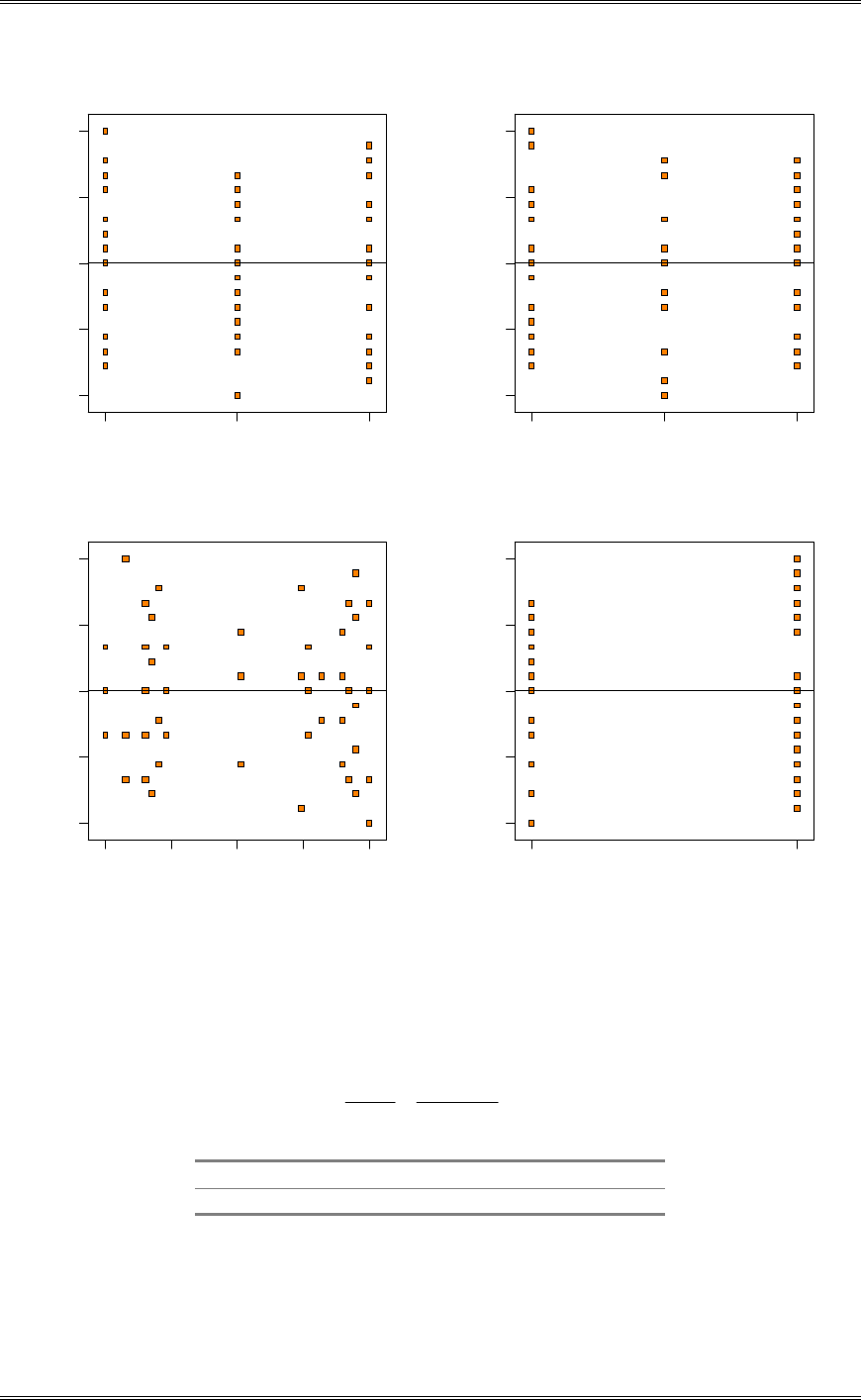
Solutions from Montgomery, D. C. (2001) Design and Analysis of Experiments, Wiley, NY
5-28
2
22
2
22
22
2
3
2
3
2
2
223
Operator
Residuals
Residuals vs. Operator
-3
-1.5
4
.26326E-014
1.5
3
123
2
33
2
2
22
3 2
2
3
2
3
2
3
2
Cycle Time
Residuals
Residuals vs. Cycle Time
-3
-1.5
4
.26326E-014
1.5
3
1 2 3
2222
2
22
2
Predicted
Residuals
Residuals vs. Predicted
-3
-1.5
4
.26326E-014
1.5
3
24.00 27.25 30.50 33.75 37.00
4
22
4
22
22
2
4
2
4
2
2
3
2
2
2
3
2
2
3
2
Temperature
Residuals
Residuals vs. Temperature
-3
-1.5
4
.26326E-014
1.5
3
1 2
5-18 In Problem 5-1, suppose that we wish to reject the null hypothesis with a high probability if the
difference in the true mean yield at any two pressures is as great as 0.5. If a reasonable prior estimate of
the standard deviation of yield is 0.1, how many replicates should be run?
n.
.
.n
b
naD 512
1032
503
22
2
2
2
2
V
)
n 2
)
)
1
1 b
X
1
2 nab
X
E
2 25 5 2 (3)(3)(1) 0.014
2 replications will be enough to detect the given difference.

Solutions from Montgomery, D. C. (2001) Design and Analysis of Experiments, Wiley, NY
5-29
5-19 The yield of a chemical process is being studied. The two factors of interest are temperature and
pressure. Three levels of each factor are selected; however, only 9 runs can be made in one day. The
experimenter runs a complete replicate of the design on each day. The data are shown in the following
table. Analyze the data assuming that the days are blocks.
Day 1 Day 2
Pressure Pressure
Temperature 250 260 270 250 260 270
Low 86.3 84.0 85.8 86.1 85.2 87.3
Medium 88.5 87.3 89.0 89.4 89.9 90.3
High 89.1 90.2 91.3 91.7 93.2 93.7
Design Expert Output
Response: Yield
ANOVA for Selected Factorial Model
Analysis of variance table [Partial sum of squares]
Sum of Mean F
Source Squares DF Square Value Prob > F
Block 13.01 1 13.01
Model 109.81 8 13.73 25.84 < 0.0001 significant
A 5.51 2 2.75 5.18 0.0360
B 99.85 2 49.93 93.98 < 0.0001
AB 4.45 4 1.11 2.10 0.1733
Residual 4.25 8 0.53
Cor Total 127.07 17
The Model F-value of 25.84 implies the model is significant. There is only
a 0.01% chance that a "Model F-Value" this large could occur due to noise.
Values of "Prob > F" less than 0.0500 indicate model terms are significant.
In this case A, B are significant model terms.
Both main effects, temperature and pressure, are significant.
5-20 Consider the data in Problem 5-5. Analyze the data, assuming that replicates are blocks.
Design Expert Output
Response: Warping
ANOVA for Selected Factorial Model
Analysis of variance table [Partial sum of squares]
Sum of Mean F
Source Squares DF Square Value Prob > F
Block 11.28 1 11.28
Model 968.22 15 64.55 9.96 < 0.0001 significant
A 698.34 3 232.78 35.92 < 0.0001
B 156.09 3 52.03 8.03 0.0020
AB 113.78 9 12.64 1.95 0.1214
Residual 97.22 15 6.48
Cor Total 1076.72 31
The Model F-value of 9.96 implies the model is significant. There is only
a 0.01% chance that a "Model F-Value" this large could occur due to noise.
Values of "Prob > F" less than 0.0500 indicate model terms are significant.
In this case A, B are significant model terms.
Both temperature and copper content are significant. This agrees with the analysis in Problem 5-5.
5-21 Consider the data in Problem 5-6. Analyze the data, assuming that replicates are blocks.

Solutions from Montgomery, D. C. (2001) Design and Analysis of Experiments, Wiley, NY
5-30
Design-Expert Output
Response: Stength
ANOVA for Selected Factorial Model
Analysis of variance table [Partial sum of squares]
Sum of Mean F
Source Squares DF Square Value Prob > F
Block 1.04 1 1.04
Model 217.46 11 19.77 4.89 0.0070 significant
A 160.33 2 80.17 19.84 0.0002
B 12.46 3 4.15 1.03 0.4179
AB 44.67 6 7.44 1.84 0.1799
Residual 44.46 11 4.04
Cor Total 262.96 23
The Model F-value of 4.89 implies the model is significant. There is only
a 0.70% chance that a "Model F-Value" this large could occur due to noise.
Values of "Prob > F" less than 0.0500 indicate model terms are significant.
In this case A are significant model terms.
Only the operator factor (A) is significant. This agrees with the analysis in Problem 5-6.
5-22 An article in the Journal of Testing and Evaluation (Vol. 16, no.2, pp. 508-515) investigated the
effects of cyclic loading and environmental conditions on fatigue crack growth at a constant 22 MPa stress
for a particular material. The data from this experiment are shown below (the response is crack growth
rate).
Environment
Frequency Air H2O Salt H2O
2.29 2.06 1.90
10 2.47 2.05 1.93
2.48 2.23 1.75
2.12 2.03 2.06
2.65 3.20 3.10
1 2.68 3.18 3.24
2.06 3.96 3.98
2.38 3.64 3.24
2.24 11.00 9.96
0.1 2.71 11.00 10.01
2.81 9.06 9.36
2.08 11.30 10.40
(a) Analyze the data from this experiment (use
D
= 0.05).
Design Expert Output
Response: Crack Growth
ANOVA for Selected Factorial Model
Analysis of variance table [Partial sum of squares]
Sum of Mean F
Source Squares DF Square Value Prob > F
Model 376.11 8 47.01 234.02 < 0.0001 significant
A 209.89 2 104.95 522.40 < 0.0001
B 64.25 2 32.13 159.92 < 0.0001
AB 101.97 4 25.49 126.89 < 0.0001
Residual 5.42 27 0.20
Lack of Fit 0.000 0
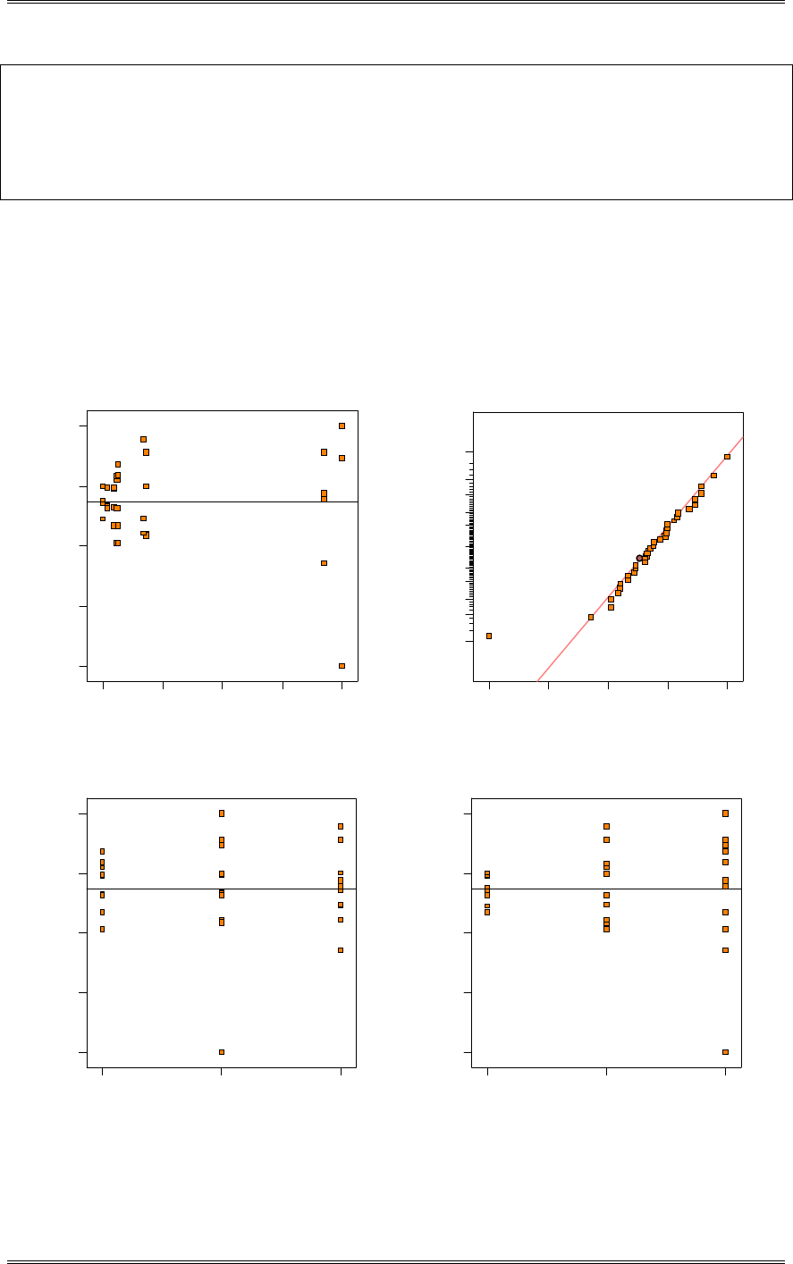
Solutions from Montgomery, D. C. (2001) Design and Analysis of Experiments, Wiley, NY
5-31
Pure Error 5.42 27 0.20
Cor Total 381.53 35
The Model F-value of 234.02 implies the model is significant. There is only
a 0.01% chance that a "Model F-Value" this large could occur due to noise.
Values of "Prob > F" less than 0.0500 indicate model terms are significant.
In this case A, B, AB are significant model terms.
Both frequency and environment, as well as their interaction are significant.
(b) Analyze the residuals.
The residual plots indicate that there may be some problem with inequality of variance. This is
particularly noticable on the plot of residuals versus predicted response and the plot of residuals versus
frequency.
22
22
Predicted
Residuals
Residuals vs. Predicted
-1.53
-0.97
-0.41
0.15
0.71
1.91 4.08 6.25 8.42 10.59
Residual
Normal % probability
Normal plot of residuals
-1.53 -0 .97 -0.41 0.15 0.71
1
5
10
20
30
50
70
80
90
95
99
22
22
Environment
Residuals
Residuals vs. Environment
-1.53
-0.97
-0.41
0.15
0.71
123
22
22
Frequency
Residuals
Residuals vs. Frequency
-1.53
-0.97
-0.41
0.15
0.71
123
(c) Repeat the analyses from parts (a) and (b) using ln(y) as the response. Comment on the results.
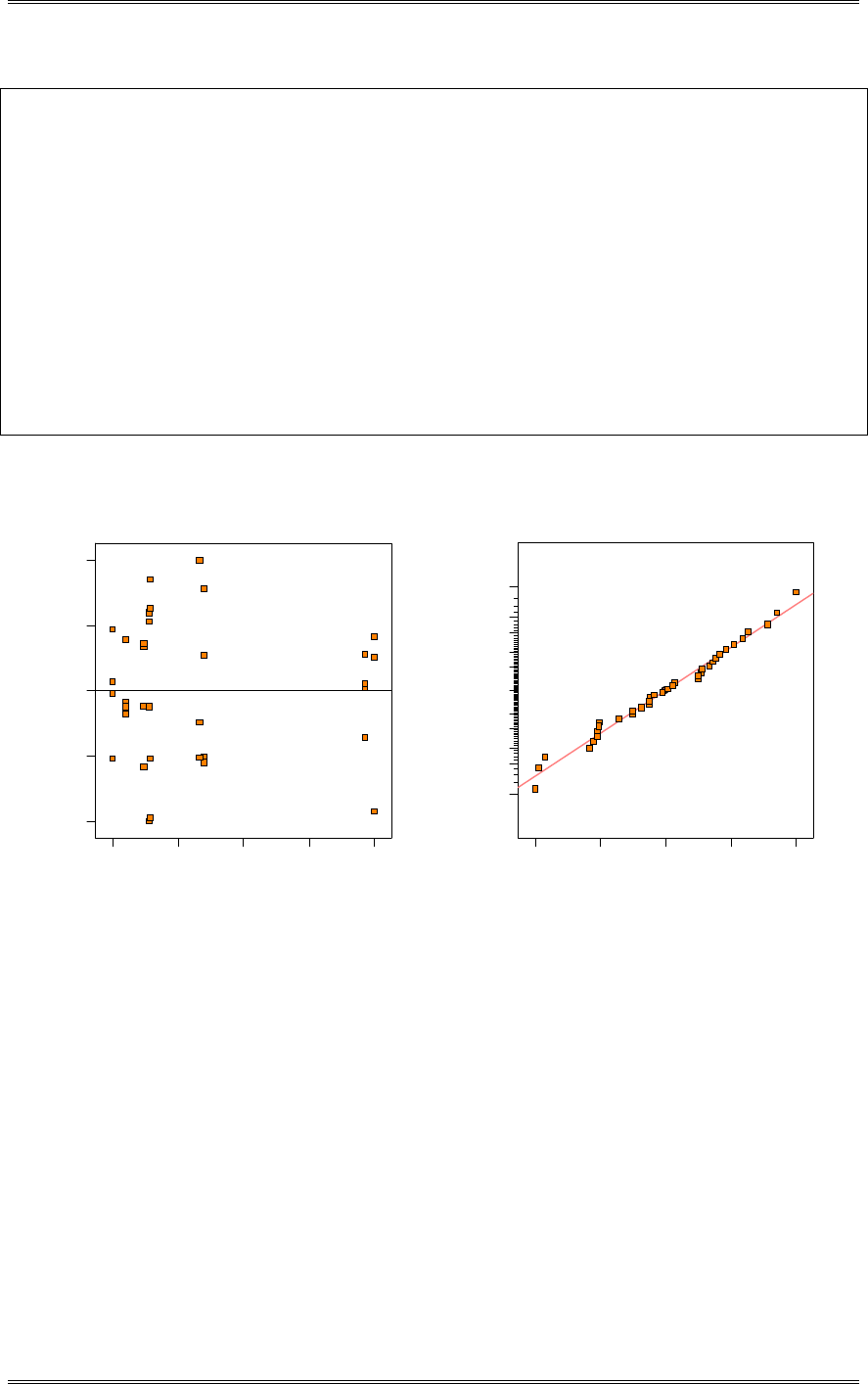
Solutions from Montgomery, D. C. (2001) Design and Analysis of Experiments, Wiley, NY
5-32
Design Expert Output
Response: Crack Growth Transform: Natural log Constant: 0.000
ANOVA for Selected Factorial Model
Analysis of variance table [Partial sum of squares]
Sum of Mean F
Source Squares DF Square Value Prob > F
Model 13.46 8 1.68 179.57 < 0.0001 significant
A 7.57 2 3.79 404.09 < 0.0001
B 2.36 2 1.18 125.85 < 0.0001
AB 3.53 4 0.88 94.17 < 0.0001
Residual 0.25 27 9.367E-003
Lack of Fit 0.000 0
Pure Error 0.25 27 9.367E-003
Cor Total 13.71 35
The Model F-value of 179.57 implies the model is significant. There is only
a 0.01% chance that a "Model F-Value" this large could occur due to noise.
Values of "Prob > F" less than 0.0500 indicate model terms are significant.
In this case A, B, AB are significant model terms.
Both frequency and environment, as well as their interaction are significant. The residual plots of the
based on the transformed data look better.
22
22
Predicted
Residuals
Residuals vs. Predicted
-0.16484
-0.0822988
0.000242214
0.0827832
0.165324
0.65 1.07 1.50 1.93 2.36
Residual
Normal % probability
Normal plot of residuals
-0.16484 -0.08229880.000242214 0.0827832 0.165324
1
5
10
20
30
50
70
80
90
95
99
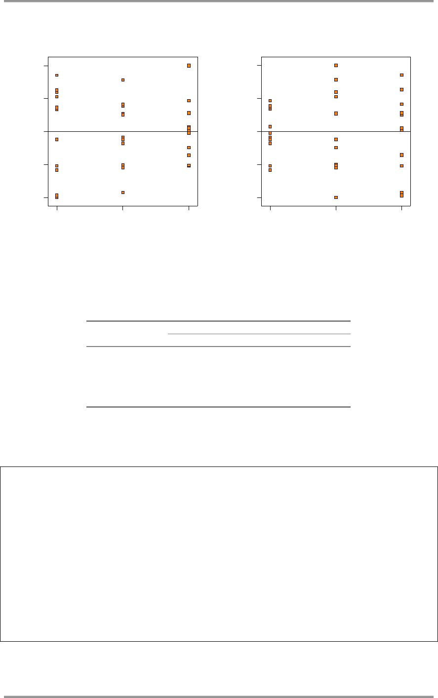
Solutions from Montgomery, D. C. (2001) Design and Analysis of Experiments, Wiley, NY
5-33
22
22
Environment
Residuals
Residuals vs. Environment
-0.16484
-0.0822988
0.000242214
0.0827832
0.165324
123
22
22
Frequency
Residuals
Residuals vs. Frequency
-0.16484
-0.0822988
0.000242214
0.0827832
0.165324
123
5-23 An article in the IEEE Transactions on Electron Devices (Nov. 1986, pp. 1754) describes a study
on polysilicon doping. The experiment shown below is a variation of their study. The response variable
is base current.
Polysilicon Anneal Temperature (°C)
Doping (ions) 900 950 1000
1 x 10 20 4.60 10.15 11.01
4.40 10.20 10.58
2 x 10 20 3.20 9.38 10.81
3.50 10.02 10.60
(a) Is there evidence (with
D
= 0.05) indicating that either polysilicon doping level or anneal temperature
affect base current?
Design Expert Output
Response: Base Current
ANOVA for Selected Factorial Model
Analysis of variance table [Partial sum of squares]
Sum of Mean F
Source Squares DF Square Value Prob > F
Model 112.74 5 22.55 350.91 < 0.0001 significant
A 0.98 1 0.98 15.26 0.0079
B 111.19 2 55.59 865.16 < 0.0001
AB 0.58 2 0.29 4.48 0.0645
Residual 0.39 6 0.064
Lack of Fit 0.000 0
Pure Error 0.39 6 0.064
Cor Total 113.13 11
The Model F-value of 350.91 implies the model is significant. There is only
a 0.01% chance that a "Model F-Value" this large could occur due to noise.
Values of "Prob > F" less than 0.0500 indicate model terms are significant.
In this case A, B are significant model terms.
Both factors, doping and anneal are significant. Their interaction is significant at the 10% level.
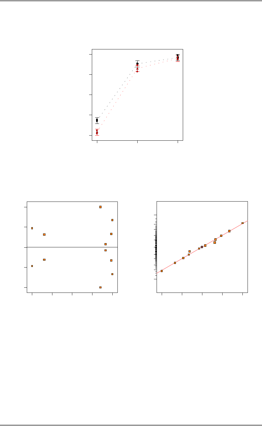
Solutions from Montgomery, D. C. (2001) Design and Analysis of Experiments, Wiley, NY
5-34
(b) Prepare graphical displays to assist in interpretation of this experiment.
Doping
Interaction Graph
Anneal
Base Current
900 950 1000
3.03986
5.05618
7.0725
9.08882
11.1051
A-
A+
(c) Analyze the residuals and comment on model adequacy.
Predicted
Residuals
Residuals vs. Predicted
-0.32
-0.16
8
.88178E-016
0.16
0.32
3.35 5.21 7.07 8.93 10.80
Residual
Normal % probability
Normal plot of residuals
-0.32 -0.16 -8.88178E-016 0.16 0.32
1
5
10
20
30
50
70
80
90
95
99
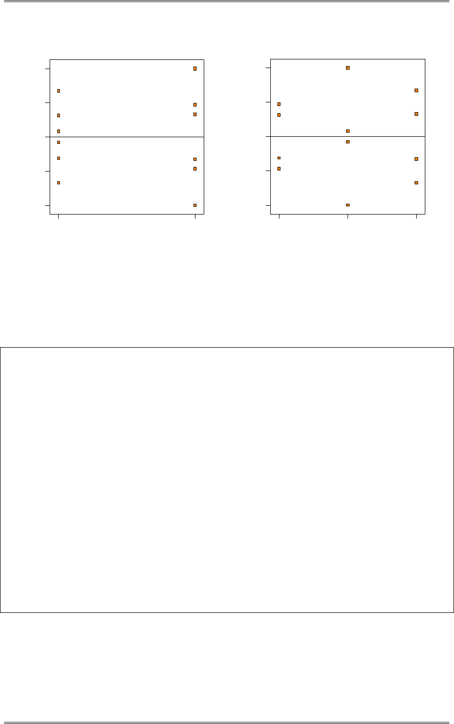
Solutions from Montgomery, D. C. (2001) Design and Analysis of Experiments, Wiley, NY
5-35
Doping
Residuals
Residuals vs. Doping
-0.32
-0.16
8
.88178E-016
0.16
0.32
1 2
Anneal
Residuals
Residuals vs. Anneal
-0.32
-0.16
8
.88178E-016
0.16
0.32
1 2 3
There is a funnel shape in the plot of residuals versus predicted, indicating some inequality of variance.
(d) Is the model
HEEEEE
2112
2
22222110 xxxxxy supported by this experiment (x1 = doping
level, x2 = temperature)? Estimate the parameters in this model and plot the response surface.
Design Expert Output
Response: Base Current
ANOVA for Response Surface Reduced Quadratic Model
Analysis of variance table [Partial sum of squares]
Sum of Mean F
Source Squares DF Square Value Prob > F
Model 112.73 4 28.18 493.73 < 0.0001 significant
A 0.98 1 0.98 17.18 0.0043
B 93.16 1 93.16 1632.09 < 0.0001
B2 18.03 1 18.03 315.81 < 0.0001
AB 0.56 1 0.56 9.84 0.0164
Residual 0.40 7 0.057
Lack of Fit 0.014 1 0.014 0.22 0.6569 not significant
Pure Error 0.39 6 0.064
Cor Total 113.13 11
The Model F-value of 493.73 implies the model is significant. There is only
a 0.01% chance that a "Model F-Value" this large could occur due to noise.
Values of "Prob > F" less than 0.0500 indicate model terms are significant.
In this case A, B, B2, AB are significant model terms.
Coefficient Standard 95% CI 95% CI
Factor Estimate DF Error Low High VIF
Intercept 9.94 1 0.12 9.66 10.22
A-Doping -0.29 1 0.069 -0.45 -0.12 1.00
B-Anneal 3.41 1 0.084 3.21 3.61 1.00
B
2 -2.60 1 0.15 -2.95 -2.25 1.00
AB 0.27 1 0.084 0.065 0.46 1.00
All of the coefficients in the assumed model are significant. The quadratic effect is easily observable in
the response surface plot.
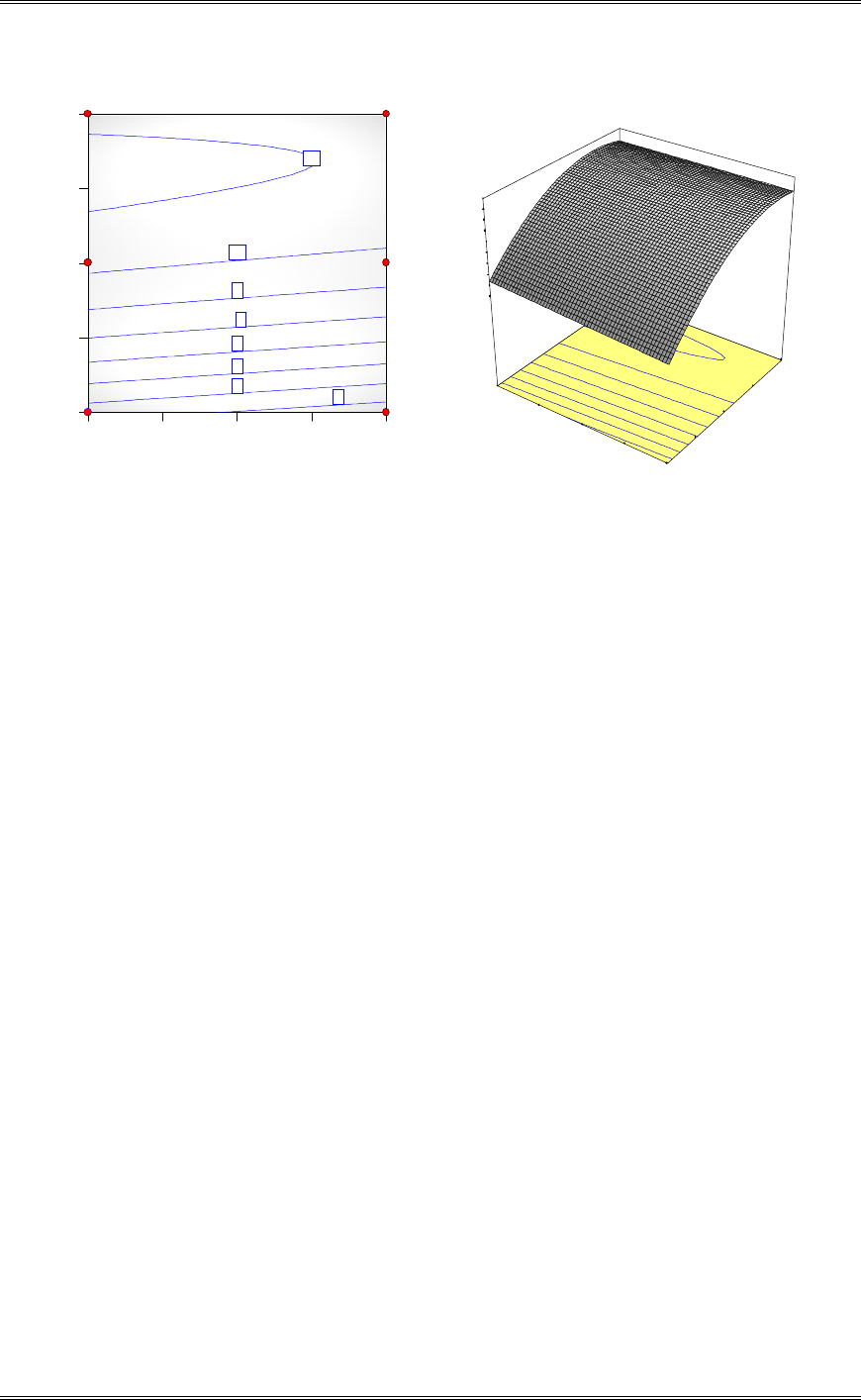
Solutions from Montgomery, D. C. (2001) Design and Analysis of Experiments, Wiley, NY
5-36
Base Current
Doping
Anneal
1.00E+20 1.25E+20 1.50E+20 1.75E+20 2.00E+20
900.00
925.00
950.00
975.00
1000.00
4
5
6
7
8
9
10
11
2 2
2 2
2 2
3
4
5
6
7
8
9
10
11
12
Base Current
1.00E+20
1.25E+20
1.50E+20
1.75E+20
2.00E+20 900.00
925.00
950.00
975.00
1000.00
Doping
Anneal
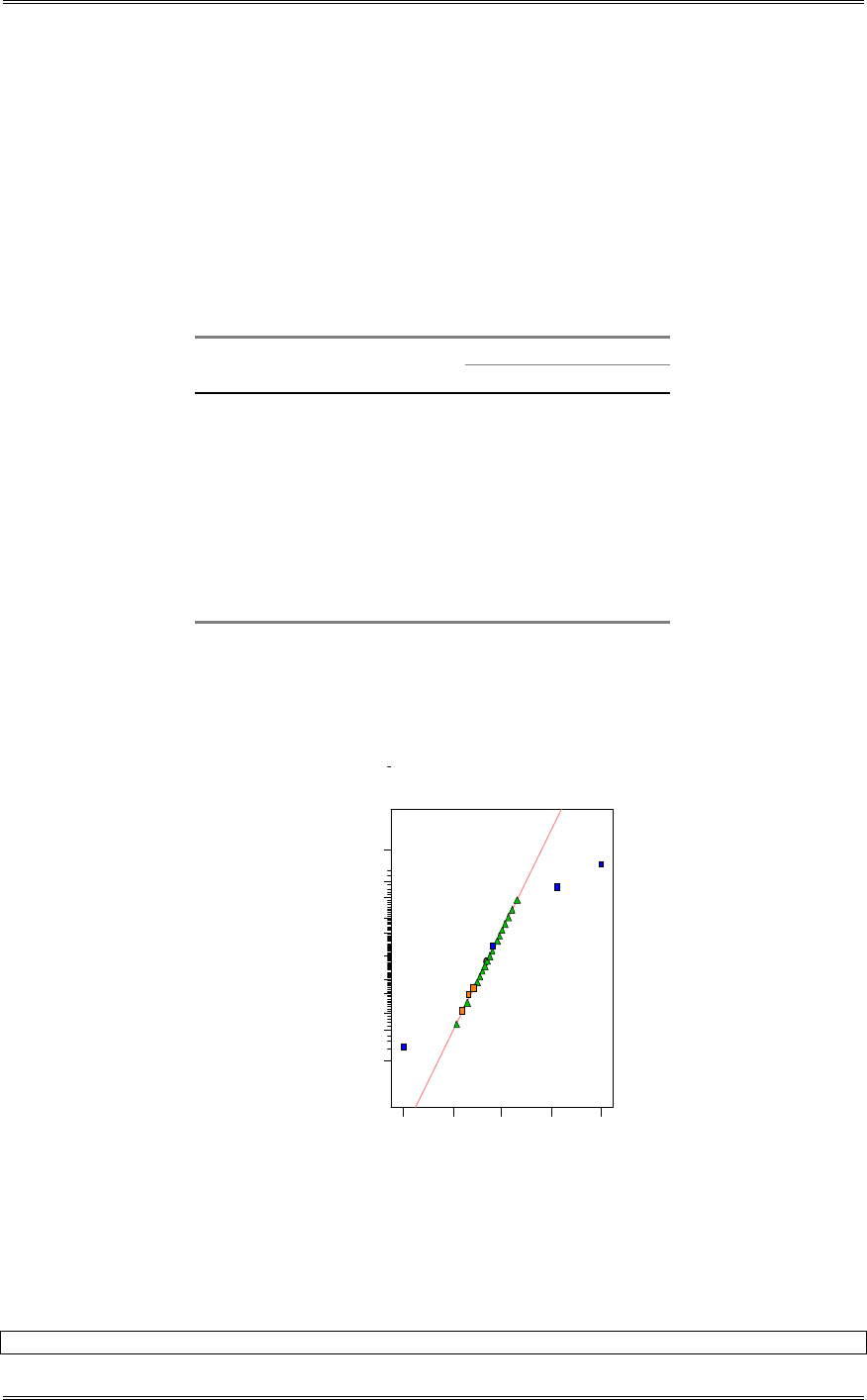
Solutions from Montgomery, D. C. (2001) Design and Analysis of Experiments, Wiley, NY
6-1
Chapter 6
The 2k Factorial Design
Solutions
6-1 An engineer is interested in the effects of cutting speed (A), tool geometry (B), and cutting angle on
the life (in hours) of a machine tool. Two levels of each factor are chosen, and three replicates of a 23
factorial design are run. The results follow:
Treatment Replicate
A B C Combination I II III
- - - (1) 22 31 25
+ - - a 32 43 29
- + - b 35 34 50
+ + - ab 55 47 46
- - + c 44 45 38
+ - + ac 40 37 36
- + + bc 60 50 54
+ + + abc 39 41 47
(a) Estimate the factor effects. Which effects appear to be large?
From the normal probability plot of effects below, factors B, C, and the AC interaction appear to be
significant.
DESIGN-EXPERT Plot
Life
A: Cutting Speed
B: Tool Geometry
C: Cutting Angle
Normal plot
Normal % probability
Effe ct
-8 .8 3 -3 .7 9 1.25 6.29 11.33
1
5
10
20
30
50
70
80
90
95
99
A
B
C
AC
(b) Use the analysis of variance to confirm your conclusions for part (a).
The analysis of variance confirms the significance of factors B, C, and the AC interaction.
Design Expert Output
Response: Life in hours

Solutions from Montgomery, D. C. (2001) Design and Analysis of Experiments, Wiley, NY
6-2
ANOVA for Selected Factorial Model
Analysis of variance table [Partial sum of squares]
Sum of Mean F
Source Squares DF Square Value Prob > F
Model 1612.67 7 230.38 7.64 0.0004 significant
A 0.67 1 0.67 0.022 0.8837
B 770.67 1 770.67 25.55 0.0001
C 280.17 1 280.17 9.29 0.0077
AB 16.67 1 16.67 0.55 0.4681
AC 468.17 1 468.17 15.52 0.0012
BC 48.17 1 48.17 1.60 0.2245
ABC 28.17 1 28.17 0.93 0.3483
Pure Error 482.67 16 30.17
Cor Total 2095.33 23
The Model F-value of 7.64 implies the model is significant. There is only
a 0.04% chance that a "Model F-Value" this large could occur due to noise.
The reduced model ANOVA is shown below. Factor A was included to maintain hierarchy.
Design Expert Output
Response: Life in hours
ANOVA for Selected Factorial Model
Analysis of variance table [Partial sum of squares]
Sum of Mean F
Source Squares DF Square Value Prob > F
Model 1519.67 4 379.92 12.54 < 0.0001 significant
A 0.67 1 0.67 0.022 0.8836
B 770.67 1 770.67 25.44 < 0.0001
C 280.17 1 280.17 9.25 0.0067
AC 468.17 1 468.17 15.45 0.0009
Residual 575.67 19 30.30
Lack of Fit 93.00 3 31.00 1.03 0.4067 not significant
Pure Error 482.67 16 30.17
Cor Total 2095.33 23
The Model F-value of 12.54 implies the model is significant. There is only
a 0.01% chance that a "Model F-Value" this large could occur due to noise.
Effects B, C and AC are significant at 1%.
(c) Write down a regression model for predicting tool life (in hours) based on the results of this
experiment.
CACBAijk xx.x.x.x..y 41674416736667516670833340
Design Expert Output
Coefficient Standard 95% CI 95% CI
Factor Estimate DF Error Low High VIF
Intercept 40.83 1 1.12 38.48 43.19
A-Cutting Speed 0.17 1 1.12 -2.19 2.52 1.00
B-Tool Geometry 5.67 1 1.12 3.31 8.02 1.00
C-Cutting Angle 3.42 1 1.12 1.06 5.77 1.00
AC -4.42 1 1.12 -6.77 -2.06 1.00
Final Equation in Terms of Coded Factors:
Life =
+40.83
+0.17 * A
+5.67 * B
+3.42 * C
-4.42 * A * C
Final Equation in Terms of Actual Factors:
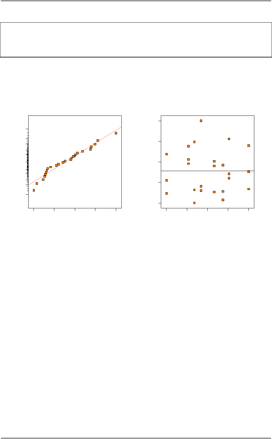
Solutions from Montgomery, D. C. (2001) Design and Analysis of Experiments, Wiley, NY
6-3
Life =
+40.83333
+0.16667 * Cutting Speed
+5.66667 * Tool Geometry
+3.41667 * Cutting Angle
-4.41667 * Cutting Speed * Cutting Angle
The equation in part (c) and in the given in the computer output form a “hierarchial” model, that is, if an
interaction is included in the model, then all of the main effects referenced in the interaction are also
included in the model.
(d) Analyze the residuals. Are there any obvious problems?
Residual
Normal % probability
Normal plot of residuals
-7.33333 -2 .6 2 5 2.08333 6.79167 11.5
1
5
10
20
30
50
70
80
90
95
99
Predicted
Residuals
Residuals vs. Predicted
-7.33333
-2 .6 25
2.08333
6.79167
11.5
27.17 33.92 40.67 47.42 54.17
There is nothing unusual about the residual plots.
(e) Based on the analysis of main effects and interaction plots, what levels of A, B, and C would you
recommend using?
Since B has a positive effect, set B at the high level to increase life. The AC interaction plot reveals that
life would be maximized with C at the high level and A at the low level.
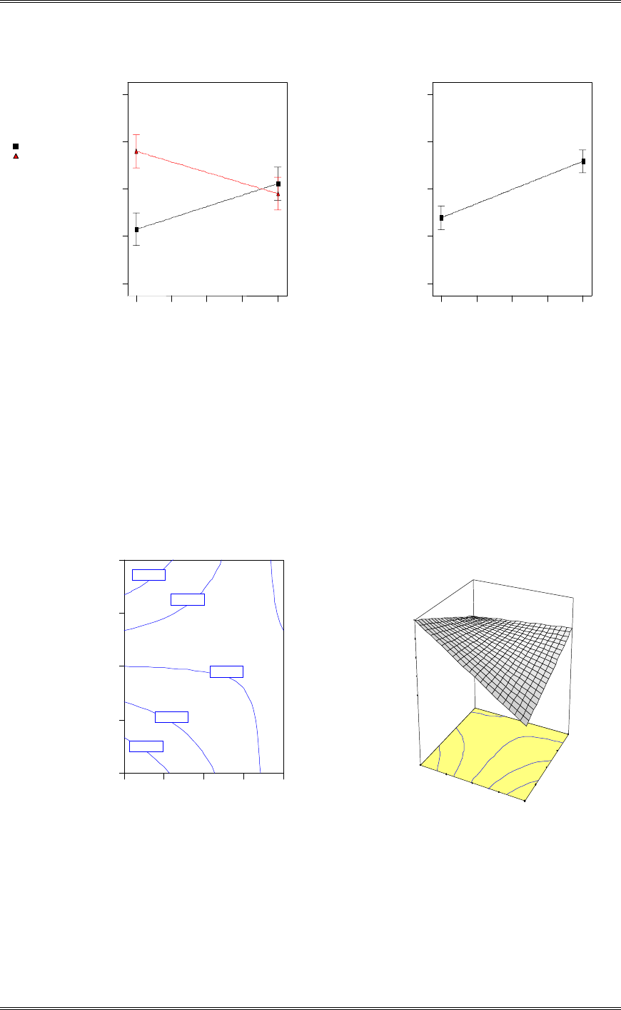
Solutions from Montgomery, D. C. (2001) Design and Analysis of Experiments, Wiley, NY
6-4
DESIGN-EXPERT Plot
Life
X = A: Cutting Speed
Y = C: Cutting Angle
C- -1.000
C+ 1.000
Actual Fa ctor
B: Tool Geometry = 0.00
Cuttin g Ang le
Inte ra c ti o n G r a p h
Cuttin g Spee d
Life
-1 .0 0 -0 .5 0 0.00 0.50 1.00
22
31.5
41
50.5
60
DESIGN-EXPERT Plot
Life
X = B: Tool Geometry
Actual Factors
A: Cutting Speed = 0.00
C: Cutting Angle = 0.00
-1 .0 0 -0 .5 0 0.00 0.50 1.00
22
31.5
41
50.5
60
Tool Geometry
Life
One Factor Plot
6-2 Reconsider part (c) of Problem 6-1. Use the regression model to generate response surface and
contour plots of the tool life response. Interpret these plots. Do they provide insight regarding the
desirable operating conditions for this process?
The response surface plot and the contour plot in terms of factors A and C with B at the high level are
shown below. They show the curvature due to the AC interaction. These plots make it easy to see the
region of greatest tool life.
DESIGN-EXPERT Plot
Life
X = A: Cutting Speed
Y = C: Cutting Angle
Actual Factor
B: Tool Geometry = 0.00
Life
Cutting Speed
Cuttin g Ang le
-1 .0 0 -0 . 5 0 0.00 0.50 1.00
-1 .0 0
-0 .5 0
0.00
0.50
1.00
35.4444
38.0556
40.6667
43.2778
45.8889
DESIGN-EXPERT Plot
Life
X = A: Cutting Speed
Y = C: Cu ttin g Angle
Actual Factor
B: Tool Geometry = 0.00
32.8333
36.75
40.6667
44.5833
48.5
Life
-1.00
-0.50
0.00
0.50
1.00
-1.00
-0.50
0.00
0.50
1.00
Cuttin
g
S
p
eed
Cuttin g Ang le
6-3 Find the standard error of the factor effects and approximate 95 percent confidence limits for the
factor effects in Problem 6-1. Do the results of this analysis agree with the conclusions from the analysis
of variance?
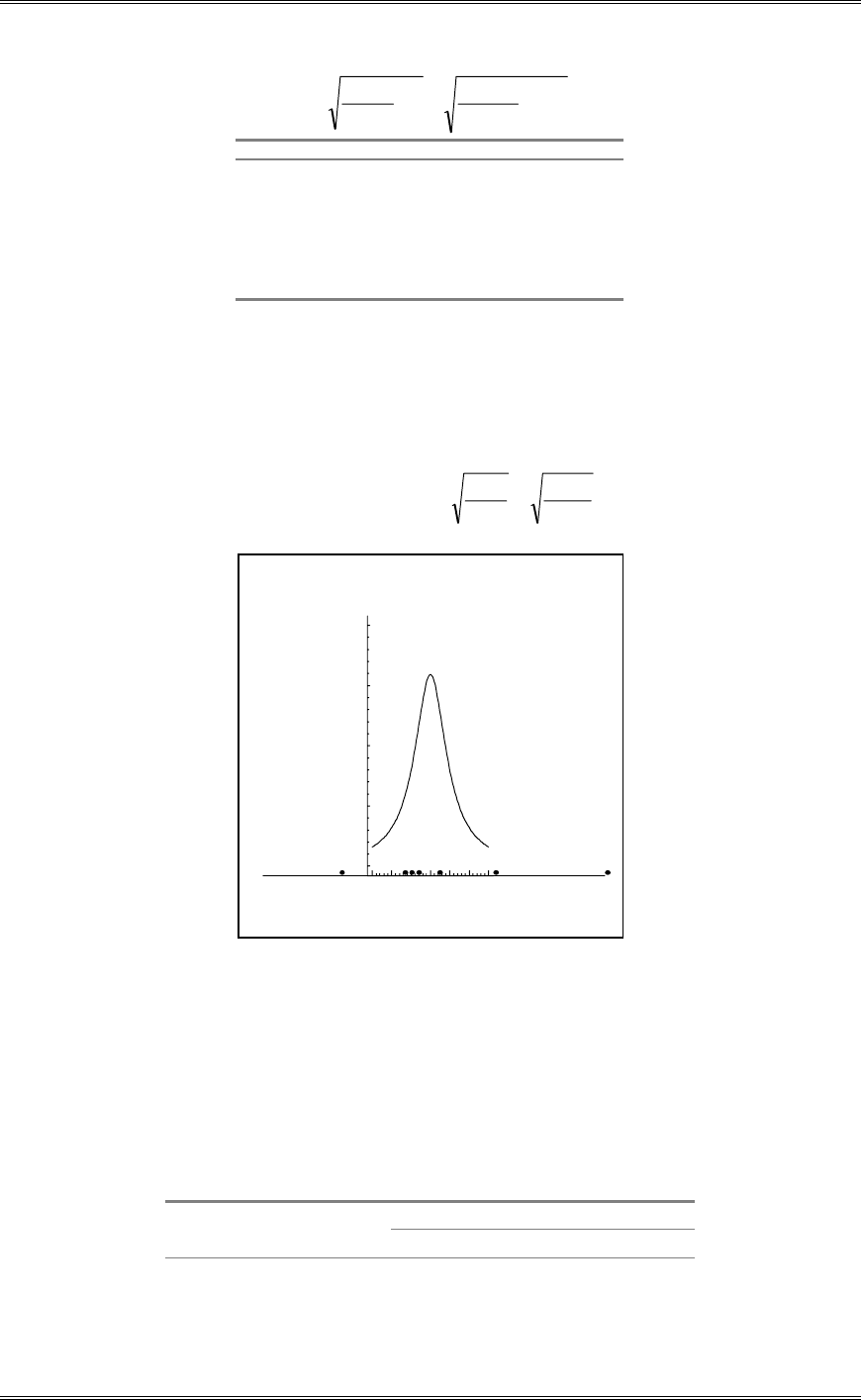
Solutions from Montgomery, D. C. (2001) Design and Analysis of Experiments, Wiley, NY
6-5
2421730
23
1
2
1
23
2
2..S
n
SE k
)effect(
Variable
Effect
CI
A
0.333
r4.395
B 11.333 r4.395 *
AB -1.667 r4.395
C 6.833 r4.395 *
AC -8.833 r4.395 *
BC -2.833 r4.395
ABC -2.167 r4.395
The 95% confidence intervals for factors B, C and AC do not contain zero. This agrees with the analysis
of variance approach.
6-4 Plot the factor effects from Problem 6-1 on a graph relative to an appropriately scaled t distribution.
Does this graphical display adequately identify the important factors? Compare the conclusions from this
plot with the results from the analysis of variance. 173
3
1730 .
.
n
MS
SE
-1 0.0 0 .0 1 0.0
Factor Effects
Scaled t Distribution
AC C B
This method identifies the same factors as the analysis of variance.
6-5 A router is used to cut locating notches on a printed circuit board. The vibration level at the
surface of the board as it is cut is considered to be a major source of dimensional variation in the notches.
Two factors are thought to influence vibration: bit size (A) and cutting speed (B). Two bit sizes (1/16 and
1/8 inch) and two speeds (40 and 90 rpm) are selected, and four boards are cut at each set of conditions
shown below. The response variable is vibration measured as a resultant vector of three accelerometers (x,
y, and z) on each test circuit board.
Treatment Replicate
A B Combination I II III IV
- - (1) 18.2 18.9 12.9 14.4
+ - a 27.2 24.0 22.4 22.5
- + b 15.9 14.5 15.1 14.2

Solutions from Montgomery, D. C. (2001) Design and Analysis of Experiments, Wiley, NY
6-6
+ + ab 41.0 43.9 36.3 39.9
(a) Analyze the data from this experiment.
Design Expert Output
Response: Vibration
ANOVA for Selected Factorial Model
Analysis of variance table [Partial sum of squares]
Sum of Mean F
Source Squares DF Square Value Prob > F
Model 1638.11 3 546.04 91.36 < 0.0001 significant
A 1107.23 1 1107.23 185.25 < 0.0001
B 227.26 1 227.26 38.02 < 0.0001
AB 303.63 1 303.63 50.80 < 0.0001
Residual 71.72 12 5.98
Lack of Fit 0.000 0
Pure Error 71.72 12 5.98
Cor Total 1709.83 15
The Model F-value of 91.36 implies the model is significant. There is only
a 0.01% chance that a "Model F-Value" this large could occur due to noise.
(b) Construct a normal probability plot of the residuals, and plot the residuals versus the predicted
vibration level. Interpret these plots.
Residual
Normal % probability
Normal plot of residuals
-3 .9 75 -2 . 0 75 -0 .1 7 5 1.725 3.625
1
5
10
20
30
50
70
80
90
95
99
Predicted
Residuals
Residuals vs. Predicted
-3 .9 75
-2 .0 75
-0 .1 75
1.725
3.625
14.92 21.26 27.60 33.94 40.27
There is nothing unusual about the residual plots.
(c) Draw the AB interaction plot. Interpret this plot. What levels of bit size and speed would you
recommend for routine operation?
To reduce the vibration, use the smaller bit. Once the small bit is specified, either speed will work equally
well, because the slope of the curve relating vibration to speed for the small tip is approximately zero.
The process is robust to speed changes if the small bit is used.
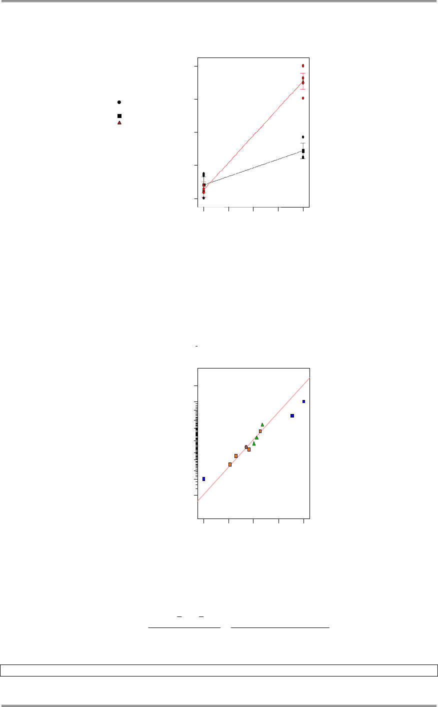
Solutions from Montgomery, D. C. (2001) Design and Analysis of Experiments, Wiley, NY
6-7
DESIGN-EXPERT Plot
Vibration
X = A: Bit Size
Y = B: Cutting Speed
Design Points
B- -1.000
B+ 1.000
Cuttin g Spee d
Inte ra c ti o n G r a p h
Bit Size
Vibration
-1 .0 0 -0 .5 0 0.00 0.50 1.00
12.9
20.65
28.4
36.15
43.9
6-6 Reconsider the experiment described in Problem 6-1. Suppose that the experimenter only
performed the eight trials from replicate I. In addition, he ran four center points and obtained the
following response values: 36, 40, 43, 45.
(a) Estimate the factor effects. Which effects are large?
DESIGN-EXPERT Plot
Life
A: Cu ttin g S peed
B: T ool Geometry
C: Cutting A ngle
Normal plot
Norm al % probability
Effe ct
-1 3 .7 5 -7 .1 3 -0 . 5 0 6.12 12.75
1
5
10
20
30
50
70
80
90
95
99
B
C
AC
Effects B, C, and AC appear to be large.
(b) Perform an analysis of variance, including a check for pure quadratic curvature. What are your
conclusions?
04170
48
000418754048 2
2
.
..
nn
yynn
SS
CF
CFCF
ticPureQuadra
Design Expert Output
Response: Life in hours

Solutions from Montgomery, D. C. (2001) Design and Analysis of Experiments, Wiley, NY
6-8
ANOVA for Selected Factorial Model
Analysis of variance table [Partial sum of squares]
Sum of Mean F
Source Squares DF Square Value Prob > F
Model 1048.88 7 149.84 9.77 0.0439 significant
A 3.13 1 3.13 0.20 0.6823
B 325.13 1 325.13 21.20 0.0193
C 190.12 1 190.12 12.40 0.0389
AB 6.13 1 6.13 0.40 0.5722
AC 378.12 1 378.12 24.66 0.0157
BC 55.12 1 55.12 3.60 0.1542
ABC 91.12 1 91.12 5.94 0.0927
Curvature 0.042 1 0.042 2.717E-003 0.9617 not significant
Pure Error 46.00 3 15.33
Cor Total 1094.92 11
The Model F-value of 9.77 implies the model is significant. There is only
a 4.39% chance that a "Model F-Value" this large could occur due to noise.
The "Curvature F-value" of 0.00 implies the curvature (as measured by difference between the
average of the center points and the average of the factorial points) in the design space is not
significant relative to the noise. There is a 96.17% chance that a "Curvature F-value"
this large could occur due to noise.
Design Expert Output
Response: Life in hours
ANOVA for Selected Factorial Model
Analysis of variance table [Partial sum of squares]
Sum of Mean F
Source Squares DF Square Value Prob > F
Model 896.50 4 224.13 7.91 0.0098 significant
A 3.13 1 3.13 0.11 0.7496
B 325.12 1 325.12 11.47 0.0117
C 190.12 1 190.12 6.71 0.0360
AC 378.12 1 378.12 13.34 0.0082
Residual 198.42 7 28.35
Lack of Fit 152.42 4 38.10 2.49 0.2402 not significant
Pure Error 46.00 3 15.33
Cor Total 1094.92 11
The Model F-value of 7.91 implies the model is significant. There is only
a 0.98% chance that a "Model F-Value" this large could occur due to noise.
Effects B, C and AC are significant at 5%. There is no effect of curvature.
(c) Write down an appropriate model for predicting tool life, based on the results of this experiment.
Does this model differ in any substantial way from the model in Problem 7-1, part (c)?
Design Expert Output
Final Equation in Terms of Coded Factors:
Life =
+40.88
+0.62 * A
+6.37 * B
+4.87 * C
-6.88 * A * C
(d) Analyze the residuals.
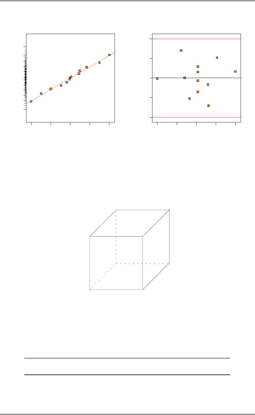
Solutions from Montgomery, D. C. (2001) Design and Analysis of Experiments, Wiley, NY
6-9
Studentized Residuals
Norm al % probability
Normal plot of residuals
-2 .1 1 -1 .0 5 0.00 1.05 2.11
1
5
10
20
30
50
70
80
90
95
99
Predicted
Studentized Residuals
Residuals vs. Predicted
-3 .0 0
-1 .5 0
0.00
1.50
3.00
22.13 31.19 40.25 49.31 58.38
(e) What conclusions would you draw about the appropriate operating conditions for this process?
To maximize life run with B at the high level, A at the low level and C at the high level
Cube Graph
Life
A: Cuttin g Speed
B: Tool Geom etry
C: C utting Angle
A- A+
B-
B+
C-
C+
22.13
45.63
34.88
58.38
37.13
33.13
49.88
45.88
6-7 An experiment was performed to improve the yield of a chemical process. Four factors were
selected, and two replicates of a completely randomized experiment were run. The results are shown in
the following table:
Treatment Replicate Replicate Treatment Replicate Replicate
Combination I II Combination I II
(1) 90 93 d 98 95
a 74 78 ad 72 76
b 81 85 bd 87 83

Solutions from Montgomery, D. C. (2001) Design and Analysis of Experiments, Wiley, NY
6-10
ab 83 80 abd 85 86
c 77 78 cd 99 90
ac 81 80 acd 79 75
bc 88 82 bcd 87 84
abc 73 70 abcd 80 80
(a) Estimate the factor effects.
Design Expert Output
Term Effect SumSqr % Contribtn
Model Intercept
Error A -9.0625 657.031 40.3714
Error B -1.3125 13.7812 0.84679
Error C -2.6875 57.7813 3.55038
Error D 3.9375 124.031 7.62111
Error AB 4.0625 132.031 8.11267
Error AC 0.6875 3.78125 0.232339
Error AD -2.1875 38.2813 2.3522
Error BC -0.5625 2.53125 0.155533
Error BD -0.1875 0.28125 0.0172814
Error CD 1.6875 22.7812 1.3998
Error ABC -5.1875 215.281 13.228
Error ABD 4.6875 175.781 10.8009
Error ACD -0.9375 7.03125 0.432036
Error BCD -0.9375 7.03125 0.432036
Error ABCD 2.4375 47.5313 2.92056
(b) Prepare an analysis of variance table, and determine which factors are important in explaining yield.
Design Expert Output
Response: yield
ANOVA for Selected Factorial Model
Analysis of variance table [Partial sum of squares]
Sum of Mean F
Source Squares DF Square Value Prob > F
Model 1504.97 15 100.33 13.10 < 0.0001 significant
A 657.03 1 657.03 85.82 < 0.0001
B 13.78 1 13.78 1.80 0.1984
C 57.78 1 57.78 7.55 0.0143
D 124.03 1 124.03 16.20 0.0010
AB 132.03 1 132.03 17.24 0.0007
AC 3.78 1 3.78 0.49 0.4923
AD 38.28 1 38.28 5.00 0.0399
BC 2.53 1 2.53 0.33 0.5733
BD 0.28 1 0.28 0.037 0.8504
CD 22.78 1 22.78 2.98 0.1038
ABC 215.28 1 215.28 28.12 < 0.0001
ABD 175.78 1 175.78 22.96 0.0002
ACD 7.03 1 7.03 0.92 0.3522
BCD 7.03 1 7.03 0.92 0.3522
ABCD 47.53 1 47.53 6.21 0.0241
Residual 122.50 16 7.66
Lack of Fit 0.000 0
Pure Error 122.50 16 7.66
Cor Total 1627.47 31
The Model F-value of 13.10 implies the model is significant. There is only
a 0.01% chance that a "Model F-Value" this large could occur due to noise.
Values of "Prob > F" less than 0.0500 indicate model terms are significant.
In this case A, C, D, AB, AD, ABC, ABD, ABCD are significant model terms.

Solutions from Montgomery, D. C. (2001) Design and Analysis of Experiments, Wiley, NY
6-11
F001116 853
.,, . , and F0025116 612
.,, . therefore, factors A and D and interactions AB, ABC, and ABD are
significant at 1%. Factor C and interactions AD and ABCD are significant at 2.5%.
(b) Write down a regression model for predicting yield, assuming that all four factors were varied over
the range from -1 to +1 (in coded units).
Model with hierarchy maintained:
Design Expert Output
Final Equation in Terms of Coded Factors:
yield =
+82.78
-4.53 * A
-0.66 * B
-1.34 * C
+1.97 * D
+2.03 * A * B
+0.34 * A * C
-1.09 * A * D
-0.28 * B * C
-0.094 * B * D
+0.84 * C * D
-2.59 * A * B * C
+2.34 * A * B * D
-0.47 * A * C * D
-0.47 * B * C * D
+1.22 * A * B * C * D
Model without hierarchy terms:
Design Expert Output
Final Equation in Terms of Coded Factors:
yield =
+82.78
-4.53 * A
-1.34 * C
+1.97 * D
+2.03 * A * B
-1.09 * A * D
-2.59 * A * B * C
+2.34 * A * B * D
+1.22 * A * B * C * D
Confirmation runs might be run to see if the simpler model without hierarchy is satisfactory.
(d) Plot the residuals versus the predicted yield and on a normal probability scale. Does the residual
analysis appear satisfactory?
There appears to be one large residual both in the normal probability plot and in the plot of residuals
versus predicted.
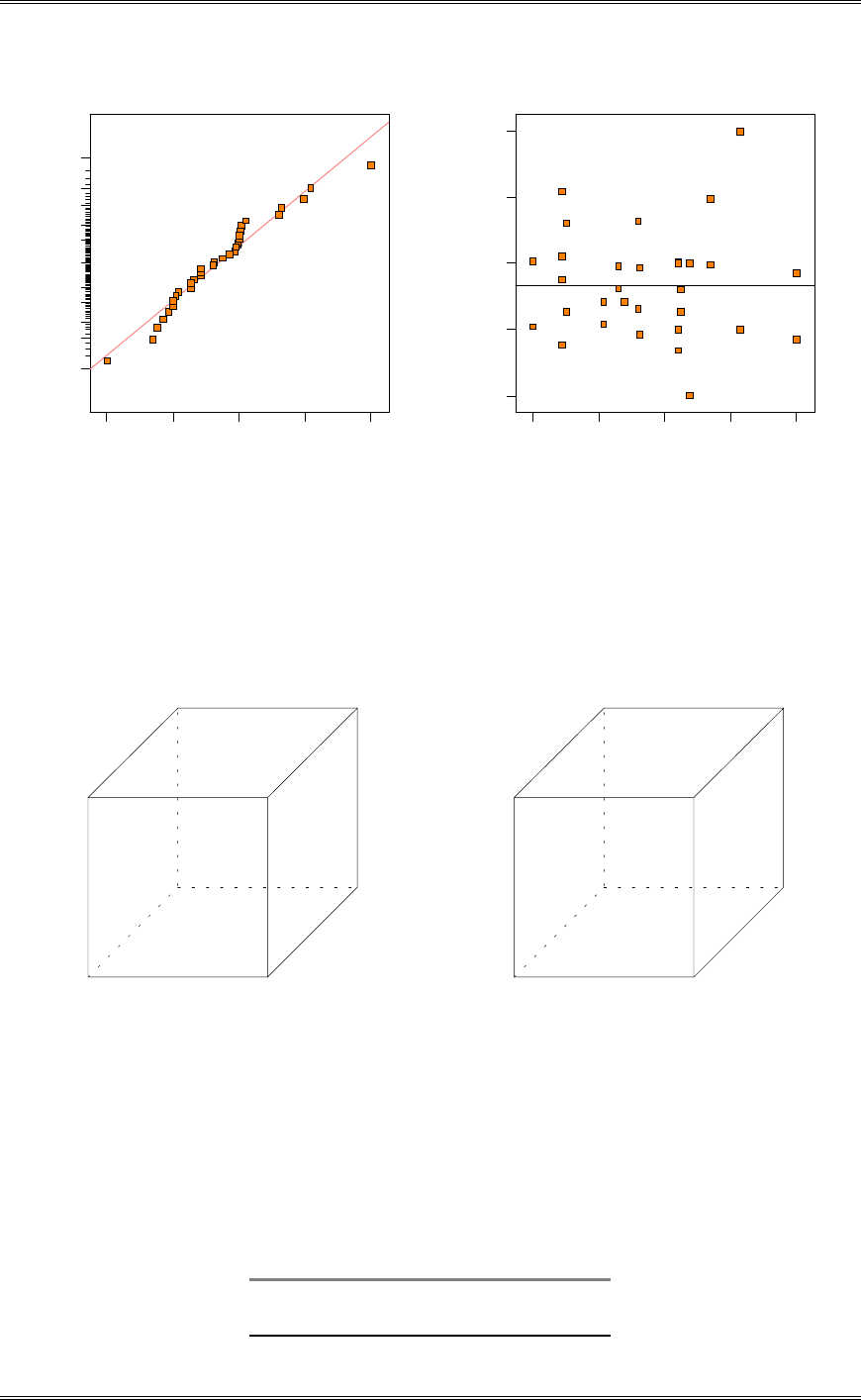
Solutions from Montgomery, D. C. (2001) Design and Analysis of Experiments, Wiley, NY
6-12
Res idual
Norm al % probability
Normal plot of residuals
-5.03125 -2.03125 0.96875 3.96875 6.96875
1
5
10
20
30
50
70
80
90
95
99
22
Predicted
Res iduals
Residuals vs. Predicted
-5.03125
-2.03125
0.96875
3.96875
6.96875
71.91 78.30 84.69 91.08 97.47
(e) Two three-factor interactions, ABC and ABD, apparently have large effects. Draw a cube plot in the
factors A, B, and C with the average yields shown at each corner. Repeat using the factors A, B, and
D. Do these two plots aid in data interpretation? Where would you recommend that the process be
run with respect to the four variables?
Cube Graph
yie ld
A: A
B: B
C: C
A- A+
B-
B+
C-
C+
93.28
85.41
84.03
86.53
74.97
77.47
84.22
76.34
Cube Graph
yie ld
A: A
B: B
D: D
A- A+
B-
B+
D-
D+
83.94
94.75
84.56
86.00
77.69
74.75
77.06
83.50
Run the process at A low B low, C low and D high.
6-8 A bacteriologist is interested in the effects of two different culture media and two different times on
the growth of a particular virus. She performs six replicates of a 22 design, making the runs in random
order. Analyze the bacterial growth data that follow and draw appropriate conclusions. Analyze the
residuals and comment on the model’s adequacy.
Culture Medium
Time 1 2
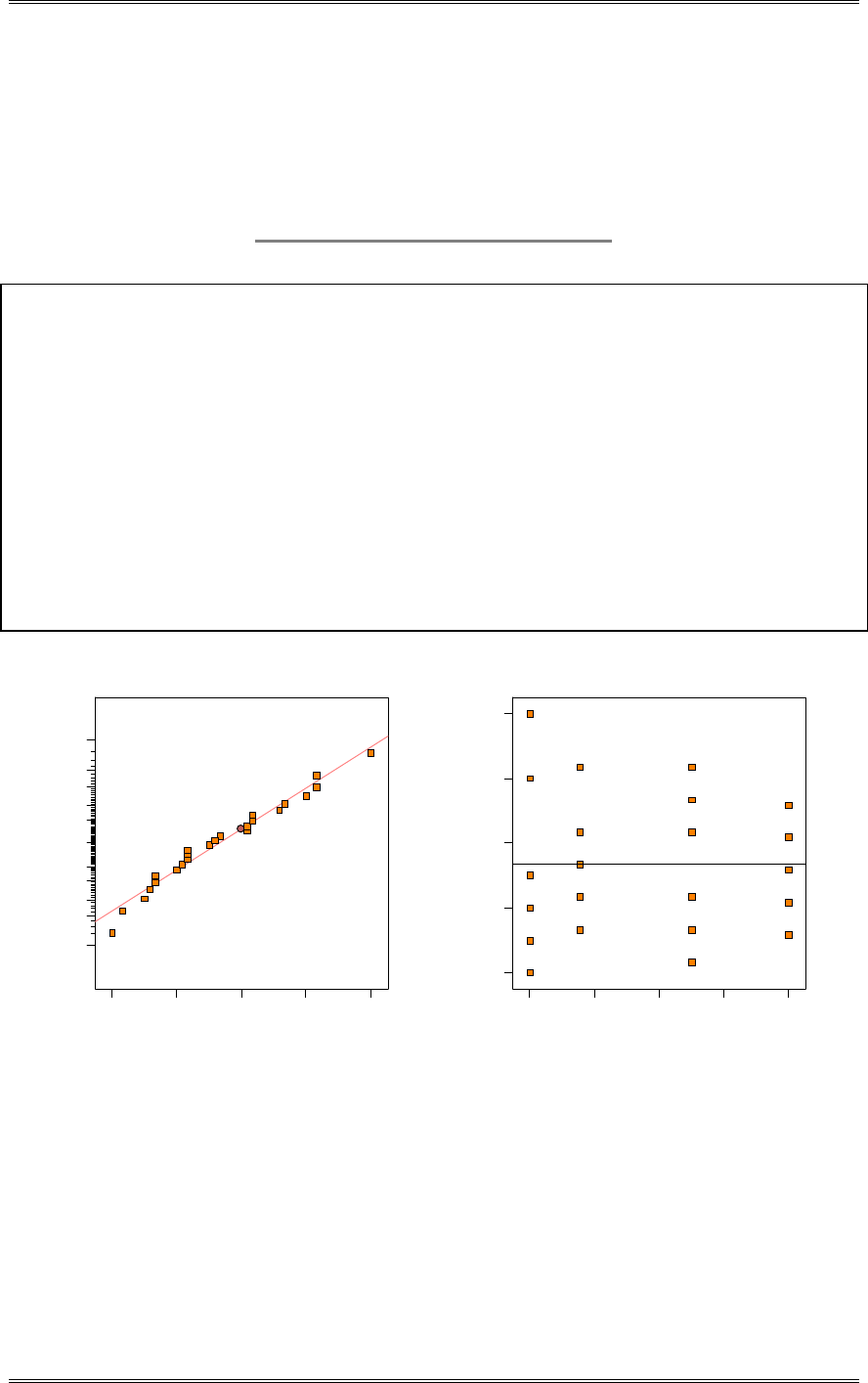
Solutions from Montgomery, D. C. (2001) Design and Analysis of Experiments, Wiley, NY
6-13
21 22 25 26
12 hr 23 28 24 25
20 26 29 27
37 39 31 34
18 hr 37 39 31 34
35 36 30 35
Design Expert Output
Response: Virus growth
ANOVA for Selected Factorial Model
Analysis of variance table [Partial sum of squares]
Sum of Mean F
Source Squares DF Square Value Prob > F
Model 691.46 3 230.49 45.12 < 0.0001 significant
A 9.38 1 9.38 1.84 0.1906
B 590.04 1 590.04 115.51 < 0.0001
AB 92.04 1 92.04 18.02 0.0004
Residual 102.17 20 5.11
Lack of Fit 0.000 0
Pure Error 102.17 20 5.11
Cor Total 793.63 23
The Model F-value of 45.12 implies the model is significant. There is only
a 0.01% chance that a "Model F-Value" this large could occur due to noise.
Values of "Prob > F" less than 0.0500 indicate model terms are significant.
In this case B, AB are significant model terms.
Residual
Norm al % probability
Normal plot of residuals
-3.33333 -1.33333 0.666667 2.66667 4.66667
1
5
10
20
30
50
70
80
90
95
99
22
22
Predicted
Residuals
Residuals vs. Predicted
-3.33333
-1.33333
0.666667
2.66667
4.66667
23.33 26.79 30.25 33.71 37.17
Growth rate is affected by factor B (Time) and the AB interaction (Culture medium and Time). There is
some very slight indication of inequality of variance shown by the small decreasing funnel shape in the
plot of residuals versus predicted.
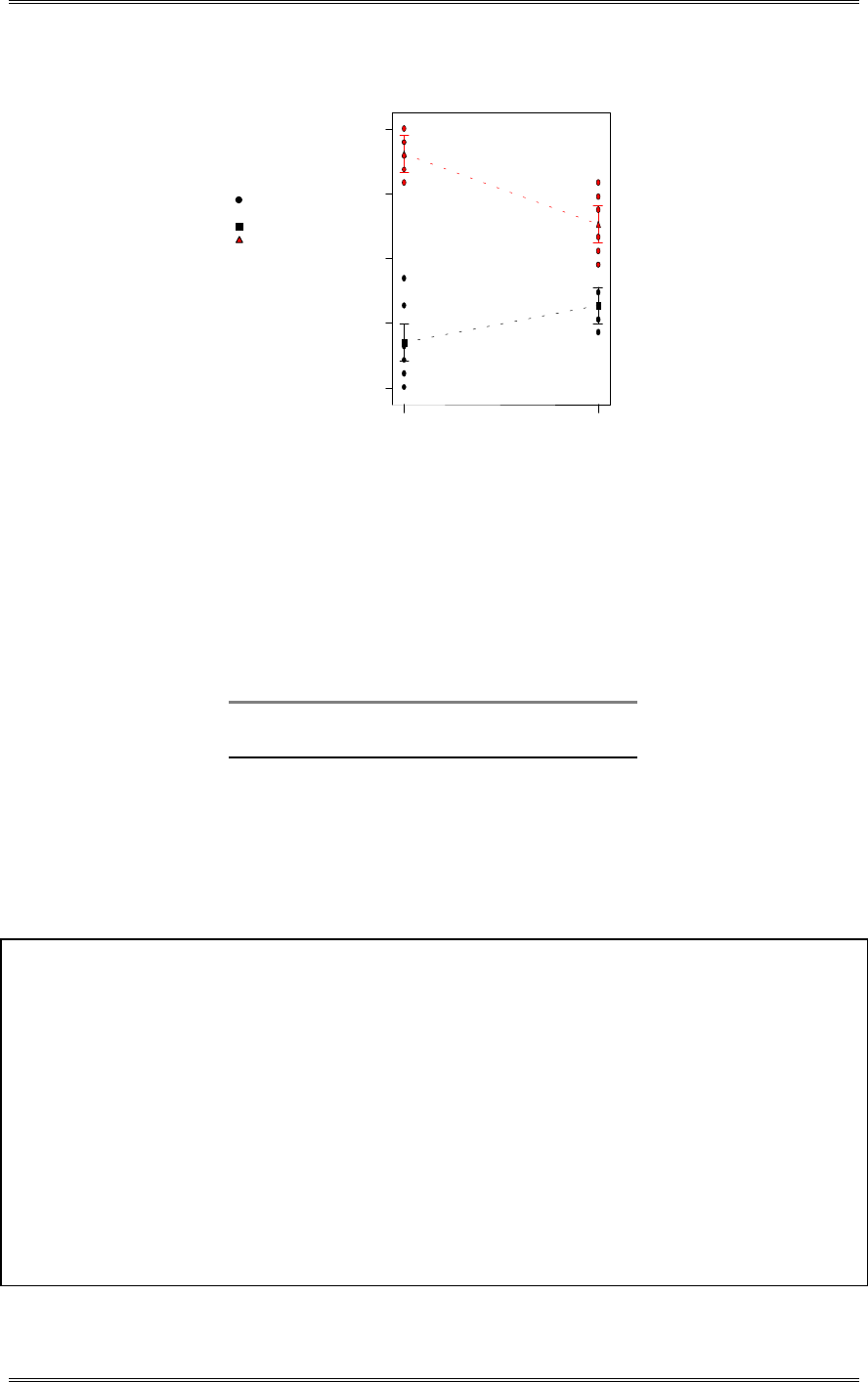
Solutions from Montgomery, D. C. (2001) Design and Analysis of Experiments, Wiley, NY
6-14
DESIGN-EXPERT Plot
Virus growth
X = A: Culture Medium
Y = B: Tim e
Design Points
B- 12.000
B+ 18.000
Tim e
Inte ra c ti o n G r a p h
Culture Medium
Virus growth
1 2
20
24.75
29.5
34.25
39
22
2
22
2
6-9 An industrial engineer employed by a beverage bottler is interested in the effects of two different
typed of 32-ounce bottles on the time to deliver 12-bottle cases of the product. The two bottle types are
glass and plastic. Two workers are used to perform a task consisting of moving 40 cases of the product 50
feet on a standard type of hand truck and stacking the cases in a display. Four replicates of a 22 factorial
design are performed, and the times observed are listed in the following table. Analyze the data and draw
the appropriate conclusions. Analyze the residuals and comment on the model’s adequacy.
Worker
Bottle Type 1 1 2 2
Glass 5.12 4.89 6.65 6.24
4.98 5.00 5.49 5.55
Plastic 4.95 4.43 5.28 4.91
4.27 4.25 4.75 4.71
Design Expert Output
Response:
Times
ANOVA for Selected Factorial Model
Analysis of variance table [Partial sum of squares]
Sum of Mean F
Source Squares DF Square Value Prob > F
Model 4.86 3 1.62 13.04 0.0004 significant
A 2.02 1 2.02 16.28 0.0017
B 2.54 1 2.54 20.41 0.0007
AB 0.30 1 0.30 2.41 0.1463
Residual 1.49 12 0.12
Lack of Fit 0.000 0
Pure Error 1.49 12 0.12
Cor Total 6.35 15
The Model F-value of 13.04 implies the model is significant. There is only
a 0.04% chance that a "Model F-Value" this large could occur due to noise.
Values of "Prob > F" less than 0.0500 indicate model terms are significant.
In this case A, B are significant model terms.
There is some indication of non-constant variance in this experiment.
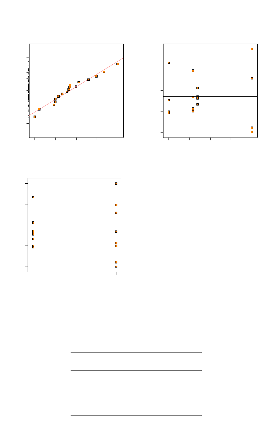
Solutions from Montgomery, D. C. (2001) Design and Analysis of Experiments, Wiley, NY
6-15
Residual
Norm al % probability
Normal plot of residuals
-0 .4 92 5 -0 . 2 02 5 0.0875 0.3775 0.6675
1
5
10
20
30
50
70
80
90
95
99
Predicted
Residuals
Residuals vs. Predicted
-0 .4 92 5
-0 .2 02 5
0.0875
0.3775
0.6675
4.47 4.85 5.23 5.61 5.98
Worker
Residuals
Residuals vs. Worker
-0 .4 92 5
-0 .2 02 5
0.0875
0.3775
0.6675
1 2
6-10 In problem 6-9, the engineer was also interested in potential fatigue differences resulting from the
two types of bottles. As a measure of the amount of effort required, he measured the elevation of heart
rate (pulse) induced by the task. The results follow. Analyze the data and draw conclusions. Analyze the
residuals and comment on the model’s adequacy.
Worker
Bottle Type 1 1 2 2
Glass 39 45 20 13
58 35 16 11
Plastic 44 35 13 10
42 21 16 15
Design Expert Output
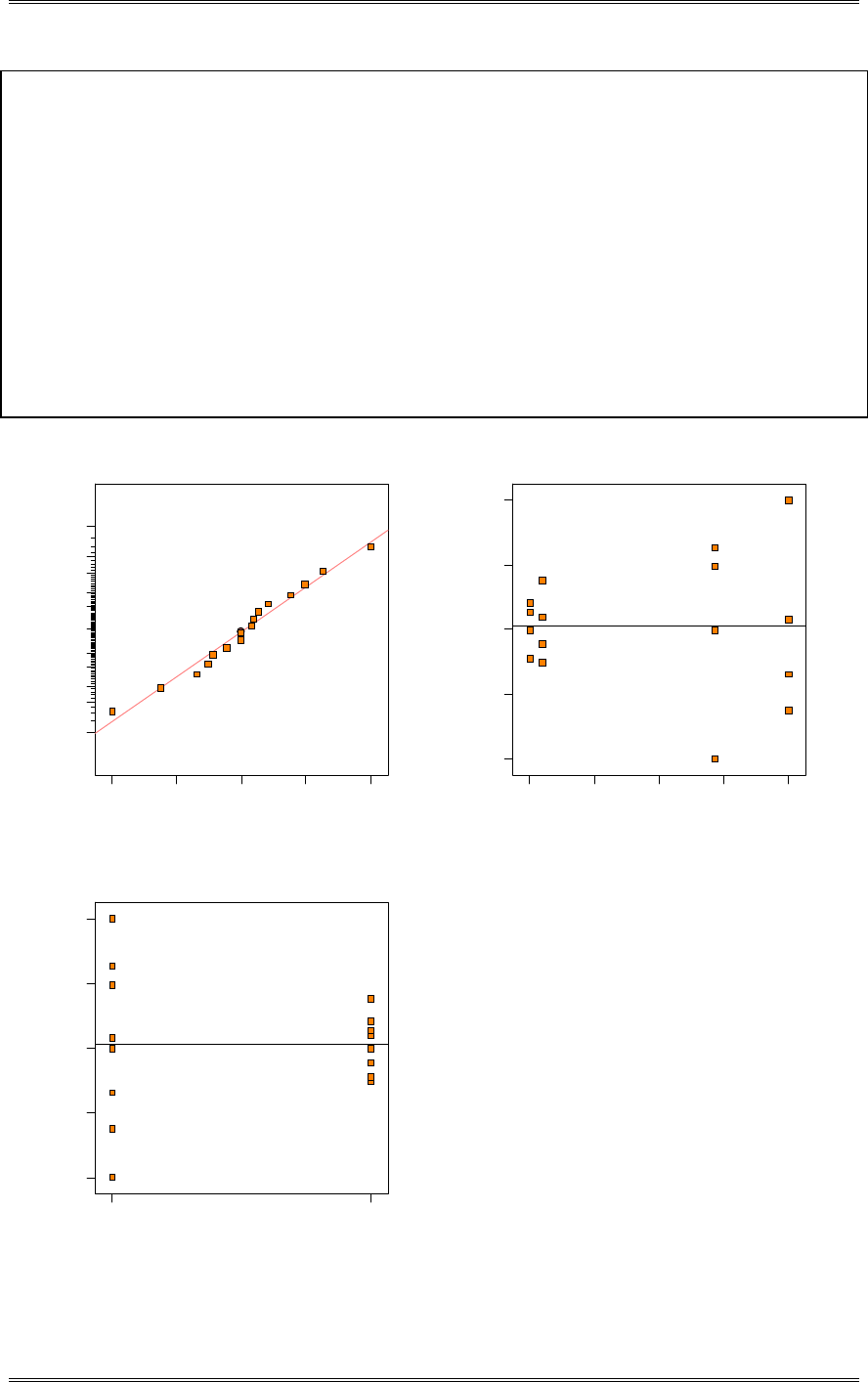
Solutions from Montgomery, D. C. (2001) Design and Analysis of Experiments, Wiley, NY
6-16
Response: Pulse
ANOVA for Selected Factorial Model
Analysis of variance table [Partial sum of squares]
Sum of Mean F
Source Squares DF Square Value Prob > F
Model 2784.19 3 928.06 16.03 0.0002 significant
A 2626.56 1 2626.56 45.37 < 0.0001
B 105.06 1 105.06 1.81 0.2028
AB 52.56 1 52.56 0.91 0.3595
Residual 694.75 12 57.90
Lack of Fit 0.000 0
Pure Error 694.75 12 57.90
Cor Total 3478.94 15
The Model F-value of 16.03 implies the model is significant. There is only
a 0.02% chance that a "Model F-Value" this large could occur due to noise.
Values of "Prob > F" less than 0.0500 indicate model terms are significant.
In this case A are significant model terms.
Residual
Normal % probability
Normal plot of residuals
-14.5 -7 .4 37 5 -0 . 3 75 6.6875 13.75
1
5
10
20
30
50
70
80
90
95
99
Predicted
Residuals
Residuals vs. Predicted
-1 4 .5
-7 .4 37 5
-0 .3 75
6.6875
13.75
13.50 21.19 28.88 36.56 44.25
Worker
Residuals
Residuals vs. Worker
-14.5
-7 .4 37 5
-0 .3 75
6.6875
13.75
1 2
There is an indication that one worker exhibits greater variability than the other.

Solutions from Montgomery, D. C. (2001) Design and Analysis of Experiments, Wiley, NY
6-17
6-11 Calculate approximate 95 percent confidence limits for the factor effects in Problem 6-10. Do the
results of this analysis agree with the analysis of variance performed in Problem 6-10?
8039057
24
1
2
1
22
2
2..S
n
SE k
)effect(
Variable Effect C.I.
A -25.625 r3.80(1.96)= r7.448
B -5.125 r3.80(1.96)= r7.448
AB -7.25 r3.80(1.96)= r7.448
The 95% confidence intervals for factors A does not contain zero. This agrees with the analysis of
variance approach.
6-12 An article in the AT&T Technical Journal (March/April 1986, Vol. 65, pp. 39-50) describes the
application of two-level factorial designs to integrated circuit manufacturing. A basic processing step is to
grow an epitaxial layer on polished silicon wafers. The wafers mounted on a susceptor are positioned
inside a bell jar, and chemical vapors are introduced. The susceptor is rotated and heat is applied until the
epitaxial layer is thick enough. An experiment was run using two factors: arsenic flow rate (A) and
deposition time (B). Four replicates were run, and the epitaxial layer thickness was measured (in mm).
The data are shown below:
Replicate Factor Levels
A B I II III IV Low (-) High (+)
- - 14.037 16.165 13.972 13.907 A 55% 59%
+ - 13.880 13.860 14.032 13.914
- + 14.821 14.757 14.843 14.878 B Short Long
+ + 14.888 14.921 14.415 14.932 (10 min) (15 min)
(a) Estimate the factor effects.
Design Expert Output
Term Effect SumSqr % Contribtn
Model Intercept
Error A -0.31725 0.40259 6.79865
Error B 0.586 1.37358 23.1961
Error AB 0.2815 0.316969 5.35274
Error Lack Of Fit 0 0
Error Pure Error 3.82848 64.6525
(b) Conduct an analysis of variance. Which factors are important?
Design Expert Output
Response: Thickness
ANOVA for Selected Factorial Model
Analysis of variance table [Partial sum of squares]
Sum of Mean F
Source Squares DF Square Value Prob > F
Model 2.09 3 0.70 2.19 0.1425 not significant
A 0.40 1 0.40 1.26 0.2833
B 1.37 1 1.37 4.31 0.0602
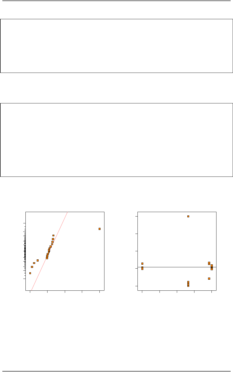
Solutions from Montgomery, D. C. (2001) Design and Analysis of Experiments, Wiley, NY
6-18
AB 0.32 1 0.32 0.99 0.3386
Residual 3.83 12 0.32
Lack of Fit 0.000 0
Pure Error 3.83 12 0.32
Cor Total 5.92 15
The "Model F-value" of 2.19 implies the model is not significant relative to the noise. There is a
14.25 % chance that a "Model F-value" this large could occur due to noise.
Values of "Prob > F" less than 0.0500 indicate model terms are significant.
In this case there are no significant model terms.
(c) Write down a regression equation that could be used to predict epitaxial layer thickness over the
region of arsenic flow rate and deposition time used in this experiment.
Design Expert Output
Final Equation in Terms of Coded Factors:
Thickness =
+14.51
-0.16 * A
+0.29 * B
+0.14 * A * B
Final Equation in Terms of Actual Factors:
Thickness =
+37.62656
-0.43119 * Flow Rate
-1.48735 * Dep Time
+0.028150 * Flow Rate * Dep Time
(d) Analyze the residuals. Are there any residuals that should cause concern? Observation #2 falls
outside the groupings in the normal probability plot and the plot of residual versus predicted.
Residual
Norm al % probability
Normal plot of residuals
-0.61325 -0.04875 0.51575 1.08025 1.64475
1
5
10
20
30
50
70
80
90
95
99
Predicted
Residuals
Residuals vs. Predicted
-0.61325
-0.04875
0.51575
1.08025
1.64475
13.92 14.15 14.37 14.60 14.82
(e) Discuss how you might deal with the potential outlier found in part (d).
One approach would be to replace the observation with the average of the observations from that
experimental cell. Another approach would be to identify if there was a recording issue in the original
data. The first analysis below replaces the data point with the average of the other three. The second
analysis assumes that the reading was incorrectly recorded and should have been 14.165.
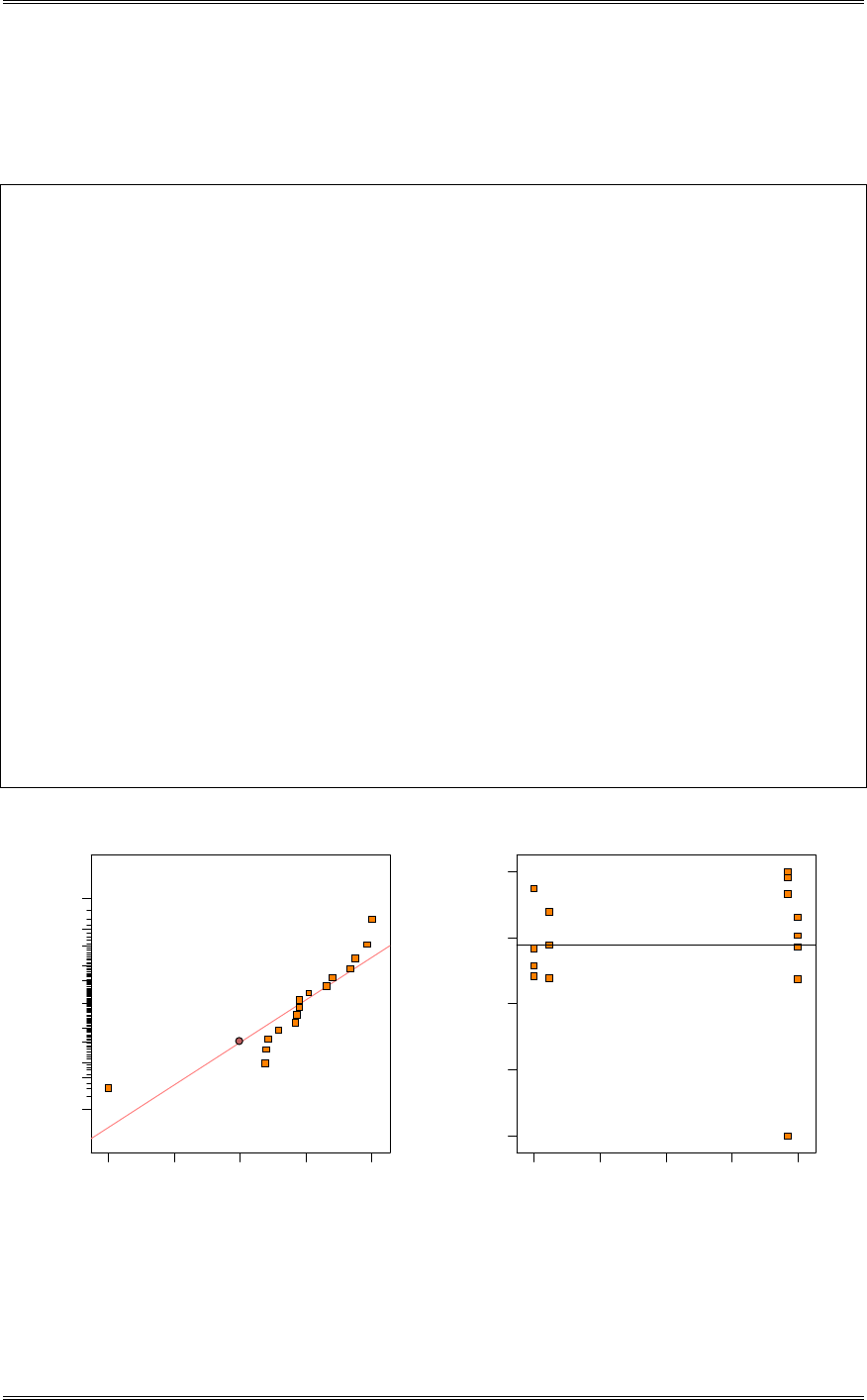
Solutions from Montgomery, D. C. (2001) Design and Analysis of Experiments, Wiley, NY
6-19
Analysis with the run associated with standard order 2 replaced with the average of the remaining three
runs in the cell, 13.972:
Design Expert Output
Response: Thickness
ANOVA for Selected Factorial Model
Analysis of variance table [Partial sum of squares]
Sum of Mean F
Source Squares DF Square Value Prob > F
Model 2.97 3 0.99 53.57 < 0.0001 significant
A 7.439E-003 1 7.439E-003 0.40 0.5375
B 2.96 1 2.96 160.29 < 0.0001
AB 2.176E-004 1 2.176E-004 0.012 0.9153
Pure Error 0.22 12 0.018
Cor Total 3.19 15
The Model F-value of 53.57 implies the model is significant. There is only
a 0.01% chance that a "Model F-Value" this large could occur due to noise.
Values of "Prob > F" less than 0.0500 indicate model terms are significant.
In this case B are significant model terms.
Final Equation in Terms of Coded Factors:
Thickness =
+14.38
-0.022 * A
+0.43 * B
+3.688E-003 * A * B
Final Equation in Terms of Actual Factors:
Thickness =
+13.36650
-0.020000 * Flow Rate
+0.12999 * Dep Time
+7.37500E-004 * Flow Rate * Dep Time
Res idual
Normal % probability
Normal plot of residuals
-0.374 -0.24475 -0.1155 0.01375 0.143
1
5
10
20
30
50
70
80
90
95
99
22
Predicted
Res iduals
Residuals vs. Predicted
-0 .3 7 4
-0.24475
-0 .1 1 5 5
0.01375
0.143
13.92 14.15 14.37 14.60 14.82
A new outlier is present and should be investigated.
Analysis with the run associated with standard order 2 replaced with the value 14.165:
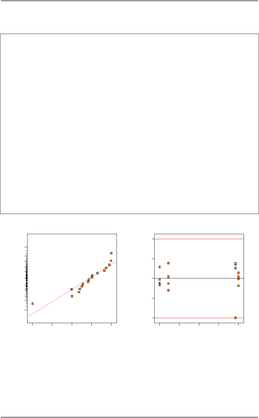
Solutions from Montgomery, D. C. (2001) Design and Analysis of Experiments, Wiley, NY
6-20
Design Expert Output
Response: Thickness
ANOVA for Selected Factorial Model
Analysis of variance table [Partial sum of squares]
Sum of Mean F
Source Squares DF Square Value Prob > F
Model 2.82 3 0.94 45.18 < 0.0001 significant
A 0.018 1 0.018 0.87 0.3693
B 2.80 1 2.80 134.47 < 0.0001
AB 3.969E-003 1 3.969E-003 0.19 0.6699
Pure Error 0.25 12 0.021
Cor Total 3.07 15
The Model F-value of 45.18 implies the model is significant. There is only
a 0.01% chance that a "Model F-Value" this large could occur due to noise.
Values of "Prob > F" less than 0.0500 indicate model terms are significant.
In this case B are significant model terms.
Final Equation in Terms of Coded Factors:
Thickness =
+14.39
-0.034 * A
+0.42 * B
+0.016 * A * B
Final Equation in Terms of Actual Factors:
Thickness =
+15.50156
-0.056188 * Flow Rate
-0.012350 * Dep Time
+3.15000E-003 * Flow Rate * Dep Time
Studentized Residuals
Norm al % probability
Normal plot of residuals
-3 .0 0 -1 .9 6 -0 . 9 2 0.12 1.16
1
5
10
20
30
50
70
80
90
95
99
Predicted
Studentized Residuals
Residuals vs. Predicted
-3 .0 0
-1 .5 0
0.00
1.50
3.00
13.92 14.15 14.37 14.60 14.82
Another outlier is present and should be investigated.
6-13 Continuation of Problem 6-12. Use the regression model in part (c) of Problem 6-12 to generate a
response surface contour plot for epitaxial layer thickness. Suppose it is critically important to obtain
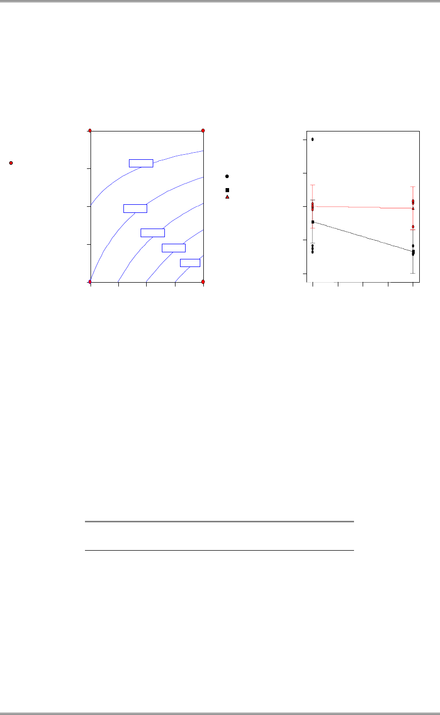
Solutions from Montgomery, D. C. (2001) Design and Analysis of Experiments, Wiley, NY
6-21
layer thickness of 14.5 mm. What settings of arsenic flow rate and deposition time would you
recommend?
Arsenic flow rate may be set at any of the experimental levels, while the deposition time should be set at
12.4 minutes.
DESIGN-EXPERT Plot
Thickness
X = A: Flow Rate
Y = B: Dep Time
Design Points
Thickness
Flow R ate
Dep Time
55.00 56.00 57.00 58.00 59.00
10.00
11.25
12.50
13.75
15.00
14.072
14.2226
14.3731
14.5237
14.6742
4 4
4 4 DESIGN-EXPERT Plot
Thickness
X = A: Flow Rate
Y = B: Dep Time
Design Points
B- 10.000
B+ 15.000
Dep Tim e
Inte ra c ti o n G r a p h
Flow R ate
Thickness
55.00 56.00 57.00 58.00 59.00
13.4864
14.156
14.8257
15.4953
16.165
6-14 Continuation of Problem 6-13. How would your answer to Problem 6-13 change if arsenic flow
rate was more difficult to control in the process than the deposition time?
Running the process at a high level of Deposition Time there is no change in thickness as flow rate
changes.
6-15 A nickel-titanium alloy is used to make components for jet turbine aircraft engines. Cracking is a
potentially serious problem in the final part, as it can lead to non-recoverable failure. A test is run at the
parts producer to determine the effects of four factors on cracks. The four factors are pouring temperature
(A), titanium content (B), heat treatment method (C), and the amount of grain refiner used (D). Two
replicated of a 24 design are run, and the length of crack (in Pm) induced in a sample coupon subjected to
a standard test is measured. The data are shown below:
Treatment Replicate Replicate
A B C D Combination I II
- - - - (1) 7.037 6.376
+ - - - a 14.707 15.219
- + - - b 11.635 12.089
+ + - - ab 17.273 17.815
- - + - c 10.403 10.151
+ - + - ac 4.368 4.098
- + + - bc 9.360 9.253
+ + + - abc 13.440 12.923
- - - + d 8.561 8.951

Solutions from Montgomery, D. C. (2001) Design and Analysis of Experiments, Wiley, NY
6-22
+ - - + ad 16.867 17.052
- + - + bd 13.876 13.658
+ + - + abd 19.824 19.639
- - + + cd 11.846 12.337
+ - + + acd 6.125 5.904
- + + + bcd 11.190 10.935
+ + + + abcd 15.653 15.053
(a) Estimate the factor effects. Which factors appear to be large?
Design Expert Output
Term Effect SumSqr % Contribtn
Model Intercept
Model A 3.01888 72.9089 12.7408
Model B 3.97588 126.461 22.099
Model C -3.59625 103.464 18.0804
Model D 1.95775 30.6623 5.35823
Model AB 1.93412 29.9267 5.22969
Model AC -4.00775 128.496 22.4548
Error AD 0.0765 0.046818 0.00818145
Error BC 0.096 0.073728 0.012884
Error BD 0.04725 0.0178605 0.00312112
Error CD -0.076875 0.0472781 0.00826185
Model ABC 3.1375 78.7512 13.7618
Error ABD 0.098 0.076832 0.0134264
Error ACD 0.019125 0.00292613 0.00051134
Error BCD 0.035625 0.0101531 0.00177426
Error ABCD 0.014125 0.00159613 0.000278923
(b) Conduct an analysis of variance. Do any of the factors affect cracking? Use
D
=0.05.
Design Expert Output
Response: Crack Lengthin mm x 10^-2
ANOVA for Selected Factorial Model
Analysis of variance table [Partial sum of squares]
Sum of Mean F
Source Squares DF Square Value Prob > F
Model 570.95 15 38.06 468.99 < 0.0001 significant
A 72.91 1 72.91 898.34 < 0.0001
B 126.46 1 126.46 1558.17 < 0.0001
C 103.46 1 103.46 1274.82 < 0.0001
D 30.66 1 30.66 377.80 < 0.0001
AB 29.93 1 29.93 368.74 < 0.0001
AC 128.50 1 128.50 1583.26 < 0.0001
AD 0.047 1 0.047 0.58 0.4586
BC 0.074 1 0.074 0.91 0.3547
BD 0.018 1 0.018 0.22 0.6453
CD 0.047 1 0.047 0.58 0.4564
ABC 78.75 1 78.75 970.33 < 0.0001
ABD 0.077 1 0.077 0.95 0.3450
ACD 2.926E-003 1 2.926E-003 0.036 0.8518
BCD 0.010 1 0.010 0.13 0.7282
ABCD 1.596E-003 1 1.596E-003 0.020 0.8902
Residual 1.30 16 0.081
Lack of Fit 0.000 0
Pure Error 1.30 16 0.081
Cor Total 572.25 31
The Model F-value of 468.99 implies the model is significant. There is only
a 0.01% chance that a "Model F-Value" this large could occur due to noise.
Values of "Prob > F" less than 0.0500 indicate model terms are significant.
In this case A, B, C, D, AB, AC, ABC are significant model terms.
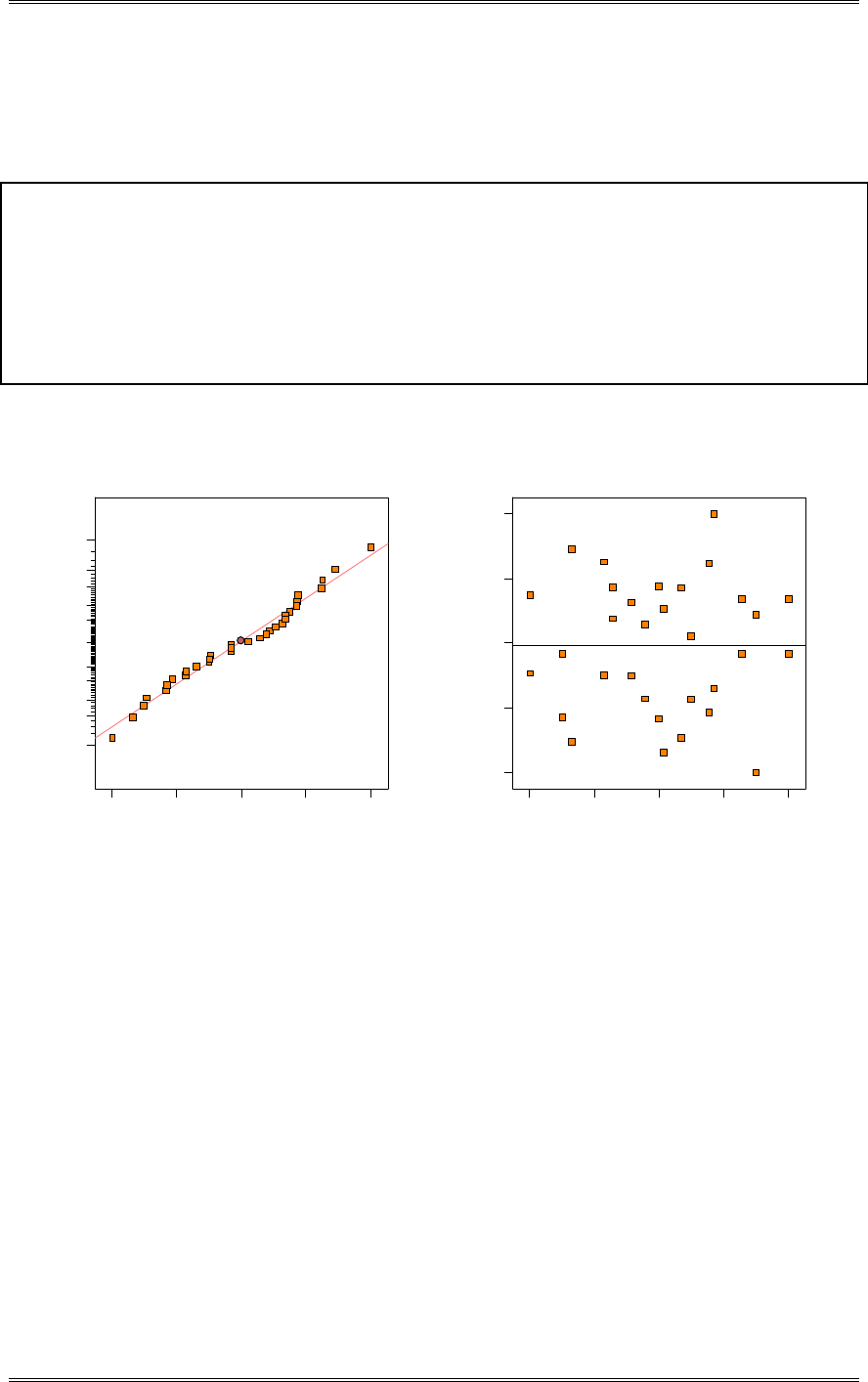
Solutions from Montgomery, D. C. (2001) Design and Analysis of Experiments, Wiley, NY
6-23
(c) Write down a regression model that can be used to predict crack length as a function of the significant
main effects and interactions you have identified in part (b).
Design Expert Output
Final Equation in Terms of Coded Factors:
Crack Length=
+11.99
+1.51 *A
+1.99 *B
-1.80 *C
+0.98 *D
+0.97 *A*B
-2.00 *A*C
+1.57 * A * B * C
(d) Analyze the residuals from this experiment.
Residual
Normal % probability
Normal plot of residuals
-0.433875 -0.211687 0.0105 0.232688 0.454875
1
5
10
20
30
50
70
80
90
95
99
Predicted
Residuals
Residuals vs. Predicted
-0 .4 33 8 7 5
-0 .2 11 6 8 7
0.0105
0.232688
0.454875
4.19 8.06 11.93 15.80 19.66
There is nothing unusual about the residuals.
(e) Is there an indication that any of the factors affect the variability in cracking?
By calculating the range of the two readings in each cell, we can also evaluate the effects of the factors on
variation. The following is the normal probability plot of effects:
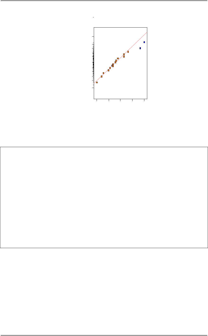
Solutions from Montgomery, D. C. (2001) Design and Analysis of Experiments, Wiley, NY
6-24
DESIGN-EXPERT Plot
Range
A: Pour T emp
B: T itanium Content
C: Heat Treat Method
D: Grain Refiner
Normal plot
Norm al % probability
Effe ct
-0 .1 0 -0 .0 2 0.05 0.13 0.20
1
5
10
20
30
50
70
80
90
95
99
AB
CD
It appears that the AB and CD interactions could be significant. The following is the ANOVA for the
range data:
Design Expert Output
Response: Range
ANOVA for Selected Factorial Model
Analysis of variance table [Partial sum of squares]
Sum of Mean F
Source Squares DF Square Value Prob > F
Model 0.29 2 0.14 11.46 0.0014 significant
AB 0.13 1 0.13 9.98 0.0075
CD 0.16 1 0.16 12.94 0.0032
Residual 0.16 13 0.013
Cor Total 0.45 15
The Model F-value of 11.46 implies the model is significant. There is only
a 0.14% chance that a "Model F-Value" this large could occur due to noise.
Values of "Prob > F" less than 0.0500 indicate model terms are significant.
In this case AB, CD are significant model terms.
Final Equation in Terms of Coded Factors:
Range =
+0.37
+0.089 * A * B
+0.10 * C * D
(f) What recommendations would you make regarding process operations?
Use interaction and/or main effect plots to assist in drawing conclusions. From the interaction plots,
choose A at the high level and B at the high level. In each of these plots, D can be at either level. From
the main effects plot of C, choose C at the high level. Based on the range analysis, with C at the high
level, D should be set at the low level.
From the analysis of the crack length data:
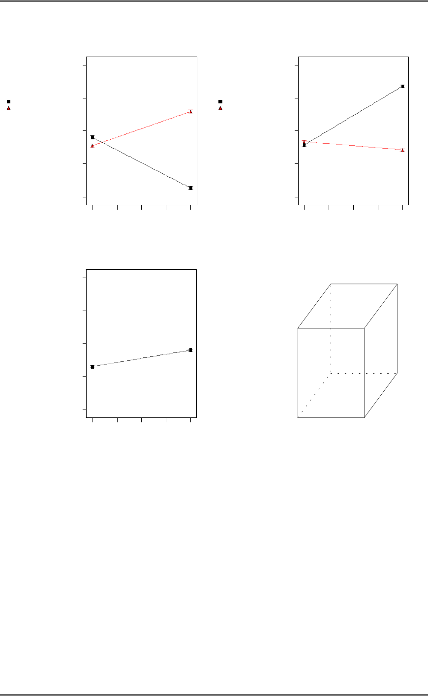
Solutions from Montgomery, D. C. (2001) Design and Analysis of Experiments, Wiley, NY
6-25
DESIGN-EXPERT Plot
Crack Length
X = A: Pour Temp
Y = B: Titanium Content
B- -1.000
B+ 1.000
Actual Factors
C: Heat Treat Method = 1
D: Grain Refiner = 0.00
B: Titanium Content
Interaction Graph
Crack Length
A: P ou r Tem p
-1 .0 0 -0 .5 0 0.00 0.50 1.00
4.098
8.0295
11.961
15.8925
19.824
DESIGN-EXPERT Plot
Crack Length
X = A: Pour Temp
Y = C: Heat Treat Method
C1 -1
C2 1
Actual Factors
B: T itanium Content = 0.00
D: Grain Refiner = 0.00
C: H ea t Trea t Metho d
Interaction Graph
Crack Length
A: P ou r Tem p
-1 .0 0 -0 .5 0 0.00 0.50 1.00
4.098
8.0295
11.961
15.8925
19.824
DESIGN-EXPERT Plot
Crack Length
X = D: Grain Refiner
Actual Factors
A: Pour T em p = 0.00
B: T itanium Content = 0.00
C: Heat Treat Method = 1
-1 .0 0 -0 .5 0 0.00 0.50 1.00
4.098
8.0295
11.961
15.8925
19.824
D: Grain Refiner
Crack Length
One Factor Plot DESIGN-EXPERT Plot
Crack Length
X = A: Pour Temp
Y = B: Titanium Content
Z = C: Heat Treat Method
Actual Factor
D: Grain Refiner = 0.00
Cube Graph
Crack Length
A: P our Tem p
B: Titanium Content
C: H eat Trea t Meth
o
A- A+
B-
B+
C-
C+
7.73
11.18
12.81
10.18
15.96
5.12
18.64
14.27
From the analysis of the ranges:
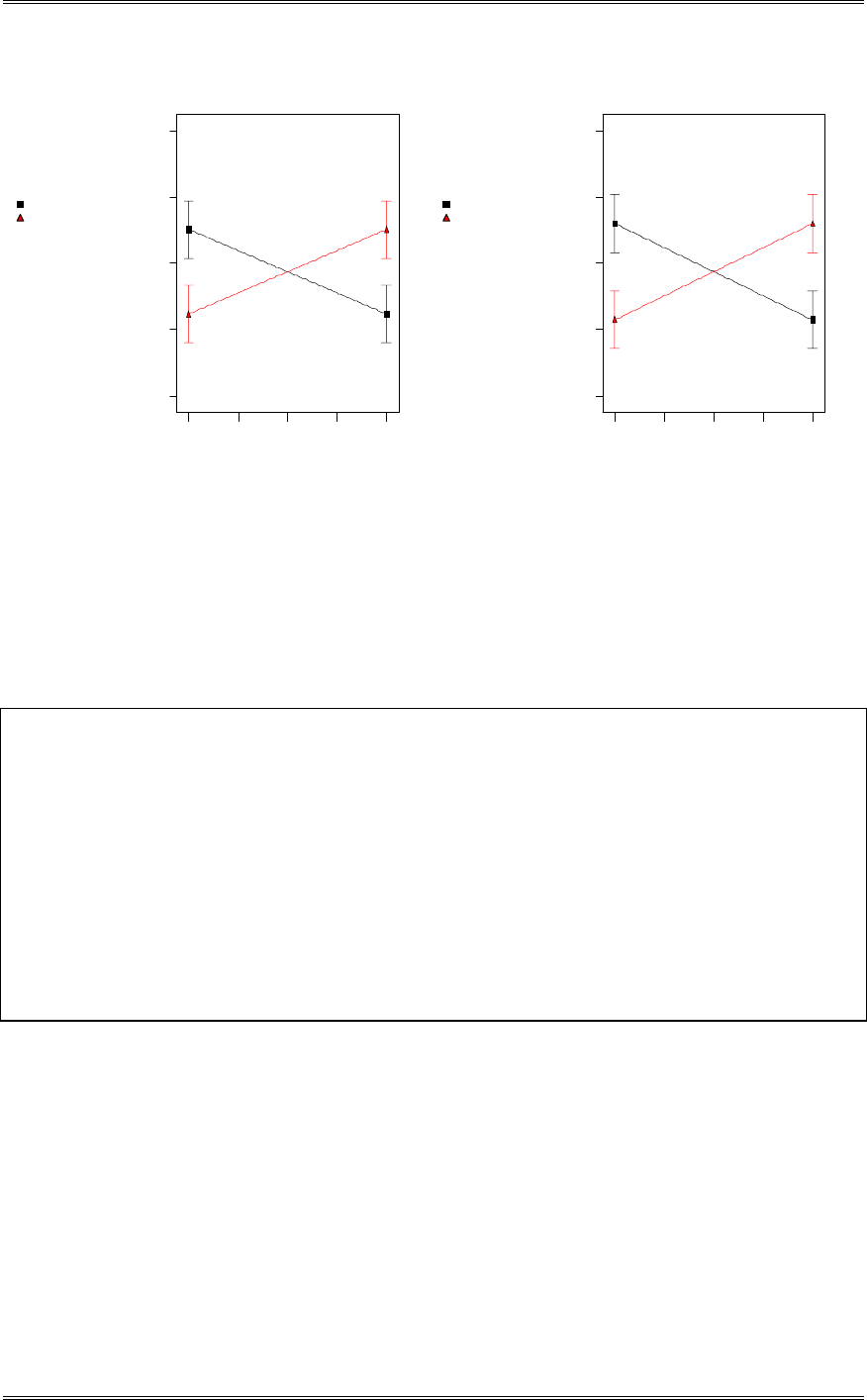
Solutions from Montgomery, D. C. (2001) Design and Analysis of Experiments, Wiley, NY
6-26
DESIGN-EXPERT Plot
Range
X = A: Pour Temp
Y = B: Titanium Content
B- -1.000
B+ 1.000
Actual Factors
C: Heat Treat Method = 0.00
D: Grain Refiner = 0.00
B: Titanium Content
Interaction Graph
Range
A: P ou r Tem p
-1 .0 0 -0 .5 0 0.00 0.50 1.00
0.107
0.2455
0.384
0.5225
0.661
DESIGN-EXPERT Plot
Range
X = C: Heat Treat Method
Y = D: Grain Refiner
D- -1.000
D+ 1.000
Actual Factors
A: Pour Temp = 0.00
B: T itanium Content = 0.00
D: Grain Refiner
Interaction Graph
Range
C: H ea t Trea t Metho d
-1 .0 0 -0 .5 0 0.00 0.50 1.00
0.107
0.2455
0.384
0.5225
0.661
6-16 Continuation of Problem 6-15. One of the variables in the experiment described in Problem 6-15,
heat treatment method (c), is a categorical variable. Assume that the remaining factors are continuous.
(a) Write two regression models for predicting crack length, one for each level of the heat treatment
method variable. What differences, if any, do you notice in these two equations?
Design Expert Output
Final Equation in Terms of Coded Factors
Heat Treat Method -1
Crack Length =
+13.78619
+3.51331 * Pour Temp
+1.93994 * Titanium Content
+0.97888 * Grain Refiner
-0.60169 * Pour Temp * Titanium Content
Heat Treat Method 1
Crack Length =
+10.18994
-0.49444 * Pour Temp
+2.03594 * Titanium Content
+0.97888 * Grain Refiner
+2.53581 * Pour Temp * Titanium Content
(b) Generate appropriate response surface contour plots for the two regression models in part (a).

Solutions from Montgomery, D. C. (2001) Design and Analysis of Experiments, Wiley, NY
6-27
DESIGN-EXPERT Plot
Crack Length
X = A: Pour Temp
Y = B: Titanium Content
Actual Factors
C: Heat Treat Method = -1
D: Grain Refiner = 0.00
Crack Length
A: P our Tem p
B: Titanium Content
-1 .0 0 -0 .5 0 0.00 0.50 1.00
-1 .0 0
-0 .5 0
0.00
0.50
1.00
10
12
14 16
18
DESIGN-EXPERT Plot
Crack Length
X = A: Pour Temp
Y = B: Titanium Content
Actual Factors
C: Heat T reat M etho d = 1
D: Grain Refiner = 0.00
Crack Length
A: Pour Tem p
B: Titanium Content
-1 .0 0 -0 .5 0 0.00 0.50 1.00
-1 .0 0
-0 .5 0
0.00
0.50
1.00
6
8
10
12
(c) What set of conditions would you recommend for the factors A, B and D if you use heat treatment
method C=+?
High level of A, low level of B, and low level of D.
(d) Repeat part (c) assuming that you wish to use heat treatment method C=-.
Low level of A, low level of B, and low level of D.
6-17 An experimenter has run a single replicate of a 24 design. The following effect estimates have been
calculated:
A = 76.95 AB = -51.32 ABC = -2.82
B = -67.52 AC = 11.69 ABD = -6.50
C = -7.84 AD = 9.78 ACD = 10.20
D = -18.73 BC = 20.78 BCD = -7.98
BD = 14.74 ABCD = -6.25
CD = 1.27
(a) Construct a normal probability plot of these effects.
The plot from Minitab follows.

Solutions from Montgomery, D. C. (2001) Design and Analysis of Experiments, Wiley, NY
6-28
500-50
99
95
90
80
70
60
50
40
30
20
10
5
1
Data
Percent
1.465AD*
Goodness of Fit
Normal Probabilit
y
Plot for Value
ML Estimates
Mean
StDev
-1.57
31.2296
ML Estimates
A
B
AB
(b) Identify a tentative model, based on the plot of the effects in part (a).
BABA xx.x.x.Intercepty
ˆ6625763347538
6-18 An article in Solid State Technology (“Orthogonal Design for Process Optimization and Its
Application in Plasma Etching,” May 1987, pp. 127-132) describes the application of factorial designs in
developing a nitride etch process on a single-wafer plasma etcher. The process uses C2F6 as the reactant
gas. Four factors are of interest: anode-cathode gap (A), pressure in the reactor chamber (B), C2F6 gas
flow (C), and power applied to the cathode (D). The response variable of interest is the etch rate for
silicon nitride. A single replicate of a 24 design in run, and the data are shown below:
Actual Etch
Run Run Rate Factor Levels
Number Order A B C D (A/min) Low (-) High (+)
1 13 - - - - 550 A (cm) 0.80 1.20
2 8 + - - - 669 B (mTorr) 4.50 550
3 12 - + - - 604 C (SCCM) 125 200
4 9 + + - - 650 D (W) 275 325
5 4 - - + - 633
6 15 + - + - 642
7 16 - + + - 601
8 3 + + + - 635
9 1 - - - + 1037
10 14 + - - + 749
11 5 - + - + 1052
12 10 + + - + 868
13 11 - - + + 1075
14 2 + - + + 860
15 7 - + + + 1063
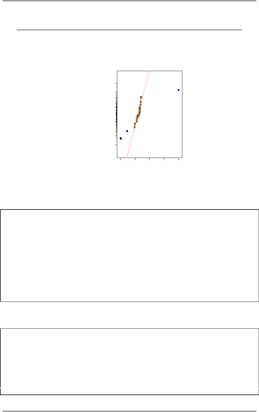
Solutions from Montgomery, D. C. (2001) Design and Analysis of Experiments, Wiley, NY
6-29
16 6 + + + + 729
(a) Estimate the factor effects. Construct a normal probability plot of the factor effects. Which effects
appear large?
DESIGN-EXPERT Plot
Etch R a te
A: Gap
B: Pressure
C: Gas Flow
D: Power
Normal plot
Norm al % probability
Effe ct
-1 5 3 .6 3 -3 8 . 69 76.25 191.19 306.13
1
5
10
20
30
50
70
80
90
95
99
A
D
AD
(b) Conduct an analysis of variance to confirm your findings for part (a).
Design Expert Output
Response: Etch Rate in A/min
ANOVA for Selected Factorial Model
Analysis of variance table [Partial sum of squares]
Sum of Mean F
Source Squares DF Square Value Prob > F
Model 5.106E+005 3 1.702E+005 97.91 < 0.0001 significant
A 41310.56 1 41310.56 23.77 0.0004
D 3.749E+005 1 3.749E+005 215.66 < 0.0001
AD 94402.56 1 94402.56 54.31 < 0.0001
Residual 20857.75 12 1738.15
Cor Total 5.314E+005 15
The Model F-value of 97.91 implies the model is significant. There is only
a 0.01% chance that a "Model F-Value" this large could occur due to noise.
Values of "Prob > F" less than 0.0500 indicate model terms are significant.
In this case A, D, AD are significant model terms.
(c) What is the regression model relating etch rate to the significant process variables?
Design Expert Output
Final Equation in Terms of Coded Factors:
Etch Rate =
+776.06
-50.81 * A
+153.06 * D
-76.81 * A * D
Final Equation in Terms of Actual Factors:
Etch Rate =
-5415.37500
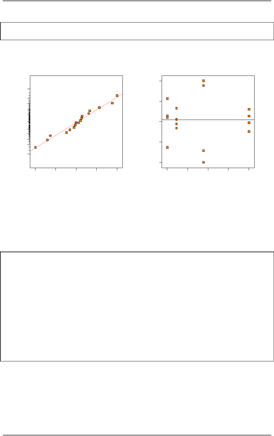
Solutions from Montgomery, D. C. (2001) Design and Analysis of Experiments, Wiley, NY
6-30
+4354.68750 * Gap
+21.48500 * Power
-15.36250 * Gap * Power
(d) Analyze the residuals from this experiment. Comment on the model’s adequacy.
Residual
Norm al % probability
Normal plot of residuals
-72.5 -37.75 -3 31.75 66.5
1
5
10
20
30
50
70
80
90
95
99
Predicted
Residuals
Residuals vs. Predicted
-7 2 .5
-3 7 .75
-3
31.75
66.5
597.00 711.94 826.88 941.81 1056.75
The residual versus predicted plot shows a slight football shape indicating very mild inequality of
variance.
(e) If not all the factors are important, project the 24 design into a 2k design with k<4 and conduct that
analysis of variance. The analysis of variance table is the same as in part (b).
Design Expert Output
Response: Etch Rate in A/min
ANOVA for Selected Factorial Model
Analysis of variance table [Partial sum of squares]
Sum of Mean F
Source Squares DF Square Value Prob > F
Model 5.106E+005 3 1.702E+005 97.91 < 0.0001 significant
A 41310.56 1 41310.56 23.77 0.0004
B 3.749E+005 1 3.749E+005 215.66 < 0.0001
AB 94402.56 1 94402.56 54.31 < 0.0001
Residual 20857.75 12 1738.15
Lack of Fit 0.000 0
Pure Error 20857.75 12 1738.15
Cor Total 5.314E+005 15
The Model F-value of 97.91 implies the model is significant. There is only
a 0.01% chance that a "Model F-Value" this large could occur due to noise.
Values of "Prob > F" less than 0.0500 indicate model terms are significant.
In this case A, B, AB are significant model terms.
(f) Draw graphs to interpret any significant interactions.
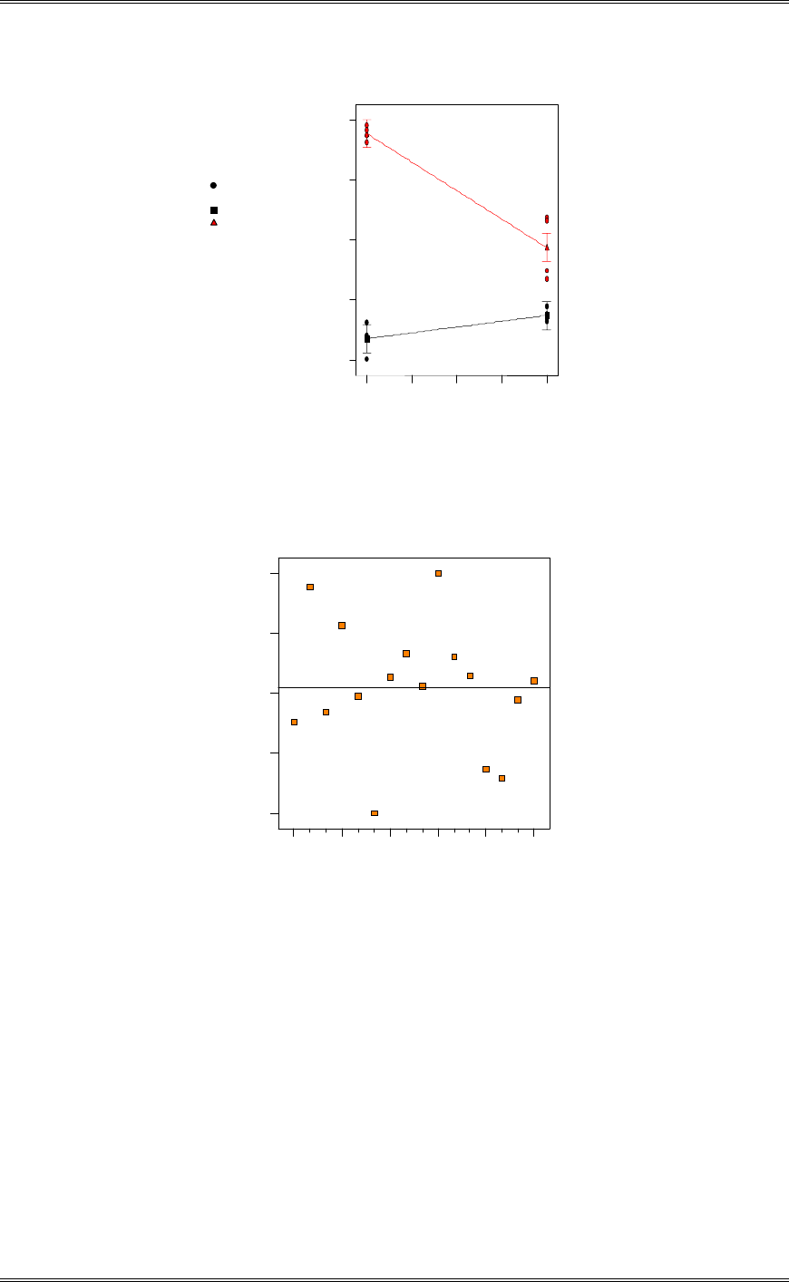
Solutions from Montgomery, D. C. (2001) Design and Analysis of Experiments, Wiley, NY
6-31
DESIGN-EXPERT Plot
Etch R a te
X = A: Gap
Y = B: Power
Design Points
B- 275.000
B+ 325.000
Power
Inte ra c ti o n G r a p h
Gap
Etch R a te
0.80 0.90 1.00 1.10 1.20
550
684.716
819.433
954.149
1088.87
(g) Plot the residuals versus the actual run order. What problems might be revealed by this plot?
Run Num ber
Residuals
Residuals vs. Run
-7 2 .5
-3 7 .75
-3
31.75
66.5
1 4 7 10 13 16
The plot of residuals versus run order can reveal trends in the process over time, inequality of variance
with time, and possibly indicate that there may be factors that were not included in the original
experiment.
6-19 Continuation of Problem 6-18. Consider the regression model obtained in part (c) of Problem 6-
18.
(a) Construct contour plots of the etch rate using this model.
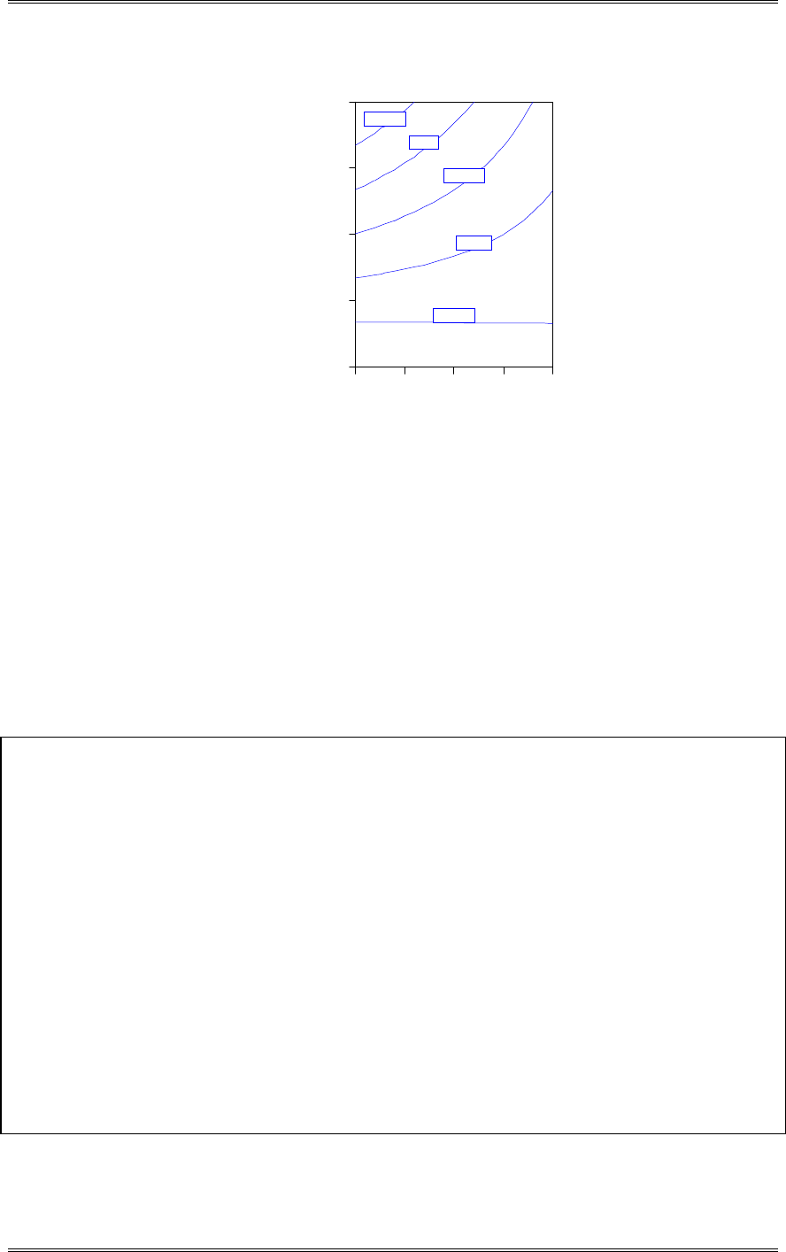
Solutions from Montgomery, D. C. (2001) Design and Analysis of Experiments, Wiley, NY
6-32
DESIGN-EXPERT Plot
Etch R a te
X = A: Gap
Y = D: Power
Actual Factors
B: Pressure = 500.00
C: Gas Flow = 162.50
Etch Rate
Gap
Power
0.80 0.90 1.00 1.10 1.20
275.00
287.50
300.00
312.50
325.00
673.625
750.25
826.875
903.5
980.125
(b) Suppose that it was necessary to operate this process at an etch rate of 800 Å/min. What settings of
the process variables would you recommend?
Run at the low level of anode-cathode gap (0.80 cm) and at a cathode power level of about 286 watts. The
curve is flatter (more robust) on the low end of the anode-cathode variable.
6-20 Consider the single replicate of the 24 design in Example 6-2. Suppose we had arbitrarily decided
to analyze the data assuming that all three- and four-factor interactions were negligible. Conduct this
analysis and compare your results with those obtained in the example. Do you think that it is a good idea
to arbitrarily assume interactions to be negligible even if they are relatively high-order ones?
Design Expert Output
Response: Etch Rate in A/min
ANOVA for Selected Factorial Model
Analysis of variance table [Partial sum of squares]
Sum of Mean F
Source Squares DF Square Value Prob > F
Model 5.212E+005 10 52123.41 25.58 0.0011 significant
A 41310.56 1 41310.56 20.28 0.0064
B 10.56 1 10.56 5.184E-003 0.9454
C 217.56 1 217.56 0.11 0.7571
D 3.749E+005 1 3.749E+005 183.99 < 0.0001
AB 248.06 1 248.06 0.12 0.7414
AC 2475.06 1 2475.06 1.21 0.3206
AD 94402.56 1 94402.56 46.34 0.0010
BC 7700.06 1 7700.06 3.78 0.1095
BD 1.56 1 1.56 7.669E-004 0.9790
CD 18.06 1 18.06 8.866E-003 0.9286
Residual 10186.81 5 2037.36
Cor Total 5.314E+005 15
The Model F-value of 25.58 implies the model is significant. There is only
a 0.11% chance that a "Model F-Value" this large could occur due to noise.
Values of "Prob > F" less than 0.0500 indicate model terms are significant.
In this case A, D, AD are significant model terms.
This analysis of variance identifies the same effects as the normal probability plot of effects approach used
in Example 6-2. In general, it is not a good idea to arbitrarily pool interactions. Use the normal
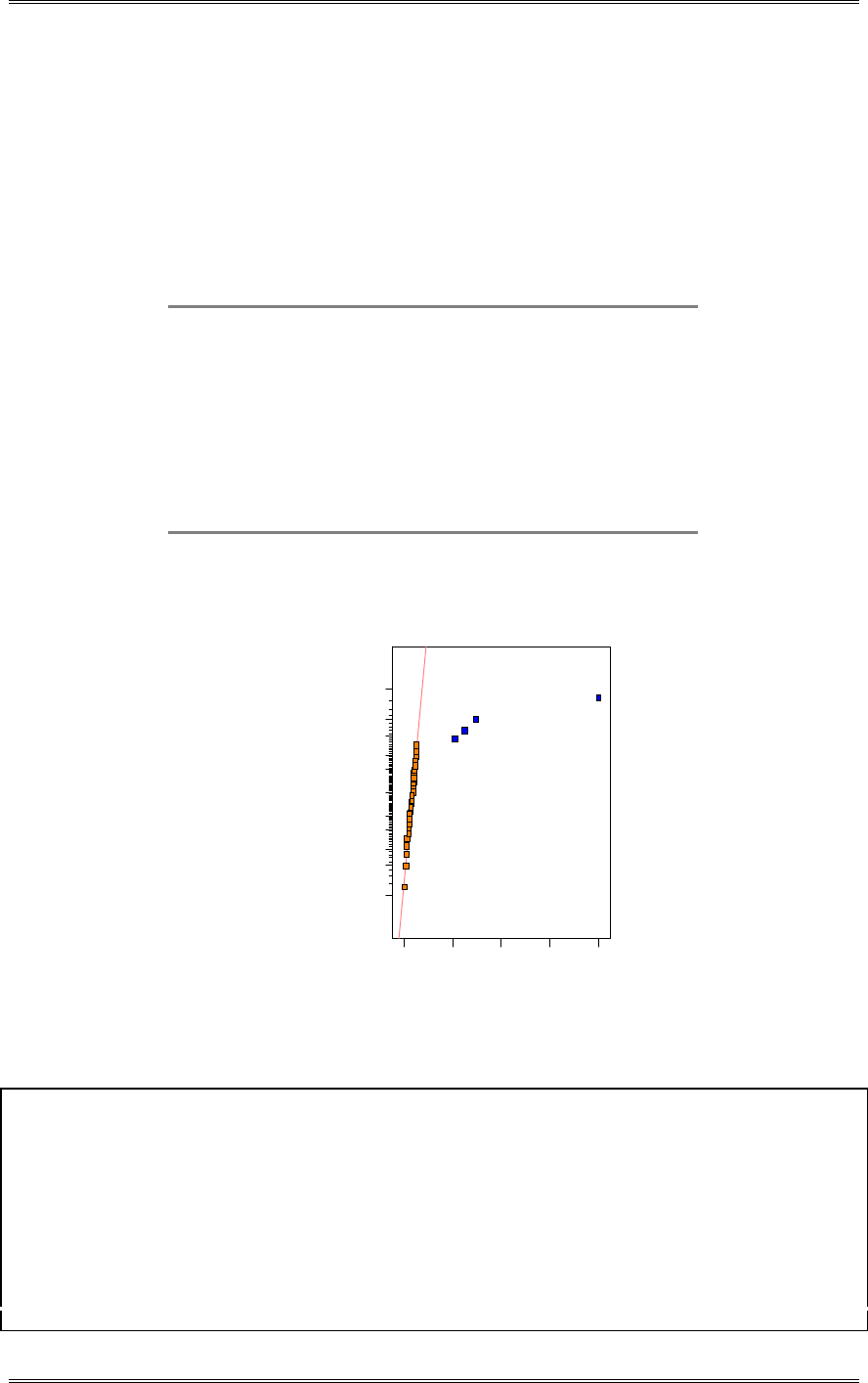
Solutions from Montgomery, D. C. (2001) Design and Analysis of Experiments, Wiley, NY
6-33
probability plot of effect estimates as a guide in the choice of which effects to tentatively include in the
model.
6-21 An experiment was run in a semiconductor fabrication plant in an effort to increase yield. Five
factors, each at two levels, were studied. The factors (and levels) were A = aperture setting (small, large),
B = exposure time (20% below nominal, 20% above nominal), C = development time (30 s, 45 s), D =
mask dimension (small, large), and E = etch time (14.5 min, 15.5 min). The unreplicated 25 design
shown below was run.
(1) = 7 d = 8 e = 8 de = 6
a = 9 ad = 10 ae = 12 ade = 10
b = 34 bd = 32 be = 35 bde = 30
ab = 55 abd = 50 abe = 52 abde = 53
c = 16 cd = 18 ce = 15 cde = 15
ac = 20 acd = 21 ace = 22 acde = 20
bc = 40 bcd = 44 bce = 45 bcde = 41
abc = 60 abcd = 61 abce = 65 abcde = 63
(a) Construct a normal probability plot of the effect estimates. Which effects appear to be large?
DESIGN-EXPERT Plot
Yield
A: Aperture
B: Exposure Time
C: Develop T im e
D: M ask Dim ension
E: Etch Time
Normal plot
Normal % probability
Effe ct
-1 .1 9 7.59 16.38 25.16 33.94
1
5
10
20
30
50
70
80
90
95
99
A
B
C
AB
(b) Conduct an analysis of variance to confirm your findings for part (a).
Design Expert Output
Response: Yield
ANOVA for Selected Factorial Model
Analysis of variance table [Partial sum of squares]
Sum of Mean F
Source Squares DF Square Value Prob > F
Model 11585.13 4 2896.28 991.83 < 0.0001 significant
A 1116.28 1 1116.28 382.27 < 0.0001
B 9214.03 1 9214.03 3155.34 < 0.0001
C 750.78 1 750.78 257.10 < 0.0001
AB 504.03 1 504.03 172.61 < 0.0001
Residual 78.84 27 2.92
Cor Total 11663.97 31
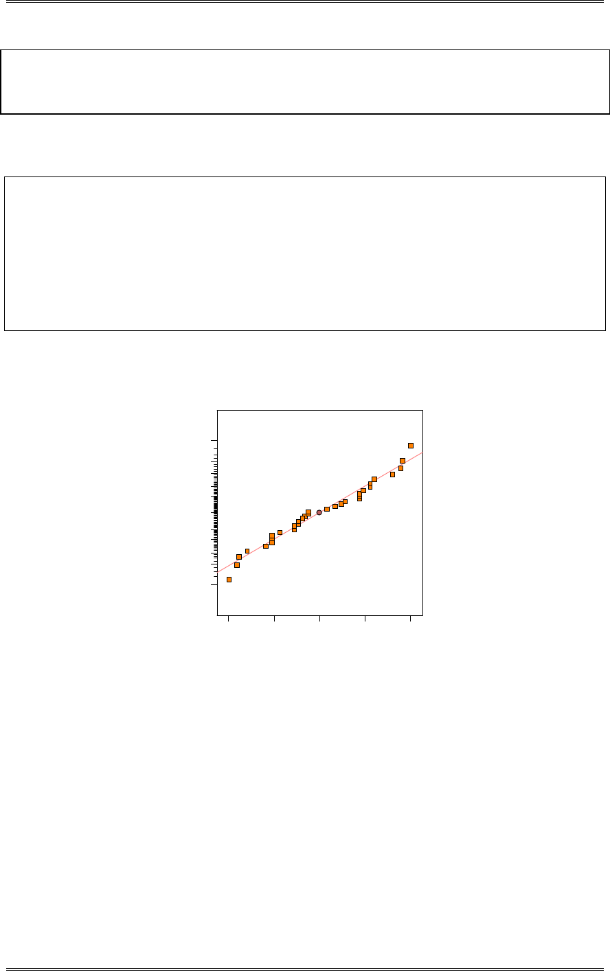
Solutions from Montgomery, D. C. (2001) Design and Analysis of Experiments, Wiley, NY
6-34
The Model F-value of 991.83 implies the model is significant. There is only
a 0.01% chance that a "Model F-Value" this large could occur due to noise.
Values of "Prob > F" less than 0.0500 indicate model terms are significant.
In this case A, B, C, AB are significant model terms.
(c) Write down the regression model relating yield to the significant process variables.
Design Expert Output
Final Equation in Terms of Actual Factors:
Aperture small
Yield =
+0.40625
+0.65000 * Exposure Time
+0.64583 * Develop Time
Aperture large
Yield =
+12.21875
+1.04688 * Exposure Time
+0.64583 * Develop Time
(d) Plot the residuals on normal probability paper. Is the plot satisfactory?
Residual
Norm al % probability
Normal plot of residuals
-2.78125 -1 .3 9 0 6 3 -3.55271E-015 1.39062 2.78125
1
5
10
20
30
50
70
80
90
95
99
There is nothing unusual about this plot.
(e) Plot the residuals versus the predicted yields and versus each of the five factors. Comment on the
plots.
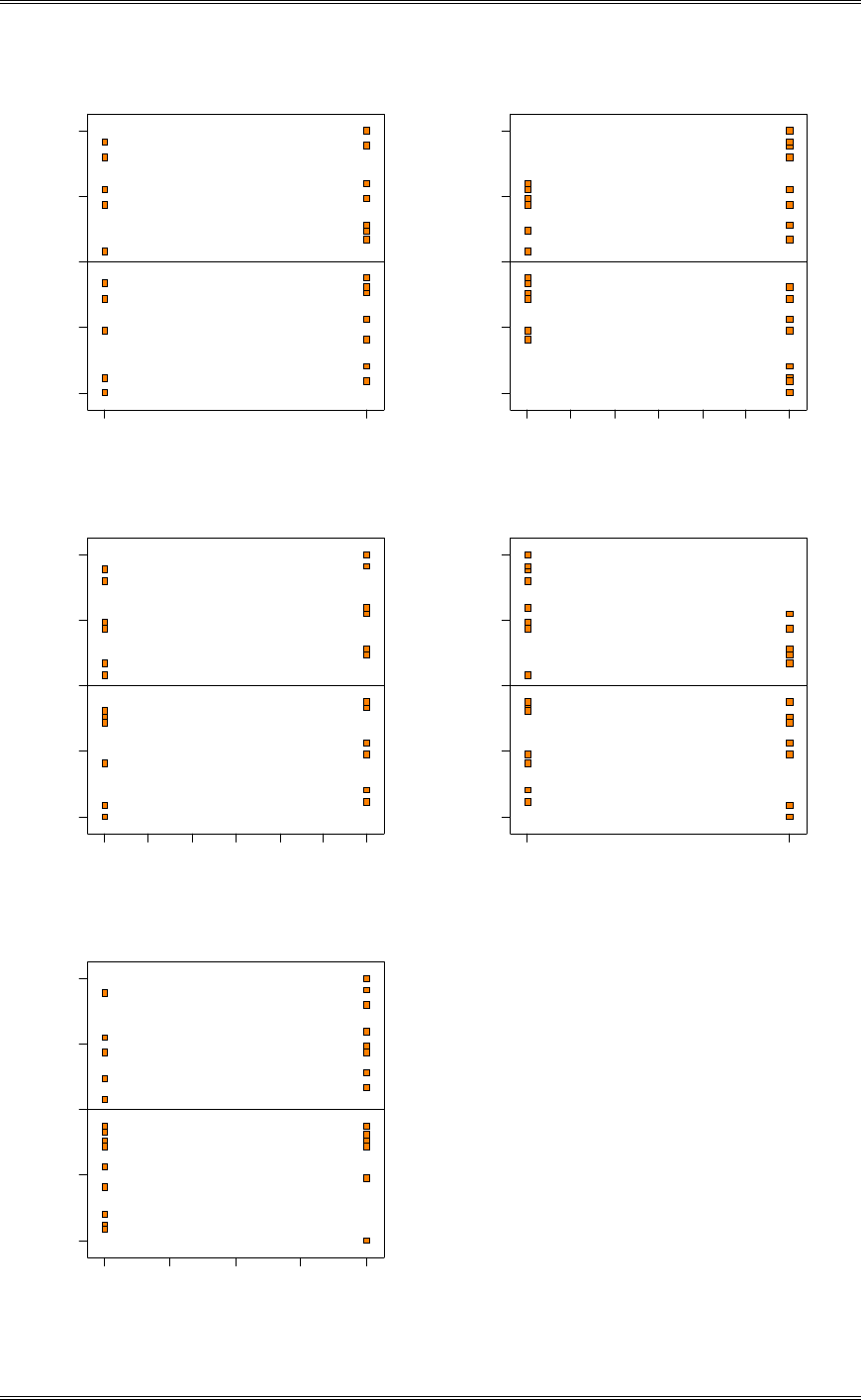
Solutions from Montgomery, D. C. (2001) Design and Analysis of Experiments, Wiley, NY
6-35
3
2
3
2
2
22
3
3
22
3
2
3
Ap e rture
Residuals
Residuals vs. Aperture
-2.78125
-1.39063
3.55271E-015
1.39062
2.78125
1 2
2
2
2
2
2
2
2
2
Expos ure Tim e
Residuals
Residuals vs. Exposure Time
-2.78125
-1.39063
3.55271E-015
1.39062
2.78125
-2 0 -1 3 -7 0 7 13 20
3
2
3
2
2
22
3
3
2
2
3
2
3
Develop Tim e
Residuals
Residuals vs. Develop Time
-2.78125
-1.39063
3.55271E-015
1.39062
2.78125
30 33 35 38 40 43 45
2
2
2
22
2
2
2
22
Mas k Dim en s ion
Residuals
Residuals vs. Mask Dimension
-2.78125
-1.39063
3.55271E-015
1.39062
2.78125
1 2
22
22
333
Etch Tim e
Residuals
Residuals vs. Etch Time
-2.78125
-1.39063
3.55271E-015
1.39062
2.78125
14.50 14.75 15.00 15.25 15.50
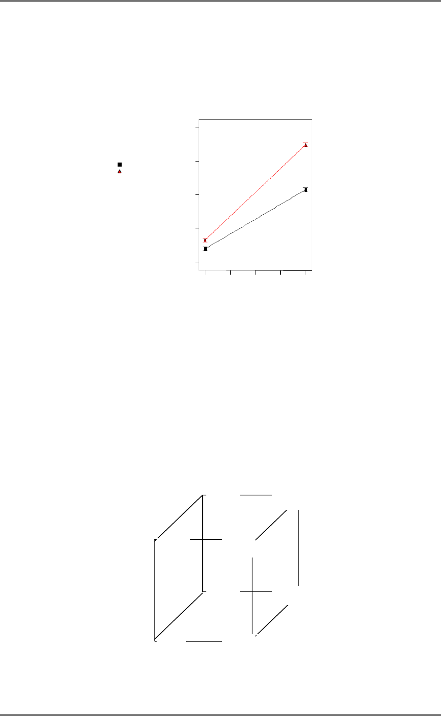
Solutions from Montgomery, D. C. (2001) Design and Analysis of Experiments, Wiley, NY
6-36
The plot of residual versus exposure time shows some very slight inequality of variance. There is no
strong evidence of a potential problem.
(f) Interpret any significant interactions.
DESIGN-EXPERT Plot
Yield
X = B: Exposure Time
Y = A: Aperture
A1 small
A2 large
Actual Factors
C: Develop T im e = 37.50
D: Mask Dimension = Small
E: Etch Time = 15.00
Ap e rture
Inte ra c ti o n G r a p h
Expos ure Time
Yie l d
-2 0 .00 -1 0 . 00 0.00 10.00 20.00
6
20.75
35.5
50.25
65
Factor A does not have as large an effect when B is at its low level as it does when B is at its high level.
(g) What are your recommendations regarding process operating conditions?
For the highest yield, run with B at the high level, A at the high level and C at the high level.
(h) Project the 25 design in this problem into a 2k design in the important factors. Sketch the design and
show the average and range of yields at each run. Does this sketch aid in interpreting the results of
this experiment?
DESIGN-EASE Analysis
Actual Yield
Aperture
E
x
p
o
s
u
r
e
T
i
m
e
Develop
Tim
e
A- A+
B-
B+
C-
C+
7.2500
R=2
16.0000
R=3
32.7500
R=5
42.5000
R=5
10.2500
R=3
20.7500
R=2
52.5000
R=5
62.2500
R=5

Solutions from Montgomery, D. C. (2001) Design and Analysis of Experiments, Wiley, NY
6-37
This cube plot aids in interpretation. The strong AB interaction and the large positive effect of C are
clearly evident.
6-22 Continuation of Problem 6-21. Suppose that the experimenter had run four runs at the center
points in addition to the 32 trials in the original experiment. The yields obtained at the center point runs
were 68, 74, 76, and 70.
(a) Reanalyze the experiment, including a test for pure quadratic curvature.
3376114
432
725312530432 2
2
.
.
nn
yynn
SS
CF
CFCF
ticPureQuadra
Design Expert Output
Response: Yield
ANOVA for Selected Factorial Model
Analysis of variance table [Partial sum of squares]
Sum of Mean F
Source Squares DF Square Value Prob > F
Model 11461.09 4 2865.27 353.92 < 0.0001 significant
A 992.25 1 992.25 122.56 < 0.0001
B 9214.03 1 9214.03 1138.12 < 0.0001
C 750.78 1 750.78 92.74 < 0.0001
AB 504.03 1 504.03 62.26 < 0.0001
Curvature 6114.34 1 6114.34 755.24 < 0.0001 significant
Residual 242.88 30 8.10
Cor Total 17818.31 35
The Model F-value of 353.92 implies the model is significant. There is only
a 0.01% chance that a "Model F-Value" this large could occur due to noise.
Values of "Prob > F" less than 0.0500 indicate model terms are significant.
In this case A, B, C, AB are significant model terms.
(b) Discuss what your next step would be.
Add axial points and fit a second-order model.
6-23 In a process development study on yield, four factors were studied, each at two levels: time (A),
concentration (B), pressure (C), and temperature (D). A single replicate of a 24 design was run, and the
resulting data are shown in the following table:
Actual
Run Run Yield Factor Levels
Number Order A B C D (lbs) Low (-) High (+)
1 5 - - - - 12 A (h) 2.5 3.0
2 9 + - - - 18 B (%) 14 18
3 8 - + - - 13 C (psi) 60 80
4 13 + + - - 16 D (ºC) 225 250
5 3 - - + - 17
6 7 + - + - 15
7 14 - + + - 20
8 1 + + + - 15
9 6 - - - + 10
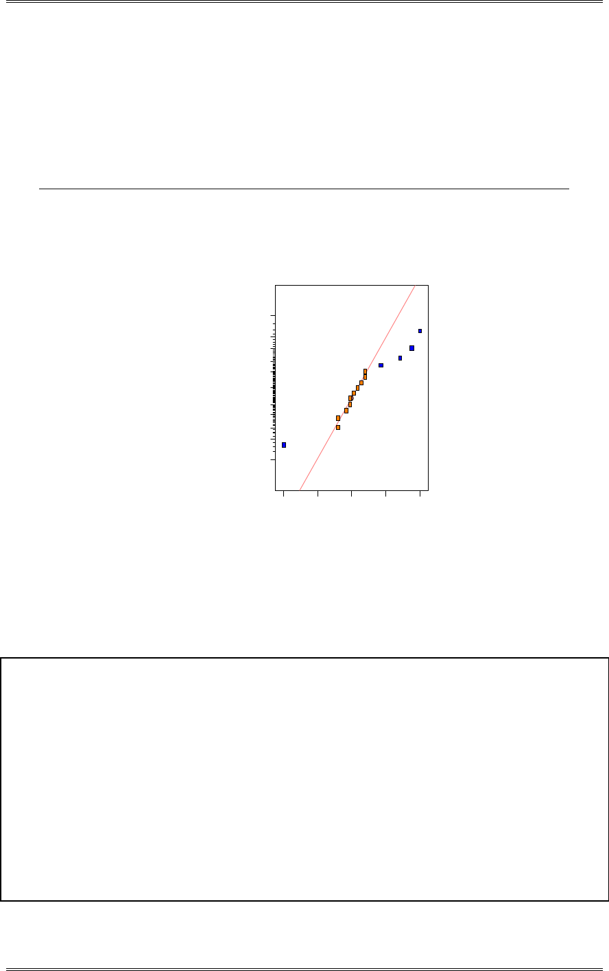
Solutions from Montgomery, D. C. (2001) Design and Analysis of Experiments, Wiley, NY
6-38
10 11 + - - + 25
11 2 - + - + 13
12 15 + + - + 24
13 4 - - + + 19
14 16 + - + + 21
15 10 - + + + 17
16 12 + + + + 23
(a) Construct a normal probability plot of the effect estimates. Which factors appear to have large
effects?
DESIGN-EXPERT Plot
Yield
A: Time
B: Concentration
C: Pressure
D: Temperature
Normal plot
Normal % probability
Effe ct
-4 .2 5 -2 .0 6 0.13 2.31 4.50
1
5
10
20
30
50
70
80
90
95
99
A
CD
AC
AD
A, C, D and the AC and AD interactions.
(b) Conduct an analysis of variance using the normal probability plot in part (a) for guidance in forming
an error term. What are your conclusions?
Design Expert Output
Response: Yield
ANOVA for Selected Factorial Model
Analysis of variance table [Partial sum of squares]
Sum of Mean F
Source Squares DF Square Value Prob > F
Model 275.50 5 55.10 33.91 < 0.0001 significant
A 81.00 1 81.00 49.85 < 0.0001
C 16.00 1 16.00 9.85 0.0105
D 42.25 1 42.25 26.00 0.0005
AC 72.25 1 72.25 44.46 < 0.0001
AD 64.00 1 64.00 39.38 < 0.0001
Residual 16.25 10 1.62
Cor Total 291.75 15
The Model F-value of 33.91 implies the model is significant. There is only
a 0.01% chance that a "Model F-Value" this large could occur due to noise.
Values of "Prob > F" less than 0.0500 indicate model terms are significant.
In this case A, C, D, AC, AD are significant model terms.
(c) Write down a regression model relating yield to the important process variables.
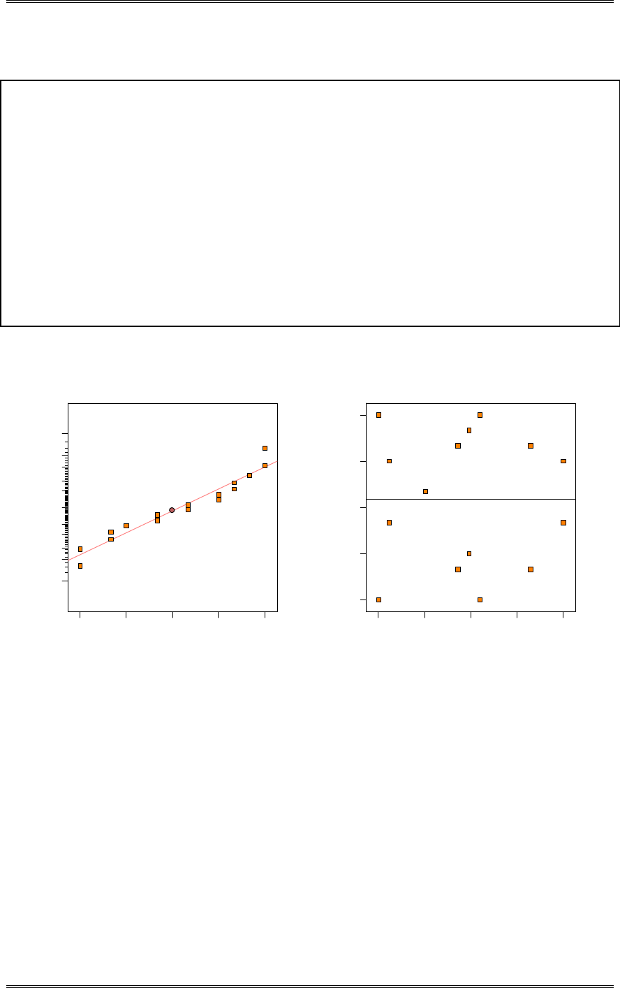
Solutions from Montgomery, D. C. (2001) Design and Analysis of Experiments, Wiley, NY
6-39
Design Expert Output
Final Equation in Terms of Coded Factors:
Yield =
+17.38
+2.25 *A
+1.00 *C
+1.63 *D
-2.13 *A*C
+2.00 *A*D
Final Equation in Terms of Actual Factors:
Yield =
+209.12500
-83.50000 * Time
+2.43750 * Pressure
-1.63000 * Temperature
-0.85000 * Time * Pressure
+0.64000 * Time * Temperature
(d) Analyze the residuals from this experiment. Does your analysis indicate any potential problems?
Residual
Normal % probability
Normal plot of residuals
-1 .6 25 -0 . 8 75 -0 .1 2 5 0.625 1.375
1
5
10
20
30
50
70
80
90
95
99
22
Predicted
Residuals
Residuals vs. Predicted
-1 .6 25
-0 .8 75
-0 .1 25
0.625
1.375
11.63 14.81 18.00 21.19 24.38
Solutions from Montgomery, D. C. (2001) Design and Analysis of Experiments, Wiley, NY
6-40
Run Num ber
Residuals
Residuals vs. Run
-1 .6 25
-0 .8 75
-0 .1 25
0.625
1.375
14710 13 16
There is nothing unusual about the residual plots.
(e) Can this design be collapsed into a 23 design with two replicates? If so, sketch the design with the
average and range of yield shown at each point in the cube. Interpret the results.
DESIGN-EASE Analysis
Actual yield
time
t
e
m
p
e
r
a
t
u
r
e
pressure
A- A+
D-
D+
C-
C+
12.5
R=1
18.5
R=3
11.5
R=3
18.0
R=2
17.0
R=2
15.0
R=0
24.5
R=1
22.0
R=2
6-24 Continuation of Problem 6-23. Use the regression model in part (c) of Problem 6-23 to generate a
response surface contour plot of yield. Discuss the practical purpose of this response surface plot.

Solutions from Montgomery, D. C. (2001) Design and Analysis of Experiments, Wiley, NY
6-41
The response surface contour plot shows the adjustments in the process variables that lead to an
increasing or decreasing response. It also displays the curvature of the response in the design region,
possibly indicating where robust operating conditions can be found. Two response surface contour plots
for this process are shown below. These were formed from the model written in terms of the original
design variables.
DESIGN-EXPERT Plot
Yield
X = A: Tim e
Y = C: Pressure
Actual Factors
B: Concentration = 16.00
D: Temperature = 237.50
Yie ld
Tim e
Pressure
2.50 2.63 2.75 2.88 3.00
60.00
65.00
70.00
75.00
80.00
13.4583
14.9167
16.375
17.8333
19.2917
DESIGN-EXPERT Plot
Yield
X = A: Tim e
Y = D: Temperature
Actual Factors
B: Concentration = 16.00
C: Pressure = 70.00
Yie ld
Tim e
Tem perature
2.50 2.63 2.75 2.88 3.00
225.00
231.25
237.50
243.75
250.00
16.375
17.8333
19.2917
6-25 The scrumptious brownie experiment. The author is an engineer by training and a firm believer
in learning by doing. I have taught experimental design for many years to a wide variety of audiences and
have always assigned the planning, conduct, and analysis of an actual experiment to the class participants.
The participants seem to enjoy this practical experience and always learn a great deal from it. This
problem uses the results of an experiment performed by Gretchen Krueger at Arizona State University.
There are many different ways to bake brownies. The purpose of this experiment was to determine how
the pan material, the brand of brownie mix, and the stirring method affect the scrumptiousness of
brownies. The factor levels were
Factor Low (-) High (+)
A = pan material Glass Aluminum
B = stirring method Spoon Mixer
C = brand of mix Expensive Cheap
The response variable was scrumptiousness, a subjective measure derived from a questionnaire given to
the subjects who sampled each batch of brownies. (The questionnaire dealt with such issues as taste,
appearance, consistency, aroma, and so forth.) An eight-person test panel sampled each batch and filled
out the questionnaire. The design matrix and the response data are shown below:
Brownie Test Panel Results
Batch A B C 1 2 3 4 5 6 7 8
1 - - - 11 9 10 10 11 10 8 9
2 + - - 15 10 16 14 12 9 6 15
3 - + - 9 12 11 11 11 11 11 12
4 + + - 16 17 15 12 13 13 11 11
5 - - + 10 11 15 8 6 8 9 14

Solutions from Montgomery, D. C. (2001) Design and Analysis of Experiments, Wiley, NY
6-42
6 + - + 12 13 14 13 9 13 14 9
7 - + + 10 12 13 10 7 7 17 13
8 + + + 15 12 15 13 12 12 9 14
(a) Analyze the data from this experiment as if there were eight replicates of a 23 design. Comment on
the results.
Design Expert Output
ANOVA for Selected Factorial Model
Analysis of variance table [Partial sum of squares]
Sum of Mean F
Source Squares DF Square Value Prob > F
Model 93.25 7 13.32 2.20 0.0475 significant
A 72.25 1 72.25 11.95 0.0010
B 18.06 1 18.06 2.99 0.0894
C 0.063 1 0.063 0.010 0.9194
AB 0.062 1 0.062 0.010 0.9194
AC 1.56 1 1.56 0.26 0.6132
BC 1.00 1 1.00 0.17 0.6858
ABC 0.25 1 0.25 0.041 0.8396
Residual 338.50 56 6.04
Lack of Fit 0.000 0
Pure Error 338.50 56 6.04
Cor Total 431.75 63
The Model F-value of 2.20 implies the model is significant. There is only
a 4.75% chance that a "Model F-Value" this large could occur due to noise.
Values of "Prob > F" less than 0.0500 indicate model terms are significant.
In this case A are significant model terms.
In this analysis, A, the pan material and B, the stirring method, appear to be significant. There are 56
degrees of freedom for the error, yet only eight batches of brownies were cooked, one for each recipe.
(b) Is the analysis in part (a) the correct approach? There are only eight batches; do we really have eight
replicates of a 23 factorial design?
The different rankings by the taste-test panel are not replicates, but repeat observations by differenttesters
on the same batch of brownies. It is not a good idea to use the analysis in part (a) because the estimate of
error may not reflect the batch-to-batch variation.
(c) Analyze the average and standard deviation of the scrumptiousness ratings. Comment on the results.
Is this analysis more appropriate than the one in part (a)? Why or why not?
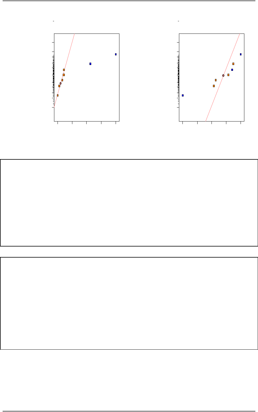
Solutions from Montgomery, D. C. (2001) Design and Analysis of Experiments, Wiley, NY
6-43
DESIGN-EXPERT Plot
Average
A: Pan M aterial
B: Stirring Method
C: Mix Brand
Normal plot
Norm al % probability
Effe ct
-0 .3 2 0.29 0.91 1.52 2.13
1
5
10
20
30
50
70
80
90
95
99
A
B
DESIGN-EXPERT Plot
Stdev
A: Pan M aterial
B: Stirring Method
C: Mix Brand
Normal plot
Norm al % probability
Effe ct
-1 .5 7 -1 .0 1 -0 .4 5 0.11 0.68
1
5
10
20
30
50
70
80
90
95
99
A
C
AC
Design Expert Output
Response: Average
ANOVA for Selected Factorial Model
Analysis of variance table [Partial sum of squares]
Sum of Mean F
Source Squares DF Square Value Prob > F
Model 11.28 2 5.64 76.13 0.0002 significant
A 9.03 1 9.03 121.93 0.0001
B 2.25 1 2.25 30.34 0.0027
Residual 0.37 5 0.074
Cor Total 11.65 7
The Model F-value of 76.13 implies the model is significant. There is only
a 0.02% chance that a "Model F-Value" this large could occur due to noise.
Values of "Prob > F" less than 0.0500 indicate model terms are significant.
In this case A, B are significant model terms.
Design Expert Output
Response: Stdev
ANOVA for Selected Factorial Model
Analysis of variance table [Partial sum of squares]
Sum of Mean F
Source Squares DF Square Value Prob > F
Model 6.05 3 2.02 9.77 0.0259 significant
A 0.24 1 0.24 1.15 0.3432
C 0.91 1 0.91 4.42 0.1034
AC 4.90 1 4.90 23.75 0.0082
Residual 0.82 4 0.21
Cor Total 6.87 7
The Model F-value of 9.77 implies the model is significant. There is only
a 2.59% chance that a "Model F-Value" this large could occur due to noise.
Values of "Prob > F" less than 0.0500 indicate model terms are significant.
In this case AC are significant model terms.
Variables A and B affect the mean rank of the brownies. Note that the AC interaction affects the standard
deviation of the ranks. This is an indication that both factors A and C have some effect on the variability
in the ranks. It may also indicate that there is some inconsistency in the taste test panel members. For the
analysis of both the average of the ranks and the standard deviation of the ranks, the mean square error is

Solutions from Montgomery, D. C. (2001) Design and Analysis of Experiments, Wiley, NY
6-44
now determined by pooling apparently unimportant effects. This is a more estimate of error than obtained
assuming that all observations were replicates.
6-26 An experiment was conducted on a chemical process that produces a polymer. The four factors
studied were temperature (A), catalyst concentration (B), time (C), and pressure (D). Two responses,
molecular weight and viscosity, were observed. The design matrix and response data are shown below:
Actual
Run Run Molecular Factor Levels
Number Order A B C D Weight Viscosity Low (-) High (+)
1 18 - - - - 2400 1400 A (ºC) 100 120
2 9 + - - - 2410 1500 B (%) 4 8
3 13 - + - - 2315 1520 C (min) 20 30
4 8 + + - - 2510 1630 D (psi) 60 75
5 3 - - + - 2615 1380
6 11 + - + - 2625 1525
7 14 - + + - 2400 1500
8 17 + + + - 2750 1620
9 6 - - - + 2400 1400
10 7 + - - + 2390 1525
11 2 - + - + 2300 1500
12 10 + + - + 2520 1500
13 4 - - + + 2625 1420
14 19 + - + + 2630 1490
15 15 - + + + 2500 1500
16 20 + + + + 2710 1600
17 1 0 0 0 0 2515 1500
18 5 0 0 0 0 2500 1460
19 16 0 0 0 0 2400 1525
20 12 0 0 0 0 2475 1500
(a) Consider only the molecular weight response. Plot the effect estimates on a normal probability scale.
What effects appear important?
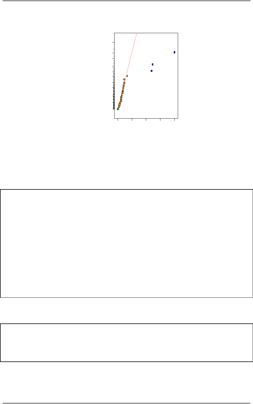
Solutions from Montgomery, D. C. (2001) Design and Analysis of Experiments, Wiley, NY
6-45
DESIGN-EXPERT Plot
Molecular Wt
A: Temperature
B: Catalyst Con.
C: Tim e
D: Pressure
Half Normal plot
Half Normal % probability
Effe ct
0.00 50.31 100.63 150.94 201.25
0
20
40
60
70
80
85
90
95
97
99
A
C
AB
A, C and the AB interaction.
(b) Use an analysis of variance to confirm the results from part (a). Is there an indication of curvature?
A,C and the AB interaction are significant. While the main effect of B is not significant, it could be
included to preserve hierarchy in the model. There is no indication of quadratic curvature.
Design Expert Output
Response: Molecular Wt
ANOVA for Selected Factorial Model
Analysis of variance table [Partial sum of squares]
Sum of Mean F
Source Squares DF Square Value Prob > F
Model 2.809E+005 3 93620.83 73.00 < 0.0001 significant
A 61256.25 1 61256.25 47.76 < 0.0001
C 1.620E+005 1 1.620E+005 126.32 < 0.0001
AB 57600.00 1 57600.00 44.91 < 0.0001
Curvature 3645.00 1 3645.00 2.84 0.1125 not significant
Residual 19237.50 15 1282.50
Lack of Fit 11412.50 12 951.04 0.36 0.9106 not significant
Pure Error 7825.00 3 2608.33
Cor Total 3.037E+005 19
The Model F-value of 73.00 implies the model is significant. There is only
a 0.01% chance that a "Model F-Value" this large could occur due to noise.
Values of "Prob > F" less than 0.0500 indicate model terms are significant.
In this case A, C, AB are significant model terms.
(c) Write down a regression model to predict molecular weight as a function of the important variables.
Design Expert Output
Final Equation in Terms of Coded Factors:
Molecular Wt =
+2506.25
+61.87 * A
+100.63 * C
+60.00 * A * B
(d) Analyze the residuals and comment on model adequacy.
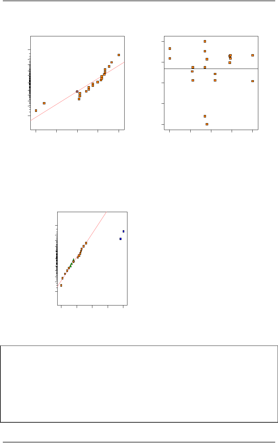
Solutions from Montgomery, D. C. (2001) Design and Analysis of Experiments, Wiley, NY
6-46
Residual
Normal % probability
Normal plot of residuals
-8 5 -53.125 -21.25 10.625 42.5
1
5
10
20
30
50
70
80
90
95
99
22
Predicted
Residuals
Residuals vs. Predicted
-8 5
-5 3 .12 5
-2 1 .25
10.625
42.5
2283.75 2395.00 2506.25 2617.50 2728.75
There are two residuals that appear to be large and should be investigated.
(e) Repeat parts (a) - (d) using the viscosity response.
DESIGN-EXPERT Plot
Viscosity
A: Temperature
B: Catalyst Con.
C: Tim e
D: Pressure
Normal plot
Normal % probability
Effe ct
-2 5 .00 5.31 35.62 65.94 96.25
1
5
10
20
30
50
70
80
90
95
99 A
B
Design Expert Output
Response: Viscosity
ANOVA for Selected Factorial Model
Analysis of variance table [Partial sum of squares]
Sum of Mean F
Source Squares DF Square Value Prob > F
Model 70362.50 2 35181.25 35.97 < 0.0001 significant
A 37056.25 1 37056.25 37.88 < 0.0001
B 33306.25 1 33306.25 34.05 < 0.0001
Curvature 61.25 1 61.25 0.063 0.8056 not significant
Residual 15650.00 16 978.13
Lack of Fit 13481.25 13 1037.02 1.43 0.4298 not significant
Pure Error 2168.75 3 722.92
Cor Total 86073.75 19
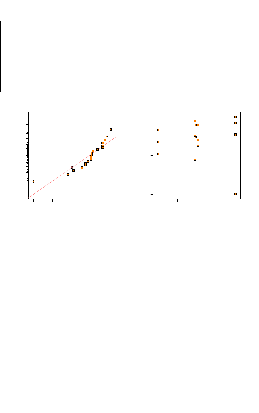
Solutions from Montgomery, D. C. (2001) Design and Analysis of Experiments, Wiley, NY
6-47
The Model F-value of 35.97 implies the model is significant. There is only
a 0.01% chance that a "Model F-Value" this large could occur due to noise.
Values of "Prob > F" less than 0.0500 indicate model terms are significant.
In this case A, B are significant model terms.
Final Equation in Terms of Coded Factors:
Viscosity =
+1500.62
+48.13 * A
+45.63 * B
Residual
Norm al % probability
Normal plot of residuals
-94.375 -61.875 -29.375 3.125 35.625
1
5
10
20
30
50
70
80
90
95
99
2
2
3
2
2
33
22
Predicted
Residuals
Residuals vs. Predicted
-9 4 .37 5
-6 1 .87 5
-2 9 .37 5
3.125
35.625
1406.87 1453.75 1500.62 1547.50 1594.37
There is one large residual that should be investigated.
6-27 Continuation of Problem 6-26. Use the regression models for molecular weight and viscosity to
answer the following questions.
(a) Construct a response surface contour plot for molecular weight. In what direction would you adjust
the process variables to increase molecular weight? Increase temperature, catalyst and time.
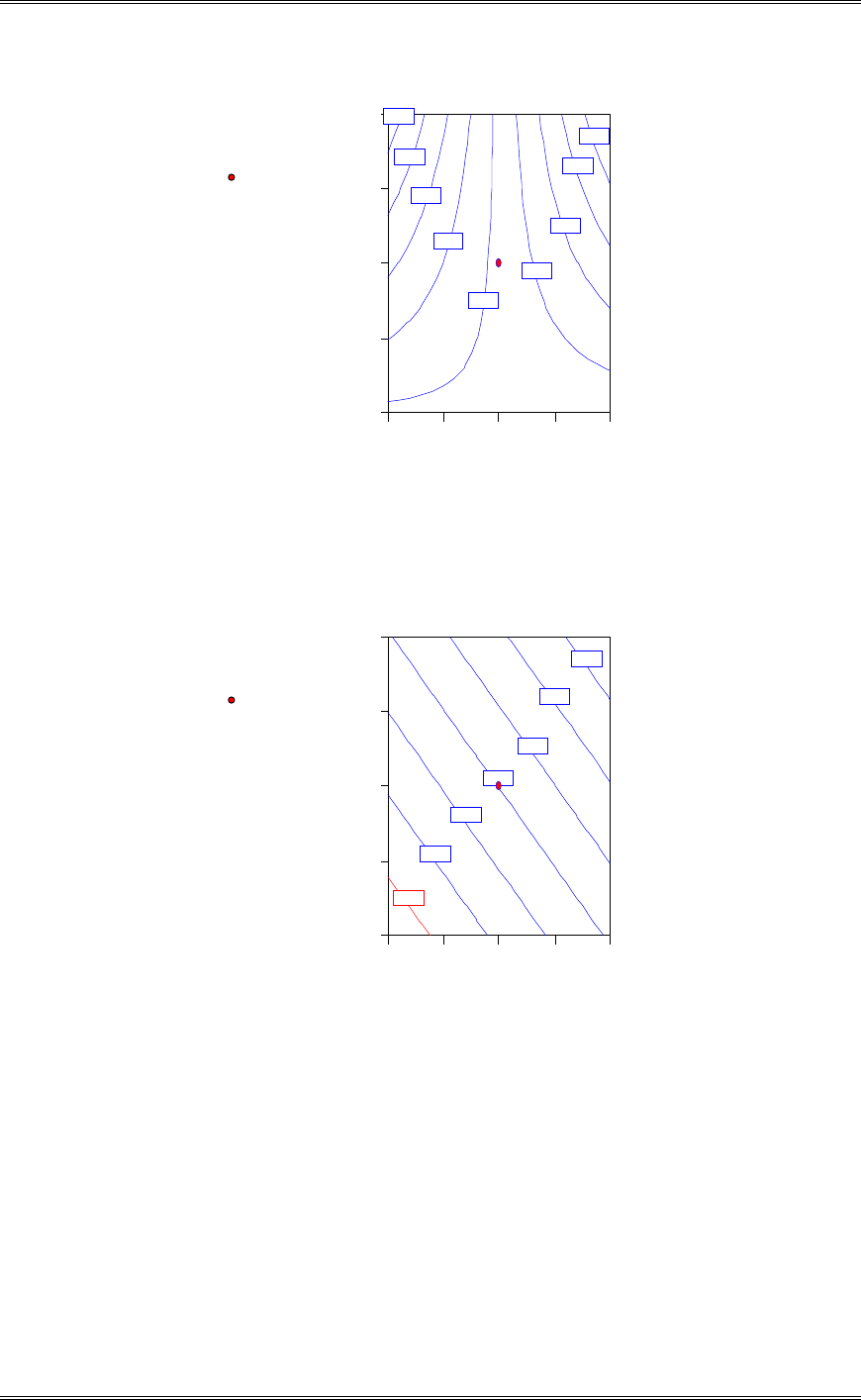
Solutions from Montgomery, D. C. (2001) Design and Analysis of Experiments, Wiley, NY
6-48
DESIGN-EXPERT Plot
Molecular Wt
X = A: Temperature
Y = B: Catalyst Con.
Design P oints
Actual Factors
C: T im e = 25 .00
D: Pressure = 67.50
Mo lec ular W t
A: Temperature
B: C atalyst C on.
100.00 105.00 110.00 115.00 120.00
4.00
5.00
6.00
7.00
8.00 2400
2425
2450
2475
2500
2525
2550
2575
2600
4
(a) Construct a response surface contour plot for viscosity. In what direction would you adjust the
process variables to decrease viscosity?
DESIGN-EXPERT Plot
V i sco si ty
X = A: Temperature
Y = B: Catalyst Con.
Design P oints
Actual Factors
C: T im e = 25 .00
D: Pressure = 67.50
Viscosity
A: Temperature
B: C atalyst C on.
100.00 105.00 110.00 115.00 120.00
4.00
5.00
6.00
7.00
8.00
1425
1450
1475
1500
1525
1550
1575
4
Decrease temperature and catalyst.
(c) What operating conditions would you recommend if it was necessary to produce a product with a
molecular weight between 2400 and 2500, and the lowest possible viscosity?

Solutions from Montgomery, D. C. (2001) Design and Analysis of Experiments, Wiley, NY
6-49
DESIGN-EXPERT Plot
Overlay Plot
X = A: Temperature
Y = B: Catalyst Con.
Actual Factors
C: T im e = 24 .50
D: Pressure = 67.50
Overlay Plot
A: Temperature
B: C atalyst C on.
100.00 105.00 110.00 115.00 120.00
4.00
5.00
6.00
7.00
8.00
Mole cular Wt: 25 00
Viscosity: 1450
Set the temperature between 100 and 105, the catalyst between 4 and 5%, and the time at 24.5 minutes.
The pressure was not significant and can be set at conditions that may improve other results of the process
such as cost.
6-28 Consider the single replicate of the 24 design in Example 6-2. Suppose that we ran five points at
the center (0,0,0,0) and observed the following responses: 73, 75, 71, 69, and 76. Test for curvature in
this experiment. Interpret the results.
Design Expert Output
Response: Filtration Rate
ANOVA for Selected Factorial Model
Analysis of variance table [Partial sum of squares]
Sum of Mean F
Source Squares DF Square Value Prob > F
Model 5535.81 5 1107.16 68.01 < 0.0001 significant
A 1870.56 1 1870.56 114.90 < 0.0001
C 390.06 1 390.06 23.96 0.0002
D 855.56 1 855.56 52.55 < 0.0001
AC 1314.06 1 1314.06 80.71 < 0.0001
AD 1105.56 1 1105.56 67.91 < 0.0001
Curvature 28.55 1 28.55 1.75 0.2066 not significant
Residual 227.93 14 16.28
Lack of Fit 195.13 10 19.51 2.38 0.2093 not significant
Pure Error 32.80 4 8.20
Cor Total 5792.29 20
The Model F-value of 68.01 implies the model is significant. There is only
a 0.01% chance that a "Model F-Value" this large could occur due to noise.
Values of "Prob > F" less than 0.0500 indicate model terms are significant.
In this case A, C, D, AC, AD are significant model terms.
The "Curvature F-value" of 1.75 implies the curvature (as measured by difference between the
average of the center points and the average of the factorial points) in the design space is not
significant relative to the noise. There is a 20.66% chance that a "Curvature F-value"
this large could occur due to noise.
There is no indication of curvature.

Solutions from Montgomery, D. C. (2001) Design and Analysis of Experiments, Wiley, NY
6-50
6-29 A missing value in a 2k factorial. It is not unusual to find that one of the observations in a 2k
design is missing due to faulty measuring equipment, a spoiled test, or some other reason. If the design is
replicated n times (n>1) some of the techniques discussed in Chapter 14 can be employed, including
estimating the missing observations. However, for an unreplicated factorial (n-1) some other method must
be used. One logical approach is to estimate the missing value with a number that makes the highest-
order interaction contrast zero. Apply this technique to the experiment in Example 6-2 assuming that run
ab is missing. Compare the results with the results of Example 6-2.
Treatment
Com bination R esponse R esponse *
ABCD ABCD A B C D
(1) 45 45 1 -1-1-1-1
a71 -71 -11-1-1-1
b48 -48 -1-11-1-1
ab missing m issing * 1111-1-1
c68 -68 -1-1-11-1
ac 60 60 1 1 -11-1
bc 80 80 1 -111-1
abc 65 -65 -1111-1
d43 -43 -1-1-1-11
ad 100 100 1 1 -1-11
bd 45 45 1 -11-11
abd 104 -104 -111-11
cd 75 75 1 -1-111
acd 86 -86 -11-111
bcd 70 -70 -1-1111
abcd 96 9611111
Contrast (ABCD ) = missing - 54 = 0
missing = 54
Substitute the value 54 for the missing run at ab.
Term Effect SumSqr % Contribtn
Model Intercept
Model A 20.25 1640.25 27.5406
Model B 1.75 12.25 0.205684
Model C 11.25 506.25 8.50019
Model D 16 1024 17.1935
Model AB -1.25 6.25 0.104941
Model AC -16.75 1122.25 18.8431
Model AD 18 1296 21.7605
Model BC 3.75 56.25 0.944465
Model BD 1 4 0.067162
Model CD -2.5 25 0.419762
Model ABC 3.25 42.25 0.709398
Model ABD 5.5 121 2.03165
Model ACD -3 36 0.604458
Model BCD -4 64 1.07459
Model ABCD 0 0 0
Lenth's ME 11.5676
Lenth's SME 23.4839
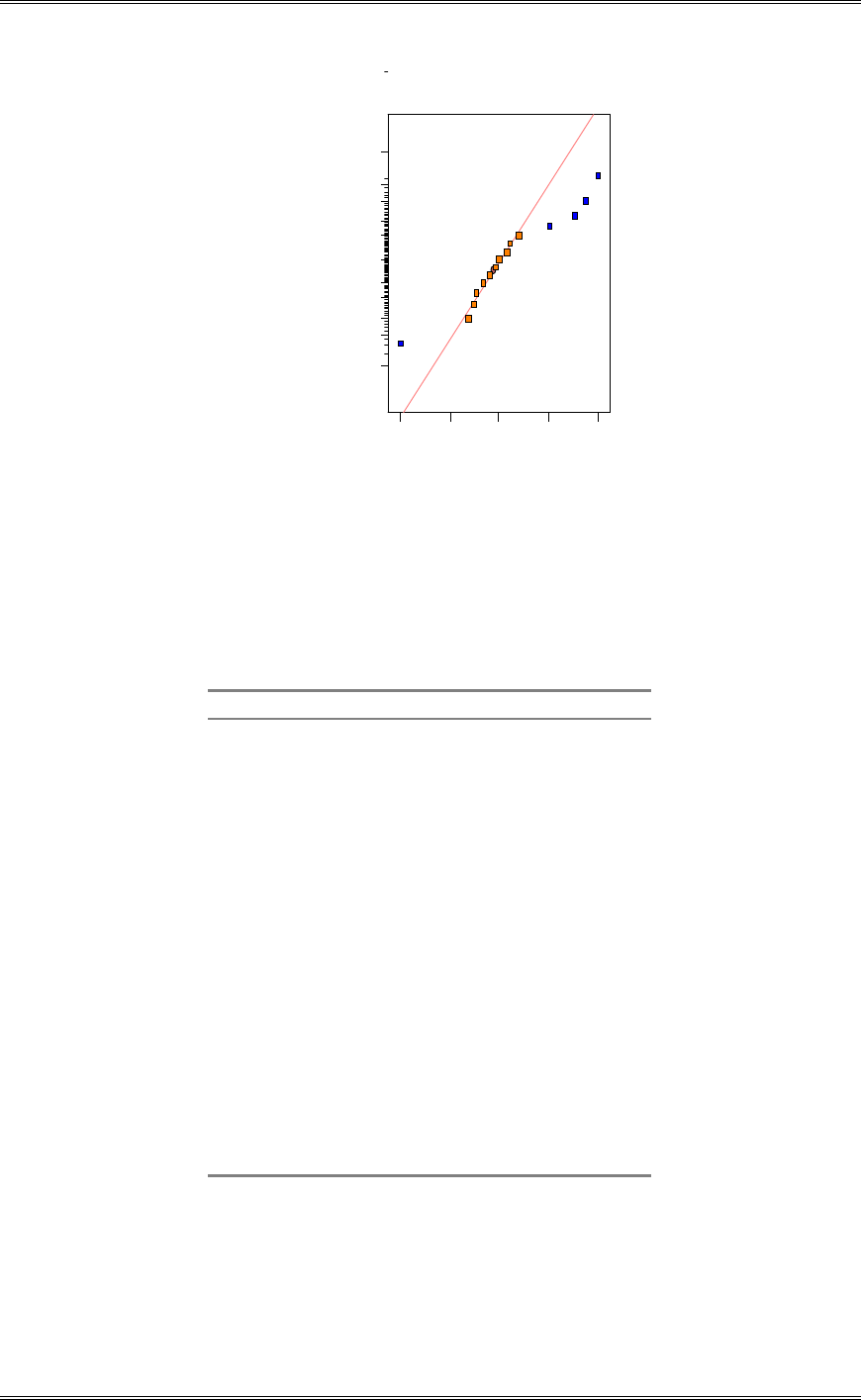
Solutions from Montgomery, D. C. (2001) Design and Analysis of Experiments, Wiley, NY
6-51
DESIGN-EXPERT Plot
Filtration Rate
A: T emperature
B: Pressure
C: Concentration
D: Stirring Rate
Normal plot
Norm al % probability
Effe ct
-16.75 -7 .5 0 1.75 11.00 20.25
1
5
10
20
30
50
70
80
90
95
99
A
CD
AC
AD
6-30 An engineer has performed an experiment to study the effect of four factors on the surface
roughness of a machined part. The factors (and their levels) are A = tool angle (12 degrees, 15 degrees),
B = cutting fluid viscosity (300, 400), C = feed rate (10 in/min, 15 in/min), and D = cutting fluid cooler
used (no, yes). The data from this experiment (with the factors coded to the usual -1, +1 levels) are shown
below.
Run A B C D Surface Roughness
1 - - - - 0.00340
2 + - - - 0.00362
3 - + - - 0.00301
4 + + - - 0.00182
5 - - + - 0.00280
6 + - + - 0.00290
7 - + + - 0.00252
8 + + + - 0.00160
9 - - - + 0.00336
10 + - - + 0.00344
11 - + - + 0.00308
12 + + - + 0.00184
13 - - + + 0.00269
14 + - + + 0.00284
15 - + + + 0.00253
16 + + + + 0.00163
(a) Estimate the factor effects. Plot the effect estimates on a normal probability plot and select a tentative
model.
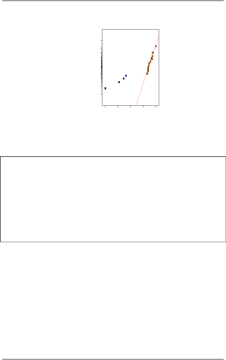
Solutions from Montgomery, D. C. (2001) Design and Analysis of Experiments, Wiley, NY
6-52
DESIGN-EXPERT Plot
Surface Roughness
A: Tool Angle
B: Viscosity
C: Feed Rate
D: Cutting Fluid
Normal plot
Normal % probability
Effe ct
-0 .0 00 9 -0 . 0 00 6 -0 .0 0 0 4 -0 .0 0 0 1 0.0001
1
5
10
20
30
50
70
80
90
95
99
A
B
C
AB
(b) Fit the model identified in part (a) and analyze the residuals. Is there any indication of model
inadequacy?
Design Expert Output
Response: Surface Roughness
ANOVA for Selected Factorial Model
Analysis of variance table [Partial sum of squares]
Sum of Mean F
Source Squares DF Square Value Prob > F
Model 6.406E-006 4 1.601E-006 114.97 < 0.0001 significant
A 8.556E-007 1 8.556E-007 61.43 < 0.0001
B 3.080E-006 1 3.080E-006 221.11 < 0.0001
C 1.030E-006 1 1.030E-006 73.96 < 0.0001
AB 1.440E-006 1 1.440E-006 103.38 < 0.0001
Residual 1.532E-007 11 1.393E-008
Cor Total 6.559E-006 15
The Model F-value of 114.97 implies the model is significant. There is only
a 0.01% chance that a "Model F-Value" this large could occur due to noise.
Values of "Prob > F" less than 0.0500 indicate model terms are significant.
In this case A, B, C, AB are significant model terms.
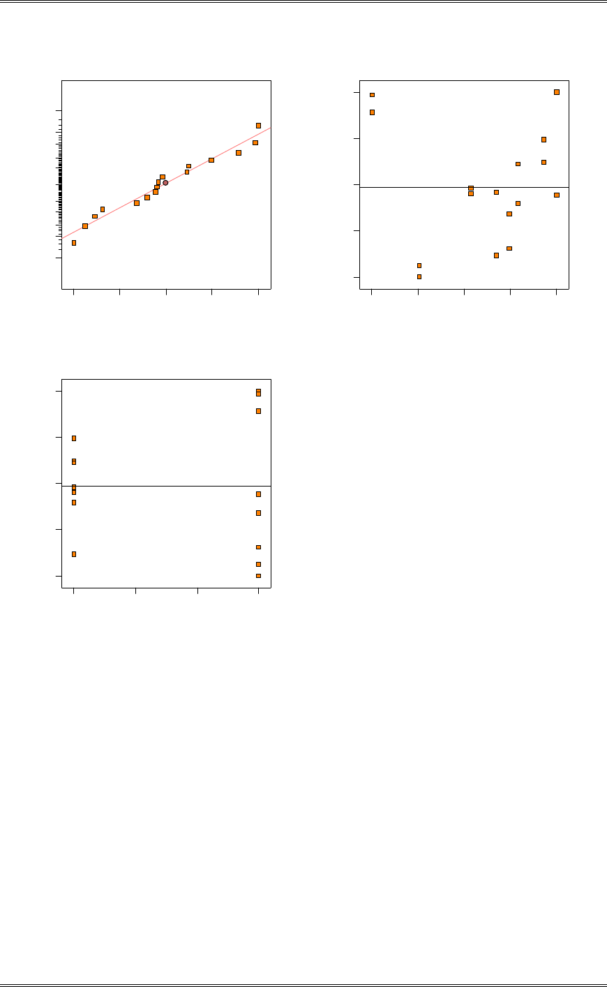
Solutions from Montgomery, D. C. (2001) Design and Analysis of Experiments, Wiley, NY
6-53
Residual
Normal % probability
Normal plot of residuals
-0.00015625-7.5625E-005 5E-006 8.5625E-005 0.00016625
1
5
10
20
30
50
70
80
90
95
99
Predicted
Residuals
Residuals vs. Predicted
-0.00015625
-7 .5 62 5 E -0 0 5
5E-006
8.5625E-005
0.00016625
0.0015 0.0020 0.0025 0.0030 0.0035
Tool Angle
Residuals
Residuals vs. Tool Angle
-0.00015625
-7.5625E-005
5E-006
8.5625E-005
0.00016625
12 13 14 15
The plot of residuals versus predicted shows a slight “u-shaped” appearance in the residuals, and the plot of
residuals versus tool angle shows an outward-opening funnel.
(c) Repeat the analysis from parts (a) and (b) using 1/y as the response variable. Is there and indication
that the transformation has been useful?
The plots of the residuals are more representative of a model that does not violate the constant variance
assumption.
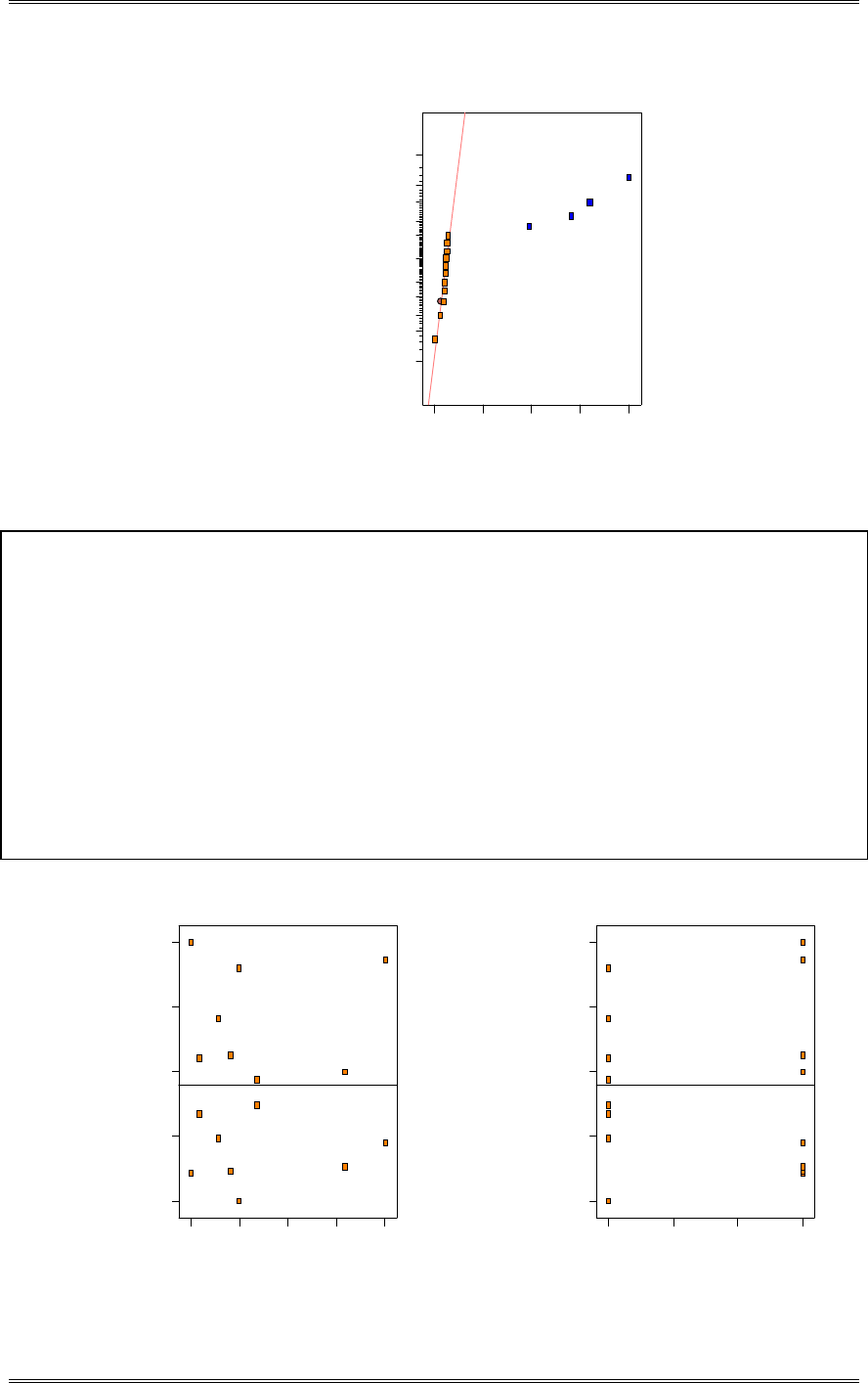
Solutions from Montgomery, D. C. (2001) Design and Analysis of Experiments, Wiley, NY
6-54
DESIGN-EXPERT Plot
1.0/(Surface Roughness)
A: Tool Angle
B: Viscosity
C: Feed Rate
D: Cutting Fluid
Normal plot
Normal % probability
Effe ct
-8 .3 0 31.14 70.59 110.04 149.49
1
5
10
20
30
50
70
80
90
95
99
A
B
C
AB
Design Expert Output
Response: Surface RoughnessTransform:
Inverse
ANOVA for Selected Factorial Model
Analysis of variance table [Partial sum of squares]
Sum of Mean F
Source Squares DF Square Value Prob > F
Model 2.059E+005 4 51472.28 1455.72 < 0.0001 significant
A 42610.92 1 42610.92 1205.11 < 0.0001
B 89386.27 1 89386.27 2527.99 < 0.0001
C 18762.29 1 18762.29 530.63 < 0.0001
AB 55129.62 1 55129.62 1559.16 < 0.0001
Residual 388.94 11 35.36
Cor Total 2.063E+005 15
The Model F-value of 1455.72 implies the model is significant. There is only
a 0.01% chance that a "Model F-Value" this large could occur due to noise.
Values of "Prob > F" less than 0.0500 indicate model terms are significant.
In this case A, B, C, AB are significant model terms.
DESIGN-EXPERT Plot
1.0/(Surface Roughness)
Predicted
Residuals
Residuals vs. Predicted
-7.25771
-3.20046
0.856791
4.91404
8.9713
281.73 365.57 449.41 533.26 617.10
DESIGN-EXPERT Plot
1.0/(Surface Roughness)
Tool Angle
Residuals
Residuals vs. Tool Angle
-7 .2 57 7 1
-3 .2 00 4 6
0.856791
4.91404
8.9713
12 13 14 15

Solutions from Montgomery, D. C. (2001) Design and Analysis of Experiments, Wiley, NY
6-55
(d) Fit a model in terms of the coded variables that can be used to predict the surface roughness. Convert
this prediction equation into a model in the natural variables.
Design Expert Output
Final Equation in Terms of Coded Factors:
1.0/(Surface Roughness) =
+397.81
+51.61 * A
+74.74 * B
+34.24 * C
+58.70 * A * B
6-31 Resistivity on a silicon wafer is influenced by several factors. The results of a 24 factorial
experiment performed during a critical process step is shown below.
Run A B C D Resistivity
1 - - - - 1.92
2 + - - - 11.28
3 - + - - 1.09
4 + + - - 5.75
5 - - + - 2.13
6 + - + - 9.53
7 - + + - 1.03
8 + + + - 5.35
9 - - - + 1.60
10 + - - + 11.73
11 - + - + 1.16
12 + + - + 4.68
13 - - + + 2.16
14 + - + + 9.11
15 - + + + 1.07
16 + + + + 5.30
(a) Estimate the factor effects. Plot the effect estimates on a normal probability plot and select a tentative
model.
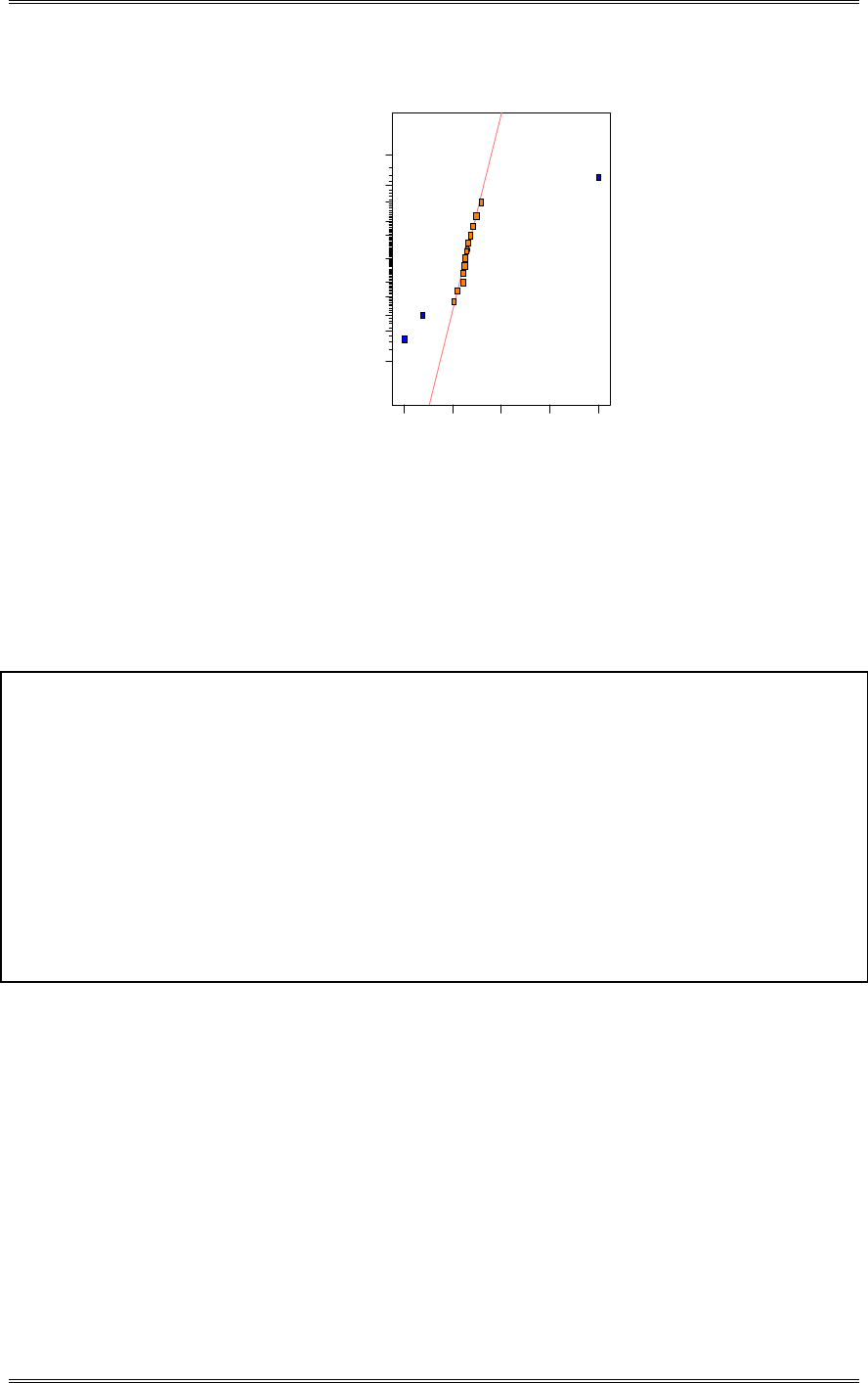
Solutions from Montgomery, D. C. (2001) Design and Analysis of Experiments, Wiley, NY
6-56
DESIGN-EXPERT Plot
R e si sti v i ty
A: A
B: B
C: C
D: D
Normal plot
Normal % probability
Effe ct
-3 .0 0 -0 .6 7 1.66 3.99 6.32
1
5
10
20
30
50
70
80
90
95
99
A
B
AB
(b) Fit the model identified in part (a) and analyze the residuals. Is there any indication of model
inadequacy?
The normal probability plot of residuals is not satisfactory. The plots of residual versus predicted, residual
versus factor A, and the residual versus factor B are funnel shaped indicating non-constant variance.
Design Expert Output
Response: Resistivity
ANOVA for Selected Factorial Model
Analysis of variance table [Partial sum of squares]
Sum of Mean F
Source Squares DF Square Value Prob > F
Model 214.22 3 71.41 148.81 < 0.0001 significant
A 159.83 1 159.83 333.09 < 0.0001
B 36.09 1 36.09 75.21 < 0.0001
AB 18.30 1 18.30 38.13 < 0.0001
Residual 5.76 12 0.48
Cor Total 219.98 15
The Model F-value of 148.81 implies the model is significant. There is only
a 0.01% chance that a "Model F-Value" this large could occur due to noise.
Values of "Prob > F" less than 0.0500 indicate model terms are significant.
In this case A, B, AB are significant model terms.
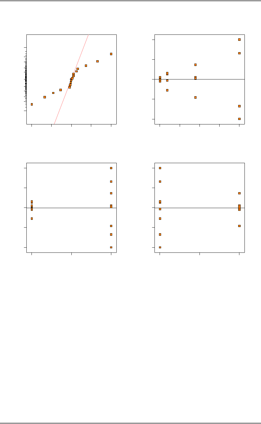
Solutions from Montgomery, D. C. (2001) Design and Analysis of Experiments, Wiley, NY
6-57
Residual
Normal % probability
Normal plot of residuals
-1 .3 02 5 -0 . 6 47 5 0.0075 0.6625 1.3175
1
5
10
20
30
50
70
80
90
95
99
Predicted
Residuals
Residuals vs. Predicted
-1 .3 02 5
-0 .6 47 5
0.0075
0.6625
1.3175
1.09 3.42 5.75 8.08 10.41
A
Residuals
Residuals vs. A
-1 .3 02 5
-0 .6 47 5
0.0075
0.6625
1.3175
-1 0 1
B
Residuals
Residuals vs. B
-1 .3 02 5
-0 .6 47 5
0.0075
0.6625
1.3175
-1 0 1
(c) Repeat the analysis from parts (a) and (b) using ln(y) as the response variable. Is there any indication
that the transformation has been useful?
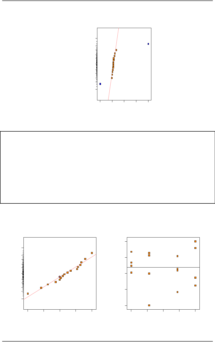
Solutions from Montgomery, D. C. (2001) Design and Analysis of Experiments, Wiley, NY
6-58
DESIGN-EXPERT Plot
L n (R e si st i v i ty )
A: A
B: B
C: C
D: D
Normal plot
Normal % probability
Effe ct
-0 .6 3 -0 .0 6 0.50 1.06 1.63
1
5
10
20
30
50
70
80
90
95
99
A
B
Design Expert Output
Response: Resistivity Transform: Natural log Constant: 0.000
ANOVA for Selected Factorial Model
Analysis of variance table [Partial sum of squares]
Sum of Mean F
Source Squares DF Square Value Prob > F
Model 12.15 2 6.08 553.44 < 0.0001 significant
A 10.57 1 10.57 962.95 < 0.0001
B 1.58 1 1.58 143.94 < 0.0001
Residual 0.14 13 0.011
Cor Total 12.30 15
The Model F-value of 553.44 implies the model is significant. There is only
a 0.01% chance that a "Model F-Value" this large could occur due to noise.
Values of "Prob > F" less than 0.0500 indicate model terms are significant.
In this case A, B are significant model terms.
The transformed data no longer indicates that the AB interaction is significant. A simpler model has
resulted from the log transformation.
Residual
Norm al % probability
Normal plot of residuals
-0.216821 -0.125219 -0.033618 0.0579833 0.149585
1
5
10
20
30
50
70
80
90
95
99
Predicted
Residuals
Residuals vs. Predicted
-0 .2 16 8 2 1
-0 .1 25 2 1 9
-0 .0 33 6 1 8
0.0579833
0.149585
0.06 0.62 1.19 1.75 2.31
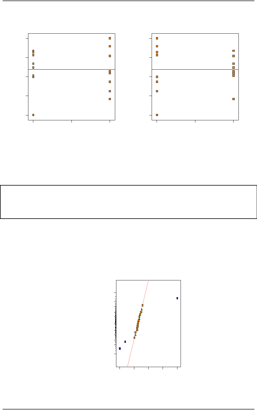
Solutions from Montgomery, D. C. (2001) Design and Analysis of Experiments, Wiley, NY
6-59
A
Residuals
Residuals vs. A
-0.216821
-0.125219
-0.033618
0.0579833
0.149585
-1 0 1
B
Residuals
Residuals vs. B
-0 .2 16 8 2 1
-0 .1 25 2 1 9
-0 .0 33 6 1 8
0.0579833
0.149585
-1 0 1
The residual plots are much improved.
(d) Fit a model in terms of the coded variables that can be used to predict the resistivity.
Design Expert Output
Final Equation in Terms of Coded Factors:
Ln(Resistivity) =
+1.19
+0.81 * A
-0.31 * B
6.32 Continuation of Problem 6-31. Suppose that the experiment had also run four center points along
with the 16 runs in Problem 6-31. The resistivity measurements at the center points are: 8.15, 7.63, 8.95,
6.48. Analyze the experiment again incorporating the center points. What conclusions can you draw
now?
DESIGN-EXPERT Plot
R e si sti v i ty
A: A
B: B
C: C
D: D
Normal plot
Norm al % probability
Effe ct
-3 .0 0 -0 .6 7 1.66 3.99 6.32
1
5
10
20
30
50
70
80
90
95
99 A
B
AB
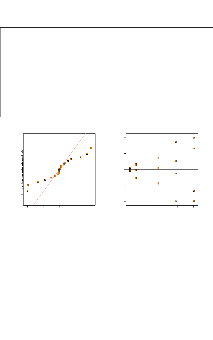
Solutions from Montgomery, D. C. (2001) Design and Analysis of Experiments, Wiley, NY
6-60
Design Expert Output
Response: Resistivity
ANOVA for Selected Factorial Model
Analysis of variance table [Partial sum of squares]
Sum of Mean F
Source Squares DF Square Value Prob > F
Model 214.22 3 71.41 119.35 < 0.0001 significant
A 159.83 1 159.83 267.14 < 0.0001
B 36.09 1 36.09 60.32 < 0.0001
AB 18.30 1 18.30 30.58 < 0.0001
Curvature 31.19 1 31.19 52.13 < 0.0001 significant
Residual 8.97 15 0.60
Lack of Fit 5.76 12 0.48 0.45 0.8632 not significant
Pure Error 3.22 3 1.07
Cor Total 254.38 19
The Model F-value of 119.35 implies the model is significant. There is only
a 0.01% chance that a "Model F-Value" this large could occur due to noise.
Values of "Prob > F" less than 0.0500 indicate model terms are significant.
In this case A, B, AB are significant model terms.
Residual
Norm al % probability
Normal plot of residuals
-1 .3 22 5 -0 . 6 62 5 -0 .0 02 5 0.6575 1.3175
1
5
10
20
30
50
70
80
90
95
99
Predicted
Residuals
Residuals vs. Predicted
-1 .3 22 5
-0 .6 62 5
-0 .0 02 5
0.6575
1.3175
1.09 3.42 5.75 8.08 10.41
Repeated analysis with the natural log transformation.
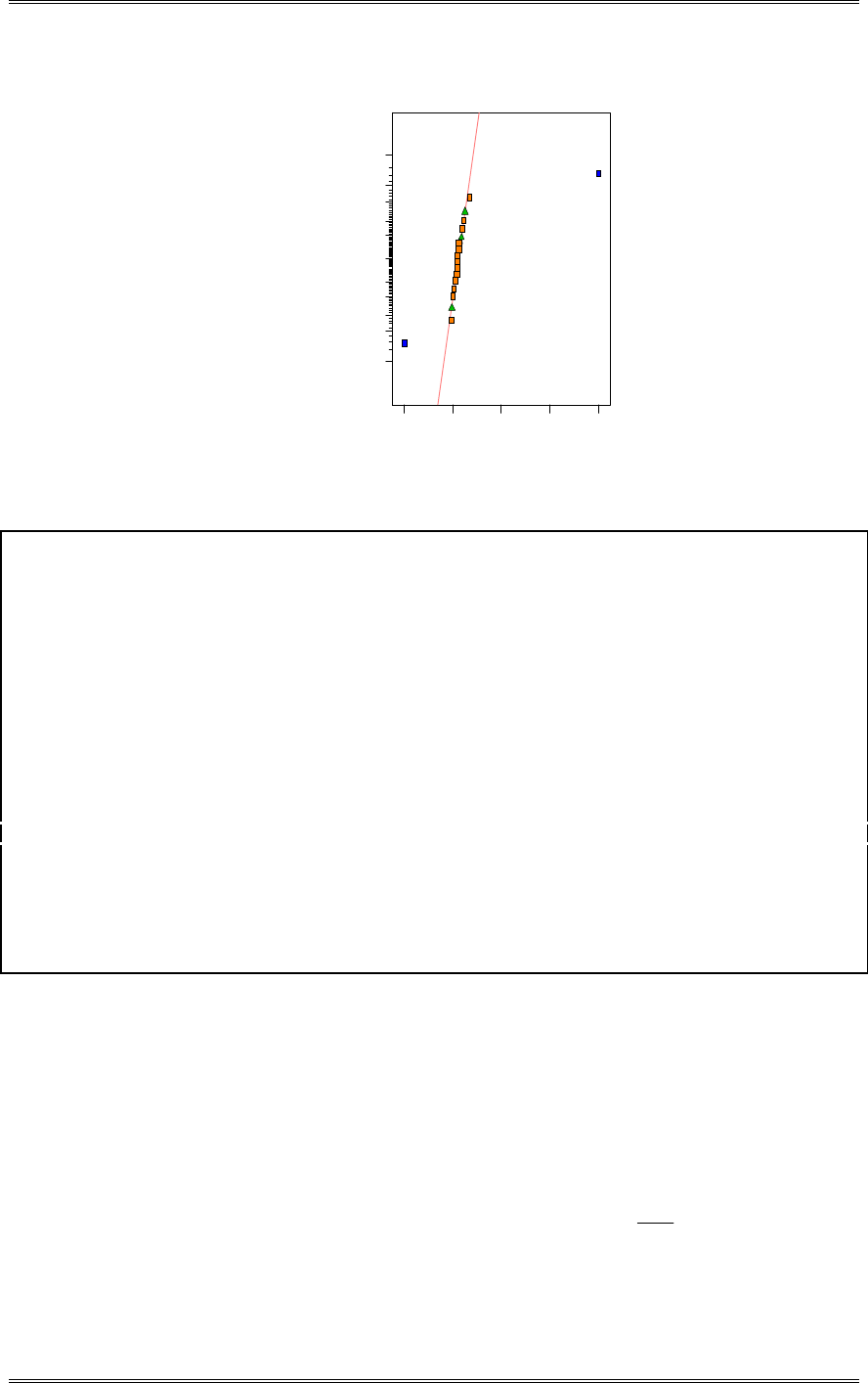
Solutions from Montgomery, D. C. (2001) Design and Analysis of Experiments, Wiley, NY
6-61
DESIGN-EXPERT Plot
L n (R e si st i v i ty )
A: A
B: B
C: C
D: D
Normal plot
Normal % probability
Effe ct
-0 .6 3 -0 .0 6 0.50 1.06 1.63
1
5
10
20
30
50
70
80
90
95
99 A
B
Design Expert Output
Response: Resistivity Transform: Natural log Constant: 0.000
ANOVA for Selected Factorial Model
Analysis of variance table [Partial sum of squares]
Sum of Mean F
Source Squares DF Square Value Prob > F
Model 12.15 2 6.08 490.37 < 0.0001 significant
A 10.57 1 10.57 853.20 < 0.0001
B 1.58 1 1.58 127.54 < 0.0001
Curvature 2.38 1 2.38 191.98 < 0.0001 significant
Residual 0.20 16 0.012
Lack of Fit 0.14 13 0.011 0.59 0.7811 not significant
Pure Error 0.056 3 0.019
Cor Total 14.73 19
The Model F-value of 490.37 implies the model is significant. There is only
a 0.01% chance that a "Model F-Value" this large could occur due to noise.
Values of "Prob > F" less than 0.0500 indicate model terms are significant.
In this case A, B are significant model terms.
The "Curvature F-value" of 191.98 implies there is significant curvature (as measured by
difference between the average of the center points and the average of the factorial points) in
the design space. There is only a 0.01% chance that a "Curvature F-value" this large
could occur due to noise.
The curvature test indicates that the model has significant pure quadratic curvature.
6.33 Often the fitted regression model from a 2k factorial design is used to make predictions at points of
interest in the design space.
(a) Find the variance of the predicted response y
ˆat the point 1
x,2
x ,…, k
x in the design space. Hint:
Remember that the x’s are coded variables, and assume a 2k design with an equal number of replicates
n at each design point so that the variance of a regression coefficient
E
ˆis k
n2
2
V
and that the
covariance between any pair of regression coefficients is zero.
Let’s assume that the model can be written as follows:

Solutions from Montgomery, D. C. (2001) Design and Analysis of Experiments, Wiley, NY
6-62
01122
ˆˆ ˆ ˆ
ˆ( )= ... pp
yxxx
EE E E
x
where 12
[, ,..., ]
k
xx x
c x are the values of the original variables in the design at the point of interest
where a prediction is required , and the variables in the model 12
, ,..., p
xx x
potentially include interaction
terms among the original k variables. Now the variance of the predicted response is
01122
01122
2
2
1
ˆˆ ˆ ˆ
ˆ
[()] ( ... )
ˆˆ ˆ ˆ
() ( ) ( )... ( )
1
2
pp
pp
p
i
k
i
Vy V x x x
VVxVx Vx
x
n
EE E E
EE E E
V
§·
¨¸
©¹
¦
x
This result follows because the design is orthogonal and all model parameter estimates have the same
variance. Remember that some of the x’s involved in this equation are potentially interaction terms.
(b) Use the result of part (a) to find an equation for a 100(1-
D
)% confidence interval on the true mean
response at the point 1
x,2
x ,…, k
x in the design space.
The confidence interval is
/2, /2,
ˆˆˆˆ
() [()] () () [()]
EE
df df
yt Vy y yt Vy
DD
ddxxxxx
where dfE is the number of degrees of freedom used to estimate 2
V
and the estimate of 2
V
has been
used in computing the variance of the predicted value of the response at the point of interest.
6.34 Hierarchical Models. Several times we have utilized the hierarchy principal in selecting a model;
that is, we have included non-significant terms in a model because they were factors involved in
significant higher-order terms. Hierarchy is certainly not an absolute principle that must be followed in
all cases. To illustrate, consider the model resulting from Problem 6-1, which required that a non-
significant main effect be included to achieve hierarchy. Using the data from Problem 6-1:
(a) Fit both the hierarchical model and the non-hierarchical model.
Design Expert Output for Hierarchial Model
Response: Life in hours
ANOVA for Selected Factorial Model
Analysis of variance table [Partial sum of squares]
Sum of Mean F
Source Squares DF Square Value Prob > F
Model 1519.67 4 379.92 12.54 < 0.0001 significant
A 0.67 1 0.67 0.022 0.8836
B 770.67 1 770.67 25.44 < 0.0001
C 280.17 1 280.17 9.25 0.0067
AC 468.17 1 468.17 15.45 0.0009
Residual 575.67 19 30.30
Lack of Fit 93.00 3 31.00 1.03 0.4067 not significant
Pure Error 482.67 16 30.17
Cor Total 2095.33 23
The Model F-value of 12.54 implies the model is significant. There is only

Solutions from Montgomery, D. C. (2001) Design and Analysis of Experiments, Wiley, NY
6-63
a 0.01% chance that a "Model F-Value" this large could occur due to noise.
Values of "Prob > F" less than 0.0500 indicate model terms are significant.
In this case B, C, AC are significant model terms.
Std. Dev. 5.50 R-Squared 0.7253
Mean 40.83 Adj R-Squared 0.6674
C.V. 13.48 Pred R-Squared 0.5616
PRESS 918.52 Adeq Precision 10.747
The "Pred R-Squared" of 0.5616 is in reasonable agreement with the "Adj R-Squared" of
0.6674. A difference greater than 0.20 between the "Pred R-Squared" and the "Adj R-Squared"
indicates a possible problem with your model and/or data.
Design Expert Output for Non-Hierarchical Model
Response: Life in hours
ANOVA for Selected Factorial Model
Analysis of variance table [Partial sum of squares]
Sum of Mean F
Source Squares DF Square Value Prob > F
Model 1519.00 3 506.33 17.57 < 0.0001 significant
B 770.67 1 770.67 26.74 < 0.0001
C 280.17 1 280.17 9.72 0.0054
AC 468.17 1 468.17 16.25 0.0007
Residual 576.33 20 28.82
Lack of Fit 93.67 4 23.42 0.78 0.5566 not significant
Pure Error 482.67 16 30.17
Cor Total 2095.33 23
The Model F-value of 17.57 implies the model is significant. There is only
a 0.01% chance that a "Model F-Value" this large could occur due to noise.
Values of "Prob > F" less than 0.0500 indicate model terms are significant.
In this case B, C, AC are significant model terms.
The "Lack of Fit F-value" of 0.78 implies the Lack of Fit is not significant relative to the pure
error. There is a 55.66% chance that a "Lack of Fit F-value" this large could occur due
to noise. Non-significant lack of fit is good -- we want the model to fit.
Std. Dev. 5.37 R-Squared 0.7249
Mean 40.83 Adj R-Squared 0.6837
C.V. 13.15 Pred R-Squared 0.6039
PRESS 829.92 Adeq Precision 12.320
The "Pred R-Squared" of 0.6039 is in reasonable agreement with the "Adj R-Squared" of
0.6837. A difference greater than 0.20 between the "Pred R-Squared" and the "Adj R-Squared"
indicates a possible problem with your model and/or data.
(b) Calculate the PRESS statistic, the adjusted R2 and the mean square error for both models.
The PRESS and R2 are in the Design Expert Output above. The PRESS is smaller for the non-
hierarchical model than the hierarchical model suggesting that the non-hierarchical model is a better
predictor.
(c) Find a 95 percent confidence interval on the estimate of the mean response at a cube corner
(1
x=2
x=3
x=1r). Hint: Use the result of Problem 6-33.
Design Expert Output
Prediction SE Mean 95% CI low 95% CI high SE Pred 95% PI low 95% PI high
Life 27.45 2.18 22.91 31.99 5.79 15.37 39.54
Life 36.17 2.19 31.60 40.74 5.80 24.07 48.26
Life 38.67 2.19 34.10 43.24 5.80 26.57 50.76
Life 47.50 2.19 42.93 52.07 5.80 35.41 59.59
Life 43.00 2.19 38.43 47.57 5.80 30.91 55.09
Life 34.17 2.19 29.60 38.74 5.80 22.07 46.26

Solutions from Montgomery, D. C. (2001) Design and Analysis of Experiments, Wiley, NY
6-64
Life 54.33 2.19 49.76 58.90 5.80 42.24 66.43
Life 45.50 2.19 40.93 50.07 5.80 33.41 57.59
(d) Based on the analyses you have conducted, which model would you prefer?
Notice that PRESS is smaller and the adjusted R2 is larger for the non-hierarchical model. This is an
indication that strict adherence to the hierarchy principle isn’t always necessary. Note also that the
confidence interval is shorter for the non-hierarchical model.

Solutions from Montgomery, D. C. (2001) Design and Analysis of Experiments, Wiley, NY
7-1
Chapter 7
Blocking and Confounding in the 2k Factorial Design
Solutions
7-1 Consider the experiment described in Problem 6-1. Analyze this experiment assuming that each
replicate represents a block of a single production shift.
Source of Sum of Degrees of Mean
Variation Squares Freedom Square F0
Cutting Speed (A) 0.67 1 0.67 <1
Tool Geometry (B) 770.67 1 770.67 22.38*
Cutting Angle (C) 280.17 1 280.17 8.14*
AB 16.67 1 16.67 <1
AC 468.17 1 468.17 13.60*
BC 48.17 1 48.17 1.40
ABC 28.17 1 28.17 <1
Blocks 0.58 2 0.29
Error 482.08 14 34.43
Total 2095.33 23
Design Expert Output
Response: Life in hours
ANOVA for Selected Factorial Model
Analysis of variance table [Partial sum of squares]
Sum of
Mean F
Source Squares DF Square Value Prob > F
Block 0.58 2 0.29
Model 1519.67 4 379.92 11.23 0.0001 significant
A 0.67 1 0.67 0.020 0.8900
B 770.67 1 770.67 22.78 0.0002
C 280.17 1 280.17 8.28 0.0104
AC 468.17 1 468.17 13.84 0.0017
Residual 575.08 17 33.83
Cor Total 2095.33 23
The Model F-value of 11.23 implies the model is significant. There is only
a 0.01% chance that a "Model F-Value" this large could occur due to noise.
Values of "Prob > F" less than 0.0500 indicate model terms are significant.
In this case B, C, AC are significant model terms.
These results agree with the results from Problem 6-1. Tool geometry, cutting angle and the cutting speed
x cutting angle factors are significant at the 5% level. The Design Expert program also includes A, speed,
in the model to preserve hierarchy.
7-2 Consider the experiment described in Problem 6-5. Analyze this experiment assuming that each
one of the four replicates represents a block.
Source of Sum of Degrees of Mean
Variation Squares Freedom Square F0
Bit Size (A) 1107.23 1 1107.23 364.22*

Solutions from Montgomery, D. C. (2001) Design and Analysis of Experiments, Wiley, NY
7-2
Cutting Speed (B) 227.26 1 227.26 74.76*
AB 303.63 1 303.63 99.88*
Blocks 44.36 3 14.79
Error 27.36 9 3.04
Total 1709.83 15
These results agree with those from Problem 6-5. Bit size, cutting speed and their interaction are
significant at the 1% level.
Design Expert Output
Response: Vibration
ANOVA for Selected Factorial Model
Analysis of variance table [Partial sum of squares]
Sum of Mean F
Source Squares DF Square Value Prob > F
Block 44.36 3 14.79
Model 1638.11 3 546.04 179.61 < 0.0001 significant
A 1107.23 1 1107.23 364.21 < 0.0001
B 227.26 1 227.26 74.75 < 0.0001
AB 303.63 1 303.63 99.88 < 0.0001
Residual 27.36 9 3.04
Cor Total 1709.83 15
The Model F-value of 179.61 implies the model is significant. There is only
a 0.01% chance that a "Model F-Value" this large could occur due to noise.
Values of "Prob > F" less than 0.0500 indicate model terms are significant.
In this case A, B, AB are significant model terms.
7-3 Consider the alloy cracking experiment described in Problem 6-15. Suppose that only 16 runs
could be made on a single day, so each replicate was treated as a block. Analyze the experiment and draw
conclusions.
The analysis of variance for the full model is as follows:
Design Expert Output
Response: Crack Lengthin mm x 10^-2
ANOVA for Selected Factorial Model
Analysis of variance table [Partial sum of squares]
Sum of Mean F
Source Squares DF Square Value Prob > F
Block 0.016 1 0.016
Model 570.95 15 38.06 445.11 < 0.0001 significant
A 72.91 1 72.91 852.59 < 0.0001
B 126.46 1 126.46 1478.83 < 0.0001
C 103.46 1 103.46 1209.91 < 0.0001
D 30.66 1 30.66 358.56 < 0.0001
AB 29.93 1 29.93 349.96 < 0.0001
AC 128.50 1 128.50 1502.63 < 0.0001
AD 0.047 1 0.047 0.55 0.4708
BC 0.074 1 0.074 0.86 0.3678
BD 0.018 1 0.018 0.21 0.6542
CD 0.047 1 0.047 0.55 0.4686
ABC 78.75 1 78.75 920.92 < 0.0001
ABD 0.077 1 0.077 0.90 0.3582
ACD 2.926E-003 1 2.926E-003 0.034 0.8557
BCD 0.010 1 0.010 0.12 0.7352
ABCD 1.596E-003 1 1.596E-003 0.019 0.8931
Residual 1.28 15 0.086
Cor Total 572.25 31
The Model F-value of 445.11 implies the model is significant. There is only

Solutions from Montgomery, D. C. (2001) Design and Analysis of Experiments, Wiley, NY
7-3
a 0.01% chance that a "Model F-Value" this large could occur due to noise.
Values of "Prob > F" less than 0.0500 indicate model terms are significant.
In this case A, B, C, D, AB, AC, ABC are significant model terms.
The analysis of variance for the reduced model based on the significant factors is shown below. The BC
interaction was included to preserve hierarchy.
Design Expert Output
Response: Crack Lengthin mm x 10^-2
ANOVA for Selected Factorial Model
Analysis of variance table [Partial sum of squares]
Sum of Mean F
Source Squares DF Square Value Prob > F
Block 0.016 1 0.016
Model 570.74 8 71.34 1056.10 < 0.0001 significant
A 72.91 1 72.91 1079.28 < 0.0001
B 126.46 1 126.46 1872.01 < 0.0001
C 103.46 1 103.46 1531.59 < 0.0001
D 30.66 1 30.66 453.90 < 0.0001
AB 29.93 1 29.93 443.01 < 0.0001
AC 128.50 1 128.50 1902.15 < 0.0001
BC 0.074 1 0.074 1.09 0.3075
ABC 78.75 1 78.75 1165.76 < 0.0001
Residual 1.49 22 0.068
Cor Total 572.25 31
The Model F-value of 1056.10 implies the model is significant. There is only
a 0.01% chance that a "Model F-Value" this large could occur due to noise.
Values of "Prob > F" less than 0.0500 indicate model terms are significant.
In this case A, B, C, D, AB, AC, ABC are significant model terms.
Blocking does not change the results of Problem 6-15.
7-4 Consider the data from the first replicate of Problem 6-1. Suppose that these observations could not
all be run using the same bar stock. Set up a design to run these observations in two blocks of four
observations each with ABC confounded. Analyze the data.
Block 1 Block 2
(1) a
ab b
ac c
bc abc
From the normal probability plot of effects, B, C, and the AC interaction are significant.
Factor A was included in the analysis of variance to preserve hierarchy.
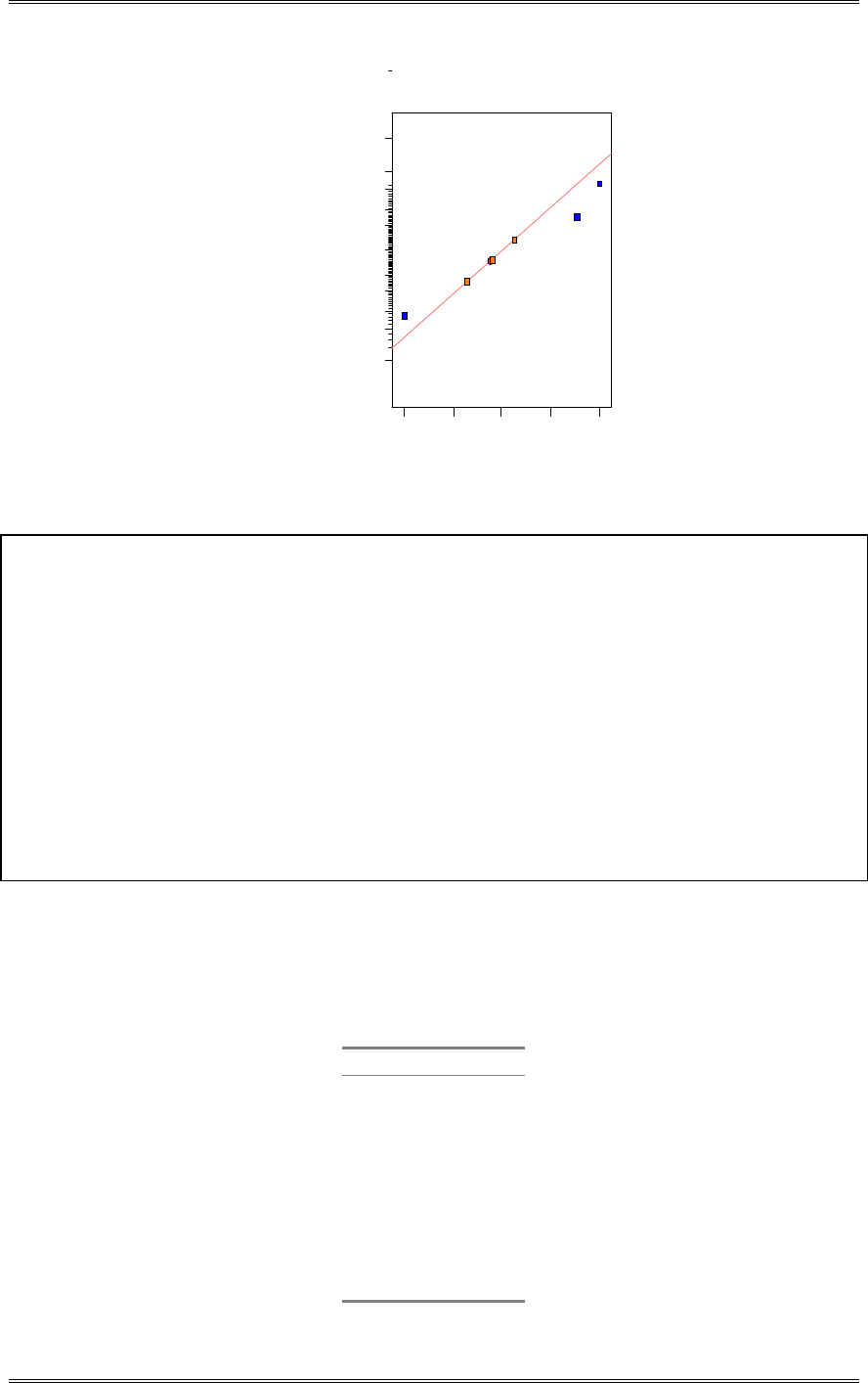
Solutions from Montgomery, D. C. (2001) Design and Analysis of Experiments, Wiley, NY
7-4
DESIGN-EXPERT Plot
Life
A: Cutting Speed
B: Tool Geometry
C: Cutting Angle
Normal plot
Norm al % probability
Effe ct
-13.75 -7 .1 3 -0 .5 0 6.13 12.75
1
5
10
20
30
50
70
80
90
95
99
B
C
AC
Design Expert Output
Response: Life in hours
ANOVA for Selected Factorial Model
Analysis of variance table [Partial sum of squares]
Sum of Mean F
Source Squares DF Square Value Prob > F
Block 91.13 1 91.13
Model 896.50 4 224.13 7.32 0.1238 not significant
A 3.13 1 3.13 0.10 0.7797
B 325.12 1 325.12 10.62 0.0827
C 190.12 1 190.12 6.21 0.1303
AC 378.13 1 378.13 12.35 0.0723
Residual 61.25 2 30.62
Cor Total 1048.88 7
The "Model F-value" of 7.32 implies the model is not significant relative to the noise. There is a
12.38 % chance that a "Model F-value" this large could occur due to noise.
Values of "Prob > F" less than 0.0500 indicate model terms are significant.
In this case there are no significant model terms.
This design identifies the same significant factors as Problem 6-1.
7-5 Consider the data from the first replicate of Problem 6-7. Construct a design with two blocks of
eight observations each with ABCD confounded. Analyze the data.
Block 1 Block 2
(1) a
ab b
ac c
bc d
ad abc
bd abd
cd acd
abcd bcd
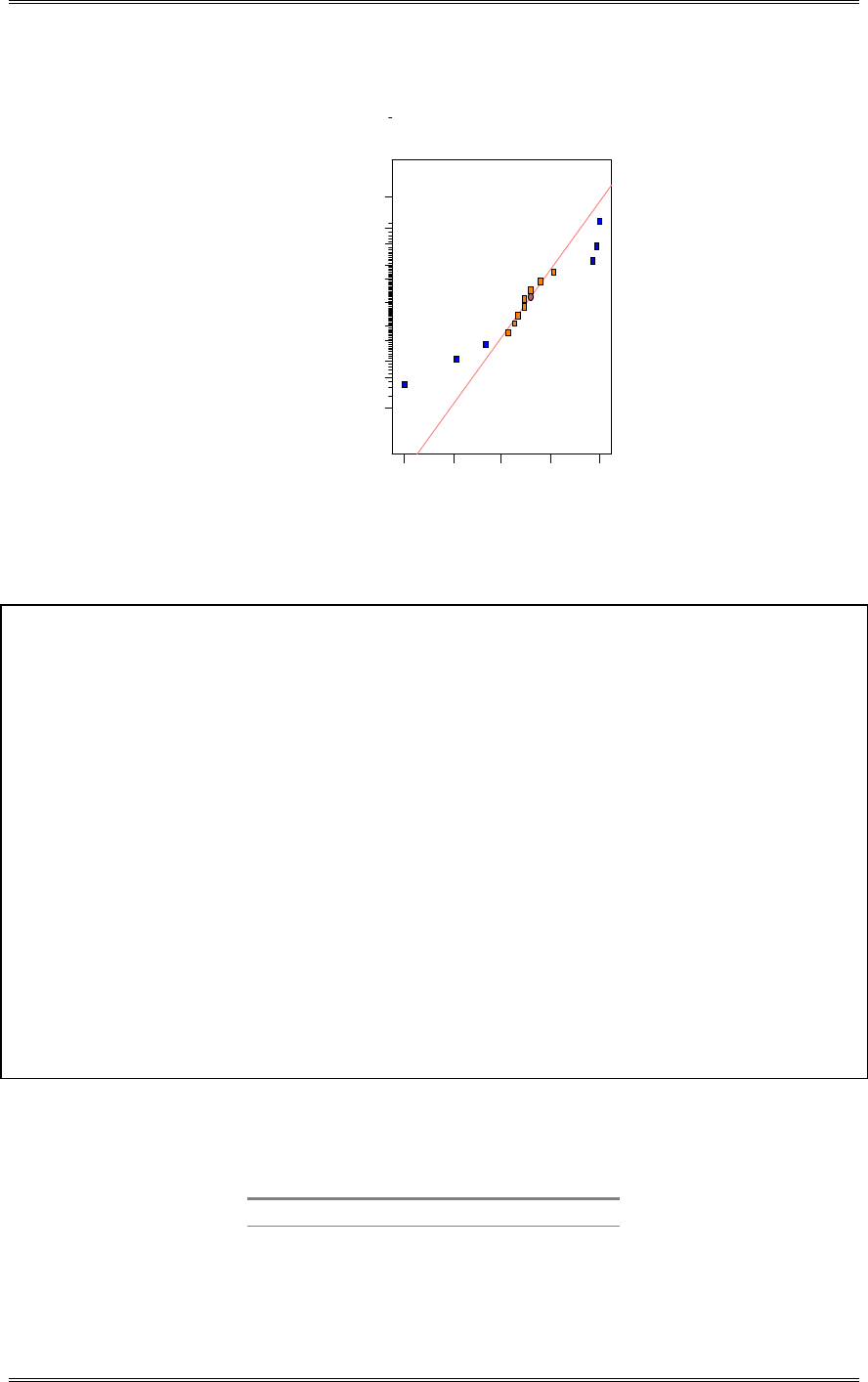
Solutions from Montgomery, D. C. (2001) Design and Analysis of Experiments, Wiley, NY
7-5
The significant effects are identified in the normal probability plot of effects below:
DESIGN-EXPERT Plot
yield
A: A
B: B
C: C
D: D
Normal plot
Norm al % probability
Effe ct
-10.00 -6 .2 5 -2 .5 0 1.25 5.00
1
5
10
20
30
50
70
80
90
95
99
A
D
AB
AD
AB C
AB D
AC, BC, and BD were included in the model to preserve hierarchy.
Design Expert Output
Response: yield
ANOVA for Selected Factorial Model
Analysis of variance table [Partial sum of squares]
Sum of Mean F
Source Squares DF Square Value Prob > F
Block 42.25 1 42.25
Model 892.25 11 81.11 9.64 0.0438 significant
A 400.00 1 400.00 47.52 0.0063
B 2.25 1 2.25 0.27 0.6408
C 2.25 1 2.25 0.27 0.6408
D 100.00 1 100.00 11.88 0.0410
AB 81.00 1 81.00 9.62 0.0532
AC 1.00 1 1.00 0.12 0.7531
AD 56.25 1 56.25 6.68 0.0814
BC 6.25 1 6.25 0.74 0.4522
BD 9.00 1 9.00 1.07 0.3772
ABC 144.00 1 144.00 17.11 0.0256
ABD 90.25 1 90.25 10.72 0.0466
Residual 25.25 3 8.42
Cor Total 959.75 15
The Model F-value of 9.64 implies the model is significant. There is only
a 4.38% chance that a "Model F-Value" this large could occur due to noise.
Values of "Prob > F" less than 0.0500 indicate model terms are significant.
In this case A, D, ABC, ABD are significant model terms.
7-6 Repeat Problem 7-5 assuming that four blocks are required. Confound ABD and ABC (and
consequently CD) with blocks.
Block 1 Block 2 Block 3 Block 4
(1) ac c a
ab bc abc b
acd d ad cd
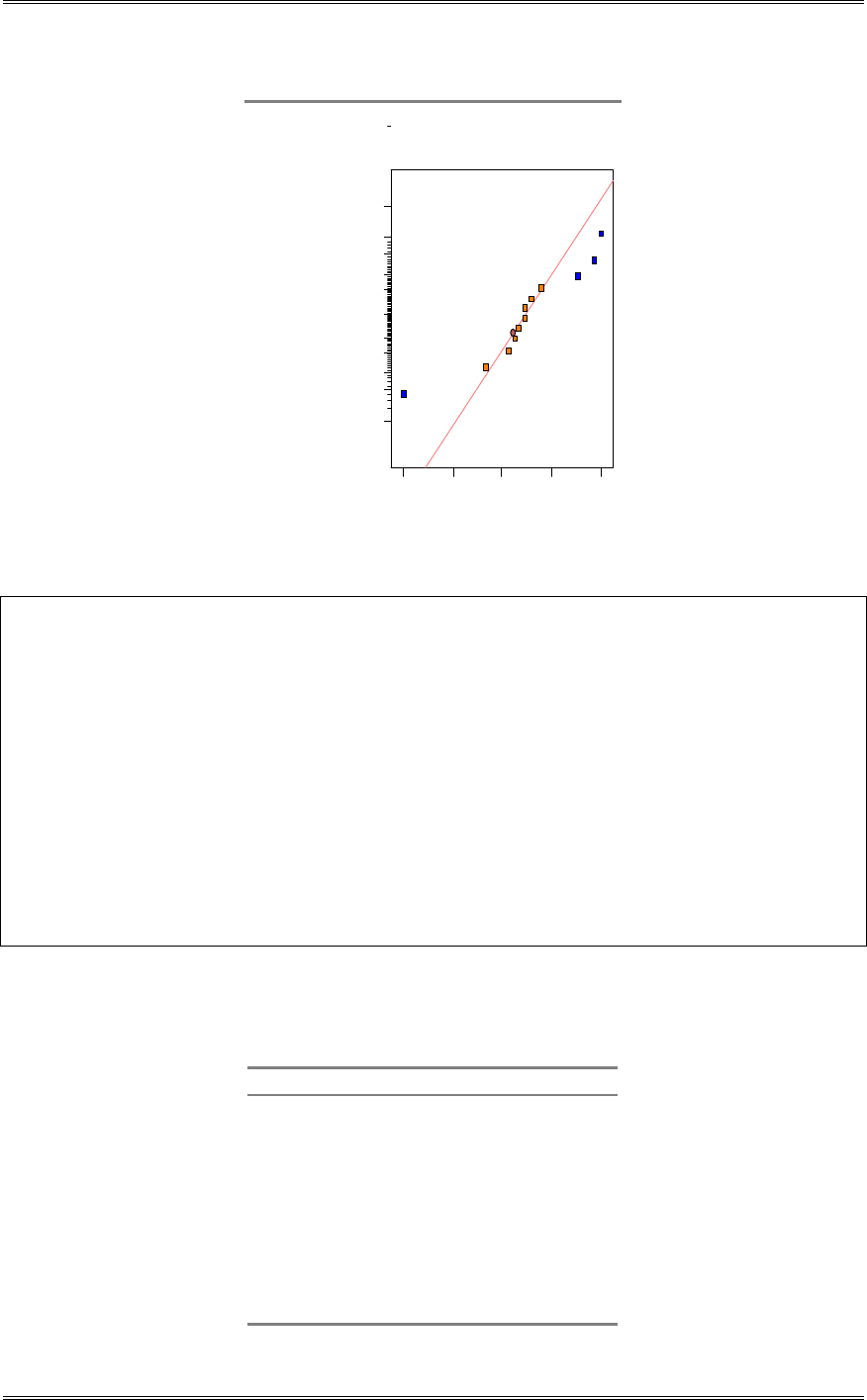
Solutions from Montgomery, D. C. (2001) Design and Analysis of Experiments, Wiley, NY
7-6
bcd abd bd abcd
DESIGN-EXPERT Plot
yield
A: A
B: B
C: C
D: D
Normal plot
Norm al % probability
Effe ct
-10.00 -6 .2 5 -2 .5 0 1.25 5.00
1
5
10
20
30
50
70
80
90
95
99
A
D
AB
AB C D
Design Expert Output
Response: yield
ANOVA for Selected Factorial Model
Analysis of variance table [Partial sum of squares]
Sum of Mean F
Source Squares DF Square Value Prob > F
Block 243.25 3 81.08
Model 623.25 4 155.81 13.37 0.0013 significant
A 400.00 1 400.00 34.32 0.0004
D 100.00 1 100.00 8.58 0.0190
AB 81.00 1 81.00 6.95 0.0299
ABCD 42.25 1 42.25 3.62 0.0934
Residual 93.25 8 11.66
Cor Total 959.75 15
The Model F-value of 13.37 implies the model is significant. There is only
a 0.13% chance that a "Model F-Value" this large could occur due to noise.
Values of "Prob > F" less than 0.0500 indicate model terms are significant.
In this case A, D, AB are significant model terms.
7-7 Using the data from the 25 design in Problem 6-21, construct and analyze a design in two blocks
with ABCDE confounded with blocks.
Block 1 Block 1 Block 2 Block 2
(1) ae a e
ab be b abe
ac ce c ace
bc abce abc bce
ad de d ade
bd abde abd bde
cd acde acd cde
abcd bcde bcd abcde
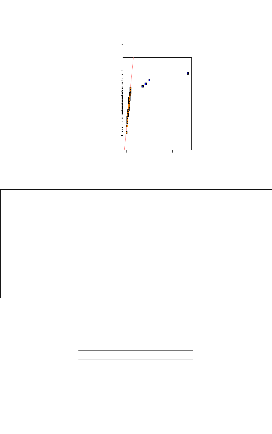
Solutions from Montgomery, D. C. (2001) Design and Analysis of Experiments, Wiley, NY
7-7
The normal probability plot of effects identifies factors A, B, C, and the AB interaction as being
significant. This is confirmed with the analysis of variance.
DESIGN-EXPERT Plot
Yield
A: Aperture
B: Exposure T ime
C: Develop Time
D: M ask Dim ension
E: Etch Time
Normal plot
Norm al % probability
Effe ct
-1 .1 9 7.59 16.38 25.16 33.94
1
5
10
20
30
50
70
80
90
95
99
A
B
C
AB
Design Expert Output
Response: Yield
ANOVA for Selected Factorial Model
Analysis of variance table [Partial sum of squares]
Sum of Mean F
Source Squares DF Square Value Prob > F
Block 0.28 1 0.28
Model 11585.13 4 2896.28 958.51 < 0.0001 significant
A 1116.28 1 1116.28 369.43 < 0.0001
B 9214.03 1 9214.03 3049.35 < 0.0001
C 750.78 1 750.78 248.47 < 0.0001
AB 504.03 1 504.03 166.81 < 0.0001
Residual 78.56 26 3.02
Cor Total 11663.97 31
The Model F-value of 958.51 implies the model is significant. There is only
a 0.01% chance that a "Model F-Value" this large could occur due to noise.
Values of "Prob > F" less than 0.0500 indicate model terms are significant.
In this case A, B, C, AB are significant model terms.
7-8 Repeat Problem 7-7 assuming that four blocks are necessary. Suggest a reasonable confounding
scheme.
Use ABC, CDE, confounded with ABDE. The four blocks follow.
Block 1 Block 2 Block 3 Block 4
(1) a ac c
ab b bc abc
acd cd d ad
bcd abcd abd bd
ace ce e ae
bce abce abe be
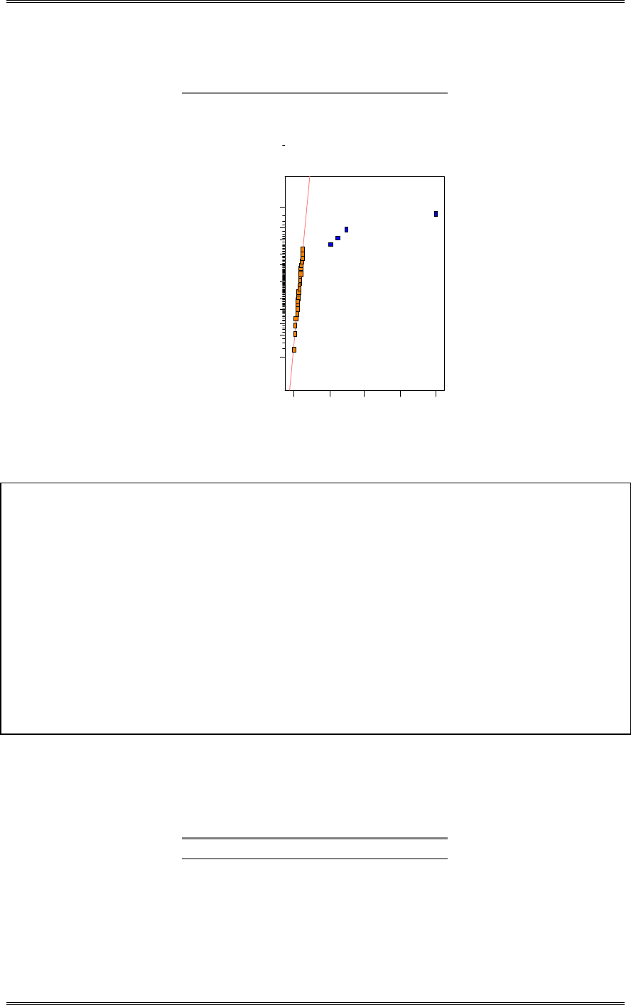
Solutions from Montgomery, D. C. (2001) Design and Analysis of Experiments, Wiley, NY
7-8
de ade acde cde
abde bde bcde abcde
The normal probability plot of effects identifies the same significant effects as in Problem 7-7.
DESIGN-EXPERT Plot
Yield
A: Aperture
B: Exposure Time
C: Develop Time
D: M ask Dim ension
E: Etch Tim e
Normal plot
Norm al % probability
Effe ct
-1 .1 9 7.59 16.38 25.16 33.94
1
5
10
20
30
50
70
80
90
95
99
A
B
C
AB
Design Expert Output
Response: Yield
ANOVA for Selected Factorial Model
Analysis of variance table [Partial sum of squares]
Sum of Mean F
Source Squares DF Square Value Prob > F
Block 13.84 3 4.61
Model 11585.13 4 2896.28 1069.40 < 0.0001 significant
A 1116.28 1 1116.28 412.17 < 0.0001
B 9214.03 1 9214.03 3402.10 < 0.0001
C 750.78 1 750.78 277.21 < 0.0001
AB 504.03 1 504.03 186.10 < 0.0001
Residual 65.00 24 2.71
Cor Total 11663.97 31
The Model F-value of 1069.40 implies the model is significant. There is only
a 0.01% chance that a "Model F-Value" this large could occur due to noise.
Values of "Prob > F" less than 0.0500 indicate model terms are significant.
In this case A, B, C, AB are significant model terms.
7-9 Consider the data from the 25 design in Problem 6-21. Suppose that it was necessary to run this
design in four blocks with ACDE and BCD (and consequently ABE) confounded. Analyze the data from
this design.
Block 1 Block 2 Block 3 Block 4
(1) a b c
ae e abe ace
cd acd bcd d
abc bc ac ab
acde cde abcde ade
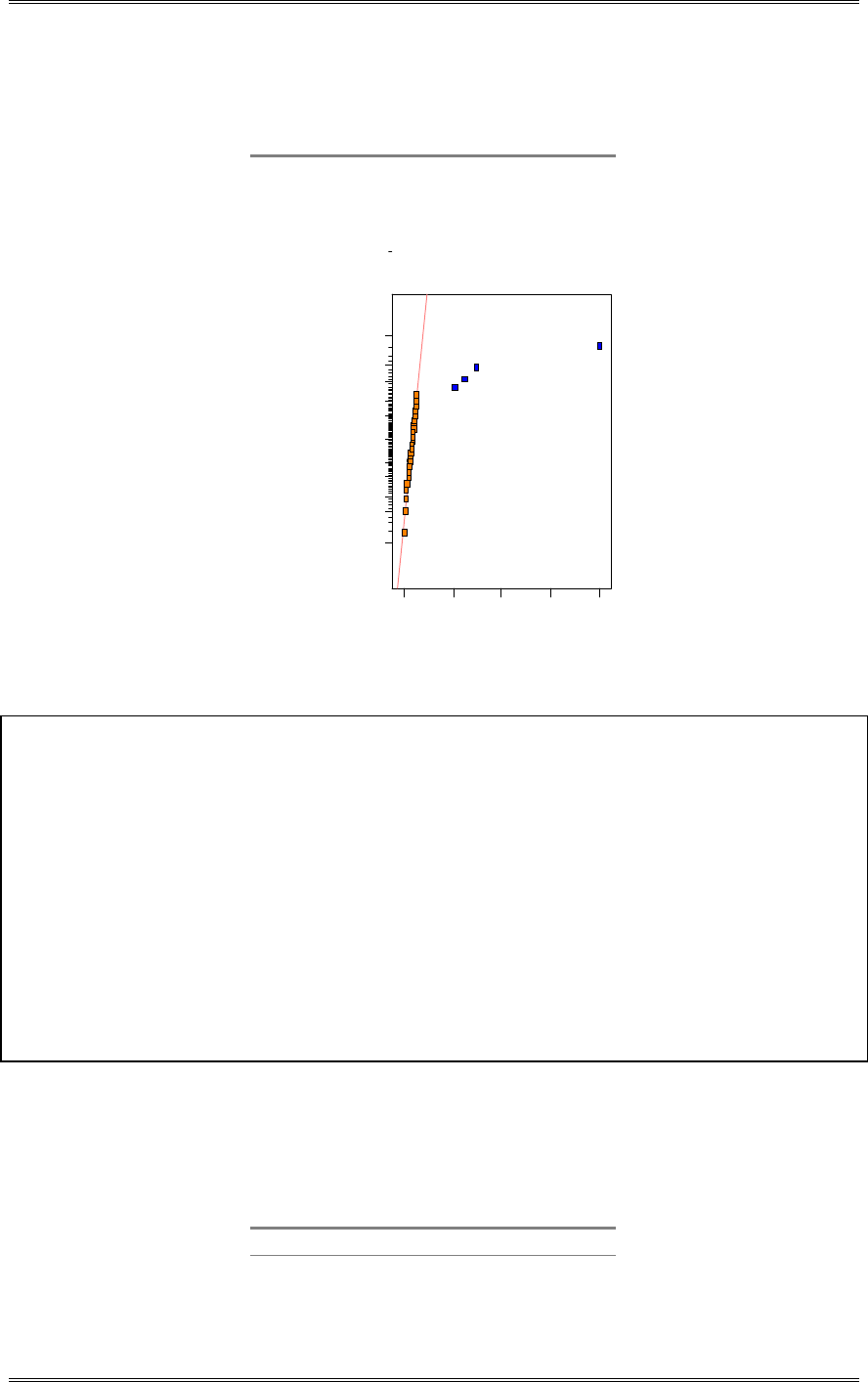
Solutions from Montgomery, D. C. (2001) Design and Analysis of Experiments, Wiley, NY
7-9
bce abce ce be
abd bd ab abcd
bde abde de bcde
Even with four blocks, the same effects are identified as significant per the normal probability plot and
analysis of variance below:
DESIGN-EXPERT Plot
Yield
A: Aperture
B: Exposure Time
C: Develop Time
D: M ask Dim ension
E: Etch Tim e
Normal plot
Norm al % probability
Effe ct
-1 .1 9 7.59 16.37 25.16 33.94
1
5
10
20
30
50
70
80
90
95
99
A
B
C
AB
Design Expert Output
Response: Yield
ANOVA for Selected Factorial Model
Analysis of variance table [Partial sum of squares]
Sum of Mean F
Source Squares DF Square Value Prob > F
Block 2.59 3 0.86
Model 11585.13 4 2896.28 911.62 < 0.0001 significant
A 1116.28 1 1116.28 351.35 < 0.0001
B 9214.03 1 9214.03 2900.15 < 0.0001
C 750.78 1 750.78 236.31 < 0.0001
AB 504.03 1 504.03 158.65 < 0.0001
Residual 76.25 24 3.18
Cor Total 11663.97 31
The Model F-value of 911.62 implies the model is significant. There is only
a 0.01% chance that a "Model F-Value" this large could occur due to noise.
Values of "Prob > F" less than 0.0500 indicate model terms are significant.
In this case A, B, C, AB are significant model terms.
7-10 Design an experiment for confounding a 26 factorial in four blocks. Suggest an appropriate
confounding scheme, different from the one shown in Table 7-8.
We choose ABCE and ABDF. Which also confounds with CDEF
Block 1 Block 2 Block 3 Block 4
a c ac (1)
b abc bc ab

Solutions from Montgomery, D. C. (2001) Design and Analysis of Experiments, Wiley, NY
7-10
cd ad d acd
abcd bd abd bcd
ace e ae ce
bce abe be abce
de acde cde ade
abde bcde abcde bde
cf af f acf
abcf bf abf bcf
adf cdf acdf df
bdf abcdf bcdf abdf
ef acef cef aef
abef bcef abcef bef
acdef def adef cdef
bcdef abdef bdef abcdef
7-11 Consider the 26 design in eight blocks of eight runs each with ABCD, ACE, and ABEF as the
independent effects chosen to be confounded with blocks. Generate the design. Find the other effects
confound with blocks.
Block 1 Block 2 Block 3 Block 4 Block 5 Block 6 Block 7 Block 8
b abc a c ac (1) bc ab
acd d bcd abd bd abcd ad cd
ce ae abce be abe bce e ace
abde bcde de acde cde ade abcde bde
abcf bf cf af f acf abf bcf
de acdf abdf bcdf abcdf bdf cdf adf
aef cef def abcef bcef abef acef ef
bcdef abdef acdef def adef cdef bdef abcdef
The factors that are confounded with blocks are ABCD, ABEF, ACE, BDE, CDEF, BCF, and ADF.
7-12 Consider the 22 design in two blocks with AB confounded. Prove algebraically that SSAB = SSBlocks.
If AB is confounded, the two blocks are:
Block 1 Block 2
(1) a
ab b
(1) + ab a + b
>@>@
>@
2
2121
4
1
2
1
222
2
222
abbaabab
SS
baabbaab
SS
Blocks
Blocks

Solutions from Montgomery, D. C. (2001) Design and Analysis of Experiments, Wiley, NY
7-11
4
2221212121 222
2ababbababaabbaab
>@
ABBlocks
Blocks
SSbaabSS
abbababaababbaab
SS
2
222
2
1
4
1
4
2212122121
7-13 Consider the data in Example 7-2. Suppose that all the observations in block 2 are increased by 20.
Analyze the data that would result. Estimate the block effect. Can you explain its magnitude? Do blocks
now appear to be an important factor? Are any other effect estimates impacted by the change you made in
the data?
Block Effect 62538
8
309
8
715
8
406
21 .yy BlockBlock
This is the block effect estimated in Example 7-2 plus the additional 20 units that were added to each
observation in block 2. All other effects are the same.
Source of Sum of Degrees of Mean
Variation Squares Freedom Square F0
A 1870.56 1 1870.56 89.93
C 390.06 1 390.06 18.75
D 855.56 1 855.56 41.13
AC 1314.06 1 1314.06 63.18
AD 1105.56 1 1105.56 53.15
Blocks 5967.56 1 5967.56
Error 187.56 9 20.8
Total 11690.93 15
Design Expert Output
Response: Filtration in gal/hr
ANOVA for Selected Factorial Model
Analysis of variance table [Partial sum of squares]
Sum of Mean F
Source Squares DF Square Value Prob > F
Block 5967.56 1 5967.56
Model 5535.81 5 1107.16 53.13 < 0.0001 significant
A 1870.56 1 1870.56 89.76 < 0.0001
C 390.06 1 390.06 18.72 0.0019
D 855.56 1 855.56 41.05 0.0001
AC 1314.06 1 1314.06 63.05 < 0.0001
AD 1105.56 1 1105.56 53.05 < 0.0001
Residual 187.56 9 20.84
Cor Total 11690.94 15
The Model F-value of 53.13 implies the model is significant. There is only
a 0.01% chance that a "Model F-Value" this large could occur due to noise.
Values of "Prob > F" less than 0.0500 indicate model terms are significant.
In this case A, C, D, AC, AD are significant model terms.

Solutions from Montgomery, D. C. (2001) Design and Analysis of Experiments, Wiley, NY
7-12
7-14 Suppose that the data in Problem 7-1 we had confounded ABC in replicate I, AB in replicate II, and
BC in replicate III. Construct the analysis of variance table.
Replicate I Replicate II Replicate III
(ABC Confounded) (AB Confounded) (BC Confounded)
Block-> 1 2 1 2 1 2
(1) a (1) a (1) b
ab b ab b bc c
ac c abc ac abc ab
bc abc c bc a ac
Source of Sum of Degrees of Mean
Variation Squares Freedom Square F0
A 0.67 1 0.67 <1
B 770.67 1 770.67 20.77
C 280.17 1 280.17 7.55
AB (reps 1 and III) 25.00 1 25.00 <1
AC 468.17 1 468.17 12.62
BC (reps I and II) 22.56 1 22.56 <1
ABC (reps II and III) 0.06 1 0.06 <1
Blocks within replicates 119.83 3 15.87
Replicates 0.58 2
Error 408.21 11 37.11
Total 2095.33 23
7-15 Repeat Problem 7-1 assuming that ABC was confounded with blocks in each replicate.
Replicate I, II, and III
(ABC Confounded)
Block-> 1 2
(1) a
ab b
ac c
bc abc
Source of Sum of Degrees of Mean
Variation Squares Freedom Square F0
A 0.67 1 0.67 <1
B 770.67 1 770.67 22.15
C 280.17 1 280.17 8.05
AB 16.67 1 16.67 <1
AC 468.17 1 468.17 13.46
BC 48.17 1 48.17 1.38
Blocks (or ABC) 119.83 1 119.83
Replicates/Lack of Fit 64.83 4

Solutions from Montgomery, D. C. (2001) Design and Analysis of Experiments, Wiley, NY
7-13
Error 471.50 12 34.79
Total 2095.33 23
7-16 Suppose that in Problem 7-7 ABCD was confounded in replicate I and ABC was confounded in
replicate II. Perform the statistical analysis of variance.
Source of Sum of Degrees of Mean
Variation Squares Freedom Square F0
A 657.03 1 657.03 84.89
B 13.78 1 13.78 1.78
C 57.78 1 57.78 7.46
D 124.03 1 124.03 16.02
AB 132.03 1 132.03 17.06
AC 3.78 1 3.78 <1
AD 38.28 1 38.28 4.95
BC 2.53 1 2.53 <1
BD 0.28 1 0.28 <1
CD 22.78 1 22.78 2.94
ABC 144.00 1 144.00 18.64
ABD 175.78 1 175.78 22.71
ACD 7.03 1 7.03 <1
BCD 7.03 1 7.03 <1
ABCD 10.56 1 10.56 1.36
Replicates 11.28 1 11.28
Blocks 118.81 2 15.35
Error 100.65 13 7.74
Total 1627.47 31
7-17 Construct a 23 design with ABC confounded in the first two replicates and BC confounded in the
third. Outline the analysis of variance and comment on the information obtained.
Replicate I Replicate II Replicate III
(ABC Confounded) (ABC Confounded) (BC Confounded)
Block-> 1 2 1 2 1 2
(1) a (1) a (1) b
ab b ab b bc c
ac c ac c abc ab
bc abc bc abc a ac
Source of Degrees of
Variation Freedom
A 1
B 1
C 1

Solutions from Montgomery, D. C. (2001) Design and Analysis of Experiments, Wiley, NY
7-14
AB 1
AC 1
BC 1
ABC 1
Replicates 2
Blocks 3
Error 11
Total 23
This design provides “two-thirds” information on BC and “one-third” information on ABC.

Solutions from Montgomery, D. C. (2001) Design and Analysis of Experiments, Wiley, NY
8-1
Chapter 8
Two-Level Fractional Factorial Designs
Solutions
8-1 Suppose that in the chemical process development experiment in Problem 6-7, it was only possible
to run a one-half fraction of the 24 design. Construct the design and perform the statistical analysis, using
the data from replicate 1.
The required design is a 24-1 with I=ABCD.
A B C D=ABC
- - - - (1) 90
+ - - + ad 72
- + - + bd 87
+ + - - ab 83
- - + + cd 99
+ - + - ac 81
- + + - bc 88
+ + + + abcd 80
Design Expert Output
Term Effect SumSqr % Contribtn
Model Intercept
Model A -12 288 64.2857
Model B -1 2 0.446429
Model C 4 32 7.14286
Model D -1 2 0.446429
Model AB 6 72 16.0714
Model AC -1 2 0.446429
Model AD -5 50 11.1607
Error BC Aliased
Error BD Aliased
Error CD Aliased
Error ABC Aliased
Error ABD Aliased
Error ACD Aliased
Error BCD Aliased
Error ABCD Aliased
Lenth's ME 22.5856
Lenth's SME 54.0516
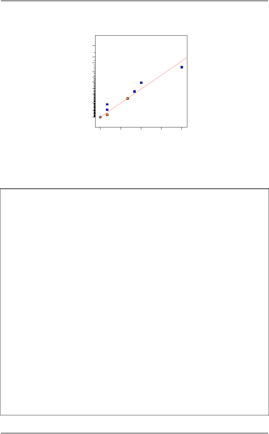
Solutions from Montgomery, D. C. (2001) Design and Analysis of Experiments, Wiley, NY
8-2
Half Normal plot
Half Normal % probability
Effe ct
0.00 3.00 6.00 9.00 12.00
0
20
40
60
70
80
85
90
95
97
99
A
B
D
AB
AD
The largest effect is A. The next largest effects are the AB and AD interactions. A plausible tentative
model would be A, AB and AD, along with B and D to preserve hierarchy.
Design Expert Output
Response: yield
ANOVA for Selected Factorial Model
Analysis of variance table [Partial sum of squares]
Sum of Mean F
Source Squares DF Square Value Prob > F
Model 414.00 5 82.80 4.87 0.1791 not significant
A 288.00 1 288.00 16.94 0.0543
B 2.00 1 2.00 0.12 0.7643
D 2.00 1 2.00 0.12 0.7643
AB 72.00 1 72.00 4.24 0.1758
AD 50.00 1 50.00 2.94 0.2285
Residual 34.00 2 17.00
Cor Total 448.00 7
The "Model F-value" of 4.87 implies the model is not significant relative to the noise. There is a
17.91 % chance that a "Model F-value" this large could occur due to noise.
Std. Dev. 4.12 R-Squared 0.9241
Mean 85.00 Adj R-Squared 0.7344
C.V. 4.85 Pred R-Squared -0.2143
PRESS 544.00 Adeq Precision 6.441
Coefficient
Standard 95% CI 95% CI
Factor Estimate DF Error Low High VIF
Intercept 85.00 1 1.46 78.73 91.27
A-A -6.00 1 1.46 -12.27 0.27 1.00
B-B -0.50 1 1.46 -6.77 5.77 1.00
D-D -0.50 1 1.46 -6.77 5.77 1.00
AB 3.00 1 1.46 -3.27 9.27 1.00
AD -2.50 1 1.46 -8.77 3.77 1.00
Final Equation in Terms of Coded Factors:
yield =
+85.00
-6.00 * A
-0.50 * B
-0.50 * D
+3.00 * A * B
-2.50 * A * D

Solutions from Montgomery, D. C. (2001) Design and Analysis of Experiments, Wiley, NY
8-3
Final Equation in Terms of Actual Factors:
yield =
+85.00000
-6.00000 * A
-0.50000 * B
-0.50000 * D
+3.00000 * A * B
-2.50000 * A * D
The Design-Expert output indicates that we really only need the main effect of factor A. The updated
analysis is shown below:
Design Expert Output
Response: yield
ANOVA for Selected Factorial Model
Analysis of variance table [Partial sum of squares]
Sum of Mean F
Source Squares DF Square Value Prob > F
Model 288.00 1 288.00 10.80 0.0167 significant
A 288.00 1 288.00 10.80 0.0167
Residual 160.00 6 26.67
Cor Total 448.00 7
The Model F-value of 10.80 implies the model is significant. There is only
a 1.67% chance that a "Model F-Value" this large could occur due to noise.
Std. Dev. 5.16 R-Squared 0.6429
Mean 85.00 Adj R-Squared 0.5833
C.V. 6.08 Pred R-Squared 0.3651
PRESS 284.44 Adeq Precision 4.648
Coefficient
Standard 95% CI 95% CI
Factor Estimate DF Error Low High VIF
Intercept 85.00 1 1.83 80.53 89.47
A-A -6.00 1 1.83 -10.47 -1.53 1.00
Final Equation in Terms of Coded Factors:
yield =
+85.00
-6.00 * A
Final Equation in Terms of Actual Factors:
yield =
+85.00000
-6.00000 * A
8-2 Suppose that in Problem 6-15, only a one-half fraction of the 24 design could be run. Construct the
design and perform the analysis, using the data from replicate I.
The required design is a 24-1 with I=ABCD.
A B C D=ABC
- - - - (1) 1.71
+ - - + ad 1.86
- + - + bd 1.79
+ + - - ab 1.67
- - + + cd 1.81
+ - + - ac 1.25
- + + - bc 1.46
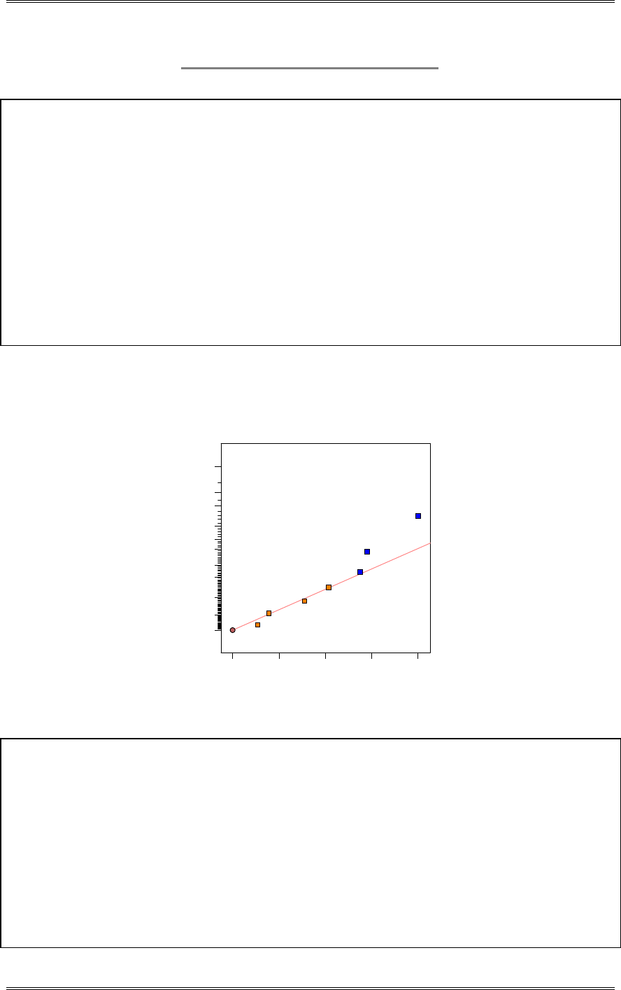
Solutions from Montgomery, D. C. (2001) Design and Analysis of Experiments, Wiley, NY
8-4
+ + + + abcd 0.85
Design Expert Output
Term Effect SumSqr % Contribtn
Model Intercept
Model A -0.285 0.16245 19.1253
Error B -0.215 0.09245 10.8842
Model C -0.415 0.34445 40.5522
Error D 0.055 0.00605 0.712267
Error AB -0.08 0.0128 1.50695
Model AC -0.3 0.18 21.1914
Error AD -0.16 0.0512 6.02778
Error BC Aliased
Error BD Aliased
Error CD Aliased
Error ABC Aliased
Error ABD Aliased
Error ACD Aliased
Error BCD Aliased
Error ABCD Aliased
Lenth's ME 1.21397
Lenth's SME 2.90528
C, A and AC + BD are the largest three effects. Now because the main effects of A and C are large, the
large effect estimate for the AC + BD alias chain probably indicates that the AC interaction is important.
Half Normal plot
Half Normal % probability
Effe ct
0.00 0.10 0.21 0.31 0.42
0
20
40
60
70
80
85
90
95
97
99
A
C
AC
Design Expert Output
Response: Crack Lengthin mm x 10^-2
ANOVA for Selected Factorial Model
Analysis of variance table [Partial sum of squares]
Sum of Mean F
Source Squares DF Square Value Prob > F
Model 0.69 3 0.23 5.64 0.0641 not significant
A 0.16 1 0.16 4.00 0.1162
C 0.34 1 0.34 8.48 0.0436
AC 0.18 1 0.18 4.43 0.1031
Residual 0.16 4 0.041
Cor Total 0.85 7
The Model F-value of 5.64 implies there is a 6.41% chance that a "Model F-Value"
this large could occur due to noise.
Std. Dev. 0.20 R-Squared 0.8087

Solutions from Montgomery, D. C. (2001) Design and Analysis of Experiments, Wiley, NY
8-5
Mean 1.55 Adj R-Squared 0.6652
C.V. 13.00 Pred R-Squared 0.2348
PRESS 0.65 Adeq Precision 5.017
Coefficient Standard 95% CI 95% CI
Factor Estimate DF Error Low High VIF
Intercept 1.55 1 0.071 1.35 1.75
A-Pour Temp -0.14 1 0.071 -0.34 0.055 1.00
C-Heat Tr Mtd -0.21 1 0.071 -0.41 -9.648E-003 1.00
AC -0.15 1 0.071 -0.35 0.048 1.00
Final Equation in Terms of Coded Factors:
Crack Length =
+1.55
-0.14 * A
-0.21 * C
-0.15 * A * C
Final Equation in Terms of Actual Factors:
Crack Length =
+1.55000
-0.14250 * Pour Temp
-0.20750 * Heat Treat Method
-0.15000 * Pour Temp * Heat Treat Method
8-3 Consider the plasma etch experiment described in Problem 6-18. Suppose that only a one-half
fraction of the design could be run. Set up the design and analyze the data.
Etch
Rate Factor Levels
A B C D=ABC (A/min) Low (-) High (+)
- - - - 550 A (cm) 0.80 1.20
+ + - - 650 B (mTorr) 4.50 550
+ - + - 642 C (SCCM) 125 200
- + + - 601 D (W) 275 325
+ - - + 749
- + - + 1052
- - + + 1075
+ + + + 729
Design Expert Output
Term Effect SumSqr % Contribtn
Model Intercept
Error A 4 32 0.0113941
Error B 11.5 264.5 0.0941791
Model C 290.5 168780 60.0967
Model D -127 32258 11.4859
Error AB -197.5 78012.5 27.7775
Error AC -25.5 1300.5 0.463062
Error AD -10 200 0.0712129
Error BC Aliased
Error BD Aliased
Model CD Aliased
Error ABC Aliased
Error ABD Aliased
Error ACD Aliased
Error BCD Aliased
Error ABCD Aliased
Lenth's ME 60.6987
Lenth's SME 145.264
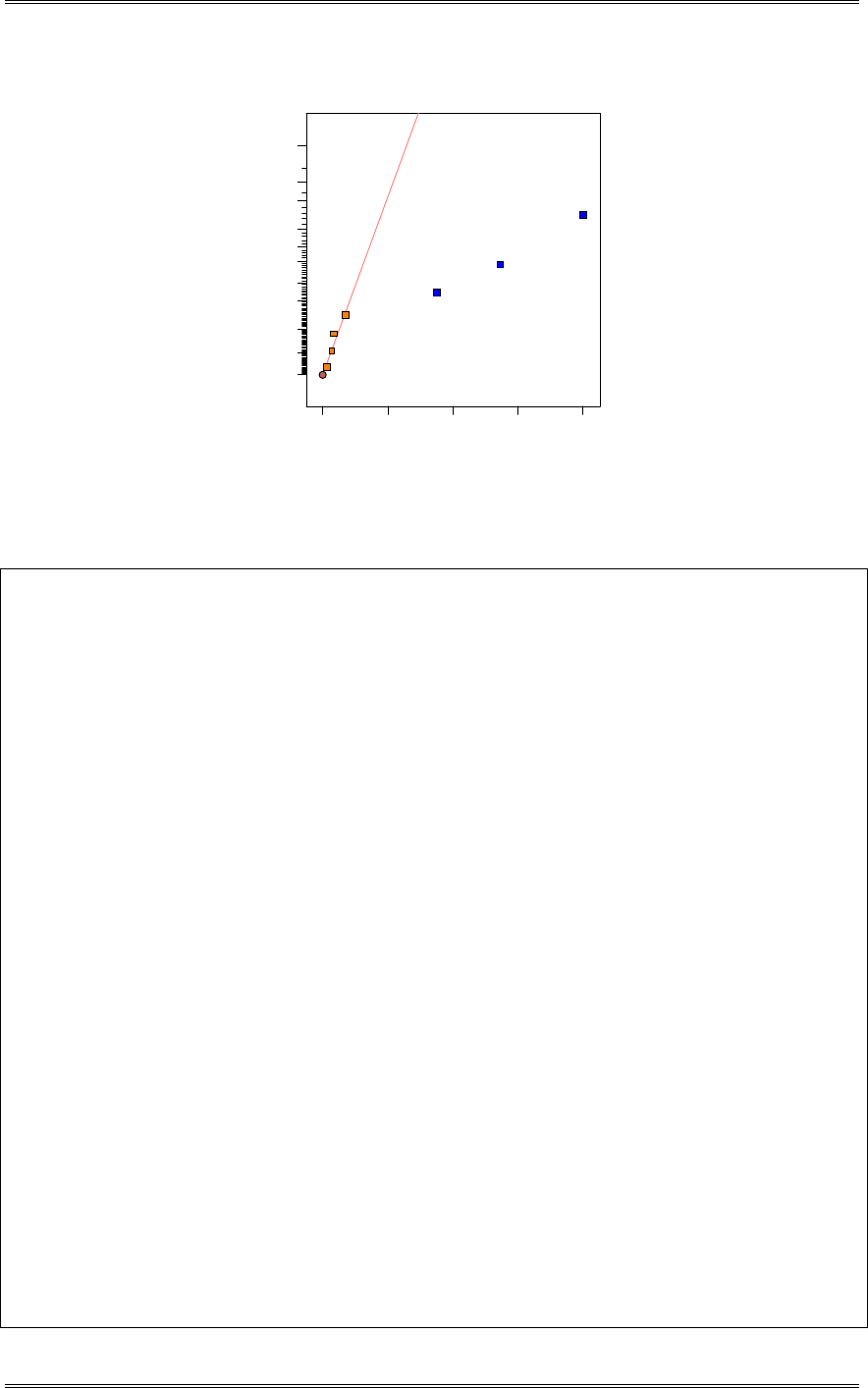
Solutions from Montgomery, D. C. (2001) Design and Analysis of Experiments, Wiley, NY
8-6
Half Normal plot
Half Normal % probability
Effe ct
0.00 72.63 145.25 217.88 290.50
0
20
40
60
70
80
85
90
95
97
99
C
D
AB
The large AB + CD alias chain is most likely the CD interaction.
Design Expert Output
Response: Etch Rate in A/min
ANOVA for Selected Factorial Model
Analysis of variance table [Partial sum of squares]
Sum of Mean F
Source Squares DF Square Value Prob > F
Model 2.791E+005 3 93017.00 207.05 < 0.0001 significant
C 1.688E+005 1 1.688E+005 375.69 < 0.0001
D 32258.00 1 32258.00 71.80 0.0011
CD 78012.50 1 78012.50 173.65 0.0002
Residual 1797.00 4 449.25
Cor Total 2.808E+005 7
The Model F-value of 207.05 implies the model is significant. There is only
a 0.01% chance that a "Model F-Value" this large could occur due to noise.
Std. Dev. 21.20 R-Squared 0.9936
Mean 756.00 Adj R-Squared 0.9888
C.V. 2.80 Pred R-Squared 0.9744
PRESS 7188.00 Adeq Precision 32.560
Coefficient Standard 95% CI 95% CI
Factor Estimate DF Error Low High VIF
Intercept 756.00 1 7.49 735.19 776.81
C-Gas Flow 145.25 1 7.49 124.44 166.06 1.00
D-Power -63.50 1 7.49 -84.31 -42.69 1.00
CD -98.75 1 7.49 -119.56 -77.94 1.00
Final Equation in Terms of Coded Factors:
Etch Rate =
+756.00
+145.25 * C
-63.50 * D
-98.75 * C * D
Final Equation in Terms of Actual Factors:
Etch Rate =
-4246.41667
+35.47333 * Gas Flow
+14.57667 * Power
-0.10533 * Gas Flow * Power
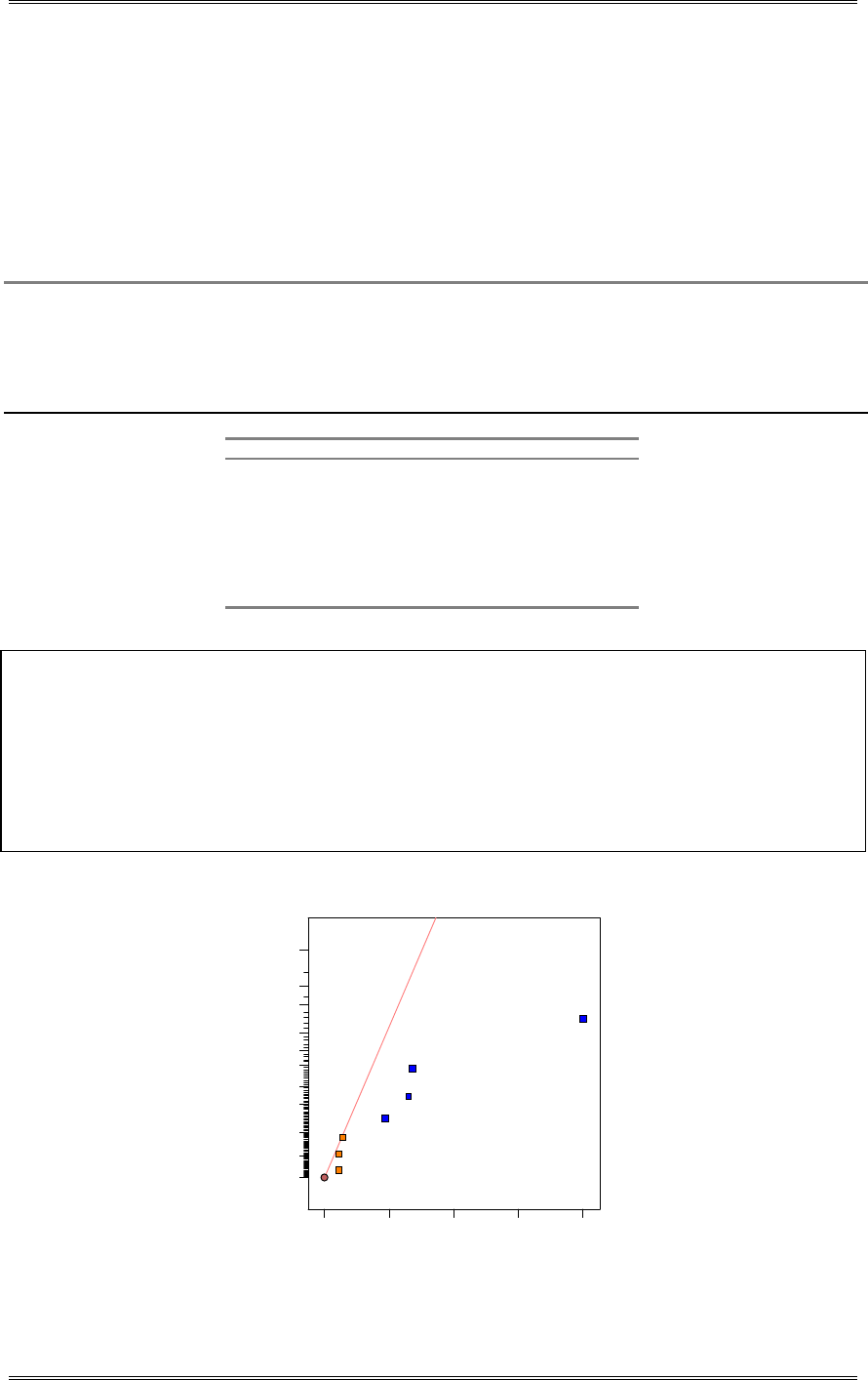
Solutions from Montgomery, D. C. (2001) Design and Analysis of Experiments, Wiley, NY
8-7
8-4 Problem 6-21describes a process improvement study in the manufacturing process of an integrated
circuit. Suppose that only eight runs could be made in this process. Set up an appropriate 25-2 design and
find the alias structure. Use the appropriate observations from Problem 6-21 as the observations in this
design and estimate the factor effects. What conclusions can you draw?
I = ABD = ACE = BCDE
A (ABD) =BD A (ACE) =CE A (BCDE) =ABCDE A=BD=CE=ABCDE
B (ABD) =AD B (ACE) =ABCE B (BCDE) =CDE B=AD=ABCE=CDE
C (ABD) =ABCD C (ACE) =AE C (BCDE) =BDE C=ABCD=AE=BDE
D (ABD) =AB D (ACE) =ACDE D (BCDE) =BCE D=AB=ACDE=BCE
E (ABD) =ABDE E (ACE) =AC E (BCDE) =BCD E=ABDE=AC=BCD
BC (ABD) =ACD BC (ACE) =ABE BC (BCDE) =DE BC=ACD=ABE=DE
BE (ABD) =ADE BE (ACE) =ABC BE (BCDE) =CD BE=ADE=ABC=CD
A B C D=AB E=AC
- - - + + de 6
+ - - - - a 9
- + - - + be 35
+ + - + - abd 50
- - + + - cd 18
+ - + - + ace 22
- + + - - bc 40
+ + + + + abcde 63
Design Expert Output
Term Effect SumSqr % Contribtn
Model Intercept
Model A 11.25 253.125 8.91953
Model B 33.25 2211.13 77.9148
Model C 10.75 231.125 8.1443
Model D 7.75 120.125 4.23292
Error E 2.25 10.125 0.356781
Error BC -1.75 6.125 0.215831
Error BE 1.75 6.125 0.215831
Lenth's ME 28.232
Lenth's SME 67.5646
Half Normal plot
Half Normal % probability
Effe ct
0.00 8.31 16.63 24.94 33.25
0
20
40
60
70
80
85
90
95
97
99
A
B
C
D

Solutions from Montgomery, D. C. (2001) Design and Analysis of Experiments, Wiley, NY
8-8
The main A, B, C, and D are large. However, recall that you are really estimating A+BD+CE, B+AD,
C+DE and D+AD. There are other possible interpretations of the experiment because of the aliasing.
Design Expert Output
Response: Yield
ANOVA for Selected Factorial Model
Analysis of variance table [Partial sum of squares]
Sum of Mean F
Source Squares DF Square Value Prob > F
Model 2815.50 4 703.88 94.37 0.0017 significant
A 253.13 1 253.13 33.94 0.0101
B 2211.12 1 2211.12 296.46 0.0004
C 231.13 1 231.13 30.99 0.0114
D 120.13 1 120.13 16.11 0.0278
Residual 22.38 3 7.46
Cor Total 2837.88 7
The Model F-value of 94.37 implies the model is significant. There is only
a 0.17% chance that a "Model F-Value" this large could occur due to noise.
Std. Dev. 2.73 R-Squared 0.9921
Mean 30.38 Adj R-Squared 0.9816
C.V. 8.99 Pred R-Squared 0.9439
PRESS 159.11 Adeq Precision 25.590
Coefficient Standard 95% CI 95% CI
Factor Estimate DF Error Low High VIF
Intercept 30.38 1 0.97 27.30 33.45
A-Aperture 5.63 1 0.97 2.55 8.70 1.00
B-Exposure Time 16.63 1 0.97 13.55 19.70 1.00
C-Develop Time 5.37 1 0.97 2.30 8.45 1.00
D-Mask Dimension 3.87 1 0.97 0.80 6.95 1.00
Final Equation in Terms of Coded Factors:
Yield =
+30.38
+5.63 * A
+16.63 * B
+5.37 * C
+3.87 * D
Final Equation in Terms of Actual Factors:
Aperture small
Mask Dimension Small
Yield =
-6.00000
+0.83125 * Exposure Time
+0.71667 * Develop Time
Aperture large
Mask Dimension Small
Yield =
+5.25000
+0.83125 * Exposure Time
+0.71667 * Develop Time
Aperture small
Mask Dimension Large
Yield =
+1.75000
+0.83125 * Exposure Time
+0.71667 * Develop Time
Aperture large
Mask Dimension Large
Yield =
+13.00000

Solutions from Montgomery, D. C. (2001) Design and Analysis of Experiments, Wiley, NY
8-9
+0.83125 * Exposure Time
+0.71667 * Develop Time
8-5 Continuation of Problem 8-4. Suppose you have made the eight runs in the 25-2 design in Problem
8-4. What additional runs would be required to identify the factor effects that are of interest? What are
the alias relationships in the combined design?
We could fold over the original design by changing the signs on the generators D = AB and E = AC to
produce the following new experiment.
A B C D=-AB E=-AC
- - - - - (1) 7
+ - - + + ade 12
- + - + - bd 32
+ + - - + abe 52
- - + - + ce 15
+ - + + - acd 21
- + + + + bcde 41
+ + + - - abc 60
A (-ABD) =-BD A (-ACE) =-CE A (BCDE) =ABCDE A=-BD=-CE=ABCDE
B (-ABD) =-AD B (-ACE) =-ABCE B (BCDE) =CDE B=-AD=-ABCE=CDE
C (-ABD) =-ABCD C (-ACE) =-AE C (BCDE) =BDE C=-ABCD=-AE=BDE
D (-ABD) =-AB D (-ACE) =-ACDE D (BCDE) =BCE D=-AB=-ACDE=BCE
E (-ABD) =-ABDE E (-ACE) =-AC E (BCDE) =BCD E=-ABDE=-AC=BCD
BC (-ABD) =-ACD BC (-ACE) =-ABE BC (BCDE) =DE BC=-ACD=-ABE=DE
BE (-ABD) =-ADE BE (-ACE) =-ABC BE (BCDE) =CD BE=-ADE=-ABC=CD
Assuming all three factor and higher interactions to be negligible, all main effects can be separated from
their two-factor interaction aliases in the combined design.
8-6 R.D. Snee (“Experimenting with a Large Number of Variables,” in Experiments in Industry:
Design, Analysis and Interpretation of Results, by R.D. Snee, L.B. Hare, and J.B. Trout, Editors, ASQC,
1985) describes an experiment in which a 25-1 design with I=ABCDE was used to investigate the effects of
five factors on the color of a chemical product. The factors are A = solvent/reactant, B = catalyst/reactant,
C = temperature, D = reactant purity, and E = reactant pH. The results obtained were as follows:
e = -0.63 d = 6.79
a = 2.51 ade = 5.47
b = -2.68 bde = 3.45
abe = 1.66 abd = 5.68
c = 2.06 cde = 5.22
ace = 1.22 acd = 4.38
bce = -2.09 bcd = 4.30
abc = 1.93 abcde = 4.05
(a) Prepare a normal probability plot of the effects. Which effects seem active?
Factors A, B, D, and the AB, AD interactions appear to be active.
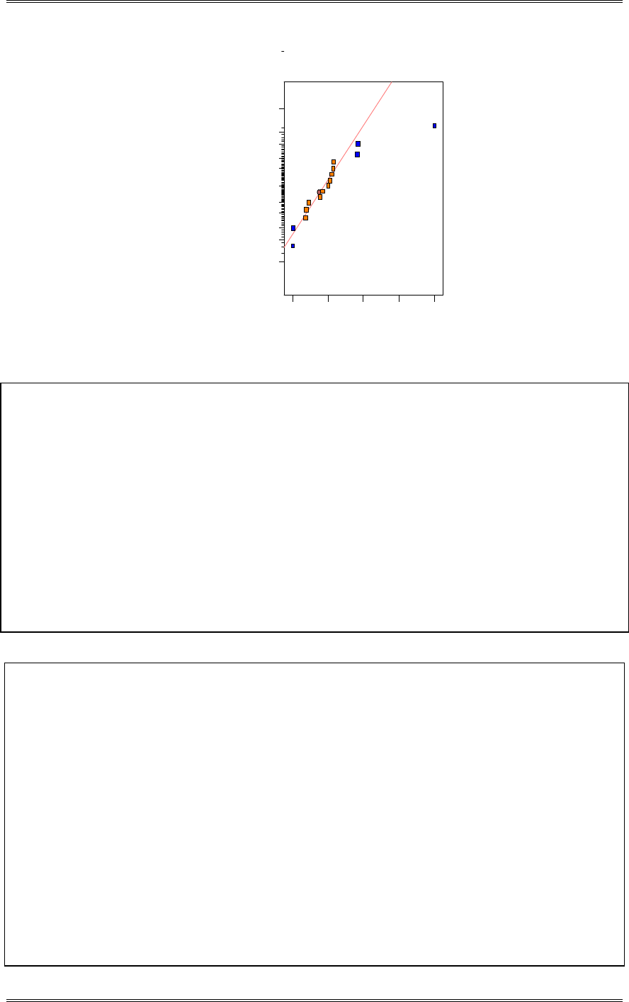
Solutions from Montgomery, D. C. (2001) Design and Analysis of Experiments, Wiley, NY
8-10
DESIGN-EXPERT Plot
Color
A: Solvent/Reactant
B: Ca talyst/Reactant
C: Temperature
D: Reactant Purity
E: Reactant pH
Normal plot
Norm al % probability
Effe ct
-1 .3 6 0.09 1.53 2.98 4.42
1
5
10
20
30
50
70
80
90
95
99
A
B
D
AB
AD
Design Expert Output
Term Effect SumSqr % Contribtn
Model Intercept
Model A 1.31 6.8644 5.98537
Model B -1.34 7.1824 6.26265
Error C -0.1475 0.087025 0.0758809
Model D 4.42 78.1456 68.1386
Error E -0.8275 2.73902 2.38828
Model AB 1.275 6.5025 5.66981
Error AC -0.7875 2.48062 2.16297
Model AD -1.355 7.3441 6.40364
Error AE 0.3025 0.366025 0.319153
Error BC 0.1675 0.112225 0.0978539
Error BD 0.245 0.2401 0.209354
Error BE 0.2875 0.330625 0.288286
Error CD -0.7125 2.03063 1.77059
Error CE -0.24 0.2304 0.200896
Error DE 0.0875 0.030625 0.0267033
Lenth's ME 1.95686
Lenth's SME 3.9727
Design Expert Output
Response: Color
ANOVA for Selected Factorial Model
Analysis of variance table [Partial sum of squares]
Sum of Mean F
Source Squares DF Square Value Prob > F
Model 106.04 5 21.21 24.53 < 0.0001 significant
A 6.86 1 6.86 7.94 0.0182
B 7.18 1 7.18 8.31 0.0163
D 78.15 1 78.15 90.37 < 0.0001
AB 6.50 1 6.50 7.52 0.0208
AD 7.34 1 7.34 8.49 0.0155
Residual 8.65 10 0.86
Cor Total 114.69 15
The Model F-value of 24.53 implies the model is significant. There is only
a 0.01% chance that a "Model F-Value" this large could occur due to noise.
Std. Dev. 0.93 R-Squared 0.9246
Mean 2.71 Adj R-Squared 0.8869
C.V. 34.35 Pred R-Squared 0.8070
PRESS 22.14 Adeq Precision 14.734
Coefficient Standard 95% CI 95% CI

Solutions from Montgomery, D. C. (2001) Design and Analysis of Experiments, Wiley, NY
8-11
Factor Estimate DF Error Low High VIF
Intercept 2.71 1 0.23 2.19 3.23
A-Solvent/Reactant 0.66 1 0.23 0.14 1.17 1.00
B-Catalyst/Reactant -0.67 1 0.23 -1.19 -0.15 1.00
D-Reactant Purity 2.21 1 0.23 1.69 2.73 1.00
AB 0.64 1 0.23 0.12 1.16 1.00
AD -0.68 1 0.23 -1.20 -0.16 1.00
Final Equation in Terms of Coded Factors:
Color =
+2.71
+0.66 * A
-0.67 * B
+2.21 * D
+0.64 * A * B
-0.68 * A * D
Final Equation in Terms of Actual Factors:
Color =
+2.70750
+0.65500 * Solvent/Reactant
-0.67000 * Catalyst/Reactant
+2.21000 * Reactant Purity
+0.63750 * Solvent/Reactant * Catalyst/Reactant
-0.67750 * Solvent/Reactant * Reactant Purity
(b) Calculate the residuals. Construct a normal probability plot of the residuals and plot the residuals
versus the fitted values. Comment on the plots.
Design Expert Output
Diagnostics Case Statistics
Standard Actual Predicted Student Cook's Outlier Run
Order Value Value Residual Leverage Residual Distance t Order
1 -0.63 0.47 -1.10 0.375 -1.500 0.225 -1.616 2
2 2.51 1.86 0.65 0.375 0.881 0.078 0.870 6
3 -2.68 -2.14 -0.54 0.375 -0.731 0.053 -0.713 14
4 1.66 1.80 -0.14 0.375 -0.187 0.003 -0.178 11
5 2.06 0.47 1.59 0.375 2.159 0.466 2.804 8
6 1.22 1.86 -0.64 0.375 -0.874 0.076 -0.863 15
7 -2.09 -2.14 0.053 0.375 0.071 0.001 0.068 10
8 1.93 1.80 0.13 0.375 0.180 0.003 0.171 3
9 6.79 6.25 0.54 0.375 0.738 0.054 0.720 4
10 5.47 4.93 0.54 0.375 0.738 0.054 0.720 5
11 3.45 3.63 -0.18 0.375 -0.248 0.006 -0.236 16
12 5.68 4.86 0.82 0.375 1.112 0.124 1.127 12
13 5.22 6.25 -1.03 0.375 -1.398 0.195 -1.478 9
14 4.38 4.93 -0.55 0.375 -0.745 0.055 -0.727 1
15 4.30 3.63 0.67 0.375 0.908 0.082 0.899 13
16 4.05 4.86 -0.81 0.375 -1.105 0.122 -1.119 7
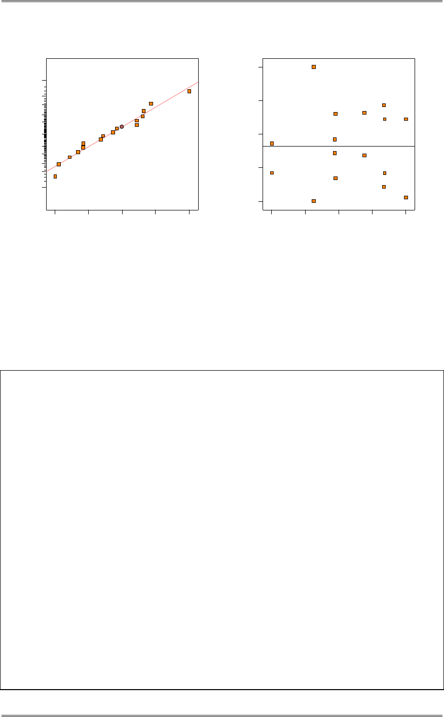
Solutions from Montgomery, D. C. (2001) Design and Analysis of Experiments, Wiley, NY
8-12
Residual
Normal % probability
Normal plot of residuals
-1 .1 02 5 -0 . 4 3 0.2425 0.915 1.5875
1
5
10
20
30
50
70
80
90
95
99
Predicted
Residuals
Residuals vs. Predicted
-1 .1 02 5
-0 .4 3
0.2425
0.915
1.5875
-2 .1 4 -0 .0 5 2.05 4.15 6.25
The residual plots are satisfactory.
(c) If any factors are negligible, collapse the 25-1 design into a full factorial in the active factors.
Comment on the resulting design, and interpret the results.
The design becomes two replicates of a 23 in the factors A, B and D. When re-analyzing the data in three
factors, D becomes labeled as C.
Design Expert Output
Response: Color
ANOVA for Selected Factorial Model
Analysis of variance table [Partial sum of squares]
Sum of Mean F
Source Squares DF Square Value Prob > F
Model 106.51 7 15.22 14.89 0.0005 significant
A 6.86 1 6.86 6.72 0.0320
B 7.18 1 7.18 7.03 0.0292
C 78.15 1 78.15 76.46 < 0.0001
AB 6.50 1 6.50 6.36 0.0357
AC 7.34 1 7.34 7.19 0.0279
BC 0.24 1 0.24 0.23 0.6409
ABC 0.23 1 0.23 0.23 0.6476
Residual 8.18 8 1.02
Lack of Fit 0.000 0
Pure Error 8.18 8 1.02
Cor Total 114.69 15
The Model F-value of 14.89 implies the model is significant. There is only
a 0.05% chance that a "Model F-Value" this large could occur due to noise.
Std. Dev. 1.01 R-Squared 0.9287
Mean 2.71 Adj R-Squared 0.8663
C.V. 37.34 Pred R-Squared 0.7148
PRESS 32.71 Adeq Precision 11.736
Coefficient Standard 95% CI 95% CI
Factor Estimate DF Error Low High VIF
Intercept 2.71 1 0.25 2.12 3.29
A-Solvent/Reactant 0.66 1 0.25 0.072 1.24 1.00
B-Catalyst/Reactant -0.67 1 0.25 -1.25 -0.087 1.00
C-Reactant Purity 2.21 1 0.25 1.63 2.79 1.00
AB 0.64 1 0.25 0.055 1.22 1.00
AC -0.68 1 0.25 -1.26 -0.095 1.00

Solutions from Montgomery, D. C. (2001) Design and Analysis of Experiments, Wiley, NY
8-13
BC 0.12 1 0.25 -0.46 0.71 1.00
ABC -0.12 1 0.25 -0.70 0.46 1.00
Final Equation in Terms of Coded Factors:
Color =
+2.71
+0.66 * A
-0.67 * B
+2.21 * C
+0.64 * A * B
-0.68 * A * C
+0.12 * B * C
-0.12 * A * B * C
Final Equation in Terms of Actual Factors:
Color =
+2.70750
+0.65500 * Solvent/Reactant
-0.67000 * Catalyst/Reactant
+2.21000 * Reactant Purity
+0.63750 * Solvent/Reactant * Catalyst/Reactant
-0.67750 * Solvent/Reactant * Reactant Purity
+0.12250 * Catalyst/Reactant * Reactant Purity
-0.12000 * Solvent/Reactant * Catalyst/Reactant * Reactant Purity
8-7 An article by J.J. Pignatiello, Jr. And J.S. Ramberg in the Journal of Quality Technology, (Vol. 17,
1985, pp. 198-206) describes the use of a replicated fractional factorial to investigate the effects of five
factors on the free height of leaf springs used in an automotive application. The factors are A = furnace
temperature, B = heating time, C = transfer time, D = hold down time, and E = quench oil temperature.
The data are shown below:
A
B
C
D
E
Free Height
-----
7.78
7.78
7.81
+ - - + - 8.15 8.18 7.88
- + - + - 7.50 7.56 7.50
+ + - - - 7.59 7.56 7.75
- - + + - 7.54 8.00 7.88
+ - + - - 7.69 8.09 8.06
- + + - - 7.56 7.52 7.44
+ + + + - 7.56 7.81 7.69
- - - - + 7.50 7.25 7.12
+ - - + + 7.88 7.88 7.44
- + - + + 7.50 7.56 7.50
+ + - - + 7.63 7.75 7.56
- - + + + 7.32 7.44 7.44
+ - + - + 7.56 7.69 7.62
- + + - + 7.18 7.18 7.25
+ + + + + 7.81 7.50 7.59
(a) Write out the alias structure for this design. What is the resolution of this design?
I=ABCD, Resolution IV
A (ABCD)= BCD
B (ABCD)= ACD
C (ABCD)= ABD
D (ABCD)= ABC
E (ABCD)= ABCDE
AB (ABCD)= CD
AC (ABCD)= BD
AD (ABCD)= BC
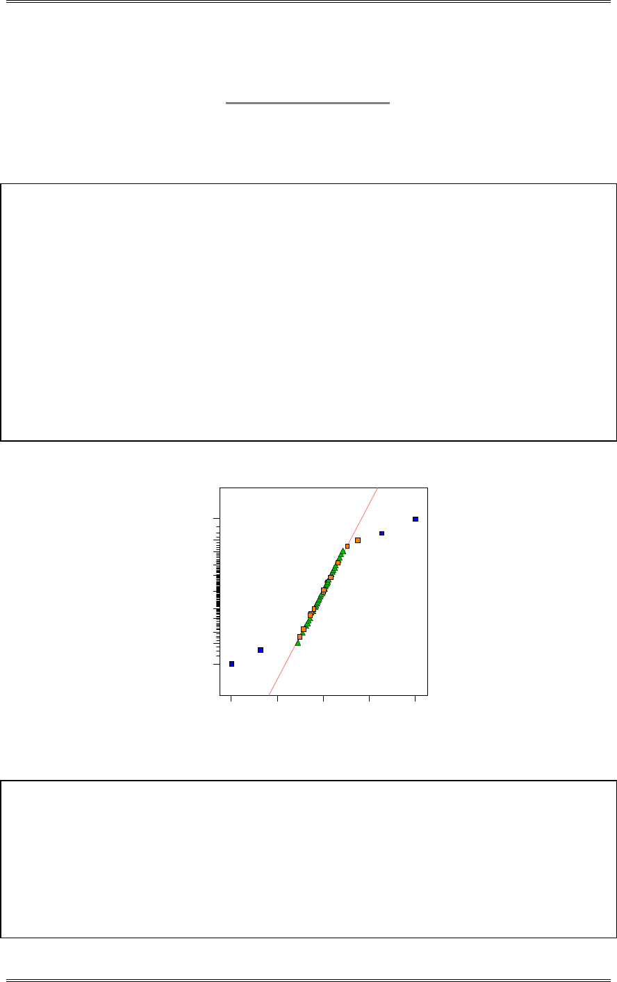
Solutions from Montgomery, D. C. (2001) Design and Analysis of Experiments, Wiley, NY
8-14
AE (ABCD)= BCDE
BE (ABCD)= ACDE
CE (ABCD)= ABDE
DE (ABCD)= ABCE
(b) Analyze the data. What factors influence the mean free height?
Design Expert Output
Term Effect SumSqr % Contribtn
Model Intercept
Model A 0.242083 0.703252 24.3274
Model B -0.16375 0.321769 11.1309
Model C -0.0495833 0.0295021 1.02056
Model D 0.09125 0.0999188 3.45646
Model E -0.23875 0.684019 23.6621
Model AB -0.0295833 0.0105021 0.363296
Model AC 0.00125 1.875E-005 0.000648614
Model AD -0.0229167 0.00630208 0.218006
Model AE 0.06375 0.0487687 1.68704
Error BC Aliased
Error BD Aliased
Model BE 0.152917 0.280602 9.70679
Error CD Aliased
Model CE -0.0329167 0.0130021 0.449777
Model DE 0.0395833 0.0188021 0.650415
Error Pure Error 0.627067 21.6919
Lenth's ME 0.088057
Lenth's SME 0.135984
Normal plot
Normal % probability
Effe ct
-0 .2 4 -0 .1 2 0.00 0.12 0.24
1
5
10
20
30
50
70
80
90
95
99 A
B
E
BE
Design Expert Output
Response:Free Height
ANOVA for Selected Factorial Model
Analysis of variance table [Partial sum of squares]
Sum of
Mean F
Source Squares DF Square Value Prob > F
Model 1.99 4 0.50 23.74 < 0.0001 significant
A 0.70 1 0.70 33.56 < 0.0001
B 0.32 1 0.32 15.35 0.0003
E 0.68 1 0.68 32.64 < 0.0001
BE 0.28 1 0.28 13.39 0.0007
Residual 0.90 43 0.021
Lack of Fit 0.27 11 0.025 1.27 0.2844 not significant

Solutions from Montgomery, D. C. (2001) Design and Analysis of Experiments, Wiley, NY
8-15
Pure Error 0.63 32 0.020
Cor Total 2.89 47
The Model F-value of 23.74 implies the model is significant. There is only
a 0.01% chance that a "Model F-Value" this large could occur due to noise.
Std. Dev. 0.14 R-Squared 0.6883
Mean 7.63 Adj R-Squared 0.6593
C.V. 1.90 Pred R-Squared 0.6116
PRESS 1.12 Adeq Precision 13.796
Coefficient
Standard 95% CI 95% CI
Factor Estimate DF Error Low High VIF
Intercept 7.63 1 0.021 7.58 7.67
A-Furnace Temp 0.12 1 0.021 0.079 0.16 1.00
B-Heating Time -0.082 1 0.021 -0.12 -0.040 1.00
E-Quench Temp -0.12 1 0.021 -0.16 -0.077 1.00
BE 0.076 1 0.021 0.034 0.12 1.00
Final Equation in Terms of Coded Factors:
Free Height =
+7.63
+0.12 * A
-0.082 * B
-0.12 * E
+0.076 * B * E
Final Equation in Terms of Actual Factors:
Free Height =
+7.62562
+0.12104 * Furnace Temp
-0.081875 * Heating Time
-0.11937 * Quench Temp
+0.076458 * Heating Time * Quench Temp
(c) Calculate the range and standard deviation of the free height for each run. Is there any indication that
any of these factors affects variability in the free height?
Design Expert Output (Range)
Term Effect SumSqr % Contribtn
Model Intercept
Model A 0.11375 0.0517563 16.2198
Model B -0.12625 0.0637563 19.9804
Model C 0.02625 0.00275625 0.863774
Error D 0.06125 0.0150063 4.70277
Model E -0.01375 0.00075625 0.236999
Error AB 0.04375 0.00765625 2.39937
Error AC -0.03375 0.00455625 1.42787
Error AD 0.03625 0.00525625 1.64724
Error AE -0.00375 5.625E-005 0.017628
Model BC Aliased
Error BD Aliased
Model BE 0.01625 0.00105625 0.331016
Error CD Aliased
Model CE -0.13625 0.0742562 23.271
Error DE -0.02125 0.00180625 0.566056
Error ABC Aliased
Error ABD Aliased
Error ABE 0.03125 0.00390625 1.22417
Error ACD Aliased
Error ACE 0.04875 0.00950625 2.97914
Error ADE 0.13875 0.0770062 24.1328
Error BCD Aliased
Model BCE Aliased
Error BDE Aliased
Error CDE Aliased
Lenth's ME 0.130136
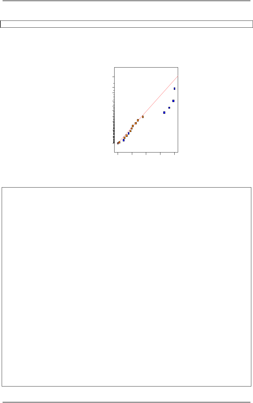
Solutions from Montgomery, D. C. (2001) Design and Analysis of Experiments, Wiley, NY
8-16
Lenth's SME 0.264194
Interaction ADE is aliased with BCE. Although the plot below identifies ADE, BCE was included in the
analysis.
DESIGN-EXPERT Plot
Range
A: Furnace Temp
B: Heating Time
C: Transfer Time
D: Hold T im e
E: Quench Temp
Half Normal plot
Half Normal % probability
|Effect|
0.00 0.03 0.07 0.10 0.14
0
20
40
60
70
80
85
90
95
97
99
A
B
C
E
CE
AD E
Design Expert Output (Range)
Response: Range
ANOVA for Selected Factorial Model
Analysis of variance table [Partial sum of squares]
Sum of
Mean F
Source Squares DF Square Value Prob > F
Model 0.28 8 0.035 5.70 0.0167 significant
A 0.052 1 0.052 8.53 0.0223
B 0.064 1 0.064 10.50 0.0142
C 2.756E-003 1 2.756E-003 0.45 0.5220
E 7.562E-004 1 7.562E-004 0.12 0.7345
BC 5.256E-003 1 5.256E-003 0.87 0.3831
BE 1.056E-003 1 1.056E-003 0.17 0.6891
CE 0.074 1 0.074 12.23 0.0100
BCE 0.077 1 0.077 12.69 0.0092
Residual 0.042 7 6.071E-003
Cor Total 0.32 15
The Model F-value of 5.70 implies the model is significant. There is only
a 1.67% chance that a "Model F-Value" this large could occur due to noise.
Std. Dev. 0.078 R-Squared 0.8668
Mean 0.22 Adj R-Squared 0.7146
C.V. 35.52 Pred R-Squared 0.3043
PRESS 0.22 Adeq Precision 7.166
Coefficient
Standard 95% CI 95% CI
Factor Estimate DF Error Low High VIF
Intercept 0.22 1 0.019 0.17 0.27
A-Furn Temp 0.057 1 0.019 0.011 0.10 1.00
B-Heat Time -0.063 1 0.019 -0.11 -0.017 1.00
C-Transfer Time 0.013 1 0.019 -0.033 0.059 1.00
E-Qnch Temp -6.875E-003 1 0.019 -0.053 0.039 1.00
BC 0.018 1 0.019 -0.028 0.064 1.00
BE 8.125E-003 1 0.019 -0.038 0.054 1.00
CE -0.068 1 0.019 -0.11 -0.022 1.00
BCE 0.069 1 0.019 0.023 0.12 1.00
Final Equation in Terms of Coded Factors:

Solutions from Montgomery, D. C. (2001) Design and Analysis of Experiments, Wiley, NY
8-17
Range =
+0.22
+0.057 * A
-0.063 * B
+0.013 * C
-6.875E-003 * E
+0.018 * B * C
+8.125E-003 * B * E
-0.068 * C * E
+0.069 * B * C * E
Final Equation in Terms of Actual Factors:
Range =
+0.21937
+0.056875 * Furnace Temp
-0.063125 * Heating Time
+0.013125 * Transfer Time
-6.87500E-003 * Quench Temp
+0.018125 * Heating Time * Transfer Time
+8.12500E-003 * Heating Time * Quench Temp
-0.068125 * Transfer Time * Quench Temp
+0.069375 * Heating Time * Transfer Time * Quench Temp
Design Expert Output (StDev)
Term Effect SumSqr % Contribtn
Model Intercept
Model A 0.0625896 0.0156698 16.873
Model B -0.0714887 0.0204425 22.0121
Model C 0.010567 0.000446646 0.48094
Error D 0.0353616 0.00500176 5.3858
Model E -0.00684034 0.000187161 0.201532
Error AB 0.0153974 0.000948317 1.02113
Error AC -0.0218505 0.00190978 2.05641
Error AD 0.0190608 0.00145326 1.56484
Error AE -0.00329035 4.33057E-005 0.0466308
Model BC Aliased
Error BD Aliased
Model BE 0.0087666 0.000307413 0.331017
Error CD Aliased
Model CE -0.0714816 0.0204385 22.0078
Error DE -0.00467792 8.75317E-005 0.0942525
Error ABC Aliased
Error ABD Aliased
Error ABE 0.0155599 0.000968437 1.0428
Error ACD Aliased
Error ACE 0.0199742 0.00159587 1.7184
Error ADE Aliased
Error BCD Aliased
Model BCE 0.0764346 0.023369 25.1633
Error BDE Aliased
Error CDE Aliased
Lenth's ME 0.0596836
Lenth's SME 0.121166
Interaction ADE is aliased with BCE. Although the plot below identifies ADE, BCE was included in the
analysis.
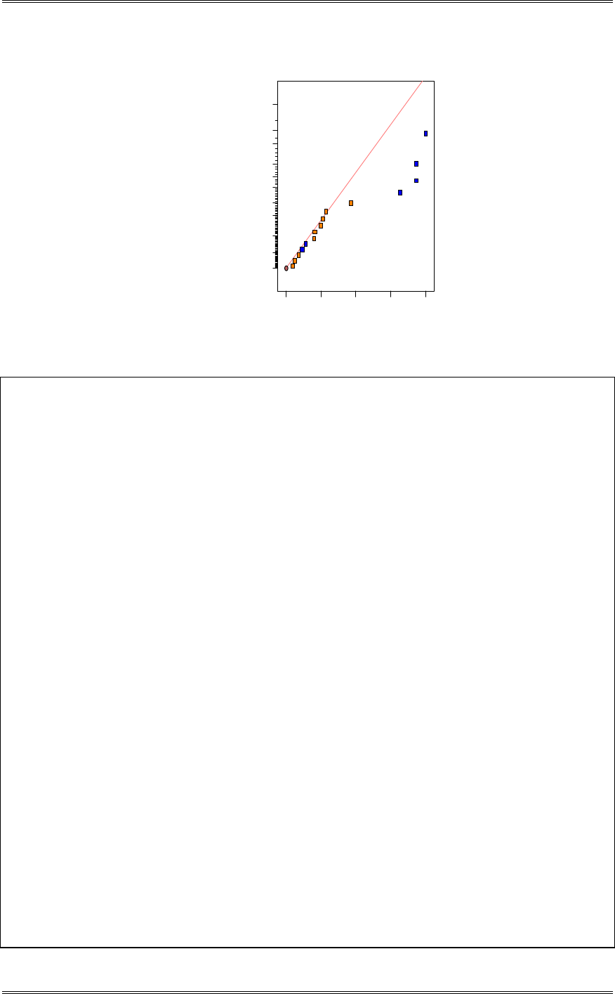
Solutions from Montgomery, D. C. (2001) Design and Analysis of Experiments, Wiley, NY
8-18
DESIGN-EXPERT Plot
StDev
A: Furnace Temp
B: Heating Time
C: Transfer Time
D: Hold T im e
E: Quench Temp
Half Normal plot
Half Normal % probability
|Effect|
0.00 0.02 0.04 0.06 0.08
0
20
40
60
70
80
85
90
95
97
99
A
B
C
BE
CE
AD E
Design Expert Output (StDev)
Response: StDev
ANOVA for Selected Factorial Model
Analysis of variance table [Partial sum of squares]
Sum of Mean F
Source Squares DF Square Value Prob > F
Model 0.082 8 0.010 6.82 0.0101 significant
A 0.016 1 0.016 10.39 0.0146
B 0.020 1 0.020 13.56 0.0078
C 4.466E-004 1 4.466E-004 0.30 0.6032
E 1.872E-004 1 1.872E-004 0.12 0.7350
BC 1.453E-003 1 1.453E-003 0.96 0.3589
BE 3.074E-004 1 3.074E-004 0.20 0.6653
CE 0.020 1 0.020 13.55 0.0078
BCE 0.023 1 0.023 15.50 0.0056
Residual 0.011 7 1.508E-003
Cor Total 0.093 15
The Model F-value of 6.82 implies the model is significant. There is only
a 1.01% chance that a "Model F-Value" this large could occur due to noise.
Std. Dev. 0.039 R-Squared 0.8863
Mean 0.12 Adj R-Squared 0.7565
C.V. 33.07 Pred R-Squared 0.4062
PRESS 0.055 Adeq Precision 7.826
Coefficient Standard 95% CI 95% CI
Factor Estimate DF Error Low High VIF
Intercept 0.12 1 9.708E-003 0.094 0.14
A-Furnace Temp 0.031 1 9.708E-003 8.340E-003 0.054 1.00
B-Heating Time -0.036 1 9.708E-003 -0.059 -0.013 1.00
C-Transfer Time 5.283E-003 1 9.708E-003 -0.018 0.028 1.00
E-Quench Temp -3.420E-003 1 9.708E-003 -0.026 0.020 1.00
BC 9.530E-003 1 9.708E-003 -0.013 0.032 1.00
BE 4.383E-003 1 9.708E-003 -0.019 0.027 1.00
CE -0.036 1 9.708E-003 -0.059 -0.013 1.00
BCE 0.038 1 9.708E-003 0.015 0.061 1.00
Final Equation in Terms of Coded Factors:
StDev =
+0.12
+0.031 * A
-0.036 * B
+5.283E-003 * C
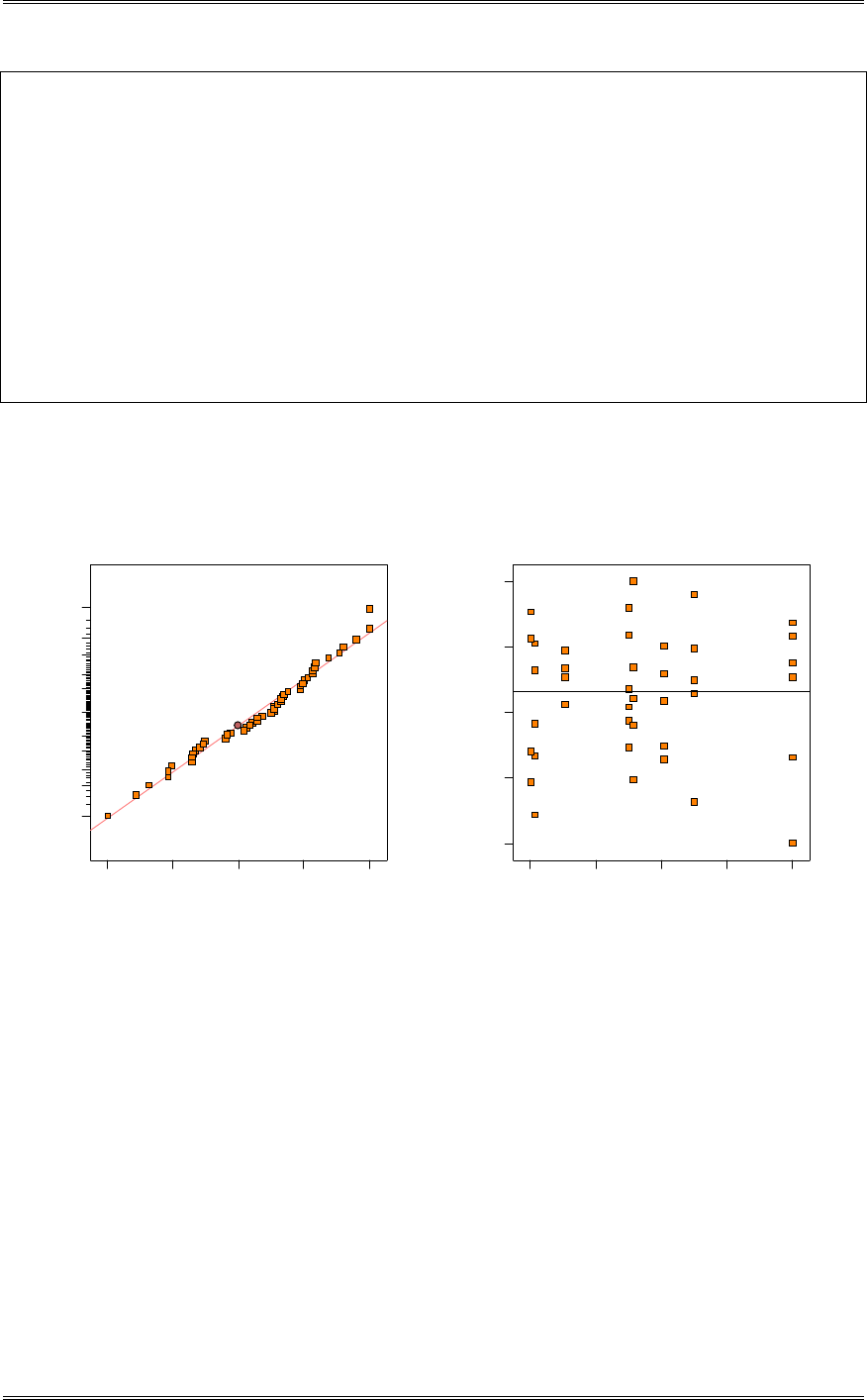
Solutions from Montgomery, D. C. (2001) Design and Analysis of Experiments, Wiley, NY
8-19
-3.420E-003 * E
+9.530E-003 * B * C
+4.383E-003 * B * E
-0.036 * C * E
+0.038 * B * C * E
Final Equation in Terms of Actual Factors:
StDev =
+0.11744
+0.031295 * Furnace Temp
-0.035744 * Heating Time
+5.28350E-003 * Transfer Time
-3.42017E-003 * Quench Temp
+9.53040E-003 * Heating Time * Transfer Time
+4.38330E-003 * Heating Time * Quench Temp
-0.035741 * Transfer Time * Quench Temp
+0.038217 * Heating Time * Transfer Time * Quench Temp
(d) Analyze the residuals from this experiment, and comment on your findings.
The residual plot follows. All plots are satisfactory.
Residual
Norm al % probability
Normal plot of residuals
-0.334375 -0.188958 -0.0435417 0.101875 0.247292
1
5
10
20
30
50
70
80
90
95
99
2
2
22
2
2
2
2
2
2
2
2
2
22
2
Predicted
Residuals
Residuals vs. Predicted
-0 .3 34 3 7 5
-0 .1 88 9 5 8
-0.0435417
0.101875
0.247292
7.38 7.54 7.70 7.86 8.02
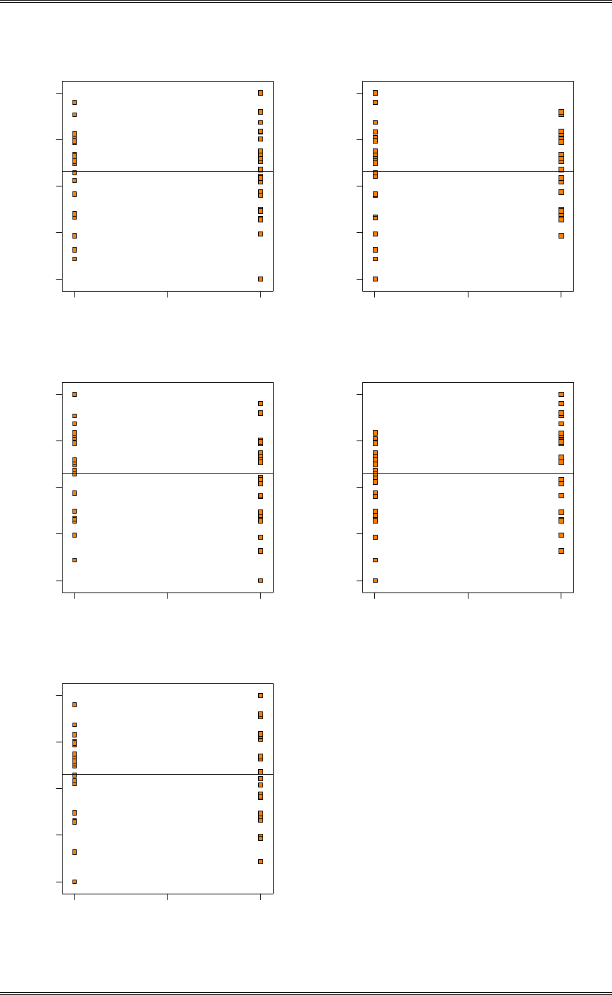
Solutions from Montgomery, D. C. (2001) Design and Analysis of Experiments, Wiley, NY
8-20
2
2
22
2
2
2
2
2
2
2
2
2
22
2
Furnace Tem p
Residuals
Residuals vs. Furnace Temp
-0.334375
-0.188958
-0.0435417
0.101875
0.247292
-1 0 1
2
2
22
2
2
2
2
2
2
2
2
2
22
2
Heating Tim e
Residuals
Residuals vs. Heating Time
-0 .3 34 3 7 5
-0 .1 88 9 5 8
-0.0435417
0.101875
0.247292
-1 0 1
2
2
22
2
2
2
2
2
22
2
Transfer Tim e
Residuals
Residuals vs. Transfer Time
-0.334375
-0.188958
-0.0435417
0.101875
0.247292
-1 0 1
2
2
22
2
2
2
2
2
22
2
Hold Tim e
Residuals
Residuals vs. Hold Time
-0 .3 34 3 7 5
-0 .1 88 9 5 8
-0.0435417
0.101875
0.247292
-1 0 1
2
2
22
2
2
2
2
2
2
2
2
2
22
2
Quench Tem p
Residuals
Residuals vs. Quench Temp
-0.334375
-0.188958
-0.0435417
0.101875
0.247292
-1 0 1

Solutions from Montgomery, D. C. (2001) Design and Analysis of Experiments, Wiley, NY
8-21
(e) Is this the best possible design for five factors in 16 runs? Specifically, can you find a fractional
design for five factors in 16 runs with a higher resolution than this one?
This was not the best design. A resolution V design is possible by setting the generator equal to the
highest order interaction, ABCDE.
8-8 An article in Industrial and Engineering Chemistry (“More on Planning Experiments to Increase
Research Efficiency,” 1970, pp. 60-65) uses a 25-2 design to investigate the effect of A = condensation, B =
amount of material 1, C = solvent volume, D = condensation time, and E = amount of material 2 on yield.
The results obtained are as follows:
e = 23.2 ad = 16.9 cd = 23.8 bde = 16.8
ab = 15.5 bc = 16.2 ace = 23.4 abcde = 18.1
(a) Verify that the design generators used were I = ACE and I = BDE.
A B C D=BE E=AC
- - - - + e
+ - - + - ad
- + - + + bde
+ + - - - ab
- - + + - cd
+ - + - + ace
- + + - - bc
+ + + + + abcde
(b) Write down the complete defining relation and the aliases for this design.
I=BDE=ACE=ABCD.
A (BDE) =ABDE A (ACE) =CE A (ABCD) =BCD A=ABDE=CE=BCD
B (BDE) =DE B (ACE) =ABCE B (ABCD) =ACD B=DE=ABCE=ACD
C (BDE) =BCDE C (ACE) =AE C (ABCD) =ABD C=BCDE=AE=ABD
D (BDE) =BE D (ACE) =ACDE D (ABCD) =ABC D=BE=ACDE=ABC
E (BDE) =BD E (ACE) =AC E (ABCD) =ABCDE E=BD=AC=ABCDE
AB (BDE) =ADE AB (ACE) =BCE AB (ABCD) =CD AB=ADE=BCE=CD
AD (BDE) =ABE AD (ACE) =CDE AD (ABCD) =BC AD=ABE=CDE=BC
(c) Estimate the main effects.
Design Expert Output
Term Effect SumSqr % Contribtn
Model Intercept
Model A -1.525 4.65125 5.1831
Model B -5.175 53.5613 59.6858
Model C 2.275 10.3512 11.5349
Model D -0.675 0.91125 1.01545
Model E 2.275 10.3513 11.5349
(d) Prepare an analysis of variance table. Verify that the AB and AD interactions are available to use as
error.
The analysis of variance table is shown below. Part (b) shows that AB and AD are aliased with other
factors. If all two-factor and three factor interactions are negligible, then AB and AD could be pooled as
an estimate of error.

Solutions from Montgomery, D. C. (2001) Design and Analysis of Experiments, Wiley, NY
8-22
Design Expert Output
Response: Yield
ANOVA for Selected Factorial Model
Analysis of variance table [Partial sum of squares]
Sum of Mean F
Source Squares DF Square Value Prob > F
Model 79.83 5 15.97 3.22 0.2537 not significant
A 4.65 1 4.65 0.94 0.4349
B 53.56 1 53.56 10.81 0.0814
C 10.35 1 10.35 2.09 0.2853
D 0.91 1 0.91 0.18 0.7098
E 10.35 1 10.35 2.09 0.2853
Residual 9.91 2 4.96
Cor Total 89.74 7
The "Model F-value" of 3.22 implies the model is not significant relative to the noise. There is a
25.37 % chance that a "Model F-value" this large could occur due to noise.
Std. Dev. 2.23 R-Squared 0.8895
Mean 19.24 Adj R-Squared 0.6134
C.V. 11.57 Pred R-Squared -0.7674
PRESS 158.60 Adeq Precision 5.044
Coefficient Standard 95% CI 95% CI
Factor Estimate DF Error Low High VIF
Intercept 19.24 1 0.79 15.85 22.62
A-Condensation -0.76 1 0.79 -4.15 2.62 1.00
B-Material 1 -2.59 1 0.79 -5.97 0.80 1.00
C-Solvent 1.14 1 0.79 -2.25 4.52 1.00
D-Time -0.34 1 0.79 -3.72 3.05 1.00
E-Material 2 1.14 1 0.79 -2.25 4.52 1.00
Final Equation in Terms of Coded Factors:
Yield =
+19.24
-0.76 * A
-2.59 * B
+1.14 * C
-0.34 * D
+1.14 * E
Final Equation in Terms of Actual Factors:
Yield =
+19.23750
-0.76250 * Condensation
-2.58750 * Material 1
+1.13750 * Solvent
-0.33750 * Time
+1.13750 * Material 2
(e) Plot the residuals versus the fitted values. Also construct a normal probability plot of the residuals.
Comment on the results.
The residual plots are satisfactory.
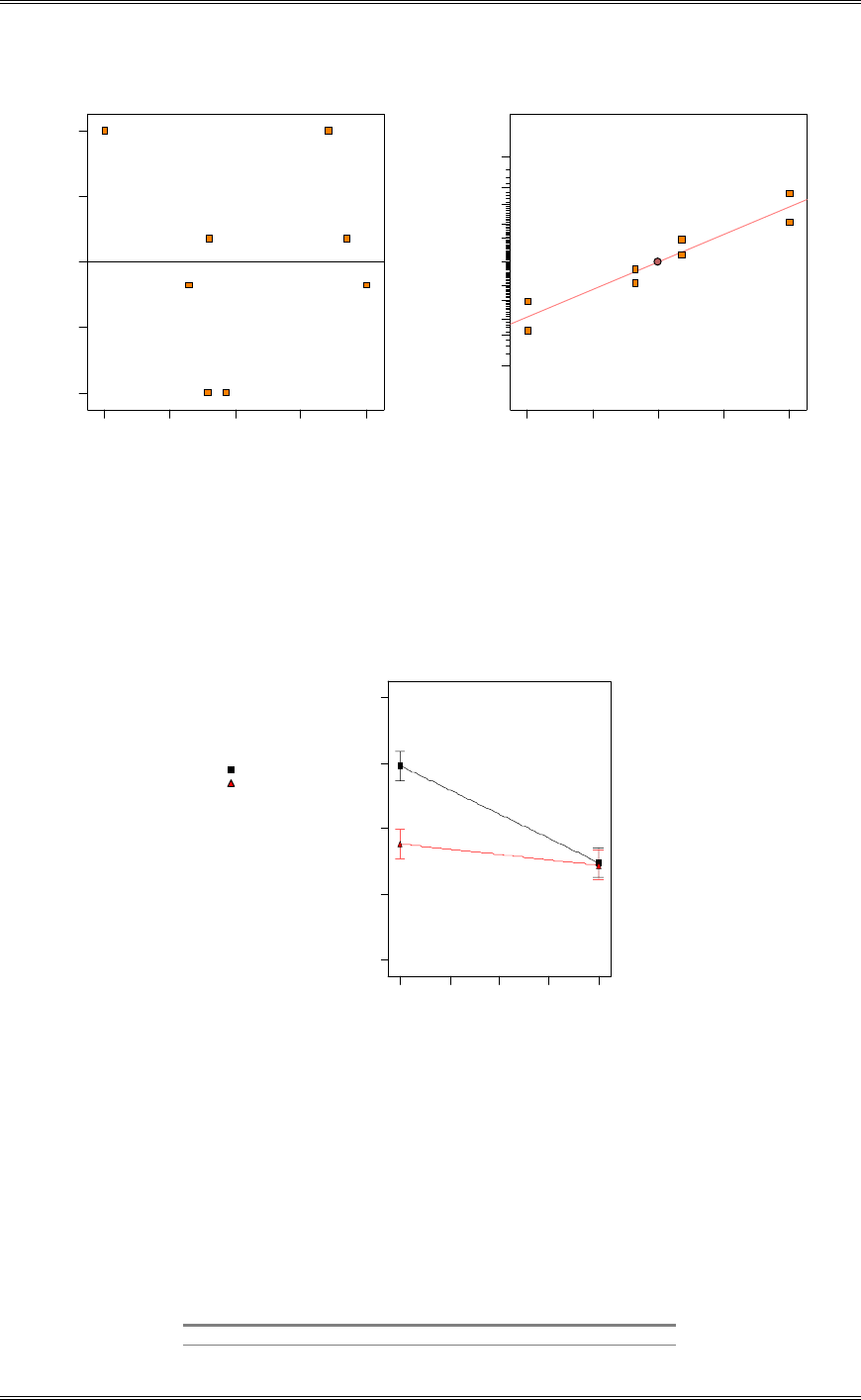
Solutions from Montgomery, D. C. (2001) Design and Analysis of Experiments, Wiley, NY
8-23
Predicted
Residuals
Residuals vs. Predicted
-1 .5 5
-0 .7 75
1.77636E-015
0.775
1.55
13.95 16.38 18.81 21.24 23.68
Residual
Normal % probability
Normal plot of residuals
-1 .5 5 -0 .7 7 5 -1.77636E-015 0.775 1.55
1
5
10
20
30
50
70
80
90
95
99
8-9 Consider the leaf spring experiment in Problem 8-7. Suppose that factor E (quench oil
temperature) is very difficult to control during manufacturing. Where would you set factors A, B, C and D
to reduce variability in the free height as much as possible regardless of the quench oil temperature used?
DESIGN-EXPERT Plot
Free Height
X = E: Quench Temp
Y = B: Heating Time
B- -1.000
B+ 1.000
Actual Factors
A: Furnace Tem p = 0.00
C: Transfer T ime = 0.00
D: Hold Tim e = 0.00
Heating Time
Interaction Graph
Quench Tem p
Free Height
-1 .0 0 -0 .5 0 0.00 0.50 1.00
7.12
7.385
7.65
7.915
8.18
Run the process with A at the high level, B at the low level, C at the low level and D at either level (the
low level of D may give a faster process).
8-10 Construct a 27-2 design by choosing two four-factor interactions as the independent generators.
Write down the complete alias structure for this design. Outline the analysis of variance table. What is
the resolution of this design?
I=CDEF=ABCG=ABDEFG, Resolution IV
A B C D E F=CDE G=ABC

Solutions from Montgomery, D. C. (2001) Design and Analysis of Experiments, Wiley, NY
8-24
1 - - - - - - - (1)
2 + - - - - - + ag
3 - + - - - - + bg
4 + + - - - - - ab
5 - - + - - + + cfg
6 + - + - - + - acf
7 - + + - - + - bcf
8 + + + - - + + abcfg
9 - - - + - + - df
10 + - - + - + + adfg
11 - + - + - + + bdfg
12 + + - + - + - abdf
13 - - + + - - + cdg
14 + - + + - - - acd
15 - + + + - - - bcd
16 + + + + - - + abcdg
17 - - - - + + - ef
18 + - - - + + + aefg
19 - + - - + + + befg
20 + + - - + + - abef
21 - - + - + - + ceg
22 + - + - + - - ace
23 - + + - + - - bce
24 + + + - + - + abceg
25 - - - + + - - de
26 + - - + + - + adeg
27 - + - + + - + bdeg
28 + + - + + - - abde
29 - - + + + + + cdefg
30 + - + + + + - acdef
31 - + + + + + - bcdef
32 + + + + + + + abcdefg
Alias Structure
A (CDEF)= ACDEF A (ABCG)= BCG A (ABDEFG)= BDEFG A=ACDEF=BCG=BDEFG
B (CDEF)= BCDEF
B
(ABCG)= ACG B (ABDEFG)= ADEFG B=BCDEF=ACG=ADEFG
C (CDEF)= DEF
C
(ABCG)= ABG C (ABDEFG)= ABCDEFG C=DEF=ABG=ABCDEFG
D (CDEF)= CEF
D
(ABCG)= ABCDG D (ABDEFG)= ABEFG D=CEF=ABCDG=ABEFG
E (CD EF)= CDF
E
(ABCG)= ABCEG E (ABDEFG)= ABDFG E=CDF=ABCEG=ABDFG
F (CDEF) = C DE
F
(ABCG)= ABCFG F (ABDEFG)= ABDEG F=CDE=ABCFG=ABDEG
G (CDEF)= CDEFG
G
(ABCG)= ABC G (ABDEFG)= ABDEF G=CDEFG=ABC=ABDEF
AB (CDEF)= ABCDEF A
B
(ABCG)= CG AB (ABDEFG)= DEFG AB=ABCDEF=CG=DEFG
AC (CDEF)= ADEF A
C
(ABCG)= BG AC (ABDEFG)= BCDEFG AC=ADEF=BG=BCDEFG
AD (CDEF)= ACEF A
D
(ABCG)= BCDG AD (ABDEFG)= BEFG AD=ACEF=BCDG=BEFG
AE (CDEF)= ACDF A
E
(ABCG)= BCEG AE (ABDEFG)= BDFG AE=ACDF=BCEG=BDFG
AF (CDEF)= ACDE A
F
(ABCG)= BCFG AF (ABDEFG)= BDEG AF=ACDE=BCFG=BDEG
AG (CDEF)= ACDEFG A
G
(ABCG)= BC AG (ABDEFG)= BDEF AG=ACDEFG=BC=BDEF
BD (CDEF)= BCEF B
D
(ABCG)= ACDG BD (ABDEFG)= AEFG BD=BCEF=ACDG=AEFG
BE (CDEF)= BCDF B
E
(ABCG)= ACEG BE (ABDEFG)= ADFG BE=BCDF=ACEG=ADFG
BF (CDEF)= BCDE B
F
(ABCG)= ACFG BF (ABDEFG)= ADEG BF=BCDE=ACFG=ADEG
CD (CDEF)= EF C
D
(ABCG)= ABDG CD (ABDEFG)= ABCEFG CD=EF=ABDG=ABCEFG
CE (CDEF)= DF C
E
(ABCG)= ABEG CE (ABDEFG)= ABCDFG CE=DF=ABEG=ABCDFG
CF (CDEF)= DE C
F
(ABCG)= ABFG CF (ABDEFG)= ABCDEG CF=DE=ABFG=ABCDEG
DG (CDEF)= CEFG D
G
(ABCG)= ABCD DG (ABDEFG)= ABEF DG=CEFG=ABCD=ABEF
EG (CD EF)= CDFG E
G
(ABCG)= ABCE EG (ABDEFG)= ABDF EG=CDFG=ABCE=ABDF
FG (CDEF) = C DEG F
G
(ABCG)= ABCF FG (ABDEFG)= ABDE FG=CDEG=ABCF=ABDE
Analysis of Variance Table
Source Degrees of Freedom
A 1
B 1
C 1
D 1
E 1
F 1
G 1
AB=CG 1

Solutions from Montgomery, D. C. (2001) Design and Analysis of Experiments, Wiley, NY
8-25
AC=BG 1
AD 1
AE 1
AF 1
AG=BC 1
BD 1
BE 1
CD=EF 1
CE=DF 1
CF=DE 1
DG 1
EG 1
FG 1
Error 9
Total 31
8-11 Consider the 25 design in Problem 6-21. Suppose that only a one-half fraction could be run.
Furthermore, two days were required to take the 16 observations, and it was necessary to confound the 25-1
design in two blocks. Construct the design and analyze the data.
A B C D E=ABCD Data
Blocks = AB Block
- - - - + e 8 + 1
+ - - - - a 9 - 2
- + - - - b 34 - 2
+ + - - + abe 52 + 1
- - + - - c 16 + 1
+ - + - + ace 22 - 2
- + + - + bce 45 - 2
+ + + - - abc 60 + 1
- - - + - d 8 + 1
+ - - + + ade 10 - 2
- + - + + bde 30 - 2
+ + - + - abd 50 + 1
- - + + + cde 15 + 1
+ - + + - acd 21 - 2
- + + + - bcd 44 - 2
+ + + + + abcde 63 + 1
Design Expert Output
Term Effect SumSqr % Contribtn
Model Intercept
Model A 10.875 473.063 8.6343
Model B 33.625 4522.56 82.5455
Model C 10.625 451.562 8.24188
Error D -0.625 1.5625 0.0285186
Error E 0.375 0.5625 0.0102667
Error AB Aliased
Error AC 0.625 1.5625 0.0285186
Error AD 0.875 3.0625 0.0558965
Error AE 1.375 7.5625 0.13803
Error BC 0.875 3.0625 0.0558965
Error BD -0.375 0.5625 0.0102667
Error BE 0.125 0.0625 0.00114075
Error CD 0.625 1.5625 0.0285186
Error CE 0.625 1.5625 0.0285186
Error DE -1.625 10.5625 0.192786
Lenth's ME 2.46263
Lenth's SME 5.0517
The AB interaction in the above table is aliased with the three-factor interaction BCD, and is also
confounded with blocks.
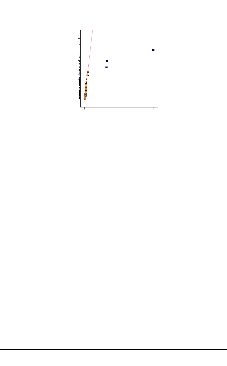
Solutions from Montgomery, D. C. (2001) Design and Analysis of Experiments, Wiley, NY
8-26
Half Normal plot
Half Normal % probability
Effe ct
0.00 8.41 16.81 25.22 33.63
0
20
40
60
70
80
85
90
95
97
99
A
B
C
Design Expert Output
Response: Yield
ANOVA for Selected Factorial Model
Analysis of variance table [Partial sum of squares]
Sum of Mean F
Source Squares DF Square Value Prob > F
Block 203.06 1 203.06
Model 5447.19 3 1815.73 630.31 < 0.0001 significant
A 473.06 1 473.06 164.22 < 0.0001
B 4522.56 1 4522.56 1569.96 < 0.0001
C 451.56 1 451.56 156.76 < 0.0001
Residual 31.69 11 2.88
Cor Total 5681.94 15
The Model F-value of 630.31 implies the model is significant. There is only
a 0.01% chance that a "Model F-Value" this large could occur due to noise.
Std. Dev. 1.70 R-Squared 0.9942
Mean 30.44 Adj R-Squared 0.9926
C.V. 5.58 Pred R-Squared 0.9878
PRESS 67.04 Adeq Precision 58.100
Coefficient Standard 95% CI 95% CI
Factor Estimate DF Error Low High VIF
Intercept 30.44 1 0.42 29.50 31.37
Block 1 3.56 1
Block 2 -3.56
A-Aperture 5.44 1 0.42 4.50 6.37 1.00
B-Exposure Time 16.81 1 0.42 15.88 17.75 1.00
C-Develop Time 5.31 1 0.42 4.38 6.25 1.00
Final Equation in Terms of Coded Factors:
Yield =
+30.44
+5.44 * A
+16.81 * B
+5.31 * C
Final Equation in Terms of Actual Factors:
Aperture small
Yield =
-1.56250
+0.84063 * Exposure Time
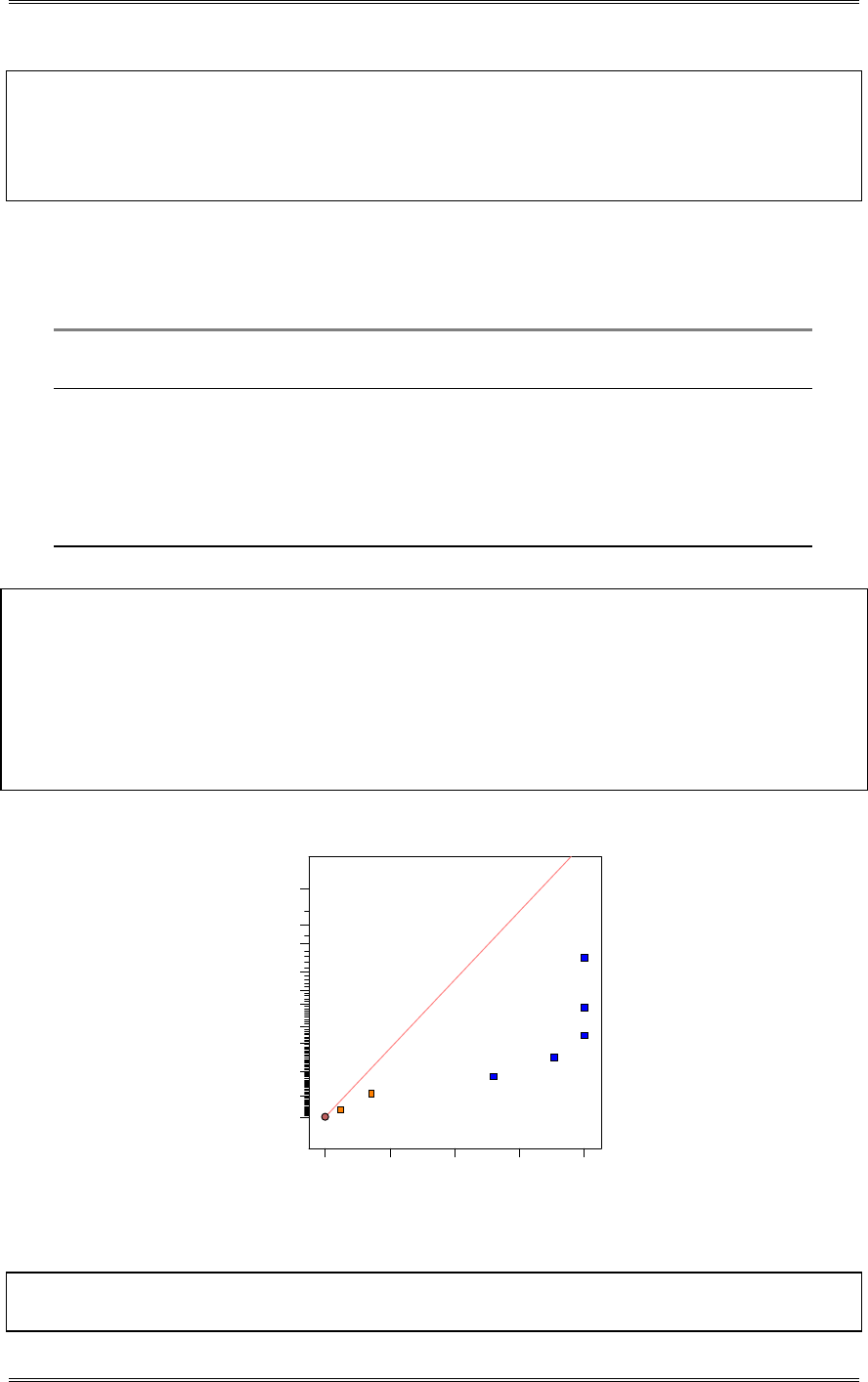
Solutions from Montgomery, D. C. (2001) Design and Analysis of Experiments, Wiley, NY
8-27
+0.70833 * Develop Time
Aperture large
Yield =
+9.31250
+0.84063 * Exposure Time
+0.70833 * Develop Time
8-12 Analyze the data in Problem 6-23 as if it came from a 14
2
IV design with I = ABCD. Project the
design into a full factorial in the subset of the original four factors that appear to be significant.
Run Yield Factor Levels
Number A B C D=ABC (lbs) Low (-) High (+)
1 - - - - (1) 12 A
(
h
)
2.5 3.0
2 + - - + ad 25 B (%) 14 18
3 - + - + bd 13 C (psi) 60 80
4 + + - - ab 16 D (ºC) 225 250
5 - - + + cd 19
6 + - + - ac 15
7 - + + - bc 20
8 + + + + abcd 23
Design Expert Output
Term Effect SumSqr % Contribtn
Model Intercept
Model A 3.75 28.125 18.3974
Error B 0.25 0.125 0.0817661
Model C 2.75 15.125 9.8937
Model D 4.25 36.125 23.6304
Error AB -0.75 1.125 0.735895
Model AC -4.25 36.125 23.6304
Model AD 4.25 36.125 23.6304
Lenth's ME 21.174
Lenth's SME 50.6734
Half Normal plot
Half Normal % probability
Effe ct
0.00 1.06 2.13 3.19 4.25
0
20
40
60
70
80
85
90
95
97
99
A
C
D
AC
AD
Design Expert Output
Response: Yield in lbs
ANOVA for Selected Factorial Model
Analysis of variance table [Partial sum of squares]

Solutions from Montgomery, D. C. (2001) Design and Analysis of Experiments, Wiley, NY
8-28
Sum of Mean F
Source Squares DF Square Value Prob > F
Model 151.63 5 30.32 48.52 0.0203 significant
A 28.13 1 28.13 45.00 0.0215
C 15.13 1 15.13 24.20 0.0389
D 36.12 1 36.12 57.80 0.0169
AC 36.12 1 36.12 57.80 0.0169
AD 36.13 1 36.13 57.80 0.0169
Residual 1.25 2 0.62
Cor Total 152.88 7
The Model F-value of 48.52 implies the model is significant. There is only
a 2.03% chance that a "Model F-Value" this large could occur due to noise.
Std. Dev. 0.79 R-Squared 0.9918
Mean 17.88 Adj R-Squared 0.9714
C.V. 4.42 Pred R-Squared 0.8692
PRESS 20.00 Adeq Precision 17.892
Coefficient Standard 95% CI 95% CI
Factor Estimate DF Error Low High VIF
Intercept 17.88 1 0.28 16.67 19.08
A-Time 1.87 1 0.28 0.67 3.08 1.00
C-Pressure 1.37 1 0.28 0.17 2.58 1.00
D-Temperature 2.13 1 0.28 0.92 3.33 1.00
AC -2.13 1 0.28 -3.33 -0.92 1.00
AD 2.13 1 0.28 0.92 3.33 1.00
Final Equation in Terms of Coded Factors:
Yield =
+17.88
+1.87 * A
+1.37 * C
+2.13 * D
-2.13 * A * C
+2.13 * A * D
Final Equation in Terms of Actual Factors:
Yield =
+227.75000
-94.50000 * Time
+2.47500 * Pressure
-1.70000 * Temperature
-0.85000 * Time * Pressure
+0.68000 * Time * Temperature
8-13 Repeat Problem 8-12 using I = -ABCD. Does use of the alternate fraction change your
interpretation of the data?
Run Yield Factor Levels
Number A B C D=ABC (lbs) Low (-) High (+)
1 - - - + d 10 A
(
h
)
2.5 3.0
2 + - - - a 18 B (%) 14 18
3 - + - - b 13 C (psi) 60 80
4 + + - + abd 24 D (ºC) 225 250
5 - - + - c 17
6 + - + + acd 21
7 - + + + bcd 17
8 + + + - abc 15
Design Expert Output
Term Effect SumSqr % Contribtn
Model Intercept
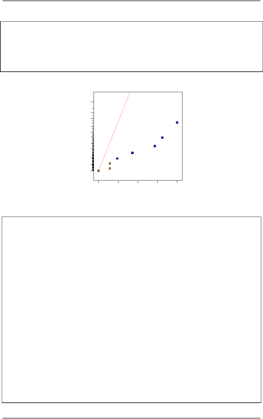
Solutions from Montgomery, D. C. (2001) Design and Analysis of Experiments, Wiley, NY
8-29
Model A 5.25 55.125 40.8712
Error B 0.75 1.125 0.834106
Model C 1.25 3.125 2.31696
Model D 2.25 10.125 7.50695
Error AB -0.75 1.125 0.834106
Model AC -4.25 36.125 26.7841
Model AD 3.75 28.125 20.8526
Lenth's ME 12.7044
Lenth's SME 30.404
Half Normal plot
Half Normal % probability
Effe ct
0.00 1.31 2.63 3.94 5.25
0
20
40
60
70
80
85
90
95
97
99
A
C
D
AC
AD
Design Expert Output
Response: Yield in lbs
ANOVA for Selected Factorial Model
Analysis of variance table [Partial sum of squares]
Sum of Mean F
Source Squares DF Square Value Prob > F
Model 132.63 5 26.52 23.58 0.0412 significant
A 55.13 1 55.13 49.00 0.0198
C 3.13 1 3.13 2.78 0.2375
D 10.13 1 10.13 9.00 0.0955
AC 36.13 1 36.13 32.11 0.0298
AD 28.13 1 28.13 25.00 0.0377
Residual 2.25 2 1.12
Cor Total 134.88 7
The Model F-value of 23.58 implies the model is significant. There is only
a 4.12% chance that a "Model F-Value" this large could occur due to noise.
Std. Dev. 1.06 R-Squared 0.9833
Mean 16.88 Adj R-Squared 0.9416
C.V. 6.29 Pred R-Squared 0.7331
PRESS 36.00 Adeq Precision 14.425
Coefficient Standard 95% CI 95% CI
Factor Estimate DF Error Low High VIF
Intercept 16.88 1 0.37 15.26 18.49
A-Time 2.63 1 0.37 1.01 4.24 1.00
C-Pressure 0.63 1 0.37 -0.99 2.24 1.00
D-Temperature 1.13 1 0.37 -0.49 2.74 1.00
AC -2.13 1 0.37 -3.74 -0.51 1.00
AD 1.88 1 0.37 0.26 3.49 1.00
Final Equation in Terms of Coded Factors:
Yield =

Solutions from Montgomery, D. C. (2001) Design and Analysis of Experiments, Wiley, NY
8-30
+16.88
+2.63 * A
+0.63 * C
+1.13 * D
-2.13 * A * C
+1.88 * A * D
Final Equation in Terms of Actual Factors:
Yield =
+190.50000
-72.50000 * Time
+2.40000 * Pressure
-1.56000 * Temperature
-0.85000 * Time * Pressure
+0.60000 * Time * Temperature
8-14 Project the 14
2
IV design in Example 8-1 into two replicates of a 22 design in the factors A and B.
Analyze the data and draw conclusions.
Design Expert Output
Response: Filtration Rate
ANOVA for Selected Factorial Model
Analysis of variance table [Partial sum of squares]
Sum of Mean F
Source Squares DF Square Value Prob > F
Model 728.50 3 242.83 0.41 0.7523 not significant
A 722.00 1 722.00 1.23 0.3291
B 4.50 1 4.50 7.682E-003 0.9344
AB 2.00 1 2.00 3.414E-003 0.9562
Residual 2343.00 4 585.75
Lack of Fit 0.000 0
Pure Error 2343.00 4 585.75
Cor Total 3071.50 7
The "Model F-value" of 0.41 implies the model is not significant relative to the noise. There is a
75.23 % chance that a "Model F-value" this large could occur due to noise.
Std. Dev. 24.20 R-Squared 0.2372
Mean 70.75 Adj R-Squared -0.3349
C.V. 34.21 Pred R-Squared -2.0513
PRESS 9372.00 Adeq Precision 1.198
Coefficient Standard 95% CI 95% CI
Factor Estimate DF Error Low High VIF
Intercept 70.75 1 8.56 46.99 94.51
A-Temperature 9.50 1 8.56 -14.26 33.26 1.00
B-Pressure 0.75 1 8.56 -23.01 24.51 1.00
AB -0.50 1 8.56 -24.26 23.26 1.00
Final Equation in Terms of Coded Factors:
Filtration Rate =
+70.75
+9.50 * A
+0.75 * B
-0.50 * A * B
Final Equation in Terms of Actual Factors:
Filtration Rate =
+70.75000
+9.50000 * Temperature
+0.75000 * Pressure
-0.50000 * Temperature * Pressure

Solutions from Montgomery, D. C. (2001) Design and Analysis of Experiments, Wiley, NY
8-31
8-15 Construct a 36
2
III design. Determine the effects that may be estimated if a second fraction of this
design is run with all signs reversed.
A B C D=AB E=AC F=BC
- - - + + + def
+ - - - - + af
- + - - + - be
+ + - + - - abd
- - + + - - cd
+ - + - + - ace
- + + - - + bcf
+ + + + + + abcdef
Principal Fraction Second Fraction
l
A=A+BD+CE
l*
A=A-BD-CE
l
B=B+AD+CF
l*
B=B-AD-CF
l
C=C+AE+BF
l*
C=C-AE-BF
l
D=D+AB+EF
l*
D=D-AB-EF
l
E=E+AC+DF
l*
E=E-AC-DF
l
F=F+BC+DE
l*
F=F-BC-DE
l
BE=BE+CD+AF
l*
BE=BE+CD+AF
By combining the two fractions we can estimate the following:
( li +l*I)/2 ( li -l*I)/2
A BD+CE
B AD+CF
C AE+BF
D AB+EF
E AC+DF
F BC+DE
BE+CD+AF
8-16 Consider the 36
2
III design in Problem 8-15. Determine the effects that may be estimated if a second
fraction of this design is run with the signs for factor A reversed.
Principal Fraction Second Fraction
l
A=A+BD+CE
l*
A=-A+BD+CE
l
B=B+AD+CF
l*
B=B-AD+CF
l
C=C+AE+BF
l*
C=C-AE+BF
l
D=D+AB+EF
l*
D=D-AB+EF
l
E=E+AC+DF
l*
E=E-AC+DF
l
F=F+BC+DE
l*
F=F+BC+DE
l
BE=BE+CD+AF
l*
BE=BE+CD-AF
By combining the two fractions we can estimate the following:
( li -l*I)/2 ( li +l*I)/2
A BD+CE
AD B+CF

Solutions from Montgomery, D. C. (2001) Design and Analysis of Experiments, Wiley, NY
8-32
AE C+BF
AB D+EF
AC E+DF
F+BC+DE
AF
8-17 Fold over the 47
2
III design in Table 8-19 to produce a eight-factor design. Verify that the resulting
design is a 48
2
IV design. Is this a minimal design?
H A B C D=AB E=AC F=BC G=ABC
+ - - - + + + -
Original + + - - - - + +
Design + - + - - + - +
+ + + - + - - -
+ - - + + - - +
+ + - + - + - -
+ - + + - - + -
+ + + + + + + +
- + + + - - - +
Second - - + + + + - -
Set of - + - + + - + -
Runs w/ - - - + - + + +
all Signs - + + - - + + -
Switched - - + - + - + +
- + - - + + - +
- - - - - - - -
After folding the original design over, we add a new factor H, and we have a design with generators
D=ABH, E=ACH, F=BCH, and G=ABC. This is a 48
2
IV design. It is a minimal design, since it contains
2k=2(8)=16 runs.
8-18 Fold over a 25
2
III design to produce a six-factor design. Verify that the resulting design is a 26
2
IV
design. Compare this 26
2
IV design to the in Table 8-10.
F A B C D=AB E=BC
+ - - - + +
Original + + - - - +
Design + - + - - -
+ + + - + -
+ - - + + -
+ + - + - -
+ - + + - +
+ + + + + +
- + + + - -
Second - - + + + -
Set of - + - + + +
Runs w/ - - - + - +
all Signs - + + - - +
Switched - - + - + +
- + - - + -
- - - - - -
If we relabel the factors from left to right as A, B, C, D, E, F, then this design becomes 26
2
IV with
generators I=ABDF and I=BCEF. It is not a minimal design, since 2k=2(6)=12 runs, and the design
contains 16 runs.
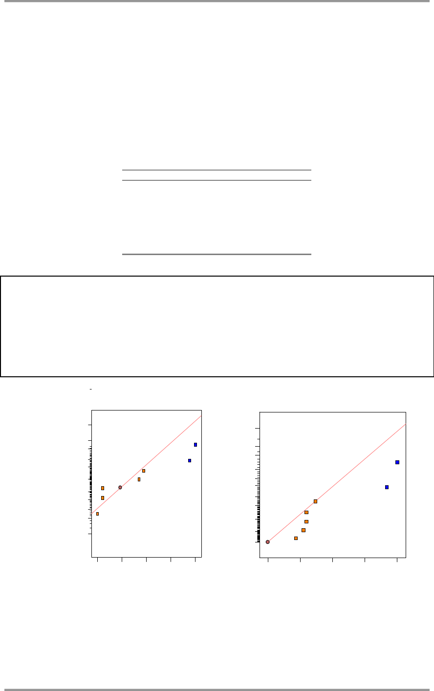
Solutions from Montgomery, D. C. (2001) Design and Analysis of Experiments, Wiley, NY
8-33
8-19 An industrial engineer is conducting an experiment using a Monte Carlo simulation model of an
inventory system. The independent variables in her model are the order quantity (A), the reorder point
(B), the setup cost (C), the backorder cost (D), and the carrying cost rate (E). The response variable is
average annual cost. To conserve computer time, she decides to investigate these factors using a 25
2
III
design with I = ABD and I = BCE. The results she obtains are de = 95, ae = 134, b = 158, abd = 190, cd
= 92, ac = 187, bce = 155, and abcde = 185.
(a) Verify that the treatment combinations given are correct. Estimate the effects, assuming three-factor
and higher interactions are negligible.
A B C D=AB E=BC
- - - + + de
+ - - - + ae
- + - - - b
+ + - + - abd
- - + + - cd
+ - + - - ac
- + + - + bce
+ + + + + abcde
Design Expert Output
Term Effect SumSqr % Contribtn
Model Intercept
Model A 49 4802 43.9502
Model B 45 4050 37.0675
Error C 10.5 220.5 2.01812
Error D -18 648 5.93081
Error E -14.5 420.5 3.84862
Error AC 13.5 364.5 3.33608
Error AE -14.5 420.5 3.84862
Lenth's ME 81.8727
Lenth's SME 195.937
DESIGN-EXPERT Plot
Avg Annual Cost
A: Order Quantity
B: R e -o rd er P oi n t
C: Setup Cost
D: Backorder Cost
E: C a rryi n g Co st
Normal plot
Norm al % probability
Effe ct
-18.00 -1 .2 5 15.50 32.25 49.00
1
5
10
20
30
50
70
80
90
95
99
A
B
Half Normal plot
Half Normal % probability
Effe ct
0.00 12.25 24.50 36.75 49.00
0
20
40
60
70
80
85
90
95
97
99
A
B
(b) Suppose that a second fraction is added to the first, for example ade = 136, e = 93, ab = 187, bd =
153, acd = 139, c = 99, abce - 191, and bcde = 150. How was this second fraction obtained? Add
this data to the original fraction, and estimate the effects.
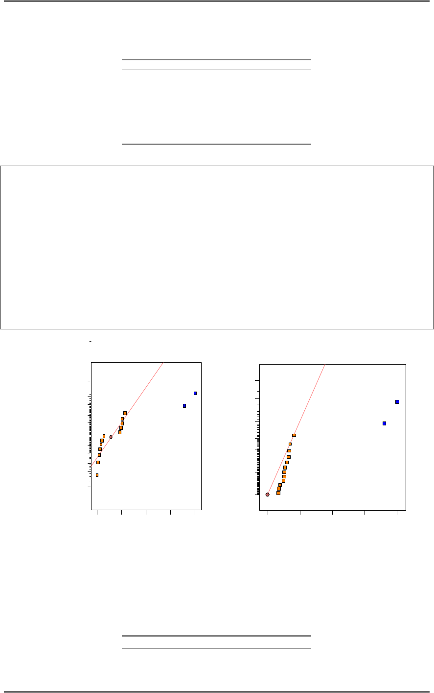
Solutions from Montgomery, D. C. (2001) Design and Analysis of Experiments, Wiley, NY
8-34
This second fraction is formed by reversing the signs of factor A.
A B C D=AB E=BC
+ - - + + ade
- - - - + e
+ + - - - ab
- + - + - bd
+ - + + - acd
- - + - - c
+ + + - + abce
- + + + + bcde
Design Expert Output
Term Effect SumSqr % Contribtn
Model Intercept
Model A 44.25 7832.25 39.5289
Model B 49.25 9702.25 48.9666
Error C 6.5 169 0.852932
Error D -8 256 1.29202
Error E -8.25 272.25 1.37403
Error AB -10 400 2.01877
Error AC 7.25 210.25 1.06112
Error AD -4.25 72.25 0.364641
Error AE -6 144 0.726759
Error BD 4.75 90.25 0.455486
Error CD -8.5 289 1.45856
Error DE 6.25 156.25 0.788584
Error ACD -6.25 156.25 0.788584
Error ADE 4 64 0.323004
Lenth's ME 25.1188
Lenth's SME 51.5273
DESIGN-EXPERT Plot
Avg Annual Cost
A: Order Quantity
B: R e -o rd er P oi n t
C: Setup Cost
D: Backorder Cost
E: C a rryi n g Co st
Normal plot
Norm al % probability
Effe ct
-9 .2 5 5.63 20.50 35.38 50.25
1
5
10
20
30
50
70
80
90
95
99
A
B
Half Normal plot
Half Normal % probability
Effe ct
0.00 12.31 24.63 36.94 49.25
0
20
40
60
70
80
85
90
95
97
99
A
B
(c) Suppose that the fraction abc = 189, ce = 96, bcd = 154, acde = 135, abe = 193, bde = 152, ad = 137,
and (1) = 98 was run. How was this fraction obtained? Add this data to the original fraction and
estimate the effects.
This second fraction is formed by reversing the signs of all factors.
A B C D=AB E=BC
+ + + - - abc
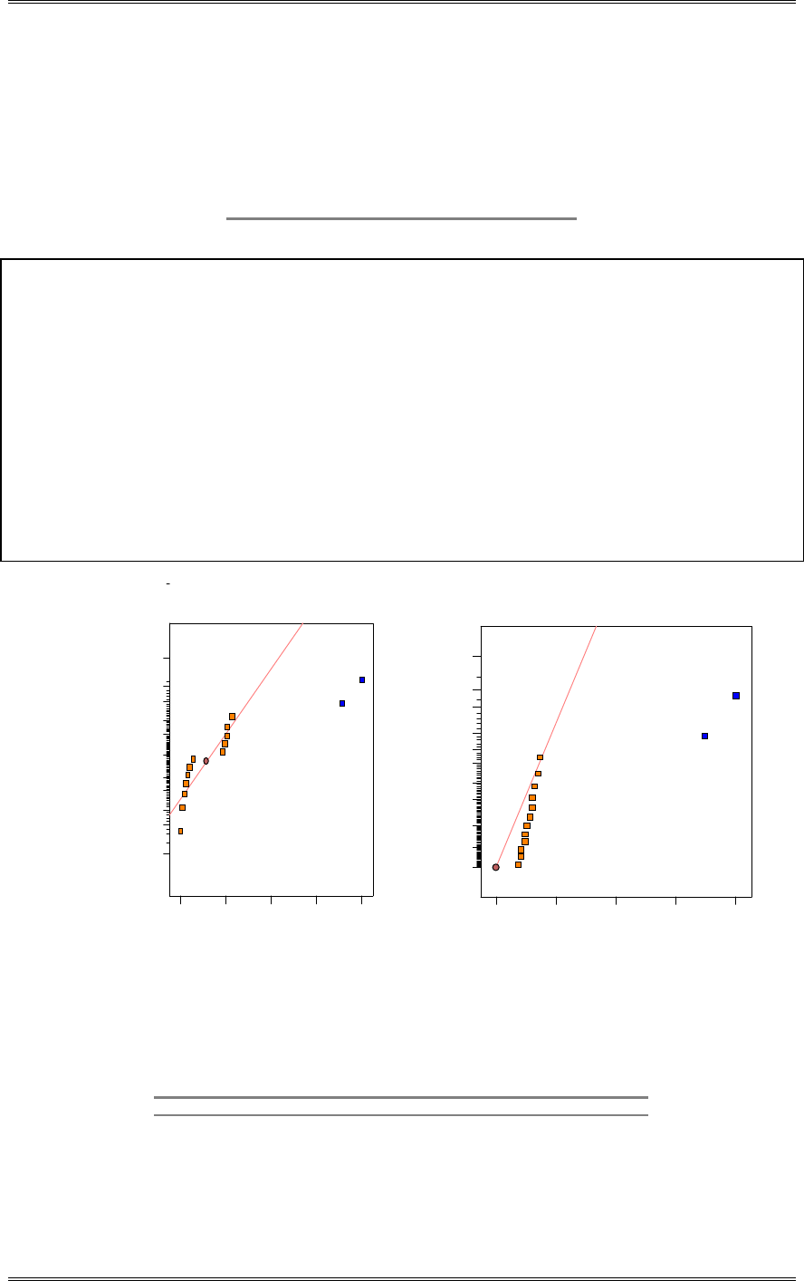
Solutions from Montgomery, D. C. (2001) Design and Analysis of Experiments, Wiley, NY
8-35
- + + + - bcd
+ - + + + acde
- - + - + ce
+ + - - + abe
- + - + + bde
+ - - + - ad
- - - - - (1)
Design Expert Output
Term Effect SumSqr % Contribtn
Model Intercept
Model A 43.75 7656.25 38.1563
Model B 50.25 10100.3 50.3364
Error C 4.5 81 0.403678
Error D -8.75 306.25 1.52625
Error E -7.5 225 1.12133
Error AB -9.25 342.25 1.70566
Error AC 6 144 0.71765
Error AD -5.25 110.25 0.549451
Error AE -6.5 169 0.842242
Error BC -7 196 0.976801
Error BD 5.25 110.25 0.549451
Error BE 6 144 0.71765
Error ABC -8 256 1.27582
Error ABE 7.5 225 1.12133
Lenth's ME 26.5964
Lenth's SME 54.5583
DESIGN-EXPERT Plot
Avg Annual Cost
A: Order Quantity
B: R e -o rd er P oi n t
C: Setup Cost
D: Backorder Cost
E: C a rryi n g Co st
Normal plot
Norm al % probability
Effe ct
-9 .2 5 5.63 20.50 35.38 50.25
1
5
10
20
30
50
70
80
90
95
99
A
B
Half Normal plot
Half Normal % probability
Effe ct
0.00 12.56 25.13 37.69 50.25
0
20
40
60
70
80
85
90
95
97
99
A
B
8-20 Construct a 251
design. Show how the design may be run in two blocks of eight observations
each. Are any main effects or two-factor interactions confounded with blocks?
A
B
C
D
E
=
ABCD
Blocks
=
AB
Block
- - - - + e + 1
+ - - - - a - 2
- + - - - b - 2
+ + - - + abe + 1
- - + - - c + 1
+ - + - + ace - 2

Solutions from Montgomery, D. C. (2001) Design and Analysis of Experiments, Wiley, NY
8-36
- + + - + bce - 2
+ + + - - abc + 1
- - - + - d + 1
+ - - + + ade - 2
- + - + + bde - 2
+ + - + - abd + 1
- - + + + cde + 1
+ - + + - acd - 2
- + + + - bcd - 2
+ + + + + abcde + 1
Blocks are confounded with AB and CDE.
8-21 Construct a 272
design. Show how the design may be run in four blocks of eight observations
each. Are any main effects or two-factor interactions confounded with blocks?
A B C D E F=CDE G=ABC Block=ACE Block=BFG Block assignment
1 - - - - - - - (1) - - 1
2 + - - - - - + ag + + 4
3 - + - - - - + bg - - 1
4 + + - - - - - ab + + 4
5 - - + - - + + cfg + - 3
6 + - + - - + - acf - + 2
7 - + + - - + - bcf + - 3
8 + + + - - + + abcfg - + 2
9 - - - + - + - df - + 2
10 + - - + - + + adfg + - 3
11 - + - + - + + bdfg - + 2
12 + + - + - + - abdf + - 3
13 - - + + - - + cdg + + 4
14 + - + + - - - acd - - 1
15 - + + + - - - bcd + + 4
16 + + + + - - + abcdg - - 1
17 - - - - + + - ef + + 4
18 + - - - + + + aefg - - 1
19 - + - - + + + befg + + 4
20 + + - - + + - abef - - 1
21 - - + - + - + ceg - + 2
22 + - + - + - - ace + - 3
23 - + + - + - - bce - + 2
24 + + + - + - + abceg + - 3
25 - - - + + - - de + - 3
26 + - - + + - + adeg - + 2
27 - + - + + - + bdeg + - 3
28 + + - + + - - abde - + 2
29 - - + + + + + cdefg - - 1
30 + - + + + + - acdef + + 4
31 - + + + + + - bcdef - - 1
32 + + + + + + + abcdefg + + 4
Blocks are confounded with ACE, BFG, and ABCEFG.
8-22 Irregular fractions of the 2k [John (1971)]. Consider a 2
4 design. We must estimate the four
main effects and the six two-factor interactions, but the full 24 factorial cannot be run. The largest
possible block contains 12 runs. These 12 runs can be obtained from the four one-quarter fractions
defined by I =
r
AB =
r
ACD =
r
BCD by omitting the principal fraction. Show how the remaining three
24-2 fractions can be combined to estimate the required effects, assuming that three-factor and higher
interactions are negligible. This design could be thought of as a three-quarter fraction.
The four 24-2 fractions are as follows:

Solutions from Montgomery, D. C. (2001) Design and Analysis of Experiments, Wiley, NY
8-37
(1) I=+AB=+ACD=+BCD
Runs: c,d,ab,abcd
(2) I=+AB=-ACD=-BCD
Runs: (1), cd, abc, abd
(3) I=-AB=+ACD=-BCD
Runs: a, bc, bd, acd
(4) I=-AB=-ACD=+BCD
Runs: b, ac, ad, bcd
If we do not run the principal fraction (1), then we can combine the remaining 3 fractions to from 3 one-
half fractions of the 24 as follows:
Fraction 1: (2) + (3) implies I=-BCD. This fraction estimates: A, AB, AC, and AD
Fraction 2: (2) + (4) implies I=-ACD. This fraction estimates: B, BC, BD, and AB
Fraction 3: (3) + (4) implies I=-AB. This fraction estimates: C, D, and CD
In estimating these effects we assume that all three-factor and higher interactions are negligible. Note
that AB is estimated in two of the one-half fractions: 1 and 2. We would average these quantities and
obtain a single estimate of AB. John (1971, pp. 161-163) discusses this design and shows that the
estimates obtained above are also the least squares estimates. John also derives the variances and
covariances of these estimators.
8-23 Carbon anodes used in a smelting process are baked in a ring furnace. An experiment is run in the
furnace to determine which factors influence the weight of packing material that is stuck to the anodes
after baking. Six variables are of interest, each at two levels: A = pitch/fines ratio (0.45, 0.55); B =
packing material type (1, 2); C = packing material temperature (ambient, 325 C); D = flue location
(inside, outside); E = pit temperature (ambient, 195 C); and F = delay time before packing (zero, 24
hours). A 26-3 design is run, and three replicates are obtained at each of the design points. The weight of
packing material stuck to the anodes is measured in grams. The data in run order are as follows: abd =
(984, 826, 936); abcdef = (1275, 976, 1457); be = (1217, 1201, 890); af = (1474, 1164, 1541); def =
(1320, 1156, 913); cd = (765, 705, 821); ace = (1338, 1254, 1294); and bcf = (1325, 1299, 1253). We
wish to minimize the amount stuck packing material.
(a) Verify that the eight runs correspond to a 36
2
III design. What is the alias structure?
A B C D=AB E=AC F=BC
- - - + + + def
+ - - - - + af
- + - - + - be
+ + - + - - abd
- - + + - - cd
+ - + - + - ace
- + + - - + bcf
+ + + + + + abcdef
I=ABD=ACE=BCF=BCDE=ACDF=ABEF=DEF, Resolution III
A=BD=CE=CDF=BEF
B=AD=CF=CDE=AEF
C=AE=BF=BDE=ADF
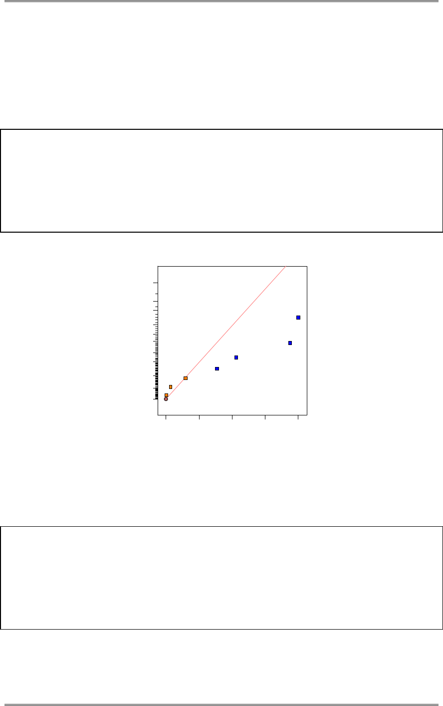
Solutions from Montgomery, D. C. (2001) Design and Analysis of Experiments, Wiley, NY
8-38
D=AB=EF=BCE=ACF
E=AC=DF=BCD=ABF
F=BC=DE=ACD=ABE
CD=BE=AF=ABC=ADE=BDF=CEF
(b) Use the average weight as a response. What factors appear to be influential?
Design Expert Output
Term Effect SumSqr % Contribtn
Model Intercept
Model A 137.9 37996.1 12.0947
Error B -8.9 156.056 0.049675
Error C 0.221108 2094.02 0.666559
Model D -259.6 136168 43.3443
Model E 99.7667 27246.7 8.67305
Model F 243.567 107863 34.3345
Error BC -38.0306 2629.69 0.837072
Lenth's ME 563.322
Lenth's SME 1348.14
Half Normal plot
Half Normal % probability
Effe ct
0.00 64.90 129.80 194.70 259.60
0
20
40
60
70
80
85
90
95
97
99
A
D
E
F
Factors A, D, E and F (and their aliases) are apparently important.
(c) Use the range of the weights as a response. What factors appear to be influential?
Design Expert Output
Term Effect SumSqr % Contribtn
Model Intercept
Error A 44.5 3960.5 2.13311
Error B 13.5 364.5 0.196319
Model C -129 33282 17.9256
Error D 75.5 11400.5 6.14028
Model E 144 41472 22.3367
Model F 163 53138 28.62
Model AF 145 42050 22.648
Lenth's ME 728.384
Lenth's SME 1743.17
Factors C, E, F and the AF interaction (and their aliases) appear to be large.
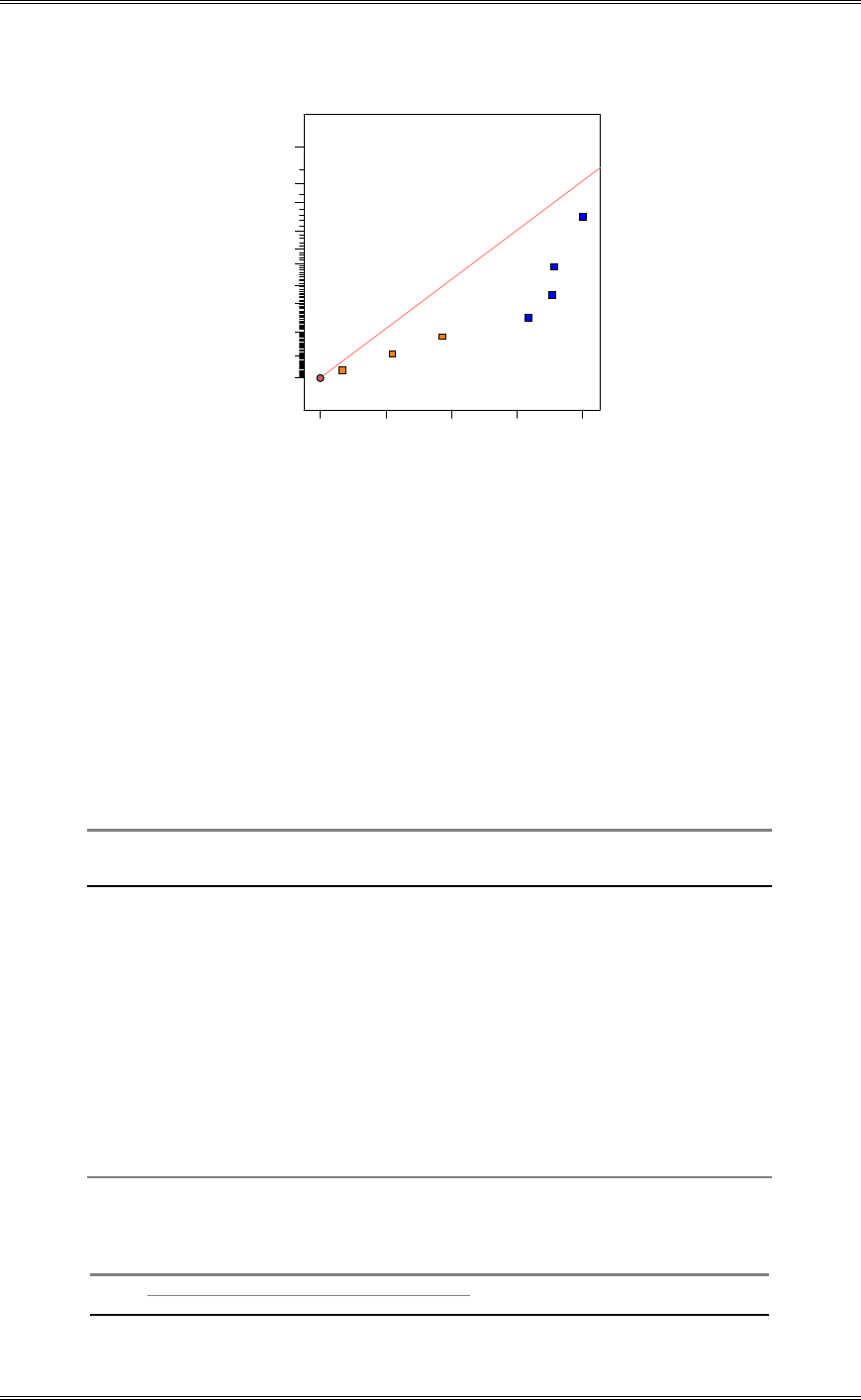
Solutions from Montgomery, D. C. (2001) Design and Analysis of Experiments, Wiley, NY
8-39
Half Normal plot
Half Normal % probability
Effe ct
0.00 40.75 81.50 122.25 163.00
0
20
40
60
70
80
85
90
95
97
99
C
E
F
AF
(d) What recommendations would you make to the process engineers?
It is not known exactly what to do here, since A, D, E and F are large effects, and because the design is
resolution III, the main effects are aliased with two-factor interactions. Note, for example, that D is
aliased with EF and the main effect could really be a EF interaction. If the main effects are really
important, then setting all factors at the low level would minimize the amount of material stuck to the
anodes. It would be necessary to run additional experiments to confirm these findings.
8-24 A 16-run experiment was performed in a semiconductor manufacturing plant to study the effects of
six factors on the curvature or camber of the substrate devices produced. The six variables and their levels
are shown below:
Lamination Lamination Lamination Firing Firing Firing
Temperature Time Pressure Temperature Cycle Time Dew Point
Run (c) (s) (tn) (c) (h) (c)
1 55 10 5 1580 17.5 20
2 75 10 5 1580 29 26
3 55 25 5 1580 29 20
4 75 25 5 1580 17.5 26
5 55 10 10 1580 29 26
6 75 10 10 1580 17.5 20
7 55 25 10 1580 17.5 26
8 75 25 10 1580 29 20
9 55 10 5 1620 17.5 26
10 75 10 5 1620 29 20
11 55 25 5 1620 29 26
12 75 25 5 1620 17.5 20
13 55 10 10 1620 29 20
14 75 10 10 1620 17.5 26
15 55 25 10 1620 17.5 20
16 75 25 10 1620 29 26
Each run was replicated four times , and a camber measurement was taken on the substrate. The data are
shown below:
Camber for Replicate (in/in) Total Mean Standard
Run 1 2 3 4 (10-4 in/in) (10-4 in/in) Deviation
1 0.0167 0.0128 0.0149 0.0185 629 157.25 24.418
2 0.0062 0.0066 0.0044 0.0020 192 48.00 20.976

Solutions from Montgomery, D. C. (2001) Design and Analysis of Experiments, Wiley, NY
8-40
3 0.0041 0.0043 0.0042 0.0050 176 44.00 4.083
4 0.0073 0.0081 0.0039 0.0030 223 55.75 25.025
5 0.0047 0.0047 0.0040 0.0089 223 55.75 22.410
6 0.0219 0.0258 0.0147 0.0296 920 230.00 63.639
7 0.0121 0.0090 0.0092 0.0086 389 97.25 16.029
8 0.0255 0.0250 0.0226 0.0169 900 225.00 39.420
9 0.0032 0.0023 0.0077 0.0069 201 50.25 26.725
10 0.0078 0.0158 0.0060 0.0045 341 85.25 50.341
11 0.0043 0.0027 0.0028 0.0028 126 31.50 7.681
12 0.0186 0.0137 0.0158 0.0159 640 160.00 20.083
13 0.0110 0.0086 0.0101 0.0158 455 113.75 31.120
14 0.0065 0.0109 0.0126 0.0071 371 92.75 29.510
15 0.0155 0.0158 0.0145 0.0145 603 150.75 6.750
16 0.0093 0.0124 0.0110 0.0133 460 115.00 17.450
(a) What type of design did the experimenters use?
The 26
2
IV , a 16-run design.
(b) What are the alias relationships in this design? The defining relation is I=ABCE=ACDF=BDEF
A (ABCE)= BCE A (ACDF)= CDF A (BDEF)= ABCDEF A=BCE=CDF=ABDEF
B (ABCE)= ACE B (ACDF)= ABCDF B (BDEF)= DEF B=ACE=ABCDF=DEF
C (ABCE)= ABE C (ACDF)= ADF C (BDEF)= BCDEF C=ABE=ADF=BCDEF
D (ABCE)= ABCDE D (ACDF)= ACF D (BDEF)= BEF D=ABCDE=ACF=BEF
E (ABCE)= ABC E (ACDF)= ACDEF E (BDEF)= BDF E=ABC=ABDEF=BDF
F (ABCE)= ABCEF F (ACDF)= ACD F (BDEF)= BDE F=ABCEF=ACD=BDE
AB (ABCE)= CE AB (ACDF)= BCDF AB (BDEF)= ADEF AB=CE=BCDF=ADEF
AC (ABCE)= BE AC (ACDF)= DF AC (BDEF)= ABCDEF AC=BE=DF=ABCDEF
AD (ABCE)= BCDE AD (ACDF)= CF AD (BDEF)= ABEF AD=BCDE=CF=ABEF
AE (ABCE)= BC AE (ACDF)= CDEF AE (BDEF)= ABDF AE=BC=CDEF=ABDF
AF (ABCE)= BCEF AF (ACDF)= CD AF (BDEF)= ABDE AF=BCEF=CD=ABDE
BD (ABCE)= ACDE BD (ACDF)= ABCF BD (BDEF)= EF BD=ACDE=ABCF=EF
BF (ABCE)= ACEF BF (ACDF)= ABCD BF (BDEF)= DE BF=ACEF=ABCD=DE
(c) Do any of the process variables affect average camber?
Yes, per the analysis below, variables A, C, D, and F affect average camber.
Design Expert Output
Term Effect SumSqr % Contribtn
Model Intercept
Model A 38.9063 6054.79 10.2962
Error B 5.78125 133.691 0.227344
Model C 56.0313 12558 21.355
Error D -14.2188 808.691 1.37519
Model E -34.4687 4752.38 8.08148
Model F -77.4688 24005.6 40.8219
Error AB 19.1563 1467.85 2.49609
Error AC 22.4063 2008.16 3.4149
Error AD -12.2188 597.191 1.01553
Error AE 18.1563 1318.6 2.24229
Error AF -19.7187 1555.32 2.64483
Error BC Aliased
Error BD 23.0313 2121.75 3.60807
Error BE Aliased
Error BF 7.40625 219.41 0.37311
Error CD Aliased
Error CE Aliased
Error CF Aliased
Error DE Aliased
Error DF Aliased
Error EF Aliased
Error ABC Aliased
Error ABD 0.53125 1.12891 0.00191972
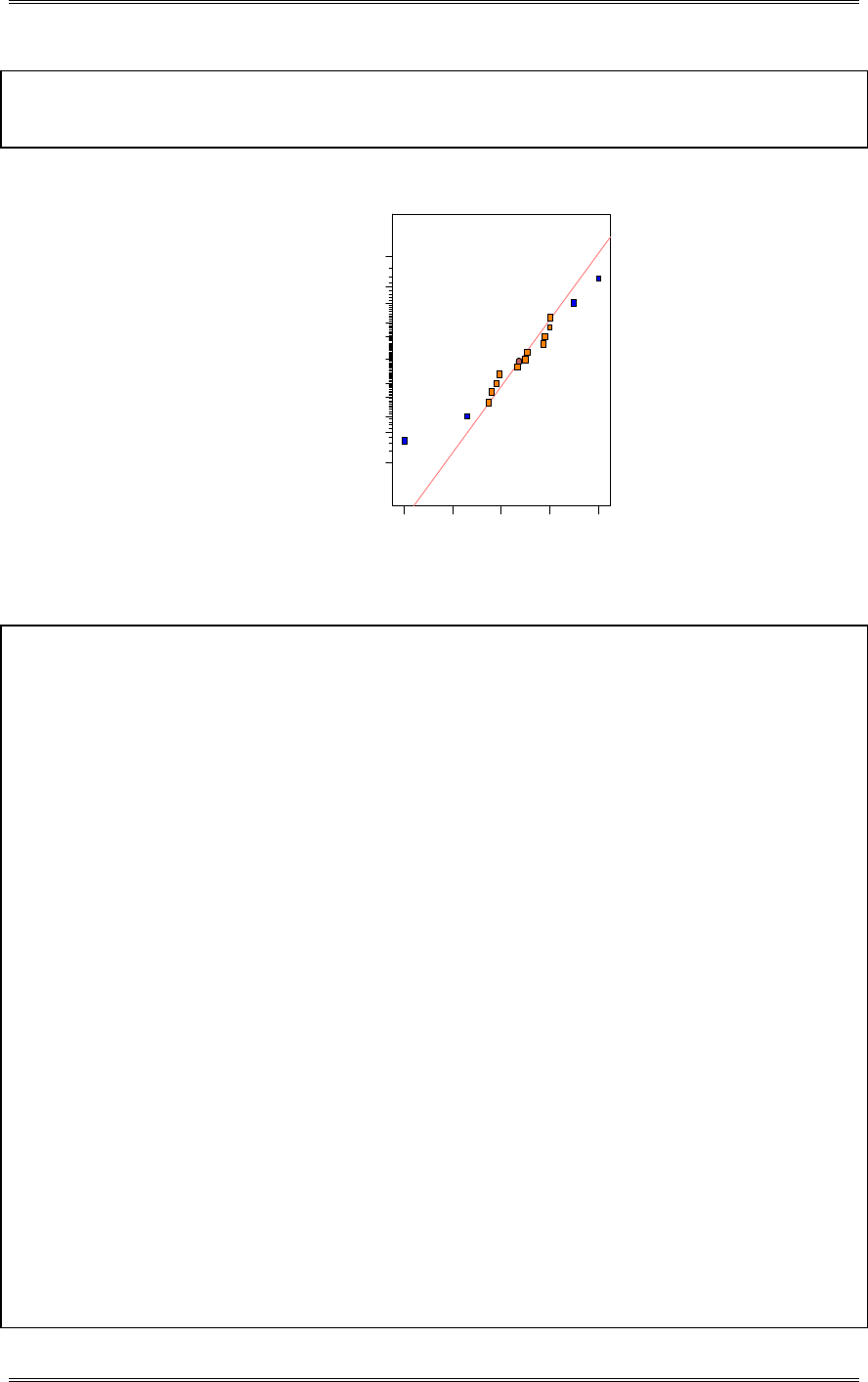
Solutions from Montgomery, D. C. (2001) Design and Analysis of Experiments, Wiley, NY
8-41
Error ABE Aliased
Error ABF -17.3438 1203.22 2.04609
Lenth's ME 71.9361
Lenth's SME 146.041
DESIGN-EXPERT Plot
Cam ber A vg
A: Lam Temp
B: Lam Time
C: Lam Pres
D: Fire Tem p
E: Fire Tim e
F: Fire DP
Normal plot
Norm al % probability
Effe ct
-7 7 .47 -4 4 . 09 -1 0 .7 2 22.66 56.03
1
5
10
20
30
50
70
80
90
95
99
A
C
E
F
Design Expert Output
Response: Camber Avg in in/in
ANOVA for Selected Factorial Model
Analysis of variance table [Partial sum of squares]
Sum of Mean F
Source Squares DF Square Value Prob > F
Model 47370.80 4 11842.70 11.39 0.0007 significant
A 6054.79 1 6054.79 5.82 0.0344
C 12558.00 1 12558.00 12.08 0.0052
E 4752.38 1 4752.38 4.57 0.0558
F 24005.63 1 24005.63 23.09 0.0005
Residual 11435.01 11 1039.55
Cor Total 58805.81 15
The Model F-value of 11.39 implies the model is significant. There is only
a 0.07% chance that a "Model F-Value" this large could occur due to noise.
Std. Dev. 32.24 R-Squared 0.8055
Mean 107.02 Adj R-Squared 0.7348
C.V. 30.13 Pred R-Squared 0.5886
PRESS 24193.08 Adeq Precision 11.478
Coefficient Standard 95% CI 95% CI
Factor Estimate DF Error Low High VIF
Intercept 107.02 1 8.06 89.27 124.76
A-Lam Temp 19.45 1 8.06 1.71 37.19 1.00
C-Lam Pres 28.02 1 8.06 10.27 45.76 1.00
E-Fire Time -17.23 1 8.06 -34.98 0.51 1.00
F-Fire DP -38.73 1 8.06 -56.48 -20.99 1.00
Final Equation in Terms of Coded Factors:
Camber Avg =
+107.02
+19.45 * A
+28.02 * C
-17.23 * E
-38.73 * F
Final Equation in Terms of Actual Factors:
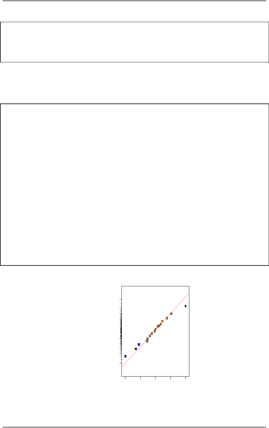
Solutions from Montgomery, D. C. (2001) Design and Analysis of Experiments, Wiley, NY
8-42
Camber Avg =
+263.17380
+1.94531 * Lam Temp
+11.20625 * Lam Pres
-2.99728 * Fire Time
-12.91146 * Fire DP
(d) Do any of the process variables affect the variability in camber measurements?
Yes, A, B, F, and AF interaction affect the variability in camber measurements.
Design Expert Output
Term Effect SumSqr % Contribtn
Model Intercept
Model A 15.9035 1011.69 27.6623
Model B -16.5773 1099.22 30.0558
Error C 5.8745 138.039 3.77437
Error D -3.2925 43.3622 1.18564
Error E -2.33725 21.851 0.597466
Model F -9.256 342.694 9.37021
Error AB 0.95525 3.65001 0.0998014
Error AC 2.524 25.4823 0.696757
Error AD -4.6265 85.618 2.34103
Error AE -0.18025 0.12996 0.00355347
Model AF -10.8745 473.019 12.9337
Error BC Aliased
Error BD -4.85575 94.3132 2.57879
Error BE Aliased
Error BF 8.21825 270.159 7.38689
Error CD Aliased
Error CE Aliased
Error CF Aliased
Error DE Aliased
Error DF Aliased
Error EF Aliased
Error ABC Aliased
Error ABD -0.68125 1.85641 0.0507593
Error ABE Aliased
Error ABF 3.39825 46.1924 1.26303
Lenth's ME 17.8392
Lenth's SME 36.2162
DESIGN-EXPERT Plot
Cam ber S tDev
A: Lam Temp
B: Lam Time
C: Lam Pres
D: Fire Tem p
E: Fire Tim e
F: Fire DP
Normal plot
Norm al % probability
Effe ct
-1 6 .58 -8 .4 6 -0 .3 4 7.78 15.90
1
5
10
20
30
50
70
80
90
95
99
A
B
F
AF

Solutions from Montgomery, D. C. (2001) Design and Analysis of Experiments, Wiley, NY
8-43
Response: Camber StDev
ANOVA for Selected Factorial Model
Analysis of variance table [Partial sum of squares]
Sum of Mean F
Source Squares DF Square Value Prob > F
Model 2926.62 4 731.65 11.02 0.0008 significant
A 1011.69 1 1011.69 15.23 0.0025
B 1099.22 1 1099.22 16.55 0.0019
F 342.69 1 342.69 5.16 0.0442
AF 473.02 1 473.02 7.12 0.0218
Residual 730.65 11 66.42
Cor Total 3657.27 15
The Model F-value of 11.02 implies the model is significant. There is only
a 0.08% chance that a "Model F-Value" this large could occur due to noise.
Std. Dev. 8.15 R-Squared 0.8002
Mean 25.35 Adj R-Squared 0.7276
C.V. 32.15 Pred R-Squared 0.5773
PRESS 1545.84 Adeq Precision 9.516
Coefficient Standard 95% CI 95% CI
Factor Estimate DF Error Low High VIF
Intercept 25.35 1 2.04 20.87 29.84
A-Lam Temp 7.95 1 2.04 3.47 12.44 1.00
B-Lam Time -8.29 1 2.04 -12.77 -3.80 1.00
F-Fire DP -4.63 1 2.04 -9.11 -0.14 1.00
AF -5.44 1 2.04 -9.92 -0.95 1.00
Final Equation in Terms of Coded Factors:
Camber StDev =
+25.35
+7.95 * A
-8.29 * B
-4.63 * F
-5.44 * A * F
Final Equation in Terms of Actual Factors:
Camber StDev =
-242.46746
+4.96373 * Lam Temp
-1.10515 * Lam Time
+10.23804 * Fire DP
-0.18124 * Lam Temp * Fire DP
(e) If it is important to reduce camber as much as possible, what recommendations would you make?
Solutions from Montgomery, D. C. (2001) Design and Analysis of Experiments, Wiley, NY
8-44
55.00 60.00 65.00 70.00 75.00
31.5
81.125
130.75
180.375
230
Lam Temp
Camber Avg
One Factor Plot
5.00 6.25 7.50 8.75 10.00
31.5
81.125
130.75
180.375
230
Lam Pres
Camber Avg
One Factor Plot
17.50 20.38 23.25 26.13 29.00
31.5
81.125
130.75
180.375
230
Fire Tim e
Camber Avg
One Factor Plot
20.00 21.50 23.00 24.50 26.00
31.5
81.125
130.75
180.375
230
Fire DP
Camber Avg
One Factor Plot
Solutions from Montgomery, D. C. (2001) Design and Analysis of Experiments, Wiley, NY
8-45
DESIGN-EXPERT Plot
Cam ber S tDev
X = A: Lam Temp
Y = F: Fire DP
F- 20.000
F+ 26.000
Actual Factors
B: Lam Time = 17.50
C: Lam Pres = 7.50
D: Fire Temp = 1600.00
E: Fire Time = 23.25
Fire DP
Inte ra c ti o n G r a p h
Camber StDev
Lam Temp
55.00 60.00 65.00 70.00 75.00
4.083
18.972
33.861
48.75
63.639
DESIGN-EXPERT Plot
Cam ber S tDev
X = B: Lam Time
Actual Factors
A: Lam T emp = 65.00
C: Lam Pres = 7.50
D: Fire Temp = 1600.00
E: Fire T im e = 23.25
F: Fire DP = 23.00
10.00 13.75 17.50 21.25 25.00
4.083
18.972
33.861
48.75
63.639
Lam Time
Camber StDev
One Factor Plot
Run A and C at the low level and E and F at the high level. B at the low level enables a lower variation
without affecting the average camber.
8-25 A spin coater is used to apply photoresist to a bare silicon wafer. This operation usually occurs
early in the semiconductor manufacturing process, and the average coating thickness and the variability in
the coating thickness has an important impact on downstream manufacturing steps. Six variables are
used in the experiment. The variables and their high and low levels are as follows:
Factor Low Level High Level
Final Spin Speed 7350 rpm 6650 rpm
Acceleration Rate 5 20
Volume of Resist Applied 3 cc 5 cc
Time of Spin 14 s 6 s
Resist Batch Variation Batch 1 Batch 2
Exhaust Pressure Cover Off Cover On
The experimenter decides to use a 26-1 design and to make three readings on resist thickness on each test
wafer. The data are shown in table 8-29.
Table 8-29
A B C D E F Resist Thick ness
Run Volume Batch Time Speed Acc. Cover Left Center Right Avg. Range
1 5 2 14 7350 5 Off 4531 4531 4515 4525.7 16
2 5 1 6 7350 5 Off 4446 4464 4428 4446 36
3 3 1 6 6650 5 Off 4452 4490 4452 4464.7 38
4 3 2 14 7350 20 Off 4316 4328 4308 4317.3 20
5 3 1 14 7350 5 Off 4307 4295 4289 4297 18
6 5 1 6 6650 20 Off 4470 4492 4495 4485.7 25
7 3 1 6 7350 5 On 4496 4502 4482 4493.3 20
8 5 2 14 6650 20 Off 4542 4547 4538 4542.3 9
9 5 1 14 6650 5 Off 4621 4643 4613 4625.7 30
10 3 1 14 6650 5 On 4653 4670 4645 4656 25
11 3 2 14 6650 20 On 4480 4486 4470 4478.7 16
12 3 1 6 7350 20 Off 4221 4233 4217 4223.7 16
13 5 1 6 6650 5 On 4620 4641 4619 4626.7 22
14 3 1 6 6650 20 On 4455 4480 4466 4467 25
15 5 2 14 7350 20 On 4255 4288 4243 4262 45
16 5 2 6 7350 5 On 4490 4534 4523 4515.7 44
17 3 2 14 7350 5 On 4514 4551 4540 4535 37
18 3 1 14 6650 20 Off 4494 4503 4496 4497.7 9

Solutions from Montgomery, D. C. (2001) Design and Analysis of Experiments, Wiley, NY
8-46
19 5 2 6 7350 20 Off 4293 4306 4302 4300.3 13
20 3 2 6 7350 5 Off 4534 4545 4512 4530.3 33
21 5 1 14 6650 20 On 4460 4457 4436 4451 24
22 3 2 6 6650 5 On 4650 4688 4656 4664.7 38
23 5 1 14 7350 20 Off 4231 4244 4230 4235 14
24 3 2 6 7350 20 On 4225 4228 4208 4220.3 20
25 5 1 14 7350 5 On 4381 4391 4376 4382.7 15
26 3 2 6 6650 20 Off 4533 4521 4511 4521.7 22
27 3 1 14 7350 20 On 4194 4230 4172 4198.7 58
28 5 2 6 6650 5 Off 4666 4695 4672 4677.7 29
29 5 1 6 7350 20 On 4180 4213 4197 4196.7 33
30 5 2 6 6650 20 On 4465 4496 4463 4474.7 33
31 5 2 14 6650 5 On 4653 4685 4665 4667.7 32
32 3 2 14 6650 5 Off 4683 4712 4677 4690.7 35
(a) Verify that this is a 26-1 design. Discuss the alias relationships in this design.
I=ABCDEF. This is a resolution VI design where main effects are aliased with five-factor interactions
and two-factor interactions are aliased with four-factor interactions.
(b) What factors appear to affect average resist thickness?
Factors B, D, and E appear to affect the average resist thickness.
Design Expert Output
Term Effect SumSqr % Contribtn
Model Intercept
Error A 9.925 788.045 0.107795
Model B 73.575 43306.2 5.92378
Error C 3.375 91.125 0.0124648
Model D -207.062 342999 46.9182
Model E -182.925 267692 36.6172
Error F -5.6625 256.511 0.0350877
Error AB -9 648 0.0886387
Error AC -7.3 426.32 0.0583155
Error AD -3.8625 119.351 0.0163258
Error AE -7.1 403.28 0.0551639
Error AF -26.9875 5826.6 0.79701
Error BC 10.875 946.125 0.129419
Error BD 18.1125 2624.5 0.359001
Error BE -28.35 6429.78 0.879518
Error BF -30.2375 7314.45 1.00053
Error CD -24.9875 4995 0.683257
Error CE 8.2 537.92 0.0735811
Error CF -6.7875 368.561 0.0504148
Error DE -38.5375 11881.1 1.6252
Error DF -3.2 81.92 0.0112057
Error EF -41.1625 13554.8 1.85414
Error ABC 0.375 1.125 0.000153887
Error ABD Aliased
Error ABE 16.5 2178 0.297925
Error ABF 31.4125 7893.96 1.0798
Error ACD 15.5875 1943.76 0.265883
Error ACE Aliased
Error ACF Aliased
Error ADE 9.5375 727.711 0.0995423
Error ADF Aliased
Error AEF Aliased
Error BCD 29.0875 6768.66 0.925873
Error BCE -1.625 21.125 0.00288965
Error BCF Aliased
Error BDE -1.8875 28.5013 0.00389863
Error BDF 3.95 124.82 0.0170739
Error BEF Aliased
Error CDE Aliased
Error CDF Aliased
Error CEF 3.1375 78.7512 0.0107722
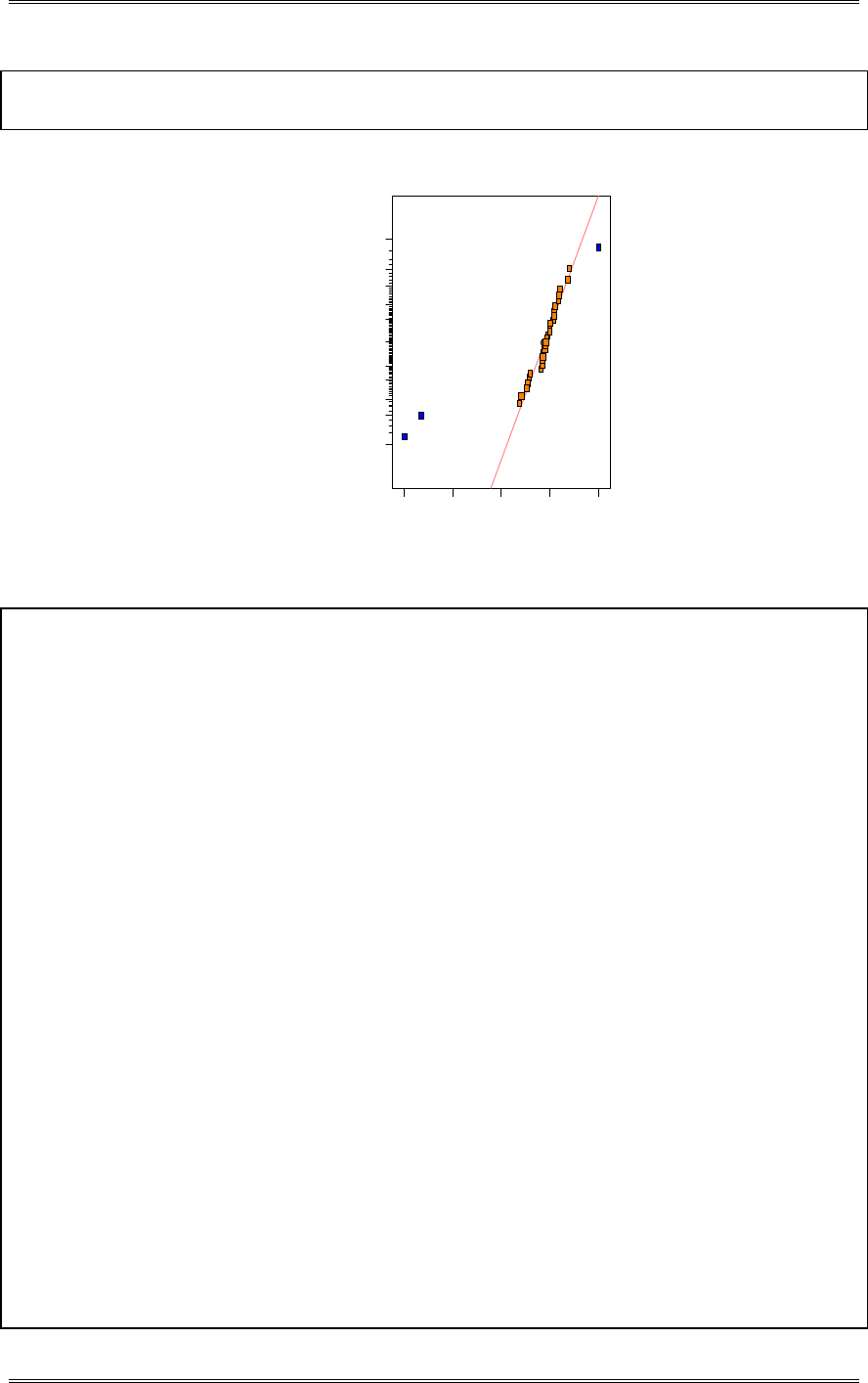
Solutions from Montgomery, D. C. (2001) Design and Analysis of Experiments, Wiley, NY
8-47
Error DEF Aliased
Lenth's ME 28.6178
Lenth's SME 54.4118
DESIGN-EXPERT Plot
Thick Avg
A: Volume
B: Batch
C: Tim e
D: Speed
E: Acc
F: Cover
Normal plot
Norm al % probability
Effe ct
-2 0 7 .0 6 -1 3 6 .9 0 -6 6 . 74 3.42 73.57
1
5
10
20
30
50
70
80
90
95
99
B
D
E
Design Expert Output
Response: Thick Avg
ANOVA for Selected Factorial Model
Analysis of variance table [Partial sum of squares]
Sum of Mean F
Source Squares DF Square Value Prob > F
Model 6.540E+005 3 2.180E+005 79.21 < 0.0001 significant
B 43306.24 1 43306.24 15.74 0.0005
D 3.430E+005 1 3.430E+005 124.63 < 0.0001
E 2.677E+005 1 2.677E+005 97.27 < 0.0001
Residual 77059.83 28 2752.14
Cor Total 7.311E+005 31
The Model F-value of 79.21 implies the model is significant. There is only
a 0.01% chance that a "Model F-Value" this large could occur due to noise.
Std. Dev. 52.46 R-Squared 0.8946
Mean 4458.51 Adj R-Squared 0.8833
C.V. 1.18 Pred R-Squared 0.8623
PRESS 1.006E+005 Adeq Precision 24.993
Coefficient Standard 95% CI 95% CI
Factor Estimate DF Error Low High VIF
Intercept 4458.51 1 9.27 4439.52 4477.51
B-Batch 36.79 1 9.27 17.79 55.78 1.00
D-Speed -103.53 1 9.27 -122.53 -84.53 1.00
E-Acc -91.46 1 9.27 -110.46 -72.47 1.00
Final Equation in Terms of Coded Factors:
Thick Avg =
+4458.51
+36.79 * B
-103.53 * D
-91.46 * E
Final Equation in Terms of Actual Factors:
Batch Batch 1
Thick Avg =
+6644.78750

Solutions from Montgomery, D. C. (2001) Design and Analysis of Experiments, Wiley, NY
8-48
-0.29580 * Speed
-12.19500 * Acc
Batch Batch 2
Thick Avg =
+6718.36250
-0.29580 * Speed
-12.19500 * Acc
(c) Since the volume of resist applied has little effect on average thickness, does this have any important
practical implications for the process engineers?
Yes, less material could be used.
(d) Project this design into a smaller design involving only the significant factors. Graphically display
the results. Does this aid in interpretation?
Cube Graph
Thick Avg
Batch
Speed
Acc
B- B+
D-
D+
E-
E+
4616.72
4433.7 9
4409.66
4226.7 3
4690.29
4507.37
4483.23
4300.31
The cube plot usually assists the experimenter in drawing conclusions.
(e) Use the range of resist thickness as a response variable. Is there any indication that any of these
factors affect the variability in resist thickness?
Design Expert Output
Term Effect SumSqr % Contribtn
Model Intercept
Model A -0.625 3.125 0.0777387
Model B 2.125 36.125 0.89866
Error C -2.75 60.5 1.50502
Error D 1.625 21.125 0.525514
Model E -5.375 231.125 5.74956
Model F 7.75 480.5 11.9531
Model AB 0.625 3.125 0.0777387
Error AC -3.5 98 2.43789
Error AD -0.125 0.125 0.00310955
Error AE 1.875 28.125 0.699649
Model AF 1.75 24.5 0.609472
Error BC 0 0 0
Error BD 0.125 0.125 0.00310955
Error BE -5.375 231.125 5.74956
Model BF 3.25 84.5 2.10206
Error CD 3.75 112.5 2.79859
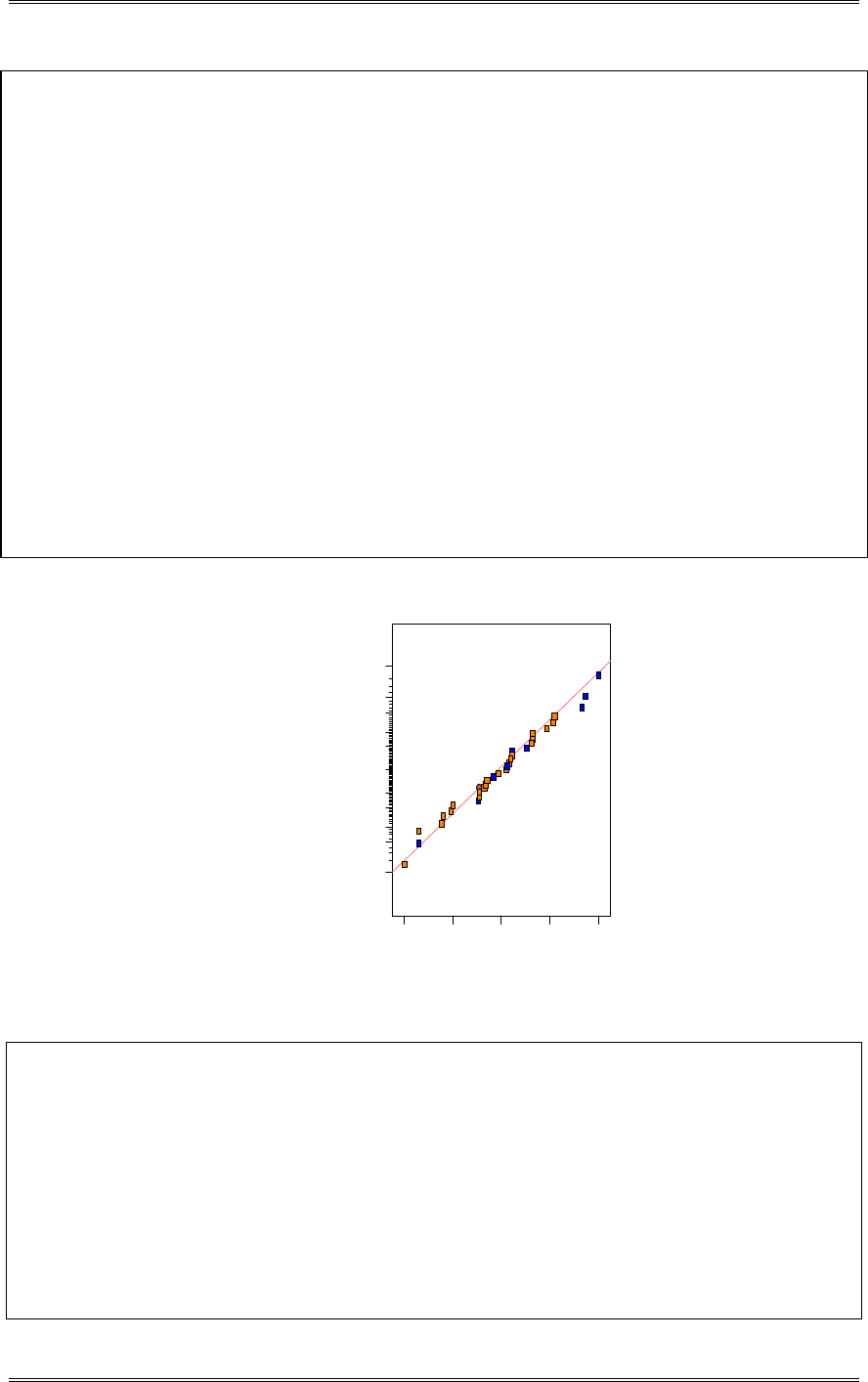
Solutions from Montgomery, D. C. (2001) Design and Analysis of Experiments, Wiley, NY
8-49
Error CE 3.75 112.5 2.79859
Error CF 4.875 190.125 4.72962
Error DE 5.375 231.125 5.74956
Error DF 5.5 242 6.02009
Model EF 8 512 12.7367
Error ABC Aliased
Error ABD Aliased
Error ABE 3.625 105.125 2.61513
Model ABF 9 648 16.1199
Error ACD -6.5 338 8.40822
Error ACE Aliased
Error ACF Aliased
Error ADE -3.375 91.125 2.26686
Error ADF -0.5 2 0.0497528
Error AEF 1 8 0.199011
Error BCD Aliased
Error BCE Aliased
Error BCF Aliased
Error BDE -2.625 55.125 1.37131
Error BDF -0.5 2 0.0497528
Error BEF Aliased
Error CDE Aliased
Error CDF Aliased
Error CEF 2.125 36.125 0.89866
Error DEF 2 32 0.796045
Lenth's ME 9.15104
Lenth's SME 17.3991
DESIGN-EXPERT Plot
Thick StDev
A: Volume
B: Batch
C: Tim e
D: Speed
E: Acc
F: Cover
Normal plot
Normal % probability
Effe ct
-6 .5 0 -2 .6 2 1.25 5.13 9.00
1
5
10
20
30
50
70
80
90
95
99
A
B
E
F
ABAF
BF
EF
AB F
Design Expert Output
Response: Thick StDev
ANOVA for Selected Factorial Model
Analysis of variance table [Partial sum of squares]
Sum of Mean F
Source Squares DF Square Value Prob > F
Model 2023.00 9 224.78 2.48 0.0400 significant
A 3.13 1 3.13 0.034 0.8545
B 36.13 1 36.13 0.40 0.5346
E 231.12 1 231.12 2.55 0.1248
F 480.50 1 480.50 5.29 0.0313
AB 3.12 1 3.12 0.034 0.8545
AF 24.50 1 24.50 0.27 0.6086
BF 84.50 1 84.50 0.93 0.3451
EF 512.00 1 512.00 5.64 0.0267
ABF 648.00 1 648.00 7.14 0.0139

Solutions from Montgomery, D. C. (2001) Design and Analysis of Experiments, Wiley, NY
8-50
Residual 1996.88 22 90.77
Cor Total 4019.88 31
The Model F-value of 2.48 implies the model is significant. There is only
a 4.00% chance that a "Model F-Value" this large could occur due to noise.
Std. Dev. 9.53 R-Squared 0.5032
Mean 26.56 Adj R-Squared 0.3000
C.V. 35.87 Pred R-Squared -0.0510
PRESS 4224.79 Adeq Precision 5.586
Coefficient Standard 95% CI 95% CI
Factor Estimate DF Error Low High VIF
Intercept 26.56 1 1.68 23.07 30.06
A-Volume -0.31 1 1.68 -3.81 3.18 1.00
B-Batch 1.06 1 1.68 -2.43 4.56 1.00
E-Acc -2.69 1 1.68 -6.18 0.81 1.00
F-Cover 3.88 1 1.68 0.38 7.37 1.00
AB 0.31 1 1.68 -3.18 3.81 1.00
AF 0.88 1 1.68 -2.62 4.37 1.00
BF 1.63 1 1.68 -1.87 5.12 1.00
EF 4.00 1 1.68 0.51 7.49 1.00
ABF 4.50 1 1.68 1.01 7.99 1.00
Final Equation in Terms of Coded Factors:
Thick StDev =
+26.56
-0.31 * A
+1.06 * B
-2.69 * E
+3.88 * F
+0.31 * A * B
+0.88 * A * F
+1.63 * B * F
+4.00 * E * F
+4.50 * A * B * F
Final Equation in Terms of Actual Factors:
Batch Batch 1
Cover Off
Thick StDev =
+22.39583
+3.00000 * Volume
-0.89167 * Acc
Batch Batch 2
Cover Off
Thick StDev =
+54.77083
-5.37500 * Volume
-0.89167 * Acc
Batch Batch 1
Cover On
Thick StDev =
+42.56250
-4.25000 * Volume
+0.17500 * Acc
Batch Batch 2
Cover On
Thick StDev =
+9.43750
+5.37500 * Volume
+0.17500 * Acc

Solutions from Montgomery, D. C. (2001) Design and Analysis of Experiments, Wiley, NY
8-51
The model here for variability isn’t very strong. Notice the small value of R2, and in particular, the
adjusted R2. Often we find that obtaining a good model for a response that expresses variability isn’t as
easy as finding a satisfactory model for a response that essentially measures the mean.
(f) Where would you recommend that the process engineers run the process?
Considering only the average thickness results, the engineers could use factors B, D and E to put the
process mean at target. Then the engineer could consider the other factors on the range model to try to set
the factors to reduce the variation in thickness at that mean.
8-26 Harry and Judy Peterson-Nedry (two friends of the author) own a vineyard in Oregon. They grow
several varieties of grapes and manufacture wine. Harry and Judy have used factorial designs for process
and product development in the winemaking segment of their business. This problem describes the
experiment conducted for their 1985 Pinot Noir. Eight variables, shown below, were originally studied in
this experiment:
Variable Low Level High Level
A Pinot Noir Clone Pommard Wadenswil
B Oak Type Allier Troncais
C Age of Barrel Old New
D Yeast/Skin Contact Champagne Montrachet
E Stems None All
F Barrel Toast Light Medium
G Whole Cluster None 10%
H Fermentation Temperature Low (75 F Max) High (92 F Max)
Harry and Judy decided to use a 284
IV
design with 16 runs. The wine was taste-tested by a panel of experts
on 8 March 1986. Each expert ranked the 16 samples of wine tasted, with rank 1 being the best. The
design and taste-test panel results are shown in Table 8-30.
Table 8-30
Run A B C D E F G H HPN JPN CAL DCM RGB ybar s
1 - - - - - - - - 12 6 13 10 7 9.6 3.05
2 + - - - - + + + 10 7 14 14 9 10.8 3.11
3 - + - - + - + + 14 13 10 11 15 12.6 2.07
4 + + - - + + - - 9 9 7 9 12 9.2 1.79
5 - - + - + + + - 8 8 11 8 10 9.0 1.41
6 + - + - + - - + 16 12 15 16 16 15.0 1.73
7 - + + - - + - + 6 5 6 5 3 5.0 1.22
8 + + + - - - + - 15 16 16 15 14 15.2 0.84
9 - - - + + + - + 1 2 3 3 2 2.2 0.84
10 + - - + + - + - 7 11 4 7 6 7.0 2.55
11 - + - + - + + - 13 3 8 12 8 8.8 3.96
12 + + - + - - - + 3 1 5 1 4 2.8 1.79
13 - - + + - - + + 2 10 2 4 5 9.6 3.29
14 + - + + - + - - 4 4 1 2 1 2.4 1.52
15 - + + + + - - - 5 15 9 6 11 9.2 4.02
16 + + + + + + + + 11 14 12 13 13 12.6 1.14
(a) What are the alias relationships in the design selected by Harry and Judy?
E = BCD, F = ACD, G = ABC, H = ABD
Defining Contrast : I = BCDE = ACDF = ABEF = ABCG = ADEG = BDFG = CEFG = ABDH
= ACEH = BCFH = DEFH = CDGH = BEGH = AFGH = ABCDEFGH
Aliases:
A = BCG = BDH = BEF = CDF = CEH = DEG = FGH
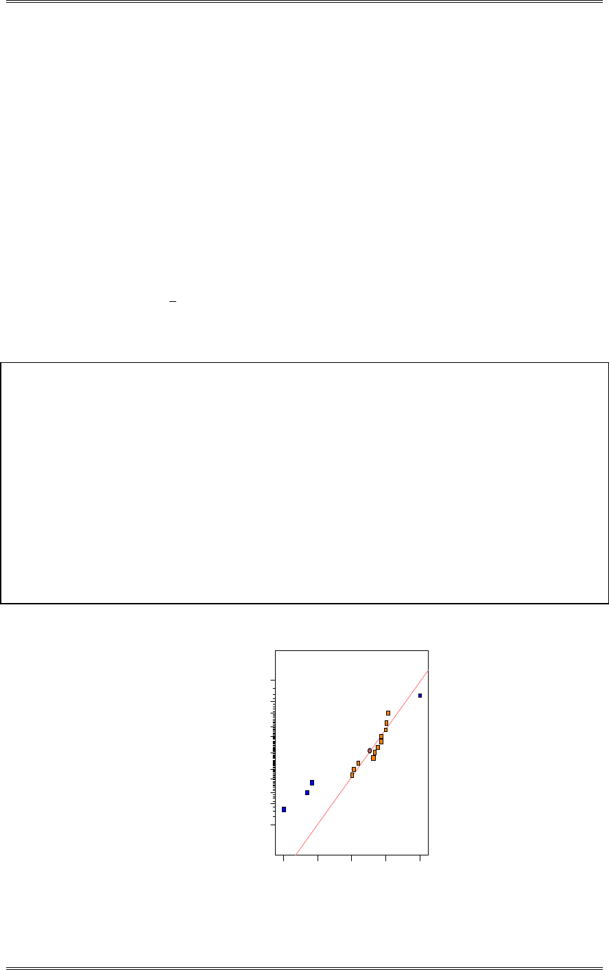
Solutions from Montgomery, D. C. (2001) Design and Analysis of Experiments, Wiley, NY
8-52
B = ACG = ADH = AEF = CDE = CFH = DFG = EGH
C = ABG = ADF = AEH = BDE = BFH = DGH = EFG
D = ABH = ACF = AEG = BCE = BFG = CGH = EFH
E = ABF = ACH = ADG = BCD = BGH = CFG = DFH
F = ABE = ACD = AGH = BCH = BDG = CEG = DEH
G = ABC = ADE = AFH = BDF = BEH = CDH = CEF
H = ABD = ACE = AFG = BCF = BEG = CDG = DEF
AB = CG = DH = EF
AC = BG = DF = EH
AD = BH = CF = EG
AE = BF = CH = DG
AF = BE = CD = GH
AG = BC = DE = FH
AH = BD = CE = FG
(b) Use the average ranks ( y) as a response variable. Analyze the data and draw conclusions. You will
find it helpful to examine a normal probability plot of effect estimates.
Design Expert Output
Term Effect SumSqr % Contribtn
Model Intercept
Error A 1.125 5.0625 2.00799
Error B 1.225 6.0025 2.38083
Error C 1.875 14.0625 5.57776
Model D -3.975 63.2025 25.0687
Error E 1.575 9.9225 3.93566
Model F -2.625 27.5625 10.9324
Model G 3.775 57.0025 22.6095
Error H 0.025 0.0025 0.000991601
Error AB -0.075 0.0225 0.00892441
Error AC 1.975 15.6025 6.18858
Model AD -2.375 22.5625 8.9492
Error AE 1.575 9.9225 3.93566
Error AF 1.375 7.5625 2.99959
Error AG 0.275 0.3025 0.119984
Error AH 1.825 13.3225 5.28424
Lenth's ME 6.073
Lenth's SME 12.3291
DESIGN-EXPERT Plot
Taste Avg
A: A
B: B
C: C
D: D
E: E
F: F
G: G
H: H
Normal plot
Normal % probability
Effe ct
-3 .9 8 -2 .0 4 -0 .1 0 1.84 3.78
1
5
10
20
30
50
70
80
90
95
99
D
F
G
AD

Solutions from Montgomery, D. C. (2001) Design and Analysis of Experiments, Wiley, NY
8-53
Design Expert Output
Response: Taste Avg
ANOVA for Selected Factorial Model
Analysis of variance table [Partial sum of squares]
Sum of Mean F
Source Squares DF Square Value Prob > F
Model 175.39 5 35.08 4.57 0.0198 significant
A 5.06 1 5.06 0.66 0.4355
D 63.20 1 63.20 8.24 0.0167
F 27.56 1 27.56 3.59 0.0873
G 57.00 1 57.00 7.43 0.0214
AD 22.56 1 22.56 2.94 0.1171
Residual 76.72 10 7.67
Cor Total 252.12 15
The Model F-value of 4.57 implies the model is significant. There is only
a 1.98% chance that a "Model F-Value" this large could occur due to noise.
Std. Dev. 2.77 R-Squared 0.6957
Mean 8.81 Adj R-Squared 0.5435
C.V. 31.43 Pred R-Squared 0.2209
PRESS 196.42 Adeq Precision 7.517
Coefficient Standard 95% CI 95% CI
Factor Estimate DF Error Low High VIF
Intercept 8.81 1 0.69 7.27 10.36
A-A 0.56 1 0.69 -0.98 2.11 1.00
D-D -1.99 1 0.69 -3.53 -0.44 1.00
F-F -1.31 1 0.69 -2.86 0.23 1.00
G-G 1.89 1 0.69 0.34 3.43 1.00
AD -1.19 1 0.69 -2.73 0.36 1.00
Final Equation in Terms of Coded Factors:
Taste Avg =
+8.81
+0.56 * A
-1.99 * D
-1.31 * F
+1.89 * G
-1.19 * A * D
Factors D, F, G and the AD interaction are important. Factor A is added to the model to preserve
hierarchy. Notice that the AD interaction is aliased with other two-factor interactions that could also be
important. So the interpretation of the two-factor interaction is somewhat uncertain. Normally, we would
add runs to the design to isolate the significant interactions, but that won’t work very well here because
each experiment requires a full growing season. In other words, it would require a very long time to add
runs to dealias the alias chain of interest.
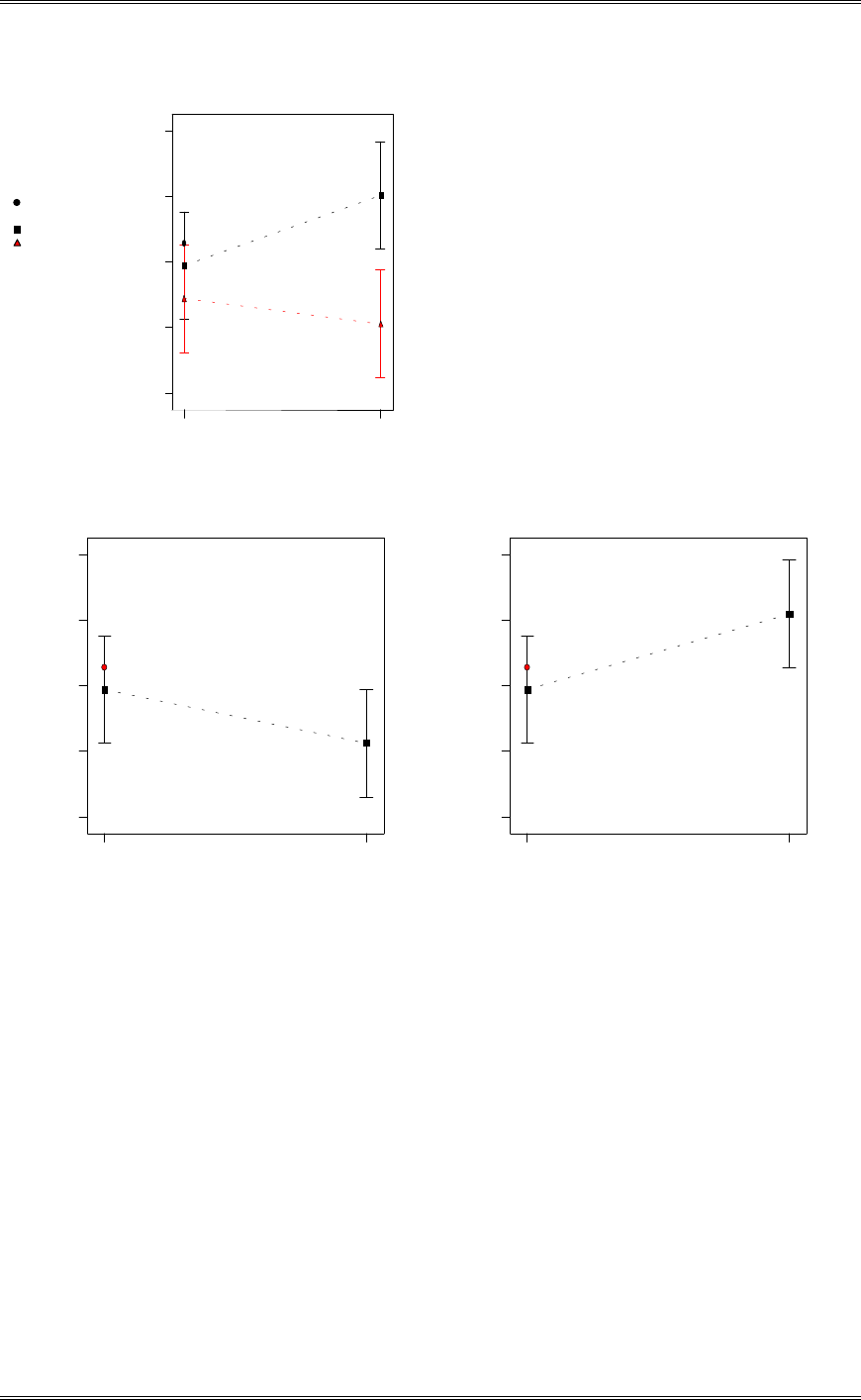
Solutions from Montgomery, D. C. (2001) Design and Analysis of Experiments, Wiley, NY
8-54
DESIGN-EXPERT Plot
Taste Avg
X = A: A
Y = D: D
Design Points
D1 D1
D2 D2
Actual Factors
B: B = B1
C: C = C1
E: E = E1
F: F = F1
G: G = G1
H: H = H1
D
Inte ra c ti o n G r a p h
Tas te Avg
A
A1 A2
2.2
5.45
8.7
11.95
15.2
F
Tas te Avg
One Factor Plot
F1 F2
2.2
5.45
8.7
11.95
15.2
G
Tas te Avg
One Factor Plot
G1 G2
2.2
5.45
8.7
11.95
15.2
(c) Use the standard deviation of the ranks (or some appropriate transformation such as log s) as a
response variable. What conclusions can you draw about the effects of the eight variables on
variability in wine quality?
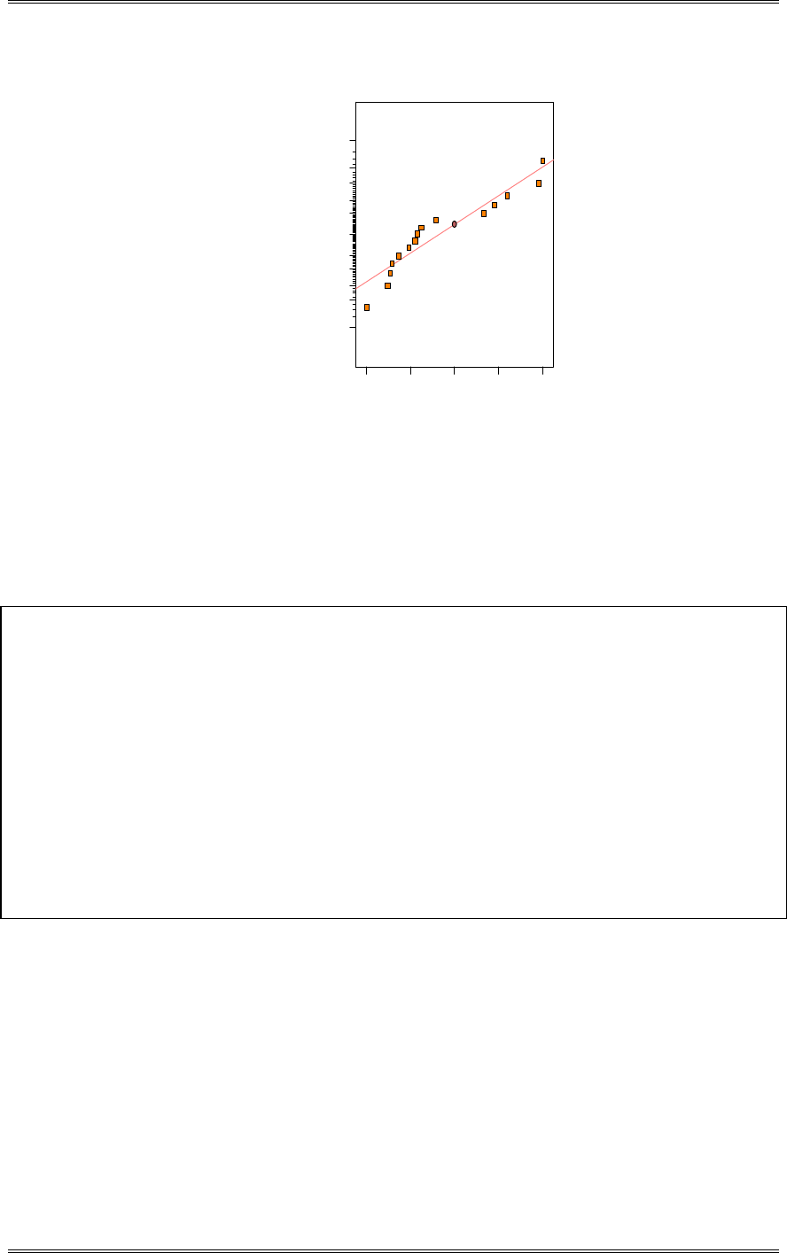
Solutions from Montgomery, D. C. (2001) Design and Analysis of Experiments, Wiley, NY
8-55
DESIGN-EXPERT Plot
Ln(Taste StDev)
A: A
B: B
C: C
D: D
E: E
F: F
G: G
H: H
Normal plot
Normal % probability
Effe ct
-0 .3 9 -0 .2 0 -0 .0 1 0.19 0.38
1
5
10
20
30
50
70
80
90
95
99
Warnin
g
! No te rm s are s el
e
There do not appear to be any significant factors.
(d) After looking at the results, Harry and Judy decide that one of the panel members (DCM) knows more
about beer than he does about wine, so they decide to delete his ranking. What affect would this have
on the results and on conclusions from parts (b) and (c)?
Design Expert Output
Term Effect SumSqr % Contribtn
Model Intercept
Model A 1.625 10.5625 4.02957
Error B 2.0625 17.0156 6.49142
Error C 1.5 9 3.43348
Model D -4.5 81 30.9013
Error E 2.4375 23.7656 9.06652
Model F -2.375 22.5625 8.60753
Model G 2.9375 34.5156 13.1676
Error H -0.6875 1.89063 0.721268
Error AB -0.5625 1.26562 0.482833
Error AC 2.375 22.5625 8.60753
Model AD -1.5 9 3.43348
Error AE 0.6875 1.89062 0.721268
Error AF 0.875 3.0625 1.16834
Error AG 0.8125 2.64062 1.00739
Error AH 2.3125 21.3906 8.16047
Lenth's ME 6.26579
Lenth's SME 12.7205
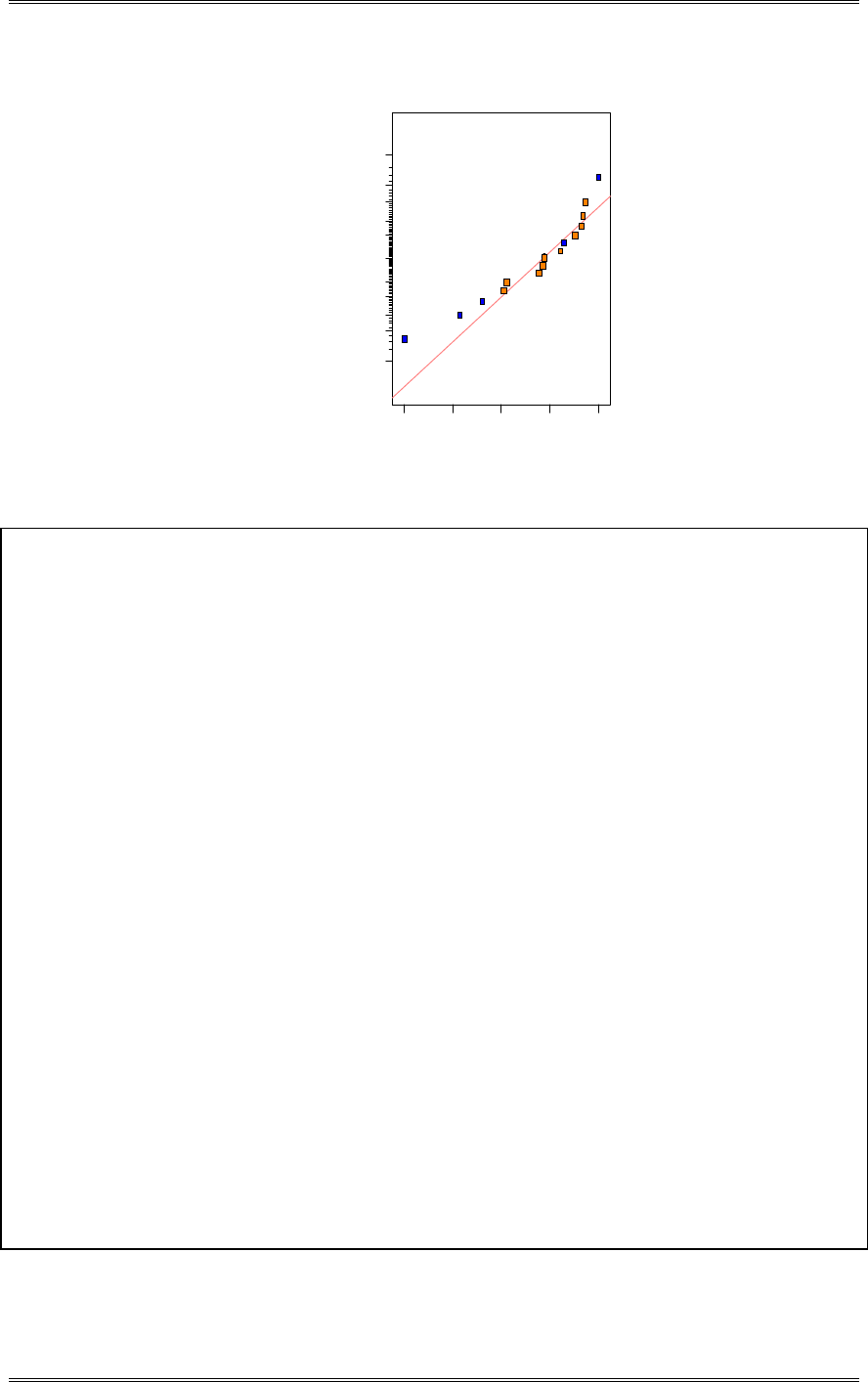
Solutions from Montgomery, D. C. (2001) Design and Analysis of Experiments, Wiley, NY
8-56
DESIGN-EXPERT Plot
Taste Avg
A: A
B: B
C: C
D: D
E: E
F: F
G: G
H: H
Normal plot
Normal % probability
Effe ct
-4 .5 0 -2 .6 4 -0 .7 8 1.08 2.94
1
5
10
20
30
50
70
80
90
95
99
A
D
F
G
AD
Design Expert Output
Response: Taste Avg
ANOVA for Selected Factorial Model
Analysis of variance table [Partial sum of squares]
Sum of Mean F
Source Squares DF Square Value Prob > F
Model 157.64 5 31.53 3.02 0.0646 not significant
A 10.56 1 10.56 1.01 0.3384
D 81.00 1 81.00 7.75 0.0193
F 22.56 1 22.56 2.16 0.1724
G 34.52 1 34.52 3.30 0.0992
AD 9.00 1 9.00 0.86 0.3752
Residual 104.48 10 10.45
Cor Total 262.13 15
The Model F-value of 3.02 implies there is a 6.46% chance that a "Model F-Value"
this large could occur due to noise.
Std. Dev. 3.23 R-Squared 0.6014
Mean 8.50 Adj R-Squared 0.4021
C.V. 38.03 Pred R-Squared -0.0204
PRESS 267.48 Adeq Precision 5.778
Coefficient Standard 95% CI 95% CI
Factor Estimate DF Error Low High VIF
Intercept 8.50 1 0.81 6.70 10.30
A-A 0.81 1 0.81 -0.99 2.61 1.00
D-D -2.25 1 0.81 -4.05 -0.45 1.00
F-F -1.19 1 0.81 -2.99 0.61 1.00
G-G 1.47 1 0.81 -0.33 3.27 1.00
AD -0.75 1 0.81 -2.55 1.05 1.00
Final Equation in Terms of Coded Factors:
Taste Avg =
+8.50
+0.81 * A
-2.25 * D
-1.19 * F
+1.47 * G
-0.75 * A * D
The results are the same for average taste without DCM as they were with DCM.
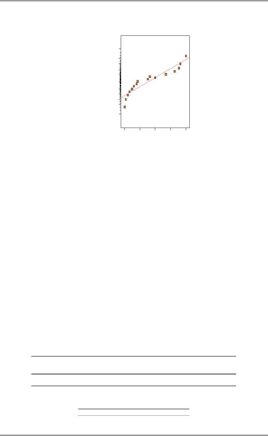
Solutions from Montgomery, D. C. (2001) Design and Analysis of Experiments, Wiley, NY
8-57
DESIGN-EXPERT Plot
Taste StDev
A: A
B: B
C: C
D: D
E: E
F: F
G: G
H: H
Normal plot
Normal % probability
Effe ct
-0 .7 4 -0 .3 5 0.03 0.41 0.79
1
5
10
20
30
50
70
80
90
95
99
Warnin
g
! No te rm s are s el
e
The standard deviation response is much the same with or without DCM’s responses. Again, there are no
significant factors.
(e) Suppose that just before the start of the experiment, Harry and Judy discovered that the eight new
barrels they ordered from France for use in the experiment would not arrive in time, and all 16 runs
would have to be made with old barrels. If Harry and Judy just drop column C from their design,
what does this do to the alias relationships? Do they need to start over and construct a new design?
The resulting design is a 273
IV
with defining relations: I = ABEF = ADEG = BDFG = ABDH = DEFH =
BEGH = AFGH.
(f) Harry and Judy know from experience that some treatment combinations are unlikely to produce good
results. For example, the run with all eight variables at the high level generally results in a poorly
rated wine. This was confirmed in the 8 March 1986 taste test. They want to set up a new design to
make the run with all eight factors at the high level. What design would you suggest?
By changing the sign of any of the design generators, a design that does not include the principal fraction
will be generated. This will give a design without an experimental run combination with all of the
variables at the high level.
8-27 In an article in Quality Engineering (“An Application of Fractional Factorial Experimental
Designs,” 1988, Vol. 1 pp. 19-23) M.B. Kilgo describes an experiment to determine the effect of CO2
pressure (A), CO2 temperature (B), peanut moisture (C), CO2 flow rate (D), and peanut particle size (E) on
the total yield of oil per batch of peanuts (y). The levels she used for these factors are as follows:
A B C D E
Coded Pressure Temp Moisture Flow Particle Size
Level (bar) (C) (% by weight) (liters/min) (mm)
-1 415 25 5 40 1.28
1 550 95 15 60 4.05
She conducted the 16-run fractional factorial experiment shown below:
A B C D E y
1 415 25 5 40 1.28 63

Solutions from Montgomery, D. C. (2001) Design and Analysis of Experiments, Wiley, NY
8-58
2 550 25 5 40 4.05 21
3 415 95 5 40 4.05 36
4 550 95 5 40 1.28 99
5 415 25 15 40 4.05 24
6 550 25 15 40 1.28 66
7 415 95 15 40 1.28 71
8 550 95 15 40 4.05 54
9 415 25 5 60 4.05 23
10 550 25 5 60 1.28 74
11 415 95 5 60 1.28 80
12 550 95 5 60 4.05 33
13 415 25 15 60 1.28 63
14 550 25 15 60 4.05 21
15 415 95 15 60 4.05 44
16 550 95 15 60 1.28 96
(a) What type of design has been used? Identify the defining relation and the alias relationships.
A 251
V
, 16-run design, with I= -ABCDE.
A(-ABCDE)= -BCDE A = -BCDE
B
(-ABCDE)= -ACDE B = -ACDE
C
(-ABCDE)= -ABDE C = -ABDE
D
(-ABCDE)= -ABCE D = -ABCE
E
(-ABCDE)= -ABCD E = -ABCD
A
B
(-ABCDE)= -CDE AB = -CDE
A
C
(-ABCDE)= -BDE AC = -BDE
A
D
(-ABCDE)= -BCE AD = -BCE
A
E
(-ABCDE)= -BCD AE = -BCD
B
C
(-ABCDE)= -ADE BC = -ADE
B
D
(-ABCDE)= -ACE BD = -ACE
B
E
(-ABCDE)= -ACD BE = -ACD
C
D
(-ABCDE)= -ABE CD = -ABE
C
E
(-ABCDE)= -ABD CE = -ABD
D
E
(-ABCDE)= -ABC DE = -ABC
(b) Estimate the factor effects and use a normal probability plot to tentatively identify the important
factors.
Design Expert Output
Term Effect SumSqr % Contribtn
Model Intercept
Error A 7.5 225 2.17119
Model B 19.75 1560.25 15.056
Error C 1.25 6.25 0.0603107
Error D 0 0 0
Model E 44.5 7921 76.4354
Error AB 5.25 110.25 1.06388
Error AC 1.25 6.25 0.0603107
Error AD -4 64 0.617582
Error AE 7 196 1.89134
Error BC 3 36 0.34739
Error BD -1.75 12.25 0.118209
Error BE 0.25 0.25 0.00241243
Error CD 2.25 20.25 0.195407
Error CE -6.25 156.25 1.50777
Error DE 3.5 49 0.472836
Lenth's ME 11.5676
Lenth's SME 23.4839
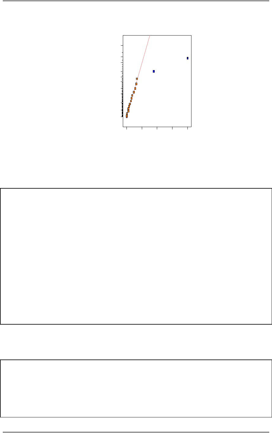
Solutions from Montgomery, D. C. (2001) Design and Analysis of Experiments, Wiley, NY
8-59
DESIGN-EXPERT Plot
Yield
A: Pressure
B: Temperature
C: M oisture
D: Flow
E: Particle Size
Half Normal plot
Half Normal % probability
|Effect|
0.00 11.13 22.25 33.38 44.50
0
20
40
60
70
80
85
90
95
97
99
B
E
(c) Perform an appropriate statistical analysis to test the hypothesis that the factors identified in part
above have a significant effect on the yield of peanut oil.
Design Expert Output
Response: Yield
ANOVA for Selected Factorial Model
Analysis of variance table [Partial sum of squares]
Sum of Mean F
Source Squares DF Square Value Prob > F
Model 9481.25 2 4740.63 69.89 < 0.0001 significant
B 1560.25 1 1560.25 23.00 0.0003
E 7921.00 1 7921.00 116.78 < 0.0001
Residual 881.75 13 67.83
Cor Total 10363.00 15
The Model F-value of 69.89 implies the model is significant. There is only
a 0.01% chance that a "Model F-Value" this large could occur due to noise.
Std. Dev. 8.24 R-Squared 0.9149
Mean 54.25 Adj R-Squared 0.9018
C.V. 15.18 Pred R-Squared 0.8711
PRESS 1335.67 Adeq Precision 18.017
Coefficient Standard 95% CI 95% CI
Factor Estimate DF Error Low High VIF
Intercept 54.25 1 2.06 49.80 58.70
B-Temperature 9.88 1 2.06 5.43 14.32 1.00
E-Particle Size 22.25 1 2.06 17.80 26.70 1.00
(d) Fit a model that could be used to predict peanut oil yield in terms of the factors that you have
identified as important.
Design Expert Output
Final Equation in Terms of Coded Factors:
Yield =
+54.25
+9.88 * B
+22.25 * E
Final Equation in Terms of Actual Factors:
Yield =
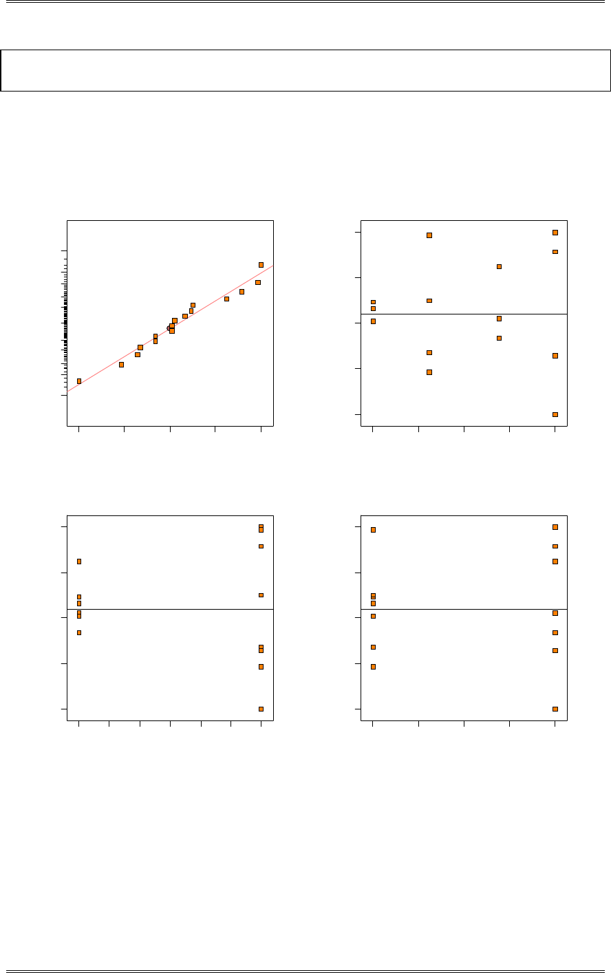
Solutions from Montgomery, D. C. (2001) Design and Analysis of Experiments, Wiley, NY
8-60
-5.49175
+0.28214 * Temperature
+16.06498 * Particle Size
(e) Analyze the residuals from this experiment and comment on model adequacy.
The residual plots are satisfactory. There is a slight tendency for the variability of the residuals to
increase with the predicted value of y.
Residual
Norm al % probability
Normal plot of residuals
-15.375 -8 .3 7 5 -1 .3 75 5.625 12.625
1
5
10
20
30
50
70
80
90
95
99
2
2
2
2
Predicted
Residuals
Residuals vs. Predicted
-1 5 .37 5
-8 .3 75
-1 .3 75
5.625
12.625
22.13 38.19 54.25 70.31 86.38
2
2
2
2
Tem perature
Residuals
Residuals vs. Temperature
-15.375
-8 .3 75
-1 .3 75
5.625
12.625
25 37 48 60 72 83 95
2
2
2
2
Particle Size
Residuals
Residuals vs. Particle Size
-1 5 .37 5
-8 .3 75
-1 .3 75
5.625
12.625
1.28 1.97 2.67 3.36 4.05
8-28 A 16-run fractional factorial experiment in 10 factors on sand-casting of engine manifolds was
conducted by engineers at the Essex Aluminum Plant of the Ford Motor Company and described in the
article “Evaporative Cast Process 3.0 Liter Intake Manifold Poor Sandfill Study,” by D. Becknell (Fourth
Symposium on Taguchi Methods, American Supplier Institute, Dearborn, MI, 1986, pp. 120-130). The
purpose was to determine which of 10 factors has an effect on the proportion of defective castings. The
design and the resulting proportion of nondefective castings p observed on each run are shown below.

Solutions from Montgomery, D. C. (2001) Design and Analysis of Experiments, Wiley, NY
8-61
This is a resolution III fraction with generators E=CD, F=BD, G=BC, H=AC, J=AB, and K=ABC.
Assume that the number of castings made at each run in the design is 1000.
F&T’s
Run A B C D E F G H J K p arcsin Modification
1 - - - - + + + + + - 0.958 1.364 1.363
2 + - - - + + + - - + 1.000 1.571 1.555
3 - + - - + - - + - + 0.977 1.419 1.417
4 + + - - + - - - + - 0.775 1.077 1.076
5 - - + - - + - - + + 0.958 1.364 1.363
6 + - + - - + - + - - 0.958 1.364 1.363
7 - + + - - - + - - - 0.813 1.124 1.123
8 + + + - - - + + + + 0.906 1.259 1.259
9 - - - + - - + + + - 0.679 0.969 0.968
10 + - - + - - + - - + 0.781 1.081 1.083
11 - + - + - + - + - + 1.000 1.571 1.556
12 + + - + - + - - + - 0.896 1.241 1.242
13 - - + + + - - - + + 0.958 1.364 1.363
14 + - + + + - - + - - 0.818 1.130 1.130
15 - + + + + + + - - - 0.841 1.161 1.160
16 + + + + + + + + + + 0.955 1.357 1.356
(a) Find the defining relation and the alias relationships in this design.
I=CDE=BDF=BCG=ACH=ABJ=ABCK=BCEF=BDEG=ADEH=ABCDEJ=ABDEK=CDFG=ABCDFH
= ADFJ=ACDFK=ABGH=ACGJ=AGK=BCHJ=BHK=CKJ
(b) Estimate the factor effects and use a normal probability plot to tentatively identify the important
factors.
Design Expert Output
Term Effect SumSqr % Contribtn
Model Intercept
Error A -0.011875 0.000564063 0.409171
Error B 0.006625 0.000175562 0.127353
Error C 0.017625 0.00124256 0.901355
Error D -0.052125 0.0108681 7.88369
Error E 0.036375 0.00529256 3.83923
Model F 0.107375 0.0461176 33.4537
Error G -0.050875 0.0103531 7.51011
Error H 0.028625 0.00327756 2.37754
Error J -0.012875 0.000663062 0.480986
Model K 0.099625 0.0397006 28.7988
Error AB Aliased
Error AC Aliased
Error AD 0.004875 9.50625E-005 0.0689584
Error AE -0.034625 0.00479556 3.4787
Error AF 0.024875 0.00247506 1.79541
Error BE -0.053125 0.0112891 8.18909
Error DK 0.015375 0.000945563 0.685911
Lenth's ME 0.103145
Lenth's SME 0.209399
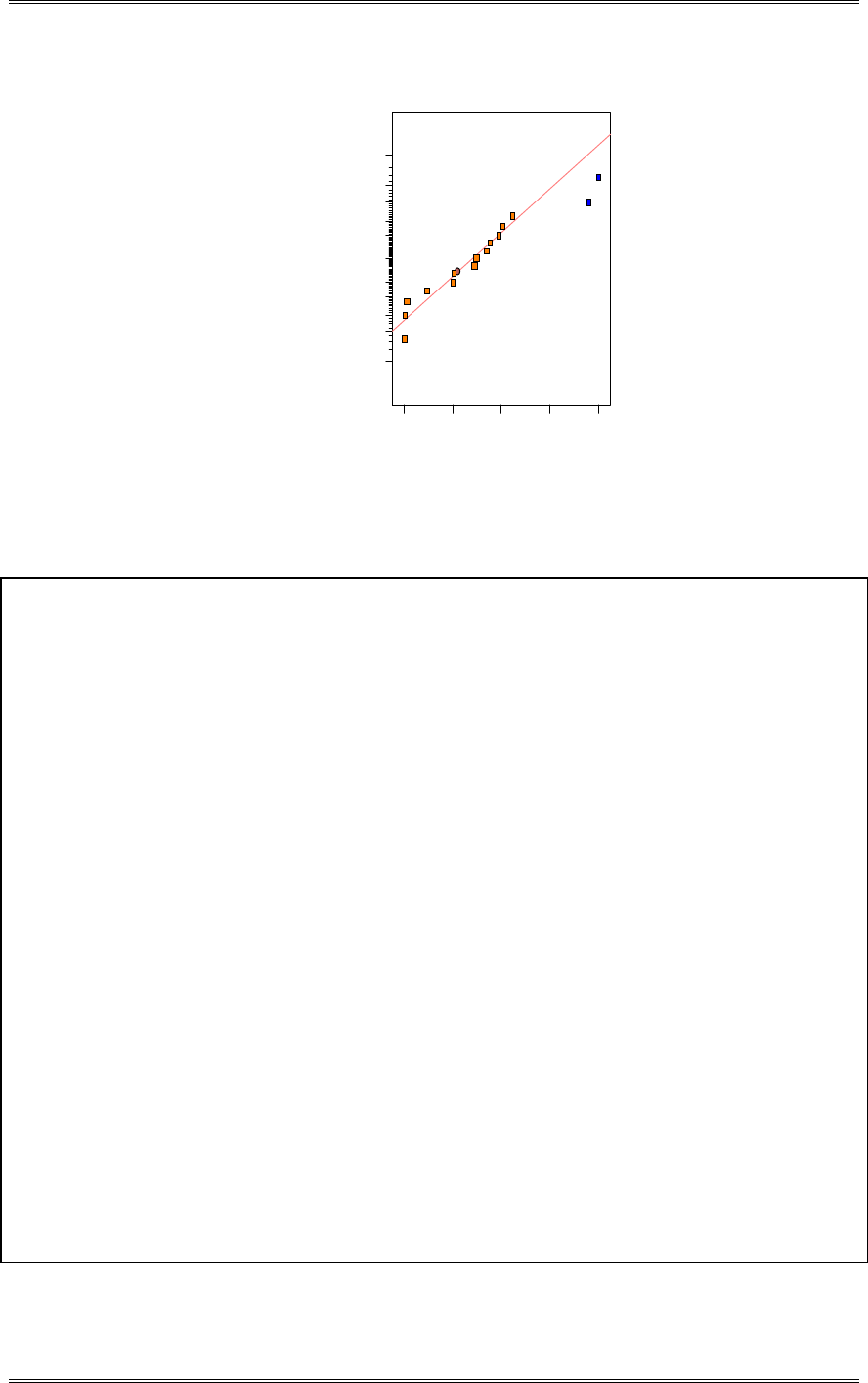
Solutions from Montgomery, D. C. (2001) Design and Analysis of Experiments, Wiley, NY
8-62
DESIGN-EXPERT Plot
p
A: A
B: B
C: C
D: D
E: E
F: F
G: G
H: H
J: J
K: K
Normal plot
Normal % probability
Effe ct
-0 .0 5 -0 .0 1 0.03 0.07 0.11
1
5
10
20
30
50
70
80
90
95
99
F
K
(c) Fit an appropriate model using the factors identified in part (b) above.
Design Expert Output
Response: p
ANOVA for Selected Factorial Model
Analysis of variance table [Partial sum of squares]
Sum of Mean F
Source Squares DF Square Value Prob > F
Model 0.086 2 0.043 10.72 0.0018 significant
F 0.046 1 0.046 11.52 0.0048
K 0.040 1 0.040 9.92 0.0077
Residual 0.052 13 4.003E-003
Cor Total 0.14 15
The Model F-value of 10.72 implies the model is significant. There is only
a 0.18% chance that a "Model F-Value" this large could occur due to noise.
Std. Dev. 0.063 R-Squared 0.6225
Mean 0.89 Adj R-Squared 0.5645
C.V. 7.09 Pred R-Squared 0.4282
PRESS 0.079 Adeq Precision 7.556
Coefficient Standard 95% CI 95% CI
Factor Estimate DF Error Low High VIF
Intercept 0.89 1 0.016 0.86 0.93
F-F 0.054 1 0.016 0.020 0.088 1.00
K-K 0.050 1 0.016 0.016 0.084 1.00
Final Equation in Terms of Coded Factors:
p =
+0.89
+0.054 * F
+0.050 * K
Final Equation in Terms of Actual Factors:
p =
+0.89206
+0.053688 * F
+0.049812 * K
(d) Plot the residuals from this model versus the predicted proportion of nondefective castings. Also
prepare a normal probability plot of the residuals. Comment on the adequacy of these plots.
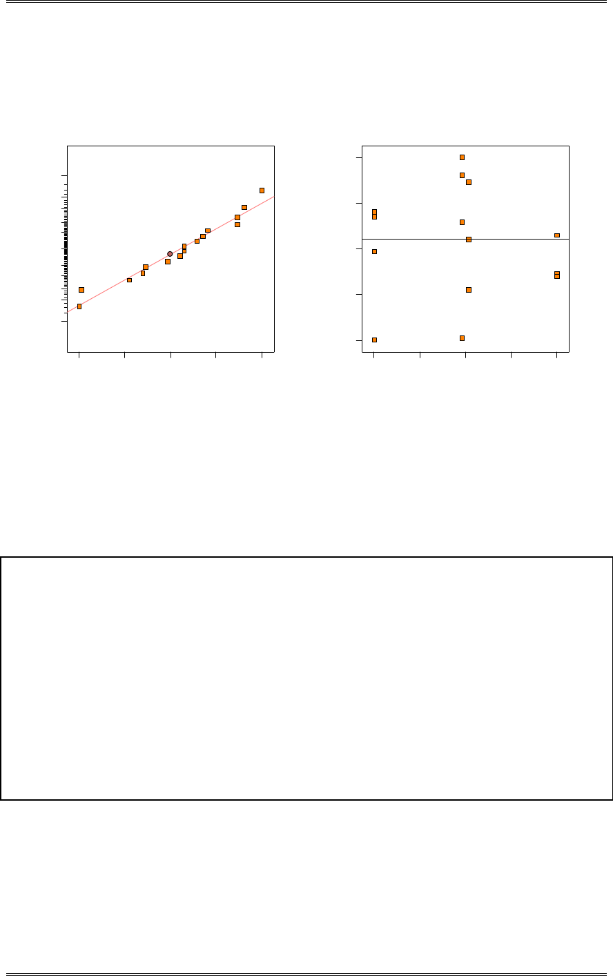
Solutions from Montgomery, D. C. (2001) Design and Analysis of Experiments, Wiley, NY
8-63
The residual versus predicted plot identifies an inequality of variances. This is likely caused by the
response variable being a proportion. A transformation could be used to correct this.
Residual
Normal % probability
Normal plot of residuals
-0.109563 -0.0599688 -0.010375 0.0392187 0.0888125
1
5
10
20
30
50
70
80
90
95
99 2
2
2
2
Predicted
Residuals
Residuals vs. Predicted
-0 .1 09 5 6 3
-0.0599688
-0 .0 10 3 7 5
0.0392187
0.0888125
0.79 0.84 0.89 0.94 1.00
(e) In part (d) you should have noticed an indication that the variance of the response is not constant
(considering that the response is a proportion, you should have expected this). The previous table
also shows a transformation on P, the arcsin square root, that is a widely used variance stabilizing
transformation for proportion data (refer to the discussion of variance stabilizing transformations is
Chapter 3). Repeat parts (a) through (d) above using the transformed response and comment on your
results. Specifically, are the residuals plots improved?
Design Expert Output
Term Effect SumSqr % Contribtn
Model Intercept
Error A -0.032 0.004096 0.884531
Error B 0.00025 2.5E-007 5.39875E-005
Error C -0.02125 0.00180625 0.39006
Error D -0.0835 0.027889 6.02263
Error E 0.05875 0.0138062 2.98146
Model F 0.19625 0.154056 33.2685
Error G -0.0805 0.025921 5.59764
Error H 0.05625 0.0126562 2.73312
Error J -0.05325 0.0113422 2.44936
Model K 0.1945 0.151321 32.6778
Error AD -0.032 0.004096 0.884531
Error AF 0.05025 0.0101003 2.18115
Error BE -0.104 0.043264 9.34286
Error DH -0.01125 0.00050625 0.109325
Error DK 0.0235 0.002209 0.477034
Lenth's ME 0.205325
Lenth's SME 0.41684
As with the original analysis, factors F and K remain significant with a slight increase with the R2.
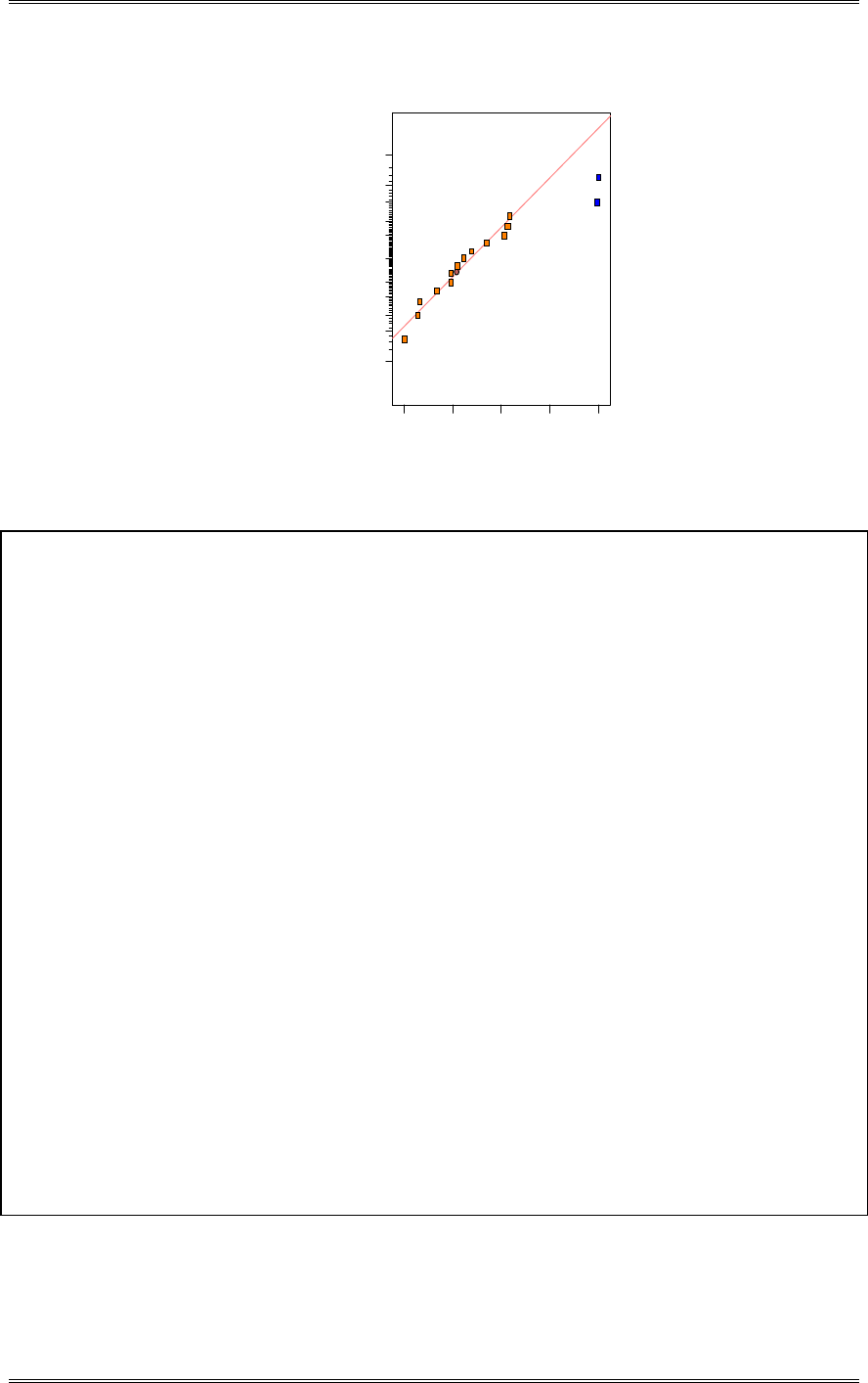
Solutions from Montgomery, D. C. (2001) Design and Analysis of Experiments, Wiley, NY
8-64
DESIGN-EXPERT Plot
arcsin
A: A
B: B
C: C
D: D
E: E
F: F
G: G
H: H
J: J
K: K
Normal plot
Normal % probability
Effe ct
-0 .1 0 -0 .0 3 0.05 0.12 0.20
1
5
10
20
30
50
70
80
90
95
99
F
K
Design Expert Output
Response: arcsin
ANOVA for Selected Factorial Model
Analysis of variance table [Partial sum of squares]
Sum of Mean F
Source Squares DF Square Value Prob > F
Model 0.31 2 0.15 12.59 0.0009 significant
F 0.15 1 0.15 12.70 0.0035
K 0.15 1 0.15 12.47 0.0037
Residual 0.16 13 0.012
Cor Total 0.46 15
The Model F-value of 12.59 implies the model is significant. There is only
a 0.09% chance that a "Model F-Value" this large could occur due to noise.
Std. Dev. 0.11 R-Squared 0.6595
Mean 1.28 Adj R-Squared 0.6071
C.V. 8.63 Pred R-Squared 0.4842
PRESS 0.24 Adeq Precision 8.193
Coefficient Standard 95% CI 95% CI
Factor Estimate DF Error Low High VIF
Intercept 1.28 1 0.028 1.22 1.34
F-F 0.098 1 0.028 0.039 0.16 1.00
K-K 0.097 1 0.028 0.038 0.16 1.00
Final Equation in Terms of Coded Factors:
arcsin =
+1.28
+0.098 * F
+0.097 * K
Final Equation in Terms of Actual Factors:
arcsin =
+1.27600
+0.098125 * F
+0.097250 * K
The inequality of variance has improved; however, there remain hints of inequality in the residuals versus
predicted plot and the normal probability plot now appears to be irregular.
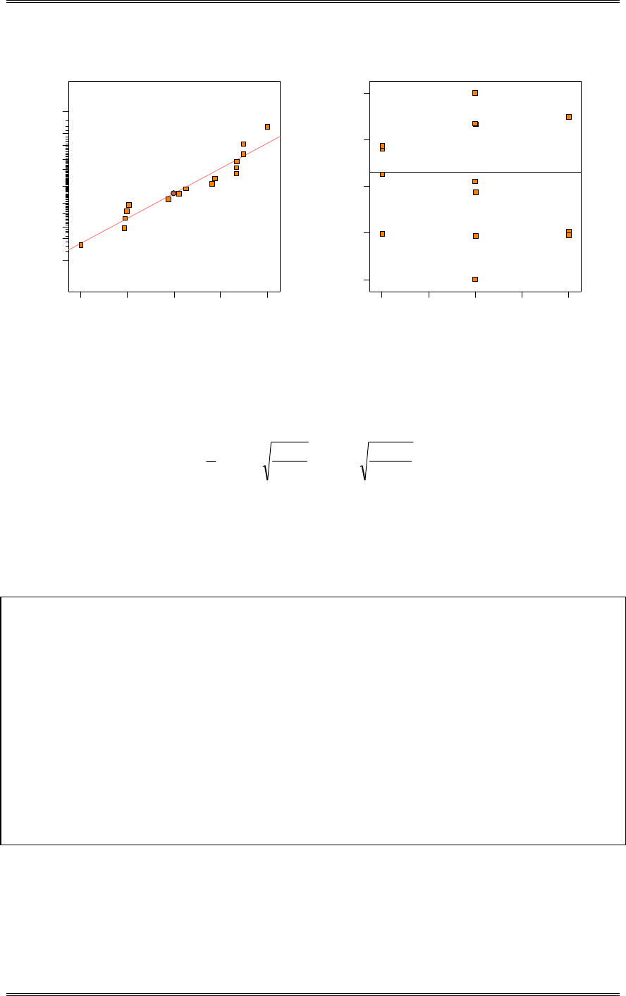
Solutions from Montgomery, D. C. (2001) Design and Analysis of Experiments, Wiley, NY
8-65
Residual
Normal % probability
Normal plot of residuals
-0.194125 -0.109625 -0.025125 0.059375 0.143875
1
5
10
20
30
50
70
80
90
95
99
2
2
2
2
Predicted
Residuals
Residuals vs. Predicted
-0 .1 94 1 2 5
-0 .1 09 6 2 5
-0 .0 25 1 2 5
0.059375
0.143875
1.08 1.18 1.28 1.37 1.47
(f) There is a modification to the arcsin square root transformation, proposed by Freeman and Tukey
(“Transformations Related to the Angular and the Square Root,” Annals of Mathematical Statistics,
Vol. 21, 1950, pp. 607-611) that improves its performance in the tails. F&T’s modification is:
»
»
¼
º
«
«
¬
ª
1
1
12
1
n
p
ˆ
n
arcsin
n
p
ˆ
n
arcsin
Rework parts (a) through (d) using this transformation and comment on the results. (For an interesting
discussion and analysis of this experiment, refer to “Analysis of Factorial Experiments with Defects or
Defectives as the Response,” by S. Bisgaard and H.T. Fuller, Quality Engineering, Vol. 7, 1994-5, pp.
429-443.)
Design Expert Output
Term Effect SumSqr % Contribtn
Model Intercept
Error A -0.031125 0.00387506 0.871894
Error B 0.000125 6.25E-008 1.40626E-005
Error C -0.017875 0.00127806 0.287566
Error D -0.082625 0.0273076 6.14424
Error E 0.057875 0.0133981 3.01458
Model F 0.192375 0.148033 33.3075
Error G -0.080375 0.0258406 5.81416
Error H 0.055875 0.0124881 2.80983
Error J -0.049625 0.00985056 2.21639
Model K 0.190875 0.145733 32.7901
Error AD -0.027875 0.00310806 0.699318
Error AF 0.049625 0.00985056 2.21639
Error BE -0.100625 0.0405016 9.1129
Error DH -0.015375 0.000945563 0.212753
Error DK 0.023625 0.00223256 0.502329
Lenth's ME 0.191348
Lenth's SME 0.388464
As with the prior analysis, factors F and K remain significant.
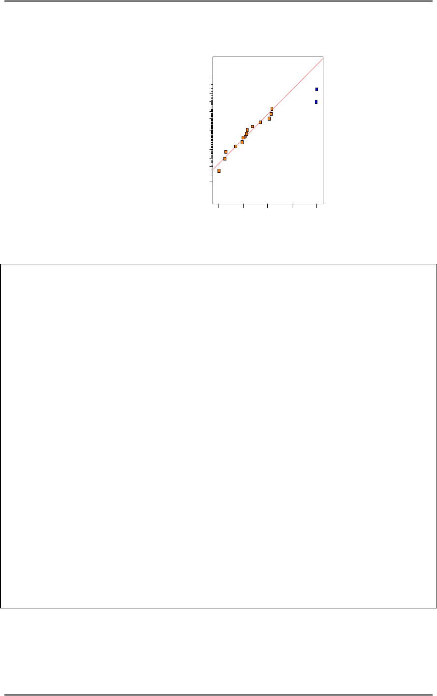
Solutions from Montgomery, D. C. (2001) Design and Analysis of Experiments, Wiley, NY
8-66
DESIGN-EXPERT Plot
F&T Transform
A: A
B: B
C: C
D: D
E: E
F: F
G: G
H: H
J: J
K: K
Normal plot
Normal % probability
Effe ct
-0 .1 0 -0 .0 3 0.05 0.12 0.19
1
5
10
20
30
50
70
80
90
95
99
F
K
Design Expert Output
Response: F&T Transform
ANOVA for Selected Factorial Model
Analysis of variance table [Partial sum of squares]
Sum of Mean F
Source Squares DF Square Value Prob > F
Model 0.29 2 0.15 12.67 0.0009 significant
F 0.15 1 0.15 12.77 0.0034
K 0.15 1 0.15 12.57 0.0036
Residual 0.15 13 0.012
Cor Total 0.44 15
The Model F-value of 12.67 implies the model is significant. There is only
a 0.09% chance that a "Model F-Value" this large could occur due to noise.
Std. Dev. 0.11 R-Squared 0.6610
Mean 1.27 Adj R-Squared 0.6088
C.V. 8.45 Pred R-Squared 0.4864
PRESS 0.23 Adeq Precision 8.221
Coefficient Standard 95% CI 95% CI
Factor Estimate DF Error Low High VIF
Intercept 1.27 1 0.027 1.22 1.33
F-F 0.096 1 0.027 0.038 0.15 1.00
K-K 0.095 1 0.027 0.037 0.15 1.00
Final Equation in Terms of Coded Factors:
F&T Transform =
+1.27
+0.096 * F
+0.095 * K
Final Equation in Terms of Actual Factors:
F&T Transform =
+1.27356
+0.096188 * F
+0.095437 * K
The residual plots appears as they did with the arcsin square root transformation.
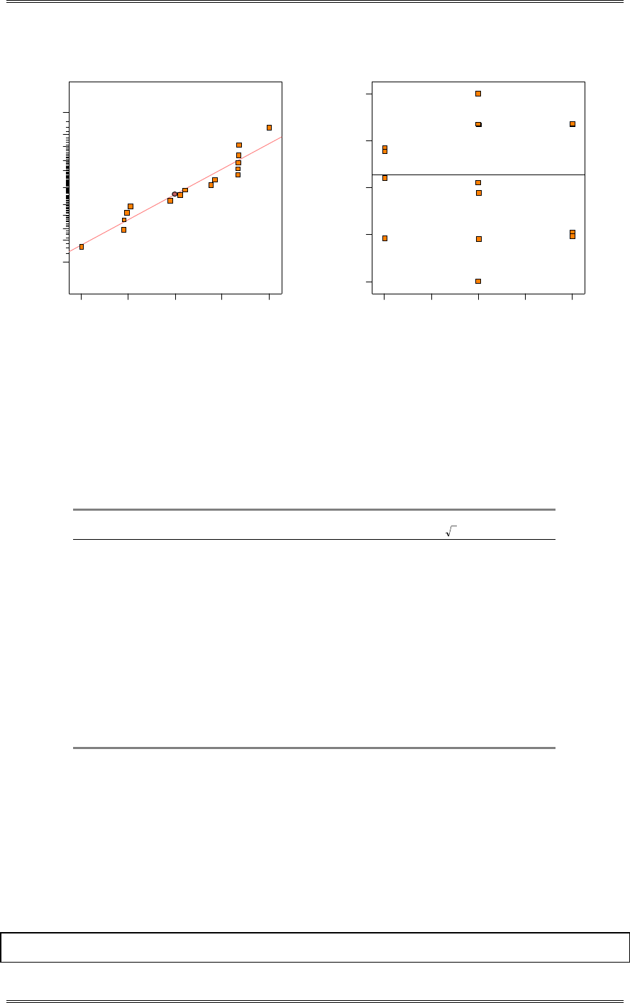
Solutions from Montgomery, D. C. (2001) Design and Analysis of Experiments, Wiley, NY
8-67
Residual
Normal % probability
Normal plot of residuals
-0.189813 -0.106313 -0.0228125 0.0606875 0.144187
1
5
10
20
30
50
70
80
90
95
99
22
Predicted
Residuals
Residuals vs. Predicted
-0 .1 89 8 1 3
-0 .1 06 3 1 3
-0.0228125
0.0606875
0.144187
1.08 1.18 1.27 1.37 1.47
8-29 A 16-run fractional factorial experiment in 9 factors was conducted by Chrysler Motors
Engineering and described in the article “Sheet Molded Compound Process Improvement,” by P.I. Hsieh
and D.E. Goodwin (Fourth Symposium on Taguchi Methods, American Supplier Institute, Dearborn, MI,
1986, pp. 13-21). The purpose was to reduce the number of defects in the finish of sheet-molded grill
opening panels. The design, and the resulting number of defects, c, observed on each run, is shown
below. This is a resolution III fraction with generators E=BD, F=BCD, G=AC, H=ACD, and J=AB.
F&T’s
Run A B C D E F G H J c c Modification
1 - - - - + - + - + 56 7.48 7.52
2 + - - - + - - + - 17 4.12 4.18
3 - + - - - + + - - 2 1.41 1.57
4 + + - - - + - + + 4 2.00 2.12
5 - - + - + + - + + 3 1.73 1.87
6 + - + - + + + - - 4 2.00 2.12
7 - + + - - - - + - 50 7.07 7.12
8 + + + - - - + - + 2 1.41 1.57
9 - - - + - + + + + 1 1.00 1.21
10 + - - + - + - - - 0 0.00 0.50
11 - + - + + - + + - 3 1.73 1.87
12 + + - + + - - - + 12 3.46 3.54
13 - - + + - - - - + 3 1.73 1.87
14 + - + + - - + + - 4 2.00 2.12
15 - + + + + + - - - 0 0.00 0.50
16 + + + + + + + + + 0 0.00 0.50
(a) Find the defining relation and the alias relationships in this design.
I=BDE=BCDF=CEF=ACG=ABCDEG=ABDEG=AEFG=ACDH=ABCEH=ABFH=ADEFH=DGH=
BEGH=BCRG=CDEFGH=ABJ=ADEJ=ACDFJ=ABCEFJ=BCGJ=CDEGJ=DEGJ=BEFGJ=BCDHJ=
CEHJ=FHJ=BDEFHJ=ABDGHJ=AEGHJ=ACEGJ=ABCDEFGHJ
(b) Estimate the factor effects and use a normal probability plot to tentatively identify the important
factors.
Design Expert Output
Term Effect SumSqr % Contribtn
Model Intercept
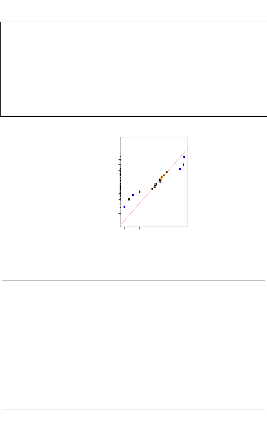
Solutions from Montgomery, D. C. (2001) Design and Analysis of Experiments, Wiley, NY
8-68
Model A -9.375 351.562 7.75573
Model B -1.875 14.0625 0.310229
Model C -3.625 52.5625 1.15957
Model D -14.375 826.562 18.2346
Error E 3.625 52.5625 1.15957
Model F -16.625 1105.56 24.3895
Model G -2.125 18.0625 0.398472
Error H 0.375 0.5625 0.0124092
Error J 0.125 0.0625 0.0013788
Model AD 11.625 540.563 11.9252
Error AE 2.125 18.0625 0.398472
Model AF 9.875 390.063 8.60507
Error AH 1.375 7.5625 0.166834
Model BC 11.375 517.563 11.4178
Model BG -12.625 637.562 14.0651
Lenth's ME 13.9775
Lenth's SME 28.3764
DESIGN-EXPERT Plot
c
A: A
B: B
C: C
D: D
E: E
F: F
G: G
H: H
J: J
Normal plot
Normal % probability
Effe ct
-1 6 .62 -9 .5 6 -2 .5 0 4.56 11.62
1
5
10
20
30
50
70
80
90
95
99
A
D
F
AD
AF
BC
BG
(c) Fit an appropriate model using the factors identified in part (b) above.
Design Expert Output
Response: c
ANOVA for Selected Factorial Model
Analysis of variance table [Partial sum of squares]
Sum of Mean F
Source Squares DF Square Value Prob > F
Model 4454.13 10 445.41 28.26 0.0009 significant
A 351.56 1 351.56 22.30 0.0052
B 14.06 1 14.06 0.89 0.3883
C 52.56 1 52.56 3.33 0.1274
D 826.56 1 826.56 52.44 0.0008
F 1105.56 1 1105.56 70.14 0.0004
G 18.06 1 18.06 1.15 0.3333
AD 540.56 1 540.56 34.29 0.0021
AF 390.06 1 390.06 24.75 0.0042
BC 517.56 1 517.56 32.84 0.0023
BG 637.56 1 637.56 40.45 0.0014
Residual 78.81 5 15.76
Cor Total 4532.94 15
The Model F-value of 28.26 implies the model is significant. There is only
a 0.09% chance that a "Model F-Value" this large could occur due to noise.
Std. Dev. 3.97 R-Squared 0.9826

Solutions from Montgomery, D. C. (2001) Design and Analysis of Experiments, Wiley, NY
8-69
Mean 10.06 Adj R-Squared 0.9478
C.V. 39.46 Pred R-Squared 0.8220
PRESS 807.04 Adeq Precision 17.771
Coefficient Standard 95% CI 95% CI
Factor Estimate DF Error Low High VIF
Intercept 10.06 1 0.99 7.51 12.61
A-A -4.69 1 0.99 -7.24 -2.14 1.00
B-B -0.94 1 0.99 -3.49 1.61 1.00
C-C -1.81 1 0.99 -4.36 0.74 1.00
D-D -7.19 1 0.99 -9.74 -4.64 1.00
F-F -8.31 1 0.99 -10.86 -5.76 1.00
G-G -1.06 1 0.99 -3.61 1.49 1.00
AD 5.81 1 0.99 3.26 8.36 1.00
AF 4.94 1 0.99 2.39 7.49 1.00
BC 5.69 1 0.99 3.14 8.24 1.00
BG -6.31 1 0.99 -8.86 -3.76 1.00
Final Equation in Terms of Coded Factors:
c =
+10.06
-4.69 * A
-0.94 * B
-1.81 * C
-7.19 * D
-8.31 * F
-1.06 * G
+5.81 * A * D
+4.94 * A * F
+5.69 * B * C
-6.31 * B * G
Final Equation in Terms of Actual Factors:
c =
+10.06250
-4.68750 * A
-0.93750 * B
-1.81250 * C
-7.18750 * D
-8.31250 * F
-1.06250 * G
+5.81250 * A * D
+4.93750 * A * F
+5.68750 * B * C
-6.31250 * B * G
(d) Plot the residuals from this model versus the predicted number of defects. Also, prepare a normal
probability plot of the residuals. Comment on the adequacy of these plots.
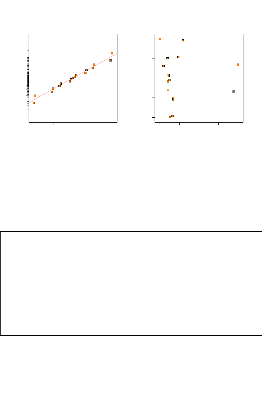
Solutions from Montgomery, D. C. (2001) Design and Analysis of Experiments, Wiley, NY
8-70
Residual
Normal % probability
Normal plot of residuals
-3 .8 12 5 -1.90625 01.90625 3.8125
1
5
10
20
30
50
70
80
90
95
99
Predicted
Residuals
Residuals vs. Predicted
-3 .8 12 5
-1.90625
0
1.90625
3.8125
-3 .8 1 10.81 25.44 40.06 54.69
There is a significant problem with inequality of variance. This is likely caused by the response variable
being a count. A transformation may be appropriate.
(e) In part (d) you should have noticed an indication that the variance of the response is not constant
(considering that the response is a count, you should have expected this). The previous table also
shows a transformation on c, the square root, that is a widely used variance stabilizing transformation
for count data (refer to the discussion of variance stabilizing transformations in Chapter 3). Repeat
parts (a) through (d) using the transformed response and comment on your results. Specifically, are
the residual plots improved?
Design Expert Output
Term Effect SumSqr % Contribtn
Model Intercept
Error A -0.895 3.2041 4.2936
Model B -0.3725 0.555025 0.743752
Error C -0.6575 1.72922 2.31722
Model D -2.1625 18.7056 25.0662
Error E 0.4875 0.950625 1.27387
Model F -2.6075 27.1962 36.4439
Model G -0.385 0.5929 0.794506
Error H 0.27 0.2916 0.390754
Error J 0.06 0.0144 0.0192965
Error AD 1.145 5.2441 7.02727
Error AE 0.555 1.2321 1.65106
Error AF 0.86 2.9584 3.96436
Error AH 0.0425 0.007225 0.00968175
Error BC 0.6275 1.57502 2.11059
Model BG -1.61 10.3684 13.894
Lenth's ME 2.27978
Lenth's SME 4.62829
The analysis of the data with the square root transformation identifies only D, F, the BG interaction as being
significant. The original analysis identified factor A and several two factor interactions as being significant.
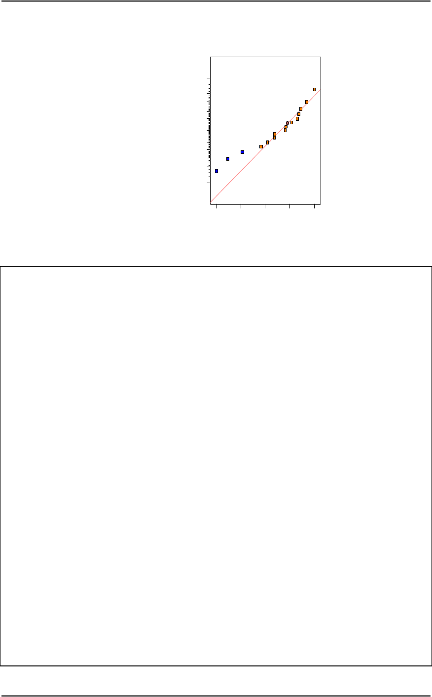
Solutions from Montgomery, D. C. (2001) Design and Analysis of Experiments, Wiley, NY
8-71
DESIGN-EXPERT Plot
sq rt
A: A
B: B
C: C
D: D
E: E
F: F
G: G
H: H
J: J
Normal plot
Normal % probability
Effe ct
-2 .6 1 -1 .6 7 -0 .7 3 0.21 1.14
1
5
10
20
30
50
70
80
90
95
99
D
F
BG
Design Expert Output
Response: sqrt
ANOVA for Selected Factorial Model
Analysis of variance table [Partial sum of squares]
Sum of Mean F
Source Squares DF Square Value Prob > F
Model 57.42 5 11.48 6.67 0.0056 significant
B 0.56 1 0.56 0.32 0.5826
D 18.71 1 18.71 10.87 0.0081
F 27.20 1 27.20 15.81 0.0026
G 0.59 1 0.59 0.34 0.5702
BG 10.37 1 10.37 6.03 0.0340
Residual 17.21 10 1.72
Cor Total 74.62 15
The Model F-value of 6.67 implies the model is significant. There is only
a 0.56% chance that a "Model F-Value" this large could occur due to noise.
Std. Dev. 1.31 R-Squared 0.7694
Mean 2.32 Adj R-Squared 0.6541
C.V. 56.51 Pred R-Squared 0.4097
PRESS 44.05 Adeq Precision 8.422
Coefficient Standard 95% CI 95% CI
Factor Estimate DF Error Low High VIF
Intercept 2.32 1 0.33 1.59 3.05
B-B -0.19 1 0.33 -0.92 0.54 1.00
D-D -1.08 1 0.33 -1.81 -0.35 1.00
F-F -1.30 1 0.33 -2.03 -0.57 1.00
G-G -0.19 1 0.33 -0.92 0.54 1.00
BG -0.80 1 0.33 -1.54 -0.074 1.00
Final Equation in Terms of Coded Factors:
sqrt =
+2.32
-0.19 * B
-1.08 * D
-1.30 * F
-0.19 * G
-0.80 * B * G
Final Equation in Terms of Actual Factors:
sqrt =
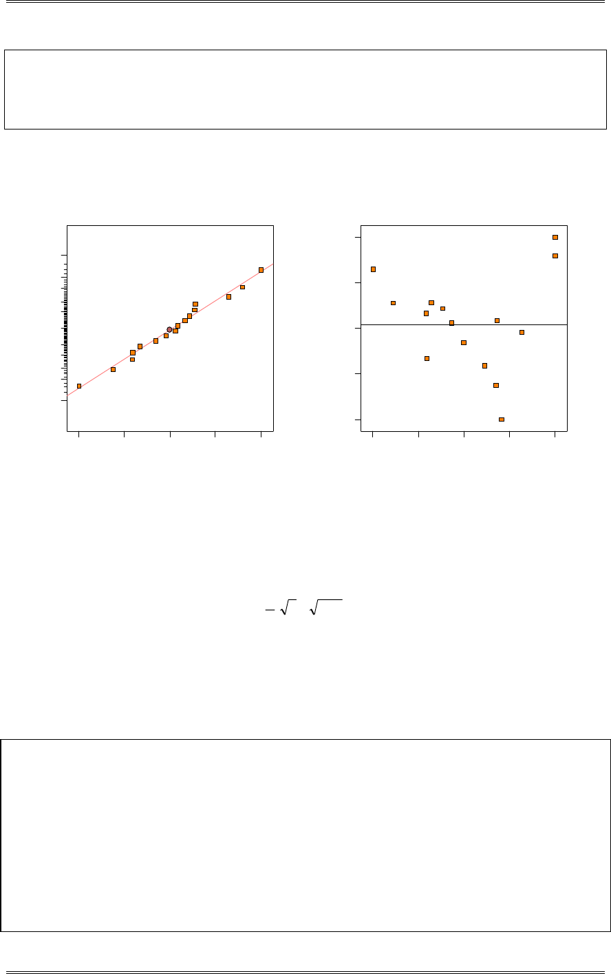
Solutions from Montgomery, D. C. (2001) Design and Analysis of Experiments, Wiley, NY
8-72
+2.32125
-0.18625 * B
-1.08125 * D
-1.30375 * F
-0.19250 * G
-0.80500 * B * G
The residual plots are acceptable; although, there appears to be a slight “u” shape to the residuals versus predicted
plot.
Residual
Norm al % probability
Normal plot of residuals
-2 .1 12 5 -1.09062 -0.06875 0.953125 1.975
1
5
10
20
30
50
70
80
90
95
99
Predicted
Residuals
Residuals vs. Predicted
-2 .1 12 5
-1.09062
-0.06875
0.953125
1.975
-1 .2 5 0.44 2.13 3.83 5.52
(f) There is a modification to the square root transformation proposed by Freeman and Tukey
(“Transformations Related to the Angular and the Square Root,” Annals of Mathematical Statistics,
Vol. 21, 1950, pp. 607-611) that improves its performance. F&T’s modification to the square root
transformation is:
>@
1
2
1 cc
Rework parts (a) through (d) using this transformation and comment on the results. (For an interesting
discussion and analysis of this experiment, refer to “Analysis of Factorial Experiments with Defects or
Defectives as the Response,” by S. Bisgaard and H.T. Fuller, Quality Engineering, Vol. 7, 1994-5, pp.
429-443.)
Design Expert Output
Term Effect SumSqr % Contribtn
Model Intercept
Error A -0.86 2.9584 4.38512
Model B -0.325 0.4225 0.626255
Error C -0.605 1.4641 2.17018
Model D -1.995 15.9201 23.5977
Error E 0.5025 1.01002 1.49712
Model F -2.425 23.5225 34.8664
Model G -0.4025 0.648025 0.960541
Error H 0.225 0.2025 0.300158
Error J 0.0275 0.003025 0.00448383
Error AD 1.1625 5.40562 8.01254
Error AE 0.505 1.0201 1.51205
Error AF 0.8825 3.11523 4.61757
Error AH 0.0725 0.021025 0.0311645
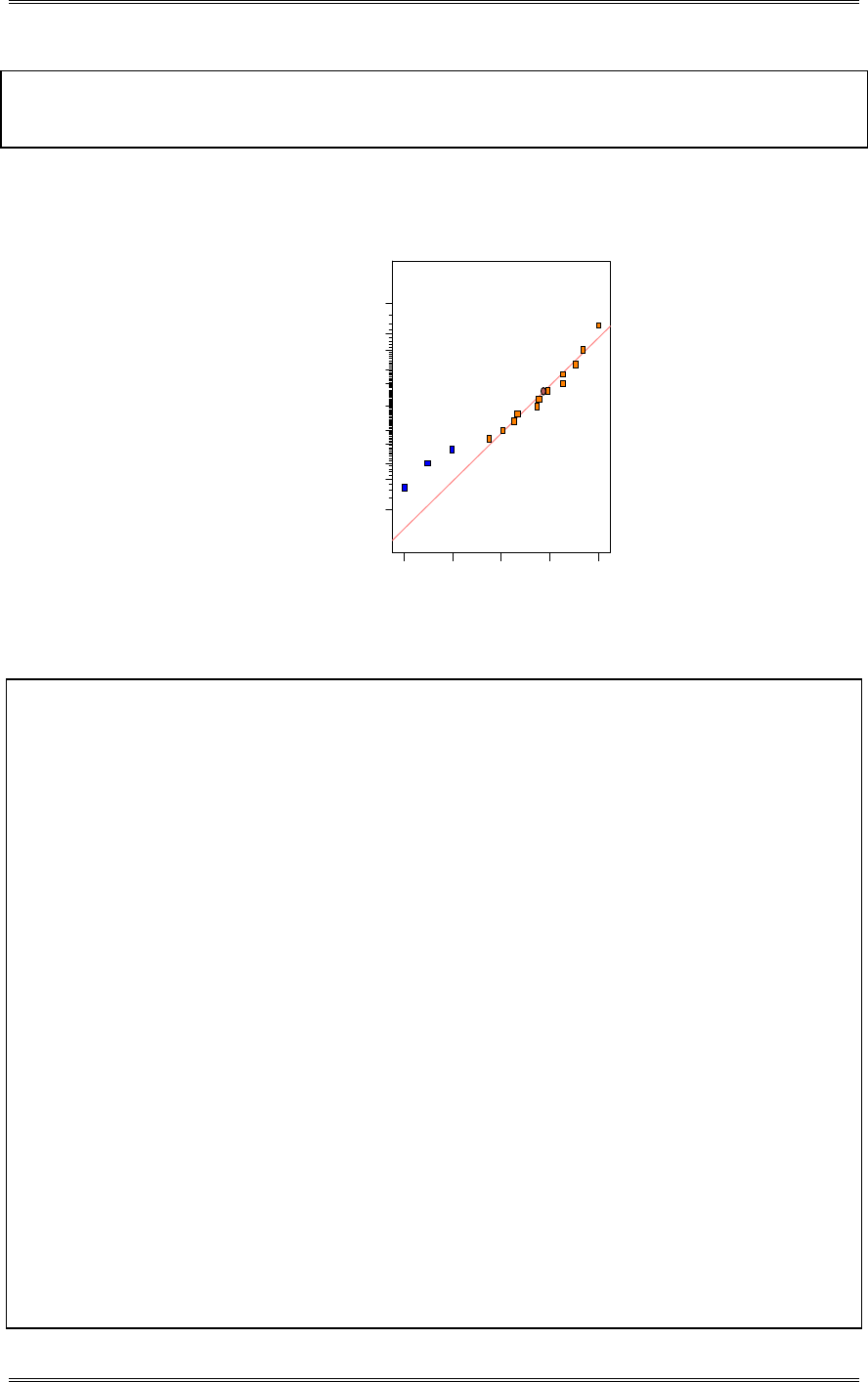
Solutions from Montgomery, D. C. (2001) Design and Analysis of Experiments, Wiley, NY
8-73
Error BC 0.7525 2.26503 3.35735
Model BG -1.54 9.4864 14.0613
Lenth's ME 2.14001
Lenth's SME 4.34453
As with the square root transformation, factors D, F, and the BG interaction remain significant.
DESIGN-EXPERT Plot
F&T
A: A
B: B
C: C
D: D
E: E
F: F
G: G
H: H
J: J
Normal plot
Norm al % probability
Effe ct
-2 .4 2 -1 .5 3 -0 .6 3 0.27 1.16
1
5
10
20
30
50
70
80
90
95
99
D
F
BG
Design Expert Output
Response: F&T
ANOVA for Selected Factorial Model
Analysis of variance table [Partial sum of squares]
Sum of Mean F
Source Squares DF Square Value Prob > F
Model 50.00 5 10.00 5.73 0.0095 significant
B 0.42 1 0.42 0.24 0.6334
D 15.92 1 15.92 9.12 0.0129
F 23.52 1 23.52 13.47 0.0043
G 0.65 1 0.65 0.37 0.5560
BG 9.49 1 9.49 5.43 0.0420
Residual 17.47 10 1.75
Cor Total 67.46 15
The Model F-value of 5.73 implies the model is significant. There is only
a 0.95% chance that a "Model F-Value" this large could occur due to noise.
Std. Dev. 1.32 R-Squared 0.7411
Mean 2.51 Adj R-Squared 0.6117
C.V. 52.63 Pred R-Squared 0.3373
PRESS 44.71 Adeq Precision 7.862
Coefficient Standard 95% CI 95% CI
Factor Estimate DF Error Low High VIF
Intercept 2.51 1 0.33 1.78 3.25
B-B -0.16 1 0.33 -0.90 0.57 1.00
D-D -1.00 1 0.33 -1.73 -0.26 1.00
F-F -1.21 1 0.33 -1.95 -0.48 1.00
G-G -0.20 1 0.33 -0.94 0.53 1.00
BG -0.77 1 0.33 -1.51 -0.034 1.00
Final Equation in Terms of Coded Factors:
F&T =
+2.51
-0.16 * B
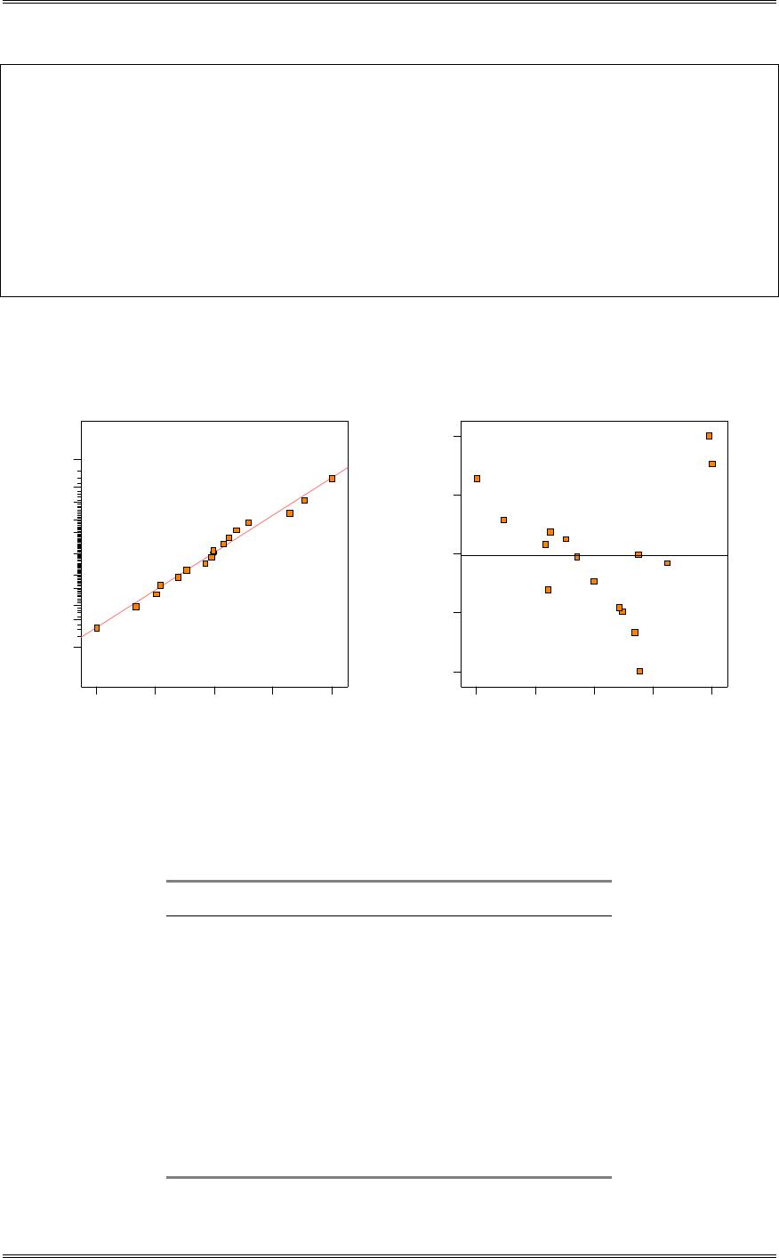
Solutions from Montgomery, D. C. (2001) Design and Analysis of Experiments, Wiley, NY
8-74
-1.00 * D
-1.21 * F
-0.20 * G
-0.77 * B * G
Final Equation in Terms of Actual Factors:
F&T =
+2.51125
-0.16250 * B
-0.99750 * D
-1.21250 * F
-0.20125 * G
-0.77000 * B * G
The following interaction plots appear as they did with the square root transformation; a slight “u” shape
is observed in the residuals versus predicted plot.
Residual
Normal % probability
Normal plot of residuals
-2 .0 17 5 -0.99625 0.025 1.04625 2.0675
1
5
10
20
30
50
70
80
90
95
99
Predicted
Residuals
Residuals vs. Predicted
-2 .0 17 5
-0.99625
0.025
1.04625
2.0675
-0 .8 3 0.76 2.35 3.94 5.53
8-30 An experiment is run in a semiconductor factory to investigate the effect of six factors on transistor
gain. The design selected is the 26
2
IV shown below.
Standard Run
Order Order A B C D E F Gain
1 2 - - - - - - 1455
2 8 + - - - + - 1511
3 5 - + - - + + 1487
4 9 + + - - - + 1596
5 3 - - + - + + 1430
6 14 + - + - - + 1481
7 11 - + + - - - 1458
8 10 + + + - + - 1549
9 15 - - - + - + 1454
10 13 + - - + + + 1517
11 1 - + - + + - 1487
12 6 + + - + - - 1596
13 12 - - + + + - 1446
14 4 + - + + - - 1473
15 7 - + + + - + 1461
16 16 + + + + + + 1563

Solutions from Montgomery, D. C. (2001) Design and Analysis of Experiments, Wiley, NY
8-75
(a) Use a normal plot of the effects to identify the significant factors.
Design Expert Output
Term Effect SumSqr % Contribtn
Model Intercept
Model A 76 23104 55.2714
Model B 53.75 11556.2 27.6459
Model C -30.25 3660.25 8.75637
Error D 3.75 56.25 0.134566
Error E 2 16 0.0382766
Error F 1.75 12.25 0.0293055
Model AB 26.75 2862.25 6.84732
Model AC -8.25 272.25 0.6513
Error AD -0.75 2.25 0.00538265
Error AE -3.5 49 0.117222
Error AF 5.25 110.25 0.26375
Error BD 0.5 1 0.00239229
Error BF 2.5 25 0.0598072
Error ABD 3.5 49 0.117222
Error ABF -2.5 25 0.0598072
Lenth's ME 9.63968
Lenth's SME 19.57
DESIGN-EXPERT Plot
Gain
A: A
B: B
C: C
D: D
E: E
F: F
Normal plot
Norm al % probability
Effe ct
-3 0 .25 -3 .6 9 22.87 49.44 76.00
1
5
10
20
30
50
70
80
90
95
99
A
B
C
AB
AC
(b) Conduct appropriate statistical tests for the model identified in part (a).
Design Expert Output
Response: Gain
ANOVA for Selected Factorial Model
Analysis of variance table [Partial sum of squares]
Sum of Mean F
Source Squares DF Square Value Prob > F
Model 41455.00 5 8291.00 239.62 < 0.0001 significant
A 23104.00 1 23104.00 667.75 < 0.0001
B 11556.25 1 11556.25 334.00 < 0.0001
C 3660.25 1 3660.25 105.79 < 0.0001
AB 2862.25 1 2862.25 82.72 < 0.0001
AC 272.25 1 272.25 7.87 0.0186
Residual 346.00 10 34.60
Cor Total 41801.00 15
The Model F-value of 239.62 implies the model is significant. There is only
a 0.01% chance that a "Model F-Value" this large could occur due to noise.
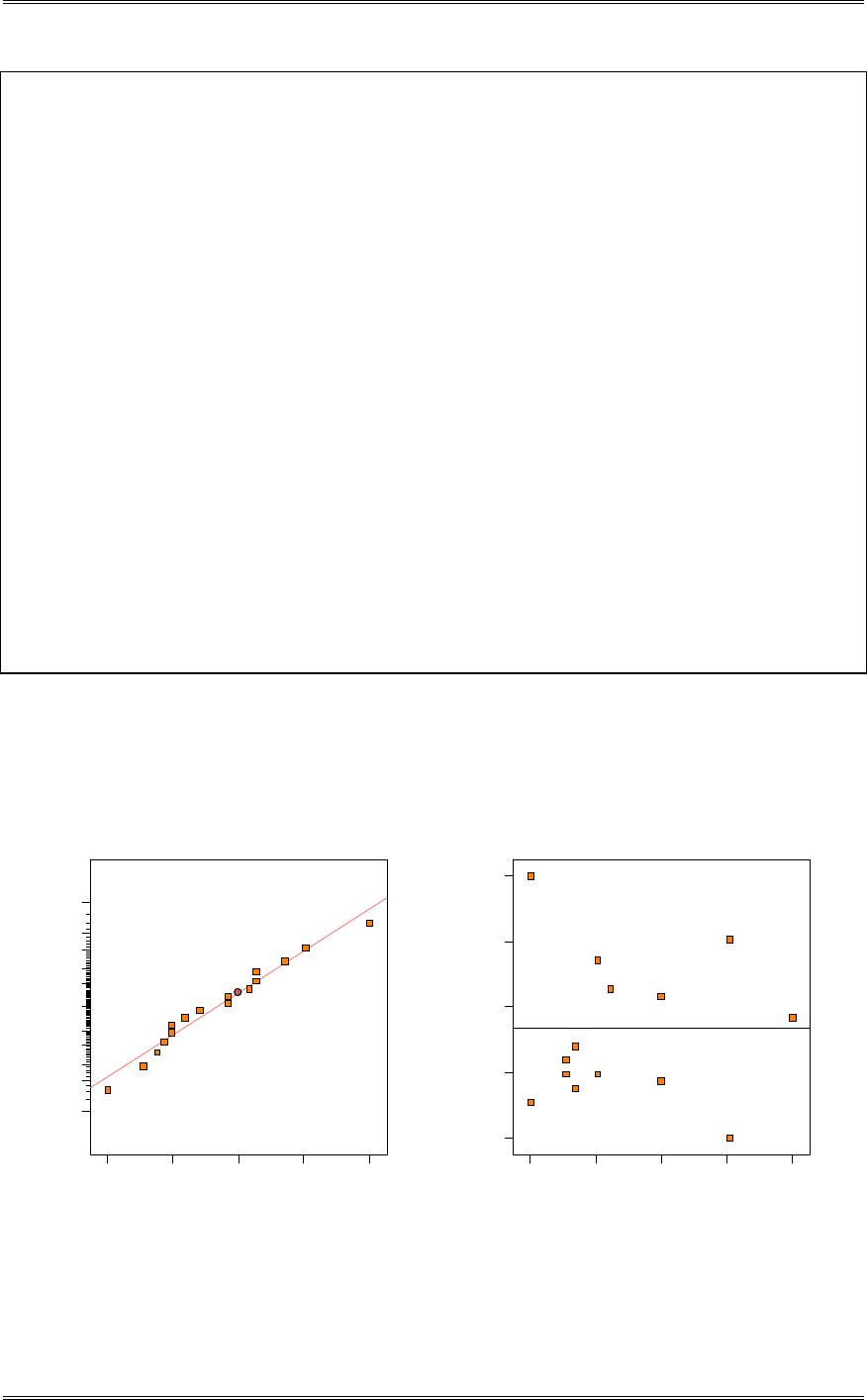
Solutions from Montgomery, D. C. (2001) Design and Analysis of Experiments, Wiley, NY
8-76
Std. Dev. 5.88 R-Squared 0.9917
Mean 1497.75 Adj R-Squared 0.9876
C.V. 0.39 Pred R-Squared 0.9788
PRESS 885.76 Adeq Precision 44.419
Coefficient Standard 95% CI 95% CI
Factor Estimate DF Error Low High VIF
Intercept 1497.75 1 1.47 1494.47 1501.03
A-A 38.00 1 1.47 34.72 41.28 1.00
B-B 26.87 1 1.47 23.60 30.15 1.00
C-C -15.13 1 1.47 -18.40 -11.85 1.00
AB 13.38 1 1.47 10.10 16.65 1.00
AC -4.12 1 1.47 -7.40 -0.85 1.00
Final Equation in Terms of Coded Factors:
Gain =
+1497.75
+38.00 * A
+26.87 * B
-15.13 * C
+13.38 * A * B
-4.12 * A * C
Final Equation in Terms of Actual Factors:
Gain =
+1497.75000
+38.00000 * A
+26.87500 * B
-15.12500 * C
+13.37500 * A * B
-4.12500 * A * C
(c) Analyze the residuals and comment on your findings.
The residual plots are acceptable. The normality and equality of variance assumptions are verified. There
does not appear to be any trends or interruptions in the residuals versus run order plot.
Residual
Normal % probability
Normal plot of residuals
-7 .7 5 -3 .1 2 5 1.5 6.125 10.75
1
5
10
20
30
50
70
80
90
95
99
2
2
2
2
Predicted
Residuals
Residuals vs. Predicted
-7 .7 5
-3 .1 25
1.5
6.125
10.75
1435.25 1475.25 1515.25 1555.25 1595.25
Solutions from Montgomery, D. C. (2001) Design and Analysis of Experiments, Wiley, NY
8-77
Run Num ber
Residuals
Residuals vs. Run
-7 .7 5
-3 .1 25
1.5
6.125
10.75
14710 13 16
2
2
2
2
A
Residuals
Residuals vs. A
-7 .7 5
-3 .1 25
1.5
6.125
10.75
-1 0 1
2
2
2
2
2
2
B
Residuals
Residuals vs. B
-7 .7 5
-3 .1 25
1.5
6.125
10.75
-1 0 1
2
2
2
2
C
Residuals
Residuals vs. C
-7 .7 5
-3 .1 25
1.5
6.125
10.75
-1 0 1
22
D
Residuals
Residuals vs. D
-7 .7 5
-3 .1 25
1.5
6.125
10.75
-1 0 1
2
2
2
2
2
2
E
Residuals
Residuals vs. E
-7 .7 5
-3 .1 25
1.5
6.125
10.75
-1 0 1
Solutions from Montgomery, D. C. (2001) Design and Analysis of Experiments, Wiley, NY
8-78
F
Residuals
Residuals vs. F
-7 .7 5
-3 .1 25
1.5
6.125
10.75
-1 0 1
(d) Can you find a set of operating conditions that produce gain of 251500 r?
Yes, see the graphs below.
DESIGN-EXPERT Plot
Gain
X = A: A
Y = B: B
B- -1.000
B+ 1.000
Actual Factors
C: C = 0.00
D: D = 0.00
E: E = 0.00
F: F = 0.00
B
Inte ra c ti o n G r a p h
Gain
A
-1 .0 0 -0 .5 0 0.00 0.50 1.00
1430
1471.5
1513
1554.5
1596
DESIGN-EXPERT Plot
Gain
X = A: A
Y = C: C
C- -1.000
C+ 1.000
Actual Factors
B: B = 0.00
D: D = 0.00
E: E = 0.00
F: F = 0.00
C
Inte ra c ti o n G r a p h
Gain
A
-1 .0 0 -0 .5 0 0.00 0.50 1.00
1430
1471.5
1513
1554.5
1596

Solutions from Montgomery, D. C. (2001) Design and Analysis of Experiments, Wiley, NY
8-79
DESIGN-EXPERT Plot
Overlay Plot
X = A: A
Y = B: B
Actual Factors
C: C = -1.00
D: D = 0.00
E: E = 0.00
F: F = 0.00
Overlay Plot
A
B
-1 .0 0 -0 . 5 0 0.00 0.50 1.00
-1 .0 0
-0 .5 0
0.00
0.50
1.00
Gain: 1475
Gain: 1525
8-31 Heat treating is often used to carbonize metal parts, such as gears. The thickness of the carbonized
layer is a critical output variable from this process, and it is usually measured by performing a carbon
analysis on the gear pitch (top of the gear tooth). Six factors were studied on a 26
2
IV design: A = furnace
temperature, B = cycle time, C = carbon concentration, D = duration of the carbonizing cycle, E = carbon
concentration of the diffuse cycle, and F = duration of the diffuse cycle. The experiment is shown below:
Standard Run
Order Order A B C D E F Pitch
1 5 - - - - + - 74
2 7 + - - - - - 190
3 8 - + - - - + 133
4 2 + + - - + + 127
5 10 - - + - - + 115
6 12 + - + - + + 101
7 16 - + + - + - 54
8 1 + + + - - - 144
9 6 - - - + + + 121
10 9 + - - + - + 188
11 14 - + - + - - 135
12 13 + + - + + - 170
13 11 - - + + - - 126
14 3 + - + + + - 175
15 15 - + + + + + 126
16 4 + + + + - + 193
(a) Estimate the factor effects and plot them on a normal probability plot. Select a tentative model.
Design Expert Output
Term Effect SumSqr % Contribtn
Model Intercept
Model A 50.5 10201 41.8777
Error B -1 4 0.016421
Model C -13 676 2.77515
Model D 37 5476 22.4804
Model E 34.5 4761 19.5451
Error F 4.5 81 0.332526
Error AB -4 64 0.262737
Error AC -2.5 25 0.102631
Error AD 4 64 0.262737
Error AE 1 4 0.016421
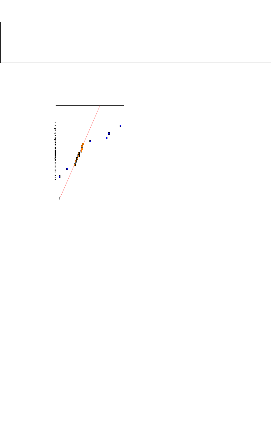
Solutions from Montgomery, D. C. (2001) Design and Analysis of Experiments, Wiley, NY
8-80
Error BD 4.5 81 0.332526
Model CD 14.5 841 3.45252
Model DE -22 1936 7.94778
Error ABD 0.5 1 0.00410526
Error ABF 6 144 0.591157
Lenth's ME 15.4235
Lenth's SME 31.3119
Factors A, C, D, E and the two factor interactions CD and DE appear to be significant. The model can be
found in the Design Expert Output below.
DESIGN-EXPERT Plot
Pitch
A: A
B: B
C: C
D: D
E: E
F: F
Normal plot
Norm al % probability
Effe ct
-2 2 .00 -3 .8 8 14.25 32.38 50.50
1
5
10
20
30
50
70
80
90
95
99
A
C
D
E
CD
DE
(b) Perform appropriate statistical tests on the model.
Design Expert Output
Response: Pitch
ANOVA for Selected Factorial Model
Analysis of variance table [Partial sum of squares]
Sum of Mean F
Source Squares DF Square Value Prob > F
Model 23891.00 6 3981.83 76.57 < 0.0001 significant
A 10201.00 1 10201.00 196.17 < 0.0001
C 676.00 1 676.00 13.00 0.0057
D 5476.00 1 5476.00 105.31 < 0.0001
E 4761.00 1 4761.00 91.56 < 0.0001
CD 841.00 1 841.00 16.17 0.0030
DE 1936.00 1 1936.00 37.23 0.0002
Residual 468.00 9 52.00
Cor Total 24359.00 15
The Model F-value of 76.57 implies the model is significant. There is only
a 0.01% chance that a "Model F-Value" this large could occur due to noise.
Std. Dev. 7.21 R-Squared 0.9808
Mean 135.75 Adj R-Squared 0.9680
C.V. 5.31 Pred R-Squared 0.9393
PRESS 1479.11 Adeq Precision 28.618
Coefficient Standard 95% CI 95% CI
Factor Estimate DF Error Low High VIF
Intercept 135.75 1 1.80 131.67 139.83
A-A 25.25 1 1.80 21.17 29.33 1.00
C-C -6.50 1 1.80 -10.58 -2.42 1.00
D-D 18.50 1 1.80 14.42 22.58 1.00
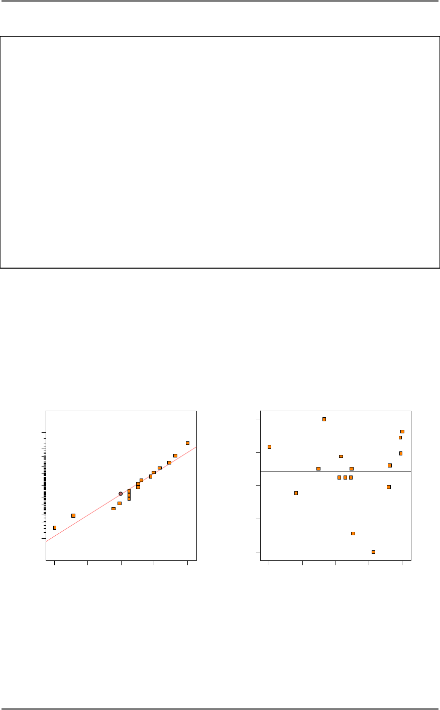
Solutions from Montgomery, D. C. (2001) Design and Analysis of Experiments, Wiley, NY
8-81
E-E 17.25 1 1.80 13.17 21.33 1.00
CD 7.25 1 1.80 3.17 11.33 1.00
DE -11.00 1 1.80 -15.08 -6.92 1.00
Final Equation in Terms of Coded Factors:
Pitch =
+135.75
+25.25 * A
-6.50 * C
+18.50 * D
+17.25 * E
+7.25 * C * D
-11.00 * D * E
Final Equation in Terms of Actual Factors:
Pitch =
+135.75000
+25.25000 * A
-6.50000 * C
+18.50000 * D
+17.25000 * E
+7.25000 * C * D
-11.00000 * D * E
(c) Analyze the residuals and comment on model adequacy.
The residual plots are acceptable. The normality and equality of variance assumptions are verified. There
does not appear to be any trends or interruptions in the residuals versus run order plot. The plots of the
residuals versus factors C and E identify reduced variation at the lower level of both variables while the
plot of residuals versus factor F identifies reduced variation at the upper level. Because C and E are
significant factors in the model, this might not affect the decision on the optimum solution for the process.
However, factor F is not included in the model and may be set at the upper level to reduce variation.
Residual
Norm al % probability
Normal plot of residuals
-1 3 -7 . 6 25 -2 .2 5 3.125 8.5
1
5
10
20
30
50
70
80
90
95
99
Predicted
Residuals
Residuals vs. Predicted
-1 3
-7 .6 25
-2 .2 5
3.125
8.5
50.00 84.13 118.25 152.38 186.50
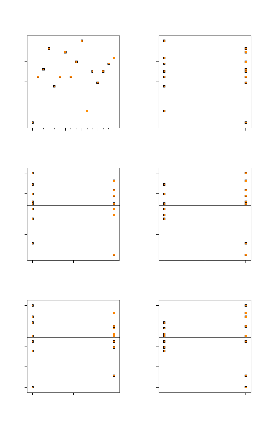
Solutions from Montgomery, D. C. (2001) Design and Analysis of Experiments, Wiley, NY
8-82
Run Num ber
Residuals
Residuals vs. Run
-1 3
-7 .6 25
-2 .2 5
3.125
8.5
14710 13 16
22
A
Residuals
Residuals vs. A
-1 3
-7 .6 25
-2 .2 5
3.125
8.5
-1 0 1
22
B
Residuals
Residuals vs. B
-1 3
-7 .6 25
-2 .2 5
3.125
8.5
-1 0 1
333
C
Residuals
Residuals vs. C
-1 3
-7 .6 25
-2 .2 5
3.125
8.5
-1 0 1
22
D
Residuals
Residuals vs. D
-1 3
-7 .6 25
-2 .2 5
3.125
8.5
-1 0 1
22
E
Residuals
Residuals vs. E
-1 3
-7 .6 25
-2 .2 5
3.125
8.5
-1 0 1
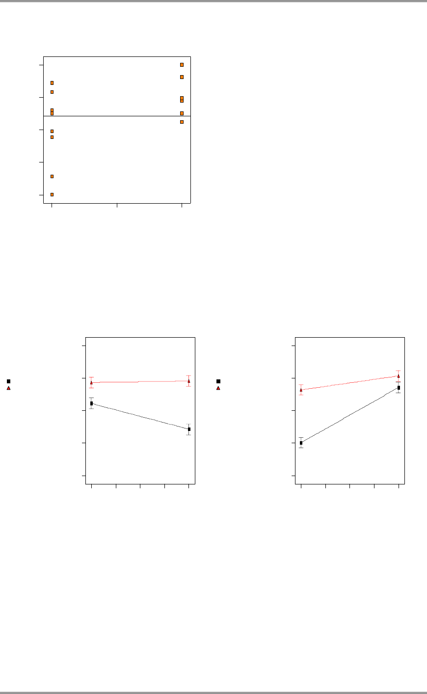
Solutions from Montgomery, D. C. (2001) Design and Analysis of Experiments, Wiley, NY
8-83
333
F
Residuals
Residuals vs. F
-1 3
-7 .6 25
-2 .2 5
3.125
8.5
-1 0 1
(d) Interpret the results of this experiment. Assume that a layer thickness of between 140 and 160 is
desirable.
The graphs below identify a region that is acceptable between 140 and 160.
DESIGN-EXPERT Plot
Pitch
X = C: C
Y = D: D
D- -1.000
D+ 1.000
Actual Factors
A: A = 0.00
B: B = 0.00
E: E = 0.00
F: F = 0.00
D
Inte ra c ti o n G r a p h
Pitch
C
-1 .0 0 -0 .5 0 0.00 0.50 1.00
54
88.75
123.5
158.25
193
DESIGN-EXPERT Plot
Pitch
X = D: D
Y = E: E
E- -1.000
E+ 1.000
Actual Factors
A: A = 0.00
B: B = 0.00
C: C = 0.00
F: F = 0.00
E
Inte ra c ti o n G r a p h
Pitch
D
-1 .0 0 -0 .5 0 0.00 0.50 1.00
54
88.75
123.5
158.25
193
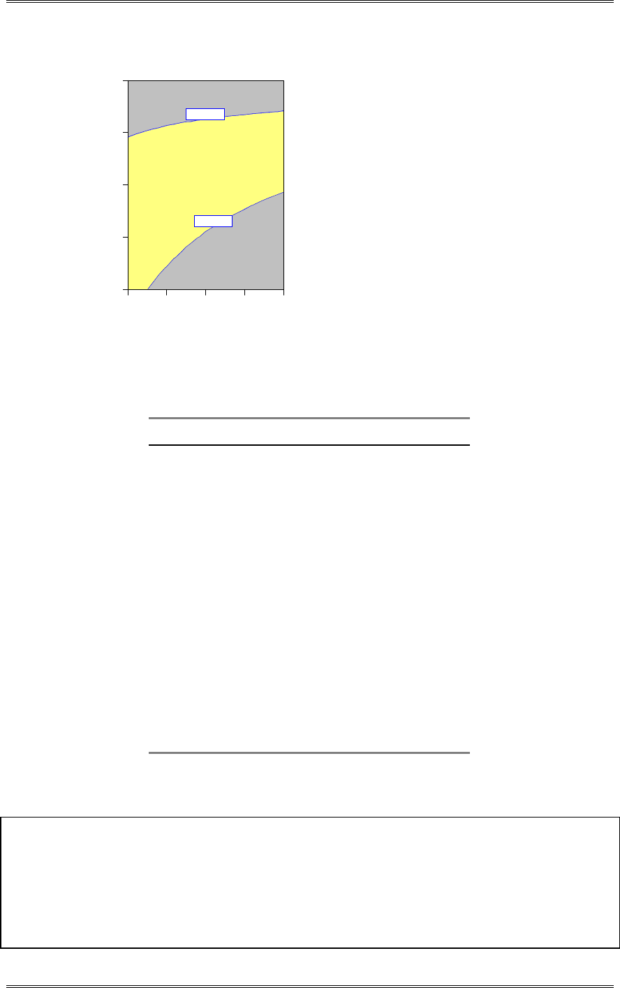
Solutions from Montgomery, D. C. (2001) Design and Analysis of Experiments, Wiley, NY
8-84
DESIGN-EXPERT Plot
Overlay Plot
X = C: C
Y = D: D
Coded Factors
A: A = 0.500
B: B = 0.000
E: E = 0.000
F: F = 0.000
Overlay Plot
C
D
-1 .0 0 -0 . 5 0 0.00 0.50 1.00
-1 .0 0
-0 .5 0
0.00
0.50
1.00
Pitch: 140
Pitch: 160
8-32 Five factors are studied in the irregular fractional factorial design of resolution V shown below.
Standard Run
Order Order A B C D E Gain
1 1 - - - - - 16.33
2 10 - + - - - 18.43
3 5 + + - - - 27.07
4 4 - - + - - 16.95
5 15 + - + - - 14.58
6 19 - + + - - 19.12
7 16 - - - + - 18.96
8 7 + - - + - 23.56
9 8 + + - + - 29.15
10 3 + - + + - 15.74
11 13 - + + + - 20.73
12 11 + + + + - 21.52
13 12 - - - - + 15.58
14 20 + - - - + 21.03
15 9 + + - - + 26.78
16 22 + - + - + 13.39
17 21 - + + - + 18.63
18 6 + + + - + 19.01
19 23 - - - + + 17.96
20 18 - + - + + 20.49
21 24 + + - + + 29.31
22 17 - - + + + 17.62
23 2 + - + + + 16.03
24 14 - + + + + 21.42
(a) Analyze the data from this experiment. What factors influence the response y?
Design Expert Output
Term Effect SumSqr % Contribtn
Model Intercept
Model A 2.9125 50.8959 11.2736
Model B 5.3275 170.294 37.7207
Model C -4.15917 103.792 22.9903
Model D 2.1325 27.2853 6.04381
Error E -0.4075 0.996338 0.220693
Model AB 1.45428 12.6896 2.8108
Model AC -3.71585 82.8451 18.3505
Error AD -0.0282843 0.0048 0.00106322
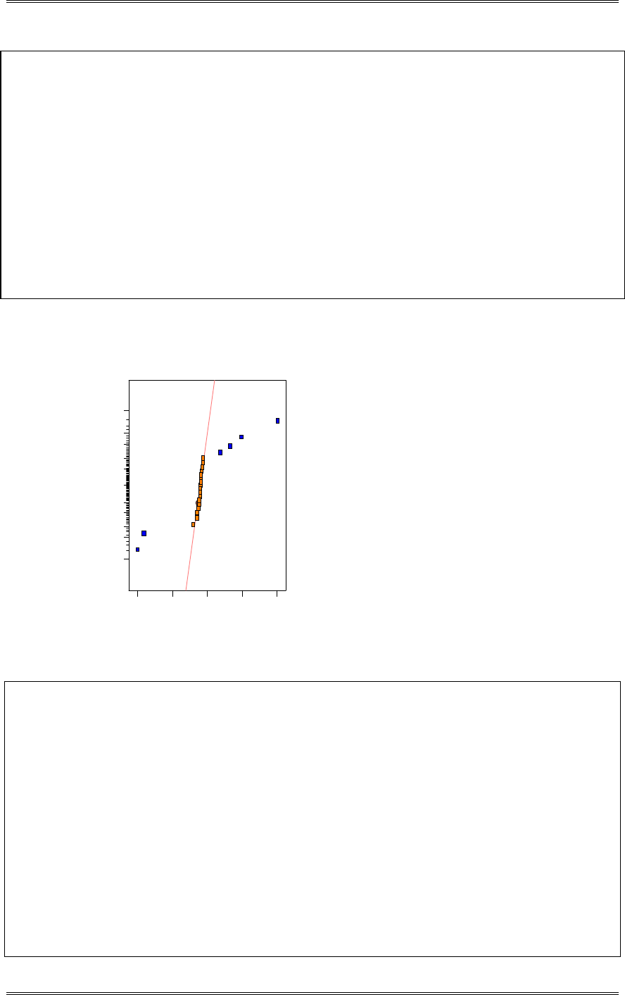
Solutions from Montgomery, D. C. (2001) Design and Analysis of Experiments, Wiley, NY
8-85
Error AE 0.113137 0.0768 0.0170115
Error BC 0.142887 7.5E-005 1.66128E-005
Error BD 0.133172 0.102704 0.0227494
Error BE 0.281664 0.710704 0.157424
Error CD -0.128458 0.0990083 0.0219307
Error CE 0.0294628 0.00520833 0.00115367
Error DE 0.291898 0.511225 0.113238
Error ABC -0.130639 0.264033 0.0584844
Error ABD 0.067361 0.027225 0.00603044
Error ABE Aliased
Error ACD 0.189835 0.216225 0.0478947
Error ACE Aliased
Error ADE 0.102062 0.0625 0.013844
Error BCD 0.155134 0.1444 0.0319852
Error BCE 0.0898146 0.0484 0.0107208
Error BDE 0.0408248 0.01 0.00221504
Error CDE 0.251073 0.378225 0.0837783
Lenth's ME 0.455325
Lenth's SME 0.881839
Factors A, B, C, D, and the AB and AC interactions appear to be significant.
DESIGN-EXPERT Plot
y
A: A
B: B
C: C
D: D
E: E
Normal plot
Normal % probability
Effe ct
-4 .1 6 -1 .7 9 0.58 2.96 5.33
1
5
10
20
30
50
70
80
90
95
99
A
B
C
D
AB
AC
Design Expert Output
Response: y
ANOVA for Selected Factorial Model
Analysis of variance table [Partial sum of squares]
Sum of Mean F
Source Squares DF Square Value Prob > F
Model 447.80 6 74.63 346.86 < 0.0001 significant
A 50.90 1 50.90 236.54 < 0.0001
B 85.92 1 85.92 399.32 < 0.0001
C 70.86 1 70.86 329.32 < 0.0001
D 27.29 1 27.29 126.81 < 0.0001
AB 12.69 1 12.69 58.98 < 0.0001
AC 82.85 1 82.85 385.02 < 0.0001
Residual 3.66 17 0.22
Cor Total 451.46 23
The Model F-value of 346.86 implies the model is significant. There is only
a 0.01% chance that a "Model F-Value" this large could occur due to noise.
Std. Dev. 0.46 R-Squared 0.9919
Mean 19.97 Adj R-Squared 0.9890
C.V. 2.32 Pred R-Squared 0.9832
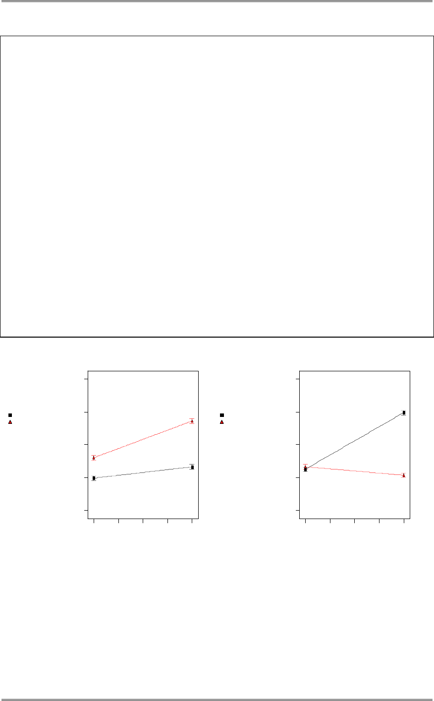
Solutions from Montgomery, D. C. (2001) Design and Analysis of Experiments, Wiley, NY
8-86
PRESS 7.60 Adeq Precision 60.974
Coefficient Standard 95% CI 95% CI
Factor Estimate DF Error Low High VIF
Intercept 19.97 1 0.095 19.77 20.17
A-A 1.46 1 0.095 1.26 1.66 1.00
B-B 2.01 1 0.10 1.79 2.22 1.13
C-C -1.82 1 0.10 -2.03 -1.61 1.13
D-D 1.07 1 0.095 0.87 1.27 1.00
AB 0.77 1 0.10 0.56 0.98 1.12
AC -1.97 1 0.10 -2.18 -1.76 1.12
Final Equation in Terms of Coded Factors:
y =
+19.97
+1.46 * A
+2.01 * B
-1.82 * C
+1.07 * D
+0.77 * A * B
-1.97 * A * C
Final Equation in Terms of Actual Factors:
y =
+19.97458
+1.45625 * A
+2.00687 * B
-1.82250 * C
+1.06625 * D
+0.77125 * A * B
-1.97062 * A * C
DESIGN-EXPERT Plot
y
X = A: A
Y = B: B
B- -1.000
B+ 1.000
Actual Factors
C: C = 0.00
D: D = 0.00
E: E = 0.00
B
Inte ra c ti o n G r a p h
y
A
-1 .0 0 -0 .5 0 0.00 0.50 1.00
13.39
17.37
21.35
25.33
29.31
DESIGN-EXPERT Plot
y
X = A: A
Y = C: C
C- -1.000
C+ 1.000
Actual Factors
B: B = 0.00
D: D = 0.00
E: E = 0.00
C
Inte ra c ti o n G r a p h
y
A
-1 .0 0 -0 .5 0 0.00 0.50 1.00
13.39
17.37
21.35
25.33
29.31
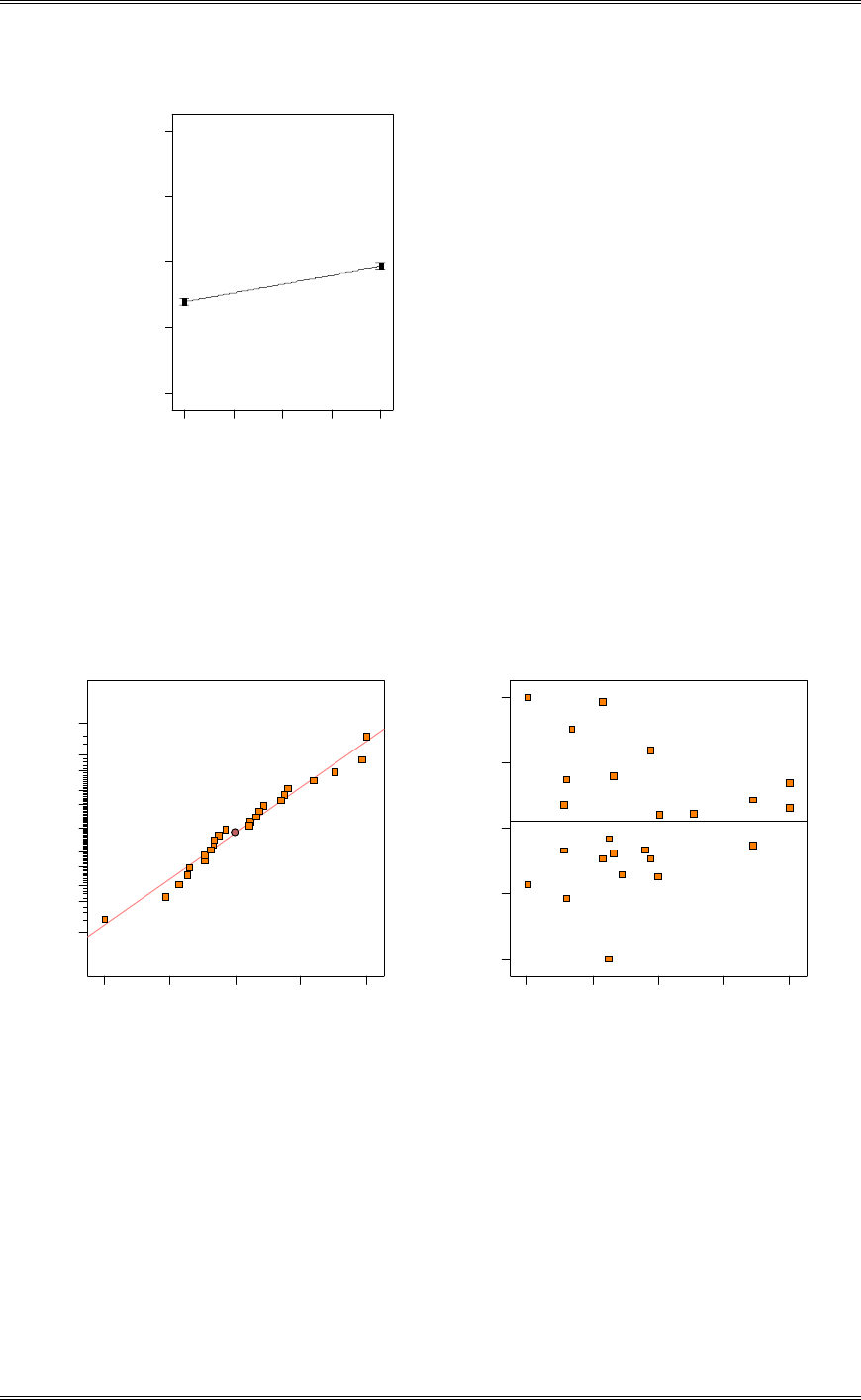
Solutions from Montgomery, D. C. (2001) Design and Analysis of Experiments, Wiley, NY
8-87
DESIGN-EXPERT Plot
y
X = D: D
Actual Factors
A: A = 0.00
B: B = 0.00
C: C = 0.00
E: E = 0.00
-1 .0 0 -0 .5 0 0.00 0.50 1.00
13.39
17.37
21.35
25.33
29.31
D
y
One Factor Plot
(b) Analyze the residuals. Comment on model adequacy.
The residual plots are acceptable. The normality and equality of variance assumptions are verified. There
does not appear to be any trends or interruptions in the residuals versus run order plot.
Residual
Norm al % probability
Normal plot of residuals
-0.877083 -0.461146 -0.0452083 0.370729 0.786667
1
5
10
20
30
50
70
80
90
95
99
Predicted
Residuals
Residuals vs. Predicted
-0 .8 77 0 8 3
-0 .4 61 1 4 6
-0.0452083
0.370729
0.786667
13.79 17.61 21.43 25.25 29.07
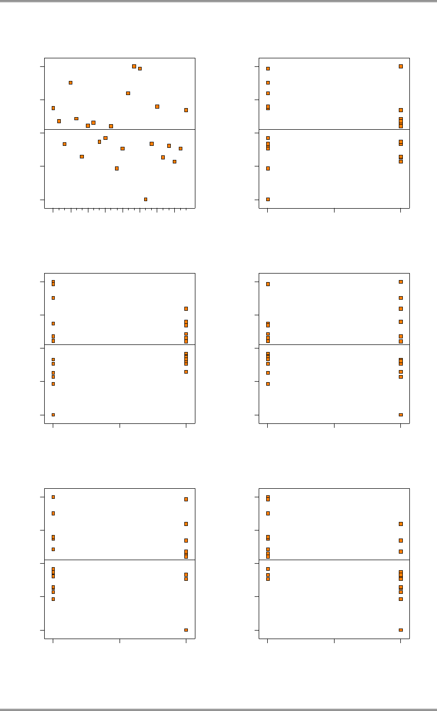
Solutions from Montgomery, D. C. (2001) Design and Analysis of Experiments, Wiley, NY
8-88
Run Num ber
Residuals
Residuals vs. Run
-0.877083
-0.461146
-0.0452083
0.370729
0.786667
1 4 7 10 13 16 19 22
A
Residuals
Residuals vs. A
-0 .8 77 0 8 3
-0 .4 61 1 4 6
-0.0452083
0.370729
0.786667
-1 0 1
B
Residuals
Residuals vs. B
-0.877083
-0.461146
-0.0452083
0.370729
0.786667
-1 0 1
C
Residuals
Residuals vs. C
-0 .8 77 0 8 3
-0 .4 61 1 4 6
-0.0452083
0.370729
0.786667
-1 0 1
D
Residuals
Residuals vs. D
-0.877083
-0.461146
-0.0452083
0.370729
0.786667
-1 0 1
E
Residuals
Residuals vs. E
-0 .8 77 0 8 3
-0 .4 61 1 4 6
-0.0452083
0.370729
0.786667
-1 0 1

Solutions from Montgomery, D. C. (2001) Design and Analysis of Experiments, Wiley, NY
9-1
Chapter 9
Three-Level and Mixed-Level
Factorial and Fractional Factorial Design
Solutions
9-1 The effects of developer concentration (A) and developer time (B) on the density of photographic
plate film are being studied. Three strengths and three times are used, and four replicates of a 32 factorial
experiment are run. The data from this experiment follow. Analyze the data using the standard methods
for factorial experiments.
Development Time (minutes)
Developer Concentration 10 14 18
10% 0 2 1 3 2 5
5 4 4 2 4 6
12% 4 6 6 8 9 10
7 5 7 7 8 5
14% 7 10 10 10 12 10
8 7 8 7 9 8
Design Expert Output
Response: Data
ANOVA for Selected Factorial Model
Analysis of variance table [Partial sum of squares]
Sum of Mean F
Source Squares DF Square Value Prob > F
Model 224.22 8 28.03 10.66 < 0.0001 significant
A 198.22 2 99.11 37.69 < 0.0001
B 22.72 2 11.36 4.32 0.0236
AB 3.28 4 0.82 0.31 0.8677
Residual 71.00 27 2.63
Lack of Fit 0.000 0
Pure Error 71.00 27 2.63
Cor Total 295.22 35
The Model F-value of 10.66 implies the model is significant. There is only
a 0.01% chance that a "Model F-Value" this large could occur due to noise.
Values of "Prob > F" less than 0.0500 indicate model terms are significant.
In this case A, B are significant model terms.
Concentration and time are significant. The interaction is not significant. By letting both A and B be
treated as numerical factors, the analysis can be performed as follows:
Design Expert Output
Response: Data
ANOVA for Selected Factorial Model
Analysis of variance table [Partial sum of squares]
Sum of Mean F
Source Squares DF Square Value Prob > F
Model 221.01 5 44.20 17.87 < 0.0001 significant
A 192.67 1 192.67 77.88 < 0.0001
B 22.04 1 22.04 8.91 0.0056
A2 5.56 1 5.56 2.25 0.1444
B2 0.68 1 0.68 0.28 0.6038
AB 0.062 1 0.062 0.025 0.8748
Residual 74.22 30 2.47
Lack of Fit 3.22 3 1.07 0.41 0.7488 not significant
Pure Error 71.00 27 2.63
Cor Total 295.22 35

Solutions from Montgomery, D. C. (2001) Design and Analysis of Experiments, Wiley, NY
9-2
The Model F-value of 17.87 implies the model is significant. There is only
a 0.01% chance that a "Model F-Value" this large could occur due to noise.
Values of "Prob > F" less than 0.0500 indicate model terms are significant.
In this case A, B are significant model terms.
9-2 Compute the I and J components of the two-factor interaction in Problem 9-1.
B
11 10 17
A 22 28 32
32 35 39
AB Totals = 77, 78, 71;
ABISSAB
39.2
36
226
12
717877 2222
AB2 Totals = 78, 74, 74;
ABJSSAB
89.0
36
226
12
747478 2222
2
28.3 ABJABISS AB
9-3 An experiment was performed to study the effect of three different types of 32-ounce bottles (A) and
three different shelf types (B) -- smooth permanent shelves, end-aisle displays with grilled shelves, and
beverage coolers -- on the time it takes to stock ten 12-bottle cases on the shelves. Three workers (factor
C) were employed in this experiment, and two replicates of a 33 factorial design were run. The observed
time data are shown in the following table. Analyze the data and draw conclusions.
Replicate I Replicate 2
Worker Bottle Type Permanent EndAisle Cooler Permanent EndAisle Cooler
1 Plastic 3.45 4.14 5.80 3.36 4.19 5.23
28-mm glass 4.07 4.38 5.48 3.52 4.26 4.85
38-mm glass 4.20 4.26 5.67 3.68 4.37 5.58
2 Plastic 4.80 5.22 6.21 4.40 4.70 5.88
28-mm glass 4.52 5.15 6.25 4.44 4.65 6.20
38-mm glass 4.96 5.17 6.03 4.39 4.75 6.38
3 Plastic 4.08 3.94 5.14 3.65 4.08 4.49
28-mm glass 4.30 4.53 4.99 4.04 4.08 4.59
38-mm glass 4.17 4.86 4.85 3.88 4.48 4.90
Design Expert Output
Response: Time
ANOVA for Selected Factorial Model
Analysis of variance table [Partial sum of squares]
Sum of Mean F
Source Squares DF Square Value Prob > F
Model 28.38 26 1.09 13.06 < 0.0001 significant
A 0.33 2 0.16 1.95 0.1618
B 17.91 2 8.95 107.10 < 0.0001
C 7.91 2 3.96 47.33 < 0.0001
AB 0.11 4 0.027 0.33 0.8583
AC 0.11 4 0.027 0.32 0.8638
BC 1.59 4 0.40 4.76 0.0049
ABC 0.43 8 0.053 0.64 0.7380
Residual 2.26 27 0.084
Lack of Fit 0.000 0
Pure Error 2.26 27 0.084
Cor Total 30.64 53
The Model F-value of 13.06 implies the model is significant. There is only

Solutions from Montgomery, D. C. (2001) Design and Analysis of Experiments, Wiley, NY
9-3
a 0.01% chance that a "Model F-Value" this large could occur due to noise.
Values of "Prob > F" less than 0.0500 indicate model terms are significant.
In this case B, C, BC are significant model terms.
Factors B and C, shelf type and worker, and the BC interaction are significant. For the shortest time
regardless of worker chose the permanent shelves. This can easily be seen in the interaction plot below.
DESIGN-EXPERT Plot
Time
X = C: Worker
Y = B: Shelf Type
Design Points
B1 Perm anent
B2 End Aisle
B3 Cooler
Actual Factor
A: Bottle Type = 28mm glass
Shelf Type
Inte ra c ti o n G r a p h
Worker
Tim e
1 2 3
3.36
4.1504
4.94081
5.73121
6.52162
9-4 A medical researcher is studying the effect of lidocaine on the enzyme level in the heart muscle of
beagle dogs. Three different commercial brands of lidocaine (A), three dosage levels (B), and three dogs
(C) are used in the experiment, and two replicates of a 33 factorial design are run. The observed enzyme
levels follow. Analyze the data from this experiment.
Replicate I Replicate 2
Lidocaine Dosage Dog
Dog
Brand Strength 1 2 3 1 2 3
1 1 86 84 85 84 85 86
2 94 99 98 95 97 90
3 101 106 98 105 104 103
2 1 85 84 86 80 82 84
2 95 98 97 93 99 95
3 108 114 109 110 102 100
3 1 84 83 81 83 80 79
2 95 97 93 92 96 93
3 105 100 106 102 111 108
Design Expert Output
Response: Enzyme Level
ANOVA for Selected Factorial Model
Analysis of variance table [Partial sum of squares]
Sum of Mean F
Source Squares DF Square Value Prob > F
Model 4490.33 26 172.71 16.99 < 0.0001 significant
A 31.00 2 15.50 1.52 0.2359
B 4260.78 2 2130.39 209.55 < 0.0001
C 28.00 2 14.00 1.38 0.2695
AB 69.56 4 17.39 1.71 0.1768
AC 3.33 4 0.83 0.082 0.9872
BC 36.89 4 9.22 0.91 0.4738
ABC 60.78 8 7.60 0.75 0.6502

Solutions from Montgomery, D. C. (2001) Design and Analysis of Experiments, Wiley, NY
9-4
Residual 274.50 27 10.17
Lack of Fit 0.000 0
Pure Error 274.50 27 10.17
Cor Total 4764.83 53
The Model F-value of 16.99 implies the model is significant. There is only
a 0.01% chance that a "Model F-Value" this large could occur due to noise.
Values of "Prob > F" less than 0.0500 indicate model terms are significant.
In this case B are significant model terms.
The dosage is significant.
9-5 Compute the I and J components of the two-factor interactions for Example 9-1.
A
134 188 44
B -155 -348 -289
176 127 288
I totals = 74,75,16 J totals = -128,321,-28
I(AB) = 126.78 J(AB) = 6174.12
SSAB = 6300.90
A
-190 -58 -211
C 399 230 394
6 -205 -140
I totals = -100,342,-77 J totals = 25,141,-1
I(AC) = 6878.78 J(AC) = 635.12
SSAC = 7513.90
B
-93 -350 -16
C -155 -133 533
-104 -309 74
I totals = -152,79,238 J totals =-253,287,131
I(BC) = 4273.00 J(BC) = 8581.34
SSBC = 12854.34
9-6 An experiment is run in a chemical process using a 32 factorial design. The design factors are
temperature and pressure, and the response variable is yield. The data that result from this experiment are
shown below.
Pressure, psig
Temperature,
qC 100 120 140
80 47.58, 48.77 64.97, 69.22 80.92, 72.60
90 51.86, 82.43 88.47, 84.23 93.95, 88.54
100 71.18, 92.77 96.57, 88.72 76.58, 83.04
(a) Analyze the data from this experiment by conducting an analysis of variance. What conclusions can
you draw?

Solutions from Montgomery, D. C. (2001) Design and Analysis of Experiments, Wiley, NY
9-5
Design Expert Output
Response: Yield
ANOVA for Selected Factorial Model
Analysis of variance table [Partial sum of squares]
Sum of
Mean F
Source Squares DF Square Value Prob > F
Model 3187.13 8 398.39 4.37 0.0205 significant
A 1096.93 2 548.47 6.02 0.0219
B 1503.56 2 751.78 8.25 0.0092
AB
586.64 4 146.66 1.61 0.2536
Pure Error 819.98 9 91.11
Cor Total 4007.10 17
The Model F-value of 4.37 implies the model is significant. There is only
a 2.05% chance that a "Model F-Value" this large could occur due to noise.
Values of "Prob > F" less than 0.0500 indicate model terms are significant.
In this case A, B are significant model terms.
Temperature and pressure are significant. Their interaction is not. An alternate analysis is performed
below with the A and B treated as numeric factors:
Design Expert Output
Response: Yield
ANOVA for Selected Factorial Model
Analysis of variance table [Partial sum of squares]
Sum of
Mean F
Source Squares DF Square Value Prob > F
Model 3073.27 5 614.65 7.90 0.0017 significant
A 850.76 1 850.76 10.93 0.0063
B 1297.92 1 1297.92 16.68 0.0015
A2 246.18 1 246.18 3.16 0.1006
B2 205.64 1 205.64 2.64 0.1300
AB 472.78 1 472.78 6.08 0.0298
Residual 933.83 12 77.82
Lack of Fit 113.86 3 37.95 0.42 0.7454 not significant
Pure Error 819.98 9 91.11
Cor Total 4007.10 17
The Model F-value of 7.90 implies the model is significant. There is only
a 0.17% chance that a "Model F-Value" this large could occur due to noise.
Values of "Prob > F" less than 0.0500 indicate model terms are significant.
In this case A, B, AB are significant model terms.
(b) Graphically analyze the residuals. Are there any concerns about underlying assumptions or model
adequacy?
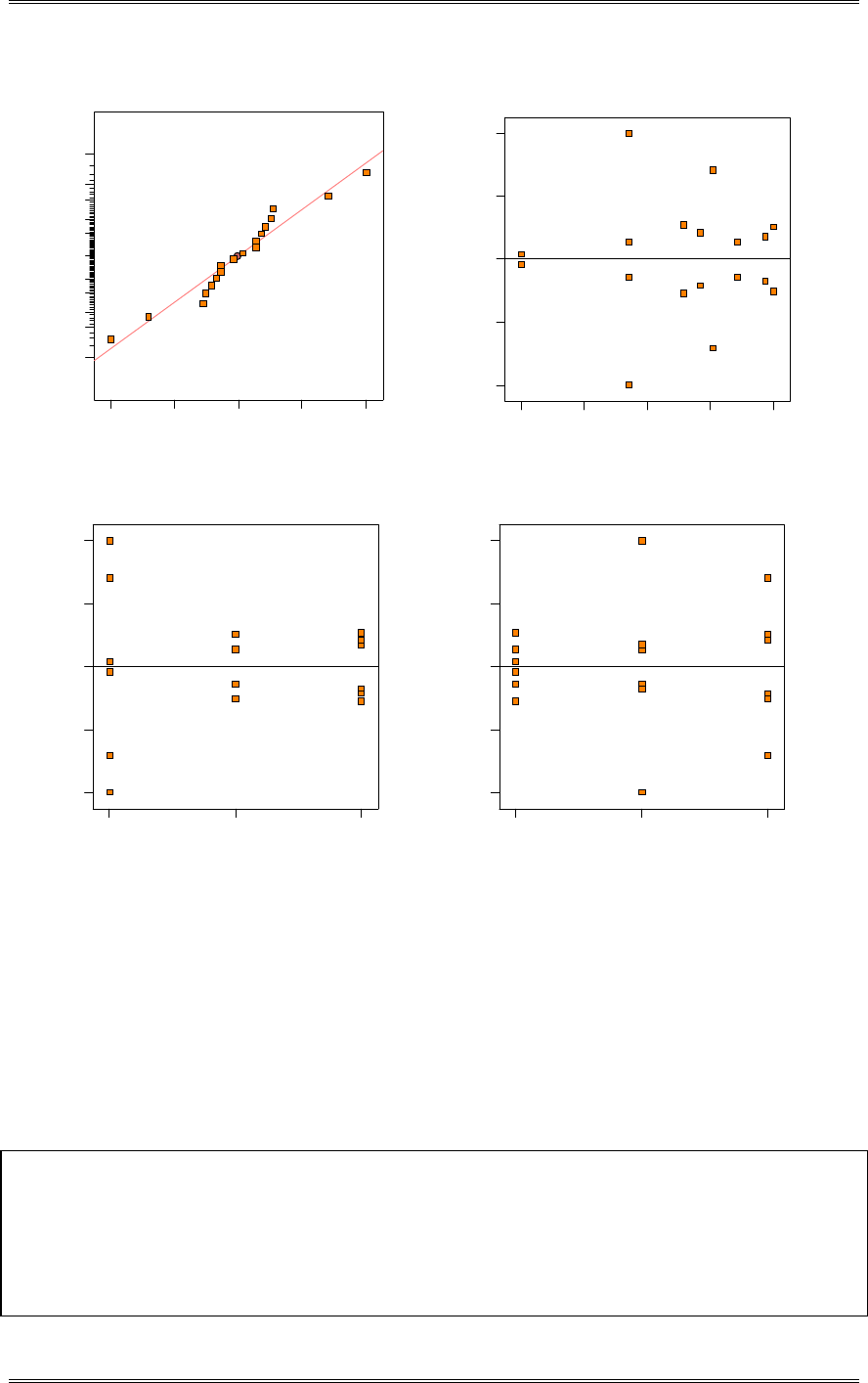
Solutions from Montgomery, D. C. (2001) Design and Analysis of Experiments, Wiley, NY
9-6
Residual
Normal % probability
Normal plot of residuals
-1 5 .2 8 5 -7.6425 07.6425 15.285
1
5
10
20
30
50
70
80
90
95
99
Predicted
Residuals
Residuals vs. Predicted
-15.285
-7 .6 4 25
0
7.6425
15.285
48.18 59.29 70.41 81.53 92.65
Pressure
Residuals
Residuals vs. Pressure
-15.285
-7 .6 4 25
0
7.6425
15.285
1 2 3
Temperature
Residuals
Residuals vs. Temperature
-15.285
-7 .6 4 25
0
7.6425
15.285
1 2 3
The plot of residuals versus pressure shows a decreasing funnel shape indicating a non-constant variance.
(c) Verify that if we let the low, medium and high levels of both factors in this experiment take on the
levels -1, 0, and +1, then a least squares fit to a second order model for yield is
......yxxxxxx 86 81 10 4 8 42 7 17 7 86 7 69
121
2
2
2
12
The coefficients can be found in the following table of computer output.
Design Expert Output
Final Equation in Terms of Coded Factors:
Yield =
+86.81
+8.42 * A
+10.40 * B
-7.84 * A
2
-7.17 * B
2
-7.69 * A * B
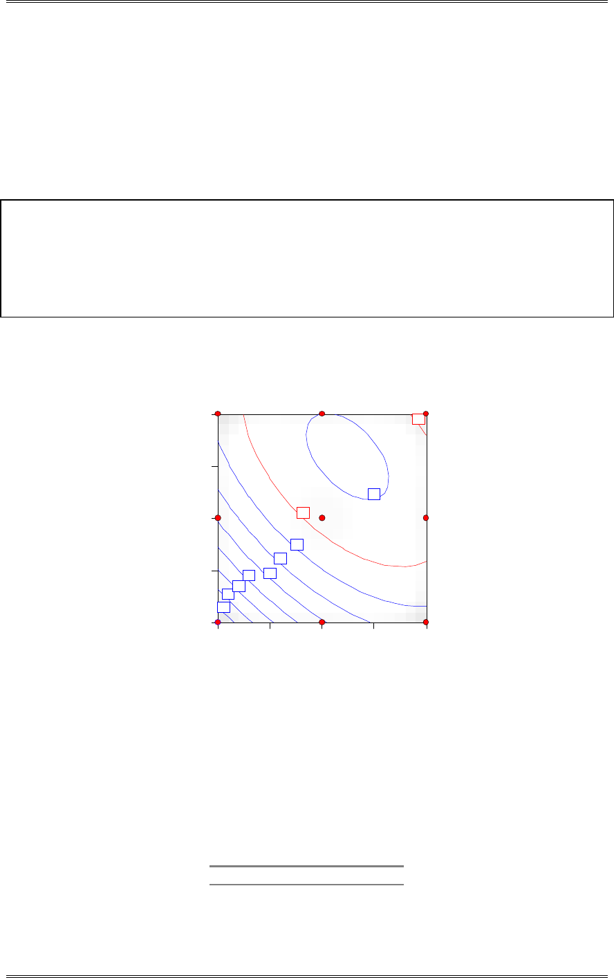
Solutions from Montgomery, D. C. (2001) Design and Analysis of Experiments, Wiley, NY
9-7
(d) Confirm that the model in part (c) can be written in terms of the natural variables temperature (T) and
pressure (P) as
.. . . . .yTPTPTP 1335 63 18 56 8 59 0 072 0 0196 0 0384
22
The coefficients can be found in the following table of computer output.
Design Expert Output
Final Equation in Terms of Actual Factors:
Yield =
-1335.62500
+8.58737 * Pressure
+18.55850 * Temperature
-0.019612 * Pressure2
-0.071700 * Temperature2
-0.038437 * Pressure * Temperature
(e) Construct a contour plot for yield as a function of pressure and temperature. Based on the
examination of this plot, where would you recommend running the process.
Yie ld
A: P res s ure
B: Temperature
100.00 110.00 120.00 130.00 140.00
80.00
85.00
90.00
95.00
100.00
50
55
60
65 70
75
80
85
85
90
2 2 2
2 2 2
2 2 2
Run the process in the oval region indicated by the yield of 90.
9-7
(a) Confound a 33 design in three blocks using the ABC2 component of the three-factor interaction.
Compare your results with the design in Figure 9-7.
L = X1 + X2 + 2X3
Block 1 Block 2 Block 3
000 100 200
112 212 012
210 010 110

Solutions from Montgomery, D. C. (2001) Design and Analysis of Experiments, Wiley, NY
9-8
120 220 020
022 122 222
202 002 102
221 021 121
101 201 001
011 111 211
The new design is a 180q rotation around the Factor B axis.
(b) Confound a 33 design in three blocks using the AB2C component of the three-factor interaction.
Compare your results with the design in Figure 9-7.
L = X1 + 2X2 + X3
Block 1 Block 2 Block 3
000 210 112
022 202 120
011 221 101
212 100 010
220 122 002
201 111 021
110 012 200
102 020 222
121 001 211
The new design is a 180q rotation around the Factor C axis.
(c) Confound a 33 design three blocks using the ABC component of the three-factor interaction.
Compare your results with the design in Figure 9-7.
L = X1 + X2 + X3
Block 1 Block 2 Block 3
000 112 221
210 022 101
120 202 011
021 100 212
201 010 122
111 220 002
012 121 200
222 001 110
102 211 020
The new design is a 90q rotation around the Factor C axis along with switching layer 0 and layer 1 in the
C axis.
(d) After looking at the designs in parts (a), (b), and (c) and Figure 9-7, what conclusions can you draw?
All four designs are relatively the same. The only differences are rotations and swapping of layers.
9-8 Confound a 34 design in three blocks using the AB2CD component of the four-factor interaction.

Solutions from Montgomery, D. C. (2001) Design and Analysis of Experiments, Wiley, NY
9-9
L = X1 + 2X2 + X3 + X4
Block 1
0000 1100 0110 0101 2200 0220 0202 1210 1201
0211 1222 2212 2221 0122 2111 1121 1112 2010
2102 0021 2001 2120 1011 2022 0012 1002 1020
Block 2
1021 1110 1202 0001 0120 0212 1012 1101 1220
0200 0022 0111 2002 2121 2210 0010 0102 0221
1000 1122 1211 2112 2201 2020 2011 2100 2222
Block 3
2012 2101 2220 1022 1111 1200 2000 2121 2211
1221 1010 1102 0020 0112 0201 1001 1120 1212
2021 2110 2202 0100 0222 0011 0002 0121 0210
9-9 Consider the data from the first replicate of Problem 9-3. Assuming that all 27 observations could
not be run on the same day, set up a design for conducting the experiment over three days with AB2C
confounded with blocks. Analyze the data.
Block 1 Block 2 Block 3
000 = 3.45 100 = 4.07 200 = 4.20
110 = 4.38 210 = 4.26 010 = 4.14
011 = 5.22 111 = 4.14 211 = 5.17
102 = 4.30 202 = 4.17 002 = 4.08
201 = 4.96 001 = 4.80 101 = 4.52
212 = 4.86 012 = 3.94 112 = 4.53
121 = 6.25 221 = 4.99 021 = 6.21
022 = 5.14 122 = 6.03 222 = 4.85
220 = 5.67 020 = 5.80 120 = 5.48
Totals-> = 44.23 43.21 43.18
Design Expert Output
Response: Time
ANOVA for Selected Factorial Model
Analysis of variance table [Partial sum of squares]
Sum of Mean F
Source Squares DF Square Value Prob > F
Block 0.23 2 0.11
Model 13.17 18 0.73 4.27 0.0404 significant
A 0.048 2 0.024 0.14 0.8723
B 8.92 2 4.46 26.02 0.0011
C 1.57 2 0.78 4.57 0.0622
AB 1.31 4 0.33 1.91 0.2284
AC 0.87 4 0.22 1.27 0.3774
BC 0.45 4 0.11 0.66 0.6410
Residual 1.03 6 0.17
Cor Total 14.43 26
The Model F-value of 4.27 implies the model is significant. There is only
a 4.04% chance that a "Model F-Value" this large could occur due to noise.
Values of "Prob > F" less than 0.0500 indicate model terms are significant.
In this case B are significant model terms.

Solutions from Montgomery, D. C. (2001) Design and Analysis of Experiments, Wiley, NY
9-10
9-10 Outline the analysis of variance table for the 34 design in nine blocks. Is this a practical design?
Source DF
A 2
B 2
C 2
D 2
AB 4
AC 4
AD 4
BC 4
BD 4
CD 4
ABC (AB2C,ABC2,AB2C2) 6
ABD (ABD,AB2D,ABD2) 6
ACD (ACD,ACD2,AC2D2) 6
BCD (BCD,BC2D,BCD2) 6
ABCD 16
Blocks (ABC,AB2C2,AC2D,BC2D2) 8
Total 80
Any experiment with 81 runs is large. Instead of having three full levels of each factor, if two levels of
each factor could be used, then the overall design would have 16 runs plus some center points. This two-
level design could now probably be run in 2 or 4 blocks, with center points in each block. Additional
curvature effects could be determined by augmenting the experiment with the axial points of a central
composite design and additional enter points. The overall design would be less than 81 runs.
9-11 Consider the data in Problem 9-3. If ABC is confounded in replicate I and ABC2 is confounded in
replicate II, perform the analysis of variance.
L
1 = X1 + X2 + X3 L2 = X1 + X2 + 2X2
Block 1 Block 2 Block 3 Block 1 Block 2 Block 3
000 = 3.45 001 = 4.80 002 = 4.08 000 = 3.36 100 = 3.52 200 = 3.68
111 = 5.15 112 = 4.53 110 = 4.38 101 = 4.44 201 = 4.39 001 = 4.40
222 = 4.85 220 = 5.67 221 = 6.03 011 = 4.70 111 = 4.65 211 = 4.75
120 = 5.48 121 = 6.25 122 = 4.99 221 = 6.38 021 = 5.88 121 = 6.20
102 = 4.30 100 = 4.07 101 = 4.52 202 = 3.88 002 = 3.65 102 = 4.04
210 = 4.26 211 = 5.17 212 = 4.86 022 = 4.49 122 = 4.59 222 = 4.90
201 = 4.96 202 = 4.17 200 = 4.20 120 = 4.85 220 = 5.58 020 = 5.23
012 = 3.94 010 = 4.14 011 = 5.22 210 = 4.37 010 = 4.19 110 = 4.26
021 = 6.21 022 = 5.14 020 = 5.80 112 = 4.08 212 = 4.48 012 = 4.08
The sums of squares for A, B, C, AB, AC, and BC are calculated as usual. The only sums of squares
presenting difficulties with calculations are the four components of the ABC interaction (ABC, ABC2,
AB2C, and AB2C2). ABC is computed using replicate I and ABC2 is computed using replicate II. AB2C
and AB2C2 are computed using data from both replicates.
We will show how to calculate AB2C and AB2C2 from both replicates. Form a two-way table of A x B at
each level of C. Find the I(AB) and J(AB) totals for each third of the A x B table.
A
C B 0 1 2 I J
0 6.81 7.59 7.88 26.70 27.55

Solutions from Montgomery, D. C. (2001) Design and Analysis of Experiments, Wiley, NY
9-11
0 1 8.33 8.64 8.63 27.25 27.17
2 11.03 10.33 11.25 26.54 25.77
0 9.20 8.96 9.35 31.41 31.25
1 1 9.92 9.80 9.92 30.97 31.29
2 12.09 12.45 12.41 31.72 31.57
0 7.73 8.34 8.05 26.09 26.29
2 1 8.02 8.61 9.34 27.31 26.11
2 9.63 9.58 9.75 25.65 26.65
The I and J components for each third of the above table are used to form a new table of diagonal totals.
C I(AB) J(AB)
0 2.670 27.25 26.54 27.55 27.17 25.77
1 31.41 30.97 31.72 31.25 31.29 31.57
2 26.09 27.31 25.65 26.29 26.11 26.65
I Totals: I Totals:
85.06,85.26,83.32 85.99,85.03,83.12
J Totals: J Totals:
85.73,83.60,84.31 83.35,85.06,85.23
Now, AB2C2 = I[C x I(AB)] = (85. ) (85. ) (83. ) ( . ) .
06 26 32
18
253 64
54 01265
222 2
and, AB2C = J[C x I(AB)]= (85. ) (83. ) (84. ) ( . ) .
73 60 31
18
253 64
54 01307
222 2
If it were necessary, we could find ABC2 as ABC2= I[C x J(AB)] and ABC as J[C x J(AB)]. However,
these components must be computed using the data from the appropriate replicate.
The analysis of variance table:
Source SS DF MS F0
Replicates 1.06696 1
Blocks within Replicates 0.2038 4
A 0.4104 2 0.2052 5.02
B 17.7514 2 8.8757 217.0
C 7.6631 2 3.8316 93.68
AB 0.1161 4 0.0290 <1
AC 0.1093 4 0.0273 <1
BC 1.6790 4 0.4198 10.26
ABC (rep I) 0.0452 2 0.0226 <1
ABC2 (rep II) 0.1020 2 0.0510 1.25
AB2C 0.1307 2 0.0754 1.60
AB2C2 0.1265 2 0.0633 1.55
Error 0.8998 22 0.0409
Total 30.3069 53
9-12 Consider the data from replicate I in Problem 9-3. Suppose that only a one-third fraction of this
design with I=ABC is run. Construct the design, determine the alias structure, and analyze the design.

Solutions from Montgomery, D. C. (2001) Design and Analysis of Experiments, Wiley, NY
9-12
The design is 000, 012, 021, 102, 201, 111, 120, 210, 222.
The alias structure is: A = BC = AB2C2
B = AC = AB2C
C = AB = ABC2
AB2 = AC2 = BC2
C
A B 0 1 2
0 3.45
0 1 5.48
2 4.26
0 6.21
1 1 5.15
2 4.96
0 3.94
2 1 4.30
2 4.85
Source SS DF
A 2.25 2
B 0.30 2
C 2.81 2
AB2 0.30 2
Total 5.66 8
9-13 From examining Figure 9-9, what type of design would remain if after completing the first 9 runs,
one of the three factors could be dropped?
A full 32 factorial design results.
9-14 Construct a 341
IV
design with I=ABCD. Write out the alias structure for this design.
The 27 runs for this design are as follows:
0000 1002 2001
0012 1011 2010
0021 1020 2022
0102 1101 2100
0111 1110 2112
0120 1122 2121
0201 1200 2202
0210 1212 2211
0222 1221 2220
A = AB2C2D2 = BCD B = AB2CD = ACD C = ABC2D = ABD D = ABCD2 = ABC
AB = ABC2D2 = CD AB2 = AC2D2 = BC2D2 AC = AB2CD2 = BD AC2 = AB2D2 = BC2D
BC = AB2C2D = AD BC2 = AB2D = AC2D BD2 = AB2C = ACD2 CD2 = ABC2 = ABCD2
AD2 = AB2C2 = BCD2

Solutions from Montgomery, D. C. (2001) Design and Analysis of Experiments, Wiley, NY
9-13
9-15 Verify that the design in Problem 9-14 is a resolution IV design.
The design in Problem 9-14 is a Resolution IV design because no main effect is aliased with a component
of a two-factor interaction, but some two-factor interaction components are aliased with each other.
9-16 Construct a 35-2 design with I=ABC and I=CDE. Write out the alias structure for this design. What
is the resolution of this design?
The complete defining relation for this design is : I = ABC = CDE = ABC2DE = ABD2E2
This is a resolution III design. The defining contrasts are L1 = X1 + X2 + X3 and L2 = X3 + X4 + X5.
00000 11120 20111
00012 22111 22222
00022 21021 01210
01200 02111 12000
02100 01222 20120
10202 12012 11111
20101 02120 22201
11102 10210 21012
21200 12021 10222
To find the alias of any effect, multiply the effect by I and I2. For example, the alias of A is:
A = AB2C2 = ACDE = AB2CDE = AB2DE = BC = AC2D2E2 = BC2DE = BD2E2
9-17 Construct a 39-6 design, and verify that is a resolution III design.
Use the generators I = AC2D2, I = AB2C2E, I = BC2F2, I = AB2CG, I = ABCH2, and I = ABJ2
000000000 021201102 102211001
022110012 212012020 001212210
011220021 100120211 211100110
221111221 122200220 020022222
210221200 010011111 222020101
202001212 201122002 200210122
112222112 002121120 121021010
101002121 111010202 110101022
120112100 220202011 012102201
To find the alias of any effect, multiply the effect by I and I2. For example, the alias of C is:
C = C(BC2F2) = BF2, At least one main effect is aliased with a component of a two-factor interaction.
9-18 Construct a 4 x 23 design confounded in two blocks of 16 observations each. Outline the analysis of
variance for this design.
Design is a 4 x 23, with ABC at two levels, and Z at 4 levels. Represent Z with two pseudo-factors D and
E as follows:

Solutions from Montgomery, D. C. (2001) Design and Analysis of Experiments, Wiley, NY
9-14
Factor Pseudo- Factors
Z D E
Z1 0 0 = (1)
Z2 1 0 = d
Z3 0 1 = e
Z4 1 1 = de
The 4 x 23 is now a 25 in the factors A, B, C, D and E. Confound ABCDE with blocks. We have given
both the letter notation and the digital notation for the treatment combinations.
Block 1 Block 2
(1) = 000 a = 1000
ab = 1100 b = 0100
ac = 1010 c = 0010
bc = 0110 abc = 1110
abcd = 1111 bcd = 0111
abce = 1112 bce = 0112
cd = 0011 acd = 1011
ce = 0012 ace = 1012
de = 0003 ade = 1003
abde = 1103 bde = 0103
bcde = 0113 abcde = 1113
be = 0102 abd = 1101
ad = 1001 abe = 1102
ae = 1002 d = 0001
acde = 1013 e = 0002
bd = 0101 cde = 0013
Source DF
A 1
B 1
C 1
Z (D+E+DE) 3
AB 1
AC 1
AZ (AD+AE+ADE) 3
BC 1
BZ (BD+BE+BDE) 3
CZ (CD+CE+CDE) 3
ABC 1
ABZ (ABD+ABE+ABDE) 3
ACZ (ACD+ACE+ACDE) 3
BCZ (BCD+BCE+BCDE) 3
ABCZ (ABCD+ABCE) 2
Blocks (or ABCDE) 1
Total 31
9-19 Outline the analysis of variance table for a 2232 factorial design. Discuss how this design may be
confounded in blocks.

Solutions from Montgomery, D. C. (2001) Design and Analysis of Experiments, Wiley, NY
9-15
Suppose we have n replicates of a 2232 factorial design. A and B are at 2 levels, and C and D are at 3
levels.
Source DF Components for Confounding
A 1 A
B 1 B
C 2 C
D 2 D
AB 1 AB
AC 2 AC
AD 2 AD
BC 2 BD
BD 2 CD,CD2
CD 4 ABC
ABC 2 ABD
ABD 2 ACD,ACD2
ACD 4 BCD,BCD2
BCD 4 ABCD,ABCD2
ABCD 4
Error 36(n-1)
Total 36n-1
Confounding in this series of designs is discussed extensively by Margolin (1967). The possibilities for a
single replicate of the 2232 design are:
2 blocks of 18 observations 6 blocks of 6 observations
3 blocks of 12 observations 9 blocks of 4 observations
4 blocks of 9 observations
For example, one component of the four-factor interaction, say ABCD2, could be selected to confound the
design in 3 blocks for 12 observations each, while to confound the design in 2 blocks of 18 observations 3
each we would select the AB interaction. Cochran and Cox (1957) and Anderson and McLean (1974)
discuss confounding in these designs.
9-20 Starting with a 16-run 24 design, show how two three-level factors can be incorporated in this
experiment. How many two-level factors can be included if we want some information on two-factor
interactions?
Use column A and B for one three-level factor and columns C and D for the other. Use the AC and BD
columns for the two, two-level factors. The design will be of resolution V.
9-21 Starting with a 16-run 24 design, show how one three-level factor and three two-level factors can be
accommodated and still allow the estimation of two-factor interactions.
Use columns A and B for the three-level factor, and columns C and D and ABCD for the three two-level
factors. This design will be of resolution V.
9-22 In Problem 9-26, you met Harry and Judy Peterson-Nedry, two friends of the author who have a
winery and vineyard in Newberg, Oregon. That problem described the application of two-level fractional
factorial designs to their 1985 Pinor Noir product. In 1987, they wanted to conduct another Pinot Noir
experiment. The variables for this experiment were
Variable Levels
Clone of Pinot Noir Wadenswil, Pommard
Berry Size Small, Large

Solutions from Montgomery, D. C. (2001) Design and Analysis of Experiments, Wiley, NY
9-16
Fermentation temperature 80F, 85F, 90/80F, 90F
Whole Berry None, 10%
Maceration Time 10 days, 21 days
Yeast Type Assmanhau, Champagne
Oak Type Troncais, Allier
Harry and Judy decided to use a 16-run two-level fractional factorial design, treating the four levels of
fermentation temperature as two two-level variables. As in Problem 8-26, they used the rankings from a
taste-test panel as the response variable. The design and the resulting average ranks are shown below:
Berry Ferm. Whole Macer. Yeast Oak Average
Run Clone Size Temp. Berry Time Type Type Rank
1 - - - - - - - - 4
2 + - - - - + + + 10
3 - + - - + - + + 6
4 + + - - + + - - 9
5 - - + - + + + - 11
6 + - + - + - - + 1
7 - + + - - + - + 15
8 + + + - - - + - 5
9 - - - + + + - + 12
10 + - - + + - + - 2
11 - + - + - + + - 16
12 + + - + - - - + 3
13 - - + + - - + + 8
14 + - + + - + - - 14
15 - + + + + - - - 7
16 + + + + + + + + 13
(a) Describe the aliasing in this design.
The design is a resolution IV design such that the main effects are aliased with three factor interactions.
Design Expert Output
Term Aliases
Intercept ABCG ABDH ABEF ACDF ACEH ADEG AFGH BCDE BCFH BDFG BEGH CDGH CEFG DEFH
A BCG BDH BEF CDF CEH DEG FGH ABCDE
B ACG ADH AEF CDE CFH DFG EGH
C ABG ADF AEH BDE BFH DGH EFG
D ABH ACF AEG BCE BFG CGH EFH
E ABF ACH ADG BCD BGH CFG DFH
F ABE ACD AGH BCH BDG CEG DEH
G ABC ADE AFH BDF BEH CDH CEF
H ABD ACE AFG BCF BEG CDG DEF
AB CG DH EF ACDE ACFH ADFG AEGH BCDF BCEH BDEG BFGH
AC BG DF EH ABDE ABFH ADGH AEFG BCDH BCEF CDEG CFGH
AD BH CF EG ABCE ABFG ACGH AEFH BCDG BDEF CDEH DFGH
AE BF CH DG ABCD ABGH ACFG ADFH BCEG BDEH CDEF EFGH
AF BE CD GH ABCH ABDG ACEG ADEH BCFG BDFH CEFH DEFG
AG BC DE FH ABDF ABEH ACDH ACEF BDGH BEFG CDFG CEGH
AH BD CE FG ABCF ABEG ACDG ADEF BCGH BEFH CDFH DEGH
(b) Analyze the data and draw conclusions.
All of the main effects except Yeast and Oak are significant. The Macer Time is the most significant.
None of the interactions were significant.
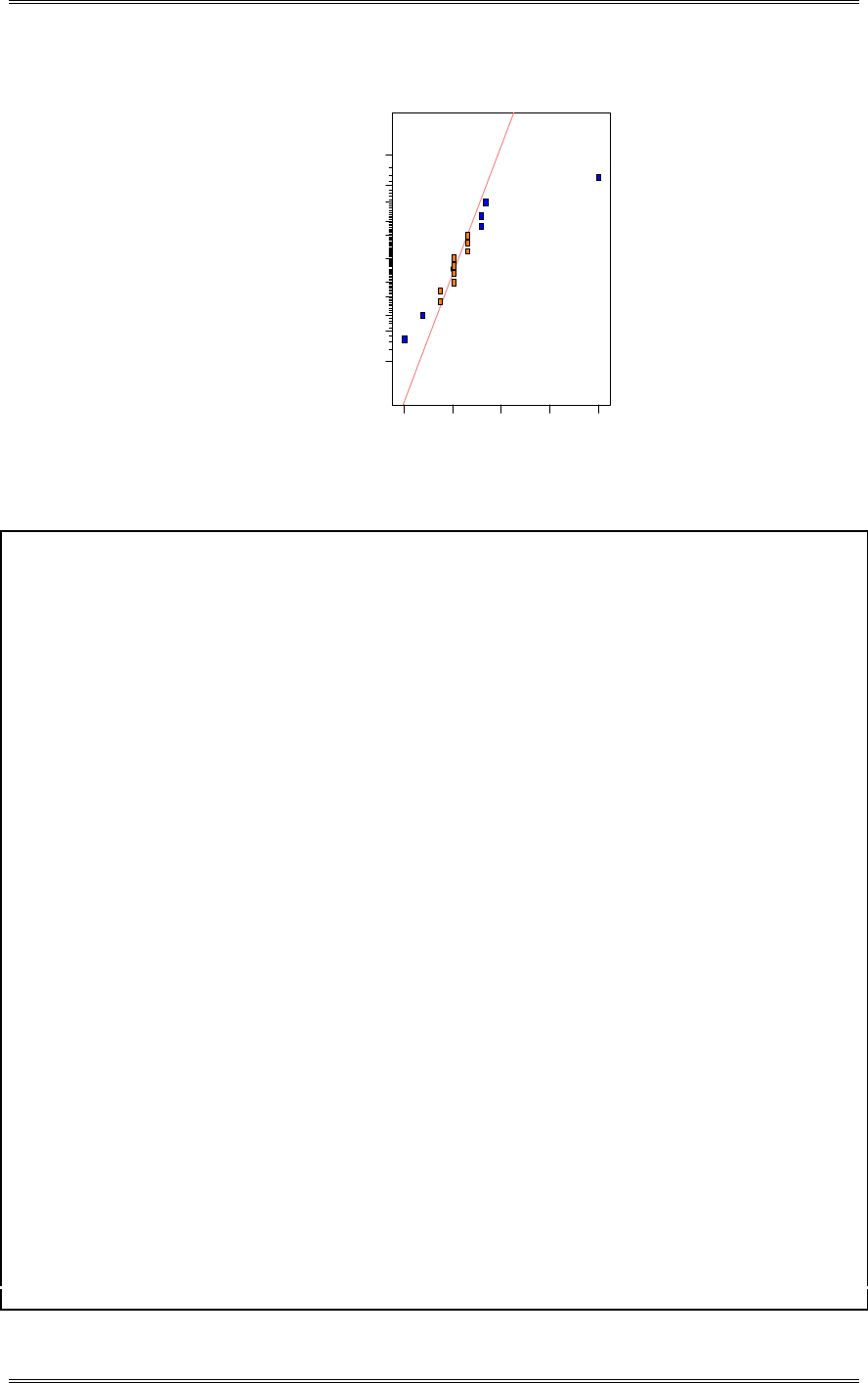
Solutions from Montgomery, D. C. (2001) Design and Analysis of Experiments, Wiley, NY
9-17
DESIGN-EXPERT Plot
Rank
A: Clone
B: Berry Size
C: Ferm T emp 1
D: Ferm T emp 2
E: W h o le B erry
F: Macer Time
G: Yeast
H: Oak
Normal plot
Normal % probability
Effe ct
-2 .7 5 -0 .0 6 2.63 5.31 8.00
1
5
10
20
30
50
70
80
90
95
99
A
B
C
D
E
F
Design Expert Output
Response: Rank
ANOVA for Selected Factorial Model
Analysis of variance table [Partial sum of squares]
Sum of Mean F
Source Squares DF Square Value Prob > F
Model 328.75 6 54.79 43.83 < 0.0001 significant
A 30.25 1 30.25 24.20 0.0008
B 9.00 1 9.00 7.20 0.0251
C 9.00 1 9.00 7.20 0.0251
D 12.25 1 12.25 9.80 0.0121
E 12.25 1 12.25 9.80 0.0121
F 256.00 1 256.00 204.80 < 0.0001
Residual 11.25 9 1.25
Cor Total 340.00 15
The Model F-value of 43.83 implies the model is significant. There is only
a 0.01% chance that a "Model F-Value" this large could occur due to noise.
Std. Dev. 1.12 R-Squared 0.9669
Mean 8.50 Adj R-Squared 0.9449
C.V. 13.15 Pred R-Squared 0.8954
PRESS 35.56 Adeq Precision 19.270
Coefficient Standard 95% CI 95% CI
Factor Estimate DF Error Low High VIF
Intercept 8.50 1 0.28 7.87 9.13
A-Clone -1.38 1 0.28 -2.01 -0.74 1.00
B-Berry Size 0.75 1 0.28 0.12 1.38 1.00
C-Ferm Temp 1 0.75 1 0.28 0.12 1.38 1.00
D-Ferm Temp 2 0.88 1 0.28 0.24 1.51 1.00
E-Whole Berry -0.87 1 0.28 -1.51 -0.24 1.00
F-Macer Time 4.00 1 0.28 3.37 4.63 1.00
Final Equation in Terms of Coded Factors:
Rank =
+8.50
-1.38 * A
+0.75 * B
+0.75 * C
+0.88 * D
-0.87 * E
+4.00 * F

Solutions from Montgomery, D. C. (2001) Design and Analysis of Experiments, Wiley, NY
9-18
(c) What comparisons can you make between this experiment and the 1985 Pinot Noir experiment from
Problem 8-26?
The experiment from Problem 8-26 indicates that yeast, barrel, whole cluster and the clone x yeast
interactions were significant. This experiment indicates that maceration time, whole berry, clone and
fermentation temperature are significant.
9-23 An article by W.D. Baten in the 1956 volume of Industrial Quality Control described an
experiment to study the effect of three factors on the lengths of steel bars. Each bar was subjected to one
of two heat treatment processes, and was cut on one of four machines at one of three times during the day
(8 am, 11 am, or 3 pm). The coded length data are shown below
(a) Analyze the data from this experiment assuming that the four observations in each cell are replicates.
The Machine effect (C) is significant, the Heat Treat Process (B) is also significant, while the Time of Day
(A) is not significant. None of the interactions are significant.
Design Expert Output
Response: Length
ANOVA for Selected Factorial Model
Analysis of variance table [Partial sum of squares]
Sum of Mean F
Source Squares DF Square Value Prob > F
Model 590.33 23 25.67 4.13 < 0.0001 significant
A 26.27 2 13.14 2.11 0.1283
B 42.67 1 42.67 6.86 0.0107
C 393.42 3 131.14 21.10 < 0.0001
AB 23.77 2 11.89 1.91 0.1552
AC 42.15 6 7.02 1.13 0.3537
BC 13.08 3 4.36 0.70 0.5541
ABC 48.98 6 8.16 1.31 0.2623
Pure Error 447.50 72 6.22
Cor Total 1037.83 95
The Model F-value of 4.13 implies the model is significant. There is only
a 0.01% chance that a "Model F-Value" this large could occur due to noise.
Std. Dev. 2.49 R-Squared 0.5688
Mean 3.96 Adj R-Squared 0.4311
Time of
Da
y
Heat Treat
Process
69791266
13550473
4665-1045
01340154
63873279
1-14810116
31642094
1-213-1163
5 4 10 11 -1 2 10 5
96646148
60870-243
371004-470
34
Machine
2
1
2
8am
11 am
3 pm
1
2
1
12

Solutions from Montgomery, D. C. (2001) Design and Analysis of Experiments, Wiley, NY
9-19
C.V. 62.98 Pred R-Squared 0.2334
PRESS 795.56 Adeq Precision 7.020
Coefficient Standard 95% CI 95% CI
Term Estimate DF Error Low High VIF
Intercept 3.96 1 0.25 3.45 4.47
A[1] 0.010 1 0.36 -0.71 0.73
A[2] -0.65 1 0.36 -1.36 0.071
B-Process -0.67 1 0.25 -1.17 -0.16 1.00
C[1] -0.54 1 0.44 -1.42 0.34
C[2] 1.92 1 0.44 1.04 2.80
C[3] -3.08 1 0.44 -3.96 -2.20
A[1]B 0.010 1 0.36 -0.71 0.73
A[2]B 0.60 1 0.36 -0.11 1.32
A[1]C[1] 0.32 1 0.62 -0.92 1.57
A[2]C[1] -1.27 1 0.62 -2.51 -0.028
A[1]C[2] -0.39 1 0.62 -1.63 0.86
A[2]C[2] -0.10 1 0.62 -1.35 1.14
A[1]C[3] 0.24 1 0.62 -1.00 1.48
A[2]C[3] 0.77 1 0.62 -0.47 2.01
BC[1] -0.25 1 0.44 -1.13 0.63
BC[2] -0.46 1 0.44 -1.34 0.42
BC[3] 0.46 1 0.44 -0.42 1.34
A[1]BC[1] -0.094 1 0.62 -1.34 1.15
A[2]BC[1] -0.44 1 0.62 -1.68 0.80
A[1]BC[2] 0.11 1 0.62 -1.13 1.36
A[2]BC[2] -1.10 1 0.62 -2.35 0.14
A[1]BC[3] -0.43 1 0.62 -1.67 0.82
A[2]BC[3] 0.60 1 0.62 -0.64 1.85
Final Equation in Terms of Coded Factors:
Length =
+3.96
+0.010 * A[1]
-0.65 * A[2]
-0.67 * B
-0.54 * C[1]
+1.92 * C[2]
-3.08 * C[3]
+0.010 * A[1]B
+0.60 * A[2]B
+0.32 * A[1]C[1]
-1.27 * A[2]C[1]
-0.39 * A[1]C[2]
-0.10 * A[2]C[2]
+0.24 * A[1]C[3]
+0.77 * A[2]C[3]
-0.25 * BC[1]
-0.46 * BC[2]
+0.46 * BC[3]
-0.094 * A[1]BC[1]
-0.44 * A[2]BC[1]
+0.11 * A[1]BC[2]
-1.10 * A[2]BC[2]
-0.43 * A[1]BC[3]
+0.60 * A[2]BC[3]
(b) Analyze the residuals from this experiment. Is there any indication that there is an outlier in one
cell? If you find an outlier, remove it and repeat the analysis from part (a). What are your
conclusions?
Standard Order 84, Time of Day at 3:00pm, Heat Treat #2, Machine #2, and length of 0, appears to be an
outlier.
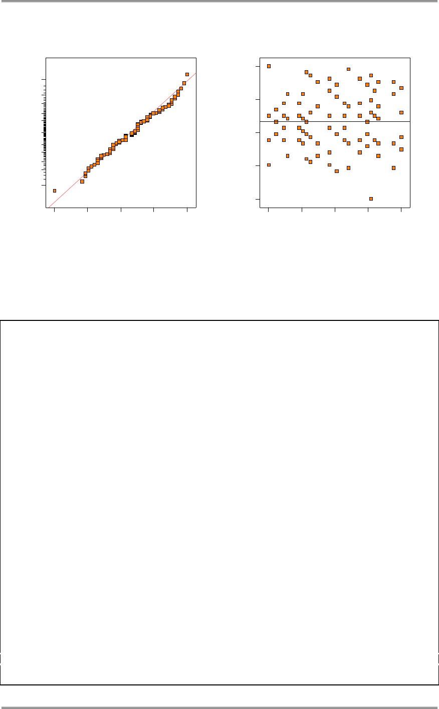
Solutions from Montgomery, D. C. (2001) Design and Analysis of Experiments, Wiley, NY
9-20
Residual
Normal % probability
Normal plot of residuals
-6 .2 5 -3 .5 6 2 5 -0 . 8 75 1.8125 4.5
1
5
10
20
30
50
70
80
90
95
99
3
3
3
2
2
2
2
2
3 3
2
232
2
33
2
2
3
32
2
3
2
3
Predicted
Residuals
Residuals vs. Predicted
-6 .2 5
-3 .5 62 5
-0 .8 75
1.8125
4.5
-0 .5 0 1.69 3.88 6.06 8.25
The following analysis was performed with the outlier described above removed. As with the original
analysis, Machine is significant and Heat Treat Process is also significant, but now Time of Day, factor A,
is also significant with an F-value of 3.05 (the P-value is just above 0.05).
Design Expert Output
Response: Length
ANOVA for Selected Factorial Model
Analysis of variance table [Partial sum of squares]
Sum of Mean F
Source Squares DF Square Value Prob > F
Model 626.58 23 27.24 4.89 < 0.0001 significant
A 34.03 2 17.02 3.06 0.0533
B 33.06 1 33.06 5.94 0.0173
C 411.89 3 137.30 24.65 < 0.0001
AB 16.41 2 8.20 1.47 0.2361
AC 50.19 6 8.37 1.50 0.1900
BC 8.38 3 2.79 0.50 0.6824
ABC 67.00 6 11.17 2.01 0.0762
Pure Error 395.42 71 5.57
Cor Total 1022.00 94
The Model F-value of 4.89 implies the model is significant. There is only
a 0.01% chance that a "Model F-Value" this large could occur due to noise.
Std. Dev. 2.36 R-Squared 0.6131
Mean 4.00 Adj R-Squared 0.4878
C.V. 59.00 Pred R-Squared 0.3100
PRESS 705.17 Adeq Precision 7.447
Coefficient Standard 95% CI 95% CI
Term Estimate DF Error Low High VIF
Intercept 4.05 1 0.24 3.z56 4.53
A[1] -0.076 1 0.34 -0.76 0.61
A[2] -0.73 1 0.34 -1.41 -0.051
B-Process -0.58 1 0.24 -1.06 -0.096 1.00
C[1] -0.63 1 0.42 -1.46 0.21
C[2] 2.18 1 0.43 1.33 3.03
C[3] -3.17 1 0.42 -4.00 -2.34
A[1]B -0.076 1 0.34 -0.76 0.61
A[2]B 0.52 1 0.34 -0.16 1.20
A[1]C[1] 0.41 1 0.59 -0.77 1.59
A[2]C[1] -1.18 1 0.59 -2.36 -6.278E-003
A[1]C[2] -0.65 1 0.60 -1.83 0.54
A[2]C[2] -0.36 1 0.60 -1.55 0.82
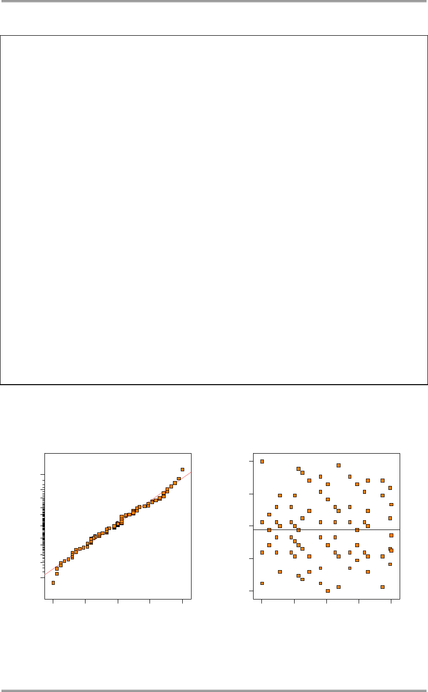
Solutions from Montgomery, D. C. (2001) Design and Analysis of Experiments, Wiley, NY
9-21
A[1]C[3] 0.33 1 0.59 -0.85 1.50
A[2]C[3] 0.86 1 0.59 -0.32 2.04
BC[1] -0.34 1 0.42 -1.17 0.50
BC[2] -0.20 1 0.43 -1.05 0.65
BC[3] 0.37 1 0.42 -0.46 1.21
A[1]BC[1] -6.944E-003 1 0.59 -1.18 1.17
A[2]BC[1] -0.35 1 0.59 -1.53 0.83
A[1]BC[2] -0.15 1 0.60 -1.33 1.04
A[2]BC[2] -1.36 1 0.60 -2.55 -0.18
A[1]BC[3] -0.34 1 0.59 -1.52 0.84
A[2]BC[3] 0.69 1 0.59 -0.49 1.87
Final Equation in Terms of Coded Factors:
Length =
+4.05
-0.076 * A[1]
-0.73 * A[2]
-0.58 * B
-0.63 * C[1]
+2.18 * C[2]
-3.17 * C[3]
-0.076 * A[1]B
+0.52 * A[2]B
+0.41 * A[1]C[1]
-1.18 * A[2]C[1]
-0.65 * A[1]C[2]
-0.36 * A[2]C[2]
+0.33 * A[1]C[3]
+0.86 * A[2]C[3]
-0.34 * BC[1]
-0.20 * BC[2]
+0.37 * BC[3]
-6.944E-003 * A[1]BC[1]
-0.35 * A[2]BC[1]
-0.15 * A[1]BC[2]
-1.36 * A[2]BC[2]
-0.34 * A[1]BC[3]
+0.69 * A[2]BC[3]
The following residual plots are acceptable. Both the normality and constant variance assumptions are
satisfied
Residual
Norm al % probability
Normal plot of residuals
-4 -1 .8 7 5 0.25 2.375 4.5
1
5
10
20
30
50
70
80
90
95
99
3
3
3
2
2
2
2
2
3 3
2
232
2
33
2
2
3
32
2
3
2
3
Predicted
Residuals
Residuals vs. Predicted
-4
-1 .8 75
0.25
2.375
4.5
-0 .5 0 1.71 3.92 6.12 8.33

Solutions from Montgomery, D. C. (2001) Design and Analysis of Experiments, Wiley, NY
9-22
(c) Suppose that the observations in the cells are the lengths (coded) of bars processed together in heat
treating and then cut sequentially (that is, in order) on the three machines. Analyze the data to
determine the effects of the three factors on mean length.
The analysis with all effects and interactions included:
Design Expert Output
Response: Length
ANOVA for Selected Factorial Model
Analysis of variance table [Partial sum of squares]
Sum of Mean F
Source Squares DF Square Value Prob > F
Model 147.58 23 6.42
A 6.57 2 3.28
B 10.67 1 10.67
C 98.35 3 32.78
AB 5.94 2 2.97
AC 10.54 6 1.76
BC 3.27 3 1.09
ABC 12.24 6 2.04
Pure Error 0.000 0
Cor Total 147.58 23
The by removing the three factor interaction from the model and applying it to the error, the analysis
identifies factor C as being significant and B as being mildly significant.
Design Expert Output
Response: Length
ANOVA for Selected Factorial Model
Analysis of variance table [Partial sum of squares]
Sum of Mean F
Source Squares DF Square Value Prob > F
Model 135.34 17 7.96 3.90 0.0502 not significant
A 6.57 2 3.28 1.61 0.2757
B 10.67 1 10.67 5.23 0.0623
C 98.35 3 32.78 16.06 0.0028
AB 5.94 2 2.97 1.46 0.3052
AC 10.54 6 1.76 0.86 0.5700
BC 3.27 3 1.09 0.53 0.6756
Residual 12.24 6 2.04
Cor Total 147.58 23
When removing the remaining insignificant factors from the model, C, Machine, is the most significant
factor while B, Heat Treat Process, is moderately significant. Factor A, Time of Day, is not significant.
Design Expert Output
Response: Avg
ANOVA for Selected Factorial Model
Analysis of variance table [Partial sum of squares]
Sum of Mean F
Source Squares DF Square Value Prob > F
Model 109.02 4 27.26 13.43 < 0.0001 significant
B 10.67 1 10.67 5.26 0.0335
C 98.35 3 32.78 16.15 < 0.0001
Residual 38.56 19 2.03
Cor Total 147.58 23
The Model F-value of 13.43 implies the model is significant. There is only
a 0.01% chance that a "Model F-Value" this large could occur due to noise.
Std. Dev. 1.42 R-Squared 0.7387
Mean 3.96 Adj R-Squared 0.6837
C.V. 35.99 Pred R-Squared 0.5831
PRESS 61.53 Adeq Precision 9.740
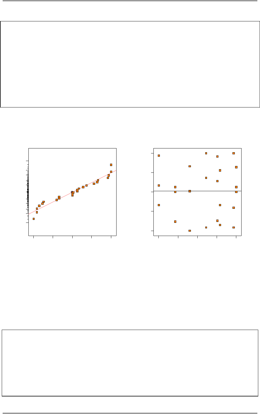
Solutions from Montgomery, D. C. (2001) Design and Analysis of Experiments, Wiley, NY
9-23
Coefficient Standard 95% CI 95% CI
Term Estimate DF Error Low High VIF
Intercept 3.96 1 0.29 3.35 4.57
B-Process -0.67 1 0.29 -1.28 -0.058 1.00
C[1] -0.54 1 0.50 -1.60 0.51
C[2] 1.92 1 0.50 0.86 2.97
C[3] -3.08 1 0.50 -4.14 -2.03
Final Equation in Terms of Coded Factors:
Avg =
+3.96
-0.67 * B
-0.54 * C[1]
+1.92 * C[2]
-3.08 * C[3]
The following residual plots are acceptable. Both the normality and uniformity of variance assumptions
are verified.
Residual
Normal % probability
Normal plot of residuals
-2 -1.02083 -0.0416667 0.9375 1.91667
1
5
10
20
30
50
70
80
90
95
99
Predicted
Residuals
Residuals vs. Predicted
-2
-1.02083
-0.0416667
0.9375
1.91667
0.21 1.79 3.38 4.96 6.54
(d) Calculate the log variance of the observations in each cell. Analyze the average length and the log
variance of the length for each of the 12 bars cut at each machine/heat treatment process combination.
What conclusions can you draw?
Factor B, Heat Treat Process, has an affect on the log variance of the observations while Factor A, Time of
Day, and Factor C, Machine, are not significant at the 5 percent level. However, A is significant at the 10
percent level, so Tome of Day has some effect on the variance.
Design Expert Output
Response: Log(Var)
ANOVA for Selected Factorial Model
Analysis of variance table [Partial sum of squares]
Sum of Mean F
Source Squares DF Square Value Prob > F
Model 2.79 11 0.25 2.51 0.0648 not significant
A 0.58 2 0.29 2.86 0.0966
B 0.50 1 0.50 4.89 0.0471
C 0.59 3 0.20 1.95 0.1757
AB 0.49 2 0.24 2.40 0.1324
BC 0.64 3 0.21 2.10 0.1538
Residual 1.22 12 0.10
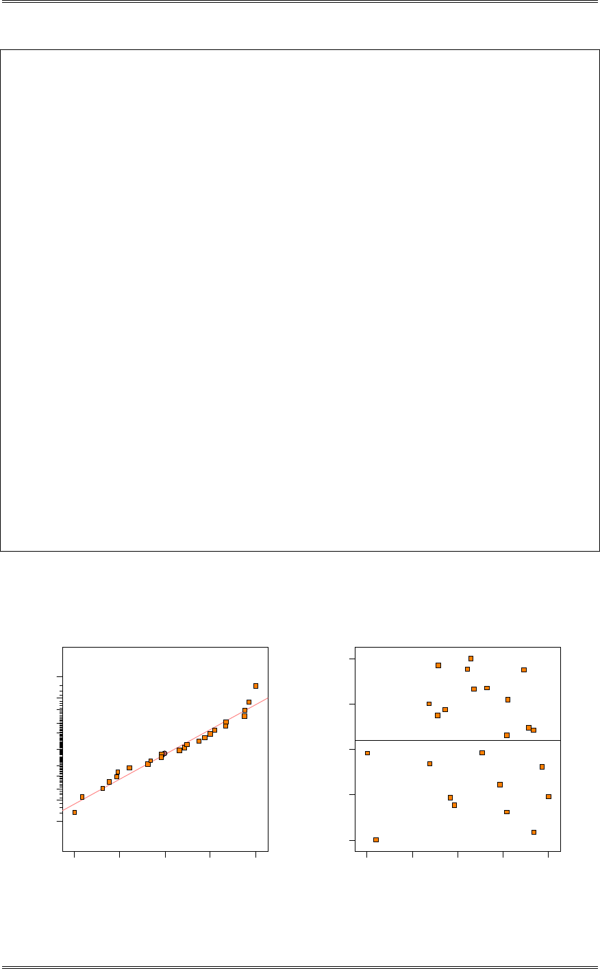
Solutions from Montgomery, D. C. (2001) Design and Analysis of Experiments, Wiley, NY
9-24
Cor Total 4.01 23
The Model F-value of 2.51 implies there is a 6.48% chance that a "Model F-Value"
this large could occur due to noise.
Std. Dev. 0.32 R-Squared 0.6967
Mean 0.65 Adj R-Squared 0.4186
C.V. 49.02 Pred R-Squared -0.2133
PRESS 4.86 Adeq Precision 5.676
Coefficient Standard 95% CI 95% CI
Term Estimate DF Error Low High VIF
Intercept 0.65 1 0.065 0.51 0.79
A[1] -0.054 1 0.092 -0.25 0.15
A[2] -0.16 1 0.092 -0.36 0.043
B-Process 0.14 1 0.065 2.181E-003 0.29 1.00
C[1] 0.22 1 0.11 -0.025 0.47
C[2] 0.066 1 0.11 -0.18 0.31
C[3] -0.19 1 0.11 -0.44 0.052
A[1]B -0.20 1 0.092 -0.40 3.237E-003
A[2]B 0.14 1 0.092 -0.065 0.34
BC[1] -0.18 1 0.11 -0.42 0.068
BC[2] -0.15 1 0.11 -0.39 0.098
BC[3] 0.14 1 0.11 -0.10 0.39
Final Equation in Terms of Coded Factors:
Log(Var) =
+0.65
-0.054 * A[1]
-0.16 * A[2]
+0.14 * B
+0.22 * C[1]
+0.066 * C[2]
-0.19 * C[3]
-0.20 * A[1]B
+0.14 * A[2]B
-0.18 * BC[1]
-0.15 * BC[2]
+0.14 * BC[3]
The following residual plots are acceptable. Both the normality and uniformity of variance assumptions
are verified.
Residual
Norm al % probability
Normal plot of residuals
-0.414972 -0.226114 -0.0372556 0.151602 0.340461
1
5
10
20
30
50
70
80
90
95
99
Predicted
Residuals
Residuals vs. Predicted
-0 .4 14 9 7 2
-0 .2 26 1 1 4
-0.0372556
0.151602
0.340461
-0 .1 2 0.20 0.52 0.84 1.16

Solutions from Montgomery, D. C. (2001) Design and Analysis of Experiments, Wiley, NY
9-25
(e) Suppose the time at which a bar is cut really cannot be controlled during routine production. Analyze
the average length and the log variance of the length for each of the 12 bars cut at each machine/heat
treatment process combination. What conclusions can you draw?
The analysis of the average length is as follows:
Design Expert Output
Response: Avg
ANOVA for Selected Factorial Model
Analysis of variance table [Partial sum of squares]
Sum of Mean F
Source Squares DF Square Value Prob > F
Model 37.43 7 5.35
A 3.56 1 3.56
B 32.78 3 10.93
AB 1.09 3 0.36
Pure Error 0.000 0
Cor Total 37.43 7
Because the Means Square of the AB interaction is much less than the main effects, it is removed from the
model and placed in the error. The average length is strongly affected by Factor B, Machine, and
moderately affected by Factor A, Heat Treat Process. The interaction effect was small and removed from
the model.
Design Expert Output
Response: Avg
ANOVA for Selected Factorial Model
Analysis of variance table [Partial sum of squares]
Sum of Mean F
Source Squares DF Square Value Prob > F
Model 36.34 4 9.09 25.00 0.0122 significant
A 3.56 1 3.56 9.78 0.0522
B 32.78 3 10.93 30.07 0.0097
Residual 1.09 3 0.36
Cor Total 37.43 7
The Model F-value of 25.00 implies the model is significant. There is only
a 1.22% chance that a "Model F-Value" this large could occur due to noise.
Std. Dev. 0.60 R-Squared 0.9709
Mean 3.96 Adj R-Squared 0.9320
C.V. 15.23 Pred R-Squared 0.7929
PRESS 7.75 Adeq Precision 13.289
Coefficient Standard 95% CI 95% CI
Term Estimate DF Error Low High VIF
Intercept 3.96 1 0.21 3.28 4.64
A-Process -0.67 1 0.21 -1.34 0.012 1.00
B[1] -0.54 1 0.37 -1.72 0.63
B[2] 1.92 1 0.37 0.74 3.09
B[3] -3.08 1 0.37 -4.26 -1.91
Final Equation in Terms of Coded Factors:
Avg =
+3.96
-0.67 * A
-0.54 * B[1]
+1.92 * B[2]
-3.08 * B[3]
The following residual plots are acceptable. Both the normality and uniformity of variance assumptions
are verified.
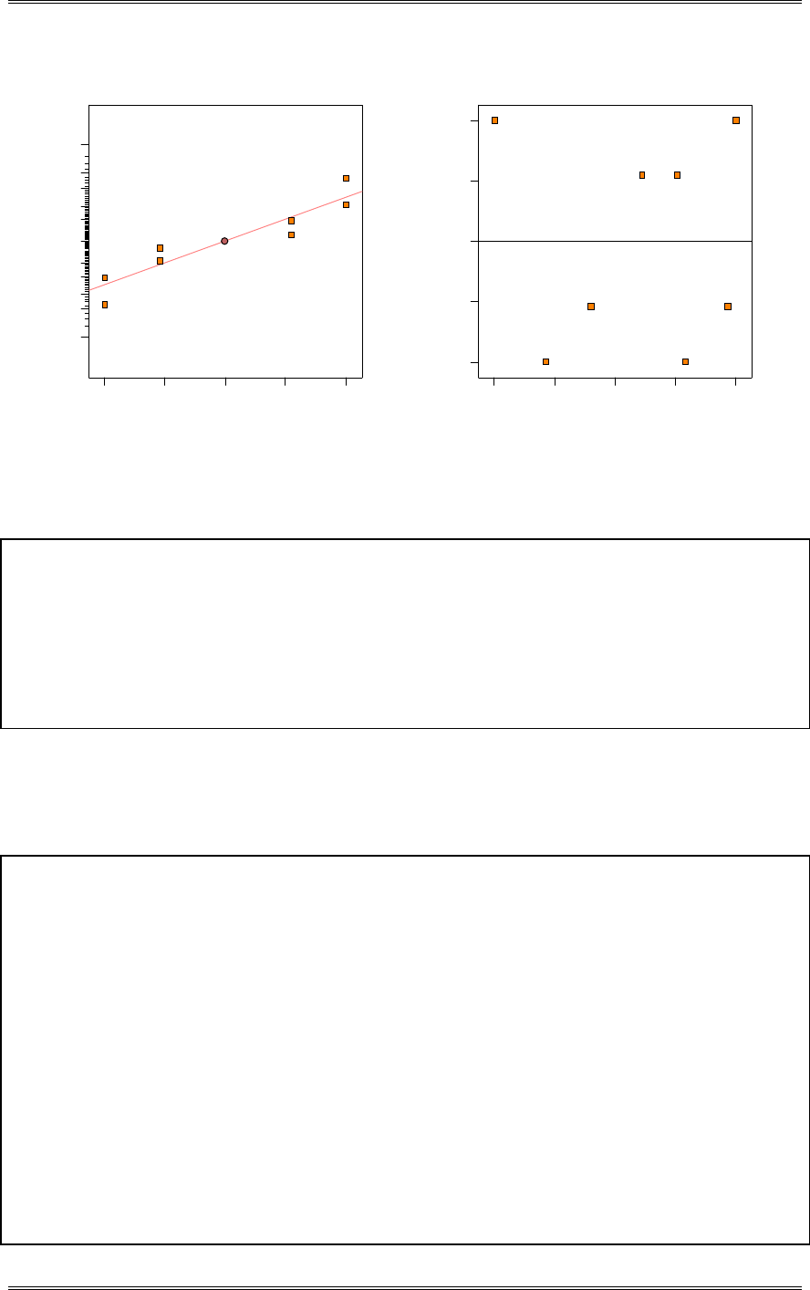
Solutions from Montgomery, D. C. (2001) Design and Analysis of Experiments, Wiley, NY
9-26
Residual
Normal % probability
Normal plot of residuals
-0.458333 -0.229167 00.229167 0.458333
1
5
10
20
30
50
70
80
90
95
99
Predicted
Residuals
Residuals vs. Predicted
-0 .4 58 3 3 3
-0 .2 29 1 6 7
0
0.229167
0.458333
0.21 1.79 3.38 4.96 6.54
The Log(Var) is analyzed below:
Design Expert Output
Response: Log(Var)
ANOVA for Selected Factorial Model
Analysis of variance table [Partial sum of squares]
Sum of Mean F
Source Squares DF Square Value Prob > F
Model 0.32 7 0.046
A 0.091 1 0.091
B 0.13 3 0.044
AB 0.098 3 0.033
Pure Error 0.000 0
Cor Total 0.32 7
Because the AB interaction has the smallest Mean Square, it was removed from the model and placed in
the error. From the following analysis of variance, neither Heat Treat Process, Machine, nor the
interaction affect the log variance of the length.
Design Expert Output
Response: Log(Var)
ANOVA for Selected Factorial Model
Analysis of variance table [Partial sum of squares]
Sum of Mean F
Source Squares DF Square Value Prob > F
Model 0.22 4 0.056 1.71 0.3441 not significant
A 0.091 1 0.091 2.80 0.1926
B 0.13 3 0.044 1.34 0.4071
Residual 0.098 3 0.033
Cor Total 0.32 7
The "Model F-value" of 1.71 implies the model is not significant relative to the noise. There is a
34.41 % chance that a "Model F-value" this large could occur due to noise.
Std. Dev. 0.18 R-Squared 0.6949
Mean 0.79 Adj R-Squared 0.2882
C.V. 22.90 Pred R-Squared -1.1693
PRESS 0.69 Adeq Precision 3.991
Coefficient Standard 95% CI 95% CI
Term Estimate DF Error Low High VIF
Intercept 0.79 1 0.064 0.59 0.99
A-Process 0.11 1 0.064 -0.096 0.31 1.00
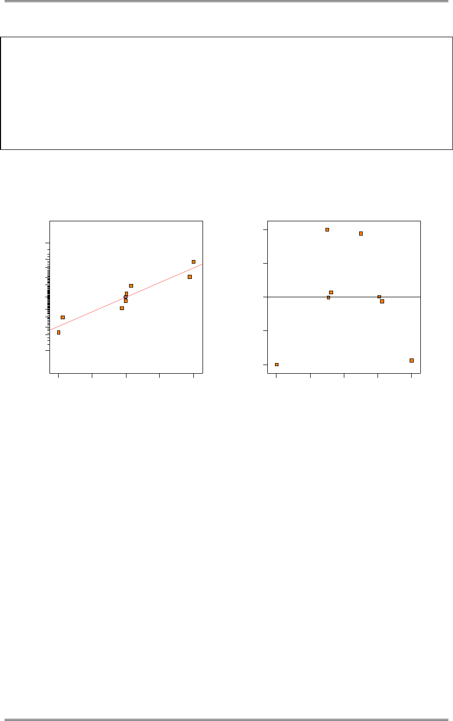
Solutions from Montgomery, D. C. (2001) Design and Analysis of Experiments, Wiley, NY
9-27
B[1] 0.15 1 0.11 -0.20 0.51
B[2] 0.030 1 0.11 -0.32 0.38
B[3] -0.20 1 0.11 -0.55 0.15
Final Equation in Terms of Coded Factors:
Log(Var) =
+0.79
+0.11 * A
+0.15 * B[1]
+0.030 * B[2]
-0.20 * B[3]
The following residual plots are acceptable. Both the normality and uniformity of variance assumptions
are verified.
Residual
Normal % probability
Normal plot of residuals
-0.160958 -0.0804791 00.0804791 0.160958
1
5
10
20
30
50
70
80
90
95
99
Predicted
Residuals
Residuals vs. Predicted
-0 .1 60 9 5 8
-0.0804791
0
0.0804791
0.160958
0.48 0.62 0.76 0.91 1.05
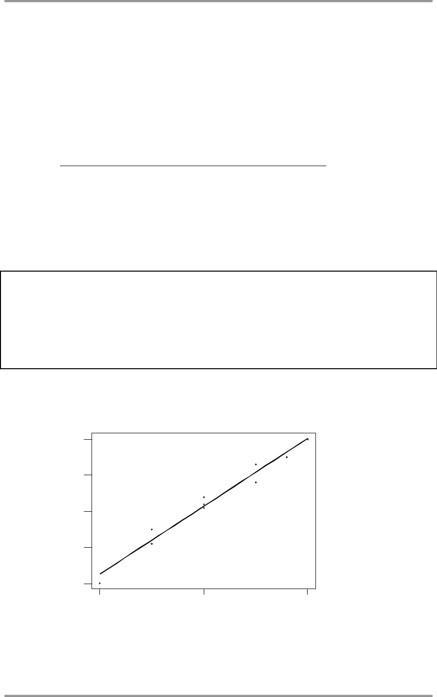
Solutions from Montgomery, D. C. (2001) Design and Analysis of Experiments, Wiley, NY
10-1
Chapter 10
Fitting Regression Models
Solutions
10-1 The tensile strength of a paper product is related to the amount of hardwood in the pulp. Ten
samples are produced in the pilot plant, and the data obtained are shown in the following table.
Strength Percent Hardwood Strength Percent Hardwood
160 10 181 20
171 15 188 25
175 15 193 25
182 20 195 28
184 20 200 30
(a) Fit a linear regression model relating strength to percent hardwood.
Minitab Output
Regression Analysis: Strength versus Hardwood
The regression equation is
Strength = 144 + 1.88 Hardwood
Predictor Coef SE Coef T P
Constant 143.824 2.522 57.04 0.000
Hardwood 1.8786 0.1165 16.12 0.000
S = 2.203 R-Sq = 97.0% R-Sq(adj) = 96.6%
PRESS = 66.2665 R-Sq(pred) = 94.91%
302010
200
190
180
170
160
Hardwood
Strength
S = 2.20320 R-Sq = 97.0 % R-Sq(adj) = 96.6 %
Strength = 143.824 + 1.87864 Hardwood
Regression Plot
(b) Test the model in part (a) for significance of regression.
Minitab Output

Solutions from Montgomery, D. C. (2001) Design and Analysis of Experiments, Wiley, NY
10-2
Analysis of Variance
Source DF SS MS F P
Regression 1 1262.1 1262.1 260.00 0.000
Residual Error 8 38.8 4.9
Lack of Fit 4 13.7 3.4 0.54 0.716
Pure Error 4 25.2 6.3
Total 9 1300.9
3 rows with no replicates
No evidence of lack of fit (P > 0.1)
(c) Find a 95 percent confidence interval on the parameter
E
1.
The 95 percent confidence interval is:
1,2111,21 ˆˆˆˆ
EEEEE
DD
setset pnpn dd
0.11653060.21.87860.11653060.21.8786 1dd
E
1473.26900.1 1dd
E
10-2 A plant distills liquid air to produce oxygen , nitrogen, and argon. The percentage of impurity in
the oxygen is thought to be linearly related to the amount of impurities in the air as measured by the
“pollution count” in part per million (ppm). A sample of plant operating data is shown below.
Purity(%) 93.3 92.0 92.4 91.7 94.0 94.6 93.6 93.1 93.2 92.9 92.2 91.3 90.1 91.6 91.9
Pollution count (ppm) 1.10 1.45 1.36 1.59 1.08 0.75 1.20 0.99 0.83 1.22 1.47 1.81 2.03 1.75 1.68
(a) Fit a linear regression model to the data.
Minitab Output
Regression Analysis: Purity versus Pollution
The regression equation is
Purity = 96.5 - 2.90 Pollution
Predictor Coef SE Coef T P
Constant 96.4546 0.4282 225.24 0.000
Pollutio -2.9010 0.3056 -9.49 0.000
S = 0.4277 R-Sq = 87.4% R-Sq(adj) = 86.4%
PRESS = 3.43946 R-Sq(pred) = 81.77%
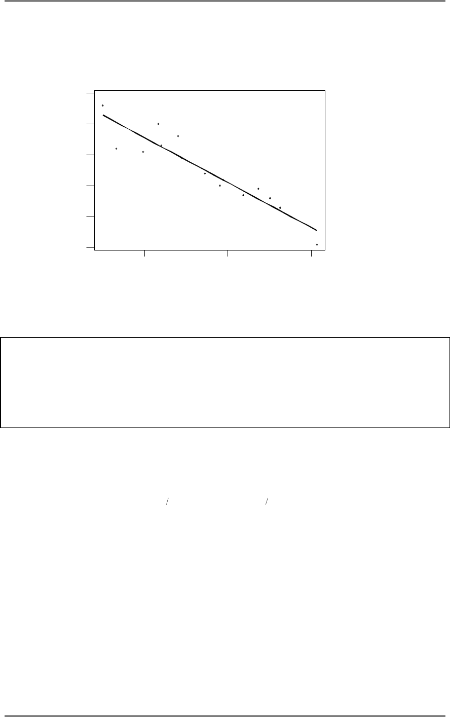
Solutions from Montgomery, D. C. (2001) Design and Analysis of Experiments, Wiley, NY
10-3
2.01.51.0
95
94
93
92
91
90
Pollution
Purity
S = 0.427745 R-Sq = 87.4 % R-Sq(adj) = 86.4 %
Purity = 96.4546 - 2.90096 Pollution
Regression Plot
(b) Test for significance of regression.
Minitab Output
Analysis of Variance
Source DF SS MS F P
Regression 1 16.491 16.491 90.13 0.000
Residual Error 13 2.379 0.183
Total 14 18.869
No replicates. Cannot do pure error test.
No evidence of lack of fit (P > 0.1)
(c) Find a 95 percent confidence interval on
E
1.
The 95 percent confidence interval is:
1,2111,21 ˆˆˆˆ
EEEEE
DD
setset pnpn dd
0.30561604.29010.2-0.30561604.29010.2- 1dd
E
2408.25612.3 1dd
E
10-3 Plot the residuals from Problem 10-1 and comment on model adequacy.
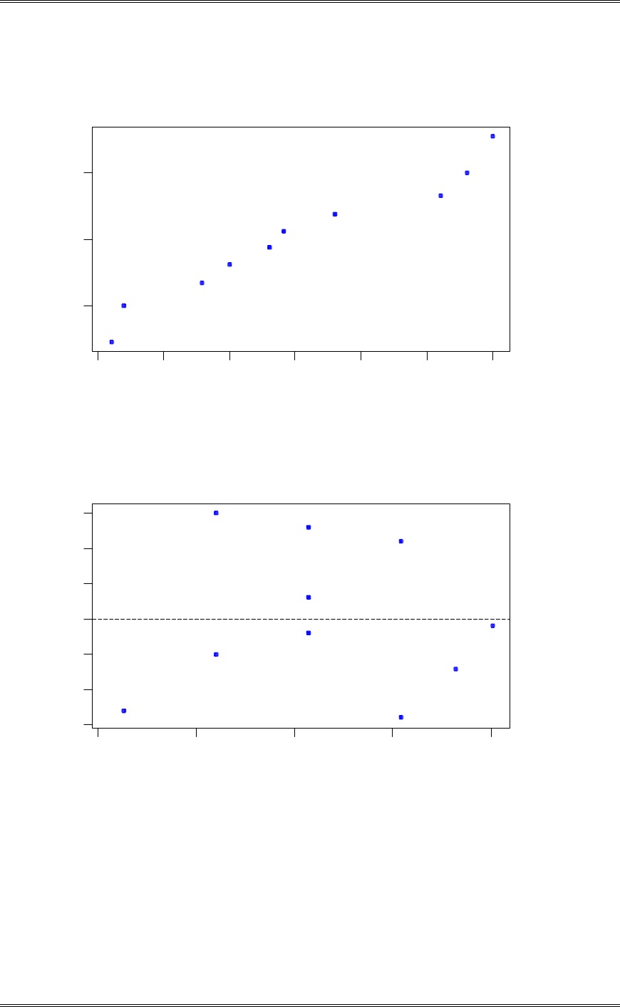
Solutions from Montgomery, D. C. (2001) Design and Analysis of Experiments, Wiley, NY
10-4
3210-1-2-3
1
0
-1
Normal Score
Residual
Normal Probability Plot of the Residuals
(response is Strength)
200190180170160
3
2
1
0
-1
-2
-3
Fitted Value
Residual
Residuals Versus the Fitted Values
(response is Strength)
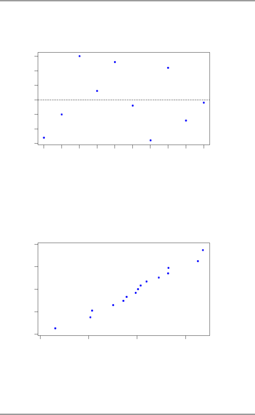
Solutions from Montgomery, D. C. (2001) Design and Analysis of Experiments, Wiley, NY
10-5
10987654321
3
2
1
0
-1
-2
-3
Observation Order
Residual
Residuals Versus the Order of the Data
(response is Strength)
There is nothing unusual about the residual plots. The underlying assumptions have been met.
10-4 Plot the residuals from Problem 10-2 and comment on model adequacy.
0.50.0-0.5-1.0
2
1
0
-1
-2
Normal Score
Residual
Normal Probability Plot of the Residuals
(response is Purity)
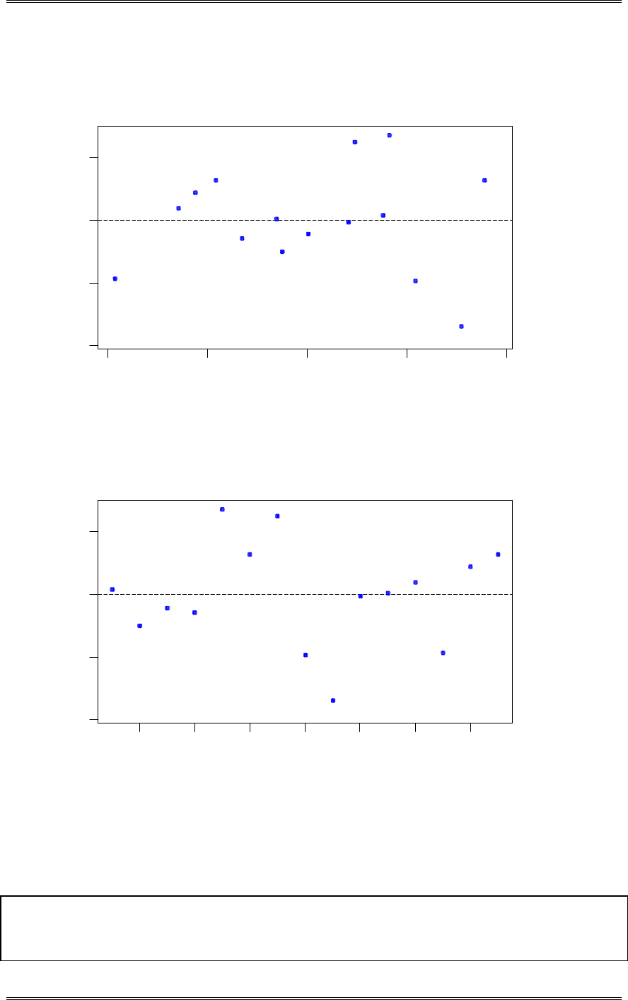
Solutions from Montgomery, D. C. (2001) Design and Analysis of Experiments, Wiley, NY
10-6
94.593.592.591.590.5
0.5
0.0
-0.5
-1.0
Fitted Value
Residual
Residuals Versus the Fitted Values
(response is Purity)
1412108642
0.5
0.0
-0.5
-1.0
Observation Order
Residual
Residuals Versus the Order of the Data
(response is Purity)
There is nothing unusual about the residual plots. The underlying assumptions have been met.
10-5 Using the results of Problem 10-1, test the regression model for lack of fit.
Minitab Output
Analysis of Variance
Source DF SS MS F P
Regression 1 1262.1 1262.1 260.00 0.000
Residual Error 8 38.8 4.9

Solutions from Montgomery, D. C. (2001) Design and Analysis of Experiments, Wiley, NY
10-7
Lack of Fit 4 13.7 3.4 0.54 0.716
Pure Error 4 25.2 6.3
Total 9 1300.9
3 rows with no replicates
No evidence of lack of fit (P > 0.1)
10-6 A study was performed on wear of a bearing y and its relationship to x1 = oil viscosity and x2 =
load. The following data were obtained.
y x1 x2
193 1.6 851
230 15.5 816
172 22.0 1058
91 43.0 1201
113 33.0 1357
125 40.0 1115
(a) Fit a multiple linear regression model to the data.
Minitab Output
Regression Analysis: Wear versus Viscosity, Load
The regression equation is
Wear = 351 - 1.27 Viscosity - 0.154 Load
Predictor Coef SE Coef T P VIF
Constant 350.99 74.75 4.70 0.018
Viscosit -1.272 1.169 -1.09 0.356 2.6
Load -0.15390 0.08953 -1.72 0.184 2.6
S = 25.50 R-Sq = 86.2% R-Sq(adj) = 77.0%
PRESS = 12696.7 R-Sq(pred) = 10.03%
(b) Test for significance of regression.
Minitab Output
Analysis of Variance
Source DF SS MS F P
Regression 2 12161.6 6080.8 9.35 0.051
Residual Error 3 1950.4 650.1
Total 5 14112.0
No replicates. Cannot do pure error test.
Source DF Seq SS
Viscosit 1 10240.4
Load 1 1921.2
* Not enough data for lack of fit test
(c) Compute t statistics for each model parameter. What conclusions can you draw?
Minitab Output
Regression Analysis: Wear versus Viscosity, Load
The regression equation is
Wear = 351 - 1.27 Viscosity - 0.154 Load
Predictor Coef SE Coef T P VIF
Constant 350.99 74.75 4.70 0.018

Solutions from Montgomery, D. C. (2001) Design and Analysis of Experiments, Wiley, NY
10-8
Viscosit -1.272 1.169 -1.09 0.356 2.6
Load -0.15390 0.08953 -1.72 0.184 2.6
S = 25.50 R-Sq = 86.2% R-Sq(adj) = 77.0%
PRESS = 12696.7 R-Sq(pred) = 10.03%
The t-tests are shown in part (a). Notice that overall regression is significant (part(b)), but neither
variable has a large t-statistic. This could be an indicator that the regressors are nearly linearly dependent.
10-7 The brake horsepower developed by an automobile engine on a dynomometer is thought to be a
function of the engine speed in revolutions per minute (rpm), the road octane number of the fuel, and the
engine compression. An experiment is run in the laboratory and the data that follow are collected.
Brake Horsepower rpm Road Octane Number Compression
225 2000 90 100
212 1800 94 95
229 2400 88 110
222 1900 91 96
219 1600 86 100
278 2500 96 110
246 3000 94 98
237 3200 90 100
233 2800 88 105
224 3400 86 97
223 1800 90 100
230 2500 89 104
(a) Fit a multiple linear regression model to the data.
Minitab Output
Regression Analysis: Horsepower versus rpm, Octane, Compression
The regression equation is
Horsepower = - 266 + 0.0107 rpm + 3.13 Octane + 1.87 Compression
Predictor Coef SE Coef T P VIF
Constant -266.03 92.67 -2.87 0.021
rpm 0.010713 0.004483 2.39 0.044 1.0
Octane 3.1348 0.8444 3.71 0.006 1.0
Compress 1.8674 0.5345 3.49 0.008 1.0
S = 8.812 R-Sq = 80.7% R-Sq(adj) = 73.4%
PRESS = 2494.05 R-Sq(pred) = 22.33%
(b) Test for significance of regression. What conclusions can you draw?
Minitab Output
Analysis of Variance
Source DF SS MS F P
Regression 3 2589.73 863.24 11.12 0.003
Residual Error 8 621.27 77.66
Total 11 3211.00
r No replicates. Cannot do pure error test.
Source DF Seq SS
rpm 1 509.35
Octane 1 1132.56
Compress 1 947.83
Lack of fit test
Possible interactions with variable Octane (P-Value = 0.028)
Possible lack of fit at outer X-values (P-Value = 0.000)
Overall lack of fit test is significant at P = 0.000
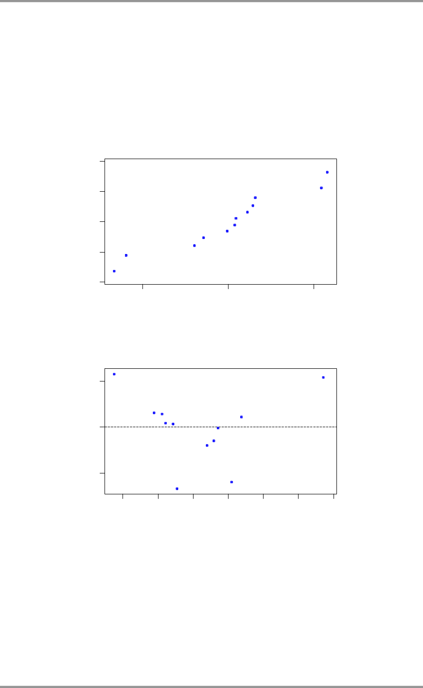
Solutions from Montgomery, D. C. (2001) Design and Analysis of Experiments, Wiley, NY
10-9
(c) Based on t tests, do you need all three regressor variables in the model?
Yes, all of the regressor variables are important.
10-8 Analyze the residuals from the regression model in Problem 10-7. Comment on model adequacy.
100-10
2
1
0
-1
-2
Normal Score
Residual
Normal Probability Plot of the Residuals
(respons e is Horsepow)
270260250240230220210
10
0
-10
Fitted Value
Residual
Residuals Versus the Fitted Values
(respons e is Horsepow)
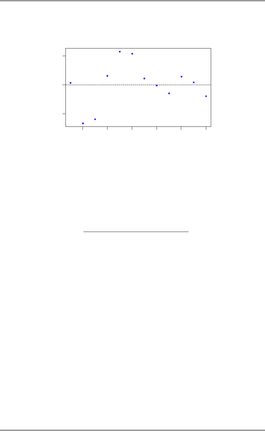
Solutions from Montgomery, D. C. (2001) Design and Analysis of Experiments, Wiley, NY
10-10
12108642
10
0
-10
Observation Order
Residual
Residuals Versus the Order of the Data
(respons e is Horsepow)
The normal probability plot is satisfactory, as is the plot of residuals versus run order (assuming that
observation order is run order). The plot of residuals versus predicted response exhibits a slight “bow”
shape. This could be an indication of lack of fit. It might be useful to consider adding some ineraction
terms to the model.
10-9 The yield of a chemical process is related to the concentration of the reactant and the operating
temperature. An experiment has been conducted with the following results.
Yield Concentration Temperature
81 1.00 150
89 1.00 180
83 2.00 150
91 2.00 180
79 1.00 150
87 1.00 180
84 2.00 150
90 2.00 180
(a) Suppose we wish to fit a main effects model to this data. Set up the X’X matrix using the data
exactly as it appears in the table.
»
»
»
¼
º
«
«
«
¬
ª
»
»
»
»
»
»
»
»
»
»
»
¼
º
«
«
«
«
«
«
«
«
«
«
«
¬
ª
»
»
»
¼
º
«
«
«
¬
ª
21960019801320
19802012
1320128
18000.21
15000.21
18000.11
15000.11
18000.21
15000.21
18000.11
15000.11
180150180150180150180150
00.200.200.100.100.200.200.100.1
11111111
(b) Is the matrix you obtained in part (a) diagonal? Discuss your response.

Solutions from Montgomery, D. C. (2001) Design and Analysis of Experiments, Wiley, NY
10-11
The X’X is not diagonal, even though an orthogonal design has been used. The reason is that we have
worked with the natural factor levels, not the orthogonally coded variables.
(c) Suppose we write our model in terms of the “usual” coded variables
5.0
5.1
1
Conc
x, 15
165
2
Temp
x
Set up the X’X matrix for the model in terms of these coded variables. Is this matrix diagonal? Discuss
your response.
111
111
111
1 1 11 1 1 11 8 0 0
111
1 1 11 1 1 11 0 8 0
111
1 1 11 1 1 11 0 0 8
111
111
111
ªº
«»
«»
«»
ªºªº
«»
«»«»
«»
«»«»
«»
«»«»
«»
¬¼¬¼
«»
«»
«»
«»
¬¼
The X’X matrix is diagonal because we have used the orthogonally coded variables.
(d) Define a new set of coded variables
0.1
0.1
1
Conc
x, 30
150
2
Temp
x
Set up the X’X matrix for the model in terms of this set of coded variables. Is this matrix diagonal?
Discuss your response.
»
»
»
¼
º
«
«
«
¬
ª
»
»
»
»
»
»
»
»
»
»
»
¼
º
«
«
«
«
«
«
«
«
«
«
«
¬
ª
»
»
»
¼
º
«
«
«
¬
ª
424
244
448
111
011
101
001
111
011
101
001
10101010
11001100
11111111
The X’X is not diagonal, even though an orthogonal design has been used. The reason is that we have not
used orthogonally coded variables.
(e) Summarize what you have learned from this problem about coding the variables.
If the design is orthogonal, use the orthogonal coding. This not only makes the analysis somewhat easier,
but it also results in model coefficients that are easier to interpret because they are both dimensionless and
uncorrelated.

Solutions from Montgomery, D. C. (2001) Design and Analysis of Experiments, Wiley, NY
10-12
10-10 Consider the 24 factorial experiment in Example 6-2. Suppose that the last observation in missing.
Reanalyze the data and draw conclusions. How do these conclusions compare with those from the
original example?
The regression analysis with the one data point missing indicates that the same effects are important.
Minitab Output
Regression Analysis: Rate versus A, B, C, D, AB, AC, AD, BC, BD, CD
The regression equation is
Rate = 69.8 + 10.5 A + 1.25 B + 4.63 C + 7.00 D - 0.25 AB - 9.38 AC + 8.00 AD
+ 0.87 BC - 0.50 BD - 0.87 CD
Predictor Coef SE Coef T P VIF
Constant 69.750 1.500 46.50 0.000
A 10.500 1.500 7.00 0.002 1.1
B 1.250 1.500 0.83 0.452 1.1
C 4.625 1.500 3.08 0.037 1.1
D 7.000 1.500 4.67 0.010 1.1
AB -0.250 1.500 -0.17 0.876 1.1
AC -9.375 1.500 -6.25 0.003 1.1
AD 8.000 1.500 5.33 0.006 1.1
BC 0.875 1.500 0.58 0.591 1.1
BD -0.500 1.500 -0.33 0.756 1.1
CD -0.875 1.500 -0.58 0.591 1.1
S = 5.477 R-Sq = 97.6% R-Sq(adj) = 91.6%
PRESS = 1750.00 R-Sq(pred) = 65.09%
Analysis of Variance
Source DF SS MS F P
Regression 10 4893.33 489.33 16.31 0.008
Residual Error 4 120.00 30.00
Total 14 5013.33
No replicates. Cannot do pure error test.
Source DF Seq SS
A 1 1414.40
B 1 4.01
C 1 262.86
D 1 758.88
AB 1 0.06
AC 1 1500.63
AD 1 924.50
BC 1 16.07
BD 1 1.72
CD 1 10.21
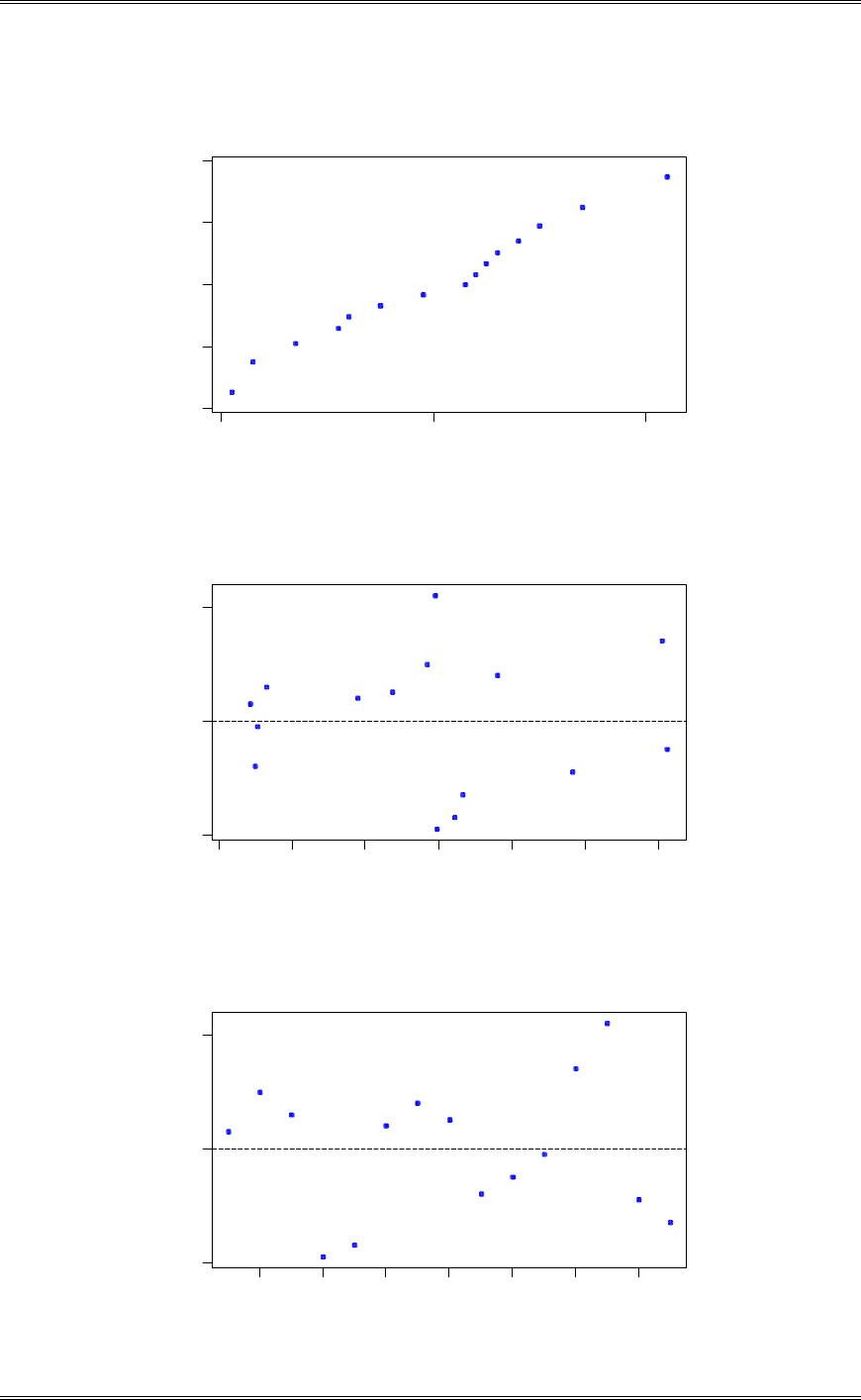
Solutions from Montgomery, D. C. (2001) Design and Analysis of Experiments, Wiley, NY
10-13
50-5
2
1
0
-1
-2
Normal Score
Residual
Normal Probability Plot of the Residuals
(response is Rate)
100908070605040
5
0
-5
Fitted Value
Residual
Residuals Versus the Fitted Values
(response is Rate)
1412108642
5
0
-5
Observation Order
Residual
Residuals Versus the Order of the Data
(response is Rate)

Solutions from Montgomery, D. C. (2001) Design and Analysis of Experiments, Wiley, NY
10-14
The residual plots are acceptable; therefore, the underlying assumptions are valid.
10-11 Consider the 24 factorial experiment in Example 6-2. Suppose that the last two observations are
missing. Reanalyze the data and draw conclusions. How do these conclusions compare with those from
the original example?
The regression analysis with the one data point missing indicates that the same effects are important.
Minitab Output
Regression Analysis: Rate versus A, B, C, D, AB, AC, AD, BC, BD, CD
The regression equation is
Rate = 71.4 + 10.1 A + 2.87 B + 6.25 C + 8.62 D - 0.66 AB - 9.78 AC + 7.59 AD
+ 2.50 BC + 1.12 BD + 0.75 CD
Predictor Coef SE Coef T P VIF
Constant 71.375 1.673 42.66 0.000
A 10.094 1.323 7.63 0.005 1.1
B 2.875 1.673 1.72 0.184 1.7
C 6.250 1.673 3.74 0.033 1.7
D 8.625 1.673 5.15 0.014 1.7
AB -0.656 1.323 -0.50 0.654 1.1
AC -9.781 1.323 -7.39 0.005 1.1
AD 7.594 1.323 5.74 0.010 1.1
BC 2.500 1.673 1.49 0.232 1.7
BD 1.125 1.673 0.67 0.549 1.7
CD 0.750 1.673 0.45 0.684 1.7
S = 4.732 R-Sq = 98.7% R-Sq(adj) = 94.2%
PRESS = 1493.06 R-Sq(pred) = 70.20%
Analysis of Variance
Source DF SS MS F P
Regression 10 4943.17 494.32 22.07 0.014
Residual Error 3 67.19 22.40
Total 13 5010.36
No replicates. Cannot do pure error test.
Source DF Seq SS
A 1 1543.50
B 1 1.52
C 1 177.63
D 1 726.01
AB 1 1.17
AC 1 1702.53
AD 1 738.11
BC 1 42.19
BD 1 6.00
CD 1 4.50
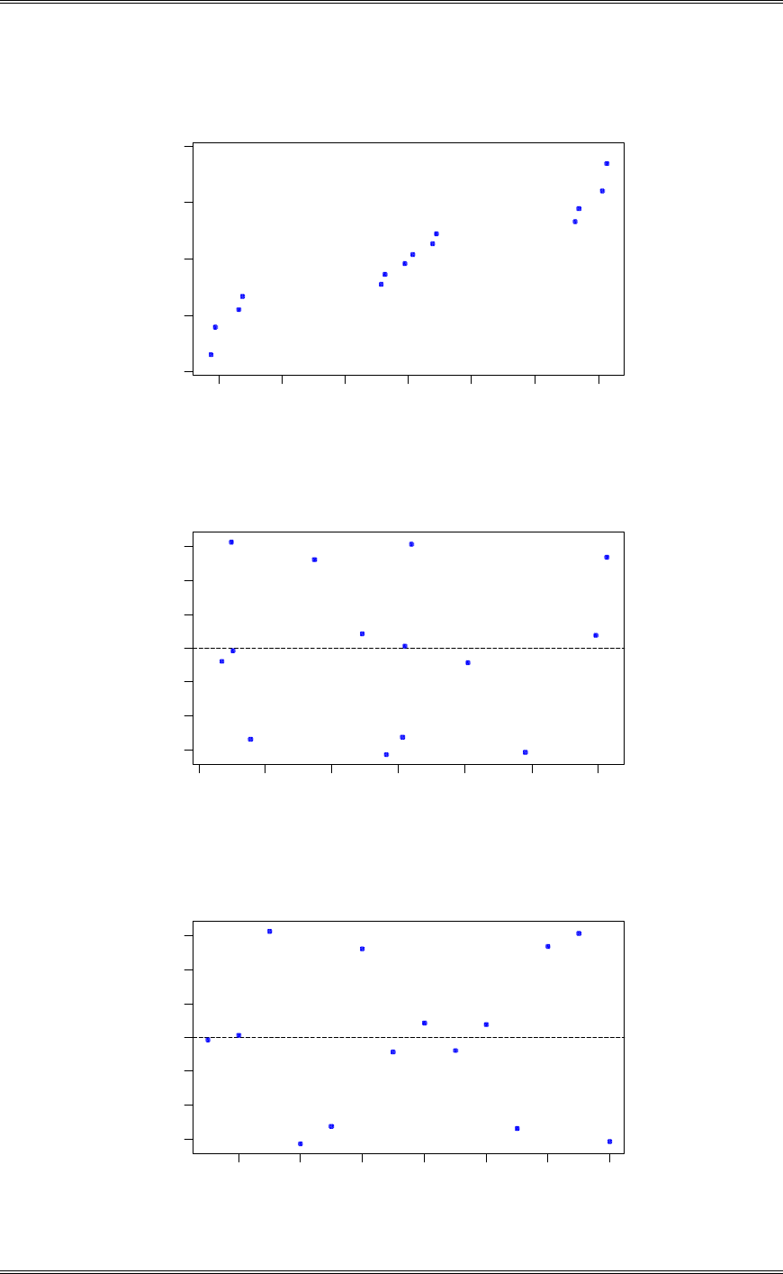
Solutions from Montgomery, D. C. (2001) Design and Analysis of Experiments, Wiley, NY
10-15
3210-1-2-3
2
1
0
-1
-2
Normal Score
Residual
Normal Probability Plot of the Residuals
(response is Rate)
100908070605040
3
2
1
0
-1
-2
-3
Fitted Value
Residual
Residuals Versus the Fitted Values
(response is Rate)
1412108642
3
2
1
0
-1
-2
-3
Observation Order
Residual
Residuals Versus the Order of the Data
(response is Rate)

Solutions from Montgomery, D. C. (2001) Design and Analysis of Experiments, Wiley, NY
10-16
The residual plots are acceptable; therefore, the underlying assumptions are valid.
10-12 Given the following data, fit the second-order polynomial regression model
HEEEEEE
2112
2
222
2
11122110 xxxxxxy
y x1 x2
26 1.0 1.0
24 1.0 1.0
175 1.5 4.0
160 1.5 4.0
163 1.5 4.0
55 0.5 2.0
62 1.5 2.0
100 0.5 3.0
26 1.0 1.5
30 0.5 1.5
70 1.0 2.5
71 0.5 2.5
After you have fit the model, test for significance of regression.
Minitab Output
Regression Analysis: y versus x1, x2, x1^2, x2^2, x1x2
The regression equation is
y = 24.4 - 38.0 x1 + 0.7 x2 + 35.0 x1^2 + 11.1 x2^2 - 9.99 x1x2
Predictor Coef SE Coef T P VIF
Constant 24.41 26.59 0.92 0.394
x1 -38.03 40.45 -0.94 0.383 89.6
x2 0.72 11.69 0.06 0.953 52.1
x1^2 34.98 21.56 1.62 0.156 103.9
x2^2 11.066 3.158 3.50 0.013 104.7
x1x2 -9.986 8.742 -1.14 0.297 105.1
S = 6.042 R-Sq = 99.4% R-Sq(adj) = 98.9%
PRESS = 1327.71 R-Sq(pred) = 96.24%
r Analysis of Variance
Source DF SS MS F P
Regression 5 35092.6 7018.5 192.23 0.000
Residual Error 6 219.1 36.5
Lack of Fit 3 91.1 30.4 0.71 0.607
Pure Error 3 128.0 42.7
Total 11 35311.7
7 rows with no replicates
Source DF Seq SS
x1 1 11552.0
x2 1 22950.3
x1^2 1 21.9
x2^2 1 520.8
x1x2 1 47.6
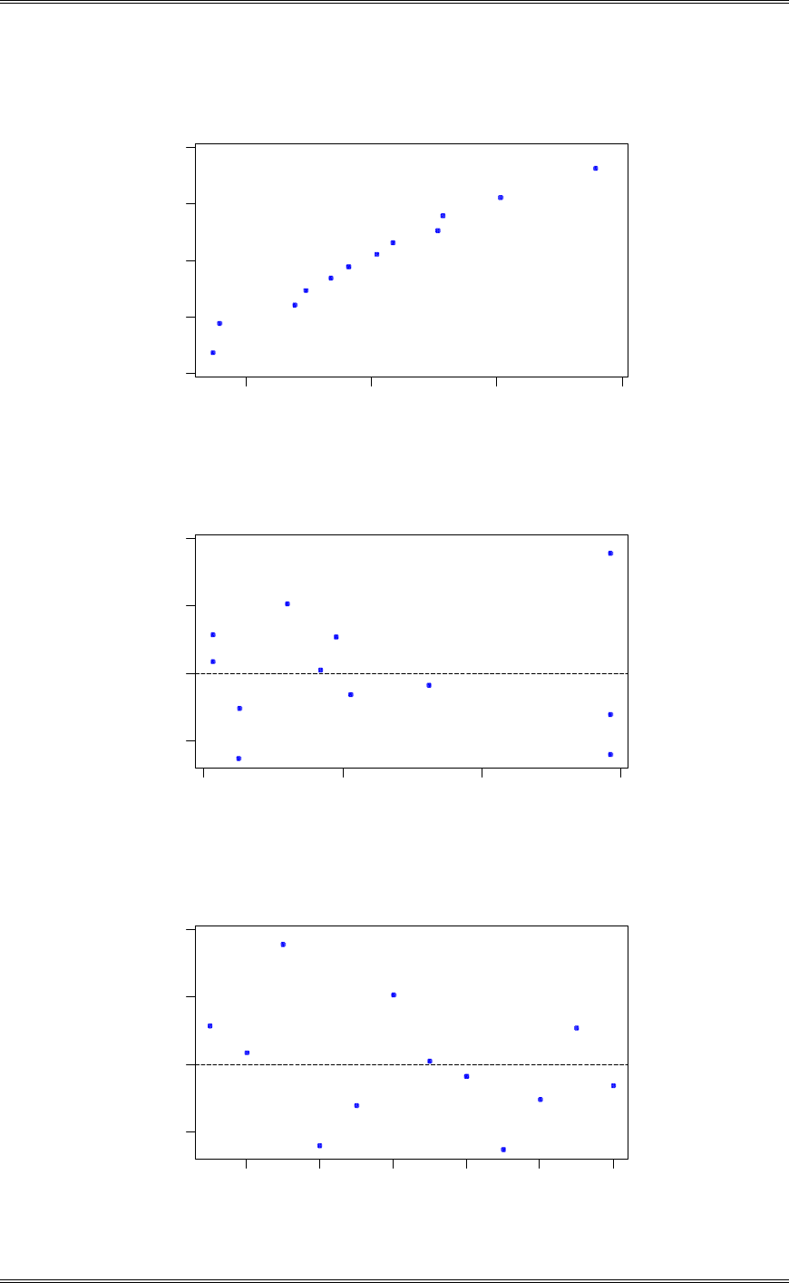
Solutions from Montgomery, D. C. (2001) Design and Analysis of Experiments, Wiley, NY
10-17
1050-5
2
1
0
-1
-2
Normal Score
Residual
Normal Probability Plot of the Residuals
(res ponse is y)
1701207020
10
5
0
-5
Fitted Value
Residual
Residuals Versus the Fitted Values
(res ponse is y)
12108642
10
5
0
-5
Observation Order
Residual
Residuals Versus the Order of the Data
(res ponse is y)
Solutions from Montgomery, D. C. (2001) Design and Analysis of Experiments, Wiley, NY
10-18
10-13
(a) Consider the quadratic regression model from Problem 10-12. Compute t statistics for each model
parameter and comment on the conclusions that follow from the quantities.
Minitab Output
Predictor Coef SE Coef T P VIF
Constant 24.41 26.59 0.92 0.394
x1 -38.03 40.45 -0.94 0.383 89.6
x2 0.72 11.69 0.06 0.953 52.1
x1^2 34.98 21.56 1.62 0.156 103.9
x2^2 11.066 3.158 3.50 0.013 104.7
x1x2 -9.986 8.742 -1.14 0.297 105.1
2
2
x is the only model parameter that is statistically significant with a t-value of 3.50. A logical model
might also include x2 to preserve model hierarchy.
(b) Use the extra sum of squares method to evaluate the value of the quadratic terms, 2
2
2
1,xx and 21 xx to
the model.
The extra sum of squares due to
E
2is
0
1021102101,02 ,,,,
E
EE
EE
EE
EE
EE
EE
EE
EE
EE
EE
EE
EE
EE
EE
EE
EE
EE
EE
EE
EE
EE
EE
EE
EE
EE
E
RRRRR SSSSSSSSSS
021,
E
EE
EE
EE
EE
EE
E
R
SS sum of squares of regression for the model in Problem 10-12 = 35092.6
0
1
E
EE
EE
EE
E
R
SS =34502.3
3.5903.345026.35092
1,02
E
EE
EE
EE
EE
EE
E
R
SS
3892.5
511.36
33.590
3
1,02
0
E
R
MS
SS
F
E
EE
EE
EE
EE
EE
E
Since 76.4
6,3,05.0 F, then the addition of the quadratic terms to the model is significant. The P-values
indicate that it’s probably the term 2
2
x that is responsible for this.
10-14 Relationship between analysis of variance and regression. Any analysis of variance model can be
expressed in terms of the general linear model y = XE
EE
E + H
HH
H , where the X matrix consists of zeros and
ones. Show that the single-factor model ijiij
y
HWP
, i=1,2,3, j=1,2,3,4 can be written in general
linear model form. Then
(a) Write the normal equations ˆ
()
cc
XX X
y
E
E E
E and compare them with the normal equations found for
the model in Chapter 3.
The normal equations are ˆ
()
cc
XX X
y
E
E E
E

Solutions from Montgomery, D. C. (2001) Design and Analysis of Experiments, Wiley, NY
10-19
»
»
»
»
¼
º
«
«
«
«
¬
ª
»
»
»
»
¼
º
«
«
«
«
¬
ª
»
»
»
»
¼
º
«
«
«
«
¬
ª
.3
.2
.1
..
3
2
1
ˆ
ˆ
ˆ
ˆ
4004
0404
0044
44412
y
y
y
y
W
W
W
P
which are in agreement with the results of Chapter 3.
(b) Find the rank of c
XX. Can 1
()
c
XX be obtained?
c
XXis a 4 x 4 matrix of rank 3, because the last three columns add to the first column. Thus (X’X)-1
does not exist.
(c) Suppose the first normal equation is deleted and the restriction ¦
3
10
ˆ
ii
n
W
is added. Can the
resulting system of equations be solved? If so, find the solution. Find the regression sum of squares
ˆcc
X
y
E
EE
E, and compare it to the treatment sum of squares in the single-factor model.
Imposing ¦
3
10
ˆ
ii
n
W
yields the normal equations
»
»
»
»
¼
º
«
«
«
«
¬
ª
»
»
»
»
¼
º
«
«
«
«
¬
ª
»
»
»
»
¼
º
«
«
«
«
¬
ª
.3
.2
.1
..
3
2
1
ˆ
ˆ
ˆ
ˆ
4004
0404
0044
4440
y
y
y
y
W
W
W
P
The solution to this set of equations is
..
..
12
ˆy
y
P
...
ˆyyii
W
This solution was found be solving the last three equations for i
W
ˆ, yielding
PW
ˆˆ . ii y, and then
substituting in the first equation to find ..
ˆy
P
The regression sum of squares is
E
EE
EE
EE
E
ˆc
R
SS X’y =
¦¦¦
a
i
i
a
i
i
a
i
in
y
an
y
n
y
an
y
yyyy
1
2
.
1
2
..
2
.
2
..
1
2
.......
with a degrees of freedom. This is the same result found in Chapter 3. For more discussion of the
relationship between analysis of variance and regression, see Montgomery and Peck (1992).
10-15 Suppose that we are fitting a straight line and we desire to make the variance of as small as
possible. Restricting ourselves to an even number of experimental points, where should we place these
points so as to minimize
1
ˆ
E
V? (Note: Use the design called for in this exercise with great caution
because, even though it minimized
1
ˆ
E
V, it has some undesirable properties; for example, see Myers and

Solutions from Montgomery, D. C. (2001) Design and Analysis of Experiments, Wiley, NY
10-20
Montgomery (1995). Only if you are very sure the true functional relationship is linear should you
consider using this design.
Since
xx
S
V
2
1
ˆ
V
E
, we may minimize
1
ˆ
E
Vby making Sxx as large as possible. Sxx is maximized by
spreading out the xj’s as much as possible. The experimenter usually has a “region of interest” for x. If n is
even, n/2 of the observations should be run at each end of the “region of interest”. If n is odd, then run
one of the observations in the center of the region and the remaining (n-1)/2 at either end.
10-16 Weighted least squares. Suppose that we are fitting the straight line
HEE
xy 10 , but the
variance of the y’s now depends on the level of x; that is,
ni
w
xyV
i
i,...,2,1,
2
2
V
V
where the wi are known constants, often called weights. Show that if we choose estimates of the
regression coefficients to minimize the weighted sum of squared errors given by
¦
n
i
iii xyw
1
2
10
EE
,
the resulting least squares normal equations are
¦¦¦
n
i
n
i
iii
n
i
ii ywxww
111
10 ˆˆ
EE
¦¦¦
n
i
n
i
iiii
n
i
iii yxwxwxw
11
2
1
10 ˆˆ
EE
The least squares normal equations are found:
0
ˆˆ
2
0
ˆˆ
2
1
1110
1
1
110
0
1
2
110
¦
¦
¦
n
i
ii
n
i
ii
n
i
ii
wxxy
L
wxy
L
wxyL
EE
wE
w
EE
wE
w
EE
which simplify to
i
n
i
i
n
i
n
i
ii
i
n
i
i
n
i
n
i
ii
yxwwxwx
ywwxw
¦¦¦
¦¦¦
1
1
11
2
1110
111
110
ˆˆ
ˆˆ
EE
EE
10-17 Consider the 14
2
IV design discussed in Example 10-5.

Solutions from Montgomery, D. C. (2001) Design and Analysis of Experiments, Wiley, NY
10-21
(a) Suppose you elect to augment the design with the single run selected in that example. Find the
variances and covariances of the regression coefficients in the model (ignoring blocks):
HEEEEEEE
43342112443322110 xxxxxxxxy
»
»
»
»
»
»
»
»
»
¼
º
«
«
«
«
«
«
«
«
«
¬
ª
»
»
»
»
»
»
»
»
»
»
»
»
¼
º
«
«
«
«
«
«
«
«
«
«
«
«
¬
ª
»
»
»
»
»
»
»
¼
º
«
«
«
«
«
«
«
¬
ª
9711111
7911111
1191111
1119111
1111911
1111191
1111119
1111111
1111111
1111111
1111111
1111111
1111111
1111111
1111111
1111111
111111111
111111111
111111111
111111111
111111111
111111111
111111111
XX'
»
»
»
»
»
»
»
»
»
¼
º
«
«
«
«
«
«
«
«
«
¬
ª
4375.0375.00625.00625.00625.00625.00625.0
375.04375.00625.00625.00625.00625.00625.0
0625.00625.0125.00000
0625.00625.00125.0000
0625.00625.000125.000
0625.00625.0000125.00
0625.00625.00000125.0
)( 1
XX'
(b) Are there any other runs in the alternate fraction that
Any other run from the alternate fraction will dealias AB from CD.
(c) Suppose you augment the design with four runs suggested in Example 10-5. Find the variance and
the covariances of the regression coefficients (ignoring blocks) for the model in part (a).
Choose 4 runs that are one of the quarter fractions not used in the principal half fraction.
»
»
»
»
»
»
»
»
»
»
»
»
»
»
»
»
»
¼
º
«
«
«
«
«
«
«
«
«
«
«
«
«
«
«
«
«
¬
ª
»
»
»
»
»
»
»
»
»
¼
º
«
«
«
«
«
«
«
«
«
¬
ª
1111111
1111111
1111111
1111111
1111111
1111111
1111111
1111111
1111111
1111111
1111111
1111111
111111111111
111111111111
111111111111
111111111111
111111111111
111111111111
111111111111
XX'

Solutions from Montgomery, D. C. (2001) Design and Analysis of Experiments, Wiley, NY
10-22
»
»
»
»
»
»
»
»
»
¼
º
«
«
«
«
«
«
«
«
«
¬
ª
12000000
01240040
04120040
00012400
00041200
04400120
00000012
XX'
»
»
»
»
»
»
»
»
»
¼
º
«
«
«
«
«
«
«
«
«
¬
ª
1785.01429.00357.0000357.00
1429.02142.00536.0000536.00
0357.00536.01071.0000179.00
0000938.00313.000
0000313.00938.000
0357.00536.00179.0001071.00
0000000833.0
1
XX'
(d) Considering parts (a) and (c), which augmentation strategy would you prefer and why?
If you only have the resources to run one more run, then choose the one-run augmentation. But if
resources are not scarce, then augment the design in multiples of two runs, to keep the design orthogonal.
Using four runs results in smaller variances of the regression coefficients and a simpler covariance
structure.
10-18 Consider the 47
2
III . Suppose after running the experiment, the largest observed effects are A +
BD, B + AD, and D + AB. You wish to augment the original design with a group of four runs to dealias
these effects.
(a) Which four runs would you make?
Take the first four runs of the original experiment and change the sign on A.
Design Expert Output
Factor 1 Factor 2 Factor 3 Factor 4 Factor 5 Factor 6 Factor 7
Std Run Block A:x1 B:x2 C:x3 D:x4 E:x5 F:x6 G:x7
1 1 Block 1 -1.00 -1.00 -1.00 1.00 1.00 1.00 -1.00
2 2 Block 1 1.00 -1.00 -1.00 -1.00 -1.00 1.00 1.00
3 3 Block 1 -1.00 1.00 -1.00 -1.00 1.00 -1.00 1.00
4 4 Block 1 1.00 1.00 -1.00 1.00 -1.00 -1.00 -1.00
5 5 Block 1 -1.00 -1.00 1.00 1.00 -1.00 -1.00 1.00
6 6 Block 1 1.00 -1.00 1.00 -1.00 1.00 -1.00 -1.00
7 7 Block 1 -1.00 1.00 1.00 -1.00 -1.00 1.00 -1.00
8 8 Block 1 1.00 1.00 1.00 1.00 1.00 1.00 1.00
9 9 Block 2 1.00 1.00 1.00 -1.00 -1.00 -1.00 -1.00
10 10 Block 2 1.00 -1.00 -1.00 1.00 -1.00 -1.00 -1.00
11 11 Block 2 -1.00 -1.00 1.00 1.00 -1.00 -1.00 -1.00
12 12 Block 2 -1.00 -1.00 -1.00 -1.00 -1.00 -1.00 -1.00
Main effects and interactions of interest are:
x1 x2 x4 x1x2 x1x4 x2x4
-1 -1 1 1 -1 -1

Solutions from Montgomery, D. C. (2001) Design and Analysis of Experiments, Wiley, NY
10-23
1 -1 -1 -1 -1 1
-1 1 -1 -1 1 -1
1 1 1 1 1 1
-1 -1 1 1 -1 -1
1 -1 -1 -1 -1 1
-1 1 -1 -1 1 -1
1 1 1 1 1 1
1 -1 1 -1 1 -1
-1 -1 -1 1 1 1
1 1 -1 1 -1 -1
-1 1 1 -1 -1 1
(b) Find the variances and covariances of the regression coefficients in the model
HEEEEEEE
4224411421124422110 xxxxxxxxxy
»
»
»
»
»
»
»
»
»
¼
º
«
«
«
«
«
«
«
«
«
¬
ª
12000040
01200400
00124000
00412000
04001200
40000120
00000012
XX'
»
»
»
»
»
»
»
»
»
¼
º
«
«
«
«
«
«
«
«
«
¬
ª
2143.01607.0000536.00714.00
1607.02143.0000714.00536.00
000938.00313.0000
000313.00938.0000
0536.00714.0001071.00179.00
0714.00536.0000178.01071.00
0000000833.0
1
XX'
(c) Is it possible to dealias these effects with fewer than four additional runs?
It is possible to dealias these effects in only two runs. By utilizing Design Expert’s design augmentation
function, the runs 9 and 10 (Block 2) were generated as follows:
Design Expert Output
Factor 1 Factor 2 Factor 3 Factor 4 Factor 5 Factor 6 Factor 7
Std Run Block A:x1 B:x2 C:x3 D:x4 E:x5 F:x6 G:x7
1 1 Block 1 -1.00 -1.00 -1.00 1.00 1.00 1.00 -1.00
2 2 Block 1 1.00 -1.00 -1.00 -1.00 -1.00 1.00 1.00
3 3 Block 1 -1.00 1.00 -1.00 -1.00 1.00 -1.00 1.00
4 4 Block 1 1.00 1.00 -1.00 1.00 -1.00 -1.00 -1.00
5 5 Block 1 -1.00 -1.00 1.00 1.00 -1.00 -1.00 1.00
6 6 Block 1 1.00 -1.00 1.00 -1.00 1.00 -1.00 -1.00
7 7 Block 1 -1.00 1.00 1.00 -1.00 -1.00 1.00 -1.00
8 8 Block 1 1.00 1.00 1.00 1.00 1.00 1.00 1.00
9 9 Block 2 -1.00 1.00 -1.00 1.00 -1.00 -1.00 -1.00
10 10 Block 2 1.00 -1.00 -1.00 -1.00 -1.00 -1.00 -1.00

Solutions from Montgomery, D. C. (2001) Design and Analysis of Experiments, Wiley, NY
11-1
Chapter 11
Response Surface Methods and
Other Approaches to Process Optimization
Solutions
11-1 A chemical plant produces oxygen by liquefying air and separating it into its component gases by
fractional distillation. The purity of the oxygen is a function of the main condenser temperature and the
pressure ratio between the upper and lower columns. Current operating conditions are temperature
)( 1
[
-220°C and pressure ratio )( 2
[
1.2. Using the following data find the path of steepest ascent.
Temperature (x1) Pressure Ratio (x2) Purity
-225 1.1 82.8
-225 1.3 83.5
-215 1.1 84.7
-215 1.3 85.0
-220 1.2 84.1
-220 1.2 84.5
-220 1.2 83.9
-220 1.2 84.3
Design Expert Output
Response: Purity
ANOVA for Selected Factorial Model
Analysis of variance table [Partial sum of squares]
Sum of
Mean F
Source Squares DF Square Value Prob > F
Model 3.14 2 1.57 26.17 0.0050 significant
A 2.89 1 2.89 48.17 0.0023
B 0.25 1 0.25 4.17 0.1108
Curvature 0.080 1 0.080 1.33 0.3125 not significant
Residual 0.24 4 0.060
Lack of Fit 0.040 1 0.040 0.60 0.4950 not significant
Pure Error 0.20 3 0.067
Cor Total 3.46 7
The Model F-value of 26.17 implies the model is significant. There is only
a 0.50% chance that a "Model F-Value" this large could occur due to noise.
Std. Dev. 0.24 R-Squared 0.9290
Mean 84.10 Adj R-Squared 0.8935
C.V. 0.29 Pred R-Squared 0.7123
PRESS 1.00 Adeq Precision 12.702
Coefficient Standard 95% CI 95% CI
Factor Estimate DF Error Low High VIF
Intercept 84.00 1 0.12 83.66 84.34
A-Temperature 0.85 1 0.12 0.51 1.19 1.00
B-Pressure Ratio 0.25 1 0.12 -0.090 0.59 1.00
Center Point 0.20 1 0.17 -0.28 0.68 1.00
Final Equation in Terms of Coded Factors:
Purity =
+84.00
+0.85 * A
+0.25 * B
Final Equation in Terms of Actual Factors:
Purity =
+118.40000

Solutions from Montgomery, D. C. (2001) Design and Analysis of Experiments, Wiley, NY
11-2
+0.17000 * Temperature
+2.50000 * Pressure Ratio
From the computer output use the model 21 25085084 x.x.y
ˆ as the equation for steepest ascent.
Suppose we use a one degree change in temperature as the basic step size. Thus, the path of steepest
ascent passes through the point (x1=0, x2=0) and has a slope 0.25/0.85. In the coded variables, one degree
of temperature is equivalent to a step of
1
x
'
1/5=0.2. Thus,
2
x
'
(0.25/0.85)0.2=0.059. The path of
steepest ascent is:
Coded Variables Natural Variables
x1 x2 1
[
2
[
Origin 0 0 -220 1.2
'
0.2 0.059 1 0.0059
Origin +
'
0.2 0.059 -219 1.2059
Origin +5
'
1.0 0.295 -215 1.2295
Origin +7
'
1.40 0.413 -213 1.2413
11-2 An industrial engineer has developed a computer simulation model of a two-item inventory system.
The decision variables are the order quantity and the reorder point for each item. The response to be
minimized is the total inventory cost. The simulation model is used to produce the data shown in the
following table. Identify the experimental design. Find the path of steepest descent.
Item 1 Item 2
Order Reorder Order Reorder Total
Quantity (x1) Point (x2) Quantity (x3) Point (x4) Cost
100 25 250 40 625
140 45 250 40 670
140 25 300 40 663
140 25 250 80 654
100 45 300 40 648
100 45 250 80 634
100 25 300 80 692
140 45 300 80 686
120 35 275 60 680
120 35 275 60 674
120 35 275 60 681
The design is a 24-1 fractional factorial with generator I=ABCD, and three center points.
Design Expert Output
Response: Total Cost
ANOVA for Selected Factorial Model
Analysis of variance table [Partial sum of squares]
Sum of
Mean F
Source Squares DF Square Value Prob > F
Model 3880.00 6 646.67 63.26 0.0030 significant
A 684.50 1 684.50 66.96 0.0038
C 1404.50 1 1404.50 137.40 0.0013
D 450.00 1 450.00 44.02 0.0070
AC 392.00 1 392.00 38.35 0.0085
AD 264.50 1 264.50 25.88 0.0147
CD 684.50 1 684.50 66.96 0.0038
Curvature 815.52 1 815.52 79.78 0.0030 significant
Residual 30.67 3 10.22
Lack of Fit 2.00 1 2.00 0.14 0.7446 not significant
Pure Error 28.67 2 14.33
Cor Total 4726.18 10
The Model F-value of 63.26 implies the model is significant. There is only

Solutions from Montgomery, D. C. (2001) Design and Analysis of Experiments, Wiley, NY
11-3
a 0.30% chance that a "Model F-Value" this large could occur due to noise.
Std. Dev. 3.20 R-Squared 0.9922
Mean 664.27 Adj R-Squared 0.9765
C.V. 0.48 Pred R-Squared 0.9593
PRESS 192.50 Adeq Precision 24.573
Coefficient Standard 95% CI 95% CI
Factor Estimate DF Error Low High VIF
Intercept 659.00 1 1.13 655.40 662.60
A-Item 1 QTY 9.25 1 1.13 5.65 12.85 1.00
C-Item 2 QTY 13.25 1 1.13 9.65 16.85 1.00
D-Item 2 Reorder 7.50 1 1.13 3.90 11.10 1.00
AC -7.00 1 1.13 -10.60 -3.40 1.00
AD -5.75 1 1.13 -9.35 -2.15 1.00
CD 9.25 1 1.13 5.65 12.85 1.00
Center Point 19.33 1 2.16 12.44 26.22 1.00
Final Equation in Terms of Coded Factors:
Total Cost =
+659.00
+9.25 * A
+13.25 * C
+7.50 * D
-7.00 * A * C
-5.75 * A * D
+9.25 * C * D
Final Equation in Terms of Actual Factors:
Total Cost =
+175.00000
+5.17500 * Item 1 QTY
+1.10000 * Item 2 QTY
-2.98750 * Item 2 Reorder
-0.014000 * Item 1 QTY * Item 2 QTY
-0.014375 * Item 1 QTY * Item 2 Reorder
+0.018500 * Item 2 QTY * Item 2 Reorder
+0.019 * Item 2 QTY * Item 2 Reorder
The equation used to compute the path of steepest ascent is 431 5072513259659 x.x.x.y
ˆ . Notice
that even though the model contains interaction, it is relatively common practice to ignore the interactions
in computing the path of steepest ascent. This means that the path constructed is only an approximation
to the path that would have been obtained if the interactions were considered, but it’s usually close enough
to give satisfactory results.
It is helpful to give a general method for finding the path of steepest ascent. Suppose we have a first-order
model in k variables, say
¦
k
i
ii x
ˆˆ
y
ˆ
1
0
EE
The path of steepest ascent passes through the origin, x=0, and through the point on a hypersphere of
radius, R where y
ˆis a maximum. Thus, the x’s must satisfy the constraint
¦
k
i
iRx
1
22
To find the set of x’s that maximize y
ˆ subject to this constraint, we maximize

Solutions from Montgomery, D. C. (2001) Design and Analysis of Experiments, Wiley, NY
11-4
»
»
¼
º
«
«
¬
ª ¦¦
k
i
i
k
i
ii Rxx
ˆˆ
L
1
22
1
0
OEE
where
O
is a LaGrange multiplier. From 0
wOwww
/Lx/L i, we find
O
E
2
i
i
ˆ
x
It is customary to specify a basic step size in one of the variables, say
'
xj, and then calculate 2
O
as
2
O
=jj x/
ˆ
'E
. Then this value of 2
O
can be used to generate the remaining coordinates of a point on
the path of steepest ascent.
We demonstrate using the data from this problem. Suppose that we use -10 units in 1
[
as the basic step
size. Note that a decrease in 1
[
is called for, because we are looking for a path of steepest decent. Now
-10 units in 1
[
is equal to -10/20 = -0.5 units change in x1.
Thus, 2
O
=11 x/
ˆ
'E
= 9.25/(-0.5) = -18.50
Consequently,
7160
5018
2513
2
3
3.
.
.
ˆ
x
O
E
'
7050
5018
507
2
4
4.
.
.
ˆ
x
O
E
'
are the remaining coordinates of points along the path of steepest decent, in terms of the coded variables.
The path of steepest decent is shown below:
Coded Variables Natural Variables
x1 x2 x3 x4 1
[
2
[
3
[
4
[
Origin 0 0 0 0 120 35 275 60
'
-0.50 0 -0.716 -0.405 -10 0 -17.91 -8.11
Origin +
'
-0.50 0 -0.716 -0.405 110 35 257.09 51.89
Origin +2
'
-1.00 0 -1.432 -0.810 100 35 239.18 43.78
11-3 Verify that the following design is a simplex. Fit the first-order model and find the path of steepest
ascent.
Position x1 x
2 x
3 y
1 0 2 -1 18.5
2 -2 0 1 19.8
3 0
-2 -1 17.4
4 2 0 1 22.5

Solutions from Montgomery, D. C. (2001) Design and Analysis of Experiments, Wiley, NY
11-5
1
2
3
4
x2
x1
x3
The graphical representation of the design identifies a tetrahedron; therefore, the design is a simplex.
Design Expert Output
Response: y
ANOVA for Selected Factorial Model
Analysis of variance table [Partial sum of squares]
Sum of
Mean F
Source Squares DF Square Value Prob > F
Model 14.49 3 4.83
A 3.64 1 3.64
B 0.61 1 0.61
C 10.24 1 10.24
Pure Error 0.000 0
Cor Total 14.49 3
Std. Dev. R-Squared 1.0000
Mean 19.55 Adj R-Squared
C.V. Pred R-Squared N/A
PRESS N/A Adeq Precision 0.000
Case(s) with leverage of 1.0000: Pred R-Squared and PRESS statistic not defined
Coefficient Standard 95% CI 95% CI
Factor Estimate DF Error Low High VIF
Intercept 19.55 1
A-x1 1.35 1 1.00
B-x2 0.55 1 1.00
C-x3 1.60 1 1.00
Final Equation in Terms of Coded Factors:
y =
+19.55
+1.35 * A
+0.55 * B
+1.60 * C
Final Equation in Terms of Actual Factors:
y =
+19.55000
+0.95459 * x1
+0.38891 * x2
+1.60000 * x3

Solutions from Montgomery, D. C. (2001) Design and Analysis of Experiments, Wiley, NY
11-6
The first order model is 321 6015503515519 x.x.x..y
ˆ .
To find the path of steepest ascent, let the basic step size be 1
3 x
'
. Then using the results obtained in
the previous problem, we obtain
O
E
'
2
3
3
ˆ
x or 1.0 =
O
2
601.
which yields 6012 .
O
. Then the coordinates of points on the path of steepest ascent are defined by
600
601
960
2
1
1.
.
.
ˆ
x
O
E
'
240
601
240
2
2
2.
.
.
ˆ
x
O
E
'
Therefore, in the coded variables we have:
Coded Variables
x1 x2 x3
Origin 0 0 0
'
0.60 0.24 1.00
Origin +
'
0.60 0.24 1.00
Origin +2
'
1.20 0.48 2.00
11-4 For the first-order model 321 02805160 x.x.x.y
ˆ find the path of steepest ascent. The
variables are coded as 11dd i
x.
Let the basic step size be 1
3 x
'
.
O
E
'
2
3
3
ˆ
x or 1.0 =
O
2
02.. Then 022 .
O
750
02
501
2
1
1.
.
.
ˆ
x
O
E
'
400
02
80
2
2
2.
.
.
ˆ
x
O
E
'
Therefore, in the coded variables we have
Coded Variables
x1 x2 x3
Origin 0 0 0
'
0.75 -0.40 1.00
Origin +
'
0.75 -0.40 1.00
Origin +2
'
1.50 -0.80 2.00
11-5 The region of experimentation for three factors are time ( 8040 1dd Tmin), temperature
( 300200 2dd T°C), and pressure ( 5020 dd Ppsig). A first-order model in coded variables has been fit
to yield data from a 23 design. The model is

Solutions from Montgomery, D. C. (2001) Design and Analysis of Experiments, Wiley, NY
11-7
321 5352530 x.x.xy
ˆ
Is the point T1 = 85, T2 = 325, P=60 on the path of steepest ascent?
The coded variables are found with the following:
20
60
1
1
T
x 50
250
2
2
T
x 15
35
1
3
P
x
5
1 T
'
250
20
5
1.x
'
O
E
'
2
1
1
ˆ
x or 0.25 =
O
2
20 202
O
1250
20
52
2
2
2.
.
ˆ
x
O
E
'
1750
20
53
2
3
3.
.
ˆ
x
O
E
'
Coded Variables Natural Variables
x1 x2 x3 T
1 T
2 P
Origin 0 0 0 60 250 35
'
0.25 0.125 0.175 5 6.25 2.625
Origin +
'
0.25 0.125 0.175 65 256.25 37.625
Origin +5
'
1.25 0.625 0.875 85 281.25 48.125
The point T1=85, T2=325, and P=60 is not on the path of steepest ascent.
11-6 The region of experimentation for two factors are temperature ( qdd 300100 TF) and catalyst feed
rate ( 3010 dd C lb/h). A first order model in the usual r1 coded variables has been fit to a molecular
weight response, yielding the following model.
21 401252000 xxy
ˆ
(a) Find the path of steepest ascent.
100
200
1
T
x 10
20
2
C
x
100 T
'
1
100
100
1 x
'
O
E
'
2
1
1
ˆ
x or
O
2
125
1 1252
O
320
125
40
2
2
2.
ˆ
x
O
E
'
Coded Variables Natural Variables
x1 x2 T C
Origin 0 0 200 20
'
1 0.32 100 3.2
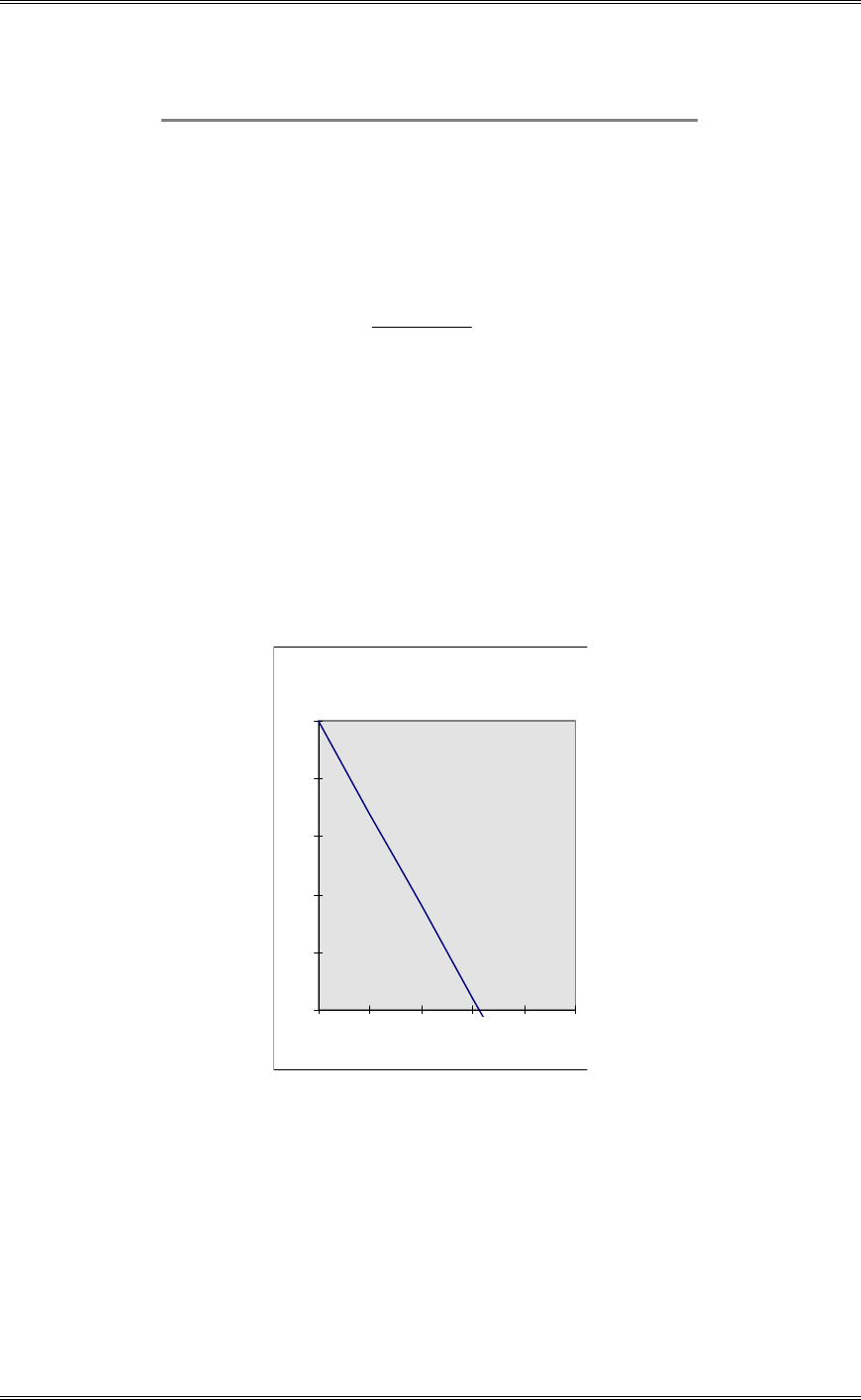
Solutions from Montgomery, D. C. (2001) Design and Analysis of Experiments, Wiley, NY
11-8
Origin +
'
1 0.32 300 23.2
Origin +5
'
5 1.60 700 36.0
(a) It is desired to move to a region where molecular weights are above 2500. Based on the information
you have from the experiment, in this region, about how may steps along the path of steepest ascent
might be required to move to the region of interest?
8137403201251
2211 ..
ˆ
x
ˆ
xy
ˆ
E'E''
4633
8137
20002500 o
.
.
Steps#
11-7 The path of steepest ascent is usually computed assuming that the model is truly first-order.; that is,
there is no interaction. However, even if there is interaction, steepest ascent ignoring the interaction still
usually produces good results. To illustrate, suppose that we have fit the model
2121 38520 xxxxy
ˆ
using coded variables (-1 d x1 d +1)
(a) Draw the path of steepest ascent that you would obtain if the interaction were ignored.
Path of Steepest Ascent for
Main Effects Model
-5
-4
-3
-2
-1
0
01 2345
X1
X2
(b) Draw the path of steepest ascent that you would obtain with the interaction included in the model.
Compare this with the path found in part (a).
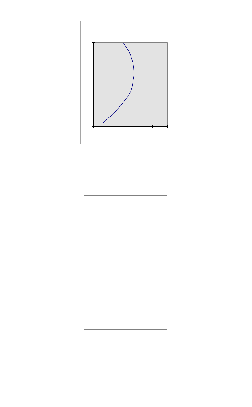
Solutions from Montgomery, D. C. (2001) Design and Analysis of Experiments, Wiley, NY
11-9
Path of Steepest Ascent for
Full Model
-5
-4
-3
-2
-1
0
-2 -1 0 1 2 3
X1
X2
11-8 The data shown in the following table were collected in an experiment to optimize crystal growth
as a function of three variables x1, x2, and x3. Large values of y (yield in grams) are desirable. Fit a
second order model and analyze the fitted surface. Under what set of conditions is maximum growth
achieved?
x1 x
2 x
3 y
-1 -1 -1 66
-1 -1 1 70
-1 1 -1 78
-1 1 1 60
1 -1 -1 80
1 -1 1 70
1 1 -1 100
1 1 1 75
-1.682 0 0 100
1.682 0 0 80
0 -1.682 0 68
0 1.682 0 63
0 0 -1.682 65
0 0 1.682 82
0 0 0 113
0 0 0 100
0 0 0 118
0 0 0 88
0 0 0 100
0 0 0 85
Design Expert Output
Response: Yield
ANOVA for Response Surface Quadratic Model
Analysis of variance table [Partial sum of squares]
Sum of
Mean F
Source Squares DF Square Value Prob > F
Model 3662.00 9 406.89 2.19 0.1194 not significant
A 22.08 1 22.08 0.12 0.7377
B 25.31 1 25.31 0.14 0.7200
C 30.50 1 30.50 0.16 0.6941

Solutions from Montgomery, D. C. (2001) Design and Analysis of Experiments, Wiley, NY
11-10
A2 204.55 1 204.55 1.10 0.3191
B2 2226.45 1 2226.45 11.96 0.0061
C2 1328.46 1 1328.46 7.14 0.0234
AB 66.12 1 66.12 0.36 0.5644
AC 55.13 1 55.13 0.30 0.5982
BC 171.13 1 171.13 0.92 0.3602
Residual 1860.95 10 186.09
Lack of Fit 1001.61 5 200.32 1.17 0.4353 not significant
Pure Error 859.33 5 171.87
Cor Total 5522.95 19
The "Model F-value" of 2.19 implies the model is not significant relative to the noise. There is a
11.94 % chance that a "Model F-value" this large could occur due to noise.
Std. Dev. 13.64 R-Squared 0.6631
Mean 83.05 Adj R-Squared 0.3598
C.V. 16.43 Pred R-Squared -0.6034
PRESS 8855.23 Adeq Precision 3.882
Coefficient Standard 95% CI 95% CI
Factor Estimate DF Error Low High VIF
Intercept 100.67 1 5.56 88.27 113.06
A-x1 1.27 1 3.69 -6.95 9.50 1.00
B-x2 1.36 1 3.69 -6.86 9.59 1.00
C-x3 -1.49 1 3.69 -9.72 6.73 1.00
A
2 -3.77 1 3.59 -11.77 4.24 1.02
B
2 -12.43 1 3.59 -20.44 -4.42 1.02
C
2 -9.60 1 3.59 -17.61 -1.59 1.02
AB 2.87 1 4.82 -7.87 13.62 1.00
AC -2.63 1 4.82 -13.37 8.12 1.00
BC -4.63 1 4.82 -15.37 6.12 1.00
Final Equation in Terms of Coded Factors:
Yield =
+100.67
+1.27 * A
+1.36 * B
-1.49 * C
-3.77 * A2
-12.43 * B2
-9.60 * C2
+2.87 * A * B
-2.63 * A * C
-4.63 * B * C
Final Equation in Terms of Actual Factors:
Yield =
+100.66609
+1.27146 * x1
+1.36130 * x2
-1.49445 * x3
-3.76749 * x12
-12.42955 * x22
-9.60113 * x32
+2.87500 * x1 * x2
-2.62500 * x1 * x3
-4.62500 * x2 * x3
There are so many nonsignificant terms in this model that we should consider eliminating some of them.
A reasonable reduced model is shown below.
Design Expert Output

Solutions from Montgomery, D. C. (2001) Design and Analysis of Experiments, Wiley, NY
11-11
Response: Yield
ANOVA for Response Surface Reduced Quadratic Model
Analysis of variance table [Partial sum of squares]
Sum of
Mean F
Source Squares DF Square Value Prob > F
Model 3143.00 4 785.75 4.95 0.0095 significant
B 25.31 1 25.31 0.16 0.6952
C 30.50 1 30.50 0.19 0.6673
B2 2115.31 1 2115.31 13.33 0.0024
C2 1239.17 1 1239.17 7.81 0.0136
Residual 2379.95 15 158.66
Lack of Fit 1520.62 10 152.06 0.88 0.5953 not significant
Pure Error 859.33 5 171.87
Cor Total 5522.95 19
The Model F-value of 4.95 implies the model is significant. There is only
a 0.95% chance that a "Model F-Value" this large could occur due to noise.
Std. Dev. 12.60 R-Squared 0.5691
Mean 83.05 Adj R-Squared 0.4542
C.V. 15.17 Pred R-Squared 0.1426
PRESS 4735.52 Adeq Precision 5.778
Coefficient Standard 95% CI 95% CI
Factor Estimate DF Error Low High VIF
Intercept 97.58 1 4.36 88.29 106.88
B-x2 1.36 1 3.41 -5.90 8.63 1.00
C-x3 -1.49 1 3.41 -8.76 5.77 1.00
B2 -12.06 1 3.30 -19.09 -5.02 1.01
C2 -9.23 1 3.30 -16.26 -2.19 1.01
Final Equation in Terms of Coded Factors:
Yield =
+97.58
+1.36 * B
-1.49 * C
-12.06 * B2
-9.23 * C2
Final Equation in Terms of Actual Factors:
Yield =
+97.58260
+1.36130 * x2
-1.49445 * x3
-12.05546 * x22
-9.22703 * x32
The contour plot identifies a maximum near the center of the design space.

Solutions from Montgomery, D. C. (2001) Design and Analysis of Experiments, Wiley, NY
11-12
DESIGN-EXPERT Plot
Yield
X = B: x2
Y = C: x3
Design Points
Actual Factor
A: x1 = 0.00
Yie ld
B: x2
C: x3
-1.00 -0.50 0.00 0.50 1.00
-1.00
-0.50
0.00
0.50
1.00
80
80
80
85
85
85
90
95
6
Prediction97.682
95% Low 69.273
95% High126.090
SE mean4.35584
SE pred 13.3281
X0.06
Y-0.08
11-9 The following data were collected by a chemical engineer. The response y is filtration time, x1 is
temperature, and x2 is pressure. Fit a second-order model.
x1 x2 y
-1 -1 54
-1 1 45
1 -1 32
1 1 47
-1.414 0 50
1.414 0 53
0 -1.414 47
0 1.414 51
0 0 41
0 0 39
0 0 44
0 0 42
0 0 40
Design Expert Output
Response: y
ANOVA for Response Surface Quadratic Model
Analysis of variance table [Partial sum of squares]
Sum of
Mean F
Source Squares DF Square Value Prob > F
Model 264.22 4 66.06 2.57 0.1194 not significant
A 13.11 1 13.11 0.51 0.4955
B 25.72 1 25.72 1.00 0.3467
A
2 81.39 1 81.39 3.16 0.1132
AB 144.00 1 144.00 5.60 0.0455
Residual 205.78 8 25.72
Lack of Fit 190.98 4 47.74 12.90 0.0148 significant
Pure Error 14.80 4 3.70
Cor Total 470.00 12
The "Model F-value" of 2.57 implies the model is not significant relative to the noise. There is a
11.94 % chance that a "Model F-value" this large could occur due to noise.
Std. Dev. 5.07 R-Squared 0.5622
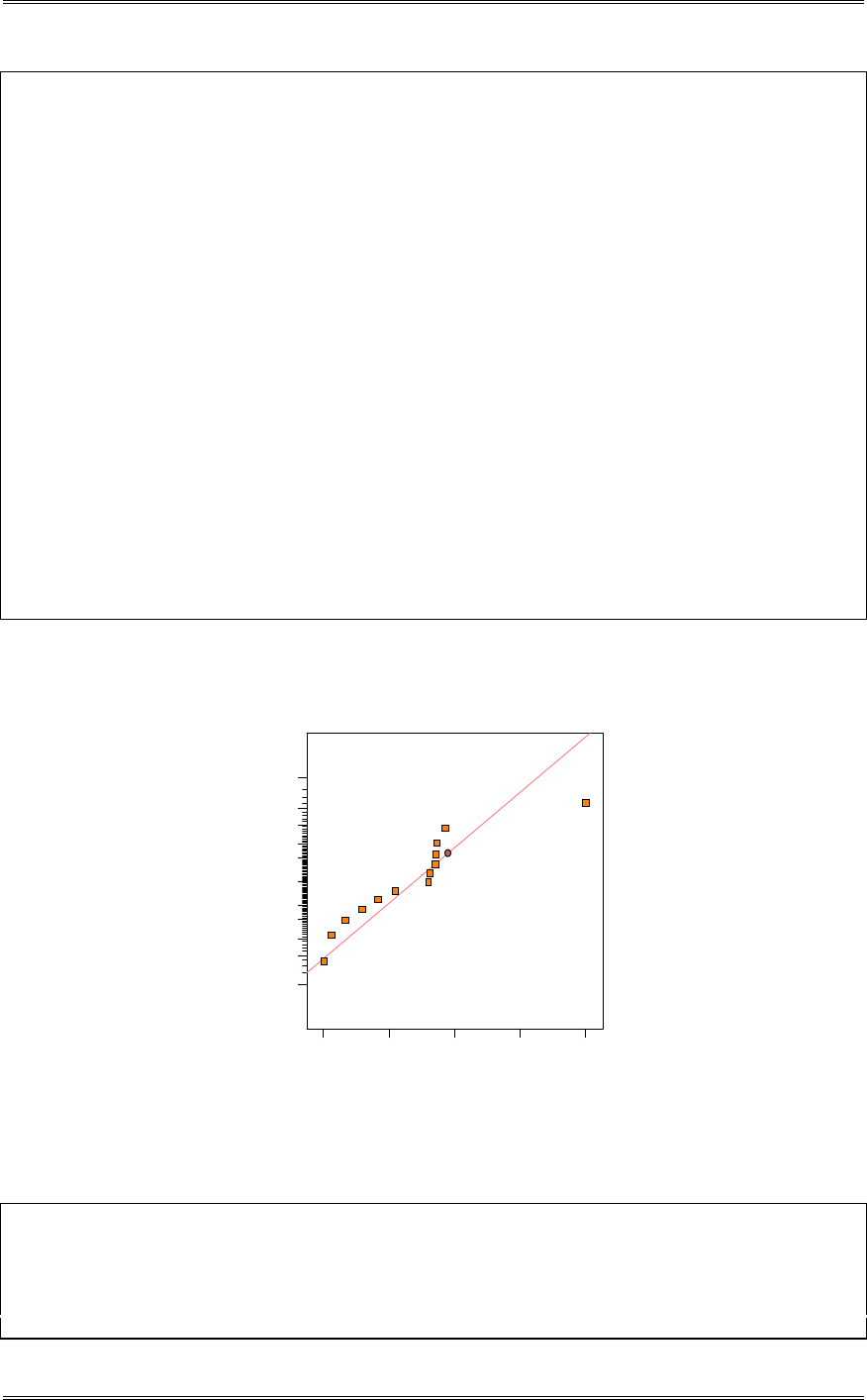
Solutions from Montgomery, D. C. (2001) Design and Analysis of Experiments, Wiley, NY
11-13
Mean 45.00 Adj R-Squared 0.3433
C.V. 11.27 Pred R-Squared -0.5249
PRESS 716.73 Adeq Precision 4.955
Coefficient Standard 95% CI 95% CI
Factor Estimate DF Error Low High VIF
Intercept 42.91 1 1.83 38.69 47.14
A-Temperature 1.28 1 1.79 -2.85 5.42 1.00
B-Pressure -1.79 1 1.79 -5.93 2.34 1.00
A
2 3.39 1 1.91 -1.01 7.79 1.00
AB 6.00 1 2.54 0.15 11.85 1.00
Final Equation in Terms of Coded Factors:
Time =
+42.91
+1.28 * A
-1.79 * B
+3.39 * A2
+6.00 * A * B
Final Equation in Terms of Actual Factors:
Time =
+42.91304
+1.28033 * Temperature
-1.79289 * Pressure
+3.39130 * Temperature2
+6.00000 * Temperature * Pressure
The lack of fit test in the above analysis is significant. Also, the residual plot below identifies an outlier
which happens to be standard order number 8.
Residual
Normal % probability
Normal plot of residuals
-5.23112 - 1.26772 2.69568 6.65909 10.6225
1
5
10
20
30
50
70
80
90
95
99
We chose to remove this run and re-analyze the data.
Design Expert Output
Response: y
ANOVA for Response Surface Quadratic Model
Analysis of variance table [Partial sum of squares]
Sum of
Mean F
Source Squares DF Square Value Prob > F
Model 407.34 4 101.84 30.13 0.0002 significant
A 13.11 1 13.11 3.88 0.0895
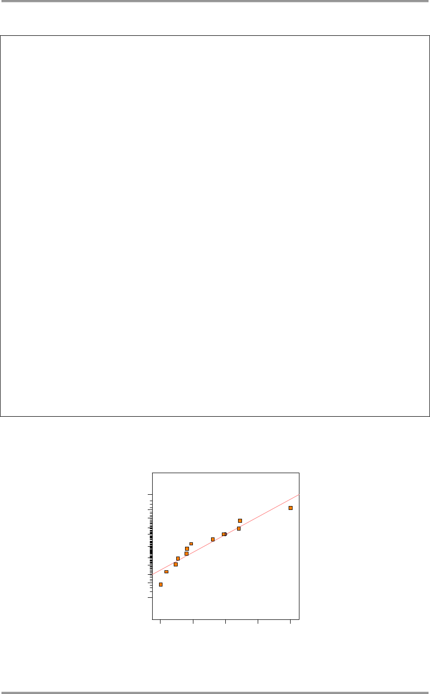
Solutions from Montgomery, D. C. (2001) Design and Analysis of Experiments, Wiley, NY
11-14
B 132.63 1 132.63 39.25 0.0004
A
2 155.27 1 155.27 45.95 0.0003
AB 144.00 1 144.00 42.61 0.0003
Residual 23.66 7 3.38
Lack of Fit 8.86 3 2.95 0.80 0.5560 not significant
Pure Error 14.80 4 3.70
Cor Total 431.00 11
The Model F-value of 30.13 implies the model is significant. There is only
a 0.02% chance that a "Model F-Value" this large could occur due to noise.
Std. Dev. 1.84 R-Squared 0.9451
Mean 44.50 Adj R-Squared 0.9138
C.V. 4.13 Pred R-Squared 0.8129
PRESS 80.66 Adeq Precision 18.243
Coefficient Standard 95% CI 95% CI
Factor Estimate DF Error Low High VIF
Intercept 40.68 1 0.73 38.95 42.40
A-Temperature 1.28 1 0.65 -0.26 2.82 1.00
B-Pressure -4.82 1 0.77 -6.64 -3.00 1.02
A
2 4.88 1 0.72 3.18 6.59 1.02
AB 6.00 1 0.92 3.83 8.17 1.00
Final Equation in Terms of Coded Factors:
Time =
+40.68
+1.28 * A
-4.82 * B
+4.88 * A2
+6.00 * A * B
Final Equation in Terms of Actual Factors:
Time =
+40.67673
+1.28033 * Temperature
-4.82374 * Pressure
+4.88218 * Temperature2
+6.00000 * Temperature * Pressure
The lack of fit test is satisfactory as well as the following normal plot of residuals:
Residual
Norm al % probability
Normal plot of residuals
-1.67673 - 0.42673 0.82327 2.07327 3.32327
1
5
10
20
30
50
70
80
90
95
99

Solutions from Montgomery, D. C. (2001) Design and Analysis of Experiments, Wiley, NY
11-15
(a) What operating conditions would you recommend if the objective is to minimize the filtration time?
Time
A: Temperature
B: Press ure
-1.00 -0.50 0.00 0.50 1.00
-1.00
-0.50
0.00
0.50
1.00
34
36
38
40
42
44
46
46
48
50
52
5
Prediction 33.195
95% Low 27.885
95% High 38.506
SE mean 1.29007
SE pred 2.24581
X
-0.68
Y1.00
(b) What operating conditions would you recommend if the objective is to operate the process at a mean
filtration time very close to 46?
Time
A: Temperature
B: Press ure
-1.00 -0.50 0.00 0.50 1.00
-1.00
-0.50
0.00
0.50
1.00
34
36
38
40
42
44
46
46
48
50
52
5
There are two regions that enable a filtration time of 46. Either will suffice; however, higher temperatures
and pressures typically have higher operating costs. We chose the operating conditions at the lower
pressure and temperature as shown.
11-10 The hexagon design that follows is used in an experiment that has the objective of fitting a second-
order model.
x1 x2 y
1 0 68

Solutions from Montgomery, D. C. (2001) Design and Analysis of Experiments, Wiley, NY
11-16
0.5 075. 74
-0.5 075. 65
-1 0 60
-0.5 -075. 63
0.5 -075. 70
0 0 58
0 0 60
0 0 57
0 0 55
0 0 69
(a) Fit the second-order model.
Design Expert Output
Response: y
ANOVA for Response Surface Quadratic Model
Analysis of variance table [Partial sum of squares]
Sum of
Mean F
Source Squares DF Square Value Prob > F
Model 245.26 5 49.05 1.89 0.2500 not significant
A 85.33 1 85.33 3.30 0.1292
B 9.00 1 9.00 0.35 0.5811
A2 25.20 1 25.20 0.97 0.3692
B2 129.83 1 129.83 5.01 0.0753
AB 1.00 1 1.00 0.039 0.8519
Residual 129.47 5 25.89
Lack of Fit 10.67 1 10.67 0.36 0.5813 not significant
Pure Error 118.80 4 29.70
Cor Total 374.73 10
The "Model F-value" of 1.89 implies the model is not significant relative to the noise. There is a
25.00 % chance that a "Model F-value" this large could occur due to noise.
Std. Dev. 5.09 R-Squared 0.6545
Mean 63.55 Adj R-Squared 0.3090
C.V. 8.01 Pred R-Squared -0.5201
PRESS 569.63 Adeq Precision 3.725
Coefficient Standard 95% CI 95% CI
Factor Estimate DF Error Low High VIF
Intercept 59.80 1 2.28 53.95 65.65
A-x1 5.33 1 2.94 -2.22 12.89 1.00
B-x2 1.73 1 2.94 -5.82 9.28 1.00
A
2 4.20 1 4.26 -6.74 15.14 1.00
B
2 9.53 1 4.26 -1.41 20.48 1.00
AB 1.15 1 5.88 -13.95 16.26 1.00
Final Equation in Terms of Coded Factors:
y =
+59.80
+5.33 * A
+1.73 * B
+4.20 * A2
+9.53 * B2
+1.15 * A * B
(a) Perform the canonical analysis. What type of surface has been found?
The full quadratic model is used in the following analysis because the reduced model is singular.
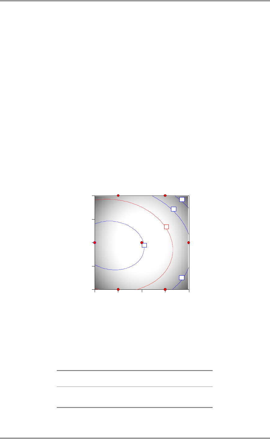
Solutions from Montgomery, D. C. (2001) Design and Analysis of Experiments, Wiley, NY
11-17
Solution
Variable Critical Value
X1 -0.627658
X2 -0.052829
Predicted Value at Solution 58.080492
Eigenvalues and Eigenvectors
Variable 9.5957 4.1382
X1 0.10640 0.99432
X2 0.99432 -0.10640
Since both eigenvalues are positive, the response is a minimum at the stationary point.
(c) What operating conditions on x1 and x2 lead to the stationary point?
The stationary point is (x1,x2) = (-0.62766, -0.05283)
(d) Where would you run this process if the objective is to obtain a response that is as close to 65 as
possible?
y
A: x1
B: x2
-1.00 -0.50 0.00 0.50 1.00
-0.87
-0.43
0.00
0.43
0.87
60
65
70
70
75
5
Any value of x1 and x2 that give a point on the contour with value of 65 would be satisfactory.
11-11 An experimenter has run a Box-Behnken design and has obtained the results below, where the
response variable is the viscosity of a polymer.
Level
Temp.
Agitation
Rate
Pressure
x1
x2
x3
High 200 10.0 25 +1 +1 +1
Middle 175 7.5 20 0 0 0
Low 150 5.0 15 -1 -1 -1

Solutions from Montgomery, D. C. (2001) Design and Analysis of Experiments, Wiley, NY
11-18
Run x1 x2 x3 y1
1 -1 -1 0 535
2 1 -1 0 580
3 -1 1 0 596
4 1 1 0 563
5 -1 0 -1 645
6 1 0 -1 458
7 -1 0 1 350
8 1 0 1 600
9 0 -1 -1 595
10 0 1 -1 648
11 0 -1 1 532
12 0 1 1 656
13 0 0 0 653
14 0 0 0 599
15 0 0 0 620
(a) Fit the second-order model.
Design Expert Output
Response: Viscosity
ANOVA for Response Surface Quadratic Model
Analysis of variance table [Partial sum of squares]
Sum of
Mean F
Source Squares DF Square Value Prob > F
Model 89652.58 9 9961.40 9.54 0.0115 significant
A 703.12 1 703.12 0.67 0.4491
B 6105.12 1 6105.12 5.85 0.0602
C 5408.00 1 5408.00 5.18 0.0719
A2 20769.23 1 20769.23 19.90 0.0066
B2 1404.00 1 1404.00 1.35 0.2985
C2 4719.00 1 4719.00 4.52 0.0868
AB 1521.00 1 1521.00 1.46 0.2814
AC 47742.25 1 47742.25 45.74 0.0011
BC 1260.25 1 1260.25 1.21 0.3219
Residual 5218.75 5 1043.75
Lack of Fit 3736.75 3 1245.58 1.68 0.3941 not significant
Pure Error 1482.00 2 741.00
Cor Total 94871.33 14
The Model F-value of 9.54 implies the model is significant. There is only
a 1.15% chance that a "Model F-Value" this large could occur due to noise.
Std. Dev. 32.31 R-Squared 0.9450
Mean 575.33 Adj R-Squared 0.8460
C.V. 5.62 Pred R-Squared 0.3347
PRESS 63122.50 Adeq Precision 10.425
Coefficient Standard 95% CI 95% CI
Factor Estimate DF Error Low High VIF
Intercept 624.00 1 18.65 576.05 671.95
A-Temperatue 9.37 1 11.42 -19.99 38.74 1.00
B-Agitation Rate 27.62 1 11.42 -1.74 56.99 1.00
C-Pressure -26.00 1 11.42 -55.36 3.36 1.00
A
2 -75.00 1 16.81 -118.22 -31.78 1.01
B
2 19.50 1 16.81 -23.72 62.72 1.01
C
2 -35.75 1 16.81 -78.97 7.47 1.01
AB -19.50 1 16.15 -61.02 22.02 1.00
AC 109.25 1 16.15 67.73 150.77 1.00
BC 17.75 1 16.15 -23.77 59.27 1.00
Final Equation in Terms of Coded Factors:

Solutions from Montgomery, D. C. (2001) Design and Analysis of Experiments, Wiley, NY
11-19
Viscosity =
+624.00
+9.37 * A
+27.62 * B
-26.00 * C
-75.00 * A2
+19.50 * B2
-35.75 * C2
-19.50 * A * B
+109.25 * A * C
+17.75 * B * C
Final Equation in Terms of Actual Factors:
Viscosity =
-629.50000
+27.23500 * Temperatue
-9.55000 * Agitation Rate
-111.60000 * Pressure
-0.12000 * Temperatue2
+3.12000 * Agitation Rate2
-1.43000 * Pressure2
-0.31200 * Temperatue * Agitation Rate
+0.87400 * Temperatue * Pressure
+1.42000 * Agitation Rate * Pressure
(b) Perform the canonical analysis. What type of surface has been found?
Solution
Variable Critical Value
X1 2.1849596
X2 -0.871371
X3 2.7586015
Predicted Value at Solution 586.34437
Eigevalues and Eigevectors
Variable
20.9229 2.5208 -114.694
X1 -0.02739 0.58118 0.81331
X2 0.99129 -0.08907 0.09703
X3 0.12883 0.80888 -0.57368
The system is a saddle point.
(c) What operating conditions on x1, x2, and x3 lead to the stationary point?
The stationary point is (x1, x2, x3) = (2.18496, -0.87167, 2.75860). This is outside the design region. It
would be necessary to either examine contour plots or use numerical optimization methods to find desired
operating conditions.
(d) What operating conditions would you recommend if it is important to obtain a viscosity that is as
close to 600 as possible?
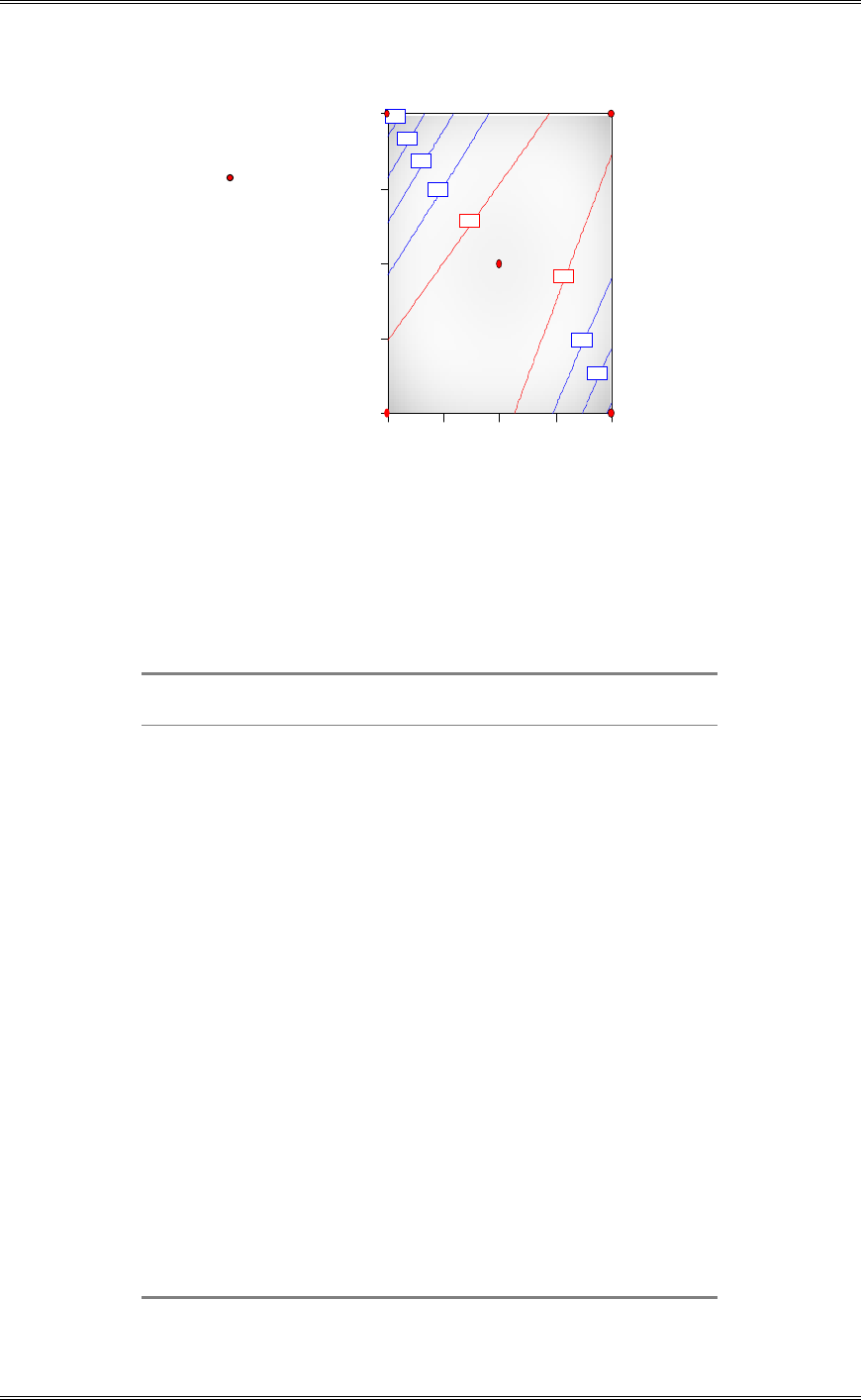
Solutions from Montgomery, D. C. (2001) Design and Analysis of Experiments, Wiley, NY
11-20
DESIGN-EXPERT Plot
V i sc o si t y
X = A: Tem peratue
Y = C: Pressure
Design Points
Actual Factor
B: Agitation Rate = 7.50
Viscosity
A: T e m pe ra tue
C: Pressure
150.00 162.50 175.00 187.50 200.00
15.00
17.50
20.00
22.50
25.00 400
450
500
500
550
550
600
600
3
Any point on either of the contours showing a viscosity of 600 is satisfactory.
11-12 Consider the three-variable central composite design shown below. Analyze the data and draw
conclusions, assuming that we wish to maximize conversion (y1) with activity (y2) between 55 and 60.
Run
Time
(min)
Temperature
(qC)
Catalyst
(%)
Conversion (%)
y1
Activity
y2
1 -1.000 -1.000 -1.000 74.00 53.20
2 1.000 -1.000 -1.000 51.00 62.90
3 -1.000 1.000 -1.000 88.00 53.40
4 1.000 1.000 -1.000 70.00 62.60
5 -1.000 -1.000 1.000 71.00 57.30
6 1.000 -1.000 1.000 90.00 67.90
7 -1.000 1.000 1.000 66.00 59.80
8 1.000 1.000 1.000 97.00 67.80
9 0.000 0.000 0.000 81.00 59.20
10 0.000 0.000 0.000 75.00 60.40
11 0.000 0.000 0.000 76.00 59.10
12 0.000 0.000 0.000 83.00 60.60
13 -1.682 0.000 0.000 76.00 59.10
14 1.682 0.000 0.000 79.00 65.90
15 0.000 -1.682 0.000 85.00 60.00
16 0.000 1.682 0.000 97.00 60.70
17 0.000 0.000 -1.682 55.00 57.40
18 0.000 0.000 1.682 81.00 63.20
19 0.000 0.000 0.000 80.00 60.80
20 0.000 0.000 0.000 91.00 58.90
Quadratic models are developed for the Conversion and Activity response variables as follows:

Solutions from Montgomery, D. C. (2001) Design and Analysis of Experiments, Wiley, NY
11-21
Design Expert Output
Response: Conversion
ANOVA for Response Surface Quadratic Model
Analysis of variance table [Partial sum of squares]
Sum of
Mean F
Source Squares DF Square Value Prob > F
Model 2555.73 9 283.97 12.76 0.0002 significant
A 14.44 1 14.44 0.65 0.4391
B 222.96 1 222.96 10.02 0.0101
C 525.64 1 525.64 23.63 0.0007
A
2 48.47 1 48.47 2.18 0.1707
B
2 124.48 1 124.48 5.60 0.0396
C
2 388.59 1 388.59 17.47 0.0019
AB 36.13 1 36.13 1.62 0.2314
AC 1035.13 1 1035.13 46.53 < 0.0001
BC 120.12 1 120.12 5.40 0.0425
Residual 222.47 10 22.25
Lack of Fit 56.47 5 11.29 0.34 0.8692 not significant
Pure Error 166.00 5 33.20
Cor Total 287.28 19
The Model F-value of 12.76 implies the model is significant. There is only
a 0.02% chance that a "Model F-Value" this large could occur due to noise.
Std. Dev. 4.72 R-Squared 0.9199
Mean 78.30 Adj R-Squared 0.8479
C.V. 6.02 Pred R-Squared 0.7566
PRESS 676.22 Adeq Precision 14.239
Coefficient Standard 95% CI 95% CI
Factor Estimate DF Error Low High VIF
Intercept 81.09 1 1.92 76.81 85.38
A-Time 1.03 1 1.28 -1.82 3.87 1.00
B-Temperature 4.04 1 1.28 1.20 6.88 1.00
C-Catalyst 6.20 1 1.28 3.36 9.05 1.00
A2 -1.83 1 1.24 -4.60 0.93 1.02
B2 2.94 1 1.24 0.17 5.71 1.02
C2 -5.19 1 1.24 -7.96 -2.42 1.02
AB 2.13 1 1.67 -1.59 5.84 1.00
AC 11.38 1 1.67 7.66 15.09 1.00
BC -3.87 1 1.67 -7.59 -0.16 1.00
Final Equation in Terms of Coded Factors:
Conversion =
+81.09
+1.03 * A
+4.04 * B
+6.20 * C
-1.83 * A2
+2.94 * B2
-5.19 * C2
+2.13 * A * B
+11.38 * A * C
-3.87 * B * C
Final Equation in Terms of Actual Factors:
Conversion =
+81.09128
+1.02845 * Time
+4.04057 * Temperature
+6.20396 * Catalyst
-1.83398 * Time2
+2.93899 * Temperature2
-5.19274 * Catalyst2
+2.12500 * Time * Temperature
+11.37500 * Time * Catalyst

Solutions from Montgomery, D. C. (2001) Design and Analysis of Experiments, Wiley, NY
11-22
-3.87500 * Temperature * Catalyst
Design Expert Output
Response: Activity
ANOVA for Response Surface Quadratic Model
Analysis of variance table [Partial sum of squares]
Sum of
Mean F
Source Squares DF Square Value Prob > F
Model 256.20 9 28.47 9.16 0.0009 significant
A 175.35 1 175.35 56.42 < 0.0001
B 0.89 1 0.89 0.28 0.6052
C 67.91 1 67.91 21.85 0.0009
A2 10.05 1 10.05 3.23 0.1024
B2 0.081 1 0.081 0.026 0.8753
C2 0.047 1 0.047 0.015 0.9046
AB 1.20 1 1.20 0.39 0.5480
AC 0.011 1 0.011 3.620E-003 0.9532
BC 0.78 1 0.78 0.25 0.6270
Residual 31.08 10 3.11
Lack of Fit 27.43 5 5.49 7.51 0.0226 significant
Pure Error 3.65 5 0.73
Cor Total 287.28 19
The Model F-value of 9.16 implies the model is significant. There is only
a 0.09% chance that a "Model F-Value" this large could occur due to noise.
Std. Dev. 1.76 R-Squared 0.8918
Mean 60.51 Adj R-Squared 0.7945
C.V. 2.91 Pred R-Squared 0.2536
PRESS 214.43 Adeq Precision 10.911
Coefficient Standard 95% CI 95% CI
Factor Estimate DF Error Low High VIF
Intercept 59.85 1 0.72 58.25 61.45
A-Time 3.58 1 0.48 2.52 4.65 1.00
B-Temperature 0.25 1 0.48 -0.81 1.32 1.00
C-Catalyst 2.23 1 0.48 1.17 3.29 1.00
A
2 0.83 1 0.46 -0.20 1.87 1.02
B
2 0.075 1 0.46 -0.96 1.11 1.02
C
2 0.057 1 0.46 -0.98 1.09 1.02
AB -0.39 1 0.62 -1.78 1.00 1.00
AC -0.038 1 0.62 -1.43 1.35 1.00
BC 0.31 1 0.62 -1.08 1.70 1.00
Final Equation in Terms of Coded Factors:
Conversion =
+59.85
+3.58 * A
+0.25 * B
+2.23 * C
+0.83 * A2
+0.075 * B2
+0.057 * C2
-0.39 * A * B
-0.038 * A * C
+0.31 * B * C
Final Equation in Terms of Actual Factors:
Conversion =
+59.84984
+3.58327 * Time
+0.25462 * Temperature
+2.22997 * Catalyst
+0.83491 * Time2
+0.074772 * Temperature2

Solutions from Montgomery, D. C. (2001) Design and Analysis of Experiments, Wiley, NY
11-23
+0.057094 * Catalyst2
-0.38750 * Time * Temperature
-0.037500 * Time * Catalyst
+0.31250 * Temperature * Catalyst
Because many of the terms are insignificant, the reduced quadratic model is fit as follows:
Design Expert Output
Response: Activity
ANOVA for Response Surface Quadratic Model
Analysis of variance table [Partial sum of squares]
Sum of
Mean F
Source Squares DF Square Value Prob > F
Model 253.20 3 84.40 39.63 < 0.0001 significant
A 175.35 1 175.35 82.34 < 0.0001
C 67.91 1 67.91 31.89 < 0.0001
A
2 9.94 1 9.94 4.67 0.0463
Residual 34.07 16 2.13
Lack of Fit 30.42 11 2.77 3.78 0.0766 not significant
Pure Error 3.65 5 0.73
Cor Total 287.28 19
The Model F-value of 39.63 implies the model is significant. There is only
a 0.01% chance that a "Model F-Value" this large could occur due to noise.
Std. Dev. 1.46 R-Squared 0.8814
Mean 60.51 Adj R-Squared 0.8591
C.V. 2.41 Pred R-Squared 0.6302
PRESS 106.24 Adeq Precision 20.447
Coefficient Standard 95% CI 95% CI
Factor Estimate DF Error Low High VIF
Intercept 59.95 1 0.42 59.06 60.83
A-Time 3.58 1 0.39 2.75 4.42 1.00
C-Catalyst 2.23 1 0.39 1.39 3.07 1.00
A
2 0.82 1 0.38 0.015 1.63 1.00
Final Equation in Terms of Coded Factors:
Activity =
+59.95
+3.58 * A
+2.23 * C
+0.82 * A2
Final Equation in Terms of Actual Factors:
Activity =
+59.94802
+3.58327 * Time
+2.22997 * Catalyst
+0.82300 * Time2
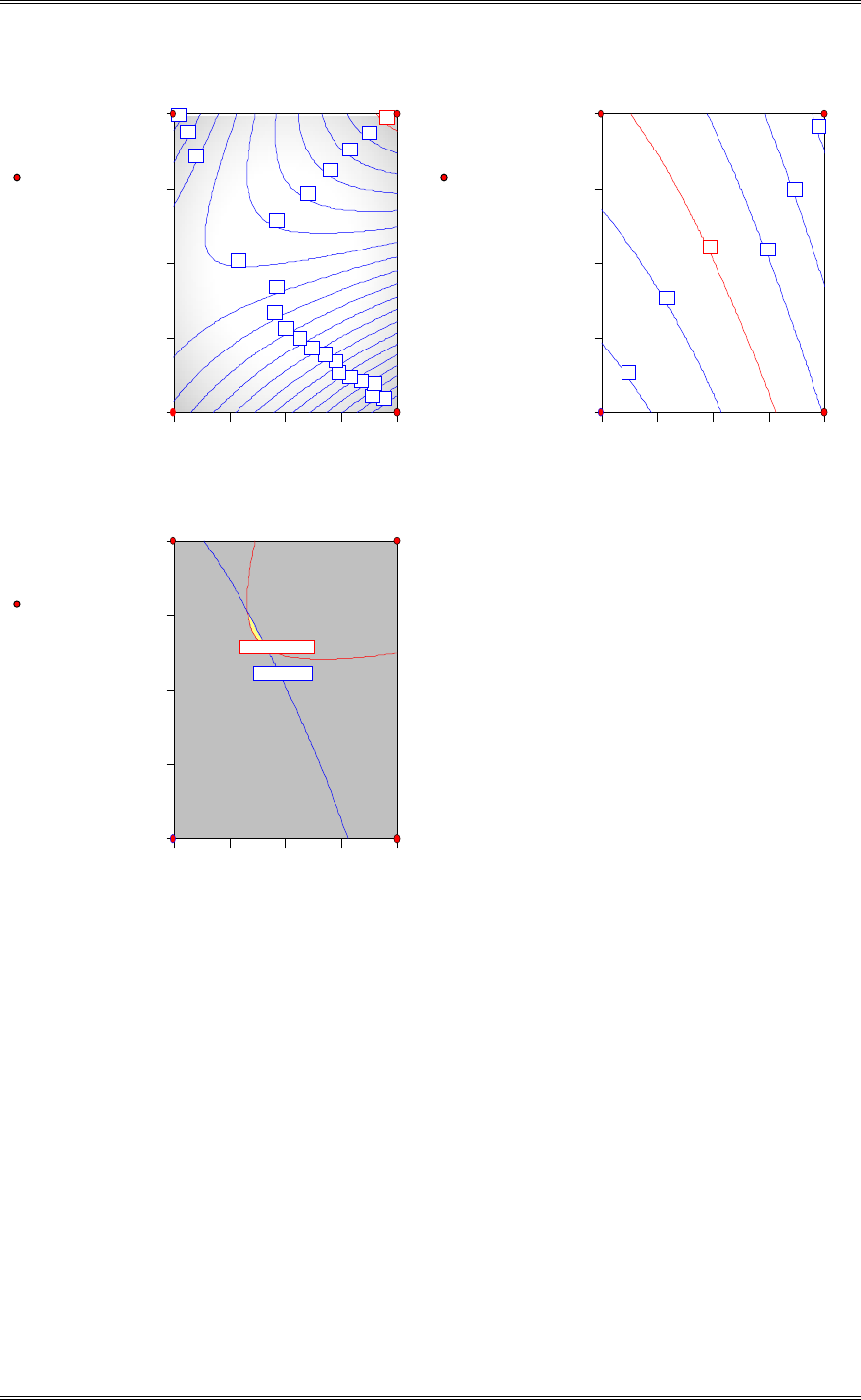
Solutions from Montgomery, D. C. (2001) Design and Analysis of Experiments, Wiley, NY
11-24
DESIGN-EXPERT Plot
Conversion
X = A: Time
Y = C: Catalyst
Design Points
Actual Factor
B: T emperature = -1.00
Conversion
A: T im e
C: Catalyst
-1.00 -0.50 0.00 0.50 1.00
-1.00
-0.50
0.00
0.50
1.00
54
56
58
60
62
64
66
68
70
72
74
74
76
76
78
78
80
82
84
86
88
90
92
DESIGN-EXPERT Plot
Activity
X = A: Time
Y = C: Catalyst
Design Points
Actual Factor
B: T emperature = -1.00
Activity
A: T im e
C: Catalyst
-1.00 -0.50 0.00 0.50 1.00
-1.00
-0.50
0.00
0.50
1.00
56
58
60 62
64
66
DESIGN-EXPERT Plot
Overlay Plot
X = A: Time
Y = C: Catalyst
Design Points
Actual Factor
B: T emperature = -1.00
Overlay Plot
A: T im e
C: Catalyst
-1.00 -0.50 0.00 0.50 1.00
-1.00
-0.50
0.00
0.50
1.00
Conv ersion: 82
Activity : 60
The contour plots visually describe the models while the overlay plots identifies the acceptable region for
the process.
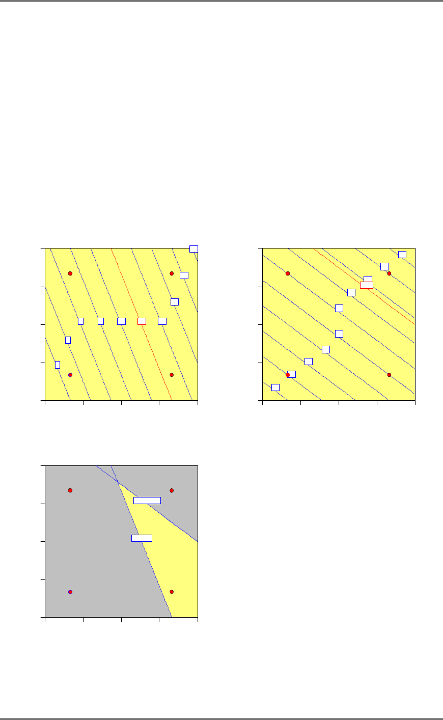
Solutions from Montgomery, D. C. (2001) Design and Analysis of Experiments, Wiley, NY
11-26
11-13 A manufacturer of cutting tools has developed two empirical equations for tool life in hours (y1)
and for tool cost in dollars (y2). Both models are linear functions of steel hardness (x1) and
manufacturing time (x2). The two equations are
212
211
4323
2510
xxy
ˆ
xxy
ˆ
and both equations are valid over the range -1.5dx1d1.5. Unit tool cost must be below $27.50 and life
must exceed 12 hours for the product to be competitive. Is there a feasible set of operating conditions for
this process? Where would you recommend that the process be run?
The contour plots below graphically describe the two models. The overlay plot identifies the feasible
operating region for the process.
Life
A: H a rd n e s s
B: Tim e
-1.50 -0.75 0.00 0.75 1.50
-1.50
-0.75
0.00
0.75
1.50
2
4
6 8 10 12 14
16
18
20
Cost
A: H a rd n e s s
B: Tim e
-1.50 -0.75 0.00 0.75 1.50
-1.50
-0.75
0.00
0.75
1.50
14
16
18
20
22
24
26
28
30
32
27.5
Overlay Plot
A: H a rd n e s s
B: Tim e
-1.50 -0.75 0.00 0.75 1.50
-1.50
-0.75
0.00
0.75
1.50
Lif e: 12
Cost: 27.5
50274323
122510
21
21
.xx
xx
d
t

Solutions from Montgomery, D. C. (2001) Design and Analysis of Experiments, Wiley, NY
11-27
11-14 A central composite design is run in a chemical vapor deposition process, resulting in the
experimental data shown below. Four experimental units were processed simultaneously on each run of
the design, and the responses are the mean and variance of thickness, computed across the four units.
x1 x2 y 2
s
-1 -1 360.6 6.689
-1 1 445.2 14.230
1 -1 412.1 7.088
1 1 601.7 8.586
1.414 0 518.0 13.130
-1.414 0 411.4 6.644
0 1.414 497.6 7.649
0 -1.414 397.6 11.740
0 0 530.6 7.836
0 0 495.4 9.306
0 0 510.2 7.956
0 0 487.3 9.127
(a) Fit a model to the mean response. Analyze the residuals.
Design Expert Output
Response: Mean Thick
ANOVA for Response Surface Quadratic Model
Analysis of variance table [Partial sum of squares]
Sum of
Mean F
Source Squares DF Square Value Prob > F
Model 47644.26 5 9528.85 16.12 0.0020 significant
A 22573.36 1 22573.36 38.19 0.0008
B 15261.91 1 15261.91 25.82 0.0023
A2 2795.58 1 2795.58 4.73 0.0726
B2 5550.74 1 5550.74 9.39 0.0221
AB 2756.25 1 2756.25 4.66 0.0741
Residual 3546.83 6 591.14
Lack of Fit 2462.04 3 820.68 2.27 0.2592 not significant
Pure Error 1084.79 3 361.60
Cor Total 51191.09 11
The Model F-value of 16.12 implies the model is significant. There is only
a 0.20% chance that a "Model F-Value" this large could occur due to noise.
Std. Dev. 24.31 R-Squared 0.9307
Mean 472.31 Adj R-Squared 0.8730
C.V. 5.15 Pred R-Squared 0.6203
PRESS 19436.37 Adeq Precision 11.261
Coefficient Standard 95% CI 95% CI
Factor Estimate DF Error Low High VIF
Intercept 505.88 1 12.16 476.13 535.62
A-x1 53.12 1 8.60 32.09 74.15 1.00
B-x2 43.68 1 8.60 22.64 64.71 1.00
A
2 -20.90 1 9.61 -44.42 2.62 1.04
B
2 -29.45 1 9.61 -52.97 -5.93 1.04
AB 26.25 1 12.16 -3.50 56.00 1.00
Final Equation in Terms of Coded Factors:
Mean Thick =
+505.88
+53.12 * A
+43.68 * B
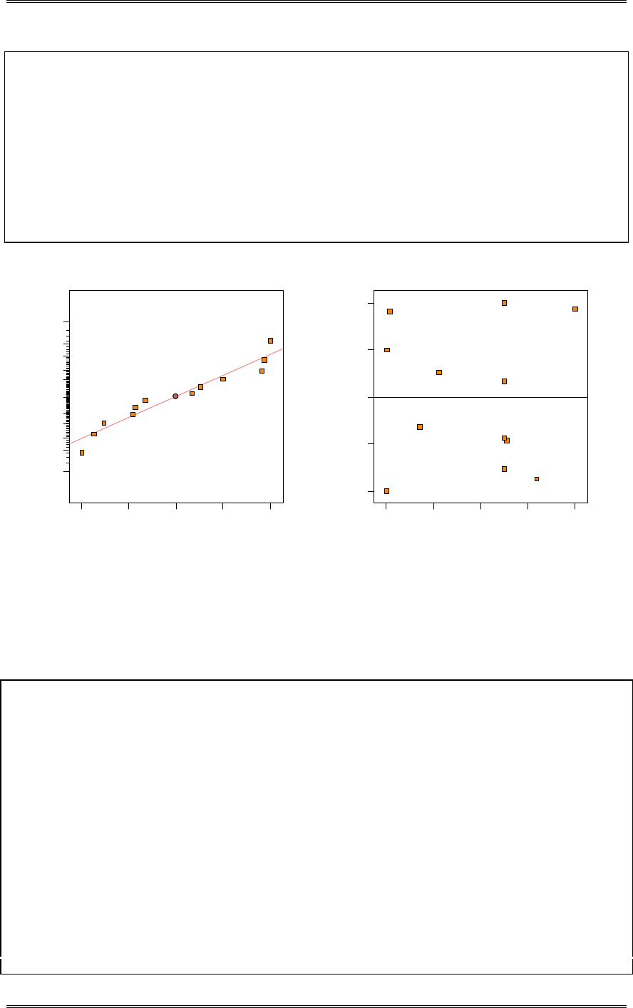
Solutions from Montgomery, D. C. (2001) Design and Analysis of Experiments, Wiley, NY
11-28
-20.90 * A2
-29.45 * B2
+26.25 * A * B
Final Equation in Terms of Actual Factors:
Mean Thick =
+505.87500
+53.11940 * x1
+43.67767 * x2
-20.90000 * x12
-29.45000 * x22
+26.25000 * x1 * x2
Residual
Normal % probability
Normal plot of residuals
-24.3779 - 12.1022 0.173533 12.4493 24.725
1
5
10
20
30
50
70
80
90
95
99
Predicted
Residuals
Residuals vs. Predicted
-24.3779
-12.1022
0.173533
12.4493
24.725
384.98 433.38 481.78 530.17 578.57
A modest deviation from normality can be observed in the Normal Plot of Residuals; however, not enough
to be concerned.
(b) Fit a model to the variance response. Analyze the residuals.
Design Expert Output
Response: Var Thick
ANOVA for Response Surface 2FI Model
Analysis of variance table [Partial sum of squares]
Sum of
Mean F
Source Squares DF Square Value Prob > F
Model 65.80 3 21.93 35.86 < 0.0001 significant
A 41.46 1 41.46 67.79 < 0.0001
B 15.21 1 15.21 24.87 0.0011
AB 9.13 1 9.13 14.93 0.0048
Residual 4.89 8 0.61
Lack of Fit 3.13 5 0.63 1.06 0.5137 not significant
Pure Error 1.77 3 0.59
Cor Total 70.69 11
The Model F-value of 35.86 implies the model is significant. There is only
a 0.01% chance that a "Model F-Value" this large could occur due to noise.
Std. Dev. 0.78 R-Squared 0.9308
Mean 9.17 Adj R-Squared 0.9048
C.V. 8.53 Pred R-Squared 0.8920
PRESS 7.64 Adeq Precision 18.572
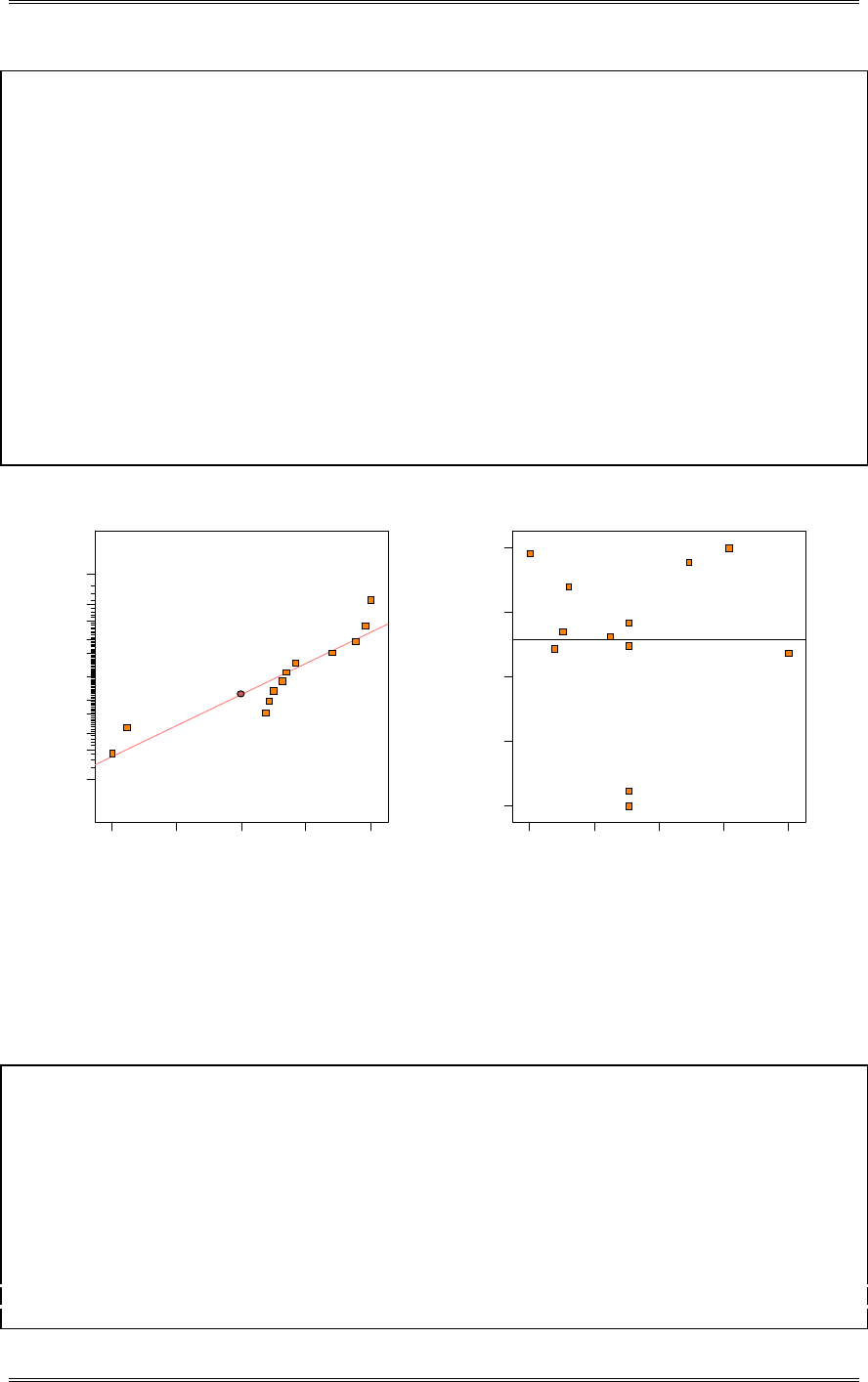
Solutions from Montgomery, D. C. (2001) Design and Analysis of Experiments, Wiley, NY
11-29
Coefficient Standard 95% CI 95% CI
Factor Estimate DF Error Low High VIF
Intercept 9.17 1 0.23 8.64 9.69
A-x1 2.28 1 0.28 1.64 2.91 1.00
B-x2 -1.38 1 0.28 -2.02 -0.74 1.00
AB -1.51 1 0.39 -2.41 -0.61 1.00
Final Equation in Terms of Coded Factors:
Var Thick =
+9.17
+2.28 * A
-1.38 * B
-1.51 * A * B
Final Equation in Terms of Actual Factors:
Var Thick =
+9.16508
+2.27645 * x1
-1.37882 * x2
-1.51075 * x1 * x2
Residual
Normal % probability
Normal plot of residuals
-1.32908 - 0.810429 - 0.291776 0.226878 0.745532
1
5
10
20
30
50
70
80
90
95
99
Predicted
Residuals
Residuals vs. Predicted
-1.32908
-0.810429
-0.291776
0.226878
0.745532
5.95 8.04 10.14 12.23 14.33
The residual plots are not acceptable. A transformation should be considered. If not successful at
correcting the residual plots, further investigation into the two apparently unusual points should be made.
(c) Fit a model to the ln(s2). Is this model superior to the one you found in part (b)?
Design Expert Output
Response: Var Thick Transform: Natural log Constant: 0
ANOVA for Response Surface 2FI Model
Analysis of variance table [Partial sum of squares]
Sum of
Mean F
Source Squares DF Square Value Prob > F
Model 0.67 3 0.22 36.94 < 0.0001 significant
A 0.46 1 0.46 74.99 < 0.0001
B 0.14 1 0.14 22.80 0.0014
AB 0.079 1 0.079 13.04 0.0069
Residual 0.049 8 6.081E-003
Lack of Fit 0.024 5 4.887E-003 0.61 0.7093 not significant
Pure Error 0.024 3 8.071E-003
Cor Total 0.72 11
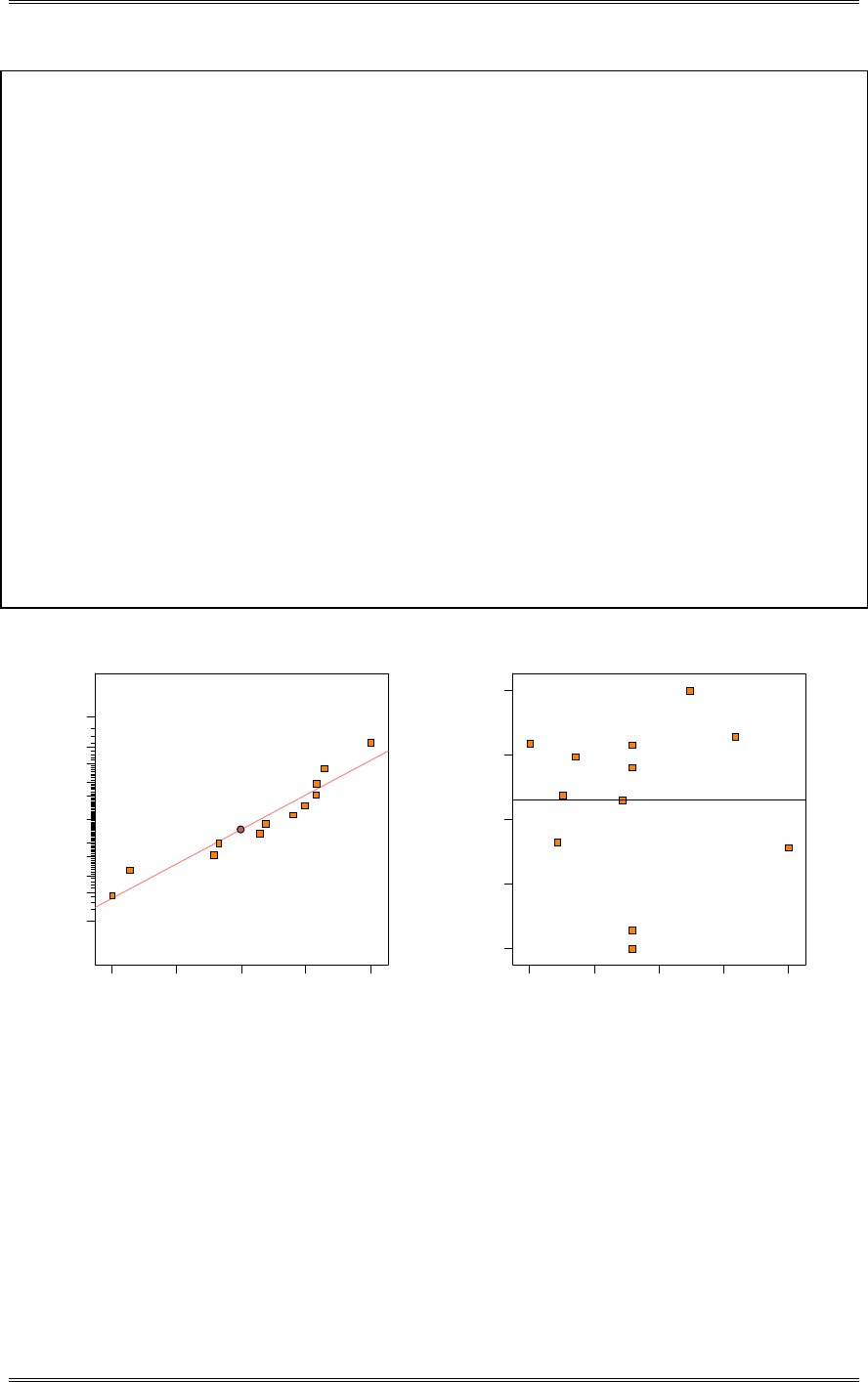
Solutions from Montgomery, D. C. (2001) Design and Analysis of Experiments, Wiley, NY
11-30
The Model F-value of 36.94 implies the model is significant. There is only
a 0.01% chance that a "Model F-Value" this large could occur due to noise.
Std. Dev. 0.078 R-Squared 0.9327
Mean 2.18 Adj R-Squared 0.9074
C.V. 3.57 Pred R-Squared 0.8797
PRESS 0.087 Adeq Precision 18.854
Coefficient Standard 95% CI 95% CI
Factor Estimate DF Error Low High VIF
Intercept 2.18 1 0.023 2.13 2.24
A-x1 0.24 1 0.028 0.18 0.30 1.00
B-x2 -0.13 1 0.028 -0.20 -0.068 1.00
AB -0.14 1 0.039 -0.23 -0.051 1.00
Final Equation in Terms of Coded Factors:
Ln(Var Thick) =
+2.18
+0.24 * A
-0.13 * B
-0.14 * A * B
Final Equation in Terms of Actual Factors:
Ln(Var Thick) =
+2.18376
+0.23874 * x1
-0.13165 * x2
-0.14079 * x1 * x2
Residual
Normal % probability
Normal plot of residuals
-0.125029 - 0.070505 - 0.0159805 0.0385439 0.0930684
1
5
10
20
30
50
70
80
90
95
99
Predicted
Residuals
Residuals vs. Predicted
-0.125029
-0.070505
-0.0159805
0.0385439
0.0930684
1.85 2.06 2.27 2.48 2.69
The residual plots are much improved following the natural log transformation; however, the two runs
still appear to be somewhat unusual and should be investigated further. They will be retained in the
analysis.
(d) Suppose you want the mean thickness to be in the interval 450±25. Find a set of operating conditions
that achieve the objective and simultaneously minimize the variance.
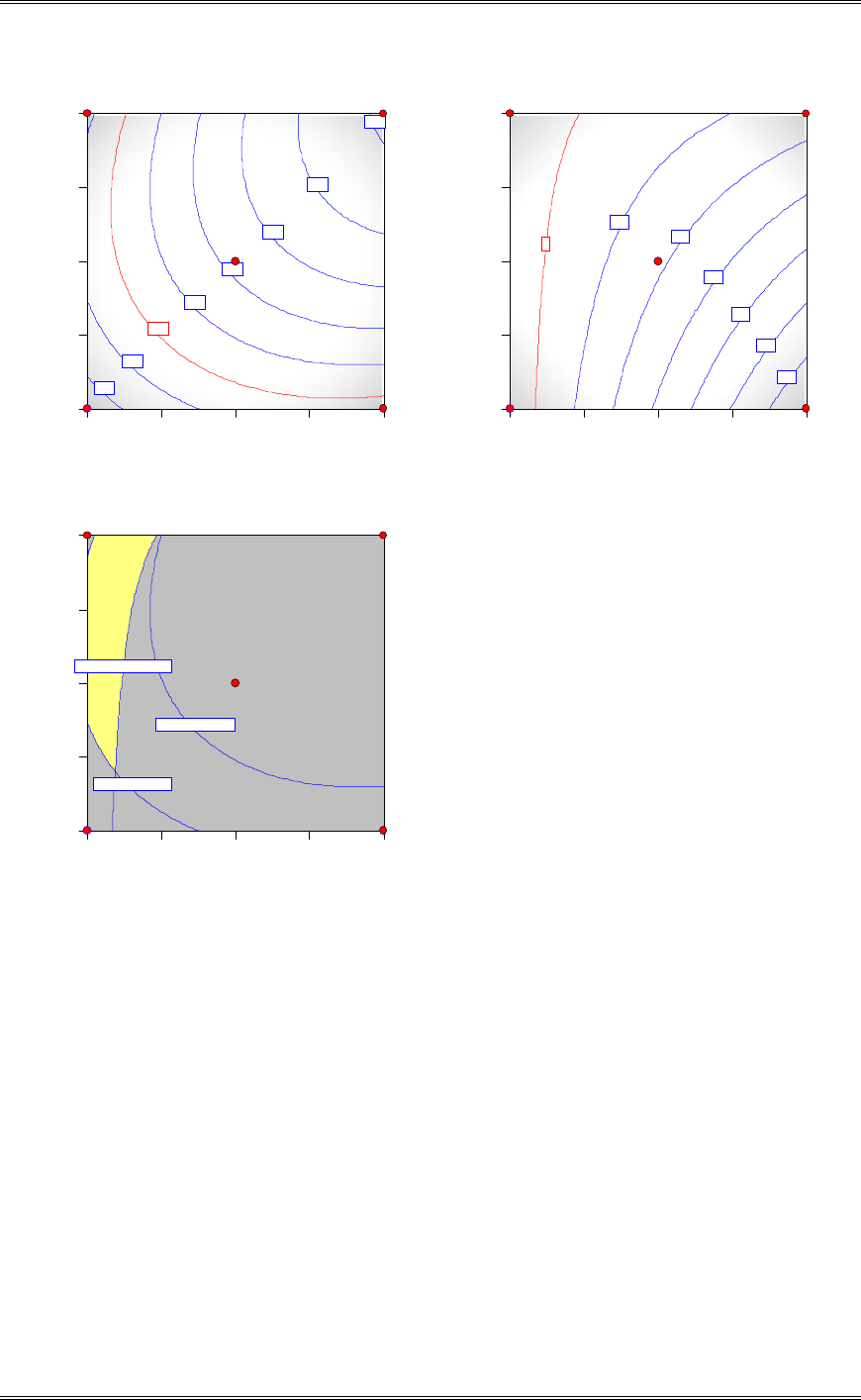
Solutions from Montgomery, D. C. (2001) Design and Analysis of Experiments, Wiley, NY
11-31
Mean Thick
A: x1
B: x2
-1.00 -0.50 0.00 0.50 1.00
-1.00
-0.50
0.00
0.50
1.00
400
425
450
475
500
525
550
575
4
Ln(Var Thick)
A: x1
B: x2
-1.00 -0.50 0.00 0.50 1.00
-1.00
-0.50
0.00
0.50
1.00
2
2.1
2.2
2.3
2.4
2.5
2.6
4
Overlay Plot
A: x1
B: x2
-1.00 -0.50 0.00 0.50 1.00
-1.00
-0.50
0.00
0.50
1.00
Mean Thick : 425
Mean Thick : 475
Ln(Var Thick): 2.000 4
The contour plots describe the two models while the overlay plot identifies the acceptable region for the
process.
(e) Discuss the variance minimization aspects of part (d). Have you minimized total process variance?
The within run variance has been minimized; however, the run-to-run variation has not been minimized
in the analysis. This may not be the most robust operating conditions for the process.
11-15 Verify that an orthogonal first-order design is also first-order rotatable.
To show that a first order orthogonal design is also first order rotatable, consider
)
ˆ
(Vx)
ˆ
(V)x
ˆˆ
(V)y
ˆ
(V
k
i
ii
k
i
ii ¦¦
1
2
0
1
0
EEEE

Solutions from Montgomery, D. C. (2001) Design and Analysis of Experiments, Wiley, NY
11-32
since all covariances between
E
i and
E
jare zero, due to design orthogonality. Furthermore, we have:
n
)
ˆ
(V...)
ˆ
(V)
ˆ
(V
ˆ
Vk
2
210
V
EEEE
, so
¦
k
i
i
x
nn
)y
ˆ
(V
1
2
22
VV
¸
¸
¹
·
¨
¨
©
§ ¦
k
i
i
x
nn
)y
ˆ
(V
1
2
22
1
VV
which is a function of distance from the design center (i.e. x=0), and not direction. Thus the design must
be rotatable. Note that n is, in general, the number of points in the exterior portion of the design. If there
are nc centerpoints, then )nn(
)
ˆ
(V
c
2
0
V
E
.
11-16 Show that augmenting a 2k design with nc center points does not affect the estimates of the
E
i (i=1,
2, . . . , k), but that the estimate of the intercept
E
0 is the average of all 2k + nc observations.
In general, the X matrix for the 2k design with nc center points and the y vector would be:
»
»
»
»
»
»
»
»
»
»
»
»
»
»
»
»
¼
º
«
«
«
«
«
«
«
«
«
«
«
«
«
«
«
«
¬
ª
0001
0001
0001
0001
1111
1111
1111
210
k
EEEE
X
Å The upper half of the matrix is the usual r 1
notation of the 2k design
Å The lower half of the matrix represents the
center points (nc rows)
»
»
»
»
»
»
»
»
»
»
»
»
»
¼
º
«
«
«
«
«
«
«
«
«
«
«
«
«
¬
ª
c
k
n
n
n
y
y
y
0
0
0
2
2
1
2
1
y
Å 2k+nc
observations
.
»
»
»
»
»
¼
º
«
«
«
«
«
¬
ª
k
k
c
kn
2
02
002
XX'
»
»
»
»
»
»
¼
º
«
«
«
«
«
«
¬
ª
k
g
g
g
g
2
1
0
yX'
Å Grand total of
all 2k+nc
observations
Å usual contrasts
from 2k

Solutions from Montgomery, D. C. (2001) Design and Analysis of Experiments, Wiley, NY
11-33
Therefore,
c
kn
g
ˆ
2
0
0
E
, which is the average of all
c
kn2 observations, while k
i
i
g
ˆ
2
E
, which does
not depend on the number of center points, since in computing the contrasts gi, all observations at the
center are multiplied by zero.
11-17 The rotatable central composite design. It can be shown that a second-order design is rotatable if
¦
n
u
b
ju
a
iu xx
10 if a or b (or both) are odd and if 2
1
2
1
43ju
n
uiu
n
uiu xxx ¦¦ . Show that for the central
composite design these conditions lead to
41 /
f
n
D
for rotatability, where nf is the number of points in
the factorial portion.
The balance between +1 and -1 in the factorial columns and the orthogonality among certain column in
the X matrix for the central composite design will result in all odd moments being zero. To solve for D
use the following relations:
4
1
42
D
¦
n
u
fiu nx , ¦
n
u
fjuiu nxx
1
22
then
4
4
4
4
2
1
2
1
4
22
32
3
f
f
f
ff
ju
n
uiu
n
uiu
n
n
n
)n(n
xxx
¦¦
D
D
D
D
11-18 Verify that the central composite design shown below blocks orthogonally.
Block 1 Block 2 Block 3
x1 x2 x3 x1 x2 x3 x1 x2 x3
0 0 0 0 0 0 -1.633 0 0
0 0 0 0 0 0 1.633 0 0
1 1 1 1 1 -1 0 -1.633 0
1 -1 -1 1 -1 1 0 1.633 0
-1 -1 1 -1 1 1 0 0 -1.633
-1 1 -1 -1 -1 -1 0 0 1.633
0 0 0
0 0 0
Note that each block is an orthogonal first order design, since the cross products of elements in different
columns add to zero for each block. To verify the second condition, choose a column, say column x2.
Now
¦
k
u
u.x
1
2
233413 , and n=20

Solutions from Montgomery, D. C. (2001) Design and Analysis of Experiments, Wiley, NY
11-34
For blocks 1 and 2,
¦
m
m
x4
2
2, nm=6
So
6
1
2
2
2
2
¦
¦
m
n
u
u
m
m
n
x
x
20
6
33413
4
.
0.3 = 0.3
and condition 2 is satisfied by blocks 1 and 2. For block 3, we have
¦
m
m.x 3345
2
2, nm = 8, so
n
n
x
x
m
n
u
u
m
m
¦
¦
1
2
2
2
2
20
8
33413
3345
.
.
0.4 = 0.4
And condition 2 is satisfied by block 3. Similar results hold for the other columns.
11-19 Blocking in the central composite design. Consider a central composite design for k = 4 variables
in two blocks. Can a rotatable design always be found that blocks orthogonally?
To run a central composite design in two blocks, assign the nf factorial points and the n01 center points to
block 1 and the 2k axial points plus n02 center points to block 2. Both blocks will be orthogonal first order
designs, so the first condition for orthogonal blocking is satisfied.
The second condition implies that
2
1
2
2
2
2
1
c
cf
m
im
m
im
nk
nn
blockx
blockx
¦
¦

Solutions from Montgomery, D. C. (2001) Design and Analysis of Experiments, Wiley, NY
11-35
However, ¦
m
fim nx2in block 1 and ¦
m
im
x22 2
D
in block 2, so
2
1
22
2c
cff
nk
nnn
D
Which gives:
2
1
1
2
2
2
»
»
¼
º
«
«
¬
ª
cf
cf
nn
nkn
D
Since 4f
n
D
if the design is to be rotatable, then the design must satisfy
2
1
2
2
2
»
»
¼
º
«
«
¬
ª
cf
cf
fnn
nkn
n
It is not possible to find rotatable central composite designs which block orthogonally for all k. For
example, if k=3, the above condition cannot be satisfied. For k=2, there must be an equal number of
center points in each block, i.e. nc1 = nc2. For k=4, we must have nc1 = 4 and nc2 = 2.
11-20 How could a hexagon design be run in two orthogonal blocks?
The hexagonal design can be blocked as shown below. There are nc1 = nc2 = nc center points with nc even.
12
3
45
6n
Put the points 1,3,and 5 in block 1 and 2,4,and 6 in block 2. Note that each block is a simplex.
11-21 Yield during the first four cycles of a chemical process is shown in the following table. The
variables are percent concentration (x1) at levels 30, 31, and 32 and temperature (x2) at 140, 142, and
144qF. Analyze by EVOP methods.
Conditions
Cycle (1) (2) (3) (4) (5)
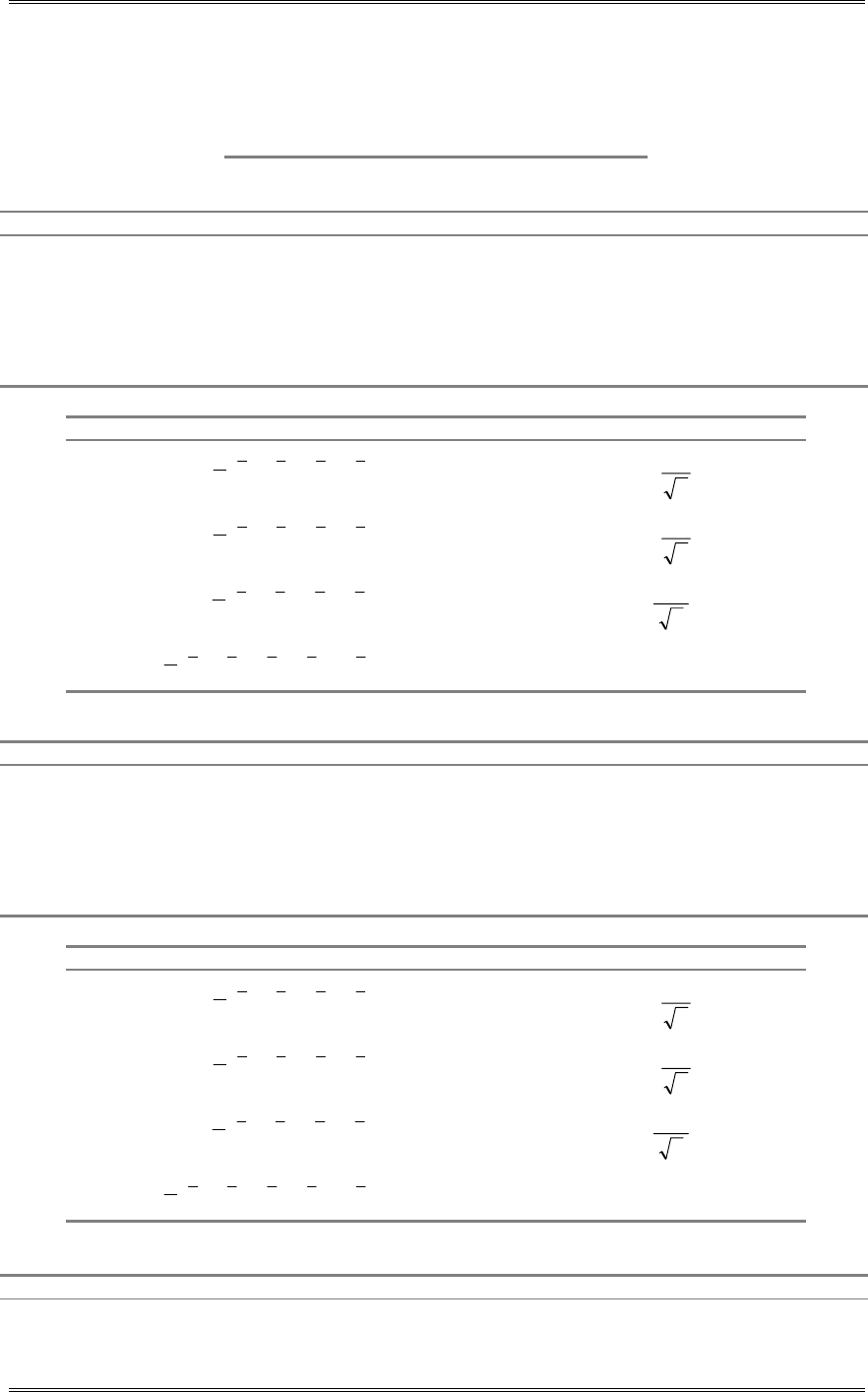
Solutions from Montgomery, D. C. (2001) Design and Analysis of Experiments, Wiley, NY
11-36
1 60.7 59.8 60.2 64.2 57.5
2 59.1 62.8 62.5 64.6 58.3
3 56.6 59.1 59.0 62.3 61.1
4 60.5 59.8 64.5 61.0 60.1
Cycle: n=1 Phase 1
Calculation of Averages Calculation of Standard Deviation
Operating Conditions (1) (2) (3) (4) (5)
(i) Previous Cycle Sum Previous Sum S=
(ii) Previous Cycle Average Previous Average =
(iii) New Observation 60.7 59.8 60.2 64.2 57.5 New S=Range x fk,n
(iv) Differences Range=
(v) New Sums 60.7 59.8 60.2 64.2 57.5 New Sum S=
(vi) New Averages 60.7 59.8 60.2 64.2 57.5 New average S = New Sum S/(n-1)=
Calculation of Effects Calculation of Error Limits
5243
2
1yyyyA 3.55
For New Average:
¸
¸
¹
·
¨
¨
©
§S
n
2
5243
2
1yyyyB -3.55
For New Effects:
¸
¸
¹
·
¨
¨
©
§S
n
2
5243
2
1yyyyAB -0.85
For CIM:
¸
¸
¹
·
¨
¨
©
§S
n
.781
15243 4
2
1yyyyyCIM -0.22
Cycle: n=2 Phase 1
Calculation of Averages Calculation of Standard Deviation
Operating Conditions (1) (2) (3) (4) (5)
(i) Previous Cycle Sum 60.7 59.8 60.2 64.2 57.5
Previous Sum S=
(ii) Previous Cycle Average 60.7 59.8 60.2 64.2 57.5
Previous Average =
(iii) New Observation 59.1 62.8 62.5 64.6 58.3
New S=Range x fk,n=1.38
(iv) Differences 1.6 -3.0 -2.3 -0.4 -0.8
Range=4.6
(v) New Sums 119.8 122.6 122.7 128.8 115.8
New Sum S=1.38
(vi) New Averages 59.90 61.30 61.35 64.40 57.90 New average S = New Sum S/(n-1)=1.38
Calculation of Effects Calculation of Error Limits
5243
2
1yyyyA 3.28
For New Average:
¸
¸
¹
·
¨
¨
©
§S
n
2
1.95
5243
2
1yyyyB -3.23
For New Effects:
¸
¸
¹
·
¨
¨
©
§S
n
2
1.95
5243
2
1yyyyAB 0.18
For CIM:
¸
¸
¹
·
¨
¨
©
§S
n
.781
1.74
15243 4
2
1yyyyyCIM 1.07
Cycle: n=3 Phase 1
Calculation of Averages Calculation of Standard Deviation
Operating Conditions (1) (2) (3) (4) (5)
(i) Previous Cycle Sum 119.8 122.6 122.7 128.8 115.8
Previous Sum S=1.38
Solutions from Montgomery, D. C. (2001) Design and Analysis of Experiments, Wiley, NY
11-37
(ii) Previous Cycle Average 59.90 61.30 61.35 64.40 57.90
Previous Average =1.38
(iii) New Observation 56.6 59.1 59.0 62.3 61.1
New S=Range x fk,n=2.28
(iv) Differences 3.30 2.20 2.35 2.10 -3.20
Range=6.5
(v) New Sums 176.4 181.7 181.7 191.1 176.9
New Sum S=3.66
(vi) New Averages 58.80 60.57 60.57 63.70 58.97 New average S = New Sum S/(n-1)=1.38
Calculation of Effects Calculation of Error Limits
5243
2
1yyyyA 2.37
For New Average:
¸
¸
¹
·
¨
¨
©
§S
n
2
2.11
5243
2
1yyyyB -2.37
For New Effects:
¸
¸
¹
·
¨
¨
©
§S
n
2
2.11
5243
2
1yyyyAB -0.77
For CIM:
¸
¸
¹
·
¨
¨
©
§S
n
.781
1.74
15243 4
2
1yyyyyCIM 1.72
Cycle: n=4 Phase 1
Calculation of Averages Calculation of Standard Deviation
Operating Conditions (1) (2) (3) (4) (5)
(i) Previous Cycle Sum 176.4 181.7 181.7 191.1 176.9
Previous Sum S=3.66
(ii) Previous Cycle Average 58.80 60.57 60.57 63.70 58.97
Previous Average =1.83
(iii) New Observation 60.5 59.8 64.5 61.0 60.1
New S=Range x fk,n=2.45
(iv) Differences -1.70 0.77 -3.93 2.70 -1.13
Range=6.63
(v) New Sums 236.9 241.5 245.2 252.1 237.0
New Sum S=6.11
(vi) New Averages 59.23 60.38 61.55 63.03 59.25 New average S = New Sum S/(n-1)=2.04
Calculation of Effects Calculation of Error Limits
5243
2
1yyyyA 2.48
For New Average:
¸
¸
¹
·
¨
¨
©
§S
n
2
2.04
5243
2
1yyyyB -1.31
For New Effects:
¸
¸
¹
·
¨
¨
©
§S
n
2
2.04
5243
2
1yyyyAB -0.18
For CIM:
¸
¸
¹
·
¨
¨
©
§S
n
.781
1.82
15243 4
2
1yyyyyCIM 1.46
From studying cycles 3 and 4, it is apparent that A (and possibly B) has a significant effect. A new phase
should be started following cycle 3 or 4.
11-22 Suppose that we approximate a response surface with a model of order d1, such as y=X1E
EE
E1+H
HH
H, when
the true surface is described by a model of order d2>d1; that is E(y)= X1E
EE
E1+ X2E
EE
E2.
(a) Show that the regression coefficients are biased, that is, that E(
E
EE
E1)=E
EE
E1+AE
EE
E2, where A=(X’
1X1)-
1X’
1X2. A is usually called the alias matrix.

Solutions from Montgomery, D. C. (2001) Design and Analysis of Experiments, Wiley, NY
11-38
>@
>@
21
221
1
11111
1
11
22111
1
11
1
1
11
1
1
111
Aββ
βXXXXβXXXX
βXβXXXX
yXXX
yXXXβ
»
¼
º
«
¬
ª
''''
''
''
''
E
E
ˆ
E
where
2
'
1
'
1XXXXA 1
1
(a) If d1=1 and d2=2, and a full 2k is used to fit the model, use the result in part (a) to determine the alias
structure.
In this situation, we have assumed the true surface to be first order, when it is really second order. If a full
factorial is used for k=2, then
X1 =
E
E
E
012
111
111
11 1
11 1
ª
ªª
ª
¬
¬¬
¬
«
««
«
«
««
«
«
««
«
«
««
«
º
ºº
º
¼
¼¼
¼
»
»»
»
»
»»
»
»
»»
»
»
»»
»
X2 =
E
11
1
1
1
1
ª
ªª
ª
¬
¬¬
¬
«
««
«
«
««
«
«
««
«
«
««
«
E
22
1
1
1
1»
»
»
»
¼
º
1
1
1
1
12
E
and A =
110
000
000
ª
ªª
ª
¬
¬¬
¬
«
««
«
«
««
«
«
««
«
º
ºº
º
¼
¼¼
¼
»
»»
»
»
»»
»
»
»»
»
Then, E
>
>>
>@
@@
@
E
EE
E1 = E
»
»
»
¼
º
«
«
«
¬
ª
»
»
»
¼
º
«
«
«
¬
ª
»
»
»
¼
º
«
«
«
¬
ª
»
»
»
¼
º
«
«
«
¬
ª
»
»
»
¼
º
«
«
«
¬
ª
2
1
22110
12
22
11
2
1
0
2
1
0
000
000
011
E
E
EEE
E
E
E
E
E
E
E
E
E
ˆ
ˆ
ˆ
The pure quadratic terms bias the intercept.
(b) If d1=1, d2=2 and k=3, find the alias structure assuming that a 23-1 design is used to fit the model.
X1 =
E
E
E
E
0123
1111
111 1
11 1 1
11 1 1
ª
ªª
ª
¬
¬¬
¬
«
««
«
«
««
«
«
««
«
«
««
«
º
ºº
º
¼
¼¼
¼
»
»»
»
»
»»
»
»
»»
»
»
»»
»
X2 =
E
11
1
1
1
1
ª
ªª
ª
¬
¬¬
¬
«
««
«
«
««
«
«
««
«
«
««
«
E
22
1
1
1
1
E
33
1
1
1
1
E
12
1
1
1
1
E
13
1
1
1
1
E
23
1
1
1
1
º
ºº
º
¼
¼¼
¼
»
»»
»
»
»»
»
»
»»
»
»
»»
»
and A =
110000
000001
000010
000100
ª
ªª
ª
¬
¬¬
¬
«
««
«
«
««
«
«
««
«
«
««
«
º
ºº
º
¼
¼¼
¼
»
»»
»
»
»»
»
»
»»
»
»
»»
»
Then, E
>
>>
>@
@@
@
E
EE
E1 = E
»
»
»
»
¼
º
«
«
«
«
¬
ª
»
»
»
»
»
»
»
»
¼
º
«
«
«
«
«
«
«
«
¬
ª
»
»
»
»
¼
º
«
«
«
«
¬
ª
»
»
»
»
¼
º
«
«
«
«
¬
ª
»
»
»
»
»
¼
º
«
«
«
«
«
¬
ª
123
132
231
2222110
23
13
12
33
22
11
3
2
1
0
3
2
1
0
001000
010000
100000
000011
EE
EE
EE
EEEE
E
E
E
E
E
E
E
E
E
E
E
E
E
E
ˆ
ˆ
ˆ
ˆ
(d) If d1=1, d2=2, k=3, and the simplex design in Problem 11-3 is used to fit the model, determine the
alias structure and compare the results with part (c).

Solutions from Montgomery, D. C. (2001) Design and Analysis of Experiments, Wiley, NY
11-39
X1 =
E
E
E
E
0123
1111
111 1
11 1 1
11 1 1
ª
ªª
ª
¬
¬¬
¬
«
««
«
«
««
«
«
««
«
«
««
«
º
ºº
º
¼
¼¼
¼
»
»»
»
»
»»
»
»
»»
»
»
»»
»
X2 =
E
11
0
2
0
2
ª
ªª
ª
¬
¬¬
¬
«
««
«
«
««
«
«
««
«
«
««
«
E
22
2
0
2
0
E
33
1
1
1
1
E
12
0
0
0
0
E
13
0
2
0
2
E23
2
0
2
0
º
ºº
º
¼
¼¼
¼
»
»»
»
»
»»
»
»
»»
»
»
»»
»
and A =
1 1 100 0
0 0 001 0
0 0 000 1
1 1000 0
ª
ªª
ª
¬
¬¬
¬
«
««
«
«
««
«
«
««
«
«
««
«
º
ºº
º
¼
¼¼
¼
»
»»
»
»
»»
»
»
»»
»
»
»»
»
Then, E
>
>>
>@
@@
@
E
EE
E1 = E
»
»
»
»
¼
º
«
«
«
«
¬
ª
»
»
»
»
»
»
»
»
¼
º
«
«
«
«
«
«
«
«
¬
ª
»
»
»
»
¼
º
«
«
«
«
¬
ª
»
»
»
»
¼
º
«
«
«
«
¬
ª
»
»
»
»
»
¼
º
«
«
«
«
«
¬
ª
22113
232
131
2222110
23
13
12
33
22
11
3
2
1
0
3
2
1
0
000011
100000
010000
000111
EEE
EE
EE
EEEE
E
E
E
E
E
E
E
E
E
E
E
E
E
E
ˆ
ˆ
ˆ
ˆ
Notice that the alias structure is different from that found in the previous part for the 23-1 design. In
general, the A matrix will depend on which simplex design is used.
11-23 In an article (“Let’s All Beware the Latin Square,” Quality Engineering, Vol. 1, 1989, pp. 453-
465) J.S. Hunter illustrates some of the problems associated with 3k-p fractional factorial designs. Factor A
is the amount of ethanol added to a standard fuel and factor B represents the air/fuel ratio. The response
variable is carbon monoxide (CO) emission in g/m2. The design is shown below.
Design Observations
A B x1 x2 y y
0 0 -1 -1 66 62
1 0 0 -1 78 81
2 0 1 -1 90 94
0 1 -1 0 72 67
1 1 0 0 80 81
2 1 1 0 75 78
0 2 -1 1 68 66
1 2 0 1 66 69
2 2 1 1 60 58
Notice that we have used the notation system of 0, 1, and 2 to represent the low, medium, and high levels
for the factors. We have also used a “geometric notation” of -1, 0, and 1. Each run in the design is
replicated twice.
(a) Verify that the second-order model
21
2
2
2
121 0904540754578 xx.x.x.x.x..y
ˆ
is a reasonable model for this experiment. Sketch the CO concentration contours in the x1, x2 space.
In the computer output that follows, the “coded factors” model is in the -1, 0, +1 scale.
Design Expert Output
Response: CO Emis
ANOVA for Response Surface Quadratic Model
Analysis of variance table [Partial sum of squares]
Sum of
Mean F
Source Squares DF Square Value Prob > F
Model 1624.00 5 324.80 50.95 < 0.0001 significant
A 243.00 1 243.00 38.12 < 0.0001
Solutions from Montgomery, D. C. (2001) Design and Analysis of Experiments, Wiley, NY
11-40
B 588.00 1 588.00 92.24 < 0.0001
A2 81.00 1 81.00 12.71 0.0039
B2 64.00 1 64.00 10.04 0.0081
AB 648.00 1 648.00 101.65 < 0.0001
Residual 76.50 12 6.37
Lack of Fit 30.00 3 10.00 1.94 0.1944 not significant
Pure Error 46.50 9 5.17
Cor Total 1700.50 17
The Model F-value of 50.95 implies the model is significant. There is only
a 0.01% chance that a "Model F-Value" this large could occur due to noise.
Std. Dev. 2.52 R-Squared 0.9550
Mean 72.83 Adj R-Squared 0.9363
C.V. 3.47 Pred R-Squared 0.9002
PRESS 169.71 Adeq Precision 21.952
Coefficient Standard 95% CI 95% CI
Factor Estimate DF Error Low High VIF
Intercept 78.50 1 1.33 75.60 81.40
A-Ethanol 4.50 1 0.73 2.91 6.09 1.00
B-Air/Fuel Ratio -7.00 1 0.73 -8.59 -5.41 1.00
A
2 -4.50 1 1.26 -7.25 -1.75 1.00
B
2 -4.00 1 1.26 -6.75 -1.25 1.00
AB -9.00 1 0.89 -10.94 -7.06 1.00
Final Equation in Terms of Coded Factors:
CO Emis =
+78.50
+4.50 * A
-7.00 * B
-4.50 * A2
-4.00 * B2
-9.00 * A * B
CO Emis
A: Ethanol
B: Air/Fuel R atio
-1 -0.5 00.5 1
-1.00
-0.50
0.00
0.50
1.00
65
65
70
75
80
85
222
222
222
(b) Now suppose that instead of only two factors, we had used four factors in a 34-2 fractional factorial
design and obtained exactly the same data in part (a). The design would be as follows:
Design Observations
A B C D x1 x2 x3 x4 y y
Solutions from Montgomery, D. C. (2001) Design and Analysis of Experiments, Wiley, NY
11-41
0 0 0 0 -1 -1 -1 -1 66 62
1 0 1 1 0 -1 0 0 78 81
2 0 2 2 +1 -1 +1 +1 90 94
0 1 2 1 -1 0 +1 0 72 67
1 1 0 2 0 0 -1 +1 80 81
2 1 1 0 +1 0 0 -1 75 78
0 2 1 2 -1 +1 0 +1 68 66
1 2 2 0 0 +1 +1 -1 66 69
2 2 0 1 +1 +1 -1 0 60 58
Confirm that this design is an L9 orthogonal array.
This is the same as the design in Table 11-22.
(c) Calculate the marginal averages of the CO response at each level of the four factors A, B, C, and D.
Construct plots of these marginal averages and interpret the results. Do factors C and D appear to
have strong effects? Do these factors really have any effect on CO emission? Why is their apparent
effect strong?
A: A
CO Emis
One Factor Plot
0 1 2
58
67
76
85
94
B: B
CO Emis
One Factor Plot
0 1 2
58
67
76
85
94
Solutions from Montgomery, D. C. (2001) Design and Analysis of Experiments, Wiley, NY
11-42
C: C
CO Emis
One Factor Plot
0 1 2
58
67
76
85
94
D: D
CO Emis
One Factor Plot
0 1 2
58
67
76
85
94
Both Factors C and D appear to have an effect on CO emission. This is probably because both C and D
are aliased with components of interaction involving A and B, and there is a strong AB interaction.
(a) The design in part (b) allows the model
¦¦
4
1
4
1
2
0
ii
iiiii xxy
HEEE
to be fitted. Suppose that the true model is
¦¦ ¦¦
4
1
4
1
2
0
ii ji
jiijiiiii xxxxy
HEEEE
Show that if
E
jrepresents the least squares estimates of the coefficients in the fitted model, then
1323124444
1412243333
3414132222
24231111
231244
241233
34141322
242311
34141300
2
2
2
2
2
2
2
2
EEEEE
EEEEE
EEEEE
EEEE
EEEE
EEEE
EEEEE
EEEE
EEEEE
/
ˆ
E
/
ˆ
E
/
ˆ
E
/
ˆ
E
/
ˆ
E
/
ˆ
E
/
ˆ
E
/
ˆ
E
ˆ
E

Solutions from Montgomery, D. C. (2001) Design and Analysis of Experiments, Wiley, NY
11-43
Let X1 =
E0
1
1
1
1
1
1
1
1
1
ª
ªª
ª
¬
¬¬
¬
«
««
«
«
««
«
«
««
«
«
««
«
«
««
«
«
««
«
«
««
«
«
««
«
«
««
«
«
««
«
«
««
«
«
««
«
E1
1
0
1
1
0
1
1
0
1
E2
1
1
1
0
0
0
1
1
1
E3
1
0
1
1
1
0
1
1
0
E4
1
0
1
0
1
1
1
1
0
E11
1
0
1
1
0
1
1
0
1
E22
1
1
1
0
0
0
1
1
1
E33
1
0
1
1
1
0
1
1
0
E44
1
0
1
0
1
1
1
1
0
º
ºº
º
¼
¼¼
¼
»
»»
»
»
»»
»
»
»»
»
»
»»
»
»
»»
»
»
»»
»
»
»»
»
»
»»
»
»
»»
»
»
»»
»
»
»»
»
»
»»
»
and X2 =
E12
1
0
1
0
0
0
1
0
1
ª
ªª
ª
¬
¬¬
¬
«
««
«
«
««
«
«
««
«
«
««
«
«
««
«
«
««
«
«
««
«
«
««
«
«
««
«
«
««
«
«
««
«
«
««
«
E13
1
0
1
1
0
0
0
0
1
E14
1
0
1
0
0
1
1
0
0
E23
1
0
1
0
0
0
0
1
1
E24
1
0
1
0
0
0
1
1
0
E34
1
0
1
0
1
0
0
1
0
º
ºº
º
¼
¼¼
¼
»
»»
»
»
»»
»
»
»»
»
»
»»
»
»
»»
»
»
»»
»
»
»»
»
»
»»
»
»
»»
»
»
»»
»
»
»»
»
»
»»
»
Then,
AXX XX
11
1
12
''
= A =
»
»
»
»
»
»
»
»
»
»
»
»
¼
º
«
«
«
«
«
«
«
«
«
«
«
«
¬
ª
00210121
02101021
210021210
02121000
00210021
02100021
210021210
02121000
100110
»
»
»
»
»
»
»
»
»
»
»
»
¼
º
«
«
«
«
«
«
«
«
«
«
«
«
¬
ª
»
»
»
»
»
»
»
»
¼
º
«
«
«
«
«
«
«
«
¬
ª
»
»
»
»
»
»
»
»
»
»
»
»
¼
º
«
«
«
«
«
«
«
«
«
«
«
«
¬
ª
»
»
»
»
»
»
»
»
»
»
»
»
¼
º
«
«
«
«
«
«
«
«
«
«
«
«
¬
ª
»
»
»
»
»
»
»
»
»
»
»
»
»
¼
º
«
«
«
«
«
«
«
«
«
«
«
«
«
¬
ª
23131244
24141233
34141322
242311
23124
24123
3414132
24231
3414130
34
24
23
14
13
12
44
33
22
11
4
3
2
1
0
44
33
22
11
4
3
2
1
0
2121
2121
212121
2121
2121
2121
212121
2121
00210121
02101021
210021210
02121000
00210021
02100021
210021210
02121000
100110
EEEE
EEEE
EEEE
EEE
EEE
EEE
EEEE
EEE
EEEE
E
E
E
E
E
E
E
E
E
E
E
E
E
E
E
E
E
E
E
E
E
E
E
E
ˆ
ˆ
ˆ
ˆ
ˆ
ˆ
ˆ
ˆ
ˆ
E
11-24 Suppose that you need to design an experiment to fit a quadratic model over the region
11 dd i
x, i=1,2 subject to the constraint 1
21 d xx . If the constraint is violated, the process will
not work properly. You can afford to make no more than n=12 runs. Set up the following designs:
(a) An “inscribed” CCD with center points at 0
21 xx
x1 x
2
-0.5 -0.5
0.5 -0.5
-0.5 0.5
0.5 0.5
-0.707 0
0.707 0

Solutions from Montgomery, D. C. (2001) Design and Analysis of Experiments, Wiley, NY
11-44
0 -0.707
0 0.707
0 0
0 0
0 0
0 0
(a)* An “inscribed” CCD with center points at 250
21 .xx so that a larger design could be fit within
the constrained region
x1 x
2
-1 -1
0.5 -1
-1 0.5
0.5 0.5
-1.664 -0.25
1.164 -0.25
-0.25 -1.664
-0.25 1.164
-0.25 -0.25
-0.25 -0.25
-0.25 -0.25
-0.25 -0.25
(a) An “inscribed” 32 factorial with center points at 25.0
21 xx
x1 x
2
-1 -1
-0.25 -1
0.5 -1
-1 -0.25
-0.25 -0.25
0.5 -0.25
-1 0.5
-0.25 0.5
0.5 0.5
-0.25 -0.25
-0.25 -0.25
-0.25 -0.25
(a) A D-optimal design.
x1 x
2
-1 -1
1 -1
-1 1
1 0
0 1
0 0
-1 0
0 -1

Solutions from Montgomery, D. C. (2001) Design and Analysis of Experiments, Wiley, NY
11-45
0.5 0.5
-1 -1
1 -1
-1 1
(a) A modified D-optimal design that is identical to the one in part (c), but with all replicate runs at the
design center.
x1 x
2
1 0
0 0
0 1
-1 -1
1 -1
-1 1
-1 0
0 -1
0.5 0.5
0 0
0 0
0 0
(a) Evaluate the 1
)(
cXX criteria for each design.
(a) (a)* (b) (c) (d)
1
cXX 0.5 0.00005248 0.007217 0.0001016 0.0002294
(a) Evaluate the D-efficiency for each design relative to the D-optimal design in part (c).
(a) (a)* (b) (c) (d)
D-efficiency 24.25% 111.64% 49.14% 100.00% 87.31%
(a) Which design would you prefer? Why?
The offset CCD, (a)*, is the preferred design based on the D-efficiency. Not only is it better than the D-
optimal design, (c), but it maintains the desirable design features of the CCD.

Solutions from Montgomery, D. C. (2001) Design and Analysis of Experiments, Wiley, NY
11-46
11-25 Consider a 23 design for fitting a first-order model.
(a) Evaluate the D-criterion 1
)(
cXX for this design.
1
)(
cXX = 2.441E-4
(b) Evaluate the A-criterion 1
)(
cXXtr for this design.
1
)(
cXXtr = 0.5
(c) Find the maximum scaled prediction variance for this design. Is this design G-optimal?
4
1
1
1
2
cc
xXXx
x
xN
y
ˆ
NVar
v
V
. Yes, this is a G-optimal design.
11-26 Repeat Problem 11-25 using a first order model with the two-factor interaction.
1
)(
cXX = 4.768E-7
1
)(
cXXtr = 0.875
7
1
1
1
2
cc
xXXx
x
xN
y
ˆ
NVar
v
V
. Yes, this is a G-optimal design.
11-27 A chemical engineer wishes to fit a calibration curve for a new procedure used to measure the
concentration of a particular ingredient in a product manufactured in his facility. Twelve samples can be
prepared, having known concentration. The engineer’s interest is in building a model for the measured
concentrations. He suspects that a linear calibration curve will be adequate to model the measured
concentration as a function of the known concentrations; that is, where x is the actual concentration. Four
experimental designs are under consideration. Design 1 consists of 6 runs at known concentration 1 and 6
runs at known concentration 10. Design 2 consists of 4 runs at concentrations 1, 5.5, and 10. Design 3
consists of 3 runs at concentrations 1, 4, 7, and 10. Finally, design 4 consists of 3 runs at concentrations 1
and 10 and 6 runs at concentration 5.5.
(a) Plot the scaled variance of prediction for all four designs on the same graph over the concentration
range. Which design would be preferable, in your opinion?
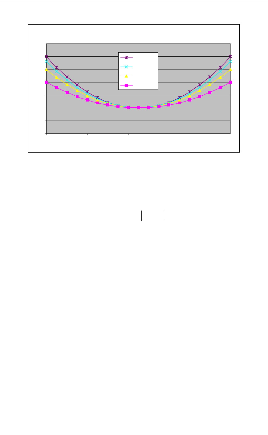
Solutions from Montgomery, D. C. (2001) Design and Analysis of Experiments, Wiley, NY
11-47
Scaled Variance of Prediction
0
0.5
1
1.5
2
2.5
3
3.5
13579
Design 4
Design 3
Design 2
Design 1
Because it has the lowest scaled variance of prediction at all points in the design space with the exception
of 5.5, Design 1 is preferred.
(b) For each design calculate the determinant of 1
)(
cXX . Which design would be preferred according
to the “D” criterion?
Design 1
)(
cXX
1 0.000343
2 0.000514
3 0.000617
4 0.000686
Design 1 would be preferred.
(c) Calculate the D-efficiency of each design relative to the “best” design that you found in part b.
Design D-efficiency
1 100.00%
2 81.65%
3 74.55%
4 70.71%
(a) For each design, calculate the average variance of prediction over the set of points given by x = 1, 1.5,
2, 2.5, . . ., 10. Which design would you prefer according to the V-criterion?
Average Variance of Prediction
Design Actual Coded
1 1.3704 0.1142
2 1.5556 0.1296
3 1.6664 0.1389
4 1.7407 0.1451
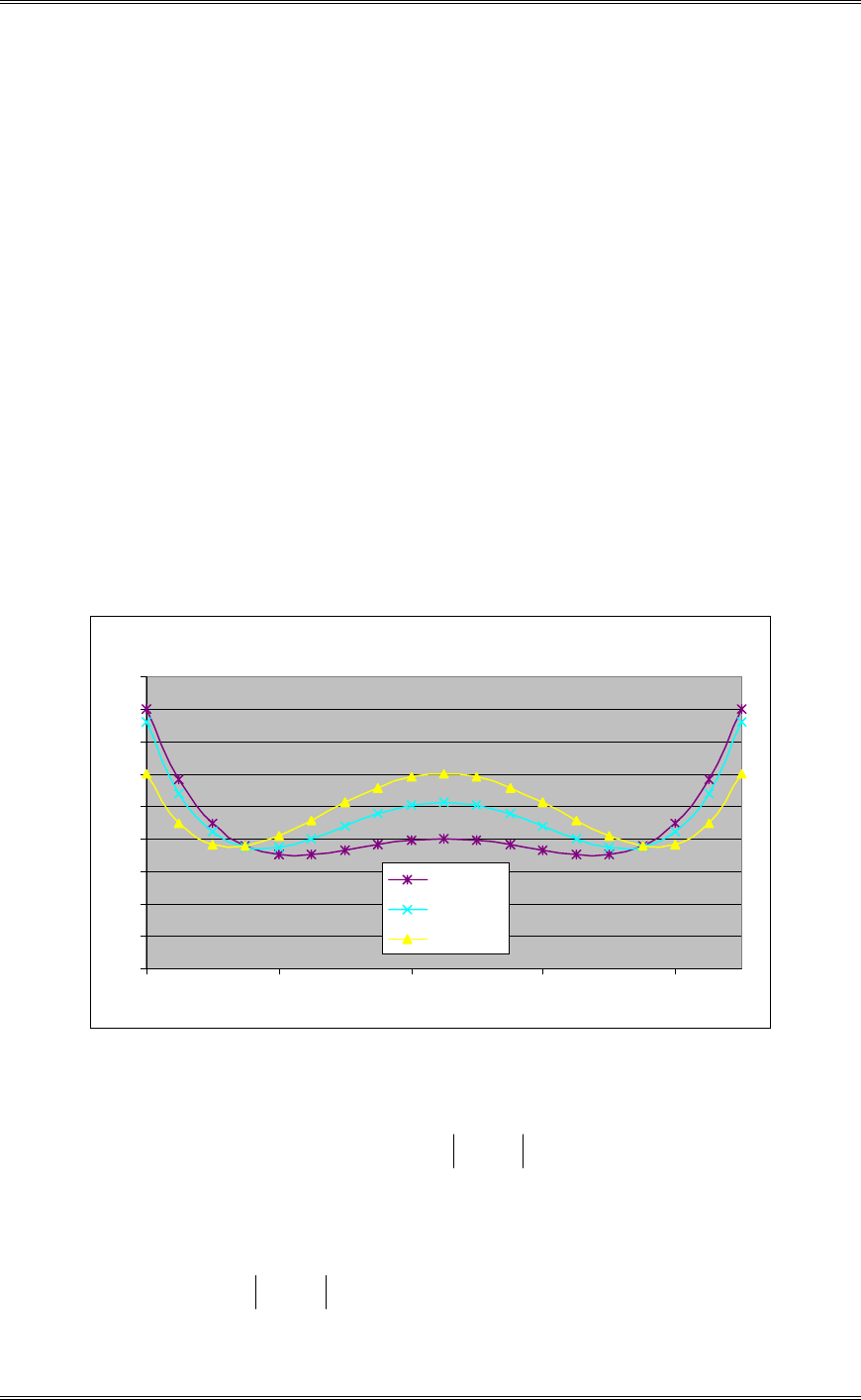
Solutions from Montgomery, D. C. (2001) Design and Analysis of Experiments, Wiley, NY
11-48
Design 1 is still preferred based on the V-criterion.
(e) Calculate the V-efficiency of each design relative to the best design you found in part (d).
Design V-efficiency
1 100.00%
2 88.10%
3 82.24%
4 78.72%
(f) What is the G-efficiency of each design?
Design G-efficiency
1 100.00%
2 80.00%
3 71.40%
4 66.70%
11-28 Rework Problem 11-27 assuming that the model the engineer wishes to fit is a quadratic.
Obviously, only designs 2, 3, and 4 can now be considered.
Scaled Variance of Prediction
0
0.5
1
1.5
2
2.5
3
3.5
4
4.5
13579
Design 4
Design 3
Design 2
2
Based on the plot, the preferred design would depend on the region of interest. Design 4 would be
preferred if the center of the region was of interest; otherwise, Design 2 would be preferred.
Design 1
)(
cXX
2 4.704E-07
3 6.351E-07
4 5.575E-07
Design 2 is preferred based on 1
)(
cXX .

Solutions from Montgomery, D. C. (2001) Design and Analysis of Experiments, Wiley, NY
11-49
Design D-efficiency
2 100.00%
3 90.46%
4 94.49%
Average Variance of Prediction
Design Actual Coded
2 2.441 0.2034
3 2.393 0.1994
4 2.242 0.1869
Design 4 is preferred.
Design V-efficiency
2 91.89%
3 93.74%
4 100.00%
Design G-efficiency
2 100.00%
3 79.00%
4 75.00%
11-29 An experimenter wishes to run a three-component mixture experiment. The constraints are the
components proportions are as follows:
7.04.0
3.01.0
4.02.0
3
2
1
dd
dd
dd
x
x
x
(a) Set up an experiment to fit a quadratic mixture model. Use n=14 runs, with 4 replicates. Use the D-
criteria.
Std x1 x2 x3
1 0.2 0.3 0.5
2 0.3 0.3 0.4
3 0.3 0.15 0.55
4 0.2 0.1 0.7
5 0.4 0.2 0.4
6 0.4 0.1 0.5
7 0.2 0.2 0.6
8 0.275 0.25 0.475
9 0.35 0.175 0.475
10 0.3 0.1 0.6
11 0.2 0.3 0.5
12 0.3 0.3 0.4
13 0.2 0.1 0.7
14 0.4 0.1 0.5
(a) Draw the experimental design region.
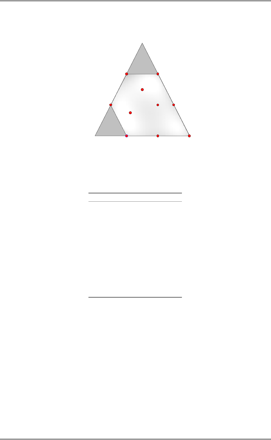
Solutions from Montgomery, D. C. (2001) Design and Analysis of Experiments, Wiley, NY
11-50
A: x1
0.50
B: x2
0.40
C: x3
0.70
0.40 0.10
0.20
2
2
2
2
(c) Set up an experiment to fit a quadratic mixture model with n=12 runs, assuming that three of these
runs are replicated. Use the D-criterion.
Std x1 x
2 x
3
1 0.3 0.15 0.55
2 0.2 0.3 0.5
3 0.3 0.3 0.4
4 0.2 0.1 0.7
5 0.4 0.2 0.4
6 0.4 0.1 0.5
7 0.2 0.2 0.6
8 0.275 0.25 0.475
9 0.35 0.175 0.475
10 0.2 0.1 0.7
11 0.4 0.1 0.5
12 0.4 0.2 0.4
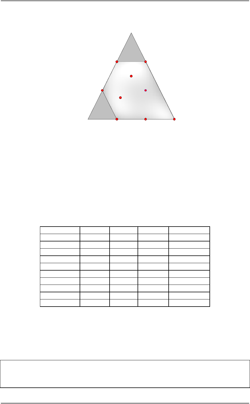
Solutions from Montgomery, D. C. (2001) Design and Analysis of Experiments, Wiley, NY
11-51
A: x1
0.50
B: x2
0.40
C: x3
0.70
0.40 0.10
0.20
2
2 2
(d) Comment on the two designs you have found.
The design points are the same for both designs except that the edge center on the x1-x3 edge is not
included in the second design. None of the replicates for either design are in the center of the
experimental region. The experimental runs are fairly uniformly spaced in the design region.
11-30 Myers and Montgomery (1995) describe a gasoline blending experiment involving three mixture
components. There are no constraints on the mixture proportions, and the following 10 run design is
used.
Design Point x1 x2 x3 y(mpg)
1 1 0 0 24.5, 25.1
2 0 1 0 24.8, 23.9
3 0 0 1 22.7, 23.6
4 ½ ½ 0 25.1
5 ½ 0 ½ 24.3
6 0 ½ ½ 23.5
7 1/3 1/3 1/3 24.8, 24.1
8 2/3 1/6 1/6 24.2
9 1/6 2/3 1/6 23.9
10 1/6 1/6 2/3 23.7
(a) What type of design did the experimenters use?
A simplex centroid design was used.
(b) Fit a quadratic mixture model to the data. Is this model adequate?
Design Expert Output
Response: y
ANOVA for Mixture Quadratic Model
Analysis of variance table [Partial sum of squares]
Sum of
Mean F
Source Squares DF Square Value Prob > F

Solutions from Montgomery, D. C. (2001) Design and Analysis of Experiments, Wiley, NY
11-52
Model 4.22 5 0.84 3.90 0.0435 significant
Linear Mixture 3.92 2 1.96 9.06 0.0088
AB 0.15 1 0.15 0.69 0.4289
AC 0.081 1 0.081 0.38 0.5569
BC 0.077 1 0.077 0.36 0.5664
Residual 1.73 8 0.22
Lack of Fit 0.50 4 0.12 0.40 0.8003 not significant
Pure Error 1.24 4 0.31
Cor Total 5.95 13
The Model F-value of 3.90 implies the model is significant. There is only
a 4.35% chance that a "Model F-Value" this large could occur due to noise.
Std. Dev. 0.47 R-Squared 0.7091
Mean 24.16 Adj R-Squared 0.5274
C.V. 1.93 Pred R-Squared 0.1144
PRESS 5.27 Adeq Precision 5.674
Coefficient Standard 95% CI 95% CI
Component Estimate DF Error Low High
A-x1 24.74 1 0.32 24.00 25.49
B-x2 24.31 1 0.32 23.57 25.05
C-x3 23.18 1 0.32 22.43 23.92
AB 1.51 1 1.82 -2.68 5.70
AC 1.11 1 1.82 -3.08 5.30
BC -1.09 1 1.82 -5.28 3.10
Final Equation in Terms of Pseudo Components:
y =
+24.74 * A
+24.31 * B
+23.18 * C
+1.51 * A * B
+1.11 * A * C
-1.09 * B * C
Final Equation in Terms of Real Components:
y =
+24.74432 * x1
+24.31098 * x2
+23.17765 * x3
+1.51364 * x1 * x2
+1.11364 * x1 * x3
-1.08636 * x2 * x3
The quadratic terms appear to be insignificant. The analysis below is for the linear mixture model:
Design Expert Output
Response: y
ANOVA for Mixture Quadratic Model
Analysis of variance table [Partial sum of squares]
Sum of
Mean F
Source Squares DF Square Value Prob > F
Model 3.92 2 1.96 10.64 0.0027 significant
Linear Mixture 3.92 2 1.96 10.64 0.0027
Residual 2.03 11 0.18
Lack of Fit 0.79 7 0.11 0.37 0.8825 not significant
Pure Error 1.24 4 0.31
Cor Total 5.95 13
The Model F-value of 10.64 implies the model is significant. There is only
a 0.27% chance that a "Model F-Value" this large could occur due to noise.
Std. Dev. 0.43 R-Squared 0.6591
Mean 24.16 Adj R-Squared 0.5972
C.V. 1.78 Pred R-Squared 0.3926
PRESS 3.62 Adeq Precision 8.751
Solutions from Montgomery, D. C. (2001) Design and Analysis of Experiments, Wiley, NY
11-53
Coefficient Standard 95% CI 95% CI
Component Estimate DF Error Low High
A-x1 24.93 1 0.25 24.38 25.48
B-x2 24.35 1 0.25 23.80 24.90
C-x3 23.19 1 0.25 22.64 23.74
Adjusted Adjusted Approx t for H0
Component Effect DF Std Error Effect=0 Prob > |t|
A-x1 1.16 1 0.33 3.49 0.0051
B-x2 0.29 1 0.33 0.87 0.4021
C-x3 -1.45 1 0.33 -4.36 0.0011
Final Equation in Terms of Pseudo Components:
y =
+24.93 * A
+24.35 * B
+23.19 * C
Final Equation in Terms of Real Components:
y =
+24.93048 * x1
+24.35048 * x2
+23.19048 * x3
(c) Plot the response surface contours. What blend would you recommend to maximize the MPG?
A: x1
1.00
B: x2
1.00
C: x3
1.00
0.00 0.00
0.00
y
23.4
23.6
23.8
24
24.2
24.4
24.6
24.8
2
2 2
To maximize the miles per gallon, the recommended blend is x1 = 1, x2 = 0, and x3 = 0.
11-31 Consider the bottle filling experiment in Example 6-1. Suppose that the percent carbonation (A) is
a noise variable (in coded units 1
2
z
V
).
(a) Fit the response model to these data. Is there a robust design problem?
From the analysis below, the AB interaction appears to have some importance. Because of this, there is
opportunity for improvement in the robustness of the process.
Design Expert Output

Solutions from Montgomery, D. C. (2001) Design and Analysis of Experiments, Wiley, NY
11-54
Response: Fill Height
ANOVA for Selected Factorial Model
Analysis of variance table [Partial sum of squares]
Sum of
Mean F
Source Squares DF Square Value Prob > F
Model 73.00 7 10.43 16.69 0.0003 significant
A 36.00 1 36.00 57.60 < 0.0001
B 20.25 1 20.25 32.40 0.0005
C 12.25 1 12.25 19.60 0.0022
AB 2.25 1 2.25 3.60 0.0943
AC 0.25 1 0.25 0.40 0.5447
BC 1.00 1 1.00 1.60 0.2415
ABC 1.00 1 1.00 1.60 0.2415
Pure Error 5.00 8 0.63
Cor Total 78.00 15
The Model F-value of 16.69 implies the model is significant. There is only
a 0.03% chance that a "Model F-Value" this large could occur due to noise.
Std. Dev. 0.79 R-Squared 0.9359
Mean 1.00 Adj R-Squared 0.8798
C.V. 79.06 Pred R-Squared 0.7436
PRESS 20.00 Adeq Precision 13.416
Coefficient Standard 95% CI 95% CI
Factor Estimate DF Error Low High VIF
Intercept 1.00 1 0.20 0.54 1.46
A-Carbination 1.50 1 0.20 1.04 1.96 1.00
B-Pressure 1.13 1 0.20 0.67 1.58 1.00
C-Speed 0.88 1 0.20 0.42 1.33 1.00
AB 0.38 1 0.20 -0.081 0.83 1.00
AC 0.13 1 0.20 -0.33 0.58 1.00
BC 0.25 1 0.20 -0.21 0.71 1.00
ABC 0.25 1 0.20 -0.21 0.71 1.00
Final Equation in Terms of Coded Factors:
Fill Height =
+1.00
+1.50 * A
+1.13 * B
+0.88 * C
+0.38 * A * B
+0.13 * A * C
+0.25 * B * C
+0.25 * A * B * C
Final Equation in Terms of Actual Factors:
Fill Height =
-225.50000
+21.00000 * Carbination
+7.80000 * Pressure
+1.08000 * Speed
-0.75000 * Carbination * Pressure
-0.10500 * Carbination * Speed
-0.040000 * Pressure * Speed
+4.00000E-003 * Carbination * Pressure * Speed
(b) Find the mean model and either the variance model or the POE.
The mean model in coded terms is:
>@
BC.C.B..z,yEz250880131001
1
x
Contour plots of the mean model and POE are shown below:
Solutions from Montgomery, D. C. (2001) Design and Analysis of Experiments, Wiley, NY
11-55
DESIGN-EXPERT Plot
Fill Height
X = B: Pressure
Y = C: Speed
Coded Factor
A: Carbination = 0.000
Fill He ig ht
B: Press ure
C: Speed
-1.000 -0.500 0.000 0.500 1.000
-1.000
-0.500
0.000
0.500
1.000
-0.5
0
0.5 1
1.5
2
2.5
3
DESIGN-EXPERT Plot
POE(Fill Height)
X = B: Pressure
Y = C: Speed
Coded Factor
A: Carbination = 0.000
POE(Fill Height)
B: Press ure
C: Speed
-1.000 -0.500 0.000 0.500 1.000
-1.000
-0.500
0.000
0.500
1.000
1.4
1.6
1.8
2
2.2
(c) Find a set of conditions that result in mean fill deviation as close to zero as possible with minimum
transmitted variability from carbonation.
The overlay plot below identifies a region that meets these requirements. The Pressure should be set at its
low level and the Speed should be set between approximately 0.0 and 0.5 in coded terms.
DESIGN-EXPERT Plot
Overlay Plot
X = B: Pressure
Y = C: Speed
Coded Factor
A: Carbination = 0.000
Overlay Plot
B: Press ure
C: Speed
-1.00 -0.50 0.00 0.50 1.00
-1.00
-0.50
0.00
0.50
1.00
Fill Height: -0.25
Fill Height: 0.25
11-32 Consider the experiment in Problem 11-12. Suppose that temperature is a noise variable ( 1
2
z
V
in coded units). Fit response models for both responses. Is there a robust design problem with respect to
both responses? Find a set of conditions that maximize conversion with activity between 55 and 60, and
that minimize the variability transmitted from temperature.
The following is the analysis of variance for the Conversion response. Because of a significant BC
interaction, there is some opportunity for improvement in the robustness of the process with regards to
Conversion.
Design Expert Output

Solutions from Montgomery, D. C. (2001) Design and Analysis of Experiments, Wiley, NY
11-56
Response: Conversion
ANOVA for Response Surface Quadratic Model
Analysis of variance table [Partial sum of squares]
Sum of
Mean F
Source Squares DF Square Value Prob > F
Model 2555.73 9 283.97 12.76 0.0002 significant
A 14.44 1 14.44 0.65 0.4391
B 222.96 1 222.96 10.02 0.0101
C 525.64 1 525.64 23.63 0.0007
A
2 48.47 1 48.47 2.18 0.1707
B
2 124.48 1 124.48 5.60 0.0396
C
2 388.59 1 388.59 17.47 0.0019
AB 36.13 1 36.13 1.62 0.2314
AC 1035.13 1 1035.13 46.53 < 0.0001
BC 120.12 1 120.12 5.40 0.0425
Residual 222.47 10 22.25
Lack of Fit 56.47 5 11.29 0.34 0.8692 not significant
Pure Error 166.00 5 33.20
Cor Total 287.28 19
The Model F-value of 12.76 implies the model is significant. There is only
a 0.02% chance that a "Model F-Value" this large could occur due to noise.
Std. Dev. 4.72 R-Squared 0.9199
Mean 78.30 Adj R-Squared 0.8479
C.V. 6.02 Pred R-Squared 0.7566
PRESS 676.22 Adeq Precision 14.239
Coefficient Standard 95% CI 95% CI
Factor Estimate DF Error Low High VIF
Intercept 81.09 1 1.92 76.81 85.38
A-Time 1.03 1 1.28 -1.82 3.87 1.00
B-Temperature 4.04 1 1.28 1.20 6.88 1.00
C-Catalyst 6.20 1 1.28 3.36 9.05 1.00
A2 -1.83 1 1.24 -4.60 0.93 1.02
B2 2.94 1 1.24 0.17 5.71 1.02
C2 -5.19 1 1.24 -7.96 -2.42 1.02
AB 2.13 1 1.67 -1.59 5.84 1.00
AC 11.38 1 1.67 7.66 15.09 1.00
BC -3.87 1 1.67 -7.59 -0.16 1.00
Final Equation in Terms of Coded Factors:
Conversion =
+81.09
+1.03 * A
+4.04 * B
+6.20 * C
-1.83 * A2
+2.94 * B2
-5.19 * C2
+2.13 * A * B
+11.38 * A * C
-3.87 * B * C
Final Equation in Terms of Actual Factors:
Conversion =
+81.09128
+1.02845 * Time
+4.04057 * Temperature
+6.20396 * Catalyst
-1.83398 * Time2
+2.93899 * Temperature2
-5.19274 * Catalyst2
+2.12500 * Time * Temperature
+11.37500 * Time * Catalyst
-3.87500 * Temperature * Catalyst

Solutions from Montgomery, D. C. (2001) Design and Analysis of Experiments, Wiley, NY
11-57
The following is the analysis of variance for the Activity response. Because there is not a significant
interaction term involving temperature, there is no opportunity for improvement in the robustness of the
process with regards to Activity.
Design Expert Output
Response: Activity
ANOVA for Response Surface Quadratic Model
Analysis of variance table [Partial sum of squares]
Sum of
Mean F
Source Squares DF Square Value Prob > F
Model 256.20 9 28.47 9.16 0.0009 significant
A 175.35 1 175.35 56.42 < 0.0001
B 0.89 1 0.89 0.28 0.6052
C 67.91 1 67.91 21.85 0.0009
A2 10.05 1 10.05 3.23 0.1024
B2 0.081 1 0.081 0.026 0.8753
C2 0.047 1 0.047 0.015 0.9046
AB 1.20 1 1.20 0.39 0.5480
AC 0.011 1 0.011 3.620E-003 0.9532
BC 0.78 1 0.78 0.25 0.6270
Residual 31.08 10 3.11
Lack of Fit 27.43 5 5.49 7.51 0.0226 significant
Pure Error 3.65 5 0.73
Cor Total 287.28 19
The Model F-value of 9.16 implies the model is significant. There is only
a 0.09% chance that a "Model F-Value" this large could occur due to noise.
Std. Dev. 1.76 R-Squared 0.8918
Mean 60.51 Adj R-Squared 0.7945
C.V. 2.91 Pred R-Squared 0.2536
PRESS 214.43 Adeq Precision 10.911
Coefficient Standard 95% CI 95% CI
Factor Estimate DF Error Low High VIF
Intercept 59.85 1 0.72 58.25 61.45
A-Time 3.58 1 0.48 2.52 4.65 1.00
B-Temperature 0.25 1 0.48 -0.81 1.32 1.00
C-Catalyst 2.23 1 0.48 1.17 3.29 1.00
A
2 0.83 1 0.46 -0.20 1.87 1.02
B
2 0.075 1 0.46 -0.96 1.11 1.02
C
2 0.057 1 0.46 -0.98 1.09 1.02
AB -0.39 1 0.62 -1.78 1.00 1.00
AC -0.038 1 0.62 -1.43 1.35 1.00
BC 0.31 1 0.62 -1.08 1.70 1.00
Final Equation in Terms of Coded Factors:
Conversion =
+59.85
+3.58 * A
+0.25 * B
+2.23 * C
+0.83 * A2
+0.075 * B2
+0.057 * C2
-0.39 * A * B
-0.038 * A * C
+0.31 * B * C
Final Equation in Terms of Actual Factors:
Conversion =
+59.84984
+3.58327 * Time
+0.25462 * Temperature
+2.22997 * Catalyst
+0.83491 * Time2

Solutions from Montgomery, D. C. (2001) Design and Analysis of Experiments, Wiley, NY
11-58
+0.074772 * Temperature2
+0.057094 * Catalyst2
-0.38750 * Time * Temperature
-0.037500 * Time * Catalyst
+0.31250 * Temperature * Catalyst
Because many of the terms are insignificant, the reduced quadratic model is fit as follows:
Design Expert Output
Response: Activity
ANOVA for Response Surface Quadratic Model
Analysis of variance table [Partial sum of squares]
Sum of
Mean F
Source Squares DF Square Value Prob > F
Model 253.20 3 84.40 39.63 < 0.0001 significant
A 175.35 1 175.35 82.34 < 0.0001
C 67.91 1 67.91 31.89 < 0.0001
A
2 9.94 1 9.94 4.67 0.0463
Residual 34.07 16 2.13
Lack of Fit 30.42 11 2.77 3.78 0.0766 not significant
Pure Error 3.65 5 0.73
Cor Total 287.28 19
The Model F-value of 39.63 implies the model is significant. There is only
a 0.01% chance that a "Model F-Value" this large could occur due to noise.
Std. Dev. 1.46 R-Squared 0.8814
Mean 60.51 Adj R-Squared 0.8591
C.V. 2.41 Pred R-Squared 0.6302
PRESS 106.24 Adeq Precision 20.447
Coefficient Standard 95% CI 95% CI
Factor Estimate DF Error Low High VIF
Intercept 59.95 1 0.42 59.06 60.83
A-Time 3.58 1 0.39 2.75 4.42 1.00
C-Catalyst 2.23 1 0.39 1.39 3.07 1.00
A
2 0.82 1 0.38 0.015 1.63 1.00
Final Equation in Terms of Coded Factors:
Activity =
+59.95
+3.58 * A
+2.23 * C
+0.82 * A2
Final Equation in Terms of Actual Factors:
Activity =
+59.94802
+3.58327 * Time
+2.22997 * Catalyst
+0.82300 * Time2
Contour plots of the mean models for the responses along with POE for Conversion are shown below:
Solutions from Montgomery, D. C. (2001) Design and Analysis of Experiments, Wiley, NY
11-59
DESIGN-EXPERT Plot
Conversion
X = A: Time
Y = C: Catalyst
Design Points
Actual Factor
B: T emperature = -1.00
Conversion
A: T im e
C: Catalyst
-1.00 -0.50 0.00 0.50 1.00
-1.00
-0.50
0.00
0.50
1.00
54
56
58
60
62
64
66
68
70
72
74
74
76
76
78
78
80
82
84
86
88
90
92
DESIGN-EXPERT Plot
Activity
X = A: Time
Y = C: Catalyst
Design Points
Actual Factor
B: T emperature = -1.00
Activity
A: T im e
C: Catalyst
-1.00 -0.50 0.00 0.50 1.00
-1.00
-0.50
0.00
0.50
1.00
56
58
60 62
64
66
DESIGN-EXPERT Plot
POE(Conversion)
X = A: Time
Y = C: Catalyst
Design Points
Actual Factor
B: T emperature = -1.00
POE(Conversion)
A: T im e
C: Catalyst
-1.00 -0.50 0.00 0.50 1.00
-1.00
-0.50
0.00
0.50
1.00
5
5
5.5
5.5
6
6
6.5
7
7.5
8
8.5
The overlay plot shown below identifies a region near the center of the design space that meets the
constraints for the process.
Solutions from Montgomery, D. C. (2001) Design and Analysis of Experiments, Wiley, NY
11-60
DESIGN-EXPERT Plot
Overlay Plot
X = A: Time
Y = B: Temperature
Design Points
Actual Factor
C: Catalyst = 0.00
Overlay Plot
A: T im e
B: Temperature
-1.00 -0.50 0.00 0.50 1.00
-1.00
-0.50
0.00
0.50
1.00
Conv ersion: 82
POE(Conv ersion): 8
Activity : 60
6
11-33 An experiment has been run in a process that applies a coating material to a wafer. Each run in the
experiment produced a wafer, and the coating thickness was measured several times at different locations
on the wafer. Then the mean y1, and standard deviation y2 of the thickness measurement was obtained.
The data [adapted from Box and Draper (1987)] are shown in the table below.
Run Speed Pressure Distance
Mean (y1) Std Dev (y2)
1 -1.000 -1.000 -1.000 24.0 12.5
2 0.000 -1.000 -1.000 120.3 8.4
3 1.000 -1.000 -1.000 213.7 42.8
4 -1.000 0.000 -1.000 86.0 3.5
5 0.000 0.000 -1.000 136.6 80.4
6 1.000 0.000 -1.000 340.7 16.2
7 -1.000 1.000 -1.000 112.3 27.6
8 0.000 1.000 -1.000 256.3 4.6
9 1.000 1.000 -1.000 271.7 23.6
10 -1.000 -1.000 0.000 81.0 0.0
11 0.000 -1.000 0.000 101.7 17.7
12 1.000 -1.000 0.000 357.0 32.9
13 -1.000 0.000 0.000 171.3 15.0
14 0.000 0.000 0.000 372.0 0.0
15 1.000 0.000 0.000 501.7 92.5
16 -1.000 1.000 0.000 264.0 63.5
17 0.000 1.000 0.000 427.0 88.6
18 1.000 1.000 0.000 730.7 21.1
19 -1.000 -1.000 1.000 220.7 133.8
20 0.000 -1.000 1.000 239.7 23.5
21 1.000 -1.000 1.000 422.0 18.5
22 -1.000 0.000 1.000 199.0 29.4
23 0.000 0.000 1.000 485.3 44.7
24 1.000 0.000 1.000 673.7 158.2
25 -1.000 1.000 1.000 176.7 55.5
26 0.000 1.000 1.000 501.0 138.9
27 1.000 1.000 1.000 1010.0 142.4
(a) What type of design did the experimenters use? Is this a good choice of design for fitting a quadratic
model?
The design is a 33. A better choice would be a 23 central composite design. The CCD gives more
information over the design region with fewer points.

Solutions from Montgomery, D. C. (2001) Design and Analysis of Experiments, Wiley, NY
11-61
(b) Build models of both responses.
The model for the mean is developed as follows:
Design Expert Output
Response: Mean
ANOVA for Response Surface Reduced Cubic Model
Analysis of variance table [Partial sum of squares]
Sum of
Mean F
Source Squares DF Square Value Prob > F
Model 1.289E+006 7 1.841E+005 60.45 < 0.0001 significant
A 5.640E+005 1 5.640E+005 185.16 < 0.0001
B 2.155E+005 1 2.155E+005 70.75 < 0.0001
C 3.111E+005 1 3.111E+005 102.14 < 0.0001
AB 52324.81 1 52324.81 17.18 0.0006
AC 68327.52 1 68327.52 22.43 0.0001
BC 22794.08 1 22794.08 7.48 0.0131
ABC 54830.16 1 54830.16 18.00 0.0004
Residual 57874.57 19 3046.03
Cor Total 1.347E+006 26
The Model F-value of 60.45 implies the model is significant. There is only
a 0.01% chance that a "Model F-Value" this large could occur due to noise.
Std. Dev. 55.19 R-Squared 0.9570
Mean 314.67 Adj R-Squared 0.9412
C.V. 17.54 Pred R-Squared 0.9056
PRESS 1.271E+005 Adeq Precision 33.333
Coefficient Standard 95% CI 95% CI
Factor Estimate DF Error Low High VIF
Intercept 314.67 1 10.62 292.44 336.90
A-Speed 177.01 1 13.01 149.78 204.24 1.00
B-Pressure 109.42 1 13.01 82.19 136.65 1.00
C-Distance 131.47 1 13.01 104.24 158.70 1.00
AB 66.03 1 15.93 32.69 99.38 1.00
AC 75.46 1 15.93 42.11 108.80 1.00
BC 43.58 1 15.93 10.24 76.93 1.00
ABC 82.79 1 19.51 41.95 123.63 1.00
Final Equation in Terms of Coded Factors:
Mean =
+314.67
+177.01 * A
+109.42 * B
+131.47 * C
+66.03 * A * B
+75.46 * A * C
+43.58 * B * C
+82.79 * A * B * C
Final Equation in Terms of Actual Factors:
Mean =
+314.67037
+177.01111 * Speed
+109.42222 * Pressure
+131.47222 * Distance
+66.03333 * Speed * Pressure
+75.45833 * Speed * Distance
+43.58333 * Pressure * Distance
+82.78750 * Speed * Pressure * Distance
The model for the Std. Dev. response is as follows. A square root transformation was applied to correct
problems with the normality assumption.

Solutions from Montgomery, D. C. (2001) Design and Analysis of Experiments, Wiley, NY
11-62
Design Expert Output
Response: Std. Dev. Transform: Square root Constant: 0
ANOVA for Response Surface Linear Model
Analysis of variance table [Partial sum of squares]
Sum of
Mean F
Source Squares DF Square Value Prob > F
Model 116.75 3 38.92 4.34 0.0145 significant
A 16.52 1 16.52 1.84 0.1878
B 26.32 1 26.32 2.94 0.1001
C 73.92 1 73.92 8.25 0.0086
Residual 206.17 23 8.96
Cor Total 322.92 26
The Model F-value of 4.34 implies the model is significant. There is only
a 1.45% chance that a "Model F-Value" this large could occur due to noise.
Std. Dev. 2.99 R-Squared 0.3616
Mean 6.00 Adj R-Squared 0.2783
C.V. 49.88 Pred R-Squared 0.1359
PRESS 279.05 Adeq Precision 7.278
Coefficient Standard 95% CI 95% CI
Factor Estimate DF Error Low High VIF
Intercept 6.00 1 0.58 4.81 7.19
A-Speed 0.96 1 0.71 -0.50 2.42 1.00
B-Pressure 1.21 1 0.71 -0.25 2.67 1.00
C-Distance 2.03 1 0.71 0.57 3.49 1.00
Final Equation in Terms of Coded Factors:
Sqrt(Std. Dev.) =
+6.00
+0.96 * A
+1.21 * B
+2.03 * C
Final Equation in Terms of Actual Factors:
Sqrt(Std. Dev.) =
+6.00273
+0.95796 * Speed
+1.20916 * Pressure
+2.02643 * Distance
Because Factor A is insignificant, it is removed from the model. The reduced linear model analysis is
shown below:
Design Expert Output
Response: Std. Dev. Transform: Square root Constant: 0
ANOVA for Response Surface Reduced Linear Model
Analysis of variance table [Partial sum of squares]
Sum of
Mean F
Source Squares DF Square Value Prob > F
Model 100.23 2 50.12 5.40 0.0116 significant
B 26.32 1 26.32 2.84 0.1051
C 73.92 1 73.92 7.97 0.0094
Residual 222.68 24 9.28
Cor Total 322.92 26
The Model F-value of 5.40 implies the model is significant. There is only
a 1.16% chance that a "Model F-Value" this large could occur due to noise.
Std. Dev. 3.05 R-Squared 0.3104
Mean 6.00 Adj R-Squared 0.2529
C.V. 50.74 Pred R-Squared 0.1476
PRESS 275.24 Adeq Precision 6.373
Coefficient Standard 95% CI 95% CI
Solutions from Montgomery, D. C. (2001) Design and Analysis of Experiments, Wiley, NY
11-63
Factor Estimate DF Error Low High VIF
Intercept 6.00 1 0.59 4.79 7.21
B-Pressure 1.21 1 0.72 -0.27 2.69 1.00
C-Distance 2.03 1 0.72 0.54 3.51 1.00
Final Equation in Terms of Coded Factors:
Sqrt(Std. Dev.) =
+6.00
+1.21 * B
+2.03 * C
Final Equation in Terms of Actual Factors:
Sqrt(Std. Dev.) =
+6.00273
+1.20916 * Pressure
+2.02643 * Distance
The following contour plots graphically represent the two models:
DESIGN-EXPERT Plot
Mean
X = B: Pressure
Y = C: Distance
Design Points
Actual Factor
A: Speed = 1.00
Mean
B: Press ure
C: Distance
-1.00 -0.50 0.00 0.50 1.00
-1.00
-0.50
0.00
0.50
1.00
250
300
350
400
450
500
550
600
650
700
750
800
850
900
950
DESIGN-EXPERT Plot
Sq rt(S td . Dev.)
X = B: Pressure
Y = C: Distance
Design Points
Actual Factor
A: Speed = 1.00
Std. Dev.
B: Press ure
C: Distance
-1.00 -0.50 0.00 0.50 1.00
-1.00
-0.50
0.00
0.50
1.00
10
15
20
25
30
35
40
45
50
55
60
65
70
75
80
(c) Find a set of optimum conditions that result in the mean as large as possible with the standard
deviation less than 60.
The overlay plot identifies a region that meets the criteria of the mean as large as possible with the
standard deviation less than 60. The optimum conditions in coded terms are approximately Speed = 1.0,
Pressure = 0.75 and Distance = 0.25.
Solutions from Montgomery, D. C. (2001) Design and Analysis of Experiments, Wiley, NY
11-64
DESIGN-EXPERT Plot
Overlay Plot
X = B: Pressure
Y = C: Distance
Design Points
Actual Factor
A: Speed = 1.00
Overlay Plot
B: Press ure
C: Distance
-1.00 -0.50 0.00 0.50 1.00
-1.00
-0.50
0.00
0.50
1.00
Mean: 700
Std. Dev .: 60
11-34 A variation of Example 6-2. In example 6-2 we found that one of the process variables
(B=pressure) was not important. Dropping this variable produced two replicates of a 23 design. The data
are shown below.
C D A(+) A(-) y 2
s
- - 45, 48 71, 65 57.75 121.19
+ - 68, 80 60, 65 68.25 72.25
- + 43, 45 100, 104 73.00 1124.67
+ + 75, 70 86, 96 81.75 134.92
Assume that C and D are controllable factors and that A is a noise factor.
(a) Fit a model to the mean response.
The following is the analysis of variance with all terms in the model:
Design Expert Output
Response: Mean
ANOVA for Selected Factorial Model
Analysis of variance table [Partial sum of squares]
Sum of
Mean F
Source Squares DF Square Value Prob > F
Model 300.05 3 100.02
A 92.64 1 92.64
B 206.64 1 206.64
AB 0.77 1 0.77
Pure Error 0.000 0
Cor Total 300.05 3
Based on the above analysis, the AB interaction is removed from the model and used as error.
Design Expert Output
Response: Mean
ANOVA for Selected Factorial Model
Analysis of variance table [Partial sum of squares]
Sum of
Mean F
Source Squares DF Square Value Prob > F
Solutions from Montgomery, D. C. (2001) Design and Analysis of Experiments, Wiley, NY
11-65
Model 299.28 2 149.64 195.45 0.0505 not significant
A 92.64 1 92.64 121.00 0.0577
B 206.64 1 206.64 269.90 0.0387
Residual 0.77 1 0.77
Cor Total 300.05 3
The Model F-value of 195.45 implies there is a 5.05% chance that a "Model F-Value"
this large could occur due to noise.
Std. Dev. 0.87 R-Squared 0.9974
Mean 70.19 Adj R-Squared 0.9923
C.V. 1.25 Pred R-Squared 0.9592
PRESS 12.25 Adeq Precision 31.672
Coefficient Standard 95% CI 95% CI
Factor Estimate DF Error Low High VIF
Intercept 70.19 1 0.44 64.63 75.75
A-Concentration 4.81 1 0.44 -0.75 10.37 1.00
B-Stir Rate 7.19 1 0.44 1.63 12.75 1.00
Final Equation in Terms of Coded Factors:
Mean =
+70.19
+4.81 * A
+7.19 * B
Final Equation in Terms of Actual Factors:
Mean =
+70.18750
+4.81250 * Concentration
+7.18750 * Stir Rate
The following is a contour plot of the mean model:
Mean
A: Concentration
B: Stir R ate
-1.00 -0.50 0.00 0.50 1.00
-1.00
-0.50
0.00
0.50
1.00
60
65
70
75
80
(b) Fit a model to the ln(s2) response.
The following is the analysis of variance with all terms in the model:
Design Expert Output
Response: Variance Transform: Natural log Constant: 0
ANOVA for Selected Factorial Model
Analysis of variance table [Partial sum of squares]

Solutions from Montgomery, D. C. (2001) Design and Analysis of Experiments, Wiley, NY
11-66
Sum of
Mean F
Source Squares DF Square Value Prob > F
Model 4.42 3 1.47
A 1.74 1 1.74
B 2.03 1 2.03
AB 0.64 1 0.64
Pure Error 0.000 0
Cor Total 4.42 3
Based on the above analysis, the AB interaction is removed from the model and applied to the residual
error.
Design Expert Output
Response: Variance Transform: Natural log Constant: 0
ANOVA for Selected Factorial Model
Analysis of variance table [Partial sum of squares]
Sum of
Mean F
Source Squares DF Square Value Prob > F
Model 3.77 2 1.89 2.94 0.3815 not significant
A 1.74 1 1.74 2.71 0.3477
B 2.03 1 2.03 3.17 0.3260
Residual 0.64 1 0.64
Cor Total 4.42 3
The "Model F-value" of 2.94 implies the model is not significant relative to the noise. There is a
38.15 % chance that a "Model F-value" this large could occur due to noise.
Std. Dev. 0.80 R-Squared 0.8545
Mean 5.25 Adj R-Squared 0.5634
C.V. 15.26 Pred R-Squared -1.3284
PRESS 10.28 Adeq Precision 3.954
Coefficient Standard 95% CI 95% CI
Factor Estimate DF Error Low High VIF
Intercept 5.25 1 0.40 0.16 10.34
A-Concentration -0.66 1 0.40 -5.75 4.43 1.00
B-Stir Rate 0.71 1 0.40 -4.38 5.81 1.00
Final Equation in Terms of Coded Factors:
Ln(Variance) =
+5.25
-0.66 * A
+0.71 * B
Final Equation in Terms of Actual Factors:
Ln(Variance) =
+5.25185
-0.65945 * Concentration
+0.71311 * Stir Rate
The following is a contour plot of the variance model in the untransformed form:

Solutions from Montgomery, D. C. (2001) Design and Analysis of Experiments, Wiley, NY
11-67
Variance
A: Concentration
B: Stir R ate
-1.00 -0.50 0.00 0.50 1.00
-1.00
-0.50
0.00
0.50
1.00
100
150
200
250
300
350
400
450
500
550
600
650
(c) Find operating conditions that result in the mean filtration rate response exceeding 75 with minimum
variance.
The overlay plot shown below identifies the region required by the process:
Overlay Plot
A: Concentration
B: Stir R ate
-1.00 -0.50 0.00 0.50 1.00
-1.00
-0.50
0.00
0.50
1.00
Mean: 75
Variance: 130
(d) Compare your results with those from Example 11-6 which used the transmission of error approach.
How similar are the two answers.
The results are very similar. Both require the Concentration to be held at the high level while the stirring
rate is held near the middle.

Solutions from Montgomery, D. C. (2001) Design and Analysis of Experiments, Wiley, NY
12-1
Chapter 12
Experiments with Random Factors
Solutions
12-1 A textile mill has a large number of looms. Each loom is supposed to provide the same output of
cloth per minute. To investigate this assumption, five looms are chosen at random and their output is noted
at different times. The following data are obtained:
Loom Output (lb/min)
1 14.0 14.1 14.2 14.0 14.1
2 13.9 13.8 13.9 14.0 14.0
3 14.1 14.2 14.1 14.0 13.9
4 13.6 13.8 14.0 13.9 13.7
5 13.8 13.6 13.9 13.8 14.0
(a) Explain why this is a random effects experiment. Are the looms equal in output? Use
D
= 0.05.
The looms used in the experiment are a random sample of all the looms in the manufacturing area. The
following is the analysis of variance for the data:
Minitab Output
ANOVA: Output versus Loom
Factor Type Levels Values
Loom random 5 1 2 3 4 5
Analysis of Variance for Output
Source DF SS MS F P
Loom 4 0.34160 0.08540 5.77 0.003
Error 20 0.29600 0.01480
Total 24 0.63760
Source Variance Error Expected Mean Square for Each Term
component term (using restricted model)
1 Loom 0.01412 2 (2) + 5(1)
2 Error 0.01480 (2)
(b) Estimate the variability between looms.
014120
5
0148008540
2.
..
n
MSMS
ˆEModel
W
V
(c) Estimate the experimental error variance.
01480
2.MS
ˆE
V
(d) Find a 95 percent confidence interval for
222
VVV WW
.
128801
11
12
.
FMS
MS
n
L
an,a,E
Model
»
»
¼
º
«
«
¬
ª
D
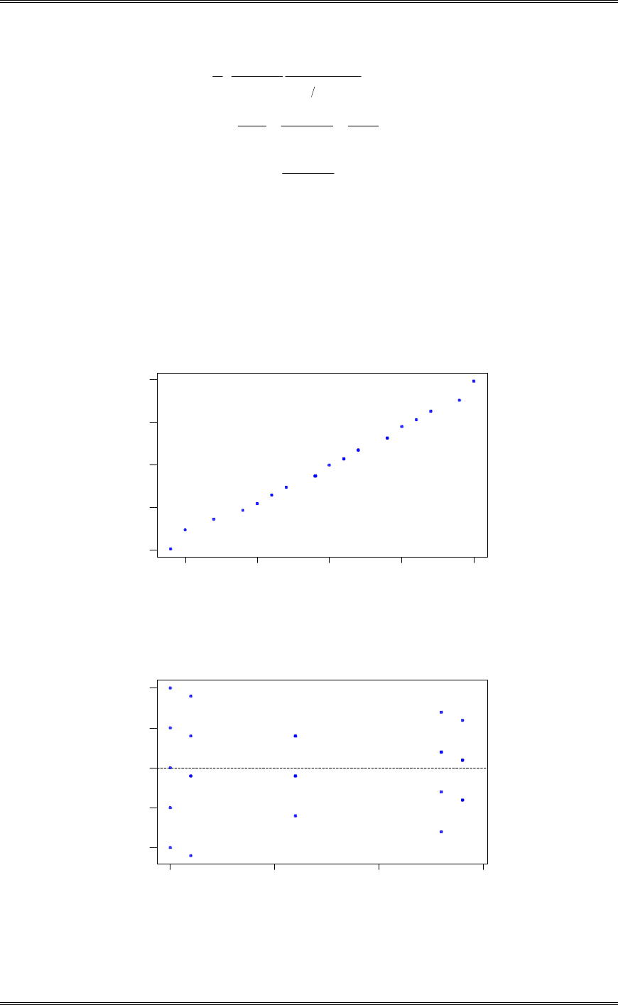
Solutions from Montgomery, D. C. (2001) Design and Analysis of Experiments, Wiley, NY
12-2
79401440
11
85131
11
22
2
22
2
121
..
U
U
L
L
.
FMS
MS
n
U
an,a,E
Model
d
d
d
d
»
»
¼
º
«
«
¬
ª
VV
V
VV
V
W
W
W
W
D
(e) Analyze the residuals from this experiment. Do you think that the analysis of variance assumptions are
satisfied?
There is nothing unusual about the residual plots; therefore, the analysis of variance assumptions are
satisfied.
0.20.10.0-0.1-0.2
2
1
0
-1
-2
Normal Score
Residual
Normal Probability Plot of the Residuals
(response is Output)
14.114.013.913.8
0.2
0.1
0.0
-0.1
-0.2
Fitted Value
Residual
Residuals Versus the Fitted Values
(response is Output)
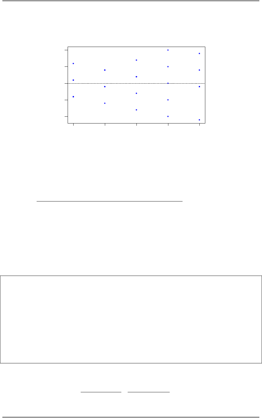
Solutions from Montgomery, D. C. (2001) Design and Analysis of Experiments, Wiley, NY
12-3
54321
0.2
0.1
0.0
-0.1
-0.2
Loom
Residual
Residuals Versus Loom
(response is Output)
12-2 A manufacturer suspects that the batches of raw material furnished by her supplier differ
significantly in calcium content. There are a large number of batches currently in the warehouse. Five of
these are randomly selected for study. A chemist makes five determinations on each batch and obtains the
following data:
Batch 1 Batch 2 Batch 3 Batch 4 Batch 5
23.46 23.59 23.51 23.28 23.29
23.48 23.46 23.64 23.40 23.46
23.56 23.42 23.46 23.37 23.37
23.39 23.49 23.52 23.46 23.32
23.40 23.50 23.49 23.39 23.38
(a) Is there significant variation in calcium content from batch to batch? Use
D
= 0.05.
Yes, as shown in the Minitab Output below, there is a difference.
Minitab Output
ANOVA: Calcium versus Batch
Factor Type Levels Values
Batch random 5 1 2 3 4 5
Analysis of Variance for Calcium
Source DF SS MS F P
Batch 4 0.096976 0.024244 5.54 0.004
Error 20 0.087600 0.004380
Total 24 0.184576
Source Variance Error Expected Mean Square for Each Term
component term (using restricted model)
1 Batch 0.00397 2 (2) + 5(1)
2 Error 0.00438 (2)
(b) Estimate the components of variance.
.. .
VW
2024244 004380
50 00397
MS MS
n
Model E
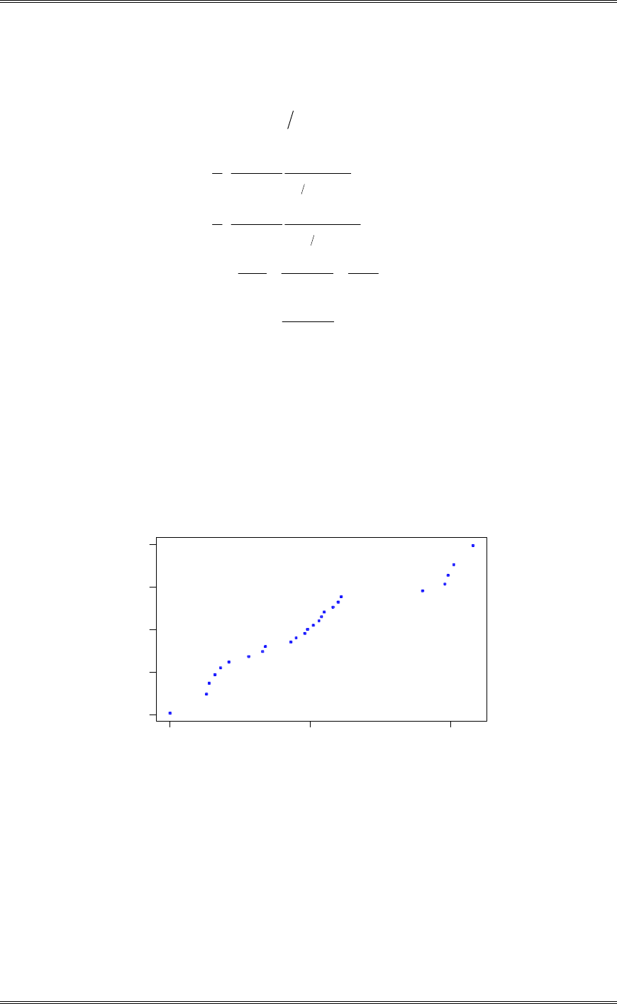
Solutions from Montgomery, D. C. (2001) Design and Analysis of Experiments, Wiley, NY
12-4
.
V
20 004380 MSE
(c) Find a 95 percent confidence interval for
222
VVV WW
.
9027010350
11
27691
11
115401
11
22
2
22
2
121
12
..
U
U
L
L
.
FMS
MS
n
U
.
FMS
MS
n
L
an,a,E
Model
an,a,E
Model
d
d
d
d
»
»
¼
º
«
«
¬
ª
»
»
¼
º
«
«
¬
ª
VV
V
VV
V
W
W
W
W
D
D
(d) Analyze the residuals from this experiment. Are the basic analysis of variance assumptions satisfied?
There are five residuals that stand out in the normal probability plot. From the Residual vs. Batch plot, we
see that one point per batch appears to stand out. A natural log transformation was applied to the data but
did not change the results of the residual analysis. Further investigation should probably be performed to
determine if these points are outliers.
0.10.0-0.1
2
1
0
-1
-2
Normal Score
Residual
Normal Probability Plot of the Residuals
(response is Calcium)
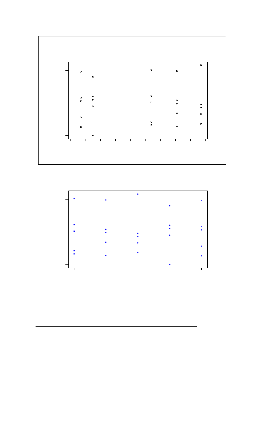
Solutions from Montgomery, D. C. (2001) Design and Analysis of Experiments, Wiley, NY
12-5
12-3 Several ovens in a metal working shop are used to heat metal specimens. All the ovens are supposed
to operate at the same temperature, although it is suspected that this may not be true. Three ovens are
selected at random and their temperatures on successive heats are noted. The data collected are as follows:
Oven Temperature
1 491.50 498.30 498.10 493.50 493.60
2 488.50 484.65 479.90 477.35
3 490.10 484.80 488.25 473.00 471.85 478.65
(a) Is there significant variation in temperature between ovens? Use
D
= 0.05.
The analysis of variance shown below identifies significant variation in temperature between the ovens.
Minitab Output
General Linear Model: Temperature versus Oven
Factor Type Levels Values
23.5323.5123.4923.4723.4523.4323.4123.3923.3723.35
0.1
0.0
-0.1
Fitted Value
Residuals Versus the Fitted Values
(response is Calcium)
54321
0.1
0.0
-0.1
Batch
Residuals Versus Batch
(response is Calcium)
Residual
Residual
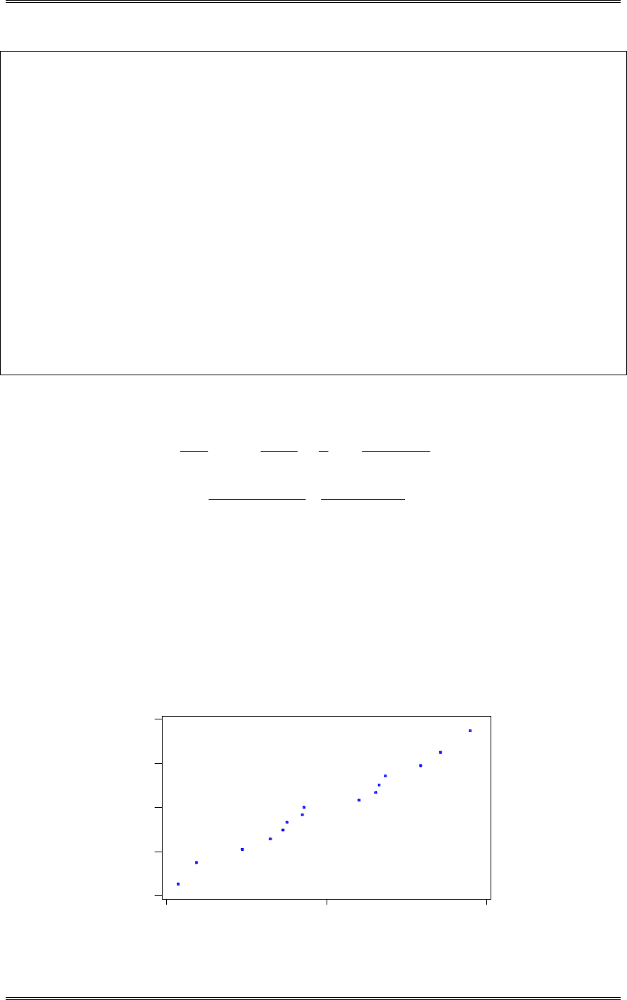
Solutions from Montgomery, D. C. (2001) Design and Analysis of Experiments, Wiley, NY
12-6
Oven random 3 1 2 3
Analysis of Variance for Temperat, using Adjusted SS for Tests
Source DF Seq SS Adj SS Adj MS F P
Oven 2 594.53 594.53 297.27 8.62 0.005
Error 12 413.81 413.81 34.48
Total 14 1008.34
Expected Mean Squares, using Adjusted SS
Source Expected Mean Square for Each Term
1 Oven (2) + 4.9333(1)
2 Error (2)
Error Terms for Tests, using Adjusted SS
Source Error DF Error MS Synthesis of Error MS
1 Oven 12.00 34.48 (2)
Variance Components, using Adjusted SS
Source Estimated Value
Oven 53.27
Error 34.48
(b) Estimate the components of variance.
nann
n
i
i
i
0
2
1
1
1
215 25 16 36
15 493
ª
¬
«
«
º
¼
»
»
ª
¬
Ǽ
¼
»
¦
¦
¦.
..
..
VW
2297 27 34 48
493 53 30
MS MS
n
Model E
.
V
234 48 MSE
(c) Analyze the residuals from this experiment. Draw conclusions about model adequacy.
There is a funnel shaped appearance in the plot of residuals versus predicted value indicating a possible
non-constant variance. There is also some indication of non-constant variance in the plot of residuals
versus oven. The inequality of variance problem is not severe.
100-10
2
1
0
-1
-2
Normal Score
Residual
Normal Probability Plot of the Residuals
(response is Temperat)
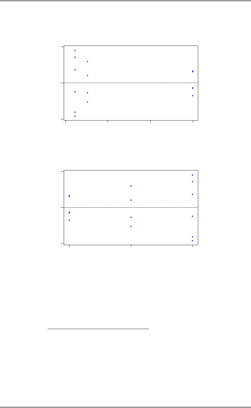
Solutions from Montgomery, D. C. (2001) Design and Analysis of Experiments, Wiley, NY
12-7
495490485480
10
0
-10
Fitted Value
Residual
Residuals Versus the Fitted Values
(response is Temperat)
321
10
0
-10
Oven
Residual
Residuals Versus Oven
(response is Temperat)
12-4 An article in the Journal of the Electrochemical Society (Vol. 139, No. 2, 1992, pp. 524-532)
describes an experiment to investigate the low-pressure vapor deposition of polysilicon. The experiment
was carried out in a large-capacity reactor at Sematech in Austin, Texas. The reactor has several wafer
positions, and four of these positions are selected at random. The response variable is film thickness
uniformity. Three replicates of the experiments were run, and the data are as follows:
Wafer Position Uniformity
1 2.76 5.67 4.49
2 1.43 1.70 2.19
3 2.34 1.97 1.47
4 0.94 1.36 1.65
(a) Is there a difference in the wafer positions? Use
D
= 0.05.
Yes, there is a difference.
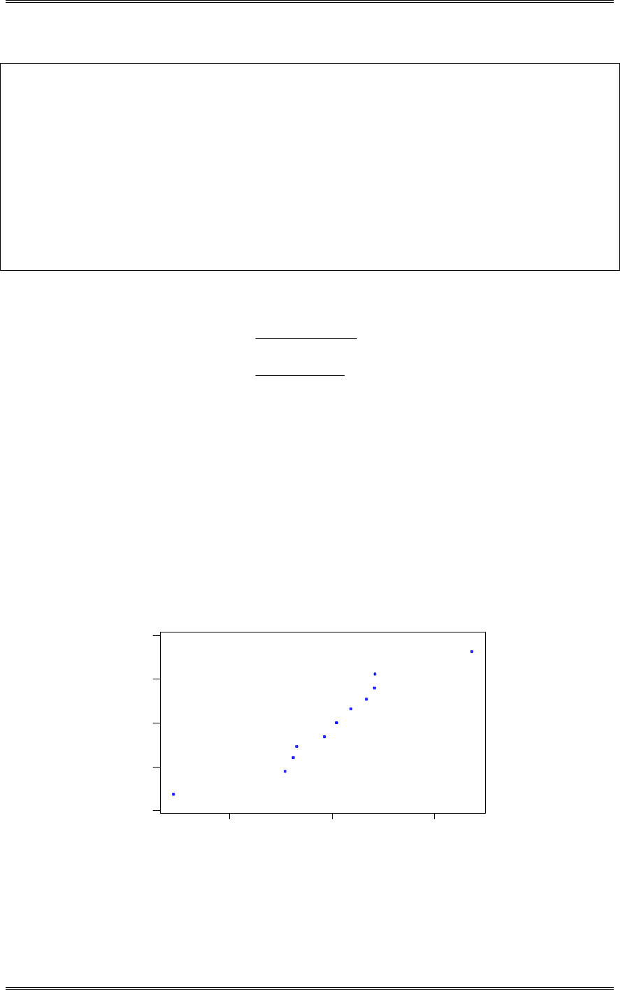
Solutions from Montgomery, D. C. (2001) Design and Analysis of Experiments, Wiley, NY
12-8
Minitab Output
ANOVA: Uniformity versus Wafer Position
Factor Type Levels Values
Wafer Po fixed 4 1 2 3 4
Analysis of Variance for Uniformi
Source DF SS MS F P
Wafer Po 3 16.2198 5.4066 8.29 0.008
Error 8 5.2175 0.6522
Total 11 21.4373
Source Variance Error Expected Mean Square for Each Term
component term (using restricted model)
1 Wafer Po 2 (2) + 3Q[1]
2 Error 0.6522 (2)
(b) Estimate the variability due to wafer positions.
...
V
V
W
W
2
254066 0 6522
315844
MS MS
n
Treatment E
(c) Estimate the random error component.
.
V
20 6522
(d) Analyze the residuals from this experiment and comment on model adequacy.
Variability in film thickness seems to depend on wafer position. These observations also show up as
outliers on the normal probability plot. Wafer position number 1 appears to have greater variation in
uniformity than the other positions.
10-1
2
1
0
-1
-2
Normal Score
Residual
Normal Probability Plot of the Residuals
(response is Uniformi)
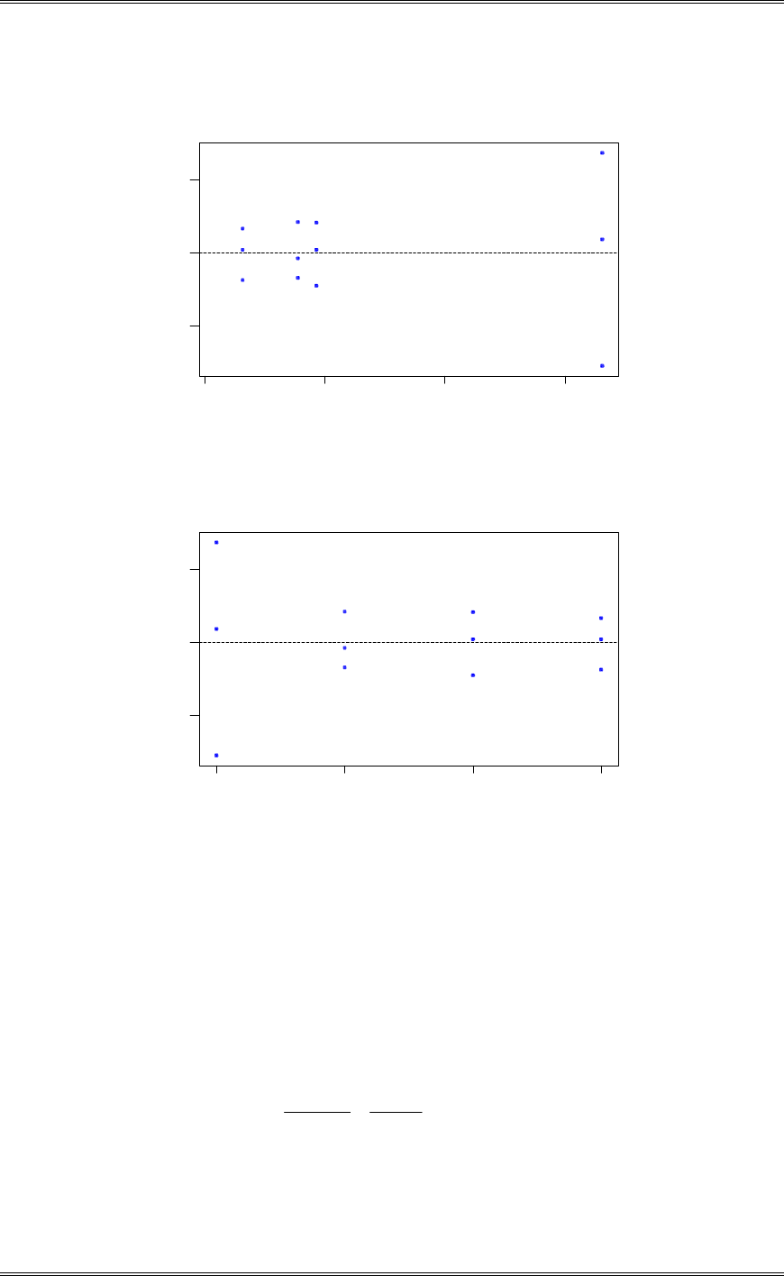
Solutions from Montgomery, D. C. (2001) Design and Analysis of Experiments, Wiley, NY
12-9
4321
1
0
-1
Fitted Value
Residual
Residuals Versus the Fitted Values
(response is Uniformi)
4321
1
0
-1
Wafer Po
Residual
Residuals Versus Wafer Po
(response is Uniformi)
12-5 Consider the vapor deposition experiment described in Problem 12-4.
(a) Estimate the total variability in the uniformity response.
237026522058481
22 ...
ˆˆ
VV W
(b) How much of the total variability in the uniformity response is due to the difference between positions
in the reactor?
708450
23702
58481
22
2
.
.
.
ˆˆ
ˆ
W
W
VV
V
(c) To what level could the variability in the uniformity response be reduced, if the position-to-position
variability in the reactor could be eliminated? Do you believe this is a significant reduction?

Solutions from Montgomery, D. C. (2001) Design and Analysis of Experiments, Wiley, NY
12-10
The variability would be reduced from 2.2370 to 65220
2.
ˆ
V
which is a reduction of approximately:
%
.
.. 71
23702
6522023702
12-6 An article in the Journal of Quality Technology (Vol. 13, No. 2, 1981, pp. 111-114) describes and
experiment that investigates the effects of four bleaching chemicals on pulp brightness. These four
chemicals were selected at random from a large population of potential bleaching agents. The data are as
follows:
Chemical Pulp Brightness
1 77.199 74.466 92.746 76.208 82.876
2 80.522 79.306 81.914 80.346 73.385
3 79.417 78.017 91.596 80.802 80.626
4 78.001 78.358 77.544 77.364 77.386
(a) Is there a difference in the chemical types? Use
D
= 0.05.
The computer output shows that the null hypothesis cannot be rejected. Therefore, there is no evidence that
there is a difference in chemical types.
Minitab Output
ANOVA: Brightness versus Chemical
Factor Type Levels Values
Chemical random 4 1 2 3 4
Analysis of Variance for Brightne
Source DF SS MS F P
Chemical 3 53.98 17.99 0.75 0.538
Error 16 383.99 24.00
Total 19 437.97
Source Variance Error Expected Mean Square for Each Term
component term (using restricted model)
1 Chemical -1.201 2 (2) + 5(1)
2 Error 23.999 (2)
(b) Estimate the variability due to chemical types.
.. .
V
V
W
W
2
217 994 23 999
51201
MS MS
n
Treatment E
which agrees with the Minitab output.
Because the variance component cannot be negative, this likely means that the variability due to chemical
types is zero.
(c) Estimate the variability due to random error.
.
V
223 999
(d) Analyze the residuals from this experiment and comment on model adequacy.
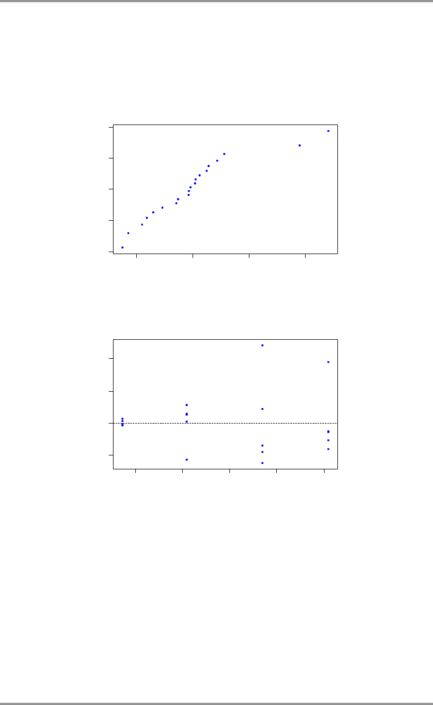
Solutions from Montgomery, D. C. (2001) Design and Analysis of Experiments, Wiley, NY
12-11
Two data points appear to be outliers in the normal probability plot of effects. These outliers belong to
chemical types 1 and 3 and should be investigated. There seems to be much less variability in brightness
with chemical type 4.
1050-5
2
1
0
-1
-2
Normal Score
Residual
Normal Probability Plot of the Residuals
(response is Brightne)
8281807978
10
5
0
-5
Fitted Value
Residual
Residuals Versus the Fitted Values
(response is Brightne)
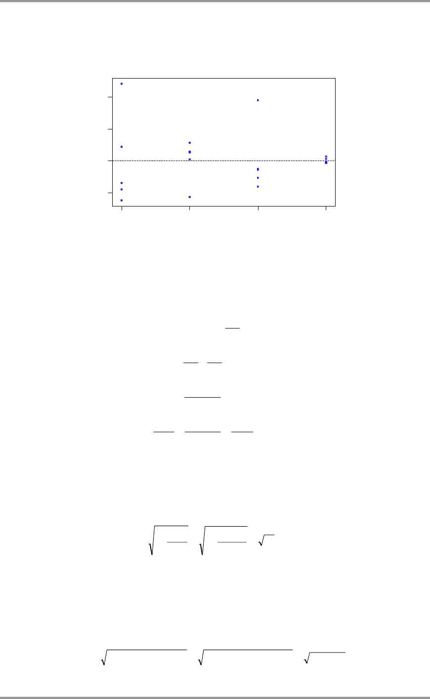
Solutions from Montgomery, D. C. (2001) Design and Analysis of Experiments, Wiley, NY
12-12
4321
10
5
0
-5
Chemical
Residual
Residuals Versus Chemical
(response is Brightne)
12-7 Consider the one-way balanced, random effects method. Develop a procedure for finding a 100(1-
D
) percent confidence interval for
VVV
W
222
/( ).
We know that PL Udd
ª
¬
«
«
º
¼
»
»
V
VD
W
2
21
PL Ud d
ª
¬
«
«
º
¼
»
» 111
2
2
2
2
V
V
V
VD
W
PL Ud d
ª
¬
«
«
º
¼
»
» 111
22
2
VV
VD
W
PL
L
U
U11
1
2
22
tt
ª
¬
«
«
º
¼
»
»
V
VV D
W
12-8 Refer to Problem 12-1.
(a) What is the probability of accepting H0 if
VW
2 is four times the error variance
V
2?
6421
45
11 2
2
2
2
.
n
V
V
V
V
OW
X
114 a
X
225 5 20 Na
E
|0 035. , from the OC curve.
(b) If the difference between looms is large enough to increase the standard deviation of an observation by
20 percent, we wish to detect this with a probability of at least 0.80. What sample size should be used?
X
114 a
X
225 5 20 Na
D
005. P accept
().
d02
>@
>@
n..nP.n 440112001011101011 22
O

Solutions from Montgomery, D. C. (2001) Design and Analysis of Experiments, Wiley, NY
12-13
Trial and Error yields:
n
X
2 O P(accept)
5 20 1.79 0.6
10 45 2.32 0.3
14 65 2.67 0.2
Choose n t 14, therefore N t 70
12-9 An experiment was performed to investigate the capability of a measurement system. Ten parts
were randomly selected, and two randomly selected operators measured each part three times. The tests
were made in random order, and the data below resulted.
Operator 1 Operator 2
Measurements Measurements
Part -------------------------- -------------------------
Number 1 2 3 1 2 3
1 50 49 50 50 48 51
2 52 52 51 51 51 51
3 53 50 50 54 52 51
4 49 51 50 48 50 51
5 48 49 48 48 49 48
6 52 50 50 52 50 50
7 51 51 51 51 50 50
8 52 50 49 53 48 50
9 50 51 50 51 48 49
10 47 46 49 46 47 48
(a) Analyze the data from this experiment.
Minitab Output
ANOVA: Measurement versus Part, Operator
Factor Type Levels Values
Part random 10 1 2 3 4 5 6 7
8 9 10
Operator random 2 1 2
Analysis of Variance for Measurem
Source DF SS MS F P
Part 9 99.017 11.002 18.28 0.000
Operator 1 0.417 0.417 0.69 0.427
Part*Operator 9 5.417 0.602 0.40 0.927
Error 40 60.000 1.500
Total 59 164.850
Source Variance Error Expected Mean Square for Each Term
component term (using restricted model)
1 Part 1.73333 3 (4) + 3(3) + 6(1)
2 Operator -0.00617 3 (4) + 3(3) + 30(2)
3 Part*Operator -0.29938 4 (4) + 3(3)
4 Error 1.50000 (4)
(b) Find point estimates of the variance components using the analysis of variance method.
V
2 MSE .
V
215

Solutions from Montgomery, D. C. (2001) Design and Analysis of Experiments, Wiley, NY
12-14
VWE
2 MS MS
n
AB E ..
VWE
20 6018519 15000000
30 , assume
VWE
2=0
VE
2 MS MS
an
BAB
73331
32
6018519000185211
2.
..
ˆ
E
V
VW
2 MS MS
bn
AAB
0
310
601851904166670
2
..
ˆ
W
V
, assume
VW
2=0
All estimates agree with the Minitab output.
12-10 Reconsider the data in Problem 5-6. Suppose that both factors, machines and operators, are chosen
at random.
(a) Analyze the data from this experiment.
Machine
Operator 1 2 3 4
1 109 110 108 110
110 115 109 108
2 110 110 111 114
112 111 109 112
3 116 112 114 120
114 115 119 117
The following Minitab output contains the analysis of variance and the variance component estimates:
Minitab Output
ANOVA: Strength versus Operator, Machine
Factor Type Levels Values
Operator random 3 1 2 3
Machine random 4 1 2 3 4
Analysis of Variance for Strength
Source DF SS MS F P
Operator 2 160.333 80.167 10.77 0.010
Machine 3 12.458 4.153 0.56 0.662
Operator*Machine 6 44.667 7.444 1.96 0.151
Error 12 45.500 3.792
Total 23 262.958
Source Variance Error Expected Mean Square for Each Term
component term (using restricted model)
1 Operator 9.0903 3 (4) + 2(3) + 8(1)
2 Machine -0.5486 3 (4) + 2(3) + 6(2)
3 Operator*Machine 1.8264 4 (4) + 2(3)
4 Error 3.7917 (4)
(b) Find point estimates of the variance components using the analysis of variance method.
V
2 MSE .
V
23 79167
VWE
2 MS MS
n
AB E .. .
VWE
27 44444 3 79167
2182639

Solutions from Montgomery, D. C. (2001) Design and Analysis of Experiments, Wiley, NY
12-15
VE
2 MS MS
an
BAB
..
()
VE
24 15278 7 44444
32 0 , assume
VE
20
VW
2 MS MS
bn
AAB
..
() .
VW
28016667 7 44444
42 9 09028
These results agree with the Minitab variance component analysis.
12-11 Reconsider the data in Problem 5-13. Suppose that both factors are random.
(a) Analyze the data from this experiment.
Column Factor
Row Factor 1 2 3 4
1 36 39 36 32
2 18 20 22 20
3 30 37 33 34
Minitab Output
General Linear Model: Response versus Row, Column
Factor Type Levels Values
Row random 3 1 2 3
Column random 4 1 2 3 4
Analysis of Variance for Response, using Adjusted SS for Tests
Source DF Seq SS Adj SS Adj MS F P
Row 2 580.500 580.500 290.250 60.40 **
Column 3 28.917 28.917 9.639 2.01 **
Row*Column 6 28.833 28.833 4.806 **
Error 0 0.000 0.000 0.000
Total 11 638.250
** Denominator of F-test is zero.
Expected Mean Squares, using Adjusted SS
Source Expected Mean Square for Each Term
1 Row (4) + (3) + 4.0000(1)
2 Column (4) + (3) + 3.0000(2)
3 Row*Column (4) + (3)
4 Error (4)
Error Terms for Tests, using Adjusted SS
Source Error DF Error MS Synthesis of Error MS
1 Row * 4.806 (3)
2 Column * 4.806 (3)
3 Row*Column * * (4)
Variance Components, using Adjusted SS
Source Estimated Value
Row 71.3611
Column 1.6111
Row*Column 4.8056
Error 0.0000
(b) Estimate the variance components.

Solutions from Montgomery, D. C. (2001) Design and Analysis of Experiments, Wiley, NY
12-16
Because the experiment is unreplicated and the interaction term was included in the model, there is no
estimate of MSE, and therefore, no estimate of 2
V
.
VWE
2 MS MS
n
AB E 80564
1
080564
2.
.
ˆ
WE
V
VE
2 MS MS
an
BAB
61111
13
8056463899
2.
..
ˆ
E
V
VW
2 MS MS
bn
AAB
361171
14
805642500290
2.
..
ˆ
W
V
These estimates agree with the Minitab output.
12-12 Suppose that in Problem 5-11 the furnace positions were randomly selected, resulting in a mixed
model experiment. Reanalyze the data from this experiment under this new assumption. Estimate the
appropriate model components.
Temperature (°C)
Position 800 825 850
570 1063 565
1 565 1080 510
583 1043 590
528 988 526
2 547 1026 538
521 1004 532
The following analysis assumes a restricted model:
Minitab Output
ANOVA: Density versus Position, Temperature
Factor Type Levels Values
Position random 2 1 2
Temperat fixed 3 800 825 850
Analysis of Variance for Density
Source DF SS MS F P
Position 1 7160 7160 16.00 0.002
Temperat 2 945342 472671 1155.52 0.001
Position*Temperat 2 818 409 0.91 0.427
Error 12 5371 448
Total 17 958691
Source Variance Error Expected Mean Square for Each Term
component term (using restricted model)
1 Position 745.83 4 (4) + 9(1)
2 Temperat 3 (4) + 3(3) + 6Q[2]
3 Position*Temperat -12.83 4 (4) + 3(3)
4 Error 447.56 (4)
V
2 MSE 56447
2.
ˆ
V
VWE
2 MS MS
n
AB E 0
3
448409
2
WE
V
ˆ assume
VWE
20

Solutions from Montgomery, D. C. (2001) Design and Analysis of Experiments, Wiley, NY
12-17
bn
MSMS
ˆEA
2
W
V
83745
33
4487160
2.
ˆ
W
V
These results agree with the Minitab output.
12-13 Reanalyze the measurement systems experiment in Problem 12-9, assuming that operators are a
fixed factor. Estimate the appropriate model components.
The following analysis assumes a restricted model:
Minitab Output
ANOVA: Measurement versus Part, Operator
Factor Type Levels Values
Part random 10 1 2 3 4 5 6 7
8 9 10
Operator fixed 2 1 2
Analysis of Variance for Measurem
Source DF SS MS F P
Part 9 99.017 11.002 7.33 0.000
Operator 1 0.417 0.417 0.69 0.427
Part*Operator 9 5.417 0.602 0.40 0.927
Error 40 60.000 1.500
Total 59 164.850
Source Variance Error Expected Mean Square for Each Term
component term (using restricted model)
1 Part 1.5836 4 (4) + 6(1)
2 Operator 3 (4) + 3(3) + 30Q[2]
3 Part*Operator -0.2994 4 (4) + 3(3)
4 Error 1.5000 (4)
V
2 MSE 50001
2.
ˆ
V
n
MSMS
ˆEAB
2
WE
V
0
3
50001601850
2
..
ˆ
WE
V
assume
VWE
20
bn
MSMS
ˆEA
2
W
V
583641
32
5000010018511
2.
..
ˆ
W
V
These results agree with the Minitab output.
12-14 In problem 5-6, suppose that there are only four machines of interest, but the operators were selected
at random.
(a) What type of model is appropriate?
A mixed model is appropriate.
(b) Perform the analysis and estimate the model components.
The following analysis assumes a restricted model:
Minitab Output
ANOVA: Strength versus Operator, Machine
Factor Type Levels Values

Solutions from Montgomery, D. C. (2001) Design and Analysis of Experiments, Wiley, NY
12-18
Operator random 3 1 2 3
Machine fixed 4 1 2 3 4
Analysis of Variance for Strength
Source DF SS MS F P
Operator 2 160.333 80.167 21.14 0.000
Machine 3 12.458 4.153 0.56 0.662
Operator*Machine 6 44.667 7.444 1.96 0.151
Error 12 45.500 3.792
Total 23 262.958
Source Variance Error Expected Mean Square for Each Term
component term (using restricted model)
1 Operator 9.547 4 (4) + 8(1)
2 Machine 3 (4) + 2(3) + 6Q[2]
3 Operator*Machine 1.826 4 (4) + 2(3)
4 Error 3.792 (4)
V
2 MSE 7923
2.
ˆ
V
VWE
2 MS MS
n
AB E 8261
2
79234447
2.
..
ˆ
WE
V
bn
MSMS
ˆEA
2
W
V
5479
24
792316780
2.
..
ˆ
W
V
These results agree with the Minitab output.
12-15 By application of the expectation operator, develop the expected mean squares for the two-factor
factorial, mixed model. Use the restricted model assumptions. Check your results with the expected mean
squares given in Table 12-11 to see that they agree.
The sums of squares may be written as
¦
a
i
.....iA yybnSS
1
2,
¦
b
j
....j.B yyanSS
1
2
¦¦
a
i
b
j
....j...i.ijAB yyyynSS
11
2,
¦¦¦
a
i
b
j
n
k
...ijkE yySS
111
2
Using the model
ijk
ij
jiijk
y
HWEEWP
, we may find that
.......
.ij
ij
ji.ij
.j.j.j.
..i
.i
i..i
y
y
y
y
HEP
HWEEWP
HEP
HEWWP
Using the assumptions for the restricted form of the mixed model,
W
. 0,
0
j.
WE
, which imply that
0
..
WE
. Substituting these expressions into the sums of squares yields

Solutions from Montgomery, D. C. (2001) Design and Analysis of Experiments, Wiley, NY
12-19
¦¦¦
¦¦
¦
¦
a
i
b
j
n
k
.ijijkE
a
i
b
j
....j...i.ij
.i
ijAB
b
j
....j.jB
a
i
.....i
.i
A
SS
)nSS
anSS
bnSS
111
2
11
2
1
2
1
2
HH
HHHHWEWE
HHE
HHWEW
Using the assumption that
0
ijk
E
H
, Vijk
()
H
0, and
0 'k'j'iijk
E
HH
, we may divide each sum of
squares by its degrees of freedom and take the expectation to produce
2
11
2
2
1
22
1
2
2
11
1
1
V
EWWEV
EV
EWWV
»
¼
º
«
¬
ª
»
¼
º
«
¬
ª
»
¼
º
«
¬
ª
¦¦
¦
¦
E
a
i
b
j
.iij
AB
b
j
jB
a
i
.i
iA
MSE
E
ba
n
MSE
b
an
MSE
E
a
bn
MSE
Note that
B
MSE and
E
MSE are the results given in Table 8-3. We need to simplify
A
MSE and
AB
MSE . Consider
A
MSE
¦
¦
¦¦
»
»
»
»
¼
º
«
«
«
«
¬
ª»
¼
º
«
¬
ª
»
»
¼
º
«
«
¬
ª
a
i
iA
a
i
iA
a
i
a
i
.i
iA
a
bn
nMSE
b
a
a
a
a
bn
MSE
ctscrossproduEE
a
bn
MSE
1
2
22
2
1
2
2
11
22
2
1
1
1
0
1
WVV
VWV
WEWV
WE
WE
since
ij
WE
is ¸
¹
·
¨
©
§2
1
0
WE
V
a
a
,NID . Consider
AB
MSE
22
2
11
2
11
2
2
11
11
11
WE
WE
VV
VV
EWWEV
nMSE
a
a
b
b
ba
n
MSE
E
ba
n
MSE
AB
a
i
b
j
AB
a
i
b
j
.iij
AB
¸
¹
·
¨
©
§
¸
¹
·
¨
©
§
¦¦
¦¦

Solutions from Montgomery, D. C. (2001) Design and Analysis of Experiments, Wiley, NY
12-20
Thus
A
MSE and
AB
MSE agree with table 12-8.
12-16 Consider the three-factor factorial design in Example 12-6. Propose appropriate test statistics for all
main effects and interactions. Repeat for the case where A and B are fixed and C is random.
If all three factors are random there are no exact tests on main effects. We could use the following:
BCAC
ABCC
BCAB
ABCB
ACAB
ABCA
MSMS
MSMS
F:C
MSMS
MSMS
F:B
MSMS
MSMS
F:A
If A and B are fixed and C is random, the expected mean squares are (assuming the restricted for m of the
model):
F F R R
a b c n
Factor i j k l E(MS)
W
i 0 b c n
¦
1
2
22
a
bcnbn i
W
VV
WJ
E
j a 0 c n
¦
1
2
22
b
acnan j
E
VV
EJ
J
k a b 1 n
VV
J
22
abn
ij
WE
0 0 c n
¦¦
11
2
22
ba
cnn ji
WE
VV
WEJ
ik
WJ
0 b 1 n
VV
WJ
22
bn
jk
EJ
a 0 1 n
VV
EJ
22
an
ijk
WEJ
0 0 1 n
VV
WEJ
22
n
lijk
H
1 1 1 1
V
2
These are exact tests for all effects.
12-17 Consider the experiment in Example 12-7. Analyze the data for the case where A, B, and C are
random.
Minitab Output
ANOVA: Drop versus Temp, Operator, Gauge
Factor Type Levels Values
Temp random 3 60 75 90
Operator random 4 1 2 3 4
Gauge random 3 1 2 3
Analysis of Variance for Drop
Source DF SS MS F P
Temp 2 1023.36 511.68 2.30 0.171 x

Solutions from Montgomery, D. C. (2001) Design and Analysis of Experiments, Wiley, NY
12-21
Operator 3 423.82 141.27 0.63 0.616 x
Gauge 2 7.19 3.60 0.06 0.938 x
Temp*Operator 6 1211.97 202.00 14.59 0.000
Temp*Gauge 4 137.89 34.47 2.49 0.099
Operator*Gauge 6 209.47 34.91 2.52 0.081
Temp*Operator*Gauge 12 166.11 13.84 0.65 0.788
Error 36 770.50 21.40
Total 71 3950.32
x Not an exact F-test.
Source Variance Error Expected Mean Square for Each Term
component term (using restricted model)
1 Temp 12.044 * (8) + 2(7) + 8(5) + 6(4) + 24(1)
2 Operator -4.544 * (8) + 2(7) + 6(6) + 6(4) + 18(2)
3 Gauge -2.164 * (8) + 2(7) + 6(6) + 8(5) + 24(3)
4 Temp*Operator 31.359 7 (8) + 2(7) + 6(4)
5 Temp*Gauge 2.579 7 (8) + 2(7) + 8(5)
6 Operator*Gauge 3.512 7 (8) + 2(7) + 6(6)
7 Temp*Operator*Gauge -3.780 8 (8) + 2(7)
8 Error 21.403 (8)
* Synthesized Test.
Error Terms for Synthesized Tests
Source Error DF Error MS Synthesis of Error MS
1 Temp 6.97 222.63 (4) + (5) - (7)
2 Operator 7.09 223.06 (4) + (6) - (7)
3 Gauge 5.98 55.54 (5) + (6) - (7)
Since all three factors are random there are no exact tests on main effects. Minitab uses an approximate F
test for the these factors.
12-18 Derive the expected mean squares shown in Table 12-14.
F R R R
a b c n
Factor i j k l E(MS)
W
i 0 b c n
¦
1
2
2222
a
bcncnbnn i
W
VVVV
WEWJWEJ
E
j a 1 c n
VV V
EJ E
22 2
an acn
J
k a b 1 n
VV V
EJ J
22 2
an abn
ij
WE
0 1 c n
VV V
WEJ WE
22 2
ncn
ik
WJ
0 b 1 n
VV V
WEJ WJ
22 2
nbn
jk
EJ
a 1 1 n
VV
EJ
22
an
ijk
WEJ
0 1 1 n
VV
WEJ
22
n
H
ijkl 1 1 1 1
V
2
12-19 Consider a four-factor factorial experiment where factor A is at a levels, factor B is at b levels, factor
C is at c levels, factor D is at d levels, and there are n replicates. Write down the sums of squares, the
degrees of freedom, and the expected mean squares for the following cases. Do exact tests exist for all
effects? If not, propose test statistics for those effects that cannot be directly tested. Assume the restricted
model on all cases. You may use a computer package such as Minitab.
The four factor model is:

Solutions from Montgomery, D. C. (2001) Design and Analysis of Experiments, Wiley, NY
12-22
kljljk
il
ikij
lkjiijklh
y
JGEGEJWGWJWEGJEWP
ijklh
ijklikljklijlijk
HWEJGWJGEJGWEGWEJ
To simplify the expected mean square derivations, let capital Latin letters represent the factor effects or
variance components. For example, Abcdn
a
i
¦
W
2
1, or Bacdn
VE
2.
(a) A, B, C, and D are fixed factors.
F F F F R
a b c d n
Factor i j k l h E(MS)
W
i 0 b c d n
V
2A
E
j a 0 c d n
V
2B
J
k a b 0 d n
V
2C
G
l a b c 0 n
V
2D
()
WE
ij 0 0 c d n
V
2AB
()
WJ
ik 0 b 0 d n
V
2AC
()
WG
il 0 b c 0 n
V
2AD
()
EJ
jk a 0 0 d n
V
2BC
()
EG
jl a 0 c 0 n
V
2BD
()
JG
kl a b 0 0 n
V
2CD
()
WEJ
ijk 0 0 0 d n
V
2ABC
()
WEG
ijl 0 0 c 0 n
V
2ABD
()
EJG
jkl a 0 0 0 n
V
2BCD
()
WJG
ikl 0 b 0 0 n
V
2ACD
()
WEJG
ijkl 0 0 0 0 n
V
2ABCD
H
()ijkl h 1 1 1 1 1
V
2
There are exact tests for all effects. The results can also be generated in Minitab as follows:
Minitab Output
ANOVA: y versus A, B, C, D
Factor Type Levels Values
A fixed 2 H L
B fixed 2 H L
C fixed 2 H L
D fixed 2 H L
Analysis of Variance for y
Source DF SS MS F P
A 1 6.13 6.13 0.49 0.492
B 1 0.13 0.13 0.01 0.921
C 1 1.13 1.13 0.09 0.767
D 1 0.13 0.13 0.01 0.921
A*B 1 3.13 3.13 0.25 0.622
A*C 1 3.13 3.13 0.25 0.622
A*D 1 3.13 3.13 0.25 0.622
B*C 1 3.13 3.13 0.25 0.622
B*D 1 3.13 3.13 0.25 0.622
C*D 1 3.13 3.13 0.25 0.622
A*B*C 1 3.13 3.13 0.25 0.622
A*B*D 1 28.13 28.13 2.27 0.151

Solutions from Montgomery, D. C. (2001) Design and Analysis of Experiments, Wiley, NY
12-23
A*C*D 1 3.13 3.13 0.25 0.622
B*C*D 1 3.13 3.13 0.25 0.622
A*B*C*D 1 3.13 3.13 0.25 0.622
Error 16 198.00 12.38
Total 31 264.88
Source Variance Error Expected Mean Square for Each Term
component term (using restricted model)
1 A 16 (16) + 16Q[1]
2 B 16 (16) + 16Q[2]
3 C 16 (16) + 16Q[3]
4 D 16 (16) + 16Q[4]
5 A*B 16 (16) + 8Q[5]
6 A*C 16 (16) + 8Q[6]
7 A*D 16 (16) + 8Q[7]
8 B*C 16 (16) + 8Q[8]
9 B*D 16 (16) + 8Q[9]
10 C*D 16 (16) + 8Q[10]
11 A*B*C 16 (16) + 4Q[11]
12 A*B*D 16 (16) + 4Q[12]
13 A*C*D 16 (16) + 4Q[13]
14 B*C*D 16 (16) + 4Q[14]
15 A*B*C*D 16 (16) + 2Q[15]
16 Error 12.38 (16)
(b) A, B, C, and D are random factors.
R R R R R
a b c d n
Factor i j k l h E(MS)
W
i 1 b c d n
V
2
ABCD ACD ABD ABC AD AC AB A
E
j a 1 c d n
V
2
ABCD BCD ABD ABC BD BC AB B
J
k a b 1 d n
V
2
ABCD ACD BCD ABC AB BC CD C
G
l a b c 1 n
V
2
ABCD ACD BCD ABD BD AD CD D
()
WE
ij 1 1 c d n
V
2
ABCD ABC ABD AB
()
WJ
ik 1 b 1 d n
V
2
ABCD ABC ACD AC
()
WG
il 1 b c 1 n
V
2
ABCD ABD ACD AD
()
EJ
jk a 1 1 d n
V
2
ABCD ABC BCD BC
()
EG
jl a 1 c 1 n
V
2
ABCD ABD BCD BD
()
JG
kl a b 1 1 n
V
2
ABCD ACD BCD CD
()
WEJ
ijk 1 1 1 d n
V
2
ABCD ABC
()
WEG
ijl 1 1 c 1 n
V
2
ABCD ABD
()
EJG
jkl a 1 1 1 n
V
2
ABCD BCD
()
WJG
ikl 1 b 1 1 n
V
2
ABCD ACD
()
WEJG
ijkl 1 1 1 1 n
V
2ABCD
H
()ijkl h 1 1 1 1 1
V
2
No exact tests exist on main effects or two-factor interactions. For main effects use statistics such as:
AF MS MS MS MS
MS MS MS MS
AABCABDACD
AB AC AD ABCD
:
For testing two-factor interactions use statistics such as: AB F MS MS
MS MS
AB ABCD
ABC ABD
:
The results can also be generated in Minitab as follows:

Solutions from Montgomery, D. C. (2001) Design and Analysis of Experiments, Wiley, NY
12-24
Minitab Output
ANOVA: y versus A, B, C, D
Factor Type Levels Values
A random 2 H L
B random 2 H L
C random 2 H L
D random 2 H L
Analysis of Variance for y
Source DF SS MS F P
A 1 6.13 6.13 **
B 1 0.13 0.13 **
C 1 1.13 1.13 0.36 0.843 x
D 1 0.13 0.13 **
A*B 1 3.13 3.13 0.11 0.796 x
A*C 1 3.13 3.13 1.00 0.667 x
A*D 1 3.13 3.13 0.11 0.796 x
B*C 1 3.13 3.13 1.00 0.667 x
B*D 1 3.13 3.13 0.11 0.796 x
C*D 1 3.13 3.13 1.00 0.667 x
A*B*C 1 3.13 3.13 1.00 0.500
A*B*D 1 28.13 28.13 9.00 0.205
A*C*D 1 3.13 3.13 1.00 0.500
B*C*D 1 3.13 3.13 1.00 0.500
A*B*C*D 1 3.13 3.13 0.25 0.622
Error 16 198.00 12.38
Total 31 264.88
x Not an exact F-test.
** Denominator of F-test is zero.
Source Variance Error Expected Mean Square for Each Term
component term (using restricted model)
1 A 1.7500 * (16) + 2(15) + 4(13) + 4(12) + 4(11) + 8(7) + 8(6)
+ 8(5) + 16(1)
2 B 1.3750 * (16) + 2(15) + 4(14) + 4(12) + 4(11) + 8(9) + 8(8)
+ 8(5) + 16(2)
3 C -0.1250 * (16) + 2(15) + 4(14) + 4(13) + 4(11) + 8(10) + 8(8)
+ 8(6) + 16(3)
4 D 1.3750 * (16) + 2(15) + 4(14) + 4(13) + 4(12) + 8(10) + 8(9)
+ 8(7) + 16(4)
5 A*B -3.1250 * (16) + 2(15) + 4(12) + 4(11) + 8(5)
6 A*C 0.0000 * (16) + 2(15) + 4(13) + 4(11) + 8(6)
7 A*D -3.1250 * (16) + 2(15) + 4(13) + 4(12) + 8(7)
8 B*C 0.0000 * (16) + 2(15) + 4(14) + 4(11) + 8(8)
9 B*D -3.1250 * (16) + 2(15) + 4(14) + 4(12) + 8(9)
10 C*D 0.0000 * (16) + 2(15) + 4(14) + 4(13) + 8(10)
11 A*B*C 0.0000 15 (16) + 2(15) + 4(11)
12 A*B*D 6.2500 15 (16) + 2(15) + 4(12)
13 A*C*D 0.0000 15 (16) + 2(15) + 4(13)
14 B*C*D 0.0000 15 (16) + 2(15) + 4(14)
15 A*B*C*D -4.6250 16 (16) + 2(15)
16 Error 12.3750 (16)
* Synthesized Test.
Error Terms for Synthesized Tests
Source Error DF Error MS Synthesis of Error MS
1 A 0.56 * (5) + (6) + (7) - (11) - (12) - (13) + (15)
2 B 0.56 * (5) + (8) + (9) - (11) - (12) - (14) + (15)
3 C 0.14 3.13 (6) + (8) + (10) - (11) - (13) - (14) + (15)
4 D 0.56 * (7) + (9) + (10) - (12) - (13) - (14) + (15)
5 A*B 0.98 28.13 (11) + (12) - (15)
6 A*C 0.33 3.13 (11) + (13) - (15)
7 A*D 0.98 28.13 (12) + (13) - (15)

Solutions from Montgomery, D. C. (2001) Design and Analysis of Experiments, Wiley, NY
12-25
8 B*C 0.33 3.13 (11) + (14) - (15)
9 B*D 0.98 28.13 (12) + (14) - (15)
10 C*D 0.33 3.13 (13) + (14) - (15)
(c) A is fixed and B, C, and D are random.
F R R R R
a b c d n
Factor i j k l h E(MS)
W
i 0 b c d n
V
2
ABCD ACD ABD ABC AD AC AB A
E
j a 1 c d n
V
2
BCD ABD BC B
J
k a b 1 d n
V
2
BCD BC CD C
G
l a b c 1 n
V
2
BCDBDCDD
()
WE
ij 0 1 c d n
V
2
ABCD ABC ABD AB
()
WJ
ik 0 b 1 d n
V
2
ABCD ABC ACD AC
()
WG
il 0 b c 1 n
V
2
ABCD ABD ACD AD
()
EJ
jk a 1 1 d n
V
2
BCD BC
()
EG
jl a 1 c 1 n
V
2
BCD BD
()
JG
kl a b 1 1 n
V
2
BCD CD
()
WEJ
ijk 0 1 1 d n
V
2
ABCD ABC
()
WEG
ijl 0 1 c 1 n
V
2
ABCD ABD
()
EJG
jkl a 1 1 1 n
V
2BCD
()
WJG
ikl 0 b 1 1 n
V
2
ABCD ACD
()
WEJG
ijkl 0 1 1 1 n
V
2ABCD
H
()ijkl h 1 1 1 1 1
V
2
No exact tests exist on main effects or two-factor interactions involving the fixed factor A. To test the fixed
factor A use
AF MS MS MS MS
MS MS MS MS
AABCABDACD
AB AC AD ABCD
:
Random main effects could be tested by, for example: DF MS MS
MS MS
DABCD
ABC ABD
:
For testing two-factor interactions involving A use: AB F MS MS
MS MS
AB ABCD
ABC ABD
:
The results can also be generated in Minitab as follows:
Minitab Output
ANOVA: y versus A, B, C, D
Factor Type Levels Values
A fixed 2 H L
B random 2 H L
C random 2 H L
D random 2 H L
Analysis of Variance for y
Source DF SS MS F P
A 1 6.13 6.13 **
B 1 0.13 0.13 0.04 0.907 x

Solutions from Montgomery, D. C. (2001) Design and Analysis of Experiments, Wiley, NY
12-26
C 1 1.13 1.13 0.36 0.761 x
D 1 0.13 0.13 0.04 0.907 x
A*B 1 3.13 3.13 0.11 0.796 x
A*C 1 3.13 3.13 1.00 0.667 x
A*D 1 3.13 3.13 0.11 0.796 x
B*C 1 3.13 3.13 1.00 0.500
B*D 1 3.13 3.13 1.00 0.500
C*D 1 3.13 3.13 1.00 0.500
A*B*C 1 3.13 3.13 1.00 0.500
A*B*D 1 28.13 28.13 9.00 0.205
A*C*D 1 3.13 3.13 1.00 0.500
B*C*D 1 3.13 3.13 0.25 0.622
A*B*C*D 1 3.13 3.13 0.25 0.622
Error 16 198.00 12.38
Total 31 264.88
x Not an exact F-test.
** Denominator of F-test is zero.
Source Variance Error Expected Mean Square for Each Term
component term (using restricted model)
1 A * (16) + 2(15) + 4(13) + 4(12) + 4(11) + 8(7) + 8(6)
+ 8(5) + 16Q[1]
2 B -0.1875 * (16) + 4(14) + 8(9) + 8(8) + 16(2)
3 C -0.1250 * (16) + 4(14) + 8(10) + 8(8) + 16(3)
4 D -0.1875 * (16) + 4(14) + 8(10) + 8(9) + 16(4)
5 A*B -3.1250 * (16) + 2(15) + 4(12) + 4(11) + 8(5)
6 A*C 0.0000 * (16) + 2(15) + 4(13) + 4(11) + 8(6)
7 A*D -3.1250 * (16) + 2(15) + 4(13) + 4(12) + 8(7)
8 B*C 0.0000 14 (16) + 4(14) + 8(8)
9 B*D 0.0000 14 (16) + 4(14) + 8(9)
10 C*D 0.0000 14 (16) + 4(14) + 8(10)
11 A*B*C 0.0000 15 (16) + 2(15) + 4(11)
12 A*B*D 6.2500 15 (16) + 2(15) + 4(12)
13 A*C*D 0.0000 15 (16) + 2(15) + 4(13)
14 B*C*D -2.3125 16 (16) + 4(14)
15 A*B*C*D -4.6250 16 (16) + 2(15)
16 Error 12.3750 (16)
* Synthesized Test.
Error Terms for Synthesized Tests
Source Error DF Error MS Synthesis of Error MS
1 A 0.56 * (5) + (6) + (7) - (11) - (12) - (13) + (15)
2 B 0.33 3.13 (8) + (9) - (14)
3 C 0.33 3.13 (8) + (10) - (14)
4 D 0.33 3.13 (9) + (10) - (14)
5 A*B 0.98 28.13 (11) + (12) - (15)
6 A*C 0.33 3.13 (11) + (13) - (15)
7 A*D 0.98 28.13 (12) + (13) - (15)
(d) A and B are fixed and C and D are random.
F F R R R
a b c d n
Factor i j k l h E(MS)
W
i 0 b c d n
V
2
ACD AD AC A
E
j a 0 c d n
V
2
BCDBCBDB
J
k a b 1 d n
V
2
CD C
G
l a b c 1 n
V
2
CD D
()
WE
ij 0 0 c d n
V
2
ABCD ABC ABD AB
()
WJ
ik 0 b 1 d n
V
2
ACD AC
()
WG
il 0 b c 1 n
V
2
ACD AD

Solutions from Montgomery, D. C. (2001) Design and Analysis of Experiments, Wiley, NY
12-27
()
EJ
jk a 0 1 d n
V
2
BCD BC
()
EG
jl a 0 c 1 n
V
2
BCD BD
()
JG
kl a b 1 1 n
V
2CD
()
WEJ
ijk 0 0 1 d n
V
2
ABCD ABC
()
WEG
ijl 0 0 c 1 n
V
2
ABCD ABD
()
EJG
jkl a 0 1 1 n
V
2BCD
()
WJG
ikl 0 b 1 1 n
V
2ACD
()
WEJG
ijkl 0 0 1 1 n
V
2ABCD
H
()ijkl h 1 1 1 1 1
V
2
There are no exact tests on the fixed factors A and B, or their two-factor interaction AB. The appropriate
test statistics are:
AF MS MS
MS MS
BF MS MS
MS MS
AACD
AC AD
BBCD
BC BD
:
:
AB F MS MS
MS MS
AB ABCD
ABC ABD
:
The results can also be generated in Minitab as follows:
Minitab Output
ANOVA: y versus A, B, C, D
Factor Type Levels Values
A fixed 2 H L
B fixed 2 H L
C random 2 H L
D random 2 H L
Analysis of Variance for y
Source DF SS MS F P
A 1 6.13 6.13 1.96 0.604 x
B 1 0.13 0.13 0.04 0.907 x
C 1 1.13 1.13 0.36 0.656
D 1 0.13 0.13 0.04 0.874
A*B 1 3.13 3.13 0.11 0.796 x
A*C 1 3.13 3.13 1.00 0.500
A*D 1 3.13 3.13 1.00 0.500
B*C 1 3.13 3.13 1.00 0.500
B*D 1 3.13 3.13 1.00 0.500
C*D 1 3.13 3.13 0.25 0.622
A*B*C 1 3.13 3.13 1.00 0.500
A*B*D 1 28.13 28.13 9.00 0.205
A*C*D 1 3.13 3.13 0.25 0.622
B*C*D 1 3.13 3.13 0.25 0.622
A*B*C*D 1 3.13 3.13 0.25 0.622
Error 16 198.00 12.38
Total 31 264.88
x Not an exact F-test.
Source Variance Error Expected Mean Square for Each Term
component term (using restricted model)
1 A * (16) + 4(13) + 8(7) + 8(6) + 16Q[1]
2 B * (16) + 4(14) + 8(9) + 8(8) + 16Q[2]
3 C -0.1250 10 (16) + 8(10) + 16(3)

Solutions from Montgomery, D. C. (2001) Design and Analysis of Experiments, Wiley, NY
12-28
4 D -0.1875 10 (16) + 8(10) + 16(4)
5 A*B * (16) + 2(15) + 4(12) + 4(11) + 8Q[5]
6 A*C 0.0000 13 (16) + 4(13) + 8(6)
7 A*D 0.0000 13 (16) + 4(13) + 8(7)
8 B*C 0.0000 14 (16) + 4(14) + 8(8)
9 B*D 0.0000 14 (16) + 4(14) + 8(9)
10 C*D -1.1563 16 (16) + 8(10)
11 A*B*C 0.0000 15 (16) + 2(15) + 4(11)
12 A*B*D 6.2500 15 (16) + 2(15) + 4(12)
13 A*C*D -2.3125 16 (16) + 4(13)
14 B*C*D -2.3125 16 (16) + 4(14)
15 A*B*C*D -4.6250 16 (16) + 2(15)
16 Error 12.3750 (16)
* Synthesized Test.
Error Terms for Synthesized Tests
Source Error DF Error MS Synthesis of Error MS
1 A 0.33 3.13 (6) + (7) - (13)
2 B 0.33 3.13 (8) + (9) - (14)
5 A*B 0.98 28.13 (11) + (12) - (15)
(e) A, B and C are fixed and D is random.
F F F R R
a b c d n
Factor i j k l h E(MS)
W
i 0 b c d n
V
2
AD A
E
j a 0 c d n
V
2
BD B
J
k a b 0 d n
V
2
CD C
G
l a b c 1 n
V
2D
()
WE
ij 0 0 c d n
V
2
ABD AB
()
WJ
ik 0 b 0 d n
V
2
ACD AC
()
WG
il 0 b c 1 n
V
2AD
()
EJ
jk a 0 0 d n
V
2
BCD BC
()
EG
jl a 0 c 1 n
V
2BD
()
JG
kl a b 0 1 n
V
2CD
()
WEJ
ijk 0 0 0 d n
V
2
ABCD ABC
()
WEG
ijl 0 0 c 1 n
V
2ABD
()
EJG
jkl a 0 0 1 n
V
2BCD
()
WJG
ikl 0 b 0 1 n
V
2ACD
()
WEJG
ijkl 0 0 0 1 n
V
2ABCD
H
()ijkl h 1 1 1 1 1
V
2
There are exact tests for all effects. The results can also be generated in Minitab as follows:
Minitab Output
ANOVA: y versus A, B, C, D
Factor Type Levels Values
A fixed 2 H L
B fixed 2 H L
C fixed 2 H L
D random 2 H L
Analysis of Variance for y
Source DF SS MS F P

Solutions from Montgomery, D. C. (2001) Design and Analysis of Experiments, Wiley, NY
12-29
A 1 6.13 6.13 1.96 0.395
B 1 0.13 0.13 0.04 0.874
C 1 1.13 1.13 0.36 0.656
D 1 0.13 0.13 0.01 0.921
A*B 1 3.13 3.13 0.11 0.795
A*C 1 3.13 3.13 1.00 0.500
A*D 1 3.13 3.13 0.25 0.622
B*C 1 3.13 3.13 1.00 0.500
B*D 1 3.13 3.13 0.25 0.622
C*D 1 3.13 3.13 0.25 0.622
A*B*C 1 3.13 3.13 1.00 0.500
A*B*D 1 28.13 28.13 2.27 0.151
A*C*D 1 3.13 3.13 0.25 0.622
B*C*D 1 3.13 3.13 0.25 0.622
A*B*C*D 1 3.13 3.13 0.25 0.622
Error 16 198.00 12.38
Total 31 264.88
Source Variance Error Expected Mean Square for Each Term
component term (using restricted model)
1 A 7 (16) + 8(7) + 16Q[1]
2 B 9 (16) + 8(9) + 16Q[2]
3 C 10 (16) + 8(10) + 16Q[3]
4 D -0.7656 16 (16) + 16(4)
5 A*B 12 (16) + 4(12) + 8Q[5]
6 A*C 13 (16) + 4(13) + 8Q[6]
7 A*D -1.1563 16 (16) + 8(7)
8 B*C 14 (16) + 4(14) + 8Q[8]
9 B*D -1.1563 16 (16) + 8(9)
10 C*D -1.1563 16 (16) + 8(10)
11 A*B*C 15 (16) + 2(15) + 4Q[11]
12 A*B*D 3.9375 16 (16) + 4(12)
13 A*C*D -2.3125 16 (16) + 4(13)
14 B*C*D -2.3125 16 (16) + 4(14)
15 A*B*C*D -4.6250 16 (16) + 2(15)
16 Error 12.3750 (16)
12-20 Reconsider cases (c), (d) and (e) of Problem 12-19. Obtain the expected mean squares assuming the
unrestricted model. You may use a computer package such as Minitab. Compare your results with those
for the restricted model.
A is fixed and B, C, and D are random.
Minitab Output
ANOVA: y versus A, B, C, D
Factor Type Levels Values
A fixed 2 H L
B random 2 H L
C random 2 H L
D random 2 H L
Analysis of Variance for y
Source DF SS MS F P
A 1 6.13 6.13 **
B 1 0.13 0.13 **
C 1 1.13 1.13 0.36 0.843 x
D 1 0.13 0.13 **
A*B 1 3.13 3.13 0.11 0.796 x
A*C 1 3.13 3.13 1.00 0.667 x
A*D 1 3.13 3.13 0.11 0.796 x
B*C 1 3.13 3.13 1.00 0.667 x
B*D 1 3.13 3.13 0.11 0.796 x
C*D 1 3.13 3.13 1.00 0.667 x
A*B*C 1 3.13 3.13 1.00 0.500
A*B*D 1 28.13 28.13 9.00 0.205

Solutions from Montgomery, D. C. (2001) Design and Analysis of Experiments, Wiley, NY
12-30
A*C*D 1 3.13 3.13 1.00 0.500
B*C*D 1 3.13 3.13 1.00 0.500
A*B*C*D 1 3.13 3.13 0.25 0.622
Error 16 198.00 12.38
Total 31 264.88
x Not an exact F-test.
** Denominator of F-test is zero.
Source Variance Error Expected Mean Square for Each Term
component term (using unrestricted model)
1 A * (16) + 2(15) + 4(13) + 4(12) + 4(11) + 8(7) + 8(6)
+ 8(5) + Q[1]
2 B 1.3750 * (16) + 2(15) + 4(14) + 4(12) + 4(11) + 8(9) + 8(8)
+ 8(5) + 16(2)
3 C -0.1250 * (16) + 2(15) + 4(14) + 4(13) + 4(11) + 8(10) + 8(8)
+ 8(6) + 16(3)
4 D 1.3750 * (16) + 2(15) + 4(14) + 4(13) + 4(12) + 8(10) + 8(9)
+ 8(7) + 16(4)
5 A*B -3.1250 * (16) + 2(15) + 4(12) + 4(11) + 8(5)
6 A*C 0.0000 * (16) + 2(15) + 4(13) + 4(11) + 8(6)
7 A*D -3.1250 * (16) + 2(15) + 4(13) + 4(12) + 8(7)
8 B*C 0.0000 * (16) + 2(15) + 4(14) + 4(11) + 8(8)
9 B*D -3.1250 * (16) + 2(15) + 4(14) + 4(12) + 8(9)
10 C*D 0.0000 * (16) + 2(15) + 4(14) + 4(13) + 8(10)
11 A*B*C 0.0000 15 (16) + 2(15) + 4(11)
12 A*B*D 6.2500 15 (16) + 2(15) + 4(12)
13 A*C*D 0.0000 15 (16) + 2(15) + 4(13)
14 B*C*D 0.0000 15 (16) + 2(15) + 4(14)
15 A*B*C*D -4.6250 16 (16) + 2(15)
16 Error 12.3750 (16)
* Synthesized Test.
Error Terms for Synthesized Tests
Source Error DF Error MS Synthesis of Error MS
1 A 0.56 * (5) + (6) + (7) - (11) - (12) - (13) + (15)
2 B 0.56 * (5) + (8) + (9) - (11) - (12) - (14) + (15)
3 C 0.14 3.13 (6) + (8) + (10) - (11) - (13) - (14) + (15)
4 D 0.56 * (7) + (9) + (10) - (12) - (13) - (14) + (15)
5 A*B 0.98 28.13 (11) + (12) - (15)
6 A*C 0.33 3.13 (11) + (13) - (15)
7 A*D 0.98 28.13 (12) + (13) - (15)
8 B*C 0.33 3.13 (11) + (14) - (15)
9 B*D 0.98 28.13 (12) + (14) - (15)
10 C*D 0.33 3.13 (13) + (14) - (15)
A and B are fixed and C and D are random.
Minitab Output
ANOVA: y versus A, B, C, D
Factor Type Levels Values
A fixed 2 H L
B fixed 2 H L
C random 2 H L
D random 2 H L
Analysis of Variance for y
Source DF SS MS F P
A 1 6.13 6.13 1.96 0.604 x
B 1 0.13 0.13 0.04 0.907 x
C 1 1.13 1.13 0.36 0.843 x
D 1 0.13 0.13 **
A*B 1 3.13 3.13 0.11 0.796 x
A*C 1 3.13 3.13 1.00 0.667 x
A*D 1 3.13 3.13 0.11 0.796 x

Solutions from Montgomery, D. C. (2001) Design and Analysis of Experiments, Wiley, NY
12-31
B*C 1 3.13 3.13 1.00 0.667 x
B*D 1 3.13 3.13 0.11 0.796 x
C*D 1 3.13 3.13 1.00 0.667 x
A*B*C 1 3.13 3.13 1.00 0.500
A*B*D 1 28.13 28.13 9.00 0.205
A*C*D 1 3.13 3.13 1.00 0.500
B*C*D 1 3.13 3.13 1.00 0.500
A*B*C*D 1 3.13 3.13 0.25 0.622
Error 16 198.00 12.38
Total 31 264.88
x Not an exact F-test.
** Denominator of F-test is zero.
Source Variance Error Expected Mean Square for Each Term
component term (using unrestricted model)
1 A * (16) + 2(15) + 4(13) + 4(12) + 4(11) + 8(7) + 8(6)
+ Q[1,5]
2 B * (16) + 2(15) + 4(14) + 4(12) + 4(11) + 8(9) + 8(8)
+ Q[2,5]
3 C -0.1250 * (16) + 2(15) + 4(14) + 4(13) + 4(11) + 8(10) + 8(8)
+ 8(6) + 16(3)
4 D 1.3750 * (16) + 2(15) + 4(14) + 4(13) + 4(12) + 8(10) + 8(9)
+ 8(7) + 16(4)
5 A*B * (16) + 2(15) + 4(12) + 4(11) + Q[5]
6 A*C 0.0000 * (16) + 2(15) + 4(13) + 4(11) + 8(6)
7 A*D -3.1250 * (16) + 2(15) + 4(13) + 4(12) + 8(7)
8 B*C 0.0000 * (16) + 2(15) + 4(14) + 4(11) + 8(8)
9 B*D -3.1250 * (16) + 2(15) + 4(14) + 4(12) + 8(9)
10 C*D 0.0000 * (16) + 2(15) + 4(14) + 4(13) + 8(10)
11 A*B*C 0.0000 15 (16) + 2(15) + 4(11)
12 A*B*D 6.2500 15 (16) + 2(15) + 4(12)
13 A*C*D 0.0000 15 (16) + 2(15) + 4(13)
14 B*C*D 0.0000 15 (16) + 2(15) + 4(14)
15 A*B*C*D -4.6250 16 (16) + 2(15)
16 Error 12.3750 (16)
* Synthesized Test.
Error Terms for Synthesized Tests
Source Error DF Error MS Synthesis of Error MS
1 A 0.33 3.13 (6) + (7) - (13)
2 B 0.33 3.13 (8) + (9) - (14)
3 C 0.14 3.13 (6) + (8) + (10) - (11) - (13) - (14) + (15)
4 D 0.56 * (7) + (9) + (10) - (12) - (13) - (14) + (15)
5 A*B 0.98 28.13 (11) + (12) - (15)
6 A*C 0.33 3.13 (11) + (13) - (15)
7 A*D 0.98 28.13 (12) + (13) - (15)
8 B*C 0.33 3.13 (11) + (14) - (15)
9 B*D 0.98 28.13 (12) + (14) - (15)
10 C*D 0.33 3.13 (13) + (14) - (15)
(e) A, B and C are fixed and D is random.
Minitab Output
ANOVA: y versus A, B, C, D
Factor Type Levels Values
A fixed 2 H L
B fixed 2 H L
C fixed 2 H L
D random 2 H L
Analysis of Variance for y
Source DF SS MS F P
A 1 6.13 6.13 1.96 0.395

Solutions from Montgomery, D. C. (2001) Design and Analysis of Experiments, Wiley, NY
12-32
B 1 0.13 0.13 0.04 0.874
C 1 1.13 1.13 0.36 0.656
D 1 0.13 0.13 **
A*B 1 3.13 3.13 0.11 0.795
A*C 1 3.13 3.13 1.00 0.500
A*D 1 3.13 3.13 0.11 0.796 x
B*C 1 3.13 3.13 1.00 0.500
B*D 1 3.13 3.13 0.11 0.796 x
C*D 1 3.13 3.13 1.00 0.667 x
A*B*C 1 3.13 3.13 1.00 0.500
A*B*D 1 28.13 28.13 9.00 0.205
A*C*D 1 3.13 3.13 1.00 0.500
B*C*D 1 3.13 3.13 1.00 0.500
A*B*C*D 1 3.13 3.13 0.25 0.622
Error 16 198.00 12.38
Total 31 264.88
x Not an exact F-test.
** Denominator of F-test is zero.
Source Variance Error Expected Mean Square for Each Term
component term (using unrestricted model)
1 A 7 (16) + 2(15) + 4(13) + 4(12) + 8(7) + Q[1,5,6,11]
2 B 9 (16) + 2(15) + 4(14) + 4(12) + 8(9) + Q[2,5,8,11]
3 C 10 (16) + 2(15) + 4(14) + 4(13) + 8(10) + Q[3,6,8,11]
4 D 1.3750 * (16) + 2(15) + 4(14) + 4(13) + 4(12) + 8(10) + 8(9)
+ 8(7) + 16(4)
5 A*B 12 (16) + 2(15) + 4(12) + Q[5,11]
6 A*C 13 (16) + 2(15) + 4(13) + Q[6,11]
7 A*D -3.1250 * (16) + 2(15) + 4(13) + 4(12) + 8(7)
8 B*C 14 (16) + 2(15) + 4(14) + Q[8,11]
9 B*D -3.1250 * (16) + 2(15) + 4(14) + 4(12) + 8(9)
10 C*D 0.0000 * (16) + 2(15) + 4(14) + 4(13) + 8(10)
11 A*B*C 15 (16) + 2(15) + Q[11]
12 A*B*D 6.2500 15 (16) + 2(15) + 4(12)
13 A*C*D 0.0000 15 (16) + 2(15) + 4(13)
14 B*C*D 0.0000 15 (16) + 2(15) + 4(14)
15 A*B*C*D -4.6250 16 (16) + 2(15)
16 Error 12.3750 (16)
* Synthesized Test.
Error Terms for Synthesized Tests
Source Error DF Error MS Synthesis of Error MS
4 D 0.56 * (7) + (9) + (10) - (12) - (13) - (14) + (15)
7 A*D 0.98 28.13 (12) + (13) - (15)
9 B*D 0.98 28.13 (12) + (14) - (15)
10 C*D 0.33 3.13 (13) + (14) - (15)
12-21 In Problem 5-17, assume that the three operators were selected at random. Analyze the data under
these conditions and draw conclusions. Estimate the variance components.
Minitab Output
ANOVA: Score versus Cycle Time, Operator, Temperature
Factor Type Levels Values
Cycle Ti fixed 3 40 50 60
Operator random 3 1 2 3
Temperat fixed 2 300 350
Analysis of Variance for Score
Source DF SS MS F P
Cycle Ti 2 436.000 218.000 2.45 0.202
Operator 2 261.333 130.667 39.86 0.000
Temperat 1 50.074 50.074 8.89 0.096

Solutions from Montgomery, D. C. (2001) Design and Analysis of Experiments, Wiley, NY
12-33
Cycle Ti*Operator 4 355.667 88.917 27.13 0.000
Cycle Ti*Temperat 2 78.815 39.407 3.41 0.137
Operator*Temperat 2 11.259 5.630 1.72 0.194
Cycle Ti*Operator*Temperat 4 46.185 11.546 3.52 0.016
Error 36 118.000 3.278
Total 53 1357.333
Source Variance Error Expected Mean Square for Each Term
component term (using restricted model)
1 Cycle Ti 4 (8) + 6(4) + 18Q[1]
2 Operator 7.0772 8 (8) + 18(2)
3 Temperat 6 (8) + 9(6) + 27Q[3]
4 Cycle Ti*Operator 14.2731 8 (8) + 6(4)
5 Cycle Ti*Temperat 7 (8) + 3(7) + 9Q[5]
6 Operator*Temperat 0.2613 8 (8) + 9(6)
7 Cycle Ti*Operator*Temperat 2.7562 8 (8) + 3(7)
8 Error 3.2778 (8)
The following calculations agree with the Minitab results:
V
2 MSE 277783
2.
ˆ
V
VWEJ
2 MS MS
n
ABC E 75622
3
277778354629611
2.
..
ˆ
WEJ
V
VEJ
2 MS MS
an
BC E
2731514
32
27777839166788
2.
..
ˆ
EJ
V
VWJ
2 MS MS
bn
AC E
261320
33
27777836296305
2.
..
ˆ
WJ
V
VJ
2 MS MS
abn
CE
077167
332
277778366667130
2.
..
ˆ
J
V
12-22 Consider the three-factor model
ijk
jkij
kjiijk
y
HEJWEJEWP
Assuming that all the factors are random, develop the analysis of variance table, including the expected
mean squares. Propose appropriate test statistics for all effects.
Source DF E(MS)
A a-1
VV V
WE W
22 2
cbc
B b-1
VV V V
WE EJ E
22 2 2
caac
C c-1
VV V
EJ J
22 2
aab
AB (a-1)(b-1)
VV
WE
22
c
BC (b-1)(c-1)
VV
EJ
22
a
Error (AC + ABC) b(a-1)(c-1)
V
2
Total abc-1
There are exact tests for all effects except B. To test B, use the statistic FMS MS
MS MS
BE
AB BC

Solutions from Montgomery, D. C. (2001) Design and Analysis of Experiments, Wiley, NY
12-34
12-23 The three-factor model for a single replicate is
yijk i j k ij jk ik ijk ijk
P
W
E
J
W
E
EJ
W
J
W
EJ
H
() () () ( )
If all the factors are random, can any effects be tested? If the three-factor interaction and the ( )
W
E
ij
interaction do not exist, can all the remaining effects be tested.
The expected mean squares are found by referring to Table 12-9, deleting the line for the error term
H
()
ijk l
and setting n=1. The three-factor interaction now cannot be tested; however, exact tests exist for the two-
factor interactions and approximate F tests can be conducted for the main effects. For example, to test the
main effect of A, use
FMS MS
MS MS
AABC
AB AC
If ( )
WEJ
ijk and ( )
WE
ij can be eliminated, the model becomes
ijk
ijkikjkij
kjiijk
y
HWEJWJEJWEJEWP
For this model, the analysis of variance is
Source DF E(MS)
A a-1
VV V
WJ W
22 2
bbc
B b-1
VV V
EJ E
22 2
aac
C c-1
VV V V
EJ WJ J
22 2 2
abab
AC (a-1)(c-1)
VV
WJ
22
b
BC (b-1)(c-1)
VV
EJ
22
a
Error (AB + ABC) c(a-1)(b-1)
V
2
Total abc-1
There are exact tests for all effect except C. To test the main effect of C, use the statistic:
FMS MS
MS MS
CE
BC AC
12-24 In Problem 5-6, assume that both machines and operators were chosen randomly. Determine the
power of the test for detecting a machine effect such that
VV
E
22
, where
VE
2 is the variance component
for the machine factor. Are two replicates sufficient?
OV
VV
E
WE
1
2
22
an
n
If
VV
E
22
, then an estimate of
VV
E
22
379 . , and an estimate of
VV
WE
22
745 n. , from the analysis
of variance table. Then

Solutions from Montgomery, D. C. (2001) Design and Analysis of Experiments, Wiley, NY
12-35
491222
457
79323
1..
.
.
O
and the other OC curve parameters are
X
13 and
X
26 . This results in
E
|075. approximately, with
D
005., or
E
|09. with
D
001. . Two replicates does not seem sufficient.
12-25 In the two-factor mixed model analysis of variance, show that Cov
>@
2
1
WEV
WEWE
a, j'iij for
izi'.
Since
¦
a
i
ij
1
0
WE
(constant) we have
0
1
»
»
¼
º
«
«
¬
ª¦
a
i
ij
V
WE
, which implies that
>@
>@
>@
>@
2
2
2
1
1
011
02
22
1
0
2
2
WE
WE
WE
VWEEW
EWWEV
WEWEV
WEWEWE
¸
¹
·
¨
©
§
»
¼
º
«
¬
ª
¸
¸
¹
·
¨
¨
©
§
¦
a
,Cov
,Covaaa
,Cov
!a!
!a
a
a
a
,Cov
a
V
j'iij
j'iij
j'iij
j'iij
a
i
ij
12-26 Show that the method of analysis of variance always produces unbiased point estimates of the
variance component in any random or mixed model.
Let g be the vector of mean squares from the analysis of variance, chosen so that E(g) does not contain any
fixed effects. Let V
VV
V2 be the vector of variance components such that E()gA V
VV
V2, where A is a matrix of
constants. Now in the analysis of variance method of variance component estimation, we equate observed
and expected mean squares, i.e.
gAssA=g -122 ˆ
Since -1
A always exists then,
22-1-1-12ssAA=gAgA=s EEE
Thus
V
VV
V2is an unbiased estimator of V
VV
V2. This and other properties of the analysis of variance method are
discussed by Searle (1971a).
12-27 Invoking the usual normality assumptions, find an expression for the probability that a negative
estimate of a variance component will be obtained by the analysis of variance method. Using this result,
write a statement giving the probability that
VW
20 in a one-factor analysis of variance. Comment on the
usefulness of this probability statement.

Solutions from Montgomery, D. C. (2001) Design and Analysis of Experiments, Wiley, NY
12-36
Suppose
V
212
MS MS
c, where MSifor i=1,2 are two mean squares and c is a constant. The
probability that 0
2
W
V
ˆ (negative) is
^`
^`
¿
¾
½
¯
®
°
°
¿
°
°
¾
½
°
°
¯
°
°
®
¿
¾
½
¯
®
2
1
2
1
2
2
1
1
2
1
21
2100 MSE
MSE
FP
MSE
MSE
MSE
MS
MSE
MS
P
MS
MS
PMSMSP
ˆ
Pv,u
V
where u is the number of degrees of freedom for MS1and v is the number of degrees of freedom for MS2.
For the one-way model, this equation reduces to
^`
PPF nPF nk
aNa aNa
,,
VV
VV
W
2
1
2
22 1
01
1
®
°
¯
°
½
¾
°
¿
°
®
¯
½
¾
¿
where 2
2
V
VW
k. Using arbitrary values for some of the parameters in this equation will give an
experimenter some idea of the probability of obtaining a negative estimate of 0
2
W
V
ˆ.
12-28 Analyze the data in Problem 12-9, assuming that the operators are fixed, using both the unrestricted
and restricted forms of the mixed models. Compare the results obtained from the two models.
The restricted model is as follows:
Minitab Output
ANOVA: Measurement versus Part, Operator
Factor Type Levels Values
Part random 10 1 2 3 4 5 6 7
8 9 10
Operator fixed 2 1 2
Analysis of Variance for Measurem
Source DF SS MS F P
Part 9 99.017 11.002 7.33 0.000
Operator 1 0.417 0.417 0.69 0.427
Part*Operator 9 5.417 0.602 0.40 0.927
Error 40 60.000 1.500
Total 59 164.850
Source Variance Error Expected Mean Square for Each Term
component term (using restricted model)
1 Part 1.5836 4 (4) + 6(1)
2 Operator 3 (4) + 3(3) + 30Q[2]
3 Part*Operator -0.2994 4 (4) + 3(3)
4 Error 1.5000 (4)
The second approach is the unrestricted mixed model.
Minitab Output
ANOVA: Measurement versus Part, Operator
Factor Type Levels Values
Part random 10 1 2 3 4 5 6 7
8 9 10
Operator fixed 2 1 2

Solutions from Montgomery, D. C. (2001) Design and Analysis of Experiments, Wiley, NY
12-37
Analysis of Variance for Measurem
Source DF SS MS F P
Part 9 99.017 11.002 18.28 0.000
Operator 1 0.417 0.417 0.69 0.427
Part*Operator 9 5.417 0.602 0.40 0.927
Error 40 60.000 1.500
Total 59 164.850
Source Variance Error Expected Mean Square for Each Term
component term (using unrestricted model)
1 Part 1.7333 3 (4) + 3(3) + 6(1)
2 Operator 3 (4) + 3(3) + Q[2]
3 Part*Operator -0.2994 4 (4) + 3(3)
4 Error 1.5000 (4)
Source Sum of
Squares
DF Mean
Square
E(MS) F-test F
A 0.416667 a-1=1 0.416667
VV
W
WE
22
2
1
1
¦
nbn
a
i
i
a
AB
A
MS
MS
F 0.692
B 99.016667 b-1=9 11.00185
VV V
WE E
22 2
nan
AB
B
MS
MS
F 18.28
AB 5.416667 (a-1)(b-1)=9 0.60185
VV
WE
22
n
E
AB
MS
MS
F 0.401
Error 60.000000 40 1.50000
V
2
Total 164.85000 nabc-1=59
In the unrestricted model, the F-test for B is different. The F-test for B in the unrestricted model should
generally be more conservative, since MSAB will generally be larger than MSE. However, this is not the
case with this particular experiment.
12-29 Consider the two-factor mixed model. Show that the standard error of the fixed factor mean (e.g. A)
is
>@
21
bn/MS AB .
The standard error is often used in Duncan’s Multiple Range test. Duncan’s Multiple Range Test requires
the variance of the difference in two means, say
..m..i yyV
where rows are fixed and columns are random. Now, assuming all model parameters to be independent, we
have the following:
¦¦¦¦¦¦
b
j
n
k
mjk
b
j
n
k
ijk
b
j
mj
b
j
ij
mi..m..i bnbnbb
yy
111111
1111
HHWEWEWW
and
bn
n
bn
bn
bn
bn
b
b
b
b
yyV ..m..i
22
2
2
2
2
2
2
2
22
1111
WE
WEWE
VV
VVVV
¸
¹
·
¨
©
§
¸
¹
·
¨
©
§
¸
¹
·
¨
©
§
¸
¹
·
¨
©
§

Solutions from Montgomery, D. C. (2001) Design and Analysis of Experiments, Wiley, NY
12-38
Since MSAB estimates
VV
WE
22
n, we would use
2MS
bn
AB
as the standard error to test the difference. However, the table of ranges for Duncan’s Multiple Range test
already include the constant 2.
12-30 Consider the variance components in the random model from Problem 12-9.
(a) Find an exact 95 percent confidence interval on V2.
fMS fMS
EE
f
EE
f
EE
FVF
DD
2
2
2
12
2
,,
dd
4324
5140
3459
5140 2
.
.
.
.dd
V
1011 2 456
2
..dd
V
(b) Find approximate 95 percent confidence intervals on the other variance components using the
Satterthwaite method.
VWE
2 and
VW
2 are negative, and the Satterthwaithe method does not apply. The confidence interval on
VE
2
is
VE
2
MS MS
an
BAB
73331
32
6018519000185211
2.
..
ˆ
E
V
018268
91
60185190
9
0018521
6018519000185211
111
22
2
22
2
.
..
..
ba
MS
b
MS
MSMS
r
ABB
ABB
rr
O
rr
,,
V
FVV
F
DE
E
D
2
2
2
2
2
12
2
d
dd
dd
dd
d
189502
73331018268
5575217
73331018268 2
.
..
.
.. dd
E
V
0 79157 6 34759
2
..d
dd
dd
dd
d
VE
12-31 Use the experiment described in Problem 5-6 and assume that both factor are random. Find an exact
95 percent confidence interval on V2. Construct approximate 95 percent confidence interval on the other
variance components using the Satterthwaite method.
V
2 MSE .
V
23 79167
fMS fMS
EE
f
EE
f
EE
FVF
DD
2
2
2
12
2
,,
dd
404
79167312
3423
79167312 2
.
.
.
.dd
V

Solutions from Montgomery, D. C. (2001) Design and Analysis of Experiments, Wiley, NY
12-39
19494 10 3409
2
..dd
V
Satterthwaite Method:
VWE
2 MS MS
n
AB E .. .
VWE
27 44444 3 79167
2182639
29402
12
791673
32
444447
791673444447
11
22
2
22
2
.
..
..
df
MS
ba
MS
MSMS
r
E
EAB
EAB
rr
rr
,,
V
FVV
F
E
DE
E
D
2
2
2
2
2
12
2
d
dd
dd
dd
d
099980
82639129402
959187
82639129402 2
.
..
.
.. dd
E
V
0 52640 41 90577
2
..d
dd
dd
dd
d
VE
VE
20 , this variance component does not have a confidence interval using Satterthwaite’s Method.
VW
2 MS MS
bn
AAB
090289
24
4444471666780
2.
..
ˆ
W
V
641081
32
444447
2
1666780
4444471666780
111
22
2
22
2
.
..
..
ba
MS
a
MS
MSMS
r
ABA
ABA
rr
rr
,,
V
FVV
F
W
DWW
D
2
2
2
2
2
12
2
d
dd
dd
dd
d
(. )( . )
.
(. )( . )
.
164108 9 09028
6 53295
164108 9 09028
0 03205
2
d
dd
dd
dd
d
VW
2 28348 465 45637
2
..d
dd
dd
dd
d
VW
12-32 Consider the three-factor experiment in Problem 5-17 and assume that operators were selected at
random. Find an approximate 95 percent confidence interval on the operator variance component.
VJ
2 MS MS
abn
CE
077167
332
277778366667130
2.
..
ˆ
J
V
900851
36
277783
2
66667130
27778366667130
1
22
2
22
2
.
..
..
df
MS
c
MS
MSMS
r
E
EC
EC
rr
rr
,,
V
FVV
F
J
DJ
J
D
2
2
2
2
2
12
2
d
dd
dd
dd
d
045040
077167900851
154679
077167900851 2
.
..
.
.. dd
J
V
146948 4298 66532
2
..d
dd
dd
dd
d
VJ

Solutions from Montgomery, D. C. (2001) Design and Analysis of Experiments, Wiley, NY
12-40
12-33 Rework Problem 12-30 using the modified large-sample approach described in Section 12-7.2.
Compare the two sets of confidence intervals obtained and discuss.
VV
E
O
BAB
MS MS
an
22
73331
32
6018519000185211
2.
..
ˆO
V
363660
183
702711834680901183
1
702711
3700
1
1
9
1
1
1
468090
881
1
1
1
1
2
22
2
1
2
1
2
2
995
995
1
9050
1
.
.
....
F
HFGF
G
.
.
.
F
H
.
.F
G
ji
jiji
i
f,f,
f,f,f,f,
ij
,.
,,.
,,.
f
f
D
DD
F
832750
6018500018511
6
1
6
1
363660601850
6
1
702710018511
6
1
468090 2
2
22
2
2
2111
22
2
2
1
22
1
2
1
.V
.......V
MSMSccGMScHMScGV
L
L
ABBABBL
¸
¹
·
¨
©
§
¸
¹
·
¨
©
§
¸
¹
·
¨
©
§
¸
¹
·
¨
©
§
LV
L
...
VE
217333 0 83275 0 82075
12-34 Rework Problem 12-32 using the modified large-sample method described in Section 12-7.2.
Compare this confidence interval with he one obtained previously and discuss.
VJ
2 MS MS
abn
CE
077167
332
277778366667130
2.
..
ˆ
J
V
745420
882
5449308826153801882
1
5449301
647280
1
1
36
1
1
1
615380
602
1
1
1
1
2
22
2
1
2
1
2
2
3695
3695
1
3050
1
.
.
....
F
HFGF
G
.
.
.
F
H
.
.F
G
ji
jiji
f,f,
f,f,f,f,
ij
,.
,,.
,,.
f
f
D
DD
F
9511220
27778366667130
18
1
18
1
745420277783
18
1
54493066667130
18
1
615380 2
2
22
2
2
2111
22
2
2
1
22
1
2
1
.V
.......V
MSMSccGMScHMScGV
L
L
ABBABBL
¸
¹
·
¨
©
§
¸
¹
·
¨
©
§
¸
¹
·
¨
©
§
¸
¹
·
¨
©
§
LV
L
...
VJ
27 07716 20 95112 2 49992

Solutions from Montgomery, D. C. (2001) Design and Analysis of Experiments, Wiley, NY
13-1
Chapter 13
Nested and Split-Plot Designs
Solutions
In this chapter we have not shown residual plots and other diagnostics to conserve space. A complete
analysis would, of course, include these model adequacy checking procedures.
13-1 A rocket propellant manufacturer is studying the burning rate of propellant from three production
processes. Four batches of propellant are randomly selected from the output of each process and three
determinations of burning rate are made on each batch. The results follow. Analyze the data and draw
conclusions.
Process 1 Process 2 Process 3
Batch 1 2 3 4 1 2 3 4 1 2 3 4
25 19 15 15 19 23 18 35 14 35 38 25
30 28 17 16 17 24 21 27 15 21 54 29
26 20 14 13 14 21 17 25 20 24 50 33
Minitab Output
ANOVA: Burn Rate versus Process, Batch
Factor Type Levels Values
Process fixed 3 1 2 3
Batch(Process) random 4 1 2 3 4
Analysis of Variance for Burn Rat
Source DF SS MS F P
Process 2 676.06 338.03 1.46 0.281
Batch(Process) 9 2077.58 230.84 12.20 0.000
Error 24 454.00 18.92
Total 35 3207.64
Source Variance Error Expected Mean Square for Each Term
component term (using restricted model)
1 Process 2 (3) + 3(2) + 12Q[1]
2 Batch(Process) 70.64 3 (3) + 3(2)
3 Error 18.92 (3)
There is no significant effect on mean burning rate among the different processes; however, different
batches from the same process have significantly different burning rates.
13-2 The surface finish of metal parts made on four machines is being studied. An experiment is
conducted in which each machine is run by three different operators and two specimens from each
operator are collected and tested. Because of the location of the machines, different operators are used on
each machine, and the operators are chosen at random. The data are shown in the following table.
Analyze the data and draw conclusions.
Machine 1 Machine 2 Machine 3 Machine 4
Operator 1 2 3 1 2 3 1 2 3 1 2 3
79 94 46 92 85 76 88 53 46 36 40 62
62 74 57 99 79 68 75 56 57 53 56 47
Minitab Output
ANOVA: Finish versus Machine, Operator

Solutions from Montgomery, D. C. (2001) Design and Analysis of Experiments, Wiley, NY
13-2
Factor Type Levels Values
Machine fixed 4 1 2 3 4
Operator(Machine) random 3 1 2 3
Analysis of Variance for Finish
Source DF SS MS F P
Machine 3 3617.67 1205.89 3.42 0.073
Operator(Machine) 8 2817.67 352.21 4.17 0.013
Error 12 1014.00 84.50
Total 23 7449.33
Source Variance Error Expected Mean Square for Each Term
component term (using restricted model)
1 Machine 2 (3) + 2(2) + 6Q[1]
2 Operator(Machine) 133.85 3 (3) + 2(2)
3 Error 84.50 (3)
There is a slight effect on surface finish due to the different processes; however, the different operators
running the same machine have significantly different surface finish.
13-3 A manufacturing engineer is studying the dimensional variability of a particular component that is
produced on three machines. Each machine has two spindles, and four components are randomly selected
from each spindle. These results follow. Analyze the data, assuming that machines and spindles are fixed
factors.
Machine 1 Machine 2 Machine 3
Spindle 1 2 1 2 1 2
12 8 14 12 14 16
9 9 15 10 10 15
11 10 13 11 12 15
12 8 14 13 11 14
Minitab Output
ANOVA: Variability versus Machine, Spindle
Factor Type Levels Values
Machine fixed 3 1 2 3
Spindle(Machine) fixed 2 1 2
Analysis of Variance for Variabil
Source DF SS MS F P
Machine 2 55.750 27.875 18.93 0.000
Spindle(Machine) 3 43.750 14.583 9.91 0.000
Error 18 26.500 1.472
Total 23 126.000
There is a significant effects on dimensional variability due to the machine and spindle factors.
13-4 To simplify production scheduling, an industrial engineer is studying the possibility of assigning
one time standard to a particular class of jobs, believing that differences between jobs is negligible. To see
if this simplification is possible, six jobs are randomly selected. Each job is given to a different group of
three operators. Each operator completes the job twice at different times during the week, and the
following results were obtained. What are your conclusions about the use of a common time standard for
all jobs in this class? What value would you use for the standard?
Job Operator 1 Operator 2 Operator 3
1 158.3 159.4 159.2 159.6 158.9 157.8

Solutions from Montgomery, D. C. (2001) Design and Analysis of Experiments, Wiley, NY
13-3
2 154.6 154.9 157.7 156.8 154.8 156.3
3 162.5 162.6 161.0 158.9 160.5 159.5
4 160.0 158.7 157.5 158.9 161.1 158.5
5 156.3 158.1 158.3 156.9 157.7 156.9
6 163.7 161.0 162.3 160.3 162.6 161.8
Minitab Output
ANOVA: Time versus Job, Operator
Factor Type Levels Values
Job random 6 1 2 3 4 5 6
Operator(Job) random 3 1 2 3
Analysis of Variance for Time
Source DF SS MS F P
Job 5 148.111 29.622 27.89 0.000
Operator(Job) 12 12.743 1.062 0.69 0.738
Error 18 27.575 1.532
Total 35 188.430
Source Variance Error Expected Mean Square for Each Term
component term (using restricted model)
1 Job 4.7601 2 (3) + 2(2) + 6(1)
2 Operator(Job) -0.2350 3 (3) + 2(2)
3 Error 1.5319 (3)
The jobs differ significantly; the use of a common time standard would likely not be a good idea.
13-5 Consider the three-stage nested design shown in Figure 13-5 to investigate alloy hardness. Using
the data that follow, analyze the design, assuming that alloy chemistry and heats are fixed factors and
ingots are random.
Alloy Chemistry
1 2
Heats 1 2 3 1 2 3
Ingots 1 2 1 2 1 2 1 2 1 2 1 2
40 27 95 69 65 78 22 23 83 75 61 35
63 30 67 47 54 45 10 39 62 64 77 42
Minitab Output
ANOVA: Hardness versus Alloy, Heat, Ingot
Factor Type Levels Values
Alloy fixed 2 1 2
Heat(Alloy) fixed 3 1 2 3
Ingot(Alloy Heat) random 2 1 2
Analysis of Variance for Hardness
Source DF SS MS F P
Alloy 1 315.4 315.4 0.85 0.392
Heat(Alloy) 4 6453.8 1613.5 4.35 0.055
Ingot(Alloy Heat) 6 2226.3 371.0 2.08 0.132
Error 12 2141.5 178.5
Total 23 11137.0
Source Variance Error Expected Mean Square for Each Term
component term (using restricted model)
1 Alloy 3 (4) + 2(3) + 12Q[1]
2 Heat(Alloy) 3 (4) + 2(3) + 4Q[2]
3 Ingot(Alloy Heat) 96.29 4 (4) + 2(3)
4 Error 178.46 (4)

Solutions from Montgomery, D. C. (2001) Design and Analysis of Experiments, Wiley, NY
13-4
Alloy hardness differs significantly due to the different heats within each alloy.
13-6 Reanalyze the experiment in Problem 13-5 using the unrestricted form of the mixed model.
Comment on any differences you observe between the restricted and unrestricted model results. You may
use a computer software package.
Minitab Output
ANOVA: Hardness versus Alloy, Heat, Ingot
Factor Type Levels Values
Alloy fixed 2 1 2
Heat(Alloy) fixed 3 1 2 3
Ingot(Alloy Heat) random 2 1 2
Analysis of Variance for Hardness
Source DF SS MS F P
Alloy 1 315.4 315.4 0.85 0.392
Heat(Alloy) 4 6453.8 1613.5 4.35 0.055
Ingot(Alloy Heat) 6 2226.3 371.0 2.08 0.132
Error 12 2141.5 178.5
Total 23 11137.0
Source Variance Error Expected Mean Square for Each Term
component term (using unrestricted model)
1 Alloy 3 (4) + 2(3) + Q[1,2]
2 Heat(Alloy) 3 (4) + 2(3) + Q[2]
3 Ingot(Alloy Heat) 96.29 4 (4) + 2(3)
4 Error 178.46 (4)
13-7 Derive the expected means squares for a balanced three-stage nested design, assuming that A is
fixed and that B and C are random. Obtain formulas for estimating the variance components.
F R R R
a b c n
Factor i j k l E(MS)
W
i 0 b c n ¦
2222
1i
a
bcn
cnn
WVVV
EJ
E
ji() 1 1 c n 222
EJ
VVV
cnn
J
kij()
1 1 1 n 22
J
VV
n
H
()ijk l 1 1 1 1
V
2
V
2
MSE
n
MSMS
ˆEBC
2
J
V
cn
MSMS
ˆBCAB
2
E
V
The expected mean squares can be generated in Minitab as follows:
Minitab Output
ANOVA: y versus A, B, C
Factor Type Levels Values
A fixed 2 -1 1
B(A) random 2 -1 1
C(A B) random 2 -1 1
Analysis of Variance for y
Source DF SS MS F P

Solutions from Montgomery, D. C. (2001) Design and Analysis of Experiments, Wiley, NY
13-5
A 1 0.250 0.250 0.06 0.831
B(A) 2 8.500 4.250 0.35 0.726
C(A B) 4 49.000 12.250 2.13 0.168
Error 8 46.000 5.750
Total 15 103.750
Source Variance Error Expected Mean Square for Each Term
component term (using restricted model)
1 A 2 (4) + 2(3) + 4(2) + 8Q[1]
2 B(A) -2.000 3 (4) + 2(3) + 4(2)
3 C(A B) 3.250 4 (4) + 2(3)
4 Error 5.750 (4)
13-8 Repeat Problem 13-7 assuming the unrestricted form of the mixed model. You may use a computer
software package. Comment on any differences you observe between the restricted and unrestricted model
analysis and conclusions.
Minitab Output
ANOVA: y versus A, B, C
Factor Type Levels Values
A fixed 2 -1 1
B(A) random 2 -1 1
C(A B) random 2 -1 1
Analysis of Variance for y
Source DF SS MS F P
A 1 0.250 0.250 0.06 0.831
B(A) 2 8.500 4.250 0.35 0.726
C(A B) 4 49.000 12.250 2.13 0.168
Error 8 46.000 5.750
Total 15 103.750
Source Variance Error Expected Mean Square for Each Term
component term (using unrestricted model)
1 A 2 (4) + 2(3) + 4(2) + Q[1]
2 B(A) -2.000 3 (4) + 2(3) + 4(2)
3 C(A B) 3.250 4 (4) + 2(3)
4 Error 5.750 (4)
In this case there is no difference in results between the restricted and unrestricted models.
13-9 Derive the expected means squares for a balanced three-stage nested design if all three factors are
random. Obtain formulas for estimating the variance components. Assume the restricted form of the
mixed model.
R R R R
a b c n
Factor i j k l E(MS)
W
i 1 b c n 2222
WEJ
VVVV
bcncnn
E
ji() 1 1 c n 222
EJ
VVV
cnn
J
kij()
1 1 1 n 22
J
VV
n
H
()ijk l 1 1 1 1
V
2
V
2
MSE ()
VJ
2
MS MS
n
CB E () ()
VE
2
MS MS
cn
BA CB ()
VJ
2
MS MS
bcn
ABA
The expected mean squares can be generated in Minitab as follows:

Solutions from Montgomery, D. C. (2001) Design and Analysis of Experiments, Wiley, NY
13-6
Minitab Output
ANOVA: y versus A, B, C
Factor Type Levels Values
A random 2 -1 1
B(A) random 2 -1 1
C(A B) random 2 -1 1
Analysis of Variance for y
Source DF SS MS F P
A 1 0.250 0.250 0.06 0.831
B(A) 2 8.500 4.250 0.35 0.726
C(A B) 4 49.000 12.250 2.13 0.168
Error 8 46.000 5.750
Total 15 103.750
Source Variance Error Expected Mean Square for Each Term
component term (using unrestricted model)
1 A -0.5000 2 (4) + 2(3) + 4(2) + 8(1)
2 B(A) -2.0000 3 (4) + 2(3) + 4(2)
3 C(A B) 3.2500 4 (4) + 2(3)
4 Error 5.7500 (4)
13-10 Verify the expected mean squares given in Table 13-1.
F F R
a b n
Factor i j l E(MS)
W
i 0 b n ¦
22
1i
a
bn
WV
ij
E
1 0 n
¦¦
22
1ij
ba
n
EV
lijk
H
1 1 1
V
2
R R R
a b n
Factor i j l E(MS)
W
i 1 b n 222
WE
VVV
bnn
ij
E
1 1 n 22
E
VV
n
lijk
H
1 1 1
V
2
F R R
a b n
Factor i j l E(MS)
Wi 0 b n ¦
222
1i
a
bn
nWVV E
ij
E 1 1 n 22 E
VV n
lijk
H 1 1 1 V2
13-11 Unbalanced designs. Consider an unbalanced two-stage nested design with bj levels of B under the
ith level of A and nij replicates in the ijth cell.

Solutions from Montgomery, D. C. (2001) Design and Analysis of Experiments, Wiley, NY
13-7
(a) Write down the least squares normal equations for this situation. Solve the normal equations.
The least squares normal equations are:
¦¦¦
a
i
b
j
...ijij
a
i
i.i..
i
y
ˆ
n
ˆ
n
ˆ
n
111
EWPP
¦
i
b
j
..iijiji.i.ii y
ˆ
n
ˆ
n
ˆ
n
1
EWPW , for ia
12,,...,
.ijijijiijijij y
ˆ
n
ˆ
n
ˆ
n
EWPE
, for ia
12, ,..., and jb
i
12,,...,
There are 1+a+b equations in 1+a+b unknowns. However, there are a+1linear dependencies in these
equations, and consequently, a+1 side conditions are needed to solve them. Any convenient set of a+1
linearly independent equations can be used. The easiest set is
P
0,
W
i
0, for i=1,2,…,a. Using these
conditions we get
P
0,
W
i
0,
() .
E
ji ij
y
as the solution to the normal equations. See Searle (1971) for a full discussion.
(b) Construct the analysis of variance table for the unbalanced two-stage nested design.
The analysis of variance table is
Source SS DF
A
..
...
a
i.i
..i
n
y
n
y2
1
2
¦
a-1
B ¦¦¦
a
i.i
..i
a
i
b
jij
.ij
n
y
n
y
i
1
2
11
2
b.-a
Error ¦¦¦¦¦
a
i
b
jij
.ij
a
i
b
j
n
k
ijk
ii ij
n
y
y
11
2
111
2 n..-b
Total
..
...
a
i
b
j
n
k
ijk n
y
y
iij 2
111
2
¦¦¦
n..-1
(c) Analyze the following data, using the results in part (b).
Factor A 1 2
Factor B 1 2 1 2 3
6 -3 5 2 1
4 1 7 4 0
8 9 3 -3
6
Note that a=2, b1=2, b2=3, b.=b1+b2=5, n11=3, n12=2, n21=4, n22=3 and n23=3
Source SS DF MS

Solutions from Montgomery, D. C. (2001) Design and Analysis of Experiments, Wiley, NY
13-8
A 0.13 1 0.13
B 153.78 3 51.26
Error 35.42 10 3.54
Total 189.33 14
The analysis can also be performed in Minitab as follows. The adjusted sum of squares is utilized by
Minitab’s general linear model routine.
Minitab Output
General Linear Model: y versus A, B
Factor Type Levels Values
A fixed 2 1 2
B(A) fixed 5 1 2 1 2 3
Analysis of Variance for y, using Adjusted SS for Tests
Source DF Seq SS Adj SS Adj MS F P
A 1 0.133 0.898 0.898 0.25 0.625
B(A) 3 153.783 153.783 51.261 14.47 0.001
Error 10 35.417 35.417 3.542
Total 14 189.333
13-12 Variance components in the unbalanced two-stage nested design. Consider the model
ijkijiijk
y
HEWP
°
¯
°
®
ij
n,...,,k
b,...,,j
a,...,,i
21
21
21
where A and B are random factors. Show that
2
2
0
2
2
2
2
1
2
V
VV
VVV
E
WE
E
AB
A
MSE
cMSE
ccMSE
where
1
1
1
2
2
111
2
1
2
1
11
2
0
¸
¸
¹
·
¨
¨
©
§
¸
¸
¹
·
¨
¨
©
§
¦
¦¦¦¦
¦¦
a
N
n
N
c
a
N
n
n
n
c
ab
n
n
N
c
a
i
.i
a
i
a
i
b
j
ij
b
j.i
ij
a
i
b
j.i
ij
ii
i

Solutions from Montgomery, D. C. (2001) Design and Analysis of Experiments, Wiley, NY
13-9
See “Variance Component Estimation in the 2-way Nested Classification,” by S.R. Searle, Annals of
Mathematical Statistics, Vol. 32, pp. 1161-1166, 1961. A good discussion of variance component
estimation from unbalanced data is in Searle (1971a).
13-13 A process engineer is testing the yield of a product manufactured on three machines. Each
machine can be operated at two power settings. Furthermore, a machine has three stations on which the
product is formed. An experiment is conducted in which each machine is tested at both power settings,
and three observations on yield are taken from each station. The runs are made in random order, and the
results follow. Analyze this experiment, assuming all three factors are fixed.
Machine 1
Machine 2 Machine 3
Station 1 2 3 1 2 3 1 2 3
Power Setting 1 34.1 33.7 36.2 32.1 33.1 32.8 32.9 33.8 33.6
30.3 34.9 36.8 33.5 34.7 35.1 33.0 33.4 32.8
31.6 35.0 37.1 34.0 33.9 34.3 33.1 32.8 31.7
Power Setting 2 24.3 28.1 25.7 24.1 24.1 26.0 24.2 23.2 24.7
26.3 29.3 26.1 25.0 25.1 27.1 26.1 27.4 22.0
27.1 28.6 24.9 26.3 27.9 23.9 25.3 28.0 24.8
The linear model is
lijk
)j(ik
jk
ij
jiijkl
y
HWJJWEEWP
Minitab Output
ANOVA: Yield versus Machine, Power, Station
Factor Type Levels Values
Machine fixed 3 1 2 3
Power fixed 2 1 2
Station(Machine) fixed 3 1 2 3
Analysis of Variance for Yield
Source DF SS MS F P
Machine 2 21.143 10.572 6.46 0.004
Power 1 853.631 853.631 521.80 0.000
Station(Machine) 6 32.583 5.431 3.32 0.011
Machine*Power 2 0.616 0.308 0.19 0.829
Power*Station(Machine) 6 28.941 4.824 2.95 0.019
Error 36 58.893 1.636
Total 53 995.808
Source Variance Error Expected Mean Square for Each Term
component term (using restricted model)
1 Machine 6 (6) + 18Q[1]
2 Power 6 (6) + 27Q[2]
3 Station(Machine) 6 (6) + 6Q[3]
4 Machine*Power 6 (6) + 9Q[4]
5 Power*Station(Machine) 6 (6) + 3Q[5]
6 Error 1.636 (6)
13-14 Suppose that in Problem 13-13 a large number of power settings could have been used and that the
two selected for the experiment were chosen randomly. Obtain the expected mean squares for this
situation and modify the previous analysis appropriately.
R F F R
2 3 3 3
Factor i j k l E(MS)
W
i 1 3 3 3 22 27
W
VV
E
j 2 0 3 3 ¦
222 99 j
EVV
WE

Solutions from Montgomery, D. C. (2001) Design and Analysis of Experiments, Wiley, NY
13-10
()
WE
ij 1 0 3 3 22 9
WE
VV
J
kj()
2 1 0 3 ¦¦
222 3)j(k
JVV
WJ
()
()
WJ
ik j 1 1 0 3 22 3
WJ
VV
H
()ijk l 1 1 1 1
V
2
The analysis of variance and the expected mean squares can be completed in Minitab as follows:
Minitab Output
ANOVA: Yield versus Machine, Power, Station
Factor Type Levels Values
Machine fixed 3 1 2 3
Power random 2 1 2
Station(Machine) fixed 3 1 2 3
Analysis of Variance for Yield
Source DF SS MS F P
Machine 2 21.143 10.572 34.33 0.028
Power 1 853.631 853.631 521.80 0.000
Station(Machine) 6 32.583 5.431 1.13 0.445
Machine*Power 2 0.616 0.308 0.19 0.829
Power*Station(Machine) 6 28.941 4.824 2.95 0.019
Error 36 58.893 1.636
Total 53 995.808
Source Variance Error Expected Mean Square for Each Term
component term (using restricted model)
1 Machine 4 (6) + 9(4) + 18Q[1]
2 Power 31.5554 6 (6) + 27(2)
3 Station(Machine) 5 (6) + 3(5) + 6Q[3]
4 Machine*Power -0.1476 6 (6) + 9(4)
5 Power*Station(Machine) 1.0625 6 (6) + 3(5)
6 Error 1.6359 (6)
13-15 Reanalyze the experiment in Problem 13-14 assuming the unrestricted form of the mixed model.
You may use a computer software program to do this. Comment on any differences between the restricted
and unrestricted model analysis and conclusions.
ANOVA: Yield versus Machine, Power, Station
Factor Type Levels Values
Machine fixed 3 1 2 3
Power random 2 1 2
Station(Machine) fixed 3 1 2 3
Analysis of Variance for Yield
Source DF SS MS F P
Machine 2 21.143 10.572 34.33 0.028
Power 1 853.631 853.631 2771.86 0.000
Station(Machine) 6 32.583 5.431 1.13 0.445
Machine*Power 2 0.616 0.308 0.06 0.939
Power*Station(Machine) 6 28.941 4.824 2.95 0.019
Error 36 58.893 1.636
Total 53 995.808
Source Variance Error Expected Mean Square for Each Term
component term (using unrestricted model)
1 Machine 4 (6) + 3(5) + 9(4) + Q[1,3]
2 Power 31.6046 4 (6) + 3(5) + 9(4) + 27(2)
3 Station(Machine) 5 (6) + 3(5) + Q[3]
4 Machine*Power -0.5017 5 (6) + 3(5) + 9(4)
5 Power*Station(Machine) 1.0625 6 (6) + 3(5)
6 Error 1.6359 (6)

Solutions from Montgomery, D. C. (2001) Design and Analysis of Experiments, Wiley, NY
13-11
There are differences between several of the expected mean squares. However, the conclusions that could
be drawn do not differ in any meaningful way from the restricted model analysis.
13-16 A structural engineer is studying the strength of aluminum alloy purchased from three vendors.
Each vendor submits the alloy in standard-sized bars of 1.0, 1.5, or 2.0 inches. The processing of
different sizes of bar stock from a common ingot involves different forging techniques, and so this factor
may be important. Furthermore, the bar stock if forged from ingots made in different heats. Each vendor
submits two tests specimens of each size bar stock from the three heats. The resulting strength data
follow. Analyze the data, assuming that vendors and bar size are fixed and heats are random.
Vendor 1
Vendor 2 Vendor 3
Heat 1 2 3 1 2 3 1 2 3
Bar Size: 1 inch 1.230 1.346 1.235 1.301 1.346 1.315 1.247 1.275 1.324
1.259 1.400 1.206 1.263 1.392 1.320 1.296 1.268 1.315
1 1/2 inch 1.316 1.329 1.250 1.274 1.384 1.346 1.273 1.260 1.392
1.300 1.362 1.239 1.268 1.375 1.357 1.264 1.265 1.364
2 inch 1.287 1.346 1.273 1.247 1.362 1.336 1.301 1.280 1.319
1.292 1.382 1.215 1.215 1.328 1.342 1.262 1.271 1.323
lijkjikjk
ij
jiijkl )(y
HWJJWEEWP
Minitab Output
ANOVA: Strength versus Vendor, Bar Size, Heat
Factor Type Levels Values
Vendor fixed 3 1 2 3
Heat(Vendor) random 3 1 2 3
Bar Size fixed 3 1.0 1.5 2.0
Analysis of Variance for Strength
Source DF SS MS F P
Vendor 2 0.0088486 0.0044243 0.26 0.776
Heat(Vendor) 6 0.1002093 0.0167016 41.32 0.000
Bar Size 2 0.0025263 0.0012631 1.37 0.290
Vendor*Bar Size 4 0.0023754 0.0005939 0.65 0.640
Bar Size*Heat(Vendor) 12 0.0110303 0.0009192 2.27 0.037
Error 27 0.0109135 0.0004042
Total 53 0.1359034
Source Variance Error Expected Mean Square for Each Term
component term (using restricted model)
1 Vendor 2 (6) + 6(2) + 18Q[1]
2 Heat(Vendor) 0.00272 6 (6) + 6(2)
3 Bar Size 5 (6) + 2(5) + 18Q[3]
4 Vendor*Bar Size 5 (6) + 2(5) + 6Q[4]
5 Bar Size*Heat(Vendor) 0.00026 6 (6) + 2(5)
6 Error 0.00040 (6)
13-17 Reanalyze the experiment in Problem 13-16 assuming the unrestricted form of the mixed model.
You may use a computer software program to do this. Comment on any differences between the restricted
and unrestricted model analysis and conclusions.
Minitab Output
ANOVA: Strength versus Vendor, Bar Size, Heat
Factor Type Levels Values
Vendor fixed 3 1 2 3
Heat(Vendor) random 3 1 2 3

Solutions from Montgomery, D. C. (2001) Design and Analysis of Experiments, Wiley, NY
13-12
Bar Size fixed 3 1.0 1.5 2.0
Analysis of Variance for Strength
Source DF SS MS F P
Vendor 2 0.0088486 0.0044243 0.26 0.776
Heat(Vendor) 6 0.1002093 0.0167016 18.17 0.000
Bar Size 2 0.0025263 0.0012631 1.37 0.290
Vendor*Bar Size 4 0.0023754 0.0005939 0.65 0.640
Bar Size*Heat(Vendor) 12 0.0110303 0.0009192 2.27 0.037
Error 27 0.0109135 0.0004042
Total 53 0.1359034
Source Variance Error Expected Mean Square for Each Term
component term (using unrestricted model)
1 Vendor 2 (6) + 2(5) + 6(2) + Q[1,4]
2 Heat(Vendor) 0.00263 5 (6) + 2(5) + 6(2)
3 Bar Size 5 (6) + 2(5) + Q[3,4]
4 Vendor*Bar Size 5 (6) + 2(5) + Q[4]
5 Bar Size*Heat(Vendor) 0.00026 6 (6) + 2(5)
6 Error 0.00040 (6)
There are some differences in the expected mean squares. However, the conclusions do not differ from
those of the restricted model analysis.
13-18 Suppose that in Problem 13-16 the bar stock may be purchased in many sizes and that the three
sizes are actually used in experiment were selected randomly. Obtain the expected mean squares for this
situation and modify the previous analysis appropriately. Use the restricted form of the mixed model.
Minitab Output
ANOVA: Strength versus Vendor, Bar Size, Heat
Factor Type Levels Values
Vendor fixed 3 1 2 3
Heat(Vendor) random 3 1 2 3
Bar Size random 3 1.0 1.5 2.0
Analysis of Variance for Strength
Source DF SS MS F P
Vendor 2 0.0088486 0.0044243 0.27 0.772 x
Heat(Vendor) 6 0.1002093 0.0167016 18.17 0.000
Bar Size 2 0.0025263 0.0012631 1.37 0.290
Vendor*Bar Size 4 0.0023754 0.0005939 0.65 0.640
Bar Size*Heat(Vendor) 12 0.0110303 0.0009192 2.27 0.037
Error 27 0.0109135 0.0004042
Total 53 0.1359034
x Not an exact F-test.
Source Variance Error Expected Mean Square for Each Term
component term (using restricted model)
1 Vendor * (6) + 2(5) + 6(4) + 6(2) + 18Q[1]
2 Heat(Vendor) 0.00263 5 (6) + 2(5) + 6(2)
3 Bar Size 0.00002 5 (6) + 2(5) + 18(3)
4 Vendor*Bar Size -0.00005 5 (6) + 2(5) + 6(4)
5 Bar Size*Heat(Vendor) 0.00026 6 (6) + 2(5)
6 Error 0.00040 (6)
* Synthesized Test.
Error Terms for Synthesized Tests
Source Error DF Error MS Synthesis of Error MS
1 Vendor 5.75 0.0163762 (2) + (4) - (5)
Notice that a Satterthwaite type test is used for vendor.

Solutions from Montgomery, D. C. (2001) Design and Analysis of Experiments, Wiley, NY
13-13
13-19 Steel in normalized by heating above the critical temperature, soaking, and then air cooling. This
process increases the strength of the steel, refines the grain, and homogenizes the structure. An
experiment is performed to determine the effect of temperature and heat treatment time on the strength of
normalized steel. Two temperatures and three times are selected. The experiment is performed by
heating the oven to a randomly selected temperature and inserting three specimens. After 10 minutes one
specimen is removed, after 20 minutes the second specimen is removed, and after 30 minutes the final
specimen is removed. Then the temperature is changed to the other level and the process is repeated.
Four shifts are required to collect the data, which are shown below. Analyze the data and draw
conclusions, assume both factors are fixed.
Temperature (F)
Shift Time(minutes) 1500 1600
1 10 63 89
20 54 91
30 61 62
2 10 50 80
20 52 72
30 59 69
3 10 48 73
20 74 81
30 71 69
4 10 54 88
20 48 92
30 59 64
This is a split-plot design. Shifts correspond to blocks, temperature is the whole plot treatment, and time
is the subtreatments (in the subplot or split-plot part of the design). The expected mean squares and
analysis of variance are shown below.
R F F R
4 2 3 1
Factor i j k l E(MS)
W
i(blocks) 1 2 3 1 22 6
W
VV
E
j(temp) 4 0 3 1
¦
222 3123 j
/
EVV
WE
ij
WE
1 0 3 1 22 2
WE
VV
J
k(time) 4 2 0 1
¦
222 282 k
/
JVV
WJ
ik
WJ
1 2 0 1 22 2
WJ
VV
jk
EJ
4 0 0 1
¦¦
2
22 312 jk
/
EJVV
WEJ
ijk
WEJ
1 0 0 1 22
WEJ
VV
lijk
H
1 1 1 1
V
2 (not estimable)
The following Minitab Output has been modified to display the results of the split-plot analysis. Minitab
will calculate the sums of squares correctly, but the expected mean squares and the statistical tests are not,
in general, correct. Notice that the Error term in the analysis of variance is actually the three factor
interaction.
Minitab Output
ANOVA: Strength versus Shift, Temperature, Time
Factor Type Levels Values
Shift random 4 1 2 3 4
Temperat fixed 2 1500 1600
Time fixed 3 10 20 30
Analysis of Variance for Strength

Solutions from Montgomery, D. C. (2001) Design and Analysis of Experiments, Wiley, NY
13-14
Standard Split Plot
Source DF SS MS F P F P
Shift 3 145.46 48.49 1.19 0.390
Temperat 1 2340.38 2340.38 29.20 0.012 29.21 0.012
Shift*Temperat 3 240.46 80.15 1.97 0.220
Time 2 159.25 79.63 1.00 0.422 1.00 0.422
Shift*Time 6 478.42 79.74 1.96 0.217
Temperat*Time 2 795.25 397.63 9.76 0.013 9.76 0.013
Error 6 244.42 40.74
Total 23 4403.63
Source Variance Error Expected Mean Square for Each Term
component term (using restricted model)
1 Shift 1.292 7 (7) + 6(1)
2 Temperat 3 (7) + 3(3) + 12Q[2]
3 Shift*Temperat 13.139 7 (7) + 3(3)
4 Time 5 (7) + 2(5) + 8Q[4]
5 Shift*Time 19.500 7 (7) + 2(5)
6 Temperat*Time 7 (7) + 4Q[6]
7 Error 40.736 (7)
13-20 An experiment is designed to study pigment dispersion in paint. Four different mixes of a
particular pigment are studied. The procedure consists of preparing a particular mix and then applying
that mix to a panel by three application methods (brushing, spraying, and rolling). The response
measured is the percentage reflectance of the pigment. Three days are required to run the experiment, and
the data obtained follow. Analyze the data and draw conclusions, assuming that mixes and application
methods are fixed.
Mix
Day App Method 1 2 3 4
1 1 64.5 66.3 74.1 66.5
2 68.3 69.5 73.8 70.0
3 70.3 73.1 78.0 72.3
2 1 65.2 65.0 73.8 64.8
2 69.2 70.3 74.5 68.3
3 71.2 72.8 79.1 71.5
3 1 66.2 66.5 72.3 67.7
2 69.0 69.0 75.4 68.6
3 70.8 74.2 80.1 72.4
This is a split plot design. Days correspond to blocks, mix is the whole plot treatment, and method is the
subtreatment (in the subplot or split plot part of the design). The expected mean squares are:
R F F R
3 4 3 1
Factor i j k l E(MS)
W
i(blocks) 1 4 3 1 22 12
W
VV
E
j(temp) 3 0 3 1
¦
222 393 j
/
EVV
WE
ij
WE
1 0 3 1 22 3
WE
VV
J
k(time) 3 4 0 1
¦
222 2124 k
/
JVV
WJ
ik
WJ
1 4 0 1 22 4
WJ
VV
jk
EJ
3 0 0 1
¦¦
2
22 63 jk
/
EJVV
WEJ
ijk
WEJ
1 0 0 1 22
WEJ
VV
lijk
H
1 1 1 1
V
2 (not estimable)
The following Minitab Output has been modified to display the results of the split-plot analysis. Minitab
will calculate the sums of squares correctly, but the expected mean squares and the statistical tests are not,

Solutions from Montgomery, D. C. (2001) Design and Analysis of Experiments, Wiley, NY
13-15
in general, correct. Notice that the Error term in the analysis of variance is actually the three factor
interaction.
Minitab Output
ANOVA: Reflectance versus Day, Mix, Method
Factor Type Levels Values
Day random 3 1 2 3
Mix fixed 4 1 2 3 4
Method fixed 3 1 2 3
Analysis of Variance for Reflecta
Standard Split Plot
Source DF SS MS F P F P
Day 2 2.042 1.021 1.39 0.285
Mix 3 307.479 102.493 135.77 0. 000 135.75 0.000
Day*Mix 6 4.529 0.755 1.03 0.451
Method 2 222.095 111.047 226.24 0.000 226.16 0.000
Day*Method 4 1.963 0.491 0.67 0.625
Mix*Method 6 10.036 1.673 2.28 0.105 2.28 0.105
Error 12 8.786 0.732
Total 35 556.930
Source Variance Error Expected Mean Square for Each Term
component term (using restricted model)
1 Day 0.02406 7 (7) + 12(1)
2 Mix 3 (7) + 3(3) + 9Q[2]
3 Day*Mix 0.00759 7 (7) + 3(3)
4 Method 5 (7) + 4(5) + 12Q[4]
5 Day*Method -0.06032 7 (7) + 4(5)
6 Mix*Method 7 (7) + 3Q[6]
7 Error 0.73213 (7)
13-21 Repeat Problem 13-20, assuming that the mixes are random and the application methods are fixed.
The expected mean squares are:
R R F R
3 4 3 1
Factor i j k l E(MS)
W
i(blocks) 1 4 3 1 222 123
WWE
VVV
E
j(temp) 3 1 3 1 222 193
EWE
VVV
ij
WE
1 1 3 1 22 3
WE
VV
J
k(time) 3 4 0 1
¦
2222 2124 k
/
JVVV
WJWEJ
ik
WJ
1 4 0 1 222 4
WJWEJ
VVV
jk
EJ
3 1 0 1 222 3
EJWEJ
VVV
ijk
WEJ
1 1 0 1 22
WEJ
VV
lijk
H
1 1 1 1
V
2 (not estimable)
The F-tests are the same as those in Problem 13-20. The following Minitab Output has been edited to
display the results of the split-plot analysis. Minitab will calculate the sums of squares correctly, but the
expected mean squares and the statistical tests are not, in general, correct. Again, the Error term in the
analysis of variance is actually the three factor interaction.
Minitab Output
ANOVA: Reflectance versus Day, Mix, Method

Solutions from Montgomery, D. C. (2001) Design and Analysis of Experiments, Wiley, NY
13-16
Factor Type Levels Values
Day random 3 1 2 3
Mix random 4 1 2 3 4
Method fixed 3 1 2 3
Analysis of Variance for Reflecta
Standard Split Plot
Source DF SS MS F P F P
Day 2 2.042 1.021 1.35 0.328
Mix 3 307.479 102.493 135.77 0.000 135.75 0.000
Day*Mix 6 4.529 0.755 1.03 0.451
Method 2 222.095 111.047 77.58 0.001 x 226.16 0.000
Day*Method 4 1.963 0.491 0.67 0.625
Mix*Method 6 10.036 1.673 2.28 0.105 2.28 0.105
Error 12 8.786 0.732
Total 35 556.930
x Not an exact F-test.
Source Variance Error Expected Mean Square for Each Term
component term (using restricted model)
1 Day 0.0222 3 (7) + 3(3) + 12(1)
2 Mix 11.3042 3 (7) + 3(3) + 9(2)
3 Day*Mix 0.0076 7 (7) + 3(3)
4 Method * (7) + 3(6) + 4(5) + 12Q[4]
5 Day*Method -0.0603 7 (7) + 4(5)
6 Mix*Method 0.3135 7 (7) + 3(6)
7 Error 0.7321 (7)
* Synthesized Test.
Error Terms for Synthesized Tests
Source Error DF Error MS Synthesis of Error MS
4 Method 3.59 1.431 (5) + (6) - (7)
13-22 Consider the split-split-plot design described in example 13-3. Suppose that this experiment is
conducted as described and that the data shown below are obtained. Analyze and draw conclusions.
Technician
1
2 3
Blocks Dose Strengths 1 2 3 1 2 3 1 2 3
Wall Thickness
1 1 95 71 108 96 70 108 95 70 100
2 104 82 115 99 84 100 102 81 106
3 101 85 117 95 83 105 105 84 113
4 108 85 116 97 85 109 107 87 115
2 1 95 78 110 100 72 104 92 69 101
2 106 84 109 101 79 102 100 76 104
3 103 86 116 99 80 108 101 80 109
4 109 84 110 112 86 109 108 86 113
3 1 96 70 107 94 66 100 90 73 98
2 105 81 106 100 84 101 97 75 100
3 106 88 112 104 87 109 100 82 104
4 113 90 117 121 90 117 110 91 112
4 1 90 68 109 98 68 106 98 72 101
2 100 84 112 102 81 103 102 78 105
3 102 85 115 100 85 110 105 80 110
4 114 88 118 118 85 116 110 95 120
Using the computer output, the F-ratios were calculated by hand using the expected mean squares found in
Table 13-18. The following Minitab Output has been edited to display the results of the split-plot
analysis. Minitab will calculate the sums of squares correctly, but the expected mean squares and the
statistical tests are not, in general, correct. Notice that the Error term in the analysis of variance is
actually the four factor interaction.
Minitab Output

Solutions from Montgomery, D. C. (2001) Design and Analysis of Experiments, Wiley, NY
13-17
ANOVA: Time versus Day, Tech, Dose, Thick
Factor Type Levels Values
Day random 4 1 2 3 4
Tech fixed 3 1 2 3
Dose fixed 3 1 2 3
Thick fixed 4 1 2 3 4
Analysis of Variance for Time
Standard Split Plot
Source DF SS MS F P F P
Day 3 48.41 16.14 3.38 0.029
Tech 2 248.35 124.17 4.62 0.061 4.62 0.061
Day*Tech 6 161.15 26.86 5.62 0.000
Dose 2 20570.06 10285.03 550.44 0.000 550.30 0.000
Day*Dose 6 112.11 18.69 3.91 0.004
Tech*Dose 4 125.94 31.49 3.32 0.048 3.32 0.048
Day*Tech*Dose 12 113.89 9.49 1.99 0.056
Thick 3 3806.91 1268.97 36.47 0.000 36.48 0.000
Day*Thick 9 313.12 34.79 7.28 0.000
Tech*Thick 6 126.49 21.08 2.26 0.084 2.26 0.084
Day*Tech*Thick 18 167.57 9.31 1.95 0.044
Dose*Thick 6 402.28 67.05 17.13 0.000 17.15 0.000
Day*Dose*Thick 18 70.44 3.91 0.82 0.668
Tech*Dose*Thick 12 205.89 17.16 3.59 0.001 3.59 0.001
Error 36 172.06 4.78
Total 143 26644.66
Source Variance Error Expected Mean Square for Each Term
component term (using restricted model)
1 Day 0.3155 15 (15) + 36(1)
2 Tech 3 (15) + 12(3) + 48Q[2]
3 Day*Tech 1.8400 15 (15) + 12(3)
4 Dose 5 (15) + 12(5) + 48Q[4]
5 Day*Dose 1.1588 15 (15) + 12(5)
6 Tech*Dose 7 (15) + 4(7) + 16Q[6]
7 Day*Tech*Dose 1.1779 15 (15) + 4(7)
8 Thick 9 (15) + 9(9) + 36Q[8]
9 Day*Thick 3.3346 15 (15) + 9(9)
10 Tech*Thick 11 (15) + 3(11) + 12Q[10]
11 Day*Tech*Thick 1.5100 15 (15) + 3(11)
12 Dose*Thick 13 (15) + 3(13) + 12Q[12]
13 Day*Dose*Thick -0.2886 15 (15) + 3(13)
14 Tech*Dose*Thick 15 (15) + 4Q[14]
15 Error 4.7793 (15)
13-23 Rework Problem 13-22, assuming that the dosage strengths are chosen at random. Use the
restricted form of the mixed model.
The following Minitab Output has been edited to display the results of the split-plot analysis. Minitab will
calculate the sums of squares correctly, but the expected mean squares and the statistical tests are not, in
general, correct. Again, the Error term in the analysis of variance is actually the four factor interaction.
Minitab Output
ANOVA: Time versus Day, Tech, Dose, Thick
Factor Type Levels Values
Day random 4 1 2 3 4
Tech fixed 3 1 2 3
Dose random 3 1 2 3
Thick fixed 4 1 2 3 4
Analysis of Variance for Time
Standard Split Plot
Source DF SS MS F P F P
Day 3 48.41 16.14 0.86 0.509
Tech 2 248.35 124.17 2.54 0.155 4.62 0.061
Day*Tech 6 161.15 26.86 2.83 0.059
Dose 2 20570.06 10285.03 550.44 0.000 550.30 0.000

Solutions from Montgomery, D. C. (2001) Design and Analysis of Experiments, Wiley, NY
13-18
Day*Dose 6 112.11 18.69 3.91 0.004
Tech*Dose 4 125.94 31.49 3.32 0.048 3.32 0.048
Day*Tech*Dose 12 113.89 9.49 1.99 0.056
Thick 3 3806.91 1268.97 12.96 0.001 x 36.48 0.000
Day*Thick 9 313.12 34.79 8.89 0.000
Tech*Thick 6 126.49 21.08 0.97 0.475 x 2.26 0.084
Day*Tech*Thick 18 167.57 9.31 1.95 0.044
Dose*Thick 6 402.28 67.05 17.13 0.000 17.15 0.000
Day*Dose*Thick 18 70.44 3.91 0.82 0.668
Tech*Dose*Thick 12 205.89 17.16 3.59 0.001 3.59 0.001
Error 36 172.06 4.78
Total 143 26644.66
x Not an exact F-test.
Source Variance Error Expected Mean Square for Each Term
component term (using restricted model)
1 Day -0.071 5 (15) + 12(5) + 36(1)
2 Tech * (15) + 4(7) + 16(6) + 12(3) + 48Q[2]
3 Day*Tech 1.447 7 (15) + 4(7) + 12(3)
4 Dose 213.882 5 (15) + 12(5) + 48(4)
5 Day*Dose 1.159 15 (15) + 12(5)
6 Tech*Dose 1.375 7 (15) + 4(7) + 16(6)
7 Day*Tech*Dose 1.178 15 (15) + 4(7)
8 Thick * (15) + 3(13) + 12(12) + 9(9) + 36Q[8]
9 Day*Thick 3.431 13 (15) + 3(13) + 9(9)
10 Tech*Thick * (15) + 4(14) + 3(11) + 12Q[10]
11 Day*Tech*Thick 1.510 15 (15) + 3(11)
12 Dose*Thick 5.261 13 (15) + 3(13) + 12(12)
13 Day*Dose*Thick -0.289 15 (15) + 3(13)
14 Tech*Dose*Thick 3.095 15 (15) + 4(14)
15 Error 4.779 (15)
* Synthesized Test.
Error Terms for Synthesized Tests
Source Error DF Error MS Synthesis of Error MS
2 Tech 6.35 48.85 (3) + (6) - (7)
8 Thick 10.84 97.92 (9) + (12) - (13)
10 Tech*Thick 15.69 21.69 (11) + (14) - (15)
The expected mean squares can also be shown as follows:
R F R F R
4 3 3 4 1
Factor i j k h l E(MS)
W
i 1 3 3 4 1 222 3612
WWJ
VVV
E
j 4 0 3 4 1 ¦
22222 24812164 j
)/(
EVVVV
WEEJWEJ
ij
WE
1 0 3 4 1 222 124
WEWEJ
VVV
J
k 4 3 1 4 1 22222 4812123
JWJJGWJG
VVVVV
ik
WJ
1 3 1 4 1 22 12
WJ
VV
jk
EJ
4 0 1 4 1 222 164
EJWEJ
VVV
ijk
WEJ
1 0 1 4 1 22 4
WEJ
VV
G
h 4 3 3 0 1
¦
22222 3369123 h
/
GVVVV
WGJGWJG
ih
WG
1 3 3 0 1 222 93
WGWJG
VVV
jh
EG
4 0 3 0 1
¦¦
22222 61234 jh
/
EGVVVV
WEGEJGWEJG
ijh
WEG
1 0 3 0 1 222 3
WEGWEJG
VVV
kh
JG
4 3 1 0 1 222 123
JGWJG
VVV

Solutions from Montgomery, D. C. (2001) Design and Analysis of Experiments, Wiley, NY
13-19
ikh
WJG
1 3 1 0 1 22 3
WJG
VV
jkh
EJG
4 0 1 0 1 222 4
EJGWEJG
VVV
ijkh
WEJG
1 0 1 0 1 22
WEJG
VV
lijk
H
1 1 1 1 1
V
2
There are no exact tests on technicians
E
j, dosage strengths
J
k, wall thickness
G
h, or the technician x
wall thickness interaction
jh
EG
. The approximate F-tests are as follows:
H0:
E
j=0
2912
4863185926
4919174124 .
..
..
MSMS
MSMS
F
BCAB
ABCB
3152
12
4919
2
174124
4919174124
122
22
2
2
2
2
.
..
..
MSMS
MSMS
p
ABC
B
ABCB
2489
4
48631
6
85926
4863185926
46
22
2
2
2
2
.
..
..
MSMS
MSMS
q
BC
AB
BCAB
Do not reject H0:
E
j=0
H0:
J
k=0
039101
7913404667
914302810285 .
..
..
MSMS
MSMS
F
ADCD
ACDC
0022
18
9143
2
02810285
914302810285
182
22
2
22
2
.
..
..
MSMS
MSMS
p
ACDC
ACDC
73611
9
79134
6
04667
7913404667
96
22
2
22
2
.
..
..
MSMS
MSMS
q
AD
CD
ADCD
Reject H0:
J
k=0
H0:
G
h=0
49912
7913404667
91439701268 .
..
..
MSMS
MSMS
F
ADCD
ACDD
0193
18
9143
3
9701268
91439701268
183
22
2
22
2
.
..
..
MSMS
MSMS
p
ACD
D
ACDD

Solutions from Montgomery, D. C. (2001) Design and Analysis of Experiments, Wiley, NY
13-20
73611
9
79134
6
04667
7913404667
96
22
2
2
2
2
.
..
..
MSMS
MSMS
q
AD
CD
ADCD
Reject H0:
G
h=0
H0:
jh
EG
=0
9770
309915717
779408121 .
..
..
MSMS
MSMS
F
ABDBCD
ABCDBD
F<1, Do not reject H0:
jh
EG
=0
13-24 Suppose that in Problem 13-22 four technicians had been used. Assuming that all the factors are
fixed, how many blocks should be run to obtain an adequate number of degrees of freedom on the test for
differences among technicians?
The number of degrees of freedom for the test is (a-1)(4-1)=3(a-1), where a is the number of blocks used.
Number of Blocks (a) DF for test
2 3
3 6
4 9
5 12
At least three blocks should be run, but four would give a better test.
13-25 Consider the experiment described in Example 13-3. Demonstrate how the order in which the
treatments combinations are run would be determined if this experiment were run as (a) a split-split-plot,
(b) a split-plot, (c) a factorial design in a randomized block, and (d) a completely randomized factorial
design.
(a) Randomization for the split-split plot design is described in Example 13-3.
(b) In the split-plot, within a block, the technicians would be the main treatment and within a block-
technician plot, the 12 combinations of dosage strength and wall thickness would be run in random
order. The design would be a two-factor factorial in a split-plot.
(c) To run the design in a randomized block, the 36 combinations of technician, dosage strength, and
wall thickness would be ran in random order within each block. The design would be a three factor
factorial in a randomized block.
(d) The blocks would be considered as replicates, and all 144 observations would be 4 replicates of a
three factor factorial.
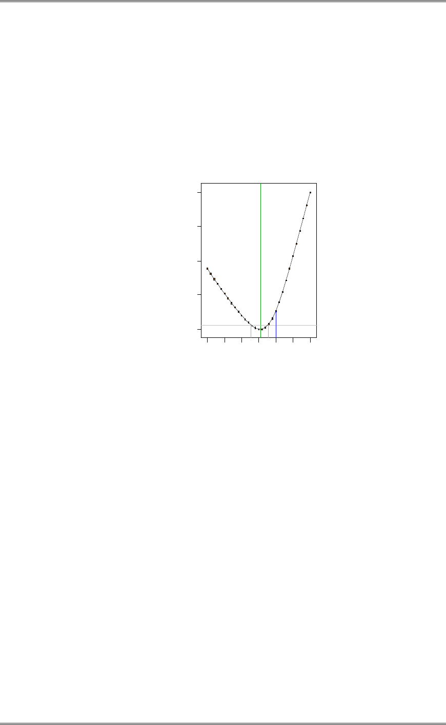
Solutions from Montgomery, D. C. (2001) Design and Analysis of Experiments, Wiley, NY
14-1
Chapter 14
Other Design and Analysis Topics
Solutions
14-1 Reconsider the experiment in Problem 5-22. Use the Box-Cox procedure to determine if a
transformation on the response is appropriate (or useful) in the analysis of the data from this experiment.
DESIGN-EXPERT Plot
Crack G rowth
Lambda
Current = 1
Best = 0.11
Low C.I. = -0.44
High C.I. = 0.56
Recommend transform:
Log
(Lambda = 0)
Lam bda
Ln(ResidualSS)
Box-Cox Plot for Power Transforms
1.10
2.23
3.36
4.49
5.62
-3 -2 -1 0123
With the value of lambda near zero, and since the confidence interval does not include one, a natural log
transformation would be appropriate.
14-2 In example 6-3 we selected a log transformation for the drill advance rate response. Use the Box-
Cox procedure to demonstrate that this is an appropriate data transformation.
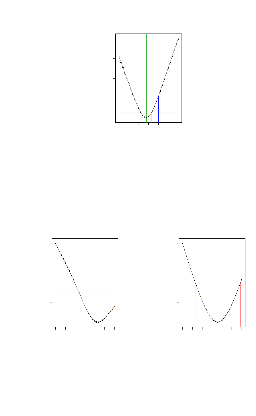
Solutions from Montgomery, D. C. (2001) Design and Analysis of Experiments, Wiley, NY
14-2
DESIGN-EXPERT Plot
Advance Rate
Lambda
Current = 1
Best = -0.23
Low C.I. = -0.79
High C.I. = 0.32
Recommend transform:
Log
(Lambda = 0)
Lam bda
Ln (Res idualSS)
Box-Cox Plot for Power Transforms
1.05
2.50
3.95
5.40
6.85
-3 -2 -1 0123
Because the value of lambda is very close to zero, and the confidence interval does not include one, the
natural log was the correct transformation chosen for this analysis.
14-3 Reconsider the smelting process experiment in Problem 8-23, where a 26-3 fractional factorial
design was used to study the weight of packing material stuck to carbon anodes after baking. Each of the
eight runs in the design was replicated three times and both the average weight and the range of the
weights at each test combination were treated as response variables. Is there any indication that that a
transformation is required for either response?
DESIGN-EXPERT Plot
Weight
Lambda
Current = 1
Best = 1.33
Low C.I. = -0.71
High C.I. = 4.29
Recommend transform:
None
(Lambda = 1)
Lam bda
Ln(ResidualSS)
Box-Cox Plot for Power Transforms
7.89
8.68
9.47
10.26
11.05
-3 -2 -1 0123
DESIGN-EXPERT Plot
Range
Lambda
Cu rre n t = 1
Best = 0.58
Low C.I. = -1.74
High C.I. = 2.92
Recommend transform:
None
(Lambda = 1)
Lam bda
Ln(ResidualSS)
Box-Cox Plot for Power Transforms
9.29
10.23
11.17
12.12
13.06
-3 -2 -1 0 1 2 3
There is no indication that a transformation is required for either response.
14-4 In Problem 8-24 a replicated fractional factorial design was used to study substrate camber in
semiconductor manufacturing. Both the mean and standard deviation of the camber measurements were
used as response variables. Is there any indication that a transformation is required for either response?
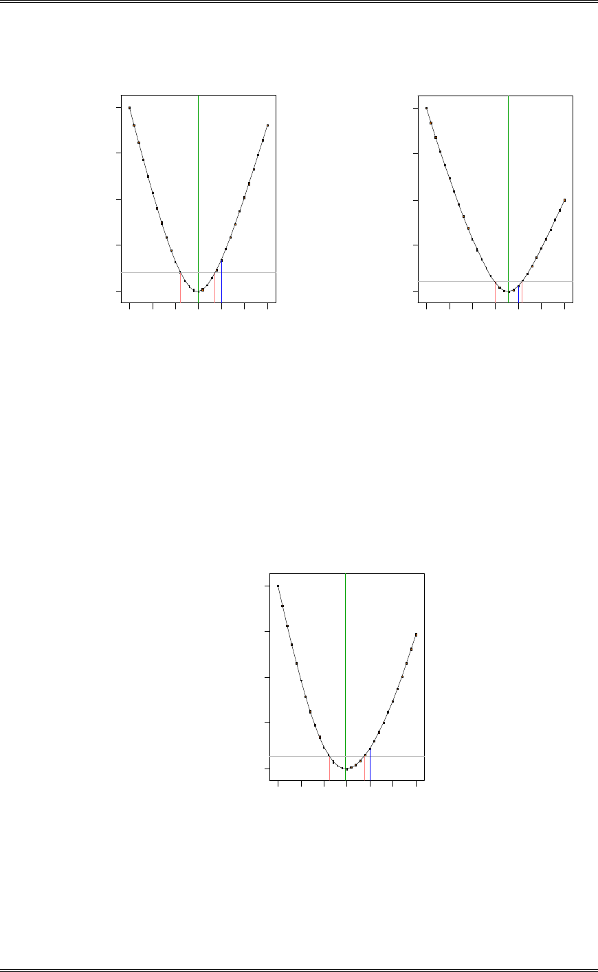
Solutions from Montgomery, D. C. (2001) Design and Analysis of Experiments, Wiley, NY
14-3
DESIGN-EXPERT Plot
Camber Avg
Lambda
Current = 1
Best = -0.03
Low C.I. = -0.79
High C.I. = 0.74
Recommend transform:
Log
(Lambda = 0)
Lam bda
Ln (Res idualSS)
Box-Cox Plot for Power Transforms
8.76
9.62
10.49
11.35
12.22
-3 -2 -1 0123
DESIGN-EXPERT Plot
Cam ber StDev
Lambda
Cu rre n t = 1
Best = 0.57
Low C.I. = -0.03
High C.I. = 1.16
Recommend transform:
None
(Lambda = 1)
Lam bda
Ln (Res idualSS)
Box-Cox Plot for Power Transforms
6.40
8.05
9.70
11.35
13.00
-3 -2 -1 0 1 2 3
The Box-Cox plot for the Camber Average suggests a natural log transformation should be applied. This
decision is based on the confidence interval for lambda not including one and the point estimate of lambda
being very close to zero. With a lambda of approximately 0.5, a square root transformation could be
considered for the Camber Standard Deviation; however, the confidence interval indicates that no
transformation is needed.
14-5 Reconsider the photoresist experiment in Problem 8-25. Use the variance of the resist thickness at
each test combination as the response variable. Is there any indication that a transformation is required?
DESIGN-EXPERT Plot
Thick StDev
Lambda
Current = 1
Best = -0.04
Low C.I. = -0.77
High C.I. = 0.76
Recommend transform:
Log
(Lambda = 0)
Lam bda
Ln (Res idualSS)
Box-Cox Plot for Power Transforms
7.31
7.97
8.62
9.28
9.93
-3 -2 -1 0123
With the point estimate of lambda near zero, and the confidence interval for lambda not inclusive of one,
a natural log transformation would be appropriate.
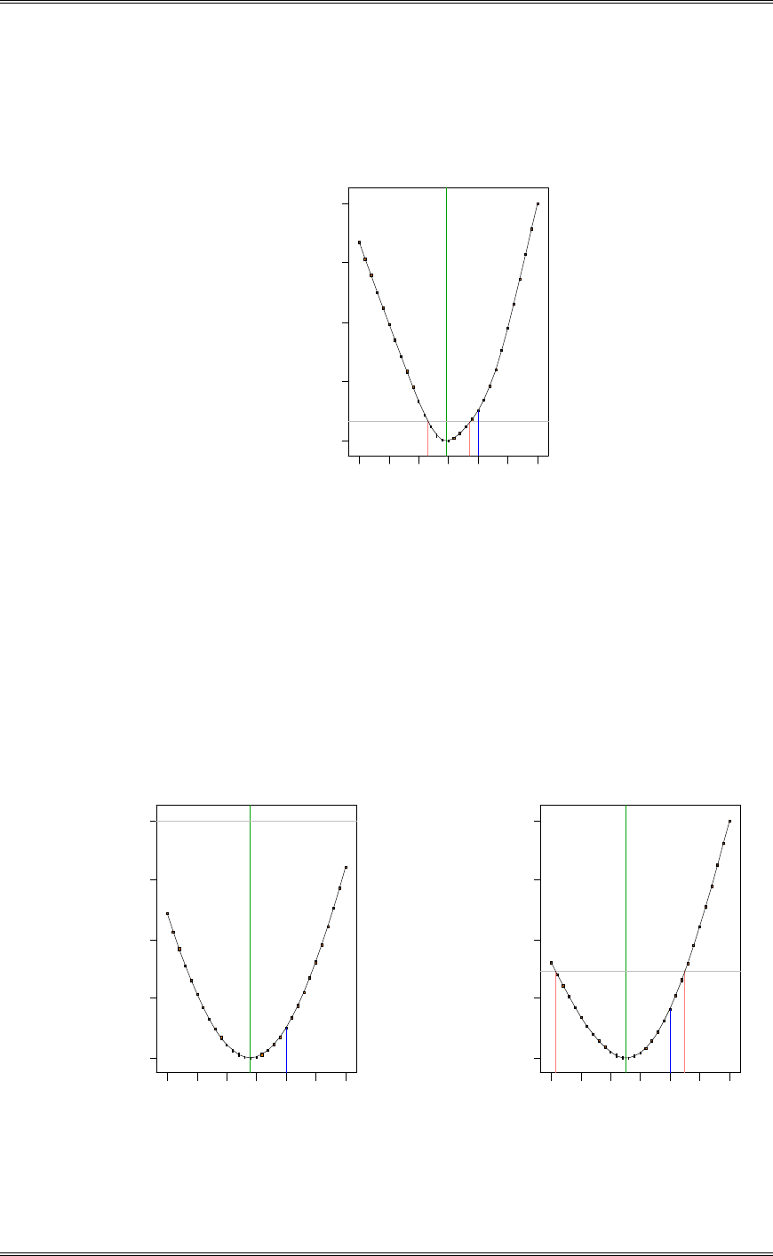
Solutions from Montgomery, D. C. (2001) Design and Analysis of Experiments, Wiley, NY
14-4
14-6 In the grill defects experiment described in Problem 8-29 a variation of the square root
transformation was employed in the analysis of the data. Use the Box-Cox method to determine if this is
the appropriate transformation.
DESIGN-EXPERT Plot
c
Lambda
Current = 1
Best = -0.06
Low C.I. = -0.69
High C.I. = 0.74
Recommend transform:
Log
(Lambda = 0)
k = 0.56
(used to make
response values
positive)
Lam bda
Ln (Res idualSS)
Box-Cox Plot for Power Transforms
3.15
5.55
7.95
10.35
12.75
-3 -2 -1 0123
Because the confidence interval for the minimum lambda does not include one, the decision to use a
transformation is correct. Because the lambda point estimate is close to zero, the natural log
transformation would be appropriate. This is a stronger transformation than the square root.
14-7 In the central composite design of Problem 11-14, two responses were obtained, the mean and
variance of an oxide thickness. Use the Box-Cox method to investigate the potential usefulness of
transformation for both of these responses. Is the log transformation suggested in part (c) of that problem
appropriate?
DESIGN-EXPERT Plot
Mean Thick
Lambda
Current = 1
Best = -0.2
Low C.I. = -3.58
High C.I. = 3.18
Recommend transform:
None
(Lambda = 1)
Lam bda
Ln(ResidualSS)
Box-Cox Plot for Power Transforms
8.09
8.25
8.41
8.57
8.73
-3 -2 -1 0123
DESIGN-EXPERT Plot
Var T hick
Lambda
Cu rre n t = 1
Best = -0.47
Low C.I. = -2.85
High C.I. = 1.51
Recommend transform:
None
(Lambda = 1)
Lam bda
Ln(ResidualSS)
Box-Cox Plot for Power Transforms
1.32
1.65
1.97
2.30
2.63
-3 -2 -1 0 1 2 3
The Box-Cox plot for the Mean Thickness model suggests that a natural log transformation could be
applied; however, the confidence interval for lambda includes one. Therefore, a transformation would

Solutions from Montgomery, D. C. (2001) Design and Analysis of Experiments, Wiley, NY
14-5
have a minimal effect. The natural log transformation applied to the Variance of Thickness model
appears to be acceptable; however, again the confidence interval for lambda includes one.
14-8 In the 33 factorial design of Problem 11-33 one of the responses is a standard deviation. Use the
Box-Cox method to investigate the usefulness of transformations for this response. Would your answer
change if we used the variance of the response?
DESIGN-EXPERT Plot
Std. Dev.
Lambda
Current = 1
Best = 0.29
Low C.I. = 0.0 1
High C.I. = 0.61
Recommend transform:
Square Root
(Lambda = 0.5)
k = 1.582
(used to make
response values
positive)
Lam bda
Ln(ResidualSS)
Box-Cox Plot for Power Transforms
9.94
13.03
16.13
19.22
22.32
-3 -2 -1 0123
Because the confidence interval for lambda does not include one, a transformation should be applied. The
natural log transformation should not be considered due to zero not being included in the confidence
interval. The square root transformation appears to be acceptable. However, notice that the value of zero
is very close to the lower confidence limit, and the minimizing value of lambda is between 0 and 0.5. It is
likely that either the natural log or the square root transformation would work reasonably well.
14-9 Problem 11-34 suggests using the ln(s2) as the response (refer to part b). Does the Box-Cox method
indicate that a transformation is appropriate?
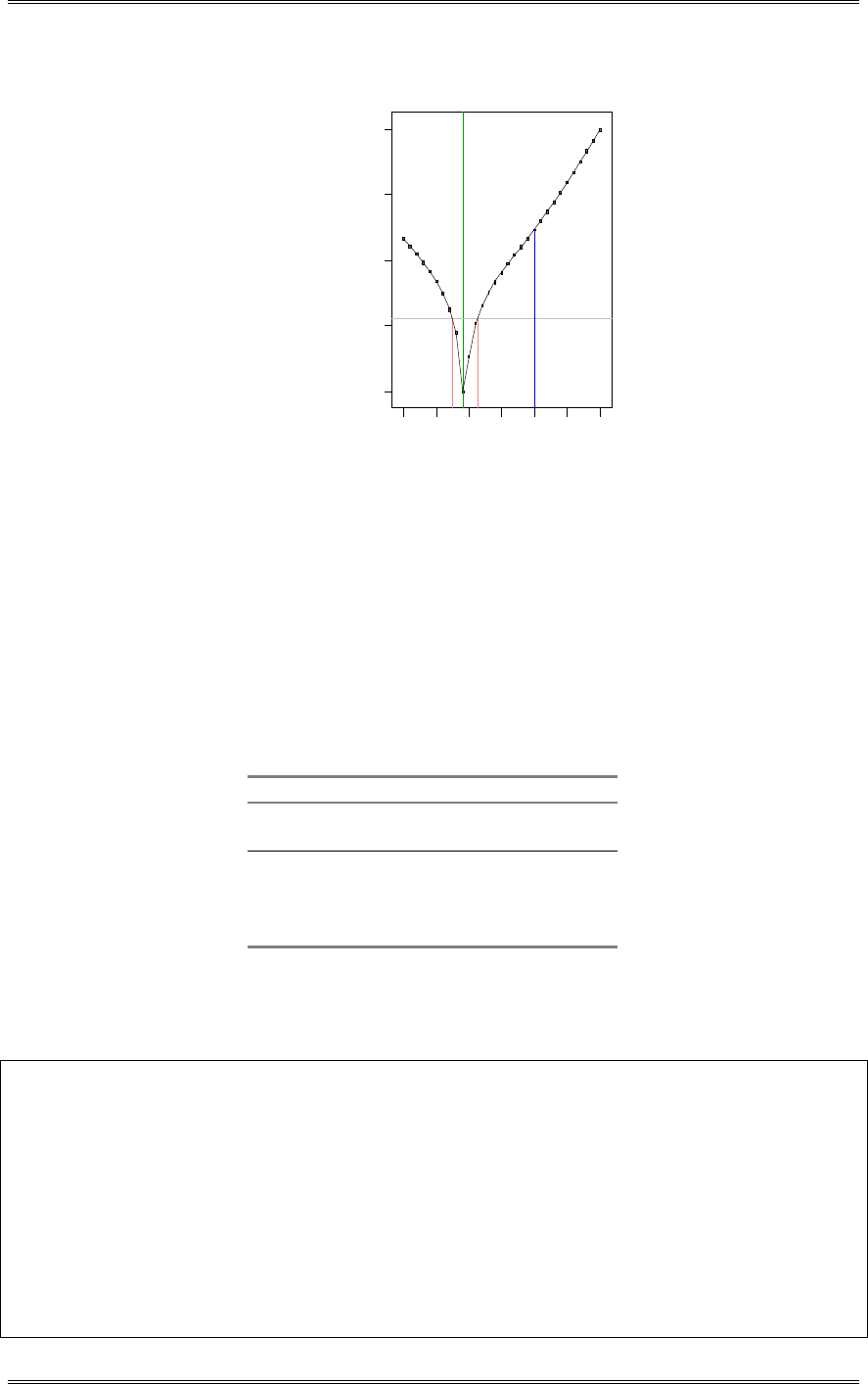
Solutions from Montgomery, D. C. (2001) Design and Analysis of Experiments, Wiley, NY
14-6
DESIGN-EXPERT Plot
Variance
Lambda
Current = 1
Best = -1.17
Low C.I. = -1.53
High C.I. = -0.7 2
Recommend transform:
Inverse
(Lambda = -1)
Lam bda
Ln (Res idualSS)
Box-Cox Plot for Power Transforms
3.85
7.28
10.70
14.13
17.56
-3 -2 -1 0123
Because the confidence interval for lambda does not include one, a transformation should be applied. The
confidence interval does not include zero; therefore, the natural log transformation is inappropriate. With
the point estimate of lambda at –1.17, the reciprocal transformation is appropriate.
14-10 A soft drink distributor is studying the effectiveness of delivery methods. Three different types of
hand trucks have been developed, and an experiment is performed in the company’s methods engineering
laboratory. The variable of interest is the delivery time in minutes (y); however, delivery time is also
strongly related to the case volume delivered (x). Each hand truck is used four times and the data that
follow are obtained. Analyze the data and draw the appropriate conclusions. Use D=0.05.
Hand Truck Type
1 1 2 2 3 3
y x y x y x
27 24 25 26 40 38
44 40 35 32 22 26
33 35 46 42 53 50
41 40 26 25 18 20
From the analysis performed in Minitab, hand truck does not have a statistically significant effect on
delivery time. Volume, as expected, does have a significant effect.
Minitab Output
General Linear Model: Time versus Truck
Factor Type Levels Values
Truck fixed 3 1 2 3
Analysis of Variance for Time, using Adjusted SS for Tests
Source DF Seq SS Adj SS Adj MS F P
Volume 1 1232.07 1217.55 1217.55 232.20 0.000
Truck 2 11.65 11.65 5.82 1.11 0.375
Error 8 41.95 41.95 5.24
Total 11 1285.67
Term Coef SE Coef T P
Constant -4.747 2.638 -1.80 0.110
Volume 1.17326 0.07699 15.24 0.000

Solutions from Montgomery, D. C. (2001) Design and Analysis of Experiments, Wiley, NY
14-7
14-11 Compute the adjusted treatment means and the standard errors of the adjusted treatment means for
the data in Problem 14-10.
adj
...i.i.i xx
ˆ
yy
E
adj
3934
12
398
4
139
1731
4
145
1..y .
¸
¹
·
¨
©
§
adj
2535
12
398
4
125
1731
4
132
2..y .
¸
¹
·
¨
©
§
adj
8632
12
398
4
134
1731
4
133
3..y .
¸
¹
·
¨
©
§
2
1
2
1
»
»
¼
º
«
«
¬
ª
°
¿
°
¾
½
°
¯
°
®
xx
...i
Ey.adj E
xx
n
MSS .i
1511
50884
17337534
4
1
245
2
1
2
1.
.
..
.S .
y.adj
»
»
¼
º
«
«
¬
ª
°
¿
°
¾
½
°
¯
°
®
1541
50884
17332531
4
1
245
2
1
2
2.
.
..
.S .
y.adj
»
»
¼
º
«
«
¬
ª
°
¿
°
¾
½
°
¯
°
®
1451
50884
17335033
4
1
245
2
1
2
3.
.
..
.S .
y.adj
»
»
¼
º
«
«
¬
ª
°
¿
°
¾
½
°
¯
°
®
The solutions can also be obtained with Minitab as follows:
Minitab Output
Least Squares Means for Time
Truck Mean SE Mean
1 34.39 1.151
2 35.25 1.154
3 32.86 1.145
14-12 The sums of squares and products for a single-factor analysis of covariance follow. Complete the
analysis and draw appropriate conclusions. Use
D
= 0.05.
Source of Degrees of Sums of Squares and Products
Variation Freedom x xy x
Treatment 3 1500 1000 650
Error 12 6000 1200 550
Total 15 7500 2200 1200
Sums of Squares & Products Adjusted
Source df x xy y y df MS F0
Treatment 3 1500 1000 650 - -
Error 12 6000 1200 550 310 11 28.18
Total 15 7500 2200 1200 559.67 14

Solutions from Montgomery, D. C. (2001) Design and Analysis of Experiments, Wiley, NY
14-8
Adjusted Treat. 244.67 3 81.56 2.89
Treatments differ only at 10%.
14-13 Find the standard errors of the adjusted treatment means in Example 14-4.
From Example 14-4 y140 38
.. , adj y24142
.. , adj y337 78
..
72310
60195
13242025
5
1
542
2
1
2
1.
.
..
.S .
y.adj
»
»
¼
º
«
«
¬
ª
°
¿
°
¾
½
°
¯
°
®
74390
60195
13240026
5
1
542
2
1
2
2.
.
..
.S .
y.adj
»
»
¼
º
«
«
¬
ª
°
¿
°
¾
½
°
¯
°
®
78710
60195
13242021
5
1
542
2
1
2
3.
.
..
.S .
y.adj
»
»
¼
º
«
«
¬
ª
°
¿
°
¾
½
°
¯
°
®
14-14 Four different formulations of an industrial glue are being tested. The tensile strength of the glue
when it is applied to join parts is also related to the application thickness. Five observations on strength
(y) in pounds and thickness (x) in 0.01 inches are obtained for each formulation. The data are shown in
the following table. Analyze these data and draw appropriate conclusions.
Glue Formulation
1 1 2 2 3 3 4 4
y x y x y x y x
46.5 13 48.7 12 46.3 15 44.7 16
45.9 14 49.0 10 47.1 14 43.0 15
49.8 12 50.1 11 48.9 11 51.0 10
46.1 12 48.5 12 48.2 11 48.1 12
44.3 14 45.2 14 50.3 10 48.6 11
From the analysis performed in Minitab, glue formulation does not have a statistically significant effect on
strength. As expected, glue thickness does affect strength.
Minitab Output
General Linear Model: Strength versus Glue
Factor Type Levels Values
Glue fixed 4 1 2 3 4
Analysis of Variance for Strength, using Adjusted SS for Tests
Source DF Seq SS Adj SS Adj MS F P
Thick 1 68.852 59.566 59.566 42.62 0.000
Glue 3 1.771 1.771 0.590 0.42 0.740
Error 15 20.962 20.962 1.397
Total 19 91.585
Term Coef SE Coef T P
Constant 60.089 1.944 30.91 0.000
Thick -1.0099 0.1547 -6.53 0.000
Unusual Observations for Strength

Solutions from Montgomery, D. C. (2001) Design and Analysis of Experiments, Wiley, NY
14-9
Obs Strength Fit SE Fit Residual St Resid
3 49.8000 47.5299 0.5508 2.2701 2.17R
R denotes an observation with a large standardized residual.
Expected Mean Squares, using Adjusted SS
Source Expected Mean Square for Each Term
1 Thick (3) + Q[1]
2 Glue (3) + Q[2]
3 Error (3)
Error Terms for Tests, using Adjusted SS
Source Error DF Error MS Synthesis of Error MS
1 Thick 15.00 1.397 (3)
2 Glue 15.00 1.397 (3)
Variance Components, using Adjusted SS
Source Estimated Value
Error 1.397
14-15 Compute the adjusted treatment means and their standard errors using the data in Problem 14-14.
adj
...i.i.i xx
ˆ
yy
E
adj
084745120013009915246
1.....y .
adj
644745128011009913048
2.....y .
adj
914745122012009911648
3.....y .
adj
434745128012009910847
4.....y .
2
1
2
1
»
»
¼
º
«
«
¬
ª
°
¿
°
¾
½
°
¯
°
®
xx
...i
Ey.adj E
xx
n
MSS .i
53600
4058
45120013
5
1
401
2
1
2
1.
.
..
.S .
y.adj
»
»
¼
º
«
«
¬
ª
°
¿
°
¾
½
°
¯
°
®
53860
4058
45128011
5
1
401
2
1
2
2.
.
..
.S .
y.adj
»
»
¼
º
«
«
¬
ª
°
¿
°
¾
½
°
¯
°
®
53060
4058
45122012
5
1
401
2
1
2
3.
.
..
.S .
y.adj
»
»
¼
º
«
«
¬
ª
°
¿
°
¾
½
°
¯
°
®
53190
4058
45128012
5
1
401
2
1
2
4.
.
..
.S .
y.adj
»
»
¼
º
«
«
¬
ª
°
¿
°
¾
½
°
¯
°
®
The adjusted treatment means can also be generated in Minitab as follows:
Minitab Output
Least Squares Means for Strength
Glue Mean SE Mean
1 47.08 0.5355
2 47.64 0.5382
3 47.91 0.5301

Solutions from Montgomery, D. C. (2001) Design and Analysis of Experiments, Wiley, NY
14-10
4 47.43 0.5314
14-16 An engineer is studying the effect of cutting speed on the rate of metal removal in a machining
operation. However, the rate of metal removal is also related to the hardness of the test specimen. Five
observations are taken at each cutting speed. The amount of metal removed (y) and the hardness of the
specimen (x) are shown in the following table. Analyze the data using and analysis of covariance. Use
D=0.05.
Cutting Speed (rpm)
1000 1000 1200 1200 1400 1400
y x y x y x
68 120 112 165 118 175
90 140 94 140 82 132
98 150 65 120 73 124
77 125 74 125 92 141
88 136 85 133 80 130
As shown in the analysis performed in Minitab, there is no difference in the rate of removal between the
three cutting speeds. As expected, the hardness does have an impact on rate of removal.
Minitab Output
General Linear Model: Removal versus Speed
Factor Type Levels Values
Speed fixed 3 1000 1200 1400
Analysis of Variance for Removal, using Adjusted SS for Tests
Source DF Seq SS Adj SS Adj MS F P
Hardness 1 3075.7 3019.3 3019.3 347.96 0.000
Speed 2 2.4 2.4 1.2 0.14 0.872
Error 11 95.5 95.5 8.7
Total 14 3173.6
Term Coef SE Coef T P
Constant -41.656 6.907 -6.03 0.000
Hardness 0.93426 0.05008 18.65 0.000
Speed
1000 0.478 1.085 0.44 0.668
1200 0.036 1.076 0.03 0.974
Unusual Observations for Removal
Obs Removal Fit SE Fit Residual St Resid
8 65.000 70.491 1.558 -5.491 -2.20R
R denotes an observation with a large standardized residual.
Expected Mean Squares, using Adjusted SS
Source Expected Mean Square for Each Term
1 Hardness (3) + Q[1]
2 Speed (3) + Q[2]
3 Error (3)
Error Terms for Tests, using Adjusted SS
Source Error DF Error MS Synthesis of Error MS
1 Hardness 11.00 8.7 (3)
2 Speed 11.00 8.7 (3)
Variance Components, using Adjusted SS
Source Estimated Value

Solutions from Montgomery, D. C. (2001) Design and Analysis of Experiments, Wiley, NY
14-11
Error 8.677
Means for Covariates
Covariate Mean StDev
Hardness 137.1 15.94
Least Squares Means for Removal
Speed Mean SE Mean
1000 86.88 1.325
1200 86.44 1.318
1400 85.89 1.328
14-17 Show that in a single factor analysis of covariance with a single covariate a 100(1-
D
) percent
confidence interval on the ith adjusted treatment mean is
2
1
2
112
1
»
»
¼
º
«
«
¬
ª
¸
¸
¹
·
¨
¨
©
§
r
xx
...i
Ena,...i.i E
xx
n
MStxx
ˆ
y
D
E
Using this formula, calculate a 95 percent confidence interval on the adjusted mean of machine 1 in
Example 14-4.
The 100(1-
D
) percent interval on the ith adjusted treatment mean would be
.i
yadjna,...i.i Stxx
ˆ
y112
r
D
E
since
...i.i xx
ˆ
y
E
is an estimator of the ith adjusted treatment mean. The standard error of the
adjusted treatment mean is found as follows:
>
@
EE
ˆ
VxxyVxx
ˆ
yVy.adjV ...i.i...i.i.i
2
Since the
^`
yi. and
E
are independent. From regression analysis, we have
xx
E
ˆ
V
2
V
E
. Therefore,
»
»
¼
º
«
«
¬
ª
xx
...i
xx
...i
.i E
xx
nE
xx
n
y.adjV
2
2
2
2
21
V
V
V
Replacing
V
2 by its estimator MSE, yields
»
»
¼
º
«
«
¬
ª
xx
...i
E.i E
xx
n
MSy.adjV
ˆ
2
1 or
2
1
2
1
°
¿
°
¾
½
°
¯
°
®
»
»
¼
º
«
«
¬
ª
xx
...i
E.i E
xx
n
MSy.adjS
Substitution of this result into
.
1)1(,2.... ˆ
i
yadjnaii Stxxy
r
D
E
will produce the desired
confidence interval. A 95% confidence interval on the mean of machine 1 would be found as follows:

Solutions from Montgomery, D. C. (2001) Design and Analysis of Experiments, Wiley, NY
14-12
3840.xx
ˆ
yy.adj ...i.i.i
E
72310.y.adjS .i
>
@
>@
>@
5913840
723102023840
723103840 110250
..
...
.t. ,.
r
r
r
Therefore, 96417938 1.. dd
P
, where
P
1 denotes the true adjusted mean of treatment one.
14-18 Show that in a single-factor analysis of covariance with a single covariate, the standard error of the
difference between any two adjusted treatment means is
2
1
2
2
»
»
¼
º
«
«
¬
ª
¸
¸
¹
·
¨
¨
©
§
xx
...i
EyAdjyAdj E
xx
n
MSS .j.i
>
@
...j.j...i.i.j.i xx
ˆ
yxx
ˆ
yy.adjy.adj
EE
...... ˆ
.. jijiji xxyyyadjyadj
E
The variance of this statistic is
>@
EE
ˆ
VxxyVyVxx
ˆ
yyV .j.i.j.i.j.i.j.i
2
»
»
¼
º
«
«
¬
ª
xx
.j.i
xx
.j.i
E
xx
nE
xx
nn
2
2
2
2
22 2
V
V
VV
Replacing
V
2by its estimator MSE, , and taking the square root yields the standard error
2
1
2
2
»
»
¼
º
«
«
¬
ª
¸
¸
¹
·
¨
¨
©
§
xx
...i
EyAdjyAdj E
xx
n
MSS .j.i
14-19 Discuss how the operating characteristic curves for the analysis of variance can be used in the
analysis of covariance.
To use the operating characteristic curves, fixed effects case, we would use as the parameter )2,
2
2
2
V
W
)
n
ai
¦
The test has a-1 degrees of freedom in the numerator and a(n-1)-1 degrees of freedom in the denominator.