Spark For Python Developers A Concise Guide To Implementing Big Data Analytics D
User Manual:
Open the PDF directly: View PDF ![]() .
.
Page Count: 206 [warning: Documents this large are best viewed by clicking the View PDF Link!]
- Cover
- Copyright
- Credits
- About the Author
- Acknowledgment
- About the Reviewers
- www.PacktPub.com
- Table of Contents
- Preface
- Chapter 1: Setting Up a Spark Virtual Environment
- Chapter 2: Building Batch and Streaming Apps with Spark
- Chapter 3: Juggling Data with Spark
- Chapter 4: Learning from Data Using Spark
- Chapter 5: Streaming Live Data with Spark
- Chapter 6: Visualizing Insights and Trends
- Index

Spark for Python Developers
Copyright © 2015 Packt Publishing
All rights reserved. No part of this book may be reproduced, stored in a retrieval
system, or transmitted in any form or by any means, without the prior written
permission of the publisher, except in the case of brief quotations embedded in
critical articles or reviews.
Every effort has been made in the preparation of this book to ensure the accuracy
of the information presented. However, the information contained in this book is
sold without warranty, either express or implied. Neither the author, nor Packt
Publishing, and its dealers and distributors will be held liable for any damages
caused or alleged to be caused directly or indirectly by this book.
Packt Publishing has endeavored to provide trademark information about all of the
companies and products mentioned in this book by the appropriate use of capitals.
However, Packt Publishing cannot guarantee the accuracy of this information.
First published: December 2015
Production reference: 1171215
Published by Packt Publishing Ltd.
Livery Place
35 Livery Street
Birmingham B3 2PB, UK.
ISBN 978-1-78439-969-6
www.packtpub.com
www.it-ebooks.info

Credits
Author
Amit Nandi
Reviewers
Manuel Ignacio Franco Galeano
Rahul Kavale
Daniel Lemire
Chet Mancini
Laurence Welch
Commissioning Editor
Amarabha Banerjee
Acquisition Editor
Sonali Vernekar
Content Development Editor
Merint Thomas Mathew
Technical Editor
Naveenkumar Jain
Copy Editor
Roshni Banerjee
Project Coordinator
Suzanne Coutinho
Proofreader
Sas Editing
Indexer
Priya Sane
Graphics
Kirk D'Penha
Production Coordinator
Shantanu N. Zagade
Cover Work
Shantanu N. Zagade
www.it-ebooks.info
About the Author
Amit Nandi studied physics at the Free University of Brussels in Belgium,
where he did his research on computer generated holograms. Computer generated
holograms are the key components of an optical computer, which is powered by
photons running at the speed of light. He then worked with the university Cray
supercomputer, sending batch jobs of programs written in Fortran. This gave him
a taste for computing, which kept growing. He has worked extensively on large
business reengineering initiatives, using SAP as the main enabler. He focused for the
last 15 years on start-ups in the data space, pioneering new areas of the information
technology landscape. He is currently focusing on large-scale data-intensive
applications as an enterprise architect, data engineer, and software developer.
He understands and speaks seven human languages. Although Python is his
computer language of choice, he aims to be able to write uently in seven
computer languages too.
www.it-ebooks.info
Acknowledgment
I want to express my profound gratitude to my parents for their unconditional love
and strong support in all my endeavors.
This book arose from an initial discussion with Richard Gall, an acquisition
editor at Packt Publishing. Without this initial discussion, this book would never
have happened. So, I am grateful to him. The follow ups on discussions and the
contractual terms were agreed with Rebecca Youe. I would like to thank her for her
support. I would also like to thank Merint Mathew, a content editor who helped me
bring this book to the nish line. I am thankful to Merint for his subtle persistence
and tactful support during the write ups and revisions of this book.
We are standing on the shoulders of giants. I want to acknowledge some of the
giants who helped me shape my thinking. I want to recognize the beauty, elegance,
and power of Python as envisioned by Guido van Rossum. My respectful gratitude
goes to Matei Zaharia and the team at Berkeley AMP Lab and Databricks for
developing a new approach to computing with Spark and Mesos. Travis Oliphant,
Peter Wang, and the team at Continuum.io are doing a tremendous job of keeping
Python relevant in a fast-changing computing landscape. Thank you to you all.
www.it-ebooks.info
About the Reviewers
Manuel Ignacio Franco Galeano is a software developer from Colombia. He
holds a computer science degree from the University of Quindío. At the moment of
publication of this book, he was studying to get his MSc in computer science from
University College Dublin, Ireland. He has a wide range of interests that include
distributed systems, machine learning, micro services, and so on. He is looking for
a way to apply machine learning techniques to audio data in order to help people
learn more about music.
Rahul Kavale works as a software developer at TinyOwl Ltd. He is interested in
multiple technologies ranging from building web applications to solving big data
problems. He has worked in multiple languages, including Scala, Ruby, and Java,
and has worked on Apache Spark, Apache Storm, Apache Kafka, Hadoop, and Hive.
He enjoys writing Scala. Functional programming and distributed computing are his
areas of interest. He has been using Spark since its early stage for varying use cases.
He has also helped with the review for the Pragmatic Scala book.
www.it-ebooks.info
Daniel Lemire has a BSc and MSc in mathematics from the University of Toronto
and a PhD in engineering mathematics from the Ecole Polytechnique and the
Université de Montréal. He is a professor of computer science at the Université du
Québec. He has also been a research ofcer at the National Research Council of
Canada and an entrepreneur. He has written over 45 peer-reviewed publications,
including more than 25 journal articles. He has held competitive research grants for
the last 15 years. He has been an expert on several committees with funding agencies
(NSERC and FQRNT). He has served as a program committee member on leading
computer science conferences (for example, ACM CIKM, ACM WSDM, ACM SIGIR,
and ACM RecSys). His open source software has been used by major corporations
such as Google and Facebook. His research interests include databases, information
retrieval and high-performance programming. He blogs regularly on computer
science at http://lemire.me/blog/.
Chet Mancini is a data engineer at Intent Media, Inc in New York, where he
works with the data science team to store and process terabytes of web travel data
to build predictive models of shopper behavior. He enjoys functional programming,
immutable data structures, and machine learning. He writes and speaks on topics
surrounding data engineering and information architecture.
He is a contributor to Apache Spark and other libraries in the Spark ecosystem.
Chet has a master's degree in computer science from Cornell University.
www.it-ebooks.info

www.PacktPub.com
Support les, eBooks, discount offers, and more
For support les and downloads related to your book, please visit www.PacktPub.com.
Did you know that Packt offers eBook versions of every book published, with PDF
and ePub les available? You can upgrade to the eBook version at www.PacktPub.com
and as a print book customer, you are entitled to a discount on the eBook copy. Get in
touch with us at service@packtpub.com for more details.
At www.PacktPub.com, you can also read a collection of free technical articles, sign
up for a range of free newsletters and receive exclusive discounts and offers on Packt
books and eBooks.
TM
https://www2.packtpub.com/books/subscription/packtlib
Do you need instant solutions to your IT questions? PacktLib is Packt's online digital
book library. Here, you can search, access, and read Packt's entire library of books.
Why subscribe?
• Fully searchable across every book published by Packt
• Copy and paste, print, and bookmark content
• On demand and accessible via a web browser
Free access for Packt account holders
If you have an account with Packt at www.PacktPub.com, you can use this to access
PacktLib today and view 9 entirely free books. Simply use your login credentials for
immediate access.
www.it-ebooks.info

[ i ]
Table of Contents
Preface v
Chapter 1: Setting Up a Spark Virtual Environment 1
Understanding the architecture of
data-intensive applications 3
Infrastructure layer 4
Persistence layer 4
Integration layer 4
Analytics layer 5
Engagement layer 6
Understanding Spark 6
Spark libraries 7
PySpark in action 7
The Resilient Distributed Dataset 8
Understanding Anaconda 10
Setting up the Spark powered environment 12
Setting up an Oracle VirtualBox with Ubuntu 13
Installing Anaconda with Python 2.7 13
Installing Java 8 14
Installing Spark 15
Enabling IPython Notebook 16
Building our rst app with PySpark 17
Virtualizing the environment with Vagrant 22
Moving to the cloud 24
Deploying apps in Amazon Web Services 24
Virtualizing the environment with Docker 24
Summary 26
www.it-ebooks.info

Table of Contents
[ ii ]
Chapter 2: Building Batch and Streaming Apps with Spark 27
Architecting data-intensive apps 28
Processing data at rest 29
Processing data in motion 30
Exploring data interactively 31
Connecting to social networks 31
Getting Twitter data 32
Getting GitHub data 34
Getting Meetup data 34
Analyzing the data 35
Discovering the anatomy of tweets 35
Exploring the GitHub world 40
Understanding the community through Meetup 42
Previewing our app 47
Summary 48
Chapter 3: Juggling Data with Spark 49
Revisiting the data-intensive app architecture 50
Serializing and deserializing data 51
Harvesting and storing data 51
Persisting data in CSV 52
Persisting data in JSON 54
Setting up MongoDB 55
Installing the MongoDB server and client 55
Running the MongoDB server 56
Running the Mongo client 57
Installing the PyMongo driver 58
Creating the Python client for MongoDB 58
Harvesting data from Twitter 59
Exploring data using Blaze 63
Transferring data using Odo 67
Exploring data using Spark SQL 68
Understanding Spark dataframes 69
Understanding the Spark SQL query optimizer 72
Loading and processing CSV les with Spark SQL 75
Querying MongoDB from Spark SQL 77
Summary 81
www.it-ebooks.info

Table of Contents
[ iii ]
Chapter 4: Learning from Data Using Spark 83
Contextualizing Spark MLlib in the app architecture 84
Classifying Spark MLlib algorithms 85
Supervised and unsupervised learning 86
Additional learning algorithms 88
Spark MLlib data types 90
Machine learning workows and data ows 92
Supervised machine learning workows 92
Unsupervised machine learning workows 94
Clustering the Twitter dataset 95
Applying Scikit-Learn on the Twitter dataset 96
Preprocessing the dataset 103
Running the clustering algorithm 107
Evaluating the model and the results 108
Building machine learning pipelines 113
Summary 114
Chapter 5: Streaming Live Data with Spark 115
Laying the foundations of streaming architecture 116
Spark Streaming inner working 118
Going under the hood of Spark Streaming 120
Building in fault tolerance 124
Processing live data with TCP sockets 124
Setting up TCP sockets 124
Processing live data 125
Manipulating Twitter data in real time 128
Processing Tweets in real time from the Twitter rehose 128
Building a reliable and scalable streaming app 131
Setting up Kafka 133
Installing and testing Kafka 134
Developing producers 137
Developing consumers 139
Developing a Spark Streaming consumer for Kafka 140
Exploring ume 142
Developing data pipelines with Flume, Kafka, and Spark 143
Closing remarks on the Lambda and Kappa architecture 146
Understanding the Lambda architecture 147
Understanding the Kappa architecture 148
Summary 149
www.it-ebooks.info

Table of Contents
[ iv ]
Chapter 6: Visualizing Insights and Trends 151
Revisiting the data-intensive apps architecture 151
Preprocessing the data for visualization 154
Gauging words, moods, and memes at a glance 160
Setting up wordcloud 160
Creating wordclouds 162
Geo-locating tweets and mapping meetups 165
Geo-locating tweets 165
Displaying upcoming meetups on Google Maps 172
Summary 178
Index 179
www.it-ebooks.info

[ v ]
Preface
Spark for Python Developers aims to combine the elegance and exibility of Python
with the power and versatility of Apache Spark. Spark is written in Scala and runs
on the Java virtual machine. It is nevertheless polyglot and offers bindings and APIs
for Java, Scala, Python, and R. Python is a well-designed language with an extensive
set of specialized libraries. This book looks at PySpark within the PyData ecosystem.
Some of the prominent PyData libraries include Pandas, Blaze, Scikit-Learn,
Matplotlib, Seaborn, and Bokeh. These libraries are open source. They are developed,
used, and maintained by the data scientist and Python developers community.
PySpark integrates well with the PyData ecosystem, as endorsed by the Anaconda
Python distribution. The book puts forward a journey to build data-intensive apps
along with an architectural blueprint that covers the following steps: rst, set up the
base infrastructure with Spark. Second, acquire, collect, process, and store the data.
Third, gain insights from the collected data. Fourth, stream live data and process it in
real time. Finally, visualize the information.
The objective of the book is to learn about PySpark and PyData libraries by building
apps that analyze the Spark community's interactions on social networks. The focus
is on Twitter data.
What this book covers
Chapter 1, Setting Up a Spark Virtual Environment, covers how to create a segregated
virtual machine as our sandbox or development environment to experiment with
Spark and PyData libraries. It covers how to install Spark and the Python Anaconda
distribution, which includes PyData libraries. Along the way, we explain the key
Spark concepts, the Python Anaconda ecosystem, and build a Spark word count app.
www.it-ebooks.info

Preface
[ vi ]
Chapter 2, Building Batch and Streaming Apps with Spark, lays the foundation of the
Data Intensive Apps Architecture. It describes the ve layers of the apps architecture
blueprint: infrastructure, persistence, integration, analytics, and engagement. We
establish API connections with three social networks: Twitter, GitHub, and Meetup.
This chapter provides the tools to connect to these three nontrivial APIs so that you
can create your own data mashups at a later stage.
Chapter 3, Juggling Data with Spark, covers how to harvest data from Twitter and
process it using Pandas, Blaze, and SparkSQL with their respective implementations
of the dataframe data structure. We proceed with further investigations and
techniques using Spark SQL, leveraging on the Spark dataframe data structure.
Chapter 4, Learning from Data Using Spark, gives an overview of the ever expanding
library of algorithms of Spark MLlib. It covers supervised and unsupervised
learning, recommender systems, optimization, and feature extraction algorithms.
We put the Twitter harvested dataset through a Python Scikit-Learn and Spark
MLlib K-means clustering in order to segregate the Apache Spark relevant tweets.
Chapter 5, Streaming Live Data with Spark, lays down the foundation of streaming
architecture apps and describes their challenges, constraints, and benets. We
illustrate the streaming concepts with TCP sockets, followed by live tweet ingestion
and processing directly from the Twitter rehose. We also describe Flume, a reliable,
exible, and scalable data ingestion and transport pipeline system. The combination
of Flume, Kafka, and Spark delivers unparalleled robustness, speed, and agility in an
ever-changing landscape. We end the chapter with some remarks and observations
on two streaming architectural paradigms, the Lambda and Kappa architectures.
Chapter 6, Visualizing Insights and Trends, focuses on a few key visualization
techniques. It covers how to build word clouds and expose their intuitive power
to reveal a lot of the key words, moods, and memes carried through thousands of
tweets. We then focus on interactive mapping visualizations using Bokeh. We build
a world map from the ground up and create a scatter plot of critical tweets. Our nal
visualization is to overlay an actual Google map of London, highlighting upcoming
meetups and their respective topics.
What you need for this book
You need inquisitiveness, perseverance, and passion for data, software engineering,
application architecture and scalability, and beautiful succinct visualizations. The
scope is broad and wide.
You need a good understanding of Python or a similar language with object-oriented
and functional programming capabilities. Preliminary experience of data wrangling
with Python, R, or any similar tool is helpful.
www.it-ebooks.info

Preface
[ vii ]
You need to appreciate how to conceive, build, and scale data applications.
Who this book is for
The target audience includes the following:
• Data scientists are the primary interested parties. This book will help you
unleash the power of Spark and leverage your Python, R, and machine
learning background.
• Software developers with a focus on Python will readily expand their skills
to create data-intensive apps using Spark as a processing engine and Python
visualization libraries and web frameworks.
• Data architects who can create rapid data pipelines and build the famous
Lambda architecture that encompasses batch and streaming processing
to render insights on data in real time, using the Spark and Python rich
ecosystem, will also benet from this book.
Conventions
In this book, you will nd a number of styles of text that distinguish between
different kinds of information. Here are some examples of these styles, and an
explanation of their meaning.
Code words in text, database table names, folder names, lenames, le extensions,
pathnames, dummy URLs, user input, and Twitter handles are shown as follows
"Launch PySpark with IPYNB in directory examples/AN_Spark where the Jupyter or
IPython Notebooks are stored".
A block of code is set as follows:
# Word count on 1st Chapter of the Book using PySpark
# import regex module
import re
# import add from operator module
from operator import add
# read input file
file_in = sc.textFile('/home/an/Documents/A00_Documents/Spark4Py
20150315')
www.it-ebooks.info

Preface
[ viii ]
Any command-line input or output is written as follows:
# install anaconda 2.x.x
bash Anaconda-2.x.x-Linux-x86[_64].sh
New terms and important words are shown in bold. Words that you see on the
screen, in menus or dialog boxes for example, appear in the text like this: "After
installing VirtualBox, let's open the Oracle VM VirtualBox Manager and click the
New button."
Warnings or important notes appear in a box like this.
Tips and tricks appear like this.
Reader feedback
Feedback from our readers is always welcome. Let us know what you think about
this book—what you liked or may have disliked. Reader feedback is important for us
to develop titles that you really get the most out of.
To send us general feedback, simply send an e-mail to feedback@packtpub.com,
and mention the book title via the subject of your message.
If there is a topic that you have expertise in and you are interested in either writing
or contributing to a book, see our author guide on www.packtpub.com/authors.
Customer support
Now that you are the proud owner of a Packt book, we have a number of things to
help you to get the most from your purchase.
Downloading the example code
You can download the example code les for all Packt books you have purchased
from your account at http://www.packtpub.com. If you purchased this book
elsewhere, you can visit http://www.packtpub.com/support and register to have
the les e-mailed directly to you.
www.it-ebooks.info

Preface
[ ix ]
Errata
Although we have taken every care to ensure the accuracy of our content, mistakes
do happen. If you nd a mistake in one of our books—maybe a mistake in the text or
the code—we would be grateful if you would report this to us. By doing so, you can
save other readers from frustration and help us improve subsequent versions of this
book. If you nd any errata, please report them by visiting http://www.packtpub.
com/submit-errata, selecting your book, clicking on the errata submission form link,
and entering the details of your errata. Once your errata are veried, your submission
will be accepted and the errata will be uploaded on our website, or added to any list of
existing errata, under the Errata section of that title. Any existing errata can be viewed
by selecting your title from http://www.packtpub.com/support.
Piracy
Piracy of copyright material on the Internet is an ongoing problem across all media.
At Packt, we take the protection of our copyright and licenses very seriously. If you
come across any illegal copies of our works, in any form, on the Internet, please
provide us with the location address or website name immediately so that we can
pursue a remedy.
Please contact us at copyright@packtpub.com with a link to the suspected
pirated material.
We appreciate your help in protecting our authors, and our ability to bring you
valuable content.
Questions
You can contact us at questions@packtpub.com if you are having a problem with
any aspect of the book, and we will do our best to address it.
www.it-ebooks.info

[ 1 ]
Setting Up a Spark Virtual
Environment
In this chapter, we will build an isolated virtual environment for development
purposes. The environment will be powered by Spark and the PyData libraries
provided by the Python Anaconda distribution. These libraries include Pandas,
Scikit-Learn, Blaze, Matplotlib, Seaborn, and Bokeh. We will perform the
following activities:
• Setting up the development environment using the Anaconda Python
distribution. This will include enabling the IPython Notebook environment
powered by PySpark for our data exploration tasks.
• Installing and enabling Spark, and the PyData libraries such as Pandas,
Scikit- Learn, Blaze, Matplotlib, and Bokeh.
• Building a word count example app to ensure that everything is
working fine.
The last decade has seen the rise and dominance of data-driven behemoths such as
Amazon, Google, Twitter, LinkedIn, and Facebook. These corporations, by seeding,
sharing, or disclosing their infrastructure concepts, software practices, and data
processing frameworks, have fostered a vibrant open source software community.
This has transformed the enterprise technology, systems, and software architecture.
This includes new infrastructure and DevOps (short for development and
operations), concepts leveraging virtualization, cloud technology, and
software-dened networks.
www.it-ebooks.info

Setting Up a Spark Virtual Environment
[ 2 ]
To process petabytes of data, Hadoop was developed and open sourced, taking
its inspiration from the Google File System (GFS) and the adjoining distributed
computing framework, MapReduce. Overcoming the complexities of scaling while
keeping costs under control has also led to a proliferation of new data stores.
Examples of recent database technology include Cassandra, a columnar
database; MongoDB, a document database; and Neo4J, a graph database.
Hadoop, thanks to its ability to process huge datasets, has fostered a vast ecosystem
to query data more iteratively and interactively with Pig, Hive, Impala, and Tez.
Hadoop is cumbersome as it operates only in batch mode using MapReduce. Spark
is creating a revolution in the analytics and data processing realm by targeting the
shortcomings of disk input-output and bandwidth-intensive MapReduce jobs.
Spark is written in Scala, and therefore integrates natively with the Java Virtual
Machine (JVM) powered ecosystem. Spark had early on provided Python API and
bindings by enabling PySpark. The Spark architecture and ecosystem is inherently
polyglot, with an obvious strong presence of Java-led systems.
This book will focus on PySpark and the PyData ecosystem. Python is one of the
preferred languages in the academic and scientic community for data-intensive
processing. Python has developed a rich ecosystem of libraries and tools in data
manipulation with Pandas and Blaze, in Machine Learning with Scikit-Learn, and in
data visualization with Matplotlib, Seaborn, and Bokeh. Hence, the aim of this book
is to build an end-to-end architecture for data-intensive applications powered by
Spark and Python. In order to put these concepts in to practice, we will analyze social
networks such as Twitter, GitHub, and Meetup. We will focus on the activities and
social interactions of Spark and the Open Source Software community by tapping
into GitHub, Twitter, and Meetup.
Building data-intensive applications requires highly scalable infrastructure, polyglot
storage, seamless data integration, multiparadigm analytics processing, and efcient
visualization. The following paragraph describes the data-intensive app architecture
blueprint that we will adopt throughout the book. It is the backbone of the book.
We will discover Spark in the context of the broader PyData ecosystem.
Downloading the example code
You can download the example code les for all Packt books you have
purchased from your account at http://www.packtpub.com. If you
purchased this book elsewhere, you can visit http://www.packtpub.
com/support and register to have the les e-mailed directly to you.
www.it-ebooks.info

Chapter 1
[ 3 ]
Understanding the architecture of
data-intensive applications
In order to understand the architecture of data-intensive applications, the following
conceptual framework is used. The is architecture is designed on the following
ve layers:
• Infrastructure layer
• Persistence layer
• Integration layer
• Analytics layer
• Engagement layer
The following screenshot depicts the ve layers of the Data Intensive
App Framework:
From the bottom up, let's go through the layers and their main purpose.
www.it-ebooks.info

Setting Up a Spark Virtual Environment
[ 4 ]
Infrastructure layer
The infrastructure layer is primarily concerned with virtualization, scalability,
and continuous integration. In practical terms, and in terms of virtualization, we
will go through building our own development environment in a VirtualBox and
virtual machine powered by Spark and the Anaconda distribution of Python. If
we wish to scale from there, we can create a similar environment in the cloud. The
practice of creating a segregated development environment and moving into test
and production deployment can be automated and can be part of a continuous
integration cycle powered by DevOps tools such as Vagrant, Chef, Puppet, and
Docker. Docker is a very popular open source project that eases the installation and
deployment of new environments. The book will be limited to building the virtual
machine using VirtualBox. From a data-intensive app architecture point of view, we
are describing the essential steps of the infrastructure layer by mentioning scalability
and continuous integration beyond just virtualization.
Persistence layer
The persistence layer manages the various repositories in accordance with data needs
and shapes. It ensures the set up and management of the polyglot data stores. It
includes relational database management systems such as MySQL and PostgreSQL;
key-value data stores such as Hadoop, Riak, and Redis; columnar databases such as
HBase and Cassandra; document databases such as MongoDB and Couchbase; and
graph databases such as Neo4j. The persistence layer manages various lesystems
such as Hadoop's HDFS. It interacts with various storage systems from native hard
drives to Amazon S3. It manages various le storage formats such as csv, json, and
parquet, which is a column-oriented format.
Integration layer
The integration layer focuses on data acquisition, transformation, quality,
persistence, consumption, and governance. It is essentially driven by the
following ve Cs: connect, collect, correct, compose, and consume.
The ve steps describe the lifecycle of data. They are focused on how to acquire the
dataset of interest, explore it, iteratively rene and enrich the collected information,
and get it ready for consumption. So, the steps perform the following operations:
• Connect: Targets the best way to acquire data from the various data sources,
APIs offered by these sources, the input format, input schemas if they exist,
the rate of data collection, and limitations from providers
www.it-ebooks.info

Chapter 1
[ 5 ]
• Correct: Focuses on transforming data for further processing and also
ensures that the quality and consistency of the data received are maintained
• Collect: Looks at which data to store where and in what format, to ease data
composition and consumption at later stages
• Compose: Concentrates its attention on how to mash up the various data sets
collected, and enrich the information in order to build a compelling data-
driven product
• Consume: Takes care of data provisioning and rendering and how the right
data reaches the right individual at the right time
• Control: This sixth additional step will sooner or later be required as the
data, the organization, and the participants grow and it is about ensuring
data governance
The following diagram depicts the iterative process of data acquisition and
renement for consumption:
Analytics layer
The analytics layer is where Spark processes data with the various models,
algorithms, and machine learning pipelines in order to derive insights. For our
purpose, in this book, the analytics layer is powered by Spark. We will delve
deeper in subsequent chapters into the merits of Spark. In a nutshell, what makes
it so powerful is that it allows multiple paradigms of analytics processing in a
single unied platform. It allows batch, streaming, and interactive analytics. Batch
processing on large datasets with longer latency periods allows us to extract patterns
and insights that can feed into real-time events in streaming mode. Interactive and
iterative analytics are more suited for data exploration. Spark offers bindings and
APIs in Python and R. With its SparkSQL module and the Spark Dataframe, it offers
a very familiar analytics interface.
www.it-ebooks.info

Setting Up a Spark Virtual Environment
[ 6 ]
Engagement layer
The engagement layer interacts with the end user and provides dashboards,
interactive visualizations, and alerts. We will focus here on the tools provided by
the PyData ecosystem such as Matplotlib, Seaborn, and Bokeh.
Understanding Spark
Hadoop scales horizontally as the data grows. Hadoop runs on commodity
hardware, so it is cost-effective. Intensive data applications are enabled by scalable,
distributed processing frameworks that allow organizations to analyze petabytes of
data on large commodity clusters. Hadoop is the rst open source implementation
of map-reduce. Hadoop relies on a distributed framework for storage called HDFS
(Hadoop Distributed File System). Hadoop runs map-reduce tasks in batch jobs.
Hadoop requires persisting the data to disk at each map, shufe, and reduce
process step. The overhead and the latency of such batch jobs adversely impact
the performance.
Spark is a fast, distributed general analytics computing engine for large-scale data
processing. The major breakthrough from Hadoop is that Spark allows data sharing
between processing steps through in-memory processing of data pipelines.
Spark is unique in that it allows four different styles of data analysis and processing.
Spark can be used in:
• Batch: This mode is used for manipulating large datasets, typically
performing large map-reduce jobs
• Streaming: This mode is used to process incoming information in near
real time
• Iterative: This mode is for machine learning algorithms such as a gradient
descent where the data is accessed repetitively in order to reach convergence
• Interactive: This mode is used for data exploration as large chunks of data
are in memory and due to the very quick response time of Spark
The following gure highlights the preceding four processing styles:
www.it-ebooks.info

Chapter 1
[ 7 ]
Spark operates in three modes: one single mode, standalone on a single machine and
two distributed modes on a cluster of machines—on Yarn, the Hadoop distributed
resource manager, or on Mesos, the open source cluster manager developed at
Berkeley concurrently with Spark:
Spark offers a polyglot interface in Scala, Java, Python, and R.
Spark libraries
Spark comes with batteries included, with some powerful libraries:
• SparkSQL: This provides the SQL-like ability to interrogate structured data
and interactively explore large datasets
• SparkMLLIB: This provides major algorithms and a pipeline framework for
machine learning
• Spark Streaming: This is for near real-time analysis of data using micro
batches and sliding widows on incoming streams of data
• Spark GraphX: This is for graph processing and computation on complex
connected entities and relationships
PySpark in action
Spark is written in Scala. The whole Spark ecosystem naturally leverages the JVM
environment and capitalizes on HDFS natively. Hadoop HDFS is one of the many
data stores supported by Spark. Spark is agnostic and from the beginning interacted
with multiple data sources, types, and formats.
PySpark is not a transcribed version of Spark on a Java-enabled dialect of Python
such as Jython. PySpark provides integrated API bindings around Spark and enables
full usage of the Python ecosystem within all the nodes of the cluster with the pickle
Python serialization and, more importantly, supplies access to the rich ecosystem of
Python's machine learning libraries such as Scikit-Learn or data processing such
as Pandas.
www.it-ebooks.info

Setting Up a Spark Virtual Environment
[ 8 ]
When we initialize a Spark program, the rst thing a Spark program must do is to
create a SparkContext object. It tells Spark how to access the cluster. The Python
program creates a PySparkContext. Py4J is the gateway that binds the Python
program to the Spark JVM SparkContext. The JVM SparkContextserializes
the application codes and the closures and sends them to the cluster for execution.
The cluster manager allocates resources and schedules, and ships the closures to
the Spark workers in the cluster who activate Python virtual machines as required.
In each machine, the Spark Worker is managed by an executor that controls
computation, storage, and cache.
Here's an example of how the Spark driver manages both the PySpark context and
the Spark context with its local lesystems and its interactions with the Spark worker
through the cluster manager:
The Resilient Distributed Dataset
Spark applications consist of a driver program that runs the user's main function,
creates distributed datasets on the cluster, and executes various parallel operations
(transformations and actions) on those datasets.
Spark applications are run as an independent set of processes, coordinated by a
SparkContext in a driver program.
The SparkContext will be allocated system resources (machines, memory, CPU)
from the Cluster manager.
www.it-ebooks.info

Chapter 1
[ 9 ]
The SparkContext manages executors who manage workers in the cluster.
The driver program has Spark jobs that need to run. The jobs are split into tasks
submitted to the executor for completion. The executor takes care of computation,
storage, and caching in each machine.
The key building block in Spark is the RDD (Resilient Distributed Dataset). A
dataset is a collection of elements. Distributed means the dataset can be on any node
in the cluster. Resilient means that the dataset could get lost or partially lost without
major harm to the computation in progress as Spark will re-compute from the data
lineage in memory, also known as the DAG (short for Directed Acyclic Graph) of
operations. Basically, Spark will snapshot in memory a state of the RDD in the cache.
If one of the computing machines crashes during operation, Spark rebuilds the RDDs
from the cached RDD and the DAG of operations. RDDs recover from node failure.
There are two types of operation on RDDs:
• Transformations: A transformation takes an existing RDD and leads to a
pointer of a new transformed RDD. An RDD is immutable. Once created, it
cannot be changed. Each transformation creates a new RDD. Transformations
are lazily evaluated. Transformations are executed only when an action
occurs. In the case of failure, the data lineage of transformations rebuilds
the RDD.
• Actions: An action on an RDD triggers a Spark job and yields a value. An
action operation causes Spark to execute the (lazy) transformation operations
that are required to compute the RDD returned by the action. The action
results in a DAG of operations. The DAG is compiled into stages where each
stage is executed as a series of tasks. A task is a fundamental unit of work.
Here's some useful information on RDDs:
• RDDs are created from a data source such as an HDFS file or a DB query.
There are three ways to create an RDD:
°Reading from a datastore
°Transforming an existing RDD
°Using an in-memory collection
• RDDs are transformed with functions such as map or filter, which yield
new RDDs.
• An action such as first, take, collect, or count on an RDD will deliver the
results into the Spark driver. The Spark driver is the client through which
the user interacts with the Spark cluster.
www.it-ebooks.info

Setting Up a Spark Virtual Environment
[ 10 ]
The following diagram illustrates the RDD transformation and action:
Understanding Anaconda
Anaconda is a widely used free Python distribution maintained by Continuum
(https://www.continuum.io/). We will use the prevailing software stack provided
by Anaconda to generate our apps. In this book, we will use PySpark and the
PyData ecosystem. The PyData ecosystem is promoted, supported, and maintained
by Continuum and powered by the Anaconda Python distribution. The Anaconda
Python distribution essentially saves time and aggravation in the installation of
the Python environment; we will use it in conjunction with Spark. Anaconda has
its own package management that supplements the traditional pip install and
easy-install. Anaconda comes with batteries included, namely some of the most
important packages such as Pandas, Scikit-Learn, Blaze, Matplotlib, and Bokeh. An
upgrade to any of the installed library is a simple command at the console:
$ conda update
www.it-ebooks.info

Chapter 1
[ 11 ]
A list of installed libraries in our environment can be obtained with command:
$ conda list
The key components of the stack are as follows:
• Anaconda: This is a free Python distribution with almost 200 Python
packages for science, math, engineering, and data analysis.
• Conda: This is a package manager that takes care of all the dependencies
of installing a complex software stack. This is not restricted to Python and
manages the install process for R and other languages.
• Numba: This provides the power to speed up code in Python with
high-performance functions and just-in-time compilation.
• Blaze: This enables large scale data analytics by offering a uniform and
adaptable interface to access a variety of data providers, which include
streaming Python, Pandas, SQLAlchemy, and Spark.
• Bokeh: This provides interactive data visualizations for large and
streaming datasets.
• Wakari: This allows us to share and deploy IPython Notebooks and other
apps on a hosted environment.
The following gure shows the components of the Anaconda stack:
www.it-ebooks.info

Setting Up a Spark Virtual Environment
[ 12 ]
Setting up the Spark powered
environment
In this section, we will learn to set up Spark:
• Create a segregated development environment in a virtual machine running
on Ubuntu 14.04, so it does not interfere with any existing system.
• Install Spark 1.3.0 with its dependencies, namely.
• Install the Anaconda Python 2.7 environment with all the required libraries
such as Pandas, Scikit-Learn, Blaze, and Bokeh, and enable PySpark, so it can
be accessed through IPython Notebooks.
• Set up the backend or data stores of our environment. We will use MySQL as
the relational database, MongoDB as the document store, and Cassandra as
the columnar database.
Each storage backend serves a specic purpose depending on the nature of the
data to be handled. The MySQL RDBMs is used for standard tabular processed
information that can be easily queried using SQL. As we will be processing a lot of
JSON-type data from various APIs, the easiest way to store them is in a document.
For real-time and time-series-related information, Cassandra is best suited as a
columnar database.
The following diagram gives a view of the environment we will build and use
throughout the book:
www.it-ebooks.info

Chapter 1
[ 13 ]
Setting up an Oracle VirtualBox with Ubuntu
Setting up a clean new VirtualBox environment on Ubuntu 14.04 is the safest way to
create a development environment that does not conict with existing libraries and
can be later replicated in the cloud using a similar list of commands.
In order to set up an environment with Anaconda and Spark, we will create a
VirtualBox virtual machine running Ubuntu 14.04.
Let's go through the steps of using VirtualBox with Ubuntu:
1. Oracle VirtualBox VM is free and can be downloaded from
https://www.virtualbox.org/wiki/Downloads. The installation
is pretty straightforward.
2. After installing VirtualBox, let's open the Oracle VM VirtualBox Manager
and click the New button.
3. We'll give the new VM a name, and select Type Linux and Version Ubuntu
(64 bit).
4. You need to download the ISO from the Ubuntu website and allocate
sufcient RAM (4 GB recommended) and disk space (20 GB recommended).
We will use the Ubuntu 14.04.1 LTS release, which is found here: http://
www.ubuntu.com/download/desktop.
5. Once the installation completed, it is advisable to install the VirtualBox
Guest Additions by going to (from the VirtualBox menu, with the new VM
running) Devices | Insert Guest Additions CD image. Failing to provide the
guest additions in a Windows host gives a very limited user interface with
reduced window sizes.
6. Once the additional installation completes, reboot the VM, and it will be
ready to use. It is helpful to enable the shared clipboard by selecting the VM
and clicking Settings, then go to General | Advanced | Shared Clipboard
and click on Bidirectional.
Installing Anaconda with Python 2.7
PySpark currently runs only on Python 2.7. (There are requests from the community
to upgrade to Python 3.3.) To install Anaconda, follow these steps:
1. Download the Anaconda Installer for Linux 64-bit Python 2.7 from
http://continuum.io/downloads#all.
www.it-ebooks.info

Setting Up a Spark Virtual Environment
[ 14 ]
2. After downloading the Anaconda installer, open a terminal and navigate to
the directory or folder where the installer has been saved. From here, run the
following command, replacing the 2.x.x in the command with the version
number of the downloaded installer le:
# install anaconda 2.x.x
bash Anaconda-2.x.x-Linux-x86[_64].sh
3. After accepting the license terms, you will be asked to specify the install
location (which defaults to ~/anaconda).
4. After the self-extraction is nished, you should add the anaconda binary
directory to your PATH environment variable:
# add anaconda to PATH
bash Anaconda-2.x.x-Linux-x86[_64].sh
Installing Java 8
Spark runs on the JVM and requires the Java SDK (short for Software Development
Kit) and not the JRE (short for Java Runtime Environment), as we will build apps
with Spark. The recommended version is Java Version 7 or higher. Java 8 is the most
suitable, as it includes many of the functional programming techniques available
with Scala and Python.
To install Java 8, follow these steps:
1. Install Oracle Java 8 using the following commands:
# install oracle java 8
$ sudo apt-get install software-properties-common
$ sudo add-apt-repository ppa:webupd8team/java
$ sudo apt-get update
$ sudo apt-get install oracle-java8-installer
2. Set the JAVA_HOME environment variable and ensure that the Java program is
on your PATH.
3. Check that JAVA_HOME is properly installed:
#
$ echo JAVA_HOME
www.it-ebooks.info

Chapter 1
[ 15 ]
Installing Spark
Head over to the Spark download page at http://spark.apache.org/downloads.
html.
The Spark download page offers the possibility to download earlier versions of
Spark and different package and download types. We will select the latest release,
pre-built for Hadoop 2.6 and later. The easiest way to install Spark is to use a Spark
package prebuilt for Hadoop 2.6 and later, rather than build it from source. Move the
le to the directory ~/spark under the root directory.
Download the latest release of Spark—Spark 1.5.2, released on November 9, 2015:
1. Select Spark release 1.5.2 (Nov 09 2015),
2. Chose the package type Prebuilt for Hadoop 2.6 and later,
3. Chose the download type Direct Download,
4. Download Spark: spark-1.5.2-bin-hadoop2.6.tgz,
5. Verify this release using the 1.3.0 signatures and checksums,
This can also be accomplished by running:
# download spark
$ wget http://d3kbcqa49mib13.cloudfront.net/spark-1.5.2-bin-hadoop2.6.tgz
Next, we'll extract the les and clean up:
# extract, clean up, move the unzipped files under the spark directory
$ tar -xf spark-1.5.2-bin-hadoop2.6.tgz
$ rm spark-1.5.2-bin-hadoop2.6.tgz
$ sudo mv spark-* spark
Now, we can run the Spark Python interpreter with:
# run spark
$ cd ~/spark
./bin/pyspark
www.it-ebooks.info

Setting Up a Spark Virtual Environment
[ 16 ]
You should see something like this:
Welcome to
____ __
/ __/__ ___ _____/ /__
_\ \/ _ \/ _ `/ __/ '_/
/__ / .__/\_,_/_/ /_/\_\ version 1.5.2
/_/
Using Python version 2.7.6 (default, Mar 22 2014 22:59:56)
SparkContext available as sc.
>>>
The interpreter will have already provided us with a Spark context object, sc,
which we can see by running:
>>> print(sc)
<pyspark.context.SparkContext object at 0x7f34b61c4e50>
Enabling IPython Notebook
We will work with IPython Notebook for a friendlier user experience than
the console.
You can launch IPython Notebook by using the following command:
$ IPYTHON_OPTS="notebook --pylab inline" ./bin/pyspark
Launch PySpark with IPYNB in the directory examples/AN_Spark where Jupyter or
IPython Notebooks are stored:
# cd to /home/an/spark/spark-1.5.0-bin-hadoop2.6/examples/AN_Spark
# launch command using python 2.7 and the spark-csv package:
$ IPYTHON_OPTS='notebook' /home/an/spark/spark-1.5.0-bin-hadoop2.6/bin/
pyspark --packages com.databricks:spark-csv_2.11:1.2.0
# launch command using python 3.4 and the spark-csv package:
$ IPYTHON_OPTS='notebook' PYSPARK_PYTHON=python3
/home/an/spark/spark-1.5.0-bin-hadoop2.6/bin/pyspark --packages com.
databricks:spark-csv_2.11:1.2.0
www.it-ebooks.info

Chapter 1
[ 17 ]
Building our rst app with PySpark
We are ready to check now that everything is working ne. The obligatory word
count will be put to the test in processing a word count on the rst chapter of
this book.
The code we will be running is listed here:
# Word count on 1st Chapter of the Book using PySpark
# import regex module
import re
# import add from operator module
from operator import add
# read input file
file_in = sc.textFile('/home/an/Documents/A00_Documents/Spark4Py
20150315')
# count lines
print('number of lines in file: %s' % file_in.count())
# add up lengths of each line
chars = file_in.map(lambda s: len(s)).reduce(add)
print('number of characters in file: %s' % chars)
# Get words from the input file
words =file_in.flatMap(lambda line: re.split('\W+', line.lower().
strip()))
# words of more than 3 characters
words = words.filter(lambda x: len(x) > 3)
# set count 1 per word
words = words.map(lambda w: (w,1))
# reduce phase - sum count all the words
words = words.reduceByKey(add)
In this program, we are rst reading the le from the directory /home/an/
Documents/A00_Documents/Spark4Py 20150315 into file_in.
We are then introspecting the le by counting the number of lines and the number of
characters per line.
www.it-ebooks.info

Setting Up a Spark Virtual Environment
[ 18 ]
We are splitting the input le in to words and getting them in lower case. For our
word count purpose, we are choosing words longer than three characters in order to
avoid shorter and much more frequent words such as the, and, for to skew the count
in their favor. Generally, they are considered stop words and should be ltered out
in any language processing task.
At this stage, we are getting ready for the MapReduce steps. To each word, we map a
value of 1 and reduce it by summing all the unique words.
Here are illustrations of the code in the IPython Notebook. The rst 10 cells
are preprocessing the word count on the dataset, which is retrieved from the
local le directory.
www.it-ebooks.info

Chapter 1
[ 19 ]
Swap the word count tuples in the format (count, word) in order to sort by count,
which is now the primary key of the tuple:
# create tuple (count, word) and sort in descending
words = words.map(lambda x: (x[1], x[0])).sortByKey(False)
# take top 20 words by frequency
words.take(20)
In order to display our result, we are creating the tuple (count, word) and
displaying the top 20 most frequently used words in descending order:
www.it-ebooks.info

Setting Up a Spark Virtual Environment
[ 20 ]
Let's create a histogram function:
# create function for histogram of most frequent words
% matplotlib inline
import matplotlib.pyplot as plt
#
def histogram(words):
count = map(lambda x: x[1], words)
word = map(lambda x: x[0], words)
plt.barh(range(len(count)), count,color = 'grey')
plt.yticks(range(len(count)), word)
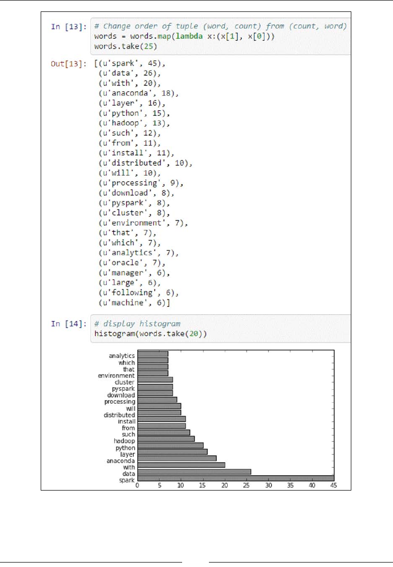
# Change order of tuple (word, count) from (count, word)
words = words.map(lambda x:(x[1], x[0]))
words.take(25)
# display histogram
histogram(words.take(25))
Here, we visualize the most frequent words by plotting them in a bar chart. We have
to rst swap the tuple from the original (count, word) to (word, count):
www.it-ebooks.info

Setting Up a Spark Virtual Environment
[ 22 ]
Virtualizing the environment with Vagrant
In order to create a portable Python and Spark environment that can be easily shared
and cloned, the development environment can be built with a vagrantfile.
We will point to the Massive Open Online Courses (MOOCs) delivered by Berkeley
University and Databricks:
• Introduction to Big Data with Apache Spark, Professor Anthony D. Joseph can
be found at https://www.edx.org/course/introduction-big-data-
apache-spark-uc-berkeleyx-cs100-1x
• Scalable Machine Learning, Professor Ameet Talwalkar can be found at https://
www.edx.org/course/scalable-machine-learning-uc-berkeleyx-
cs190-1x
The course labs were executed on IPython Notebooks powered by PySpark. They can
be found in the following GitHub repository: https://github.com/spark-mooc/
mooc-setup/.
Once you have set up Vagrant on your machine, follow these instructions to get
started: https://docs.vagrantup.com/v2/getting-started/index.html.
Clone the spark-mooc/mooc-setup/ github repository in your work directory
and launch the command $ vagrant up, within the cloned directory:
Be aware that the version of Spark may be outdated as the vagrantfile may not be
up-to-date.
You will see an output similar to this:
C:\Programs\spark\edx1001\mooc-setup-master>vagrant up
Bringing machine 'sparkvm' up with 'virtualbox' provider...
==> sparkvm: Checking if box 'sparkmooc/base' is up to date...
==> sparkvm: Clearing any previously set forwarded ports...
==> sparkvm: Clearing any previously set network interfaces...
==> sparkvm: Preparing network interfaces based on configuration...
sparkvm: Adapter 1: nat
==> sparkvm: Forwarding ports...
sparkvm: 8001 => 8001 (adapter 1)
sparkvm: 4040 => 4040 (adapter 1)
sparkvm: 22 => 2222 (adapter 1)
==> sparkvm: Booting VM...
==> sparkvm: Waiting for machine to boot. This may take a few minutes...
sparkvm: SSH address: 127.0.0.1:2222
sparkvm: SSH username: vagrant
sparkvm: SSH auth method: private key
www.it-ebooks.info

Chapter 1
[ 23 ]
sparkvm: Warning: Connection timeout. Retrying...
sparkvm: Warning: Remote connection disconnect. Retrying...
==> sparkvm: Machine booted and ready!
==> sparkvm: Checking for guest additions in VM...
==> sparkvm: Setting hostname...
==> sparkvm: Mounting shared folders...
sparkvm: /vagrant => C:/Programs/spark/edx1001/mooc-setup-master
==> sparkvm: Machine already provisioned. Run `vagrant provision` or use
the `--provision`
==> sparkvm: to force provisioning. Provisioners marked to run always
will still run.
C:\Programs\spark\edx1001\mooc-setup-master>
This will launch the IPython Notebooks powered by PySpark on localhost:8001:
www.it-ebooks.info

Setting Up a Spark Virtual Environment
[ 24 ]
Moving to the cloud
As we are dealing with distributed systems, an environment on a virtual machine
running on a single laptop is limited for exploration and learning. We can move to
the cloud in order to experience the power and scalability of the Spark distributed
framework.
Deploying apps in Amazon Web Services
Once we are ready to scale our apps, we can migrate our development environment
to Amazon Web Services (AWS).
How to run Spark on EC2 is clearly described in the following page:
https://spark.apache.org/docs/latest/ec2-scripts.html.
We emphasize ve key steps in setting up the AWS Spark environment:
1. Create an AWS EC2 key pair via the AWS console http://aws.amazon.com/
console/.
2. Export your key pair to your environment:
export AWS_ACCESS_KEY_ID=accesskeyid
export AWS_SECRET_ACCESS_KEY=secretaccesskey
3. Launch your cluster:
~$ cd $SPARK_HOME/ec2
ec2$ ./spark-ec2 -k <keypair> -i <key-file> -s <num-slaves> launch
<cluster-name>
4. SSH into a cluster to run Spark jobs:
ec2$ ./spark-ec2 -k <keypair> -i <key-file> login <cluster-name>
5. Destroy your cluster after usage:
ec2$ ./spark-ec2 destroy <cluster-name>
Virtualizing the environment with Docker
In order to create a portable Python and Spark environment that can be easily shared
and cloned, the development environment can be built in Docker containers.
We wish capitalize on Docker's two main functions:
• Creating isolated containers that can be easily deployed on different
operating systems or in the cloud.
www.it-ebooks.info

Chapter 1
[ 25 ]
• Allowing easy sharing of the development environment image with all its
dependencies using The DockerHub. The DockerHub is similar to GitHub.
It allows easy cloning and version control. The snapshot image of the
configured environment can be the baseline for further enhancements.
The following diagram illustrates a Docker-enabled environment with Spark,
Anaconda, and the database server and their respective data volumes.
Docker offers the ability to clone and deploy an environment from the Dockerle.
You can nd an example Dockerle with a PySpark and Anaconda setup at the
following address: https://hub.docker.com/r/thisgokeboysef/pyspark-
docker/~/dockerfile/.
www.it-ebooks.info

Setting Up a Spark Virtual Environment
[ 26 ]
Install Docker as per the instructions provided at the following links:
• http://docs.docker.com/mac/started/ if you are on Mac OS X
• http://docs.docker.com/linux/started/ if you are on Linux
• http://docs.docker.com/windows/started/ if you are on Windows
Install the docker container with the Dockerle provided earlier with the
following command:
$ docker pull thisgokeboysef/pyspark-docker
Other great sources of information on how to dockerize your environment can be seen
at Lab41. The GitHub repository contains the necessary code:
https://github.com/Lab41/ipython-spark-docker
The supporting blog post is rich in information on thought processes involved in
building the docker environment: http://lab41.github.io/blog/2015/04/13/
ipython-on-spark-on-docker/.
Summary
We set the context of building data-intensive apps by describing the overall
architecture structured around the infrastructure, persistence, integration, analytics,
and engagement layers. We also discussed Spark and Anaconda with their respective
building blocks. We set up an environment in a VirtualBox with Anaconda and
Spark and demonstrated a word count app using the text content of the rst chapter
as input.
In the next chapter, we will delve more deeply into the architecture blueprint for
data-intensive apps and tap into the Twitter, GitHub, and Meetup APIs to get a feel
of the data we will be mining with Spark.
www.it-ebooks.info

[ 27 ]
Building Batch and Streaming
Apps with Spark
The objective of the book is to teach you about PySpark and the PyData libraries
by building an app that analyzes the Spark community's interactions on social
networks. We will gather information on Apache Spark from GitHub, check the
relevant tweets on Twitter, and get a feel for the buzz around Spark in the broader
open source software communities using Meetup.
In this chapter, we will outline the various sources of data and information. We will
get an understanding of their structure. We will outline the data processing pipeline,
from collection to batch and streaming processing.
In this section, we will cover the following points:
• Outline data processing pipelines from collection to batch and stream
processing, effectively depicting the architecture of the app we are planning
to build.
• Check out the various data sources (GitHub, Twitter, and Meetup), their data
structure (JSON, structured information, unstructured text, geo-location,
time series data, and so on), and their complexities. We also discuss the tools
to connect to three different APIs, so you can build your own data mashups.
The book will focus on Twitter in the following chapters.
www.it-ebooks.info

Building Batch and Streaming Apps with Spark
[ 28 ]
Architecting data-intensive apps
We dened the data-intensive app framework architecture blueprint in the previous
chapter. Let's put back in context the various software components we are going
to use throughout the book in our original framework. Here's an illustration of
the various components of software mapped in the data-intensive architecture
framework:
Spark is an extremely efcient, distributed computing framework. In order to exploit
its full power, we need to architect our solution accordingly. For performance
reasons, the overall solution needs to also be aware of its usage in terms of CPU,
storage, and network.
www.it-ebooks.info

Chapter 2
[ 29 ]
These imperatives drive the architecture of our solution:
• Latency: This architecture combines slow and fast processing. Slow
processing is done on historical data in batch mode. This is also called data
at rest. This phase builds precomputed models and data patterns that will
be used by the fast processing arm once live continuous data is fed into the
system. Fast processing of data or real-time analysis of streaming data refers
to data in motion. Data at rest is essentially processing data in batch mode
with a longer latency. Data in motion refers to the streaming computation of
data ingested in real time.
• Scalability: Spark is natively linearly scalable through its distributed in-
memory computing framework. Databases and data stores interacting with
Spark need to be also able to scale linearly as data volume grows.
• Fault tolerance: When a failure occurs due to hardware, software, or network
reasons, the architecture should be resilient enough and provide availability
at all times.
• Flexibility: The data pipelines put in place in this architecture can be adapted
and retrofitted very quickly depending on the use case.
Spark is unique as it allows batch processing and streaming analytics on the same
unied platform.
We will consider two data processing pipelines:
• The first one handles data at rest and is focused on putting together the
pipeline for batch analysis of the data
• The second one, data in motion, targets real-time data ingestion and
delivering insights based on precomputed models and data patterns
Processing data at rest
Let's get an understanding of the data at rest or batch processing pipeline. The
objective in this pipeline is to ingest the various datasets from Twitter, GitHub, and
Meetup; prepare the data for Spark MLlib, the machine learning engine; and derive
the base models that will be applied for insight generation in batch mode or in
real time.
www.it-ebooks.info

Building Batch and Streaming Apps with Spark
[ 30 ]
The following diagram illustrates the data pipeline in order to enable processing data
at rest:
Processing data in motion
Processing data in motion introduces a new level of complexity, as we are
introducing a new possibility of failure. If we want to scale, we need to consider
bringing in distributed message queue systems such as Kafka. We will dedicate a
subsequent chapter to understanding streaming analytics.
The following diagram depicts a data pipeline for processing data in motion:
www.it-ebooks.info

Chapter 2
[ 31 ]
Exploring data interactively
Building a data-intensive app is not as straightforward as exposing a database
to a web interface. During the setup of both the data at rest and data in motion
processing, we will capitalize on Spark's ability to analyse data interactively and
rene the data richness and quality required for the machine learning and streaming
activities. Here, we will go through an iterative cycle of data collection, renement,
and investigation in order to get to the dataset of interest for our apps.
Connecting to social networks
Let's delve into the rst steps of the data-intensive app architecture's integration
layer. We are going to focus on harvesting the data, ensuring its integrity and
preparing for batch and streaming data processing by Spark at the next stage. This
phase is described in the ve process steps: connect, correct, collect, compose, and
consume. These are iterative steps of data exploration that will get us acquainted with
the data and help us rene the data structure for further processing.
The following diagram depicts the iterative process of data acquisition and
renement for consumption:
We connect to the social networks of interest: Twitter, GitHub, and Meetup. We
will discuss the mode of access to the APIs (short for Application Programming
Interface) and how to create a RESTful connection with those services while
respecting the rate limitation imposed by the social networks. REST (short for
Representation State Transfer) is the most widely adopted architectural style on the
Internet in order to enable scalable web services. It relies on exchanging messages
predominantly in JSON (short for JavaScript Object Notation). RESTful APIs and
web services implement the four most prevalent verbs GET, PUT, POST, and DELETE.
GET is used to retrieve an element or a collection from a given URI. PUT updates a
collection with a new one. POST allows the creation of a new entry, while DELETE
eliminates a collection.
www.it-ebooks.info

Building Batch and Streaming Apps with Spark
[ 32 ]
Getting Twitter data
Twitter allows access to registered users to its search and streaming tweet services
under an authorization protocol called OAuth that allows API applications to
securely act on a user's behalf. In order to create the connection, the rst step is to
create an application with Twitter at https://apps.twitter.com/app/new.
Once the application has been created, Twitter will issue the four codes that will
allow it to tap into the Twitter hose:
CONSUMER_KEY = 'GetYourKey@Twitter'
CONSUMER_SECRET = ' GetYourKey@Twitter'
OAUTH_TOKEN = ' GetYourToken@Twitter'
OAUTH_TOKEN_SECRET = ' GetYourToken@Twitter'
www.it-ebooks.info

Chapter 2
[ 33 ]
If you wish to get a feel for the various RESTful queries offered, you can explore
the Twitter API on the dev console at https://dev.twitter.com/rest/tools/
console:
We will make a programmatic connection on Twitter using the following code,
which will activate our OAuth access and allows us to tap into the Twitter API
under the rate limitation. In the streaming mode, the limitation is for a GET request.
www.it-ebooks.info

Building Batch and Streaming Apps with Spark
[ 34 ]
Getting GitHub data
GitHub uses a similar authentication process to Twitter. Head to the developer
site and retrieve your credentials after duly registering with GitHub at
https://developer.github.com/v3/:
Getting Meetup data
Meetup can be accessed using the token issued in the developer resources to
members of Meetup.com. The necessary token or OAuth credential for Meetup API
access can be obtained on their developer's website at https://secure.meetup.
com/meetup_api:
www.it-ebooks.info

Chapter 2
[ 35 ]
Analyzing the data
Let's get a rst feel for the data extracted from each of the social networks and get an
understanding of the data structure from each these sources.
Discovering the anatomy of tweets
In this section, we are going to establish connection with the Twitter API. Twitter
offers two connection modes: the REST API, which allows us to search historical
tweets for a given search term or hashtag, and the streaming API, which delivers
real-time tweets under the rate limit in place.
www.it-ebooks.info

Building Batch and Streaming Apps with Spark
[ 36 ]
In order to get a better understanding of how to operate with the Twitter API, we
will go through the following steps:
1. Install the Twitter Python library.
2. Establish a connection programmatically via OAuth, the authentication
required for Twitter.
3. Search for recent tweets for the query Apache Spark and explore the results
obtained.
4. Decide on the key attributes of interest and retrieve the information from the
JSON output.
Let's go through it step-by-step:
1. Install the Python Twitter library. In order to install it, you need to write pip
install twitter from the command line:
$ pip install twitter
2. Create the Python Twitter API class and its base methods for authentication,
searching, and parsing the results. self.auth gets the credentials from
Twitter. It then creates a registered API as self.api. We have implemented
two methods: the rst one to search Twitter with a given query and the
second one to parse the output to retrieve relevant information such as the
tweet ID, the tweet text, and the tweet author. The code is as follows:
import twitter
import urlparse
from pprint import pprint as pp
class TwitterAPI(object):
"""
TwitterAPI class allows the Connection to Twitter via OAuth
once you have registered with Twitter and receive the
necessary credentiials
"""
# initialize and get the twitter credentials
def __init__(self):
consumer_key = 'Provide your credentials'
consumer_secret = 'Provide your credentials'
access_token = 'Provide your credentials'
access_secret = 'Provide your credentials'
self.consumer_key = consumer_key
self.consumer_secret = consumer_secret
www.it-ebooks.info

Chapter 2
[ 37 ]
self.access_token = access_token
self.access_secret = access_secret
#
# authenticate credentials with Twitter using OAuth
self.auth = twitter.oauth.OAuth(access_token, access_
secret, consumer_key, consumer_secret)
# creates registered Twitter API
self.api = twitter.Twitter(auth=self.auth)
#
# search Twitter with query q (i.e. "ApacheSpark") and max. result
def searchTwitter(self, q, max_res=10,**kwargs):
search_results = self.api.search.tweets(q=q, count=10,
**kwargs)
statuses = search_results['statuses']
max_results = min(1000, max_res)
for _ in range(10):
try:
next_results = search_results['search_metadata']
['next_results']
except KeyError as e:
break
next_results = urlparse.parse_qsl(next_results[1:])
kwargs = dict(next_results)
search_results = self.api.search.tweets(**kwargs)
statuses += search_results['statuses']
if len(statuses) > max_results:
break
return statuses
#
# parse tweets as it is collected to extract id, creation
# date, user id, tweet text
def parseTweets(self, statuses):
return [ (status['id'],
status['created_at'],
status['user']['id'],
status['user']['name'],
status['text'], url['expanded_url'])
for status in statuses
for url in status['entities']['urls']
]
www.it-ebooks.info

Building Batch and Streaming Apps with Spark
[ 38 ]
3. Instantiate the class with the required authentication:
t= TwitterAPI()
4. Run a search on the query term Apache Spark:
q="ApacheSpark"
tsearch = t.searchTwitter(q)
5. Analyze the JSON output:
pp(tsearch[1])
{u'contributors': None,
u'coordinates': None,
u'created_at': u'Sat Apr 25 14:50:57 +0000 2015',
u'entities': {u'hashtags': [{u'indices': [74, 86], u'text':
u'sparksummit'}],
u'media': [{u'display_url': u'pic.twitter.com/
WKUMRXxIWZ',
u'expanded_url': u'http://twitter.com/
bigdata/status/591976255831969792/photo/1',
u'id': 591976255156715520,
u'id_str': u'591976255156715520',
u'indices': [143, 144],
u'media_url':
...(snip)...
u'text': u'RT @bigdata: Enjoyed catching up with @ApacheSpark
users & leaders at #sparksummit NYC: video clips are out
http://t.co/qrqpP6cG9s http://t\u2026',
u'truncated': False,
u'user': {u'contributors_enabled': False,
u'created_at': u'Sat Apr 04 14:44:31 +0000 2015',
u'default_profile': True,
u'default_profile_image': True,
u'description': u'',
u'entities': {u'description': {u'urls': []}},
u'favourites_count': 0,
u'follow_request_sent': False,
u'followers_count': 586,
u'following': False,
u'friends_count': 2,
u'geo_enabled': False,
u'id': 3139047660,
u'id_str': u'3139047660',
u'is_translation_enabled': False,
u'is_translator': False,
www.it-ebooks.info

Chapter 2
[ 39 ]
u'lang': u'zh-cn',
u'listed_count': 749,
u'location': u'',
u'name': u'Mega Data Mama',
u'notifications': False,
u'profile_background_color': u'C0DEED',
u'profile_background_image_url': u'http://abs.twimg.
com/images/themes/theme1/bg.png',
u'profile_background_image_url_https': u'https://abs.
twimg.com/images/themes/theme1/bg.png',
...(snip)...
u'screen_name': u'MegaDataMama',
u'statuses_count': 26673,
u'time_zone': None,
u'url': None,
u'utc_offset': None,
u'verified': False}}
6. Parse the Twitter output to retrieve key information of interest:
tparsed = t.parseTweets(tsearch)
pp(tparsed)
[(591980327784046592,
u'Sat Apr 25 15:01:23 +0000 2015',
63407360,
u'Jos\xe9 Carlos Baquero',
u'Big Data systems are making a difference in the fight against
cancer. #BigData #ApacheSpark http://t.co/pnOLmsKdL9',
u'http://tmblr.co/ZqTggs1jHytN0'),
(591977704464875520,
u'Sat Apr 25 14:50:57 +0000 2015',
3139047660,
u'Mega Data Mama',
u'RT @bigdata: Enjoyed catching up with @ApacheSpark users &
leaders at #sparksummit NYC: video clips are out http://t.co/
qrqpP6cG9s http://t\u2026',
u'http://goo.gl/eF5xwK'),
(591977172589539328,
u'Sat Apr 25 14:48:51 +0000 2015',
2997608763,
u'Emma Clark',
u'RT @bigdata: Enjoyed catching up with @ApacheSpark users &
leaders at #sparksummit NYC: video clips are out http://t.co/
qrqpP6cG9s http://t\u2026',
u'http://goo.gl/eF5xwK'),
www.it-ebooks.info

Building Batch and Streaming Apps with Spark
[ 40 ]
... (snip)...
(591879098349268992,
u'Sat Apr 25 08:19:08 +0000 2015',
331263208,
u'Mario Molina',
u'#ApacheSpark speeds up big data decision-making http://t.
co/8hdEXreNfN',
u'http://www.computerweekly.com/feature/Apache-Spark-speeds-up-
big-data-decision-making')]
Exploring the GitHub world
In order to get a better understanding on how to operate with the GitHub API, we
will go through the following steps:
1. Install the GitHub Python library.
2. Access the API by using the token provided when we registered in the
developer website.
3. Retrieve some key facts on the Apache foundation that is hosting the
spark repository.
Let's go through the process step-by-step:
1. Install the Python PyGithub library. In order to install it, you need to pip
install PyGithub from the command line:
pip install PyGithub
2. Programmatically create a client to instantiate the GitHub API:
from github import Github
# Get your own access token
ACCESS_TOKEN = 'Get_Your_Own_Access_Token'
# We are focusing our attention to User = apache and Repo = spark
USER = 'apache'
REPO = 'spark'
g = Github(ACCESS_TOKEN, per_page=100)
user = g.get_user(USER)
repo = user.get_repo(REPO)
www.it-ebooks.info

Chapter 2
[ 41 ]
3. Retrieve key facts from the Apache User. There are 640 active Apache
repositories in GitHub:
repos_apache = [repo.name for repo in g.get_user('apache').get_
repos()]
len(repos_apache)
640
4. Retrieve key facts from the Spark repository, The programing languages
used in the Spark repo are given here under:
pp(repo.get_languages())
{u'C': 1493,
u'CSS': 4472,
u'Groff': 5379,
u'Java': 1054894,
u'JavaScript': 21569,
u'Makefile': 7771,
u'Python': 1091048,
u'R': 339201,
u'Scala': 10249122,
u'Shell': 172244}
5. Retrieve a few key participants of the wide Spark GitHub repository
network. There are 3,738 stargazers in the Apache Spark repository at the
time of writing. The network is immense. The rst stargazer is Matei Zaharia,
the cofounder of the Spark project when he was doing his PhD in Berkeley.
stargazers = [ s for s in repo.get_stargazers() ]
print "Number of stargazers", len(stargazers)
Number of stargazers 3738
[stargazers[i].login for i in range (0,20)]
[u'mateiz',
u'beyang',
u'abo',
u'CodingCat',
u'andy327',
u'CrazyJvm',
u'jyotiska',
u'BaiGang',
u'sundstei',
u'dianacarroll',
u'ybotco',
u'xelax',
www.it-ebooks.info

Building Batch and Streaming Apps with Spark
[ 42 ]
u'prabeesh',
u'invkrh',
u'bedla',
u'nadesai',
u'pcpratts',
u'narkisr',
u'Honghe',
u'Jacke']
Understanding the community through
Meetup
In order to get a better understanding of how to operate with the Meetup API,
we will go through the following steps:
1. Create a Python program to call the Meetup API using an
authentication token.
2. Retrieve information of past events for meetup groups such as
London Data Science.
3. Retrieve the prole of the meetup members in order to analyze their
participation in similar meetup groups.
Let's go through the process step-by-step:
1. As there is no reliable Meetup API Python library, we will programmatically
create a client to instantiate the Meetup API:
import json
import mimeparse
import requests
import urllib
from pprint import pprint as pp
MEETUP_API_HOST = 'https://api.meetup.com'
EVENTS_URL = MEETUP_API_HOST + '/2/events.json'
MEMBERS_URL = MEETUP_API_HOST + '/2/members.json'
GROUPS_URL = MEETUP_API_HOST + '/2/groups.json'
RSVPS_URL = MEETUP_API_HOST + '/2/rsvps.json'
PHOTOS_URL = MEETUP_API_HOST + '/2/photos.json'
GROUP_URLNAME = 'London-Machine-Learning-Meetup'
# GROUP_URLNAME = 'London-Machine-Learning-Meetup' # 'Data-
Science-London'
www.it-ebooks.info

Chapter 2
[ 43 ]
class Mee
tupAPI(object):
"""
Retrieves information about meetup.com
"""
def __init__(self, api_key, num_past_events=10, http_
timeout=1,
http_retries=2):
"""
Create a new instance of MeetupAPI
"""
self._api_key = api_key
self._http_timeout = http_timeout
self._http_retries = http_retries
self._num_past_events = num_past_events
def get_past_events(self):
"""
Get past meetup events for a given meetup group
"""
params = {'key': self._api_key,
'group_urlname': GROUP_URLNAME,
'status': 'past',
'desc': 'true'}
if self._num_past_events:
params['page'] = str(self._num_past_events)
query = urllib.urlencode(params)
url = '{0}?{1}'.format(EVENTS_URL, query)
response = requests.get(url, timeout=self._http_timeout)
data = response.json()['results']
return data
def get_members(self):
"""
Get meetup members for a given meetup group
"""
params = {'key': self._api_key,
'group_urlname': GROUP_URLNAME,
'offset': '0',
'format': 'json',
'page': '100',
'order': 'name'}
query = urllib.urlencode(params)
www.it-ebooks.info

Building Batch and Streaming Apps with Spark
[ 44 ]
url = '{0}?{1}'.format(MEMBERS_URL, query)
response = requests.get(url, timeout=self._http_timeout)
data = response.json()['results']
return data
def get_groups_by_member(self, member_id='38680722'):
"""
Get meetup groups for a given meetup member
"""
params = {'key': self._api_key,
'member_id': member_id,
'offset': '0',
'format': 'json',
'page': '100',
'order': 'id'}
query = urllib.urlencode(params)
url = '{0}?{1}'.format(GROUPS_URL, query)
response = requests.get(url, timeout=self._http_timeout)
data = response.json()['results']
return data
2. Then, we will retrieve past events from a given Meetup group:
m = MeetupAPI(api_key='Get_Your_Own_Key')
last_meetups = m.get_past_events()
pp(last_meetups[5])
{u'created': 1401809093000,
u'description': u"<p>We are hosting a joint meetup between Spark
London and Machine Learning London. Given the excitement in the
machine learning community around Spark at the moment a joint
meetup is in order!</p> <p>Michael Armbrust from the Apache Spark
core team will be flying over from the States to give us a talk in
person.\xa0Thanks to our sponsors, Cloudera, MapR and Databricks
for helping make this happen.</p> <p>The first part of the talk
will be about MLlib, the machine learning library for Spark,\
xa0and the second part, on\xa0Spark SQL.</p> <p>Don't sign up if
you have already signed up on the Spark London page though!</p>
<p>\n\n\nAbstract for part one:</p> <p>In this talk, we\u2019ll
introduce Spark and show how to use it to build fast, end-to-end
machine learning workflows. Using Spark\u2019s high-level API, we
can process raw data with familiar libraries in Java, Scala or
Python (e.g. NumPy) to extract the features for machine learning.
Then, using MLlib, its built-in machine learning library, we can
run scalable versions of popular algorithms. We\u2019ll also cover
upcoming development work including new built-in algorithms and
R bindings.</p> <p>\n\n\n\nAbstract for part two:\xa0</p> <p>In
www.it-ebooks.info

Chapter 2
[ 45 ]
this talk, we'll examine Spark SQL, a new Alpha component that is
part of the Apache Spark 1.0 release. Spark SQL lets developers
natively query data stored in both existing RDDs and external
sources such as Apache Hive. A key feature of Spark SQL is the
ability to blur the lines between relational tables and RDDs,
making it easy for developers to intermix SQL commands that query
external data with complex analytics. In addition to Spark SQL,
we'll explore the Catalyst optimizer framework, which allows
Spark SQL to automatically rewrite query plans to execute more
efficiently.</p>",
u'event_url': u'http://www.meetup.com/London-Machine-Learning-
Meetup/events/186883262/',
u'group': {u'created': 1322826414000,
u'group_lat': 51.52000045776367,
u'group_lon': -0.18000000715255737,
u'id': 2894492,
u'join_mode': u'open',
u'name': u'London Machine Learning Meetup',
u'urlname': u'London-Machine-Learning-Meetup',
u'who': u'Machine Learning Enthusiasts'},
u'headcount': 0,
u'id': u'186883262',
u'maybe_rsvp_count': 0,
u'name': u'Joint Spark London and Machine Learning Meetup',
u'rating': {u'average': 4.800000190734863, u'count': 5},
u'rsvp_limit': 70,
u'status': u'past',
u'time': 1403200800000,
u'updated': 1403450844000,
u'utc_offset': 3600000,
u'venue': {u'address_1': u'12 Errol St, London',
u'city': u'EC1Y 8LX',
u'country': u'gb',
u'id': 19504802,
u'lat': 51.522533,
u'lon': -0.090934,
u'name': u'Royal Statistical Society',
u'repinned': False},
u'visibility': u'public',
u'waitlist_count': 84,
u'yes_rsvp_count': 70}
www.it-ebooks.info

Building Batch and Streaming Apps with Spark
[ 46 ]
3. Get information about the Meetup members:
members = m.get_members()
{u'city': u'London',
u'country': u'gb',
u'hometown': u'London',
u'id': 11337881,
u'joined': 1421418896000,
u'lat': 51.53,
u'link': u'http://www.meetup.com/members/11337881',
u'lon': -0.09,
u'name': u'Abhishek Shivkumar',
u'other_services': {u'twitter': {u'identifier': u'@
abhisemweb'}},
u'photo': {u'highres_link': u'http://photos3.meetupstatic.com/
photos/member/9/6/f/3/highres_10898643.jpeg',
u'photo_id': 10898643,
u'photo_link': u'http://photos3.meetupstatic.com/
photos/member/9/6/f/3/member_10898643.jpeg',
u'thumb_link': u'http://photos3.meetupstatic.com/
photos/member/9/6/f/3/thumb_10898643.jpeg'},
u'self': {u'common': {}},
u'state': u'17',
u'status': u'active',
u'topics': [{u'id': 1372, u'name': u'Semantic Web', u'urlkey':
u'semweb'},
{u'id': 1512, u'name': u'XML', u'urlkey': u'xml'},
{u'id': 49585,
u'name': u'Semantic Social Networks',
u'urlkey': u'semantic-social-networks'},
{u'id': 24553,
u'name': u'Natural Language Processing',
...(snip)...
u'name': u'Android Development',
u'urlkey': u'android-developers'}],
u'visited': 1429281599000}
www.it-ebooks.info

Chapter 2
[ 47 ]
Previewing our app
Our challenge is to make sense of the data retrieved from these social networks,
nding the key relationships and deriving insights. Some of the elements of interest
are as follows:
• Visualizing the top influencers: Discover the top influencers in
the community:
°Heavy Twitter users on Apache Spark
°Committers in GitHub
°Leading Meetup presentations
• Understanding the Network: Network graph of GitHub committers,
watchers, and stargazers
• Identifying the Hot Locations: Locating the most active location for Spark
The following screenshot provides a preview of our app:
www.it-ebooks.info

Building Batch and Streaming Apps with Spark
[ 48 ]
Summary
In this chapter, we laid out the overall architecture of our app. We explained the
two main paradigms of processing data: batch processing, also called data at rest,
and streaming analytics, referred to as data in motion. We proceeded to establish
connections to three social networks of interest: Twitter, GitHub, and Meetup.
We sampled the data and provided a preview of what we are aiming to build. The
remainder of the book will focus on the Twitter dataset. We provided here the tools
and API to access three social networks, so you can at a later stage create your own
data mashups. We are now ready to investigate the data collected, which will be the
topic of the next chapter.
In the next chapter, we will delve deeper into data analysis, extracting the key
attributes of interest for our purposes and managing the storage of the information
for batch and stream processing.
www.it-ebooks.info

[ 49 ]
Juggling Data with Spark
As per the batch and streaming architecture laid out in the previous chapter, we
need data to fuel our applications. We will harvest data focused on Apache Spark
from Twitter. The objective of this chapter is to prepare data to be further used by
the machine learning and streaming applications. This chapter focuses on how
to exchange code and data across the distributed network. We will get practical
insights into serialization, persistence, marshaling, and caching. We will get to
grips with on Spark SQL, the key Spark module to interactively explore structured
and semi-structured data. The fundamental data structure powering Spark SQL
is the Spark dataframe. The Spark dataframe is inspired by the Python Pandas
dataframe and the R dataframe. It is a powerful data structure, well understood
and appreciated by data scientists with a background in R or Python.
In this chapter, we will cover the following points:
• Connect to Twitter, collect the relevant data, and then persist it in various
formats such as JSON and CSV and data stores such as MongoDB
• Analyze the data using Blaze and Odo, a spin-off library from Blaze, in order
to connect and transfer data from various sources and destinations
• Introduce Spark dataframes as the foundation for data interchange between
the various Spark modules and explore data interactively using Spark SQL
www.it-ebooks.info

Juggling Data with Spark
[ 50 ]
Revisiting the data-intensive app
architecture
Let's rst put in context the focus of this chapter with respect to the data-intensive
app architecture. We will concentrate our attention on the integration layer and
essentially run through iterative cycles of the acquisition, renement, and persistence
of the data. This cycle was termed the ve Cs. The ve Cs stand for connect, collect,
correct, compose, and consume. They are the essential processes we run through in the
integration layer in order to get to the right quality and quantity of data retrieved
from Twitter. We will also delve deeper in the persistence layer and set up a data
store such as MongoDB to collect our data for processing later.
We will explore the data with Blaze, a Python library for data manipulation, and
Spark SQL, the interactive module of Spark for data discovery powered by the Spark
dataframe. The dataframe paradigm is shared by Python Pandas, Python Blaze, and
Spark SQL. We will get a feel for the nuances of the three dataframe avors.
The following diagram sets the context of the chapter's focus, highlighting the
integration layer and the persistence layer:
www.it-ebooks.info

Chapter 3
[ 51 ]
Serializing and deserializing data
As we are harvesting data from web APIs under rate limit constraints, we need to
store them. As the data is processed on a distributed cluster, we need consistent
ways to save state and retrieve it for later usage.
Let's now dene serialization, persistence, marshaling, and caching or memorization.
Serializing a Python object converts it into a stream of bytes. The Python object needs
to be retrieved beyond the scope of its existence, when the program is shut. The
serialized Python object can be transferred over a network or stored in a persistent
storage. Deserialization is the opposite and converts the stream of bytes into the
original Python object so the program can carry on from the saved state. The most
popular serialization library in Python is Pickle. As a matter of fact, the PySpark
commands are transferred over the wire to the worker nodes via pickled data.
Persistence saves a program's state data to disk or memory so that it can carry on
where it left off upon restart. It saves a Python object from memory to a le or a
database and loads it later with the same state.
Marshalling sends Python code or data over a network TCP connection in a
multicore or distributed system.
Caching converts a Python object to a string in memory so that it can be used
as a dictionary key later on. Spark supports pulling a dataset into a cluster-wide,
in-memory cache. This is very useful when data is accessed repeatedly such as
when querying a small reference dataset or running an iterative algorithm such
as Google PageRank.
Caching is a crucial concept for Spark as it allows us to save RDDs in memory or
with a spillage to disk. The caching strategy can be selected based on the lineage of
the data or the DAG (short for Directed Acyclic Graph) of transformations applied
to the RDDs in order to minimize shufe or cross network heavy data exchange. In
order to achieve good performance with Spark, beware of data shufing. A good
partitioning policy and use of RDD caching, coupled with avoiding unnecessary
action operations, leads to better performance with Spark.
Harvesting and storing data
Before delving into database persistent storage such as MongoDB, we will look at
some useful le storages that are widely used: CSV (short for comma-separated
values) and JSON (short for JavaScript Object Notation) le storage. The enduring
popularity of these two le formats lies in a few key reasons: they are human
readable, simple, relatively lightweight, and easy to use.
www.it-ebooks.info

Juggling Data with Spark
[ 52 ]
Persisting data in CSV
The CSV format is lightweight, human readable, and easy to use. It has delimited
text columns with an inherent tabular schema.
Python offers a robust csv library that can serialize a csv le into a Python
dictionary. For the purpose of our program, we have written a python class
that manages to persist data in CSV format and read from a given CSV.
Let's run through the code of the class IO_csv object. The __init__ section of the
class basically instantiates the le path, the lename, and the le sufx (in this case,
.csv):
class IO_csv(object):
def __init__(self, filepath, filename, filesuffix='csv'):
self.filepath = filepath # /path/to/file without the /'
at the end
self.filename = filename # FILE_NAME
self.filesuffix = filesuffix
The save method of the class uses a Python named tuple and the header elds of
the csv le in order to impart a schema while persisting the rows of the CSV. If the
csv le already exists, it will be appended and not overwritten otherwise; it will
be created:
def save(self, data, NTname, fields):
# NTname = Name of the NamedTuple
# fields = header of CSV - list of the fields name
NTuple = namedtuple(NTname, fields)
if os.path.isfile('{0}/{1}.{2}'.format(self.filepath, self.
filename, self.filesuffix)):
# Append existing file
with open('{0}/{1}.{2}'.format(self.filepath, self.
filename, self.filesuffix), 'ab') as f:
writer = csv.writer(f)
# writer.writerow(fields) # fields = header of CSV
writer.writerows([row for row in map(NTuple._make,
data)])
# list comprehension using map on the NamedTuple._
make() iterable and the data file to be saved
# Notice writer.writerows and not writer.writerow
(i.e. list of multiple rows sent to csv file
else:
# Create new file
www.it-ebooks.info

Chapter 3
[ 53 ]
with open('{0}/{1}.{2}'.format(self.filepath, self.
filename, self.filesuffix), 'wb') as f:
writer = csv.writer(f)
writer.writerow(fields) # fields = header of CSV -
list of the fields name
writer.writerows([row for row in map(NTuple._make,
data)])
# list comprehension using map on the NamedTuple._
make() iterable and the data file to be saved
# Notice writer.writerows and not writer.writerow
(i.e. list of multiple rows sent to csv file
The load method of the class also uses a Python named tuple and the header elds
of the csv le in order to retrieve the data using a consistent schema. The load
method is a memory-efcient generator to avoid loading a huge le in memory:
hence we use yield in place of return:
def load(self, NTname, fields):
# NTname = Name of the NamedTuple
# fields = header of CSV - list of the fields name
NTuple = namedtuple(NTname, fields)
with open('{0}/{1}.{2}'.format(self.filepath, self.filename,
self.filesuffix),'rU') as f:
reader = csv.reader(f)
for row in map(NTuple._make, reader):
# Using map on the NamedTuple._make() iterable and the
reader file to be loaded
yield row
Here's the named tuple. We are using it to parse the tweet in order to save or retrieve
them to and from the csv le:
fields01 = ['id', 'created_at', 'user_id', 'user_name', 'tweet_text',
'url']
Tweet01 = namedtuple('Tweet01',fields01)
def parse_tweet(data):
"""
Parse a ``tweet`` from the given response data.
"""
return Tweet01(
id=data.get('id', None),
created_at=data.get('created_at', None),
user_id=data.get('user_id', None),
user_name=data.get('user_name', None),
tweet_text=data.get('tweet_text', None),
url=data.get('url')
)
www.it-ebooks.info

Juggling Data with Spark
[ 54 ]
Persisting data in JSON
JSON is one of the most popular data formats for Internet-based applications. All the
APIs we are dealing with, Twitter, GitHub, and Meetup, deliver their data in JSON
format. The JSON format is relatively lightweight compared to XML and human
readable, and the schema is embedded in JSON. As opposed to the CSV format,
where all records follow exactly the same tabular structure, JSON records can vary
in their structure. JSON is semi-structured. A JSON record can be mapped into a
Python dictionary of dictionaries.
Let's run through the code of the class IO_json object. The __init__ section of the
class basically instantiates the le path, the lename, and the le sufx (in this case,
.json):
class IO_json(object):
def __init__(self, filepath, filename, filesuffix='json'):
self.filepath = filepath # /path/to/file without the /'
at the end
self.filename = filename # FILE_NAME
self.filesuffix = filesuffix
# self.file_io = os.path.join(dir_name, .'.join((base_
filename, filename_suffix)))
The save method of the class uses utf-8 encoding in order to ensure read and write
compatibility of the data. If the JSON le already exists, it will be appended and not
overwritten; otherwise it will be created:
def save(self, data):
if os.path.isfile('{0}/{1}.{2}'.format(self.filepath, self.
filename, self.filesuffix)):
# Append existing file
with io.open('{0}/{1}.{2}'.format(self.filepath, self.
filename, self.filesuffix), 'a', encoding='utf-8') as f:
f.write(unicode(json.dumps(data, ensure_ascii=
False))) # In python 3, there is no "unicode" function
# f.write(json.dumps(data, ensure_ascii= False)) #
create a \" escape char for " in the saved file
else:
# Create new file
with io.open('{0}/{1}.{2}'.format(self.filepath, self.
filename, self.filesuffix), 'w', encoding='utf-8') as f:
f.write(unicode(json.dumps(data, ensure_ascii=
False)))
# f.write(json.dumps(data, ensure_ascii= False))
www.it-ebooks.info

Chapter 3
[ 55 ]
The load method of the class just returns the le that has been read. A further json.
loads function needs to be applied in order to retrieve the json out of the le read:
def load(self):
with io.open('{0}/{1}.{2}'.format(self.filepath, self.
filename, self.filesuffix), encoding='utf-8') as f:
return f.read()
Setting up MongoDB
It is crucial to store the information harvested. Thus, we set up MongoDB as our
main document data store. As all the information collected is in JSON format and
MongoDB stores information in BSON (short for Binary JSON), it is therefore a
natural choice.
We will run through the following steps now:
• Installing the MongoDB server and client
• Running the MongoDB server
• Running the Mongo client
• Installing the PyMongo driver
• Creating the Python Mongo client
Installing the MongoDB server and client
In order to install the MongoDB package, perform through the following steps:
1. Import the public key used by the package management system (in our
case, Ubuntu's apt). To import the MongoDB public key, we issue the
following command:
sudo apt-key adv --keyserver hkp://keyserver.ubuntu.com:80 --recv
7F0CEB10
2. Create a list le for MongoDB. To create the list le, we use the following
command:
echo "deb http://repo.mongodb.org/apt/ubuntu "$("lsb_release
-sc)"/ mongodb-org/3.0 multiverse" | sudo tee /etc/apt/sources.
list.d/mongodb-org-3.0.list
3. Update the local package database as sudo:
sudo apt-get update
www.it-ebooks.info

Juggling Data with Spark
[ 56 ]
4. Install the MongoDB packages. We install the latest stable version of
MongoDB with the following command:
sudo apt-get install -y mongodb-org
Running the MongoDB server
Let's start the MongoDB server:
1. To start MongoDB server, we issue the following command to start mongod:
sudo service mongodb start
2. To check whether mongod has started properly, we issue the command:
an@an-VB:/usr/bin$ ps -ef | grep mongo
mongodb 967 1 4 07:03 ? 00:02:02 /usr/bin/mongod
--config /etc/mongod.conf
an 3143 3085 0 07:45 pts/3 00:00:00 grep --color=auto
mongo
In this case, we see that mongodb is running in process 967.
3. The mongod server sends a message to the effect that it is waiting for
connection on port 27017. This is the default port for MongoDB.
It can be changed in the conguration le.
4. We can check the contents of the log le at /var/log/mongod/mongod.log:
an@an-VB:/var/lib/mongodb$ ls -lru
total 81936
drwxr-xr-x 2 mongodb nogroup 4096 Apr 25 11:19 _tmp
-rw-r--r-- 1 mongodb nogroup 69 Apr 25 11:19 storage.bson
-rwxr-xr-x 1 mongodb nogroup 5 Apr 25 11:19 mongod.lock
-rw------- 1 mongodb nogroup 16777216 Apr 25 11:19 local.ns
-rw------- 1 mongodb nogroup 67108864 Apr 25 11:19 local.0
drwxr-xr-x 2 mongodb nogroup 4096 Apr 25 11:19 journal
5. In order to stop the mongodb server, just issue the following command:
sudo service mongodb stop
www.it-ebooks.info

Chapter 3
[ 57 ]
Running the Mongo client
Running the Mongo client in the console is as easy as calling mongo, as highlighted in
the following command:
an@an-VB:/usr/bin$ mongo
MongoDB shell version: 3.0.2
connecting to: test
Server has startup warnings:
2015-05-30T07:03:49.387+0200 I CONTROL [initandlisten]
2015-05-30T07:03:49.388+0200 I CONTROL [initandlisten]
At the mongo client console prompt, we can see the databases with the
following commands:
> show dbs
local 0.078GB
test 0.078GB
We select the test database using use test:
> use test
switched to db test
We display the collections within the test database:
> show collections
restaurants
system.indexes
We check a sample record in the restaurant collection listed previously:
> db.restaurants.find()
{ "_id" : ObjectId("553b70055e82e7b824ae0e6f"), "address : { "building
: "1007", "coord" : [ -73.856077, 40.848447 ], "street : "Morris Park
Ave", "zipcode : "10462 }, "borough : "Bronx", "cuisine : "Bakery",
"grades : [ { "grade : "A", "score" : 2, "date" : ISODate("2014-
03-03T00:00:00Z") }, { "date" : ISODate("2013-09-11T00:00:00Z"),
"grade : "A", "score" : 6 }, { "score" : 10, "date" : ISODate("2013-
01-24T00:00:00Z"), "grade : "A }, { "date" : ISODate("2011-11-
23T00:00:00Z"), "grade : "A", "score" : 9 }, { "date" : ISODate("2011-
03-10T00:00:00Z"), "grade : "B", "score" : 14 } ], "name : "Morris
Park Bake Shop", "restaurant_id : "30075445" }
www.it-ebooks.info

Juggling Data with Spark
[ 58 ]
Installing the PyMongo driver
Installing the Python driver with anaconda is easy. Just run the following command
at the terminal:
conda install pymongo
Creating the Python client for MongoDB
We are creating a IO_mongo class that will be used in our harvesting and processing
programs to store the data collected and retrieved saved information. In order to
create the mongo client, we will import the MongoClient module from pymongo. We
connect to the mongodb server on localhost at port 27017. The command is as follows:
from pymongo import MongoClient as MCli
class IO_mongo(object):
conn={'host':'localhost', 'ip':'27017'}
We initialize our class with the client connection, the database (in this case, twtr_db),
and the collection (in this case, twtr_coll) to be accessed:
def __init__(self, db='twtr_db', coll='twtr_coll', **conn ):
# Connects to the MongoDB server
self.client = MCli(**conn)
self.db = self.client[db]
self.coll = self.db[coll]
The save method inserts new records in the preinitialized collection and database:
def save(self, data):
# Insert to collection in db
return self.coll.insert(data)
The load method allows the retrieval of specic records according to criteria and
projection. In the case of large amount of data, it returns a cursor:
def load(self, return_cursor=False, criteria=None,
projection=None):
if criteria is None:
criteria = {}
if projection is None:
cursor = self.coll.find(criteria)
else:
www.it-ebooks.info

Chapter 3
[ 59 ]
cursor = self.coll.find(criteria, projection)
# Return a cursor for large amounts of data
if return_cursor:
return cursor
else:
return [ item for item in cursor ]
Harvesting data from Twitter
Each social network poses its limitations and challenges. One of the main obstacles
for harvesting data is an imposed rate limit. While running repeated or long-running
connections between rates limit pauses, we have to be careful to avoid collecting
duplicate data.
We have redesigned our connection programs outlined in the previous chapter to
take care of the rate limits.
In this TwitterAPI class that connects and collects the tweets according to the search
query we specify, we have added the following:
• Logging capability using the Python logging library with the aim of
collecting any errors or warning in the case of program failure
• Persistence capability using MongoDB, with the IO_mongo class exposed
previously as well as JSON file using the IO_json class
• API rate limit and error management capability, so we can ensure more
resilient calls to Twitter without getting barred for tapping into the firehose
Let's go through the steps:
1. We initialize by instantiating the Twitter API with our credentials:
class TwitterAPI(object):
"""
TwitterAPI class allows the Connection to Twitter via OAuth
once you have registered with Twitter and receive the
necessary credentials
"""
def __init__(self):
consumer_key = 'get_your_credentials'
consumer_secret = get your_credentials'
access_token = 'get_your_credentials'
www.it-ebooks.info

Juggling Data with Spark
[ 60 ]
access_secret = 'get your_credentials'
self.consumer_key = consumer_key
self.consumer_secret = consumer_secret
self.access_token = access_token
self.access_secret = access_secret
self.retries = 3
self.auth = twitter.oauth.OAuth(access_token, access_
secret, consumer_key, consumer_secret)
self.api = twitter.Twitter(auth=self.auth)
2. We initialize the logger by providing the log level:
°logger.debug(debug message)
°logger.info(info message)
°logger.warn(warn message)
°logger.error(error message)
°logger.critical(critical message)
3. We set the log path and the message format:
# logger initialisation
appName = 'twt150530'
self.logger = logging.getLogger(appName)
#self.logger.setLevel(logging.DEBUG)
# create console handler and set level to debug
logPath = '/home/an/spark/spark-1.3.0-bin-hadoop2.4/
examples/AN_Spark/data'
fileName = appName
fileHandler = logging.FileHandler("{0}/{1}.log".
format(logPath, fileName))
formatter = logging.Formatter('%(asctime)s - %(name)s -
%(levelname)s - %(message)s')
fileHandler.setFormatter(formatter)
self.logger.addHandler(fileHandler)
self.logger.setLevel(logging.DEBUG)
4. We initialize the JSON le persistence instruction:
# Save to JSON file initialisation
jsonFpath = '/home/an/spark/spark-1.3.0-bin-hadoop2.4/
examples/AN_Spark/data'
jsonFname = 'twtr15053001'
self.jsonSaver = IO_json(jsonFpath, jsonFname)
www.it-ebooks.info

Chapter 3
[ 61 ]
5. We initialize the MongoDB database and collection for persistence:
# Save to MongoDB Intitialisation
self.mongoSaver = IO_mongo(db='twtr01_db', coll='twtr01_
coll')
6. The method searchTwitter launches the search according to the
query specied:
def searchTwitter(self, q, max_res=10,**kwargs):
search_results = self.api.search.tweets(q=q, count=10,
**kwargs)
statuses = search_results['statuses']
max_results = min(1000, max_res)
for _ in range(10):
try:
next_results = search_results['search_metadata']
['next_results']
# self.logger.info('info' in searchTwitter - next_
results:%s'% next_results[1:])
except KeyError as e:
self.logger.error('error' in searchTwitter: %s',
%(e))
break
# next_results = urlparse.parse_qsl(next_results[1:])
# python 2.7
next_results = urllib.parse.parse_qsl(next_
results[1:])
# self.logger.info('info' in searchTwitter - next_
results[max_id]:', next_results[0:])
kwargs = dict(next_results)
# self.logger.info('info' in searchTwitter - next_
results[max_id]:%s'% kwargs['max_id'])
search_results = self.api.search.tweets(**kwargs)
statuses += search_results['statuses']
self.saveTweets(search_results['statuses'])
if len(statuses) > max_results:
self.logger.info('info' in searchTwitter - got %i
tweets - max: %i' %(len(statuses), max_results))
break
return statuses
www.it-ebooks.info

Juggling Data with Spark
[ 62 ]
7. The saveTweets method actually saves the collected tweets in JSON and
in MongoDB:
def saveTweets(self, statuses):
# Saving to JSON File
self.jsonSaver.save(statuses)
# Saving to MongoDB
for s in statuses:
self.mongoSaver.save(s)
8. The parseTweets method allows us to extract the key tweet information
from the vast amount of information provided by the Twitter API:
def parseTweets(self, statuses):
return [ (status['id'],
status['created_at'],
status['user']['id'],
status['user']['name']
status['text''text'],
url['expanded_url'])
for status in statuses
for url in status['entities']['urls']
]
9. The getTweets method calls the searchTwitter method described
previously. The getTweets method ensures that API calls are made
reliably whilst respecting the imposed rate limit. The code is as follows:
def getTweets(self, q, max_res=10):
"""
Make a Twitter API call whilst managing rate limit and
errors.
"""
def handleError(e, wait_period=2, sleep_when_rate_
limited=True):
if wait_period > 3600: # Seconds
self.logger.error('Too many retries in getTweets:
%s', %(e))
raise e
if e.e.code == 401:
self.logger.error('error 401 * Not Authorised * in
getTweets: %s', %(e))
return None
elif e.e.code == 404:
self.logger.error('error 404 * Not Found * in
getTweets: %s', %(e))
www.it-ebooks.info

Chapter 3
[ 63 ]
return None
elif e.e.code == 429:
self.logger.error('error 429 * API Rate Limit
Exceeded * in getTweets: %s', %(e))
if sleep_when_rate_limited:
self.logger.error('error 429 * Retrying in 15
minutes * in getTweets: %s', %(e))
sys.stderr.flush()
time.sleep(60*15 + 5)
self.logger.info('error 429 * Retrying now *
in getTweets: %s', %(e))
return 2
else:
raise e # Caller must handle the rate limiting
issue
elif e.e.code in (500, 502, 503, 504):
self.logger.info('Encountered %i Error. Retrying
in %i seconds' % (e.e.code, wait_period))
time.sleep(wait_period)
wait_period *= 1.5
return wait_period
else:
self.logger.error('Exit - aborting - %s', %(e))
raise e
10. Here, we are calling the searchTwitter API with the relevant query based
on the parameters specied. If we encounter any error such as rate limitation
from the provider, this will be processed by the handleError method:
while True:
try:
self.searchTwitter( q, max_res=10)
except twitter.api.TwitterHTTPError as e:
error_count = 0
wait_period = handleError(e, wait_period)
if wait_period is None:
return
Exploring data using Blaze
Blaze is an open source Python library, primarily developed by Continuum.io,
leveraging Python Numpy arrays and Pandas dataframe. Blaze extends to
out-of-core computing, while Pandas and Numpy are single-core.
www.it-ebooks.info

Juggling Data with Spark
[ 64 ]
Blaze offers an adaptable, unied, and consistent user interface across various
backends. Blaze orchestrates the following:
• Data: Seamless exchange of data across storages such as CSV, JSON, HDF5,
HDFS, and Bcolz files.
• Computation: Using the same query processing against computational
backends such as Spark, MongoDB, Pandas, or SQL Alchemy.
• Symbolic expressions: Abstract expressions such as join, group-by, filter,
selection, and projection with a syntax similar to Pandas but limited in scope.
Implements the split-apply-combine methods pioneered by the R language.
Blaze expressions are lazily evaluated and in that respect share a similar processing
paradigm with Spark RDDs transformations.
Let's dive into Blaze by rst importing the necessary libraries: numpy, pandas,
blaze and odo. Odo is a spin-off of Blaze and ensures data migration from
various backends. The commands are as follows:
import numpy as np
import pandas as pd
from blaze import Data, by, join, merge
from odo import odo
BokehJS successfully loaded.
We create a Pandas Dataframe by reading the parsed tweets saved in a CSV le,
twts_csv:
twts_pd_df = pd.DataFrame(twts_csv_read, columns=Tweet01._fields)
twts_pd_df.head()
Out[65]:
id created_at user_id user_name tweet_text url
1 598831111406510082 2015-05-14 12:43:57 14755521
raulsaeztapia RT @pacoid: Great recap of @StrataConf EU in L...
http://www.mango-solutions.com/wp/2015/05/the-...
2 598831111406510082 2015-05-14 12:43:57 14755521
raulsaeztapia RT @pacoid: Great recap of @StrataConf EU in L...
http://www.mango-solutions.com/wp/2015/05/the-...
3 98808944719593472 2015-05-14 11:15:52 14755521
raulsaeztapia RT @alvaroagea: Simply @ApacheSpark http://t.c...
http://www.webex.com/ciscospark/
4 598808944719593472 2015-05-14 11:15:52 14755521
raulsaeztapia RT @alvaroagea: Simply @ApacheSpark http://t.c...
http://sparkjava.com/
www.it-ebooks.info

Chapter 3
[ 65 ]
We run the Tweets Panda Dataframe to the describe() function to get some overall
information on the dataset:
twts_pd_df.describe()
Out[66]:
id created_at user_id user_name tweet_text url
count 19 19 19 19 19 19
unique 7 7 6 6 6 7
top 598808944719593472 2015-05-14 11:15:52 14755521
raulsaeztapia RT @alvaroagea: Simply @ApacheSpark http://t.c...
http://bit.ly/1Hfd0Xm
freq 6 6 9 9 6 6
We convert the Pandas dataframe into a Blaze dataframe by simply passing it
through the Data() function:
#
# Blaze dataframe
#
twts_bz_df = Data(twts_pd_df)
We can retrieve the schema representation of the Blaze dataframe by passing the
schema function:
twts_bz_df.schema
Out[73]:
dshape("""{
id: ?string,
created_at: ?string,
user_id: ?string,
user_name: ?string,
tweet_text: ?string,
url: ?string
}""")
The .dshape function gives a record count and the schema:
twts_bz_df.dshape
Out[74]:
dshape("""19 * {
id: ?string,
created_at: ?string,
user_id: ?string,
user_name: ?string,
tweet_text: ?string,
url: ?string
}""")
www.it-ebooks.info

Juggling Data with Spark
[ 66 ]
We can print the Blaze dataframe content:
twts_bz_df.data
Out[75]:
id created_at user_id user_name tweet_text url
1 598831111406510082 2015-05-14 12:43:57 14755521
raulsaeztapia RT @pacoid: Great recap of @StrataConf EU in L...
http://www.mango-solutions.com/wp/2015/05/the-...
2 598831111406510082 2015-05-14 12:43:57 14755521
raulsaeztapia RT @pacoid: Great recap of @StrataConf EU in L...
http://www.mango-solutions.com/wp/2015/05/the-...
...
18 598782970082807808 2015-05-14 09:32:39 1377652806
embeddedcomputer.nl RT @BigDataTechCon: Moving Rating
Prediction w... http://buff.ly/1QBpk8J
19 598777933730160640 2015-05-14 09:12:38 294862170 Ellen
Friedman I'm still on Euro time. If you are too check o...
http://bit.ly/1Hfd0Xm
We extract the column tweet_text and take the unique values:
twts_bz_df.tweet_text.distinct()
Out[76]:
tweet_text
0 RT @pacoid: Great recap of @StrataConf EU in L...
1 RT @alvaroagea: Simply @ApacheSpark http://t.c...
2 RT @PrabhaGana: What exactly is @ApacheSpark a...
3 RT @Ellen_Friedman: I'm still on Euro time. If...
4 RT @BigDataTechCon: Moving Rating Prediction w...
5 I'm still on Euro time. If you are too check o...
We extract multiple columns ['id', 'user_name','tweet_text'] from the
dataframe and take the unique records:
twts_bz_df[['id', 'user_name','tweet_text']].distinct()
Out[78]:
id user_name tweet_text
0 598831111406510082 raulsaeztapia RT @pacoid: Great recap of @
StrataConf EU in L...
1 598808944719593472 raulsaeztapia RT @alvaroagea: Simply @
ApacheSpark http://t.c...
2 598796205091500032 John Humphreys RT @PrabhaGana: What exactly
is @ApacheSpark a...
3 598788561127735296 Leonardo D'Ambrosi RT @Ellen_Friedman: I'm
still on Euro time. If...
4 598785545557438464 Alexey Kosenkov RT @Ellen_Friedman: I'm
still on Euro time. If...
www.it-ebooks.info

Chapter 3
[ 67 ]
5 598782970082807808 embeddedcomputer.nl RT @BigDataTechCon:
Moving Rating Prediction w...
6 598777933730160640 Ellen Friedman I'm still on Euro time. If
you are too check o...
Transferring data using Odo
Odo is a spin-off project of Blaze. Odo allows the interchange of data. Odo ensures
the migration of data across different formats (CSV, JSON, HDFS, and more) and
across different databases (SQL databases, MongoDB, and so on) using a very
simple predicate:
Odo(source, target)
To transfer to a database, the address is specied using a URL. For example, for a
MongoDB database, it would look like this:
mongodb://username:password@hostname:port/database_name::collection_
name
Let's run some examples of using Odo. Here, we illustrate odo by reading a CSV le
and creating a Blaze dataframe:
filepath = csvFpath
filename = csvFname
filesuffix = csvSuffix
twts_odo_df = Data('{0}/{1}.{2}'.format(filepath, filename,
filesuffix))
Count the number of records in the dataframe:
twts_odo_df.count()
Out[81]:
19
Display the ve initial records of the dataframe:
twts_odo_df.head(5)
Out[82]:
id created_at user_id user_name tweet_text url
0 598831111406510082 2015-05-14 12:43:57 14755521
raulsaeztapia RT @pacoid: Great recap of @StrataConf EU in L...
http://www.mango-solutions.com/wp/2015/05/the-...
1 598831111406510082 2015-05-14 12:43:57 14755521
raulsaeztapia RT @pacoid: Great recap of @StrataConf EU in L...
http://www.mango-solutions.com/wp/2015/05/the-...
2 598808944719593472 2015-05-14 11:15:52 14755521
raulsaeztapia RT @alvaroagea: Simply @ApacheSpark http://t.c...
www.it-ebooks.info

Juggling Data with Spark
[ 68 ]
http://www.webex.com/ciscospark/
3 598808944719593472 2015-05-14 11:15:52 14755521
raulsaeztapia RT @alvaroagea: Simply @ApacheSpark http://t.c...
http://sparkjava.com/
4 598808944719593472 2015-05-14 11:15:52 14755521
raulsaeztapia RT @alvaroagea: Simply @ApacheSpark http://t.c...
https://www.sparkfun.com/
Get dshape information from the dataframe, which gives us the number of records
and the schema:
twts_odo_df.dshape
Out[83]:
dshape("var * {
id: int64,
created_at: ?datetime,
user_id: int64,
user_name: ?string,
tweet_text: ?string,
url: ?string
}""")
Save a processed Blaze dataframe into JSON:
odo(twts_odo_distinct_df, '{0}/{1}.{2}'.format(jsonFpath, jsonFname,
jsonSuffix))
Out[92]:
<odo.backends.json.JSONLines at 0x7f77f0abfc50>
Convert a JSON le to a CSV le:
odo('{0}/{1}.{2}'.format(jsonFpath, jsonFname, jsonSuffix), '{0}/{1}.
{2}'.format(csvFpath, csvFname, csvSuffix))
Out[94]:
<odo.backends.csv.CSV at 0x7f77f0abfe10>
Exploring data using Spark SQL
Spark SQL is a relational query engine built on top of Spark Core. Spark SQL uses a
query optimizer called Catalyst.
Relational queries can be expressed using SQL or HiveQL and executed against
JSON, CSV, and various databases. Spark SQL gives us the full expressiveness of
declarative programing with Spark dataframes on top of functional programming
with RDDs.
www.it-ebooks.info

Chapter 3
[ 69 ]
Understanding Spark dataframes
Here's a tweet from @bigdata announcing Spark 1.3.0, the advent of Spark SQL
and dataframes. It also highlights the various data sources in the lower part of the
diagram. On the top part, we can notice R as the new language that will be gradually
supported on top of Scala, Java, and Python. Ultimately, the Data Frame philosophy
is pervasive between R, Python, and Spark.
Spark dataframes originate from SchemaRDDs. It combines RDD with a schema
that can be inferred by Spark, if requested, when registering the dataframe. It allows
us to query complex nested JSON data with plain SQL. Lazy evaluation, lineage,
partitioning, and persistence apply to dataframes.
www.it-ebooks.info

Juggling Data with Spark
[ 70 ]
Let's query the data with Spark SQL, by rst importing SparkContext and
SQLContext:
from pyspark import SparkConf, SparkContext
from pyspark.sql import SQLContext, Row
In [95]:
sc
Out[95]:
<pyspark.context.SparkContext at 0x7f7829581890>
In [96]:
sc.master
Out[96]:
u'local[*]'
''In [98]:
# Instantiate Spark SQL context
sqlc = SQLContext(sc)
We read in the JSON le we saved with Odo:
twts_sql_df_01 = sqlc.jsonFile ("/home/an/spark/spark-1.3.0-bin-
hadoop2.4/examples/AN_Spark/data/twtr15051401_distinct.json")
In [101]:
twts_sql_df_01.show()
created_at id tweet_text user_id
user_name
2015-05-14T12:43:57Z 598831111406510082 RT @pacoid: Great... 14755521
raulsaeztapia
2015-05-14T11:15:52Z 598808944719593472 RT @alvaroagea: S... 14755521
raulsaeztapia
2015-05-14T10:25:15Z 598796205091500032 RT @PrabhaGana: W... 48695135
John Humphreys
2015-05-14T09:54:52Z 598788561127735296 RT @Ellen_Friedma...
2385931712 Leonardo D'Ambrosi
2015-05-14T09:42:53Z 598785545557438464 RT @Ellen_Friedma... 461020977
Alexey Kosenkov
2015-05-14T09:32:39Z 598782970082807808 RT @BigDataTechCo...
1377652806 embeddedcomputer.nl
2015-05-14T09:12:38Z 598777933730160640 I'm still on Euro... 294862170
Ellen Friedman
We print the schema of the Spark dataframe:
twts_sql_df_01.printSchema()
root
|-- created_at: string (nullable = true)
|-- id: long (nullable = true)
www.it-ebooks.info

Chapter 3
[ 71 ]
|-- tweet_text: string (nullable = true)
|-- user_id: long (nullable = true)
|-- user_name: string (nullable = true)
We select the user_name column from the dataframe:
twts_sql_df_01.select('user_name').show()
user_name
raulsaeztapia
raulsaeztapia
John Humphreys
Leonardo D'Ambrosi
Alexey Kosenkov
embeddedcomputer.nl
Ellen Friedman
We register the dataframe as a table, so we can execute a SQL query on it:
twts_sql_df_01.registerAsTable('tweets_01')
We execute a SQL statement against the dataframe:
twts_sql_df_01_selection = sqlc.sql("SELECT * FROM tweets_01 WHERE
user_name = 'raulsaeztapia'")
In [109]:
twts_sql_df_01_selection.show()
created_at id tweet_text user_id
user_name
2015-05-14T12:43:57Z 598831111406510082 RT @pacoid: Great... 14755521
raulsaeztapia
2015-05-14T11:15:52Z 598808944719593472 RT @alvaroagea: S... 14755521
raulsaeztapia
Let's process some more complex JSON; we read the original Twitter JSON le:
tweets_sqlc_inf = sqlc.jsonFile(infile)
Spark SQL is able to infer the schema of a complex nested JSON le:
tweets_sqlc_inf.printSchema()
root
|-- contributors: string (nullable = true)
|-- coordinates: string (nullable = true)
|-- created_at: string (nullable = true)
|-- entities: struct (nullable = true)
| |-- hashtags: array (nullable = true)
| | |-- element: struct (containsNull = true)
www.it-ebooks.info

Juggling Data with Spark
[ 72 ]
| | | |-- indices: array (nullable = true)
| | | | |-- element: long (containsNull = true)
| | | |-- text: string (nullable = true)
| |-- media: array (nullable = true)
| | |-- element: struct (containsNull = true)
| | | |-- display_url: string (nullable = true)
| | | |-- expanded_url: string (nullable = true)
| | | |-- id: long (nullable = true)
| | | |-- id_str: string (nullable = true)
| | | |-- indices: array (nullable = true)
... (snip) ...
| |-- statuses_count: long (nullable = true)
| |-- time_zone: string (nullable = true)
| |-- url: string (nullable = true)
| |-- utc_offset: long (nullable = true)
| |-- verified: boolean (nullable = true)
We extract the key information of interest from the wall of data by selecting specic
columns in the dataframe (in this case, ['created_at', 'id', 'text', 'user.
id', 'user.name', 'entities.urls.expanded_url']):
tweets_extract_sqlc = tweets_sqlc_inf[['created_at', 'id', 'text',
'user.id', 'user.name', 'entities.urls.expanded_url']].distinct()
In [145]:
tweets_extract_sqlc.show()
created_at id text id
name expanded_url
Thu May 14 09:32:... 598782970082807808 RT @BigDataTechCo...
1377652806 embeddedcomputer.nl ArrayBuffer(http:...
Thu May 14 12:43:... 598831111406510082 RT @pacoid: Great... 14755521
raulsaeztapia ArrayBuffer(http:...
Thu May 14 12:18:... 598824733086523393 @rabbitonweb spea...
...
Thu May 14 12:28:... 598827171168264192 RT @baandrzejczak... 20909005
Paweł Szulc ArrayBuffer()
Understanding the Spark SQL query optimizer
We execute a SQL statement against the dataframe:
tweets_extract_sqlc_sel = sqlc.sql("SELECT * from Tweets_xtr_001 WHERE
name='raulsaeztapia'")
www.it-ebooks.info

Chapter 3
[ 73 ]
We get a detailed view of the query plans executed by Spark SQL:
• Parsed logical plan
• Analyzed logical plan
• Optimized logical plan
• Physical plan
The query plan uses Spark SQL's Catalyst optimizer. In order to generate the
compiled bytecode from the query parts, the Catalyst optimizer runs through
logical plan parsing and optimization followed by physical plan evaluation and
optimization based on cost.
This is illustrated in the following tweet:
www.it-ebooks.info

Juggling Data with Spark
[ 74 ]
Looking back at our code, we call the .explain function on the Spark SQL query
we just executed, and it delivers the full details of the steps taken by the Catalyst
optimizer in order to assess and optimize the logical plan and the physical plan and
get to the result RDD:
tweets_extract_sqlc_sel.explain(extended = True)
== Parsed Logical Plan ==
'Project [*]
'Filter ('name = raulsaeztapia)'name' 'UnresolvedRelation' [Tweets_
xtr_001], None
== Analyzed Logical Plan ==
Project [created_at#7,id#12L,text#27,id#80L,name#81,expanded_url#82]
Filter (name#81 = raulsaeztapia)
Distinct
Project [created_at#7,id#12L,text#27,user#29.id AS id#80L,user#29.
name AS name#81,entities#8.urls.expanded_url AS expanded_url#82]
Relation[contributors#5,coordinates#6,created_
at#7,entities#8,favorite_count#9L,favorited#10,geo#11,id#12L,id_
str#13,in_reply_to_screen_name#14,in_reply_to_status_id#15,in_reply_
to_status_id_str#16,in_reply_to_user_id#17L,in_reply_to_user_id_str#
18,lang#19,metadata#20,place#21,possibly_sensitive#22,retweet_count#2
3L,retweeted#24,retweeted_status#25,source#26,text#27,truncated#28,us
er#29] JSONRelation(/home/an/spark/spark-1.3.0-bin-hadoop2.4/examples/
AN_Spark/data/twtr15051401.json,1.0,None)
== Optimized Logical Plan ==
Filter (name#81 = raulsaeztapia)
Distinct
Project [created_at#7,id#12L,text#27,user#29.id AS id#80L,user#29.
name AS name#81,entities#8.urls.expanded_url AS expanded_url#82]
Relation[contributors#5,coordinates#6,created_
at#7,entities#8,favorite_count#9L,favorited#10,geo#11,id#12L,id_
str#13,in_reply_to_screen_name#14,in_reply_to_status_id#15,in_reply_
to_status_id_str#16,in_reply_to_user_id#17L,in_reply_to_user_id_str#
18,lang#19,metadata#20,place#21,possibly_sensitive#22,retweet_count#2
3L,retweeted#24,retweeted_status#25,source#26,text#27,truncated#28,us
er#29] JSONRelation(/home/an/spark/spark-1.3.0-bin-hadoop2.4/examples/
AN_Spark/data/twtr15051401.json,1.0,None)
== Physical Plan ==
Filter (name#81 = raulsaeztapia)
Distinct false
Exchange (HashPartitioning [created_at#7,id#12L,text#27,id#80L,name#
81,expanded_url#82], 200)
Distinct true
Project [created_at#7,id#12L,text#27,user#29.id AS id#80L,user#29.
name AS name#81,entities#8.urls.expanded_url AS expanded_url#82]
PhysicalRDD [contributors#5,coordinates#6,created_
at#7,entities#8,favorite_count#9L,favorited#10,geo#11,id#12L,id_
www.it-ebooks.info

Chapter 3
[ 75 ]
str#13,in_reply_to_screen_name#14,in_reply_to_status_id#15,in_reply_
to_status_id_str#16,in_reply_to_user_id#17L,in_reply_to_user_id_str#
18,lang#19,metadata#20,place#21,possibly_sensitive#22,retweet_count#2
3L,retweeted#24,retweeted_status#25,source#26,text#27,truncated#28,us
er#29], MapPartitionsRDD[165] at map at JsonRDD.scala:41
Code Generation: false
== RDD ==
Finally, here's the result of the query:
tweets_extract_sqlc_sel.show()
created_at id text id
name expanded_url
Thu May 14 12:43:... 598831111406510082 RT @pacoid: Great... 14755521
raulsaeztapia ArrayBuffer(http:...
Thu May 14 11:15:... 598808944719593472 RT @alvaroagea: S... 14755521
raulsaeztapia ArrayBuffer(http:...
In [148]:
Loading and processing CSV les with Spark
SQL
We will use the Spark package spark-csv_2.11:1.2.0. The command to be used
to launch PySpark with the IPython Notebook and the spark-csv package should
explicitly state the –packages argument:
$ IPYTHON_OPTS='notebook' /home/an/spark/spark-1.5.0-bin-hadoop2.6/bin/
pyspark --packages com.databricks:spark-csv_2.11:1.2.0
This will trigger the following output; we can see that the spark-csv package is
installed with all its dependencies:
an@an-VB:~/spark/spark-1.5.0-bin-hadoop2.6/examples/AN_Spark$ IPYTHON_
OPTS='notebook' /home/an/spark/spark-1.5.0-bin-hadoop2.6/bin/pyspark
--packages com.databricks:spark-csv_2.11:1.2.0
... (snip) ...
Ivy Default Cache set to: /home/an/.ivy2/cache
The jars for the packages stored in: /home/an/.ivy2/jars
:: loading settings :: url = jar:file:/home/an/spark/spark-1.5.0-bin-
hadoop2.6/lib/spark-assembly-1.5.0-hadoop2.6.0.jar!/org/apache/ivy/
core/settings/ivysettings.xml
com.databricks#spark-csv_2.11 added as a dependency
:: resolving dependencies :: org.apache.spark#spark-submit-parent;1.0
confs: [default]
found com.databricks#spark-csv_2.11;1.2.0 in central
found org.apache.commons#commons-csv;1.1 in central
www.it-ebooks.info

Juggling Data with Spark
[ 76 ]
found com.univocity#univocity-parsers;1.5.1 in central
:: resolution report :: resolve 835ms :: artifacts dl 48ms
:: modules in use:
com.databricks#spark-csv_2.11;1.2.0 from central in [default]
com.univocity#univocity-parsers;1.5.1 from central in [default]
org.apache.commons#commons-csv;1.1 from central in [default]
----------------------------------------------------------------
| | modules || artifacts |
| conf | number| search|dwnlded|evicted|| number|dwnlded|
----------------------------------------------------------------
| default | 3 | 0 | 0 | 0 || 3 | 0
----------------------------------------------------------------
:: retrieving :: org.apache.spark#spark-submit-parent
confs: [default]
0 artifacts copied, 3 already retrieved (0kB/45ms)
We are now ready to load our csv le and process it. Let's rst import the
SQLContext:
#
# Read csv in a Spark DF
#
sqlContext = SQLContext(sc)
spdf_in = sqlContext.read.format('com.databricks.spark.csv')\
.options(delimiter=";").
options(header="true")\
.options(header='true').load(csv_
in)
We access the schema of the dataframe created from the loaded csv:
In [10]:
spdf_in.printSchema()
root
|-- : string (nullable = true)
|-- id: string (nullable = true)
|-- created_at: string (nullable = true)
|-- user_id: string (nullable = true)
|-- user_name: string (nullable = true)
|-- tweet_text: string (nullable = true)
We check the columns of the dataframe:
In [12]:
spdf_in.columns
Out[12]:
['', 'id', 'created_at', 'user_id', 'user_name', 'tweet_text']
www.it-ebooks.info

Chapter 3
[ 77 ]
We introspect the dataframe content:
In [13]:
spdf_in.show()
+---+------------------+--------------------+----------+--------------
----+--------------------+
| | id| created_at| user_id| user_
name| tweet_text|
+---+------------------+--------------------+----------+--------------
----+--------------------+
| 0|638830426971181057|Tue Sep 01 21:46:...|3276255125| True
Equality|ernestsgantt: Bey...|
| 1|638830426727911424|Tue Sep 01 21:46:...|3276255125| True
Equality|ernestsgantt: Bey...|
| 2|638830425402556417|Tue Sep 01 21:46:...|3276255125| True
Equality|ernestsgantt: Bey...|
... (snip) ...
| 41|638830280988426250|Tue Sep 01 21:46:...| 951081582| Jack
Baldwin|RT @cloudaus: We ...|
| 42|638830276626399232|Tue Sep 01 21:46:...| 6525302|Masayoshi
Nakamura|PynamoDB使使使使使使使 |
+---+------------------+--------------------+----------+--------------
----+--------------------+
only showing top 20 rows
Querying MongoDB from Spark SQL
There are two major ways to interact with MongoDB from Spark: the rst is
through the Hadoop MongoDB connector, and the second one is directly from
Spark to MongoDB.
The rst approach to interact with MongoDB from Spark is to set up a Hadoop
environment and query through the Hadoop MongoDB connector. The connector
details are hosted on GitHub at https://github.com/mongodb/mongo-hadoop/
wiki/Spark-Usage. An actual use case is described in the series of blog posts
from MongoDB:
• Using MongoDB with Hadoop & Spark: Part 1 - Introduction & Setup (https://
www.mongodb.com/blog/post/using-mongodb-hadoop-spark-part-1-
introduction-setup)
• Using MongoDB with Hadoop and Spark: Part 2 - Hive Example (https://www.
mongodb.com/blog/post/using-mongodb-hadoop-spark-part-2-hive-
example)
• Using MongoDB with Hadoop & Spark: Part 3 - Spark Example & Key Takeaways
(https://www.mongodb.com/blog/post/using-mongodb-hadoop-spark-
part-3-spark-example-key-takeaways)
www.it-ebooks.info

Juggling Data with Spark
[ 78 ]
Setting up a full Hadoop environment is bit elaborate. We will favor the second
approach. We will use the spark-mongodb connector developed and maintained
by Stratio. We are using the Stratio spark-mongodb package hosted at spark.
packages.org. The packages information and version can be found in spark.
packages.org:
Releases
Version: 0.10.1 ( 8263c8 | zip | jar ) / Date: 2015-11-18 / License:
Apache-2.0 / Scala version: 2.10
(http://spark-packages.org/package/Stratio/spark-
mongodb)
The command to launch PySpark with the IPython Notebook and the
spark-mongodb package should explicitly state the packages argument:
$ IPYTHON_OPTS='notebook' /home/an/spark/spark-1.5.0-bin-hadoop2.6/bin/
pyspark --packages com.stratio.datasource:spark-mongodb_2.10:0.10.1
This will trigger the following output; we can see that the spark-mongodb package is
installed with all its dependencies:
an@an-VB:~/spark/spark-1.5.0-bin-hadoop2.6/examples/AN_Spark$ IPYTHON_
OPTS='notebook' /home/an/spark/spark-1.5.0-bin-hadoop2.6/bin/pyspark
--packages com.stratio.datasource:spark-mongodb_2.10:0.10.1
... (snip) ...
Ivy Default Cache set to: /home/an/.ivy2/cache
The jars for the packages stored in: /home/an/.ivy2/jars
:: loading settings :: url = jar:file:/home/an/spark/spark-1.5.0-bin-
hadoop2.6/lib/spark-assembly-1.5.0-hadoop2.6.0.jar!/org/apache/ivy/
core/settings/ivysettings.xml
com.stratio.datasource#spark-mongodb_2.10 added as a dependency
:: resolving dependencies :: org.apache.spark#spark-submit-parent;1.0
confs: [default]
found com.stratio.datasource#spark-mongodb_2.10;0.10.1 in central
[W 22:10:50.910 NotebookApp] Timeout waiting for kernel_info reply
from 764081d3-baf9-4978-ad89-7735e6323cb6
found org.mongodb#casbah-commons_2.10;2.8.0 in central
found com.github.nscala-time#nscala-time_2.10;1.0.0 in central
found joda-time#joda-time;2.3 in central
found org.joda#joda-convert;1.2 in central
found org.slf4j#slf4j-api;1.6.0 in central
found org.mongodb#mongo-java-driver;2.13.0 in central
found org.mongodb#casbah-query_2.10;2.8.0 in central
found org.mongodb#casbah-core_2.10;2.8.0 in central
downloading https://repo1.maven.org/maven2/com/stratio/datasource/
spark-mongodb_2.10/0.10.1/spark-mongodb_2.10-0.10.1.jar ...
www.it-ebooks.info

Chapter 3
[ 79 ]
[SUCCESSFUL ] com.stratio.datasource#spark-
mongodb_2.10;0.10.1!spark-mongodb_2.10.jar (3130ms)
downloading https://repo1.maven.org/maven2/org/mongodb/casbah-
commons_2.10/2.8.0/casbah-commons_2.10-2.8.0.jar ...
[SUCCESSFUL ] org.mongodb#casbah-commons_2.10;2.8.0!casbah-
commons_2.10.jar (2812ms)
downloading https://repo1.maven.org/maven2/org/mongodb/casbah-
query_2.10/2.8.0/casbah-query_2.10-2.8.0.jar ...
[SUCCESSFUL ] org.mongodb#casbah-query_2.10;2.8.0!casbah-query_2.10.
jar (1432ms)
downloading https://repo1.maven.org/maven2/org/mongodb/casbah-
core_2.10/2.8.0/casbah-core_2.10-2.8.0.jar ...
[SUCCESSFUL ] org.mongodb#casbah-core_2.10;2.8.0!casbah-core_2.10.
jar (2785ms)
downloading https://repo1.maven.org/maven2/com/github/nscala-time/
nscala-time_2.10/1.0.0/nscala-time_2.10-1.0.0.jar ...
[SUCCESSFUL ] com.github.nscala-time#nscala-time_2.10;1.0.0!nscala-
time_2.10.jar (2725ms)
downloading https://repo1.maven.org/maven2/org/slf4j/slf4j-api/1.6.0/
slf4j-api-1.6.0.jar ...
[SUCCESSFUL ] org.slf4j#slf4j-api;1.6.0!slf4j-api.jar (371ms)
downloading https://repo1.maven.org/maven2/org/mongodb/mongo-java-
driver/2.13.0/mongo-java-driver-2.13.0.jar ...
[SUCCESSFUL ] org.mongodb#mongo-java-driver;2.13.0!mongo-java-
driver.jar (5259ms)
downloading https://repo1.maven.org/maven2/joda-time/joda-time/2.3/
joda-time-2.3.jar ...
[SUCCESSFUL ] joda-time#joda-time;2.3!joda-time.jar (6949ms)
downloading https://repo1.maven.org/maven2/org/joda/joda-convert/1.2/
joda-convert-1.2.jar ...
[SUCCESSFUL ] org.joda#joda-convert;1.2!joda-convert.jar (548ms)
:: resolution report :: resolve 11850ms :: artifacts dl 26075ms
:: modules in use:
com.github.nscala-time#nscala-time_2.10;1.0.0 from central in
[default]
com.stratio.datasource#spark-mongodb_2.10;0.10.1 from central in
[default]
joda-time#joda-time;2.3 from central in [default]
org.joda#joda-convert;1.2 from central in [default]
org.mongodb#casbah-commons_2.10;2.8.0 from central in [default]
org.mongodb#casbah-core_2.10;2.8.0 from central in [default]
org.mongodb#casbah-query_2.10;2.8.0 from central in [default]
org.mongodb#mongo-java-driver;2.13.0 from central in [default]
org.slf4j#slf4j-api;1.6.0 from central in [default]
-------------------------------------------------------------------
--
www.it-ebooks.info

Juggling Data with Spark
[ 80 ]
| | modules || artifacts
|
| conf | number| search|dwnlded|evicted||
number|dwnlded|
-------------------------------------------------------------------
--
| default | 9 | 9 | 9 | 0 || 9 | 9
|
-------------------------------------------------------------------
--
:: retrieving :: org.apache.spark#spark-submit-parent
confs: [default]
9 artifacts copied, 0 already retrieved (2335kB/51ms)
... (snip) ...
We are now ready to query MongoDB on localhost:27017 from the collection
twtr01_coll in the database twtr01_db.
We rst import the SQLContext:
In [5]:
from pyspark.sql import SQLContext
sqlContext.sql("CREATE TEMPORARY TABLE tweet_table USING com.stratio.
datasource.mongodb OPTIONS (host 'localhost:27017', database 'twtr01_
db', collection 'twtr01_coll')")
sqlContext.sql("SELECT * FROM tweet_table where id=598830778269769728
").collect()
Here's the output of our query:
Out[5]:
[Row(text=u'@spark_io is now @particle - awesome news - now I can
enjoy my Particle Cores/Photons + @sparkfun sensors + @ApacheSpark
analytics :-)', _id=u'55aa640fd770871cba74cb88', contributors=None,
retweeted=False, user=Row(contributors_enabled=False, created_at=u'Mon
Aug 25 14:01:26 +0000 2008', default_profile=True, default_profile_
image=False, description=u'Building open source tools for and teaching
enterprise software developers', entities=Row(description=Row(ur
ls=[]), url=Row(urls=[Row(url=u'http://t.co/TSHp13EWeu', indices=[0,
22],
... (snip) ...
www.it-ebooks.info

Chapter 3
[ 81 ]
9], name=u'Spark is Particle', screen_name=u'spark_io'),
Row(id=487010011, id_str=u'487010011', indices=[17, 26],
name=u'Particle', screen_name=u'particle'), Row(id=17877351,
id_str=u'17877351', indices=[88, 97], name=u'SparkFun
Electronics', screen_name=u'sparkfun'), Row(id=1551361069, id_
str=u'1551361069', indices=[108, 120], name=u'Apache Spark', screen_
name=u'ApacheSpark')]), is_quote_status=None, lang=u'en', quoted_
status_id_str=None, quoted_status_id=None, created_at=u'Thu May
14 12:42:37 +0000 2015', retweeted_status=None, truncated=False,
place=None, id=598830778269769728, in_reply_to_user_id=3187046084,
retweet_count=0, in_reply_to_status_id=None, in_reply_to_screen_
name=u'spark_io', in_reply_to_user_id_str=u'3187046084', source=u'<a
href="http://twitter.com" rel="nofollow">Twitter Web Client</a>',
id_str=u'598830778269769728', coordinates=None, metadata=Row(iso_
language_code=u'en', result_type=u'recent'), quoted_status=None)]
#
Summary
In this chapter, we harvested data from Twitter. Once the data was acquired, we
explored the information using Continuum.io's Blaze and Odo libraries. Spark SQL
is an important module for interactive data exploration, analysis, and transformation,
leveraging the Spark dataframe datastructure. The dataframe concept originates
from R and then was adopted by Python Pandas with great success. The dataframe
is the workhorse of the data scientist. The combination of Spark SQL and dataframe
creates a powerful engine for data processing.
We are now gearing up for extracting the insights from the datasets using machine
learning from Spark MLlib.
www.it-ebooks.info

[ 83 ]
Learning from Data
Using Spark
As we have laid the foundation for data to be harvested in the previous chapter, we
are now ready to learn from the data. Machine learning is about drawing insights
from data. Our objective is to give an overview of the Spark MLlib (short for
Machine Learning library) and apply the appropriate algorithms to our dataset
in order to derive insights. From the Twitter dataset, we will be applying an
unsupervised clustering algorithm in order to distinguish between Apache
Spark-relevant tweets versus the rest. We have as initial input a mixed bag of
tweets. We rst need to preprocess the data in order to extract the relevant
features, then apply the machine learning algorithm to our dataset, and nally
evaluate the results and the performance of our model.
In this chapter, we will cover the following points:
• Providing an overview of the Spark MLlib module with its algorithms and
the typical machine learning workflow.
• Preprocessing the Twitter harvested dataset to extract the relevant features,
applying an unsupervised clustering algorithm to identify Apache Spark-
relevant tweets. Then, evaluating the model and the results obtained.
• Describing the Spark machine learning pipeline.
www.it-ebooks.info

Learning from Data Using Spark
[ 84 ]
Contextualizing Spark MLlib in the app
architecture
Let's rst contextualize the focus of this chapter on data-intensive app architecture.
We will concentrate our attention on the analytics layer and more precisely
machine learning. This will serve as a foundation for streaming apps as we
want to apply the learning from the batch processing of data as inference
rules for the streaming analysis.
The following diagram sets the context of the chapter's focus, highlighting
the machine learning module within the analytics layer while using tools for
exploratory data analysis, Spark SQL, and Pandas.
www.it-ebooks.info

Chapter 4
[ 85 ]
Classifying Spark MLlib algorithms
Spark MLlib is a rapidly evolving module of Spark with new algorithms added with
each release of Spark.
The following diagram provides a high-level overview of Spark MLlib algorithms
grouped in the traditional broad machine learning techniques and following the
categorical or continuous nature of the data:
www.it-ebooks.info

Learning from Data Using Spark
[ 86 ]
We categorize the Spark MLlib algorithms in two columns, categorical or continuous,
depending on the type of data. We distinguish between data that is categorical or
more qualitative in nature versus continuous data, which is quantitative in nature.
An example of qualitative data is predicting the weather; given the atmospheric
pressure, the temperature, and the presence and type of clouds, the weather will
be sunny, dry, rainy, or overcast. These are discrete values. On the other hand, let's
say we want to predict house prices, given the location, square meterage, and the
number of beds; the real estate value can be predicted using linear regression.
In this case, we are talking about continuous or quantitative values.
The horizontal grouping reects the types of machine learning method used.
Unsupervised versus supervised machine learning techniques are dependent on
whether the training data is labeled. In an unsupervised learning challenge, no labels
are given to the learning algorithm. The goal is to nd the hidden structure in its
input. In the case of supervised learning, the data is labeled. The focus is on making
predictions using regression if the data is continuous or classication if the data
is categorical.
An important category of machine learning is recommender systems, which leverage
collaborative ltering techniques. The Amazon web store and Netix have very
powerful recommender systems powering their recommendations.
Stochastic Gradient Descent is one of the machine learning optimization techniques
that is well suited for Spark distributed computation.
For processing large amounts of text, Spark offers crucial libraries for feature
extraction and transformation such as TF-IDF (short for Term Frequency – Inverse
Document Frequency), Word2Vec, standard scaler, and normalizer.
Supervised and unsupervised learning
We delve more deeply here in to the traditional machine learning algorithms offered
by Spark MLlib. We distinguish between supervised and unsupervised learning
depending on whether the data is labeled. We distinguish between categorical or
continuous depending on whether the data is discrete or continuous.
The following diagram explains the Spark MLlib supervised and unsupervised
machine learning algorithms and preprocessing techniques:
www.it-ebooks.info

Chapter 4
[ 87 ]
The following supervised and unsupervised MLlib algorithms and preprocessing
techniques are currently available in Spark:
• Clustering: This is an unsupervised machine learning technique where the
data is not labeled. The aim is to extract structure from the data:
°K-Means: This partitions the data in K distinct clusters
°Gaussian Mixture: Clusters are assigned based on the maximum
posterior probability of the component
°Power Iteration Clustering (PIC): This groups vertices of a graph
based on pairwise edge similarities
°Latent Dirichlet Allocation (LDA): This is used to group collections
of text documents into topics
°Streaming K-Means: This means clusters dynamically streaming
data using a windowing function on the incoming data
• Dimensionality Reduction: This aims to reduce the number of features
under consideration. Essentially, this reduces noise in the data and focuses
on the key features:
°Singular Value Decomposition (SVD): This breaks the matrix that
contains the data into simpler meaningful pieces. It factorizes the
initial matrix into three matrices.
°Principal Component Analysis (PCA): This approximates a high
dimensional dataset with a low dimensional sub space.
www.it-ebooks.info

Learning from Data Using Spark
[ 88 ]
• Regression and Classification: Regression predicts output values using
labeled training data, while Classification groups the results into classes.
Classification has dependent variables that are categorical or unordered
whilst Regression has dependent variables that are continuous and ordered:
°Linear Regression Models (linear regression, logistic regression,
and support vector machines): Linear regression algorithms can be
expressed as convex optimization problems that aim to minimize
an objective function based on a vector of weight variables. The
objective function controls the complexity of the model through the
regularized part of the function and the error of the model through
the loss part of the function.
°Naive Bayes: This makes predictions based on the conditional
probability distribution of a label given an observation. It assumes
that features are mutually independent of each other.
°Decision Trees: This performs recursive binary partitioning of
the feature space. The information gain at the tree node level is
maximized in order to determine the best split for the partition.
°Ensembles of trees (Random Forests and Gradient-Boosted Trees):
Tree ensemble algorithms combine base decision tree models in order
to build a performant model. They are intuitive and very successful
for classification and regression tasks.
• Isotonic Regression: This minimizes the mean squared error between given
data and observed responses.
Additional learning algorithms
Spark MLlib offers more algorithms than the supervised and unsupervised learning
ones. We have broadly three more additional types of machine learning methods:
recommender systems, optimization algorithms, and feature extraction.
www.it-ebooks.info

Chapter 4
[ 89 ]
The following additional MLlib algorithms are currently available in Spark:
• Collaborative filtering: This is the basis for recommender systems. It creates
a user-item association matrix and aims to fill the gaps. Based on other users
and items along with their ratings, it recommends an item that the target
user has no ratings for. In distributed computing, one of the most successful
algorithms is ALS (short for Alternating Least Square):
°Alternating Least Squares: This matrix factorization technique
incorporates implicit feedback, temporal effects, and confidence
levels. It decomposes the large user item matrix into a lower
dimensional user and item factors. It minimizes a quadratic loss
function by fixing alternatively its factors.
• Feature extraction and transformation: These are essential techniques for
large text document processing. It includes the following techniques:
°Term Frequency: Search engines use TF-IDF to score and rank
document relevance in a vast corpus. It is also used in machine
learning to determine the importance of a word in a document or
corpus. Term frequency statistically determines the weight of a term
relative to its frequency in the corpus. Term frequency on its own can
be misleading as it overemphasizes words such as the, of, or and that
give little information. Inverse Document Frequency provides the
specificity or the measure of the amount of information, whether the
term is rare or common across all documents in the corpus.
www.it-ebooks.info

Learning from Data Using Spark
[ 90 ]
°Word2Vec: This includes two models, Skip-Gram and Continuous
Bag of Word. The Skip-Gram predicts neighboring words given a
word, based on sliding windows of words, while Continuous Bag of
Words predicts the current word given the neighboring words.
°Standard Scaler: As part of preprocessing, the dataset must often be
standardized by mean removal and variance scaling. We compute
the mean and standard deviation on the training data and apply the
same transformation to the test data.
°Normalizer: We scale the samples to have unit norm. It is useful for
quadratic forms such as the dot product or kernel methods.
°Feature selection: This reduces the dimensionality of the vector space
by selecting the most relevant features for the model.
°Chi-Square Selector: This is a statistical method to measure the
independence of two events.
• Optimization: These specific Spark MLlib optimization algorithms focus
on various techniques of gradient descent. Spark provides very efficient
implementation of gradient descent on a distributed cluster of machines. It
looks for the local minima by iteratively going down the steepest descent. It
is compute-intensive as it iterates through all the data available:
°Stochastic Gradient Descent: We minimize an objective function
that is the sum of differentiable functions. Stochastic Gradient
Descent uses only a sample of the training data in order to update
a parameter in a particular iteration. It is used for large-scale and
sparse machine learning problems such as text classification.
• Limited-memory BFGS (L-BFGS): As the name says, L-BFGS uses limited
memory and suits the distributed optimization algorithm implementation of
Spark MLlib.
Spark MLlib data types
MLlib supports four essential data types: local vector, labeled point, local matrix,
and distributed matrix. These data types are widely used in Spark MLlib algorithms:
• Local vector: This resides in a single machine. It can be dense or sparse:
°Dense vector is a traditional array of doubles. An example of dense
vector is [5.0, 0.0, 1.0, 7.0].
°Sparse vector uses integer indices and double values. So the sparse
representation of the vector [5.0, 0.0, 1.0, 7.0] would be (4,
[0, 2, 3], [5.0, 1.0, 7.0]), where represent the dimension of
the vector.
www.it-ebooks.info

Chapter 4
[ 91 ]
Here's an example of local vector in PySpark:
import numpy as np
import scipy.sparse as sps
from pyspark.mllib.linalg import Vectors
# NumPy array for dense vector.
dvect1 = np.array([5.0, 0.0, 1.0, 7.0])
# Python list for dense vector.
dvect2 = [5.0, 0.0, 1.0, 7.0]
# SparseVector creation
svect1 = Vectors.sparse(4, [0, 2, 3], [5.0, 1.0, 7.0])
# Sparse vector using a single-column SciPy csc_matrix
svect2 = sps.csc_matrix((np.array([5.0, 1.0, 7.0]), np.array([0,
2, 3])), shape = (4, 1))
• Labeled point. A labeled point is a dense or sparse vector with a label
used in supervised learning. In the case of binary labels, 0.0 represents the
negative label whilst 1.0 represents the positive value.
Here's an example of a labeled point in PySpark:
from pyspark.mllib.linalg import SparseVector
from pyspark.mllib.regression import LabeledPoint
# Labeled point with a positive label and a dense feature vector.
lp_pos = LabeledPoint(1.0, [5.0, 0.0, 1.0, 7.0])
# Labeled point with a negative label and a sparse feature vector.
lp_neg = LabeledPoint(0.0, SparseVector(4, [0, 2, 3], [5.0, 1.0,
7.0]))
• Local Matrix: This local matrix resides in a single machine with integer-type
indices and values of type double.
Here's an example of a local matrix in PySpark:
from pyspark.mllib.linalg import Matrix, Matrices
# Dense matrix ((1.0, 2.0, 3.0), (4.0, 5.0, 6.0))
dMatrix = Matrices.dense(2, 3, [1, 2, 3, 4, 5, 6])
# Sparse matrix ((9.0, 0.0), (0.0, 8.0), (0.0, 6.0))
sMatrix = Matrices.sparse(3, 2, [0, 1, 3], [0, 2, 1], [9, 6, 8])
www.it-ebooks.info

Learning from Data Using Spark
[ 92 ]
• Distributed Matrix: Leveraging the distributed mature of the RDD,
distributed matrices can be shared in a cluster of machines. We
distinguish four distributed matrix types: RowMatrix, IndexedRowMatrix,
CoordinateMatrix, and BlockMatrix:
°RowMatrix: This takes an RDD of vectors and creates a distributed
matrix of rows with meaningless indices, called RowMatrix, from the
RDD of vectors.
°IndexedRowMatrix: In this case, row indices are meaningful. First,
we create an RDD of indexed rows using the class IndexedRow and
then create an IndexedRowMatrix.
°CoordinateMatrix: This is useful to represent very large and very
sparse matrices. CoordinateMatrix is created from RDDs of the
MatrixEntry points, represented by a tuple of type (long, long, or
float)
°BlockMatrix: These are created from RDDs of sub-matrix blocks,
where a sub-matrix block is ((blockRowIndex, blockColIndex),
sub-matrix).
Machine learning workows and data
ows
Beyond algorithms, machine learning is also about processes. We will discuss
the typical workows and data ows of supervised and unsupervised
machine learning.
Supervised machine learning workows
In supervised machine learning, the input training dataset is labeled. One of the
key data practices is to split input data into training and test sets, and validate the
mode accordingly.
We typically go through a six-step process ow in supervised learning:
• Collect the data: This step essentially ties in with the previous chapter and
ensures we collect the right data with the right volume and granularity in
order to enable the machine learning algorithm to provide reliable answers.
www.it-ebooks.info

Chapter 4
[ 93 ]
• Preprocess the data: This step is about checking the data quality by
sampling, filling in the missing values if any, scaling and normalizing the
data. We also define the feature extraction process. Typically, in the case
of large text-based datasets, we apply tokenization, stop words removal,
stemming, and TF-IDF.
In the case of supervised learning, we separate the input data into a training
and test set. We can also implement various strategies of sampling and
splitting the dataset for cross-validation purposes.
• Ready the data: In this step, we get the data in the format or data type
expected by the algorithms. In the case of Spark MLlib, this includes local
vector, dense or sparse vectors, labeled points, local matrix, distributed
matrix with row matrix, indexed row matrix, coordinate matrix, and
block matrix.
• Model: In this step, we apply the algorithms that are suitable for the problem
at hand and get the results for evaluation of the most suitable algorithm
in the evaluate step. We might have multiple algorithms suitable for the
problem; their respective performance will be scored in the evaluate step
to select the best preforming ones. We can implement an ensemble or
combination of models in order to reach the best results.
• Optimize: We may need to run a grid search for the optimal parameters of
certain algorithms. These parameters are determined during training, and
fine-tuned during the testing and production phase.
• Evaluate: We ultimately score the models and select the best one in terms
of accuracy, performance, reliability, and scalability. We move the best
performing model to test with the held out test data in order to ascertain the
prediction accuracy of our model. Once satisfied with the fine-tuned model,
we move it to production to process live data.
www.it-ebooks.info

Learning from Data Using Spark
[ 94 ]
The supervised machine learning workow and dataow are represented in the
following diagram:
Unsupervised machine learning workows
As opposed to supervised learning, our initial data is not labeled in the case of
unsupervised learning, which is most often the case in real life. We will extract the
structure from the data by using clustering or dimensionality reduction algorithms.
In the unsupervised learning case, we do not split the data into training and test, as
we cannot make any prediction because the data is not labeled. We will train the data
along six steps similar to those in supervised learning. Once the model is trained, we
will evaluate the results and ne-tune the model and then release it for production.
Unsupervised learning can be a preliminary step to supervised learning. Namely, we
look at reducing the dimensionality of the data prior to attacking the learning phase.
www.it-ebooks.info

Chapter 4
[ 95 ]
The unsupervised machine learning workows and dataow are represented
as follows:
Clustering the Twitter dataset
Let's rst get a feel for the data extracted from Twitter and get an understanding
of the data structure in order to prepare and run it through the K-Means clustering
algorithms. Our plan of attack uses the process and dataow depicted earlier for
unsupervised learning. The steps are as follows:
1. Combine all tweet les into a single dataframe.
2. Parse the tweets, remove stop words, extract emoticons, extract URL, and
nally normalize the words (for example, mapping them to lowercase and
removing punctuation and numbers).
www.it-ebooks.info

Learning from Data Using Spark
[ 96 ]
3. Feature extraction includes the following:
°Tokenization: This breaks down the parsed tweet text into individual
words or tokens
°TF-IDF: This applies the TF-IDF algorithm to create feature vectors
from the tokenized tweet texts
°Hash TF-IDF: This applies a hashing function to the token vectors
4. Run the K-Means clustering algorithm.
5. Evaluate the results of the K-Means clustering:
°Identify tweet membership to clusters
°Perform dimensionality reduction to two dimensions with the Multi-
Dimensional Scaling or the Principal Component Analysis algorithm
°Plot the clusters
6. Pipeline:
°Fine-tune the number of relevant clusters K
°Measure the model cost
°Select the optimal model
Applying Scikit-Learn on the Twitter dataset
Python's own Scikit-Learn machine learning library is one of the most reliable,
intuitive, and robust tools around. Let's run through a preprocessing and unsupervised
learning using Pandas and Scikit-Learn. It is often benecial to explore a sample of the
data using Scikit-Learn before spinning off clusters with Spark MLlib.
We have a mixed bag of 7,540 tweets. It contains tweets related to Apache Spark,
Python, the upcoming presidential election with Hillary Clinton and Donald Trump
as protagonists, and some tweets related to fashion and music with Lady Gaga and
Justin Bieber. We are running the K-Means clustering algorithm using Python
Scikit-Learn on the Twitter dataset harvested. We rst load the sample data into
a Pandas dataframe:
import pandas as pd
csv_in = 'C:\\Users\\Amit\\Documents\\IPython Notebooks\\AN00_Data\\
unq_tweetstxt.csv'
twts_df01 = pd.read_csv(csv_in, sep =';', encoding='utf-8')
In [24]:
www.it-ebooks.info

Chapter 4
[ 97 ]
twts_df01.count()
Out[24]:
Unnamed: 0 7540
id 7540
created_at 7540
user_id 7540
user_name 7538
tweet_text 7540
dtype: int64
#
# Introspecting the tweets text
#
In [82]:
twtstxt_ls01[6910:6920]
Out[82]:
['RT @deroach_Ismoke: I am NOT voting for #hilaryclinton http://t.co/
jaZZpcHkkJ',
'RT @AnimalRightsJen: #HilaryClinton What do Bernie Sanders and
Donald Trump Have in Common?: He has so far been th... http://t.co/
t2YRcGCh6…',
'I understand why Bill was out banging other chicks........I mean
look at what he is married to.....\n@HilaryClinton',
'#HilaryClinton What do Bernie Sanders and Donald Trump Have in
Common?: He has so far been th... http://t.co/t2YRcGCh67 #Tcot
#UniteBlue']
We rst perform a feature extraction from the tweets' text. We apply a sparse
vectorizer to the dataset using a TF-IDF vectorizer with 10,000 features and
English stop words:
In [37]:
print("Extracting features from the training dataset using a sparse
vectorizer")
t0 = time()
Extracting features from the training dataset using a sparse
vectorizer
In [38]:
vectorizer = TfidfVectorizer(max_df=0.5, max_features=10000,
min_df=2, stop_words='english',
use_idf=True)
X = vectorizer.fit_transform(twtstxt_ls01)
#
www.it-ebooks.info

Learning from Data Using Spark
[ 98 ]
# Output of the TFIDF Feature vectorizer
#
print("done in %fs" % (time() - t0))
print("n_samples: %d, n_features: %d" % X.shape)
print()
done in 5.232165s
n_samples: 7540, n_features: 6638
As the dataset is now broken into a 7540 sample with vectors of 6,638 features, we
are ready to feed this sparse matrix to the K-Means clustering algorithm. We will
choose seven clusters and 100 maximum iterations initially:
In [47]:
km = KMeans(n_clusters=7, init='k-means++', max_iter=100, n_init=1,
verbose=1)
print("Clustering sparse data with %s" % km)
t0 = time()
km.fit(X)
print("done in %0.3fs" % (time() - t0))
Clustering sparse data with KMeans(copy_x=True, init='k-means++', max_
iter=100, n_clusters=7, n_init=1,
n_jobs=1, precompute_distances='auto', random_state=None,
tol=0.0001,
verbose=1)
Initialization complete
Iteration 0, inertia 13635.141
Iteration 1, inertia 6943.485
Iteration 2, inertia 6924.093
Iteration 3, inertia 6915.004
Iteration 4, inertia 6909.212
Iteration 5, inertia 6903.848
Iteration 6, inertia 6888.606
Iteration 7, inertia 6863.226
Iteration 8, inertia 6860.026
Iteration 9, inertia 6859.338
Iteration 10, inertia 6859.213
Iteration 11, inertia 6859.102
Iteration 12, inertia 6859.080
Iteration 13, inertia 6859.060
Iteration 14, inertia 6859.047
Iteration 15, inertia 6859.039
Iteration 16, inertia 6859.032
www.it-ebooks.info

Chapter 4
[ 99 ]
Iteration 17, inertia 6859.031
Iteration 18, inertia 6859.029
Converged at iteration 18
done in 1.701s
The K-Means clustering algorithm converged after 18 iterations. We see in the
following results the seven clusters with their respective key words. Clusters 0 and
6 are about music and fashion with Justin Bieber and Lady Gaga-related tweets.
Clusters 1 and 5 are related to the U.S.A. presidential elections with Donald Trump-
and Hilary Clinton-related tweets. Clusters 2 and 3 are the ones of interest to us as
they are about Apache Spark and Python. Cluster 4 contains Thailand-related tweets:
#
# Introspect top terms per cluster
#
In [49]:
print("Top terms per cluster:")
order_centroids = km.cluster_centers_.argsort()[:, ::-1]
terms = vectorizer.get_feature_names()
for i in range(7):
print("Cluster %d:" % i, end='')
for ind in order_centroids[i, :20]:
print(' %s' % terms[ind], end='')
print()
Top terms per cluster:
Cluster 0: justinbieber love mean rt follow thank hi https
whatdoyoumean video wanna hear whatdoyoumeanviral rorykramer happy lol
making person dream justin
Cluster 1: donaldtrump hilaryclinton rt https trump2016
realdonaldtrump trump gop amp justinbieber president clinton emails
oy8ltkstze tcot like berniesanders hilary people email
Cluster 2: bigdata apachespark hadoop analytics rt spark training
chennai ibm datascience apache processing cloudera mapreduce data sap
https vora transforming development
Cluster 3: apachespark python https rt spark data amp databricks using
new learn hadoop ibm big apache continuumio bluemix learning join open
Cluster 4: ernestsgantt simbata3 jdhm2015 elsahel12 phuketdailynews
dreamintentions beyhiveinfrance almtorta18 civipartnership 9_a_6
25whu72ep0 k7erhvu7wn fdmxxxcm3h osxuh2fxnt 5o5rmb0xhp jnbgkqn0dj
ovap57ujdh dtzsz3lb6x sunnysai12345 sdcvulih6g
Cluster 5: trump donald donaldtrump starbucks trumpquote
trumpforpresident oy8ltkstze https zfns7pxysx silly goy stump
trump2016 news jeremy coffee corbyn ok7vc8aetz rt tonight
Cluster 6: ladygaga gaga lady rt https love follow horror cd story
ahshotel american japan hotel human trafficking music fashion diet
queen ahs
www.it-ebooks.info

Learning from Data Using Spark
[ 100 ]
We will visualize the results by plotting the cluster. We have 7,540 samples
with 6,638 features. It will be impossible to visualize that many dimensions.
We will use the Multi-Dimensional Scaling (MDS) algorithm to bring down the
multidimensional features of the clusters into two tractable dimensions to be able to
picture them:
import matplotlib.pyplot as plt
import matplotlib as mpl
from sklearn.manifold import MDS
MDS()
#
# Bring down the MDS to two dimensions (components) as we will plot
# the clusters
#
mds = MDS(n_components=2, dissimilarity="precomputed", random_state=1)
pos = mds.fit_transform(dist) # shape (n_components, n_samples)
xs, ys = pos[:, 0], pos[:, 1]
In [67]:
#
# Set up colors per clusters using a dict
#
cluster_colors = {0: '#1b9e77', 1: '#d95f02', 2: '#7570b3', 3:
'#e7298a', 4: '#66a61e', 5: '#9990b3', 6: '#e8888a'}
#
#set up cluster names using a dict
#
cluster_names = {0: 'Music, Pop',
1: 'USA Politics, Election',
2: 'BigData, Spark',
3: 'Spark, Python',
4: 'Thailand',
5: 'USA Politics, Election',
6: 'Music, Pop'}
In [115]:
#
# ipython magic to show the matplotlib plots inline
#
www.it-ebooks.info

Chapter 4
[ 101 ]
%matplotlib inline
#
# Create data frame which includes MDS results, cluster numbers and
tweet texts to be displayed
#
df = pd.DataFrame(dict(x=xs, y=ys, label=clusters, txt=twtstxt_ls02_
utf8))
ix_start = 2000
ix_stop = 2050
df01 = df[ix_start:ix_stop]
print(df01[['label','txt']])
print(len(df01))
print()
# Group by cluster
groups = df.groupby('label')
groups01 = df01.groupby('label')
# Set up the plot
fig, ax = plt.subplots(figsize=(17, 10))
ax.margins(0.05)
#
# Build the plot object
#
for name, group in groups01:
ax.plot(group.x, group.y, marker='o', linestyle='', ms=12,
label=cluster_names[name], color=cluster_colors[name],
mec='none')
ax.set_aspect('auto')
ax.tick_params(\
axis= 'x', # settings for x-axis
which='both', #
bottom='off', #
top='off', #
labelbottom='off')
ax.tick_params(\
axis= 'y', # settings for y-axis
which='both', #
www.it-ebooks.info

Learning from Data Using Spark
[ 102 ]
left='off', #
top='off', #
labelleft='off')
ax.legend(numpoints=1) #
#
# Add label in x,y position with tweet text
#
for i in range(ix_start, ix_stop):
ax.text(df01.ix[i]['x'], df01.ix[i]['y'], df01.ix[i]['txt'],
size=10)
plt.show() # Display the plot
label text
2000 2 b'RT @BigDataTechCon: '
2001 3 b"@4Quant 's presentat"
2002 2 b'Cassandra Summit 201'
Here's a plot of Cluster 2, Big Data and Spark., represented by blue dots along with
Cluster 3, Spark and Python, represented by red dots, and some sample tweets related
to the respective clusters:
www.it-ebooks.info

Chapter 4
[ 103 ]
We have gained some good insights into the data with the exploration and
processing done with Scikit-Learn. We will now focus our attention on Spark
MLlib and take it for a ride on the Twitter dataset.
Preprocessing the dataset
Now, we will focus on feature extraction and engineering in order to ready the
data for the clustering algorithm run. We instantiate the Spark Context and read
the Twitter dataset into a Spark dataframe. We will then successively tokenize the
tweet text data, apply a hashing Term frequency algorithm to the tokens, and nally
apply the Inverse Document Frequency algorithm and rescale the data. The code is
as follows:
In [3]:
#
# Read csv in a Panda DF
#
#
import pandas as pd
csv_in = '/home/an/spark/spark-1.5.0-bin-hadoop2.6/examples/AN_Spark/
data/unq_tweetstxt.csv'
pddf_in = pd.read_csv(csv_in, index_col=None, header=0, sep=';',
encoding='utf-8')
In [4]:
sqlContext = SQLContext(sc)
In [5]:
#
# Convert a Panda DF to a Spark DF
#
#
spdf_02 = sqlContext.createDataFrame(pddf_in[['id', 'user_id', 'user_
name', 'tweet_text']])
In [8]:
spdf_02.show()
In [7]:
www.it-ebooks.info

Learning from Data Using Spark
[ 104 ]
spdf_02.take(3)
Out[7]:
[Row(id=638830426971181057, user_id=3276255125, user_name=u'True
Equality', tweet_text=u'ernestsgantt: BeyHiveInFrance: 9_A_6:
dreamintentions: elsahel12: simbata3: JDHM2015: almtorta18:
dreamintentions:\u2026 http://t.co/VpD7FoqMr0'),
Row(id=638830426727911424, user_id=3276255125, user_name=u'True
Equality', tweet_text=u'ernestsgantt: BeyHiveInFrance:
PhuketDailyNews: dreamintentions: elsahel12: simbata3: JDHM2015:
almtorta18: CiviPa\u2026 http://t.co/VpD7FoqMr0'),
Row(id=638830425402556417, user_id=3276255125, user_name=u'True
Equality', tweet_text=u'ernestsgantt: BeyHiveInFrance: 9_A_6:
ernestsgantt: elsahel12: simbata3: JDHM2015: almtorta18:
CiviPartnership: dr\u2026 http://t.co/EMDOn8chPK')]
In [9]:
from pyspark.ml.feature import HashingTF, IDF, Tokenizer
In [10]:
#
# Tokenize the tweet_text
#
tokenizer = Tokenizer(inputCol="tweet_text", outputCol="tokens")
tokensData = tokenizer.transform(spdf_02)
In [11]:
tokensData.take(1)
Out[11]:
[Row(id=638830426971181057, user_id=3276255125, user_name=u'True
Equality', tweet_text=u'ernestsgantt: BeyHiveInFrance:
9_A_6: dreamintentions: elsahel12: simbata3: JDHM2015:
almtorta18: dreamintentions:\u2026 http://t.co/VpD7FoqMr0',
tokens=[u'ernestsgantt:', u'beyhiveinfrance:', u'9_a_6:',
u'dreamintentions:', u'elsahel12:', u'simbata3:', u'jdhm2015:',
u'almtorta18:', u'dreamintentions:\u2026', u'http://t.co/
vpd7foqmr0'])]
In [14]:
www.it-ebooks.info

Chapter 4
[ 105 ]
#
# Apply Hashing TF to the tokens
#
hashingTF = HashingTF(inputCol="tokens", outputCol="rawFeatures",
numFeatures=2000)
featuresData = hashingTF.transform(tokensData)
In [15]:
featuresData.take(1)
Out[15]:
[Row(id=638830426971181057, user_id=3276255125, user_name=u'True
Equality', tweet_text=u'ernestsgantt: BeyHiveInFrance:
9_A_6: dreamintentions: elsahel12: simbata3: JDHM2015:
almtorta18: dreamintentions:\u2026 http://t.co/VpD7FoqMr0',
tokens=[u'ernestsgantt:', u'beyhiveinfrance:', u'9_a_6:',
u'dreamintentions:', u'elsahel12:', u'simbata3:', u'jdhm2015:',
u'almtorta18:', u'dreamintentions:\u2026', u'http://t.co/vpd7foqmr0'],
rawFeatures=SparseVector(2000, {74: 1.0, 97: 1.0, 100: 1.0, 160: 1.0,
185: 1.0, 742: 1.0, 856: 1.0, 991: 1.0, 1383: 1.0, 1620: 1.0}))]
In [16]:
#
# Apply IDF to the raw features and rescale the data
#
idf = IDF(inputCol="rawFeatures", outputCol="features")
idfModel = idf.fit(featuresData)
rescaledData = idfModel.transform(featuresData)
for features in rescaledData.select("features").take(3):
print(features)
In [17]:
rescaledData.take(2)
Out[17]:
[Row(id=638830426971181057, user_id=3276255125, user_name=u'True
Equality', tweet_text=u'ernestsgantt: BeyHiveInFrance:
9_A_6: dreamintentions: elsahel12: simbata3: JDHM2015:
almtorta18: dreamintentions:\u2026 http://t.co/VpD7FoqMr0',
tokens=[u'ernestsgantt:', u'beyhiveinfrance:', u'9_a_6:',
www.it-ebooks.info

Learning from Data Using Spark
[ 106 ]
u'dreamintentions:', u'elsahel12:', u'simbata3:', u'jdhm2015:',
u'almtorta18:', u'dreamintentions:\u2026', u'http://t.co/vpd7foqmr0'],
rawFeatures=SparseVector(2000, {74: 1.0, 97: 1.0, 100: 1.0, 160:
1.0, 185: 1.0, 742: 1.0, 856: 1.0, 991: 1.0, 1383: 1.0, 1620: 1.0}),
features=SparseVector(2000, {74: 2.6762, 97: 1.8625, 100: 2.6384, 160:
2.9985, 185: 2.7481, 742: 5.5269, 856: 4.1406, 991: 2.9518, 1383:
4.694, 1620: 3.073})),
Row(id=638830426727911424, user_id=3276255125, user_name=u'True
Equality', tweet_text=u'ernestsgantt: BeyHiveInFrance:
PhuketDailyNews: dreamintentions: elsahel12: simbata3:
JDHM2015: almtorta18: CiviPa\u2026 http://t.co/VpD7FoqMr0',
tokens=[u'ernestsgantt:', u'beyhiveinfrance:', u'phuketdailynews:',
u'dreamintentions:', u'elsahel12:', u'simbata3:', u'jdhm2015:',
u'almtorta18:', u'civipa\u2026', u'http://t.co/vpd7foqmr0'],
rawFeatures=SparseVector(2000, {74: 1.0, 97: 1.0, 100: 1.0, 160:
1.0, 185: 1.0, 460: 1.0, 987: 1.0, 991: 1.0, 1383: 1.0, 1620: 1.0}),
features=SparseVector(2000, {74: 2.6762, 97: 1.8625, 100: 2.6384,
160: 2.9985, 185: 2.7481, 460: 6.4432, 987: 2.9959, 991: 2.9518, 1383:
4.694, 1620: 3.073}))]
In [21]:
rs_pddf = rescaledData.toPandas()
In [22]:
rs_pddf.count()
Out[22]:
id 7540
user_id 7540
user_name 7540
tweet_text 7540
tokens 7540
rawFeatures 7540
features 7540
dtype: int64
In [27]:
feat_lst = rs_pddf.features.tolist()
In [28]:
www.it-ebooks.info

Chapter 4
[ 107 ]
feat_lst[:2]
Out[28]:
[SparseVector(2000, {74: 2.6762, 97: 1.8625, 100: 2.6384, 160: 2.9985,
185: 2.7481, 742: 5.5269, 856: 4.1406, 991: 2.9518, 1383: 4.694, 1620:
3.073}),
SparseVector(2000, {74: 2.6762, 97: 1.8625, 100: 2.6384, 160: 2.9985,
185: 2.7481, 460: 6.4432, 987: 2.9959, 991: 2.9518, 1383: 4.694, 1620:
3.073})]
Running the clustering algorithm
We will use the K-Means algorithm against the Twitter dataset. As an unlabeled
and shufed bag of tweets, we want to see if the Apache Spark tweets are grouped
in a single cluster. From the previous steps, the TF-IDF sparse vector of features
is converted into an RDD that will be the input to the Spark MLlib program.
We initialize the K-Means model with 5 clusters, 10 iterations of 10 runs:
In [32]:
from pyspark.mllib.clustering import KMeans, KMeansModel
from numpy import array
from math import sqrt
In [34]:
# Load and parse the data
in_Data = sc.parallelize(feat_lst)
In [35]:
in_Data.take(3)
Out[35]:
[SparseVector(2000, {74: 2.6762, 97: 1.8625, 100: 2.6384, 160: 2.9985,
185: 2.7481, 742: 5.5269, 856: 4.1406, 991: 2.9518, 1383: 4.694, 1620:
3.073}),
SparseVector(2000, {74: 2.6762, 97: 1.8625, 100: 2.6384, 160: 2.9985,
185: 2.7481, 460: 6.4432, 987: 2.9959, 991: 2.9518, 1383: 4.694, 1620:
3.073}),
www.it-ebooks.info

Learning from Data Using Spark
[ 108 ]
SparseVector(2000, {20: 4.3534, 74: 2.6762, 97: 1.8625, 100: 5.2768,
185: 2.7481, 856: 4.1406, 991: 2.9518, 1039: 3.073, 1620: 3.073, 1864:
4.6377})]
In [37]:
in_Data.count()
Out[37]:
7540
In [38]:
# Build the model (cluster the data)
clusters = KMeans.train(in_Data, 5, maxIterations=10,
runs=10, initializationMode="random")
In [53]:
# Evaluate clustering by computing Within Set Sum of Squared Errors
def error(point):
center = clusters.centers[clusters.predict(point)]
return sqrt(sum([x**2 for x in (point - center)]))
WSSSE = in_Data.map(lambda point: error(point)).reduce(lambda x, y: x
+ y)
print("Within Set Sum of Squared Error = " + str(WSSSE))
Evaluating the model and the results
One way to ne-tune the clustering algorithm is by varying the number of clusters
and verifying the output. Let's check the clusters and get a feel for the clustering
results so far:
In [43]:
cluster_membership = in_Data.map(lambda x: clusters.predict(x))
In [54]:
www.it-ebooks.info

Chapter 4
[ 109 ]
cluster_idx = cluster_membership.zipWithIndex()
In [55]:
type(cluster_idx)
Out[55]:
pyspark.rdd.PipelinedRDD
In [58]:
cluster_idx.take(20)
Out[58]:
[(3, 0),
(3, 1),
(3, 2),
(3, 3),
(3, 4),
(3, 5),
(1, 6),
(3, 7),
(3, 8),
(3, 9),
(3, 10),
(3, 11),
(3, 12),
(3, 13),
(3, 14),
(1, 15),
(3, 16),
(3, 17),
(1, 18),
(1, 19)]
In [59]:
cluster_df = cluster_idx.toDF()
In [65]:
www.it-ebooks.info

Learning from Data Using Spark
[ 110 ]
pddf_with_cluster = pd.concat([pddf_in, cluster_pddf],axis=1)
In [76]:
pddf_with_cluster._1.unique()
Out[76]:
array([3, 1, 4, 0, 2])
In [79]:
pddf_with_cluster[pddf_with_cluster['_1'] == 0].head(10)
Out[79]:
Unnamed: 0 id created_at user_id user_name tweet_text _1
_2
6227 3 642418116819988480 Fri Sep 11 19:23:09 +0000 2015
49693598 Ajinkya Kale RT @bigdata: Distributed Matrix Computations
i... 0 6227
6257 45 642391207205859328 Fri Sep 11 17:36:13 +0000 2015
937467860 Angela Bassa [Auto] I'm reading ""Distributed Matrix
Comput... 0 6257
6297 119 642348577147064320 Fri Sep 11 14:46:49 +0000
2015 18318677 Ben Lorica Distributed Matrix Computations in @
ApacheSpar... 0 6297
In [80]:
pddf_with_cluster[pddf_with_cluster['_1'] == 1].head(10)
Out[80]:
Unnamed: 0 id created_at user_id user_name tweet_text _1
_2
6 6 638830419090079746 Tue Sep 01 21:46:55 +0000 2015
2241040634 Massimo Carrisi Python:Python: Removing \xa0 from
string? - I ... 1 6
15 17 638830380578045953 Tue Sep 01 21:46:46 +0000 2015
57699376 Rafael Monnerat RT @ramalhoorg: Noite de autógrafos do
Fluent ... 1 15
18 41 638830280988426250 Tue Sep 01 21:46:22 +0000 2015
951081582 Jack Baldwin RT @cloudaus: We are 3/4 full! 2-day @
swcarpen... 1 18
19 42 638830276626399232 Tue Sep 01 21:46:21 +0000 2015
6525302 Masayoshi Nakamura PynamoDB #AWS #DynamoDB #Python
http://... 1 19
www.it-ebooks.info

Chapter 4
[ 111 ]
20 43 638830213288235008 Tue Sep 01 21:46:06 +0000 2015
3153874869 Baltimore Python Flexx: Python UI tookit based on web
technolog... 1 20
21 44 638830117645516800 Tue Sep 01 21:45:43 +0000 2015
48474625 Radio Free Denali Hmm, emerge --depclean wants to remove
somethi... 1 21
22 46 638829977014636544 Tue Sep 01 21:45:10 +0000 2015
154915461 Luciano Ramalho Noite de autógrafos do Fluent Python no
Garoa ... 1 22
23 47 638829882928070656 Tue Sep 01 21:44:47 +0000 2015
917320920 bsbafflesbrains @DanSWright Harper channeling Monty
Python. "... 1 23
24 48 638829868679954432 Tue Sep 01 21:44:44 +0000 2015
134280898 Lannick Technology RT @SergeyKalnish: I am #hiring:
Senior Back e... 1 24
25 49 638829707484508161 Tue Sep 01 21:44:05 +0000 2015
2839203454 Joshua Jones RT @LindseyPelas: Surviving Monty Python
in Fl... 1 25
In [81]:
pddf_with_cluster[pddf_with_cluster['_1'] == 2].head(10)
Out[81]:
Unnamed: 0 id created_at user_id user_name tweet_text _1
_2
7280 688 639056941592014848 Wed Sep 02 12:47:02 +0000 2015
2735137484 Chris A true gay icon when will @ladygaga @Madonna @...
2 7280
In [82]:
pddf_with_cluster[pddf_with_cluster['_1'] == 3].head(10)
Out[82]:
Unnamed: 0 id created_at user_id user_name tweet_text _1
_2
0 0 638830426971181057 Tue Sep 01 21:46:57 +0000 2015
3276255125 True Equality ernestsgantt: BeyHiveInFrance: 9_A_6:
dreamint... 3 0
1 1 638830426727911424 Tue Sep 01 21:46:57 +0000 2015
3276255125 True Equality ernestsgantt: BeyHiveInFrance:
PhuketDailyNews... 3 1
2 2 638830425402556417 Tue Sep 01 21:46:56 +0000 2015
3276255125 True Equality ernestsgantt: BeyHiveInFrance: 9_A_6:
ernestsg... 3 2
3 3 638830424563716097 Tue Sep 01 21:46:56 +0000 2015
3276255125 True Equality ernestsgantt: BeyHiveInFrance:
PhuketDailyNews... 3 3
www.it-ebooks.info

Learning from Data Using Spark
[ 112 ]
4 4 638830422256816132 Tue Sep 01 21:46:56 +0000 2015
3276255125 True Equality ernestsgantt: elsahel12: 9_A_6:
dreamintention... 3 4
5 5 638830420159655936 Tue Sep 01 21:46:55 +0000 2015
3276255125 True Equality ernestsgantt: BeyHiveInFrance:
PhuketDailyNews... 3 5
7 7 638830418330980352 Tue Sep 01 21:46:55 +0000 2015
3276255125 True Equality ernestsgantt: elsahel12: 9_A_6:
dreamintention... 3 7
8 8 638830397648822272 Tue Sep 01 21:46:50 +0000 2015
3276255125 True Equality ernestsgantt: BeyHiveInFrance:
PhuketDailyNews... 3 8
9 9 638830395375529984 Tue Sep 01 21:46:49 +0000 2015
3276255125 True Equality ernestsgantt: elsahel12: 9_A_6:
dreamintention... 3 9
10 10 638830392389177344 Tue Sep 01 21:46:49 +0000 2015
3276255125 True Equality ernestsgantt: BeyHiveInFrance:
PhuketDailyNews... 3 10
In [83]:
pddf_with_cluster[pddf_with_cluster['_1'] == 4].head(10)
Out[83]:
Unnamed: 0 id created_at user_id user_name tweet_text _1
_2
1361 882 642648214454317056 Sat Sep 12 10:37:28 +0000 2015
27415756 Raymond Enisuoh LA Chosen For US 2024 Olympic Bid -
LA2016 See... 4 1361
1363 885 642647848744583168 Sat Sep 12 10:36:01 +0000 2015
27415756 Raymond Enisuoh Prison See: https://t.co/x3EKAExeFi … … …
… … ... 4 1363
5412 11 640480770369286144 Sun Sep 06 11:04:49 +0000 2015
3242403023 Donald Trump 2016 " igiboooy! @ Starbucks https://t.
co/97wdL... 4 5412
5428 27 640477140660518912 Sun Sep 06 10:50:24 +0000 2015
3242403023 Donald Trump 2016 " @ Starbucks https://t.co/
wsEYFIefk7 " - D... 4 5428
5455 61 640469542272110592 Sun Sep 06 10:20:12 +0000 2015
3242403023 Donald Trump 2016 " starbucks @ Starbucks Mam Plaza
https://t.co... 4 5455
5456 62 640469541370372096 Sun Sep 06 10:20:12 +0000 2015
3242403023 Donald Trump 2016 " Aaahhh the pumpkin spice latte is
back, fall... 4 5456
5457 63 640469539524898817 Sun Sep 06 10:20:12 +0000 2015
3242403023 Donald Trump 2016 " RT kayyleighferry: Oh my goddd
Harry Potter ... 4 5457
5458 64 640469537176031232 Sun Sep 06 10:20:11 +0000 2015
3242403023 Donald Trump 2016 " Starbucks https://t.co/3xYYXlwNkf
" - Donald... 4 5458
www.it-ebooks.info

Chapter 4
[ 113 ]
5459 65 640469536119070720 Sun Sep 06 10:20:11 +0000 2015
3242403023 Donald Trump 2016 " A Starbucks is under construction
in my neig... 4 5459
5460 66 640469530435813376 Sun Sep 06 10:20:10 +0000 2015
3242403023 Donald Trump 2016 " Babam starbucks'tan fotogtaf atıyor
bende du... 4 5460
We map the 5 clusters with some sample tweets. Cluster 0 is about Spark. Cluster 1
is about Python. Cluster 2 is about Lady Gaga. Cluster 3 is about Thailand's Phuket
News. Cluster 4 is about Donald Trump.
Building machine learning pipelines
We want to compose the feature extraction, preparatory activities, training, testing,
and prediction activities while optimizing the best tuning parameter to get the best
performing model.
The following tweet captures perfectly in ve lines of code a powerful machine
learning Pipeline implemented in Spark MLlib:
www.it-ebooks.info

Learning from Data Using Spark
[ 114 ]
The Spark ML pipeline is inspired by Python's Scikit-Learn and creates a succinct,
declarative statement of the successive transformations to the data in
order to quickly deliver a tunable model.
Summary
In this chapter, we got an overview of Spark MLlib's ever-expanding library of
algorithms Spark MLlib. We discussed supervised and unsupervised learning,
recommender systems, optimization, and feature extraction algorithms. We then put
the harvested data from Twitter into the machine learning process, algorithms, and
evaluation to derive insights from the data. We put the Twitter-harvested dataset
through a Python Scikit-Learn and Spark MLlib K-means clustering in order to
segregate the tweets relevant to Apache Spark. We also evaluated the performance
of the model.
This gets us ready for the next chapter, which will cover Streaming Analytics using
Spark. Let's jump right in.
www.it-ebooks.info

[ 115 ]
Streaming Live Data
with Spark
In this chapter, we will focus on live streaming data owing into Spark and
processing it. So far, we have discussed machine learning and data mining with
batch processing. We are now looking at processing continuously owing data and
detecting facts and patterns on the y. We are navigating from a lake to a river.
We will rst investigate the challenges arising from such a dynamic and ever
changing environment. After laying the grounds on the prerequisite of a streaming
application, we will investigate various implementations using live sources of data
such as TCP sockets to the Twitter rehose and put in place a low latency, high
throughput, and scalable data pipeline combining Spark, Kafka and Flume.
In this chapter, we will cover the following points:
• Analyzing a streaming application's architectural challenges, constraints,
and requirements
• Processing live data from a TCP socket with Spark Streaming
• Connecting to the Twitter firehose directly to parse tweets in quasi real time
• Establishing a reliable, fault tolerant, scalable, high throughput, low latency
integrated application using Spark, Kafka, and Flume
• Closing remarks on Lambda and Kappa architecture paradigms
www.it-ebooks.info

Streaming Live Data with Spark
[ 116 ]
Laying the foundations of streaming
architecture
As customary, let's rst go back to our original drawing of the data-intensive apps
architecture blueprint and highlight the Spark Streaming module that will be the
topic of interest.
The following diagram sets the context by highlighting the Spark Streaming module
and interactions with Spark SQL and Spark MLlib within the overall data-intensive
apps framework.
www.it-ebooks.info

Chapter 5
[ 117 ]
Data ows from stock market time series, enterprise transactions, interactions,
events, web trafc, click streams, and sensors. All events are time-stamped
data and urgent. This is the case for fraud detection and prevention, mobile
cross-sell and upsell, or trafc alerts. Those streams of data require immediate
processing for monitoring purposes, such as detecting anomalies, outliers, spam,
fraud, and intrusion; and also for providing basic statistics, insights, trends, and
recommendations. In some cases, the summarized aggregated information is
sufcient to be stored for later usage. From an architecture paradigm perspective,
we are moving from a service-oriented architecture to an event-driven architecture.
Two models emerge for processing streams of data:
• Processing one record at a time as they come in. We do not buffer the
incoming records in a container before processing them. This is the case of
Twitter's Storm, Yahoo's S4, and Google's MillWheel.
• Micro-batching or batch computations on small intervals as performed by
Spark Streaming and Storm Trident. In this case, we buffer the incoming
records in a container according to the time window prescribed in the
micro-batching settings.
Spark Streaming has often been compared against Storm. They are two different
models of streaming data. Spark Streaming is based on micro-batching. Storm is
based on processing records as they come in. Storm also offers a micro-batching
option, with its Storm Trident option.
The driving factor in a streaming application is latency. Latency varies from the
milliseconds range in the case of RPC (short for Remote Procedure Call) to several
seconds or minutes for micro batching solution such as Spark Streaming.
RPC allows synchronous operations between the requesting programs waiting
for the results from the remote server's procedure. Threads allow concurrency of
multiple RPC calls to the server.
An example of software implementing a distributed RPC model is Apache Storm.
Storm implements stateless sub millisecond latency processing of unbounded tuples
using topologies or directed acyclic graphs combining spouts as source of data
streams and bolts for operations such as lter, join, aggregation, and transformation.
Storm also implements a higher level abstraction called Trident which, similarly to
Spark, processes data streams in micro batches.
www.it-ebooks.info

Streaming Live Data with Spark
[ 118 ]
So, looking at the latency continuum, from sub millisecond to second, Storm is a
good candidate. For seconds to minutes scale, Spark Streaming and Storm Trident
are excellent ts. For several minutes onward, Spark and a NoSQL database such as
Cassandra or HBase are adequate solutions. For ranges beyond the hour and with
high volume of data, Hadoop is the ideal contender.
Although throughput is correlated to latency, it is not a simple inversely linear
relationship. If processing a message takes 2 ms, which determines the latency,
then one would assume the throughput is limited to 500 messages per sec. Batching
messages allows for higher throughput if we allow our messages to be buffered for 8
ms more. With a latency of 10 ms, the system can buffer up to 10,000 messages. For a
bearable increase in latency, we have substantially increased throughput. This is the
magic of micro-batching that Spark Streaming exploits.
Spark Streaming inner working
The Spark Streaming architecture leverages the Spark core architecture. It
overlays on the SparkContext a StreamingContext as the entry point to the
Stream functionality. The Cluster Manager will dedicate at least one worker node as
Receiver, which will be an executor with a long task to process the incoming stream.
The Executor creates Discretized Streams or DStreams from input data stream and
replicates by default, the DStream to the cache of another worker. One receiver
serves one input data stream. Multiple receivers improve parallelism and generate
multiple DStreams that Spark can unite or join Resilient Distributed Datasets (RDD).
The following diagram gives an overview of the inner working of Spark Streaming.
The client interacts with the Spark Cluster via the cluster manager, while Spark
Streaming has a dedicated worker with a long running task ingesting the input
data stream and transforming it into discretized streams or DStreams. The data is
collected, buffered and replicated by a receiver and then pushed to a stream
of RDDs.
www.it-ebooks.info

Chapter 5
[ 119 ]
Spark receivers can ingest data from many sources. Core input sources range from
TCP socket and HDFS/Amazon S3 to Akka Actors. Additional sources include
Apache Kafka, Apache Flume, Amazon Kinesis, ZeroMQ, Twitter, and custom or
user-dened receivers.
We distinguish between reliable resources that acknowledges receipt of data to the
source and replication for possible resend, versus unreliable receivers who do not
acknowledge receipt of the message. Spark scales out in terms of the number of
workers, partition and receivers.
www.it-ebooks.info

Streaming Live Data with Spark
[ 120 ]
The following diagram gives an overview of Spark Streaming with the possible
sources and the persistence options:
Going under the hood of Spark Streaming
Spark Streaming is composed of Receivers and powered by Discretized Streams and
Spark Connectors for persistence.
As for Spark Core, the essential data structure is the RDD, the fundamental
programming abstraction for Spark Streaming is the Discretized Stream or DStream.
The following diagram illustrates the Discretized Streams as continuous sequences of
RDDs. The batch intervals of DStream are congurable.
www.it-ebooks.info

Chapter 5
[ 121 ]
DStreams snapshots the incoming data in batch intervals. Those time steps typically
range from 500 ms to several seconds. The underlying structure of a DStream is
an RDD.
A DStream is essentially a continuous sequence of RDDs. This is powerful
as it allows us to leverage from Spark Streaming all the traditional functions,
transformations and actions available in Spark Core and allows us to dialogue with
Spark SQL, performing SQL queries on incoming streams of data and Spark MLlib.
Transformations similar to those on generic and key-value pair RDDs are applicable.
The DStreams benet from the inner RDDs lineage and fault tolerance. Additional
transformation and output operations exist for discretized stream operations. Most
generic operations on DStream are transform and foreachRDD.
The following diagram gives an overview of the lifecycle of DStreams. From creation
of the micro-batches of messages materialized to RDDs on which transformation
function and actions that trigger Spark jobs are applied. Breaking down the steps
illustrated in the diagram, we read the diagram top down:
1. In the Input Stream, the incoming messages are buffered in a container
according to the time window allocated for the micro-batching.
2. In the discretized stream step, the buffered micro-batches are transformed
as DStream RDDs.
3. The Mapped DStream step is obtained by applying a transformation
function to the original DStream. These rst three steps constitute the
transformation of the original data received in predened time windows. As
the underlying data structure is the RDD, we conserve the data lineage of the
transformations.
www.it-ebooks.info

Streaming Live Data with Spark
[ 122 ]
4. The nal step is an action on the RDD. It triggers the Spark job.
Transformation can be stateless or stateful. Stateless means that no state is maintained
by the program, while stateful means the program keeps a state, in which case
previous transactions are remembered and may affect the current transaction.
A stateful operation modies or requires some state of the system, and a stateless
operation does not.
Stateless transformations process each batch in a DStream at a time. Stateful
transformations process multiple batches to obtain results. Stateful transformations
require the checkpoint directory to be congured. Check pointing is the main
mechanism for fault tolerance in Spark Streaming to periodically save data and
metadata about an application.
There are two types of stateful transformations for Spark Streaming:
updateStateByKey and windowed transformations.
www.it-ebooks.info

Chapter 5
[ 123 ]
updateStateByKey are transformations that maintain state for each key in a stream
of Pair RDDs. It returns a new state DStream where the state for each key is updated
by applying the given function on the previous state of the key and the new values
of each key. An example would be a running count of given hashtags in a stream
of tweets.
Windowed transformations are carried over multiple batches in a sliding window.
A window has a dened length or duration specied in time units. It must be a
multiple of a DStream batch interval. It denes how many batches are included in
a windowed transformation.
A window has a sliding interval or sliding duration specied in time units. It must
be a multiple of a DStream batch interval. It denes how many batches to slide a
window or how frequently to compute a windowed transformation.
The following schema depicts the windowing operation on DStreams to derive
window DStreams with a given length and sliding interval:
A sample function is countByWindow (windowLength, slideInterval). It returns
a new DStream in which each RDD has a single element generated by counting the
number of elements in a sliding window over this DStream. An illustration in this
case would be a running count of given hashtags in a stream of tweets every 60
seconds. The window time frame is specied.
Minute scale window length is reasonable. Hour scale window length is not
recommended as it is compute and memory intensive. It would be more
convenient to aggregate the data in a database such as Cassandra or HBase.
Windowed transformations compute results based on window length and window
slide interval. Spark performance is primarily affected by on window length,
window slide interval, and persistence.
www.it-ebooks.info

Streaming Live Data with Spark
[ 124 ]
Building in fault tolerance
Real-time stream processing systems must be operational 24/7. They need to be
resilient to all sorts of failures in the system. Spark and its RDD abstraction are
designed to seamlessly handle failures of any worker nodes in the cluster.
Main Spark Streaming fault tolerance mechanisms are check pointing, automatic
driver restart, and automatic failover. Spark enables recovery from driver failure
using check pointing, which preserves the application state.
Write ahead logs, reliable receivers, and le streams guarantees zero data loss
as of Spark Version 1.2. Write ahead logs represent a fault tolerant storage for
received data.
Failures require recomputing results. DStream operations have exactly-one
semantics. Transformations can be recomputed multiple times but will yield the
same result. DStream output operations have at least once semantics. Output
operations may be executed multiple times.
Processing live data with TCP sockets
As a stepping stone to the overall understanding of streaming operations, we will
rst experiment with TCP socket. TCP socket establishes two-way communication
between client and server, and it can exchange data through the established
connection. WebSocket connections are long lived, unlike typical HTTP connections.
HTTP is not meant to keep an open connection from the server to push continuously
data to the web browsers. Most web applications hence resorted to long polling
via frequent Asynchronous JavaScript (AJAX) and XML requests. WebSockets,
standardized and implemented in HTML5, are moving beyond web browsers and
are becoming a cross-platform standard for real-time communication between client
and server.
Setting up TCP sockets
We create a TCP Socket Server by running netcat, a small utility found in most
Linux systems, as a data server with the command > nc -lk 9999, where 9999 is
the port where we are sending data:
#
# Socket Server
#
an@an-VB:~$ nc -lk 9999
www.it-ebooks.info

Chapter 5
[ 125 ]
hello world
how are you
hello world
cool it works
Once netcat is running, we will open a second console with our Spark Streaming
client to receive the data and process. As soon as the Spark Streaming client console
is listening, we start typing the words to be processed, that is, hello world.
Processing live data
We will be using the example program provided in the Spark bundle for Spark
Streaming called network_wordcount.py. It can be found on the GitHub repository
under https://github.com/apache/spark/blob/master/examples/src/main/
python/streaming/network_wordcount.py. The code is as follows:
"""
Counts words in UTF8 encoded, '\n' delimited text received from the
network every second.
Usage: network_wordcount.py <hostname> <port>
<hostname> and <port> describe the TCP server that Spark Streaming
would connect to receive data.
To run this on your local machine, you need to first run a Netcat
server
`$ nc -lk 9999`
and then run the example
`$ bin/spark-submit examples/src/main/python/streaming/network_
wordcount.py localhost 9999`
"""
from __future__ import print_function
import sys
from pyspark import SparkContext
from pyspark.streaming import StreamingContext
if __name__ == "__main__":
if len(sys.argv) != 3:
print("Usage: network_wordcount.py <hostname> <port>",
file=sys.stderr)
exit(-1)
sc = SparkContext(appName="PythonStreamingNetworkWordCount")
ssc = StreamingContext(sc, 1)
www.it-ebooks.info

Streaming Live Data with Spark
[ 126 ]
lines = ssc.socketTextStream(sys.argv[1], int(sys.argv[2]))
counts = lines.flatMap(lambda line: line.split(" "))\
.map(lambda word: (word, 1))\
.reduceByKey(lambda a, b: a+b)
counts.pprint()
ssc.start()
ssc.awaitTermination()
Here, we explain the steps of the program:
1. The code rst initializes a Spark Streaming Context with the command:
ssc = StreamingContext(sc, 1)
2. Next, the streaming computation is set up.
3. One or more DStream objects that receive data are dened to connect to
localhost or 127.0.0.1 on port 9999:
stream = ssc.socketTextStream("127.0.0.1", 9999)
4. The DStream computation is dened: transformations and output operations:
stream.map(x: lambda (x,1))
.reduce(a+b)
.print()
5. Computation is started:
ssc.start()
6. Program termination is pending manual or error processing completion:
ssc.awaitTermination()
7. Manual completion is an option when a completion condition is known:
ssc.stop()
We can monitor the Spark Streaming application by visiting the Spark monitoring
home page at localhost:4040.
Here's the result of running the program and feeding the words on the netcat
4server console:
#
# Socket Client
# an@an-VB:~/spark/spark-1.5.0-bin-hadoop2.6$ ./bin/spark-submit
examples/src/main/python/streaming/network_wordcount.py localhost 9999
www.it-ebooks.info

Chapter 5
[ 127 ]
Run the Spark Streaming network_count program by connecting to the socket
localhost on port 9999:
an@an-VB:~/spark/spark-1.5.0-bin-hadoop2.6$ ./bin/spark-submit examples/
src/main/python/streaming/network_wordcount.py localhost 9999
-------------------------------------------
Time: 2015-10-18 20:06:06
-------------------------------------------
(u'world', 1)
(u'hello', 1)
-------------------------------------------
Time: 2015-10-18 20:06:07
-------------------------------------------
. . .
-------------------------------------------
Time: 2015-10-18 20:06:17
-------------------------------------------
(u'you', 1)
(u'how', 1)
(u'are', 1)
-------------------------------------------
Time: 2015-10-18 20:06:18
-------------------------------------------
. . .
-------------------------------------------
Time: 2015-10-18 20:06:26
-------------------------------------------
(u'', 1)
(u'world', 1)
(u'hello', 1)
www.it-ebooks.info

Streaming Live Data with Spark
[ 128 ]
-------------------------------------------
Time: 2015-10-18 20:06:27
-------------------------------------------
. . .
-------------------------------------------
Time: 2015-10-18 20:06:37
-------------------------------------------
(u'works', 1)
(u'it', 1)
(u'cool', 1)
-------------------------------------------
Time: 2015-10-18 20:06:38
-------------------------------------------
Thus, we have established connection through the socket on port 9999,
streamed the data sent by the netcat server, and performed a word count
on the messages sent.
Manipulating Twitter data in real time
Twitter offers two APIs. One search API that essentially allows us to retrieve past
tweets based on search terms. This is how we have been collecting our data from
Twitter in the previous chapters of the book. Interestingly, for our current purpose,
Twitter offers a live streaming API which allows to ingest tweets as they are emitted
in the blogosphere.
Processing Tweets in real time from the
Twitter rehose
The following program connects to the Twitter rehose and processes the incoming
tweets to exclude deleted or invalid tweets and parses on the y only the relevant
ones to extract screen name, the actual tweet, or tweet text, retweet count, geo-
location information. The processed tweets are gathered into an RDD Queue by
Spark Streaming and then displayed on the console at a one-second interval:
"""
Twitter Streaming API Spark Streaming into an RDD-Queue to process
tweets live
www.it-ebooks.info

Chapter 5
[ 129 ]
Create a queue of RDDs that will be mapped/reduced one at a time in
1 second intervals.
To run this example use
'$ bin/spark-submit examples/AN_Spark/AN_Spark_Code/s07_
twitterstreaming.py'
"""
#
import time
from pyspark import SparkContext
from pyspark.streaming import StreamingContext
import twitter
import dateutil.parser
import json
# Connecting Streaming Twitter with Streaming Spark via Queue
class Tweet(dict):
def __init__(self, tweet_in):
super(Tweet, self).__init__(self)
if tweet_in and 'delete' not in tweet_in:
self['timestamp'] = dateutil.parser.parse(tweet_
in[u'created_at']
).replace(tzinfo=None).isoformat()
self['text'] = tweet_in['text'].encode('utf-8')
#self['text'] = tweet_in['text']
self['hashtags'] = [x['text'].encode('utf-8') for x in
tweet_in['entities']['hashtags']]
#self['hashtags'] = [x['text'] for x in tweet_
in['entities']['hashtags']]
self['geo'] = tweet_in['geo']['coordinates'] if tweet_
in['geo'] else None
self['id'] = tweet_in['id']
self['screen_name'] = tweet_in['user']['screen_name'].
encode('utf-8')
#self['screen_name'] = tweet_in['user']['screen_name']
self['user_id'] = tweet_in['user']['id']
def connect_twitter():
twitter_stream = twitter.TwitterStream(auth=twitter.OAuth(
token = "get_your_own_credentials",
token_secret = "get_your_own_credentials",
consumer_key = "get_your_own_credentials",
consumer_secret = "get_your_own_credentials"))
www.it-ebooks.info

Streaming Live Data with Spark
[ 130 ]
return twitter_stream
def get_next_tweet(twitter_stream):
stream = twitter_stream.statuses.sample(block=True)
tweet_in = None
while not tweet_in or 'delete' in tweet_in:
tweet_in = stream.next()
tweet_parsed = Tweet(tweet_in)
return json.dumps(tweet_parsed)
def process_rdd_queue(twitter_stream):
# Create the queue through which RDDs can be pushed to
# a QueueInputDStream
rddQueue = []
for i in range(3):
rddQueue += [ssc.sparkContext.parallelize([get_next_
tweet(twitter_stream)], 5)]
lines = ssc.queueStream(rddQueue)
lines.pprint()
if __name__ == "__main__":
sc = SparkContext(appName="PythonStreamingQueueStream")
ssc = StreamingContext(sc, 1)
# Instantiate the twitter_stream
twitter_stream = connect_twitter()
# Get RDD queue of the streams json or parsed
process_rdd_queue(twitter_stream)
ssc.start()
time.sleep(2)
ssc.stop(stopSparkContext=True, stopGraceFully=True)
When we run this program, it delivers the following output:
an@an-VB:~/spark/spark-1.5.0-bin-hadoop2.6$ bin/spark-submit examples/
AN_Spark/AN_Spark_Code/s07_twitterstreaming.py
-------------------------------------------
Time: 2015-11-03 21:53:14
-------------------------------------------
www.it-ebooks.info

Chapter 5
[ 131 ]
{"user_id": 3242732207, "screen_name": "cypuqygoducu", "timestamp":
"2015-11-03T20:53:04", "hashtags": [], "text": "RT @VIralBuzzNewss:
Our Distinctive Edition Holiday break Challenge Is In this article!
Hooray!... - https://t.co/9d8wumrd5v https://t.co/\u2026", "geo": null,
"id": 661647303678259200}
-------------------------------------------
Time: 2015-11-03 21:53:15
-------------------------------------------
{"user_id": 352673159, "screen_name": "melly_boo_orig", "timestamp":
"2015-11-03T20:53:05", "hashtags": ["eminem"], "text": "#eminem
https://t.co/GlEjPJnwxy", "geo": null, "id": 661647307847409668}
-------------------------------------------
Time: 2015-11-03 21:53:16
-------------------------------------------
{"user_id": 500620889, "screen_name": "NBAtheist", "timestamp": "2015-11-
03T20:53:06", "hashtags": ["tehInterwebbies", "Nutters"], "text": "See?
That didn't take long or any actual effort. This is #tehInterwebbies
... #Nutters Abound! https://t.co/QS8gLStYFO", "geo": null, "id":
661647312062709761}
So, we got an example of streaming tweets with Spark and processing them on
the y.
Building a reliable and scalable
streaming app
Ingesting data is the process of acquiring data from various sources and storing it for
processing immediately or at a later stage. Data consuming systems are dispersed
and can be physically and architecturally far from the sources. Data ingestion is often
implemented manually with scripts and rudimentary automation. It actually calls for
higher level frameworks like Flume and Kafka.
The challenges of data ingestion arise from the fact that the sources are physically
spread out and are transient which makes the integration brittle. Data production
is continuous for weather, trafc, social media, network activity, shop oor sensors,
security, and surveillance. Ever increasing data volumes and rates coupled with ever
changing data structure and semantics makes data ingestion ad hoc and error prone.
www.it-ebooks.info

Streaming Live Data with Spark
[ 132 ]
The aim is to become more agile, reliable, and scalable. Agility, reliability, and
scalability of the data ingestion determine the overall health of the pipeline. Agility
means integrating new sources as they arise and incorporating changes to existing
sources as needed. In order to ensure safety and reliability, we need to protect
the infrastructure against data loss and downstream applications from silent
data corruption at ingress. Scalability avoids ingest bottlenecks while keeping
cost tractable.
Ingest Mode Description Example
Manual or Scripted File copy using command line
interface or GUI interface
HDFS Client, Cloudera
Hue
Batch Data
Transport
Bulk data transport using tools DistCp, Sqoop
Micro Batch Transport of small batches of data Sqoop, Sqoop2
Storm
Pipelining Flow like transport of event streams Flume Scribe
Message Queue Publish Subscribe message bus of
events
Kafka, Kinesis
In order to enable an event-driven business that is able to ingest multiple streams
of data, process it in ight, and make sense of it all to get to rapid decisions, the key
driver is the Unied Log.
A Unied Log is a centralized enterprise structured log available for real-time
subscription. All the organization's data is put in a central log for subscription.
Records are numbered beginning with zero in the order that they are written. It is
also known as a commit log or journal. The concept of the Unied Log is the central
tenet of the Kappa architecture.
The properties of the Unied Log are as follows:
• Unified: There is a single deployment for the entire organization
• Append only: Events are immutable and are appended
• Ordered: Each event has a unique offset within a shard
• Distributed: For fault tolerance purpose, the Unified Log is distributed
redundantly on a cluster of computers
• Fast: The systems ingests thousands of messages per second
www.it-ebooks.info

Chapter 5
[ 133 ]
Setting up Kafka
In order to isolate downstream particular consumption of data from the vagaries
of upstream emission of data, we need to decouple the providers of data from the
receivers or consumers of data. As they are living in two different worlds with
different cycles and constraints, Kafka decouples the data pipelines.
Apache Kafka is a distributed publish subscribe messaging system rethought as a
distributed commit log. The messages are stored by topic.
Apache Kafka has the following properties. It supports:
• High throughput for high volume of events feeds
• Real-time processing of new and derived feeds
• Large data backlogs and persistence for offline consumption
• Low latency as enterprise wide messaging system
• Fault tolerance thanks to its distributed nature
Messages are stored in partition with a unique sequential ID called offset.
Consumers track their pointers via tuple of (offset, partition, topic).
Let's dive deeper in the anatomy of Kafka.
Kafka has essentially three components: producers, consumers and brokers. Producers
push and write data to brokers. Consumers pull and read data from brokers. Brokers
do not push messages to consumers. Consumers pull message from brokers. The
setup is distributed and coordinated by Apache Zookeeper.
The brokers manage and store the data in topics. Topics are split in replicated
partitions. The data is persisted in the broker, but not removed upon consumption,
but until retention period. If a consumer fails, it can always go back to the broker to
fetch the data.
Kafka requires Apache ZooKeeper. ZooKeeper is a high-performance coordination
service for distributed applications. It centrally manages conguration, registry or
naming service, group membership, lock, and synchronization for coordination
between servers. It provides a hierarchical namespace with metadata, monitoring
statistics, and state of the cluster. ZooKeeper can introduce brokers and consumers
on the y and then rebalances the cluster.
www.it-ebooks.info

Streaming Live Data with Spark
[ 134 ]
Kafka producers do not need ZooKeeper. Kafka brokers use ZooKeeper to provide
general state information as well elect leader in case of failure. Kafka consumers use
ZooKeeper to track message offset. Newer versions of Kafka will save the consumers
to go through ZooKeeper and can retrieve the Kafka special topics information.
Kafka provides automatic load balancing for producers.
The following diagram gives an overview of the Kafka setup:
Installing and testing Kafka
We will download the Apache Kafka binaries from the dedicated web page at
http://kafka.apache.org/downloads.html and install the software in our
machine using the following steps:
1. Download the code.
2. Download the 0.8.2.0 release and un-tar it:
> tar -xzf kafka_2.10-0.8.2.0.tgz
> cd kafka_2.10-0.8.2.0
www.it-ebooks.info

Chapter 5
[ 135 ]
3. Start zooeeper. Kafka uses ZooKeeper so we need to rst start a ZooKeeper
server. We will use the convenience script packaged with Kafka to get a
single-node ZooKeeper instance.
> bin/zookeeper-server-start.sh config/zookeeper.properties
an@an-VB:~/kafka/kafka_2.10-0.8.2.0$ bin/zookeeper-server-start.sh
config/zookeeper.properties
[2015-10-31 22:49:14,808] INFO Reading configuration from:
config/zookeeper.properties (org.apache.zookeeper.server.quorum.
QuorumPeerConfig)
[2015-10-31 22:49:14,816] INFO autopurge.snapRetainCount set to 3
(org.apache.zookeeper.server.DatadirCleanupManager)...
4. Now launch the Kafka server:
> bin/kafka-server-start.sh config/server.properties
an@an-VB:~/kafka/kafka_2.10-0.8.2.0$ bin/kafka-server-start.sh
config/server.properties
[2015-10-31 22:52:04,643] INFO Verifying properties (kafka.utils.
VerifiableProperties)
[2015-10-31 22:52:04,714] INFO Property broker.id is overridden to
0 (kafka.utils.VerifiableProperties)
[2015-10-31 22:52:04,715] INFO Property log.cleaner.enable is
overridden to false (kafka.utils.VerifiableProperties)
[2015-10-31 22:52:04,715] INFO Property log.dirs is overridden to
/tmp/kafka-logs (kafka.utils.VerifiableProperties) [2013-04-22
15:01:47,051] INFO Property socket.send.buffer.bytes is overridden
to 1048576 (kafka.utils.VerifiableProperties)
5. Create a topic. Let's create a topic named test with a single partition and only
one replica:
> bin/kafka-topics.sh --create --zookeeper localhost:2181
--replication-factor 1 --partitions 1 --topic test
6. We can now see that topic if we run the list topic command:
> bin/kafka-topics.sh --list --zookeeper localhost:2181
Test
an@an-VB:~/kafka/kafka_2.10-0.8.2.0$ bin/kafka-topics.sh --create
--zookeeper localhost:2181 --replication-factor 1 --partitions 1
--topic test
Created topic "test".
www.it-ebooks.info

Streaming Live Data with Spark
[ 136 ]
an@an-VB:~/kafka/kafka_2.10-0.8.2.0$ bin/kafka-topics.sh --list
--zookeeper localhost:2181
test
7. Check the Kafka installation by creating a producer and consumer. We rst
launch a producer and type a message in the console:
an@an-VB:~/kafka/kafka_2.10-0.8.2.0$ bin/kafka-console-producer.sh
--broker-list localhost:9092 --topic test
[2015-10-31 22:54:43,698] WARN Property topic is not valid (kafka.
utils.VerifiableProperties)
This is a message
This is another message
8. We then launch a consumer to check that we receive the message:
an@an-VB:~$ cd kafka/
an@an-VB:~/kafka$ cd kafka_2.10-0.8.2.0/
an@an-VB:~/kafka/kafka_2.10-0.8.2.0$ bin/kafka-console-consumer.sh
--zookeeper localhost:2181 --topic test --from-beginning
This is a message
This is another message
The messages were appropriately received by the consumer:
1. Check Kafka and Spark Streaming consumer. We will be using the Spark
Streaming Kafka word count example provided in the Spark bundle. A word
of caution: we have to bind the Kafka packages, --packages org.apache.
spark:spark-streaming-kafka_2.10:1.5.0, when we submit the Spark
job. The command is as follows:
./bin/spark-submit --packages org.apache.spark:spark-streaming-
kafka_2.10:1.5.0 \ examples/src/main/python/streaming/kafka_
wordcount.py \
localhost:2181 test
2. When we launch the Spark Streaming word count program with Kafka, we
get the following output:
an@an-VB:~/spark/spark-1.5.0-bin-hadoop2.6$ ./bin/spark-submit
--packages org.apache.spark:spark-streaming-kafka_2.10:1.5.0
examples/src/main/python/streaming/kafka_wordcount.py
localhost:2181 test
-------------------------------------------
Time: 2015-10-31 23:46:33
www.it-ebooks.info

Chapter 5
[ 137 ]
-------------------------------------------
(u'', 1)
(u'from', 2)
(u'Hello', 2)
(u'Kafka', 2)
-------------------------------------------
Time: 2015-10-31 23:46:34
-------------------------------------------
-------------------------------------------
Time: 2015-10-31 23:46:35
-------------------------------------------
3. Install the Kafka Python driver in order to be able to programmatically
develop Producers and Consumers and interact with Kafka and Spark using
Python. We will use the road-tested library from David Arthur, aka, Mumrah
on GitHub (https://github.com/mumrah). We can pip install it as follows:
> pip install kafka-python
an@an-VB:~$ pip install kafka-python
Collecting kafka-python
Downloading kafka-python-0.9.4.tar.gz (63kB)
...
Successfully installed kafka-python-0.9.4
Developing producers
The following program creates a Simple Kafka Producer that will emit the message
this is a message sent from the Kafka producer: ve times, followed by a time stamp
every second:
#
# kafka producer
#
#
import time
from kafka.common import LeaderNotAvailableError
from kafka.client import KafkaClient
from kafka.producer import SimpleProducer
www.it-ebooks.info

Streaming Live Data with Spark
[ 138 ]
from datetime import datetime
def print_response(response=None):
if response:
print('Error: {0}'.format(response[0].error))
print('Offset: {0}'.format(response[0].offset))
def main():
kafka = KafkaClient("localhost:9092")
producer = SimpleProducer(kafka)
try:
time.sleep(5)
topic = 'test'
for i in range(5):
time.sleep(1)
msg = 'This is a message sent from the kafka producer: ' \
+ str(datetime.now().time()) + ' -- '\
+ str(datetime.now().strftime("%A, %d %B %Y
%I:%M%p"))
print_response(producer.send_messages(topic, msg))
except LeaderNotAvailableError:
# https://github.com/mumrah/kafka-python/issues/249
time.sleep(1)
print_response(producer.send_messages(topic, msg))
kafka.close()
if __name__ == "__main__":
main()
When we run this program, the following output is generated:
an@an-VB:~/spark/spark-1.5.0-bin-hadoop2.6/examples/AN_Spark/AN_Spark_
Code$ python s08_kafka_producer_01.py
Error: 0
Offset: 13
Error: 0
Offset: 14
Error: 0
Offset: 15
Error: 0
Offset: 16
www.it-ebooks.info

Chapter 5
[ 139 ]
Error: 0
Offset: 17
an@an-VB:~/spark/spark-1.5.0-bin-hadoop2.6/examples/AN_Spark/AN_Spark_
Code$
It tells us there were no errors and gives the offset of the messages given by the
Kafka broker.
Developing consumers
To fetch the messages from the Kafka brokers, we develop a Kafka consumer:
# kafka consumer
# consumes messages from "test" topic and writes them to console.
#
from kafka.client import KafkaClient
from kafka.consumer import SimpleConsumer
def main():
kafka = KafkaClient("localhost:9092")
print("Consumer established connection to kafka")
consumer = SimpleConsumer(kafka, "my-group", "test")
for message in consumer:
# This will wait and print messages as they become available
print(message)
if __name__ == "__main__":
main()
When we run this program, we effectively conrm that the consumer received all
the messages:
an@an-VB:~$ cd ~/spark/spark-1.5.0-bin-hadoop2.6/examples/AN_Spark/AN_
Spark_Code/
an@an-VB:~/spark/spark-1.5.0-bin-hadoop2.6/examples/AN_Spark/AN_Spark_
Code$ python s08_kafka_consumer_01.py
Consumer established connection to kafka
OffsetAndMessage(offset=13, message=Message(magic=0, attributes=0,
key=None, value='This is a message sent from the kafka producer:
11:50:17.867309Sunday, 01 November 2015 11:50AM'))
...
OffsetAndMessage(offset=17, message=Message(magic=0, attributes=0,
key=None, value='This is a message sent from the kafka producer:
11:50:22.051423Sunday, 01 November 2015 11:50AM'))
www.it-ebooks.info

Streaming Live Data with Spark
[ 140 ]
Developing a Spark Streaming consumer for Kafka
Based on the example code provided in the Spark Streaming bundle, we will create
a Spark Streaming consumer for Kafka and perform a word count on the messages
stored with the brokers:
#
# Kafka Spark Streaming Consumer
#
from __future__ import print_function
import sys
from pyspark import SparkContext
from pyspark.streaming import StreamingContext
from pyspark.streaming.kafka import KafkaUtils
if __name__ == "__main__":
if len(sys.argv) != 3:
print("Usage: kafka_spark_consumer_01.py <zk> <topic>",
file=sys.stderr)
exit(-1)
sc = SparkContext(appName="PythonStreamingKafkaWordCount")
ssc = StreamingContext(sc, 1)
zkQuorum, topic = sys.argv[1:]
kvs = KafkaUtils.createStream(ssc, zkQuorum, "spark-streaming-
consumer", {topic: 1})
lines = kvs.map(lambda x: x[1])
counts = lines.flatMap(lambda line: line.split(" ")) \
.map(lambda word: (word, 1)) \
.reduceByKey(lambda a, b: a+b)
counts.pprint()
ssc.start()
ssc.awaitTermination()
Run this program with the following Spark submit command:
./bin/spark-submit --packages org.apache.spark:spark-streaming-
kafka_2.10:1.5.0 examples/AN_Spark/AN_Spark_Code/s08_kafka_spark_
consumer_01.py localhost:2181 test
www.it-ebooks.info

Chapter 5
[ 141 ]
We get the following output:
an@an-VB:~$ cd spark/spark-1.5.0-bin-hadoop2.6/
an@an-VB:~/spark/spark-1.5.0-bin-hadoop2.6$ ./bin/spark-submit \
> --packages org.apache.spark:spark-streaming-kafka_2.10:1.5.0 \
> examples/AN_Spark/AN_Spark_Code/s08_kafka_spark_consumer_01.py
localhost:2181 test
...
:: retrieving :: org.apache.spark#spark-submit-parent
confs: [default]
0 artifacts copied, 10 already retrieved (0kB/18ms)
-------------------------------------------
Time: 2015-11-01 12:13:16
-------------------------------------------
-------------------------------------------
Time: 2015-11-01 12:13:17
-------------------------------------------
-------------------------------------------
Time: 2015-11-01 12:13:18
-------------------------------------------
-------------------------------------------
Time: 2015-11-01 12:13:19
-------------------------------------------
(u'a', 5)
(u'the', 5)
(u'11:50AM', 5)
(u'from', 5)
(u'This', 5)
(u'11:50:21.044374Sunday,', 1)
(u'message', 5)
(u'11:50:20.036422Sunday,', 1)
(u'11:50:22.051423Sunday,', 1)
(u'11:50:17.867309Sunday,', 1)
...
-------------------------------------------
Time: 2015-11-01 12:13:20
-------------------------------------------
-------------------------------------------
Time: 2015-11-01 12:13:21
-------------------------------------------
www.it-ebooks.info

Streaming Live Data with Spark
[ 142 ]
Exploring ume
Flume is a continuous ingestion system. It was originally designed to be a log
aggregation system, but it evolved to handle any type of streaming event data.
Flume is a distributed, reliable, scalable, and available pipeline system for efcient
collection, aggregation, and transport of large volumes of data. It has built-in support
for contextual routing, ltering replication, and multiplexing. It is robust and fault
tolerant, with tunable reliability mechanisms and many failover and recovery
mechanisms. It uses a simple extensible data model that allows for real time analytic
application.
Flume offers the following:
• Guaranteed delivery semantics
• Low latency reliable data transfer
• Declarative configuration with no coding required
• Extendable and customizable settings
• Integration with most commonly used end-points
The anatomy of Flume contains the following elements:
• Event: An event is the fundamental unit of data that is transported by Flume
from source to destination. It is like a message with a byte array payload
opaque to Flume and optional headers used for contextual routing.
• Client: A client produces and transmits events. A client decouples Flume
from the data consumers. It is an entity that generates events and sends them
to one or more agents. Custom client or Flume log4J append program or
embedded application agent can be client.
• Agent: An agent is a container hosting sources, channels, sinks, and other
elements that enable the transportation of events from one place to the other.
It provides configuration, life cycle management and monitoring for hosted
components. An agent is a physical Java virtual machine running Flume.
• Source: Source is the entity through which Flume receives events. Sources
require at least one channel to function in order to either actively poll data
or passively wait for data to be delivered to them. A variety of sources allow
data to be collected, such as log4j logs and syslogs.
• Sink: Sink is the entity that drains data from the channel and delivers it to
the next destination. A variety of sinks allow data to be streamed to a range
of destinations. Sinks support serialization to user's format. One example is
the HDFS sink that writes events to HDFS.
www.it-ebooks.info

Chapter 5
[ 143 ]
• Channel: Channel is the conduit between the source and the sink that buffers
incoming events until drained by sinks. Sources feed events into the channel
and the sinks drain the channel. Channels decouple the impedance of
upstream and downstream systems. Burst of data upstream is damped by the
channels. Failures downstream are transparently absorbed by the channels.
Sizing the channel capacity to cope with these events is key to realizing these
benefits. Channels offer two levels of persistence: either memory channel,
which is volatile if the JVM crashes, or File channel backed by Write Ahead
Log that stores the information to disk. Channels are fully transactional.
Let's illustrate all these concepts:
Developing data pipelines with Flume, Kafka,
and Spark
Building resilient data pipeline leverages the learnings from the previous sections.
We are plumbing together data ingestion and transport with Flume, data brokerage
with a reliable and sophisticated publish and subscribe messaging system such as
Kafka, and nally process computation on the y using Spark Streaming.
The following diagram illustrates the composition of streaming data pipelines as
sequence of connect, collect, conduct, compose, consume, consign, and control activities.
These activities are congurable based on the use case:
• Connect establishes the binding with the streaming API.
• Collect creates collection threads.
• Conduct decouples the data producers from the consumers by creating a
buffer queue or publish-subscribe mechanism.
www.it-ebooks.info
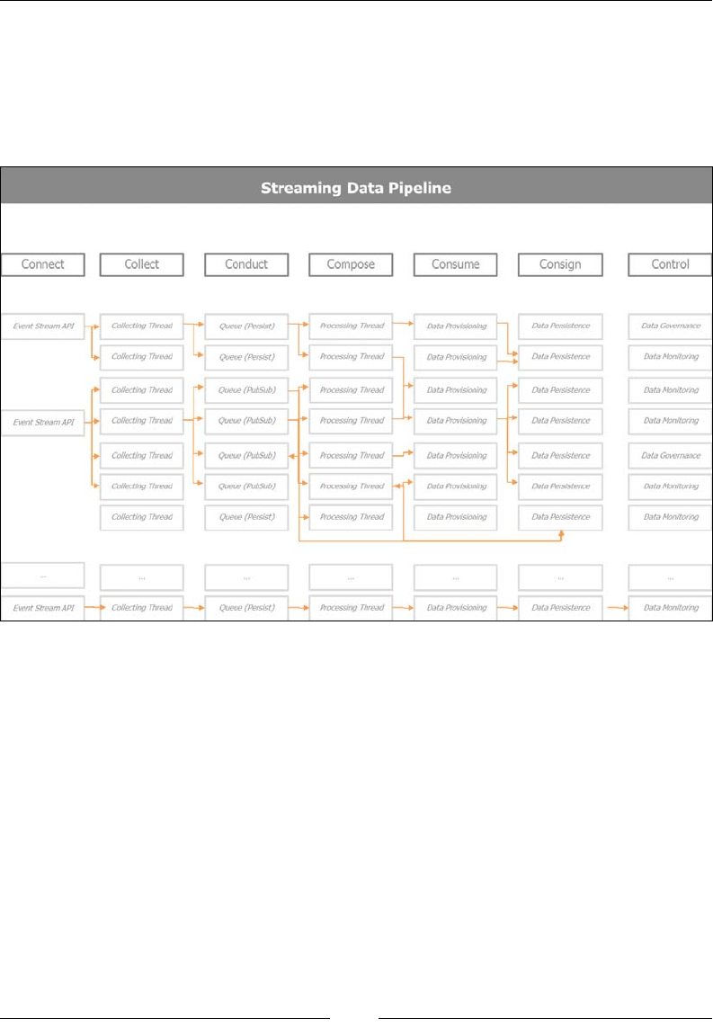

Chapter 5
[ 145 ]
The following diagram illustrates the concepts of the streaming data pipelines with
its key components: Spark Streaming, Kafka, Flume, and low latency databases. In
the consuming or controlling applications, we are monitoring our systems in real
time (depicted by a monitor) or sending real-time alerts (depicted by red lights) in
case certain thresholds are crossed.
The following diagram illustrates Spark's unique ability to process in a single
platform data in motion and data at rest while seamlessly interfacing with multiple
persistence data stores as per the use case requirement.
www.it-ebooks.info

Streaming Live Data with Spark
[ 146 ]
This diagram brings in one unied whole all the concepts discussed up to now. The
top part describes the streaming processing pipeline. The bottom part describes the
batch processing pipeline. They both share a common persistence layer in the middle
of the diagram depicting the various modes of persistence and serialization.
Closing remarks on the Lambda and
Kappa architecture
Two architecture paradigms are currently in vogue: the Lambda and
Kappa architectures.
www.it-ebooks.info

Chapter 5
[ 147 ]
Lambda is the brainchild of the Storm creator and main committer, Nathan Marz. It
essentially advocates building a functional architecture on all data. The architecture
has two branches. The rst is a batch arm envisioned to be powered by Hadoop,
where historical, high-latency, high-throughput data are pre-processed and made
ready for consumption. The real-time arm is envisioned to be powered by Storm,
and it processes incrementally streaming data, derives insights on the y, and feeds
aggregated information back to the batch storage.
Kappa is the brainchild of one the main committer of Kafka, Jay Kreps, and his
colleagues at Conuent (previously at LinkedIn). It is advocating a full streaming
pipeline, effectively implementing, at the enterprise level, the unied log enounced
in the previous pages.
Understanding Lambda architecture
Lambda architecture combines batch and streaming data to provide a unied query
mechanism on all available data. Lambda architecture envisions three layers: a batch
layer where precomputed information are stored, a speed layer where real-time
incremental information is processed as data streams, and nally the serving layer
that merges batch and real-time views for ad hoc queries. The following diagram
gives an overview of the Lambda architecture:
www.it-ebooks.info

Streaming Live Data with Spark
[ 148 ]
Understanding Kappa architecture
The Kappa architecture proposes to drive the full enterprise in streaming mode.
The Kappa architecture arose from a critique from Jay Kreps and his colleagues at
LinkedIn at the time. Since then, they moved and created Conuent with Apache
Kafka as the main enabler of the Kappa architecture vision. The basic tenet is to
move in all streaming mode with a Unied Log as the main backbone of the
enterprise information architecture.
A Unied Log is a centralized enterprise structured log available for real-time
subscription. All the organization's data is put in a central log for subscription.
Records are numbered beginning with zero so that they are written. It is also known
as a commit log or journal. The concept of the Unied Log is the central tenet of the
Kappa architecture.
The properties of the unied log are as follows:
• Unified: There is a single deployment for the entire organization
• Append only: Events are immutable and are appended
• Ordered: Each event has a unique offset within a shard
• Distributed: For fault tolerance purpose, the unified log is distributed
redundantly on a cluster of computers
• Fast: The systems ingests thousands of messages per second
The following screenshot captures the moment Jay Kreps announced his reservations
about the Lambda architecture. His main reservation about the Lambda architecture
is implementing the same job in two different systems, Hadoop and Storm, with each
of their specic idiosyncrasies, and with all the complexities that come along with it.
Kappa architecture processes the real-time data and reprocesses historical data
in the same framework powered by Apache Kafka.
www.it-ebooks.info

Chapter 5
[ 149 ]
Summary
In this chapter, we laid out the foundations of streaming architecture apps and
described their challenges, constraints, and benets. We went under the hood and
examined the inner working of Spark Streaming and how it ts with Spark Core and
dialogues with Spark SQL and Spark MLlib. We illustrated the streaming concepts
with TCP sockets, followed by live tweet ingestion and processing directly from the
Twitter rehose. We discussed the notions of decoupling upstream data publishing
from downstream data subscription and consumption using Kafka in order to
maximize the resilience of the overall streaming architecture. We also discussed
Flume—a reliable, exible, and scalable data ingestion and transport pipeline system.
The combination of Flume, Kafka, and Spark delivers unparalleled robustness,
speed, and agility in an ever changing landscape. We closed the chapter with some
remarks and observations on two streaming architectural paradigms, the Lambda
and Kappa architectures.
www.it-ebooks.info

Streaming Live Data with Spark
[ 150 ]
The Lambda architecture combines batch and streaming data in a common query
front-end. It was envisioned with Hadoop and Storm in mind initially. Spark has
its own batch and streaming paradigms, and it offers a single environment with
common code base to effectively bring this architecture paradigm to life.
The Kappa architecture promulgates the concept of the unied log, which creates
an event-oriented architecture where all events in the enterprise are channeled in a
centralized commit log that is available to all consuming systems in real time.
We are now ready for the visualization of the data collected and processed so far.
www.it-ebooks.info

[ 151 ]
Visualizing Insights
and Trends
So far, we have focused on the collection, analysis, and processing of data
from Twitter. We have set the stage to use our data for visual rendering and
extracting insights and trends. We will give a quick lay of the land about
visualization tools in the Python ecosystem. We will highlight Bokeh as a
powerful tool for rendering and viewing large datasets. Bokeh is part of the
Python Anaconda Distribution ecosystem.
In this chapter, we will cover the following points:
• Gauging the key words and memes within a social network community
using charts and wordcloud
• Mapping the most active location where communities are growing around
certain themes or topics
Revisiting the data-intensive apps
architecture
We have reached the nal layer of the data-intensive apps architecture: the
engagement layer. This layer focuses on how to synthesize, emphasize, and visualize
the key context relevant information for the data consumers. A bunch of numbers in
a console will not sufce to engage with end-users. It is critical to present the mass of
information in a rapid, digestible, and attractive fashion.
www.it-ebooks.info

Visualizing Insights and Trends
[ 152 ]
The following diagram sets the context of the chapter's focus highlighting the
engagement layer.
For Python plotting and visualizations, we have quite a few tools and libraries.
The most interesting and relevant ones for our purpose are the following:
• Matplotlib is the grandfather of the Python plotting libraries. Matplotlib was
originally the brainchild of John Hunter who was an open source software
proponent and established Matplotlib as one of the most prevalent plotting
libraries both in the academic and the data scientific communities. Matplotlib
allows the generation of plots, histograms, power spectra, bar charts, error
charts, scatterplots, and so on. Examples can be found on the Matplotlib
dedicated website at http://matplotlib.org/examples/index.html.
www.it-ebooks.info

Chapter 6
[ 153 ]
• Seaborn, developed by Michael Waskom, is a great library to quickly
visualize statistical information. It is built on top of Matplotlib and integrates
seamlessly with Pandas and the Python data stack, including Numpy.
A gallery of graphs from Seaborn at http://stanford.edu/~mwaskom/
software/seaborn/examples/index.html shows the potential of
the library.
• ggplot is relatively new and aims to offer the equivalent of the famous
ggplot2 from the R ecosystem for the Python data wranglers. It has the
same look and feel of ggplot2 and uses the same grammar of graphics as
expounded by Hadley Wickham. The ggplot the Python port is developed
by the team at yhat. More information can be found at http://ggplot.
yhathq.com.
• D3.js is a very popular, JavaScript library developed by Mike Bostock. D3
stands for Data Driven Documents and brings data to life on any modern
browser leveraging HTML, SVG, and CSS. It delivers dynamic, powerful,
interactive visualizations by manipulating the DOM, the Document
Object Model. The Python community could not wait to integrate D3 with
Matplotlib. Under the impulse of Jake Vanderplas, mpld3 was created with
the aim of bringing matplotlib to the browser. Examples graphics are
hosted at the following address: http://mpld3.github.io/index.html.
• Bokeh aims to deliver high-performance interactivity over very large or
streaming datasets whilst leveraging lot of the concepts of D3.js without
the burden of writing some intimidating javascript and css code. Bokeh
delivers dynamic visualizations on the browser with or without a server.
It integrates seamlessly with Matplotlib, Seaborn and ggplot and renders
beautifully in IPython notebooks or Jupyter notebooks. Bokeh is actively
developed by the team at Continuum.io and is an integral part of the
Anaconda Python data stack.
Bokeh server provides a full-edged, dynamic plotting engine that materializes a
reactive scene graph from JSON. It uses web sockets to keep state and update the
HTML5 canvas using Backbone.js and Coffee-script under the hoods. Bokeh, as it is
fueled by data in JSON, creates easy bindings for other languages such as R, Scala,
and Julia.
This gives a high-level overview of the main plotting and visualization library.
It is not exhaustive. Let's move to concrete examples of visualizations.
www.it-ebooks.info

Visualizing Insights and Trends
[ 154 ]
Preprocessing the data for visualization
Before jumping into the visualizations, we will do some preparatory work on the
data harvested:
In [16]:
# Read harvested data stored in csv in a Panda DF
import pandas as pd
csv_in = '/home/an/spark/spark-1.5.0-bin-hadoop2.6/examples/AN_Spark/
data/unq_tweetstxt.csv'
pddf_in = pd.read_csv(csv_in, index_col=None, header=0, sep=';',
encoding='utf-8')
In [20]:
print('tweets pandas dataframe - count:', pddf_in.count())
print('tweets pandas dataframe - shape:', pddf_in.shape)
print('tweets pandas dataframe - colns:', pddf_in.columns)
('tweets pandas dataframe - count:', Unnamed: 0 7540
id 7540
created_at 7540
user_id 7540
user_name 7538
tweet_text 7540
dtype: int64)
('tweets pandas dataframe - shape:', (7540, 6))
('tweets pandas dataframe - colns:', Index([u'Unnamed: 0',
u'id', u'created_at', u'user_id', u'user_name', u'tweet_text'],
dtype='object'))
For the purpose of our visualization activity, we will use a dataset of 7,540 tweets.
The key information is stored in the tweet_text column. We preview the data
stored in the dataframe calling the head() function on the dataframe:
In [21]:
pddf_in.head()
Out[21]:
Unnamed: 0 id created_at user_id user_name tweet_text
0 0 638830426971181057 Tue Sep 01 21:46:57 +0000 2015
3276255125 True Equality ernestsgantt: BeyHiveInFrance: 9_A_6:
dreamint...
1 1 638830426727911424 Tue Sep 01 21:46:57 +0000 2015
3276255125 True Equality ernestsgantt: BeyHiveInFrance:
PhuketDailyNews...
2 2 638830425402556417 Tue Sep 01 21:46:56 +0000 2015
3276255125 True Equality ernestsgantt: BeyHiveInFrance: 9_A_6:
ernestsg...
www.it-ebooks.info

Chapter 6
[ 155 ]
3 3 638830424563716097 Tue Sep 01 21:46:56 +0000 2015
3276255125 True Equality ernestsgantt: BeyHiveInFrance:
PhuketDailyNews...
4 4 638830422256816132 Tue Sep 01 21:46:56 +0000 2015
3276255125 True Equality ernestsgantt: elsahel12: 9_A_6:
dreamintention...
We will now create some utility functions to clean up the tweet text and parse the
twitter date. First, we import the Python regular expression regex library re and the
time library to parse dates and time:
In [72]:
import re
import time
We create a dictionary of regex that will be compiled and then passed as function:
• RT: The first regex with key RT looks for the keyword RT at the beginning of
the tweet text:
re.compile(r'^RT'),
• ALNUM: The second regex with key ALNUM looks for words including
alphanumeric characters and underscore sign preceded by the @ symbol in
the tweet text:
re.compile(r'(@[a-zA-Z0-9_]+)'),
• HASHTAG: The third regex with key HASHTAG looks for words including
alphanumeric characters preceded by the # symbol in the tweet text:
re.compile(r'(#[\w\d]+)'),
• SPACES: The fourth regex with key SPACES looks for blank or line space
characters in the tweet text:
re.compile(r'\s+'),
• URL: The fifth regex with key URL looks for url addresses including
alphanumeric characters preceded with https:// or http:// markers
in the tweet text:
re.compile(r'([https://|http://]?[a-zA-Z\d\/]+[\.]+[a-zA-
Z\d\/\.]+)')
In [24]:
regexp = {"RT": "^RT", "ALNUM": r"(@[a-zA-Z0-9_]+)",
"HASHTAG": r"(#[\w\d]+)", "URL":
r"([https://|http://]?[a-zA-Z\d\/]+[\.]+[a-zA-Z\d\/\.]+)",
"SPACES":r"\s+"}
www.it-ebooks.info

Visualizing Insights and Trends
[ 156 ]
regexp = dict((key, re.compile(value)) for key, value in regexp.
items())
In [25]:
regexp
Out[25]:
{'ALNUM': re.compile(r'(@[a-zA-Z0-9_]+)'),
'HASHTAG': re.compile(r'(#[\w\d]+)'),
'RT': re.compile(r'^RT'),
'SPACES': re.compile(r'\s+'),
'URL': re.compile(r'([https://|http://]?[a-zA-Z\d\/]+[\.]+[a-zA-
Z\d\/\.]+)')}
We create a utility function to identify whether a tweet is a retweet or an
original tweet:
In [77]:
def getAttributeRT(tweet):
""" see if tweet is a RT """
return re.search(regexp["RT"], tweet.strip()) != None
Then, we extract all user handles in a tweet:
def getUserHandles(tweet):
""" given a tweet we try and extract all user handles"""
return re.findall(regexp["ALNUM"], tweet)
We also extract all hashtags in a tweet:
def getHashtags(tweet):
""" return all hashtags"""
return re.findall(regexp["HASHTAG"], tweet)
Extract all URL links in a tweet as follows:
def getURLs(tweet):
""" URL : [http://]?[\w\.?/]+"""
return re.findall(regexp["URL"], tweet)
We strip all URL links and user handles preceded by @ sign in a tweet text. This
function will be the basis of the wordcloud we will build soon:
def getTextNoURLsUsers(tweet):
""" return parsed text terms stripped of URLs and User Names in
tweet text
' '.join(re.sub("(@[A-Za-z0-9]+)|([^0-9A-Za-z \t])|(\w+:\/\/\
S+)"," ",x).split()) """
return ' '.join(re.sub("(@[A-Za-z0-9]+)|([^0-9A-Za-z \t])|(\
w+:\/\/\S+)|(RT)"," ", tweet).lower().split())
www.it-ebooks.info

Chapter 6
[ 157 ]
We label the data so we can create groups of datasets for the wordcloud:
def setTag(tweet):
""" set tags to tweet_text based on search terms from tags_list"""
tags_list = ['spark', 'python', 'clinton', 'trump', 'gaga',
'bieber']
lower_text = tweet.lower()
return filter(lambda x:x.lower() in lower_text,tags_list)
We parse the twitter date in the yyyy-mm-dd hh:mm:ss format:
def decode_date(s):
""" parse Twitter date into format yyyy-mm-dd hh:mm:ss"""
return time.strftime('%Y-%m-%d %H:%M:%S', time.strptime(s,'%a %b
%d %H:%M:%S +0000 %Y'))
We preview the data prior to processing:
In [43]:
pddf_in.columns
Out[43]:
Index([u'Unnamed: 0', u'id', u'created_at', u'user_id', u'user_name',
u'tweet_text'], dtype='object')
In [45]:
# df.drop([Column Name or list],inplace=True,axis=1)
pddf_in.drop(['Unnamed: 0'], inplace=True, axis=1)
In [46]:
pddf_in.head()
Out[46]:
id created_at user_id user_name tweet_text
0 638830426971181057 Tue Sep 01 21:46:57 +0000 2015 3276255125
True Equality ernestsgantt: BeyHiveInFrance: 9_A_6: dreamint...
1 638830426727911424 Tue Sep 01 21:46:57 +0000 2015 3276255125
True Equality ernestsgantt: BeyHiveInFrance: PhuketDailyNews...
2 638830425402556417 Tue Sep 01 21:46:56 +0000 2015 3276255125
True Equality ernestsgantt: BeyHiveInFrance: 9_A_6: ernestsg...
3 638830424563716097 Tue Sep 01 21:46:56 +0000 2015 3276255125
True Equality ernestsgantt: BeyHiveInFrance: PhuketDailyNews...
4 638830422256816132 Tue Sep 01 21:46:56 +0000 2015 3276255125
True Equality ernestsgantt: elsahel12: 9_A_6: dreamintention...
www.it-ebooks.info

Visualizing Insights and Trends
[ 158 ]
We create new dataframe columns by applying the utility functions described. We
create a new column for htag, user handles, URLs, the text terms stripped from
URLs, and unwanted characters and the labels. We nally parse the date:
In [82]:
pddf_in['htag'] = pddf_in.tweet_text.apply(getHashtags)
pddf_in['user_handles'] = pddf_in.tweet_text.apply(getUserHandles)
pddf_in['urls'] = pddf_in.tweet_text.apply(getURLs)
pddf_in['txt_terms'] = pddf_in.tweet_text.apply(getTextNoURLsUsers)
pddf_in['search_grp'] = pddf_in.tweet_text.apply(setTag)
pddf_in['date'] = pddf_in.created_at.apply(decode_date)
The following code gives a quick snapshot of the newly generated dataframe:
In [83]:
pddf_in[2200:2210]
Out[83]:
id created_at user_id user_name tweet_text htag urls
ptxt tgrp date user_handles txt_terms search_grp
2200 638242693374681088 Mon Aug 31 06:51:30 +0000 2015 19525954
CENATIC El impacto de @ApacheSpark en el procesamiento...
[#sparkSpecial] [://t.co/4PQmJNuEJB] el impacto de en el
procesamiento de datos y e... [spark] 2015-08-31 06:51:30 [@
ApacheSpark] el impacto de en el procesamiento de datos y e...
[spark]
2201 638238014695575552 Mon Aug 31 06:32:55 +0000 2015 51115854
Nawfal Real Time Streaming with Apache Spark\nhttp://... [#IoT,
#SmartMelboune, #BigData, #Apachespark] [://t.co/GW5PaqwVab] real
time streaming with apache spark iot smar... [spark] 2015-08-
31 06:32:55 [] real time streaming with apache spark iot smar...
[spark]
2202 638236084124516352 Mon Aug 31 06:25:14 +0000 2015 62885987
Mithun Katti RT @differentsachin: Spark the flame of digita...
[#IBMHackathon, #SparkHackathon, #ISLconnectIN... [] spark
the flame of digital india ibmhackathon ... [spark] 2015-08-
31 06:25:14 [@differentsachin, @ApacheSpark] spark the flame of
digital india ibmhackathon ... [spark]
2203 638234734649176064 Mon Aug 31 06:19:53 +0000 2015 140462395
solaimurugan v Installing @ApacheMahout with @ApacheSpark 1.4...
[] [1.4.1, ://t.co/3c5dGbfaZe.] installing with 1 4 1 got many
more issue whil... [spark] 2015-08-31 06:19:53 [@ApacheMahout,
@ApacheSpark] installing with 1 4 1 got many more issue whil...
[spark]
www.it-ebooks.info

Chapter 6
[ 159 ]
2204 638233517307072512 Mon Aug 31 06:15:02 +0000 2015
2428473836 Ralf Heineke RT @RomeoKienzler: Join me @velocityconf
on #m... [#machinelearning, #devOps, #Bl] [://t.co/U5xL7pYEmF]
join me on machinelearning based devops operat... [spark] 2015-08-
31 06:15:02 [@RomeoKienzler, @velocityconf, @ApacheSpark] join me
on machinelearning based devops operat... [spark]
2205 638230184848687106 Mon Aug 31 06:01:48 +0000 2015 289355748
Akim Boyko RT @databricks: Watch live today at 10am PT is...
[] [1.5, ://t.co/16cix6ASti] watch live today at 10am pt is 1
5 presented b... [spark] 2015-08-31 06:01:48 [@databricks, @
ApacheSpark, @databricks, @pwen... watch live today at 10am pt is 1
5 presented b... [spark]
2206 638227830443110400 Mon Aug 31 05:52:27 +0000 2015 145001241
sachin aggarwal Spark the flame of digital India @ #IBMHackath...
[#IBMHackathon, #SparkHackathon, #ISLconnectIN... [://t.co/
C1AO3uNexe] spark the flame of digital india ibmhackathon ...
[spark] 2015-08-31 05:52:27 [@ApacheSpark] spark the flame of
digital india ibmhackathon ... [spark]
2207 638227031268810752 Mon Aug 31 05:49:16 +0000 2015 145001241
sachin aggarwal RT @pravin_gadakh: Imagine, innovate and Igni...
[#IBMHackathon, #ISLconnectIN2015] [] gadakh imagine innovate
and ignite digital ind... [spark] 2015-08-31 05:49:16 [@pravin_
gadakh, @ApacheSpark] gadakh imagine innovate and ignite digital
ind... [spark]
2208 638224591920336896 Mon Aug 31 05:39:35 +0000 2015 494725634
IBM Asia Pacific RT @sachinparmar: Passionate about Spark?? Hav...
[#IBMHackathon, #ISLconnectIN] [India..] passionate about spark
have dreams of clean sa... [spark] 2015-08-31 05:39:35 [@
sachinparmar] passionate about spark have dreams of clean sa...
[spark]
2209 638223327467692032 Mon Aug 31 05:34:33 +0000 2015
3158070968 Open Source India "Game Changer" #ApacheSpark speeds up
#bigdata... [#ApacheSpark, #bigdata] [://t.co/ieTQ9ocMim] game
changer apachespark speeds up bigdata pro... [spark] 2015-08-
31 05:34:33 [] game changer apachespark speeds up bigdata pro...
[spark]
We save the processed information in a CSV format. We have 7,540 records and 13
columns. In your case, the output will vary according to the dataset you chose:
In [84]:
f_name = '/home/an/spark/spark-1.5.0-bin-hadoop2.6/examples/AN_Spark/
data/unq_tweets_processed.csv'
pddf_in.to_csv(f_name, sep=';', encoding='utf-8', index=False)
In [85]:
pddf_in.shape
Out[85]:
(7540, 13)
www.it-ebooks.info

Visualizing Insights and Trends
[ 160 ]
Gauging words, moods, and memes at a
glance
We are now ready to proceed with building the wordclouds which will give us a
sense of the important words carried in those tweets. We will create wordclouds
for the datasets harvested. Wordclouds extract the top words in a list of words
and create a scatterplot of the words where the size of the word is correlated to its
frequency. The more frequent the word in the dataset, the bigger will be the font
size in the wordcloud rendering. They include three very different themes and two
competing or analogous entities. Our rst theme is obviously data processing and
analytics, with Apache Spark and Python as our entities. Our second theme is the
2016 presidential election campaign, with the two contenders: Hilary Clinton and
Donald Trump. Our last theme is the world of pop music with Justin Bieber and
Lady Gaga as the two exponents.
Setting up wordcloud
We will illustrate the programming steps by analyzing the spark related tweets.
We load the data and preview the dataframe:
In [21]:
import pandas as pd
csv_in = '/home/an/spark/spark-1.5.0-bin-hadoop2.6/examples/AN_Spark/
data/spark_tweets.csv'
tspark_df = pd.read_csv(csv_in, index_col=None, header=0, sep=',',
encoding='utf-8')
In [3]:
tspark_df.head(3)
Out[3]:
id created_at user_id user_name tweet_text htag urls
ptxt tgrp date user_handles txt_terms search_grp
0 638818911773856000 Tue Sep 01 21:01:11 +0000 2015 2511247075
Noor Din RT @kdnuggets: R leads RapidMiner, Python catc... [#KDN]
[://t.co/3bsaTT7eUs] r leads rapidminer python catches up big data
... [spark, python] 2015-09-01 21:01:11 [@kdnuggets] r leads
rapidminer python catches up big data ... [spark, python]
1 622142176768737000 Fri Jul 17 20:33:48 +0000 2015 24537879
IBM Cloudant Be one of the first to sign-up for IBM Analyti...
[#ApacheSpark, #SparkInsight] [://t.co/C5TZpetVA6, ://t.co/
R1L29DePaQ] be one of the first to sign up for ibm analyti...
[spark] 2015-07-17 20:33:48 [] be one of the first to sign up
for ibm analyti... [spark]
www.it-ebooks.info

Chapter 6
[ 161 ]
2 622140453069169000 Fri Jul 17 20:26:57 +0000 2015 515145898
Arno Candel Nice article on #apachespark, #hadoop and #dat...
[#apachespark, #hadoop, #datascience] [://t.co/IyF44pV0f3] nice
article on apachespark hadoop and datasci... [spark] 2015-07-
17 20:26:57 [@h2oai] nice article on apachespark hadoop and
datasci... [spark]
The wordcloud library we will use is the one developed by Andreas
Mueller and hosted on his GitHub account at https://github.com/
amueller/word_cloud.
The library requires PIL (short for Python Imaging Library). PIL is easily installable
by invoking conda install pil. PIL is a complex library to install and is not yet
ported on Python 3.4, so we need to run a Python 2.7+ environment to be able to see
our wordcloud:
#
# Install PIL (does not work with Python 3.4)
#
an@an-VB:~$ conda install pil
Fetching package metadata: ....
Solving package specifications: ..................
Package plan for installation in environment /home/an/anaconda:
The following packages will be downloaded:
package | build
---------------------------|-----------------
libpng-1.6.17 | 0 214 KB
freetype-2.5.5 | 0 2.2 MB
conda-env-2.4.4 | py27_0 24 KB
pil-1.1.7 | py27_2 650 KB
------------------------------------------------------------
Total: 3.0 MB
The following packages will be UPDATED:
conda-env: 2.4.2-py27_0 --> 2.4.4-py27_0
freetype: 2.5.2-0 --> 2.5.5-0
libpng: 1.5.13-1 --> 1.6.17-0
pil: 1.1.7-py27_1 --> 1.1.7-py27_2
Proceed ([y]/n)? y
www.it-ebooks.info

Visualizing Insights and Trends
[ 162 ]
Next, we install the wordcloud library:
#
# Install wordcloud
# Andreas Mueller
# https://github.com/amueller/word_cloud/blob/master/wordcloud/
wordcloud.py
#
an@an-VB:~$ pip install wordcloud
Collecting wordcloud
Downloading wordcloud-1.1.3.tar.gz (163kB)
100% |████████████████████████████████| 163kB 548kB/s
Building wheels for collected packages: wordcloud
Running setup.py bdist_wheel for wordcloud
Stored in directory: /home/an/.cache/pip/wheels/32/a9/74/58e379e5dc6
14bfd9dd9832d67608faac9b2bc6c194d6f6df5
Successfully built wordcloud
Installing collected packages: wordcloud
Successfully installed wordcloud-1.1.3
Creating wordclouds
At this stage, we are ready to invoke the wordcloud program with the generated list
of terms from the tweet text.
Let's get started with the wordcloud program by rst calling %matplotlib inline to
display the wordcloud in our notebook:
In [4]:
%matplotlib inline
In [11]:
We convert the dataframe txt_terms column into a list of words. We make sure it
is all converted into the str type to avoid any bad surprises and check the list's rst
four records:
len(tspark_df['txt_terms'].tolist())
Out[11]:
2024
In [22]:
tspark_ls_str = [str(t) for t in tspark_df['txt_terms'].tolist()]
In [14]:
len(tspark_ls_str)
Out[14]:
www.it-ebooks.info

Chapter 6
[ 163 ]
2024
In [15]:
tspark_ls_str[:4]
Out[15]:
['r leads rapidminer python catches up big data tools grow spark
ignites kdn',
'be one of the first to sign up for ibm analytics for apachespark
today sparkinsight',
'nice article on apachespark hadoop and datascience',
'spark 101 running spark and mapreduce together in production
hadoopsummit2015 apachespark altiscale']
We rst call the Matplotlib and the wordcloud libraries:
import matplotlib.pyplot as plt
from wordcloud import WordCloud, STOPWORDS
From the input list of terms, we create a unied string of terms separated by a
whitespace as the input to the wordcloud program. The wordcloud program
removes stopwords:
# join tweets to a single string
words = ' '.join(tspark_ls_str)
# create wordcloud
wordcloud = WordCloud(
# remove stopwords
stopwords=STOPWORDS,
background_color='black',
width=1800,
height=1400
).generate(words)
# render wordcloud image
plt.imshow(wordcloud)
plt.axis('off')
# save wordcloud image on disk
plt.savefig('./spark_tweets_wordcloud_1.png', dpi=300)
# display image in Jupyter notebook
plt.show()
www.it-ebooks.info

Visualizing Insights and Trends
[ 164 ]
Here, we can visualize the wordclouds for Apache Spark and Python. Clearly, in
the case of Spark, Hadoop, big data, and analytics are the memes, while Python recalls
the root of its name Monty Python with a strong focus on developer, apache spark,
and programming with some hints to java and ruby.
We can also get a glimpse in the following wordclouds of the words preoccupying
the North American 2016 presidential election candidates: Hilary Clinton and
Donald Trump. Seemingly Hilary Clinton is overshadowed by the presence of her
opponents Donald Trump and Bernie Sanders, while Trump is heavily centered
only on himself:
Interestingly, in the case of Justin Bieber and Lady Gaga, the word love appears. In
the case of Bieber, follow and belieber are key words, while diet, weight loss, and fashion
are the preoccupations for the Lady Gaga crowd.
www.it-ebooks.info

Chapter 6
[ 165 ]
Geo-locating tweets and mapping
meetups
Now, we will dive into the creation of interactive maps with Bokeh. First, we create
a world map where we geo-locate sample tweets and, on moving our mouse over
these locations, we can see the users and their respective tweets in a hover box.
The second map is focused on mapping upcoming meetups in London. It could
be an interactive map that would act as a reminder of date, time, and location for
upcoming meetups in a specic city.
Geo-locating tweets
The objective is to create a world map scatter plot of the locations of important
tweets on the map, and the tweets and authors are revealed on hovering over
these points. We will go through three steps to build this interactive visualization:
1. Create the background world map by rst loading a dictionary of all
the world country boundaries dened by their respective longitude
and latitudes.
2. Load the important tweets we wish to geo-locate with their respective
coordinates and authors.
3. Finally, scatter plot on the world map the tweets coordinates and activate the
hover tool to visualize interactively the tweets and author on the highlighted
dots on the map.
www.it-ebooks.info

Visualizing Insights and Trends
[ 166 ]
In step one, we create a Python list called data that will contain all the world
countries boundaries with their respective latitude and longitude:
In [4]:
#
# This module exposes geometry data for World Country Boundaries.
#
import csv
import codecs
import gzip
import xml.etree.cElementTree as et
import os
from os.path import dirname, join
nan = float('NaN')
__file__ = os.getcwd()
data = {}
with gzip.open(join(dirname(__file__), 'AN_Spark/data/World_Country_
Boundaries.csv.gz')) as f:
decoded = codecs.iterdecode(f, "utf-8")
next(decoded)
reader = csv.reader(decoded, delimiter=',', quotechar='"')
for row in reader:
geometry, code, name = row
xml = et.fromstring(geometry)
lats = []
lons = []
for i, poly in enumerate(xml.findall('.//outerBoundaryIs/
LinearRing/coordinates')):
if i > 0:
lats.append(nan)
lons.append(nan)
coords = (c.split(',')[:2] for c in poly.text.split())
lat, lon = list(zip(*[(float(lat), float(lon)) for lon,
lat in
coords]))
lats.extend(lat)
lons.extend(lon)
data[code] = {
'name' : name,
'lats' : lats,
'lons' : lons,
}
www.it-ebooks.info

Chapter 6
[ 167 ]
In [5]:
len(data)
Out[5]:
235
In step two, we load a sample set of important tweets that we wish to visualize with
their respective geo-location information:
In [69]:
# data
#
#
In [8]:
import pandas as pd
csv_in = '/home/an/spark/spark-1.5.0-bin-hadoop2.6/examples/AN_Spark/
data/spark_tweets_20.csv'
t20_df = pd.read_csv(csv_in, index_col=None, header=0, sep=',',
encoding='utf-8')
In [9]:
t20_df.head(3)
Out[9]:
id created_at user_id user_name tweet_text htag urls
ptxt tgrp date user_handles txt_terms search_grp lat
lon
0 638818911773856000 Tue Sep 01 21:01:11 +0000 2015 2511247075
Noor Din RT @kdnuggets: R leads RapidMiner, Python catc... [#KDN]
[://t.co/3bsaTT7eUs] r leads rapidminer python catches up big data
... [spark, python] 2015-09-01 21:01:11 [@kdnuggets] r
leads rapidminer python catches up big data ... [spark, python]
37.279518 -121.867905
1 622142176768737000 Fri Jul 17 20:33:48 +0000 2015 24537879
IBM Cloudant Be one of the first to sign-up for IBM Analyti...
[#ApacheSpark, #SparkInsight] [://t.co/C5TZpetVA6, ://t.co/
R1L29DePaQ] be one of the first to sign up for ibm analyti...
[spark] 2015-07-17 20:33:48 [] be one of the first to sign up
for ibm analyti... [spark] 37.774930 -122.419420
2 622140453069169000 Fri Jul 17 20:26:57 +0000 2015 515145898
Arno Candel Nice article on #apachespark, #hadoop and #dat...
[#apachespark, #hadoop, #datascience] [://t.co/IyF44pV0f3] nice
article on apachespark hadoop and datasci... [spark] 2015-07-
17 20:26:57 [@h2oai] nice article on apachespark hadoop and
datasci... [spark] 51.500130 -0.126305
In [98]:
len(t20_df.user_id.unique())
Out[98]:
19
In [17]:
www.it-ebooks.info

Visualizing Insights and Trends
[ 168 ]
t20_geo = t20_df[['date', 'lat', 'lon', 'user_name', 'tweet_text']]
In [24]:
#
t20_geo.rename(columns={'user_name':'user', 'tweet_text':'text' },
inplace=True)
In [25]:
t20_geo.head(4)
Out[25]:
date lat lon user text
0 2015-09-01 21:01:11 37.279518 -121.867905 Noor Din RT
@kdnuggets: R leads RapidMiner, Python catc...
1 2015-07-17 20:33:48 37.774930 -122.419420 IBM Cloudant
Be one of the first to sign-up for IBM Analyti...
2 2015-07-17 20:26:57 51.500130 -0.126305 Arno Candel
Nice article on #apachespark, #hadoop and #dat...
3 2015-07-17 19:35:31 51.500130 -0.126305 Ira Michael
Blonder Spark 101: Running Spark and #MapReduce togeth...
In [22]:
df = t20_geo
#
In step three, we rst imported all the necessary Bokeh libraries. We will instantiate
the output in the Jupyter Notebook. We get the world countries boundary
information loaded. We get the geo-located tweet data. We instantiate the
Bokeh interactive tools such as wheel and box zoom as well as the hover tool.
In [29]:
#
# Bokeh Visualization of tweets on world map
#
from bokeh.plotting import *
from bokeh.models import HoverTool, ColumnDataSource
from collections import OrderedDict
# Output in Jupiter Notebook
output_notebook()
# Get the world map
world_countries = data.copy()
# Get the tweet data
tweets_source = ColumnDataSource(df)
# Create world map
www.it-ebooks.info

Chapter 6
[ 169 ]
countries_source = ColumnDataSource(data= dict(
countries_xs=[world_countries[code]['lons'] for code in world_
countries],
countries_ys=[world_countries[code]['lats'] for code in world_
countries],
country = [world_countries[code]['name'] for code in world_
countries],
))
# Instantiate the bokeh interactive tools
TOOLS="pan,wheel_zoom,box_zoom,reset,resize,hover,save"
We are now ready to layer the various elements gathered into an object gure called
p. Dene the title, width, and height of p. Attach the tools. Create the world map
background by patches with a light background color and borders. Scatter plot the
tweets according to their respective geo-coordinates. Then, activate the hover tool
with the users and their respective tweet. Finally, render the picture on the browser.
The code is as follows:
# Instantiante the figure object
p = figure(
title="%s tweets " %(str(len(df.index))),
title_text_font_size="20pt",
plot_width=1000,
plot_height=600,
tools=TOOLS)
# Create world patches background
p.patches(xs="countries_xs", ys="countries_ys", source = countries_
source, fill_color="#F1EEF6", fill_alpha=0.3,
line_color="#999999", line_width=0.5)
# Scatter plots by longitude and latitude
p.scatter(x="lon", y="lat", source=tweets_source, fill_
color="#FF0000", line_color="#FF0000")
#
# Activate hover tool with user and corresponding tweet information
hover = p.select(dict(type=HoverTool))
hover.point_policy = "follow_mouse"
hover.tooltips = OrderedDict([
("user", "@user"),
("tweet", "@text"),
])
# Render the figure on the browser
www.it-ebooks.info
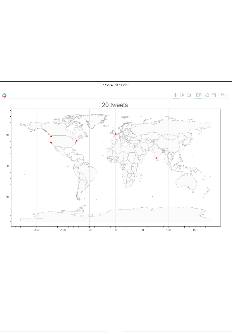
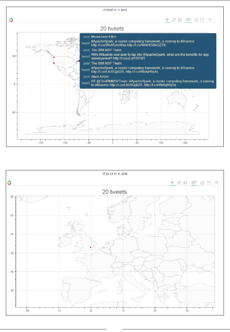

Visualizing Insights and Trends
[ 172 ]
Finally, we can reveal the tweets in the given zoomed-in location:
Displaying upcoming meetups on Google
Maps
Now, our objective is to focus on upcoming meetups in London. We are mapping
three meetups Data Science London, Apache Spark, and Machine Learning. We
embed a Google Map within a Bokeh visualization and geo-locate the three meetups
according to their coordinates and get information such as the name of the upcoming
event for each meetup with a hover tool.
First, import all the necessary Bokeh libraries:
In [ ]:
#
# Bokeh Google Map Visualization of London with hover on specific
points
#
#
from __future__ import print_function
www.it-ebooks.info

Chapter 6
[ 173 ]
from bokeh.browserlib import view
from bokeh.document import Document
from bokeh.embed import file_html
from bokeh.models.glyphs import Circle
from bokeh.models import (
GMapPlot, Range1d, ColumnDataSource,
PanTool, WheelZoomTool, BoxSelectTool,
HoverTool, ResetTool,
BoxSelectionOverlay, GMapOptions)
from bokeh.resources import INLINE
x_range = Range1d()
y_range = Range1d()
We will instantiate the Google Map that will act as the substrate upon which our
Bokeh visualization will be layered:
# JSON style string taken from: https://snazzymaps.com/style/1/pale-
dawn
map_options = GMapOptions(lat=51.50013, lng=-0.126305, map_
type="roadmap", zoom=13, styles="""
[{"featureType":"administrative","elementType":"all","stylers":[{"visi
bility":"on"},{"lightness":33}]},
{"featureType":"landscape","elementType":"all","stylers":[{"color":"
#f2e5d4"}]},
{"featureType":"poi.park","elementType":"geometry","stylers":[{"color
":"#c5dac6"}]},
{"featureType":"poi.park","elementType":"labels","stylers":[{"visibil
ity":"on"},{"lightness":20}]},
{"featureType":"road","elementType":"all","stylers":[{"lightne
ss":20}]},
{"featureType":"road.highway","elementType":"geometry","stylers":[{"c
olor":"#c5c6c6"}]},
{"featureType":"road.arterial","elementType":"geometry","stylers":[{"
color":"#e4d7c6"}]},
{"featureType":"road.local","elementType":"geometry","stylers":[{"col
or":"#fbfaf7"}]},
{"featureType":"water","elementType":"all","stylers":[{"visibility":"
on"},{"color":"#acbcc9"}]}]
""")
www.it-ebooks.info

Visualizing Insights and Trends
[ 174 ]
Instantiate the Bokeh object plot from the class GMapPlot with the dimensions and
map options from the previous step:
# Instantiate Google Map Plot
plot = GMapPlot(
x_range=x_range, y_range=y_range,
map_options=map_options,
title="London Meetups"
)
Bring in the information from our three meetups we wish to plot and get the
information by hovering above the respective coordinates:
source = ColumnDataSource(
data=dict(
lat=[51.49013, 51.50013, 51.51013],
lon=[-0.130305, -0.126305, -0.120305],
fill=['orange', 'blue', 'green'],
name=['LondonDataScience', 'Spark', 'MachineLearning'],
text=['Graph Data & Algorithms','Spark Internals','Deep
Learning on Spark']
)
)
Dene the dots to be drawn on the Google Map:
circle = Circle(x="lon", y="lat", size=15, fill_color="fill", line_
color=None)
plot.add_glyph(source, circle)
Dene the stings for the Bokeh tools to be used in this visualization:
# TOOLS="pan,wheel_zoom,box_zoom,reset,hover,save"
pan = PanTool()
wheel_zoom = WheelZoomTool()
box_select = BoxSelectTool()
reset = ResetTool()
hover = HoverTool()
# save = SaveTool()
plot.add_tools(pan, wheel_zoom, box_select, reset, hover)
overlay = BoxSelectionOverlay(tool=box_select)
plot.add_layout(overlay)
www.it-ebooks.info

Chapter 6
[ 175 ]
Activate the hover tool with the information that will be carried:
hover = plot.select(dict(type=HoverTool))
hover.point_policy = "follow_mouse"
hover.tooltips = OrderedDict([
("Name", "@name"),
("Text", "@text"),
("(Long, Lat)", "(@lon, @lat)"),
])
show(plot)
Render the plot that gives a pretty good view of London:
www.it-ebooks.info
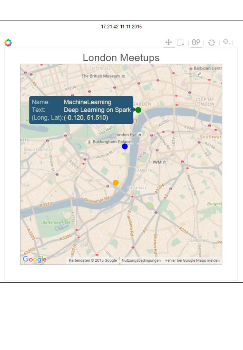
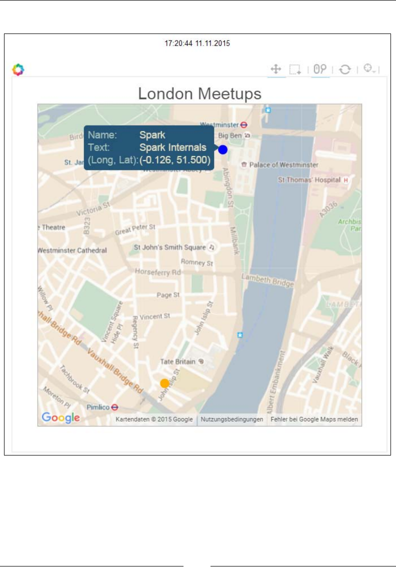

Visualizing Insights and Trends
[ 178 ]
Summary
In this chapter, we focused on few visualization techniques. We saw how to build
wordclouds and their intuitive power to reveal, at a glance, lots of the key words,
moods, and memes carried through thousands of tweets.
We then discussed interactive mapping visualizations using Bokeh. We built a world
map from the ground up and created a scatter plot of critical tweets. Once the map
was rendered on the browser, we could interactively hover from dot to dot and
reveal the tweets originating from different parts of the world.
Our nal visualization was focused on mapping upcoming meetups in London on
Spark, data science, and machine learning and their respective topics, making a
beautiful interactive visualization with an actual Google Map.
www.it-ebooks.info

[ 179 ]
Index
A
Amazon Web Services (AWS)
about 24
apps, deploying with 24
Anaconda
dening 10, 11
Anaconda installer
URL 14
Anaconda stack
Anaconda 11
Blaze 11
Bokeh 11
Conda 11
Numba 11
Wakari 11
analytics layer 5
Apache Kafka
about 133
properties 133
Apache Spark 172
APIs (Application Programming
Interface) 31
apps
deploying, with Amazon
Web Services (AWS) 24
previewing 47
architecture, data-intensive applications
about 3
analytics layer 5
engagement layer 6
infrastructure layer 4
integration layer 4
persistence layer 4
Asynchronous JavaScript (AJAX) 124
AWS console
URL 24
B
Big Data, with Apache Spark
references 22
Blaze
used, for exploring data 63-66
BSON (Binary JSON) 55
C
Catalyst 68
Clustering
Gaussian Mixture 87
K-Means 87
Latent Dirichlet Allocation (LDA) 87
Power Iteration Clustering (PIC) 87
Cluster manager 8
comma-separated values (CSV) 51
D
D3.js
about 153
URL 153
DAG (Directed Acyclic Graph) 9, 51
data
deserializing 51
exploring, Blaze used 63-66
exploring, Spark SQL used 68
harvesting 51
www.it-ebooks.info

[ 180 ]
harvesting from Twitter 59-63
MongoDB, setting up 55
persisting, in CSV 52, 53
persisting, in JSON 54
preprocessing, for visualization 154-159
serializing 51
storing 51
transferring, Odo used 67, 68
data analysis
dening 35
Tweets anatomy, discovering 35-39
Data Driven Documents (D3) 153
data ows 92
data-intensive apps
about 151-153
architecture, dening 50
data at rest, processing 29
data, exploring 31
data in motion, processing 30
fault tolerance 29
exibility 29
latency 29
scalability 29
data lifecycle
Collect 5
Compose 5
Connect 4
Consume 5
Control 5
Correct 5
data types, Spark MLlib
distributed matrix 92
labeled point 91
local matrix 91
local vector 90
Decision Trees 88
Dimensionality Reduction
Principal Component Analysis (PCA) 87
Singular Value Decomposition (SVD) 87
Docker
about 4
environment, virtualizing with 24-26
references 25
DStream (Discretized Stream)
dening 120, 121
E
elements, Flume
Channel 143
Client 142
Event 142
Sink 142
Source 142
engagement layer 6
environment
virtualizing, with Docker 24-26
virtualizing, with Vagrant 22, 23
F
rst app
building, with PySpark 17-21
Flume
about 142
advantages 142
elements 142, 143
G
ggplot
about 153
URL 153
GitHub
about 40, 41
operating, with Meetup API 42-44
URL 34
Google File System (GFS) 2
Google Maps
upcoming meetups, displaying on 172-176
H
Hadoop MongoDB connector
URL 77
HDFS (Hadoop Distributed File System) 6
I
infrastructure layer 4
Ingest mode
Batch Data Transport 132
www.it-ebooks.info

[ 181 ]
Message Queue 132
Micro Batch 132
Pipelining 132
integration layer 4
J
Java 8
installing 14
Java Virtual Machine (JVM) 2
JRE (Java Runtime Environment) 14
JSON (JavaScript Object Notation) 31, 51
K
Kafka
consumers, developing 139
installing 134-137
producers, developing 137-139
setting up 133, 134
Spark Streaming consumer,
developing for 140
testing 134-137
URL 134
Kappa architecture
dening 146-148
L
Lambda architecture
dening 146, 147
linear regression models 88
M
machine learning pipelines
building 113, 114
machine learning workows 92
Massive Open Online Courses (MOOCs) 22
Matplotlib
about 152
URL 152
Meetup API
URL 34
meetups
mapping 165
MLlib algorithms
Collaborative ltering 89
feature extraction and transformation 89
Limited-memory BFGS (L-BFGS) 90
optimization 90
MLlib (Machine Learning library) 83
models
dening, for processing streams of data 117
MongoDB
about 4
Mongo client, running 57
MongoDB server and client, installing 55
MongoDB server, running 56
PyMongo driver, installing 58
Python client, creating for 58
references 77
setting up 55
MongoDB, from Spark SQL
URL 78
Mumrah, on GitHub
URL 137
MySQL 4
N
Neo4j 4
network_wordcount.py
URL 125
O
Odo
about 67
used, for transferring data 67, 68
operations, on RDDs
action 9
transformations 9
P
persistence layer 4
PIL (Python Imaging Library) 161
PostgreSQL 4
Puppet 4
PySpark
rst app, building with 17-21
www.it-ebooks.info

[ 182 ]
R
RDD (Resilient Distributed
Dataset) 8, 9, 118
REST (Representation State Transfer) 31
RPC (Remote Procedure Call) 117
S
SDK (Software Development Kit) 14
Seaborn
about 153
URL 153
social networks
connecting to 31
GitHub data, obtaining 34
Meetup data, obtaining 34
Twitter data, obtaining 32, 33
Spark
Batch 6
Clustering 87
dening 6
Dimensionality Reduction 87
Interactive 6
Isotonic Regression 88
Iterative 6
libraries 7
MLlib algorithms 89
Regression and Classication 88
Streaming 6
URL 15
Spark dataframes
dening 69-72
Spark libraries
PySpark, dening 7, 8
RDD (Resilient Distributed Dataset) 8, 9
Spark GraphX 7
SparkMLlib 7
SparkSQL 7
Spark Streaming 7
Spark MLlib
contextualizing, in app architecture 84
data types 90-92
Spark MLlib algorithms
additional learning algorithms 88-90
classifying 85, 86
supervised learning 86-88
unsupervised learning 86-88
Spark, on EC2
URL 24
Spark powered environment
Anaconda, installing with Python 2.7 13
IPython Notebook, enabling 16
Java 8, installing 14
Oracle VirtualBox, setting up
with Ubuntu 13
setting up 12
Spark, installing 15
Spark SQL
about 68
CSV les, loading with 75, 76
CSV les, processing with 75, 76
MongoDB, querying from 77-80
used, for exploring data 68
Spark SQL query optimizer
dening 72-75
Spark streaming
building, in fault tolerance 124
dening 118-123
Stochastic Gradient Descent 86
streaming app
building 131, 132
data pipelines, developing
with Flume 143-146
data pipelines, developing
with Kafka 143-146
data pipelines, developing
with Spark 143-146
ume, exploring 142, 143
Kafka, setting up 133, 134
streaming architecture 116, 117
supervised machine learning workow 92
T
TCP sockets
live data, processing with 124-128
setting up 124, 125
tweets
geo-locating 165-172
Twitter
URL 32
Twitter API, on dev console
URL 33
www.it-ebooks.info

[ 183 ]
Twitter data
manipulating 128
tweets, processing from
Twitter rehose 128-130
Twitter dataset
clustering 95, 96
clustering algorithm, running 107
dataset, preprocessing 103
model and results, evaluating 108-113
Scikit-Learn, applying on 96-103
U
Ubuntu 14.04.1 LTS release
URL 13
Unied Log
properties 132, 148
unsupervised machine
learning workow 94
V
Vagrant
about 4
environment, virtualizing with 22, 23
reference 22
VirtualBox VM
URL 13
visualization
data, preprocessing for 154-159
W
wordclouds
creating 160-164
setting up 160-162
URL 161
www.it-ebooks.info

Thank you for buying
Spark for Python Developers
About Packt Publishing
Packt, pronounced 'packed', published its rst book, Mastering phpMyAdmin for Effective
MySQL Management, in April 2004, and subsequently continued to specialize in publishing
highly focused books on specic technologies and solutions.
Our books and publications share the experiences of your fellow IT professionals in adapting
and customizing today's systems, applications, and frameworks. Our solution-based books
give you the knowledge and power to customize the software and technologies you're using
to get the job done. Packt books are more specic and less general than the IT books you have
seen in the past. Our unique business model allows us to bring you more focused information,
giving you more of what you need to know, and less of what you don't.
Packt is a modern yet unique publishing company that focuses on producing quality,
cutting-edge books for communities of developers, administrators, and newbies alike.
For more information, please visit our website at www.packtpub.com.
About Packt Open Source
In 2010, Packt launched two new brands, Packt Open Source and Packt Enterprise, in order
to continue its focus on specialization. This book is part of the Packt Open Source brand,
home to books published on software built around open source licenses, and offering
information to anybody from advanced developers to budding web designers. The Open
Source brand also runs Packt's Open Source Royalty Scheme, by which Packt gives a royalty
to each open source project about whose software a book is sold.
Writing for Packt
We welcome all inquiries from people who are interested in authoring. Book proposals should
be sent to author@packtpub.com. If your book idea is still at an early stage and you would
like to discuss it rst before writing a formal book proposal, then please contact us; one of our
commissioning editors will get in touch with you.
We're not just looking for published authors; if you have strong technical skills but no writing
experience, our experienced editors can help you develop a writing career, or simply get some
additional reward for your expertise.
www.it-ebooks.info

Machine Learning with Spark
ISBN: 978-1-78328-851-9 Paperback: 338 pages
Create scalable machine learning applications to
power a modern data-driven business using Spark
1. A practical tutorial with real-world use cases
allowing you to develop your own machine
learning systems with Spark.
2. Combine various techniques and models
into an intelligent machine learning system.
3. Use SparkTs powerful tools to load, analyze,
clean, and transform your data.
Learning Real-time Processing
with Spark Streaming
ISBN: 978-1-78398-766-5 Paperback: 202 pages
Building scalable and fault-tolerant streaming
applications made easy with Spark streaming
1. Process live data streams more efciently with
better fault recovery using Spark Streaming.
2. Implement and deploy real-time log le
analysis.
3. Learn about integration with Advance Spark
Libraries – GraphX, Spark SQL, and MLib.
Please check www.PacktPub.com for information on our titles
www.it-ebooks.info

Spark Cookbook
ISBN: 978-1-78398-706-1 Paperback: 226 pages
Over 60 recipes on Spark, covering Spark Core, Spark
SQL, Spark Streaming, MLlib, and GraphX libraries
1. Become an expert at graph processing using
GraphX.
2. Use Apache Spark as your single big data
compute platform and master its libraries.
3. Learn with recipes that can be run on a single
machine as well as on a production cluster
of thousands of machines.
Practical Data Science Cookbook
ISBN: 978-1-78398-024-6 Paperback: 396 pages
89 hands-on recipes to help you complete real-world
data science projects in R and Python
1. Learn about the data science pipeline and use
it to acquire, clean, analyze, and visualize data.
2. Understand critical concepts in data science in
the context of multiple projects.
3. Expand your numerical programming skills
through step-by-step code examples
and learn more about the robust features
of R and Python.
Please check www.PacktPub.com for information on our titles
www.it-ebooks.info
