Squeeze Meta Manual V1.0.0beta

User Manual:

Open the PDF directly: View PDF .
Page Count: 32

SqueezeMeta: a fully

automated

metagenomics

pipeline, from reads

to bins

Version 1.0beta, April 2019

Javier Tamames and Fernando

Puente-Sánchez

CNB- CSIC, Madrid, Spain

SqueezeMeta v1.0beta

Index

INDEX 2

1. WHAT IS SQUEEZEMETA? 3

2. INSTALLATION 4

3. DOWNLOADING OR BUILDING DATABASES 4

4. EXECUTION, RESTART AND RUNNING SCRIPTS 5

5. USING EXTERNAL DATABASES FOR FUNCTIONAL ANNOTATION 8

6. EXTRA-SENSITIVE DETECTION OF ORFS 9

7. TESTING SQUEEZEMETA 10

8. WORKING WITH OXFORD NANOPORE MINION AND PACBIO READS 10

9. WORKING ON A LOW MEMORY ENVIRONMENT 10

10. SETTING UP THE MYSQL DATABASE 10

11. UPDATING SQUEEZEMETA 11

12. LICENSE AND THIRD-PARTY SOFTWARE 11

13. ABOUT 11

SCRIPTS, FILES AND FILE FORMAT 12

OTHER SCRIPTS IN THE UTILS DIRECTORY 21

EXPLANATION OF SQUEEZEMETA ALGORITHMS 28

SqueezeMeta v1.0beta

SqueezeMeta: a fully automated

metagenomics pipeline, from reads to

bins

Version 1.0beta, April 2019

1. What is SqueezeMeta?

SqueezeMeta is a full automatic pipeline for metagenomics/metatranscriptomics,

covering all steps of the analysis. SqueezeMeta includes multi-metagenome support

allowing the co-assembly of related metagenomes and the retrieval of individual

genomes via binning procedures. Thus, SqueezeMeta features several unique

characteristics:

1. Co-assembly procedure with read mapping for estimation of the abundances of genes in

each metagenome

2. Co-assembly of a large number of metagenomes via merging of individual metagenomes

3. Includes binning and bin checking, for retrieving individual genomes

4. The results are stored in a database, where they can be easily exported and shared, and

can be inspected anywhere using a web interface.

5. Internal checks for the assembly and binning steps inform about the consistency of

contigs and bins, allowing to spot potential chimeras.

6. Metatranscriptomic support via mapping of cDNA reads against reference metagenomes

SqueezeMeta can be run in three different modes, depending of the type of multi-

metagenome support. These modes are:

• Sequential mode: All samples are treated individually and analysed sequentially.

This mode does not include binning.

• Coassembly mode: Reads from all samples are pooled and a single assembly is

performed. Then reads from individual samples are mapped to the coassembly to

obtain gene abundances in each sample. Binning methods allow to obtain genome

bins.

• Merged mode: if many big samples are available, co-assembly could crash because

of memory requirements. This mode allows the co-assembly of a very large

number of samples, using a procedure inspired by the one used by Benjamin Tully

for analysing TARA Oceans data

(https://dx.doi.org/10.17504/protocols.io.hfqb3mw ). Briefly, samples are

assembled individually and the resulting contigs are merged in a single co-

assembly. Then the analysis proceeds as in the co-assembly mode. This is not the

recommended procedure (use co-assembly if possible) since the possibility of

SqueezeMeta v1.0beta

creating chimeric contigs is higher. But it is a viable alternative when standard

co-assembly is not possible.

SqueezeMeta uses a combination of custom scripts and external software packages for

the different steps of the analysis:

1. Assembly

2. RNA prediction and classification

3. ORF (CDS) prediction

4. Homology searching against taxonomic and functional databases

5. Hmmer searching against Pfam database

6. Taxonomic assignment of genes

7. Functional assignment of genes

8. Blastx on parts of the contigs with no gene prediction or no hits (OPTIONAL)

9. Taxonomic assignment of contigs, and check for taxonomic disparities

10. Coverage and abundance estimation for genes and contigs

11. Estimation of taxa abundances

12. Estimation of function abundances

13. Merging of previous results to obtain the ORF table

14. Binning with MaxBin

15. Binning with MetaBAT

16. Binning integration with DAS tool

17. Taxonomic assignment of bins, and check for taxonomic disparities

18. Checking of bins with CheckM

19. Merging of previous results to obtain the bin table

20. Merging of previous results to obtain the contig table

21. Prediction of kegg and metacyc patwhays for each bin

22. Final statistics for the run

2. Installation

For installing SqueezeMeta, download the latest release from the GitHub repository and

uncompress the tarball in a suitable directory. The tarball includes the SqueezeMeta

scripts as well as the third-party software redistributed with SqueezeMeta (see section

6). The INSTALL files contain detailed installation instructions, including all the external

libraries required to make SqueezeMeta run in a vanilla Ubuntu 14.04 or CentOS7 (DVD

iso) installation.

3. Downloading or building databases

SqueezeMeta uses several databases. GenBank nr for taxonomic assignment, and eggnog,

KEGG and Pfam for functional assignment. The script download_databases.pl can be run

to download a pre-formatted version of all the databases required by SqueezeMeta.

SqueezeMeta v1.0beta

<installpath>/SqueezeMeta/scripts/preparing_databases/download_databases.pl

, where <datapath> is the destination folder. This is the recommended option.

Alternatively, the script make_databases.pl can be run to download from source and

format the latest version of the databases.

<installpath>/SqueezeMeta/scripts/preparing_databases/make_databases.pl

The databases occupy 200Gb, but we recommend having at least 350Gb free disk space

during the building process.

If the SqueezeMeta databases are already built in another location in the system, a

different copy of SqueezeMeta can be configured to use them with

<installpath>/SqueezeMeta/scripts/preparing_databases/configure_nodb.pl

<database_location>

4. Execution, restart and running scripts

Scripts location

The scripts composing the SqueezeMeta pipeline can be found in the

.../SqueezeMeta/scripts directory. We recommend adding it to your $PATH environment

variable.

Execution

The command for running SqueezeMeta has the following syntax:

SqueezeMeta.pl -m <mode> -p <projectname> -s <equivfile> -f <raw fastq dir>

Arguments

Mandatory parameters

• -m <mode>: Run mode (sequential, coassembly, merged) (REQUIRED)

• -p <project>: Project name (REQUIRED in coassembly and merged modes)

• -s <samples file>|-samples: Samples file (REQUIRED)

• -f|-seq <sequence dir>: Fastq read files' directory (REQUIRED)

Filtering

• --cleaning: Filters with Trimmomatic (Off by default)

• -cleaning_options [options]: Options for Trimmomatic (Default if not specified:LEADING:8

TRAILING:8 SLIDINGWINDOW:10:15 MINLEN:30)

SqueezeMeta v1.0beta

Assembly

• -a [assembler]: assembler (megahit,spades,canu) (Default: megahit)

• -assembly_options [options]: Options for the assembler (refer to manual of the specified

assembler)

• -c|-contiglen <contig size>: Minimum length of contigs to keep (Default: 200)

• -extassembly <file>: Name of the file containing an external assembly provided by the

user. The file must contain contigs in fasta format. This overrides the assembly step of

SqueezeMeta.

Mapping

• -map <mapper>: mapping (aligner) software [bowtie,bwa,minimap2-ont,minimap2-

pb,minimap2-sr] (Default: bowtie)

Annotation

• --nocog: Skip COG assignment

• --nokegg: Skip KEGG assignment

• --nopfam: Skip Pfam assignment

• -extdb <database file>: List of user-provided databases for functional annotations.

• -b|-block-size <block size>: block size for diamond against the nr database. Lower values

reduce RAM memory usage. Set it to 3 or below for running in a desktop computer

(Default: 8)

• --D|--doublepass: Extra-sensitive ORF prediction. First pass looking for genes using gene

prediction, second pass using BlastX (Off by default)

Binning

• --nobins: Skip all binning

• --nomaxbin: Skip MaxBin binning

• --nometabat: Skip MetaBat2 binning

Performance

• -t <threads>: Number of threads (Default: 12)

• -canumem <memory>: memory for canu in Gb (Default: 32)

• --lowmem: run on less than 16 Gb of RAM memory (Default:no)

Settings for MinION

• --minion: Run on MinION reads (use canu and minimap2)

Information

• -v: Version number

• -h: Help

SqueezeMeta v1.0beta

Example SqueezeMeta call: SqueezeMeta.pl -m coassembly -p test -s test.samples -f

mydir --nopfam -miniden 60

This will create a project "test" for co-assembling the samples specified in the file

"test.samples", using a minimum identity of 60% for taxonomic and functional

assignment, and skipping Pfam annotation. The -p parameter indicates the name under

which all results and data files will be saved. This is not required for sequential mode,

where the name will be taken from the samples file instead. The -f parameter indicates

the directory where the read files specified in the sample file are stored.

The samples file

The samples file specifies the samples, the names of their corresponding raw read files

and the sequencing pair represented in those files, separated by tabulators.

It has the format: <Sample> <filename> <pair1|pair2>

An example would be

Sample1 readfileA_1.fastq pair1

Sample1 readfileA_2.fastq pair2

Sample1 readfileB_1.fastq pair1

Sample1 readfileB_2.fastq pair2

Sample2 readfileC_1.fastq.gz pair1

Sample2 readfileC_2.fastq.gz pair2

Sample3 readfileD_1.fastq pair1 noassembly

Sample3 readfileD_2.fastq pair2 noassembly

The first column indicates the sample id (this will be the project name in sequential

mode), the second contains the file names of the sequences, and the third specifies the

pair number of the reads. A fourth optional column can take the "noassembly" value,

indicating that these sample must not be assembled with the rest (but will be mapped

against the assembly to get abundances). This is the case for RNAseq reads that can

hamper the assembly but we want them mapped to get transcript abundance of the

genes in the assembly. Notice also that paired reads are expected, and that a sample

can have more than one set of paired reads. The sequence files can be in either fastq or

fasta format, and can be gzipped.

The parameters file

The file parameters.pl stored in the scripts directory sets several parameters used

by SqueezeMeta's scripts. You can change them to adjust the performance of the

pipeline.

Restart

Any interrupted SqueezeMeta run can be restarted using the program restart.pl. It has

the syntax:

SqueezeMeta v1.0beta

restart.pl <projectname>

This command must be issued in the upper directory to the project, and will restart the

run of that project by reading the progress.txt file to find out the point where the run

stopped.

Alternatively, the user can specify the step in which to restart the analysis, using the -

step option (refer to the scripts section for the list of steps):

restart.pl <projectname> -step <step number>

Running scripts

Also, any individual script of the pipeline can be run in the upper directory to the

project using the same syntax:

script <projectname> (for instance, 04.rundiamond.pl <projectname> to repeat the

DIAMOND run for the project)

5. Using external databases for functional annotation

Version 1.0 of SqueezeMeta implements the possibility of using one or several external

databases (user-provided) for functional annotation. This is invoked using the --extdb

option. The argument must be a file (external database file) with the following format

(tab-separated fields):

For example, we can create the file mydb.list containing information of two databases:

DB1 /path/to/my/database1 /path/to/annotations/database1

DB2 /path/to/my/database2 /path/to/annotations/database2

and give it to SqueezeMeta using --extdb mydb.list.

Each database must be a fasta file of aminoacid sequences, in which the sequences must

have a header in the format:

>ID|...|Function

Where ID can be any identifier for the entry, and Function is the associated function

that will be used for annotation. For example, a KEGG entry could be something like:

>WP_002852319.1|K02835

MKEFILAKNEIKTMLQIMPKEGVVLQGDLASKTSLVQAWVKFLVLGLDRVDSTPTFSTQKYE...

You can put anything you want between the first and last pipe, because these are the

only fields that matter. For instance, the previous entry could also be:

SqueezeMeta v1.0beta

>WP_002852319.1|KEGGDB|27/02/2019|K02835

MKEFILAKNEIKTMLQIMPKEGVVLQGDLASKTSLVQAWVKFLVLGLDRVDSTPTFSTQKYE...

Just remember not to put blank spaces, because they act as field separators in the fasta

format.

This database must be formatted for Diamond usage. For avoiding compatibility issues

between different versions of Diamond, it is advisable that you use the Diamond that is

shipped with SqueezeMeta, and is placed in the bin directory of SqueezeMeta

distribution. You can do the formatting with the command:

/path/to/SqueezeMeta/bin/diamond makedb -d /path/to/my/formatted/database --in

/path/to/my/fastadatabase

For each database, you can OPTIONALLY provide a file with functional annotations, such

as the name of the enzyme or whatever you want. Its location must be specified in the

last field of the external database file. It must have only two columns separated by

tabulators, the first with the function, the second with the additional information. For

instance:

K02835 peptide chain release factor 1

The ORF table will show both the database ID and the associated annotation for each

external database you provided.

6. Extra-sensitive detection of ORFs

Version 1.0 implements the -D option (doublepass), that attempts to provide a more

sensitive ORF detection by combining the Prodigal prediction with a BlastX search on

parts of the contigs where no ORFs were predicted, or where predicted ORFs did not

match anything in the taxonomic and functional databases. The procedure starts after

the usual taxonomic and functional annotation. It masks the parts of the contigs in

which there is a predicted ORF with some (taxonomic and functional) annotation. The

remaining sequence corresponds to zones with no ORF prediction or orphan genes (no

hits). The first could correspond to missed ORFs, the second to wrongly predicted ORFs.

Then a Diamond BlastX is run only on these zones, using the same databases. The

resulting hits are added as newly predicted ORFs, and the pipeline continues taking into

account these new ORFs.

The pros: This procedure is able to detect missing genes or correct errors in gene

prediction (for example, these derived from frameshifts). For prokaryotic metagenomes,

we estimate a gain of 2-3% in the number of ORFs. This method is especially useful when

you suspect that gene prediction can underperform, for instance in cases in which

eukaryotes and viruses are present. Prodigal is a prokaryotic gene predictor and its

behaviour for other kingdoms is uncertain. In these cases, the gain can be higher than

for prokaryotes.

SqueezeMeta v1.0beta

The con: Since it has to do an additional diamond run (and using six frame-Blastx) it

slows down the analysis, especially in the case of big and/or many metagenomes.

7. Testing SqueezeMeta

The download_databases.pl and make_databases.pl scripts also download two datasets

for testing that the program is running correctly. Assuming either was run with the

directory <datapath> as its target the test run can be executed with

cd <datapath> SqueezeMeta.pl -m coassembly -p Hadza -s test.samples -f raw

Alternatively, -m sequential or -m merged can be used.

8. Working with Oxford Nanopore MinION and PacBio reads

Since version 0.3.0, SqueezeMeta is able to seamlessly work with single-end reads. In

order to obtain better mappings of MinION and PacBio reads agains the assembly, we

advise to use minimap2 for read counting, by including the -map minimap2-ont (MinION)

or -map minimap2-pb (PacBio) flags when calling SqueezeMeta. We also include the canu

assembler, which is specially tailored to work with long, noisy reads. It can be selected

by including the -a canu flag when calling SqueezeMeta. As a shortcut, the --minion flag

will use both canu and minimap2 for Oxford Nanopore MinION reads.

9. Working on a low memory environment

In our experience, assembly and DIAMOND against the nr database are the most memory-

hungry parts of the pipeline. DIAMOND memory usage can be controlled via the -b

parameter (DIAMOND will consume ~5*b Gb of memory). Assembly memory usage is

trickier, as memory requirements increase with the number of reads in a sample. We

have managed to run SqueezeMeta with as much as 42M 2x100 Illumina HiSeq pairs on a

virtual machine with only 16Gb of memory. Conceivably, larger samples could be split an

assembled in chunks using the merged mode. We include the shortcut flag --lowmem,

which will set DIAMOND block size to 3, and canu memory usage to 15Gb. This is enough

to make SqueezeMeta run on 16Gb of memory, and allows the in situ analysis of Oxford

Nanopore MinION reads. Under such computational limtations, we have been able to

coassemble and analyze 10 MinION metagenomes (taken from SRA project SRP163045) in

less than 4 hours.

10. Setting up the MySQL database

SqueezeMeta includes a built in MySQL database that can be queried via a web-based

interface, in order to facilitate the exploration of metagenomic results. Code and

instruction installations can be found at https://github.com/jtamames/SqueezeMdb.

SqueezeMeta v1.0beta

11. Updating SqueezeMeta

Assuming your databases are not inside the SqueezeMeta directory, just remove it,

download the new version and configure it with

<installpath>/SqueezeMeta/scripts/preparing_databases/configure_nodb.pl

<database_location>

12. License and third-party software

SqueezeMeta is distributed under a GPL-3 license. Additionally, SqueezeMeta

redistributes the following third-party software:

• Megahit

• Spades

• canu

• prinseq

• prodigal

• cd-hit

• amos

• mummer

• hmmer

• DIAMOND

• bwa

• minimap2

• bowtie2

• barrnap

• MaxBin

• MetaBAT

• DAS tool

• checkm

• MinPath

• RDP classifier

• pullseq

13. About

SqueezeMeta is developed by Javier Tamames and Fernando Puente-Sánchez. Feel free

to contact us for support (jtamames@cnb.csic.es, fpuente@cnb.csic.es).

SqueezeMeta v1.0beta

Scripts, files and file format

Files marked in blue are placed in the "results" directory; in green, files in

"intermediate" directory; orange, in "ext_tables" directory:

Step 1: Assembly

Script: 01.run_assembly.pl (or 01.run_assembly_merged.pl)

Files produced:

• 01.<project>.fasta: Fasta file containing the contigs resulting from the assembly

• 01.<project>.lon: Length of the contigs

(Merged mode will also produce a .fasta and a .lon file for each sample)

• 01.<project>.stats: Some statistics on the assembly (N50, N90, number of reads,

etc)

Step 2: RNA finding

Script: 02.run_barrnap.pl

Files produced:

• 02.<project>.rnas: Fasta file containing all RNAs found

• 02.<project>.16S: Assignment (RDP classifier) for the 16S rRNAs sequences found.

• 02.<project>.maskedrna.fasta: Fasta file containing the contigs resulting from the

assembly, masking the positions where a RNA was found.

Step 3: Gen prediction

Script: 03.run_prodigal.pl

Files produced:

• 03.<project>.fna: Nucleotide sequences for predicted ORFs

• 03.<project>.faa: Aminoacid sequences for predicted ORFs

• 03.<project>.gff: Features and position in contigs for each of the predicted genes

(moves to intermediate if -D option is selected)

SqueezeMeta v1.0beta

Step 4: Homology searching against taxonomic (nr) and functional (COG, KEGG)

databases

Script: 04.rundiamond.pl

Files produced:

• 04.<project>.nr.diamond: Result of the homology searching for nr

• 04.<project>.eggnog.diamond: Result of the homology searching for COG

• 04.<project>.kegg.diamond: Result of the homology searching for KEGG

(nr and COGs databases are updated regularly. KEGG database requires licensing,

therefore we use the last public available version)

• 04.<project>.optdb.diamond: Result of the homology searching for the optional

database provided

Step 5: HMM search for Pfam database

Script: 05.run_hmmer.pl

Files produced:

• 05.<project>.pfam.hmm: Results of the HMM search

(Pfam database is updated regularly)

Step 6: Taxonomic assignment

Script: 06.lca.pl

Files produced:

• 06.<project>.fun3.tax.wranks: Taxonomic assignment for each ORF, including

taxonomic ranks (moves to intermediate if -D option is selected)

• 06.<project>.fun3.tax.noidfilter.wranks: Same as above, but assignment was done

not considering identity filters (refer to the explanation of the LCA algorithm in

the algorithm section)

Step 7: Functional assignment

Script: 07.fun3assign.pl

Files produced:

• 07.<project>.fun3.cog: COG functional assignment for each ORF. (moves to

intermediate if -D option is selected)

SqueezeMeta v1.0beta

• 07.<project>.fun3.kegg: KEGG functional assignment for each ORF. (moves to

intermediate if -D option is selected)

• 07.<project>.fun3.optdb: Functional assignment for each ORF for the optional

database provided. (moves to intermediate if -D option is selected)

Format of these files:

§ Column 1: Name of the ORF

§ Column 2: Best hit assigment

§ Column 3: Best average assignment (refer to the explanation of the

fun3 algorithm)

• 07.<project>.pfam: PFAM functional assignment for each ORF.

Step 8: Blastx on parts of the contigs without gene prediction or without hits

Script: 08.blastx.pl

Files produced:

• 08.<project>.gff: Features and position in contigs for each of the mix of prodigal

and Blastx ORFs.

• 08.<project>.blastx.fna: Nucleotide sequences for blastx ORFs

• 08.<project>.fun3.tax.wranks: Taxonomic assignment for the mix of prodigal and

Blastx ORFs, including taxonomic ranks

• 08.<project>.fun3.cog: COG functional assignment for the mix of prodigal and

Blastx ORFs

• 08.<project>.fun3.kegg: KEGG functional assignment for the mix of prodigal and

Blastx ORFs

• 08.<project>.fun3.opt_db: Functional assignment for the mix of prodigal and

Blastx ORFs, for the optional database provided.

The format of these last three files is the same than above (step 7)

Step 9: Contig assignment

Script: 09.summarycontigs3.pl

Files produced:

• 09.<project>.contiglog: Assignment of contigs based on ORFs annotations

Format of the file:

§ Column 1: Name of the contig

§ Column 2: Taxonomic assignment, with ranks

§ Column 3: Lower rank of the assignment

§ Column 4: Disparity value (refer to the algorithm section)

§ Column 5: Number of genes in the contig

For detailed information on the algorithm, please refer to algorithm’s section at the end

of this manual.

SqueezeMeta v1.0beta

Step 10: Mapping of reads to contigs and calculation of abundance measures

Script: 10.mapsamples.pl

Files produced:

• 10.<project>.mapcount: Several measures regarding mapping of reads to ORFs

Format of the file:

§ Column 1: ORF name

§ Column 2: Length of the ORF

§ Column 3: Number of reads mapped to that ORF

§ Column 4: Number of bases mapped to that ORF

§ Column 5: RPKM value for the ORF (Reads mapped x 10^6 / ORF length x

Total reads)

§ Column 6: Coverage value for the ORF (Bases mapped / ORF length)

§ Column 7: TPM value for the ORF (Reads mapped x 10 ^6/ å(Reads mapped

/ ORF length))

§ Column 7: Sample to which these abundance values correspond

• 10.<project>.contigcov: Several measures regarding mapping of reads to contigs

Format of the file:

§ Column 1: ORF name

§ Column 2: Coverage value for the contig (Bases mapped / contig length)

§ Column 3: RPKM value for the contig (Reads mapped x 10^6 / contig length

x Total reads)

§ Column 4: TPM value for the contig (Reads mapped x 10 ^6/ å(Reads

mapped / contig length))

§ Column 5: Length of the contig

§ Column 6: Number of reads mapped to that contig

§ Column 7: Number of bases mapped to that contig

§ Column 8: Sample to which these abundance values correspond

• 10.<project>.mappingstat: Mapping percentage of reads to samples

Format of the file:

§ Column 1: Sample name

§ Column 2: Total reads for the sample

§ Column 3: Mapped reads

§ Column 4: Percentage of mapped reads

§ Column 5: Total bases for the sample

Step 11: Calculation of the abundance of all taxa

Script: 11.mcount.pl

Files produced:

• 11.<project>.mcount

SqueezeMeta v1.0beta

Format of the file:

§ Column 1: Taxonomic rank for the taxon

§ Column 2: Taxon

§ Column 3: Accumulated contig size: Sum of the length of all contigs for

that taxon

§ Column 4 (and all even columns from this one): Number of reads mapping

to the taxon in the corresponding sample

§ Column 5 (and all odd columns from this one): Number of bases mapping to

the taxon in the corresponding sample

Step 12: Calculation of the abundance of all functions

Script: 12.funcover.pl

Files produced:

• 12.<project>.cog.stamp: COG function table for STAMP

(http://kiwi.cs.dal.ca/Software/STAMP).

Format of the file:

§ Column 1: Functional class for the COG

§ Column 2: COG id and function name

§ Column 3 and above: Abundance of reads for that COG in the corresponding

sample

• 12.<project>.kegg.stamp: KEGG function table for STAMP

Format of the file:

§ Column 1: KEGG id and function name

§ Column 2 and above: Abundance of reads for that KEGG in the

corresponding sample

• 12.<project>.cog.funcover: Several measures of the abundance and distribution of

each COG

Format of the file:

§ Column 1: COG id

§ Column 2: Sample name

§ Column 3: Number of different ORFs of this function in the corresponding

sample (copy number)

§ Column 4: Sum of the length of all ORFs of this function in the

corresponding sample (Total length)

§ Column 5: Sum of the bases mapped to all ORFs of this function in the

corresponding sample (Total bases)

§ Column 6: Coverage of the function (Total bases / Total length)

§ Column 7: Normalized coverage by size of the sample ( Total bases x 10^6 /

Total length x Total number of bases in sample)

§ Column 8: Normalized coverage by size of the sample per copy ( Total

bases x 10^6 x copy number / Total length x Total number of bases in

sample)

SqueezeMeta v1.0beta

§ Column 9: TPM for the function (Reads mapped x 10 ^6/ å(Reads mapped /

å contig length for the function))

§ Column 9: Number of the different taxa per rank (k: kingdom, p: phylum;

c: class; o: order; f: family; g: genus; s: species) in which this COG has

been found

§ Column 10: Function of the COG

• 12.<project>.kegg.funcover: Several measures of the abundance and distribution

of each KEGG

Format of the file: Same format than previous one but replacing COGs by KEGGs

In addition, .funcover and .stamp files will be created for the user-provided databases

specified via the --extdb argument.

Step 13: Creation of the ORF table

Script: 13.mergeannot2.pl

File produced:

• 13.<project>.orftable

Format of the file:

§ Column 1: ORF name

§ Column 2: Contig name

§ Column 3: Molecule (CDS or RNA)

§ Column 4: Method of ORF prediction (prodigal, barrnap, blastx)

§ Column 5: Length of the ORF (nucleotides)

§ Column 6: Length of the ORF (amino acids)

§ Column 7: GC percentage for the ORF

§ Column 8: Functional name of the ORF

§ Column 9: Taxonomy for the ORF

§ Column 10: KEGG id for the ORF (If a * sign is shown here, it means that the

functional assignment was done by both best hit and best average scores,

therefore is more reliable. Otherwise, the assignment was done using just

the best hit, but there is evidence of a conflicting annotation)

§ Column 11: KEGG function

§ Column 12: KEGG functional class

§ Column 13: COG id for the ORF (If a * sign is shown here, it means that the

functional assignment was done by both best hit and best average scores,

therefore is more reliable. Otherwise, the assignment was done using just

the best hit, but there is evidence of a conflicting annotation)

§ Column 14: COG function

§ Column 15: COG functional class

§ Column 16: Function in the external database provided

SqueezeMeta v1.0beta

§ Column 17: Functional class or associated information provided for the

external database.

§ (If there is more than one external databases, all of them will be shown

here)

§ Column 18: Pfam annotation

§ Column 19 and beyond: TPM, coverage, read count and base count for the

ORF in the different samples

Step 14: Binning with MaxBin

Script: 14.bin_maxbin.pl

Files produced:

• Directory maxbin containing fasta files of contigs corresponding to each bin

Step 15: Binning with MetaBat2

Script: 15.bin_metabat2.pl

Files produced:

• Directory metabat containing fasta files of contigs corresponding to each bin

Step 16: Merging bins with DAS Tool

Script: 16.dastool.pl

Files produced:

• Directory DAS containing fasta files of contigs corresponding to each bin

Step 17: Taxonomic assignment of bins

Script: 17.addtax2.pl

Files produced:

• tax files for each fasta in the directory DAS (or the binning directory)

• 17.<project>.bintax:

Format of the file:

§ Column 1: Binning method

SqueezeMeta v1.0beta

§ Column 2: Name of the bin

§ Column 3: Taxonomic assignment for the bin, with ranks

§ Column 4: Size of the bin (accumulated sum of contig lengths)

§ Column 5: Disparity of the bin (refer to the algorithm section)

For detailed information on the algorithm, please refer to algorithm’s section at the end

of this manual.

Step 18: Bin assessment with CheckM

Script: 18.checkM_batch.pl

File produced:

• 18.<project>.checkM

Format of the file: Concatenated CheckM output for each bin

Step 19: Creation of the bin table

Script: 19.getbins.pl

Files produced:

• 19.<project>.bincov: Coverage and RPKM values for each bin

Format of the file:

§ Column 1: Bin name

§ Column 2: Binning method

§ Column 3: Coverage of the bin in the corresponding sample (Sum of bases

from reads in the sample mapped to contigs in the bin / Sum of length of

contigs in the bin)

§ Column 4: RPKM for the bin in the corresponding sample (Sum of reads from

the corresponding sample mapping to contigs in the bin x 10^6 / Sum of

length of contigs in the bin x Total number of reads)

§ Column 5: Sample name

• 19.<project>.bintable: Compilation of all data for bins

Format of the file:

§ Column 1: Bin name

§ Column 2: Binning method

§ Column 3: Taxonomic annotation (from the annotations of the contigs)

§ Column 4: Taxonomy for the 16S rRNAs if the bin (if any)

§ Column 5: Bin size (sum of length of the contigs)

§ Column 6: GC percentage for the bin

§ Column 7: Number of contigs in the bin

§ Column 8: Disparity of the bin

§ Column 9: Completeness of the bin (checkM)

§ Column 10: Contamination of the bin (checkM)

§ Column 11: Strain heterogeneity of the bin (checkM)

SqueezeMeta v1.0beta

§ Column 12 and beyond: Coverage and RPKM values for the bin in each

sample.

Step 20: Creation of the contig table

Script: 20.getcontigs.pl

Files produced:

• 20.<project>.contigsinbins: List of contigs and corresponding bins

• 20.<project>.contigtable: Compilation of data for contigs

Format of the file:

§ Column 1: Contig name

§ Column 2: Taxonomic annotation for the contig (from the annotations of

the ORFs)

§ Column 3: Disparity of the contig

§ Column 4: GC percentage for the contig

§ Column 5: Contig length

§ Column 6: Number of genes in the contig

§ Column 7: Bin to which the contig belong (if any)

§ Column 8 and beyond: Values of coverage, RPKM and number of mapped

reads for the contig in each sample

Step 21: Prediction of pathway presence in bins using MinPath

Script: 21. minpath.pl

Files produced:

• 21.<project>.kegg.pathways: Prediction of KEGG pathways in bins

Format of the file:

§ Column 1: Bin name

§ Column 2: Taxonomic annotation for the bin

§ Column 3: Number of KEGG pathways found

§ Column 4 and beyond: NF indicates that the pathway was not predicted. A

number shows that the pathway was predicted to be present, and

correspond to the number of enzymes of that pathway that were found.

• 21.<project>.metacyc.pathways: Prediction of Metacyc pathways in bins

Format of the file: Same as for KEGG, but using MetaCyc pathways

Step 22: Final statistics for the run

Script: 22.stats.pl

File produced:

• 22.<project>.stats: Several statistics regarding ORFs, contigs and bins.

SqueezeMeta v1.0beta

Other scripts in the utils directory

Directory utils contains several accessory scripts that are not directly related to the

main analysis but extend SqueezeMeta distribution with additional capabilities.

SQM_reads.pl

This procedure performs taxonomic and functional assignments directly on the reads.

This is useful when the assembly is not good, usually because of low sequencing depth,

high diversity of the microbiome, or both. One indication that this is happening can be

found in the mappingstat file. Should you find there low mapping percentages (below

50%), it means that most of your reads are not represented in the assembly and can we

can try to classify the reads instead of the genes/contigs. It will probably provide an

increment in the number of annotations. But on the other hand, the annotations could

be less precise (we are working with a smaller sequence) and you lose the capacity to

map reads onto an assembly and thus comparing metagenomes using a common

reference. This method is also less suited to analyze long MinION reads where more than

one gene can be represented.

The usage of SQM_reads is very similar to that of SqueezeMeta:

SQM_reads.pl -p <projectname> -s <equivfile> -f <raw fastq dir>

Arguments

Mandatory parameters

• -p: Project name (REQUIRED)

• -s|-samples: Samples file (REQUIRED)

• -f|-seq: Fastq read files' directory (REQUIRED)

Options

• --nocog: Skip COG assignment

• --nokegg: Skip KEGG assignment

• -t: Number of threads (Default: 12)

• -b|-block-size: block size for diamond against the nr database. Lower values

reduce RAM memory usage. Set it to 3 or below for running in a desktop computer

(Default: 8)

• -e|-evalue: max e-value for discarding hits in the diamond run (Default: 1e-03)

SqueezeMeta v1.0beta

• -miniden: identity percentage for discarding hits in diamond run (Default: 50)

The method will do a Diamond Blastx alignement of the reads with nr, COG and KEGG

databases, and will assign taxa as functions using the lca and fun3 methods, as

SqueezeMeta does.

Output

It produces the following files:

• <project>.out.allreads: Taxonomic and functional assignment for each read

Format of the file:

§ Column 1: Sample name

§ Column 2: Read name

§ Column 3: Corresponding taxon

§ Column 4 and beyond Functional assignments (COG, KEGG)

• <project>.out.mcount: Abundance of all taxa

Format of the file:

§ Column 1: Taxonomic rank for the taxon

§ Column 2: Taxon

§ Column 3: Accumulated read number: Number of reads for that taxon in all

samples

§ Column 4 and beyond: Number of reads for the taxon in the corresponding

sample

• <project>.out.funcog: Abundance of all COG functions

Format of the file:

§ Column 1: COG ID

§ Column 2: Accumulated read number: Number of reads for that COG in all

samples

§ Column 3 and beyond: Number of reads for the COG in the corresponding

sample

§ Next to last column: COG function

§ Last column: COG functional class

SqueezeMeta v1.0beta

• <project>.out.funkegg: Abundance of all KEGG functions

Format of the file:

§ Column 1: KEGG ID

§ Column 2: Accumulated read number: Number of reads for that KEGG in all

samples

§ Column 3 and beyond: Number of reads for the KEGG in the corresponding

sample

§ Next to last column: KEGG function

§ Last column: KEGG functional class

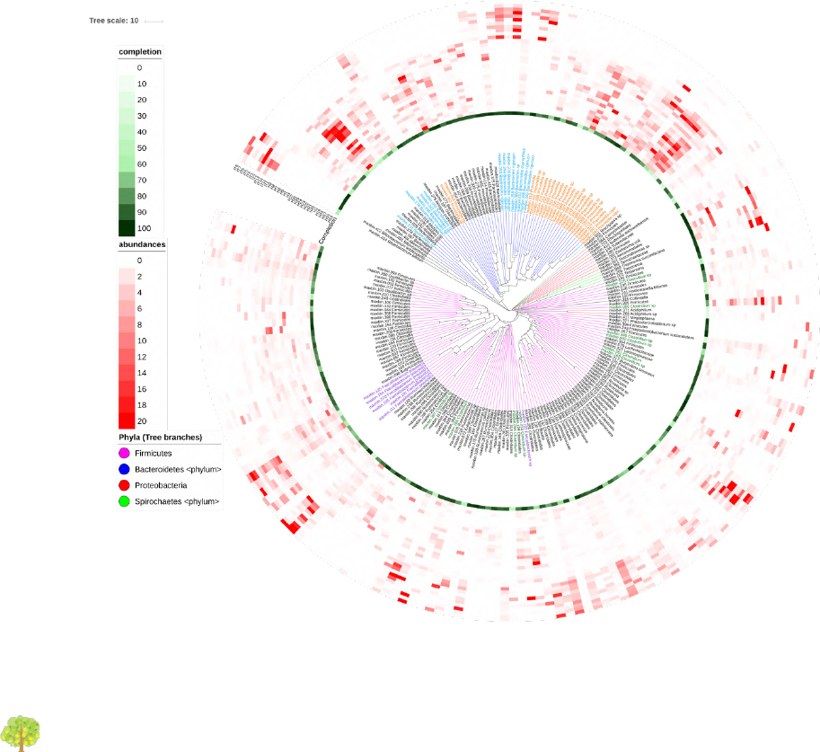
sqm2itol.pl

This program generates the files for creating a radial plot of abundances using iTOL

(https://itol.embl.de/), such as the ones below, taken from the SqueezeMeta paper:

SqueezeMeta v1.0beta

Figure 1: Taxonomic plot. Abundance of bins in the diverse samples.

Bins were compared with the CompareM software (https://github.com/dparks1134/CompareM) to

estimate their reciprocal similarities. The distances calculated between the bins were used to create a

phylogenetic tree illustrating their relationships. The tree is shown in the inner part of the Figure.

Branches in the tree corresponding to the four more abundant phyla in the tree (Firmicutes,

Bacteriodetes, Proteobacteria and Spirochaetes) were colored. Bins were named with their id number

and original genera, and labels for the most abundant genera were also colored.

Outer circles correspond to: the completeness of the bins (green-colored, most internal circle), and the

abundance of each bin in each sample (red-colored). Each circle corresponds to a different sample,

and the red color intensities correspond to the bin’s abundance in the sample.

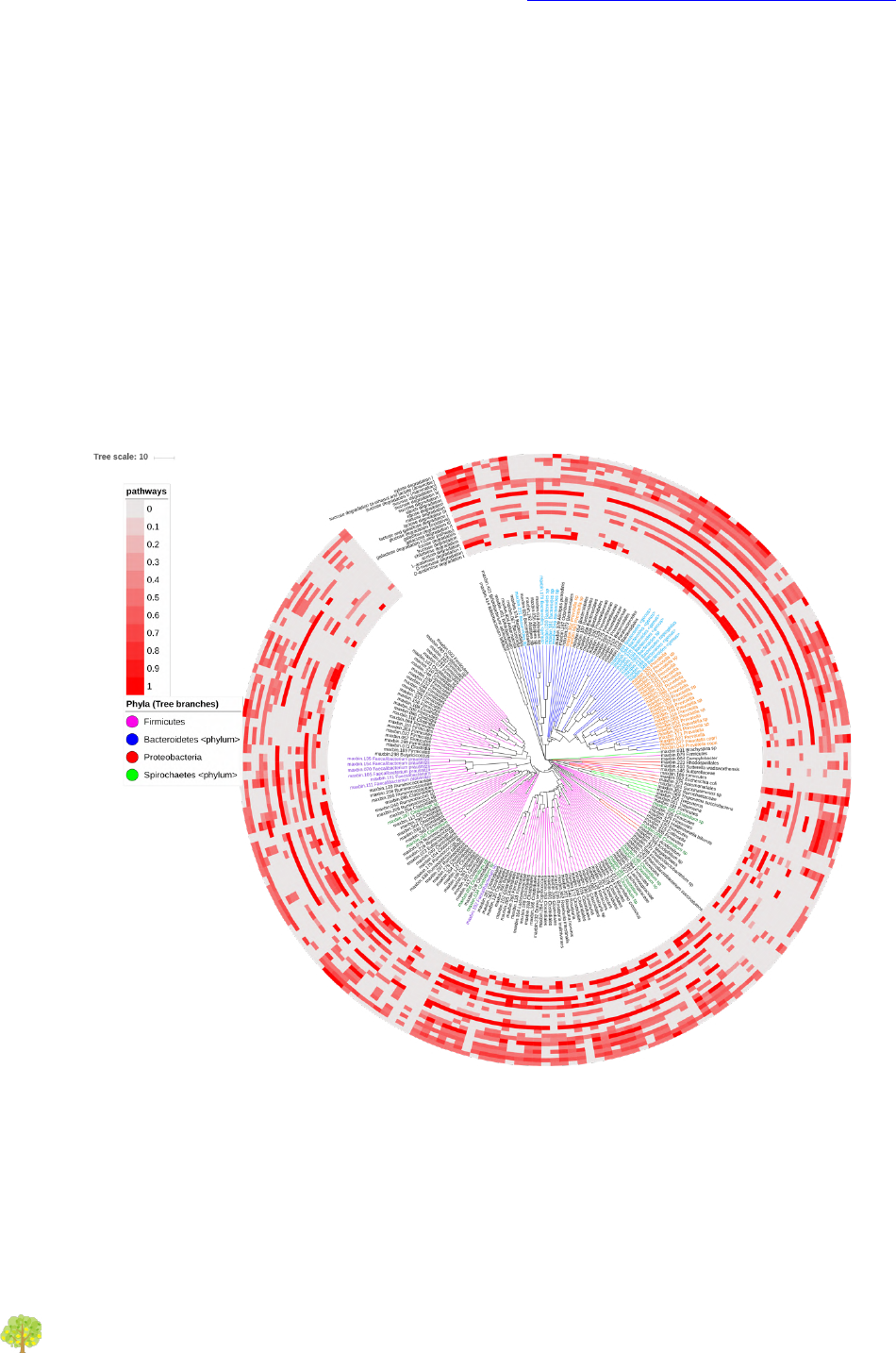
Figure 2: Functional plot. Presence of several carbohydrate degradation pathways in bins.

The outer circles indicate the percentage of genes from a pathway present in each of the bins. According

to that gene profile, MinPath estimates whether or not the pathway is present. Only pathways inferred to

be present are colored. As in Figure 1, the bins tree is performed from a distance matrix of the

orthologous genes’ amino acid identity, using the compareM software. The four most abundant phyla are

SqueezeMeta v1.0beta

colored (branches in the tree), as well as the most abundant genera (bin labels). The picture was

elaborated using the iTOL software.

Usage:

sqm2itol.pl <options> -p projectname

Arguments

• -p: Project name (REQUIRED). Containing a valid SqueezeMeta analysis

• -completion [percentage]: Select only bins with completion above that threshold

(default: 30)

• -contamination [percentage]: Select only bins with contamination below that

threshold (default: 100)

• -classification [metacyc|kegg]: Functional classification to use (default: metacyc)

• functions [file]: File containing the name of the functions to be considered (for

functional plots). For example:

arabinose degradation

galactose degradation

glucose degradation

The program will generate several datafiles that you must upload to iTOL to produce

the figure.

make-tables.py

This script generates tabular outputs, suitable for analysis in environments such as R,

from a SqueezeMeta run. It will aggregate the abundances of the ORFs assigned to the

same feature (be it a given taxon or a given function) and produce tables with features

in rows and samples in columns.

Usage:

make-tables.py [options] <project_name> <output_directory>

Arguments

SqueezeMeta v1.0beta

Mandatory parameters

• Project name (REQUIRED)

• Output directory

Options

• --ignore_unclassified: ignore ORFs with no functional classification when

aggregating abundances for functional categories (KO, COG, PFAM).

Output

• For each functional classification system (KO, COG, PFAM) the script will produce

the following files:

◦ <project_name>.<classification>.abunds.tsv: raw abundances of each

functional category in the different samples.

◦ <project_name>.<classification>.tpm.tsv: normalized (TPM) abundances of

each functional category in the different samples. This normalization takes

into account both sequencing depth and gene length.

▪ The --ignore_unclassified can be used to control whether unclassified ORFs

are counted towards the total for normalization.

• For each taxonomic rank (superkingdom, phylum, class, order, family, genus,

species) the script will produce the following files:

◦ <project_name>.<rank>.allfilter.abund.tsv: raw abundances of each taxon for

that taxonomic rank in the different samples, applying the identity filters for

taxonomic assignment (see explanation for LCA algoritm below)

◦ <project_name>.<rank>.allfilter.percent.tsv: percent abundances of each

taxon for that taxonomic rank in the different samples.

◦ taxon for that taxonomic rank in the different samples. Identity filters for

taxonomic assignment are applied to prokaryotic (bacteria + archaea) ORFs

but not to Eukaryotes (see below).

◦ <project_name>.<rank>.prokfilter.abund.tsv: percent abundances of each

taxon for that taxonomic rank in the different samples. Identity filters for

taxonomic assignment are applied to prokaryotic (bacteria + archaea) ORFs

but not to Eukaryotes (see below).

Details

SqueezeMeta v1.0beta

• By default, SqueezeMeta applies Luo’s et al (2014) identity cutoffs in order to

assign a ORF to a given taxonomic rank (see section XX LINK A LCA). In our tests,

these cutoffs resulted in a very low percentage of annotation for eukaryotic ORFs.

To circunvent this issue, the *.prokfilter.* files generated by this script contain

the aggregated taxonomic abundances obtained by applying Luo’s filter only to

Bacteria and Archaea, but not to Eukaryotes.

• SqueezeMeta uses NCBI’s nr database for taxonomic annotation, and reports the

superkingdom, phylum, class, order, family, genus and species ranks. In some

cases, the NCBI taxonomy is missing some intermediate ranks. For example, the

NCBI taxonomy for the order Trichomonadida is:

◦ superkingdom:Eukaryota

◦ no rank:Parabasalia

◦ order: Trichomonadida

NCBI does not assign Trichomonadida to any taxa in the class and phylum ranks.

For clarity, the make-tables.py will indicate this by recycling the highest

available taxonomy and adding the “(no <rank> in NCBI)” string after. For

example, ORFs that can be classified down to the Trichomonadida order (but are

unclassified at the family level) will be reported as:

In that example, the make-tables.py script would report the taxonomy as:

◦ superkingdom: Eukaryota

◦ phylum: Trichomonadida (no phylum in NCBI)

◦ class: Trichomonadida (no class in NCBI)

◦ order: Trichomonadida

◦ family: Unclassified Trichomonadida

◦ genus: Unclassified Trichomonadida

◦ species: Unclassified Trichomonadida

• Some ORFs will have multiple KEGG/COG annotations in the 13.*.orftable file.

This is due to their best hit in the KEGG/COG databases actually being annotated

with more than one function. The script will split the abundances of those ORFs

between the different functions they have been assigned to.

make-SqueezeMdb-files.py

Generates all the files required for loading a SqueezeMeta project into the web

interface (https://github.com/jtamames/SqueezeMdb).

Usage:

make-SqueezeMdb-files.py <project_name> <output_directory>

SqueezeMeta v1.0beta

Explanation of SqueezeMeta algorithms

The LCA algorithm

We use a Last Common Ancestor (LCA) algorithm to assign taxa to genes.

For the aminoacid sequence of each gene, diamond (blastp) homology searches are done

against the GenBank nr database (updated weekly). A e-value cutoff of 1e-03 is set by

default. The best hit is obtained, and then we select a range of hits (valid hits) having

at least 80% of the bitscore of the best hit and differing in less than 10% identity also

with the best hit (these values can be set). The LCA of all these hits is obtained, that is,

the taxon common to all hits. This LCA can be found at diverse taxonomic ranks (from

phylum to species). We allow some flexibility in the definition of LCA: a small number of

hits belonging to other taxa than the LCA can be allowed. In this way we deal with

putative transfer events, or incorrect annotations in the database. This value is by

default 10% of the total number of valid hits, but can be set by the user. Also, the

minimum number of hits to the LCA taxa can be set.

An example is shown in the next table:

GenID

Hit ID

Hit taxonomy

Identity

e-value

Gen1

Genus:Polaribacter

Family: Flavobacteriaceae

Order:Flavobacteriales

75.2

1e-94

Gen1

Genus:Polaribacter

Family: Flavobacteriaceae

Order:Flavobacteriales

71.3

6e-88

Gen1

Family: Flavobacteriaceae

Order:Flavobacteriales

70.4

2e-87

Gen1

Genus:Algibacter

Family: Flavobacteriaceae

Order:Flavobacteriales

68.0

2e-83

Gen1

Genus:Rhodospirillum

Family: Rhodospirillaceae

Order:Rhodospirillales

60.2

6e-68

In this case, the four first hits are the valid ones. Hit 5 does not make the identity and e-

value thresholds. The LCA for the four valid hits is Family: Flavobacteriaceae, that

would be the reported result.

SqueezeMeta v1.0beta

Our LCA algorithm includes strict cut-off identity values for different taxonomic ranks,

according to Luo et al, Nucleic Acids Research 2014, 42, e73. This means that hits must

pass a minimum (aminoacid) identity level in order to be used for assigning particular

taxonomic ranks. These thresholds are 85, 60, 55, 50, 46, 42 and 40% for species, genus,

family, order, class, phylum and superkingdom ranks, respectively. Hits below these

levels cannot be used to make assignments for the corresponding rank. For instance, a

protein will not be assigned to species level if it has no hits above 85% identity. Also, a

protein will remain unclassified if it has no hits above 40% identity. The inclusion of

these thresholds guarantees that no assignments are done based on weak, inconclusive

hits.

The fun3 algorithm

Fun3 is the algorithm that produces functional assignments (for COGs, KEGG and

external databases). It reads the Diamond Blastx output of the homology search of the

metagenomic genes for these databases. The homology search has been done with the

defined parameters of e-value and dentity, so that no hits below above the minimum e-

value or below the minimum identity are found. Also, partial hits (where query and hits

align in less than the percentage given by the user, 30% by default) are discarded. The

hits that pass the filters can correspond to more than one functional id (for instance,

COG or KEGG ID). Fun3 provides two types of classification: Best hit is just the

functional id of the highest scoring hit. Best average tries to evaluate also if that

functional id is significantly better than the rest. For that, it takes the first n hits

corresponding to each functional id (n set by the user, default is 5) and calculates their

average bitscore. The gene is assigned to the functional id with the highest average

bitscore that exceeds in a given percentage (given by the user, by default 10%) the

score of the second one. This method reports less assignments but it is also more

precise, avoiding confusions between closely related protein families.

A unique functional assignment, the best hit, is shown in the gene table. There, the

functional id is shown with a * symbol to indicate that the assignment is supported also

by the best average method.

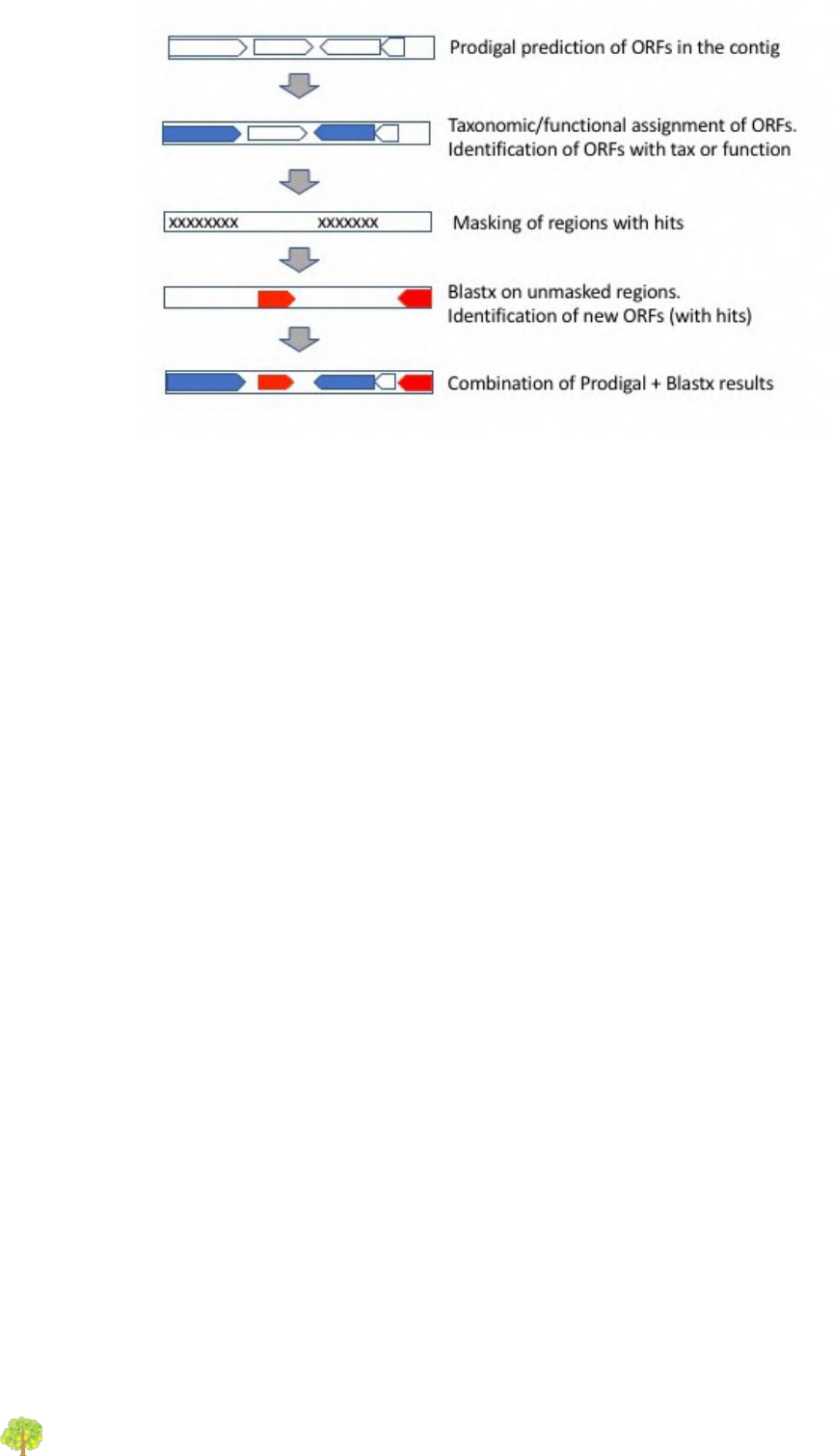
Doublepass: Blastx on contig gaps

The -D option activates the doublepass procedure, where regions of the contigs where no ORFs

where predicted, or where these ORFs could not be assigned taxonomically and functionally, are

queried against the databases using blastx. This method allows to recover putative ORFs missed

by Prodigal, or to correct wrongly predicted ORFs. The following figure illustrates the steps of

the doublepass procedure:

SqueezeMeta v1.0beta

Consensus taxonomic annotation for contigs and bins

The consensus algorithm attempts to obtain a consensus taxonomic annotation for the

contigs according to the annotations of each of its genes. The consensus taxon is the one

fulfilling:

-50% of the genes of the contig belong to (are annotated to) this taxon, and

-70% of the annotated genes belong to (are annotated to) this taxon.

Notice that the first criterion refers to all genes in the contig, regardless if they have

been annotated or not, while the second refers exclusively to annotated genes.

As the assignment can be done at different taxonomic ranks, the consensus is the

deepest taxon fulfilling the criteria above.

For instance, consider the following example for a contig with 6 genes:

Gen1: k_Bacteria;p_Proteobacteria;c_Gamma-Proteobacteria;o_Enterobacteriales;f_

Enterobacteriaceae;g_Escherichia;s_Escherichia coli

Gen2: k_Bacteria;p_Proteobacteria;c_Gamma-Proteobacteria;o_Enterobacteriales;f_

Enterobacteriaceae;g_Escherichia

Gen3: k_Bacteria;p_Proteobacteria;c_Gamma-Proteobacteria;o_Enterobacteriales;f_

Enterobacteriaceae;g_Escherichia

Gen4: k_Bacteria;p_Proteobacteria;c_Gamma-Proteobacteria;o_Enterobacteriales;f_

Enterobacteriaceae

SqueezeMeta v1.0beta

Gen5: No hits

Gen6: k_Bacteria;p_Firmicutes

In this case, the contig will be assigned to k_Bacteria;p_Proteobacteria;c_Gamma-

Proteobacteria;o_ Enterobacteriales;f_ Enterobacteriaceae, which is the deepest taxon

fulfilling 50% of all the genes belonging to that taxon (4/6=66%), and having 70% of the

annotated genes (4/5=80%). The assignment to genus Escherichia was not done since just

3/5=60% of the annotated genes belong to it, which is below the cutoff threshold.

For annotating the consensus of bins, the procedure is the same, but using the

annotations of the corresponding contigs instead.

Disparity calculation

Notice that in the example above, the end part of the contig seems to depart from the

common taxonomic origin of the rest. This can be due to misassembly resulting in

chimerism, or other causes such as a recent LCA transfer or a wrong annotation for the

gene. The disparity index attempts to measure this effect, so that the contigs can be

flagged accordingly (for instance, we could decide not trusting contigs with high

disparity).

Disparity index is calculated for the taxonomic rank assigned by consensus algorithm (in

the previous example, family). We compare the assignments at that level for every pair

of genes in the contig, and count the number of agreements and disagreements. If one

of the taxa has no annotation at that level, is not counted for agreement but it is

counted for disagreements if previous ranks do not coincide (we assume that if higher

ranks do not agree, lower ranks will not either). That is:

Gen1-Gen2: Agree

Gen1-Gen3: Agree

Gen1-Gen4: Agree

Gen1-Gen5: Unknown

Gen1-Gen6: Disagree (at phylum level)

Gen2-Gen3: Agree

Gen2-Gen4: Agree

Gen2-Gen5: Unknown

Gen2-Gen6: Disagree (at phylum level)

Gen3-Gen4: Agree

Gen3-Gen5: Unknown

Gen3-Gen6: Disagree (at phylum level)

Gen4-Gen5: Unknown

Gen4-Gen6: Disagree (at phylum level)

Gen5-Gen6: Unknown

SqueezeMeta v1.0beta

Disparity index is the ratio between the number of disagreements and the total number

of comparisons, in this case 4/15=0.26

For calculating the disparity of bins, the procedure is the same, just using the

annotations for the contigs belonging to the bin instead.

Squeeze Meta Manual V1.0.0beta

Navigation menu

Versions of this User Manual:

Views

Navigation