Big Data And Social Science (Statistics In The Behavioral Sciences Series) Ian Foster, Rayid Ghani, Ron S. Jarmin
(Statistics%20in%20the%20social%20and%20behavioral%20sciences%20series)%20Ian%20Foster%2C%20Rayid%20Ghani%2C%20Ron%20S.%20Jarmin
User Manual:
Open the PDF directly: View PDF ![]() .
.
Page Count: 377 [warning: Documents this large are best viewed by clicking the View PDF Link!]
- Cover
- Half Title
- Title
- Copyright
- Contents
- Preface
- Editors
- Contributors
- 1: Introduction
- I: Capture and Curation
- 2: Working with Web Data and APIs
- 2.1: Introduction
- 2.2: Scraping information from the web
- 2.3: New data in the research enterprise
- 2.4: A functional view
- 2.5: Programming against an API
- 2.6: Using the ORCID API via a wrapper
- 2.7: Quality, scope, and management
- 2.8: Integrating data from multiple sources
- 2.9: Working with the graph of relationships
- 2.10: Bringing it together: Tracking pathways to impact
- 2.11: Summary
- 2.12: Resources
- 2.13: Acknowledgements and copyright
- 3: Record Linkage
- 4: Databases
- 5: Programming with Big Data
- 2: Working with Web Data and APIs
- II: Modeling and Analysis
- 6: Machine Learning
- 6.1: Introduction
- 6.2: What is machine learning?
- 6.3: The machine learning process
- 6.4: Problem formulation: Mapping a problem to machine learning methods
- 6.5: Methods
- 6.6: Evaluation
- 6.7: Practical tips
- 6.8: How can social scientists benefit from machine learning?
- 6.9: Advanced topics
- 6.10: Summary
- 6.11: Resources
- 7: Text Analysis
- 8: Networks: The Basics
- 6: Machine Learning
- III: Inference and Ethics
- 9: Information Visualization
- 10: Errors and Inference
- 10.1: Introduction
- 10.2: The total error paradigm
- 10.3: Illustrations of errors in big data
- 10.4: Errors in big data analytics
- 10.5: Some methods for mitigating, detecting, and compensating for errors
- 10.6: Summary
- 10.7: Resources
- 11: Privacy and Confidentiality
- 12: Workbooks
- Bibliography�������������������
- Index������������

BIG DATA AND
SOCIAL SCIENCE
A Practical Guide to Methods and Tools

Statistics in the Social and Behavioral Sciences Series
Aims and scope
Large and complex datasets are becoming prevalent in the social and behavioral
sciences and statistical methods are crucial for the analysis and interpretation of such
data. This series aims to capture new developments in statistical methodology with
particular relevance to applications in the social and behavioral sciences. It seeks to
promote appropriate use of statistical, econometric and psychometric methods in
these applied sciences by publishing a broad range of reference works, textbooks and
handbooks.
The scope of the series is wide, including applications of statistical methodology in
sociology, psychology, economics, education, marketing research, political science,
criminology, public policy, demography, survey methodology and ofcial statistics. The
titles included in the series are designed to appeal to applied statisticians, as well as
students, researchers and practitioners from the above disciplines. The inclusion of real
examples and case studies is therefore essential.
Jeff Gill
Washington University, USA
Wim J. van der Linden
Pacic Metrics, USA
Steven Heeringa
University of Michigan, USA
J. Scott Long
Indiana University, USA
Series Editors
Chapman & Hall/CRC
Tom Snijders
Oxford University, UK
University of Groningen, NL
Published Titles
Analyzing Spatial Models of Choice and Judgment with R
David A. Armstrong II, Ryan Bakker, Royce Carroll, Christopher Hare, Keith T. Poole, and Howard Rosenthal
Analysis of Multivariate Social Science Data, Second Edition
David J. Bartholomew, Fiona Steele, Irini Moustaki, and Jane I. Galbraith
Latent Markov Models for Longitudinal Data
Francesco Bartolucci, Alessio Farcomeni, and Fulvia Pennoni
Statistical Test Theory for the Behavioral Sciences
Dato N. M. de Gruijter and Leo J. Th. van der Kamp
Multivariable Modeling and Multivariate Analysis for the Behavioral Sciences
Brian S. Everitt
Multilevel Modeling Using R
W. Holmes Finch, Jocelyn E. Bolin, and Ken Kelley
Big Data and Social Science: A Practical Guide to Methods and Tools
Ian Foster, Rayid Ghani, Ron S. Jarmin, Frauke Kreuter, and Julia Lane
Ordered Regression Models: Parallel, Partial, and Non-Parallel Alternatives
Andrew S. Fullerton and Jun Xu
Bayesian Methods: A Social and Behavioral Sciences Approach, Third Edition
Jeff Gill
Multiple Correspondence Analysis and Related Methods
Michael Greenacre and Jorg Blasius
Applied Survey Data Analysis
Steven G. Heeringa, Brady T. West, and Patricia A. Berglund
Informative Hypotheses: Theory and Practice for Behavioral and Social Scientists
Herbert Hoijtink
Generalized Structured Component Analysis: A Component-Based Approach to Structural Equation Modeling
Heungsun Hwang and Yoshio Takane
Bayesian Psychometric Modeling
Roy Levy and Robert J. Mislevy
Statistical Studies of Income, Poverty and Inequality in Europe: Computing and Graphics in R Using EU-SILC
Nicholas T. Longford
Foundations of Factor Analysis, Second Edition
Stanley A. Mulaik
Linear Causal Modeling with Structural Equations
Stanley A. Mulaik
Age–Period–Cohort Models: Approaches and Analyses with Aggregate Data
Robert M. O’Brien
Handbook of International Large-Scale Assessment: Background, Technical Issues, and Methods of Data
Analysis
Leslie Rutkowski, Matthias von Davier, and David Rutkowski
Generalized Linear Models for Categorical and Continuous Limited Dependent Variables
Michael Smithson and Edgar C. Merkle
Incomplete Categorical Data Design: Non-Randomized Response Techniques for Sensitive Questions in
Surveys
Guo-Liang Tian and Man-Lai Tang
Handbook of Item Response Theory, Volume 1: Models
Wim J. van der Linden
Handbook of Item Response Theory, Volume 2: Statistical Tools
Wim J. van der Linden
Handbook of Item Response Theory, Volume 3: Applications
Wim J. van der Linden
Computerized Multistage Testing: Theory and Applications
Duanli Yan, Alina A. von Davier, and Charles Lewis

Statistics in the Social and Behavioral Sciences Series
Chapman & Hall/CRC
BIG DATA AND
SOCIAL SCIENCE
A Practical Guide to Methods and Tools
Edited by
Ian Foster
University of Chicago
Argonne National Laboratory
Rayid Ghani
University of Chicago
Ron S. Jarmin
U.S. Census Bureau
Frauke Kreuter
University of Maryland
University of Manheim
Institute for Employment Research
Julia Lane
New York University
American Institutes for Research

CRC Press
Taylor & Francis Group
6000 Broken Sound Parkway NW, Suite 300
Boca Raton, FL 33487-2742
© 2017 by Taylor & Francis Group, LLC
CRC Press is an imprint of Taylor & Francis Group, an Informa business
No claim to original U.S. Government works
Printed on acid-free paper
Version Date: 20160414
International Standard Book Number-13: 978-1-4987-5140-7 (Hardback)
This book contains information obtained from authentic and highly regarded sources. Reasonable efforts have been made to publish reliable data and information, but
the author and publisher cannot assume responsibility for the validity of all materials or the consequences of their use. The authors and publishers have attempted to
trace the copyright holders of all material reproduced in this publication and apologize to copyright holders if permission to publish in this form has not been obtained.
If any copyright material has not been acknowledged please write and let us know so we may rectify in any future reprint.
Except as permitted under U.S. Copyright Law, no part of this book may be reprinted, reproduced, transmitted, or utilized in any form by any electronic, mechanical,
or other means, now known or hereafter invented, including photocopying, microfilming, and recording, or in any information storage or retrieval system, without
written permission from the publishers.
For permission to photocopy or use material electronically from this work, please access www.copyright.com (http://www.copyright.com/) or contact the Copyright
Clearance Center, Inc. (CCC), 222 Rosewood Drive, Danvers, MA 01923, 978-750-8400. CCC is a not-for-profit organization that provides licenses and registration for a
variety of users. For organizations that have been granted a photocopy license by the CCC, a separate system of payment has been arranged.
Trademark Notice: Product or corporate names may be trademarks or registered trademarks, and are used only for identification and explanation without intent to
infringe.
Library of Congress Cataloging‑in‑Publication Data
Names: Foster, Ian, 1959- editor.
Title: Big data and social science : a practical guide to methods and tools /
edited by Ian Foster, University of Chicago, Illinois, USA, Rayid Ghani,
University of Chicago, Illinois, USA, Ron S. Jarmin, U.S. Census Bureau,
USA, Frauke Kreuter, University of Maryland, USA, Julia Lane, New York
University, USA.
Description: Boca Raton, FL : CRC Press, [2017] | Series: Chapman & Hall/CRC
statistics in the social and behavioral sciences series | Includes
bibliographical references and index.
Identifiers: LCCN 2016010317 | ISBN 9781498751407 (alk. paper)
Subjects: LCSH: Social sciences--Data processing. | Social
sciences--Statistical methods. | Data mining. | Big data.
Classification: LCC H61.3 .B55 2017 | DDC 300.285/6312--dc23
LC record available at https://lccn.loc.gov/2016010317
Visit the Taylor & Francis Web site at
http://www.taylorandfrancis.com
and the CRC Press Web site at
http://www.crcpress.com

Contents
Preface xiii
Editors xv
Contributors xix
1 Introduction 1
1.1 Whythisbook?................................... 1
1.2 Defining big data and its value . . . . . . . . . . . . . . . . . . . . . . . . . . 3
1.3 Social science, inference, and big data . . . . . . . . . . . . . . . . . . . . . . 4
1.4 Social science, data quality, and big data . . . . . . . . . . . . . . . . . . . . 7
1.5 Newtoolsfornewdata............................... 9
1.6 Thebook’s“usecase” ............................... 10
1.7 The structure of the book . . . . . . . . . . . . . . . . . . . . . . . . . . . . . 13
1.7.1 Part I: Capture and curation . . . . . . . . . . . . . . . . . . . . . . . 13
1.7.2 Part II: Modeling and analysis . . . . . . . . . . . . . . . . . . . . . . . 15
1.7.3 Part III: Inference and ethics . . . . . . . . . . . . . . . . . . . . . . . 16
1.8 Resources...................................... 17
I Capture and Curation 21
2 Working with Web Data and APIs 23
Cameron Neylon
2.1 Introduction .................................... 23
2.2 Scraping information from the web . . . . . . . . . . . . . . . . . . . . . . . . 24
2.2.1 Obtaining data from the HHMI website . . . . . . . . . . . . . . . . . . 24
2.2.2 Limitsofscraping ............................. 30
2.3 New data in the research enterprise . . . . . . . . . . . . . . . . . . . . . . . 31
2.4 Afunctionalview.................................. 37
2.4.1 Relevant APIs and resources . . . . . . . . . . . . . . . . . . . . . . . 38
2.4.2 RESTful APIs, returned data, and Python wrappers . . . . . . . . . . . 38
2.5 Programming against an API . . . . . . . . . . . . . . . . . . . . . . . . . . . 41
vii

viii Contents
2.6 Using the ORCID API via a wrapper . . . . . . . . . . . . . . . . . . . . . . . . 42
2.7 Quality, scope, and management . . . . . . . . . . . . . . . . . . . . . . . . . 44
2.8 Integrating data from multiple sources . . . . . . . . . . . . . . . . . . . . . . 46
2.8.1 TheLagottoAPI .............................. 46
2.8.2 Working with a corpus . . . . . . . . . . . . . . . . . . . . . . . . . . . 52
2.9 Working with the graph of relationships . . . . . . . . . . . . . . . . . . . . . 58
2.9.1 Citation links between articles . . . . . . . . . . . . . . . . . . . . . . 58
2.9.2 Categories, sources, and connections . . . . . . . . . . . . . . . . . . . 60
2.9.3 Data availability and completeness . . . . . . . . . . . . . . . . . . . . 61
2.9.4 The value of sparse dynamic data . . . . . . . . . . . . . . . . . . . . . 62
2.10 Bringing it together: Tracking pathways to impact . . . . . . . . . . . . . . . 65
2.10.1 Network analysis approaches . . . . . . . . . . . . . . . . . . . . . . . 66
2.10.2 Future prospects and new data sources . . . . . . . . . . . . . . . . . 66
2.11 Summary...................................... 67
2.12 Resources...................................... 69
2.13 Acknowledgements and copyright . . . . . . . . . . . . . . . . . . . . . . . . . 70
3 Record Linkage 71
Joshua Tokle and Stefan Bender
3.1 Motivation ..................................... 71
3.2 Introduction to record linkage . . . . . . . . . . . . . . . . . . . . . . . . . . . 72
3.3 Preprocessing data for record linkage . . . . . . . . . . . . . . . . . . . . . . . 76
3.4 Indexingandblocking............................... 78
3.5 Matching ...................................... 80
3.5.1 Rule-based approaches . . . . . . . . . . . . . . . . . . . . . . . . . . 82
3.5.2 Probabilistic record linkage . . . . . . . . . . . . . . . . . . . . . . . . 83
3.5.3 Machine learning approaches to linking . . . . . . . . . . . . . . . . . 85
3.5.4 Disambiguating networks . . . . . . . . . . . . . . . . . . . . . . . . . 88
3.6 Classification.................................... 88
3.6.1 Thresholds ................................. 89
3.6.2 One-to-onelinks.............................. 90
3.7 Record linkage and data protection . . . . . . . . . . . . . . . . . . . . . . . . 91
3.8 Summary...................................... 92
3.9 Resources...................................... 92
4 Databases 93
Ian Foster and Pascal Heus
4.1 Introduction .................................... 93
4.2 DBMS:Whenandwhy............................... 94
4.3 RelationalDBMSs ................................. 100
4.3.1 Structured Query Language (SQL) . . . . . . . . . . . . . . . . . . . . 102
4.3.2 Manipulating and querying data . . . . . . . . . . . . . . . . . . . . . 102
4.3.3 Schema design and definition . . . . . . . . . . . . . . . . . . . . . . . 105

Contents ix
4.3.4 Loadingdata ................................ 107
4.3.5 Transactions and crash recovery . . . . . . . . . . . . . . . . . . . . . 108
4.3.6 Database optimizations . . . . . . . . . . . . . . . . . . . . . . . . . . 109
4.3.7 Caveats and challenges . . . . . . . . . . . . . . . . . . . . . . . . . . 112
4.4 Linking DBMSs and other tools . . . . . . . . . . . . . . . . . . . . . . . . . . 113
4.5 NoSQLdatabases ................................. 116
4.5.1 Challenges of scale: The CAP theorem . . . . . . . . . . . . . . . . . . 116
4.5.2 NoSQL and key–value stores . . . . . . . . . . . . . . . . . . . . . . . 117
4.5.3 Other NoSQL databases . . . . . . . . . . . . . . . . . . . . . . . . . . 119
4.6 Spatialdatabases ................................. 120
4.7 Whichdatabasetouse? .............................. 122
4.7.1 RelationalDBMSs ............................. 122
4.7.2 NoSQLDBMSs............................... 123
4.8 Summary...................................... 123
4.9 Resources...................................... 124
5 Programming with Big Data 125
Huy Vo and Claudio Silva
5.1 Introduction .................................... 125
5.2 The MapReduce programming model . . . . . . . . . . . . . . . . . . . . . . . 127
5.3 Apache Hadoop MapReduce . . . . . . . . . . . . . . . . . . . . . . . . . . . . 129
5.3.1 The Hadoop Distributed File System . . . . . . . . . . . . . . . . . . . 130
5.3.2 Hadoop: Bringing compute to the data . . . . . . . . . . . . . . . . . . 131
5.3.3 Hardware provisioning . . . . . . . . . . . . . . . . . . . . . . . . . . . 134
5.3.4 Programming language support . . . . . . . . . . . . . . . . . . . . . . 136
5.3.5 Faulttolerance............................... 137
5.3.6 Limitations of Hadoop . . . . . . . . . . . . . . . . . . . . . . . . . . . 137
5.4 ApacheSpark.................................... 138
5.5 Summary...................................... 141
5.6 Resources...................................... 143
II Modeling and Analysis 145
6 Machine Learning 147
Rayid Ghani and Malte Schierholz
6.1 Introduction .................................... 147
6.2 What is machine learning? . . . . . . . . . . . . . . . . . . . . . . . . . . . . 148
6.3 The machine learning process . . . . . . . . . . . . . . . . . . . . . . . . . . . 150
6.4 Problem formulation: Mapping a problem to machine learning methods . . . . 151
6.5 Methods....................................... 153
6.5.1 Unsupervised learning methods . . . . . . . . . . . . . . . . . . . . . . 153
6.5.2 Supervised learning . . . . . . . . . . . . . . . . . . . . . . . . . . . . 161

x Contents
6.6 Evaluation ..................................... 173
6.6.1 Methodology ................................ 173
6.6.2 Metrics ................................... 176
6.7 Practicaltips .................................... 180
6.7.1 Features .................................. 180
6.7.2 Machine learning pipeline . . . . . . . . . . . . . . . . . . . . . . . . . 181
6.7.3 Multiclass problems . . . . . . . . . . . . . . . . . . . . . . . . . . . . 181
6.7.4 Skewed or imbalanced classification problems . . . . . . . . . . . . . . 182
6.8 How can social scientists benefit from machine learning? . . . . . . . . . . . . 183
6.9 Advancedtopics .................................. 185
6.10 Summary...................................... 185
6.11 Resources...................................... 186
7 Text Analysis 187
Evgeny Klochikhin and Jordan Boyd-Graber
7.1 Understanding what people write . . . . . . . . . . . . . . . . . . . . . . . . . 187
7.2 Howtoanalyzetext ................................ 189
7.2.1 Processing text data . . . . . . . . . . . . . . . . . . . . . . . . . . . . 190
7.2.2 How much is a word worth? . . . . . . . . . . . . . . . . . . . . . . . . 192
7.3 Approaches and applications . . . . . . . . . . . . . . . . . . . . . . . . . . . 193
7.3.1 Topicmodeling............................... 193
7.3.1.1 Inferring topics from raw text . . . . . . . . . . . . . . . . . 194
7.3.1.2 Applications of topic models . . . . . . . . . . . . . . . . . . 197
7.3.2 Information retrieval and clustering . . . . . . . . . . . . . . . . . . . 198
7.3.3 Otherapproaches ............................. 205
7.4 Evaluation ..................................... 208
7.5 Textanalysistools ................................. 210
7.6 Summary...................................... 212
7.7 Resources...................................... 213
8 Networks: The Basics 215
Jason Owen-Smith
8.1 Introduction .................................... 215
8.2 Networkdata.................................... 218
8.2.1 Forms of network data . . . . . . . . . . . . . . . . . . . . . . . . . . . 218
8.2.2 Inducing one-mode networks from two-mode data . . . . . . . . . . . 220
8.3 Networkmeasures................................. 224
8.3.1 Reachability ................................ 224
8.3.2 Whole-network measures . . . . . . . . . . . . . . . . . . . . . . . . . 225
8.4 Comparing collaboration networks . . . . . . . . . . . . . . . . . . . . . . . . 234
8.5 Summary...................................... 238
8.6 Resources...................................... 239

Contents xi
III Inference and Ethics 241
9 Information Visualization 243
M. Adil Yalçın and Catherine Plaisant
9.1 Introduction .................................... 243
9.2 Developing effective visualizations . . . . . . . . . . . . . . . . . . . . . . . . 244
9.3 A data-by-tasks taxonomy . . . . . . . . . . . . . . . . . . . . . . . . . . . . . 249
9.3.1 Multivariatedata.............................. 249
9.3.2 Spatialdata................................. 251
9.3.3 Temporaldata ............................... 252
9.3.4 Hierarchicaldata.............................. 255
9.3.5 Networkdata................................ 257
9.3.6 Textdata .................................. 259
9.4 Challenges ..................................... 259
9.4.1 Scalability ................................. 260
9.4.2 Evaluation ................................. 261
9.4.3 Visualimpairment............................. 261
9.4.4 Visualliteracy ............................... 262
9.5 Summary...................................... 262
9.6 Resources...................................... 263
10 Errors and Inference 265
Paul P. Biemer
10.1 Introduction .................................... 265
10.2 The total error paradigm . . . . . . . . . . . . . . . . . . . . . . . . . . . . . . 266
10.2.1 The traditional model . . . . . . . . . . . . . . . . . . . . . . . . . . . 266
10.2.2 Extending the framework to big data . . . . . . . . . . . . . . . . . . . 273
10.3 Illustrations of errors in big data . . . . . . . . . . . . . . . . . . . . . . . . . 275
10.4 Errors in big data analytics . . . . . . . . . . . . . . . . . . . . . . . . . . . . 277
10.4.1 Errors resulting from volume, velocity, and variety, assuming perfect
veracity................................... 277
10.4.2 Errors resulting from lack of veracity . . . . . . . . . . . . . . . . . . . 279
10.4.2.1 Variable and correlated error . . . . . . . . . . . . . . . . . . 280
10.4.2.2 Models for categorical data . . . . . . . . . . . . . . . . . . . 282
10.4.2.3 Misclassification and rare classes . . . . . . . . . . . . . . . 283
10.4.2.4 Correlation analysis . . . . . . . . . . . . . . . . . . . . . . . 284
10.4.2.5 Regression analysis . . . . . . . . . . . . . . . . . . . . . . . 288
10.5 Some methods for mitigating, detecting, and compensating for errors . . . . . 290
10.6 Summary...................................... 295
10.7 Resources...................................... 296

xii Contents
11 Privacy and Confidentiality 299
Stefan Bender, Ron Jarmin, Frauke Kreuter, and Julia Lane
11.1 Introduction .................................... 299
11.2 Why is access important? . . . . . . . . . . . . . . . . . . . . . . . . . . . . . 303
11.3 Providingaccess .................................. 305
11.4 Thenewchallenges ................................ 306
11.5 Legal and ethical framework . . . . . . . . . . . . . . . . . . . . . . . . . . . . 308
11.6 Summary...................................... 310
11.7 Resources...................................... 311
12 Workbooks 313
Jonathan Scott Morgan, Christina Jones, and Ahmad Emad
12.1 Introduction .................................... 313
12.2 Environment .................................... 314
12.2.1 Running workbooks locally . . . . . . . . . . . . . . . . . . . . . . . . 314
12.2.2 Central workbook server . . . . . . . . . . . . . . . . . . . . . . . . . . 315
12.3 Workbookdetails.................................. 315
12.3.1 Social Media and APIs . . . . . . . . . . . . . . . . . . . . . . . . . . . 315
12.3.2Databasebasics .............................. 316
12.3.3DataLinkage................................ 316
12.3.4MachineLearning ............................. 317
12.3.5TextAnalysis................................ 317
12.3.6Networks .................................. 318
12.3.7Visualization ................................ 318
12.4 Resources...................................... 319
Bibliography 321
Index 349

Preface
The class on which this book is based was created in response to a
very real challenge: how to introduce new ideas and methodologies
about economic and social measurement into a workplace focused
on producing high-quality statistics. We are deeply grateful for the
inspiration and support of Census Bureau Director John Thompson
and Deputy Director Nancy Potok in designing and implementing
the class content and structure.
As with any book, there are many people to be thanked. We
are grateful to Christina Jones, Ahmad Emad, Josh Tokle from
the American Institutes for Research, and Jonathan Morgan from
Michigan State University, who, together with Alan Marco and Julie
Caruso from the US Patent and Trademark Office, Theresa Leslie
from the Census Bureau, Brigitte Raumann from the University of
Chicago, and Lisa Jaso from Summit Consulting, actually made the
class happen.
We are also grateful to the students of three “Big Data for Fed-
eral Statistics” classes in which we piloted this material, and to the
instructors and speakers beyond those who contributed as authors
to this edited volume—Dan Black, Nick Collier, Ophir Frieder, Lee
Giles, Bob Goerge, Laure Haak, Madian Khabsa, Jonathan Ozik,
Ben Shneiderman, and Abe Usher. The book would not exist with-
out them.
We thank Trent Buskirk, Davon Clarke, Chase Coleman, Ste-
phanie Eckman, Matt Gee, Laurel Haak, Jen Helsby, Madian Khabsa,
Ulrich Kohler, Charlotte Oslund, Rod Little, Arnaud Sahuguet, Tim
Savage, Severin Thaler, and Joe Walsh for their helpful comments
on drafts of this material.
We also owe a great debt to the copyeditor, Richard Leigh; the
project editor, Charlotte Byrnes; and the publisher, Rob Calver, for
their hard work and dedication.
xiii


Editors
Ian Foster is a Professor of Computer Science at the University of
Chicago and a Senior Scientist and Distinguished Fellow at Argonne
National Laboratory.
Ian has a long record of research contributions in high-perfor-
mance computing, distributed systems, and data-driven discovery.
He has also led US and international projects that have produced
widely used software systems and scientific computing infrastruc-
tures. He has published hundreds of scientific papers and six books
on these and other topics. Ian is an elected fellow of the Amer-
ican Association for the Advancement of Science, the Association
for Computing Machinery, and the British Computer Society. His
awards include the British Computer Society’s Lovelace Medal and
the IEEE Tsutomu Kanai award.
Rayid Ghani is the Director of the Center for Data Science and
Public Policy and a Senior Fellow at the Harris School of Public
Policy and the Computation Institute at the University of Chicago.
Rayid is a reformed computer scientist and wannabe social scientist,
but mostly just wants to increase the use of data-driven approaches
in solving large public policy and social challenges. He is also pas-
sionate about teaching practical data science and started the Eric
and Wendy Schmidt Data Science for Social Good Fellowship at the
University of Chicago that trains computer scientists, statisticians,
and social scientists from around the world to work on data science
problems with social impact.
Before joining the University of Chicago, Rayid was the Chief
Scientist of the Obama 2012 Election Campaign, where he focused
on data, analytics, and technology to target and influence voters,
donors, and volunteers. Previously, he was a Research Scientist
and led the Machine Learning group at Accenture Labs. Rayid did
his graduate work in machine learning at Carnegie Mellon Univer-
sity and is actively involved in organizing data science related con-
xv

xvi Editors
ferences and workshops. In his ample free time, Rayid works with
non-profits and government agencies to help them with their data,
analytics, and digital efforts and strategy.
Ron S. Jarmin is the Assistant Director for Research and Method-
ology at the US Census Bureau. He formerly was the Bureau’s Chief
Economist and Chief of the Center for Economic Studies and a Re-
search Economist. He holds a PhD in economics from the University
of Oregon and has published papers in the areas of industrial or-
ganization, business dynamics, entrepreneurship, technology and
firm performance, urban economics, data access, and statistical
disclosure avoidance. He oversees a broad research program in
statistics, survey methodology, and economics to improve economic
and social measurement within the federal statistical system.
Frauke Kreuter is a Professor in the Joint Program in Survey Meth-
odology at the University of Maryland, Professor of Methods and
Statistics at the University of Mannheim, and head of the statistical
methods group at the German Institute for Employment Research
in Nuremberg. Previously she held positions in the Department of
Statistics at the University of California Los Angeles (UCLA), and
the Department of Statistics at the Ludwig-Maximillian’s University
of Munich. Frauke serves on several advisory boards for National
Statistical Institutes around the world and within the Federal Sta-
tistical System in the United States. She recently served as the
co-chair of the Big Data Task Force of the American Association
for Public Opinion Research. She is a Gertrude Cox Award win-
ner, recognizing statisticians in early- to mid-career who have made
significant breakthroughs in statistical practice, and an elected fel-
low of the American Statistical Association. Her textbooks on Data
Analysis Using Stata and Practical Tools for Designing and Weighting
Survey Samples are used at universities worldwide, including Har-
vard University, Johns Hopkins University, Massachusetts Insti-
tute of Technology, Princeton University, and the University College
London. Her Massive Open Online Course in Questionnaire De-
sign attracted over 70,000 learners within the first year. Recently
Frauke launched the international long-distance professional edu-
cation program sponsored by the German Federal Ministry of Edu-
cation and Research in Survey and Data Science.

Editors xvii
Julia Lane is a Professor at the New York University Wagner Grad-
uate School of Public Service and at the NYU Center for Urban Sci-
ence and Progress, and she is a NYU Provostial Fellow for Innovation
Analytics.
Julia has led many initiatives, including co-founding the UMET-
RICS and STAR METRICS programs at the National Science Foun-
dation. She conceptualized and established a data enclave at
NORC/University of Chicago. She also co-founded the creation and
permanent establishment of the Longitudinal Employer-Household
Dynamics Program at the US Census Bureau and the Linked Em-
ployer Employee Database at Statistics New Zealand. Julia has
published over 70 articles in leading journals, including Nature and
Science, and authored or edited ten books. She is an elected fellow
of the American Association for the Advancement of Science and a
fellow of the American Statistical Association.


Contributors
Stefan Bender
Deutsche Bundesbank
Frankfurt, Germany
Paul P. Biemer
RTI International
Raleigh, NC, USA
University of North Carolina
Chapel Hill, NC, USA
Jordan Boyd-Graber
University of Colorado
Boulder, CO, USA
Ahmad Emad
American Institutes for Research
Washington, DC, USA
Pascal Heus
Metadata Technology North America
Knoxville, TN, USA
Christina Jones
American Institutes for Research
Washington, DC, USA
Evgeny Klochikhin
American Institutes for Research
Washington, DC, USA
Jonathan Scott Morgan
Michigan State University
East Lansing, MI, USA
Cameron Neylon
Curtin University
Perth, Australia
Jason Owen-Smith
University of Michigan
Ann Arbor, MI, USA
Catherine Plaisant
University of Maryland
College Park, MD, USA
Malte Schierholz
University of Mannheim
Mannheim, Germany
Claudio Silva
New York University
New York, NY, USA
Joshua Tokle
Amazon
Seattle, WA, USA
Huy Vo
City University of New York
New York, NY, USA
M. Adil Yalçın
University of Maryland
College Park, MD, USA
xix


Introduction
Chapter 1
This section provides a brief overview of the goals and structure of
the book.
1.1 Why this book?
The world has changed for empirical social scientists. The new types
of “big data” have generated an entire new research field—that of
data science. That world is dominated by computer scientists who
have generated new ways of creating and collecting data, developed
new analytical and statistical techniques, and provided new ways of
visualizing and presenting information. These new sources of data
and techniques have the potential to transform the way applied
social science is done.
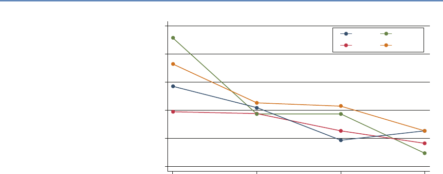
Research has certainly changed. Researchers draw on data that
are “found” rather than “made” by federal agencies; those publish-
ing in leading academic journals are much less likely today to draw
on preprocessed survey data (Figure 1.1).
The way in which data are used has also changed for both gov-
ernment agencies and businesses. Chief data officers are becoming
as common in federal and state governments as chief economists
were decades ago, and in cities like New York and Chicago, mayoral
offices of data analytics have the ability to provide rapid answers
to important policy questions [233]. But since federal, state, and
local agencies lack the capacity to do such analysis themselves [8],
they must make these data available either to consultants or to the
research community. Businesses are also learning that making ef-
fective use of their data assets can have an impact on their bottom
line [56].
And the jobs have changed. The new job title of “data scien-
tist” is highlighted in job advertisements on CareerBuilder.com and
Burning-glass.com—in the same category as statisticians, economists,
and other quantitative social scientists if starting salaries are useful
indicators.
1
2 1. Introduction
100
80
60
40
Micro-data Base Articles using Survey Data (%)
20
0
1980 1990
Note: “Pre-existing survey” data sets refer to micro surveys such as the CPS or
SIPP and do not include surveys designed by researchers for their study.
Sample excludes studies whose primary data source is from developing countries.
AER QJE
ECMA
JPE
2000
Year
2010
Figure 1.1. Use of pre-existing survey data in publications in leading journals,
1980–2010 [74]
The goal of this book is to provide social scientists with an un-
derstanding of the key elements of this new science, its value, and
the opportunities for doing better work. The goal is also to identify
the many ways in which the analytical toolkits possessed by social
scientists can be brought to bear to enhance the generalizability of
the work done by computer scientists.
We take a pragmatic approach, drawing on our experience of
working with data. Most social scientists set out to solve a real-
world social or economic problem: they frame the problem, identify
the data, do the analysis, and then draw inferences. At all points,
of course, the social scientist needs to consider the ethical ramifi-
cations of their work, particularly respecting privacy and confiden-
tiality. The book follows the same structure. We chose a particular
problem—the link between research investments and innovation—
because that is a major social science policy issue, and one in which
social scientists have been addressing using big data techniques.
While the example is specific and intended to show how abstract
concepts apply in practice, the approach is completely generaliz-
able. The web scraping, linkage, classification, and text analysis
methods on display here are canonical in nature. The inference

1.2. Defining big data and its value 3
and privacy and confidentiality issues are no different than in any
other study involving human subjects, and the communication of
results through visualization is similarly generalizable.
1.2 Defining big data and its value
There are almost as many definitions of big data as there are new
types of data. One approach is to define big data as anything too big ◮This topic is discussed in
more detail in Chapter 5.
to fit onto your computer. Another approach is to define it as data
with high volume, high velocity, and great variety. We choose the
description adopted by the American Association of Public Opinion
Research: “The term ‘Big Data’ is an imprecise description of a
rich and complicated set of characteristics, practices, techniques,
ethical issues, and outcomes all associated with data” [188].
The value of the new types of data for social science is quite
substantial. Personal data has been hailed as the “new oil” of the
twenty-first century, and the benefits to policy, society, and public
opinion research are undeniable [139]. Policymakers have found
that detailed data on human beings can be used to reduce crime,
improve health delivery, and manage cities better [205]. The scope
is broad indeed: one of this book’s editors has used such data to
not only help win political campaigns but also show its potential
for public policy. Society can gain as well—recent work shows data-
driven businesses were 5% more productive and 6% more profitable
than their competitors [56]. In short, the vision is that social sci-
ence researchers can potentially, by using data with high velocity,
variety, and volume, increase the scope of their data collection ef-
forts while at the same time reducing costs and respondent burden,
increasing timeliness, and increasing precision [265].
Example: New data enable new analyses
Spotshotter data, which have fairly detailed information for each gunfire incident,
such as the precise timestamp and the nearest address, as well as the type of
shot, can be used to improve crime data [63]; Twitter data can be used to improve
predictions around job loss, job gain, and job postings [17]; and eBay postings can
be used to estimate demand elasticities [104].
But most interestingly, the new data can change the way we
think about measuring and making inferences about behavior. For

4 1. Introduction
example, it enables the capture of information on the subject’s en-
tire environment—thus, for example, the effect of fast food caloric
labeling in health interventions [105]; the productivity of a cashier
if he is within eyesight of a highly productive cashier but not oth-
erwise [252]. So it offers the potential to understand the effects of
complex environmental inputs on human behavior. In addition, big
data, by its very nature, enables us to study the tails of a distribu-
tion in a way that is not possible with small data. Much of interest
in human behavior is driven by the tails of the distribution—health
care costs by small numbers of ill people [356], economic activity
and employment by a small number of firms [93,109]—and is impos-
sible to study with the small sample sizes available to researchers.
Instead we are still faced with the same challenges and respon-
sibilities as we were before in the survey and small data collection
environment. Indeed, social scientists have a great deal to offer to a
(data) world that is currently looking to computer scientists to pro-
vide answers. Two major areas to which social scientists can con-
tribute, based on decades of experience and work with end users,
are inference and attention to data quality.
1.3 Social science, inference, and big data
The goal of empirical social science is to make inferences about a
population from available data. That requirement exists regardless
of the data source—and is a guiding principle for this book. For
probability-based survey data, methodology has been developed to
overcome problems in the data generating process. A guiding prin-
ciple for survey methodologists is the total survey error framework,
and statistical methods for weighting, calibration, and other forms
of adjustment are commonly used to mitigate errors in the survey
process. Likewise for “broken” experimental data, techniques like
propensity score adjustment and principal stratification are widely
used to fix flaws in the data generating process. Two books provide
frameworks for survey quality [35, 143].
◮This topic is discussed in
more detail in Chapter 10.
Across the social sciences, including economics, public policy,
sociology, management, (parts of) psychology and the like, we can
identify three categories of analysis with three different inferential
goals: description, causation, and prediction.
Description The job of many social scientists is to provide descrip-
tive statements about the population of interest. These could be
univariate, bivariate, or even multivariate statements. Chapter 6

1.3. Social science, inference, and big data 5
on machine learning will cover methods that go beyond simple de-
scriptive statistics, known as unsupervised learning methods.
Descriptive statistics are usually created based on census data
or sample surveys to generate some summary statistics like a mean,
median, or a graphical distribution to describe the population of in-
terest. In the case of a census, the work ends right there. With
sample surveys the point estimates come with measures of uncer-
tainties (standard errors). The estimation of standard errors has
been worked out for most descriptive statistics and most common
survey designs, even complex ones that include multiple layers of
sampling and disproportional selection probabilities [154, 385].
Example: Descriptive statistics
The US Bureau of Labor Statistics surveys about 60,000 households a month and
from that survey is able to describe national employment and unemployment levels.
For example, in November 2015, total nonfarm payroll employment increased by
211,000 in November, and the unemployment rate was unchanged at 5.0%. Job
gains occurred in construction, professional and technical services, and health
care. Mining and information lost jobs [57].
Proper inference, even for purely descriptive purposes, from a
sample to the population rests usually on knowing that everyone
from the target population had the chance to be included in the
survey, and knowing the selection probability for each element in
the population. The latter does not necessarily need to be known
prior to sampling, but eventually a probability is assigned for each
case. Getting the selection probabilities right is particularly impor-
tant when reporting totals [243]. Unfortunately in practice, samples
that start out as probability samples can suffer from a high rate of
nonresponse. Because the survey designer cannot completely con-
trol which units respond, the set of units that ultimately respond
cannot be considered to be a probability sample [257]. Nevertheless,
starting with a probability sample provides some degree of comfort
that a sample will have limited coverage errors (nonzero probability
of being in the sample), and there are methods for dealing with a
variety of missing data problems [240].
Causation In many cases, social scientists wish to test hypotheses,
often originating in theory, about relationships between phenomena
of interest. Ideally such tests stem from data that allow causal infer-

6 1. Introduction
ence: typically randomized experiments or strong nonexperimental
study designs. When examining the effect of Xon Y, knowing how
cases were selected into the sample or data set is much less impor-
tant in the estimation of causal effects than for descriptive studies,
for example, population means. What is important is that all ele-
ments of the inferential population have a chance of being selected
for the treatment [179]. In the debate about probability and non-
probability surveys, this distinction is often overlooked. Medical
researchers have operated with unknown study selection mecha-
nisms for years: for example, randomized trials that enroll only
selected samples.
Example: New data and causal inference
One of the major risks with using big data without thinking about the data source
is the misallocation of resources. Overreliance on, say, Twitter data in targeting re-
sources after hurricanes can lead to the misallocation of resources towards young,
Internet-savvy people with cell phones, and away from elderly or impoverished
neighborhoods [340]. Of course, all data collection approaches have had similar
risks. Bad survey methodology led the Literary Digest to incorrectly call the 1936
election [353]. Inadequate understanding of coverage, incentive and quality issues,
together with the lack of a comparison group, has hampered the use of adminis-
trative records—famously in the case of using administrative records on crime to
make inference about the role of death penalty policy in crime reduction [95].
Of course, in practice it is difficult to ensure that results are
generalizable, and there is always a concern that the treatment
effect on the treated is different than the treatment effect in the
full population of interest [365]. Having unknown study selection
probabilities makes it even more difficult to estimate population
causal effects, but substantial progress is being made [99,261]. As
long as we are able to model the selection process, there is no reason
not to do causal inference from so-called nonprobability data.
Prediction Forecasting or prediction tasks are a little less common
among applied social science researchers as a whole, but are cer-
tainly an important element for users of official statistics—in partic-
ular, in the context of social and economic indicators—as generally
for decision-makers in government and business. Here, similar to
the causal inference setting, it is of utmost importance that we do
know the process that generated the data, and we can rule out any
unknown or unobserved systematic selection mechanism.

1.4. Social science, data quality, and big data 7
Example: Learning from the flu
“Five years ago [in 2009], a team of researchers from Google announced a remark-
able achievement in one of the world’s top scientific journals, Nature. Without
needing the results of a single medical check-up, they were nevertheless able to
track the spread of influenza across the US. What’s more, they could do it more
quickly than the Centers for Disease Control and Prevention (CDC). Google’s track-
ing had only a day’s delay, compared with the week or more it took for the CDC
to assemble a picture based on reports from doctors’ surgeries. Google was faster
because it was tracking the outbreak by finding a correlation between what people
searched for online and whether they had flu symptoms. . . .
“Four years after the original Nature paper was published, Nature News had
sad tidings to convey: the latest flu outbreak had claimed an unexpected victim:
Google Flu Trends. After reliably providing a swift and accurate account of flu
outbreaks for several winters, the theory-free, data-rich model had lost its nose for
where flu was going. Google’s model pointed to a severe outbreak but when the
slow-and-steady data from the CDC arrived, they showed that Google’s estimates
of the spread of flu-like illnesses were overstated by almost a factor of two.
“The problem was that Google did not know—could not begin to know—what
linked the search terms with the spread of flu. Google’s engineers weren’t trying to
figure out what caused what. They were merely finding statistical patterns in the
data. They cared about correlation rather than causation” [155].
1.4 Social science, data quality, and big data
Most data in the real world are noisy, inconsistent, and suffers from
missing values, regardless of its source. Even if data collection
is cheap, the costs of creating high-quality data from the source—
cleaning, curating, standardizing, and integrating—are substantial. ◮This topic is discussed in
more detail in Chapter 3.
Data quality can be characterized in multiple ways [76]:
•Accuracy: How accurate are the attribute values in the data?
•Completeness: Is the data complete?
•Consistency: How consistent are the values in and between
the database(s)?
•Timeliness: How timely is the data?
•Accessibility: Are all variables available for analysis?

8 1. Introduction
Social scientists have decades of experience in transforming
messy, noisy, and unstructured data into a well-defined, clearly
structured, and quality-tested data set. Preprocessing is a complex
and time-consuming process because it is “hands-on”—it requires
judgment and cannot be effectively automated. A typical workflow
comprises multiple steps from data definition to parsing and ends
with filtering. It is difficult to overstate the value of preprocessing
for any data analysis, but this is particularly true in big data. Data
need to be parsed, standardized, deduplicated, and normalized.
Parsing is a fundamental step taken regardless of the data source,
and refers to the decomposition of a complex variable into compo-
nents. For example, a freeform address field like “1234 E 56th St”
might be broken down into a street number “1234” and a street
name “E 56th St.” The street name could be broken down further
to extract the cardinal direction “E” and the designation “St.” An-
other example would be a combined full name field that takes the
form of a comma-separated last name, first name, and middle initial
as in “Miller, David A.” Splitting these identifiers into components
permits the creation of more refined variables that can be used in
the matching step.
In the simplest case, the distinct parts of a character field are
delimited. In the name field example, it would be easy to create the
separate fields “Miller” and “David A” by splitting the original field
at the comma. In more complex cases, special code will have to
be written to parse the field. Typical steps in a parsing procedure
include:
1. Splitting fields into tokens (words) on the basis of delimiters,
2. Standardizing tokens by lookup tables and substitution by a
standard form,
3. Categorizing tokens,
4. Identifying a pattern of anchors, tokens, and delimiters,
5. Calling subroutines according to the identified pattern, therein
mapping of tokens to the predefined components.
Standardization refers to the process of simplifying data by re-
placing variant representations of the same underlying observation
by a default value in order to improve the accuracy of field com-
parisons. For example, “First Street” and “1st St” are two ways of
writing the same street name, but a simple string comparison of
these values will return a poor result. By standardizing fields—and
1.5. New tools for new data 9
using the same standardization rules across files!—the number of
true matches that are wrongly classified as nonmatches (i.e., the
number of false nonmatches) can be reduced.
Some common examples of standardization are:
•Standardization of different spellings of frequently occurring
words: for example, replacing common abbreviations in street
names (Ave, St, etc.) or titles (Ms, Dr, etc.) with a common
form. These kinds of rules are highly country- and language-
specific.
•General standardization, including converting character fields
to all uppercase and removing punctuation and digits.
Deduplication consists of removing redundant records from a
single list, that is, multiple records from the same list that refer to
the same underlying entity. After deduplication, each record in the
first list will have at most one true match in the second list and vice
versa. This simplifies the record linkage process and is necessary if
the goal of record linkage is to find the best set of one-to-one links
(as opposed to a list of all possible links). One can deduplicate a list
by applying record linkage techniques described in this chapter to
link a file to itself.
Normalization is the process of ensuring that the fields that are
being compared across files are as similar as possible in the sense
that they could have been generated by the same process. At min-
imum, the same standardization rules should be applied to both
files. For additional examples, consider a salary field in a survey.
There are number different ways that salary could be recorded: it
might be truncated as a privacy-preserving measure or rounded to
the nearest thousand, and missing values could be imputed with
the mean or with zero. During normalization we take note of exactly
how fields are recorded.
1.5 New tools for new data
The new data sources that we have discussed frequently require
working at scales for which the social scientist’s familiar tools are
not designed. Fortunately, the wider research and data analytics
community has developed a wide variety of often more scalable and
flexible tools—tools that we will introduce within this book.
Relational database management systems (DBMSs) are used ◮This topic is discussed in
more detail in Chapter 4.
throughout business as well as the sciences to organize, process,
10 1. Introduction
and search large collections of structured data. NoSQL DBMSs are
used for data that is extremely large and/or unstructured, such as
collections of web pages, social media data (e.g., Twitter messages),
and clinical notes. Extensions to these systems and also special-
ized single-purpose DBMSs provide support for data types that are
not easily handled in statistical packages such as geospatial data,
networks, and graphs.
Open source programming systems such as Python (used ex-
tensively throughout this book) and R provide high-quality imple-
mentations of numerous data analysis and visualization methods,
from regression to statistics, text analysis, network analysis, and
much more. Finally, parallel computing systems such as Hadoop
and Spark can be used to harness parallel computer clusters for
extremely large data sets and computationally intensive analyses.
These various components may not always work together as
smoothly as do integrated packages such as SAS, SPSS, and Stata,
but they allow researchers to take on problems of great scale and
complexity. Furthermore, they are developing at a tremendous rate
as the result of work by thousands of people worldwide. For these
reasons, the modern social scientist needs to be familiar with their
characteristics and capabilities.
1.6 The book’s “use case”
This book is about the uses of big data in social science. Our focus
is on working through the use of data as a social scientist normally
approaches research. That involves thinking through how to use
such data to address a question from beginning to end, and thereby
learning about the associated tools—rather than simply engaging in
coding exercises and then thinking about how to apply them to a
potpourri of social science examples.
There are many examples of the use of big data in social science
research, but relatively few that feature all the different aspects
that are covered in this book. As a result, the chapters in the book
draw heavily on a use case based on one of the first large-scale big
data social science data infrastructures. This infrastructure, based
on UMETRICS*data housed at the University of Michigan’s Insti-
⋆UMETRICS: Universi-
ties Measuring the Impact
of Research on Innovation
and Science [228]
tute for Research on Innovation and Science (IRIS) and enhanced
◮iris.isr.umich.edu with data from the US Census Bureau, provides a new quantitative
analysis and understanding of science policy based on large-scale
computational analysis of new types of data.

1.6. The book’s “use case” 11
The infrastructure was developed in response to a call from the
President’s Science Advisor (Jack Marburger) for a science of science
policy [250]. He wanted a scientific response to the questions that
he was asked about the impact of investments in science.
Example: The Science of Science Policy
Marburger wrote [250]: “How much should a nation spend on science? What
kind of science? How much from private versus public sectors? Does demand for
funding by potential science performers imply a shortage of funding or a surfeit
of performers? These and related science policy questions tend to be asked and
answered today in a highly visible advocacy context that makes assumptions that
are deserving of closer scrutiny. A new ‘science of science policy’ is emerging, and
it may offer more compelling guidance for policy decisions and for more credible
advocacy. . . .
“Relating R&D to innovation in any but a general way is a tall order, but not
a hopeless one. We need econometric models that encompass enough variables
in a sufficient number of countries to produce reasonable simulations of the effect
of specific policy choices. This need won’t be satisfied by a few grants or work-
shops, but demands the attention of a specialist scholarly community. As more
economists and social scientists turn to these issues, the effectiveness of science
policy will grow, and of science advocacy too.”
Responding to this policy imperative is a tall order, because it in-
volves using all the social science and computer science tools avail-
able to researchers. The new digital technologies can be used to
capture the links between the inputs into research, the way in which
those inputs are organized, and the subsequent outputs [396,415].
The social science questions that are addressable with this data in-
frastructure include the effect of research training on the placement
and earnings of doctoral recipients, how university trained scien-
tists and engineers affect the productivity of the firms they work for,
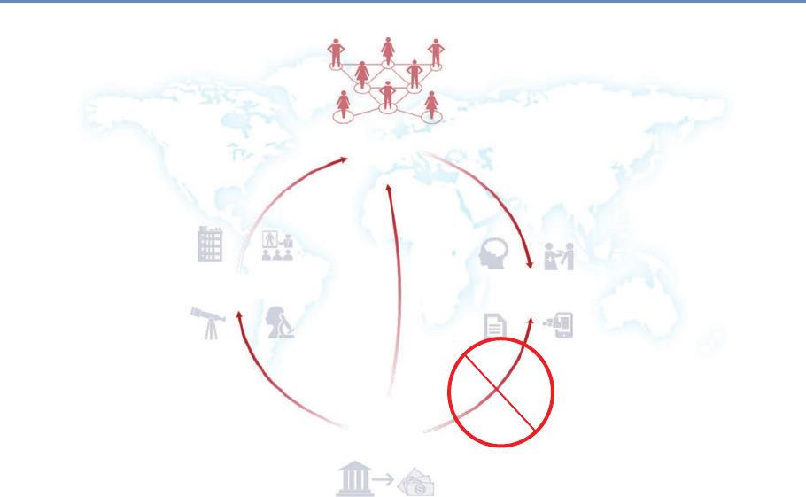
and the return on investments in research. Figure 1.2 provides an
abstract representation of the empirical approach that is needed:
data about grants, the people who are funded on grants, and the
subsequent scientific and economic activities.
First, data must be captured on what is funded, and since the
data are in text format, computational linguistics tools must be
applied (Chapter 7). Second, data must be captured on who is
funded, and how they interact in teams, so network tools and ana-
lysis must be used (Chapter 8). Third, information about the type of
results must be gleaned from the web and other sources (Chapter 2).
12 1. Introduction
Co-Author Collaborate
Train
Pays for &
Is Awarded to
People
Funding
Institutions Products
E
m
p
l
o
y
A
w
a
r
d
e
d
t
o
S
u
p
p
o
r
t
s
P
r
o
d
u
c
e
&
u
s
e
Figure 1.2. A visualization of the complex links between what and who is funded, and the results; tracing the direct
link between funding and results is misleading and wrong
Finally, the disparate complex data sets need to be stored in data-
bases (Chapter 4), integrated (Chapter 3), analyzed (Chapter 6), and
used to make inferences (Chapter 10).
The use case serves as the thread that ties many of the ideas
together. Rather than asking the reader to learn how to code “hello
world,” we build on data that have been put together to answer a
real-world question, and provide explicit examples based on that
data. We then provide examples that show how the approach gen-
eralizes.
For example, the text analysis chapter (Chapter 7) shows how
to use natural language processing to describe what research is
being done, using proposal and award text to identify the research
topics in a portfolio [110, 368]. But then it also shows how the
approach can be used to address a problem that is not just limited
to science policy—the conversion of massive amounts of knowledge
that is stored in text to usable information.

1.7. The structure of the book 13
Similarly, the network analysis chapter (Chapter 8) gives specific
examples using the UMETRICS data and shows how such data can
be used to create new units of analysis—the networks of researchers
who do science, and the networks of vendors who supply research
inputs. It also shows how networks can be used to study a wide
variety of other social science questions.
In another example, we use APIs*provided by publishers to de- ⋆Application Programming
Interfaces
scribe the results generated by research funding in terms of pub-
lications and other measures of scientific impact, but also provide
code that can be repurposed for many similar APIs.
And, of course, since all these new types of data are provided
in a variety of different formats, some of which are quite large (or
voluminous), and with a variety of different timestamps (or velocity),
we discuss how to store the data in different types of data formats.
1.7 The structure of the book
We organize the book in three parts, based around the way social
scientists approach doing research. The first set of chapters ad-
dresses the new ways to capture, curate, and store data. The sec-
ond set of chapters describes what tools are available to process and
classify data. The last set deals with analysis and the appropriate
handling of data on individuals and organizations.
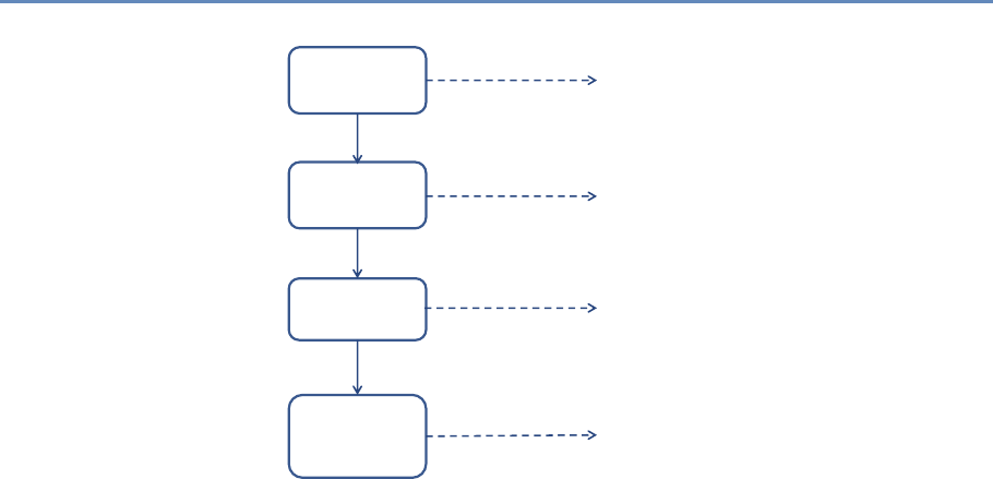
1.7.1 Part I: Capture and curation
The four chapters in Part I (see Figure 1.3) tell you how to capture
and manage data.
Chapter 2 describes how to extract information from social me-
dia about the transmission of knowledge. The particular applica-
tion will be to develop links to authors’ articles on Twitter using
PLOS articles and to pull information about authors and articles
from web sources by using an API. You will learn how to retrieve
link data from bookmarking services, citations from Crossref, links
from Facebook, and information from news coverage. In keep-
ing with the social science grounding that is a core feature of the
book, the chapter discusses what data can be captured from online
sources, what is potentially reliable, and how to manage data quality
issues.
Big data differs from survey data in that we must typically com-
bine data from multiple sources to get a complete picture of the
activities of interest. Although computer scientists may sometimes
14 1. Introduction
API and Web
Scraping
Record
Linkage
Storing Data
Processing
Large
Data Sets
Chapter 2: Dierent ways of collecting data
Chapter 3: Combining dierent data sets
Chapter 4: Ingest, query and export data
Chapter 5: Output (creating innovation measures)
Figure 1.3. The four chapters of Part I focus on data capture and curation
simply “mash” data sets together, social scientists are rightfully
concerned about issues of missing links, duplicative links, and
erroneous links. Chapter 3 provides an overview of traditional
rule-based and probabilistic approaches to data linkage, as well
as the important contributions of machine learning to the linkage
problem.
Once data have been collected and linked into different files, it
is necessary to store and organize it. Social scientists are used to
working with one analytical file, often in statistical software tools
such as SAS or Stata. Chapter 4, which may be the most impor-
tant chapter in the book, describes different approaches to stor-
ing data in ways that permit rapid and reliable exploration and
analysis.
Big data is sometimes defined as data that are too big to fit onto
the analyst’s computer. Chapter 5 provides an overview of clever
programming techniques that facilitate the use of data (often using
parallel computing). While the focus is on one of the most widely
used big data programming paradigms and its most popular imple-
mentation, Apache Hadoop, the goal of the chapter is to provide a
conceptual framework to the key challenges that the approach is
designed to address.
1.7. The structure of the book 15
Machine
Learning
Text
Analysis
Networks
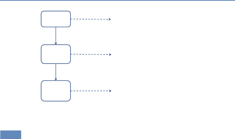
Chapter 6: Classifying data in new ways
Chapter 7: Creating new data from text
Chapter 8: Creating new measures of
social and economic activity
Figure 1.4. The four chapters in Part II focus on data modeling and analysis
1.7.2 Part II: Modeling and analysis
The three chapters in Part II (see Figure 1.4) introduce three of the
most important tools that can be used by social scientists to do new
and exciting research: machine learning, text analysis, and social
network analysis.
Chapter 6 introduces machine learning methods. It shows the
power of machine learning in a variety of different contexts, par-
ticularly focusing on clustering and classification. You will get an
overview of basic approaches and how those approaches are applied.
The chapter builds from a conceptual framework and then shows
you how the different concepts are translated into code. There is
a particular focus on random forests and support vector machine
(SVM) approaches.
Chapter 7 describes how social scientists can make use of one of
the most exciting advances in big data—text analysis. Vast amounts
of data that are stored in documents can now be analyzed and
searched so that different types of information can be retrieved.
Documents (and the underlying activities of the entities that gener-
ated the documents) can be categorized into topics or fields as well
as summarized. In addition, machine translation can be used to
compare documents in different languages.
16 1. Introduction
Social scientists are typically interested in describing the activi-
ties of individuals and organizations (such as households and firms)
in a variety of economic and social contexts. The frames within
which data are collected have typically been generated from tax or
other programmatic sources. The new types of data permit new
units of analysis—particularly network analysis—largely enabled by
advances in mathematical graph theory. Thus, Chapter 8 describes
how social scientists can use network theory to generate measurable
representations of patterns of relationships connecting entities. As
the author points out, the value of the new framework is not only in
constructing different right-hand-side variables but also in study-
ing an entirely new unit of analysis that lies somewhere between
the largely atomistic actors that occupy the markets of neo-classical
theory and the tightly managed hierarchies that are the traditional
object of inquiry of sociologists and organizational theorists.
1.7.3 Part III: Inference and ethics
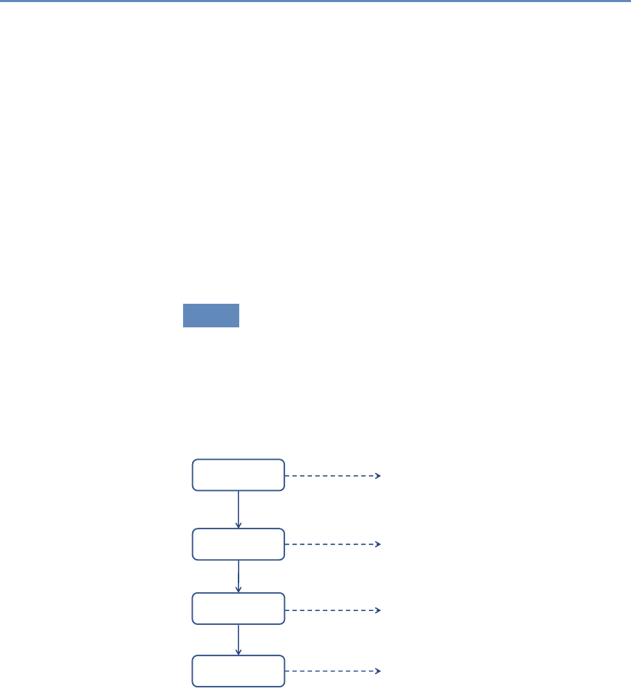
The four chapters in Part III (see Figure 1.5) cover three advanced
topics relating to data inference and ethics—information visualiza-
tion, errors and inference, and privacy and confidentiality—and in-
troduce the workbooks that provide access to the practical exercises
associated with the text.
Visualization
Inference
Privacy and
Condentiality
Chapter 9: Making sense of the data
Chapter 10: Drawing statistically valid conclusions
Chapter 11: Handling data appropriately
Chapter 12: Applying new models and tools
Workbooks
Figure 1.5. The four chapters in Part III focus on inference and ethics

1.8. Resources 17
Chapter 9 introduces information visualization methods and de-
scribes how you can use those methods to explore data and com-
municate results so that data can be turned into interpretable, ac-
tionable information. There are many ways of presenting statis-
tical information that convey content in a rigorous manner. The
goal of this chapter is to explore different approaches and exam-
ine the information content and analytical validity of the different
approaches. It provides an overview of effective visualizations.
Chapter 10 deals with inference and the errors associated with
big data. Social scientists know only too well the cost associated
with bad data—we highlighted the classic Literary Digest example
in the introduction to this chapter, as well as the more recent Google
Flu Trends. Although the consequences are well understood, the
new types of data are so large and complex that their properties
often cannot be studied in traditional ways. In addition, the data
generating function is such that the data are often selective, in-
complete, and erroneous. Without proper data hygiene, errors can
quickly compound. This chapter provides a systematic way to think
about the error framework in a big data setting.
Chapter 11 addresses the issue that sits at the core of any study
of human beings—privacy and confidentiality. In a new field, like the
one covered in this book, it is critical that many researchers have
access to the data so that work can be replicated and built on—that
there be a scientific basis to data science. Yet the rules that social
scientists have traditionally used for survey data, namely anonymity
and informed consent, no longer apply when the data are collected
in the wild. This concluding chapter identifies the issues that must
be addressed for responsible and ethical research to take place.
Finally, Chapter 12 provides an overview of the practical work
that accompanies each chapter—the workbooks that are designed,
using Jupyter notebooks, to enable students and interested prac- ◮See jupyter.org.
titioners to apply the new techniques and approaches in selected
chapters. We hope you have a lot of fun with them.
1.8 Resources
For more information on the science of science policy, see Husbands
et al.’s book for a full discussion of many issues [175] and the online
resources at the eponymous website [352].
This book is above all a practical introduction to the methods and
tools that the social scientist can use to make sense of big data,
and thus programming resources are also important. We make

18 1. Introduction
extensive use of the Python programming language and the MySQL
database management system in both the book and its supporting
workbooks. We recommend that any social scientist who aspires
to work with large data sets become proficient in the use of these
two systems, and also one more, GitHub. All three, fortunately, are
quite accessible and are supported by excellent online resources.
Time spent mastering them will be repaid many times over in more
productive research.
For Python, Alex Bell’s Python for Economists (available online
◮Read this! http://bit.ly/
1VgytVV [31]) provides a wonderful 30-page introduction to the use of Python
in the social sciences, complete with XKCD cartoons. Economists
Tom Sargent and John Stachurski provide a very useful set of lec-
tures and examples at http://quant-econ.net/. For more detail, we
recommend Charles Severance’s Python for Informatics: Exploring
Information [338], which not only covers basic Python but also pro-
vides material relevant to web data (the subject of Chapter 2) and
MySQL (the subject of Chapter 4). This book is also freely available
online and is supported by excellent online lectures and exercises.
For MySQL, Chapter 4 provides introductory material and point-
ers to additional resources, so we will not say more here.
We also recommend that you master GitHub. A version control
system is a tool for keeping track of changes that have been made
to a document over time. GitHub is a hosting service for projects
that use the Git version control system. As Strasser explains [363],
Git/GitHub makes it straightforward for researchers to create digi-
tal lab notebooks that record the data files, programs, papers, and
other resources associated with a project, with automatic tracking
of the changes that are made to those resources over time. GitHub
also makes it easy for collaborators to work together on a project,
whether a program or a paper: changes made by each contribu-
tor are recorded and can easily be reconciled. For example, we
used GitHub to create this book, with authors and editors check-
ing in changes and comments at different times and from many time
zones. We also use GitHub to provide access to the supporting work-
books. Ram [314] provides a nice description of how Git/GitHub can
be used to promote reproducibility and transparency in research.
One more resource that is outside the scope of this book but that
you may well want to master is the cloud [21,236]. It used to be that
when your data and computations became too large to analyze on
your laptop, you were out of luck unless your employer (or a friend)
had a larger computer. With the emergence of cloud storage and
computing services from the likes of Amazon Web Services, Google,
and Microsoft, powerful computers are available to anyone with a


Working with Web Data and APIs
Chapter 2
Cameron Neylon
This chapter will show you how to extract information from social
media about the transmission of knowledge. The particular appli-
cation will be to develop links to authors’ articles on Twitter using
PLOS articles and to pull information using an API. You will get link
data from bookmarking services, citations from Crossref, links from
Facebook, and information from news coverage. The examples that
will be used are from Twitter. In keeping with the social science
grounding that is a core feature of the book, it will discuss what can
be captured, what is potentially reliable, and how to manage data
quality issues.
2.1 Introduction
A tremendous lure of the Internet is the availability of vast amounts
of data on businesses, people, and their activity on social media.
But how can we capture the information and make use of it as we
might make use of more traditional data sources? In this chapter,
we begin by describing how web data can be collected, using the
use case of UMETRICS and research output as a readily available
example, and then discuss how to think about the scope, coverage,
and integration issues associated with its collection.
Often a big data exploration starts with information on people or
on a group of people. The web can be a rich source of additional in-
formation. It can also act as pointers to new sources of information,
allowing a pivot from one perspective to another, from one kind of
query to another. Often this is exploratory. You have an existing
core set of data and are looking to augment it. But equally this
exploration can open up whole new avenues. Sometimes the data
are completely unstructured, existing as web pages spread across a
23

24 2. Working with Web Data and APIs
site, and sometimes they are provided in a machine-readable form.
The challenge is in having a sufficiently diverse toolkit to bring all
of this information together.
Using the example of data on researchers and research outputs,
we will explore obtaining information directly from web pages (web
scraping) as well as explore the uses of APIs—web services that allow
an interaction with, and retrieval of, structured data. You will see
how the crucial pieces of integration often lie in making connections
between disparate data sets and how in turn making those connec-
tions requires careful quality control. The emphasis throughout
this chapter is on the importance of focusing on the purpose for
which the data will be used as a guide for data collection. While
much of this is specific to data about research and researchers, the
ideas are generalizable to wider issues of data and public policy.
2.2 Scraping information from the web
With the range of information available on the web, our first ques-
tion is how to access it. The simplest approach is often to manually
go directly to the web and look for data files or other information.
For instance, on the NSF website [268] it is possible to obtain data
dumps of all grant information. Sometimes data are available only
on web pages or we only want a subset of this information. In this
case web scraping is often a viable approach.
Web scraping involves using a program to download and process
web pages directly. This can be highly effective, particularly where
tables of information are made available online. It is also useful in
cases where it is desirable to make a series of very similar queries.
In each case we need to look at the website, identify how to get the
information we want, and then process it. Many websites deliber-
ately make this difficult to prevent easy access to their underlying
data.
2.2.1 Obtaining data from the HHMI website
Let us suppose we are interested in obtaining information on those
investigators that are funded by the Howard Hughes Medical Insti-
tute (HHMI). HHMI has a website that includes a search function
for funded researchers, including the ability to filter by field, state,
and role. But there does not appear to be a downloadable data set
of this information. However, we can automate the process with
code to create a data set that you might compare with other data.

2.2. Scraping information from the web 25
This process involves first understanding how to construct a URL
that will do the search we want. This is most easily done by playing
with search functionality and investigating the URL structures that
are returned. Note that in many cases websites are not helpful
here. However, with HHMI if we do a general search and play with
the structure of the URL, we can see some of the elements of the URL
that we can think of as a query. As we want to see all investigators,
we do not need to limit the search, and so with some fiddling we
come up with a URL like the following. (We have broken the one-line
URL into three lines for ease of presentation.)
http://www.hhmi.org/scientists/browse?
kw=&sort_by=field_scientist_last_name&
sort_order=ASC&items_per_page=20&page=0
The requests module, available natively in Jupyter Python note-
books, is a useful set of tools for handling interactions with web-
sites. It lets us construct the request that we just presented in
terms of a base URL and query terms, as follows:
>> BASE_URL = "http://www.hhmi.org/scientists/browse"
>> query = {
"kw" :"",
"sort_by" :"field_scientist_last_name",
"sort_order" :"ASC",
"items_per_page" : 20,
"page" : None
}
With our request constructed we can then make the call to the
web page to get a response.
>> import requests
>> response = requests.get(BASE_URL, params=query)
The first thing to do when building a script that hits a web page
is to make sure that your call was successful. This can be checked
by looking at the response code that the web server sent—and, obvi-
ously, by checking the actual HTML that was returned. A 200 code
means success and that everything should be OK. Other codes may
mean that the URL was constructed wrongly or that there was a
server error.
>> response.status_code
200
With the page successfully returned, we now need to process
the text it contains into the data we want. This is not a trivial
exercise. It is possible to search through and find things, but there
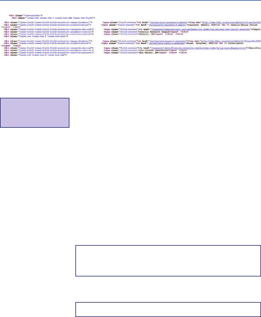
26 2. Working with Web Data and APIs
Figure 2.1. Source HTML from the portion of an HHMI results page containing information on HHMI investigators;
note that the webscraping results in badly formatted html which is difficult to read.
are a range of tools that can help with processing HTML and XML
data. Among these one of the most popular is a module called
BeautifulSoup*[319], which provides a number of useful functions
⋆Python features many
useful libraries; Beautiful-
Soup is particularly helpful
for webscraping.
for this kind of processing. The module documentation provides
more details.
We need to check the details of the page source to find where the
information we are looking for is kept (see, for example, Figure 2.1).
Here, all the details on HHMI investigators can be found in a <div>
element with the class attribute view-content. This structure is not
something that can be determined in advance. It requires knowl-
edge of the structure of the page itself. Nested inside this <div>
element are another series of divs, each of which corresponds to
one investigator. These have the class attribute view-rows. Again,
there is nothing obvious about finding these, it requires a close ex-
amination of the page HTML itself for any specific case you happen
to be looking at.
We first process the page using the BeautifulSoup module (into
the variable soup) and then find the div element that holds the
information on investigators (investigator_list). As this element
is unique on the page (I checked using my web browser), we can
use the find method. We then process that div (using find_all) to
create an iterator object that contains each of the page segments
detailing a single investigator (investigators).
>> from bs4 import BeautifulSoup
>> soup = BeautifulSoup(response.text, "html5lib")
>> investigator_list = soup.find(’div’, class_ = "view-content")
>> investigators = investigator_list.find_all("div", class_ = "
views-row")
As we specified in our query parameters that we wanted 20 res-
ults per page, we should check whether our list of page sections has
the right length.
>> len(investigators)
20

2.2. Scraping information from the web 27
# Given a request response object, parse for HHMI investigators
def scrape(page_response):
# Obtain response HTML and the correct <div> from the page
soup = BeautifulSoup(response.text, "html5lib")
inv_list = soup.find('div', class_ = "view-content")
# Create a list of all the investigators on the page
investigators = inv_list.find_all("div", class_ = "views-row")
data = [] # Make the data object to store scraping results
# Scrape needed elements from investigator list
for investigator in investigators:
inv = {} # Create a dictionary to store results
# Name and role are in same HTML element; this code
# separates them into two data elements
name_role_tag = investigator.find("div",
class_ = "views-field-field-scientist-classification")
strings = name_role_tag.stripped_strings
for string,a in zip(strings, ["name","role"]):
inv[a] = string
# Extract other elements from text of specific divs or from
# class attributes of tags in the page (e.g., URLs)
research_tag = investigator.find("div",
class_ = "views-field-field-scientist-research-abs-nod")
inv["research"] = research_tag.text.lstrip()
inv["research_url"] = "http://hhmi.org"
+ research_tag.find("a").get("href")
institution_tag = investigator.find("div",
class_ = "views-field-field-scientist-academic-institu")
inv["institute"] = institution_tag.text.lstrip()
town_state_tag = investigator.find("div",
class_ = "views-field-field-scientist-institutionstate"
)
inv["town"], inv["state"] = town_state_tag.text.split(",")
inv["town"] = inv.get("town").lstrip()
inv["state"] = inv.get("state").lstrip()
thumbnail_tag = investigator.find("div",
class_ = "views-field-field-scientist-image-thumbnail")
inv["thumbnail_url"] = thumbnail_tag.find("img")["src"]
inv["url"] = "http://hhmi.org"
+ thumbnail_tag.find("a").get("href")
# Add the new data to the list
data.append(inv)
return data
Listing 2.1. Python code to parse for HHMI investigators

28 2. Working with Web Data and APIs
Finally, we need to process each of these segments to obtain the
data we are looking for. This is the actual “scraping” of the page
to get the information we want. Again, this involves looking closely
at the HTML itself, identifying where the information is held, what
tags can be used to find it, and often doing some postprocessing to
clean it up (removing spaces, splitting different elements up).
Listing 2.1 provides a function to handle all of this. The function
accepts the response object from the requests module as its input,
processes the page text to soup, and then finds the investigator_list
as above and processes it into an actual list of the investigators. For
each investigator it then processes the HTML to find and clean up
the information required, converting it to a dictionary and adding it
to our growing list of data.
Let us check what the first two elements of our data set now look
like. You can see two dictionaries, one relating to Laurence Abbott,
who is a senior fellow at the HHMI Janelia Farm Campus, and one
for Susan Ackerman, an HHMI investigator based at the Jackson
Laboratory in Bar Harbor, Maine. Note that we have also obtained
URLs that give more details on the researcher and their research
program (research_url and url keys in the dictionary) that could
provide a useful input to textual analysis or topic modeling (see
Chapter 7).
>> data = scrape(response)
>> data[0:2]
[{’institute’: u’Janelia Research Campus ’,
’name’: u’Laurence Abbott, PhD’,
’research’: u’Computational and Mathematical Modeling of Neurons
and Neural... ’,
’research_url’: u’http://hhmi.org/research/computational-and-
mathematical-modeling-neurons-and-neural-networks’,
’role’: u’Janelia Senior Fellow’,
’state’: u’VA ’,
’thumbnail_url’: u’http://www.hhmi.org/sites/default/files/Our
%20Scientists/Janelia/Abbott-112x112.jpg’,
’town’: u’Ashburn’,
’url’: u’http://hhmi.org/scientists/laurence-f-abbott’},
{’institute’: u’The Jackson Laboratory ’,
’name’: u’Susan Ackerman, PhD’,
’research’: u’Identification of the Molecular Mechanisms
Underlying... ’,
’research_url’: u’http://hhmi.org/research/identification-
molecular-mechanisms-underlying-neurodegeneration’,
’role’: u’Investigator’,
’state’: u’ME ’,
’thumbnail_url’:
u’http://www.hhmi.org/sites/default/files/Our%20Scientists/
Investigators/Ackerman-112x112.jpg’,

2.2. Scraping information from the web 29
’town’: u’Bar Harbor’,
’url’: u’http://hhmi.org/scientists/susan-l-ackerman’}]
So now we know we can process a page from a website to generate
usefully structured data. However, this was only the first page of
results. We need to do this for each page of results if we want
to capture all the HHMI investigators. We could just look at the
number of pages that our search returned manually, but to make
this more general we can actually scrape the page to find that piece
of information and use that to calculate how many pages we need
to work through.
The number of results is found in a div with the class “view-
headers” as a piece of free text (“Showing 1–20 of 493 results”). We
need to grab the text, split it up (I do so based on spaces), find the
right number (the one that is before the word “results”) and convert
that to an integer. Then we can divide by the number of items we
requested per page (20 in our case) to find how many pages we need
to work through. A quick mental calculation confirms that if page
0 had results 1–20, page 24 would give results 481–493.
>> # Check total number of investigators returned
>> view_header = soup.find("div", class_ = "view-header")
>> words = view_header.text.split(" ")
>> count_index = words.index("results.") - 1
>> count = int(words[count_index])
>> # Calculate number of pages, given count & items_per_page
>> num_pages = count/query.get("items_per_page")
>> num_pages
24
Then it is a simple matter of putting the function we constructed
earlier into a loop to work through the correct number of pages. As
we start to hit the website repeatedly, we need to consider whether
we are being polite. Most websites have a file in the root directory
called robots.txt that contains guidance on using programs to inter-
act with the website. In the case of http://hhmi.org the file states
first that we are allowed (or, more properly, not forbidden) to query
http://www.hhmi.org/scientists/ programmatically. Thus, you can
pull down all of the more detailed biographical or research informa-
tion, if you so desire. The file also states that there is a requested
“Crawl-delay” of 10. This means that if you are making repeated
queries (as we will be in getting the 24 pages), you should wait for
10 seconds between each query. This request is easily accommo-
dated by adding a timed delay between each page request.

30 2. Working with Web Data and APIs
>> for page_num in range(num_pages):
>> # We already have page zero and we need to go to 24:
>> # range(24) is [0,1,...,23]
>> query["items_per_page"] = page_num + 1
>> page = requests.get(BASE_URL, params=query)
>> # We use extend to add list for each page to existing list
>> data.extend(scrape(page))
>> print "Retrieved and scraped page number:", query.get("
items_per_page")
>> time.sleep(10) # robots.txt at hhmi.org specifies a crawl delay
of 10 seconds
Retrieved and scraped page number: 1
Retrieved and scraped page number: 2
...
Retrieved and scraped page number: 24
Finally we can check that we have the right number of results
after our scraping. This should correspond to the 493 records that
the website reports.
>> len(data)
493
2.2.2 Limits of scraping
While scraping websites is often necessary, is can be a fragile and
messy way of working. It is problematic for a number of reasons: for
example, many websites are designed in ways that make scraping
difficult or impossible, and other sites explicitly prohibit this kind
of scripted analysis. (Both reasons apply in the case of the NSF and
Grants.gov websites, which is why we use the HHMI website in our
example.)
In many cases a better choice is to process a data dump from
an organization. For example, the NSF and Wellcome Trust both
provide data sets for each year that include structured data on all
their awarded grants. In practice, integrating data is a continual
challenge of figuring out what is the easiest way to proceed, what is
allowed, and what is practical and useful. The selection of data will
often be driven by pragmatic rather than theoretical concerns.
Increasingly, however, good practice is emerging in which orga-
nizations provide APIs to enable scripted and programmatic access
to the data they hold. These tools are much easier and generally
more effective to work with. They are the focus of much of the rest
of this chapter.

2.3. New data in the research enterprise 31
2.3 New data in the research enterprise
The new forms of data we are discussing in this chapter are largely
available because so many human activities—in this case, discus-
sion, reading, and bookmarking—are happening online. All sorts of
data are generated as a side effect of these activities. Some of that
data is public (social media conversations), some private (IP ad-
dresses requesting specific pages), and some intrinsic to the service
(the identity of a user who bookmarks an article). What exactly are
these new forms of data? There are broadly two new directions that
data availability is moving in. The first is information on new forms
of research output, data sets, software, and in some cases physical
resources. There is an interest across the research community in
expanding the set of research outputs that are made available and,
to drive this, significant efforts are being made to ensure that these
nontraditional outputs are seen as legitimate outputs. In particular
there has been a substantial policy emphasis on data sharing and,
coupled with this, efforts to standardize practice around data cita-
tion. This is applying a well-established measure (citation) to a new
form of research output.
The second new direction, which is more developed, takes the
alternate route, providing new forms of information on existing types
of output, specifically research articles. The move online of research
activities, including discovery, reading, writing, and bookmarking,
means that many of these activities leave a digital trace. Often
these traces are public or semi-public and can be collected and
tracked. This certainly raises privacy issues that have not been
comprehensively addressed but also provides a rich source of data
on who is doing what with research articles.
There are a wide range of potential data sources, so it is useful
to categorize them. Figure 2.2 shows one possible categorization,
in which data sources are grouped based on the level of engage-
ment and the stage of use. It starts from the left with “views,”
measures of online views and article downloads, followed by “saves”
where readers actively collect articles into a library of their own,
through online discussion forums such as blogs, social media and
new commentary, formal scholarly recommendations, and, finally,
formal citations.
These categories are a useful way to understand the classes of
information available and to start digging into the sources they can
be obtained from. For each category we will look at the kind of
usage that the indicator is a proxy for, which users are captured by
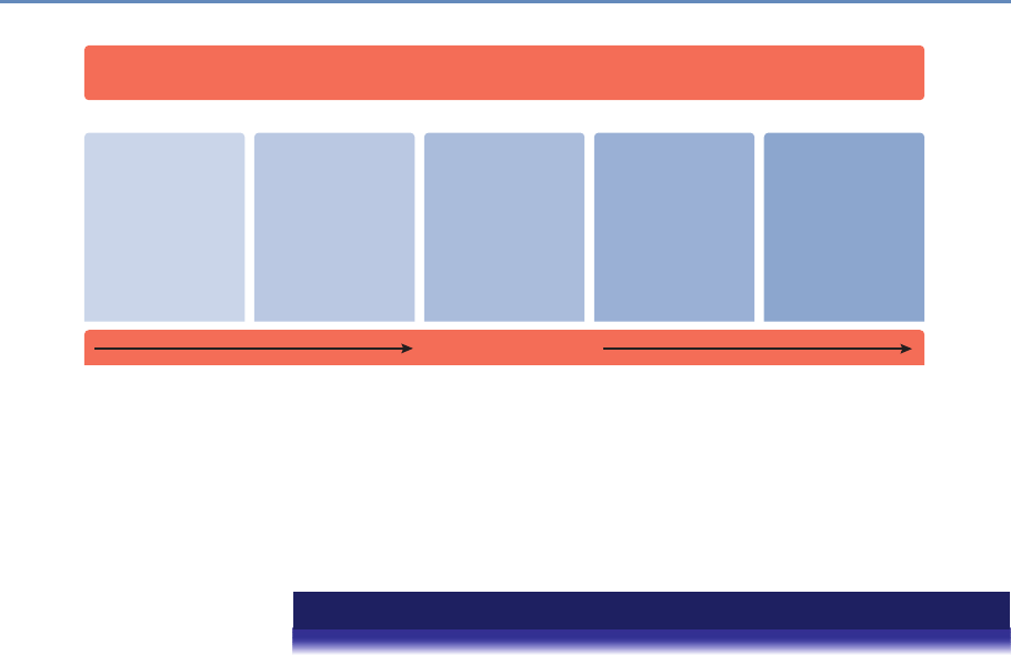
32 2. Working with Web Data and APIs
Research Article
Viewed Saved
PLOS HTML CiteULike
Mendeley
NatureBlogs F1000 Prime Crossref
PMC
Web of Science
Scopus
ScienceSeeker
Twitter
Facebook
Increasing Engagement
Wikipedia
PLOS Comments
ResearchBlogging
PLOS PDF
PLOS XML
PMC HTML
PMC PDF
Discussed CitedRecommended
Figure 2.2. Classes of online activity related to research journal articles. Reproduced from Lin and Fenner [237],
under a Creative Commons Attribution v 3.0 license
the indicator, the limitations that the indicator has as a measure,
and the sources of data. We start with the familiar case of formal
literature citations to provide context.
Example: Citations
Most quantitative analyses of research have focused on citations from research ar-
ticles to other research articles. Many familiar measures—such as Impact Factors,
Scimago Journal Rank, or Eigenfactor—are actually measures of journal rather
than article performance. However, information on citations at the article level is
increasingly the basis for much bibliometric analysis.
•Kind of usage
◦Citing a scholarly work is a signal from a researcher that a specific
work has relevance to, or has influenced, the work they are describing.
◦It implies significant engagement and is a measure that carries some
weight.
•Users
◦Researchers, which means usage by a specific group for a fairly small
range of purposes.
◦With high-quality data, there are some geographical, career, and dis-
ciplinary demographic details.
•Limitations
◦The citations are slow to accumulate, as they must pass through a
peer-review process.

2.3. New data in the research enterprise 33
◦It is seldom clear from raw data why a paper is being cited.
◦It provides a limited view of usage, as it only reflects reuse in research,
not application in the community.
•Sources
◦Public sources of citation data include PubMed Central and Europe
PubMed Central, which mine publicly available full text to find cita-
tions.
◦Proprietary sources of citation data include Thomson Reuters’ Web of
Knowledge and Elsevier’s Scopus.
◦Some publishers make citation data collected by Crossref available.
Example: Page views and downloads
A major new source of data online is the number of times articles are viewed. Page
views and downloads can be defined in different ways and can be reached via a
range of paths. Page views are an immediate measure of usage. Viewing a paper
may involve less engagement than citation or bookmarking, but it can capture
interactions with a much wider range of users.
The possibility of drawing demographic information from downloads has sig-
nificant potential for the future in providing detailed information on who is reading
an article, which may be valuable for determining, for example, whether research
is reaching a target audience.
•Kind of usage
◦It counts the number of people who have clicked on an article page or
downloaded an article.
•Users
◦Page views and downloads report on use by those who have access
to articles. For publicly accessible articles this could be anyone; for
subscription articles it is likely to be researchers.
•Limitations
◦Page views are calculated in different ways and are not directly com-
parable across publishers. Standards are being developed but are not
yet widely applied.
◦Counts of page views cannot easily distinguish between short-term
visitors and those who engage more deeply with an article.
◦There are complications if an article appears in multiple places, for
example at the journal website and a repository.

34 2. Working with Web Data and APIs
•Sources
◦Some publishers and many data repositories make page view data
available in some form. Publishers with public data include PLOS,
Nature Publishing Group, Ubiquity Press, Co-Action Press, and Fron-
tiers.
◦Data repositories, including Figshare and Dryad, provide page view
and download information.
◦PubMed Central makes page views of articles hosted on that site avail-
able to depositing publishers. PLOS and a few other publishers make
this available.
Example: Analyzing bookmarks
Tools for collecting and curating personal collections of literature, or web content,
are now available online. They make it easy to make copies and build up indexes of
articles. Bookmarking services can choose to provide information on the number
of people who have bookmarked a paper.
Two important services targeted at researchers are Mendeley and CiteULike.
Mendeley has the larger user base and provides richer statistics. Data include
the number of users that who bookmarked a paper, groups that have collected a
paper, and in some cases demographics of users, which can include discipline,
career stage, and geography.
Bookmarks accumulate rapidly after publication and provide evidence of schol-
arly interest. They correlate quite well with the eventual number of citations. There
are also public bookmarking services that provide a view onto wider interest in re-
search articles.
•Kind of usage
◦Bookmarking is a purposeful act. It may reveal more interest than a
page view, but less than a citation.
◦Its uses are different from those captured by citations.
◦The bookmarks may include a variety of documents, such as papers for
background reading, introductory material, position or policy papers,
or statements of community positions.
•Users
◦Academic-focused services provide information on use by researchers.
◦Each service has a different user profile in, for instance, sciences or
social sciences.

2.3. New data in the research enterprise 35
◦All services have a geographical bias towards North America and Eu-
rope.
◦There is some demographic information, for instance, on countries
where users are bookmarking the most.
•Limitations
◦There is bias in coverage of services; for instance, Mendeley has good
coverage of biomedical literature.
◦It can only report on activities of signed-up users.
◦It is not usually possible to determine why a bookmark has been cre-
ated.
•Sources
◦Mendeley and CiteULike both have public APIs that provide data that
are freely available for reuse.
◦Most consumer bookmarking services provide some form of API, but
this often has restrictions or limitations.
Example: Discussions on social media
Social media are one of the most valuable new services producing information
about research usage. A growing number of researchers, policymakers, and tech-
nologists are on these services discussing research.
There are three major features of social media as a tool. First, among a large
set of conversations, it is possible to discover a discussion about a specific paper.
Second, Twitter makes it possible to identify groups discussing research and to
learn whether they were potential targets of the research. Third, it is possible to
reconstruct discussions to understand what paths research takes to users.
In the future it will be possible to identify target audiences and to ask whether
they are being reached and how modified distribution might maximize that reach.
This could be a powerful tool, particularly for research with social relevance.
Twitter provides the most useful data because discussions and the identity of
those involved are public. Connections between users and the things they say
are often available, making it possible to identify communities discussing work.
However, the 140-character limit on Twitter messages (“tweets”) does not support
extended critiques. Facebook has much less publicly available information—but
being more private, it can be a site for frank discussion of research.
•Kind of usage
◦Those discussing research are showing interest potentially greater than
page views.

36 2. Working with Web Data and APIs
◦Often users are simply passing on a link or recommending an article.
◦It is possible to navigate to tweets and determine the level and nature
of interest.
◦Conversations range from highly technical to trivial, so numbers should
be treated with caution.
◦Highly tweeted or Facebooked papers also tend to have significant
bookmarking and citation.
◦Professional discussions can be swamped when a piece of research
captures public interest.
•Users
◦The user bases and data sources for Twitter and Facebook are global
and public.
◦There are strong geographical biases.
◦A rising proportion of researchers use Twitter and Facebook for profes-
sional activities.
◦Many journalists, policymakers, public servants, civil society groups,
and others use social media.
•Limitations
◦Frequent lack of explicit links to papers is a serious limitation.
◦Use of links is biased towards researchers and against groups not
directly engaged in research.
◦There are demographic issues and reinforcement effects—retweeting
leads to more retweeting in preference to other research—so analysis
of numbers of tweets or likes is not always useful.
Example: Recommendations
A somewhat separate form of usage is direct expert recommendations. The best-
known case of this is the F1000 service on which experts offer recommendations
with reviews of specific research articles. Other services such as collections or
personal recommendation services may be relevant here as well.
•Kind of usage
◦Recommendations from specific experts show that particular outputs
are worth looking at in detail, are important, or have some other value.
◦Presumably, recommendations are a result of in-depth reading and a
high level of engagement.

2.4. A functional view 37
•Users
◦Recommendations are from a selected population of experts depending
on the service in question.
◦In some cases this might be an algorithmic recommendation service.
•Limitations
◦Recommendations are limited to the interests of the selected popula-
tion of experts.
◦The recommendation system may be biased in terms of the interests of
recommenders (e.g., towards—or away from—new theories vs. develop-
ing methodology) as well as their disciplines.
◦Recommendations are slow to build up.
2.4 A functional view
The descriptive view of data types and sources is a good place to
start, but it is subject to change. Sources of data come and go,
and even the classes of data types may expand and contract in the
medium to long term. We also need a more functional perspective
to help us understand how these sources of data relate to activities
in the broader research enterprise.
Consider Figure 1.2 in Chapter 1. The research enterprise has
been framed as being made up of people who are generating out-
puts. The data that we consider in this chapter relate to connections
between outputs, such as citations between research articles and
tweets referring to articles. These connections are themselves cre-
ated by people, as shown in Figure 2.3. The people in turn may be
classed as belonging to certain categories or communities. What is
interesting, and expands on the simplified picture of Figure 1.2, is
that many of these people are not professional researchers. Indeed,
in some cases they may not be people at all but automated systems
of some kind. This means we need to expand the set of actors we are
considering. As described above, we are also expanding the range
of outputs (or objects) that we are considering as well.
In the simple model of Figure 2.3, there are three categories of
things (nodes on the graph): objects, people, and the communities
they belong to. Then there are the relationships between these el-
ements (connections between nodes). Any given data source may
provide information on different parts of this graph, and the in-
formation available is rarely complete or comprehensive. Data from
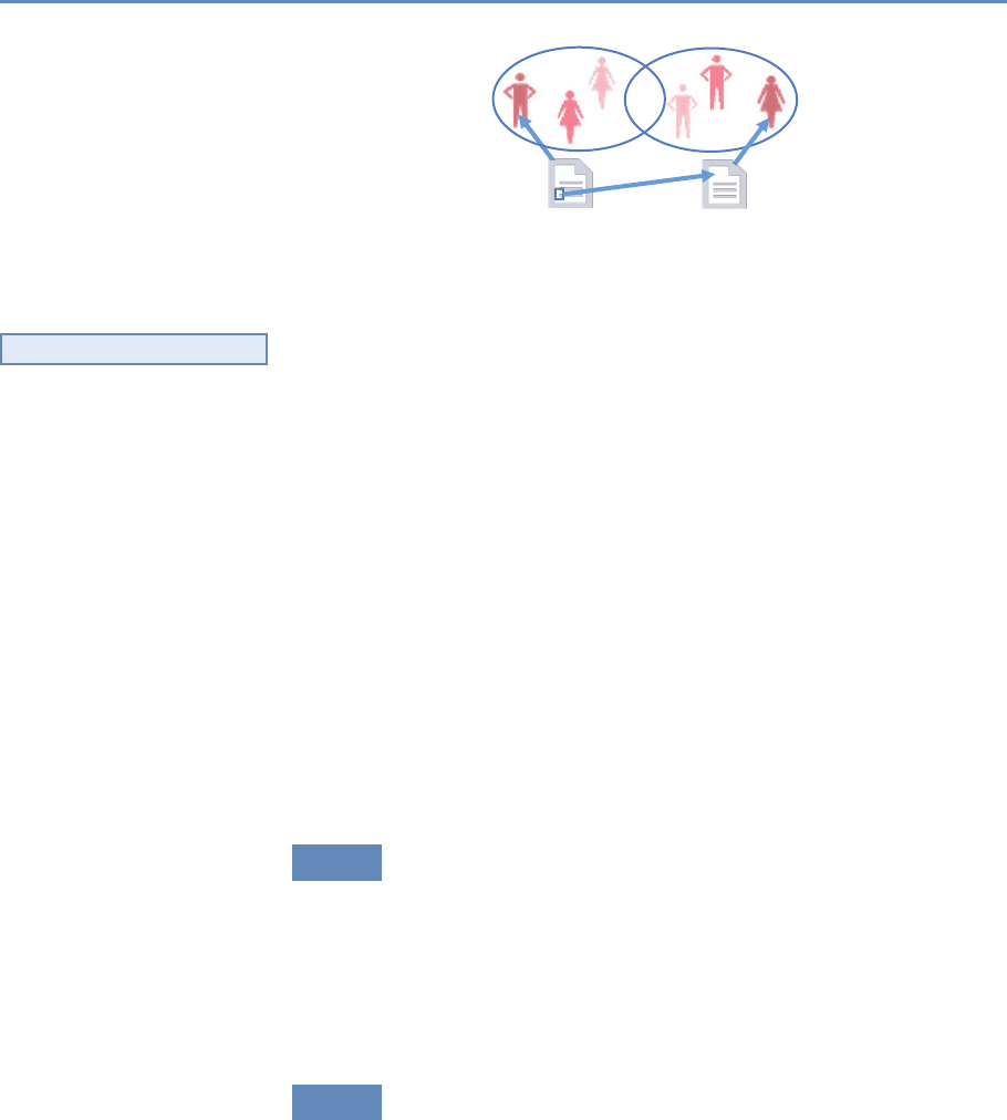
38 2. Working with Web Data and APIs
Refers to
Created byCreated by
Figure 2.3. A simplified model of online interactions between research outputs
and the objects that refer to them
different sources can also be difficult to integrate. As with any
◮See Section 3.2.
data integration, combining sources relies on being able to confi-
dently identify those nodes that are common between data sources.
Therefore identifying unique objects and people is critical to making
progress.
These data are not necessarily public but many services choose
to make some data available. An important characteristic of these
data sources is that they are completely in the gift of the service
provider. Data availability, its presentation, and upstream analysis
can change without notice. Data are sometimes provided as a dump
but is also frequently provided through an API.
An API is simply a tool that allows a program to interface with a
service. APIs can take many different forms and be of varying quality
and usefulness. In this section we will focus on one common type
of API and examples of important publicly available APIs relevant
to research communications. We will also cover combining APIs
and the benefits and challenges of bringing multiple data sources
together.
2.4.1 Relevant APIs and resources
There is a wide range of other sources of information that can be
used in combination with the APIs featured above to develop an
overview of research outputs and of where and how they are being
used. There are also other tools that can allow deeper analysis of the
outputs themselves. Table 2.1 gives a partial list of key data sources
and APIs that are relevant to the analysis of research outputs.
2.4.2 RESTful APIs, returned data, and Python wrappers
The APIs we will focus on here are all examples of RESTful services.
REST stands for Representational State Transfer [121, 402], but for

2.4. A functional view 39
Table 2.1. Popular sources of data relevant to the analysis of research outputs
Source Description API Free
Bibliographic Data
PubMed An online index that combines bibliographic data from Medline and
PubMed Central. PubMed Central and Europe PubMed Central also
provide information.
Y Y
Web of Science The bibliographic database provided by Thomson Reuters. The ISI
Citation Index is also available.
Y N
Scopus The bibliographic database provided by Elsevier. It also provides
citation information.
Y N
Crossref Provides a range of bibliographic metadata and information obtained
from members registering DOIs.
Y Y
Google Scholar Provides a search index for scholarly objects and aggregates citation
information.
N Y
Microsoft Academic Search Provides a search index for scholarly objects and aggregates citation
information. Not as complete as Google Scholar, but has an API.
Y Y
Social Media
Altmetric.com A provider of aggregated data on social media and mainstream media
attention of research outputs. Most comprehensive source of infor-
mation across different social media and mainstream media conver-
sations.
Y N
Twitter Provides an API that allows a user to search for recent tweets and
obtain some information on specific accounts.
Y Y
Facebook The Facebook API gives information on the number of pages, likes,
and posts associated with specific web pages.
Y Y
Author Profiles
ORCID Unique identifiers for research authors. Profiles include information
on publication lists, grants, and affiliations.
Y Y
LinkedIn CV-based profiles, projects, and publications. Y *
Funder Information
Gateway to Research A database of funding decisions and related outputs from Research
Councils UK.
Y Y
NIH Reporter Online search for information on National Institutes of Health grants.
Does not provide an API but a downloadable data set is available.
N Y
NSF Award Search Online search for information on NSF grants. Does not provide an
API but downloadable data sets by year are available.
N Y
* The data are restricted: sometimes fee based, other times not.
our purposes it is most easily understood as a means of transfer-
ring data using web protocols. Other forms of API require addi-
tional tools or systems to work with, but RESTful APIs work directly
over the web. This has the advantage that a human user can also
with relative ease play with the API to understand how it works.
Indeed, some websites work simply by formatting the results of
API calls.

40 2. Working with Web Data and APIs
As an example let us look at the Crossref API. This provides a
range of information associated with Digital Object Identifiers (DOIs)
registered with Crossref. DOIs uniquely identify an object, and
Crossref DOIs refer to research objects, primarily (but not entirely)
research articles. If you use a web browser to navigate to http://api.
crossref.org/works/10.1093/nar/gni170, you should receive back
a webpage that looks something like the following. (We have laid it
out nicely to make it more readable.)
{"status" :"ok",
"message-type" :"work",
"message-version" :"1.0.0",
"message" :
{"subtitle":[],
"subject" :["Genetics"],
"issued" :{"date-parts" :[[2005,10,24]] },
"score" :1.0,
"prefix" :"http://id.crossref.org/prefix/10.1093",
"author" :["affiliation" :[],
"family" :"Whiteford",
"given" :"N."}],
"container-title" :["Nucleic Acids Research"],
"reference-count" :0,
"page" :"e171-e171",
"deposited" :{"date-parts" :[[2013,8,8]],
"timestamp" :1375920000000},
"issue" :"19",
"title" :
["An analysis of the feasibility of short read sequencing"]
,
"type" :"journal-article",
"DOI" :"10.1093/nar/gni170",
"ISSN" :["0305-1048","1362-4962"],
"URL" :"http://dx.doi.org/10.1093/nar/gni170",
"source" :"Crossref",
"publisher" :"Oxford University Press (OUP)",
"indexed" :{"date-parts" :[[2015,6,8]],
"timestamp" :1433777291246},
"volume" :"33",
"member" :"http://id.crossref.org/member/286"
}
}
This is a package of JavaScript Object Notation (JSON)*data
⋆JSON is an open stan-
dard way of storing and ex-
changing data.
returned in response to a query. The query is contained entirely
in the URL, which can be broken up into pieces: the root URL
(http://api.crossref.org) and a data “query,” in this case made up of
a “field” (works) and an identifier (the DOI 10.1093/nar/gni170). The
Crossref API provides information about the article identified with
this specific DOI.
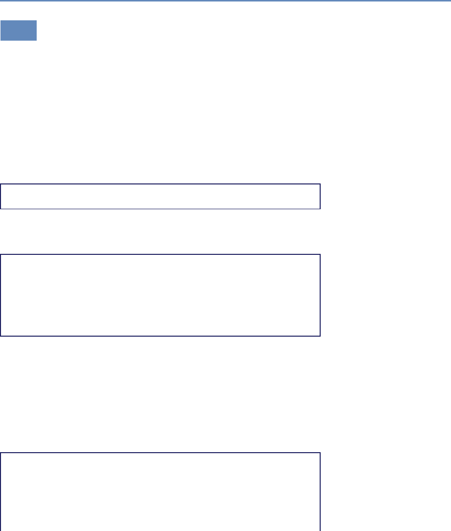
2.5. Programming against an API 41
2.5 Programming against an API
Programming against an API involves constructing HTTP requests
and parsing the data that are returned. Here we use the Cross-
ref API to illustrate how this is done. Crossref is the provider of
DOIs used by many publishers to uniquely identify scholarly works.
Crossref is not the only organization to provide DOIs. The scholarly
communication space DataCite is another important provider. The
documentation is available at the Crossref website [394].
Once again the requests Python library provides a series of con-
venience functions that make it easier to make HTTP calls and to
process returned JSON. Our first step is to import the module and
set a base URL variable.
>> import requests
>> BASE_URL = "http://api.crossref.org/"
A simple example is to obtain metadata for an article associated
with a specific DOI. This is a straightforward call to the Crossref
API, similar to what we saw earlier.
>> doi = "10.1093/nar/gni170"
>> query = "works/"
>> url = BASE_URL + query + doi
>> response = requests.get(url)
>> url
http://api.crossref.org/works/10.1093/nar/gni170
>> response.status_code
200
The response object that the requests library has created has a
range of useful information, including the URL called and the re-
sponse code from the web server (in this case 200, which means
everything is OK). We need the JSON body from the response ob-
ject (which is currently text from the perspective of our script) con-
verted to a Python dictionary. The requests module provides a
convenient function for performing this conversion, as the following
code shows. (All strings in the output are in Unicode, hence the u’
notation.)
>> response_dict = response.json()
>> response_dict
{u’message’ :
{u’DOI’ :u’10.1093/nar/gni170’,
u’ISSN’ :[u’0305-1048’,u’1362-4962’],
u’URL’ :u’http://dx.doi.org/10.1093/nar/gni170’,
u’author’ :[ {u’affiliation’ :[],
u’family’ :u’Whiteford’,

42 2. Working with Web Data and APIs
u’given’ :u’N.’} ],
u’container-title’ :[u’Nucleic Acids Research’ ],
u’deposited’ :{u’date-parts’ :[[2013,8,8]],
u’timestamp’ :1375920000000 },
u’indexed’ :{u’date-parts’ :[[2015,6,8]],
u’timestamp’ :1433777291246 },
u’issue’ :u’19’,
u’issued’ :{u’date-parts’ :[[2005,10,24]] },
u’member’ :u’http://id.crossref.org/member/286’,
u’page’ :u’e171-e171’,
u’prefix’ :u’http://id.crossref.org/prefix/10.1093’,
u’publisher’ :u’Oxford University Press (OUP)’,
u’reference-count’ :0,
u’score’ :1.0,
u’source’ :u’Crossref’,
u’subject’ :[u’Genetics’],
u’subtitle’ :[],
u’title’ :[u’An analysis of the feasibility of short read
sequencing’],
u’type’ :u’journal-article’,
u’volume’ :u’33’
},
u’message-type’ :u’work’,
u’message-version’ :u’1.0.0’,
u’status’ :u’ok’
}
This data object can now be processed in whatever way the user
wishes, using standard manipulation techniques.
The Crossref API can, of course, do much more than simply look
up article metadata. It is also valuable as a search resource and
for cross-referencing information by journal, funder, publisher, and
other criteria. More details can be found at the Crossref website.
2.6 Using the ORCID API via a wrapper
ORCID, which stands for “Open Research and Contributor Identi-
fier” (see orcid.org; see also [145]), is a service that provides unique
identifiers for researchers. Researchers can claim an ORCID profile
and populate it with references to their research works, funding and
affiliations. ORCID provides an API for interacting with this infor-
mation. For many APIs there is a convenient Python wrapper that
can be used. The ORCID–Python wrapper works with the ORCID
v1.2 API to make various API calls straightforward. This wrapper
only works with the public ORCID API and can therefore only access
publicly available data.
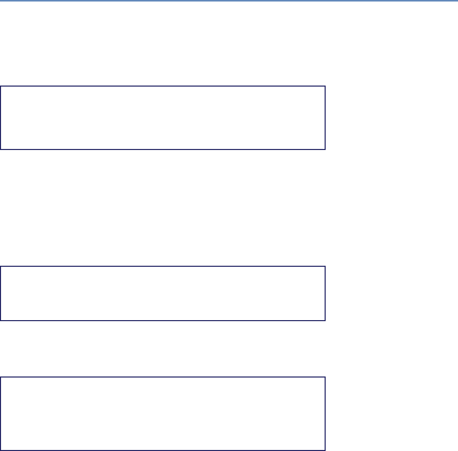
2.6. Using the ORCID API via a wrapper 43
Using the API and wrapper together provides a convenient means
of getting this information. For instance, given an ORCID, it is
straightforward to get profile information. Here we get a list of pub-
lications associated with my ORCID and look at the the first item
on the list.
>> import orcid
>> cn = orcid.get("0000-0002-0068-716X")
>> cn
<Author Cameron Neylon, ORCID 0000-0002-0068-716X>
>> cn.publications[0]
<Publication "Principles for Open Scholarly Infrastructures-v1">
The wrapper has created Python objects that make it easier to
work with and manipulate the data. It is common to take the return
from an API and create objects that behave as would be expected
in Python. For instance, the publications object is a list popu-
lated with publications (which are also Python-like objects). Each
publication in the list has its own attributes, which can then be
examined individually. In this case the external IDs attribute is a
list of further objects that include a DOI for the article and the ISSN
of the journal the article was published in.
>> len(cn.publications)
70
>> cn.publications[12].external_ids
[<ExternalID DOI:10.1371/journal.pbio.1001677>, <ExternalID ISSN
:1545-7885>]
As a simple example of data processing, we can iterate over the
list of publications to identify those for which a DOI has been pro-
vided. In this case we can see that of the 70 publications listed in
this ORCID profile (at the time of testing), 66 have DOIs.
>> exids = []
>> for pub in cn.publications:
if pub.external_ids:
exids = exids + pub.external_ids
>> DOIs = [exid.id for exid in exids if exid.type == "DOI"]
>> len(DOIs)
66
Wrappers generally make operating with an API simpler and
cleaner by abstracting away the details of making HTTP requests.
Achieving the same by directly interacting with the ORCID API
would require constructing the appropriate URLs and parsing the
returned data into a usable form. Where a wrapper is available it
is generally much easier to use. However, wrappers may not be
actively developed and may lag the development of the API. Where

44 2. Working with Web Data and APIs
possible, use a wrapper that is directly supported or recommended
by the API provider.
2.7 Quality, scope, and management
The examples in the previous section are just a small dip into the
surface of the data available, but we already can see a number of
issues that are starting to surface. A great deal of care needs to
be taken when using these data, and a researcher will need to ap-
ply subject matter knowledge as well as broader data management
expertise. Some of the core issues are as follows:
◮See Chapter 10.
Integration In the examples given above with Crossref and ORCID,
we used a known identifier (a DOI or an ORCID). Integrating data
from Crossref to supplement the information from an ORCID profile
is possible, but it depends on the linking of identifiers. Note that
for the profile data we obtained, only 66 or the 70 items had DOIs.
Data integration across multiple data sources that reference DOIs
is straightforward for those objects that have DOIs, and messy or
impossible for those that do not. In general, integration is possible,
but it depends on a means of cross-referencing between data sets.
Unique identifiers that are common to both are extremely powerful
but only exist in certain cases (see also Chapter 3).
Coverage Without a population frame, it is difficult to know
whether the information that can be captured is comprehensive.
For example, “the research literature” is at best a vague concept. A
variety of indexes, some openly available (PubMed, Crossref), some
proprietary (Scopus, Web of Knowledge, many others), cover differ-
ent partially overlapping segments of this corpus of work. Each in-
dex has differing criteria for inclusion and differing commitments to
completeness. Sampling of “the literature” is therefore impossible,
and the choice of index used for any study can make a substantial
difference to the conclusions.
Completeness Alongside the question of coverage (how broad is
a data source?), with web data and opt-in services we also need to
probe the completeness of a data set. In the example above, 66 of 70
objects have a DOI registered. This does not mean that those four
other objects do not have a DOI, just that there are none included in
the ORCID record. Similarly, ORCID profiles only exist for a subset
of researchers at this stage. Completeness feeds into integration

2.7. Quality, scope, and management 45
challenges. While many researchers have a Twitter profile and many
have an ORCID profile, only a small subset of ORCID profiles provide
a link to a Twitter profile. See below for a worked example.
Scope In survey data sets, the scope is defined by the question
being asked. This is not the case with much of these new data.
For example, the challenges listed above for research articles, tra-
ditionally considered the bedrock of research outputs, at least in
the natural sciences, are much greater for other forms of research
outputs. Increasingly, the data generated from research projects,
software, materials, and tools, as well as reports and presentations,
are being shared by researchers in a variety of settings. Some of
these are formal mechanisms for publication, such as large disci-
plinary databases, books, and software repositories, and some are
highly informal. Any study of (a subset of) these outputs has as its
first challenge the question of how to limit the corpus to be studied.
Source and validity The challenges described above relate to the
identification and counting of outputs. As we start to address ques-
tions of how these outputs are being used, the issues are com-
pounded. To illustrate some of the difficulties that can arise, we
examine the number of citations that have been reported for a sin-
gle sample article on a biochemical methodology [68]. This article
has been available for eight years and has accumulated a reason-
able number of citations for such an article over that time.
However, the exact number of citations identified varies radi-
cally, depending on the data source. Scopus finds 40, while Web
of Science finds only 38. A Google Scholar search performed on
the same date identified 59. These differences relate to the size of
the corpus from which inward citations are being counted. Web of
Science has the smallest database, with Scopus being larger and
Google Scholar substantially larger again. Thus the size of the in-
dex not only affects output counting, it can also have a substantial
effect on any analysis that uses that corpus. Alongside the size
of the corpus, the means of analysis can also have an effect. For
the same article, PubMed Central reports 10 citations but Europe
PubMed Central reports 18, despite using a similar corpus. The
distinction lies in differences in the methodology used to mine the
corpus for citations.
Identifying the underlying latent variable These issues multiply as
we move into newer forms of data. These sparse and incomplete
sources of data require different treatment than more traditional

46 2. Working with Web Data and APIs
structured and comprehensive forms of data. They are more useful
as a way of identifying activities than of quantifying or comparing
them. Nevertheless, they can provide new insight into the pro-
cesses of knowledge dissemination and community building that
are occurring online.
2.8 Integrating data from multiple sources
We often must work across multiple data sources to gather the in-
formation needed to answer a research question. A common pattern
is to search in one location to create a list of identifiers and then use
those identifiers to query another API. In the ORCID example above,
we created a list of DOIs from a single ORCID profile. We could use
those DOIs to obtain further information from the Crossref API and
other sources. This models a common path for analysis of research
outputs: identifying a corpus and then seeking information on its
performance.
In this example, we will build on the ORCID and Crossref ex-
amples to collect a set of work identifiers from an ORCID profile
and use a range of APIs to identify additional metadata as well as
information on the performance of those articles. In addition to the
ORCID API, we will use the PLOS Lagotto API. Lagotto is the soft-
ware that was built to support the Article Level Metrics program at
PLOS, the open access publisher, and its API provides information
on various metrics of PLOS articles. A range of other publishers
and service providers, including Crossref, also provide an instance
of this API, meaning the same tools can be used to collect informa-
tion on articles from a range of sources.
2.8.1 The Lagotto API
The module pyalm is a wrapper for the Lagotto API, which is served
from a range of hosts. We will work with two instances in particular:
one run by PLOS, and the Crossref DOI Event Tracker (DET, recently
renamed Crossref Event Data) pilot service. We first need to provide
the details of the URLs for these instances to our wrapper. Then
we can obtain some information for a single DOI to see what the
returned data look like.
>> import pyalm
>> pyalm.config.APIS = {’plos’ : {’url’ :
>> ’http://alm.plos.org/api/v5/articles’},
>> ’det’ : {’url’ :

2.8. Integrating data from multiple sources 47
>> ’http://det.labs.crossref.org/api/v5/articles’}
>> }
>> det_alm_test = pyalm.get_alm(’10.1371/journal.pbio.1001677’,
>> info=’detail’, instance=’det’)
det_alm_test
{’articles’ : [<ArticleALM Expert Failure: Re-evaluating Research
Assessment, DOI 10.1371/journal.pbio.1001677>],
’meta’ : {u’error’ : None, u’page’ : 1,
u’total’ : 1, u’total_pages’ : 1}
}
The library returns a Python dictionary containing two elements.
The articles key contains the actual data and the meta key includes
general information on the results of the interaction with the API.
In this case the library has returned one page of results containing
one object (because we only asked about one DOI). If we want to
collect a lot of data, this information helps in the process of paging
through results. It is common for APIs to impose some limit on
the number of results returned, so as to ensure performance. By
default the Lagotto API has a limit of 50 results.
The articles key holds a list of ArticleALM objects as its value.
Each ArticleALM object has a set of internal attributes that contain
information on each of the metrics that the Lagotto instance col-
lects. These are derived from various data providers and are called
sources. Each can be accessed by name from a dictionary called
“sources.” The iterkeys() function provides an iterator that lets us
loop over the set of keys in a dictionary. Within the source object
there is a range of information that we will dig into.
>> article = det_alm_test.get(’articles’)[0]
>> article.title
u’Expert Failure: Re-evaluating Research Assessment’
>> for source in article.sources.iterkeys():
>> print source, article.sources[source].metrics.total
reddit 0
datacite 0
pmceuropedata 0
wikipedia 1
pmceurope 0
citeulike 0
pubmed 0
facebook 0
wordpress 0
pmc 0
mendeley 0
crossref 0
The DET service only has a record of citations to this article
from Wikipedia. As we will see below, the PLOS service returns
more results. This is because some of the sources are not yet being
queried by DET.

48 2. Working with Web Data and APIs
Because this is a PLOS paper we can also query the PLOS Lagotto
instance for the same article.
>> plos_alm_test = pyalm.get_alm(’10.1371/journal.pbio.1001677’,
info=’detail’, instance=’plos’)
>> article_plos = plos_alm_test.get(’articles’)[0]
>> article_plos.title
u’Expert Failure: Re-evaluating Research Assessment’
>> for source in article_plos.sources.iterkeys():
>> print source, article_plos.sources[source].metrics.total
datacite 0
twitter 130
pmc 610
articlecoveragecurated 0
pmceurope 1
pmceuropedata 0
researchblogging 0
scienceseeker 0
copernicus 0
f1000 0
wikipedia 1
citeulike 0
wordpress 2
openedition 0
reddit 0
nature 0
relativemetric 125479
figshare 0
facebook 1
mendeley 14
crossref 3
plos_comments 2
articlecoverage 0
counter 12551
scopus 2
pubmed 1
orcid 3
The PLOS instance provides a greater range of information but
also seems to be giving larger numbers than the DET instance in
many cases. For those sources that are provided by both API in-
stances, we can compare the results returned.
>> for source in article.sources.iterkeys():
>> print source, article.sources[source].metrics.total,
>> article_plos.sources[source].metrics.total
reddit 0 0
datacite 0 0
pmceuropedata 0 0
wikipedia 1 1
pmceurope 0 1
citeulike 0 0
pubmed 0 1

2.8. Integrating data from multiple sources 49
facebook 0 1
wordpress 0 2
pmc 0 610
mendeley 0 14
crossref 0 3
The PLOS Lagotto instance is collecting more information and
has a wider range of information sources. Comparing the results
from the PLOS and DET instances illustrates the issues of coverage
and completeness discussed previously. The data may be sparse for
a variety of reasons, and it is important to have a clear idea of the
strengths and weaknesses of a particular data source or aggregator.
In this case the DET instance is returning information for some
sources for which it is does not yet have data.
We can dig deeper into the events themselves that the met-
rics.total count aggregates. The API wrapper collects these into
an event object within the source object. These contain the JSON
returned from the API in most cases. For instance, the Crossref
source is a list of JSON objects containing information on an article
that cites our article of interest. The first citation event in the list is
a citation from the Journal of the Association for Information Science
and Technology by Du et al.
>> article_plos.sources[’crossref’].events[0]
{u’event’ :
{u’article_title’ : u’The effects of research level and article
type on the differences between citation metrics and F1000
recommendations’,
u’contributors’ :
{u’contributor’ :
[ { u’contributor_role’ : u’author’,
u’first_author’ : u’true’,
u’given_name’ : u’Jian’,
u’sequence’ : u’first’,
u’surname’ : u’Du’ },
{ u’contributor_role’ : u’author’,
u’first_author’ : u’false’,
u’given_name’ : u’Xiaoli’,
u’sequence’ : u’additional’,
u’surname’ : u’Tang’},
{ u’contributor_role’ : u’author’,
u’first_author’ : u’false’,
u’given_name’ : u’Yishan’,
u’sequence’ : u’additional’,
u’surname’ : u’Wu’} ]
},
u’doi’ : u’10.1002/asi.23548’,
u’first_page’ : u’n/a’,
u’fl_count’ : u’0’,
u’issn’ : u’23301635’,

50 2. Working with Web Data and APIs
u’journal_abbreviation’ : u’J Assn Inf Sci Tec’,
u’journal_title’ : u’Journal of the Association for
Information Science and Technology’,
u’publication_type’ : u’full_text’,
u’year’ : u’2015’
},
u’event_csl’ : {
u’author’ :
[ { u’family’ : u’Du’, u’given’ : u’Jian’},
{u’family’ : u’Tang’, u’given’ : u’Xiaoli’},
{u’family’ : u’Wu’, u’given’ : u’Yishan’} ],
u’container-title’ : u’Journal of the Association for
Information Science and Technology’,
u’issued’ : {u’date-parts’ : [[2015]]},
u’title’ : u’The Effects Of Research Level And Article Type
On The Differences Between Citation Metrics And F1000
Recommendations’,
u’type’ : u’article-journal’,
u’url’ : u’http://doi.org/10.1002/asi.23548’
},
u’event_url’ : u’http://doi.org/10.1002/asi.23548’
}
Another source in the PLOS data is Twitter. In the case of the
Twitter events (individual tweets), this provides the text of the tweet,
user IDs, user names, URL of the tweet, and the date. We can see
from the length of the events list that there are at least 130 tweets
that link to this article.
>> len(article_plos.sources[’twitter’].events)
130
Again, noting the issues of coverage, scope, and completeness,
it is important to consider the limitations of these data. This is a
lower bound as it represents search results returned by searching
the Twitter API for the DOI or URL of the article. Other tweets that
discuss the article may not include a link, and the Twitter search
API also has limitations that can lead to incomplete results. The
number must therefore be seen as both incomplete and a lower
bound.
We can look more closely at data on the first tweet on the list.
Bear in mind that the order of the list is not necessarily special.
This is not the first tweet about this article chronologically.
>> article_plos.sources[’twitter’].events[0]
{ u’event’ : {u’created_at’: u’2013-10-08T21:12:28Z’,
u’id’ : u’387686960585641984’,
u’text’ : u’We have identified the Higgs boson; it is surely not
beyond our reach to make research assessment useful http://t
.co/Odcm8dVRSU#PLOSBiology’,

2.8. Integrating data from multiple sources 51
u’user’ : u’catmacOA’,
u’user_name’ : u’Catriona MacCallum’,
u’user_profile_image’ :
u’http://a0.twimg.com/profile_images/1779875975/
CM_photo_reduced_normal.jpg’},
u’event_time’ : u’2013-10-08T21:12:28Z’,
u’event_url’ : u’http://twitter.com/catmacOA/status
/387686960585641984’
}
We could use the Twitter API to understand more about this
person. For instance, we could look at their Twitter followers and
whom they follow, or analyze the text of their tweets for topic mod-
eling. Much work on social media interactions is done with this
kind of data, using forms of network and text analysis described
elsewhere in this book.
◮See Chapters 7 and 8.
A different approach is to integrate these data with informa-
tion from another source. We might be interested, for instance,
in whether the author of this tweet is a researcher, or whether they
have authored research papers. One thing we could do is search
the ORCID API to see if there are any ORCID profiles that link to
this Twitter handle.
>> twitter_search = orcid.search("catmacOA")
>> for result in twitter_search:
>> print unicode(result)
>> print result.researcher_urls}
<Author Catriona MacCallum, ORCID 0000-0001-9623-2225>
[<Website twitter [http://twitter.com/catmacOA]>]
So the person with this Twitter handle seems to have an ORCID
profile. That means we can also use ORCID to gather more infor-
mation on their outputs. Perhaps they have authored work which
is relevant to our article?
>> cm = orcid.get("0000-0001-9623-2225")
>> for pub in cm.publications[0:5]:
>> print pub.title
The future is open: opportunities for publishers and institutions
Open Science and Reporting Animal Studies: Who’s Accountable?
Expert Failure: Re-evaluating Research Assessment
Why ONE Is More Than 5
Reporting Animal Studies: Good Science and a Duty of Care
From this analysis we can show that this tweet is actually from
one of my co-authors of the article.
To make this process easier we write the convenience function
shown in Listing 2.2 to go from a Twitter user handle to try and find
an ORCID for that person.

52 2. Working with Web Data and APIs
# Take a twitter handle or user name and return an ORCID
2def twitter2orcid(twitter_handle,
resp = 'orcid', search_depth = 10):
4search = orcid.search(twitter_handle)
s = [r for rin search]
6orc = None
i = 0
8while i < search_depth and orc == None and i < len(s):
arr = [('twitter.com' in website.url)
10 for website in s[i].researcher_urls]
if True in arr:
12 index = arr.index(True)
url = s[i].researcher_urls[index].url
14 if url.lower().endswith(twitter_handle.lower()):
orc = s[i].orcid
16 return orc
i+=1
18 return None
Listing 2.2. Python code to find ORCID for Twitter handle
Let us do a quick test of the function.
>> twitter2orcid(’catmacOA’)
u’0000-0001-9623-2225’
2.8.2 Working with a corpus
In this case we will continue as previously to collect a set of works
from a single ORCID profile. This collection could just as easily be
a date range, or subject search at a range of other APIs. The target
is to obtain a set of identifiers (in this case DOIs) that can be used
to precisely query other data sources. This is a general pattern
that reflects the issues of scope and source discussed above. The
choice of how to construct a corpus to analyze will strongly affect
the results and the conclusions that can be drawn.
>> # As previously, collect DOIs available from an ORCID profile
>> cn = orcid.get("0000-0002-0068-716X")
>> exids = []
>> for pub in cn.publications:
>> if pub.external_ids:
>> exids = exids + pub.external_ids
>> DOIs = [exid.id for exid in exids if exid.type == "DOI"]
>> len(DOIs)
66

2.8. Integrating data from multiple sources 53
We have recovered 66 DOIs from the ORCID profile. Note that we
have not obtained an identifier for every work, as not all have DOIs.
This result illustrates an important point about data integration. In
practice it is generally not worth the effort of attempting to integrate
data on objects unless they have a unique identifier or key that
can be used in multiple data sources, hence the focus on DOIs and
ORCIDs in these examples. Even in our search of the ORCID API
for profiles that are associated with a Twitter account, we used the
Twitter handle as a unique ID to search on.
While it is possible to work with author names or the titles of
works directly, disambiguating such names and titles is substan-
tially more difficult than working with unique identifiers. Other
chapters (in particular, Chapter 3) deal with issues of data cleaning
and disambiguation. Much work has been done on this basis, but
increasingly you will see that the first step in any analysis is simply
to discard objects without a unique ID that can be used across data
sources.
We can obtain data for these from the DET API. As is common
with many APIs, there is a limit to how many queries can be simul-
taneously run, in this case 50, so we divide our query into batches.
>> batches = [DOIs[0:50], DOIs[51:-1]]
>> det_alms = []
>> for batch in batches:
>> alms_response = pyalm.get_alm(batch, info="detail",
instance="det")
>> det_alms.extend(alms_response.get(’articles’))
>> len(det_alms)
24
The DET API only provides information on a subset of Cross-
ref DOIs. The process that Crossref has followed to populate its
database has focused on more recently published articles, so only
24 responses are received in this case for the 66 DOIs we queried on.
A good exercise would be to look at which of the DOIs are found and
which are not. Let us see how much interesting data is available in
the subset of DOIs for which we have data.
>> for r in [d for d in det_alms if d.sources[’wikipedia’].metrics
.total != 0]:
>> print r.title
>> print ’ ’, r.sources[’pmceurope’].metrics.total, ’
pmceurope citations’
>> print ’ ’, r.sources[’wikipedia’].metrics.total, ’
wikipedia citations’
Architecting the Future of Research Communication: Building the
Models and Analytics for an Open Access Future

54 2. Working with Web Data and APIs
1 pmceurope citations
1 wikipedia citations
Expert Failure: Re-evaluating Research Assessment
0 pmceurope citations
1 wikipedia citations
LabTrove: A Lightweight, Web Based, Laboratory "Blog" as a Route
towards a Marked Up Record of Work in a Bioscience Research
Laboratory
0 pmceurope citations
1 wikipedia citations
The lipidome and proteome of oil bodies from Helianthus annuus (
common sunflower)
2 pmceurope citations
1 wikipedia citations
As discussed above, this shows that the DET instance, while it
provides information on a greater number of DOIs, has less com-
plete data on each DOI at this stage. Only four of the 24 responses
have Wikipedia references. You can change the code to look at the
full set of 24, which shows only sparse data. The PLOS Lagotto
instance provides more data but only on PLOS articles. However, it
does provide data on all PLOS articles, going back earlier than the
set returned by the DET instance. We can collect the set of articles
from the profile published by PLOS.
>> plos_dois = []
>> for doi in DOIs:
>> # Quick and dirty, should check Crossref API for publisher
>> if doi.startswith(’10.1371’):
>> plos_dois.append(doi)
>> len(plos_dois)
7
>> plos_alms = pyalm.get_alm(plos_dois, info=’detail’, instance=’
plos’).get(’articles’)
>> for article in plos_alms:
>> print article.title
>> print ’ ’, article.sources[’crossref’].metrics.total, ’
Crossref citations’
>> print ’ ’, article.sources[’twitter’].metrics.total, ’
tweets’
Architecting the Future of Research Communication: Building the
Models and Analytics for an Open Access Future
2 Crossref citations
48 tweets
Expert Failure: Re-evaluating Research Assessment
3 Crossref citations
130 tweets
LabTrove: A Lightweight, Web Based, Laboratory "Blog" as a Route
towards a Marked Up Record of Work in a Bioscience Research
Laboratory
6 Crossref citations

2.8. Integrating data from multiple sources 55
1 tweets
More Than Just Access: Delivering on a Network-Enabled Literature
4 Crossref citations
95 tweets
Article-Level Metrics and the Evolution of Scientific Impact
24 Crossref citations
5 tweets
Optimal Probe Length Varies for Targets with High Sequence
Variation: Implications for Probe
Library Design for Resequencing Highly Variable Genes
2 Crossref citations
1 tweets
Covalent Attachment of Proteins to Solid Supports and Surfaces via
Sortase-Mediated Ligation
40 Crossref citations
0 tweets
From the previous examples we know that we can obtain in-
formation on citing articles and tweets associated with these 66
articles. From that initial corpus we now have a collection of up to
86 related articles (cited and citing), a few hundred tweets that refer
to (some of) those articles, and perhaps 500 people if we include
authors of both articles and tweets. Note how for each of these
links our query is limited, so we have a subset of all the related
objects and agents. At this stage we probably have duplicate articles
(one article might cite multiple in our set of seven) and duplicate
people (authors in common between articles and authors who are
also tweeting).
These data could be used for network analysis, to build up a new
corpus of articles (by following the citation links), or to analyze the
links between authors and those tweeting about the articles. We do
not pursue an in-depth analysis here, but will gather the relevant
objects, deduplicate them as far as possible, and count how many
we have in preparation for future analysis.
>> # Collect all citing DOIs & author names from citing articles
>> citing_dois = []
>> citing_authors = []
>> for article in plos_alms:
>> for cite in article.sources[’crossref’].events:
>> citing_dois.append(cite[’event’][’doi’])
>> # Use ’extend’ because the element is a list
>> citing_authors.extend(cite[’event_csl’][’author’])
>> print ’\nBefore de-deduplication:’
>> print ’ ’, len(citing_dois), ’DOIs’
>> print ’ ’, len(citing_authors), ’citing authors’
>>
>> # Easiest way to deduplicate is to convert to a Python set
>> citing_dois = set(citing_dois)
>> citing_authors = set([author[’given’] + author[’family’] for

56 2. Working with Web Data and APIs
author in citing_authors])
>> print ’\nAfter de-deduplication:’
>> print ’ ’, len(citing_dois), ’DOIs’
>> print ’ ’, len(citing_authors), ’citing authors’
Before de-deduplication:
81 DOIs
346 citing authors
After de-deduplication:
78 DOIs
278 citing authors
>> # Collect all tweets, usernames; check for ORCIDs
>> tweet_urls = set()
>> twitter_handles = set()
>> for article in plos_alms:
>> for tweet in article.sources[’twitter’].events:
>> tweet_urls.add(tweet[’event_url’])
>> twitter_handles.add(tweet[’event’][’user’])
>> # No need to explicitly deduplicate as we created sets directly
>> print len(tweet_urls), ’tweets’
>> print len(twitter_handles), ’Twitter users’
280 tweets
210 Twitter users
It could be interesting to look at which Twitter users interact
most with the articles associated with this ORCID profile. To do
that we would need to create not a set but a list, and then count the
number of duplicates in the list. The code could be easily modified
to do this. Another useful exercise would be to search ORCID for
profiles corresponding to citing authors. The best way to do this
would be to obtain ORCIDs associated with each of the citing ar-
ticles. However, because ORCID data are sparse and incomplete,
there are two limitations here. First, the author may not have an
ORCID. Second, the article may not be explicitly linked to another
article. Try searching ORCID for the DOIs associated with each of
the citing articles.
In this case we will look to see how many of the Twitter handles
discussing these articles are associated with an ORCID profile we
can discover. This in turn could lead to more profiles and more
cycles of analysis to build up a network of researchers interacting
through citation and on Twitter. Note that we have inserted a delay
between calls. This is because we are making a larger number of API
calls (one for each Twitter handle). It is considered polite to keep
the pace at which calls are made to an API to a reasonable level.
The ORCID API does not post suggested limits at the moment, but
delaying for a second between calls is reasonable.

2.8. Integrating data from multiple sources 57
>> tweet_orcids = []
>> for handle in twitter_handles:
>> orc = twitter2orcid(handle)
>> if orc:
>> tweet_orcids.append(orc)
>> time.sleep(1) # wait one second between each call to the
ORCID API
>> print len(tweet_orcids)
12
In this case we have identified 12 ORCID profiles that we can
link positively to tweets about this set of articles. This is a substan-
tial underestimate of the likely number of ORCIDs associated with
these tweets. However, relatively few ORCIDs have Twitter accounts
registered as part of the profile. To gain a broader picture a search
and matching strategy would need to be applied. Nevertheless, for
these 12 we can look more closely into the profiles.
The first step is to obtain the actual profile information for each
of the 12 ORCIDs that we have found. Note that at the moment
what we have is the ORCIDs themselves, not the retrieved profiles.
>> orcs = []
>> for id in tweet_orcids:
>> orcs.append(orcid.get(id))
With the profiles retrieved we can then take a look at who they
are, and check that we do in fact have sensible Twitter handles
associated with them. We could use this to build up the network of
related authors and Twitter users for further analysis.
>> for orc in orcs:
>> i = [(’twitter.com’ in website.url) for website in orc.
researcher_urls].index(True)
>> twitter_url = orc.researcher_urls[i].url
>> print orc.given_name, orc.family_name, orc.orcid,
twitter_url
Catriona MacCallum 0000-0001-9623-2225 http://twitter.com/catmacOA
John Dupuis 0000-0002-6066-690X https://twitter.com/dupuisj
Johannes Velterop 0000-0002-4836-6568 https://twitter.com/
Villavelius
Stuart Lawson 0000-0002-1972-8953 https://twitter.com/Lawsonstu
Nelson Piedra 0000-0003-1067-8707 http://www.twitter.com/nopiedra
Iryna Kuchma 0000-0002-2064-3439 https://twitter.com/irynakuchma
Frank Huysmans 0000-0002-3468-9032 https://twitter.com/fhuysmans
Salvatore Salvi VICIDOMINI 0000-0001-5086-7401 https://twitter.com
/SalViVicidomini
William Gunn 0000-0002-3555-2054 http://twitter.com/mrgunn
Stephen Curry 0000-0002-0552-8870 https://twitter.com/
Stephen_Curry
Cameron Neylon 0000-0002-0068-716X http://twitter.com/

58 2. Working with Web Data and APIs
cameronneylon
Graham Steel 0000-0003-4681-8011 https://twitter.com/McDawg
2.9 Working with the graph of relationships
In the above examples we started with the profile of an individual,
used this to create a corpus of works, which in turn led us to other
citing works (and their authors) and commentary about those works
on Twitter (and the people who wrote those comments). Along the
way we built up a graph of relationships between objects and people.
◮See Chapter 8.
In this section we will look at this model of the data and how it
reveals limitations and strengths of these forms of data and what
can be done with them.
2.9.1 Citation links between articles
A citation in a research article (or a policy document or working
paper) defines a relationship between that citing article and the
cited article. The exact form of the relationship is generally poorly
defined, at least at the level of large-scale data sets. A citation
might be referring to previous work, indicating the source of data,
or supporting (or refuting) an idea. While efforts have been made to
codify citation types, they have thus far gained little traction.
In our example we used a particular data source (Crossref) for
information about citations. As previously discussed, this will give
different results than other sources (such as Thomson Reuters, Sco-
pus, or Google Scholar) because other sources look at citations from
a different set of articles and collect them in a different way. The
completeness of the data will always be limited. We could use the
data to clearly connect the citing articles and their authors because
author information is generally available in bibliographic metadata.
However, we would have run into problems if we had only had
names. ORCIDs can provide a way to uniquely identify authors
and ensure that our graph of relationships is clean.
Acitation is a reference from an object of one type to an object
of the same type. We also sought to link social media activity with
specific articles. Rather than a link between objects that are the
same (articles) we started to connect different kinds of objects to-
gether. We are also expanding the scope of the communities (i.e.,
people) that might be involved. While we focused on the question of
which Twitter handles were connected with researchers, we could

2.9. Working with the graph of relationships 59
Funder
Institution
Researchers
Outputs
Research group
Authored by
Articles
Tweeted by
Patient group
Other Agents/Stakeholders
Links to
Tweets
Figure 2.4. A functional view of proxies and relationships
just as easily have focused on trying to discover which comments
came from people who are not researchers.
We used the Lagotto API at PLOS to obtain this information.
The PLOS API in turn depends on the Twitter Search API. A tweet
that refers explicitly to a research article, perhaps via a Crossref
DOI, can be discovered, and a range of services do these kinds of
checks. These services generally rely either on Twitter Search or,
more generally, on a search of “the firehose,” a dump of all Twitter
data that are available for purchase. The distinction is important
because Twitter Search does not provide either a complete or a con-
sistent set of results. In addition, there will be many references to
research articles that do not contain a unique identifier, or even a
link. These are more challenging to discover. As with citations, the
completeness of any data set will always be limited.
However, the set of all tweets is a more defined set of objects than
the set of all “articles.” Twitter is a specific social media service with
a defined scope. “Articles” is a broad class of objects served by a
very wide range of services. Twitter is clearly a subset of all discus-
sions and is highly unlikely to be representative of “all discussions.”
Equally the set of all objects with a Crossref DOI, while defined, is
unlikely to be representative of all articles.
Expanding on Figure 2.3, we show in Figure 2.4 agents and ac-
tors (people) and outputs. We place both agents and outputs into
categories that may be more or less well defined. In practice our
analysis is limited to those objects that we discover by using some
“selector” (circles in this diagram), which may or may not have a

60 2. Working with Web Data and APIs
close correspondence with the “real” categories (shown with graded
shapes). Our aim is to identify, aggregate, and in some cases count
the relationships between and within categories of objects; for in-
stance, citations are relationships between formal research outputs.
A tweet may have a relationship (“links to”) with a specific formally
published research output. Both tweets and formal research out-
puts relate to specific agents (“authors”) of the content.
2.9.2 Categories, sources, and connections
We can see in this example a distinction between categories of ob-
jects of interest (articles, discussions, people) and sources of infor-
mation on subsets of those categories (Crossref, Twitter, ORCID).
Any analysis will depend on one or more data sources, and in turn
be limited by the coverage of those data sources. The selectors
used to generate data sets from these sources will have their own
limitations.
Similar to a query on a structured data set, the selector itself may
introduce bias. The crucial difference between filtering on a com-
prehensive (or at least representative) data set and the data sources
we are discussing here is that these data sources are by their very
nature incomplete. Survey data may include biases introduced in
the way that the survey itself is structured or the sampling is de-
signed, but the intent is to be comprehensive. Many of these new
forms of data make no attempt to be comprehensive or avowedly
avoid such an attempt.
Understanding this incompleteness is crucial to understanding
the forms of inference that can be made from these data. Sampling
is only possible within a given source or corpus, and this limits the
conclusions that can be drawn to the scope of that corpus. It is
frequently possible to advance a plausible argument to claim that
such findings are more broadly applicable, but it is crucial to avoid
assuming that this is the case. In particular, it is important to
be clear about what data sources a finding applies to and where
the boundary between the strongly evidenced finding and a claim
about its generalization lies. Much of the literature on scholarly
communications and research impact is poor on this point.
If this is an issue in identifying the objects of interest, it is even
more serious when seeking to identify the relationships between
them, which are, after all generally the thing of interest. In some
cases there are reasonably good sources of data between objects of
the same class (at least those available from the same data sources)
such as citations between journal articles or links between tweets.

2.9. Working with the graph of relationships 61
However, as illustrated in this chapter, detecting relationships be-
tween tweets and articles is much more challenging.
These issues can arise both due to the completeness of the
data source itself (e.g., ORCID currently covers only a subset of
researchers; therefore, the set of author–article relationships is lim-
ited) or due to the challenges of identification (e.g., in the Twitter
case above) or due to technical limitations at source (the difference
between the Twitter search API and the firehose). In addition, be-
cause the source data and the data services are both highly dynamic
and new, there is often a mismatch. Many services tracking Twitter
data only started collecting data relatively recently. There is a range
of primary and secondary data sources working to create more com-
plete data sets. However, once again it is important to treat all of
these data as sparse and limited as well as highly dynamic and
changeable.
2.9.3 Data availability and completeness
With these caveats in hand and the categorization discussed above,
we can develop a mapping of what data sources exist, what objects
those data sources inform us about, the completeness of those data
sources, and how well the relationships between the different data
sources are tracked. Broadly speaking, data sources concern them-
selves with either agents (mostly people) or objects (articles, books,
tweets, posts), while additionally providing additional data about
the relationships of the agents or objects that they describe with
other objects or agents.
The five broad types of data described above are often treated
as ways of categorizing the data source. They are more properly
thought of as relationships between objects, or between objects and
agents. Thus, for example, citations are relationships between ar-
ticles; the tweets that we are considering are actually relationships
between specific Twitter posts and articles; and “views” are an event
associating a reader (agent) with an article. The last case illustrates
that often we do not have detailed information on the relationship
but merely a count of them. Relationships between agents (such as
co-authorship or group membership) can also be important.
With this framing in hand, we can examine which types of re-
lationships we can obtain data on. We need to consider both the
quality of data available and the completeness of the data availabil-
ity. These metrics are necessarily subjective and any analysis will
be a personal view of a particular snapshot in time. Nevertheless,
some major trends are available.

62 2. Working with Web Data and APIs
We have growing and improving data on the relationships be-
tween a wide range of objects and agents and traditional scholarly
outputs. Although it is sparse and incomplete in many places,
nontraditional information on traditional outputs is becoming more
available and increasingly rich. By contrast, references from tradi-
tional outputs to nontraditional outputs are weaker and data that
allow us to understand the relationships between nontraditional
outputs is very sparse.
In the context of the current volume, a major weakness is our
inability to triangulate around people and communities. While it
may be possible to collect a set of co-authors from a bibliographic
data source and to identify a community of potential research users
on Twitter or Facebook, it is extremely challenging to connect these
different sets. If a community is discussing an article or book on
social media, it is almost impossible to ascertain whether the au-
thors (or, more generically, interested parties such as authors of
cited works or funders) are engaged in that conversation.
2.9.4 The value of sparse dynamic data
Two clear messages arise from our analysis. These new forms of
data are incomplete or sparse, both in quality and in coverage, and
they change. A data source that is poor today may be much im-
proved tomorrow. A query performed one minute may give different
results the next. This can be both a strength and a weakness: data
are up to the minute, giving a view of relationships as they form
(and break), but it makes ensuring consistency within analyses and
across analyses challenging. Compared to traditional surveys, these
data sources cannot be relied on as either representative samples
or to be stable.
A useful question to ask, therefore, is what kind of statements
these data can support. Questions like this will be necessarily differ-
ent from the questions that can be posed with high-quality survey
data. More often they provide an existence proof that something
has happened—but they cannot, conversely, show that it has not.
They enable some forms of comparison and determination of the
characteristics of activity in some cases.
Provide evidence that . . . Because much of the data that we have
is sparse, the absence of an indicator cannot reliably be taken to
mean an absence of activity. For example, a lack of Mendeley book-
marks may not mean that a paper is not being saved by researchers,

2.9. Working with the graph of relationships 63
just that those who do save the article are not using Mendeley to
do it. Similarly, a lack of tweets about an article does not mean the
article is not being discussed. But we can use the data that do exist
to show that some activity is occurring. Here are some examples:
•Provide evidence that relevant communities are aware of a spe-
cific paper. I identified the fact that a paper by Jewkes et
al. [191] was mentioned by crisis centers, sexual health orga-
nizations, and discrimination support groups in South Africa
when I was looking for University of Cape Town papers that
had South African Twitter activity using Altmetric.com.
•Provide evidence that a relatively under-cited paper is having
a research impact. There is a certain kind of research article,
often a method description or a position paper, that is influ-
ential without being (apparently) heavily cited. For instance,
the PLoS One article by Shen et al. [341] has a respectable
14,000 views and 116 Mendeley bookmarks, but a relatively
(for the number of views) small number of WoS citations (19)
compared to, say, another article, by Leahy et al. [231] and
also in PLoS One, that is similar in age and number of views
but has many more citations.
•Provide evidence of public interest in some topic. Many art-
icles at the top of lists ordered by views or social media men-
tions are of ephemeral (or prurient) interest—the usual trilogy
of sex, drugs, and rock and roll. However, if we dig a little
deeper, a wide range of articles surface, often not highly cited
but clearly of wider interest. For example, an article on Y-
chromosome distribution in Afghanistan [146] has high page
views and Facebook activity among papers with a Harvard af-
filiation but is not about sex, drugs, nor rock and roll. Unfor-
tunately, because this is Facebook data we cannot see who is
talking about it, which limits our ability to say which groups
are talking about it, which could be quite interesting.
Compare . . . Comparisons using social media or download stat-
istics need real care. As noted above, the data are sparse so it is
important that comparisons are fair. Also, comparisons need to be
on the basis of something that the data can actually tell you: for ex-
ample, “which article is discussed more by this online community,”
not “which article is discussed more.”
•Compare the extent to which these articles are discussed by
this online patient group, or possibly specific online communi-

64 2. Working with Web Data and APIs
ties in general. Here the online communities might be a proxy
for a broader community, or there might be a specific interest
in knowing whether the dissemination strategy reaches this
community. It is clear that in the longer term social media will
be a substantial pathway for research to reach a wide range
of audiences, and understanding which communities are dis-
cussing what research will help us to optimize the communi-
cation.
•Compare the readership of these articles in these countries.
One thing that most data sources are weak on at the moment
is demographics, but in principle the data are there. Are these
articles that deal with diseases of specific areas actually being
viewed by readers in those areas? If not, why not? Do they
have Internet access, could lay summaries improve dissemi-
nation, are they going to secondary online sources instead?
•Compare the communities discussing these articles online. Is
most conversation driven by science communicators or by re-
searchers? Are policymakers, or those who influence them,
involved? What about practitioner communities? These com-
parisons require care, and simple counting rarely provides
useful information. But understanding which people within
which networks are driving conversations can give insight into
who is aware of the work and whether it is reaching target
audiences.
What flavor is it? Priem et al. [310] provide a thoughtful analysis
of the PLOS Article Level Metrics data set. They used principal
component analysis to define different “flavors of impact” based on
the way different combinations of signals seemed to point to different
kinds of interest. Many of the above use cases are variants on this
theme—what kind of article is this? Is it a policy piece, of public
interest? Is it of interest to a niche research community or does it
have wider public implications? Is it being used in education or in
health practice? And to what extent are these different kinds of use
independent from each other?
It is important to realize that these kinds of data are proxies of
things that we do not truly understand. They are signals of the flow
of information down paths that we have not mapped. To me this
is the most exciting possibility and one we are only just starting to
explore. What can these signals tell us about the underlying path-

2.10. Bringing it together: Tracking pathways to impact 65
ways down which information flows? How do different combinations
of signals tell us about who is using that information now, and how
they might be applying it in the future? Correlation analysis cannot
answer these questions, but more sophisticated approaches might.
And with that information in hand we could truly design schol-
arly communication systems to maximize their reach, value, and
efficiency.
2.10 Bringing it together: Tracking pathways
to impact
Collecting data on research outputs and their performance clearly
has significant promise. However, there are a series of substantial
challenges in how best to use these data. First, as we have seen,
it is sparse and patchy. Absence of evidence cannot be taken as
evidence of absence. But, perhaps more importantly, it is unclear
in many cases what these various proxies actually mean. Of course
this is also true of more familiar indicators like citations.
Finally, there is a challenge in how to effectively analyze these
data. The sparse nature of the data is a substantial problem in it-
self, but in addition there are a number of significantly confounding
effects. The biggest of these is time. The process of moving research
outputs and their use online is still proceeding, and the uptake and
penetration of online services and social media by researchers and
other relevant communities has increased rapidly over the past few
years and will continue to do so for some time.
These changes are occurring on a timescale of months, or even
weeks, so any analysis must take into account how those changes
may contribute to any observed signal. Much attention has focused
on how different quantitative proxies correlate with each other. In
essence this has continued the mistake that has already been made
with citations. Focusing on proxies themselves implicitly makes the
assumption that it is the proxy that matters, rather than the un-
derlying process that is actually of interest. Citations are irrelevant;
what matters is the influence that a piece of research has had. Cita-
tions are merely a proxy for a particular slice of influence, a (limited)
indicator of the underlying process in which a research output is
used by other researchers.
Of course, these are common challenges for many “big data”
situations. The challenge lies in using large, but disparate and
messy, data sets to provide insight while avoiding the false positives

66 2. Working with Web Data and APIs
that will arise from any attempt to mine data blindly for correlations.
Using the appropriate models and tools and careful validation of
findings against other sources of data are the way forward.
2.10.1 Network analysis approaches
One approach is to use these data to dissect and analyze the (visible)
network of relationships between agents and objects. This approach
can be useful in defining how networks of collaborators change over
time, who is in contact with whom, and how outputs are related to
each other. This kind of analysis has been productive with citation
graphs (see Eigenfactor for an example) as well as with small-scale
analysis of grant programs (see, for instance, the Lattes analysis of
the network grant program).
Network analysis techniques and visualization are covered in
Chapter 8 (on networks) and clustering and categorization in Chap-
ter 6 (on machine learning). Networks may be built up from any
combination of outputs, actors/agents, and their relationships to
each other. Analyses that may be particularly useful are those
searching for highly connected (proxy for influential) actors or out-
puts, clustering to define categories that emerge from the data itself
(as opposed to external categorization) and comparisons between
networks, both between those built from specific nodes (people,
outputs) and between networks that are built from data relating
to different time frames.
Care is needed with such analyses to make sure that compar-
isons are valid. In particular, when doing analyses of different time
frames, it is important to compare any change in the network char-
acteristics that are due to general changes over time as opposed
to specific changes. As noted above, this is particularly important
with networks based on social media data, as any networks are
likely to have increased in size and diversity over the past few years
as more users interested in research have joined. It is important
to distinguish in these cases between changes relating to a spe-
cific intervention or treatment and those that are environmental.
As with any retrospective analysis, a good counterfactual sample is
required.
2.10.2 Future prospects and new data sources
As the broader process of research moves online we are likely to
have more and more information on what is being created, by whom,

2.11. Summary 67
and when. As access to these objects increases, both through pro-
vision of open access to published work and through increased data
sharing, it will become more and more feasible to mine the objects
themselves to enrich the metadata. And finally, as the use of unique
identifiers increases for both outputs and people, we will be able to
cross-reference across data sources much more strongly.
Much of the data currently being collected is of poor quality or
is inconsistently processed. Major efforts are underway to develop
standards and protocols for initial processing, particularly for page
view and usage data. Alongside efforts such as the Crossref DOI
Event Tracker Service to provide central clearing houses for data,
both consistency and completeness will continue to rise, making
new and more comprehensive forms of analysis feasible.
Perhaps the most interesting prospect is new data that arise as
more of the outputs and processes of research move online. As the
availability of data outputs, software products, and even potentially
the raw record of lab notebooks increases, we will have opportuni-
ties to query how (and how much) different reagents, techniques,
tools, and instruments are being used. As the process of policy de-
velopment and government becomes more transparent and better
connected, it will be possible to watch in real time as research has
its impact on the public sphere. And as health data moves online
there will be opportunities to see how both chemical and behavioral
interventions affect health outcomes in real time.
In the end all of this data will also be grist to the mill for further
research. For the first time we will have the opportunity to treat the
research enterprise as a system that is subject to optimization and
engineering. Once again the challenges of what it is we are seeking
to optimize for are questions that the data itself cannot answer, but
in turn the data can better help us to have the debate about what
matters.
2.11 Summary
The term research impact is difficult and politicized, and it is used
differently in different areas. At its root it can be described as the
change that a particular part of the research enterprise (e.g., re-
search project, researcher, funding decision, or institute) makes in
the world. In this sense, it maps well to standard approaches in
the social sciences that seek to identify how an intervention has led
to change.

68 2. Working with Web Data and APIs
The link between “impact” and the distribution of limited re-
search resources makes its definition highly political. In fact, there
are many forms of impact, and the different pathways to different
kinds of change, further research, economic growth, improvement
in health outcomes, greater engagement of citizenry, or environ-
mental change may have little in common beyond our interest in
how they can be traced to research outputs. Most public policy
on research investment has avoided the difficult question of which
impacts are most important.
In part this is due to the historical challenges of providing ev-
idence for these impacts. We have only had good data on for-
mal research outputs, primarily journal articles, and measures
have focused on naïve metrics such as productivity or citations, or
on qualitative peer review. Broader impacts have largely been evi-
denced through case studies, an expensive and nonscalable
approach.
The move of research processes online is providing much richer
and more diverse information on how research outputs are used
and disseminated. We have the prospect of collecting much more
information around the performance and usage of traditional re-
search outputs as well as greater data on the growing diversity of
nontraditional research outputs that are now being shared.
It is possible to gain quantitative information on the numbers of
people looking at research, different groups talking about research
(in different places), those citing research in different places, and
recommendations and opinions on the value of work. These data
are sparse and incomplete and its use needs to acknowledge these
limitations, but it is nonetheless possible to gain new and valuable
insights from analysis.
Much of this data is available from web services in the form of ap-
plication programming interfaces. Well-designed APIs make it easy
to search for, gather, and integrate data from multiple sources. A
key aspect of successfully integrating data is the effective use and
application of unique identifiers across data sets that allow straight-
forward cross-referencing. Key among the identifiers currently be-
ing used are ORCIDs to uniquely identify researchers and DOIs,
from both Crossref and increasingly DataCite, to identify research
outputs. With good cross-referencing it is possible to obtain rich
data sets that can be used as inputs to many of the techniques
described elsewhere in the book.
The analysis of this new data is a nascent field and the quality of
work done so far has been limited. In my view there is a substantial
opportunity to use these rich and diverse data sets to treat the

2.12. Resources 69
underlying question of how research outputs flow from the academy
to their sites of use. What are the underlying processes that lead
to various impacts? This means treating these data sets as time
domain signals that can be used to map and identify the underlying
processes. This approach is appealing because it offers the promise
of probing the actual process of knowledge diffusion while making
fewer assumptions about what we think is happening.
2.12 Resources
We talked a great deal here about how to access publications and
other resources via their DOIs. Paskin [297] provides a nice sum-
mary of the problems that DOIs solve and how they work.
ORCIDs are another key piece of this puzzle, as we have seen
throughout this chapter. You might find some of the early articles
describing the need for unique author IDs useful, such as Bourne
et al. [46], as well as more recent descriptions [145]. More recent
initiatives on expanding the scope of identifiers to materials and
software have also been developed [24].
More general discussions of the challenges and opportunities
of using metrics in research assessment may be found in recent
reports such as the HEFCE Expert Group Report [405], and I have
covered some of the broader issues elsewhere [274].
There are many good introductions to web scraping using Beau-
tifulSoup and other libraries as well as API usage in general. Given
the pace at which APIs and Python libraries change, the best and
most up to date source of information is likely to be a web search.
In other settings, you may be concerned with assigning DOIs to
data that you generate yourself, so that you and others can easily
and reliably refer to and access that data in their own work. Here we
face an embarrassment of riches, with many systems available that
each meet different needs. Big data research communities such
as climate science [404], high-energy physics [304], and astron-
omy [367] operate their own specialized infrastructures that you
are unlikely to require. For small data sets, Figshare [122] and
DataCite [89] are often used. The Globus publication service [71]
permits an institution or community to build their own publication
system.

70 2. Working with Web Data and APIs
2.13 Acknowledgements and copyright
Section 2.3 is adapted in part from Neylon et al. [275], copyright In-
ternational Development Research Center, Canada, used here un-
der a Creative Commons Attribution v 4.0 License.
Section 2.9.4 is adapted in part from Neylon [273], copyright
PLOS, used here under a Creative Commons Attribution v 4.0
License.

Record Linkage
Chapter 3
Joshua Tokle and Stefan Bender
Big data differs from survey data in that it is typically necessary
to combine data from multiple sources to get a complete picture
of the activities of interest. Although computer scientists tend to
simply “mash” data sets together, social scientists are rightfully
concerned about issues of missing links, duplicative links, and
erroneous links. This chapter provides an overview of traditional
rule-based and probabilistic approaches, as well as the important
contribution of machine learning to record linkage.
3.1 Motivation
Big data offers social scientists great opportunities to bring together
many different types of data, from many different sources. Merg-
ing different data sets provides new ways of creating population
frames that are generated from the digital traces of human activity
rather than, say, tax records. These opportunities, however, cre-
ate different kinds of challenges from those posed by survey data.
Combining information from different sources about an individual,
business, or geographic entity means that the social scientist must
determine whether or not two entities on two different files are the
same. This determination is not easy. In the UMETRICS data, if
data are to be used to measure the impact of research grants, is
David A. Miller from Stanford, CA, the same as David Andrew Miller
from Fairhaven, NJ, in a list of inventors? Is Google the same as
Alphabet if the productivity and growth of R&D-intensive firms is
to be studied? Or, more generally, is individual A the same person
as the one who appears on a list of terrorists that has been com-
piled? Does the product that a customer is searching for match the
products that business B has for sale?
71

72 3. Record Linkage
The consequences of poor record linkage decisions can be sub-
stantial. In the business arena, Christen reports that as much as
12% of business revenues are lost due to bad linkages [76]. In the
security arena, failure to match travelers to a “known terrorist” list
may result in those individuals entering the country, while over-
zealous matching could lead to numbers of innocent citizens being
detained. In finance, incorrectly detecting a legitimate purchase as
a fraudulent one annoys the customer, but failing to identify a thief
will lead to credit card losses. Less dramatically, in the scientific
arena when studying patenting behavior, if it is decided that two in-
ventors are the same person, when in fact they are not, then records
will be incorrectly grouped together and one researcher’s productiv-
ity will be overstated. Conversely, if the records for one inventor are
believed to correspond to multiple individuals, then that inventor’s
productivity will be understated.
This chapter discusses current approaches to joining multiple
data sets together—commonly called record linkage. Other names
associated with record linkage are entity disambiguation, entity res-
olution, co-reference resolution, statistical matching, and data fu-
sion, meaning that records which are linked or co-referent can be
thought of as corresponding to the same underlying entity. The
number of names is reflective of a vast literature in social science,
statistics, computer science, and information sciences. We draw
heavily here on work by Winkler, Scheuren, and Christen, in par-
ticular [76, 77, 165]. To ground ideas, we use examples from a re-
cent paper examining the effects of different algorithms on studies
of patent productivity [387].
3.2 Introduction to record linkage
There are many reasons to link data sets. Linking to existing data
sources to solve a measurement need instead of implementing a new
survey results in cost savings (and almost certainly time savings as
well) and reduced burden on potential survey respondents. For
some research questions (e.g., a survey of the reasons for death of a
longitudinal cohort of individuals) a new survey may not be possible.
In the case of administrative data or other automatically generated
data, the sample size is much greater than would be possible from
a survey.
Record linkage can be used to compensate for data quality is-
sues. If a large number of observations for a particular field are
missing, it may be possible to link to another data source to fill

3.2. Introduction to record linkage 73
in the missing values. For example, survey respondents might not
want to share a sensitive datum like income. If the researcher has
access to an official administrative list with income data, then those
values can be used to supplement the survey [5].
Record linkage is often used to create new longitudinal data sets
by linking the same entities over time [190]. More generally, linking
separate data sources makes it possible to create a combined data
set that is richer in coverage and measurement than any of the
individual data sources [4].
Example: The Administrative Data Research Network
The UK’s Administrative Data Research Network*(ADRN) is a major investment by ⋆“Administrative data” typ-
ically refers to data gener-
ated by the administration
of a government program,
as distinct from deliberate
survey collection.
the United Kingdom to “improve our knowledge and understanding of the society
we live in . . . [and] provide a sound base for policymakers to decide how to tackle a
range of complex social, economic and environmental issues” by linking adminis-
trative data from a variety of sources, such as health agencies, court records, and
tax records in a confidential environment for approved researchers. The linkages
are done by trusted third-party providers. [103]
Linking is straightforward if each entity has a corresponding
unique identifier that appears in the data sets to be linked. For
example, two lists of US employees may both contain Social Secu-
rity numbers. When a unique identifier exists in the data or can be
created, no special techniques are necessary to join the data sets.
If there is no unique identifier available, then the task of identi-
fying unique entities is challenging. One instead relies on fields that
only partially identify the entity, like names, addresses, or dates of
birth. The problem is further complicated by poor data quality and
duplicate records, issues well attested in the record linkage litera-
ture [77] and sure to become more important in the context of big
data. Data quality issues include input errors (typos, misspellings,
truncation, extraneous letters, abbreviations, and missing values)
as well as differences in the way variables are coded between the
two data sets (age versus date of birth, for example). In addition
to record linkage algorithms, we will discuss different data prepro-
cessing steps that are necessary first steps for the best results in
record linkage.
To find all possible links between two data sets it would be neces-
sary to compare each record of the first data set with each record of
the second data set. The computational complexity of this approach

74 3. Record Linkage
grows quadratically with the size of the data—an important consid-
eration, especially in the big data context. To compensate for this
complexity, the standard second step in record linkage, after pre-
processing, is indexing or blocking, which creates subsets of similar
records and reduces the total number of comparisons.
The outcome of the matching step is a set of predicted links—
record pairs that are likely to correspond to the same entity. After
these are produced, the final stage of the record linkage process is
to evaluate the result and estimate the resulting error rates. Unlike
other areas of application for predictive algorithms, ground truth
or gold standard data sets are rarely available. The only way to
create a reliable truth data set sometimes is through an expensive
clerical review process that may not be viable for a given application.
Instead, error rates must be estimated.
An input data set may contribute to the linked data in a variety of
ways, such as increasing coverage, expanding understanding of the
measurement or mismeasurement of underlying latent variables, or
adding new variables to the combined data set. It is therefore im-
portant to develop a well-specified reason for linking the data sets,
and to specify a loss function to proxy the cost of false negative
matches versus false positive matches that can be used to guide
match decisions. It is also important to understand the coverage of
the different data sets being linked because differences in coverage
may result in bias in the linked data. For example, consider the
problem of linking Twitter data to a sample-based survey—elderly
adults and very young children are unlikely to use Twitter and so
the set of records in the linked data set will have a youth bias, even
if the original sample was representative of the population. It is also
essential to engage in critical thinking about what latent variables
are being captured by the measures in the different data sets—an
“occupational classification” in a survey data set may be very dif-
ferent from a “job title” in an administrative record or a “current
position” in LinkedIn data.
◮This topic is discussed in
more detail in Chapter 10.
Example: Employment and earnings outcomes of
doctoral recipients
A recent paper in Science matched UMETRICS data on doctoral recipients to Cen-
sus data on earnings and employment outcomes. The authors note that some
20% of the doctoral recipients are not matched for several reasons: (i) the recip-
ient does not have a job in the US, either for family reasons or because he/she
goes back to his/her home country; (ii) he/she starts up a business rather than
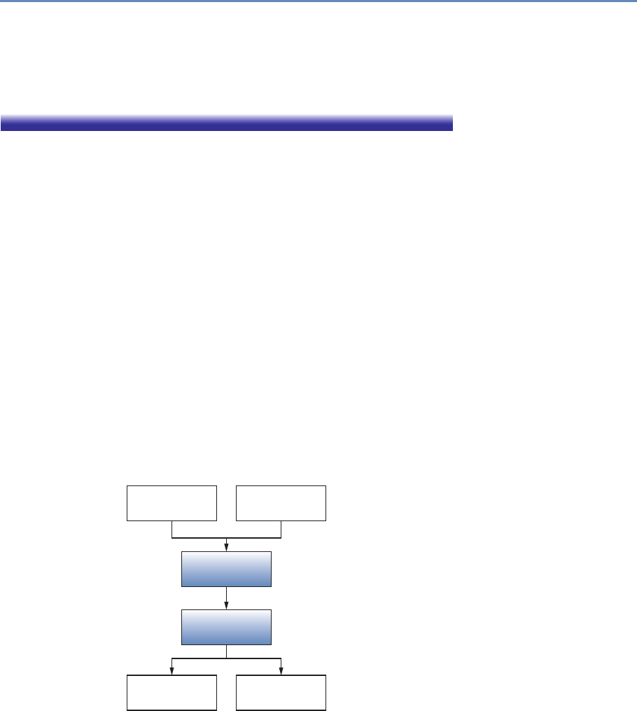
3.2. Introduction to record linkage 75
choosing employment; or (iii) it is not possible to uniquely match him/her to a
Census Bureau record. They correctly note that there may be biases introduced in
case (iii), because Asian names are more likely duplicated and harder to uniquely
match [415]. Improving the linkage algorithm would increase the estimate of the
effects of investments in research and the result would be more accurate.
Comparing the kinds of heterogeneous records associated with
big data is a new challenge for social scientists, who have tradition-
ally used a technique first developed in the 1960s to apply comput-
ers to the problem of medical record linkage. There is a reason why
this approach has survived: it has been highly successful in linking
survey data to administrative data, and efficient implementations
of this algorithm can be applied at the big data scale. However,
the approach is most effective when the two files being linked have
a number of fields in common. In the new landscape of big data,
there is a greater need to link files that have few fields in common
but whose noncommon fields provide additional predictive power to
determine which records should be linked. In some cases, when
sufficient training data can be produced, more modern machine
learning techniques may be applied.
The canonical record linkage workflow process is shown in Fig-
ure 3.1 for two data files, A and B. The goal is to identify all pairs of
records in the two data sets that correspond to the same underlying
individual. One approach is to compare all data units from file A
Data le A
Comparison
Classication
Links Non links
Data le B
Figure 3.1. The preprocessing pipeline
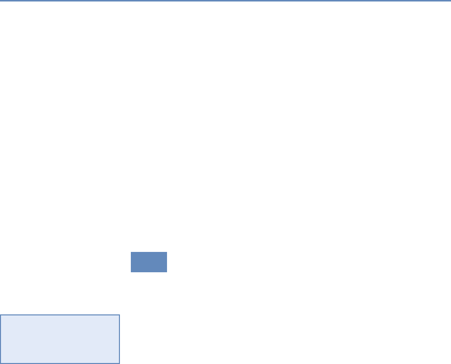
76 3. Record Linkage
with all units in file B and classify all of the comparison outcomes
to decide whether or not the records match. In a perfect statistical
world the comparison would end with a clear determination of links
and nonlinks.
Alas, a perfect world does not exist, and there is likely to be
noise in the variables that are common to both data sets and that
will be the main identifiers for the record linkage. Although the
original files A and B are the starting point, the identifiers must be
preprocessed before they can be compared. Determining identifiers
for the linkage and deciding on the associated cleaning steps are
extremely important, as they result in a necessary reduction of the
possible search space.
In the next section we begin our overview of the record linkage
process with a discussion of the main steps in data preprocess-
ing. This is followed by a section on approaches to record linkage
that includes rule-based, probabilistic, and machine learning algo-
rithms. Next we cover classification and evaluation of links, and we
conclude with a discussion of data privacy in record linkage.
3.3 Preprocessing data for record linkage
As noted in the introductory chapter, all data work involves prepro-
cessing, and data that need to be linked is no exception. Preprocess-
ing refers to a workflow that transforms messy, noisy, and unstruc-
tured data into a well-defined, clearly structured, and quality-tested
data set. Elsewhere in this book, we discuss general strategies for
◮This topic (quality of
data, preprocessing issues)
is discussed in more detail
in Section 1.4.
data preprocessing. In this section, we focus specifically on pre-
processing steps relating to the choice of input fields for the record
linkage algorithm. Preprocessing for any kind of a new data set is
a complex and time-consuming process because it is “hands-on”: it
requires judgment and cannot be effectively automated. It may be
tempting to minimize this demanding work under the assumption
that the record linkage algorithm will account for issues in the data,
but it is difficult to overstate the value of preprocessing for record
linkage quality. As Winkler notes: “In situations of reasonably
high-quality data, preprocessing can yield a greater improvement
in matching efficiency than string comparators and ‘optimized’ pa-
rameters. In some situations, 90% of the improvement in matching
efficiency may be due to preprocessing” [406].
The first step in record linkage is to develop link keys, which are
the record fields that will be used to predict link status. These can
include common identifiers like first and last name. Survey and ad-

3.3. Preprocessing data for record linkage 77
ministrative data sets may include a number of clearly identifying
variables like address, birth date, and sex. Other data sets, like
transaction records or social media data, often will not include ad-
dress or birth date but may still include other identifying fields like
occupation, a list of interests, or connections on a social network.
Consider this chapter’s illustrative example of the US Patent and
Trademark Office (USPTO) data [387]:
USPTO maintains an online database of all patents is-
sued in the United States. In addition to identifying in-
formation about the patent, the database contains each
patent’s list of inventors and assignees, the companies,
organizations, individuals, or government agencies to
which the patent is assigned. . . . However, inventors and
assignees in the USPTO database are not given unique
identification numbers, making it difficult to track inven-
tors and assignees across their patents or link their in-
formation to other data sources.
There are some basic precepts that are useful when considering
identifying fields. The more different values a field can take, the less
likely it is that two randomly chosen individuals in the population
will agree on those values. Therefore, fields that exhibit a wider
range of values are more powerful as link keys: names are much
better link keys than sex or year of birth.
Example: Link keys in practice
“A Harvard professor has re-identified the names of more than 40 percent of a
sample of anonymous participants in a high-profile DNA study, highlighting the
dangers that ever greater amounts of personal data available in the Internet era
could unravel personal secrets. . . . Of the 1,130 volunteers Sweeney and her
team reviewed, about 579 provided zip code, date of birth and gender, the three
key pieces of information she needs to identify anonymous people combined with
information from voter rolls or other public records. Of these, Sweeney succeeded
in naming 241, or 42 percent of the total. The Personal Genome Project confirmed
that 97 percent of the names matched those in its database if nicknames and first
name variations were included” [369].
Complex link keys like addresses can be broken down into com-
ponents so that the components can be compared independently of
one another. This way, errors due to data quality can be further

78 3. Record Linkage
isolated. For example, assigning a single comparison value to the
complex fields “1600 Pennsylvania” and “160 Pennsylvania Ave” is
less informative than assigning separate comparison values to the
street number and street name portions of those fields. A record
linkage algorithm that uses the decomposed field can make more
nuanced distinctions by assigning different weights to errors in each
component.
Sometimes a data set can include different variants of a field,
like legal first name and nickname. In these cases match rates
can be improved by including all variants of the field in the record
comparison. For example, if only the first list includes both vari-
ants, and the second list has a single “first name” field that could
be either a legal first name or a nickname, then match rates can be
improved by comparing both variants and then keeping the better
of the two comparison outcomes. It is important to remember, how-
ever, that some record linkage algorithms expect field comparisons
to be somewhat independent. In our example, using the outcome
from both comparisons as separate inputs into the probabilistic
model we describe below may result in a higher rate of false nega-
tives. If a record has the same value in the legal name and nickname
fields, and if that value happens to agree with the first name field
in the second file, then the agreement is being double-counted. By
the same token, if a person in the first list has a nickname that
differs significantly from their legal first name, then a comparison
of that record to the corresponding record will unfairly penalize the
outcome because at least one of those name comparisons will show
a low level of agreement.
Preprocessing serves two purposes in record linkage. First, to
correct for issues in data quality that we described above. Second,
to account for the different ways that the input files were generated,
which may result in the same underlying data being recorded on
different scales or according to different conventions.
Once preprocessing is finished, it is possible to start linking the
records in the different data sets. In the next section we describe a
technique to improve the efficiency of the matching step.
3.4 Indexing and blocking
There is a practical challenge to consider when comparing the records
in two files. If both files are roughly the same size, say 100 records
in the first and 100 records in the second file, then there are 10,000
possible comparisons, because the number of pairs is the product

3.4. Indexing and blocking 79
of the number of records in each file. More generally, if the number
of records in each file is approximately n, then the total number of
possible record comparisons is approximately n2. Assuming that
there are no duplicate records in the input files, the proportion of
record comparisons that correspond to a link is only 1/n. If we
naively proceed with all n2possible comparisons, the linkage algo-
rithm will spend the bulk of its time comparing records that are not
matches. Thus it is possible to speed up record linkage significantly
by skipping comparisons between record pairs that are not likely to
be linked.
Indexing refers to techniques that determine which of the poss-
ible comparisons will be made in a record linkage application. The
most used technique for indexing is blocking. In this approach you
construct a “blocking key” for each record by concatenating fields
or parts of fields. Two records with identical blocking keys are
said to be in the same block, and only records in the same block
are compared. This technique is effective because performing an
exact comparison of two blocking keys is a relatively quick operation
compared to a full record comparison, which may involve multiple
applications of a fuzzy string comparator.
Example: Blocking in practice
Given two lists of individuals, one might construct the blocking key by concate-
nating the first letter of the last name and the postal code and then “blocking”
on first character of last name and postal code. This reduces the total number of
comparisons by only comparing those individuals in the two files who live in the
same locality and whose last names begin with the same letter.
There are important considerations when choosing the blocking
key. First, the choice of blocking key creates a potential bias in
the linked data because true matches that do not share the same
blocking key will not be found. In the example, the blocking strategy
could fail to match records for individuals whose last name changed
or who moved. Second, because blocking keys are compared ex-
actly, there is an implicit assumption that the included fields will
not have typos or other data entry errors. In practice, however, the
blocking fields will exhibit typos. If those typos are not uniformly
distributed over the population, then there is again the possibility
of bias in the linked data set. One simple strategy for dealing with
◮This topic is discussed in
more detail in Chapter 10.
imperfect blocking keys is to implement multiple rounds of block-

80 3. Record Linkage
ing and matching. After the first set of matches is produced, a new
blocking strategy is deployed to search for additional matches in the
remaining record pairs.
Blocking based on exact field agreements is common in practice,
but there are other approaches to indexing that attempt to be more
error tolerant. For example, one may use clustering algorithms to
identify sets of similar records. In this approach an index key, which
is analogous to the blocking key above, is generated for both data
sets and then the keys are combined into a single list. A distance
function must be chosen and pairwise distances computed for all
keys. The clustering algorithm is then applied to the combined list,
and only record pairs that are assigned to the same cluster are
compared. This is a theoretically appealing approach but it has the
drawback that the similarity metric has to be computed for all pairs
of records. Even so, computing the similarity measure for a pair of
blocking keys is likely to be cheaper than computing the full record
comparison, so there is still a gain in efficiency. Whang et al. [397]
provide a nice review of indexing approaches.
In addition to reducing the computational burden of record link-
age, indexing plays an important secondary role. Once implemented,
the fraction of comparisons made that correspond to true links will
be significantly higher. For some record linkage approaches that
use an algorithm to find optimal parameters—like the probabilis-
tic approach—having a larger ratio of matches to nonmatches will
produce a better result.
3.5 Matching
The purpose of a record linkage algorithm is to examine pairs of
records and make a prediction as to whether they correspond to the
same underlying entity. (There are some sophisticated algorithms
that examine sets of more than two records at a time [359], but
pairwise comparison remains the standard approach.) At the core
of every record linkage algorithm is a function that compares two
records and outputs a “score” that quantifies the similarity between
those records. Mathematically, the match score is a function of the
output from individual field comparisons: agreement in the first
name field, agreement in the last name field, etc. Field comparisons
may be binary—indicating agreement or disagreement—or they may
output a range of values indicating different levels of agreement.
There are a variety of methods in the statistical and computer sci-
ence literature that can be used to generate a match score, includ-

3.5. Matching 81
ing nearest-neighbor matching, regression-based matching, and
propensity score matching. The probabilistic approach to record
linkage defines the match score in terms of a likelihood ratio [118].
Example: Matching in practice
Long strings, such as assignee and inventor names, are susceptible to typograph-
ical errors and name variations. For example, none of Sony Corporation, Sony
Corporatoin and Sony Corp. will match using simple exact matching. Similarly,
David vs. Dave would not match [387].
Comparing fields whose values are continuous is straightforward:
often one can simply take the absolute difference as the comparison
value. Comparing character fields in a rigorous way is more com-
plicated. For this purpose, different mathematical definitions of
the distance between two character fields have been defined. Edit
distance, for example, is defined as the minimum number of edit
operations—chosen from a set of allowed operations—needed to con-
vert one string to another. When the set of allowed edit operations is
single-character insertions, deletions, and substitutions, the corre-
sponding edit distance is also known as the Levenshtein distance.
When transposition of adjacent characters is allowed in addition
to those operations, the corresponding edit distance is called the
Levenshtein–Damerau distance.
Edit distance is appealing because of its intuitive definition, but
it is not the most efficient string distance to compute. Another
standard string distance known as Jaro–Winkler distance was de-
veloped with record linkage applications in mind and is faster to
compute. This is an important consideration because in a typical
record linkage application most of the algorithm run time will be
spent performing field comparisons. The definition of Jaro–Winkler
distance is less intuitive than edit distance, but it works as ex-
pected: words with more characters in common will have a higher
Jaro–Winkler value than those with fewer characters in common.
The output value is normalized to fall between 0 and 1. Because
of its history in record linkage applications, there are some stan-
dard variants of Jaro–Winkler distance that may be implemented in
record linkage software. Some variants boost the weight given to
agreement in the first few characters of the strings being compared.
Others decrease the score penalty for letter substitutions that arise
from common typos.

82 3. Record Linkage
Once the field comparisons are computed, they must be com-
bined to produce a final prediction of match status. In the following
sections we describe three types of record linkage algorithms: rule-
based, probabilistic, and machine learning.
3.5.1 Rule-based approaches
A natural starting place is for a data expert to create a set of ad hoc
rules that determine which pairs of records should be linked. In the
classical record linkage setting where the two files have a number
of identifying fields in common, this is not the optimal approach.
However, if there are few fields in common but each file contains
auxiliary fields that may inform a linkage decision, then an ad hoc
approach may be appropriate.
Example: Linking in practice
Consider the problem of linking two lists of individuals where both lists contain
first name, last name, and year of birth. Here is one possible linkage rule: link all
pairs of records such that
•the Jaro–Winkler comparison of first names is greater than 0.9
•the Jaro–Winkler comparison of last names is greater than 0.9
•the first three digits of the year of birth are the same.
The result will depend on the rate of data errors in the year of birth field and typos
in the name fields.
By auxiliary field we mean data fields that do not appear on both
data sets, but which may nonetheless provide information about
whether records should be linked. Consider a situation in which the
first list includes an occupation field and the second list includes
educational history. In that case one might create additional rules
to eliminate matches where the education was deemed to be an
unlikely fit for the occupation.
This method may be attractive if it produces a reasonable-looking
set of links from intuitive rules, but there are several pitfalls. As
the number of rules grows it becomes harder to understand the
ways that the different rules interact to produce the final set of
links. There is no notion of a threshold that can be increased or
decreased depending on the tolerance for false positive and false
negative errors. The rules themselves are not chosen to satisfy any
kind of optimality, unlike the probabilistic and machine learning

3.5. Matching 83
methods. Instead, they reflect the practitioner’s domain knowledge
about the data sets.
3.5.2 Probabilistic record linkage
In this section we describe the probabilistic approach to record
linkage, also known as the Fellegi–Sunter algorithm [118]. This
approach dominates in traditional record linkage applications and
remains an effective and efficient way to solve the record linkage
problem today.
In this section we give a somewhat formal definition of the statis-
tical model underlying the algorithm. By understanding this model,
one is better equipped to define link keys and record comparisons
in an optimal way.
Example: Usefulness of probabilistic record linkage
In practice, it is typically the case that a researcher will want to combine two or
more data sets containing records for the same individuals or units that possi-
bly come from different sources. Unless the sources all contain the same unique
identifiers, linkage will likely require matching on standardized text strings. Even
standardized data are likely to contain small differences that preclude exact match-
ing as in the matching example above. The Census Bureau’s Longitudinal Busi-
ness Database (LBD) links establishment records from administrative and survey
sources. Exact numeric identifiers do most of the heavy lifting, but mergers, ac-
quisitions, and other actions can break these linkages. Probabilistic record linkage
on company names and/or addresses is used to fix these broken linkages that bias
statistics on business dynamics [190].
Let Aand Bbe two lists of individuals whom we wish to link.
The product set A×Bcontains all possible pairs of records where
the first element of the pair comes from Aand the second element
of the pair comes from B. A fraction of these pairs will be matches,
meaning that both records in the pair represent the same underlying
individual, but the vast majority of them will be nonmatches. In
other words, A×Bis the disjoint union of the set of matches M
and the set of nonmatches U, a fact that we denote formally by
A×B=M∪U.
Let γbe a vector-valued function on A×Bsuch that, for a∈Aand
b∈B,γ(a, b)represents the outcome of a set of field comparisons
between aand b. For example, if both Aand Bcontain data on

84 3. Record Linkage
individuals’ first names, last names, and cities of residence, then γ
could be a vector of three binary values representing agreement in
first name, last name, and city. In that case γ(a, b)=(1,1,0)would
mean that the records aand bagree on first name and last name,
but disagree on city of residence.
For this model, the comparison outcomes in γ(a, b)are not re-
quired to be binary, but they do have to be categorical: each com-
ponent of γ(a, b)should take only finitely many values. This means
that a continuous comparison outcome—such as output from the
Jaro–Winkler string comparator—has to be converted to an ordinal
value representing levels of agreement. For example, one might cre-
ate a three-level comparison, using one level for exact agreement,
one level for approximate agreement defined as a Jaro–Winkler score
greater than 0.85, and one level for nonagreement corresponding to
a Jaro–Winkler score less than 0.85.
If a variable being used in the comparison has a significant num-
ber of missing values, it can help to create a comparison outcome
level to indicate missingness. Consider two data sets that both have
middle initial fields, and suppose that in one of the data sets the
middle initial is filled in only about half of the time. When compar-
ing records, the case where both middle initials are filled in but are
not the same should be treated differently from the case where one
of the middle initials is blank, because the first case provides more
evidence that the records do not correspond to the same person.
We handle this in the model by defining a three-level comparison
for the middle initial, with levels to indicate “equal,” “not equal,”
and “missing.”
Probabilistic record linkage works by weighing the probability of
seeing the result γ(a, b)if (a, b)belongs to the set of matches M
against the probability of seeing the result if (a, b)belongs to the
set of nonmatches U. Conditional on Mor U, the distribution of the
individual comparisons defined by γare assumed to be mutually
independent. The parameters that define the marginal distributions
of γ|Mare called m-weights, and similarly the marginal distributions
of γ|Uare called u-weights.
In order to apply the Fellegi–Sunter method, it is necessary to
choose values for these parameters, m-weights and u-weights. With
labeled data—a pair of lists for which the match status is known—
it is straightforward to solve for optimal values. Training data are
not usually available, however, and the typical approach is to use
expectation maximization to find optimal values.
We have noted that primary motivation for record linkage is to
create a linked data set for analysis that will have a richer set of fields

3.5. Matching 85
than either of the input data sets alone. A natural application is to
perform a linear regression using a combination of variables from
both files as predictors. With all record linkage approaches it is a
challenge to understand how errors from the linkage process will
manifest in the regression. Probabilistic record linkage has an ad-
vantage over rule-based and machine learning approaches in that
there are theoretical results concerning coefficient bias and errors
[221, 329]. More recently, Chipperfield and Chambers have devel-
oped an approach based on the bootstrap to account for record link-
age errors when making inferences for cross-tabulated variables [75].
3.5.3 Machine learning approaches to linking
Computer scientists have contributed extensively in parallel litera-
ture focused on linking large data sets [76]. Their focus is on iden-
tifying potential links using approaches that are fast and scalable,
and approaches are developed based on work in network algorithms
and machine learning.
While simple blocking as described in Section 3.4 is standard in
Fellegi–Sunter applications, computer scientists are likely to use the
more sophisticated clustering approach to indexing. Indexing may
also use network information to include, for example, records for in-
dividuals that have a similar place in a social graph. When linking
lists of researchers, one might specify that comparisons should be
made between records that share the same address, have patents
in the same patent class, or have overlapping sets of coinventors.
These approaches are known as semantic blocking, and the com-
putational requirements are similar to standard blocking [76].
In recent years machine learning approaches have been applied
◮This topic is discussed in
more detail in Chapter 6.
to record linkage following their success in other areas of prediction
and classification. Computer scientists couch the analytical prob-
lem as one of entity resolution, even though the conceptual problem
is identical. As Wick et al. [400] note:
Entity resolution, the task of automatically determining
which mentions refer to the same real-world entity, is a
crucial aspect of knowledge base construction and man-
agement. However, performing entity resolution at large
scales is challenging because (1) the inference algorithms
must cope with unavoidable system scalability issues and
(2) the search space grows exponentially in the number
of mentions. Current conventional wisdom declares that
performing coreference at these scales requires decom-

86 3. Record Linkage
posing the problem by first solving the simpler task of
entity-linking (matching a set of mentions to a known set
of KB entities), and then performing entity discovery as a
post-processing step (to identify new entities not present
in the KB). However, we argue that this traditional ap-
proach is harmful to both entity-linking and overall coref-
erence accuracy. Therefore, we embrace the challenge of
jointly modeling entity-linking and entity discovery as a
single entity resolution problem.
Figure 3.2 provides a useful comparison between classical record
linkage and learning-based approaches. In machine learning there
is a predictive model and an algorithm for “learning” the optimal
set of parameters to use in the predictive algorithm. The learning
algorithm relies on a training data set. In record linkage, this would
be a curated data set with true and false matches labeled as such.
See [387] for an example and a discussion of how a training data
set was created for the problem of disambiguating inventors in the
USPTO database. Once optimal parameters are computed from the
training data, the predictive model can be applied to unlabeled data
to find new links. The quality of the training data set is critical; the
model is only as good as the data it is trained on.
An example of a machine learning model that is popular for
record linkage is the random forest model [50]. This is a classi-
◮See Chapter 6.
fication model that fits a large number of classification trees to a
labeled training data set. Each individual tree is trained on a boot-
strap sample of all labeled cases using a random subset of predictor
variables. After creating the classification trees, new cases are la-
beled by giving each tree a vote and keeping the label that receives
the most votes. This highly randomized approach corrects for a
problem with simple classification trees, which is that they may
overfit to training data.
As shown in Figure 3.2, a major difference between probabilistic
and machine learning approaches is the need for labeled training
data to implement the latter approach. Usually training data are
created through a painstaking process of clerical review. After an
initial round of record linkage, a sample of record pairs that are
not clearly matches or nonmatches is given to a research assistant
who makes the final determination. In some cases it is possible to
create training data by automated means. For example, when there
is a subset of the complete data that contains strongly identifying
fields. Suppose that both of the candidate lists contain name and
date of birth fields and that in the first list the date of birth data are
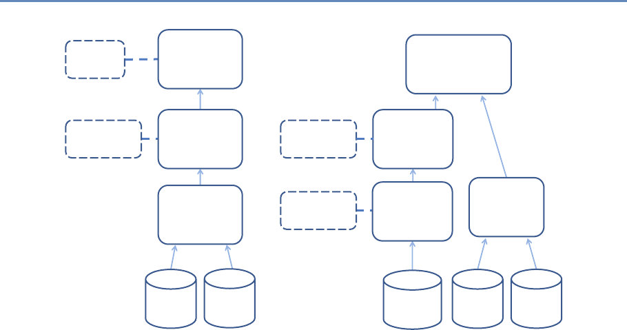
3.5. Matching 87
Match
Decision
Similarity
Computation
reshold
• Similarity Function
• Attribute Selection
Blocking
Source Target Source Target
Blocking
Model
Application
Training
Data
Selection
Training
Data
• No. of Examples
• Selection Scheme
• reshold
Model
Generation
• Learning Algorithm
• Matcher Selection
Figure 3.2. Probabilistic (left) vs. machine learning (right) approaches to linking. Source: Köpcke et al. [213]
complete, but in the second list only about 10% of records contain
date of birth. For reasonably sized lists, name and date of birth
together will be a nearly unique identifier. It is then possible to
perform probabilistic record linkage on the subset of records with
date of birth and be confident that the error rates would be small.
If the subset of records with date of birth is representative of the
complete data set, then the output from the probabilistic record
linkage can be used as “truth” data.
Given a quality training data set, machine learning approaches
may have advantages over probabilistic record linkage. Consider
the random forest model. Random forests are more robust to corre-
lated predictor variables, because only a random subset of predic-
tors is included in any individual classification tree. The conditional
independence assumption, to which we alluded in our discussion
of the probabilistic model, can be dropped. An estimate of the gen-
eralization error can be computed in the form of “out-of-bag error.”
A measure of variable importance is computed that gives an idea of
how powerful a particular field comparison is in terms of correctly
predicting link status. Finally, unlike the Fellegi–Sunter model,
predictor variables can be continuous.
The combination of being robust to correlated variables and pro-
viding a variable importance measure makes random forests a use-

88 3. Record Linkage
ful diagnostic tool for record linkage models. It is possible to refine
the record linkage model iteratively, by first including many pre-
dictor variables, including variants of the same comparison, and
then using the variable importance measure to narrow down the
predictors to a parsimonious set.
There are many published studies on the effectiveness of random
forests and other machine learning algorithms for record linkage.
Christen and Ahmed et al. provide some pointers [77, 108].
3.5.4 Disambiguating networks
The problem of disambiguating entities in a network is closely re-
lated to record linkage: in both cases the goal is to consolidate mul-
tiple records corresponding to the same entity. Rather than finding
the same entity in two data sets, however, the goal in network dis-
ambiguation is to consolidate duplicate records in a network data
set. By network we mean that the data set contains not only typical
record fields like names and addresses but also information about
how entities relate to one another: entities may be coauthors, coin-
ventors, or simply friends in a social network.
The record linkage techniques that we have described in this
chapter can be applied to disambiguate a network. To do so, one
must convert the network to a form that can be used as input into
a record linkage algorithm. For example, when disambiguating a
social network one might define a field comparison whose output
gives the fraction of friends in common between two records. Ven-
tura et al. demonstrated the relative effectiveness of the probabilis-
tic method and machine learning approaches to disambiguating a
database of inventors in the USPTO database [387]. Another ap-
proach is to apply clustering algorithms from the computer science
literature to identify groups of records that are likely to refer to the
same entity. Huang et al. [172] have developed a successful method
based on an efficient computation of distance between individuals
in the network. These distances are then fed into the DBSCAN
clustering algorithm to identify unique entities.
3.6 Classification
Once the match score for a pair of records has been computed us-
ing the probabilistic or random forest method, a decision has to be
made whether the pair should be linked. This requires classifying
the pair as either a “true” or a “false” match. In most cases, a third
classification is required—sending for manual review and classifica-
tion.

3.6. Classification 89
3.6.1 Thresholds
In the probabilistic and random forest approaches, both of which
output a “match score” value, a classification is made by establish-
ing a threshold Tsuch that all records with a match score greater
than Tare declared to be links. Because of the way these algorithms
are defined, the match scores are not meaningful by themselves and
the threshold used for one linkage application may not be appro-
priate for another application. Instead, the classification threshold
must be established by reviewing the model output.
Typically one creates an output file that includes pairs of records
that were compared along with the match score. The file is sorted
by match score and the reviewer begins to scan the file from the
highest match scores to the lowest. For the highest match scores the
record pairs will agree on all fields and there is usually no question
about the records being linked. However, as the scores decrease the
reviewer will see more record pairs whose match status is unclear
(or that are clearly nonmatches) mixed in with the clear matches.
There are a number of ways to proceed, depending on the resources
available and the goal of the project.
Rather than set a single threshold, the reviewer may set two
thresholds T1> T2. Record pairs with a match score greater than
T1are marked as matches and removed from further consideration.
The set of record pairs with a match score between T1and T2are be-
lieved to contain significant numbers of matches and nonmatches.
These are sent to clerical review, meaning that research assistants
will make a final determination of match status. The final set of
links will include clear matches with a score greater than T1as well
as the record pairs that pass clerical review. If the resources are
available for this approach and the initial threshold T1is set suf-
ficiently high, then the resulting data set will contain a minimal
number of false positive links. The collection of record pairs with
match scores between T1and T2is sometimes referred to as the
clerical review region.
The clerical review region generally contains many more pairs
than the set of clear matches, and it can be expensive and time-
consuming to review each pair. Therefore, a second approach is to
establish tentative threshold Tand send only a sample of record
pairs with scores in a neighborhood of Tto clerical review. This
results in data on the relative numbers of true matches and true
nonmatches at different score levels, as well as the characteristics
of record pairs that appear at a given level. Based on the review
and the relative tolerance for false positive errors and false negative

90 3. Record Linkage
errors, a final threshold T′is set such that pairs with a score greater
than T′are considered to be matches.
After viewing the results of the clerical review, it may be deter-
mined that the parameters to the record linkage algorithm could be
improved to create a clearer delineation between matches and non-
matches. For example, a research assistant may determine that
many potential false positives appear near the tentative threshold
because the current set of record linkage parameters is giving too
much weight to agreement in first name. In this case the reviewer
may decide to update the record linkage model to produce an im-
proved set of match scores. The update may consist in an ad hoc
adjustment of parameters, or the result of the clerical review may
be used as training data and the parameter-fitting algorithm may
be run again. An iterative approach like this is common when first
linking two data sets because the clerical review process can im-
prove one’s understanding of the data sets involved.
Setting the threshold value higher will reduce the number of false
positives (record pairs for which a link is incorrectly predicted) while
increasing the number of false negatives (record pairs that should
be linked but for which a link is not predicted). The proper tradeoff
between false positive and false negative error rates will depend
on the particular application and the associated loss function, but
there are some general concerns to keep in mind. Both types of
errors create bias, which can impact the generalizability of analyses
conducted on the linked data set. Consider a simple regression
on the linked data that includes fields from both data sets. If the
threshold is too high, then the linked data will be biased toward
records with no data entry errors or missing values, and whose
fields did not change over time. This set of records may not be
representative of the population as a whole. If a low threshold is
used, then the set of linked records will contain more pairs that
are not true links and the variables measured in those records are
independent of each other. Including these records in a regression
amounts to adding statistical noise to the data.
3.6.2 One-to-one links
In the probabilistic and machine learning approaches to record link-
age that we have described, each record pair is compared and a link
is predicted independently of all other record pairs. Because of the
independence of comparisons, one record in the first file may be
predicted to link to multiple records in the second file. Under the
assumption that each input file has been deduplicated, at most one

3.7. Record linkage and data protection 91
of these predictions can correspond to a true link. For many ap-
plications it is preferable to extract a set of “best” links with the
property that each record in one file links to at most one record
in the second file. A set of links with this property is said to be
one-to-one.
One possible definition of “best” is a set of one-to-one links such
that the sum of the match scores of all included links is maximal.
This is an example of what is known as the assignment problem in
combinatorial optimization. In the linear case above, where we care
about the sum of match scores, the problem can be solved exactly
using the Hungarian algorithm [216].
◮This topic is discussed in
more detail in Chapter 6.
3.7 Record linkage and data protection
In many social science applications data sets there is no need for
data to include identifying fields like names and addresses. These
fields may be left out intentionally out of concern for privacy, or
◮See Chapter 11.
they may simply be irrelevant to the research question. For record
linkage, however, names and addresses are among the best possible
identifiers. We describe two approaches to the problem of balancing
needs for both effective record linkage and privacy.
The first approach is to establish a trusted third party or safe
center. The concept of trusted third parties (TTPs) is well known
in cryptography. In the case of record linkage, a third party takes
a place between the data owners and the data users, and it is this
third party that actually performs the linkage work. Both the data
owners and data users trust the third party in the sense that it
assumes responsibility for data protection (data owners) and data
competence (data users) at the same time. No party other than the
TTP learns about the private data of the other parties. After record
linkage only the linked records are revealed, with no identifiers at-
tached. The TTP ensures that the released linked data set cannot
be relinked to any of the source data sets. Possible third parties
are safe centers, which are operated by lawyers, or official trusted
institutions like the US Census Bureau. Some countries like the
UK and Germany are establishing new institutions specifically to
act as TTPs for record linkage work.
The second approach is known as privacy-preserving record link-
age. The goal of this approach is to find the same individual in sep-
arate data files without revealing the identity of the individual [80].
In privacy-preserving record linkage, cryptographic procedures are
used to encrypt or hash identifiers before they are shared for record
linkage. Many of these procedures require exact matching of the
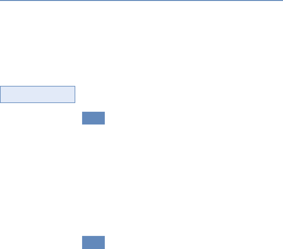
92 3. Record Linkage
identifiers, however, and do not tolerate any errors in the original
identifiers. This leads to information loss because it is not possible
to account for typos or other small variations in hashed fields. To
account for this, Schnell has developed a method to calculate string
similarity of encrypted fields using bloom filters [330,332].
In many countries these approaches are combined. For exam-
ple, when the UK established the ADRN, the latter established the
concept of trusted third parties. That third party is provided with
data in which identifying fields have been hashed. This solves the
challenge of trust between the different parties. Some authors ar-
gue that transparency of data use and informed consent will help
to build trust. In the context of big data this is more challenging..
◮This topic is discussed in
more detail in Chapter 11.
3.8 Summary
Accurate record linkage is critical to creating high-quality data sets
for analysis. However, outside of a few small centers for record
linkage research, linking data sets historically relied on artisan ap-
proaches, particularly for parsing and cleaning data sets. As the
creation and use of big data increases, so does the need for system-
atic record linkage. The history of record linkage is long by computer
science standards, but new data challenges encourage the develop-
ment of new approaches like machine learning methods, clustering
algorithms, and privacy-preserving record linkage.
Record linkage stands on the boundary between statistics, in-
formation technology, and privacy. We are confident that there will
continue to be exciting developments in this field in the years to
come.
3.9 Resources
Out of many excellent resources on the subject, we note the follow-
ing:
•We strongly recommend Christen’s book [76].
•There is a wealth of information available on the ADRN website
[103].
•Winkler has a series of high-quality survey articles [407].
•The German Record Linkage Center is a resource for research,
software, and ongoing conference activities [331].

Databases
Chapter 4
Ian Foster and Pascal Heus
Once the data have been collected and linked into different files, it
is necessary to store and organize them. Social scientists are used
to working with one analytical file, often in SAS, Stata, SPSS, or
R. This chapter, which may be the most important chapter in the
book, describes different approaches to storing data in ways that
permit rapid and reliable exploration and analysis.
4.1 Introduction
We turn now to the question of how to store, organize, and manage
the data used in data-intensive social science. As the data with
which you work grow in volume and diversity, effective data man-
agement becomes increasingly important if you are to avoid issues
of scale and complexity from overwhelming your research processes.
In particular, when you deal with data that get frequently updated,
with changes made by different people, you will frequently want to
use database management systems (DBMSs) instead of maintaining
data in single files or within siloed statistical packages such as SAS,
SPSS, Stata, and R. Indeed, we go so far as to say: if you take away
just one thing from this book, it should be this: Use a database!
As we explain in this chapter, DBMSs provide an environment
that greatly simplifies data management and manipulation. They
require a little bit of effort to set up, but are worth it. They permit
large amounts of data to be organized in multiple ways that allow
for efficient and rapid exploration via powerful declarative query
languages; durable and reliable storage, via transactional features
that maintain data consistency; scaling to large data sizes; and in-
tuitive analysis, both within the DBMS itself and via bridges to other
data analysis packages and tools when specialized analyses are re-
quired. DBMSs have become a critical component of a great variety
93

94 4. Databases
of applications, from handling transactions in financial systems to
delivering data as a service to power websites, dashboards, and ap-
plications. If you are using a production-level enterprise system,
chances are there is a database in the back end. They are multi-
purpose and well suited for organizing social science data and for
supporting analytics for data exploration.
DBMSs make many easy things trivial, and many hard things
easy. They are easy to use but can appear daunting to those un-
familiar with their concepts and workings. A basic understanding
of databases and of when and how to use DBMSs is an important
element of the social data scientist’s knowledge base. We therefore
provide in this chapter an introduction to databases and how to
use them. We describe different types of databases and their var-
ious features, and how different types can be applied in different
contexts. We describe basic features like how to get started, set
up a database schema, ingest data, query data within a database,
and get results out. We also discuss how to link from databases
to other tools, such as Python, R, and Stata (if you really have
to). Chapter 5 describes how to apply parallel computing methods
when needed.
4.2 DBMS: When and why
Consider the following three data sets:
1. 10,000 records describing research grants, each specifying the
principal investigator, institution, research area, proposal ti-
tle, award date, and funding amount in comma-separated-
value (CSV) format.
2. 10 million records in a variety of formats from funding agen-
cies, web APIs, and institutional sources describing people,
grants, funding agencies, and patents.
3. 10 billion Twitter messages and associated metadata—around
10 terabytes (1013 bytes) in total, and increasing at a terabyte
a month.
Which tools should you use to manage and analyze these data sets?
The answer depends on the specifics of the data, the analyses that
you want to perform, and the life cycle within which data and ana-
lyses are embedded. Table 4.1 summarizes relevant factors, which
we now discuss.

4.2. DBMS: When and why 95
Table 4.1. When to use different data management and analysis technologies
Text files, spreadsheets, and scripting language
•Your data are small
•Your analysis is simple
•You do not expect to repeat analyses over time
Statistical packages
•Your data are modest in size
•Your analysis maps well to your chosen statistical package
Relational database
•Your data are structured
•Your data are large
•You will be analyzing changed versions of your data over time
•You want to share your data and analyses with others
NoSQL database
•Your data are unstructured
•Your data are extremely large
In the case of data set 1 (10,000 records describing research
grants), it may be feasible to leave the data in their original file,
use spreadsheets, pivot tables, or write programs in scripting lan-
guages*such as Python or R to ask questions of those files. For
⋆A scripting language is
a programming language
used to automate tasks that
could otherwise be per-
formed one by one be the
user.
example, someone familiar with such languages can quickly create
a script to extract from data set 1 all grants awarded to one inves-
tigator, compute average grant size, and count grants made each
year in different areas.
However, this approach also has disadvantages. Scripts do not
provide inherent control over the file structure. This means that if
you obtain new data in a different format, your scripts need to be
updated. You cannot just run them over the newly acquired file.
Scripts can also easily become unreasonably slow as data volumes
grow. A Python or R script will not take long to search a list of
1,000 grants to find those that pertain to a particular institution.
But what if you have information about 1 million grants, and for
each grant you want to search a list of 100,000 investigators, and
for each investigator, you want to search a list of 10 million papers
to see whether that investigator is listed as an author of each paper?
You now have 1,000,000×100,000×10,000,000 =1018 comparisons
to perform. Your simple script may now run for hours or even days.
You can speed up the search process by constructing indices, so
that, for example, when given a grant, you can find the associated
investigators in constant time rather than in time proportional to
the number of investigators. However, the construction of such
indices is itself a time-consuming and error-prone process.
96 4. Databases
For these reasons, the use of scripting languages alone for data
analysis is rarely to be recommended. This is not to say that
all analysis computations can be performed in database systems.
A programming language will also often be needed. But many
data access and manipulation computations are best handled in
a database.
Researchers in the social sciences frequently use statistical pack-
ages*such as R, SAS, SPSS, and Stata for data analysis. Because
⋆A statistical package is
a specialized compute pro-
gram for analysis in statis-
tics and economics.
these systems integrate some crude data management, statistical
analysis, and graphics capabilities in a single package, a researcher
can often carry out a data analysis project of modest size within the
same environment. However, each of these systems has limitations
that hinder its use for modern social science research, especially as
data grow in size and complexity.
Take Stata, for example. Stata always loads the entire data set
into the computer’s working memory, and thus you would have
no problems loading data set 1. However, depending on your com-
puter’s memory, it could have problems dealing with with data set 2
and certainly would not be able to handle data set 3. In addition,
you would need to perform this data loading step each time you
start working on the project, and your analyses would be limited
to what Stata can do. SAS can deal with larger data sets, but is
renowned for being hard to learn and use. Of course there are
workarounds in statistical packages. For example, in Stata you can
deal with larger file sizes by choosing to only load the variables or
cases that you need for the analysis [211]. Likewise, you can deal
with more complex data by creating a system of files that each can
be linked as needed for a particular analysis through a common
identifier variable.
◮For example, the Panel
Study of Income Dynamics
[181] has a series of files
that are related and can be
combined through common
identifier variables [182].
Those solutions essentially mimic core functions of a DBMS, and
you would be well advised to set up such system, especially if you
find yourself in a situation where the data set is constantly updated
through different users, if groups of users have different rights to
use your data or should only have access to subsets of the data,
and if the analysis takes place on a server that sends results to
a client (browser). Statistics packages also have difficulty working
with more than one data source at a time—something that DBMSs
are designed to do well.
These considerations bring us to the topic of this chapter, namely
database management systems. A DBMS*handles all of the is-
⋆DBMS is a system
that interacts with users,
other applications, and the
database itself to capture
and analyze data.
sues listed above, and more. As we will see below when we look
at concrete examples, a DBMS allows the programmer to define a
logical design that fits the structure of their data. The DBMS then

4.2. DBMS: When and why 97
implements a data model (more on this below) that allows these data
to be stored, queried, and updated efficiently and reliably on disk,
thus providing independence from underlying physical storage. It
supports efficient access to data through query languages and auto-
matic optimization of those queries to permit fast analysis. Impor-
tantly, it also support concurrent access by multiple users, which is
not an option for file-based data storage. It supports transactions,
meaning that any update to a database is performed in its entirety
or not at all, even in the face of computer failures or multiple con-
current updates. And it reduces the time spent both by analysts,
by making it easy to express complex analytical queries concisely,
and on data administration, by providing simple and uniform data
administration interfaces.
Adatabase is a structured collection of data about entities and
their relationships. It models real-world objects—both entities (e.g.,
grants, investigators, universities) and relationships (e.g., “Steven
Weinberg” works at “University of Texas at Austin”)—and captures
structure in ways that allow these entities and relationships to be
queried for analysis. A database management system is a software
suite designed to safely store and efficiently manage databases, and
to assist with the maintenance and discovery of the relationships
that database represents. In general, a DBMS encompasses three
key components, as shown in Table 4.2: its data model (which
defines how data are represented: see Box 4.1), its query language
(which defines how the user interacts with the data), and support
for transactions and crash recovery (to ensure reliable execution
despite system failures).*⋆Some key DBMS fea-
tures are often lacking in
standard statistical pack-
ages: a standard query lan-
guage (with commands that
allow analyses or data ma-
nipulation on a subgroup
of cases defined during
the analysis, for example
“group by . . . ,” “order by
. . . ”), keys (for speed im-
provement), and an explicit
model of a relational data
structure.
Box 4.1: Data model
Adata model specifies the data elements associated with a
problem domain, the properties of those data elements, and
how those data elements relate to one another. In developing
a data model, we commonly first identity the entities that are
to be modeled and then define their properties and relation-
ships. For example, when working on the science of science
policy (see Figure 1.2), the entities include people, products,
institutions, and funding, each of which has various properties
(e.g., for a person, their name, address, employer); relationships
include “is employed by” and “is funded by.” This conceptual
data model can then be translated into relational tables or some
other database representation, as we describe next.

98 4. Databases
Table 4.2. Key components of a DBMS
Data model Query language Transactions, crash recovery
User-facing For example: relational,
semi-structured
For example: SQL (for
relational), XPath (for
semi-structured)
Transactions
Internal Mapping data to storage
systems; creating and
maintaining indices
Query optimization and
evaluation; consistency
Locking, concurrency control,
recovery
Literally hundreds of different open source, commercial, and
cloud-hosted versions DBMSs are available. However, you only
need to understand a relatively small number of concepts and ma-
jor database types to make sense of this diversity. Table 4.3 defines
the major classes of DBMSs that we will consider in this book. We
consider only a few of these in any detail.
Relational DBMSs are the most widely used and mature sys-
tems, and will be the optimal solution for many social science data
analysis purposes. We describe relational DBMSs in detail below,
but in brief, they allow for the efficient storage, organization, and
analysis of large quantities of tabular data: data organized as ta-
◮Sometimes, as discussed
in Chapter 3, the links are
one to one and sometimes
one to many.
bles, in which rows represent entities (e.g., research grants) and
columns represent attributes of those entities (e.g., principal inves-
tigator, institution, funding level). The associated Structured Query
Language (SQL) can then be used to perform a wide range of anal-
yses, which are executed with high efficiency due to sophisticated
indexing and query planning techniques.
While relational DBMSs have dominated the database world for
decades, other database technologies have become popular for var-
ious classes of applications in recent years. As we will see, these
alternative NoSQL DBMSs have typically been motivated by a de-
sire to scale the quantities of data and/or number of users that can
be supported and/or to deal with unstructured data that are not
easily represented in tabular form. For example, a key–value store
can organize large numbers of records, each of which associates an
arbitrary key with an arbitrary value. These stores, and in partic-
ular variants called document stores that permit text search on the
stored values, are widely used to organize and process the billions
of records that can be obtained from web crawlers. We review be-
low some of these alternatives and the factors that may motivate
their use.

4.2. DBMS: When and why 99
Table 4.3. Types of databases: relational (first row) and various types of NoSQL (other rows)
Type Examples Advantages Disadvantages Uses
Relational
database
MySQL,
PostgreSQL,
Oracle, SQL
Server, Teradata
Consistency (ACID) Fixed schema;
typically harder to
scale
Transactional systems:
order processing, retail,
hospitals, etc.
Key–value
store
Dynamo, Redis Dynamic schema; easy
scaling; high
throughput
Not immediately
consistent; no
higher-level queries
Web applications
Column
store
Cassandra,
HBase
Same as key–value;
distributed; better
compression at column
level
Not immediately
consistent; using
all columns is
inefficient
Large-scale analysis
Document
store
CouchDB,
MongoDB
Index entire document
(JSON)
Not immediately
consistent; no
higher-level queries
Web applications
Graph
database
Neo4j,
InfiniteGraph
Graph queries are fast Difficult to do
non-graph analysis
Recommendation
systems, networks,
routing
Relational and NoSQL databases (and indeed other solutions,
such as statistical packages) can also be used together. Consider,
for example, Figure 4.1, which depicts data flows commonly en-
countered in large research projects. Diverse data are being col-
lected from different sources: JSON documents from web APIs, web
pages from web scraping, tabular data from various administrative
databases, Twitter data, and newspaper articles. There may be hun-
dreds or even thousands of data sets in total, some of which may be
extremely large. We initially have no idea of what schema*to use for
⋆A schema defines the
structure of a database in
a formal language defined
by the DBMS. See Sec-
tion 4.3.3.
the different data sets, and indeed it may not be feasible to define
a unified set of schema, so diverse are the data and so rapidly are
new data sets being acquired. Furthermore, the way we organize
the data may vary according to our intended purpose. Are we in-
terested in geographic, temporal, or thematic relationships among
different entities? Each type of analysis may require a different
organization.
For these reasons, a common storage solution is to first load
all data into a large NoSQL database. This approach makes all
data available via a common (albeit limited) query interface. Re-
searchers can then extract from this database the specific elements
that are of interest for their work, loading those elements into a re-
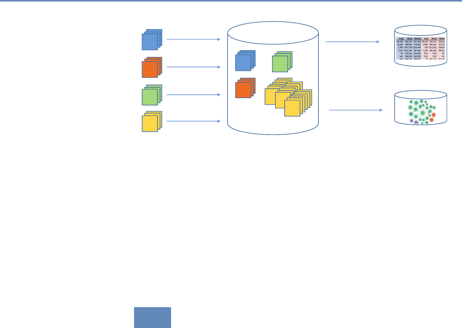
100 4. Databases
PubMed
abstracts
Researcher
web pages
Patent
abstracts
Twitter
messages
Big NoSQL database
Extracted
research area
Domain-specic
relational database
Extracted
collaboration
network
Graph database
Figure 4.1. A research project may use a NoSQL database to accumulate large
amounts of data from many different sources, and then extract selected subsets to
a relational or other database for more structured processing
lational DBMS, another specialized DBMS (e.g., a graph database),
or a statistical package for more detailed analysis. As part of the
process of loading data from the NoSQL database into a relational
database, the researcher will necessarily define schemas, relation-
ships between entities, and so forth. Analysis results can be stored
in a relational database or back into the NoSQL store.
4.3 Relational DBMSs
We now provide a more detailed description of relational DBMSs.
Relational DBMSs implement the relational data model, in which
data are represented as sets of records organized in tables. This
model is particularly well suited for the structured, regular data
with which we frequently deal in the social sciences; we discuss in
Section 4.5 alternative data models, such as those used in NoSQL
databases.
We use the data shown in Figure 4.2 to introduce key con-
cepts. These two CSV format files describe grants made by the
US National Science Foundation (NSF). One file contains informa-
tion about grants, the other information about investigators. How
should you proceed to manipulate and analyze these data?
The main concept underlying the relational data model is a ta-
ble (also referred to as a relation): a set of rows (also referred to as
tuples, records, or observations), each with the same columns (also
referred to as fields, attributes or variables). A database consists of
multiple tables. For example, we show in Figure 4.3 how the data

4.3. Relational DBMSs 101
The file grants.csv
# Identifier,Person,Funding,Program
1316033,Steven Weinberg,666000,Elem. Particle Physics/Theory
1336199,Howard Weinberg,323194,ENVIRONMENTAL ENGINEERING
1500194,Irving Weinberg,200000,Accelerating Innovation Rsrch
1211853,Irving Weinberg,261437,GALACTIC ASTRONOMY PROGRAM
The file investigators.csv
# Name,Institution,Email
Steven Weinberg,University of Texas at Austin,weinberg@utexas.edu
Howard Weinberg,University of North Carolina Chapel Hill,
Irving Weinberg,University of Maryland College Park,irving@ucmc.edu
Figure 4.2. CSV files representing grants and investigators. Each line in the first table specifies a grant number,
investigator name, total funding amount, and NSF program name; each line in the second gives an investigator
name, institution name, and investigator email address
contained in the two CSV files of Figure 4.2 may be represented as
two tables. The Grants table contains one tuple for each row in
grants.csv, with columns GrantID,Person,Funding, and Program.
The Investigators table contains one tuple for each row in inves-
tigators.csv, with columns ID,Name,Institution, and Email. The
CSV files and tables contain essentially the same information, al-
beit with important differences (the addition of an ID field in the
Investigators table, the substitution of an ID column for the Person
column in the Grants table) that we will explain below.
The use of the relational data model provides for physical inde-
pendence: a given table can be stored in many different ways. SQL
queries are written in terms of the logical representation of tables
(i.e., their schema definition). Consequently, even if the physical
organization of the data changes (e.g., a different layout is used
to store the data on disk, or a new index is created to speed up
access for some queries), the queries need not change. Another
advantage of the relational data model is that, since a table is a
set, in a mathematical sense, simple and intuitive set operations
(e.g., union, intersection) can be used to manipulate the data, as
we discuss below. We can easily, for example, determine the inter-
section of two relations (e.g., grants that are awarded to a specific
institution), as we describe in the following. The database further
ensures that the data comply with the model (e.g., data types, key
uniqueness, entity relationships), essentially providing core quality
assurance.

102 4. Databases
Number Person Funding Program
1316033 1 660,000 Elem. Particle Physics/Theory
1336199 2 323,194 ENVIRONMENTAL ENGINEERING
1500194 3 200,000 Accelerating Innovation Rsrch
1211853 3 261,437 GALACTIC ASTRONOMY PROGRAM
ID Name Institution Email
1 Steven Weinberg University of Texas at Austin weinberg@utexas.edu
2 Howard Weinberg University of North Carolina Chapel Hill
3 Irving Weinberg University of Maryland College Park irving@ucmc.edu
Figure 4.3. Relational tables Grants and Investigators corresponding to the grants.csv and investigators.csv
data in Figure 4.2, respectively. The only differences are the representation in a tabular form, the introduction of a
unique numerical investigator identifier (ID) in the Investigators table, and the substitution of that identifier for
the investigator name in the Grants table
4.3.1 Structured Query Language (SQL)
We use query languages to manipulate data in a database (e.g.,
to add, update, or delete data elements) and to retrieve (raw and
aggregated) data from a database (e.g., data elements that certain
properties). Relational DBMSs support SQL, a simple, powerful
query language with a strong formal foundation based on logic, a
foundation that allows relational DBMSs to perform a wide variety of
sophisticated optimizations. SQL is used for three main purposes:
•Data definition: e.g., creation of new tables,
•Data manipulation: queries and updates,
•Control: creation of assertions to protect data integrity.
We introduce each of these features in the following, although not
in that order, and certainly not completely. Our goal here is to give
enough information to provide the reader with insights into how
relational databases work and what they do well; an in-depth SQL
tutorial is beyond the scope of this book but is something we highly
recommend readers seek elsewhere.
4.3.2 Manipulating and querying data
SQL and other query languages used in DBMSs support the concise,
declarative specification of complex queries. Because we are eager
to show you something immediately useful, we cover these features
first, before talking about how to define data models.

4.3. Relational DBMSs 103
Example: Identifying grants of more than $200,000
Here is an SQL query to identify all grants with total funding of at most $200,000:
select *from Grants
where Funding <= 200,000;
(Here and elsewhere in this chapter, we show SQL key words in blue.)
Notice SQL’s declarative nature: this query can be read almost as the English
language statement, “select all rows from the Grants table for which the Funding
column has value less than or equal 200,000.” This query is evaluated as follows:
1. The input table specified by the from clause, Grants, is selected.
2. The condition in the where clause, Funding <= 200,000, is checked
against all rows in the input table to identify those rows that match.
3. The select clause specifies which columns to keep from the matching rows,
that is, which columns make the schema of the output table. (The “*” indi-
cates that all columns should be kept.)
The answer, given the data in Figure 4.3, is the following single-row table. (The
fact that an SQL query returns a table is important when it comes to creating more
complex queries: the result of a query can be stored into the database as a new
table, or passed to another query as input.)
Number Person Funding Program
1500194 3 200,000 Accelerating Innovation Rsrch
DBMSs automatically optimize declarative queries such as the
example that we just presented, translating them into a set of low-
level data manipulations (an imperative query plan) that can be eval-
uated efficiently. This feature allows users to write queries without
having to worry too much about performance issues—the database
does the worrying for you. For example, a DBMS need not consider
every row in the Grants table in order to identify those with funding
less than $200,000, a strategy that would be slow if the Grants ta-
ble were large: it can instead use an index to retrieve the relevant
records much more quickly. We discuss indices in more detail in
Section 4.3.6.
The querying component of SQL supports a wide variety of ma-
nipulations on tables, whether referred to explicitly by a table name
(as in the example just shown) or constructed by another query.
We just saw how to use the select operator to both pick certain
rows (what is termed selection) and certain columns (what is called
projection) from a table.
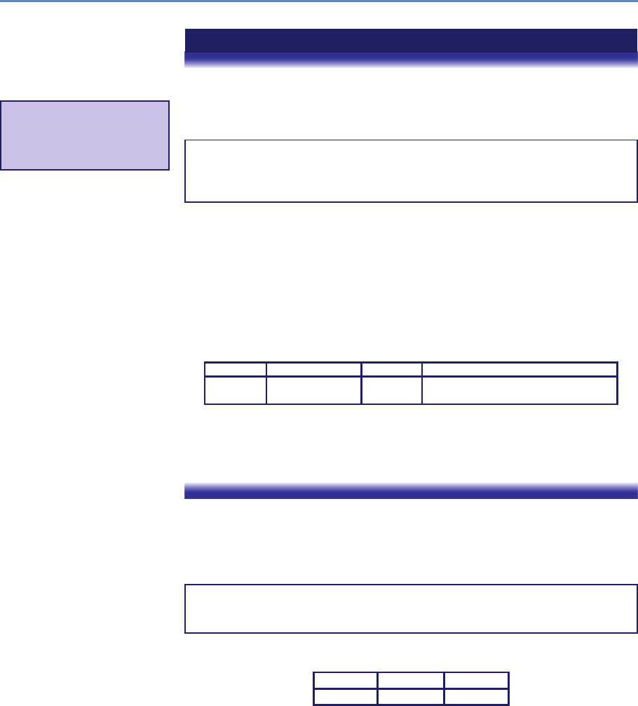
104 4. Databases
Example: Finding grants awarded to an investigator
We want to find all grants awarded to the investigator with name “Irving Weinberg.”
The information required to answer this question is distributed over two tables,
Grants and Investigators, and so we join*the two tables to combine tuples
⋆In statistical packages,
the term merge or append
is often used when data
sets are combined.
from both:
select Number, Name, Funding, Program
from Grants, Investigators
where Grants.Person = Investigators.ID
and Name = "Irving Weinberg";
This query combines tuples from the Grants and Investigators tables
for which the Person and ID fields match. It is evaluated in a similar fashion
to the query presented above, except for the from clause: when multiple tables
are listed, as here, the conditions in the where clause are checked for all different
combinations of tuples from the tables defined in the from clause (i.e., the cartesian
product of these tables)—in this case, a total of 3 ×4=12 combinations. We
thus determine that Irving Weinberg has two grants. The query further selects
the Number,Name,Funding, and Program fields from the result, giving the
following:
Number Name Funding Program
1500194 Irving Weinberg 200,000 Accelerating Innovation Rsrch
1211853 Irving Weinberg 261,437 GALACTIC ASTRONOMY PROGRAM
This ability to join two tables in a query is one example of how SQL permits
concise specifications of complex computations. This joining of tables via a carte-
sian product operation is formally called a cross join. Other types of join are also
supported. We describe one such, the inner join, in Section 4.6.
SQL aggregate functions allow for the computation of aggregate
statistics over tables. For example, we can use the following query
to determine the total number of grants and their total and average
funding levels:
select count(*)as 'Number',sum(Funding) as 'Total',
avg(Funding) as 'Average'
from Grants;
This yields the following:
Number Total Average
4 1444631 361158
The group by operator can be used in conjunction with the ag-
gregate functions to group the result set by one or more columns.

4.3. Relational DBMSs 105
For example, we can use the following query to create a table with
three columns: investigator name, the number of grants associated
with the investigator, and the aggregate funding:
select Name, count(*)as 'Number',
avg(Funding) as 'Average funding'
from Grants, Investigators
where Grants.Person = Investigators.ID
group by Name;
We obtain the following:
Name Number Average Funding
Steven Weinberg 1 666000
Howard Weinberg 1 323194
Irving Weinberg 2 230719
4.3.3 Schema design and definition
We have seen that a relational database comprises a set of tables.
The task of specifying the structure of the data to be stored in a
database is called logical design. This task may be performed by
a database administrator, in the case of a database to be shared
by many people, or directly by users, if they are creating databases
themselves. More specifically, the logical design process involves
defining a schema. A schema comprises a set of tables (including,
for each table, its columns and their types), their relationships, and
integrity constraints.
The first step in the logical design process is to identify the en-
tities that need to be modeled. In our example, we identified two
important classes of entity: “grants” and “investigators.” We thus
define a table for each; each row in these two tables will correspond
to a unique grant or investigator, respectively. (In a more complete
and realistic design, we would likely also identify other entities, such
as institutions and research products.) During this step, we will of-
ten find ourselves breaking information up into multiple tables, so
as to avoid duplicating information.
For example, imagine that we were provided grant information
in the form of one CSV file rather than two, with each line pro-
viding a grant number, investigator, funding, program, institution,
and email. In this file, the name, institution, and email address
for Irving Weinberg would then appear twice, as he has two grants,
which can lead to errors when updating values and make it difficult
to represent certain information. (For example, if we want to add an
investigator who does not yet have a grant, we will need to create
106 4. Databases
a tuple (row) with empty slots for all columns (variables) associated
with grants.) Thus we would want to break up the single big table
into the two tables that we defined here. This breaking up of infor-
mation across different tables to avoid repetition of information is
referred to as normalization.*
⋆Normalization involves
organizing columns and ta-
bles of a relational database
to minimize data redun-
dancy.
The second step in the design process is to define the columns
that are to be associated with each entity. For each table, we define
a set of columns. For example, given the data in Figure 4.2, those
columns will likely include, for a grant, an award identifier, title,
investigator, and award amount; for an investigator, a name, uni-
versity, and email address. In general, we will want to ensure that
each row in our table has a key: a set of columns that uniquely iden-
tifies that row. In our example tables, grants are uniquely identified
◮Normalization can be
done in statistical packages
as well. For example, as
noted above, PSID splits
its data into different files
linked through ID variables.
The difference here is that
the DBMS makes creat-
ing, navigating, and query-
ing the resulting data partic-
ularly easy.
by Number and investigators by ID.
The third step in the design process is to capture relationships
between entities. In our example, we are concerned with just one
relationship, namely that between grants and investigators: each
grant has an investigator. We represent this relationship between
tables by introducing a Person column in the Grants table, as shown
in Figure 4.3. Note that we do not simply duplicate the investigator
names in the two tables, as was the case in the two CSV files shown
in Figure 4.2: these names might not be unique, and the duplication
of data across tables can lead to later inconsistencies if a name is
updated in one table but not the other.
The final step in the design process is to represent integrity con-
straints (or rules) that must hold for the data. In our example, we
may want to specify that each grant must be awarded to an investi-
gator; that each value of the grant identifier column must be unique
(i.e., there cannot be two grants with the same number); and total
funding can never be negative. Such restrictions can be achieved by
specifying appropriate constraints at the time of schema creation,
as we show in Listing 4.1, which contains the code used to create
the two tables that make up our schema.
Listing 4.1 contains four SQL statements. The first two state-
ments, lines 1 and 2, simply set up our new database. The create
table statement in lines 4–10 creates our first table. It specifies
the table name (Investigators) and, for each of the four columns,
the column name and its type.*Relational DBMSs offer a rich set
⋆These storage types
will be familiar to many of
you from statistical software
packages.
of types to choose from when designing a schema: for example,
int or integer (synonyms); real or float (synonyms); char(n),
a fixed-length string of ncharacters; and varchar(n), a variable-
length string of up to ncharacters. Types are important for several
reasons. First, they allow for more efficient encoding of data. For

4.3. Relational DBMSs 107
create database grantdata;
2use grantdata;
4create table Investigators (
ID int auto_increment,
6Name varchar(100) not null,
Institution varchar(256) not null,
8Email varchar(100),
primary key(ID)
10 );
12 create table Grants (
Number int not null,
14 Person int not null,
Funding float unsigned not null,
16 Program varchar(100),
primary key(Number)
18 );
Listing 4.1. Code to create the grantdata database and its Investigators
and Grants tables
example, the Funding field in the grants.csv file of Figure 4.2 could
be represented as a string in the Grants table, char(15), say, to
allow for large grants. By representing it as a floating point number
instead (line 15 in Listing 4.1), we reduce the space requirement
per grant to just four bytes. Second, types allow for integrity checks
on data as they are added to the database: for example, that same
type declaration for Funding ensures that only valid numbers will be
entered into the database. Third, types allow for type-specific op-
erations on data, such as arithmetic operations on numbers (e.g.,
min, max, sum).
Other SQL features allow for the specification of additional con-
straints on the values that can be placed in the corresponding
column. For example, the not null constraints for Name and
Institution (lines 6, 7) indicate that each investigator must have
a name and an institution, respectively. (The lack of such a con-
straint on the Email column shows that an investigator need not
have an email address.)
4.3.4 Loading data
So far we have created a database and two tables. To complete
our simple SQL program, we show in Listing 4.2 the two state-
ments that load the data of Figure 4.2 into our two tables. (Here
and elsewhere in this chapter, we use the MySQL DBMS. The SQL

108 4. Databases
load data local infile "investigators.csv"
2into table Investigators
fields terminated by ","
4ignore 1lines
(Name, Institution, Email);
6
load data local infile "grants.csv" into table Grants
8fields terminated by ","
ignore 1lines
10 (Number, @var, Funding, Program)
set Person = (select ID from Investigators
12 where Investigators.Name=@var);
Listing 4.2. Code to load data into the Investigators and Grants tables
syntax used by different DBMSs differs in various, mostly minor
ways.) Each statement specifies the name of the file from which
data is to be read and the table into which it is to be loaded.
The fields terminated by "," statement tells SQL that values are
separated by columns, and ignore 1 lines tells SQL to skip the
header. The list of column names is used to specify how values
from the file are to be assigned to columns in the table.
For the Investigators table, the three values in each row of
the investigators.csv file are assigned to the Name,Institution, and
Email columns of the corresponding database row. Importantly, the
auto_increment declaration on the ID column (line 5 in Listing 4.1)
causes values for this column to be assigned automatically by the
DBMS, as rows are created, starting at 1. This feature allows us to
assign a unique integer identifier to each investigator as its data are
loaded.
For the Grants table, the load data call (lines 7–12) is somewhat
more complex. Rather than loading the investigator name (the sec-
ond column of each line in our data file, represented here by the
variable @var) directly into the database, we use an SQL query (the
select statement in lines 11–12) to retrieve from the Investigators
table the ID corresponding to that name. By thus replacing the
investigator name with the unique investigator identifier, we avoid
replicating the name across the two tables.
4.3.5 Transactions and crash recovery
A DBMS protects the data that it stores from computer crashes: if
your computer stops running suddenly (e.g., your operating system
crashes or you unplug the power), the contents of your database are

4.3. Relational DBMSs 109
not corrupted. It does so by supporting transactions. A transaction
is an atomic sequence of database actions. In general, every SQL
statement is executed as a transaction. You can also specify sets
of statements to be combined into a single transaction, but we do
not cover that capability here. The DBMS ensures that each trans-
action is executed completely even in the case of failure or error: if
the transaction succeeds, the results of all operations are recorded
permanently (“persisted”) in the database, and if it fails, all opera-
tions are “rolled back” and no changes are committed. For example,
suppose we ran the following SQL statement to convert the funding
amounts in the Grants table from dollars to euros, by scaling each
number by 0.9. The update statement specifies the table to be up-
dated and the operation to be performed, which in this case is to
update the Funding column of each row. The DBMS will ensure that
either no rows are altered or all are altered.
update Grants set Grants.Funding = Grants.Funding*0.9;
Transactions are also key to supporting multi-user access. The
concurrency control mechanisms in a DBMS allow multiple users to
operate on a database concurrently, as if they were the only users
of the system: transactions from multiple users can be interleaved
to ensure fast response times, while the DBMS ensures that the
database remains consistent. While entire books could be (and have
been) written on concurrency in databases, the key point is that
read operations can proceed concurrently, while update operations
are typically serialized.
4.3.6 Database optimizations
A relational DBMS applies query planning and optimization meth-
ods with the goal of evaluating queries as efficiently as possible.
For example, if a query asks for rows that fit two conditions, one
cheap to evaluate and one expensive, a relational DBMS may filter
first on the basis of the first condition, and then apply the second
conditions only to the rows identified by that first filter. These sorts
of optimization are what distinguish SQL from other programming
languages, as they allow the user to write queries declaratively and
rely on the DBMS to come up with an efficient execution strategy.
Nevertheless, the user can help the DBMS to improve perform-
ance. The single most powerful performance improvement tool is
the index, an internal data structure that the DBMS maintains to
speed up queries. While various types of indices can be created,
with different characteristics, the basic idea is simple. Consider the

110 4. Databases
column ID in our Investigators table. Assume that there are N
rows in the table. In the absence of an index, a query that refers
to a column value (e.g., where ID=3) would require a linear scan of
the table, taking on average N/2 comparisons and in the worst case
Ncomparisons. A binary tree index allows the desired value to be
found with just log2Ncomparisons.
Example: Using indices to improve database performance
Consider the following query:
select ID, Name, sum(Funding) as TotalFunding
from Grants, Investigators
where Investigators.ID=Grants.Person
group by ID;
This query joins our two tables to link investigators with the grants that they
hold, groups grants by investigator (using group by), and finally sums the funding
associated with the grants held by each investigator. The result is the following:
ID Name TotalFunding
1 Steven Weinberg 666000
2 Howard Weinberg 323194
3 Irving Weinberg 461437
In the absence of indices, the DBMS must compare each row in Investi-
gators with each row in Grants, checking for each pair whether Investiga-
tors.ID = Grants.Person holds. As the two tables in our sample database
have only three and four rows, respectively, the total number of comparisons is
only 3 ×4=12. But if we had, say, 1 million investigators and 1 million grants,
then the DBMS would have to perform 1 trillion comparisons, which would take
a long time. (More importantly in many cases, it would have to perform a large
number of disk I/O operations if the tables did not fit in memory.) An index on
the ID column of the Investigators table reduces the number of operations
dramatically, as the DBMS can then take each of the 1 million rows in the Grants
table and, for each row, identify the matching row(s) in Investigators via an
index lookup rather than a linear scan.
In our example table, the ID column has been specified to be a primary key,
and thus an index is created for it automatically. If it were not, we could easily
create the desired index as follows:
alter table Investigators add index(ID);
It can be difficult for the user to determine when an index is required. A good
rule of thumb is to create an index for any column that is queried often, that
is, appears on the right-hand side of a where statement. However, the presence
of indices makes updates more expensive, as every change to a column value
requires that the index be rebuilt to reflect the change. Thus, if your data are

4.3. Relational DBMSs 111
highly dynamic, you should carefully select which indices to create. (For bulk load
operations, a common practice is to drop indices prior to the data import, and
re-create them once the load is completed.) Also, indices take disk space, so you
need to consider the tradeoff between query efficiency and resources.
The explain command can be useful for determining when indices are re-
quired. For example, we show in the following some of the output produced when
we apply explain to our query. (For this example, we have expanded the two ta-
bles to 1,000 rows each, as our original tables are too small for MySQL to consider
the use of indices.) The output provides useful information such as the key(s) that
could be used, if indices exist (Person in the Grants table, and the primary key,
ID, for the Investigators table); the key(s) that are actually used (the primary
key, ID, in the Investigators table); the column(s) that are compared to the
index (Investigators.ID is compared with Grants.Person); and the number
of rows that must be considered (each of the 1,000 rows in Grants is compared
with one row in Investigators, for a total of 1,000 comparisons).
mysql> explain select ID, Name, sum(Funding) as TotalFunding
from Grants, Investigators
where Investigators.ID=Grants.Person group by ID;
+---------------+---------------+---------+---------------+------+
|table | possible_keys | key | ref | rows |
+---------------+---------------+---------+---------------+------+
| Grants | Person | NULL |NULL | 1000 |
| Investigators | PRIMARY |PRIMARY | Grants.Person | 1 |
+---------------+---------------+---------+---------------+------+
Contrast this output with the output obtained for equivalent tables in which
ID is not a primary key. In this case, no keys are used and thus 1,000 ×1,000 =
1,000,000 comparisons and the associated disk reads must be performed.
+---------------+---------------+------+------+------+
|table | possible_keys | key | ref | rows |
+---------------+---------------+------+------+------+
| Grants | Person | NULL |NULL | 1000 |
| Investigators | ID | NULL |NULL | 1000 |
+---------------+---------------+------+------+------+
A second way in which the user can contribute to performance
improvement is by using appropriate table definitions and data
types. Most DBMSs store data on disk. Data must be read from
disk into memory before it can be manipulated. Memory accesses
are fast, but loading data into memory is expensive: accesses to
main memory can be a million times faster than accesses to disk.
Therefore, to ensure queries are efficient, it is important to minimize
the number of disk accesses. A relational DBMS automatically op-
timizes queries: based on how the data are stored, it transforms
a SQL query into a query plan that can be executed efficiently,

112 4. Databases
and chooses an execution strategy that minimizes disk accesses.
But users can contribute to making queries efficient. As discussed
above, the choice of types made when defining schemas can make
a big difference. As a rule of thumb, only use as much space as
needed for your data: the smaller your records, the more records
can be transferred to main memory using a single disk access. The
design of relational tables is also important. If you put all columns
in a single table (do not normalize), more data will come into memory
than is required.
4.3.7 Caveats and challenges
It is important to keep the following caveats and challenges in mind
when using SQL technology with social science data.
Data cleaning Data created outside an SQL database, such as data
in files, are not always subject to strict constraints: data types
may not be correct or consistent (e.g., numeric data stored as text)
and consistency or integrity may not be enforced (e.g., absence of
primary keys, missing foreign keys). Indeed, as the reader probably
knows well from experience, data are rarely perfect. As a result,
the data may fail to comply with strict SQL schema requirements
and fail to load, in which case either data must be cleaned before
or during loading, or the SQL schema must be relaxed.
Missing values Care must be taken when loading data in which
some values may be missing or blank. SQL engines represent and
refer to a missing or blank value as the built-in constant null.
Counterintuitively, when loading data from text files (e.g., CSV),
many SQL engines require that missing values be represented ex-
plicitly by the term null; if a data value is simply omitted, it may
fail to load or be incorrectly represented, for example as zero or the
empty string (" ") instead of null. Thus, for example, the second
row in the investigators.csv file of Figure 4.2:
Howard Weinberg,University of North Carolina Chapel Hill,
may need to be rewritten as:
Howard Weinberg,University of North Carolina Chapel Hill,null

4.4. Linking DBMSs and other tools 113
Metadata for categorical variables SQL engines are metadata poor:
they do not allow extra information to be stored about a variable
(field) beyond its base name and type (int,char, etc., as introduced
in Section 4.3.3). They cannot, for example, record directly the fact
that the column class can only take one of three values, animal,
vegetable, or mineral, or what these values mean. Common prac-
tice is thus to store information about possible values in another
table (commonly referred to as a dimension table) that can be used
as a lookup and constraint, as in the following:
Table class_values
Value Description
animal Is alive
vegetable Grows
mineral Isn’t alive and doesn’t grow
A related concept is that a column or list of columns may be
declared primary key or unique. Either says that no two tuples of
the table may agree in all the column(s) on the list. There can be
only one primary key for a table, but several unique columns. No
column of a primary key can ever be null in any tuple. But columns
declared unique may have nulls, and there may be several tuples
with null.
4.4 Linking DBMSs and other tools
Query languages such as SQL are not general-purpose program-
ming languages; they support easy, efficient access to large data
sets, but are not intended to be used for complex calculations.
When complex computations are required, one can embed query
language statements into a programming language or statistical
package. For example, we might want to calculate the interquartile
range of funding for all grants. While this calculation can be ac-
complished in SQL, the resulting SQL code will be complicated.
Languages like Python make such statistical calculations straight-
forward, so it is natural to write a Python (or R, SAS, Stata, etc.)
program that connects to the DBMS that contains our data, fetches
the required data from the DBMS, and then calculates the inter-
quartile range of those data. The program can then, if desired,
store the result of this calculation back into the database.
Many relational DBMSs also have built-in analytical functions
or often now embed the R engine, providing significant in-database

114 4. Databases
from mysql.connector import MySQLConnection, Error
2from python_mysql_dbconfig import read_db_config
4def retrieve_and_analyze_data():
try:
6# Open connection to the MySQL database
dbconfig = read_db_config()
8conn = MySQLConnection(**dbconfig)
cursor = conn.cursor()
10 # Transmit the SQL query to the database
cursor.execute('select Funding from Grants;')
12 # Fetch all rows of the query response
rows = [row for row in cur.fetchall()]
14 calculate_inter_quartile_range(rows)
except Error as e:
16 print(e)
finally:
18 cursor.close()
conn.close()
20
if __name__ == '__main__':
22 retrieve_and_analyze_data()
Listing 4.3. Embedding SQL in Python
statistical and analytical capabilities and alleviating the need for
external processing.
Example: Embedding database queries in Python
The Python script in Listing 4.3 shows how this embedding of database queries in
Python is done. This script establishes a connection to the database (lines 7–9),
transmits the desired SQL query to the database (line 11), retrieves the query
results into a Python array (line 13), and calls a Python procedure (not given) to
perform the desired computation (line 14). A similar program could be used to load
the results of a Python (or R, SAS, Stata, etc.) computation into a database.
Example: Loading other structured data
We saw in Listing 4.2 how to load data from CSV files into SQL tables. Data in other
formats, such as the commonly used JSON, can also be loaded into a relational
DBMS. Consider, for example, the following JSON format data, a simplified version
of data shown in Chapter 2.

4.4. Linking DBMSs and other tools 115
1[
2{
3institute :Janelia Campus,
4name :Laurence Abbott,
5role :Senior Fellow,
6state :VA,
7town :Ashburn
8},
9{
10 institute :Jackson Lab,
11 name :Susan Ackerman,
12 role :Investigator,
13 state :ME,
14 town :Bar Harbor
15 }
16 ]
While some relational DBMSs provide built-in support for JSON objects, we
assume here that we want to convert these data into normal SQL tables. Using
one of the many utilities for converting JSON into CSV, we can construct the
following CSV file, which we can load into an SQL table using the method shown
earlier.
institute,name,role,state,town
Janelia Campus,Laurence Abbott,Senior Fellow,VA,Ashburn
Jackson Lab,Susan Ackerman,Investigator,ME,Bar Harbor
But into what table? The two records each combine information about a person
with information about an institute. Following the schema design rules given in
Section 4.3.3, we should normalize the data by reorganizing them into two tables,
one describing people and one describing institutes. Similar problems arise when
JSON documents contain nested structures. For example, consider the following
alternative JSON representation of the data above. Here, the need for normalization
is yet more apparent.
1[
2{
3name :Laurence Abbott,
4role :Senior Fellow,
5employer :{institute :Janelia Campus,
6state :VA,
7town :Ashburn}
8},
9{
10 name :Susan Ackerman,
11 role :Investigator,
12 employer:{institute :Jackson Lab,
13 state :ME,
14 town :Bar Harbor}
15 }
16 ]

116 4. Databases
Thus, the loading of JSON data into a relational database usually requires both
work on schema design (Section 4.3.3) and data preparation.
4.5 NoSQL databases
While relational DBMSs have dominated the database world for sev-
eral decades, other database technologies exist and indeed have
become popular for various classes of applications in recent years.
As we will see, these alternative technologies have typically been
motivated by a desire to scale the quantities of data and/or num-
ber of users that can be supported, and/or to support specialized
data types (e.g., unstructured data, graphs). Here we review some
of these alternatives and the factors that may motivate their use.
4.5.1 Challenges of scale: The CAP theorem
For many years, the big relational database vendors (Oracle, IBM,
Sybase, and to a lesser extent Microsoft) have been the mainstay of
how data were stored. During the Internet boom, startups looking
for low-cost alternatives to commercial relational DBMSs turned to
MySQL and PostgreSQL. However, these systems proved inadequate
for big sites as they could not cope well with large traffic spikes, for
example when many customers all suddenly wanted to order the
same item. That is, they did not scale.
An obvious solution to scaling databases is to partition and/or
replicate data across multiple computers, for example by distribut-
ing different tables, or different rows from the same table, over multi-
ple computers. However, partitioning and replication also introduce
challenges, as we now explain. Let us first define some terms. In a
system that comprises multiple computers:
•Consistency indicates that all computers see the same data at
the same time.
•Availability indicates that every request receives a response
about whether it succeeded or failed.
•Partition tolerance indicates that the system continues to op-
erate even if a network failure prevents computers from com-
municating.

4.5. NoSQL databases 117
An important result in distributed systems (the so-called “CAP
theorem” [51]) observes that it is not possible to create a distributed
system with all three properties. This situation creates a challenge
with large transactional data sets. Partitioning is needed in or-
der to achieve high performance, but as the number of comput-
ers grows, so too does the likelihood of network disruption among
pair(s) of computers. As strict consistency cannot be achieved at
the same time as availability and partition tolerance, the DBMS de-
signer must choose between high consistency and high availability
for a particular system.
The right combination of availability and consistency will de-
pend on the needs of the service. For example, in an e-commerce
setting, it makes sense to choose high availability for a checkout
process, in order to ensure that requests to add items to a shop-
ping cart (a revenue-producing process) can be honored. Errors
can be hidden from the customer and sorted out later. However, for
order submission—when a customer submits an order—it makes
sense to favor consistency because several services (credit card pro-
cessing, shipping and handling, reporting) need to access the data
simultaneously. However, in almost all cases, availability is chosen
over consistency.
4.5.2 NoSQL and key–value stores
Relational DBMSs were traditionally motivated by the need for trans-
action processing and analysis, which led them to put a premium
on consistency and availability. This led the designers of these
systems to provide a set of properties summarized by the acronym
ACID [137,347]:
•Atomic: All work in a transaction completes (i.e., is committed
to stable storage) or none of it completes.
•Consistent: A transaction transforms the database from one
consistent state to another consistent state.
•Isolated: The results of any changes made during a transaction
are not visible until the transaction has committed.
•Durable: The results of a committed transaction survive fail-
ures.
The need to support extremely large quantities of data and num-
bers of concurrent clients has led to the development of a range of
alternative database technologies that relax consistency and thus

118 4. Databases
these ACID properties in order to increase scalability and/or avail-
ability. These systems are commonly referred to as NoSQL (for “not
SQL”—or, more recently, “not only SQL,” to communicate that they
may support SQL-like query languages) because they usually do
not require a fixed table schema nor support joins and other SQL
features. Such systems are sometimes referred to as BASE [127]:
Basically Available (the system seems to work all the time), Soft
state (it does not have to be consistent all the time), and Eventu-
ally consistent (it becomes consistent at some later time). The data
systems used in essentially all large Internet companies (Google,
Yahoo!, Facebook, Amazon, eBay) are BASE.
Dozens of different NoSQL DBMSs exist, with widely varying
characteristics as summarized in Table 4.3. The simplest are key–
value stores such as Redis, Amazon Dynamo, Apache Cassandra,
and Project Voldemort. We can think of a key–value store as a rela-
tional database with a single table that has just two columns, key
and value, and that supports just two operations: store (or update)
a key–value pair, and retrieve the value for a given key.
Example: Representing investigator data in a NoSQL
database
We might represent the contents of the investigators.csv file of Figure 4.2 (in a
NoSQL database) as follows.
Key Value
Investigator_StevenWeinberg_Institution University of Texas at Austin
Investigator_StevenWeinberg_Email weinberg@utexas.edu
Investigator_HowardWeinberg_Institution University of North Carolina Chapel Hill
Investigator_IrvingWeinberg_Institution University of Maryland College Park
Investigator_IrvingWeinberg_Email irving@ucmc.edu
A client can then read and write the value associated with a given key by using
operations such as the following:
•Get(key) returns the value associated with key.
•Put(key,value) associates the supplied value with key.
•Delete(key) removes the entry for key from the data store.
Key–value stores are thus particularly easy to use. Furthermore, because there
is no schema, there are no constraints on what values can be associated with a
key. This lack of constraints can be useful if we want to store arbitrary data. For
example, it is trivial to add the following records to a key–value store; adding this
information to a relational table would require schema modifications.
Key Value
Investigator_StevenWeinberg_FavoriteColor Blue
Investigator_StevenWeinberg_Awards Nobel

4.5. NoSQL databases 119
Another advantage is that if a given key would have no value (e.g., Investiga-
tor_HowardWeinberg_Email), we need not create a record. Thus, a key–value store
can achieve a more compact representation of sparse data, which would have many
empty fields if expressed in relational form.
A third advantage of the key–value approach is that a key–value store is easily
partitioned and thus can scale to extremely large sizes. A key–value DBMS can
partition the space of keys (e.g., via a hash on the key) across different computers
for scalability. It can also replicate key–value pairs across multiple computers
for availability. Adding, updating, or querying a key–value pair requires simply
sending an appropriate message to the computer(s) that hold that pair.
The key–value approach also has disadvantages. As we can see from the exam-
ple, users must be careful in their choice of keys if they are to avoid name collisions.
The lack of schema and constraints can also make it hard to detect erroneous keys
and values. Key–value stores typically do not support join operations (e.g., “which
investigators have the Nobel and live in Texas?”). Many key–value stores also relax
consistency constraints and do not provide transactional semantics.
4.5.3 Other NoSQL databases
The simple structure of key–value stores allows for extremely fast
and scalable implementations. However, as we have seen, many
interesting data cannot be easily modeled as key–value pairs. Such
concerns have motivated the development of a variety of other NoSQL
systems that offer, for example, richer data models: document-
based (CouchDB and MongoDB), graph-based (Neo4J), and column-
based (Cassandra, HBase) databases.
In document-based databases, the value associated with a key
can be a structured document: for example, a JSON document,
permitting the following representation of our investigators.csv file
plus the additional information that we just introduced.
Key Value
Investigator_StevenWeinberg { institution : University of Texas at Austin,
email : weinberg@utexas.edu,
favcolor : Blue,
award : Nobel }
Investigator_HowardWeinberg { institution : University of North Carolina
Chapel Hill }
Investigator_IrvingWeinberg { institution : University of Maryland College
Park, email : irving@ucmc.edu }
Associated query languages may permit queries within the docu-
ment, such as regular expression searches, and retrieval of selected

120 4. Databases
fields, providing a form of a relational DBMS’s selection and projec-
tion capabilities (Section 4.3.2). For example, MongoDB allows us
to ask for documents in a collection called investigators that have
“University of Texas at Austin” as their institution and the Nobel as
an award.
db.investigators.find(
{ institution: ’University of Texas at Austin’,
award: ’Nobel’ }
)
A column-oriented DBMS stores data tables by columns rather
than by rows, as is common practice in relational DBMSs. This
approach has advantages in settings where aggregates must fre-
quently be computed over many similar data items: for example, in
clinical data analysis. Google Cloud BigTable and Amazon RedShift
are two cloud-hosted column-oriented NoSQL databases. HBase
and Cassandra are two open source systems with similar charac-
teristics. (Confusingly, the term column oriented is also often used
to refer to SQL database engines that store data in columns instead
of rows: for example, Google BigQuery, HP Vertica, Terradata, and
the open source MonetDB. Such systems are not to be confused
with column-based NoSQL databases.)
Graph databases store information about graph structures in
terms of nodes, edges that connect nodes, and attributes of nodes
and edges. Proponents argue that they permit particularly straight-
forward navigation of such graphs, as when answering queries such
as “find all the friends of the friends of my friends”—a task that
would require multiple joins in a relational database.
4.6 Spatial databases
Social science research commonly involves spatial data. Socio-
economic data may be associated with census tracts, data about
the distribution of research funding and associated jobs with cities
and states, and crime reports with specific geographic locations.
Furthermore, the quantity and diversity of such spatially resolved
data are growing rapidly, as are the scale and sophistication of the
systems that provide access to these data. For example, just one
urban data store, Plenario, contains many hundreds of data sets
about the city of Chicago [64].
Researchers who work with spatial data need methods for repre-
senting those data and then for performing various queries against
them. Does crime correlate with weather? Does federal spending

4.6. Spatial databases 121
on research spur innovation within the locales where research oc-
curs? These and many other questions require the ability to quickly
determine such things as which points exist within which regions,
the areas of regions, and the distance between two points. Spatial
databases address these and many other related requirements.
Example: Spatial extensions to relational databases
Spatial extensions have been developed for many relational databases: for exam-
ple, Oracle Spatial, DB2 Spatial, and SQL Server Spatial. We use the PostGIS
extensions to the PostgreSQL relational database here. These extensions im-
plement support for spatial data types such as point,line, and polygon, and
operations such as st_within (returns true if one object is contained within
another), st_dwithin (returns true if two objects are within a specified dis-
tance of each other), and st_distance (returns the distance between two objects).
Thus, for example, given two tables with rows for schools and hospitals in Illinois
(illinois_schools and illinois_hospitals, respectively; in each case,
the column the_geom is a polygon for the object in question) and a third table
with a single row representing the city of Chicago (chicago_citylimits), we
can easily find the names of all schools within the Chicago city limits:
select illinois_schools.name
from illinois_schools, chicago_citylimits
where st_within(illinois_schools.the_geom,
chicago_citylimits.the_geom);
We join the two tables illinois_schools and chicago_citylimits,
with the st_within constraint constraining the selected rows to those represent-
ing schools within the city limits. Here we use the inner join introduced in Sec-
tion 4.3.2. This query could also be written as:
select illinois_schools.name
from illinois_schools left join chicago_citylimits
on st_within(illinois_schools.the_geom,
chicago_citylimits.the_geom);
We can also determine the names of all schools that do not have a hospital
within 3,000 meters:
select s.name as 'School Name'
from illinois_schools as s
left join illinois_hospitals as h
on st_dwithin(s.the_geom, h.the_geom, 3000)
where h.gid is null;
Here, we use an alternative form of the join operator, the left join—or, more
precisely, the left excluding join. The expression
table1 left join table2 on constraint
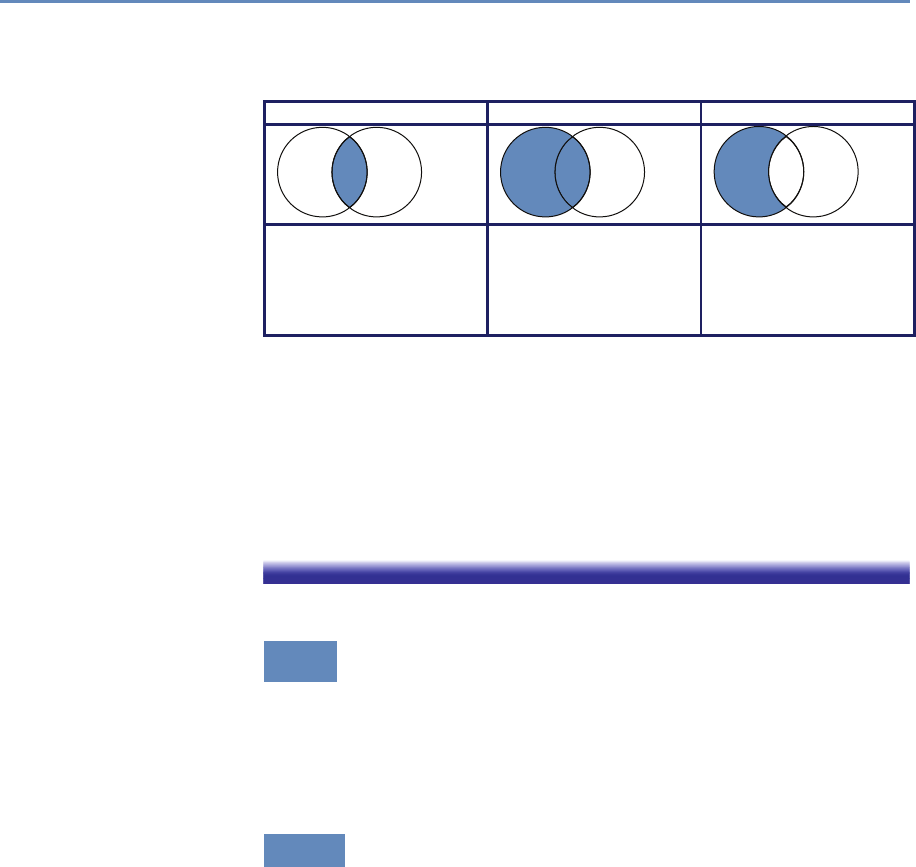
122 4. Databases
Table 4.4. Three types of join illustrated: the inner join, as used in Section 4.3.2,
the left join, and left excluding join
Inner join Left join Left excluding join
A B
A B
A B
select columns select columns select columns
from Table_A A from Table_A A from Table_A A
inner join Table_B B left join Table_B B left join Table_B B
on A.Key = B.Key on A.Key = B.Key on A.Key = B.Key
where B.Key is null
returns all rows from the left table (table1) with the matching rows in the right
table (table2), with the result being null in the right side when there is no match.
This selection is illustrated in the middle column of Table 4.4. The addition of
the where h.gid is null then selects only those rows in the left table with
no right-hand match, as illustrated in the right-hand column of Table 4.4. Note
also the use of the as operator to rename the columns illinois_schools and
illinois_hospitals. In this case, we rename them simply to make our query
more compact.
4.7 Which database to use?
The question of which DBMS to use for a social sciences data man-
agement and analysis project depends on many factors. We in-
troduced some relevant rules in Table 4.1. We expand on those
considerations here.
4.7.1 Relational DBMSs
If your data are structured, then a relational DBMS is almost cer-
tainly the right technology to use. Many open source, commercial,
and cloud-hosted relational DBMSs exist. Among the open source
DBMSs, MySQL and PostgreSQL (often simply Postgres) are partic-
ularly widely used. MySQL is the most popular. It is particularly
easy to install and use, but does not support all features of the SQL
standard. PostgreSQL is fully standard compliant and supports
useful features such as full text search and the PostGIS extensions

4.8. Summary 123
mentioned in the previous section, but can be more complex to work
with.
Popular commercial relational DBMSs include IBM DB2, Mi-
crosoft SQL Server, and Oracle RDMS. These systems are heav-
ily used in commercial settings. There are free community edi-
tions, and some large science projects use enterprise features via
academic licensing: for example, the Sloan Digital Sky Survey uses
Microsoft SQL Server [367] and the CERN high-energy physics lab
uses Oracle [132].
We also see increasing use being made of cloud-hosted relational
DBMSs such as Amazon Relational Database Service (RDS; this
supports MySQL, PostgreSQL, and various commercial DBMSs),
Microsoft Azure, and Google Cloud SQL. These systems obviate the
need to install local software, administer a DBMS, or acquire hard-
ware to run and scale your database. Particularly if your database
is bigger than can fit on your workstation, a cloud-hosted solution
can be a good choice.
4.7.2 NoSQL DBMSs
Few social science problems have the scale that might motivate the
use of a NoSQL DBMS. Furthermore, while defining and enforc-
ing a schema can involve some effort, the benefits of so doing are
considerable. Thus, the use of a relational DBMS is usually to be
recommended.
Nevertheless, as noted in Section 4.2, there are occasions when a
NoSQL DBMS can be a highly effective, such as when working with
large quantities of unstructured data. For example, researchers
analyzing large collections of Twitter messages frequently store the
messages in a NoSQL document-oriented database such as Mon-
goDB. NoSQL databases are also often used to organize large num-
bers of records from many different sources, as illustrated in Fig-
ure 4.1.
4.8 Summary
A key message of this book is that you should, whenever possible,
use a database. Database management systems are one of the great
achievements of information technology, permitting large amounts
of data to be stored and organized so as to allow rapid and reliable
exploration and analysis. They have become a central component

124 4. Databases
of a great variety of applications, from handling transactions in fi-
nancial systems to serving data published in websites. They are
particularly well suited for organizing social science data and for
supporting analytics for data exploration.
DBMSs provide an environment that greatly simplifies data man-
agement and manipulation. They make many easy things trivial,
and many hard things easy. They automate many other error-
prone, manual tasks associated with query optimization. While
they can by daunting to those unfamiliar with their concepts and
workings, they are in fact easy to use. A basic understanding of
databases and of when and how to use DBMSs is an important
element of the social data scientist’s knowledge base.
4.9 Resources
The enormous popularity of DBMSs means that there are many good
books to be found. Classic textbooks such as those by Silberschatz
et al. [347] and Ramakrishnan and Gherke [316] provide a great deal
of technical detail. The DB Engines website collects information on
DBMSs [351]. There are also many also useful online tutorials,
and of course StackExchange and other online forums often have
answers to your technical questions.
Turning to specific technologies, the SQL Cookbook [260] pro-
vides a wonderful introduction to SQL. We also recommend the
SQL Cheatsheet [22] and a useful visual depiction of different SQL
join operators [259]. Two good books on the PostGIS geospatial ex-
tensions to the PostgreSQL database are the PostGIS Cookbook [85]
and PostGIS in Action [285]. The online documentation is also excel-
lent [306]. The monograph NoSQL Databases [364] provides much
useful technical detail.
We did not consider in this chapter the native extensible Markup
Language (XML) and Resource Description Framework (RDF) triple
stores, as these are not typically used for data management. How-
ever, they do play a fundamental role in metadata and knowledge
management. See, for example, Sesame [53, 336]
If you are interested in the state of database and data manage-
ment research, the recent Beckman Report [2] provides a useful
perspective.
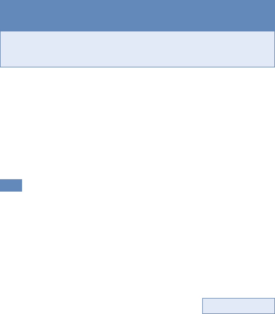
Programming with Big Data
Chapter 5
Huy Vo and Claudio Silva
Big data is sometimes defined as data that are too big to fit onto
the analyst’s computer. This chapter provides an overview of clever
programming techniques that facilitate the use of data (often using
parallel computing). While the focus is on one of the most widely
used big data programming paradigms and its most popular imple-
mentation, Apache Hadoop, the goal of the chapter is to provide a
conceptual framework to the key challenges that the approach is
designed to address.
5.1 Introduction
There are many definitions of big data, but perhaps the most popu-
lar one is from Laney’s report [229] in 2001 that defines big data as
data with the three Vs: volume (large data sets), velocity (real-time
streaming data), and variety (various data forms). Other authors
have since proposed additional Vs for various purposes: veracity,
value,variability, and visualization. It is common nowadays to see
big data being associated with five or even seven Vs—the big data
definition itself is also getting “big” and getting difficult to keep track.
A simpler but also broader definition of big data is data sets that
are “so large or complex that traditional data processing applica-
tions are inadequate,” as described by Wikipedia. We note that in
this case, the definition adapts to the task at hand, and it is also
tool dependent.
For example, we could consider a problem to involve big data if
a spreadsheet gets so large that Excel can no longer load the entire
data set into memory for analysis—or if there are so many features
◮See Chapter 6, in partic-
ular Section 6.5.2.
in a data set that a machine learning classifier would take an unrea-
sonable amount of time (say days) to finish instead of a few seconds
125

126 5. Programming with Big Data
or minutes. In such cases, the analyst has to develop customized
solutions to interrogate the data, often by taking advantage of paral-
lel computing. In particular, one may have to get a larger computer,
with more memory and/or stronger processors, to cope with expen-
sive computations; or get a cluster of machines to speed up the
computing time by distributing the workload among them. While
the former solution would not scale well due to the limited amount
of processors a single computer can have, the latter solution needs
to deal with nontraditional programming infrastructures. Big data
technologies, in a nutshell, are the technologies that make these
infrastructures more usable by users without a computer science
background.
Parallel computing and big data are hardly new ideas for deal-
ing with computational challenges. Scientists have routinely been
working on data sets much larger than a single machine can han-
dle for several decades, especially at the DOE National Laborato-
ries [87,337] where high-performance computing has been a major
technology trend. This is also demonstrated by the history of re-
search in distributed computing and data management going back
to the 1980s [401].
There are major technological differences between this type of
big data technology and what is covered in this chapter. True par-
allel computing involves designing clever parallel algorithms, often
from scratch, taking into account machine-dependent constraints
to achieve maximum performance from the particular architecture.
They are often implemented using message passing libraries, such
as implementations of the Message Passing Interface (MPI) stan-
dard [142] (available since the mid-1990s). Often the expectation is
that the code developed will be used for substantial computations.
In that scenario it makes sense to optimize a code for maximum
performance knowing the same code will be used repeatedly. Con-
trast that with big data for exploration, where we might need to
keep changing the analysis code very often. In this case, what we
are trying to optimize is the analyst’s time, not computing time.
With storage and networking getting significantly cheaper and
faster, big data sets could easily become available to data enthu-
siasts with just a few mouse clicks, e.g., the Amazon Web Service
Public Data Sets [11]. These enthusiasts may be policymakers, gov-
ernment employees, or managers who would like to draw insights
and (business) value from big data. Thus, it is crucial for big data
to be made available to nonexpert users in such a way that they
can process the data without the need for a supercomputing ex-
pert. One such approach is to build big data frameworks within

5.2. The MapReduce programming model 127
which commands can be implemented just as they would in a small
data framework. Also, such a framework should be as simple as
possible, even if not as efficient as custom-designed parallel solu-
tions. Users should expect that if their code works within these
frameworks for small data, it will also work for big data.
In order to achieve scalability for big data, many frameworks only
implement a small subset of data operations and fully automate the
parallelism of these operations. Users are expected to develop their
codes using only the subset if they expect their code to scale to
large data sets. MapReduce, one of the most widely used big data
programming paradigms, is no exception to this rule. As its name
suggests, the framework only supports two operations: map and
reduce. The next sections will provide an overview of MapReduce
and its most popular implementation, Apache Hadoop.
5.2 The MapReduce programming model
The MapReduce framework was proposed by Jeffrey Dean and San-
jay Ghemawat at Google in 2004 [91]. Its origins date back to
conceptually similar approaches first described in the early 1980s.
MapReduce was indeed inspired by the map and reduce functions
of functional programming, though its reduce function is more of a
group-by-key function, producing a list of values, instead of the tra-
ditional reduce, which outputs only a single value. MapReduce is a
record-oriented model, where each record is treated as a key–value
pair; thus, both map and reduce functions operate on key–value pair
data.
A typical MapReduce job is composed of three phases—map,
shuffle, and reduce—taking a list of key–value pairs [(k$_1$,v$_2$),
(k$_2$,v$_2$), ..., (k$_n$,v$_n$)] as input. In the map phase,
each input key–value pair is run through the map function, and zero
or more new key–value pairs are output. In the shuffle phase, the
framework sorts the outputs of the map phase, grouping pairs by
keys before sending each of them to the reduce function. In the
reduce phase, each grouping of values are processed by the reduce
function, and the result is a list of new values that are collected for
the job output.
In brief, a MapReduce job just takes a list of key–value pairs as
input and produces a list of values as output. Users only need to
implement interfaces of the map and reduce functions (the shuffle
phase is not very customizable) and can leave it up to the system
that implements MapReduce to handle all data communications

128 5. Programming with Big Data
and parallel computing. We can summarize the MapReduce logic
as follows:
map: (ki, vi)→
→
→[f(k′
i1, v′
i1),f(k′
i2, v′
i2),..]
for a user-defined function f.
reduce: (k′′
i, [v′′
i1,v′′
i2,..]) →
→
→[v′′′
1,v′′′
2,..]
where {k′
i} ≡ {k′′
j}and v′′′ =g(v′′)for a user-defined function g.
Example: Counting NSF awards
To gain a better understanding of these MapReduce operators, imagine that we
have a list of NSF principal investigators, along with their email information and
award IDs as below. Our task is to count the number of awards for each institu-
tion. For example, given the four records below, we will discover that the Berkeley
Geochronology Center has two awards, while New York University and the Univer-
sity of Utah each have one.
AwardId,FirstName,LastName,EmailAddress
0958723,Roland,Mundil,rmundil@bgc.org
0958915,Randall,Irmis,irmis@umnh.utah.edu
1301647,Zaher,Hani,zh8@nyu.edu
1316375,David,Shuster,dshuster@bgc.org
We observe that institutions can be distinguished by their email address do-
main name. Thus, we adopt of a strategy of first grouping all award IDs by domain
names, and then counting the number of distinct award within each group. In
order to do this, we first set the map function to scan input lines and extract insti-
tution information and award IDs. Then, in the reduce function, we simply count
unique IDs on the data, since everything is already grouped by institution. Python
pseudo-code is provided in Listing 5.1.
In the map phase, the input will be transformed into tuples of institutions and
award ids:
"0958723,Roland,Mundil,rmundil@bgc.org" →
→
→("bgc.org", 0958723)
"0958915,Randall,Irmis,irmis@umnh.utah.edu" →
→
→("utah.edu", 0958915)
"1301647,Zaher,Hani,zh8@nyu.edu" →
→
→("nyu.edu", 1301647)
"1316375,David,Shuster,dshuster@bgc.org" →
→
→("bgc.org", 1316375)
Then the tuples will be grouped by institutions and be counted by the reduce
function.
("bgc.org", [0958723,1316375]) →
→
→("bgc.org", 2)
("utah.edu", [0958915]) →
→
→("utah.edu", 1)
("nyu.edu", [1301647]) →
→
→("nyu.edu", 1)

5.3. Apache Hadoop MapReduce 129
# Input : a list of text lines
2# Output : a list of domain name and award ids
def MAP(lines):
4for line in lines:
fields = line.strip('\n').split(',')
6awardId = fields[0]
domainName = fields[3].split('@')[-1].split('.')[-2:]
8yield (domainName, awardId)
10 # Input : a list of domain name and award ids
# Output : a list of domain name and award count
12 def REDUCE(pairs):
for (domainName, awardIds) in pairs:
14 count = len(set(awardIds))
yield (domainName, count)
Listing 5.1. Python pseudo-code for the map and reduce functions to count the
number of awards per institution
As we have seen so far, the MapReduce programming model is
quite simple and straightforward, yet it supports a simple paral-
lelization model. In fact, it has been said to be too simple and criti-
cized as “a major step backwards” [94] for large-scale, data-intensive
applications. It is hard to argue that MapReduce is offering some-
thing truly innovative when MPI has been offering similar scatter
and reduce operations since 1995, and Python has had high-order
functions (map,reduce,filter, and lambda) since its 2.2 release in
1994. However, the biggest strength of MapReduce is its simplic-
ity. Its simple programming model has brought many nonexpert
users to big data analysis. Its simple architecture has also inspired
many developers to develop advanced capabilities, such as support
for distributed computing, data partitioning, and streaming pro-
cessing. (A downside of this diversity of interest is that available
features and capabilities can vary considerably, depending on the
specific implementation of MapReduce that is being used.)
We next describe two specific implementations of the MapReduce
model: Hadoop and Spark.
5.3 Apache Hadoop MapReduce
The names MapReduce and Apache Hadoop (or Hadoop)*are often ⋆The term Hadoop refers
to the creator’s son’s toy
elephant.
used interchangeably, but they are conceptually different. MapRe-
duce is simply a programming paradigm with a layer of abstraction
that allows a set of data processing pipelines to be expressed with-
out too much tailoring for how it will be executed exactly. The

130 5. Programming with Big Data
MapReduce model tells us which class of data structure (key–value
pairs) and data transformations (map and reduce) it is supporting;
however, it does not specifically state how the framework should
be implemented; for example, it does not specify how data should
be stored or how the computation be executed (in particular, par-
allelized). Hadoop [399], on the other hand, is a specific imple-
mentation of MapReduce with exact specifications of how data and
computation are handled inside the system.
Hadoop was originally designed for batch data processing at
scale, with the target of being able to run in environments with
thousands of machines. Supporting such a large computing envi-
ronment puts several constraints on the system; for instance, with
so many machines, the system had to assume computing nodes
would fail. Hadoop is an enhanced MapReduce implementation
with the support for fault tolerance, distributed storage, and data
parallelism through two added key design features: (1) a distributed
file system called the Hadoop Distributed File System (HDFS); and
(2) a data distribution strategy that allows computation to be moved
to the data during execution.
5.3.1 The Hadoop Distributed File System
The Hadoop Distributed File System [345] is arguably the most im-
portant component that Hadoop added to the MapReduce frame-
work. In a nutshell, it is a distributed file system that stripes data
across all the nodes of a Hadoop cluster. HDFS splits large data
files into smaller blocks which are managed by different nodes in
the cluster. Each block is also replicated across several nodes as an
attempt to ensure that a full copy of the data is still available even
in the case of computing node failures. The block size as well as
the number of replications per block are fully customized by users
when they create files on HDFS. By default, the block size is set
to 64 MB with a replication factor of 3, meaning that the system
may encounter at least two concurrent node failures without losing
any data. HDFS also actively monitors failures and re-replicates
blocks on failed nodes to make sure that the number of replications
for each block always stays at the user-defined settings. Thus, if a
node fails, and only two copies of some data exist, the system will
quickly copy those data to a working node, thus raising the num-
ber of copies to three again. This dynamic replication the primary
mechanism for fault tolerance in Hadoop.
Note that data blocks are replicated and distributed across sev-
eral machines. This could create a problem for users, because

5.3. Apache Hadoop MapReduce 131
if they had to manage the data manually, they might, for exam-
ple, have to access more than one machine to fetch a large data
file. Fortunately, Hadoop provides infrastructure for managing this
complexity, including command line programs as well as an API
that users can employ to interact with HDFS as if it were a local file
system.
This is one example that reinforces our discussion on big data
technology being all about making things work seamlessly regard-
less of the computational environment; it should be possible for the
user to use the system as though they are using their local worksta-
tion. Hadoop and HDFS are great examples of this approach. For
example, one can run ls and mkdir to list and create a directory on
HDFS, or even use tail to inspect file contents as one would expect
in a Linux file system. The following code shows some examples of
interacting with HDFS.
# Creating a temporary folder
hadoop dfs -mkdir /tmp/mytmp
# Upload a CSV file from our local machine to HDFS
hadoop dfs -put myfile.csv /tmp/mytmp
# Listing all files under mytmp folder
hadoop dfs -ls /tmp/mytmp
# Upload another file with five replications and 128MB per block
hadoop -D dfs.replication=5 -D dfs.block.size=128M \
dfs -put mylargefile.csv /tmp/mytmp
# Download a file to our local machine
hadoop dfs -get /tmp/mytmp/myfile.csv .
5.3.2 Hadoop: Bringing compute to the data
The configuration of parallel computing infrastructure is a fairly
complex task. At the risk of oversimplifying, we consider the com-
puting environment as comprising a compute cluster with substan-
tial computing power (e.g., thousands of computing cores), and a
storage cluster with petabytes of disk space, capable of storing and
serving data quickly to the compute cluster. These two clusters
have quite different hardware specifications: the first is optimized
for CPU performance and the second for storage occupancy. The two
systems are typically configured as separate physical hardware.
Running compute jobs on such hardware often goes like this.
When a user requests to run an intensive task on a particular data
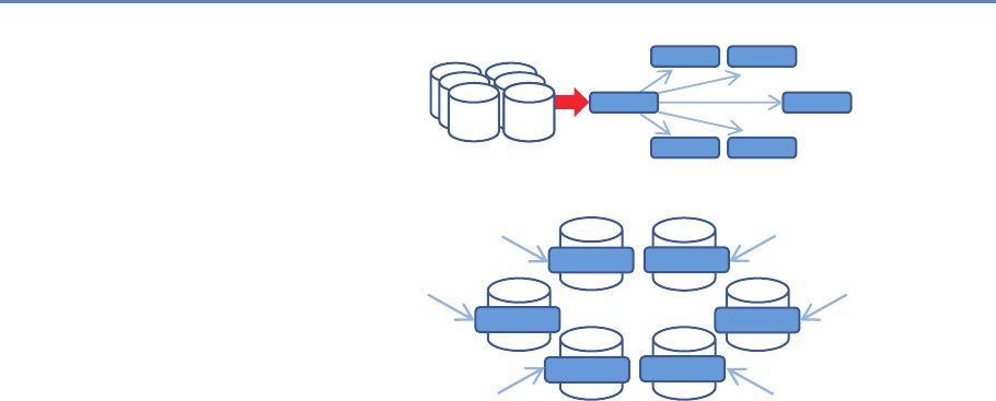
132 5. Programming with Big Data
Task 3
Task 1 Task 2
Task 4Task 5
Data Data Task 0
(a)
Task 0 Task 3
Task 1 Task 2
Task 4
Task 5
(b)
Figure 5.1. (a) The traditional parallel computing model where data are brought to
the computing nodes. (b) Hadoop’s parallel computing model: bringing compute
to the data [242]
set, the system will first reserve a set of computing nodes. Then
the data are partitioned and copied from the storage server into
these computing nodes before the task is executed. This process is
illustrated in Figure 5.1(a). This computing model will be referred
to as bringing data to computation. In this model, if a data set
is being analyzed in multiple iterations, it is very likely that the
data will be copied multiple times from the storage cluster to the
compute nodes without reusability. This is because the compute
node scheduler normally does not have or keep knowledge of where
data have previously been held. The need to copy data multiple
times tends to make such a computation model inefficient, and I/O
becomes the bottleneck when all tasks constantly pull data from
the storage cluster (the green arrow). This in turn leads to poor
scalability; adding more nodes to the computing cluster would not
increase its performance.
To solve this problem, Hadoop implements a bring compute to the
data strategy that combines both computing and storage at each
node of the cluster. In this setup, each node offers both computing
power and storage capacity. As shown in Figure 5.1(b), when users
submit a task to be run on a data set, the scheduler will first look
for nodes that contain the data, and if the nodes are available, it
will schedule the task to run directly on those nodes. If a node is

5.3. Apache Hadoop MapReduce 133
busy with another task, data will still be copied to available nodes,
but the scheduler will maintain records of the copy for subsequent
use of the data. In addition, data copying can be minimized by
increasing the data duplication in the cluster, which also increases
the potential for parallelism, since the scheduler has more choices
to allocate computing without copying. Since both the compute and
data storage are closely coupled for this model, it is best suited for
data-intensive applications.
Given that Hadoop was designed for batch data processing at
scale, this model fits the system nicely, especially with the sup-
port of HDFS. However, in an environment where tasks are more
compute intensive, a traditional high-performance computing envi-
ronment is probably best since it tends to spend more resources on
CPU cores. It should be clear now that the Hadoop model has hard-
ware implications, and computer architects have optimized systems
for data-intensive computing.
Now that we are equipped with the knowledge that Hadoop is
a MapReduce implementation that runs on HDFS and a bring-
compute-to-the-data model, we can go over the design of a Hadoop
MapReduce job. A MapReduce job is still composed of three phases:
map, shuffle, and reduce. However, Hadoop divides the map and
reduce phases into smaller tasks.
Each map phase in Hadoop is divided into five tasks: input for-
mat,record reader,mapper,combiner, and partitioner. An input
format task is in charge of talking to the input data presumably
sitting on HDFS, and splitting it into partitions (e.g., by breaking
lines at line breaks). Then a record reader task is responsible for
translating the split data into the key–value pair records so that
they can be processed by the mapper. By default, Hadoop parses
files into key–value pairs of line numbers and line contents. How-
ever, both input formats and record readers are fully customizable
and can be programmed to read custom data including binary files.
It is important to note that input formats and record readers only
provide data partitioning; they do not move data around computing
nodes.
After the records are generated, mappers are spawned—typically
on nodes containing the blocks—to run through these records and
output zero or more new key–value pairs. A mapper in Hadoop
is equivalent to the map function of the MapReduce model that we
discussed earlier. The selection of the key to be output from the
mapper will heavily depend on the data processing pipeline and
could greatly affect the performance of the framework. Mappers are
executed concurrently in Hadoop as long as resources permit.

134 5. Programming with Big Data
A combiner task in Hadoop is similar to a reduce function in the
MapReduce framework, but it only works locally at each node: it
takes output from mappers executed on the same node and pro-
duces aggregated values. Combiners are optional but can be used
to greatly reduce the amount of data exchange in the shuffle phase;
thus, users are encouraged to implement this whenever possible.
A common practice is when a reduce function is both commutative
and associative, and has the same input and output format, one
can just use the reduce function as the combiner. Nevertheless,
combiners are not guaranteed to be executed by Hadoop, so this
should only be treated as a hint. Its execution must not affect the
correctness of the program.
A partitioner task is the last process taking place in the map
phase on each mapper node, where it hashes the key of each key–
value pair output from the mappers or the combiners into bins.
By default, the partitioner uses object hash codes and modulus
operations to direct a designated reducer to pull data from a map
node. Though it is possible to customize the partitioner, it is only
advisable to do so when one fully understands the intermediate data
distribution as well as the specifications of the cluster. In general,
it is better to leave this job to Hadoop.
Each reduce phase in Hadoop is divided into three tasks: re-
ducer,output format, and record writer. The reducer task is equiv-
alent to the reduce function of the MapReduce model. It basically
groups the data produced by the mappers by keys and runs a reduce
function on each list of grouping values. It outputs zero or more
key–value pairs for the output format task, which then translates
them into a writable format for the record writer task to serialize
on HDFS. By default, Hadoop will separate the key and value with
a tab and write separate records on separate lines. However, this
behavior is fully customizable. Similarly, the map phase reducers
are also executed concurrently in Hadoop.
5.3.3 Hardware provisioning
Hadoop requires a distributed cluster of machines to operate ef-
ficiently. (It can be set up to run entirely on a single computer,
but this should only be done for technology demonstration pur-
poses.) This is mostly because the MapReduce performance heavily
depends on the total I/O throughput (i.e., disk read and write) of
the entire system. Having a distributed cluster, where each ma-
chine has its own set of hard drives, is one of the most efficient
ways to maximize this throughput.
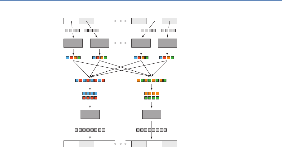
5.3. Apache Hadoop MapReduce 135
Data on HDFS
Input Partition
Shuing
Sort in Parallel
Output Partition
Data on HDFS
Map
Reduce Reduce
Map Map Map
Figure 5.2. Data transfer and communication of a MapReduce job in Hadoop.
Data blocks are assigned to several maps, which emit key–value pairs that are
shuffled and sorted in parallel. The reduce step emits one or more pairs, with
results stored on the HDFS
A typical Hadoop cluster consists of two types of machine: mas-
ters and workers. Master machines are those exclusively reserved
for running services that are critical to the framework operations.
Some examples are the NameNode and the JobTracker services,
which are tasked to manage how data and tasks are distributed
among the machines, respectively. The worker machines are re-
served for data storage and for running actual computation tasks
(i.e., map and reduce). It is normal to have worker machines that
can be included or removed from an operational cluster on demand.
This ability to vary the number of worker nodes makes the overall
system more tolerant of failure. However, master machines are
usually required to be running uninterrupted.
Provisioning and configuring the hardware for Hadoop, like any
other parallel computing, are some of the most important and com-
plex tasks in setting up a cluster, and they often require a lot
of experience and careful consideration. Major big data vendors
provide guidelines and tools to facilitate the process [18, 23, 81].

136 5. Programming with Big Data
#!/usr/bin/env python
import sys
def parseInput():
for line in sys.stdin:
yield line
if __name__=='__main__':
for line in parseInput():
fields = line.strip('\n').split(',')
awardId = fields[0]
domainName = fields[3].split('@')[-1].split('.')[-2:]
print '%s\t%s' % (domainName,awardId)
Listing 5.2. A Hadoop streaming mapper in Python
Nevertheless, most decisions will be based on the types of analysis
to be run on the cluster, for which only you, as the user, can provide
the best input.
5.3.4 Programming language support
Hadoop is written entirely in Java, thus it is best supporting appli-
cations written in Java. However, Hadoop also provides a streaming
API that allows arbitrary code to be run inside the Hadoop MapRe-
duce framework through the use of UNIX pipes. This means that we
can supply a mapper program written in Python or C++ to Hadoop
as long as that program reads from the standard input and writes to
the standard output. The same mechanism also applies for the com-
biner and reducer. For example, we can develop from the Python
pseudo-code in Listing 5.1 to a complete Hadoop streaming mapper
(Listing 5.2) and reducer (Listing 5.3).
#!/usr/bin/env python
import sys
def parseInput():
for line in sys.stdin:
yield line
if __name__=='__main__':
for line in parseInput():
(domainName, awardIds) = line.split('\t')
count = len(set(awardIds))
print '%s\t%s' % (domainName, count)
Listing 5.3. A Hadoop streaming reducer in Python

5.3. Apache Hadoop MapReduce 137
It should be noted that in Hadoop streaming, intermediate key–
value pairs (the data flowing between mappers and reducers) must
be in tab-delimited format, thus we replace the original yield com-
mand with a print formatted with tabs. Though the input format
and record reader are still customizable in Hadoop streaming, they
must be supplied as Java classes. This is one of the biggest limita-
tions of Hadoop for Python developers. They not only have to split
their code into separate mapper and reducer programs, but also
need to learn Java if they want to work with nontextual data.
5.3.5 Fault tolerance
By default, HDFS uses checksums to enforce data integrity on its
file system use data replication for recovery of potential data losses.
Taking advantage of this, Hadoop also maintains fault tolerance of
MapReduce jobs by storing data at every step of a MapReduce job
to HDFS, including intermediate data from the combiner. Then the
system checks whether a task fails by either looking at its heart-
beats (data activities) or whether it has been taking too long. If a
task is deemed to have failed, Hadoop will kill it and run it again on
a different node. The time limit for the heartbeats and task running
duration may also be customized for each job. Though the mecha-
nism is simple, it works well on thousands of machines. It is indeed
highly robust because of the simplicity of the model.
5.3.6 Limitations of Hadoop
Hadoop is a great system, and probably the most widely used MapRe-
duce implementation. Nevertheless, it has important limitations, as
we now describe.
•Performance: Hadoop has proven to be a scalable implemen-
tation that can run on thousands of cores. However, it is
also known for having a relatively high job setup overheads
and suboptimal running time. An empty task in Hadoop (i.e.,
with no mapper or reducer) can take roughly 30 seconds to
complete even on a modern cluster. This overhead makes it
unsuitable for real-time data or interactive jobs. The problem
comes mostly from the fact that Hadoop monitoring processes
only lives within a job, thus it needs to start and stop these
processes each time a job is submitted, which in turns results
in this major overhead. Moreover, the brute force approach of

138 5. Programming with Big Data
maintaining fault tolerance by storing everything on HDFS is
expensive, especially when for large data sets.
•Hadoop streaming support for non-Java applications: As men-
tioned previously, non-Java applications may only be inte-
grated with Hadoop through the Hadoop streaming API. How-
ever, this API is far from optimal. First, input formats and
record readers can only be written in Java, making it impos-
sible to write advanced MapReduce jobs entirely in a differ-
ent language. Second, Hadoop streaming only communicates
with Hadoop through Unix pipes, and there is no support for
data passing within the application using native data struc-
ture (e.g., it is necessary to convert Python tuples into strings
in the mappers and convert them back into tuples again in
reducers).
•Real-time applications: With the current setup, Hadoop only
supports batch data processing jobs. This is by design, so it is
not exactly a limitation of Hadoop. However, given that more
and more applications are dealing with real-time massive data
sets, the community using MapReduce for real-time processing
is constantly growing. Not having support for streaming or
real-time data is clearly a disadvantage of Hadoop over other
implementations.
•Limited data transformation operations: This is more of a lim-
itation of MapReduce than Hadoop per se. MapReduce only
supports two operations, map and reduce, and while these op-
erations are sufficient to describe a variety of data processing
pipelines, there are classes of applications that MapReduce is
not suitable for. Beyond that, developers often find themselves
rewriting simple data operations such as data set joins, find-
ing a min or max, and so on. Sometime, these tasks require
more than one map-and-reduce operation, resulting in multi-
ple MapReduce jobs. This is both cumbersome and inefficient.
There are tools to automate this process for Hadoop; however,
they are only a layer above, and it is not easy to integrate with
existing customized Hadoop applications.
5.4 Apache Spark
In addition to Apache Hadoop, other notable MapReduce implemen-
tations include MongoDB, GreenplumDB, Disco, Riak, and Spark.

5.4. Apache Spark 139
MongoDB, Riak, and Greenplum DB are all database systems and ◮See Chapter 4.
thus their MapReduce implementations focus more on the inter-
operability of MapReduce and the core components such as Mon-
goDB’s aggregation framework, and leave it up to users to customize
the MapReduce functionalities for broader tasks. Some of these
systems, such as Riak, only parallelize the map phase, and run the
reduce phase on the local machine that request the tasks. The main
advantage of the three implementations is the ease with which they
connect to specific data stores. However, their support for general
data processing pipelines is not as extensive as that of Hadoop.
Disco, similar to Hadoop, is designed to support MapReduce in
a distributed computing environment, but it written in Erlang with
a Python interface. Thus, for Python developers, Disco might be a
better fit. However, it has significantly fewer supporting applica-
tions, such as access control and workflow integration, as well as a
smaller developing community. This is why the top three big data
platforms, Cloudera, Hortonworks, and MapR, still build primarily
on Hadoop.
Apache Spark is another implementation that aims to support
beyond MapReduce. The framework is centered around the con-
cept of resilient distributed data sets and data transformations that
can operate on these objects. An innovation in Spark is that the
fault tolerance of resilient distributed data sets can be maintained
without flushing data onto disks, thus significantly improving the
system performance (with a claim of being 100 times faster than
Hadoop). Instead, the fault-recovery process is done by replaying
a log of data transformations on check-point data. Though this
process could take longer than reading data straight from HDFS,
it does not occur often and is a fair tradeoff between processing
performance and recovery performance.
Beyond map and reduce, Spark also supports various other
transformations [147], including filter, data join, and aggregation.
Streaming computation can also be done in Spark by asking Spark
to reserve resources on a cluster to constantly stream data to/from
the cluster. However, this streaming method might be resource in-
tensive (still consuming resources when there is no data coming).
Additionally, Spark plays well with the Hadoop ecosystem, particu-
larly with the distributed file system (HDFS) and resource manager
(YARN), making it possible to be built on top of current Hadoop
applications.
Another advantage of Spark is that it supports Python natively;
thus, developers can run Spark in a fraction of the time required for
Hadoop. Listing 5.4 provides the full code for the previous example

140 5. Programming with Big Data
import sys
from pyspark import SparkContext
def mapper(lines):
for line in lines:
fields = line.strip('\n').split(',')
awardId = fields[0]
domainName = fields[3].split('@')[-1].split('.')[-2:]
yield (domainName, awardId)
def reducer(pairs):
for (domainName, awardIds) in pairs:
count = len(set(awardIds))
yield (domainName, count)
if __name__=='__main__':
hdfsInputPath = sys.argv[1]
hdfsOutputFile = sys.argv[2]
sc = SparkContext(appName="Counting Awards")
output = sc.textFile(hdfsInputPath) \
.mapPartitions(mapper) \
.groupByKey() \
.mapPartitions(reducer)
output.saveAsTextFile(hdfsInputPath)
Listing 5.4. Python code for a Spark program that counts the number of awards
per institution using MapReduce
written entirely in Spark. It should be noted that Spark’s concept
of the reduceByKey operator is not the same as Hadoop’s, as it is
designed to aggregate all elements of a data set into a single ele-
ment. The closest simulation of Hadoop’s MapReduce pattern is a
combination of mapPartitions,groupByKey and mapPartitions, as
shown in the next example.
Example: Analyzing home mortgage disclosure
application data
We use a financial services analysis problem to illustrate the use of Apache Spark.
Mortgage origination data provided by the Consumer Protection Financial Bu-
reau provide insightful details of the financial health of the real estate market.
The data [84], which are a product of the Home Mortgage Disclosure Act (HMDA),
highlight key attributes that function as strong indicators of health and lending
patterns.
Lending institutions, as defined by section 1813 in Title 12 of the HMDA, decide
on whether to originate or deny mortgage applications based on credit risk. In
order to determine this credit risk, lenders must evaluate certain features relative

5.5. Summary 141
Table 5.1. Home Mortgage Disclosure Act data size
Year Records File Size (Gigabytes)
2007 26,605,696 18
2008 17,391,571 12
2009 19,493,492 13
2010 16,348,558 11
2011 14,873,416 9.4
2012 18,691,552 12
2013 17,016,160 11
Total 130,420,445 86.4
Table 5.2. Home Mortgage Disclosure Act data fields
Index Attribute Type
0 Year Integer
1 State String
2 County String
3 Census Tract String
4 Loan Amount Float
5 Applicant Income Float
6 Loan Originated Boolean
··· ··· ···
to the applicant, the underlying property, and the location. We want to determine
whether census tract clusters could be created based on mortgage application
data and whether lending institutions’ perception of risk is held constant across
the entire USA.
For the first step of this process, we study the debt–income ratio for loans
originating in different census tracts. This could be achieved simply by computing
the debt–income ratio for each loan application and aggregating them for each
year by census tract number. A challenge, however, is that the data set provided
by HMDA is quite extensive. In total, HMDA data contain approximately 130
million loan applications between 2007 and 2013. As each record contains 47
attributes, varying in types from continuous variables such as loan amounts and
applicant income to categorical variables such as applicant gender, race, loan type,
and owner occupancy, the entire data set results in about 86 GB of information.
Parsing the data alone could take up to hours on a single machine if using a naïve
approach that scans through the data sequentially. Tables 5.1 and 5.2 highlight
the breakdown in size per year and data fields of interest.
Observing the transactional nature of the data, where the aggregation process
could be distributed and merged across multiple partitions of the data, we could
complete this task in much less time by using Spark. Using a cluster consisting
of 1,200 cores, the Spark program in Listing 5.5 took under a minute to complete.
The substantial performance gain comes not so much from the large number of
processors available, but mostly from the large I/O bandwidth available on the
cluster thanks to the 200 distributed hard disks and fast network interconnects.
5.5 Summary
Big data means that it is necessary to both store very large collec-
tions of data and perform aggregate computations on those data.
This chapter spelled out an important data storage approach (the
Hadoop Distributed File System) and a way of processing large-scale

142 5. Programming with Big Data
import ast
import sys
from pyspark import SparkContext
def mapper(lines):
for line in lines:
fields = ast.literal_eval('(%s)' % line)
(year, state, county, tract) = fields[:4]
(amount, income, originated) = fields[4:]
key = (year, state, county, tract)
value = (amount, income)
# Only count originated loans
if originated:
yeild (key, value)
def sumDebtIncome(debtIncome1, debtIncome2):
return (debtIncome1[0] + debtIncome2[0], debtIncome1[1] +
debtIncome2[1])
if __name__=='__main__':
hdfsInputPath = sys.argv[1]
hdfsOutputFile = sys.argv[2]
sc = SparkContext(appName="Counting Awards")
sumValues = sc.textFile(hdfsInputPath) \
.mapPartitions(mapper) \
.reduceByKey(sumDebtIncome)
# Actually compute the aggregated debt income
output = sumValues.mapValues(lambda debtIncome: debtIncome[0]/
debtIncome[1])
output.saveAsTextFile(hdfsInputPath)
Listing 5.5. Python code for a Spark program to aggregate the debt–income ratio
for loans originated in different census tracts
data sets (the MapReduce model, as implemented in both Hadoop
and Spark). This in-database processing model enables not only
high-performance analytics but also the provision of more flexi-
bility for analysts to work with data. Instead of going through a
database administrator for every data gathering, data ingestion, or
data transformation task similar to a traditional data warehouse
approach, the analysts rather “own” the data in the big data en-
vironment. This increases the analytic throughput as well as the
time to insight, speeding up the decision-making process and thus
increasing the business impact, which is one of the main drivers for
big data analytics.

5.6. Resources 143
5.6 Resources
There are a wealth of online resources describing both Hadoop and
Spark. See, for example, the tutorials on the Apache Hadoop [19]
and Spark [20] websites. Albanese describes how to use Hadoop for
social science [9], and Lin and Dyer discuss the use of MapReduce
for text analysis [238].
We have not discussed here how to deal with data that are lo-
cated remotely from your computer. If such data are large, then
moving them can be an arduous task. The Globus transfer ser-
vice [72] is commonly used for the transfer and sharing of such
data. It is available on many research research systems and is easy
to install on your own computer.


Machine Learning
Chapter 6
Rayid Ghani and Malte Schierholz
This chapter introduces you to the value of machine learning in the
social sciences, particularly focusing on the overall machine learn-
ing process as well as clustering and classification methods. You
will get an overview of the machine learning pipeline and methods
and how those methods are applied to solve social science problems.
The goal is to give an intuitive explanation for the methods and to
provide practical tips on how to use them in practice.
6.1 Introduction
You have probably heard of “machine learning” but are not sure
exactly what it is, how it differs from traditional statistics, and what
you can do with it. In this chapter, we will demystify machine
learning, draw connections to what you already know from statis-
tics and data analysis, and go deeper into some of the unique con-
cepts and methods that have been developed in this field. Although
the field originates from computer science (specifically, artificial in-
telligence), it has been influenced quite heavily by statistics in the
past 15 years. As you will see, many of the concepts you will learn
are not entirely new, but are simply called something else. For
example, you already are familiar with logistic regression (a classi-
fication method that falls under the supervised learning framework
in machine learning) and cluster analysis (a form of unsupervised
learning). You will also learn about new methods that are more
exclusively used in machine learning, such as random forests and
support vector machines. We will keep formalisms to a minimum
and focus on getting the intuition across, as well as providing practi-
cal tips. Our hope is this chapter will make you comfortable and fa-
miliar with machine learning vocabulary, concepts, and processes,
and allow you to further explore and use these methods and tools
in your own research and practice.
147

148 6. Machine Learning
6.2 What is machine learning?
When humans improve their skills with experience, they are said to
learn. Is it also possible to program computers to do the same?
Arthur Samuel, who coined the term machine learning in 1959
[323], was a pioneer in this area, programming a computer to play
checkers. The computer played against itself and human oppo-
nents, improving its performance with every game. Eventually,
after sufficient training (and experience), the computer became a
better player than the human programmer. Today, machine learn-
ing has grown significantly beyond learning to play checkers. Ma-
chine learning systems have learned to drive (and park) autonomous
cars, are embedded inside robots, can recommend books, prod-
ucts, and movies we are (sometimes) interested in, identify drugs,
proteins, and genes that should be investigated further to cure dis-
eases, detect cancer and other diseases in medical imaging, help
us understand how the human brain learns language, help identify
which voters are persuadable in elections, detect which students are
likely to need extra support to graduate high school on time, and
help solve many more problems. Over the past 20 years, machine
learning has become an interdisciplinary field spanning computer
science, artificial intelligence, databases, and statistics. At its core,
machine learning seeks to design computer systems that improve
over time with more experience. In one of the earlier books on ma-
chine learning, Tom Mitchell gives a more operational definition,
stating that: “A computer program is said to learn from experience
Ewith respect to some class of tasks Tand performance measure
P, if its performance at tasks in T, as measured by P, improves with
experience E” [258].
Machine learning grew from the need to build systems that were
adaptive, scalable, and cost-effective to build and maintain. A lot
of tasks now being done using machine learning used to be done
by rule-based systems, where experts would spend considerable
time and effort developing and maintaining the rules. The problem
with those systems was that they were rigid, not adaptive, hard to
scale, and expensive to maintain. Machine learning systems started
becoming popular because they could improve the system along all
of these dimensions. Box 6.1 mentions several examples where
◮See Chapter 3.
machine learning is being used in commercial applications today.
Social scientists are uniquely placed today to take advantage of the
same advances in machine learning by having better methods to
solve several key problems they are tackling. We will give concrete
examples later in this chapter.

6.2. What is machine learning? 149
Box 6.1: Commercial machine learning examples
•Speech recognition: Speech recognition software uses ma-
chine learning algorithms that are built on large amounts
of initial training data. Machine learning allows these sys-
tems to be tuned and adapt to individual variations in
speaking as well as across different domains.
•Autonomous cars: The ongoing development of self-
driving cars applies techniques from machine learning.
An onboard computer continuously analyzes the incom-
ing video and sensor streams in order to monitor the sur-
roundings. Incoming data are matched with annotated
images to recognize objects like pedestrians, traffic lights,
and potholes. In order to assess the different objects, huge
training data sets are required where similar objects al-
ready have been identified. This allows the autonomous
car to decide on which actions to take next.
•Fraud detection: Many public and private organizations
face the problem of fraud and abuse. Machine learning
systems are widely used to take historical cases of fraud
and flag fraudulent transactions as they take place. These
systems have the benefit of being adaptive, and improving
with more data over time.
•Personalized ads: Many online stores have personalized
recommendations promoting possible products of interest.
Based on individual shopping history and what other sim-
ilar users bought in the past, the website predicts prod-
ucts a user may like and tailors recommendations. Netflix
and Amazon are two examples of companies whose recom-
mendation software predicts how a customer would rate
a certain movie or product and then suggests items with
the highest predicted ratings. Of course there are some
caveats here, since they then adjust the recommendations
to maximize profits.
•Face recognition: Surveillance systems, social network-
ing platforms, and imaging software all use face detec-
tion and face recognition to first detect faces in images
(or video) and then tag them with individuals for various
tasks. These systems are trained by giving examples of
faces to a machine learning system which then learns to
detect new faces, and tag known individuals.

150 6. Machine Learning
This chapter is not an exhaustive introduction to machine learn-
ing. There are many books that have done an excellent job of
that [124, 159, 258]. Instead, we present a short and understand-
able introduction to machine learning for social scientists, give an
overview of the overall machine learning process, provide an intu-
itive introduction to machine learning methods, give some practical
tips that will be helpful in using these methods, and leave a lot of
the statistical theory to machine learning textbooks. As you read
more about machine learning in the research literature or the me-
dia, you will encounter names of other fields that are related (and
practically the same for most social science audiences), such as
statistical learning, data mining, and pattern recognition.
6.3 The machine learning process
When solving problems using machine learning methods, it is im-
portant to think of the larger data-driven problem-solving process of
◮See Chapter 10.
which these methods are a small part. A typical machine learning
problem requires researchers and practitioners to take the following
steps:
1. Understand the problem and goal: This sounds obvious but is
often nontrivial. Problems typically start as vague descriptions
of a goal—improving health outcomes, increasing graduation
rates, understanding the effect of a variable Xon an outcome
Y, etc. It is really important to work with people who under-
stand the domain being studied to dig deeper and define the
problem more concretely. What is the analytical formulation
of the metric that you are trying to optimize?
2. Formulate it as a machine learning problem: Is it a classifica-
tion problem or a regression problem? Is the goal to build a
model that generates a ranked list prioritized by risk, or is it to
detect anomalies as new data come in? Knowing what kinds
of tasks machine learning can solve will allow you to map the
problem you are working on to one or more machine learning
settings and give you access to a suite of methods.
3. Data exploration and preparation: Next, you need to carefully
explore the data you have. What additional data do you need
or have access to? What variable will you use to match records
for integrating different data sources? What variables exist in
the data set? Are they continuous or categorical? What about

6.4. Problem formulation: Mapping a problem to machine learning methods 151
missing values? Can you use the variables in their original
form or do you need to alter them in some way?
4. Feature engineering: In machine learning language, what you
might know as independent variables or predictors or factors
or covariates are called “features.” Creating good features is
probably the most important step in the machine learning pro-
cess. This involves doing transformations, creating interaction
terms, or aggregating over data points or over time and space.
5. Method selection: Having formulated the problem and created
your features, you now have a suite of methods to choose from.
It would be great if there were a single method that always
worked best for a specific type of problem, but that would
make things too easy. Typically, in machine learning, you
take a collection of methods and try them out to empirically
validate which one works the best for your problem. We will
give an overview of leading methods that are being used today
in this chapter.
6. Evaluation: As you build a large number of possible models,
you need a way to select the model that is the best. This
part of the chapter will cover the validation methodology to
first validate the models on historical data as well as discuss a
variety of evaluation metrics. The next step is to validate using
a field trial or experiment.
7. Deployment: Once you have selected the best model and val-
idated it using historical data as well as a field trial, you are
ready to put the model into practice. You still have to keep in
mind that new data will be coming in, and the model might
change over time. We will not cover too much of those aspects
in this chapter, but they are important to keep in mind.
6.4 Problem formulation: Mapping a problem
to machine learning methods
When working on a new problem, one of the first things we need to
do is to map it to a class of machine learning methods. In general,
the problems we will tackle, including the examples above, can be
grouped into two major categories:
1. Supervised learning: These are problems where there exists a
target variable (continuous or discrete) that we want to predict

152 6. Machine Learning
or classify data into. Classification, prediction, and regression
all fall into this category. More formally, supervised learning
methods predict a value Ygiven input(s) Xby learning (or
estimating or fitting or training) a function F, where F(X)=Y.
Here, Xis the set of variables (known as features in machine
learning, or in other fields as predictors) provided as input and
Yis the target/dependent variable or a label (as it is known in
machine learning).
The goal of supervised learning methods is to search for that
function Fthat best predicts Y. When the output Yis categor-
ical, this is known as classification. When Yis a continuous
value, this is called regression. Sound familiar?
One key distinction in machine learning is that the goal is not
just to find the best function Fthat can predict Yfor observed
outcomes (known Ys) but to find one that best generalizes to
new, unseen data. This distinction makes methods more fo-
cused on generalization and less on just fitting the data we
have as best as we can. It is important to note that you do
that implicitly when performing regression by not adding more
and more higher-order terms to get better fit statistics. By
getting better fit statistics, we overfit to the data and the per-
formance on new (unseen) data often goes down. Methods like
the lasso [376] penalize the model for having too many terms
by performing what is known as regularization.*
⋆In statistical terms, reg-
ularization is an attempt to
avoid overfitting the model. 2. Unsupervised learning: These are problems where there does
not exist a target variable that we want to predict but we want
to understand “natural” groupings or patterns in the data.
Clustering is the most common example of this type of analysis
where you are given Xand want to group similar Xs together.
Principal components analysis (PCA) and related methods also
fall into the unsupervised learning category.
In between the two extremes of supervised and unsupervised
learning, there is a spectrum of methods that have different levels
of supervision involved (Figure 6.1). Supervision in this case is the
presence of target variables (known in machine learning as labels).
In unsupervised learning, none of the data points have labels. In
supervised learning, all data points have labels. In between, either
the percentage of examples with labels can vary or the types of
labels can vary. We do not cover the weakly supervised and semi-
supervised methods much in this chapter, but this is an active area
of research in machine learning. Zhu [414] provides more details.
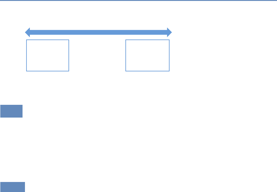
6.5. Methods 153
Machine Learning Spectrum
Unsupervised “Weakly” supervised Fully supervised
Clustering
PCA
MDS
Association Rules
…
Classication
Prediction
Regression
Figure 6.1. Spectrum of machine learning methods from unsupervised to super-
vised learning
6.5 Methods
We will start by describing unsupervised learning methods and then
go on to supervised learning methods. We focus here on the intu-
ition behind the methods and the algorithm, as well as practical
tips, rather than on the statistical theory that underlies the meth-
ods. We encourage readers to refer to machine learning books listed
in Section 6.11 for more details. Box 6.2 gives brief definitions of
several terms we will use in this section.
6.5.1 Unsupervised learning methods
As mentioned earlier, unsupervised learning methods are used when
we do not have a target variable to predict but want to understand
“natural” clusters or patterns in the data. These methods are often
used for initial data exploration, as in the following examples:
1. When faced with a large corpus of text data—for example, email
records, congressional bills, speeches, or open-ended free-text
survey responses—unsupervised learning methods are often
used to understand and get a handle on what the data contain.
2. Given a data set about students and their behavior over time
(academic performance, grades, test scores, attendance, etc.),
one might want to understand typical behaviors as well as tra-
jectories of these behaviors over time. Unsupervised learning
methods (clustering) can be applied to these data to get stu-
dent “segments” with similar behavior.
3. Given a data set about publications or patents in different
fields, we can use unsupervised learning methods (association

154 6. Machine Learning
Box 6.2: Machine learning vocabulary
•Learning: In machine learning, you will notice the term
learning that will be used in the context of “learning” a
model. This is what you probably know as fitting or esti-
mating a function, or training or building a model. These
terms are all synonyms and are used interchangeably in
the machine learning literature.
•Examples: These are data points and instances.
•Features: These are independent variables, attributes,
predictor variables, and explanatory variables.
•Labels: These include the response variable, dependent
variable, and target variable.
•Underfitting: This happens when a model is too sim-
ple and does not capture the structure of the data well
enough.
•Overfitting: This happens when a model is possibly too
complex and models the noise in the data, which can re-
sult in poor generalization performance. Using in-sample
measures to do model selection can result in that.
•Regularization: This is a general method to avoid overfit-
ting by applying additional constraints to the model that
is learned. A common approach is to make sure the model
weights are, on average, small in magnitude. Two common
regularizations are L1regularization (used by the lasso),
which has a penalty term that encourages the sum of the
absolute values of the parameters to be small; and L2reg-
ularization, which encourages the sum of the squares of
the parameters to be small.
rules) to figure out which disciplines have the most collabo-
ration and which fields have researchers who tend to publish
across different fields.
Clustering Clustering is the most common unsupervised learning
technique and is used to group data points together that are similar
to each other. The goal of clustering methods is to produce clusters

6.5. Methods 155
with high intra-cluster (within) similarity and low inter-cluster (be-
tween) similarity.
Clustering algorithms typically require a distance (or similarity)
metric*to generate clusters. They take a data set and a distance ⋆Distance metrics are
mathematical formulas to
calculate the distance be-
tween two objects.
For example, Manhattan
distance is the distance a
car would drive from one
place to another place in
a grid-based street system,
whereas Euclidian distance
(in two-dimensional space)
is the “straight-line” dis-
tance between two points.
metric (and sometimes additional parameters), and they generate
clusters based on that distance metric. The most common dis-
tance metric used is Euclidean distance, but other commonly used
metrics are Manhattan, Minkowski, Chebyshev, cosine, Hamming,
Pearson, and Mahalanobis. Often, domain-specific similarity met-
rics can be designed for use in specific problems. For example,
when performing the record linkage tasks discussed in Chapter 3,
you can design a similarity metric that compares two first names
and assigns them a high similarity (low distance) if they both map
to the same canonical name, so that, for example, Sammy and Sam
map to Samuel.
Most clustering algorithms also require the user to specify the
number of clusters (or some other parameter that indirectly deter-
mines the number of clusters) in advance as a parameter. This
is often difficult to do a priori and typically makes clustering an
iterative and interactive task. Another aspect of clustering that
makes it interactive is often the difficulty in automatically evaluat-
ing the quality of the clusters. While various analytical clustering
metrics have been developed, the best clustering is task-dependent
and thus must be evaluated by the user. There may be different
clusterings that can be generated with the same data. You can
imagine clustering similar news stories based on the topic content,
based on the writing style or based on sentiment. The right set of
clusters depends on the user and the task they have. Clustering is
therefore typically used for exploring the data, generating clusters,
exploring the clusters, and then rerunning the clustering method
with different parameters or modifying the clusters (by splitting or
merging the previous set of clusters). Interpreting a cluster can be
nontrivial: you can look at the centroid of a cluster, look at fre-
quency distributions of different features (and compare them to the
prior distribution of each feature), or you can build a decision tree
(a supervised learning method we will cover later in this chapter)
where the target variable is the cluster ID that can describe the
cluster using the features in your data. A good example of a tool
that allows interactive clustering from text data is Ontogen [125].
k-means clustering The most commonly used clustering algorithm
is called k-means, where kdefines the number of clusters. The
algorithm works as follows:

156 6. Machine Learning
1. Select k(the number of clusters you want to generate).
2. Initialize by selecting kpoints as centroids of the kclusters.
This is typically done by selecting kpoints uniformly at ran-
dom.
3. Assign each point a cluster according to the nearest centroid.
4. Recalculate cluster centroids based on the assignment in (3)
as the mean of all data points belonging to that cluster.
5. Repeat (3) and (4) until convergence.
The algorithm stops when the assignments do not change from
one iteration to the next (Figure 6.2). The final set of clusters, how-
ever, depend on the starting points. If they are initialized differently,
it is possible that different clusters are obtained. One common
practical trick is to run k-means several times, each with different
(random) starting points. The k-means algorithm is fast, simple,
and easy to use, and is often a good first clustering algorithm to try
and see if it fits your needs. When the data are of the form where
the mean of the data points cannot be computed, a related method
called K-medoids can be used [296].
Expectation-maximization (EM) clustering You may be familiar
with the EM algorithm in the context of imputing missing data.
EM is a general approach to maximum likelihood in the presence
of incomplete data. However, it is also used as a clustering method
where the missing data are the clusters a data point belongs to.
Unlike k-means, where each data point gets assigned to only one
cluster, EM does a soft assignment where each data point gets a
probabilistic assignment to various clusters. The EM algorithm iter-
ates until the estimates converge to some (locally) optimal solution.
The EM algorithm is fairly good at dealing with outliers as well
as high-dimensional data, compared to k-means. It also has a few
limitations. First, it does not work well with a large number of
clusters or when a cluster contains few examples. Also, when the
value of kis larger than the number of actual clusters in the data,
EM may not give reasonable results.
Mean shift clustering Mean shift clustering works by finding dense
regions in the data by defining a window around each data point and
computing the mean of the data points in the window. Then it shifts
the center of the window to the mean and repeats the algorithm till
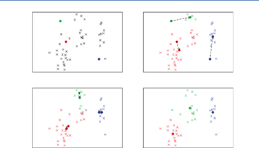
6.5. Methods 157
Number of people working on the project
Project budget
Project budget
Number of people working on the project
Number of people working on the project
m1
m1
m2
m2
m3
m3
Project budget
Project budget
Number of people working on the project
Figure 6.2. Example of k-means clustering with k=3. The upper left panel shows the distribution of the data and
the three starting points m1, m2, m3placed at random. On the upper right we see what happens in the first iteration.
The cluster means move to more central positions in their respective clusters. The lower left panel shows the second
iteration. After six iterations the cluster means have converged to their final destinations and the result is shown in
the lower right panel
it converges. After each iteration, we can consider that the window
shifts to a denser region of the data set. The algorithm proceeds as
follows:
1. Fix a window around each data point (based on the bandwidth
parameter that defines the size of the window).
2. Compute the mean of data within the window.
3. Shift the window to the mean and repeat till convergence.
Mean shift needs a bandwidth parameter hto be tuned, which
influences the convergence rate and the number of clusters. A large
hmight result in merging distinct clusters. A small hmight result
in too many clusters. Mean shift might not work well in higher

158 6. Machine Learning
dimensions since the number of local maxima is pretty high and it
might converge to a local optimum quickly.
One of the most important differences between mean shift and k-
means is that k-means makes two broad assumptions: the number
of clusters is already known and the clusters are shaped spherically
(or elliptically). Mean shift does not assume anything about the
number of clusters (but the value of hindirectly determines that).
Also, it can handle arbitrarily shaped clusters.
The k-means algorithm is also sensitive to initializations, where-
as mean shift is fairly robust to initializations. Typically, mean shift
is run for each point, or sometimes points are selected uniformly
randomly. Similarly, k-means is sensitive to outliers, while mean
shift is less sensitive. On the other hand, the benefits of mean shift
come at a cost—speed. The k-means procedure is fast, whereas
classic mean shift is computationally slow but can be easily paral-
lelized.
Hierarchical clustering The clustering methods that we have seen
so far, often termed partitioning methods, produce a flat set of clus-
ters with no hierarchy. Sometimes, we want to generate a hierarchy
of clusters, and methods that can do that are of two types:
1. Agglomerative (bottom-up): Start with each point as its own
cluster and iteratively merge the closest clusters. The iter-
ations stop either when the clusters are too far apart to be
merged (based on a predefined distance criterion) or when
there is a sufficient number of clusters (based on a predefined
threshold).
2. Divisive (top-down): Start with one cluster and create splits
recursively.
Typically, agglomerative clustering is used more often than divi-
sive clustering. One reason is that it is significantly faster, although
both of them are typically slower than direct partition methods such
as k-means and EM. Another disadvantage of these methods is that
they are greedy, that is, a data point that is incorrectly assigned to
the “wrong” cluster in an earlier split or merge cannot be reassigned
again later on.
Spectral clustering Figure 6.3 shows the clusters that k-means
would generate on the data set in the figure. It is obvious that the
clusters produced are not the clusters you would want, and that is
one drawback of methods such as k-means. Two points that are far
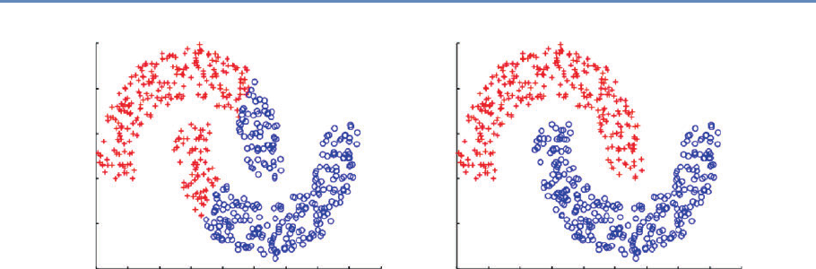
6.5. Methods 159
15
10
5
0
–5
–10
–15 –10 –5 0 5 10
(a) k-means
15 20 25 30 –15 –10 –5 0 5 10
(b) Spectral Clustering
15 20 25 30
15
10
5
0
–5
–10
Figure 6.3. The same data set can produce drastically different clusters: (a) k-means; (b) spectral clustering
away from each other will be put in different clusters even if there are
other data points that create a “path” between them. Spectral clus-
tering fixes that problem by clustering data that are connected but
not necessarily (what is called) compact or clustered within convex
boundaries. Spectral clustering methods work by representing data
as a graph (or network), where data points are nodes in the graph
and the edges (connections between nodes) represent the similarity
between the two data points.
The algorithm works as follows:
1. Compute a similarity matrix from the data. This involves deter-
mining a pairwise distance function (using one of the distance
functions we described earlier).
2. With this matrix, we can now perform graph partitioning, where
connected graph components are interpreted as clusters. The
graph must be partitioned such that edges connecting different
clusters have low weights and edges within the same cluster
have high values.
3. We can now partition these data represented by the similarity
matrix in a variety of ways. One common way is to use the
normalized cuts method. Another way is to compute a graph
Laplacian from the similarity matrix.
4. Compute the eigenvectors and eigenvalues of the Laplacian.

160 6. Machine Learning
5. The keigenvectors are used as proxy data for the original data
set, and they are fed into k-means clustering to produce clus-
ter assignments for each original data point.
Spectral clustering is in general much better than k-means in
clustering performance but much slower to run in practice. For
large-scale problems, k-means is a preferred clustering algorithm
to run because of efficiency and speed.
Principal components analysis Principal components analysis is
another unsupervised method used for finding patterns and struc-
ture in data. In contrast to clustering methods, the output is not a
set of clusters but a set of principal components that are linear com-
binations of the original variables. PCA is typically used when you
have a large number of variables and you want a reduced number
that you can analyze. This approach is often called dimensionality
reduction. It generates linearly uncorrelated dimensions that can be
used to understand the underlying structure of the data. In math-
ematical terms, given a set of data on ndimensions, PCA aims to
find a linear subspace of dimension dlower than nsuch that the
data points lie mainly on this linear subspace.
PCA is related to several other methods you may already know
about. Multidimensional scaling, factor analysis, and independent
component analysis differ from PCA in the assumptions they make,
but they are often used for similar purposes of dimensionality re-
duction and discovering the underlying structure in a data set.
Association rules Association rules are a different type of analysis
method and originate from the data mining and database commu-
nity, primarily focused on finding frequent co-occurring associa-
tions among a collection of items. This methods is sometimes re-
ferred to as “market basket analysis,” since that was the original
application area of association rules. The goal is to find associations
of items that occur together more often than you would randomly
expect. The classic example (probably a myth) is “men who go to the
store to buy diapers will also tend to buy beer at the same time.”
This type of analysis would be performed by applying association
rules to a set of supermarket purchase data.
Association rules take the form X1, X2, X3⇒Ywith support S
and confidence C, implying that when a transaction contains items
{X1, X2, X3}C% of the time, they also contain item Yand there are at
least S% of transactions where the antecedent is true. This is useful
in cases where we want to find patterns that are both frequent and

6.5. Methods 161
statistically significant, by specifying thresholds for support Sand
confidence C.
Support and confidence are useful metrics to generate rules but
are often not enough. Another important metric used to gener-
ate rules (or reduce the number of spurious patterns generated) is
lift. Lift is simply estimated by the ratio of the joint probability of
two items, xand y, to the product of their individual probabilities:
P(x, y)/[P(x)P(y)]. If the two items are statistically independent,
then P(x, y)=P(x)P(y), corresponding to a lift of 1. Note that anti-
correlation yields lift values less than 1, which is also an interesting
pattern, corresponding to mutually exclusive items that rarely occur
together.
Association rule algorithms work as follows: Given a set of trans-
actions (rows) and items for that transaction:
1. Find all combinations of items in a set of transactions that oc-
cur with a specified minimum frequency. These combinations
are called frequent itemsets.
2. Generate association rules that express co-occurrence of items
within frequent itemsets.
For our purposes, association rule methods are an efficient way
to take a basket of features (e.g., areas of publication of a re-
searcher, different organizations an individual has worked at in
their career, all the cities or neighborhoods someone may have lived
in) and find co-occurrence patterns. This may sound trivial, but as
data sets and number of features get larger, it becomes computa-
tionally expensive and association rule mining algorithms provide a
fast and efficient way of doing it.
6.5.2 Supervised learning
We now turn to the problem of supervised learning, which typically
involves methods for classification, prediction, and regression. We
will mostly focus on classification methods in this chapter since
many of the regression methods in machine learning are fairly simi-
lar to methods with which you are already familiar. Remember that
classification means predicting a discrete (or categorical) variable.
Some of the classification methods that we will cover can also be
used for regression, a fact that we will mention when describing
that method.
In general, supervised learning methods take as input pairs of
data points (X, Y )where Xare the predictor variables (features) and

162 6. Machine Learning
Yis the target variable (label). The supervised learning method
then uses these pairs as training data and learns a model F, where
F(X)∼Y. This model Fis then used to predict Ys for new data
points X. As mentioned earlier, the goal is not to build a model that
best fits known data but a model that is useful for future predictions
and minimizes future generalization error. This is the key goal that
differentiates many of the methods that you know from the methods
that we will describe next. In order to minimize future error, we
want to build models that are not just overfitting on past data.
Another goal, often prioritized in the social sciences, that ma-
chine learning methods do not optimize for is getting a structural
form of the model. Machine learning models for classification can
take different structural forms (ranging from linear models, to sets
of rules, to more complex forms), and it may not always be possible
to write them down in a compact form as an equation. This does
not, however, make them incomprehensible or uninterpretable. An-
other focus of machine learning models for supervised learning is
prediction, and not causal inference. Some of these models can
◮The topic of causal infer-
ence is addressed in more
detail in Chapter 10. be used to help with causal inference, but they are typically opti-
mized for prediction tasks. We believe that there are many social
science and policy problems where better prediction methods can
be extremely beneficial.
In this chapter, we mostly deal with binary classification prob-
lems: that is, problems in which the data points are to be classified
into one of two categories. Several of the methods that we will
cover can also be used for multiclass classification (classifying a
data point into one of ncategories) or for multi-label classification
(classifying a data point into mof ncategories where m≥1). There
are also approaches to take multiclass problems and turn them into
a set of binary problems that we will mention briefly at the end of
the chapter.
Before we describe supervised learning methods, we want to re-
cap a few principles as well as terms that we have used and will be
using in the rest of the chapter.
Training a model Once we have finished data exploration, filled in
missing values, created predictor variables (features), and decided
what our target variable (label) is, we now have pairs of X, Y to start
training (or building) the model.
Using the model to score new data We are building this model
so we can predict Yfor a new set of Xs—using the model means,
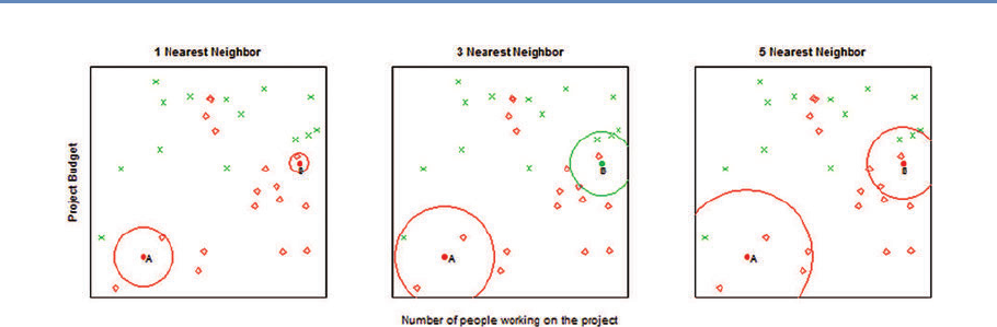
6.5. Methods 163
Figure 6.4. Example of k-nearest neighbor with k=1,3,5neighbors. We want to predict the points A and B. The
1-nearest neighbor for both points is red (“Patent not granted”), the 3-nearest neighbor predicts point A (B) to be red
(green) with probability 2/3, and the 5-nearest neighbor predicts again both points to be red with probabilities 4/5
and 3/5, respectively.
getting new data, generating the same features to get the vector X,
and then applying the model to produce Y.
One common technique for supervised learning is logistic re-
gression, a method you will already be familiar with. We will give an
overview of some of the other methods used in machine learning.
It is important to remember that as you use increasingly powerful
classification methods, you need more data to train the models.
k-nearest neighbor The method k-nearest neighbor (k-NN) is one
of the simpler classification methods in machine learning. It be-
longs to a family of models sometimes known as memory-based
models or instance-based models. An example is classified by find-
ing its knearest neighbors and taking majority vote (or some other
aggregation function). We need two key things: a value for kand a
distance metric with which to find the knearest neighbors. Typi-
cally, different values of kare used to empirically find the best one.
Small values of klead to predictions having high variance but can
capture the local structure of the data. Larger values of kbuild
more global models that are lower in variance but may not capture
local structure in the data as well.
Figure 6.4 provides an example for k=1,3,5 nearest neighbors.
The number of neighbors (k) is a parameter, and the prediction
depends heavily on how it is determined. In this example, point B
is classified differently if k=3.
Training for k-NN just means storing the data, making this
method useful in applications where data are coming in extremely

164 6. Machine Learning
quickly and a model needs to be updated frequently. All the work,
however, gets pushed to scoring time, since all the distance calcu-
lations happen when a new data point needs to be classified. There
are several optimized methods designed to make k-NN more efficient
that are worth looking into if that is a situation that is applicable to
your problem.
In addition to selecting kand an appropriate distance metric, we
also have to be careful about the scaling of the features. When dis-
tances between two data points are large for one feature and small
for a different feature, the method will rely almost exclusively on
the first feature to find the closest points. The smaller distances on
the second feature are nearly irrelevant to calculate the overall dis-
tance. A similar problem occurs when continuous and categorical
predictors are used together. To resolve the scaling issues, various
options for rescaling exist. For example, a common approach is to
center all features at mean 0 and scale them to variance 1.
There are several variations of k-NN. One of these is weighted
nearest neighbors, where different features are weighted differently
or different examples are weighted based on the distance from the
example being classified. The method k-NN also has issues when
the data are sparse and has high dimensionality, which means that
every point is far away from virtually every other point, and hence
pairwise distances tend to be uninformative. This can also happen
when a lot of features are irrelevant and drown out the relevant
features’ signal in the distance calculations.
Notice that the nearest-neighbor method can easily be applied to
regression problems with a real-valued target variable. In fact, the
method is completely oblivious to the type of target variable and can
potentially be used to predict text documents, images, and videos,
based on the aggregation function after the nearest neighbors are
found.
Support vector machines Support vector machines are one of the
most popular and best-performing classification methods in ma-
chine learning today. The mathematics behind SVMs has a lot of
prerequisites that are beyond the scope of this book, but we will
give you an intuition of how SVMs work, what they are good for,
and how to use them.
We are all familiar with linear models that separate two classes
by fitting a line in two dimensions (or a hyperplane in higher dimen-
sions) in the middle (see Figure 6.5). An important decision that lin-
ear models have to make is which linear separator we should prefer
when there are several we can build.
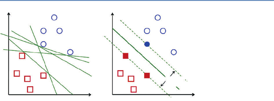
6.5. Methods 165
x2x2
x1x1
Maximum
margin
Optimal hyperplane
Figure 6.5. Support vector machines
You can see in Figure 6.5 that multiple lines offer a solution
to the problem. Is any of them better than the others? We can
intuitively define a criterion to estimate the worth of the lines: A
line is bad if it passes too close to the points because it will be noise
sensitive and it will not generalize correctly. Therefore, our goal
should be to find the line passing as far as possible from all points.
The SVM algorithm is based on finding the hyperplane that max-
imizes the margin of the training data. The training examples that
are closest to the hyperplane are called support vectors since they
are supporting the margin (as the margin is only a function of the
support vectors).
An important concept to learn when working with SVMs is ker-
nels. SVMs are a specific instance of a class of methods called kernel
methods. So far, we have only talked about SVMs as linear mod-
els. Linear works well in high-dimensional data but sometimes you
need nonlinear models, often in cases of low-dimensional data or in
image or video data. Unfortunately, traditional ways of generating
nonlinear models get computationally expensive since you have to
explicitly generate all the features such as squares, cubes, and all
the interactions. Kernels are a way to keep the efficiency of the lin-
ear machinery but still build models that can capture nonlinearity
in the data without creating all the nonlinear features.
You can essentially think of kernels as similarity functions and
use them to create a linear separation of the data by (implicitly) map-
ping the data to a higher-dimensional space. Essentially, we take
an n-dimensional input vector X, map it into a high-dimensional

166 6. Machine Learning
(possibly infinite-dimensional) feature space, and construct an op-
timal separating hyperplane in this space. We refer you to relevant
papers for more detail on SVMs and nonlinear kernels [334, 339].
SVMs are also related to logistic regression, but use a different
loss/penalty function [159].
When using SVMs, there are several parameters you have to
optimize, ranging from the regularization parameter C, which de-
termines the tradeoff between minimizing the training error and
minimizing model complexity, to more kernel-specific parameters.
It is often a good idea to do a grid search to find the optimal param-
eters. Another tip when using SVMs is to normalize the features;
one common approach to doing that is to normalize each data point
to be a vector of unit length.
Linear SVMs are effective in high-dimensional spaces, especially
when the space is sparse such as text classification where the num-
ber of data points (perhaps tens of thousands) is often much less
than the number of features (a hundred thousand to a million or
more). SVMs are also fairly robust when the number of irrelevant
features is large (unlike the k-NN approaches that we mentioned
earlier) as well as when the class distribution is skewed, that is,
when the class of interest is significantly less than 50% of the data.
One disadvantage of SVMs is that they do not directly provide
probability estimates. They assign a score based on the distance
from the margin. The farther a point is from the margin, the higher
the magnitude of the score. This score is good for ranking examples,
but getting accurate probability estimates takes more work and re-
quires more labeled data to be used to perform probability calibra-
tions.
In addition to classification, there are also variations of SVMs
that can be used for regression [348] and ranking [70].
Decision trees Decision trees are yet another set of methods that
are helpful for prediction. Typical decision trees learn a set of rules
from training data represented as a tree. An exemplary decision
tree is shown in Figure 6.6. Each level of a tree splits the tree to
create a branch using a feature and a value (or range of values). In
the example tree, the first split is made on the feature number of
visits in the past year and the value 4. The second level of the tree
now has two splits: one using average length of visit with value 2
days and the other using the value 10 days.
Various algorithms exist to build decision trees. C4.5, CHAID,
and CART (Classification and Regression Trees) are the most popular.
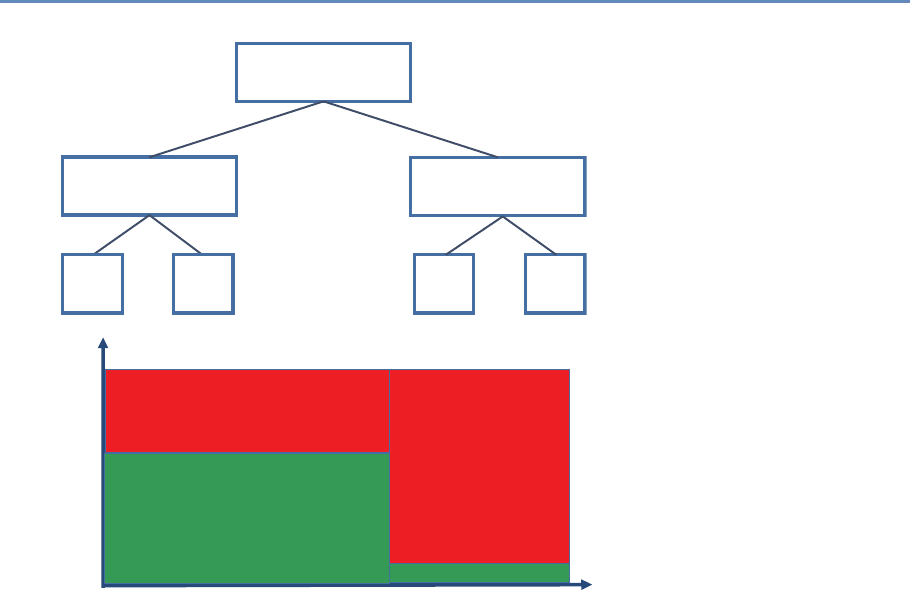
6.5. Methods 167
# of Visits in past year
≥ 4
Average length of visit
≥ 2 days
Average length of visit
≥ 10 days
N
Y
YN
Risk
High
YN
Risk
Low
Risk
High
Risk
Low
# of Visits in Past Year
Average Length of Stay
123 4 5 6
4
8
12
16
Risk = High
Risk = High
Risk = Low
Risk = Low
Figure 6.6. An exemplary decision tree. The top figure is the standard repre-
sentation for trees. The bottom figure offers an alternative view of the same tree.
The feature space is partitioned into numerous rectangles, which is another way
to view a tree, representing its nonlinear character more explicitly
Each needs to determine the next best feature to split on. The goal
is to find feature splits that can best reduce class impurity in the
data, that is, a split that will ideally put all (or as many as possible)
positive class examples on one side and all (or as many as possi-
ble) negative examples on the other side. One common measure of
impurity that comes from information theory is entropy, and it is
calculated as
H(X)=−X
x
p(x) log p(x).
Entropy is maximum (1) when both classes have equal numbers
of examples in a node. It is minimum (0) when all examples are

168 6. Machine Learning
from the same class. At each node in the tree, we can evaluate
all the possible features and select the one that most reduces the
entropy given the tree so far. This expected change in entropy is
known as information gain and is one of the most common criteria
used to create decision trees. Other measures that are used instead
of information gain are Gini and chi-squared.
If we keep constructing the tree in this manner, selecting the
next best feature to split on, the tree ends up fairly deep and tends
to overfit the data. To prevent overfitting, we can either have a
stopping criterion or prune the tree after it is fully grown. Common
stopping criteria include minimum number of data points to have
before doing another feature split, maximum depth, and maximum
purity. Typical pruning approaches use holdout data (or cross-
validation, which will be discussed later in this chapter) to cut off
parts of the tree.
Once the tree is built, a new data point is classified by running it
through the tree and, once it reaches a terminal node, using some
aggregation function to give a prediction (classification or regres-
sion). Typical approaches include performing maximum likelihood
(if the leaf node contains 10 examples, 8 positive and 2 negative,
any data point that gets into that node will get an 80% probability
of being positive). Trees used for regression often build the tree as
described above but then fit a linear regression model at each leaf
node.
Decision trees have several advantages. The interpretation of a
tree is straightforward as long as the tree is not too large. Trees
can be turned into a set of rules that experts in a particular domain
can possibly dig deeper into, validate, and modify. Trees also do not
require too much feature engineering. There is no need to create
interaction terms since trees can implicitly do that by splitting on
two features, one after another.
Unfortunately, along with these benefits come a set of disadvan-
tages. Decision trees, in general, do not perform well, compared to
SVMs, random forests, or logistic regression. They are also unsta-
ble: small changes in data can result in very different trees. The lack
of stability comes from the fact that small changes in the training
data may lead to different splitting points. As a consequence, the
whole tree may take a different structure. The suboptimal predic-
tive performance can be seen from the fact that trees partition the
predictor space into a few rectangular regions, each one predicting
only a single value (see the bottom part of Figure 6.6).

6.5. Methods 169
Ensemble methods Combinations of models are generally known
as model ensembles. They are among the most powerful techniques
in machine learning, often outperforming other methods, although
at the cost of increased algorithmic and model complexity.
The intuition behind building ensembles of models is to build
several models, each somewhat different. This diversity can come
from various sources such as: training models on subsets of the
data; training models on subsets of the features; or a combination
of these two.
Ensemble methods in machine learning have two things in com-
mon. First, they construct multiple, diverse predictive models from
adapted versions of the training data (most often reweighted or re-
sampled). Second, they combine the predictions of these models in
some way, often by simple averaging or voting (possibly weighted).
Bagging Bagging stands for “bootstrap aggregation”:*we first cre- ⋆Bootstrap is a general
statistical procedure that
draws random samples of
the original data with re-
placement.
ate bootstrap samples from the original data and then aggregate the
predictions using models trained on each bootstrap sample. Given
a data set of size N, the method works as follows:
1. Create kbootstrap samples (with replacement), each of size N,
resulting in kdata sets. Only about 63% of the original train-
ing examples will be represented in any given bootstrapped
set.
2. Train a model on each of the kdata sets, resulting in kmodels.
3. For a new data point X, predict the output using each of the k
models.
4. Aggregate the kpredictions (typically using average or voting)
to get the prediction for X.
A nice feature of this method is that any underlying model can
be used, but decision trees are often the most commonly used base
model. One reason for this is that decision tress are typically high
variance and unstable, that is, they can change drastically given
small changes in data, and bagging is effective at reducing the vari-
ance of the overall model. Another advantage of bagging is that
each model can be trained in parallel, making it efficient to scale to
large data sets.
Boosting Boosting is another popular ensemble technique, and it
often results in improving the base classifier being used. In fact,

170 6. Machine Learning
if your only goal is improving accuracy, you will most likely find
that boosting will achieve that. The basic idea is to keep training
classifiers iteratively, each iteration focusing on examples that the
previous one got wrong. At the end, you have a set of classifiers,
each trained on smaller and smaller subsets of the training data.
Given a new data point, all the classifiers predict the target, and a
weighted average of those predictions is used to get the final pre-
diction, where the weight is proportional to the accuracy of each
classifier. The algorithm works as follows:
1. Assign equal weights to every example.
2. For each iteration:
(a) Train classifier on the weighted examples.
(b) Predict on the training data.
(c) Calculate error of the classifier on the training data.
(d) Calculate the new weighting on the examples based on
the errors of the classifier.
(e) Reweight examples.
3. Generate a weighted classifier based on the accuracy of each
classifier.
One constraint on the classifier used within boosting is that it
should be able to handle weighted examples (either directly or by
replicating the examples that need to be overweighted). The most
common classifiers used in boosting are decision stumps (single-
level decision trees), but deeper trees can also work well.
Boosting is a common way to boost the performance of a classi-
fication method but comes with additional complexity, both in the
training time and in interpreting the predictions. A disadvantage of
boosting is that it is difficult to parallelize since the next iteration of
boosting relies on the results of the previous iteration.
A nice property of boosting is its ability to identify outliers: ex-
amples that are either mislabeled in the training data, or are inher-
ently ambiguous and hard to categorize. Because boosting focuses
its weight on the examples that are more difficult to classify, the
examples with the highest weight often turn out to be outliers. On
the other hand, if the number of outliers is large (lots of noise in
the data), these examples can hurt the performance of boosting by
focusing too much on them.

6.5. Methods 171
Random forests Given a data set of size Nand containing Mfea-
tures, the random forest training algorithm works as follows:
1. Create nbootstrap samples from the original data of size N.
Remember, this is similar to the first step in bagging. Typically
nranges from 100 to a few thousand but is best determined
empirically.
2. For each bootstrap sample, train a decision tree using mfea-
tures (where mis typically much smaller than M) at each node
of the tree. The mfeatures are selected uniformly at random
from the Mfeatures in the data set, and the decision tree will
select the best split among the mfeatures. The value of mis
held constant during the forest growing.
3. A new test example/data point is classified by all the trees,
and the final classification is done by majority vote (or another
appropriate aggregation method).
Random forests are probably the most accurate classifiers being
used today in machine learning. They can be easily parallelized,
making them efficient to run on large data sets, and can handle a
large number of features, even with a lot of missing values. Random
forests can get complex, with hundreds or thousands of trees that
are fairly deep, so it is difficult to interpret the learned model. At
the same time, they provide a nice way to estimate feature impor-
tance, giving a sense of what features were important in building
the classifier.
Another nice aspect of random forests is the ability to compute a
proximity matrix that gives the similarity between every pair of data
points. This is calculated by computing the number of times two
examples land in the same terminal node. The more that happens,
the closer the two examples are. We can use this proximity matrix
for clustering, locating outliers, or explaining the predictions for a
specific example.
Stacking Stacking is a technique that deals with the task of learn-
ing a meta-level classifier to combine the predictions of multiple
base-level classifiers. This meta-algorithm is trained to combine
the model predictions to form a final set of predictions. This can be
used for both regression and classification. The algorithm works as
follows:
1. Split the data set into nequal-sized sets: set1, set2, . . . , setn.

172 6. Machine Learning
2. Train base models on all possible combinations of n−1 sets
and, for each model, use it to predict on setiwhat was left out
of the training set. This would give us a set of predictions on
every data point in the original data set.
3. Now train a second-stage stacker model on the predicted classes
or the predicted probability distribution over the classes from
the first-stage (base) model(s).
By using the first-stage predictions as features, a stacker model
gets more information on the problem space than if it were trained in
isolation. The technique is similar to cross-validation, an evaluation
methodology that we will cover later in this chapter.
Neural networks and deep learning Neural networks are a set of
multi-layer classifiers where the outputs of one layer feed into the
inputs of the next layer. The layers between the input and output
layers are called hidden layers, and the more hidden layers a neu-
ral network has, the more complex functions it can learn. Neural
networks were popular in the 1980s and early 1990s, but then fell
out of fashion because they were slow and expensive to train, even
with only one or two hidden layers. Since 2006, a set of techniques
has been developed that enable learning in deeper neural networks.
These techniques have enabled much deeper (and larger) networks
to be trained—people now routinely train networks with five to ten
hidden layers. And it turns out that these perform far better on
many problems than shallow neural networks (with just a single
hidden layer). The reason for the better performance is the ability
of deep nets to build up a complex hierarchy of concepts, learning
multiple levels of representation and abstraction that help to make
sense of data such as images, sound, and text.
Usually, with a supervised neural network you try to predict a
target vector, Y, from a matrix of inputs, X. But when you train
a deep neural network, it uses a combination of supervised and
unsupervised learning. In an unsupervised neural network, you
try to predict the matrix Xusing the same matrix Xas the input.
In doing this, the network can learn something intrinsic about the
data without the help of a separate target or label. The learned
information is stored as the weights of the network.
Currently, deep neural networks are trendy and a lot of research
is being done on them. It is, however, important to keep in mind
that they are applicable for a narrow class of problems with which
social scientists would deal and that they often require a lot more

6.6. Evaluation 173
data than are available in most problems. Training deep neural
networks also requires a lot of computational power, but that is
less likely to be an issue for most people. Typical cases where deep
learning has been shown to be effective involve lots of images, video,
and text data. We are still in the early stages of development of this
class of methods, and the next few years will give us a much better
understanding of why they are effective and the problems for which
they are well suited.
6.6 Evaluation
The previous section introduced us to a variety of methods, all with
certain pros and cons, and no single method guaranteed to outper-
forms others for a given problem. This section focuses on evaluation
methods, with three primary goals:
1. Model selection: How do we select a method to use? What
parameters should we select for that method?
2. Performance estimation: How well will our model do once it is
deployed and applied to new data?
3. A deeper understanding of the model can point to inaccuracies
of existing methods and provide a better understanding of the
data and the problem we are tackling.
This section will cover evaluation methodologies as well as met-
rics that are commonly used. We will start by describing common
evaluation methodologies that use existing data and then move on
to field trials. The methodologies we describe below apply both to
regression and classification problems.
6.6.1 Methodology
In-sample evaluation As social scientists, you already evaluate
methods on how well they perform in-sample (on the set that the
model was trained on). As we mentioned earlier in the chapter, the
goal of machine learning methods is to generalize to new data, and
validating models in-sample does not allow us to do that. We fo-
cus here on evaluation methodologies that allow us to optimize (as
best as we can) for generalization performance. The methods are
illustrated in Figure 6.7.

174 6. Machine Learning
Training Set Test Set
Data (Size = N)
N1
Size = N/5
N2
Size = N/5
N3
Size = N/5
N4
Size = N/5
N5
Size = N/5
Out-of-Sample (Holdout Set)
Original Data Set
5-Fold Cross-Validation
Figure 6.7. Validation methodologies: holdout set and cross-validation
Out-of-sample and holdout set The simplest way to focus on gen-
eralization is to pretend to generalize to new (unseen) data. One
way to do that is to take the original data and randomly split them
into two sets: a training set and a test set (sometimes also called
the holdout or validation set). We can decide how much to keep in
each set (typically the splits range from 50–50 to 80–20, depending
on the size of the data set). We then train our models on the train-
ing set and classify the data in the test set, allowing us to get an
estimate of the relative performance of the methods.
One drawback of this approach is that we may be extremely
lucky or unlucky with our random split. One way to get around the
problem that is to repeatedly create multiple training and test sets.
We can then train on TR1and test on TE1, train on TR2and test
on TE2, and so on. The performance measures on each test set can
then give us an estimate of the performance of different methods
and how much they vary across different random sets.
Cross-validation Cross-validation is a more sophisticated holdout
training and testing procedure that takes away some of the short-
comings of the holdout set approach. Cross-validation begins by
splitting a labeled data set into kpartitions (called folds). Typically,
kis set to 5 or 10. Cross-validation then proceeds by iterating k
times. In each iteration, one of the kfolds is held out as the test
set, while the other k−1 folds are combined and used to train
the model. A nice property of cross-validation is that every exam-
ple is used in one test set for testing the model. Each iteration of
cross-validation gives us a performance estimate that can then be
aggregated (typically averaged) to generate the overall estimate.

6.6. Evaluation 175
Train Test
Train Test
Train Test
2010 2011 2012 2013 2014
2010 2011 2012 2013 2014
2010 2011 2012 2013 2014
Figure 6.8. Temporal validation
An extreme case of cross-validation is called leave-one-out cross-
validation, where given a data set of size N, we create Nfolds. That
means iterating over each data point, holding it out as the test set,
and training on the rest of the N−1 examples. This illustrates the
benefit of cross-validation by giving us good generalization estimates
(by training on as much of the data set as possible) and making sure
the model is tested on each data point.
Temporal validation The cross-validation and holdout set ap-
proaches described above assume that the data have no time de-
pendencies and that the distribution is stationary over time. This
assumption is almost always violated in practice and affects perfor-
mance estimates for a model.
In most practical problems, we want to use a validation strategy
that emulates the way in which our models will be used and pro-
vides an accurate performance estimate. We will call this temporal
validation. For a given point in time ti, we train our models only on
information available to us before tito avoid training on data from
the “future.” We then predict and evaluate on data from tito ti+d
and iterate, expanding the training window while keeping the test
window size constant at d. Figure 6.8 shows this validation process
with ti=2010 and d=1 year. The test set window ddepends
on a few factors related to how the model will be deployed to best
emulate reality:
1. How far out in the future do predictions need to be made? For
example, if the set of students who need to be targeted for

176 6. Machine Learning
interventions has to be finalized at the beginning of the school
year for the entire year, then d=1 year.
2. How often will the model be updated? If the model is being
updated daily, then we can move the window by a day at a
time to reflect the deployment scenario.
3. How often will the system get new data? If we are getting new
data frequently, we can make predictions more frequently.
Temporal validation is similar to how time series models are eval-
uated and should be the validation approach used for most practical
problems.
6.6.2 Metrics
The previous subsection focused on validation methodologies as-
suming we have a evaluation metric in mind. This section will go
over commonly used evaluation metrics. You are probably familiar
with using R2, analysis of the residuals, and mean squared error
(MSE) to evaluate the quality of regression models. For regression
problems, the MSE calculates the average squared differences be-
tween predictions ˆyiand true values yi. When prediction models
have smaller MSE, they are better. However, the MSE itself is hard
to interpret because it measures quadratic differences. Instead, the
root mean squared error (RMSE) is more intuitive as it as measure
of mean differences on the original scale of the response variable.
Yet another alternative is the mean absolute error (MAE), which
measures average absolute distances between predictions and true
values.
We will now describe some additional evaluation metrics com-
monly used in machine learning for classification. Before we dive
into metrics, it is important to highlight that machine learning mod-
els for classification typically do not predict 0/1 values directly.
SVMs, random forests, and logistic regression all produce a score
(which is sometimes a probability) that is then turned into 0 or 1
based on a user-specific threshold. You might find that certain tools
(such as sklearn) use a default value for that threshold (often 0.5),
but it is important to know that it is an arbitrary threshold and
you should select the threshold based on the data, the model, and
the problem you are solving. We will cover that a little later in this
section.
Once we have turned the real-valued predictions into 0/1 clas-
sification, we can now create a confusion matrix from these pre-

6.6. Evaluation 177
True
Class
Predicted Class
1 0 total
1True
Positives
False
Negatives P′
0False
Positives
True
Negatives N′
total P N
Figure 6.9. Aconfusion matrix created from real-valued predictions
dictions, shown in Figure 6.9. Each data point belongs to either
the positive class or the negative class, and for each data point
the prediction of the classifier is either correct or incorrect. This is
what the four cells of the confusion matrix represent. We can use
the confusion matrix to describe several commonly used evaluation
metrics.
Accuracy is the ratio of correct predictions (both positive and
negative) to all predictions:
Accuracy =TP +TN
TP +TN +FP +FN =TP +TN
P+N=TP +TN
P′+N′,
where TP denotes true positives, TN true negatives, FP false posi-
tives, FN false negatives, and other symbols denote row or column
totals as in Figure 6.9. Accuracy is the most commonly described
evaluation metric for classification but is surprisingly the least use-
ful in practical situations (at least by itself). One problem with
accuracy is that it does not give us an idea of lift compared to base-
line. For example, if we have a classification problem with 95% of
the data as positive and 5% as negative, a classifier with 85% is
performing worse than a dumb classifier that predicts positive all
the time (and will have 95% accuracy).
Two additional metrics that are often used are precision and
recall, which are defined as follows:
Precision =TP
TP +FP =TP
P,
Recall =TP
TP +FN =TP
P′

178 6. Machine Learning
(see also Box 7.3). Precision measures the accuracy of the classifier
when it predicts an example to be positive. It is the ratio of correctly
predicted positive examples (TP) to all examples predicted as positive
(TP +FP). This measure is also called positive predictive value in
other fields. Recall measures the ability of the classifier to find
positive examples. It is the ratio of all the correctly predicted positive
examples (TP) to all the positive examples in the data (TP +FN). This
is also called sensitivity in other fields.
You might have encountered another metric called specificity in
other fields. This measure is the true negative rate: the proportion
of negatives that are correctly identified.
Another metric that is used is the F1score, which is the harmonic
mean of precision and recall:
F1=2∗Precision ∗Recall
Precision +Recall
(see also equation (7.1)). This is often used when you want to bal-
ance both precision and recall.
There is often a tradeoff between precision and recall. By se-
lecting different classification thresholds, we can vary and tune the
precision and recall of a given classifier. A highly conservative clas-
sifier that only predicts a 1 when it is absolutely sure (say, a thresh-
old of 0.9999) will most often be correct when it predicts a 1 (high
precision) but will miss most 1s (low recall). At the other extreme, a
classifier that says 1 to every data point (a threshold of 0.0001) will
have perfect recall but low precision. Figure 6.10 show a precision–
recall curve that is often used to represent the performance of a
given classifier.
If we care about optimizing for the entire precision recall space, a
useful metric is the area under the curve (AUC-PR), which is the area
under the precision–recall curve. AUC-PR must not be confused
with AUC-ROC, which is the area under the related receiver operat-
ing characteristic (ROC) curve. The ROC curve is created by plotting
recall versus (1 – specificity). Both AUCs can be helpful metrics to
compare the performance of different methods and the maximum
value the AUC can take is 1. If, however, we care about a specific
part on the precision–recall curve, we have to look at finer-grained
metrics.
Let us consider an example from public health. Most public
health agencies conduct inspections of various sorts to detect health
hazard violations (lead hazards, for example). The number of possi-
ble places (homes or businesses) to inspect far exceeds the inspec-
tion resources typically available. Let us assume further that they
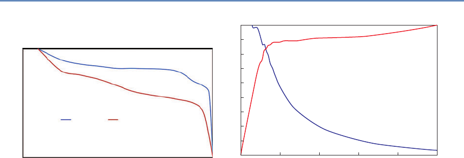
6.6. Evaluation 179
1
0.8
0.6
0.4
0.2
00 0.2 0.4 0.6
Precision
Classier A Classier B
Recall
0.8 1
Figure 6.10. Precision–recall curve
1.0
0.9
0.8
0.7
0.6
Precision
Recall
0.5
0.4
0.3
0.2
0.1
0.0 0.2 0.4 0.6
Percent of Population
1.0
0.8
0.6
0.4
0.2
0.0
0.8 1.0
Figure 6.11. Precision or recall at different thresholds
can only inspect 5% of all possible places; they would clearly want
to prioritize the inspection of places that are most likely to contain
the hazard. In this case, the model will score and rank all the pos-
sible inspection places in order of hazard risk. We would then want
to know what percentage of the top 5% (the ones that will get in-
spected) are likely to be hazards, which translates to the precision
in the top 5% of the most confidence predictions—precision at 5%,
as it is commonly called (see Figure 6.11). Precision at top k percent
is a common class of metrics widely used in information retrieval
and search engine literature, where you want to make sure that the
results retrieved at the top of the search results are accurate. More
generally, this metric is often used in problems in which the class
distribution is skewed and only a small percentage of the examples
will be examined manually (inspections, investigations for fraud,
etc.). The literature provides many case studies of such applica-
tions [219,222, 307].
One last metric we want to mention is a class of cost-sensitive
metrics where different costs (or benefits) can be associated with
the different cells in the confusion matrix. So far, we have implicitly
assumed that every correct prediction and every error, whether for
the positive class or the negative class, has equal costs and benefits.
In many practical problems, that is not the case. For example, we
may want to predict whether a patient in a hospital emergency room
is likely to go into cardiac arrest in the next six hours. The cost of a
false positive in this case is the cost of the intervention (which may
be a few extra minutes of a physician’s time) while the cost of a false
negative could be death. This type of analysis allows us to calculate

180 6. Machine Learning
the expected value of the predictions of a classifier and select the
model that optimizes this cost-sensitive metric.
6.7 Practical tips
Here we highlight some practical tips that will be helpful when work-
ing with machine learning methods.
6.7.1 Features
So far in this chapter, we have focused a lot on methods and pro-
cess, and we have not discussed features in detail. In social science,
they are not called features but instead are known as variables or
predictors. Good features are what makes machine learning sys-
tems effective. Feature generation (or engineering, as it is often
called) is where the bulk of the time is spent in the machine learn-
ing process. As social science researchers or practitioners, you have
spent a lot of time constructing features, using transformations,
dummy variables, and interaction terms. All of that is still required
and critical in the machine learning framework. One difference you
will need to get comfortable with is that instead of carefully selecting
a few predictors, machine learning systems tend to encourage the
creation of lots of features and then empirically use holdout data to
perform regularization and model selection. It is common to have
models that are trained on thousands of features. Commonly used
approaches to create features include:
•Transformations, such as log, square, and square root.
•Dummy (binary) variables: This is often done by taking cate-
gorical variables (such as city) and creating a binary variable
for each value (one variable for each city in the data). These
are also called indicator variables.
•Discretization: Several methods require features to be discrete
instead of continuous. Several approaches exist to convert
continuous variables into discrete ones, the most common of
which is equal-width binning.
•Aggregation: Aggregate features often constitute the majority
of features for a given problem. These aggregations use differ-
ent aggregation functions (count, min, max, average, standard
deviation, etc.), often over varying windows of time and space.

6.7. Practical tips 181
For example, given urban data, we would want to calculate the
number (and min, max, mean, variance) of crimes within an
m-mile radius of an address in the past tmonths for varying
values of mand t, and then to use all of them as features in a
classification problem.
In general, it is a good idea to have the complexity in features
and use a simple model, rather than using more complex models
with simple features. Keeping the model simple makes it faster to
train and easier to understand.
6.7.2 Machine learning pipeline
When working on machine learning projects, it is a good idea to
structure your code as a modular pipeline so you can easily try dif-
ferent approaches and methods without major restructuring. The
Python workbooks supporting this book will give you an example of
a machine learning pipeline. A good pipeline will contain modules
for importing data, doing exploration, feature generation, classifica-
tion, and evaluation. You can then instantiate a specific workflow
by combining these modules.
An important component of the machine learning pipeline is
comparing different methods. With all the methods out there and
all the hyperparameters they come with, how do we know which
model to use and which hyperparameters to select? And what hap-
pens when we add new features to the model or when the data have
“temporal drift” and change over time? One simple approach is to
have a nested set of for loops that loop over all the methods you
have access to, then enumerate all the hyperparameters for that
method, create a cross-product, and loop over all of them, compar-
ing them across different evaluation metrics and selecting the best
one to use going forward. You can even add different feature subsets
and time slices to this for loop, as the example in the supporting
workbooks will show.
6.7.3 Multiclass problems
In the supervised learning section, we framed classification prob-
lems as binary classification problems with a 0 or 1 output. There
are many problems where we have multiple classes, such as clas-
sifying companies into their industry codes or predicting whether a
student will drop out, transfer, or graduate. Several solutions have
been designed to deal with the multiclass classification problem:

182 6. Machine Learning
•Direct multiclass: Use methods that can directly perform mul-
ticlass classification. Examples of such methods are K-nearest
neighbor, decision trees, and random forests. There are ex-
tensions of support vector machines that exist for multiclass
classification as well [86], but they can often be slow to train.
•Convert to one versus all (OVA): This is a common approach
to solve multiclass classification problems using binary clas-
sifiers. Any problem with nclasses can be turned into nbi-
nary classification problems, where each classifier is trained
to distinguish between one versus all the other classes. A new
example can be classified by combining the predictions from
all the nclassifiers and selecting the class with the highest
score. This is a simple and efficient approach, and one that is
commonly used, but it suffers from each classification problem
possibly having an imbalanced class distribution (due to the
negative class being a collection of multiple classes). Another
limitation of this approach is that it requires the scores of each
classifier to be calibrated so that they are comparable across
all of them.
•Convert to pairwise: In this approach, we can create binary
classifiers to distinguish between each pair of classes, result-
ing in n
2binary classifiers. This results in a large number of
classifiers, but each classifier usually has a balanced classifi-
cation problem. A new example is classified by taking the pre-
dictions of all the binary classifiers and using majority voting.
6.7.4 Skewed or imbalanced classification problems
A lot of problems you will deal with will not have uniform (balanced)
distributions for both classes. This is often the case with problems
in fraud detection, network security, and medical diagnosis where
the class of interest is not very common. The same is true in many
social science and public policy problems around behavior predic-
tion, such as predicting which students will not graduate on time,
which children may be at risk of getting lead poisoning, or which
homes are likely to be abandoned in a given city. You will notice
that applying standard machine learning methods may result in all
the predictions being for the most frequent category in such situa-
tions, making it problematic to detect the infrequent classes. There
has been a lot of work in machine learning research on dealing with
such problems [73, 217] that we will not cover in detail here. Com-

6.8. How can social scientists benefit from machine learning? 183
mon approaches to deal with class imbalance include oversampling
from the minority class and undersampling from the majority class.
It is important to keep in mind that the sampling approaches do not
need to result in a 1 :1 ratio. Many supervised learning methods
described in this chapter (such as SVMs) can work well even with
a 10 :1 imbalance. Also, it is critical to make sure that you only
resample the training set; keep the distribution of the test set the
same as that of the original data since you will not know the class
labels of new data in practice and will not be able to resample.
6.8 How can social scientists benefit from
machine learning?
In this chapter, we have introduced you to some new methods (both
unsupervised and supervised), validation methodologies, and eval-
uation metrics. All of these can benefit social scientists as they
tackle problems in research and practice. In this section, we will
give a few concrete examples where what you have learned so far
can be used to improve some social science tasks:
•Use of better prediction methods and methodology: Traditional
statistics and social sciences have not focused much on meth-
ods for prediction. Machine learning researchers have spent
the past 30 years developing and adapting methods focusing
on that task. We believe that there is a lot of value for so-
cial science researchers and practitioners in learning more
about those methods, applying them, and even augmenting
them [210]. Two common tasks that can be improved us-
ing better prediction methods are generating counterfactuals
(essentially a prediction problem) and matching. In addition,
holdout sets and cross-validation can be used as a model se-
lection methodology with any existing regression and classi-
fication methods, resulting in improved model selection and
error estimates.
•Model misspecification: Linear and logistic regressions are
common techniques for data analysis in the social sciences.
One fundamental assumption within both is that they are ad-
ditive over parameters. Machine learning provides tools when
this assumption is too limiting. Hainmueller and Hazlett [148],
for example, reanalyze data that were originally analyzed with

184 6. Machine Learning
logistic regression and come to substantially different conclu-
sions. They argue that their analysis, which is more flexible
and based on supervised learning methodology, provides three
additional insights when compared to the original model. First,
predictive performance is similar or better, although they do
not need an extensive search to find the final model specifi-
cation as it was done in the original analysis. Second, their
model allows them to calculate average marginal effects that
are mostly similar to the original analysis. However, for one
covariate they find a substantially different result, which is
due to model misspecification in the original model. Finally,
the reanalysis also discovers interactions that were missed in
the original publication.
•Better text analysis: Text is everywhere, but unfortunately hu-
mans are slow and expensive in analyzing text data. Thus,
computers are needed to analyze large collections of text. Ma-
chine learning methods can help make this process more ef-
ficient. Feldman and Sanger [117] provide an overview of
different automatic methods for text analysis. Grimmer and
Stewart [141] give examples that are more specific for social
scientists, and Chapter 7 provides more details on this topic.
•Adaptive surveys: Some survey questions have a large num-
ber of possible answer categories. For example, international
job classifications describe more than 500 occupational cat-
egories, and it is prohibitive to ask all categories during the
survey. Instead, respondents answer an open-ended question
about their job and machine learning algorithms can use the
verbatim answers to suggest small sets of plausible answer
options. The respondents can then select which option is the
best description for their occupation, thus saving the costs for
coding after the interview.
•Estimating heterogeneous treatment effects: A standard ap-
proach to causal inference is the assignment of different treat-
ments (e.g., medicines) to the units of interest (e.g., patients).
Researchers then usually calculate the average treatment
effect—the average difference in outcomes for both groups. It is
also of interest if treatment effects differ for various subgroups
(e.g., is a medicine more effective for younger people?). Tra-
ditional subgroup analysis has been criticized and challenged
by various machine learning techniques [138, 178].

6.9. Advanced topics 185
•Variable selection: Although there are many methods for vari-
able selection, regularized methods such as the lasso are highly
effective and efficient when faced with large amounts of data.
Varian [386] goes into more detail and gives other methods
from machine learning that can be useful for variable selec-
tion. We can also find interactions between pairs of variables
(to feed into other models) using random forests, by looking
at variables that co-occur in the same tree, and by calculating
the strength of the interaction as a function of how many trees
they co-occur in, how high they occur in the trees, and how
far apart they are in a given tree.
6.9 Advanced topics
This has been a short but intense introduction to machine learn-
ing, and we have left out several important topics that are useful
and interesting for you to know about and that are being actively
researched in the machine learning community. We mention them
here so you know what they are, but will not describe them in detail.
These include:
•Semi-supervised learning,
•Active learning,
•Reinforcement learning,
•Streaming data,
•Anomaly detection,
•Recommender systems.
6.10 Summary
Machine learning is a active research field, and in this chapter we
have given you an overview of how the work developed in this field
can be used by social scientists. We covered the overall machine
learning process, methods, evaluation approaches and metrics, and
some practical tips, as well as how all of this can benefit social sci-
entists. The material described in this chapter is a snapshot of
a fast-changing field, and as we are seeing increasing collabora-
tions between machine learning researchers and social scientists,

186 6. Machine Learning
the hope and expectation is that the next few years will bring ad-
vances that will allow us to tackle social and policy problems much
more effectively using new types of data and improved methods.
6.11 Resources
Literature for further reading that also explains most topics from
this chapter in greater depth:
•Hastie et al.’s The Elements of Statistical Learning [159] is a
classic and is available online for free.
•James et al.’s An Introduction to Statistical Learning [187], from
the same authors, includes less mathematics and is more ap-
proachable. It is also available online.
•Mitchell’s Machine Learning [258] is a good introduction to
some of the methods and gives a good motivation underlying
them.
•Provost and Fawcett’s Data Science for Business [311] is a good
practical handbook for using machine learning to solve real-
world problems.
•Wu et al.’s “Top 10 Algorithms in Data Mining” [409].
Software:
•Python (with libraries like scikit-learn,pandas, and more).
•R has many relevant packages [168].
•Cloud-based: AzureML, Amazon ML.
•Free: KNIME, Rapidminer, Weka (mostly for research use).
•Commercial: IBM Modeler, SAS Enterprise Miner, Matlab.
Many excellent courses are available online [412], including Hastie
and Tibshirani’s Statistical Learning [158].
Major conferences in this area include the International Confer-
ence on Machine Learning [177], the Annual Conference on Neu-
ral Information Processing Systems (NIPS) [282], and the ACM In-
ternational Conference on Knowledge Discovery and Data Mining
(KDD) [204].

Text Analysis
Chapter 7
Evgeny Klochikhin and Jordan Boyd-Graber
This chapter provides an overview of how social scientists can make
use of one of the most exciting advances in big data—text analysis.
Vast amounts of data that are stored in documents can now be
analyzed and searched so that different types of information can be
retrieved. Documents (and the underlying activities of the entities
that generated the documents) can be categorized into topics or
fields as well as summarized. In addition, machine translation can
be used to compare documents in different languages.
7.1 Understanding what people write
You wake up and read the newspaper, a Facebook post, or an aca-
demic article a colleague sent you. You, like other humans, can
digest and understand rich information, but an increasingly cen-
tral challenge for humans is to cope with the deluge of information
we are supposed to read and understand. In our use case of sci-
ence, even Aristotle struggled with categorizing areas of science;
the vast increase in the scope of written research has only made the
challenge greater.
One approach is to use rule-based methods to tag documents
for categorization. Businesses used to employ human beings to
read the news and tag documents on topics of interest for senior
management. The rules on how to assign these topics and tags were
developed and communicated to these human beings beforehand.
Such a manual categorization process is still common in multiple
applications, e.g., systematic literature reviews [52].
However, as anyone who has used a search engine knows, newer
approaches exist to categorize text and help humans cope with over-
load: computer-aided text analysis. Text data can be used to enrich
187

188 7. Text Analysis
“conventional” data sources, such as surveys and administrative
data, since the words spoken or written by individuals often provide
more nuanced and unanticipated insights. Chapter 3 discusses
◮See Chapter 3.
how to link data to create larger, more diverse data sets. The link-
age data sets need not just be numeric, but can also include data
sets consisting of text data.
Example: Using text to categorize scientific fields
The National Center for Science and Engineering Statistics, the US statistical
agency charged with collecting statistics on science and engineering, uses a rule-
based system to manually create categories of science; these are then used to
categorize research as “physics” or “economics” [262, 288]. In a rule-based system
there is no ready response to the question “how much do we spend on climate
change, food safety, or biofuels?” because existing rules have not created such
categories. Text analysis techniques can be used to provide such detail without
manual collation. For example, data about research awards from public sources
and about people funded on research grants from UMETRICS can be linked with
data about their subsequent publications and related student dissertations from
ProQuest. Both award and dissertation data are text documents that can be used
to characterize what research has been done, provide information about which
projects are similar within or across institutions, and potentially identify new fields
of study [368].
Overall, text analysis can help with specific tasks that define
application-specific subfields including the following:
•Searches and information retrieval: Text analysis tools can
help find relevant information in large databases. For exam-
ple, we used these techniques in systematic literature reviews
to facilitate the discovery and retrieval of relevant publica-
tions related to early grade reading in Latin America and the
Caribbean.
•Clustering and text categorization: Tools like topic modeling
can provide a big picture of the contents of thousands of doc-
uments in a comprehensible format by discovering only the
most important words and phrases in those documents.
•Text summarization: Similar to clustering, text summariza-
tion can provide value in processing large documents and text
corpora. For example, Wang et al. [393] use topic modeling to

7.2. How to analyze text 189
produce category-sensitive text summaries and annotations
on large-scale document collections.
•Machine translation: Machine translation is an example of a
text analysis method that provides quick insights into docu-
ments written in other languages.
7.2 How to analyze text
Human language is complex and nuanced, which makes analysis
difficult. We often make simplifying assumptions: we assume our
input is perfect text; we ignore humor [149] and deception [280,
◮See Chapter 6 for a dis-
cussion of speech recogni-
tion, which can turn spoken
language into text.
292]; and we assume “standard” English [212].
Recognizing this complexity, the goal of text mining is to reduce
the complexity of text and extract important messages in a com-
prehensible and meaningful way. This objective is usually achieved
through text categorization or automatic classification. These tools ◮Classification, a machine
learning method, is dis-
cussed in Chapter 6.
can be used in multiple applications to gain salient insights into the
relationships between words and documents. Examples include us-
ing machine learning to analyze the flow and topic segmentation of
political debates and behaviors [276, 279] and to assign automated
tags to documents [379].
Information retrieval has a similar objective of extracting the
most important messages from textual data that would answer a
particular query. The process analyzes the full text or metadata re-
lated to documents and allows only relevant knowledge to be discov-
ered and returned to the query maker. Typical information retrieval
tasks include knowledge discovery [263], word sense disambigu-
ation [269], and sentiment analysis [295].
The choice of appropriate tools to address specific tasks signifi-
cantly depends on the context and application. For example, doc-
ument classification techniques can be used to gain insights into
the general contents of a large corpus of documents [368], or to
discover a particular knowledge area, or to link corpora based on
implicit semantic relationships [54].
In practical terms, some of the questions can be: How much does
the US government invest in climate change research and nano-
technology? Or what are the main topics in the political debate
on guns in the United States? Or how can we build a salient and
dynamic taxonomy of all scientific research?
We begin with a review of established techniques to begin the
process of analyzing text. Section 7.3 provides an overview of topic

190 7. Text Analysis
modeling, information retrieval and clustering, and other approaches
accompanied by practical examples and applications. Section 7.4
reviews key evaluation techniques used to assess the validity, ro-
bustness and utility of derived results.
7.2.1 Processing text data
The first important step in working with text data is cleaning and
processing. Textual data are often messy and unstructured, which
◮Cleaning and processing
are discussed extensively in
Chapter 3.
makes many researchers and practitioners overlook their value. De-
pending on the source, cleaning and processing these data can re-
quire varying amounts of effort but typically involve a set of estab-
lished techniques.
Text corpora A set of multiple similar documents is called a corpus.
For example, the Brown University Standard Corpus of Present-Day
American English, or just the Brown Corpus [128], is a collection
of processed documents from works published in the United States
in 1961. The Brown Corpus was a historical milestone: it was a
machine-readable collection of a million words across 15 balanced
genres with each word tagged with its part of speech (e.g., noun,
verb, preposition). The British National Corpus [383] repeated the
same process for British English at a larger scale. The Penn Tree-
bank [251] provides additional information: in addition to part-of-
speech annotation, it provides syntactic annotation. For example,
what is the object of the sentence “The man bought the hat”? These
standard corpora serve as training data to train the classifiers and
machine learning techniques to automatically analyze text [149].
However, not every corpus is effective for every purpose: the
number and scope of documents determine the range of questions
that you can ask and the quality of the answers you will get back:
too few documents result in a lack of coverage, too many of the
wrong kind of documents invite confusing noise.
Tokenization The first step in processing text is deciding what
terms and phrases are meaningful. Tokenization separates sen-
tences and terms from each other. The Natural Language Toolkit
(NLTK) [39] provides simple reference implementations of standard
natural language processing algorithms such as tokenization—for
example, sentences are separated from each other using punctua-
tion such as period, question mark, or exclamation mark. However,
this does not cover all cases such as quotes, abbreviations, or infor-

7.2. How to analyze text 191
mal communication on social media. While separating sentences in
a single language is hard enough, some documents “code-switch,”
combining multiple languages in a single document. These com-
plexities are best addressed through data-driven machine learning
frameworks [209].
Stop words Once the tokens are clearly separated, it is possible to
perform further text processing at a more granular, token level. Stop
words are a category of words that have limited semantic meaning
regardless of the document contents. Such words can be preposi-
tions, articles, common nouns, etc. For example, the word “the”
accounts for about 7% of all words in the Brown Corpus, and “to”
and “of” are more than 3% each [247].
Hapax legomena are rarely occurring words that might have
only one instance in the entire corpus. These words—names, mis-
spellings, or rare technical terms—are also unlikely to bear signifi-
cant contextual meaning. Similar to stop words, these tokens are
often disregarded in further modeling either by the design of the
method or by manual removal from the corpus before the actual
analysis.
N-grams However, individual words are sometimes not the correct
unit of analysis. For example, blindly removing stop words can ob-
scure important phrases such as “systems of innovation,” “cease
and desist,” or “commander in chief.” Identifying these N-grams
requires looking for statistical patterns to discover phrases that of-
ten appear together in fixed patterns [102]. These combinations
of phrases are often called collocations, as their overall meaning is
more than the sum of their parts.
Stemming and lemmatization Text normalization is another im-
portant aspect of preprocessing textual data. Given the complexity
of natural language, words can take multiple forms dependent on
the syntactic structure with limited change of their original mean-
ing. For example, the word “system” morphologically has a plural
“systems” or an adjective “systematic.” All these words are seman-
tically similar and—for many tasks—should be treated the same.
For example, if a document has the word “system” occurring three
times, “systems” once, and “systematic” twice, one can assume that
the word “system” with similar meaning and morphological struc-
ture can cover all instances and that variance should be reduced to
“system” with six instances.
192 7. Text Analysis
The process for text normalization is often implemented using
established lemmatization and stemming algorithms. A lemma is
the original dictionary form of a word. For example, “go,” “went,”
and “goes” will all have the lemma “go.” The stem is a central part
of a given word bearing its primary semantic meaning and uniting
a group of similar lexical units. For example, the words “order” and
“ordering” will have the same stem “ord.” Morphy (a lemmatizer
provided by the electronic dictionary WordNet), Lancaster Stemmer,
and Snowball Stemmer are common tools used to derive lemmas
and stems for tokens, and all have implementations in the NLTK
[39].
All text-processing steps are critical to successful analysis. Some
of them bear more importance than others, depending on the spe-
cific application, research questions, and properties of the corpus.
Having all these tools ready is imperative to producing a clean input
for subsequent modeling and analysis. Some simple rules should be
followed to prevent typical errors. For example, stop words should
not be removed before performing n-gram indexing, and a stemmer
should not be used where data are complex and require accounting
for all possible forms and meanings of words. Reviewing interim
results at every stage of the process can be helpful.
7.2.2 How much is a word worth?
Not all words are worth the same; in an article about electronics,
“capacitor” is more important than “aspect.” Appropriately weight-
ing and calibrating words is important for both human and machine
consumers of text data: humans do not want to see “the” as the
◮Term weighting is an ex-
ample of feature engineer-
ing discussed in Chapter 6. most frequent word of every document in summaries, and classifi-
cation algorithms benefit from knowing which features are actually
important to making a decision.
Weighting words requires balancing how often a word appears
in a local context (such as a document) with how much it appears
overall in the document collection. Term frequency–inverse docu-
ment frequency (TFIDF) [322] is a weighting scheme to explicitly
balance these factors and prioritize the most meaningful words.
The TFIDF model takes into account both the term frequency of a
given token and its document frequency (Box 7.1) so that if a highly
frequent word also appears in almost all documents, its meaning
for the specific context of the corpus is negligible. Stop words
are a good example when highly frequent words also bear limited
meaning since they appear in virtually all documents of a given
corpus.

7.3. Approaches and applications 193
Box 7.1: TFIDF
For every token tand every document din the corpus D, TFIDF
is calculated as
tfidf (t, d, D)=tf (t, d)×idf (t, D),
where term frequency is either a simple count,
tf (t, d)=f(t, d),
or a more balanced quantity,
tf (t, d)=0.5+0.5×f(t, d)
max{f(t, d) : t∈d},
and inverse document frequency is
idf (t, D)=log N
|{d∈D:t∈d}|.
7.3 Approaches and applications
In this section, we discuss several approaches that allow users to
perform an unsupervised analysis of large text corpora. That is,
approaches that do not require extensive investment of time from
experts or programmers to begin to understand large text corpora.
The ease of using these approaches provides additional opportu-
nities for social scientists and policymakers to gain insights into
policy and research questions through text analysis.
First, we discuss topic modeling, an approach that discovers top-
ics that constitute the high-level themes of a corpus. Topic modeling
is often described as an information discovery process: describing
what concepts are present in a corpus. Second, we discuss infor-
mation retrieval, which finds the closest documents to a particular
concept a user wants to discover. In contrast to topic modeling
(exposing the primary concepts the corpus, heretofore unknown),
information retrieval finds documents that express already known
concepts. Other approaches can be used for document classifica-
tion, sentiment analysis, and part-of-speech tagging.
7.3.1 Topic modeling
As topic modeling is a broad subfield of natural language processing
and machine learning, we will restrict our focus to a single exemplar:
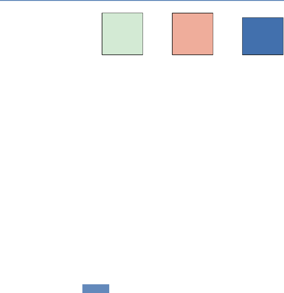
194 7. Text Analysis
Computer,
technology,
system,
service, site,
phone, internet,
machine
Topic 1
Sell, sale,
store, product,
business,
advertising,
market,
consumer
Topic 2
Play, film,
movie, theater,
production,
star, director,
stage
Topic 3
Figure 7.1. Topics are distributions over words. Here are three example topics
learned by latent Dirichlet allocation from a model with 50 topics discovered from
the New York Times [324]. Topic 1 seems to be about technology, Topic 2 about
business, and Topic 3 about the arts
latent Dirichlet allocation (LDA) [43]. LDA is a fully Bayesian exten-
sion of probabilistic latent semantic indexing [167], itself a proba-
bilistic extension of latent semantic analysis [224]. Blei and Laf-
ferty [42] provide a more detailed discussion of the history of topic
models.
LDA, like all topic models, assumes that there are topics that
form the building blocks of a corpus. Topics are distributions over
words and are often shown as a ranked list of words, with the high-
est probability words at the top of the list (Figure 7.1). However, we
do not know what the topics are a priori; the challenge is to discover
what they are (more on this shortly).
In addition to assuming that there exist some number of topics
that explain a corpus, LDA also assumes that each document in a
corpus can be explained by a small number of topics. For example,
taking the example topics from Figure 7.1, a document titled “Red
Light, Green Light: A Two-Tone LED to Simplify Screens” would
be about Topic 1, which appears to be about technology. How-
ever, a document like “Forget the Bootleg, Just Download the Movie
Legally” would require all three of the topics. The set of topics that
are used by a document is called the document’s allocation (Fig-
ure 7.2). This terminology explains the name latent Dirichlet alloca-
tion: each document has an allocation over latent topics governed
by a Dirichlet distribution.
7.3.1.1 Inferring topics from raw text
Algorithmically, the problem can be viewed as a black box. Given a
corpus and an integer Kas input, provide the topics that best de-
scribe the document collection: a process called posterior inference.
The most common algorithm for solving this problem is a technique
called Gibbs sampling [131].
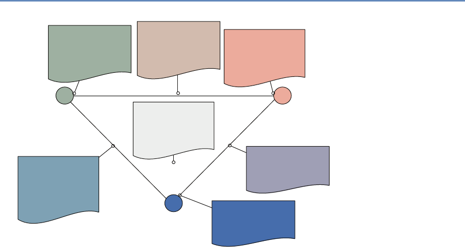
7.3. Approaches and applications 195
Forget the
Bootleg, Just
Download the
Movie Legally
Multiplex Heralded
As Linchpin To
Growth
e Shape of
Cinema,
Transformed At
the Click of a
Mouse A Peaceful Crew
Puts Muppets
Where Its Mouth Is
Stock Trades: A
Better Deal For
Investors Isn't
Simple
Internet Portals
Begin to Distinguish
among emselves
as Shopping Malls
Red Light, Green
Light: A
2-Tone L.E.D. to
Simplify Screens
TOPIC 3
"ENTERTAINMENT"
TOPIC 1
"TECHNOLOGY"
TOPIC 2
"BUSINESS"
Figure 7.2. Allocations of documents to topics
Gibbs sampling works at the word level to discover the topics that
best describe a document collection. Each word is associated with a
single topic, explaining why that word appeared in a document. For
example, consider the sentence “Hollywood studios are preparing
to let people download and buy electronic copies of movies over the
Internet.” Each word in this sentence is associated with a topic:
“Hollywood” might be associated with an arts topic; “buy” with a
business topic; and “Internet” with a technology topic (Figure 7.3).
This is where we should eventually get. However, we do not know
this to start. So we can initially assign words to topics randomly.
This will result in poor topics, but we can make those topics better.
We improve these topics by taking each word, pretending that we
do not know the topic, and selecting a new topic for the word.
A topic model wants to do two things: it does not want to use
many topics in a document, and it does not want to use many words
in a topic. So the algorithm will keep track of how many times a
document dhas used a topic k,Nd,k , and how many times a topic
khas used a word w,Vk,w. For notational convenience, it will also
be useful to keep track of marginal counts of how many words are
in a document,
Nd,·≡X
k
Nd,k ,
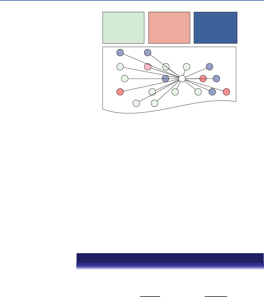
196 7. Text Analysis
Hollywood studios are preparing to let people
download and buy electronic copies of movies over
the Internet, much as record labels now sell songs for
99 cents through Apple Computer's iTunes music store
and other online services ...
Hollywood
studios
download
movies
buy
electronic
copies
Internet,
cents
Apple
Compute
sell
unes
store
music
songs
other online
servic
record
record
computer,
technology,
system, service,
site, phone,
internet, machine
play, film, movie,
theater, production,
star, director, stage
sell, sale, store,
product, business,
advertising, market,
consumer
Figure 7.3. Each word is associated with a topic. Gibbs sampling inference iter-
atively resamples the topic assignments for each word to discover the most likely
topic assignments that explain the document collection
and how many words are associated with a topic,
Vk,·≡X
w
Vk,w.
The algorithm removes the counts for a word from Nd,k and Vk,w and
then changes the topic of a word (hopefully to a better topic than
the one it had before). Through many thousands of iterations of this
process, the algorithm can find topics that are coherent, useful, and
characterize the data well.
The two goals of topic modeling—balancing document allocations
to topics and topics’ distribution over words—come together in an
equation that multiplies them together. A good topic will be both
common in a document and explain a word’s appearance well.
Example: Gibbs sampling for topic models
The topic assignment zd,n of word nin document dis proportional to
p(zd,n =k)∝
Nd,k +α
Nd,·+Kα
| {z }
how much doc likes the topic
Vk,wd,n +
Vk,·+V
| {z }
how much topic likes the word
,

7.3. Approaches and applications 197
where αand are smoothing factors that prevent a topic from having zero prob-
ability if a topic does not use a word or a document does not use a topic [390].
Recall that we do not include the token that we are sampling in the counts for N
or V.
For the sake of concreteness, assume that we have three documents with the
following topic assignments:
Document 1: Adog3Bcat2Ccat3Dpig1
Document 2: Ehamburger2Fdog3Ghamburger1
Document 3: Hiron1Iiron3Jpig2Kiron2
If we want to sample token B (the first instance of of “cat” in document 1), we
compute the conditional probability for each of the three topics (z=1,2,3):
p(zB=1)=1+1.000
3+3.000 ×0+1.000
3+5.000 =0.333 ×0.125 =0.042,
p(zB=2)=0+1.000
3+3.000 ×0+1.000
3+5.000 =0.167 ×0.125 =0.021, and
p(zB=3)=2+1.000
3+3.000 ×1+1.000
4+5.000 =0.500 ×0.222 =0.111.
To reiterate, we do not include token B in these counts: in computing these con-
ditional probabilities, we consider topic 2 as never appearing in the document and
“cat” as never appearing in topic 2. However, “cat” does appear in topic 3 (token C),
so it has a higher probability than the other topics. After renormalizing, our con-
ditional probabilities are (0.24,0.12,0.64). We then sample the new assignment
of token B to be topic 3 two times out of three. Griffiths and Steyvers [140] provide
more details on the derivation of this equation.
Example code Listing 7.1 provides a function to compute the conditional proba-
bility of a single word and return the (unnormalized) probability to sample from.
7.3.1.2 Applications of topic models
Topic modeling is most often used for topic exploration, allowing
users to understand the contents of large text corpora. Thus,
topic models have been used, for example, to understand what
the National Institutes of Health funds [368]; to compare and con-
trast what was discussed in the North and South in the Civil War
[270]; and to understand how individuals code in large program-
ming projects [253].
Topic models can also be used as features to more elaborate
algorithms such as machine translation [170], detecting objects in
images [392], or identifying political polarization [298].

198 7. Text Analysis
def class_sample(docs, vocab, d, n, alpha,
beta, theta, phi, num_topics):
# Get the vocabulary ID of the word we are sampling
type = docs[d][n]
# Dictionary to store final result
result = {}
# Consider each topic possibility
for kk in xrange(num_topics):
# theta stores the number of times the document d uses
# each topic kk; alpha is a smoothing parameter
doc_contrib = (theta[d][kk] + alpha) / \
(sum(theta[d].values()) + num_topics *alpha)
# phi stores the number of times topic kk uses
# this word type; beta is a smoothing parameter
topic_contrib = (phi[kk][type] + beta) / \
(sum(phi[kk].values()) + len(vocab) *beta)
result[kk] = doc_contrib *topic_contrib
return result
Listing 7.1. Python code to compute conditional probability of a single word and
return the probability from which to sample
7.3.2 Information retrieval and clustering
Information retrieval is a large subdiscipline that encompasses a
variety of methods and approaches. Its main advantage is using
large-scale empirical data to make analytical inferences and class
assignments. Compared to topic modeling, discussed above, infor-
mation retrieval techniques can use external knowledge repositories
to categorize given corpora as well as discover smaller and emerging
areas within a large database.
A major concept of information retrieval is a search query that is
usually a short phrase presented by a human or machine to retrieve
a relevant answer to a question or discover relevant knowledge.
A good example of a large-scale information retrieval system is a
search engine, such as Google or Yahoo!, that provides the user with
an opportunity to search the entire Internet almost instantaneously.
Such fast searches are achieved by complex techniques that are
linguistic (set-theoretic), algebraic, probabilistic, or feature-based.
Set-theoretic operations and Boolean logic Set-theoretic opera-
tions proceed from the assumption that any query is a set of linked
components all of which need to be present in the returned result for

7.3. Approaches and applications 199
it to be relevant. Boolean logic serves as the basis for such queries;
it uses Boolean operators such as AND,OR, and NOT to combine query
components. For example, the query
induction AND (physics OR logic)
will retrieve all documents in which the word “induction” is used,
whether in a physical or logical sense. The extended Boolean model
and fuzzy retrieval are enhanced approaches to calculating the rel-
evance of retrieved documents based on such queries [232].
Search queries can be also enriched by wildcards and other con-
nectors. For example, the character “*” typically substitutes for
any possible character or characters depending on the settings of
the query engine. (In some instances, search queries can run in
nongreedy mode, in which case, for example, the phrase inform*
might retrieve only text up to the end of the sentence. On the other
hand, a greedy query might retrieve full text following the word or
part of word, denoted as inform*, up to the end of the document,
which would essentially mean the same as inform*$.) The wildcard
“?” expects either one or no character in its place, and the wild-
card “.” expects exactly one character. Search queries enhanced
with such symbols and Boolean operators are referred to as regular
expressions.
Various databases and search engines can interpret Boolean op-
erators and wildcards differently depending on their settings and
therefore are prone to return rather different results. This behavior
should be expected and controlled for while running searches on
different data sources.
Example: Discover food safety awards
Food safety is an interdisciplinary research area that spans multiple scientific
disciplines including biological sciences, agriculture, and food science. To retrieve
food safety-related awards, we have to construct a Boolean-based search string
that would look for terms and phrases in those documents and return only relevant
results.
An example of such a string would typically be subdivided by category or search
group connected to each other by the AND or OR operator:
1. General terms: (food safety OR food securit*OR food
insecurit*)
2. Food pathogens: (food*) AND (acanthamoeba OR actinobacteri*
OR (anaerobic organ*) OR DDT OR ...)
3. Biochemistry and toxicology: (food*) AND (toxicolog*OR
(activated carbon*) OR (acid-hydrol?zed vegetable
protein*) OR aflatoxin*OR ...)

200 7. Text Analysis
4. Food processing and preservation: (food*) AND (process*OR
preserv*OR fortif*OR extrac*OR ...)
5. Food quality and quality control: (food*) AND (qualit*OR (danger
zon*) OR test*OR (risk analys*) OR ...)
6. Food-related diseases: (food*OR foodbo?rn*OR food-rela*)
AND (diseas*OR hygien*OR allerg*OR diarrh?ea*OR
nutrit*OR ...)
Different websites and databases use different search functions to return most rel-
evant results given a query (e.g., “food safety”). Ideally, a user has access to a full
database and can apply the same Python code based on regular expressions to
all textual data. However, this is not always possible (e.g., when using proprietary
databases, such as Web of Science). In those cases, it is important to follow the con-
ventions of the information retrieval system. For example, one source might need
phrases to be embedded in parentheses (i.e., (x-ray crystallograph.*))
while another database interface would require such phrases to be contained
within quotation marks (i.e., ‘‘x-ray crystallograph.*’’). It is then criti-
cal to explore the search tips and rules on those databases to ensure that the most
complete information is gathered and further analyzed.
Example code Python’s built-in re package provides all the capability needed to
construct and search with complex regular expressions. Listing 7.2 provides an
example.
def fs_regex(nsf_award_abstracts,outfilename):
# Construct simple search string divided by search groups
food = "food.*"
general = "safety|secur.*|insecur.*"
pathogens = "toxicolog.*|acid-hydrolyzed vegetable protein.*|
activated carbon.*"
process = "process.*|preserv.*|fortif.*"#and so on
# Open csv table with all NSF award abstracts in 2000-2014
inpfile = open(nsf_award_abstracts,'rb')
inpdata = csv.reader(infile)
outfile = open(outfilename,'wb')
output = csv.writer(outfile)
for line in inpdata:
award_id = line[0]
title = line[1]
abstract = line[2]
if re.search(food,abstract) and (re.search(general,abstract)
or re.search(pathogens,abstract) or re.search(process,
abstract)):
output.writerow(i+['food safety award'])
Listing 7.2. Python code to identify food safety related NSF awards with regular
expressions

7.3. Approaches and applications 201
Algebraic models Algebraic models turn text into numbers to run
mathematical operations and discover inherent interdependencies
between terms and phrases, also defining the most important and
meaningful among them. The vector space representation is a typ-
ical way of converting words into numbers, wherein every token is
assigned with a sequential ID and a respective weight, be it a simple
term frequency, TFIDF value, or any other assigned number.
Latent Dirichlet allocation, discussed in the preceding section,
is a good example of a probabilistic model, while unsupervised ma-
chine learning techniques, such as random forest, can be used for
◮Random forests are dis-
cussed for record linkages
in Chapter 3 and described
in more detail in Chapter 10.
feature-based modeling and information retrieval.
Similarity measures and approaches Based on algebraic models,
the user can either compare documents between each other or train
a model that can be further inferred on a different corpus. Typ-
ical metrics involved in this process include cosine similarity and
Kullback–Leibler divergence [218].
Cosine similarity is a popular measure in document classifica-
tion. Given two documents daand dbpresented as term vectors −→
ta
and −→
tb, the cosine similarity is
SIMC(−→
ta,−→
tb)=−→
ta·−→
tb
|−→
ta| ∗ |−→
tb|
.
Example: Measuring cosine similarity between documents
NSF awards are not labeled by scientific field—they are labeled by program. This
administrative classification is not always useful to assess the effects of certain
funding mechanisms on disciplines and scientific communities. One approach
is to understand how awards align with each other even if they were funded by
different programs. Cosine similarity allows us to do just that.
Example code The Python numpy module is a powerful library of tools for efficient
linear algebra computation. Among other things, it can be used to compute the
cosine similarity of two documents represented by numeric vectors, as described
above. The gensim module that is often used as a Python-based topic modeling
implementation can be used to produce vector space representations of textual
data. Listing 7.3 provides an example of measuring cosine similarity using these
modules.

202 7. Text Analysis
# Define cosine similarity function
def coss(v1,v2):
return np.dot(v1,v2) /
(np.sqrt(np.sum(np.square(v1))) *
np.sqrt(np.sum(np.square(v2))))
def coss_nsf(nsf_climate_change,nsf_earth_science,outfile):
# Open the source and compared to documents
source = csv.reader(file(nsf_climate_change,'rb'))
comparison = csv.reader(file(nsf_earth_science,'rb'))
# Create an output file
output = csv.writer(open(outfile,'wb'))
# Read through the source and store value in static data container
data = {}
for row in source:
award_id = row[0]
abstract = row[1]
data[award_id] = abstract
# Read through the comparison file and compute similarity
for row in comparison:
award_id = row[0]
# Assuming that abstract is cleaned, processed, tokenized, and
# stored as a space-separated string of tokens
abstract = row[1]
abstract_for_dict = abstract.split(" ")
# Construct dictionary of tokens and IDs
dict_abstract = corpora.dictionary.Dictionary(abstract_for_dict)
# Construct vector from dictionary
# of all tokens and IDs in abstract
abstr_vector = dict(dict_abstract.doc2bow(abstract))
# Iterate through all stored abstracts in source corpus
# and assign same token IDs using dictionary
for key,value in data.items():
source_id = key
# Get all tokens from source abstract, assuming it is
# tokenized and space-separated
source_abstr = value.split(" ")
source_vector = dict(dict_abstract.doc2bow(source_abstr))
# Cosine similarity requires having same shape vectors.
# Thus impute zeros for any missing tokens in source
# abstract as compared to the target one
add = { n:0 for nin abstr_vector.keys()
if nnot in source_dict.keys() }
# Update source vector
source_vector.update(add)
source_vector = sorted(source_vector.items())
abstr_vector = sorted(abstr_vector.items())
# Compute cosine similarity
similarity = coss(np.array([item[1] for item in abstr_vector]),
np.array([item[1] for item in source_dict])
output.writerow([source_id,award_id,similarity])
Listing 7.3. Python code to measure cosine similarity between Climate Change
and all other Earth Science NSF awards

7.3. Approaches and applications 203
Kullback–Leibler (KL) divergence is an asymmetric measure that
is often enhanced by averaged calculations to ensure unbiased re-
sults when comparing documents between each other or running a
classification task. Given two term vectors −→
taand −→
tb, the KL diver-
gence from vector −→
tato −→
tbis
DKL (−→
ta||−→
tb)=
m
X
t=1
wt,a ×log wt,a
wt,b !,
where wt,a and wt,b are term weights in two vectors, respectively.
An averaged KL divergence metric is then defined as
DAvgKL (−→
ta||−→
tb)=
m
X
t=1
(π1×D(wt,a ||wt)+π2×D(wt,b||wt)),
where π1=wt,a
wt,a +wt,b , π2=wt,b
wt,a +wt,b , and wt=π1×wt,a +π2×wt,b [171].
A Python-based scikit-learn library provides an implementa-
tion of these measures as well as other machine learning models
and approaches.
Knowledge repositories Information retrieval can be significantly
enriched by the use of established knowledge repositories that can
provide enormous amounts of organized empirical data for modeling
and relevance calculations. Established corpora, such as the Brown
Corpus and Lancaster–Oslo–Bergen Corpus, are one type of such
preprocessed repositories.
Wikipedia and WordNet are examples of another type of lexi-
cal and semantic resources that are dynamic in nature and that
can provide a valuable basis for consistent and salient information
retrieval and clustering. These repositories have the innate hierar-
chy, or ontology, of words (and concepts) that are explicitly linked
to each other either by inter-document links (Wikipedia) or by the
inherent structure of the repository (WordNet). In Wikipedia, con-
cepts thus can be considered as titles of individual Wikipedia pages
and the contents of these pages can be considered as their extended
semantic representation.
Information retrieval techniques build on these advantages of
WordNet and Wikipedia. For example, Meij et al. [256] mapped
search queries to the DBpedia ontology (derived from Wikipedia top-
ics and their relationships), and found that this mapping enriches
the search queries with additional context and concept relation-
ships. One way of using these ontologies is to retrieve a predefined

204 7. Text Analysis
list of Wikipedia pages that would match a specific taxonomy. For
example, scientific disciplines are an established way of tagging
documents—some are in physics, others in chemistry, engineer-
ing, or computer science. If a user retrieves four Wikipedia pages
on “Physics,” “Chemistry,” “Engineering,” and “Computer Science,”
they can be further mapped to a given set of scientific documents to
label and classify them, such as a corpus of award abstracts from
the US National Science Foundation.
Personalized PageRank is a similarity system that can help with
the task. This system uses WordNet to assess semantic relation-
ships and relevance between a search query (document d) and pos-
sible results (the most similar Wikipedia article or articles). This
system has been applied to text categorization [269] by compar-
ing documents to semantic model vectors of Wikipedia pages con-
structed using WordNet. These vectors account for the term fre-
quency and their relative importance given their place in the Word-
Net hierarchy, so that the overall wiki vector is defined as:
SMVwiki (s)=Pw∈Synonyms(s)
tfwiki (w)
|Synsets(w)|,
where wis a token within wiki,sis a WordNet synset that is associ-
ated with every token win WordNet hierarchy, Synonyms(s)is the
set of words (i.e., synonyms) in the synset s,tfwiki (w)is the term fre-
quency of the word win the Wikipedia article wiki, and Synsets(w)
is the set of synsets for the word w.
The overall probability of a candidate document d(e.g., an NSF
award abstract or a PhD dissertation abstract) matching the target
query, or in our case a Wikipedia article wiki, is
wikiBEST =Xwt∈doc max
s∈Synsets(wt)SMVwiki(s),
where Synsets(wt)is the set of synsets for the word wtin the target
document document (e.g., NSF award abstract) and SMVwiki (s)is
the semantic model vector of a Wikipedia page, as defined above.
Applications Information retrieval can be used in a number of ap-
plications. Knowledge discovery, or information extraction, is per-
haps its primary mission; in contrast, for users, the purpose of
information retrieval applications is to retrieve the most relevant
response to a query.
Document classification is another popular task where informa-
tion retrieval methods can be helpful. Such systems, however, typi-
cally require a two-step process: The first phase defines all relevant

7.3. Approaches and applications 205
information needed to answer the query. The second phase clus-
ters the documents according to a set of rules or by allowing the
machine to actively learn the patterns and classes. For example,
one approach is to generate a taxonomy of concepts with associated
Wikipedia pages and then map other documents to these pages
through Personalized PageRank. In this case, disciplines, such as
physics, chemistry, and engineering, can be used as the original la-
bels, and NSF award abstracts can be mapped to these disciplinary
categories through the similarity metrics (i.e., whichever of these
disciplines scores the highest is the most likely to fit the disciplinary
profile of an award abstract).
Another approach is to use the Wikipedia structure as a clus-
tering mechanism in itself. For example, the article about “nano-
technology” links to a number of other Wikipedia pages as ref-
erenced in its content. “Quantum realm,” “nanometer” or “Na-
tional Nanotechnology Initiative” are among the meaningful con-
cepts used in the description of nanotechnology that also have their
own individual Wikipedia pages. Using these pages, we can assume
that if a scientific document, such as an NSF award abstract, has
enough similarity with any one of the articles associated with nano-
technology, it can be tagged as such in the classification exercise.
The process can also be turned around: if the user knows ex-
actly the clusters of documents in a given corpus, these can be
mapped to an external knowledge repository, such as Wikipedia, to
discover yet unknown and emerging relationships between concepts
that are not explicitly mentioned in the Wikipedia ontology at the
current moment. This situation is likely given the time lag between
the discovery of new phenomena, their introduction to the research
community, and their adoption by the wider user community re-
sponsible for writing Wikipedia pages.
Examples Some examples from our recent work can demonstrate
how Wikipedia-based labeling and labeled LDA [278,315] cope with
the task of document classification and labeling in the scientific
domain. See Table 7.1.
7.3.3 Other approaches
Our focus in this chapter is on approaches that are language in-
dependent and require little (human) effort to analyze text data.
In addition to topic modeling and information retrieval discussed
above, natural language processing and computational linguistics

206 7. Text Analysis
Table 7.1. Wikipedia articles as potential labels generated by n-gram indexing of NSF awards
Abstract excerpt ProQuest
subject category Labeled LDA Wikipedia-
based labeling
Reconfigurable computing platform for small-
scale resource-constrained robot. Specific appli-
cations often require robots of small size for rea-
sons such as costs, access, and stealth. Small-
scale robots impose constraints on resources such
as power or space for modules . . .
Engineering,
Electronics and
Electrical;
Engineering,
Robotics
Motor controller
Robotics,
Robot, Field-
programmable
gate array
Genetic mechanisms of thalamic nuclei speci-
fication and the influence of thalamocortical
axons in regulating neocortical area formation.
Sensory information from the periphery is essential
for all animal species to learn, adapt, and survive in
their environment. The thalamus, a critical struc-
ture in the diencephalon, receives sensory informa-
tion . . .
Biology,
Neurobiology HSD2 neurons
Sonic hedgehog,
Induced stem
cell, Nervous
system
Poetry ’n acts: The cultural politics of twentieth-
century American poets’ theater. This study fo-
cuses on the disciplinary blind spot that obscures
the productive overlap between poetry and dramatic
theater and prevents us from seeing the cultural
work that this combination can perform . . .
Literature,
American;
Theater
Audience
Counter-
culture of the
1960s, Novel,
Modernism
are rich, well-developed subdisciplines of computer science that can
help analyze text data. While covering these subfields is beyond this
chapter, we briefly discuss some of the most widely used approaches
to process and understand natural language texts.
In contrast to the unsupervised approaches discussed above,
most techniques in natural language processing are supervised ma-
chine learning algorithms. Supervised machine learning produce
◮Chapter 6 reviews super-
vised machine learning ap-
proaches. labels ygiven inputs x—the algorithm’s job is to learn how to auto-
matically produce correct labels given automatic inputs x.
However, the algorithm must have access to many examples of
xand y, often of the order of thousands of examples. This is expen-
sive, as the labels often require linguistic expertise [251]. While it
is possible to annotate data using crowdsourcing [350], this is not
a panacea, as it often forces compromises in the complexity of the
task or the quality of the labels.

7.3. Approaches and applications 207
In the sequel, we discuss how different definitions of xand y—
both in the scope and structure of the examples and labels—define
unique analyses of linguistic data.
Document classification If the examples xare documents and y
are what these documents are about, the problem is called docu-
ment classification. In contrast to the techniques in Section 7.3.1,
document classification is used when you know the specific docu-
ment types for which you are looking and you have many examples
of those document types.
One simple but ubiquitous example of document classification
is spam detection: an email is either an unwanted advertisement
(spam) or it is not. Document classification techniques such as
naïve Bayes [235] touch essentially every email sent worldwide,
making email usable even though most emails are spam.
Sentiment analysis Instead of being what a document is about, a
label ycould also reveal the speaker. A recent subfield of natural
language processing is to use machine learning to reveal the internal
state of speakers based on what they say about a subject [295]. For
example, given an example of sentence x, can we determine whether
the speaker is a Liberal or a Conservative? Is the speaker happy or
sad?
Simple approaches use dictionaries and word counting meth-
ods [299], but more nuanced approaches make use of domain-
specific information to make better predictions. One uses different
approaches to praise a toaster than to praise an air conditioner [44];
liberals and conservatives each frame health care differently from
how they frame energy policy [277].
Part-of-speech tagging When the examples xare individual words
and the labels yrepresent the grammatical function of a word (e.g.,
whether a word is a noun, verb, or adjective), the task is called
part-of-speech tagging. This level of analysis can be useful for dis-
covering simple patterns in text: distinguishing between when “hit”
is used as a noun (a Hollywood hit) and when “hit” is used as a verb
(the car hit the guard rail).
Unlike document classification, the examples xare not indepen-
dent: knowing whether the previous word was an adjective makes
it far more likely that the next word will be a noun than a verb.
Thus, the classification algorithms need to incorporate structure
into the decisions. Two common algorithms for this problem are
hidden Markov models [313] and conditional random fields [220].

208 7. Text Analysis
7.4 Evaluation
Evaluation techniques are common in economics, policy analysis,
and development. They allow researchers to justify their conclu-
sions using statistical means of validation and assessment. Text,
however, is less amenable to standard definitions of error: it is clear
that predicting that revenue will be $110 when it is really $100 is
far better than predicting $900; however, it is hard to say how far
“potato harvest” is from “journalism” if you are attempting to auto-
matically label documents. Documents are hard to transform into
numbers without losing semantic meanings and context.
Content analysis, discourse analysis, and bibliometrics are all
common tools used by social scientists in their text mining exer-
cises [134, 358]. However, they are rarely presented with robust
evaluation metrics, such as type I and type II error rates, when re-
trieving data for further analysis. For example, bibliometricians
◮Chapter 10 discusses
how to measure and diag-
nose errors in big data. often rely on search strings derived from expert interviews and
workshops. However, it is hard to certify that those search strings
are optimal. For instance, in nanotechnology research, Porter et
al. [305] developed a canonical search strategy for retrieving nano-
related papers from major scientific databases. Nevertheless, others
adopt their own search string modifications and claim similar va-
lidity [144, 374].
Evaluating these methods depends on reference corpora. We
discuss metrics that help you understand whether a collection of
documents for a query is a good one or not or whether a labeling of
a document collection is consistent with an existing set of labels.
Purity Suppose you are tasked with categorizing a collection of
documents based on what they are about. Reasonable people may
disagree: I might put “science and medicine” together, while an-
other person may create separate categories for “energy,” “scientific
research,” and “health care,” none of which is a strict subset of
my “science and medicine” category. Nevertheless, we still want to
know whether two categorizations are consistent.
Let us first consider the case where the labels differ but all cat-
egories match (i.e., even though you call one category “taxes” and
I call it “taxation,” it has exactly the same constituent documents).
This should be the best case; it should have the highest score poss-
ible. Let us say that this maximum score should be 1.
The opposite case is if we both simply assign labels randomly.
There will still be some overlap in our labeling: we will agree some-

7.4. Evaluation 209
times, purely by chance. On average, if we both assign one label,
selected from the same set of Klabels, to each document, then we
should expect to agree on about 1
Kof the labels. This is a lower
bound on performance.
The formalization of this measure is called purity: how much
overlap there is between each of my labels and the “best” match
from your labels. Box 7.2 shows how to calculate it.
Box 7.2: Purity calculation
We compute purity by assigning each cluster to the class that is
most frequent in the cluster, and then measuring the accuracy
of this assignment by counting correctly assigned documents
and dividing by the number of all documents, N[248]. In formal
terms,
Purity(Ω,C)=1
NX
k
max
j|wk∩cj|,
where Ω = {w1, w2, . . . , wk}is the set of candidate clusters and
C={c1, c2, . . . , cj}is the gold set of classes.
Precision and recall Chapter 6 already touched on the importance
of precision and recall for evaluating the results of information re-
trieval and machine learning models (Box 7.3 provides a reminder
of the formulae). Here we look at a particular example of how these
metrics can be computed when working with scientific documents.
We assume that a user has three sets of documents Da={da1,
da2, . . . , dn},Db={db1, db2, . . . , dk}, and Dc={dc1, dc2, . . . , di}. All
three sets are clearly tagged with a disciplinary label: Daare com-
puter science documents, Dbare physics, and Dcare chemistry.
The user also has a different set of documents—Wikipedia pages
on “Computer Science,” “Chemistry,” and “Physics.” Knowing that
all documents in Da,Db, and Dchave clear disciplinary assign-
ments, let us map the given Wikipedia pages to all documents within
those three sets. For example, the Wikipedia-based query on “Com-
puter Science” should return all computer science documents and
none in physics or chemistry. So, if the query based on the “Com-
puter Science” Wikipedia page returns only 50% of all computer
science documents, then 50% of the relevant documents are lost:
the recall is 0.5.
On the other hand, if the same “Computer Science” query re-
turns 50% of all computer science documents but also 20% of the

210 7. Text Analysis
Box 7.3: Precision and recall
These two metrics are commonly used in information retrieval
and computational linguistics [318]. Precision computes the
type I errors—false positives—in a similar manner to the purity
measure; it is formally defined as
Precision =|{relevant documents} ∩ {retrieved documents}|
|{retrieved documents}| .
Recall accounts for type II errors—false negatives—and is de-
fined as
Recall =|{relevant documents} ∩ {retrieved documents}|
|{relevant documents}| .
physics documents and 50% of the chemistry documents, then all
of the physics and chemistry documents returned are false posi-
tives. Assuming that all document sets are of equal size, so that
|Da|=10, |Db|=10 and |Dc|=10, then the precision is 5
12 =0.42.
Fscore The F score takes precision and recall measures a step
further and considers the general accuracy of the model. In formal
terms, the Fscore is a weighted average of the precision and recall:
F1=2·Precision ·Recall
Precision +Recall.(7.1)
In terms of type I and type II errors:
F=(1+̙2)·true positive
(1+̙2)·true positive +̙2·false negative +false positive,
where ̙is the balance between precision and recall. Thus, F2puts
more emphasis on the recall measure and F0.5puts more emphasis
on precision.
7.5 Text analysis tools
We are fortunate to have access to a set of powerful open source
text analysis tools. We describe three here.

7.5. Text analysis tools 211
The Natural Language Toolkit The NLTK is a commonly used nat-
ural language toolkit that provides a large number of relevant so-
lutions for text analysis. It is Python-based and can be easily in-
tegrated into data processing and analytical scripts by a simple
import nltk (or similar for any one of its submodules).
The NLTK includes a set of tokenizers, stemmers, lemmatiz-
ers and other natural language processing tools typically applied
in text analysis and machine learning. For example, a user can
extract tokens from a document doc by running the command
tokens = nltk.word_tokenize(doc).
Useful text corpora are also present in the NLTK distribution.
For example, the stop words list can be retrieved by running the
command stops=nltk.corpus.stopwords.words(language). These
stop words are available for several languages within NTLK, includ-
ing English, French, and Spanish.
Similarly, the Brown Corpus or WordNet can be called by run-
ning from nltk.corpus import wordnet/brown. After the corpora
are loaded, their various properties can be explored and used in
text analysis; for example, dogsyn = wordnet.synsets(’dog’)will
return a list of WordNet synsets related to the word “dog.”
Term frequency distribution and n-gram indexing are other tech-
niques implemented in NLTK. For example, a user can compute fre-
quency distribution of individual terms within a document doc by
running a command in Python: fdist=nltk.FreqDist(text). This
command returns a dictionary of all tokens with associated fre-
quency within doc.
N-gram indexing is implemented as a chain-linked collocations
algorithm that takes into account the probability of any given two,
three, or more words appearing together in the entire corpus. In
general, n-grams can be discovered as easily as running bigrams =
nltk.bigrams(text). However, a more sophisticated approach is
needed to discover statistically significant word collocations, as we
show in Listing 7.4.
Bird et al. [39] provide a detailed description of NLTK tools and
techniques. See also the official NLTK website [284].
Stanford CoreNLP While NLTK’s emphasis is on simple reference
implementations, Stanford’s CoreNLP [249, 354] is focused on fast
implementations of cutting-edge algorithms, particularly for syntac-
tic analysis (e.g., determining the subject of a sentence).

212 7. Text Analysis
def bigram_finder(texts):
# NLTK bigrams from a corpus of documents separated by new line
tokens_list = nltk.word_tokenize(re.sub("\n"," ",texts))
bgm = nltk.collocations.BigramAssocMeasures()
finder = nltk.collocations.BigramCollocationFinder.from_words(
tokens_list)
scored = finder.score_ngrams( bgm.likelihood_ratio )
# Group bigrams by first word in bigram.
prefix_keys = collections.defaultdict(list)
for key, scores in scored:
prefix_keys[key[0]].append((key[1], scores))
# Sort keyed bigrams by strongest association.
for key in prefix_keys:
prefix_keys[key].sort(key = lambda x: -x[1])
Listing 7.4. Python code to find bigrams using NLTK
MALLET For probabilistic models of text, MALLET, the MAchine
Learning for LanguagE Toolkit [255], often strikes the right balance
between usefulness and usability. It is written to be fast and effi-
cient but with enough documentation and easy enough interfaces to
be used by novices. It offers fast, popular implementations of condi-
tional random fields (for part-of-speech tagging), text classification,
and topic modeling.
7.6 Summary
Much “big data” of interest to social scientists is text: tweets, Face-
book posts, corporate emails, and the news of the day. However,
the meaning of these documents is buried beneath the ambigui-
ties and noisiness of the informal, inconsistent ways by which hu-
mans communicate with each other. Despite attempts to formalize
the meaning of text data through asking users to tag people, apply
metadata, or to create structured representations, these attempts
to manually curate meaning are often incomplete, inconsistent, or
both.
These aspects make text data difficult to work with, but also a
rewarding object of study. Unlocking the meaning of a piece of text
helps bring machines closer to human-level intelligence—as lan-
guage is one of the most quintessentially human activities—and
helps overloaded information professionals do their jobs more ef-
fectively: understand large corpora, find the right documents, or

7.7. Resources 213
automate repetitive tasks. And as an added bonus, the better com-
puters become at understanding natural language, the easier it is
for information professionals to communicate their needs: one day
using computers to grapple with big data may be as natural as
sitting down to a conversation over coffee with a knowledgeable,
trusted friend.
7.7 Resources
Text analysis is one of the more complex tasks in big data analysis.
Because it is unstructured, text (and natural language overall) re-
quires significant processing and cleaning before we can engage
in interesting analysis and learning. In this chapter we have refer-
enced several resources that can be helpful in mastering text mining
techniques:
•The Natural Language Toolkit is one of the most popular Python-
based tools for natural language processing. It has a variety of
methods and examples that are easily accessible online [284].
The book by Bird et al. [39], available online, contains multiple
examples and tips on how to use NLTK.
•The book Pattern Recognition and Machine Learning by Christo-
pher Bishop [40] is a useful introduction to computational
techniques, including probabilistic methods, text analysis, and
machine learning. It has a number of tips and examples that
are helpful to both learning and experienced researchers.
•A paper by Anna Huang [171] provides a brief overview of
the key similarity measures for text document clustering dis-
cussed in this chapter, including their strengths and weak-
nesses in different contexts.
•Materials at the MALLET website [255] can be specialized for
the unprepared reader but are helpful when looking for specific
solutions with topic modeling and machine classification using
this toolkit.
•David Blei, one of the authors of the latent Dirichlet allocation
algorithm (topic modeling), maintains a helpful web page with
introductory resources for those interested in topic modeling
[41].

214 7. Text Analysis
•We provide an example of how to run topic modeling using
MALLET on textual data from the National Science Foundation
and Norwegian Research Council award abstracts [49].
•Weka, developed at the University of Waikato in New Zealand,
is a useful resource for running both complex text analysis
and other machine learning tasks and evaluations [150, 384].

Networks: The Basics
Chapter 8
Jason Owen-Smith
Social scientists are typically interested in describing the activities
of individuals and organizations (such as households and firms) in
a variety of economic and social contexts. The frame within which
data has been collected will typically have been generated from tax
or other programmatic sources. The new types of data permit new
units of analysis—particularly network analysis—largely enabled by
advances in mathematical graph theory. This chapter provides an
overview of how social scientists can use network theory to generate
measurable representations of patterns of relationships connecting
entities. As the author points out, the value of the new framework is
not only in constructing different right-hand-side variables but also
in studying an entirely new unit of analysis that lies somewhere
between the largely atomistic actors that occupy the markets of
neo-classical theory and the tightly managed hierarchies that are
the traditional object of inquiry of sociologists and organizational
theorists.
8.1 Introduction
This chapter provides a basic introduction to the analysis of large
networks. The following introduces the basic logic of network anal-
ysis, then turn to a summary of data structures and essential mea-
sures before presenting a primer on network visualization and a
more elaborated descriptive case comparison of the collaboration
networks of two research-intensive universities. Both those collab-
oration networks and a grant co-employment network for a large
public university also examined in this chapter are derived from
data produced by the multi-university Committee on Institutional
Cooperation (CIC)’s UMETRICS project [228]. The snippets of code
215

216 8. Networks: The Basics
that are provided are from the igraph package for network analysis
as implemented in Python.
At their most basic, networks are measurable representations of
patterns of relationships connecting entities in an abstract or actual
space. What this means is that there are two fundamental ques-
tions to ask of any network presentation or measure, First, what are
the nodes? Second, what are the ties? While the network methods
sketched in this chapter are equally applicable to technical or bio-
logical networks (e.g., the hub-and-spoke structure of the worldwide
air travel system, or the neuronal network of a nematode worm), I
focus primarily on social networks; patterns of relationships among
people or organizations that are created by and come to influence
individual action. This chapter draws most of its examples from
the world of science, technology, and innovation. Thus, this chap-
ter focuses particularly on networks developed and maintained by
the collaborations of scientists and by the contractual relationships
organizations form in pursuit of innovation.
This substantive area is of great interest because a great deal of
research in sociology, management, and related fields demonstrates
that networks of just these sorts are essential to understanding the
process of innovation and outcomes at both the individual and the
organizational level.
In other words, networks offer not just another convenient set
of right-hand-side variables, but an entirely new unit of analysis
that lies somewhere between the largely atomistic actors that oc-
cupy the markets of neo-classical theory and the tightly managed
hierarchies that are the traditional object of inquiry of sociologists
and organizational theorists. As Walter W. Powell [308] puts it in a
description of buyer supplier networks of small Italian firms: “when
the entangling of obligation and reputation reaches a point where
the actions of the parties are interdependent, but there is no com-
mon ownership or legal framework . . . such a transaction is neither
a market exchange nor a hierarchical governance structure, but a
separate, different mode of exchange.”
Existing as they do between the uncoordinated actions of inde-
pendent individuals and coordinated work of organizations, net-
works offer a unique level of analysis for the study of scientific
and creative teams [410], collaborations [202], and clusters of en-
trepreneurial firms [294]. The following sections introduce you
to this approach to studying innovation and discovery, focusing
on examples drawn from high-technology industries and particu-
larly from the scientific collaborations among grant-employed re-
searchers at UMETRICS universities. I make particular use of a

8.1. Introduction 217
network that connects individual researchers to grants that paid
their salaries in 2012 for a large public university. The grants net-
work for university A includes information on 9,206 individuals who
were employed on 3,389 research grants from federal science agen-
cies in a single year.
Before turning to those more specific substantive topics, the
chapter first introduces the most common structures for large net-
work data, briefly introduce three key social “mechanisms of action”
by which social networks are thought to have their effects, and then
present a series of basic measures that can be used to quantify
characteristics of entire networks and the relative position individ-
ual people or organizations hold in the differentiated social structure
created by networks.
Taken together, these measures offer an excellent starting point
for examining how global network structures create opportunities
and challenges for the people in them, for comparing and explaining
the productivity of collaborations and teams, and for making sense
of the differences between organizations, industries, and markets
that hinge on the pattern of relationships connecting their partici-
pants.
But what is a network? At its simplest, a network is a pattern
of concrete, measurable relationships connecting entities engaged
in some common activity. While this chapter focuses my attention
on social networks, you could easily use the techniques described
here to examine the structure of networks such as the World Wide
Web, the national railway route map of the USA, the food web of
an ecosystem, or the neuronal network of a particular species of
animal. Networks can be found everywhere, but the primary exam-
ple used here is a network connecting individual scientists through
their shared work on particular federal grants. The web of partner-
ships that emerges from university scientists’ decentralized efforts
to build effective collaborations and teams generates a distinctive
social infrastructure for cutting-edge science.
Understanding the productivity and effects of university research
thus requires an effort to measure and characterize the networks on
which it depends. As suggested, those networks influence outcomes
in three ways: first, they distinguish among individuals; second,
they differentiate among teams; and third, they help to distinguish
among research-performing universities. Most research-intensive
institutions have departments and programs that cover similar ar-
rays of topics and areas of study. What distinguishes them from
one another is not the topics they cover but the ways in which their
distinctive collaboration networks lead them to have quite different
scientific capabilities.

218 8. Networks: The Basics
8.2 Network data
Networks are comprised of nodes, which represent things that can
be connected to one another, and of ties that represent the relation-
ships connecting nodes. When ties are undirected they are called
edges. When they are directed (as when I lend money to you and
you do or do not reciprocate) they are called arcs. Nodes, edges
and arcs can, in principle, be anything: patents and citations, web
pages and hypertext links, scientists and collaborations, teenagers
and intimate relationships, nations and international trade agree-
ments. The very flexibility of network approaches means that the
first step toward doing a network analysis is to clearly define what
counts as a node and what counts as a tie.
While this seems like an easy move, it often requires deep thought.
For instance, an interest in innovation and discovery could take
several forms. We could be interested in how universities differ in
their capacity to respond to new requests for proposals (a macro
question that would require the comparison of full networks across
campuses). We could wonder what sorts of training arrangements
lead to the best outcomes for graduate students (a more micro-level
question that requires us to identify individual positions in larger
networks). Or we could ask what team structure is likely to lead
to more or less radical discoveries (a decidedly meso-level question
that requires we identify substructures and measure their features).
Each of these is a network question that relies on the ways in
which people are connected to one another. The first challenge of
measurement is to identify the nodes (what is being connected) and
the ties (the relationships that matter) in order to construct the
relevant networks. The next is to collect and structure the data in
a fashion that is sufficient for analysis. Finally, measurement and
visualization decisions must be made.
8.2.1 Forms of network data
Network ties can be directed (flowing from one node to another)
or undirected. In either case they can be binary (indicating the
presence or absence of a tie) or valued (allowing for relationships
of different types or strengths). Network data can be represented
in matrices or as lists of edges and arcs. All these types of rela-
tionships can connect one type of node (what is commonly called
one-mode network data) or multiple types of nodes (what is called
two-mode or affiliation data). Varied data structures correspond to
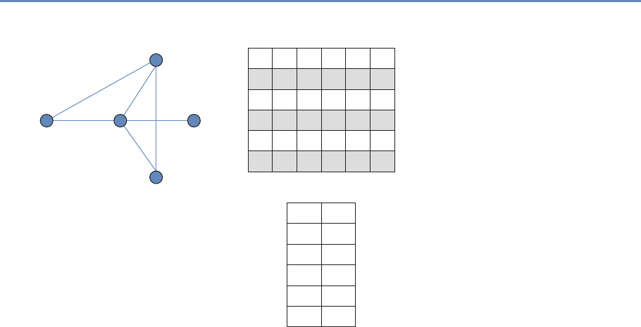
8.2. Network data 219
A
A
B
C
D
E
1
1
0
0
1
1
1
1
1
1
1
0
0
1
1
0
0
A
A
B
B
B
C
A
Represented as an edge list
Undirected (edge), binary data
Example: Actors are rms,
ties represent the presence
of any strategic alliance
Represented as a symmetric square matrixTies among a group of actors
C
C
D
E
D
B
B C D E
1
0
0
BE
C
D
Figure 8.1. Undirected, binary, one-mode network data
different classes of network data. The simplest form of network data
represents instances where the same kinds of nodes are connected
by undirected ties (edges) that are binary. An example of this type
of data is a network where nodes are firms and ties indicate the
presence of a strategic alliance connecting them [309]. This net-
work would be represented as a square symmetric matrix or a list
of edges connecting nodes. Figure 8.1 summarizes this simple data
structure, highlighting the idea that network data of this form can
be represented either as a matrix or as an edge list.
A much more complicated network would be one that is both
directed and valued. One example might be a network of nations
connected by flows of international trade. Goods and services flow
from one nation to another and the value of those goods and ser-
vices (or their volume) represents ties of different strengths. When
networks connecting one class of nodes (in this case nations) are
directed and valued, they can be represented as asymmetric valued
matrices or lists of arcs with associated values. (See Figure 8.2 for
an example.)
While many studies of small- to medium-sized social networks
rely on one-mode data. Large-scale social network data of this type
are relatively rare, but one-mode data of this sort are fairly common
in relationships among other types of nodes such as hyperlinks
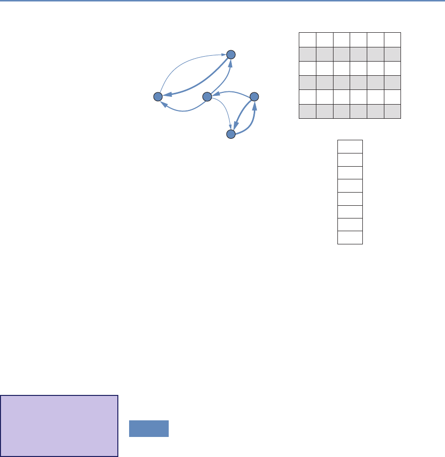
220 8. Networks: The Basics
A
A
B
C
D
E
3
4
0
0
0
0
0
2
1
3
0
0
0
1
0
5
0
A
B A 3
B C 3
B D 1
C A 4
D E 5
E B 2
E D 5
A C 1
Represented as an arc list
Directed (arc), valued data
Example: Nodes are faculty,
ties represent the number of
payments from one principal
investigator’s grant to another’s
Represented as an asymmetric square matrixTies among a group of actors
B C D E
0
0
5
BE
C
D
Figure 8.2. Directed, valued, one-mode network data
connecting web pages or citations connecting patents or publica-
tions. Nevertheless, much “big” social network analysis is con-
ducted using two-mode data. The UMETRICS employee data set
is a two-mode network that connects people (research employees)
to the grants that pay their wages. These two types of nodes can
be represented as a rectangular matrix that is either valued or bi-
nary. It is relatively rare to analyze untransformed two-mode net-
work data. Instead, most analyses take advantage of the fact that
such networks are dual [398]. In other words, a two-mode network
connecting grants and people can be conceptualized (and analyzed)
as two one-mode networks, or projections.*
⋆Key insight: A two-mode
network can be conceptual-
ized and analyzed as two
one-mode networks, or pro-
jections.
8.2.2 Inducing one-mode networks from two-mode data
The most important trick in large-scale social network analysis is
that of inducing one-mode, or unipartite, networks (e.g., employee
×employee relationships) from two-mode, or bipartite, data. But
the ubiquity and potential value of two-mode data can come at a
cost. Not all affiliations are equally likely to represent real, mean-
ingful relationships. While it seems plausible to assume that two
individuals paid by the same grant have interactions that reason-

8.2. Network data 221
ably pertain to the work funded by the grant, this need not be the
case.
For example, consider the two-mode grant ×person network for
university A. I used SQL to create a representation of this network
that is readable by a freeware network visualization program called
Pajek [30]. In this format, a network is represented as two lists:
avertex list that lists the nodes in the graph and an edge list that
lists the connections between those nodes. In our grant ×person
network, we have two types of nodes, people and grants, and one
kind of edge, used to represent wage payments from grants to indi-
viduals.
I present a brief snippet of the resulting network file in what fol-
lows, showing first the initial 10 elements of the vertex list and then
the initial 10 elements of the edge list, presented in two columns for
compactness. (The complete file comprises information on 9,206
employees and 3,389 grants, for a total of 12,595 vertices and
15,255 edges. The employees come first in the vertex list, and so
the 10 rows shown below all represent employees.) Each vertex
is represented by a vertex number–label pair and each edge by a
pair of vertices plus an optional value. Thus, the first entry in the
edge list (1 10419) specifies that the vertex with identifier 1 (which
happens to be the first element of the vertex list, which has value
“00100679”) is connected to the vertex with identifier 10419 by an
edge with value 1, indicating that employee “00100679” is paid by
the grant described by vertex 10419.
*Grant-Person-Network
*Vertices 12595 9206 *Edges
1 "00100679" 1 10419
2 "00107462" 2 10422
3 "00109569" 3 9855
4 "00145355" 3 9873
5 "00153190" 4 9891
6 "00163131" 7 10432
7 "00170348" 7 12226
8 "00172339" 8 10419
9 "00176582" 9 11574
10 "00203529" 10 11196
The network excerpted above is two-mode because it represents
relationships between two different classes of nodes, grants, and
people. In order to use data of this form to address questions about
patterns of collaboration on UMETRICS campuses, we must first
transform it to represent collaborative relationships.
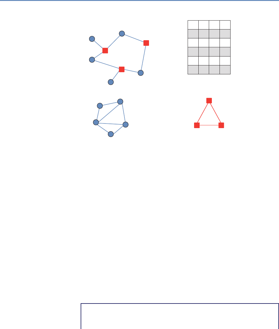
222 8. Networks: The Basics
A
A
A
B
C
D
E
1 1
1
0
0
01
0
1
1
0
0
0
1
1
1
XX’ yields a g × g
symmetrical matrix
that represents
co-employment ties
among individuals
X’X yields an h × h
symmetrical matrix
that represents
grants connected
by people
X = g × h matrix
X’ = h × g transpose
Example: Researchers and grants
Represented by a rectangular matrixTies linking nodes of two dierent types
2 3
B
B
E
E
C
C
D
D
3
3
2
2
1
1
Figure 8.3. Two-mode affiliation data
A person-by-person projection of the original two-mode network
assumes that ties exist between people when they are paid by the
same grant. By the same token, a grant-by-grant projection of the
original two-mode network assumes that ties exist between grants
when they pay the same people. Transforming two-mode data into
one-mode projections is a fairly simple matter. If Xis a rectangular
matrix, p×g, then a one-mode projection, p×p, can be obtained
by multiplying Xby its transpose X′. Figure 8.3 summarizes this
transformation.
In the following snippet of code, I use the igraph package in
Python to read in a Pajek file and then transform the original two-
mode network into two separate projections. Because my focus
in this discussion is on relationships among people, I then move
on to work exclusively with the employee-by-employee projection.
However, every technique that I describe below can also be used
with the grant-by-grant projection, which provides a different view
of how federally funded research is put together by collaborative
relationships on campus.
from igraph import *
# Read the graph
g = Graph.Read_Pajek("public_a_2m.net")

8.2. Network data 223
# Look at result
summary(g)
# IGRAPH U-WT 12595 15252 --
# + attr: color (v), id (v), shape (v), type (v), x (v), y (v), z
(v), weight (e)
# ...
# ...
# Transform to get 1M projection
pr_g_proj1, pr_g_proj2= g.bipartite_projection()
# Look at results
summary(pr_g_proj1)
# IGRAPH U-WT 9206 65040 --
# + attr: color (v), id (v), shape (v), type (v), x (v), y (v), z
(v), weight (e)
summary(pr_g_proj2)
# IGRAPH U-WT 3389 12510 --
# + attr: color (v), id (v), shape (v), type (v), x (v), y (v), z
(v), weight (e)
# pr_g_proj1 is the employeeXemployee projection, n=9,206 nodes
# Rename to emp for use in future calculations
emp=pr_g_proj1
We now can work with the graph emp, which represents the col-
laborative network of federally funded research on this campus.
Care must be taken when inducing one-mode network projections
from two-mode network data because not all affiliations provide
equally compelling evidence of actual social relationships. While
assuming that people who are paid by the same research grants
are collaborating on the same project seems plausible, it might be
less realistic to assume that all students who take the same uni-
versity classes have meaningful relationships. For the remainder of
this chapter, the examples I discuss are based on UMETRICS em-
ployee data rendered as a one-mode person-by-person projection of
the original two-mode person-by-grants data. In constructing these
networks I assume that a tie exists between two university research
employees when they are paid any wages from the same grant dur-
ing the same year. Other time frames or thresholds might be used
to define ties if appropriate for particular analyses.*
⋆Key insight: Care must
be taken when inducing
one-mode network projec-
tions from two-mode net-
work data because not all
affiliations provide equally
compelling evidence of ac-
tual social relationships.
224 8. Networks: The Basics
8.3 Network measures
The power of networks lies in their unique flexibility and ability to
address many phenomena at multiple levels of analysis. But har-
nessing that power requires the application of measures that take
into account the overall structure of relationships represented in a
given network. The key insight of structural analysis is that out-
comes for any individual or group are a function of the complete
pattern of connections among them. In other words, the explana-
tory power of networks is driven as much by the pathways that
indirectly connect nodes as by the particular relationships that di-
rectly link members of a given dyad. Indirect ties create reachability
in a network.*
⋆Key insight: Structural
analysis of outcomes for
any individual or group are
a function of the com-
plete pattern of connections
among them.
8.3.1 Reachability
Two nodes are said to be reachable when they are connected by
an unbroken chain of relationships through other nodes. For in-
stance, two people who have never met may nonetheless be able
to reach each other through a common acquaintance who is posi-
tioned to broker an introduction [286] or the transfer of information
and resources [60]. It is the reachability that networks create that
makes them so important for understanding the work of science
and innovation.
Consider Figure 8.4, which presents three schematic networks.
In each, one focal node, ego, is colored orange. Each ego has four
alters, but the fact that each has connections to four other nodes
masks important differences in their structural positions. Those dif-
ferences have to do with the number of other nodes they can reach
through the network and the extent to which the other nodes in the
network are connected to each other. The orange node (ego) in each
network has four partners, but their positions are far from equiv-
alent. Centrality measures on full network data can tease out the
differences. The networks also vary in their gross characteristics.
Those differences, too, are measurable.*
⋆Key insight: Much of
the power of networks (and
their systemic features) is
due to indirect ties that cre-
ate reachability. Two nodes
can reach each other if they
are connected by an unbro-
ken chain of relationships.
These are often called indi-
rect ties.
Networks in which more of the possible connections among nodes
are realized are denser and more cohesive than networks in which
fewer potential connections are realized. Consider the two smaller
networks in Figure 8.4, each of which is comprised of five nodes.
Just five ties connect those nodes in the network on the far right
of the figure. One smaller subset of that network, the triangle con-
necting ego and two alters at the center of the image, represents
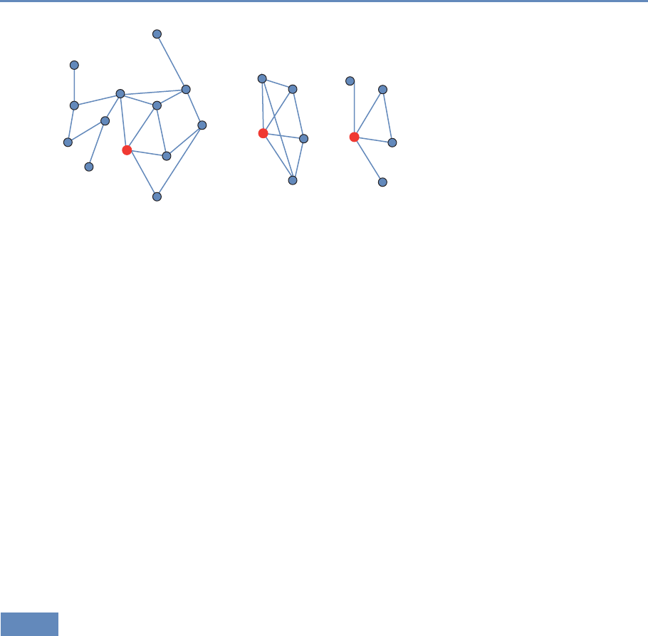
8.3. Network measures 225
Figure 8.4. Reachability and indirect ties
a more cohesively connected subset of the networks. In contrast,
eight of the nine ties that are possible connect the five nodes in
the middle figure; no subset of those nodes is clearly more inter-
connected than any other. While these kinds of differences may
seem trivial, they have implications for the orange nodes, and for
the functioning of the networks as a whole. Structural differences
between the positions of nodes, the presence and characteristics
of cohesive “communities” within larger networks [133], and many
important properties of entire structures can be quantified using
different classes of network measures. Newman [272] provides the
most recent and most comprehensive look at measures and algo-
rithms for network research.
The most essential thing to be able to understand about larger
scale networks is the pattern of indirect connections among nodes.
What is most important about the structure of networks is not nec-
essarily the ties that link particular pairs of nodes to one another.
Instead, it is the chains of indirect connections that make networks
function as a system and thus make them worthwhile as new levels
of analysis for understanding social and other dynamics.
8.3.2 Whole-network measures
The basic terms needed to characterize whole networks are fairly
simple. It is useful to know the size (in terms of nodes and ties) of
each network you study. This is true both for the purposes of being
able to generally gauge the size and connectivity of an entire network
and because many of the measures that one might calculate using
such networks should be standardized for analytic use. While the
list of possible network measures is long, a few commonly used

226 8. Networks: The Basics
indices offer useful insights into the structure and implications of
entire network structures.
Components and reachability As we have seen, a key feature of
networks is reachability. The reachability of participants in a net-
work is determined by their membership in what network theorists
call components, subsets of larger networks where every member
of a group is indirectly connected to every other. If you imagine a
standard node and line drawing of a network, a component is a por-
tion of the network where you can trace paths between every pair
of nodes without ever having to lift your pen.
Most large networks have a single dominant component that typ-
ically includes anywhere from 50% to 90% of its participants as well
as many smaller components and isolated nodes that are discon-
nected from the larger portion of the network. Because the path
length centrality measures described below can only be computed
on connected subsets of networks, it is typical to analyze the largest
component of any given network. Thus any description of a network
or any effort to compare networks should report the number of com-
ponents and the percentage of nodes reachable through the largest
component. In the code snippet below, I identify the weakly con-
nected components of the employee network, emp.
# Add component membership
emp.vs["membership"] = emp.clusters(mode="weak").membership
# Add component size
emp.vs["csize"] = [emp.clusters(mode="weak").sizes()[i] for i in
emp.clusters(mode="weak").membership]
# Identify the main component
# Get indices of max clusters
maxSize = max(emp.clusters(mode="weak").sizes())
emp.vs["largestcomp"] = [1 if maxSize == x else 0for x in emp.vs[
"csize"]]
# Add component membership
emp.vs["membership"] = emp.clusters(mode="weak").membership
The main component of a network is commonly analyzed and
visualized because the graph-theoretic distance among unconnected
nodes is infinite, which renders calculation of many common net-
work measures impossible without strong assumptions about just
how far apart unconnected nodes actually are. While some re-
searchers replace infinite path lengths with a value that is one plus
the longest path, called the network’s diameter, observed in a given

8.3. Network measures 227
structure, it is also common to simply analyze the largest connected
component of the network.
Path length One of the most robust and reliable descriptive statis-
tics about an entire network is the average path length, lG, among
nodes. Networks with shorter average path lengths have structures
that may make it easier for information or resources to flow among
members in the network. Longer path lengths, by comparison, are
associated with greater difficulty in the diffusion and transmission
of information or resources. Let gbe the number of nodes or vertices
in a network. Then
lG=1
g(g−1)X
i,j
d(ni, nj).
As with other measures based on reachability, it is most common to
report the average path length for the largest connected component
of the network because the graph-theoretic distance between two
unconnected nodes is infinite. In an electronic network such as the
World Wide Web, a shorter path length means that any two pages
can be reached through fewer hyperlink clicks.
The snippet of code below identifies the distribution of shortest
path lengths among all pairs of nodes in a network and the aver-
age path length. I also include a line of code that calculates the
network distance among all nodes and returns a matrix of those
distances. That matrix (saved as empdist) can be used to calculate
additional measures or to visualize the graph-theoretic proximities
among nodes.
# Calculate distances and construct distance table
dfreq=emp.path_length_hist(directed=False)
print(dfreq)
# N = 12506433, mean +- sd: 5.0302 +- 1.7830
# Each *represents 51657 items
# [ 1, 2): *(65040)
# [ 2, 3): ********* (487402)
# [ 3, 4): *********************************** (1831349)
# [ 4, 5): ******************************************************
**** (2996157)
# [ 5, 6): ****************************************************
(2733204)
# [ 6, 7): ************************************** (1984295)
# [ 7, 8): ************************ (1267465)
# [ 8, 9): ************ (649638)
# [ 9, 10): ***** (286475)

228 8. Networks: The Basics
# [10, 11): ** (125695)
# [11, 12): *(52702)
# [12, 13): (18821)
# [13, 14): (5944)
# [14, 15): (1682)
# [15, 16): (403)
# [16, 17): (128)
# [17, 18): (28)
# [18, 19): (5)
print(dfreq.unconnected)
# 29864182
print(emp.average_path_length(directed=False))
#[1] 5.030207
empdist= emp.shortest_paths()
These measures provide a few key insights into the employee
network we have been considering. First, the average pair of nodes
that are connected by indirect paths are slightly more than five
steps from one another. Second, however, many node pairs in this
network ($unconnected = 29,864,182) are unconnected and thus
unreachable to each other. Figure 8.5 presents a histogram of the
distribution of path lengths in the network. It represents the nu-
meric values returned by the distance.table command in the code
snippet above. In this case the diameter of the network is 18 and five
pairs of nodes are reachable at this distance, but the largest group
of dyads is reachable (N=2,996,157 dyads) at distance 4. In short,
nearly 3 million pairs of nodes are collaborators of collaborators of
collaborators of collaborators.
Degree distribution Another powerful way to describe and com-
pare networks is to look at the distribution of centralities across
nodes. While any of the centrality measures described above could
be summarized in terms of their distribution, it is most common to
plot the degree distribution of large networks. Degree distributions
commonly have extremely long tails. The implication of this pattern
is that most nodes have a small number of ties (typically one or two)
and that a small percentage of nodes account for the lion’s share of
a network’s connectivity and reachability. Degree distributions are
typically so skewed that it is common practice to plot degree against
the percentage of nodes with that degree score on a log–log scale.
High-degree nodes are often particularly important actors. In the
UMETRICS networks that are employee ×employee projections of
employee ×grant networks, for instance, the nodes with the high-
est degree seem likely to include high-profile faculty—the investi-
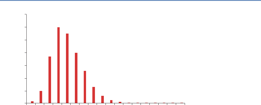
8.3. Network measures 229
3500000
3000000
2500000
1500000
2000000
Number of Dyads
1000000
500000
0
12345678910
Path Length
11 12 1413 15 16 17 18
Figure 8.5. Histogram of path lengths for university A employee network
gators on larger institutional grants such as National Institutes of
Health-funded Clinical and Translational Science Awards and Na-
tional Science Foundation-funded Science and Technology Centers,
and perhaps staff whose particular skills are in demand (and paid
for) by multiple research teams. For instance, the head technician
in a core microscopy facility or a laboratory manager who serves
multiple groups might appear highly central in the degree distribu-
tion of a UMETRICS network.
Most importantly, the degree distribution is commonly taken to
provide insight into the dynamics by which a network was created.
Highly skewed degree distributions often represent scale-free net-
works [25, 271, 309], which grow in part through a process called
preferential attachment, where new nodes entering the network are
more likely to attach to already prominent participants. In the kinds
of scientific collaboration networks that UMETRICS represents, a
scale-free degree distribution might come about as faculty new to an
institution attempt to enroll more established colleagues on grants
as coinvestigators. In the comparison exercise outlined below, I
plot degree distributions for the main components of two different
university networks.
Clustering coefficient The third commonly used whole-network mea-
sure captures the extent to which a network is cohesive, with many

230 8. Networks: The Basics
nodes interconnected. In networks that are more cohesively clus-
tered, there are fewer opportunities for individuals to play the kinds
of brokering roles that we will discuss below in the context of be-
tweenness centrality. Less cohesive networks, with lower levels
of clustering, are potentially more conducive to brokerage and the
kinds of innovation that accompany it.
However, the challenge of innovation and discovery is both the
moment of invention, the “aha!” of a good new idea, and the often
complicated, uncertain, and collaborative work that is required to
turn an initial insight into a scientific finding. While less clustered,
open networks are more likely to create opportunities for brokers to
develop fresh ideas, more cohesive and clustered networks support
the kinds of repeated interactions, trust, and integration that are
necessary to do uncertain and difficult collaborative work.
While it is possible to generate a global measure of cohesiveness
in networks, which is generically the number of closed triangles
(groups of three nodes all connected to one another) as a proportion
of the number of possible triads, it is more common to take a local
measure of connectivity and average it across all nodes in a net-
work. This local connectivity measure more closely approximates
the notion of cohesion around nodes that is at the heart of stud-
ies of networks as means to coordinate difficult, risky work. The
code snippet below calculates both the global clustering coefficient
and a vector of node-specific clustering coefficients whose average
represents the local measure for the employee ×employee network
projection of the university A UMETRICS data.
# Calculate clustering coefficients
emp.transitivity_undirected()
# 0.7241
local_clust=emp.transitivity_local_undirected(mode="zero")
# (isolates="zero" sets clustering to zero rather than undefined)
import pandas as pd
print(pd.Series(local_clust).describe())
# count 9206.000000
# mean 0.625161
# std 0.429687
# min 0.000000
# 25% 0.000000
# 50% 0.857143
# 75% 1.000000
# max 1.000000
#--------------------------------------------------#

8.3. Network measures 231
Together, these summary statistics—number of nodes, average
path length, distribution of path lengths, degree distribution, and
the clustering coefficient—offer a robust set of measures to examine
and compare whole networks. It is also possible to distinguish
among the positions nodes hold in a particular network. Some
of the most powerful centrality measures also rely on the idea of
indirect ties.*⋆Key insight: Some of
the most powerful centrality
measures also rely on the
idea of indirect ties.
Centrality measures This class of measures is the most common
way to distinguish between the positions individual nodes hold in
networks. There are many different measures of centrality that cap-
ture different aspects of network positions, but they fall into three
general types. The most basic and intuitive measure of central-
ity, degree centrality, simply counts the number of ties that a node
has. In a binary undirected network, this measure resolves into
the number of unique alters each node is connected to. In mathe-
matical terms it is the row or column sum of the adjacency matrix
that characterizes a network. Degree centrality, CD(ni), represents
a clear measure of the prominence or visibility of a node. Let
CD(ni)=X
j
xij.
The degree of a node is limited by the size of the network in which it
is embedded. In a network of gnodes the maximum degree of any
node is g−1. The two orange nodes in the small networks presented
in Figure 8.4 have the maximum degree possible (4). In contrast,
the orange node in the larger, 13-node network in that figure has the
same number of alters but the possible number of partners is three
times as large (12). For this reason it is problematic to compare raw
degree centrality measures across networks of different sizes. Thus,
it is common to normalize degree by the maximum value defined by
g−1:
C′
D(ni)=Pjxij
g−1.
While the normalized degree centrality of the two orange nodes
of the smaller networks in Figure 8.4 is 1.0, the normalized value
for the node in the large network of 13 nodes is 0.33. Despite the
fact that the highlighted nodes in the two smaller networks have the
same degree centrality, the pattern of indirect ties connecting their
alters means they occupy meaningfully different positions. There
are a number of degree-based centrality measures that take more

232 8. Networks: The Basics
of the structural information from a complete network into account
by using a variety of methods to account not just for the number of
partners a particular ego might have but also for the prominence of
those partners. Two well-known examples are eigenvector centrality
and page rank (see [272, Ch. 7.2 and 8.4]).
Consider two additional measures that capture aspects of cen-
trality that have more to do with the indirect ties that increase
reachability. Both make explicit use of the idea that reachability
is the source of many of the important social and economic benefits
of salutary network positions, but they do so with different sub-
stantive emphases. Both of these approaches rely on the idea of
a network geodesic, the longest shortest path*connecting any pair
⋆Ashortest path is a path
that does not repeat any
nodes or ties. Most pairs
have several of those. The
geodesic is the longest
shortest path. So, if two
people are directly con-
nected (path length 1) and
connected through shared
ties to another person
(path length 2), then their
geodesic distance is two.
of actors. Because these measures rely on reachability, they are
only useful when applied to components. When nodes have no ties
(degree 0) they are called isolates. The geodesic distances are infi-
nite and thus path-based centrality measures cannot be calculated.
This is a shortcoming of these measures, which can only be used
on connected subsets of graphs where each node has at least one
tie to another and all are indirectly connected.
Closeness centrality, CC, is based on the idea that networks po-
sition some individuals closer to or farther away from other par-
ticipants. The primary idea is that shorter network paths between
actors increase the likelihood of communication and with it the abil-
ity to coordinate complicated activities. Let d(ni, nj)represent the
number of network steps in the geodesic path connecting two nodes
iand j. As dincreases, the network distance between a pair of nodes
grows. Thus a standard measure of closeness is the inverse of the
sum of distances between any given node and all the others that are
reachable in a network:
CC(ni)=1
Pg
j=1d(ni, nj).
The maximum of closeness centrality occurs when a node is di-
rectly connected to every possible partner in the network. As with
degree centrality, closeness depends on the number of nodes in a
network. Thus, it is necessary to standardize the measure to allow
comparisons across multiple networks:
C′
C(ni)=g−1
Pg
j=1d(ni, nj).
Like closeness centrality, betweenness centrality, CB, relies on
the concept of geodesic paths to capture nuanced differences between

8.3. Network measures 233
the positions of nodes in a connected network. Where closeness as-
sumes that communication and the flow of information increase
with proximity, betweenness captures the idea of brokerage that
was made famous by Burt [59]. Here too the idea is that flows of
information and resources pass between nodes that are not directly
connected through indirect paths. The key to the idea of brokerage
is that such paths pass through nodes that can interdict, or other-
wise profit from their position “in between” unconnected alters. This
idea has been particularly important in network studies of innova-
tion [60,293], where flows of information through strategic alliances
among firms or social networks connecting individuals loom large
in explanations of why some organizations or individuals are better
able to develop creative ideas than others.
To calculate betweenness as originally specified, two strong as-
sumptions are required [129]. First, one must assume that when
people (or organizations) search for new information through their
networks, they are capable of identifying the shortest path to what
they seek. When multiple paths of equal length exist, we assume
that each path is equally likely to be used. Newman [271] de-
scribes an alternative betweenness measure based on random paths
through a network, rather than shortest paths, that relaxes these
assumptions. For now, let gjk equal the number of geodesic paths
linking any two actors. Then 1/gjk is the probability that any given
path will be followed on a particular node’s search for information or
resources in a network. In order to calculate the betweenness score
of a particular actor, i, it is then necessary to determine how many
of the geodesic paths connecting jto kinclude i. That quantity is
gjk (ni). With these (unrealistic) assumptions in place, we calculate
CB(ni)as
CB(ni)=X
j<k
g(ni)
jk /gjk .
Here, too, the maximum value depends on the size of the network.
CB(ni)=1 if isits on every geodesic path in the network. While
this is only likely to occur in small, star-shaped networks, it is
still common to standardize the measure. Instead of conceptual-
izing network size in terms of the number of nodes, however, this
measure requires that we consider the number of possible pairs
of actors (excluding ego) in a structure. When there are gnodes,
that quantity is (g−1)(g−2)/2 and the standardized betweenness
measure is
C′
B(ni)=CB(ni)
(g−1)(g−2)/2.

234 8. Networks: The Basics
Centrality measures of various sorts are the most commonly
used means to examine network effects at the level of individual
participants in a network. In the context of UMETRICS, such in-
dices might be applied to examine the differential scientific or ca-
reer success of graduate students as a function of their positions
in the larger networks of their universities. In such an analysis,
care must be taken to use the standardized measures as university
collaboration networks can vary dramatically in size and structure.
Describing and accounting for such variations and the possibility of
analyses conducted at the level of entire networks or subsets of net-
works, such as teams and labs, requires a different set of measures.
The code snippet presented below calculates each of these measures
for the university A employee network we have been examining.
# Calculate centrality measures
emp.vs["degree"]=emp.degree()
emp.vs["close"]=emp.closeness(vertices=emp.vs)
emp.vs["btc"]=emp.betweenness(vertices=emp.vs, directed=False)
8.4 Comparing collaboration networks
Consider Figure 8.6, which presents visualizations of the main com-
ponent of two university networks. Both of these representations
are drawn from a single year (2012) of UMETRICS data. Nodes rep-
resent people, and ties reflect the fact that those individuals were
paid with the same federal grant in the same year. The images are
scaled so that the physical location of any node is a function of
its position in the overall pattern of relationships in the network.
The size and color of nodes represent their betweenness centrality.
Larger, darker nodes are better positioned to play the role of bro-
kers in the network. A complete review of the many approaches to
network visualization and their dangers in the absence of descrip-
tive statistics such as those presented above is beyond the scope of
this chapter, but consider the guidelines presented in Chapter 9 on
information visualization as well as useful discussions by Powell et
al. [309] and Healy and Moody [163].
Consider the two images. University A is a major public institu-
tion with a significant medical school. University B, likewise, is a
public institution but lacks a medical school. It is primarily known
for strong engineering. The two networks manifest some interest-
ing and suggestive differences. Note first that the network on the
left (university A) appears much more tightly connected. There is a

8.4. Comparing collaboration networks 235
University A University B
Figure 8.6. The main component of two university networks
dense center and there are fewer very large nodes whose positions
bridge less well-connected clusters. Likewise, the network on the
right (university B) seems at a glance to be characterized by a num-
ber of densely interconnected groups that are pulled together by ties
through high-degree brokers. One part of this may have to do with
the size and structure of university A’s medical school, whose sig-
nificant NIH funding dominates the network. In contrast, university
B’s engineering-dominated research portfolio seems to be arranged
around clusters of researchers working on similar topic areas and
lacks the dominant central core apparent in university B’s image.
The implications of these kinds of university-level differences are
just starting to be realized, and the UMETRICS data offer great pos-
sibilities for exactly this kind of study. These networks, in essence,
represent the local social capacity to respond to new problems and
to develop scientific findings. Two otherwise similar institutions
might have quite different capabilities based on the structure and
composition of their collaboration networks.
The intuitions suggested by Figure 8.6 can also be checked
against some of the measures we have described. Figure 8.7, for in-
stance, presents degree distributions for each of the two networks.
Figure 8.8 presents the histogram of path lengths for each network.
It is evident from Figure 8.7 that they are quite different in
character. University A’s network follows a more classic skewed
distribution of the sort that is often associated with the kinds of
power-law degree distributions common to scale-free networks. In
contrast, university B’s distribution has some interesting features.
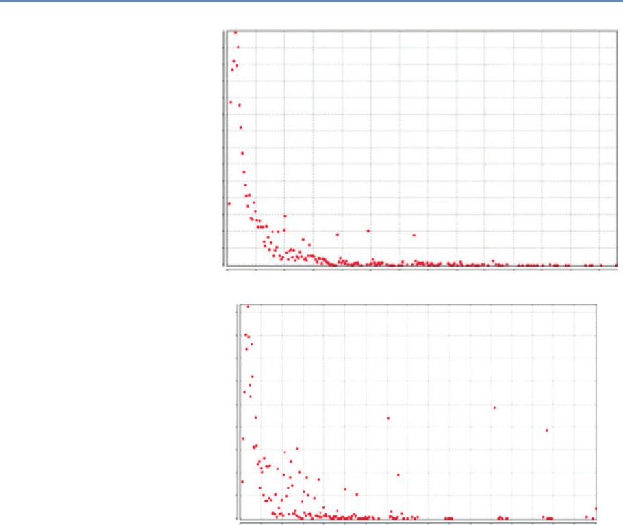
236 8. Networks: The Basics
225
250
275
300
325 University A
200
175
150
125
100
75
50
25
0
Count
0 20 40 60 80 100 120 140 160 180 200 220 240 260
Value
225
University B
200
175
150
125
100
75
50
25
0
Count
0 20 40 60 80 100 120 140 160 180 200 220 240 260 280 300 320 340
Value
Figure 8.7. Degree distribution for two universities
First, the left-hand side of the distribution is more dispersed than
it is for university A, suggesting that there are many nodes with
moderate degree. These nodes may also have high betweenness
centrality if their ties allow them to span different subgroups within
the networks. Of course this might also reflect the fact that each
cluster also has members that are more locally prominent. Finally,
consider the few instances on the right-hand end of the distribution
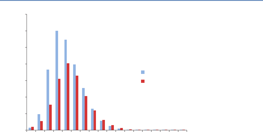
8.4. Comparing collaboration networks 237
3500000
3000000
2500000
1500000
2000000
Number of Dyads
1000000
University A
University B
500000
0
12345678910
Path Length
11 12 1413 15 16 17 18
Figure 8.8. Distribution of path lengths for universities A and B
where there are relatively large numbers of people with surprisingly
high degree. I suspect these are the result of large training grants
or center grants that employ many people. A quirk of relying on
one-mode projections of two-mode data is that every person asso-
ciated with a particular grant is connected to every other. More
work needs to be done to bear out these hypotheses, but for now
it suffices to say that the degree distribution of the networks bears
out the intuition we drew from the images that they are significantly
different.
The path length histogram presented in Figure 8.8 suggests a
similar pattern. While the average distance among any pair of con-
nected nodes in both networks is fairly similar (see Table 8.1), uni-
versity B has a larger number of unconnected nodes and university
A has a greater concentration of more closely connected dyads. The
preponderance of shorter paths in this network could also be a re-
sult of a few larger grants that connect many pairs of nodes at unit
distance and thus shorten overall path lengths.
But how do the descriptive statistics shake out? Table 8.1
presents the basic descriptive statistics we have discussed for each

238 8. Networks: The Basics
Table 8.1. Descriptive statistics for the main components of two university net-
works
University A University B
Nodes 4,999 4,144
Edges (total) 57,756 91,970
% nodes in main component 68.67% 67.34%
Diameter 18 18
Average degree 11.554 44.387
Clustering coefficient 0.855 0.913
Density 0.005 0.011
Average path length 5.034 5.463
network. University A’s network includes 855 more nodes than
university B’s, a difference of about 20%. In contrast, there are far
fewer edges connecting university A’s research employees than con-
necting university B’s, a difference that appears particularly starkly
in the much higher density of university B’s network. Part of the
story can be found in the average degree of nodes in each network.
As the degree distributions presented in Figure 8.6 suggested, the
average researcher at university B is much more highly connected
to others than is the case at university A. The difference is stark and
quite likely has to do with the presence of larger grants that employ
many individuals.
Both schools have a low average path length (around 5), suggest-
ing that no member of the network is more than five acquaintances
away from any other. Likewise, the diameter of both networks is 18,
which means that on each campus the most distant pair of nodes is
separated by just 18 steps. University A’s slightly lower path length
may be accounted for by the centralizing effect of its large medical
school grant infrastructure. Finally, consider the clustering coeffi-
cient. This measure approaches 1 as it becomes more likely that
two partners to a third node will themselves be connected. The like-
lihood that collaborators of collaborators will collaborate is high on
both campuses, but substantially higher at university B.
8.5 Summary
This chapter has provided a brief overview of the basics of networks,
using UMETRICS data as a source for examples. While network
measures can produce new and exciting ways to characterize social
dynamics, they are also important levels of analysis in their own

8.6. Resources 239
right. There are essential concepts that need to be mastered, such
as reachability, cohesion, brokerage, and reciprocity. Numbers are
important, for a variety of reasons—they can be used to describe
networks in terms of their composition and community structure.
This chapter provides a classic example of how well social science
meets data science. Social science is needed to identify the nodes
(what is being connected) and the ties (the relationships that mat-
ter) in order to construct the relevant networks. Computer science
is necessary to collect and structure the data in a fashion that is
sufficient for analysis. The combination of data science and social
science is key to making the right measurement and visualization
decisions.
8.6 Resources
For more information about network analysis in general, the Inter-
national Network for Social Network Analysis (http://www.insna.
org/) is a large, interdisciplinary association dedicated to network
analysis. It publishes a traditional academic journal, Social Net-
works, an online journal, Journal of Social Structure, and a short-
format journal, Connections, all dedicated to social network analy-
sis. Its several listservs offer vibrant international forums for dis-
cussion of network issues and questions. Finally, its annual meet-
ings include numerous opportunities for intensive workshops and
training for both beginning and advanced analysts.
A new journal, Network Science (http://journals.cambridge.org/
action/displayJournal?jid=NWS), published by Cambridge Univer-
sity Press and edited by a team of interdisciplinary network schol-
ars, is a good venue to follow for cutting-edge articles on compu-
tational network methods and for substantive findings from a wide
range of social, natural, and information science applications.
There are some good software packages available. Pajek (http://
mrvar.fdv.uni-lj.si/pajek/) is a freeware package for network anal-
ysis and visualization. It is routinely updated and has a vibrant
user group. Pajek is exceptionally flexible for large networks and
has a number of utilities that allow import of its relatively simple
file types into other programs and packages for network analysis.
Gephi (https://gephi.org/) is another freeware package that sup-
ports large-scale network visualization. Though I find it less flexible
than Pajek, it offers strong support for compelling visualizations.
Network Workbench (http://nwb.cns.iu.edu/) is a freeware pack-
age that supports extensive analysis and visualization of networks.

240 8. Networks: The Basics
This package also includes numerous shared data sets from many
different fields that can used to test and hone your network analytic
skills.
iGraph (http://igraph.org/redirect.html) is my preferred package
for network analysis. Implementations are available in R, in Python,
and in C libraries. The examples in this chapter were coded in
iGraph for Python.
Nexus (http://nexus.igraph.org/api/dataset_info?format=html&
limit=10&offset=20&operator=or&order=date) is a growing reposi-
tory for network data sets that includes some classic data dating
back to the origins of social science network research as well as
more recent data from some of the best-known publications and
authors in network science.


Information Visualization
Chapter 9
M. Adil Yalçın and Catherine Plaisant
This chapter will show you how to explore data and communicate
results so that data can be turned into interpretable, actionable
information. There are many ways of presenting statistical infor-
mation that convey content in a rigorous manner. The goal of this
chapter is to present an introductory overview of effective visualiza-
tion techniques for a range of data types and tasks, and to explore
the foundations and challenges of information visualization.
9.1 Introduction
One of the most famous discoveries in science—that disease was
transmitted through germs, rather than through pollution—resulted
from insights derived from a visualization of the location of London
cholera deaths near a water pump [349]. Information visualization
in the twenty-first century can be used to generate similar insights:
detecting financial fraud, understanding the spread of a contagious
illness, spotting terrorist activity, or evaluating the economic health
of a country. But the challenge is greater: many (102–107) items
may be manipulated and visualized, often extracted or aggregated
from yet larger data sets, or generated by algorithms for analytics.
Visualization tools can organize data in a meaningful way that
lowers the cognitive and analytical effort required to make sense
of the data and make data-driven decisions. Users can scan, rec-
ognize, understand, and recall visually structured representations
more rapidly than they can process nonstructured representations.
The science of visualization draws on multiple fields such as percep-
tual psychology, statistics, and graphic design to present informa-
tion, and on advances in rapid processing and dynamic displays
to design user interfaces that permit powerful interactive visual
analysis.
243
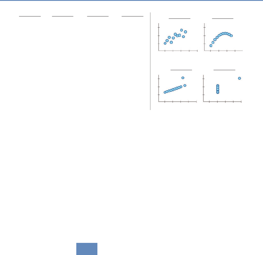
244 9. Information Visualization
Data Set A Data Set B Data Set C
Data Set C
Data Set D
Data Set D
10
8
13
9
11
14
6
4
12
7
5
8.04
6.95
7.58
8.81
8.33
9.96
7.24
4.26
10.84
4.82
5.68
y y
9.14
8.14
8.74
8.77
9.26
8.1
6.13
3.1
9.13
7.26
4.74
y
7.46
6.77
12.74
7.11
7.81
8.84
6.08
5.39
8.15
6.42
5.73
yy
x
6.58
5.76
7.71
8.84
8.47
7.04
5.25
12.5
5.56
7.91
6.89
x
10
8
13
9
11
14
6
4
12
7
5
x
10
8
13
9
11
14
6
4
12
7
5
x
8
8
8
8
8
8
8
19
8
8
8
x
12
8
4
48 12 16 20
y
x
12
8
4
4 8 12 16 20
Data Set A Data Set B
y
x
12
8
4
4 8 12 16 20
y
x
12
8
4
4 8 12 16 20
Average =Average =Average =Average
Variance =Variance =Variance =Variance
Correlation =Correlation =Correlation =Correlation
0.816 0.816 0.816 0.816
11 4.12
9 7.50 9 7.50 9 7.50 9 7.50
11 4.12 11 4.12 11 4.12
Figure 9.1. Anscombe’s quartet [16]
Figure 9.1, “Anscombe’s quartet” [16], provides a classic example
of the value of visualization compared to basic descriptive statisti-
cal analysis. The left-hand panel includes raw data of four small
number-pair data sets (A, B, C, D), which have the same average,
median, and standard deviation and have correlation across num-
ber pairs. The right-hand panel shows these data sets visualized
with each point plotted on perpendicular axes (scatterplots), reveal-
ing dramatic differences between the data sets, trends, and outliers
visually.
In broad terms, visualizations are used either to present results
or for analysis and open-ended exploration. This chapter provides
an overview of how modern information visualization, or visual data
mining, can be used to in the context of big data.
9.2 Developing effective visualizations
The effectiveness of a visualization depends on both analysis needs
and design goals. Sometimes, questions about the data are known
in advance; in other cases, the goal may be to explore new data sets,
generate insights, and answer questions that are unknown before
starting the analysis. The design, development, and evaluation of a
visualization is guided by understanding the background and goals
of the target audience (see Box 9.1).

9.2. Developing effective visualizations 245
Box 9.1:
The development of an effective visualization is an iterative pro-
cess that generally includes the following steps:
•Specify user needs, tasks, accessibility requirements and
criteria for success.
•Prepare data (clean, transform).
•Design visual representations.
•Design interaction.
•Plan sharing of insights, provenance.
•Prototype/evaluate, including usability testing.
•Deploy (monitor usage, provide user support, manage re-
vision process).
If the goal is to present results, there is a wide spectrum of users
◮See Chapters 2, 3, 4, and
5 for an overview of collect-
ing, merging, storing, and
processing data sets.
and a wide range of options. If the audience is broad, then info-
graphics can be developed by graphic designers, as described in
classic texts (see [119,380,381] or the examples compiled by Harri-
son et al. [157,206]). If, on the other hand, the audience comprises
domain experts interested in monitoring the overview status of dy-
namic processes on a continuous basis, dashboards can be used.
Examples include the monitoring of sales, or the number of tweets
about people, or symptoms of the flu and how they compare to a
baseline [120]. Dashboards can increase situational awareness so
that problems can be noticed and solved early and better decisions
can be made with up-to-date information.
Another goal of visualization is to enable interactive exploratory
analysis for casual users as well as professional analysts. One
casual example is BabyNameVoyager [156], which lets users type in
a name and see a graph of its popularity over the past century. *
⋆As the baby name is
typed letter by letter, Baby-
NameVoyager visualizes
the popularity of all the
names starting with the
letters entered so far, and
it animates smoothly with
each new letter input. For
example, typing “Jo” shows
all the names starting with
“Jo”. This view reveals
that Joyce and Joan were
popular girl names in the
1930s, and the use of
“John” has declined since
the 1960s.
Data analysis tools can enable analysis of structured and generic
data sets. Figure 9.2 shows an exploratory browser of a selection of
awards (grants) from the US Department of Agriculture, created us-
ing the web-based data exploration tool Keshif (http://www.keshif.
me). The awards (records) are listed in the middle panel by latest
start date first. Attributes of the awards, such as funding source,
are shown on side panels, revealing the range of their values. The
awards with status new are focused per the filtering selection, and
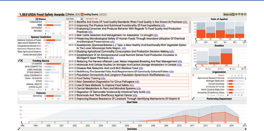
246 9. Information Visualization
Figure 9.2. A data analysis browser of a selection of grants from the US Department of Agriculture was created by
using the web-based tool Keshif
are visualized using darker gray colors. Lighter gray colors provide
visual cues to the distribution of all awards. The orange selection
highlights distributions of awards with formula funding, known as
Hatch funding. The analyst can explore trends in new or old awards,
funding resources, and other attributes in this rich award portfolio.
Commercial tools such as Spotfire and Tableau, among many
other tools (see Section 9.6), allow users to create visualizations by
offering chart types and visual design environments to analyze their
data, and to combine them in potent dashboards rapidly shared
with colleagues. For example, Figure 9.3 shows the charting in-
terface of Tableau on a transaction data set. The left-hand panel
shows the list of attributes associated with vendor transactions for a
given university. The visualization (center) is constructed by placing
the month of spending in chart columns, and the sum of payment
amount on the chart row, with data encoded using line mark type.
Agencies are broken down by color mapping. The agency list, to the
right, allows filtering the agencies, which can be used to simplify the
chart view. A peak in the line chart is annotated with an explanation
of the spike. On the rightmost side, the Show Me panel suggests
the applicable chart types potentially appropriate for the selected
attributes. This chart can be combined with other charts focus-
ing on other aspects in interactive dashboards. Figure 9.4 shows
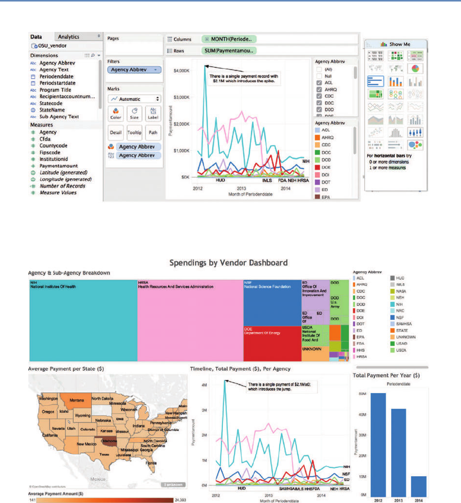
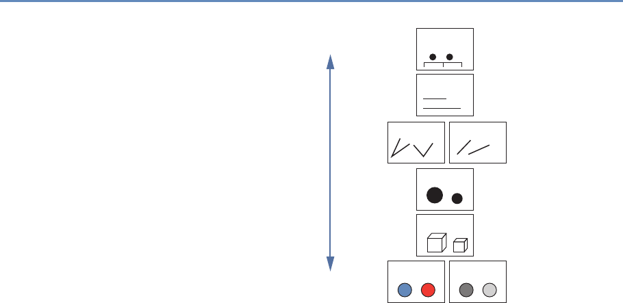
248 9. Information Visualization
More accurate Position
Length
Angle Slope
Area
Volume
Color Density
Less accurate
Figure 9.5. Visual elements described by MacKinlay [245]
a treemap [192] for agency and sub-agency spending breakdown,
combined with a map showing average spending per state. Okla-
homa state stands out with few but large expenditures. Mousing-
over Oklahoma reveals details of these expenditures. An additional
histogram provides an overview of spending change across three
years.
Creating effective visualizations requires careful consideration of
many components. Data values may be encoded using one or more
visual elements, like position, length, color, angle, area, and texture
(Figure 9.5; see also [79, 380]). Each of these can be organized in a
multitude of ways, discussed in more detail by Munzner [264]. In
addition to visual data encoding, units for axes, labels, and legends
need to be provided as well as explanations of the mappings when
the design is unconventional. (The website “A World of Terror” pro-
vides some compelling examples [301].) Annotations or comments
can be used to guide viewer attention and to describe related in-
sights. Providing attribution and data source, where applicable, is
an ethical practice that also enables validating data, and promotes
reuse to explore new perspectives.
The following is a short list of guidelines: provide immediate
feedback upon interaction with the visualization; generate tightly
coupled views (i.e., so that selection in one view updates the oth-
ers); and use a high “data to ink ratio” [380]. Use color carefully
9.3. A data-by-tasks taxonomy 249
and ensure that the visualization is truthful (e.g., watch for per-
ceptual biases or distortion). Avoid use of three-dimensional rep-
resentations or embellishments, since comparing 3D volumes is
perceptually challenging and occlusion is a problem. Labels and
legends should be meaningful, novel layouts should be carefully ex-
plained, and online visualizations should adapt to different screen
sizes. For extended and in-depth discussions, see various text-
books [119,208, 264, 380,381,395].
We provide a summary of the basic tasks that users typically
perform during visual analysis of data in the next section.
9.3 A data-by-tasks taxonomy
We give an overview of visualization approaches for six common
data types: multivariate, spatial, temporal, hierarchical, network,
and text [344]. For each data type listed in this section, we dis-
cuss its distinctive properties, the common analytical questions,
and examples. Real-life data sets often include multiple data types
coming from multiple sources. Even a single data source can in-
clude a variety of data types. For example, a single data table of
countries (as rows) can have a list of attributes with varying types:
the growth rate in the last 10 years (one observation per year, time
series data), their current population (single numerical data), the
amount of trade with other countries (networked/linked data), and
the top 10 exported products (if grouped by industry, hierarchical
data). Furthermore, we provide an overview of common tasks for vi-
sual data analysis in Box 9.2, which can be applied across different
data types based on goals and types of visualizations.
Interactive visualization design is also closely coupled with the
targeted devices. Conventionally, visualizations have been designed
for mouse and keyboard interaction on desktop computers. How-
ever, a wider range of device forms, such as mobile devices with
small displays and touch interaction, is becoming common. Creat-
ing visualizations for new forms requires special care, though basic
design principles such as “less is more” still apply.
9.3.1 Multivariate data
In common tabular data, each record (row) has a list of attributes
(columns), whose value is mostly categorical or numerical. The
analysis of multivariate data with basic categorical and interval
types aims to understand patterns within and across data attributes.

250 9. Information Visualization
Box 9.2: A task categorization for visual data analysis
Select/Query
•Filter to focus on a subset of the data
•Retrieve details of item
•Brush linked selections across multiple charts
•Compare across multiple selections
Navigate
•Scroll along a dimension (1D)
•Pan along two dimensions (2D)
•Zoom along the third dimension (3D)
Derive
•Aggregate item groups and generate characteristics
•Cluster item groups by algorithmic techniques
•Rank items to define ordering
Organize
•Select chart type and data encodings to organize data
•Layout multiple components or panels in the interface
Understand
•Observe distributions
•Compare items and distributions
•Relate items and patterns
Communicate
•Annotate findings
•Share results
•Trace action histories

9.3. A data-by-tasks taxonomy 251
Given a larger number of attributes, one of the challenges in data
exploration and analytics is to select the attributes and relations to
focus on. Expertise in the data domain can be helpful for targeting
relevant attributes.
Multivariate data can be presented in multiple forms of charts
depending on the data and relations being explored. One-dimen-
sional (1D) charts present data on a single axis only. An example
is a box-plot, which shows quartile ranges for numerical data. So-
called 1.5D charts list the range of possible values on one axis, and
describe a measurement of data on the other. Bar charts are a ubiq-
uitous example, in order to show, for example, a numeric grade per
student, or grade average for aggregated student groups by gen-
der. Records can also be grouped over numerical ranges, and bars
can show the number of items in each grouping, which generates
ahistogram chart. Two-dimensional charts plot data along two at-
tributes, such as scatterplots. Matrix (grid) charts can also be used
to show relations between two attributes. Heatmaps visualize each
matrix cell using color to represent its value. Correlation matrices
show the relation between attribute pairs.
To show relations of more than two attributes (3D+), one option is
to use additional visual encodings in a single chart, for example, by
adding point size/shape as a data variable in scatterplots. Another
option is to use alternative visual designs that can encode multiple
relations within a single chart. For example, a parallel coordinate
plot [180] has multiple parallel axes, each one representing an at-
tribute; each record is shown as connected lines passing through
the record’s values on each attribute. Charts can also show part-of-
whole relations using appropriate mappings based on subdividing
the chart space, such as stacked charts or pie charts.
Finally, another approach to analyzing multidimensional data is
to use clustering algorithms to identify similar items. Clusters are
typically represented as a tree structure (see Section 9.3.4). For
example, k-means clustering starts by users specifying how many
clusters to create; the algorithm then places every item into the
most appropriate cluster. Surprising relationships and interesting
outliers may be identified by these techniques on mechanical anal-
ysis algorithms. However, such results may require more effort to
interpret.
9.3.2 Spatial data
Spatial data convey a physical context, commonly in a 2D space,
such as geographical maps or floor plans. Several of the most

252 9. Information Visualization
famous examples of information visualization include maps, from
the 1861 representation of Napoleon’s ill-fated Russian campaign
by Minard (popularized by Tufte [380] and Kraak [214]) to the in-
teractive HomeFinder application that introduced the concept of dy-
namic queries [7]. The tasks include finding adjacent items, regions
containing certain items or with specific characteristics, and paths
between items—and performing the basic tasks listed in Box 9.1.
The primary form of visualizing spatial data is maps. In choro-
pleth maps, color encoding is used to add represent one data at-
tribute. Cartograms aim to encode the attribute value with the size
of regions by distorting the underlying physical space. Tile grid
maps reduce each spatial area to a uniform size and shape (e.g.,
a square) so that the color-coded data are easier to observe and
compare, and they arrange the tiles to approximate the neighbor
relations between physical locations [92,355]. Grid maps also make
selection of smaller areas (such as small cities or states) easier. Con-
tour (isopleth) maps connect areas with similar measurements and
color each one separately. Network maps aim to show network con-
nectivity between locations, such as flights to/from many regions
of the world. Spatial data can be also presented with a nonspatial
emphasis (e.g., as a hierarchy of continents, countries, and cities).
Maps are commonly combined with other visualizations. For ex-
ample, in Figure 9.6, the US Cancer Atlas combines a map showing
patterns across states on one attribute, with a sortable table provid-
ing additional statistical information and a scatterplot that allows
users to explore correlations between attributes.
9.3.3 Temporal data
Time is the unique dimension in our physical world that steadily
flows forward. While we cannot control time, we frequently record
it as a point or interval. Time has multiple levels of representation
(year, month, day, hour, minute, and so on) with irregularities (leap
year, different days per month, etc.). As we measure time based
on cyclic events in nature (day/night), our representations are also
commonly cyclic. For example, January follows December (first
month follows last). This cyclic nature can be captured by circular
visual encodings, such as the the conventional clock with hour,
minute, and second hands.
Time series data (Figures 9.7 and 9.8) describe values measured
at regular intervals, such as stock market or weather data. The
focus of analysis is to understand temporal trends and anomalies,
querying for specific patterns, or prediction. To show multiple time-


254 9. Information Visualization
Figure 9.8. EventFlow (www.cs.umd.edu/hcil/eventflow) is used to visualize sequences of innovation activities by
Illinois companies. Created with EventFlow; data sources include NIH, NSF, USPTO, SBIR. Image created by C.
Scott Dempwolf, used with permission
series trends across different data categories in a very compact chart
area, each trend can be shown with small height using a multi-
layered color approach, creating horizon graphs. While perceptually
effective after learning to read its encoding, this chart design may
not be appropriate for audiences who may lack such training or
familiarity.
Another form of temporal analysis is understanding sequences of
events. The study of human activity often includes analyzing event
sequences. For example, students’ records include events such as
attending orientation, getting a grade in a class, going on intern-
ship, and graduation. In the analysis of event sequences, finding
the most common patterns, spotting rare ones, searching for spe-
cific sequences, or understanding what leads to particular types of
events is important (e.g., what events lead to a student dropping
out, precede a medical error, or a company filing bankruptcy). Fig-
ure 9.8 shows EventFlow used to visualize sequences of innovation
activities by Illinois companies. Activity types include research, in-
vention, prototyping, and commercialization. The timeline (right
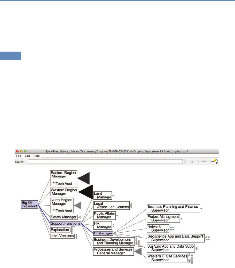
9.3. A data-by-tasks taxonomy 255
panel) shows the sequence of activities for each company. The
overview panel (center) summarizes all the records aligned by the
first prototyping activity of the company. In most of the sequences
shown here, the company’s first prototype is preceded by two or
more patents with a lag of about a year.
9.3.4 Hierarchical data
Data are often organized in a hierarchical fashion. Each item ap-
pears in one grouping (e.g., like a file in a folder), and groups can be
grouped to form larger groups (e.g., a folder within a folder), up to
the root (e.g., a hard disk). Items, and the relations between items
and their grouping, can have their own attributes. For example,
the National Science Foundation is organized into directorates and
divisions, each with a budget and a number of grant recipients.
Analysis may focus on the structure of the relations, by ques-
tions such as “how deep is the tree?”, “how many items does this
branch have?”, or “what are the characteristics of one branch com-
pared to another?” In such cases, the most appropriate repre-
sentation is usually a node-link diagram [62, 303]. In Figure 9.9,
Figure 9.9. SpaceTree (www.cs.umd.edu/hcil/spacetree/)
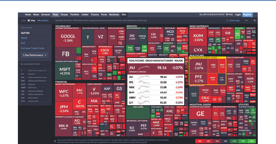
256 9. Information Visualization
Figure 9.10. The Finviz treemap helps users monitor the stock market (www.finviz.com)
Spacetree is used to browse a company organizational chart. Since
not all the nodes of the tree fit on the screen, we see an iconic repre-
sentation of the branches that cannot be displayed, indicating the
size of each branch. As the tree branches are opened or closed,
the layout is updated with smooth multiple-step animations to help
users remain oriented.
When the structure is less important but the attribute values
of the leaf nodes are of primary interest, treemaps, a space-filling
approach, are preferable as they can show arbitrary-sized trees in
a fixed rectangular space and map one attribute to the size of each
rectangle and another to color. For example, Figure 9.10 shows the
Finviz treemap that helps users monitor the stock market. Each
stock is shown as a rectangle. The size of the rectangle represents
market capitalization, and color indicates whether the stock is going
up or down. Treemaps are effective for situation awareness: we can
see that today is a fairly bad day as most stocks are red (i.e., down).
Stocks are organized in a hierarchy of industries, allowing users
to see that “healthcare technology” is not doing as poorly as most
other industries. Users can also zoom on healthcare to focus on
that industry.
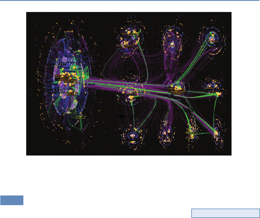
9.3. A data-by-tasks taxonomy 257
Automotive | Electronics Illinois-based
Toronto-based Electronics Paper |
Packaging
Industrial Biotech
Controls Photonics? Automotive
Parts
Chem & Materials Ag Equipment
Figure 9.11. NodeXL showing innovation networks of the Great Lakes manufacturing region. Created with NodeXL.
Data source: USPTO. Image created by C. Scott Dempwolf, used with permission
9.3.5 Network data
Network data encode relationships between items: for example, ◮See Chapter 8.
social connection patterns (friendships, follows and reposts, etc.),
travel patterns (such as trips between metro stations), and commu-
nication patterns (such as emails). The network overviews attempt
to reveal the structure of the network, show clusters of related items
(e.g., groups of tightly connected people), and allow the path be-
tween items to be traced. Analysis can also focus on attributes of
the items and the links in between, such as age of people in com-
munication or the average duration of communications.
Node-link diagrams are the most common representation of net-
work structures and overviews (Figures 9.11 and 9.12), and may
use linear (arc), circular, or force-directed layouts for positioning
the nodes (items). Matrices or grid layouts are also a valuable way
to represent networks [164]. Hybrid solutions have been proposed,
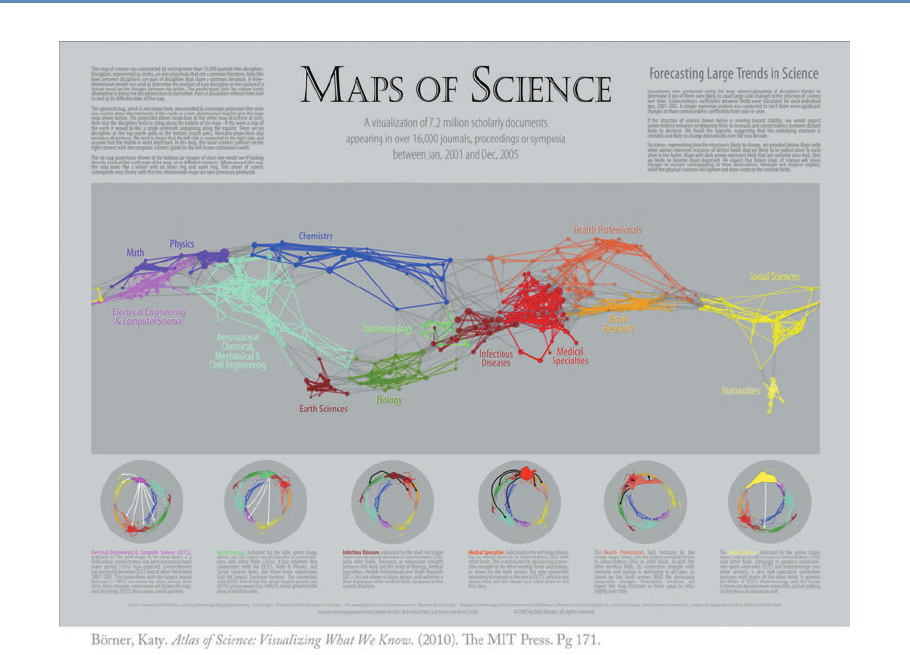
258 9. Information Visualization
Figure 9.12. An example from “Maps of Science: Forecasting Large Trends in Science,” 2007, The Regents of the
University of California, all rights reserved [45]
with powerful ordering algorithms to reveal clusters [153]. A ma-
jor challenge in network data exploration is in dealing with larger
networks where nodes and edges inevitably overlap by virtue of the
underlying network structure, and where aggregation and filtering
may be needed before effective overviews can be presented to users.
Figure 9.11 shows the networks of inventors (white) and compa-
nies (orange) and their patenting connections (purple lines) in the
network visualization NodeXL. Each company and inventor is also
connected to a location node (blue = USA; yellow = Canada). Green
lines are weak ties based on patenting in the same class and sub-
class, and they represent potential economic development leads.

9.4. Challenges 259
The largest of the technology clusters are shown using the group-
in-a-box layout option, which makes the clusters more visible. Note
the increasing level of structure moving from the cluster in the lower
right to the main cluster in the upper left. NodeXL is designed for
interactive network exploration; many controls (not shown in the
figure) allow users to zoom on areas of interest or change options.
Figure 9.12 shows an example of network visualization on science as
a topic used for data presentation in a book and a traveling exhibit.
Designed for print media, it includes a clear title and annotations
and shows a series of topic clusters at the bottom with a summary
of the insights gathered by analysts.
9.3.6 Text data
Text is usually preprocessed (for word/paragraph counts, sentiment ◮See Chapter 7 for text
analysis approaches.
analysis, categorization, etc.) to generate metadata about text seg-
ments, which are then visualized. Simple visualizations like tag
clouds display statistics about word usage in a text collection, or can
be used to compare two collections or text segments. While visually
appealing, they can easily be misinterpreted and are often replaced
by word indexes sorted by some count of interest. Specialized visual
text analysis tools combine multiple visualizations of data extracted
from the text collections, such as matrices to see relations, network
diagrams, or parallel coordinates to see entity relationships (e.g.,
between what, who, where, and when). Timelines can be mapped to
the linear dimension of text. Figure 9.13 shows an example using
Jigsaw [357] for the exploration of car reviews. Entities have been
extracted automatically (in this case make, model, features, etc.),
and a cluster analysis has been performed, visualized in the bottom
right. A separate view (rightmost) allows analysts to review links be-
tween entities. Another view allows traversing word sequences as a
tree. Reading original documents is critical, so all the visualization
elements are linked to the corresponding text.
9.4 Challenges
While information visualization is a powerful tool, there are many
obstacles to its effective use. We note here four areas of particu-
lar concern: scalability, evaluation, visual impairment, and visual
literacy.
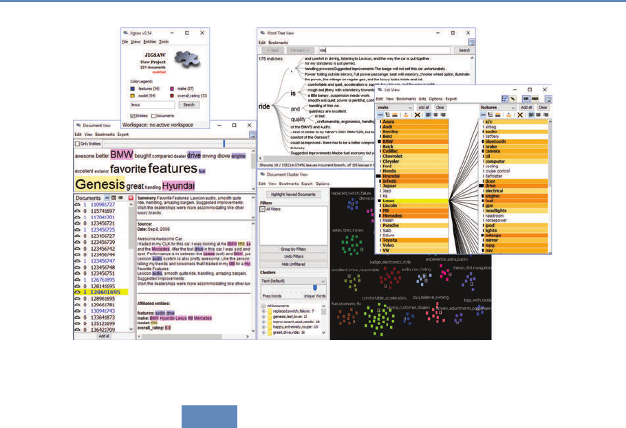
260 9. Information Visualization
Figure 9.13. Jigsaw used to explore a collection of car reviews
9.4.1 Scalability
Most visualizations handle relatively small data sets (between a
thousand and a hundred thousand, sometimes up to millions, de-
pending on the technique) but scaling visualizations from millions
to billions of records does require careful coordination of analytic
algorithms to filter data or perform rapid aggregation, effective vi-
sual summary designs, and rapid refreshing of displays [343]. The
visual information seeking mantra, “Overview first, zoom and filter,
then details on demand,” remains useful with data at scale. To
accommodate a billion records, aggregate markers (which may rep-
resent thousands of records) and density plots are useful [101]. In
some cases the large volume of data can be aggregated meaningfully
into a small number of pixels. One example is Google Maps and its
visualization of road conditions. A quick glance at the map allows
drivers to use a highly aggregated summary of the speed of a large
number of vehicles and only a few red pixels are enough to decide
when to get on the road.
While millions of graphic elements may be represented on large
screens [116], perception issues need to be taken into considera-

9.4. Challenges 261
tion [411]. Extraction and filtering may be necessary before even
attempting to visualize individual records [408]. Preserving interac-
tive rates in querying big data sources is a challenge, with a variety
of methods proposed, such as approximations [123] and compact
caching of aggregated query results [239]. Progressive loading and
processing will help users review the results as they appear and
steer the lengthy data processing [115, 135]. Systems are starting
to emerge, and strategies to cope with volume and variety of pat-
terns are being described [344].
9.4.2 Evaluation
Human-centric evaluation of visualization techniques can generate
qualitative and quantitative assessments of their potential quality,
with early studies focusing on the effectiveness of basic visual vari-
ables [245]. To this day, user studies remain the workhorse of eval-
uation. In laboratory settings, experiments can demonstrate faster
task completion, reduced error rates, or increased user satisfaction.
These studies are helpful for comparing visual and interaction de-
signs. For example, studies are reporting on the effects of latency
on interaction and understanding [241], and often reveal that dif-
ferent visualizations perform better for different tasks [303, 321].
Evaluations may also aim to measure and study the amount and
value of the insights revealed by the use of exploratory visualiza-
tion tools [325]. Diagnostic usability evaluation remains a corner-
stone of user-centered design. Usability studies can be conducted
at various stages of the development process to verify that users are
able to complete benchmark tasks with adequate speed and accu-
racy. Comparisons with the technology previously used by target
users may also be possible to verify improvements. Metrics need
to address the learnability and utility of the system, in addition to
performance and user satisfaction [223]. Usage data logging, user
interviews, and surveys can also help identification of potential im-
provements in visualization and interaction design.
9.4.3 Visual impairment
Color impairment is a common condition that needs to be taken
into consideration [291]. For example, red and green are appealing
for their intuitive mapping to positive or negative outcomes (also
depending on cultural associations); however, users with red–green
color blindness, one of the most common forms, would not be able to
differentiate such scales clearly. To assess and assist visual design

262 9. Information Visualization
under different color deficiencies, color simulation tools can be used
(see additional resources). The impact of color impairment can be
mitigated by careful selection of limited color schemes, using double
encoding when appropriate (i.e., using symbols that vary by both
shape and color), and allowing users to change or customize color
palettes. To accommodate users with low vision, adjustable size and
zoom settings can be useful. Users with severe visual impairments
may require alternative accessibility-first interface and interaction
designs.
9.4.4 Visual literacy
While the number of people using visualization continues to grow,
not everyone is able to accurately interpret graphs and charts.
When designing a visualization for a population of users who are ex-
pected to make sense of the data without training, it is important to
adequately estimate the level of visual literacy of those users. Even
simple scatterplots can be overwhelming for some users. Recent
work has proposed new methods for assessing visual literacy [47],
but user testing with representative users in the early stages of de-
sign and development will remain necessary to verify that adequate
designs are being used. Training is likely to be needed to help ana-
lysts get started when using more visual analytics tools. Recorded
video demonstrations and online support for question answering
are helpful to bring users from novice to expert levels.
9.5 Summary
The use of information visualization is spreading widely, with a
growing number of commercial products and additions to statis-
tical packages now available. Careful user testing should be con-
ducted to verify that visual data presentations go beyond the desire
for eye-candy in visualization, and to implement designs that have
demonstrated benefits for realistic tasks. Visualization is becom-
ing increasingly used by the general public and attention should be
given to the goal of universal usability so the widest range of users
can access and benefit from new approaches to data presentation
and interactive analysis.

9.6. Resources 263
9.6 Resources
We have referred to various textbooks throughout this chapter.
Tufte’s books remain the classics, as inspiring to read as they are
instructive [380, 381]. We also recommend Few’s books on infor-
mation visualization [119] and information dashboard design [120].
See also the book’s website for further readings.
Given the wide variety of goals, tasks, and use cases of visual-
ization, many different data visualization tools have been developed
that address different needs and appeal to different skill levels. In
this chapter we can only point to a few examples to get started.
To generate a wide range of visualizations and dashboards, and to
quickly share them online, Tableau and Tableau Public provide a
flexible visualization design platform. If a custom design is required
and programmers are available, d3 is the de facto low-level library
of choice for many web-based visualizations, with its native integra-
tion to web standards and flexible ways to convert and manipulate
data into visual objects as a JavaScript library. There exist other
JavaScript web libraries that offer chart templates (such as High-
charts), or web services that can be used to create a range of charts
from given (small) data sets, such as Raw or DataWrapper. To clean,
transform, merge, and restructure data sources so that they can be
visualized appropriately, tools like Trifacta and Alteryx can be used
to create pipelines for data wrangling. For statistical analysis and
batch-processing data, programming environments such as R or li-
braries for languages such as Python (for example, the Python Plotly
library) can be used.
An extended list of tools and books is available at http://www.
keshif.me/demo/VisTools.


Errors and Inference
Chapter 10
Paul P. Biemer
This chapter deals with inference and the errors associated with big
data. Social scientists know only too well the cost associated with
bad data—we highlighted both the classic Literary Digest example
and the more recent Google Flu Trends problems in Chapter 1.
Although the consequences are well understood, the new types of
data are so large and complex that their properties often cannot
be studied in traditional ways. In addition, the data generating
function is such that the data are often selective, incomplete, and
erroneous. Without proper data hygiene, the errors can quickly
compound. This chapter provides, for the first time, a systematic
way to think about the error framework in a big data setting.
10.1 Introduction
The massive amounts of high-dimensional and unstructured data
in big data bring both new opportunities and new challenges to the
data analyst. Many of the problems with big data are well known
(see, for example, the AAPOR report by Japec et al. [188]). The
volume, variety, and velocity of big data can overwhelm traditional
methods of data analysis. Add to this complexity the fact that, as it
is generated, big data is often selective, incomplete, and erroneous.
As it is processed, new errors can be introduced in downstream
operations.
Big data is typically aggregated from disparate sources at various
points in time and integrated to form data sets. These processes
involve linking records together, transforming them to form new
attributes (or variables), documenting the actions taken (although
sometimes inadequately), and interpreting the newly created fea-
tures of the data. These activities may introduce new errors into
the data set: errors that may be either variable (i.e., errors that
265

266 10. Errors and Inference
create random noise resulting in poor reliability) or systematic (i.e.,
errors that tend to be directional, thus exacerbating biases). Using
big data in statistically valid ways is increasingly challenging in this
environment; however, it is important for data analysts to be aware
of the error risks and the potential effects of big data error on infer-
ences and decision-making. The massiveness, high dimensionality,
and accelerating pace of big data, combined with the risks of vari-
able and systematic data errors, requires new, robust approaches
to data analysis.
The core issue confronting big data veracity is that such data
may not be generated from instruments and methods designed to
produce valid and reliable data for scientific analysis and discovery.
Rather, this is data that are being repurposed for uses not origi-
nally intended. Big data has been referred to as “found” data or
“data exhaust” because it is generated for purposes that often do
not align with those of the data analyst. In addition to inadvertent
errors, there are also errors from mischief in big data; for example,
automated systems have been written to generate bogus content in
the social media that is indistinguishable from legitimate or authen-
tic data. Regardless of the source, many big data generators have
little or no regard for the quality of the data that are cast off from
their processes. Big data analysts must be keenly aware of these
limitations and should take the necessary steps to understand and
hopefully mitigate the effects of hidden errors on their results.
10.2 The total error paradigm
We now provide a framework for describing, mitigating, and inter-
preting the errors in essentially any data set, be it structured or
unstructured, massive or small, static or dynamic. This framework
has been referred to as the total error framework or paradigm. We
begin by reviewing the traditional paradigm, acknowledging its lim-
itations for truly big data sets, and we suggest how this framework
can be extended to encompass the new error structures often asso-
ciated with big data.
10.2.1 The traditional model
Dealing with the risks that errors introduce in big data analysis can
be facilitated through a better understanding of the sources and
nature of those errors. Such knowledge is gained through in-depth

10.2. The total error paradigm 267
understanding of the data generating mechanism, the data pro-
cessing/transformation infrastructure, and the approaches used to
create a specific data set or the estimates derived from it. For sur-
vey data, this knowledge is embodied in the well-known total survey
error (TSE) framework that identifies all the major sources of error
contributing to data validity and estimator accuracy [33, 35, 143].
The TSE framework attempts to describe the nature of the error
sources and what they may suggest about how the errors could af-
fect inference. The framework parses the total error into bias and
variance components that, in turn, may be further subdivided into
subcomponents that map the specific types of errors to unique com-
ponents of the total mean squared error. It should be noted that,
while our discussion on issues regarding inference has quantitative
analyses in mind, some of the issues discussed here are also of
interest to more qualitative uses of big data.
For surveys, the TSE framework provides useful insights regard-
ing how the many steps in the data generating, reformatting, and
file preparation processes affect estimation and inference, and may
also suggest methods for either reducing the errors at their source
or adjusting for their effects in the final data products to produce
inferences of higher quality. The AAPOR Task Force Report on big
data referenced above [188] describes the concept of data quality
for big data and provides a total error framework for big data that
we consider and further extend in this chapter. This approach was
closely modeled after the TSE framework since, as we shall see,
both share a number of common error sources. However, the big
data total error (BDTE) framework, as it is called in the AAPOR re-
port, necessarily includes additional error sources that are unique
to big data and can create substantial biases and uncertainties in
big data products. Like the TSE framework, the BDTE framework
aids our understanding of the limitations of the data, leading to
better-informed analyses and applications of the results. It may
also inform a research agenda for reducing the effects of error on
big data analytics.
In Figure 10.1, a canonical data file is represented as an array
consisting of rows (records) and columns (variables), with their size
denoted by Nand p, respectively. Many data sets derived from big
data can be represented in this way, at least conceptually. Later,
we will consider data sets that do not conform to this rectangular
structure and may even be unstructured.
Many administrative data sets have a simple tabular structure,
as do survey sampling frames, population registers, and account-
ing spreadsheets. Let us assume that the data set is intended to

268 10. Errors and Inference
Record # V1V2VP
...
1
2
...
N
Figure 10.1. A typical rectangular data file format
represent some target population to which inference will be made in
the subsequent analysis. Thus, the rows are typically aligned with
units or elements of this target population, the columns represent
characteristics, variables (or features) of the row elements, and the
cells correspond to values of the column features for elements on
the rows.
The total error for this data set may be expressed by the following
heuristic formula:
Total error =Row error +Column error +Cell error.
Row error For the situations considered in this chapter, the row
errors may be of three types:
•Omissions: Some rows are missing, which implies that ele-
ments in the target population are not represented on the file.
•Duplications: Some population elements occupy more than
one row.
•Erroneous inclusions: Some rows contain elements or entities
that are not part of the target population.
For survey sample data sets, omissions include members of the
target population that are either inadvertently or deliberately ab-
sent from the frame, as well as nonsampled frame members. For
big data, the selectivity of the capture mechanism is a common
form of omissions. For example, a data set consisting of persons
who conducted a Google search in the past week necessarily ex-
cludes persons not satisfying that criterion who may have quite
different characteristics from those who do. Such exclusions can
therefore be viewed as a source of selectivity bias if inference is to
be made to the general population. For one, persons who do not
have access to the Internet are excluded from the data set. These

10.2. The total error paradigm 269
exclusions may be biasing in that persons with Internet access may
have quite different demographic characteristics from persons who
do not have Internet access. The selectivity of big data capture is
similar to frame noncoverage in survey sampling and can bias in-
ferences when researchers fail to consider it and compensate for it
in their analyses.
Example: Google searches
As an example, in the United States, the word “Jewish” is included in 3.2 times
more Google searches than “Mormon” [360]. This does not mean that the Jewish
population is 3.2 times larger than the Mormon population. Another possible
explanation is that Jewish people use the Internet in higher proportions or have
more questions that require using the word “Jewish.” Thus Google search data are
more useful for relative comparisons than for estimating absolute levels.
A well-known formula in the survey literature provides a use-
ful expression for the so-called coverage bias in the mean of some
variable, V. Denote the mean by ¯
V, and let ¯
VTdenote the (possibly
hypothetical because it may not be observable) mean of the target
population of NTelements, including the NT−Nelements that are
missing from the observed data set. Then the bias due to this non-
coverage is BNC =¯
V−¯
VT=(1−N/NT)( ¯
VC−¯
VNC), where ¯
VCis the
mean of the covered elements (i.e., the elements in the observed
data set) and ¯
VNC is the mean of the NT−Nnoncovered elements.
Thus we see that, to the extent that the difference between the cov-
ered and noncovered elements is large or the fraction of missing
elements (1−N/NT)is large, the bias in the descriptive statistic will
also be large. As in survey research, often we can only speculate
about the sizes of these two components of bias. Nevertheless, spec-
ulation is useful for understanding and interpreting the results of
data analysis and cautioning ourselves regarding the risks of false
inference.
We can also expect that big data sets, such as a data set con-
taining Google searches during the previous week, could have the
same person represented many times. People who conducted many
searches during the data capture period would be disproportion-
ately represented relative to those who conducted fewer searchers.
If the rows of the data set correspond to tweets in a Twitter feed,
duplication can arise when the same tweet is retweeted or when
some persons are quite active in tweeting while others lurk and

270 10. Errors and Inference
tweet much less frequently. Whether such duplications should be
regarded as “errors” depends upon the goals of the analysis.
For example, if inference is to be made to a population of per-
sons, persons who tweet multiple times on a topic would be over-
represented. If inference is to be made to the population of tweets,
including retweets, then such duplication does not bias inference.
When it is a problem, it still may not be possible to identify
duplications in the data. Failing to account for them could generate
duplication biases in the analysis. If these unwanted duplications
can be identified, they can either be removed from the data file (i.e.,
deduplication). Alternatively, if a certain number of rows, say d,
correspond to the same population unit, those row values can be
weighted by 1/d to correct the estimates for the duplications.
Erroneous inclusions can also create biases. For example, Google
searches or tweets may not be generated by a person but rather by a
computer either maliciously or as part of an information-gathering
or publicity-generating routine. Likewise, some rows may not sat-
isfy the criteria for inclusion in an analysis—for example, an analy-
sis by age or gender includes some row elements not satisfying the
criteria. If the criteria can be applied accurately, the rows violating
the criteria can be excluded prior to analysis. However, with big
data, some out-of-scope elements may still be included as a result
of missing or erroneous information, and these inclusions will bias
inference.
Column error The most common type of column error in survey
data analysis is caused by inaccurate or erroneous labeling of the
column data—an example of metadata error. In the TSE framework,
this is referred to as a specification error. For example, a business
register may include a column labeled “number of employees,” de-
fined as the number of persons in the company who received a
payroll check in the month preceding. Instead the column contains
the number of persons on the payroll whether or not they received
a check in the prior month, thus including, for example, persons on
leave without pay.
For big data analysis, such errors would seem to be quite com-
mon because of the complexities involved in producing a data set.
For example, data generated from a source, such as an individual
tweet, may undergo a number of transformations before it is in-
cluded in the analysis data set. This transformative process can
be quite complex, involving parsing phrases, identifying words, and
classifying them as to subject matter and then perhaps further clas-

10.2. The total error paradigm 271
sifying them as either positive or negative expressions about some
phenomenon like the economy or a political figure. There is con-
siderable risk of the resulting variables being either inaccurately
defined or misinterpreted by the data analyst.
Example: Specification error with Twitter data
As an example, consider a Twitter data set where the rows correspond to tweets
and one of the columns supposedly contains an indicator of whether the tweet
contained one of the following key words: marijuana, pot, cannabis, weed, hemp,
ganja, or THC. Instead, the indicator actually corresponds to whether the tweet
contained a shorter list of words; say, either marijuana or pot. The mislabeled
column is an example of specification error which could be a biasing factor in an
analysis. For example, estimates of marijuana use based upon the indicator could
be underestimates.
Cell errors Finally, cell errors can be of three types: content error,
specification error, or missing data. A content error occurs when
the value in a cell satisfies the column definition but still deviates
from the true value, whether or not the true value is known. For
example, the value satisfies the definition of “number of employees”
but is outdated because it does not agree with the current number of
employees. Errors in sensitive data such as drug use, prior arrests,
and sexual misconduct may be deliberate. Thus, content errors may
be the result of the measurement process, a transcription error, a
data processing error (e.g., keying, coding, editing), an imputation
error, or some other cause.
Specification error is just as described for column error but ap-
plied to a cell. For example, the column is correctly defined and
labeled; however, a few companies provided values that, although
otherwise highly accurate, were nevertheless inconsistent with the
required definition. Missing data, as the name implies, are just
empty cells that should be filled. As described in Kreuter and
Peng [215], data sets derived from big data are notoriously affected
by all three types of cell error, particularly missing or incomplete
data, perhaps because that is the most obvious deficiency.
The traditional TSE framework is quite general in that it can be
applied to essentially any data set that conform to the format in Fig-
ure 10.1. However, in most practical situations it is quite limited
because it makes no attempt to describe how the processes that

272 10. Errors and Inference
generated the data may have contributed to what could be con-
strued as data errors. In some cases, these processes constitute
a “black box,” and the best approach is to attempt to evaluate the
quality of the end product. For survey data, the TSE framework pro-
vides a fairly complete description of the error-generating processes
for survey data and survey frames [33]. In addition, there has been
some effort to describe these processes for population registers and
administrative data [391]. But at this writing, little effort has been
devoted to enumerating the error sources and the error generating
processes for big data.
As previously noted, missing data can take two forms: missing
information in a cell of a data matrix (referred to as item missing-
ness) or missing rows (referred to as unit missingness), with the for-
mer being readily observable whereas the latter can be completely
hidden from the analyst. Much is known from the survey research
literature about how both types of missingness affect data analysis
(see, for example, Little and Rubin [240, 320]). Rubin [320] intro-
duced the term missing completely at random (MCAR) to describe
data where the data that are available (say, the rows of a data set)
can be considered as a simple random sample of the inferential
population (i.e., the population to which inferences from the data
analysis will be made). Since the data set represents the population,
MCAR data provide results that are generalizable to this population.
A second possibility also exists for the reasons why data are
missing. For example, students who have high absenteeism may
be missing because they were ill on the day of the test. They may
otherwise be average performers on the test so, in this case, it has
little to do with how they would score. Thus, the values are missing
for reasons related to another variable, health, that may be avail-
able in the data set and completely observed. Students with poor
health tend to be missing test scores, regardless of those student’s
performance on the test. Rubin [320] uses the term missing at ran-
dom (MAR) to describe data that are missing for reasons related
to completely observed variables in the data set. It is possible to
compensate for this type of missingness in statistical inferences by
modeling the missing data mechanism.
However, most often, missing data may be related to factors that
are not represented in the data set and, thus, the missing data
mechanism cannot be adequately modeled. For example, there may
be a tendency for test scores to be missing from school adminis-
trative data files for students who are poor academic performers.
Rubin calls this form of missingness nonignorable. With nonignor-
able missing data, the reasons for the missing observations depend

10.2. The total error paradigm 273
on the values that are missing. When we suspect a nonignorable
missing data mechanism, we need to use procedures much more
complex than will be described here. Little and Rubin [240] and
Schafer [326] discuss methods that can be used for nonignorable
missing data. Ruling out a nonignorable response mechanism can
simplify the analysis considerably.
In practice, it is quite difficult to obtain empirical evidence about
whether or not the data are MCAR or MAR. Understanding the data
generation process is invaluable for specifying models that appro-
priately represent the missing data mechanism and that will then
be successful in compensating for missing data in an analysis.
(Schafer and Graham [327] provide a more thorough discussion
of this issue.)
One strategy for ensuring that the missing data mechanism can
be successfully modeled is to have available on the data set many
variables that may be causally related to missing data. For example,
features such as personal income are subject to high item missing-
ness, and often the missingness is related to income. However, less
sensitive, surrogate variables such as years of education or type
of employment may be less subject to missingness. The statisti-
cal relationship between income and other income-related variables
increases the chance that information lost in missing variables is
supplemented by other completely observed variables. Model-based
methods use the multivariate relationship between variables to han-
dle the missing data. Thus, the more informative the data set, the
more measures we have on important constructs, the more suc-
cessfully we can compensate for missing data using model-based
approaches.
10.2.2 Extending the framework to big data
The processes involved in generating big data are as varied as big
data itself. This diversity substantially complicates the goal of pro-
viding a detailed error framework that is applicable to all big data.
Nevertheless, some progress can be made by considering the steps
that are typically involved in creating a data set from big data, which
often includes three stages: (a) data generation (see Chapter 2), (b)
extract, transform and load (ETL), and (c) analysis (see, for exam-
ple, Chapter 7). As noted there, this mapping of the process is
oversimplified for some applications. For example, data that flow
continuously from their sources may not be directed through an
ETL process at all. Rather it may be gathered in real time and
processed on an ad hoc basis. Likewise, the ETL processes may

274 10. Errors and Inference
Source 1
Source 2
Source 3
Generation
Extract
Transform
(Cleanse)
Load
(Store)
Filter/Reduction
(Sampling)
Computation/
Analysis
(Visualization)
ETL Analysis
Figure 10.2. Big data process map
be recursive in that, as errors are identified, the processes may be
altered and refined. In addition, the transform stage may gener-
ate new data (e.g., proxy variables). The analysis stage may also
involve language transformations such as translation and charac-
ter set transformations. Finally, there may downstream processes
that lead to additional iterations of the stages in the process map.
Thus, the model outline here is but an initial attempt to capture the
tremendous complexities that may be involved in the big data life
cycle.
Figure 10.2 graphically depicts the flow of data along the major
steps in the process. One might imagine many more arrows among
the boxes within the ETL and analysis stages that represent the
recursive nature of those stages. The severity of the errors that
arise from these processes will depend on the specific data sources
and analytic goals involved. Nevertheless, we can still consider how
each stage might create errors in a more generic fashion.
For example, data generation error is somewhat analogous to
errors arising in survey data collection. Like surveys, the data-
generating process for big data is subject to erroneous, incomplete,
and missing data. In addition, the data-generating sources may be
selective in that the data collected may not represent a well-defined
population or one that is representative of a target population of
inference in an analysis. Thus, data generation errors include low
signal-to-noise ratio, lost signals, incomplete or missing values, sys-
tematic errors, selective elements, and metadata that are lacking,
absent, or erroneous.
ETL processes may be quite similar to various data processing
stages for surveys. These may include creating or enhancing meta-

10.3. Illustrations of errors in big data 275
data, record matching, variable coding, editing, data munging (or
scrubbing), and data integration (i.e., linking and merging records
and files across disparate systems). ETL errors include specifica-
tion errors (including errors in metadata), matching errors, coding
errors, editing errors, data munging errors, and data integration
errors.
Finally, the analysis of big data introduces risks for a number of
errors that will be described in more detail in the next section. These
risks may be due to noise accumulation, coincidental correlations,
and incidental endogeneity. As we shall see, these errors arise as a
consequence of big data volume and variety even when the big data
itself is infallible. Erroneous data compound these problems and
can lead to other issues that are described in some detail below.
For example, big data can be subject to sampling errors when the
data are filtered, sampled, or otherwise reduced to form more man-
ageable or representative data sets. So-called nonsampling errors
can arise when the analysis involves further transforming the data
and weighting the data elements, as well as can be errors due to
modeling and estimation. The latter errors are similar to modeling
and estimation errors in surveys and may include inadequate or er-
roneous adjustments for representativeness, improper or erroneous
weighting, computation and algorithmic errors, model misspecifica-
tion, and so on.
10.3 Illustrations of errors in big data
A well-known example of the risks of big data error is provided
by the Google Flu Trends series that uses Google searches on flu
◮See the discussion in
Section 1.3.
symptoms, remedies, and other related key words to provide near-
real-time estimates of flu activity in the USA and 24 other countries.
Compared to CDC data, the Google Flu Trends provided remarkably
accurate indicators of flu incidence in the USA between 2009 and
2011. However, for the 2012–2013 flu seasons, Google Flu Trends
predicted more than double the proportion of doctor visits for flu-
like symptoms compared to the CDC [61]. Lazer et al. [230] cite two
causes of this error: big data hubris and algorithm dynamics.
Hubris occurs when the big data researcher believes that the
volume of the data compensates for any of its deficiencies, thus
obviating the need for traditional, scientific analytic approaches.
As Lazer et al. [230] note, big data hubris fails to recognize that
“quantity of data does not mean that one can ignore foundational
issues of measurement and construct validity and reliability.”

276 10. Errors and Inference
Algorithm dynamics refers to properties of algorithms that al-
low them to adapt and “learn” as the processes generating the data
change over time. Although explanations vary, the fact remains
that Google Flu Trends was too high and by considerable margins
for 100 out of 108 weeks starting in July 2012. Lazer et al. [230] also
blame “blue team dynamics,” which arises when the data generating
engine is modified in such a way that the formerly highly predictive
search terms eventually failed to work. For example, when a Google
user searched on “fever” or “cough,” Google’s other programs started
recommending searches for flu symptoms and treatments—the very
search terms the algorithm used to predict flu. Thus, flu-related
searches artificially spiked as a result of these changes to the al-
gorithm and the impact these changes had on user behavior. In
survey research, this is similar to the measurement biases induced
by interviewers who suggest to respondents who are coughing that
they might have flu, then ask the same respondents if they think
they might have flu.
Algorithm dynamic issues are not limited to Google. Platforms
such as Twitter and Facebook are also frequently modified to im-
prove the user experience. A key lesson provided by Google Flu
Trends is that successful analyses using big data today may fail to
produce good results tomorrow. All these platforms change their
methodologies more or less frequently, with ambiguous results for
any kind of long-term study unless highly nuanced methods are
routinely used. Recommendation engines often exacerbate effects
in a certain direction, but these effects are hard to tease out. Fur-
thermore, other sources of error may affect Google Flu Trends to
an unknown extent. For example, selectivity may be an impor-
tant issue because the demographics of people with Internet access
are quite different from the demographic characteristics related to
flu incidence [375]. Thus, the “at risk” population for influenza
and the implied population based on Google searches do not cor-
respond. This illustrates just one type of representativeness issue
that often plagues big data analysis. In general it is an issue that
algorithms are not (publicly) measured for accuracy, since they are
often proprietary. Google Flu Trends is special in that it publicly
failed. From what we have seen, most models fail privately and
often without anyone at all noticing.
In the next section, we consider the impact of errors on some
forms of analysis that are common in the big data literature. Due to
space limitations, our focus is limited to the effects of content errors
on data analysis. However, there are numerous resources available
for studying and mitigating the effects of missing data on analysis;
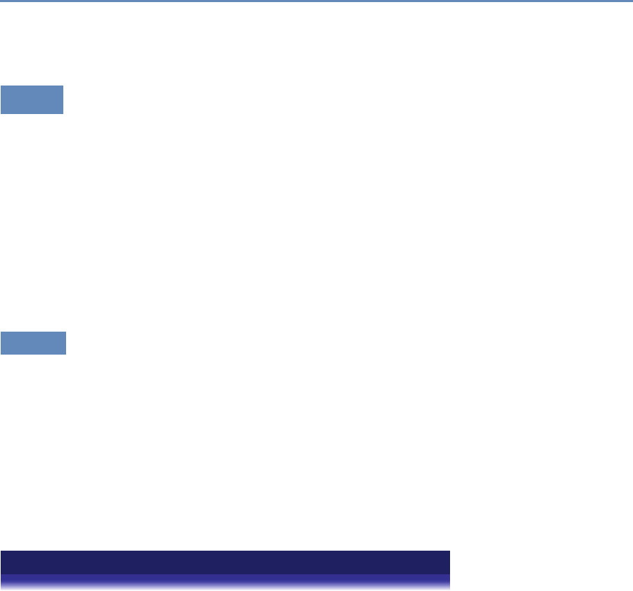
10.4. Errors in big data analytics 277
in particular, the books by Little and Rubin [240], Schafer [326],
and Allison [10] are quite relevant to big data analytics.
10.4 Errors in big data analytics
In this section, we consider some common types of errors in big
data analytics. The next section considers analytic errors caused
by the so-called “three Vs” of big data, namely, volume, velocity,
and variety, under the assumption of perfect “veracity.” If we relax
the assumption of perfect veracity, the errors that afflict big data as
a result of the three Vs can be exacerbated in largely unpredictable
ways. Section 10.4.2 considers three common types of analysis
when data lack veracity: classification, correlation, and regression.
While the scope of our review is necessarily limited, hopefully the
discussion will lay the foundation for further study regarding the
effects of errors on big data analytics.
10.4.1 Errors resulting from volume, velocity, and variety,
assuming perfect veracity
Data deficiencies represent only one set of challenges for the big data
analyst. Other challenges arise solely as a result of the massive size,
rapid generation, and vast dimensionality of the data. As a conse-
quence of these so-called three Vs of big data, Fan et al. [111] iden-
tify three issues—noise accumulation, spurious correlations, and
incidental endogeneity—which will be briefly discussed in this sec-
tion. These issues should concern big data analysts even if the data
could be regarded as infallible. Content errors, missing data, and
other data deficiencies will only exacerbate these problems.
Example: Noise accumulation
To illustrate noise accumulation, Fan et al. [111] consider the following scenario.
Suppose an analyst is interested in classifying individuals into two categories, C1
and C2, based upon the values of 1,000 variables in a big data set. Suppose further
that, unknown to the researcher, the mean value for persons in C1is 0 on all 1,000
variables while persons in C2have a mean of 3 on the first 10 variables and 0 on all
other variables. Since we are assuming the data are error-free, a classification rule
based upon the first m≤10 variables performs quite well, with little classification
error. However, as more and more variables are included in the rule, classification
error increases because the uninformative variables (i.e., the 990 variables having
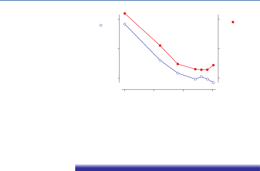
278 10. Errors and Inference
2,000
1,500
Piars of Breeding Storks ( )
Millions of Newborn Babies ( )
1,000
1.0
0.75
0.5
1965 1970 1975
Year
1980
Figure 10.3. An illustration of coincidental correlation between two variables: stork
die-off linked to human birth decline [346]
no discriminating power) eventually overwhelm the informative signals (i.e., the
first 10 variables). In the Fan et al. [111] example, when m > 200, the accumulated
noise exceeds the signal embedded in the first 10 variables and the classification
rule becomes equivalent to a coin-flip classification rule.
High dimensionality can also introduce coincidental (or spuri-
ous) correlations in that many unrelated variables may be highly
correlated simply by chance, resulting in false discoveries and er-
roneous inferences. The phenomenon depicted in Figure 10.3 is an
illustration of this. Many more examples can be found on a web-
site and in a book devoted to the topic [388, 389]. Fan et al. [111]
explain this phenomenon using simulated populations and rela-
tively small sample sizes. They illustrate how, with 800 indepen-
dent (i.e., uncorrelated) variables, the analyst has a 50% chance of
observing an absolute correlation that exceeds 0.4. Their results
suggest that there are considerable risks of false inference associ-
ated with a purely empirical approach to predictive analytics using
high-dimensional data.
Finally, turning to incidental endogeneity, a key assumption in
regression analysis is that the model covariates are uncorrelated
with the residual error; endogeneity refers to a violation of this
assumption. For high-dimensional models, this can occur purely
by chance—a phenomenon Fan and Liao [113] call incidental endo-
geneity. Incidental endogeneity leads to the modeling of spurious

10.4. Errors in big data analytics 279
variation in the outcome variables resulting in errors in the model
selection process and biases in the model predictions. The risks
of incidental endogeneity increase as the number of variables in
the model selection process grows large. Thus it is a particularly
important concern for big data analytics.
Fan et al. [111] as well as a number of other authors [114, 361]
(see, for example, Hall and Miller [151]; Fan and Liao, [112]) suggest
robust statistical methods aimed at mitigating the risks of noise
accumulation, spurious correlations, and incidental endogeneity.
However, as previously noted, these issues and others are further
compounded when data errors are present in a data set. Biemer and
Trewin [37] show that data errors will bias the results of traditional
data analysis and inflate the variance of estimates in ways that are
difficult to evaluate or mitigate in the analysis process.
10.4.2 Errors resulting from lack of veracity
The previous section examined some of the issues big data analysts ◮The volume, velocity, and
variety of big data make it
challenging to analyze be-
cause of noise accumula-
tion, spurious correlations,
and incidental endogeneity.
But, the three Vs are also
the scourge of veracity—
i.e., errors in big data.
face as either Nor pin Figure 10.1 becomes extremely large. When
row, column, and cell errors are added into the mix, these volumatic
problems can be further exacerbated. For example, noise accumu-
lation can be expected to accelerate when random noise (i.e., content
errors) afflicts the data. Spurious correlations that give rise to both
incidental endogeneity and coincidental correlations can render cor-
relation analysis meaningless if the error levels in big data are not
mitigated. In this section, we consider some of the issues that arise
in classification, correlation, and regression analysis as a result of
content errors that may be either variable or systematic. The cur-
rent literature on big data error acknowledges that the data may be
noisy, that is, subject to variable errors. However, there appears to
be little recognition of the problems associated with systematic or
correlated errors, particularly those introduced when data are com-
bined from disparate sources that may be subject to source-specific
errors.
There are various important findings in this section. First, for
rare classes, even small levels of error can impart considerable bi-
ases in classification analysis. Second, variable errors will atten-
uate correlations and regression slope coefficients; however, these
effects can be mitigated by forming meaningful aggregates of the
data and substituting these aggregates for the individual units in
these analyses. Third, unlike random noise, systematic errors can
bias correlation and regression analysis is unpredictable ways, and
these biases cannot be effectively mitigated by aggregating the data.

280 10. Errors and Inference
Finally, multilevel modeling can be an important mitigation strat-
egy for dealing with systematic errors emanating from multiple data
sources. These issues will be examined in some detail in the remain-
der of this section.
10.4.2.1 Variable and correlated error
Error models are essential for understanding the effects of error on
data sets and the estimates that may be derived from them. They
allow us to concisely and precisely communicate the nature of the
errors that are being considered, the general conditions that give
rise to them, how they affect the data, how they may affect the
analysis of these data, and how their effects can be evaluated and
mitigated. In the remainder of this chapter, we focus primarily on
content errors and consider two types of error, variable errors and
correlated errors, the latter a subcategory of systematic errors.
Variable errors are sometimes referred to as random noise or
uncorrelated errors. For example, administrative databases often
contain errors from a myriad of random causes, including mistakes
in keying or other forms of data capture, errors on the part of the
persons providing the data due to confusion about the information
requested, difficulties in recalling information, the vagaries of the
terms used to request the inputs, and other system deficiencies.
Correlated errors, on the other hand, carry a systematic effect
that results in a nonzero covariance between the errors of two dis-
tinct units. For example, quite often, an analysis data set may
combine multiple data sets from different sources and each source
may impart errors that follow a somewhat different distribution. As
we shall see, these differences in error distributions can induce cor-
related errors in the merged data set. It is also possible that corre-
lated errors are induced from a single source as a result of different
operators (e.g., computer programmers, data collection personnel,
data editors, coders, data capture mechanisms) handling the data.
Differences in the way these operators perform their tasks have the
potential to alter the error distributions so that data elements han-
dled by the same operator have errors that are correlated [35].
These concepts may be best expressed by a simple error model.
Let yrc denote the cell value for variable con the rth unit in the data
set, and let εrc denote the error associated with this value. Suppose
it can be assumed that there is a true value underlying yrc, which
is denoted by µrc. Then we can write
yrc =µrc +εrc.(10.1)

10.4. Errors in big data analytics 281
At this point, εrc is not stochastic in nature because a statistical
process for generating the data has not yet been assumed. There-
fore, it is not clear what correlated error really means. To remedy
this problem, we can consider the hypothetical situation where the
processes generating the data set can be repeated under the same
general conditions (i.e., at the same point in time with the same
external and internal factors operating). Each time the processes
are repeated, a different set of errors may be realized. Thus, it is
assumed that although the true values, µrc , are fixed, the errors,
εrc, can vary across the hypothetical, infinite repetitions of the data
set generating process. Let E(·)denote the expected value over all
these hypothetical repetitions, and define the variance, Var(·), and
covariance, Cov(·), analogously.
For the present, error correlations between variables are not con-
sidered, and thus the subscript, c, is dropped to simplify the nota-
tion. For the uncorrelated data model, we assume that E(yr|r)=µr,
Var(yr|r)=σ2
ε, and Cov(yr, ys|r, s)=0, for r,s. For the corre-
lated data model, the latter assumption is relaxed. To add a bit
more structure to the model, suppose the data set is the product
of combining data from multiple sources (or operators) denoted by
j=1,2, . . . , J, and let bjdenote the systematic effect of the jth
source. Here we also assume that, with each hypothetical repeti-
tion of the data set generating process, these systematic effects can
vary stochastically. (It is also possible to assume the systematic
effects are fixed. See, for example, Biemer and Stokes [36] for more
details on this model.) Thus, we assume that E(bj)=0, Var(bj)=σ2
b,
and Cov(bj, bk)=0 for j,k.
Finally, for the rth unit within the jth source, let εrj =bj+erj.
Then it follows that
Cov(εrj, εsk )=
σ2
b+σ2
εfor r=s, j =k,
σ2
εfor r=s, j ,k,
0 for r,s, j ,k.
The case where σ2
b=0 corresponds to the uncorrelated error model
(i.e., bj=0) and thus εrj is purely random noise.
Example: Speed sensor
Suppose that, due to calibration error, the jth speed sensor in a traffic pattern
study underestimates the speed of vehicle traffic on a highway by an average of 4
miles per hour. Thus, the model for this sensor is that the speed for the rth vehicle

282 10. Errors and Inference
recorded by this sensor (yrj )is the vehicle’s true speed (µrj)minus 4 mph (bj) plus
a random departure from −4 for the rth vehicle (εrj ). Note that to the extent that
bjvaries across sensors j=1, . . . , J in the study, σ2
bwill be large. Further, to the
extent that ambient noise in the readings for jth sensor causes variation around
the values µrc +bj, then σ2
εwill be large. Both sources of variation will reduce
the reliability of the measurements. However, as shown in Section 10.4.2.4, the
systematic error component is particularly problematic for many types of analysis.
10.4.2.2 Models for categorical data
For variables that are categorical, the model of the previous section
is not appropriate because the assumptions it makes about the
error structure do not hold. For example, consider the case of a
binary (0/1) variable. Since both yrand µrshould be either 1 or 0,
the error in equation (10.1) must assume the values of −1, 0, or 1.
A more appropriate model is the misclassification model described
by Biemer [34], which we summarize here.
Let φrdenote the probability of a false positive error (i.e., φr=
Pr(yr=1|µr=0)), and let θrdenote the probability of a false negative
error (i.e., θr=Pr(yr=0|µr=1)). Thus, the probability that the
value for row ris correct is 1 −θrif the true value is 1, and 1 −φrif
the true value is 0.
As an example, suppose an analyst wishes to compute the pro-
portion, P=Pryr/N, of the units in the file that are classified as
1, and let π=Prµr/N denote the true proportion. Then under the
assumption of uncorrelated error, Biemer [34] shows that
P=π(1−θ)+(1−π)φ,
where θ=Prθr/N and φ=Prφr/N.
In the classification error literature, the sensitivity of a classi-
fier is defined as 1 −θ, that is, the probability that a true positive
is correctly classified. Correspondingly, 1 −φis referred to as the
specificity of the classifier, that is, the probability that a true nega-
tive is correctly classified. Two other quantities that will be useful in
our study of misclassification error are the positive predictive value
(PPV) and negative predictive value (NPV) given by
PPV =Pr(µr=1|yr=1),NPV =Pr(µr=0|yr=0).
The PPV (NPV) is the probability that a positive (negative) classifica-
tion is correct.

10.4. Errors in big data analytics 283
10.4.2.3 Misclassification and rare classes
Fan et al. [111] and many others have stated that one of the strengths
of big data is the ability to study rare population groups that sel-
dom show up in large enough numbers in designed studies such as
surveys and clinical trials. While this is true in theory, in practice
content errors can quickly overwhelm such an analysis, rendering
the data useless for this purpose. We illustrate this using the fol-
lowing contrived and somewhat amusing example. The results in
this section are particularly relevant to the approaches considered
in Chapter 6.
Example: Thinking about probabilities
Suppose, using big data and other resources, we construct a terrorist detector and
boast that the detector is 99.9% accurate. In other words, both the probability of a
false negative (i.e., classifying a terrorist as a nonterrorist, θ) and the probability of
a false positive (i.e., classifying a nonterrorist as a terrorist, φ) are 0.001. Assume
that about 1 person in a million in the population is a terrorist, that is, π=
0.000001 (hopefully, somewhat of an overestimate). Your friend, Terry, steps into
the machine and, to Terry’s chagrin (and your surprise) the detector declares that
he is a terrorist! What are the odds that the machine is right? The surprising
answer is only about 1 in 1000. That is, 999 times out of 1,000 times the machine
classifies a person as a terrorist, the machine will be wrong!
How could such an accurate machine be wrong so often in the
terrorism example? Let us do the math.
The relevant probability is the PPV of the machine: given that
the machine classifies an individual (Terry) as a terrorist, what is
the probability the individual is truly a terrorist? Using the notation
in Section 10.4.2.2 and Bayes’ rule, we can derive the PPV as
Pr(µr=1|yr=1)=Pr(yr=1|µr=1) Pr(µr=1)
Pr(yr=1)
=(1−θ)π
π(1−θ)+(1−π)φ
=0.999 ×0.000001
0.000001 ×0.999 +0.99999 ×0.001
≈0.001.
This example calls into question whether security surveillance
using emails, phone calls, etc. can ever be successful in finding

284 10. Errors and Inference
Table 10.1. Positive predictive value (%) for rare subgroups, high specificity, and
perfect sensitivity
πkSpecificity
99% 99.9% 99.99%
0.1 91.70 99.10 99.90
0.01 50.30 91.00 99.00
0.001 9.10 50.00 90.90
0.0001 1.00 9.10 50.00
rare threats such as terrorism since to achieve a reasonably high
PPV (say, 90%) would require a sensitivity and specificity of at least
1−10−7, or less than 1 chance in 10 million of an error.
To generalize this approach, note that any population can be
regarded as a mixture of subpopulations. Mathematically, this can
be written as
f(y|x;θ)=π1f(y|x;θ1)+π2f(y|x;θ2)+. . . +πKf(y|x;θK),
where f(y|x;θ)denotes the population distribution of ygiven the
vector of explanatory variables xand the parameter vector θ=
(θ1, θ2, . . . , θK),πkis the proportion of the population in the kth
subgroup, and f(y|x;θk)is the distribution of yin the kth sub-
group. A rare subgroup is one where πkis quite small (say, less
than 0.01).
Table 10.1 shows the PPV for a range of rare subgroup sizes when
the sensitivity is perfect (i.e., no misclassification of true positives)
and specificity is not perfect but still high. This table reveals the
fallacy of identifying rare population subgroups using fallible clas-
sifiers unless the accuracy of the classifier is appropriately matched
to the rarity of the subgroup. As an example, for a 0.1% subgroup,
the specificity should be at least 99.99%, even with perfect sensi-
tivity, to attain a 90% PPV.
10.4.2.4 Correlation analysis
In Section 10.4.1, we considered the problem of incidental corre-
lation that occurs when an analyst correlates pairs of variables
selected from big data stores containing thousands of variables.
In this section, we discuss how errors in the data can exacerbate
this problem or even lead to failure to recognize strong associations
among the variables. We confine the discussion to the continuous
variable model of Section 10.4.2.1 and begin with theoretical re-

10.4. Errors in big data analytics 285
sults that help explain what happens in correlation analysis when
the data are subject to variable and systematic errors.
For any two variables in the data set, cand d, define the covari-
ance between yrc and yrd as
σy|cd =PrE(yrc −¯yc)(yrd −¯yd)
N,
where the expectation is with respect to the error distributions and
the sum extends over all rows in the data set. Let
σµ|cd =Pr(µrc −¯µc)(µrd −¯µd)
N
denote the population covariance. (The population is defined as the
set of all units corresponding to the rows of the data set.) For any
variable c, define the variance components
σ2
y|c=Pr(yrc −¯yc)2
N, σ2
µ|c=Pr(µrc −¯µc)2
N,
and let
Rc=
σ2
µ|c
σ2
µ|c+σ2
b|c+σ2
ε|c
, ρc=
σ2
b|c
σ2
µ|c+σ2
b|c+σ2
ε|c
,
with analogous definitions for d. The ratio Rcis known as the relia-
bility ratio, and ρcwill be referred to as the intra-source correlation.
Note that the reliability ratio is the proportion of total variance that
is due to the variation of true values in the data set. If there were
no errors, either variable or systematic, then this ratio would be 1.
To the extent that errors exist in the data, Rcwill be less than 1.
Likewise, ρcis also a ratio of variance components that reflects
the proportion of total variance that is due to systematic errors
with biases that vary by data source. A value of ρcthat exceeds
0 indicates the presence of systematic error variation in the data.
As we shall see, even small values of ρccan cause big problems in
correlation analysis.
Using the results in Biemer and Trewin [37], it can be shown that
the correlation between yrc and yrd , defined as ρy|cd =σy|cd/σy|cσy|d,
can be expressed as
ρy|cd =pRcRdρµ|cd +√ρcρd.(10.2)
Note that if there are no errors (i.e., when σ2
b|c=σ2
ε|c=0), then
Rc=1, ρc=0, and the correlation between ycand ydis just the
population correlation.

286 10. Errors and Inference
Let us consider the implications of these results first without
systematic errors (i.e., only variable errors) and then with the effects
of systematic errors.
Variable errors only If the only errors are due to random noise,
then the additive term on the right in equation (10.2) is 0 and
ρy|cd =√RcRdρµ|cd, which says that the correlation is attenuated
by the product of the root reliability ratios. For example, suppose
Rc=Rd=0.8, which is considered excellent reliability. Then the
observed correlation in the data will be about 80% of the true cor-
relation; that is, correlation is attenuated by random noise. Thus,
√RcRdwill be referred to as the attenuation factor for the correlation
between two variables.
Quite often in the analysis of big data, the correlations being
explored are for aggregate measures, as in Figure 10.3. Therefore,
suppose that, rather than being a single element, yrc and yrd are the
means of nrc and nrd independent elements, respectively. For exam-
ple, yrc and yrd may be the average rate of inflation and the average
price of oil, respectively, for the rth year, for r=1, . . . , N years.
Aggregated data are less affected by variable errors because, as we
sum up the values in a data set, the positive and negative values
of the random noise components combine and cancel each other
under our assumption that E(εrc)=0. In addition, the variance of
the mean of the errors is of order O(n−1
rc ).
To simplify the result for the purposes of our discussion, suppose
nrc =nc, that is, each aggregate is based upon the same sample size.
It can be shown that equation (10.2) still applies if we replace Rcby
its aggregated data counterpart denoted by RA
c=σ2
µ|c/(σ2
µ|c+σ2
ε|c/nc).
Note that RA
cconverges to 1 as ncincreases, which means that ρy|cd
will converge to ρµ|cd. Figure 10.4 illustrates the speed at which this
convergence occurs.
In this figure, we assume nc=nd=nand vary nfrom 0 to
60. We set the reliability ratios for both variables to 0.5 (which
is considered to be a “fair” reliability) and assume a population
correlation of ρµ|cd =0.5. For nin the range [2,10], the attenuation
is pronounced. However, above 10 the correlation is quite close to
the population value. Attenuation is negligible when n > 30. These
results suggest that variable error can be mitigated by aggregating
like elements that can be assumed to have independent errors.
Both variable and systematic errors If both systematic and vari-
able errors contaminate the data, the additive term on the right in

10.4. Errors in big data analytics 287
0.6
0.5
0.4
0.3
Correlation
0.2
0.1
00 10 20 30
Sample Size (n)
40 50 60
Figure 10.4. Correlation as a function of sample size for ρµ|cd =0.5and Rc=Rd=
0.5
equation (10.2) is positive. For aggregate data, the reliability ratio
takes the form
RA
c=
σ2
µ|c
σ2
µ|c+σ2
b|c+n−1
cσ2
ε|c
,
which converges not to 1 as in the case of variable error only, but to
σ2
µ|c/(σ2
µ|c+σ2
b|c), which will be less than 1. Thus, some attenuation
is possible regardless of the number of elements in the aggregate.
In addition, the intra-source correlation takes the form
ρA
c=
σ2
b|c
σ2
µ|c+σ2
b|c+n−1
cσ2
ε|c
,
which converges to ρA
c=σ2
b|c/(σ2
µ|c+σ2
b|c), which converges to 1 −
RA
c. Thus, the systematic effects may still operate for correlation
analysis without regard to the number of elements comprising the
aggregates.
For example, consider the illustration in Figure 10.4 with nc=
nd=n, reliability ratios (excluding systematic effects) set at 0.5 and
population correlation at ρµ|cd =0.5. In this scenario, let ρc=ρd=
0.25. Figure 10.5 shows the correlation as a function of the sample
size with systematic errors (dotted line) compared to the correlation
without systematic errors (solid line). Correlation with systematic
errors is both inflated and attenuated. However, at the assumed
level of intra-source variation, the inflation factor overwhelms the

288 10. Errors and Inference
0.7
0.6
0.5
0.4
0.3
Correlation
0.2
0.1
00 20 40 60
Sample Size (n)
80 100 120
Figure 10.5. Correlation as a function of sample size for ρµ|cd =0.5,Rc=Rd=0.5,
and ρc=ρd=0.25
attenuation factors and the result is a much inflated value of the
correlation across all aggregate sizes.
To summarize these findings, correlation analysis is attenuated
by variable errors, which can lead to null findings when conduct-
ing a correlation analysis and the failure to identify associations
that exist in the data. Combined with systematic errors that may
arise when data are extracted and combined from multiple sources,
correlation analysis can be unpredictable because both attenuation
and inflation of correlations can occur. Aggregating data mitigates
the effects of variable error but may have little effect on systematic
errors.
10.4.2.5 Regression analysis
The effects of variable errors on regression coefficients are well
known [37, 82, 130]. The effects of systematic errors on regression
have been less studied. We review some results for both types of
errors in this section.
Consider the simple situation where we are interested in com-
puting the population slope and intercept coefficients given by
b=Pr(yr−¯y)(xr−¯x)
Pr(xr−¯x)2and b0=¯y−b¯x,
where, as before, the sum extends over all rows in the data set.
When xis subject to variable errors, it can be shown that the ob-
served regression coefficient will be attenuated from its error-free
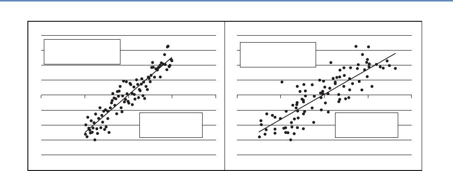
10.4. Errors in big data analytics 289
–100 –50
No errors regression
Rx = 1.0
Intercept = –0.61
Slope = 1.05
50 100 –100 –50
Regression with error
Rx = 0.73
Intercept = –2.51
Slope = 0.77
50 100
Figure 10.6. Regression of yon xwith and without variable error. On the left is the population regression with no
error in the xvariable. On the right, variable error was added to the x-values with a reliability ratio of 0.73. Note its
attenuated slope, which is very near the theoretical value of 0.77
counterpart. Let Rxdenote the reliability ratio for x. Then
b=RxB,
where B=Pr(yr−¯y)(µr|x−¯µx)/Pr(µr|x−¯µx)2is the population slope
coefficient, with xr=µr|x+εr|x, where εr|xis the variable error with
mean 0 and variance σ2
ε|x. It can also be shown that Bias(b0)≈
B(1−Rx) ¯µx.
As an illustration of these effects, consider the regressions dis-
played in Figure 10.6, which are based upon contrived data. The
regression on the left is the population (true) regression with a slope
of 1.05 and an intercept of −0.61. The regression on the left uses
the same y- and x-values. The only difference is that normal error
was added to the x-values, resulting in a reliability ratio of 0.73. As
the theory predicted, the slope was attenuated toward 0 in direct
proportion to the reliability, Rx. As random error is added to the
x-values, reliability is reduced and the fitted slope will approach 0.
When the dependent variable, y, only is subject to variable error,
the regression deteriorates, but the expected values of the slope
and intercept coefficients are still equal to true to their population
values. To see this, suppose yr=µy|r+εy|r, where µr|ydenotes the
error-free value of yrand εr|yis the associated variable error with
variance σ2
ε|y. The regression of yon xcan now be rewritten as
µy|r=b0+bxr+er−εr|y,(10.3)
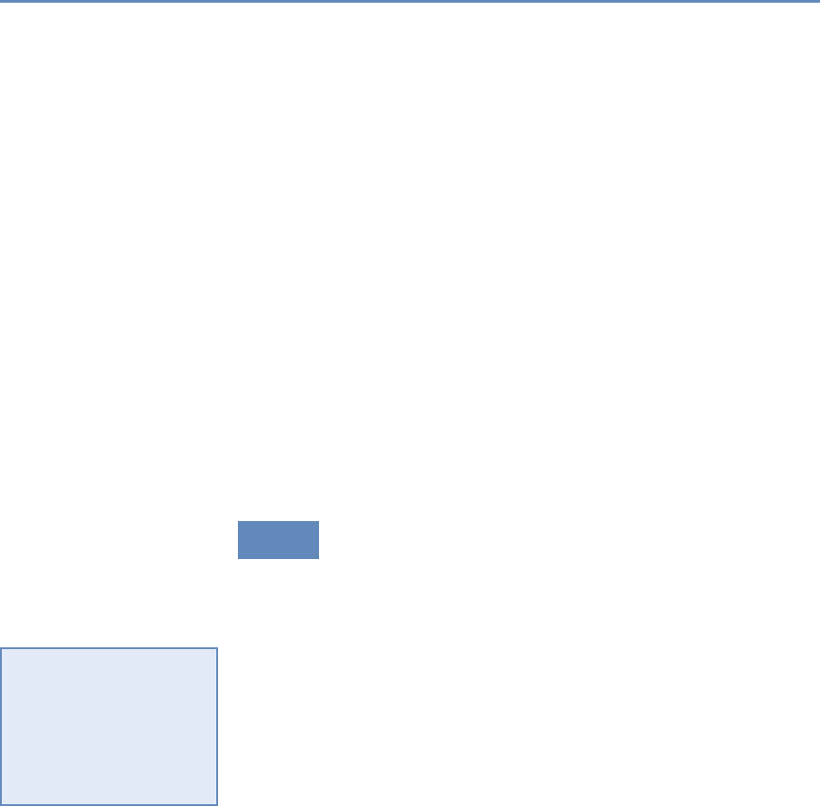
290 10. Errors and Inference
where eris the usual regression residual error with mean 0 and
variance σ2
e, which is assumed to be uncorrelated with εr|y. Letting
e′=er−εr|y, it follows that the regression in equation (10.3) is
equivalent to the previously considered regression of yon xwhere
yis not subject to error, but now the residual variance is increased
by the additive term, that is, σ′2
e=σ2
ε|y+σ2
e.
Chai [67] considers the case of systematic errors in the regres-
sion variables that may induce correlations both within and between
variables in the regression. He shows that, in the presence of sys-
tematic errors in the independent variable, the bias in the slope
coefficient may either attenuate the slope or increase its magnitude
in ways that cannot be predicted without extensive knowledge of
the error properties. Thus, like the results from correlation anal-
ysis, systematic errors greatly increase the complexity of the bias
effects and their effects on inference can be quite severe.
One approach for dealing with systematic error at the source
level in regression analysis is to model it using, for example, random
effects [169]. In brief, a random effects model specifies yijk =̙∗
0i+
̙xijk +εijk , where ε′
ijk =bi+εijk and Var(ε′
ijk )=σ2
b+σ2
ε|j. The next section
considers other mitigation strategies that attempt to eliminate the
error rather than model it.
10.5 Some methods for mitigating, detecting,
and compensating for errors
For survey data and other designed data collections, error mitiga-
tion begins at the data generation stage by incorporating design
strategies that generate high-quality data that are at least adequate
for the purposes of the data users. For example, missing data can
◮Data errors further com-
plicate analysis and exac-
erbate the analytical prob-
lems. There are essentially
three solutions: prevention,
remediation, and the choice
of analysis methodology.
be mitigated by repeated follow-up of nonrespondents, question-
naires can be perfected through pretesting and experimentation,
interviewers can be trained in the effective methods for obtaining
highly accurate responses, and computer-assisted interviewing in-
struments can be programmed to correct errors in the data as they
are generated. For big data, the data generation process is often
outside the purview of the data collectors, as noted in Section 10.1,
and there is limited opportunity to address deficiencies in the data
generation process. This is because big data is often a by-product
of systems designed with little or no thought given to the potential
secondary uses of the data. Instead, error mitigation must neces-
sarily begin at the data processing stage, which is the focus of this
chapter, particularly with regard to data editing and cleaning.

10.5. Some methods for mitigating, detecting, and compensating for errors 291
In survey collections, data processing may involve data entry,
coding textual responses, creating new variables, editing the data,
imputing missing cells, weighting the observations, and preparing
the file, including the application of disclosure-limiting processes.
For big data, many of these same operations could be needed to
some extent, depending upon requirements of the data, its uses,
and the prevailing statutory requirements. Of all the operations
◮For example, Title 13 in
the US code is explicit in
terms of data statutory pro-
tections and—as you will
see in the next chapter—
can have substantial impact
on the quality of subsequent
inference.
comprising data processing, the area that has the greatest potential
to both alter data quality and consume vast resources is data edit-
ing. For example, Biemer and Lyberg [35] note that national statis-
tical offices may spend as much as 40% or more of their production
budgets on data editing for some surveys. Recent computer tech-
nologies have automated many formerly manual processes, which
has greatly reduced these expenditures. Nevertheless, editing re-
mains a key component of the quality improvement process for big
data. Therefore, the remainder of this chapter will discuss the issue
of editing big data.
Biemer and Lyberg [35] define data editing as a set of method-
ologies for identifying and correcting (or transforming) anomalies
in the data. It often involves verifying that various relationships
among related variables of the data set are plausible and, if they are
not, attempting to make them so. Editing is typically a rule-based
approach where rules can apply to a particular variable, a combi-
nation of variables, or an aggregate value that is the sum over all
the rows or a subset of the rows in a data set.
In small data sets, data editing usually starts as a bottom-up pro-
cess that applies various rules to the cell values—often referred to
as micro-editing. The rules specify that the values for some variable
or combinations of variables (e.g., a ratio or difference between two
values) should be within some specified range. Editing may reveal
impossible values (so-called fatal edits) as well as values that are
simply highly suspect (leading to query edits). For example, a preg-
nant male would generate a fatal edit, while a property that sold
for $500,000 in a low-income neighborhood might generate a query
edit. Once the anomalous values are identified, the process at-
tempts to deduce more accurate values based upon other variables
in the data set or, perhaps, from an external data set.
The identification of anomalies can be handled quite efficiently
and automatically using editing software. Recently, data mining
and machine learning techniques have been applied to data edit-
ing with excellent results (see Chandola et al. [69] for a review).
Tree-based methods such as classification and regression trees and
random forests are particularly useful for creating editing rules for

292 10. Errors and Inference
anomaly identification and resolution [302]. However, some human
review may be necessary to resolve the most complex situations.
For big data, the identification of data anomalies could result in
possibly billions of edit failures. Even if only a tiny proportion of
these required some form of manual review for resolution, the task
could still require the inspection of tens or hundreds of thousands of
query edits, which would be infeasible for most applications. Thus,
micro-editing must necessarily be a completely automated process
unless it can be confined to a relatively small subset of the data.
As an example, a representative (random) subset of the data set
could be edited using manual editing for purposes of evaluating
the error levels for the larger data set, or possibly to be used as a
training data set, benchmark, or reference distribution for further
processing, including recursive learning.
To complement fully automated micro-editing, big data editing
usually involves top-down or macro-editing approaches. For such
approaches, analysts and systems inspect aggregated data for con-
formance to some benchmark values or data distributions that are
known from either training data or prior experience. When unex-
pected or suspicious aggregates are identified, the analyst can “drill
down” into the data to discover and, if possible, remove the discrep-
ancy by either altering the value at the source (usually a micro-data
element) or delete the edit-failed value.
Note that an aggregate that is not flagged as suspicious in macro-
editing passes the edit and is deemed correct. However, because
serious offsetting errors can be masked by aggregation, there is no
guarantee that the elements comprising the aggregate are indeed
accurate. Recalling the discussion in Section 10.4.2.1 regarding
random noise, we know that the data may be quite noisy while
the aggregates may appear to be essentially error-free. However,
macro-editing can be an effective control for systematic errors and
egregious and some random errors that create outliers and other
data anomalies.
Given the volume, velocity, and variety of big data, even macro-
editing can be challenging when thousands of variables and billions
of records are involved. In such cases, the selective editing strategies
developed in the survey research literature can be helpful [90,136].
Using selective macro-editing, query edits are selected based upon
the importance of the variable for the analysis under study, the
severity of the error, and the cost or level of effort involved in in-
vestigating the suspicious aggregate. Thus, only extreme errors, or
less extreme errors on critical variables, would be investigated.

10.5. Some methods for mitigating, detecting, and compensating for errors 293
There are a variety of methods that may be effective in macro-
editing. Some of these are based upon data mining [267], ma-
chine learning [78], cluster analysis [98, 162], and various data vi-
sualization tools such as treemaps [192, 342, 372] and tableplots
[312, 371, 373]. The tableplot seems particularly well suited for the
three Vs of big data and will be discussed in some detail.
Like other visualization techniques examined in Chapter 9, the
tableplot has the ability to summarize a large multivariate data set
in a single plot [246]. In editing big data, it can be used to de-
tect outliers and unusual data patterns. Software for implementing
this technique has been written in R and is available without cost
from the Comprehensive R Archive Network (https://cran.r-project.
org/). Figure 10.7 shows an example. The key idea is that micro-
aggregates of two related variables should have similar data pat-
terns. Inconsistent data patterns may signal errors in one of the
aggregates that can be investigated and corrected in the editing
process to improve data quality. The tableplot uses bar charts cre-
ated for the micro-aggregates to identify these inconsistent data
patterns.
Each column in the tableplot represents some variable in the
data table, and each row is a “bin” containing a subset of the data.
A statistic such as the mean or total is computed for the values in
a bin and is displayed as a bar (for continuous variables) or as a
stacked bar for categorical variables.
The sequence of steps typically involved in producing a tableplot
is as follows:
1. Sort the records in the data set by the key variable.
2. Divide the sorted data set into Bbins containing the same
number of rows.
3. For continuous variables, compute the statistic to be compared
across variables for each row bin, say Tb, for b=1, . . . , B, for
each continuous variable, V, ignoring missing values. The
level of missingness for Vmay be represented by the color or
brightness of the bar. For categorical variables with Kcate-
gories, compute the proportion in the kth category, denoted by
Pbk. Missing values are assigned to a new (K+1)th category
(“missing”).
4. For continuous variables, plot the Bvalues Tbas a bar chart.
For categorical variables, plot the Bproportions Pbk as a
stacked bar chart.
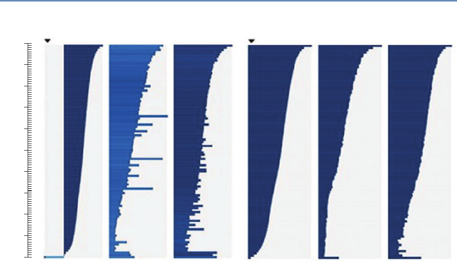
294 10. Errors and Inference
0%
90%
80%
70%
60%
40%
50%
30%
20%
10%
100%
Unedited Edited
log(Turnover) log(Employees) log(Personnel costs) log(Turnover) log(Employees) log(Personnel costs)
Figure 10.7. Comparison of tableplots for the Dutch Structural Business Statistics Survey for five variables before
and after editing. Row bins with high missing and unknown numeric values are represented by lighter colored bars
Typically, Tbis the mean, but other statistics such as the median
or range could be plotted if they aid in the outlier identification
process. For highly skewed distributions, Tennekes and de Jonge
[372] suggest transforming Tbby the log function to better capture
the range of values in the data set. In that case, negative values can
be plotted as log(−Tb)to the left of the origin and zero values can
be plotted on the origin line. For categorical variables, each bar in
the stack should be displayed using contrasting colors so that the
divisions between categories are apparent.
Tableplots appear to be well suited for studying the distributions
of variable values, the correlation between variables, and the occur-
rence and selectivity of missing values. Because they can help vi-
sualize massive, multivariate data sets, they seem particularly well
suited for big data. Currently, the R implementation of tableplot is
limited to 2 billion records.

10.6. Summary 295
The tableplot in Figure 10.7 is taken from Tennekes and de
Jonge [372] for the annual Dutch Structural Business Statistics
survey, a survey of approximately 58,000 business units annually.
Topics covered in the questionnaire include turnover, number of
employed persons, total purchases, and financial results. Figure
10.7 was created by sorting on the first column, viz., log(turnover),
and dividing the 57,621 observed units into 100 bins, so that each
row bin contains approximately 576 records. To aid the compar-
isons between unedited and edited data, the two tableplots are dis-
played side by side, with the unedited graph on the left and the
edited graph on the right. All variables were transformed by the log
function.
The unedited tableplot reveals that all four of the variables in
the comparison with log(turnover) show some distortion by large
values for some row bins. In particular, log(employees) has some
fairly large nonconforming bins with considerable discrepancies. In
addition, that variable suffers from a large number of missing val-
ues, as indicated by the brightness of the bar color. All in all, there
are obvious data quality issues in the unprocessed data set for all
four of these variables that should be dealt with in the subsequent
processing steps.
The edited tableplot reveals the effect of the data checking and
editing strategy used in the editing process. Notice the much darker
color for the number of employees for the graph on the left compared
to same graph on the right. In addition, the lack of data in the
lowest part of the turnover column has been somewhat improved.
The distributions for the graph on the right appear smoother and
are less jagged.
10.6 Summary
This review of big data errors should dispel the misconception that
the volume of the data can somehow compensate for other data
deficiencies. To think otherwise is big data “hubris,” according to
Lazer et al. [230]. In fact, the errors in big data are at least as severe
and impactful for data analysis as are the errors in designed data
collections. For the latter, there is a vast literature that developed
during the last century on mitigating and adjusting for the error
effects on data analysis. But for the former, the corresponding
literature is still in its infancy. While the survey literature can form
a foundation for the treatment of errors in big data, its utility is
also quite limited because, unlike for smaller data sets, it is often

296 10. Errors and Inference
quite difficult to eliminate all but the most egregious errors from big
data due to its size. Indeed, volume, velocity, and variety may be
regarded as the three curses of big data veracity.
This chapter considers only a few types of data analysis that are
common in big data analytics: classification, correlation, and re-
gression analysis. We show that even when there is veracity, big
data analytics can result in poor inference as a result of the three
Vs. These issues include noise accumulation, spurious correla-
tions, and incidental endogeneity. However, relaxing the assump-
tion of veracity compounds these inferential issues and adds many
new ones. Analytics can suffer in unpredictable ways.
One solution we propose is to clean up the data before analysis.
Another option that was not discussed is the possibility of using
analytical techniques that attempt to model errors and compensate
for them in the analysis. Such techniques include the use of latent
class analysis for classification error [34], multilevel modeling of
systematic errors from multiple sources [169], and Bayesian statis-
tics for partitioning massive data sets across multiple machines and
then combining the results [176, 335].
The BDTE perspective can be helpful when we consider using
a big data source. In the end, it is the responsibility of big data
analysts to be aware of the many limitations of the data and to take
the necessary steps to limit the effects of big data error on analytical
results.
Finally, we note that the BDTE paradigm focuses on the accu-
racy dimension of Total Quality (writ large). Accuracy may also
impinge on other quality dimensions such as timeliness, compara-
bility, coherence, and relevance that we have not considered in this
chapter. However, those other dimensions are equally important
to some consumers of big data analytics. For example, timeliness
often competes with accuracy because achieving acceptable levels
of the latter often requires greater expenditures of resources and
time. In fact, some consumers prefer analytic results that are less
accurate for the sake of timeliness. Biemer and Lyberg [35] discuss
these and other issues in some detail.
10.7 Resources
The American Association of Public Opinion Research has a number
of resources on its website [1]. See, in particular, its report on big
data [188].


Privacy and Confidentiality
Chapter 11
Stefan Bender, Ron Jarmin, Frauke Kreuter, and Julia Lane
This chapter addresses the issue that sits at the core of any study
of human beings—privacy and confidentiality. In a new field, like
the one covered in this book, it is critical that many researchers
have access to the data so that work can be replicated and built
upon—that there be a scientific basis to data science. Yet the rules
that social scientists have traditionally used for survey data, namely
anonymity and informed consent, no longer apply when data are
collected in the wild. This concluding chapter identifies the issues
that must be addressed for responsible and ethical research to take
place.
11.1 Introduction
Most big data applications in the social sciences involve data on
units such as individuals, households, and different types of busi-
ness, educational, and government organizations. Indeed, the ex-
ample running throughout this book involves data on individuals
(such as faculty and students) and organizations (such as universi-
ties and firms). In circumstances such as these, researchers must
ensure that such data are used responsibly and ethically—that the
subjects under study suffer no harm from their data being accessed,
analyzed, and reported. A clear distinction must be made between
analysis done for the public good and that done for private gain. In
practical terms, this requires that the private interests of individ-
ual privacy and data confidentiality be balanced against the social
benefits of research access and use.
Privacy “encompasses not only the famous ‘right to be left alone,’
or keeping one’s personal matters and relationships secret, but also
the ability to share information selectively but not publicly” [287].
299

300 11. Privacy and Confidentiality
Utility
Privacy
Initial
utility/privacy
frontier
Frontier after
increase in
external data
U*
P2P1
Figure 11.1. The privacy–utility tradeoff
Confidentiality is “preserving authorized restrictions on information
access and disclosure, including means for protecting personal pri-
vacy and proprietary information” [254]. Doing so is not easy—the
challenge to the research community is how to balance the risk of
providing access with the associated utility [100]. To give a sim-
ple example, if means and percentages are presented for a large
number of people, it will be difficult to infer an individual’s value
from such output, even if one knew that a certain individual or unit
contributed to the formation of that mean or percentage. However,
if those means and percentages are presented for subgroups or in
multivariate tables with small cell sizes, the risk for disclosure in-
creases [96]. As a result, the quality of data analysis is typically
degraded with the production of public use data [100].
In general, the greater the access to data and their original val-
ues, the greater the risk of reidentification for individual units. We
depict this tradeoff graphically in Figure 11.1. The concave curves
in this hypothetical example depict the technological relationship
between data utility and privacy for an organization such as a busi-
ness firm or a statistical agency. At one extreme, all information
is available to anybody about all units, and therefore high analytic
utility is associated with the data that are not at all protected. At
the other extreme, nobody has access to any data and no utility is

11.1. Introduction 301
achieved. Initially, assume the organization is on the outer frontier.
Increased external data resources (those not used by the organiza-
tion) increase the risk of reidentification. This is represented by an
inward shift of the utility/privacy frontier in Figure 11.1. Before the
increase in external data, the organization could achieve a level of
data utility U∗and privacy P1. The increase in externally available
data now means that in order to maintain utility at U∗, privacy is
reduced to P2. This simple example represents the challenge to all
organization that release statistical or analytical products obtained
from underlying identifiable data in the era of big data. As more
data become available externally, the more difficult it is to maintain
privacy.
Before the big data era, national statistical agencies had the ca-
pacity and the mandate to make dissemination decisions: they as-
sessed the risk, they understood the data user community and the
associated utility from data releases. And they had the wherewithal
to address the legal, technical, and statistical issues associated with
protecting confidentiality [377].
But in a world of big data, many once-settled issues have new
complications, and wholly new issues arise that need to be ad-
dressed, albeit under the same rubrics. The new types of data have
much greater potential utility, often because it is possible to study
small cells or the tails of a distribution in ways not possible with
small data. In fact, in many social science applications, the tails of
the distribution are often the most interesting and hardest-to-reach
parts of the population being studied; consider health care costs
for a small number of ill people [356], or economic activity such as
rapid employment growth by a small number of firms [93].
Example: The importance of activity in the tails
Spending on health care services in the United States is highly concentrated among
a small proportion of people with extremely high use. For the overall civilian
population living in the community, the latest data indicate that more than 20% of
all personal health care spending in 2009 ($275 billion) was on behalf of just 1%
of the population [333].
It is important to understand where the risk of privacy breaches
comes from. Let us assume for a moment that we conducted a
traditional small-scale survey with 1,000 respondents. The survey
contains information on political attitudes, spending and saving in

302 11. Privacy and Confidentiality
a given year, and income, as well as background variables on in-
come and education. If name and address are saved together with
this data, and someone gets access to the data, obviously it is easy
to identify individuals and gain access to information that is other-
wise not public. If the personal identifiable information (name and
address) are removed from this data file, the risk is much reduced.
If someone has access to the survey data and sees all the individual
values, it might be difficult to assess with certainty who among the
320 million inhabitants in the USA is associated with an individual
data record. However, the risk is higher if one knows some of this
information (say, income) for a person, and knows that this person
is in the survey. With these two pieces of information, it is likely
possible to uniquely identify the person in the survey data.
Big data increases the risk precisely for this reason. Much data
is available for reidentification purposes [289]. Most obviously, the
risk of reidentification is much greater because the new types of
data have much richer detail and a much larger public community
has access to ways to reidentify individuals. There are many famous
examples of reidentification occurring even when obvious personal
information, such as name and social security number, has been
removed and the data provider thought that the data were conse-
quently deidentified. In the 1990s, Massachusetts Group Insurance
released “deidentified” data on the hospital visits of state employ-
ees; researcher Latanya Sweeney quickly reidentified the hospital
records of the then Governor William Weld using nothing more
than state voter records about residence and date of birth [366].
In 2006, the release of supposedly deidentified web search data
by AOL resulted in two New York Times reports being able to rei-
dentify a customer simply from her browsing habits [26]. And in
2012, statisticians at the department store, Target, used a young
teenager’s shopping patterns to determine that she was pregnant
before her father did [166].
But there are also less obvious problems. What is the legal
framework when the ownership of data is unclear? In the past,
when data were more likely to be collected and used within the
same entity—for example, within an agency that collects adminis-
trative data or within a university that collects data for research
purposes—organization-specific procedures were (usually) in place
and sufficient to regulate the usage of these data. In a world of big
data, legal ownership is less clear.
Who has the legal authority to make decisions about permission,
access, and dissemination and under what circumstances? The
answer is often not clear. The challenge in the case of big data is

11.2. Why is access important? 303
that data sources are often combined, collected for one purpose, and
used for another. Data providers often have a poor understanding
of whether or how their data will be used.
Example: Knowledge is power
In a discussion of legal approaches to privacy in the context of big data, Strandburg
[362] says: “‘Big data’ has great potential to benefit society. At the same time,
its availability creates significant potential for mistaken, misguided or malevolent
uses of personal information. The conundrum for the law is to provide space for big
data to fulfill its potential for societal benefit, while protecting citizens adequately
from related individual and social harms. Current privacy law evolved to address
different concerns and must be adapted to confront big data’s challenges.”
It is critical to address privacy and confidentiality issues if the
full public value of big data is to be realized. This chapter high-
lights why the challenges need to be met (i.e., why access to data
is crucial), review the pre-big data past, point out challenges with
this approach in the context of big data, briefly describe the current
state of play from a legal, technical, and statistical perspective, and
point to open questions that need to be addressed in the future.
11.2 Why is access important?
This book gives detailed examples of the potential of big data to pro-
vide insights into a variety of social science questions—particularly
the relationship between investments in R&D and innovation. But
that potential is only realized if researchers have access to the
data [225]: not only to perform primary analyses but also to validate
the data generation process (in particular, data linkage), replicate
analyses, and build a knowledge infrastructure around complex
data sets.
Validating the data generating process Research designs requir-
ing a combination of data sources and/or analysis of the tails of
populations challenge the traditional paradigm of conducting sta-
tistical analysis on deidentified or aggregated data. In order to com-
bine data sets, someone in the chain that transforms raw data into
research outputs needs access to link keys contained in the data
sets to be combined. High-quality link keys uniquely identify the

304 11. Privacy and Confidentiality
subjects under study and typically are derived from items such as
individual names, birth dates, social security numbers, and busi-
ness names, addresses, and tax ID numbers. From a privacy and
confidentiality perspective, link keys are among most sensitive in-
formation in many data sets of interest to social scientists. This is
why many organizations replace link keys containing personal iden-
tifiable information (PII)*with privacy-protecting identifiers [332].
⋆PII is “any information
about an individual main-
tained by an agency, in-
cluding (1) any information
that can be used to distin-
guish or trace an individ-
ual’s identity, such as name,
social security number, date
and place of birth, mother’s
maiden name, or biometric
records; and (2) any other
information that is linked
or linkable to an individ-
ual, such as medical, edu-
cational, financial, and em-
ployment information” [254].
Regardless, at some point in the process those must be generated
out of the original information, thus access to the latter is impor-
tant.
Replication John Ioannidis has claimed that most published re-
search findings are false [184]; for example, the unsuccessful repli-
cation of genome-wide association studies, at less than 1%, is stag-
gering [29]. Inadequate understanding of coverage, incentive, and
quality issues, together with the lack of a comparison group, can re-
sult in biased analysis—famously in the case of using administrative
records on crime to make inference about the role of death penalty
policy in crime reduction [95, 234]. Similarly, overreliance on, say,
Twitter data, in targeting resources after hurricanes can lead to
the misallocation of resources towards young, Internet-savvy people
with cell phones and away from elderly or impoverished neighbor-
hoods [340], just as bad survey methodology led the Literary Digest
to incorrectly call the 1936 election [353]. The first step to repli-
cation is data access; such access can enable other researchers to
ascertain whether the assumptions of a particular statistical model
are met, what relevant information is included or excluded, and
whether valid inferences can be drawn from the data [215].
Building knowledge infrastructure Creating a community of prac-
tice around a data infrastructure can result in tremendous new
insights, as the Sloan Digital Sky Survey and the Polymath project
have shown [281]. In the social science arena, the Census Bu-
reau has developed a productive ecosystem that is predicated on
access to approved external experts to build, conduct research us-
ing, and improve key data assets such as the Longitudinal Busi-
ness Database [190] and Longitudinal Employer Household Dy-
namics [4], which have yielded a host of new data products and
critical policy-relevant insights on business dynamics [152] and la-
bor market volatility [55], respectively. Without providing robust,
but secure, access to confidential data, researchers at the Census
Bureau would have been unable to undertake the innovations that

11.3. Providing access 305
made these new products and insights possible.
11.3 Providing access
The approaches to providing access have evolved over time. Sta-
tistical agencies often employ a range of approaches depending on
the needs of heterogeneous data users [96, 126]. Dissemination
of data to the public usually occurs in three steps: an evaluation
of disclosure risks, followed by the application of an anonymiza-
tion technique, and finally an evaluation of disclosure risks and
analytical quality of the candidate data release(s). The two main
approaches have been statistical disclosure control techniques to
produce anonymized public use data sets, and controlled access
through a research data center.
Statistical disclosure control techniques Statistical agencies have
made data available in a number of ways: through tabular data,
public use files, licensing agreements and, more recently, through
synthetic data [317]. Hundepool et al. [174] define statistical dis-
closure control as follows:
concepts and methods that ensure the confidentiality of
micro and aggregated data that are to be published. It is
methodology used to design statistical outputs in a way
that someone with access to that output cannot relate a
known individual (or other responding unit) to an element
in the output.
Traditionally, confidentiality protection has been accomplished
by releasing only aggregated tabular data. This practice works well
in settings where the primary purpose is enumeration, such as cen-
sus taking. However, tabular data are poorly suited to describing
the underlying distributions and covariance across variables that
are often the focus of applied social science research [100].
To provide researchers access to data that permitted analysis
of the underlying variance–covariance structure of the data, some
agencies have constructed public use micro-data samples. To prod-
uct confidentiality in such public use files, a number of statisti-
cal disclosure control procedures are typically applied. These in-
clude stripping all identifying (e.g., PII) fields from the data, topcod-
ing highly skewed variables (e.g., income), and swapping records
[96,413]. However, the mosaic effect—where disparate pieces of in-
formation can be combined to reidentify individuals—dramatically

306 11. Privacy and Confidentiality
increases the risk of releasing public use files [88]. In addition,
there is more and more evidence that the statistical disclosure pro-
cedure applied to produce them decreases their utility across many
applications [58].
Some agencies provide access to confidential micro-data through
licensing arrangements. A contract specifies the conditions of use
and what safeguards must be in place. In some cases, the agency
has the authority to conduct random inspections. However, this
approach has led to a number of operational challenges, including
version control, identifying and managing risky researcher behavior,
and management costs [96].
More recently, synthetic data have been created whereby key
features of the original data are preserved but the original data are
replaced by results from estimations (synthetic data) so that no in-
dividual or business entity can be found in the released data [97].
Two examples of synthetic data sets are the SIPP Synthetic-Beta [5]
of linked Survey of Income and Program Participation (SIPP) and So-
cial Security Administration earnings data, and the Synthetic Lon-
gitudinal Business Database (SynLBD) [207]. Jarmin et al. [189]
discuss how synthetic data sets lack utility in many research set-
tings but are useful for generating flexible data sets underlying data
tools and apps such as the Census Bureau’s OnTheMap.
Research data centers The second approach is establishing re-
search data centers. Here, qualified researchers gain access to
micro-level data after they are sworn in to protect the confiden-
tially of the data they access. Strong input and output controls
are in place to ensure that published findings comply with the pri-
vacy and confidentiality regulations [161]. Some RDCs allow access
through remote execution, where no direct access to the data is al-
lowed, but it is not necessary to travel; others allow remote direct
access.
11.4 The new challenges
While there are well-established policies and protocols surrounding
access to and use of survey and administrative data, a major new
challenge is the lack of clear guidelines governing the collection of
data about human activity in a world in which all public, and some
private, actions generate data that can be harvested [287,289,362].
The twin pillars on which so much of social science have rested—
informed consent and anonymization—are virtually useless in a big

11.4. The new challenges 307
data setting where multiple data sets can be and are linked together
using individual identifiers by a variety of players beyond social sci-
entists with formal training and whose work is overseen by institu-
tional review boards. This rapid expansion in data and their use is
very much driven by the increased utility of the linked information
to businesses, policymakers, and ultimately the taxpayer. In addi-
tion, there are no obvious data stewards and custodians who can
be entrusted with preserving the privacy and confidentiality with
regard to both the source data collected from sensors, social media,
and many other sources, and the related analyses [226].
It is clear that informed consent as historically construed is no
longer feasible. As Nissenbaum [283] points out, notification is ei-
ther comprehensive or comprehensible, but not both. While ideally
human subjects are offered true freedom of choice based on a sound
and sufficient understanding of what the choice entails, in reality
the flow of data is so complex and the interest in the data usage
so diverse that simplicity and clarity in the consent statement un-
avoidably result in losses of fidelity, as anyone who has accepted a
Google Maps agreement is likely to understand [160]. In addition,
informed consent requires a greater understanding of the breadth
of type of privacy breaches, the nature of harm as diffused over
time, and an improved valuation of privacy in the big data con-
text. Consumers may value their own privacy in variously flawed
ways. They may, for example, have incomplete information, or an
overabundance of information rendering processing impossible, or
use heuristics that establish and routinize deviations from rational
decision-making [6].
It is also nearly impossible to anonymize data. Big data are
often structured in such a way that essentially everyone in the file
is unique, either because so many variables exist or because they
are so frequent or geographically detailed, that they make it easy
to reidentify individual patterns [266]. It is also no longer possible
to rely on sampling or measurement error in external files as a
buffer for data protection, since most data are not in the hands of
statistical agencies.
There are no data stewards controlling access to individual data.
Data are often so interconnected (think social media network data)
that one person’s action can disclose information about another
person without that person even knowing that their data are be-
ing accessed. The group of students posting pictures about a beer
party is an obvious example, but, in a research context, if the prin-
cipal investigator grants access to the proposal, information could
be divulged about colleagues and students. In other words, volun-

308 11. Privacy and Confidentiality
teered information of a minority of individuals can unlock the same
information about many—a type of “tyranny of the minority” [28].
There are particular issues raised by the new potential to link
information based on a variety of attributes that do not include PII.
Barocas and Nissenbaum write as follows [27]:
Rather than attempt to deanonymize medical records, for
instance, an attacker (or commercial actor) might instead
infer a rule that relates a string of more easily observable
or accessible indicators to a specific medical condition,
rendering large populations vulnerable to such inferences
even in the absence of PII. Ironically, this is often the
very thing about big data that generate the most excite-
ment: the capacity to detect subtle correlations and draw
actionable inferences. But it is this same feature that
renders the traditional protections afforded by anonymity
(again, more accurately, pseudonymity) much less effec-
tive.
In light of these challenges, Barocas and Nissenbaum continue
the value of anonymity inheres not in namelessness, and
not even in the extension of the previous value of name-
lessness to all uniquely identifying information, but in-
stead to something we called “reachability,” the possi-
bility of knocking on your door, hauling you out of bed,
calling your phone number, threatening you with sanc-
tion, holding you accountable—with or without access to
identifying information.
It is clear that the concepts used in the larger discussion of
privacy and big data require updating. How we understand and
assess harms from privacy violations needs updating. And we must
rethink established approaches to managing privacy in the big data
context. The next section discusses the framework for doing so.
11.5 Legal and ethical framework
The Fourth Amendment to the US Constitution, which constrains
the government’s power to “search” the citizenry’s “persons, houses,
papers, and effects” is usually cited as the legal framework for pri-
vacy and confidentiality issues. In the US a “sectoral” approach to
privacy regulation, for example, the Family Education Rights and

11.5. Legal and ethical framework 309
Privacy Act and the Health Insurance Portability and Accountability
Act, is also used in situations where different economic areas have
separate privacy laws [290]. In addition, current legal restrictions
and guidance on data collection in the industrial setting include the
Fair Information Practice Principles dating from 1973 and underly-
ing the Fair Credit Reporting Act from 1970 and the Privacy Act from
1974 [362]. Federal agencies often have statutory oversight, such
as Title 13 of the US Code for the Census Bureau, the Confiden-
tial Information Protection and Statistical Efficiency Act for federal
statistical agencies, and Title 26 of the US Code for the Internal
Revenue Service.
Yet the generation of big data often takes place in the open, or
through commercial transactions with a business, and hence is not
covered by these frameworks. There are major questions as to what
is reasonably private and what constitutes unwarranted intrusion
[362]. There is a lack of clarity on who owns the new types of data—
whether it is the person who is the subject of the information, the
person or organization who collects these data (the data custodian),
the person who compiles, analyzes, or otherwise adds value to the
information, the person who purchases an interest in the data, or
society at large. The lack of clarity is exacerbated because some
laws treat data as property and some treat it as information [65].
The ethics of the use of big data are also not clear, because
analysis may result in being discriminately against unfairly, being
limited in one’s life choices, being trapped inside stereotypes, being
unable to delineate personal boundaries, or being wrongly judged,
embarrassed, or harassed. There is an entire research agenda to be
pursued that examines the ways that big data may threaten inter-
ests and values, distinguishes the origins and nature of threats to
individual and social integrity, and identifies different solutions [48].
The approach should be to describe what norms and expectations
are likely to be violated if a person agrees to provide data, rather
than to describe what will be done during the research.
What is clear is that most data are housed no longer in sta-
tistical agencies, with well-defined rules of conduct, but in busi-
nesses or administrative agencies. In addition, since digital data
can be alive forever, ownership could be claimed by yet-to-be-born
relatives whose personal privacy could be threatened by release of
information about blood relations.
Traditional regulatory tools for managing privacy, notice, and
consent have failed to provide a viable market mechanism allowing
a form of self-regulation governing industry data collection. Going
forward, a more nuanced assessment of tradeoffs in the big data

310 11. Privacy and Confidentiality
context, moving away from individualized assessments of the costs
of privacy violations, is needed [362]. Ohm advocates for a new
conceptualization of legal policy regarding privacy in the big data
context that uses five guiding principles for reform: first, that rules
take into account the varying levels of inherent risk to individuals
across different data sets; second, that traditional definitions of PII
need to be rethought; third, that regulation has a role in creating
and policing walls between data sets; fourth, that those analyzing
big data must be reminded, with a frequency in proportion to the
sensitivity of the data, that they are dealing with people; and fi-
nally, that the ethics of big data research must be an open topic for
continual reassessment.
11.6 Summary
The excitement about how big data can change the social science re-
search paradigm should be tempered by a recognition that existing
ways of protecting confidentiality are no longer viable [203]. There
is a great deal of research that can be used to inform the develop-
ment of such a structure, but it has been siloed into disconnected
research areas, such as statistics, cybersecurity, and cryptography,
as well as a variety of different practical applications, including the
successful development of remote access secure data enclaves. We
must piece together the knowledge from these various fields to de-
velop ways in which vast new sets of data on human beings can be
collected, integrated, and analyzed while protecting them [227].
It is possible that the confidentiality risks of disseminating data
may be so high that traditional access models will no longer hold;
that the data access model of the future will be to take the analysis
to the data rather than the data to the analyst or the analyst to the
data. One potential approach is to create an integrated system in-
cluding (a) unrestricted access to highly redacted data, most likely
some version of synthetic data, followed by (b) means for approved
researchers to access the confidential data via remote access so-
lutions, combined with (c) verification servers that allows users to
assess the quality of their inferences with the redacted data so as
to be more efficient with their use (if necessary) of the remote data
access. Such verification servers might be a web-accessible system
based on a confidential database with an associated public micro-
data release, which helps to analyze the confidential database [203].
Such approaches are starting to be developed, both in the USA and
in Europe [106,193].

11.7. Resources 311
There is also some evidence that people do not require complete
protection, and will gladly share even private information provided
that certain social norms are met [300, 403]. There is a research
agenda around identifying those norms as well; characterizing the
interests and wishes of actors (the information senders and recipi-
ents or providers and users); the nature of the attributes (especially
types of information about the providers, including how these might
be transformed or linked); and identifying transmission principles
(the constraints underlying the information flows).
However, it is likely that it is no longer possible for a lone social
scientist to address these challenges. One-off access agreements to
individuals are conducive to neither the production of high-quality
science nor the high-quality protection of data [328]. The curation,
protection, and dissemination of data on human subjects cannot
be an artisan activity but should be seen as a major research in-
frastructure investment, like investments in the physical and life
sciences [3, 38, 173]. In practice, this means that linkages become
professionalized and replicable, research is fostered within research
data centers that protect privacy in a systematic manner, knowledge
is shared about the process of privacy protections disseminated in
a professional fashion, and there is ongoing documentation about
the value of evidence-based research. It is thus that the risk–utility
tradeoff depicted in Figure 11.1 can be shifted in a manner that
serves the public good.
11.7 Resources
The American Statistical Association’s Privacy and Confidentiality
website provides a useful source of information [12].
An overview of federal activities is provided by the Confidentiality
and Data Access Committee of the Federal Committee on Statistics
and Methodology [83].
The World Bank and International Household Survey Network
provide a good overview of data dissemination “best practices” [183].
There is a Journal of Privacy and Confidentiality based at Carnegie
Mellon University [195], and also a journal called Transactions in
Data Privacy [370].
The United Nations Economic Commission on Europe hosts work-
shops and conferences and produces occasional reports [382].

Workbooks
Chapter 12
Jonathan Scott Morgan, Christina Jones, and Ahmad Emad
This final chapter provides an overview of the Python workbooks
that accompany each chapter. These workbooks combine text ex-
planation and code you can run, implemented in Jupyter note- ◮See jupyter.org.
books, to explain techniques and approaches selected from each
chapter and to provide thorough implementation details, enabling
students and interested practitioners to quickly get up to speed on
and start using the technologies covered in the book. We hope you
have a lot of fun with them.
12.1 Introduction
We provide accompanying Juptyer IPython workbooks for most
chapters in this book. These workbooks explain techniques and
approaches selected from each chapter and provide thorough im-
plementation details so that students and interested practitioners
can quickly start using the technologies covered within.
The workbooks and related files are stored in the Big-Data- ◮github.com/
BigDataSocialScience
Workbooks GitHub repository, and so are freely available to be
downloaded by anyone at any time and run on any appropriately
configured computer. These workbooks are a live set of documents
that could potentially change over time, so see the repository for the
most recent set of information.
These workbooks provide a thorough overview of the work needed
to implement the selected technologies. They combine explanation,
basic exercises, and substantial additional Python code to provide a
conceptual understanding of each technology, give insight into how
key parts of the process are implemented through exercises, and
then lay out an end-to-end pattern for implementing each in your
own work. The workbooks are implemented using IPython note-
313

314 12. Workbooks
books, interactive documents that mix formatted text and Python
code samples that can be edited and run in real time in a Jupyter
notebook server, allowing you to run and explore the code for each
technology as you read about it.
12.2 Environment
The Big-Data-Workbooks GitHub repository provides two different
types of workbooks, each needing a different Python setup to run.
The first type of workbooks is intended to be downloaded and
run locally by individual users. The second type is designed to
be hosted, assigned, worked on, and graded on a single server,
using jupyterhub (https://github.com/jupyter/jupyterhub) to host
and run the notebooks and nbgrader (https://github.com/jupyter/
nbgrader) to assign, collect, and grade.
The text, images, and Python code in the workbooks are the same
between the two versions, as are the files and programs needed to
complete each.
The differences in the workbooks themselves relate to the code
cells within each notebook where users implement and test exer-
cises. In the workbooks intended to be used locally, exercises are
implemented in simple interactive code cells. In the nbgrader ver-
sions, these cells have additional metadata and contain the solu-
tions for the exercises, making them a convenient answer key even
if you are working on them locally.
12.2.1 Running workbooks locally
To run workbooks locally, you will need to install Python on your
system, then install ipython, which includes a local Jupyter server
you can use to run the workbooks. You will also need to install
additional Python packages needed by the workbooks, and a few
additional programs.
The easiest way to get this all working is to install the free
Anaconda Python distribution provided by Continuum Analytics
(https://www.continuum.io/downloads). Anaconda includes a Jupyter
server and precompiled versions of many packages used in the
workbooks. It includes multiple tools for installing and updating
both Python and installed packages. It is separate from any OS-
level version of Python, and is easy to completely uninstall.
Anaconda also works on Windows as it does on Mac and Linux.
Windows is a much different operating system from Apple’s OS X

12.3. Workbook details 315
and Unix/Linux, and Python has historically been much trickier
to install, configure, and use on Windows. Packages are harder to
compile and install, the environment can be more difficult to set
up, etc. Anaconda makes Python easier to work with on any OS,
and on Windows, in a single run of the Anaconda installer, it inte-
grates Python and common Python utilities like pip into Windows
well enough that it approximates the ease and experience of using
Python within OS X or Unix/Linux (no small feat).
You can also create your Python environment manually, in-
stalling Python, package managers, and Python packages sepa-
rately. Packages like numpy and pandas can be difficult to get work-
ing, however, particularly on Windows, and Anaconda simplifies
this setup considerably regardless of your OS.
12.2.2 Central workbook server
Setting up a server to host workbooks managed by nbgrader is more
involved. Some of the workbooks consume multiple gigabytes of
memory per user and substantial processing power. A hosted im-
plementation where all users work on a single server requires sub-
stantial hardware, relatively complex configuration, and ongoing
server maintenance. Detailed instructions are included in the Big-
Data-Workbooks GitHub repository. It is not rocket science, but it
is complicated, and you will likely need an IT professional to help
you set up, maintain, and troubleshoot. Since all student work
will be centralized in this one location, you will also want a robust,
multi-destination backup plan.
For more information on installing and running the workbooks
that accompany this book, see the Big-Data-Workbooks GitHub
repository.
12.3 Workbook details
Most chapters have an associated workbook, each in its own direc-
tory in the Big-Data-Workbooks GitHub repository. Below is a list
of the workbooks, along with a short summary of the topics that
each covers.
12.3.1 Social Media and APIs
The Social Media and APIs workbook introduces you to the use
of Internet-based web service APIs for retrieving data from online

316 12. Workbooks
data stores. Examples include retrieving information on articles
from Crossref (provider of Digital Object Identifiers used as unique
IDs for publications) and using the PLOS Search and ALM APIs to
retrieve information on how articles are shared and referenced in
social media, focusing on Twitter. In this workbook, you will learn
how to:
•Set up user API keys,
•Connect to Internet-based data stores using APIs,
•Collect DOIs and Article-Level Metrics data from web APIs,
•Conduct basic analysis of publication data.
12.3.2 Database basics
In the Database workbook you will learn the practical benefits that
stem from using a database management system. You will imple-
ment basic SQL commands to query grants, patents, and vendor
data, and thus learn how to interact with data stored in a rela-
tional database. You will also be introduced to using Python to
execute and interact with the results of SQL queries, so you can
write programs that interact with data stored in a database. In this
workbook, you will learn how to:
•Connect to a database through Python,
•Query the database by using SQL in Python,
•Begin to understand to the SQL query language,
•Close database connections.
12.3.3 Data Linkage
In the Data Linkage workbook you will use Python to clean input
data, including using regular expressions, then learn and imple-
ment the basic concepts behind the probabilistic record linkage: us-
ing different types of string comparators to compare multiple pieces
of information between two records to produce a score that indicates
how likely it is that the records are data about the same underlying
entity. In this workbook, you will learn how to:
•Parse a name string into first, middle, and last names using
Python’s split method and regular expressions,

12.3. Workbook details 317
•Use and evaluate the results of common computational
string comparison algorithms including Levenshtein distance,
Levenshtein–Damerau distance, and Jaro–Winkler distance,
•Understand the Fellegi–Sunter probabilistic record linkage
method, with step-by-step implementation guide.
12.3.4 Machine Learning
In the Machine Learning workbook you will train a machine learn-
ing model to predict missing information, working through the pro-
cess of cleaning and prepping data for training and testing a model,
then training and testing a model to impute values for a missing
categorical variable, predicting the academic department of a given
grant’s primary investigator based on other traits of the grant. In
this workbook, you will learn how to:
•Read, clean, filter, and store data with Python’s pandas data
analysis package,
•Recognize the types of data cleaning and refining needed to
make data more compatible with machine learning models,
•Clean and refine data,
•Manage memory when working with large data sets,
•Employ strategies for dividing data to properly train and test a
machine learning model,
•Use the scikit-learn Python package to train, fit, and evalu-
ate machine learning models.
12.3.5 Text Analysis
In the Text Analysis workbook, you will derive a list of topics from
text documents using MALLET, a Java-based tool that analyzes
clusters of words across a set of documents to derive common top-
ics within the documents, defined by sets of key words that are
consistently used together. In this workbook, you will learn how to:
•Clean and prepare data for automated text analysis,
•Set up data for use in MALLET,
•Derive a set of topics from a collection of text documents,

318 12. Workbooks
•Create a model that detects these topics in documents, and
use this model to categorize documents.
12.3.6 Networks
In the Networks workbook you will create network data where the
nodes are researchers who have been awarded grants, and ties are
created between each researcher on a given grant. You will use
Python to read the grant data and translate them into network data,
then use the networkx Python library to calculate node- and graph-
level network statistics and igraph to create and refine network
visualizations. You will also be introduced to graph databases, an
alternative way of storing and querying network data. In this work-
book, you will learn how to:
•Develop strategies for detecting potential network data in rela-
tional data sets,
•Use Python to derive network data from a relational database,
•Store and query network data using a graph database like
neo4j,
•Load network data into networkx, then use it to calculate node-
and graph-level network statistics,
•Use networkx to export graph data into commonly shared for-
mats (graphml, edge lists, different tabular formats, etc.),
•Load network data into the igraph Python package and then
create graph visualizations.
12.3.7 Visualization
The Visualization workbook introduces you to Tableau, a data anal-
ysis and visualization software package that is easy to learn and
use. Tableau allows you to connect to and integrate multiple data
sources into complex visualizations without writing code. It allows
you to dynamically shift between views of data to build anything
from single visualizations to an interactive dashboard that contains
multiple views of your data. In this workbook, you will learn how
to:
•Connect Tableau to a relational database,
•Interact with Tableau’s interface,

12.4. Resources 319
•Select, combine, and filter the tables and columns included in
visualizations,
•Create bar charts, timeline graphs, and heat maps,
•Group and aggregate data,
•Create a dashboard that combines multiple views of your data.
12.4 Resources
We noted in Section 1.8 the importance of Python, MySQL, and Git/
GitHub for the social scientist who intends to work with large data.
See that section for pointers to useful online resources, and also this
book’s website, at https://github.com/BigDataSocialScience, where
we have collected many useful web links, including the following.
For more on getting started with Anaconda, see Continuum’s
Anaconda documentation [13], Anaconda FAQ [14], and Anaconda
quick start guide [15].
For more information on IPython and the Jupyter notebook server,
see the IPython site [186], IPython documentation [185], Jupyter
Project site [197], and Jupyter Project documentation [196].
For more information on using jupyterhub and nbgrader to host,
distribute, and grade workbooks using a central server, see the
jupyterhub GitHub repository [198], jupyterhub documentation [199],
nbgrader GitHub repository [201], and nbgrader documentation [200].


Bibliography
[1] AAPOR. American association for public opinion research website. http://
www.aapor.org. Accessed February 1, 2016.
[2] Daniel Abadi, Rakesh Agrawal, Anastasia Ailamaki, Magdalena Balazinska,
Philip A Bernstein, Michael J Carey, Surajit Chaudhuri, Jeffrey Dean, An-
Hai Doan, Michael J Franklin, et al. The Beckman Report on Database
Research. ACM SIGMOD Record, 43(3):61–70, 2014. http://beckman.cs.
wisc.edu/beckman-report2013.pdf.
[3] Kevork N. Abazajian, Jennifer K. Adelman-McCarthy, Marcel A. Agüeros,
Sahar S. Allam, Carlos Allende Prieto, Deokkeun An, Kurt S. J. Anderson,
Scott F. Anderson, James Annis, Neta A. Bahcall, et al. The seventh data
release of the Sloan Digital Sky Survey. Astrophysical Journal Supplement
Series, 182(2):543, 2009.
[4] John M. Abowd, John Haltiwanger, and Julia Lane. Integrated longitudinal
employer-employee data for the United States. American Economic Review,
94(2):224–229, 2004.
[5] John M. Abowd, Martha Stinson, and Gary Benedetto. Final report to the
Social Security Administration on the SIPP/SSA/IRS Public Use File Project.
Technical report, Census Bureau, Longitudinal Employer-Household Dy-
namics Program, 2006.
[6] Alessandro Acquisti. The economics and behavioral economics of privacy.
In Julia Lane, Victoria Stodden, Stefan Bender, and Helen Nissenbaum,
editors, Privacy, Big Data, and the Public Good: Frameworks for Engagement,
pages 98–112. Cambridge University Press, 2014.
[7] Christopher Ahlberg, Christopher Williamson, and Ben Shneiderman. Dy-
namic queries for information exploration: An implementation and evalua-
tion. In Proceedings of the SIGCHI Conference on Human Factors in Computing
Systems, pages 619–626. ACM, 1992.
[8] Suha Alawadhi, Armando Aldama-Nalda, Hafedh Chourabi, J. Ramon Gil-
Garcia, Sofia Leung, Sehl Mellouli, Taewoo Nam, Theresa A. Pardo, Hans J.
Scholl, and Shawn Walker. Building understanding of smart city initiatives.
In Electronic Government, pages 40–53. Springer, 2012.
[9] Ed Albanese. Scaling social science with Hadoop. http://blog.cloudera.com/
blog/2010/04/scaling-social-science-with-hadoop/. Accessed February 1,
2016.
321

322 BIBLIOGRAPHY
[10] Paul D Allison. Missing Data. Sage Publications, 2001.
[11] Amazon. AWS public data sets. http://aws.amazon.com/datasets.
[12] American Statistical Association. ASA Privacy and Confidentiality Subcom-
mittee. http://community.amstat.org/cpc/home.
[13] Continuum Analytics. Anaconda. http://docs.continuum.io/anaconda. Ac-
cessed February 1, 2016.
[14] Continuum Analytics. Anaconda FAQ. http://docs.continuum.io/
anaconda/faq. Accessed February 1, 2016.
[15] Continuum Analytics. Anaconda quick start guide. https://
www.continuum.io/sites/default/files/Anaconda-Quickstart.pdf. Accessed
February 1, 2016.
[16] Francis J. Anscombe. Graphs in statistical analysis. American Statistician,
27(1):17–21, 1973.
[17] Dolan Antenucci, Michael Cafarella, Margaret Levenstein, Christopher Ré,
and Matthew D. Shapiro. Using social media to measure labor market flows.
Technical report, National Bureau of Economic Research, 2014.
[18] Apache Software Foundation. Apache ambari. http://ambari.apache.org.
Accessed February 1, 2016.
[19] Apache Software Foundation. Apache Hadoop documentation site. https://
hadoop.apache.org/docs/current/. Accessed February 1, 2016.
[20] Apache Software Foundation. Apache Spark documentation site. https://
spark.apache.org/docs/current/. Accessed February 1, 2016.
[21] Michael Armbrust, Armando Fox, Rean Griffith, Anthony D. Joseph, Randy
Katz, Andy Konwinski, Gunho Lee, David Patterson, Ariel Rabkin, Ion Stoica,
et al. A view of cloud computing. Communications of the ACM, 53(4):50–58,
2010.
[22] Art Branch Inc. SQL Cheatsheet. http://www.sql-tutorial.net/
SQL-Cheat-Sheet.pdf. Accessed December 1, 2015.
[23] Eric Baldeschwieler. Best practices for selecting Apache
Hadoop hardware. Hortonworks, http://hortonworks.com/blog/
best-practices-for-selecting-apache-hadoop-hardware/, September 1,
2011.
[24] Anita Bandrowski, Matthew Brush, Jeffery S. Grethe, Melissa A. Haendel,
David N. Kennedy, Sean Hill, Patrick R. Hof, Maryann E Martone, Maaike
Pols, Serena S. Tan, et al. The Resource Identification Initiative: A cultural
shift in publishing. Brain and Behavior, 2015.
[25] Albert-László Barabási and Réka Albert. Emergence of scaling in random
networks. Science, 286(5439):509–512, 1999.
[26] Michael Barbaro, Tom Zeller, and Saul Hansell. A face is exposed for AOL
searcher no. 4417749. New York Times, August 9, 2006.

BIBLIOGRAPHY 323
[27] Solon Barocas and Helen Nissenbaum. Big data’s end run around procedural
privacy protections. Communications of the ACM, 57(11):31–33, 2014.
[28] Solon Barocas and Helen Nissenbaum. The limits of anonymity and consent
in the big data age. In Julia Lane, Victoria Stodden, Stefan Bender, and Helen
Nissenbaum, editors, Privacy, Big Data, and the Public Good: Frameworks
for Engagement. Cambridge University Press, 2014.
[29] Hilda Bastian. Bad research rising: The 7th Olympiad of re-
search on biomedical publication. Scientific American, http://blogs.
scientificamerican.com/absolutely-maybe/bad-research-rising-the-7th
-olympiad-of-research-on-biomedical-publication/, 2013.
[30] Vladimir Batagelj and Andrej Mrvar. Pajek—program for large network anal-
ysis. Connections, 21(2):47–57, 1998.
[31] Alex Bell. Python for economists. http://cs.brown.edu/~ambell/pyseminar/
pyseminar.html, 2012.
[32] Krithika Bhuvaneshwar, Dinanath Sulakhe, Robinder Gauba, Alex Ro-
driguez, Ravi Madduri, Utpal Dave, Lukasz Lacinski, Ian Foster, Yuriy Gu-
sev, and Subha Madhavan. A case study for cloud based high throughput
analysis of NGS data using the Globus Genomics system. Computational
and Structural Biotechnology Journal, 13:64–74, 2015.
[33] Paul P. Biemer. Total survey error: Design, implementation, and evaluation.
Public Opinion Quarterly, 74(5):817–848, 2010.
[34] Paul P. Biemer. Latent Class Analysis of Survey Error. John Wiley & Sons,
2011.
[35] Paul P. Biemer and Lars E. Lyberg. Introduction to Survey Quality. John
Wiley & Sons, 2003.
[36] Paul P. Biemer and S. L. Stokes. Approaches to modeling measurement error.
In Paul P. Biemer, R. Groves, L. Lyberg, N. Mathiowetz, and S. Sudman,
editors, Measurement Errors in Surveys, pages 54–68. John Wiley, 1991.
[37] Paul P. Biemer and Dennis Trewin. A review of measurement error effects
on the analysis of survey data. In L. Lyberg, P. Biemer, M. Collins, E. De
Leeuw, C. Dippo, N. Schwarz, and D. Trewin, editors, Survey Measurement
and Process Quality, pages 601–632. John Wiley & Sons, 1997.
[38] Ian Bird. Computing for the Large Hadron Collider. Annual Review of Nuclear
and Particle Science, 61:99–118, 2011.
[39] Steven Bird, Ewan Klein, and Edward Loper. Natural Language Processing
with Python: Analyzing Text with the Natural Language Toolkit. O’Reilly
Media, 2009. Available online at http://www.nltk.org/book/.
[40] Christopher M. Bishop. Pattern Recognition and Machine Learning. Springer,
2006.
[41] David M. Blei. Topic modeling. http://www.cs.columbia.edu/~blei/
topicmodeling.html. Accessed February 1, 2016.

324 BIBLIOGRAPHY
[42] David M. Blei and John Lafferty. Topic models. In Ashok Srivastava and
Mehran Sahami, editors, Text Mining: Theory and Applications. Taylor &
Francis, 2009.
[43] David M. Blei, Andrew Ng, and Michael Jordan. Latent Dirichlet allocation.
Journal of Machine Learning Research, 3:993–1022, 2003.
[44] John Blitzer, Mark Dredze, and Fernando Pereira. Biographies, Bollywood,
boom-boxes and blenders: Domain adaptation for sentiment classification.
In Proceedings of the Association for Computational Linguistics, 2007.
[45] Katy Börner. Atlas of Science: Visualizing What We Know. MIT Press, 2010.
[46] Philip E. Bourne and J. Lynn Fink. I am not a scientist, I am a number.
PLoS Computational Biology, 4(12):e1000247, 2008.
[47] Jeremy Boy, Ronald Rensink, Enrico Bertini, Jean-Daniel Fekete, et al. A
principled way of assessing visualization literacy. IEEE Transactions on Vi-
sualization and Computer Graphics, 20(12):1963–1972, 2014.
[48] Danah Boyd and Kate Crawford. Critical questions for big data: Provoca-
tions for a cultural, technological, and scholarly phenomenon. Information,
Communication & Society, 15(5):662–679, 2012.
[49] Jordan Boyd-Graber. http://www.umiacs.umd.edu/~jbg/lda_demo. Ac-
cessed February 1, 2016.
[50] Leo Breiman. Random forests. Machine Learning, 45(1):5–32, 2001.
[51] Eric Brewer. CAP twelve years later: How the “rules” have changed. Com-
puter, 45(2):23–29, 2012.
[52] C. Brody, T. de Hoop, M. Vojtkova, R. Warnock, M. Dunbar, P. Murthy, and
S. L. Dworkin. Economic self-help group programs for women’s empower-
ment: A systematic review. Campbell Systematic Reviews, 11(19), 2015.
[53] Jeen Broekstra, Arjohn Kampman, and Frank Van Harmelen. Sesame: A
generic architecture for storing and querying RDF and RDF schema. In The
Semantic Web—ISWC 2002, pages 54–68. Springer, 2002.
[54] Marc Bron, Bouke Huurnink, and Maarten de Rijke. Linking archives using
document enrichment and term selection. In Proceedings of the 15th Inter-
national Conference on Theory and Practice of Digital Libraries: Research and
Advanced Technology for Digital Libraries, pages 360–371. Springer, 2011.
[55] Clair Brown, John Haltiwanger, and Julia Lane. Economic Turbulence: Is a
Volatile Economy Good for America? University of Chicago Press, 2008.
[56] Erik Brynjolfsson, Lorin M. Hitt, and Heekyung Hellen Kim. Strength in
numbers: How does data-driven decisionmaking affect firm performance?
Available at SSRN 1819486, 2011.
[57] Bureau of Labor Statistics. The employment situation—November 2015.
http://www.bls.gov/news.release/archives/empsit_12042015.pdf, Decem-
ber 4, 2015.

BIBLIOGRAPHY 325
[58] Richard V. Burkhauser, Shuaizhang Feng, and Jeff Larrimore. Improving
imputations of top incomes in the public-use current population survey
by using both cell-means and variances. Economics Letters, 108(1):69–72,
2010.
[59] Ronald S. Burt. The social structure of competition. Explorations in Economic
Sociology, 65:103, 1993.
[60] Ronald S. Burt. Structural holes and good ideas. American Journal of Soci-
ology, 110(2):349–399, 2004.
[61] Declan Butler. When Google got flu wrong. Nature, 494(7436):155, 2013.
[62] Stuart K. Card and David Nation. Degree-of-interest trees: A component of
an attention-reactive user interface. In Proceedings of the Working Conference
on Advanced Visual Interfaces, pages 231–245. ACM, 2002.
[63] Jillian B. Carr and Jennifer L. Doleac. The geography, incidence, and un-
derreporting of gun violence: New evidence using ShotSpotter data. Techni-
cal report, http://jenniferdoleac.com/wp-content/uploads/2015/03/Carr_
Doleac_gunfire_underreporting.pdf, 2015.
[64] Charlie Catlett, Tanu Malik, Brett Goldstein, Jonathan Giuffrida, Yetong
Shao, Alessandro Panella, Derek Eder, Eric van Zanten, Robert Mitchum,
Severin Thaler, and Ian Foster. Plenario: An open data discovery and ex-
ploration platform for urban science. Bulletin of the IEEE Computer Society
Technical Committee on Data Engineering, pages 27–42, 2014.
[65] Joe Cecil and Donna Eden. The legal foundations of confidentiality. In Key
Issues in Confidentiality Research: Results of an NSF workshop. National
Science Foundation, 2003.
[66] Centers for Disease Control and Prevention. United States cancer statis-
tic: An interactive cancer atlas. http://nccd.cdc.gov/DCPC_INCA. Accessed
February 1, 2016.
[67] John J. Chai. Correlated measurement errors and the least squares estima-
tor of the regression coefficient. Journal of the American Statistical Associa-
tion, 66(335):478–483, 1971.
[68] Lilyan Chan, Hannah F. Cross, Joseph K. She, Gabriel Cavalli, Hugo F. P.
Martins, and Cameron Neylon. Covalent attachment of proteins to solid
supports and surfaces via Sortase-mediated ligation. PLoS One, 2(11):e1164,
2007.
[69] Varun Chandola, Arindam Banerjee, and Vipin Kumar. Anomaly detection:
A survey. ACM Computing Surveys, 41(3):15, 2009.
[70] O. Chapelle and S. S. Keerthi. Efficient algorithms for ranking with SVMs.
Information Retrieval, 13(3):201–215, 2010.
[71] Kyle Chard, Jim Pruyne, Ben Blaiszik, Rachana Ananthakrishnan, Steven
Tuecke, and Ian Foster. Globus data publication as a service: Lowering
barriers to reproducible science. In 11th IEEE International Conference on
eScience, 2015.

326 BIBLIOGRAPHY
[72] Kyle Chard, Steven Tuecke, and Ian Foster. Efficient and secure transfer,
synchronization, and sharing of big data. Cloud Computing, IEEE, 1(3):46–
55, 2014. See also https://www.globus.org.
[73] Nitesh V. Chawla. Data mining for imbalanced datasets: An overview. In
Oded Maimon and Lior Rokach, editors, The Data Mining and Knowledge
Discovery Handbook, pages 853–867. Springer, 2005.
[74] Raj Chetty. The transformative potential of administrative data for microe-
conometric research. http://conference.nber.org/confer/2012/SI2012/LS/
ChettySlides.pdf. Accessed February 1, 2016, 2012.
[75] James O. Chipperfield and Raymond L. Chambers. Using the bootstrap to
account for linkage errors when analysing probabilistically linked categorical
data. Journal of Official Statistics, 31(3):397–414, 2015.
[76] Peter Christen. Data Matching: Concepts and Techniques for Record Linkage,
Entity Resolution, and Duplicate Detection. Springer, 2012.
[77] Peter Christen. A survey of indexing techniques for scalable record linkage
and deduplication. IEEE Transactions on Knowledge and Data Engineering,
24(9):1537–1555, 2012.
[78] Claire Clarke. Editing big data with machine learning methods. Paper pre-
sented at the Australian Bureau of Statistics Symposium, Canberra, 2014.
[79] William S. Cleveland and Robert McGill. Graphical perception: Theory, ex-
perimentation, and application to the development of graphical methods.
Journal of the American Statistical Association, 79(387):531–554, 1984.
[80] C. Clifton, M. Kantarcioglu, A. Doan, G. Schadow, J. Vaidya, A.K. Elma-
garmid, and D. Suciu. Privacy-preserving data integration and sharing. In
G. Das, B. Liu, and P. S. Yu, editors, 9th ACM SIGMOD Workshop on Re-
search Issues in Data Mining and Knowledge Discovery, pages 19–26. ACM,
June 2006.
[81] Cloudera. Cloudera Manager. https://www.cloudera.com/content/www/
en-us/products/cloudera-manager.html. Accessed April 16, 2016.
[82] William G. Cochran. Errors of measurement in statistics. Technometrics,
10(4):637–666, 1968.
[83] Confidentiality and Data Access Committee. Federal Committee on Statistics
and Methodology. http://fcsm.sites.usa.gov/committees/cdac/. Accessed
April 16, 2016.
[84] Consumer Financial Protection Bureau. Home mortgage disclosure act
data. http://www.consumerfinance.gov/hmda/learn-more. Accessed April
16, 2016.
[85] Paolo Corti, Thomas J. Kraft, Stephen Vincent Mather, and Bborie Park.
PostGIS Cookbook. Packt Publishing, 2014.
[86] Koby Crammer and Yoram Singer. On the algorithmic implementation of
multiclass kernel-based vector machines. Journal of Machine Learning Re-
search, 2:265–292, 2002.

BIBLIOGRAPHY 327
[87] Patricia J. Crossno, Douglas D. Cline, and Jeffrey N Jortner. A heterogeneous
graphics procedure for visualization of massively parallel solutions. ASME
FED, 156:65–65, 1993.
[88] John Czajka, Craig Schneider, Amang Sukasih, and Kevin Collins. Mini-
mizing disclosure risk in HHS open data initiatives. Technical report, US
Department of Health & Human Services, 2014.
[89] DataCite. DataCite homepage. https://www.datacite.org. Accessed February
1, 2016.
[90] Ton De Waal, Jeroen Pannekoek, and Sander Scholtus. Handbook of Statis-
tical Data Editing and Imputation. John Wiley & Sons, 2011.
[91] Jeffrey Dean and Sanjay Ghemawat. MapReduce: Simplified data processing
on large clusters. In Proceedings of the 6th Conference on Symposium on
Opearting Systems Design & Implementation—Volume 6, OSDI’04. USENIX
Association, 2004.
[92] Danny DeBelius. Let’s tesselate: Hexagons for tile grid maps. NPR Visuals
Team Blog, http://blog.apps.npr.org/2015/05/11/hex-tile-maps.html, May
11, 2015.
[93] Ryan A. Decker, John Haltiwanger, Ron S. Jarmin, and Javier Miranda.
Where has all the skewness gone? The decline in high-growth (young) firms
in the US. European Economic Review, to appear.
[94] David J. DeWitt and Michael Stonebraker. MapReduce: A major step back-
wards. http://www.dcs.bbk.ac.uk/~dell/teaching/cc/paper/dbc08/dewitt_
mr_db.pdf, January 17, 2008.
[95] John J. Donohue III and Justin Wolfers. Uses and abuses of empirical
evidence in the death penalty debate. Technical report, National Bureau of
Economic Research, 2006.
[96] Pat Doyle, Julia I. Lane, Jules J. M. Theeuwes, and Laura V. Zayatz. Confi-
dentiality, Disclosure, and Data Access: Theory and Practical Applications for
Statistical Agencies. Elsevier Science, 2001.
[97] Jörg Drechsler. Synthetic Datasets for Statistical Disclosure Control: Theory
and Implementation. Springer, 2011.
[98] Lian Duan, Lida Xu, Ying Liu, and Jun Lee. Cluster-based outlier detection.
Annals of Operations Research, 168(1):151–168, 2009.
[99] Eva H. DuGoff, Megan Schuler, and Elizabeth A. Stuart. Generalizing ob-
servational study results: Applying propensity score methods to complex
surveys. Health Services Research, 49(1):284–303, 2014.
[100] G. Duncan, M. Elliot, and J. J. Salazar-González. Statistical Confidentiality:
Principles and Practice. Springer, 2011.
[101] Cody Dunne and Ben Shneiderman. Motif simplification: Improving network
visualization readability with fan, connector, and clique glyphs. In Proceed-
ings of the SIGCHI Conference on Human Factors in Computing Systems,
pages 3247–3256. ACM, 2013.

328 BIBLIOGRAPHY
[102] Ted Dunning. Accurate methods for the statistics of surprise and coinci-
dence. Computational Linguistics, 19(1):61–74, 1993.
[103] Economic and Social Research Council. Administrative Data Research Net-
work, 2016.
[104] Liran Einav and Jonathan D. Levin. The data revolution and economic anal-
ysis. Technical report, National Bureau of Economic Research, 2013.
[105] B. Elbel, J. Gyamfi, and R. Kersh. Child and adolescent fast-food choice and
the influence of calorie labeling: A natural experiment. International Journal
of Obesity, 35(4):493–500, 2011.
[106] Peter Elias. A European perspective on research and big data access. In Ju-
lia Lane, Victoria Stodden, Stefan Bender, and Helen Nissenbaum, editors,
Privacy, Big Data, and the Public Good: Frameworks for Engagement, pages
98–112. Cambridge University Press, 2014.
[107] Joshua Elliott, David Kelly, James Chryssanthacopoulos, Michael Glotter,
Kanika Jhunjhnuwala, Neil Best, Michael Wilde, and Ian Foster. The parallel
system for integrating impact models and sectors (pSIMS). Environmental
Modelling & Software, 62:509–516, 2014.
[108] Ahmed K. Elmagarmid, Panagiotis G. Ipeirotis, and Vassilios S. Verykios.
Duplicate record detection: A survey. IEEE Transactions on Knowledge and
Data Engineering, 19(1):1–16, 2007.
[109] David S. Evans. Tests of alternative theories of firm growth. Journal of
Political Economy, 95:657–674, 1987.
[110] J. A. Evans and J. G. Foster. Metaknowledge. Science, 331(6018):721–725,
2011.
[111] Jianqing Fan, Fang Han, and Han Liu. Challenges of big data analysis.
National Science Review, 1(2):293–314, 2014.
[112] Jianqing Fan and Yuan Liao. Endogeneity in ultrahigh dimension. Technical
report, Princeton University, 2012.
[113] Jianqing Fan and Yuan Liao. Endogeneity in high dimensions. Annals of
Statistics, 42(3):872, 2014.
[114] Jianqing Fan, Richard Samworth, and Yichao Wu. Ultrahigh dimensional
feature selection: Beyond the linear model. Journal of Machine Learning
Research, 10:2013–2038, 2009.
[115] Jean-Daniel Fekete. ProgressiVis: A toolkit for steerable progressive analyt-
ics and visualization. Paper presented at 1st Workshop on Data Systems for
Interactive Analysis, Chicago, IL, October 26, 2015.
[116] Jean-Daniel Fekete and Catherine Plaisant. Interactive information visual-
ization of a million items. In IEEE Symposium on Information Visualization,
pages 117–124. IEEE, 2002.
[117] Ronen Feldman and James Sanger. Text Mining Handbook: Advanced Ap-
proaches in Analyzing Unstructured Data. Cambridge University Press, 2006.

BIBLIOGRAPHY 329
[118] Ivan P. Fellegi and Alan B. Sunter. A theory for record linkage. Journal of
the American Statistical Association, 64(328):1183–1210, 1969.
[119] Stephen Few. Now You See It: Simple Visualization Techniques for Quantita-
tive Analysis. Analytics Press, 2009.
[120] Stephen Few. Information Dashboard Design: Displaying Data for At-a-Glance
Monitoring. Analytics Press, 2013.
[121] Roy T. Fielding and Richard N. Taylor. Principled design of the modern Web
architecture. ACM Transactions on Internet Technology, 2(2):115–150, 2002.
[122] Figshare. Figshare homepage. http://figshare.com. Accessed February 1,
2016.
[123] Danyel Fisher, Igor Popov, Steven Drucker, and m. c. schraefel. Trust me, I’m
partially right: Incremental visualization lets analysts explore large datasets
faster. In Proceedings of the SIGCHI Conference on Human Factors in Com-
puting Systems, pages 1673–1682. ACM, 2012.
[124] Peter Flach. Machine Learning: The Art and Science of Algorithms That Make
Sense of Data. Cambridge University Press, 2012.
[125] Blaz Fortuna, Marko Grobelnik, and Dunja Mladenic. OntoGen: Semi-
automatic ontology editor. In Proceedings of the 2007 Conference on Human
Interface: Part II, pages 309–318. Springer, 2007.
[126] Lucia Foster, Ron S. Jarmin, and T. Lynn Riggs. Resolving the tension
between access and confidentiality: Past experience and future plans at the
US Census Bureau. Technical Report 09-33, US Census Bureau Center for
Economic Studies, 2009.
[127] Armando Fox, Steven D. Gribble, Yatin Chawathe, Eric A. Brewer, and Paul
Gauthier. Cluster-based scalable network services. ACM SIGOPS Operating
Systems Review, 31(5), 1997.
[128] W. N. Francis and H. Kucera. Brown corpus manual. Technical report,
Department of Linguistics, Brown University, Providence, Rhode Island, US,
1979.
[129] Linton C. Freeman. Centrality in social networks conceptual clarification.
Social Networks, 1(3):215–239, 1979.
[130] Wayne A. Fuller. Regression estimation in the presence of measurement
error. In Paul P. Biemer, Robert M. Groves, Lars E. Lyberg, Nancy A.
Mathiowetz, and Seymour Sudman, editors, Measurement Errors in Surveys,
pages 617–635. John Wiley & Sons, 1991.
[131] S. Geman and D. Geman. Stochastic relaxation, Gibbs distributions, and the
Bayesian restoration of images. In Glenn Shafer and Judea Pearl, editors,
Readings in Uncertain Reasoning, pages 452–472. Morgan Kaufmann, 1990.
[132] Maria Girone. CERN database services for the LHC computing grid. In Jour-
nal of Physics: Conference Series, volume 119, page 052017. IOP Publishing,
2008.

330 BIBLIOGRAPHY
[133] Michelle Girvan and Mark E. J. Newman. Community structure in social
and biological networks. Proceedings of the National Academy of Sciences,
99(12):7821–7826, 2002.
[134] Wolfgang Glänzel. Bibliometric methods for detecting and analysing emerg-
ing research topics. El Profesional de la Información, 21(1):194–201, 2012.
[135] Michael Glueck, Azam Khan, and Daniel J. Wigdor. Dive in! Enabling
progressive loading for real-time navigation of data visualizations. In Pro-
ceedings of the SIGCHI Conference on Human Factors in Computing Systems,
pages 561–570. ACM, 2014.
[136] Leopold Granquist and John G. Kovar. Editing of survey data: How much
is enough? In L. Lyberg, P. Biemer, M. Collins, E. De Leeuw, C. Dippo,
N. Schwarz, and D. Trewin, editors, Survey Measurement and Process Qual-
ity, pages 415–435. John Wiley & Sons, 1997.
[137] Jim Gray. The transaction concept: Virtues and limitations. In Proceedings
of the Seventh International Conference on Very Large Data Bases, volume 7,
pages 144–154, 1981.
[138] Donald P. Green and Holger L. Kern. Modeling heterogeneous treatment
effects in survey experiments with Bayesian additive regression trees. Public
Opinion Quarterly, 76:491–511, 2012.
[139] Daniel Greenwood, Arkadiusz Stopczynski, Brian Sweatt, Thomas Hardjono,
and Alex Pentland. The new deal on data: A framework for institutional
controls. In Julia Lane, Victoria Stodden, Stefan Bender, and Helen Nis-
senbaum, editors, Privacy, Big Data, and the Public Good: Frameworks for
Engagement, page 192. Cambridge University Press, 2014.
[140] Thomas L. Griffiths and Mark Steyvers. Finding scientific topics. Proceedings
of the National Academy of Sciences, 101(Suppl. 1):5228–5235, 2004.
[141] Justin Grimmer and Brandon M. Stewart. Text as data: The promise and
pitfalls of automatic content analysis methods for political texts. Political
Analysis, 21(3):267–297, 2013.
[142] William Gropp, Ewing Lusk, and Anthony Skjellum. Using MPI: Portable
Parallel Programming with the Message-Passing Interface. MIT Press, 2014.
[143] Robert M. Groves. Survey Errors and Survey Costs. John Wiley & Sons,
2004.
[144] Jiancheng Guan and Nan Ma. China’s emerging presence in nanoscience
and nanotechnology: A comparative bibliometric study of several
nanoscience ‘giants’. Research Policy, 36(6):880–886, 2007.
[145] Laurel L. Haak, Martin Fenner, Laura Paglione, Ed Pentz, and Howard Rat-
ner. ORCID: A system to uniquely identify researchers. Learned Publishing,
25(4):259–264, 2012.
[146] Marc Haber, Daniel E. Platt, Maziar Ashrafian Bonab, Sonia C. Youhanna,
David F. Soria-Hernanz, Begoña Martínez-Cruz, Bouchra Douaihy, Michella
Ghassibe-Sabbagh, Hoshang Rafatpanah, Mohsen Ghanbari, et al.

BIBLIOGRAPHY 331
Afghanistan’s ethnic groups share a Y-chromosomal heritage structured by
historical events. PLoS One, 7(3):e34288, 2012.
[147] Apache Hadoop. HDFS architecture. http://spark.apache.org/docs/latest/
programming-guide.html#transformations.
[148] Jens Hainmueller and Chad Hazlett. Kernel regularized least squares: Re-
ducing misspecification bias with a flexible and interpretable machine learn-
ing approach. Political Analysis, 22(2):143–168, 2014.
[149] Alon Halevy, Peter Norvig, and Fernando Pereira. The unreasonable effec-
tiveness of data. IEEE Intelligent Systems, 24(2):8–12, 2009.
[150] Mark Hall, Eibe Frank, Geoffrey Holmes, Bernhard Pfahringer, Peter Reute-
mann, and Ian H Witten. The Weka data mining software: An update. ACM
SIGKDD Explorations Newsletter, 11(1):10–18, 2009.
[151] P. Hall and H. Miller. Using generalized correlation to effect variable selection
in very high dimensional problems. Journal of Computational and Graphical
Statistics, 18:533–550, 2009.
[152] John Haltiwanger, Ron S. Jarmin, and Javier Miranda. Who creates jobs?
Small versus large versus young. Review of Economics and Statistics,
95(2):347–361, 2013.
[153] Derek Hansen, Ben Shneiderman, and Marc A. Smith. Analyzing Social
Media Networks with NodeXL: Insights from a Connected World. Morgan
Kaufmann, 2010.
[154] Morris H. Hansen, William N. Hurwitz, and William G. Madow. Sample
Survey Methods and Theory. John Wiley & Sons, 1993.
[155] Tim Harford. Big data: A big mistake? Significance, 11(5):14–19, 2014.
[156] Lane Harrison, Katharina Reinecke, and Remco Chang. Baby Name Voyager.
http://www.babynamewizard.com/voyager/. Accessed February 1, 2016.
[157] Lane Harrison, Katharina Reinecke, and Remco Chang. Infographic aesthet-
ics: Designing for the first impression. In Proceedings of the 33rd Annual
ACM Conference on Human Factors in Computing Systems, pages 1187–1190.
ACM, 2015.
[158] Trevor Hastie and Rob Tibshirani. Statistical learning course. https://
lagunita.stanford.edu/courses/HumanitiesandScience/StatLearning/
Winter2015/about. Accessed February 1, 2016.
[159] Trevor Hastie, Robert Tibshirani, and Jerome Friedman. The Elements of
Statistical Learning. Springer, 2001.
[160] Erica Check Hayden. Researchers wrestle with a privacy problem. Nature,
525(7570):440, 2015.
[161] Erika Check Hayden. A broken contract. Nature, 486(7403):312–314, 2012.
[162] Zengyou He, Xiaofei Xu, and Shengchun Deng. Discovering cluster-based
local outliers. Pattern Recognition Letters, 24(9):1641–1650, 2003.

332 BIBLIOGRAPHY
[163] Kieran Healy and James Moody. Data visualization in sociology. Annual
Review of Sociology, 40:105–128, 2014.
[164] Nathalie Henry and Jean-Daniel Fekete. MatrixExplorer: A dual-
representation system to explore social networks. IEEE Transactions on
Visualization and Computer Graphics, 12(5):677–684, 2006.
[165] Thomas N. Herzog, Fritz J. Scheuren, and William E. Winkler. Data Quality
and Record Linkage Techniques. Springer, 2007.
[166] Kashmir Hill. How Target figured out a teen girl was pregnant before her
father did. Forbes, http://www.forbes.com/sites/kashmirhill/2012/02/16/
how-target-figured-out-a-teen-girl-was-pregnant-before-her-father-did/#
7280148734c6, February 16, 2012.
[167] Thomas Hofmann. Probabilistic latent semantic analysis. In Proceedings of
Uncertainty in Artificial Intelligence, 1999.
[168] Torsten Hothorn. Cran task view: Machine learning & statistical learn-
ing. https://cran.r-project.org/web/views/MachineLearning.html. Accessed
February 1, 2016.
[169] Joop Hox. Multilevel Analysis: Techniques and Applications. Routledge,
2010.
[170] Yuening Hu, Ke Zhai, Vlad Eidelman, and Jordan Boyd-Graber. Polylingual
tree-based topic models for translation domain adaptation. In Proceedings
of the 52nd Annual Meeting of the Association for Computational Linguistics,
2014.
[171] Anna Huang. Similarity measures for text document clustering. Paper pre-
sented at New Zealand Computer Science Research Student Conference,
Christchurch, New Zealand, April 14–18, 2008.
[172] Jian Huang, Seyda Ertekin, and C. Lee Giles. Efficient name disambiguation
for large-scale databases. In Knowledge Discovery in Databases: PKDD 2006,
pages 536–544. Springer, 2006.
[173] Human Microbiome Jumpstart Reference Strains Consortium, K. E. Nelson,
G. M. Weinstock, et al. A catalog of reference genomes from the human
microbiome. Science, 328(5981):994–999, 2010.
[174] Anco Hundepool, Josep Domingo-Ferrer, Luisa Franconi, Sarah Giessing,
Rainer Lenz, Jane Longhurst, E. Schulte Nordholt, Giovanni Seri, and
P. Wolf. Handbook on statistical disclosure control. Technical report, Net-
work of Excellence in the European Statistical System in the Field of Statis-
tical Disclosure Control, 2010.
[175] Kaye Husband Fealing, Julia Ingrid Lane, Jack Marburger, and Stephanie
Shipp. Science of Science Policy: The Handbook. Stanford University Press,
2011.
[176] Joseph G. Ibrahim and Ming-Hui Chen. Power prior distributions for regres-
sion models. Statistical Science, 15(1):46–60, 2000.

BIBLIOGRAPHY 333
[177] ICML. International conference on machine learning. http://icml.cc/. Ac-
cessed February 1, 2016.
[178] Kosuke Imai, Marc Ratkovic, et al. Estimating treatment effect heterogeneity
in randomized program evaluation. Annals of Applied Statistics, 7(1):443–
470, 2013.
[179] Guido W. Imbens and Donald B. Rubin. Causal Inference in Statistics, Social,
and Biomedical Sciences. Cambridge University Press, 2015.
[180] Alfred Inselberg. Parallel Coordinates. Springer, 2009.
[181] Institute for Social Research. Panel study of income dynamics. http://
psidonline.isr.umich.edu. Accessed February 1, 2016.
[182] Institute for Social Research. PSID file structure and merging PSID data files.
Technical report. http://psidonline.isr.umich.edu/Guide/FileStructure.pdf.
September 17, 2013.
[183] International Household Survey Network. Data Dissemination. http://www.
ihsn.org/home/projects/dissemination. Accessed April 16, 2016.
[184] J. P. A. Ioannidis. Why most published research findings are false. PLoS
Medicine, 2(8):e124, 2005.
[185] IPython development team. IPython documentation. http://ipython.
readthedocs.org/. Accessed February 1, 2016.
[186] IPython development team. IPython website. http://ipython.org/. Accessed
February 1, 2016.
[187] Gareth James, Daniela Witten, Trevor Hastie, and Robert Tibshirani. An
Introduction to Statistical Learning. Springer, 2013.
[188] Lilli Japec, Frauke Kreuter, Marcus Berg, Paul Biemer, Paul Decker, Cliff
Lampe, Julia Lane, Cathy O’Neil, and Abe Usher. Big data in survey research:
AAPOR Task Force Report. Public Opinion Quarterly, 79(4):839–880, 2015.
[189] Ron S. Jarmin, Thomas A. Louis, and Javier Miranda. Expanding the role
of synthetic data at the US Census Bureau. Statistical Journal of the IAOS,
30(2):117–121, 2014.
[190] Ron S. Jarmin and Javier Miranda. The longitudinal business database.
Available at SSRN 2128793, 2002.
[191] Rachel Jewkes, Yandisa Sikweyiya, Robert Morrell, and Kristin Dunkle. The
relationship between intimate partner violence, rape and HIV amongst South
African men: A cross-sectional study. PLoS One, 6(9):e24256, 2011.
[192] Brian Johnson and Ben Shneiderman. Tree-maps: A space-filling approach
to the visualization of hierarchical information structures. In Proceedings of
the IEEE Conference on Visualization, pages 284–291. IEEE, 1991.
[193] Paul Jones and Peter Elias. Administrative data as a research resource: A se-
lected audit. Technical report, ESRC National Centre for Research Methods,
2006.

334 BIBLIOGRAPHY
[194] JOS. Journal of official statistics website. http://www.jos.nu. Accessed
February 1, 2016.
[195] JPC. Journal of Privacy and Confidentiality. http://repository.cmu.edu/
jpc/. Accessed April 16, 2016.
[196] Jupyter. Jupyter project documentation. http://jupyter.readthedocs.org/.
Accessed February 1, 2016.
[197] Jupyter. Jupyter project website. http://jupyter.org/. Accessed February 1,
2016.
[198] Jupyter. jupyterhub GitHub repository. https://github.com/jupyter/
jupyterhub/. Accessed February 1, 2016.
[199] Jupyter. jupyterhyb documentation. http://jupyterhub.readthedocs.org/.
Accessed February 1, 2016.
[200] Jupyter. nbgrader documentation. http://nbgrader.readthedocs.org/. Ac-
cessed February 1, 2016.
[201] Jupyter. nbgrader GitHub repository. https://github.com/jupyter/
nbgrader/. Accessed February 1, 2016.
[202] Felichism Kabo, Yongha Hwang, Margaret Levenstein, and Jason Owen-
Smith. Shared paths to the lab: A sociospatial network analysis of collabo-
ration. Environment and Behavior, 47(1):57–84, 2015.
[203] Alan Karr and Jerome P. Reiter. Analytical frameworks for data release: A
statistical view. In Julia Lane, Victoria Stodden, Stefan Bender, and Helen
Nissenbaum, editors, Privacy, Big Data, and the Public Good: Frameworks
for Engagement. Cambridge University Press, 2014.
[204] KDD. ACM international conference on knowledge discovery and data mining
(KDD). http://www.kdd.org. Accessed February 1, 2016.
[205] Sallie Ann Keller, Steven E. Koonin, and Stephanie Shipp. Big data and city
living: What can it do for us? Significance, 9(4):4–7, 2012.
[206] Keshif. Infographics aesthetics dataset browser. http://keshif.me/demo/
infographics_aesthetics. Accessed February 1, 2016.
[207] Satkartar K. Kinney, Jerome P. Reiter, Arnold P. Reznek, Javier Miranda,
Ron S. Jarmin, and John M. Abowd. Towards unrestricted public use busi-
ness microdata: The synthetic Longitudinal Business Database. Interna-
tional Statistical Review, 79(3):362–384, 2011.
[208] Andy Kirk. Data Visualization: A Successful Design Process. Packt Publish-
ing, 2012.
[209] Tibor Kiss and Jan Strunk. Unsupervised multilingual sentence boundary
detection. Computational Linguistics, 32(4):485–525, 2006.
[210] Jon Kleinberg, Jens Ludwig, Sendhil Mullainathan, and Ziad Obermeyer.
Prediction policy problems. American Economic Review, 105(5):491–95,
2015.

BIBLIOGRAPHY 335
[211] Ulrich Kohler and Frauke Kreuter. Data Analysis Using Stata, 3rd Edition.
Stata Press, 2012.
[212] Lingpeng Kong, Nathan Schneider, Swabha Swayamdipta, Archna Bhatia,
Chris Dyer, and Noah A. Smith. A dependency parser for tweets. In Pro-
ceedings of the 2014 Conference on Empirical Methods in Natural Language
Processing (EMNLP), pages 1001–1012. Association for Computational Lin-
guistics, October 2014.
[213] Hanna Köpcke, Andreas Thor, and Erhard Rahm. Evaluation of entity res-
olution approaches on real-world match problems. Proceedings of the VLDB
Endowment, 3(1–2):484–493, 2010.
[214] Menno-Jan Kraak. Mapping Time: Illustrated by Minard’s Map of Napoleon’s
Russian Campaign of 1812. ESRI Press, 2014.
[215] Frauke Kreuter and Roger D. Peng. Extracting information from big data:
Issues of measurement, inference, and linkage. In Julia Lane, Victoria Stod-
den, Stefan Bender, and Helen Nissenbaum, editors, Privacy, Big Data, and
the Public Good: Frameworks for Engagement, pages 257–275. Cambridge
University Press, 2014.
[216] H. W. Kuhn. The Hungarian method for the assignment problem. Naval
Research Logistics, 52(1):7–21, 2005.
[217] Max Kuhn and Kjell Johnson. Applied Predictive Modeling. Springer Science
& Business Media, 2013.
[218] Solomon Kullback and Richard A. Leibler. On information and sufficiency.
Annals of Mathematical Statistics, 22(1):79–86, 1951.
[219] Mohit Kumar, Rayid Ghani, and Zhu-Song Mei. Data mining to predict
and prevent errors in health insurance claims processing. In Proceedings of
the 16th ACM SIGKDD International Conference on Knowledge Discovery and
Data Mining, KDD ’10, pages 65–74. ACM, 2010.
[220] John D. Lafferty, Andrew McCallum, and Fernando C. N. Pereira. Condi-
tional random fields: Probabilistic models for segmenting and labeling se-
quence data. In Proceedings of the Eighteenth International Conference on
Machine Learning, pages 282–289. Morgan Kaufmann, 2001.
[221] Partha Lahiri and Michael D Larsen. Regression analysis with linked data.
Journal of the American Statistical Association, 100(469):222–230, 2005.
[222] Himabindu Lakkaraju, Everaldo Aguiar, Carl Shan, David Miller, Nasir
Bhanpuri, Rayid Ghani, and Kecia L. Addison. A machine learning frame-
work to identify students at risk of adverse academic outcomes. In Pro-
ceedings of the 21th ACM SIGKDD International Conference on Knowledge
Discovery and Data Mining, KDD ’15, pages 1909–1918. ACM, 2015.
[223] Heidi Lam, Enrico Bertini, Petra Isenberg, Catherine Plaisant, and Sheelagh
Carpendale. Empirical studies in information visualization: Seven scenar-
ios. IEEE Transactions on Visualization and Computer Graphics, 18(9):1520–
1536, 2012.

336 BIBLIOGRAPHY
[224] T. Landauer and S. Dumais. Solutions to Plato’s problem: The latent seman-
tic analysis theory of acquisition, induction and representation of knowledge.
Psychological Review, 104(2):211–240, 1997.
[225] Julia Lane. Optimizing access to micro data. Journal of Official Statistics,
23:299–317, 2007.
[226] Julia Lane and Victoria Stodden. What? Me worry? what to do about
privacy, big data, and statistical research. AMSTAT News, 438:14, 2013.
[227] Julia Lane, Victoria Stodden, Stefan Bender, and Helen Nissenbaum, edi-
tors. Privacy, Big Data, and the Public Good: Frameworks for Engagement.
Cambridge University Press, 2014.
[228] Julia I. Lane, Jason Owen-Smith, Rebecca F. Rosen, and Bruce A. Weinberg.
New linked data on research investments: Scientific workforce, productivity,
and public value. Research Policy, 44:1659–1671, 2015.
[229] Douglas Laney. 3D data management: Controlling data volume, velocity,
and variety. Technical report, META Group, February 2001.
[230] David Lazer, Ryan Kennedy, Gary King, and Alessandro Vespignani. The
parable of Google Flu: Traps in big data analysis. Science, 343(14 March),
2014.
[231] Sinead C. Leahy, William J. Kelly, Eric Altermann, Ron S. Ronimus, Carl J
Yeoman, Diana M Pacheco, Dong Li, Zhanhao Kong, Sharla McTavish, Carrie
Sang, C. Lambie, Peter H. Janssen, Debjit Dey, and Graeme T. Attwood. The
genome sequence of the rumen methanogen Methanobrevibacter ruminan-
tium reveals new possibilities for controlling ruminant methane emissions.
PLoS One, 2010. DOI: 10.1371/journal.pone.0008926.
[232] Whay C. Lee and Edward A. Fox. Experimental comparison of schemes for
interpreting Boolean queries. Technical Report TR-88-27, Computer Science,
Virginia Polytechnic Institute and State University, 1988.
[233] Yang Lee, WooYoung Chung, Stuart Madnick, Richard Wang, and Hongyun
Zhang. On the rise of the Chief Data Officers in a world of big data. In
Pre-ICIS 2012 SIM Academic Workshop, Orlando, Florida, 2012.
[234] Steven D. Levitt and Thomas J. Miles. Economic contributions to the under-
standing of crime. Annual Review of Law Social Science, 2:147–164, 2006.
[235] David D. Lewis. Naive (Bayes) at forty: The independence assumption in
information retrieval. In Proceedings of European Conference of Machine
Learning, pages 4–15, 1998.
[236] D. Lifka, I. Foster, S. Mehringer, M. Parashar, P. Redfern, C. Stewart, and
S. Tuecke. XSEDE cloud survey report. Technical report, National Science
Foundation, USA, http://hdl.handle.net/2142/45766, 2013.
[237] Jennifer Lin and Martin Fenner. Altmetrics in evolution: Defining and re-
defining the ontology of article-level metrics. Information Standards Quar-
terly, 25(2):20, 2013.

BIBLIOGRAPHY 337
[238] Jimmy Lin and Chris Dyer. Data-Intensive Text Processing with MapReduce.
Morgan & Claypool Publishers, 2010.
[239] Lauro Lins, James T Klosowski, and Carlos Scheidegger. Nanocubes for
real-time exploration of spatiotemporal datasets. IEEE Transactions on Visu-
alization and Computer Graphics, 19(12):2456–2465, 2013.
[240] Roderick J. A. Little and Donald B Rubin. Statistical Analysis with Missing
Data. John Wiley & Sons, 2014.
[241] Zhicheng Liu and Jeffrey Heer. The effects of interactive latency on ex-
ploratory visual analysis. IEEE Transactions on Visualization and Computer
Graphics, 20(12):2122–2131, 2014.
[242] Glenn K. Lockwood. Conceptual overview of map-reduce and hadoop. http://
www.glennklockwood.com/data-intensive/hadoop/overview.html, October
9, 2015.
[243] Sharon Lohr. Sampling: Design and Analysis. Cengage Learning, 2009.
[244] Alan M. MacEachren, Stephen Crawford, Mamata Akella, and Gene
Lengerich. Design and implementation of a model, web-based, GIS-enabled
cancer atlas. Cartographic Journal, 45(4):246–260, 2008.
[245] Jock Mackinlay. Automating the design of graphical presentations of rela-
tional information. ACM Transactions on Graphics, 5(2):110–141, 1986.
[246] Waqas Ahmed Malik, Antony Unwin, and Alexander Gribov. An interactive
graphical system for visualizing data quality–tableplot graphics. In Classifi-
cation as a Tool for Research, pages 331–339. Springer, 2010.
[247] K. Malmkjær. The Linguistics Encyclopedia. Routledge, 2002.
[248] Christopher D. Manning, Prabhakar Raghavan, and Hinrich Schütze. Intro-
duction to Information Retrieval. Cambridge University Press, 2008.
[249] Christopher D. Manning, Mihai Surdeanu, John Bauer, Jenny Finkel,
Steven J. Bethard, and David McClosky. The Stanford CoreNLP natural
language processing toolkit. In Proceedings of 52nd Annual Meeting of the
Association for Computational Linguistics: System Demonstrations, pages 55–
60, 2014.
[250] John H Marburger. Wanted: Better benchmarks. Science, 308(5725):1087,
2005.
[251] Mitchell P. Marcus, Beatrice Santorini, and Mary A. Marcinkiewicz. Building
a large annotated corpus of English: The Penn treebank. Computational
Linguistics, 19(2):313–330, 1993.
[252] Alexandre Mas and Enrico Moretti. Peers at work. American Economic Re-
view, 99(1):112–145, 2009.
[253] Girish Maskeri, Santonu Sarkar, and Kenneth Heafield. Mining business
topics in source code using latent Dirichlet allocation. In Proceedings of the
1st India Software Engineering Conference, pages 113–120. ACM, 2008.

338 BIBLIOGRAPHY
[254] Erika McCallister, Timothy Grance, and Karen A Scarfone. SP 800-122.
Guide to Protecting the Confidentiality of Personally Identifiable Information
(PII). National Institute of Standards and Technology, 2010.
[255] Andrew Kachites McCallum. Mallet: A machine learning for language toolkit.
http://mallet.cs.umass.edu, 2002.
[256] Edgar Meij, Marc Bron, Laura Hollink, Bouke Huurnink, and Maarten Rijke.
Learning semantic query suggestions. In Proceedings of the 8th International
Semantic Web Conference, ISWC ’09, pages 424–440. Springer, 2009.
[257] Bruce D. Meyer, Wallace K. C. Mok, and James X. Sullivan. Household
surveys in crisis. Journal of Economic Perspectives, 29(4):199–226, 2015.
[258] Tom M. Mitchell. Machine Learning. McGraw-Hill, 1997.
[259] C. L. Moffatt. Visual representation of SQL joins. http://www.codeproject.
com/Articles/33052/Visual-Representation-of-SQL-Joins, February 3,
1999.
[260] Anthony Molinaro. SQL Cookbook: Query Solutions and Techniques for
Database Developers. O’Reilly Media, 2005.
[261] Stephen L. Morgan and Christopher Winship. Counterfactuals and Causal
Inference. Cambridge University Press, 2014.
[262] Peter Stendahl Mortensen, Carter Walter Bloch, et al. Oslo Manual: Guide-
lines for Collecting and Interpreting Innovation Data. Organisation for Eco-
nomic Co-operation and Development, 2005.
[263] Sougata Mukherjea. Information retrieval and knowledge discovery utilising
a biomedical semantic web. Briefings in Bioinformatics, 6(3):252–262, 2005.
[264] Tamara Munzner. Visualization Analysis and Design. CRC Press, 2014.
[265] Joe Murphy, Michael W Link, Jennifer Hunter Childs, Casey Langer Tesfaye,
Elizabeth Dean, Michael Stern, Josh Pasek, Jon Cohen, Mario Callegaro,
and Paul Harwood. Social media in public opinion research: Report of the
AAPOR Task Force on emerging technologies in public opinion research.
Public Opinion Quarterly, 78(4):788–794, 2014.
[266] Arvind Narayanan and Vitaly Shmatikov. Robust de-anonymization of large
sparse datasets. In IEEE Symposium on Security and Privacy, pages 111–125.
IEEE, 2008.
[267] Kalaivany Natarajan, Jiuyong Li, and Andy Koronios. Data Mining Tech-
niques for Data Cleaning. Springer, 2010.
[268] National Science Foundation. Download awards by year. http://nsf.gov/
awardsearch/download.jsp. Accessed February 1, 2016.
[269] Roberto Navigli, Stefano Faralli, Aitor Soroa, Oier de Lacalle, and Eneko
Agirre. Two birds with one stone: Learning semantic models for text cate-
gorization and word sense disambiguation. In Proceedings of the 20th ACM
International Conference on Information and Knowledge Management. ACM,
2011.

BIBLIOGRAPHY 339
[270] Robert K. Nelson. Mining the dispatch. http://dsl.richmond.edu/dispatch/,
2010.
[271] Mark Newman. A measure of betweenness centrality based on random
walks. Social Networks, 27(1):39–54, 2005.
[272] Mark Newman. Networks: An Introduction. Oxford University Press, 2010.
[273] Cameron Neylon. Altmetrics: What are they good for? http://blogs.plos.
org/opens/2014/10/03/altmetrics-what-are-they-good-for/, 2014.
[274] Cameron Neylon. The road less travelled. In Sarita Albagli, Maria Lucia
Maciel, and Alexandre Hannud Abdo, editors, Open Science, Open Issues.
IBICT, UNIRIO, 2015.
[275] Cameron Neylon, Michelle Willmers, and Thomas King. Impact beyond ci-
tation: An introduction to Altmetrics. http://hdl.handle.net/11427/2314,
2014.
[276] Viet-An Nguyen, Jordan Boyd-Graber, and Philip Resnik. SITS: A hierar-
chical nonparametric model using speaker identity for topic segmentation in
multiparty conversations. In Proceedings of the Association for Computational
Linguistics, 2012.
[277] Viet-An Nguyen, Jordan Boyd-Graber, and Philip Resnik. Lexical and hi-
erarchical topic regression. In Advances in Neural Information Processing
Systems, 2013.
[278] Viet-An Nguyen, Jordan Boyd-Graber, Philip Resnik, and Jonathan Chang.
Learning a concept hierarchy from multi-labeled documents. In Proceedings
of the Annual Conference on Neural Information Processing Systems. Morgan
Kaufmann, 2014.
[279] Viet-An Nguyen, Jordan Boyd-Graber, Philip Resnik, and Kristina Miler. Tea
Party in the House: A hierarchical ideal point topic model and its application
to Republican legislators in the 112th Congress. In Association for Compu-
tational Linguistics, 2015.
[280] Vlad Niculae, Srijan Kumar, Jordan Boyd-Graber, and Cristian Danescu-
Niculescu-Mizil. Linguistic harbingers of betrayal: A case study on an online
strategy game. In Association for Computational Linguistics, 2015.
[281] Michael Nielsen. Reinventing Discovery: The New Era of Networked Science.
Princeton University Press, 2012.
[282] NIPS. Annual conference on neural information processing systems (NIPS).
https://nips.cc/. Accessed February 1, 2016.
[283] Helen Nissenbaum. A contextual approach to privacy online. Daedalus,
140(4):32–48, 2011.
[284] NLTK Project. NLTK: The natural language toolkit. http://www.nltk.org.
Accessed February 1, 2016.
[285] Regina O. Obe and Leo S. Hsu. PostGIS in Action, 2nd Edition. Manning
Publications, 2015.

340 BIBLIOGRAPHY
[286] David Obstfeld. Social networks, the tertius iungens orientation, and in-
volvement in innovation. Administrative Science Quarterly, 50(1):100–130,
2005.
[287] President’s Council of Advisors on Science and Technology. Big data and
privacy: A technological perspective. Technical report, Executive Office of
the President, 2014.
[288] Organisation of Economic Co-operation and Development. A summary of
the Frascati manual. Main definitions and conventions for the measurement
of research and experimental development, 84, 2004.
[289] Paul Ohm. Broken promises of privacy: Responding to the surprising failure
of anonymization. UCLA Law Review, 57:1701, 2010.
[290] Paul Ohm. The legal and regulatory framework: what do the rules say about
data analysis? In Julia Lane, Victoria Stodden, Helen Nissenbaum, and
Stefan Bender, editors, Privacy, Big Data, and the Public Good: Frameworks
for Engagement. Cambridge University Press, 2014.
[291] Judy M. Olson and Cynthia A. Brewer. An evaluation of color selections
to accommodate map users with color-vision impairments. Annals of the
Association of American Geographers, 87(1):103–134, 1997.
[292] Myle Ott, Yejin Choi, Claire Cardie, and Jeffrey T. Hancock. Finding decep-
tive opinion spam by any stretch of the imagination. In Proceedings of the
49th Annual Meeting of the Association for Computational Linguistics: Human
Language Technologies—Volume 1, HLT ’11, pages 309–319, Stroudsburg,
PA, 2011. Association for Computational Linguistics.
[293] Jason Owen-Smith and Walter W. Powell. The expanding role of university
patenting in the life sciences: Assessing the importance of experience and
connectivity. Research Policy, 32(9):1695–1711, 2003.
[294] Jason Owen-Smith and Walter W. Powell. Knowledge networks as channels
and conduits: The effects of spillovers in the Boston biotechnology commu-
nity. Organization Science, 15(1):5–21, 2004.
[295] Bo Pang and Lillian Lee. Opinion Mining and Sentiment Analysis. Now Pub-
lishers, 2008.
[296] Hae-Sang Park and Chi-Hyuck Jun. A simple and fast algorithm for k-
medoids clustering. Expert Systems with Applications, 36(2):3336–3341,
2009.
[297] Norman Paskin. Digital object identifier (doi) system. Encyclopedia of Library
and Information Sciences, 3:1586–1592, 2008.
[298] Michael Paul and Roxana Girju. A two-dimensional topic-aspect model for
discovering multi-faceted topics. In Association for the Advancement of Arti-
ficial Intelligence, 2010.
[299] James W. Pennebaker and Martha E. Francis. Linguistic Inquiry and Word
Count. Lawrence Erlbaum, 1999.

BIBLIOGRAPHY 341
[300] Alex Pentland, Daniel Greenwood, Brian Sweatt, Arek Stopczynski, and
Yves-Alexandre de Montjoye. Institutional controls: The new deal on data.
In Julia Lane, Victoria Stodden, Stefan Bender, and Helen Nissenbaum, ed-
itors, Privacy, Big Data, and the Public Good: Frameworks for Engagement,
pages 98–112. Cambridge University Press, 2014.
[301] PERISCOPIC. A world of terror. http://terror.periscopic.com/. Accessed
February 1, 2016.
[302] George Petrakos, Claudio Conversano, Gregory Farmakis, Francesco Mola,
Roberta Siciliano, and Photis Stavropoulos. New ways of specifying data
edits. Journal of the Royal Statistical Society, Series A, 167(2):249–274, 2004.
[303] Catherine Plaisant, Jesse Grosjean, and Benjamin B. Bederson. SpaceTree:
Supporting exploration in large node link tree, design evolution and em-
pirical evaluation. In IEEE Symposium on Information Visualization, pages
57–64. IEEE, 2002.
[304] Ruth Pordes, Don Petravick, Bill Kramer, Doug Olson, Miron Livny, Alain
Roy, Paul Avery, Kent Blackburn, Torre Wenaus, Frank Würthwein, et al.
The Open Science Grid. Journal of Physics: Conference Series, 78(1):012057,
2007.
[305] Alan L. Porter, Jan Youtie, Philip Shapira, and David J. Schoeneck. Re-
fining search terms for nanotechnology. Journal of Nanoparticle Research,
10(5):715–728, 2008.
[306] PostGIS Project Steering Committee. PostGIS documentation. http://postgis.
net/documentation/. Accessed December 1, 2015.
[307] Eric Potash, Joe Brew, Alexander Loewi, Subhabrata Majumdar, Andrew
Reece, Joe Walsh, Eric Rozier, Emile Jorgenson, Raed Mansour, and Rayid
Ghani. Predictive modeling for public health: Preventing childhood lead
poisoning. In Proceedings of the 21th ACM SIGKDD International Conference
on Knowledge Discovery and Data Mining, KDD ’15, pages 2039–2047. ACM,
2015.
[308] W. Powell. Neither market nor hierarchy. Sociology of Organizations: Classic,
Contemporary, and Critical Readings, 315:104–117, 2003.
[309] Walter W. Powell, Douglas R. White, Kenneth W. Koput, and Jason Owen-
Smith. Network dynamics and field evolution: The growth of interorgani-
zational collaboration in the life sciences. American Journal of Sociology,
110(4):1132–1205, 2005.
[310] Jason Priem, Heather A Piwowar, and Bradley M Hemminger. Altmetrics
in the wild: Using social media to explore scholarly impact. Preprint, arXiv
1203.4745, 2012.
[311] Foster Provost and Tom Fawcett. Data Science for Business: What You Need
to Know About Data Mining and Data-analytic Thinking. O’Reilly Media, 2013.
[312] Marco Puts, Piet Daas, and Ton de Waal. Finding errors in Big Data. Signif-
icance, 12(3):26–29, 2015.

342 BIBLIOGRAPHY
[313] Lawrence R. Rabiner. A tutorial on hidden Markov models and selected
applications in speech recognition. Proceedings of the IEEE, 77(2):257–286,
1989.
[314] Karthik Ram. Git can facilitate greater reproducibility and increased trans-
parency in science. Source Code for Biology and Medicine, 8(1):7, 2013.
[315] Daniel Ramage, David Hall, Ramesh Nallapati, and Christopher Manning.
Labeled LDA: A supervised topic model for credit attribution in multi-labeled
corpora. In Proceedings of Empirical Methods in Natural Language Processing,
2009.
[316] Raghu Ramakrishnan and Johannes Gehrke. Database Management Sys-
tems, 3rd Edition. McGraw-Hill, 2002.
[317] Jerome P. Reiter. Statistical approaches to protecting confidentiality for
microdata and their effects on the quality of statistical inferences. Public
Opinion Quarterly, 76(1):163–181, 2012.
[318] Philip Resnik and Jimmy Lin. Evaluation of NLP systems. In Alex Clark,
Chris Fox, and Shalom Lappin, editors, Handbook of Computational Linguis-
tics and Natural Language Processing. Wiley Blackwell, 2010.
[319] Leonard Richardson. Beautiful Soup. http://www.crummy.com/software/
BeautifulSoup/. Accessed February 1, 2016.
[320] Donald B. Rubin. Inference and missing data. Biometrika, 63:581–592,
1976.
[321] Bahador Saket, Paolo Simonetto, Stephen Kobourov, and Katy Börner. Node,
node-link, and node-link-group diagrams: An evaluation. IEEE Transactions
on Visualization and Computer Graphics, 20(12):2231–2240, 2014.
[322] Gerard Salton. Automatic Information Organization and Retrieval. McGraw-
Hill, 1968.
[323] Arthur L. Samuel. Some studies in machine learning using the game of
Checkers. IBM Journal of Research and Development, 3(3):210–229, 1959.
[324] Evan Sandhaus. The New York Times annotated corpus. Linguis-
tic Data Consortium, http://www.ldc.upenn.edu/Catalog/CatalogEntry.jsp?
catalogId=LDC2008T19, 2008.
[325] Purvi Saraiya, Chris North, and Karen Duca. An insight-based methodology
for evaluating bioinformatics visualizations. IEEE Transactions on Visualiza-
tion and Computer Graphics, 11(4):443–456, 2005.
[326] Joseph L. Schafer. Analysis of Incomplete Multivariate Data. CRC Press,
1997.
[327] Joseph L Schafer and John W Graham. Missing data: Our view of the state
of the art. Psychological Methods, 7(2):147, 2002.
[328] Michael Schermann, Holmer Hemsen, Christoph Buchmüller, Till Bitter,
Helmut Krcmar, Volker Markl, and Thomas Hoeren. Big data. Business &
Information Systems Engineering, 6(5):261–266, 2014.

BIBLIOGRAPHY 343
[329] Fritz Scheuren and William E. Winkler. Regression analysis of data files that
are computer matched. Survey Methodology, 19(1):39–58, 1993.
[330] Rainer Schnell. An efficient privacy-preserving record linkage technique for
administrative data and censuses. Statistical Journal of the IAOS, 30:263–
270, 2014.
[331] Rainer Schnell. German Record Linkage Center, 2016.
[332] Rainer Schnell, Tobias Bachteler, and Jörg Reiher. Privacy-preserving record
linkage using Bloom filters. BMC Medical Informatics and Decision Making,
9(1):41, 2009.
[333] Julie A. Schoenman. The concentration of health care spending. NIHCM
foundation data brief, National Institute for Health Care Management, 2012.
http://www.nihcm.org/pdf/DataBrief3%20Final.pdf.
[334] Bernhard Scholkopf and Alexander J. Smola. Learning with Kernels: Support
Vector Machines, Regularization, Optimization, and Beyond. MIT Press, 2001.
[335] Steven L. Scott, Alexander W. Blocker, Fernando V. Bonassi, H. Chipman,
E. George, and R. McCulloch. Bayes and big data: The consensus Monte
Carlo algorithm. In EFaBBayes 250 conference, volume 16, 2013. http://
bit.ly/1wBqh4w, Accessed January 1, 2016.
[336] Sesame. Sesame RDF triple store. http://rdf4j.org. Accessed February 1,
2016.
[337] James A. Sethian, Jean-Philippe Brunet, Adam Greenberg, and Jill P.
Mesirov. Computing turbulent flow in complex geometries on a massively
parallel processor. In Proceedings of the 1991 ACM/IEEE Conference on Su-
percomputing, pages 230–241. ACM, 1991.
[338] Charles Severance. Python for informatics: Exploring information. http://
www.pythonlearn.com/book.php, 2013.
[339] John Shawe-Taylor and Nello Cristianini. Kernel Methods for Pattern Analy-
sis. Cambridge University Press, 2004.
[340] Taylor Shelton, Ate Poorthuis, Mark Graham, and Matthew Zook. Mapping
the data shadows of Hurricane Sandy: Uncovering the sociospatial dimen-
sions of ‘big data’. Geoforum, 52:167–179, 2014.
[341] Aimee Shen, Patrick J. Lupardus, Montse Morell, Elizabeth L. Ponder, A. Ma-
soud Sadaghiani, K. Christopher Garcia, Matthew Bogyo, et al. Simplified,
enhanced protein purification using an inducible, autoprocessing enzyme
tag. PLoS One, 4(12):e8119, 2009.
[342] Ben Shneiderman. Tree visualization with tree-maps: 2-D space-filling ap-
proach. ACM Transactions on Graphics, 11(1):92–99, 1992.
[343] Ben Shneiderman. Extreme visualization: Squeezing a billion records into
a million pixels. In Proceedings of the 2008 ACM SIGMOD International Con-
ference on Management of Data, pages 3–12. ACM, 2008.

344 BIBLIOGRAPHY
[344] Ben Shneiderman and Catherine Plaisant. Sharpening analytic focus to
cope with big data volume and variety. Computer Graphics and Applications,
IEEE, 35(3):10–14, 2015. See also http://www.cs.umd.edu/hcil/eventflow/
Sharpening-Strategies-Help.pdf.
[345] Konstantin Shvachko, Hairong Kuang, Sanjay Radia, and Robert Chansler.
The Hadoop distributed file system. In IEEE 26th Symposium on Mass Stor-
age Systems and Technologies (MSST), pages 1–10. IEEE, 2010.
[346] Helmut Sies. A new parameter for sex education. Nature, 332(495), 1988.
[347] Abraham Silberschatz, Henry F. Korth, and S. Sudarshan. Database System
Concepts, 6th Edition. McGraw-Hill, 2010.
[348] Alex J. Smola and Bernhard Schölkopf. A tutorial on support vector regres-
sion. Statistics and Computing, 14(3):199–222, August 2004.
[349] John Snow. On the Mode of Communication of Cholera. John Churchill,
1855.
[350] Rion Snow, Brendan O’Connor, Daniel Jurafsky, and Andrew Ng. Cheap and
fast—but is it good? Evaluating non-expert annotations for natural language
tasks. In Proceedings of Empirical Methods in Natural Language Processing,
2008.
[351] Solid IT. DB Engines. http://db-engines.com/en/. Accessed February 1,
2016.
[352] SOSP. Science of science policy. http://www.scienceofsciencepolicy.net/.
Accessed February 1, 2016.
[353] Peverill Squire. Why the 1936 Literary Digest poll failed. Public Opinion
Quarterly, 52(1):125–133, 1988.
[354] Stanford. Stanford CoreNLP—a suite of core NLP tools. http://nlp.stanford.
edu/software/corenlp.shtml. Accessed February 1, 2016.
[355] Stanford Visualization Group. Dorling cartograms in ProtoVis. http://
mbostock.github.io/protovis/ex/cartogram.html. Accessed January 10,
2015.
[356] Mark W Stanton and MK Rutherford. The High Concentration of US Health
Care Expenditures. Agency for Healthcare Research and Quality, 2006.
[357] John Stasko, Carsten Görg, and Zhicheng Liu. Jigsaw: Supporting inves-
tigative analysis through interactive visualization. Information Visualization,
7(2):118–132, 2008.
[358] Steve Stemler. An overview of content analysis. Practical Assessment, Re-
search & Evaluation, 7(17), 2001.
[359] Rebecca C Steorts, Rob Hall, and Stephen E Fienberg. SMERED: a Bayesian
approach to graphical record linkage and de-duplication. Preprint, arXiv
1403.0211, 2014.
[360] S. Stephens-Davidowitz and H. Varian. A hands-on guide to Google
data. http://people.ischool.berkeley.edu/~hal/Papers/2015/primer.pdf.
Accessed October 12, 2015.

BIBLIOGRAPHY 345
[361] James H. Stock and Mark W. Watson. Forecasting using principal compo-
nents from a large number of predictors. Journal of the American Statistical
Association, 97(460):1167–1179, 2002.
[362] Katherine J. Strandburg. Monitoring, datafication and consent: Legal ap-
proaches to privacy in the big data context. In Julia Lane, Victoria Stod-
den, Stefan Bender, and Helen Nissenbaum, editors, Privacy, Big Data, and
the Public Good: Frameworks for Engagement. Cambridge University Press,
2014.
[363] Carly Strasser. Git/GitHub: A primer for researchers. http://datapub.cdlib.
org/2014/05/05/github-a-primer-for-researchers/, May 5, 2014.
[364] Christof Strauch. Nosql databases. http://www.christof-strauch.de/
nosqldbs.pdf, 2009.
[365] Elizabeth A. Stuart. Matching methods for causal inference: A review and a
look forward. Statistical Science, 25(1):1, 2010.
[366] Latanya Sweeney. Computational disclosure control: A primer on data pri-
vacy protection. Technical report, MIT, 2001. http://groups.csail.mit.edu/
mac/classes/6.805/articles/privacy/sweeney-thesis-draft.pdf.
[367] Alexander S. Szalay, Jim Gray, Ani R. Thakar, Peter Z. Kunszt, Tanu Malik,
Jordan Raddick, Christopher Stoughton, and Jan vandenBerg. The SDSS
skyserver: Public access to the Sloan digital sky server data. In Proceedings
of the 2002 ACM SIGMOD International Conference on Management of Data,
pages 570–581. ACM, 2002.
[368] Edmund M. Talley, David Newman, David Mimno, Bruce W. Herr II,
Hanna M. Wallach, Gully A. P. C. Burns, A. G. Miriam Leenders, and An-
drew McCallum. Database of NIH grants using machine-learned categories
and graphical clustering. Nature Methods, 8(6):443–444, 2011.
[369] Adam Tanner. Harvard professor re-identifies anonymous volunteers in
DNA study. Forbes, http://www.forbes.com/sites/adamtanner/2013/04/
25/harvard-professor-re-identifies-anonymous-volunteers-in-dna-study/#
6cc7f6b43e39, April 25, 2013.
[370] TDP. Transactions on Data Privacy. http://www.tdp.cat/. Accessed April 16,
2016.
[371] M. Tennekes, E. de Jonge, and P. Daas. Innovative visual tools for data
editing. Presented at the United Nations Economic Commission for Europe
Work Session on Statistical Data. Available online at http://www.pietdaas.
nl/beta/pubs/pubs/30_Netherlands.pdf, 2012.
[372] Martijn Tennekes and Edwin de Jonge. Top-down data analysis with
treemaps. In Proceedings of the International Conference on Imaging Theory
and Applications and International Conference on Information Visualization
Theory and Applications, pages 236–241. SciTePress, 2011.
[373] Martijn Tennekes, Edwin de Jonge, and Piet J. H. Daas. Visualizing and
inspecting large datasets with tableplots. Journal of Data Science, 11(1):43–
58, 2013.

346 BIBLIOGRAPHY
[374] Alexander I. Terekhov. Evaluating the performance of Russia in the research
in nanotechnology. Journal of Nanoparticle Research, 14(11), 2012.
[375] William W. Thompson, Lorraine Comanor, and David K. Shay. Epidemiology
of seasonal influenza: Use of surveillance data and statistical models to esti-
mate the burden of disease. Journal of Infectious Diseases, 194(Supplement
2):S82–S91, 2006.
[376] Robert Tibshirani. Regression shrinkage and selection via the lasso. Journal
of the Royal Statistical Society, Series B, pages 267–288, 1996.
[377] D. Trewin, A. Andersen, T. Beridze, L. Biggeri, I. Fellegi, and T. Toczyn-
ski. Managing statistical confidentiality and microdata access: Principles
and guidelines of good practice. Technical report, Conference of European
Statisticians, United Nations Economic Commision for Europe, 2007.
[378] TSE15. 2015 international total survey error conference website. https://
www.tse15.org. Accessed February 1, 2016.
[379] Suppawong Tuarob, Line C. Pouchard, and C. Lee Giles. Automatic tag
recommendation for metadata annotation using probabilistic topic modeling.
In Proceedings of the 13th ACM/IEEE-CS Joint Conference on Digital Libraries,
JCDL ’13, pages 239–248. ACM, 2013.
[380] Edward Tufte. The Visual Display of Quantitative information, 2nd Edition.
Graphics Press, 2001.
[381] Edward Tufte. Beautiful Evidence, 2nd Edition. Graphics Press, 2006.
[382] United Nations Economic Commission for Europe. Statistical confiden-
tiality and disclosure protection. http://www.unece.org/stats/mos/meth/
confidentiality.html. Accessed April 16, 2016.
[383] University of Oxford. British National Corpus. http://www.natcorp.ox.ac.
uk/, 2006.
[384] University of Waikato. Weka 3: Data mining software in java. http://www.
cs.waikato.ac.nz/ml/weka/. Accessed February 1, 2016.
[385] Richard Valliant, Jill A Dever, and Frauke Kreuter. Practical Tools for De-
signing and Weighting Survey Samples. Springer, 2013.
[386] Hal R. Varian. Big data: New tricks for econometrics. Journal of Economic
Perspectives, 28(2):3–28, 2014.
[387] Samuel L. Ventura, Rebecca Nugent, and Erica R. H. Fuchs. Seeing the
non-stars:(some) sources of bias in past disambiguation approaches and a
new public tool leveraging labeled records. Research Policy, 2015.
[388] Tyler Vigen. Spurious correlations. http://www.tylervigen.com/
spurious-correlations. Accessed February 1, 2016.
[389] Tyler Vigen. Spurious Correlations. Hachette Books, 2015.
[390] Hanna Wallach, David Mimno, and Andrew McCallum. Rethinking LDA:
Why priors matter. In Advances in Neural Information Processing Systems,
2009.

BIBLIOGRAPHY 347
[391] Anders Wallgren and Britt Wallgren. Register-Based Statistics: Administra-
tive Data for Statistical Purposes. John Wiley & Sons, 2007.
[392] Chong Wang, David Blei, and Li Fei-Fei. Simultaneous image classification
and annotation. In Computer Vision and Pattern Recognition, 2009.
[393] Yi Wang, Hongjie Bai, Matt Stanton, Wen-Yen Chen, and Edward Y. Chang.
PLDA: parallel latent Dirichlet allocation for large-scale applications. In Inter-
national Conference on Algorithmic Aspects in Information and Management,
2009.
[394] Karl J. Ward. Crossref REST API. http://api.crossref.org. Accessed February
1, 2016.
[395] Matthew O. Ward, Georges Grinstein, and Daniel Keim. Interactive Data
Visualization: Foundations, Techniques, and Applications. CRC Press, 2010.
[396] Bruce A. Weinberg, Jason Owen-Smith, Rebecca F Rosen, Lou Schwarz,
Barbara McFadden Allen, Roy E. Weiss, and Julia Lane. Science funding
and short-term economic activity. Science, 344(6179):41, 2014.
[397] Steven Euijong Whang, David Menestrina, Georgia Koutrika, Martin
Theobald, and Hector Garcia-Molina. Entity resolution with iterative block-
ing. In Proceedings of the 2009 ACM SIGMOD International Conference on
Management of data, pages 219–232. ACM, 2009.
[398] Harrison C. White, Scott A. Boorman, and Ronald L. Breiger. Social structure
from multiple networks. I. Block models of roles and positions. American
Journal of Sociology, pages 730–780, 1976.
[399] Tom White. Hadoop: The Definitive Guide. O’Reilly, 2012.
[400] Michael Wick, Sameer Singh, Harshal Pandya, and Andrew McCallum. A
joint model for discovering and linking entities. In Proceedings of the 2013
Workshop on Automated Knowledge Base Construction, pages 67–72. ACM,
2013.
[401] Wikipedia. List of computer science conferences. http://en.wikipedia.org/
wiki/List_of_computer_science_conferences. Accessed April 16, 2016.
[402] Wikipedia. Representational state transfer. https://en.wikipedia.org/wiki/
Representational_state_transfer. Accessed January 10, 2016.
[403] John Wilbanks. Portable approaches to informed consent and open data.
In Julia Lane, Victoria Stodden, Stefan Bender, and Helen Nissenbaum,
editors, Privacy, Big Data, and the Public Good: Frameworks for Engagement,
pages 98–112. Cambridge University Press, 2014.
[404] Dean N. Williams, R. Drach, R. Ananthakrishnan, I. T. Foster, D. Fraser,
F. Siebenlist, D. E. Bernholdt, M. Chen, J. Schwidder, S. Bharathi, et al.
The earth system grid: Enabling access to multimodel climate simulation
data. Bulletin of the American Meteorological Society, 90(2):195–205, 2009.
[405] James Wilsdon, Liz Allen, Eleonora Belfiore, Philip Campbell, Stephen
Curry, Steven Hill, Richard Jones, Roger Kain, Simon Kerridge, Mike Thel-
wall, Jane Tinkler, Ian Viney, Paul Wouters, Jude Hill, and Ben Johnson.

348 BIBLIOGRAPHY
The metric tide: Report of the independent review of the role of metrics
in research assessment and management. http://www.hefce.ac.uk/pubs/
rereports/Year/2015/metrictide/Title,104463,en.html, 2015.
[406] William E. Winkler. Record linkage. In D. Pfeffermann and C. R. Rao, ed-
itors, Handbook of Statistics 29A, Sample Surveys: Design, Methods and
Applications, pages 351–380. Elsevier, 2009.
[407] William E. Winkler. Matching and record linkage. Wiley Interdisciplinary
Reviews: Computational Statistics, 6(5):313–325, 2014.
[408] Krist Wongsuphasawat and Jimmy Lin. Using visualizations to monitor
changes and harvest insights from a global-scale logging infrastructure at
twitter. In Proceedings of the IEEE Conference on Visual Analytics Science
and Technology, pages 113–122. IEEE, 2014.
[409] Xindong Wu, Vipin Kumar, J. Ross Quinlan, Joydeep Ghosh, Qiang Yang,
Hiroshi Motoda, Geoffrey J. McLachlan, Angus Ng, Bing Liu, S. Yu Philip,
Zhi-Hua Zhou, Michael Steinbach, David J. Hand, and Dan Steinberg. Top
10 algorithms in data mining. Knowledge and Information Systems, 14(1):1–
37, 2008.
[410] Stefan Wuchty, Benjamin F Jones, and Brian Uzzi. The increasing domi-
nance of teams in production of knowledge. Science, 316(5827):1036–1039,
2007.
[411] Beth Yost, Yonca Haciahmetoglu, and Chris North. Beyond visual acuity:
The perceptual scalability of information visualizations for large displays.
In Proceedings of the SIGCHI Conference on Human Factors in Computing
Systems, pages 101–110. ACM, 2007.
[412] Zygmunt Z. Machine learning courses online. http://fastml.com/
machine-learning-courses-online, January 7, 2013.
[413] Laura Zayatz. Disclosure avoidance practices and research at the US Census
Bureau: An update. Journal of Official Statistics, 23(2):253, 2007.
[414] Xiaojin Zhu. Semi-supervised learning literature survey. http://pages.cs.
wisc.edu/~jerryzhu/pub/ssl_survey.pdf, 2008.
[415] Nikolas Zolas, Nathan Goldschlag, Ron Jarmin, Paula Stephan, Jason
Owen-Smith, Rebecca F Rosen, Barbara McFadden Allen, Bruce A Wein-
berg, and Julia Lane. Wrapping it up in a person: Examining employment
and earnings outcomes for Ph.D. recipients. Science, 350(6266):1367–1371,
2015.

Index
Note: Page numbers ending in “f” refer to figures. Page numbers ending in “t” refer to tables.
A
Administrative Data Research
Network (ADRN), 73
Algebraic models, 201
Algorithm dynamic issues,
275–277
Analysis, 15–16, 15f
“AnscombeÕs quartet,” 244, 244f
Apache Hadoop, 129–138. See
also Hadoop
Apache Spark, 138–143, 141t
APIs
Crossref API, 40
DOIs and, 40–47, 50–59,
67–69
Lagotto API, 46–52, 59
ORCID API, 42–43, 46,
52–58, 68
programming against, 41–42
relevant APIs, 38, 39t
resources, 38
RESTful APIs, 38–39
returned data and, 38–40
streaming API, 136–138
web data and, 23–70
wrappers and, 38–43
Article citations, 58–60
Article links, 58–60, 203–205,
206t
Association rules, 160–161
B
Bar charts, 251
Big data
analytics and, 277–290
challenges with, 65–66,
265–266
confidentiality and, 299–311
correlation analysis,
284–287, 288f
data generation, 29–31, 45,
273
data quality and, 7–8
defining, 3–4, 125
editing process, 291–295
errors and, 265–297
inference and, 4–5
macro-editing, 292–293
micro-editing, 291–292
positive predictive values,
283–284, 284t
privacy and, 299–311
process map, 274, 274f
programming and, 125–143
regression analysis,
288–290, 289f
selective editing, 292
social science and, 4–13
tableplots, 293–295, 294f
“three Vs,” 125, 277
tools for, 9–10
uses of, 10–11
value of, 3–4
Bookmark analysis, 34–35
Boolean logic, 198–199
Bootstrap aggregation, 169
Box plots, 251
C
CAP theorem, 116–117
Capture, 13–14, 14f
Cartograms, 252
Causal inference, 5–6, 162, 184
Cell errors, 271–273
Charts, 246–247, 247f, 251
Choropleth maps, 252
Citations, 32–33, 58–60
Cloud, 18–19
Clustering algorithms, 80, 88, 92,
154–160, 251
Clustering coefficient, 229–231
Collocations, 191, 211–212
Color blindness, 261–262
Column errors, 270–271
Column-oriented databases, 120
Comma-separated-value (CSV)
files, 100–101, 101f, 105–106,
114–115
Compute cluster, 10, 131
Confidentiality
big data and, 299–311
349

350 Index
challenges with, 300–308
definition of, 300
knowledge infrastructures,
304–305
legal issues with, 301–303,
308–310
licensing arrangements, 306
link keys, 303–304
new challenges with,
306–308
privacy and, 299–311
public use files, 305–306
research data centers,
305–306
risks with, 300–302
statistical disclosure,
305–306
synthetic data, 305–306, 310
Confusion matrix, 176–177, 177f
Contour maps, 252
CoreNLP, 211–212
Corpus of works, 52–58, 190
Correlation matrices, 251
Cosine similarity, 201–203
Coverage bias, 269–270
Crash recovery, 97–98, 98t,
108–109
Curation, 13–14, 14f
D
Dashboards, 245, 247f
Data
access to, 303–306
APIs and, 23–70
availability of, 61–62
bookmark examples, 34–35
capturing, 23–70
categorizing, 31–32, 32f
citations, 32–33
comparisons, 63–64
completeness of, 44–45,
61–62
data-by-tasks taxonomy,
249–259
document stores, 98
download examples, 33–34
dynamic data, 62–65
expert recommendations,
36–37
“flavors of impact,” 64–65
functional view of, 37–40
from HHMI website, 24–30,
26f
hierarchical data, 255–256,
255f
link keys, 303–304
loading, 107–108, 114–115,
125–126
multivariate data, 249–251
network data, 218–224,
219f, 220f, 238–239,
257–259
new sources, 66–67
online interactions, 37–38,
38f
overfitting, 152, 154, 162,
168
ownership of data, 302
page view examples, 33–34
parsing, 8, 41–43, 92, 141,
270–271
in research enterprise,
31–37, 32f
returned data, 38–40
scope of, 44–45
scraping, 24–30, 26f
social media discussions,
35–36
source of, 23–31, 36–38,
44–58
spatial data, 120–121,
251–252
survey data, 1–4, 2f
synthetic data, 305–306, 310
tabular data, 98–99,
249–250, 305
temporal data, 252–255,
253f, 254f
text data, 153–155,
184–192, 259, 260f
“three Vs,” 125, 277
timescale, 65–66
validity of, 45
from web, 24–30
Data analysis tools, 245–246,
246f
Data cleaning, 112
Data integration
corpus of works, 52–58
Lagotto API, 46–52
ORCID API, 46, 52–58
Data management, 44–46
Data manipulation, 102–103. See
also Database management
systems
Data model, 96–98, 98t
Data protection, 91–92
Data quality, 7–8, 72–78, 86–92
Data storage, 111–112
Database management systems
(DBMSs)
availability, 116
challenges with, 112–113
components of, 97–98, 98t
concurrency control, 109
consistency, 116
crash recovery support,
97–98, 98t, 108–109
CSV files, 100–101, 101f,
105–106, 114–115
data cleaning, 112
data definition, 102
data integrity, 102
data manipulation, 102–103
data model and, 96–98, 98t
data storage, 111–112
description of, 9–10, 93–94,
97

Index 351
dimension table, 113
embedding queries, 114
features of, 97
JSON documents, 114–116,
119
key–value stores, 117–119
linking, 113–116
loading data, 107–108,
114–115, 125–126
metadata, 113
missing values, 112
optimization methods,
109–112
partition tolerance, 116
query languages, 97–98, 98t,
102–103
query plan, 103, 109–112
relational DBMSs, 9–10,
98–117, 120–123
resources for, 124
SQL queries, 102–103
transactions support, 97–98,
98t, 108–109
types of, 98–100, 99t,
116–120
uses of, 94–96, 95t
Databases
cross join, 104
description of, 97
inner join, 104, 121–122,
122t
join techniques, 104,
120–122, 122t
loading data, 107–108
management systems, 9–10,
93–94
overview of, 93–94
projections, 103
resources for, 124
scaling, 116–117
selections, 103
tables, 100–102, 102f,
103–107
types of, 98–99, 99t,
116–123
uses of, 94–96
Data-by-tasks taxonomy,
249–259
Decision trees, 166–168, 167f
Deduplication, 9, 270
Descriptive statistics, 5, 227, 234,
237–238, 238t
Digital Object Identifiers (DOIs),
40–47, 50–59, 67–69
Dimensionality reduction, 160
Disco, 138–139
Distance metrics, 155
Document classification, 207
Document stores, 98
Document-based databases,
119–120
Download examples, 33–34
Dynamic data, 62–65
E
EM algorithm, 156
Errors
algorithm dynamics,
275–277
analytics and, 277–290
attenuation factor, 286
big data and, 265–297
categorical variables, 282
cell errors, 271–273
coincidental correlations,
278, 278f, 296
column errors, 270–271
compensating for, 290–296
correlated errors, 280–281
correlation analysis, 287f
coverage bias and, 269–270
detecting, 290–295
ETL processes, 273–275,
274f
framework for, 266–275,
268f
illustrations of, 275–277
incidental endogeneity, 275,
277–279, 296
inference and, 265–297
interpreting, 266–275
misclassification, 283–284
missing data, 272–273
mitigating, 290–295
models for, 266–275, 268f
noise accumulation,
275–279, 296
paradigm for, 266–275
regression analysis,
288–290, 289f
resources for, 296–297
searches and, 268–270,
275–276
spurious correlations,
277–278, 296
systematic errors, 286–290,
287f, 288f
total survey error, 267,
270–273
variable errors, 277–283,
286–290, 289f
veracity problems, 279
volumatic problems,
277–279
Ethics, 16–17, 16f
ETL processes, 273–275, 274f
Expectation-maximization (EM)
clustering, 156
Expert recommendations, 36–37
Exploratory analysis, 245
F
Facebook
algorithm dynamic issues,
276
dynamic data, 62–63
link data, 13
social media discussions,
35–36

352 Index
text analysis, 187, 212
web data, 23
“Flavors of impact,” 64–65
G
Gibbs sampling, 194–196, 196f
GitHub resources, 18, 313, 319
Google Flu Trends, 7, 17, 265,
275–276
Google searches, 268–270,
275–276
Graph databases, 120
Graph of relationships, 58–63
GreenplumDB, 138–139
Grid maps, 252
H
Hadoop
fault tolerance, 137
hardware for, 134–135, 135f
limitations of, 137–138
MapReduce and, 129–138,
135f
parallel computing and,
131–132, 132f, 135
performance of, 137–138
programming support,
136–137
real-time applications, 138
resources for, 143
streaming API, 136–138
Hadoop Distributed File System
(HDFS), 130–138, 135f
Hatch funding, 246
Heatmaps, 251
Hierarchical clustering, 158
Hierarchical data, 255–256, 255f
Histogram charts, 251
I
Inference
causal inference, 5–6, 162,
184
errors and, 265–297
ethics and, 16–17, 16f
posterior inference, 194–195
Infographics, 245
Information discovery, 193–194
Information retrieval, 198
Information visualization
bar charts, 251
box plots, 251
cartograms, 252
challenges with, 259–262
charts, 246–247, 247f, 251
choropleth maps, 252
clustering algorithms, 251
contour maps, 252
correlation matrices, 251
dashboards, 245, 247f
data analysis tools, 245–246,
246f
data-by-tasks taxonomy,
249–259
development of, 244–249,
246f, 247f, 248f
effectiveness of, 243–249
evaluation of, 261
explanation of, 243–244
exploratory analysis, 245
grid maps, 252
group-in-a-box layout, 257f,
259
guidelines for, 248–249
Hatch funding, 246
heatmaps, 251
hierarchical data, 255–256,
255f
histogram charts, 251
infographics, 245
interactive analysis, 245
interactive design, 243–244,
249–251
isopleth maps, 252
maps, 252, 253f
matrix charts, 251
multivariate data, 249–251
network data, 257–259,
257f, 258f
network maps, 252, 257f,
258f
node-link diagrams,
257–258, 257f, 258f
overview of, 243–244,
249–250
parallel coordinate plot, 251
resources for, 263
scalability, 260–261
scatterplots, 251, 253f
spatial data, 251–252
tableplots, 293–295, 294f
temporal data, 252–255,
253f, 254f
text data, 259, 260f
tile grid maps, 252
tools for, 243–263, 293–295
treemaps, 247–248, 247f,
255–256, 255f, 256f, 293
visual impairment, 261–262
visual literacy, 262
Instance-based models, 163
Interactive analysis, 245
Interactive design, 243–244,
249–251. See also Information
visualization
Isopleth maps, 252
J
JavaScript Object Notation
(JSON), 40–41, 49, 99,
114–116, 119
K
Kernel methods, 165
Key–value stores, 117–119
k-means clustering, 155–160,
157f, 159f, 163, 163f, 251
Knowledge infrastructures,
304–305

Index 353
Knowledge repositories, 203–204
Kullback–Leibler (KL) divergence,
201–203
L
Lagotto API, 46–52, 59
Latent Dirichlet allocation (LDA),
193–194, 194f
Legal issues, 301–303, 308–310
Lemmatization, 191–192
Licensing arrangements, 306
Link keys, 76–78, 83, 303–304.
See also Record linkage
Logical design, 105–107
M
Machine learning
accuracy, 177–178
advanced topics, 185
association rules, 160–161
bagging, 169
benefits from, 183–185
boosting, 169–170
classification, 152, 182–183
clustering algorithms, 80,
88, 92, 154–160
confusion matrix, 176–177,
177f
data exploration, 150–151
decision trees, 166–168,
167f
deployment method, 151
description of, 85–86,
147–150
dimensionality reduction,
160
direct multiclass, 182
distance metrics, 155
EM clustering, 156
evaluation method, 151,
173–180
features, 151–152, 154,
180–183
hierarchical clustering, 158
instance-based models, 163
kernel methods, 165
k-means clustering,
155–160, 157f, 159f, 163,
163f
labels, 152, 154
mean shift clustering,
156–157
memory-based models, 163
methods, 150–180, 153f
metrics, 176–180, 179f
model building, 162–163
model ensembles, 169–170
model misspecification,
183–184
multiclass problems,
181–182
neural networks, 172–173
one-versus-all conversion,
182
overfitting data, 152, 154,
162, 168
pairwise conversion, 182
partitioning methods, 158
pipeline, 181
precision, 177–178, 179f
prediction, 152, 177–178,
183–184
principal components, 160
problem formulation,
151–152
processes for, 147–186
random forests, 171
recall, 177–178, 179f
record linkage and, 85–88,
87f
regression, 152
regularization, 152, 154, 166
resources for, 186
spectral clustering, 158–159,
159f
stacking technique, 171–172
steps in, 150–151
supervised learning,
151–163, 153f, 172, 181,
206
support vector machines,
164–166, 165f
surveys, 184
text analysis, 184
tips, 180–183
treatment effects, 184
underfitting data, 154
unsupervised learning,
152–160, 153f, 172
validation methods,
174–176, 174f, 175f
variable selection, 185
vocabulary, 154
MALLET, 212, 213
MapReduce
Hadoop and, 129–138, 135f
limitations of, 138
performance of, 134–135
Spark and, 138–142, 141t
uses of, 127–129
Maps, 252, 253f
Matrix charts, 251
Mean shift clustering, 156–157
Mean squared error (MSE),
176–177
Memory-based models, 163
Missing at random (MAR), 272
Missing completely at random
(MCAR), 272
Missing data, 272–273. See also
Errors
Modeling, 15–16, 15f
MongoDB, 138–139
Multivariate data, 249–251
MySQL resources, 18, 319
N
Natural Language Toolkit (NLTK),
211, 213

354 Index
Networks
analysis of, 66
basics of, 215–240
centrality measures,
231–234
clustering coefficient,
229–231
collaboration networks,
234–238
comparisons, 234–238, 235f,
236f
components of, 226–227,
234–238, 235f, 236f, 238t
data for, 218–224, 219f,
220f, 238–239, 257–259
degree distribution, 228–229
explanation of, 217–218
maps of, 252, 257f, 258f
measures for, 224–234,
238–239
neural networks, 172–173
node-link diagrams,
257–258, 257f, 258f
nodes, 218
one-mode networks,
220–223
path lengths, 227–228, 229f,
237–238, 237f
reachability, 224–226, 225f
resources for, 239–240
structures for, 217–218
two-mode networks,
220–223, 222f
visualization of, 215, 221,
234, 239, 258–259, 258f
whole-network measures,
225–226
Node-link diagrams, 257–258,
257f, 258f
Noise accumulation, 275–279,
296
Nonignorable missing data,
272–273
NoSQL databases
ACID properties, 117–118
availability, 116
CAP theorem, 116–117
consistency, 116
description of, 116–117
key–value stores, 117–119
management systems, 10,
98–100, 99t, 100f
operations, 118
partition tolerance, 116
scaling challenges, 116–117
types of, 116–120
uses of, 95t, 123
O
One versus all (OVA), 182
Online interactions, 37–38, 38f
ORCID API, 42–43, 46, 52–58, 68
Ownership of data, 302. See also
Privacy
P
Page view examples, 33–34
Parallel computing
big data and, 10, 14,
125–128
Hadoop and, 131–132, 132f,
135
Parallel coordinates, 251, 259
Parsing data, 8, 41–43, 92, 141,
270–271
Part-of-speech tagging, 207
Personal identifiable information
(PII), 304–305, 308, 310
Positive predictive value (PPV),
283–284, 284t
Posterior inference, 194–195
Prediction methods, 3–7, 152,
162–183
Principal components, 160
Privacy
big data and, 299–311
breaches in, 301–302, 307
challenges with, 300–308
confidentiality and, 299–311
data ownership, 302
definition of, 299
knowledge infrastructures,
304–305
legal issues with, 301–303,
308–310
link keys, 303–304
new challenges with,
306–308
personal identifiable
information, 304–305,
308, 310
privacy-protecting
identifiers, 304–305,
311
privacy–utility tradeoff, 300,
300f
public use files, 305–306
research data centers,
305–306
risks with, 300–302
statistical disclosure,
305–306
synthetic data, 305–306, 310
Privacy-protecting identifiers,
304–305, 311
Privacy–utility tradeoff, 300, 300f
Programming big data, 125–143.
See also Big data
Programming resources, 17–19,
313–319
Public use files, 305–306
Python
features of, 26–27
functions, 128–129
linking databases, 113–116
resources for, 18, 313, 319
Spark and, 139–140, 142
wrappers and, 38–40

Index 355
Q
Query languages, 97–98, 98t
Query plan, 103, 109–112
R
Random forests, 171
Record linkage
blocking keys, 78–80
classification method, 86–91
classification thresholds,
89–90
data protection and, 91–92
data quality and, 72–78,
86–92
disambiguating networks,
88–89
examples of, 73–75, 75f
explanation of, 71–76
fields for, 72–92
indexing techniques, 78–80,
85
link keys, 76–78, 83
machine learning
approaches, 85–88, 87f
match scores, 80–91
matching technique, 80–92
one-to-one links, 90–91
overview of, 71–72
preprocessing data for,
76–78
probabilistic approaches,
83–85, 87f
random forest model, 86–89
record comparisons, 77–92
rule-based approaches,
82–83
trusted third parties, 91–92
uses of, 71–76
workflow process, 75–76, 75f
Relational database management
systems
challenges with, 112–113
concurrency control, 109
CSV files, 100–101, 101f,
105–106, 114–115
data cleaning, 112
data definition, 102
data integrity, 102
data manipulation, 102–103
data storage, 111–112
description of, 9–10, 98–101
dimension table, 113
join techniques, 104,
120–122, 122t
key concepts, 100–101, 101f
loading data, 107–108,
114–115, 125–126
logical design, 105–107
metadata, 113
missing values, 112
normalization, 106
optimization methods,
109–112
query languages, 102–103
query plan, 103, 109–112
schema design, 105–107
SQL queries, 102–103
tables, 100–101, 102f
transactions support, 97–98,
98t, 108–109
types of, 98–100, 99t
uses of, 95t, 122–123
Relationship connections, 58–63,
59f
Replications, 130–131, 304
Research data centers, 305–306
Research enterprise, 31–37, 32f
Research impact, 65–69
Resources, 17–19
Riak, 138–139
Root mean squared error (RMSE),
176–177
S
Scaling databases, 116–117
Scatterplots, 251
Schema design, 99, 105–107
Science policy, 11, 12f, 17
Scraping data, 24–30, 26f
Scraping limits, 30
Scripting languages, 95–96
Sentiment analysis, 207
Set-theoretic operations, 198–199
Social media discussions, 35–36
Source HTML, 26, 26f
Spark, 138–143, 141t
Spatial data, 120–121, 251–252
Spatial databases, 120–121
Spectral clustering, 158–159,
159f
Standardization, 8–9
Statistical disclosure, 305–306
Statistical packages, 96, 104
Storage cluster, 131–132
Structured Query Language (SQL)
database management and,
97–98, 98t
queries, 101–103, 108,
111–114
query plan, 103
uses of, 102–103
Supervised learning, 151–163,
153f, 171, 181, 206. See also
Machine learning
Support vector machines (SVMs),
164–166, 165f
Survey data, 1–4, 2f
Synthetic data, 305–306, 310
T
Tableplots, 293–295, 294f
Tabular data, 98–99, 249–250,
305
Temporal data, 252–255, 253f,
254f
Term frequency–inverse
document frequency (TFIDF),
192–193, 201
Term weighting, 192–193

356 Index
Text analysis
algebraic models, 201
applications, 197–207
approaches, 193–207
Boolean logic, 198–199
collocations, 191, 211–212
corpus of works, 52–58, 190
cosine similarity, 201–203
document classification, 207
evaluation techniques,
208–210
examples of, 196–204, 206t
Gibbs sampling, 194–196,
196f
hapax legomena, 191
information discovery,
193–194
information retrieval, 198
KL divergence, 201–203
knowledge repositories,
203–204
latent Dirichlet allocation,
193–194, 194f
lemmatization, 191–192
machine learning and, 184
N-grams, 191
part-of-speech tagging, 207
posterior inference, 194–195
process of, 189–192
resources for, 213–214
sentiment analysis, 207
set-theoretic operations,
198–199
similarity systems, 201–204
stemming, 191–192
stop words, 191
term weighting, 192–193
text normalization, 191–192
tokenization, 190–191
toolkits for, 210–214
topic modeling, 193–198,
194f, 195f
understanding, 187–189
uses of, 187–189
Text data, 153–155, 184–192,
259, 260f
Text normalization, 191–192
“Three Vs,” 125, 277
Tile grid maps, 252
Tokenization, 190–191
Topic modeling, 193–198, 194f,
195f
Total survey error (TSE), 4–5,
267, 270–273, 297
Transactions, 97–98, 98t,
108–109
Treemaps, 247–248, 247f,
255–256, 255f, 256f, 293
Trusted third parties (TTPs),
91–92
Twitter
algorithm dynamic issues,
276
data collection, 99
data management, 45
data reliance, 304
data sets, 94
errors and, 269–271, 276
link data, 13
record linkage, 74
social media discussions,
35–36
text analysis, 123
web data, 3, 6, 10, 23, 50–63
U
Unsupervised learning, 152–160,
153f, 172. See also Machine
learning
V
Visual impairment, 261–262
Visual literacy, 262
Visualization tools, 243–263,
293–295. See also Information
visualization
W
Web data, 23–70
Web scraping, 24–30, 26f
Wikipedia articles, 203–205, 206t
Workbooks
APIs, 315–316
data linkage, 316
database basics, 316
details, 315–319
machine learning, 317
networks, 318
overview of, 313–319
running locally, 314–315
servers, 314–315
social media, 315–316
text analysis, 317–318
visualization, 318–319
