Study Guide COMP557 2018 09
User Manual:
Open the PDF directly: View PDF ![]() .
.
Page Count: 20
- I Introduction
- II Transformations
- III Viewing and Projection
COMP 557 Study guide
Francis Pich´e
October 17, 2018
1

Francis Pich´e CONTENTS
Contents
I Introduction 4
1 Disclaimer 4
2 About This Guide 4
II Transformations 4
3 Notation 4
3.1 ImplicitRepresentation.............................. 4
3.2 Explicit (Parametric) Representation . . . . . . . . . . . . . . . . . . . . . . 4
4 Linear Transformations 5
4.1 Combining Linear Transforms with Translation . . . . . . . . . . . . . . . . 5
4.1.1 Homogeneous Coordinates . . . . . . . . . . . . . . . . . . . . . . . . 5
4.2 AffineTransformations.............................. 6
4.3 RigidMotions................................... 6
4.4 Composing to change axes . . . . . . . . . . . . . . . . . . . . . . . . . . . . 7
4.5 Pointsvs.Vectors................................. 7
5 Change of Coordinates 7
6 Aside: Classes of transforms 8
7 3D Transformations 8
7.1 Rotationsin3D.................................. 9
7.2 EulerAngles.................................... 9
7.2.1 GimbalLock ............................... 10
7.2.2 Interpolation of Euler Angles . . . . . . . . . . . . . . . . . . . . . . 10
8 Scene Graphs 10
8.1 Transforms on the Graph . . . . . . . . . . . . . . . . . . . . . . . . . . . . . 11
9 Quaternions 11
10 Considerations For Choosing Rotations 12
10.1LinearInterpolation ............................... 12
11 Building Rotations 13
12 Transforming Normal Vectors 13
2

Francis Pich´e CONTENTS
III Viewing and Projection 14
13 Image Order and Object Order 14
14 Camera Transformation 14
14.1LookatTransformation.............................. 14
15 Orthographic Projection 15
15.1 Orthographic Viewport Transformation . . . . . . . . . . . . . . . . . . . . . 15
16 Planar Perspective Projection 16
16.1 Homogeneous Coordinates Revisited . . . . . . . . . . . . . . . . . . . . . . 16
16.2 Carrying Depth Through Perspective . . . . . . . . . . . . . . . . . . . . . . 17
16.3 OpenGL Transformation Pipeline . . . . . . . . . . . . . . . . . . . . . . . . 18
16.4FrustumApplications............................... 18
17 Projection Taxonomy 19
17.1ParallelProjection ................................ 19
17.1.1 Orthographic ............................... 19
17.1.2 Oblique .................................. 20
17.2Perspective .................................... 20
17.2.1 Shifted Perspective . . . . . . . . . . . . . . . . . . . . . . . . . . . . 20
18 Field of View 20
3

Francis Pich´e 3 NOTATION
Part I
Introduction
1 Disclaimer
These notes are curated from Professor Paul Kry COMP557 lectures at McGill University.
They are for study purposes only. They are not to be used for monetary gain.
2 About This Guide
I make my notes freely available for other students as a way to stay accountable for taking
good notes. If you spot anything incorrect or unclear, don’t hesitate to contact me via
Facebook or e-mail at http://francispiche.ca/contact/
Part II
Transformations
3 Notation
3.1 Implicit Representation
(1){~v|f(~v) = 0}
In English, this means the set of all vectors v, such that some function fof vgives zero. For
example, if f=~v ·~u +k. Then the set of all vectors which satisfy (1) would be some line
(since the dot product gives a scalar, and the kis a scalar. So we need to dot product to be
−k). If kis 0, then the set is just the set of vectors orthogonal to ~u, which is a line.
Another example:
{~v|(~v −~p)·(~v −~p)−~r2= 0}
This is just a fancy way of expressing the equation of a circle centered at ~p. (Plug some
sample vectors in if you don’t believe it)
3.2 Explicit (Parametric) Representation
A parameter is given with a specified domain to describe the equation. For example:
{~p +rcos(t)
sin(t)|t∈[0,2π]}
describes a circle.
4

Francis Pich´e 4 LINEAR TRANSFORMATIONS
4 Linear Transformations
A great video (and series) to visualize the linear algebra used in graphics is this from
3Blue1Brown on YouTube.
Transformations are like ”functions” that operate on a set of points.
Parametric form of a mapping from one set to another using some transform T:
{f(t)|t∈D}→{T(f(t))|t∈D}
Implicit form:
{~v|f(~v = 0)}→{T(~v)|f(~v) = 0}
={~v|f(T−1(~v)) = 0}
To convince yourself of that last equality, try it on few examples.
Translation:
T(~v) = ~v +~u
See the slides for visual representations of the common linear transformations: (translation,
sheer, scale, rotation, reflection etc.) The video mentioned above is also nice for getting a
feel of how it works.
4.1 Combining Linear Transforms with Translation
Could do it this way:
T(~p) = M~p +~u
for some matrix M, but if you try to do that with a composition:
T(~p) = MT~p +~uT
S(~p) = MS~p +~uS
then
(S◦T) = MS(MT~p +~uT) + ~uS
which is honestly pretty gross to look at. We can do better using homogeneous coordinates.
4.1.1 Homogeneous Coordinates
This is the use of a 3x3 matrix to perform translation with a linear transformation. We add
an extra component w, to our 2x2 vectors, and an extra row (0,0, w) and column
0
0
w
For
points in an affine space, w= 1.
5

Francis Pich´e 4 LINEAR TRANSFORMATIONS
Linear transformations:
a b 0
c d 0
0 0 1
x
y
1
=
ax +by
cx +dy
1
Translation (uses the extra column):
1 0 t
0 1 s
0 0 1
x
y
1
=
x+t
y+s
1
If we now do composition, we can do it like this (using block notation):
MS~uS
0 1 MT~uT
0 1 p
1
=MSMTMS~uT+~uS
0 1 p
1
Which is essentially the same, but cleaner and will be more useful later.
4.2 Affine Transformations
These are transformations in which lines that were straight, and lines that were parallel to
each other are still straight and parallel to each other. Also, the ratios of lengths along lines
are preserved.
Common transforms:
Translation:
1 0 tx
0 1 ty
0 0 1
is a translation of txin the xdirection and tyin the y.
Scale:
sx0 0
0sy0
0 0 1
to scale sxin the x-axis and syin the y-axis.
4.3 Rigid Motions
A transformation made up of only translation and rotation is a rigid motion.
6

Francis Pich´e 5 CHANGE OF COORDINATES
Note that for rotations, the inverse is the transpose (rotation matrices are orthogonal),
and so the inverse of a rigid motion Eis:
E=R ~u
0 1
E−1=RT−RT~u
0 1
4.4 Composing to change axes
To rotate about a point other than the origin, first we translate, then rotate, and translate
back.
M=T−1RT
To scale along a particular axis and point, you would move it to the point, rotate so that
the axis lines up with the x or y axis, scale, then undo all the operations.
M=T−1R−1SRT
4.5 Points vs. Vectors
Points and vectors are NOT the same. Points are locations in space, whereas vectors can be
thought of displacements in space, or a tuple of distance and direction between points.
In homogeneous coordinates, vectors have w= 0.
Translations do not affect vectors:
M t
0 1p
1=Mp +t
1
M t
0 1v
0=Mv
0
5 Change of Coordinates
This is similar to the idea of moving an object to the origin to apply transformations and
moving it back, but more formulaic. (A computer could do it!)
Te=F TFF−1
Where Teis the transform expressed with respect to the canonical basis (The form we’re
used to). TFis the transformation expressed in the natural frame. Fis the transform which
takes us from the new basis to the canonical one. It’s form is: ~u ~v ~pwhere u, v are
the axes and p is the new origin.
7

Francis Pich´e 7 3D TRANSFORMATIONS
6 Aside: Classes of transforms
There is a sort of ”hierarchy” of transforms. The classes are as follows:
•Homographies (Lines remain lines)
•Affine (preserve parallel lines)
•Conformal (Also preserve angles)
•Rigid (also preserve lengths)
where:
Rigid ⊆Conformal ⊆Affine ⊆Homographies
7 3D Transformations
3D Transformations are essentially the same as 2D. (where we add the extra row/column
and put a 1 or 0) We simply use a 4x4 matrix instead of a 3x3. For example:
x0
y0
z0
1
=
1 0 0 tx
0 1 0 ty
0 0 1 tz
0 0 0 1
x
y
z
1
Would be a translation by tx,tyand tz.
Rotations get a little weird. We not only have to specify an angle, but now also an axis
of rotation. So:
x0
y0
z0
1
=
cos(θ)−sin(θ) 0 0
sin(θ)cos(θ) 0 0
0 0 1 0
0 0 0 1
x
y
z
1
Would be a rotation about the zaxis.
x0
y0
z0
1
=
1 0 0 0
0cos(θ)−sin(θ) 0
0sin(θ cos(θ) 0
0 0 0 1
x
y
z
1
Would be a rotation about the xaxis.
As you can see, this is pretty messy to come up with for an arbitrary axis. It would be
nice to represent rotations in more intuitive ways.
A matrix for a reflection in the plane which passes through the origin, with normal nwould
8

Francis Pich´e 7 3D TRANSFORMATIONS
be derived as follows. First, we need to project the point ponto the normal n, using the dot
product
(n·p)n
. (You can imagine the dot was moved onto the normal line) Then multiplying by -2 to move
the dot through the plane backwards:
−2(n·p)n
We now move the dot to where it should float in space by adding p.
−2(n·p) + p
To now express this as a matrix, we use nand pas vectors, and add Ip at the end instead
of p.
p0=−2(
nx
ny
nz
nxnynz) +
1 0 0
0 1 0
0 0 1
px
py
pz
7.1 Rotations in 3D
In general, 3D scaling, rotation and translation do not commute. Think of a rotation
followed by a non-uniform scale. This will appear to mutate the object. See (https:
//www.youtube.com/watch?v=ThD1h-0_noE for an illustration) The reason is that the axis
of scaling changes before the scale is applied.
Similarly, a translation followed by a rotation does not commute. The axis of rotation
will be relative to the origin, but we’re no longer at the origin, so the object would move in
a wide arc around the origin rather than rotate around it’s center as we’d expect.
Note that 3D rotations are defined as:
R∈R3x3:RT=R−1, det(R) = 1
Also note that we have 3 more degrees of freedom in 3D, since we can rotate about any axis.
So knowing the angle, and the axis direction is all the info required to describe a rotation.
7.2 Euler Angles
Coming up with general rotation matrices is kind of hard, so it can be useful to break them
down into rotations about the canonical axes. This is possible with Euler Angles.
Any rotation can be broken down into 3 rotations about the x,y, or zaxis.
The first rotation is rotating in the canonical frame, while the others are rotating with
respect to the object frame.
9

Francis Pich´e 8 SCENE GRAPHS
It takes exactly 3 rotations, with no two successive rotations being along the same axis
to be able to express ANY rotation. (Euler’s Theorem)
7.2.1 Gimbal Lock
This is a problem that can occur with using Euler Angles if the first rotation ”squashes” an
axis. That is, the rotation places the new axis directly on top on an existing axis, removing
a possible axis of rotation.
For example a rotation of 90 degrees about the zaxis would leave the zon top of the
x, removing the possibility of rotating about the zand xaxes independently.
This video that Prof. Kry put in the slides is super useful for understanding Euler angles
and Gimbal lock. https://www.youtube.com/watch?v=zc8b2Jo7mno
7.2.2 Interpolation of Euler Angles
If you simply interpolate each rotation one after the other, you’ll get different paths for
different orders of rotation. For example if you rotate xyx you’d get a different path than
xyz even if the end rotation is the same. Changing the order of rotations can also be
leveraged to avoid Gimbal lock.
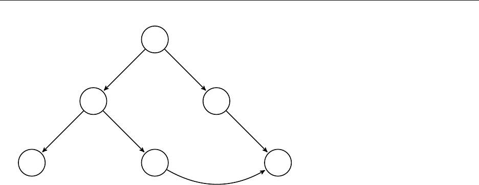
8 Scene Graphs
When you have multiple objects in a scene, and need them to have working relationships in
terms of how they move, we use a scene graph.
This allows for the grouping of objects in a way that makes sense. For example, you can (as
in the assignment) make a character with limbs that can move independently, or together
depending on where you apply transformations in the graph.
In general, we use a ”group” node to keep sets of objects together. Interior nodes in the
graph are groups, and the leaves are objects.
However, we can also have relations to multiple ”parents” so we actually have a directed
acyclic graph, not a tree (DAG).
10
Francis Pich´e 9 QUATERNIONS
1
2 3
45 6
So here, tranforming 1 will apply the same transform to all the nodes, whereas transforming
3 or 4 will affect 6, and transforming 6 will affect only 6.
Having multiple parents is called ”instancing”.
Object orientation is useful since we can naturally implement a hierarchy with the extends
relationship.
8.1 Transforms on the Graph
Transforms accumulate from the root (ie the leaves are the leftmost matrices, the root is on
the right)
Traversal in OpenGL is done by keeping a matrix stack. We can keep sub-trees separate
conceptually by creating matrices for each sub-tree and adding it to the stack. We then pop
it when we’re done.
We often want to group nodes by adding an identity node as a parent, or ungroup notes by
pushing the transform of the parent to the children.
We can also re-parent by moving a node from
9 Quaternions
Like complex numbers but with more dimensions:
ijk =i2=j2=k2=−1
They are manipulated similarly to complex numbers.
A=a0+a1i+a2j+a3k
B=b0+b1i+b2j+b3k
AB =a0b0−a1b1−a2b2−a3b3+ (a0b1+a1b0+a2b3+a2b3−a3b2)i...
11

Francis Pich´e 10 CONSIDERATIONS FOR CHOOSING ROTATIONS
Quaternions can be used to represent rotations!
It represents a rotation by an angle θalong an axis (x, y, z).
q= (c, sx, sy, sz)≡c+sxi +syj +szk
where c=cos(θ/2) and s=sin(θ/2). It’s θ/2 because qand −qare exactly the same
rotation!
10 Considerations For Choosing Rotations
There are many considerations for choosing what kind of rotation specification we want. For
example, we may want to avoid euler angles if Gimbal lock is a problem, or we may prefer
the interpolation of one over another.
•Numerical issues (matrix multiplication may get messed up)
•Space (matrices use more memory than vectors etc)
•Conversions (converting from a matrix to Euler angles is hard etc)
•Speed (Composing for points is faster with Quaternions, but for vectors is slower)
10.1 Linear Interpolation
To linearly interpolate (or Lerp) between two points aand b:
Lerp(t, a, b) = (1 −t)a+ (t)b
where 0 ≤t≤1.
Notice that Lerp with Euler angles is going to move in different directions before getting to
the final destination, while a quaternion or single matrix will do it in one smooth motion.
Spherical linear interpolation is given by:
Slerp(t, a, b) = sin((1 −t)θ)
sin(θ)a+sin(tθ)
sin(θ)b
where θ=cos−1(a·b)
This is used for smoothly interpolating two rotations given by a quaternion. But be careful!
If a·bis negative, the direction of rotation changes, and since for quaternions the negative
is the same rotation, you get two different interpolations for the same angle!
12

Francis Pich´e 12 TRANSFORMING NORMAL VECTORS
11 Building Rotations
If we wanted to build some arbitrary rotation matrix, we could just compose it with elemen-
tary transforms, (multiply by some translation Tand rotation Rso that the rotation axis we
want to rotate by is aligned with the x-axis.) then apply the rotation, and move everything
back. In 3-D, you would need to:
•Translate rotation axis to pass through the origin
•Rotate about y to align the object with the x-y plane
•Rotate about the z axis so that the axis we want to rotate by is along the x.
We could also just construct a change of coordinates:
T=F RX(θ)F−1
where
F=u v w p
0 0 0 1
Where pis a point the axis of rotation run through, and u,vand ware chosen as follows:
If you have two vectors, aand b, you can take:
u=u
||u||
w=uxb
v=wxu
where umatches the rotation axis, and pis a point along u.
We count our degrees of freedom in a transformation by counting the number of matrix
elements we can change. For example:
a b c d
e f g h
i j k l
0 0 0 w
We can’t change wor the zero’s so we have 12 degrees of freedom in 3D.
12 Transforming Normal Vectors
Normals are vectors that are perpendicular to the object surface. They are covectors (not
differences between points!) so they can get messed up by non-uniform scales and sheers
(but not rotations or rotations!)
13

Francis Pich´e 14 CAMERA TRANSFORMATION
To ”fix” them you will need to use
X= (MT)−1
where Mis the transformation matrix on the object. This is because:
Mt ·Xn =tTMTXn
=tTMT(MT)−1n=tTn= 0
Where tis a vector tangent to the surface and nis the normal.
Part III
Viewing and Projection
13 Image Order and Object Order
With image order, the scene is generated by calculating rays coming from the eye, through
each pixel on the screen and calculating how rays of light would interact with the objects.
This is known as ray tracing.
In contrast, Object order viewing is when we take points on the object and project them
onto a 2 plane (the screen).
14 Camera Transformation
When dealing with viewing, we always talk about the eye as the origin, and we always ”look”
down the zaxis.
14.1 Lookat Transformation
We want to find a transformation that will put our view to look at a specific point.
We do this by computing a transform from points:
•ethe eye point
•lthe lookat point
•vup to know which way is up.
14

Francis Pich´e 15 ORTHOGRAPHIC PROJECTION
We do this by first rotating by some matrix R, then translating by T.
Similar to how we did 3D transformations, we need a matrix:
u v w e
0 0 0 1−1
wis a vector pointing in the opposite direction of the direction we want to look, so
w=l−e
||l−e||
To get v, we project vup onto the plane perpendicular to w.
v=vup −(vup ·w)w
Then lastly we want uto by perpendicular to both so :
u=vxw
I’ll be honest I had to review projections to understand this, but I really recommend it!
Now we can apply the transformation as a change of basis like we do normally.
15 Orthographic Projection
In graphics, we specify a near plane, and a far plane. The near plane is what we are going
to see, and it lies in front of the center of projection (the eye).
In orthographic projection, we simply remove the zaxis.
x0
y0
z0
=
x
y
z
1 0 0 0
0 1 0 0
0 0 0 1
x
y
z
1
15.1 Orthographic Viewport Transformation
To be able to put the image on the screen, we need to think in terms of pixel units. So if
our view is xby y, we have nxby nypixels, where each pixel has size 2/nxby 2/ny
The transformation is then:
xcanonical
ycanonical
nx
20nx−1
2
0ny
2
ny−1
2
0 0 1
=
xscreen
yscreen
1
15
Francis Pich´e 16 PLANAR PERSPECTIVE PROJECTION
Now, we need to specify a viewing volume. That is, some planes that restrict what we’ll be
seeing, to set limits for the rendering. All we need to specify is a near, n, far f, left land
right r.
This is a 3D windowing transformation, so:
2
r−l0 0 −r+l
r−l
02
t−b0−t+b
t−b
0 0 2
n−f−n+f
n−f
0 0 0 1
16 Planar Perspective Projection
To implement perspective, points that are further away need to be proportionally ”shrunk”.
This is done as follows:
If dis the distance down the −zdirection, and yis the height of an object, then:
y0
d=y
z
Were dis the distance to the plane that we’re projecting onto, y0is the shortened height,
and y, z are the coordinates of the original object.
We can do this due to similar triangles, and this means that
y0=−dy/z
16.1 Homogeneous Coordinates Revisited
Recall that points in 3d can be represented as:
wx
wy
wz
w
For w6= 0. But now think if wwas arbitrarily close to 0, we would be scaling the points so
far that it would be a point at infinity. This could be the point at which parallel line intersect.
With perspective projection, we put −zinto w. Using the similar triangles fact from before,
we know
−dx/z
−dy/z
1
dx
dy
−z
So then
16

Francis Pich´e 16 PLANAR PERSPECTIVE PROJECTION
16.2 Carrying Depth Through Perspective
Doing perspective projection like above is fine, but we lose all information about the orig-
inal depth! (Since we’re projecting onto a flat plane). We need some way to maintain this
information, so that we can know which objects are supposed to be ”in front” of other objects.
We can do this by adding some special aand bto our matrix.
n0 0 0
0n0 0
0 0 a b
0 0 −1 0
Where we choose aand bsuch that: z0(−n) = −nand z0(−f) = −f
It turns out that:
a=n=f
,
nf =b
. See slide 35 of the Projection slides for the derivation.
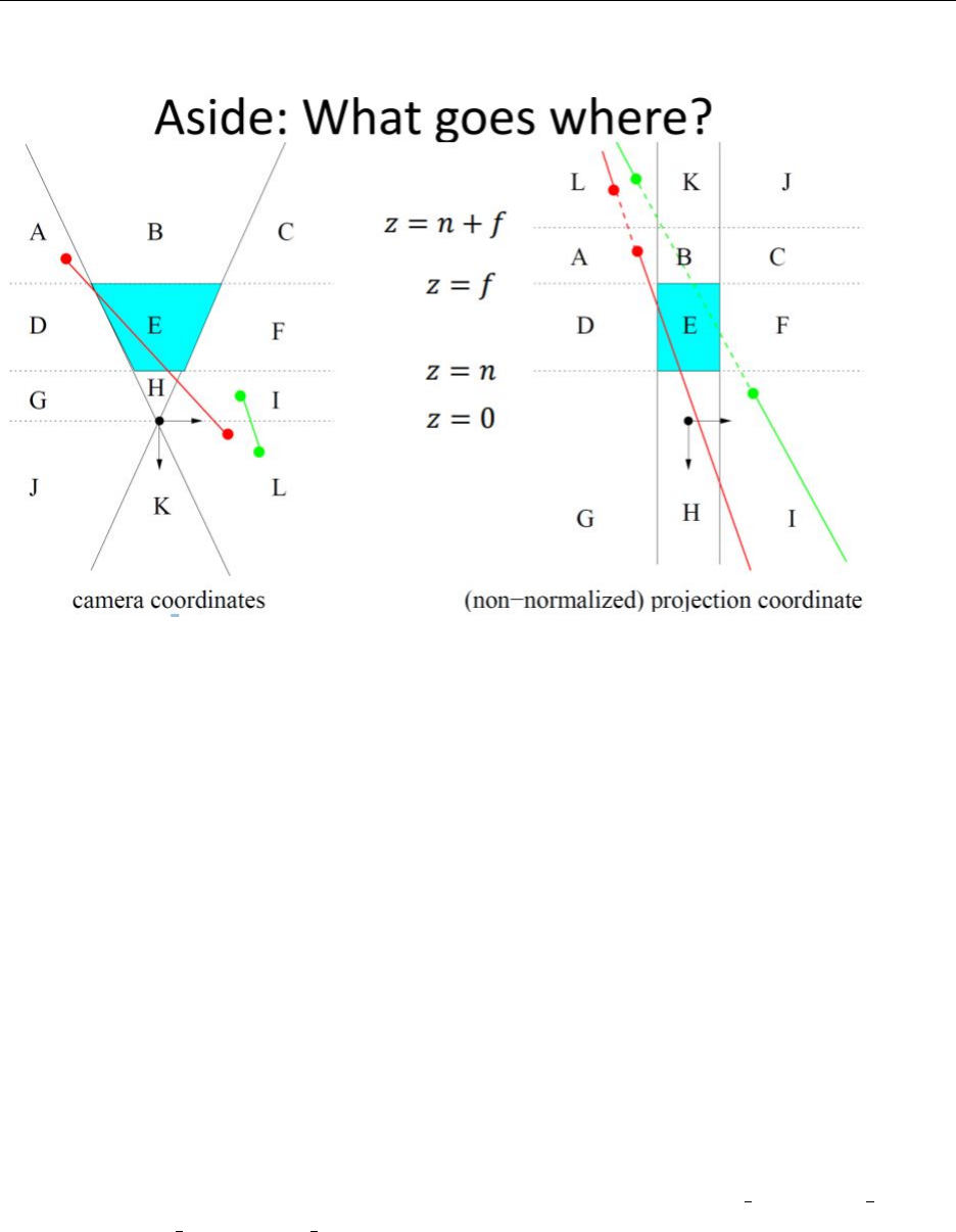
Using this, we can see that:
•Lines through the origin become parallel
•Vectors map to the plane: z=n+f
•Points on a plane with a z-normal which runs throuh the center of projection get
mapped to points at infinity.
•Points halfway between the near and far plane get mapped to a point where z
•Points behind the camera get mapped beyond the n+fplane, and the x, y coordinates
get reflected.
17
Francis Pich´e 16 PLANAR PERSPECTIVE PROJECTION
Figure 1. Paul Kry 3D Viewing, Orthographic and Perspective Projection slide #37
We can then use the orthographic windowing transform, combined with our projection ma-
trix to get the full projection and window;
Mper =MorthP
Where Pis the perspective projection.
16.3 OpenGL Transformation Pipeline
In OpenGL, the position on the screen, psof a point in the world pois given by the following
transformations:
MvpMorthP McamMmpo
Or (from right to left) the point, times the modelview matrix, times the camera transfor-
mation (the transform into camera coordinates, aka lookat), times the perspective matrix,
times the orthogonal projection matrix, times the viewport matrix.
In open GL, this breaks down into 3 matrices. McamMMis the GL MODELVIEW MATRIX,
MorthPis the GL PROJECTION MATRIX and the viewport is by itself.
16.4 Frustum Applications
As done in assignment 2, we can implement different frustums to achieve different effects.
For example, depth of field can be achieved by overlaying multiple views from shifted per-
18
Francis Pich´e 17 PROJECTION TAXONOMY
spectives, such that the focal plane is the point of intersection of all the frustums. Or we
can make 3D anaglyphs by using two shifted eye positions.
EVERYTHING IS WITH SIMILAR TRIANGLES. That’s it. There are no other tricks.
It’s all about drawing the correct picture and choosing the correct triangles. See slides 51-53
on the Viewing slide deck for some really useful pictures.
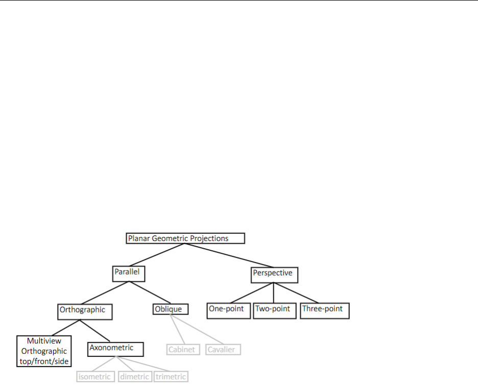
17 Projection Taxonomy
Projections can be broken down in to classes depending on behavior. Names are assigned to
be able to describe them precisely, like biologists with their kingdoms, classes, families and
species.
Figure 2. Paul Kry 3D Projection Taxonomy slide #3
17.1 Parallel Projection
Parallel projection is when the viewing rays are parallel. So instead of having an eye from
which there is a field of view and rays would come out in a sort of arc, all rays come straight
out and parallel.
17.1.1 Orthographic
Orthographic projection breaks down into mulitview and axonometric.
Multiview is when the projection plane is parallel to some coordinate plane. Ie: Look-
ing directly down the x, y, or z axis.
Axonometric is an off-axis parallel projection. This splits into trimetric, dimetric, and
isometric. The difference between them is the number of viewing axes that are equally
forshortened, with isometric at all, and trimetric at none.
19

Francis Pich´e 19
17.1.2 Oblique
Oblique projection is when the projection plane is parallel to a coordinate plane, but not
parallel to a projection direction. This breaks down into cabinet(half length in z) and cavalier
(same length in all directions).
17.2 Perspective
This breaks down into one point, two point and three point perspective, where the difference
is the number of axis that are affected by the perspective projection.
The field of view will determine the ”strength” of the perspective effect. For example, a
close viewpoint with wide angle would cause strong foreshortening, while a far viewpoint
with narrow angle would cause very little.
17.2.1 Shifted Perspective
This is when the projection plane is not perpendicular to the view direction. ie) if you had
a focal plane which was tilted, or an eye position that was off-center but still looking at the
same rectangle than if it wasn’t shifted (like the assignment).
This allows for more control over the convergence of parallel lines. For example, if you
look straight at a building, the top will be the same size as the bottom, but if you look up
(tilt the viewing frame) the top will seem smaller.
18 Field of View
This is the angle between the opposite edges of a perspective image. That is, if you look at
the shape of the frustum, the angle between the the top/bottom of the view volume, or the
left/right. The field of view can have interesting effects on the ”strength” of a perspective
effect (similar to the close/far viewpoint). Having a narrow angle will cause a ”flattening”
whereas a wider angle will cause a ”deeper” perspective.
Part IV
Lighting
19
20
