Surf Cut User Guide
User Manual:
Open the PDF directly: View PDF ![]() .
.
Page Count: 20
Step by step user guide for signal layer extraction using
the ImageJ plugin SurfCut
Prerequisites:
- Fiji (https://fiji.sc).
- The "SurfCut.ijm" macro file (https://github.com/sverger/SurfCut).
- Data: 3D confocal stacks in .tif format, in which the top of the stack should also be the top
of the sample (example data available at https://github.com/sverger/SurfCut/ test_File ).
Procedure
A. Image acquisition:
Our image analysis pipeline was developed to extract cell contours or specific layers of signal
in confocal images of plant samples, either stained with a cell wall or membrane fluorescent
dye, or carrying a fluorescent membrane reporter. For a better-quality output, it is
recommended to use a Z interval of maximum 1 µm.
B. Starting the SurfCut macro:
To manually determine the proper settings for the signal layer extraction.
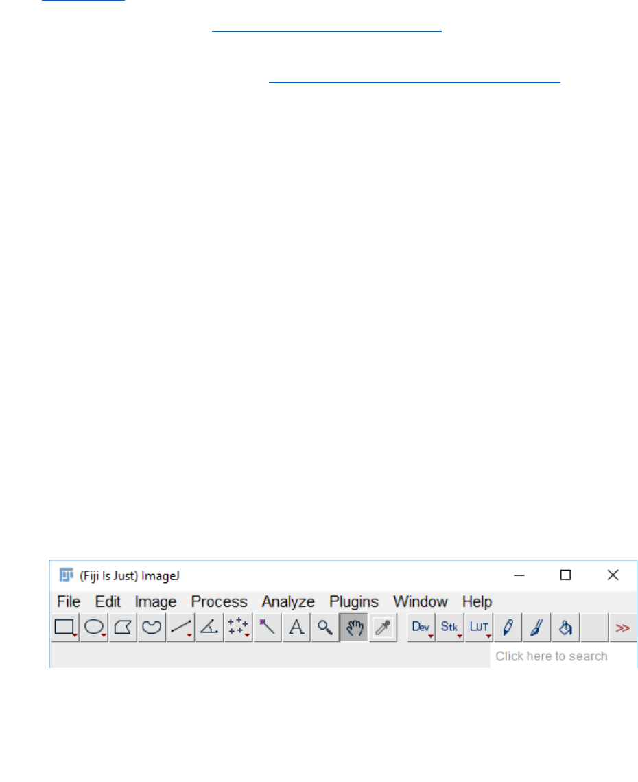
1. Start Fiji.
2. Run the macro: In Fiji go to “Plugins” and then “Macros” and “Run...”.
This will open a navigation window from which you can select the “SurfCut.ijm” file,
wherever you have downloaded it. Then click on “open”.
Note that alternatively you can drag and drop the “SurfCut.ijm” file on the Fiji
window, and click “run” in the new window.
1
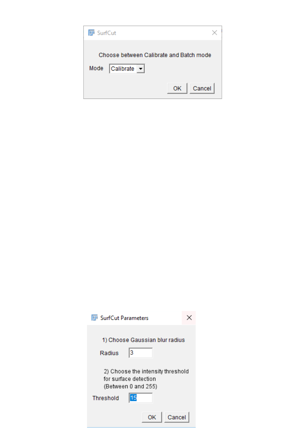
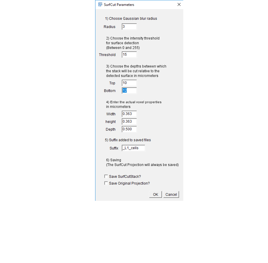
3. The macro will start and display the window below.
The macro has two modes: the first one, called “Calibrate”, is to be used in order to
manually find the proper settings for the signal layer extraction, but can also be used
to process samples manually one by one. The second one, called “Batch”, can then be
used to run batch signal layer extraction on series of equivalent Z-stacks, using
appropriate parameters as determined with the “Calibrate” mode. Go to section C. for
the calibration mode and section D. for the batch mode.
C. Calibration mode
4. First, select the “Calibrate” mode and click OK.
5. A navigation window opens. Select the confocal stack that will be used for the
calibration.
Remember that the stack should be in .tif and that the top of the stack should also be
the top of the sample.
Note that in addition a log window will open. It will display information on the
processing throughout the use of the macro.
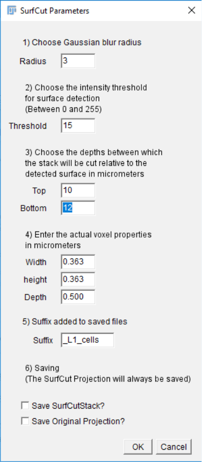
6. The stack will open, and a pop-up window will ask you to define the input values for
“Gaussian Blur” and “Threshold”.
2
The Gaussian Blur is a mean to reduce the noise and smooth the signal. This is
particularly important in order to obtain a smooth signal detection during the
binarization of the signal. We found that a value of 3 µm works usually well for us.
However, if your signal is very heterogeneous, e.g. for cortical microtubules, a higher
value can help homogenize the signal and obtain a good surface detection.
The threshold value then depends on the intensity of the signal in your stack.
You can start with the pre-set values and check the result
7. Click on “OK” to initiate the image processing: (1) Gaussian Blur, (2) signal
binarization, (3) edge detection, and (4) output binarized image and 3D visualisation
of the output image in the 3D Viewer.
Note that you can follow the progresses of the image processing in the log window.
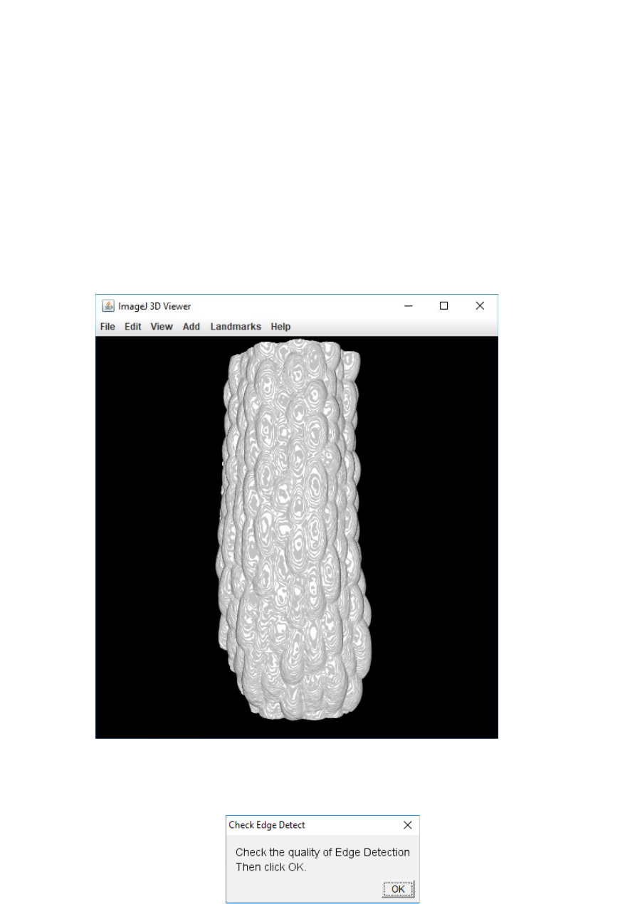
8. A new pop-up window will prompt you to check the quality of the edge detection.
3
While this window is open you can freely interact with the 3D viewer in order to
zoom-in and rotate the sample to check if the detected surface is smooth,
homogeneous and presents no holes.
Below, on the left, is an example in which the Gaussian Blur was too low and the
threshold too high.
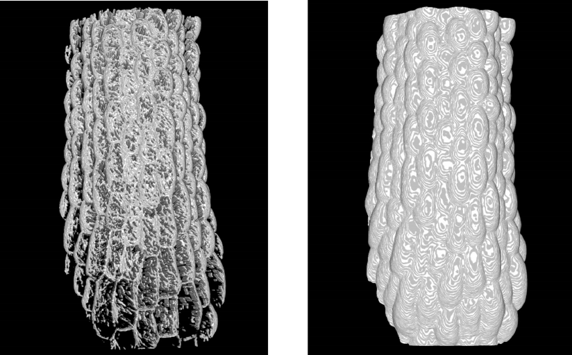
4
Good: Smooth continuous surface
Gaussian Blur = 3
Threshold = 15
Bad: Many holes throughout the sample
Gaussian Blur = 1
Threshold = 80
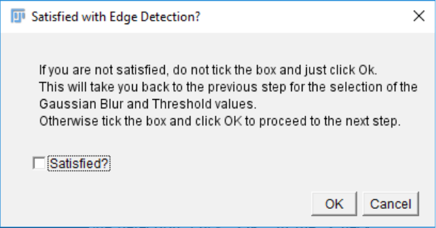
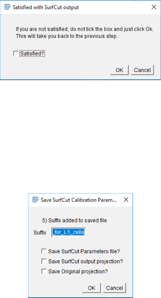
9. Once you have checked the quality of the edge detection, click “OK” in the “Check
Edge Detect” pop up window. A new pop up window will appear and ask you whether
you are satisfied with the edge detection:
- If you are satisfied, tick the “Satisfied” box and click “OK”. This will take you to the
next step.
- If you are not satisfied simply don’t tick the “Satisfied?” box and click “OK”. This
will take you back to step 6, where you will be able to test new values for the Gaussian
Blur and the Threshold. You can repeat this as many times as necessary until you find
the proper settings for edge detection.
5
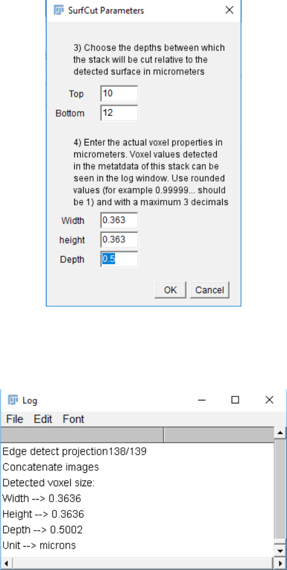
10. When you proceed to the next step, a pop-up window will ask you to choose the
depths between which the stack will be cropped relative to the detected surface. This
value is in micrometers. This step requires that you enter the voxel properties of your
image, in micrometers as well.
Note that while the image properties can readily be found by loading the original
stack in Fiji and looking at its properties, for simplicity the voxel properties are also
printed in the log window.
6
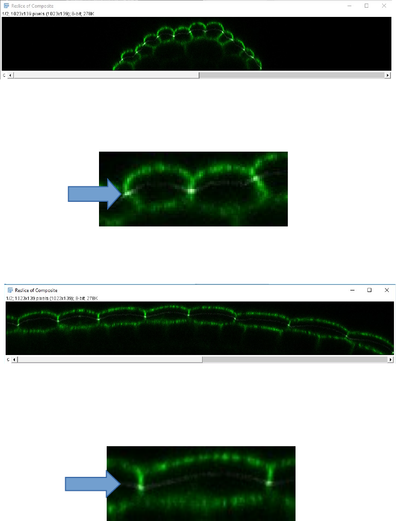
11. Once you have entered all the required values and pressed “OK”, the stack is
processed, and the macro generates four images that can be useful to check the quality
of the output:
- Two orthogonal reslices in the X and Y axis, through the center of the stack
showing an overlap of the raw signal (green) and the cropped stack (thin white
line; The thickness of this line depends on the thickness of the cropped signal
layer)
7
- The original stack max intensity projection
- And the SurfCut output max projection
Note that by choosing the values for top and bottom depth of cropping you
incidentally choose the thickness of the cropped stack. Although usually the thinner
layers output nicer results, you cannot use values lower that the Z interval between
the slices of your stack.
8
12. Similarly to step 8, a pop-up window will prompt you to check the quality of the
SurfCut output. While this window is open you can freely interact with the different
images generated in order to check the quality of the output and determine whether it
matches with your expectations of signal layer extraction.
13. Similarly to step 9, once you have checked the quality of the SurfCut output, click
“OK” in the “Check SurfCut Result” pop up window. A new pop up window will
appear and ask you whether you are satisfied with the SurfCut Output. You can repeat
this step as many times as necessary until you find the proper settings.
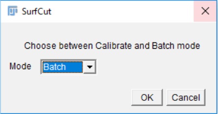
14. If the cropped image is satisfying, you will then choose which files will be saved. You
can add a suffix to the files to specify some characteristic of the parameter that you
calibrated. e.g for cell contour of the L1 layer, outer cortical signal (see exemple in the
next part).
You can choose to save the parameter file, containing all the parameters you have used
to obtain the final SurfCut projection of this calibration step. You can also save the
SurfCut projection as well as the original whole stack projection for comparison.
Then click OK.
9
15. At the end of this calibration step, you can find a folder named “SurfCutCalibrate” in
the same directory as your confocal stack. This folder contains the files saved in step
14.
D. Running the script in batch mode
1. Run the SurfCut macro (Follow steps 1 to 3 as explained in the “Calibration” mode).
2. This time choose the “Batch” mode and click OK.
3. A navigation window will appear. From this window select the folder containing the
confocal stacks that you want to process in batch with SurfCut.
Note that it is preferable that this folder contains only the confocal stacks that you want to
process with SurfCut. Remember that the stacks should be in .tif and that the top of the
stack should also be the top of the sample.
10
4. Set the proper parameters as determined in the calibration mode. You can open the .txt
file generated during the calibration in order to help you fill these values.
The SurfCut projections generated will be automatically saved, but you can also
choose to save the SurfCut stack (3D stack of the signal layer extracted) if you wish to
keep the 3D information, as well as the projection of the whole original stack, for
comparison.
Then click ok to run the batch processing.
Note that you can follow the processing in the log window.
5. The SurfCut macro creates a results folder in the working directory defined in step 3,
named “SurfCutResults”. It contains all the saved output (e.g SurfCut projection, SurfCut
stack, Original projection) as .tif files, as well as a .txt file containing the input parameters
and a log of the analysis.
11
Application example:
Semi-automated high-throughput cortical microtubule
array analysis.
Because the method that we describe is a signal layer extraction method, it is not only limited
to the extraction of cell contours and can, for instance, extend to extract outer epidermal
cortex signal as well. This is particularly useful in the case of cortical microtubule (CMTs)
organisation quantification, because multiple layers of CMT arrays overlap in a classical 2D
projection, which affects the proper analysis of this signal. In addition, because the confocal
signal acquired is anisotropic (different resolution in Z compared to X,Y) in many cases it
remains preferable to carry out analyses in 2D (with a 2D projected image) in order to avoid
such bias.
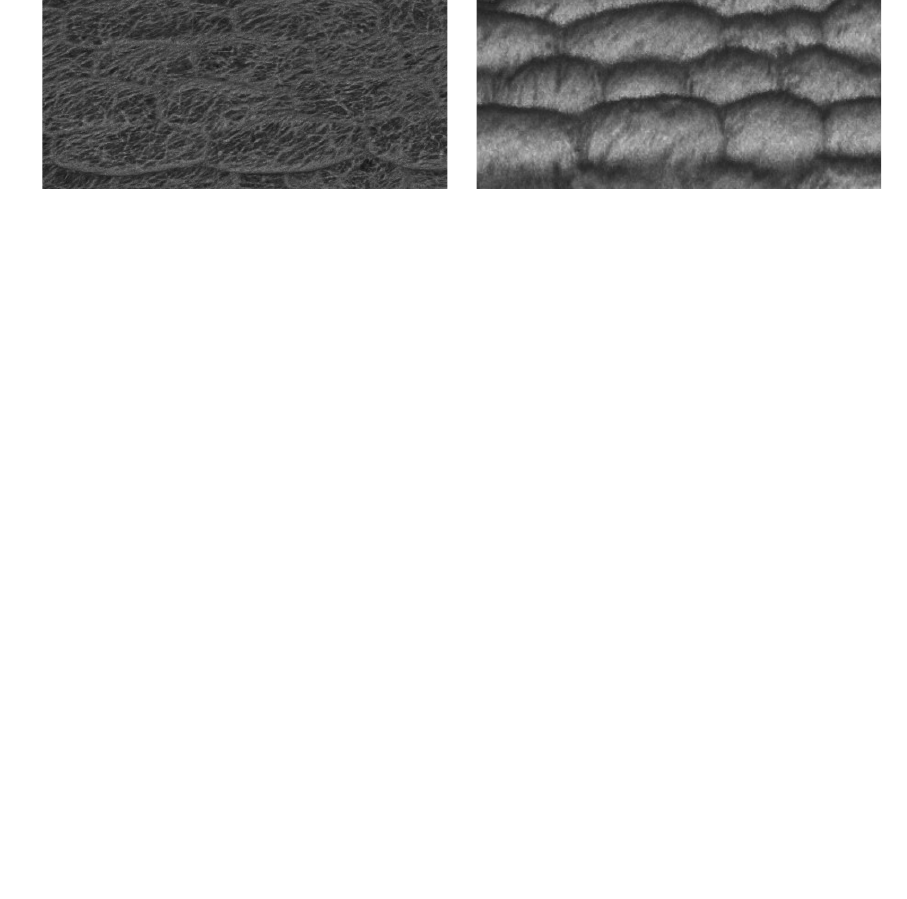
Left is the x,y view (from the top in Fiji 3D viewer) while right is the y,z view (from the side),
showing the anisotropic nature of the confocal signal.
Here we describe the use of a pipeline that we have designed to semi-automatically quantify
CMT arrays from 3D confocal stacks. The part of this pipeline after the SurfCut signal
extraction (part C and D) has already been reported in (Verger et al. 2018) in which signal
layer extraction (part B) was performed manually with MorphoGraphX (Barbier de Reuille et
al. 2015).
Briefly, (1) we use SurfCut to specifically extract the cell contour signal as well as the outer
epidermal CMT signal. (2) We use the cell contour signal to create ROIs for each cell in each
sample. (3) These ROIs are applied to the extracted CMT signal and CMT arrays are analysed
with an automated version of FibrilTool (Boudaoud et al. 2014; Louveaux and Boudaoud
2018).
These three processes correspond to three successive Fiji macros (“SurfCut.ijm”,
“Segmentation4FTBatch.ijm” and “FibrilTool_BatchSeg.ijm”; see prerequisites). Each of
these macros can be used to process batch samples, making the analysis high-throughput.
A. Prerequisites
12
- Fiji (https://fiji.sc).
- The "SurfCut.ijm" macro file (https://github.com/sverger/SurfCut).
- The “Segmentation4FTBatch.ijm” macro file (https://github.com/sverger /SurfCut /test_File ).
- The “FibrilTool_BatchSeg.ijm” macro file (https://github.com/sverger/SurfCut /test_File ).
- The imageJ “MorphoLibJ” library (for the segmentation in “Segmentation4FTBatch.ijm”)
(Legland, Arganda-Carreras, and Andrey 2016). See installation procedure at
https://imagej.net/MorphoLibJ.
- Data: A folder containing 3D confocal stacks in .tif format, in which the top of the stack
should also be the top of the sample (example data available at
https://github.com/sverger/SurfCut/ test_File ).
B. Signal layer extraction with SurfCut
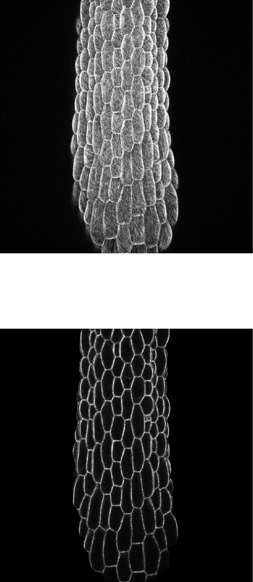
1. The first step is to extract both the cell contour and the outer epidermal CMT signal for all
your images using SurfCut. You should first define the proper parameters for both type of
extraction with one of your stacks, using the “Calibrate” mode.
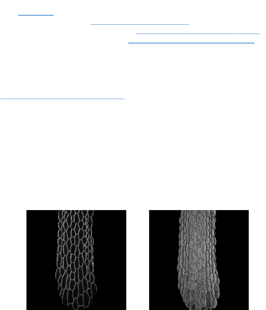
For instance, in the images below, we have cropped the signal at a distance of 10 µm to 12
µm from the surface to extract the cell contours (left), and at a distance of 1 µm to 3 µm from
the surface to extract the outer epidermal cortex (Right).
13
2. Once you have adequate parameters, first run the batch signal extraction for the cell
contours.
Note: It is important at this step to add in the SurfCut parameter window, a suffix for your
images finishing with “_cells”.
Also do not save the SurfCut stack nor the original projection.
14
3. Run the same batch signal extraction for the outer epidermal CMT signal, using the proper
parameters, and this time using the suffix “_MTs”.
4. The “SurfCutResult” folder should now contain for each stack, a 2D cell contour projection
(e.g. SampleName_1_cells.tif, SampleName_2_cells.tif, ...) and a 2D outer epidermal CMT
projection (e.g. SampleName_1_MTs.tif, SampleName_2_MTs.tif, …), as well as the
parameter files for both signal extractions.
Note that it is critical for the following macros to work that the suffix of these images be
respectively ..._cells.tif and ..._MTs.tif.
C. Segmentation and ROIs creation
1. Run the “Segmentation4FTBatch.ijm” macro.
2. A navigation window will open. From this window select the “SurfCutResult” folder
created in the previous step (B.).
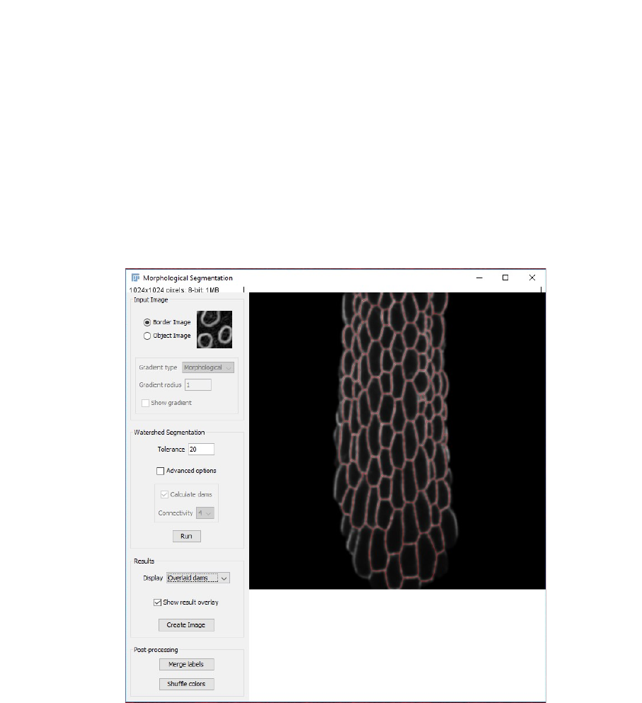
3. You will then have to process each image semi-automatically: First a Gaussian Blur of
Radius 3 microns is automatically applied, and the image is opened with the Morphological
segmentation tool of the MorphoLibJ library. A segmentation is run automatically with the
default parameters (Watershed Segmentation Tolerance = 10).
15
4. The automatic segmentation in step 3 may not be adequate (over- or under-segmentation).
Check the segmentation and if necessary, re-run it. You can empirically find the best
“Watershed Segmentation Tolerance” value (see image above in the red rectangle, in this case
the value was changed to 20) and re-run the segmentation as many times as necessary. When
you are satisfied click “OK” in the window below.
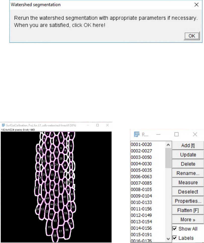
5. Next an outline of the segmentation (watershed lines) is generated and is automatically
dilated four times. This is to exclude some of the signal from the cell contours (that can be
remaining in the CMT image) that could bias the CMT array analysis. The Fiji “Analyse
Particles...” function is then automatically run on this dilated segmented cell contour image,
showing the identified ROIs as an overlay as well as in the ROI manager.
16
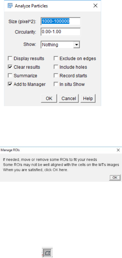
7. The “Analyse particles...” function is run by default with the particle size parameter at
1000-100000 pixels. This is to filter out the background as well as the smaller cells that would
be meaningless for the analysis (too few pixels to analyse for FibrilTool). However, this may
depend on your analysis and the nature of your images. If you are not satisfied with this
parameter, you can un-tick the “Satisfied” box and click “OK”. This will take you to the
“Analyse particles...” parameter window, where you can set your preferred parameters and re-
run the “Analyse Particles...” function. This can be repeated as many times as necessary.
8. Next the generated ROIs are overlaid on the corresponding CMT image. At this step you
can check whether the ROIs are properly positioned.
ROIs can be moved, deleted (see centre image) and created (see right image, blue ROI). You
can for instance delete ROIs which are too much on the side of a curved sample since their
analysis will be less meaningful. You can select individual ROIs by clicking on their label
number, delete them with the backspace or del key, and create new ROIs with the Fiji
“Polygon selections” tool.
The closed polygon can then be added to the ROI list by pressing Ctrl + T.
17
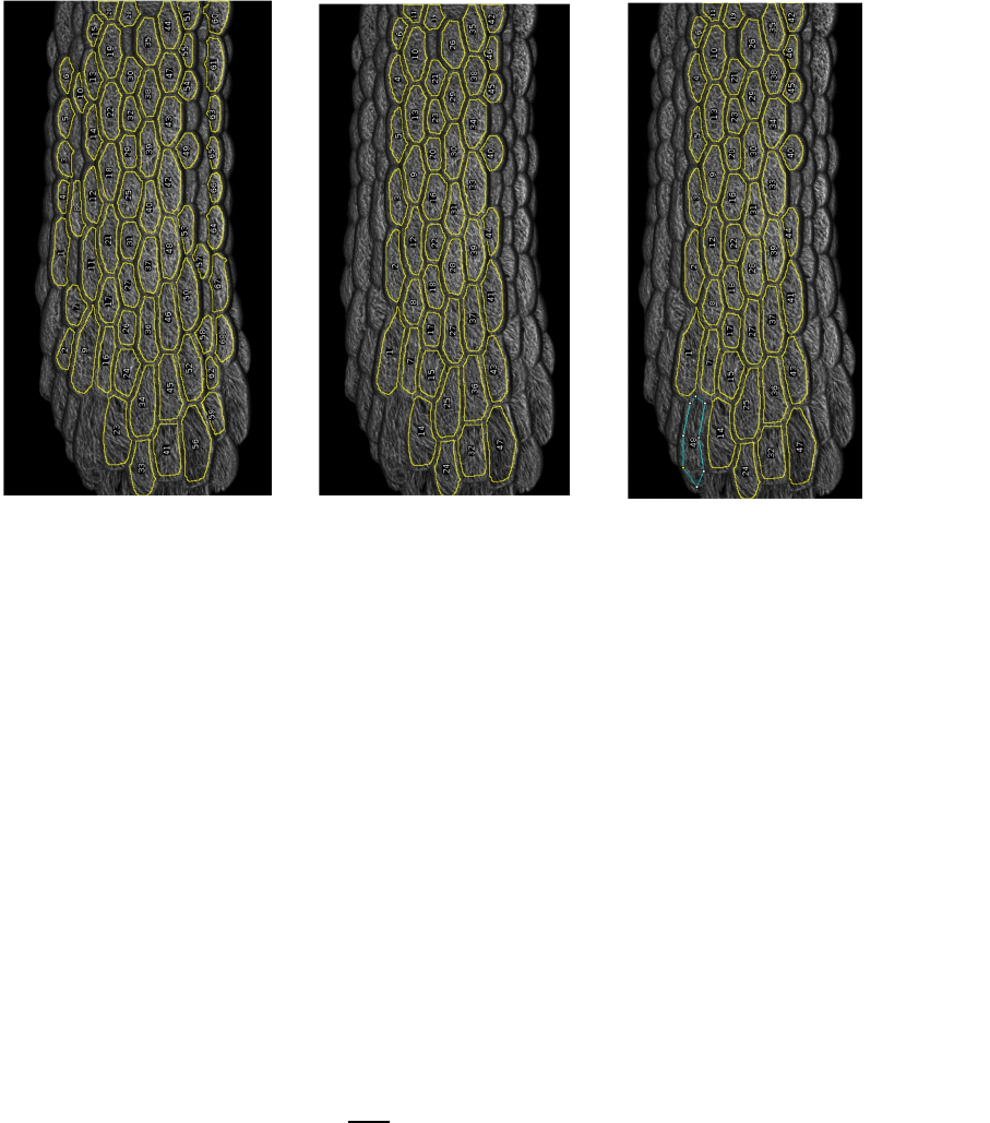
9. When satisfied with your ROI set click “OK” in the “Manage ROIs” window. This will
save the ROI set in a .zip file with the suffix “..._cells_RoiSet.zip” and proceed to the next
sample.
10. After processing all the samples, the “SurfCutResult” folder should now contain for each
stack, an additional ROI set file (e.g. SampleName_1_cells_RoiSet.zip,
SampleName_2_cells_RoiSet.zip, …).
D. FibrilTool Batch
Note that before running FibrilTool batch you should make sure that the log window is empty
or close it. This will avoid pre-existing text in the log window to be saved in .txt output files of
FibrilTool.
1. Run the “FibrilTool_BatchSeg.ijm” macro.
2. A navigation window will open. From this window select the “SurfCutResult” folder
created in step (B.).
3. Choose the channel in the pop-up window. Click “OK”.
18
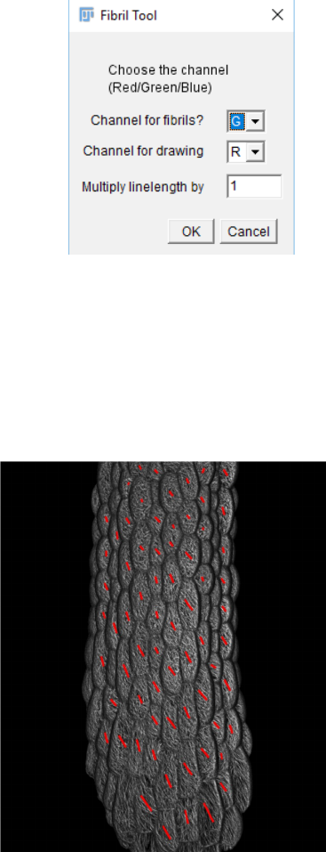
4. The macro will process all the ROIs of all the samples in the selected folder automatically
and for each sample, save the FibrilTool output (red lines) overlaid on the CMTs in a .tif
image with the suffix “..._FT-Mts.tif”, as well as a “..._Log.txt file containing the values of
anisotropy and principal angle of the CMT array for each ROI (see (Boudaoud et al. 2014;
Marion Louveaux and Arezki Boudaoud 2018) for the details of FibrilTool file output).
Barbier de Reuille, Pierre, Anne-Lise Routier-Kierzkowska, Daniel Kierzkowski, George W
Bassel, Thierry Schüpbach, Gerardo Tauriello, Namrata Bajpai, et al. 2015.
“MorphoGraphX: A Platform for Quantifying Morphogenesis in 4D.” ELife 4 (May):
e05864. https://doi.org/10.7554/eLife.05864.
Boudaoud, Arezki, Agata Burian, Dorota Borowska-Wykręt, Magalie Uyttewaal, Roman
Wrzalik, Dorota Kwiatkowska, and Olivier Hamant. 2014. “FibrilTool, an ImageJ
Plug-in to Quantify Fibrillar Structures in Raw Microscopy Images.” Nature
Protocols 9 (2): 457–63. https://doi.org/10.1038/nprot.2014.024.
Legland, David, Ignacio Arganda-Carreras, and Philippe Andrey. 2016. “MorphoLibJ:
Integrated Library and Plugins for Mathematical Morphology with ImageJ.”
Bioinformatics 32 (22): 3532–34. https://doi.org/10.1093/bioinformatics/btw413.
Louveaux, Marion, and Boudaoud, Arezki. 2018. FibrilTool Batch: An Automated Version of
the ImageJ/Fiji Plugin FibrilTool. Zenodo. https://doi.org/10.5281/zenodo.2528872.
19
Verger, Stéphane, Yuchen Long, Arezki Boudaoud, and Olivier Hamant. 2018. “A Tension-
Adhesion Feedback Loop in Plant Epidermis.” ELife 7 (April): e34460. https://doi.org/
10.7554/eLife.34460.
20
