1 TASC Manual

User Manual:

Open the PDF directly: View PDF .
Page Count: 18

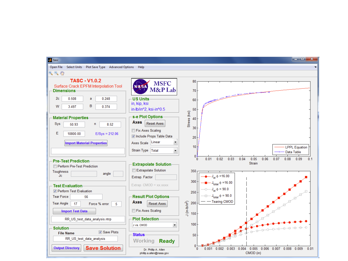
TASC – V1.0.2 (Tool for Analysis of Surface Cracks)

Interpolated Elastic-Plastic J-Integral Solutions

Phillip Allen – NASA MSFC – Phillip.a.allen@nasa.gov

June 2014

LPPL Equations

Introduction

Tool for Analysis of Surface Cracks (TASC) is a computer program created in

MATLAB® to enable easy computation of nonlinear J-integral solutions for

surface cracked plates in tension by accessing and interpolating between the 600

nonlinear surface crack solutions documented in NASA/TP–2011-217480*. The

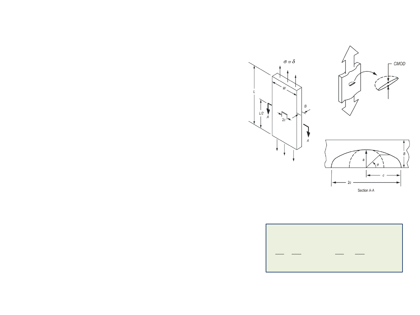
only required inputs are the surface crack dimensions (2c and a), plate cross-

section dimensions (W and B), and linear plus power law (LPPL) material

properties of elastic modulus, E, yield strength,

ys or Sys, and strain hardening

coefficient, n. With the geometry and material parameters entered, TASC

interpolates to the appropriate J(

) vs. crack mouth opening displacement

(CMOD) and far-field tension stress,

vs. CMOD solution, providing the full

solution as CMOD ranges from zero out to the CMOD limit of the solution space

for the given input parameters. (Note:

is the parametric crack front angle.)

TASC provides interpolated solutions over a wide range of crack shapes and

depths (shape: 0.2 ≤ a/c ≤ 1.0, depth: 0.2 ≤ a/B ≤ 0.8) and material flow

properties (elastic modulus to yield ratio: 100 ≤ E/

ys ≤ 1000, and hardening: 3 ≤

n ≤ 20). With surface crack test design and analysis in mind, TASC also has

several other useful features such as:

1. material property import capability with automated material constant

fitting,

2. pre-test prediction capabilities based on a critical J-integral value and

critical

location,

3. test record force, P, vs. CMOD evaluation and comparison with analysis,

4. the ability to review multiple result plots such as J(

), J vs. CMOD, and

deformation limit comparisons, and,

5. the ability to save the solution, input, and plot files.

;

ys ys

ys ys ys ys

 s  s

   

 s  s



   





* Details of the solution space, interpolation methods, and nomenclature are documented in

NASA/TP-2013-217480, Elastic-Plastic J-Integral Solutions for Surface Cracks in Tension Using

an Interpolation Methodology, which is available for download from the NASA Center for

Aerospace Information (CASI) at <http://www.sti.nasa.gov>.

Revision History

June 2014 - Version 1.0.2

•interp_solution_SCGui_CMOD_log_int.m – Corrected error in code that sometimes prevented interpolation to first load step

results for very small initial increments of CMOD. In rare cases, this error created “NaN” results for the first load step of the

interpolation solution and prevented the pretest prediction from functioning properly.

•plt_crk_front_condition_int.m – Added this new file that creates a plot of the crack front constraint and deformation

conditions as a function of loading. This plot corresponds to Figure 8 in ASTM E2899.

•Changed three plot routines to plot the

(90°) results as light gray to differentiate the 90 results from the tearing prediction

results. Updated code in: plt_crk_front_condition_int.m, plt_deform_epfm_fea_int.m, and plt_J_CMOD_fea_int.m.

February 2014 - Version 1.0.1

•Released standalone executable versions of TASC V1.0.1 for Windows® 64-bit and Mac OS X® 64-bit, and the TASC source

code under the NASA Open Source Agreement. Files are posted the NASA TASC Sourceforge project at

http://sourceforge.net/projects/tascnasa/.

•tasc.m – Added a start-up box that requires users to read and accept the NASA Open Source Agreement before using TASC.

•create_summary_table.m – Added additional output in the results summary file including: E, a, 2c, rfa, and rfb.

•plt_force_CMOD_interp2_int.m – Added J(

) value displayed on plot for test analysis prediction.

•plt_stress_CMOD_interp_int.m – Added J(

) value displayed on plot for test analysis prediction.

November 2013 - Version 1.0.0

•Released standalone executable versions of TASC V1.0.0 for Windows® 64-bit and Mac OS X® 64-bit under the NASA Public

Release Agreement.

Some Important Standalone Executable Details

•TASC is a standalone executable program available for Windows® 64-bit and Mac OS X® 64-bit. Individual users of the

standalone executables do not need a MATLAB license due to the royalty-free MATLAB Complier Runtime (MCR) distribution

provided with the program installation package.

•Installation details are in the readme.txt file included in the distribution package. The correct version of the MCR package

must first be installed on each computer on which you want to run TASC. The correct MCR installation file (MCRInstaller.exe)

is included in the distribution package. The TASC standalone executable file (TASC_V1P0P2.exe for Windows and

TASC_V1P0P2_mac.app for Mac) can be located in any convenient place on your computer. Double click TASC_V1P0P2.exe

for Windows or execute run_TASC_V1P0P2_mac.sh from the terminal for Mac to start TASC.

•TASC takes 10 to 60 seconds to start, depending on your computer because the MCR files are essentially starting a version of

Matlab in the background. Unfortunately using the Matlab graphical user interface (GUI) system, there is no practical way to

have a start up splash screen to show you the program is starting; please be patient. Once the TASC GUI is running, each

elastic-plastic solution is computed in seconds.

•The first time you run TASC, a start up window will appear stating “I have read and accept the terms of the NASA Open

Source Agreement included in the TASC distribution package.” You must select “Yes” to run TASC. Selecting “Yes” creates a

small text file, TASC_lic.txt” in your executable directory. You will not be asked to accept the agreement again unless you

move or copy the executable file to another directory.

•Example TASC input files (*.ntrp ), material property files (*.prop), and test data files (*.txt) for both US and SI units are

included in the Distribution_Example_Files directory. The use and description of these files are explained later in this

manual.

•The GUI was created and formatted on the Windows platform. As a result, on the Mac platform the GUI appearance for

items such as font sizes are not optimized. In addition the Mac version does not have the capability to save an Excel

summary of the results in *.xlsx format. The results are output in text format and drop cleanly into Excel if so desired. Also

the Mac version does not have the ability to save plot images in the *.emf format so instead defaults to the *.tiff format.

•Background information on surface crack tension testing including deformation limits and critical

calculation methods is

documented in ASTM E2899, Standard Test Method for Measurement of Initiation Toughness in Surface Cracks Under Tension

and Bending, which is available from ASTM, <http://www.astm.org>.

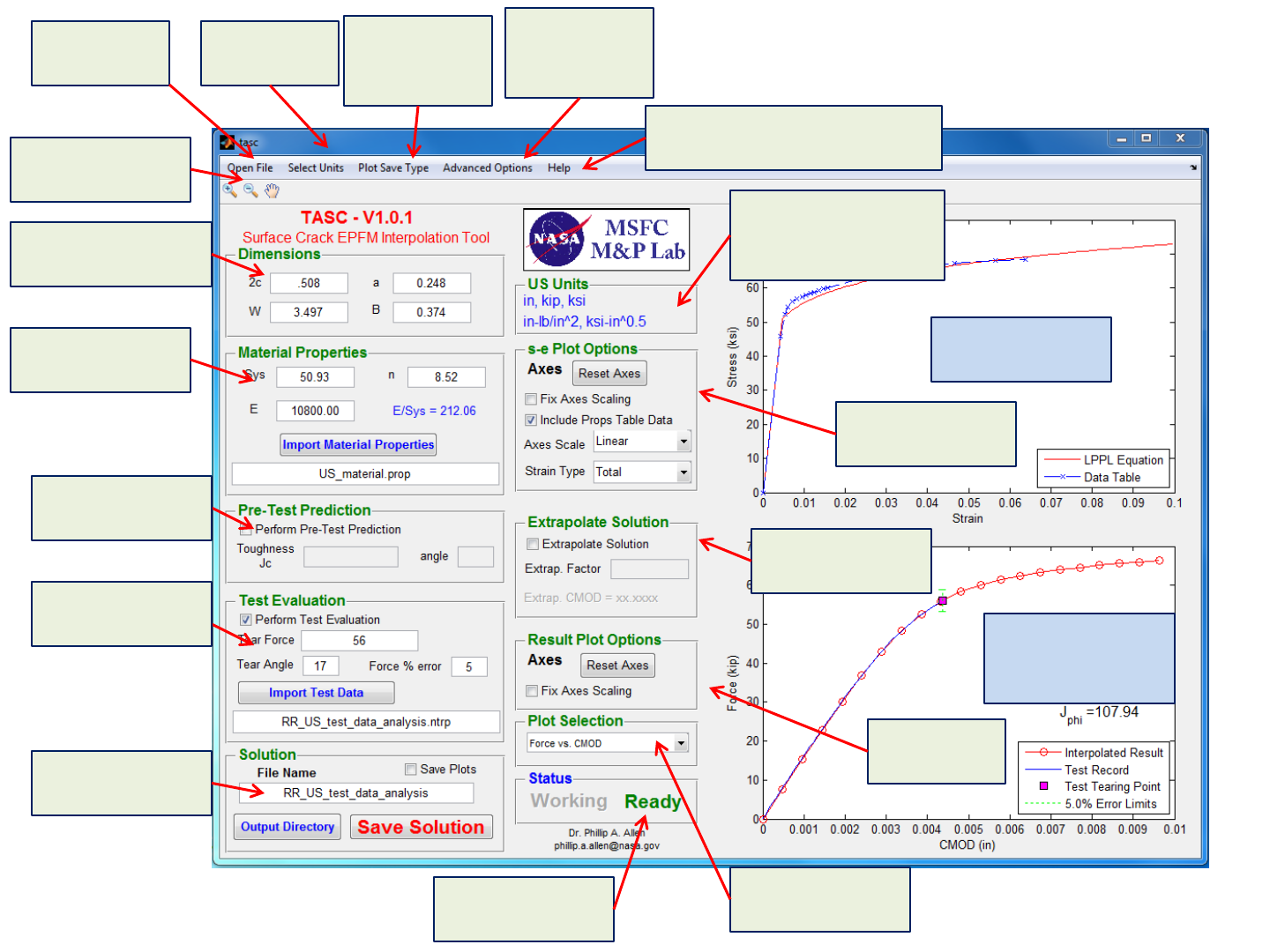
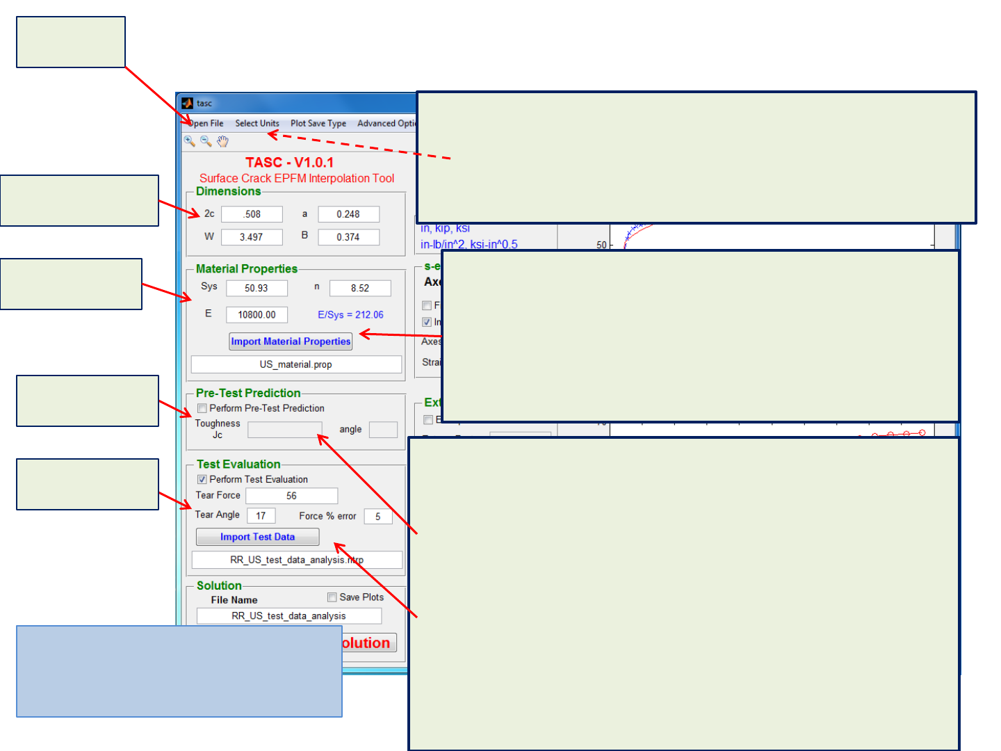
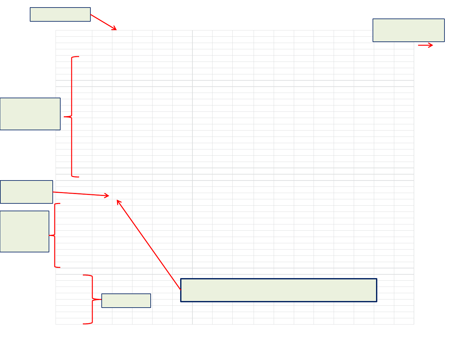
Basic Layout

A. Input plate and

crack dimensions

B. Input Material

Properties

Plot zoom and

pan controls

Open input

(*ntrp) file

Select SI or

US units

Show

interpolation

details

C. Pre-test

prediction inputs

D. Test evaluation

inputs

Save solution

options

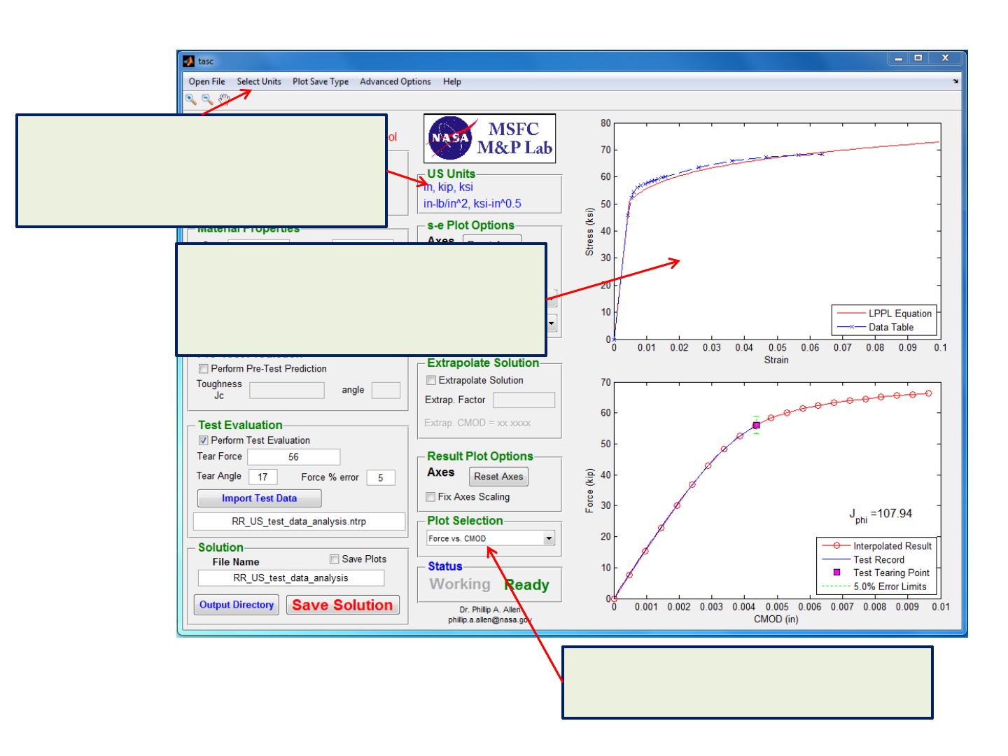
Units details:

Length, Force, Stress

J-integral, K

Stress-strain

properties plot

Analysis results

output plots (10

choices)

Stress-strain plot

options

Result plot

options

Extrapolate

Solution options

Analysis Status

Lights

Result plot

selection box

Choose plot

electronic file

type

Help: show surface crack

picture or open user manual

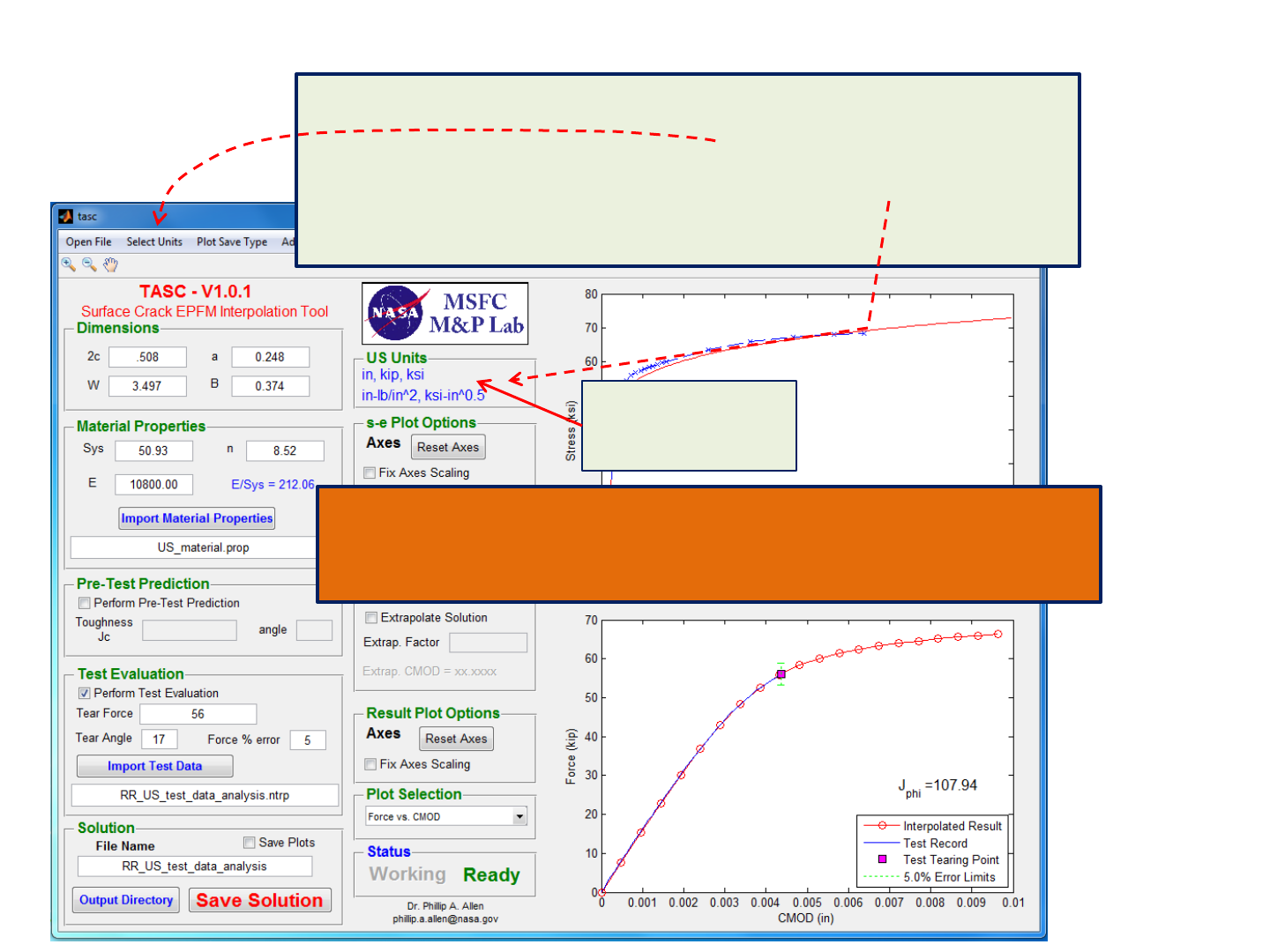
Important Units Considerations

Units Details:

Length, Force, Stress

J-integral, K

The underlying solution database is dimensionless. Therefore TASC relies on the user to

input a consistent set of units to get output in the expected and desired units. The user

must first decide on SI or US units by using the Select Units menu or by specifying the

units type in the *.ntrp file. The expected units type for length, force, stress, J-integral

and K (and output units where applicable) are shown in the Units Details Box on the GUI

and at the end of the output file. The units type for SI and US were chosen based on

typical values used in a test lab environment.

CAUTION: Switching units type from SI to US or vice-versa will NOT convert any

previously input numerical data into the new units system. Units must be entered as

specified on the GUI for the given units system. Choosing the units type (SI or US) simply

sets the appropriate internal calculation factors and output labels for that units type.

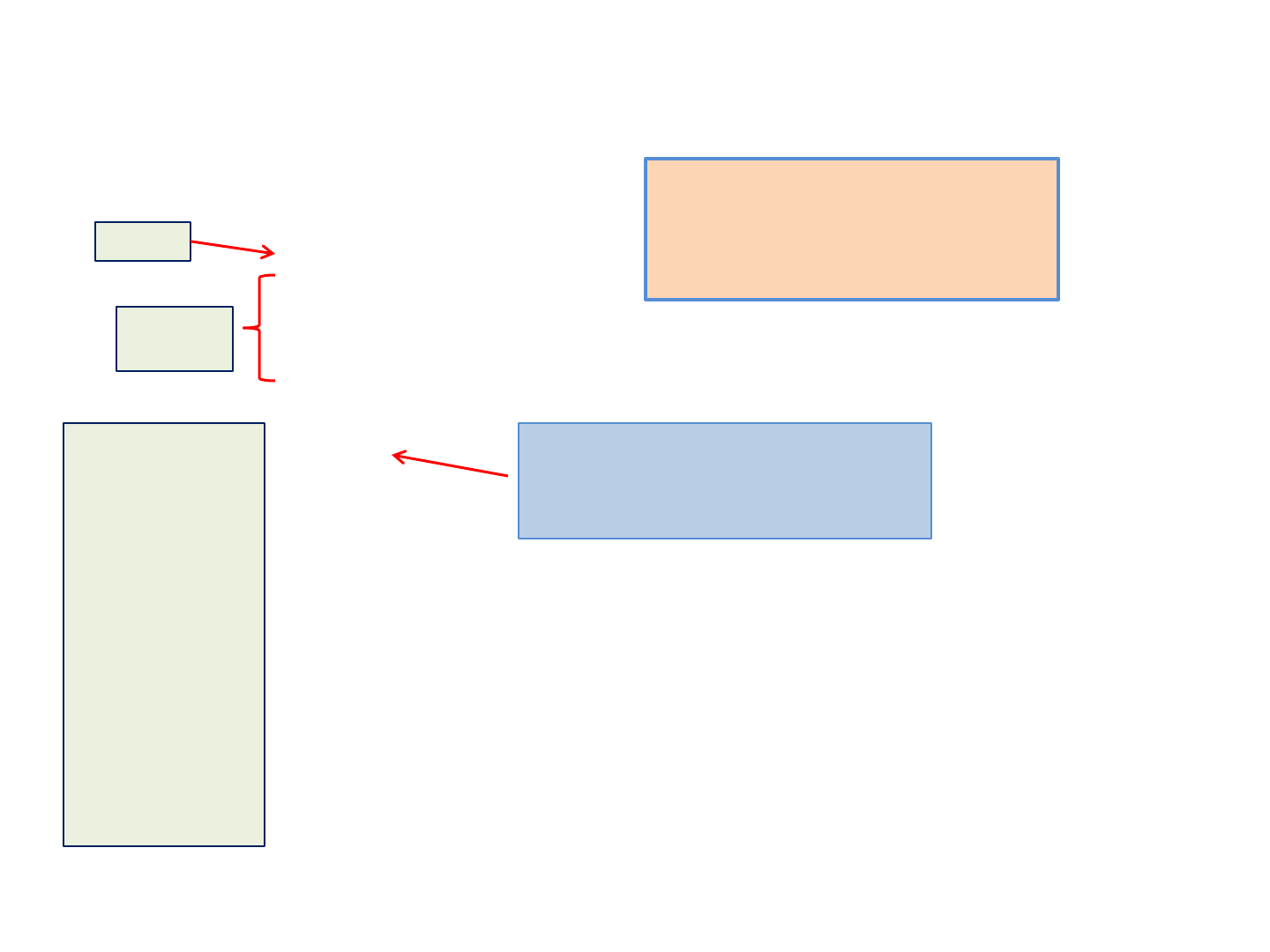
Get started and perform analysis

A. Input plate and

crack dimensions

B. Input Material

Properties

There are three independent analysis options:

1) A elastic-plastic solution with no test data evaluation is performed by

filling in (A )& (B) and not marking (C) and (D) checkboxes. This gives you

esentially all the outputs you would get from running a nonlinear FEM.

2) Choose (C) checkbox and fill in estimations for the critical toughness, Jc,

and the critical crack front angle to get a pre-test prediction of the tearing

force, CMOD, and crack front conditions. This option is intended for pre-

test planning and design.

3) Choose (D) to perform a test analysis. Fill in the tearing force and tearing

crack front angle and import the force-CMOD test record. The code will

attempt to find the test tearing CMOD value corresponding to the tear

force that is input. If the analysis reaction force corresponding to the

tearing CMOD is within 5% of the test tearing force, the code will perform

several calculations and report out tearing analysis results for your test.

The % error allowed can be changed in the Force % error box.

Open input

(*ntrp) file

Two choices to begin analysis:

1) Open a *.ntrp file. Data boxes will be filled in and analysis performed based

on information given in *.ntrp file

2) First select units system, and then manually type in values in boxes (A) and

(B). Once the values are entered and no errors are found, the analysis will

be performed.

Material properties for box (B) can be imported using the “Import

material properties button.” The material properties file can contain:

1. Sys, n and E, or

2. the file can contain E and a stress vs. plastic strain table. If a table is

present, the code will set Sys as the average of the first 3 stress

values in the table and determine a “n” value by fitting the stress-

plastic strain curve. This provides starting approximations for Sys and

n that can then be adjusted as necessary by the user.

C. Pre-test

prediction inputs

D. Test evaluation

inputs

NOTE: Poisson's ratio,

, is not a required

material input. All of the solutions have a

fixed value of

= 0.30 from the interpolated

solutions data set.

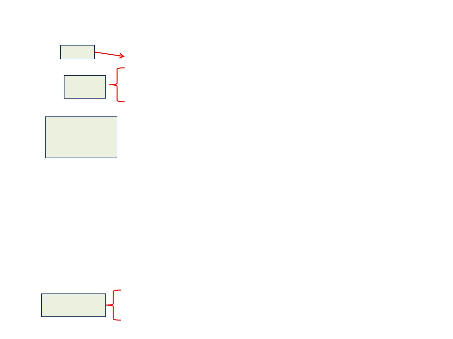
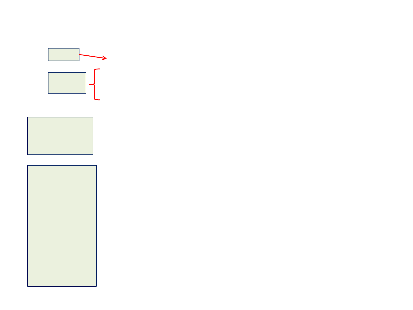
Explore results

The linear plus power law (LPPL) curve for the

analysis is shown in red. If stress-plastic strain data

is available, it is plotted in blue. Any change to

material properties updates the plots and reruns

the analysis.

One of 10 plots can be picked from this list. Any

change to the GUI values reruns the analysis and

updates the plots.

The code supports SI or US units. The units choice

is made through the “Select Units” menu or

specified in the *.ntrp file. The acceptable input

units for length, force, stress and the output units

for K and J are given in the Units graphic.

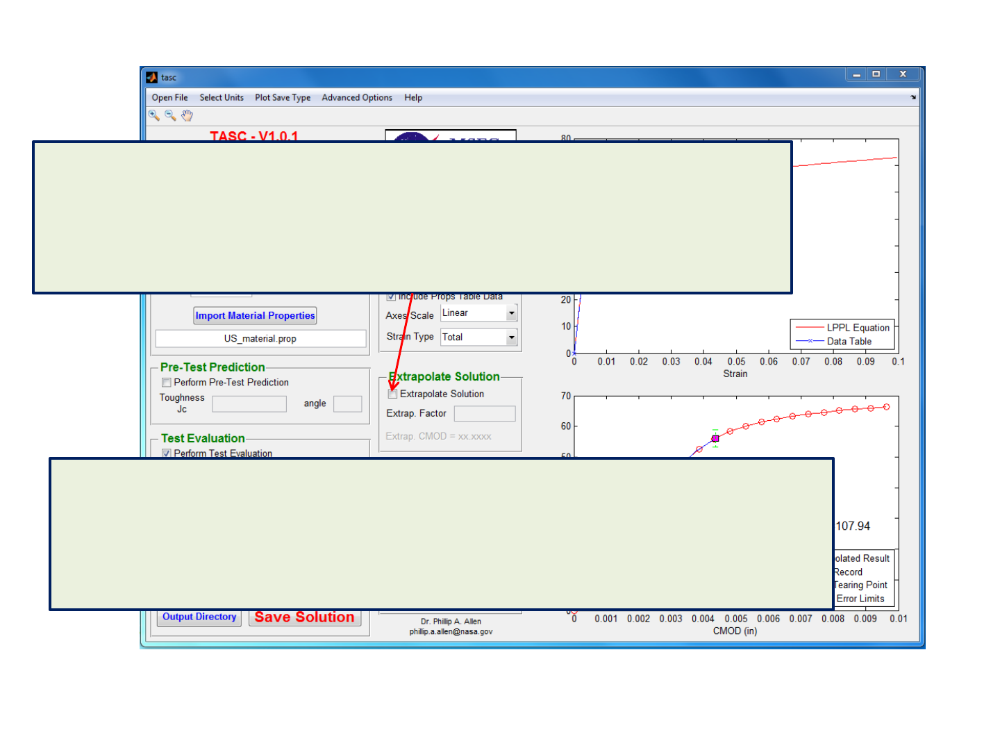
Extrapolate Solution Option

In some instances you may desire a solution at a higher J value or deformation level than what is available

from the last step of the interpolated analysis. The code allows you to extrapolate the solution based upon a

factor on CMOD. The “extrap. factor” is multiplied by the last CMOD value in the interpolated solution and

provides an estimated solution at the new extrapolated CMOD value . This new solution step is listed as

“step 21” in the analysis output. Permissible values for the extrap. factor are between 1 and 2. Please use

extra scrutiny when using the extrapolation option, because these estimated solutions are beyond the final

converged solution sets used in the interpolation routines.

When the “extrapolate solution” option is chosen, TASC estimates new J(

) values and

value corresponding to

the new extrapolated CMOD value. To estimate the J values, the J-CMOD trajectory for each

location is linearly

extrapolated to the new extrapolated CMOD value. This should provide a good estimate of the J-values because

the J vs. CMOD response is essentially linear in the elastic-plastic regime. To estimate the

(or P) corresponding

to the extrapolated CMOD, TASC fits a power law of the form

(CMOD)

to the last 5

vs. CMOD data

points in the solution set and estimates the new

using the power law function. Therefore the extrapolated

value may not have the same level of accuracy as the extrapolated J values.

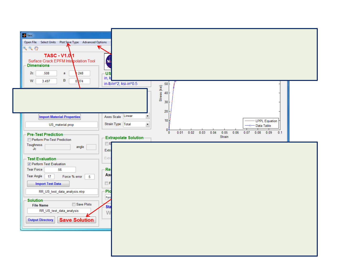
Save results

Once you are satisfied with the analysis, push the “save solution” button to save the

analysis values. The initial default save directory is the directory where the *.exe file

is installed. If you have loaded an *.ntrp file, the default save location is the same

directory as the *.ntrp file. You can change the save location by pushing the “output

directory” button. The file name defaults to a generic name or the name of the

*.ntrp file.

Pressing the “save solution” button creates a “Solution_Files” directory and stores 4

files : (1) an Excel file (Windows only) and (2) a *.txt file with identical summary

information, (3) a Matlab database *.mat file is also created for convenience for

Matlab users, and (4) a filename_inputs.ntrp file that is a new *.ntrp file capturing all

of your current solution inputs.

If “Save Plots” is checked, the code also creates a “Plot_Files” directory and saves

files for all of the plots in the analysis.

The filenames all have the solution filename as a prefix.

If you would like to see some details of the interpolated solution, you can choose

“Advanced Options – Interpolation Details.” The code will then make four sets of

subplots showing the a/c, a/B, n, and E/Sys interpolation process. The plots are

opened in separate windows. The plots are also saved as *.emf or *.tiff files in a

“Interp_Detail_plots” directory. The initial default location for the the

“Interp_Detail_plots” directory where the *.exe file is installed. If you have loaded an

*.ntrp file, the save location is the same directory as the *.ntrp file.

Plot save file type options are *.emf (Win. default),

*jpeg, or *.tiff (Mac default) based on selection in

“Plot Save Type” menu.

index a/B a/c n E/Sys W B Sys E a 2c

0.66_0.98_9_10800 0.66 0.98 8.52 212.1 3.497 0.374 50.93 10800 0.248 0.508

** ** phi 0246810 12 14 16 18 20 22 24 26

step stress CMOD J0 J2 J4 J6 J8 J10 J12 J14 J16 J18 J20 J22 J24 J26

1 5.85E+00 4.81E-04 1.70E+00 1.72E+00 1.73E+00 1.68E+00 1.64E+00 1.59E+00 1.55E+00 1.52E+00 1.49E+00 1.46E+00 1.43E+00 1.41E+00 1.39E+00 1.37E+00

2 1.17E+01 9.63E-04 6.33E+00 6.59E+00 6.79E+00 6.62E+00 6.44E+00 6.27E+00 6.11E+00 5.98E+00 5.85E+00 5.74E+00 5.63E+00 5.53E+00 5.45E+00 5.37E+00

3 1.74E+01 1.44E-03 1.30E+01 1.41E+01 1.50E+01 1.48E+01 1.45E+01 1.41E+01 1.38E+01 1.35E+01 1.32E+01 1.29E+01 1.27E+01 1.24E+01 1.22E+01 1.21E+01

4 2.29E+01 1.93E-03 2.11E+01 2.35E+01 2.56E+01 2.57E+01 2.56E+01 2.51E+01 2.45E+01 2.40E+01 2.35E+01 2.31E+01 2.26E+01 2.22E+01 2.19E+01 2.15E+01

5 2.82E+01 2.41E-03 3.01E+01 3.42E+01 3.78E+01 3.86E+01 3.91E+01 3.86E+01 3.80E+01 3.73E+01 3.67E+01 3.60E+01 3.54E+01 3.48E+01 3.42E+01 3.37E+01

6 3.29E+01 2.89E-03 3.98E+01 4.57E+01 5.12E+01 5.29E+01 5.42E+01 5.40E+01 5.36E+01 5.29E+01 5.21E+01 5.13E+01 5.06E+01 4.98E+01 4.91E+01 4.84E+01

7 3.69E+01 3.37E-03 5.00E+01 5.79E+01 6.52E+01 6.82E+01 7.04E+01 7.07E+01 7.06E+01 7.00E+01 6.93E+01 6.84E+01 6.76E+01 6.67E+01 6.59E+01 6.51E+01

8 4.02E+01 3.85E-03 6.05E+01 7.05E+01 7.97E+01 8.40E+01 8.73E+01 8.82E+01 8.85E+01 8.81E+01 8.75E+01 8.68E+01 8.59E+01 8.49E+01 8.40E+01 8.31E+01

9 4.28E+01 4.33E-03 7.13E+01 8.34E+01 9.46E+01 1.00E+02 1.05E+02 1.06E+02 1.07E+02 1.07E+02 1.07E+02 1.06E+02 1.05E+02 1.04E+02 1.03E+02 1.02E+02

10 4.46E+01 4.81E-03 8.22E+01 9.64E+01 1.10E+02 1.16E+02 1.22E+02 1.24E+02 1.26E+02 1.26E+02 1.26E+02 1.26E+02 1.25E+02 1.24E+02 1.23E+02 1.22E+02

11 4.60E+01 5.30E-03 9.30E+01 1.09E+02 1.25E+02 1.33E+02 1.40E+02 1.43E+02 1.45E+02 1.45E+02 1.46E+02 1.45E+02 1.45E+02 1.44E+02 1.43E+02 1.42E+02

12 4.70E+01 5.78E-03 1.04E+02 1.22E+02 1.40E+02 1.49E+02 1.57E+02 1.61E+02 1.64E+02 1.65E+02 1.65E+02 1.65E+02 1.65E+02 1.64E+02 1.63E+02 1.62E+02

13 4.78E+01 6.26E-03 1.14E+02 1.35E+02 1.55E+02 1.65E+02 1.74E+02 1.79E+02 1.82E+02 1.84E+02 1.85E+02 1.85E+02 1.85E+02 1.84E+02 1.83E+02 1.82E+02

14 4.84E+01 6.74E-03 1.24E+02 1.48E+02 1.70E+02 1.82E+02 1.92E+02 1.97E+02 2.01E+02 2.03E+02 2.04E+02 2.05E+02 2.05E+02 2.04E+02 2.03E+02 2.02E+02

15 4.90E+01 7.22E-03 1.35E+02 1.61E+02 1.85E+02 1.98E+02 2.09E+02 2.15E+02 2.20E+02 2.22E+02 2.24E+02 2.24E+02 2.24E+02 2.24E+02 2.23E+02 2.22E+02

16 4.94E+01 7.70E-03 1.45E+02 1.73E+02 2.00E+02 2.14E+02 2.27E+02 2.33E+02 2.39E+02 2.41E+02 2.43E+02 2.44E+02 2.44E+02 2.44E+02 2.43E+02 2.42E+02

17 4.98E+01 8.18E-03 1.55E+02 1.86E+02 2.15E+02 2.31E+02 2.44E+02 2.51E+02 2.57E+02 2.61E+02 2.63E+02 2.64E+02 2.64E+02 2.64E+02 2.63E+02 2.63E+02

18 5.01E+01 8.67E-03 1.65E+02 1.98E+02 2.30E+02 2.47E+02 2.62E+02 2.70E+02 2.76E+02 2.80E+02 2.82E+02 2.84E+02 2.84E+02 2.84E+02 2.83E+02 2.83E+02

19 5.05E+01 9.15E-03 1.75E+02 2.11E+02 2.44E+02 2.63E+02 2.79E+02 2.88E+02 2.95E+02 2.99E+02 3.02E+02 3.04E+02 3.04E+02 3.04E+02 3.04E+02 3.03E+02

20 5.07E+01 9.63E-03 1.84E+02 2.23E+02 2.59E+02 2.79E+02 2.97E+02 3.06E+02 3.14E+02 3.18E+02 3.22E+02 3.23E+02 3.24E+02 3.24E+02 3.24E+02 3.23E+02

end

** ** phi 0246810 12 14 16 18 20 22 24 26

T/Sigma -7.32E-01 -7.32E-01 -7.32E-01 -7.32E-01 -6.73E-01 -6.36E-01 -6.14E-01 -6.02E-01 -5.93E-01 -5.84E-01 -5.76E-01 -5.69E-01 -5.64E-01 -5.59E-01

Tearing Point Summary Values ** ** **

J_tear 7.21E+01 8.43E+01 9.56E+01 1.01E+02 1.06E+02 1.07E+02 1.08E+02 1.08E+02 1.08E+02 1.07E+02 1.06E+02 1.05E+02 1.05E+02 1.04E+02

T/Sys -6.16E-01 -6.16E-01 -6.16E-01 -6.16E-01 -5.67E-01 -5.36E-01 -5.17E-01 -5.07E-01 -4.99E-01 -4.92E-01 -4.85E-01 -4.80E-01 -4.75E-01 -4.71E-01

K_Jel 3.29E+01 3.30E+01 3.30E+01 3.26E+01 3.22E+01 3.17E+01 3.13E+01 3.10E+01 3.07E+01 3.04E+01 3.01E+01 2.98E+01 2.96E+01 2.94E+01

K_Jtotal 2.92E+01 3.16E+01 3.37E+01 3.47E+01 3.54E+01 3.57E+01 3.59E+01 3.59E+01 3.58E+01 3.57E+01 3.55E+01 3.54E+01 3.52E+01 3.51E+01

Tearing Point Values At Tearing Phi Location

Stress Force CMOD Phi J T/Sys K_Jel K_Jtotal Sigma/Sys Ma Mb r_phi_a r_phi_b

4.29E+01 5.61E+01 4.37E-03 17 1.08E+02 -4.99E-01 3.07E+01 3.58E+01 0.84 114.46 511.78 0.243 1.085

end_summary

US Units

length (in)

Force (kip)

Stress (ksi)

J (in-lb/in^{2})

K (ksi-in^{0.5})

Phi (deg)

end_units

Output file

Continues every 2

degrees to phi = 90

Values per load

step and phi

location

Summary of

tearing point

values if

available

Output Units

Input Summary

Normalized T-

Stress = T/

Note: The normalized elastic T-stress values are interpolated

from the T-stress tables in Annex A2 of ASTM E2899

Analysis only *.ntrp (“interp”) file

Geometry

Values

Units

Material properties

stress, plastic strain

end

%-----Interpolation Analysis Input File-----%

%words proceeded with * are keywords for the

%text scanning program

%---Set Units----% (options are SI or US)

*units SI

%---Geometry Values----%

*2c 12.70

*a 6.17

*W 88.82

*B 9.5

%---Material Properties----%

*material

*E 74.460e3

*stress pl_strain

317.02,0

361.08,0.00055

375.35,0.00105

385.97,0.00203

391.83,0.00309

396.17,0.00422

399.55,0.0052

402.86,0.00618

405.07,0.00703

408.51,0.00813

411.41,0.00928

414.31,0.01022

437.40,0.02013

454.36,0.03003

464.84,0.04042

469.81,0.05014

472.22,0.05743

*end_material

NOTE: Poisson's ratio,

, is not a required

material input. All of the solutions have a

fixed value of

= 0.30 from the interpolated

solutions data set.

NOTE: The *keywords are strings that are

searched for in the code and must appear as

shown in this example. The numeric values

next to or below the keywords are changed

to create new analysis input files.

Analysis only *.ntrp file with simple

material definition

Geometry

Values

Units

Material properties

Yield Stress

n (hardening)

end

%-----Interpolation Analysis Input File-----%

%words proceeded with * are keywords for the

%text scanning program

%---Set Units----% (options are SI or US)

*units SI

%---Geometry Values----%

*2c 12.70

*a 6.17

*W 88.82

*B 9.5

%---Material Properties----%

*material

*E 74.460e3

*Sys 351.6

*n 8.5

*end_material

Pre-Test prediction *.ntrp

Geometry

Values

Units

Critical Toughness

Critical angle

Material properties

Can be entered in

table or short

format

%-----Interpolation Analysis Input File-----%

%words proceeded with * are keywords for the

%text scanning program

%---Set Units----% (options are SI or US)

*units SI

%---Geometry Values----%

*2c 12.70

*a 6.17

*W 88.82

*B 9.5

%---Material Properties----%

*material

*E 74.460e3

*stress pl_strain

317.02,0

361.08,0.00055

375.35,0.00105

385.97,0.00203

391.83,0.00309

396.17,0.00422

399.55,0.0052

402.86,0.00618

405.07,0.00703

408.51,0.00813

411.41,0.00928

414.31,0.01022

437.40,0.02013

454.36,0.03003

464.84,0.04042

469.81,0.05014

472.22,0.05743

*end_material

%---Pre-test Prediction Values----%

*pretest

*Jc 21.0

*phi_crit 17

%-----Interpolation Analysis Input File-----%

%words proceeded with * are keywords for the

%text scanning program

%---Set Units----% (options are SI or US)

*units SI

%---Geometry Values----%

*2c 12.70

*a 6.17

*W 88.82

*B 9.5

%---Material Properties----%

*material

*E 74.460e3

*Sys 351.6

*n 8.5

*end_material

%---Test Evaluation----%

*test_eval

*tear_force 251.8

*tear_phi 17

*CMOD Force

0.0000,0.095

0.0000,0.149

0.0005,1.195

0.0013,3.638

0.0023,6.788

0.0036,10.616

0.0048,14.756

0.0064,19.195

0.1123,250.593

0.1135,251.814

*end_test_data

Test Analysis *.ntrp file

Geometry

Values

Units

Material properties

Can be entered in

table or short

format

Test Tearing force

Tearing angle

CMOD, Force Table

End_test_data

%---Material Properties----%

*material

*E 10.8e3

*stress pl_strain

45.98,0.00000

52.37,0.00055

54.44,0.00105

55.98,0.00203

56.83,0.00309

57.46,0.00422

57.95,0.00520

58.43,0.00618

58.75,0.00703

59.25,0.00813

59.67,0.00928

60.09,0.01022

63.44,0.02013

65.90,0.03003

67.42,0.04042

68.14,0.05014

68.49,0.05743

*end_material

Example material property *.prop files –

Use with the “Import Material Properties Button”

Material properties

stress, plastic strain

end

NOTE: Poisson's ratio,

, is not a required

material input. All of the solutions have a

fixed value of

= 0.30 from the interpolated

solutions data set.

NOTE: The *keywords are strings that are

searched for in the code and must appear as

shown in this example. The numeric values

next to or below the keywords are changed

to create new analysis input files.

%---Material Properties----%

*material

*E 10.8e3

*Sys 51.0

*n 8.5

*end_material

File containing

stress-plastic_strain

table

Short format file

with no stress-

plastic_strain table

Stress – plastic strain data can be tab, space,

or comma delimited

Example test data*.txt files –

Use with the “Import Test Data” button

NOTE: The *keywords are strings that are

searched for in the code and must appear as

shown in this example. The numeric values

next to or below the keywords are changed

to create new analysis input files.

%Unlimited header lines at top

%ensure that "*CMOD" keyword precedes the data

%and "*end_test_data" is at the end of the data

%Example test data in US units

*CMOD Force

0 0.0214

0 0.0336

0.00002 0.2686

0.00005 0.8179

0.00009 1.5259

0.00014 2.3865

0.00019 3.3173

0.00025 4.3152

0.00406 54.0283

0.00424 55.2063

0.00442 56.3355

0.00447 56.6101

*end_test_data

CMOD and force data can be tab, space, or

comma delimited

Source File Information

•If so desired, TASC can be run from the source files available from the NASA TASC Sourceforge project at

http://sourceforge.net/projects/tascnasa/. Running TASC from the source files requires a current Matlab license along with

a Matlab Curve Fitting Toolbox license and a Matlab Image Processing Toolbox License.

•Type ‘”tasc” from the Matlab command prompt to start TASC.

•The first time you run TASC, a start up window will appear stating “I have read and accept the terms of the NASA Open

Source Agreement included in the TASC distribution package.” You must select “Yes” to run TASC. Selecting “Yes” creates a

small text file, TASC_lic.txt” in your executable directory. You will not be asked to accept the agreement again unless you

move or copy the executable file to another directory.

•The interpolation routines rely on the interpolated solutions database file, interp_solution_database.mat, located in the

source file directory. The *.mat database is a 4-D Matlab structure. The solution database is arranged in a result(I,J,K,L).fea

structure where the result indices are result(a/B, a/c, n ,E/

ys). Details of the solution space, interpolation methods, and

nomenclature are documented in NASA/TP-2013-217480, Elastic-Plastic J-Integral Solutions for Surface Cracks in Tension

Using an Interpolation Methodology, which is available for download from the NASA Center for Aerospace Information (CASI)

at <http://www.sti.nasa.gov>.

1 TASC Manual

Navigation menu

Versions of this User Manual:

Views

Navigation