TA Lab Manual
User Manual:
Open the PDF directly: View PDF ![]() .
.
Page Count: 70
PHYS 102: TA Lab Manual
Nikolas Provatas (Instructor),
Anh-Khoi Trinh, Cesar Daniel Rodriguez Rosenblueth
November 26, 2018
Contents
I General Guidelines 3
1 Lab Format 4
1.1 Introduction, Learning Objectives and Lab Structure . . . . . . . . . . . . . 4
1.2 LabLogBooks .................................. 6
1.3 GradingRubric .................................. 7
2 Data Analysis and Presentation 9
2.1 GeneralGuidelines ................................ 9
2.2 DataPresentation................................. 10
2.3 BasicStatistics .................................. 11
2.4 ErrorAnalysis................................... 13
II Lab Manuals 17
3 Lab 1 - Capacitance 18
3.1 Learningobjectives................................ 18
3.2 Introduction.................................... 18
3.2.1 Pre-labactivity.............................. 19
3.2.2 What is a capacitor? . . . . . . . . . . . . . . . . . . . . . . . . . . . 20
3.3 Protocol...................................... 24
3.3.1 Sessiona.................................. 24
3.3.2 Sessionb.................................. 29
3.4 MeasurementAnalysis .............................. 29
4 Lab 2 - RC Circuits 30
4.1 Learningobjectives................................ 30
4.2 Introduction.................................... 30
4.2.1 Pre-labactivity.............................. 31
4.2.2 RCCircuits ................................ 31
4.2.3 Equivalent resistance and capacitance . . . . . . . . . . . . . . . . . . 32
1
4.2.4 Data Acquisition Equipment . . . . . . . . . . . . . . . . . . . . . . . 33
4.3 Sessiona...................................... 33
4.4 Sessionb...................................... 40
5 Lab 3 - Magnetic Field of Solenoids and Coils 43
5.1 Learningobjectives................................ 43
5.2 Introduction.................................... 43
5.2.1 Pre-labactivity.............................. 44
5.3 Sessiona...................................... 45
5.3.1 Solenoidsetup............................... 45
5.3.2 Magnetic Field Lines . . . . . . . . . . . . . . . . . . . . . . . . . . . 47
5.3.3 Currentdependence ........................... 49
5.3.4 Distance dependence . . . . . . . . . . . . . . . . . . . . . . . . . . . 50
5.4 Sessionb...................................... 52
5.4.1 Electric motor setup . . . . . . . . . . . . . . . . . . . . . . . . . . . 53
5.4.2 Protocol.................................. 55
III Appendix 57
A Introduction to Excel 58
B Lab Equipment 62
B.1 Multimeter .................................... 62
B.2 Arduino ...................................... 63
B.3 ReadingResistors................................. 64
B.4 BreadBoards ................................... 65
B.5 IOLab ....................................... 66
B.6 Oscilloscope.................................... 66
C More about statistics 69
2
Part I
General Guidelines
3
Chapter 1
Lab Format
1.1 Introduction, Learning Objectives and Lab Struc-
ture
Welcome to PHYS 102! The focus of these lab sessions will be to practice critical thinking
about data collected from experiments, a skill that can be applied in many other STEM
fields and in your own personal lives. You will also learn how to acquire and analyse data
quantitatively in experiments pertaining to electromagnetism experiments.
Learning objectives
In an age where information has never been so accessible, one might feel overwhelmed by
the abundance of information and misinformation. As scientists, we are trained to evaluate
data on a daily basis in order to discover objective truths. The goal of these labs is to teach
you how to evaluate data.
While the labs will be related to electromagnetism topics that you will learn in class,
the main focus of these labs will be for you to learn how to properly acquire data, and then
evaluate it. Along the way, you will also learn how to properly take notes during experiments,
present your data and conclusions, and most importantly, collaborate with peers.
Lab structure
In these labs, you will have two 2-hour sessions to complete each lab: there is one session
per week over the span of two weeks. You will have different tasks to accomplish per session.
The goal of this two-session format is to allow students to make mistakes in their experimental
procedure and interpretation during the first session, think critically about these, and improve
your experimental data and or interpretation of these in the second session. In some labs,
the first session serves as a practice round where students will familiarize themselves with
the setup and concepts, and during the second session, they must apply what they’ve learned
4

from the previous session. Contrary to other lab courses that you may have taken, the
emphasis here is to evaluate a student’s critical thinking process. This is best achieved when
acquiring crude or bad data at first (relative to a hypothesis in question), thinking about
sources of error, and following up with subsequent improvement. The critical thinking process
of improving one’s data, and interpretations from that data, is the main focus of these labs.
To evaluate your critical thinking, you will be solely graded on the content of your log
book. Given the focus on critical thinking, the instructions for each lab will be minimal.
Students are therefore encouraged to learn to acquire meaningful data to test a hypothesis.
Discussions with peers and TAs are crucial and strongly encouraged
. To properly evaluate
you, students’ thinking process must be reflected in their log book with enough clarity,
organization and precision to allow evaluation of their thought process. The TAs main
involvement will be to guide students throughout discussion about the labs.
To ensure that you are discussing the appropriate concepts during each session,
we expect
you to either answer a question or to write down some discussion 1 associated
with text that has a blue font. Take note of this if you intend to print the manual using
black/white ink.
At the start of the first session, each student will be asked to answer in their log book
some basic pre-lab questions posed in the lab manual. Student groups of three (to be
determined in a so-called Lab 0 prior to the start of labs) will then perform measurements
as a team to collect data related to the posed question(s). All methods, experimental data
collected, and interpretations should be written in a log book. The log book will be in a
Word file on the lab computer. By the end of the first session, students are asked to upload
a single log book per team
(in PDF format) to Crowdmark. You should not edit the log file
after upload, however, you are allowed (and encouraged) to take pictures of the log book to
think about your results between the two sessions and plan ahead what you intend to do in
the second session to improve your experiments. Although you will work with two teammates,
and submit one joint log book, as is common in scientific research, we highly encourage
discussions with other teams and students outside of the lab session. Such discussions will
start in session a, where TAs will facilitate group discussions between groups to help students
troubleshoot their experiments and understand sources of error.
In second session of the same lab, you will resume on the same log book in session b
(saved on the computer at the end of session a), where you will document your improved
experiment, collect new data and any revise any interpretations necessary. By the end of the
second session, students will again submit their log book for evaluation. For most labs, there
will be an individual work station and a collective work station. The former offers the base
materials and supplies for each group to successfully finish the lab, while the collective work
station offers additional material that can be used to improve your data.
5

Comments for TAs
Throughout this lab manual, blue boxes like this will appear. These are
instructions specific to TAs and will not be available in the student version of
the lab manual. These are additional information on the data acquired and
expected discussions for all the labs. You will also find figures, appropriately
labelled, that are only made available to the TA version of the lab manual.
Note that this may shift certain equation and figure numbers relative to the
student’s version.
1.2 Lab Log Books
The log book will be your primary source of evaluation. You will be asked to submit the
log book to Crowdmark twice, each time at the end of a session, and each time containing
entries in different parts. You can access the log book on the lab computer. The structure of
the log book is as follows:
i) Introduction (Both sessions)
We expect a few lines. In session a, clearly state your hypotheses. Write down what you
intend to verify experimentally, and why the method you use is an appropriate verification
of your hypothesis. Clearly state your experimental goal. This can be a brief re-statement
of the question, or of your method chosen to obtain good data to prove the hypothesis. In
session b, you may summarize in your log book what you’ve learned from the last session.
ii) General Notes: Methodology and Rough data (Both sessions)
In this section of the log book, you are expected to succinctly write all your observations so
that we can see your thought process as you are performing the lab.
As opposed to other lab reports that you may have submitted, we do not expect you to
follow or report a strictly ordered point-by-point list of manipulations. In fact, you may start
following one protocol and realize it contained some errors, necessitating that you change
your original protocol. We recommend writing short sentence to this effect (in intelligible and
readable notes) and continue. Similarly, if you do encounter unexpected problems, always
write down what they were, and how you resolved them.
We encourage you to record your measurements and rough calculations in your log book as
you perform your experiments. If you choose to compile and analyze your data in Excel, you
should simply write out a few sample calculations in the log book.
The important thing
is that you should write down all your observations and sample calculations.
Measurements, discussions, calculations and plots reported in your log book can be
somewhat messy, as long as the information that you want to convey is reasonably clear. We
6

recommend boxing, colouring, underlining and/or labelling important measurements, calcula-
tions or observations. Discussions with other groups and the TAs is strongly encouraged (in
both sessions) in order to learn. It is expected that each group discuss their observations
and experiments with at least one other group in each session. Students must report within
their log book notes the number of the group with which they discussed their observations,
procedure and results.
iii) Presentation of Results (Both sessions)
In session a, you must simply answer questions, or discuss topics written written in a blue
font in the text when applicable. We do not expect you to present complete results for session
a, and sample calculations and graphs need not have error analysis for this session.
In session b, you will present your data and discussions
in their final form to be assessed
.
This differs from session a in the way that you present your results and interpretations; here
significant figures, graph rules, etc., have to be followed, see sections 2.1-2.2. You will also
state your observation and analysis in this part in a way that builds on or refines what you
learned in discussions during session a. Be sure to answer questions in or discuss topics with
a blue font in the text.
iv) Conclusions and future work (Both sessions)
In this section, you will conclude how well your experimental data support (or not) the
hypotheses you set out to prove. Also included here can be a brief discussion on other physical
properties that can be studied, or offering a better methodology to study this phenomenon
in session b.
You must motivate a proposed follow-up project by clearly stating what you expect
to observe (a hypothesis) and support your claim based on your current experiment. The
proposed future projects must be
realistic in their scope
. This can be a simple follow-up
experiment from the one you just did. For lab reports submitted at the end of the first session,
for Lab 1 and 2, be mindful that you must execute your proposed improvements/protocol
during the second session. As discussed earlier, if you decide to change protocols in the
second session relative to what you wrote in your conclusion of the first session, you must
explain what made you change your mind.
1.3 Grading Rubric
The point distribution will vary per lab, but the overall format will remain the same. We
will attribute points to the following rubric:
•Pre-lab activity
Here, we expect that you complete your pre-lab activity.
7

•General log book structure
Here, we expect only that you follow the structure of the log book outlined above. As
quaint as the introduction and conclusion sections might seem, we value the evolution
of your thought process, and therefore we expect the outline above to be followed.
Here we expect them to simply write an appropriate introduction and con-
clusion. This is more for them to write something down, to ensure that they
know what they are about to do and what they’ll do during the next session.
This will help you can engage in a discussion and stimulate their critical
thinking process. We expect everyone to have appropriate
General Notes
and
Results
. sections and the discussion and presentation of these will be
where most emphasis will be placed.
•Conceptual questions and Critical thinking
In evaluating your log book, we will be focusing on your understanding and ability to
evaluate your data, regardless if it is correct or not. We thus expect that you answer
the questions and respond to the discussions in blue fonts. We further expect you to
appropriately analyze your data, and draw appropriate conclusions from them.
•Data presentation
We also expect that you be able to present your data appropriately in your
Results
section by following the guidelines in sections 2.1-2.2. We also expect that your
calculations be done by following the instructions in Chapter 2.
While we expect them to perform appropriate calculations, it is unreasonable
to ask you to check all of it. Simply verify if their calculations make sense,
and correct them if they don’t. You must however be aware of the standards
that we ask of them in terms of calculation approaches and presentation of
graphs and tables.
The point system is distributed into four categories, each with a varying weights depending
on the lab (since not all require the same amount of work in each lab). These weights are:
unsatisfactory, minimally satisfactory, and exceeding expectations (bonus points).
8

Chapter 2
Data Analysis and Presentation
2.1 General Guidelines
The following is a list of general guidelines for your log book:
•Measurements must always include units.
•
Measurements must include an uncertainty (
standard deviation
). We will sometimes
use interchangeably the terms “uncertainty”, “standard deviation” and “error”. The
use of this terminology will be emphasized in section 2.4.
•
Tables (and any other data representation method) must also include appropriate labels,
units and standard deviation.
•
When comparing to a known quantity (theoretical value), the former does not have a
standard deviation attributed to it, unless that information is found from an experiment,
in which case there should be an associated standard deviation.
•Recall that vector-data has both a magnitude and a direction.
•Write down all your observations and some commentary about them.
Figures must
•Include a title.
•Include labels on your axes.
•Include units on your axes.
•Include a few tick markers for the audience to know the scale.
•Use an appropriate scale.
9
•Include a legend for the different curves shown on a single plot.
•Fit equation (and R2value) if a fit was used.
2.2 Data Presentation
One of the most important aspects of doing research is to be able to communicate efficiently
your findings. In physics, this is done mostly by means of one of the following:
•A quoted result
•A table of results
•A figure
As emphasized previously, all quoted results must include an uncertainty i.e. a standard
deviation and units. For example, if I measured the gravitational acceleration, I can quote it
as
g= 9.8±0.2m/s2.(2.1)
Usually, if you have a single result, you must explain whether it came from a single measure-
ment, or some type of analysis (average, fit, other). Whatever the method that you used,
there is a specific way to obtain the correct uncertainties. This will be explained in the next
sections.
On rare occasions, there are certain quantities that do not need a standard deviation.
This could include percentages of error or absolute error differences.
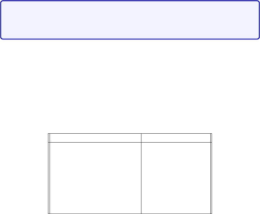
If you choose to present multiple results, you may opt for a table. In this case, you still
must include standard deviations and units.
Voltage (±0.2 V) Current (±0.1 A)
3.1 15.5
5.4 25.2
7.3 35.6
Table 2.1: Example of a table where all measurements have the same standard deviation. If
they didn’t, you must still include them individually next to each entry.
Tables are useful to show the explicit values of your results. However sometimes the exact
values aren’t as important as the general trend. In this case, you would opt to present your
data in chart form.
There are many types of charts. The most useful one for us will be the scatter plot. An
example of a scatter plot is shown in Fig. 2.1.
10
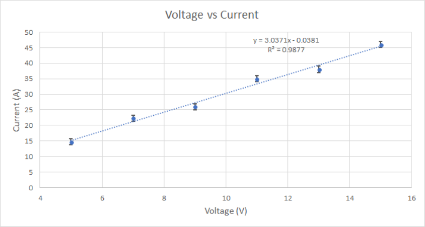
Figure 2.1: Example of a scatter plot. Each measurement is displayed as a point. One can
add error bars in both the x and y axes (although only the y direction is displayed here).
One can also fit an equation to the data set.
A scatter plot allows you to see the general trend of your data. If you expect a specific
behaviour, you can fit a trendline to your data to match a specific equation. By further
plotting error bars, you can compare how far away your data points are from the expected
trendline. This gives you some insight into whether your data matches your expected trend.
From the trendline, you can also see the actual coefficient of the fit. As shown in Fig. 2.1,
you can also display a
R2
value, which is called the coefficient of determination. This tells
you how good your fit was to your data. A perfect
R2
value is 1. See the appendix C for
details. For the example of Fig. 2.1, the
R2
value is good and most of the measurements fall
within a standard deviation of the fit, therefore this says that the current is proportional to
the voltage by a proportionality factor of 3.0371.
In summary, to present your data, you will need to know certain things: how to perform
an average and other basic statistics, how to evaluate the uncertainty in your measurements
and by extension, the final results you obtain from these, how many digits to display in your
final answer, and most importantly, how to analyse your data. This will be the subject of the
following sections.
2.3 Basic Statistics
Mean (Average)
Let
y
(
x
) be a function of
xi
data points. The value of
y
for
xi
can be denoted by
y
(
xi
) or
11

yi. The mean, or average, denoted by ¯yof a dataset with Ndatapoints is given by
¯y=1
N
N
X
i
y(xi) = 1
N(y(x1) + y(x2) + ... +y(xN)) .(2.2)
Standard deviation
The standard deviation of a function
y
(
x
) is denoted by
σy
. One says that a measurement
y(xi) has an uncertainty of
yi±σyi.(2.3)
The standard deviation tells you up to what value is your data precise: your data point can
vary between
yi
+
σyi
and
yi−σyi
. This means that your measurement
yi
can vary by 2
σyi
.
A good set of measurement would have a very small standard deviation: this gives you the
bounds under which your measurement is considered precise. You will see in section “
Error
Analysis” how to calculate this quantity.
Significant Numbers
To present results, one must present an appropriate number of significant numbers. In this
course, we will not be concerned with the number of significant digits, but more with consis-
tency in reporting the precision attributed to a measurement. When quoting a measurement,
the last digit should be fixed by the uncertainty of the measurement: it must match the order of
magnitude of the standard deviation. In other words, the standard deviation fixes up to what
precision (roughly decimal place) you can quote your results. Table 2.2 lists some common
mistakes and how to present those results appropriately. In the context of this course, we will
simplify our conventions by
keeping only one significant number for the standard deviation
.
Recall that leading zeros do not count as a significant number and trailing zeros (after the
precision of the standard deviation) should be discarded.
Incorrect Correct
324.9453 ±0.02m 324.95 ±0.02m
20 ±0.1$20.0±0.1$
3×10⁴±2N 3000 ±2N
31.02 ±0.10$31.0±0.1$
0.003564 ±0.00012m/s 0.0036 ±0.0001m/s
Table 2.2: Significant numbers. Common mistakes and the correct way to present such
results.
Precision versus Accuracy
Precision
refers to how closely related two measurements are from each other. This
means that one expects a small standard deviation for highly precise measurements.
12

Accuracy
measurements refers to the closeness of a measurement from a known value.
This means that one must calculate the
difference
of the measurement to the known value
in terms of standard deviations
. For example, if
y
= 0
.
4
±
0
.
1m, and the known value is
yt= 0.7m, then the measurement differs by 3σy.
Often, one may encounter a highly precise set of measurements, but also very inaccurate.
This is a signal that there may have been a
systematic error
in your results. This is a type
of error that propagates throughout your experiment and offsets your results by a constant
factor. For example, recall the equation of the period of oscillation of a pendulum is
T= 2πsL
g.(2.4)
If one incorrectly measured the length
L
of the string, then the results would be offset by a
constant factor of pLgood −Lbad.
2.4 Error Analysis
Measurements carry an inherent uncertainty to them. To characterize this uncertainty, we
write attribute them a value to which the measurement can vary. This standard variation
is called a standard deviation. For this reason, we will often use is interchangeably with
the term uncertainty. Note that there is a formal mathematical definition of the concept
of standard deviation, but for the context of this course, we will abstain of such definition.
Sometimes, a measurement must be manipulated with other measurements in order to obtain
another variable. To keep track of how the uncertainty of each measurement is propagate
through this manipulation, we use error propagation techniques. This characterizes the error
on this derived quantity, and therefore, it is another type of uncertainty. Thus, we will also
use the term error interchangeably with uncertainty.
Standard deviation of a measurement
The rule of thumb for finding the standard deviation of measurements is as follows:
each measurement can vary by half of the smallest available precision from your measuring
instrument, and you must add the uncertainties of the measurement. Consider the example
of measuring a distance with a 30cm ruler. The smallest increment is a mm. When you
measure a distance between
two points
, you take
two
measurements: one at each point. Thus
the uncertainty on the measurement is 2
×
0
.
5mm, so 1mm. This is exactly the smallest
available increment of your measuring device. Therefore, unless otherwise specified, the
standard deviation of a measurement is the smallest available measurable value allowed by
your instrument.
13

Another example is measuring the time difference between two events. Again, there will
be two measurements: the initial and end time. Stopwatches often allow one to view up
to ms precision. However, the average visual time reaction is roughly 0
.
3s, and therefore
each initial and final time measurement varies by 0
.
15s and so the uncertainty for the whole
measurement is 0.3s.
Standard deviation for fluctuating data
For fluctuating datasets where each measurement is independent of the previous, to reliably
represent your data, you should take some form of average over some number of measurements.
Measurements that are random are said to follow a Poisson distribution. To study these
types of measurements, one typically chooses a subset of
N
data points, and calculate its
mean. Given the mean, one must approximate the error as
di=yi−¯y. (2.5)
The standard deviation on the average of your measurements will therefore be given as
σ¯y=v
u
u
t
1
N
N
X
i=1
d2
i.(2.6)
This can be obtained in Excel by using the function =STDEV.P(x).
Error propagation
The standard deviation value above is attributed to
a single measurement
. However, often
one would be interested in deriving a quantity that depends on multiple measurements. To
describe the standard deviation on the end result, one must use error propagation techniques.
For these labs, you will only need to know the following two error propagation formulas.
Consider first the following function
f(x, y) = x×y. (2.7)
The standard deviation σfon fwill be
σf=q(xσy)2+ (yσx)2.(2.8)
This will be useful for example to calculate the error on the area given two length measurements,
or in Lab 2, you can calculate the error on the time constant in a similar way.
Consider also the function
f(x) = 1
x.(2.9)
14

The standard deviation for this case is
σf=σx
x2.(2.10)
Measurement analysis
To understand the significance of a measurement, one can compare it in different ways.
When a theoretical value is known, one can compare a set of measurements by calculating
the absolute error, the percentage error or the standard deviation error. One can also analyse
a dataset by studying fits in a similar manner.
Absolute error
The absolute error indicates the difference between the known value, and either a mea-
surement, the mean value of a set of measurements, or a fit parameter. One can also compare
a set of measurement to the fit of the dataset in this matter. Let
yt
be the theoretical value
and ybe one of the variables mentioned before, then the absolute value is
Absolute error = |yt−y|(2.11)
Percentage error
The percentage error is simply the ratio of absolute error relative to the known value.
This gives an indication, in percentage, of how far away with respect to the known value is
the measurement. It is given as
Percentage error =
yt−y
yt×100 (2.12)
Standard deviation error
The standard deviation error indicates how many standard deviations away is a measure-
ment when compared to the known value. It is given as
Standard deviation error =
yt−y
σy
(2.13)
You will have to recognize which one of the above is useful and representative of the
information that you wish to convey for the data analysis that you have to perform. Note
that we’ve taken the absolute values of the above, but by not doing so, we could convey
information about the “direction” of the error i.e. whether the measurements are higher or
lower than the known theoretical value.
Fit analysis
As mentioned before, a good way to know whether your fit is correct is to compute the
15
coefficient of determination
R2
. To compare your fit to your data, you should see whether
your data points all (or mostly) fall within one standard deviation of the fitted equation, that
is if the standard deviation error should be less than 1
σ
for all data points when compared
to
yfit
. Note that for small
R2
, it could be possible that the fit falls within the error bars of
your graph, and therefore one would like to obtain R2≈1 with small error bars.
It is worth mentioning that in realistic settings, what is considered a “good”
R2
value
varies depending on context. In physics, simple models can yield
R2≈
1. In contrast, a
good
R2
value in biological systems can be in the range of 0
.
7, and in social sciences, the
standards are often lower. This highlights the quantitative nature of physics and its eloquent
relation to mathematics, and therefore this serves as an optimal stage for you to learn about
quantitative data analysis.
16
Part II
Lab Manuals
17
Chapter 3
Lab 1 - Capacitance
3.1 Learning objectives
•How to acquire data
•How to quantify error
•How to present data
•Learn about linear fits
•Confirm capacitance law
3.2 Introduction
In this lab you will be asked to accomplish the following tasks:
•
Find possible parameters that could affect the capacitance of a parallel plate capacitor
system.
•Support your conclusion based on a quantitative evaluation of your data.
You will have to chose some parameters and quantify their affect on the capacitance of
the setup. In the process, you will learn how to acquire good data and how to quantify and
present your data. We would like to re-emphasize that collaborations and discussions are
encouraged and expected throughout the two sessions of the lab.
In the first session, you will work together to find possible parameters that can affect the
capacitance of a pair of parallel plates. Measurements at this stage may be crude; do not
worry about that, we are not evaluating the usefulness of the data at this stage, rather the
process of thinking about what this data means, and your thinking process about how to
improve your experiment to obtain better data.
18
During the second session, you will be asked to obtain quantitatively improved data and
to compare it with data from the previous session. You must then conclude, based on a
quantitative evaluation of your data, whether or not, and how, your chosen parameter affects
the capacitance of a parallel plate capacitor.
Role as a TA
Your role as a TA will be to guide them through the “script” that we present
in this protocol. You should guide them by asking questions and making them
think about their results as opposed to giving them the right answer immedi-
ately. You are also required to bring teams together to collaborate/discuss
with each other. You should clarify the grading method, emphasizing that the
major part of their grade comes from the materials presented in the log book.
3.2.1 Pre-lab activity
To answer some of these questions, we encourage you to review Chapter 2 of the lab manual
on Data Analysis.
1.
What is a measurement? Give your own definition of what constitutes a measurement
based on your previous courses with lab components (biology, chemistry, physics).
Answer
This is more open-ended. Measurements can be taught of as quantifying
observations. Measurements must come with an inherent uncertainty.
2.
Two engineers must measure the distance between the McGill metro station to the
athletic centre to build an underground tunnel. One engineer finds that the distance is
9134
±
5m while the other finds that the distance is 9150
±
20m. In what ways can
they compare their measurements? Do their measurements agree? Explain.
Answer
They should compare the standard deviations to conclude that the measure-
ments of the two engineers agree.
3.
The city is considering to build a metro line between McGill station and the station at
University of Montreal. To do this, an engineer decides to use a km-long ruler whose
smallest divider is a meter. She did not use any other measuring devices. She takes
her measurements and presents her findings to her team as 3653
.
4500m. What is the
19

uncertainty on this measurement? Did she present enough, too little or too many digits
about her measurement? Why?
Answer
The correct way to present this measurement is 3653
±
1m since the smallest
increment on her measuring instrument is a meter. She presented too many
digits since her measuring tool cannot give such precision.
4.
Two groups of researchers are trying to test their new methodology to measure the speed
of light
c
. Current research shows that the speed of light is roughly
c
= 2
.
99792
×
10
8
m/s. The first group finds that
c
= 2
.
88
±
0
.
02
×
10
8
m/s while the second group
finds that
c
= 3
.
0
±
0
.
2
×
10
8
m/s. What do these measurements tell you about their
methodology in the context of precision and accuracy? What type of mistake may have
caused the discrepancy in the first group’s results?
Answer
These measurements show that the first group has a more
precise
method-
ology, while the second team has a more
accurate
one. The first group
probably has a systematic error that causes this offset.
5.
How do you know if an experimental result is acceptable and trustworthy? What gives
you confidence that your data is trustworthy?
Answer
They should say something about the standard deviation and fit coefficient of
determination. Ideally, they would mention that the methodology must be
questioned as well.
3.2.2 What is a capacitor?
You learned in class that charges can attract and repel each other. This is because point
charges source electric fields that apply a force on a test charge. Since there exists a force
between two point charges, there exists a potential energy difference ∆
U
between two point
charges (relative to some reference separation) due to this force. We define electrical potential
difference as the potential energy difference per unit charge,
∆V=∆U
q(3.1)
20
where here
q
is the charge of a test particle displaced in the electric field of a source charge
Q
. In practice, it is more useful to define an electrical potential difference to move
any
test
charge qfrom r=∞to a distance Rfrom a source charge Qas
V=kQ
R(3.2)
where
k
is Coulomb’s constant
k
= 1
/4π0
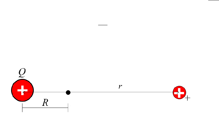
. This will have units of voltage V. This process is
depicted in Fig. 3.1.
Figure 3.1: The electrical potential due to a source charge
Q
(left) at a distance
R
. The
test charge (right) is placed at a distance
r
from the location that we measure the electrical
potential difference.
Now consider a pair of parallel conducting plates separated by a distance
d
connected
to a battery as shown in Fig. 3.2. A pair of parallel plates separated by air or another
(non-conducting) material can be assembled into a capacitor : on each parallel plate, because
of the battery, there will accumulate a number of equal and opposite charges: electrons on the
negative plate such that the total charge is
−Q
, and +
Q
will accumulate on the positive plate.
Because of the gap (separation) between the plates, there now exists an electric potential
between the plates, which is given by eq. (3.1).
One defines the capacitance of a capacitor as the constant of proportionality between the
total number of charges
Q
(same magnitude on either plate) and the electric potential
V
stored between the plates, i.e.
Q=CV. (3.3)
Capacitance is measured in Farads F. In this lab, you will be asked to verify what affects the
capacitance
C
of a parallel plate capacitor system. (A useful constant in such setup is the
vacuum permittivity = 8.85 ×10⁻¹² F/m.)
21
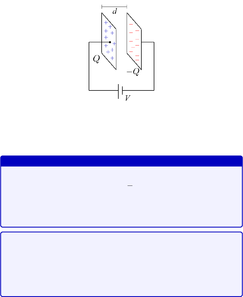
Figure 3.2: Parallel plate setup. The battery with voltage
V
creates a flow of electrons such
that there will accumulate a total charge of
−Q
on the negative plate, and +
Q
on the positive
plate. Since the plates are separated by a distance
d
, there will be a electrical potential
difference between the two plates.
Expected result
We expect them to find
C=A
d(3.4)
where
is the relative permittivity. They should be able to test the area
correlation with the plates given, and the distance correlation by stacking
multiple sheets of dielectric between the plates.
We expect them to plot their data and fit a linear regression between
C
and
A
with standard deviation error bars as shown in Fig. 3.3. Knowing the distance
between the plates, they can also plot the relative permittivity versus the
area, and compare with the mean value of
to see the consistency of their
results as shown in Fig. 3.4. You should encourage them to compare the
R2
of the linear fit relative to comparison with a constant value.
22
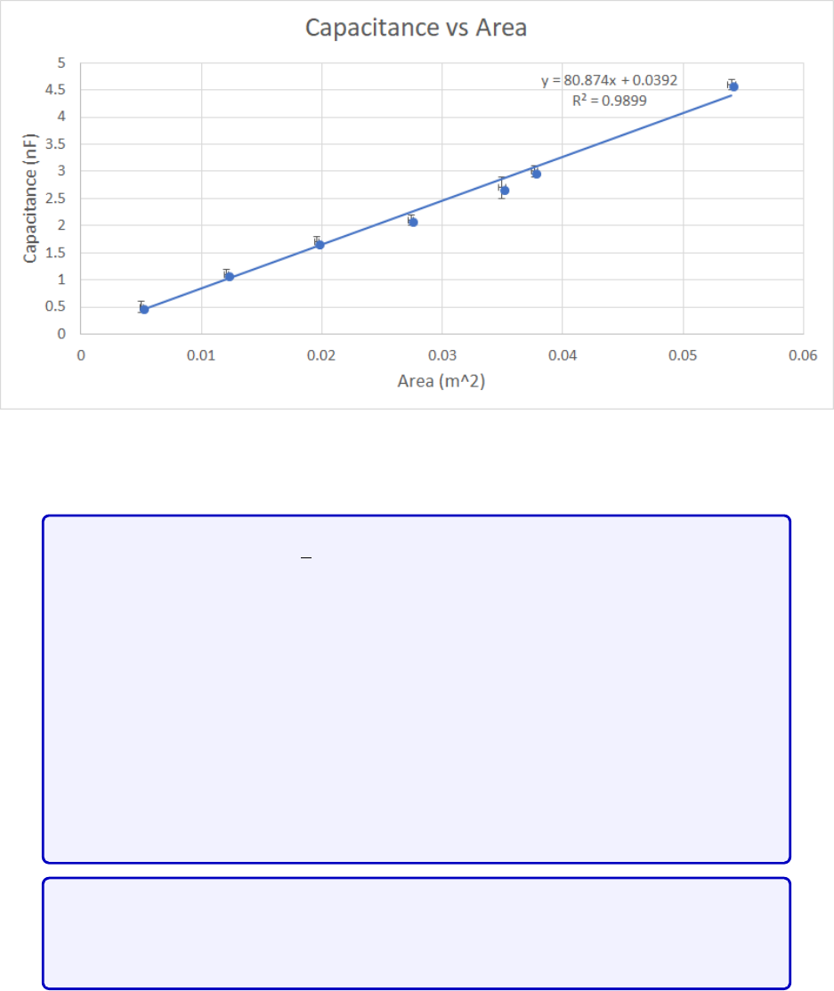
Figure 3.3: [Figure only available to TAs] Data of capacitance versus area. We expect them
to display the equation and R2value. They should be able to find a good linear fit.
When testing for the
d
dependence, the data showed that for
n >
3 sheets,
there seems to be a 1
/√d
correction that appears, and therefore students
aren’t expected to find a perfect fit for large distances of
d
. This is mostly
due to some polarization effect from stacking the dielectrics, and therefore
one should view the 1
/d
dependence as a “small distance” approximation.
You should encourage students to find this disparity between experiment and
theory and encourage them to discuss the cause of this. The data is shown in
Fig. 3.5. They may struggle with this part since it won’t be a simple linear fit
and they will not know about polarization, etc. But encourage them to take
data diligently and discuss with others, and then you can coax them into the
correct interpretation at the end during the discussion phase.
Students are also encouraged to discuss about other parameters such as shape,
volume, mass applied to the dielectric, and the use of other dielectrics, but
these aren’t easily quantifiable parameters.
23
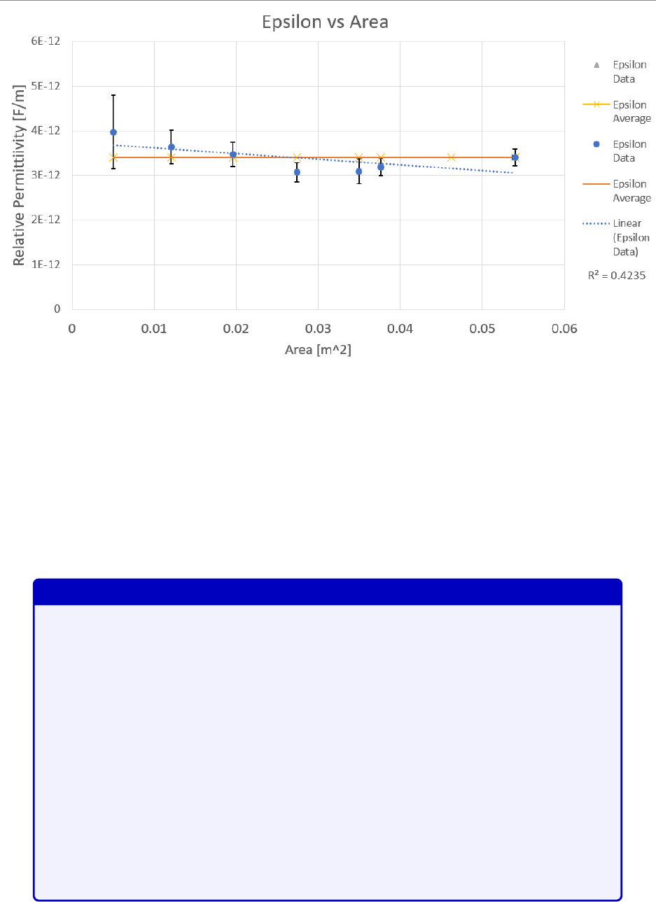
Figure 3.4: [Figure only available to TAs] Data of the relative permittivity versus the area,
compared to the mean value, and a linear regression fit. The average
from the data is
3
.
4
±
0
.
3
×
10
−12
F/m. They should find that it is a constant since by definition, this is the
constant of proportionality of eq. (3.4), and we expect theirs results to be similar.
3.3 Protocol
3.3.1 Session a
Session #1
We suggest the following time distribution for this session:
During the first 20mins, assemble everyone to the front and do a quick
introduction, and maybe a demo of the manipulations. You should then ask
everyone what they think could affect the capacitance of a capacitor, and
push them to give a physical reason behind their hypotheses. Have them
consider the units of capacitance [
Q/V
], and thus motivate that for parallel
conducting plates, larger area would allow for more charges to accumulate, and
since electrical potential is given by the relative distance between two charged
objects eq.
(3.2)
suggests that there may be 1
/r
dependence to capacitance.
Recommend that they work together to cover more parameters e.g. one team
takes care of area, the other does distance.
24
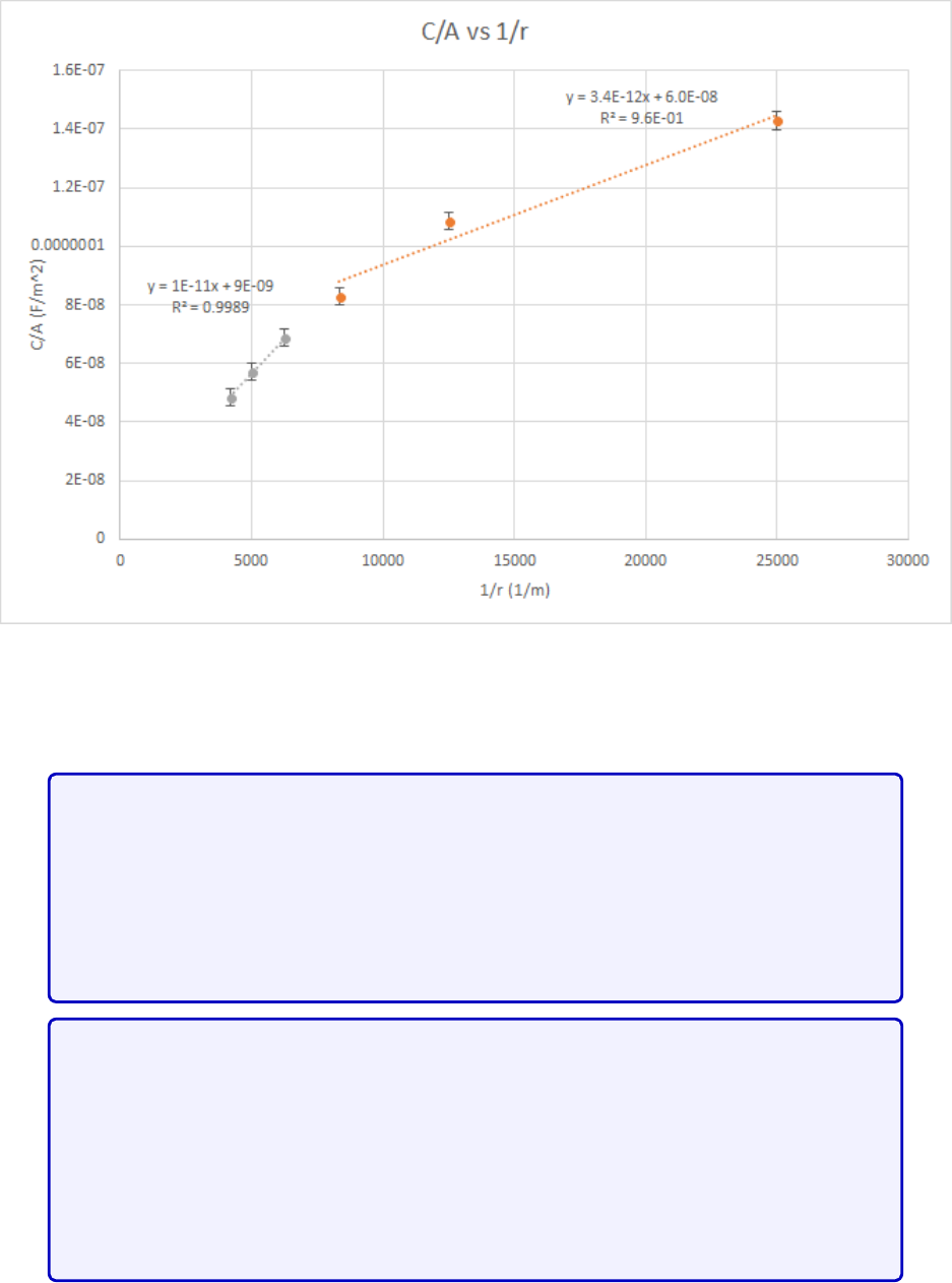
Figure 3.5: [Figure only available to TAs] Data of
C/A
versus 1
/r
. The data points in orange
are those of the first three layers. The linear fit matches the average
found from the area
experiment.
Give them about 60-75mins to perform their measurements while walking
around, answering questions and facilitating discussions between teams and
teammates. During this period, make sure that everyone makes at least three
measurements of varying area with the two plates perfectly aligned. This will
serve as a baseline to put them on the right track. Also, do not forget to
verify that students have done their pre-labs.
After about 90mins of the 2-hour session, ask your assigned groups to describe
their findings. Enumerate what could affect capacitance and why. Make sure
that they support their findings with statistics (standard deviations and fits),
and ask them whether the correlations that they find are well supported and
which warrant extra verification during the next session. After this discussion
period, make sure that everyone understands what they have to be looking for
to verify the effects of area and distance of the plates during the next session.
25
For the remainder of the time, students can try and take additional mea-
surements, and prepare notes for the next session. Do not forget to ask the
students to upload the log book to crowdmark.
The available materials to be used in your experiments are listed in Table 3.1. The metallic
rectangular plates will be of varying dimensions. The manipulations are straightforward:
insert either a plastic or paper sheet between the two plates and use the Arduino unit (see
below) to measure the capacitance. At this point, you do not need to know how the Arduino
unit works, simply how to use it. You will learn how it works in the next lab. The plates
must not touch each, otherwise you will not see a measurement: this causes a short-circuit
and therefore you will not see a capacitance measurement. You can assume that the distance
between the plates is the thickness of the plastic or paper sheet.
Individual station Collective station
Laptop Aluminum foil
Arduino capacitance setup Blocks of wood
Metallic plates Small weights
30cm ruler Assorted capacitors
Plastic sheets Assorted resistors
Paper sheets Extra wires
Micrometer
Multimeter
Table 3.1: Available material for Lab # 1
Information about using the Arduino code can be found here. To use the Arduino unit:
1. Plug the USB-port into the laptop
2. Open the Arduino Genuino application on the laptop.
3.
Open the capacitanceMeter.ino file found by opening Windows Explorer and typing
\\altima\Physics_DFS\Physics_102 in the address bar.
4.
In the tabs above, go into the drop-down menu Tools
→
Port. Choose whichever COM
is labelled by “(Arduino/Genuino Uno)”.
26
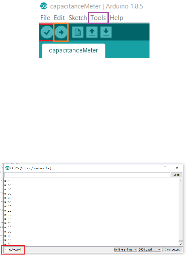
Figure 3.6: Arduino application menu bar. Note that the color boxes were added to guide
the eye. The red checkmark box is the
verify
button. It serves to verify whether there is an
error in the code. The orange right arrow box is the
upload
button, and the purple box is
the Tools drop-down menu bar.
5.
Verify the script by clicking the icon with the checkmark. If there is an error, call the
TA.
6. Upload the script by clicking the icon with the right arrow.
7.
In the tabs above, go into Tools
→
Serial Monitor (or on your keyboard, press
Ctrl+Shift+M). You should see that a window open as follows (without the num-
bers):
Figure 3.7: Arduino Serial Monitor. This is a pop-up screen where you will see your
capacitance measurements scroll by. The Arduino unit takes a capcitance measurement at
a fixed frequency. Unless otherwise specified, the output is in nanoFarads. Units aren’t
displayed so as to simplify the transfer from the monitor screen to Excel, but one could
display the units by changing the command in the Arduino script. To stop the scrolling of
measurements, click on the Autoscroll box.
27

8.
Take the two wires (see Fig. [updated setup]) and simply touch each side of the parallel
plates: you should see a multitude of measurements scrolling down the monitor window,
as in Fig. 3.7. If you do not see many measurements scrolling in the monitor window, it
is likely that the plates are touching each other and you therefore have a short circuit.
[input new setup pic]
9.
You can stop the auto-scroll by clicking the bottom-left box to better see your results
(see Fig. 3.7).
Notice that in Fig. 3.7, the data fluctuates. You will have to determine how many
capacitance measurements you should average over to acquire a good representation of a
particular capacitance measurement. We refer you to the Part I, section 2.4 of the lab manual.
Using this setup, proceed to conduct you experiments and collect data that will let you
evaluate
C
in eq.
(3.3)
as a function of different geometrical parameters of the capacitor
system.
You will have the opportunity to test whatever hypothesis you may have, however
every group must at least include a capacitance measurements for three or more
different pairs of plate sizes while inserting a single sheet of plastic between them.
The plates must be perfectly aligned on top of each other
. After doing so, you may
explore in more details the consequences of these measurements, or you may study other
possible parameters that could affect the capacitance.
The three area measurements will serve as a baseline for students in case some
of them attempt to test unconventional hypotheses.
Given the measurement of the two sides
L1
and
L2
of a rectangle and their corresponding
standard deviations σL1and σL2, the standard deviation on the area is given by
σA=q(L1σL2)2+ (L2σL1)2.(3.5)
While studying other parameters, if you are unsure of the standard deviation of a certain
parameter, you may ask the TAs to help derive the appropriate derived standard deviation
for that parameter.
To analyse your data, we refer you to section 3.4. Enter your set up, measurement process
and data in your log book. Before handing in your log book, be sure to write down your
observations in the
General Notes
section of your log book, and a rough plan of what you
intend to do during the next session in the
Conclusions and future work
section. The
latter part should be done after discussions with at least one other group.
28

3.3.2 Session b
Session #2
In this session, you should remind everyone that last time, you discovered
together that
C∝A/d
, so this session should be simpler as they will know
what to do, and will simply have to improve on the data and interpretations,
particularly with regards to the 1/d measurements.
We recommend that you bring whatever material that you think could help you acquire
better data in Session b. By now, you should know what parameters affect the capacitance,
and therefore you should plan in advance your own “protocol” to verify your hypothesis
quantitatively with improved data, compared to that in Session a. This protocol does
not
have to match what you wrote in your log book in Session a, but if it does differ, you must
explain what made you change your mind.
We expect that you contrast your results from this session versus those you obtained in
the previous one: explain how your measurements improved or differed.
Be mindful that you will be evaluated based on your data presentation, data analysis
and explanation of the physics from this session, therefore be certain to fully, but succinctly,
describe your thought process.
3.4 Measurement Analysis
During this lab, you will have to use data analysis techniques to understand your data. For
each session, we recommend that you analyse your data as follows.
To study a system, one typically isolates as many variables as possible to see each of its
individual affect on the whole system. If we are able to isolate such a variable, mathematically,
that is the equivalent of finding some
f
(
x
) that depends just on one variable
x
. In this lab,
you will find as many variables that can affect the capacitance as possible by isolating each
such variable, one at a time.
For each dataset, corresponding to each parameter you measure, you must abide by the
error analysis rules outlined in chapter 2. The data analysis can be done much more rapidly
with Execl spreadsheets, therefore we highly recommend that you read appendix A.
Once you have result from your data, you must offer a physical explanation that supports
your results. Explain why physically each parameter affects the capacitance of the system.
Support any claims you make by proposing a possible experiment to test your claims, and
offer possible outcomes that one could observe from your experiment. Recall that bouncing
your ideas off peers is an invaluable way to actually test the rational of your hypothesis.
29
Chapter 4
Lab 2 - RC Circuits
4.1 Learning objectives
•Learn how to connect circuits
•Learn about exponential functions
•Learn about RC circuits
•Learn about equivalent resistance and capacitance
4.2 Introduction
In this lab you will characterize an RC circuit. An RC circuit is a circuit that contains a
resistor (R) and a capacitor (C), connected in series with an EMF source during charging and
without the battery during discharging. The data analysis tool we will use is called a PASCO
850 Universal Interface, the use of which will be explained below. Specifically, we will use a
voltmeter and a signal generator tool to examine the charging and discharging of a capacitor.
In the first lab session, you will be asked to
measure the time constant τ
of a given
RC circuit (more on tbis below). In the process, you will learn how to measure time constants
and understand subtleties in the data acquisition apparatus. This session will be more like a
traditional lab where you will follow well outlined instructions.
In the second session, you will be asked to
build an RC circuit with a specific time
constant
and to show, based on well supported data, that your circuit has the appropriate
time constant. When you arrive at the second session, you will receive a sheet that asks you
to build an RC circuit with a specific number of parallel branches. You will have to deduce
how to choose an appropriate number of resistors and capacitors for these branches to obtain
a specific time constant.
30
4.2.1 Pre-lab activity
1. Why would we want to fit a dataset to an equation?
Answer
Curve fitting allows one to match data to a quantitative theoretical model. A
good model is able to predict future outcomes of similar experiments.
2. What is exevaluated at x= 0, x= 1 and x=−1?
3. For f(x) = e−x, what is the value of xso that f(x) = 0?
4. What does a,band cdo in the following function?
f(x) = aebx +c(4.1)
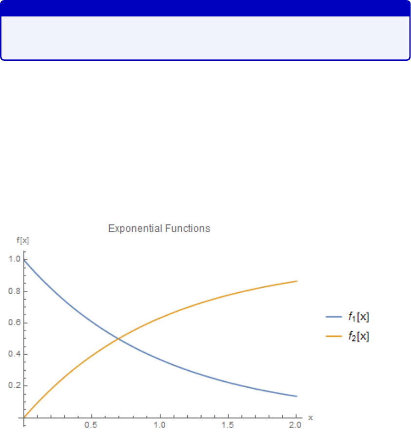
5. What is the difference between these two plots:
Figure 4.1: Exponential functions.
4.2.2 RC Circuits
Recall that the capacitance is defined as the proportionality constant between the total charge
accumulated by a capacitor and the voltage difference across the circuit
Q=C∆V. (4.2)
31

In this equation, the charge
Q
is expressed in Coulomb (C), the voltage ∆
V
, in volts (V)
and the capacitance Cin farads (F).
In this lab you will study both the charging and discharging process of an RC circuit.
During the charging process, an electrical EMF source accumulates charges on each side
of the parallel plate capacitor. During the discharging process, the capacitor releases all
its charges into the circuit (which now does not contain the battery). Capacitors charge
and discharge exponentially in time. During the discharge of a capacitor, the instantaneous
voltage ∆VCbetween the ends of the capacitor also drops and is given by
∆VC= ∆Vmaxe−t/τ (4.3)
where ∆
Vmax
is the maximum voltage across the capacitor, i.e. the voltage to which the
capacitor was initially charged, tis the time and τis the time constant given by
τ=ReqCeq (4.4)
where
Req
and
Ceq
are, respectively, the equivalent resistance and capacitance to which we
can reduce the circuit. Although the theoretical discharge time is infinite, in practice we
consider that the discharge is over when the voltage at the bounds of the capacitor is at 1%
of its maximal value.
4.2.3 Equivalent resistance and capacitance
To find the equivalent resistance and capacitance of a circuit, one must apply the correct
equations to sum the contributions of all the components. The equivalent quantity differs
depending on whether the resistors and capacitors are combined in series or in parallel. For
resistors, the equivalent resistance is given as
Rseries =R1+R2+R3+...Rn=
n
X
i=1
Ri(4.5)
1
Rparallel
=1
R1
+1
R2
+1
R3
+... +1
Rn
=
n
X
i=1
1
Ri
(4.6)
For capacitors, the equivalent capacitance is given as
Cparallel =C1+C2+C3+...Cn=
n
X
i=1
Ci(4.7)
1
Cseries
=1
C1
+1
C2
+1
C3
+... +1
Cn
=
n
X
i=1
1
Ci
(4.8)
32
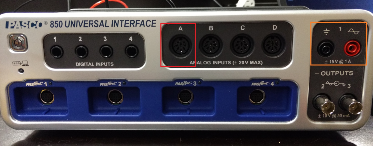
4.2.4 Data Acquisition Equipment
In this lab you will use the PASCO 850 Universal Interface to measure and plot voltages as
a function of time in an RC circuit. We will use two terminals of the PASCO device. The
first connects to the input/output voltage source. The other (Analog connectors) is a pair
of probes which measures the voltage across the capacitor of the circuit. See Fig. 4.2 for
location of terminals.
Figure 4.2: PASCO 850 Universal Interface The red box is the probe Analog input. The
voltage source (Output 1) is boxed in orange.
Given the nature on these measurements, there is an inherent fluctuation to the data
that is difficult to characterize. During the first session, you are not required to produce
quantitatively well supported data: unless otherwise specified, you will not need to keep
track of standard deviations. For the second session, you can completely ignore standard
deviations. You are still required to generate
R2
values or other quantities that might be
relevant to your goal.
4.3 Session a
Hooking up the Equipment
During the first session, you will receive an RC circuit fastened onto a wooded board. Before
proceeding with measurements related to charging and discharging capacitors, conduct the
following steps:
1.
Turn the wooden board over to reveal the circuit Fig. 4.3. There are actually two
circuits here, one consisting of a 100kΩ rheostat (variable resistor) and the 100
µ
F
capacitor, the other consisting of a 470Ω resistor and a 0
.
1
µ
F capacitor. We will not
use the 0.1µF capacitor, or the rheostat.
2.
Connect the Output 1 of the PASCO 850 Universal Interface to the wooden board’s
terminals as well as the Analog Input A in order to complete the circuit as shown on
33
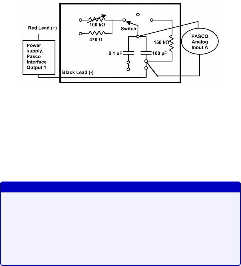
Fig. 4.3. The 100
µ
F capacitor can now charge through the 470Ω resistor (when in the
“charge” state on the wooden board) and discharge through the 150kΩ resistor (when
in the “discharge” state). The charging voltage is read on the computer as Input A
measures the voltage across the 100
µ
F capacitor. The Output 1 is the one with the red
and black connectors and the analog inputs are labelled with letters on upper half of
the interface and on the right.
Figure 4.3: Circuit for session 1.
Protocol
You will execute the following steps in order to understand how to use the PASCO interface to
characterize an RC circuit. For this session, we recommend that you record your measurements
in an Excel spreadsheet, and rewrite the relevant results in your log book and your observations
in the General Notes section of your log book. You must also answer the questions that are
embedded in the following instructions in the Results part of your log book. You should also
write down any technical notes about the apparatus and how an RC circuit works in order
for you to fast-track your manipulations for the next session.
Session #1
In this session you will supervise students as they perform the protocol below.
You may gather students in the beginning to give a brief introduction and
summary of the lab. By the end, they should be comfortable measuring
charging/discharging time constants. When they use the square wave input,
make sure that they understand how to vary the parameters to obtain useful
data, i.e. changing the frequency of the function generator and the frequency
of data acquisition.
1. Connect the circuit as shown in Fig. 4.3 and explained above.
2.
The PASCO file can be found by opening Windows Explorer and typing
\\altima\
Physics_DFS\Physics_102 in the address bar.
34
3. Turn on the PASCO and plug in the USB into the computer.
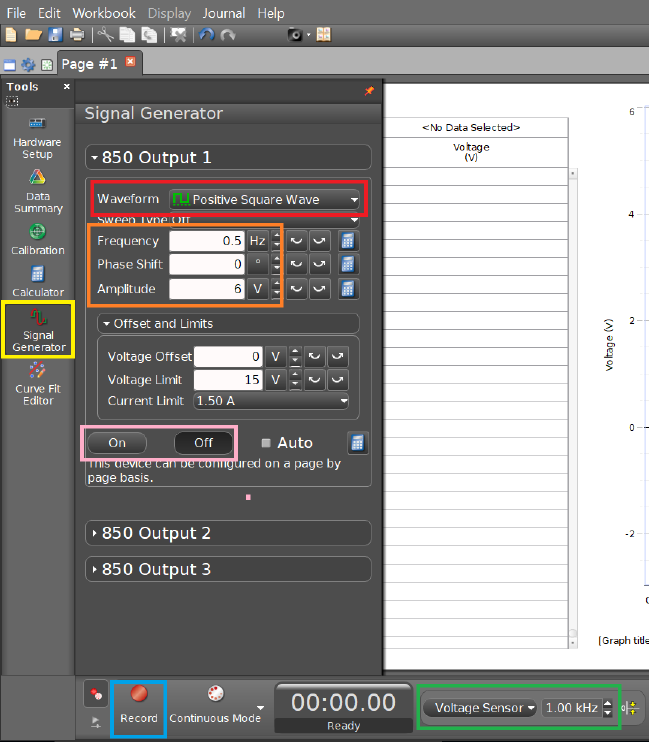
4.
In the software, open the “Signal Generator” tool, which is located on the left hand
side panel and make sure that the signal is set to ”Positive Square Wave” with an
amplitude of 6V and frequency of 0.5 Hz. This is equivalent turning on and off a DC
voltage 2 times per second. Change the data acquisition frequency found at the bottom
of the interface to 1kHz. See Fig. 4.4.
Figure 4.4: Settings for a positive square wave input. You must first select the “Signal
Generator” setting in the yellow box. The red box allows to change the waveform. Change
the frequency and amplitude according to the orange box. Change the data acquisition
frequency to the values in the green box. Once you are ready to record your data, select the
record button (blue box), and turn on the voltage source (pink box)
5.
With this input from the ”Signal Generator” you won’t need to use the ”charge” and
”discharge” switch from the wooded board. Instead you will simply turn On and Off
(pink box) the power supply under the 850 Output 1 panel above the 850 Output 2
35
panel before and after recording measurements. So leave the switch on “charge” for the
rest of the experiment.
6.
After turning on the signal generator, press the record button twice to record and stop
the recording after observing a few charge/discharge cycles.
7.
Zoom in on a region with both charging and discharging behaviours by rescaling the
axes, and figure out which section corresponds to charging/discharging. Ask a TA
about axis rescaling if necessary.
8.
For the charging part, measure and record the time difference between the moment
the voltage starts increasing to the moment where the voltage is at a value 1 −1/e of
the maximum voltage
V0
. You should understand why you are measuring this time
difference. Further calculate the standard deviation for a time constant measurement
using the techniques in Chapter 2. We do not need the exact number, only its order of
magnitude.
Since we are measuring the difference in time between
V0
and
V
(
t
=
τ
),
we expect them to use the standard deviation technique described in the
beginning of section 2.4 of chapter 2.
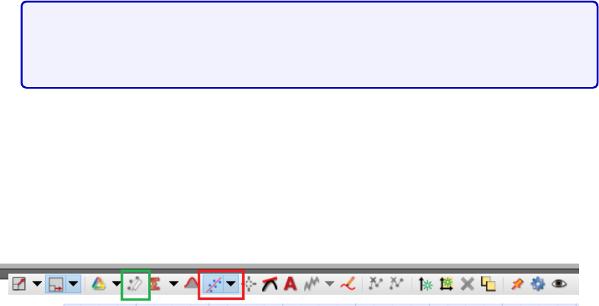
9.
For the discharging part, you will use the Curve fitting tool in the software. The
software can perform an exponential regression on the data you record. To make good
use of that, activate the Curve Fitting option (see Fig. 4.5). The curve of eq.
(4.3)
will
be fit to the whole data set. To fit it on the right segment on the data set, use the
highlighting tool and select/box the values that are most relevant. Verify that the time
constant corresponds to the parameter 1/B in the curve fitting data window.
Figure 4.5: Graphing toolbar. The toolbar appears when moving the mouse to the top of
the graph. The red boxed icon is the Curve fitting tool. Select the “Natural Exponential”
function. The highlighting tool is boxed in green. This allows to select a smaller subset of
data to apply the curve fitting.
Use this to fit an exponential curve to the discharging region, and record the value of
the parameter Band the order of magnitude of the standard deviation.
10.
Compare the time constants obtained from both the charging and discharging regions.
Can you explain the difference in order of magnitude between the standard deviation
of the charging versus the discharging measurements?
36

Answer
They should find that the time constants are the same. For the standard
deviation, the charging measurement relies on the difference of two data points,
thus the standard deviation
σ
is larger than the discharging measurement
where the PASCO interface fits N2 data points to generate σ.
They should also note that the standard deviation derived from the discharge
fit is insignificant relative to the amplitude of the measurements, thus it isn’t
useful to use it as an error bar.
Calculate the theoretical time constant based on the known values of resistance and
capacitance. You can repeat steps 6-10 for different segments of charging/discharging
in your data if you want to verify the consistency of your measurements.
11.
Answer the following questions in the results section of your log book. Should all the
time constants be the same or different? Why and why not? What would happen if we
had used the rheostat instead of the 470Ω resistor in Fig. 4.3 and used a DC voltage
source (with the On/Off switch on the board) instead of a wavefunction source: would
we have the same time constant for both charging and discharging? If you have time,
you should test your hypotheses experimentally.
Answer
All the time constants should be the same because we are charging and
discharging across the same resistor. If we had used the rheostat with a DC
voltage and the On/Off switch, since we’re charging and discharging across
different resistors, the time constants should be different. By eq.
(4.4)
, the
resistance should affect the time constant linearly.
12.
Answer the following in the results section of your log book. Assuming the voltage,
when completely charged, is set to
V0
= 1 and by considering the variables
τ
for time
constant and
t
for time, what are the equations for of charging and discharging? Support
your answer by physical arguments.
Answer
Discharging is
V
=
e−t/τ
and charging goes as
V
= 1
−e−t/τ
. At
t
= 0, we
expect the charging function to be 0 and the discharging function to be 1.
Similarly, at t→ ∞, the reverse must be true.
37
13.
Answer the following in the results section of your log book. Your draft calculations
can be shown in the “General Notes” section of the log book. In the circuit of Fig. 4.6,
how will the fully charged capacitor affect the current and potential in R6? Answer
this in your log book.
Figure 4.6: Effect of a fully charged capacitor on the circuit.
Answer
The current is defined as the change in charge over time. In other words,
dQ
dt =CdV
dt =I. (4.9)
Therefore if the capacitor is fully charged, the change in voltage vanishes and
so the current also vanishes: it is then considered like an open-circuit. Thus
the potential across R6 vanishes.
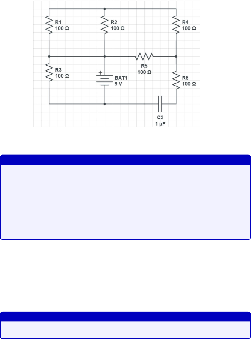
14.
Answer the following in the results section of your log book. Your draft calculations
can be shown in the “General Notes” section of the log book. Given Fig. 4.7, what
must be the value of C2 such that the time constant of the equivalent circuit is
approximately
τ
= 12
.
5ms? If one replaces C2 by two capacitors in series, one of which
has
C
5 = 250
µ
F. What must be the capacitance of the second capacitor to preserve
the same time constant?
Answer
For the first part, C2≈50µF. For the second part, C2≈61µF.
38
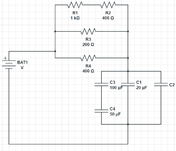
Figure 4.7: Time constant practice.
15.
If you want to keep a trace of a graph produced by the PASCO, click on the Final
results tab and select which graph you want by choosing the right run in the scrolling
menu of the colored triangle. Click on the camera icon on the top panel. This will take
a picture that will be accessible in the journal, on the right hand side, where it can be
saved as jpeg or html. Alternatively, you can also save your whole set of measurements
by going to the top left tab “File”, and select “Save As”.
Note: as you step through he above manipulations, make sure to record important
technicalities of the time constant measuring methodology in order to accelerate your data
acquisition process for the next session. You should perform any further tests that you believe
would help you better understand the RC circuit in preparation for the next session.
Resistors and capacitors can be found in the lab. Instructions about reading the resistance
color-code for resistors can be found in the Appendix. We recommend that you try and
read the resistance of a few resistors and confirm by using the in-lab multimeters. An
example circuit board that you will use during the next session will be available for you to
contemplate. We recommend that you observe the set up of the circuit board and think about
how you would connect the resistors and capacitors to obtain different equivalent resistance
and capacitance setup.
39

4.4 Session b
Session #2
In this session you will help students connect their circuits and guide them
through the analysis of their data.
By using small time constants, we expect each measurement to fluctuate by
±
5% from the theoretical value. It may be that some measurements don’t fall
within a standard deviation of the line of best fit, but if you plot your graphs
using error bars showing percentage error instead of standard deviation error,
the data should look good.
We expect students to consider the possibility of internal impedance from the
PASCO unit. We expect them to propose possible methods to extract the
internal impedance of the PASCO. Testing showed that a rigorous experiment
to extract the internal impedance would be too time consuming for these lab
sessions.
Through testing, we found that the internal impedance of the PASCO is not
large enough to allow measurements of time constants of the order of 10s. To
remedy the situation, one can add a large impedance to the probes of the
PASCO. For more advanced students, push them to think of how the PASCO
and multimeters measure voltages and hence the limitations of the setup.
In this session, you are asked to build an RC circuit with a specific time constant. When
you enter the lab, each station will receive a unique circuit design and a given time constant.
Your circuit will have two sub-circuits: one that consists only of resistors and another one
that consists only of capacitors. You are to place both of these in series with the PASCO
source as shown in Fig. 4.8.
You will only use the “Positive Square Wave” input for this lab. Adjust the frequency
and amplitude settings accordingly to your calculated theoretical time constant for each
measurement. Sometimes, the data fitting tool cannot give standard deviations: this is
because the data acquisition frequency isn’t properly set. Modify the frequency setting until
the PASCO’s fit function gives an uncertainty for the Bparameter.
Be aware that this is an issue we couldn’t completely resolve.
So TAs must
practice this in advance to see what parameters are optimal for
measuring roughly 10ms time constants.
40
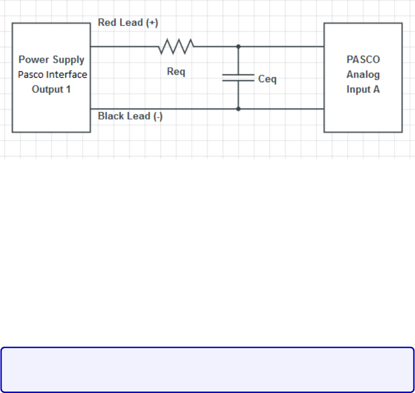
Figure 4.8: RC Circuit. You are to assemble sub-circuits that produces an equivalent
resistance
Req
and capacitance
Ceq
, in such a way as to obtain a desired time constant of the
equivalent circuit.
There will be a few communal multimeters that allow you to measure capacitance, while
every team will have their own multimeter that can only measure resistance. There will
also be boxes containing different resistors and capacitors. Their values will be labelled but
you can double-check their values using the multimeters. Note that we are using so-called
polarized capacitors and therefore you must be careful when connecting them to the circuit:
the voltage input must be attached to a specific leg of the capacitor. If not the capacitor
might explode. If you are unsure, ask the TAs for help.
You should verify how polarized capacitors work, and explain to them the
proper way to connect them.
While every team will have to build a different RC circuit, the time constants that we are
asking are of the order of ms, and therefore you will have to use the ”Positive Square Wave”
input from the signal generator. You have the liberty to choose different values of frequency
depending on your estimate time constant. Changing the frequency of the input source does
not change the time constant: this only changes the duration that the source is ”turned on”.
Each team will have 5 capacitors of 10
±
1
µ
F and 5 resistors of 50
±
1 Ω from which to
construct equivalent resistors and capacitors in their circuits. Since there is a limited quantity
of multimeters that can measure capacitance, you can assume that these standard deviations
are correct. A summary of the equipment for this session is shown in Table 4.1.
The goal of this lab is for you to demonstrate that you’ve constructed the right RC circuit
with the required time constant. You should discuss among yourselves and the TAs in order
to find appropriate tests to support your claim.
41
Individual station Collective station
Laptop Assorted resistors
PASCO 850 interface Assorted capacitors
Resistance multimeter Capacitance multimeter
Resistance and capacitance sub-circuit setups
Five 10 ±1µF capacitors
Five 50 ±1 Ω resistors
Table 4.1: Available material for Lab # 2
You must lead the discussion here. We want them to provide (at least) two
arguments.
You must get them to reach the following conclusions.
It is not part of their instructions. It is your responsibility to get
them to reach the following conclusions.
The first is to simply measure
the effective resistance and capacitance of the circuit, and show a sample of
their time constant measurement.
The second is to incrementally increase the resistance and capacitance sep-
arately. Doing so, and plotting
τ
as a function of the varying parameter,
they should find that the slope is the effective resistance or capacitance. This
provides an alternative approach to measuring the effective resistance and
capacitance of their setup, one that has more data points. The easiest ap-
proach is to connect resistors (the 50Ω ones) in series to the original effective
resistor, and capacitors in parallel (the 10
µ
F ones) in parallel to the initial
capacitance.
Document your results and argue whether or not your RC circuit has the required time
constant. If you believe that it does, argue using standard data analysis methods. What is the
most appropriate measure to characterize the error of your measurements (see “Measurement
analysis” section of the “Basic statistics” section)? If your data doesn’t produce the correct
time constant, explain why. Explain what you must change in your circuit to remedy the
situation. Also discuss whether you believe this experiment is adequate to obtain RC time
constants. If possible, propose a better way to obtain time constants and/or decrease the
error in your experiment.
42
Chapter 5
Lab 3 - Magnetic Field of Solenoids
and Coils
5.1 Learning objectives
•Learn about solenoids.
•Learn how to use the right hand rule.
•Learn about vector nature if magnetic field.
•Learn about electric motors.
5.2 Introduction
The goal of this lab will be to learn about real-world applications of magnetism. In particular,
we will study the solenoid in the first session, and build on this to study the electric motor in
the second. You will use your data analysis skills previously acquired from the other labs to
characterize the magnetic field in these setups.
In the first session, you will be asked to draw the magnetic field lines of the solenoid
and to explain your findings in terms of the right hand rule. You will then quantitatively
characterize your solenoid’s magnetic field. Namely, you will verify the dependence of the
magnetic field
B
of the solenoid on the current
I
through the solenoid and on the the position
zfrom the end of the solenoid’s central axis.
In the second session, having learned how the magnetic field strength of the solenoid
varies with distance, you will now use a permanent magnet to construct and characterize an
electric motor.
43
5.2.1 Pre-lab activity
1. How would you present data that consists of vectors?
Answer
Any vector data consists of information about its
magnitude
and
orien-
tation
. This can be presented as a vector diagram, or tabulated into a
table.
2.
What is a vector diagram? What needs to be present when drawing a vector diagram?
Answer
Magnitude and orientation. Typically, vectors are connected end-to-end, or
drawn from a common origin.
3.
Given the wire below, draw the field lines of the magnetic field generated from the
current in the wire.
Figure 5.1: Wire with a current Igoing from right to left.
4.
Does the strength of the magnetic field increase, decrease or is it constant as we go
further away from the wire?
5.
Imagine stacking multiple wires similar to that of Fig. 5.1 parallel to each other, with
the current of each all running in the same direction. Would the magnetic field close to
the stack of wires be greater, equal or smaller than the scenario with a single wire?
6.
Given the wire below with a constant magnetic field
B
pointing downwards, what is
the direction of the magnetic force that Bexerts on the wire?
44
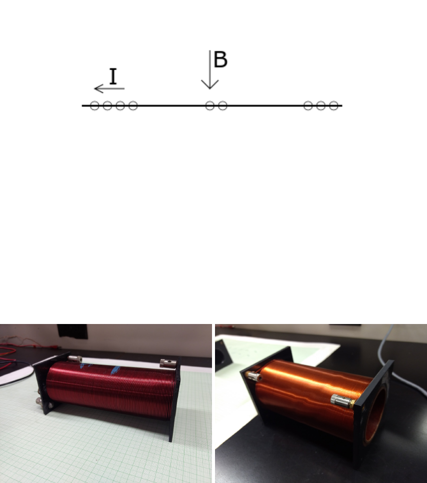
Figure 5.2: A wire has a current running through it, hence electrons are running from right
to left. A constant magnetic field is present and points downwards. The circles are electrons.
5.3 Session a
5.3.1 Solenoid setup
In this session, you will use the IOLab that you previously used in PHYS 101 last semester
to measure magnetic field strength of a solenoid at different locations around the solenoid.
Figure 5.3: Available solenoids. The one one the left has a smaller radius (2
.
25 cm radius,
550 turns of wire, 15 cm of length, #16 gauge wire), while the one on the right is larger (3
cm radius, 560 turns and 15 cm of length, #19 gauge wire).
Each team will have access to two solenoids as shown in Fig. 5.3. We will mostly use the
one with the smaller radius. You are to connect the two leads to the power supply. This will
generate a current through the wire turns.
Fig. 5.4 shows a typical power supply used for this lab. To use the power supply:
1.
Make sure both knobs (red and green box) on the “master” side are completely turned
down.
45
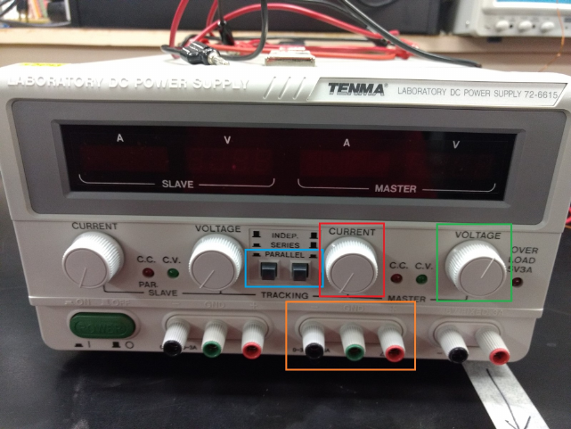
Figure 5.4: Power supply.
2. Connect your wires to terminals in the orange box (red for input, black for output).
3. Make sure to press down on both buttons in the blue box so that the power supply is
set on “parallel”. This will allow you to go up to 6A of current.
4.
Turn the voltage knob to halfway (green box). This sets the maximum amount of
voltage allowed.
5.
You will control the voltage and current of the power supply by slowly turning the
current knob (red box).
To measure magnetic field data, you will use the IOLab:
1. Connect the IOLab USB to your laptop and open the IOLab software.
2. Calibrate your IOLab as shown in Fig. 5.5
3.
On the left of the interface, select the “Magnetometer” and “Wheel” sensors. We will
only need the position data, not the velocity or acceleration plots.
4.
When you are ready to acquire data, you can start recording by clicking the record
button. The data should appear as in Fig. 5.6.
The protocol is straightforward: you will move the IOLab to a given position and observe
the magnetic field strength at that position. Leave the IOLab at that position for a few
46
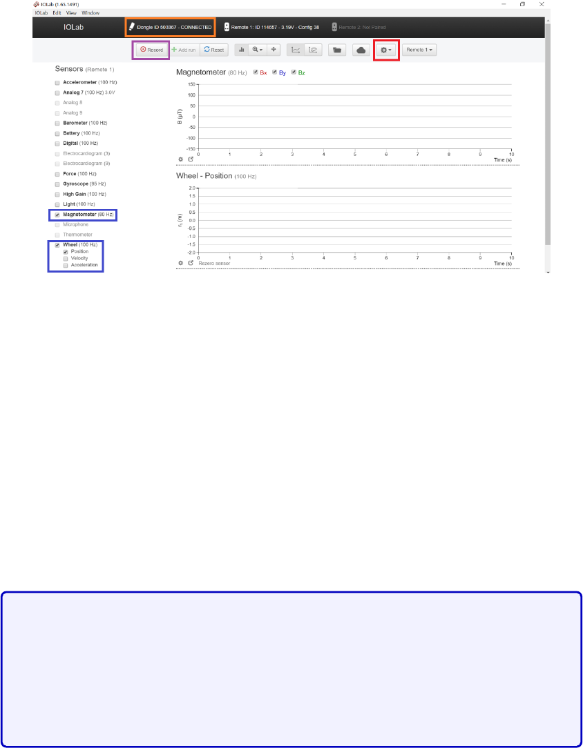
Figure 5.5: IOLab interface. Firstly, make sure the IOLab is connected to the bluetooth USB
stick: the area labelled by the orange box should indicate “Connected”. Afterwards, calibrate
your IOLab by clicking the button labelled by the red box
→
“Calibration”
→
“Remote
1”
→
“Accel - magn - gyro” and follow the subsequent on-screen instructions. We will use
the “Magnetometer” and “Wheel” sensors (see blue boxes). When you are ready to make
measurements, press the record button (purple box).
seconds so that you can select that interval in your data to obtain the standard deviation (
σ
)
and mean (
µ
) of that measurement (See Fig. 5.6). Repeat the above for all the positions that
you wish to measure the magnetic field.
Further details about the IOLab can be found in the appendix.
5.3.2 Magnetic Field Lines
For this part of the lab, you will mostly help them understand the right hand
rule and how this can be used to determine the
B
field of a solenoid. As they
progress with the protocol below and answering the questions, push them to
think about the direction of the
B
field from one wire, and then that same
wire as it loops on itself. After that, have them deduce how
B
must point
inside and outside the solenoid, and its origin in terms of the right-hand rule.
Once the solenoid has been properly connected, you are asked to draw field lines on the
graph paper on which the solenoid is placed as shown in Fig. 5.3. For this, we will use the
compass and IOLab. Place the compass on top of the sensor. Note that the magnetometer
isn’t centered in the IOLab; the magnetometer sensor of the IOLab is located in one of the
corners of the device as shown in Fig. 5.7.
First, chose at least a dozen points on the graph paper to place the IOLab. For each
47
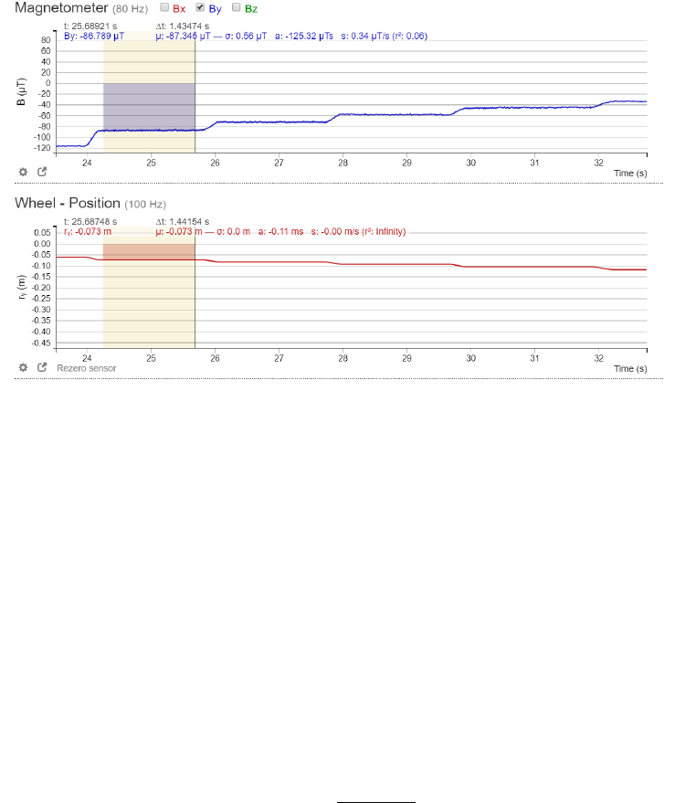
Figure 5.6: Data sample. You can select an interval of your data. Doing so, you can obtain
directly the average (
µ
) and the standard deviation (
σ
) of your data within that interval. For
this lab, you should move the IOLab to a desired position, and wait a few seconds before
moving it again. This way, you can obtain an average value of the magnetic field at that
position. In the figure above you see a plateau, its size depends on the amount of time you
left the IOLab at each position. You should only average the magnetic field during each of
the plateaus to make sure you are not registering data at intermediate positions. By doing
this incrementally, your data should look like a staircase as a function of time.
point, you are to measure the orientation of the magnetic field with the compass, draw a
vector arrow associated with your observation, and write next to the vector the measured
strength of the the magnetic field. Recall that the total magnitude of the magnetic field will
be given by Pythagoras’ theorem:
|B|=qB2
x+B2
y.(5.1)
Both vector components can be obtained from the IOLab (see Fig. 5.6). Normally, one would
draw the length of the vector to represent the magnitude of the vector, however for the
amount of vector lines you are asked to draw, we will simply write the magnitude next to the
drawn vector.
Once you have measured
B
of the solenoid at enough points, and have explored the
possible orientations of the magnetic field vector lines, answer the following questions in the
General Notes Section of your log book:
1. Draw a diagram of the solenoid with the appropriate field lines surrounding it.
2.
What is the behaviour of the magnetic field inside the solenoid? Support your claim of
the field lines inside the solenoid in terms of the right hand rule.
48
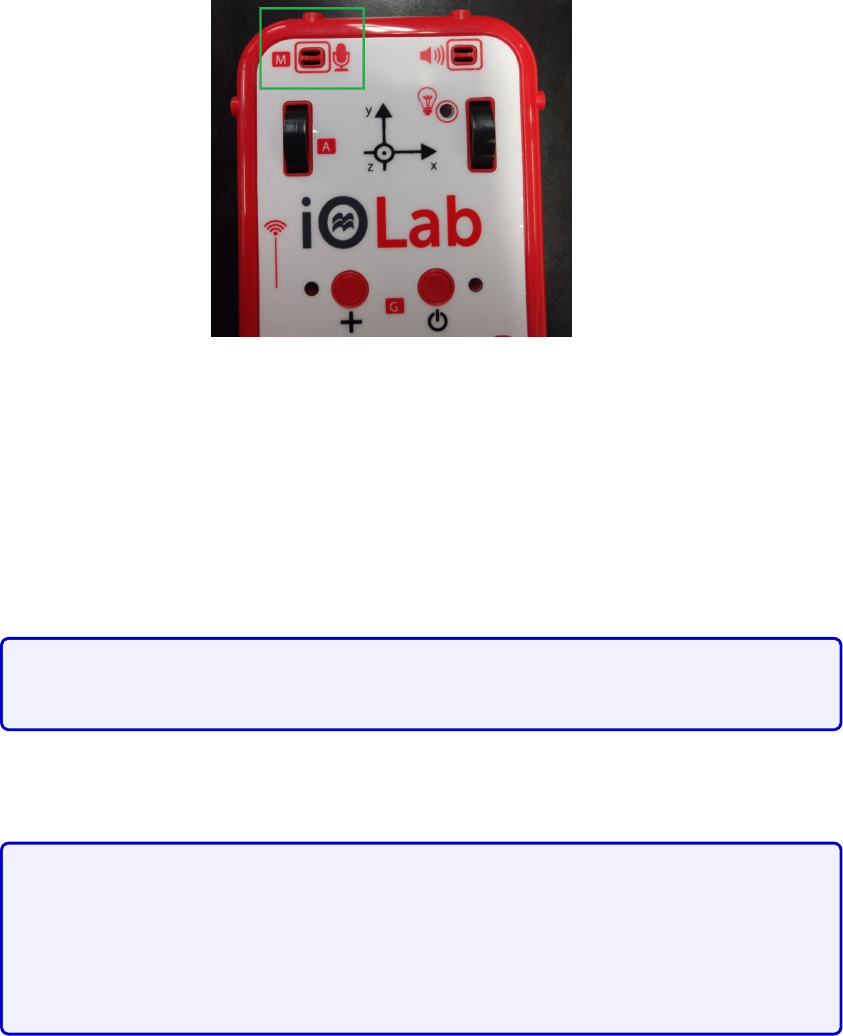
Figure 5.7: Position of the magnetometer on the IOLab (green box). Place the compass on
top at this position to obtain precisely the direction of the magnetic field detected by the
IOLab.
3.
What happens if you swap the connections of the solenoid? What would change?
Explain this in terms of the right hand rule.
4.
Do these field lines look like any other magnetic object that you’ve seen? Explain why
this observation is true.
They should be reminded of the field lines of a bar magnet. Encourage them
to consider why the field lines must loop around instead of simply diverging.
5.
What parameters do you expect to affect the strength of the magnetic field of the
solenoid? Give a brief explanation for each parameter.
We expect them to consider the current
I
, the number of turns
N
and
the distance
z
away from the central axis (and distance in general). We
expect them to motivate the
N
dependence from a physical motivation (either
increasing or decreasing with
N
), and we will ask them to verify the
I
and
B
dependence explicitly below.
5.3.3 Current dependence
Now that you have a qualitative idea how a solenoid generates a magnetic field, we will
quantitatively verify its dependence on some of the possible parameters of this set up.
We will first verify the
B
dependence of the solenoid on the current through the wires.
Place the IOLab on the ramp at a fixed distance away from one end of the solenoid (not too
far) as shown in Fig. 5.8, and increase the current through the wires with the power supply.
49
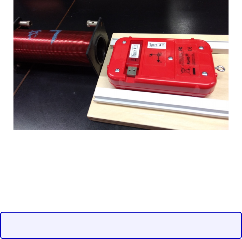
Figure 5.8: Measuring the distance dependence of the magnetic field. Place the ramp in front
of the solenoid and use it as a guide for moving the IOLab.
Verify how
B
depends on
I
using your data analysis skills from previous labs. Find the
parametric dependence on the current
I
and carefully support your claim by generating a
graph with an appropriate fit and error analysis. Recall that you are not evaluated on the
rigorous standards of
data presentation
during this session, however you should perform
an appropriate analysis to be confidant in your data.
By taking increments of 0
.
5A, the data should be near perfect as the depen-
dence was found to be linear with an approximate R2≈0.99 accuracy.
5.3.4 Distance dependence
We will now verify the magnetic field generated by a solenoid at a distance
z
(on the central
axis) away from the front of the solenoid.
Place the ramp in front of the solenoid such that the IOLab sensor is centred in front the
solenoid (see Fig. 5.8). Recall that the sensor isn’t centered. Move the IOLab incrementally,
and at each position, use the interface in order to obtain the average and standard deviation
of the position and magnetic field of the measurement. You will not need to go further than
30 cm. We recommend that you perform multiple trials to obtain many data points.
Once you have data for the magnetic field for numerous positions
z <
30cm, we will first
restrict our analysis to the behaviour of
B
at large distances
z
. It turns out that the
B
field should follow a 1
/z3
behaviour as
z
moves far from the centre of the solenoid. Select
appropriate data points that are far enough away (called the ”far
z
” region) such that you
50

see a good 1
/z3
fit. Can you explain the minimum value of
z
for which you performed a
cutoff in your data? You may perform this analysis again with the other solenoid if you wish.
There are many subtleties in this experiment. Firstly, they won’t be able to
find the correct 1
/z3
dependence without subtracting off background field
measurements: we found that surrounding electronics (laptop, phone, etc.)
will affect the magnitude of
B
. They must perform a run with and without
the
B
field of the solenoid turned on. Make sure you tell them this after a
brief discussion to try and get them to deduce it.
Having done that, through testing, we found that the far
z
behaviour corre-
sponds to
z >
4
R
, where
R
is the radius of the solenoid. We don’t expect
them to explain the factor of 4, but they should appreciate that it depends
on
R
, and it should be
zR
. Make them consider the consequences of the
near zbehaviour, that is z→0.
Why do you think that we find a 1
/z3
behaviour far away? Why doesn’t this fit work for
other regimes of
z
? Can you compare the 1
/z3
behaviour to other electromagnetic systems
that you may know: the electric field of a point charge, the magnetic field from a line ?
For most students, we expect them to find the 1
/z3
behaviour, and you are
to lead a discussion about why this fit only works for
zR
. They should
at least deduce, or be pushed to deduce, that the real
B
equation is more
complex than a simple power law.
51

For the ambitious students: you can write down the equation of
B
for a solenoid
on the board, and they can try to compare their data to this theoretical curve.
Let the solenoid be centered at the origin
z
= 0, and
zL, zR
are the two ends
of the solenoid. Define
L
as the length of the solenoid
L
=
zR−zL
,
N
the
number of turns, Ithe current, then we have
Bz=µ0NI
2L z−zL
p(z−zL)2+R2−z−zR
p(z−zR)2+R2!
Bz≈µ0NI
L
R2
z3+O1
z5.(5.2)
In the last line, we expanded to leading order in the limit
z→ ∞
. We want
them to see that taking appropriate limits, the equation simplifies greatly.
Since they don’t know calculus, you can show the first and last line of the
equation above which makes the relation obvious when zis large.
5.4 Session b
WARNING!
The permanent magnets used in this experiment are quite strong. Avoid
bringing any objects that are magnetizable (made of iron/steel/Ni/Co, ID /credit cards) near
the magnets. Students with pacemakers could be excused from this lab.
Important Announcement
Since most of the points are attributed to data analysis and presentation, you
should tell students to focus on obtaining some data rather than obtaining
good/perfect ones.
In this session, we will study the electric motor. The electric motor is a device that
converts electrical energy into mechanical energy. Electric motors and their counter-parts,
electric generators, have been around for decades now and have become so ubiquitous in
our daily lives that life without them would seem almost impossible. Over the years, these
motors have grown in complexity and sophistication in order to perform a number of different
tasks but the basic physical principles behind their operation have not changed.
The goal of this lab is to provide a general understanding of how a simple DC motor
works with the hope that it might lead to a better appreciation for the more sophisticated
devices found all around us. This lab is not “complicated” to do, but will require a number
of different concepts in electricity, magnetism and circuit theory to complete.
52

The main observable of this lab is the frequency of rotation
f
of the motor. In class,
you’ve seen how torque can be generated on a loop carrying current. Explain physically how
the frequency of rotation that you are observing is related to the torque. In fact, the torque
is proportional to the frequency of rotation. Similar to the first capacitance lab, you are also
asked to find possible parameters that could affect the frequency of rotation of the motor.
We expect them to find the frequency and understand that it is caused by a
torque on the current loop given by
τ=NABI sin(θ),(5.3)
where
N
is the number of turns,
A
is the area of the loop,
B
is the magnetic
field,
I
is the current through the coil and
θ
is the angle coming from the
cross product of
B
and
I
. Therefore, in measuring the frequency, these are
the possible parameters to vary;
B
and
I
. They can’t vary the first two
parameters
N
and
A
, but since the latter two scale linearly, the data analysis
should be familiar to them by now. Since this is the last lab session, you
should try and give them less advice as they should know how to analyse
linear fits.
5.4.1 Electric motor setup
For this lab, you are given a power supply, a digital oscilloscope, an electric motor and a
magnet. Fig. 5.9 shows the schematic diagram of the setup we will use in this experiment
and Fig. 5.10 shows a photograph of the actual setup.
To set up the apparatus:
•Make sure the power supply is turned off
•Connect the leads from the coil to the power supply.
•See the instructions for the oscilloscope in the appendix.
The coil current and the voltage will be read from the power supply meters. The coil’s
period of rotation will be measured by a photodiode detector connected to a digital oscilloscope.
The photodiode emits light and detects its reflection from the shiny strip covering one side
of the coil. The other side is covered by a non-reflective strip. When the coil is rotating, a
signal/pulse will be seen on the oscilloscope screen every time the reflected light strikes the
detector. The period will be the time interval between two reflected signals/pulses. From the
period you can calculate the frequency.
53
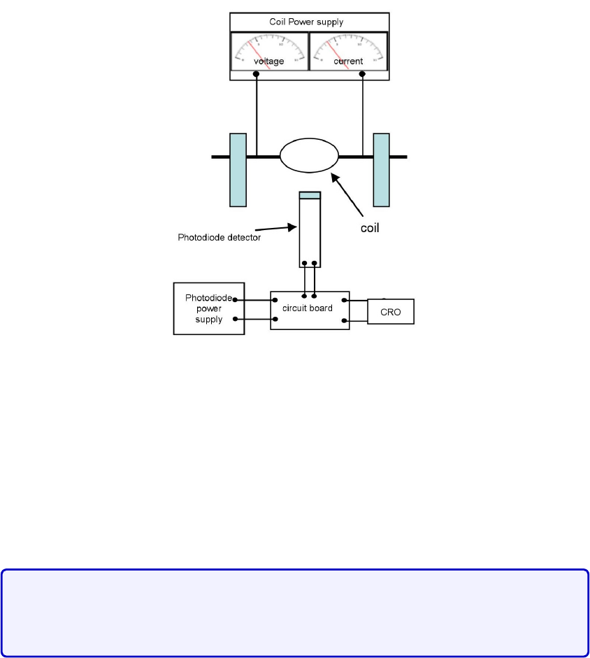
Figure 5.9: Circuit diagram of the setup (front view)
The performance of the motor and preciseness of measurements are extremely sensitive
to the positions of the photodiode and brushes.
Please be careful with the apparatus,
and do not make any adjustments from how it was set up.
In addition to the electric motor, you are given a magnet that can move on a track.
Figure 5.11 below is a calibration of the magnet. This should remind you of your data in the
last session.
The main concern for this lab is the equipment. It has been reported that
students tend to easily damage the apparatus and therefore you must be
vigilant of any deviations to the instructions.
Please respect the following instructions in order to avoid dam-
aging the apparatus:
•
Do not exceed a voltage of 10 V. Do not add the voltages in the slave and master
display.
•Do not let the magnet be any closer than 1 cm to the coils.
•
It may happen that for a large enough voltage and close enough distance, the magnet
might vibrate or be pulled towards the coils. Do not let it be any closer than 1 cm to
the coils! Hold your magnet in place if necessary.
54
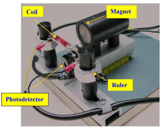
Figure 5.10: Photograph of the setup (Oscilloscope and power supply out of the picture
range.)
•
If you are using high voltages (greater than 8 V), try to move quickly through the
higher voltages to reduce wear on the brushes.
•
Remember to turn off the power supply after you have finished all your measurements.
5.4.2 Protocol
In this lab, you will find what parameters affect the frequency of rotation of the motor
f
.
The magnetic field driving the motor will be that of a solenoid, and looks like the one you
measured in the previous session. It has been pre-tabulated and given in Fig. 5.11.
To characterize frequency, recall that you must isolate your system and vary one parameter
at a time in order to perform the analysis. As a starting point, we suggest that you draw
a force diagram of the coils of the motor (recall magnetic moment from class). Recall your
answers from the pre-lab activity.
To make a measurement,
1.
Make sure you read the previous instructions (above) in order to avoid damaging the
apparatus.
2. Set the magnet at a desired position (greater than 1 cm away from the coils).
3. Turn the power supply to a desired voltage (do not exceed 10 V).
4.
The coil should start to rotate, though you will likely need to flick it gently with your
finger to get it started.
55
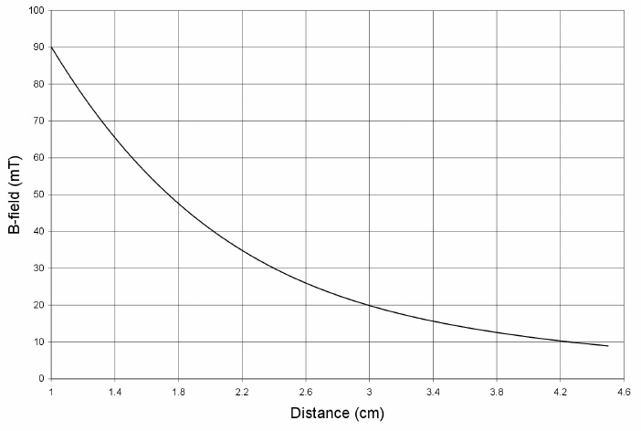
Figure 5.11: Bfield as a function of distance from the face of the magnet.
5.
Measure the period
T
from the time interval between two successive pulses from the
oscilloscope.
6.
For better precision, you may count the time interval between a few pulses and divide
it by the number of intervals to get a better value for
T
. The frequency will be given
by
f
= 1
/T
. Note the value of
f
in an Excel sheet as a function of any other relevant
parameters you varied in this measurement. Remember to keep track of errors in your
measurements.
Through performing your measurements, and through discussions with your lab partners,
other teams and the TA, establish a (mathematical) relation between possible parameters
that could affect the frequency of rotation of the electric motor. Support your claims based
on data and figures as usual. Record your procedures and record your data, and discuss your
rational in your log book.
56
Part III
Appendix
57
Appendix A
Introduction to Excel
These labs will make use of Excel to plot data. There will be a ”lab 0”/tutorial session before
official labs start to review error analysis and Excel, the latter of which is also summarized in
this appendix, which should be brought to Lab 0. Every McGill student can obtain a free
copy of Microsoft Office software by clicking here. Excel spreadsheet boxes can take in strings
of letters of numbers as input. If the input is a number, we can easily perform calculations.
Performing Spreadsheet Calculations
•
To initialize the math environment, simply click on a box, and press the “=” key on
your keyboard. Press “Enter” when you are done.
•
One can perform basic addition (+), subtraction (-), multiplication (*) and division
(/) between two boxes. One can also take powers by using “ ˆ ” i.e. xˆ2 would be
x2
. First, press “=”, click on the box of your first variable, choose one of the above
manipulations and choose another box as your second variable.
•
Excel obeys order of operators: multiplication and division come before addition and
subtraction. Parentheses are done first.
•
Note that the middle bar above states the equality function in terms of boxes of the
spreadsheet.
•
It is useful to separate your data into columns. In this way, say your first two columns
are your
x
and
y
variables that were obtained from a measurement. You should compute
f
(
xi, yi
) in another column. Doing so, after performing the mathematical manipulation
that you wish, you can click the bottom right green border of a box, and pull down to
the column to apply the same function along the columns of the input variables. In the
example of Fig. A.1, one could obtain the multiplication of each element of columns A
times those of column B displayed in column C.
58
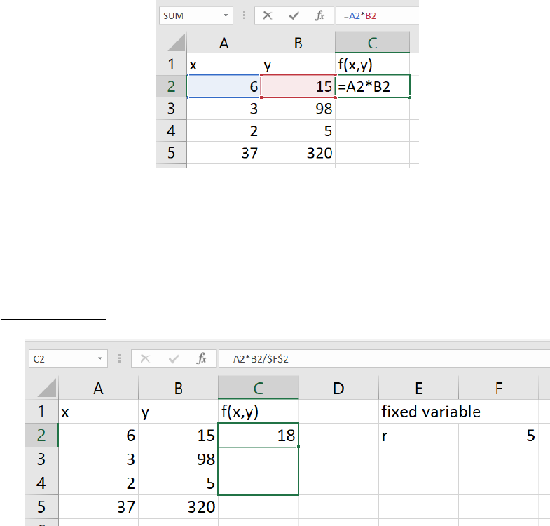
Figure A.1: Example of multiplication between two variables
x
and
y
. Notice that the selected
box has a green border around which the bottom right corner has an enlarged square.
•
When defining a function with the intent of dragging the select-box down to apply the
whole function to all elements of columns, it is sometimes useful to define a box that
doesn’t change
as you drag the select-box. To do so, one uses the
$
sign as in Fig. A.2.
Figure A.2: Fixing a box value when applying a function down a column. The
$
sign before
the column letter means that we are fixing the column, and the
$
sign before the row number
means that we are fixing the row. One can only use one
$
sign to fix either the column or
row as desired.
•
Excel also has functions that are included. Functions are called by some special
command in all caps. One typically calls a function, for example the sum, as
=SUM(B2:B5)
The colon means that we take every box between B2 and B5. One could have also used
that function by listing every box individually, separated by a coma. Alternatively, one
could, after writing “=SUM(”, selected the boxes that one wants to be included in the
function. This re-emphasizes the usefulness of arranging the data in columns.
•Other useful functions include:
59
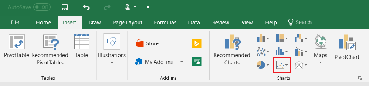
–=STDEV.P(x)
to calculate the standard deviation of a fluctuation population as
shown in eq. (2.6).
–=SQRT(x) to calculate square root of x.
–=Exp(x) to calculate exponentials ex.
–PI() to use the constant π. Note that there is no input.
–=Sin(x)
and
=Cos(x)
to calculate values in radians. The input
x
must be in
radians.
–=AVERAGE(A2:A10) computes the average of the boxes between A2 and A10.
There exists many other functions that could be useful.
Figures
One can also create figures from data sets in Excel. To do so, select too columns and
go into the
Insert
tab as shown in Fig. A.3 to choose the type of figure that you with to
display. You can choose not-adjacent columns by selecting one column, press and hold Ctrl
while selecting the other column.
Figure A.3: Creating a plot based on some data. After selecting your data, go into the
Insert
tab and choose the type of figure that you want. The red boxed symbol is the one for scatter
plots, which will most likely be your most used data display option.
Doing, so you should obtain something similar to Fig A.4. From here, one can do multiple
things.
•
By clicking the green “ + ” symbol to the top right of the figure, you can add titles to
your axes, error bars, a legend and a trendline.
•
By right-clicking the data points, you should see an option to “Format Data Series”.
Clicking that, you will see a right bar appear, and in the “Pain bucket” symbol, you
can change the size, shape and colors of your markers.
•
By right-clicking a data point, you can add a
trendline
, in which case a right bar will
also appear. Here you can choose the type of equation that you wish to fit, and if
you scroll down completely, you will have the option to set an intercept, display the
equation on the chart, and display the R-squared value on the chart. You can also add
multiple trendlines to a single dataset to compare different fits.
60
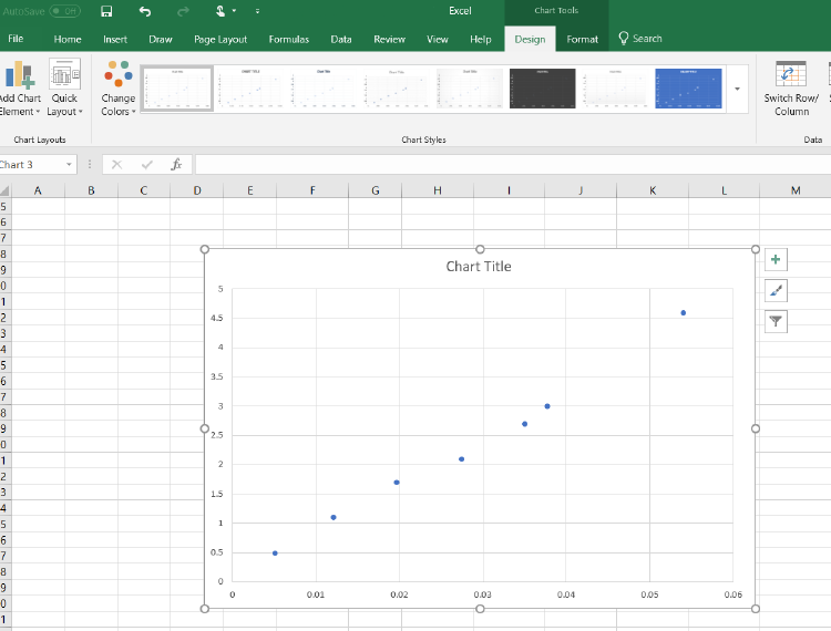
Figure A.4: Scatter plot from data
•
If you right-click an empty space on the grid of the chart, you can add multiple data
sets to a single chart by click “Select Data”. A pop-up window will appear with the
option of renaming how your datasets will appear on the legend, and the ability to
add/remove more datasets.
•
Playing around with these options, you will have the ability to change the font size of
titles, colors of data points and texts, as well as change the thickness of the data points
and trendlines. You can move equations, legends or other things around your chart.
Don’t forget that data presented must be clear.
Finally, you can add data from .txt files. To do so, go into the data tab, and in the “Get
& Transform Data” section, there will be an option to add .txt and other types of files. Once
the popup screen to import data appears, you can click on “Edit” in the bottom right corner
to have more options to manipulate your data. A useful modification is to flip your rows and
columns. To do so, after clicking “Edit”, go into the “Transform” tab in the new window,
and select “Transpose”. Go back to the “Home” tab once you are done editing your file.
61
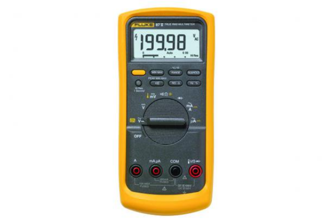
Appendix B
Lab Equipment
B.1 Multimeter
A multimeter allows one to measure various electronic properties. We will be mainly interested
in measuring the resistance or resistors, the capacitance of capacitors and the voltage and
current of a circuit. To use the multimeter, one must attach two wires into the input and
output. One can have alligator clips to attach to conducting wires more easily if necessary.
Figure B.1: Communal DMM (model 87V Fluke). Note that you may have a different model
at your individual station, but the symbols for the settings are the same. The Ω symbol
(center position) allows to measure resistance. The yellow symbol with one vertical line, and
another slightly curved one (next to the Ω symbol) allows to measure capacitance. You must
press the yellow function button to access it.
To measure the resistance, simply take a resistor, turn the knob of the multimeter to the
resistance seting (Ω) and attach each wire to the two sides of a resistor. To measure the
62
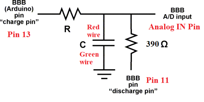
capacitance of a capacitor, simply do the same as for the resistor, but turning the knob to
the capacitance setting.
To measure the voltage and current of a circuit,
B.2 Arduino
The Arduino unit requires the Arduino IDE software to run the desired scripts. Information
about the Arduino code for the capacitance lab can be found here.
The Arduinio setup is schematically shown in Fig. B.2 where the example shows two
resistors: one with a resistance of 400Ω, the other is unspecified. We recommend using
at least 10
6
Ω for the unspecified resistor: you can choose different values to vary the time
constant of the RC circuit. This will change the precision of your setup.
Figure B.2: Arduino circuit scheme. The labels are associated with the pins and wire colors
of Fig. B.3.
To change the resistance of the resistor, you must also change the value in the Arduino
script. See Fig. B.2.
63
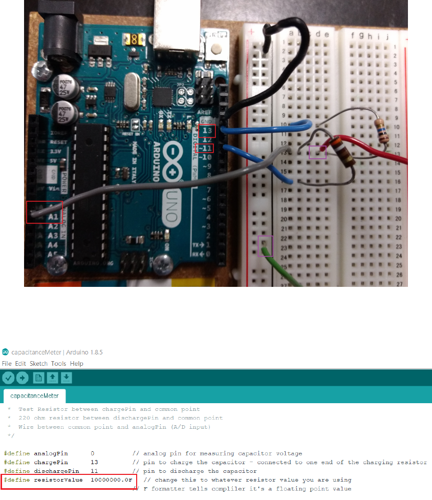
Figure B.3: Corresponding real setup of the Arduino unit. The red boxes label the pins while
the purple boxes label the wiring that should make contact to each side of the capacitor.
Figure B.4: Arduino resistor value. Change the value in the red box to the resistance value
of your setup. We suggest using at least 106Ω.
B.3 Reading Resistors
The color code for resistors changes according to where the position (or number) of the band
is in the resistor, starting from where there is a greater number of bands. In the above
image this is from left to right. As a rule, the last two bands correspond to the multiplier
and tolerance respectively, while the rest correspond to the ohmic value. For example, as
64
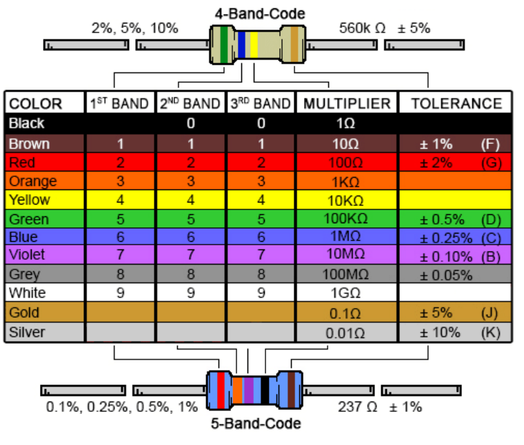
Figure B.5: Resistor color chart.
shown in the figure, for the 4-Band-Code resistor we have: Green (5) and Blue (6), times 10
KΩ (Yellow) with a tolerance of
±
5% (Gold) so that resistor is 560 (
±
5%) KΩ. For the
5-Band-Code resistor we have: Red (2), Orange (3) and Purple(7), times 1 Ω (Black) with a
tolerance of ±1%(Brown) that is a resistor of 237 ±1% Ω.
B.4 Bread Boards
In Lab 2, you will use a bread board similar to that of Fig. B.6 to connect your RC circuit.
In the middle section of the bread board, there are metallic strips for every row (see for
example the green strips for rows 25-27 in the figure). On the side, there vertical strips as
shown for the red “+” column on the right. You may have another type of bread board, but
the design remains the same: you will have a section where metallic strips are distributed
horizontally, and another one where the strips are laid out vertically.
65
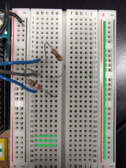
Figure B.6: A typical bread board used in Lab 2.
B.5 IOLab
Here are additional comments about the functionality of the IOLab
•You can zoom in and out
•How to get STD and mean
•How to load previous datasets
B.6 Oscilloscope
In lab 3, we will use a digital oscilloscope. An oscilloscope is a valuable tool often used
in many applications. Its most important function is the ability to measure voltages that
vary in time. The oscilloscope allows us to “visualize” how this voltage changes. To fully
characterize a voltage that varies in time using a hand-held voltmeter, you would have to
plot how the readings change with time on a graph. This is not only time consuming, but
impossible to do if the voltage changes too rapidly (for example, the voltage from a wall
socket changes sinusoidally from +115 V to -115 V and back to +115 V in 1/60th of a second).
To understand the principle behind an oscilloscope we will explain how an analog cathode ray
66
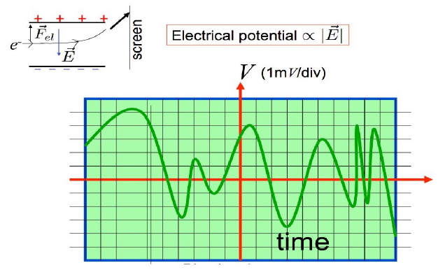
oscilloscope (CRO) works. The CRO report voltage by tracking the vertical position of an
electron beam rapidly sticking a fluorescent screen as it exists the space between two charged
parallel conducting plates as is illustrated in Fig. B.7. It plots the voltage on a screen along a
vertical axis, and can also track changes of this voltage in time (horizontal axis) in a fraction
of a microsecond.
Figure B.7: Operation of a CRO
To use the oscilloscope you must first plug it into an outlet, turn it on by clicking the
’run/stop’ button glowing green, and then plug in your BNC cable into the connection labeled
Channel A - shown in red in Figure B.8. You must then adjust the position and scale knobs,
shown in green until you see a signal on the screen. The vertical position knob on the left
will adjust the
y
position of the signal on the screen. The scale knob on the other hand, will
modify the value in volts and time in yand xrespectively of each of the squares or divisions
on the screen. Explained in another manner these knobs allow you to control the zoom (or
scale) in/out in each direction separately. You can also use the button labeled cursor, shown
in orange, to adjust the cursor on the screen to aid you in measuring the frequency or voltage
of the signal. The oscilloscope has other options such as DC or AC coupling that will already
be set up for you. It will not be necessary to play around with any of the other options
during the lab.
67
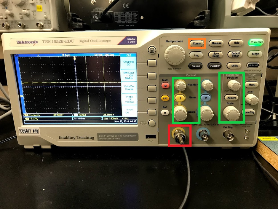
Figure B.8: Photograph of a digital model
68

Appendix C
More about statistics
Coefficient of determination
To determine the precision of a fit, one can look at its
R2
value, also known as the
coefficient of determination. Consider a dataset of
N
datapoints with values
yi
,
i
going from
1 to N. We define the total sum of squares as
SStot =
N
X
i=1
(yi−¯y)2= (y1−¯y)2+ (y2−¯y)2+...(yN−¯y)2.(C.1)
This is a measure of how your dataset differs from its average.
Now consider the values
fi
of a fit, where
i
are the values of the fit corresponding to
xi
of
yi
value. We can also define the residual sum of squares which is a measure of how your fit
differs from your fit. This is given as
SSres =
N
X
i=1
(yi−fi)2= (y1−f1)2+ (y2−f2)2+...(yN−fN)2.(C.2)
Finally, given the results above, we can define the coefficient of determination as
R2= 1 −SSres
SStot
(C.3)
which is a ratio of how your data fluctuations with respect to how you data differs from its fit.
A good coefficient of determination is
R2
= 1. This can be computed automatically in Excel.
69
