TRM Instruments: Processing And Calculations Instrument Guide
User Manual:
Open the PDF directly: View PDF ![]() .
.
Page Count: 930 [warning: Documents this large are best viewed by clicking the View PDF Link!]
- Contents
- Preface
- Chapter 1 Concepts
- Chapter 2 Market standards and calculations
- 2.1 Market standards
- 2.1.1 Date basis
- 2.1.2 Interest types
- 2.1.3 Price types
- 2.1.4 Yield/price conversions
- 2.1.4.1 Price/yield conversion
- 2.1.4.2 Yield/price conversion
- 2.1.4.2.1 *ISMA-30/360-BIMONTHLY (financial/instrument/isma@price)
- 2.1.4.2.2 *ISMA-30E360-ANNUAL (financial/instrument/isma@price)
- 2.1.4.2.3 *ISMA-30E360-SEMI-ANNUAL (financial/instrument/isma@price)
- 2.1.4.2.4 *ISMA-30E360-QUARTERLY (financial/instrument/isma@price)
- 2.1.4.2.5 *ISMA-ACTACT-ANNUAL (financial/instrument/isma@price)
- 2.1.4.2.6 *ISMA-ACTACT-QUARTERLY (financial/instrument/isma@price)
- 2.1.4.2.7 *ISMA-ACTACT-SEMI-ANNUAL (financial/instrument/isma@price)
- 2.1.4.2.8 *ISMA-ACT360-ANNUAL (financial/instrument/isma@price)
- 2.1.4.2.9 *ISMA-ACT365-ANNUAL (financial/instrument/isma@price)
- 2.1.4.2.10 *U.S.STREET-ACT365-SEMIANNUAL (financial/instrument/us-street@price)
- 2.1.4.2.11 *U.S.STREET-ACTACT-SEMIANNUAL (financial/instrument/us-street@price)
- 2.1.4.2.12 *U.S.STREET-ACTACT-ANNUAL (financial/instrument/us-street@price-1)
- 2.1.4.2.13 *U.S. Treasury (financial/instrument/us-treasury@price)
- 2.1.4.2.14 BOND-BR-LFT (financial/instrument/isma@price)
- 2.1.4.2.15 BOND-BR-NBC (financial/instrument/isma@price)
- 2.1.4.2.16 BOND-BR-NTN (financial/instrument/isma@price)
- 2.1.4.2.17 GOVT-AU (financial/instrument/australian@price)
- 2.1.4.2.18 GOVT-CA (financial/instrument/canadian@price)
- 2.1.4.2.19 GOVT-CH (financial/instrument/isma@price)
- 2.1.4.2.20 GOVT-DK-OLD-30E360 (financial/instrument/isma@price)
- 2.1.4.2.21 GOVT-DK (financial/instrument/isma@price)
- 2.1.4.2.22 GOVT-EUROZONE (financial/instrument/isma@price)
- 2.1.4.2.23 GOVT-FR-OAT-OLD-AIR3 (financial/instrument/isma@price)
- 2.1.4.2.24 GOVT-FR-OAT (financial/instrument/isma@price)
- 2.1.4.2.25 GOVT-GR-OLD-30E360 (financial/instrument/isma@price)
- 2.1.4.2.26 GOVT-HU (financial/instrument/isma@price)
- 2.1.4.2.27 GOVT-IT (financial/instrument/isma@price)
- 2.1.4.2.28 GOVT-IT-ZC (financial/instrument/isma@price)
- 2.1.4.2.29 GOVT-JP (financial/instrument/simple-yield@price)
- 2.1.4.2.30 GOVT-MALAYSIA (financial/instrument/isma@price)
- 2.1.4.2.31 GOVT-NO (financial/instrument/norwegian@price)
- 2.1.4.2.32 GOVT-NZ (financial/instrument/isma@price)
- 2.1.4.2.33 GOVT-SE (financial/instrument/isma@price)
- 2.1.4.2.34 GOVT-SG (financial/instrument/us-street@price)
- 2.1.4.2.35 GOVT-UK (financial/instrument/isma@price)
- 2.1.4.2.36 GOVT-US (financial/instrument/us-street@price)
- 2.1.4.2.37 GOVT-USAGENCY (financial/instrument/isma@price)
- 2.1.4.2.38 GOVT-ZA (financial/instrument/south-african@price)
- 2.1.4.2.39 INDEX-UK (function/index-uk@price)
- 2.1.5 Discount Margin
- 2.1.6 Calculation methods
- 2.2 Yield curves
- 2.2.1 Yield curve
- 2.2.2 Basis swaps
- 2.2.3 Yield Curve interpolation
- 2.2.4 FX rate interpolation
- 2.3 Key-figures
- 2.3.1 Valuation
- 2.3.2 Profit and Loss
- 2.3.2.1 Accrued Interest
- 2.3.2.2 Accrued Interest Local
- 2.3.2.3 Accrued Profit
- 2.3.2.4 Accrued Profit Local
- 2.3.2.5 FX Profit
- 2.3.2.6 Accrued Margin Profit
- 2.3.2.7 Accrued Margin Profit Local
- 2.3.2.8 Margin Profit
- 2.3.2.9 Margin Profit Local
- 2.3.2.10 Total Margin Profit
- 2.3.2.11 Total Margin Profit Local
- 2.3.2.12 MtoM Profit
- 2.3.2.13 MtoM Profit Local
- 2.3.2.14 Other Profit
- 2.3.2.15 Other Profit Local
- 2.3.2.16 Total Profit
- 2.3.2.17 Total Profit Local
- 2.3.3 Option figures
- 2.3.4 Risk
- 2.3.5 Dual currency
- 2.4 Performance calculations
- 2.4.1 Actual basis and all cash basis
- 2.4.2 Trade date and value date based performance
- 2.4.3 Time-weighted rate of return (TWR)
- 2.4.4 Money-weighted return
- 2.4.5 Instrument market values for third currency
- 2.4.6 Instrument market values and cashflows
- 2.4.7 Example portfolio
- 2.4.8 Risk-adjusted returns
- 2.4.9 Risk-adjusted return measures
- 2.4.10 Performance attribution
- 2.4.11 Performance measurement key-figures
- 2.5 Value-at-Risk calculations
- 2.1 Market standards
- Chapter 3 Debt instruments
- 3.1 Bond
- 3.2 Structured bonds
- 3.3 Schuldscheindarlehen
- 3.4 Denominated bond
- 3.5 Convertible bond
- 3.6 Index-linked bond
- 3.6.1 Instrument setup
- 3.6.2 Deal capture
- 3.6.3 Processing
- 3.6.4 Australian index-linked annuity bond
- 3.6.5 Australian index-linked bond
- 3.6.6 Brazilian (LFT) selic-linked security
- 3.6.7 Brazilian FX-linked NBC-E/NTN-D
- 3.6.8 Brazilian inflation-linked NTN
- 3.6.9 Canadian real return bond
- 3.6.10 French OATıi
- 3.6.11 Greek index-linked bond
- 3.6.12 Israeli index-linked bond
- 3.6.13 Italian BTP ıi
- 3.6.14 Japanese index-linked bond
- 3.6.15 Swedish index-linked bond
- 3.6.16 UK index-linked gilt
- 3.6.17 US Tips
- 3.7 Asset backed security
- 3.8 Short term loan
- 3.9 Discount paper
- 3.10 Loan
- Chapter 4 Equities
- Chapter 5 Security lending
- Chapter 6 Forex
- Chapter 7 Index
- Chapter 8 Cash
- Chapter 9 Futures
- 9.1 Forward rate agreement
- 9.2 Bond forward
- 9.3 Money market future
- 9.4 Bond future
- 9.5 Equity future
- 9.6 FX future
- 9.7 Index future
- Chapter 10 Options
- 10.1 Cap/floor/collar
- 10.2 Swaption
- 10.3 Option on MM future
- 10.4 Bond option
- 10.5 Bond Future Option
- 10.6 Equity option
- 10.7 Index option
- 10.8 FX option
- 10.9 Exchange traded FX option
- Chapter 11 Swaps
- 11.1 Interest rate swap
- 11.1.1 Single-currency IR swap
- 11.1.2 Asset swap
- 11.1.3 Cross-currency swap
- 11.1.4 Brazilian IDxUSD Swap
- 11.1.5 Overnight index swap
- 11.1.6 Other swap structures
- 11.2 Total return swap
- 11.3 Credit default swap
- 11.1 Interest rate swap
- Chapter 12 Commodities
- Chapter 13 Funds
- Appendix A Features
- A.1 Categories of features
- A.2 List of features
- A.2.1 ABS - Asset Backed Security
- A.2.2 ABS Valuation
- A.2.3 Accrual Yield Setup
- A.2.4 Allow Ad-Hoc Instructions
- A.2.5 Allow Ad-Hoc Clients/Instructions
- A.2.6 Allow Forcing Type to Spot
- A.2.7 Allow FX Currency Pair Shift
- A.2.8 Allow Manual Classification
- A.2.9 Allow Roll Over
- A.2.10 Allow Roll Over (Dual Currency)
- A.2.11 Allow Roll Over (FX)
- A.2.12 Allow Roll Over (FX - Margin Result)
- A.2.13 Allow Roll Over (repo)
- A.2.14 Allow Roll Over (Short Loan)
- A.2.15 Allow Roll Over (Short Loan - Margin Result)
- A.2.16 Allow Roll Over (FX - Swap Style)
- A.2.17 Allow Roll Over (FX - Swap Style - Margin Result)
- A.2.18 Allow Roll Over (Guarantee)
- A.2.19 Allow Security Loan
- A.2.20 Allow Sight Account Transfer
- A.2.21 Allow Signature Date
- A.2.22 Allow Spread Curves
- A.2.23 Allow Swap
- A.2.24 Allow Transaction Transfer
- A.2.25 Allow Weight Difference
- A.2.26 Allow Valuation Curves
- A.2.27 Alternative Repayment Estimates
- A.2.28 Australian Bond Future Option
- A.2.29 Australian CIB
- A.2.30 Australian FRN
- A.2.31 Australian FRN Method
- A.2.32 Australian IAB
- A.2.33 Australian IAB Valuation
- A.2.34 Australian IAB (Round to 3)
- A.2.35 Australian IAB Valuation (Round to 3)
- A.2.36 Australian IAB Par Curve Valuation
- A.2.37 Australian IAB Par Curve Valuation (Round to 3)
- A.2.38 Australian Index-Linked Bond Valuation
- A.2.39 Australian MBS
- A.2.40 Australian MBS Valuation
- A.2.41 Average FX Rate Forward
- A.2.42 Average FX Rate Valuation
- A.2.43 Average FX Rate Option
- A.2.44 Average FX Rate Option Valuation
- A.2.45 Bank Account Balance
- A.2.46 Bank Account Interest
- A.2.47 Bank Account Valuation
- A.2.48 Base IR Exposure Setup
- A.2.49 Base IR Setup
- A.2.50 Base Valuation Setup
- A.2.51 Bond
- A.2.52 Bond - Brazilian LFT
- A.2.53 Bond - Brazilian LFT Valuation
- A.2.54 Bond - Brazilian FX-Linked NBC
- A.2.55 Bond - Brazilian FX-Linked NBC Valuation
- A.2.56 Bond - Brazilian Inflation-Linked NTN
- A.2.57 Bond - Brazilian Inflation-Linked NTN Valuation
- A.2.58 Bond - Canadian RRB
- A.2.59 Bond - Canadian Index-Linked Bond Valuation
- A.2.60 Bond Denominations Setup
- A.2.61 Bond Forward
- A.2.62 Bond Forward (Swedish)
- A.2.63 Bond Forward Dates
- A.2.64 Bond Forward Valuation
- A.2.65 Bond - French OATıi
- A.2.66 Bond - French Index-Linked Bond Valuation
- A.2.67 Bond Future
- A.2.68 Bond Future - Australian
- A.2.69 Bond Future Valuation
- A.2.70 Bond Future Option Valuation
- A.2.71 Bond - Greek Index-Linked Bond
- A.2.72 Bond - Greek Index-linked Bond Valuation
- A.2.73 Bond - Israeli Index-Linked Bond
- A.2.74 Bond - Israeli Index-Linked Bond Valuation
- A.2.75 Bond - Italian BTPıi
- A.2.76 Bond - Italian Index-Linked Bond Valuation
- A.2.77 Bond Option
- A.2.78 Bond Option Valuation
- A.2.79 Bond Pricing
- A.2.80 Branch Codes
- A.2.81 Bootstrap Instrument
- A.2.82 Call Account
- A.2.83 Call Account Valuation
- A.2.84 Call Money
- A.2.85 Call Money Valuation
- A.2.86 Cancel Provisional Settlements
- A.2.87 Cap/Floor/Collar
- A.2.88 Cap/Floor/Collar Valuation
- A.2.89 Cashflow Charges
- A.2.90 Cash Collateral Account
- A.2.91 Cash Payment
- A.2.92 Choose Coupon
- A.2.93 Collateral
- A.2.94 Collateral Delivery
- A.2.95 Collateral Setup
- A.2.96 Collateral Transfer
- A.2.97 Collateral Valuation
- A.2.98 Competitive Premiums
- A.2.99 Competitive Prices
- A.2.100 Competitive Rates
- A.2.101 Competitive Rates (FX Swap)
- A.2.102 Complex Payment (cash)
- A.2.103 Convertible Bond
- A.2.104 Convertible Bond Valuation
- A.2.105 Convertible Bond Setup
- A.2.106 Cost of Carry Balance
- A.2.107 Cost of Carry Interest
- A.2.108 Cost of Carry Valuation
- A.2.109 Credit Client Setup
- A.2.110 Credit Default Swap
- A.2.111 Credit Default Swap Valuation
- A.2.112 CreditManager position template
- A.2.113 Credit Rating
- A.2.114 Credit Default Swap Curve Setup
- A.2.115 Credit-Step-Up
- A.2.116 CTD Future
- A.2.117 Currency Conversion
- A.2.118 Debt Flows Valuation (payment amount extraction)
- A.2.119 Delivery
- A.2.120 Denominated Bond
- A.2.121 Discount Paper
- A.2.122 Discount Paper OTC
- A.2.123 Discount Valuation
- A.2.124 Dividend Estimate
- A.2.125 Dual Currency
- A.2.126 Dual Currency Forecast
- A.2.127 Equity
- A.2.128 Equity Cash Dividend
- A.2.129 Equity Conversion
- A.2.130 Equity Detachment
- A.2.131 Equity Future
- A.2.132 Equity Info
- A.2.133 Equity Option
- A.2.134 Equity Option Pricing
- A.2.135 Equity Option Setup
- A.2.136 Equity Option Valuation
- A.2.137 Equity Return of Capital
- A.2.138 Equity Split
- A.2.139 Estimation Curve Setup
- A.2.140 Exotic Structure (Option)
- A.2.141 Expiry Date Setup
- A.2.142 External Valuation
- A.2.143 Fed Fund Future Chain
- A.2.144 Fed Fund Future Dates
- A.2.145 Fed Fund Future Par Valuation
- A.2.146 Fed Fund Future Valuation
- A.2.147 Filtered Valuation
- A.2.148 Fixed Bond Valuation
- A.2.149 Fixed IR Quote Valuation
- A.2.150 Fixed IR Valuation
- A.2.151 Fixed Quoted Valuation
- A.2.152 Force Trade Date Performance
- A.2.153 Forecast
- A.2.154 Forecast Valuation
- A.2.155 Forward Price Setup
- A.2.156 FRA Dates
- A.2.157 Forward Rate Agreement (Deposit)
- A.2.158 Forward Rate Agreement (Discount)
- A.2.159 Forward Rate Agreement (Swedish)
- A.2.160 FRA Valuation
- A.2.161 FRA Option
- A.2.162 FRA Option Valuation
- A.2.163 FRA Periods
- A.2.164 FRN Valuation
- A.2.165 Fund
- A.2.166 Fund Fee Accrual and Realization
- A.2.167 Fund Fee Valuation
- A.2.168 Future Dates
- A.2.169 Future Valuation
- A.2.170 FX
- A.2.171 FX Cross Method
- A.2.172 FX Estimate (Forward)
- A.2.173 FX Estimate (IR Difference)
- A.2.174 FX Fixing
- A.2.175 FX Forward
- A.2.176 FX Future
- A.2.177 FX Future Netting
- A.2.178 FX Future Valuation
- A.2.179 FX - Lagged FX Function
- A.2.180 FX Margin Result
- A.2.181 FX Valuation
- A.2.182 FX Option
- A.2.183 FX Option Compound
- A.2.184 FX Option Digital
- A.2.185 FX Option Listed
- A.2.186 FX Option Premium
- A.2.187 FX Option Pricing
- A.2.188 FX Option Setup
- A.2.189 FX Option Valuation
- A.2.190 FX Pricer (Forward)
- A.2.191 FX Pricer (Option)
- A.2.192 FX Setup
- A.2.193 FX Swap
- A.2.194 FX Swap Cost-of-Funding
- A.2.195 FX Swap Margin Result
- A.2.196 FX Swap Quote Default
- A.2.197 FX Swap Split
- A.2.198 FX Time Option
- A.2.199 FX Time Option Valuation
- A.2.200 FX Trading Platform
- A.2.201 Generic IR Valuation
- A.2.202 Generic Loan
- A.2.203 Index
- A.2.204 Index Averaging
- A.2.205 Index Composite
- A.2.206 Index Derived
- A.2.207 Index Estimate
- A.2.208 Index Future
- A.2.209 Index - Lagged Index Function
- A.2.210 Index-Linked Bond
- A.2.211 Index Option
- A.2.212 Index Option Setup
- A.2.213 Index Option Valuation
- A.2.214 Index Rebase (Index-Linked Bond)
- A.2.215 Index Totaling
- A.2.216 Index - UK Index Function
- A.2.217 Index Valuation
- A.2.218 Instrument Quote Estimate
- A.2.219 Internal Deal Mirroring
- A.2.220 IR Derivative Valuation
- A.2.221 IR Derivative Valuation Setup
- A.2.222 IR Pricer (Swap)
- A.2.223 IR Pricer (Swaption)
- A.2.224 Issue
- A.2.225 Japanese JGBi
- A.2.226 Japanese Index-Linked Bond Valuation
- A.2.227 Loan Structure
- A.2.228 Manual Charges
- A.2.229 Margin Movement
- A.2.230 Maturity Date Setup
- A.2.231 MM Future
- A.2.232 MM Future - Australian Bank Bill Future
- A.2.233 MM Future - Australian 90-Day Bank Bill Future Chain
- A.2.234 MM Future - Money Market Future Chain
- A.2.235 MM Future - Money Market 1M Future Chain
- A.2.236 MM Future - Money Market 3M Future Chain
- A.2.237 MM Future Method - Australian
- A.2.238 MM Future Dates
- A.2.239 MM Future Option
- A.2.240 MM Future Option - Australian Bank Bill Future Option
- A.2.241 MM Future Option Valuation
- A.2.242 Money Market Future Par Valuation
- A.2.243 Money Market Future Valuation
- A.2.244 Mode Specific Method
- A.2.245 Mode/Transaction Specific Method
- A.2.246 MtoM Instrument Setup
- A.2.247 Netted Instrument
- A.2.248 Non Deliverable Forward FX Instrument
- A.2.249 NumeriX Asset Swap Setup
- A.2.250 NumeriX Setup
- A.2.251 NumeriX Single-Swap Valuation
- A.2.252 NumeriX Swap Valuation
- A.2.253 NumeriX Valuation
- A.2.254 Option Dates
- A.2.255 Option Premium
- A.2.256 Option Template Setup
- A.2.257 Payment Agent
- A.2.258 Performance, Cash In/Out
- A.2.259 Performance, FX Hedge
- A.2.260 Performance, Index
- A.2.261 Per-Leg Cashflow Valuation
- A.2.262 Premium
- A.2.263 Premium Date Setup
- A.2.264 Price Exposure Setup
- A.2.265 Price Valuation
- A.2.266 Quote Default
- A.2.267 Quote Default (Australian FRN)
- A.2.268 Quote Default (Australian MBS)
- A.2.269 Quote Default (Chain)
- A.2.270 Quote Default (Collateral)
- A.2.271 Quote Default (Discount Paper OTC)
- A.2.272 Quote Default (FX)
- A.2.273 Quote Default (Short Loan)
- A.2.274 Quoted
- A.2.275 Quoted Chain
- A.2.276 Range Accrual
- A.2.277 Repo Cash Delivery
- A.2.278 Repo Cash Delivery (Floating)
- A.2.279 Repo Cash Delivery (Substitution)
- A.2.280 Repo Rounding
- A.2.281 Repo Valuation
- A.2.282 Repo Valuation (Floating)
- A.2.283 Repurchase Agreement
- A.2.284 Repurchase Agreement (Floating)
- A.2.285 Result
- A.2.286 Result with Classification
- A.2.287 RiskManager position template
- A.2.288 Risk Setup (BOND)
- A.2.289 Risk Setup (FRN)
- A.2.290 Risk Venture Capital
- A.2.291 Risk Yield
- A.2.292 Schedule Data
- A.2.293 Schedule Template Setup
- A.2.294 Schuldschein
- A.2.295 Security Identifiers
- A.2.296 Security Info
- A.2.297 Security Loan
- A.2.298 Settlement Setup
- A.2.299 Short Term Loan
- A.2.300 Short Term Loan Margin Result
- A.2.301 Short Term Loan Valuation
- A.2.302 Single Swap Valuation
- A.2.303 Special Issue
- A.2.304 Spot Date Setup
- A.2.305 Spread Curve Setup
- A.2.306 Substitution
- A.2.307 Swap
- A.2.308 Swap (Book, FX Rate)
- A.2.309 Swap (Deal, FX Rate)
- A.2.310 Swap Valuation
- A.2.311 Swaption Valuation
- A.2.312 Swaption Pricing
- A.2.313 Swap Per Leg Valuation
- A.2.314 Swap Pricing
- A.2.315 Swaption
- A.2.316 Swap, Upfront
- A.2.317 Swedish Index-Linked Treasury Bond
- A.2.318 Swedish Index-Linked Bond Valuation
- A.2.319 Ticks Netting
- A.2.320 Trading Unit (Derivative)
- A.2.321 Trading Unit (Equity)
- A.2.322 Trading Unit (Index)
- A.2.323 Trading Yield
- A.2.324 Transaction Charges
- A.2.325 Transaction Conversion
- A.2.326 Transfer (cash)
- A.2.327 TRS - Total Return Swap
- A.2.328 TRS Deferred
- A.2.329 UK ILG (3M)
- A.2.330 UK ILG (8M)
- A.2.331 UK Index-Linked Bond (3M) Valuation
- A.2.332 UK Index-Linked Bond (8M) Valuation
- A.2.333 US Index-Linked Bond Valuation
- A.2.334 US TIPS
- A.2.335 US TIPS (with Rounding)
- A.2.336 VaR Mapping Type
- A.2.337 Valuation Curve Setup
- A.2.338 Valuation Setup (Floating)
- A.2.339 Value Date Setup
- A.2.340 Volatility Surface Setup
- A.2.341 XAU Loan
- A.2.342 Yield
- A.2.343 Z-DM/Spread Setup
- Appendix B Schedules
- B.1 Schedule parameters
- B.2 Templates
- B.2.1 System-defined templates
- B.2.1.1 Primary templates
- B.2.1.1.1 ABS-MBS, Fixed Rate
- B.2.1.1.2 ABS-MBS, Floating Rate
- B.2.1.1.3 Australian Capital Indexed Bond
- B.2.1.1.4 Australian Indexed Annuity Bond
- B.2.1.1.5 Brazilian FX-Linked Bond (NBC)
- B.2.1.1.6 Brazilian IDxUSD Swap
- B.2.1.1.7 Brazilian LFT Bond
- B.2.1.1.8 Canadian Real Return Bond
- B.2.1.1.9 Cap
- B.2.1.1.10 Cap and Floor
- B.2.1.1.11 Collar
- B.2.1.1.12 Cost of Carry Compounding, Bullet Repayment
- B.2.1.1.13 Credit Default Swap
- B.2.1.1.14 Credit Default Swap, ISDA Standard
- B.2.1.1.15 Dual Currency, Known FX Rate
- B.2.1.1.16 Dual Currency, Known FX Rate, Floating
- B.2.1.1.17 Dual Currency, Unknown FX Rate
- B.2.1.1.18 Exercise
- B.2.1.1.19 Fixed Expression, Bullet Repayment
- B.2.1.1.20 Fixed, Annuity Repayment
- B.2.1.1.21 Fixed, Bullet Repayment
- B.2.1.1.22 Floating, Bullet Repayment
- B.2.1.1.23 Floor
- B.2.1.1.24 French Index-Linked Bond (OAT)
- B.2.1.1.25 Greek Index-Linked Bond
- B.2.1.1.26 Guarantee, Fixed underlying
- B.2.1.1.27 Guarantee, Floating underlying
- B.2.1.1.28 Israeli Index-Linked Bond
- B.2.1.1.29 Israeli Index-Linked Bond Galil
- B.2.1.1.30 Italian Index-Linked Bond (BTP)
- B.2.1.1.31 Japanese Index-Linked Bond
- B.2.1.1.32 LPI-Linked Annuity Repayment
- B.2.1.1.33 Multi Currency, Bullet Repayment
- B.2.1.1.34 Revisable, Bullet Repayment
- B.2.1.1.35 Revisable, Open-ended, Bullet Repayment
- B.2.1.1.36 RPI-Linked Interest and Capital, Annuity Repayment
- B.2.1.1.37 RPI-Linked Interest and Capital, Bullet Repayment
- B.2.1.1.38 Swedish Index-Linked Bond
- B.2.1.1.39 Swedish Index-Linked ZC Bond
- B.2.1.1.40 Target Redemption
- B.2.1.1.41 Target Redemption, Fixed Then Floating
- B.2.1.1.42 United Kingdom Index-Linked Gilt (3M)
- B.2.1.1.43 United Kingdom Index-Linked Gilt (8M)
- B.2.1.1.44 US Treasury Inflation Protected Security
- B.2.1.1.45 XAU, Unknown FX Rate, Fixed
- B.2.1.1.46 Zero-Coupon
- B.2.1.1.47 Zero-Coupon Swap Leg
- B.2.1.2 Secondary templates
- B.2.1.2.1 Accreting Dates
- B.2.1.2.2 Amortization
- B.2.1.2.3 Amortization, Floating
- B.2.1.2.4 Amortization, To Propagate to Other Legs
- B.2.1.2.5 Call/Put
- B.2.1.2.6 Call/Put, Referenced
- B.2.1.2.7 Capitalizing
- B.2.1.2.8 Capitalizing, with Amortization
- B.2.1.2.9 Compounding
- B.2.1.2.10 Compounding, with special Fixing Offset
- B.2.1.2.11 Convertible Conversion
- B.2.1.2.12 Currency Conversion
- B.2.1.2.13 Delaying
- B.2.1.2.14 Ex Dates
- B.2.1.2.15 Fixing Dates
- B.2.1.2.16 Interest, Fixed
- B.2.1.2.17 Interest, Fixed Annuity
- B.2.1.2.18 Interest, Fixed, In Sequence
- B.2.1.2.19 Interest, Fixed, Referenced
- B.2.1.2.20 Interest, Fixed, Up-Front
- B.2.1.2.21 Interest, Fixed, Up-Front, Referenced
- B.2.1.2.22 Interest, Floating
- B.2.1.2.23 Interest, Floating, In Sequence
- B.2.1.2.24 Interest, Floating, Referenced
- B.2.1.2.25 Interest, LPI-Linked
- B.2.1.2.26 Interest, LPI-Linked Annuity
- B.2.1.2.27 Interest, RPI-Linked
- B.2.1.2.28 Knock-In
- B.2.1.2.29 Knock-In with Rebate
- B.2.1.2.30 Knock-Out
- B.2.1.2.31 Knock-Out with Rebate
- B.2.1.2.32 Margin
- B.2.1.2.33 Payment Dates
- B.2.1.2.34 Principal Increase
- B.2.1.2.35 Principal Increase, Floating
- B.2.1.2.36 Principal Increase, RPI-Linked
- B.2.1.2.37 Principal Increase, with Amortization
- B.2.1.2.38 Redemption Premium
- B.2.1.2.39 Redemption Premium, Floating
- B.2.1.2.40 Referee, Floating
- B.2.1.2.41 Transaction Conversion, to Fixed Interest
- B.2.1.2.42 Transaction Conversion, to Fixed Interest, Referenced
- B.2.1.2.43 Transaction Conversion, to Floating Interest
- B.2.1.2.44 Transaction Conversion, to Floating Interest, Referenced
- B.2.1.2.45 Trigger
- B.2.1.2.46 Up-Front Discounting
- B.2.1.2.47 Value Dates
- B.2.1.1 Primary templates
- B.2.2 User-defined templates
- B.2.1 System-defined templates
- B.3 Schedule template groups
- Appendix C Option schedules
- Appendix D Expressions
- D.1 Expression syntax
- D.2 Market references in expressions
- D.3 Constants in expressions
- D.4 Functions in expressions
- D.4.1 Basic functions
- D.4.2 Referring functions
- D.4.3 Special functions
- D.4.3.1 UK RPI index market reference - ixuk
- D.4.3.2 Index lag
- D.4.3.3 FX lag
- D.4.3.4 Index Ratio - ixratio
- D.4.3.5 Instrument-specific index - iix
- D.4.3.6 Swedish CPI market reference - ixse
- D.4.3.7 Price - price
- D.4.3.8 Instrument quotes - iq
- D.4.3.9 Range accrual - range
- D.4.3.10 Compound
- D.4.3.11 Average
- D.4.3.12 Dual
- D.4.3.13 ixau
- D.4.4 Special characters

2
Information in this document is subject to change without notice and does not represent a commitment on the part
of Wall Street Systems. The software and documentation, which includes information contained in any databases,
described in this document is furnished under a license agreement or nondisclosure agreement and may only be
used or copied in accordance with the terms of the agreement. It is against the law to copy the software or
documentation except as specially allowed in the license or nondisclosure agreement. No part of this publication
may be reproduced, stored in a retrieval system, or transmitted, in any form or by any means, electronic, mechanical,
photocopying, recording, or otherwise, without the prior written permission of Wall Street Systems.
Although Wall Street Systems has tested the software and reviewed the documentation, Wall Street Systems
makes herein no warranty or representation, either expressed or implied, with respect to software or
documentation, its quality, performance, marketability, or fitness for a particular purpose. As a result, this
software is provided "as is", and in no event will Wall Street Systems be liable for direct, indirect, special,
incidental, or consequential damages from any defect in the software or by virtue of providing this
documentation, even if advised of the possibility of such damages. The documentation may contain technical
inaccuracies and omissions.
The mention of an activity or instrument in this publication does not imply that all matters relating to that activity or
instrument are supported by Wallstreet Suite, nor does it imply that processing of or by that activity or instrument is
carried out in any particular way, even if such processing is customary in some or all parts of the industry.
The windows and screen images shown herein were obtained from prototypes during software development. The
actual windows and screen images in the software may differ.
Wall Street Systems, WSS, WALLSTREET, WALLSTREET SUITE and the Wall Street Systems logos are
trademarks of Wall Street Systems Delaware, Inc.
Finance KIT, Trema and Trema logo are trademarks of Wall Street Systems Sweden AB.
Microsoft and Windows are either registered trademarks or trademarks of Microsoft Corporation in the United States
and/or other countries.
Adobe, Acrobat, and Acrobat Reader are either registered trademarks or trademarks of Adobe Systems
Incorporated in the United States and/or other countries.
All other products mentioned in this book may be trademarks or service marks of their respective companies or
organizations.
Company names, people names, and data used in examples are fictitious unless otherwise noted.
This edition applies to Wallstreet Suite version 7.3.14 and to all later releases and versions until indicated in new
editions or Wall Street Systems communications. Make sure you are using the latest edition for the release level of
the Wall Street Systems product.
© Copyright 2011 Wall Street Systems IPH AB. All rights reserved.
Second Edition (May 2011)
Transaction & Risk Management Module (TRM) Instruments: Processing and Calculations 3
Contents
Preface ...........................................................................................................................19
Intended audience ........................................................................................................................ 19
Associated documents ................................................................................................................ 19
Change history ............................................................................................................................. 20
1 Concepts ....................................................................................................................21
1.1 Instruments ............................................................................................................................ 21
1.2 Classes and types ................................................................................................................. 21
1.2.1 Creating types ................................................................................................................. 22
1.2.2 Customizing types ........................................................................................................... 22
1.3 Instrument templates ............................................................................................................ 23
1.4 Groups ................................................................................................................................... 23
1.5 Features ................................................................................................................................. 24
1.5.1 Primary and trading features ........................................................................................... 25
1.5.2 Action features ................................................................................................................ 25
1.5.3 Valuation approach and valuation setup features ........................................................... 25
1.6 Schedules .............................................................................................................................. 25
1.7 Deal capture ........................................................................................................................... 27
1.7.1 Input data ........................................................................................................................ 27
1.7.2 Generated data ............................................................................................................... 27
1.8 Processing ............................................................................................................................. 28
1.8.1 Setup ............................................................................................................................... 28
1.8.2 Execution ........................................................................................................................ 29
1.8.3 Cancellation .................................................................................................................... 29
1.9 Valuation and results ............................................................................................................ 29
1.9.1 Market value ................................................................................................................... 29
1.9.2 Profits and results ........................................................................................................... 29
1.9.3 Valuation modes ............................................................................................................. 30
2 Market standards and calculations .........................................................................33
2.1 Market standards .................................................................................................................. 33
2.1.1 Date basis ....................................................................................................................... 33
2.1.2 Interest types .................................................................................................................. 37
2.1.3 Price types ...................................................................................................................... 38
2.1.4 Yield/price conversions ...................................................................................................38
2.1.5 Discount Margin .............................................................................................................. 66
4 © Wall Street Systems IPH AB - Confidential
2.1.6 Calculation methods .......................................................................................................67
2.2 Yield curves ........................................................................................................................... 81
2.2.1 Yield curve ...................................................................................................................... 81
2.2.2 Basis swaps .................................................................................................................... 91
2.2.3 Yield Curve interpolation .................................................................................................98
2.2.4 FX rate interpolation ...................................................................................................... 110
2.3 Key-figures .......................................................................................................................... 112
2.3.1 Valuation ....................................................................................................................... 112
2.3.2 Profit and Loss .............................................................................................................. 113
2.3.3 Option figures ................................................................................................................ 115
2.3.4 Risk ............................................................................................................................... 119
2.3.5 Dual currency ................................................................................................................ 147
2.4 Performance calculations .................................................................................................. 149
2.4.1 Actual basis and all cash basis ..................................................................................... 150
2.4.2 Trade date and value date based performance ............................................................ 150
2.4.3 Time-weighted rate of return (TWR) ............................................................................. 151
2.4.4 Money-weighted return ................................................................................................. 154
2.4.5 Instrument market values for third currency .................................................................. 155
2.4.6 Instrument market values and cashflows ...................................................................... 160
2.4.7 Example portfolio .......................................................................................................... 163
2.4.8 Risk-adjusted returns .................................................................................................... 166
2.4.9 Risk-adjusted return measures ..................................................................................... 175
2.4.10 Performance attribution ............................................................................................... 180
2.4.11 Performance measurement key-figures ...................................................................... 189
2.5 Value-at-Risk calculations .................................................................................................. 200
2.5.1 TRM approach to VaR calculations .............................................................................. 201
2.5.2 RiskMetrics data ........................................................................................................... 201
2.5.3 Market variables ............................................................................................................ 202
2.5.4 Transforming RiskMetrics data ..................................................................................... 204
2.5.5 VaR calculations ........................................................................................................... 207
2.5.6 Incremental VaR ........................................................................................................... 212
3 Debt instruments .....................................................................................................215
3.1 Bond ..................................................................................................................................... 215
3.1.1 Fixed-rate bond ............................................................................................................. 215
3.1.2 Floating rate note .......................................................................................................... 228
3.1.3 Australian floating rate note .......................................................................................... 236
3.1.4 Zero-coupon bond ......................................................................................................... 239
3.1.5 Amortizing bond ............................................................................................................ 241
3.1.6 Step-up bond ................................................................................................................ 243
3.2 Structured bonds ................................................................................................................ 244
3.2.1 Callable bond ................................................................................................................ 244
3.2.2 Dual-currency bond ....................................................................................................... 246
3.2.3 Credit step-up bond ...................................................................................................... 249
3.3 Schuldscheindarlehen ........................................................................................................ 250
3.3.1 Instrument setup ........................................................................................................... 250
Transaction & Risk Management Module (TRM) Instruments: Processing and Calculations 5
3.3.2 Deal capture .................................................................................................................. 251
3.3.3 Processing .................................................................................................................... 251
3.3.4 Position monitoring ....................................................................................................... 251
3.4 Denominated bond .............................................................................................................. 254
3.4.1 Instrument setup ........................................................................................................... 254
3.4.2 Deal capture .................................................................................................................. 255
3.4.3 Processing .................................................................................................................... 256
3.4.4 Position monitoring ....................................................................................................... 256
3.5 Convertible bond ................................................................................................................. 258
3.5.1 Instrument setup ........................................................................................................... 258
3.5.2 Deal capture .................................................................................................................. 259
3.5.3 Processing .................................................................................................................... 259
3.6 Index-linked bond ............................................................................................................... 260
3.6.1 Instrument setup ........................................................................................................... 260
3.6.2 Deal capture .................................................................................................................. 262
3.6.3 Processing .................................................................................................................... 262
3.6.4 Australian index-linked annuity bond ............................................................................ 263
3.6.5 Australian index-linked bond ......................................................................................... 267
3.6.6 Brazilian (LFT) selic-linked security .............................................................................. 270
3.6.7 Brazilian FX-linked NBC-E/NTN-D ................................................................................ 271
3.6.8 Brazilian inflation-linked NTN ........................................................................................ 272
3.6.9 Canadian real return bond ............................................................................................ 273
3.6.10 French OAT€i .............................................................................................................. 274
3.6.11 Greek index-linked bond ............................................................................................. 277
3.6.12 Israeli index-linked bond ............................................................................................. 279
3.6.13 Italian BTP €i ............................................................................................................... 281
3.6.14 Japanese index-linked bond ....................................................................................... 282
3.6.15 Swedish index-linked bond ......................................................................................... 283
3.6.16 UK index-linked gilt ..................................................................................................... 287
3.6.17 US Tips ....................................................................................................................... 292
3.7 Asset backed security ........................................................................................................ 297
3.7.1 Instrument setup ........................................................................................................... 297
3.7.2 Deal capture .................................................................................................................. 299
3.7.3 Processing .................................................................................................................... 300
3.7.4 Position monitoring ....................................................................................................... 302
3.7.5 Australian MBS ............................................................................................................. 302
3.8 Short term loan .................................................................................................................... 305
3.8.1 Instrument setup ........................................................................................................... 306
3.8.2 Deal capture .................................................................................................................. 307
3.8.3 Processing .................................................................................................................... 308
3.8.4 Position monitoring ....................................................................................................... 311
3.9 Discount paper .................................................................................................................... 316
3.9.1 Instrument setup ........................................................................................................... 316
3.9.2 Deal capture .................................................................................................................. 317
3.9.3 Processing .................................................................................................................... 319
3.9.4 Position monitoring ....................................................................................................... 320
6 © Wall Street Systems IPH AB - Confidential
3.10 Loan .................................................................................................................................... 326
3.10.1 Fixed-rate loan ............................................................................................................ 326
3.10.2 Floating-rate loan ........................................................................................................ 337
3.10.3 Other loan structures .................................................................................................. 340
4 Equities ....................................................................................................................345
4.1 Equity ................................................................................................................................... 345
4.1.1 Instrument setup ........................................................................................................... 345
4.1.2 Deal capture .................................................................................................................. 346
4.1.3 Processing .................................................................................................................... 347
4.1.4 Position monitoring ....................................................................................................... 352
5 Security lending ......................................................................................................355
5.1 Repurchase agreement ...................................................................................................... 355
5.1.1 Repo (classic) ............................................................................................................... 355
5.1.2 Buy/sell back and sell/buy back .................................................................................... 362
5.1.3 Floating Repo ................................................................................................................ 363
5.1.4 Collateral ....................................................................................................................... 365
5.1.5 Substitution ................................................................................................................... 366
5.1.6 Margin movement ......................................................................................................... 370
5.1.7 Cash Collateral ............................................................................................................. 376
5.2 Security loan ........................................................................................................................ 380
5.2.1 Instrument setup ........................................................................................................... 380
5.2.2 Deal capture .................................................................................................................. 380
5.2.3 Processing .................................................................................................................... 381
6 Forex ........................................................................................................................383
6.1 FX spot and FX forward ...................................................................................................... 383
6.1.1 Instrument setup ........................................................................................................... 383
6.1.2 Market information ........................................................................................................ 384
6.1.3 Deal capture .................................................................................................................. 384
6.1.4 Processing .................................................................................................................... 387
6.1.5 Position monitoring ....................................................................................................... 393
6.2 Average FX rate forward ..................................................................................................... 406
6.2.1 Instrument setup ........................................................................................................... 406
6.2.2 Deal capture .................................................................................................................. 406
6.2.3 Processing .................................................................................................................... 408
6.2.4 Position monitoring ....................................................................................................... 409
6.3 Open Window FX Forward (FX Time Option) ................................................................... 409
6.3.1 Instrument setup ........................................................................................................... 410
6.3.2 Deal capture .................................................................................................................. 410
6.3.3 Processing .................................................................................................................... 411
6.3.4 Position monitoring ....................................................................................................... 411
6.4 FX swap ................................................................................................................................ 416
6.4.1 Instrument setup ........................................................................................................... 416
Transaction & Risk Management Module (TRM) Instruments: Processing and Calculations 7
6.4.2 Market information ........................................................................................................ 418
6.4.3 Deal capture .................................................................................................................. 418
6.4.4 Processing .................................................................................................................... 420
6.4.5 Position monitoring ....................................................................................................... 422
6.5 Cost-of-funding FX swap .................................................................................................... 422
6.5.1 Instrument setup ........................................................................................................... 423
6.5.2 Deal capture .................................................................................................................. 423
6.5.3 Processing .................................................................................................................... 424
6.5.4 Position monitoring ....................................................................................................... 424
7 Index .........................................................................................................................425
7.1 Index types .......................................................................................................................... 425
7.2 Instrument setup ................................................................................................................. 426
7.2.1 Simple Index ................................................................................................................. 426
7.2.2 Composite Index ........................................................................................................... 427
7.2.3 Derived Index ................................................................................................................ 430
7.2.4 Performance averaging index ....................................................................................... 433
7.2.5 Performance totaling index ........................................................................................... 436
7.3 Market information .............................................................................................................. 440
7.4 Processing ........................................................................................................................... 440
7.4.1 Revision ........................................................................................................................ 440
7.4.2 Freezing Index Values .................................................................................................. 440
7.4.3 Updating Factors and Cash .......................................................................................... 441
7.4.4 Rebalancing .................................................................................................................. 441
8 Cash .........................................................................................................................443
8.1 Bank account ....................................................................................................................... 443
8.1.1 Instrument setup ........................................................................................................... 443
8.1.2 Deal capture .................................................................................................................. 444
8.1.3 Processing .................................................................................................................... 445
8.2 Call account ......................................................................................................................... 446
8.2.1 Instrument setup ........................................................................................................... 446
8.2.2 Deal capture .................................................................................................................. 447
8.2.3 Processing .................................................................................................................... 447
8.3 Call money ........................................................................................................................... 450
8.3.1 Instrument setup ........................................................................................................... 450
8.3.2 Deal capture .................................................................................................................. 451
8.3.3 Processing .................................................................................................................... 451
8.3.4 Position monitoring ....................................................................................................... 454
8.4 Cash ..................................................................................................................................... 454
8.4.1 Payment ........................................................................................................................ 454
8.4.2 Transfer ......................................................................................................................... 455
8.4.3 Complex payment ......................................................................................................... 457
8.5 Forecast ............................................................................................................................... 459
8.5.1 Instrument setup ........................................................................................................... 459
8 © Wall Street Systems IPH AB - Confidential
8.5.2 Deal capture .................................................................................................................. 459
8.5.3 Processing .................................................................................................................... 459
8.6 Cost-of-carry ........................................................................................................................ 460
8.6.1 Instrument setup ........................................................................................................... 461
8.6.2 Deal capture .................................................................................................................. 462
8.6.3 Processing .................................................................................................................... 462
9 Futures .....................................................................................................................465
9.1 Forward rate agreement ..................................................................................................... 465
9.1.1 FRA deposit and FRA discount ..................................................................................... 465
9.1.2 Australian FRA .............................................................................................................. 476
9.1.3 Swedish FRA ................................................................................................................ 477
9.2 Bond forward ....................................................................................................................... 479
9.2.1 Bond forward ................................................................................................................. 479
9.2.2 Swedish Bond forward .................................................................................................. 482
9.3 Money market future ........................................................................................................... 485
9.3.1 Money market future (single contract) .......................................................................... 485
9.3.2 Money market future chain ........................................................................................... 503
9.4 Bond future .......................................................................................................................... 506
9.4.1 Bond future ................................................................................................................... 506
9.4.2 CTD future .................................................................................................................... 509
9.4.3 Australian bond future ................................................................................................... 518
9.5 Equity future ........................................................................................................................ 519
9.5.1 Instrument setup ........................................................................................................... 519
9.5.2 Deal capture .................................................................................................................. 521
9.5.3 Processing .................................................................................................................... 521
9.6 FX future .............................................................................................................................. 523
9.6.1 Instrument setup ........................................................................................................... 523
9.6.2 Deal capture .................................................................................................................. 525
9.6.3 Processing .................................................................................................................... 525
9.6.4 Position monitoring ....................................................................................................... 527
9.7 Index future .......................................................................................................................... 529
9.7.1 Instrument setup ........................................................................................................... 530
9.7.2 Deal capture .................................................................................................................. 531
9.7.3 Processing .................................................................................................................... 531
10 Options ...................................................................................................................533
10.1 Cap/floor/collar .................................................................................................................. 533
10.1.1 Vanilla cap/floor/collar ................................................................................................. 533
10.1.2 Exotic cap/floor/collar .................................................................................................. 544
10.2 Swaption ............................................................................................................................ 546
10.2.1 Instrument setup ......................................................................................................... 547
10.2.2 Deal capture ................................................................................................................ 548
10.2.3 Processing .................................................................................................................. 549
10.2.4 Position monitoring ..................................................................................................... 550
Transaction & Risk Management Module (TRM) Instruments: Processing and Calculations 9
10.3 Option on MM future ......................................................................................................... 559
10.3.1 Instrument setup ......................................................................................................... 560
10.3.2 Market information ...................................................................................................... 562
10.3.3 Deal capture ................................................................................................................ 562
10.3.4 Processing .................................................................................................................. 563
10.3.5 Position monitoring ..................................................................................................... 564
10.3.6 Australian MM Future option ....................................................................................... 568
10.4 Bond option ....................................................................................................................... 569
10.4.1 Instrument setup ......................................................................................................... 570
10.4.2 Deal capture ................................................................................................................ 572
10.4.3 Processing .................................................................................................................. 573
10.5 Bond Future Option .......................................................................................................... 574
10.5.1 Instrument setup ......................................................................................................... 574
10.5.2 Australian Bond Future Option .................................................................................... 574
10.6 Equity option ..................................................................................................................... 575
10.6.1 Instrument setup ......................................................................................................... 576
10.6.2 Deal capture ................................................................................................................ 577
10.6.3 Processing .................................................................................................................. 578
10.6.4 Position monitoring ..................................................................................................... 579
10.7 Index option ....................................................................................................................... 582
10.7.1 Instrument setup ......................................................................................................... 582
10.7.2 Deal capture ................................................................................................................ 583
10.7.3 Processing .................................................................................................................. 584
10.8 FX option ............................................................................................................................ 585
10.8.1 Vanilla FX option ......................................................................................................... 585
10.8.2 Digital FX option .......................................................................................................... 593
10.8.3 Barrier FX option ......................................................................................................... 596
10.8.4 Compound FX option .................................................................................................. 601
10.8.5 Average FX rate option ............................................................................................... 605
10.8.6 Position monitoring ..................................................................................................... 610
10.9 Exchange traded FX option .............................................................................................. 628
11 Swaps .....................................................................................................................629
11.1 Interest rate swap .............................................................................................................. 629
11.1.1 Single-currency IR swap ............................................................................................. 629
11.1.2 Asset swap .................................................................................................................. 656
11.1.3 Cross-currency swap .................................................................................................. 656
11.1.4 Brazilian IDxUSD Swap .............................................................................................. 677
11.1.5 Overnight index swap ................................................................................................. 677
11.1.6 Other swap structures ................................................................................................. 682
11.2 Total return swap .............................................................................................................. 682
11.2.1 Instrument setup ......................................................................................................... 683
11.2.2 Deal capture ................................................................................................................ 684
11.2.3 Processing .................................................................................................................. 685
11.3 Credit default swap ........................................................................................................... 688
10 © Wall Street Systems IPH AB - Confidential
11.3.1 Instrument setup ......................................................................................................... 688
11.3.2 Market information ...................................................................................................... 690
11.3.3 Deal capture ................................................................................................................ 690
11.3.4 Processing .................................................................................................................. 692
11.3.5 Position monitoring ..................................................................................................... 694
12 Commodities .........................................................................................................699
12.1 Gold .................................................................................................................................... 699
12.1.1 Gold deposit ................................................................................................................ 699
12.1.2 Gold IR swap .............................................................................................................. 702
12.2 Setting up commodities as currencies ........................................................................... 702
12.3 Commodity futures ........................................................................................................... 703
12.3.1 Setting up instruments ................................................................................................ 703
12.4 Commodity swaps and forwards ..................................................................................... 703
12.4.1 Schedule structure ...................................................................................................... 703
12.4.2 Setting up instruments ................................................................................................ 704
12.4.3 Deal capture ................................................................................................................ 705
13 Funds .....................................................................................................................707
13.1 Fund shares ....................................................................................................................... 707
13.1.1 Instrument setup ......................................................................................................... 707
13.1.2 Deal capture ................................................................................................................ 708
13.2 Fund fees ........................................................................................................................... 708
13.2.1 Instrument setup ......................................................................................................... 708
13.2.2 Deal capture ................................................................................................................ 710
13.2.3 Processing .................................................................................................................. 710
Appendix A: Features ............................................................................................................713
A.1 Categories of features ........................................................................................................ 713
A.2 List of features .................................................................................................................... 713
A.2.1 ABS - Asset Backed Security ....................................................................................... 713
A.2.2 ABS Valuation .............................................................................................................. 714
A.2.3 Accrual Yield Setup ...................................................................................................... 714
A.2.4 Allow Ad-Hoc Instructions ............................................................................................. 715
A.2.5 Allow Ad-Hoc Clients/Instructions ................................................................................. 715
A.2.6 Allow Forcing Type to Spot ........................................................................................... 715
A.2.7 Allow FX Currency Pair Shift ........................................................................................ 716
A.2.8 Allow Manual Classification .......................................................................................... 716
A.2.9 Allow Roll Over ............................................................................................................. 716
A.2.10 Allow Roll Over (Dual Currency) ................................................................................. 717
A.2.11 Allow Roll Over (FX) ................................................................................................... 717
A.2.12 Allow Roll Over (FX - Margin Result) .......................................................................... 718
A.2.13 Allow Roll Over (repo) ................................................................................................ 719
A.2.14 Allow Roll Over (Short Loan) ...................................................................................... 719
A.2.15 Allow Roll Over (Short Loan - Margin Result) ............................................................. 719
Transaction & Risk Management Module (TRM) Instruments: Processing and Calculations 11
A.2.16 Allow Roll Over (FX - Swap Style) .............................................................................. 720
A.2.17 Allow Roll Over (FX - Swap Style - Margin Result) .................................................... 720
A.2.18 Allow Roll Over (Guarantee) ....................................................................................... 720
A.2.19 Allow Security Loan .................................................................................................... 721
A.2.20 Allow Sight Account Transfer ..................................................................................... 721
A.2.21 Allow Signature Date .................................................................................................. 721
A.2.22 Allow Spread Curves .................................................................................................. 721
A.2.23 Allow Swap ................................................................................................................. 722
A.2.24 Allow Transaction Transfer ......................................................................................... 722
A.2.25 Allow Weight Difference ............................................................................................. 722
A.2.26 Allow Valuation Curves ............................................................................................... 723
A.2.27 Alternative Repayment Estimates .............................................................................. 723
A.2.28 Australian Bond Future Option ................................................................................... 724
A.2.29 Australian CIB ............................................................................................................. 724
A.2.30 Australian FRN ........................................................................................................... 724
A.2.31 Australian FRN Method .............................................................................................. 725
A.2.32 Australian IAB ............................................................................................................. 725
A.2.33 Australian IAB Valuation ............................................................................................. 725
A.2.34 Australian IAB (Round to 3) ........................................................................................ 725
A.2.35 Australian IAB Valuation (Round to 3) ........................................................................ 726
A.2.36 Australian IAB Par Curve Valuation ............................................................................ 726
A.2.37 Australian IAB Par Curve Valuation (Round to 3) ....................................................... 727
A.2.38 Australian Index-Linked Bond Valuation ..................................................................... 727
A.2.39 Australian MBS ........................................................................................................... 727
A.2.40 Australian MBS Valuation ........................................................................................... 728
A.2.41 Average FX Rate Forward .......................................................................................... 728
A.2.42 Average FX Rate Valuation ........................................................................................ 728
A.2.43 Average FX Rate Option ............................................................................................ 729
A.2.44 Average FX Rate Option Valuation ............................................................................ 729
A.2.45 Bank Account Balance ............................................................................................... 729
A.2.46 Bank Account Interest ................................................................................................ 730
A.2.47 Bank Account Valuation ............................................................................................. 732
A.2.48 Base IR Exposure Setup ............................................................................................ 732
A.2.49 Base IR Setup ............................................................................................................ 733
A.2.50 Base Valuation Setup ................................................................................................. 734
A.2.51 Bond ........................................................................................................................... 734
A.2.52 Bond - Brazilian LFT ................................................................................................... 737
A.2.53 Bond - Brazilian LFT Valuation ................................................................................... 737
A.2.54 Bond - Brazilian FX-Linked NBC ................................................................................ 737
A.2.55 Bond - Brazilian FX-Linked NBC Valuation ................................................................ 737
A.2.56 Bond - Brazilian Inflation-Linked NTN ........................................................................ 738
A.2.57 Bond - Brazilian Inflation-Linked NTN Valuation ........................................................ 738
A.2.58 Bond - Canadian RRB ................................................................................................ 738
A.2.59 Bond - Canadian Index-Linked Bond Valuation .......................................................... 738
A.2.60 Bond Denominations Setup ........................................................................................ 739
A.2.61 Bond Forward ............................................................................................................. 739
A.2.62 Bond Forward (Swedish) ............................................................................................ 740
A.2.63 Bond Forward Dates ................................................................................................... 741
12 © Wall Street Systems IPH AB - Confidential
A.2.64 Bond Forward Valuation ............................................................................................. 741
A.2.65 Bond - French OAT€i .................................................................................................. 741
A.2.66 Bond - French Index-Linked Bond Valuation .............................................................. 742
A.2.67 Bond Future ................................................................................................................ 742
A.2.68 Bond Future - Australian ............................................................................................. 743
A.2.69 Bond Future Valuation ................................................................................................ 743
A.2.70 Bond Future Option Valuation .................................................................................... 743
A.2.71 Bond - Greek Index-Linked Bond ............................................................................... 744
A.2.72 Bond - Greek Index-linked Bond Valuation ................................................................ 744
A.2.73 Bond - Israeli Index-Linked Bond ............................................................................... 744
A.2.74 Bond - Israeli Index-Linked Bond Valuation ............................................................... 745
A.2.75 Bond - Italian BTP€i .................................................................................................... 745
A.2.76 Bond - Italian Index-Linked Bond Valuation ............................................................... 745
A.2.77 Bond Option ................................................................................................................ 745
A.2.78 Bond Option Valuation ................................................................................................ 746
A.2.79 Bond Pricing ............................................................................................................... 746
A.2.80 Branch Codes ............................................................................................................. 747
A.2.81 Bootstrap Instrument .................................................................................................. 747
A.2.82 Call Account ............................................................................................................... 747
A.2.83 Call Account Valuation ............................................................................................... 749
A.2.84 Call Money .................................................................................................................. 750
A.2.85 Call Money Valuation .................................................................................................. 750
A.2.86 Cancel Provisional Settlements .................................................................................. 750
A.2.87 Cap/Floor/Collar ......................................................................................................... 751
A.2.88 Cap/Floor/Collar Valuation ......................................................................................... 751
A.2.89 Cashflow Charges ...................................................................................................... 751
A.2.90 Cash Collateral Account ............................................................................................. 752
A.2.91 Cash Payment ............................................................................................................ 754
A.2.92 Choose Coupon .......................................................................................................... 755
A.2.93 Collateral .................................................................................................................... 755
A.2.94 Collateral Delivery ...................................................................................................... 755
A.2.95 Collateral Setup .......................................................................................................... 756
A.2.96 Collateral Transfer ...................................................................................................... 756
A.2.97 Collateral Valuation .................................................................................................... 756
A.2.98 Competitive Premiums ............................................................................................... 756
A.2.99 Competitive Prices ...................................................................................................... 757
A.2.100 Competitive Rates .................................................................................................... 757
A.2.101 Competitive Rates (FX Swap) .................................................................................. 757
A.2.102 Complex Payment (cash) ......................................................................................... 757
A.2.103 Convertible Bond ...................................................................................................... 759
A.2.104 Convertible Bond Valuation ...................................................................................... 759
A.2.105 Convertible Bond Setup ............................................................................................ 759
A.2.106 Cost of Carry Balance .............................................................................................. 760
A.2.107 Cost of Carry Interest ............................................................................................... 760
A.2.108 Cost of Carry Valuation ............................................................................................ 761
A.2.109 Credit Client Setup ................................................................................................... 761
A.2.110 Credit Default Swap .................................................................................................. 762
A.2.111 Credit Default Swap Valuation .................................................................................. 763
Transaction & Risk Management Module (TRM) Instruments: Processing and Calculations 13
A.2.112 CreditManager position template .............................................................................. 764
A.2.113 Credit Rating ............................................................................................................. 764
A.2.114 Credit Default Swap Curve Setup ............................................................................. 764
A.2.115 Credit-Step-Up .......................................................................................................... 765
A.2.116 CTD Future ............................................................................................................... 765
A.2.117 Currency Conversion ................................................................................................ 767
A.2.118 Debt Flows Valuation (payment amount extraction) ................................................. 767
A.2.119 Delivery ..................................................................................................................... 767
A.2.120 Denominated Bond ................................................................................................... 767
A.2.121 Discount Paper ......................................................................................................... 768
A.2.122 Discount Paper OTC ................................................................................................ 770
A.2.123 Discount Valuation .................................................................................................... 770
A.2.124 Dividend Estimate ..................................................................................................... 771
A.2.125 Dual Currency ........................................................................................................... 771
A.2.126 Dual Currency Forecast ............................................................................................ 772
A.2.127 Equity ........................................................................................................................ 772
A.2.128 Equity Cash Dividend ............................................................................................... 773
A.2.129 Equity Conversion .................................................................................................... 773
A.2.130 Equity Detachment ................................................................................................... 774
A.2.131 Equity Future ............................................................................................................ 775
A.2.132 Equity Info ................................................................................................................. 776
A.2.133 Equity Option ............................................................................................................ 776
A.2.134 Equity Option Pricing ................................................................................................ 777
A.2.135 Equity Option Setup .................................................................................................. 777
A.2.136 Equity Option Valuation ............................................................................................ 778
A.2.137 Equity Return of Capital ............................................................................................ 778
A.2.138 Equity Split ................................................................................................................ 779
A.2.139 Estimation Curve Setup ............................................................................................ 780
A.2.140 Exotic Structure (Option) .......................................................................................... 780
A.2.141 Expiry Date Setup ..................................................................................................... 781
A.2.142 External Valuation .................................................................................................... 781
A.2.143 Fed Fund Future Chain ............................................................................................ 781
A.2.144 Fed Fund Future Dates ............................................................................................ 782
A.2.145 Fed Fund Future Par Valuation ................................................................................ 782
A.2.146 Fed Fund Future Valuation ....................................................................................... 783
A.2.147 Filtered Valuation ...................................................................................................... 783
A.2.148 Fixed Bond Valuation ............................................................................................... 783
A.2.149 Fixed IR Quote Valuation ......................................................................................... 783
A.2.150 Fixed IR Valuation .................................................................................................... 784
A.2.151 Fixed Quoted Valuation ............................................................................................ 784
A.2.152 Force Trade Date Performance ................................................................................ 784
A.2.153 Forecast .................................................................................................................... 784
A.2.154 Forecast Valuation .................................................................................................... 785
A.2.155 Forward Price Setup ................................................................................................. 785
A.2.156 FRA Dates ................................................................................................................ 785
A.2.157 Forward Rate Agreement (Deposit) .......................................................................... 786
A.2.158 Forward Rate Agreement (Discount) ........................................................................ 787
A.2.159 Forward Rate Agreement (Swedish) ........................................................................ 788
14 © Wall Street Systems IPH AB - Confidential
A.2.160 FRA Valuation .......................................................................................................... 789
A.2.161 FRA Option ............................................................................................................... 790
A.2.162 FRA Option Valuation ............................................................................................... 790
A.2.163 FRA Periods ............................................................................................................. 790
A.2.164 FRN Valuation .......................................................................................................... 791
A.2.165 Fund ......................................................................................................................... 791
A.2.166 Fund Fee Accrual and Realization .......................................................................... 792
A.2.167 Fund Fee Valuation .................................................................................................. 794
A.2.168 Future Dates ............................................................................................................. 795
A.2.169 Future Valuation ....................................................................................................... 795
A.2.170 FX ............................................................................................................................. 795
A.2.171 FX Cross Method ...................................................................................................... 796
A.2.172 FX Estimate (Forward) ............................................................................................. 797
A.2.173 FX Estimate (IR Difference) ...................................................................................... 797
A.2.174 FX Fixing .................................................................................................................. 797
A.2.175 FX Forward ............................................................................................................... 797
A.2.176 FX Future .................................................................................................................. 798
A.2.177 FX Future Netting ..................................................................................................... 798
A.2.178 FX Future Valuation .................................................................................................. 799
A.2.179 FX - Lagged FX Function ......................................................................................... 799
A.2.180 FX Margin Result ...................................................................................................... 800
A.2.181 FX Valuation ............................................................................................................. 800
A.2.182 FX Option ................................................................................................................. 800
A.2.183 FX Option Compound ............................................................................................... 801
A.2.184 FX Option Digital ...................................................................................................... 801
A.2.185 FX Option Listed ....................................................................................................... 802
A.2.186 FX Option Premium .................................................................................................. 803
A.2.187 FX Option Pricing ..................................................................................................... 803
A.2.188 FX Option Setup ....................................................................................................... 804
A.2.189 FX Option Valuation ................................................................................................. 805
A.2.190 FX Pricer (Forward) .................................................................................................. 805
A.2.191 FX Pricer (Option) ..................................................................................................... 806
A.2.192 FX Setup ................................................................................................................... 806
A.2.193 FX Swap ................................................................................................................... 807
A.2.194 FX Swap Cost-of-Funding ........................................................................................ 807
A.2.195 FX Swap Margin Result ............................................................................................ 808
A.2.196 FX Swap Quote Default ............................................................................................ 808
A.2.197 FX Swap Split ........................................................................................................... 810
A.2.198 FX Time Option ........................................................................................................ 810
A.2.199 FX Time Option Valuation ........................................................................................ 811
A.2.200 FX Trading Platform ................................................................................................. 811
A.2.201 Generic IR Valuation ................................................................................................ 811
A.2.202 Generic Loan ............................................................................................................ 812
A.2.203 Index ......................................................................................................................... 813
A.2.204 Index Averaging ........................................................................................................ 813
A.2.205 Index Composite ....................................................................................................... 814
A.2.206 Index Derived ........................................................................................................... 816
A.2.207 Index Estimate .......................................................................................................... 817
Transaction & Risk Management Module (TRM) Instruments: Processing and Calculations 15
A.2.208 Index Future ............................................................................................................. 818
A.2.209 Index - Lagged Index Function ................................................................................. 818
A.2.210 Index-Linked Bond .................................................................................................... 818
A.2.211 Index Option ............................................................................................................. 818
A.2.212 Index Option Setup ................................................................................................... 819
A.2.213 Index Option Valuation ............................................................................................. 820
A.2.214 Index Rebase (Index-Linked Bond) .......................................................................... 820
A.2.215 Index Totaling ........................................................................................................... 821
A.2.216 Index - UK Index Function ........................................................................................ 822
A.2.217 Index Valuation ......................................................................................................... 822
A.2.218 Instrument Quote Estimate ....................................................................................... 822
A.2.219 Internal Deal Mirroring .............................................................................................. 823
A.2.220 IR Derivative Valuation ............................................................................................. 823
A.2.221 IR Derivative Valuation Setup ................................................................................... 823
A.2.222 IR Pricer (Swap) ....................................................................................................... 824
A.2.223 IR Pricer (Swaption) ................................................................................................. 824
A.2.224 Issue ......................................................................................................................... 825
A.2.225 Japanese JGBi ......................................................................................................... 825
A.2.226 Japanese Index-Linked Bond Valuation ................................................................... 826
A.2.227 Loan Structure .......................................................................................................... 826
A.2.228 Manual Charges ....................................................................................................... 826
A.2.229 Margin Movement ..................................................................................................... 827
A.2.230 Maturity Date Setup .................................................................................................. 827
A.2.231 MM Future ................................................................................................................ 827
A.2.232 MM Future - Australian Bank Bill Future ................................................................... 828
A.2.233 MM Future - Australian 90-Day Bank Bill Future Chain ............................................ 829
A.2.234 MM Future - Money Market Future Chain ................................................................ 830
A.2.235 MM Future - Money Market 1M Future Chain .......................................................... 831
A.2.236 MM Future - Money Market 3M Future Chain .......................................................... 831
A.2.237 MM Future Method - Australian ................................................................................ 832
A.2.238 MM Future Dates ...................................................................................................... 832
A.2.239 MM Future Option ..................................................................................................... 833
A.2.240 MM Future Option - Australian Bank Bill Future Option ........................................... 834
A.2.241 MM Future Option Valuation ..................................................................................... 834
A.2.242 Money Market Future Par Valuation ......................................................................... 834
A.2.243 Money Market Future Valuation ............................................................................... 834
A.2.244 Mode Specific Method .............................................................................................. 835
A.2.245 Mode/Transaction Specific Method .......................................................................... 836
A.2.246 MtoM Instrument Setup ............................................................................................ 836
A.2.247 Netted Instrument ..................................................................................................... 837
A.2.248 Non Deliverable Forward FX Instrument .................................................................. 837
A.2.249 NumeriX Asset Swap Setup ..................................................................................... 838
A.2.250 NumeriX Setup ......................................................................................................... 839
A.2.251 NumeriX Single-Swap Valuation .............................................................................. 840
A.2.252 NumeriX Swap Valuation .......................................................................................... 841
A.2.253 NumeriX Valuation .................................................................................................... 841
A.2.254 Option Dates ............................................................................................................. 841
A.2.255 Option Premium ........................................................................................................ 842
16 © Wall Street Systems IPH AB - Confidential
A.2.256 Option Template Setup ............................................................................................. 842
A.2.257 Payment Agent ......................................................................................................... 842
A.2.258 Performance, Cash In/Out ........................................................................................ 843
A.2.259 Performance, FX Hedge ........................................................................................... 843
A.2.260 Performance, Index .................................................................................................. 843
A.2.261 Per-Leg Cashflow Valuation ..................................................................................... 844
A.2.262 Premium ................................................................................................................... 844
A.2.263 Premium Date Setup ................................................................................................ 844
A.2.264 Price Exposure Setup ............................................................................................... 845
A.2.265 Price Valuation ......................................................................................................... 845
A.2.266 Quote Default ........................................................................................................... 845
A.2.267 Quote Default (Australian FRN) ................................................................................ 846
A.2.268 Quote Default (Australian MBS) ............................................................................... 846
A.2.269 Quote Default (Chain) ............................................................................................... 847
A.2.270 Quote Default (Collateral) ......................................................................................... 847
A.2.271 Quote Default (Discount Paper OTC) ....................................................................... 847
A.2.272 Quote Default (FX) ................................................................................................... 848
A.2.273 Quote Default (Short Loan) ...................................................................................... 849
A.2.274 Quoted ...................................................................................................................... 849
A.2.275 Quoted Chain ........................................................................................................... 851
A.2.276 Range Accrual .......................................................................................................... 852
A.2.277 Repo Cash Delivery .................................................................................................. 853
A.2.278 Repo Cash Delivery (Floating) ................................................................................. 853
A.2.279 Repo Cash Delivery (Substitution) ........................................................................... 853
A.2.280 Repo Rounding ......................................................................................................... 854
A.2.281 Repo Valuation ......................................................................................................... 854
A.2.282 Repo Valuation (Floating) ......................................................................................... 854
A.2.283 Repurchase Agreement ............................................................................................ 854
A.2.284 Repurchase Agreement (Floating) ........................................................................... 856
A.2.285 Result ....................................................................................................................... 856
A.2.286 Result with Classification .......................................................................................... 857
A.2.287 RiskManager position template ................................................................................ 857
A.2.288 Risk Setup (BOND) .................................................................................................. 858
A.2.289 Risk Setup (FRN) ..................................................................................................... 858
A.2.290 Risk Venture Capital ................................................................................................. 859
A.2.291 Risk Yield .................................................................................................................. 859
A.2.292 Schedule Data .......................................................................................................... 859
A.2.293 Schedule Template Setup ........................................................................................ 859
A.2.294 Schuldschein ............................................................................................................ 860
A.2.295 Security Identifiers .................................................................................................... 860
A.2.296 Security Info .............................................................................................................. 861
A.2.297 Security Loan ............................................................................................................ 861
A.2.298 Settlement Setup ...................................................................................................... 861
A.2.299 Short Term Loan ....................................................................................................... 862
A.2.300 Short Term Loan Margin Result ............................................................................... 863
A.2.301 Short Term Loan Valuation ....................................................................................... 863
A.2.302 Single Swap Valuation .............................................................................................. 863
A.2.303 Special Issue ............................................................................................................ 864
Transaction & Risk Management Module (TRM) Instruments: Processing and Calculations 17
A.2.304 Spot Date Setup ....................................................................................................... 864
A.2.305 Spread Curve Setup ................................................................................................. 865
A.2.306 Substitution ............................................................................................................... 865
A.2.307 Swap ......................................................................................................................... 866
A.2.308 Swap (Book, FX Rate) .............................................................................................. 867
A.2.309 Swap (Deal, FX Rate) ............................................................................................... 867
A.2.310 Swap Valuation ......................................................................................................... 867
A.2.311 Swaption Valuation ................................................................................................... 868
A.2.312 Swaption Pricing ....................................................................................................... 868
A.2.313 Swap Per Leg Valuation ........................................................................................... 868
A.2.314 Swap Pricing ............................................................................................................. 868
A.2.315 Swaption ................................................................................................................... 869
A.2.316 Swap, Upfront ........................................................................................................... 869
A.2.317 Swedish Index-Linked Treasury Bond ...................................................................... 869
A.2.318 Swedish Index-Linked Bond Valuation ..................................................................... 870
A.2.319 Ticks Netting ............................................................................................................. 870
A.2.320 Trading Unit (Derivative) ........................................................................................... 871
A.2.321 Trading Unit (Equity) ................................................................................................. 871
A.2.322 Trading Unit (Index) .................................................................................................. 872
A.2.323 Trading Yield ............................................................................................................ 872
A.2.324 Transaction Charges ................................................................................................ 873
A.2.325 Transaction Conversion ............................................................................................ 873
A.2.326 Transfer (cash) ......................................................................................................... 874
A.2.327 TRS - Total Return Swap ......................................................................................... 875
A.2.328 TRS Deferred ........................................................................................................... 875
A.2.329 UK ILG (3M) ............................................................................................................. 876
A.2.330 UK ILG (8M) ............................................................................................................. 876
A.2.331 UK Index-Linked Bond (3M) Valuation ..................................................................... 876
A.2.332 UK Index-Linked Bond (8M) Valuation ..................................................................... 877
A.2.333 US Index-Linked Bond Valuation .............................................................................. 877
A.2.334 US TIPS .................................................................................................................... 877
A.2.335 US TIPS (with Rounding) ......................................................................................... 877
A.2.336 VaR Mapping Type ................................................................................................... 878
A.2.337 Valuation Curve Setup .............................................................................................. 878
A.2.338 Valuation Setup (Floating) ........................................................................................ 879
A.2.339 Value Date Setup ..................................................................................................... 879
A.2.340 Volatility Surface Setup ............................................................................................ 880
A.2.341 XAU Loan ................................................................................................................. 880
A.2.342 Yield .......................................................................................................................... 881
A.2.343 Z-DM/Spread Setup .................................................................................................. 882
Appendix B: Schedules .........................................................................................................883
B.1 Schedule parameters ......................................................................................................... 883
B.2 Templates ............................................................................................................................ 889
B.2.1 System-defined templates ............................................................................................ 889
B.2.2 User-defined templates ................................................................................................ 909
B.3 Schedule template groups ................................................................................................. 910
18 © Wall Street Systems IPH AB - Confidential
Appendix C: Option schedules.............................................................................................911
C.1 Option schedule parameters ............................................................................................. 911
C.2 Templates ............................................................................................................................ 913
C.2.1 System-defined templates ............................................................................................ 913
C.2.2 User-defined templates ................................................................................................ 915
C.3 Option schedule template groups .................................................................................... 915
Appendix D: Expressions......................................................................................................917
D.1 Expression syntax .............................................................................................................. 917
D.2 Market references in expressions ..................................................................................... 917
D.2.1 Using Fixing Quote ....................................................................................................... 917
D.2.2 Not using Fixing Quote ................................................................................................. 918
D.3 Constants in expressions .................................................................................................. 919
D.4 Functions in expressions .................................................................................................. 920
D.4.1 Basic functions ............................................................................................................. 920
D.4.2 Referring functions ....................................................................................................... 921
D.4.3 Special functions .......................................................................................................... 922
D.4.4 Special characters ........................................................................................................ 929
Transaction & Risk Management Module (TRM) Instruments: Processing and Calculations 19
Preface
Welcome to the Transaction & Risk Management Module (TRM) Instruments: Processing and
Calculations guide. This guide describes the following for TRM:
•The financial instruments that TRM supports and their required setup.
•The calculations that TRM performs to produce the key-figures–market value, risk exposure, and
profit/loss–used to analyze a position.
Intended audience
This guide is intended for TRM users who require information to support the following tasks:
•Set up and customize instruments: For users with back office and middle office experience
who have a good understanding of TRM.
•Valuation: For experienced TRM users who need to understand how calculations are performed
in TRM.
Associated documents
Associated documents can be accessed from the Help menu of the Wallstreet Suite’s applications.
•TRM User Guide
•TRM System Administration Guide
•ACM User Guide
•CLM User Guide
•WebSuite User Guide.

20 © Wall Street Systems IPH AB - Confidential
Change history
Edition Date Changes Updated By
0.1 April 2011 Initial release 7.3.14.
Features: Positive spread, Negative spread
Bonds: Asset swap (minor changes)
Dual currency: FX Fixing and Generic IR Valuation
Risk profiles: Output (replaced the description)
AI method: Australian Floater (3 decimals)
Bond Futures: Position monitoring setup, Risk Setup (BOND)
Yield/price conversion: Malaysian government bonds
Bank Account, Cost of Carry, and Funds: Update Realization
Date
TRM Dev Team
0.2 May 2011 Israeli Index-Linked Bonds: time-dependent, Index Rebase TRM Dev Team
Transaction & Risk Management Module (TRM) Instruments: Processing and Calculations 21
Chapter 1 Concepts
In the Wallstreet Suite Transaction & Risk Management Module (TRM), all instruments rely on the
same key concepts. It is important to be familiar with these concepts to understand how the system
works and to be able to use it effectively.
TRM’s concepts are referred to frequently throughout this guide. Each one is explained in more
detail in the relevant section.
1.1 Instruments
In TRM, all instruments share several main characteristics:
•Unique ID (and an optional Name)
•Instrument Type (mandatory) (see 1.2 Classes and types on page 21 for more information)
•Active From / Active To period (from/to dates inclusive) to restrict the period in which the
instrument can be traded in TRM (optional)
•Instrument Group for use in rules, monitoring, and reporting
•Labeling for Buy/Sell transactions (optional Buy Label and Sell Label naming) to override the
default settings.
The following information is also available for each instrument:
•History of all modifications made to an instrument since it was defined in the system
•Links to documents or Web pages attached to the instrument which can be opened through the
editor
•User-defined properties that can be added to the instrument.
Finally, an instrument is made up of features. Features are the most important of the key concepts.
They are the building blocks of an instrument and are responsible for driving the processes in TRM.
Features are explained in a later section of this chapter.
First however, it is important to understand the concepts of instrument classes and types.
1.2 Classes and types
The notion of instrument class is specific to TRM. Instrument classes denote the different categories
of instruments which are supported by TRM. They are pre-defined in the system and cannot be
changed by the user.
An instrument class is only used as a basis on which to define an instrument type. Once the types
have been defined, the instrument classes are no longer used.
1 Concepts
1.2 Classes and types
22 © Wall Street Systems IPH AB - Confidential
1.2.1 Creating types
The first step in defining instruments involves creating all the instrument types that are necessary to
use the system. It is possible to create an infinite number of types with each class.
However, it is not recommended to create instrument types that are based on an instrument class
that you do not need.
In contrast, you may wish to create more than one instrument type based on the same class to
create more specific instrument definitions. For example, the Bond instrument class is used to define
many different types of bonds instruments, such as fixed-rate bonds, floating-rate bonds,
dual-currency bonds, and so on. Creating and customizing an instrument type for each type of bond
makes it easier to define the instruments. Nevertheless, it is still possible to have only one
instrument type, and differentiate the setup later, when the instrument is created.
1.2.2 Customizing types
As mentioned in the earlier section, features are the most important of the key concepts. Features
drive the behavior of an instrument in TRM. Each instrument class contains a set of available
features: some features are mandatory, some are assigned by default, and others are optional. An
instrument type is derived from an instrument class. The type inherits all the features contained in
the instrument class automatically.
Apart from mandatory features, which cannot be changed or removed, the default and optional
features within the list can be modified as follows:
•Default features can be made mandatory, optional, or be removed completely
•Optional features can be made mandatory, default, or be removed completely.
When the instrument type is assigned to an instrument, the instrument inherits the features as
follows:
•Mandatory features from the instrument type are assigned to the instrument and cannot be
removed
•Default features from the instrument type are assigned to the instrument but may be removed
•Optional features from the instrument type can be manually applied to the instrument if
required.
For example, assume you need to define some fixed-rate bonds, some FRNs, and some
dual-currency bonds in your system. You could simply create one Bond instrument type that exactly
replicates the Bond instrument class. It will then be possible to set up any kind of bond instrument
using this type.
However, you may prefer to simplify the setup of bond instruments by creating three different
instrument types based on the same instrument class. You could modify the set of features in the
instrument class by selecting only the relevant features for each type of bond:
•For the fixed-rate bond, you remove the features related to dual-currency, and everything
related to floating-rates
•For the FRN instrument, you assign as mandatory the FRN valuation method, and remove all
features related to dual-currency, and anything else not related to an FRN
•For the dual-currency bond, you assign as mandatory the Dual Currency feature, and remove
anything else not related to the instrument you want to set up.
By customizing an instrument type to correspond to a particular category of instrument, a significant
part of the set up is done at type level making the task of setting up instruments much easier. It is
important to keep in mind that the instrument type is a visible attribute of the instrument. Its
definition is an important step in the process of instrument setup and therefore must be made with
care.
1 Concepts
1.3 Instrument templates
Transaction & Risk Management Module (TRM) Instruments: Processing and Calculations 23
1.3 Instrument templates
Instrument templates use the framework of static data template editors. In the context of
instrument setup, templates can be used to define more closely the characteristics of instruments
that can be set up using a given instrument type, as follows:
•The selected optional and default features of the given type can be modified to reflect more
accurately the nature of instruments for which the template is designed.
•Subentities and individual fields can be identified as mandatory or frozen in the instrument setup
in a similar way to the features. Thus, you can control the instrument at the field level.
•Values for default or frozen setup of the instrument can be already defined in the template.
Thus, instruments based on a template, already inherits these configured values.
As in with other static data templates, when you select a template in Instrument Editor, the
template will automatically load all configured information, so that you only have to provide a
limited set of values when you create the new instrument.
For information about using the Instrument Template Editor, see TRM User Guide.
1.4 Groups
Instrument groups facilitate reporting and monitoring of instruments and their subsequent
transactions. They are also used in the setting up of rules as a means to identify individual cashflows
in order to direct them to the correct place in the transaction flow. Each instrument is assigned to an
instrument group during the setup process.
Instrument groups are arranged into a simple hierarchy, where each group is assigned one parent.
Instruments can only be assigned to a single instrument group in the hierarchy.
Default instrument groups for the first level in the hierarchy are pre-defined in the system, but can
be modified at implementation according to your organization’s requirements. You then create
further instrument groups for the lower levels of the hierarchy to reflect the requirements of your
organization.
The first level of the hierarchy could typically represent the class of instruments in which you trade;
such as Debt Instrument, Foreign Exchange, and Equity. Instrument groups in the second level
could correspond to different types of instruments traded in these markets, and any lower levels
would usually be created for instruments, which are derived from the same instrument type, but
have different characteristics.
Instrument groups from any level in the hierarchy can be used as a parameter when setting up
reports or rules, and when monitoring instruments. The instrument group you use depends on how
specific the rule, report, or position needs to be.

1 Concepts
1.5 Features
24 © Wall Street Systems IPH AB - Confidential
Consider the following example which illustrates how an instrument group hierarchy may be set up
and used.
In the example hierarchy, if the Government instrument group in level 4 is used as one of the
parameters to run a report, the generated report will only contain data resulting from any
Government Bonds assigned to this instrument group. Alternatively, if the Fixed-Rate Bond
instrument group in level 3 is used as the start-up parameter, the resulting report will include data
from both Corporate and Government Bonds. If an overview of all debt instruments is required in
the report, the Debt Instrument group in level 1 should be selected.
1.5 Features
The notion of the Instrument Class/Feature association is specific to TRM. Features are an integral
part of setting up instruments.
Features are system-defined entities used to give instruments their distinctive functionality and
enable deal capture, transaction processing, and position monitoring.
A feature is a combination of Setup and Process:
•Setup refers to the number of database tables that are attached to a feature. It is only possible
to populate the information related to these tables in the editor if the feature is attached to the
instrument.
•Process refers to the number of units of processing that are attached to a feature. The code that
is linked to the feature is triggered only when the feature is attached to the instrument.
The major benefits of this architecture are two-fold:
•Setting up instruments becomes much easier because the system only proposes the necessary
information according to the behavior required by the user for the instrument.
•Processing is completely modular. This means that many independent units of code are triggered
in sequence to handle the processing of the deals. This very low level dependency ensures an
Level 1
Level 2
Level 3
Level 4

1 Concepts
1.6 Schedules
Transaction & Risk Management Module (TRM) Instruments: Processing and Calculations 25
improved stability of the system should any modifications be made, and also an improved
capacity for the addition of new processing features.
Features are organized into the following categories: Primary, Trading, Action, Valuation, and
Valuation Setup. These categories are pre-defined in the system and cannot be modified by the
user.
Features are frequently referred to throughout this guide. The combination of features associated
with an instrument completely defines the instrument’s characteristics. Any parameters that need to
be defined for the set up and processing of the features and their related actions are explained in
more detail in the relevant section.
Note: In Appendix A Features on page 713 you can find a list of the available features together
with an explanation of how they are used.
1.5.1 Primary and trading features
Primary features are responsible for the core deal generation (such as, transaction and cashflows),
and core instrument setup. There can be only one primary feature associated with an instrument.
Primary features contain the largest part of the business logic. They are used during instrument
setup and throughout deal-entry.
For example, the primary feature Bond enables the setup of the main characteristics of a bond and
its associated cashflows. It also manages the creation and modification of a bond deal by calculating
amounts and generating the cashflows.
Trading features introduce additional setup possibilities and some additional rules for deal
management. More than one trading feature can be applied to an instrument, and some trading
features can be used for several different classes of instrument.
For example, the trading feature Trading Unit enables the setup of a denomination size, a minimum
bid size, and a minimum price unit for an instrument. It also ensures that this setup is verified when
a deal is entered and will adjust the deal accordingly if the deal does not correspond to the setup.
The processing units of primary and trading features are assigned with a priority number. This
number ensures that the processes are executed in the correct order.
1.5.2 Action features
Action features enable deal processing, some of which are also linked to a setup. The parameters
defined in the setup are used when the action is performed. Action features are called each time the
user wants to execute a business process.
For example, the action feature Allow Roll Over (FX) enables roll over of FX forwards and FX swaps.
1.5.3 Valuation approach and valuation setup features
Valuation Approach and Valuation Setup features work together: they determine which valuation
approach is used for the instrument. With these features, it is possible to specify the market
variables used in the valuation, such as yield curves, date basis, and discounting methods.
Valuation can still be performed on an instrument even without any specific setup. In this case, the
default settings for valuation are employed to find the market variables used to value the
instrument.
Note that, in TRM, as well as being responsible for calculating market value, the valuation approach
is also responsible for calculating other figures, such as unrealized results and risk figures.
1.6 Schedules
The concept of Schedules is used in several places in TRM.
1 Concepts
1.6 Schedules
26 © Wall Street Systems IPH AB - Confidential
There are two types of schedules; Schedules and Option Schedules:
•Schedules are used for most debt instruments (and their derivatives):
Asset Backed Securities, Bonds, Caps, Floors, and Collars, Loans, and Commercial Loans,
Swaps, Total Return Swaps, and Swaptions.
•Option Schedules are used for Exotic FX Options.
Option schedules are a simplified version of schedules. They are used to enable the definition of
option events, such as barriers or Bermudan exercise periods.
In TRM, schedules and option schedules drive the generation of a set of cashflows.
When the cashflow structure is frozen for an instrument, as is the case for Asset Backed Securities
and Bonds, schedules are linked to the instrument itself, together with the generated cashflows.
When the cashflow structure is not frozen (for example, with instruments such as Caps, Floors, and
Collars, Loans, FX Options with Barriers, and so on), schedules can be associated with the deal
instead of with the instrument. The cashflows are then generated at deal entry.
Schedules contain a number of values that determine how a set of cashflows are generated. The
information that can be defined in a schedule is explained in the appendices.
TRM provides a number of Schedule Templates and Option Schedule Templates. A template groups
together the prepackaged set of individual schedules that are necessary to set up a deal or type of
instrument. Some of the characteristics of the deal or instrument are then used to automatically
update many of the values in the schedule.
When a template is applied, the schedules included in the template are simply copied onto the deal
or instrument. Consequently, there is not a dynamic link between the deal or instrument and the
schedule template. If any changes are subsequently made to a template, they are not reflected in
the characteristics of the deal or instrument to which it had previously been applied.
Many templates are provided by the system and users can use these as a basis on which to create
their own.
The following simple example illustrates the concept of schedules in TRM:
•A 3-year fixed-rate loan paying 5% interest per annum with a bullet repayment of the principal
amount
A deal involving this instrument has two distinct types of cashflow: interest cashflows, and the
principal payback cashflow. Two schedules need to be associated to the deal: one schedule to drive
the creation of the interest cashflows, and another schedule to drive the creation of the principal
payback cashflow.
The following information is required for the interest schedule:
Type:
Category:
Start Date:
End Date:
Currency:
Method:
Frequency:
Rate Type:
Rate:
Interest
Payback
Value date of the deal
Maturity date of the deal
Currency of the deal
Times/Year
1
Interest Rate
5

1 Concepts
1.7 Deal capture
Transaction & Risk Management Module (TRM) Instruments: Processing and Calculations 27
The following information is required for the principal schedule:
TRM provides a system template (called Fixed, Bullet Repayment) which contains both these
schedules. The template also contains some defaulting rules. As a result, when the schedule is
applied to the instrument most of the information relating to the cashflow structure is defaulted
automatically by TRM.
Note: For more details about system templates and how they can be grouped or specialized into
user templates, see Appendix B Schedules on page 883 and Appendix C Option schedules
on page 911.)
1.7 Deal capture
In TRM, dealing is carried out in Transaction Manager or in Enter Board.
1.7.1 Input data
Some deal information that needs to be input is common to all transaction types, no matter what
type of instrument is involved.
This generic input data includes the following:
•Instrument to be used in the deal
•Opening Date of the deal when it is taken into account in the system
•Portfolio that is impacted by the deal
•Counterparty, that is, the other party involved in the deal.
Other required input data is specific to an instrument type, for example, premium flow parameters
for option transactions. Some input data can be defined either in the instrument definition or it can
be specified at deal entry.
1.7.2 Generated data
Some information is automatically set by the system on a new deal when the deal has been saved,
such as:
•Transaction Number which identifies the deal in the system
•State which shows the transaction’s position in the workflow
•Status, which gives additional information about the status of the deal.
The deal’s associated cashflows, for example, interest flows, settlement or premium amounts, and
position flows are generated, according to the instrument and its setup.
Note: Deal capture information that is specific to an instrument type is explained in the relevant
Deal capture section of this guide. For information about entering deals that is common to
all instruments: see the TRM User Guide.
Type:
Category:
Start Date:
End Date:
Currency:
Method:
Principal
Payback
Value date of the deal
Maturity date of the deal
Currency of the deal
Bullet

1 Concepts
1.8 Processing
28 © Wall Street Systems IPH AB - Confidential
1.8 Processing
Processing deals in TRM is mainly done through Transaction Manager; although some back office
operations are performed using activities.
There are a number of commands that can be performed on all deals. These commands are used to
save, reject, or cancel a deal and move the deal through TRM’s process flow, and include:
•Apply, Commit, Accept, Reject, Re-Open, and so on
These commands are used to move a transaction to a different state in the workflow. The new
state of the transaction when one of these actions is performed depends on how the transaction
flow has been defined for the system.
•Reset
The Reset command resets all changes made to a deal since the last time it was saved in the
system. If the reset command is performed on a new deal, the deal is removed.
•Cancel
Using this command, it is possible to cancel a deal which has been entered in error.
Another of the concepts on which TRM is based is that of actions. An action is something you can
execute on a deal (or several deals) in order to perform a business task.
Some actions are available for all instruments, either by default, or through the addition of a
feature:
•Duplicate
This action creates a new deal with the same characteristics as the initial transaction, apart from
Transaction Number and State. After the deal has been duplicated, it is possible to change some
of the characteristics of the new deal. This is a useful function when you need to create many
deals with similar characteristics using the same instrument.
•Package
The Package action assigns a deal to a package. Packaging several deals together creates a link
between them. Packages can be used as criteria in position monitoring or reports.
•Add Transaction Charge or Cashflow Charge
These actions allow you to add one or more charges to a deal. They are available when the
respective feature is applied to the instrument. The charges are stored as separate cashflows.
Many actions are specific to certain instruments, and details of these can be found in the relevant
Processing section of this guide.
Examples of instrument-specific actions in TRM are: Early Expiration of a loan; Exercise of an option;
Fixing of a cashflow; and the Netting of a future. These actions are often only available once the deal
has reached a certain stage in the process flow.
Note: See the TRM User Guide for more information about executing actions on deals and
processing deals through the transaction flow.
1.8.1 Setup
The ability to execute certain actions on an instrument can either be linked to the presence of
instrument-specific features applied to the instrument definition, or for other instruments, the
execution is automatically included in the instrument setup.
In all cases, the availability of an action can be made dependent on the state of the transaction. For
example, it is possible to allow a tax to be added for newly entered transactions, but not for
confirmed ones.
1 Concepts
1.9 Valuation and results
Transaction & Risk Management Module (TRM) Instruments: Processing and Calculations 29
1.8.2 Execution
The availability of the action is also often driven by certain conditions that are built into the action
itself. The exercise of an option for example, recognizes that it can only be executed during the
exercise period. The exercise action is unavailable outside the exercise period.
Many frequently performed actions can be automated through batch activities. It is important to
note that the batch activity executes exactly the same code as the user for the execution of the
action.
1.8.3 Cancellation
Sometimes, it is necessary to cancel the execution of an action. In TRM, all actions can be canceled
or reversed.
1.9 Valuation and results
1.9.1 Market value
In TRM, market value can be calculated using two different valuation methods:
•Quoted valuation method which is a direct mark-to-market quote of an instrument
•Theoretical valuation method which is a theoretical valuation model defined in the system.
Generally, quotes can be obtained from the market for exchange-traded (listed) instruments and
can be applied directly to establish the market value of a position, whereas over-the-counter (OTC)
transactions need to be valued using a theoretical model. Theoretical models are set up in TRM and
can range from models used for simple discounting of cashflows to complex multi-factor option
valuation models.
Regardless of the approach taken, users have two additional decisions to make that will have a
minor impact on the market value of each position. More specifically, for each instrument, the
following needs to be defined:
•Market value calculation period
–If market value is calculated to the spot date (as of the valuation date) of the instrument
–If market value is discounted from the spot date to the valuation date of the instrument.
•Market value calculation of foreign currency positions (into the base currency of the portfolio or
another currency)
–If market value is calculated using the spot rate between the two currencies
–If the spot rate is further adjusted by O/N and T/N points
–If the spot rate is adjusted by the interest rate differential between the two currencies from
valuation date to spot date.
1.9.2 Profits and results
The market value is used when calculating the total profit of a position.
In TRM, the term profit refers to the profit/loss on a position at a given point in time since its
inception or since a subsequent realization (for example, the payment of interest).
The term result refers to the profit/loss over a specific period of time (for example, from January 1
to January 31).
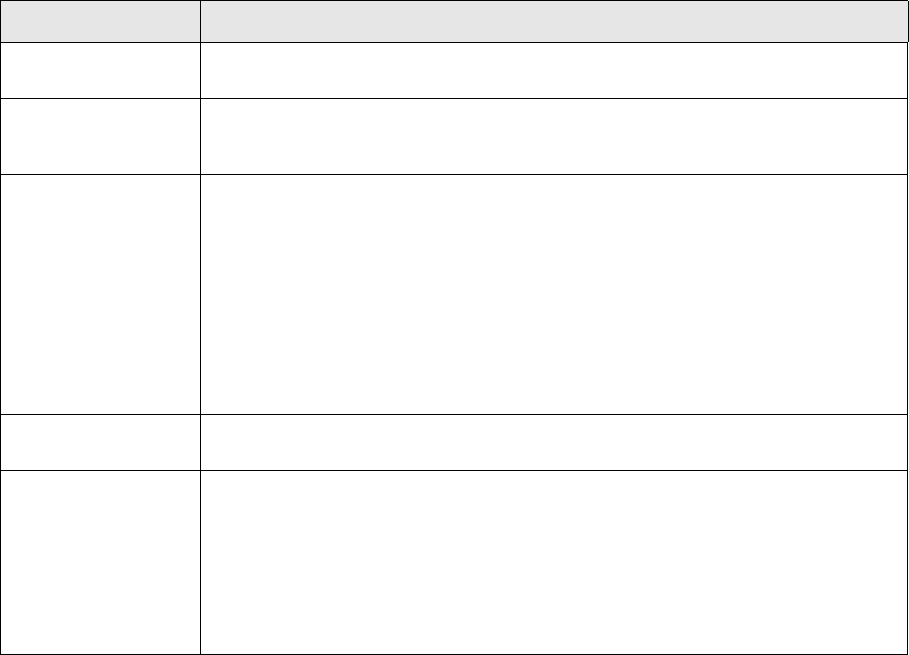
1 Concepts
1.9 Valuation and results
30 © Wall Street Systems IPH AB - Confidential
In general terms, the market value of a position is compared to capital invested, and the difference
is the total profit of the position. Total profit is further split into the following components (the exact
description of each component may vary slightly according to the instrument):
1.9.3 Valuation modes
Sometimes, it is necessary to calculate market value and results in different ways. For example,
even if market value can be obtained from market quotes, occasionally it may be useful to run the
valuation using a theoretical model. Furthermore, for accounting purposes, it may also be necessary
to do the valuation using specific benchmark yield curves, and to apply specific accounting
treatment for the difference between normal and benchmark valuation.
Valuation modes allow users to define different valuation methods and models and to use different
market parameters to value the same instrument. Every time valuation is requested by a user, the
user specifies the valuation mode, and the system performs the valuation using the setup applicable
to that mode.
The standard system provides three different valuation modes:
•Default
•Theoretical
•Benchmark.
The valuation modes themselves are simply identifiers. Users need to specify the type of valuation
that is to be carried out at instrument level. For example, if the Theoretical valuation mode is
selected, the system will not switch automatically to a theoretical model. Rather, the user needs to
link the appropriate valuation methods and models for each instrument, which are then called each
time theoretical valuation is requested.
Valuation Mode can be used as a start-up parameter for monitoring the treasury position, for running
profit/loss reports, and for closing-the books. If no mode is specified, the system’s Default valuation
mode is used.
Profit Description
Accrued Interest Interest accrued since the value date of the transaction or the previous coupon date
until the valuation date.
Accrued Profit Accrued/amortized discount/premium, accrued fees, or amortized option premiums
since the value date of the transaction or the payment date of the premium/fee, until
the valuation date.
MtoM Profit Profit/loss resulting from the difference between market valuation (excluding accrued
interest and accrued profit) and capital invested.
For example, for instruments with a market quotation, MtoM profit is generally the
difference between the market price and the deal price.However, when accruals and
fees need to be taken into account, the calculation of MtoM Profit becomes more
complex.
MtoM profit is calculated to the spot date of the instrument, and not discounted to the
valuation date.
Note: For details of the MtoM Profit calculation for a particular type of instrument, see
the relevant section of this guide.
FX Profit Profit/loss resulting from the change in FX rates, between the value (or trade) date
and the valuation date, calculated on the invested amount.
Other Profit The residual profit/loss after the above components are separated from total profit.
This residual is usually the end-product when total result is calculated correctly
theoretically, but the other components are calculated according to general
accounting practices.
For example, the market value for a bond includes the accrued interest calculated
until the spot date of the instrument (that is, the amount which would be received if
the bond was sold today), while accrued interest includes the interest accrued until
the valuation date.
1 Concepts
1.9 Valuation and results
Transaction & Risk Management Module (TRM) Instruments: Processing and Calculations 31
New valuation modes can be added during implementation according to your organization’s
requirements.
1 Concepts
1.9 Valuation and results
32 © Wall Street Systems IPH AB - Confidential
Transaction & Risk Management Module (TRM) Instruments: Processing and Calculations 33
Chapter 2 Market standards and calculations
2.1 Market standards
2.1.1 Date basis
Date bases are used to calculate the length, in years, of the period between two dates. The formula
for this calculation is t=d/B, where d is the number of days in the period, and B is the basis
denominator. Both d and B depend on the date basis used. Different date bases may result in
different values for d and B for the same period and, consequently, in different period lengths.
TRM uses date bases when an interest rate is defined over a period. The definition of the rate must
include how the length of the period is calculated.
•360 date bases
In these date bases, the denominator B is always 360, but the calculation of the numerator
varies. However, there is a difference in the way the 31st day at the beginning and at the end of
the period under consideration is handled.
The formulas used show how the period d between date1 (y1, m1, d1) and date2 (y2, m2, d2) is
calculated: yi, mi, and di represent the year, month, and day, respectively; and min is the
minimum value in the set. For example, min(d2, 30) means "use the lesser value of d2 and 30."
•Actual date bases
Actual date bases allow for different lengths of months and are, therefore, more accurate than
the 360 date bases. The Actual date bases generally differ in the way that they handle leap
years.

2 Market standards and calculations
2.1 Market standards
34 © Wall Street Systems IPH AB - Confidential
Example period 1991-06-30 to 1996-01-31
The period 1991-06-30 to 1996-01-31 is used in some of the following examples to show how the
various date bases calculate the number of days between two dates.
Name Description
30E/360 Any 31st day of the month is considered to be the 30th of the month. The formal
definition is:
d = min(d2,30) - min (d1,30) + 30(m2 - m1) + 360(y2 - y1)
For the example period:
d = min(31,30) - min(30,30) + 30*(1 - 6) + 360*(1996 -1991) = 1650
The length of the period in years is 1650/360 = 4.583
30E/360 EOM This is a variation of the 30E/360 basis, with the month of February having an
invariable 30 days.
Example: For the 2003-08-31 through 2004-02-29:
d = min(30,30) min (31,30 + 30*(2 - 8 360*(2004 - 2003 = 180
The length of the period in years is 180/360 = 0.5
30/360 This is a variation of the 30E/360 basis. The difference occurs when d1 < 30. In this
case, no rounding of the date occurs, and the above equation is replaced by:
d = d2, - d1 + 30(m2 - m1) + 360(y2 - y1)
For the example period:
d1 = 30, so the 30E/360 formula is used and d = 1650
However, if the beginning of the period was the 29th instead of the 30th, the result
would be:
d = 31 - 29 + 30*(1 - 6) + 360*(1996 - 1991) = 1652
The length of the period in years would then be 1652/360 = 4.589.
30E+/360 This is a variation of the 30E/360 basis. The difference is that rounding is applied only
to the earlier date. The equation is then:
d = d2 - min(d1,30) + 30(m2 - m1) + 360(y2 - y1)
For the example period:
d = 31 - min(31,30) + 30*(1 - 6) + 360*(1996 -1991) = 1651
The length of the period in years is 1651/360 = 4.586
Actual/Actual ISDA If no leap year is involved in the calculation, then t = d/B where d = the actual
number of days and B = 365.
If there is a leap year, then t = d1/B1 + d2/B2, where
d1 = the actual number of days in the leap year and B1 = 366
d2 = the actual number of days in the non-leap year and B2 = 365
Actual+/Actual ISDA This is a variation on Actual/Actual ISDA, for which the first day is excluded for the
day count.
Actual-/365 d = the actual number of days excluding all leap days (29th of February).
B = 365 days.
For the example period:
The number of days between 1991-06-30 and 1996-01-31 is 1676, but since there is
one leap day within that period, d = 1675.
The length of the period in years, t, is 1675/365 = 4.589
Actual-/365+ d = the actual number of days excluding all leap days (29th of February).
B = the number of days in the year in which the coupon value date falls.

2 Market standards and calculations
2.1 Market standards
Transaction & Risk Management Module (TRM) Instruments: Processing and Calculations 35
Actual-/365L d = the actual number of days excluding all leap days (29th of February).
B = 366 if the last partial year of the period contains a leap day; otherwise, B = 365.
The last partial year is the remaining period when the maximum number of full years
have been counted off, starting from the beginning of the period.
For the example period:
The last partial year is the period from 1995-06-30 to 1996-01-31, which does not
contain a leap day, so B = 365. The number of days between 1991-06-30 and
1996-01-31 is 1676, but since there is one leap day within that period, d = 1675.
The length of the period in years, t, is 1675/365 = 4.589.
If, instead, the end of the period were on 1996-02-29, the number of days would be
1675+29-1=1703 (the leap day is not counted), and the last partial year would
contain a leap day, so that t would be 1703/366 = 4.653.
Actual/360 d = the actual number of days.
B = 360 days.
For the example period:
d = 1676 and B = 360, so t = 1676/360 = 4.656
Actual/365 d = the actual number of days.
B = 365 days.
For the example period:
d = 1676 and B = 365 so t = 1676/365 = 4.592
Actual/365+ d = the actual number of days.
B = 366 if the end of the period falls on a leap year; otherwise, B = 365.
For the example period:
The number of days between 1991-06-30 and 1996-01-31 is 1676. B = 366 since
1996 is a leap year. So t = 1675/366 = 4.577
Actual/365L d = the actual number of days.
B = 366 if the last partial year of the period contains a leap day; otherwise B = 365.
The last partial year is the remaining period when the maximum number of full years
have been counted off, starting from the beginning of the period.
For the example period:
The last partial year is the period from 1995-06-30 to 1996-01-31, which does not
contain a leap day, so B = 365 and t = 1676/365 = 4.592
Actual/Actual ISDA If no leap year is involved in the calculation, then t = d/B where d = the actual
number of days and B = 365.
If there is a leap year, then t = d1/B1 + d2/B2, where
d1 = the actual number of days in the leap year and B1 = 366
d2 = the actual number of days in the non-leap year and B2 = 365.
Name Description

2 Market standards and calculations
2.1 Market standards
36 © Wall Street Systems IPH AB - Confidential
Actual/Actual (n)The variable n is 1, 2, or 4, specifying the frequency of coupons. The corresponding
coupon periods are 12, 6, and 3 months (= 12 / n), respectively. The time between
the dates d1 and d2 is calculated by first calculating the number (p) of the whole
periods that fit into the interval (d1, d2), from the date (d2) backwards, and then by
adding the length of the first fractional period.
The end and start dates of the periods are generated by repeatedly subtracting 12, 6,
or 3 from the month number of d2. If the month thus generated has fewer days than
the day of month of the end date (d2), the period end date is the end date of the
month in question. That is, if d2 = 2008-05-31 and n = 4, then the start date of the
last period is 2008-02-29.
If the date (d1) is a start date of a whole period, then the time in years between d1
and d2 is simply the number of whole periods:
Equation 2-1 Actual/Actual (n): number of whole periods
Otherwise, let ds and de be the start and end dates of the whole period wherein the
date (d1) falls. Then the time in years between d1 and d2 is:
Equation 2-2 Actual/Actual (n): time in years between d1 and d2
Example
Let the start and end dates be d1 = 2008-03-31 and d2 = 2009-09-30, and the
frequency be n = 2. Then, the dates generated are as follows:
• 2009-09-30
• 2009-03-30
• 2008-09-30 = de
• 2008-03-30 = ds
There are two (2) whole periods, and the time between d1 and d2 is:
Equation 2-3 Actual/Actual (n): Example with 2 whole periods
Actual/Actual (n) EOM Note: The Actual/Actual (n) EOM data basis is TRM-specific, i.e. non-market standard.
This date basis is similar to Actual/Actual (n) except that the period end and start
dates are moved to the last date of the month in question. That is, all the whole
periods begin and end at the last day of the month.
Example
Let the start and end dates be d1 = 2008-03-31 and d2 = 2009-09-30,
and frequency be n = 2. Then the dates generated are as follows:
• 2009-09-30
• 2009-03-31
• 2008-09-30 = de
• 2008-03-31 = ds
That is, the dates in March have been moved to the end of March. There are three (3)
whole periods, and no fractional part. Therefore, time in years is as follows:
Equation 2-4 Actual/Actual (n) EOM: Example with 3 whole periods
Name Description
tpn⁄=
tpn⁄ded1
–
nd
eds
–()
------------------------
+=
t32⁄1.5==

2 Market standards and calculations
2.1 Market standards
Transaction & Risk Management Module (TRM) Instruments: Processing and Calculations 37
2.1.2 Interest types
BRL/252 This date basis calculates time as business days according to the Brazilian (BRL)
calendar divided by 252.
Example
Take the period between 2003/12/16 and 2004/02/02. For this period, the BRL
calendar is set up with the following public holidays: 2003/12/25, 2003/12/26, and
2004/01/01, as well as 14 weekend days.
Therefore, there are 31 business days in the period, and so, using this date basis, the
resulting time is: 31/252 = 0.123015873
(instead of 48/365 = 0.131506849 if the Actual/365 date basis was used).
Name Description
Name Discount factor in terms of
interest rate
Interest rate in terms of discount
factor
Annually Compounded Rate
Semi-Annually Compounded
Rate
Quarterly Compounded Rate
Monthly Compounded Rate
Daily Compounded Yield
(B = denominator of date basis)
Continuous Yield
Discount Rate
Interest Rate Depending on time:
•Periodic Rate for maturities less than one year
•Continuous Yield for maturities equal to or over one year.
Periodic Rate
D1
r
100
---------
+
⎝⎠
⎛⎞
t–
=r 100 D 1t⁄–1–()=
D1
r
200
---------
+
⎝⎠
⎛⎞
2t–
=r 200 D 12t()⁄–1–()=
D1
r
400
---------
+
⎝⎠
⎛⎞
4t–
=r 400 D 14t()⁄–1–()=
D1r
1200
------------
+
⎝⎠
⎛⎞
12t–
=r 1200 D 112t()⁄–1–()=
D1r
100B
-------------
+
⎝⎠
⎛⎞
Bt–
=r 100B D 1Bt()⁄–1–()=
De
r
100
---------t–
=r100
t
---------Dlog–=
D1r
100
---------t–=r100
1D–
t
-------------
=
D1
1r
100
---------t+
--------------------
=r100
t
---------1
D
----1–
⎝⎠
⎛⎞
=

2 Market standards and calculations
2.1 Market standards
38 © Wall Street Systems IPH AB - Confidential
2.1.3 Price types
2.1.3.1 Trading Margin
The conversion of the quotation (trading margin) into the price is handled by specific quote handlers
for Australian FRNs and MBS. The formula used to convert the trading margin (market quote) to the
instruments price is described in 3.1.3 Australian floating rate note on page 236 and 3.7.5
Australian MBS on page 302 respectively.
2.1.4 Yield/price conversions
Bonds are traded on either yield or price depending on the market conventions. At deal entry, the
user can enter either the yield or the price of the bond, the missing value is then calculated from the
entered one. For example, if you enter the price then the yield is calculated, and vice versa.
The yield/price conversion of a bond is set by including the Trading Yield feature and associating the
relevant yield convention with the instrument in the Instrument Editor. The convention determines
which price and yield method are used for the conversion.
When no convention is selected at the instrument level, the default convention for calculating the
yield (deal rate) is ISMA with Actual/Actual date basis and Annually Compounded yield.
The following information is provided in this section for each convention:
2.1.4.1 Price/yield conversion
The yield y is in most cases converted from the clean price of a fixed rate bond by using either
the ISMA or the Simple Yield formula. This section describes these two calculations.
Semi-Annual/Periodic Rate
Quarterly/Periodic Rate
Monthly/Periodic Rate
These interest types work in a similar way to interest type Interest Rate:
• If time is shorter than six months/three months/month, then the
discount factor is periodic:
1 / (1 + rate/100 * time)
• If time is longer than six months/three months/month, then the
discount factor is compounded with frequency of 2, 4, or 12:
(1 + rate / (frequency * 100))^(-frequency * time)
("^" means to the power)
Note: The number of months is calculated as calendar months. For
example, from 15 February to 15 March is one month, regardless
of date basis.
ISDA CDS This interest type works in a similar way to interest type Periodic Rate
except that the last coupon period is one day longer, i.e. it includes both
first and last date.
Name Discount factor in terms of
interest rate
Interest rate in terms of discount
factor
Field Description
Name The name of the convention as it appears in TRM.
Description General description of the method and standard calculations.
Usage Describes with which instrument this method is typically used.
Pc

2 Market standards and calculations
2.1 Market standards
Transaction & Risk Management Module (TRM) Instruments: Processing and Calculations 39
2.1.4.1.1 ISMA (financial/instrument/isma@yield)
2.1.4.1.2 Simple Yield (financial/instrument/simple-yield@yield)
Information Description
Name ISMA
Description The ISMA yield uses a goal seeker method id in the system seeks for the yield which gives
the input price.
The algorithm iterates the yield y until the equation equals zero:
Equation 2-5 ISMA method
where
• is the clean market price
• and represent the ith cashflow and its date (coupon date)
• is the discount factor for that cashflow
• is the accrued interest
Usage This method applies to all bonds except Japanese government bonds, which use the simple
yield. See 2.1.4.2 Yield/price conversion on page 40.
pc
cidi
D
Ia
Information Description
Name Simple Yield
Description The simple yield calculates the yield from the clean market price as follows:
Equation 2-6 Simple Yield
where
• is the coupon rate
•
is the clean market price
• is the time in years from the valuation date to maturity
From this, the conversion equation for simple yield is:
Equation 2-7 Simple Yield: conversion equation
Usage This method applies only to Japanese government bonds (GOVT-JP). See 2.1.4.2.29
GOVT-JP (financial/instrument/simple-yield@price) on page 59.
r
pc
tm

2 Market standards and calculations
2.1 Market standards
40 © Wall Street Systems IPH AB - Confidential
2.1.4.2 Yield/price conversion
The clean price of a fixed rate bond is in most cases converted from the yield y by the formula:
Equation 2-8 Yield/price conversion: clean price
where
• is the clean market price
• and represent the ith cashflow and its date (coupon date)
• is the discount factor for that cashflow
• is the accrued interest.
If the dirty price is used, then accrued interest in the above equation is dropped.
The methods of calculating the discount factor and the accrued interest may depend on market
conventions as explained in the following sections.
Hint:
For the following bond conventions, when the yield is not specifically mentioned then the
convention uses ISMA.
2.1.4.2.1 *ISMA-30/360-BIMONTHLY (financial/instrument/isma@price)
2.1.4.2.2 *ISMA-30E360-ANNUAL (financial/instrument/isma@price)
Field Description
Name *ISMA-30/360-BIMONTHLY
Description *ISMA-30/360-BIMONTHLY bonds are regular fixed coupon securities with bi-monthly coupons
and 30/360 date basis. With *ISMA-30/360-BIMONTHLY, the coupons for the ith cashflow on date
are discounted using the following formula:
Equation 2-9 European bonds before the Euro
where
• is the time in years between the value date and the coupon date .
Usage Convention used for australian bonds.
Field Description
Name *ISMA-30E360-ANNUAL
Description *ISMA-30E360-ANNUAL bonds are regular fixed coupon securities with annual coupons and
30E/360 date basis. With *ISMA-30E360-ANNUAL, the coupons for the ith cashflow on date
are discounted using the following formula:
Equation 2-10 European bonds before the Euro
where
• is the time in years between the value date and the coupon date .
Pc
pc
cidi
D
Ia
di
Dyd
i
,()1y6⁄+()
ti
=
tidi
di
Dyd
i
,()1y+()
ti
=
tidi

2 Market standards and calculations
2.1 Market standards
Transaction & Risk Management Module (TRM) Instruments: Processing and Calculations 41
2.1.4.2.3 *ISMA-30E360-SEMI-ANNUAL (financial/instrument/isma@price)
2.1.4.2.4 *ISMA-30E360-QUARTERLY (financial/instrument/isma@price)
2.1.4.2.5 *ISMA-ACTACT-ANNUAL (financial/instrument/isma@price)
Usage Convention used for European bonds (Belgium, Finland, and Germany) issued before the
introduction of the Euro.
Field Description
Name *ISMA-30E360-SEMI-ANNUAL
Description *ISMA-30E360-SEMI-ANNUAL bonds are regular fixed coupon securities with semi-annual
coupons and 30E/360 date basis. With *ISMA-30E360-SEMI-ANNUAL, the coupons for the ith
cashflow on date are discounted using the following formula:
Equation 2-11 Sovereign and corporate bonds
where
• is the time in years between the value date and the coupon date .
Usage Convention used for some sovereign or corporate bonds.
Field Description
Name *ISMA-30E360-QUARTERLY
Description *ISMA-30E360-QUARTERLY bonds are regular fixed coupon securities with quarterly
coupons and 30E/360 date basis.
With *ISMA-30E360-QUARTERLY, the coupons for the ith cashflow on date are discounted
using the following formula:
Equation 2-12 ISMA 30E360 Quarterly bonds
where
• is the time in years between the value date and the coupon date .
Usage Supranational or regional bond issuer, for example, German Landesbank.
Field Description
Name *ISMA-ACTACT-ANNUAL
Field Description
di
Dyd
i
,()1y2⁄+()
ti
=
tidi
di
Dyd
i
,()1y
4
---
+
⎝⎠
⎛⎞
ti
=
tidi
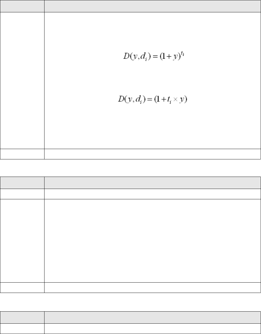
2 Market standards and calculations
2.1 Market standards
42 © Wall Street Systems IPH AB - Confidential
2.1.4.2.6 *ISMA-ACTACT-QUARTERLY (financial/instrument/isma@price)
2.1.4.2.7 *ISMA-ACTACT-SEMI-ANNUAL (financial/instrument/isma@price)
Description This yield convention is used according to the Eurozone. With *ISMA-ACTACT-ANNUAL, the
coupons for the ith cashflow on date are discounted using the following formula:
•If
Equation 2-13 Standard Eurozone: when time in years is more than 1
•If
Equation 2-14 Standard Eurozone: when time in years is less than or equal to 1
where
• is the time in years between the value date and the coupon date
• is the time in years from the valuation date to the maturity of the bond.
Usage Standard Euro Zone convention that can be applied to other corporate bonds.
Field Description
Name *ISMA-ACTACT-QUARTERLY
Description *ISMA-ACTACT-QUARTERLY bonds are regular fixed coupon securities with quarterly coupons
and Act/Act date basis.
With *ISMA-ACTACT-QUARTERLY the coupons for the ith cashflow on date di are discounted
using the following formula:
Equation 2-15 ISMA Act/Act Quarterly bonds
where
• is the time in years between the value date and the coupon date .
Usage Supranational or regional bond issuer, for example, EIB.
Field Description
Name *ISMA-ACTACT-SEMI-ANNUAL
Field Description
di
tm1>
tm1≤
tidi
tm
Dyd
i
,()1y
4
---
+
⎝⎠
⎛⎞
ti
=
tidi
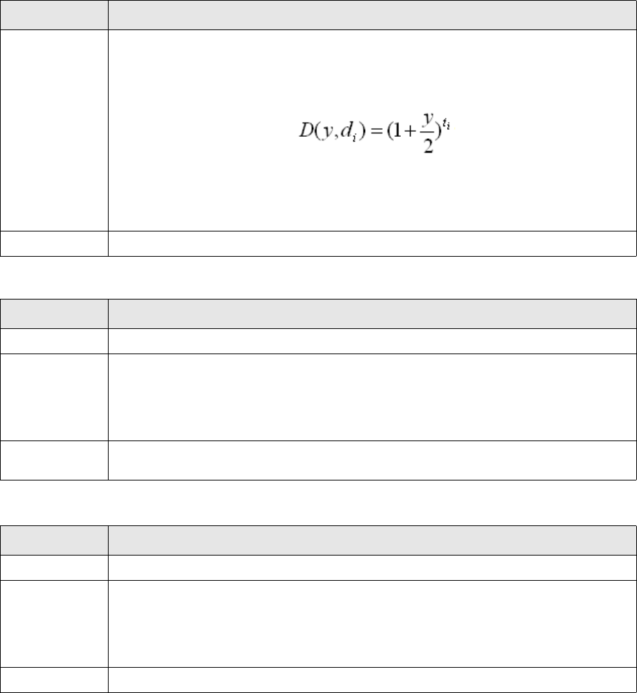
2 Market standards and calculations
2.1 Market standards
Transaction & Risk Management Module (TRM) Instruments: Processing and Calculations 43
2.1.4.2.8 *ISMA-ACT360-ANNUAL (financial/instrument/isma@price)
2.1.4.2.9 *ISMA-ACT365-ANNUAL (financial/instrument/isma@price)
Description ISMA-ACTACT-SEMI-ANNUAL bonds are regular fixed coupon securities with semi-annual
coupons and Act/Act date basis. With *ISMA-ACTACT-SEMI-ANNUAL, the coupons for the ith
cashflow on date are discounted using the following formula:
Equation 2-16 Standard UK government bondS
where
• is the time in years between the value date and the coupon date
Usage Standard UK government bond convention that can be applied by other corporate bonds.
Field Description
Name *ISMA-ACT360-ANNUAL
Description ISMA-ACT360-ANNUAL bonds are regular fixed coupon securities with annual coupons and
Act/360 date basis.
ISMA-ACT360-ANNUAL bonds are calculated using the same formula as
ISMA-30E360-ANNUAL, see 2.1.4.2.2 *ISMA-30E360-ANNUAL
(financial/instrument/isma@price) on page 40.
Usage This convention is used for bond instruments bonds (Interest FIXBIS) issued by sovereign
issuers such as the Bank for International Settlement (BIS).
Field Description
Name *ISMA-ACT365-ANNUAL
Description *ISMA-ACT365-ANNUAL bonds are regular fixed coupon securities with annual coupons and
Act/365 date basis.
ISMA-ACT360-ANNUAL bonds are calculated using the same formula as
ISMA-30E360-ANNUAL, see 2.1.4.2.2 *ISMA-30E360-ANNUAL
(financial/instrument/isma@price) on page 40.
Usage This convention is used for some sovereign bond instruments.
Field Description
di
tidi
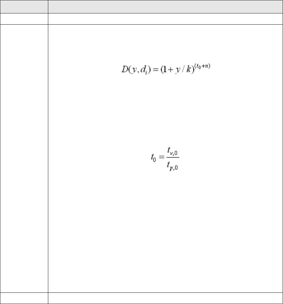
2 Market standards and calculations
2.1 Market standards
44 © Wall Street Systems IPH AB - Confidential
2.1.4.2.10 *U.S.STREET-ACT365-SEMIANNUAL (financial/instrument/us-street@price)
Field Description
Name *U.S.STREET-ACT365-SEMIANNUAL
Description U.S.STREET-ACT365-SEMIANNUAL bonds are regular or irregular securities with Act/365
date basis. With *U.S.STREET-ACT365-SEMIANNUAL, the coupons for the ith cashflow on date
are discounted using the following formula:
Equation 2-17 U.S. Treasury Notes
where
• is the compounding frequency of the yield. For example, for semi-annual yield)
• is the time in years from the value date to the first coupon date.
is calculated using the following formula:
Equation 2-18 U.S. Treasury Notes: time in years
where
- is the period in years between the valuation date and the first coupon date
- is the period in years between the previous and the next coupon date,
calculated using the date basis Act/365.
• is the number of coupon periods between and , the ith coupon date.
is calculated using:
Equation 2-19 U.S. Treasury Notes: number of coupon periods
where
- is the time (in years) between and .
Usage U.S. Treasury Notes market convention on the secondary market.
di
kk2=
t0d0
t0
tv0,
tp0,
nd
0di
n
n round k ti
×()=
tid0di
2 Market standards and calculations
2.1 Market standards
Transaction & Risk Management Module (TRM) Instruments: Processing and Calculations 45
2.1.4.2.11 *U.S.STREET-ACTACT-SEMIANNUAL (financial/instrument/us-street@price)
2.1.4.2.12 *U.S.STREET-ACTACT-ANNUAL (financial/instrument/us-street@price-1)
Field Description
Name *U.S.STREET-ACTACT-SEMIANNUAL
Description U.S.STREET-ACTACT-SEMIANNUAL bonds are based on the same formula as
U.S.STREET-ACT365-SEMIANNUAL, but have Act/Act date basis.
See 2.1.4.2.10 *U.S.STREET-ACT365-SEMIANNUAL (financial/instrument/us-street@price)
on page 44.
Usage Zero-coupon markets, such as, the U.S. and the UK strips.
Field Description
Name *U.S.STREET-ACTACT-ANNUAL
Description U.S.STREET-ACTACT-ANNUAL bonds are based on the same formula as
U.S.STREET-ACT365-SEMIANNUAL, but have annual coupon and Act/Act date basis.
See 2.1.4.2.10 *U.S.STREET-ACT365-SEMIANNUAL (financial/instrument/us-street@price)
on page 44.
Usage Some sovereign bonds, for example, on the Euro Dollar market.
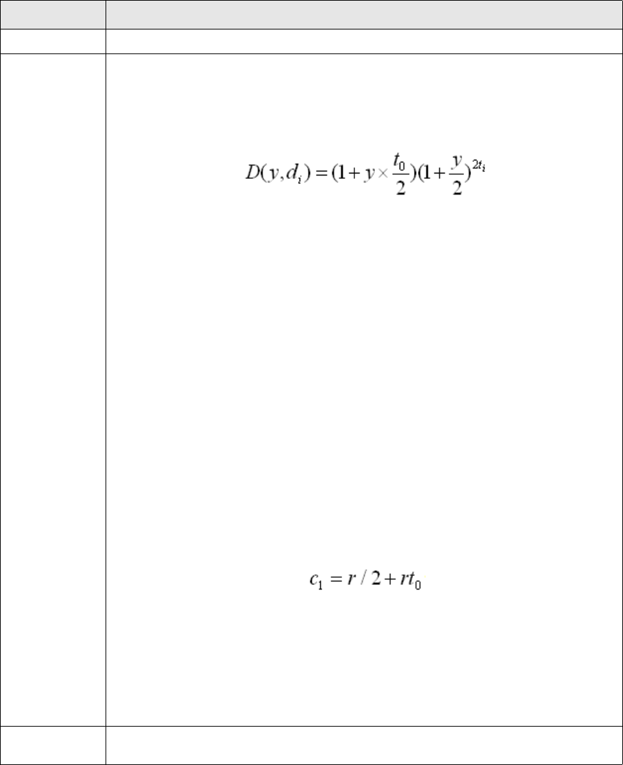
2 Market standards and calculations
2.1 Market standards
46 © Wall Street Systems IPH AB - Confidential
2.1.4.2.13 *U.S. Treasury (financial/instrument/us-treasury@price)
Field Description
Name *U.S.TREASURY
Description U.S.TREASURY bonds are regular and irregular fixed coupon securities with semi-annual
coupons and Act/365 date basis.
With *U.S.TREASURY, a periodic rather than compound rate is used for discounting over the
partial period from the value date to the next coupon date :
Equation 2-20 U.S. Treasury notes and bonds
where
• is the time in years from the value date to the next coupon date (calculated as in
*U.S.STREET-ACT365-SEMIANNUAL, see 2.1.4.2.10 on page 44)
• is time in years from the value date to the coupon date.
U.S. Treasury notes and bonds may have an odd first coupon, that is, the length of the first
coupon period may be longer or shorter than the normal coupon period:
• If the first coupon period is shorter, the coupon amount is calculated as:
Equation 2-21 U.S. Treasury notes and bonds: shorter first coupon period
where
- is the nominal interest rate as a percentage of the par value
- is the time (in years) between the value date of the interest accrual (i.e.
beginning of interest accrual) and the first coupon date.
• If first coupon periods longer than the regular coupon period, the first coupon amount is
given by:
Equation 2-22 U.S. Treasury notes and bonds: longer first coupon period
where
- is the nominal interest rate as a percentage of the par value
- is time (in years) between the value date of the interest accrual and the date six
months before the first coupon date.
Note: If the first coupon period is exactly half a year, both equations give the same result.
Usage Standard U.S. Treasury Notes and bonds convention that can be applied to other corporate
bonds.
di
t0
ti
c1rt1
=
r
t1
r
t0
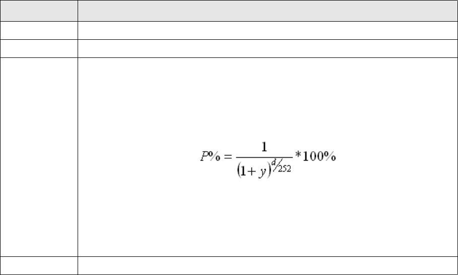
2 Market standards and calculations
2.1 Market standards
Transaction & Risk Management Module (TRM) Instruments: Processing and Calculations 47
2.1.4.2.14 BOND-BR-LFT (financial/instrument/isma@price)
Information Description
ID BOND-BR-LFT
Name Brazilian LFT
Description BOND-BR-LFT bonds are Brazilian Zero Coupon Bonds linked to the O/N-SELIC-interest
rate. The maturities can be over 2 years. They are traded and quoted in 1000's (Dirty Price,
Date basis: Business Days/252) and have a unique security ID (ISIN number), issue date and
maturity date.
The price is derived from the traded yield according to the following equation:
Equation 2-23 Brazilian zero coupon bond
where
•P is the price (as a percentage of the par value)
•y is the annual yield-to-maturity (as a percentage)
•d denotes the number of business dates from settlement date to maturity date.
Usage Brazilian Zero Coupon Bonds

2 Market standards and calculations
2.1 Market standards
48 © Wall Street Systems IPH AB - Confidential
2.1.4.2.15 BOND-BR-NBC (financial/instrument/isma@price)
2.1.4.2.16 BOND-BR-NTN (financial/instrument/isma@price)
Information Description
ID BOND-BR-NBC
Name Brazilian NBC
Description BOND-BR-NBC bonds are fixed rate bonds linked to the PTAX-index (FX-rate). The
maturities are 2Y, 3Y and 5Y. The fixed rate is 12% p.a. They are traded and quoted in
1000’s and have a unique security ID (ISIN number), issue date and maturity date.
The price is calculated as a dirty price and is derived from the traded market rate quoted as
a semiannual yield according to the following equation:
Equation 2-24 Brazilian NBC bonds
where
•P is the price (as a percentage of the par value)
•y is the annual yield-to-maturity (as a percentage)
•d360(k) is the number of days between settlement date and cashflow value date
according to 30/360 date basis
•c is the coupon rate (12%)
•L is the number of future coupons
•PTAX(t-1) is the PTAX-index rate valid at time t-1, and ID is the issue date
•PTAX(ID-1) is the PTAX-index rate valid at Issue Date-1.
Usage Brazilian NBC Bonds
Information Description
ID BOND-BR-NTN
Name Brazilian NTN

2 Market standards and calculations
2.1 Market standards
Transaction & Risk Management Module (TRM) Instruments: Processing and Calculations 49
Description BOND-BR-NTN bonds are bonds linked to the IGPM-index (NTN-C) and the ICPA-index
(NTN-B). The maturities are 2Y, 3Y and 5Y. The fixed rate is 12% p.a. or 6% p.a. They are
traded and quoted in 1000’s and have a unique security ID (ISIN number), issue date and
maturity date.
The price is calculated as a dirty price and is derived from the traded market rate quoted as
a compound yield according to the following equation:
Equation 2-25 Brazilian NTN bonds
where
•P is the price (as a percentage of the par value)
•y is the annual yield-to-maturity (as a percentage)
•bd(k) is the number of business days between settlement date and cashflow value date
•L is the number of future coupons.
•c is the coupon rate (12% or 6%)
The nominal value is 1 000 at issue date for both NTN-B and NTN-C instruments. The
nominal value is then adjusted by the IGPM-rates (NTN-C) and IPCA-rates (NTN-B)
respectively. These rates are inflation rates published every month as a monthly (p.m.)
rate.
Usage Brazilian NTN Bonds
Information Description

2 Market standards and calculations
2.1 Market standards
50 © Wall Street Systems IPH AB - Confidential
2.1.4.2.17 GOVT-AU (financial/instrument/australian@price)
Information Description
ID GOVT-AU
Name Australian Government bond
Description GOVT-AU bonds are medium to long-term debt securities with a fixed coupon paid
semi-annually in arrears, redeemable at face value on the maturity date. Treasury Bonds
are traded on a yield to maturity basis with the price per $100 face value calculated using
the following pricing formulae:
• Basic formula
Equation 2-26 Australian government bond: Basic formula
•Ex interest bonds
Equation 2-27 Australian government bond: Ex interest bonds
• Near-maturity bonds: Specifically, those entitling a purchaser to only the final coupon
payment and repayment of principal.
Equation 2-28 Australian government bond: Near-maturity bonds
where
•P is the price per $100 face value (the computed price is rounded to 3 decimal spaces)
•v is
•i is the annual percentage yield to maturity divided by 200 in Equation 2-26 on page 50
and Equation 2-27 on page 50, or the annual percentage yield to maturity divided by
100 in Equation 2-28 on page 50
•f is the number of days from the date of settlement to the next interest payment date
in Equation 2-26 on page 50 and Equation 2-27 on page 50 or to the maturity date in
Equation 2-28 on page 50.
• If the next interest payment date or maturity date falls on a non-business day, the next
good business day (a day on which banks are open for business in Melbourne or Sydney,
i.e. not a Saturday or Sunday) is used in the calculation of f.
•d is the number of days in the half year ending on the next interest payment date
•g is the half-yearly rate of coupon payment per $100 face value
•n is the term in half years from the next interest-payment date to maturity
Settlement amounts are rounded to the nearest cent (0.50 cent is rounded up). That is, the
pricing formula used for computing the price from the yield is the ISMA method. But in the
case of near maturing bonds, i.e. when the bond is settled six months plus seven days
before maturity, it is treated as a special case, using the pricing of Treasury Notes.
Equation 2-29 Treasury Notes equation
1
1i+
-----------

2 Market standards and calculations
2.1 Market standards
Transaction & Risk Management Module (TRM) Instruments: Processing and Calculations 51
2.1.4.2.18 GOVT-CA (financial/instrument/canadian@price)
Usage Australian government bond
Information Description
ID GOVT-CA
Name Canadian Government bond
Description GOVT-CA bonds are regular, fixed-coupon securities with equal, semi-annual coupon
payments and Act/365 date basis. These bonds are traded on a clean price basis.
Although Canadian government bonds share similarities with U.S. Treasury bonds, they
differ in the accrued interest calculation. The accrued interest on Canadian Government
bonds is calculated as follows:
Equation 2-30 Canadian government bonds
where
•AI is the accrued interest
•r is the nominal interest rate (to be paid at time i) as a percentage of the par value
•P
AI is the number of accrued interest days computed in the following way:
where
- coupon days (pc) is the actual number of days in the current coupon period,
calculated as coupon value date minus the start of the current coupon period
- is the actual number of days in the period over which the accrued interest is
calculated (calculated as accrued interest date minus the start of the current
coupon period).
Then:
- if is less than or equal to 182, then , or
- if is greater than 182, then
Usage Canadian government bond
Information Description
pAI
act
pAI
act pAI pAI
act
=
pAI
act pAI 182.5 pcpAI
act
–()–()=
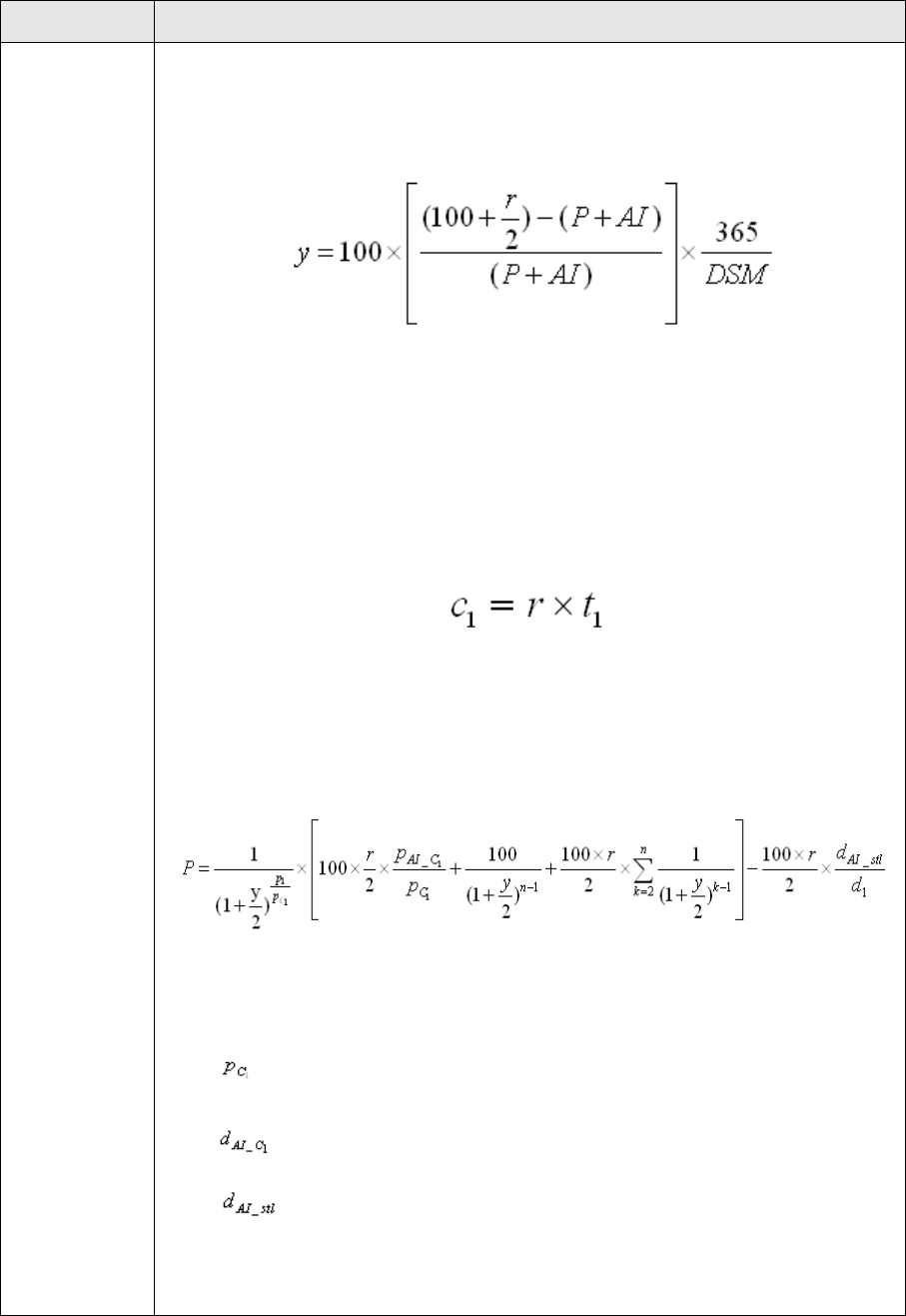
2 Market standards and calculations
2.1 Market standards
52 © Wall Street Systems IPH AB - Confidential
Yield The following algorithm is used to calculate the yield (Y) based on the price of Canadian
Government bonds:
• If one coupon payment remains, then the following algorithm is used to calculate the
yield (Y) based on the price of Canadian Government bonds:
Equation 2-31 Canadian government bonds: one coupon payment remains
where
-y is the annual yield-to-maturity (as a percentage)
-r is the nominal interest rate (to be paid at time i) as a percentage of the par value
-P is the clean price (as a percentage of the par value)
-DSM is the days from settlement date to maturity date
-AI is the accrued interest calculated as described in Equation 2-30 on page 51.
• If the first coupon is a short coupon, then the Yield formula of Canadian Bond (yield
convention GOVT-CA) takes into account the first coupon as follows:
Equation 2-32 Canadian government bonds: if first coupon is a short coupon
Where
-r is the nominal interest rate
-t1 is the time (in years) between the beginning of the interest accrual and the first
coupon date
and then applies to the following Yield/Price formula:
Equation 2-33 Canadian government bonds: Yield/Price formula
Where
-P is the clean price (as a percentage) of the Par value
-y is the annual Yield-to-Maturity (as a percentage)
-p1 is the number of days from the settlement date to the first coupon date
- is the number of days in the quasi-coupon period ending on the first coupon
payment date
-r is the nominal interest rate
- is the number of days from interest accrual date to first payment date
-n is the number of coupon payments remaining
- is the number of days from the interest accrual date to the settlement date.
• If more than one coupon payment remains, the US Treasury bond market conventions
(i.e. US Street calculation method) are used for the price/yield calculations. See
2.1.4.2.10 *U.S.STREET-ACT365-SEMIANNUAL (financial/instrument/us-street@price)
on page 44.
Information Description

2 Market standards and calculations
2.1 Market standards
Transaction & Risk Management Module (TRM) Instruments: Processing and Calculations 53
2.1.4.2.19 GOVT-CH (financial/instrument/isma@price)
2.1.4.2.20 GOVT-DK-OLD-30E360 (financial/instrument/isma@price)
Information Description
ID GOVT-CH
Name Swiss Government bond
Description GOVT-CH bonds are regular, fixed-coupon securities with equal, annual coupon payments
and 30E/360 date basis (the date basis where the 31st of the month is treated as the 30th.)
With GOVT-CH, the coupons for the ith cashflow on date are discounted using the
following formula:
Equation 2-34 Swiss government bonds
where
• is the time in years between the value date and the coupon date
Usage Swiss government bond.
di
tidi
Information Description
ID GOVT-DK-OLD-30E360
Name Danish Government 30E360 before 8 February 2001
Description GOVT-DK-OLD-30E360 bonds are regular, fixed-coupon securities with annual coupon
payments and 30E/360 date basis (the date basis where the 31st of the month is treated as
the 30th).
With GOVT-DK-OLD-30E360, the coupons for the ith cashflow on date are discounted
using the following formula:
Equation 2-35 Danish government bond issued before 8 February 2001
where
• is the time in years between the value date and the coupon date
With GOVT-DK-OLD-30E360, the Accrued Interest calculation is calculated using a 30E/360
date basis:
Equation 2-36
where
• is the accrued interest
•r is the nominal interest rate (to be paid at time i) as a percentage of the par value
• is the number of calendar days between the previous coupon payment (inclusive)
and the settlement date (exclusive).
• equals 360. It represents the number of days between the last and next coupon
dates. 360 is also used for leap years.
di
ti
Ia
ta
ti

2 Market standards and calculations
2.1 Market standards
54 © Wall Street Systems IPH AB - Confidential
2.1.4.2.21 GOVT-DK (financial/instrument/isma@price)
Usage Danish government bond issued before 8 February 2001.
Information Description
ID GOVT-DK
Name Danish Government bond issued after 8 February 2001.
Description GOVT-DK bonds are regular, fixed-coupon securities with equal, annual coupon payments
and Act/Act date basis.
With GOVT-DK, the coupons for the ith cashflow on date are discounted using the
following formula:
•If , then
Equation 2-37
•If , then
Equation 2-38
where
• is the time in years between the value date and the coupon date
• is the time in years from the valuation date to maturity of the bond.
Usage Danish government bond. This corresponds to the standard Euro Zone convention. From 8
February 2001 the Danish Government bonds follow the Euro Zone convention. See
2.1.4.2.22 GOVT-EUROZONE (financial/instrument/isma@price) on page 55
Information Description
di
tm1>
tm1≤
tidi
tm

2 Market standards and calculations
2.1 Market standards
Transaction & Risk Management Module (TRM) Instruments: Processing and Calculations 55
2.1.4.2.22 GOVT-EUROZONE (financial/instrument/isma@price)
Field Description
Name GOVT-EUROZONE
Description Euro Zone government bonds are regular, fixed-coupon securities with equal, annual
coupon payments and a bullet redemption using Act/Act date basis. These bonds are traded
on a clean-price basis.
With GOVT-EUROZONE, the coupons for the ith cashflow on date are discounted using the
following formula:
•If
Equation 2-39 GOVT-EUROZONE: time in years is more than 1
•If
Equation 2-40 EGOVT-EUROZONE: time in years is less than or equal to 1
where
- is the time in years between the value date and the coupon date
- is the time in years from the valuation date to the maturity of the bond.
With GOVT-EUROZONE, the Accrued Interest is calculated as follows according to ISMA Rule
251:
Equation 2-41 GOVT-EUROZONE: Accrued Interest
where
• is the accrued interest
• is the nominal interest rate (to be paid at time i) as a percentage of the par value
• is the actual number of days between the last coupon payment date (inclusive) and
the current value date (exclusive)
• is the actual number of days in the coupon period between the last (inclusive) and
next (exclusive) coupon dates multiplied by the number of coupon periods in the year.
However, the denominator calculation is subject to exceptions in relation to irregular
coupon periods (see below)
• is the number of coupon periods in the year.
Usage This is the standard Euro Zone convention. This convention applies to the following
government bonds: Austria, Belgium, Cyprus, Finland, France (BTAN), German, Greece,
Ireland, Luxembourg, Malta, Netherlands, Portugal, Slovakia, Slovenia, Spain.
Note: France (OAT) and Italy also belong to the Eurozone, but apply small variants to the
Euro Zone convention.
di
tm1>
tm1≤
tidi
tm
Ia
r
ta
ti
nc

2 Market standards and calculations
2.1 Market standards
56 © Wall Street Systems IPH AB - Confidential
2.1.4.2.23 GOVT-FR-OAT-OLD-AIR3 (financial/instrument/isma@price)
2.1.4.2.24 GOVT-FR-OAT (financial/instrument/isma@price)
Information Description
ID GOVT-FR-OAT-OLD-AIR3
Name French Government OAT Old.
Description GOVT-FR-OAT-OLD-AIR3 bonds are regular, fixed-coupon securities with equal, annual
coupon payments, and Act/Act date basis. These bonds are traded on a clean price basis.
With GOVT-FR-OAT-OLD-AIR3, the accrued interest calculation is rounded to 3 decimals
using an Actual/Actual date basis:
Equation 2-42 Old French OAT convention
where
• is the accrued interest
•r is the nominal interest rate (to be paid at time i) as a percentage of the par value
• is the time in years between the last coupon date (inclusive) and the value date
(exclusive), calculated using the accrual date basis,
• is the time in years between the last (inclusive) and next (exclusive) coupon dates,
calculated using the appropriate Actual/Actual date basis.
Usage Old French OAT convention for bonds issued before 18 April 2005, where the convention
required an Accrued Interest calculation rounded to 3 decimals using an Actual/Actual date
basis. This convention has been replaced by a rounding to 7 decimals. The old 3-decimal
rounding is still accepted.
Information Description
ID GOVT-FR-OAT
Name French Government OAT
Description French government OATs follow the Euro Zone standard convention. However, in the
GOVT-FR-OAT method the accrued interest calculation is rounded to 7 decimals using an
Actual/Actual date basis:
Equation 2-43 French government OAT
where
• is the accrued interest
•r is the nominal interest rate (to be paid at time i) as a percentage of the par value
• is the time in years between the last coupon date (inclusive) and the value date
(exclusive), calculated using the accrual date basis
• is the time in years between the last (inclusive) and next (exclusive) coupon dates,
calculated using the appropriate Actual/Actual date basis.
Usage French OAT convention for bonds issued after 18 April 2005
Ia
ta
ti
Ia
ta
ti

2 Market standards and calculations
2.1 Market standards
Transaction & Risk Management Module (TRM) Instruments: Processing and Calculations 57
2.1.4.2.25 GOVT-GR-OLD-30E360 (financial/instrument/isma@price)
2.1.4.2.26 GOVT-HU (financial/instrument/isma@price)
2.1.4.2.27 GOVT-IT (financial/instrument/isma@price)
Information Description
ID GOVT-GR-OLD-30E360
Name Greek Government 30E360 before 1 January 2001
Description GOVT-GR-OLD-30E360 bonds are fixed-coupon securities with annual coupon payments,
and 30E/360 date basis (the date basis where the 31st of the month is treated as the 30th).
These bonds are traded on a clean price basis.
With GOVT-GR-OLD-30E360, the coupons for the ith cashflow on date are discounted
using the following formula:
Equation 2-44 Greek government bond
where
• is the time in years between the value date and the coupon date .
Usage Greek government bond issued before 1 January 2001.
Field Description
ID GOVT-HU
Name Hungarian Government
Description With this yield convention, the coupons for the ith cashflow on date are discounted using
the following formula:
•If
Equation 2-45 Hungarian government bonds: when time in years is more than 1
•If
Equation 2-46 Hungarian government bonds: when time in years is less than or equal to 1
where
• is the time in years between the value date and the coupon date
• is the time in years from the valuation date to the maturity of the bond.
Usage Hungarian government bonds. This convention uses the accrued interest method Hungarian
(4 decimals), see Hungarian (4 decimals) on page 75.
Information Description
ID GOVT-IT
di
tidi
di
tm1>
tm1≤
tidi
tm
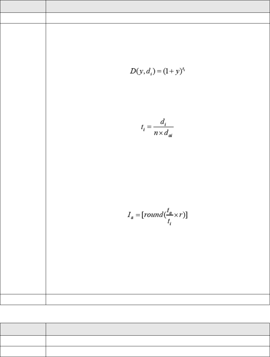
2 Market standards and calculations
2.1 Market standards
58 © Wall Street Systems IPH AB - Confidential
2.1.4.2.28 GOVT-IT-ZC (financial/instrument/isma@price)
Name Italian Government
Description GOVT-IT bonds are regular, fixed-coupon securities with equal, semi-annual coupon
payments, and Actual/Actual date basis.
With GOVT-IT, the coupons for the ith cashflow on date are discounted using the
following formula:
Equation 2-47 Italian government bonds
where
• is the time in years between the value date and the coupon date
Equation 2-48 Italian government bonds: time in years
- is the number of days between the value date and the coupon date d
-n is the number of coupons i.e. 2.
- is the number of days during the coupon period
With GOVT-IT, the accrued interest calculation is rounded to 5 decimals using an
Actual/Actual date basis:
Equation 2-49 Italian government bonds: accrued interest calculation
• is the accrued interest
•r is the nominal interest rate (to be paid at time i) as a percentage of the par value
• is the time in years between the last coupon date (inclusive) and the value date
(exclusive), calculated using the accrual date basis
• is the time in years between the last (inclusive) and next (exclusive) coupon dates,
calculated using the appropriate Actual/Actual date basis.
Usage Italian government bonds.
Field Description
ID GOVT-IT-ZC
Name Italian Government Zero Coupon
Information Description
di
tidi
di
dc
Ia
ta
ti
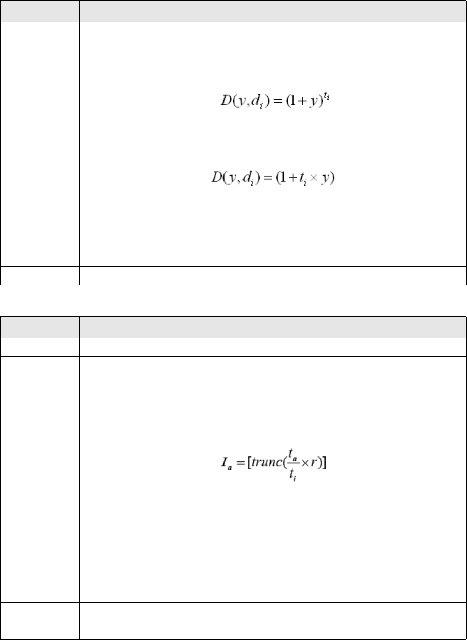
2 Market standards and calculations
2.1 Market standards
Transaction & Risk Management Module (TRM) Instruments: Processing and Calculations 59
2.1.4.2.29 GOVT-JP (financial/instrument/simple-yield@price)
Description This yield convention is used for the Italian Government Bond with Zero Coupon. The date
basis is Actual-/365 and the discount factor is calculated according to the following formula:
•If
Equation 2-50 Italian ZC government bonds: when time in years is more than 1
•If
Equation 2-51 Italian ZC government bonds: when time in years is less than or equal to 1
where
• is the time in years between the value date and the coupon date
• is the time in years from the valuation date to the maturity of the bond.
Usage Italian Government Bond with Zero Coupon
Information Description
ID GOVT-JP
Name Japanese Government
Description GOVT-JP bonds are regular, fixed-coupon securities with equal, annual coupon payments,
and Actual-/365 date basis. These bonds are traded on a clean price basis.
With GOVT-JP, the Accrued Interest calculation is truncated to 7 decimals using Actual/365
date basis:
Equation 2-52 Japanese government bonds
• is the accrued interest
•r is the nominal interest rate (to be paid at time i) as a percentage of the par value
• is the time in years between the last coupon date (inclusive) and the value date
(exclusive), calculated using the accrual date basis
• is the time in years between the last (inclusive) and next (exclusive) coupon dates,
calculated using the appropriate Actual/365 date basis.
Usage Japanese government bonds
Yield Simple Yield
Field Description
tm1>
tm1≤
tidi
tm
Ia
ta
ti
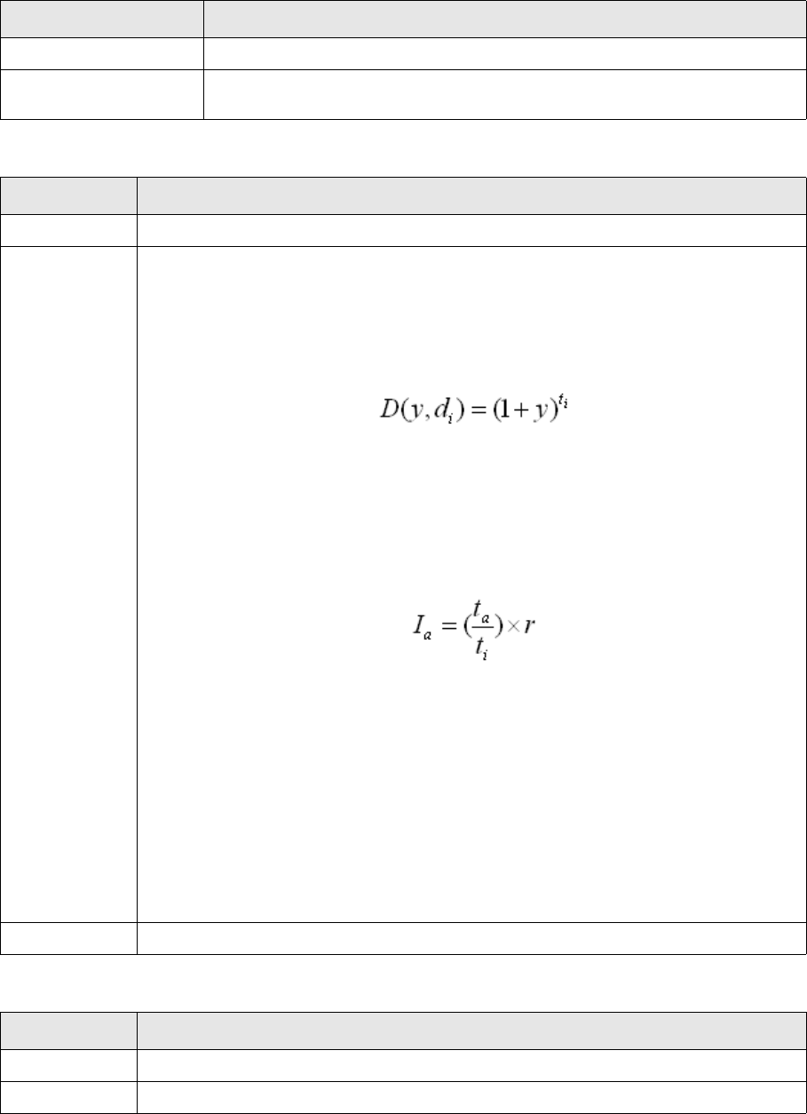
2 Market standards and calculations
2.1 Market standards
60 © Wall Street Systems IPH AB - Confidential
2.1.4.2.30 GOVT-MALAYSIA (financial/instrument/isma@price)
2.1.4.2.31 GOVT-NO (financial/instrument/norwegian@price)
2.1.4.2.32 GOVT-NZ (financial/instrument/isma@price)
Information Description
Name GOVT-MALAYSIA
Usage Used to support Malaysian Government bonds. These bonds have semi-annual
coupon payments with Act/2Act date basis.
Information Description
Name GOVT-NO
Description Norwegian government bonds are regular, fixed-coupon securities with equal, annual
coupon payments and a bullet redemption on an Act/365 date basis. These bonds are
traded on a clean-price basis.
With GOVT-NO, the coupons for the ith cashflow on date are discounted using the
following formula:
Equation 2-53 Norwegian government bonds
where
• is the time in years between the value date and the coupon date calculated using the
date basis Actual/365
With GOVT-NO, the Accrued Interest calculation is calculated using date basis Actual/365:
Equation 2-54 Norwegian government bonds: Accrued Interest
where
• is the accrued interest
• is the nominal interest rate (to be paid at time i) as a percentage of the par value
• is the actual number of calendar days between the previous coupon payment and the
settlement date. The actual number of calendar days include leap years
• is equal to 365 and represents the number of days between the last and next coupon
dates.
Note: 365 is also used for leap years.
Usage Norwegian government bonds
Information Description
ID GOVT-NZ
Name New Zealand Government Bond
di
ti
Ia
r
ta
ti
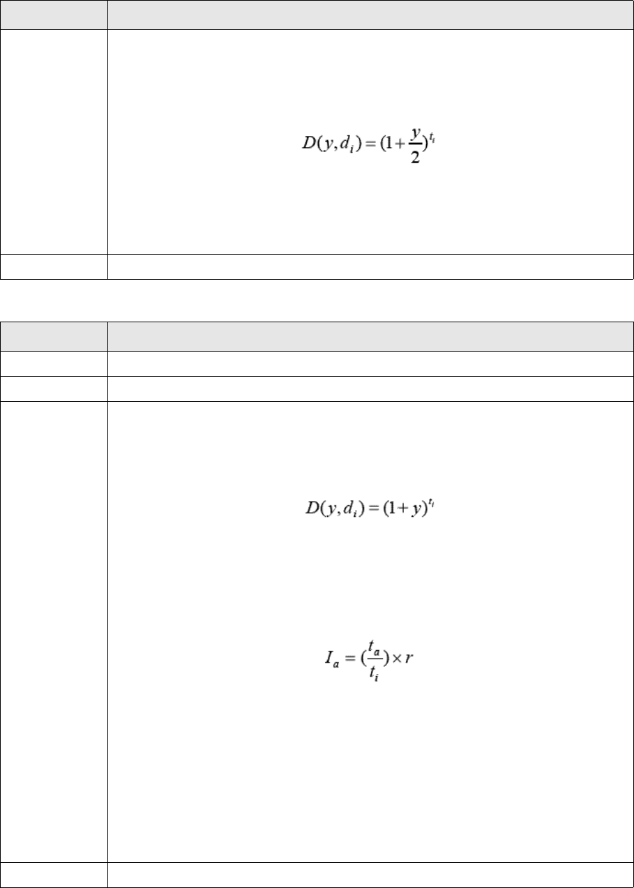
2 Market standards and calculations
2.1 Market standards
Transaction & Risk Management Module (TRM) Instruments: Processing and Calculations 61
2.1.4.2.33 GOVT-SE (financial/instrument/isma@price)
Description GOVT-NZ bonds are regular, fixed-coupon securities with semi-annual coupon payments,
and Actual/Actual date basis. These bonds are traded on a clean price basis.
With GOVT-NZ, the coupons for the ith cashflow on date are discounted using the
following formula:
Equation 2-55 New Zealand government bonds
where
• is the time in years between the value date and the coupon date calculated using
the date basis Actual/Actual.
Usage New Zealand government bonds
Information Description
ID GOVT-SE
Name Swedish Government Bond
Description GOVT-SE bonds are regular, fixed-coupon securities with equal, annual coupon payments,
and 30E/360 date basis (the date basis whereby the 31st of the month is treated as the
30th). These bonds are traded on a clean price basis. With GOVT-SE, the coupons for the
ith cashflow on date are discounted using the following formula:
Equation 2-56 Swedish government bonds
where
• is the time in years between the value date and the coupon date
With GOVT-SE, the accrued interest calculation is calculated using an 30E/360 date basis:
Equation 2-57
where
• is the accrued interest
•r is the nominal interest rate (to be paid at time i) as a percentage of the par value
• is the number of calendar days between the previous coupon payment (inclusive)
and the settlement date (exclusive)
• equals 360. It represents the number of days between the last and next coupon
dates. 360 is also used for leap years.
Usage Swedish government bonds.
Information Description
di
tidi
di
tidi
Ia
ta
ti
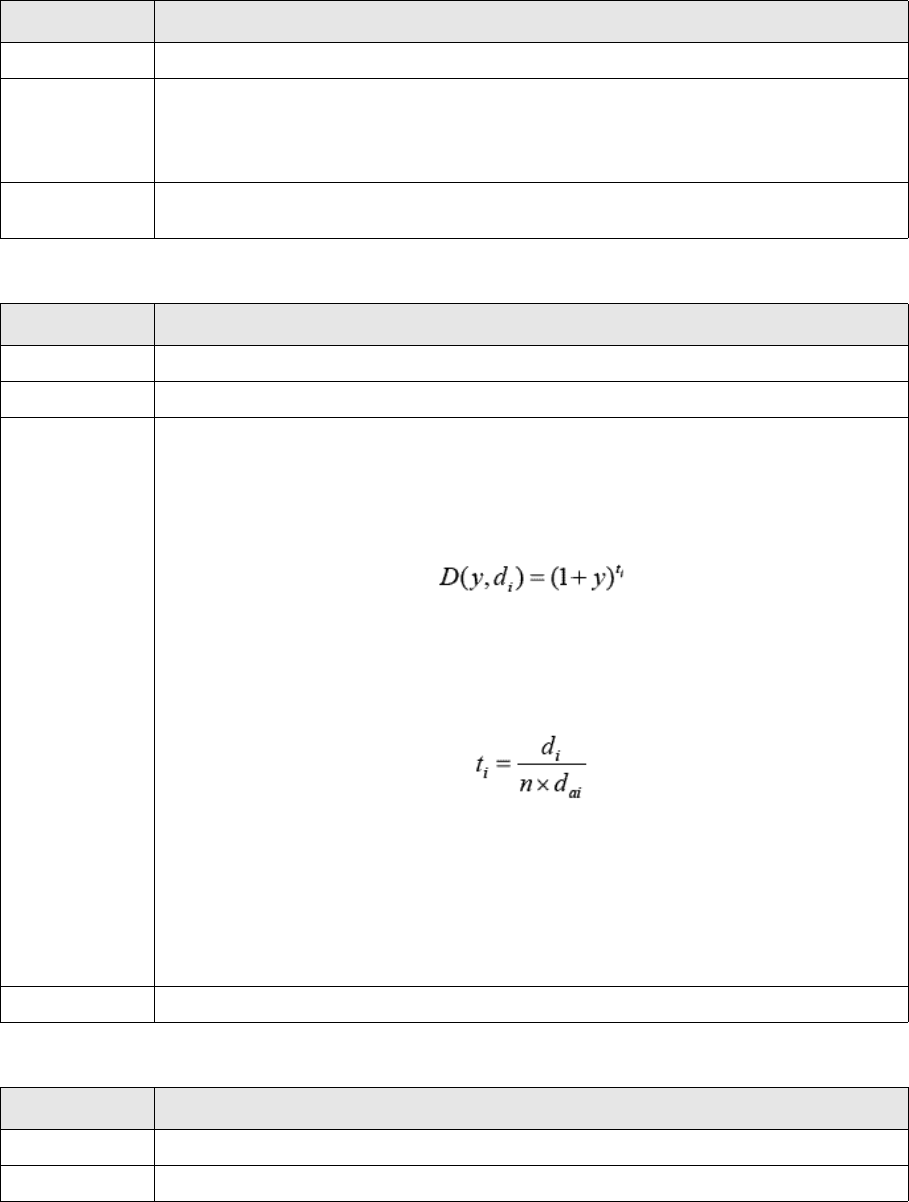
2 Market standards and calculations
2.1 Market standards
62 © Wall Street Systems IPH AB - Confidential
2.1.4.2.34 GOVT-SG (financial/instrument/us-street@price)
2.1.4.2.35 GOVT-UK (financial/instrument/isma@price)
2.1.4.2.36 GOVT-US (financial/instrument/us-street@price)
Field Description
Name GOVT-SG
Description Singaporean Government Bonds are based on the same formula as
U.S.STREET-ACTACT-SEMIANNUAL.
See 2.1.4.2.11 *U.S.STREET-ACTACT-SEMIANNUAL (financial/instrument/us-street@price)
on page 45.
Usage Singaporean government bond convention. This convention uses the accrued interest
method Singaporean (8 decimals), see Singaporean (8 decimals) on page 77.
Information Description
ID GOVT-UK
Name UK Government Bond
Description GOVT-UK bonds are regular, fixed-coupon securities with equal, semi-annual coupon
payments, and Actual/Actual date basis. These bonds are traded on a clean price basis.
With GOVT-UK, the coupons for the ith cashflow on date are discounted using the
following formula:
Equation 2-58
where
• is the time in years between the value date and the coupon date
Equation 2-59
where
- is the number of days between the value date and the coupon date d
-n is the number of coupons i.e. 2.
- is the number of days during the coupon period
Usage UK government bond convention.
Information Description
ID GOVT-US
Name United States Government
di
tidi
di
dc
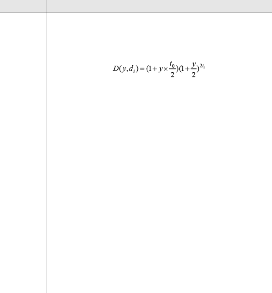
2 Market standards and calculations
2.1 Market standards
Transaction & Risk Management Module (TRM) Instruments: Processing and Calculations 63
Description U.S. Treasury government bonds are regular and irregular fixed-coupon securities with
semi-annual coupon payments and Actual/365 date basis. These bonds are traded on a clean
price basis.
With GOVT-US, a periodic rather than compound rate is used for discounting over the
partial period from the value date to the next coupon date :
Equation 2-60 U.S Treasury government bonds
where
• is the time in years from the value date to the next coupon date (calculated as in the
U.S. Street method)
• is the time in years from the value date to .
U.S. Treasury notes and bonds may have a first coupon of an unequal length. That is, the
length of the first coupon period may be longer or shorter than the normal coupon period.
• If the first coupon period is shorter, the coupon amount is calculated as follows:
Equation 2-61 First coupon period shorter
where
-r is the nominal interest rate
- is the time (in years) between the dated date (the beginning of interest accrual)
and the first coupon date.
• If the first coupon period is longer, the first coupon amount is calculated as follows:
Equation 2-62 First coupon period longer
where
- is time (in years) between the dated date and the date six months before the
first coupon date.
• If the first coupon period is exactly half a year, both equations give the same result.
Usage This is the US government bond convention based on U.S. Street
Information Description
di
t0
tidi
c1rt1
=
t1
c1r2 rt
0
+⁄=
t0
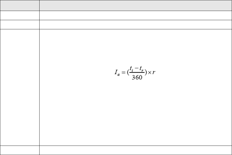
2 Market standards and calculations
2.1 Market standards
64 © Wall Street Systems IPH AB - Confidential
2.1.4.2.37 GOVT-USAGENCY (financial/instrument/isma@price)
Information Description
ID GOVT-USAGENCY
Name United States Government Agency
Description GOVT- USAGENCY bonds are fixed-coupon securities with annual coupon payments, and
30/360 date basis. These bonds are traded on a clean price basis.
With GOVT-USAGENCY, the accrued interest is calculated as follows using a 30/360 date
basis:
Equation 2-63 United States Government Agency
where
• is the accrued interest
•r is the nominal interest rate (to be paid at time i) as a percentage of the par value
• is the length of the coupon period calculated using the accrual date basis of 30/360
(or coupon date basis if the former is missing)
• is the length of the remaining accrual period (i.e. the time between the accrual date
and the end date of the coupon).
Usage US government Agencies bond convention
Ia
ti
tr

2 Market standards and calculations
2.1 Market standards
Transaction & Risk Management Module (TRM) Instruments: Processing and Calculations 65
2.1.4.2.38 GOVT-ZA (financial/instrument/south-african@price)
Information Description
ID GOVT-ZA
Name South African Government bond
Description GOVT-ZA bonds are regular, fixed-coupon securities with semi-annual coupon payments,
and Actual/365 date basis. These bonds are traded on a clean price basis.
With GOVT-ZA, the Accrued Interest calculation is rounded to 5 decimals using an Actual/365
date basis:
Equation 2-64 South African Government bond
where
• is the accrued interest
•r is the nominal interest rate (to be paid at time i) as a percentage of the par value
• is the time in years between the last coupon date (inclusive) and the value date
(exclusive), calculated using the accrual date basis
• is the time in years between the last (inclusive) and next (exclusive) coupon dates,
calculated using the appropriate Actual/365 date basis.
With GOVT-ZA, the coupons for the ith cashflow on date are discounted using the
following formula:
Equation 2-65
where
•k is the compounding frequency of the yield (for example, k=2 for semi-annual yield)
• is time in years from the value date to , the first coupon date. is calculated
using the following formula:
Equation 2-66 Time in years from value date to first coupon date
where
- and are the periods in years between the valuation date and the first
coupon date, and between the previous and the next coupon date, respectively,
calculated using the date basis Act/365
-n is the number of coupon periods between and , the ith coupon date.
The number of coupon periods is calculated using:
where is the time (in years) from the next coupon date to the maturity of the
bond, and round rounds the number to the nearest integer.
Usage South African Government bond convention
Ia
ta
ti
di
t0d0t0
t0
tv0,
tp0,
---------
=
tv0,tp0,
d0di
n round kxti
()=
ti
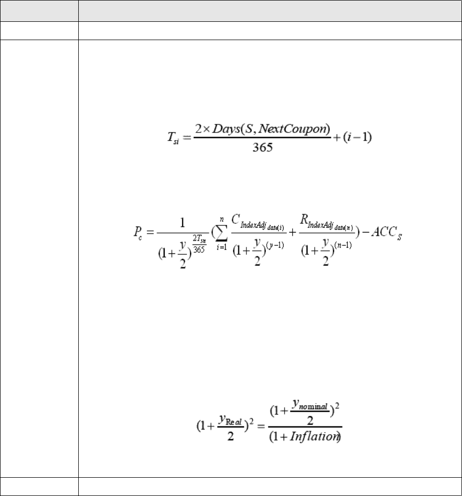
2 Market standards and calculations
2.1 Market standards
66 © Wall Street Systems IPH AB - Confidential
2.1.4.2.39 INDEX-UK (function/index-uk@price)
2.1.5 Discount Margin
Discount margin is the spread that, when added to the discounting zero curve, will equate the
theoretical value of a floating rate note (see 3.1.2 Floating rate note on page 228) to the quoted
price. Discount Margin is calculated at instrument level and shown in Rate Monitor or in Transaction
Manager (Figure Discount Margin). In this calculation, the day count method and yield type specified
in Discount Margin page are used, and the spread is added to the discounting curve defined in this
page.
When discount margin is used in the valuation, it is added to the valuation curve specified for the
instrument, and the day count method and yield type used are taken from the interpolation method
of this valuation curve. For the results to be consistent, the day count method and yield type
specified in Discount Margin page should match these. Also, the instrument's valuation curve should
ID INDEX-UK
Name Index-linked UK Government bond
Description The prevailing market conventions for price/yield calculations in the UK index-linked market
are different from the conventions used for the Swedish and US index-linked markets.
The market practice is to assume that all future semi-annual coupon periods have the same
length as the present accrued period. Therefore, the overall period between settlement
and the ith coupon, in the date basis actual/365, is given by:
Equation 2-67 Index-linked UK Government bond
The market quoted clean price and the semi-annual nominal yield to maturity are
calculated by the following price/yield formula:
Equation 2-68 Price/yield equation
where
• is the index adjusted coupons
• (prolonged RPI index figures) is the redemption.
Given the price, the nominal yield is obtained by numerical methods.
The real yield to maturity is derived from the nominal yield and the assumed inflation
rate using the Fisher equation:
Equation 2-69 Fisher equation
Usage Index-linked UK Government bonds
Tsi
Ynominal
CIndexAdj
RIndexAdj
yReal

2 Market standards and calculations
2.1 Market standards
Transaction & Risk Management Module (TRM) Instruments: Processing and Calculations 67
be used for discount margin calculation. Discount margin valuation is enabled by the feature FRN
Valuation, see A.2.164 FRN Valuation on page 791.
At instrument level, discount margin m is calculated by solving the equation:
Equation 2-70 Discount margin
Where:
– The dirty price (at spot) of the bond, based on the market quote.
– The coupon dates.
– The fixed or estimated coupons.
– The discount factors (from spot) from the discounting curve on dates .
Note: Coupons have to be fixed in Instrument Editor for the fixing to have an effect on the
discount margin calculation.
– and are the rate-to-discount-factor and discount-factor-to-rate conversions
(from spot date) using the day count method and yield type specified in the discount margin
setup.
2.1.6 Calculation methods
2.1.6.1 Accrued interest calculations
The generic formula for accrued interest AI is:
Equation 2-71 Accrued interest (generic formula)
where C is the coupon amount, T is the length of the coupon period (in years, calculated with the
appropriate date basis), and t is the length of the accrual period (in years).
There are many variations of this basic formula.
Note: For bonds, the method used for the accrued interest calculation is specified in the AI Method
field in Instrument Editor’s Bond page. The date basis used for period length calculations is
specified in the Cashflow page (Accrual Date Basis field). If the accrual date basis is not
defined, then the date basis of the cashflow is used. Both these pages are available in the
editor when the Bond feature is present in the instrument definition (see A.2.51 Bond on
page 734).
Some AI methods use neither the accrual nor the cashflow’s date basis. This is because the day
count method is built in the method.
The following table lists the symbols used in the accrued interest calculations:
Pd
di
ci
Dy
idi
AI t
T
--- C×=
Symbol Description
PPrincipal on which the coupon amount and accrued interest are calculated.
CCoupon amount.
rCoupon interest rate (as a decimal number).

2 Market standards and calculations
2.1 Market standards
68 © Wall Street Systems IPH AB - Confidential
2.1.6.1.1 Generic methods
The following sections describe the generic methods for calculating accrued interest in TRM.
Linear
Equation 2-72 Accrued Interest: Linear
Linear 30/360 EOM
The Linear 30/360 EOM method ensures that the calculation of accrued interest follows the same
month-end behavior as accrued interest used in the calculation of accrued profit.
This method is used when defining the Result IR setup for a result treatment (in Result Editor). It
achieves a constant yield when a 30E/360 EOM date basis is selected (in Result Editor’s Accrual Yield
page).
See the TRM User Guide for more information about setting up result treatments.
Linear (Closing)
The Linear (Closing) method ensures that in closing the books, February is considered as having 30
days when 30-day date bases (such as, the 30/360 and 30E/360 date bases) are used.
This means that in accounting, these date bases result in equal interest accrual amount postings in
each month.
Actual/Actual
Equation 2-73 Accrued Interest: Actual/Actual
where D is the interest period length in actual days, and d is the length of the accrual period in
actual days.
This method will ignore any date basis conventions associated with the coupon.
Actual/Actual (Inclusive)
This method accrues interest linearly over the interest period, including the first day and excluding
the last day of the period.
Actual/Actual Annually
In the following methods, Actual/Actual Annually, Actual/Actual Semi-Annually, and Actual/Actual
Quarterly, the basic formula is used, but the period length calculation is more complicated, as
follows:
•The coupon period is divided into 12/N -month segments, starting from the end of the coupon
period.
TCoupon period in years.
tAccrual period in years.
DCoupon period in days.
dAccrual period in days.
Symbol Description
AI t
T
--- C×=
AI d
D
----C×=

2 Market standards and calculations
2.1 Market standards
Transaction & Risk Management Module (TRM) Instruments: Processing and Calculations 69
•The number of months in each segment, 12/N, may be 12, 6, or 3, depending on the method
chosen (respectively, Annually, Semi-Annually, or Quarterly).
•The segments are created by moving the coupon end date back in 12/N -month steps.
•If a date created by such a move does not exist (that is, it falls after the end of month), the
end-of-the-month date is substituted for it.
Let ith such segment span d
i
s
days, and the part of the period within the segment contain d
i
p
days;
then the total period length in years is:
Equation 2-74 Accrued Interest: Actual/Actual Annually - total period length
Note: If the period extends over an entire segment, then d
i
p
= d
i
s
and the contribution to the
total period length of that segment is simply 1/N years.
This calculation is repeated for the coupon period (T) and for the accrual period (t), and finally the
accrued interest is:
Equation 2-75 Accrued Interest: Actual/Actual Annually
These methods will ignore any date basis conventions associated with the coupon.
Actual/Actual Annually (5 decimals)
Non-government Italian bonds are based on annual coupon and Actual/Actual accrual date basis
with a rounding to the fifth decimal. This method can be used for more generic purposes as well as
for non-government Italian bonds.
Accrued Interest is calculated as follows:
Equation 2-76 Actual/Actual Annually (5 decimals): accrued interest
Where
Index ratio:
Equation 2-77 Actual/Actual Annually (5 decimals): index ratio
tdp
i
ds
iN
---------
i
∑
=
AI t
T
--- C×=
AI R7rdD⁄×[]P×=
AI Accrued interest
r Nominal interest rate (to be paid at time i) as a real number.
d Time in years between the last coupon date (inclusive) and the value date
(exclusive), calculated using the accrual date basis.
D Time in years between the last (inclusive) and next (exclusive) coupon dates,
calculated using the appropriate Actual/Actual date basis.
PPrincipal
IndexRatio R5
Index
IssueIndex
-----------------------------
⎝⎠
⎛⎞
=

2 Market standards and calculations
2.1 Market standards
70 © Wall Street Systems IPH AB - Confidential
Index Accrued Interest:
Equation 2-78 Actual/Actual Annually (5 decimals): index accrued interest
Coupon % methods
With the Coupon % methods, the accrued interest is calculated directly from the principal (P) and
the coupon rate (r). It may happen that the accrued interest thus calculated is larger than the actual
coupon amount (for example, if the date basis used in the AI calculation is different from the date
basis used for the calculation of the coupon amount). In this case, accrued interest is capped at the
coupon amount, and the daily accrual towards the end of the coupon period may be zero.
•Coupon %
Equation 2-79 Accrued Interest: Coupon %
•Coupon % Relative Semi-Annually
Equation 2-80 Accrued Interest: Coupon % Relative Semi-Annually
Here T is calculated using the date basis of the cashflow, not the accrual date basis.
•Coupon % Relative Quarterly
Equation 2-81 Accrued interest: Coupon % Relative Quarterly
Here T is calculated using the date basis of the cashflow, not the accrual date basis.
•Coupon % Compound Annually
Equation 2-82 Accrued interest: Coupon % Compound Annually
•Coupon % Compound Semi-Annually
Equation 2-83 Accrued interest: Coupon % Compound Semi-Annually
•Coupon % Compound Quarterly
Equation 2-84 Accrued interest: Coupon % Compound Quarterly
Expression
If the coupon is fixed in arrears, the fixing rate is not known when figure accrued interest is
calculated. As an estimate, the system uses the current market rate for the fixing period.
IndexAI IndexRatio AI×=
AI min r t P C,××[]=
AI min rtP××
2T
------------------- C,=
AI min rtP××
4T
------------------- C,=
AI min 1 r+()
t1C],–[=
AI min 1 r 2⁄+()
2t 1C],–[=
AI min 1 r 4⁄+()
4t 1C],–[=

2 Market standards and calculations
2.1 Market standards
Transaction & Risk Management Module (TRM) Instruments: Processing and Calculations 71
The formula for accrued interest is then:
Equation 2-85 Accrued interest: Coupon % Expression
where:
–t is the time in years between the start of the coupon period and the valuation date
–T is the length in years of the coupon period
–A is the coupon amount calculated using the expression defined for the coupon cashflow.
Dual currency
•Dual-Currency Estimated
The settlement amount is calculated using the forward FX rates.
•Dual-Currency Last
The settlement amount is calculated using the FX rate of the previous FX fixing.
Note: Both methods round the figure value in the cashflow currency before converting it into the
settlement currency.
Range
For range accrual transactions, several specific accrued interest calculation methods exist. They are
all based on the principle that the interest (coupon) rate has to be scaled down by a factor
depending on the number of days the market variable being observed has been within the range.
Once the interest rate has been scaled down, the accrued interest is calculated linearly based on the
time spent until valuation date, the total interest period and the date basis of the cashflow.
The accrued interest methods and the corresponding factors are:
•Range Proportional
Days In Range / Observation Days until valuation date
•Range So Far In
Days In Range / Total Interest Period
•Range So Far Out
(Total Interest Period - Days Out of Range) / Total Interest Period
•Range Fixing
Assumes the variable observed will remain in the same state as on valuation date, i.e. So Far In
if it is out of range and So Far Out otherwise.
Note that the default observation period includes the first date of the interest period and excludes
the last date (i.e payment date) of the interest period.
For example:
Let us consider the interest period from 01/06/2003 until 01/12/2003 with the interest calculation
expression as:
max[0, 4.85 * range(Euribor/6M, 0, 4.00, up-in/down-in, 2, EUR, ACT/365)]
Valuation date is 30/06/2003, i.e. there have been 30 observation days, and 29 days on interest
accrual.
The total interest period is 183 days.
AI A t
T
---
×=

2 Market standards and calculations
2.1 Market standards
72 © Wall Street Systems IPH AB - Confidential
Assume that the 6M Euribor rate was in the range 20 times.
The accrued interest would be (using date basis Act/365):
•Range Proportional method:
4.85% * 20/30 * 29/365 * Nominal Amount
•So-Far-In method:
4.85% * 20/183 * 29/365 * Nominal Amount
•So-Far-Out method:
4.85% * (183 - 10)/183 * 29/365 * Nominal Amount, i.e.
4.85% * 173/183 * 29/365 * Nominal Amount
Yield Accrued Interest
This yield based method is used only for the yield accrual of discount/premium – it is not to be used
for actual accrued interest calculation. It converts the coupon rate to the same basis as with which
yield to maturity is calculated (in a manner that the total coupon remains the same, but the rate of
accrual changes). Yield accrual is then based on the coupon accruing with this rate.
ISDA CDS
The ISDA CDS method is used with credit default swap. This AI method is based on the Linear AI
method except that the last period coupon is one day longer, i.e. it includes both the first and last
dates in the AI calculation.
2.1.6.1.2 Market-specific methods
The following sections describe the market-specific methods for calculating accrued interest in TRM.
Note: With regards to rounding, we use the symbol Rn to indicate the rounding to n decimal
places. In the applications the interest rate r is given as a % (e.g. r = 3.85 is treated as
3.85% = 0.0385). In the calculation, the system uses the real number. This means that an
AI Method (3 decimals) corresponds to a rounding (R5) of the real number to 5 decimals.
Australian (3 decimals)
This is the AI method rounded to 3 decimals using the Actual/Actual date basis:
Equation 2-86 Accrued interest: Australian (3 decimals)
where d is the length of the accrual period in actual days and D is the interest period length in actual
days.
Australian Floater (3 decimals)
This is the method used for australian domestic floating rate note, rounded to 3 decimals using
instrument date basis.
Equation 2-87 Accrued interest: Australian Floater (3 decimals)
where
–r is the fixing rate of the current coupon
–P is the Principal
AI R5r2⁄()dD⁄×[]P×=
AI R5rt×[]P×=

2 Market standards and calculations
2.1 Market standards
Transaction & Risk Management Module (TRM) Instruments: Processing and Calculations 73
–t is the length of the accrual period in years, calculated using the coupon date basis.
Moreover, during the ex coupon period, accrued interest is based directly on the number of
remaining days to the next coupon using the following equation:
Equation 2-88 Accrued interest: Australian Floater (3 decimals): ex coupon period
Where
–P is the principal
–t is the length of the remaining period (to the next coupon) in years, calculated using the
coupon date basis.
Australian Index Linked
These are the Australian Index Linked (IAB) or Australian Index Linked (CIB) AI methods used for Australian
index-linked bonds or Australian capital indexed bonds respectively.
Note: For three decimal places rounding, use AI method Australian Index Linked (IAB) (3 dec).
Belgian
The following calculation applies for all coupon lengths (except short coupons); see Equation 2-74
on page 69 for more details:
For short coupons, the calculation is the following; see Equation 2-79 on page 70 for more details:
Canadian
The Actual/365 (Canadian Bond) date basis considers a year to have 365 days, whereas the length
of a coupon period is represented by 365 divided by the number of coupon periods in a year. For the
most common Canadian domestic bond structures, which pay a semi-annual coupon, this implies
the length of a coupon period is 365/2 = 182.5 days.
Where f is the annual payment frequency (or number of coupon periods per year), the Actual/365
Canadian Bond measures the fraction of a coupon period represented by a given number of days as
follows:
•If the number of days of interest accrual is less than the actual number of days in the coupon
period:
Equation 2-89 Accrued Interest: Canadian
AI R5rt×[]P×=
pc
frac{} df×
365
-----------
=

2 Market standards and calculations
2.1 Market standards
74 © Wall Street Systems IPH AB - Confidential
Which, for semi-annual pay bonds where f = 2 , reduces to:
Equation 2-90 Accrued Interest: Canadian semi annual pay bonds
Then
Equation 2-91 Canadian AI calculation
•If the number of days of interest accrual exceeds 365/f, or 182.5 days for a semi-annual pay
bond:
Equation 2-92 Accrued Interest: Canadian when interest accrual exceeds 365/f or 182.5 days
Where
– is the actual number of days from the valuation date to the next coupon date.
Then
Equation 2-93 Canadian AI calculation when interest accrual exceeds 365/f or 182.5 days
French (3 decimals)
Equation 2-94 Accrued interest: French (3 decimals)
where t is the length of the accrual period in years, calculated using the accrual date basis, operator
R5 signifies the rounding, and Tc and t are the length of the coupon period calculated using the
coupon date basis and the accrual date basis, respectively.
French (4 decimals)
This method is the same as French (3 decimals) except that the rounding operator = R6.
French (7 decimals)
This method is the same as French (3 decimals) except that the rounding operator = R9.
Greek (3 decimals)
Greek index-linked bonds are based on the annual coupon and Actual/Actual Accrual date basis with a
rounding to the third decimal. This method is used for Greek index-linked bonds.
Accrued Interest is calculated as follows:
Equation 2-95 Accrued interest: Greeks (3 decimals)
pc
frac{} d
182.5
-------------
=
AI Acpc
frac{}
×=
pc
frac{} 1dff×
365
-------------
–=
df
AI Acpc
frac{}
×=
AI max R51rt+[]1–()PC],×[=
AI R5rdD⁄×[]P×=
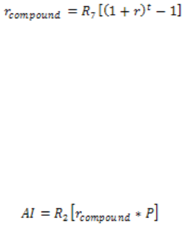
2 Market standards and calculations
2.1 Market standards
Transaction & Risk Management Module (TRM) Instruments: Processing and Calculations 75
Where
Index ratio:
Equation 2-96 Accrued interest: Greeks (3 decimals) - index ratio
Index Accrued Interest:
Equation 2-97 Accrued interest: Greeks (3 decimals) - index accrued interest
Hungarian (4 decimals)
This is the AI method rounded to 4 decimals using the Actual/Actual accrual date basis:
Equation 2-98 Accrued interest: Hungarian (4 decimals)
where t is the length of the accrual period in years, calculated using the accrual date basis, the
operator R6 signifies the rounding, and Tc and t are the length of the coupon period calculated using
the coupon date basis and the accrual date basis, respectively.
Israeli (Annual Compound, 5 decimals)
•Bond
Bond coupon rate r (in %) is converted to the annual compound rate as follows:
Equation 2-99 Accrued Interest: Israeli (Annual Compound, 5 decimals) Bond
Where:
t = Time in years between the last (inclusive) and next (exclusive) coupon dates, calculated
using the appropriate Actual/365 date basis.
r = nominal interest rate
Then, the AI is computed as follows:
Equation 2-100 Israeli (Annual Compound, 5 decimals) Bond - AI calculation
Where P is the principal.
AI Accrued interest
r Nominal interest rate (to be paid at time i) as a real number.
d Time in years between the last coupon date (inclusive) and the value date
(exclusive), calculated using the accrual date basis.
D Time in years between the last (inclusive) and next (exclusive) coupon dates,
calculated using the appropriate Actual/Actual date basis.
PPrincipal
IndexRatio R3
Index
IssueIndex
-----------------------------
⎝⎠
⎛⎞
=
IndexAI IndexRatio AI×=
AI max R61rt+[]1–()PC],×[=
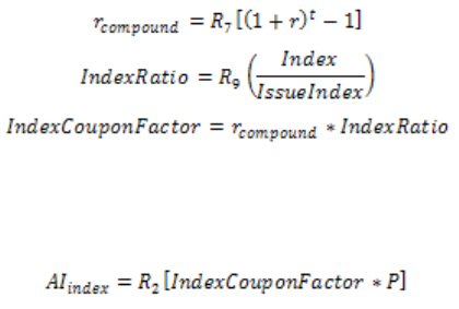
2 Market standards and calculations
2.1 Market standards
76 © Wall Street Systems IPH AB - Confidential
•Index Linked Bond
Coupon rate r (in %) is converted to the annual compound rate as follows:
Equation 2-101 Israeli (Annual Compound, 5 decimals) Index Linked Bond
Then, the Index AI is computed as follows:
Equation 2-102 Israeli (Annual Compound, 5 decimals) Index Linked Bond - AI calculation
Where P is the principal.
Israeli (Linear, 5 decimals)
This is the AI method rounded to 5 decimals using the Actual/365 date basis:
Equation 2-103 Accrued Interest: Israeli (Linear, 5 decimals)
where
The index (inflation-adjusted) Accrued Interest is rounded to 5 decimals using Actual/365 date
basis:
•Index Ratio
Equation 2-104 Accrued Interest: Israeli (Linear, 5 decimals) - index ratio
•Index Accrued Interest %
Equation 2-105 Accrued Interest: Israeli (Linear, 5 decimals) - index accrued interest %
AI R7rdD⁄×[]P×=
AI Accrued interest
r Nominal interest rate (to be paid at time i) as a real number.
d Time in years between the last coupon date (inclusive) and the value date
(exclusive) calculated using the accrual date basis.
D Time in years between the last (inclusive) and next (exclusive) coupon dates,
calculated using the appropriate Actual/365 date basis.
PPrincipal
IndexRatio R9
Index
IssueIndex
-----------------------------
⎝⎠
⎛⎞
=
IndexAI IndexRatio AI×=
2 Market standards and calculations
2.1 Market standards
Transaction & Risk Management Module (TRM) Instruments: Processing and Calculations 77
Italian (5 decimals)
This is the Actual/Actual AI method rounded to 5 decimals:
Equation 2-106 Accrued interest: Italian (5 decimals)
where d is the length of the accrual period in actual days and D is the interest period length in actual
days.
Japanese Yield (7 decimals)
This is the Coupon % AI method ( Coupon % methods on page 70) truncated to 7 decimals:
Equation 2-107 Accrued Interest: Japanese Yield
where t is the length of the accrual period in years.
Norwegian
The Norwegian accrued interest method is calculated during ex-coupon and based directly on the
number of remaining days next to the coupon using the following equation:
Equation 2-108 Accrued Interest: Norwegian
Where
Singaporean (8 decimals)
This is the Actual/Actual AI method rounded to 8 decimals:
Equation 2-109 Accrued interest: Singaporean (8 decimals)
where
–d is the time in years between the last coupon date (inclusive) and the value date
(exclusive), calculated using the accrual date basis.
–D is the time in years between the last (inclusive) and next (exclusive) coupon dates,
calculated using the appropriate Actual/Actual date basis.
South African (5 decimals)
This is the Coupon % AI method truncated to 5 decimals:
Equation 2-110 Accrued interest: South African (5 decimals)
CThe coupon interest percent per annum.
The actual number of calendar days from the settlement date (transaction value
date) to the next coupon payment date divided by 365.
AI R7r2⁄()dD⁄×[]P×=
AI min R91r
t
+()PP–×()C,[]=
AI C t
365
---------
×=
t
365
---------
AI R10 r2⁄()dD⁄×[]P×=
AI min R71r
t
+()1–()PC,[]=
2 Market standards and calculations
2.1 Market standards
78 © Wall Street Systems IPH AB - Confidential
where t is the length of the accrual period in years.
US Agency
Equation 2-111 Accrued interest: US Agency
where T is the length of the coupon period calculated using the accrual date basis (or coupon’s date
basis if the former is missing), and tr is the length of the remaining accrual period (that is, the time
between the accrual date and the end date of the coupon).
2.1.6.2 Annuity calculations
Annuity calculations are based on all interest cashflows having Kind = Annuity Component and a
matching value date, with the amortization cashflows also having Kind = Annuity Component.
This allows cashflows from several interest schedules to be included in the calculation.
Grace periods can be handled by setting up a forward starting amortization schedule: the coupon
dates before will not match the amortization dates and will therefore behave outside any annuity
calculation. The later ones will be part of the annuity calculation.
In practical terms, this means one of the following:
•Instrument setup can start from a normal fixed rate loan and be defined so that interest and
amortization share the value dates, or create a reference interest schedule from the
amortization schedule
•Select the calculation methods (either Annuity or Fixed Annuity), on both schedules (P stands for
Principal, Ri for the repayment as i-th value date, Ci for the coupon amount, n the number of
dates).
See the following sections for more information.
2.1.6.2.1 General annuity calculation
This works for any date basis, irregular dates, varying interest rate, and so on, when Interest and
Amortization Calculation Method = Annuity.
Ri + Ci = Ri-1 + Ci-1 whenever i and sum(Ri) = -P
Ci is calculated as usual from the outstanding nominal (that is, P+sum(Ri) where i from 1 to i-1)
Ri and Ci are rounded according to the Leg Amount Precision
Rn is adjusted so that Rn = P + sum(rounded(Ri)) where i from 1 to n-1
–If the 1st coupon period is short, then you get a "big" amortization and a small coupon
amount
–Rounded(Ri) + rounded(Ci) are not always equal because of the rounding effect (couple of
rounding units difference maximum)
Note that the cashflow part of the calculation is given the attribute Kind = Annuity Component.
For an irregular annuity, if a rate is specified in the principal schedule, the annuity is computed
equally across all flows, except for the last one. The last payment is adjusted according to the
outstanding principal amount (100 - r).
2.1.6.2.2 Fixed annuity calculation
This works only when the same discount factor is used for all periods, that is, the same interest rate
and date bases, so all periods are worth the same (for example, 30/360 for semi-annual or
quarterly, Actual/Actual for yearly, and so on), when Interest and Amortization Calculation Method =
Fixed Annuity.
AI r T tr
–()×P×=
2 Market standards and calculations
2.1 Market standards
Transaction & Risk Management Module (TRM) Instruments: Processing and Calculations 79
The calculation always uses the last interest period to calculate the annuity amount. It calculates the
repayment amount from a direct formula that assumes that you have the same discount factor for
all periods. The calculation will not work if there are different periods or uneven date bases.
The simplified formula is:
Ri = P * (D-1) * D^(i-1) / (1 – D^n)
D being the discount factor for 1 period, that is (1+rate*180/360), for a semi-annual 30/360
interest.
Therefore, the annuity amount is calculated from:
Cn+Rn = Rn*(D-1) + Rn = Rn * D = P * (D-1) * D^(n-1) / (1 – D^n) * D = P * (D-1) * D^n /
(1 – D^n)
This accumulated annuity is used as the reference annuity amount for all value dates in the rest of
the calculation.
Once amortizations are calculated (using the direct formula), for each date, the remaining amount
from the reference annuity is distributed between interest flows that have Kind = Fixed Annuity, in
relation to their Amount % value (in the case where there are many interest amounts for the same
date).
To handle the short 1st coupon, the attribute 1st Coupon Excluded must be set on the interest
schedule: this removes the Fixed Annuity kind so that the interest amount is calculated as usual,
based on the principal.
Note that the cashflows part of the calculation is given the Fixed Annuity kind as well as the Annuity
Component kind.
2.1.6.2.3 Annuity calculation with rounded repayment factors
This works when Interest Calculation Method = Annuity, and Amortization Calculation Method = Fixed
Annuity.
The calculation precision is set to the number of decimals for the repayment/principal ratio %.
The amortization calculation is similar to the fixed annuity calculation, except that the Ri/P
calculation is rounded to the specified precision.
The interest amounts have to be calculated from the outstanding nominal (requires the Annuity
calculation method) and the sum of repayment and interest varies significantly because of the
repayment ratio% rounding effect.
The same attribute is used to handle the short 1st coupon.
2.1.6.3 FX rate calculation
The following three methods are available for the calculation of valuation date's FX rate (Sv) from FX
Spot rate (S):
•Spot Rate: This method uses the FX Spot Rate to convert the cashflow currency to the valuation
currency, i.e. the rate is unchanged from the default method.
Equation 2-112 FX method: Spot Rate calculation
•Today's Rate (Forward Points): This method modifies the FX Spot rate with forward points
between the valuation date and the spot date.
Equation 2-113 FX method: Today’s Rate (Forward Points) calculation
SvS=
SvS p 0.0001×–=
2 Market standards and calculations
2.1 Market standards
80 © Wall Street Systems IPH AB - Confidential
where p is the forward points. Typically there are O/N and T/N quotes between the valuation
date and the spot date, in which case:
Equation 2-114 FX method: Today’s Rate (Forward Points) calculation
where the superscripts a and b refer to Ask and Bid quotes respectively, and subscripts 1 and 2
refer to O/N and T/N.
•Today's Rate (IR Differential): This method modifies the FX Spot rate with the ratio of the
two currencies' discount factors.
Equation 2-115 Today's Rate (IR Differential) calculation
where
–Dv is the valuation currency discount factor between the valuation date and the spot date
–Dc is the cashflow currency discount factor between the valuation date and the spot date.
2.1.6.3.1 Example of FX rate calculation
The following example shows the calculations using the following market date (Rate Monitor):
•FX Rate
•Discount Factors
•Forward Points
Equation 2-116 Example - FX method: Today’s Rate (Forward Points) calculation
Spot S = 1.5
O/N points • Bid • Ask
T/N points • Bid • Ask
O/N T/N
Cashflow Currency ••
Valuation Currency ••
pp
1
ap1
b
+()2p
2
ap2
b
+()+⁄2⁄=
SvSDvDc
⁄=
p1
b0.02=p
1
a0.06=
p2
b0.03–=p
2
a0.01–=
D1
c0.999992955609=D
2
c0.999985555764=
D1
v0.999964445709=D
2
v0.999948197128=
pp
1
ap1
b
+()2p
2
ap2
b
+()+⁄2⁄0.02==
SvS p 0.0001×– 1.499998==

2 Market standards and calculations
2.2 Yield curves
Transaction & Risk Management Module (TRM) Instruments: Processing and Calculations 81
•IR Differential
Equation 2-117 Example - FX method: Today's Rate (IR Differential) calculation
2.2 Yield curves
TRM boot straps zero coupon yield curves in order to carry out valuations that are based on
discounting future cashflows and/or estimating the amounts of unfixed future cashflows. Three
types of bootstrapped zero coupon yield curves exist in TRM:
•Yield Curves, i.e. zero coupon yield curves calculated from IR quotes (e.g. deposit, swap and
FRA quotes) MM futures and/or bonds. These curves are generally used for discounting (and
estimating) any arbitrary set of cashflow.
•Tenor Basis Swap Curve, i.e. zero coupon yield curves calculated from tenor basis swap quotes
and a base yield curve. These curves are used as estimation curves in tenor basis swap valuation
(of the leg for which the spread is quoted) in order to capture the affect of the tenor basis spread
quotes.
•Cross Currency Basis Swap Curve, i.e. zero coupon yield curves calculated from cross currency
basis swap quotes and a base yield curve. These curves are used as valuation curves in cross
currency basis swap valuation (of the leg for which the spread is quoted) in order to capture the
affect of the cross currency basis spread quotes.
The bootstrapping logic for all these yield curves is explained below.
Note: See the TRM User Guide for general information about setting up yield curves.
2.2.1 Yield curve
A yield curve is a curve that gives the prices of discount bonds maturing in the future as a function
of time. Since any cashflow maturing in the future can be regarded as a discount bond, a yield curve
can be used to value any instrument that can be represented as a collection of cashflows.
In principle, it is also possible to price linear derivatives which have a price that only depends on
forward interest rates (for example, short futures, ignoring convexity adjustment) using forward
rates derived from the zero curve. In practice, however, this should be treated with caution since
the derived forward rate will depend on the method used in the construction of the zero curve much
more than the spot rates depend on it.
The information on interest rates that can be observed in the market comes in various forms. There
are deposit rates that give the discount bond prices directly, but these are mainly available only for
DcD1
cD2
c0.999977500389355==
DvD1
vD2
v0.999912644678814==
SvSDvDc
⁄1.49990271424530==
2 Market standards and calculations
2.2 Yield curves
82 © Wall Street Systems IPH AB - Confidential
maturities shorter than one year. Longer interest rates are embedded in the swap rates, FRA and
short future rates, and bond prices.
The objective of yield curve construction is to recover the discount bond price information from the
market information. The guiding principle is that when the quoted instruments are priced against
the zero coupon curve, the original quotes should be reproduced. Since this requirement does not
uniquely define the zero curve, some additional conditions on the functional form and the
smoothness of the curve have to be imposed.
Discount factors are the fundamental elements on which most valuation calculations are based. If
valuation needs for example an interest rate over a period in order to calculate the market value of
a caplet, it is the discount factors for the start and end dates of that period that are given as input to
valuation, and the desired interest rate is derived from these.
2.2.1.1 Input
The starting point of a bootstrap curve is a given set of interest rate related market information.
This information may consist of deposit prices, bond prices, or swap prices, for example.
In general, any instrument for which a liquid quote exists, and the theoretical price can be
calculated using only zero-coupon information, can be used.
Normally, it is assumed that all the instruments have the same risk offset. That is, the bootstrap
calculation produces a zero curve that is the sum of the risk-free rate and the spread.
Each price quote creates a set of cashflows, which are used as input for the bootstrap algorithm (see
2.2.1.3 Bootstrap algorithm on page 83).
2.2.1.1.1 Deposit quotes
A deposit quote generates a negative unit cashflow at spot, and a positive unit plus interest cashflow
at the maturity of the deposit. The interest amount corresponds to the interest type defined for the
deposit quote. The maturity date of the deposit follows the definition of the tenor of the deposit.
2.2.1.1.2 Swap quotes
A swap quote creates a negative unit cashflow at spot, and a positive unit cashflow at the maturity
of the swap. In addition, the fixed coupons (yearly, semi-annual, and so on) of the swap are
created, and their amounts calculated using the date basis and interest type of the quote.
2.2.1.1.3 FRA quotes
Each FRA creates a node point at its maturity. The bootstrap curve will have the property that the
discount factor over the FRA period is equal to the discount factor implied by the FRA quote.
The market quote of an FRA provides an estimate of the interest rate between two dates in the
future: the value date and the maturity date of the FRA. This can be converted into the forward price
on the value date of a zero-coupon bond on the maturity date of the FRA.
Given the market quote of the FRA (r) and the length of the FRA period (t) (calculated using the
appropriate date basis), the price on the value date (dv) of a discount bond that matures on the
maturity date (dm) of the FRA is given by:
Equation 2-118 FRA quotes
2.2.1.1.4 Money market future quotes
Each MM future creates a node point at its maturity. The bootstrap curve will have the property that
the discount factor over the future period is equal to the discount factor implied by the future quote.
The market quote of the price of the future provides an estimate of the forward interest rate over
the period of the future. This can be converted into a discount factor between the start and the end
of the future period.
Pd
vdm
,()
1
1rt+
-------------
=
2 Market standards and calculations
2.2 Yield curves
Transaction & Risk Management Module (TRM) Instruments: Processing and Calculations 83
Given the MM future quote (F), the corresponding interest rate over the period of the future is r
=100 - F, from which the discount price over the period can be calculated, either using the equation
for FRA quotes, or if the quote is of the discount type using:
Equation 2-119 Money market figure quotes
2.2.1.2 Bootstrap date basis and interest type
If a cashflow of a bootstrapping instrument (swap, bond, FRA, or MM future) does not fall on a node
point of the bootstrap curve, interpolation is needed to find the discount factor for the date in
question.
Note: The base date for interpolation is the spot date corresponding to the figure date of the
calculation.
2.2.1.3 Bootstrap algorithm
The bootstrap curve has the following properties:
•The (zero coupon) market prices derived from the bootstrap curve will be equal to the given
market prices.
•The bootstrap curve follows a given functional format and satisfies a smoothness condition
(bootstrap curve is continuous).
Within each interval, the chosen bootstrap rate is given by:
Equation 2-120 Bootstrap algorithm
where:
–ai and bi are parameters calculated by the bootstrap process, and ti is the starting point of
the interval in question.
–The default interest type is Continuous Yield.
2.2.1.3.1 Node points
The maturities of the input instruments are always used as node points.
2.2.1.4 Example: Bootstrapping zero-coupon curve
In this example, the zero-coupon curve is based on deposit quotes for the short end (for maturity
periods of up to one year) and swap quotes for the long end (for maturity periods of two years and
longer).
Note: The number of periods in the curves has been kept to a minimum in order to simplify the
illustration of the method. In reality, the curves would have many more periods defined.
•Depo Quotes
For the deposit quotes, the following periods have been defined:
Pd
vdm
,()1rt–=
yt() aibitt
i
–()+=
Tenor Date Basis Interest Type Interest Structure
O/N Actual/360 Periodic Rate At Maturity
T/N Actual/360 Periodic Rate At Maturity
6M Actual/360 Periodic Rate At Maturity
1Y Actual/360 Periodic Rate At Maturity

2 Market standards and calculations
2.2 Yield curves
84 © Wall Street Systems IPH AB - Confidential
•Swap Quotes
For the swap quotes, the following periods have been defined:
•Parameters
Interpolation method is Linear (with flat rate extrapolation), based on Continuous Yield, date
basis 30/360.
The deposit and swap quotes are as follows:
The yield curve uses the average of the bid and ask quotes as input. The deposit quotes are
already zero-coupon quotes, thus the resulting yield curve is simply the average of the deposit
bid and ask quotes:
The remaining rates for the yield curve, for the 2Y and 3Y periods, have to be solved from the
existing rates using bootstrapping.
2.2.1.4.1 Finding the 2-year rate
The object of the zero-coupon curve calculation is to derive a set of rates that, when used to price
the fixed leg of the swap specified in the underlying swap curve, will price all the fixed-leg payments
at par on the spot date.
Period Date Basis Interest Type Interest Structure
2Y 30/360 Periodic Rate Annual
3Y 30/360 Periodic Rate Annual
Period Deposit Swap
Bid Ask Bid Ask
O/N 4.8 4.88
T/N 4.78 4.84
6M 5.1 5.1
1Y 5.161 5.161
2Y 5.257 5.257
3Y 5.32 5.32
Period Deposit Swap Yield Curve
BidAskBidAskAverage
O/N 4.8 4.88 4.84
T/N 4.78 4.84 4.81
6M 5.1 5.1 5.1
1Y 5.161 5.161 5.161
2Y 5.257 5.257
3Y 5.32 5.32

2 Market standards and calculations
2.2 Yield curves
Transaction & Risk Management Module (TRM) Instruments: Processing and Calculations 85
To calculate the market value at spot MVspot of the fixed leg of a 2-year swap, the following
equation is used:
Equation 2-121 2-year swap: market value at spot MVspot
where:
–A = nominal amount
–r2s = 2-year swap rate
–cp1 = period from the spot date to the first coupon date
–cp2 = period from the first coupon date to the second coupon date
–D1Y = discount factor for the period between the spot date and the 1 year date
–D2Y = discount factor for the period between the spot date and the 2 year date.
If the swap is priced at par, then the market value at par is equal to the nominal amount:
Equation 2-122 Swap priced at par
therefore:
Since the 1 year zero-coupon rate is already known (it is taken directly from the underlying deposit
quotes), the 1 year discount factor can be calculated.
This equation can be rearranged to solve as follows:
Equation 2-123
The coupon periods cp1 and cp2 are calculated from the spot date and the swap coupon dates using
the date basis of the swap quote (30/360).
The date counts for the swap coupons are as follows:
Since the 30/360 date basis is used for the interpolation, the period lengths are:
= 362 / 360
= (721 - 362) / 360 = 359 / 360
The 2-year swap rate (from the swap quotes) = 5.257%.
MVspot
Ar
2s cp1
××
D1Y
--------------------------------A1r
2s cp2)×+(×
D2Y
-----------------------------------------------
+=
AAr
2s cp1
××
D1Y
--------------------------------A1r
2s)cp2
×+(×
D2Y
-----------------------------------------------
+=
1r2s cp1
×
D1Y
--------------------- 1r
2s cp2)×+(
D2Y
------------------------------------
+=
D2Y
D2Y
1r
2s cp2)×+(
1r
2s cp1D1Y
⁄×))(–(
--------------------------------------------------------
=
Period Date Days from spot (30/360
date basis)
Days from spot
(Actual/360 date basis)
Spot 24-11-2000 0 0
1Y coupon 26-11-2001 362 367
2Y coupon 25-11-2002 721 731
cp1
cp2
r2s

2 Market standards and calculations
2.2 Yield curves
86 © Wall Street Systems IPH AB - Confidential
The discount factor for the 1 year rate, D1Y, can be calculated from the 1 year rate (5.161%), using
the date basis (Actual/360) and interest type (Periodic Rate) defined for that tenor:
The discount factor D2Y then becomes:
From this the 2-year zero-coupon rate r2Y can be calculated, using the date basis (30/360) and
interest type (Compound Yield) defined for that tenor:
therefore:
2.2.1.4.2 Finding the 3-year rate
The zero-coupon curve must also price the 3-year swap at par, and so the 3 year discount factor D3Y
for the period from the spot date to the 3-year date must satisfy the following condition:
where:
–r3s = the 3-year swap rate
–cp1 = the period from the spot date to the first coupon date
–cp2 = the period from the first coupon date to the second coupon date
–cp3 = the period from the second coupon date to the third coupon date
–D1Y = the discount factor for the period between the spot date and the 1 year date:
–D2Y = the discount factor for the period between the spot date and the 2 year date:
This equation can be rearranged to solve D3Y as follows:
The coupon periods cp1, cp2, and cp3 are calculated from the spot date and the swap coupon dates
using the date basis defined for the bootstrapping (30/360).
The following date counts for the swap instrument coupons are as follows:
Since the 30/360 date basis is used for the interpolation, the period lengths are:
cp1 = 362 / 360
Period Date Days from spot
(30/360 date basis)
Days from spot
(Actual/360 date basis)
Spot 24-11-2000 0 0
1Y coupon 26-11-2001 362 367
2Y coupon 25-11-2002 721 731
3Y coupon 24-11-2003 1080 1095
D1Y 15.161
100
------------- 367
360
---------
×⎠
⎞1.05261353=+
⎝
⎛
=
D2Y
1 0.05257 359 360 )⁄×+(
10.05257 362 360⁄×
1.0526135
----------------------------------------------- ⎠
⎞⎠
⎞
⎝
⎛
–
⎝
⎛
--------------------------------------------------------------------- 1.1080711==
1r
2Y )721 360 )⁄( D2Y
=+(
r2y 1.1080711 360 721 )⁄( 1 0.05257465=–=
1r3s cp1
×
D1Y
--------------------- r3s cp2
×
D2Y
--------------------- 1r
3s cp3)×+(
D3Y
------------------------------------
++=
D3Y
1r
3s cp3
×)+(
1r
3s cp1D1Y )r3s cp2
×D2Y
⁄)(–⁄×)(–(
--------------------------------------------------------------------------------------------------------
=

2 Market standards and calculations
2.2 Yield curves
Transaction & Risk Management Module (TRM) Instruments: Processing and Calculations 87
cp2 = (721 - 362) / 360 = 359 / 360
cp3 = (1080 -721) / 360 = 359 / 360
The 3-year swap rate (from the swap quotes) r3s = 5.32%.
The discount factors for the 1 year and 2 year rates (D1Y and D2Y) have already been calculated:
D1Y = 1.0526135
D2Y = 1.1080711
So the discount factor D3Y becomes:
From this the 3-year zero-coupon rate r3Y, can be calculated using the date basis 30/360 and the
interest type Continuous Yield defined for that tenor:
therefore:
The complete zero-coupon curve is shown in the table below:
2.2.1.4.3 Finding the 3-year rate
The zero-coupon yield curve must also price the 3-year swap at par, and so the 3 year discount
factor D3Y for the period from the spot date to the 3-year date must satisfy the following condition:
where:
–r3s = the 3-year swap rate
–cp1 = the period from the spot date to the first coupon date
–cp2 = the period from the first coupon date to the second coupon date
–cp3 = the period from the second coupon date to the third coupon date
–D1Y = the discount factor for the period between the spot date and the 1 year date:
–D2Y = the discount factor for the period between the spot date and the 2 year date:
Period Deposit Swap Yield Curve
Bid Ask Bid Ask Average
O/N 4.8 4.88 4.84
T/N 4.78 4.84 4.81
6M 5.1 5.1 5.1
1Y 5.161 5.161 5.161
2Y 5.257 5.257 5.257465
3Y 5.32 5.32 5.323865
D3Y
1 0.0532 359 360 )⁄×+(
10.0532 362 360⁄×
1.0526135
-------------------------------------------- ⎠
⎞0.0532 359 360⁄×
1.1080711
-------------------------------------------- ⎠
⎞⎠
⎞
⎝
⎛
–
⎝
⎛
–
⎝
⎛
----------------------------------------------------------------------------------------------------------------------------1.1683699==
1r
3Y)1080 360 )⁄( D3Y
=+(
r3Y 1.1683699 360 1080 )⁄( 1 0.05323865=–=
1r3s cp1
×
D1Y
--------------------- r3s cp2
×
D2Y
--------------------- 1r
3s cp3)×+(
D3Y
------------------------------------
++=

2 Market standards and calculations
2.2 Yield curves
88 © Wall Street Systems IPH AB - Confidential
This equation can be rearranged to solve D3Y as follows:
The coupon periods cp1, cp2, and cp3 are calculated from the spot date and the swap coupon dates
using the date basis defined for the bootstrapping (30/360).
The following date counts for the swap instrument coupons are as follows:
Since the 30/360 date basis is used for the bootstrapping, the period lengths are:
cp1 = 362 / 360
cp2 = (721 - 362) / 360 = 359 / 360
cp3 = (1080 -721) / 360 = 359 / 360
The 3-year swap rate (from the swap quotes) r3s = 5.32%.
The discount factors for the 1 year and 2 year rates (D1Y and D2Y) have already been calculated:
D1Y = 1.0526135
D2Y = 1.1080711
So the discount factor D3Y becomes:
From this the 3-year zero-coupon rate r3Y, can be calculated using the date basis 30/360 and the
interest type Continuous Yield defined for that tenor:
therefore:
The complete zero-coupon curve is shown in the table below:
Period Date Days from spot
(30/360 date basis)
Days from spot
(Actual/360 date basis)
Spot 24-11-2000 0 0
1Y coupon 26-11-2001 362 367
2Y coupon 25-11-2002 721 731
3Y coupon 24-11-2003 1080 1095
Period Deposit Swap Yield Curve
Bid Ask Bid Ask Average
O/N 4.8 4.88 4.84
T/N 4.78 4.84 4.81
6M 5.1 5.1 5.1
1Y 5.161 5.161 5.161
2Y 5.257 5.257 5.257465
D3Y
1r
3s cp3
×)+(
1r
3s cp1D1Y )r3s cp2
×D2Y
⁄)(–⁄×)(–(
--------------------------------------------------------------------------------------------------------
=
D3Y
1 0.0532 359 360 )⁄×+(
10.0532 362 360⁄×
1.0526135
-------------------------------------------- ⎠
⎞0.0532 359 360⁄×
1.1080711
-------------------------------------------- ⎠
⎞⎠
⎞
⎝
⎛
–
⎝
⎛
–
⎝
⎛
----------------------------------------------------------------------------------------------------------------------------1.1683699==
1r
3Y)1080 360 )⁄( D3Y
=+(
r3Y 1.1683699 360 1080 )⁄( 1 0.05323865=–=

2 Market standards and calculations
2.2 Yield curves
Transaction & Risk Management Module (TRM) Instruments: Processing and Calculations 89
2.2.1.5 Example: Yield Curve calculated using bonds
Consider this example of a bootstrap yield curve calculated using bond prices, with the following
definition:
For the deposit, there is the following data:
In addition, two bond instruments are used as input for the curve.
•The cashflow structure of the first bond is:
The first cashflow is the dirty price of the bond at the effective date.
•The cashflow structure of the second bond is:
3Y 5.32 5.32 5.323865
Period Deposit Swap Yield Curve
Bid Ask Bid Ask Average
Data Value
Spot Days 2
Calculation Date 18-07-2005
Effective Date 20-07-2005
Periods Dates Date Basis Rate Discount Factor
0/N 19-07-2005 Actual/360 4 0.9998889012
T/N 20-07-2005 Actual/360 4.1 0.9998861241
1W 27-07-2005 Actual/360 4.12 0.9989747482
1M 22-08-2005 Actual/360 4.14 0.9959952360
2M 20-09-2005 Actual/360 4.15 0.9926801325
3M 20-10-2005 Actual/360 4.16 0.9892581249
6M 20-01-2006 Actual/360 4.17 0.9789111777
9M 20-04-2006 Actual/360 4.18 0.9689484804
1Y 20-07-2006 Actual/360 4.19 0.9590334329
Amount Value Date Time
-99.014305 20-07-2005 0.005479452
5.0694444 08-04-2006 0.723287671
5.069444 08-04-2007 1.723287671
100 08-04-2007 1.723287671
Amount Value Date Time
-98.01367611 20-07-2005 0.005479452
4.84639 08-04-2006 0.723287671
4.84639 08-04-2007 1.723287671
2 Market standards and calculations
2.2 Yield curves
90 © Wall Street Systems IPH AB - Confidential
The first cashflow is the bond dirty price at the effective date.
The assumption is that the zero curve is piecewise linear between two node points. In this specific
case, it is assumed that the zero rate is continuously compounding and the date basis is Actual/365.
The maturity of the instrument is used as node points in the bootstrap algorithm: see 2.2.1.5.1
Scenario 1 - Maturity of bonds as node points on page 90.
2.2.1.5.1 Scenario 1 - Maturity of bonds as node points
For the period [20/07/2006,08/04/2007]
For the first bond, the coupon date 08-04-2006 falls between the 6M and the 9M periods. The
discount factor is converted into continuous compound rate and the rate is interpolated to derive the
discount factor at 08-04-2006:
Since the zero rate is piecewise linear between the node points, that is, between one year and bond
maturity [20/07/2006,08/04/2007], the one year discount factor needs to be converted into a
continuous compound rate:
Let us denote the slope by b, so the Pricing equation for the first bond can be written as:
From this we can deduce that b = 0.031411691
The rate and the discount factor at the first bond maturity are as follows:
For the period [08/04/2007,08/04/2009]
At the beginning of the period, we have:
4.85967 08-04-2008 2.726027397
4.84639 08-04-2009 3.726027397
100 08-04-2009 3.726027397
Date Discount Factor Time Rate
20-01-2006 0.50958904 0.041826583 0.9789111777
08-04-2006 0.72328767 0.041730381 0.9702678903
20-04-2006 0.75616438 0.041715581 0.9689484804
Date Discount Factor Time Rate
20-07-2006 0.959033433 1.005479452 0.041601389586
Date Discount Factor Time Rate
08-04-2007 0.895344149 1.723287671 0.064148959214
Amount Value Date Time
99.0143 0.99977504
5.069444
=×
0.97026789
105.069444
+×
0.04160139 b 1.72328 1.0054794 )) 1.72328 )×–(×+(–(exp×
–
0.04160139 b 1.7232877 1.0054794 )0.06414896
0.04160139 b 1.7232877 1.0054794 )) 1.7232877 )0.89534415=×–(×+(–(exp
=–(×+
2 Market standards and calculations
2.2 Yield curves
Transaction & Risk Management Module (TRM) Instruments: Processing and Calculations 91
Again, since the zero rate is a piecewise linear function, the slope of the line needs to be found so
that the Pricing equation for the second bond is satisfied:
The slope b is then calculated as -0.00364043.
The time between the effective date 18-07-2005 and the 2Y node point 20-07-2007 is
2.005479452.
The 2Y rate and discount factor at the value date 20-07-2007 can be calculated as:
The time between the 18-07-2005 and the maturity of the second bond (08-04-2009) is
3.726027397.
The rate and the discount factor are then:
For the period [08/04/2009, +[
08-04-2009 is the last node point.
The algorithm makes a flat extrapolation based on the continuous compound rate (that is,
0.056858126).
Therefore, the 5Y discount factor corresponding to 20-07-2010 (that is, for time 5.008219178), is:
2.2.2 Basis swaps
2.2.2.1 Tenor Basis Swap Curve
This section describes the algorithm used in converting tenor basis swap spreads into discount
factors. The input to the algorithm consists of a base yield curve and a series of tenor basis spread
quotes, resulting in a tenor basis swap curve. We search for a series of discount factors such that
the value of the tenor basis swap is at par. The estimation curve method is used in tenor basis
swaps, i.e. the underlying curve is used for discounting, and the derived tenor basis swap curve for
the estimation of the swap coupon amounts (for the leg for which the spread is quoted).
2.2.2.1.1 Input
•Spot date
•Basis swap quotes: These are tuples (start date, maturity, spread, coupon frequency), with
some implicit rules for the generation of coupons.
•Discount curve: A fixed curve that provides discount factors ( ) for required dates.
•Coupon estimation: This is a function that returns a coupon estimate, given two
discount factors, coupon period, and a spread.
The bootstrap algorithm input is generated from this data.
98.01368 0.99977504
4.84639
=×
0.97026789 4.84639 0.89534415
4.85967
+×+×
0.06414896 b 2.7260274 1.7232877 )) 2.7260274 ))
104.84639
+×–(×+(–((exp×
0.06414896 b 3.7260274 1.7232877 )) 3.7260274 ))×–×+(–((exp×
–
0.06414896 b 2.0054795 1.7232877 )0.06312166
0.06414896 b 2.0054795 1.7232877 )) 2.0054795 )0.88109556=×–(×+(–(exp
=–(×+
0.06414896 b 3.7260274 1.7232877 )0.05685813
0.06414896 b 3.7260274 1.7232877–(×))+(–(exp
=–(×
3.7260274 )0.80908206=×
+
∞
0.05685813 )5.0082192 )0.75219629=×(–(exp
D
d
ED
1D2sϒ,,,[]
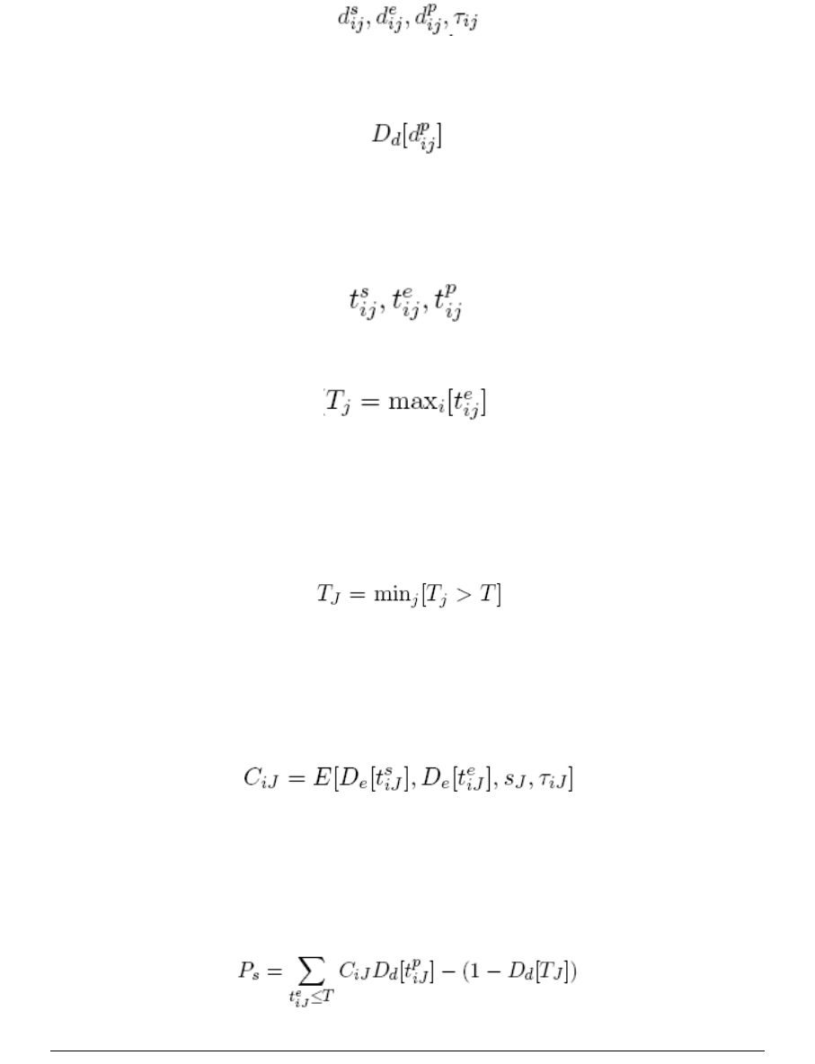
2 Market standards and calculations
2.2 Yield curves
92 © Wall Street Systems IPH AB - Confidential
For each swap quote we generate the coupon date data (see Equation 2-124 on page 92),
corresponding to the start, end, and payment dates, and the length of the coupon period of the ith
coupon of the jth quote.
Equation 2-124 Coupon date data
We shall also need the discount factors derived from the discount curve for all payment dates:
Equation 2-125 Discount factors for all payment dates
Given the interpolation date basis, all dates are transformed into times from spot date, so that we
have coupon time triplets (Equation 2-126 on page 92) and swap maturity times (Equation 2-127 on
page 92).
Equation 2-126 Coupon time triplets
Equation 2-127 Swap maturity times
2.2.2.1.2 Algorithm
Initially, set T, the last known node point, to zero (i.e. spot).
1. Choose the smallest maturity greater than the last known node point T, i.e. choose J:
Equation 2-128 Smallest maturity
There could, in principle be more than one, but start by assuming that J is unique.
2. For all i such that , calculate the coupon estimate based on the known part of the
bootstrap curve:
Equation 2-129 Coupon estimate
Where some interpolation may be needed, use the interpolation method specified for the derived
curve.
3. Calculate the stub price of the swap as the sum of the known coupons of each leg:
Equation 2-130 Stub price of the swap
Note: For discounting, we use the discount curve that was given as input. The term can be
interpreted as the discounted value of the redemption payment, in which case the other
te
iJT≤
DdTJ
[]
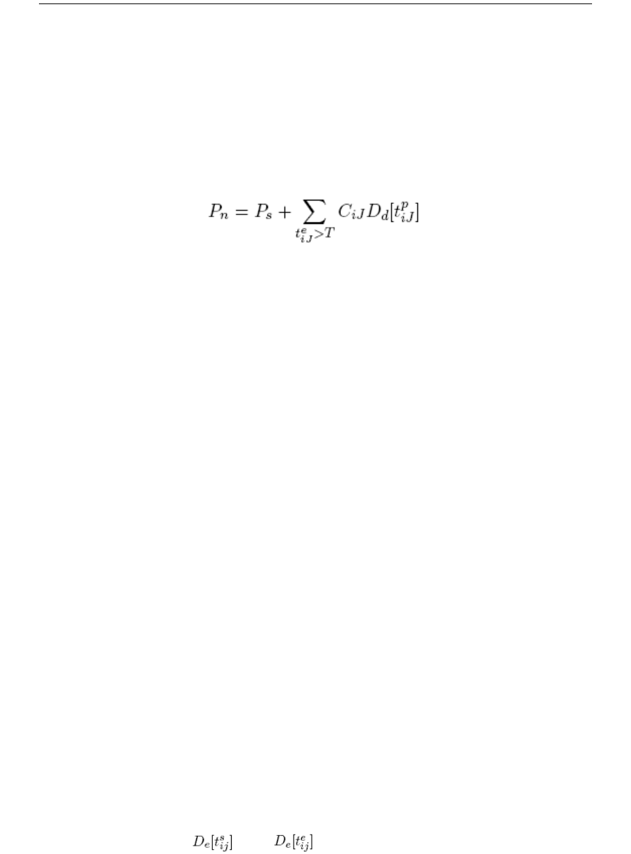
2 Market standards and calculations
2.2 Yield curves
Transaction & Risk Management Module (TRM) Instruments: Processing and Calculations 93
leg has value 1. Likewise, we may interpret the term as the value of the other leg
in case there is no principal exchange.
4. Initialize iteration: Create a new node point for the bootstrap curve at , with initial value
5. For each coupon with , calculate the estimate based on (known) and , see
Equation 2-129 on page 92.
where the discount factors may have to be interpolated from and , using the
interpolation method specified for the derived curve.
Calculate the value of the swap:
Equation 2-131 Swap value
If is positive, let , and . If is negative, stop.
6. Repeat step 5. on page 93 using .
If is negative let and . If is positive, stop.
7. Generic step: Use a goal seek algorithm and the method described in step 5. on page 93 to find
so that the value of the Jth swap is zero.
8. Set and create new node . If , then go to step 1. on page 92,
otherwise stop.
2.2.2.2 Cross Currency Basis Swap Curve
This section describes the algorithm used in converting cross currency basis swap spreads into
discount factors. The input to the algorithm consists of a base yield curve and a series of cross
currency basis spread quotes, resulting in a cross currency basis swap curve. We search for a series
of discount factors such that the value of the cross currency basis swap is at par. The discount curve
method is used in cross currency basis swaps, i.e. the underlying curve is used for estimating the
swap coupon amounts, and the derived cross currency basis swap curve for discounting (the leg for
which the spread is quoted).
2.2.2.2.1 Input
•Spot date
•Cross currency basis swap quotes: These are tuples (start date, maturity, spread, coupon
frequency), with some implicit rules for the generation of coupons.
•Estimation curve: A fixed curve that provides discount factors ( ) for the required dates.
•Coupon estimation: This is a function that returns a coupon estimate, given two
discount factors, coupon period, and a spread.
The bootstrap algorithm input is generated from this data.
For each swap quote, we generate the coupon date data (see Equation 2-124 on page 92),
corresponding to the start, end, and payment dates; and the length of the coupon period of the ith
coupon of the jth quote.
Then, using the estimation method, together with the estimation curve discount factors for the start
and end dates of the coupon, and , we can create the corresponding coupons using
Equation 2-129 on page 92.
1D
d
–T
J
[]
TJ
Dn0.00001=
te
iJT>DeT[] Dn
DeT[] Dn
PnDpDn
=P
pPn
=Pn
Dn1=
PnDlDn
=P
lPn
=P
n
Dn
TT
J
=D
eTJ
[] Dn
=Tmax
jTj
[]<
De
ED
1D2sϒ,,,[]

2 Market standards and calculations
2.2 Yield curves
94 © Wall Street Systems IPH AB - Confidential
Given the interpolation date basis, all dates are transformed into times from spot date, so that we
have coupon payment times and swap maturity times (Equation 2-127 on page 92).
2.2.2.2.2 Algorithm
Initially, set T, the last known node point, to zero (i.e. spot).
1. Choose the smallest maturity greater than the last node point: That is, choose J so that
.
There could, in principle be more than one, but start by assuming that J is unique.
2. Calculate the stub price of the swap as the sum of the known discounted coupons minus the
known price of the other leg (assumed at par, i.e. principals are exchanged).
Equation 2-132 Discount curve: stub price
3. Initialize iteration: Create a new node point for the bootstrap curve at , with initial value
.
4. Calculate the value of swap:
Equation 2-133 Discount curve: swap value
where the discount factors may have to be interpolated from and , using the
interpolation method specified for the derived curve. The last term is the principal payment: in
this method, we always assume that principals are exchanged.
If is positive, let and . If is negative, stop.
5. Repeat step 4. on page 94 using .
If is negative, let let and . If is positive, stop.
6. Generic step: Use a goal seek algorithm and the method described in step 4. on page 94 to find
so that the value of the Jth swap is zero.
7. Set and create new node . If go to step 1. on page 94, otherwise
stop.
2.2.2.3 Basis swap bootstrapping
This section describes the algorithm used in converting basis swap spreads into discount factors.
Two different approaches are presented: estimation curve bootstrapping and discount curve
bootstrapping.
In both approaches, the input to the algorithm consists of an underlying zero curve and a series of
basis spread quotes. In both algorithms, we search for a series of discount factors such that the
value of the calculated spread leg is at par. (Section 2.2.2.3.3 Non-par market value on page 97
addresses the case when the other leg is not at par.)
The estimation curve method is used in tenor basis swaps, while the discount curve method is used
in cross currency basis swaps.
TJminj T
j
T>[]=
TJ
Dn1.0=
DdT[] Dn
PnDpDn
=P
pPn
=Pn
Dn0.0000001=
PnDlDn
=P
lPn
=Pn
Dn
TT
J
=D
dTJ
[] Dn
=TmaxjTj[]<
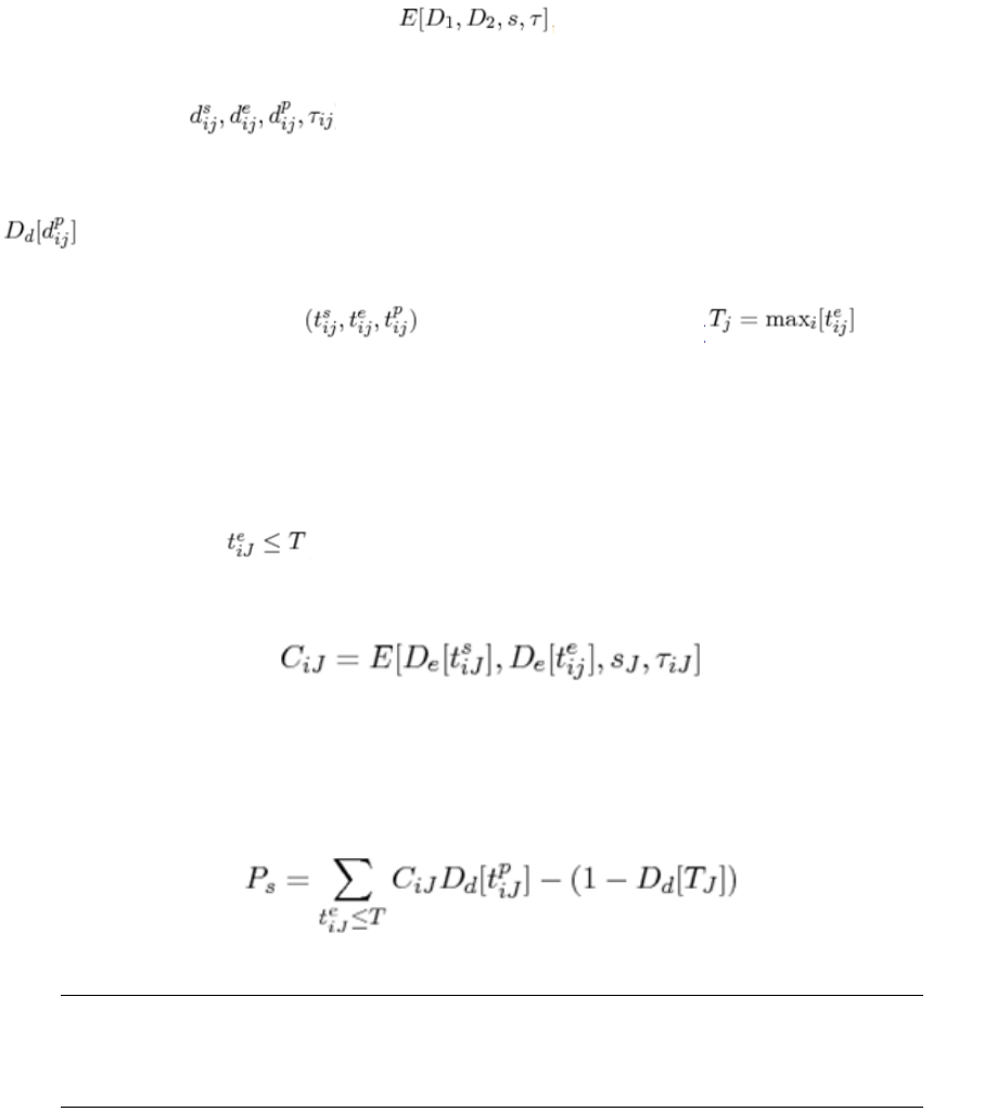
2 Market standards and calculations
2.2 Yield curves
Transaction & Risk Management Module (TRM) Instruments: Processing and Calculations 95
2.2.2.3.1 Estimation curve bootstrapping
This section describes the bootstrap algorithm for estimation curve bootstrapping. In estimation
curve bootstrapping, we use the underlying curve for discounting, and the bootstrapped curve for
the estimation of the swap coupon amounts. This method is used in tenor basis swaps.
Input data generation
•Spot date
•Basis swap quotes: These are tuples (start date, maturity, spread, coupon frequency), with
some implicit rules for the generation of coupons.
•Discount curve: A fixed curve that provides discount factors (Dd) for the required dates.
•Coupon estimation: This function returns a coupon estimate, given two
discount factors, coupon period, and a spread.
The bootstrap algorithm input is generated from this data. For each swap quote, we generate the
coupon date data ( ), corresponding to the start, end, and payment dates and the
length of the coupon period of the ith coupon of the Jth quote.
We shall also need the discount factors derived from the discount curve for all payment dates:
.
Given the interpolation date basis, all dates are transformed into times from the spot date, so that
we have coupon time triplets ( ), and swap maturity times ( ).
The algorithm
Initially, set T, the last known node point, to zero (i.e. spot).
1. Choose the smallest maturity greater than the last known node point T. That is, choose J so that
TJ=minj[Tj > T]. There could, in principle, be more than one, but start by assuming that J is
unique.
2. For all i such that , calculate coupon estimate based on the known part of the
bootstrapped curve:
Equation 2-134 Estimation curve bootstrapping: coupon estimate
–If interpolation is needed, use the interpolation method specified for the bootstrapped curve.
3. Calculate the stub price of the swap as the sum of the known coupons of each leg:
Equation 2-135 Estimation curve bootstrapping: calculated stub price of the swap
Note: For discounting, we use the discount curve given as input. The term can be interpreted as
the discounted value of the redemption payment, in which case the other leg has value
Dd[TJ]. Similarly, we may interpret the term as the value of the other leg in case there is
no principal exchange.
4. Initialize iteration: Create a new node point for the bootstrap curve at TJ, with initial value
Dn=0.00001

2 Market standards and calculations
2.2 Yield curves
96 © Wall Street Systems IPH AB - Confidential
5. For each coupon with , calculate the estimate based on De[T] (known) and Dn:
Equation 2-136 Estimation curve bootstrapping: calculate the estimate
–Where the discount factors may have to be interpolated from De[T] and Dn, using the
interpolation method specified for the bootstrapped curve, calculate the value of swap:
Equation 2-137 Estimation curve bootstrapping: calculate the value of the swap
–If the value is negative, stop. Otherwise, let Dp=Dn and Pp=Pn
6. Repeat step 5. on page 96 using Dn=1. If the resulting price is positive, stop. Otherwise, let and
Dl=Dn and Pl=Pn
7. Generic step: Use a goal seeker algorithm and the method described in step 5. on page 96 to
find Dn so that the value of the Jth swap is zero.
8. Set T = TJ and create the new node De[TJ]=Dn. If T < maxj[Tj] go to step 1. on page 95,
otherwise stop.
2.2.2.3.2 Discount curve bootstrapping
This section describes the bootstrap algorithm for discount curve bootstrapping. In discount curve
bootstrapping these roles are exchanged: the underlying curve generates the coupon estimates, and
the bootstrapped curve is used in discounting. The discount curve method is used in cross currency
basis swaps.
Input data generation
•Spot date
•Basis swap quotes: These are tuples (start date, maturity, spread, coupon frequency), with
some implicit rules for the generation of coupons.
•Estimation curve: A fixed curve that provides discount factors (De) for required dates.
•Coupon estimation: This is a function that returns a coupon estimate, given
two discount factors, coupon period, and a spread.
The bootstrap algorithm input is generated from this data. For each swap quote, we first generate
the coupon date data ( ), corresponding to the start, end, and payment dates, and the
length of the coupon period ith of the coupon jth of the quote (sj). Then, using the estimation
method with the estimation curve discount factors for the start and end dates of the coupon,
and , we can create the corresponding coupons using the following equation:
Equation 2-138 Discount curve bootstrapping: creating the coupons
Given the interpolation date basis, all dates are transformed into times from spot date, so that we
have coupon payment times ( ) and swap maturity times ( )
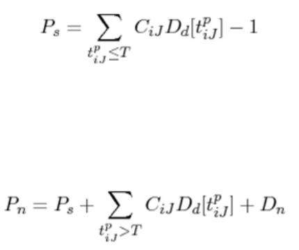
2 Market standards and calculations
2.2 Yield curves
Transaction & Risk Management Module (TRM) Instruments: Processing and Calculations 97
The algorithm
Initially, set T, the last known node point, to zero (i.e. spot).
1. Choose the smallest maturity greater than the last node point: That is, choose J so that
TJ=minj[Tj>T]. There could, in principle be more than one, but start by assuming that J is
unique.
2. Calculate the stub price of the swap as the sum of the known discounted coupons minus the
known price of the other leg (assumed at par, i.e. the principals are exchanged).
Equation 2-139 Discount curve bootstrapping: stub price
3. Initialize iteration: Create a new node point for the bootstrap curve at Tj, with initial value
Dn=1.0.
4. Calculate the value of swap:
Equation 2-140 Discount curve bootstrapping: value of the swap
–Where the discount factors may have to be interpolated from Dd[T] and Dn, using the
interpolation method specified for the bootstrapped curve. The last term is the principal
payment: in this method, we always assume that the principals are exchanged.
–If the value is negative, stop. Otherwise, let Dp=Dn and Pp=Pn.
5. Repeat step 4. on page 97 using Dn=0.0000001. If the resulting price is positive, stop.
Otherwise, let Dl=Dn and Pl=Pn.
6. Generic step: Use a goal seeker algorithm and the method described in step 4. on page 97 to
find Dn so that the value of the swap is zero.
7. Set T=TJ and create the new node Dd[TJ]=Dn. If T < maxj[Tj]. If go to step 1. on page 97,
otherwise stop.
2.2.2.3.3 Non-par market value
The bootstrapping algorithm described in section 2.2.2.3 Basis swap bootstrapping on page 94
applies to the basic setup, where we want to bootstrap a new curve (estimation or discounting) for
the spread leg, and assume that the other leg (i.e the leg whose value is taken as an input to the
bootstrapping algorithm) of the swap is valued at par.
There are cases when this assumption is no longer valid:
•Case 1. Instead of spread leg, we calculate the new curve for the flat leg. In this case the other
leg is the spread leg, which is not at par.
•Case 2. We want to use two different curves for estimation and discounting of the other leg,
which will then have a non-par value.
In these cases the value of the other leg needs to be calculated: We have to generate its cashflows
(using the estimation curve defined for the other leg) and discount them (using the discount curve
defined for the other leg). The coupon structure of the other leg may differ from the structure of the
calculated leg and is given in IR Quote and Yield Curve Editor's Tenor page. The estimation and
calculation curves are given in IR Quote and Yield Curve Editor's Other Leg Yield Curves page once the
optional feature Other Leg Yield Curves is selected. For more information about this editor, see TRM
User Guide.

2 Market standards and calculations
2.2 Yield curves
98 © Wall Street Systems IPH AB - Confidential
Using the same notation as above, but with bars above the symbols to indicate that they refer to the
other leg and are known in advance, the value of the other leg becomes:
Equation 2-141 Non-par market value
This value has to replace the value in Equation 2-135 on page 95, which becomes:
Equation 2-142 Non-par market value
Otherwise, bootstrapping follows the same steps as described previously.
2.2.2.4 Interpolation before first swap quote
The first calculated node of a basis swap curve is usually at one year. Without any additional
information, one would use the interest rate of the bootstrapped curve at the first node for all dates
before it. However, it is reasonable to assume that instead of being flat, the bootstrapped curve
should follow the underlying curve.
To achieve this, the yield creation algorithm creates an additional virtual quote for each gap of the
underlying curve that is no closer than 14 days before the first actual quote. Each virtual quote has
the same value as the first actual quote, but they are treated as deposits instead of swaps.
The virtual quotes are included in the bootstrapping process, and their presence causes the
bootstrapped curve to follow the shape of the underlying curve also before the first spread quote.
2.2.3 Yield Curve interpolation
An interpolation method is a way of estimating the shape of a yield curve between points for which
quotes exist. TRM performs interpolation to calculate these rates from the closest known quotes
according to the variables specified in the interpolation method.
The default interpolation method of yield curves is Linear, Flat Rate Extrapolation with date basis
Actual/365 and interest type Continuous Yield.
2.2.3.1 Interpolation periods
The starting point of yield curve interpolation is a set of known yields for a number of periods (the
node points), all having the same start date (spot date). The objective is to find the discount factor
between the spot date and another date for which there is no direct data.
All input quotes are first converted into discount factors between the spot date and the end date of
the quote period (or start date, if the quote is for a period before the spot).
Quotes that do not start or end at the spot date can be used if there is also a series of quotes
starting from or ending at the spot date (for example, T/N and S/N in markets where the spot date is
today). By combining the discount factors from the spot to the end dates of the forward quotes, a
synthetic quote from the spot can be obtained. This can then be used in the same way as regular
quotes from the spot.
Before the first input period and after the last, extrapolation is required. The methods required are
specified in the interpolation method definition.

2 Market standards and calculations
2.2 Yield curves
Transaction & Risk Management Module (TRM) Instruments: Processing and Calculations 99
2.2.3.2 Interpolation date basis
The interpolation algorithm uses the period lengths, between the common starting point of all
periods and the end point of each period, as input data.
When the interpolation result is requested for a target date, the period length between the common
start date and the target date is needed. To calculate these period lengths, a date basis is required.
The same date basis is used for all periods, regardless of the date basis used for the discount factor.
The date basis specified in the interpolation method definition is used both for the calculation of the
interpolation period lengths and to convert discount factors into the interpolation rate (except, of
course, if the interpolation rate is a discount factor, in which case, conversion is not needed).
2.2.3.3 Interpolation over spot date
When we seek a discount factor for a date after spot and before the first forward quote (most often
the one week quote), the nearest known discount factor before the target date is for spot (D=1).
However, that discount factor cannot be converted into rate, since the period length is zero.
Therefore, the previous existing quote (usually, O/N) is used as if it were the quote for the
zero-length period from spot to spot.
2.2.3.4 Type of interpolation
2.2.3.4.1 Linear
To calculate the interest rate for a date for which no direct quote exists, linear interpolation is used
to calculate the interest rate rm for the period tm (to spot date) between the closest quoted periods
t1 and t2 such that t1 < tm < t2.
1. The rates r1 and r2 need to be converted to the correct interest type before they can be used in
the linear interpolation.
To do this, two calculations need to be done:
a. Calculate the discount factors D1 and D2 for the periods t1 and t2.
For example, if the interest type is Annually Compounded Rate and the date basis is Actual/365,
then the discount factors D1 and D2 are calculated as follows:
Equation 2-143 Linear interpolation: Discount factor D1
Period t1tmt2
r1
rm
r2
Interest
%
Period
D11r1
100
---------
+
⎝⎠
⎛⎞
d1
–
365
---------
=
2 Market standards and calculations
2.2 Yield curves
100 © Wall Street Systems IPH AB - Confidential
and
Equation 2-144 Linear interpolation: Discount factor D2
where d1 and d2 are the actual number of days between the spot date and the period end
dates for the periods t1 and t2.
b. From these discount factors D1 and D2, the rates can be calculated with the correct interest
type (r1C and r2C). The interest type and date basis that you selected for the interpolation of
the yield curve will be used.
Here, we use the interest type Continuous Yield date basis Actual/365:
Equation 2-145 Linear interpolation: interest type r1C
and
Equation 2-146 Linear interpolation: interest type r1C
2. Linear interpolation is then used to calculate the rate rmc.
The date basis used is the one selected in the interpolation setup. The interpolation setup is
described in the TRM User Guide.
This rate will have the same interest type as r1C and r2C:
Equation 2-147 Linear interpolation: calculated rate rmc
3. The discount factor Dm, from the cashflow value date to the spot date, is calculated from the
linearly interpolated rate rmc.
The form of the equation is based on the date basis and interest type of the linear interpolation
method.
For continuous yield:
Equation 2-148 Linear interpolation: Continuous Yield
4. The discount factor Dm derived from the linearly interpolated rate rmc is multiplied by the
discount factors for the period from the spot date to the valuation date, using market quotes.
For example, if the number of spot days is 2, we would use DO/N and DT/N:
D = DO/NDT/NDm
D21r2
100
---------
+
⎝⎠
⎛⎞
d2
–
365
---------
=
r1C
100–
t1
------------1nD1
=
r2C
100–
t2
------------1nD2
=
rmc
t2tm
–()r1C tmt1
–()r2C
+
t2t1
–
----------------------------------------------------------------
=
Dme
rmc
–
100
-----------tm
=

2 Market standards and calculations
2.2 Yield curves
Transaction & Risk Management Module (TRM) Instruments: Processing and Calculations 101
Example: Interest rate interpolation
In this example, the interest rate for a cashflow at 1.5 years is calculated using two IR quotes at 1
and 2 years.
Note: In this example, all calculated amounts are rounded.
For this example, it is assumed that a linear interpolation method has been defined with the date
basis Actual/365 and interest type of Continuous Yield.
•Step 1 - Convert the reference rates to continuous yield rates
To convert the reference rates r1 and r2 to continuous yield rates, first the discount factors for
these rates is calculated, using the date bases and interest types defined for these two quotes.
–The 1Y quote has an Actual/360 date basis and Periodic Rate interest type.
This gives the following formula:
Equation 2-149 Example: Interest Rate Interpolation
–The 2Y quote has a 30/360 date basis and Annually Compounded Rate interest type.
This gives the following formula:
Equation 2-150 Example: Interest Rate Interpolation
Data Symbol Value
Value Date 22-11-2000
Spot Days 2
Spot Date 24-11-2000
IR quote (1Y) r15.161%
Date basis of 1Y quote d/B Actual/360
Number of days from spot date to 1Y cashflow on 26-11-2001 367
Interest type of 1Y quote Periodic
IR quote (2Y) r25.2575%
Date basis of 2Y quote d/B 30/360
Number of days from spot date to 2Y cashflow on 25-11-2002 721
Interest type of 2Y quote Annually Compounded Rate
O/N quote rO/N 4.84%
T/N quote rT/N 4.81%
Date basis of O/N and T/N quotes d/B Actual/360
Instrument date basis d/B Actual/360
Number of days from spot date to 1.5Y on 24-05-2002 using
instrument date basis
546
D11r1
100
---------d1
360
---------
×+
⎝⎠
⎛⎞
1–
15.161
100
-------------367
360
---------
×+
⎝⎠
⎛⎞
1–
0.950016== =
D21r2
100
---------
+
⎝⎠
⎛⎞
d– 2
360
---------
15.2575
100
----------------
+
⎝⎠
⎛⎞
721–
360
------------
0.902469== =

2 Market standards and calculations
2.2 Yield curves
102 © Wall Street Systems IPH AB - Confidential
–Next, the continuous yield rates r1C and r2C are calculated from these discount factors, using
the interpolation method date basis Actual/365 and interest type Continuous Yield):
Equation 2-151 Example: Interest Rate Interpolation
Equation 2-152 Example: Interest Rate Interpolation
•Step 2 - Linear interpolation
Linear interpolation with the recalculated reference rates from the first step is used to calculate
the continuous yield rate rmc.
Note: tm is recalculated using the interpolation method date basis Actual/365.
Equation 2-153 Linearly interpolated rate rmc
•Step 3 - Discount factor to spot date (Dm)
The discount factor Dm, from the cashflow value date to the spot date, is calculated from the
linearly interpolated rate rmc from the previous step (Equation 2-153 on page 102). The
equation in this example is based on the interpolation interest type Continuous Yield and date
basis Actual/365:
Equation 2-154 Discount factor to spot date
•Step 4 - Discount factor to valuation date (D)
To get the discount factor to the valuation date, the discount factor Dm to the spot date is
multiplied by the discount factors for the period from the spot date to the valuation date, DO/N
and DT/N. The number of spot days is 2.
This gives the following equation:
D = DO/NDT/NDm
The discount factors DO/N and DT/N are calculated from the O/N and T/N rates, using the date
basis and interest type defined for the quotes.
In this case, they have both been defined with date basis Actual/360 and interest type Periodic
Rate.
Equation 2-155 Discount factors DO/N
r1C
100–
t1
------------1nD1
100–
367 365⁄
----------------------1n 0.950016()5.0997== =
r2C
100–
t2
------------1nD2
100–
731()365⁄
-------------------------- 1n 0.902469()5.124== =
rmc
t2tm
–()r1C tmt1
–()r2C
+
t2t1
–
----------------------------------------------------------------
731 546–
365
------------------------
⎝⎠
⎛⎞
5.0997 546 367–
365
------------------------
⎝⎠
⎛⎞
5.124+
731 367–
365
------------------------
⎝⎠
⎛⎞
------------------------------------------------------------------------------------------------ 5.11165== =
Dme
rmc
100
---------
⎝⎠
⎛⎞
tm
–
e
5.11165
100
-------------------
⎝⎠
⎛⎞
546 365⁄()–
0.926386== =
DON⁄14.84
100
---------- 1
360
---------
×+
⎝⎠
⎛⎞
1–
0.9998656==

2 Market standards and calculations
2.2 Yield curves
Transaction & Risk Management Module (TRM) Instruments: Processing and Calculations 103
and
Equation 2-156 Discount factors DT/N
D = DO/NDT/NDm = 0.926386 * 0.9998656 * 0.9998664 = 0.926137
If a discount factor between two dates is needed, neither of which is the spot, the two discount
factors between the spot and the two days in question are calculated, and divided one by the
other.
2.2.3.4.2 Cubic splines interpolation
The interpolation method is defined by choosing the optional feature Yield Curve Interpolation Setup,
and then, in the Interpolation page, by selecting one of the interpolation methods. Choices for cubic
spline are: Hermite Spline (Two Points), Hermite Spline (Three Points) or Cubic Spline. The first two refer to
Hermite Spline ( Hermite spline on page 105) with slopes at node points (mi) defined by either a
two-point difference or a three-point difference, as explained in section Setting the slopes at node
points on page 106. The third option (Cubic Spline) corresponds to classic spline described in section
Classic spline on page 104. For more information about setting up yield curves, see TRM User Guide.
The input to the interpolation module is a set of points, usually giving the value of interest rate at a
set of times. The task of the interpolator is to provide the value of the dependent variable (e.g.
interest rate) at an arbitrary point, i.e. to extend a function defined at a restricted number of points
to a function defined everywhere (or more typically, for non-negative numbers when we are dealing
with time as an independent variable). The interpolation function will go through the points given as
input.
In the quasi-cubic spline interpolation, we also require that the interpolation function be continuous
and differentiable at all points. Furthermore, a classic spline will have a continuous second derivative
at all points.
The yield curve interpolation is used in two different settings: where the input points are known in
advance and when the shorter end of the curve is needed to construct new points in the longer end.
The latter situation takes place in bootstrapping when there are coupons falling on dates, which are
not maturity dates of the input quotes. (That is, we need to interpolate from the existing curve to
discount such coupons.)
The classic spline has the property that when any input point is changed, the whole curve moves. On
the other hand, Hermite splines depend only on two or four points around the interval to be
interpolated, and are therefore easier to use in bootstrapping.
Technical definition
Given a set of points (with and ,
a cubic spline is a continuous function that goes through the points in I, and is a cubic polynomial
within each interval intervals altogether), and is either continuously
differentiable (quasi-cubic spline) or has a continuous second derivative (classic cubic spline).
Boundary conditions
Let us call Pi the cubic polynomial forming the spline within interval Ii. Then, a quasi-cubic spline
satisfies the following conditions:
Equation 2-157 Cubic spline: conditions
DTN⁄14.81
100
---------- 1
360
---------
×+
⎝⎠
⎛⎞
1–
0.9998664==

2 Market standards and calculations
2.2 Yield curves
104 © Wall Street Systems IPH AB - Confidential
This gives us 3N - 4 conditions. For classic splines, the continuity of the second derivative provides
another N - 2 conditions:
Equation 2-158 Cubic spline: classic splines
To determine all N - 1 cubic polynomials, 4N - 4 parameters need to be set. This means that for
classic spline, two additional conditions are needed, while for quasi-cubic splines N additional
conditions are necessary.
With classic spline, the additional two conditions are usually set at either boundary, for example:
Equation 2-159 Cubic spline: natural condition and clamped spline
where and are the slope of the curve at either end.
For the bootstrapping algorithm, it is convenient to be able to set the two additional conditions at
the short end of the curve:
Equation 2-160 Cubic spline: bootstrapping algorithm conditions
Classic spline
The value of the spline at a point is given in terms of the second derivatives at node
points (zi) as shown in Equation 2-161 on page 104:
Equation 2-161 Classic spline: value of spline
where
λ1λN

2 Market standards and calculations
2.2 Yield curves
Transaction & Risk Management Module (TRM) Instruments: Processing and Calculations 105
The parameters zi can be solved by requiring that the derivatives at interior nodes
( ) be continuous:
Equation 2-162 Classic spline: continuous derivatives at interior nodes
and that the boundary conditions are satisfied, which in case of clamped boundary conditions
means:
Equation 2-163 Classic spline: clamped boundary conditions
In matrix form, Equation 2-162 on page 105 and Equation 2-163 on page 105 can be written as
follows:
Equation 2-164 Classic spline: matrix
Hermite spline
In each sub interval Ii, we can normalize the argument t by mapping it to the interval [0, 1]
Equation 2-165 Classic spline: normalize t
where
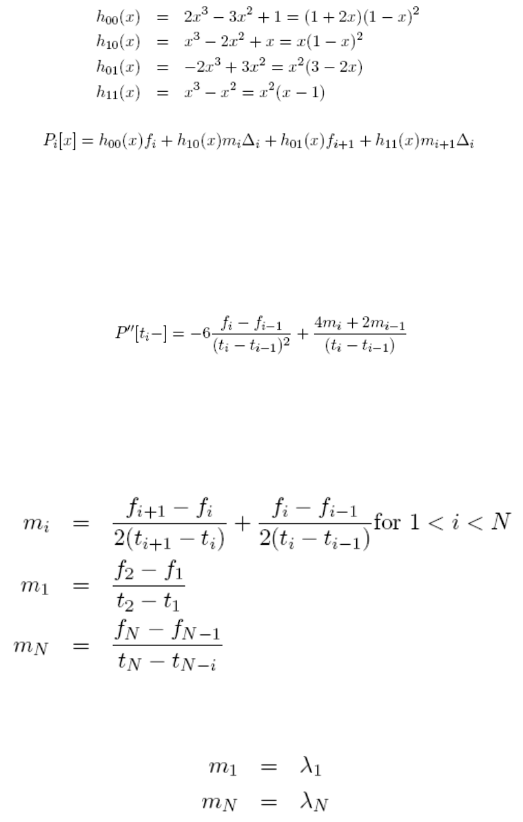
2 Market standards and calculations
2.2 Yield curves
106 © Wall Street Systems IPH AB - Confidential
Then, we may represent the cubic polynomial as a linear combination of the third order Hermite
polynomials over the normalized interval [0, 1]:
Equation 2-166 Classic spline: third order Hermite polynomials
where mi is the derivative at point ti.
It is the setting of these N derivatives at the node points that uniquely determines the quasi-cubic
spline.
From Equation 2-166 on page 106 we can find the value of the second derivative of the curve at
each node. The left hand-side derivative is:
Equation 2-167 Classic spline: Left hand side derivative
•Setting the slopes at node points
There are various methods for determining mi, and we shall consider the following four:
–Three-point difference
Equation 2-168 Cubic spline: three-point difference method
If we use clamped initial and final conditions, then:
Equation 2-169 Cubic spline: three-point difference method, clamped
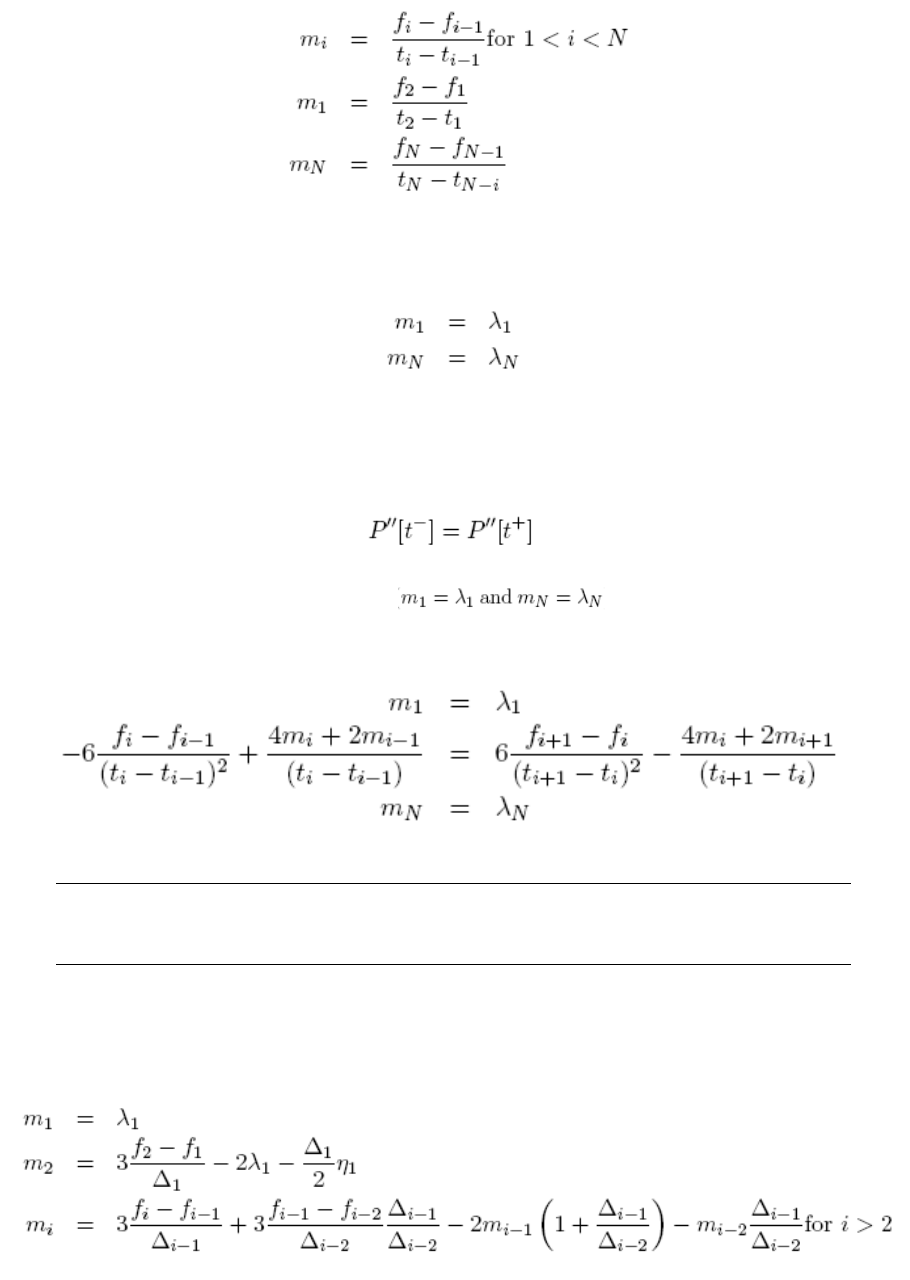
2 Market standards and calculations
2.2 Yield curves
Transaction & Risk Management Module (TRM) Instruments: Processing and Calculations 107
–Two-point difference
Equation 2-170 Two-point difference
If we use clamped initial and final conditions, then:
Equation 2-171 Two-point difference: clamped initial and final conditions
For the classic (continuous second derivative) case, we have the additional N - 2 conditions
that the second derivative at each interior node point is continuous:
Equation 2-172 Two-point difference: Classic
–With clamped boundary conditions , mi can be solved from the
following set of equations:
Equation 2-173 Clamped boundary conditions: equations
Note: Equation 2-173 on page 107 is equivalent to Equation 2-162 on page 105 and Equation
2-163 on page 105, except that here we use the slopes as parameters, while in the classic
formulation second derivatives are used.
–Replacing the long end boundary condition (mN = 2) with an initial condition on the second
derivative () we have the following set of equations, which can be solved sequentially:
Equation 2-174 Clamped boundary conditions: initial condition on the second derivative
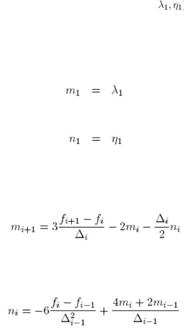
2 Market standards and calculations
2.2 Yield curves
108 © Wall Street Systems IPH AB - Confidential
Extrapolation
For values t < t1 and t > tN we have to use extrapolation. For yield curve interpolation it makes
sense to use linear interpolation, typically with zero slope. In this case, to maintain continuity of the
first derivative, clamped boundary conditions are appropriate for the spline itself. If we apply two
initial conditions for a classic spline, we have no control over the slope at the long end of the curve,
and the first derivative will be discontinuous.
2.2.3.4.3 Spline building algorithm
The structure of the spline building algorithm depends on whether the node points (ti, fi) are all
known in advance, or whether we have to solve the values if as we go along (as in bootstrapping).
There are three cases:
•All node points are known: In case the values at the node points are known, we can use the
methods described in Setting the slopes at node points on page 106 directly.
•Bootstrapping is required to construct the curve, but interpolation is not necessary during curve
construction.
•Bootstrapping uses interpolation. If interpolation is needed during bootstrapping, there are two
possibilities:
–If the information up to a given point fully defines the interpolation curve up to that point,
then we can use sequential bootstrapping ( Sequential bootstrapping on page 108).
–If the information beyond the current node is necessary for the interpolator, we need an
iterative algorithm ( Iterative algorithm on page 109).
Sequential bootstrapping
If we have to boot strap the values at node points, or if we use classic spline, a sequential algorithm
is needed. We only consider classic case with initial conditions ( ) and quasi-cubic case with
the two-point difference, since these are the cases amenable to the bootstrapping type of algorithm.
Classic spline with boundary conditions and quasi-cubic spline with three-point difference are
described in section Iterative algorithm on page 109.
Set
Equation 2-175 Spline building algorithm: sequential bootstrapping
Equation 2-176 Spline building algorithm: sequential bootstrapping - Classic case only
For the ith interval, given the value fi+1 at the right-hand end of the interval, we set for the classic
case:
Equation 2-177 Spline building algorithm: sequential bootstrapping - ith interval
where for i > 1:
Equation 2-178 Spline building algorithm: sequential bootstrapping (i > 1)
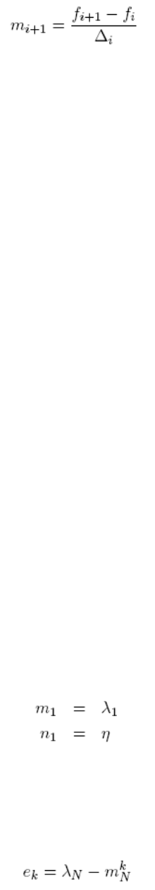
2 Market standards and calculations
2.2 Yield curves
Transaction & Risk Management Module (TRM) Instruments: Processing and Calculations 109
And for the quasi-cubic case:
Equation 2-179 Spline building algorithm: sequential bootstrapping (quasi-cubic case)
In either case, the ith spline is now given in terms fi+1.
If fi+1 is known, then the sequential bootstrapping is finished. Otherwise, this function can now be
used iteratively to solve the bootstrapping step, yielding a value fi+1 that provides the market price
for the ith bootstrapping instrument.
Iterative algorithm
The sequential algorithm for classic spline, while well adapted to the solving of the bootstrap
problem, cannot be made to satisfy the boundary condition at the long end of the curve. On the
other hand, for quasi-cubic spline with three-point differences the sequential algorithm cannot be
applied at all. For these cases we need an iterative approach.
•Quasi-cubic spline
In this algorithm, we solve the problem of missing node values by using the values from the
previous iteration round. To initialize the values, we use sequential bootstrapping with two-point
differences.
–Bootstrap using the sequential algorithm with two-point differences.
–Bootstrap using the sequential algorithm with three-point differences. Takes the values for
nodes beyond the current one from the previous iteration round. Repeat until slopes no
longer change.
In practice, only one iteration is needed.
•Classic spline
The objective here is to use the sequential algorithm iteratively to find a classic spline with the
proper slope at the long end of the curve. The idea is to apply sequential bootstrapping with the
given initial slope and to adjust the initial second derivative so that the final slope, which is
determined by the initial conditions and the sequential bootstrapping process, will be equal to
the requested value.
To ensure a good initial guess, we first carry out bootstrapping using linear interpolation and
create a cubic spline through its node points. We then use the second derivative at the first node
point as the initial value ( ) for the iteration algorithm.
Iteration algorithm
1. Initialize: Set the initial slope and second derivative:
Equation 2-180 Cubic spline interpolation: Iteration algorithm
2. Sequential bootstrapping: Using the initial conditions and sequential bootstrapping (see
Sequential bootstrapping on page 108), find the interpolation curve.
3. Iteration k: Find the error in the end condition slope:
Equation 2-181 Cubic spline interpolation: Iteration algorithm
η
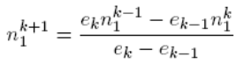
2 Market standards and calculations
2.2 Yield curves
110 © Wall Street Systems IPH AB - Confidential
where is the target value, and is the slope at the kth iteration. If |ek| is small enough,
stop, otherwise adjust the free initial variable:
Equation 2-182 Cubic spline interpolation: Iteration algorithm
Slope to a change in the initial second derivative. Go to 2. on page 109.
2.2.3.4.4 Reference time
In interpolating a yield curve, the value to be interpolated is either the discount factor between two
dates or the corresponding interest rate. One of these dates has to be common to all interpolated
values, and the interpolation results depend on the choice of the common date. Since usually most
of the market quotes used in the construction of the curve are from the spot, TRM uses the spot
date as the common reference point for all interpolated values.
This leads to a two-phased bootstrapping process:
•Before spot: In the first phase, we use the valuation date as reference and apply bootstrapping
only to the input quotes with maturity on or before the spot date, thus creating a stub yield
curve between the valuation date and spot date.
•After spot: In the second phase, we move the reference date to spot, and apply bootstrapping
to all input quotes with maturity after the spot date. To these quotes, we add the discount
factors between the spot date and each date from the valuation date to the spot date (including
the former and excluding the latter) derived from the stub curve constructed in the first phase.
Whenever a discount factor between two dates (d1 and d2) is needed, the following steps are taken:
1. Find the discount factor (D1) between the spot date (ds) and d1. To do this, calculate the length
of period between ds and d1 in year using the interpolation date basis defined for the curve, and
find the value of the interpolation variable at that point of time. If the interpolation variable is
not a discount factor but a rate, convert the rate into discount factor by using the rate type and
date basis defined for the curve.
2. Similarly, find the discount factor (D2) between ds and d2.
3. Finally, the discount factor between dates d1 and d2 is D12 = D2/D1.
2.2.3.4.5 Exponential splines
If scaling is set to Logarithmic (interpolation setup), then the interpolation is carried out on the
logarithms of the original values.
The interpolation curve then has the form:
Equation 2-183 Exponential splines: interpolation curve
where:
•The parameters a, b, c, d vary from interval to interval.
2.2.4 FX rate interpolation
Forward FX rates are the result of interest rate differences.
When a market FX exchange rate is needed on a date for which no direct quote is available, the
exchange rate needs to be interpolated from other quotes. In FX markets, all market rates except S
(spot) are quoted in terms of F (forward points) that are to be added to S.
λ1mN
k
yx() eabxcx
2dx3
++ +
=
Δ
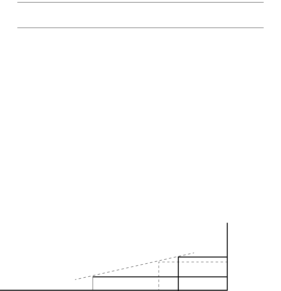
2 Market standards and calculations
2.2 Yield curves
Transaction & Risk Management Module (TRM) Instruments: Processing and Calculations 111
To find out, on valuation date dr, a market rate F on a future date d, one of the following methods is
used:
•If d is before the next banking day, then:
Equation 2-184 FX rate interpolation: market rate
where:
–dO/N is the number of days from the valuation date to the next business day.
Note: For FX rates before the spot date, the forward points are taken from the opposite side of
the spread. That is, the bid rate is calculated from the bid spot rate and ask points and the
ask rate is calculated from the ask spot rate and bid points.
•If d is before the spot date but after the next business day, then:
Equation 2-185 FX rate interpolation: before spot date. after business day
where:
–dT is the next business day and dT/N is the number of days from the next business day to the
spot.
•If d is the spot date, then:
F = S
•If there is an exact quote Fd (number of forward points) for date d, then:
Equation 2-186 FX rate interpolation: exact number of forward points
•If there are two market quotes Fd1 and Fd2 such that d1 < d < d2 then:
Equation 2-187 FX rate interpolation: two market quotes
This is illustrated in the following figure.
•If the quote for d1 is S, then
FSΔFT/N
–ΔFO/N
dd
r
–()
dO/N
------------------
–=
FS
ΔFT/N
dd
T
–()
dT/N
---------------------
–=
Δ
FSΔFd
+=
ΔΔ
FSΔFd1
ΔFd2ΔFd1
–
d2d1
–
--------------------------- dd
1
–()++=
Period d1d2
d
Forward
points
%
ΔFd2
ΔFd1
ΔFd
ΔFd1 0=

2 Market standards and calculations
2.3 Key-figures
112 © Wall Street Systems IPH AB - Confidential
•If the date d is after the last quoted rate, then we extrapolate linearly using the slope between
the two last quotes:
Equation 2-188 FX rate interpolation: after last quoted rate
where is the last quote date and is the penultimate quote date.
2.2.4.1 Example: FX rate interpolation
In this example, the USD/JPY exchange rate is calculated at a date 121 days after spot, with spot
date 11-01-1999.
We have the following data:
d1 = 31 + 28 + 31 = 90
d2 = 31 + 28 + 31 + 30 + 31 + 30 = 181
Therefore, using the following equation:
Equation 2-189 FX rate interpolation: interpolated forward rate
The interpolated forward rate for 121 days = 137.65:
Equation 2-190 FX rate interpolation: example interpolated forward rate
2.3 Key-figures
The following section describes the available key-figures for basic fixed cashflows. For key figures
for dual currency cashflows, see 2.3.5 Dual currency on page 147.
2.3.1 Valuation
Detailed calculations are available in the instrument-specific sections.
dNdN1–
Data Symbol Value
Maturity d 121 days
USD/JPY spot rate S 137.9
Quote for 3 months in forward points -190
Quote for 6 months in forward points -380
Date basis for currency Actual/360
ΔFd1
ΔFd2
FSΔFd1
ΔFd2ΔFd1
–
d2d1
–
--------------------------- dd
1
–()++=
F 137.9=0.190–()
0.380–0.190–()–
181 90
–
-----------------------------------------121 90–()++ 137.9 0.254– 137.65==

2 Market standards and calculations
2.3 Key-figures
Transaction & Risk Management Module (TRM) Instruments: Processing and Calculations 113
2.3.1.1 Interest Rate
The interest rate is the rate that is used in the calculation of IR exposure for the period between the
cashflow's risk date and spot date. The interest rate is based on the Present Value Discount Factor
(Dv) and Present Value Spot Discount Factor (Ds):
where R[] is the rate type defined in the Instrument Editor's IR Exposure page (Base IR Exposure Setup
feature), and t is the time between the spot date and risk date, calculated using the Date Basis
defined in the Instrument Editor's IR Exposure page.
Note: If the risk calculation is based on the risk yield, the yield type and date basis are derived
from the setup in the Risk Yield page (Risk Yield feature) of the Instrument Editor.
Depending on the setup, the Interest Rate key figure displays:
•The zero coupon rates of the valuation curve (by default)
•The same rate (yield-to-maturity), when the instrument's risk yield is set with Method =
Yield-to-Maturity in the Risk Setup page (the Risk Setup page is available when the Feature Risk Setup
(Bond) is selected).
2.3.1.2 Market Value
The market value of the transaction (cashflow) calculated using the valuation method specified for
the instrument, given in the figure currency.
2.3.1.3 Market Value Local
The market value of the transaction (cashflow) calculated using the valuation method specified for
the instrument, given in the currency of the transaction (cashflow).
2.3.2 Profit and Loss
2.3.2.1 Accrued Interest
Accrued interest of the coupon converted into figure currency.
2.3.2.2 Accrued Interest Local
Accrued interest in the coupon/cashflow currency.
2.3.2.3 Accrued Profit
Non-interest accrued profit, for example, accrued discount premium for bonds, or amortized fees
and option premiums, converted into figure currency.
2.3.2.3.1 Accrued Profit (BVC)
The Accrued Profit (BVC) component of accrued profit is a Closing the Books figure which is
calculated separately for each BVC adjustment, as follows:
Accrued Profit (BVC) = BVC Amount (D_left - D_total) / (1 - D_total)
Where:
–D_total = discount factor for the period from adjustment to maturity using all-in yield as of
the adjustment date.
–D_left = discount factor for the period from valuation to maturity using all-in yield as of the
adjustment date.
2 Market standards and calculations
2.3 Key-figures
114 © Wall Street Systems IPH AB - Confidential
2.3.2.3.2 Accrued Profit (Costs)
This is a Closing the Books figure and is the part of Accrued Profit directly related to costs (for
example, fees), which is calculated separately for each fee, as follows:
Accrued Fee Profit = Fee Amount (D_left - D_total) / (1 - D_total)
Where:
–D_total = discount factor for the period from adjustment to maturity using all-in yield as of
the adjustment date.
–D_left = discount factor for the period from valuation to maturity using all-in yield as of the
adjustment date.
2.3.2.3.3 Accrued Profit (Discount)
This is a Closing the Books figure and is the part of Accrued Profit directly related to Discount
Premium (for example, fees), which is calculated for the Discount (Premium) of a Bond, as follows:
Accrued Discount Profit = Discount/Premium Amount (D_left - D_total) / (1 - D_total)
Where:
–D_total = discount factor for the period from adjustment to maturity using all-in yield as of
the adjustment date.
–D_left = discount factor for the period from valuation to maturity using all-in yield as of the
adjustment date.
2.3.2.3.4 Accrued Profit (Residual)
The Accrued Profit (Residual) figure (that is, the discount/premium component) is then the
difference between the total Accrued Profit figure and the Accrued Profit (Costs) and Accrued Profit
(BVC) figures.
2.3.2.4 Accrued Profit Local
Non-interest accrued profit, for example, accrued discount premium for bonds, or amortized fees
and option premiums, in the currency of the transaction (cashflow).
2.3.2.5 FX Profit
The part of the difference between the market value and the book value of the transaction
(cashflow) due to changes in FX Spot rates.
2.3.2.6 Accrued Margin Profit
Accrued Margin Profit Local converted to figure currency.
2.3.2.7 Accrued Margin Profit Local
Accrued part of the margin amount. The margin profit is calculated by accruing the margin amount
calculated linearly throughout the life of the transaction.
2.3.2.8 Margin Profit
Margin Profit Local converted to figure currency.
2.3.2.9 Margin Profit Local
The residual margin profit, i.e. Total Margin Profit Local - Accrued Margin Profit Local.
2.3.2.10 Total Margin Profit
Margin Profit Local converted to figure currency.

2 Market standards and calculations
2.3 Key-figures
Transaction & Risk Management Module (TRM) Instruments: Processing and Calculations 115
2.3.2.11 Total Margin Profit Local
Profit resulting from transaction margins, i.e. the discounted margin amount, expressed in the
currency of the transaction/margin. Margins are currently supported for short-term loans (3.8 Short
term loan on page 305) and FX spots and FX forwards (6.1 FX spot and FX forward on page 383 and
FX swaps (6.4 FX swap on page 416.)
2.3.2.12 MtoM Profit
The part of the Profit due to changes in market variables other than FX rates, converted into figure
currency.
2.3.2.13 MtoM Profit Local
The part of the Local Profit due to changes in market variables other than FX rates, expressed in the
currency of the transaction (cashflow).
2.3.2.14 Other Profit
The part of the Profit not attributable to the other profit types (MtoM, FX, or Accrued), converted
into the figure currency.
2.3.2.15 Other Profit Local
The part of the Local Profit not attributable to the other profit types (MtoM, FX, or Accrued),
expressed in the currency of the transaction (cashflow).
2.3.2.16 Total Profit
The difference between the market value and the book value of the transaction (cashflow),
converted into figure currency.
2.3.2.17 Total Profit Local
The difference between the market value and the book value of the transaction (cashflow),
expressed in the currency of the transaction (cashflow).
2.3.3 Option figures
FX option key figures are calculated using the valuation model set up by the user:
Note: For more information about option valuation models, see section 10.8.6.2.2 on page 611.
Equation 2-191
where
–S is the FX Spot Rate
–X is the FX Strike Rate
– is the Asset currency continuous rate
– is the Cash currency continuous rate
– is the time to expiry date
– is the time delay between expiry and payment date
– is the volatility
Γa
Γc
τe
dρ
σ

2 Market standards and calculations
2.3 Key-figures
116 © Wall Street Systems IPH AB - Confidential
The valuation formula may use other transaction parameters, such as gap, barrier, or exercise
schedule, or model parameters, such as Quality, but these will be considered implied and not shown
in the formulas.
2.3.3.1 Asset and cash currencies
The values of some key figures will depend on the choice of asset and cash currencies. The asset
currency is by default the currency with the higher priority (as defined in Currency Priority Editor),
or the base currency in case the traded currencies have no priorities defined. For more information
about setting currency priorities, see TRM User Guide, Client Priorities.
You can change the (defaulted) asset currency in Transaction Manager. This impacts the option
figures displayed in Transaction Manager.
2.3.3.2 Greeks
Greeks are sensitivities of option price to changes in the variables determining the price. These are
calculated numerically using:
Equation 2-192 Greeks - sensitivities of option price
where is a small number.
TRM calculates the Greeks described in the following sections:
ε
Basic sensitivities Formula Cross sensitivities Formula
Delta Asset Rho Speed
Gamma Cash Rho Speed
Strike Delta Vega Speed (Vanna, Wega)
Strike Gamma Theta Speed
Asset Rho Delta Bleed
Asset Yield Gamma Gamma Bleed

2 Market standards and calculations
2.3 Key-figures
Transaction & Risk Management Module (TRM) Instruments: Processing and Calculations 117
For barrier options, TRM offers some additional key figures, which describe the behavior of the
option’s value near the barrier. These figures replicate the standard sensitivity calculations, except
that the valuation is done at the barrier, without crossing it.
Cash Rho Asset Rho Bleed
Cash Yield Gamma Cash Rho Bleed
Vega Vega Bleed
Sigma Gamma (Volga)
Theta
Time Gamma
Basic sensitivities Formula Cross sensitivities Formula
Upper barrier sensitivities Formula Lower barrier sensitivities Formula
Upper Barrier Delta Gap Lower Barrier Delta Gap
Upper Barrier Gamma Gap Lower Barrier Gamma Gap
Upper Barrier Strike Delta Gap Lower Barrier Strike Delta Gap
Upper Barrier Strike Gamma Gap Lower Barrier Strike Gamma Gap
Upper Barrier Asset Rho Gap Lower Barrier Asset Rho Gap
Upper Barrier Asset Yield Gamma Gap Lower Barrier Asset Yield Gamma Gap

2 Market standards and calculations
2.3 Key-figures
118 © Wall Street Systems IPH AB - Confidential
2.3.3.3 Intrinsic and time value
There are three methods for intrinsic value calculation:
For barrier options intrinsic value calculated at upper and lower barriers is called Upper Barrier
Digital and Lower Barrier Digital respectively.
2.3.3.4 Risk figures
Sensitivity figures are calculated for one unit of asset currency and expressed in cash currency. To
convert them into risk key figures they are multiplied by cash amount (including the sign of the
transaction) and FX rate between the cash currency and the figure currency. In addition, theta
figures, which are originally calculated for one unit of time (year), are divided by 365 so that they
will correspond to a daily change in option value.
Similarly, volatility figures (vega, vanna, wega) are calculated for one unit change in volatility
(100%). They are divided by 100 so that they will correspond to a change of one percentage unit in
volatility.
Upper Barrier Cash Rho Gap Lower Barrier Cash Rho Gap
Upper Barrier Cash Yield Gamma Gap Lower Barrier Cash Yield Gamma Gap
Upper Barrier Vega Gap Lower Barrier Vega Gap
Upper Barrier Sigma Gamma Gap Lower Barrier Sigma Gamma Gap
Upper Barrier Theta Gap Lower Barrier Theta Gap
Upper barrier sensitivities Formula Lower barrier sensitivities Formula
Method Formula Description
Zero Volatility Calculate option price assuming volatility
zero.
Forward Calculate option price assuming volatility
zero, and substituting zero for cash rate
and IR difference for asset rate.
Spot Calculate option price assuming volatility
zero, and substituting zero for cash and
asset rates.

2 Market standards and calculations
2.3 Key-figures
Transaction & Risk Management Module (TRM) Instruments: Processing and Calculations 119
2.3.4 Risk
Note: For Theoretical valuation, present value is equal to market value in all cases except for
bond futures in IR risk figures calculation.
2.3.4.1 Exposures
Exposures in general measure sensitivity of the present value to a change in a market rate.
2.3.4.1.1 FX Exposure
The sensitivity of the present value of the cashflow to a change in the FX Spot rate.
The magnitude of the change is defined for each currency in Currency Editor (as a percentage).
FX exposures are netted within each currency (in Currency Editor), as well as within each class
currency (in Currency Class Editor), see TRM User Guide. Totals that include different currencies or
different currency classes are taken from the absolute values of the currency or the total exposures
of the currency class.
2.3.4.1.2 IR Exposure 1
The sensitivity of the present value of the cashflow to a parallel shift of 1 basis point (1bp) in the
yield curve.
The value of a position can be seen as a function of a number of discount factors for different
maturities:
V = V [ D1, D2, ... , Dn]
where other dependencies, such as FX rates, have been suppressed since they are immaterial to the
issue under consideration.
Alternatively, since each discount factor depends on the interest rate for the period in question, it is
possible to write:
V = Vr [ r1, r2, ... , rn]
However, the interest rates in the second formula depend on the definition of the date basis as well
as on the type of interest rate (periodic, compounded, and so on).
Therefore, the first formula is more fundamental, and IR exposure calculations are based on that
one.
Based on the first equation, the sensitivities on discount factors can be calculated as:
For fixed cashflows, Vi is simply the amount of the cashflow, while for floating-rate instruments and
derivatives, the formula will be more complex.
Once the sensitivity with respect to the discount factor is found, the corresponding sensitivity with
respect to an interest rate can be derived, given the type of interest rate and date basis.
Vi
∂V
∂Di
---------
=

2 Market standards and calculations
2.3 Key-figures
120 © Wall Street Systems IPH AB - Confidential
For example, for a yearly compounded rate:
where:
–ti is the length of period calculated according to the chosen date basis.
For other interest rate types, we get similar formulae.
However, the term does not change with the choice of risk yield type and date basis.
The value of is shown in Transaction Manager as the Figure Risk Value.
Note: The date basis and yield type that is used for IR exposure calculations can be defined at
instrument level using the feature Base IR Exposure Setup: see A.2.48 Base IR Exposure
Setup on page 732.
If the instrument uses the feature Risk Yield, the date basis and yield type defined for the
risk yield override the IR exposure setup for the period from spot date to risk date: see
A.2.291 Risk Yield on page 859.
2.3.4.1.3 Discounting via spot date
Often, discounting to the valuation date is done via spot date, with two different yield curves used
for the part between the risk date and spot date (Valuation Curve), and the spot date and the
valuation date (Discount Curve).
In this case, we calculate the discount factor sensitivity separately for each discount factor (
from the risk date to the spot date, from the spot date to the valuation date where interest
rate and discount rate are the rates over the corresponding periods). The total sensitivity to
change in discount factors is then:
Equation 2-193 IR exposure 1: total sensitivity of DF
2.3.4.1.4 To spot
If the switch To Spot in IR Exposure page of the Instrument Editor is set (see A.2.48 Base IR Exposure
Setup on page 732), IR exposure calculation is based on discounting to spot instead of to valuation
Dtr,[] 1r+()
t–
=
∂D
∂r
------- t1 r)t–1–tD t1+()t⁄
–=+(–=
∂V
∂ri
------- V∂
Di
∂
-------- Di
∂
ri
∂
-------- V∂
Di
∂
-------- tiDi
ti1+()ti
⁄
–==
E1bp
∂V
∂ri
------- 0.0001 V∂
Di
∂
-------- ti
–=×Di
ti1+()ti
⁄0.0001×=
Vr
∂V
∂Di
---------
=
Vr
D2r2
[]
D1r1
[]
r2r1

2 Market standards and calculations
2.3 Key-figures
Transaction & Risk Management Module (TRM) Instruments: Processing and Calculations 121
date. That is, ,the discount factor between the spot date and the valuation date is set to 1
(and the corresponding sensitivity to zero):
Equation 2-194 IR exposure 1: with To Spot switch
2.3.4.2 Spot IR Exposure 1
Spot IR Exposure 1 only takes into account the part of IR exposure due to a movement of the
interest rate between the spot date and the risk date:
Equation 2-195 Spot IR Exposure 1
where
• is the discount factor between the spot date and the risk date,
• is the corresponding interest rate, converted from using the date basis and rate type
defined in the IR Exposure page of Instrument Editor. is shown as Figure Interest Rate.
Note: The switch To Spot in IR Exposure page of the Instrument Editor has no effect on Spot IR
Exposure 1bp.
2.3.4.3 Present Value
The market value of the transaction (cashflow) calculated using the risk method specified for the
instrument, given in the figure currency.
2.3.4.4 Present Value Local
The market value of the transaction (cashflow) calculated using the risk method specified for the
instrument, given in the currency of the transaction (cashflow).
2.3.4.5 Basis Point Value
Basis point value is used in the risk calculations of bond instruments and represents the value of 1
basis point.
The figure is scaled so that it corresponds to a unit of the instrument, not to the position size, and is
calculated as follows:
(10,000.0 * (- ir_exp_down + ir_exp_up) / 2.0 / (nominal_amount * fx_convert)
Where:
–IR Exposure Down and IR Exposure Up are calculated with an offset equal to 0.0001
–The offset returns a value of 10,000.0 (1 / 0.0001)
–2.0 reflects the approximation used for the calculation of the numerical derivative.
The individual figures can be found in Transaction Manager (that is, the sum of Figure IR Exposure
Down / Up from cashflows, Nominal Amount of the transaction, and Figure FX Convert from the
cashflows).
D1r1
[]
D2
r2D2
r2
2 Market standards and calculations
2.3 Key-figures
122 © Wall Street Systems IPH AB - Confidential
2.3.4.6 Yield
Yield is shown at transaction and position levels. It is defined as:
Equation 2-196 Yield key figure
where
• is the interest rate used for discounting the cashflow in the position
• is the present value of the cashflow.
If an instrument is set up with the Risk Yield feature (A.2.291 Risk Yield on page 859), the same
interest rate (yield to maturity) is used for the discounting of all cashflows and key figure Yield
shows the yield to maturity:
Equation 2-197 Yield key figure: Yield to Maturity
2.3.4.7 Spread
2.3.4.7.1 Z-DM (Discount Margin)
Z-DM is the (constant) spread that has to be added to the risk-free rate used to discount the future
(fixed or estimated) cashflows of a bond in order to have the total of the discounted cashflows equal
to the market value of the bond (at spot date). The date basis and interest type used in the Z-DM
calculation can be set up by adding feature Z-DM/Spread Setup to the instrument: see A.2.343
Z-DM/Spread Setup on page 882. If there is no setup, then the default values are used: Date Basis:
Actual/Actual ISDA, Interest Type: Continuous.
Z-DM ( ) is calculated by solving:
Equation 2-198 Key figures: Spread = Z-DM calculation
where P is the (dirty) price of the instrument at spot, Di and Dmat are discount factors from the risk
free curve between spot and payment dates of cashflows, ti and tmat are the times between spot
date and payment dates, and ci are the coupon amounts (fixed or estimated) per unit nominal
amount. Functions D[] and R[] convert the interest rate into the discount factor, and vice versa,
according to the interest type setup.
2.3.4.7.2 Z-Spread
Z-spread is the ratio between the Present Value Discount Factor and the Risk Free Discount Factor,
converted into the rate using the date basis and interest type defined for risk free curve's
interpolation. The risk free curve can be defined in the Currency Editor: see TRM User Guide. If it is
not defined, the default curve of the currency is used.
y
ri
∑Vp
i
Vp
i
∑
-----------------
=
riith
Vp
i
y
r
∑Vp
i
Vp
i
∑
----------------r
Vp
i
∑
Vp
i
∑
------------- r===
μ
Pc
iDRD
iti]μti]DRD
mat tmat ]μtmat ],+,[[+,+,[[
∑
=
2 Market standards and calculations
2.3 Key-figures
Transaction & Risk Management Module (TRM) Instruments: Processing and Calculations 123
The calculation for Z-Spread ( ) is:
Equation 2-199 Key figures: Spread: Z-Spread calculation
Where Dp and Drf are Present Value Discount Factor and Risk Free Discount Factor, respectively, and
t is time between risk base date and cashflow risk date, and is the function that converts discount
factor into rate.
Risk method Z-Spread
In the risk method Z-Spread, the Present Value Discount Factor is calculated by adding Z-DM to the
risk free rate (for the period from the spot to the risk date). Discounting from the spot to the
valuation date uses the discount curve defined for the instrument as usual.
When Z-DM is added to the risk free rate (rrf), it will be used according to the date basis and
interest type defined for the risk free rate. For consistency, the Z-DM/Spread Setup has to use the
same date basis and interest type as the risk free rate.
The key figures Z-DM and Z-Spread are very similar, but not necessarily the same. Even if Z-DM
and risk free curve setups match, there is the difference that Z-DM is calculated for the period
between the spot and the payment date, while Z-Spread is calculated for the period between the
risk base date and the payment date. If IR Exposure Setup (A.2.48 Base IR Exposure Setup on page
732) uses the To Spot switch, Z-DM and Z-spread will be calculated using the same time period.
There is still another difference: While Z-DM is added to the risk free rate, Z-Spread is based on the
ratio of discount factors. If the time period used (To Spot), the date basis, and the interest type
setups match, we have:
Equation 2-200 Key figures: Spread discount factors
If we use Continuous Yield, i.e. and
then we get:
So, in this case, Z-DM is equal to Z-Spread. If the other interest types are used, there may be some
minor differences.
2.3.4.7.3 Spread IR Exposure 1 bp
The Spread IR Exposure 1 bp is the sensitivity of the present value of the cashflow to a shift in the
yield used for discounting from risk date to risk base date. It is defined for fixed cashflows as:
Equation 2-201 Key figures: Spread IR Exposure 1 bp
μz
μzRD
pDrf t,⁄][=
μzRDr
rf μt,+[]Dr
rf t]+[⁄ t],[=
Drt,[] rt×–[]exp=DDt,[] D[]t⁄log–=
μzrrf μ+()t×–[]rrf t×–[]exp⁄exp[]t⁄log–=
μzμt×–[]exp[]t⁄log–μ==
EμVrD1
D2
∂
r2
∂
--------- D2
D1
∂
r1
∂
---------
+
⎝⎠
⎛⎞
0.0001×=
2 Market standards and calculations
2.3 Key-figures
124 © Wall Street Systems IPH AB - Confidential
That is, the formula is the same as for IR Exposure 1 bp: see 2.3.4.1.2 IR Exposure 1 on page 119.
For floating cashflows, there is a new (not displayed) key figure, Spread Risk Value, which is equal
to Figure Payment Amount for the interest cash flow, and zero for the pseudo risk cash flows. In
terms of spread risk value, spread IR exposure 1bp is:
Equation 2-202 Key figures: Spread IR Exposure 1 bp
Where is the spread risk value.
That is, the exposure formula is the same for both floating and fixed cashflows, the only difference
being how the risk value is obtained.
The date basis and interest type used in these calculations are determined either by the IR exposure
setup (feature Base IR Exposure Setup), if given, or by the interpolation method specified in the curve
in the discounting (the valuation curve specified in the risk method Zero-Coupon, and the risk-free
curve in the risk method Z-Spread). See A.2.289 Risk Setup (FRN) on page 858 or A.2.288 Risk Setup
(BOND) on page 858. For fixed bonds, if the risk method Yield to Maturity is used, then the date basis
and interest rate defined for the risk yield are applied, even if there is an IR exposure setup (feature
Base IR Exposure Setup). See A.2.48 Base IR Exposure Setup on page 732.
2.3.4.7.4 Beta exposure
The beta exposure is simply the Spread IR Exposure 1bp scaled with risk method Z-Spread:
Equation 2-203 Key figure: beta exposure
Where is the Z-Spread.
2.3.4.8 Risk profiles
This section describes each risk profile by explaining which risk dates are created, what market and
cashflow data are used, and how calculations are carried out. A risk profile is a method to carry out
interest rate risk calculations that are specific to a certain type of instrument.
Risk profiles are set up at the instrument level by attaching the feature Floating Valuation Setup
(A.2.338 Valuation Setup (Floating) on page 879). Each risk profile generates risk cashflows for the
cashflows of the transaction, calculating risk values and convexity matrix in the prescribed manner.
Risk values can be viewed in the Cashflow / Event Figure view of Transaction Manager. For more
information on how IR exposure is calculated from risk values, see 2.3.4 Risk on page 119.
Input
A risk profile calculation uses two types of input data: market data and cashflow data. Market data
includes estimation curve, valuation curve and discount curve. These are set up in the Instrument
Editor, Yield Curves page. Additionally, certain risk profiles use volatility and past quotes for the fixing
rate.
EμVrD1
D2
∂
r2
∂
--------- D2
D1
∂
r1
∂
---------
+
⎝⎠
⎛⎞
0.0001×=
EμVμD1
D2
∂
r2
∂
--------- D2
D1
∂
r1
∂
---------
+
⎝⎠
⎛⎞
0.0001×=
Vμ
EβEμμz
×=
μz
2 Market standards and calculations
2.3 Key-figures
Transaction & Risk Management Module (TRM) Instruments: Processing and Calculations 125
All risk profile calculations are carried out at the cashflow level. Different risk profiles use different
properties of the cashflow in the calculations. The following sections provide detailed information
about these profiles.
Output
Each risk profile creates a list of risk dates and a corresponding list of risk values, which together
characterize the interest rate exposure of the specific cashflow. In addition, for each cashflow the
risk profile estimates the fixing rate and the amount of the coupon.
2.3.4.8.1 Plain Vanilla
Plain vanilla risk profile corresponds to the standard floating cashflow, where the coupon period is
the same as the fixing period. Risk dates are: payment date, coupon start date (since when), and
coupon end date (until when).
Input data used in calculations:
Coupon estimate
Equation 2-204 Risk profile: Plain vanilla: Estimated amount
Valuation
Risk values:
Equation 2-205 Plain vanilla: Risk values
Coupon period length
Spread
Discount factor for the payment date (from valuation and discount curves)
Discount factor for the start of the coupon period (from estimation curve)
Discount factor for the end of the coupon period (from estimation curve)
tc
s
Dp
D1
Dn
AeD1Dn1–st
c
+⁄=
Vp
D1
Dn
------ 1–st
c
+=
V1
Dp
Dn
------
=
Vn
DpD1
Dn
2
-------------
=

2 Market standards and calculations
2.3 Key-figures
126 © Wall Street Systems IPH AB - Confidential
Convexity matrix:
Equation 2-206 Plain vanilla: Convexity matrix
2.3.4.8.2 Generic
Risk dates are: payment date, fixing period start date, and fixing period end date.
Input data used in calculations:
Calculated variables:
Time to fixing date
Fixing period length
Coupon period length
Volatility
Convexity adjustment volatility
Spread
Cap rate
Floor rate
Factor (=-1 for inverse floater)
, , Discount factors
Forward rate
Adjusted rate
Convexity adjustment
Cap adjustment
Floor adjustment
, Black76 factors
Normal distribution
Vpp 0=
Vp1
1
Dn
------
=
Vpn
D1
Dn
2
------
–=
V11 0=
V1n
Dp
Dn
2
------
=
Vnn 2
DpD1
Dn
3
-------------
=
t
tf
tc
σ
σc
s
Xc
Xf
f
DpD1Dn
F
R
aa
ac
af
d1d2
2 Market standards and calculations
2.3 Key-figures
Transaction & Risk Management Module (TRM) Instruments: Processing and Calculations 127
where
Equation 2-207 Generic
The risk values are calculated numerically.
2.3.4.8.3 Constant Maturity
Risk dates are: Payment date, start dates, and coupon dates of the underlying swap. We shall
consider an individual constant maturity swap (CMS) coupon, since all unfixed coupons are handled
in the same way. A fixed coupon becomes a fixed cashflow and is handled likewise.
Input data:
Time to payment date
Start date of the coupon period
End date of the coupon period
Start date of the underlying swap
Vt
cRfsa
caf
++ +()Dp
=
F
D1
Dn
------ 1–
tf
----------------
⎝⎠
⎜⎟
⎜⎟
⎜⎟
⎛⎞
=
aa
etσc
2
1–
⎝⎠
⎛⎞
tfF2
tfF1+
---------------------------------
=
RFa
a
+=
acNd
1
()RNd
2
()X–=
afNd–2
()XNd–1
()R–=
d1
R
Xs–
------------
⎝⎠
⎛⎞
σ2t
2
--------
+log
σt
-----------------------------------------
=
d2
R
Xs–
------------
⎝⎠
⎛⎞
σ2t
2
--------
–log
σt
-----------------------------------------
=
tp
t1
t2
ts

2 Market standards and calculations
2.3 Key-figures
128 © Wall Street Systems IPH AB - Confidential
Calculated variables:
The fair value of CMS coupon is:
Equation 2-208 fair value of CMS coupon
where yc, the convexity adjusted forward swap rate, is calculated as shown below.
For risk values and convexity matrix, we regard the adjusted swap rate as a function of discount
factors, and calculate numerically the following derivatives:
Equation 2-209 Constant maturity: derivative calculations
Convexity adjusted swap rate
First, we calculate the forward swap yield from the underlying discount factors:
Equation 2-210 Constant maturity: Forward swap yield
where D1 and D2 are discount factors at the start and end of the swap, respectively, and
are the swap coupons’ period lengths (where we set t0 = ts).
The convexity adjustment applied to the forward yield y for a swap, starting at time T is given by:
Equation 2-211 Constant maturity: convexity adjustment
Start dates of the underlying swap coupons
End dates of the underlying swap coupons
Volatility
Discount factors corresponding to the previously mentioned dates
Forward rate
Convexity-adjusted rate
Convexity adjustment
si
ei
σ
DpD1Di
sDi
e
,,,
y
yc
ac
Vy
ct2t1
–()=
Vx
∂V
∂Dx
----------t2t1
–()
∂yc
∂Dx
----------
==
Vxy
∂2V
∂Dx∂Dy
-------------------- t2t1
–()
∂2yc
∂Dx∂Dy
--------------------
==
yD1D1
–
τiDi
∑
-------------------
=
τititi
–1–
=

2 Market standards and calculations
2.3 Key-figures
Transaction & Risk Management Module (TRM) Instruments: Processing and Calculations 129
where is the yield volatility and p[yd;y] is the price of the fixed leg of the swap as function of the
yield yd.
The price function is given by:
Equation 2-212 Constant maturity: price function
where are the payment dates of the fixed leg , are the length of the coupon periods and the
discount factor D[yd;ti] are calculated using compounding with the swap frequency.
The adjusted swap yield is then:
Equation 2-213 Constant maturity: adjusted swap yield
2.3.4.8.4 Compound (O/N)
The Compound (O/N) risk profile corresponds to a coupon determined by compounding overnight
rates over the coupon period. Within the compounding period, the result of the compounding up to
the valuation date is known, and the rate compounded over the remaining period is estimated from
discount factors at the beginning and end of the remaining period. Therefore, the risk dates are:
payment date, valuation date, and the coupon end date (until when).
Before the start of the coupon period, valuation date is replaced by coupon start date (since when).
Input data used in calculations:
The coupon amount is compounded over the period from to , typically including only business
days:
Equation 2-214 Compound (O/N) coupon amount
where is the overnight rate for day d and is the length of the period between two consecutive
days using the appropriate day count method. The coupon amount can be estimated by:
Equation 2-215 Compound (O/N) estimated coupon amount
Discount factor for the payment date (from valuation and discount curves)
During the coupon period = 1, before coupon period discount factor for the start of
the coupon period (from estimation curve)
Discount factor for the end of the coupon period (from estimation curve)
σ
py
dy;[]Dy
dtn
,[]ycτiDy
dti
,[]
i
∑
+=
tiτi
Dp
D1
Dn
dsde
rdld

2 Market standards and calculations
2.3 Key-figures
130 © Wall Street Systems IPH AB - Confidential
where is the known part of the compound factor:
Equation 2-216 Compound (O/N) compound factor
and we use as the estimate for the compounding factor for the rest of the period.
Risk values:
Equation 2-217 Compound (O/N) risk values
Convexity matrix is:
Equation 2-218 Compound (O/N) convexity matrix
2.3.4.8.5 Generic Compound (O/N)
The Generic Compound risk profile is a generalization of Compound (O/N) risk profile, allowing
multiplicative spread as well as an additive one. In addition, the daily rate may be capped.
Input data:
Spread
Multiplicative spread
Cap for the daily rate (spread-adjusted).
Discount factor for the payment date (from valuation and discount curves)
Af
s
h
c
Dp

2 Market standards and calculations
2.3 Key-figures
Transaction & Risk Management Module (TRM) Instruments: Processing and Calculations 131
The payment amount of a compound floater with additive and multiplicative spreads and a cap is:
Equation 2-219 Generic Compound (O/N)
where the product is taken over the compounding period, A is the nominal amount of the transaction
(from now on we use A = 1.0, and leave it out from subsequent formulas), s (additive spread), h
(multiplicative spread), and c (cap) are constants, d is the length of a day (e.g 1/360 or 1/252,
depending on the date basis, and is the compounding rate for day i (expressed as annually
compounded rate).
Valuation
On a given valuation day k, we know the historical part of the compounding:
Equation 2-220 Generic Compound (O/N) valuation day
and in terms of the known part the estimated payment amount becomes:
Equation 2-221 Generic Compound (O/N) estimated payment amount
Writing , and for the discount factor between valuation day k and the payment date,
the fair value of the payment becomes:
Equation 2-222 Generic Compound (O/N) fair value of payment
where E[] is the expectation operator. The fair value (Equation 2-222 on page 131) can be
calculated numerically given an interest rate model. However, for practical purposes the
non-linearity of this instrument is negligible, and it will be more efficient to ignore the optional
features embedded in the min operator, and carry out the valuation in a deterministic world. Also,
we shall not consider the effect of rounding, since rounding renders the fair value function
non-differentiable, and its effect on valuation is small anyway.
Furthermore, in order to get rid of the dependence on the O/N discount factors, we shall apply the
following approximation:
Assume that either for all or for all
During the coupon period = 1, before coupon period discount factor for the start of
the coupon period (from estimation curve)
Discount factor for the end of the coupon period (from estimation curve)
D1
Dn
ri
AfAk1+= Dp
ric≤ik>ric>ik>

2 Market standards and calculations
2.3 Key-figures
132 © Wall Street Systems IPH AB - Confidential
That is, if , we shall use the estimate
Equation 2-223 Generic Compound (O/N) estimate
Otherwise,
Equation 2-224 Generic Compound (O/N) estimate
•Fixed estimate
In the first case, the cashflow can be treated as fixed, for which standard cashflow valuation and
risk analysis will suffice. That is, let n be the number of days left in the fixing period.
Then the estimated amount is:
Equation 2-225 Generic Compound (O/N) fixed estimate
As we now consider this cashflow fixed, risk values are:
Generic Compound (O/N) fixed estimate risk values
and the convexity matrix is empty.
•Variable estimate
In the second case, we shall use the following approximation:
Let n be the number of days left in the fixing period and let and be the discount factors
for the start and end of the (remaining) fixing period respectively.
A1
A
D1Dn

2 Market standards and calculations
2.3 Key-figures
Transaction & Risk Management Module (TRM) Instruments: Processing and Calculations 133
Then we make the approximation:
Equation 2-226 Generic Compound (O/N) variable estimate
where we have set . That is, we assume that the overnight rates during
the remaining fixing period are equal. Finally, let us write:
Equation 2-227
Then, the estimated fixing amount becomes:
Equation 2-228
The risk profile calculates the following key figures:
–Estimated Amount
Equation 2-229 Generic Compound (O/N) variable estimate: estimated amount
–Present Value
Equation 2-230 Generic Compound (O/N) variable estimate: present value
Risk Values (Discount Factor Sensitivities):
For risk values, it is useful to define the following differentials:
Equation 2-231 Generic Compound (O/N) variable estimate: risk value differentials

2 Market standards and calculations
2.3 Key-figures
134 © Wall Street Systems IPH AB - Confidential
Then, risk factors become:
Equation 2-232 Generic Compound (O/N) variable estimate: risk factors

2 Market standards and calculations
2.3 Key-figures
Transaction & Risk Management Module (TRM) Instruments: Processing and Calculations 135
–Fixing Period Start
Equation 2-233 Generic Compound (O/N) variable estimate: fixing period start
–Fixing Period End
Equation 2-234 Generic Compound (O/N) variable estimate: fixing period end
–Convexity Matrix
Equation 2-235 Generic Compound (O/N) variable estimate: convexity matrix
Notice that if the multiplicative spread h is zero, we get:
Equation 2-236 Generic Compound (O/N) variable estimate: multiplicative spread is zero
and if the additive spread s is zero, we get:
Equation 2-237 Generic Compound (O/N) variable estimate: additive spread is zero

2 Market standards and calculations
2.3 Key-figures
136 © Wall Street Systems IPH AB - Confidential
2.3.4.8.6 Compound (Simple)
The Compound (Simple) risk profile is applicable to coupons based on compounded average interest
rate. The actual compounding expression is only used for the estimation of the current coupon
amount. Future coupons and risk are calculated using a simple generic approximation.
Input data used in calculations:
Coupon period length
Fixing period length
Spread
Compounded rate up to the valuation day
Discount factor for the payment date (from valuation and discount curves)
During the coupon period = 1, before coupon period discount factor for the start of
the coupon period (from estimation curve)
Discount factor for the end of the coupon period (from estimation curve)
tc
tf
s
r
Dp
D1
Dn

2 Market standards and calculations
2.3 Key-figures
Transaction & Risk Management Module (TRM) Instruments: Processing and Calculations 137
Coupon estimation
Before the start of the coupon period, the estimated coupon is:
Equation 2-238 Compound (Simple) estimated coupon
During the coupon period, we use an estimate that combines the currently known compounded rate
up to the valuation day (r) with a simple estimate of the discount factor for the rest of the period:
Equation 2-239 Compound (Simple) during coupon period: estimate
where D[] and R[] are rate to discount and discount to rate conversion functions, respectively, and
is the length of the remaining fixing period.
Valuation
Risk values per unit nominal amount are calculated as:
Equation 2-240 Compound (Simple) risk values
Convexity matrix is:
Equation 2-241 Compound (Simple) convexity matrix
tr
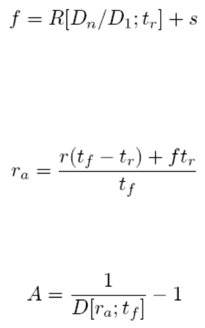
2 Market standards and calculations
2.3 Key-figures
138 © Wall Street Systems IPH AB - Confidential
2.3.4.8.7 Average (Simple)
The Average (Simple) risk profile is applicable to coupons based on interest rate averaged over a
period. The actual averaging expression is only used for the estimation of the current coupon
amount. Future coupons and risk are calculated using a simple generic approximation.
Input data used in calculations:
Coupon estimate
First, we calculate the estimated forward rate (f) for the remaining fixing period:
Equation 2-242 Average (Simple) estimated forward rate
where is the length of the remaining fixing period, and R[] is the function that converts the
discount factor into interest rate according to fixing type. Next, we calculate the expected fixing
rate, based on the rate known up to the valuation date (r) and the estimated forward rate f:
Equation 2-243 Average (Simple) fixing rate
Finally, the estimated amount is:
Equation 2-244 Average (Simple) estimated amount
where D[] is the function that converts interest rate into discount factor according to fixing type.
Coupon period length
Fixing period length
Spread
Compounded rate up to the valuation day
Discount factor for the payment date (from valuation and discount curves)
During the coupon period = 1, before coupon period discount factor for the start of
the coupon period (from estimation curve)
Discount factor for the end of the coupon period (from estimation curve)
tc
tf
s
r
Dp
D1
Dn
tr
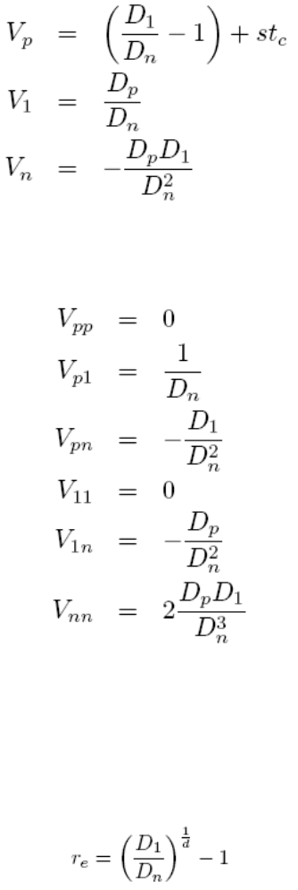
2 Market standards and calculations
2.3 Key-figures
Transaction & Risk Management Module (TRM) Instruments: Processing and Calculations 139
Valuation
Risk values per unit nominal amount are calculated as:
Equation 2-245 Average (Simple) risk values
Convexity matrix is:
Equation 2-246 Average (Simple) convexity matrix
2.3.4.8.8 Fed Fund
The Fed Fund risk profile corresponds to the coupon calculated from the average overnight rate over
the coupon period. This average is estimated by assuming that the overnight discount factor stays
constant over the coupon period, in which case, this rate can be calculated as follows:
Equation 2-247 Fed funds: Average overnight rate
where and are the discount factors for the start and end of the coupon period, and d is the
number of days in the period.
For the coupon with start date after the valuation date, the risk dates are payment date, coupon
start date (Since When), and coupon end date (Until When).
D1Dn
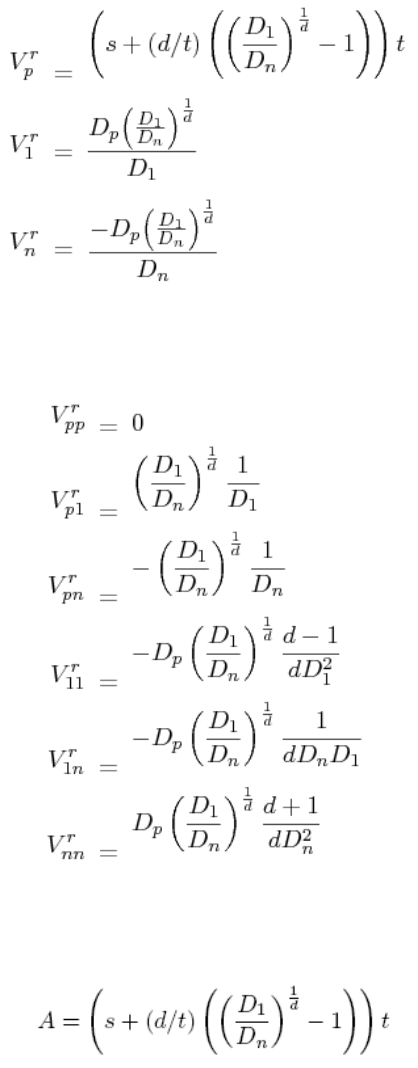
2 Market standards and calculations
2.3 Key-figures
140 © Wall Street Systems IPH AB - Confidential
Risk values:
Equation 2-248 Fed funds: Risk values
Convexity matrix
Equation 2-249 Fed funds: Convexity matrix
Estimated amount:
Equation 2-250 Fed Funds: estimated amount
where
tcCoupon period length
Discount factor for the coupon payment (from valuation and discount curves)
Discount factor for the start of the coupon period (from estimation curve)
Discount factor for the end of the coupon period (from estimation curve)
Dp
D1
Dn
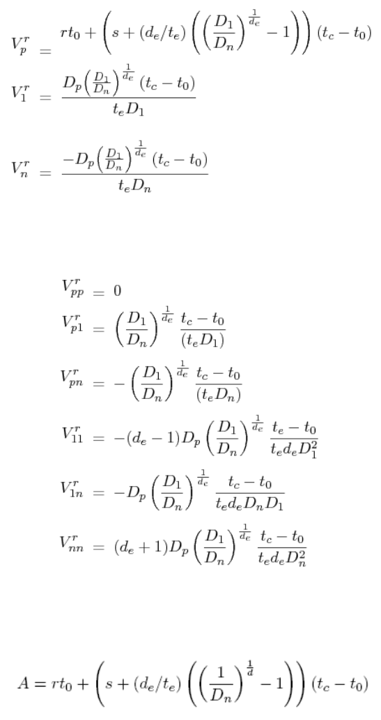
2 Market standards and calculations
2.3 Key-figures
Transaction & Risk Management Module (TRM) Instruments: Processing and Calculations 141
Running coupon
For the running coupon, we already know the average rate up to the valuation date. Let r be that
rate, and t0 the length of the known period, te the length of the remaining period, and de the
number of days in the remaining coupon period.
Risk values:
Equation 2-251 Fed Funds - running coupons: risk values
Convexity matrix:
Equation 2-252 Fed funds - running coupon: Convexity matrix
Estimated amount:
Equation 2-253 Fed Funds - running coupons: estimated amount
sSpread
dNumber of days in the coupon period.

2 Market standards and calculations
2.3 Key-figures
142 © Wall Street Systems IPH AB - Confidential
2.3.4.9 Duration figures
2.3.4.9.1 Duration
Duration is the mean maturity of money in a transaction. For a simple cashflow, the duration is
simply the maturity t of the cashflow. For transactions containing several cashflows, the duration is
considered as the weighted average maturity of each cashflow, with the weights, the present values
of the cashflows.
Equation 2-254 Key figures: Duration
Where
2.3.4.9.2 Duration (Days)
Duration (Days) is the Duration expressed in days. The Duration (Days) key figure is calculated as
follows:
Equation 2-255 Key figures: Duration (Days) calculation
Where
2.3.4.9.3 Effective Duration
Effective duration is the relative change of the present value of a position with respect to a change
to the interest rate. Thus, it can be represented as a relative figure of IR Exposure, based on the IR
exposure calculated with 1 bp (basis point):
Equation 2-256 Key figures: Effective Duration
Note: For a single bond evaluated with the par method and continuously compounded yield, the
effective duration is the same as the Macauley duration; for yearly compounded yield, the
effective duration is the same as the modified duration (see 2.3.4.9.5 Modified Duration on
page 145).
Present value of the cashflow i with .
Time to maturity of the cashflow i with .
UDuration
BThe date basis defined at the instrument level, for example, 365, 360, and so on,
U
ΣtiVi
ΣVi
-------------
=
Viti0>
titi0>
UDays()
UB×=
Ueff
10000 E×i1{}
Vp
-----------------------------------
–=
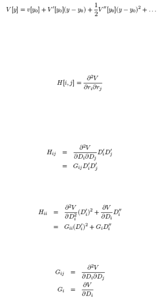
2 Market standards and calculations
2.3 Key-figures
Transaction & Risk Management Module (TRM) Instruments: Processing and Calculations 143
For a position with present value close to zero, the effective duration, as well as Duration and
Duration (Days), may be unstable (present value in the denominator). For example, if the present
value of the position changes from a small positive number to a small negative number, the
effective duration will change from a large positive number to a large negative number. (This
happens particularly when a bond has been bought but is still in the pending state: the settlement
amount belongs to the position and has a present value very close to the bond's present value.)
In fact, when present value is zero, effective duration would be infinite, and will therefore not be
shown.
2.3.4.9.4 Effective Convexity
Convexity is related to the second order term in the Taylor expansion of the value of an asset as a
function of yield:
Equation 2-257 Convexity
In this case, convexity is defined as
If instead of yield, we consider zero coupon valuation, there are several variables, and the second
order derivative becomes a matrix:
Equation 2-258
where are the zero rates taken into account in the valuation of the asset.
We want to use derivatives with respect to the discount factors , in which case
Equation 2-259
for off diagonal elements, and
Equation 2-260
Here we have written:
Equation 2-261
CV''/V=
ri
Diri
[]
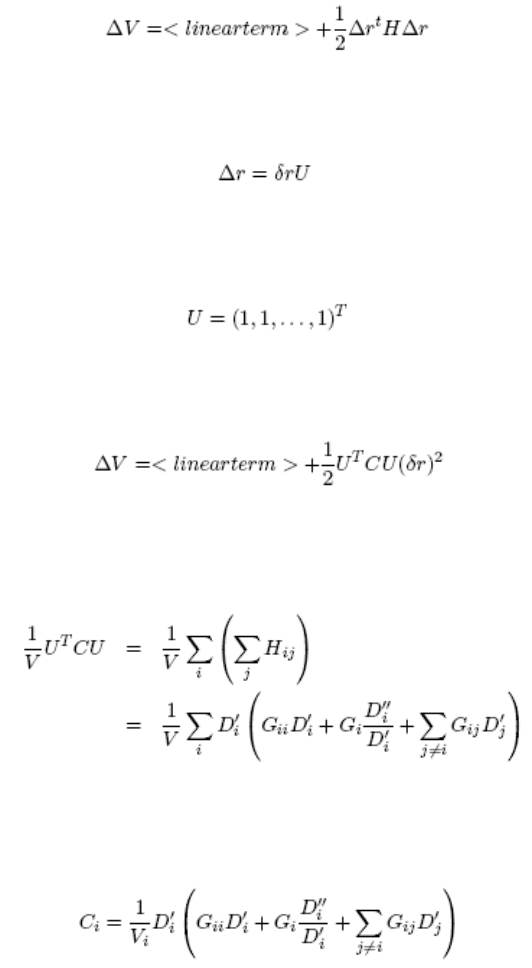
2 Market standards and calculations
2.3 Key-figures
144 © Wall Street Systems IPH AB - Confidential
for the part that is independent of the type of the interest rate and can therefore be calculated just
by knowing the discount factors.
Once we know the risk values and convexity matrix, we can estimate the change in the market
value due to a small change in the valuation curve by:
Equation 2-262 Duration figures - Effective Convexity: change in market value
Usually, we are interested only in the parallel shift, in which case
Equation 2-263 Duration figures - Effective Convexity: parallel shift
where
Equation 2-264 Duration figures - Effective Convexity: parallel shift
and
Equation 2-265 Duration figures - Effective Convexity: parallel shift
Effective convexity can now be defined as:
Equation 2-266 Duration figures - Effective Convexity
and the convexity term corresponding to an individual risk date is:
Equation 2-267 Duration figures - Effective Convexity: risk date
where is the present value of the ith cashflow.
Note that for an asset with fixed cashflows, the cross-derivatives are equal to zero when .
Δr
Vi
Hij ij≠

2 Market standards and calculations
2.3 Key-figures
Transaction & Risk Management Module (TRM) Instruments: Processing and Calculations 145
In this case we get:
Equation 2-268 Duration figures - Effective Convexity: asset with fixed cashflows
In particular, if the present value is calculated using yield-to-maturity method, i.e. if every cashflow
is discounted with the same yield , we obtain:
Equation 2-269 Duration figures - Effective Convexity: YTM method
2.3.4.9.5 Modified Duration
For on-balance instruments modified duration is a relative figure of the IR exposure (1 bp) of the
transaction based on the present value of the transaction. For off-balance instruments (as well as
for on-balance instruments during the settlement period), where the present value is close to zero
and not a good measure of risk taken, we substitute an estimate of the size of the underlying
position.
This estimate depends on the instrument type:
•FRA and MM future: Average of the absolute value of the present values of the risk values at
each end of the underlying contract period.
•Bond future: Average of the absolute values of the present value of the position cashflows and
the settlement cashflows of the underlying CTD bond.
•IR Swap: Average of the present values of the legs.
Example: Bond - Transaction/instrument grouping
If you group by transaction or by instrument in Treasury Monitor, modified duration is calculated as follows:
Equation 2-270 Grouping by transaction: modified duration calculation
Where
ym
Umod
10000 E i1{}
×
φVp
sett Vp
pos
+()×
-------------------------------------------------
=
The IR exposure to 1 bp change in the interest rate for the cashflows after the figure Spot Date
(i.e. excluding cashflows before or on the figure Spot Date).
The present value of the settlement cashflows after the figure Spot Date. The value date of the
settlement cashflows is the same as the transaction’s value date.
The present value of the position cashflows after the figure Spot Date. Position cashflows
correspond to all other cashflows, i.e. not settlement.
The average of the present value components. = 0.5 or 1 depending on the number of
present value components.
Note: For example, if you have a spot position, the only component is the present value of the
position cashflows and in this case = 1.
Eil{}
Vp
sett
Vp
pos
φφ
φ

2 Market standards and calculations
2.3 Key-figures
146 © Wall Street Systems IPH AB - Confidential
Note: Settlement cashflows are cashflows with the same date as the value; position cashflows
are all other cashflows.
The IR Exposure 1bp and the Present Value figures are calculated to Valuation Date.
Note: In the case of a partial forward sell or purchase of a position, you should group Instrument
and Liquidity Type (extended), and monitor the 'Committed' part. This excludes the
pending settlement that causes a jump in the present value weight at the instrument level.
Example: Bond - Total grouping
if you group by total in Treasury Monitor, modified duration is calculated as follows:
Equation 2-271 Grouping by total: modified duration calculation
where
Example: IR Swap - Transaction/instrument grouping
If you group by transaction or by instrument in Treasury Monitor, modified duration is calculated as
follows:
Equation 2-272 Modified Duration: IR Swap
Where
2.3.4.9.6 Effective Spread Duration
Equation 2-273 Key figures: Effective Spread Duration
where is the total spread IR exposure of the position and Vp is the total present value of the
position.
VpThe present value.
The IR exposure to 1 basis point (bp) change in the interest rate.
The IR exposure to 1 bp change in the interest rate for the cashflows after the figure Spot Date
(i.e. excluding cashflows before or on the figure Spot Date).
The present value of the cashflows of the first leg after the figure Spot Date.
The present value of the cashflows of the second leg after the figure Spot Date.
The average of the present value components.
Note: = 0.5, in the case of IR Swap as we have two present value components (one per leg).
Umod Ueff
Ei1{}
–
Vp
---------------
⎝⎠
⎛⎞
10000×==
Ei1{}
Umod
10000 E i1{}
×
φVp
leg1 Vp
leg2
+()×
----------------------------------------------------
=
Eil{}
Vp
leg1
Vp
leg2
φ
φ
Uμ
Eμ
Vp0.0001×
-----------------------------
=
Eμ

2 Market standards and calculations
2.3 Key-figures
Transaction & Risk Management Module (TRM) Instruments: Processing and Calculations 147
2.3.4.9.7 Effective Beta Duration
Effective beta duration (duration times spread or DTS) is effective spread duration scaled by
Z-spread. It gives the sensitivity to a relative change in spread, where spread duration is the
sensitivity to an absolute change in spread:
Equation 2-274 Key figures: Effective Beta Duration
See Risk method Z-Spread on page 123.
2.3.5 Dual currency
A dual currency cashflow is a cashflow where the actual payment is in a different currency to the
cashflow currency. The FX rate used in calculating the settlement amount may be fixed or floating.
The cashflow currency amount may also be fixed or floating. TRM supports the following three
cases:
•Fixed amount, fixed FX rate, see 2.3.5.1 Fixed amount, fixed FX rate on page 147.
•Fixed amount, floating FX rate, see 2.3.5.2 Fixed amount, floating FX rate on page 148.
•Floating amount, fixed FX rate, see 2.3.5.3 Floating amount, fixed FX rate on page 148.
The following sections describe how dual currency cashflows are valuated.
2.3.5.1 Fixed amount, fixed FX rate
In this case the payment amount is known, so that it can be treated the same way as any fixed
cashflow. The essential figures are:
•Settlement Amount As
As = ASs
where A is Amount, and Ss is Settlement FX Rate
•Figure Market Value
V = AsD/(SxS)
where Sx is the FX rate between cashflow currency and the settlement currency, S is Figure FX
Convert (between the cashflow currency and the figure currency) and D is the Figure Market
Value Discount Factor.
2.3.5.1.1 Example: Fixed amount, fixed FX rate
Let us consider the following cashflow and market data:
UβUμμz
×=
Name Symbol Value
Amount A7500.0
Settlement FX Rate Ss10.0
FX Rate Sx9.799
Figure FX Convert S1.2
Figure Market Value Discount Factor D0.9948283718493263

2 Market standards and calculations
2.3 Key-figures
148 © Wall Street Systems IPH AB - Confidential
Key figures are:
2.3.5.2 Fixed amount, floating FX rate
This case is a risk-wise equivalent to an ordinary single currency cashflow, except that Figure
Payment Amount has to be estimated:
•Payment Amount Apay
Apay = ASx
where A is Amount, and Sx is FX Rate between cashflow and settlement currencies (not shown in
Transaction Admin).
•Figure Market Value
Since the FX rate is floating, the market value (and risks) are the same as for a fixed cashflow in
the cashflow currency.
V = AD/S
where D is Figure Market Value Discount Factor (in the cashflow currency).
2.3.5.2.1 Example: Fixed amount, floating FX rate
Market data:
Key figures are:
2.3.5.3 Floating amount, fixed FX rate
In this case IR exposure is divided between the settlement and cashflow currencies, while FX
exxposure is in the cashflow currency.
•Payment Amount Ap is estimated using the risk profile defined for the instrument:
Ap = A[D1,D2,s]Ss
where D1 and D2 are the discount factors (in cashflow currency) for the start and end dates of the
interest period, s is the spread, and Ss is the Settlement FX Rate. Function A[] is the payment
amount estimation method provided by the risk profile.
•Figure Market Value is the estimated payment amount discounted and converted to the figure
currency.
Name Symbol Value
Settlement Amount Market Value As7500.0 × 10.0 = 75000.0
Market Value V75000.0 x 0.9948 / (9.799 x 1.2) = 6345:22
Name Symbol Value
Amount A1000000.0
FX Rate Sx9.799
Figure FX Convert S1.2
Figure Market Value Discount Factor D0.993433829648000
Name Symbol Value
Payment Amount Apay 1000000.0 × 9.799 = 9799000.0
Market Value V1000000.0 x 0.9934 / 1.2 = 827861.52

2 Market standards and calculations
2.4 Performance calculations
Transaction & Risk Management Module (TRM) Instruments: Processing and Calculations 149
V = ApayDpay/(SxS)
where Dp is the discount factor for payment date (in settlement currency).
2.3.5.3.1 Example: Floating amount, fixed FX rate
This example shows calculations with plain vanilla risk profile without spread.
Key figures are:
2.4 Performance calculations
Performance measurement is an area that has become increasingly important as clients of asset
managers have become more sophisticated and demanding. Portfolio managers are expected to
meet or beat a specified benchmark on a regular basis. In order to facilitate calculations and
comparisons of traded and benchmark portfolios, common standards have evolved, such as the
Performance Presentation Standards set up by the Association of Investment Management and
Research (AIMR-PPS). The performance measurement implemented in TRM in Performance Monitor is
based on these standards.
One objective of the performance measurement process is to calculate the performance of traded
portfolios and then compare it to the performance of selected benchmarks. In principle it is possible
to outperform the benchmark by (i) stock (bond) picking, in other words being over or under
exposed in a specific security relative to the benchmark and (ii) using leveraged instruments that
have different payoff profiles than the underlying cash (spot) instruments. Examples of leveraged
instruments include forwards, futures, and options.
The benchmark portfolios used for comparison against the traded portfolios consist of transactions
created from index compositions which represent the target performance for a portfolio. Risk, for
performance measurement, is the amount of deviation from the benchmark rather than absolute
changes in the portfolio market value. Treasury Monitor can be used to produce a key-figure level
analysis of the traded portfolio versus the benchmark.
Performance is measured by the time-weighted rate of return (TWR). TWR measures the change in
the value of a portfolio as a percentage of the capital that has actually been invested.
Name Symbol Value
Amount A1000000.0
FX Rate Sx9.799
Settlement FX Rate Ss10.0
Figure FX Convert S1.2
Figure Market Value Discount Factor D0.996858127940000
Figure Present Value Discount Factor (1) D10.999053805572000
Figure Present Value Discount Factor (2) D20.996858127940000
Figure Present Value Discount Factor (p) Dp0.996858127940000
Name Symbol Value
Payment Amount Apay 1000000.0 x (0.9991 / 0.9969 - 1) x 10.0 = 22025.98
Market Value V22025.98 x 0.9969 / (9.799 x 1.2) = 1867.26
2 Market standards and calculations
2.4 Performance calculations
150 © Wall Street Systems IPH AB - Confidential
2.4.1 Actual basis and all cash basis
The AIMR-PPS standards require that performance is measured on both an actual basis and an all
cash basis. Actual basis and all cash basis can be defined as follows:
•Actual basis measures the growth of the actual invested capital, in other words it is a
combination of both stock picking and leverage.
•All cash basis attempts to eliminate the effects of leverage by restating the position into an
equivalent cash position having the same market exposure (the spot equivalent position, SEP).
The all cash basis performance is then the performance measured on the restated cash
equivalent position.
If a fund is using leverage, the AIMR-PPS standards require the presentation of both actual and all
cash basis performance. Since the benchmark is normally non-levered, the comparison between the
benchmark and all cash basis show the stock picking ability of the fund manager whereas the
difference between the actual and the all cash basis performance indicate timely and efficient use of
leverage in managing the fund.
2.4.2 Trade date and value date based performance
Typically a cash (spot) transaction is committed on the trade date but physically delivered and paid
some days later on the value date. Clearly, a bought position is exposed to the market from trade
date but the market value during the period until value date depends on whether the trade or value
date approach is adopted. The two methods are defined as follows:
•With the trade date method, the market value on the trade date is equal to the value of the
position side of the transaction, and consequently, the cashflow term on the trade date is equal
to the settlement payment. Thus, the trade date method can be seen as trading with
immediately delivery and payment.
•With the value date method, the market value during the period between trade and value date is
the net value of the position and the settlement payment. On the value day the cashflow term is
equal to the settlement payment and the market value is equal to the value of the position side.
Traditional investment management has adopted the trade date approach, whereas the value date
approach is more prevalent among corporate treasuries. TRM supports both approaches. The default
is the trade date method. The AIMR-PPS standards stated that trade date valuation was required
after 1/1/2005.
2.4.2.1 Bank accounts
If the position includes bank accounts then buying a cash (spot) instrument is just a reallocation of
the needed cash from the bank account into the bought instrument. This should of course not cause
any jumps in the total market value of the position, neither should there be any cashflows in or out
of the aggregated position.
In value date based performance, the total market value does not show any jumps since the money
is physically drawn on the bank account the same day as the bought instrument takes on the full
un-netted market value. The cashflow into the instrument is balanced by the negative cashflow at
the bank account and thus on the aggregated level there are no cashflows in or out of the position.
Using trade date based performance the cashflows do not cancel each other out since the flow into
the instrument happens on the trade date whereas the physical out flow on the bank account is at
value date. Also the total market value jumps as an effect of the trade; at trade date the total value
increases due to the mismatch between the un-netted market value of the bought instrument and
the fact that the money is still in the bank account balance (and will earn interest) until the value
date.
The observed problem can be solved by including a fictitious bank account in the position. On the
calculated fictive account the settlements of bought (sold) instruments are drawn (deposited) at
trade date and subsequently reversed at value date. In this way, when buying (selling) an
instrument we get a negative (positive) cashflow at trade date in the fictitious bank account
balancing the cashflow into (out of) the instrument, and one positive (negative) cashflow at value
date in the fictitious account balancing the flow out of (into) the real bank account. The increase
(decrease) in the market value at instrument level is balanced by the negative (positive) balance in
2 Market standards and calculations
2.4 Performance calculations
Transaction & Risk Management Module (TRM) Instruments: Processing and Calculations 151
the fictitious account. On the aggregated position level, there are no cashflows and no jumps in the
market value, either at the trade date or the value date.
2.4.3 Time-weighted rate of return (TWR)
The ideal TWR index for the period 0 to T, with valuation whenever cashflows occur, is given by:
Equation 2-275
where
–l = {0, ..., L} is the time, in the period 0 to T, at which the cashflows occur
–MVl is the market value including accrued income but before any deposits/withdrawals
to/from the portfolio at time l
–Cl represents the cashflows (deposits, positive flow / withdrawals, negative flow) to/from the
portfolio at time l.
The definitions of the market values and the cashflow terms will depend on: (i) whether
performance is measured on the actual basis or the all cash basis, (ii) whether the trade date or
value date approach is used and (iii) the transaction type, for example whether it is a spot,
forward/future, option or composite instruments such as a swap.
The major drawback with the ideal TWR index is that it requires re-valuing the portfolio each time
there is a cash inflow or outflow. If the portfolio does not include the cash position then every
buy/sell creates a cashflow in/out of the portfolio. Thus, the portfolio has to be re-valued every time
a transaction takes place. This is neither feasible nor practical and thus the ideal TWR index is
normally approximated with the TWR daily sampled index:
Equation 2-276
where
–MVt is the market value including accrued income but before any deposits/withdrawals
to/from the portfolio on day t,
–Ct represents the sum of all cashflows (deposits, positive flow / withdrawals, negative flow)
to/from the portfolio during day t:
The Dietz method overcomes the need to know the valuation of the portfolio on the date of each
cashflow by assuming a constant rate of return on the portfolio during the period. The original Dietz
method assumed that all cashflows occurred at the midpoint of the period. The modified Dietz
PTWRT0,
MV1
MV0C0
+
-------------------------.... MVl1+
MVlCl
+
-----------------------.... ×MVL
MVL1–CL1–
+
--------------------------------------- MVT
MVLCL
+
--------------------------
××××=
PDailyT0,
MV1
MV0C0
+
-------------------------.... MVt1+
MVtCt
+
-----------------------.... ×MVT
MVT1–CT1–
+
---------------------------------------
×××=
CtCl
˜
l
˜t1–t {,}∈
∑
=
2 Market standards and calculations
2.4 Performance calculations
152 © Wall Street Systems IPH AB - Confidential
method weights each cashflow by the amount of time it is held in the portfolio. The modified Dietz
method for the period from 0 to T is given by:
Equation 2-277
where the weight factor Wl is the proportion of the period (from 0 to T) that the cashflow Cl has been
in/out of the portfolio:
The original Dietz method is obtained by setting the weight Wl = 1/2, for all l.
The AIMR-PPS standards currently require that portfolio performance is evaluated using TWR
calculations at least quarterly and these interim returns are geometrically linked. From 1/1/2001
(periods from that date), monthly valuations are required. The AIMR accept approximation methods
such as the modified Dietz method.
2.4.3.1 Percentage growth from the TWR index
Assuming positive market values, the percentage growth (return) during day t is given by:
Equation 2-278
Similarly for the whole period from 0 to T the percentage growth is:
Equation 2-279
2.4.3.2 TWR calculations in TRM
In order to calculate daily return in TRM, the intraday Dietz returns are first calculated. Then, the
intraday Dietz returns are geometrically linked as a Time-Weighted Return Index: the product of the
Dietz returns allows for transitions from a short/long position to a long/short position in period 0 to
T. Finally, the daily return in TRM is derived as the growth from the TWR Index between time t and
t-1.
PDietzT0,
MVTWl1–()Cl
l0=
L
∑
+
MV0WlCl
l0=
L
∑
+
-------------------------------------------------------
=
Wl
Tl–
T
-----------
=
PTWRtt 1–,
%PTWRtt 1–,1–()100×=
PTWRT0,
%PTWRT0,1–()100×=
2 Market standards and calculations
2.4 Performance calculations
Transaction & Risk Management Module (TRM) Instruments: Processing and Calculations 153
2.4.3.2.1 Intraday Dietz returns
Due to the problems of determining the exact time of each intra-day cashflow to calculate the
intra-day performance, we assume a constant cashflow weighted by factor W. The intraday Dietz
return is then given by:
Equation 2-280
where
–U is the position and u an instrument in that position,
–MVt(u) is the market value of the instrument u at time t including cashflows during the
period t-1 to t (one day),
–Ct(u) is the sum of all cashflows in (positive flow) / out (negative flow) to/from the
instrument u during the period t-1 to t:
–W is the constant weight factor applied to the sum of the cashflows (not the individual
cashflows) giving the proportion of the day the intra-day cashflows are assumed to have
been in or out of the position. With w = 1, 1/2, or 0, all cashflows are assumed to take place
at the beginning, middle or end of the day, respectively.
2.4.3.2.2 Geometric linking of intraday Dietz returns
These intraday returns can then be geometrically linked as a Time-Weighted Return Index to
provide PDietzT,0 for the period from 0 to T. This method allows for transitions from a short/long
position to a long/short position in the period 0 to T. With this method, each transition is assumed to
occur at the end of a day.
The M (end day) transition points are collected in the set A:
Equation 2-281
where the variables are as described for Equation 2-280 on page 153 and A(m) is the mth transition
from long/short to short/long (m=1,...,M).
The return for a long sub-period [A(m), A(m+1)] is given by:
Equation 2-282
and for a short sub-period:
Equation 2-283
PDietztt 1–,
MVtu()
uU∈
∑W1–()Ctu()
uU∈
∑
+
MVt1–u()
uU∈
∑WCtu()
uU∈
∑
+
----------------------------------------------------------------------------------
=
Ctu() Cl
˜u()
l
˜t-1 t {,}∈
∑
=
At: sign MV
tu()
uU∈
∑W1–()Ct1–u()
uU∈
∑
+
⎝⎠
⎜⎟
⎛⎞
sign MVtu()
uU∈
∑WCtu()
uU∈
∑
+
⎝⎠
⎜⎟
⎛⎞
≠t=1,..,T{,}=
PFK_TWR A m()Am 1+()[, ]
U() PDietztt 1–,U()
tAm()+1=
Am+1()
∏
=
2 Market standards and calculations
2.4 Performance calculations
154 © Wall Street Systems IPH AB - Confidential
The combined return index for the whole period from 0 to T, assuming A(0)=0 and A(M+1)=T, is
given by the following:
Equation 2-284
where
is given by either
if
or
if
2.4.3.2.3 TRM Return as the percentage growth of the TWR Index
Finally, the return during day t is given by:
Equation 2-285 TRM Return as the percentage growth of the TWR Index
2.4.4 Money-weighted return
Given a portfolio with initial market value V0, cashflows ci on dates ti, and final market value VT at
time T, money weighted return, or internal rate of return (y), is defined as the constant interest rate
PshortFK_TWR A m()Am 1+()[, ]
U() 2P
Dietztt 1–,U()
tAm()+1=
Am+1()
∏
–=
PFK_TWR T 0[,]U() P
˜FK_TWR A m()Am 1+()[, ]
U()
m0=
M
∏
=
P
˜FK_TWR A m()Am 1+()[, ]
U()
PFK_TWR A m()Am 1+()[, ]
U()
sign PFK_TWR A m()0[,]
U()()sign MVAm()
u()
uU∈
∑WCAm()
u()
uU∈
∑
+
⎝⎠
⎜⎟
⎛⎞
=
PshortFK_TWR A m()Am 1+()[, ]
U()
sign PFK_TWR A m()0[,]
U()()sign MVAm()
u()
uU∈
∑WCAm()
u()
uU∈
∑
+
⎝⎠
⎜⎟
⎛⎞
≠
PTWRtt 1–,
%PTWRtt 1–,1–()100×=
2 Market standards and calculations
2.4 Performance calculations
Transaction & Risk Management Module (TRM) Instruments: Processing and Calculations 155
such that the total of the initial value and all cashflows prolonged to time T with y is equal to the
final value:
Equation 2-286
If the type of the interest rate is compounded (at any frequency), it is possible to choose to discount
all cashflows to the start date, or any other date for that matter, and obtain the same result.
Periodic rate and discount rate will usually provide different results depending on the valuation date.
2.4.4.1 Periodic Rate
If we use interest type Periodic Rate and prolong to the end date of the observation period, the
above equation can be solved without iteration:
Equation 2-287
2.4.5 Instrument market values for third currency
The saved Performance Data (Market Value) of a Portfolio is based on Treasury Monitor's market
value calculation. This performance data is saved by running the Performance Data Calculation
activity.
The Performance Data Calculation activity saves the home currency market value and the local
market value as they are calculated by Treasury Monitor.
Equation 2-288 Home currency market value and local currency market value
where
V0
DyT,()
------------------ci
DyT t
i
–(, )
--------------------------VT0=–
i
∑
+
V01yT+()ci1yTt
i))–V
T0=–(+(
i
∑
+
VTV0
–ΣciyV
0Tc
iTt
i)–(
i
∑
+
⎝⎠
⎜⎟
⎛⎞
=–
yVTV0
–Σci
–
V0TΣiciTt
i)–(+
---------------------------------------------
=
The saved performance data (market value)
The FX conversion from the transaction's Trading Currency (for example GBP) into
the chosen Figure Currency (for example, EUR or USD) depends on the FX method
that is defined at the instrument level (Instrument Editor - Base Valuation page).
See A.2.50 Base Valuation Setup on page 734.
FX method calculations are described in section 2.1.6.3 FX rate calculation on
page 79.
LocalCCY The transaction currency
HomeCCY The currency in which the Performance Data Calculation activity was run.
VHomeCCY VLocalCCY S×v LocalCCY HomeCCY⁄{}
=
VHomeCCY
Sv
2 Market standards and calculations
2.4 Performance calculations
156 © Wall Street Systems IPH AB - Confidential
2.4.5.1 Converting the portfolio home currency into figure currency
By default, the Performance Monitor's market value is calculated and stored in the portfolio trading
currency. Therefore, in order to display the market value in a third currency (i.e. in a figure currency
other than the portfolio trading currency) the Performance Monitor converts the home currency
market value into the third currency using the FX spot rate.
Note: If you want to avoid the FX spot conversion and use the figure currency data that is
calculated in the same way as in the Treasury Monitor, see 2.4.5.2 Figure currency based
on Treasury Monitor's market value calculation on page 156.
To convert the portfolio home currency into the figure currency you use the Performance Data
Calculation activity as follows:
To display the market value in a third currency in the FX Spot Rate figure, the Performance Monitor
converts the home currency market value to the third currency.
Equation 2-289 Home currency market value and local currency market value
where
Note: Only one home currency market value is saved at a time. When you run the activity again,
the previous market value is replaced with the new one.
2.4.5.2 Figure currency based on Treasury Monitor's market value calculation
The Performance Monitor's market value can also be directly expressed (i.e. without an FX spot
conversion as detailed in 2.4.5.1 Converting the portfolio home currency into figure currency on
page 156) in a third currency i.e. in a figure currency other than the portfolio trading currency.
In this case, like in the Treasury Monitor, the FX conversion of the transaction's cashflow currency
(for example GBP) into the chosen figure currency (for example, EUR or USD) depends on the FX
Method set up in the Instrument Editor in the Base Valuation page (Base Valuation Setup feature). The FX
methods can be:
•Spot Rate
•Today's Rate (Forward points)
•Today's Rate (IR Differential)
See A.2.50 Base Valuation Setup on page 734 for more information.
Field Description
Top Portfolio To Process Name of the top portfolio. The activity saves the home currency market value in
the portfolio base currency. This is the default behavior if nothing is set in the
Figure Currency field.
Figure Currency Leave this field empty to save the home currency market value in the portfolio
base currency.
SThe FX Spot.
VThirdCCY VHomeCCY SHomeCCY ThirdCCY⁄{}
×=
2 Market standards and calculations
2.4 Performance calculations
Transaction & Risk Management Module (TRM) Instruments: Processing and Calculations 157
To convert the portfolio home currency directly into the figure currency you use the Performance Data
Calculation activity as follows:
For example, if you run the Performance Data Calculation activity with a top portfolio base currency of
USD and nothing in the Figure Currency field, and then you run the activity again with Figure Currency
= EUR, the activity will store both the USD home currency market value and the EUR home currency
market value in the database.
2.4.5.3 Examples
The following the examples illustrate the different FX method calculations for a transaction of
100000000 GBP using the following data:
2.4.5.3.1 FX Method = Spot Rate (Default)
This example illustrates two scenarios, one with the Top Portfolio and one with the Portfolio using
the Spot Rate method. The Today' s Rate (Forward Points) method is very similar to the Spot Rate
method and is not described separately.
Note: For the trading of futures, you need to specify a cost of carry instrument at the portfolio
level.
Scenario 1: The activity is run for the Top Portfolio in USD
When the Performance Data Calculation activity is run on the Top Portfolio with a different base
currency to the Trading Portfolio's, the Market Value is saved in the Top Portfolio currency and over
the previously saved market value for the trading currency is overridden.
Equation 2-290 Example - Spot Rate equation
Equation 2-291 Example - Spot Rate
Equation 2-292 Example - Spot Rate: Top Currency calculation
Field Description
Top Portfolio To Process Name of the top portfolio. The activity saves the home currency market value in
the portfolio base currency. This is the default behavior if nothing is set in the
Figure Currency field.
Figure Currency The activity saves the home currency market value in the selected figure currency.
Data Example
Top Portfolio base currency USD
Trading Portfolio base currency EUR
Transaction currency GBP
VHomeCCY VLocalCCY
1
SLocalCCY HomeCCY⁄{}
------------------------------------------------------
×=
SGBP USD⁄{}
1.50=
VTopHomeCCY 100000000 1.50×USD150000000==
2 Market standards and calculations
2.4 Performance calculations
158 © Wall Street Systems IPH AB - Confidential
Furthermore, in Performance Monitor, when the user selects both the Top and the Trading Portfolios,
the stored Market Value in the Top Portfolio currency (USD) is converted to the Trading Portfolio
currency (EUR) using the FX Spot Rate. The third currency is calculated as follows:
Equation 2-293 Example - Spot Rate: Third Currency equation
Equation 2-294 Example - Spot Rate
Equation 2-295 Example - Spot Rate: Third Currency conversion
Scenario 2 The activity is run for the trading portfolio in EUR
When the activity is run for the Trading Portfolio the following calculations are done:
Equation 2-296 Example - Spot Rate: Trading Portfolio equation
Equation 2-297 Example - Spot Rate: Trading Portfolio FX Spot
Equation 2-298 Example - Spot Rate: Trading Portfolio Currency conversion
Furthermore, in Performance Monitor, when the user selects both the Top and the Trading Portfolios,
the stored Market Value in the Trading Portfolio currency (EUR) is converted to the Top Portfolio
currency (USD) using the FX Spot Rate. The third currency is calculated as follows:
Equation 2-299 Example - Spot Rate: Trading Portfolio Third Currency equation
Equation 2-300 Example - Spot Rate: Trading Portfolio
Equation 2-301 Example - Spot Rate: Trading Portfolio Third Currency conversion
VThirdCCY VHomeCCY
1
SThirdCCY HomeCCY⁄{}
------------------------------------------------------
×=
SEUR USD⁄{}
1.20=
VThirdCCY 150000000 1
1.20
----------
×EUR125000000==
VHomeCCY VLocalCCY S×v LocalCCY HomeCCY⁄{}
=
SGBP EUR⁄{}
1.25=
VTopHomeCCY 100000000 1.25×EUR125000000==
VThirdCCY VHomeCCY SHomeCCY ThirdCCY⁄{}
×=
SEUR USD⁄{}
1.20=
VThirdCCY 125000000 1.20×USD150000000==
2 Market standards and calculations
2.4 Performance calculations
Transaction & Risk Management Module (TRM) Instruments: Processing and Calculations 159
2.4.5.3.2 FX Method = Today' s Rate (IR Differential)
Scenario 1: The activity is run for the Top Portfolio in USD
Equation 2-302 Example - Today' s Rate (IR Differential) Top Portfolio equation
Equation 2-303 Example - Today' s Rate (IR Differential) Top Portfolio currency conversion
Equation 2-304 Example - Today' s Rate (IR Differential) Top Portfolio
Furthermore, in Performance Monitor, when the user selects both the Top and the Trading Portfolios,
the stored Market Value in the Top Portfolio currency (USD) is converted to the Trading Portfolio
currency (EUR) using the FX Spot Rate. The third currency is calculated as follows:
Equation 2-305 Example - Today' s Rate (IR Differential) Top Portfolio: Third Currency equation
Equation 2-306 Example - Today' s Rate (IR Differential) Top Portfolio: FX Spot
Equation 2-307 Example - Today' s Rate (IR Differential) Top Portfolio: Third Currency conversion
Scenario 2: The activity is run for the Trading Portfolio in EUR
Equation 2-308 Example - Today' s Rate (IR Differential): Trading Portfolio equation
Equation 2-309 Example - Today' s Rate (IR Differential): Trading Portfolio FX Spot
Equation 2-310 Example - Today' s Rate (IR Differential): Trading Portfolio Currency conversion
VHomeCCY VLocalCCY S×v LocalCCY HomeCCY⁄{}
=
SvGBP USD⁄{}
1.49983775759643=
VTopHomeCCY 100000000 1.49983775759×USD149983775.76==
VThirdCCY VHomeCCY
1
SThirdCCY HomeCCY⁄{}
------------------------------------------------------
×=
SEUR USD⁄{}
1.20=
VThirdCCY 149983775.76 1
1.2
-------
×EUR124986479.80==
VHomeCCY VLocalCCY S×vLocalCCYHomeCCY⁄{}
=
SvGBPEUR⁄{}
1.24988909927463=
VTradingCCY 100000000 1.24988909927×EUR124988909.93==
2 Market standards and calculations
2.4 Performance calculations
160 © Wall Street Systems IPH AB - Confidential
Furthermore, in Performance Monitor, when the user selects both the Top and the Trading Portfolios,
the stored Market Value in the Trading Portfolio currency (EUR) is converted to the Top Portfolio
currency (USD) using the FX Spot Rate. The third currency is calculated as follows:
Equation 2-311 Example - Spot Rate: Trading Portfolio Third Currency equation
Equation 2-312 Example - Spot Rate: Trading Portfolio
Equation 2-313 Example - Spot Rate: Trading Portfolio Third Currency conversion
2.4.6 Instrument market values and cashflows
2.4.6.1 Spot instruments
Spot instruments are un-leveraged instruments and therefore performance measurement based on
actual basis and all cash basis will be identical for those instruments. For the actual basis approach,
the selected trade or value date method defined for the instrument will determine the market values
and cashflows terms. For the all cash basis approach, the trade date values are used.
2.4.6.2 Forward/future instruments
For forward and future instruments the delivery price is typically set such that the contract cost
nothing to enter. The payoff function is linear since a 1 unit increase (decrease) in the unit forward
price implies a 1 unit increase (decrease) in the market value of the (long) forward/future contract.
However, since no initial investment is required the instrument has a leveraged percentage payoff
compared with an equivalent spot position.
As an example, consider a forward contract with delivery price 90, forward price 100 and thus a
market value of 10. If the forward price increases by 1 unit to 101 then the market value of the
forward also increases by 1 unit to 11 leading to a percentages return of (11/10 -1) 10%. The
percentages return on the spot position is around (101/100 - 1) 1% and thus the forward position
can be regarded as geared 10 times compared to the spot position.
The market value at time t of a forward contract is given by:
Equation 2-314
where
Ft is the forward price at time t, K is the delivery price and #unit is the contract size. The
sensitivity with respect to the spot rate St is given by:
Equation 2-315
where we have used the arbitrage free relation between the spot and forward rates expressed by
the discount factor D(t,T) for the period between t and the maturity of the contract T.
VThirdCCY VHomeCCY SHomeCCY ThirdCCY⁄{}
×=
SEUR USD⁄{}
1.20=
VThirdCCY 124988909.93 1.20×USD149986691.91==
MVtFt#unit K #unit×–×=
MVt
∂
St
∂
--------------Ft#×unit()∂
St
∂
-------------------------------- StDtT( , ) #unit××()∂
St
∂
------------------------------------------------------ DtT( , ) #unit×===
2 Market standards and calculations
2.4 Performance calculations
Transaction & Risk Management Module (TRM) Instruments: Processing and Calculations 161
The spot equivalent position, SEP (used for the all cash basis approach to performance
measurement) should have the same market exposure as the forward.
Therefore:
Equation 2-316
The market value of the spot equivalent position MVSEPt is given by the value of the position side of
the forward/future transaction.
The market values and cashflow terms for the two performance methods are:
•Actual basis: The performance should measure the growth of the actual invested capital, in
other words the market value is MVt given by Equation 2-314 on page 161. If the transaction
has a cash settlement then the cashflow term at value date is equal to the settled cash amount.
If the transaction results in delivery of the underlying, then this is handled as a spot transaction
committed at the notification date.
•All cash basis: The effect of the used leveraged should be eliminated by restating the position
into a spot equivalent one, in other words the market value is given by MVSEPt in Equation 2-316
on page 161. The cashflow term at trade date should be equal to the cash needed to buy the
spot equivalent position:
Equation 2-317
The periodical fixing of futures will cause the period market value change to be realized. From a
performance perspective this is equivalent to selling/buying market value and thus the cashflow
term will balance the change in market value such that the performance is unaffected by the
mark-to-market process.
2.4.6.3 Option instruments
There is a large variety of different option contracts in the market which have a non-linear payoff
function with respect to the price of some underlying instrument. One option position and one spot
position requiring the same initial investment will certainly have very different percentages returns.
Typically, the return of the option position will have larger volatility than the return of the spot
position. In this sense the option position is a leveraged position.
First we assume an option valuation model, in TRM it is the Black-Scholes model, linking the
theoretical unit value of the option f and the spot rate of the underlying instrument St:
Equation 2-318
The sensitivity of the option position is then given by:
Equation 2-319
where the partial derivative using the Black-Scholes model is delta, a risk key-figure. The spot
equivalent position (SEP) should have the same instantaneous market exposure as the option
position.
Therefore:
Equation 2-320
MVSEPt
∂
St
∂
-----------------------DtT( , ) #unit×=MV
SEPt StDtT(, ) #unit×× Ft#unit()×==→
C0MVSEP0 F0#×unit K #×unit===
MVtfS
tt ....,,()=
MVt
∂
St
∂
--------------fS
tt ....,,()()∂
St
∂
--------------------------------- #unit× ΔStt ....,,()#unit×==
2 Market standards and calculations
2.4 Performance calculations
162 © Wall Street Systems IPH AB - Confidential
Thus, the SEP position is equal to:
units of the underlying instrument. The delta typically varies over the life of the option and thus the
unit size of the SEP position is not constant over time.
From the above analysis the following definitions follow:
•Actual basis: The performance should measure the growth of the actual invested capital, in
other words the market value is MVt given by Equation 2-318 on page 162. If the transaction
has a cash settlement then the cashflow term at value date is equal to the settled cash amount.
If the transaction results in delivery of the underlying, then this is handled as a spot transaction
committed at the exercise date.
•All cash basis: The effect of the used leveraged should be eliminated by restating the position
into a spot equivalent one, in other words the market value is given by MVSEPt in Equation 2-320
on page 162. The cashflow term at trade date should be equal to the cash needed to buy the
spot equivalent position:
Equation 2-321
where
S0 and
are the spot rate and delta, respectively, at the time the position was committed. The unit size
of the SEP position may vary with time: increases can be regarded as more units being bought
and decreases as some units being sold. Thus, from a performance perspective the result is a
re-balancing cashflow of:
Equation 2-322
2.4.6.4 Swaps and other composite instruments
Swaps and composite instruments such as buy/sell back repos are essentially a combination of other
instruments. In general the actual basis approach treats the composite as a separate instrument
whereas the all cash basis approach handles the components of the composite as separate
transactions. For example, when using the actual basis the market value of a regular interest rate
swap is the net value of the receiving and the paying leg. For the all cash basis however the swap is
regarded as one long spot position in the receiving leg and one short spot position in the paying leg.
2.4.7 Example portfolio
As an example portfolio we will use a cash position together with a spot and forward position in the
same instrument. The initial cash position is 100. On day 1 we first commit one spot transaction of 1
unit at the price 50 for delivery at day 3. Secondly we commit a one month forward transaction of 1
unit at the delivery price 50.5. The market rates used are given in the table below. The overnight
balance on the bank account will earn the constant O/N interest rate of 0.1%.
MVSEPt
∂
St
∂
-----------------------ΔStt ....,,()#unit×=MV
SEPt StΔStt ....,,()#unit××=→
ΔStt ....,,()#unit×
C0MVSEP0 S0ΔS00 ....,,()#unit××==
ΔS00 ....,,()
CtStΔStt ....,,()ΔSt1–t1– ....,,()–()×#unit×=
Day Spot Rate Forward Rate O/N Interest Rate
0 50 50.5 0.1%
1 51 51.5 0.1%
2 Market standards and calculations
2.4 Performance calculations
Transaction & Risk Management Module (TRM) Instruments: Processing and Calculations 163
2.4.7.1 Actual basis performance with value date method
The market values and the cashflow terms have been calculated according to the value date version
of the actual basis performance method (see table below). Day 3 is the value date of the spot
transaction and it can be seen that the instrument level cashflow of 50 is balanced by the bank
account cashflow of -50 such that no cashflows occur at the aggregated (portfolio) level.
On the portfolio level the performance (see Equation 2-280 on page 153 and Equation 2-279 on
page 152) is given by:
Thus the growth of the invested capital has been 18.60% over the period.
The spot instrument level performance with the weight factor W set to 1 is given by:
The high period performance is more or less due only to the 100% return of day 2 (the infinite
performance of the first day is skipped by setting 1/0 = 1). The high return on day 2 is a
consequence of using the value date method - the market value of the position side and the
2 52 52.5 0.1%
3 53 53.5 0.1%
4 54 54.5 0.1%
5 55 55.5 0.1%
6 56 56.5 0.1%
7 57 57.5 0.1%
8 58 58.5 0.1%
9 59 59.5 0.1%
Day Spot Rate Forward Rate O/N Interest Rate
Day Spot Forward Bank Account Portfolio
Market
Value
Cash
flow
Market
Value
Cash
flow
Market
Value
Cash
flow
Market
Value
Cash
flow
0 0 0 0 0 100 0 100 0
1 1 0 1 0 100.10 0 102.1 0
2 2 0 2 0 100.20 0 104.2 0
3 53 50 3 0 50.30 -50 106.3 0
4 54 0 4 0 50.35 0 108.35 0
5 55 0 5 0 50.40 0 110.40 0
6 56 0 6 0 50.45 0 112.45 0
7 57 0 7 0 50.50 0 114.50 0
8 58 0 8 0 50.55 0 116.55 0
9 59 0 9 0 50.60 0 118.60 0
PDietz90,
102.1
100
------------- 104.2
102.1
------------- 106.3
104.2
-------------
×× 108.35
106.3
----------------
×110.40
108.35
----------------
×112.45
110.40
----------------
×114.50
112.45
----------------
×116.55
114.50
----------------
×118.60
116.55
----------------
×=
118.60
100
---------------- 1.1860==P
Dietz90,
%PDietz90,1–()100 18.60%=×=→

2 Market standards and calculations
2.4 Performance calculations
164 © Wall Street Systems IPH AB - Confidential
payment side of the transaction is netted between trade date and value date. This gives a distorted
instrument level performance that is not easily interpreted.
2.4.7.2 Actual Basis Performance with Trade Date Method
The market values and the cashflow terms have been calculated according to the trade date version
of the actual basis performance method (see table below). On day 1 the spot transaction is
committed and thus we have a cashflow of 50 at the instrument level. In the table we can see that
this cashflow is balanced by the negative cashflow of -50 in the calculated fictive bank account called
Settlement. We also notice that the market value at spot instrument level from trade to value date
is matched by the negative balance in the fictive bank account, such that the market value at
portfolio level is the same as for the value date version of actual basis shown above.
On the portfolio level the performance is the same as calculated for the value date method, 18.60%.
The performance at the spot instrument level with the weight factor W set to 1 is now given by:
showing that the instrument level performance is both stable and connected to the underlying rate
change. In this example the spot rate percentages return is also 18% and thus the match is exact.
With more buys and sells creating more cashflows in and out the match will not be 100%, still the
connection is very strong. The performance attribution analysis of the selection effect have to be
based on the trade date version and not on the value date version since the latter one is distorted by
the trading in the instrument.
The performance of the forward instrument is given by:
PDietz90,
1
0
---2
1
---53
250+
---------------
×× 54
53
------
×55
54
------
×56
55
------
×57
56
------
×58
57
------
×59
58
------
×2.2692
PDietz90,
%PDietz90,1–()100 ×126.92%==→
==
Day Spot Forward Bank Account Settlement Portfolio
Market
Value
Cash
flow
Market
Value
Cash
flow
Market
Value
Cash
flow
Market
Value
Cash
flow
Market
Value
Cash
flow
0 0 0 0 0 100 0 0 0 100 0
1 51 50 1 0 100.10 0 -50 -50 102.1 0
2 52 0 2 0 100.20 0 -50 0 104.2 0
3 53 0 3 0 50.30 -50 0 50 106.3 0
4 54 0 4 0 50.35 0 0 0 108.35 0
5 55 0 5 0 50.40 0 0 0 110.40 0
6 56 0 6 0 50.45 0 0 0 112.45 0
7 57 0 7 0 50.50 0 0 0 114.50 0
8 58 0 8 0 50.55 0 0 0 116.55 0
9 59 0 9 0 50.60 0 0 0 118.60 0
PDietz90,
51
050+
---------------52
51
------53
52
------
×× 54
53
------
×55
54
------
×56
55
------
×57
56
------
×58
57
------
×59
58
------
×1.18 PDietz90,
%18%=→==
PDietz90,
1
0
---2
1
---3
2
---
×× 4
3
---
×5
4
---
×6
5
---
×7
6
---
×8
7
---
×9
8
---
×9.00 PDietz90,
%800%=→==
2 Market standards and calculations
2.4 Performance calculations
Transaction & Risk Management Module (TRM) Instruments: Processing and Calculations 165
Skipping day 0 (setting 1/0 = 1), the return of the forward was 800%. In comparison to the return
on the spot position of 18%, the forward is clearly a leveraged instrument.
2.4.7.3 All cash basis performance (trade date only)
The market values and the cashflow terms have been calculated according to the all cash basis
performance method (see table below). With this method, all spot transactions are handled
according to the trade date version. The figures for the spot transaction in the table below are
therefore the same as for the actual basis performance with trade date method (previous page). The
differences in the rest of the table are due to the fact that the forward position has been restated
into the spot equivalent position (SEP) using the definition in 2.4.6.2 Forward/future instruments on
page 160 (Equation 2-316 on page 161).
On the forward instrument level the performance (W = 1) is now given by:
It can be seen that the all cash basis performance for the forward instrument is very similar to the
18% return on the spot position.
The use of forwards and futures gives the fund manager the possibility to gear the portfolio. In other
words, they can take on more market exposure than there is cash in the portfolio to buy. In this
sense the fund manager borrows money from the market. This implicit borrowing of the fund is
represented at the aggregated portfolio level by a cashflow into the fund at the trade date of the
forward / future. In the table above this can be seen as a cashflow of 50.5 on day 1 at the portfolio
level.
The all cash basis performance on the total portfolio level is given by:
Note that the capital base of the fund was not fully invested; there was about 50 money that could
have been invested in the spot instrument for example. If so, the all cash basis performance at the
portfolio level would have been around 18%.
Day Spot Forward Bank Account Settlement Portfolio
Market
Value
Cash
flow
Market
Value
Cash
flow
Market
Value
Cash
flow
Market
Value
Cash
flow
Market
Value
Cash
flow
00 0 0 0 100 0 0 0 100 0
1 51 50 51.50 50.5 100.10 0 -50 -50 152.60 50.5
2 52 0 52.50 0 100.20 0 -50 0 154.70 0
3 53 0 53.50 0 50.30 -50 0 50 156.80 0
4 54 0 54.50 0 50.35 0 0 0 158.85 0
5 55 0 55.50 0 50.40 0 0 0 160.90 0
6 56 0 56.50 0 50.45 0 0 0 162.95 0
7 57 0 57.50 0 50.50 0 0 0 165.00 0
8 58 0 58.50 0 50.55 0 0 0 167.05 0
9 59 0 59.50 0 50.60 0 0 0 169.10 0
PDietz90,
51
0 50.5+
------------------- 52.5
51.5
---------- 53.5
52.5
----------
×× 54.5
53.5
----------
×55.5
54.5
----------
×56.5
55.5
----------
×
·57.5
56.5
----------
×58.5
57.5
----------
×59.5
58.5
----------
×1.1782
PDietz90,
%17.82%=→
==
2 Market standards and calculations
2.4 Performance calculations
166 © Wall Street Systems IPH AB - Confidential
2.4.8 Risk-adjusted returns
TRM produces risk-adjusted return figures in Performance Monitor. This allows you to measure the
performance of your portfolio in relation to the amount of risk taken.
Throughout this section a simplified notation for the time weighted rate of return (TWR) is used. The
linked intraday Dietz returns used as TWR figures in TRM, defined in Equation 2-284 on page 154
as:
will here be denoted simply as:
2.4.8.1 Sampling frequency
As described in 2.4.3.2 TWR calculations in TRM on page 152, the time-weighted rate of return
(TWR) in TRM is calculated from the intraday Dietz returns, based on daily market values and
cashflows. These returns are then geometrically linked to calculate the TWR for longer periods. Due
to the method of linking, it is generally not possible to calculate the TWR of a sub-period directly
from the sub-period market values and cashflows. The sub-period (from b to a, b ≥ a) TWR of a
portfolio P is instead given by the following equation:
Equation 2-323
where
TWRx,0(P) is the cumulative performance, from time 0 to x (a or b) of the portfolio P based on
intraday Dietz returns.
2.4.8.1.1 Sub-period return
The periodic return (%) of the sub-period is:
Equation 2-324
The continuously compounded return (%) for the sub-period is:
Equation 2-325
PDietz90,
152.6
100 50.5+
------------------------- 154.7
152.6
------------- 156.8
154.7
-------------
×× 158.85
156.8
----------------
×160.9
158.85
----------------
×162.95
160.9
----------------
×165
162.95
----------------
×167.05
165
----------------
×169.1
167.05
----------------
1.1236=
×
PDietz90,
%12.36%=→
=
PFK_TWR T 0[,]U()
TWRT0,P()
TWRba,P() TWRb0,P()
TWRa0,P()
-----------------------------
=
Rperiodic b a,()
P() 100 TWRba,P() 1–()×=
Rcont b a,()
P() 100 TWRba,P()()ln×=
2 Market standards and calculations
2.4 Performance calculations
Transaction & Risk Management Module (TRM) Instruments: Processing and Calculations 167
where
ln() is the natural logarithm. Research has shown that the periodic return data tend to be
skewed whereas the continuously compounded return data are more normally distributed. This
is a tendency which becomes more pronounced with longer sub-periods. The measures of
risk-adjusted return implemented in TRM assume normally distributed returns.
The following sampling frequencies T, or sub-periods, expressed in calendar days are supported in
TRM:
During non-business days, the portfolio is assumed to have zero return and will therefore only
accrue interest. For business days, the return for the sub-period, expressed in calendar days from
d-T to d is therefore:
Equation 2-326
(continuous yield)
Equation 2-327
(periodic)
2.4.8.2 Aggregation periods
Statistical measures (mean, variance and standard deviation) of the return given by Equation 2-326
on page 167 or Equation 2-327 on page 167 above can be calculated for either fixed or moving
aggregation periods. Each measure will be associated with (and displayed at) the end date of the
aggregation period. The aggregation period is expressed in terms of the sampling frequency, or
T-periods (1 day, 1 week etc.). The total aggregation period length is given as N T-periods, where N
is an integer.
The return calculations, and hence the statistical measures, are based on the daily linked TWR
series. If the length of the TWR series (which is in days) is not an integer multiple of N*T for fixed
periods, or simply T for the moving periods, then the first period will be a short period.
For example, assume that we have daily returns for one and a half years from 31/12/96 to 30/6/98,
monthly sampling (T =1M) and a 12-month fixed aggregation period (N=12). The set of end dates
would then be given by:
Datesfixed = {30/6/98, 30/6/97}
where the first period, to 30/6/97, would be a short period (only 6 months data available, from
31/12/96). For a 12-month moving aggregation period the set of end dates would be given by:
Datesmoving = {30/6/98, 31/5/98, 30/4/98, 31/3/98, 28/2/98, 31/1/98, 31/12/97}
and the first period, to 31/12/97, would be a full 12-month period.
T (sampling frequency) Calendar Days
11 day
1W 7 days
1M 30 days
3M 90 days
Rdd T–,P() 100 TWRd0,P()
TWRdT–0,P()
------------------------------------
⎝⎠
⎛⎞
ln×=
Rdd T–,P() 100 TWRd0,P()
TWRdT–0,P()
------------------------------------ 1–
⎝⎠
⎛⎞
×=
2 Market standards and calculations
2.4 Performance calculations
168 © Wall Street Systems IPH AB - Confidential
2.4.8.3 Portfolio returns
The cumulative return of portfolio P for the aggregation period consisting of N T-periods and with
an end date d is denoted by Rd,d-NT(P) and is calculated in the same way as for the sub-period
return (Equation 2-326 on page 167 or Equation 2-327 on page 167):
Equation 2-328
(continuous yield)
Equation 2-329
(periodic)
The annualized return is then given by:
Equation 2-330
(continuous yield)
Equation 2-331
(periodic)
where
K(T) is the number of T-periods making up a business year. The number of days, weeks and so
on of a business year will differ from year to year. In order to simplify the calculations K(T) is
fixed according to the sampling frequency T as follows:
Annualizing the returns in this way makes the returns for different period lengths and sampling
frequencies more comparable. Fund reports typically present return and risk adjusted return figures
on an annualized basis.
T (Sampling frequency) K(T) (no. of T-periods in business year)
1 (non-business days included) 365
1 (non-business days excluded) 260
1W 52
1M 12
3M 4
Rdd NT–,P() 100 TWRd0,P()
TWRdNT–0,P()
----------------------------------------
⎝⎠
⎛⎞
ln×=
Rdd NT–,P() 100 TWRd0,P()
TWRdNT–0,P()
----------------------------------------1–
⎝⎠
⎛⎞
×=
Rannual, d d NT–,P() KT()
N
-------------
⎝⎠
⎛⎞
R=
dd NT–,P()
Rannual, d d NT–,P() 100 1 Rdd NT–,P()
100
------------------------------
+
⎝⎠
⎛⎞
KT()
N
-------------
1–
⎝⎠
⎜⎟
⎜⎟
⎛⎞
×=

2 Market standards and calculations
2.4 Performance calculations
Transaction & Risk Management Module (TRM) Instruments: Processing and Calculations 169
2.4.8.3.1 Statistics of the portfolio return
The mean, variance and standard deviation of the portfolio return for portfolio P over the
aggregation period are given as key-figures in Performance Monitor. Zero returns (from
non-business days) are not included in these calculations and so these are estimates of the
underlying market. A slightly different notation to that used for the return figures is employed for
statistical figures.
Mean
Equation 2-332
Variance
Equation 2-333
Standard Deviation
Equation 2-334
where
d is a period end date (as defined in 2.4.8.2 Aggregation periods on page 168), T is one of the
supported sampling frequencies, N is the length of the period, expressed in T-periods
and is the number of T-periodic returns that are non-null (business days).
To clarify the notation used here for the statistical figures, we shall calculate the mean and variance
for the last period ending 30/6/98 from the example given above in 2.4.8.2 Aggregation periods on
page 168. (Daily returns for one and a half years from 31/12/96 to 30/6/98, monthly sampling (T
=1M) and a 12-month aggregation period (N=12). The last period is the same for both the fixed and
moving aggregation periods.
Mean
Rd
TN,P() 1
N
˜
----RdnT,d–n1+()T– P()
n0=
N1–
∑
=
Var Rd
TN,P()()
1
N
˜1–
-------------RdnT,d–n1+()T– P() Rd
TN,P()–()
2
n0=
N1–
∑
=
σRd
TN,P()()Var Rd
TN,P()()=
N
˜
R30/6/98
1M,12 P() 1
12
------R30/6/98-n 1M, 30/6/98- n 1+()1M×× P()
n=0
11
∑
=
1
12
------R30/6/98, 31/5/98 P() ........ R31/7/97, 30/6/97 P()++()=

2 Market standards and calculations
2.4 Performance calculations
170 © Wall Street Systems IPH AB - Confidential
Variance
The volatility is the annualized standard deviation of the cumulative return.
Volatility
Equation 2-335
where
K(T) is the number of T-periods making up the business year. This scaling makes the volatility
from one sampling frequency comparable with the volatility calculated from a different sampling
frequency.
The covariance between two portfolios describes the association between them. For example if a
positive (negative) return in the portfolio P is associated with a positive (negative) return in the
benchmark portfolio B, then the covariance between the portfolios will be positive. If a positive
return in one of them is associated with a negative return in the other, then the covariance between
them will be negative. Given that the returns are normally distributed then a covariance of zero
implies that the returns are totally independent; if you observe the return of one portfolio it gives
you no additional information about the likely return of the other portfolio. The covariance
calculations in TRM exclude the null returns (the returns for non-business days) and so the
covariance estimates are based on the underlying market.
Covariance
Equation 2-336
The standardized covariance is called the correlation coefficient and can have values ranging
from -1 to +1. A correlation coefficient of +1 implies perfect positive correlation and -1 implies
perfect negative correlation. Perfect positive (negative) correlation means that there is a positive
(negative) linear relation between the returns of the two portfolios. For example if you observe a
positive return in the benchmark portfolio B then you also know the positive (negative) return of the
portfolio P.
Var R30/6/98
1M,12 P()()
1
11
------R30/6/98-n 1M, 30/6/98- n 1+()1M×× P() R30/6/98
1M,12 P()–()
2
n=0
11
∑
=
1
11
------R30/6/98, 31/5/98 P() R30/6/98
1M,12 P()–()
2R31/7/97, 30/6/97 P() R30/6/98
1M,12 P()–()
2
+()=
σannual Rd
TN,P()()KT() σRd
TN,P()()×=
Cov Rd
TN,P(), Rd
TN,B()()
1
N
˜1–
-------------RdnT,d–n1+()T– P() Rd
TN,P()–()RdnT,d–n1+()T– B() Rd
TN,B()–()×
n0=
N1–
∑
=
2 Market standards and calculations
2.4 Performance calculations
Transaction & Risk Management Module (TRM) Instruments: Processing and Calculations 171
Correlation Coefficient
Equation 2-337
2.4.8.3.2 TRM variables
The following key-figures related to portfolio return are available in Performance Monitor. The statistics
are provided for user analysis. Standard risk adjusted return measures (for example the Sharpe
Ratio and the Treynor Ratio) are also provided, and are described in 2.4.9 Risk-adjusted return
measures on page 175.
•The return, cumulative return and annualized return figures: Return, Return (Cumulative) and
Return (Annualized) key-figures, respectively.
•The statistics of the portfolio (cumulative) return: Return Mean, Return Variance, Return
Standard Deviation, Return Volatility, Covariance, Correlation Coefficient.
2.4.8.4 Excess returns
In performance analysis the fund manager is more interested in the return relative to the
benchmark portfolio than the return of the portfolio itself. The cumulative excess return of
portfolio P relative to the benchmark portfolio B is the difference in returns:
Equation 2-338
The annualized excess return is then calculated in a similar way to the annualized return as
shown above:
Equation 2-339
(continuous yield)
Equation 2-340
(periodic)
2.4.8.4.1 Statistics of the excess return
The mean, variance, and standard deviation of the excess return of the portfolio P relative to the
benchmark B are given as key-figures in Performance Monitor. Tracking error is the same as
the standard deviation. The annualized tracking error is calculated in the same way as the
volatility figure above. Zero returns (from non-business days) are not included in these calculations.
ρRd
TN,P(), Rd
TN,B()()
Cov Rd
TN,P(), Rd
TN,B()()
Var Rd
TN,P()()Var Rd
TN,B()()×
---------------------------------------------------------------------------------------
=
Rdd NT–,PB–()Rdd NT–,P() Rdd NT–,B()–=
Rannual, d d NT–,PB–()
KT()
N
-------------
⎝⎠
⎛⎞
R=
dd NT–,PB–()
Rannual, d d NT–,PB–()100 1 Rdd NT–,PB–()
100
----------------------------------------
+
⎝⎠
⎛⎞
KT()
N
-------------
1–
⎝⎠
⎜⎟
⎜⎟
⎛⎞
×=

2 Market standards and calculations
2.4 Performance calculations
172 © Wall Street Systems IPH AB - Confidential
Mean
Equation 2-341
Variance
Equation 2-342
Standard Deviation
Equation 2-343
Tracking Error
Equation 2-344
Tracking Error (Annualized)
Equation 2-345
where
–d is a period end date (as defined in 2.4.8.2 Aggregation periods on page 168)
–T is one of the supported sampling frequencies
–N is the length of the period, expressed in T-periods
– is the number of T-periodic returns that are non-null (business days) and
–K(T) is the number of T-periods making up the business year.
2.4.8.4.2 TRM variables
The following key-figures are available in Performance Monitor. The statistics are provided for user
analysis. Standard risk adjusted return measures (for example Alpha, Beta, the Information Ratio)
are also provided, and are described in 2.4.9 Risk-adjusted return measures on page 175.
•The excess return, cumulative excess return and annualized excess return: Excess Return,
Excess Return (Cumulative) and Excess Return (Annualized) key-figures, respectively.
Rd
TN,PB–()
1
N
˜
----RdnT,d–n1+()T– P() RdnT,d–n1+()T– B()–
n0=
N1–
∑
=
Var Rd
TN,PB–()()
1
N
˜1–
-------------RdnT,d–n1+()T– P() RdnT,d–n1+()T– B()–()Rd
TN,PB–()–()
2
n0=
N1–
∑
=
σRd
TN,PB–()()Var Rd
TN,PB–()()=
TE Rd
TN,PB–()() σRd
TN,PB–()()=
TEannual Rd
TN,PB–()() KT() TE Rd
TN,PB–()()×=
N
˜
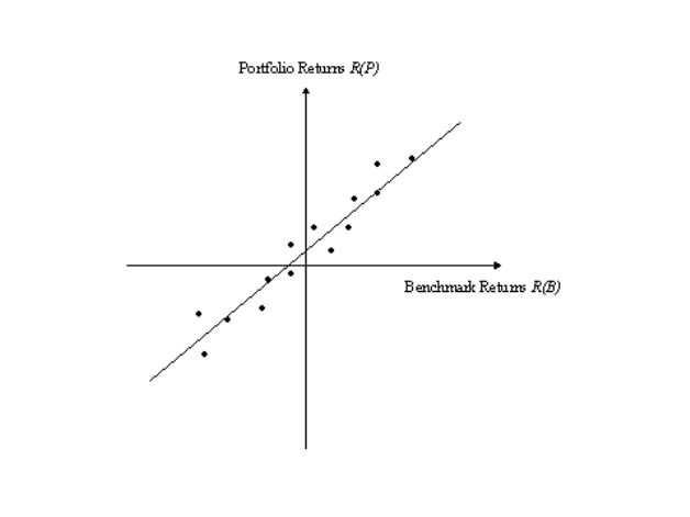
2 Market standards and calculations
2.4 Performance calculations
Transaction & Risk Management Module (TRM) Instruments: Processing and Calculations 173
•The statistics of the excess return: Excess Return Mean, Excess Return Variance, Excess Return
Standard Deviation, Tracking Error, Tracking Error (Annualized), Excess Return Volatility (same
as Tracking Error (Annualized)).
2.4.8.5 Linear regression
The figure below shows concurrent portfolio and benchmark returns together with the estimated
best-fit linear regression (least squares method).
If we assume that we have the following set of concurrent portfolio returns:
where
n represents each ‘pair’ of concurrent portfolio R(P) and benchmark R(B) returns, then the linear
regression function for each pair is then given by the following straight-line equation:
Equation 2-346
α (alpha) and β (beta) are selected such that the sum of the squared differences between each
pair of concurrent returns (estimation error) is minimized. The estimation error is given by:
Equation 2-347
RdnT,d–n1+()T– P(), RdnT,d–n1+()T– B()(), n 0, ..... , N -1 ={}
RdnT,d–n1+()T– P() α β RdnT,d–n1+()T– B()×+=
Errd
TN,αβ,() RdnT,d–n1+()T– P() (α–βRdnT,d–n1+()T– B())×+[]
2
n0=
N1–
∑
=

2 Market standards and calculations
2.4 Performance calculations
174 © Wall Street Systems IPH AB - Confidential
Minimizing the estimation error gives the following relationships:
Equation 2-348
Equation 2-349
Equation 2-350
where
R2 is given by:
Equation 2-351
α* and β* are the best fit values of the alpha α and beta β. Alpha is the intercept on the y-axis
and beta is the slope of the linear regression function.
Alpha represents the part of the return from portfolio P which is independent of the benchmark
movement and beta is the sensitivity of the return with respect to the benchmark.
The variable R2, a least squares measure (the correlation coefficient given by Equation 2-337 on
page 171 squared), is an indication of the goodness of fit of the linear regression to the data. The
higher the value of R2, the better the fit of the linear function to the data - in other words, the more
the portfolio returns are determined by the benchmark returns.
2.4.9 Risk-adjusted return measures
In all risk-adjusted return measures the return is related to the risk taken. Therefore we need to
quantify the risk. The most common measures are the portfolio return standard deviation, beta and
the tracking error. The standard deviation can be seen as the risk from the perspective of the end
investor in the fund whereas beta and the tracking error represent more the risk taken by the fund
manager. Other risk figures, described below, are also provided for user risk analysis.
2.4.9.1 TRM variables
The following risk adjusted return measures are provided. These are described in more detail below.
General statistics (mean, variance, standard deviation) of the portfolio and excess returns are also
provided (see 2.4.8.3 Portfolio returns on page 168 and 2.4.8.4 Excess returns on page 171).
•Risk adjusted return measures: Return Standard Deviation (standard deviation of the portfolio
return), Return Volatility (annualized standard deviation of the portfolio return), Beta, Tracking
Error, Tracking Error (Annualized), Alpha, Alpha (Annualized), Information Ratio, Sharpe Ratio,
Modigliani-Modigliani, Treynor Ratio, Jensen’s Alpha.
α*R
d
TN,P() β*R
d
TN,B()×–=
β*Cov Rd
TN,P(), Rd
TN,B()()
Var Rd
TN,B()()
--------------------------------------------------------------
=
Errd
TN,α*β*,()N1–()Var Rd
TN,P()()×1R
2
–()×=
R2Rd
TN,P(), Rd
TN,B()()
Cov Rd
TN,P(), Rd
TN,B()()
Var Rd
TN,P()()Var Rd
TN,B()()×
---------------------------------------------------------------------------------------
⎝⎠
⎜⎟
⎜⎟
⎛⎞
2
=
2 Market standards and calculations
2.4 Performance calculations
Transaction & Risk Management Module (TRM) Instruments: Processing and Calculations 175
2.4.9.2 Return standard deviation
The end investor’s main concern is typically the absolute level of the portfolio returns. For the
investor the risk is therefore the uncertainty of the future portfolio returns. The historical risk is
often measured as the N period standard deviation of the T-periodic returns of the portfolio P, as
shown in Equation 2-334 on page 169 (square root of the variance). If we assume that the portfolio
returns are normally distributed then we can calculate confidence intervals for the future returns,
based on the historical standard deviation (SD) and mean. For example, we can say that the future
returns will be in the interval mean +/- 1SD with 68% confidence and in the interval mean +/- 2SD
with 95% confidence.
2.4.9.3 Return volatility
The volatility is the annualized standard deviation of the cumulative portfolio return -standard
deviation scaled by √K(T), where K(T) is, as shown above, the number of T-periods making up the
business year (Equation 2-335 on page 170). This scaling makes the volatility from one sampling
frequency comparable with the volatility calculated from a different sampling frequency.
2.4.9.4 Beta
The risk for the fund manager is more the uncertainty of the future returns relative to the
benchmark portfolio than the return of the portfolio itself; the risk-less portfolio for a fund manager
is a portfolio that is guaranteed the same future returns as the benchmark. The historical risk
relative to the benchmark can be measured by beta which, as shown in the previous section, is a
measure of the sensitivity of the portfolio P with respect to changes in the benchmark portfolio B:
Equation 2-352
where the covariance is given by Equation 2-336 on page 171 and the variance by Equation 2-333
on page 169. A beta of 1 implies that the portfolio will tend to move with the benchmark, and thus
the fund manager has zero risk relative to the benchmark. A beta greater (less) than 1 means that
the portfolio will fluctuates more (less) than the benchmark and therefore the fund manager has
taken a position relative to the benchmark.
2.4.9.5 Tracking error
Tracking error is another benchmark related risk measure defined as the N period standard
deviation of the T-periodic excess return of the portfolio P relative to the benchmark B (Equation
2-344 on page 172). The annualized tracking error for excess returns is calculated in the same way
as the annualized volatility for portfolio returns above; tracking error scaled by √K(T), where K(T) is
the number of T-periods making up the business year. This scaling, as before, means that
annualized tracking errors calculated with different sampling frequencies (T-periods) can be
compared.
If we assume that the excess returns are normally distributed and that the historical tracking error
is a good prediction of the future then, as for the portfolio return itself above, we can predict
confidence intervals for the future excess returns (mean +/- 1SD with 68% confidence and mean
+/- 2SD with 95% confidence).
2.4.9.6 Alpha
This is the alpha term in the linear regression presented in 2.4.8.5 Linear regression on page 173.
This figure can be written in terms of T-period return:
Equation 2-353
where as before, the covariance is given by Equation 2-336 on page 171, the variance by Equation
2-333 on page 169, and the means by Equation 2-332 on page 169.
βRd
TN,P(), Rd
TN,B()()
Cov Rd
TN,P(), Rd
TN,B()()
Var Rd
TN,B()()
--------------------------------------------------------------
=

2 Market standards and calculations
2.4 Performance calculations
176 © Wall Street Systems IPH AB - Confidential
The annualized alpha is then given by:
Equation 2-354
(continuous yield)
Equation 2-355
(periodic)
where
K(T) is, as before, the number of T-periods making up a business year.
The alpha is the part of the return from portfolio P that can’t be attributed to the risk taken in terms
of beta. A positive alpha can be obtained by stock picking and/or market timing. With stock picking
the fund manager tries to be overexposed or underexposed in securities having a mean return
above or below the benchmark return, respectively. With market timing the manager tries to
fine-tune the beta of the fund such that it is less or greater than 1 when the benchmark return is
negative or positive, respectively. A fund tracking the benchmark will, by definition, have an alpha
value of zero. The alpha value can therefore be seen as the contribution to the portfolio’s return
coming from active fund management.
2.4.9.7 R squared
The R2 figure is a measure of how much information alpha and beta provide about the portfolio. It is
a least squares variable (see 2.4.8.5 Linear regression on page 173), an indication of the goodness
of fit of the linear regression to the data. The higher the value of R2, the better the fit of the linear
function to the data - in other words, the more the portfolio returns can be described in relation to
the benchmark returns. Figures over 0.75 or under 0.25 are considered to indicate that the
explanatory power is high or low, respectively. In other words, R2 provides an indication of how well
the behavior of the portfolio returns is described by the alpha and beta values.
2.4.9.8 Information ratio
The information ratio is the annualized period excess return of the portfolio P relative to the
benchmark B, divided by the annualized tracking error:
Equation 2-356
where
the annualized excess return is given by Equation 2-339 on page 171 (continuously
compounded returns) or Equation 2-340 on page 172 (periodic returns), and the annualized
tracking error by Equation 2-341 on page 172.
αRd
TN,P(), Rd
TN,B()()Rd
TN,P() - Cov Rd
TN,P(), Rd
TN,B()()
Var Rd
TN,B()()
--------------------------------------------------------------Rd
TN,B()×=
αannual Rd
TN,P(), Rd
TN,B()()KT() α×Rd
TN,P(), Rd
TN,B()()=
αannual Rd
TN,P(), Rd
TN,B()()100 1 αRd
TN,P(), Rd
TN,B()()
100
-------------------------------------------------------
+
⎝⎠
⎜⎟
⎛⎞
KT()
1–
⎝⎠
⎜⎟
⎛⎞
×=
IRd
TN,PB,()
Rannual, d d NT–,PB–()
TEannual Rd
TN,PB–()()
---------------------------------------------------------
=
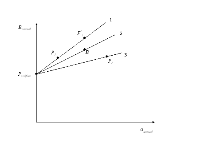
2 Market standards and calculations
2.4 Performance calculations
Transaction & Risk Management Module (TRM) Instruments: Processing and Calculations 177
For example:
is the information ratio calculated from the monthly excess returns during the 12-month period
starting at 970630 (980630 - 12*1M) and ending at 980630. A positive information ratio indicates
that the investment decision to deviate from the benchmark was a good decision since it resulted in
a higher return. The higher the information ratio the more excess return was obtained by the same
risk taken. An information ratio of +0.5 is considered to be an acceptable result, a ratio of +0.75 a
good result and a figure of +1.0 is typically seen as an excellent result.
2.4.9.9 Sharpe ratio
The figure below shows the risks and returns of some portfolios - the benchmark B, example
portfolios and a risk-free portfolio. The return is measured as the annualized period return, Rannual,
and the risk as the annualized standard deviation of the T-periodic returns (the volatility σannual).
2.4.9.9.1 Risk-return characteristics (risk measured by volatility)
It is clear that the benchmark B is preferable to portfolio P2 since the return is higher and the risk is
less. The comparison against P1 is not so clear cut; the return of P1 is lower but so is the risk. In
portfolio theory the existence of a risk-free portfolio is usually assumed. The return of the risk-free
portfolio is fixed (in other words the volatility is zero) and known in advance. Furthermore the
investor is allowed to buy the portfolio (invest money at the risk-free interest rate), or sell short the
portfolio (borrow money at the risk-free interest rate, and invest the proceeds in the risky portfolio).
All combinations of the risk-free portfolio and a risky portfolio lie along the straight line connecting
them (line 1 for P1 and line 3 for P2) in the risk-return diagram above. By borrowing at the risk-free
interest rate and investing the proceeds in portfolio P1, the investor can construct the portfolio P′1
that has the same risk as the benchmark B but a higher return. Given the existence of the risk-free
portfolio a rational investor will prefer portfolio P1 to B and P2(and B to P2). The preferred portfolio is
the one with the greatest slope, that is to say with the largest Sharpe ratio:
Equation 2-357
IR30/6/98
1M 12,PB,()
Sharped
TN,PP
riskfree
,()
Rannual, d d NT–,P() Rannual, d d NT–,Priskfree
()–
σannual Rd
TN,P()()
------------------------------------------------------------------------------------------------------------------
=
2 Market standards and calculations
2.4 Performance calculations
178 © Wall Street Systems IPH AB - Confidential
where the annualized returns are given by Equation 2-330 on page 168 (continuously compounded
returns) or Equation 2-331 on page 169 (periodic returns), and the volatility by Equation 2-335 on
page 170. A high Sharpe Ratio is therefore an indication of high returns relative to the risk taken.
2.4.9.10 Modigliani-Modigliani (M2)
This is a version of the Sharpe ratio analysis that ranks portfolios in exactly the same order as the
Sharpe analysis but gives the result in terms of return and not as a ratio. The risk-adjusted return
measure is called Modigliani-Modigliani, or M2 for short. Given a portfolio P, M2 is the return of the
combination of the risk-free portfolio and P that has the same risk (in terms of volatility) as the
benchmark B. Thus, for portfolio P1 in the figure above (Risk-return characteristics (risk
measured by volatility)), M2 is equal to the return of portfolio P′1. A high value of M2 is therefore
an indication of high returns relative to the risk taken. Mathematically, M2 of portfolio P is given by:
Equation 2-358
The annualized returns are given by Equation 2-330 on page 168 (continuously compounded
returns) or Equation 2-331 on page 169 (periodic returns), and the volatility by Equation 2-335 on
page 170.
M2 d
TN,PBP,riskfree
,()
Rannual, d d NT–,Priskfree
()σ
annual Rd
TN,B()()Sharped
TN,PP
riskfree
,()×+=
Rannual, d d NT–,Priskfree
()
σannual Rd
TN,B()()
σannual Rd
TN,P()()
--------------------------------------------Rannual, d d NT–,P() Rannual, d d NT–,Priskfree
()–×
+=
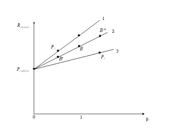
2 Market standards and calculations
2.4 Performance calculations
Transaction & Risk Management Module (TRM) Instruments: Processing and Calculations 179
2.4.9.11 Treynor ratio
The Treynor ratio is similar to the Sharpe ratio but with beta as the risk measure. The figure below
shows the risk and return characteristics for some portfolios where the risk measure is beta. Note
that the benchmark B has a beta of 1 and the risk free portfolio is assumed to have a beta of zero.
2.4.9.11.1 Risk-return characteristics (risk measured by beta)
The Treynor ratio measures the slope of the line connecting the risk-free portfolio and the risky
portfolio:
Equation 2-359
where the annualized returns are, as before, given by Equation 2-330 on page 168 (continuously
compounded returns) or Equation 2-331 on page 169 (periodic returns), and the beta by Equation
2-352 on page 175. As for both the Sharpe Ratio and M2, a high value of this ratio is an indication
of high returns relative to the risk taken.
The fund manager has outperformed the benchmark if the fund has a higher Treynor ratio than the
benchmark. In the figure above, portfolio P1 has outperformed the benchmark in terms of Treynor
ratio (but not P2).
2.4.9.12 Jensen’s Alpha
If the benchmark consists of all securities the fund can invest in (for example the issued equities in
all listed companies besides the tobacco related ones), we make the assumption that the line
connecting the risk-free portfolio and the benchmark (line 2) represents the set of risk-return
effective portfolios. So for every risk level the largest expected return is obtained by investing in a
combination of the risk-free portfolio and the benchmark that has the wanted risk level. If the
wanted risk level in beta terms is then the expected annualized period return of the effective
portfolio is given by:
Equation 2-360
Treynord
TN,PBP,riskfree
,()
Rannual, d d NT–,P() Rannual, d d NT–,Priskfree
()–
βRd
TN,P(), Rd
TN,B()()
------------------------------------------------------------------------------------------------------------------
=
β
˜
2 Market standards and calculations
2.4 Performance calculations
180 © Wall Street Systems IPH AB - Confidential
Jensen’s Alpha is calculated as the actual return of the portfolio P less the return of the effective
portfolio (Equation 2-360 on page 179) with identical beta:
Equation 2-361
where the annualized returns are, as for the Treynor ratio, given by Equation 2-330 on page 168
(continuously compounded returns) or Equation 2-331 on page 169 (periodic returns), and the beta
by Equation 2-352 on page 175. A positive value of Jensen’s Alpha indicates that the portfolio has a
higher return than the effective portfolio (a benchmark with the same level of risk) and a negative
value implies a lower return.
In the figure above (Risk-return characteristics (risk measured by beta)), we have a positive
value of Jensen’s alpha for portfolio P1 (the return is higher than for B′) and a negative value for
portfolio P2 (the return is less than for B′′). Therefore portfolio P1 is a more risk-return effective
portfolio than the benchmark (but not P2).
2.4.10 Performance attribution
The goal of performance attribution is to quantify the contribution of the various investment
decisions to the final overall portfolio (excess) return.
The investment decision variables supported are the ones expressed via the Performance Monitor
grouping dimensions, for example, Market, Currency, Branch Codes, Issuer, Maturity Period, and so
on.
The attribution models split the excess return into Allocation, Selection and Interaction effects:
•Allocation is the investment decision between the selected grouping
•Selection measures the investment decision within the selected grouping
•Interaction is the interaction between the allocation and selection term
The benchmark is represented as a portfolio with transactions.
2.4.10.1 Performance attribution methods
The following attribution methods are used in TRM:
•Single currency portfolios
The Brinson framework.
•Multi currency portfolios
The Karnosky and Singer framework.
•Combining attribution effects over time
The Cariño method.
The calculations used in each of these methods are described in the next section.
Rannual, d d NT–,Pβ
˜
()()
Rannual, d d NT–,Priskfree
()β
˜Rannual, d d NT–,P() Rannual, d d NT–,Priskfree
()–×+=
Jensend
TN,PBP,riskfree
,()Rannual, d d NT–,P() Rannual, d d NT–,Priskfree
()–
βRd
TN,P(), Rd
TN,B()()Rannual, d d NT–,P() Rannual, d d NT–,Priskfree
()–()×–
=

2 Market standards and calculations
2.4 Performance calculations
Transaction & Risk Management Module (TRM) Instruments: Processing and Calculations 181
2.4.10.1.1 Base currency performance attribution
Here are the calculations used for the Brinson attribution of excess return:
Equation 2-362
Allocation
Equation 2-363
Selection
Equation 2-364
Interaction
Equation 2-365
where
wi is the fraction of the market value invested in the i-th sector, and Ri is the return.
The corresponding benchmark values are denoted by and .
2.4.10.1.2 Multi- currency performance attribution
The return of the multi-currency portfolio is given by:
Equation 2-366
where:
–wi is the fraction of the market value invested in the i-th asset.
–Ri is the return of the assets in the i-th segment expressed in the local currency.
– is the local currency risk free return.
–hccy is the currency weight of FX overlay hedge transactions.
–εccy is the change in the spot FX rate (common to all investments in each currency).
–Cccy is the local currency return of FX overlay hedge transactions.
RR–Σ
iwiRiΣ
iwiRi
–ASI++==
AΣ
iwiwi
–()RiR–()=
SΣ
iwiRiRi
–()=
IΣ
iwiwi
–()RiRi
–()=
wiRi
Rbase Σ
iwiRiC
˜ccy i()
–()Σ
ccy wiccy()
hccy
+()C
˜ccy εbase ccy,
+()
Σ
ccy hccy Cccy C
˜ccy
–()
+
+
=
Cccy

2 Market standards and calculations
2.4 Performance calculations
182 © Wall Street Systems IPH AB - Confidential
2.4.10.1.3 Asset-related performance attribution
Brinson style factors:
Equation 2-367
Equation 2-368
Equation 2-369
where BRP is the benchmark local return premium:
Equation 2-370
Asset leverage:
Equation 2-371
Equation 2-372
2.4.10.1.4 Currency related performance attribution
Brinson style factors:
Equation 2-373
Equation 2-374
Equation 2-375
where CRP is the benchmark currency return:
Equation 2-376
Aasset Σ
iwiwi
–()RiC
˜ccy i()
–()BRP–()=
Sasset Σ
iwiRiRi
–()=
Iasset Σ
iwiwi
–()RiRi
–()=
BRP Σ
iwiRiC
˜ccy i()
–()=
Lasset BRP–()Σ
iwiΣ
iwi
–()=
Σ
iwiΣ
ccy hccy
+1=()
Ahedge Σ
ccy wi ccy()
hccy
+()wiccy()
hccy
+()–()C
˜ccy εbase ccy,
+()BCR–()=
Shedge Σ
ccy hccy Cccy C
˜ccy
–()=
Ihedge Σ
ccy hccy hccy
–()Cccy C
˜ccy
–()=

2 Market standards and calculations
2.4 Performance calculations
Transaction & Risk Management Module (TRM) Instruments: Processing and Calculations 183
Assumed common FX return might imply a small unexplained residual:
Equation 2-377
2.4.10.1.5 Linking attribution factors over time
Daily attribution is preferable as weight factors wi are time dependent.
Excess return and arithmetical factors are not additive over time:
Equation 2-378
The error can be distributed over time such that:
Equation 2-379
where
Equation 2-380
and
Equation 2-381
2.4.10.2 Example of single currency performance attribution
This example is based on four equities grouped into two sectors by branch code: Automobiles-sector
(BMW and General Motors) and Telecom-sector (Motorola and Nokia). There are two portfolios: a
managed trading portfolio and a benchmark portfolio. The performance of the managed trading
portfolio is measured against the benchmark, where each stock has an equal 25% weight at the
beginning of the period.
For the sake of simplification, the performance measurement period is only one day, 23rd of April
2003. The market rates used in this example are fictitious and are set to illustrate the mechanism of
performance attribution.
In the managed trading portfolio, the Telecom-sector is over weighted and, respectively, the
Automobiles-sector is under weighted in comparison to the benchmark with equal weights. The
weights, amounts and returns for equities, sectors, managed portfolio and benchmark are presented
in the Performance Monitor view below.
BCR Σ
ccy wi ccy()
hccy
+()Cccy εbase ccy,
+()=
Rbase Rbase
–A
asset Sasset Iasset Lasset Ahedge Shedge Ihedge
++++ + +=
RR–1R
1
+()1R
2
+()1R
1)1(R2)++ R
1R1
–(≠()–R
2
(R2)–+=
RR–1
K
----Σ
tktRtRt
–()=
K1R+()ln 1 R+()ln–
RR–
-----------------------------------------------------
=
kt
1R
t
+()ln 1 Rt
+()ln–
RtRt
–
--------------------------------------------------------
=
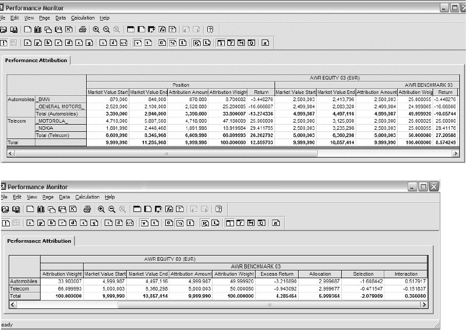
2 Market standards and calculations
2.4 Performance calculations
184 © Wall Street Systems IPH AB - Confidential
The benchmark portfolio has a return of 8.57 % and the managed portfolio has a return of 12.86 %.
The investment decisions of the managed portfolio have created a 4.29% excess return, which can
be further analyzed by Performance Attribution Key-Figures in Performance Monitor.
The Key-Figures Allocation, Selection and Interaction for Automobiles and Telecom sector are
calculated as shown in the following sections.
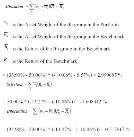
2 Market standards and calculations
2.4 Performance calculations
Transaction & Risk Management Module (TRM) Instruments: Processing and Calculations 185
2.4.10.2.1 Automobiles
2.4.10.2.2 Telecoms sector
Allocation = (66.00% - 50.00%) * (27.21% - 8.57%) = 2.999677 %.
Selection = 50.00% * (26.26% - 27.21%) = -0.471547 %.
Interaction = (66.10% - 50.00%) * (26.26% - 27.21%) = -0.151837 %.
The Allocation Figure expresses how successful the asset manager has been in allocating funds
between sectors. In this example, it is the decision to overweight the Telecom sector and to
underweight the Automobiles sector. The Telecom sector return is considerably higher than the
negative one of the Automobiles sector. The positive Allocation Figure of the Telecom sector is
intuitively straightforward, since the sector performed well and it was over weighted in the managed
portfolio. The positive Allocation Figure of the Automobiles sector is due to the fact that this lower
return sector was under weighted in the managed portfolio in comparison to the benchmark.
The Selection Figure expresses how successful the asset manager has been in stock picking (to
select equities within a certain group) here within a sector. The negative Figure Selection means
that within the sector, higher return equity was underweighted and lower return equity was
overweighted, in comparison to the benchmark portfolio.
The Figure Intersection represents the part of the excess return that cannot be attributed either to
allocation or selection decisions. The sum of the Allocation, Selection and Interaction figures equals
the difference between managed portfolio and benchmark portfolio returns, that is, the excess
return.
2.4.10.3 Example of multi-currency performance attribution
The following example is based on four equities, which are grouped according to currency
denomination; EUR for BMW and NOKIA and USD for GENERAL MOTORS and MOTOROLA.
The benchmark portfolio consists of these four stocks which have an initial weight of 25 % each.
Therefore, the benchmark portfolio has initially equivalent exposures in both currencies.
The managed trading portfolio consists of the investments in these four stocks, but with different
weights than in the benchmark portfolio. In comparison with the benchmark, USD assets are

2 Market standards and calculations
2.4 Performance calculations
186 © Wall Street Systems IPH AB - Confidential
over-weighted: USD denominated stocks total 72% and EUR stocks 28% of the initial market value
of the managed portfolio.
In order to bring currency exposure of the managed portfolio in line with the benchmark, USD
dollars are sold against EUR by FX-Forward transaction. As a result of the hedge, the managed
portfolio has 49.60 % exposure in EUR and 50.40 % exposure in USD.
For the sake of simplification, the performance measurement period is only one day, 23rd of April
2003. During the day, USD is set to depreciate 10 % against the EUR. The market rates used in this
example are fictitious and are set to illustrate the mechanism of multi-currency attribution. All
market values are expressed in EUR.
The following image displays asset market values at the beginning and end of the period:
This image illustrates the portfolio structure:

2 Market standards and calculations
2.4 Performance calculations
Transaction & Risk Management Module (TRM) Instruments: Processing and Calculations 187
These are the intermediate results used to calculate attribution figures:
The Key-Figures Asset Allocation, Asset Selection, Asset Interaction and Asset Leverage for EUR
denominated investments is calculated as follows:
2.4.10.3.1 Asset allocation
The value added by the decision to deviate from the benchmark’s asset allocation is indicated by the
asset allocation key figure.
For multicurrency investments, the relevant benchmark to be used to analyze the value added of
local currency allocation decisions is the average local currency return premium, known as BRP.
Equation 2-382 A asset
where
BRP is the benchmark local return premium:
Equation 2-383 BRP
Asset Allocation = (27.62%-50.00%) * (12.97%-8.38%) = -1.028916306%
Equation 2-384 S asset
Asset Weight of the ith group in the Portfolio
Asset Weight of the ith group in the Benchmark
Return of the ith group in the Benchmark
local currency risk free rate of return
Wi
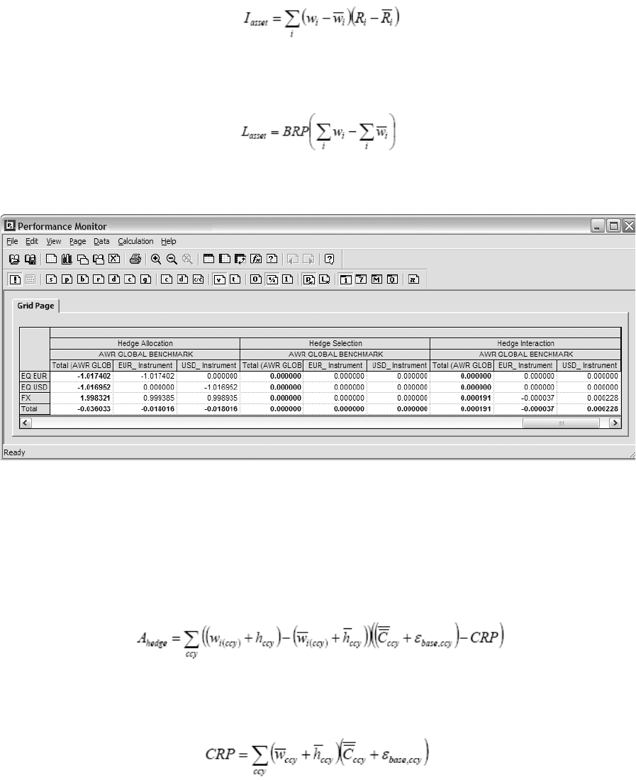
2 Market standards and calculations
2.4 Performance calculations
188 © Wall Street Systems IPH AB - Confidential
Asset Selection = 50.00% * (19.06% - 12.98%) = 3.0397352%
Asset Interaction = (27.62% - 50.00%) * (19.06% - 12.98%) = -1.36075776%
Equation 2-385
Asset Leverage = 8.38% * (99.99% - 100.00%) = -0.000836592%
Equation 2-386
The Key-Figures Hedge Allocation, Hedge Selection and Hedge Interaction for EUR denominated
investments are calculated as follows:
2.4.10.3.2 Hedge allocation
The value added by the decision to deviate from the benchmark’s currency allocation is indicated by
the hedge allocation key figure. When determining the amount allocated to a certain currency, both
the underlying investments and currency overlays are taken into account. When determining
currency returns, both the risk-free return of a currency and change in the FX rate against the
portfolio's base currency are taken into account.
Equation 2-387 A hedge
where
CRP is the benchmark currency return. It expresses the currency return (risk free rate + change
in FX rate against the portfolio's base currency) of the benchmark.
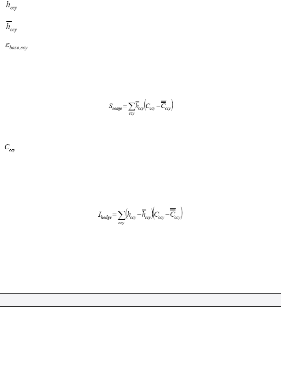
2 Market standards and calculations
2.4 Performance calculations
Transaction & Risk Management Module (TRM) Instruments: Processing and Calculations 189
Hedge Allocation = (49.60%-50.00%)*(0.01% - (-4.54%)) = -0.018016123%
Hedge Selection
Equation 2-388 Hedge selection
where
In this example, the hedge selection figure is zero, since there are no hedges in the benchmark
portfolio.
Hedge Interaction = (21.99% - 0.00%) * (0.01% - 0.009722%) = -0.000038688%.
Equation 2-389 Hedge interaction
2.4.11 Performance measurement key-figures
The key-figures available in Performance Monitor are described in the following table.
These figures include the risk adjusted return measures, for example the Information Ratio and
Modigliani-Modigliani (see 2.4.8 Risk-adjusted returns on page 166). More details about these
key-figures and how they are calculated are given in the section 2.4 Performance calculations on
page 149.
Currency weight of portfolio FX overlay hedge transactions.
Currency weight of Benchmark FX overlay hedge transactions.
Change in the spot FX rate (common to all investments in a particular currency)
Local currency return of FX overlay hedge transactions.
Figure Definition
Allocation The Brinson performance attribution factor measuring how well money has been
allocated (relative benchmark) between the selected groups (such as Branch Code),
given by:
Allocation_i (T) = (w_it - W_it)*(R_it - R_i)
where
w_it is the Attribution Weight of the ith group in the portfolio
W_it is the Attribution Weight of the ith group in the Benchmark
R_it is the Return of the ith group in the Benchmark
R_t is the Benchmark total return at time T

2 Market standards and calculations
2.4 Performance calculations
190 © Wall Street Systems IPH AB - Confidential
Allocation
(Cumulative)
The allocation factor (A) that is additive over time:
where
R = cumulative total Portfolio Return
= cumulative total Benchmark Return
and
Rt = total Portfolio return on day t
= total Benchmark Return on day t
Allocation (cumulative) T = sum t=1 to T Excess Return Factor (t) *
Allocation (t) / Excess Return Factor (Cumulative)
Alpha The part of the return on a portfolio that cannot be attributed to the risk taken (the
risk taken in terms of beta). It is the intercept of the y-axis of the linear regression
function between the portfolio and the benchmark portfolio.
Alpha (Annualized) The alpha of the portfolio, converted into an annualized figure.
Asset Allocation The multi-currency performance attribution is based on Karnosky and Singer
framework. The Allocation, Selection, and Interaction terms follow Brinson et al.
framework, similar to the single currency performance attribution.
The Asset Allocation is the performance attribution factor measuring how successfully
funds have been allocated relative to the benchmark between the selected groups
(such as Branch Code) given by:
where
Asset Weight of the ith group in the Portfolio
Asset Weight of the ith group in the Benchmark
Return of the ith group in the Benchmark
Local currency risk free rate of return
BRP is the benchmark local return premium:
Figure Definition
R
Rt
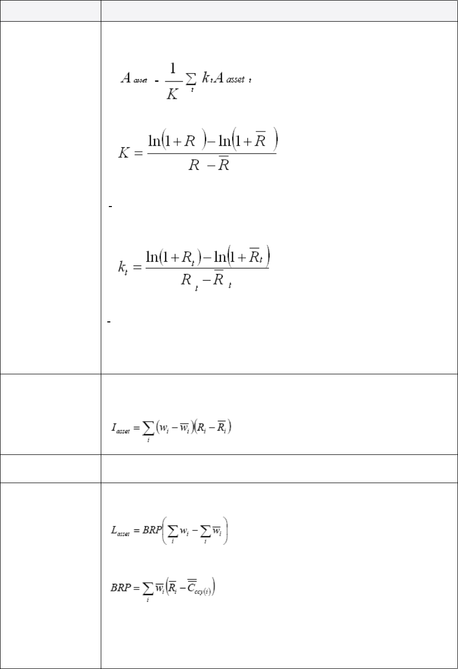
2 Market standards and calculations
2.4 Performance calculations
Transaction & Risk Management Module (TRM) Instruments: Processing and Calculations 191
Asset Allocation
(Cumulative)
Since Excess Return and arithmetical factors are not directly additive over time, the
following methodology ("Combining Attribution Effects over Time" by D.R . Carino) is
applied to link attribution effects over time:
where
R = cumulative total Portfolio Return
= cumulative total Benchmark Return
and
R = cumulative total Portfolio Return
= cumulative total Benchmark Return
AAsset is the portfolio's cumulative Asset Allocation
AAssett is the portfolio's Asset Allocation effect at time point t.
Asset Interaction Performance attribution factor measuring the interaction between Asset Allocation
and Asset Selection. It is part of the Excess Return that cannot be divided to either
Allocation or Selection.
Asset Interaction
(Cumulative)
See Key-Figure Asset Allocation (Cumulative), where methodology to link effects over
time is described.
Asset Leverage The return contribution from leveraged market investment in respect to the total
portfolio market value due to unrealized result of FX hedge transactions.
For example, you buy US bonds worth 100 M Euro and hedge the currency exposure
into Euro using FX forwards. If the dollar goes up 10% the bonds are worth around
110M Euro and you have an offsetting unrealized loss of 10M from the FX forwards. In
this case your bond position is leveraged since you have 110M of a portfolio total of
100M invested into it.
Figure Definition
R
Rt
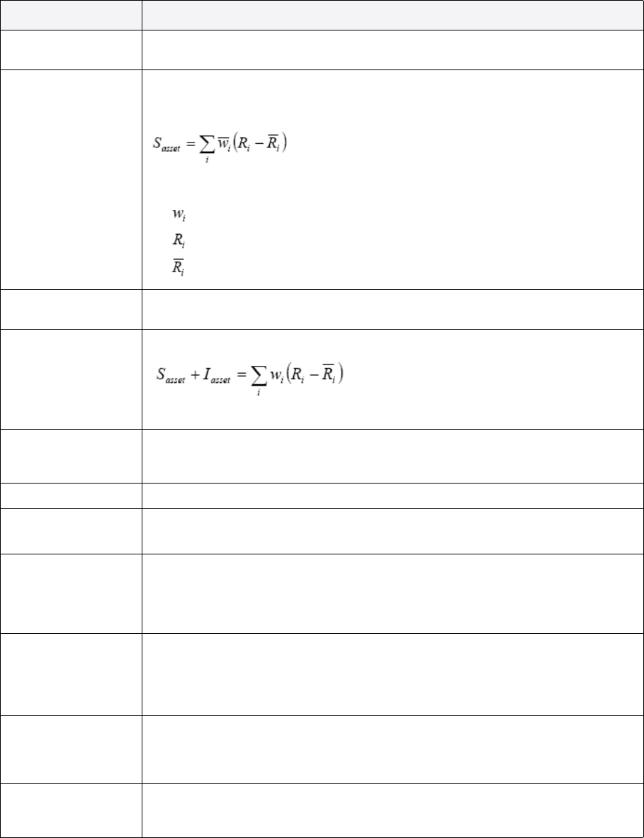
2 Market standards and calculations
2.4 Performance calculations
192 © Wall Street Systems IPH AB - Confidential
Asset Leverage
(Cumulative)
See Key-Figure Asset Allocation (Cumulative), where methodology to link effects over
time is described.
Asset Selection Performance attribution factor measuring how successful you have been at selecting
securities relative to the benchmark within the selected groups (such as Branch
Code), given by:
where
Asset Weight of the ith group in the Benchmark
Return of the ith group in the Portfolio
Return of the ith group in the Benchmark
Asset Selection
(Cumulative)
See Key-Figure Asset Allocation (Cumulative), where methodology to link effects over
time is described.
Asset
Selection/Interaction
The combined Asset Selection and Asset Interaction factors given by:
Note: As a difference to the pure Asset Selection, Portfolio Weight is used here.
Asset Selection/
Interaction
(Cumulative)
See Key-Figure Asset Allocation (Cumulative), where the methodology to link effects
over time is described.
Asset Weight Fraction of the market value invested in ith asset.
Attribution Amount The market value allocated to the selected cell i at beginning of day t, given by:
Attribution Amount (T) = Market Value Start (T) + Weight Factor * Cashflows (T)
Attribution Weight The percentage of total Attribution Amount allocated into cell i at time t:
Attribution Weight (T) = Attribution Amount (T) / Total Attribution Amount (T)
(The Total level is defined by the user in the X,Y axis selection lists as in Treasury
Monitor.)
Beta The gradient of the linear regression function between the portfolio and the
benchmark portfolio. This is a measure of the sensitivity of the portfolio with respect
to changes in the benchmark portfolio. A value of beta greater than 1 means that the
portfolio returns will be more than the benchmark returns (less than 1 means the
returns will vary less).
Correlation The correlation coefficient between the portfolio and the benchmark portfolio
(standardized covariance). A positive (negative) value indicates that if there is a
positive return for the benchmark portfolio, then there will also be a positive
(negative) return for the portfolio.
Covariance The covariance between the portfolio and the benchmark portfolio. A positive
(negative) value indicates that if there is a positive return for the benchmark portfolio,
then there will also be a positive (negative) return for the portfolio.
Figure Definition
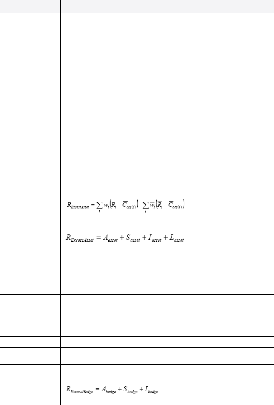
2 Market standards and calculations
2.4 Performance calculations
Transaction & Risk Management Module (TRM) Instruments: Processing and Calculations 193
Difference Result The difference of the monetary returns between a trading portfolio and a benchmark
portfolio, expressed as daily Monetary P/L Excess Return and calculated as follows:
where
REt is the Monetary P/L Excess Return for day t
REP,t is the Monetary Portfolio Return for day t
REB,t is the Monetary Benchmark Return for day t
This key-figure behaves like Excess Return, except that money amounts are used.
Note: In Treasury Monitor, the key-figures Market Value and Market Value Start are
used. Monetary P/L Excess Return is the difference between the trading
portfolio’s Market Value Change and that of the benchmark portfolio.
Difference Result
(Cumulative)
The sum of daily Monetary P/L Excess Returns during a period of n days.
Difference Return
Contribution
Displayed under the benchmark, this figure is the line-by-line difference between the
Return Contribution of the portfolio and the Return Contribution of the benchmark.
Difference Return Contribution (Cumulative) measures the same difference over time.
Excess Return This is the portfolio return relative to the benchmark return for the specified interval.
Excess Return
(Annualized)
The difference between the Return (Cumulative) of the portfolio and the Return
(Cumulative) of the benchmark portfolio, converted into an annual figure.
Excess Return Asset
Contribution
This is the difference between local portfolio return premium and base currency
benchmark return premium.
Alternatively, this is the sum of the Asset attribution factors at time point t:
Excess Return Asset
Contribution
(Cumulative)
This is the sum of cumulative Asset attribution factors.
Excess Return
Contribution
This is the sum of the attribution factors at time T:
Excess Return Contribution (T) = Allocation (T) + Selection (T) + Interaction (T)
Excess Return
Contribution
(Cumulative)
This is the sum of the cumulative attribution factors:
Excess Return Contribution (Cumulative) = Allocation (Cumulative) + Selection
(Cumulative) + Interaction (Cumulative)
Excess Return
(Cumulative)
The difference between the Return (Cumulative) of the portfolio and the Return
(Cumulative) of the benchmark portfolio.
Excess Return Factor Daily factor used for linking attribution effects over time.
Excess Return Factor
(Cumulative)
Total period factor used for linking attribution effects over time.
Excess Return Hedge
Contribution
Excess return contribution from the hedge strategy, which is the sum of the Hedge
attribution factors at time t:
Figure Definition
REtREPt,REBt,
–=
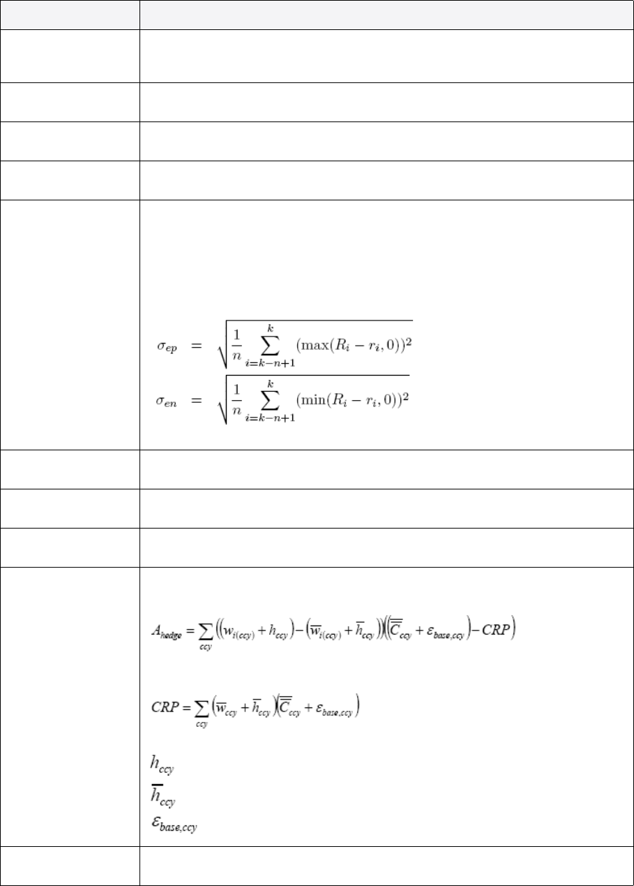
2 Market standards and calculations
2.4 Performance calculations
194 © Wall Street Systems IPH AB - Confidential
Excess Return Hedge
Contribution
(Cumulative)
This is the sum of the cumulative Hedge attribution factors. See Key-Figure Asset
Allocation (Cumulative), where the methodology to link effects over time is described.
Excess Return (N
Samples)
This is the portfolio return relative to the benchmark return over N sub-periods
(T-periods) of sampling frequency T.
Excess Return
(Sample)
This is the portfolio return relative to the benchmark return over one sub-period
(T-period) of sampling frequency T.
Excess Return Mean The mean value of excess returns over the aggregation period (aggregation period
length expressed as N T-periods).
Excess Return
Semideviation
Key-figures:
Excess Return Semideviation (Positive)
Excess Return Semideviation (Negative)
measure the semideviation of excess return over a benchmark.
If the sample returns of the benchmark are ri, then
Excess Return
Standard Deviation
The standard deviation of excess returns over the aggregation period (aggregation
period length expressed as N T-periods).
Excess Return
Variance
The variance of excess returns over the aggregation period (aggregation period length
expressed as N T-periods).
Excess Return
Volatility
The standard deviation of excess returns over the aggregation period (aggregation
period length expressed as N T-periods), converted into an annualized figure.
Hedge Allocation The performance attribution factor measuring how successful we have been in our
currency strategy in comparison to the benchmark given by:
where CRP is the benchmark currency return
currency weight of portfolio FX overlay hedge transactions
currency weight of Benchmark FX overlay hedge transactions
change in the spot FX rate (common to all investments in each currency)
Hedge Allocation
(Cumulative)
See Key-Figure Asset Allocation (Cumulative), where methodology to link effects over
time is described.
Figure Definition
σep
σen
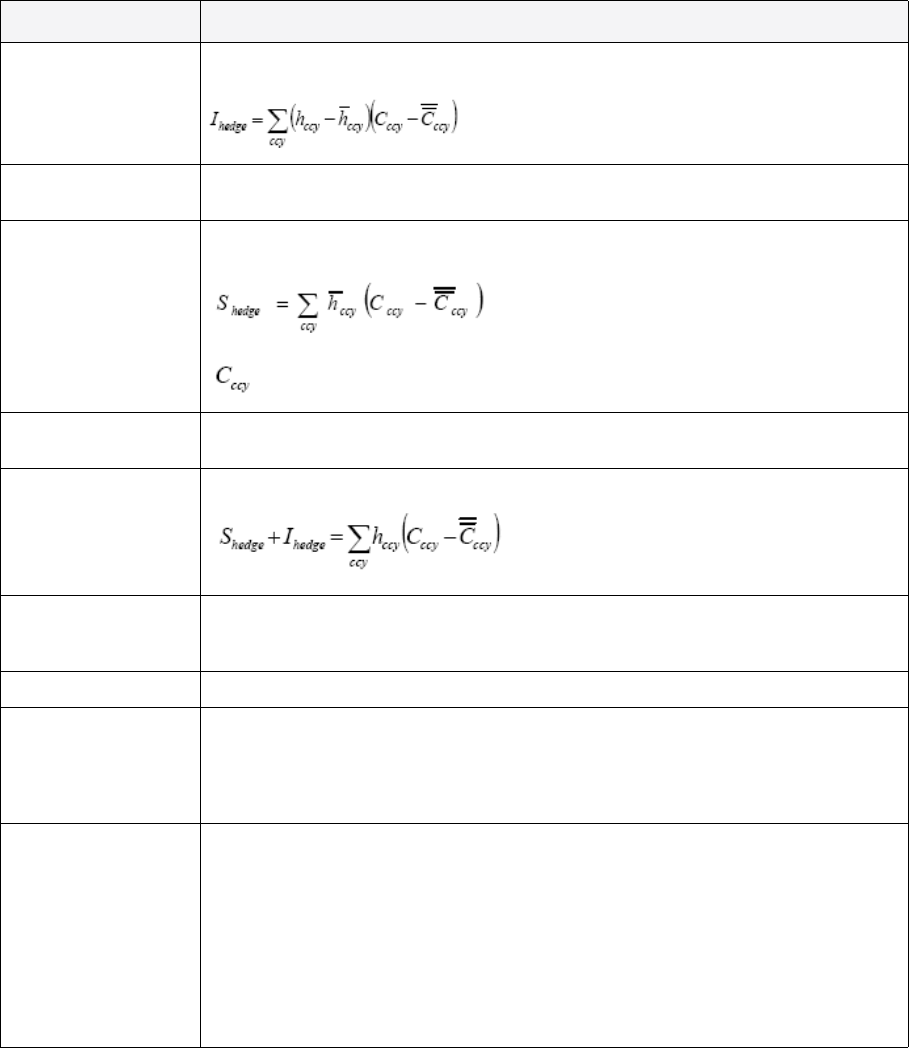
2 Market standards and calculations
2.4 Performance calculations
Transaction & Risk Management Module (TRM) Instruments: Processing and Calculations 195
Hedge Interaction The performance attribution factor measuring the interaction between Hedge
Allocation and Hedge Selection is given by:
Hedge Interaction
(Cumulative)
See Key-Figure Asset Allocation (Cumulative), where the methodology to link effects
over time is described.
Hedge Selection The performance attribution factor measuring how successful you have been in
hedging the selection of optimal maturity of the hedge transactions is given by:
Local currency return of FX overlay hedge transactions.
Hedge Selection
(Cumulative)
See Key-Figure Asset Allocation (Cumulative), where the methodology to link effects
over time is described.
Hedge
Selection/Interaction
The combined Hedge Selection and Hedge Interaction factors are given by:
Hedge
Selection/Interaction
(Cumulative)
See Key-Figure Asset Allocation (Cumulative), where the methodology to link effects
over time is described.
Hedge Weight The currency weight of FX overlay hedge transaction.
Information Ratio A measurement of the return of the portfolio in terms of the risk taken (risk adjusted
return measure). The Excess Return (Annualized) divided by the Tracking Error
(Annualized). A positive value indicates that the decision to deviate from the
benchmark was a good one since it resulted in a higher return. The higher the value of
the Information Ratio, the more excess return was obtained by the same risk taken.
Interaction The Brinson performance attribution factor measuring the interaction between
allocation and selection, given by:
Interaction_i (T) = (w_it – W_it)*(r_it-R_it)
where
W_it is the Attribution Weight of the ith group in the Benchmark
w_it is the Attribution Weight of the ith group in the portfolio
r_it is the Return of the ith group in the Portfolio
R_it is the Return of the ith group in the Benchmark
Figure Definition
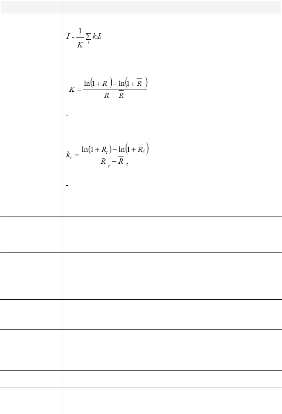
2 Market standards and calculations
2.4 Performance calculations
196 © Wall Street Systems IPH AB - Confidential
Interaction
(Cumulative)
Interaction factors (I) that are additive over time.
where
R = cumulative total Portfolio Return
= cumulative total Benchmark Return
and
Rt = total Portfolio return on day t
= total Benchmark Return on day t
Interaction (cumulative) T = sum t=1 to T Excess Return Factor (t)
* Interaction (t) / Excess Return Factor (Cumulative)
Jensen's Alpha A measurement of the return of the portfolio in terms of the risk taken (risk adjusted
return measure). Jensen’s Alpha is defined as the difference between the return on
the portfolio and the return on the ‘effective’ benchmark portfolio with the same beta.
A positive (negative) value implies that the portfolio has a higher (lower) return than
the effective benchmark with the same level of risk.
Market Value
Movements
Movements between buckets/branches are considered to happen between the dates,
that is, at midnight. Thus, for an instrument worth X moving from bucket B to A at
date T, the market value start at date T will be equal to the market value end at day
T-1 plus the amount X. The Market Value Movements key-figure is equal to X.
In general:
Market Value Start (T) = Market Value End (T-1) + Market Value Movements (T)
Modigliani-
Modigliani
A measurement of the return of the portfolio in terms of the risk taken (risk adjusted
return measure). Defined as the return of a combination of the portfolio and the
risk-free portfolio that has the same risk (volatility) as the benchmark portfolio. A
high Modigliani-Modigliani value indicates high returns relative to the risk taken.
R2R squared, is the fit of the linear regression function between the portfolio and the
benchmark portfolio. A measure of how well the behavior of the portfolio returns is
described by the Alpha and Beta values. Figures over 0.75 or under 0.25 are
considered to indicate that the explanatory power is high or low, respectively.
Return The rate of return (percentage growth) of the portfolio over a specified interval.
Return (Annualized) The return on the portfolio over the aggregation period (length of this period
expressed as N T-periods), converted into an annualized figure.
Return Contribution The contribution of the selected cell to the total absolute performance, given by:
Return Contribution (T) = Attribution Weight (T) * Return (T) = Result (T) / Total
Attribution Amount (T)
Figure Definition
R
Rt
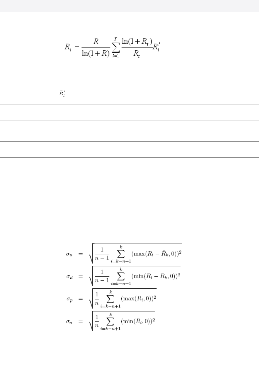
2 Market standards and calculations
2.4 Performance calculations
Transaction & Risk Management Module (TRM) Instruments: Processing and Calculations 197
Return Contribution
(Cumulative)
The cumulative value of Return Contribution.
Rt, Cumulative Return Contribution for cell i over period from 1 to T is:
Here,
R is the cumulative total performance,
Rt is the total performance for period t, and
is the performance of cell i for period t.
Return (Cumulative) The return on the portfolio over the aggregation period (length of this period
expressed as N T-periods).
Return (N Samples) The portfolio return over N sub-periods (T-periods) of sampling frequency T.
Return (Sample) The portfolio return over one sub-period (T-period) of sampling frequency T.
Return Mean The mean of the cumulative returns over the aggregation period (length of this period
expressed as N T-periods).
Return Semideviation Displays the standard deviations of returns which are below (above) the average
returns, respectively.
Key-figures:
Return Semideviation (Upside) ( )
Return Semideviation (Downside) ( )
Return Semideviation (Positive) ( )
Return Semideviation (Negative) ( )
are based an sample returns Ri.
Let sample count (the number of consecutive samples used in averaging) be n. Then
for the kth sample:
where is the sample mean return.
Return Standard
Deviation
The standard deviation of the cumulative returns over the aggregation period (length
of this period expressed as N T-periods).
Return Variance The variance of the cumulative returns over the aggregation period (length of this
period expressed as N T-periods).
Figure Definition
σuσd
σp
σn
Ri
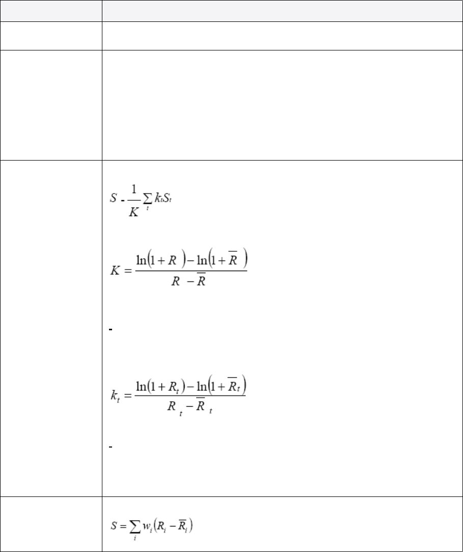
2 Market standards and calculations
2.4 Performance calculations
198 © Wall Street Systems IPH AB - Confidential
Return Volatility The standard deviation of the cumulative returns over the aggregation period (length
of this period expressed as N T-periods), converted into an annualized figure.
Selection The Brinson performance attribution factor measuring how good you have been at
selecting securities (relative benchmark) within the selected groups (such as Branch
code), given by:
Selection_i (T) = W_it*(r_it-R_it)
where
W_it is the Attribution Weight of the ith group in the Benchmark
r_it is the Return of the ith group in the Portfolio
R_it is the Return of the ith group in the Benchmark
Selection (Cumulative) The selection factors (S) that are additive over time.
where
R = cumulative total Portfolio Return
= cumulative total Benchmark Return
and
Rt = total Portfolio return on day t
= total Benchmark Return on day t
Selection (cumulative) T = sum t=1 to T Excess Return Factor (t) * Selection (t) /
Excess Return Factor (Cumulative)
Selection/
Interaction
The combined Selection and Interaction factors given by:
Figure Definition
R
Rt
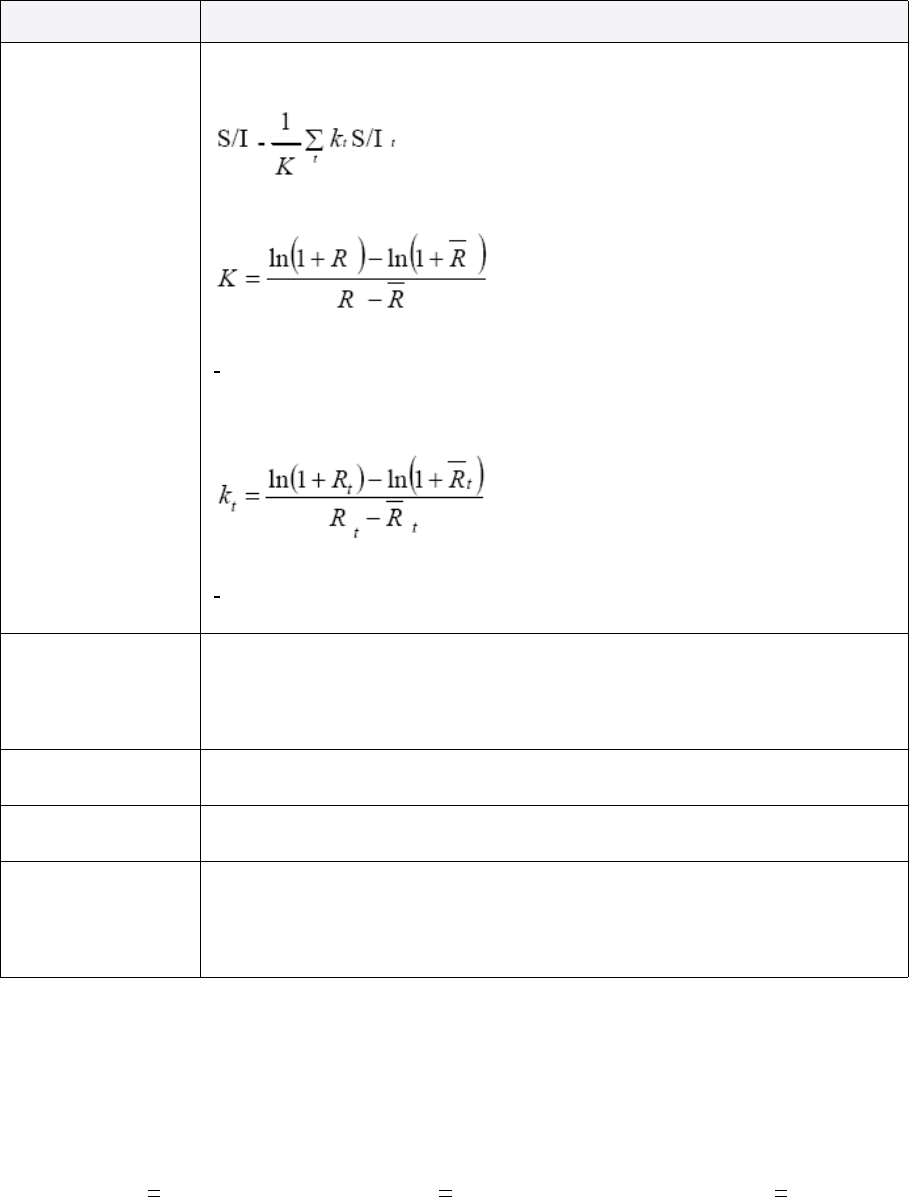
2 Market standards and calculations
2.4 Performance calculations
Transaction & Risk Management Module (TRM) Instruments: Processing and Calculations 199
2.4.11.1 Performance measurement (debug) key-figures
Debug key-figures in Performance Monitor are intermediate results for multi-currency performance
attribution.
The return for the multi-currency portfolio is given by the following equation:
Selection/
Interaction
(Cumulative)
Since Excess Return and arithmetical factors are not directly additive over time, the
following methodology is applied in order to link attribution effects over time:
where
R = cumulative total Portfolio Return
= cumulative total Benchmark Return
and
Rt = total Portfolio return on day t
= total Benchmark Return on day t
Sharpe Ratio A measurement of the return of the portfolio in terms of the risk taken (risk adjusted
return measure). Defined as the difference between the annualized return of the
portfolio and the annualized return of a risk-free portfolio, expressed as a ratio of the
annual standard deviation (volatility) of the portfolio. A high Sharpe Ratio indicates
high returns relative to the risk taken.
Tracking Error The standard deviation of excess returns over the aggregation period (length of this
period expressed as N T-periods).
Tracking Error
(Annualized)
The standard deviation of excess returns over the aggregation period (length of this
period expressed as N T-periods), converted into an annualized figure.
Treynor Ratio A measurement of the return of the portfolio in terms of the risk taken (risk adjusted
return measure). Defined as the difference between the annualized return of the
portfolio and the annualized return of a risk-free portfolio, expressed as a ratio of the
beta between the portfolio and the benchmark portfolio. A high Treynor Ratio
indicates high returns relative to the risk taken.
Figure Definition
R
Rt
Rbase
wiRiCccy i()
–()wiccy()
hccy
+()Cccy εbase ccy,
+()hccy Cccy Cccy
–(
)
ccy
∑
+
ccy
∑
+
i
∑
=
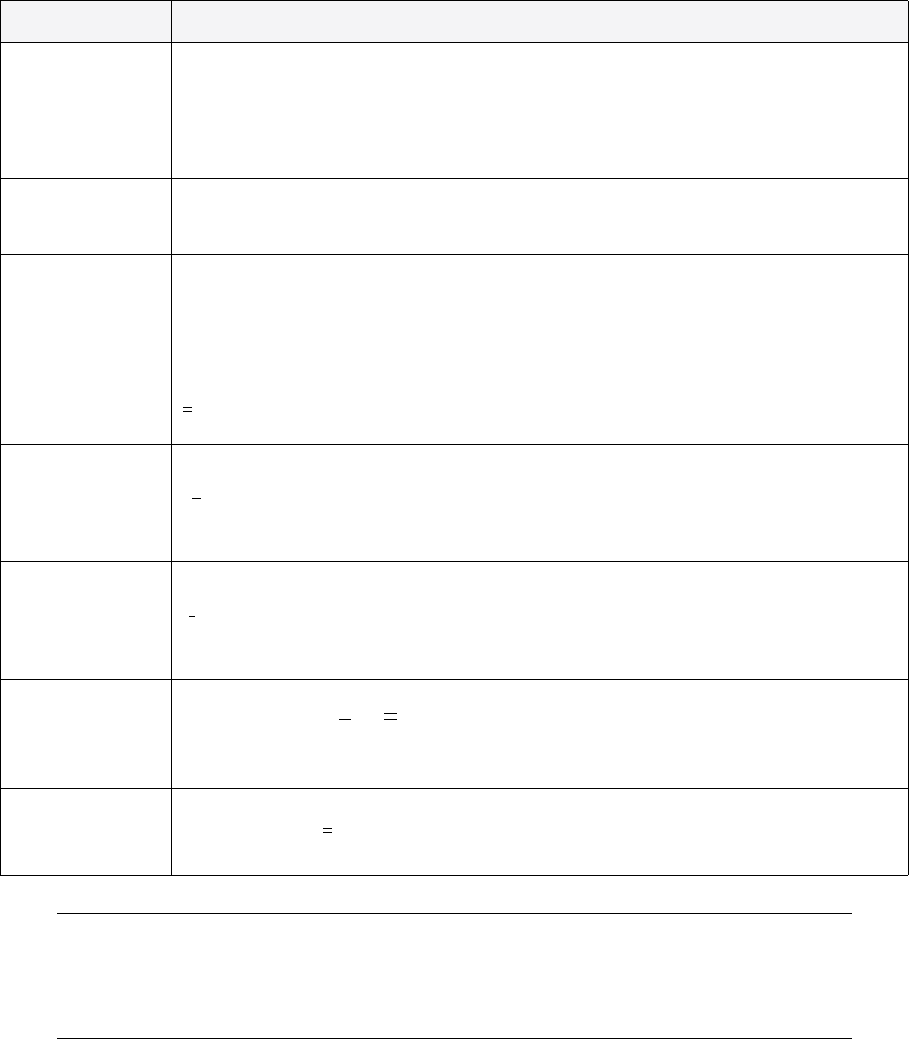
2 Market standards and calculations
2.5 Value-at-Risk calculations
200 © Wall Street Systems IPH AB - Confidential
The following key-figures are found in the Debug key-figure folder:
Note: The configuration of implicitly matched instruments in TRM should lead to identical FX
valuations. Any differences will cause the sum of the attribution terms to not sum exactly
to the portfolio excess return. Given the extensive instrument coverage and the flexibility
in valuation techniques in TRM, it is likely that the user will have to accept same degree of
mismatch between the attribution figures and the excess return.
2.5 Value-at-Risk calculations
Value-at-risk (VaR) is a measure of the potential change in value of a portfolio or position with a
defined level of confidence over a selected risk horizon (one day, one month, and so on). For
example, you could measure your maximum potential loss with a 95% confidence level on an FX
deal due to an unfavorable change in the FX rate over one day. (A 95% confidence level means that
your maximum potential loss will not exceed the change in value predicted by this method 95% of
the time, i.e. 5% of the time you risk losing more than this value.)
Figure Definition
FX Rate FX rate between the base currency and the currency in question (for example, Instrument
Currency). Multi-currency attribution uses an implied FX rate (from all transactions
except FX) because, under the multi-currency framework, only one common FX rate for
all transaction types is accepted. Combinations of, for example, O/N, T/N, and Spot rates,
as they are applied elsewhere in TRM valuation depending on the cashflow value date, are
not accepted.
FX Return Return of the currency with respect to the base currency during the period. This is
basically the return that is the result of the changes in the (implied) FX rate. In the return
formula for multi-currency attribution, this term is marked with
ε
base,ccy.
IR Return The currency risk-free rate of return for the period (the shortest maturity rate from the
yield curve defined for the currency).
This rate is taken from the risk-free curve defined for the currency. This yield curve
should only have the O/N-period defined; the rate set for that period will define the
risk-free return of the currency.
In the return formula for multi-currency attribution, this term is marked with:
Adjusted Asset
Return
Local rate of return for the assets within the respective group. In the return formula for
multi-currency attribution, this term is marked with Ri (or
if the key-figure is displayed under the Benchmark).
Adjusted Hedge
Return
The currency return of the legs of the hedge transaction within the respective group. In
the return formula for multi-currency attribution, this term is marked with hi (or
if the key-figure is displayed under the Benchmark).
Return Premium Local return premium
Deposit Return This is the currency exposure return:
Cccy i()
Ri
hi
BRP wiRiCccy i()
–()
i
∑
=
wiccy()
hccy
+()Cccy εbase ccy,
+()
2 Market standards and calculations
2.5 Value-at-Risk calculations
Transaction & Risk Management Module (TRM) Instruments: Processing and Calculations 201
The value-at-risk (VaR) calculations in TRM are performed in an integrated real-time module that
allows the full functionality of Treasury Monitor to be used with the VaR key-figures produced.
In order to perform these calculations, certain statistical data (volatility and correlation) of the
market variables are required. These data can be imported from RiskMetrics or any other source
with a similar file interface. The data source can be augmented with proprietary data on market
variables which it doesn't cover. Mapping between TRM market variables and the imported statistical
data is carried out in VaR Mapping Editor. The flexibility of this board allows instruments such as
bonds to be mapped to their own volatility and correlation data instead of using a zero-coupon
curve.
VaR Data Board provides the possibility for extensive stress testing by simulating changes in the
market conditions. User-defined scenarios can be created and the correlation and volatility data can
be edited.
The required confidence level and risk horizon can be defined for each portfolio. In order to do so,
the properties VAR-CONFIDENCE-LEVEL and VAR-HORIZON-ID should be added to the Properties
page in Portfolio Editor.
See TRM User Guide for more information about TRM VaR related applications and portfolio
properties.
The rest of this section assumes that RiskMetrics is the source of the statistical data.
2.5.1 TRM approach to VaR calculations
In order to calculate the VaR figures for a position, an estimate of the probability distribution for that
position is required. This is created from the imported statistical data (the volatilities and
correlations of the market variables) and the sensitivity of the position to changes in those market
variables (deltas).
To use the statistical data to assess the value-at-risk of a position, you need to first perform the
following steps:
•Import the statistical data into the system (see 2.5.3.1 RiskMetrics data on page 203).
•Calculate any missing data (see 2.5.4 Transforming RiskMetrics data on page 204).
•Map the cashflows of the position to the RiskMetrics maturity vertices (see 2.5.4.3 Cashflow
mapping on page 205.
•Calculate the VaR deltas of the position (see 2.5.5.1 Calculating VaR deltas on page 207).
2.5.2 RiskMetrics data
In RiskMetrics, the basic underlying assumption is that the relative change in each market variable
X, from one period to another, is normally distributed with a mean of zero and standard deviation
:
Equation 2-390 VaR: RiskMetrics data
Furthermore, the joint distribution of the relative changes in all market variables is assumed to
follow a multivariate normal distribution with the correlations between the market variables given in
the correlation matrix C.
RiskMetrics provides the correlation matrix C and the volatilities of the different market variables.
The volatility V of market variable X is defined as 1.65 .
A detailed description of the creation of these data and the format in which they are available is
given in the RiskMetrics Technical Document.
σ
XtXt1–
–
Xt1–
------------------------N0σx
,()∼
σx

2 Market standards and calculations
2.5 Value-at-Risk calculations
202 © Wall Street Systems IPH AB - Confidential
2.5.2.1 Variance-covariance matrix
It is simple to reconstruct the standard deviations of the market variables, , from the volatility
data supplied by RiskMetrics (volatility is defined as 1.65 times standard deviation). If other data
sets are used (not RiskMetrics) then the measure of volatility may be different, in which case the
multiplier I0, (1.65 in the case of RiskMetrics) will be given in the data file and stored with the
volatility data.
TRM works with the variance-covariance matrix :
Equation 2-391 variance-covariance matrix
where C is the correlation matrix, is a diagonal matrix of the standard deviations of the market
variables and the elements are given by
Equation 2-392 VaR: Correlation-diagonal matrix
This matrix contains both the volatility and correlation information. Note that since the diagonal
elements of the correlation matrix are equal to one (Cii = 1), the diagonal elements of are the
variances (standard deviations squared: ). Also (Cji = Cij).
2.5.2.2 Risk horizons
The range of values within which a market variable is likely to move depends on the time horizon
used. RiskMetrics provide data for two horizons: one day and one month. The maximum potential
loss is sometimes referred to as DEaR, Daily Earnings at Risk, for the one day time horizon whereas
the risk measure for the one month horizon is referred to as VaR, Value at Risk. The data in the
RiskMetrics files are given for the period in question, not as yearly rates.
Theoretically, the volatilities for different time horizons should be obtained from the one day
volatility by multiplying by the square root of time. For example, if is the one day volatility and
the five day volatility, the following equation should hold:
Equation 2-393 VaR: Risk horizons
However, there is evidence that long term volatilities differ from the values obtained using this
equation. Therefore the one month horizon is also needed for calculating long term risk measures.
For risk horizons beyond one month we use the formula above, replacing the one day volatility with
the one month volatility. Risk horizons between one day and one month are interpolated from these
two figures as described in 2.5.4.2 Interpolating volatilities and correlations on page 204.
2.5.3 Market variables
A market variable is any variable for which there is a market quote (for example rate, yield or price)
which affects the value of a cashflow.
The market variables recognized by RiskMetrics differ from those used by TRM. The RiskMetrics
market variables are mapped to the correct TRM market variables in VaR Mapping Editor. The
RiskMetrics data may also have to be transformed in one way or another before it can be used for
calculations in TRM.
σx
Σ
ΣσCσ=
σ
Σij σiCijσj
=
Σ
Σii σi
2
=
σ1σ5
σ55σ1
=
2 Market standards and calculations
2.5 Value-at-Risk calculations
Transaction & Risk Management Module (TRM) Instruments: Processing and Calculations 203
This section describes these different types of data. The section 2.5.4 Transforming RiskMetrics data
on page 204 describes how the RiskMetrics data are transformed into data suitable for TRM.
2.5.3.1 RiskMetrics data
The RiskMetrics data provided are the volatilities and correlations for the market variables given
below. The data are provided for certain periods, the RiskMetrics vertices (for example, 1 month, 2
months, and so on) since providing data for all periods would be unfeasible. Data for periods
in-between these vertices are calculated using cashflow mapping (see 2.5.4.3 Cashflow mapping on
page 205).
•Foreign exchange (FX) spot rates for certain currencies.
The data are always calculated with US dollar (USD) as the quote currency, for example
SEK/USD. The volatility of an FX rate does not depend on the direction in which it is quoted
(SEK/USD or USD/SEK), but the sign of the correlation between the two rates will change if the
direction is changed.
The symbol for spot quotes is XS (for example, the Swedish krona spot quote is SEK.XS).
•Money market (MM) rates for the same set of currencies. These rates are for the periods
(vertices) O/N, 1 week, and 1, 2, 3, 6, and 12 months.
The symbols for these rates are of the form R001, R007, R030, and so on (for example,
SEK.R001, SEK.R007).
•Government bond zero rates for different currencies. Periods (vertices) included are 2, 3, 4, 5, 7,
9 10, 15, 20, and 30 years. The symbols for government zero rates are of the form Z02, Z03, Z04
and so on (for example, for Swedish bonds SEK.Z02, SEK.Z03, SEK.Z04).
•Swap zero rates for different currencies.
Periods (vertices) included are 2, 3, 4, 5, 7, and 10 years. The symbols for these rates are of the
form S02,S03 and so on (for example, SEK.S02,SEK.S03).
•Equity indexes. The symbol for a stock index is SE (for example Swedish stock index is SEK.SE).
2.5.3.2 TRM market data
The market data for TRM falls into the following categories:
•Foreign Exchange (FX) spot rates for any currency involved in trading.
Since the present value of a position is expressed in the portfolio base currency or the
monitoring currency selected in Treasury Monitor, the VaR key-figures should also be expressed
in the same currency. The original data from RiskMetrics are always expressed in terms of US
dollars and so they have to be converted into correlations and volatilities in terms of the base
currency (see 2.5.4.1 Reference currency on page 204).
•Interest rate (IR) reference rates
In TRM, there are several ways to derive an IR reference rate (see 2.2 Yield curves on page 81).
A reference rate is taken from a defined yield curve. The simplest way to define a yield curve is
to use direct market quotes. It is also possible to derive a zero-coupon yield curve from a set of
instruments or other reference rate yield curves, for example, by using a depo curve for the
short end and a swap curve for the long end. Offsets can be added to previously defined rates in
the yield curve to derive new rates.
Due to the possible complexity of this rate derivation, it is not feasible to derive the correlations
for the derived yield curve from the correlations of the underlying yield curve. Therefore, each IR
reference curve has to be mapped separately to its correlation vertices on the Interest Rate
Mapping page of VaR Mapping Editor.
•IR instruments
An IR instrument, such as a bond and a bond future can be either mapped to volatilities and
correlations of a yield curve, or directly to its individual volatility and correlation data, if such is
available.
2 Market standards and calculations
2.5 Value-at-Risk calculations
204 © Wall Street Systems IPH AB - Confidential
In the former case, the default is to use the VaR mapping specified for the instrument's
currency, but it is also possible to choose a different mapping by bringing in the feature VaR
Mapping Type, see A.2.336 VaR Mapping Type on page 878.
To use instrument-specific volatility and correlation data, the instrument has to be given its own
mapping in VaR Mapping Editor (Instrument Mapping page).
•Equities
Equities can either be mapped onto their individual volatility and correlation data or onto a
common index. In the latter case, the beta of the equity is used to obtain the equity's volatility
from the volatility of the index. The beta defined in Rate Monitor can be overridden for VaR
calculations.
2.5.4 Transforming RiskMetrics data
This section describes how the RiskMetrics data are transformed into data suitable for TRM.
2.5.4.1 Reference currency
In RiskMetrics all currencies are quoted against the US dollar. This means that when value-at-risk is
calculated in a different currency, typically the portfolio base currency, or the figure currency of
Treasury Monitor, the variance-covariance matrix has to undergo a transformation. To get
covariances for the cross rates X=A/B and Y=C/D we use the following equation:
Equation 2-394 VaR: Covariances cross rates
If X and Y are the same rate, in other words A=C and B=D, then
Equation 2-395 VaR: Covariances same rate
If one of the rates is not a cross rate, for example if Y=C, then
Equation 2-396 VaR: Covariances one of the rates is not a cross rate
2.5.4.2 Interpolating volatilities and correlations
RiskMetrics provide volatility and correlation data for risk horizons of one day and one month.
Whenever risk horizons differing from these are used, the data have to be interpolated.
2.5.4.2.1 Volatility
It is appropriate to use quadratic interpolation to calculate volatilities for risk horizons (maturities)
other than one day and one month.
•Case 1: Risk horizon t between t1 (one day) and t2 (one month).
If t is the risk horizon for which the standard deviation is needed and t1 < t < t2, let
Equation 2-397 VaR: Case 1 - Volatility
Cov X Y,()Σ
AC ΣBD ΣAD
–ΣBC
–+=
σx
2Cov X X,()σ
A
2σB
22ΣAB
–+==
Cov X C,()Σ
AC ΣBC
–=
τtt
1
–
t2t1
–
--------------
=

2 Market standards and calculations
2.5 Value-at-Risk calculations
Transaction & Risk Management Module (TRM) Instruments: Processing and Calculations 205
then the volatility is given by:
Equation 2-398 VaR: Case 1 - Volatility calculation
•Case 2: For t outside the range [t1, t2], the volatility is scaled by the square root of time.
–For t < t1:
Equation 2-399 VaR: Case 2 - Volatility
–For t > t2:
Equation 2-400 VaR: Case 2 - Volatility calculation
2.5.4.2.2 Correlation data
For correlations, linear interpolation is used. That is, if the two known correlations for the risk
horizons t1 (one day) and t2 (one month) are and , then the correlation for the risk horizon
t can be calculated using one of the following methods:
•Case 1: Risk horizon t between t1 and t2.
Equation 2-401 VaR: Correlation data
•Case 2: Risk horizon t outside the range [t1, t2].
–For t < t1:
–For t > t2:
2.5.4.3 Cashflow mapping
A financial position is made up of one or more cashflows which need to be marked-to-market
(present value) using current market rates for the VaR calculations. The present value of most
cashflows depends on two variables:
•The spot rate of the cashflow currency
•The interest rate for the maturity of the cashflow.
This means that the number of market variables is of the same order as the number of cashflow
dates in the portfolio that is under scrutiny. The volatilities and correlations for all these variables
could be derived from the original data set leading to a very large correlation matrix.
An alternative approach is to restrict the set of market variables to consist of only the spot rates and
interest rates for a given set of periods (the RiskMetrics' vertex periods - 2.5.2 RiskMetrics data on
page 201 gives details of the vertices for the different market variables in RiskMetrics). The
σ
σtτtσ2
2
t2
------1τ–()tσ1
2
t1
------
+=
σttt
1
⁄()σ
1
=
σttt
2
⁄()σ
2
=
ρ1ρ2ρt
ρtτρ21τ–()ρ
1
+=
ρtρ1
=
ρtρ2
=

2 Market standards and calculations
2.5 Value-at-Risk calculations
206 © Wall Street Systems IPH AB - Confidential
cashflows that fall between the vertex periods have to be mapped (redistributed) onto a standard
grid of maturity vertices. This is illustrated as follows.
In this way, the market variables of the cashflows are mapped onto the market variables of the
RiskMetrics vertices. For example, if the interest rate of the second cashflow in the previous figure
(at 5 months) is rc and r3m and r6m are the interest rates of the 3 month and 6 month RiskMetrics
vertices respectively, then the present value of the cashflow, Vp(rc) will become Vp(r3m, r6m).
The next step in the VaR approach is to calculate the vector (see 2.5.5.1 Calculating VaR deltas on
page 207). This vector contains the VaR deltas (sensitivity of the position to a change in a market
variable) for every market variable.
The goal of the cashflow mapping is to transform this vector into another one, , which contains
the sensitivities to changes in the market variables at the maturity vertices used in the VaR
calculations.
This transformation takes the form of a matrix M where the elements Mij provide the mapping from
the ith TRM market variable to the jth VaR market variable.
Equation 2-402 VaR: Cashflow mapping
2.5.4.3.1 Risk equivalent method
The mapping of a cashflow that falls between RiskMetrics vertices is based on the idea that the
interest rate for such a cashflow can be considered as a result of an interpolation from the adjacent
vertices. More precisely, consider a cashflow whose present value is a function Vp(rd) of the interest
rate rd with maturity d. We can regard rd as a linear function of the two closest vertex interest rates
r1 and r2.
Equation 2-403 VaR: Risk equivalent method
where a and b are interpolation coefficients.
Now, we can consider the present value of our cashflow to be a function Vp(ar1+br2) of r1 and r2
instead of rd.
Using the risk equivalent method, we do not need to calculate the mapped cashflows as previously
described to transform the VaR delta vector into , but can simply calculate from the IR
exposure (delta) of the original cashflow. This is particularly convenient for derivative instruments
where the IR exposure is not calculated directly from the cashflows.
δ
δδ
m
δmMδ=
rdar1br2
+=
δδ
mδm
2 Market standards and calculations
2.5 Value-at-Risk calculations
Transaction & Risk Management Module (TRM) Instruments: Processing and Calculations 207
To be more specific, we have:
Equation 2-404 VaR: Risk equivalent method
and
Equation 2-405 VaR: Risk equivalent method
Also since a+b=1, the total IR sensitivity is
Equation 2-406 VaR: Total IR sensitivity
It can therefore be seen that in this risk equivalent method, the cashflow itself does not get
mapped, but the IR risk (exposure) does.
2.5.5 VaR calculations
The method used in TRM to calculate value-at-risk is the linear (delta) method. The function V() of
the value of the position is approximated with a linear function via a Taylor series expansion:
Equation 2-407 VaR: Linear (delta) method (Taylor series expansion)
where Vp is the current present value, the xi represent the market variables and Xi the current
values of those market variables, the (elements of the VaR delta vector ) are the partial
derivatives of the value function V() with respect to each xi (see 2.5.5.1 Calculating VaR deltas on
page 207).
In order to produce an estimate of the value-at-risk, first of all the VaR deltas need to be calculated
(shown in next section). The standard deviation of the position in question can then be calculated
using these VaR deltas and the variance-covariance matrix (see 2.5.2.1 Variance-covariance matrix
on page 202). From the standard deviation we know the probability function of the position and this
is then used to estimate the value-at-risk at a certain confidence level (probability).
2.5.5.1 Calculating VaR deltas
In order to be able to calculate the overall risk for our position, we shall need the vector
∂V
∂r1
------- ∂V
∂rd
------- ∂rd
∂r1
-------
=
a= ∂Vp
∂rd
----------
∂V
∂r2
------- ∂V
∂rd
------- ∂rd
∂r2
-------
=
b= ∂Vp
∂rd
----------
∂Vp
∂rd
----------∂Vp
∂r1
----------∂Vp
∂r2
----------
+=
Vx
1x2…xn
,,,()Vpδ1x1X1
–()δ
2x2X2
–()…δ
nxnXn
–()++++≈Vpδx
+=
δiδ
δδ
1δ2…δ
n
,,,()′=

2 Market standards and calculations
2.5 Value-at-Risk calculations
208 © Wall Street Systems IPH AB - Confidential
defined by
Equation 2-408 VaR: Vector
where is the sensitivity of the present value Vp to a change in the market variable xi
2.5.5.1.1 Simple cashflows
The present value of a simple cashflow of amount A is
Equation 2-409 VaR: Present value (simple cashflows)
where S is the spot rate between the cashflow currency and the portfolio currency and D(r,t) is the
discount factor calculated with interest rate r and period t. There is therefore dependency on two
market variables, S and r, the spot rate and the interest rate for the cashflow date.
Note: Strictly speaking, due to the complicated method of calculating the discount factor, it may
depend on the interest rate on more than one date. The error made in ignoring this fact is,
however, insignificant.
The corresponding VaR deltas are:
•FX Delta
Equation 2-410 VaR: FX delta
•IR Delta
Depending on the value of the configuration parameter called var yield volatility, the IR deltas will
not be calculated in the same way. The var yield volatility parameter is described in more detail in
the TRM System Admin Guide.
δi
∂Vp
∂xi
----------
=
δi
Vp
A
Drt,()
----------------SV
p
lS×==
Vp
lA
Drt,()
----------------
=
δFX S∂
∂Vp A
Drt,()
----------------
==
2 Market standards and calculations
2.5 Value-at-Risk calculations
Transaction & Risk Management Module (TRM) Instruments: Processing and Calculations 209
When the value is true, TRM considers the volatilities stored in the VaR scenarios to be yield
volatilities and calculates the IR deltas as follows:
Equation 2-411 VaR: IR delta calculations
so that
In TRM terms:
IR Delta = 1000 x IR Exposure (1bp) x Interest Rate
with
IR Exposure (1bp): Sensitivity of your cashflow Present Value to a change of 1 basis point in the
interest rate.
Interest Rate: Zero-coupon rate used in the Present Value and IR Exposure (1bp) calculation.
When the parameter - var yield volatility is set to false, TRM considers that the volatilities stored in
the VaR scenarios are price volatilities and calculates the IR deltas as follows:
Equation 2-412 VaR: IR delta calculations (in TRM)
so that
In TRM terms:
IR Delta = Discounted Risk Value
VpVp
lS×=
ΔVpSΔ× Vp
lVp
lΔS×+=
ΔVpS∂Vp
l
∂r
----------
×Δr×Vp
lΔS×+=
ΔVp
∂Vp
∂r
----------Δr×Vp
lΔS×+=
ΔVpr∂Vp
∂r
----------Δr
r
------
×× Vp
lΔS×+=
δIR r∂Vp
∂r
----------
×=
VpVp
lS×=
ΔVpSΔ× Vp
lVp
lΔS×+=
ΔVpS∂Vp
l
∂D
----------
×ΔD×Vp
lΔS×+=
ΔVp
∂Vp
∂D
----------ΔD×Vp
lΔS×+=
ΔVpD∂Vp
∂D
----------ΔD
D
--------
×× Vp
lΔS×+=
δIR D∂Vp
∂D
----------
×=
2 Market standards and calculations
2.5 Value-at-Risk calculations
210 © Wall Street Systems IPH AB - Confidential
2.5.5.1.2 Par method
If Quoted method is used for the value-at-risk of an instrument (see 2.5.3.2 TRM market data on
page 203) then delta is the present value of the instrument itself.
2.5.5.1.3 FX options
For FX options, we have option deltas for both the asset and cash currencies, and which are
calculated with the normal FX option formulas. Similarly the VaR deltas with respect to the interest
rates are obtained by multiplying the IR exposures of the corresponding FX forward deal by the delta
of the option.
2.5.5.1.4 IR options
From cashflows associated with IR options the VaR currency delta is obtained by dividing the FX
exposure by the FX risk offset, and the VaR IR delta by dividing the IR exposure by the IR risk offset
(as shown in 2.5.5.1.1 Simple cashflows on page 208).
2.5.5.1.5 Equities
An equity transaction creates FX, IR, and Price (equity) exposures. The FX and IR exposures are
used to calculate the VaR FX and IR deltas in the normal manner: the FX or IR exposure is divided
by the corresponding risk offset (as in 2.5.5.1.1 Simple cashflows on page 208).
For Price exposure there are two alternatives. The first is that each equity is mapped to its own
market variable. This approach requires that there is volatility and correlation data for each equity
dealt with. However, it is more realistic to assume that the volatility and correlation data only exist
for each equity index. Each equity can then be mapped to the index it belongs to. With this
approach, the variation between the volatilities of the various equities can be determined via the
betas. Each equity is assigned its own beta factor which describes how strong the link between
the movement of the stock and the index is. (The betas for individual stocks are calculated outside
TRM and are fed in through Rate Monitor.) If beta is equal to one, the volatility of the equity is the
same as the index volatility (the price of the stock is directly proportional to the value of the index).
If beta is two, the equity's volatility is double the index's volatility and so on. A negative beta means
that the price of the stock varies inversely to the value of the index; for example a beta of -2 means
that the value of the stock decreases by 20% if there is an increase of 10% in the value of the index.
The VaR equity delta of an equity is calculated by:
Equation 2-413 VaR: Equities
where N is the number of equities in the position.
2.5.5.1.6 Equity options
The equity exposure of an equity option is based on the delta of the option. Therefore, the VaR
equity delta of an equity option is calculated from:
Equation 2-414 VaR: Equity options
where N is the number of underlying shares in the contract and is the option's delta.
2.5.5.2 Mapped deltas
The VaR IR deltas described above may need to be mapped to RiskMetrics vertices as described in
the 2.5.4.3.1 Risk equivalent method on page 206.
δaδc
β
δEQ βN=
δEQ βδN=
δ
2 Market standards and calculations
2.5 Value-at-Risk calculations
Transaction & Risk Management Module (TRM) Instruments: Processing and Calculations 211
If the VaR IR delta is with respect to an interest rate r for a period t which is not VaR vertex, then
if the closest VaR vertices to t are t1 and t2, is mapped to corresponding deltas and so that
Equation 2-415 VaR: Mapped deltas
where
2.5.5.3 Proportional deltas
The correlation and volatility data from RiskMetrics are given as relative values. To get the actual
values, we have to multiply these relative values by the current values of the market variables. In
order to do this, we use the vector , defined below, instead of the VaR delta vector in the VaR
calculations (Equation 2-408 on page 208).
Equation 2-416 VaR: Proportional deltas
where is the VaR delta corresponding to the present value in question, and Xi is the current value
of the market variable.
2.5.5.4 Value-at-Risk
Once we know the delta vector for the position (which is then converted into the vector as shown
in Equation 2-416 on page 211) and the appropriate covariances (the variance-covariance matrix
as defined in Equation 2-392 on page 202), we can obtain the standard deviation of the total
position:
Equation 2-417 VaR: standard deviation of the total position
From , we can construct various risk measures, the most common of which is the (two-sided)
confidence interval . The probability that the value of our position changes under the risk
horizon less than I90 is 90%. Other confidence intervals can be derived, for example, the probability
that the value of the position changes less than is 95%.
Even if the value does not remain within the interval, it is not necessary that the position's value
diminish, since the value could move up instead of down. Since the tails of the distribution are
symmetric, the probability of moving up beyond the confidence interval is 5% for the interval
and 2.5% for the interval. Thus, the probability of losing more than is, in fact, only 5%
and the probability of losing more than just 2.5%.
δ
δδ
1δ2
δ1aδr
=
δ2bδr
=
at2t–
t2t1
–
--------------
=
btt
1
–
t2t1
–
--------------
=
Δδ
Δδ
1X1δ2X2…δ
nXn
,,,()=
δ1
Δ
Σ
σ
σp
2′ΣΔΔ=
ΔiΣijΔj
j
∑
i
∑
=
σ
I90 1.65σp
=
I95 1.96σp
=
1.65σp
1.96σp1.65σp
1.96σp
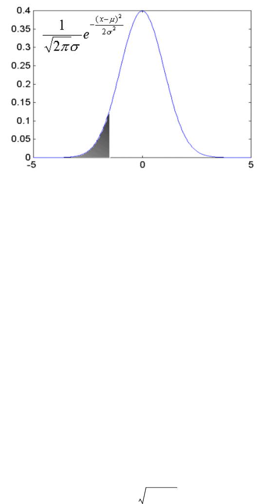
2 Market standards and calculations
2.5 Value-at-Risk calculations
212 © Wall Street Systems IPH AB - Confidential
In the following figure, the shaded area represents the probability that the value of the position will
move below the value-at-risk figure . This probability is 5%.
The VaR key-figures which can be selected in Treasury Monitor are described in more detail in the
TRM User Guide.
2.5.6 Incremental VaR
Incremental VaR is a statistic providing information on the sensitivity of VaR to changes in portfolio
holdings. Let wi be the i component of the delta vector of the portfolio and VaR the total value at
risk of the portfolio, with the i component of the incremental VAR defined as:
Equation 2-418 VaR: Incremental VaR definition
As a consequence of the definition,
Equation 2-419 VaR: Incremental VaR calculation
2.5.6.1 Calculation of incremental VaR
Let Cij denote the covariance matrix, w the delta vector and wT the transpose of the delta vector.
Since
Equation 2-420 VaR: Incremental VaR calculation
the i component of the incremental VaR (IVAR) is defined as
Equation 2-421 Incremental VaR (IVAR)
Incremental VaR can then be interpreted as the product of the exposures of the position with
respect to each risk factor wi and the sensitivity of the VaR of the portfolio with respect to changes
in each of those risk factors.
1.65σ
IVARiwi
∂VAR
∂wi
----------------
=
I
i
∑VARiVAR=
VAR wTCw=
2 Market standards and calculations
2.5 Value-at-Risk calculations
Transaction & Risk Management Module (TRM) Instruments: Processing and Calculations 213
IVARiwi
Cijwj
j
∑
VAR
--------------------
=
2 Market standards and calculations
2.5 Value-at-Risk calculations
214 © Wall Street Systems IPH AB - Confidential
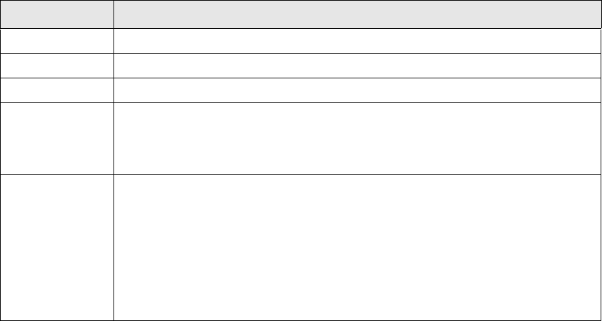
Transaction & Risk Management Module (TRM) Instruments: Processing and Calculations 215
Chapter 3 Debt instruments
3.1 Bond
Bonds are negotiable issues, which means that their cashflows are known (in terms of structure and
dates) when the bond is issued. They can be traded in the market.
In TRM, there is a clear distinction between loans and bonds. Loan agreements are set up mostly at
deal entry, while bond issues must be completely defined at instrument level (notably in terms of
cashflows).
As is the case for loans, the definition of cashflows relies completely on the schedule concept (or
cashflow structure).
See Appendix B Schedules on page 883.
Several schedules must be attached to a bond and they drive the generation of the cashflow
structure for the deal.
For the simplest bond, two schedules are associated with the deal: one schedule for interest flows;
and one schedule for principal flows. It is possible to have additional interest schedules in the case
of parallel interest flows.
Bond instruments must be based on an instrument type derived from the class BOND.
3.1.1 Fixed-rate bond
This is the simplest type of bond. Fixed-rate bonds are usually managed as described in the
following sections.
3.1.1.1 Instrument setup
•Bond main characteristics
This information may be relevant to any kind of fixed-rate bond.
Information Description
Issuer Issuer of the bond.
Currency Currency in which the bond is issued.
Amount Rounding Specify with how many decimals and with which method the amounts will be rounded.
Default Price
Denom.
For fractional prices, defines the default denominator. If a default price denominator is
specified, the Deal Price can be entered as a fraction at deal entry.
For example, if you enter 32 in this field, a Deal Price entered as 100-5 is displayed as
100 5/32. See the TRM User Guide.
Accrued Interest
Method
How the system computes settlement accrued interest. For most bonds, the Linear
method can be used, but some bonds require a specific method.
For bonds traded at dirty price (i.e. price that includes accrued interest), it is also
possible to specify an accrued interest method. In this case, the accrued interest is
calculated for accounting purposes only (as settlement principal based on dirty price
already includes accrued interest). If this field is left blank, no settlement AI is
calculated
See 2.1.6.1 Accrued interest calculations on page 67 for details of accrued interest
methods.
3 Debt instruments
3.1 Bond
216 © Wall Street Systems IPH AB - Confidential
See A.2.51 Bond on page 734.
–Dates details
The issue date and the maturity date must be specified for the bond.
–Trading unit details
It is possible to define a minimum bid size or trading units of a bond. If a minimum
denomination is defined, deal entry is available either in units or amount and TRM ensures
that the amount is a multiple of the denomination size.
•Schedules
Select the cashflow structure template you want for the instrument. For each set of cashflows
defined in the template, select the generation parameters.
One system template is provided for fixed-rate plain vanilla bonds (see B.2.1.1.21 Fixed, Bullet
Repayment on page 894); you can choose this template or any other template derived from it.
Once the template is applied to the instrument, the schedules are created and it is then possible
to define their characteristics, such as, date basis, payment convention, calendars, and so on.
See Appendix B Schedules on page 883.
•Cashflows
As the cashflows are an intrinsic characteristic of an issue, they must be defined at instrument
level. Generation of the cashflows is automatically done in the instrument setup and takes into
account all the information specified in the schedule. Some fields can be manually modified at
cashflow level if necessary.
The cashflows are saved in the database along with the instrument, and they will be used
directly to generate the cashflows of the deal when the bond is sold or purchased.
•Trad ing yield
Specify how the yield/price conversion will be made when dealing the instrument.
See A.2.323 Trading Yield on page 872.
•Quoted
It is necessary to specify how a bond is quoted on the market.
Settlement
Switches
If the bond is traded in dirty price it has to be specified here.
It is also possible to define whether rounding of the settlement principal is per trading
unit, that is, the rounding is done for one unit and then the amount is multiplied by
the number of units to obtain the settlement principal and accrued interest.
Coupon Rate The interest rate of the fixed-rate bond.
Information Description
Yield Convention The convention defines how the yield/price conversion will be made. TRM supports the
standard conventions. See 2.1.4 Yield/price conversions on page 38.
Price and Rate
rounding
Defines how the system should round prices and rates.
Information Description
Price Type Price % or Yield for a bond.
Quote Handling If the Bond quote handling is used, the system will notify Rate Monitor that it is a
fixed-rate bond.
Information Description
3 Debt instruments
3.1 Bond
Transaction & Risk Management Module (TRM) Instruments: Processing and Calculations 217
See A.2.274 Quoted on page 849.
It is also possible to set up:
•Spot day calculations
•Cashflow and transaction charge rules
•Collateral
•Branch Codes
•Security Identifiers
•Delivery.
See Appendix A Features on page 713.
3.1.1.2 Deal capture
3.1.1.2.1 Input data
In addition to the standard deal parameters, the following information is required to enter a deal on
a fixed-rate bond.
In addition, the following optional information can be captured:
Currency This quoted notion is time dependant (price type and/or currency may change over
the life of a bond).
Information Description
Information Description
Deal Price or Deal Rate If there is a yield/price convention set on the instrument, it is possible to enter either
a rate or a price. The conversion will be made automatically.
If there is no convention set, the deal must be entered in price.
If a default price denominator is specified at instrument setup, Deal Price can be
entered as a fraction. For more information about fractional prices, see the TRM User
Guide.
By default, Deal Price is considered as clean (i.e. does not include accrued interest).
Deal Price is considered dirty if so defined at instrument level (in Settlement Switches) or
if you set the Force Dirty Price transaction column value to Yes when entering the
transaction.
Nominal Amount
Face Amount
Enter either the nominal amount or face amount, and the system will compute the
other automatically.
Value Date Official date when money is transferred. This defaults to the spot date of the
transaction.
Information Description
Units
Tradi ng Unit Size
If the denomination of a bond instrument is specified at instrument setup, the deal
can be input in units, and the nominal and face amounts are computed by the system.

3 Debt instruments
3.1 Bond
218 © Wall Street Systems IPH AB - Confidential
3.1.1.2.2 Generated data
•Transaction
Book Value (BV) = NA * price / 100
where:
NA = nominal amount
price = deal price
•Cashflows
TRM copies all the future cashflows of the bond and scales them according to the nominal
amount engaged (using rounding).
Additionally, the system generates a settlement cashflow with amount = BV (see above) and an
accrued interest cashflow according to the AI Method.
The following cashflow structure is generated for a fixed-rate bond:
3.1.1.3 Processing
This section describes the actions that can be done throughout the life of a bond.
3.1.1.3.1 Asset swap
You can easily create an asset swap from a bond transaction by executing the Asset Swap action. The
asset swap is an interest rate swap where the cashflow structure of one leg (the asset leg) is similar
but opposite to the cashflow structure of the bond, and the other leg corresponds to what you have
specified (e.g. quarterly floating).
•Setup
To enable this action, the Allow Swap feature must be associated with the instrument.
See A.2.23 Allow Swap on page 722.
•Execution
Right-click a bond transaction that uses an instrument with the Allow Swap feature, and select
Asset Swap action in Transaction Manager. When you execute this action, use the following table
to specify the parameters.
Information Description
Swap Instrument Select the instrument for the asset swap transaction.
See 11.1.2 Asset swap on page 656 for information about setting up the Swap
Instrument.

3 Debt instruments
3.1 Bond
Transaction & Risk Management Module (TRM) Instruments: Processing and Calculations 219
Opening Date
Value Date
The opening date and value date of the asset swap transaction.
Swap Amount The nominal amount being swapped, which defaults to the nominal amount of the
underlying bond transaction. This can be changed in order to swap a fraction of the
bond.
Asset Amount Read-only. The nominal amount of the underlying bond.
Swap Units Read-only. The number of units being swapped (if the underlying bond is traded by
units).
Asset Units Read-only. The number of units of the underlying bond (if the underlying bond is
traded by units).
Leg Leg of the swap that will reflect the asset leg, i.e. which reverses the cashflows of the
bond.
Zero-Coupon
Style
Switch on so that the nominal amount of the other leg (i.e. the non-asset leg) of the
asset swap is adjusted with the deal price of the underlying bond.
The system automatically defaults to the zero-coupon style when there are no interest
cashflows found in the bond transaction.
Include Fees after
Value Date
Switch on so that fees that are to be settled after the value date of the bond are also
copied and reversed asset swap.
If this switch is not on, the fees after the value date are ignored.
Price/Fee Method Method for reflecting the deal price and the fees of the bond in the asset swap
transaction. As for all swaps, a price that is different from par (100) will result in
upfront payments in the swap.
Choose from:
•All-In Price - All-In Price of the underlying bond is used as the price of the asset leg
of the swap.
•Deal Price - Deal Price of the underlying bond is used as the price of the asset leg of
the swap.
•Deal Price with Fees - Deal Price of the underlying bond is used as the price of the
asset leg of the swap. In addition, the fees of the bond transaction can be
reflected (copied and reversed) as upfront payments in the asset swap
transaction. The Copied Fees field is used for determining which fees are to be
reflected in the swap.
•Par - Price of the asset leg of the swap is Par, i.e. 100.
•Par with Discount/Premium and Fees - Price of the asset leg of the swap is Par, i.e. 100,
but in addition discount/premium and fees of the bond transaction can be reflected
(copied and reversed) as upfront payments in the asset swap transaction. The
Copied Fees field is used for determining which fees are to be reflected in the swap.
•Re-Offer Price - Re-Offer Price of the underlying bond is used as the price of the asset
leg of the swap.
Copied Fees Select which fees are to be copied (as reversed) from the bond transaction to the
swap transaction as upfront payments:
•None - No fees are copied.
•All Fees - All fees are copied.
•All-In Fees - Only All-In fees are copied (i.e. fees with the All-In attribute).
•Re-Offer Fees - Only Re-Offer fees are copied (i.e. fees with the Re-Offer attribute).
Fees (<CCY>) The fee amounts (in the relevant currency) copied/reversed from the underlying bond
transaction and considered as upfront payments in the asset swap transaction. The
values are defaulted from the bond transaction according to the selections in Price/Fee
Method and Copied Fees fields. You can modify the amounts if needed.
Information Description
3 Debt instruments
3.1 Bond
220 © Wall Street Systems IPH AB - Confidential
The execution of the action generates a swap transaction.
•Cancellation
Cancellation of the action is done by canceling the swap transaction.
3.1.1.3.2 Pricing
Pricing of bond transactions can be performed at transaction level using a right-click processing
action.
•Setup
A choice of two types of Pricing action are available on the transaction if the Bond Pricing feature
is associated with the instrument: Swap Spread or Yield/Price to Maturity.
See A.2.79 Bond Pricing on page 746.
•Execution
–Swap Spread
This Pricing action calculates the spread to be add to the floating leg of an asset swap
generated from a given bond so that the market value of the asset swap is zero.
–Yield/Price to Maturity
This Pricing action calculates a yield (Price) using a given price (Yield) and vice versa. The
calculation assumes the Yield Convention (*ISMA-30E360-ANNUAL or other) as defined in the
Trading Yield page of the Instrument.
Adjust Leg 2 Price
With Up-Fronts
Switch on so that the Deal Price of the other leg (i.e. the non-asset leg) of the asset
swap is adjusted with the upfront payments on the asset leg.
By Nominal
Amount
If the underlying bond is traded in units, you can 'force' the swap transaction to be
based on the nominal amount rather than units by setting this switch. If the swap is
based on units, the interest amounts are calculated by one unit and multiplied by the
number of units.
Information Description
Swap Instrument ID of the Asset Swap instrument.
Floating Leg
Currency
Currency of the floating leg.
Floating Leg
Frequency
Frequency of the floating coupon.
Swap Deal Price Deal price of the swap.
Swap Spread Calculated spread after pricing.
Information Description
Interest Rate Rate type of the yield.
Date Basis Date basis used to convert the time.
Pricing Date Opening date of the bond transaction.
Pricing Variable Yield (or the price).
Pricing Target
Variable
(Information only)
Price (or the yield).
Information Description

3 Debt instruments
3.1 Bond
Transaction & Risk Management Module (TRM) Instruments: Processing and Calculations 221
3.1.1.3.3 Benchmarking
It is possible to analyze and compare a bond issue against those of another bond (the benchmark)
or a swap curve, in terms of yields, swap spreads, or par swap rates.
See 3.2 Structured bonds on page 244.
3.1.1.3.4 Transaction conversion
It is possible to allow schedule conversion at predefined dates during a bond's life.
•Setup (at instrument level)
This process is available on the transaction if the Transaction Conversion feature is associated
with the instrument.
See A.2.325 Transaction Conversion on page 873.
Then, the user can attach conversion schedules (at the instrument level) in the Schedule page of
the Instrument Editor.
•Execution
–At instrument level:
To execute the conversion at a predefined date, in the Instrument Editor, Cashflow page, the
user selects the conversion flow and performs Convert action. After this conversion, when
capturing a transaction, cashflows are generated according to the converted schedules.
–At transaction level:
When capturing a transaction before the conversion date, conversion events are also
generated in the transaction. To execute the conversion, the user right-clicks the row of the
corresponding transaction event and selects Transaction Conversion. The conversion inputs are
displayed.
See A.2.325 Transaction Conversion on page 873.
The execution generates a conversion transaction with the following attributes:
–Kind: Conversion
–Opening Date: Conversion opening date
–Value Date: Conversion value date.
The remaining attributes are inherited from the initial transaction.
The conversion transaction generates closing cashflows for the initial transaction; and future
cashflows are reopened according to the conversion schedules defined at instrument level.
3.1.1.4 Position monitoring
3.1.1.4.1 Setup
The cashflow discounting method used in IR risk calculation depends on the instrument set up:
•Risk setup:
The default risk method is Zero-Coupon or you can select Z-Spread or Yield to Maturity. For more
information about these methods, see A.2.288 Risk Setup (BOND) on page 858.
Pricing Target (in %) Target value that you want to achieve.
Pricing Result (Information only)
Calculated value of the variable after pricing.
Information Description

3 Debt instruments
3.1 Bond
222 © Wall Street Systems IPH AB - Confidential
•IR exposure setup:
–By default, TRM uses the valuation curve interpolation settings (IR Quote and Yield Curve
Editor - Interpolation page). For example, if the interpolation settings are set up with Interest
Type Continuous Yield, then risk calculations use continuously compounding discounting of the
cashflows.
–If IR Exposure is set up at the instrument level, then TRM uses these settings. For example,
if IR exposure is set up with yield type Periodic Rate, then risk calculations use periodic
discounting of the cashflows. See A.2.48 Base IR Exposure Setup on page 732.
–If the risk method Yield to Maturity is used, then the date basis and interest rate defined for the
risk yield are applied, even if there is an IR exposure setup.
For more information about these calculations, see 2.3 Key-figures on page 112.
3.1.1.4.2 Calculations
In this section, numerical examples demonstrate how the different figures are calculated for
fixed-rate bonds.
If you need more theoretical information about the method used in these calculations, see Chapter 2
Market standards and calculations on page 33.
This example shows a fixed-rate bond with the following deal data:
Unless otherwise stated, the figure date used in the calculations is 2001-05-15. On this date, the
market data is as follows:
Other figures calculated by the system are as follows:
•Time to Spot
t_s = d_fs / B
0.005555556 = 2 / 360
Setup data
Instrument Date Basis Act/360
Currency EUR
Valuation Method Theoretical
Risk Method Theoretical
Valuation Date Figure Date
Risk Date Figure Date
Risk Yield Type Continuous
AI Method Linear
Schedule Fixed, Bullet Repayment
Result IR: Accrued Interest Linear
Result IR: Accrual Method Linear Accrual
Accrual Yield: Interest Type Periodic Rate
Accrual Yield: Date Basis Actual/360
Market data on 2001-05-15
Figure Date d_f 2001-05-15
Days to Spot d_fs 2
Discount Rate r_d 3.048771%
3 Debt instruments
3.1 Bond
Transaction & Risk Management Module (TRM) Instruments: Processing and Calculations 223
• MV Spot Discount Factor
D_s = EXP (-t_s * r_d) = 0.9998306382
Transaction data specific to the principal cashflow is as follows:
On the figure date, the market data specific to the principal amount is as follows:
Other market data and figures specific to the principal amount are calculated by the system as
follows:
• Time to Payment
t_p.p = (dt_p.p - d_f) / B
2.67222222 = (2004/01/02 – 2001/05/15) / 360
• MV Discount Factor
D_V.p = D_s * D_f.p = 0.8851322685
• PV Discount Factor
D_P.p = D_s * D_f.p = 0.8851322685
• Discount Factor From Spot
D_f.p = EXP (-(t_p.p - t_s) * r.p) = 0.8852822015
On the figure date, the market data specific to the coupons is as follows:
Transaction data specific to the coupon cashflows is as follows:
Other market data and figures specific to the coupons are calculated by the system as follows:
•Coupon 1
Time to Payment
t_p.c1 = (dt_p.c1 - d_f) / B
0.644444444 = (2002/01/02– 2001/05/15) / 360
MV Discount Factor
D_V.c1 = D_s * D_f.c1 = 0.977418468
PV Discount Factor
D_P.c1 = D_s * D_f.c1 = 0.977418468
Transaction data
Opening Date 2001-02-16
Nominal Amount A 1,000,000
Value Date dt_v.p 2004-01-01
Payment Date dt_p.p 2004-01-02
Issue Date dt_i 2001-01-01
Book Value V_b.p = A 1,000,000
Market data on 2001-05-15
Interest Rate r.p 4.56933049%
Market data Coupon 1 Coupon 2 Coupon 3
Interest Rate r.c1 3.5485079% r.c2 4.145317% r.c3 4.56933049%
Transaction data Coupon 1 Coupon 2 Coupon 3
Amount A.c1 50,000 A.c2 50,000 A.c3 50,000
Value Date dt_v.c1 2002-01-01 dt_v.c2 2003-01-01 dt_v.c3 2004-01-01
Payment Date dt_p.c1 2002-01-02 dt_p.c2 2003-01-02 dt_p.c3 2004-01-02
3 Debt instruments
3.1 Bond
224 © Wall Street Systems IPH AB - Confidential
Discount Factor from Spot
D_f.c1 = EXP (- (t_p.c1 - t_s) * r.c1) = 0.977584034
•Coupon 2
Time to Payment
t_p.c2 = (dt_p.c2 - d_f) / B
1.658333333 = (2003/01/02 – 2001/05/15) / 360
MV Discount Factor
D_V.c2 = D_s * D_f.c2 = 0.933623285
PV Discount Factor
D_P.c2 = D_s * D_f.c2 = 0.933623285
Discount Factor from Spot
D_f.c2 = EXP (- (t_p.c2 - t_s) * r.c2) = 0.933781432
•Coupon 3
Time to Payment
t_p.c3 = (dt_p.c3 - d_f) / B
2.672222222 = (2004/01/02 – 2001/05/15) / 360
MV Discount Factor
D_V.c3 = D_s * D_f.c3 = 0.885132268
PV Discount Factor
D_P.c3 = D_s * D_f.c3 = 0.885132268
Discount Factor from Spot
D_f.c3 = EXP (- (t_p.c3 - t_s) * r.c3) = 0.885282201
3.1.1.4.3 Valuation figures
The valuation method commonly used for a fixed-rate bond is the Theoretical method.
• Principal flow figures
Market Value
V. p = A * D _ V. p
885,132.27 = 1,000,000 * 0.8851322685
Clean Market Value
CMV.p = A * D_f.p
885,282.20 = 1,000,000 * 0.8852822015
• Coupon 1 figures
Market Value
V.c1 = A.c1 * D_V.c1
48,870.92 = 50,000 * 0.977418468
Clean Market Value
CMV.c1 = A.c1 * D_f.c1 - Accrued_Interest_Spot
29,990.31 = 50,000 * 0.977584034 - 18,888.89
• Coupon 2 figures
Market Value
V.c2 = A.c2 * D_V.c2
46,681.16 = 50,000 * 0.933623285
Clean Market Value
CMV.c2 = A.c2 * D_f.c2
46,689.07 = 50,000 * 0.933781432
• Coupon 3 figures
Market Value
V.c3 = A.c3 * D_V.c3
44,256.61 = 50,000 * 0.885132280
Clean Market Value
CMVc3 = A.c3 * D_f.c3
44,264.11 = 50,000 * 0.885282201
• Total transaction figures
Market Value
= V.p +V.c1 + V.c2 + V.c3
= 1,024,940.97
3 Debt instruments
3.1 Bond
Transaction & Risk Management Module (TRM) Instruments: Processing and Calculations 225
Clean Market Value
= CMV.p + CMV.c1 + CMV.c2 + CMV.c3
=1,006,225.70
3.1.1.4.4 Result figures
The setup of the instrument impacts the way result figures are computed.
• Principal flow figures
Tot al P rof it
Tot al_ Prof it. p = V.p - V _ b. p
-114,867.73 = 885,132.27 – 1,000,000
MtoM Profit
MtoM_Profit.p = A * D_f.p - V_b.p
-114,717.80 = 1,000,000 * 0.8852822015 – 1,000,000
Other Profit
Other_Profit.p = Total_Profit.p - MtoM_Profit.p
-149.93 = -114,867.73 – (-114,717.80)
• Coupon 1 figures
Tot al P rof it
Total_Profit.c1 = = V.c1 - V_b.c1
48,870.92 = 48,870.92 - 0
MtoM Profit
MtoM_Profit.c1 = A.c1 * D_f.c1 - V_b.c1 - Accrued_Interest.Spot
29,990.31 = 50,000 * 0.977584034 – 0 – 18,888.89
Accrued Interest
Accrued_Interest.c1 = A.c1 * (d_f - dt_i) / B
18,611.11 = 50,000 * (2001/05/15 – 2001/01/01) / 360
Other Profit
Other_Profit.c1 = Total_Profit.c1 - MtoM_Profit.c1 - Accrued_Interest.c1
269.50 = 48,870.92 - 29,990.31 - 18,611.11
• Coupon 2 figures
Tot al P rof it
Tot al_ Prof it. c 2 = V.c2 - V_b.c2
46,681.16 = 46,681.16 - 0
MtoM Profit
MtoM_Profit.c2 = A.c2 * D_f.c2 - V_b.c2
46,689.07 = 50,000 * 0.933781432 - 0
Other Profit
Other_Profit.c2 = Total_Profit.c2 - MtoM_Profit.c2
-7.91 = 46,681.16 - 46,689.07
• Coupon 3 figures
Tot al P rof it
Tot al_ Prof it. c 3 = V.c3 - V_b.c3
44,256.61 = 44,256.61 - 0
MtoM Profit
MtoM_Profit.c3 = A.c3 * D_f.c3 - V_b.c3
44,264.11 = 50,000 * 0.885282201 - 0
Other Profit
Other_Profit.c3 = Total_Profit.c3 - MtoM_Profit.c3
-7.50 = 44,256.61 - 44,264.11
• Total transaction figures
Tot al P rof it
= Total_Profit.p + Total_Profit.c1 +Total_Profit.c2 + Total_Profit.c3
= 24,940.97
MtoM Profit
= MtoM_Profit.p + MtoM_Profit.c1 + MtoM_Profit.c2 + MtoM_Profit.c3
= 6,225.70
3 Debt instruments
3.1 Bond
226 © Wall Street Systems IPH AB - Confidential
Accrued Interest
= Accrued_Interest.c1
= 18,611.11
Other Profit
= Total_Profit.total - MtoM_Profit.total - Accrued_Interest.total
= 104.16
3.1.1.4.5 Risk figures
The risk method commonly used for a bond is the Theoretical method.
• Principal flow figures
IR Exposure 1bp
E_i.p = A * (- (t_p.p - t_s) * D_f.p * D_s - t_s * D_f.p * D_s) * 0.0001
-236.53 = 1,000,000*(-(2.6722222-0.005555556)*0.8852822015*0.9998306382-t_s*D_f.p*D_s)*0.0001
Effective Duration
U_eff.p = -E_i.p / V.p / 0.0001
2.672222 = -(-236.53) / 885,132.27 / 0.0001
• Coupon 1 figures
IR Exposure 1bp
E_i.c1 = A.c1 * (- (t_p.c1 - t_s) * D_f.c1 * D_s - t_s * D_f.c1 * D_s) * 0.0001
-3.15 = 50,000 * (-(0.64444444–0.005555556)*0.977584034*0.9998306382–t_s*D_f.c1*D_s)*0.0001
Effective Duration
U_eff.c1 = -E_i.c1 / V.c1 / 0.0001
0.64444 = -3.15 / 48,870.92 / 0.0001
• Coupon 2 figures
IR Exposure 1bp
E_i.c2 = A.c2 * (- (t_p.c2 - t_s) * D_f.c2 * D_s - t_s * D_f.c2 * D_s) * 0.0001
-7.74 = 50,000 * (-(1.658333333-0.005555556)*0.933781432*0.9998306382-t_s*D_f.c2* D_s)*0.0001
Effective Duration
U_eff.c2 = -E_i.c2 / V.c2 / 0.0001
1.65833 = -7.74 / 46,681.16 / 0.0001
• Coupon 3 figures
IR Exposure 1bp
E_i.c3 = A.c3 * (-(t_p.c3 - t_s) * D_f.c3 * D_s - t_s * D_f.c3 * D_s) * 0.0001
-11.83 = 50.000*(-(2.672222222-0.005555556)*0.885282201*0.9998306382-t_s*D_f.c3* D_s)*0.0001
Effective Duration
U_eff.c3 = -E_i.c3 / V.c3 / 0.0001
2.672222222 = -11.83 / 44,256.61 / 0.0001
• Total transaction figures
IR Exposure 1bp
= E_i.p +E_i.c1 + E_i.c2 + E_i.c3
= -259.24
Effective Duration
= -E_i.total / V.total / 0.0001
= 2.529357
3 Debt instruments
3.1 Bond
Transaction & Risk Management Module (TRM) Instruments: Processing and Calculations 227
3.1.1.5 Norwegian government bond
Norwegian government bonds are based on annual coupon and Actual/365 accrual date basis. The
ex-coupon period starts 14 calendar days prior to the interest payment. Accrued interest is
calculated as shown in Equation 2-51 Accrued Interest: Norwegian on page 55.
3.1.1.5.1 Instrument setup
Norwegian bond instruments must be based on an instrument type derived from the class BOND.
•Main characteristics
They are set up in a similar way to bonds (3.1.1 Fixed-rate bond on page 215), except for the
following.
–Schedule
Select a cashflow structure based on the Fixed, Bullet Repayment system template,
(FIXED-BULLET). See B.2.1.1.21 Fixed, Bullet Repayment on page 894.
•Trad ing Yield
See A.2.323 Trading Yield on page 872.
•Quoted parameters
See A.2.274 Quoted on page 849.
•Result parameters
See A.2.49 Base IR Setup on page 733.
Information Description
Currency NOK
AI Method Norwegian. See Norwegian on page 77.
Information Description
Yield Convention GOVT-NO-ACT365 (Norwegian Government Actual365)
Information Description
Price Type Yield
Quote Handling Bond
Currency NOK
Information Description
AI Method Coupon %

3 Debt instruments
3.1 Bond
228 © Wall Street Systems IPH AB - Confidential
3.1.2 Floating rate note
Floating Rate Notes (FRNs) have interest payments linked to a reference rate which has to be fixed
for each coupon.
3.1.2.1 Instrument setup
Instrument setup for a floating rate note is similar to that of a fixed-rate bond (see 3.1.1 Fixed-rate
bond on page 215), except for the following:
•Bond main characteristics
The coupon rate needs to be null.
•Schedules
Select the cashflow structure template you want for the instrument and, for each set of
cashflows defined in the template, select the generation parameters.
One system template is provided for floating rate bonds (B.2.1.1.22 Floating, Bullet Repayment
on page 894); you can choose this template or any other template derived from it. Once the
template is applied to the instrument, the schedules are created and it is then possible to define
their characteristics.
One important set of characteristics in the case of a floating rate note are the fixing parameters:
–Fixing Rate (the yield curve) optionally * by a factor and + a spread
–Fixing period (3M, 6M, 1Y, and so on)
–Price Scenario used to retrieve the price which will be used for fixing
–Fixing offset and type (in advance or in arrears). If in advance, the rate of the first cashflow
is required.
See Appendix B Schedules on page 883.
•Discount margin calculation
Most FRNs have a known first/next coupon payment, while subsequent coupons will usually be
set in terms of a margin over a specific reference rate (such as, LIBOR). As a result, a current
margin relative to the reference rate is often calculated.
–Discount margin setup
Define the parameters used to calculate the discount margin if you want to take it into
account in the estimation of the instrument’s future flows.
See A.2.343 Z-DM/Spread Setup on page 882.
–Quoted
It is necessary to specify how the FRN is quoted on the market.
It will then be possible to use the Bid Z-DM/Spread and Ask Z-DM/Spread figures to convert
Price into Discount Margin in Rate Monitor.
See A.2.274 Quoted on page 849.
Information Description
Quote Handling FRN
3 Debt instruments
3.1 Bond
Transaction & Risk Management Module (TRM) Instruments: Processing and Calculations 229
–Risk parameters
After the calculation of the discount margin, the payment discount factor of each flow is
adjusted. The derived risk structure is achieved by setting the following parameter:
See A.2.338 Valuation Setup (Floating) on page 879.
3.1.2.2 Deal capture
3.1.2.2.1 Input data
In addition to the standard deal parameters, the following information is required to enter a deal on
a floating-rate bond.
In addition, the following optional information can be captured:
3.1.2.2.2 Generated data
•Transaction
Book Value (BV) = NA * price / 100
where:
NA = nominal amount
price = deal price
•Cashflows
The system copies all the future cashflows of the bond and scales them according to the nominal
amount engaged (using rounding).
Additionally the system generates a settlement cashflow with amount = BV (see above) and an
accrued interest cashflow according to the AI Method.
Note: The bond must be fixed at instrument level in order for the accrued interest flow to be
generated (see 3.1.2.3.1 Fixing on page 230).
Information Description
Risk Profile Plain Vanilla
Information Description
Deal Price Price paid for the FRN as a percentage of the Nominal Amount.
Nominal Amount
Face Amount
Enter either the nominal amount or face amount, and the system will compute the
other automatically.
Value Date Official date when money is transferred. This defaults to the spot date of the
transaction.
Information Description
Units
Tradi ng Unit Size
If the denomination of a bond instrument is specified at instrument setup, the deal
can be input in units, and the nominal and face amounts are computed by the system.
Nominal/Spot Rate Current "running" coupon can be entered in this field (if fixing of the first coupon has
not been carried out in Instrument Editor: see 3.1.2.3.1 Fixing on page 230).
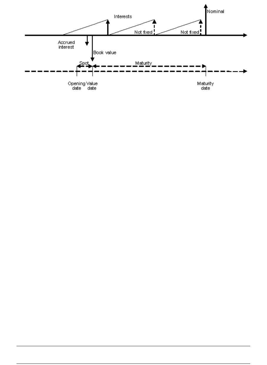
3 Debt instruments
3.1 Bond
230 © Wall Street Systems IPH AB - Confidential
The following cashflow structure is generated for a floating-rate bond:
3.1.2.3 Processing
This section describes the actions that can be done throughout the life of a floating-rate bond.
3.1.2.3.1 Fixing
The major process for a floating-rate note is the fixing of the flows.
•Setup
Depending on the instrument setup (schedules) the fixing can be done in advance (the standard
case, at the beginning of each coupon period) or in arrears (at the end of each coupon period).
In both cases there can be an offset of n days (before the beginning or end of the coupon
period).
•Execution
When fixing is executed, the rate is retrieved for the specified fixing rate and period according to
the designated fixing scenario. The scenario to be used for fixing is configured at the system
level, see TRM System Admin Guide. The fixing subscenario is specified at the cashflow level.
The following information is stored on the fixed cashflow:
The fixing date
The rate of the yield curve
The coupon rate which is the rate of the yield curve (and optionally * factor
+ spread)
The amount of the coupon.
The fixing process can be performed in two ways in TRM: the process itself is exactly the same in
each case: the coupon is fixed at both instrument and transaction level.
The methods of fixing are as follows:
–Directly on the cashflow (in Instrument Editor’s Cashflow page) using the Fix Price action: the
fixing affects all deals on this instrument.
–Using the Fixing Bond Cashflow activity: all instruments and their deals that need to be fixed
for a particular date are affected.
See the TRM User Guide for information on the activity parameters.
Note: The bond issue must be fixed at instrument level in order for the accrued interest flow to
be generated (for transactions captured between coupon fixing date and fixing value date).
3 Debt instruments
3.1 Bond
Transaction & Risk Management Module (TRM) Instruments: Processing and Calculations 231
•Cancellation
It is possible to cancel the cashflow fixing either manually, using the Undo Fixing action in
Instrument Editor; or automatically, using the Fixing Bond Cashflow - Undo activity.
See the TRM User Guide for information on the activity parameters.
3.1.2.4 Position monitoring
3.1.2.4.1 Setup
The cashflow discounting method used in IR risk calculation depends on the instrument set up:
•Risk setup:
–The default risk method is Zero-Coupon or you can select risk method Zero Discount Margin
(Z-DM). For more information about these methods, see A.2.289 Risk Setup (FRN) on page
858.
–If discount margin is set up at the instrument level (see A.2.164 FRN Valuation on page
791), then the discount margin is used in the valuation and is added to the valuation curve
specified for the instrument, and the day count method and yield type used are taken from
the interpolation method of this valuation curve. For more information about Discount Margin
calculations, see 2.1.5 Discount Margin on page 66.
•IR exposure setup:
–By default, TRM uses the valuation curve interpolation settings (IR Quote and Yield Curve
Editor - Interpolation page). For example, if the interpolation settings are set up with Interest
Type Continuous Yield, then risk calculations use continuously compounding discounting of the
cashflows.
–If IR Exposure is set up at the instrument level, then TRM uses these settings. For example,
if IR exposure is set up with yield type Periodic Rate, then risk calculations use periodic
discounting of the cashflows. See A.2.48 Base IR Exposure Setup on page 732.
For more information about these calculations, see 2.3 Key-figures on page 112.
3.1.2.4.2 Calculations - Discount Margin example
Let us consider a floating rate note with two coupons remaining, where the next coupon is fixed:
•Input data
Data Symbol Example
Next coupon (fixed) c1 0.0556111111111111
Last coupon (estimated) c2 0.0232101439796721
Time from spot to next coupon (Act/365) t1 13/365 = 0.035616438356164383
Time from spot to last coupon (Act/365) t2 196/365 = 0.53698630136986303
Discount factor from spot to next coupon D1 0.999066136779281
Discount factor from spot to last coupon D2 0.981278683885205
Clean price from market quote P 0.98
Accrued interest 0.05163888888888888
Dirty price Pd P + = 1.0316388888888888
Ia
Ia
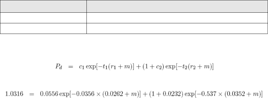
3 Debt instruments
3.1 Bond
232 © Wall Street Systems IPH AB - Confidential
Choosing continuous compounded rate as the discount margin yield type, we get the following
results:
Discount margin must satisfy the following equation:
from which we can solve numerically: m = 0.052423976963667664.
3.1.2.4.3 Calculations - FRN example
The numerical example in this section demonstrates how the different figures are calculated for a
floating-rate note.
Instrument data
•Schedule page (Floating Coupon)
•Base Valuation page
•IR Exposure page
•Floating Valuation page
Transaction data
•Calculated transaction data
Data Calculation
Underlying rate to next coupon r1 = - log[D1] / t1 = - log[0.999] / 0.0356 = 0.026232256389534768
Underlying rate to last coupon r2 = - log[D2] / t2 = - log[0.981] / 0.0537 = 0.035194153518686676
Interest Type Periodic Rate
Date Basis (B) Actual/360 360
(Valuation) Method Theoretical
Date Basis (B_r) Actual/360 360
Yield Type Continuous Yield
Risk Profile Plain Vanilla
Nominal Amount A = 1,000,000.00
Deal Price p = 98.00%
Spot Date d_v = 2002-02-26
Rate r_c = 0.05
Book Value V_b = p*A = 980000
3 Debt instruments
3.1 Bond
Transaction & Risk Management Module (TRM) Instruments: Processing and Calculations 233
Market data
Valuation data
Valuation figures
•Figure Market Value (_V_)
•Figure Fixing Rate (_r_x)
•Figure Amount (_A_e)
Coupon Period
(_p_c)
Time to Value
Date (_t_v) Risk Date (_d_r) Time to Risk
Date (_t_r)
Principal 1.713888889 2/22/2004 1.713888889
Coupon 1 0.188888889 8/22/2002 0.188888889
Coupon 2 0.7
Risk Cash Flow Start 2 177 8/22/2002 0.188888889
Risk Cash Flow End 2 184 2/22/2003 0.7
Coupon 3 1.202777778
Risk Cash Flow Start 3 2/22/2003 0.7
Risk Cash Flow End 3 181 8/22/2003 1.202777778
Coupon 4 1.713888889
Risk Cash Flow Start 4 8/22/2003 1.202777778
Risk Cash Flow End 4 184 2/22/2004 1.713888889
Figure or Valuation Date d_f = 2002-06-15
Figure Market Value Spot
Discount Factor
D_s = 0.999746283358179
Principal =_A_e*_D_p = 930990.3649
Coupon 1 =_A_e*_D_p = 24432.46813
Coupon 2 =_A_e*_D_p = 18638.33299
Coupon 3 =_A_e*_D_p = 20688.99262
Coupon 4 =_A_e*_D_p = 23545.42006
Transaction V_Tr = SUM(_V) = 1018295.579
Coupon 1 =r_c = 0.05
Coupon 2 =(INDEX(_D_p,A28,1)/(_D_p)-1)/(_p_c/360) = 0.037392717
Coupon 3 =(INDEX(_D_p,A29,1)/(_D_p)-1)/(_p_c/360) = 0.043109308
Coupon 4 =(INDEX(_D_p,A32,1)/(_D_p)-1)/(_p_c/360) = 0.049481851
Principal =A = 1000000
Coupon 1 =A*_r_x*_p_c/B = 24583.33333
Coupon 2 =A*_r_x*_p_c/B = 19111.8329
3 Debt instruments
3.1 Bond
234 © Wall Street Systems IPH AB - Confidential
•Figure IR Exposure 1bp (_E_i1)
•Figure Risk Value (_V_r)
•Figure Present Value (_V_p)
Coupon 3 =A*_r_x*_p_c/B = 21674.4023
Coupon 4 =A*_r_x*_p_c/B = 25290.72367
Principal =_V_r*(-_t_r*_D_p)*0.0001 = -159.5614042
Coupon 1 =_V_r*(-_t_r*_D_p)*0.0001 = -0.461502176
Coupon 2
Risk Cash Flow Start 2 =_V_r*(-_t_r*_D_p)*0.0001 = -18.77296987
Risk Cash Flow End 2 =_V_r*(-_t_r*_D_p)*0.0001 = 68.26573443
Coupon 3
Risk Cash Flow Start 3 =_V_r*(-_t_r*_D_p)*0.0001 = -68.26573443
Risk Cash Flow End 3 =_V_r*(-_t_r*_D_p)*0.0001 = 114.809443
Coupon 4
Risk Cash Flow Start 4 =_V_r*(-_t_r*_D_p)*0.0001 = -114.809443
Risk Cash Flow End 4 =_V_r*(-_t_r*_D_p)*0.0001 = 159.5614042
Transaction E_i1_Tr = SUM(_E_i1) = -19.23447204
Principal = A = 1000000
Coupon 1 = _A_e = 24583.33333
Coupon 2
Risk Cash Flow Start 2 = A = 1000000
Risk Cash Flow End 2 = -A = -1000000
Coupon 3
Risk Cash Flow Start 3 = A = 1000000
Risk Cash Flow End 3 = -A = -1000000
Coupon 4
Risk Cash Flow Start 4 = A = 1000000
Risk Cash Flow End 4 = -A = -1000000
Trans ac ti on
Principal = _V_r*_D_p = 930990.3649
Coupon 1 = _V_r*_D_p = 24432.46813
Coupon 2
Risk Cash Flow Start 2 = _V_r*_D_p = 993863.1105
Risk Cash Flow End 2 = _V_r*_D_p = -975224.7775
Coupon 3
3 Debt instruments
3.1 Bond
Transaction & Risk Management Module (TRM) Instruments: Processing and Calculations 235
Result figures
•Figure MtoM Profit (_P_m)
•Figure Accrued Interest (_AI)
•Figure Accrued Profit (_P_a)
•Figure Other Profit (_P_o)
•Total Profit (_P_T)
Risk Cash Flow Start 3 = _V_r*_D_p = 975224.7775
Risk Cash Flow End 3 = _V_r*_D_p = -954535.7849
Coupon 4
Risk Cash Flow Start 4 = _V_r*_D_p = 954535.7849
Risk Cash Flow End 4 = _V_r*_D_p = -930990.3649
Transaction V_p_Tr = SUM(_V_p) = 1018295.579
Principal =A*_D_p/D_s-V_b-_P_a = -51776.12227
Coupon 1 =_A_e*_D_p/D_s-_AI = 9299.779742
Coupon 2 =_A_e*_D_p/D_s-_AI = 18643.06305
Coupon 3 =_A_e*_D_p/D_s-_AI = 20694.24309
Coupon 4 =_A_e*_D_p/D_s-_AI = 23551.39544
Transaction P_m_Tr = SUM(_P_m) = 20412.35905
Coupon 1 = (d_f-d_v)/(_d_v-d_v)*_A_e = 15138.88889
Transaction AI_Tr = SUM(_AI) = 15138.88889
Principal = (d_f-d_v)/(_d_v-d_v)*(A-V_b) = 3002.754821
Transaction P_a_Tr = SUM(_P_a) = 3002.754821
Principal = _P_T-_P_m-_P_a-_AI = -236.267694
Coupon 1 = _P_T-_P_m-_P_a-_AI = -6.200496936
Coupon 2 = _P_T-_P_m-_P_a-_AI = -4.73005535
Coupon 3 = _P_T-_P_m-_P_a-_AI = -5.250473862
Coupon 4 = _P_T-_P_m-_P_a-_AI = -5.975380961
Transaction P_o_Tr = SUM(_P_o) = -258.4241011
Principal =_V-V_b = -49009.63514
Coupon 1 =_V = 24432.46813
Coupon 2 =_V = 18638.33299
Coupon 3 =_V = 20688.99262
Coupon 4 =_V = 23545.42006
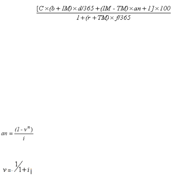
3 Debt instruments
3.1 Bond
236 © Wall Street Systems IPH AB - Confidential
Risk figures
•Figure Effective Duration
3.1.3 Australian floating rate note
An Australian floating rate note (FRN) is a medium-term bond that provides investors with the
ability to achieve returns at a fixed margin above a floating benchmark, usually the 90-day Bank Bill
Swap Rate (BBSW). BBSW rates are compiled daily by the Australian Financial Markets Association
using the mid-rates of 14 banks. Australian floating rate notes are traded at a trading margin and
swap rate, not at a price or yield. The interest margin is determined on the issue date by the credit
rating of the issuer, the term to maturity and the market perception of the issuer.
The official Treasury Adjustable Rate Bond Pricing Formula is as follows:
Price per $100 face value:
Equation 3-1 Official Treasury Adjustable Rate Bond Pricing formula
where:
Transaction U_eff_Tr = E_i1_Tr/V_Tr/0.0001 = -0.188888889
C0 if the next interest is not fixed at instrument level, otherwise 1.
b The Index (as a percentage) from the last interest reset date to the next
interest payment date defined as the average three month Australian bank
bill swap reference mid-rate (BBSW) as indicated by Reuters, rounded to
four decimal places.
IM Spread% defined at schedule level.
d The number of days in the current interest period.
TM Trading Margin (expressed as a percentage) to express the yield margin to
the Index.
an
v
n The number of complete interest periods to maturity at the next interest
payment date.
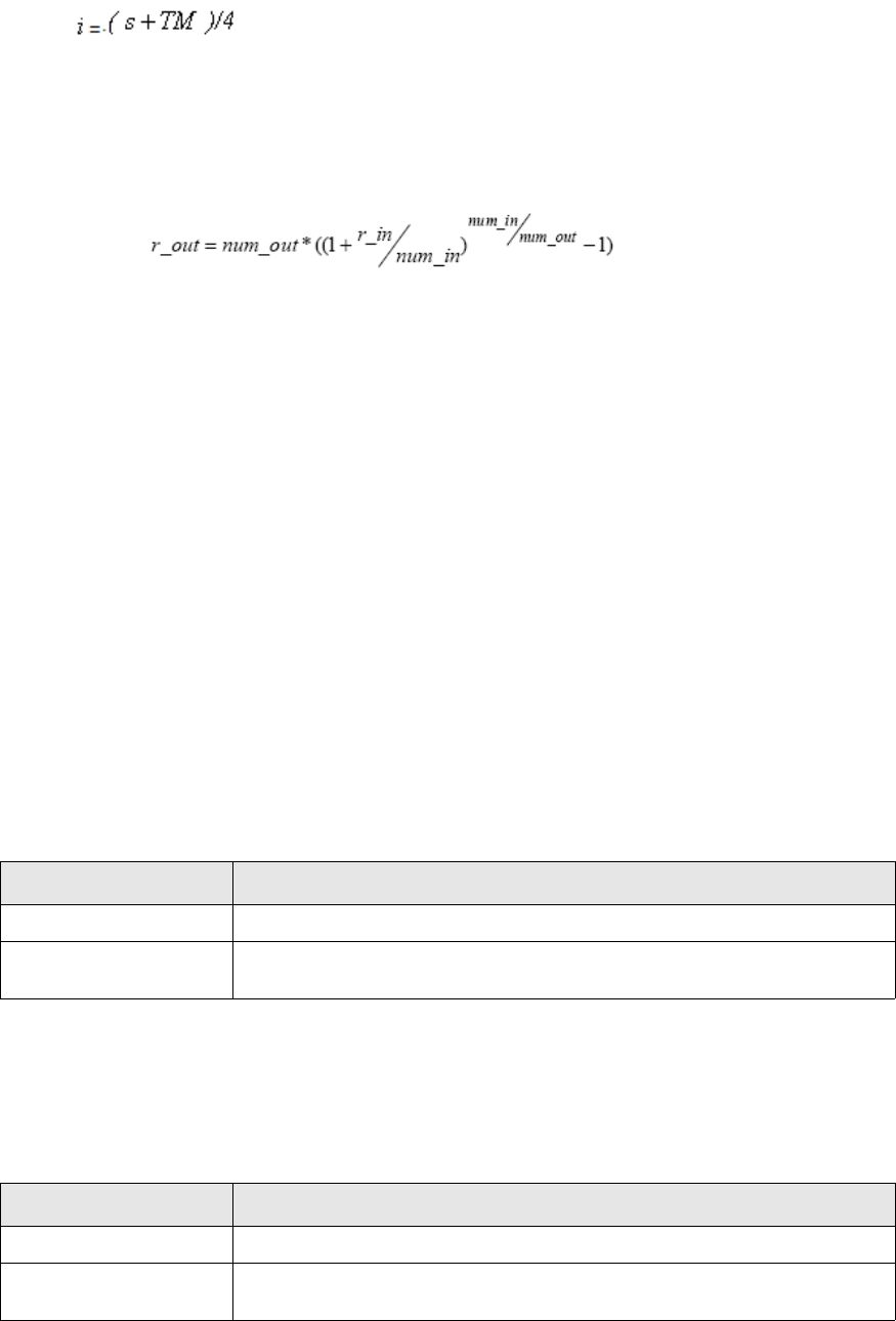
3 Debt instruments
3.1 Bond
Transaction & Risk Management Module (TRM) Instruments: Processing and Calculations 237
3.1.3.1 Instrument setup
Australian FRN instruments must be based on an instrument type derived from the class BOND.
They are set up in a similar way to bonds, but require a different primary feature.
•Main characteristics
Same set up as for a usual FRN, see 3.1.2 Floating rate note on page 228.
See A.2.30 Australian FRN on page 724.
•Quotation information
See A.2.274 Quoted on page 849.
•Yield Curve Default
The setup of the feature Quote Default (Australian FRN) is similar to the usual Quote Default
feature, except that it adds the Yield Curve Default page to select the Par rate yield curve to be
used for reference rate defaulting.
A.2.267 Quote Default (Australian FRN) on page 846.
i
s The quarterly swap rate for the period starting on the settlement date and
ending on the maturity date. If the frequency of the swap rate is not
quarterly, the swap rate is converted to a quarterly compounding rate before
it is used. The conversion formula is given as follows:
Equation 3-2 Swap Rate Conversion
where:
•r_in is the swap rate to be converted.
•r_out is the resultant compounding rate, num_in and num_out are the
number of periods in a year for the frequencies related to r_in and
r_out respectively. For example, the number of periods in a year for a
quarterly frequency is 4.
•r is the discount rate (expressed as a percentage) as determined on the
offering date for the period from the settlement date to the next interest
payment date, and rounded to four decimal places.
•f is the number of days from the settlement date to the next interest
payment date.
Information Description
Price Type Select Trading Margin to trade Australian FRN instruments at a trading margin.
Quote Handling Select FRN Australian to convert the quotation (trading margin) to the price of
the instrument. See Equation 3-1 on page 236.
Information Description
Currency The currency that you want to specify. Select AUD.
Yield Curve Select corresponding yield curve to be used instead of the yield curve defined
at the currency level (Currency Editor).
3 Debt instruments
3.1 Bond
238 © Wall Street Systems IPH AB - Confidential
•Valuation approach
To use the quoted valuation method, i.e. market value calculation using the trading margin to
price formula (Equation 3-1 on page 236).
A.2.31 Australian FRN Method on page 725.
3.1.3.2 Deal capture
3.1.3.2.1 Input data
In addition to the standard deal parameters, the following information is required to enter a deal on
an Australian FRN:
In addition, the following defaulted information can be modified:
3.1.3.2.2 Generated data
Same as for usual FRN, see 3.1.2.2.2 Generated data on page 229.
3.1.3.3 Processing
The actions that can be done throughout the life of an Australian FRN are the same ones as for a
usual FRN, see 3.1.2.3 Processing on page 230.
3.1.3.4 Position monitoring
There are two basic methods for valuation of Australian FRN instruments: Quoted or Theoretical.
When the Theoretical valuation method is used, the Australian FRN is valuated in the same way as a
usual FRN instruments. On the other hand, if you want to use the pricing formula (Equation 3-1 on
page 236) to compute the market value with the reference rate and discount rate taken on the
valuation date as described previously, then you need to attach feature Australian FRN Method (A.2.31
Australian FRN Method on page 725) and use the Quoted valuation method.
Swap and discount rates used in the pricing formula are retrieved as follows:
•Reference Rate: The quarterly swap rate for the period from valuation date to maturity date is
computed from the yield curve specified in the Yield Curves page (Valuation Curve Setup feature)
with Usage set to Valuation when provided, otherwise uses the valuation yield curve defined at
the currency level.
•Discount Rate: Computed between valuation date and next coupon date of the instrument
(computed from the yield curve specified in the Yield Curves page (Valuation Curve Setup feature)
Information Description
Trading Margin Instrument quotation.
Information Description
Reference Rate Quarterly swap rate for the period from settlement date to maturity date (from
the yield curve specified in Yield Curve Default page when provided, otherwise uses
the default yield curve defined at currency level).
Discount Rate Computed from the settlement date and the next coupon date of the instrument
(from the default yield curve defined at currency level).
AU Rate Scenario Scenario used to calculate the reference and discount rates. This scenario defaults
to the scenario defined at the instrument level (Quote Default page). You can
change the default scenario by selecting Quote Default Configuration from the Options
menu. See TRM User Guide for more information about changing this
configuration.
Deal Price Computed using the trading margin to the price formula (Equation 3-1 on page
236).

3 Debt instruments
3.1 Bond
Transaction & Risk Management Module (TRM) Instruments: Processing and Calculations 239
with Usage set to Discount when provided, otherwise uses the valuation yield curve defined at
currency level).
Note: For the valuation when the next coupon is not fixed, the estimation curve is used to
compute the next fixing rate and the discount rate in the pricing formula. If the estimation
curve is not defined at the instrument level, then the currency estimation curve is used
instead. If no currency estimation curve is defined, then the currency valuation curve will
be used.
See feature A.2.337 Valuation Curve Setup on page 878.
3.1.4 Zero-coupon bond
A zero-coupon bond does not pay any interest during its life, but is instead paid at a significant
discount and repays its entire face value at maturity.
3.1.4.1 Instrument setup
Instrument setup for a zero-coupon bond resembles a fixed-rate bond except for the following:
•Bond main characteristics
The coupon rate needs to be null.
•Schedules
Select the cashflow structure template you want for the instrument and, for each set of cashflow
defined in the template, select the generation parameters.
One system template is provided for zero-coupon bonds (B.2.1.1.46 Zero-Coupon on page 899);
you can choose this template or any other template derived from it. Once the template is applied
to the instrument, the schedules are created and it is then possible to define their
characteristics.
See Appendix B Schedules on page 883.
•Trad ing yield
Specify how the yield/price conversion will be made when dealing the instrument.
See A.2.323 Trading Yield on page 872.
3.1.4.2 Deal capture
3.1.4.2.1 Input data
In addition to the standard deal parameters, the following information is required to enter a deal on
a zero-coupon bond.
Information Description
Yield Convention Select *ISMA-30E360-ANNUAL.
For more information about these conventions, see 2.1.4 Yield/price conversions on
page 38.
Note: *U.S.STREET can also be used when applicable. For example, use
*U.S.STREET-ACTACT-SEMIANNUAL for U.S. and UK STRIPS.
Information Description
Deal Price or
Deal Rate
If there is a yield/price convention set on the instrument, it is possible to enter either
a rate or a price and conversion is made automatically. If there is no convention set,
the deal must be entered in price.
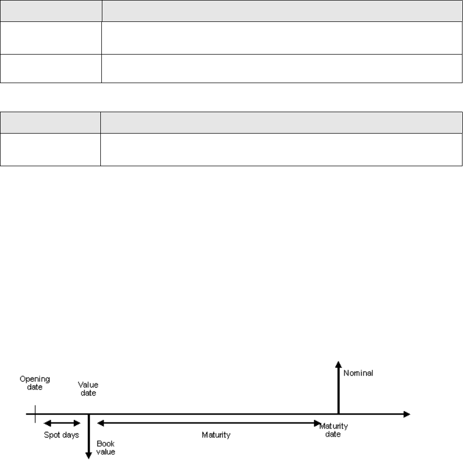
3 Debt instruments
3.1 Bond
240 © Wall Street Systems IPH AB - Confidential
In addition, the following optional information can be captured:
3.1.4.2.2 Generated data
•Transaction
Book Value (BV) = NA * price / 100
where:
NA = nominal amount
price = deal price
•Cashflows
TRM generates a settlement cashflow with amount = BV (see above) and a principal payback
cashflow for the nominal amount.
The following cashflow structure is generated for a Zero-Coupon bond (bought):
3.1.4.3 Processing
This section describes the actions that can be done throughout the life of a zero-coupon bond.
3.1.4.3.1 Asset swap
It is possible to carry out the Asset Swap action on a zero-coupon bond (see 3.1.1.3.1 Asset swap on
page 218).
In this case, the Zero-Coupon Style switch is on by default (no interest flows) and the Book Value
instead of the Nominal Amount is used for the second leg of the swap.
3.1.4.3.2 Transaction conversion
It is possible to allow schedule conversion at predefined dates during a bond's life.
•Setup (at instrument level)
This process is available on the transaction if the Transaction Conversion feature is associated
with the instrument.
Nominal Amount
Face Amount
Enter either the nominal amount or face amount, and the system will compute the
other automatically.
Value Date Official date when money is transferred. This defaults to the spot date of the
transaction.
Information Description
Units
Tradi ng Unit Size
If the denomination of a bond instrument is specified at instrument setup, the deal
can be input in units, and the nominal and face amounts are computed by the system.
Information Description

3 Debt instruments
3.1 Bond
Transaction & Risk Management Module (TRM) Instruments: Processing and Calculations 241
See A.2.325 Transaction Conversion on page 873.
Then, the user can attach conversion schedules (at the instrument level) in the Schedule page of
the Instrument Editor.
•Execution
–At instrument level:
To execute the conversion at a predefined date, in the Instrument Editor, Cashflow page, the
user selects the conversion flow and performs Convert action. After this conversion, when
capturing a transaction, cashflows are generated according to the converted schedules.
–At transaction level:
When capturing a transaction before the conversion date, conversion events are also
generated in the transaction. To execute the conversion, the user right-clicks the row of the
corresponding transaction event and selects Transaction Conversion. The conversion inputs are
displayed.
See A.2.325 Transaction Conversion on page 873.
The execution generates a conversion transaction with the following attributes:
–Kind: Conversion
–Opening Date: Conversion opening date
–Value Date: Conversion value date.
The remaining attributes are inherited from the initial transaction.
The conversion transaction generates closing cashflows for the initial transaction; and future
cashflows are reopened according to the conversion schedules defined at instrument level. If
the conversion price is different to the original deal price, then a P/L flow is generated,
showing the differences between the conversion price and the original deal price.
3.1.5 Amortizing bond
An amortizing bond repays the principal according to a pre-defined schedule.
Amortizing bonds can be fixed-rate or floaters.
A special case of an amortizing bond is the constant annuity. In this case, the rate is fixed and the
repayments, occurring at each coupon payment, are calculated so that the sum of the interest + the
repayment is constant during the life of the bond. In simple terms, this means that the interest
payments are decreasing, while the principal payments are increasing.
Note: TRM does not support repayments in the middle of a coupon period but only at coupon
payment dates.
3.1.5.1 Instrument setup
Most of the characteristics of an amortizing bond are the same as for a fixed/floating rate bond -
with the following differences.
•Schedules
Select the cashflow structure template you want for the instrument and, for each set of cashflow
defined in the template, select the generation parameters.
Depending on whether the rate is floating or fixed, you need to apply either the Floating, Bullet
Repayment template (see B.2.1.1.22 Floating, Bullet Repayment on page 894), or the Fixed,
Bullet Repayment template (see B.2.1.1.21 Fixed, Bullet Repayment on page 894), or any other
template derived from them.
Then, for the principal schedule you have to specify the repayment frequency, the method used
for repayment calculation, and how much is repaid at each amortization.
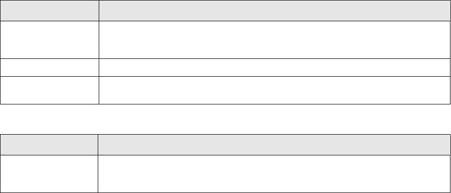
3 Debt instruments
3.1 Bond
242 © Wall Street Systems IPH AB - Confidential
The most common methods are: linear, percentage, and amount. For the interest schedule, the
parameters are the same as those for fixed or floating rate bonds.
See Appendix B Schedules on page 883.
Note that for an annuity repayment, you have to select the Fixed, Annuity Repayment template
(see B.2.1.1.20 Fixed, Annuity Repayment on page 894).
3.1.5.2 Deal capture
3.1.5.2.1 Input data
In addition to the standard deal parameters, the following information is required to enter a deal on
an amortizing fixed-rate bond.
In addition, the following optional information can be captured:
3.1.5.2.2 Generated data
•Transaction
Book Value (BV) = NA * price / 100
where:
NA = nominal amount
price = deal price
•Cashflows
The system copies all the future cashflows of the bond and scales them according to the nominal
amount engaged (using rounding).
Additionally, TRM generates a settlement cashflow with amount = BV (see above) and an
accrued interest cashflow according to the AI Method.
Information Description
Deal Price or
Deal Rate
If there is a yield/price convention set on the instrument, it is possible to enter either
a rate or a price, and conversion is made automatically. If there is no convention set,
the deal must be entered in price.
Nominal Amount Nominal amount of the deal.
Value Date Official date when money is transferred. This defaults to the spot date of the
transaction.
Information Description
Tradi ng Units
Face Amount
If the denomination of a bond instrument is specified at instrument setup, the deal
can be input in face amount/units and the Nominal Amount will be computed by the
system.
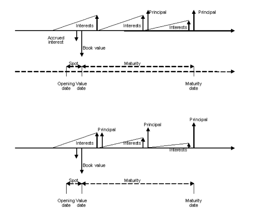
3 Debt instruments
3.1 Bond
Transaction & Risk Management Module (TRM) Instruments: Processing and Calculations 243
The following cashflow structure is generated for an amortizing fixed-rate bond:
For a fixed annuity they are as follows:
3.1.6 Step-up bond
Step-up bonds have interest payments which increase during the life of the bond.
3.1.6.1 Instrument setup
Instrument setup for a step-up bond is similar to that of a fixed-rate bond, except for the following:
•Schedules
The cashflow structure template assigned to the instrument can be the same one used for a
fixed-rate bond. However, you also have to specify the rate offset to be applied for each coupon.
See Appendix B Schedules on page 883.
3.1.6.2 Deal capture
3.1.6.2.1 Input data
The data required is the same as for a fixed-rate bond (see 3.1.1 Fixed-rate bond on page 215).
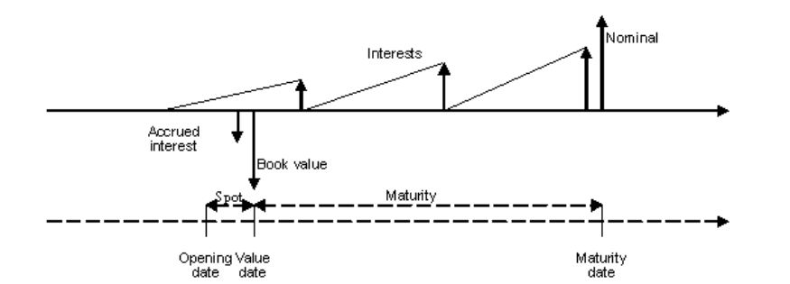
3 Debt instruments
3.2 Structured bonds
244 © Wall Street Systems IPH AB - Confidential
3.1.6.2.2 Generated data
•Transaction
Book Value (BV) = NA * price / 100
where:
NA = nominal amount
price = deal price
•Cashflows
The following cashflow structure is generated for a step-up bond:
3.2 Structured bonds
3.2.1 Callable bond
A callable (or puttable) bond is modeled by adding a call or put event to an ordinary bond cashflow
structure template.
3.2.1.1 Instrument setup
Instrument setup for a callable bond is similar to that of a standard bond (see 3.1.1 Fixed-rate bond
on page 215 or 3.1.2 Floating rate note on page 228), except for the following:
•Schedule
Select the cashflow structure template you want for the instrument. For each set of cashflows
defined in the template, select the generation parameters.
Call or put events are added to a cashflow structure using a secondary template. Several
system-defined secondary templates are provided for use with callable bonds: see B.2.1.2
Secondary templates on page 900; you can choose one of these templates or a user-defined
template derived from one of them.
Once the template is applied to the instrument, the schedules are created and it is then possible
to define their characteristics.
The call or put event should specify the following information:
–Call/put periods or dates
–Call/put price
3 Debt instruments
3.2 Structured bonds
Transaction & Risk Management Module (TRM) Instruments: Processing and Calculations 245
–Any other characteristics, for example, whether the call/put option gives the issuer of the
bond the right to terminate (call: Transaction Sign = "+") or the holder (put: Transaction
Sign = "-").
–If a call/put event has the attribute Special, the original call/put price can be overwritten at
call execution.
3.2.1.2 Processing
This section describes the processing actions that are specific to transactions on callable bonds.
3.2.1.2.1 Call/Put
•Setup
To add call or put events to a cashflow structure, you need to select a system-defined secondary
template or a user-defined template derived from one of them.
•Execution
The Execute Call/Put action performed in Transaction Manager's Event view allows you to specify
the following information:
Executing the Call/Put action on a bond creates a transaction similar to a normal buyback or sell
transaction. In other words, the resulting transaction is generated with settlement and position
cashflows.
Call/Put transactions can be identified as follows:
Transaction Kind = Call/Put (Bond)
Closing and P/L cashflows are created as part of the end-of-day processing according to the
selling method (average balance, FIFO selling, or by manual matching).
Information Description
Settlement Date The settlement date of the selected event.
Amount to Call Defaults to the amount left. Should be less than or equal to the amount left.
Counterparty Defaults to the bond issuer. The counterparty of the call transaction.
Match with Parent at
Apply
Automatically matches the call transaction with the original transaction when
applied.
3 Debt instruments
3.2 Structured bonds
246 © Wall Street Systems IPH AB - Confidential
3.2.2 Dual-currency bond
Bond issues can be structured to involve several different currencies. With a dual-currency bond, the
currency in which the bond is issued (principal currency) differs from the currency in which the
principal is repaid (redemption currency). The currency of the coupon can be either the principal
currency, the redemption currency, or another currency.
The FX rate to apply can be known (determined on the date of issue) or unknown (determined a
number of days before the payment date of the interest cashflow or period start of the coupon).
Setting up a dual-currency bond in TRM involves specifying the Dual Currency feature in the
instrument definition. Schedule templates for known FX rates or unknown rates (whose rates will be
fixed at a defined date) are also applied at instrument level.
3.2.2.1 Instrument setup
Instrument setup for a dual-currency bond is similar to that of a standard bond (see 3.1.1 Fixed-rate
bond on page 215 or 3.1.2 Floating rate note on page 228), except for the following:
•Bond main characteristics
•Dual-currency attributes
This information defines the characteristics of the principal cashflow.
See A.2.125 Dual Currency on page 771.
•Schedules
Select a suitable Dual Currency cashflow structure template for the instrument. For each set of
cashflows defined in the template, specify the generation parameters.
The following system templates are provided for dual-currency structures:
–Dual-Currency Known FX
This is a fixed bullet structure used for dual currency instruments when the FX rate is known
when the deal is entered. For both interest and redemption schedules you can choose a
different settlement currency and specify the settlement FX rate.
Information Description
AI Method The method used by the system to compute settlement accrued interests.
The usual AI Methods (e.g. linear, and so on) are relevant. See 2.1.6.1 Accrued
interest calculations on page 67 for more information.
Note: The AI Settlement is generated when the fixing date method is set to In
Advance. However, when the fixing date method is set to In Arrears, the accrued
interest settlement is unknown and so no AI is calculated.
Information Description
Settlement
Currency
Currency in which the principal cashflow is settled.
Settlement FX
Rate
Rate used to calculate the settlement amount of the principal cashflow.
Need Fixing Specify whether the FX rate needs to be fixed:
• Select No when the FX rate is known
• Select Yes, Unmarked when the FX rate is unknown.
Fixing Offset Number of days’ offset allowed, that is, the difference in days between the fixing date
and the due date (default = 0).
Fixing Max. Offset Maximum number of days’ offset allowed.

3 Debt instruments
3.2 Structured bonds
Transaction & Risk Management Module (TRM) Instruments: Processing and Calculations 247
See B.2.1.1.15 Dual Currency, Known FX Rate on page 893.
–Dual-Currency Known FX Floating
This is a floating bullet structure used for dual currency instruments when the FX rate is
known when the deal is entered. For both interest and redemption schedules you can choose
a different settlement currency and specify the settlement FX rate.
See B.2.1.1.16 Dual Currency, Known FX Rate, Floating on page 893.
–Dual-Currency Unknown FX
This is a fixed bullet structure used for dual currency instruments when the settlement FX
rate is not known beforehand. For both interest and principal schedules you can choose a
different settlement currency.
See B.2.1.1.17 Dual Currency, Unknown FX Rate on page 893.
Note: This template covers fixed interest rates only. For floating rate issues, you also have to use
the Fixing Dates secondary template (see B.2.1.2.15 Fixing Dates on page 903).
You can choose one of these templates or any other template derived from them. After the
template is applied to the instrument, the schedules are created, it is then possible to define the
settlement currency characteristics, as well as other characteristics, such as date basis, payment
convention, calendars, and so on.
See Appendix A Features on page 713.
•FX fixing
If the settlement FX rate is unknown when the deal is entered, then this feature needs to be
included in the instrument definition.
See A.2.174 FX Fixing on page 797.
3.2.2.2 Deal capture
3.2.2.2.1 Input data
Deals on dual-currency bonds are captured in the same way as a standard bond (see 3.1.1
Fixed-rate bond on page 215 or 3.1.2 Floating rate note on page 228).
3.2.2.2.2 Generated data
•Cashflows
Settlement Currency = Settlement Currency (as defined in the schedule)
Settlement FX Rate = Settlement FX Rate (as defined in the schedule)
Settlement Amount = Amount * Settlement FX Rate
3.2.2.3 Processing
This section describes the actions that can be done throughout the life of a dual-currency bond.
3.2.2.3.1 FX fixing
When the settlement FX rate of a dual-currency bond is not known beforehand, the FX rates need to
be fixed at the agreed fixing date.
•Setup
Depending on the instrument setup, the fixing can be done in advance (at the beginning of each
coupon period) or in arrears (the standard case, at the end of each coupon period).
In both cases there can be an offset of n days (before the beginning or end of the coupon
period).
3 Debt instruments
3.2 Structured bonds
248 © Wall Street Systems IPH AB - Confidential
•Execution
There are two ways to execute the FX Fixing action, one in the Instrument Editor, the other in
Transaction Manager as described further on.
–The FX Fixing action performed in Instrument Editor's Cashflow page allows you to set the FX
rate. The following values can be input:
The fixing process is performed directly on an individual cashflow in the Cashflow page. It is
possible to modify the fixing values.
–Alternatively, the FX Fixing action performed in Transaction Manager’s Cashflow view on the
cashflow allows you to set the FX rate. The following values can be input:
The fixing process is performed directly on an individual cashflow in the Cashflow view. It is
possible to modify the fixing values.
•Cancellation
It is possible to undo the FX fixing using the Undo FX Fixing action.
3.2.2.3.2 Asset swap
It is possible to carry out the Asset Swap action on a dual-currency bond (see 3.1.1.3.1 Asset swap
on page 218).
3.2.2.4 Position monitoring
For the valuation of the dual-currency bond, an estimation of the future accrued interests can be
defined by setting up the feature Generic IR Valuation with the following parameters (see A.2.201
Generic IR Valuation on page 811 for more details):
Information Description
Settlement FX
Rate
Fixing market quote to be entered manually.
After the manual entry, the Fix Fx Rate action is available and should be performed
to fix the specified FX rate.
Information Description
Fixing Date Day the cashflow is fixed.
Reference FX Rate Fixing market quote.
This is defaulted by the system to the FX cross rate between the actual currency and
the currency on the fixing date and can be changed by the user.
Information Description
AI Method The method used by the system to compute accrued interests in the calculation of
the market value. For dual-currency bonds, there are two types of dual-currency
methods:
•Dual Currency Estimated - The estimated accrued interest is calculated using the
forward FX rates.
•Dual Currency Last - The accrued interest is calculated using the FX rate of the
previous FX fixing.
Note: Both methods round the figure value in the cashflow currency before
converting it into the settlement currency. See 2.1.6.1 Accrued interest
calculations on page 67 for more information.
3 Debt instruments
3.2 Structured bonds
Transaction & Risk Management Module (TRM) Instruments: Processing and Calculations 249
For information about dual currency calculations, see 2.3.5 Dual currency on page 147.
3.2.3 Credit step-up bond
Credit step-up bonds are corporate bonds that contain a provision stating that the coupon payment
increases as the credit rating of the issuer declines. When the credit rating of the issuer goes up
again, the coupon payment goes back down but is floored by the initial rate.
A credit-linked note usually offers a higher yield compared to a vanilla bond with a similar credit
rating. A Collateralized Debt Obligation (CDO), a common type of credit-linked note, represents a
leveraged position in a portfolio of credit risk and enables investors to gain exposure to a large
diversified pool of underlying credit risk.
3.2.3.1 Instrument setup
Credit step-up bonds are based on an instrument type derived from the class CREDIT-STEP-UP.
Instrument setup for a credit step-up bond is similar to that of a fixed-rate or floating-rate bond
(see 3.1.1 Fixed-rate bond on page 215 and 3.1.2 Floating rate note on page 228), except for the
following additional attributes.
•Credit step-up characteristics
You set the credit event information at instrument level.
When the credit event information is saved, the coupon flows at transaction level are updated.
See A.2.115 Credit-Step-Up on page 765.
•Schedule
The cashflow structure template assigned to the instrument can be the same one used for a
fixed-rate or floating-rate bond. However, you also have to specify the rate offset or spread
offset to be applied for each coupon.
See Appendix B Schedules on page 883.
Settlement Switches Activate the switches that apply to this instrument:
•Dirty Price - determines whether price used for valuation includes accrued
interest (dirty price) or not.
Note: If it is on, the market value for accrued interest is not calculated, even if the
AI Method has been configured.
Method For dual-currency bond, leave empty.
Valuation Modes Valuation mode: Default, Benchmark, or Theoretical.
Information Description
Information Description
Credit event type Select from Downgrade or Upgrade:
• Downgrade when the credit rating deteriorates
• Upgrade when the credit rating improves.
Date information Date the step up/down action comes into effect and the date after which the coupons
are affected by the change in credit rating.
Offset parameters Offset that applies to fixed rate or floating rate flows.
3 Debt instruments
3.3 Schuldscheindarlehen
250 © Wall Street Systems IPH AB - Confidential
3.2.3.2 Deal capture
3.2.3.2.1 Input data
Deals on credit step-up bonds are captured in the same way as a standard bond (see 3.1.1
Fixed-rate bond on page 215 and 3.1.2 Floating rate note on page 228).
3.2.3.2.2 Generated data
Credit events (downgrade/upgrade) saved at instrument level trigger the recalculation of the
yield-to-maturity used for accruing discount (or amortizing premium) on transactions on credit
step-up bonds.
3.2.3.3 Processing
The processing actions that are available on credit step-up bonds are the same as those on standard
bonds (see 3.1.1 Fixed-rate bond on page 215 and 3.1.2 Floating rate note on page 228), except for
the following.
3.2.3.3.1 Credit event
Adding or removing a credit event on the instrument triggers the invalidation of the future cashflows
on all the existing deals. It also triggers the regeneration of a new set of cashflows with the new rate
or spread defined in the instrument setup.
3.3 Schuldscheindarlehen
Schuldscheindarlehen is a bond security representing collateralized ownership in a German loan,
with the lending bank participating in the underlying group of banks.
Schuldscheindarlehen is a special type of Bond and differs from a plain vanilla bond in the following
manner:
•The Schuldscheindarlehen is traded without any accrued interest settlement by the buyer.
Instead, the issuer pays at the end of the coupon period the exact portion of the coupon that the
buyer is entitled to, on a pro-rata-temporis basis (e.g. if the owner buys the Schuldschein at half
year and the coupon is due at the end of the year, the owner will only receive half of the coupon
amount).
•The issuer also pays any previous owners within the coupon period the interest amount on a
pro-rata-temporis basis to compensate them for holding the Schuldscheindarlehen for a given
period. The coupon amount is split between the different owners during the coupon period
according to their holding period.
3.3.1 Instrument setup
Schuldschein bonds are based on an instrument type derived from the class BOND.
Instrument setup for a Schuldscheindarlehen is similar to that of a fixed-rate bond (see 3.1.1
Fixed-rate bond on page 215), except for the following:
•Schuldschein
This feature indicates that no accrued interest is settled, but the first coupon is adjusted to the
pro-rata-temporis ownership of the coupon, and is settled on the coupon payment date directly
by the issuer.
A.2.294 Schuldschein on page 860.

3 Debt instruments
3.3 Schuldscheindarlehen
Transaction & Risk Management Module (TRM) Instruments: Processing and Calculations 251
3.3.2 Deal capture
3.3.2.1 Input data
In addition to the standard deal parameters, the following information is required to enter a
Schuldscheindarlehen (both primary and secondary markets):
Note: If you need to monitor the ownership transfer, you must record and maintain the
subsequent transactions in the secondary market. You can then use standard TRM
monitoring and reporting tools to monitor the identity of the holders, the volume of the
bonds held by each holder, and the date of purchase and sale of the bonds by the holders.
3.3.2.2 Generated data
•Transaction
Yields are calculated from the reduced coupon.
•Cashflows
–The first coupon is reduced and settled on the pro-rata-temporis of the ownership from the
transaction's value date to the coupon value date.
No accrued interest is generated.
–On the coupon payment date, the Issuer of the Schuldschein calculates the interest for each
holder of the bond according to their holding period (from the purchase value date to the
sale value date).
3.3.3 Processing
The actions that can be done throughout the life of a Schuldschein bond are the same ones as for a
fixed-rate bond (see 3.1.1.3 Processing on page 218).
3.3.4 Position monitoring
This section describes how the Schuldschein bonds are calculated and provides a numerical example
that demonstrates the calculations of a Schuldschein bond instrument.
3.3.4.1 Setup
There are two basic methods for valuation of Schuldschein bond instruments: Quoted or Theoretical.
When the Theoretical method is used, the valuation is similar to the one used to calculate a
fixed-rate bond (3.1.1.4 Position monitoring on page 221). When the Quoted method is used, the
calculations are processed as described in section 3.3.4.2 Calculations on page 251.
3.3.4.2 Calculations
This section describes the model and calculations of Schuldschein bond instruments.
Information Description
Nominal Amount
Face Amount
Enter either the nominal amount or face amount, and the system will compute the
other automatically.
Value Date Official date when money is transferred. This defaults to the spot date of the
transaction.
Deal Price Price paid for the bond (expressed as a percentage of the nominal amount).

3 Debt instruments
3.3 Schuldscheindarlehen
252 © Wall Street Systems IPH AB - Confidential
3.3.4.2.1 Valuation model
The market value of a quoted Schuldschein (Quoted valuation method) is calculated as follows:
Equation 3-3 Quoted Schuldschein bond
where
3.3.4.2.2 Numerical example
This section demonstrates how the different figures are calculated for a quoted
Schuldscheindarlehen.
This example shows a Schuldscheindarlehen EUR 1,000,000.00, 5%, issued on 2008-01-01, and
due on 2012-01-01.
•Setup:
•Transaction data (Schuldschein issue - primary market):
P The price of the deal.
A The nominal amount.
The accrued interest is calculated according to the generic formula described in 2.1.6.1 Accrued
interest calculations on page 67.
where:
•C is the coupon
• t is the length of the accrual period (in years), calculated as follows:
• T is the length of the coupon period (in years, calculated with the appropriate date basis)
D_f The Discount Factor from figure spot to figure valuation date.
Data Symbol Example
Instrument Date Basis (30E/360) B 360
Valuation Method Quoted
First Coupon Payment 2009-01-01
Issue Date dt_i 2008-01-01
Maturity Date d_m 2012-01-01
Coupon Rate c 5%
Coupon Frequency 1
Spot Days 3
Currency EUR
AI Method Linear
Schedule Fixed, Bullet Repayment
Ia
3 Debt instruments
3.3 Schuldscheindarlehen
Transaction & Risk Management Module (TRM) Instruments: Processing and Calculations 253
On 2008-01-01, Bank1 issues 100,000,000.00 to Bank2.
•Transaction data (transfer of ownership - secondary market):
On 2008-01-02, Bank2 sells its position EUR 30,000,000 and EUR 70,000,000 to two different
holders: Holder1 and Holder2 respectively.
and
•Valuation Figure:
Data Symbol Example Formula
Opening Date dt_o_1 2008-01-01
Nominal Amount A_1 100,000,000.00
Issuer Bank1
Counterparty Bank2
Price P 100%
Value Date dt_v.p 2008-01-04
Issue Date 2008-01-01
Book Value V_b.p 100,000,000.00 =A
Coupon 1 Amount A_1.c1 5,000,000.00
Coupon 1 Time to Value
Date
t_v.c1 360
Data Symbol Example Formula
Seller Bank2
Counterparty Holder1
Opening Date dt_o_2 2008-01-02
Nominal Amount A_2 30,000,000.00
Value Date dt_v.p 2008-01-07
Book Value V_b.p 30,000,000.00 =A_2
Data Symbol Example Formula
Seller Bank2
Counterparty Holder2
Opening Date dt_o_2 2008-01-02
Nominal Amount A_3 70,000,000.00
Value Date dt_v.p 2008-01-07
Book Value V_b.p 70,000,000.00 =A_3
Data Symbol Example Formula
Figure Date d_f 2008-01-02
Time to Spot d_s 2008-01-07

3 Debt instruments
3.4 Denominated bond
254 © Wall Street Systems IPH AB - Confidential
•Calculated transaction data (first coupon payment):
2009-01-01, the issuer Bank1 pays the coupon amount pro-rata-temporis of the ownership to
each holder.
3.4 Denominated bond
Bonds (and swaps) with multiple denominations are traditionally a spin off from markets where
physical bonds or certificates were used. Some markets still trade bonds or certificates, and these
are physically delivered between parties. These certificates were used for secondary trading and
made it easier for traders to break down a large issue tranche, facilitating smaller value trades on
the back of the original issue. The denominations are aggregated into a single transaction but
denomination details are maintained and recorded.
In case of physical presentation of coupons, clearing houses and/or paying agents have to pay
investors (retail) the exact coupon amounts. However, with the advent of settlement houses the
practice of physical delivery is now the exception rather than the rule. The settlement agents merely
move electronic representations of the bonds or certificates between accounts.
3.4.1 Instrument setup
Denominated bonds must be based on an instrument type derived from the class BOND or SWAP.
The setup for multiple-denomination bonds and swaps is similar to that of a fixed-rate bond (see
3.1.1 Fixed-rate bond on page 215), except that you can define the denominations that can be used
when capturing transactions at the instrument or hedging swap leg level:
•Bond main characteristics
Principal A_1.P 100,000,000.00
Accrued Interest
(Coupon 1)
69,444.44 A_1.c1 * (d_s - d_f) / B
Data Symbol Example Formula
Amount (Coupon 1) A.c1 5,000,000.00
Value Date (Coupon 1) dt_v.c1 2009-01-01
First coupon to Bank2 1c.p 13,888.89 A_1.c * (dt_0_2 – dt_0_1)/B
First coupon to Holder1 2c.p 1,495,833.33 A_2.c * (t_v.c1 -dt_0_2)/B
First coupon to Holder2 3c.p 3,490,277.77 A_3.c * (t_v.c1 -dt_0_2)/B
Data Symbol Example Formula
Information Description
Amount Rounding Nearest number to which the coupon amount is rounded. By default, it is set
to 2 decimals (0.01).
Note: The rounding step applies to the accrued interest when the Settlement
Switch, Round Per Unit is activated (see below).
Rounding Method Up, Down or Nearest. The amount is rounded up, down, or to the nearest figure
as calculated using the specified Amount Rounding number.
Settlement Switches Round Per Unit
If the switch Round per Unit is activated, Accrued Interest is based on rounding
per denomination (see 3.4.4.2 Calculations on page 256).
3 Debt instruments
3.4 Denominated bond
Transaction & Risk Management Module (TRM) Instruments: Processing and Calculations 255
•Denominated bond
If the denomination of a bond instrument is specified at instrument level using feature
Denominated Bond, the deal can be input in units and the Nominal Amount is computed by the
system.
A.2.120 Denominated Bond on page 767.
•Bond Denominations Setup
The valid denominations can be defined at the instrument level. Only those denominations will
be allowed at deal capture.
A.2.60 Bond Denominations Setup on page 739.
Note: For monitoring purposes, you can view the positions by Trading Unit in Treasury Monitor,
Transaction grouping. For more information, see TRM User Guide.
3.4.2 Deal capture
3.4.2.1 Input data
In addition to the standard deal parameters, the following information is required to enter a
denominated bond:
•Transaction view:
•Denomination view:
3.4.2.2 Generated data
•Transaction
Book Value (BV) = NA * price / 100
where:
NA = Nominal Amount
price = Deal Price
•Cashflows
Information Description
New Denomination The deal is captured by selecting the denominations defined at the instrument
level.
To select a denomination, right-click the transaction, select the action New
Denomination from the drop-down list, and then select the relevant
denomination from the list.
A new row is added to the Denomination view. You need to populate the Unit
column.
Note: To delete a denomination, simply right-click the row you want to delete
and select Delete Denomination.
Information Description
Trading Unit Displays the selected denomination.
Units The deal can be input in units and the Nominal Amount is calculated by the
system.
Leg Group Displays the number of the (Swap) leg group where the denomination applies.

3 Debt instruments
3.4 Denominated bond
256 © Wall Street Systems IPH AB - Confidential
When denominations are used at deal capture, the interest (coupon) payments are calculated
separately for each denomination according to the following formula:
Ic = Units * round[Denomination * Period Length * Coupon Rate,Amount Rounding]
where:
Ic = interest (coupon) payments
Amount Rounding = number of decimals to be used when rounding amounts.
3.4.3 Processing
This section describes the actions that can be done throughout the life of a denominated bond.
3.4.3.1 Buyback (sale) and Unwinding (early expiration)
When an issue is bought back (or a long position is sold), or when a swap is unwound
(early-expired), you enter the denominations and units in the same way as when entering a new
transaction. See 3.4.2.1 Input data on page 255 for more information about capturing
denominations and units.
This information is used the same way as for new transactions, to 'close' (offset) the future interest
and redemption payments accordingly.
For a swap, a net amount (amount to be settled between the parties) is entered in the same way as
in a swap without denominations. See 11.1.2 Asset swap on page 656.
Note: For accounting purposes: The fact that buybacks or corresponding issues may have
multiple denominations has no impact on realized results. The reason for this is that
buybacks are booked at par, and the difference between par and buyback price is recorded
directly into P/L. So, there is no linking between the issue price and the buyback price per
denomination.
3.4.4 Position monitoring
There are two basic methods for valuation of denominated bond instruments: Quoted or Theoretical.
3.4.4.1 Setup
The valuation setup for denominated is the same as for usual bonds. 3.1.1.4 Position monitoring on
page 221.
3.4.4.2 Calculations
The numerical example in this section demonstrates how the different figures are calculated for a
multiple denominated bond using the Theoretical method.
This example shows a multiple denominated bond with the following data:
•Setup
Data Symbol Example
Issue Date dt_i 2008-01-01
Maturity Date 2012-01-01
Currency EUR
Valuation Method Theoretical
Coupon 5.6333%
AI Method Actual/Actual Annually
3 Debt instruments
3.4 Denominated bond
Transaction & Risk Management Module (TRM) Instruments: Processing and Calculations 257
•Transaction data:
Note: When entering a transaction the coupon amount will be different in the two denominations.
•Accrued interest may be based on rounding per denomination or not depending on whether the
settlement switch Round Per Unit (Instrument Editor - Bond page) is activated at the instrument
level.
–If the switch Round Per Unit is not activated, the accrued interest is calculated like any other
bond (Equation 2-71 Accrued interest (generic formula) on page 67):
Amount Rounding 0.01
Rounding Method Nearest
Schedule Fixed, Bullet Repayment
Denominations Trading Units 1000 and 5000
Data Symbol Example
Data Symbol Example Formula
Opening Data dt_o 2008-01-23
Value Date dt_v 2008-01-25
Interest Rate r 5.6333%
First Denomination de_1 1000
Trading Units (First
Denomination)
n_m_1 100
Nominal Amount (First
Denomination)
A_1 100 000 de_1 * n_m_1
Coupon Amount (First
Denomination)
Ic_1 5633 (rounding to 2
decimals)
r* de_1=56.333 = 56.33 * n_m_1
Second Denomination de_2 5000
Trading Units (Second
Denomination)
n_m_2 20
Nominal Amount
(Second Denomination)
A_2 = 100 000 de_1 * n_m_1
Coupon Amount
(Second Denomination)
Ic_2 5633.4 (rounding to 2
decimals)
r* de_2=281.665 = 281.67 * n_m_2
Data Symbol Example Formula
Date Basis B 366
Time to Accrued
Interest
2008-01-25 -
2008-01-01 = 24
dt_v - dt_i
Accrued Interest (First
Denomination)
Ia _1 = 369.38 (rounded to 2
decimal places)
Ic_1*(dt_v - dt_i)/B= 369.377
Accrued Interest
(Second Denomination)
Ia _2 = 369.40 (rounded to 2
decimal places)
Ic_2*( dt_v - dt_i)/B= 369.4033

3 Debt instruments
3.5 Convertible bond
258 © Wall Street Systems IPH AB - Confidential
–"If the switch Round Per Unit is activated, the accrued interest is calculated using the
denomination rounding calculation:
Equation 3-4 Denomination rounding equation
Note: Accrued interest at settlement, and 'clean' settlement (principal) amount (i.e. the full
settlement amount minus accrued interest and fees/taxes) is calculated directly from the
total interest (coupon) amount and total nominal amount respectively, i.e. they are not
calculated separately for each denomination.
3.5 Convertible bond
Convertible bonds are fixed rate bonds that can be converted to equity, typically to shares of the
issuer. The bond can be converted on certain dates or during certain periods. Usually the holder of
the bond can decide to convert the bond but sometimes the issuer also has the right to force the
conversion. Some convertibles are also callable.
The conversion price (and ratio) may depend on time. Usually corporate actions (splits and
dividends) also affect the conversion price.
3.5.1 Instrument setup
Convertible bond instruments must be based on an instrument type derived from the class
CONVERTIBLE-BOND. They are set up in a similar way to fixed-rate bonds (see 3.1.1 Fixed-rate
bond on page 215), except for the following characteristics.
•Schedules
Select a suitable schedule template that includes coupons, redemptions, call events (if the bond
is callable), and conversion events.
To define the conversion events, TRM provides a pre-defined secondary template designed for
this purpose (see B.2.1.2.11 Convertible Conversion on page 902).
See Appendix B Schedules on page 883.
Data Symbol Example Formula
Date Basis B 366
Time to Accrued
Interest
2008-01-25 -
2008-01-01 = 24
dt_v - dt_i
Accrued Interest (First
Denomination)
Ia _1 = 369 (rounded to 2
decimal places)
r* de_1*(dt_v - dt_i)/B= 3.693967 =
3.69* n_m_1
Accrued Interest
(Second Denomination)
Ia _2 = 369.40 (rounded to 2
decimal places)
r* de_2*(dt_v - dt_i)/B= 18.46984 =
18.47 * n_m_2
Ia Unit round Denomination Periodlength CouponRate AmountRounding,××[]×=

3 Debt instruments
3.5 Convertible bond
Transaction & Risk Management Module (TRM) Instruments: Processing and Calculations 259
•Convertible Bond
The conversion price (or ratio) is defined using this feature. Initially one entry is needed. If the
conversion price changes due to corporate actions, a new entry must be added each time.
See A.2.103 Convertible Bond on page 759.
3.5.2 Deal capture
3.5.2.1 Input data
The data required is the same as for a fixed-rate bond (see 3.1.1 Fixed-rate bond on page 215).
3.5.2.2 Generated data
•Cashflows
The following cashflow structure is generated for a convertible bond:
3.5.3 Processing
This section describes the actions that can be done throughout the life of a convertible bond.
3.5.3.1 Conversion
The convertible bond is converted to the underlying instrument using the Conversion action.
Information Description
Active From
Active To
Period during which this conversion price is applicable.
Type Defines whether the user can enter conversion price or conversion ratio.
Par Value If the convertible bond is traded using units, enter the par value of one unit.
Conversion Price If Type = Conversion Price, you can enter the conversion ratio.
Otherwise, it is calculated using the conversion price and par value:
Conversion Price = Par Value/Conversion Ratio
Conversion Ratio If Type = Conversion Ratio, you can enter the conversion price.
Otherwise it is calculated using the conversion ratio and par value:
Conversion Ratio = Par Value/Conversion Price
Underlying The instrument into which the convertible can be converted.
Comment Any comment you want to add about the instrument.
Accrued
interest
Interest flows Nominal
Book value
Spot
Opening
date
Value
date
Maturity
Maturity
date

3 Debt instruments
3.6 Index-linked bond
260 © Wall Street Systems IPH AB - Confidential
•Setup
Conversion parameters are defined in the instrument setup.
•Execution
Conversion can be executed in Transaction Manager. The following parameters are used:
The execution of the action generates a conversion transaction which closes the existing
convertible position and replaces it with the appropriate number of units of the underlying
instrument.
•Cancellation
Cancellation of the action is done by canceling the conversion transaction.
3.6 Index-linked bond
Index-linked bonds are linked in some way to a standard index.
The bond’s cashflows vary according to an underlying index. For example, in inflation index-linked
bonds, the coupon and principal payments are adjusted to compensate for changes in inflation.
These payments are adjusted in relation to a Consumer Price Index (CPI) value or a Retail Prices
Index (RPI) value for a country.
A period of time usually elapses between the measurement of price levels and the publication of an
index, therefore the index value associated with a given cashflow will be the index as published for a
time in the past. This time difference is called the indexation lag.
The way in which the index-linked bonds are traded and valued varies according to market
conventions.
Index-linked bonds must be based on an instrument type derived from the class
INDEX-LINKED-BOND.
3.6.1 Instrument setup
The following information is relevant to any kind of index-linked bond.
Index-linked bonds are set up in a similar way to fixed-rate bonds (see 3.1.1 Fixed-rate bond on
page 215) or zero-coupon bonds (see 3.1.4 Zero-coupon bond on page 239), depending on whether
there are any coupon payments.
The additional values required to set up index-linked bonds are described in the following sections.
Information Description
Conversion Date Date on which the conversion is done.
Amount to
Convert
Nominal amount of the convertible to convert.
Delivery Type Usually Delivery Type = Physical Delivery.
If the underlying is not delivered, but the profit/loss is settled instead, select Delivery
Type = Cash Settlement.
Scenario Scenario from which you want to retrieve the market price of the underlying. This
parameter is used for cash settlement only.
Price Price of the underlying. This parameter is used for cash settlement only.
Cash to Receive Amount of cash to receive. This parameter is used for cash settlement or settling the
residual if the number of units to be delivered is rounded.
This field can be modified.
3 Debt instruments
3.6 Index-linked bond
Transaction & Risk Management Module (TRM) Instruments: Processing and Calculations 261
•Index-linked bond main characteristics
–The primary feature A.2.210 Index-Linked Bond on page 818.
•Trading characteristics
Each index-linked bond type has its own specific trading feature. Special risk characteristics
•Special risk characteristics
Interest sensitivity of index-linked bonds is, by default, calculated in the same way as for similar
fixed rate bonds. However, you can capture a factor (e.g. yield beta, a number between 0 and 1)
for scaling the IR sensitivity of the instrument, which is then used as a multiplier for scaling IR
exposure and duration figures. Effective convexity is scaled by the factor squared. This factor
can be entered either as a static sensitivity scaling factor at instrument level using the
instrument feature Base IR Exposure Setup, or as Beta for the instrument in Rate Monitor
allowing time-dependent scaling factors.
For more information relating to the setup and structure of specific types of index-linked bond,
see:
–3.6.4 Australian index-linked annuity bond on page 263
–3.6.5 Australian index-linked bond on page 267
–3.6.6 Brazilian (LFT) selic-linked security on page 270
–3.6.7 Brazilian FX-linked NBC-E/NTN-D on page 271
–3.6.8 Brazilian inflation-linked NTN on page 272
–3.6.9 Canadian real return bond on page 273
–3.6.10 French OAT€i on page 274
–3.6.11 Greek index-linked bond on page 277
–3.6.12 Israeli index-linked bond on page 279
–3.6.13 Italian BTP €i on page 281
–3.6.14 Japanese index-linked bond on page 282
–3.6.15 Swedish index-linked bond on page 283
–3.6.16 UK index-linked gilt on page 287
–3.6.17 US Tips on page 292.
•Schedules
Select the cashflow structure template that is appropriate for the instrument.
System templates are provided for several types of index-linked bonds; you can choose one of
these templates or any other template derived from them. Once a template is applied to the
instrument, the schedules are created and it is then possible to define their characteristics, such
as, date basis, payment convention, calendars, and so on.
See Appendix B Schedules on page 883.
•Quoted
It is necessary to specify how the index-linked bond is quoted on the market. Each index-linked
bond type has its own specific quote handler.
See A.2.274 Quoted on page 849.
•Valuation approach
Each index-linked bond type has its own specific valuation approach feature.

3 Debt instruments
3.6 Index-linked bond
262 © Wall Street Systems IPH AB - Confidential
3.6.2 Deal capture
3.6.2.1 Input data
In addition to the standard deal parameters, the information required to enter a deal on an
index-linked bond is similar to the data required for a fixed-rate bond (see 3.1.1 Fixed-rate bond on
page 215).
In addition, the following optional information can be captured:
3.6.2.2 Generated data
•Cashflows
The following cashflows are generated:
–Principal
–Interest (unless it is a zero-coupon index-linked bond)
–Redemption.
3.6.3 Processing
This section describes the actions that can be done throughout the life of an index-linked bond.
3.6.3.1 Fixing
The major process for an index-linked bond is the fixing of the coupon and the redemption flows.
These need to be adjusted to account for changes in the index.
•Setup
Depending on the instrument setup (schedules) the fixing can be done in advance or in arrears.
In both cases there can be an offset of n days (before the beginning or end of the coupon
period).
The fixing parameters that define how the fixing rate is calculated are defined in the schedule.
Information Description
Deal Price or
Deal Rate
If there is a yield/price convention set on the instrument, it is possible to enter either
a rate or a price and conversion is made automatically. If there is no convention set,
the deal must be entered in price.
Nominal Amount
Face Amount
Enter either the nominal amount or face amount, and the system will compute the
other automatically.
Value Date Official date when money is transferred. This defaults to the spot date of the
transaction.
Index Value of the index (to which the instrument is index-linked) at trade date.
Information Description
Units
Tradi ng Unit Size
If the denomination of a bond instrument is specified at instrument setup, the deal
can be input in units, and the nominal and face amounts are computed by the system.
Index Prolong Rate (For UK index-linked bonds only)
Interest rate by which the index rate is prolonged into the future.
Index Ratio Index ratio used to adjust the coupon and redemption flows of the bond.
Note: If this is defined at instrument level, this is used as the default in the
transaction and cannot be modified: for example, see 3.6.7 Brazilian FX-linked
NBC-E/NTN-D on page 271.
3 Debt instruments
3.6 Index-linked bond
Transaction & Risk Management Module (TRM) Instruments: Processing and Calculations 263
•Execution
When fixing is executed, the rate is retrieved for the specified fixing rate and period according to
the designated fixing scenario. The fixing scenario is configured at the system level, see TRM
System Admin Guide. The fixing subscenario is specified at the cashflow level.
The expression value gives the current value of the expression and is used to calculate the index
value.
The following information is stored on the fixed cashflow:
The fixing date
The fixing quote
The expression and expression value
The amount of the coupon or redemption flow.
The fixing process can be performed in two ways in TRM: the process is exactly the same in each
case: the coupon is fixed at both instrument and transaction level.
The methods of fixing are as follows:
–Directly on the cashflow (in Instrument Editor’s Cashflow page) using the Fix Price action: the
fixing affects all deals on this instrument.
–Using an activity (Fixing Bond Cashflow): all instruments and their deals which need to be
fixed for a particular date are affected.
Note: The bond issue must be fixed at instrument level in order for the accrued interest flow to
be generated (for transactions captured between coupon fixing date and fixing value date).
•Cancellation
It is possible to cancel the cashflow fixing either manually, using the Undo Fixing action in
Instrument Editor; or automatically, using the Fixing Bond Cashflow - Undo activity.
3.6.4 Australian index-linked annuity bond
The following sections describe the characteristics that are specific to Australian index-linked
annuity bonds.
3.6.4.1 Instrument setup
Instrument setup for this type of index-linked bond is the same as for other index-linked bonds (see
3.6 Index-linked bond on page 260) except for the following:
•Trading characteristics - issue index parameters
The Australian CPI is published quarterly and is applied to settlement calculations and valuations
starting from the publication date. The index is set up similarly to other indexes.
See A.2.32 Australian IAB on page 725 or A.2.34 Australian IAB (Round to 3) on page 725.
•Bond characteristics
Information Description
Index Select the Instrument ID of the underlying index you previously defined.
See 7.1 Index types on page 425.
Issue Index Enter the value of the underlying index at issue. This value is used to adjust the
coupon and redemption flows of the bond.
Information Description
Currency AUD

3 Debt instruments
3.6 Index-linked bond
264 © Wall Street Systems IPH AB - Confidential
•Schedule parameters
Select the cashflow structure template BOND-AU-IAB (Australian Indexed Annuity Bond). See
B.2.1.1.4 Australian Indexed Annuity Bond on page 890.
In the Interest Adjustment schedule, set the parameter Factor equal to the rounded value of the
annuity payment.
Note: For rounding to three decimal places, change the expression in the Interest Adjustment
schedule to: round((ixau/divider)*factor,0.001)*100 - 100 * factor
Set the required fixing characteristics as follows:
After you have generated the cashflows, remove the default value from the field Amount
Rounding in the Schedule page and leave the field Amount Rounding empty for all Interest
Adjustment cashflows in the Cashflow page.
•Trading yield parameters
•Quoted
AI Method Australian Index Linked (IAB), or for three decimal places rounding, Australian Index Linked
(IAB) (3 dec).
Settlement
Switches
Dirty Price.
Coupon Rate Coupon rate of the bond.
Information Description
Factor Enter the annuity payment percentage.
Note: The Fixing Rate and Divider fields default to the values you selected in the
Issue Index page.
Method Select 4th Wednesday (M) as the index is published (and index adjustment
cashflows fixed) on the 4th Wednesday of the publishing month.
Frequency Enter 3.
First Date Enter the first publishing (fixing) date applicable to this instrument. The
subsequent publishing dates are calculated from this date onwards using the
monthly frequency specified in the Frequency field.
Information Description
Yield Convention Australian Government Index Annuity - GOVT-AU-IX-ANNUITY
Information Description
Price Type Yield (w/o rounding)
Quote Handling Depending on how you want to round the adjusted annuity, select one of the
following:
•Index-Linked Annuity Bond (Australian): six decimal places rounding
•Index-Linked Annuity Bond (Australian 3 Digits Rounding): three decimal places rounding
Currency AUD
Information Description

3 Debt instruments
3.6 Index-linked bond
Transaction & Risk Management Module (TRM) Instruments: Processing and Calculations 265
•Result parameters
•Valuation approach
Australian Indexed Annuity Bonds can be valuated either using a direct (yield) quote, or taken
from the yield curve.
–For a direct quote, see A.2.33 Australian IAB Valuation on page 725), or if adjusted annuities
are to be rounded to 3 decimal places, see A.2.35 Australian IAB Valuation (Round to 3) on
page 726.
–For a valuation taken from the yield curve (loans only), see A.2.36 Australian IAB Par Curve
Valuation on page 726, or if adjusted annuities are to be rounded to 3 decimal places, see
A.2.37 Australian IAB Par Curve Valuation (Round to 3) on page 727.
Note: To use a yield curve, you must first set one up in the IR Quote and Yield Curve Editor. For
general information about setting up yield curves, see TRM User Guide.
3.6.4.2 Deal capture
3.6.4.2.1 Input data
In addition to standard deal parameters, the information required to enter a deal on an australian
index-linked bond is similar to usual index-linked bonds (see 3.6 Index-linked bond on page 260).
In addition, the following optional information can be captured:
3.6.4.2.2 Generated data
•Transaction
The formula used to calculate the price depends on whether the CPI value that will determine
the next coupon is known or not.
Information Description
AI Method Australian Index Linked (IAB), or for three decimal places rounding, Australian Index Linked
(IAB) (3 dec).
Information Description
Face Amount Enter the face amount. The Nominal Amount is automatically calculated by the
system.
Nominal Amount Shows the remaining amount taking into account the annuity payments.
Information Description
Index The system automatically fetches the latest available CPI value for the settlement
date. You may change the index value.
Note: In Rate Monitor, the index value of a given quarter is associated with the
first day of the quarter (Jan. 1, Apr. 1, Jul. 1, Oct. 1). The publication date is
given in the field Period From.
Deal Rate Enter the trade yield.
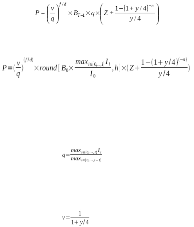
3 Debt instruments
3.6 Index-linked bond
266 © Wall Street Systems IPH AB - Confidential
–If the value is not known, we use the inflation rate (q) for coupon estimation:
Equation 3-5 Coupon estimation: CPI value unknown
–If the value is known, the formula is:
Equation 3-6 Coupon estimation: CPI value known
where
•Cashflows
The following cashflows are generated:
–Principal
–Interest
–Interest Adjustment
–Amortization
–Delivery.
Previous annuity payment
Original unadjusted annuity payment
hRounding precision, 3 or 6, depending on the issue
qQuarterly inflation factor
CPI for quarter I: where I = 0 corresponds to the quarter
before the issue date of the bond, and I = 1 corresponds to
the latest quarter for which the CPI has been issued on the
settlement date
yTrading yield
v
nNumber of full quarters from the next annuity payment to
maturity
fNumber of days from settlement to the next annuity
payment date
dNumber of days in the full quarter ending on the next
annuity payment date
Z1 if there is an annuity payment to the purchaser at the
next annuity payment date, otherwise 0.
Br1–
B0
Ii
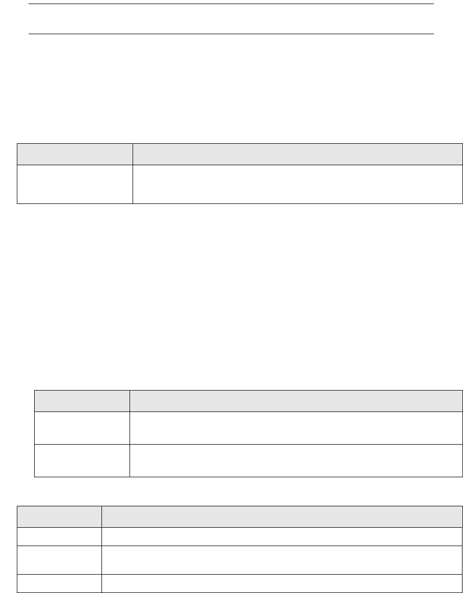
3 Debt instruments
3.6 Index-linked bond
Transaction & Risk Management Module (TRM) Instruments: Processing and Calculations 267
•Fixing
In the fixing of Australian index-linked annuity bonds, rounding is carried out at the total annuity
payment level. To make sure that the total of the fixed interest and amortization payments are
correct, one of the cashflows takes into account the rounding of the other.
Note: In Rate Monitor, the index value of a given quarter is associated with the first day of the
quarter (Jan. 1, Apr. 1, Jul. 1, Oct. 1). The publication date is given in the field Period From.
3.6.4.3 Processing
3.6.4.3.1 Fixing
The fixing of the inflation adjustment (Interest Adjustment cashflow) is carried out at the instrument
level in Instrument Editor - Cashflow page.
•Execution
Update the cashflows (click Update) and save the instrument.
3.6.5 Australian index-linked bond
The following sections describe the characteristics that are specific to Australian index-linked bonds.
3.6.5.1 Instrument setup
Instrument setup for this type of index-linked bond is the same as for other index-linked bonds (see
3.6 Index-linked bond on page 260) except for the following:
•Trading characteristics
See A.2.29 Australian CIB on page 724.
–Issue Index parameters
•Bond characteristics
Information Description
Fixing Quote Select action Fix Price. The appropriate CPI value is displayed and the amount
of the inflation adjustment is automatically calculated. You can also first set
the relevant CPI value, and then select the action Fix Price.
Information Description
Index Instrument ID of the underlying index.
See 7.1 Index types on page 425.
Issue Index (Not used for Australian index-linked bonds)
However, a value must be entered as 100.00 for calculation purposes only.
Information Description
Currency AUD
Settlement
parameters
Dirty Price.
Coupon Rate Coupon rate of the bond.
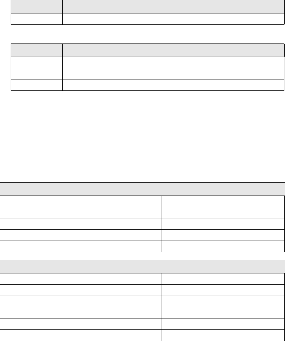
3 Debt instruments
3.6 Index-linked bond
268 © Wall Street Systems IPH AB - Confidential
•Schedule parameters
Select the cashflow structure template BOND-AU-CIB (Australian Capital Indexed Bond). See
B.2.1.1.3 Australian Capital Indexed Bond on page 890.
•Trad ing yield
•Quoted
•Valuation approach
See A.2.38 Australian Index-Linked Bond Valuation on page 727.
3.6.5.2 Position monitoring
In this section, numerical examples demonstrate how the different figures are calculated for
Australian Treasury index-linked bonds.
If you need more theoretical information about the method used in these calculations, see Chapter 2
Market standards and calculations on page 33.
This example shows an Australian Treasury index-linked bond, with the following deal data:
Information Description
Yield Convention Australian Government Index - GOVT-AU-IX
Information Description
Price Type Yield (w/o rounding)
Quote Handling Index-Linked Bond (Australian)
Currency AUD
Setup data
First interest payment date 1994-08-20 (Q3 / 1994)
First reference quarter Q4 / 1993
Maturity date dt_m 2015-08-20
Interest r 4.00%
Face amount 1,000.00
Transaction data
Settlement date dt_s 2007-01-23
Next coupon date dt_c 2007-02-20 (Q1 / 2007)
Yield y 2.76%
Current quarter length dp 92
Index factor p 1.25
Adjustment factor K_t 141.270 (Q3 / 2006)
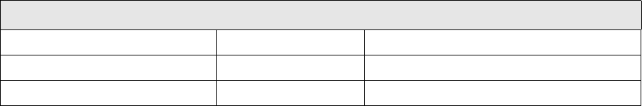
3 Debt instruments
3.6 Index-linked bond
Transaction & Risk Management Module (TRM) Instruments: Processing and Calculations 269
Other important deal data is calculated by the system as follows:
• Quarters left
n = FLOOR(YEARFRAC(dt_s, st_m, 0) * 4, 1)
= 34
• Reference index
v = ROUND (1 / (1 + y / 4), 9)
= 99.31%
• Days to next coupon
dc = dt_c - dt_s
28 = 2007/02/20 - 2007/01/23
•Time to next coupon
t_n = dc / dp
0.3043478 = 28 / 92
• Unadjusted dirty price
Pdu =ROUND (POWER (v, t_n) * (ROUND (r / 4,9) * (1 + ROUND ((1 - POWER (v., n)) / (y / 4), 9)) +
POWER (v, n)) * POWER (1 + p / 100, -t_n.), 9)
= 109.71994%
• Adjusted dirty price
P_d = ROUND (K_t. * Pdu / 100,5)
= 155.001%
• Accrued interest
I_a = ROUND ((r / 4) * K_t / 100 * (dp - dc) / dp, 5)
= 0.98300000000%
• Clean price
P_c = P_d - I_a
= 154.018%
3.6.5.2.1 Settlement figures
Settlement flows for the transaction are calculated as follows:
• Nominal amount
A.s = 10,000,000.00
• Clean price
P_c.s = A * P_c
15,401,800.00 = 10,000,000.00 * 1.54018
• Accrued interest
I_a.s = A * I_a
98,300.00
•Total
= 15,500,100.00
3.6.5.2.2 Fixing figures
Fixing flows for the transaction are calculated using the following data:
Fixing data
Coupon date 2007-05-20
Fixing date 2007-02-20
Reference quarter 141.82 (Q4 / 2006)
3 Debt instruments
3.6 Index-linked bond
270 © Wall Street Systems IPH AB - Confidential
• Index adjustment factor
cf = 141.82 / 100
= 1.41820
• Nominal coupon
cn = r / 4
0.0100000 = 0.04 /4
• Adjusted amount
Ap = A * cn *cf
141,820.00 = 10,000,000 * 0.010000 * 1.41820
3.6.5.2.3 Valuation figures
Unless otherwise stated, the figure date used in the calculations is 2007-01-20. On this date, the
market data is as follows:
•Market value
= p_q / 100 * A * D_s
15,493,829.60 = 155.00 / 100 * 10,000,000 * 0.99960191
3.6.6 Brazilian (LFT) selic-linked security
Brazilian LFT (Letra Financeira do Tesouro) instruments are zero-coupon bonds linked to the O/N
SELIC interest rate. The maturities can be over two years.
These instruments are traded and quoted in 1000’s (Date Basis = BRL/252) and have a unique
security ID (ISIN number), issue and maturity date.
3.6.6.1 Instrument setup
Instrument setup for this type of index-linked bond is the same as for other index-linked bonds (see
3.6 Index-linked bond on page 260) except for the following parameters:
•Trading characteristics
See A.2.52 Bond - Brazilian LFT on page 737.
•Bond characteristics
•Schedule parameters
The Brazilian LFT Bond system-defined primary template is provided for this type of index-linked
bond, where:
–Fixing parameters
Need Fixing = Yes
Fixing Date Method = In Arrears
Expression = iix/trading unit
where:
iix = instrument-specific index entered in Rate Monitor together with Bid and Ask (select the
Rate Monitor figure Index Value).
See B.2.1.1.7 Brazilian LFT Bond on page 891.
Market data on 2007-01-20
Market quote (dirty, adjusted) p_q 155.00
Figure D D_s 0.99960191
Information Description
Currency BRL
3 Debt instruments
3.6 Index-linked bond
Transaction & Risk Management Module (TRM) Instruments: Processing and Calculations 271
•Trad ing yield
•Quoted
•Valuation approach
See A.2.53 Bond - Brazilian LFT Valuation on page 737.
3.6.7 Brazilian FX-linked NBC-E/NTN-D
NBC-E/NTN-D instruments are fixed-rate bonds linked to the PTAX-index (FX rate). The maturities
are 2Y, 3Y, and 5Y. The fixed rate is 12% pa.
These instruments are traded and quoted in 1000’s and have a unique security ID (ISIN number),
issue date, and maturity date.
The coupons and redemption cashflows are adjusted by the index ratio, and the fixing dates are the
coupon/redemption value dates.
3.6.7.1 Instrument setup
Instrument setup for these index-linked bonds is the same as for other index-linked bonds (see 3.6
Index-linked bond on page 260) except for the following parameters:
•Trading characteristics
See A.2.54 Bond - Brazilian FX-Linked NBC on page 737.
–Issue index parameters
•Bond characteristics
•Schedule
The Brazilian FX-Linked Bond (NBC) system-defined primary template is provided for these
index-linked bonds, where:
Information Description
Yield Convention Brazilian LFT - BOND-BR-LFT
Information Description
Price Type Yield
Quote Handling Index-Link Bond (LFT)
Currency BRL
Information Description
Index Instrument ID of the underlying index: PTAX-index (FX rate).
See 7.1 Index types on page 425.
Issue Index Value of the underlying index at issue. This value is used to adjust the coupon
and redemption flows of the bond.
Information Description
Currency BRL
Settlement
parameters
Dirty Price
Coupon Rate Coupon rate is 12% and the coupon is paid semi-annually.
3 Debt instruments
3.6 Index-linked bond
272 © Wall Street Systems IPH AB - Confidential
–Fixing parameters
Need Fixing = Yes
Fixing Date Method = In Arrears
Expression = ixlag_d/divider*price
where:
ixlag_d = lagged index value of one day
divider = index value on the transaction’s opening date inserted on deal capture
price = quoted bond price
See B.2.1.1.5 Brazilian FX-Linked Bond (NBC) on page 890.
•Trad ing yield
•Quoted
•Valuation approach
See A.2.55 Bond - Brazilian FX-Linked NBC Valuation on page 737.
3.6.8 Brazilian inflation-linked NTN
Brazilian NTN-B/NTN-C (Nota do Tesouro Nacional) instruments are inflation-linked securities, setup
as fixed-rate bonds, linked to the IGPM-index (NTN-C) or the ICPA-index (NTN-B). The maturities
are 2Y, 3Y, and 5Y. The fixed rate is 12% p.a. or 6% p.a.
These instruments are traded and quoted in 1000’s and have a unique security ID (ISIN number),
issue date, and maturity date.
The coupons and redemption cashflow are adjusted by the index ratio and the fixing dates are the
coupon/redemption value dates.
3.6.8.1 Instrument setup
Instrument setup for this type of index-linked bond is the same as for other index-linked bonds (see
3.6 Index-linked bond on page 260) except for the following parameters:
•Trading characteristics
See A.2.56 Bond - Brazilian Inflation-Linked NTN on page 738.
–Issue Index parameters
Information Description
Yield Convention Brazilian NBC - BOND-BR-NBC
Information Description
Price Type Yield
Quote Handling Index-Link Bond (NBC)
Currency BRL
Information Description
Index Instrument ID of the underlying index: IGPM-index (NTN-C) or the ICPA-index
(NTN-B).
See 7.1 Index types on page 425.
Issue Index Value of the underlying index at issue. This value is used to adjust the coupon
and redemption flows of the bond.

3 Debt instruments
3.6 Index-linked bond
Transaction & Risk Management Module (TRM) Instruments: Processing and Calculations 273
•Schedule
•Bond characteristics
•Trad ing yield
•Quoted
•Valuation approach
See A.2.57 Bond - Brazilian Inflation-Linked NTN Valuation on page 738.
3.6.9 Canadian real return bond
The following sections describe the characteristics that are specific to Canadian real return bonds.
3.6.9.1 Instrument setup
Instrument setup for Canadian real return bonds is the same as for other index-linked bonds (see
3.6 Index-linked bond on page 260) except for the following parameters:
•Trading characteristics
–Issue Index parameters
See A.2.58 Bond - Canadian RRB on page 738.
Information Description
Fixing parameters • Need Fixing = Yes
• Fixing Date Method = In Arrears
• Expression = ix/divider*price
Information Description
Currency BRL
Settlement
parameters
Dirty Price
Coupon Rate Coupon rate is 6% or 12% and the coupon is paid semi-annually.
Information Description
Yield Convention Brazilian NTN - BOND-BR-NTN
Information Description
Price Type Yield
Quote Handling Bond
Currency BRL
Information Description
Index Instrument ID of the underlying index.
See 7.1 Index types on page 425.
Issue Index Value of the underlying index at issue. This value is used to adjust the coupon
and redemption flows of the bond.
3 Debt instruments
3.6 Index-linked bond
274 © Wall Street Systems IPH AB - Confidential
•Bond characteristics
See A.2.210 Index-Linked Bond on page 818.
•Schedule parameters
The Canadian real return bonds system-defined primary template is provided for these
index-linked bonds, where:
See B.2.1.1.8 Canadian Real Return Bond on page 891.
•Trad ing yield
•Quoted
•Valuation approach
See A.2.59 Bond - Canadian Index-Linked Bond Valuation on page 738.
3.6.10 French OAT€i
The following sections describe the characteristics that are specific to French OAT€i bonds.
3.6.10.1 Instrument setup
Instrument setup for this type of index-linked bond is the same as for other index-linked bonds (see
3.6 Index-linked bond on page 260) except for the following parameters:
•Trading characteristics
See A.2.65 Bond - French OAT€i on page 741.
Information Description
AI Method Canadian
See Canadian on page 73.
Currency CAD
Coupon Rate Coupon rate of the bond.
Information Description
Fixing parameters •Need Fixing = Yes
•Fixing Date Method = In Arrears
•Expression = ixratio*price
Information Description
Yield Convention Canadian Government
See 2.1.4.2.18 GOVT-CA (financial/instrument/canadian@price) on page 51.
Information Description
Price Type Price %
Quote Handling Index-Linked Bond (Canadian)
Currency CAD

3 Debt instruments
3.6 Index-linked bond
Transaction & Risk Management Module (TRM) Instruments: Processing and Calculations 275
–Issue Index parameters
•Bond characteristics
•Schedule parameters
–The French Index-Linked Bond (OAT) system-defined primary template is provided for this
type of index-linked bond, where:
See B.2.1.1.24 French Index-Linked Bond (OAT) on page 895.
•Trad ing yield
•Quoted
•Valuation approach
See A.2.66 Bond - French Index-Linked Bond Valuation on page 742.
3.6.10.2 Position monitoring
In this section, numerical examples demonstrate how the different figures are calculated for French
OAT€i linked bonds.
If you need more theoretical information about the method used in these calculations, see Chapter 2
Market standards and calculations on page 33.
Information Description
Index Instrument ID of the underlying index.
See 7.1 Index types on page 425.
Issue Index Value of the underlying index at issue. This value is used to adjust the coupon
and redemption flows of the bond.
Information Description
Currency EUR
Coupon Rate Coupon rate of the bond.
Information Description
Fixing parameters • Need Fixing = Yes
• Fixing Date Method = In Arrears
• Expression = max (ixratio, 1) * price
Information Description
Yield Convention French Government OAT - GOVT-FR-OAT
Information Description
Price Type Price %
Quote Handling Index-Linked Bond (French)
Currency EUR
3 Debt instruments
3.6 Index-linked bond
276 © Wall Street Systems IPH AB - Confidential
This example shows a French OAT€i linked bond, with the following deal data:
Other important deal data is calculated by the system as follows:
• Coupons left
n_c = FLOOR (YEARFRAC (dt_s, dt_m, 4), 1) +1
= 6
• Reference index
v = ROUND (v_1 + (d_1 - 1) / DAY (EOMONTH (dt_s, 0)) * (v_2 - v_1), decimals)
= 103.80800
• Dirty price
p_d_n = (POWER (1 + y, -n_c. + 1) + c_m * ((1 + y) * (1 - POWER (1 + y, -n_c))) / (y)) *
POWER (1 + y, -d_c / 365)
= 105.57230%
• Accrued interest unadjusted
I_a_n = c_m * (365 - d_c) / 365
2.7123288% = 0.03 * (365 - 35) / 365
• Accrued interest
I_a = g_i * I_a_n
3.0280710% = 1.1164100000 * 0.027123288
• Clean price unadjusted
p_c_n = p_d_n - ROUND (I_a_n, y_round)
= 102.8600%
• Clean price
p_c = p_c_n * g_i
114.83393259% = 1.028600 * 1.1164100000
• Days to next coupon
dcv = DAYS360 (dt_s, dt_c)
= 35
• Index adjustment factor
g_i = ROUND (v / v_0, decimals)
= 1.1164100000
3.6.10.2.1 Settlement figures
Settlement flows for the transaction are calculated as follows:
• Nominal amount
A = 1,000,000.00
Setup data
Index at issue v_0 92.98393
Maturity date dt_m 2012-07-25
Interest c_m 3.00%
Rounding decimals 5
Yield rounding y_round 6
Transaction data
Settlement date dt_s 2007-06-20
Next coupon date dt_c 2007-07-25
Yield y 2.40% (= round(2.396461364098%, 2))
Last index (2007-03) v_1 103.39
Current index (2007-04) v_2 104.05
Day of month d_1 20
3 Debt instruments
3.6 Index-linked bond
Transaction & Risk Management Module (TRM) Instruments: Processing and Calculations 277
• Clean price
p_c.s = A * p_c
1,148,339.33 = 1,000,000.00 * 1.1483393259
• Accrued interest
I_a.s = A * I_a
30,280.71 = 1,000,000.00 * 0.03280710
•Total
= 1,178,620.04
3.6.10.2.2 Fixing figures
Fixing flows for the transaction are calculated using the following data:
• Index adjustment factor
gf = ROUND (vf / v_0, decimals)
1.12923 = 105 / 92.98393
• Nominal coupon
cn = ROUND(c_m * gf, 7)
0.033876900 = ROUND (0.03 * 1.12923, 7)
• Adjusted amount
Ap = A * cn
33,876.00 = 1,000,000 * 0.033876900
3.6.10.2.3 Valuation figures
Unless otherwise stated, the figure date used in the calculations is 2007-06-18. On this date, the
market data is as follows:
• Accrued interest
ai.f = A * c_m * (365 - dcv) / 365 * gv * Ds
30,274.73 = 1,000,000 * 0.03 * (365 / 35) / 365 * 1.11641 * 0.9998027
• Clean price
= A * p_q * gv * Ds
1,148,112.72 = 1,000,000 * 1.0286 * 1.11641 * 0.9998027
3.6.11 Greek index-linked bond
The following sections describe the characteristics that are specific to Greek index-linked bonds.
Fixing data
Fixing date 2007-07-25
Index on 2007-04-25 vf 105
Market data on 2007-06-18
Figure date 2007-06-18
Figure spot date d_s.f 2007-06-20
Market quote (clean unadjusted) p_q 102.86%
Index adjustment factor gv 1.11641
Spot discount factor Ds 0.9998027
Days to next coupon dcv 35

3 Debt instruments
3.6 Index-linked bond
278 © Wall Street Systems IPH AB - Confidential
3.6.11.1 Instrument setup
Instrument setup for this type of index-linked bond is the same as for other index-linked bonds (see
3.6 Index-linked bond on page 260) except for the following parameters:
•Trading characteristics
See A.2.71 Bond - Greek Index-Linked Bond on page 744.
–Issue Index parameters
•Bond characteristics
•Schedule parameters
–The Greek Index-Linked Bond system-defined primary template is provided for this type of
index-linked bond, where:
See B.2.1.1.25 Greek Index-Linked Bond on page 895.
•Trad ing yield
•Quoted
•Valuation approach
See A.2.72 Bond - Greek Index-linked Bond Valuation on page 744.
Information Description
Index Instrument ID of the underlying index.
See 7.2.1 Simple Index on page 426.
Issue Index Value of the underlying index at issue. This value is used to adjust the coupon
and redemption flows of the bond.
Information Description
Currency EUR
AI Method Greek (3 decimals). See Greek (3 decimals) on page 74.
Coupon Rate Coupon rate of the bond.
Information Description
Fixing parameters • Need Fixing = Yes
•Expression = ixratio*price
Information Description
Yield Convention GOVT-EUROZONE
Information Description
Price Type Price %
Quote Handling Index-Linked Bond (Greek)
Currency EUR

3 Debt instruments
3.6 Index-linked bond
Transaction & Risk Management Module (TRM) Instruments: Processing and Calculations 279
3.6.12 Israeli index-linked bond
Israeli index-linked bond instruments must be based on an instrument type derived from the class
INDEX-LINKED-BOND. The following sections describe the characteristics that are specific to Israeli
index-linked bonds.
3.6.12.1 Instrument setup
Instrument setup for this type of index-linked bond is the same as for other index-linked bonds (see
3.6 Index-linked bond on page 260) except for the following parameters:
•Trading characteristics - Issue Index parameters
See A.2.73 Bond - Israeli Index-Linked Bond on page 744.
•Bond characteristics
•Schedule parameters
The Israeli Index-Linked Bond system-defined primary template (BOND-IL-IX) is provided for
this type of index-linked bond, where:
See B.2.1.1.28 Israeli Index-Linked Bond on page 895.
Information Description
Index Instrument ID of the underlying index.
See 7.1 Index types on page 425.
Issue Index Value of the underlying index at issue. This value is used to adjust the coupon and
redemption flows of the bond.
Information Description
Currency ILS
AI Method Israeli (Linear, 5 decimals)
See Israeli (Linear, 5 decimals) on page 76.
Settlement
Switches
Dirty Price.
Note: According to the market convention, the deal price of Israeli index-linked bonds
is treated not just as Dirty Price but as an inflation-adjusted dirty price. At deal
entry, this means that you should capture the dirty price as well as the index
ratio. The settlement amount is equal to the deal price times the nominal
amount.
Coupon Rate Coupon rate of the bond.
Information Description
Fixing parameters •Need Fixing = Yes
•Fixing Date Method = In Arrears
•Expression = round(ixratio*price,0.0000001)

3 Debt instruments
3.6 Index-linked bond
280 © Wall Street Systems IPH AB - Confidential
For Israeli GALIL Index-Linked Bond, the system-defined primary template (BOND-IL-IX-GALIL)
is provided for this type of index-linked bond, where:
See B.2.1.1.29 Israeli Index-Linked Bond Galil on page 896.
•Trad ing yield
•Quoted
•Optionally, time-dependent index value
Complete the following parameters:
See A.2.214 Index Rebase (Index-Linked Bond) on page 820.
•Valuation approach
See A.2.74 Bond - Israeli Index-Linked Bond Valuation on page 745.
Information Description
Fixing parameters •Need Fixing = Yes
•Fixing Date Method = In Arrears
•Expression =
round((max(ixratio,1)*((1+price/100)^(years)-1)),0.0000001)*nom
inal
• Fixing rate Type = Amount
Information Description
Yield Convention *U.S.STREET-ACTACT-SEMIANNUAL
See 2.1.4.2.12 *U.S.STREET-ACTACT-ANNUAL
(financial/instrument/us-street@price-1) on page 45.
Information Description
Price Type Price %
Quote Handling Index-Linked Bond (Israeli)
Currency ILS
Information Description
Date Date when rebasing is done.
Type Choices are: Value or Factor
•Value - When you select this option, the New / Old Value fields are available for
editing, the Factor field is no longer available.
•Factor - When you select this option, only the Factor field is available for editing,
the New / Old Value fields are no longer available.
Old Value Index value before the rebase. Defaults to the same value as specified in the Factor
field when type Factor is selected.
New Value Index Value after the rebase. Defaults to 1 when type Factor is selected.
Factor Rebase factor. When type Value is selected, this field displays Old Value / New
Value, rounded to 9 decimals (i.e. trailing zeros are not displayed).

3 Debt instruments
3.6 Index-linked bond
Transaction & Risk Management Module (TRM) Instruments: Processing and Calculations 281
3.6.12.2 Deal capture
In addition to standard deal parameters, the information required to enter a deal on an Israeli
index-linked bond is similar to usual index-linked bonds (see 3.6 Index-linked bond on page 260).
3.6.12.2.1 Input data
Index at Issue and Index Ratio columns (take into account all the rebases that took place from the
bond's issue date until (and including) the transaction's opening date).
3.6.12.3 Processing
The processing of an Israeli index-linked bond is the same as for a standard index-linked bond, see
3.6 Index-linked bond on page 260.
3.6.13 Italian BTP €i
The following sections describe the characteristics that are specific to Italian BTP€i bonds.
3.6.13.1 Instrument setup
Instrument setup for this type of index-linked bond is the same as for other index-linked bonds (see
3.6 Index-linked bond on page 260) except for the following parameters:
•Trading characteristics
See A.2.75 Bond - Italian BTP€i on page 745.
–Issue Index parameters
Information Description
Index at Issue The Index at Issue column is calculated according to the issue index value defined at
instrument level (Issue Index page), divided by each published rebase factor
between the bond's issue date and the transaction's opening date:
Equation 3-7 Israel index-linked bonds: Index at Issue calculations
Where
-V0 is the base index of the bond on the issue day as defined in the Issue
Index page of the index-linked bond.
-rbti is the rebase factor at time ti between the issue date and the
opening date of the transaction, as defined in the Rebase page of the
index.
Index Ratio The Index Ratio takes into account the rebased index at issue and and the latest
index value. For Israeli index-linked bond the Index Ratio is rounded to 7
decimals. For information about this calculation, see D.4.3.4.3 Calculation for
Israeli index-linked bonds on page 925.
Information Description
Index Instrument ID of the underlying index.
See 7.2.1 Simple Index on page 426.
Issue Index Value of the underlying index at issue. This value is used to adjust the coupon
and redemption flows of the bond.
3 Debt instruments
3.6 Index-linked bond
282 © Wall Street Systems IPH AB - Confidential
•Bond characteristics
•Schedule parameters
–The Italian Index-Linked Bond (BTP) system-defined primary template is provided for this
type of index-linked bond, where:
See B.2.1.1.30 Italian Index-Linked Bond (BTP) on page 896.
•Trad ing yield
•Quoted
•Valuation approach
See A.2.76 Bond - Italian Index-Linked Bond Valuation on page 745.
3.6.14 Japanese index-linked bond
The following sections describe the characteristics that are specific to Japanese index-linked bonds.
3.6.14.1 Instrument setup
Instrument setup for this type of index-linked bond is the same as for other index-linked bonds (see
3.6 Index-linked bond on page 260) except for the following parameters:
•Trading characteristics
–Issue Index parameters
See A.2.225 Japanese JGBi on page 825.
Information Description
Currency EUR
AI Method Italian (5 decimals). See Italian (5 decimals) on page 77.
Coupon Rate Coupon rate of the bond.
Information Description
Fixing parameters • Need Fixing = Yes
• Expression = max (ixratio, 1) * price
Information Description
Yield Convention Italian Government - GOVT-IT
Information Description
Price Type Price %
Quote Handling Index-Linked Bond (Italian)
Currency EUR
Information Description
Index Instrument ID of the underlying index.
See 7.1 Index types on page 425.
Issue Index Value of the underlying index at issue. This value is used to adjust the coupon
and redemption flows of the bond.
3 Debt instruments
3.6 Index-linked bond
Transaction & Risk Management Module (TRM) Instruments: Processing and Calculations 283
•Bond characteristics
•Schedule parameters
The Japanese Index-Linked Bond system-defined primary template is provided for this type of
index-linked bond, where:
See B.2.1.1.31 Japanese Index-Linked Bond on page 896.
•Trad ing yield
•Quoted
•Valuation approach
See A.2.226 Japanese Index-Linked Bond Valuation on page 826.
3.6.15 Swedish index-linked bond
The following sections describe the characteristics that are specific to Swedish index-linked bonds.
Information Description
Currency JPY
AI Method Japanese Yield (7 decimals)
See Japanese Yield (7 decimals) on page 77.
Coupon Rate Coupon rate of the bond.
Information Description
Fixing parameters •Need Fixing = Yes
•Fixing Date Method = In Arrears
•Expression = ixratio*price
Information Description
Yield Convention Japanese Government
See 2.1.4.2.29 GOVT-JP (financial/instrument/simple-yield@price) on page 59.
Information Description
Price Type Price %
Quote Handling Index-Linked Bond (Japanese)
Currency JPY
3 Debt instruments
3.6 Index-linked bond
284 © Wall Street Systems IPH AB - Confidential
3.6.15.1 Instrument setup
Instrument setup for this type of index-linked bond is the same as for other index-linked bonds (see
3.6 Index-linked bond on page 260) except for the following parameters:
•Trading characteristics
–Issue Index parameters
See A.2.317 Swedish Index-Linked Treasury Bond on page 869.
•Bond characteristics
•Schedule parameters
–The Swedish Index-Linked Bond system-defined primary template is provided for this type of
index-linked bond, where:
See B.2.1.1.38 Swedish Index-Linked Bond on page 898.
–For zero-coupon bonds, the Swedish Index-Linked Zero-Coupon Bond system-defined
primary template is provided, where:
See B.2.1.1.39 Swedish Index-Linked ZC Bond on page 898.
•Trad ing yield
Information Description
Index Instrument ID of the underlying index.
See 7.1 Index types on page 425.
Issue Index Value of the underlying index at issue. This value is used to adjust the coupon
and redemption flows of the bond.
Information Description
Currency SEK
Coupon Rate Coupon rate of the bond (unless it is a zero-coupon bond).
Information Description
Fixing parameters •Need Fixing = Yes
•Fixing Date Method = In Arrears
•Expression = round (ixse / divider * price, 0.0000001)
ixse = expression specific to Swedish index-linked bonds, see D.4.3.6
Swedish CPI market reference - ixse on page 926.
Information Description
Fixing parameters •Need Fixing = Yes
•Fixing Date Method = In Arrears
•Expression = max (ixse / divider, 1) * price
ixse = expression specific to Swedish index-linked bonds.
Information Description
Yield Convention Swedish Government - GOVT-SE
3 Debt instruments
3.6 Index-linked bond
Transaction & Risk Management Module (TRM) Instruments: Processing and Calculations 285
•Quoted
•Valuation approach
See A.2.318 Swedish Index-Linked Bond Valuation on page 870.
3.6.15.2 Position monitoring
In this section, numerical examples demonstrate how the different figures are calculated for
Swedish index-linked bonds.
If you need more theoretical information about the method used in these calculations, see Chapter 2
Market standards and calculations on page 33.
This example shows a Swedish index-linked bond, with the following deal data:
Other important deal data is calculated by the system as follows:
• Coupons left
n_c = FLOOR (YEARFRAC (dt_s, dt_m, 4), 1) + 1
= 6
• Dirty price
p_d = (POWER (1 + y, -n_c + 1) + c_m * ((1 + y) * (1 - POWER (1 + y, -n_c))) / (y)) *
Information Description
Price Type Yield
Quote Handling Index-Linked Bond (Swedish)
Currency SEK
Setup data
Index at issue v_0 245.1
Maturity date dt_m 2008-12-01
Interest c_m 4.00%
Transaction data
Settlement date dt_s 2003-04-30
Next coupon date dt_c 2003-12-01
Yield y 2.30%
Nominal amount A 1,000,000.00
Last index (2003-01-01) v_1 276.0
Current index (2003-02-01) v_2 278.4
Day of month d_1 30
3 Debt instruments
3.6 Index-linked bond
286 © Wall Street Systems IPH AB - Confidential
POWER (1 + y, -d_c / 360) * g_i
= 125.43308%
• Accrued interest
I_a = g_i * (360 - d_c) / 360 * c_m
= 0.018799437871
• Clean price
p_c = p_d - I_a
= 123.55313963%
• Reference index
v = v_1 + (MIN(d_1, 30) -1) / 30 *(v_2 - v_1)
= 278.32
• Days to next coupon
d_c = DAYS360 (dt_s, dt_c)
= 211
• Index adjustment factor
g_i = v / v_0
= 1.1355365157
3.6.15.2.1 Settlement figures
Settlement flows for the transaction are calculated as follows:
• Principal flow
P = A * P_c
1,235,531.40 = 1,000,000 * 1.2355313963
• Accrued interest flow
AI = A * I_a
18,799.44 = 1,000,000 * 0.018799437871
3.6.15.2.2 Fixing figures
Fixing flows for the transaction are calculated using the following data:
• Index adjustment factor
gf = vf / v_0
1.11995104 = 274.50 / 245.1
• Nominal coupon
cn = ROUND(c_m * gf, 7)
0.0447980 = ROUND (0.04 * 1.11995104, 7)
• Adjusted amount
Ap = A * cn
44,798.00 = 1,000,000 * 0.0447980
3.6.15.2.3 Valuation figures
Unless otherwise stated, the figure date used in the calculations is 2003-04-28. On this date, the
market data is as follows:
Fixing data
Fixing date 2002-12-01
Index on 2002-09-01 vf 274.50
Market data on 2003-04-28
Figure date 2003-04-28
Figure spot date d_s.f 2003-04-30
Market quote (real yield) y_f 2.30%
Index adjustment factor g_f 1.135536516
3 Debt instruments
3.6 Index-linked bond
Transaction & Risk Management Module (TRM) Instruments: Processing and Calculations 287
• Days to next coupon
d_c.f = DAYS360 (d_s.f, dt_c)
= 211.00
• Dirty price
d_p.f = (POWER(1 + y_f, -n_c. + 1) + c_m * ((1 + y_f) * (1 - POWER (1 + y_f, -n_c))) / (y_f.)) *
POWER (1 + y_f,- d_c.f / 360) * g_f
1.254330834
• Accrued interest
ai.f = g_f * (360 - d_c.f) / 360 * c_m
= 0.018799438
• Clean price
= p_d.f - ai.f
= 1.235531396
•Market value
= A * ai.f * D_s.f + A * p_c.f * D_s.f
= 1,254,330.83
3.6.16 UK index-linked gilt
The following sections describe the characteristics that are specific to UK (3 month and 8 month)
index-linked gilts.
3.6.16.1 Instrument setup
Instrument setup for UK index-linked gilts is the same as for index-linked bonds (see 3.6
Index-linked bond on page 260) except for the following parameters:
•Trading characteristics
See A.2.329 UK ILG (3M) on page 876 and A.2.330 UK ILG (8M) on page 876.
–Issue Index parameters
•Bond characteristics
•Schedule parameters
Select the appropriate cashflow structure template, BOND-UK-IG-3M or BOND-UK-IG-8M.
See B.2.1.1.42 United Kingdom Index-Linked Gilt (3M) on page 898 or B.2.1.1.43 United
Kingdom Index-Linked Gilt (8M) on page 899.
Note: These templates correspond to rounding down to 4 decimal places. Some issues (both 8M
and 3M) use different rounding conventions. To round down to 2 decimal places, replace
Spot discount factor D_s.f 1.00
Market data on 2003-04-28
Information Description
Index Instrument ID of the underlying index.
See 7.1 Index types on page 425.
Issue Index Value of the underlying index at issue. This value is used to adjust the coupon
and redemption flows of the bond.
Information Description
Currency GBP
Coupon Rate Coupon rate of the bond.

3 Debt instruments
3.6 Index-linked bond
288 © Wall Street Systems IPH AB - Confidential
the function round ( , 0.000001, -1) by round ( ,0.0001, -1). To round to nearest 6
decimal places, use round ( , 0.00000001).
•Trad ing yield
•Quoted
•Valuation approach
See A.2.331 UK Index-Linked Bond (3M) Valuation on page 876 and A.2.332 UK Index-Linked
Bond (8M) Valuation on page 877.
3.6.16.2 Position monitoring
In the following sections, numerical examples demonstrate how the different figures are calculated
for UK 3 month and 8 month index-linked gilts.
If you need more theoretical information about the method used in these calculations, see Chapter 2
Market standards and calculations on page 33.
3.6.16.2.1 Calculations - UK 3 month
This example shows a UK 3 month index-linked gilt, with the following deal data:
•Setup
•Transaction data
Information Description
Yield Convention UK Government - GOVT-UK
Information Description
Price Type Price %
Quote Handling Index-Linked Bond (UK 3M) or Index-Linked Bond (UK 8M)
Currency GBP
Data Symbol Example
Index at issue v_0 193.725
Maturity date dt_m 2012-11-22
Interest c_m 1.25%
Rounding decimals 5
Yield rounding y_round 6
Dividend rounding decimals_div 6
Data Symbol Example
Settlement date dt_s 2007-06-18
Previous coupon date dt_p 2007-05-22
Next coupon date dt_c 2007-11-22
Coupons left n_c 21
Yield y 2.19%
3 Debt instruments
3.6 Index-linked bond
Transaction & Risk Management Module (TRM) Instruments: Processing and Calculations 289
Other important deal data is calculated by the system as follows:
• Dirty price
d_p = (POWER (1 + y / 2, -n_c + 1) + c_m / 2 * ((1 + y / 2) * (1 - POWER (1 + y / 2, -n_c))) / (y / 2)) *
POWER (1 + y / 2, -d_c / 183)
= 91.37171%
• Accrued interest unadjusted
I_u = c_m / 2 * (p_c - d_c) / p_c = 0.0917120%
• Accrued interest
I_ a = g_i * I_u = 0.0970340%
• Clean price unadjusted
p_cu = d_p - I_u = 91.2800%
• Clean price
Pca =p_cu * g_i = 96.57697839%
• Reference index
v = ROUND (v_1 + (d_1 - 1) / DAY(EOMONTH (dt_s, 0)) * (v_2 - v_1), decimals) = 204.96667
• Coupon period
p_c = dt_c - dt_p = 184
• Days to next coupon
d_c = dt_c - dt_s = 157
• Index adjustment factor
g_i = ROUND (v / v_0, decimals) = 1.0580300000
Settlement figures
Settlement flows for the transaction are calculated as follows:
• Nominal amount
A = 1,000,000.00
• Clean price
Pca.s = A * Pca = 965,769.78
• Accrued Interest
I_a.s = A * I_a = 970.34
•Total
= 966,740.12
Fixing figures
Fixing flows for the transaction are calculated using the following data:
Last index (2007-03) v_1 204.40
Current index (2007-04) v_2 205.40
Day of month d_1 18
Data Symbol Example
Data Symbol Example
Fixing date 2007-11-22
Index on 2007-08-22 vf 205.40

3 Debt instruments
3.6 Index-linked bond
290 © Wall Street Systems IPH AB - Confidential
• Index adjustment factor
gf = ROUND (vf / v_0, decimals) = 1.06027
• Nominal coupon
cn = ROUND (c_m / 2 * gf, decimals_div + 2) = 0.006626690
• Adjusted amount
Ap = A * cn = 6,626.69
Valuation figures
Unless otherwise stated, the figure date used in the calculations is 2007-06-16. On this date, the
market data is as follows:
•Market data on 2007-06-16
• Accrued interest
= A * (c_m / 2) * (p_c - dnv) / p_c * gv * D_s = 969.92
•Principal
= A * Pcu * gv * D_s = 965,348.87
3.6.16.2.2 Calculations - UK 8 month
This example shows a UK 8 month index-linked gilt, with the following deal data:
•Setup data
•Transaction data
Data Symbol Example
Figure date 2007-06-16
Figure spot date d_s.f 2007-06-18
Market quote (clean unadjusted) Pcu 91.28%
Index adjustment factor gv 1.05803
Spot discount factor Ds 0.999564
Days to next coupon dnv 157
Data Symbol Example
Issue date 1982-01-28
Index at issue (5/1981) 294.10
Rebasing index (2/1983) 394.50
Index at issue rebased v_0 74.55006337136
Maturity date dt_m 20011-08-23
Interest r 2.50%
Rounding decimals dec 0.0001000
Data Symbol Example
Opening date 2007-03-28
Settlement date d.s 2007-03-29
Previous coupon date d.pc 2007-02-23
Next coupon date dt.c 2007-08-23

3 Debt instruments
3.6 Index-linked bond
Transaction & Risk Management Module (TRM) Instruments: Processing and Calculations 291
Note: Index Prolong Rate (for the underlying index) is shown in Rate Monitor under key figure
Index Rate. If the index rate is not given, the default value is 3%.
Other important deal data is calculated by the system as follows:
• Index forecast factor
g_f = (v_l / v0) * POWER (u, m_d * 2 / 12) = 2.710955377
• Next but one coupon amount estimate
d2 = (r / 2) * g_f / u = 3.4391490%
• Days to next coupon
d.n = dt.c - d.s = 147
• Current coupon period
p = dt.c - d.pc = 181
•Time to next coupon
t_n = d.n / p = 0.81215
Price from real yield
• Yield (real)
y = 2.2656270%
• Semi-annual real discount factor)
w = 1 / (1 + y. / 2) = 0.988798754
• Semi-annual inflation factor)
u = POWER (1 + pi, -0.5) = 0.985329278
• Dirty price
P_d = (d1 + d2 * u * w + (g_f * r * w * w) / (2 * (1 - w)) * (1 - POWER (w, n -1))) *
POWER (u * w, d.n / p) + g_f * POWER (u, d.n / p) * POWER (w, n + d.n / p)
= 271.106796%
• Accrued interest (adjusted)
I_a = d1 * ((p - d.n) / p) = 0.63679558%
• Clean price (adjusted)
p_c = P_d - I_a = 270.4700%
• Nominal from real
= 2 * ((y / 2 + 1) * SQRT(1 + pi) - 1) = 5.2771916%
Settlement figures
Settlement flows for the transaction are calculated as follows:
• Nominal amount
A = 10,000,000.00
• Clean price
p_c.s = A * p_c = 27,047,000.00
• Accrued interest
I_a.s = I_a * A = 63,679.56
•Total
= 27,110,679.56
Reference index for next coupon v 202.70
Latest published index v_l 203.10
Forecast delay months m_d 2
Next but one coupon date 2008-02-23
Coupons left n 8
Index Prolong Rate pi 3%
Data Symbol Example
3 Debt instruments
3.6 Index-linked bond
292 © Wall Street Systems IPH AB - Confidential
Fixing figures
Fixing flows for the transaction are calculated using the following data:
• Index adjustment factor
g_i = v / v0 = 2.718978239
• Adjusted coupon
d1 = FLOOR ((r / 2) * g_i, dec) = 3.3900%
• Adjusted amount
Ap = A * d1 = 339,000.00
Valuation figures
Unless otherwise stated, the figure date used in the calculations is 2007-03-28. On this date, the
market data is as follows:
• Principal market value
= A * Pc * Ds = 27,043,069.49
• Accrued interest market value
= A * d1 * (p - dvc) / p * Ds = 63,670.30
3.6.17 US Tips
The following sections describe the characteristics that are specific to US Treasury index-linked
bonds.
3.6.17.1 Instrument setup
Instrument setup for US Tips is the same as for other index-linked bonds (see 3.6 Index-linked bond
on page 260) except for the following parameters:
•Trading characteristics
See A.2.334 US TIPS on page 877.
–Issue Index parameters
Fixing data
Coupon date 2007-08-23
Index on 2006-12-01 vf 202.70
Market data on 2007-03-28
Figure date 2007-03-28
Figure spot date d_s.f 2007-03-29
Discount factor for spot date Ds 0.999854679
Market quote Pc 270.47%
Days to next coupon dvc 147
Information Description
Index Instrument ID of the underlying index.
See 7.1 Index types on page 425.
Issue Index Value of the underlying index at issue. This value is used to adjust the coupon
and redemption flows of the bond.
3 Debt instruments
3.6 Index-linked bond
Transaction & Risk Management Module (TRM) Instruments: Processing and Calculations 293
•Bond characteristics
•Schedule parameters
The US Treasury Inflation Protected Security system-defined primary template is provided for
these index-linked bonds, where:
See B.2.1.1.44 US Treasury Inflation Protected Security on page 899.
•Trad ing yield
•Quoted
•Valuation approach
See A.2.333 US Index-Linked Bond Valuation on page 877.
3.6.17.2 Position monitoring
In the following sections, numerical examples demonstrate how the different figures are calculated
for US Treasury index-linked bonds, both at the time of issue and at trading.
If you need more theoretical information about the method used in these calculations, see Chapter 2
Market standards and calculations on page 33.
3.6.17.2.1 Calculations - at issue
This example shows a US Treasury index-linked bond, with the following deal data (at issue):
Information Description
Currency USD
Coupon Rate Coupon rate of the bond.
Information Description
Fixing parameters •Need Fixing = Yes
•Fixing Date Method = In Arrears
•Expression = ixratio*price
Information Description
Yield Convention U.S. Treasury - *U.S.TREASURY
Information Description
Price Type Price %
Quote Handling Index-Linked Bond (US TIPS)
Currency USD
Setup data
Issue date 1998-01-15
Index at issue v_0 161.55484
Maturity date dt_m 2008-01-15
Interest r 3.625%

3 Debt instruments
3.6 Index-linked bond
294 © Wall Street Systems IPH AB - Confidential
Other important deal data is calculated by the system as follows:
• Coupons left
c_n = FLOOR (YEARFRAC (dt_c, dt_m, 0) * 2, 1) = 18
• Yield factor
vy = 1 / (1 + y / 2) = 0.9821
• Dirty price unadjusted
P_u = (r / 2 + (1 - POWER (vy, c_n)) / (y / 2) * (r / 2) + POWER (vy, c_n)) / (1 + (d / p) * (y / 2))
= 100.7032666%
• Accrued interest unadjusted
I_u = ROUND ((pn - dn) / pn * r / 2, 8) = 0.00906250
• Accrued interest adjusted
I_a = ROUND (I_u * g_i, 8) = 0.0091598300
Transaction data
Opening date 1998-10-13
Spot days 2
Settlement date dt_s 1998-10-15
Previous coupon date dt_c0 1998-07-15
Next coupon date dt_c 1999-01-15
Yield y 3.650%
Last index v_1 163.20
Current index v_2 163.40
Day of month d_1 (= dt_s) 15
Length of month m_1 31
3 Debt instruments
3.6 Index-linked bond
Transaction & Risk Management Module (TRM) Instruments: Processing and Calculations 295
• Clean price unadjusted
P_cu = ROUND (P_u - I_u, 5) = 99.79700%
• Clean price adjusted
P_a = ROUND (P_cu * g_i, 5) = 100.86900%
• Reference index
v = ROUND (v1 + (d_1 - 1) / m_1 * (v2 - v1), 5) = 163.2903200
• Index adjustment factor
g_i = ROUND (v / v_0, 5) = 1.0107400000
• Days to next coupon
d = dt_c - dt_s = 92
• Current coupon period
p = dt_c - dt_c0 = 184
Settlement figures
• Nominal amount
An = 1,000,000.00
• Clean price
= An * P_a = 1,008,690.00
• Accrued interest
= An * I_a = 9,159.83
•Total
= 1,017,849.83
Fixing figures
Fixing flows for the transaction are calculated using the following data:
• Index adjustment factor
gf = ROUND (vf / v_0, 5) = 1.01514
• Nominal coupon
cn = r / 2 * gf = 0.0183994
• Adjusted amount
Ap = cn * An = 18,399.41
Valuation figures
Unless otherwise stated, the figure date used in the calculations is 1998-10-13. On this date, the
market data is as follows:
Fixing data
Coupon date 1999-01-15
Index on 2002-09-01 vf 164
Market data on 1998-10-13
Figure date 1998-10-13
Figure spot date d_s.f 1998-10-15
Market quote
(clean unadjusted price)
Pq 99.7970%
Index adjustment factor g_v 1.010740
Spot discount factor D_s 1
Days to next coupon dcv 92

3 Debt instruments
3.6 Index-linked bond
296 © Wall Street Systems IPH AB - Confidential
• Accrued interest
= An * ROUND ((pn - dcv) / pn * r / 2, 8) * g_v * D_s = 9,159.83
•Principal
= An * Pq * g_v = 1,008,688.20
3.6.17.2.2 Calculations - at trading
This example shows a US Treasury index-linked bond, with the following deal data (at trading):
Other important deal data is calculated by the system as follows:
• Coupons left
c_n = FLOOR (YEARFRAC (dt_c, dt_m, 0) * 2, 1) = 17
• Yield factor
vy = 1 / (1 + y / 2) = 0.9863
• Dirty price unadjusted
P_u = (r / 2 + (1 - POWER (vy, c_n)) / (y / 2) * (r / 2) + POWER (vy, c_n)) / (1 + (d_1 / m_1) * (y / 2))
= 94.9133290%
• Accrued interest unadjusted
I_u = ROUND ((pn - dn) / pn * r / 2, 8) = 0.00850829
• Accrued interest adjusted
I_a = I_u * g_i = 0.0088354338
• Clean price unadjusted
P_a = P_u - I_u = 94.06250%
• Clean price adjusted
P_a = P_cu * g_i = 97.67920%
• Reference index
v = ROUND (v1 + (d_1 - 1) / m_1 * (v2 - v1), 5) = 206.1079300
• Index adjustment factor
g_i = ROUND (v / v_0, 5) = 1.0384500000
• Days to next coupon
dn = dt_c - dt_s = 27
• Current coupon period
pn = dt_c - dt_c0 = 181
Setup data
Index at issue v_0 198.47742
Maturity date dt_m 2016-01-15
Interest r 2.00%
Transaction data
Settlement date dt_s 2007-06-18
Previous coupon date dt_c0 2007-01-15
Next coupon date dt_c 2007-07-15
Yield y 2.783%
Last index v_1 205.35200
Current index v_2 206.68600
Day of month d_1 (= dt_s) 18
Length of month m_1 30

3 Debt instruments
3.7 Asset backed security
Transaction & Risk Management Module (TRM) Instruments: Processing and Calculations 297
Settlement figures
• Nominal amount
An = 1,000,000.00
• Clean price
= An * P_a = 976,792.03
• Accrued Interest
= An * I_a = 8,835.43
•Total
= 985,627.47
3.7 Asset backed security
With normal bonds, the investor is dependent on the creditworthiness of the issuer for payment of
the coupons and repayment of the original investment. In contrast, asset-backed securities have a
pool of assets that collateralize the bond and generate the cashflows.
Asset-backed securities (ABS) are backed by assets such as consumer loans, credit card receivables,
royalties, and leases. However, the majority of the market consists of securities backed by
residential mortgage loans with mortgage-backed securities (MBS).
The main risk for the investor is the risk of repayment.
When an individual asset is repaid (repayment), the security is amortized by the principal amount of
that mortgage or loan. The structure of the security determines precisely how this amortization is
passed on to investors; however it is done, it is impossible to predict the cashflows precisely for
fixed or floating-rate instruments.
Note: TRM does not support repayments in the middle of a coupon period but only at coupon
payment dates.
3.7.1 Instrument setup
Asset-backed security instruments must be based on an instrument type derived from the class
ABS.
They are set up in a similar way to standard bonds (see 3.1 Bond on page 215).
The additional values required to set up ABS instruments are described in the following sections.
•ABS main characteristics
The main characteristics of an ABS are defined in the same way as a Bond instrument, but using
the primary feature ABS: see A.2.1 ABS - Asset Backed Security on page 713.
•Schedules
Select the cashflow structure template that is appropriate for the instrument.
System templates are provided for both fixed-rate ABS (see B.2.1.1.1 ABS-MBS, Fixed Rate on
page 890) and floating-rate ABS (see B.2.1.1.2 ABS-MBS, Floating Rate on page 890); you can
choose one of these templates or any other template derived from them.
Note: It is possible to modify the Start Date value for the redemption cashflow to reflect any
restrictions on the date when repayments are allowed to begin on the ABS.
•Repayment estimation
The estimations of future repayments are defined and stored in the Repayment Estimates page. To
define a new set of repayments, click Generate to open the resulting dialog and enter the
following parameters:
3 Debt instruments
3.7 Asset backed security
298 © Wall Street Systems IPH AB - Confidential
Important: Do not use the Add/Remove and Clear buttons in the Repayment Estimates page.
Click OK to display the repayments generated for this date. The information displayed is as
follows:
Information Description
Estimation Date Date from when the estimation is valid.
Outstanding Read-only. Percentage of the initial nominal amount which is outstanding (the current
repayment included) on the Estimation Date.
Legal Maturity Read-only. Legal maturity of the instrument.
Expected Maturity Expected maturity of the instrument.
The date must be later than the estimation date and earlier or equal to the legal
maturity date. Default is the legal maturity date.
Method Defines which method to use to generate the estimate:
•Annuity does a fixed annuity calculation.
•Copy Previous + Fixed % copies the previous estimation, if it exists, and adds %
between % From and % To.
•Fixed % creates a repayment of % between % From and % To.
•Linear performs linear amortization of the outstanding principal until the date
specified in the Expected Maturity field.
•WAL Date allow the user to enter an expected maturity date different from the
coupon date. The selected WAL (Weighted Average Life) date is displayed in WAL
Date field of the Repayment Estimates page. When this method is used, two
repayments are automatically created from this date, by splitting the redemption
amount between previous and next coupon dates (according to the WAL date) as
follows:
-PrevCD is the first coupon value date immediately before the WAL date:
P*OutstandingAmount is prepaid at PrevCD.
-NextCD is the first coupon value date immediately after the WAL date:
(1-P)* OutstandingAmount is paid at NextCD.
where
P = (WAL date - PrevCD)/(NextCD - PrevCD)
Note: WAL Date is visible in Transaction Manager.
Interest Rate The last known fixed rate (only used for annuity calculation).
% From Date from when % should apply in Copy Previous + Fixed % and Fixed % methods.
% To Date until when % should apply in Copy Previous + Fixed % and Fixed % methods.
% Percentage to use in Copy Previous + Fixed % and Fixed % methods.
Information Description
Outstanding Read-only. Percentage of the initial nominal amount which is outstanding (the current
repayment included).
WAL Date This date is used when the expected maturity date is different to the coupon date, i.e.
when the method WAL Date is selected during the generation.
Value Date Read-only. Date on which the repayment may occur for the selected row, valid for the
specified estimation date.
Estimation Date Date from when the estimation is valid.
3 Debt instruments
3.7 Asset backed security
Transaction & Risk Management Module (TRM) Instruments: Processing and Calculations 299
Each row displayed consists of a repayment estimate, valid for a given period (defined by the
fields Active From/Active To).
–To refine the repayment estimate for this value date, you can edit the percentage of a row.
Click Update to validate the modification.
–To generate a new set of estimates for a different date, enter this date in Estimation Date and
generate again as described above.
–To remove a set of estimations, click Delete. All the estimates with Active From included in the
period defined in the Delete dialog are removed.
•Alternative repayment parameters
Optionally, you can add the feature Alternative Repayment Estimates to override the repayment
parameters set up in the Repayment Estimates page. This feature adds two pages, Alternative
Repayment Estimate Setup and Alternative Repayment Estimates. The Alternative Repayment Estimates
page is set up in the same way as the Repayment Estimates page.
A.2.27 Alternative Repayment Estimates on page 723.
Note: For accounting: Alternative repayments should not be used for the valuation modes used
in accounting. Accounting should use the set of estimates defined in the Repayment Estimates
page to ensure that the accrual figures are consistent with the yield calculation. (The yield
is calculated based on the estimates defined in the Repayment Estimates page.)
3.7.2 Deal capture
A deal involving an asset-backed security is entered in a similar way to a bond deal.
3.7.2.1 Input data
In addition to the standard deal parameters, the following information is required to enter a deal on
an asset-backed security.
3.7.2.2 Generated data
•Cashflows
Only definite cashflows are generated on a deal with an ABS instrument:
–Position cashflow
Percentage For the selected row, the percentage of the principal which is estimated to be repaid
on a specified estimation date.
Active From/To Read-only. First and/or last date that the estimation is valid.
Information Description
Information Description
Price or Rate If there is a yield/price convention set on the instrument, it is possible to enter either
a rate or a price, and conversion is made automatically. If there is no convention set,
the deal must be entered in price.
Face Amount
or
Units
The deal can be input in face amount or units, in which case, the Nominal Amount is
computed by the system.
Amount Nominal amount of the deal. This amount is computed by the system when the face
amount or units are entered.
3 Debt instruments
3.7 Asset backed security
300 © Wall Street Systems IPH AB - Confidential
–Known future amortization flows and corresponding interest flows (no uncertain cashflows
are generated)
–Accrued interest flow
–Delivery flow (pseudo)
3.7.3 Processing
This section describes the actions that can be done throughout the life of an ABS.
3.7.3.1 Fixing repayment flows
Repayment flows for an ABS are not known in advance and can only be estimated. Therefore, when
you know a repayment is definitely going to take place, the cashflow needs to be fixed.
The following information is needed to fix a repayment:
Fixing Rate = Real percentage of principal
•Execution
There are two ways to execute fixing of repayment flows. In both cases, the results of the action
are identical. The action parameters are defaulted from the repayment percentage specified in
the Repayment page. If the WAL (Years) is provided, then it is used to calculate the expected
maturity in the subsequent estimate regeneration.
The methods of fixing are as follows:
–Directly on the cashflow (in Instrument Editor’s Cashflow page) using the Fix Repayment action:
the fixing affects all deals on the instrument by updating the cashflows at transaction level
when the instrument is saved.
–Using the activity Fixing ABS Repayment: all instruments and their deals which need to be fixed
for a particular date are affected by the activity.
Note: See the TRM User Guide for general information on running activities, and also specific
information on the activity parameters.
When the fixing of the repayment is done, the cashflows are updated as follows:
–The repayment flow and the next interest flow are added to the deal.
–The position flow is added to reflect the outstanding principal amount.
Additionally, after the fixing of the repayment, the system automatically prompts to re-estimate
the repayment estimate based on the result of the fixing. The action parameters are defaulted
from the previous estimation.
Click OK to accept these defaults.
Note: This action can be executed automatically using the Selling Values activity. See the TRM
User Guide for information on the activity parameters.
In case of Floating Rate ABS, the next interest should be fixed before the repayment can be
fixed. This is required to ensure the correct recalculation of yield accrual and regeneration of
estimates for a annuity repayment.
3.7.3.2 Full Repayment
When an ABS is fully repaid, the current position of the corresponding ABS is closed by creating a
Sell transaction with the outstanding amount as the nominal amount.
•Execution
There are two ways for full repayment of an ABS, in both cases, the results are identical.
3 Debt instruments
3.7 Asset backed security
Transaction & Risk Management Module (TRM) Instruments: Processing and Calculations 301
–Directly on the cashflow at the instrument level (Instrument Editor - Cashflow page) using the
Full Repayment action. This closes the current position on the corresponding ABS as follows:
A Sell transaction is generated (consolidated per Portfolio/Counterparty/Result mode) with a
nominal amount equal to the amount left at the full repayment date. The Sell transaction has
a position flow that closes the current position and a settlement flow to repay the ABS.
Note: No delivery flow is generated in this transaction in order to reflect the market practice
where the issuer may call back the security, usually after the full repayment date. You can
generate the security settlement (delivery flow) at a later date as described in the next
section.
–Using the activity Fixing ABS Repayment (Full Repayment), see TRM User Guide for more
information about this activity.
After a full repayment, you can generate the security settlement (delivery flow) by right-clicking
the previously generated Sell transaction and selecting ABS Custody Account Clearing. This action
also clears the custody balance.
Enter the following parameters in the resulting dialog:
Click OK.
A transfer transaction is created to generate a delivery cashflow between the Owner of the
transaction and the Issuer of the ABS.
Note: You can cancel the transfer transaction by clicking the Cancel command at the transaction
level.
•Cancellation
You can cancel a full repayment by selecting the Cancel Full Repayment action on the
corresponding redemption flow (Instrument Editor - Cashflow page).
3.7.3.3 Fixing coupon flows
The unknown interest flows for a floating-rate ABS need to be fixed. The procedure for fixing these
flows is the same as the one used for floating-rate notes.
See 3.1.2.3.1 Fixing on page 230 for more information.
3.7.3.4 Selling Values activity
If yield accrual is used, you can set up an activity (using type Selling Values) to have accrued profit
available for the selling process. You must run the activity before processing the selling. This can be
Information Description
Opening Date Defaults to the opening date of the Sell transaction.
Value Date Defaults to the opening date plus the spot date.
From (Read-only) Defaults to the owner of the original transaction.
From Custodian Custody account defined for the owner. Only the accounts with Custody account kind
are available for selection.
From Account Account from the custody account you selected in the From Custodian field.
To Defaults to the issuer of the ABS. You can modify the issuer.
To Custodian Custody account defined for the issuer you selected in the To field. Only the accounts
with Custody account kind are available for selection.
To Account Account from the custody account you selected in the To Custodian field.
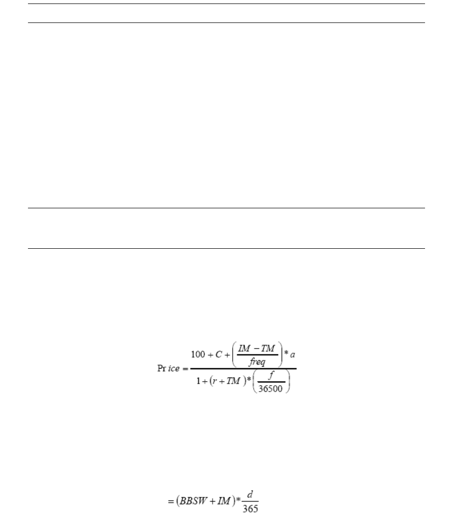
3 Debt instruments
3.7 Asset backed security
302 © Wall Street Systems IPH AB - Confidential
done by setting activity to run automatically, for example, at the end of each day, before the end of
day accounting processing.
Note: See the TRM User Guide for information about how to set up and use activities in general.
3.7.4 Position monitoring
3.7.4.1 Setup
The presence of the valuation method feature ABS Valuation in the instrument definition determines
that the instrument is valuated as an asset-backed security.
See A.2.2 ABS Valuation on page 714.
3.7.4.2 Calculations
TRM values an asset-backed security according to the current valid estimates on the valuation
dates. It does so by expanding a cashflow structure matching the estimated repayment structure
according to the parameters defined at the instrument level.
Note: The expanded repayment estimate of an ABS that can be seen in Treasury Monitor
corresponds to the cashflow structure of an equivalent bond instrument. Therefore, ABS
valuation behaves in exactly the same way as valuation of an equivalent bond.
3.7.5 Australian MBS
Australian MBS are similar to other MBS instruments already handled by TRM, except that they are
quoted in trading margin, and that the formula used to compute the price is specific. This specific
formula is used to convert the trading margin (market quote) to the instrument's price:
Equation 3-8 Trading Margin conversion - Australian MBS
then
MarketValue = Price * Outs tan ding Principal
where:
C Next coupon amount per $100 FV
IM Spread% defined at schedule level.
TM Quoted yield in %
f Number of days from settlement to next coupon date.
d Number of days between previous and next coupon dates.
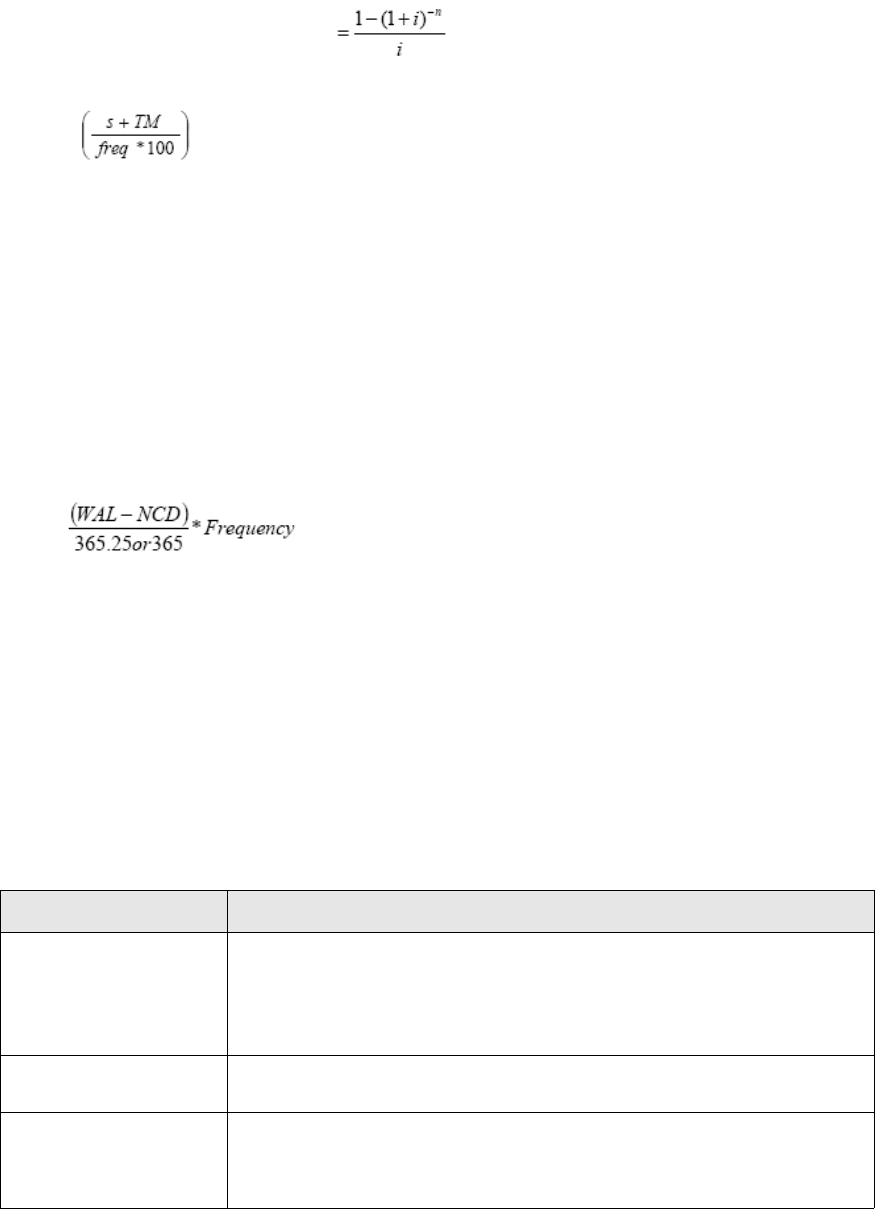
3 Debt instruments
3.7 Asset backed security
Transaction & Risk Management Module (TRM) Instruments: Processing and Calculations 303
3.7.5.1 Instrument setup
Australian MBS must be based on an instrument type derived from the class ABS. They are set up in
a similar way to ABS, but require a different primary feature.
•Main characteristics
Same setup as for usual ABS with the following additional parameter:
See A.2.39 Australian MBS on page 727.
a Annuity Factor
i
s Quarterly Swap Rate between settlement date and maturity date, this rate is
interpolated on the yield curve defined in the Quote Default page at the instrument
level. The corresponding frequency is retrieved from the Yield Type field of the
yield curve.
Note: If not quarterly, the corresponding rate is converted according to the
Equation 3-2 on page 237.
r Discount Rate between settlement date and next coupon date (interpolated on the
default yield curve defined at currency editor level).
n Number of coupon periods between the next coupon date and the Weighted
Average Life (WAL) date with the appropriate ’n’ rounding convention applied (see
3.7.5.1 Instrument setup on page 303 for information about this setup):
Equation 3-9 Number of coupon periods
where:
• WAL is calculated as shown in 3.7.5.2.1 Input data on page 304.
• 365.25 or 365 corresponds to the Days Divisor selected at the instrument level
in the Bond page.
Information Description
N-Periods’ Rounding Nearest number to which the number of coupon periods ’n’ (as calculated in
Equation 3-9 on page 303) between the next coupon date and the Weighted
Average Life date is rounded.
For example, 0 for none, 1 for an integer, or 0.1 for a rounding to the first
decimal.
N-Periods’ Rounding
Method
Up, Down or Nearest. The amount is rounded up, down, or to the nearest
figure as calculated using the specified N-Periods’ Rounding number.
Days Divisor The divisor used in the pricing (valuation) formula . Choices are:
•365
• 365.25.

3 Debt instruments
3.7 Asset backed security
304 © Wall Street Systems IPH AB - Confidential
•Quotation information
See A.2.274 Quoted on page 849.
•Yield Curve Default
The setup of the feature Quote Default (Australian MBS) is similar to the usual Quote Default
feature except that it adds the Yield Curve Default page to select the Par rate yield curve to be
used for reference rate defaulting.
A.2.268 Quote Default (Australian MBS) on page 846.
•Valuation approach
To allow quoted valuation of market value calculation instead of the usual valuation of ABS.
A.2.40 Australian MBS Valuation on page 728.
3.7.5.2 Deal capture
3.7.5.2.1 Input data
In addition to the standard deal parameters, the following information is required to enter a deal on
an Australian MBS:
In addition, the following defaulted information can be modified:
Information Description
Price Type Select Trading Margin to trade Australian MBS at a trading margin.
Quote Handling Select MBS (Australian) to convert the quotation (trading margin) to the price of
the instrument. See Equation 3-8 on page 302.
Information Description
Currency The currency that you want to specify. Select AUD.
Yield Curve Select corresponding yield curve to be used instead of the yield curve defined
at the currency level (Currency Editor).
Information Description
Trading Margin Instrument quotation.
Information Description
Reference Rate Quarterly swap rate for the period from settlement date to maturity date (from
the yield curve specified in Yield Curve Default page when provided, otherwise uses
the default yield curve defined at currency level).
Discount Rate Computed from the settlement date and the next coupon date of the instrument
(from the default yield curve defined at currency level).
AU Rate Scenario Scenario used to calculate the reference and discount rates. This scenario defaults
to the scenario defined at the instrument level (Quote Default page). You can
change the default scenario by selecting Quote Default Configuration from the Options
menu. See TRM User Guide for more information about changing this
configuration.

3 Debt instruments
3.8 Short term loan
Transaction & Risk Management Module (TRM) Instruments: Processing and Calculations 305
3.7.5.3 Processing
The actions that can be done throughout the life of an Australian MBS are the same ones as for a
usual MBS (see 3.7.3 Processing on page 300).
3.7.5.4 Position monitoring
There are two basic methods for valuation of Australian MBS instruments: Quoted or Theoretical.
3.7.5.4.1 Setup
When the Theoretical valuation method is used, the Australian MBS is valuated in the same way as a
usual MBS. On the other hand, if you want to use the pricing formula (Equation 3-8 on page 302) to
compute the market value, then you need to attach the feature Australian MBS Method (A.2.40
Australian MBS Valuation on page 728) and use the Quoted valuation method.
Swap and discount rates used in the pricing formula are retrieved as follows:
•Reference Rate: The quarterly swap rate for the period from valuation date to maturity date is
computed from the yield curve specified in the Yield Curves page (Valuation Curve Setup feature)
with Usage set to Valuation, when provided, otherwise uses the valuation yield curve defined at
the currency level.
•Discount Rate: Computed between valuation date and next coupon date of the instrument
(computed from the yield curve specified in the Yield Curves page (Valuation Curve Setup feature)
with Usage set to Discount, when provided, otherwise uses the valuation yield curve defined at
currency level).
Note: For the valuation when the next coupon is not fixed, the estimation curve is used to
compute the next fixing rate and the discount rate in the pricing formula. If the estimation
curve is not defined at the instrument level, then the currency estimation curve is used
instead. If no currency estimation curve is defined, then the currency valuation curve will
be used.
See feature A.2.337 Valuation Curve Setup on page 878.
3.8 Short term loan
Deposits and short-term loans are usually fixed-rate agreements to deposit or borrow a specified
amount for a specified period. They are basically the same instrument, with the name simply
depending on whether they are seen from the borrower's (loan) or the depositor's (deposit)
standpoint. A buy transaction is made by the lender while a sell transaction is made by the
borrower. The maturity is usually less than one year and the principal and interest are paid out at
expiration.
WAL Date If repayments were created with the WAL Date method at the instrument level,
then the entered date is automatically populated according to that date, otherwise
the WAL date is computed as follows for each row of repayments according to the
value date to the transaction settlement date:
Equation 3-10 WAL Date
Deal Price Computed using the trading margin to the price formula (Equation 3-8 on page
302).
Information Description
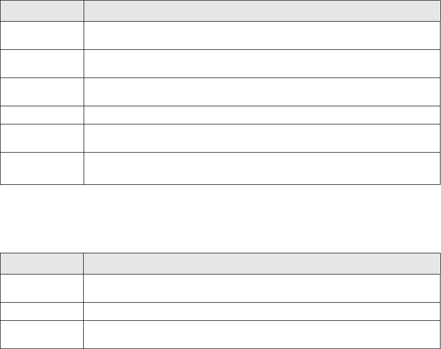
3 Debt instruments
3.8 Short term loan
306 © Wall Street Systems IPH AB - Confidential
3.8.1 Instrument setup
Short-term loans must be based on an instrument type derived from the class SHORT-LOAN.
•Main characteristics
The following basic information may be captured when defining the instrument. This information
is relevant to any kind of short term loan/deposit.
See A.2.299 Short Term Loan on page 862.
•Maturity definition
It is possible to set up maturity information at instrument level.
See A.2.230 Maturity Date Setup on page 827.
•Short loan margin definition
It is possible to input margins when entering a loan.
See A.2.300 Short Term Loan Margin Result on page 863.
For a short-term loan/deposit it is also possible to set up:
•Spot date calculation
•Value date calculation to enable easy entry of forward deals with this instrument
•Cashflow and transaction charge rules
•Manual charges
•Branch codes
•Deal rate defaulting when entering the transaction
See Appendix A Features on page 713.
Information Description
Currency Currency of the instrument. If the currency is not defined at instrument level, it needs
to be specified separately for each transaction.
Date Basis Date basis of the instrument. If the date basis is not defined at instrument level, it
can be specified separately for each transaction.
Rounding
parameters
Method and precision used to round cashflow amounts.
Interest Type Interest rate type used to calculate the cashflows of the instrument.
Transaction Sign Sign of the transaction. If the sign is not defined at instrument level, it needs to be
specified separately for each transaction.
Principal Subtype
Interest Subtype
Type of repayment and interest cashflows (default values are Redemption and
Interest).
Information Description
Calendar
parameters
Calendars used to calculate the maturity date.
Gap Set Gap set used for supplying the available maturity periods.
Maturity Date
Period
If defined, this maturity period is applied to each transaction.

3 Debt instruments
3.8 Short term loan
Transaction & Risk Management Module (TRM) Instruments: Processing and Calculations 307
3.8.2 Deal capture
3.8.2.1 Input data
Note: For margin loans, make sure that the columns Margin and Margin (bp) are visible in the
Transaction view.
In addition to the standard deal parameters, the following information is required to enter a
short-term loan/deposit:
In addition, the following optional information can be captured:
3.8.2.2 Generated data
•Transaction
–Book value of the transaction is automatically defaulted to the nominal amount.
–Issuer is determined by the transaction direction:
Information Description
Currency Currency of the transaction.
Value Date Date when the loan/deposit starts, and from which interest starts to accrue. This
defaults to the spot date of the transaction.
Maturity Date
Maturity Code
Date when the transaction matures. If you enter a maturity code, the date is
calculated automatically; otherwise you can enter the date manually.
If the maturity definition parameters are defined at instrument level, these are used
by default and cannot be modified.
Nominal Amount Amount deposited/lent, that is, the amount exchanged on the value date of the
transaction, and the amount on which interest is calculated.
Deal Rate Rate at which interest is calculated for the transaction.
Information Description
Value Date Code If the Value Date Setup feature is applied at instrument level, you can enter the value
date period you want to use to calculate the value date for the transaction, for
example, 3M (3 months).
This can be used to compute the value date for a forward purchase of a short-term
loan/deposit.
Note: If you specify a value date period in the instrument setup, this is used as the
default in the transaction and cannot be modified: see A.2.339 Value Date
Setup on page 879.
Date Basis Date basis of the transaction. If the date basis is not defined at instrument level, it can
be specified separately for each transaction.
Margin
Margin (bp)
You can enter the margin as a percentage in the Margin column or as basis points in
the Margin (bp) column, in which case, the margins are stored as a percentage but
displayed as basis points (multiplied by 100).
The margin added or subtracted from the Nominal/Spot Rate to get Deal Rate. Positive
margins are always in favor of the portfolio owner and negative margins against the
portfolio owner. Thus, for short-term loans placed, the margin will be added to
Nominal/Spot Rate to get Deal Rate, and for short-term loans taken, the margin will
be subtracted from Nominal/Spot Rate to get Deal Rate. The exact calculation is the
following:
Deal Rate = Nominal / Spot Rate + Transaction Sign * Margin
Nominal Spot / Rate The interest rate excluding margins.

3 Debt instruments
3.8 Short term loan
308 © Wall Street Systems IPH AB - Confidential
Transaction Sign = Buy, Issuer = Counterparty
Transaction Sign = Sell, Issuer = Portfolio Owner
•Cashflows
The following cashflow structure is generated for a bought transaction (depositor side).
The interest amount is calculated as follows:
rounder (A * (1 / D - 1))
where:
D = discount factor
A = nominal amount
rounder depends on the instrument’s rounding parameters
–Margin cashflows
A Margin cashflow is generated if a transaction margin rate is entered and the instrument
has the feature Short Term Loan Margin. The Margin cashflow is only used for calculating
Margin Profit. The Margin cashflow is calculated in the same way as the interest, using the
captured margin rate. This cashflow effectively represents the margin rates contribution in
the final interest amount.
3.8.3 Processing
This section describes the actions that can be done throughout the life of a short-term loan/deposit.
3.8.3.1 Early expiration
Short-term loans/deposits can be matured earlier than their agreed maturity date. This process is
referred to as early expiration. However, the action is only enabled for transactions that have
reached a certain state in the transaction flow.
•Execution
Early expiration of short-term deposits/loans can be done in two different ways. In both cases,
the following information is needed to process the early-expiration:
Information Description
Opening Date Date when the early expiration is executed. By default, this is today’s date.
Value Date Date when the early expiration is settled. This must be earlier than the original
maturity date and later than the original value date of the initial transaction.
Amount to Expire Amount to be early expired. This defaults to the amount still available to be early
expired, taking into account previous partial early expirations and roll overs.
Rate Rate at which the early expiration is done.
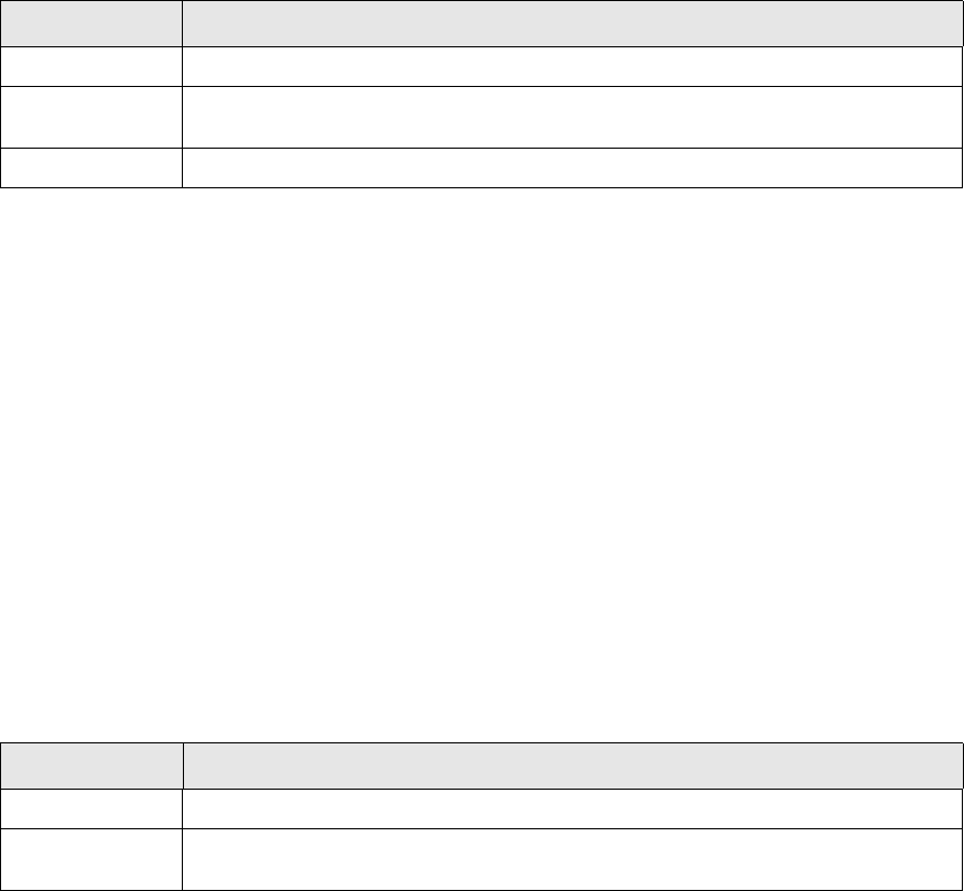
3 Debt instruments
3.8 Short term loan
Transaction & Risk Management Module (TRM) Instruments: Processing and Calculations 309
The execution generates an early expiration transaction with the following attributes:
Transaction sign = opposite of initial transaction
Nominal amount = amount to expire
Rate = early expiration rate
Opening date = date when the early expiration is done
Value date = date when the early expiration is settled
Kind = Early Expiration
The remaining attributes are inherited from the initial transaction.
•Cancellation
You can undo the early expiration by canceling the early expiration transaction.
3.8.3.2 Early expiration with margins
You can also specify margins when you early expire short term loans.
See A.2.300 Short Term Loan Margin Result on page 863.
•Execution
When early expiring a short loan with margin, the following information is displayed/ calculated
instead of the Rate field:
When a transaction being early expired has margin cashflows (i.e. instrument has feature Short
Term Loan Margin), the margin accrued from the value date of the underlying deposit until the
settlement date of the early expiration is realized.
•Cancellation
You can undo the early expiration by canceling the early expiration transaction.
3.8.3.3 Roll over
You can defer the maturity of a short-term loan/deposit to a later date. This process is referred to as
a roll-over.
See A.2.14 Allow Roll Over (Short Loan) on page 719.
•Setup
It is possible to restrict the use of the roll-over methods at instrument level (see below for
methods description). It is also possible to specify the default method for the instrument.
•Execution
Roll-over of short-term deposits/loans can be done in four different ways. In all cases, the
following information is needed to process the roll-over:
Information Description
Nominal Rate Defaulted from the original deal.
Margin Defaulted from the original deal and cannot be modified. Margin is added to or
subtracted from the Nominal Rate to get the Deal Rate.
Deal Rate Rate at which the early expiration is done. Defaulted from the original deal.
Information Description
Roll Over Date Date when the roll-over is executed.
Value Date Date of the roll over transaction. Corresponds to the maturity date of the initial
transaction.
3 Debt instruments
3.8 Short term loan
310 © Wall Street Systems IPH AB - Confidential
The outcome of the roll-over depends on the method chosen as follows:
Roll Over Method Method used for the roll over: Settle All, Settle Interest, Delay Interest, Compound
Interest, Settle Interest and Allow Increase, Capitalize Interest and Allow Increase.
The outcome of the roll over depends on the chosen method, see further on in this
section for more information.
Nominal Amount Amount of the roll-over. This defaults to the amount left of the initial transaction but
you can override this if you want to perform a partial roll-over.
Additional Amount Amount to be added to the initial principal amount if you want to increase capital at
roll over.
This field becomes available when one of the Allow Increase roll over methods has
been selected.
New Nominal
Amount
Original nominal amount plus interest (if interest is capitalized) plus the additional
amount.
This field becomes available when one of the Allow Increase roll over methods has
been selected.
Gap Gap set used for supplying the available maturity periods.
Maturity Date The maturity date for the loan/deposit. The defaulting is defined as follows:
• If the parent transaction was defined with a maturity period, the roll over maturity
date defaults according to that period, otherwise you have to enter the maturity
date.
• If the switch No Maturity Defaulting is selected at the instrument level (Roll Over
page), then the maturity date of the rollover is never defaulted and you must
enter it.
Note: If the specified maturity date does not fall on a business day, you can choose to
keep the non business day or to change it.
Deal Rate (Mandatory) New interest rate for the roll-over, that is, the rate at which interest is
calculated from the old maturity date until the new maturity date.
By default, the rate is defaulted from the initial transaction however it is possible to
disable this defaulting by selecting the switch No Rate Defaulting at the instrument level
(Roll Over page).
Method Description
Settle All The initial transaction is paid in its entirety at the initial maturity date. The default
nominal amount of the roll-over transaction equals the sum of the interest and
principal cashflows of the initial transaction.
Settle Interest The interest of the initial transaction is paid at the initial maturity date, but the
principal payment is deferred. The part of the principal which is rolled over is paid
back at the end of the roll-over transaction.
The default nominal amount of the roll-over transaction equals the principal cashflow
of the initial transaction but can be reduced (partial roll-over).
Settle Interest,
Allow Increase
This method allows the user to provide additional capital (increase the principal) as
part of the roll over process.
The interest from the underlying deposit/loan is settled, and the original principal
amount (plus the additional capital) is rolled over.
Capitalize
Interest, Allow
Increase
This method allows the user to provide additional capital (increase the principal) as
part of the roll over process.
The interest from the underlying deposit/loan is capitalized (that is, realized and
added to the initial nominal amount) and included with the additional capital in the roll
over.
Information Description

3 Debt instruments
3.8 Short term loan
Transaction & Risk Management Module (TRM) Instruments: Processing and Calculations 311
The execution generates a new transaction with the following attributes:
Nominal amount = amount (can be smaller than the initial transaction)
Rate = roll-over rate
Opening date = date when the roll-over is done
Value date = maturity date of the initial transaction
Maturity date = maturity of the roll-over
Kind = Roll-over
•Cancellation
You can undo the roll-over by canceling the roll-over transaction.
3.8.3.4 Roll over with margins
You can specify margins in case you roll over short term loans.
See A.2.15 Allow Roll Over (Short Loan - Margin Result) on page 719.
•Execution
This roll over behaves exactly as the roll over without margins, except that instead of just the
Deal Rate field, the following fields are available:
•Cancellation
You can undo the roll-over by canceling the roll-over transaction.
3.8.4 Position monitoring
3.8.4.1 Setup
The presence of the valuation method feature Short Term Loan Valuation in the instrument
definition determines that the instrument is valuated as a short term loan.
See A.2.301 Short Term Loan Valuation on page 863.
3.8.4.2 Calculations
In this section, numerical examples demonstrate how the different figures are calculated for
short-term deposit/loan transactions.
Delay Interest Nothing is paid at the initial maturity date: both the interest and principal payments
are deferred. The parts of the principal and interest cashflows which are rolled over
are paid back at the end of the roll-over transaction.
The default nominal amount of the roll-over transaction equals the principal cashflow
of the initial transaction but can be reduced (partial roll-over).
Compound
Interest
This method is the same as Delay Interest, but the closed interest of the initial
transaction is reinvested in the roll-over. New interest accrues on top of the initial
transaction’s interest.
The default nominal amount of the roll-over transaction equals the principal cashflow
of the initial transaction but can be reduced (partial roll-over).
Method Description
Information Description
Nominal Rate Defaulted from the original deal.
Margin Defaulted from the original deal. Added to or subtracted from the Nominal Rate to get
Deal Rate.

3 Debt instruments
3.8 Short term loan
312 © Wall Street Systems IPH AB - Confidential
If you need more theoretical information about the method used in these calculations, see Chapter 2
Market standards and calculations on page 33.
This example shows a 6 month USD deposit with a 3% Periodic Rate, with the following deal data:
Other important deal data is calculated by the system as follows:
•Period
t_p = (d_m - d_p) / B
0.508333333 = (2004/12/03 – 2004/06/03) / 360
•Discount Factor
D_b = 1 / (1 + t_p * r_b)
0.984979069 = 1 / (1 + 0.508333333 * 0.03)
• Interest Cashflow
c_I = c_m * r_b * t_p
15,250.00 = 1,000,000 * 0.03 * 0.508333333
•Book Value (Local)
V_b = (c_m + c_I) * D_b
1,000,000.00= (1,000,000 + 15,250) * 0.984979069
•Book Value
V_bp = ROUND(V_b / S_b ,2)
842,389.02 = ROUND(1,000,000 / 1.18710 ,2)
Setup data
Instrument Date Basis Act/360
Instrument Yield Type Periodic
Valuation Method Theoretical
Risk Method Theoretical
Valuation Date Figure Date
Result IR: AI Method Linear
Result IR: Accrual Method Linear Accrual
Accrual Yield: Interest Type Periodic Rate
Accrual Yield: Date Basis Actual/360
Result FX: Profit Method FX Forward
FX Exposure Offset e_fx 0.01
IR Risk Rate e_ir 0.0001
Transaction data
Opening Date 2004-06-01
Spot Date d_p 2004-06-03
Maturity Date d_m 2004-12-03
Nominal Amount c_m 1,000,000
Deal Rate r_b 3%
Base Book FX Rate (EUR/USD) S_b 1.18710
Currency USD
Portfolio Currency EUR
3 Debt instruments
3.8 Short term loan
Transaction & Risk Management Module (TRM) Instruments: Processing and Calculations 313
Unless otherwise stated, the figure date used in the calculations is 2004-08-17. On this date, the
market data is as follows:
Other figures are calculated by the system as follows:
• Days to Maturity
= d_m - d_f
108 = 2004/12/03 – 2004/08/17
• Time to Maturity
t_m = (d_m - d_f) / B
0.30000 = 108 / 360
•Time to Spot
t_s = d_fs / B
0.00555556 = 2 / 360
• Market Value Discount Factor
D_V = D_s * D_I = 0.9966917723
• Present Value Discount Factor
D_P = D_s * D_I = 0.9966917723
• Market Value Spot Discount Factor
D_s = EXP(-t_s * r_d) = 0.9999419470
• Discount Factor From Spot
D_I =EXP(-(t_m - t_s)* r_f) = 0.9967496366
3.8.4.2.1 Valuation figures
The valuation method commonly used for a short-term loan/deposit is the Theoretical method.
• Principal flow figures
Local Market Value
V_lp = c_m * D_V
996,691.77 = 1,000,000 * 0.9966917723
Market Value
V_p = V_lp / S
830,576.48 = 996,691.77 / 1.200
Clean Market Value
CMV_p = V_p / D_s
830,624.70 = 830,576.48 / 0.9999419470
• Interest flow figures
Local Market Value
V_li = c_I * D_V
15,199.55 = 15,250 * 0.9966917723
Market Value
V_i = V_li / S
12,666.29 = 15,199.55 / 1.200
Clean Market Value
CMV_i = (c_I * D_V / D_s - (c_I * (t_p - t_m + t_s)) / t_p) / S
7,319.80 = (15,250 * 0.9966917723 - (c_I * (0.50833333 - 0.3 + 0.00555556)) / t_p) / 1.2
Market data on 2004-08-17
Figure Date d_f 2004-08-17
Days to Spot d_fs 2
Interest Rate r_f 1.105695%
Discount Rate r_d 1.044985%
FX Spot Rate S 1.20000
FX Spot CCY Base Rate S_p 1.2
3 Debt instruments
3.8 Short term loan
314 © Wall Street Systems IPH AB - Confidential
• Transaction figures
Local Market Value
= V_lp + V_li
1,011,891.32 = 996,691.77 + 15,199.55
Market Value
= V_p + V_i
843,242.77 = 830,576.48 + 12,666.29
Clean Market Value
= CMV_p + CMV_i
837,944.50 = 830,624.70 + 7,319.80
3.8.4.2.2 Result figures
The setup of the instrument impacts the way result figures are computed.
• Principal flow figures
Tot al P rof it (L oca l )
P_tlp = V_lp - V_b
-3,308.23 = 996,691.77 – 1,000,000
MtoM Profit (Local)
P_mlp = c_m * D_V / D_s - V_b
-3,250.36 = 1,000,000 * (0.9966917723/0.9999419470) – 1,000,000
Accrued Interest (Local)
I_alp = 0
Accrued Profit (Local)
P_alp = 0
Other Profit (Local)
P_olp = P_tlp - P_mlp
-57.86 = (-3,308.23) – (-3,250.36)
FX Profit
P_fxp = V_b * (1 / S_p) - V_bp
-9,055.68 = 1,000,000 * (1 / 1.2000) – 842,389.02
Tot al P rof it
P_tp = V_p - V_bp
-11,812.54 = 830,576.48 – 842,389.02
MtoM Profit
P_mp = P_mlp / S
-2,708.64 = -3,250.36 / 1.2
Accrued Interest
I_ap = 0
Accrued Profit
P_ap = 0
Other Profit
P_op = P_tp - P_fxp - P_mp
-48.22 = (-11,812.54) – (-9,055.68) – (-2,708.64)
• Interest flow figures
Tot al P rof it (L oca l )
P_tli = V_li
= 15,199.55
MtoM Profit (Local)
P_mli = =c_I * D_V / D_s - (c_I * (t_p - t_m + t_s)) / t_p
8,783.77 = 15,250 * (0.9966917723 / 0.9999419470) – (c_I * (0.508333333 - 0.3 + 0.00555556)) / t_p
Accrued Interest (Local)
I_ali = c_I * (t_p - t_m) / t_p
6,250.00 = 15,250 * (0.508333333 – 0.3) / 0.508333333
Other Profit (Local)
P_oli = P_tli - P_mli – I_ali
165.78 = 15,199.55 – 8,783.77 – 6,250.00
3 Debt instruments
3.8 Short term loan
Transaction & Risk Management Module (TRM) Instruments: Processing and Calculations 315
Tot al P rof it
P_ti = V_i
= 12,666.29
MtoM Profit
P_mi = P_mli / S
7,319.80 = 8,783.77 / 1.2
Accrued Interest
I_ai = I_ali / S
5,208.33 = 6,250.00 / 1.2
Other Profit
P_oi = P_ti - P_mi – I_ai
138.15 = 12,666.29 -7,319.80 – 5,208.33
• Transaction figures
Tot al P rof it (L oca l )
= P_tlp + P_tli
11,891.32 = -3,308.23 + 15,199.55
MtoM Profit (Local)
= P_mlp + P_mli
5,533.40 = -3,250.36 + 8,783.77
Accrued Interest (Local)
= I_ali
= 6,250.00
Other Profit (Local)
= P_olp + P_oli
-58.75 = (-57.86) + (-0.88)
FX Profit
= P_fxp
= -9,055.69
Tot al P rof it
= P_tp + P_ti
853.75 = -11,812.54 + 12,666.29
MtoM Profit
= P_mp + P_mi
4,611.17 = -2,708.64 + 7,319.80
Accrued Interest
= I_ap + I_ai
5,208.33 = 0 + 5,208.33
Other Profit
= P_op + P_oi
89.93 = (-48.22) + 138.15
3.8.4.2.3 Risk figures
The risk method commonly used for a short-term loan/deposit is the Theoretical method.
• Principal flow figures
IR Exposure 1bp
E_ip = (c_m) * (-(t_m - t_s)*D_I*D_s - t_s*D_I*D_s) / S * e_ir
-24.92 =
1,000,000*(-(0.3-0.005555556)*0.9967496366*0.9999419470-0.005555556*D_I*D_s) /1.2*0.0001
FX Exposure
E_fxp = V_p * e_fx
8,305.76 = 830,576.48 * 0.01
Effective Duration
U_eff = -E_ip / V_p / 0.0001
0.300000 = -(-24.92) / 830,576.48 / 0.0001
• Interest flow figures
IR Exposure 1bp
E_ipi = (c_I) * (-(t_m - t_s)* D_I * D_s - t_s * D_I * D_s) / S * e_ir
-0.38 =
15,250.00 *(-(0.3 - 0.005555556) * 0.9967496366 * 0.9999419470 - t_s * D_I * D_s) / 1.2 * 0.0001
3 Debt instruments
3.9 Discount paper
316 © Wall Street Systems IPH AB - Confidential
FX Exposure
E_fxi = V_i * e_fx
126.66 = 12,666.29 * 0.01
Effective Duration
U_eff = -E_ipi / V_i / 0.0001
0.300000 = -(-0.38) / 12,666.29 / 0.0001
• Transaction figures
IR Exposure 1bp
= E_ip + E_ipi
-25.30 = (-24.92) + (-0.38)
FX Exposure
= E_fxp + E_fxi
8432.43 = 8,305.76 + 126.66
Effective Duration
U_eff = -(E_ip + E_ipi) / (V_p + V_i) / 0.0001
0.300000 = -((-24.92) + (-0.38)) / (830,576.48 + 12,666.29) / 0.0001
3.9 Discount paper
A discount paper is a short-term instrument which pays its face amount at maturity and is
purchased at a discount price. Most discount papers are listed instruments. The most commonly
traded discount paper is the US Treasury-Bill.
3.9.1 Instrument setup
Discount papers are based on an instrument type derived from the class DISCOUNT.
•Main characteristics
The following basic information may be captured when defining the instrument. This information
is relevant to any kind of discount paper.
See A.2.121 Discount Paper on page 768 or A.2.122 Discount Paper OTC on page 770.
–Date details
For listed discount papers, you must specify the issue date and maturity date of the
instrument.
Information Description
Currency Currency of the discount paper (that is, if it is a listed discount paper).
Leave this field blank if you want to specify the currency when you enter the deal in
Transaction Manager when you are defining an OTC discount paper.
Date Basis Date basis of the instrument. If the date basis is not defined at instrument level, it
needs to be specified separately for each transaction.
Rounding
parameters
Method and precision used to round cashflow amounts.
Yield Type Yield type of the discount paper, typically a discount rate.
Transaction Sign Sign of the transaction. If the sign is not defined at instrument level, it needs to be
specified separately for each transaction.
Principal Subtype
Interest Subtype
Type of principal or interest cashflows.
Issuer Issuer of the instrument.
3 Debt instruments
3.9 Discount paper
Transaction & Risk Management Module (TRM) Instruments: Processing and Calculations 317
For OTC discount papers, you can set up maturity information.
–Trading unit details
It is possible to define a minimum bid size or trading units of a discount paper. If a minimum
denomination is defined, deal entry is available either in units or amount and TRM ensures
that the amount is a multiple of the denomination size.
•Quoted
If you want to enter quotes for a discount paper, this must be specified at instrument level.
See A.2.274 Quoted on page 849.
•Valuation approach
Discount papers can be valuated using either Fixed IR Valuation or Discount Valuation features.
See A.2.150 Fixed IR Valuation on page 784 or A.2.123 Discount Valuation on page 770.
Examples of calculations using these methods are provided in section 3.9.4 Position monitoring
on page 320.
It is also possible to set up:
•Spot date calculation
•Value date calculation to enable easy entry of forward deals with this instrument
•Cashflow and transaction charge rules
•Collateral
•Branch codes
•Quotation information.
See Appendix A Features on page 713.
3.9.2 Deal capture
3.9.2.1 Input data
In addition to the standard deal parameters, the following information is required to enter a discount
paper:
Information Description
Calendar Calendars used to calculate the maturity date.
Gap Set Gap set used for supplying the available maturity periods.
Maturity Date Period If defined, this maturity period is applied to each transaction.
Information Description
Price Type Select Yield.
Quote Handling Select Discount Paper to display yields and prices in Rate Monitor.
Information Description
Currency Currency of the transaction.
If you specified the currency in the instrument setup (for example, for a US T-Bill),
this is used as the default currency in the transaction and cannot be modified.
3 Debt instruments
3.9 Discount paper
318 © Wall Street Systems IPH AB - Confidential
In addition, the following optional information can be captured:
3.9.2.2 Generated data
•Transaction
A discount paper is bought or sold at a discount price. This means that the Book Value (BV) is
equal to the nominal amount discounted with the deal rate.
BV = NA * D
•Cashflows
The following cashflows are generated:
–The principal/settlement cashflow is generated with amount = book value
–There is only one payback cashflow (principal/payback)
–There is no interest cashflow.
Maturity Date
Maturity Code
Date for the maturity of the contract. If you enter a maturity code, the date is
calculated automatically; otherwise you can enter the date manually.
Note: For listed discount papers, the maturity date defaults from the instrument setup
and cannot be changed.
Value Date Date when the transaction starts. This defaults to the spot date of the transaction.
Nominal Amount
Units
Amount of the discount paper. This is equal to the principal (the amount on which the
interest is calculated).
For listed discount papers, the nominal amount must be a multiple of the minimum
contract size defined in the instrument setup.
Deal Rate Rate used to discount the nominal amount (the book rate).
Information Description
Deal Price Deal price of the transaction (expressed as a percentage of the nominal amount) used
to calculate the book value and the settlement amount.
Value Date Code If the Value Date Setup feature is applied at instrument level, you can enter the value
date period you want to use to calculate the value date for the transaction, for
example, 3M (3 months).
This can be used to compute the value date for a forward purchase of a discount
paper.
Note: If you specify a value date period in the instrument setup, this is used as the
default in the transaction and cannot be modified: see A.2.339 Value Date
Setup on page 879.
Issuer Issuer of the discount paper.
If Issuer is defined at instrument level, this is used by default and cannot be modified.
Date Basis Date basis of the transaction.
If this value is defined at instrument level, this is used by default and cannot be
modified at deal entry.
Information Description
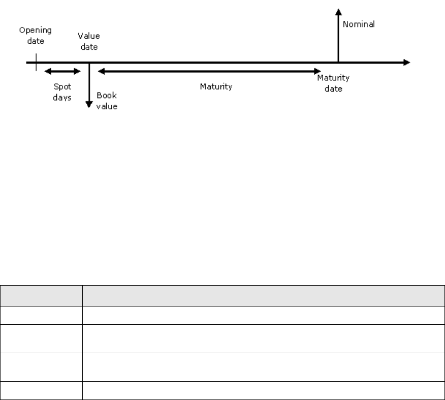
3 Debt instruments
3.9 Discount paper
Transaction & Risk Management Module (TRM) Instruments: Processing and Calculations 319
The figure below illustrates the cashflows which are established in TRM when a discount paper is
purchased.
3.9.3 Processing
This section describes the actions that can be done throughout the life of a discount paper.
3.9.3.1 Early expiration
Discount papers can be matured earlier than their agreed maturity date. This process is referred to
as early expiration. However, the action is only enabled for transactions that have reached a certain
state in the transaction flow.
•Execution
The following information is needed to process the early-expiration:
The execution generates an early expiration transaction with the following attributes:
Transaction sign = opposite of initial transaction
Nominal amount = amount to expire
Rate = early expiration rate
Opening date = date when the early expiration is done
Value date = date when the early expiration is settled
Kind = Early Expiration
The remaining attributes are inherited from the initial transaction.
•Cancellation
You can undo the early expiration by canceling the early expiration transaction.
Information Description
Opening Date Date when the early expiration is executed. By default, this is today’s date.
Value Date Date when the early expiration is settled. This must be earlier than the original
maturity date and later than the original value date of the initial transaction.
Amount to Expire Amount to be early expired. This defaults to the amount still available to be early
expired, taking into account previous partial early expirations and roll overs.
Rate Rate at which the early expiration is done.
3 Debt instruments
3.9 Discount paper
320 © Wall Street Systems IPH AB - Confidential
3.9.4 Position monitoring
3.9.4.1 Setup
In addition to the basic valuation setup which can be set up for every instrument (see A.2.50 Base
Valuation Setup on page 734) it is possible to set up the following:
3.9.4.2 Calculations - Theoretical
In this section, numerical examples demonstrate how the different figures are calculated for
discount papers.
See Chapter 2 Market standards and calculations on page 33.
This example shows a US T-Bill, with the following deal data:
Information Description
AI Method It is possible to override the standard linear method in order to accrue interest
differently for the valuation figures (see A.2.49 Base IR Setup on page 733, Chapter 1
Concepts on page 21, A.2.337 Valuation Curve Setup on page 878).
Spread Curve It is possible to add spread curves to correspond to the credit risk (see A.2.305
Spread Curve Setup on page 865, Chapter 1 Concepts on page 21, A.2.337 Valuation
Curve Setup on page 878).
Setup data
Instrument Date Basis Act/360
Instrument Yield Type Discount
Valuation Method Theoretical
Valuation Date Figure Date
Risk Date Figure Date
Risk Yield Type Continuous
Result IR: Accrued Interest Linear
Result IR: Accrual Method Linear Accrual
Accrual Yield: Interest Type Periodic Rate
Accrual Yield: Date Basis Actual/360
FX Exposure Offset e_fx 0.01
Transaction data
Opening Date 2004-02-02
Nominal Amount c_m 1,000,000
Deal Rate r_b 3%
Base Book FX Rate (EUR/USD) S_b 1.2
Maturity Date d_m 2004-07-01
Value Date d_a 2004-02-04
Currency USD
Portfolio Currency EUR
3 Debt instruments
3.9 Discount paper
Transaction & Risk Management Module (TRM) Instruments: Processing and Calculations 321
Other important deal data is calculated by the system as follows:
•Book Value (Local)
V_b = c_m * D_b
987,750.00 = 1,000,000 * 0.98775
•Book Value
V_p = V_b / S_b
823,125.00 = 987,750.00 / 1.2
•Period
t_p = DAYS360(d_a,d_m,TRUE) / B
0.408333333 = (2004/02/04,2004/07/01,TRUE) / 360
•Discount Factor
D_b = 1 – t_p * r_b
0.98775 = 1 – 0.408333333 * 0.03
Unless otherwise stated, the figure date used in the calculations is 2004-03-01. On this date, the
market data is as follows:
Other figures are calculated by the system as follows:
• Days to Maturity
= d_m - d_f
122 = 2004/07/01 – 2004/03/01
• Time to Maturity
t_m = (d_m - d_f) / B
0.33888889 = 122 / 360
•Time to Spot
t_s = d_fs / B
0.005555556 = 2 / 360
• Market Value Discount Factor
D_V = D_s * D_I = 0.996238639
• Present Value Discount Factor
D_P = D_s * D_I = 0.996238639
• Spot Discount Factor
D_s = EXP(-t_s*r_d) = 0.999941947
• Spot-Maturity Discount Factor
D_I =EXP(-(t_m-t_s)*r_f) = 0.996296478
Valuation figures
The valuation method commonly used for a discount paper is the Theoretical method.
• Local Market Value
V_l = c_m * D_V
996,238.64 = 1,000,000 * 0.996239
•Market Value
V = V_l / S
790,665.59 = 996,238.64 / 1.2600
• Clean Market Value
= V / D_s
790,711.49 = 790,665.59 / 0.999941947
Market data on 2004-03-01
Figure Date d_f 2004-03-01
Interest Rate r_f 1.113119%
Days to Spot d_fs 2
Discount Rate r_d 1.044985%
FX Conversion Rate S 1.260000

3 Debt instruments
3.9 Discount paper
322 © Wall Street Systems IPH AB - Confidential
Result figures
The setup of the instrument impacts the way result figures are computed.
• Total Profit (Local)
P_tl = V_l – V_b
8,488.64 = 996,238.64 – 987,750.00
• MtoM Profit (Local)
P_ml = -c_m * ((1 - r_b * (t_m - t_s)) - (D_I))
6,296.48 = 1,000,000*((1 - 0.03 *(0.33888889-0.005555556)) - 0.996296478
• Accrued Profit (Local)
P_al = = -c_m * (D_b -(1 - (t_m - t_s) * r_b))
2,250.00 = -1,000,000*(0.98775-(1-(0.33888889-0.005555556)*0.03))
• Other Profit (Local)
P_ol = P_tl - P_ml - P_al
-57.84 = 8,488.64 – 6,296.48 – 2,250
•FX Profit
P_fx = V_b * (1/S - 1/S_b)
-39,196.43 = 987,750.00*(1 / 1.260000 – 1 / 1.20000)
• Total Profit
P_t = V – V_p
-32,459.41 = 790,665.59 – 823,125.00
•MtoM Profit
P_m = P_ml / S
4,997.20 = 6,296.48 / 1.260000
• Accrued Profit
P_a = P_al / S
1,785.71 = 2,250.00 / 1.260000
•Other Profit
P_o = P_t - P_m - P_a - P_fx
-45.90 = -32,459.41 - 4,997.20 - 1,785.71 – (-39,196.43)
Risk figures
The risk method commonly used for a discount paper is the Theoretical method.
•IR Exposure 1bp
E_ip = c_m * (-(t_m-t_s) * D_I*D_s - t_s *D_I* D_s) /S * 0.0001
-26.79 =
1,000,000*(-(0.33888889-0.005555556)*0.996296478*0.999941947-t_s*(D_I*D_s)/1.26*0.0001
• IR Exposure 1bp from spot
E_is = c_m * (-(t_m - t_s) * D_I) / S * 0.0001
-26.357050 = 1,000,000 * (-(0.33888889-0.005555556)*0.996296478 / 1.26 * 0.0001
•FX Exposure
E_fx = e_fx * V
7,906.66 = 0.01 * 790,665.59
• Effective Duration
U_eff = -E_ip / V / 0.0001
0.338889 = -(-26.79) / 790,665.59 / 0.0001
3.9.4.3 Calculations - Discount Yield
Discount yield is calculated from quoted market value at spot, using Yield Type and Date Basis
defined in IR Exposure page in the Instrument Editor:
Equation 3-11 Discount yield
where
–V is market value at spot, A is the amount
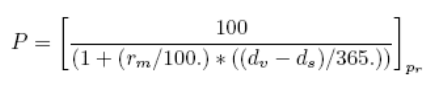
3 Debt instruments
3.9 Discount paper
Transaction & Risk Management Module (TRM) Instruments: Processing and Calculations 323
– is time between spot date and value date calculated using the IR Exposure date basis
–R[] is the function that converts discount factor into rate, according to the Yield Type defined
for IR Exposure .
3.9.4.3.1 Example
Instrument data
•Discount Paper page
•Dates page
•Base Valuation page
•IR Exposure page
Transaction data
Valuation data
Calculated data
•Price (P)
Let mean rounding to k decimal places. Then
Equation 3-12 Discount Yield Price
= 95.263
Date Basis Actual/365
Interest Type Periodic Rate
Price Rounding 0.001 (3 decimal places)
Maturity Date 2009-08-05
Method Quoted
Switches To Spot
Date Basis Actual/365
Yield Type Continuous Yield
Switches To Spot
Nominal Amount
Valuation Date 2008-08-05
Figure Market Quote
Days to Maturity Date
Days to Spot
tv
pr3=
A 100000=
rm5=
dv 365=
ds2=
X[]
k

3 Debt instruments
3.9 Discount paper
324 © Wall Street Systems IPH AB - Confidential
•Discount Yield (y)
Using
Equation 3-13 Discount Yield: Discount Yield (y)
= 0.994520547945206
The discount yield (Figure Interest Rate) is:
Equation 3-14 Discount Yield: Figure Interest Rate
= 0.0487960741031
•IR Exposure (E1)
Figure Risk Value is:
= 1000000
Sensitivity of discount factor is (for continuous yield):
Equation 3-15 Discount Yield: IR Exposure (E1)
= -0.947410109589
Figure IR Exposure 1bp is:
Equation 3-16 Discount Yield: IR Exposure (1bp)
= -94.7410109589
3.9.4.4 Calculations - Modified Duration / Effective Duration
The following numerical example demonstrates how Modified Duration and Effective Duration figures
are calculated for depo/discount papers. For more information about Duration key figures, see
2.3.4.9 Duration figures on page 142.
3.9.4.4.1 Example: Depo/Discount Paper
The example in this section shows an overnight paper of 100,000,000 at 0.70 with a price of
99,998,088.89.
Transaction data
•On November 9th, the Principal cashflow was equal to -99 998 088.89
•On November 10th, the Principal cashflow was equal to 100,000,000.00
VrA=
E1VrDr0.0001×=

3 Debt instruments
3.9 Discount paper
Transaction & Risk Management Module (TRM) Instruments: Processing and Calculations 325
Valuation data
Risk figures
•Principal cashflow (risk date = 2009-11-09)
Equation 3-17 Time to maturity of the cashflow
•Amortization cashflow (risk date = 2009-11-10)
Equation 3-18 Time to maturity of the cashflow
Transaction figures
Valuation Date 2009-11-09
Valuation Mode Theoretical
Date Basis Actual/365
ti
drdv
–
365
----------------0==
Present Value Discount Factor Dp = 1
Present Value Vp= -99,998,088.89
IR Exposure Ei1{} 0=
ti
drdv
–
365
----------------1 365⁄==
Present Value Discount Factor Dp = 0.999964445709
Present Value Vp = -99,996,444.57
IR Exposure Ei1{} Vpti0.0001××– 27.39628618==
IR Exposure
Present Value Vp = -99,998,088.89+99,996,444.57 = -1644.3
Modified Duration
Effective Duration
Ei1{} Vpti0.0001××– 0 27.39628618+ 27.39628618===
UMod
1000 Ei1
Sett Ei1
Pos
+[]×
0.5 Vp
Sett Vp
Pos
+()×
------------------------------------------------------- 10000 27.39628618[]×
0.5 99 998 088.89,,– 99 996 444.57,,+()×
-------------------------------------------------------------------------------------------------------------0.002739704== =
Ueff
Ei1{}
–
Vp
----------------
⎝⎠
⎛⎞
10000×27.39628618–
1644.3191–
----------------------------------
⎝⎠
⎛⎞
10000×166.6117372== =

3 Debt instruments
3.10 Loan
326 © Wall Street Systems IPH AB - Confidential
3.10 Loan
In TRM, loans are agreements to lend or borrow money for a medium/long term with multiple
interest (and potentially principal) payments occurring during the life of the deal.
The key concept concerning loans is that of the cashflow schedule. Several schedules must be
attached to a loan deal, and they drive the generation of the cashflow structure for the deal.
For the simplest types of loans, two schedules are associated with the deal: one schedule for
interest flows; and one schedule for principal flows. For more complex deals, there will be additional
schedules for optional events, additional interest cashflows, and so on.
Loans belong to the instrument class LOAN. This class covers a diverse set of instruments: from
fixed annual interest / bullet repayment loans to more complex, exotic structures. Therefore, this
chapter is organized into the following sections:
–How TRM handles fixed-rate loans
–How TRM deals with floating-rate loans
–A list of more exotic deals that can be set up in TRM.
3.10.1 Fixed-rate loan
Fixed-rate loans pay interest at a pre-defined (fixed) rate.
3.10.1.1 Instrument setup
•Loan main characteristics
The following basic information may be captured when defining the instrument. This information
is relevant to any kind of fixed-rate loan.
See A.2.202 Generic Loan on page 812.
Information Description
Currency Currency of the loan.
Leave this field blank if you want to specify the currency when you enter the deal in
Trans action Manager.
Transaction Sign Sign of the transaction. If the sign is not defined at instrument level, it needs to be
specified separately for each transaction.
AI Method Method used to calculate accrued interest if interest starts to accrue before the value
date of the transaction.
Settlement
Switches
Dirty Price: Switch on to use the dirty price for the instrument, that is, to include
accrued interest in the instrument’s price.
Par: Switch on in order to have the deal price defaulted to 100.
Rounding
Parameters
Method and precision used to round cashflow amounts.
Structure Schedule template to be used for the loan.
If a structure is not defined at instrument level, a schedule needs to be specified for
each transaction. Usually the structure is defined at the instrument level. If this is not
the case, then you have to define it for each transaction at transaction level.

3 Debt instruments
3.10 Loan
Transaction & Risk Management Module (TRM) Instruments: Processing and Calculations 327
•Maturity definition
It is possible to set up maturity information at instrument level.
See A.2.230 Maturity Date Setup on page 827.
•Selectable cashflow structures
With this option, you can limit the choice of schedules available to assign to a loan in Transaction
Manager by associating one or several schedule template groups to the instrument. At deal
entry, only the templates belonging to these groups will be available for selection.
If a cashflow structure is already set up in the instrument’s main characteristics, it will override
any schedule groups.
See A.2.293 Schedule Template Setup on page 859.
It is also possible to set up:
•Spot day calculations
•Manual charges
•Cashflow and transaction charge rules
•Branch codes.
See Appendix A Features on page 713.
3.10.1.2 Deal capture
Depending on the selected cashflow structure, the information needed to deal the instrument and
the generated cashflows are very different.
The transaction level information is the same.
3.10.1.2.1 Input data
In addition to the standard deal parameters, the following information is required to enter a deal on
a fixed rate loan:
Information Description
Calendar
parameters
Calendars used to calculate the maturity date.
Gap Set Gap set used for supplying the available maturity periods.
Maturity Date
Period
If defined, this maturity period is applied to each transaction.
Information Description
Currency Currency of the transaction.
If you specified the currency in the instrument setup, this is used as the default
currency in the transaction and cannot be modified.
Maturity Date Date for the maturity of the contract.
If you use maturity date setup, the date is calculated automatically from the selected
maturity period, otherwise you can enter the date manually.
Nominal Amount Amount of the loan. This is equal to the principal (the amount on which the interest is
calculated).
Deal Price Deal price of the transaction (expressed as a percentage of the nominal amount) used
to calculate the book value and the settlement amount. In order to have the deal
price defaulted to 100, you should set the settlement switch Par in Instrument Editor.

3 Debt instruments
3.10 Loan
328 © Wall Street Systems IPH AB - Confidential
These values alone are not sufficient to define the deal. To complete the creation of a fixed-rate
loan, the cashflow structure of the deal also needs to be specified, either in the instrument setup, or
at deal entry, by applying a schedule template.
The following sections explain how the system handles standard fixed-rate cashflow structures.
3.10.1.2.2 Generated data
•Book Value (clean price):
BV = A * p /100
where:
A = Nominal Amount
p = deal price
•Book Value (dirty price):
BV = (A * p /100) - AI
where:
A = Nominal Amount
p = deal price
AI = Accrued Interest
3.10.1.2.3 Bullet repayment structure
A fixed-rate loan with periodic interest and total repayment of the principal at maturity represents a
bullet repayment structure.
•Input data
To define this kind of structure, a template is required which contains at least one schedule for
fixed-rate interest flows, and one schedule for repayment flows. TRM provides a pre-defined
system template designed for this: see B.2.1.1.21 Fixed, Bullet Repayment on page 894.
For each set of cashflows, the following information must be supplied at deal entry:
–Interest flows
–Repayment flows
No information required.
•Generated data
–Schedule
When a template is selected, one schedule is created for each item in the template. Some of
the values are automatically defaulted from the transaction parameters (see Appendix B
Schedules on page 883), while others can be modified at deal entry (see above).
Information Description
Frequency Method
and Period
The frequency method/period for the interest cashflows (for example, Years/1
generates one interest flow per year).
Interest Rate The fixed interest rate (for example, 5%).

3 Debt instruments
3.10 Loan
Transaction & Risk Management Module (TRM) Instruments: Processing and Calculations 329
–Cashflows
For a fixed-rate loan with repayment at maturity, the cashflows generated are as follows:
3.10.1.2.4 Fixed-rate loan - amortizing structure
A fixed-rate loan with periodic interest and repayment of the principal in several steps during the
deal represents an amortizing structure.
•Input data
To define this kind of structure, a template which contains at least one schedule for fixed-rate
interest cashflows, and one schedule for repayment cashflows is required. TRM provides a
pre-defined system template (B.2.1.1.21 Fixed, Bullet Repayment on page 894) designed for
this purpose.
For each set of cashflows, the following information must be supplied at deal entry:
–Interest flows
–Repayment flows
•Generated data
–Schedule
When a template is selected, one schedule is created for each item in the template. Some of
the values are automatically defaulted from the transaction parameters, while others can be
modified at deal entry.
Information Description
Frequency Method
and Period
The frequency method/period for the interest cashflows (for example, Years/1
generates one interest flow per year).
Interest Rate The fixed interest rate (for example, 5%).
Information Description
Frequency Method
and Period
The frequency method/period for the repayment cashflow (for example,
Times/Year-1 means that one repayment will occur every year).
Calculation Method
and Repayment %
Defines how the repayments have to be generated.
For example, using percentage 10% as the method means 10% of the initial
capital at each repayment, with the remaining capital being repaid at maturity.
Start Date Start date can be moved forward in order to start amortizing later.
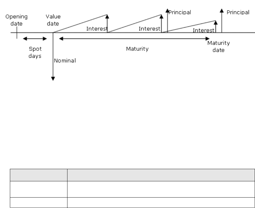
3 Debt instruments
3.10 Loan
330 © Wall Street Systems IPH AB - Confidential
–Cashflows
For an amortizing loan, the cashflows generated are as follows:
3.10.1.2.5 Fixed-rate loan - fixed annuity structure
A fixed-rate loan with a fixed amount of principal and interest over the life of the deal represents a
fixed annuity structure.
•Input data
To define this kind of structure, TRM provides a pre-defined system template (B.2.1.1.20 Fixed,
Annuity Repayment on page 894) designed for this purpose.
For each set of cashflows, the following information must be supplied at deal entry:
–Interest flows
–Repayment flows
No information required.
•Generated data
–Schedule
When a template is selected, one schedule is created for each item in the template. Some of
the values are automatically defaulted from the transaction parameters (see Appendix B
Schedules on page 883), while others can be modified at deal entry (see above).
Information Description
Frequency Method
and Period
The frequency method/period for the interest cashflows (for example, Years/1
generates one interest flow per year).
Interest Rate The fixed interest rate (for example, 5%).
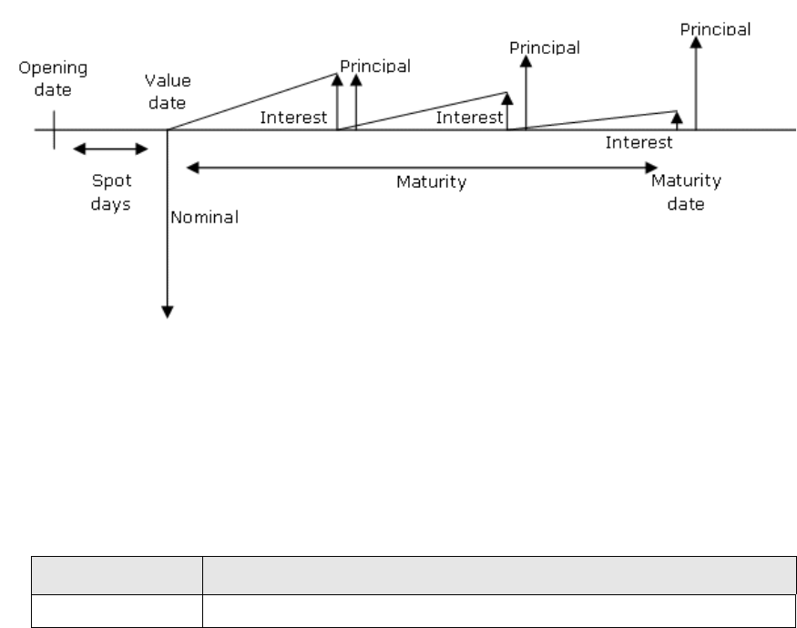
3 Debt instruments
3.10 Loan
Transaction & Risk Management Module (TRM) Instruments: Processing and Calculations 331
–Cashflows
For a fixed-annuity loan, the cashflows generated are as follows:
3.10.1.2.6 Fixed-rate loan - irregular annuity
With an irregular annuity, the flows are computed equally throughout the life of the loan except for
the final payment, which is adjusted according to how much of the loan remains outstanding.
•Input data
To define this kind of structure, the following information must be supplied at deal entry in the
Schedule view:
–Principal schedule
•Generated data
–The annuity is computed equally across all flows, except the last one.
–The remaining principal is repaid on the final cashflow (100 - rate).
3.10.1.2.7 Fixed-rate loan - margin
It is possible to specify a margin when entering a fixed rate loan. As well as the standard fixed-rate
loan input data and generated cashflows there are input data and generated cashflows for margins.
•Input data
For margin loans, you need to attach a secondary schedule Margin to the interest schedule and
specify the margin in the Spread schedule field (of the Margin schedule).
•Generated data
–Margin flows
A Margin cashflow is generated if a margin schedule is attached to the transaction and a
margin rate is entered (in the Spread field). The Margin cashflow is only used for calculating
Margin Profit. The Margin cashflow is calculated in the same way as the interest, using the
captured margin rate. This cashflow effectively represents the margin rates contribution in
the final interest amount.
Information Description
Interest Rate The fixed interest rate (for example, 5%).
3 Debt instruments
3.10 Loan
332 © Wall Street Systems IPH AB - Confidential
3.10.1.3 Processing
This section describes the actions that can be done throughout the life of a loan.
3.10.1.3.1 Early expiration
Loans can be matured earlier than their agreed maturity date. This process is referred to as early
expiration.
•Execution
Early expiration of loans requires the following information:
The execution generates an early expiration transaction with the following attributes:
Transaction sign = opposite of initial transaction
Nominal amount = amount to expire
Price = early expiration rate
Opening date = date when the early expiration is done
Value date = date when the early expiration is settled
Kind = Early Expiration
The remaining attributes are inherited from the initial transaction.
The early expiration transaction generates closing cashflows for the initial transaction and P/L
cashflows if there is a difference between the early expiration price and the original deal price.
Information Description
Opening Date Date when the early expiration is executed.
By default, this is today’s date unless a Fixing/Action Date was specified at transaction
level.
Value Date Date when the early expiration is settled. This must be earlier than the original
maturity date and later than the original value date of the initial transaction.
Settlement Date Date when early-expiration price is paid.
Amount to Expire Amount to be early expired. This defaults to the amount still available to be early
expired, taking into account previous partial early expirations and roll overs.
Price The premium or discount the early expiration is made at.
Settlement Price
Method
Clean Price: AI is created as Payable cashflow and P/L flow is the difference between
early-expiration price and original deal price.
Dirty Price: AI is created as Not Payable cashflow, and P/L flow is reduce by the AI
amount.
Accrued Interest The accrued interest that will be paid in the early expiration transaction. This value
can be modified.
Options •Amortize P/L
Switch on to amortize the P/L from the value date until the original maturity date.
If this switch is off, the Sell P/L flow created by the early expiration (arising from
Net Amount – Accrued Interest) occurs on the early expiration value date.
• No Fee Realization
Switch on to continue to amortize fees to maturity. For example, this can be used
in the case of an asset swap, which mirrors the issue fees, to keep the fees
amortizing even when the asset swap is fully unwound.
If this switch is off, at early expiration, the fees that were amortizing until the
maturity date are closed.
•Delay Interest (only available when the settlement price method is set to Clean Price)
Switch on to delay the accrued interest payment to the next interest payment
date.
3 Debt instruments
3.10 Loan
Transaction & Risk Management Module (TRM) Instruments: Processing and Calculations 333
•Cancellation
You can undo the early expiration by canceling the early expiration transaction.
3.10.1.3.2 Roll over
You can defer the maturity of a loan to a later date. This process is referred to as a roll-over.
See A.2.9 Allow Roll Over on page 716.
•Setup
It is possible to restrict the use of the roll-over methods at instrument level (see below for
methods description).
It is also possible to specify the default roll over method for the instrument.
•Execution
Roll-over of loans can be done in four different ways. In all cases, the following information is
needed to process the roll over:
The outcome of the roll-over depends on the method chosen as follows:
Information Description
Roll Over Date Date when the roll over is executed.
Maturity Date New maturity date for the loan. This must be later than the maturity date of the initial
transaction. The maturity date is calculated automatically from the maturity period of
the initial transaction.
Nominal Amount Amount of the roll over. This defaults to the amount left of the initial transaction but
you can override this if you want to perform a partial roll over.
Additional Amount Amount to be added to the initial principal amount if you want to increase capital at
roll over.
This field becomes available when one of the Allow Increase roll over methods has
been selected.
New Nominal
Amount
Original nominal amount plus interest (if interest is capitalized) plus the additional
amount.
This field becomes available when one of the Allow Increase roll over methods has
been selected.
Rate A new interest rate for the roll over, that is, the rate at which interest is calculated
from the old maturity date until the new maturity date.
By default, the rate displayed is taken from the interest schedule information, and is
used to generate the interest schedule of the new roll over transaction.
Roll Over Method Method used for the roll over.
Method Description
Settle All The initial transaction is paid in its entirety at the initial maturity date. The default
nominal amount of the roll over transaction equals the sum of the interest and
principal cashflows of the initial transaction.
Settle Interest The interest of the initial transaction is paid at the initial maturity date, but the
principal payment is deferred. The part of the principal which is rolled over is paid
back at the end of the roll over transaction.
Settle Interest,
Allow Increase
This method allows the user to provide additional capital (increase the principal) as
part of the roll over process.
The interest from the underlying loan is settled, and the original principal amount
(plus the additional capital) is rolled over.
3 Debt instruments
3.10 Loan
334 © Wall Street Systems IPH AB - Confidential
The execution generates a new transaction with the following attributes:
Nominal amount = amount (can be smaller than initial one)
Rate = roll-over rate
Opening date = date when the roll-over is done
Value date = maturity date of the initial transaction
Maturity date = maturity of the roll-over
Kind = Roll-over
•Cancellation
You can undo the roll over by canceling the roll over transaction.
3.10.1.3.3 Trade assignment
Trade assignments are changes of ownership of transactions.
•Execution
Change of ownership during the life of a transaction can be performed in two steps:
–Right-click the existing transaction and choose Assignment(sale) action. This action closes the
existing transaction, and when required, exchanges settlement amounts between the old
and new owners of the transaction.
–Right-click the generated transaction and choose Assignment (purchase) action. This action
creates the new transaction with the new owner.
Assignment (sale) of a transaction to another client requires the following information:
Capitalize
Interest, Allow
Increase
This method allows the user to provide additional capital (increase the principal) as
part of the roll over process.
The interest from the underlying loan is capitalized (that is, realized and added to the
initial nominal amount) and included with the additional capital in the roll over.
Delay Interest Nothing is paid at the initial maturity date: both the interest and principal payments
are deferred. The parts of the principal and interest cashflows which are rolled over
are paid back when the first interest payment of the roll over transaction occurs.
Compound
Interest
This method is the same as Delay Interest, but the closed interest of the initial
transaction is reinvested in the roll over. New interest accrues on top of the initial
transaction’s interest.
Information Description
Opening Date Date when the early expiration is executed.
By default, this is today’s date unless a Fixing/Action Date was specified at transaction
level.
Value Date Date when the early expiration is settled. This must be earlier than the original
maturity date and later than the original value date of the initial transaction.
Settlement Date Date when assignment price is paid.
Amount Left Read-only. Remaining amount of the initial transaction.
Assignee New owner of the transaction
Settlement Price
Method
Clean Price: AI is created as Payable cashflow and P/L flow is the difference between
assignment price and original deal price.
Dirty Price: AI is created as Not Payable cashflow, and P/L flow is reduce by the AI
amount.
Currency Read-only. Currency of loan.
Method Description
3 Debt instruments
3.10 Loan
Transaction & Risk Management Module (TRM) Instruments: Processing and Calculations 335
Execution generates an Assignment transaction with following cashflows:
–Cashflows to close the future cashflows of the original transactions (closing of cashflows
where payment date is after the assignment value date)
–Settlement flows between the assignor and the assignee, reflecting the settlement amounts.
The generated transaction has the following attributes:
The original transaction remains unchanged.
The assignee can then select the Assignment (purchase) action on the generated closing
transaction. Selecting the portfolio from the resulting dialog generates a new transaction,
reflecting the future cashflows of the original transaction and settlement flows between assignee
and assignor.
Note: The Counterparty field is open, to allow Counterparty change if required.
•Cancellation
You can undo the assignment action by canceling the generated assignment transaction.
3.10.1.3.4 Changing the counterparty of a transaction
You can terminate the existing transaction against one counterparty and reopen it against another
counterparty. The following information is required:
Settlement Price The price of the assignment.
Accrued Interest Read-only. Interest accrued on specified date.
Options • Amortize P/L
Switch on Amortize P/L to amortize the P/L from the value date until the original
maturity date. If this switch is off, the Sell P/L flow created by the assignment
(arising from Net Amount – Accrued Interest) occurs on the assignment value
date.
•No Fee Realization
Switch on No Fee Realization so that fees keep amortizing to maturity.
If this switch is off at assignment, the fees that were amortizing until the maturity
date are closed.
Information Description
Transaction Sign Opposite of the original transaction sign.
Nominal Amount Amount to assign.
Opening Date Opening date of action.
Value Date Value date of action.
Kind Assignment.
Information Description
Opening Date Date when the transfer is executed. By default, this is today’s date unless a
Fixing/Action Date was specified at transaction level.
Value Date Date when the transfer is settled. This must be earlier than the original maturity date
and later than the original value date of the initial transaction.
Counterparty New counterparty for the transaction.
Information Description

3 Debt instruments
3.10 Loan
336 © Wall Street Systems IPH AB - Confidential
A transaction will be generated whose Kind is Counterparty Conversion. The characteristics of the
new transaction will be the same than the old one, except for Counterparty and opening/value date.
This action generates closing cashflows for the future cashflows from the original transaction, and
futures cashflows between the original owner and the new counterparty.
No settlement/result flows will be affected to the generated transaction, as the assignment is
between the counterparties only.
The generated transaction can be canceled to undo the action.
3.10.1.3.5 Transferring transactions between portfolios
You can transfer the transaction from one portfolio to another. This is effectively a sale in one
portfolio and a purchase in another. Portfolio transfer of an existing transaction can be performed at
transaction level by right-clicking and choosing Transfer. Transfer of a transaction to another
portfolio requires the following information:
Two Transfer transactions are generated:
1. A sale is created in the source portfolio of the transfer, i.e. closing cashflows of the original
transaction and settlement flows (real or pseudo, depending on inputs).
2. A purchase is then created in the receiving portfolio, with future flows and settlement flows (real
or pseudo, depending on inputs).
The original transaction remains unchanged. The user can undo the portfolio transfer action by
canceling the generated transactions.
3.10.1.3.6 Transaction Conversion
To allow schedule conversion at predefined dates during transaction's life.
•Setup
This process is available on the transaction if the Transaction Conversion feature is associated
with the instrument.
See A.2.325 Transaction Conversion on page 873.
Information Description
Opening Date Date when the transfer is executed. By default, this is today’s date unless a
Fixing/Action Date was specified at transaction level.
Value Date Date when the transfer is settled. This must be earlier than the original maturity date
and later than the original value date of the initial transaction.
Settlement Date Payment date for settlement flows.
New Portfolio New portfolio for the transaction
No Settlement
switch
If On, the generated settlement amount is marked as pseudo (i.e. not bookable, not
payable).
Settlement Price
Method
Clean Price: AI is created as Payable cashflow and P/L flow is the difference between
transfer price and original deal price.
Dirty Price: AI is created as Not Payable cashflow, and P/L flow is reduce by the AI
amount.
Currency Read-only. Currency of loan.
Settlement Price The price of the assignment.
Accrued Interest Read-only. Interest accrued on specified date.
Options • Amortize P/L
•No Fee Realization
3 Debt instruments
3.10 Loan
Transaction & Risk Management Module (TRM) Instruments: Processing and Calculations 337
Then, the user is allowed to attach the Conversion schedule to the existing schedule and to
define conversion events and converted schedules.
•Execution
When conversion schedules are defined, the user is allowed to execute generated conversion
events. The conversion inputs are displayed.
See A.2.325 Transaction Conversion on page 873.
The execution generates a conversion transaction with the following attributes:
–Kind: Conversion
–Opening Date: Conversion opening date
–Value Date: Conversion value date.
The conversion transaction generates closing cashflows for the initial transaction.
If the conversion price is different to the original deal price, then a P/L flow is generated,
showing the differences between the conversion price and the original deal price.
3.10.1.4 Position monitoring
3.10.1.4.1 Setup
The cashflow discounting method (periodic, continuously compounded) used in IR risk calculation
depends on the instrument set up.
By default, TRM uses the valuation curve interpolation settings (IR Quote and Yield Curve Editor -
Interpolation page). For example, if the interpolation settings are set up with Interest Type Continuous
Yield, then risk calculations use continuously compounding discounting of the cashflows.
If IR Exposure is set up at the instrument level, then TRM uses these settings. For example, if IR
exposure is set up with Yield Type Periodic, then risk calculations use periodic discounting of the
cashflows.
For more information about risk calculations, see 2.3 Key-figures on page 112.
3.10.2 Floating-rate loan
Interest cashflows for a floating-rate loan are linked to a market reference. The market reference
has to be observed for each interest period. The fixing of the interest rate can be done before
interest starts accruing (classical in-advance fixing), or at the end of the period (in-arrears fixing).
3.10.2.1 Instrument setup
Floating-rate loans are set up in a similar way to fixed-rate loans, but refer to a different type of
cashflow structure: the structure you choose needs to generate floating interest cashflows.
You can pre-define the cashflow structure in the main characteristics of the loan, or restrict the
available schedule templates at deal entry using the Schedule Groups option.
See A.2.293 Schedule Template Setup on page 859.
3.10.2.2 Deal capture
Depending on the selected cashflow structure, the information needed to deal the instrument and
the generated cashflows are very different.
The transaction level information is always the same.

3 Debt instruments
3.10 Loan
338 © Wall Street Systems IPH AB - Confidential
3.10.2.2.1 Input data
In addition to the standard deal parameters, the following information is required to enter a deal on
a floating-rate loan:
3.10.2.2.2 Generated data
•Book Value (clean price):
BV = A * p /100
where:
A = Nominal Amount
p = deal price
•Book Value (dirty price):
BV = (A * p /100) - AI
where:
A = Nominal Amount
p = deal price
AI = Accrued Interest
These values alone are not sufficient to define the deal. To complete the creation of a
floating-rate loan, the cashflow structure of the deal also needs to be specified, either in the
instrument setup, or at deal entry.
See Appendix B Schedules on page 883.
3.10.2.2.3 Bullet repayment structure
For a floating-rate loan, a template which contains at least one schedule for floating-rate interest
cashflows and one schedule for repayment flows is required.
•Input data
For each set of cashflows, the following information must be supplied:
–Interest flows
Information Description
Currency Currency of the transaction.
If you specified the currency in the instrument setup, this is used as the default
currency in the transaction and cannot be modified.
Maturity Date Date for the maturity of the contract.
If you use maturity date setup the date is calculated automatically from the selected
maturity period, otherwise you can enter the date manually.
Nominal Amount Amount of the loan. This is equal to the principal (the amount on which the interest is
calculated).
Deal Price Deal price of the transaction (expressed as a percentage of the nominal amount) used
to calculate the book value and the settlement amount.
Information Description
Frequency Method
and Period
The frequency method/period for the interest cashflows (for example, Years/1
generates one interest flow per year).
Interest Rate The first rate of interest (for example, 5%), if known.

3 Debt instruments
3.10 Loan
Transaction & Risk Management Module (TRM) Instruments: Processing and Calculations 339
–Repayment flows
Some other parameters in the schedule can be adjusted to modify the way the cashflows are
generated.
See Appendix B Schedules on page 883.
•Generated data
–Schedule
When a template is selected, one schedule is created for each item in the template. Some of
the values are automatically defaulted from the transaction parameters (see Appendix B
Schedules on page 883), while others can be modified at deal entry (see above).
–Cashflows
For a floating-rate loan with repayment at maturity, the cashflows generated are as follows:
3.10.2.3 Processing
Floating-rate loans are processed in a similar way to fixed-rate loans, but with the following
additional process.
3.10.2.3.1 Interest fixing
For a floating-rate loan, the amount of each interest flow has to be determined before it is paid: this
process is known as fixing.
•Execution
Fixing parameters Formulae used to evaluate the rate.
This is known as an "expression" in TRM. Typical expressions would be, for
example, "ir", referring to an ir rate market reference (yield curve) or "ir +
spread%". See Appendix D Expressions on page 917.
Yield curve to be used in the expression.
Period (for example, 3M or 6M) and the scenario used to get the rates when
fixing the cashflows.
Define if the fixing will be done in-advance or in-arrears and enter the offset in
days.
Information Description
Information Description
Frequency Method
and Period
The frequency method/period for the repayment cashflow (for example, Bullet
means that the loan will be entirely repaid at maturity). It is also possible to
define amortizable or accreting principal cashflows.
3 Debt instruments
3.10 Loan
340 © Wall Street Systems IPH AB - Confidential
Each interest cashflow of a floating-rate deal contains some parameters that define how its
amount is fixed.
–The fixing period determined by a from/to date value pair indicates when the amount of the
flow has to be fixed; it can be before the interest starts accruing (in-advance fixing), or
before the payment of the interest (in-arrears fixing).
–The fixing parameters (expression, rate, spread, and so on) that define how the fixing rate is
calculated.
–An "expression value" which is informative and gives the current value of the expression.
Executing the fixing modifies the cashflow as follows:
Marks it as being fixed
Sets the fixing date
Stores the rate of the market reference used for fixing
Stores the effective interest rate (nominal rate) on the cashflow
Sets the amount of the cashflow
The fixing process can be performed in four ways in TRM: the process which is triggered is
exactly the same in the four cases, the only difference being the quantity of deals or cashflows
which are affected. The four ways of fixing are as follows:
–Directly on the deal: the fixing only affects the deal
–Directly on an individual cashflow in the Cashflow view: the fixing affects an individual
cashflow
–On the instrument (in Instrument Editor): the fixing affects all the deals on this instrument
–Using an automated activity (Fixing Transaction Cashflow): potentially all deals which have
to be fixed for a particular date may be affected.
See the TRM User Guide for general information on running activities, and also specific
information on the activity parameters.
If the Fixing action is carried out directly on an individual cashflow using the second method, it is
possible to modify the fixing values. When the fixing quote is modified, this updates both the
nominal rate and the amount accordingly. Similarly, if the nominal rate is modified, the amount
is affected (but not the fixing quote). It is also possible to modify the amount independently
from the other fixing values. This may be necessary when rounding differences arise, for
example.
•Cancellation
It is possible to cancel the fixing either manually, using the Undo Fixing action; or automatically,
using the Fixing Transaction Cashflow - Undo activity.
See the TRM User Guide for general information on running activities, and also specific
information on the activity parameters.
3.10.3 Other loan structures
All the cashflow structures available for bonds are also available for loans (see 3.1 Bond on page
215). You can also find information about all system-defined cashflow structures available in TRM in
Appendix B Schedules on page 883.
Some of the structures that can be generated for a loan are described in this section.
3.10.3.1 Dual currency structure
•Regular dual-currency:
The currency in which the instrument is issued (principal currency) differs from the currency in
which the principal is repaid (redemption currency). The currency of the interest flow can be
either the principal currency or the redemption currency.
The FX rate to apply can be known (determined on the date of issue) or fixed later (determined
a number of days before the payment date of the interest cashflow).
3 Debt instruments
3.10 Loan
Transaction & Risk Management Module (TRM) Instruments: Processing and Calculations 341
•Reverse dual-currency:
The principal currency and redemption currency are identical, but interest payments are in a
different currency.
The FX rate used for the calculation of interest is either known when the loan is agreed or fixed
later.
3.10.3.1.1 Instrument setup
Instrument setup for a dual-currency loan is similar to that of a standard loan (see 3.10 Loan on
page 326), except for the following:
•Loan main characteristics
•Dual-currency attributes
This information defines the characteristics of the principal cashflow. Leave these fields blank if
you want to specify the details when you enter the deal.
See A.2.125 Dual Currency on page 771.
•FX fixing
If the settlement FX rate is unknown when the deal is entered, then this feature needs to be
included in the instrument definition.
See A.2.174 FX Fixing on page 797.
3.10.3.1.2 Deal capture
•Input data
Deals on dual-currency loans are captured in a similar way to those on a standard loan. To
complete the creation of a dual-currency loan transaction, the cashflow structure of the deal also
needs to be specified, either in the instrument setup, or at deal entry, by applying a schedule
template.
The following system templates are provided for dual-currency structures:
Information Description
AI Method The method used by the system to compute settlement accrued interests. For
dual-currency loans, there are two types of dual-currency methods:
• Dual Currency Estimated
• Dual Currency Last.
See 2.1.6.1 Accrued interest calculations on page 67 for more information.
Information Description
Settlement
Currency
Currency in which the principal cashflow is settled.
Settlement FX
Rate
Rate used to calculate the settlement amount of the principal cashflow.
Need Fixing Specify whether the FX rate needs to be fixed:
• Select No when the FX rate is known
• Select Yes, FX Rate when the FX rate is unknown.
The old value "Yes, Unmarked" is not used.
Fixing Offset Number of days’ offset allowed, that is, the difference in days between the fixing date
and the due date (default = 0).
Fixing Max. Offset Maximum number of days’ offset allowed.

3 Debt instruments
3.10 Loan
342 © Wall Street Systems IPH AB - Confidential
–Dual-Currency Known FX
This is a fixed bullet structure used for dual currency instruments when the FX rate is known
when the deal is entered.
For both interest and redemption schedules you can choose a different settlement currency
and specify the settlement FX rate.
See B.2.1.1.15 Dual Currency, Known FX Rate on page 893.
–Dual-Currency Known FX Floating
This is a floating bullet structure used for dual currency instruments when the FX rate is
known when the deal is entered.
For both interest and redemption schedules you can choose a different settlement currency
and specify the settlement FX rate.
See B.2.1.1.16 Dual Currency, Known FX Rate, Floating on page 893.
–Dual-Currency Unknown FX
This is a fixed bullet structure used for dual currency instruments when the settlement FX
rate is not known beforehand.
For both interest and principal schedules you can choose a different settlement currency.
See B.2.1.1.17 Dual Currency, Unknown FX Rate on page 893.
Note that this template covers fixed interest rates only. For floating rates, you also have to
use the Fixing Dates secondary template (see B.2.1.2.15 Fixing Dates on page 903).
You can choose one of these templates or any other template derived from them. Once the
template is applied to the transaction, the schedules are created and it is then possible to define
the settlement currency characteristics, as well as other characteristics such as, date basis,
payment convention, calendars, and so on.
See Appendix B Schedules on page 883.
•Generated data
–Cashflows
Settlement Currency = Settlement Currency (as defined in the schedule)
Settlement FX Rate = Settlement FX Rate (as defined in the schedule)
Settlement Amount = Amount * Settlement FX Rate
3.10.3.1.3 Processing
•Early expiration
The early expiration of a dual currency loan is similar to that of a standard loan, except that you
can set the Settlement FX Rate and view the settlement amount. See 3.10.1.3 Processing on
page 332.
–Execution
You perform the Early Expiration action in the Transaction Manager’s Transaction view on the
transaction that you want to early expire. You can enter the following information:
Information Description
Settlement Currency (Read-only) Currency to use for settlement.
Settlement FX Rate Rate used to calculate the settlement amount of the principal cashflow.
Settlement Accrued
Interest
Final amount to be settled.

3 Debt instruments
3.10 Loan
Transaction & Risk Management Module (TRM) Instruments: Processing and Calculations 343
•FX fixing
When the settlement FX rate of a dual-currency loan is not known beforehand, the FX rates need
to be fixed at the agreed fixing date.
–Setup
Depending on the instrument setup, the fixing can be done in advance or in arrears. In both
cases there can be an offset of n days (before the beginning or end of the interest period).
–Execution
The FX Fixing action performed in Transaction Manager’s Cashflow view on the cashflow
allows you to set the FX rate. The following values can be input:
The fixing process is performed directly on an individual cashflow in the Cashflow view. It is
possible to modify the fixing values.
–Cancellation
It is possible to undo the FX fixing using the Undo FX Fixing action.
3.10.3.1.4 Position monitoring
For information about dual currency calculations, see 2.3.5 Dual currency on page 147.
3.10.3.2 Rainbow coupon structure
In these structures there is an option on each interest payment to choose the payment in a different
currency (a maximum of three currencies can be defined in TRM).
3.10.3.3 Callable structure
These structures are used to create callable/puttable loans. Call/Put can be simply optional or
triggered by a market event. It is also possible to have a Call/Put with barriers (in or out).
3.10.3.4 Currency transaction option
Options for repayment to occur in a different currency: this option can be simple, triggered or linked
with a barrier. This option can be applied to a principal repayment or a call option
3.10.3.5 Transaction conversion option
Deals with an embedded option to move to a different cashflow structure, for example, an option to
move from a fixed to a floating rate, or from an annual to a zero coupon structure. These
transaction conversions can also be linked to barriers or triggers.
Information Description
Fixing Date Day the cashflow is fixed.
Reference FX Rate Fixing market quote.
This is defaulted by the system to the FX cross rate between the actual
currency and the currency on the fixing date and can be changed by the user.
3 Debt instruments
3.10 Loan
344 © Wall Street Systems IPH AB - Confidential

Transaction & Risk Management Module (TRM) Instruments: Processing and Calculations 345
Chapter 4 Equities
In TRM, the term equity is used to cover the following instruments:
•Common stock
Common stock is security that represents ownership in a company that has issued stock. The
stockholder has a right to receive dividends and the right to vote in the shareholders’ meeting.
•Preferred stock
Preferred stock is security that represents ownership in a company that has issued stock.
Preferred stock typically has better rights to dividends than common stock, but less voting rights
(or even none at all).
•Subscription rights
A subscription right gives the holder the right to buy the underlying security at a predetermined
price. Typically, the rights have a short lifetime: they are detached from stock at a specific date
and expire worthless if they are not used to purchase the underlying stock.
•Mutual fund shares
A mutual fund share represents one unit of ownership in the assets of a mutual fund.
4.1 Equity
Equity instruments must be based on an instrument type derived from the class EQUITY.
4.1.1 Instrument setup
•Equity main characteristics
The following basic information may be captured when defining the instrument. This information
is relevant to any kind of equity instrument.
See A.2.127 Equity on page 772.
•Equity information
The outstanding number of shares and voting rights for the equity may change over time. It is
possible to define this information at instrument level.
See A.2.132 Equity Info on page 776.
Information Description
Issuer and
Guarantor
parameters
Issuer and guarantor information for the equity instrument.
Currency Currency in which the equity is traded.
Rounding
parameters
Method and precision used to round cashflow amounts.
4 Equities
4.1 Equity
346 © Wall Street Systems IPH AB - Confidential
•Quotation
You can specify quotation information for the equity at instrument level.
See A.2.274 Quoted on page 849.
•Trading unit
Equities can be traded in multiples of a minimum bid size. It is possible to define this information
in the instrument setup.
See A.2.321 Trading Unit (Equity) on page 871.
For an equity instrument, it is also possible to set up:
•Spot date calculation
•Value date calculation
•Delivery (custodian) information
•Cashflow and transaction charge rules
•Manual charges
•Branch codes.
See Appendix A Features on page 713.
4.1.2 Deal capture
4.1.2.1 Input data
In addition to the standard deal parameters, the following information is required to enter a
transaction with an equity instrument:
In addition, the following optional information can be captured:
Information Description
Value Date Official date when money is transferred. This defaults to the spot date as defined for
the instrument.
Trading Units Number of units bought or sold.
The Equity Trading Unit feature is used to define the minimum bid size of shares or
fund shares.
See A.2.321 Trading Unit (Equity) on page 871.
Deal Price Price of one unit.
Information Description
Value Date Code If the Value Date Setup feature is applied at instrument level, you can enter the value
date period you want to use to calculate the value date for the transaction, for
example, 3M (3 months).
This can be used to compute the value date for a forward purchase of equity.
Note: If you specify a value date period in the instrument setup, this is used as the
default in the transaction and cannot be modified: see A.2.339 Value Date
Setup on page 879.
4 Equities
4.1 Equity
Transaction & Risk Management Module (TRM) Instruments: Processing and Calculations 347
4.1.2.2 Generated data
•Cashflows
For an equity instrument, the cashflows generated are as follows:
4.1.3 Processing
When managing an equity portfolio, there are various corporate actions that need to be processed.
The processing in TRM of the most commonly used corporate actions is described in this section.
4.1.3.1 Cash dividend
In most cases, the holders of common stock, preferred stock, or mutual fund shares receive regular
cash dividends up to four times each year. In addition, they may receive special dividends.
•Setup
When the information about the cash dividend is declared by the issuer of the security, the
instrument definition needs to be updated with the dividend information.
See A.2.128 Equity Cash Dividend on page 773.
•Execution
On the ex-dividend date, the equity is quoted without the dividend and the market price drops
approximately by the amount of the dividend. The exact amount of the dividend is known at the
end of the previous business day. It is calculated from the position at the close of business prior
to the ex-dividend date. The activity Dividend that creates the dividend transaction(s) needs to
be performed at the beginning of the ex-dividend date (or at the end of the previous day).
The following information is needed to process the cash dividend:
Note: See the TRM User Guide for information about this activity and how to set up activities in
general.
The execution creates the dividend transaction, which has an incoming cashflow on the dividend
payment date. From the ex-dividend date onwards, the market value of this transaction is
calculated separately from the equity position.
The execution processes each portfolio (and owner) separately: a dividend transaction is created
in each portfolio (and for each owner) where there is a position on the relevant equity on the day
preceding the ex-dividend date.
Opening
date
Spot
days
Position
cashflow
Delivery
cashflow
Settlement
amount
Value
date
Information Description
Portfolio The dividend is calculated for this portfolio and all of its subportfolios.
Minimum
Transaction State
The minimum transaction state that is taken into account when the position is
determined for the dividend calculation.
4 Equities
4.1 Equity
348 © Wall Street Systems IPH AB - Confidential
•Cancellation
In case the dividend transactions are incorrect it is possible to cancel them manually and rerun
the dividend activity.
4.1.3.2 Split and reverse split
When an equity instrument is split, the number of outstanding shares increases: each share is split
into a certain number of shares.
For example:
Before the split:
Buy 5,000 units of equity
where the price of each unit = 10 EUR (total book value = 50,000 EUR)
split 1 unit into 5 shares
After the split:
The position is 25,000 units of equity
where the price of each unit = 2 EUR (total book value = 50,000 EUR)
In a reverse split, the number of outstanding shares decreases with a certain ratio.
For example:
Before the split:
Buy 5,000 units of equity
where the price of each unit = 10 EUR (total book value = 50,000 EUR)
split 5 units into 1 share
After the split:
The position is 1,000 units of equity
where the price of each unit = 50 EUR (total book value = 50,000 EUR)
•Setup
The data used to split an equity position is defined in the instrument setup. The following
information is required to process the split:
See A.2.138 Equity Split on page 779.
•Execution
If there are no Odd Lots or, if you do not want to create an Odd Lot adjustment transaction, you
can perform the split or reverse split simply by defining the split information using the Equity
Split feature in the instrument setup (see above).
Otherwise, if any Odd Lots do result from the split or reverse split (and you do want to create
the corresponding adjustment transactions), the Split activity must be used.
Note: See the TRM User Guide for general information on running activities, and also specific
information on the activity parameters.
Information Description
Date Date on which the split was declared or the information was entered in the instrument
setup.
Split parameters Date of the split, the split ratio, and the action required if an Odd Lot results from the
split.

4 Equities
4.1 Equity
Transaction & Risk Management Module (TRM) Instruments: Processing and Calculations 349
Each portfolio is processed separately. Based on the existing position, a new position is created
using the following rules:
Old units = Number of units in the position at the moment of the split (that
is, at the end of the day before the split date)
New units = Old units * From/To Units, rounded using the rounding parameters
specified in the feature
Odd lot = Old units – Used units
Factor = Used units / Old units
If there is an Odd Lot, a Sell transaction is created to sell the Odd Lot for the specified
compensation price (as defined in the instrument definition):
Odd lot compensation = Odd lot compensation price * Odd lot
The existing position is adjusted so that the Odd Lot compensation amount (the resulting
number of units) is now considered as new units. The book value is adjusted by the factor.
If the factor = 1, there is no Odd Lot compensation and the book value is not adjusted.
•Cancellation
If you need to cancel or correct the split or reverse split:
–Correct the Equity Split parameters defined in the instrument setup
–Cancel the incorrect Odd Lot transactions, if any
–Rerun the Split activity, if you wish to create Odd Lot adjustment transactions.
4.1.3.3 Detachment
Detachment is a corporate action that takes place typically when a shareholder receives subscription
rights in place of equity. The number of subscription rights received by the shareholder is
proportional to the number of equity units held.
If subscription rights are detached from an equity, it is also possible to transfer part of the book
value from the equity to the subscription right (when the value of the equity and the value of the
right are specified).
For example:
Before the detachment:
Buy 5,000 units of equity
where the price of each unit = 10 EUR (total book value = 50,000 EUR)
Detachment of subscription rights: 1 right per 5 shares
Market price for 1 share = 8 EUR
Market price for subscription right = 2 EUR
After the detachment:
The book value that is transferred for the original position to the new one:
50,000 EUR * (1/5) * (2/8) = 2,500 EUR
Receipt of subscription rights incurs a cost (1 EUR), therefore the following
position cashflow is added to the generated detachment transaction:
New units * Price per unit = 5,000 * (1/5) * 1 = 1,000
Note: At a later date, subscription rights can also be used to buy equity (either the same as the
original equity or different equity) at a certain price (see 4.1.3.4 Conversion on page 351).
4 Equities
4.1 Equity
350 © Wall Street Systems IPH AB - Confidential
•Setup
When the information about the detachment is known, the instrument definition needs to be
updated.
See A.2.130 Equity Detachment on page 774.
•Execution
The Detachment activity is used to calculate what the shareholder gets per share held.
Note: See the TRM User Guide for general information on running activities, and also specific
information on the Detachment activity parameters.
Each portfolio is processed separately. Based on the existing position, a new position is created
using the following rules:
Old units = Number of units in the position at the moment of detachment
(in general, this is the position at the end of the previous day)
If, for example, there is a split on the same day as the detachment, you must define whether the
detachment is processed before or after the split.
New units = Units to receive * Round(Old units / Units to sell)
rounded using the rounding parameters specified for the detachment at
instrument level
Odd units are computed as follows:
Odd lot = Old units – Units to sell * Truncate(Old units / Units to sell)
Odd lot compensation = Odd lot compensation price * Odd lot
If there is an odd lot, the compensation amount is added as a profit/loss cashflow to the
detachment transaction.
Price to pay = Price to pay per unit * New units
The price to pay is added as settlement principal to the detachment transaction.
When subscription rights are detached from an equity, it is possible to determine the book value
amount that is transferred from the equity to the subscription right, using the following
calculation:
Book value amount * (Units to receive * Value of right)/(Units to sell * Value
of equity)
•Cancellation
You can cancel the detachment action by cancelling the detachment transactions and also the
generated cashflows in the original transaction.
Information Description
Date Date on which the detachment was declared or the information was entered in the
instrument setup.
Detachment
parameters
Date of the detachment and the action required if an Odd Lot results from the
detachment.
Value of the Right
Value of the
Equity
Values required to determine how much of the book value is transferred from the
original equity to the new one.
4 Equities
4.1 Equity
Transaction & Risk Management Module (TRM) Instruments: Processing and Calculations 351
4.1.3.4 Conversion
Subscription rights can be used to purchase new shares (either the same as the original equity or
different equity) at a certain price. This corporate action is known as Conversion. Conversion can be
used, for example, in a merger where shares held in one company are converted to shares in
another company.
•Setup
When the information about the conversion is known, the instrument definition needs to be
updated.
See A.2.129 Equity Conversion on page 773.
•Execution
The Conversion activity is used to convert shares or subscription rights into new equity. The
following information is needed to run the activity:
Note: See the TRM User Guide for information about how to set up activities in general.
Each portfolio is processed separately. Based on the existing position, a new position is created
using the following rules:
Old units = Number of units in the position at the moment of conversion
New units = Units to receive * Round(Old units / Units to sell), rounded using
the rounding parameters specified for the detachment at instrument level
The new position is created with the correct number of units with regard to the rounding
conventions.
Price to pay = Price to pay per unit * New units
This amount is added as settlement principal to the conversion transaction.
Factor = Units to sell * Truncate(Old units / Units to sell) / Old units
This factor determines the part of the book value that is moved from the old position to the new
converted position.
The old position is closed completely if there is no odd lot (that is, a sell transaction is generated
with the whole number of units).
The position is closed partially in the case of an odd lot. The odd lot is sold at the compensation
price. The odd lot sell transaction has the following characteristics:
Odd lot units = Old units - Units to sell * Truncate(Old units / Units to sell)
Book value = Odd lot compensation = Odd lot selling price * Odd lot units
Information Description
Date Date on which the conversion was declared or the information was entered in the
instrument setup.
Conversion
parameters
Date of the conversion, the conversion ratio, and the action required if an Odd Lot
results from the conversion.
Information Description
Portfolio Conversion is processed for this portfolio and all of its subportfolios.
Minimum
Transaction State
Minimum transaction state that is taken into account when the position is determined
for the conversion.

4 Equities
4.1 Equity
352 © Wall Street Systems IPH AB - Confidential
•Cancellation
You can cancel the conversion by cancelling the conversion transactions.
4.1.3.5 Return of capital
Return of Capital occurs when the company pays back part of the capital to the shareholders. This
corporate action differs from a cash dividend (see 4.1.3.1 Cash dividend on page 347), because the
book value of the shares is decreased by the amount of the capital returned.
•Setup
When the information about the return of capital is known, the instrument definition needs to be
updated.
See A.2.137 Equity Return of Capital on page 778.
•Execution
The Return of Capital activity is used to pay back the capital to the shareholders.
Running this activity decreases the book value by the amount of capital returned (the number of
units multiplied by capital per unit). The returned capital is shown as a principal cashflow.
Note: See the TRM User Guide for general information on running activities, and also specific
information on the activity parameters.
•Cancellation
You can cancel the return of capital action by cancelling the return of capital transactions and
also the generated cashflows in the original transaction.
4.1.4 Position monitoring
In this section, numerical examples demonstrate how the different figures are calculated for an
equity instrument.
If you need more theoretical information about the method used in these calculations, see Chapter 2
Market standards and calculations on page 33.
This example shows a share, with the following deal data:
•Setup
•Transaction
Information Description
Date Date on which the return of capital was declared or the information was entered in the
instrument setup.
Return of capital
parameters
Date of the return of capital, and information required to determine the capital to be
returned.
Data Symbol Example
Valuation Method Quoted, to Spot
FX Exposure Offset h_fx 0.01
Data Symbol Example
Opening Date 2004-02-02
Trading Units n_m 10,000

4 Equities
4.1 Equity
Transaction & Risk Management Module (TRM) Instruments: Processing and Calculations 353
Other important deal data is calculated by the system as follows:
Unless otherwise stated, the figure date used in the calculations is 2004-03-01. On this date, the
market data is as follows:
•Market data on 2004-03-01
•Valuation figures
The valuation method commonly used for an equity instrument is the Par method.
Note that if the instrument is not defined as being valued To Spot, Market Value will be discounted
from spot to the figure date. However, Clean Market Value will not; therefore, the Clean Market
Value figure may be different from the Market Value figure.
•Result figures
The setup of the instrument impacts the way result figures are computed.
Deal Price P_b 3.00
Base Book FX Rate (EUR/USD) S_b 1.2
Value Date d_a 2004-02-04
Currency USD
Portfolio Currency EUR
Data Symbol Example
Data Symbol Example Formula
Book Value (Local) V_b 30,000.00 = 10,000 * 3.00 = n_m * P_b
Book Value V_p 25,000.00 = 30,000.00 / 1.2 = V_b / S_b
Data Symbol Example
Figure date d_f 2004-03-01
Market Price P_f 3.20
FX Conversion Rate S 1.260000
Data Symbol Example Formula
Local Market Value V_l 32,000.00 = 10,000 * 3.20 = n_m * P_f
Market Value V 25,396.93 = 32,000.00 / 1.2600 = V_l / S
Clean Market Value V_clean 32,000 = 10,000 * 3.20 / 1.2600 = n_m * P_f / S
Data Symbol Example Formula
Total Profit (Local) P_tl 2,000.00 = 32,000.00 – 30,000.00 = V_l – V_b
MtoM Profit (Local) P_ml 2,000.00 = 32,000.00 – 30,000.00 = V_l – V_b
FX Profit P_fx -1,190.48 = 30,000.00*(1/1.260000 – 1/1.20000) = V_b*(1/S - 1/S_b)
Total Profit P_t 396.83 = 25,396.83 – 25,000.00 = V – V_p
MtoM Profit P_m 1,587.30 = 2,000.00 / 1.260000 = P_ml / S

4 Equities
4.1 Equity
354 © Wall Street Systems IPH AB - Confidential
•Risk figures
Data Symbol Example Formula
FX Exposure E_fx 253.97 = 0.01 * 25,396.83 = h_fx * V
Transaction & Risk Management Module (TRM) Instruments: Processing and Calculations 355
Chapter 5 Security lending
5.1 Repurchase agreement
In a repurchase agreement (repo), one party sells a security to another party with the agreement to
repurchase the same security at a fixed future date and at an agreed price.
In essence, the seller of the security is borrowing the amount received from the sale and placing the
sold securities with the purchaser as collateral.
The difference between the sale price of the security and the cost of repurchase is, in effect, interest
charged to the borrower. The period of time between the sale and the repurchase is called the repo
period.
Physical transfer of the security from the custody of the borrower to the custody of the lender
usually takes place, but in the case of overnight repos, for example, there may be no transfer. If the
security does not physically change hands, the buyer of the security is exposed to a higher credit
risk.
Underlying a repo transaction is usually a fixed-rate government bond or discount paper. Collateral
delivered against the cash in a repo transaction can be in a single (single-collateral repo) or in
multiple (multi-collateral repo) underlying instruments. These collateral instruments must be
defined with the feature Collateral in order to be available as collateral, see 5.1.4 Collateral on page
365. TRM also allows you to use cash as collateral. To do so, you must define cash collateral account
instruments, see 5.1.7 Cash Collateral on page 376. You can use both collateral instruments and
cash collateral instruments for margin movement transactions.
Margin movements are required when the exposure exceeds the threshold defined in the collateral
agreement (Margin page). You must set up specific margin movement instruments to handle this
type of situation, see 5.1.6 Margin movement on page 370.
In some situations, you may need to substitute a collateral instrument for another during the
lifetime of a repo transaction. You must set up specific substitution instruments for this event, see
5.1.5 Substitution on page 366. To enable substitution, you need to set up the conditions for
substitution in the collateral agreement (Substitution page). See TRM User Guide for more
information about collateral agreements.
Repos are driven either by the need to lend or borrow cash, or the need to borrow a specific
security.
5.1.1 Repo (classic)
The following information is relevant to any kind of repo. If you want to setup a Buy/sell back repo
see 5.1.2 Buy/sell back and sell/buy back on page 362.
5.1.1.1 Instrument setup
Repo instruments must be based on an instrument type derived from the class REPO.
•Repo main characteristics

5 Security lending
5.1 Repurchase agreement
356 © Wall Street Systems IPH AB - Confidential
This information may be relevant to any kind of repo instrument.
See A.2.283 Repurchase Agreement on page 854.
•Maturity definition
Information Description
Currency Currency of the repo deal.
Leave this field blank if you want to specify the currency of the repo
transaction when you enter the deal.
Transaction Sign Sign to be applied to the transaction: Reverse Repo (Buy/Lend) or Repo
(Sell/Borrow).
• Select either Repo or Reverse Repo if you want this to be the default
direction of the transaction, that is, the direction cannot be modified at
deal entry.
• Leave this field blank if you want to specify the direction of the repo deal at
deal entry.
Interest Type Type of interest rate used to calculate the repo interest amount, for example,
Periodic Rate.
Date Basis Date basis used to calculate the interest of the repo.
If this is not defined at instrument level, the date basis of the currency is used
unless you provide another date basis at deal entry.
Amount Rounding
parameters
Method used to round cashflow amounts of the repo.
Principal Cashflow Type Type of repayment cashflow (for example, Principal or Expiration).
Interest Cashflow Type Type of interest cashflows.
Collateral Calculation
Method
Calculation method defaulted to transaction column Collateral Calculation
Method of new transactions in repo instrument and applied when collateral
amount of a collateral entry in a repo transaction is manually updated.
•Single: Select Single, if you want the system to keep settlement amount of
the collateral and recalculate collateral market price to match the new
collateral amount, This method can only be used in single collateral repo
transaction.
•Multiple: Select Multiple, if you want the system to keep the collateral
market price of the collateral and recalculate settlement amount to match
the new collateral amount. This method allows you to enter multiple
collateral to a repo transaction.
Note: The Collateral Calculation Method always defaults to Multiple in
substitution and open margin transactions, but can be manually set to
Single.
Switches •Use Dirty Price: Switch on to define that the Collateral Price/Maturity
Collateral Price should be expressed as the dirty price. This information is
displayed at transaction level as Dirty Collateral Price.
•Use Collateral Price Rounding: Switch on to define that Collateral Price and
Maturity Collateral Price are rounded using the rounding parameters of the
underlying collateral instrument. If this switch is not on, collateral prices
are always calculated exactly. If the feature Repo Rounding is used, the
rounding parameters are taken from the rounding setup of the collateral
instrument (see A.2.280 Repo Rounding on page 854). Otherwise, the
rounding parameters are taken from Trading Yield setup of the collateral
instrument (see A.2.323 Trading Yield on page 872).
5 Security lending
5.1 Repurchase agreement
Transaction & Risk Management Module (TRM) Instruments: Processing and Calculations 357
It is possible to set up maturity information at instrument level.
See A.2.230 Maturity Date Setup on page 827.
•Collateral agreement definition
It is possible to set up collateral agreement to be used in transactions at instrument level.
See A.2.95 Collateral Setup on page 756.
•Collateral Quote defaulting
If feature Quote Default (Collateral) is selected for a repo instrument, the current market price
or yield is automatically defaulted according to the setup of the feature to fields collateral market
price or collateral market rate of a new collateral entry in a repo transaction as soon as a new
collateral instrument has been selected.
See A.2.270 Quote Default (Collateral) on page 847.
•Repo Cash Delivery definition
This feature sets all non-delivery cashflows of a repo transaction with the attribute Not Payable
and creates a separate cash delivery flow corresponding to a delivery flow for each collateral
instrument. Concretely, the total settlement and maturity amounts on value date and maturity
date of the repo, respectively, are split by collateral instrument for settlement purposes. As cash
delivery flows have corresponding collateral instrument as leg instrument of the flow, these
flows can be identified by leg instrument in rules. This enables the setting of cash settlement
instructions correctly when they are dependent on collateral instruments. The splitting of
settlement amounts by collateral instrument also enables delivery versus payment (DvP)
settlements to be generated from multi-collateral repos.
Information Description
Calendar parameters Calendars used to calculate the maturity date.
Gap Set Gap set used for supplying the available maturity periods.
Maturity Date Period If defined, this maturity period is applied to each transaction.
Information Description
Agreement The collateral agreement you want to use in the repo transactions.
• If defined, this collateral agreement is defaulted to all new transactions.
The defaulted agreement can be changed to any other valid collateral
agreement in Transaction Manager.
• If not defined, collateral agreement is defaulted according to collateral
agreement setup given in Client Editor for the owner of the transaction.
For more information about the setup of a collateral agreement at the
client-level, see TRM User Guide.
Information Description
Scenario Scenario to use to price the transactions.
Mode Pricing mode:
• Select Automatic if you want to retrieve the quotes automatically in Transaction
Manager.
• Select Manual if you want to retrieve the quotes manually in Transaction
Manager.
Method Defaulting method: Ask, Bid, Buy/Sell, or Mid.
If you select Buy/Sell: when the transaction sign is positive the Ask price is used,
and when the transaction sign is negative, the Bid price is used.
5 Security lending
5.1 Repurchase agreement
358 © Wall Street Systems IPH AB - Confidential
See A.2.277 Repo Cash Delivery on page 853.
It is also possible to set up:
•Spot day and value date calculations
•Manual charges
•Cashflow and transaction charge rules
•Branch codes.
See Appendix A Features on page 713.
5.1.1.2 Deal capture
Repo transactions can be entered in a cash-driven or collateral-driven manner depending on if the
transaction is initially agreed with the counterparty for a specific cash amount against any
acceptable collateral or for a specific amount of particular collateral.
5.1.1.2.1 Input data – cash amount
In addition to the standard deal parameters, the following information is required if you want to
trade cash versus general collateral.
•Transaction view
Information Description
Currency Currency of the repo deal.
If the currency is not defined at instrument level, it can be specified separately
for each transaction.
Maturity Date
Maturity Code
Date when the repo deal matures.
• If you enter a maturity code, the date is calculated automatically;
otherwise you can enter the date manually.
• (Information only.) If the maturity definition parameters are defined at
instrument level, these are used by default.
Nominal Amount Cash amount of the repo.
Deal Rate Repo rate (expressed as a percentage) used to calculate the repo interest
(cash).
Date Basis Date basis of the repo deal.
If the date basis is not defined at instrument level, it can be specified
separately for each transaction.
Collateral Agreement Collateral Agreement of the repo deal.
If the agreement is not defined at instrument level, it defaults according to
collateral agreement definition given in Client Editor for the owner of the
transaction. You can change the default agreement to any other collateral
agreement as long as it is valid for the counterparty of the repo.
Collateral agreement specifies various conditions applied for the repo
including:
• Collateral Valuation Currency
• Collateral Requirement calculation
• Cover Haircut of the repo
• Total Collateral Haircut
• Eligible collateral
• Collateral Substitution
• Margin calls and returns
See TRM User Guide for more information about the Collateral Agreement
Editor.
5 Security lending
5.1 Repurchase agreement
Transaction & Risk Management Module (TRM) Instruments: Processing and Calculations 359
•Repo view
In this view, you can add collateral to the repo transaction by using the New Collateral action.
The system calculates the required amount of collateral automatically based on the above
transaction and repo attributes as well as the following:
–Cover Haircut of the repo.
–Total Collateral Haircut.
These are assigned automatically by the system according to the selected collateral agreement.
The calculated collateral amount or collateral units is rounded up to the closest deliverable
amount/units using minimum bid size or trading units definition of the collateral instrument.
If the multiple collateral are delivered against cash, the Collateral Calculation Method must be
set to Multiple at the transaction level and the collateral amount or collateral units of the first
collateral must be manually adjusted down to the correct amount/units before adding a new
collateral in Repo view by using the New Collateral action.
If the Collateral Calculation Method is set to Single before adjusting down collateral amount, the
system recalculates collateral market price to match settlement amount of the collateral and the
new collateral amount, instead of recalculating the settlement amount. Adding new collateral
after that will not be possible because the transaction is already fully collateralized.
Note: Manually changing the collateral calculation method of the transaction at any time will
always affect the calculations of the last collateral of the transaction.
When a collateral instrument is selected, the eligibility of the selected instrument is validated
against the selected collateral agreement.
5.1.1.2.2 Input data - collateral amount
If you want to trade a specific amount of a security against cash, then the nominal amount of the
transaction is not given. Unlike a cash-driven scenario where you only have to enter the collateral
instrument and collateral market price, in a collateral-driven scenario, you must also give collateral
instrument, collateral market price and collateral amount. Based on this information, the system
calculates automatically correct nominal amount for the transaction., using collateral price rounding
if the repo instrument is set up with switch Use Collateral Price Rounding.
As long as nominal amount of the transaction has not been manually given, the system continues to
treat the transaction as a collateral-driven one and updates the nominal amount according to
collateral attributes that you provided.
5.1.1.3 Processing
This section describes the actions that can be done throughout the life of a repo transaction.
5.1.1.3.1 Roll over
You can defer the maturity of a repo transaction to a later date. This process is called a rollover.
Information Description
Collateral
Instrument
Instrument (bonds, discount papers, and additionally cash collateral account) to be
used as collateral. Only instruments with the Collateral feature (A.2.93 Collateral on
page 755) attached and not flagged as ineligible in Collateral Haircut definition of the
selected collateral agreement are available for selection.
For information about the collateral instrument setup, 5.1.4 Collateral on page 365.
Collateral Market
Price
Market price of the collateral instrument. This price can be defaulted by the system
when the feature Quote Default (Collateral) is used.
See A.2.270 Quote Default (Collateral) on page 847.

5 Security lending
5.1 Repurchase agreement
360 © Wall Street Systems IPH AB - Confidential
•Setup
The feature Allow Roll Over (repo) enables repo transactions to be rolled over. Repo transactions
can be rolled over in a similar manner to short-term loans.
•See A.2.13 Allow Roll Over (repo) on page 719.
•Execution
Rollover of a repo is always collateral-driven in that any partial rollovers are identified by
adjusting down the collateral amount of one or several collaterals of the maturing repo.
Rollover transactions are created by executing the Roll Over action from an outstanding repo deal
in Transaction Manager or Collateral Valuation Board. Rollover is available if the remaining
collateral amount of at least one of the collateral instruments is greater than zero. This action
can be triggered from the following places:
–Transaction Manager - Transaction view (for all collaterals of the transaction)
–Transaction Manager - Repo view (for a specific collateral)
–Collateral Valuation Board - Collateral Position view (for all collaterals of the transaction). See
TRM User Guide for more information.
Rollover transactions are created by executing the Roll Over action from an outstanding repo deal
in Transaction Manager or Collateral Valuation Board. Rollover is available if the remaining
collateral amount of at least one of the collateral instruments is greater than zero. This action
can be triggered from either of the following places:
–Transaction Manager - Transaction view (for all collaterals of the transaction)
–Transaction Manager - Repo view (for a specific collateral)
–Collateral Valuation Board - Collateral Position view (for all collaterals of the transaction)
Required input for the rollover is given in the Roll Over dialog but can be modified or completed in
Repo view of Transaction Manager in the new row created by the action.
When the action is selected from the right-click action, the system opens one of two dialogs
depending on whether single or multiple maturing collateral instruments are affected by the
rollover. Note, that all previous collateral substitutions are taken into account when the system
identifies collateral for the roll-over transaction. This means that the roll-over collateral is not
necessarily the same as the original collateral of the repo being rolled over.
If the action is executed from Transaction view of Transaction Manager and multiple collateral
instruments with remaining collateral amount greater than zero are found, you must capture the
following information:
Information Description
Opening Date Opening date of the rollover transaction.
Defaulted to the current date or if given before selecting the action, as
fixing/action date of the underlying transaction.
Value Date (Information only.) Value date of the rollover transaction.
Defaulted to the opening date adjusted with spot days of the repo instrument.
Roll over Method (Mandatory) Method used for the rollover.
Defaulted according to the select default method at instrument-level, but can
be modified to any of the other methods if these are not identified as
excluded.
Gap Gap used to calculate new maturity date from value date of the rollover.
If the maturity gap is identified in the maturing repo, the same gap is
defaulted to the rollover as well, but can be modified to any other gap.

5 Security lending
5.1 Repurchase agreement
Transaction & Risk Management Module (TRM) Instruments: Processing and Calculations 361
If only one collateral instrument with a remaining collateral amount greater than zero is found,
the dialog contains the following additional fields:
All deliveries of rolled-over collateral (as well as settlements of maturing principal) are always
deferred to the maturity date of the rollover. The various rollover methods available in the dialog
reflect different treatments of maturing interest in the rollover. Each method can be used with or
without Re-Price Collateral, resulting in an additional cash settlement that reflects the difference
between original and current value of the rolled-over collateral, increasing or decreasing the
nominal amount of the rollover transaction accordingly. The following methods are supported:
Maturity Date Maturity Date of the rollover.
The maturity date is calculated by the system based on value date and
selected the maturity gap, but can be modified to any other valid date.
Deal Rate Repo rate of the rollover.
Defaulted to the deal rate of the maturing repo, but can be modified to any
other rate.
Re-Price Collateral If set the collateral of the repo transaction is re-priced using the market price
at the time of the rollover to calculate the cash amount of the rollover. The
difference between the maturing cash amount of the repo and new cash
amount of the rollover is settled as part of the maturity settlement of the
maturing repo and included in the nominal amount of the rollover.
This is defaulted according to corresponding setup in the repo instrument but
can be manually set/cleared in the dialog.
Information Description
Collateral Instrument (Information only.) Collateral instrument of the maturing collateral.
Collateral Amount Collateral amount of the maturing collateral.
Defaulted to the remaining collateral amount, but can be modified to any
amount that does not exceed the remaining amount.
Collateral Units Units of the maturing collateral if the collateral instrument is set up with
trading units.
Collateral Market Rate Current market yield of the collateral instrument, if Re-Price Collateral is used.
Collateral Market Price Current market price of the collateral instrument, if Re-Price Collateral is used.
Method Description
Settle Interest The interest of the maturing repo transaction is paid at the initial maturity
date.
The nominal amount of the rolled over transaction is equal to the principal
cashflow of the initial transaction according to the collateral amount of the
rollover (i.e. if half of the maturing collateral is rolled over, the nominal
amount is half of the principal) adjusted up or down when Re-Price Collateral is
used.
Delay Interest The interest of the maturing repo transaction is deferred to the new maturity
date of the rollover.
The nominal amount of the rolled over transaction is equal to the principal
cashflow of the initial transaction according to the collateral amount of the
rollover adjusted up or down when Re-Price Collateral is used.
Information Description
5 Security lending
5.1 Repurchase agreement
362 © Wall Street Systems IPH AB - Confidential
Accepting the dialog creates a new rollover transaction, if necessary, you can finalize this
rollover transaction in the Repo view of Transaction Manager.
If the action was executed from Transaction view of Transaction Manager for more than one
maturing collateral instruments, you can modify the defaulted collateral amount or units of each
collateral to a smaller value in the event of a partial rollover, or delete one or several of the
maturing collaterals to restrict the rollover to a subset of collaterals. If Re-Price Collateral was
used, you can also adjust the defaulted collateral market prices.
•Cancellation
You can undo the roll-over by canceling the roll-over transaction.
5.1.2 Buy/sell back and sell/buy back
Sell/buy backs and buy/sell backs are similar to classic repos and reverse repos respectively. With
sell/buy backs and buy/sell backs, however, the coupon that is payable during the repo term and
received by the buyer of the bond is not immediately transferred to the seller, as in a classic repo or
reverse repo, but paid back at the end of the repo term, compounded by the repo rate.
5.1.1 Repo (classic) on page 355.
5.1.2.1 Instrument setup
A buy/sell back (and sell/buy back) instrument is set up in the same way as a normal repo
instrument (see 5.1.1 Repo (classic) on page 355) with the following additional attributes:
•Repo main characteristics
See A.2.283 Repurchase Agreement on page 854.
5.1.2.2 Deal capture
•Input data
Buy/sell back (and sell/buy back) deals are captured in a similar way to collateral-driven repo
deals (see 5.1.1.2 Deal capture on page 358). The following additional fields may also be used at
deal entry.
Compound Interest The interest of the maturing repo transaction is deferred to the new maturity
date of the rollover, and the new interest of the rollover transaction is
calculated based on the total of the nominal amount and deferred interest.
The nominal amount of the rolled over transaction is equal to the principal
cashflow of the initial transaction according to the collateral amount of the
rollover adjusted up or down when Re-Price Collateral is used.
Capitalize Interest The interest of the maturing repo transaction is capitalized to the principal of
the rollover transaction, and the new interest of the rollover transaction is
calculated from the nominal amount including capitalized interest.
The nominal amount of the rolled over transaction is equal equal to the total of
principal and interest cashflows of the initial transaction according to the
collateral amount of the rollover adjusted up or down when Re-Price Collateral is
used.
Method Description
Information Description
Switches •Reinvest Coupon: Switch on for a buy/sell back where the coupon is received by the
buyer of the bond and only paid back at the end of the repo.
This information is displayed in the Reinvest Coupon column in Transaction Manager’s
Transaction view.
5 Security lending
5.1 Repurchase agreement
Transaction & Risk Management Module (TRM) Instruments: Processing and Calculations 363
–Transaction view
5.1.3 Floating Repo
A floating repo is like a classic repo except that the single interest payment (which is payable at repo
maturity) is not agreed up front as with a normal repo but is fixed in arrears at the end of the repo
period. In all other aspects, the transaction is like a normal classic repo.
5.1.3.1 Instrument setup
The setup for a floating-repo instrument is, for the most part, identical to that of a normal fixed-rate
repo instrument. The differences are described below.
Floating-repo instruments must be based on an instrument type derived from the class
REPO-FLOATING.
•Main characteristics
In addition to the standard information that applies to any repo instrument (provided in the Repo
page), you can define the floating characteristics of the instrument in the Floating Repo page.
See A.2.284 Repurchase Agreement (Floating) on page 856.
•Repo cash delivery (floating) definition
Information Description
Reinvestment Rate Rate used to reinvest the coupon.
By default, this is the same as the repo rate (i.e Deal Rate of the transaction)
but can be set manually to a different rate.
Information Description
Interest Method Interest calculation method that controls which expression is used in the
floating interest cashflow of the transaction. The following methods are
available:
• Average: The expression 'average' is used to support the calculation of the
interest rate as an average of daily observations during the interest period.
• Average (Business Days): The expression 'average_q' is used to support
the calculation of the interest rate as an average of daily observations
during the interest period using quotations on business days only.
• Compound: The expression 'compound' is used to support the calculation
of the interest rate as a compund rate using daily observations during the
interest period.
• In Arrears: The expression 'ir+spread' is used to support the calculation of
the interest rate using a single observation at the end of the interest
period.
Fixing Rate IR Quote reference used when fixing the cashflow.
Fixing Period Tenor from which the quotation is retrieved when fixing the interest rate of the
transaction, for example, O/N or 1M.
Fixing Subscenario Rate subscenario from which the interest rate is retrieved.
Fixing Offset Number of business days before the interest date.
Fixing of interest occurs on this date. If the fixing offset is set to anything
other than 0 when average/compound interest methods are used, the
quotation of the fixing date is used for all dates between the fixing date and
the interest date.
Fixing Calendar Calendar used for fixing.

5 Security lending
5.1 Repurchase agreement
364 © Wall Street Systems IPH AB - Confidential
The feature Repo Cash Delivery (Floating), like the feature Repo Cash Delivery for fixed-rate
repos, sets all non-delivery cashflows of a repo transaction to Not Payable and creates a separate
cash delivery flow corresponding to a delivery flow for each collateral instrument. The difference
between the two features is that in floating-rate repos, cash delivery flows are only created for
the value date of the repo when the transaction is captured. Corresponding flows for the
maturity date are created by the Fixing action executed on the fixing date of the interest
cashflow.
See A.2.278 Repo Cash Delivery (Floating) on page 853.
•Repo valuation (floating) definition
The normal valuation setup options used in floating loans are available in floating-repo
instruments too. In particular, it is important to select the correct risk profile after selecting the
feature Valuation Setup (Floating). For information on risk profiles see 2.3.4.8 Risk profiles on
page 124.
See A.2.338 Valuation Setup (Floating) on page 879.
5.1.3.2 Deal capture
Floating repo transactions are entered in the same way as fixed-rate repos with the few exceptions
described below.
5.1.3.2.1 Input data
In addition to the standard deal parameters and repo specific parameters described earlier (see
5.1.2.1 Instrument setup on page 362), the following information is required if you want to trade a
floating-rate repo.
•Transaction view
Information Description
Deal Rate The Deal Rate of a floating-rate repo is the spread over or under the reference
given as basis points.
For example, 2.50 is interpreted as a spread of 0.025%. The value given in
this field is propagated to the Spread field of the interest cashflow. This field is
mandatory.
Fixing Rate IR Quote reference used when fixing the cashflow.
This field is automatically populated if the Fixing Rate is given at instrument
level. If not, any valid IR Quote with usage Fixing can be given for the
transaction.
This field is mandatory.
Fixing Period Tenor from which the quotation is retrieved when fixing the interest rate of the
transaction, for example, O/N or 1M.
This field is automatically populated if the Fixing Period is given at instrument
level. Otherwise, any valid tenor in the identified Fixing Rate can be given for
the transaction. This field is mandatory.
Fixing Subscenario Rate subscenario from which the interest rate is retrieved.
This field is automatically populated if the Fixing Subscenario is given at
instrument level. Otherwise, any valid subscenario can be given for the
transaction. If nothing is given, the system uses the default subscenario.
Fixing Offset Number of business days before the interest date.
This field is automatically populated if the Fixing Offset is given at instrument
level. Otherwise, any number of business days can be given in the field. If
nothing is given, 0 is used by the system and the Fixing To date of the floating
interest cashflow is always set to the Maturity Date of the transaction.
5 Security lending
5.1 Repurchase agreement
Transaction & Risk Management Module (TRM) Instruments: Processing and Calculations 365
5.1.3.3 Processing
This section describes the different actions that can be done throughout the life of a floating-rate
repo transaction as opposed to a fixed-rate repo transaction.
5.1.3.3.1 Interest fixing
Like for a floating-rate loan, the amount of each interest flow in a floating repo transaction has to be
determined before it is paid: this process is known as fixing. Fixing is done in exactly the same way
as for a floating loan transaction.
When fixing is executed for a floating repo transaction with an instrument with feature Repo Cash
Delivery (Floating), the system also creates Cash Delivery flows required for maturity date settlement.
This cannot be done before fixing because the final cash settlement amount on the maturity date is
not known.
See 3.10.2.3.1 Interest fixing on page 339 for more information.
5.1.3.3.2 Roll over
Floating repo transactions can be rolled over in the same way as fixed-rate repos but with two minor
differences:
1. The Rollover action is only available for a floating repo transaction after it has been fixed. This is
because the final interest payment at the maturity of the original floating-repo transaction must
be known before the rollover can be successfully processed.
2. In the same way as in the capture of a new floating repo transaction, the Deal Rate of the rollover
given in the Rollover action dialog is interpreted as a spread over or under the fixing reference as
basis points and passed to the Spread field of the floating interest cashflow of the new rollover
transaction.
See 5.1.1.3.1 Roll over on page 359 for more information.
5.1.4 Collateral
Some instrument setup affecting repo transactions is made directly in the collateral instruments
instead of the repo instrument. You can define the following instruments as collateral instruments
available for repo transactions:
•Bonds: 3.1 Bond on page 215.
•Discount papers: 3.9 Discount paper on page 316.
•Floating Rate Notes (FRNs): 3.1.2 Floating rate note on page 228.
To use these instruments as collateral, you must ensure that they are properly set up with feature
Collateral, see A.2.93 Collateral on page 755.
Additionally, you can define the following instruments to support using cash as margin collateral in
repo operations:
•Cash collateral account: 5.1.7 Cash Collateral on page 376.
5.1.4.1 Instrument setup
•Main characteristics
–Trading Units definition
Fixing Calendar Calendar used for fixing.
This field is automatically populated if Fixing Calendar is given at the instrument
level. Otherwise, any valid calendar can be given for the transaction. If
nothing is given, the calendar of the currency of the transaction is used when
setting the fixing date for the floating interest cashflow.
Information Description
5 Security lending
5.1 Repurchase agreement
366 © Wall Street Systems IPH AB - Confidential
Smallest possible denomination of the security that can be delivered under a (Repo)
transaction in the market can be identified in Trading Unit setup of the collateral instrument.
Refer to the relevant primary feature.
•Collateral definition
This feature identifies the instrument as a valid collateral to be used in repo transactions.
See A.2.93 Collateral on page 755.
•Repo rounding feature
This feature allows you to define the pricing precision to be used in repo transactions for the
collateral instrument. If defined, this setup overrides the rounding parameters of the instrument
specified with the Trading Yield feature (unless Use Bond Rounding has been set in the repo
instrument) when collateral price and collateral maturity price are calculated in repo
transactions.
See A.2.280 Repo Rounding on page 854.
5.1.5 Substitution
Collateral substitution takes place when existing collateral that is held or given against a repo
exposure is partially or fully substituted against new collateral.
The return of the existing collateral and receipt of the new collateral can be settled free or versus a
cash payment. If delivery versus payment is used, the cash amount to be settled against the
delivery of securities can be either the initial amount of cash that was originally settled against the
delivery of existing collateral or the value of original collateral at the time of substitution. In both
cases, the same amount of cash is used in the delivery of both collateral instruments. The net cash
effect is zero but both deliveries take place as DvP (Delivery versus Payment).
Information Description
Trading Units If the instrument is traded in units, the size of one unit is given here (for
example, 10,000.00).
Units definition should only be used if the instrument is structured in
units. This setup should not be made only to indicate the smallest
deliverable denomination since trading units definition makes all cashflow
calculations (for example, interest amounts) to be first made for one unit
of instrument and then multiplied by the number of units of the
transaction, instead of calculating the amounts for the full nominal
amount of the transaction directly.
Minimum Bid Size If the instrument is traded and delivered in nominal amount instead of
units, the smallest deliverable denomination can be given as Minimum Bid
Size (for example, 10,000.00).
Minimum Bid Size has no impact on cashflow calculations, only on
rounding of nominal amount (transactions traded directly in the
instrument) and collateral amount (repo transactions using the instrument
as collateral).
Note that only one of the definitions can be given for any given instrument
(either Trading Units or Minimum Bid Size).
Information Description
Price rounding
parameters
Rounding used for collateral price.
This can be specified at deal entry in the Repo view.
Maturity price rounding
parameters
Rounding used for maturity collateral price.
This can be specified at deal entry in the Repo view.
5 Security lending
5.1 Repurchase agreement
Transaction & Risk Management Module (TRM) Instruments: Processing and Calculations 367
The value of original collateral to be substituted is used to calculate required amount of new
collateral. Either initial value of the substituted collateral in the repo transaction or the current value
of it at the time of substitution can be used as a basis for this calculation. The method used is
specified at collateral agreement level by identifying the substitution method to be used in the
agreement. If no method has been identified in a collateral agreement, substitutions are not allowed
for any repos in it.
The substitution is modeled with an independent action transaction created from the original repo.
The substitution transaction is not created in the original repo instrument but a separate substitution
instrument is used instead.
5.1.5.1 Instrument setup
Substitution instruments must be based on an instrument type derived from the class
SUBSTITUTION.
•Main characteristics
Substitution features use the primary feature Substitution (see A.2.306 Substitution on page
865). Substitution instruments do not require any specific set up.
•Collateral Quote defaulting
This feature can also be used in a substitution instrument to make the system automatically
default current market price or yield according to the setup of the feature for both old (if
substitution method Current Value is used) and new collateral in a substitution transaction.
See A.2.270 Quote Default (Collateral) on page 847.
•Repo Cash Delivery definition
The feature Repo Cash Delivery (Substitution) must be used in substitution instruments when
delivery-versus-payment settlements are required on the value date of the substitution.
Typically, a substitution instrument with this feature is used if the repo instrument of the
transaction from which the substitution transaction is created uses feature Repo Cash Delivery.
This feature creates a separate Cash Delivery flow corresponding to a delivery flow in each
collateral instrument on the value date of the substitution. As in a repo, the total settlement
amount on the value date of the substitution is split by the collateral instrument for settlement
purposes.
See A.2.277 Repo Cash Delivery on page 853.
It is also possible to set up:
•Spot day calculations
•Manual charges
•Cashflow and transaction charge rules
•Branch codes.
See Appendix A Features on page 713.
5.1.5.2 Deal capture
5.1.5.2.1 Input data
Substitution transactions are always created by executing a Substitution action from an outstanding
repo or earlier substitution deal. This action can be triggered from one of the following places:
•Transaction view of Transaction Manager (for all collaterals of the transaction).
•Repo view of Transaction Manager (for a specific collateral).
•Collateral view of Collateral Valuation Board (for a specific collateral).
When the action is triggered from Transaction view of Transaction Manager, any number of existing
collateral holdings can be substituted in the same substitution action from a multi-collateral repo. In

5 Security lending
5.1 Repurchase agreement
368 © Wall Street Systems IPH AB - Confidential
the other two views, this action is executed from a specific collateral holding and only that collateral
is substituted. In all cases, old collateral can be substituted for new collateral in one or several
collateral instruments.
5.1.5.3 Processing
This section describes the actions that can be done throughout the life of a repo transaction.
5.1.5.3.1 Substitution
Substitution action is available if the remaining collateral amount of at least one of the collateral
instruments is greater than zero and if the collateral agreement of the transaction allows
substitutions. Required input data for the substitution is given in the action dialog and in the new
transaction created by the action in the Repo view of Transaction Manager.
•Setup
The collateral agreement defines whether the Substitution action is enabled (Collateral Agreement
Editor - Substitution page).
See the TRM User Guide for more information about collateral agreements.
•Execution
When the Substitution action is selected from the right-click menu, the system opens one of two
dialogs depending on whether single or multiple old collateral instruments are affected by the
substitution.
If the action is executed from Transaction view of Transaction Manager and multiple collateral
instruments with remaining collateral amount greater than zero are found, you must provide the
following information.
If only one collateral instrument with the remaining collateral amount greater than zero is found,
the dialog contains the following additional fields.
Information Description
Opening Date Opening Date of the substitution transaction.
This is defaulted as current date or, if given before selecting the action, as
fixing/action date of the underlying transaction.
Value Date Value Date of the substitution transaction.
This is defaulted as opening date adjusted with spot days of the substitution
instrument identified in the collateral agreement of the underlying transaction.
Substitution Method Method used to calculate the value of substituted collateral.
This is defaulted as the method identified in the Collateral Agreement of the
underlying transaction as one of the following:
•Original Collateral Value
Original value of old collateral in the underlying transaction is used to
calculate required amount of new collateral
•Current Collateral Value
Current value of old collateral calculated by using the latest available
collateral market price is used to calculate required amount of new
collateral.
Information Description
Substitution Collateral (Information only.) The collateral instrument of the old collateral.
Amount Amount of old collateral.
This is defaulted to the full remaining collateral amount but can be modified to
any smaller amount.

5 Security lending
5.1 Repurchase agreement
Transaction & Risk Management Module (TRM) Instruments: Processing and Calculations 369
Accepting the dialog creates a new substitution transaction which must be completed by adding
the new collateral delivered against the substituted collateral in Repo view of Transaction
Manager.
–If the action is executed from Collateral Valuation Board, a Transaction Manager application
in which the substitution transaction is created is opened automatically.
–If the action is executed from Transaction view of Transaction Manager for more than one old
collateral instrument, you can modify defaulted collateral amount/units of each collateral to a
smaller value in case of a partial substitution, or delete one or several of the old collaterals to
restrict the substitution to a subset of collaterals. If the substitution method Current Collateral
Value is used, you can also adjust defaulted collateral market prices of old collaterals. After
this, you can add the first new collateral using the New Collateral action. When the first new
collateral is added, the old collateral is frozen and can no longer be modified.
–If the action was executed for a single old collateral instrument, the system freezes the old
collateral and creates the first new collateral automatically.
After the first new collateral has been manually or automatically created, you can finalize the
transaction by giving the details of new collateral delivered against the substituted collateral as
follows:
When new collateral is added to a substitution transaction, it behaves like a cash-driven repo
transaction. The system sets the nominal amount of the transaction as the value of old collateral
and automatically calculates the required collateral amount/units of new collateral based on
collateral market price as soon as the collateral instrument has been selected.
Note: The Collateral Calculation Method always defaults to Multiple in substitution transactions,
but it can be manually set to Single to affect calculations resulting from a manual
adjustment of collateral amount in the last new collateral of the substitution transaction in
the same manner as in a cash-driven repo transaction.
Units Units of old collateral if collateral instrument has been set up with trading
units.
Market Rate This field is used to identify current market yield of the collateral instrument if
the substitution method Current Collateral Value is used.
Market Price This field is used to identify current market price of the collateral instrument if
the substitution method Current Collateral Value is used.
Information Description
Collateral Instrument Instrument (bonds, discount papers, and additionally cash collateral account)
to be used as collateral. Only instruments with the Collateral feature (A.2.93
Collateral on page 755) attached and not flagged as ineligible in collateral
haircut definition of the selected collateral agreement are available for
selection.
For information about the collateral instrument setup, 5.1.4 Collateral on page
365.
Collateral Market Price Market price of the collateral instrument. This price can be defaulted by the
system when the feature Quote Default (Collateral) is used.
See A.2.269 Quote Default (Collateral) on page 673.
Collateral Amount Amount of the collateral.
Collateral Units Number of units of the collateral if collateral instrument has been set up with
Trading Units.
Information Description

5 Security lending
5.1 Repurchase agreement
370 © Wall Street Systems IPH AB - Confidential
5.1.6 Margin movement
A margin movement transaction (a margin call) is required when exposure exceeds the threshold
defined in a collateral agreement and an additional deposit of collateral is required.
Note: Managing collateral is described in the TRM User Guide.
5.1.6.1 Instrument setup
Margin movement instruments must be based on an instrument type derived from the class
MARGIN-MOVEMENT.
•Main characteristics
Margin movement instruments do not require any specific set up. They are simply recognized by
the following feature in the Margin Movement instrument class:
–The primary feature Margin-Movement (see A.2.229 Margin Movement on page 827).
•Collateral Quote defaulting
If feature Quote Default (Collateral) is selected for a margin instrument, current market price or
yield is automatically defaulted according to the setup of the feature to fields collateral market
price or collateral market rate of a new collateral entry in a margin transaction as soon as a new
collateral instrument has been selected.
See A.2.270 Quote Default (Collateral) on page 847.
•Collateral Agreement definition
It is possible to set up collateral agreement to be used in transactions at instrument level.
See A.2.95 Collateral Setup on page 756.
It is also possible to set up:
•Spot day calculations
•Manual charges
•Cashflow and transaction charge rules
•Branch codes.
See Appendix A Features on page 713.
5.1.6.2 Deal capture
Margin movements can be made for an indefinite maturity against overall exposure of a
counterparty under a specific collateral agreement (Open Margin) or for the remaining maturity of a
specific repo transaction against the exposure of that particular repo (Margin).
5.1.6.2.1 Input data - Open Margin
Open Margin transactions are independent new transactions that can be captured in Transaction
Manager or through the Open Margin Movement action in Collateral Position view of Collateral Valuation
Board.
Information Description
Agreement If defined, this collateral agreement is defaulted to all new transactions. The
defaulted agreement can be changed to any other valid collateral agreement
in Transaction Manager.
If not defined, collateral agreement is defaulted according to collateral
agreement setup given in Client Editor for the owner of the transaction.

5 Security lending
5.1 Repurchase agreement
Transaction & Risk Management Module (TRM) Instruments: Processing and Calculations 371
Capturing an open margin transaction directly in Transaction Manager is very similar to capturing a
new repo transaction. Margin movements are normally made to deliver a specific value of collateral
required to bring the total value of collateral in balance with the value of underlying exposure it is
securing. Consequently, transactions are typically entered in a cash-driven manner where the target
value of margin collateral is given as nominal amount of the transaction before identifying the
collateral. It is also possible to enter an open margin transaction in a collateral-driven manner.
In addition to the standard deal parameters, the following information is required, if you want to
capture a margin call directly in Transaction Manager.
•Transaction view
•Repo view
In this view, you can add collateral to the open margin transaction by click New Collateral from the
right-click menu.
Information Description
Nominal Amount Value of the margin collateral.
If the nominal amount is not given, the system automatically calculates it
based on collateral amounts and collateral market prices of the selected
collateral instruments.
Collateral Agreement Collateral agreement of the margin call.
If the agreement is not defined at the instrument level, it is defaulted
according to collateral agreement definition given in Client Editor for the
Owner of the transaction. You can change the default agreement to any other
valid collateral agreement for the counterparty of the repo.
Collateral agreement specifies various conditions applied for the margin call
transaction including:
• Currency
• Total Collateral Haircut
• Eligible collateral.
Information Description
Collateral
Instrument
Instrument (bonds, discount papers, and additionally cash collateral account) to be
used as collateral. Only instruments with the Collateral feature (A.2.93 Collateral on
page 755) attached and not flagged as ineligible in Collateral Haircut definition of the
selected collateral agreement are available for selection.
For information about the collateral instrument setup, 5.1.4 Collateral on page 365.
Collateral Market
Price
Market price of the collateral instrument. This price can be defaulted by the system
when the feature Quote Default (Collateral) is used.
See A.2.270 Quote Default (Collateral) on page 847.
Collateral Amount Amount of collateral
If the nominal amount was given in the transaction, the system calculates the
required amount of the collateral automatically based on the above transaction and
repo attributes, as well as valuation haircut of the collateral instrument assigned
automatically by the system according to the setup of the selected collateral
agreement.
If multiple margin collateral is delivered against a target value identified in nominal
amount of transaction, the collateral amount of the first collateral must be manually
adjusted down to the correct amount before adding a new collateral in Repo view by
clicking New Collateral in the right-click menu.
Collateral Units Units of collateral if the collateral instrument is set up with Trading Units.

5 Security lending
5.1 Repurchase agreement
372 © Wall Street Systems IPH AB - Confidential
Note: As in substitutions, the Collateral Calculation Method always defaults to Multiple, but can be
manually set to Single to affect calculations resulting from a manual adjustment of
collateral amount in the last new collateral of the margin transaction in the same manner
as in a cash-driven repo transaction.
5.1.6.2.2 Generated data
•Transaction Type = Margin or Open Margin:
–If a specific maturity date is specified (maturity date of the underlying repo transaction),
Transaction Type = Margin.
–If the maturity date is not specified at deal entry, Transaction Type = Open Margin.
•Collateral Amount
–If the amount is input at deal entry, the collateral amount (nominal amount) is calculated
from the collateral instrument/market price and valuation haircut.
–The calculation of the collateral amount also takes into account the contract size of the
collateral.
•Collateral Amount Rounding
–If margin is received, the collateral amount is rounded up.
–If margin is given, the collateral amount is rounded down.
5.1.6.3 Processing
5.1.6.3.1 Open Margin Movement
•Execution
If an open margin transaction is created using Open Margin Movement action from Collateral Position
view of Collateral Valuation Board, a dialog with following fields is opened:
Information Description
Opening Date Opening date of the open margin transaction.
Defaulted to the current date but can be modified to any other valid date.
Value Date Value date of the open margin transaction.
Defaulted to the opening date adjusted with spot days of the margin
instrument identified in the collateral agreement of the collateral position but
can be modified to any other valid date.
Portfolio Portfolio of the open margin transaction.
Defaulted to the portfolio of the collateral position but can be modified to any
other valid portfolio.
Counterparty Counterparty of the open margin transaction.
Defaulted to the counterparty of the collateral position and cannot be
changed.
Collateral Agreement Collateral agreement of the open margin transaction.
Defaulted to the collateral agreement of the collateral position and cannot be
changed.
Sign Transaction sign of the open margin transaction.
Default according to the action in the column Collateral Action of the collateral
position and cannot be changed.
Currency (Information only.) Currency of the open margin transaction.
Defaulted to the currency of the collateral position.

5 Security lending
5.1 Repurchase agreement
Transaction & Risk Management Module (TRM) Instruments: Processing and Calculations 373
When the dialog is accepted, a Transaction Manager application is opened and a new open
margin transaction with the first new collateral is automatically created in it. You can then
finalize the transaction by giving the details of margin collateral normally in Repo view of
Transaction Manager.
Since open margin transactions are for an indefinite period of time, return of the margin
collateral does not happen automatically, you must create a separate margin return transaction
must be created when you want the margin collateral to be returned. Also, all future cashflows
of fixed income securities, including both coupons and principal repayments, are created in the
open margin transactions to support settlements of these flows both against the issuer or
clearing client of the security and against the counterparty of margin transaction.
•Cancellation
You can undo this action by canceling the open margin movement transaction.
5.1.6.3.2 Margin Movement
Margin transactions are always created by using the Margin Movement action from an outstanding
repo transaction either in Transaction Manager or in Collateral Position view of Collateral Valuation
Board.
•Execution
If the action is selected directly from an existing repo transaction in Transaction Manager, the
action dialog contains the following fields and default values:
Value Target value of the margin collateral.
Defaulted based on cover difference of the collateral position and can be
modified to any other value larger than minimum movement value of the
collateral agreement of the collateral position.
Information Description
Opening Date Opening date of the margin transaction.
Defaulted to the current date or, if given before selecting the action, as
fixing/action date of the underlying transaction but can be modified to any
other valid date
Value Date Value date of the margin transaction.
Defaulted to the opening date adjusted with spot days of the margin
instrument identified in the collateral agreement of the underlying transaction
but can be modified to any other valid date
Sign Transaction sign of the margin transaction.
Defaulted to +1 (i.e. collateral received from margin call).
Currency Currency of the margin transaction.
Defaulted to the currency of the collateral agreement of the underlying
transaction and cannot be changed.
Value Target value of the margin collateral.
Defaulted to the minimum movement value of the collateral agreement of the
underlying transaction but can be modified to any higher value.
Information Description
5 Security lending
5.1 Repurchase agreement
374 © Wall Street Systems IPH AB - Confidential
If the action is selected from Collateral Position view (grouped by Collateral Number) of Collateral
Valuation Board, the action dialog is slightly different:
Note: If the action was executed from Collateral Valuation Board, a Transaction Manager
application in which the margin call transaction is created is opened automatically.
In both cases, a new margin transaction with the first new collateral is automatically created.
You can then finalize the transaction by giving the details of margin collateral normally in Repo
view of Transaction Manager.
Since margin transactions are for the specific remaining maturity of the underlying repo
transaction, return of the margin collateral happens automatically on the maturity date of the
underlying repo. Also, coupons and principal repayment cashflows of fixed income securities are
only created if they are due for payment before the maturity of the underlying repo transaction.
•Cancellation
You can undo this action by canceling the margin movement transaction.
5.1.6.3.3 Margin Return
A separate margin return (of an earlier margin call) transaction is required when margin collateral
must be returned in an unscheduled manner. This is always true when returning margin collateral
delivered in an earlier open margin transaction and when the collateral received in a margin
transaction must be returned before the scheduled return on the maturity date of the underlying
repo transaction.
Margin return transactions can only be created using a margin return action from Collateral view of
Collateral Valuation Board for a margin collateral holding in a specific collateral instrument. The logic
for Margin Return is exactly the same as for Open Margin Return.
•Execution
Information Description
Opening Date Opening date of the margin transaction.
Defaulted to the current date but can be modified to any other valid date
Value Date Value Date of the margin transaction.
Defaulted to the opening date adjusted with spot days of the margin
instrument identified in the collateral agreement of the collateral position but
can be modified to any other valid date.
Collateral Number (Information only.) Transaction number of the repo transaction underlying the
collateral position.
This is defaulted as collateral number of the collateral position.
Sign (Information only.) Transaction sign of the margin transaction.
Default according to the action in the column Collateral Action of the collateral
position.
Currency (Information only.) Currency of the margin transaction.
Defaulted to the currency of the collateral agreement of the collateral
position.
Value Target value of the margin collateral.
This is defaulted based on cover difference of the collateral position and can
be modified to any other value larger than minimum movement value of the
collateral agreement of the collateral position.

5 Security lending
5.1 Repurchase agreement
Transaction & Risk Management Module (TRM) Instruments: Processing and Calculations 375
When an Open Margin Return or Margin Return action is selected in the Collateral view of Collateral
Valuation Board, a dialog with following fields is opened:
Information Description
Opening Date Opening date of the margin return transaction.
Defaulted to the current date but can be modified to any other valid date
Value Date Value date of the margin return transaction.
Defaulted to the opening date adjusted with spot days of the margin
instrument identified in the Collateral Agreement of the underlying margin
transaction(s) but can be modified to any other valid date
Portfolio Portfolio of the margin return transaction.
Defaulted to the portfolio of the underlying margin transaction(s) and cannot
be changed.
Counterparty Counterparty of the margin return transaction.
Defaulted to the counterparty of the underlying margin transaction(s) and
cannot be changed.
Collateral Agreement Collateral agreement of the margin return transaction.
Defaulted to the collateral agreement of the underlying margin transaction(s)
and cannot be changed.
Sign Transaction Sign of the margin return transaction.
Defaulted to the opposite of the sign of the underlying margin transaction(s)
and cannot be changed.
Currency Currency of the margin return transaction.
Defaulted to the currency of the collateral agreement of the underlying margin
transaction(s) and cannot be changed.
Collateral Currency Currency of the margin collateral instrument.
Defaulted to the currency of the collateral instrument of the underlying margin
transaction(s) and cannot be changed.
FX Rate FX Rate used to convert value of collateral instrument from collateral currency
to Currency of the collateral agreement.
Defaulted to the current FX spot rate between collateral currency and currency
but can be modified to any other rate when collateral currency and currency
are not the same.
Instrument Collateral instrument being returned.
Defaulted to the collateral instrument of the underlying margin transaction(s)
and cannot be changed.
Collateral Amount Amount of collateral to return.
Calculated by the system as the smallest deliverable of the collateral amount
with adequate collateral value to match total collateral value to return, but can
be modified to any other deliverable amount less than total collateral amount
of the underlying margin transaction(s).
Collateral Units Units of collateral to return when collateral instrument has been set up with
trading units.
Collateral Market Price Current market price of collateral instrument.
Collateral Market Rate Current market yield of collateral instrument.
Cover Value Cover value of the identified collateral amount of the collateral instrument.
Calculated by the system using collateral amount, collateral market price and
valuation haircuts as defined in the collateral agreement. This value can be
modified to any other value, in which case the new collateral amount is
calculated accordingly.

5 Security lending
5.1 Repurchase agreement
376 © Wall Street Systems IPH AB - Confidential
When the dialog is accepted, a Transaction Manager application is opened, all underlying margin
or open margin transactions affected by the margin return are identified and a new margin
return transaction is created, returning the given amount of collateral and closing the current
margin or open margin transaction. The new transaction is completed with the data given in the
dialog and can be applied and accepted forward in the flow directly.
•Cancellation
You can undo this action by canceling the margin return transaction.
5.1.7 Cash Collateral
Cash can also be used as collateral for an underlying exposure in a collateral agreement. Cash
collateral is delivered in a similar manner to security collateral in margin movement transactions
(margin calls).
Cash collateral is managed in the system as balances with ability to accrue interest. The general
characteristics of cash collateral account transactions are the same as those of call Account
transactions.
See 8.2 Call account on page 446.
5.1.7.1 Instrument setup
Cash collateral instruments must be based on an instrument type derived from the class
CASH-COLLATERAL-ACCOUNT.
•Main characteristics
The following basic information may be captured when defining a cash collateral account
instrument.
•Interest accrual parameters
For cash collateral accounts, you can specify the interest rates used, and the method and
frequency that interest is accrued on the cash collateral account.
•Interest realization parameters
You can also specify how the accrued interest is realized on the cash collateral account.
See A.2.90 Cash Collateral Account on page 752.
It is also possible to set up:
Total Cover Value To
Return
(Information only.) Total cover value required to be returned to correct
over-collateralization of the collateral position.
Defaulted to the cover difference of collateral position.
Cover Difference The difference between cover value and total cover value to return. This value
is informative only and can be used to check whether cover value of selected
collateral to be returned is sufficient. A negative value indicates that more
collateral must be returned to correct over-collateralization of the collateral
position.
Information Description
Information Description
Currency Currency of the cash collateral account.
Balance
information
Minimum and maximum balance allowed on the cash collateral account.
Notice period information Required notice period for cash movements.

5 Security lending
5.1 Repurchase agreement
Transaction & Risk Management Module (TRM) Instruments: Processing and Calculations 377
•Spot day calculations
•Collateral
•Manual charges
•Cashflow and transaction charge rules
•Branch codes.
See Appendix A Features on page 713.
5.1.7.2 Deal capture
Cash collateral account transactions are made for an indefinite maturity either against overall
exposure of a counterparty under a specific collateral agreement (Open Cash Collateral) or against
the exposure of a particular repo operation (Cash Collateral).
In order to be able to use cash collateral in a collateral agreement, at least one cash collateral
instrument must be identified as eligible collateral in the agreement.
5.1.7.2.1 Input data – Open Cash Collateral
New Open Cash Collateral (Account) transactions as well as new movements in existing transactions
can be captured and managed in Cash Collateral applications in a similar manner to call accounts.
New transactions and movements can also be created using actions from the Collateral Position view
in Collateral Valuation Board.
Capturing an Open Margin transaction directly in a Cash Collateral Account application is almost
identical to capturing a call account transaction. The only difference is that a cash collateral
transaction must always be attached to a collateral agreement. Open Cash Collateral transactions
are not linked to an existing collateral number, but always attached to a collateral agreement.
In addition to the standard deal parameters, the following information is required if you want to
capture a new cash collateral account in a Cash Collateral Account application.
•Transaction view
•Movement view
In this view, you can add a cash collateral movement to an existing transaction using the New
Movement action.
5.1.7.2.2 Input data – Cash Collateral
New Cash Collateral Account transactions targeting specific repos as well as new movements in
them are always captured using actions either from the repo transaction in Transaction Manager
or in the Collateral Valuation Board.
Information Description
Movement / Initial
Balance
Initial cash movement (inflow or outflow) on the cash collateral account.
This amount can be zero if you want to open a cash collateral account without
any initial movement of cash.
Collateral Agreement Collateral Agreement of the cash collateral account.
Information Description
Opening Date Opening date of the new movement.
Value Date Value date of the new movement.
This is set automatically by the system based on opening date and notice
period setup of the instrument but can be manually changed to a different
date.
Amount Amount of the new movement.
5 Security lending
5.1 Repurchase agreement
378 © Wall Street Systems IPH AB - Confidential
If the Cash Collateral action is selected directly from an existing repo transaction in Transaction
Manager, the action dialog contains the following fields and default values:
5.1.7.3 Processing
5.1.7.3.1 Open Cash Collateral
•Execution
A cash Collateral transaction or movement can be created through the Open Cash Collateral action
from Collateral Position view of Collateral Valuation Board. The following dialog is displayed:
Information Description
Opening Date Opening date of the cash collateral transaction or movement.
Defaulted to the current date or, if given before selecting the action, as
fixing/action date of the underlying transaction but can be modified to any
other valid date.
Value Date Value Date of the cash collateral transaction or movement.
Defaulted to the opening date adjusted with spot days of the selected cash
collateral instrument but can be modified to any other valid date.
Margin Instrument Instrument used for the cash collateral transaction or movement.
Manually select one of the eligible cash collateral instruments in the collateral
agreement of the underlying repo transaction.
Sign Transaction sign of the margin transaction.
Defaulted to +1 (i.e. cash collateral given from margin call).
Currency Currency of the margin transaction.
Defaulted to the currency of the collateral agreement of the underlying repo
transaction and cannot be changed.
Amount Amount of the cash collateral movement.
Defaulted to the minimum movement value of the collateral agreement of the
underlying repo transaction but can be modified to any higher value.
Information Description
Opening Date Opening date of the cash collateral transaction or movement.
Defaulted to the current date but can be modified to any other valid date.
Value Date Value date of the cash collateral transaction or movement.
Defaulted to the opening date adjusted with spot days of the selected cash
collateral instrument but can be modified to any other valid date.
Portfolio Portfolio of the cash collateral transaction or movement.
Defaulted to the portfolio of the collateral position but can be modified to any
other valid portfolio.
Counterparty Counterparty of the cash collateral transaction or movement.
Defaulted to the counterparty of the collateral position and cannot be
changed.
Collateral Agreement Collateral agreement of the cash collateral transaction or movement.
This is defaulted as the collateral agreement of the collateral position and
cannot be changed.
Margin Instrument Instrument used for the cash collateral transaction or movement.
This must be manually selected as one of the eligible cash collateral
instruments in the collateral agreement.
5 Security lending
5.1 Repurchase agreement
Transaction & Risk Management Module (TRM) Instruments: Processing and Calculations 379
When the dialog is accepted, a Cash Collateral Account application opens, usually Cash Collateral
Account Trading (default setup).
If the system cannot find an existing cash collateral transaction that matches the following
values with those given in the dialog, a new cash collateral transaction with a first movement is
automatically created:
–Portfolio
–Counterparty
–Collateral Agreement
–Margin Instrument
–Currency.
If an existing transaction is found, a new movement is added to the identified cash collateral
transaction.
There is no separate return of the cash collateral. Instead, both positive and negative
movements of cash can be made in the same cash collateral transaction using the same
functionality.
•Cancellation
To undo this action cancel the new movement, or if a new account transaction was created,
cancel the whole transaction.
5.1.7.3.2 Cash Collateral
•Execution
If the Cash Collateral action is selected from Collateral Position view (grouped by Collateral Number)
of Collateral Valuation Board, the dialog is the same as the Open Cash Collateral dialog with the
following additions:
When the dialog is accepted in Transaction Manager or in Collateral Valuation Board, a Cash
Collateral Account application opens, usually Cash Collateral Account Trading (default setup).
Sign Sign of the cash collateral transaction or movement.
Default according to the action in the column Collateral Action of the collateral
position and cannot be changed.
Currency (Information only.) Currency of the cash collateral transaction or movement.
Defaulted to the currency of the collateral position.
Amount Amount of the cash collateral movement.
Defaulted according to the cover difference of the collateral position and can
be modified to any other value larger than minimum movement value of the
collateral agreement of the collateral position.
Information Description
Return Date Scheduled return date of the cash collateral.
Defaulted to the maturity date of the underlying repo transaction and cannot
be changed. The field is informative only and indicates the date as of which
the underlying exposures is scheduled to expire.
Collateral Number Transaction number of the repo transaction underlying the collateral position.
Defaulted to the collateral number of the collateral position and cannot be
changed.
Information Description
5 Security lending
5.2 Security loan
380 © Wall Street Systems IPH AB - Confidential
If the system cannot find an existing cash collateral transaction that matches the following
values with those given in the dialog, a new cash collateral transaction with a first movement is
automatically created.
–Portfolio
–Counterparty
–Collateral Agreement
–Margin Instrument
–Currency
–Collateral Number.
If an existing transaction is found, a new movement is added to the identified cash collateral
transaction.
There is no automatic return of the cash collateral on the maturity date of the underlying repo
transaction, therefore you must create a separate cash collateral movement in the Cash
Collateral Account application when the cash is returned.
•Cancellation
To undo this action cancel the new movement, or if a new account transaction was created,
cancel the whole transaction.
5.2 Security loan
A security loan is a transaction in which a given interest-bearing or equity security is lent against a
financial compensation. The loan is agreed for an open-ended transaction.
Security loans impact only custody movements and balances. The actual security positions for
purposes of valuation and accounting, for example, are not impacted. Coupons and dividends are
also calculated without considering the security loan transactions.
5.2.1 Instrument setup
Security loan instruments must be based on an instrument type derived from the class
SECURITY-LOAN. The ALLOW-SECURITY-LOAN feature (see A.2.19 Allow Security Loan on page
721) specifies if the instrument can be loaned.
5.2.2 Deal capture
5.2.2.1 Input data
In addition to the standard deal parameters, the following information is required to enter a
securities loan:
Information Description
Secondary Instrument The security being lent (bond or equity).
Nominal Amount or
Tradi ng Unit
nominal amount (bond) or trading unit (equity) to be lent out.
Nominal Spot/Rate Lending fee.
Currency Currency of instrument.
5 Security lending
5.2 Security loan
Transaction & Risk Management Module (TRM) Instruments: Processing and Calculations 381
5.2.3 Processing
This section describes the actions that can be taken throughout the life of a security loan.
5.2.3.1 Entering security loan fees
A security loan fee can be entered at any time by selecting the Security Loan Fee action.
•Execution
The following information is required:
•Cancellation
An Undo Security Loan Fee action is available for undoing (deleting) selected fees.
5.2.3.2 Cutting a security loan transaction
The security loan can be cut (matured) by selecting the Security Loan Cut action.
•Execution
The following information is required:
•Cancellation
An Undo Security Loan Cut action is available to undo (delete) a captured cut.
Information Description
Direction Fee direction (In or Out).
Amount Fee amount.
Opening Date Fee opening date.
Value Date Fee value date.
Payment Date Fee payment date.
From When Date Date from which fee payment is based.
Information Description
Opening Date Date of execution, used as opening date.
Value Date Closing date of the transaction.
Fee Direction In or Out.
Fee Amount Amount.
Fee Opening Date Fee opening date.
Fee Value Date Fee value date.
Fee Payment Date Fee payment date.
Fee From When Date Date from which fee payment is based.
5 Security lending
5.2 Security loan
382 © Wall Street Systems IPH AB - Confidential
Transaction & Risk Management Module (TRM) Instruments: Processing and Calculations 383
Chapter 6 Forex
6.1 FX spot and FX forward
In the foreign exchange market, buyers and sellers conduct foreign exchange (FX) transactions.
A currency spot or forward transaction is a deal where one currency is exchanged for another (a
base currency and a quote currency). If the value date is the spot date, then the transaction is
called a spot deal. If the value date is further in the future, the transaction is a forward.
Non-deliverable forwards (NDFs) are FX forward deals that can have a net settlement.
Spot rates are quoted as one unit of the base currency against a number of units of the quote
currency. In international financial markets, the US dollar is used as the base currency in most
quotes.
A direct quote is a foreign exchange rate quoted as the domestic currency per unit of the foreign
currency. For example, in the US, a direct quote for Japanese yen would be USD/JPY. Conversely, in
Japan, a direct quote for US dollars would be JPY/USD.
An indirect quote is a foreign exchange rate quoted as the foreign currency per unit of the domestic
currency. For example, in the US, an indirect quote for Japanese yen would be JPY/USD. Conversely,
in Japan, an indirect quote for US dollars would be USD/JPY.
In TRM, FX spot and forward transactions belong to the instrument class FX.
6.1.1 Instrument setup
FX spot/forward instruments are based on an instrument type derived from the class FX.
•Rate defaulting
You can specify that you expect the system to default the rates from the market at deal entry.
See A.2.272 Quote Default (FX) on page 848.
•Currency information
You can specify the currencies of the FX transaction either in the instrument setup or at deal
entry.
See A.2.192 FX Setup on page 806.
•Date information
It is possible to set up value date information at instrument level.
For an FX instrument, it is also possible to set up:
•Spot date calculation
Information Description
Calendar
parameters
Calendars used to calculate the value date.
Gap Set Gap set used for supplying the available value periods.
Value Date Period If defined, this value period is applied to each transaction.
6 Forex
6.1 FX spot and FX forward
384 © Wall Street Systems IPH AB - Confidential
Note that it is recommended that you do not specify the spot days in the instrument setup as
these are taken by default from the spot days of the two currencies at deal entry.
•Cashflow and transaction charge rules
•Manual charges
•Branch codes
•FX Margin Result.
See Appendix A Features on page 713.
The attributes required for the different types of FX instrument are described in the following
sections.
6.1.1.1 FX forward
FX forward instruments are set up in a similar way to FX spot instruments. To calculate forward
points from currency pairs interest rates, you can specify additional parameters such as Absolute IR
Difference.
See A.2.175 FX Forward on page 797.
6.1.1.2 Non-deliverable forward (NDF)
NDFs are FX forward deals that can have a net settlement. NDFs are set up in a similar way to FX
forward instruments. NDFs should use the primary feature Non Deliverable Forward FX Instrument.
See A.2.248 Non Deliverable Forward FX Instrument on page 837.
6.1.1.3 FX cross deal
An FX spot/forward deal where neither currency is the portfolio base currency is called a cross deal.
FX cross deals are set up in a similar way to FX spot/forward instruments, with the following
additional parameters:
•FX cross rate calculation
You need to define how the FX rates (Base Spot FX and Base FX Rate) are calculated.
See A.2.171 FX Cross Method on page 796.
6.1.2 Market information
6.1.2.1 Currencies
Some additional parameters need to be defined for the currencies which are relevant to your FX
transactions: see the TRM User Guide.
6.1.2.2 Quotations and market information
Quotations for currencies can be viewed and modified in Rate Monitor. It is possible to define market
information feeds for each currency (for example, from Reuters): see the TRM User Guide.
6.1.3 Deal capture
6.1.3.1 Input data
•FX spot

6 Forex
6.1 FX spot and FX forward
Transaction & Risk Management Module (TRM) Instruments: Processing and Calculations 385
In addition to the standard deal parameters, the following information is required to enter an FX
spot transaction:
•FX forward (input forward points)
In addition to the standard deal parameters, the following information is required to enter an FX
forward transaction where the forward points are input manually:
•FX forward (calculated forward points)
In addition to the standard deal parameters, the following information is required to enter an FX
forward transaction where the forward points are calculated from Base Currency Interest % and
Quote Currency Interest %:
Information Description
Base Currency
(Currency)
Base currency of the transaction.
Quote Currency
(Currency 2nd)
Quote currency of the transaction.
FX Base Amount Amount of the FX transaction in the base currency.
FX Quote Amount Amount of the FX transaction in the quote currency.
Deal Rate Final FX rate of the transaction =
Nominal / Spot Rate + FX Forward Points (+ Margins if applicable)
Information Description
Base Currency
(Currency)
Base currency of the transaction.
Quote Currency
(Currency 2nd)
Quote currency of the transaction.
Value Date Official date when money is transferred.
FX Base Amount Amount of the FX transaction in the base currency.
FX Quote Amount Amount of the FX transaction in the quote currency.
Nominal/Spot
Rate
Final FX spot rate.
FX Forward Points Forward points for the transaction.
Deal Rate Final FX rate of the transaction =
Nominal / Spot Rate + FX Forward Points (+ Margins if applicable)
Information Description
Base Currency
(Currency)
Base currency of the transaction.
Quote Currency
(Currency 2nd)
Quote currency of the transaction.
Value Date Official date when money is transferred.
FX Base Amount Amount of the FX transaction in the base currency.
FX Quote Amount Amount of the FX transaction in the quote currency.

6 Forex
6.1 FX spot and FX forward
386 © Wall Street Systems IPH AB - Confidential
6.1.3.2 Generated data
•Cashflows
The figure below illustrates the cashflows which are established in TRM for an FX spot
transaction.
The figure below illustrates the cashflows which are established in TRM for an FX forward
transaction:
The figure below illustrates the cashflows which are established in TRM for a non-deliverable
forward transaction:
The following section describes the cashflows when the feature FX Margin Result is used. FX
Margin Result creates one cashflow of type Margin with following characteristics:
Currency = quote currency
Active From = Opening date of the transaction
Value Date; Payment Date; From When; Until When; Active To = Value date of the
transaction
Fixing Rate; Fixing Quote = Spot Margin + Forward Margin
Amount = transaction quote amount - quote amount we would have had without any
margin
Nominal/Spot
Rate
Final FX spot rate.
Base CCY Interest
%
Interest rate of the base currency for the period from the opening date to the value
date.
Quote CCY
Interest %
Interest rate of the quote currency for the period from the opening date to the value
date.
Information Description

6 Forex
6.1 FX spot and FX forward
Transaction & Risk Management Module (TRM) Instruments: Processing and Calculations 387
6.1.4 Processing
This section describes the actions that can be done throughout the life of an FX transaction.
6.1.4.1 Early expiration
You can force FX transactions to mature earlier than their value date. This process is referred to as
early expiration.
•Execution
The following information is needed to process the early expiration:
The execution generates an early expiration transaction with the following attributes:
If the original input amount was FX Base Amount:
FX base amount = amount to expire
If the original input amount was FX Quote Amount:
FX quote amount = amount to expire
Deal Rate = early expiration deal rate
Opening date = date when the early expiration is done
Value date = date when the early expiration is settled
Kind = Early Expiration
The remaining attributes are inherited from the initial transaction.
•Cancellation
You can undo the early expiration by canceling the early expiration transaction.
•Redo
You can redo the action on the generated transaction.
Information Description
Early Expiration
Date
Date when the early expiration is executed.
By default, this is today’s date unless a Fixing/Action Date is specified at transaction
level.
Value Date Date when the early expiration is settled. This cannot be later than the maturity date
of the initial transaction.
Amount to Expire Amount to be early-expired. This defaults to the amount left and is expressed in the
same currency (base or quote) as the input amount of the initial transaction. You can
enter any amount between 0 and the remaining amount of the initial transaction.
Currency The currency in which the above amount is expressed, can be base or quote currency
depending on the initial transaction. (Read-only.)
Forward Points Forward points of the early expiration transaction. This defaults to the number of
forward points between the early expiration date and the maturity date of the initial
transaction.
Deal Rate Deal rate for the early expiration transaction.
Deal Rate = Original Deal Rate - Forward Points
Original Deal Rate The deal rate of the initial transaction. (Read-only.)
Quote Amount The corresponding amount of the transaction.
Quote Currency Shows the currency of the deal. The currency can be quote or base depending on
default Currency.

6 Forex
6.1 FX spot and FX forward
388 © Wall Street Systems IPH AB - Confidential
6.1.4.2 Early expiration of NDFs
You can force netted non-deliverable forwards to mature earlier than their value date.
•Execution
The following information is needed to process the early expiration of netted NDFs:
The following fields are only visible if the initial NDF can be settled in a different currency to the
netting currency.
Early expiring a netted NDF results in the following:
–All cashflows are closed at the original transaction’s maturity
–A single netting cashflow is created at the early expiration date, where Amount = FX netting
at maturity discounted to the early expiration date.
The netting amount is calculated using the date basis and rate type defined for the
interpolation method of the currency’s default curve.
•Redo
Information Description
Early Expiration Date Date when the early expiration is executed. By default, this is today's date
unless a Fixing/Action Date is specified at transaction level.
Value Date Date when the early expiration is settled. This cannot be later than the
maturity date of the initial transaction.
Base Currency Base currency of the transaction (information).
Base Amount Left Amount left in base currency (information).
Base Amount to Expire Defaults to the base amount left. (Modifiable if the initial deal was entered in
base currency.) You can enter any amount between 0 and the amount left.
Quote Currency Quote currency of the transaction (information).
Quote Amount Left Amount left in quote currency (information).
Quote Amount to Expire Defaults to the base amount left. (Modifiable if the initial deal was entered in
base currency.) You can enter any amount between 0 and the amount left.
Original Deal Rate The forward rate on the original NDF (information).
FX Forward Rate The forward market rate at the date of Early Expiration. You can enter a
different rate agreed with the counterparty.
Netting Currency The currency in which the netting is calculated, either base or quote. (This is
copied from the original deal and depends on the netting method specified on
the instrument.)
Forward Netting Amount Amount corresponding to the difference between the initial deal rate and the
current forward rate (information).
Discount Rate This is the rate to be used to discount the Forward Netting Amount to calculate
the netting amount. (Modifiable)
Netting Amount Amount to be settled, calculated as previously explained.
Information Description
Settlement Currency Currency to use for settlement (information)
Settlement FX Rate Cross rate between netting currency and settlement currency at settlement
date (can be modified)
Settlement Amount Final amount to be settled

6 Forex
6.1 FX spot and FX forward
Transaction & Risk Management Module (TRM) Instruments: Processing and Calculations 389
You can redo the action on the generated transaction.
6.1.4.3 Roll over
You can defer the maturity of an FX transaction to a later date. This process is referred to as
roll-over.
See A.2.11 Allow Roll Over (FX) on page 717.
•Execution
If the Spot Rate for the roll-over equals the Original Deal Rate, the following information is
needed to process the roll over:
The execution generates a roll over transaction with the following attributes:
If the original input amount was FX Base Amount:
FX Base amount = amount to roll over
If the original input amount was FX Quote Amount:
FX Quote amount = amount to roll over
Deal Rate = roll over deal rate
Opening Date = date when the roll over is done
Maturity Date = new maturity date
Kind = Roll Over
The remaining attributes are inherited from the initial transaction.
If the Spot Rate for the roll-over is different from the Original Deal Rate, the following additional
information is needed to process the roll over and settle the subsequent difference:
Information Description
Roll Over Date Date when the roll over is done. The opening date of the roll over transaction.
Value Date Value date of the roll over transaction. This corresponds to the maturity date of the
initial transaction.
Maturity Code Gap to add to the value date to calculate the maturity date.
Maturity Date New maturity date of the FX deal. This must be later than the maturity date of the
initial transaction.
This defaults to the maturity code of the initial transaction.
Amount Left Remaining amount of the initial transaction. (Read-only.)
Amount Amount to roll over defaults to the amount left and is expressed in the same currency
(base or quote) as the input amount of the initial transaction. You can enter any
amount between 0 and the remaining amount of the initial transaction.
Currency Shows the currency of the amount to roll over. The amount is expressed in either base
or quote currency depending on the initial transaction. (Read-only.)
Information Description
Settle Differential By default, this switch is off: the Spot Rate for the roll over is equal to the Original
Deal Rate.
Switch on if the Spot Rate for the roll-over is different from the Original Deal Rate.
If this switch is on: the Spot Rate (see below) defaults to the spot rate of the market
but can be modified. The roll over generates a netting cashflow to handle the
settlement of the difference.
Original Deal Rate The deal rate of the initial transaction. (Read-only.)

6 Forex
6.1 FX spot and FX forward
390 © Wall Street Systems IPH AB - Confidential
The execution generates a roll over transaction as before with an additional cashflow as follows:
A netting cashflow is created to handle the settlement of the difference
Value Date = Roll over value date
Currency = Roll over currency 2
Amount = Base Amount * Original Deal Rate - (-Base Amount * Spot Rate)
•Cancellation
You can undo the roll over by canceling the roll over transaction.
•Redo
You can redo the action on the generated transaction.
6.1.4.4 Roll over with margins
You can specify margins in case you roll over FX transactions.
A.2.12 Allow Roll Over (FX - Margin Result) on page 718
•Execution
If the Spot Rate for the roll-over margin equals the Original Deal Rate, the following information
is needed to process the roll over:
Spot Rate Exchange spot rate of the roll over. This defaults to the Original Deal Rate.
If Settle Differential is activated (see above), this field becomes available. The Spot
Rate defaults to the spot rate of the market but can be modified.
Note: Roll Over Date, Value Date, Maturity Code, Maturity Date, and Settle
Differential are adjusted automatically.
Base CCY Interest
%
Interest rate of the base currency for the period from the original settlement date to
the new settlement date.
Quote CCY
Interest %
Interest rate of the quote currency for the period from the original settlement date to
the new settlement date.
Forward Points Forward points of the roll over transaction. This defaults to the number of forward
points from the roll over date to the maturity date.
Note: Roll Over Date, Value Date, Maturity Code, and Maturity Date are adjusted
automatically.
Deal Rate Deal rate for the roll over.
• If the Spot Rate for the roll-over is equal to the Original Deal Rate:
Deal Rate = Original Deal Rate + Forward Points
• If the Spot Rate for the roll-over is different from the Original Deal Rate:
Deal Rate = Spot Rate + Forward Points
Quote Amount The corresponding amount of the roll over transaction. (Read-only.)
Quote Currency Shows the currency of the deal. The currency can be quote or base depending on
default Currency.(Read-only.)
Clear Packaging Clears all packages from the roll over transaction.
Information Description
Information Description
Roll Over Date Date when the roll over is done. The opening date of the roll over transaction.
Value Date Date of the roll over transaction. Corresponds to the maturity date of the initial
transaction.
Maturity Code Gap to add to the value date to calculate the maturity date.
6 Forex
6.1 FX spot and FX forward
Transaction & Risk Management Module (TRM) Instruments: Processing and Calculations 391
The execution generates a roll over transaction with the following attributes:
If the original input amount was FX Base Amount:
FX Base amount = amount to roll over
If the original input amount was FX Quote Amount:
FX Quote amount = amount to roll over
Deal Rate = roll over deal rate
Opening Date = date when the roll over is done
Maturity Date = new maturity date
Kind = Roll Over Margin
The remaining attributes are inherited from the initial transaction.
If the Spot Rate for the roll-over margin is different from the Original Deal Rate, the following
additional information is needed to process the roll over and settle the subsequent difference:
Maturity Date Maturity date of the roll over transaction.
Amount Left Remaining amount of the initial transaction. (Read-only.)
Amount The amount you want to roll over, which can be any amount between 0 and the
remaining amount of the initial transaction. Defaults to the amount left and is
expressed in the same currency (base or quote) as the input amount of the initial
transaction.
Currency Shows the currency of the transaction. The amount is expressed in either base or
quote currency depending on the initial transaction. (Read-only.)
Information Description
Settle Differential Switch on if the Spot Rate for the roll-over is different from the Original Deal Rate.
By default, this switch is off.
Original Deal Rate The deal rate of the initial transaction. (Read-only.)
Spot Rate The spot rate of the roll over transaction. If Settle Differential is activated, this field
becomes available.
Spot Rate defaults to the spot rate of the market but this value can be modified.
Note: Roll Over Date, Value Date, Maturity Code, Maturity Date, and Settle
Differential are adjusted automatically.
Spot Margin Margin to apply to the near leg of the roll over transaction. If Settle Differential is
enabled, Spot Margin defaults to the price.
Note: Settle Differential is adjusted automatically.
Final Spot Rate (Read-only.)
Spot rate including margins. If Settle Differential is activated, then
Spot Rate + (Sign * Spot Margin / 10000)
Forward Points Forward points of the roll over transaction. This defaults to the number of forward
points from the roll over date to the maturity date.
Note: Roll Over Date, Value Date, Maturity Code, and Maturity Date are adjusted
automatically.
Forward Margin Margin applied on the far leg of the roll over transaction.
Deal Rate Deal rate for the roll over.
Deal Rate = Spot Rate + Forward Points
Quote Amount The corresponding amount of the roll over transaction. (Read-only.)
Information Description

6 Forex
6.1 FX spot and FX forward
392 © Wall Street Systems IPH AB - Confidential
The execution generates a roll over transaction as before with an additional cashflow as follows:
A netting cashflow is created to handle the settlement of the difference
Value Date = Roll over value date
Currency = Roll over currency 2
Amount = Base Amount * Original Deal Rate - (-Base Amount * Spot Rate)
•Redo
You can redo the action on the generated transaction.
6.1.4.5 Netting
Non-deliverable forwards (NDFs) are FX forward deals that can have a net settlement. Instead of
exchanging principal amounts, the counterparties agree on the value date and the contractual spot
rate. The difference between the actual spot rate and the contractual rate, multiplied by the nominal
amount of the deal, is paid.
See A.2.248 Non Deliverable Forward FX Instrument on page 837.
•Setup
The fixing parameters for the netting of non-deliverable forwards can be defined either at
instrument level or at transaction level. Where the fixing parameters are defined depends on
how narrow or open the instrument definition needs to be.
The following information is required to set up netting for an NDF:
•Execution
The following information is needed to process the netting:
Quote Currency Shows the currency of the deal. The currency can be quote or base depending on
default Currency.(Read-only.)
Information Description
Information Description
Fixing Offset Number of days’ offset allowed, that is, the difference in days between the fixing date
and the due date (default = 0).
Fixing
Subscenario
Subscenario from which the FX spot rate is retrieved.
Calendar Calendar to use when calculating the fixing date.
Netting Method Home Currency:
When this method is used the netting currency is set to either base or quote, if one of
those is equal to the portfolio currency; otherwise, it defaults to the base currency.
Information Description
Netting Date Date when netting is executed.
Netting Currency Currency used to compute netting amount, either base or quote depending on
instrument setup (read-only).
Note: You can change the netting currency in the FX Netting Currency field in the
Transaction view.
Other Currency Shows the other currency involved (read-only).
Original Deal Rate The forward rate on the original NDF (read-only).
FX Rate The current FX rate.

6 Forex
6.1 FX spot and FX forward
Transaction & Risk Management Module (TRM) Instruments: Processing and Calculations 393
The following fields are only visible if the initial NDF can be settled in a different currency to the
netting currency.
The execution sets the amount of the netting cashflow to the calculated net settlement amount
(P/L).
•Cancellation
You can undo the netting of cash settlements for an FX transaction.
6.1.4.6 Currency pair shift
It is possible to split a position from one underlying currency pair into two new positions, each of
which contains one of the currencies with a third currency (usually, the portfolio currency). This
process is called an FX Pair Shift.
•Setup
The FX Pair Shift action is available on an FX transaction if the Allow FX Currency Pair Shift
feature is included in the instrument definition: see A.2.7 Allow FX Currency Pair Shift on page
716.
•Execution
See the TRM User Guide for information about this action.
6.1.5 Position monitoring
There are two basic methods for valuation of FX instruments: Theoretical or Quoted:
•In the Theoretical method, each cashflow is discounted to the spot date using the cashflow
currency interest rate, converted to the portfolio currency using the spot rate, then discounted
from spot date to valuation date using the portfolio currency interest rate.
See 6.1.5.2 Calculations - Theoretical valuation method on page 394.
•In the Quoted method, the cashflow is valuated using the forward FX rate between the cashflow
currency and the valuation currency, and discounted using the valuation currency interest rate.
See 6.1.5.3 Calculations - Quoted valuation method on page 402.
Theoretical corresponds to the zero-coupon method and quoted to the par method.
6.1.5.1 Setup
By default, the figures are calculated using the Theoretical valuation method. This is the default
behavior, but it can be overridden using Base Valuation Setup.
See A.2.50 Base Valuation Setup on page 734.
If you need more information about the methods used in these calculations, see Chapter 2 Market
standards and calculations on page 33.
Netting Amount Amount to be settled calculated in netting currency.
Information Description
Settlement Currency Currency to use for settlement (read-only).
Settlement FX Rate Cross rate between netting currency and settlement currency at settlement
date (can be modified).
Settlement Amount Final amount to be settled.
Information Description
6 Forex
6.1 FX spot and FX forward
394 © Wall Street Systems IPH AB - Confidential
6.1.5.2 Calculations - Theoretical valuation method
In this section, numerical examples demonstrate how the figures are calculated for the example FX
forward deal using the Theoretical valuation method.
This example shows an FX forward Buy 1,000,000 USD/EUR 3M, with the following deal data.
•Setup data
•Portfolio data
•Transaction data
•Calculated transaction data
Data Symbol Example
Instrument Date Basis B Act/360
Point Factor p_fact 0.0001 (from currency)
FX Forward Points p_fx From Market
Valuation Method Theoretical
Valuation Date Figure Date
Risk Date Figure Date
Risk Yield Type Continuous
Data Symbol Example
FX Exposure Offset e_fx 0.01
Data Symbol Example Formula
Opening Date dt_o 2004-06-24
Spot Date dt_s 2004-06-28
Value Date dt_v 2004-09-28
Nominal Amount A 1,000,000
FX Spot Rate S_0 1.187100
FX Forward Points p_fx -0.1560000 = (F_0 - S_0) * 100
Currency USD
Currency 2nd EUR
Portfolio Currency EUR
Base CCY Interest % r_0.b 1.100000%
Quote CCY Interest % r_0.q 1.616348% = (S_0 / F_0 / D.b - 1) / t_p
Date basis B 360
Data Symbol Example Formula
Deal Rate F_0 1.185540 = 1.1871 + (-15.6) * 0.0001 = S_0 + p_fx * p_fact
FX Quote Amount A.q -843,497.48 = -1,000,000 / 1.18554 = -A / F_0
Period t_p 0.2555556 = (2004/09/28 – 2004/06/28) / 360 = (dt_v – dt_s) / B
6 Forex
6.1 FX spot and FX forward
Transaction & Risk Management Module (TRM) Instruments: Processing and Calculations 395
•Calculated transaction data - Base CCY
•Calculated transaction data - Quote CCY
•Market data on Figure Date
•Calculated market data on Figure Date
•The market data specific to the base currency on the figure date
Data Symbol Example Formula
Discount Factor D.b 0.99719677 = 1/(1+0.011*0.2555556) =1 / (1 + r_0.b * t_p)
Result Value (Local) V_bl.b 997,196.77 = 1,000,000 * 0.99719677 = A * D.b
Result Value V_b.b 840,027.60 = 997,196.77 / 1.1871 = V_bl.b / S_0
Base CCY Yield % 1.104512% = POWER(D, -1 / t_p) -1
Implied Interest 1.100000% = (1.185540 / 1.187100 /
0.99588633 - 1) / 0.255556
= (F_0 / S_0 / D.q - 1) / t_p
Data Symbol Example Formula
Discount Factor D.q 0.99588633 = 1 / (1 + 0.01616348 *
0.2555556)
= 1 / (1 + r_0.q * t_p)
Result Value (Local) V_bl.q -840,027.60 = -V_b.b
Result Value V_b.q -840,027.60 = V_bl.q
Quote CCY Yield % 1.626098% = POWER (D.q, -1 / t_p) -1
Implied Interest 1.616348% = (1.187100 / 1.185540 /
0.99719677 – 1) / 0.2555556
=(S_0 / F_0 / D.b - 1) / t_p
Data Symbol Example
Figure date dt_f 2004-08-16
Days to Spot d_fs 2
Discount Rate r_d 3.048771%
FX Conversion Rate S 1.200000
FX Forward F 1.325000
Base CCY Interest Rate r_f.b 1.067917%
Quote CCY Interest Rate r_f.q 3.197691%
Data Symbol Example Formula
Days to Maturity 43 = 2004/09/28 -2004/08/16 = dt_v - dt_f
Time to Spot t_s 0.00555556 = 2 / 360 = d_fs / B
Time to Maturity t_m 0.11944444 = (2004/09/28 -2004/08/16) / 360 = (dt_v - dt_f) / B
Discount Factor Spot D_s 0.999830638 = EXP (-t_s * r_d)
Data Symbol Example Formula
Market Value Discount Factor D_V.b 0.998615345
6 Forex
6.1 FX spot and FX forward
396 © Wall Street Systems IPH AB - Confidential
•The market data specific to the quote currency on the figure date
6.1.5.2.1 Valuation figures
The valuation method used for this deal is the Theoretical method.
•Base currency figures
•Quote currency figures
6.1.5.2.2 Result figures
•Base currency figures
•Quote currency figures
Present Value Discount Factor D_P.b 0.998615345 = 0.999830638 *
0.998784501
= D_s * D_f.b
Discount Factor Spot Forward D_f.b 0.99878450 = EXP(-(t_m - t_s) * r_f.b)
Data Symbol Example Formula
Data Symbol Example Formula
Market Value Discount Factor D_V.q 0.996196063
Present Value Discount Factor D_P.q 0.996196062 = 0.999830638 *
0.996364809
= D_s * D_f.q
Discount Factor Spot Forward D_f.q 0.996364809 = EXP (-r_f.q * (t_m - t_s))
Data Symbol Example Formula
Local Market Value Local_Market_Value 998,615.35 = 1,000,000 *
0.998615345
= A * D_V.b
Market Value V 832,179.45 = 998,615.35 /
1.2000
= Local_Market_Value / S
Data Symbol Example Formula
Local Market Value V_l_q -840,288.87 = -843,497.48 *
0.996196063
= A.q * D_V.q
Market Value V.q -840,288.87 = V_l_q
Data Symbol Example Formula
Total Profit (Local) Total_Profit_Local 1,418.58 = 998,615.35 –
997,196.77
= Local_Market_Value -
V_bl.b
Total Profit Total_Profit.b -7,848.15 = 832,179.45 –
840,027.60
= V - V_b.b
Data Symbol Example Formula
Total Profit Total_Profit.q -261.26 = -840,288.87 –
(-840,027.60)
= V.q - V_b.q
6 Forex
6.1 FX spot and FX forward
Transaction & Risk Management Module (TRM) Instruments: Processing and Calculations 397
Profit Method = FX Forward
•Base currency figures
•Quote currency figures
Profit Method = FX IR Difference
•Base currency figures
Data Symbol Example Formula
MtoM Profit (Local) MtoM_Profit_Local.b 1,587.73 = 1,000,000 *
0.998784501 – 997,196.77
= A * D_f.b - V_bl.b
Accrued Interest
(Local)
Accrued_Interest_Local.b = 0
Accrued Profit (Local) P_al = 0
Other Profit (Local) Other_Profit_Local.b -169.16 = 1,418.58 -
1,587.73 – 0 - 0
= Total_Profit_Local.b -
MtoM_Profit_Local.b -
Accrued_Interest_Local.b –
P_al
FX Profit FX_Profit -9,021.23 = 1,000,000 *
(1/1.2 – 1/1.1871) *
0.9961960626
= A * (1 / S - 1 / S_0) *
D_V.q
MtoM Profit MtoM_Profit.b 1,323.11 = 1,587.73 / 1.2 = MtoM_Profit_Local.b / S
Other Profit Other_Profit_b -150.03 = -7,848.15 -
1,323.11 – (-9,021.23)
= Total_Profit.b -
MtoM_Profit.b - FX_Profit
Clean Market Value CMV_b 832,179.45 = V
Data Symbol Example Formula
Accrued Interest
(Local)
Accrued_Interest.q = 0
Accrued Profit (Local) P_al = 0
MtoM Profit MtoM_Profit.q -403.60 = -843,497.48
* 0.996364809 –
(-840,027.60)
= A.q * D_f.q - V_b.q
Other Profit Other_Profit_q 142.34 = -261.26 –
(-403.60) – 0
= Total_Profit.q - MtoM_Profit.q
- Accrued_Interest.q
Clean Market Value CMV_q -840,288.87 = V.q
Data Symbol Example Formula
MtoM Profit (Local) MtoM_Profit_Local.b 2,288.57 = 1,000,000 *
0.998784501 – 997,196.77
- (-700.84)
= A * D_f.b - V_bl.b -
Accrued_Interest_Local.b
Accrued Interest
(Local)
Accrued_Interest_Local.b -700.84 = 997,196.77 *
(-0.516348) * (2004/08/16
- 2004/06/28) / 360
= V_bl.b * (-dr) * (dt_f -
dt_s) / B
Other Profit (Local) Other_Profit_Local.b -169.16 = 1,418.58 –
2,288.57 – (-700.84)
=Total_Profit_Local.b -
MtoM_Profit_Local.b -
Accrued_Interest_Local.b
6 Forex
6.1 FX spot and FX forward
398 © Wall Street Systems IPH AB - Confidential
•Quote currency figures
Profit Method = FX Interest
•Base currency figures
FX Profit FX_Profit -9,021.23 = 1,000,000 *
(1/1.2 – 1/1.1871) *
0.996196063
= A * (1 / S - 1 / S_0) *
D_V.q
MtoM Profit MtoM_Profit.b 1,913.49 = (1,000,000 *
0.998784501 - 997,196.77)
/ 1.2 - (-590.38)
= (A * D_f.b - V_bl.b) / S -
Accrued_Interest.b
Accrued Interest Accrued_Interest.b -590.38 = -840,027.60 *
0.516348 * (2004/08/16 -
2004/06/08) / 360
= (V_bl.q) * dr * (dt_f -
dt_s) / B
Other Profit Other_Profit.b -150.03 = -7,848.15 -
1,913.49 – (-590.38) –
(-9,021.23)
= Total_Profit.b -
MtoM_Profit.b -
Accrued_Interest.b -
FX_Profit
Clean Market Value CMV_b 832,769.83 = 832,179.45 -
(-590.38)
= V - Accrued_Interest.b
Data Symbol Example Formula
Data Symbol Example Formula
Accrued Interest
(Local)
Accrued_Interest_Local.b = 0
MtoM Profit MtoM_Profit.q -403.60 = -843,497.48 *
0.996364809 – (-840,027.60)
= A.q * D_f.q - V_b.q
Other Profit (Local) Other_Profit.q 142.34 = -261.26 – (-403.60)
– 0
= Total_Profit.q -
MtoM_Profit.q -
Accrued_Interest.q
Clean Market Value CMV_q -840,288.87 = V.q
Data Symbol Example Formula
MtoM Profit (Local) MtoM_Profit_Local.b 1,587.73 = 1,000,000 *
0.998784501 –
997,196.77
= A * D_f.b - V_bl.b
Accrued Interest
(Local)
Accrued_Interest_Local.b = 0
Other Profit (Local) Other_Profit_Local.b -169.16 = 1,418.58 –
1,587.73
= Total_Profit_Local.b -
MtoM_Profit_Local.b
FX Profit FX_Profit -9,055.68 = 1,000,000 *
(1 / 1.2000 – 1 /
1.187100)
= A * (1 / S - 1 / S_0)
MtoM Profit MtoM_Profit.b 1,323.11 = 1,587.73 /
1.2000
= MtoM_Profit_Local.b / S
Accrued Interest Accrued_Interest.b 0 = Accrued_Interest_Local.b / S
Other Profit Other_Profit.b -115.58 = -7,848.15 –
1,323.11 – (-9,055.68)
= Total_Profit.b -
MtoM_Profit.b - FX_Profit
Clean Market Value CMV_b 832,179.45 =
832,179.45 - 0
= V - Accrued_Interest.b
6 Forex
6.1 FX spot and FX forward
Transaction & Risk Management Module (TRM) Instruments: Processing and Calculations 399
•Quote currency figures
Profit Method = FX IR DIfference No Discount
•Base currency figures
•Quote currency figures
Data Symbol Example Formula
MtoM Profit (Local) MtoM_Profit_Local.q 186.78 = -843,497.48 *
0.996364809 – (-840,027.60)
– (-590.38)
= A.q * D_f.q - V_b.q -
Accrued_Interest.q
Accrued Interest
(Local)
Accrued_Interest.q -590.38 = -840,027.60
*0.00516348) * (2004/08/16 -
2004/06/28) / 360
= V_bl.q * dr * (dt_f - dt_s) / B
Other Profit (Local) Other_Profit.q 142.34 = -261.26 – 186.78 –
(-590.38)
= Total_Profit.q -
MtoM_Profit_Local.q -
Accrued_Interest.q
Clean Market Value CMV_q -839,698.49 = -840,288.87 -
(-590.38)
= V.q - Accrued_Interest.q
Data Symbol Example Formula
MtoM Profit (Local) MtoM_Profit_Local.b 2,288.57 = 1,000,000 *
0.998784501 -
997,196.77 - (-700.84)
= A * D_f.b - V_bl.b -
Accrued_Interest_Local.b
Accrued Interest
(Local)
Accrued_Interest_Local.b -700.84 = 997,196.77 *
(-0.516348) *
(2004/08/16 -
2004/06/28) / 360
= V_bl.b * (-dr) * (dt_f - dt_s)
/ B
Other Profit (Local) Other_Profit_Local.b -169.16 = 1,418.58 -
2,288.57 - (-700.84)
= Total_Profit_Local.b -
MtoM_Profit_Local.b -
Accrued_Interest_Local.b
FX Profit FX_Profit -9,055.68 = 1,000,000 *
(1/1.2 - 1/1.187100)
= A * (1 / S - 1 / S_0)
MtoM Profit MtoM_Profit.b 1,913.49 = (1,000,000 *
0.998784501 -
997,196.77) / 1.2 -
(-590.38)
= (A * D_f.b - V_bl.b) / S -
Accrued_Interest.b
Accrued Interest Accrued_Interest.b -590.38 = (-840,027.60) *
0.516348 * (2004/08/16 -
2004/06/28) / 360
= (V_bl.q) * dr * (dt_f - dt_s) /
B
Other Profit Other_Profit.b -115.58 = -7,848.15 -
1,913.49 - (-590.38) -
(-9,055.68)
= Total_Profit.b - MtoM_Profit.b
- Accrued_Interest.b - FX_Profit
Clean Market Value CMV_b 832,769.83 = 832,179.45
- (-590.38)
= V - Accrued_Interest.b
Data Symbol Example Formula
MtoM Profit (Local) MtoM_Profit.q -403.60 = -843,497.48 *
0.996364809 -
(-840,027.60)
= A.q * D_f.q - V_b.q
Accrued Interest
(Local)
Accrued_Interest.q = 0

6 Forex
6.1 FX spot and FX forward
400 © Wall Street Systems IPH AB - Confidential
Profit Method = FX Implied Interest
•Base currency figures
•Quote currency figures
Other Profit (Local) Other_Profit.q 142.34 = -261.26 -
(-403.60) - 0
= Total_Profit.q - MtoM_Profit.q
- Accrued_Interest.q
Clean Market Value CMV_q -840,288.87 = V.q
Data Symbol Example Formula
Data Symbol Example Formula
MtoM Profit (Local) MtoM_Profit_Local.b 94.71 = 1,000,000 *
0.998784501 –
997,196.77 – 1,493.03
= A * D_f.b - V_bl.b -
Accrued_Interest_Local.b
Accrued Interest
(Local)
Accrued_Interest_Local.b 1,493.03 = 997,196.77 *
0.01100 * (2004/08/16 –
2004/06/28) / 360
= V_bl.b * r_0.b * (dt_f - dt_s)
/ B
Other Profit (Local) Other_Profit_Local.b -169.16 = 1,418.58 –
94.71 -1,493.03
= Total_Profit_Local.b -
MtoM_Profit_Local.b -
Accrued_Interest_Local.b
FX Profit FX_Profit -9,030.30 = 997,196.77 *
(1 / 1.2000 – 1 /
1.187100)
= V_bl.b * (1 / S – 1 / S_0)
MtoM Profit MtoM_Profit.b 78.92 = 94.71 / 1.2000 = MtoM_Profit_Local.b / S
Accrued Interest Accured_Interest.b 1,244.19 = 1,493.03 /
1.2000
= Accrued_Interest_Local.b / S
Other Profit Other_Profit.b -140.96 = -7,848.15 –
78.92 - 1,244.19 –
(-9,030.30)
= Total_Profit.b - MtoM_Profit.b
- Accrued_Interest.b - FX_Profit
Clean Market Value CMV_b 830,935.27 = 832,179.45
-1,244.19
= V - Accrued_Interest.b
Data Symbol Example Formula
MtoM Profit (Local) MtoM_Profit.q 1,444.49 = -843,497.48
*0.996364809 – (-840,027.60) –
(-1,848.09)
= A.q * D_f.q - V_b.q -
Accrued_Interest.q
Accrued Interest
(Local)
Accrued_Interest.q -1,848.08 = -840,027.60 *
0.01616348 * (2004/08/16
-2004/06/28) / B
= V_bl.q * r_0.q * (dt_f - dt_s)
/ B
Other Profit (Local) Other_Profit.q 142.34 = -261.26 – 1,444.49 –
(-1,848.09)
= Total_Profit.q - MtoM_Profit.q
- Accrued_Interest.q
Clean Market Value CMV_q -838,440.78 = -840,288.87 -
(-1,848.08)
= V.q - Accrued_Interest.q

6 Forex
6.1 FX spot and FX forward
Transaction & Risk Management Module (TRM) Instruments: Processing and Calculations 401
Profit Method = FX Implied Yield
•Base currency figures
•Quote currency figures
6.1.5.2.3 Risk figures
The risk method used for this FX forward deal is the Theoretical method.
•Base currency figures
Data Symbol Example Formula
MtoM Profit (Local) MtoM_Profit_Local.b 95.69 = 1,000,000 *
0.998784501 –
997,196.77 - 1,492.05
= A * D_f.b - V_bl.b -
Accrued_Interest_Local.b
Accrued Interest
(Local)
Accrued_Interest_Local.b 1,492.05 =
1,000,000*(POWER(1+0.0
1104512, -0.11944444) –
POWER(1+0.01104512,
-0.2555556))
= A *
(POWER(1+Base_CCY_Yield, -
t_m) -
POWER(1+Base_CCY_Yield,
-t_p))
Other Profit (Local) Other_Profit_Local.b -169.16 = 1,418.58 –
95.69 – 1,492.05
= Total_Profit_Local.b -
MtoM_Profit_Local.b -
Accrued_Interest_Local.b
FX Profit FX_Profit -9,030.30 = 997,196.77 *
(1 / 1.2000 – 1 /
1.187100)
= V_bl.b * (1 / S – 1 / S_0)
MtoM Profit MtoM_Profit.b 79.74 = 95.69 / 1.2000 = MtoM_Profit_Local.b / S
Accrued Interest Accrued_Interest.b 1,243.37 = 1,492.05 /
1.2000
= Accrued_Interest_Local.b / S
Other Profit Other_Profit.b -140.96 = -7,848.15 –
79.74 - 1,243.37 –
(-9,030.30)
= Total_Profit.b - MtoM_Profit.b
- Accrued_Interest.b -
FX_Profit
Clean Market Value CMV_b 830,936.08 = 832,179.45
- 1,243.37
= V - Accrued_Interest.b
Data Symbol Example Formula
MtoM Profit (Local) MtoM_Profit.q 1,442.71 = -843,497.48 *
0.996364809 – (-840,027.60)
= A.q * D_f.q - V_b.q -
Accrued_Interest.q
Accrued Interest
(Local)
Accrued_Interest.q -1,846.30 = -843,497.48 *
(POWER(1+0.01626098, -
0.11944444) – POWER(1 +
0.01626098, - 0.2555556)
= A.q * (POWER(1 +
Quote_CCY_Yield, - t_m) -
POWER(1 + Quote_CCY_Yield,
-t_p))
Other Profit (Local) Other_Profit.q 142.34 = -261.26 – 1,442.71 –
(-1,846.30)
=Total_Profit.q - MtoM_Profit.q
- Accrued_Interest.q
Clean Market Value CMV_q -838,442.56 = -840,288.87 -
(-1,846.30)
= V.q - Accrued_Interest.q
Data Symbol Example Formula
IR Exposure 1bp E_ip -9.94 = 1,000,000 *
(-(0.11944444-0.00555556) *
0.01067917-t_s*D_f.b*D_s)/1.0*0.0001
= A * (-(t_m-t_s) * D_f.b * D_s
- t_s *D_f.b* D_s) / S * 0.0001
FX Exposure E_fx 8,321.79 = 0.01 * 832,179.45 = e_fx * V

6 Forex
6.1 FX spot and FX forward
402 © Wall Street Systems IPH AB - Confidential
•Quote currency figures
6.1.5.3 Calculations - Quoted valuation method
In this section, numerical examples demonstrate how the different figures are calculated for the
example FX forward deal using the Quoted valuation method.
This example shows an FX forward Buy 1,000,000 USD/EUR 3M, with the following deal data.
Transaction data
Calculated transaction data
Effective Duration U_eff 0.1194444 = -9.94 / 832,179.45 / 0.0001 = -E_ip / V / 0.0001
Data Symbol Example Formula
Data Symbol Example Formula
IR Exposure 1bp E_ipq 10.04 = -843,497.48 *
(-(0.11944444-0.00555556) *
0.996364809*0.999830638-t_s*D_f.q*D_s)
* 0.0001
= A.q * (-(t_m-t_s) * D_f.q *
D_s - t_s * D_f.q * D_s) *
0.0001
FX Exposure E_fx = 0
Effective Duration U_eff 0.1194444 = 10.04 / (-840,288.87) / 0.0001 = -E_ipq / V.q / 0.0001
Data Symbol Example
Opening Date 2009-04-04
Spot Date dt_s 2009-04-07
Nominal Amount A_q 1,000,000
Deal Rate F_0 1.350000
FX Spot Rate S_0 1.400000
Base Spot FX Rate (Quote
CCY)
S_0_q 1.400000
Base Spot FX Rate (Base CCY) S_0_b 1.000000
Base FX Rate (Quote CCY) F_0_q 1.350000
Base FX Rate (Base CCY) F_0_b 1.000000
Base CCY Interest % r_0.b 2.000000%
Maturity Date dt_m 2010-04-07
Date Basis (Base CCY) B_b 360
Date Basis (Quote CCY) B_q 360
Data Symbol Example Formula
Base Amount A_b -740,740.74 =-A_q /F_0
IR Difference d_r 3.727042% =r_0.q*t_p_q / t_p_b -r_0.b
Period t_p 1.0138889 =(dt_m-dt_s)/B_b
Period (Quote CCY) t_p_q 1.0138889 =(dt_m-dt_s)/B_q

6 Forex
6.1 FX spot and FX forward
Transaction & Risk Management Module (TRM) Instruments: Processing and Calculations 403
Market data on Figure Date
6.1.5.3.1 Valuation figures
The valuation method used for this deal is the Quoted method.
6.1.5.3.2 Result figures
Base CCY Yield y_0.b 5.724808% =POWER(D_0_q, -1/t_p) - 1
Quote CCY Yield y_0.q 1.999724% =POWER(D_0_b,-1/t_p_q)-1
Discount Factor Base CCY: D_0_b
Quote CCY: D_0_q
0.98012524
0.94512077
=1/(1+r_0_b * t_p_b)
=1/(1+r_0_q*t_p_q)
Book/Reference Value Base CCY: V_b_b
Quote CCY: V_b_q
-700,089.46
980,125.24
=A_b * D_0_q
=A_q * D_0_b
Data Symbol Example Formula
Figure date dt_f 2009-06-15
Market Value Discount Factor Base CCY: D_V_b
Quote CCY: D_V_q
0.971428368804
Discount Factor Spot Base CCY: D_s_b
Quote CCY: D_s_q
0.999862792158
FX Spot Rate Base CCY: S_b
Quote CCY: S_q
1.000000000
1.2936
FX Rate Base CCY: F_b
Quote CCY: F_q
1.000000000
1.2963
Time to maturity Base CCY: t_m_b
Quote CCY: t_m_q
0.822222
0.822222
=(dt_m- dt_f)/B_b
=(dt_m - dt_f)/B_q
Data Symbol Example Formula
Market Value Base CCY: V_b
Quote CCY: V_q
-719,576.57
749,385.46
=A_b * D_V_b / F_b
=A_q *D_V_q / F_q
Result Value Base CCY: V_p_b
Quote CCY: V_p_q
-719,576.57
719,576.57
= A_b * D_V_b / F_0_b
= A_q * D_V_q / F_0_q
Data Symbol Example Formula
Total Profit per CCY Base CCY: P_t_b
Quote CCY: P_t_q
0.00
29,808.89
= V_b - V_p_b
= V_q - V_p_q
Data Symbol Example Formula
6 Forex
6.1 FX spot and FX forward
404 © Wall Street Systems IPH AB - Confidential
Profit Method = FX Forward
Profit Method = FX/IR Difference
Profit Method = FX/IR Difference No Discounting
Data Symbol Example Formula
FX Profit Base CCY: P_fx_b
Quote CCY: P_fx_q
0.00
57,072.17
=A_b * (1 / S_b-1 / S_0_b) * D_V_b
= A_q * (1 / S_q-1 / S_0_q) * D_V_q
MtoM Profit Base CCY: P_mtom_b
Quote CCY: P_mtom_q
.00
-27,259.19
=_b/D_s_b - V_p_b/D_s_b - P_fx_b
=V_q/D_s_q - V_p_q/D_s_q - P_fx_q
Other Profit Base CCY:
Quote CCY:
0.00
-4.09
= P_t_b - P_fx_b - P_mtom_b
= P_t_q - P_fx_q - P_mtom_q
Data Symbol Example Formula
Accrued Interest Base CCY: Ai_b
Quote CCY: Ai_q
.000000
-5,001.09
=A_b*(1/S_0_b-1/F_0_b)*(t_p_b-t_m_b)/t_p_b
=A_q*(1/S_0_q-1/F_0_q) * (t_p_q -
t_m_q)/t_p_q
FX Profit Base CCY:
Quote CCY:
.00
57,072.17
=P_fx_b
=P_fx_q
MtoM Profit Base CCY: P_mtom_b_2
Quote CCY: P_mtom_q_2
.00
-22,258.10
=V_b/D_s_b - V_p_b / D_s_b - P_fx_b - Ai_b
=V_q/D_s_q - V_p_q/D_s_q - P_fx_q - Ai_q
Other Profit Base CCY:
Quote CCY:
.00
-4.09
=P_t_b - P_fx_b - P_mtom_b_2 - Ai_b
=P_t_q - P_fx_q - P_mtom_q_2 - Ai_q
Data Symbol Example Formula
Accrued Interest Base CCY:
Quote CCY:
.00
-5,001.09
=Ai_b
=Ai_q
FX Profit Base CCY: P_fx_b_2
Quote CCY: P_fx_q_2
.00
58,750.77
=A_b*(1/S_b-1/S_0_b )
=A_q*(1/S_q-1/S_0_q)
MtoM Profit Base CCY: P_mtom_b_3
Quote CCY: P_mtom_q_3
.00
-23,937.79
= V_b/D_s_b - V_p_b / D_s_b - P_fx_b_2 -
Ai_b
=V_q / D_s_q - V_p_q / D_s_q - P_fx_q_2 -
Ai_q
Other Profit Base CCY: missing
Quote CCY: missing
.00
-4.09
= P_t_b - P_fx_b_2 - P_mtom_b_3 - Ai_b
=P_t_q - P_fx_q_2 - P_mtom_q_3 - Ai_q
6 Forex
6.1 FX spot and FX forward
Transaction & Risk Management Module (TRM) Instruments: Processing and Calculations 405
Profit Method = FX Interest
Profit Method = FX Implied Interest
Profit Method = FX Implied Yield
6.1.5.3.3 Risk figures
The risk method used for this FX forward deal is the Theoretical method: see 6.1.5.2.3 Risk figures
on page 401.
Data Symbol Example Formula
Accrued Interest Base CCY: Ai_b_3
Quote CCY:
-5,001.09
.00
=A_b*(1 - F_0/S_0) * (t_p_b - t_m_b)/t_p_b
=0
FX Profit Base CCY:
Quote CCY:
.00
58,750.77
=0
=P_fx_q_2
MtoM Profit Base CCY: P_mtom_b_4
Quote CCY: P_mtom_q_4
5,001.09
-28,937.79
=V_b / D_s_b - V_p_b / D_s_b - P_fx_b_2 -
Ai_b_3
=V_q / D_s_q - V_p_q / D_s_q - P_fx_q_2
Other Profit Base CCY:
Quote CCY:
.00
-4.09
=P_t_b - P_fx_b_2 - P_mtom_b_4 - Ai_b_3
=P_t_q - P_fx_q_2 - P_mtom_q_4
Data Symbol Example Formula
Accrued Interest Base CCY: Ai_b_2
Quote CCY: Ai_q_2
-7,684.76
2,904.41
=A_b*r_0_q * (dt_f-dt_s)/B_q *D_0_q / S_b
=A_q*r_0_b * (dt_f-dt_s)/B_b *D_0_b / S_q
FX Profit Base CCY: P_fx_b_3
Quote CCY: P_fx_q_3
.00
57,583.12
=0
=V_b_q * (1/S_q-1/S_0_q)
MtoM Profit Base CCY: P_mtom_b_5
Quote CCY: P_mtom_q_5
7,684.76
-30,674.55
=V_b / D_s_b - V_p_b / D_s_b - P_fx_b_3 -
Ai_b_2
=V_q / D_s_q - V_p_q / D_s_q - P_fx_q_3 -
Ai_q_2
Other Profit Base CCY:
Quote CCY:
.00
-4.09
=P_t_b - P_fx_b_3 - P_mtom_b_5- Ai_b_2
=P_t_q - P_fx_q_3 - P_mtom_q_5- Ai_q_2
Data Symbol Example Formula
Accrued Interest Base CCY: Ai_b_4
Quote CCY: Ai_q_4
-7,509.92
2,880.82
=A_b * (POWER(1+y_0.b,-t_m_b)
-POWER(1+y_0.b,-t_p ))/S_b
=A_q * (POWER(1+y_0.q,-t_m_q)
-POWER(1+y_0.q,-t_p ))/S_q
FX Profit Base CCY:
Quote CCY:
.00
57,583.12
=0
=P_fx_q_3
MtoM Profit Base CCY: P_mtom_b_6
Quote CCY: P_mtom_q_6
7,509.92
-30,650.96
=V_b / D_s_b - V_p_b / D_s_b - P_fx_b_3 -
Ai_b_4
=V_q / D_s_q - V_p_q / D_s_q - P_fx_q_3 -
Ai_q_4
Other Profit Base CCY:
Quote CCY:
.00
-4.09
=P_t_b - P_fx_b_3 - P_mtom_b_6- Ai_b_4
=P_t_q - P_fx_q_3 - P_mtom_q_6- Ai_q_4

6 Forex
6.2 Average FX rate forward
406 © Wall Street Systems IPH AB - Confidential
6.2 Average FX rate forward
An average rate forward gives the buyer the ability to create a hedge rate for a future exposure by
locking in forward points and a spot rate today. At some point in the future, there is an averaging
period of spot observations to determine an average rate which, when compared to the hedge rate,
will set the payout. Unlike options, this hedge tool is a forward contract and has no premium cost
associated with it.
If the receivable currency is weaker during the averaging period compared to the hedge rate, the
forward seller will make a payment to the forward buyer. Conversely, if the receivable currency
appreciates during the averaging period, the forward buyer must make a payment to the forward
seller. These structures are cash-settled.
6.2.1 Instrument setup
Average FX rate forwards are based on an instrument type derived from the class FX.
•Main characteristics
Average FX rate forwards are set up in a similar way to non-deliverable FX forwards, except that
you can configure the type of average rate forward in terms of observation dates and weights:
See A.2.41 Average FX Rate Forward on page 728.
6.2.2 Deal capture
6.2.2.1 Input data
In addition to the standard deal parameters, the following mandatory information is required to
enter an average FX rate forward transaction. See 6.1.3.1 Input data on page 384.
•Transaction view
Note: This information defaults to the information defined at the instrument level.
Information Description
Observation Method Choices are: Irregular and Business Days.
• If you select Business Days, observation dates are defined for all business
days (regarding the fixing currency at transaction level) between the spot
date and the value date - the fixing offset (specified in the Netting page).
• If you select Irregular, you can define the observation dates and weights at
deal entry in the views Observation Date and Observation Schedule in
Transaction Manager.
Weighting Method Choices are: Irregular Weights and Equally Weighted (default).
Note: Only editable when the observation method is Irregular.
Average Rounding Method
Average Rounding
Rounding method and precision to be used for the average.
Information Description
Observation
Method
Choices are: Irregular and Business Days.
• If you select Business Days, observation dates are defined for all business days
(regarding the fixing currency at transaction level) between the spot date and the
value date - the fixing offset (specified in the Netting page).
• If you select Irregular, you can define the observation dates and weights at deal
entry in the views Observation Date and Observation Schedule in Transaction Manager.

6 Forex
6.2 Average FX rate forward
Transaction & Risk Management Module (TRM) Instruments: Processing and Calculations 407
The Fixing Calendar field can be edited at the transaction level to enable the user to specify the
calendar to be used to generate the observation dates. The Fixing Subscenario field can be
edited to specify the subscenario to be used for FX rates observations.
When the observation method is set to Business Days, the observation dates are defined by the
business days (according to the fixing calendar specified at the transaction level) between spot
date and value date – fixing offset (specified at the instrument level in the Netting page)
If you selected to use the Irregular method, you need to provide the relevant information in order
to generate the observation dates.
•Observation Schedule view
Weighting
Method
Choices are: Equally Weighted (default) and Irregular Weights.
If you select Irregular Weights, you will need to enter the weights manually at the
transaction level in the Observation Date view.
Note: Only editable when the observation method is Irregular.
Average
Rounding Method
Average
Rounding
Rounding method and precision to be used for the average.
Information Description
Start Date Defaults to the spot date of the transaction.
End Date Defaults to the transaction value value - the fixing offset.
Method Combined with the specified frequency defines how often the cashflows will be
generated. (Used with Frequency.)
•Days, Business Days, Weeks, Months or Years: One flow every specified
frequency days or business days or weeks or months or years. For
example, if you select year and you specify a frequency of 1, you will have
one flow every year; a frequency of 2, one flow every two years, and so
on.
•Times/Year: The specified frequency determines how many times per year.
For example, if you specify a frequency of 1, the cashflows will be
generated once per year; if you specify 2, the cashflows will be generated
twice per year.
•Last of Month: One flow the last day of every specified frequency month.
•Months (sticky): The same as Last of Month, if the end date falls at month
end, otherwise like Months.
•ISDA Dates (Q): 15 March, 15 June, 15 Sept. and 15 Dec.
•IMM Dates (M): One flow every 3rd Wednesday of every specified frequency
month
•Manual: Select if you want to be able to enter the dates directly in the
Observation Date view. When this method is selected, the dates will no
longer be generated from the transaction, and the following fields are
cleared and are no longer editable.
Frequency Number of time units (to be used with Method).
Information Description

6 Forex
6.2 Average FX rate forward
408 © Wall Street Systems IPH AB - Confidential
•Observation Date
6.2.2.2 Generated data
The generated cashflows are the same as for non-deliverable forwards, i.e. two pseudo FX
settlement flows and one netting flow.
6.2.3 Processing
This section describes the actions that can be done throughout the life of an average FX rate forward
transaction. These actions are similar to those that can be done on non-deliverable forwards except
for the differences explained further on.
6.2.3.1 Early expiration
This action remains unchanged to FX non-deliverable forwards, except that the defaulted FX
Forward Rate is replaced by the average of the already observed FX Rate and Forward FX rate based
on the early expiration date:
•Execution
Right-click the transaction and select Early Expiration. As well as the usual information for an early
expiration on a standard FX non-deliverable forward, the following information is required:
Convention Convention used to adjust the observation dates:
•Backward - previous business day
•Following - next business day
•Modified Backward - previous business day except if not in the same month
(next in this case)
•Modified Following - next business day except if not in the same month
(previous in this case)
•None - no adjustment.
Holiday Calendar Additional calendar to supplement the calendar specified in the Fixing Calendar
column (at the transaction level).
Roll from Start Yes or No:
When set to Yes, dates are calculated from Start Date rather than from the End
Date.
Long Stub Yes or No:
To change the first coupon period to a long first coupon. By default, it is a
short first coupon when the period is broken.
For example, selecting Yes in the Roll from Start field causes a long last coupon.
Fixed Roll Date Specific date to be used in the schedule each year, without reference to the
year: for example, 15 March annually.
Information Description
Observation Date If you selected to enter the observation dates manually (Manual method in the
Observation Schedule view), enter the dates, otherwise the dates generated
from the inputs in the observation schedule are displayed.
Weight Enter the weight if you selected the Irregular Weights method.
Information Description
Information Description
Avg FX Observed Rate Average value of already observed Fx rates.

6 Forex
6.3 Open Window FX Forward (FX Time Option)
Transaction & Risk Management Module (TRM) Instruments: Processing and Calculations 409
See 6.1.4.2 Early expiration of NDFs on page 388.
6.2.3.2 Netting
The netting action is similar to the netting action of a non-deliverable forward FX instrument, except
that the FX Rate is replaced by the Average FX Rate.
•Execution
Right-click the netting cashflow and select Execute Netting. As well as the usual information for a
netting action on a standard FX non-deliverable forward, the following information is needed:
As usual, the execution of this action sets the amount of the netting cashflow, and stores the
netting price in the Nominal Rate field at the cashflow level.
See 6.1.4.5 Netting on page 392.
6.2.4 Position monitoring
6.2.4.1 Setup
You need to use the specific valuation feature Average FX Rate Valuation to support specific Quoted
valuation needed for this instrument. See A.2.42 Average FX Rate Valuation on page 728.
6.2.4.2 Calculations
With this valuation feature Average FX Rate Valuation, the average rate forward is taken instead of
forward FX rate when computing market value. Indeed, the cashflow is converted using the forward
rate between cashflow currency and valuation currency before being discounted with valuation
currency interest rate. The average rate is computed with the already observed FX rates and
forecasted FX rates for the future dates regarding the valuation. This average FX rate is visible in
Figure FX Rate.
The Theoretical valuation is the same as for FX non-deliverable forward instruments. See 6.1.5
Position monitoring on page 393.
6.3 Open Window FX Forward (FX Time Option)
An open window FX forward differs from a regular FX Forward in that the owner of the contract can
choose the date (from within a defined time window) when the forward cashflows are exchanged.
This means that the transaction is specified in terms of a maturity window rather than a single
maturity date. The owner of the contract must also be specified.
Avg FX Forecasted Rate Average value of the forecast value of FX Rate (observations in the future
according to the early expiration date).
Avg FX Forward Rate Average value of the observed and forecast FX rates.
Information Description
Information Description
Avg FX Rate Defaults to the average value of past observation dates.
Netting Amount Computed and rounded according to the values defined at the instrument and
transaction levels.
6 Forex
6.3 Open Window FX Forward (FX Time Option)
410 © Wall Street Systems IPH AB - Confidential
6.3.1 Instrument setup
Open Window FX Forward instruments are based on an instrument type derived from the class
FX-TIME-OPTION.
•Main characteristics
The main characteristics of an Open Window FX Forward instrument are defined using the
primary feature FX Time Option.
–Date information
It is possible to define the periods for which the start and end of the exercise window are
derived.
–Time option owner
It is possible to define the owner (counterparty or portfolio owner).
See A.2.198 FX Time Option on page 810.
6.3.2 Deal capture
In addition to the standard deal parameters, the following information is required to enter an open
window FX forward transaction:
Information Description
Value Date Period Period from which start of exercise window is derived.
Maturity Date Period Period from which end of exercise window is derived.
Information Description
Base Currency
Quote Currency
Base and quote currencies for the instrument.
Leave these fields blank if you want to specify the currencies when you enter the
deal.
Transaction Sign Sign to be applied to the transaction: Any (default), Buy/Lend, or Sell/Borrow:
• Select Any or leave this field blank if you want to specify the direction of the
transaction when you enter the deal.
• Select either Buy/Lend or Sell/Borrow if you want this to be the direction of the
transactions, that is, the direction cannot be modified at deal entry.
Owner Owner of the contract. Select Counterparty or Portfolio Owner.
Leave this field blank if you want to specify the owner when you enter the deal.
Note: This is used with Optimal maturity method when you are using the valuation
approach FX Time Option Valuation.
Information Description
Value Date Start of the exercise period
Maturity Date End of the exercise period.
Time option
owner
The person who chooses the exercise day of the transaction (Portfolio Owner or
Counterparty).
If the owner is not defined at instrument level, it can be specified at the transaction level.
Note: This is used with Optimal maturity method when you are using the valuation
approach FX Time Option Valuation Method.
6 Forex
6.3 Open Window FX Forward (FX Time Option)
Transaction & Risk Management Module (TRM) Instruments: Processing and Calculations 411
6.3.3 Processing
This section describes the actions that can be done throughout the life of an FX transaction.
6.3.3.1 Exercise
Within the window period, it is possible to exercise the transaction. That is, to determine the
payment dates of the cashflows.
•Execution
The following information is needed to process the early expiration:
6.3.4 Position monitoring
6.3.4.1 Setup
Time option valuation is chosen with the feature FX-TIME-OPTION-METHOD.
6.3.4.2 Calculations
This section describes the valuation and provides numerical examples to illustrate the calculations of
Open Window FX Forward (FX Time Option) deals.
6.3.4.2.1 Valuation
FX Time Option instruments use a special valuation feature FX Time Option Valuation (A.2.199 FX
Time Option Valuation on page 811). This valuation method simply creates a virtual payment date
for the forward cashflows, and then uses the standard fixed method for key figures. That is, the
calculation of an Open Window FX Forward (FX Time Option) deal is similar to that of a regular FX
Forward (6.1 FX spot and FX forward on page 383), except that we need to assume a payment date
(from within a defined time window). To do this, the user chooses a maturity method from the
available methods:
•Earliest: Calculate open transactions with maturity at the start of the window.
Information Description
Early Expiration
Date
Date when the exercise is done.
By default, this is today’s date unless a Fixing/Action Date is specified at transaction
level.
Value Date Date when the early expiration is settled. This cannot be later than the maturity date
of the initial transaction.
Amount Left Remaining amount of the initial transaction. (Read-only.)
Amount to Expire Amount to be exercised. This defaults to the amount left and is expressed in the same
currency (base or quote) as the input amount of the initial transaction. You can enter
any amount between 0 and the remaining amount of the initial transaction.
Currency The currency in which the above amount is expressed, can be base or quote currency
depending on the initial transaction. (Read-only.)
Deal Rate Agreed forward rate for the exercised transaction.
Quote Amount The corresponding amount of the transaction.
Quote Currency Shows the currency of the deal. The currency can be quote or base depending on
default Currency.
Information Description
Maturity Method Choose from Earliest, Latest, Optimal
Valuation Modes Choose from Benchmark, Default, Theoretical.
6 Forex
6.3 Open Window FX Forward (FX Time Option)
412 © Wall Street Systems IPH AB - Confidential
•Latest: Calculate open transactions with maturity at the end of the window.
For Earliest or Latest method, the payment date is directly copied from the window.
•Optimal: Calculate open transactions with maturity at either start (earliest) or end (latest) of the
window, so that the value for the owner is maximized. Refer to the following section for a
detailed description of the calculation.
Optimal method calculation
For the Optimal method, the following logic is used to determine whether the start or end date of the
window should be chosen as the virtual payment date to obtain the best value for the time option
owner. (To set up the owner refer to 6.3.1 Instrument setup on page 410.)
Let and be the (absolute) amounts of the bought and sold currencies, respectively, and
and the corresponding spot exchange rates against the portfolio currency.
Let be the discount factors for the two currencies (superscript q or b) for the start
and the end of the window (subscript 1 or 2).
Then, if we own the right to choose the exercise date (Owner set to Portfolio Owner), the closer date
is chosen if
Equation 6-1
Otherwise, the end date of the window is chosen.
If the counterparty owns the right to choose (Owner set to Counterparty), then the decision logic is
reversed.
If Quoted valuation method is used, the closer date is chosen if
Equation 6-2 Quoted valuation method
where now all discount factors are in portfolio currency, and are forward FX rates between the
cashflow and portfolio currencies.
If the currency pair’s figure spot date is within the window period, the start date used in the
valuation is the spot date corresponding to the figure date.
Result calculations are similar to those of an FX forward maturing on the virtual payment date.
However, accrued interest is always calculated for the maturity period, regardless of the virtual
payment date.
6.3.4.3 Numerical examples
The numerical examples in this section demonstrate how the different figures are calculated for the
example Open Window FX forward deal using the Theoretical valuation method.
This example shows an FX forward Buy 1,000,000 USD/EUR 3M, with the following deal data:
•Setup
AbAqSb
Sq
qqbb DDDD 2121 ,,,
q
qq
b
bb
q
qq
b
bb DASDASDASDAS 2211 −>−
p
sq
p
bb
p
sq
p
bb DAFDAFDAFDAF 2
2
2
2
1
1
1
1−>−
j
i
F
Data Symbol Example
Valuation Method Theoretical
6 Forex
6.3 Open Window FX Forward (FX Time Option)
Transaction & Risk Management Module (TRM) Instruments: Processing and Calculations 413
•Transaction data
•Calculated transaction data
•Other important calculated transaction data
•Market Data on Figure Date
Data Symbol Example
Opening Date dt_o 2007-11-09
Spot Date dt_s 2007-11-13
Nominal Amount A 1,000,000
Deal Rate F_0 2.050000
FX Spot Rate S_0 2.010000
Base FX Spot Rate S_B.b 1.430000 (base)
Base FX Spot Rate S_B.q 1.405594 (quote)
Base FX Rate F_B.* 1.434600
Base CCY Interest % r_0.b 5.000000%
Value Date dt_v 2008-06-16
Maturity Date dt_m 2008-12-15
Date Basis (Base CCY) B 360
Date Basis (Quote CCY) B.q 365
Data Symbol Example Formula
Amount (Base CCY) 1,000,000.00 = A
Amount (Quote CCY) A.q -487,804.88 = -A / F_0
FX Forward Points p_fx 400 =10000*(F_0-S_0)
IR Difference dr -1.862483% = (S_0 / F_0 / D.b - 1) / t_p-r_0.b
Quote CCY Interest % r_0.q
End Period t_p 1.1055556 =(dt_m-dt_s)/B
Data Symbol Example Formula
Discount Factor D.b 0.94761779 =1/(1+r_0.b*t_p)
Base Value (Base CCY) 1,000,000.00 =A
Base Value (Quote CCY) BaseValue.q -497,512.44 =-A / S_0
Result Value (Base CCY) ResultValue.b 662,669.79 =ResultValueLocal.b /S_B.b
Result Value (Quote CCY) ResultValue.q -662,669.59 =ResultValueLocal.q * S_B.q
Local Result Value (Base CCY) ResultValueLocal.b 947,617.79 = A * D.b
Local Result Value (Quote CCY) ResultValueLocal.q -471,451.64 =-ResultValueLocal.b / S_0
Data Symbol Example
Figure Date dt_f 12/12/2007
6 Forex
6.3 Open Window FX Forward (FX Time Option)
414 © Wall Street Systems IPH AB - Confidential
•Calculated Market Data on Figure Date
6.3.4.3.1 Window start
Key Figures on Figure Date
Result Figures - Method FX Forward
FX Spot Rate (Base CCY) F_S.b 1.4844
FX Spot Rate (Quote CCY) F_S.q 1.390697
Data Symbol Example
Data Symbol Example Formula
FX Convert (Base CCY) S 0.673673 = 1 / F_S.b
FX Convert (Quote CCY) S.q 1.390697 =F_S.q
MV Discount Factor Start (Base
CCY)
D_V.s.b 0.961217301872
MV Discount Factor Start (Quote
CCY)
D_V.s.q 0.970243996748
MV Discount Factor End (Base
CCY)
D_V.e.b 0.925429031747
MV Discount Factor End (Quote
CCY)
D_V.e.q 0.942867984024
Discount Factor Spot (Base CCY) D_s 0.99975004706
Discount Factor Spot (Quote
CCY)
D_s.q 0.99975004706
Data Symbol Example Formula
Local Market Value (Base CCY) LocalMarketV
alue.s.b
961,217.30 =A*D_V.s.b
Local Market Value (Quote CCY) LocalMarketV
alue.s.q
-473,289.75 =A.q*D_V.s.q
Market Value (Base CCY) V.s.b 647,546.01 =LocalMarketValue.s.b * S
Market Value (Quote CCY) V.s.q -639,631.06 =LocalMarketValue.s.q * S.q
Data Symbol Example Formula
Local Total Profit (Base CCY) TotalProfitLo
cal.s.b
13,599.51 =LocalMarketValue.s.b -
ResultValueLocal.b
Local Total Profit (Quote CCY) TotalProfitLo
cal.s.q
-1,838.12 = LocalMarketValue.s.q -
ResultValueLocal.q
Total Profit (Base CCY) TotalProfit.s.
b
-15,123.77 = V.s.b - ResultValue.b
Total Profit (Quote CCY) TotalProfit.s.
q
4,466.95 =V.s.q - ResultValue.q
Local MtoM Profit (Base CCY) MtoMProfitLo
cal.s.b
13,839.83 = A * D_V.s.b/D_s -
ResultValueLocal.b
6 Forex
6.3 Open Window FX Forward (FX Time Option)
Transaction & Risk Management Module (TRM) Instruments: Processing and Calculations 415
6.3.4.3.2 Window end
Key Figures on Figure Date
Result Figures - Method FX Forward
Local MtoM Profit (Quote CCY) MtoMProfitLo
cal.s.q
-2,663.78 = A.q * D_V.s.q/D_s.q -
ResultValueLocal.q -
AccruedInterestLocal.s.q
Local Accrued Interest (Quote CCY) AccruedInter
estLocal.s.q
707.33 = ResultValueLocal.q * dr * (dt_f -
dt_s) / B
Local Other Profit (Base CCY) Other_Profit
_Local.b
-240.32 =TotalProfitLocal.s.b-MtoMProfitLoca
l.s.b
Local Other Profit (Quote CCY) 118.33 =TotalProfitLocal.s.q -
MtoMProfitLocal.s.q -
AccruedInterestLocal.s.q
FX Profit (Base CCY) FXProfit.s.b -25,627.83 = A * (1/F_S.b-1/S_B.b)
FX Profit (Quote CCY) FXProfit.s.q 7,411.44 = BaseValue.q * (F_S.q-S_B.q)
MtoM Profit (Base CCY) MtoMProfit.s.
b
9,323.52 = MtoMProfitLocal.s.b / F_S.b
MtoM Profit (Quote CCY) MtoMProfit.s.
q
-3,704.51 =MtoMProfitLocal.s.q * F_S.q
Accrued Interest (Quote CCY) AccruedInter
est.s.q
983.69 =AccruedInterestLocal.s.q * S.q
Other Profit (Base CCY) Other_Profit
_h
1,180.55 = TotalProfit.s.b - MtoMProfit.s.b -
FXProfit.s.b
Other Profit (Quote CCY) -223.67 = TotalProfit.s.q - FXProfit.s.q
-MtoMProfit.s.q -AccruedInterest.s.q
Data Symbol Example Formula
Local Market Value (Base CCY) LocalMarket
Value.e.b
925,429.03 =A*D_V.e.b
Local Market Value (Quote CCY) LocalMarket
Value.e.q
-459,935.60 =A.q*D_V.e.q
Market Value (Base CCY) V.e.b 623,436.43 =LocalMarketValue.e.b * S
Market Value (Quote CCY) V.e.q -639,631.06 =LocalMarketValue.e.q * S.q
Data Symbol Example Formula
Local Total Profit (Base CCY) TotalProfitLo
cal.e.b
-22,188.76 =LocalMarketValue.e.b -
ResultValueLocal.b
Local Total Profit (Quote CCY) TotalProfitLo
cal.e.q
11,516.04 = LocalMarketValue.e.q -
ResultValueLocal.q
Total Profit (Base CCY) TotalProfit.e.
b
-39,233.36 = V.e.b - ResultValue.b
Total Profit (Quote CCY) TotalProfit.e.
q
23,038.53 =V.e.q - ResultValue.q
Data Symbol Example Formula

6 Forex
6.4 FX swap
416 © Wall Street Systems IPH AB - Confidential
6.4 FX swap
A currency swap transaction in the inter-bank market is the simultaneous purchase and sale of a
given amount of foreign exchange for two different value dates. Both purchase and sale are with the
same counterparty. A common type of swap is spot against forward. The dealer buys a currency as
a spot market transaction and simultaneously sells the same amount back to the same counterparty
as a forward transaction. Since this is executed as a single transaction with the same counterparty,
TRM has a separate trade entry for FX swap transactions.
In TRM, FX swaps belong to the instrument class FX-SWAP.
6.4.1 Instrument setup
FX swaps are based on an instrument type derived from the class FX-SWAP. They are set up in a
similar way to FX spot/forward instruments.
•FX Swap main characteristics
For an FX swap, you may want to set up maturity date and value date information. The maturity
of the contract is calculated using the periods specified for both the maturity date and the value
date. For example, to define a 3M/6M forward FX swap, you need to specify 3M for both periods.
Local MtoM Profit (Base CCY) MtoMProfitLo
cal.e.b
-21,957.39 = A * D_V.e.b/D_s -
ResultValueLocal.b
Local MtoM Profit (Quote CCY) MtoMProfitLo
cal.e.q
10,693.71 = A.q * D_V.e.q /D_s.q-
ResultValueLocal.q -
AccruedInterestLocal.e.q
Local Accrued Interest (Quote CCY) AccruedInter
estLocal.e.q
707.33 = ResultValueLocal.q * dr * (dt_f -
dt_s) / B
Local Other Profit (Base CCY) -231.37 =TotalProfitLocal.e.b -
MtoMProfitLocal.e.b
Local Other Profit (Quote CCY) 114.99 =TotalProfitLocal.e.q -
MtoMProfitLocal.e.q -
AccruedInterestLocal.e.q
FX Profit (Base CCY) FXProfit.e.b -25,627.83 = A * (1/F_S.b-1/S_B.b)
FX Profit (Quote CCY) FXProfit.e.q 7,411.44 =BaseValue.q * (F_S.q-S_B.q)
MtoM Profit (Base CCY) MtoMProfit.e
.b
-14,792.10 =MtoMProfitLocal.e.b / F_S.b
MtoM Profit (Quote CCY) MtoMProfit.e
.q
14,871.71 =MtoMProfitLocal.e.q * F_S.q
Accrued Interest (Quote CCY) AccruedInter
est.e.q
983.69 = AccruedInterestLocal.e.q * F_S.q
Other Profit (Base CCY) OtherProfit.e
.b
1,186.57 =TotalProfit.e.b - FXProfit.e.b -
MtoMProfit.e.b
Other Profit (Quote CCY) OtherProfit.e
.q
-228.31 =TotalProfit.e.q - MtoMProfit.e.q -
AccruedInterest.e.q - FXProfit.e.q
Data Symbol Example Formula
6 Forex
6.4 FX swap
Transaction & Risk Management Module (TRM) Instruments: Processing and Calculations 417
For maturity and value date information:
A.2.193 FX Swap on page 807.
•Currency information
You can specify the currencies of the FX swap either in the instrument setup or at deal entry.
See A.2.192 FX Setup on page 806.
•Forward points calculation
You can specify whether forward points are taken from the market or calculated. If you do not
define a method for obtaining or calculating forward points, the FX spot rate is taken from the
market and the forward points need to be input manually.
See A.2.175 FX Forward on page 797.
•FX cross rate calculation
For an FX swap where neither currency is the portfolio base currency, you need to define how
the FX rates (Base Spot FX and Base FX Rate) are calculated.
See A.2.171 FX Cross Method on page 796.
For an FX swap, it is also possible to set up:
•Cashflow and transaction charge rules
•Manual charges
•Branch codes
•Competitive Rates (FX Swap)
Information Description
Gap Set Gap set used for supplying the value date periods; these in turn are used to define
exact dates.
Value Date Period Value date period used to calculate the value date for the instrument at deal entry.
If this is specified at the instrument level, it is used as default in the transaction
and cannot be modified.
Maturity Date Period Maturity period used to calculate the maturity date for an instrument at deal entry,
for example, 6M or 1Y.
If you specify the maturity date period in the instrument setup, this is used as the
default in the transaction and cannot be modified.
Spot Days Number of business days between opening and value dates. Defaults to currency
spot days when left blank.
Note: It is recommended not to specify the spot days in the instrument setup as
these are taken by default from the spot days of the two currencies at deal
entry.
Calendar
Holiday Calendar
Calendar and Holiday Calendar used to calculate the value date.
If you enter both a Calendar and a Holiday Calendar, the value date calculation
takes both calendars into account.
Note: When you define the Calendar or Holiday Calendar in one date setup, the
Calendar fields in all date setup pages applied to the instrument default to
the same values.
Spot Time
Spot Time Zone
Cut-off time for operations.
For global operations, a cut-off time has to be defined: deals before that time have
the number of spot days calculated from that day; deals after that time have the
spot days calculated from the following day. Define a time (Spot Time) within a
selected time zone (Spot Time Zone).
The market convention is 5 p.m. New York time.
6 Forex
6.4 FX swap
418 © Wall Street Systems IPH AB - Confidential
•FX Swap Margin.
See Appendix A Features on page 713.
6.4.2 Market information
6.4.2.1 Currencies
Some additional parameters need to be defined for the currencies which are relevant to your FX
transactions: see the TRM User Guide.
6.4.2.2 Quotations and market information
Quotations for currencies can be viewed and modified in Rate Monitor. It is possible to define market
information feeds for each currency (for example, from Reuters): see the TRM User Guide.
6.4.3 Deal capture
6.4.3.1 Input data
In addition to the standard deal parameters, the following information is needed to enter an FX swap
transaction:
•FX swap (input forward points)
In addition to the standard deal parameters, the following information is required to enter an FX
swap transaction where the forward points are input manually:
•Uneven FX swap
In addition to the standard deal parameters, the following information is required to enter an
uneven FX swap transaction, where the input amount of the near leg is different from the input
amount of the far leg:
Information Description
Base Currency
(Currency)
Base currency of the transaction.
Quote Currency
(Currency 2nd)
Quote currency of the transaction.
Value Date Date of the near leg (spot transaction).
Maturity Date Date of the far leg (forward transaction) and maturity of the contract.
FX Base Spot
Amount
Amount of the near leg (spot transaction) in the base currency.
FX Quote Spot
Amount
Amount of the near leg (spot transaction) in the quote currency.
Nominal/Spot
Rate
Exchange rate of the near leg (spot transaction).
FX Forward Points Forward points for the transaction.
Deal Rate Exchange rate of the far leg =
Nominal / Spot Rate + FX Forward Points (+ Margins if applicable)
Information Description
Base Currency
(Currency)
Base currency of the transaction.
6 Forex
6.4 FX swap
Transaction & Risk Management Module (TRM) Instruments: Processing and Calculations 419
•FX swap (with interest rate)
In addition to the standard deal parameters, the following information is required to enter an FX
swap transaction with interest rate where the forward points are input manually:
6.4.3.2 Generated data
•Cashflows
Quote Currency
(Currency 2nd)
Quote currency of the transaction.
Value Date Date of the near leg (spot transaction).
Maturity Date Date of the far leg (forward transaction) and maturity of the contract.
FX Base Spot
Amount
Amount of the near leg (spot transaction) in the base currency.
FX Quote Spot
Amount
Amount of the near leg (spot transaction) in the quote currency.
FX Base Amount Amount of the far leg (forward transaction) in the base currency.
FX Quote Amount Amount of the far leg (forward transaction) in the quote currency.
Nominal/Spot
Rate
Exchange Rate of the near leg (spot transaction)
FX Forward Points Forward points for the transaction.
Deal Rate Exchange rate of the far leg =
Nominal / Spot Rate + FX Forward Points (+ Margins if applicable)
Information Description
Base Currency
(Currency)
Base currency of the transaction.
Quote Currency
(Currency 2nd)
Quote currency of the transaction.
Value Date Date of the near leg (spot transaction).
Maturity Date Date of the far leg (forward transaction) and maturity of the contract.
FX Base Spot
Amount
Amount of the near leg (spot transaction) in the base currency.
FX Quote Spot
Amount
Amount of the near leg (spot transaction) in the quote currency.
Nominal/Spot
Rate
Exchange Rate of the near leg (spot transaction)
FX Finance Rate Implied borrowing rate for an FX swap transaction.
FX Forward Points Forward points for the transaction.
Deal Rate Exchange rate of the far leg =
Nominal / Spot Rate + FX Forward Points (+ Margins if applicable)
Information Description
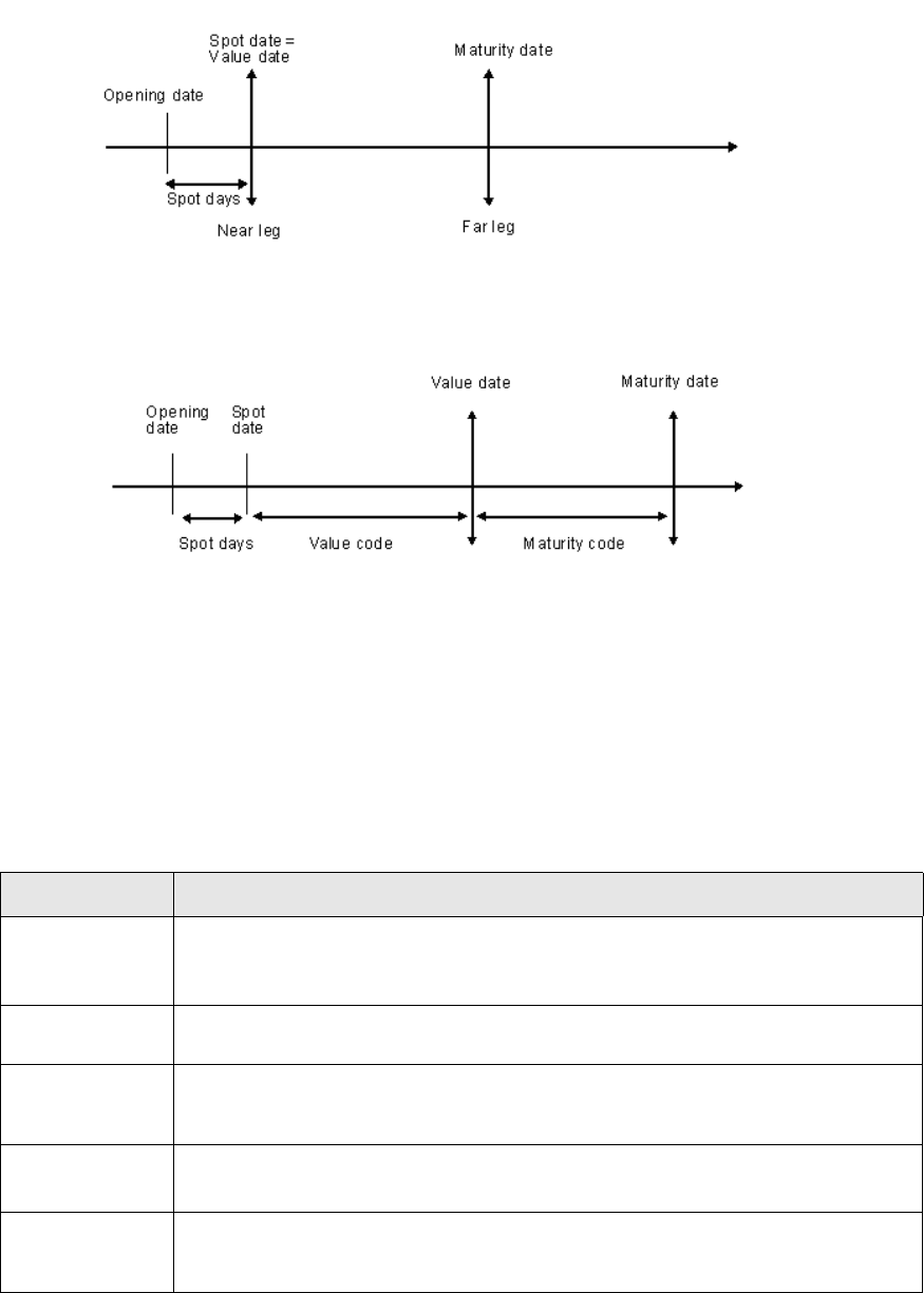
6 Forex
6.4 FX swap
420 © Wall Street Systems IPH AB - Confidential
The figure below illustrates the cashflows which are established in TRM for an FX swap
transaction.
The figure below illustrates the cashflows which are established in TRM for a forward FX swap
transaction.
6.4.4 Processing
This section describes the actions that can be done throughout the life of an FX swap.
6.4.4.1 Early expiration
You can force the forward leg of an FX swap to mature earlier using the action Early Expiration.
•Execution
The following information is needed to process the early expiration:
The execution generates an early expiration transaction with the following attributes:
Information Description
Early Expiration
Date
Date when the early expiration is executed. By default, this is today’s date unless a
Fixing/Action Date is specified at transaction level.
Opening Date must be after the near leg of the initial FX swap.
Value Date Date when the early expiration is settled. This cannot be later than the maturity date
of the initial transaction.
Amount Amount to be early-expired. This defaults to the amount left and is expressed in the
same currency (base or quote) as the input amount of the initial transaction. You can
enter any amount between 0 and the remaining amount of the initial transaction.
Deal Rate Deal rate for the early expiration transaction.
Deal Rate = Original Spot Rate - Forward Points
Forward Points Forward points of the early expiration transaction. This defaults to the number of
forward points between the early expiration date and the maturity date of the initial
transaction.

6 Forex
6.4 FX swap
Transaction & Risk Management Module (TRM) Instruments: Processing and Calculations 421
If the original input amount was Base Amount:
FX Base amount = amount to expire
If the original input amount was Quote Amount:
FX Quote amount = amount to expire
Deal Rate = early expiration deal rate
Opening date = date when the early expiration is done
Value date = date when the early expiration is settled
Kind = Early Expiration
The remaining attributes are inherited from the initial transaction.
•Cancellation
You can undo the early expiration by canceling the early expiration transaction.
6.4.4.2 Roll over
You can defer the maturity of the forward leg of an FX swap to a later date. This process is referred
to as roll-over.
See A.2.11 Allow Roll Over (FX) on page 717.
•Execution
If the Spot Rate for the roll-over equals the Original Deal Rate, the following information is
needed to process the roll over:
The execution generates a roll over transaction with the following attributes:
If the original input amount was FX Base Amount:
FX Base amount = amount to roll over
If the original input amount was FX Quote Amount:
FX Quote amount = amount to roll over
Deal Rate = roll over deal rate
Opening Date = date when the roll over is done
Maturity Date = new maturity date
Kind = Roll Over
The remaining attributes are inherited from the initial transaction.
Information Description
Roll Over Date Date when the roll over is done.
Maturity Date New maturity date of the FX deal. This must be later than the maturity date of the
initial transaction.
Amount Amount to roll over defaults to the amount left and is expressed in the same currency
(base or quote) as the input amount of the initial transaction. You can enter any
amount between 0 and the remaining amount of the initial transaction.
Forward Points Forward points of the roll over transaction. This defaults to the number of forward
points from the roll over date to the maturity date.
Deal Rate Deal rate for the roll over.
Deal Rate = Original Spot Rate + Forward Points

6 Forex
6.5 Cost-of-funding FX swap
422 © Wall Street Systems IPH AB - Confidential
If the Spot Rate for the roll-over is different from the Original Deal Rate, the following additional
information is needed to process the roll over and settle the subsequent difference:
The execution generates a roll over transaction as before with an additional cashflow as follows:
A netting cashflow is created to handle the settlement of the difference
Value Date = Roll over value date
Currency = Roll over currency 2
Amount = Base Amount * Original Deal Rate - (-Base Amount * Spot Rate)
•Cancellation
You can undo the roll over by canceling the roll over transaction.
6.4.4.3 Currency pair shift
It is possible to split a position from one underlying currency pair into two new positions, each of
which contains one of the currencies with a third currency (usually, the portfolio currency). This
process is called an FX Pair Shift.
•Setup
The FX Pair Shift action is available on an FX swap transaction if the Allow FX Currency Pair Shift
feature is included in the instrument definition: see A.2.7 Allow FX Currency Pair Shift on page
716.
•Execution
See the TRM User Guide for information about this action.
6.4.5 Position monitoring
Figures for FX swaps are calculated in the same way as the figures for FX forwards: see 6.1.5
Position monitoring on page 393.
6.5 Cost-of-funding FX swap
Cost-of-funding FX swaps are a special case of FX swap, where the nominal amount for the far leg is
based on the nominal amount of the near leg and an interest rate component.
This instrument enables you to set up defaulting for the interest rate/spread value. Then, at deal
entry, the base amount of the far leg will be defaulted to the base amount of the near leg with the
interest computed between the value date and the maturity date of the FX swap.
Information Description
Settle Differential Switch on if the Spot Rate for the roll-over is different from the Original Deal Rate.
By default, this switch is off.
Spot Rate If Settle Differential is activated, this field becomes available.
Spot Rate defaults to the spot rate of the market but this value can be modified.
The Forward Points and Deal rate are adjusted automatically.
Base CCY Interest
%
Interest rate of the base currency for the period from the original settlement date to
the new settlement date.
Quote CCY
Interest %
Interest rate of the quote currency for the period from the original settlement date to
the new settlement date.
Deal Rate Deal rate for the roll over.
Deal Rate = Spot Rate + Forward Points
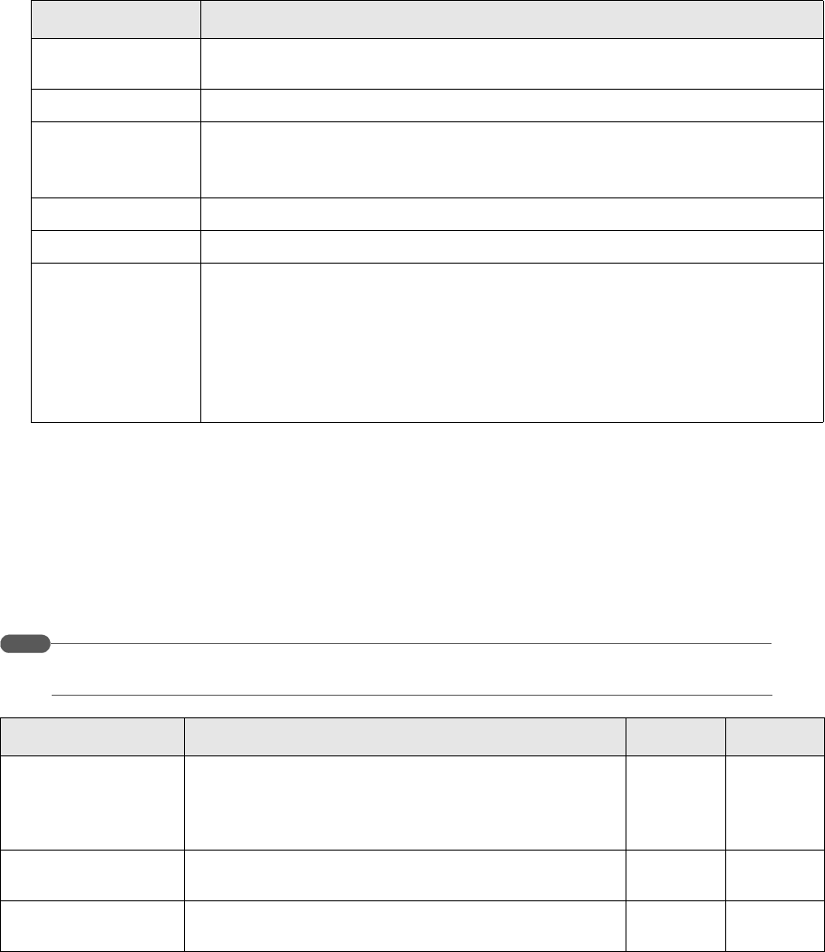
6 Forex
6.5 Cost-of-funding FX swap
Transaction & Risk Management Module (TRM) Instruments: Processing and Calculations 423
This interest is computed based on the interest rate and the spread value according to date basis of
the base currency. FX quote amounts are defaulted as usual from base amounts by using FX
rate/forward points.
6.5.1 Instrument setup
The set up is the same as for a standard FX swap except that you need to attach the trading feature
FX Swap Cost-of-Funding.
•cost-of-funding characteristics
See A.2.194 FX Swap Cost-of-Funding on page 807.
6.5.2 Deal capture
6.5.2.1 Input data
In addition to the standard FX swap deal parameters, the following information is needed to enter a
cost-of-funding FX swap:
Hint:
You will need to display the following columns in the Transaction view: C-o-F Curve, C-o-F
Rate, C-o-F Spread %, C-o-F Spread Curve, C-o-F Subscenario, and C-o-F Tenor.
Information Description
Active from/to Set active from and to dates if you want the defaulting to be used only for a given
period.
Currency Currency you want to specify.
C-o-F Curve The default curve from which the interest rate will be defaulted.
Note: Only IR quotes (i.e. curve with fixing/interest calculation usage) defined with
the Bootstrap Yield Curve feature are available.
C-o-F Spread Curve The default spread curve from which the spread will be defaulted.
Scenario The default scenario from which the values will be retrieved.
Method Defaulting method: Ask, Bid, Bid/Ask (Spread Against), Bid/Ask (Spread in Favor), or Mid.
•If you select Bid/Ask (Spread Against): if you are buying the base currency of the
quoted currency pair, the Ask price is used; if you are selling the base currency
of the quoted currency pair, the Bid price is used.
•If you select Bid/Ask (Spread in Favor): if you are buying the base currency of the
quoted currency pair, the Bid price is used; if you are selling the base currency
of the quoted currency pair, the Ask price is used.
Label Value Editable Mandatory
C-o-F curve ID of the curve to be used to default the cost-of-funding
rate.
Defaults to the curve specified at instrument level for the
base currency, otherwise, it is empty.
YN
C-o-F Subscenario Subscenario to be used to compute the cost-of-funding
rate. By default, it is empty.
YN
C-o-F Tenor Fixing period to be used to retrieve the cost-of-funding
rate. By default, it is empty.
YN
6 Forex
6.5 Cost-of-funding FX swap
424 © Wall Street Systems IPH AB - Confidential
6.5.3 Processing
The actions you can perform on a cost-of-funding swap are the same as for a standard FX swap, see
6.4.4 Processing on page 420.
6.5.4 Position monitoring
Figures for cost-of-funding swaps are calculated in the same way as for FX swaps: see 6.4.5 Position
monitoring on page 422.
C-o-F Rate Defaults to the rate defined at the curve level for the
specific tenor, otherwise, defaults to the interpolated rate
between the transaction value date and the maturity date
according to the date basis and rate type set up at the
curve level.
Note: For a forward-forward FX swap, the forward FX rate
computed between the value and maturity dates.
YY
C-o-F Spread Curve Defaults to the spread curve defined at instrument level,
otherwise, it is left empty.
YN
C-o-F Spread % If the C-o-F Spread Curve is populated then the displayed
value for the tenor is equal to the maturity date,
otherwise, it is left empty.
YN
FX Finance Rate(*) Computed from C-o-F Rate and C-o-F Spread:
FX Finance Rate = C-o-F Rate + C-o-F Spread
NY
Quote Currency Yield Yield computed from quote amounts of the FX swap as
follows:
QuoteCurrencyYield =
(FXQuoteAmount-FXQuoteSpotAmount)* B /
MaturityDate - ValueDate * 1 /
FXQuoteSpotAmount
where
• B is the date basis defined at the currency level for the
quote currency (Currency Editor - Journal page).
NY
Label Value Editable Mandatory
Transaction & Risk Management Module (TRM) Instruments: Processing and Calculations 425
Chapter 7 Index
7.1 Index types
TRM supports the following index types:
•Simple index
A simple index does not contain information on composition; it is a simple instrument to which a
price can be input. It can be used as an underlying for derivatives, and the price is used for
valuation and payoff calculations. It is also used in performance measurement for return
comparison.
•Composite index
A composite index is an index defined in the product as a basket of several equities, discount
papers, or bonds, for example, CAC-40. If you do not want to manage the composition in TRM,
the composite index is treated as a simple index.
•Derived index
A derived index is an index derived from several simple indexes. They can be composites, but
are treated as simple: their internal composition is not considered. A derived index can be
re-balanced. It can be used in performance measurement whenever internal performance
(allocation) is not needed
•Performance index
A performance index is a special type of composite index, used to compute the payback of a
specific issue. TRM implements the following two index performance formulae to compute the
index value.
–Performance averaging index
This is calculated as follows:
where:
P = number of observation dates for the denominator
N = number of observation dates for the numerator
NbComp = number of components of the index
Wk = weight of kst component of the index
1
N
----Indexi
i1=
N
∑
1
P
---Indexj
j1=
P
∑
------------------------------- 1–
Indexi
1
NbComp
----------------------- wkCompik,
k1=
NbComp
∑
=
7 Index
7.2 Instrument setup
426 © Wall Street Systems IPH AB - Confidential
Compi,k = value of the kst component at time i
–Performance Totaling Index
This is calculated as follows:
where:
N = number of observation dates for the numerator
Floor = predefined constant floor value
Cap = predefined constant cap value
NbComp = number of components of the index
Wk = weight of kst component of the index
Compi,k = value of the kst component at time i
7.2 Instrument setup
Index instruments must be set up in the following order:
7.2.1 Simple Index
Index instruments are based on an instrument type derived from the class INDEX.
•Main characteristics (Quoted page):
This information enables you to either enter the quotation manually in Rate Monitor, or to
retrieve it automatically in real-time.
Note: Real-time market information is set up for the instrument in the Market Info page.
See A.2.203 Index on page 813.
It is also possible to set up:
•Branch codes. See Appendix A Features on page 713.
Max Floor Min Cap IndexjIndexj1–
–
Indexj1–
----------------------------------------------⎠
⎞⎠
⎞
;
⎝
⎛
;
⎝
⎛
j1=
N
∑
Indexi
1
NbComp
----------------------- WkCompik,
k1=
NbComp
∑
=
Information Description
Price Type
information
Index.
Quote Handling Index.
Currency Currency of the index.

7 Index
7.2 Instrument setup
Transaction & Risk Management Module (TRM) Instruments: Processing and Calculations 427
7.2.2 Composite Index
Composite Index instruments are based on an instrument type derived from the class INDEX.
•Main characteristics
Features INDEX-COMPOSITE (primary) and QUOTED must be used.
See A.2.205 Index Composite on page 814.
This feature allows you to define the information in the instrument setup tabs as described in the
following sections.
7.2.2.1 Structure
Defines the principal characteristics of the index.
Information Description
Currency Reference currency for the index, used as the basis of index calculations.
Composition Type Defines the component types used in this index: DEBT-SECURITY (bond, quoted
Discount Paper), EQUITY, and COMPOSITE (other composite index).
Weight Cap The max % of the market value a single component can attain.
Calculation Method Defines how Composite Indexes are calculated. The following methods can be used
to take the outflows (coupons, dividends and bond accrued interest) into account:
•Clean Price: Used mainly for bonds. Only takes into account price return, not
accrued interest or cashflows. Unlike the other methods, this method discards
the accrued interest from the calculations of bond indices.
•Hold Cash On Security: Cashflows are held under security until the index is
revised, but not reinvested. In which case, the field amount contains the
amount of the cashflow, and is populated when the cashflow is detached from
the security (in security currency). The amounts between two rebalancings are
added to the security amount (price * units) and eventually, accrued interest
before being converted to index currency.
•Hold Cash On Index: Cashflows are held under index until the index is revised, but
not reinvested. In which case, the field amount contains the amount of the
cashflow converted to the index currency, and is populated when cashflow is
detached from the security. The amounts between two rebalancings are added
to the market value of the index.
•Reinvest Cash On Security: The amount of the cashflow is reinvested on the
security from which it is detached. TRM calculates a factor to simulate
reinvestment of the cash in the security itself (stored in the Rebalance page).
•Reinvest Cash On Index: The amount of the cashflow is reinvested in the index.
TRM calculates a factor which is applied to the whole index (stored in the
Rebase page).
Rounding Precision Rounding precision to be applied in calculations.
Rounding Method Rounding method to be applied in calculations.
Input Method Defines how weightings are input (see 7.2.2.3 Composition on page 429). Available
methods are:
•Units/Nominal: the absolute units for the component
•Market Value: the market value of the component in index currency
•Weight %: the % of the total market value of the component
•Outstanding: number of times the outstanding units/nominal (typically 1).
Available for Bond and Equity
•Free Float: same as above but with the units available for trading. Available only
for Equity.
7 Index
7.2 Instrument setup
428 © Wall Street Systems IPH AB - Confidential
7.2.2.2 Base
Periodically models the revisions of the index including the initial definition
Actions
•Copy composition from template
Initializes an index from one or more template indexes, available only for the initial base. The
template must be selected for this action to be visible. A factor can be used to scale template
composition. The action can be executed several times to combine several templates.
•Duplicate previous composition
Duplicates composition which can be manually revised: when using outstanding and free float
methods this does automatic revision without requiring manual intervention (it re-fetches new
market information at revision time). Only on revision bases (when you have more than one
base).
•Update composition attributes
Automatically sets or resets the Keep Input flag for all the components of the base, so component
flags need not be set or reset manually (see 7.2.2.3 Composition on page 429).
•Calculate...
This button is used to recalculate the specified base when Components are added, removed, or
modified. The calculation makes sure that the setup of the base is consistent: that the sum of all
the components amount matches the market value of the base and, if input method is weight %,
that the inputs sum to 100%.
The calculation is affected by the Keep Market Value switch of the base and the Keep Inputs flags
of the components. When Keep Market Value is switched on, the system adjusts component inputs
that are not marked with Keep Input. Otherwise the market value can be re-calculated.
When the input method is Weight %, the Keep Market Value flag is forced to True.
Note: If the flags are set in a way that makes resolution of the equation impossible, Calculate...
flags the base with the attribute Error, and the instrument cannot be saved. It is possible to
Information Description
From Date of the revision
To Read-only. Date up to which this revision is valid.
Index Value • For the initial base the default is 100. This can be changed if you want to start
the index with another value. For example, to manage the CAC-40 today, you
would use the CAC-40’s current value.
• For revision bases this is defaulted to the last known frozen base (from the
previous day). It can be changed (if incorrect in the database for example) but
should normally not be changed: it will be used as the base for index
calculations for every date until the next revision.
Market Value The total market value of the index in the index currency. It is automatically set
with Calculate (see Actions). It can also be forced, and then Calculate will adjust
composition to match it.
Last Market Value Read-only.
Attributes •Error: calculation of the base is impossible (incorrect base/component attributes
and/or inputs/market value)
•Keep Market Value: affects Calculate button behavior (see below); always on
when input method is Weight %.
•Modified: composition has been modified for this base and calculation must be
done before saving
7 Index
7.2 Instrument setup
Transaction & Risk Management Module (TRM) Instruments: Processing and Calculations 429
temporarily save an index with an inconsistent base by unswitching the attributes
manually, but the user must fix the problem before using the index.
7.2.2.3 Composition
Defines the composition of the index for a given base
7.2.2.4 Rebase
Stores the impact of cashflows, depending on the method of calculation. This is used when
cashflows are impacted at index level.
Information Description
Base Date Reference of the base (corresponds to Base "From").
Component Id of the component; available components are filtered according to index type.
Currency Read-only. Currency of the component, retrieved from component characteristics.
Calendar Calendar of the component, retrieved from component characteristics.
FX Rate Cross-rate between Component currency and index currency, defaulted from fixing
scenario. Can be changed by the user. It is the base rate used in calculation relative
to this base for this component.
Component Value Price of the component. This is defaulted from the fixing scenario and can be
changed by the user. It is the base price used in calculations relative to this base for
this component.
Input It is the base weight for this component. The significance of this weight depends on
the input method defined in the index structure (see 7.2.2.1 Structure on page
427).
Units/Nominal Read-only. This is the absolute weight in units (for equities) or in nominal (for
bonds) which is calculated for the component depending on the input method.
Accrued Interest For bond index, amount of accrued interest for the component at base date.
Amount Read-only. Shows the amount of the component for the base in index currency. The
sum of the amount of all components for a base gives the base market value of the
index.
Attributes Keep Input forces the Calculate action to keep the input for this component.
Information Description
Date Date of the market value shift
Old Value Market value of the index before the external event was taken into account
New Value Market value of the index including the impact of the external event.
Cash Amount to be added to index MV from the specified date onwards.
Source Read-only. Shows what event triggers the rebasing. Manual means that the user
can enter it manually, and in which case, it is modifiable in the editor.
Other choices are: Amortization, Cash Dividend, Coupon, Split.
7 Index
7.2 Instrument setup
430 © Wall Street Systems IPH AB - Confidential
7.2.2.5 Rebalance
Stores the impact of cashflows, depending on the method of calculation. This is used when
cashflows are impacted at component level. It is also used to compensate for the effect of equity
splits.
7.2.3 Derived Index
Features INDEX-DERIVED (primary) and QUOTED must be used.
7.2.3.1 Structure
Defines the currency, index type, and maximum weight for any component for the corresponding
index composition.
7.2.3.2 Base
Periodically models the revisions of the index including the initial definition
Information Description
Date Date of the CA to be balanced.
Component Id of the component; available components are filtered according to index type.
Old Units/Nominal Number of units before rebalancing
New Units/Nominal Number of units after rebalancing
Cash Amount to be added to component MV from the specified date onwards.
Source Read-only. Shows what event triggers the rebasing. Manual means that the user
can enter it manually, and in which case, it is modifiable in the editor.
Information Description
Currency Reference currency for the index, used as the basis of index calculations.
Composition Type Index is the only available type.
Weight Cap The max % of the market value a single component can attain.
Input Method Defines how weightings are input (see 7.2.3.3 Composition on page 431). Available
methods are:
•Units/Nominal: the absolute units for the component
•Weight %: the % of the total market value of the component.
Rounding Precision Rounding precision to be applied in calculations.
Rounding Method Rounding method to be applied in calculations.
Calculation Method Not used for a derived index.
Information Description
From Date of the revision
To Read-only. Date up to which this revision is valid.
Index Value • For the initial base the default is 100. This can be changed if you want to start
the index with another value.
• For revision bases this is defaulted to the last known frozen base (from the
previous day). It can be changed (if incorrect in the database for example) but
should normally not be changed: it will be used as the base for index
calculations for every date until the next revision.
7 Index
7.2 Instrument setup
Transaction & Risk Management Module (TRM) Instruments: Processing and Calculations 431
Actions
•Copy composition from template
Initializes an index from one or more template indexes, available only for the initial base. The
template must be selected for the action to be visible. A factor can be used to scale template
composition. The action can be executed several times to combine several templates.
•Duplicate previous composition
Duplicates composition which can be then manually revised. Only on revision bases (when there
is more than one base).
•Update composition attributes
Automatically sets or resets the Keep Input flag for all the components of the base: this is a
shortcut (see 7.2.3.3 Composition on page 431).
•Calculate...
This button recalculates the specified base when Components are added, removed, or modified.
The calculation makes sure that the setup of the base is consistent: that the sum of all the
components amount matches the market value of the base and, if input method is Weight %,
that the inputs sum to 100%.
The calculation is affected by the Keep Market Value switch of the base and the Keep Inputs flags
of the components. When Keep Market Value is switched on, the system adjusts component inputs
that are not marked with Keep Input. Otherwise the market value can be re-calculated.
When the input method is Weight %, the Keep Market Value flag is forced to True.
Note: If the flags are set in a way that makes resolution of the equation impossible, Calculate...
flags the base with the attribute Error, and the instrument cannot be saved. It is possible to
temporarily save an index with an inconsistent base by unswitching the attributes
manually, but the user must fix the problem before using the index.
7.2.3.3 Composition
Defines the composition of the index for a given base.
Market Value The total market value of the index in the index currency. It is automatically set
with the Calculate... button (see Actions). It can also be forced, and then calculate
will adjust composition to match it.
Last Market Value Read-only.
Attributes •Error: calculation of the base is impossible (incorrect base/component attributes
and/or inputs/market value)
•Keep Market Value: affects Calculate button behavior (see below); always on
when method is %.
•Modified: composition has been modified for this base and calculation must be
done before saving
Information Description
Information Description
Base Date Reference of the base (corresponds to Base "From").
Component Id of the component; available components are indexes.
Currency Read-only. Currency of the component, retrieved from component characteristics.
Calendar Read-only. Calendar of the component, retrieved from component characteristics.
7 Index
7.2 Instrument setup
432 © Wall Street Systems IPH AB - Confidential
7.2.3.4 Schedule
Defines rebalance schedules, which will be used to generate rebalance dates.
7.2.3.5 Rebalance Date
Shows rebalance dates.
Actions
•Generate
Generates a set of rebalance dates according to the schedules. If Method is "Days" or "Business
Days" and Frequency is 1, only the first rebalance date is generated; next rebalance dates are
generated by clicking Rebalance (see below).
•Rebalance
Performs index rebalancing. The input method for the index must be Weight %. The system
creates rows in the Rebalance page for the components of the index to adjust their units so that
the percentages match the definition of the base. It is possible to trigger this action
automatically via an activity (see 7.4 Processing on page 440).
FX Rate Cross-rate between Component currency and index currency, defaulted from fixing
scenario. Can be changed by the user. It is the base rate used in calculation relative
to this base for this component.
Component Value Price of the component. This is defaulted from the fixing scenario and can be
changed by the user. It is the base price used in calculations relative to this base for
this component.
Input It is the base weight for this component. The significance of this weight depends on
the input method defined in the index structure (see above).
Units/Nominal Read-only. This is the absolute weight in units which is calculated for the component
depending on the input method.
Amount Read-only. Shows the amount of the component for the base in index currency. The
sum of the amount of all components for a base gives the base market value of the
index.
Attributes Keep Input forces the Calculate action to keep the input for this component.
Information Description
Information Description
Start Date Date from when rebalancing starts.
End Date Date when rebalancing stops (if you do not know if it will stop, just use a distant
future date).
Method Specifies how the rebalancing dates are calculated.
Frequency A function of the Method selected. For example, if method is Months, entering 3
here gives a frequency of 3 months.
Convention Business convention to be followed.
Roll from Start Yes or No.
Date Type Select Re-balance.
Information Description
Date Date when rebalancing is executed.
7 Index
7.2 Instrument setup
Transaction & Risk Management Module (TRM) Instruments: Processing and Calculations 433
7.2.3.6 Rebalance
Stores the impact of re-balancing.
7.2.4 Performance averaging index
•Main characteristics
Features INDEX-AVERAGING (primary) and QUOTED must be used.
See A.2.204 Index Averaging on page 813.
This feature allows you to define the following information in the instrument setup tabs:
7.2.4.1 Structure
Defines the currency, index type, and maximum weight for any component for the corresponding
index composition.
7.2.4.2 Base
Periodically models the revisions of the index including the initial definition
Information Description
Date Date of rebalancing.
Component Id of the component.
Old Units/Nominal Number of units before rebalancing.
New Units/Nominal Number of units after rebalancing.
Cash Amount to be added to component MV from the specified date onwards.
Source Read-only. Shows what event triggers the rebasing. Manual means that the user
can enter it manually, and in which case, it is modifiable in the editor.
Information Description
Currency Reference currency for the index, used as the basis of index calculations.
Composition Type Defines the component types used in this index: equities, bonds or indexes.
Weight Cap The max % of the market value a single component can attain.
Calculation Method Clean Price is the only method supported.
Rounding Precision Rounding precision to be applied in calculations.
Rounding Method Rounding method to be applied in calculations.
Input Method Defines how weightings are input (see 7.2.4.3 Composition on page 435). Available
methods are:
•Units/Nominal: the absolute units for the component
•Market value: the market value of the component in index currency
•Weight %: the % of the total market value of the component
•Outstanding: the number of times the outstanding units/nominal (typically 1).
Available for Bond and Equity.
•Free Float: same as above, but with the units available for trading. Available only
for Equity.
Information Description
From Date of the revision
7 Index
7.2 Instrument setup
434 © Wall Street Systems IPH AB - Confidential
Actions
•Copy composition from template
Initializes an index from one or more template indexes, available only for the initial base. The
template must be selected for the action to be visible. A factor can be used to scale template
composition. This action can be repeated to combine several templates.
•Duplicate previous composition
Duplicates composition which can then be manually revised: when using outstanding and
free-float methods, this does automatic revision without manual intervention (it re-fetches new
market information at revision time). Only on revision bases.
•Update composition attributes
Automatically sets or resets the Keep Input flag for all the components of the base: this is a
short cut (see 7.2.4.3 Composition on page 435).
To Read-only. Date up to which this revision is valid.
Index Value • For the initial base the default is 100.
• For revision bases this is defaulted to the last known frozen base (from the
previous day). It can be changed (if incorrect in the database for example) but
should normally not be changed: it will be used as the base for index
calculations for every date until the next revision.
Market Value The total market value of the index in the index currency. It is automatically set
with Calculate (see Actions). It can also be forced and then Calculate will adjust
composition to match it.
Last Market Value Read-only.
Attributes •Error: calculation of the base is impossible (incorrect base/component attributes
and/or inputs/market value)
•Keep Market Value: affects Calculate button behavior (see below); always on
when method is %.
•Modified: composition has been modified for this base and calculation must be
done before saving
Information Description
7 Index
7.2 Instrument setup
Transaction & Risk Management Module (TRM) Instruments: Processing and Calculations 435
•Calculate...
This button recalculates the specified base when Components are added, removed, or modified.
The calculation makes sure that the setup of the base is consistent: that the sum of all the
components amount matches the market value of the base, and if the input method is Weight %,
that the inputs sum to 100%.
The calculation is affected by the Keep Market Value switch of the base, and the Keep Inputs flags of
the components. When Keep Market Value is switched on, the system adjusts component inputs
that are not marked with Keep Input. Otherwise the market value can be re-calculated.
When input method is Weight %, the Keep Market Value flag is forced to True; when the input
method is Outstanding or Free Float, it is forced to False.
Note: If the flags are set in a way that makes resolution of the equation impossible, Calculate...
flags the base with attribute Error, and the instrument cannot be saved. It is possible to
temporarily save an index with an inconsistent base by unswitching the attributes
manually, but the user must fix this problem before using the index.
7.2.4.3 Composition
Defines the composition of the index for a given base.
7.2.4.4 Rebalance
Balances the impact of any equity splits.
Information Description
Base Date Reference of the base (corresponds to Base "From").
Component Id of the component; available components are filtered according to index type.
Currency Read-only. Currency of the component, retrieved from component characteristics.
Calendar Read-only. Calendar of the component, retrieved from component characteristics.
FX Rate Cross-rate between Component currency and index currency, defaulted from fixing
scenario. Can be changed by the user. It is the base rate used in calculation relative
to this base for this component.
Component Value Price of the component. This is defaulted from the fixing scenario and can be
changed by the user. It is the base price used in calculations relative to this base for
this component.
Input It is the base weight for this component. The significance of this weight depends on
the input method defined in the index structure (see above).
Units/Nominal Read-only. This is the absolute weight in units (for equities) or in nominal (for
bonds) which is calculated for the component depending on the input method.
Amount Read-only. Shows the amount of the component for the base in index currency. The
sum of the amount of all components for a base gives the base market value of the
index.
Attributes Keep Input forces the Calculate action to keep the input for this component.
Information Description
Date Date of the CA to be balanced.
Component Id of the component; available components are filtered according to index type.
Old Units/Nominal Number of units before split.
New Units/Nominal Number of units after split.
7 Index
7.2 Instrument setup
436 © Wall Street Systems IPH AB - Confidential
7.2.4.5 Schedule
Defines schedules, used to generate numerator and denominator dates.
7.2.4.6 Denominator Date and Numerator Date
These pages show the dates when performance calculations are performed
Actions
•Generate
Generates a set of Numerator and Denominator dates according to the schedules and individual
calendars of the components.
7.2.5 Performance totaling index
•Main characteristics
Features INDEX-TOTALING (primary) and QUOTED must be used.
See A.2.215 Index Totaling on page 821.
This feature allows you to define the information in the instrument setup tabs described in the
following sections.
Cash Amount to be added to component MV from the specified date onwards.
Source Read-only. Shows what event triggers the rebasing. Manual means that the user
can enter it manually, and in which case, it is modifiable in the editor.
Information Description
Information Description
Start Date Date from when generation starts.
End Date Date when generation stops (if you do not know when generation will stop, just use
a distant future date).
Method Defines how the generation dates are calculated.
Frequency A function of the Method selected. For example, if method is Months, entering 3
here gives a frequency of 3 months.
Convention Business convention to be used.
Roll from Start Yes or No.
Date Type Use Avg. Numerator and Avg. Denominator.
Information Description
Date Input Date of the calculation.
Observation Date Date when the price is retrieved for the components following the given calendar.
Calendar For each Date Input there must be as many records as distinct calendars in the
components. Observation date might be different for each calendar.
7 Index
7.2 Instrument setup
Transaction & Risk Management Module (TRM) Instruments: Processing and Calculations 437
7.2.5.1 Structure
Defines the currency, index type, and maximum weight for any component for the corresponding
index composition.
7.2.5.2 Base
Periodically models the revisions of the index including the initial definition
Actions
•Copy composition from template
Information Description
Currency Reference currency for the index, used as the basis of index calculations.
Composition Type Defines the component types used in this index: equities, bonds or indexes.
Weight Cap The max % of the market value a single component can attain.
Calculation Method Clean Price is the only supported method.
Rounding Precision Rounding precision to be applied in calculations.
Rounding Method Rounding method to be applied in calculations.
Input Method Defines how weightings are input (see 7.2.5.3 Composition on page 438). Available
methods are:
•Units/Nominal: the absolute units for the component
•Market value: the market value of the component in index currency
•Weight %: the % of the total market value of the component
•Outstanding: the number of times the outstanding units/nominal (typically 1).
Available for Bond and Equity.
•Free Float: same as above but with the units available for trading. Available only
for Equity.
Information Description
From Date of the revision
To Read-only. Date up to which this revision is valid.
Index Value • For the initial base the default is 100.
• For revision bases this is defaulted to the last known frozen base (from the
previous day). It can be changed (if incorrect in the database for example) but
should normally not be changed: it will be used as the base for index
calculations for every date until the next revision.
Market Value The total market value of the index in the index currency. It is automatically set
with Calculate (see Actions). It can also be forced and then calculate will adjust
composition to match it.
Last Market Value Read-only.
Attributes •Error: calculation of the base is impossible (incorrect base/component attributes
and/or inputs/market value)
•Keep Market Value: affects Calculate button behavior (see below); always on
when method is %.
•Modified: composition has been modified for this base and calculation must be
done before saving
7 Index
7.2 Instrument setup
438 © Wall Street Systems IPH AB - Confidential
Initializes an index from one or more template indexes, available only for the initial base. The
template must be selected for the action to be visible. A factor can be used to scale template
composition. This action can be repeated to combine several templates.
•Duplicate previous composition
Duplicates composition which can be then manually revised: when using outstanding and free
float methods this does automatic revision without requiring manual intervention (it re-fetches
new market information at revision time). Only on revision bases.
•Update composition attributes
Automatically sets or resets the Keep Input flag for all the components of the base: this is a
short cut (see 7.2.5.3 Composition on page 438).
•Calculate...
This button recalculates the specified base when Components are added, removed, or modified.
The calculation makes sure that the setup of the base is consistent: that the sum of all the
components amount matches the market value of the base and, if input method is Weight %, that
the inputs sum to 100%.
The calculation is affected by the Keep Market Value switch of the base and the Keep Inputs flags of
the components. When Keep Market Value is switched on, the system adjusts component inputs
that are not flagged with Keep Input. Otherwise the Market Value can be re-calculated.
When input method is Weight %, the Keep Market Value flag is forced to True; when method is
Outstanding or Free Float it is forced to False.
Note: If the flags are set in a way that makes resolution of the equation impossible, Calculate...
marks the base with attribute Error, and the instrument cannot be saved. It is possible to
temporarily save an index with an inconsistent base by unswitching the attributes
manually, but the user must fix this problem before using the index.
7.2.5.3 Composition
Defines the composition of the index for a given base
Information Description
Base Date Reference of the base (corresponds to Base "From").
Component Id of the component; available components are filtered according to index type.
Currency Read-only. Currency of the component, retrieved from component characteristics.
Calendar Read-only. Calendar of the component, retrieved from component characteristics.
FX Rate Cross-rate between Component currency and index currency, defaulted from fixing
scenario. Can be changed by the user. It is the base rate used in calculation relative
to this base for this component.
Component Value Price of the component. This is defaulted from the fixing scenario and can be
changed by the user. It is the base price used in calculations relative to this base for
this component.
Input It is the base weight for this component. The significance of this weight depends on
the input method defined in the index structure (see above).
Units/Nominal Read-only. This is the absolute weight in units (for equities) or in nominal (for
bonds) which is calculated for the component depending on the input method.
Amount Read-only. Shows the amount of the component for the base in index currency. The
sum of the amount of all components for a base gives the base market value of the
index.
7 Index
7.2 Instrument setup
Transaction & Risk Management Module (TRM) Instruments: Processing and Calculations 439
7.2.5.4 Rebalance
Balances the impact of any equity splits
7.2.5.5 Totaling
Defines cap and floor to use in totaling formula (see – Performance Totaling Index on page 426).
7.2.5.6 Schedule
Defines schedules, used to generate totaling dates.
7.2.5.7 Totaling Date
This page shows the dates when performance calculation is done.
Attributes Keep Input forces the Calculate action to keep the input for this component.
Information Description
Information Description
Date Date of the CA to be balanced.
Component Id of the component; available components are filtered according to index type.
Old Units/Nominal Number of units before rebalancing
New Units/Nominal Number of units after rebalancing
Cash Amount to be added to component MV from the specified date onwards.
Source Read-only. Shows what event triggers the rebasing. Manual means that the user
can enter it manually, and in which case, it is modifiable in the editor.
Information Description
Floor The floor to use in the totaling formulae.
Cap The cap to use in the totaling formulae.
Information Description
Start Date Date from when generation starts.
End Date Date when generation stops (if you do not know if it will stop, just use a date very
far in the future).
Method Defines how the generation dates are calculated.
Frequency A function of the Method selected. For example, if method is Months, entering 3
here gives a frequency of 3 months.
Convention Business convention to be used.
Roll from Start Yes or No.
Date Type Use average numerator and denominator for date types.
Information Description
Date Input Date of the calculation.
Observation Date The date when the price will be retrieved for the components following the given
calendar.
7 Index
7.3 Market information
440 © Wall Street Systems IPH AB - Confidential
Actions
•Generate
Generates a set of totaling dates according to the schedules and individual calendars of the
components.
7.3 Market information
Rate Monitor is used to visualize and maintain index prices. See the TRM User Guide for more
information.
7.4 Processing
This section describes the processing that you can perform, either manually in the relevant
application, or automatically, as an activity, in Activity Monitor.
7.4.1 Revision
Revision is a manual process which consists of updating an index to reflect the market more
accurately. This operation is done in the Instrument Editor by creating a new base and a new
composition.
Note: It is also possible to import revisions using one of the TRM connectivity tools.
7.4.2 Freezing Index Values
Rate Monitor enables you to view both calculated and quoted (Q) values, but only the quoted values
are used by the rest of the system. Values of composite, derived and performance indexes are
calculated automatically in real time according to market data changes (FX rates or component
values). It is nevertheless important to be able to freeze these results at any time.
In Rate Monitor, use the command Command - Freeze to freeze these values; the current content of
the calculated cells are copied to the Quoted (Q) cells. When you have frozen these values, use the
Save button to store them in the database like any other standard price. Both index values and
detailed composition information are stored.
Note: You can import Quoted (Q) values directly from an external data feed, either as a
replacement or in parallel, by using another scenario and/or subscenario.
You can also use the Index Freeze activity in Activity Manager to perform the freeze.
Note: See the TRM User Guide for general information on running activities, and also specific
information on the activity parameters.
Calendar For each Date Input there must be as many records as there are distinct calendars
in the components. The Observation Dates for each calendar can be different.
Information Description

7 Index
7.4 Processing
Transaction & Risk Management Module (TRM) Instruments: Processing and Calculations 441
7.4.3 Updating Factors and Cash
Use the activity Index Adjustment in Activity Manager to automatically update factors and cash. This
activity reads the characteristics of the underlyings, and depending on the Index Type and the
Calculation Method, inserts the relevant information into the Rebase and Rebalance pages.
Note: See the TRM User Guide for general information on running activities, and also specific
information on the activity parameters.
7.4.4 Rebalancing
A common use for a derived index is to rebalance the index periodically, so that each component
weight is readjusted to the original percentage weighting. After the setup of rebalancing dates is
done, (see setup above), you can execute rebalancing for an index directly in the editor, by clicking
Rebalance.
You can also use the Index Rebalance activity in Activity Manager to perform this task.
Note: See the TRM User Guide for general information on running activities, and also specific
information on the activity parameters.
7 Index
7.4 Processing
442 © Wall Street Systems IPH AB - Confidential

Transaction & Risk Management Module (TRM) Instruments: Processing and Calculations 443
Chapter 8 Cash
8.1 Bank account
Bank account balances and any interest accrued on a bank account are displayed in the system as
transactions.
Bank accounts can be used either: to track your own bank balance by checking your current position
adjusted by the existing balance, and to calculate the estimated accrued interest on the bank
account; or, if you represent an In-house Bank (that is, you hold accounts for your subsidiaries),
you can calculate end-of-day balances and provide your subsidiaries with the appropriate
information, as well as calculating any accrued interest on the accounts.
You need to set up one instrument to calculate bank balances, and another which is specifically used
to calculate accrued interest. Both instruments are assigned to accounts in the Accounts page of
Client Editor: see the TRM User Guide for more information.
It is recommended that a separate Balance portfolio is defined for the balance and
interest-calculation transactions. One reason is that you can restrict update access to the balance
information to people in the back office, while the trading portfolios can only be updated by people
in the front office and middle office.
If you operate as an In-house Bank, you may also find it useful to have a Balance portfolio for each
of the bank accounts of your subsidiaries.
Note: Information about how to assign balance instruments to accounts and how to create
Balance portfolios is described in the TRM User Guide.
Bank account balances and interest-calculation instruments belong to the instrument class
BANK-ACCOUNT.
8.1.1 Instrument setup
Both bank account balance and bank account interest instruments share the same primary feature.
8.1.1.1 Bank account balance
Bank account balance instruments are assigned to the accounts for which you want to calculate the
balance. The balance can either be derived from payable cashflows in the system, or from paid
cashflows. It is also possible to define in how much detail you want the balance to be calculated, for
example, if you need one balance transaction per counterparty.
Balance instruments do not require any specific set up. They are simply recognized by the following
features in the Bank-Account instrument class:
•The primary feature Bank Account Balance (see A.2.45 Bank Account Balance on page 729)
•The valuation feature Bank Account Method (see A.2.47 Bank Account Valuation on page 732).
8.1.1.2 Bank account interest-calculation
Interest-calculation instruments are assigned to the accounts for which you want to calculate the
accrual of interest.
•Main characteristics
8 Cash
8.1 Bank account
444 © Wall Street Systems IPH AB - Confidential
The bank account interest instrument uses the same primary feature as the bank account
balance instrument (see 8.1.1.1 Bank account balance on page 443).
•Trading information
–Interest accrual parameters
For bank balances, you can specify the interest rates used, and the method and frequency
that interest is accrued.
–Interest realization parameters
You can specify how the accrued interest is realized on the balance.
See A.2.46 Bank Account Interest on page 730.
8.1.2 Deal capture
Bank account balances and interest transactions are system-generated transactions, performed by
scheduled activities (see the TRM User Guide for more information). Once the activity has run, the
transactions are generated in the Bank Account Balances application.
8.1.2.1 Generated data
•Transaction
Transaction Type = Balance
Counterparty = Bank that holds the balance, unless the balances are calculated
by counterparty
•Cashflows
–One cashflow per balance (only if the balance has changed)
Information Description
Date Basis Date basis used to calculate accrued interest for this instrument.
Interest Rate Curve Underlying yield curve (set up in IR Quote and Yield Curve Editor) used for
interest calculation.
Note: If you specify a yield curve (and/or Period, Positive Spread, or
Negative Spread), you do not need to specify any Ladder values (see
Ladder Rule and Ladder).
Period Period of the underlying yield curve to be used for interest calculation (for
example, O/N).
Scenario Rate scenario to be used for calculating interest for this instrument.
Information Description
Frequency Frequency of interest realization (if Method = Periodically).
Frequency Unit Unit of time to use for interest realization: Business Days, Days, Months,
Weeks, or Years.
Method Method of realizing interest:
•At Withdrawal - not applicable.
•Periodically - interest is realized at regular intervals (see Frequency
field).
•At Expiration - not applicable.
Settlement Method Interest payment method: Capitalize to compound interest or Settle to
receive or pay interest.
8 Cash
8.1 Bank account
Transaction & Risk Management Module (TRM) Instruments: Processing and Calculations 445
–If the interest is unrealized: daily accrued interest
–If the interest is realized: realized interest cashflows or the capitalizing balance cashflow.
8.1.3 Processing
This section describes the processing that you can perform, either manually in the relevant
application, or automatically, as an activity, in Activity Manager. See the TRM User Guide for
information about these activities and how to set up activities in general.
8.1.3.1 Calculating bank account balance and interest
Bank account balance and accrued interest-calculation transactions are generated by the activity
Bank Account Balances which you can schedule to run as often as required (see the TRM User Guide
for more information).
8.1.3.2 Realize AI
Bank account accrued interest can be realized automatically or manually (for automatic realization,
see the TRM User Guide).
You can realize interest manually, by right-clicking on the transaction in the Transaction view of the
Bank Account Balances application and selecting the Realize AI action.
•Execution
The following information is needed to process the realization:
Note: It is not possible to realize accrued interest for future dates using the Realize AI action.
•Cancellation
Information Description
Date Date of the action i.e. the realization date.
Opening Date The opening date of the transaction.
Payment Date By default, the Payment Date is the realization date. However, you can change
the default.
Amount Amount of the realized interest cashflow.
By default, this is the total amount of accrued interest, but it can be changed to
a lesser amount if you do not want to realize the total amount.
Interest Sign Positive: To receive interest.
Negative: To pay interest.
Settlement Method Capitalize or Settle. The accrued interest is either settled or capitalized.
Note: By default, the settlement method will be the one defined in the Interest
Realization page of Instrument Editor.
Interest Bank ID of a bank if you want to settle the interest realization in a specific bank,
which differs from the default bank.
Interest Account ID of a bank account if you want to settle the interest realization in a specific
account, which differs from the default bank account.
Update Realization Date Switch on to allow the next interest realization date to be automatically
updated.

8 Cash
8.2 Call account
446 © Wall Street Systems IPH AB - Confidential
You can cancel interest manually by right-clicking on the transaction in the Transaction view of
the Bank Account Balances application and selecting the Undo Realize AI action. The following
information is needed to process the cancellation:
8.2 Call account
Call Account is similar to a normal bank account. The client can withdraw and deposit funds (lend or
borrow) from the account whenever it is necessary. The funds earn interest on the account at a rate
that is fixed daily. The interest is accrued and paid or capitalized at regular intervals. The client can
withdraw all or part of the interest from the account when interest is payable (without first having to
capitalize the interest).
The main difference between Call Money and Call Account is the presumed length of the transaction.
Call Money is assumed to mature on a daily basis, while Call Account is automatically rolled over
every day.
In TRM, call account instruments belong to the instrument class CALL-ACCOUNT.
8.2.1 Instrument setup
Call accounts are based on an instrument type derived from the instrument class CALL-ACCOUNT.
•Main characteristics
The following basic information may be captured when defining a call account instrument.
–Interest accrual parameters
For call accounts, you can specify the interest rates used, and the method and frequency
that interest is accrued on the call account.
–Interest realization parameters
You can also specify how the accrued interest is realized on the call account.
See A.2.82 Call Account on page 747.
For a call account instrument, it is also possible to set up:
•Spot date calculation
•Cashflow and transaction charge rules
•Manual charges
•Branch codes.
See Appendix A Features on page 713.
Information Description
Date Date of the action i.e. the undo realization date.
By default the date is today's date.
Information Description
Currency Currency of the call account.
Balance
information
Minimum and maximum balance allowed on the call account.
Notice period
information
Required notice period for calling the money.
8 Cash
8.2 Call account
Transaction & Risk Management Module (TRM) Instruments: Processing and Calculations 447
8.2.2 Deal capture
Call account transactions are entered in the Call Account trading mode of Transaction Manager’s Call
Manager layout.
Note: See the TRM User Guide for more information about this Transaction Manager layout.
8.2.2.1 Input data
In addition to the standard deal parameters, the following information is required to enter a call
account transaction:
•Transaction view
Interest rate and balance information defined at instrument level default to the date in the Roll
Over Date field. If the Roll Over Date field is empty, then today’s date is used. If no interest rate
is available for today, then the rate applied yesterday is used. Similarly, if no balance is
available, then the closing balance from the previous day is shown.
8.2.2.2 Generated data
Movements on call accounts can be viewed in the Movement view of Call Manager.
•Movement view
8.2.3 Processing
This section describes the actions that can be done throughout the life of a call account transaction.
8.2.3.1 Update account
A call account instrument needs to be updated each day.
•Execution
–Automatic updating of a call account is done using the Call Money Account Update activity.
This activity should be scheduled to run on a daily basis to ensure that the call account
instrument is updated each day.
Information Description
Movement/Initial
Balance
Initial movement (inflow or outflow) on the call account.
This amount can be zero if the initial movement is intended to open the account only,
and does not involve a deposit or withdrawal of funds.
Interest Rate At contract level, this is the last roll over rate.
Roll Over Date Date of the next roll over.
Capitalize Account Transaction number of an alternative call account on which to realize the capitalized
interest.
Information Description
Movement ID Log number for each movement carried out on a transaction.
This number is used to identify individual movements when multiple identical
movements are performed on the same transaction on the same day.
Interest Rate At movement level, this is the interest rate of the movement.
If the transaction has not yet been rolled over, the previous interest rate is displayed.
Once the transaction has been rolled over, the rate is updated from the underlying
yield curve. If no underlying curve has been defined and a rate change has been
agreed with the counterparty, this rate needs to be updated manually.
8 Cash
8.2 Call account
448 © Wall Street Systems IPH AB - Confidential
The following information is needed to process the activity:
Note: See the TRM User Guide for information about these activities and how to set up activities
in general.
8.2.3.2 New movement
It is possible to make a deposit or withdrawal (movement) on a call account.
•Execution
To include new movements on call account transactions, execute the New Movement processing
action on the transaction for which you want to include additional lending or borrowing.
In the new row that is added in the Movement view, the following data is required.
8.2.3.3 Change interest
It is possible to change the interest rate but not create a new movement on a call account using the
Change Interest processing action.
•Execution
Parameter Description
Minimum Transaction
State
Minimum transaction state the call account transaction needs to have to be
included in the process
Portfolio Portfolio containing the call account transaction.
Owner Client (portfolio owner) of the portfolio.
Counterparty Counterparty of the call account transaction.
Counterparty Main
Group
Counterparty main group of the call account transaction.
Counterparty Group Counterparty group of the call account transaction.
Instrument ID of the call account instrument.
Instrument Group Instrument group to which the call account instrument belongs.
Currency Currency of the call account transaction.
Interest Rate Curve Yield curve attached to the call money or call account instrument.
Information Description
Interest Rate Interest rate for the new movement.
Amount Amount of the movement.
Information Description
Date Date from when the new interest rate applies.
Rate New interest rate.
8 Cash
8.2 Call account
Transaction & Risk Management Module (TRM) Instruments: Processing and Calculations 449
8.2.3.4 Expire
A call account with no outstanding balance can be closed by selecting the Expire right-click action on
the call account transaction.
•Execution
Note that call accounts can have a zero balance and still remain active in the system for future
transactions if required; they are not automatically closed when the balance is zero.
8.2.3.5 Update balance
You can update the balance using the Update Balance right-click action.
•Execution
8.2.3.6 Update AI
You can update accrued interest on call account transactions using the Update AI action.
•Execution
8.2.3.7 Realize interest
You can realize accrued interest on call account transactions using the Realize AI action.
•Execution
Note that it is not possible to realize AI for future dates using this action.
•Cancellation
You can cancel the action using Undo Realize AI.
Information Description
Closing Date Date when the call account expires.
Information Description
From
To
Start and end dates of the period for which you want to update the balance.
Information Description
Date Date on which you want to recalculate the accrued interest.
Rate New interest rate you want to use to recalculate the accrued interest.
Information Description
Date Date of the action.
Opening Date Opening date of the realized interest cashflow.
Payment Date By default, the Payment Date is the realize date + payment offset. However, you can
change the given default date.
Amount Amount of the realized interest cashflow.
By default, this is the total amount of accrued interest, but it can be changed to a
lesser amount if you do not want to realize the total.
Settlement
Method
Capitalize or Settle.
The accrued interest is then either settled or capitalized with the nominal amount of
the transaction, depending on the Settlement Method.
8 Cash
8.3 Call money
450 © Wall Street Systems IPH AB - Confidential
8.2.3.8 Dormant/Pledged
You can mark call accounts as being dormant (no transactions allowed) or pledged (restricted
movements).
•Execution
Use the Dormant/Pledged processing action. You are then prompted for new minimum/maximum
values: for a dormant account, the minimum and maximum values are both zero.
8.3 Call money
Call Money is an overnight deposit used in the wholesale banking market. Although such
transactions are normally expired the following day, they can also be rolled over and the interest
rate changed. It is possible to increase/decrease the principal of the original deal. In addition, the
interest can be paid, capitalized, or simply accrued.
The main difference between Call Money and Call Account is the presumed length of the transaction.
Call Money is assumed to mature on a daily basis, while Call Account is automatically rolled over
every day.
In TRM, call money instruments belong to the instrument class CALL-MONEY.
8.3.1 Instrument setup
Call Money instruments are based on an instrument type derived from the class CALL-MONEY.
•Main characteristics
The following basic information may be captured when defining a call money instrument.
–Interest accrual parameters
For call money, you can specify the interest rates used, and the method and frequency that
interest is accrued on the call money.
–Interest realization parameters
You can also specify how the accrued interest is realized on the call money.
–Roll over parameters
You can define the frequency of the roll over and the convention used.
See A.2.84 Call Money on page 750.
•Valuation approach
See A.2.85 Call Money Valuation on page 750.
For a call money instrument, it is also possible to set up:
•Spot date calculation
•Cashflow and transaction charge rules
Information Description
Currency Currency of the call money.
Balance
information
Minimum and maximum balance allowed on the call money.
Notice period
information
Required notice period for calling the money.
8 Cash
8.3 Call money
Transaction & Risk Management Module (TRM) Instruments: Processing and Calculations 451
•Manual charges
•Branch codes.
See Appendix A Features on page 713.
8.3.2 Deal capture
Call money transactions are entered in the Call Money trading mode of Transaction Manager’s Call
Manager layout.
Note: See the TRM User Guide for more information about this Transaction Manager layout.
8.3.2.1 Input data
•Transaction view
In addition to the standard deal parameters, the following information is required to enter a call
money transaction:
Interest rate and balance information defined at instrument level default to the date in the Roll
Over Date field. If the Roll Over Date field is empty, then today’s date is used. If no interest rate
is available for today, then the rate applied yesterday is used. Similarly, if no balance is
available, then the closing balance from the previous day is shown.
8.3.2.2 Generated data
Movements of call money can be viewed in the Movement view of Call Manager.
•Movement view
Settlement instructions are also displayed in this view.
8.3.3 Processing
This section describes the actions that can be done throughout the life of a call money transaction.
8.3.3.1 Roll over
Call money is assumed to mature on a daily basis, unless it is prolonged through roll over. Roll over
of call money can be done either manually or automatically using an activity.
Normally, the roll over of call instruments should be done as soon as the relevant fixing rates are
available.
Information Description
Movement/Initial
Balance
Change in amount (inflow or outflow) that occurs.
Interest Rate Interest rate of the movement.
If the transaction has not yet been rolled over, the previous interest rate is displayed.
Once the transaction has been rolled over, the rate is updated from the underlying
yield curve. If no underlying curve has been defined and a rate change has been
agreed with the counterparty, this rate needs to be updated manually.
Roll Over Date Date of the next roll over.
Capitalize Account Transaction number of an alternative call money instrument on which to realize the
capitalized interest.
Information Description
Movement ID Log number for each movement carried out on a transaction.
8 Cash
8.3 Call money
452 © Wall Street Systems IPH AB - Confidential
•Setup
The frequency and conventions for the roll over are determined in the instrument definition.
•Execution
–Manual roll over of call money instruments is done using the Roll Over action in the
Transaction view of Call Manager.
If you want to change the amount or interest rate for a call money transaction during roll
over, you can enter the changes directly in the following fields: Interest %, Movement, or
Closing Amount).
If you enter changes in any of these fields, the selected transaction is automatically rolled
over. You can enter changes in the fields even after you have selected the Roll Over
command.
–Automatic roll over is done using the Call Money Roll Over activity.
This activity ensures that any unrolled transactions are prolonged automatically at the end of
the business day instead of the system creating expiry instruments.
The Call Money Account Update activity is then used to update the balances after the roll
over.
Note: See the TRM User Guide for information on the activity parameters for these activities and
how to set up activities in general.
•Undo Roll Over
You can also undo this action by selecting Undo Roll Over.
8.3.3.2 New movement
When rolling over call money transactions, it is possible to include additional lending or borrowing
(movements). It is also possible to include new movements after the roll over has been carried out.
•Execution
To include new movements in call money transactions, execute the New Movement action on the
transaction for which you want to include additional lending or borrowing.
This command is only available for transactions that have been rolled over and applied.
In the new row that is added in the Movement view, the following data is required.
8.3.3.3 Expire
Call money transactions are expired when there is no longer any lending or borrowing (balance is
zero).
Note: TRM will not allow you to expire the transaction before the current roll over date.
Information Description
Interest Rate Interest rate for the new movement.
Amount Amount of the movement.
8 Cash
8.3 Call money
Transaction & Risk Management Module (TRM) Instruments: Processing and Calculations 453
•Execution
–Call money transactions are manually expired using the Expire action in Call Money Manager.
When the transaction is expired, the interest is realized and a payable cashflow is created for
the realized interest.
8.3.3.4 Update balance
To update the balance, use the Update Balance right-click action.
•Execution
8.3.3.5 Update AI
You can update accrued interest on call money transactions using the Update AI action.
•Execution
8.3.3.6 Realize interest
•Execution
You can realize accrued interest on call money transactions using the Realize AI action.
Note that it is not possible to realize AI for future dates using this action: you cannot enter a
date that is equal to or later than the transaction’s roll over date.
Information Description
Opening Date Date on which the call money transaction is expired.
Value Date Value date for the call money transaction. This date defaults from the Roll Over
Date.
(Interest) Payment
Date
By default, it is the expiry date. However, you can change this date to a later
date at which you want interest to be paid.
Information Description
From
To
Start and end dates of the period for which you want to update the balance.
Information Description
Date Date on which you want to recalculate the accrued interest.
Rate New interest rate you want to use to recalculate the accrued interest.
Information Description
Date Date of the action.
Opening Date Opening date of the realized interest cashflow.
Payment Date By default, the Payment Date is the realize date + payment offset. However, you can
change the given default date.
Amount Amount of the realized interest cashflow.
By default, this is the total amount of accrued interest, but it can be changed to a
lesser amount if you do not want to realize the total.
Settlement
Method
Capitalize or Settle.
The accrued interest is then either settled or capitalized with the nominal amount of
the transaction, depending on the Settlement Method.
8 Cash
8.4 Cash
454 © Wall Street Systems IPH AB - Confidential
•Cancellation
You can cancel the action using Undo Realize AI.
8.3.4 Position monitoring
8.3.4.1 Setup
Call money transactions are valued by discounting the future cashflows from the maturity date of
the roll-over.
8.4 Cash
Movements in cash, be it payments or receipts, or transfers, that are not generated directly from a
transaction need to be defined as individual instruments. They can then be entered in Transaction
Manager as deals in the same way as any other type of instrument.
Payment cash instruments are based on an instrument type derived from the class CASH.
Note: It is also possible to define cash forecast instruments: see 8.5 Forecast on page 459.
8.4.1 Payment
Payment cash instruments represent stand-alone movements of cash, and can be either a negative
flow (payment) or a positive flow (receipt).
8.4.1.1 Instrument setup
The following basic information may be captured when defining the instrument. This information is
relevant to any kind of payment (or receipt).
•Main characteristics
See A.2.91 Cash Payment on page 754.
Information Description
Transaction Sign Sign of the payment.
If the sign is not defined at instrument level, it needs to be specified separately for
each payment transaction.
Currency Currency of the payment.
Leave this field blank if you want to specify the currency when you enter the payment
in Transaction Manager.
Rounding
parameters
Method and precision used to round cashflow amounts.
Cashflow Type
details
Type and subtype assigned to a cashflow. For a generic payment instrument: select
Payment.
Attribute
parameters
Attributes of the cashflow: Nominal Amount, Not Bookable, Not Payable, or Pseudo.
Client and bank
account details
The client (portfolio-owner) making the payment, and the client’s bank account
information.
Counterparty and
bank account
details
The counterparty of the payment, and the counterparty’s bank account information.
8 Cash
8.4 Cash
Transaction & Risk Management Module (TRM) Instruments: Processing and Calculations 455
For a payment instrument it is also possible to set up:
•Spot date and value date calculations
•Cashflow and transaction charge rules
•Manual charges
•Branch codes.
See Appendix A Features on page 713.
8.4.1.2 Deal capture
8.4.1.2.1 Input data
In addition to the standard deal parameters, the following information is required to enter a
payment instrument:
8.4.1.2.2 Generated data
•Cashflows
–One cashflow per payment transaction.
8.4.1.3 Processing
Apart from the standard processing actions which are common to all transactions (such as Duplicate
and Package), there are no other actions in Transaction Manager that are specific to payment
instruments.
Settlement of cashflows and reconciliation of payments and receipts with the bank account are
managed in Settlement Processing and Settlement Reconciliation: see the TRM User Guide for more
information.
8.4.2 Transfer
Transfers are also set up as cash instruments. Transfers differ from a payment transaction in that
they have two cashflows rather than one: one to debit the account making the payment, and the
other to credit the account receiving the payment.
Transfer instruments are based on an instrument type derived from the class CASH.
8.4.2.1 Instrument setup
The following basic information may be captured when defining the instrument. This information is
relevant to any kind of cash transfer.
Information Description
Currency Currency of the payment.
Nominal Amount Amount of the payment.
Value Date Date when the payment is made. This defaults to the spot date of the transaction if
the value date has not been specified in the instrument definition.
Value Date Code If the Value Date Setup feature is applied at instrument level, you can enter the value
date period you want to use to calculate the value date for the transaction, for
example, 3M (3 months).
Note: If you specify a value date period in the instrument setup, this is used by
default and cannot be modified.

8 Cash
8.4 Cash
456 © Wall Street Systems IPH AB - Confidential
•Main characteristics
See A.2.326 Transfer (cash) on page 874.
For a transfer instrument it is also possible to set up:
•Spot date and value date calculations
•Cashflow and transaction charge rules
•Manual charges
•Branch codes.
See Appendix A Features on page 713.
8.4.2.2 Deal capture
8.4.2.2.1 Input data
In addition to the standard deal parameters, the following information is required to enter a transfer
instrument:
8.4.2.2.2 Generated data
•Cashflows
Information Description
Transaction Sign Sign of the transfer.
If the sign is not defined at instrument level, it needs to be specified separately for
each transfer transaction.
Currency Currency of the transfer.
Leave this field blank if you want to specify the currency when you enter the transfer
in Transaction Manager.
Rounding
parameters
Method and precision used to round cashflow amounts.
Cashflow Type
details
Type and subtype assigned to a cashflow. For a generic transfer instrument: select
Payment.
Attribute
parameters
Attributes of the cashflow: Nominal Amount, Not Bookable, Not Payable, or Pseudo.
Client and bank
account details
The client (portfolio-owner) making the transfer, and the client’s bank account
information.
Counterparty and
bank account
details
The counterparty of the transfer, and the counterparty’s bank account information.
Information Description
Currency Currency of the transfer.
Nominal Amount Amount of the transfer.
Value Date Date when the transfer is made. This defaults to the spot date of the transaction.
Value Date Code If the Value Date Setup feature is applied at instrument level, you can enter the value
date period you want to use to calculate the value date for the transaction, for
example, 3M (3 months).
Note: If you specify a value date period in the instrument setup, this is used as the
default in the transaction and cannot be modified: see A.2.339 Value Date
Setup on page 879.
8 Cash
8.4 Cash
Transaction & Risk Management Module (TRM) Instruments: Processing and Calculations 457
–A transfer generates two cashflows: one negative cashflow for the source account and one
positive cashflow for the target account.
–If Counterparty = Owner, then the cash instructions are reversed.
8.4.2.3 Processing
Apart from the standard processing actions which are common to all transactions (such as Duplicate
and Package), there are no other actions in Transaction Manager that are specific to transfer
instruments.
Settlement of cashflows and reconciliation of transfers with the bank account are managed in
Settlement Processing and Settlement Reconciliation: see the TRM User Guide for more information.
8.4.3 Complex payment
A complex payment instrument allows you to define a payment instrument with multiple cashflows
in the same currency. The direction (transaction sign) and cashflow type of each individual cashflow
within the one payment instrument can be configured separately.
Note that if you need to define a complex payment instrument consisting of different currencies, you
should use an FX deal instead.
Complex payment instruments are based on an instrument type derived from the class CASH.
8.4.3.1 Instrument setup
The following basic information may be captured when defining the instrument. This information is
relevant to any kind of complex payment.
•Main characteristics
•Cashflow Leg characteristics
Information Description
Transaction Sign Sign of the initial payment transaction.
If the sign is not defined at instrument level, it needs to be specified separately for
each payment transaction at deal entry.
The parameters of the initial payment are defined in the Movement Leg page.
Information Description
ID Number representing the order in which the payment is made. The ID of the initial
transaction = 0.
The ID is displayed in the Origin column in Transaction Manager’s Cashflow view.
Payment Sign Select from: Any, Negative, or Positive. The payment sign for the cashflow leg is
relative to the transaction sign of the initial payment transaction.
Currency Currency of the payment.
Leave this field blank if you want to specify the currency when you enter the payment
in Transaction Manager.
Rounding
parameters
Method and precision used to round cashflow amounts.
Cashflow Type
details
Type and subtype assigned to a cashflow. For a generic transfer instrument: select
Payment.
Attribute
parameters
Attributes of the cashflow: Nominal Amount, Not Bookable, Not Payable, or Pseudo.
Client and bank
account details
The client (portfolio-owner) making the transfer, and the client’s bank account
information.
8 Cash
8.4 Cash
458 © Wall Street Systems IPH AB - Confidential
See A.2.102 Complex Payment (cash) on page 757.
For a complex payment instrument it is also possible to set up:
•Spot date and value date calculations
•Cashflow and transaction charge rules
•Manual charges
•Branch codes.
See Appendix A Features on page 713.
8.4.3.2 Deal capture
8.4.3.2.1 Input data
In addition to the standard deal parameters, the following information is required to enter a complex
payment instrument:
8.4.3.2.2 Generated data
•Cashflows
–A complex payment generates multiple cashflows
–All cashflows are in the same currency
–The sign and type of each cashflow can be different.
8.4.3.3 Processing
Apart from the standard processing actions which are common to all transactions (such as Duplicate
and Package), there are no other actions in Transaction Manager that are specific to complex
payment instruments.
Settlement of cashflows and reconciliation of payments and receipts with the bank account are
managed in Settlement Processing and Settlement Reconciliation: see the TRM User Guide for more
information.
Counterparty and
bank account
details
The counterparty of the transfer, and the counterparty’s bank account information.
Information Description
Information Description
Currency Currency of the payment.
Nominal Amount Amount of the payment.
Value Date Date when the payment is made. This defaults to the spot date of the transaction.
Value Date Code If the Value Date Setup feature is applied at instrument level, you can enter the value
date period you want to use to calculate the value date for the transaction, for
example, 3M (3 months).
Note: If you specify a value date period in the instrument setup, this is used as the
default in the transaction and cannot be modified: see A.2.339 Value Date
Setup on page 879.

8 Cash
8.5 Forecast
Transaction & Risk Management Module (TRM) Instruments: Processing and Calculations 459
8.5 Forecast
A cash forecast instrument can be defined to record cashflow forecasts in the system.
Using a dual-currency forecast instrument, it is possible to view cash exposures in two different
currencies.
Forecast instruments are based on an instrument type derived from the class FORECAST.
8.5.1 Instrument setup
The following basic information may be captured when defining a forecast instrument.
•Main characteristics
See A.2.153 Forecast on page 784.
For a forecast instrument it is also possible to set up:
•Spot date and value date calculations
•Cashflow and transaction charge rules
•Manual charges
•Branch codes.
See Appendix A Features on page 713.
8.5.1.1 Dual-currency forecast
Using a dual-currency forecast instrument, it is possible to view forecast exposures in two different
currencies.
Dual-currency cashflow forecast instruments are set up in the same way as single currency
forecasts, except that they are set up with a different primary feature.
See A.2.126 Dual Currency Forecast on page 772.
8.5.2 Deal capture
Forecast exposures are imported into TRM using the Forecast Exposures from CMM activity which
you can schedule to run as often as required (for example, nightly).
These forecasts can then be retrieved in the Forecast Exposure Board for further monitoring or
processing.
Note: See the TRM User Guide for more information about importing cashflow forecasts into TRM
and managing cashflow forecasts in general.
8.5.3 Processing
This section describes the actions that can be done throughout the life of a forecast exposure.
Information Description
Currency Currency of the cashflow forecast.
Rounding
parameters
Method and precision used to round cashflow amounts.
Price Type Price type for the quotation used to determine which FX rate is used in risk
calculations.
8 Cash
8.6 Cost-of-carry
460 © Wall Street Systems IPH AB - Confidential
8.5.3.1 Adjust
In some rare cases, it may be necessary to adjust the amount of a forecast. This can be done using
the Adjust right-click action on the selected forecast.
•Execution
An Adjustment flow is added to the forecast exposure.
8.5.3.2 Calculate figures
The Calculate Figures right-click action calculates the figures for forecast exposures and displays the
results in Forecast Exposure Board’s Figures view.
8.5.3.3 Drill Down
The Drill Down action on a retrieved forecast exposure allows you to drill down further into the
forecast exposure’s underlying details, for example, to see the underlying component cashflow
forecasts of a global forecast amount at a specific date.
The underlying components are displayed in Forecast Exposure Board’s Exposure Drilldown view.
8.6 Cost-of-carry
Cost-of-carry is used to capture the internal funding cost of outstanding cash. The cost-of-carry
balance can be used to monitor how much cash is outstanding for a position and to calculate the
accrued interest on the balance. Cost-of-carry can be calculated automatically for any portfolios with
a position.
Cost-of-carry balances and any accrued interest are displayed in the system as transactions: there
is one cost-of-carry transaction per currency dealt in the portfolio.
In order to calculate the cost-of-carry of a position, a cost-of-carry instrument needs to be defined
and assigned to the portfolio.
Only one cost-of-carry instrument needs to be set up to calculate both the balances and the accrued
interest.
Note: Information about how to assign cost-of-carry instruments to portfolios is described in the
TRM User Guide.
Cost-of-carry instruments are based on an instrument type derived from the class COST-OF-CARRY.
Information Description
Active From Date from when the adjustment applies.
Adjustment
Amount
Amount of the adjustment.
Active Until
Method
Date until when the adjustment applies:
• Until Next Import – the adjustment applies until the next time the activity to
import the forecasts from CMM is run, at which time the adjustment is deactivated
(but not deleted).
• Until Specific Date – the adjustment applies until the date defined in the Active Until
field, at which time the adjustment is deactivated (but not deleted).
• Always – the adjustment applies indefinitely.
Active Until Date until when the adjustment applies when Active Until Method = Until Specific
Date.
8 Cash
8.6 Cost-of-carry
Transaction & Risk Management Module (TRM) Instruments: Processing and Calculations 461
8.6.1 Instrument setup
Cost-of-carry instruments are assigned to the portfolios for which you want to calculate the cost
associated with funding a position. The balance can either be derived from payable cashflows in the
system, or from paid cashflows.
Cost-of-carry balance instruments are assigned to portfolios in the Cost of Carry page of Portfolio
Editor: see the TRM User Guide for more information.
•Main characteristics
Cost-of-carry instruments (that do not have accrued interest calculated on the balance) do not
require any specific setup. They are simply recognized by the following features in the Cost of
Carry instrument class:
–The primary feature COST-OF-CARRY-BALANCE (see A.2.106 Cost of Carry Balance on page
760)
–The valuation feature COST-OF-CARRY-METHOD (see A.2.108 Cost of Carry Valuation on
page 761).
•Interest information
Cost-of-carry instruments that have accrued interest calculated on the balance use the feature
COST-OF-CARRY-INTEREST and require the following setup:
–Interest accrual parameters
There are some additional parameters that must be defined to calculate the accrual of
interest on the cost-of-carry balance. You can specify the interest rates used, and the
method and frequency that interest is accrued.
Note that if the feature COST-OF-CARRY-INTEREST is not defined in the instrument setup,
interest will not be calculated on the cost-of-carry balance.
–Interest realization parameters
You can specify how the accrued interest is realized on the balance.
Information Description
Date Basis Date basis used to calculate accrued interest for this instrument.
Interest Rate Curve Underlying yield curve used for interest calculation.
Note: If you specify a yield curve, you do not need to specify any Ladder
values (see Ladder Rule and Ladder).
Period Period of the underlying yield curve to be used for interest calculation (for
example, O/N).
Scenario Rate scenario to be used for calculating interest for this instrument.
Information Description
Frequency Frequency of interest realization (if Method = Periodically).
Frequency Unit Unit of time to use for interest realization: Business Days, Days, Months,
Weeks, or Years.
Method Method of realizing interest:
•At Withdrawal - not applicable.
•Periodically - interest is realized at regular intervals (see Frequency
field).
•At Expiration - not applicable.
Settlement Method Interest payment method: Only Capitalize is used for cost-of-carry.
8 Cash
8.6 Cost-of-carry
462 © Wall Street Systems IPH AB - Confidential
See A.2.107 Cost of Carry Interest on page 760.
8.6.2 Deal capture
Cost-of-carry transactions are system-generated transactions, performed by scheduled activities
(see the TRM User Guide for more information). When an activity has run, you can view the
transactions in the Cost of Carry application.
8.6.2.1 Generated data
•Transaction
–One transaction per currency:
Transaction Type = Balance
Counterparty = Portfolio-owner
•Cashflows
–One cashflow per balance (only if the balance has changed)
–Daily accrued interest (if the Cost of Carry Interest feature is assigned to the instrument).
–If the interest is realized: realized interest cashflows.
–If zero-balancing is used: another balance cashflow with the opposite sign. A zero balance
cashflow is also generated the next day.
8.6.3 Processing
This section describes the processing that you can perform, either manually in the relevant
application, or automatically, as an activity, in Activity Manager.
8.6.3.1 Calculating cost-of-carry balance and interest
Cost-of-carry balance and accrued interest-calculation transactions are generated by the activity
Cost of Carry which you can schedule to run as often as required (see the TRM User Guide for more
information).
8.6.3.2 Realizing cost-of-carry interest
Cost-of-carry accrued interest can be realized automatically or manually (for automatic realization,
see the TRM User Guide).
You can realize interest manually, by right-clicking on the transaction in the Transaction view of the
Cost of Carry application and selecting the Realize AI action.
•Execution
8 Cash
8.6 Cost-of-carry
Transaction & Risk Management Module (TRM) Instruments: Processing and Calculations 463
The following information is needed to process the realization:
Note: It is not possible to realize accrued interest for future dates using the Realize AI action.
•Cancellation
You can cancel interest manually by right-clicking on the transaction in the Transaction view of
the Cost of Carry application and selecting the Undo Realize AI action. The following
information is needed to process the cancellation:.
8.6.3.3 Setting the cost-of-carry balance to zero
It is possible to close out the outstanding cost-of-carry balance without realizing any interest using
the activity Cost of Carry Zero Balancing. See the TRM User Guide for more information.
Information Description
Date Date of the action i.e. the realization date.
Opening Date The opening date of the transaction.
Payment Date By default, the Payment Date is the realization date. However, you can change
the default.
Amount Amount of the realized cost-of-carry interest cashflow. By default, this is the
total amount of accrued interest, but it can be changed to a lesser amount if
you do not want to realize the total amount.
Zero Balancing Yes or No (default).
•Yes - the accrued cost-of-carry interest and the cost-of-carry balance are
closed out, so that the next day, the starting cost-of-carry balance is zero
when the cost-of-carry activity is run.
•No - the accrued cost-of-carry interest is realized today, and the next day,
the starting cost-of-carry balance is today's balance.
Update Realization Date Switch on to allow the next interest realization date to be automatically
updated.
Information Description
Date Date of the action i.e. the undo realization date.
By default the date is today's date.
8 Cash
8.6 Cost-of-carry
464 © Wall Street Systems IPH AB - Confidential
Transaction & Risk Management Module (TRM) Instruments: Processing and Calculations 465
Chapter 9 Futures
9.1 Forward rate agreement
A Forward Rate Agreement (FRA) is an obligation between two parties to enter into a deposit or
discount contract in the future at a predefined interest rate.
An FRA is an off-balance sheet instrument where the underlying contract is not entered at expiry,
but the difference between the pre-agreed rate and the actual rate at expiry is settled between the
two parties.
The date on which the comparison is made is known as the fixing date. Payment of the interest
differential is made up-front, at the start of the future period. The amount is therefore calculated on
a discounted basis since it is settled in advance.
FRA contracts are traded in reversed sign (the market convention). This means that the purchase of
an FRA creates a negative position and a negative interest rate risk, whereas the sale of an FRA
produces a positive position and a positive interest rate risk.
The most common maturities for FRAs are between 1 and 12 months and the US dollar is the major
currency used. FRAs are labeled by period (for example, 3M/6M means a contract that starts in
three months and ends in six).
9.1.1 FRA deposit and FRA discount
The following basic information may be captured when defining the instrument. This information is
relevant to any kind of FRA contract (discount paper or deposit).
For more information relating to the setup and structure of specific types of FRA, see 9.1.2
Australian FRA on page 476.
9.1.1.1 Instrument setup
Forward rate agreements are based on an instrument type derived from the class FRA.
•Main characteristics
The following basic information may be captured when defining the instrument. This information
is relevant to any kind of FRA contract (discount paper or deposit).
Information Description
Currency Currency of the FRA (that is, if it is a listed forward rate agreement).
Leave this field blank if you want to specify the currency at deal entry (if you are
defining an OTC forward rate agreement).
Date Basis Date basis of the instrument. If the date basis is not defined at instrument level, it
needs to be specified separately for each transaction.
Rounding
parameters
Method and precision used to round cashflow amounts.
Yield Type Yield type of the forward rate agreement.
Principal Subtype
Interest Subtype
Type of principal or interest cashflows, if you want to override the default settings.
9 Futures
9.1 Forward rate agreement
466 © Wall Street Systems IPH AB - Confidential
•Netting parameters
See A.2.157 Forward Rate Agreement (Deposit) on page 786 and A.2.158 Forward Rate
Agreement (Discount) on page 787.
•Date information
For listed FRA contracts, you must specify the fixing, settlement, and maturity information.
See A.2.156 FRA Dates on page 785.
For OTC FRA contracts, you need to set up the FRA period information. The maturity date and
value date of the contract is calculated using these values.
See A.2.163 FRA Periods on page 790.
•Quotation information
Information Description
Fixing Offset Minimum number of days’ offset allowed, that is, the difference in days between
the fixing date and the due date (default = 0).
Leave this field blank if you want to specify the fixing offset when you enter the
deal.
Fixing Subscenario Prices scenario from which the floating rate is retrieved (for example, EUR/USD
Spot 9:00 London, or EUR/USD Spot 9:00 Tokyo).
Leave this field blank if you want to specify it when you enter the deal.
Calendar Calendar to use when calculating the fixing date.
Switches Activate the switches that apply to the instrument.
•Settlement Currency - switch on if the P/L cashflow is paid in a different currency.
Settlement Currency Currency in which the P/L cashflow is paid (if the switch Settlement Currency is
switched on).
Leave this field blank if you want to specify the settlement currency when you enter
the deal.
Payment Offset Number of business days after which effective payment of the P/L is made
Fixing Rate ID of the yield curve used to calculate the closing price of the forward contract. The
forward contract is fixed with the price and TRM calculates the profit/loss using this
closing price and the deal rate.
Leave this field blank if you want to specify it when you enter the deal.
Fixing Period Length of time for which fixing is to be executed (for example, 3M, 6M, 1Y, and so
on).
Leave this field blank if you want to specify the fixing period when you enter the
deal.
Information Description
Calendar
parameters
Calendars used to calculate the dates.
Gap Set Gap set used for supplying the available value/maturity periods for an OTC FRA
contract; these in turn are used to define exact dates.
Gap Specific gap (within the gap set) defined for the FRA period. This value is used to
calculate the value date and maturity date for an OTC FRA contract at deal entry.
If you specify the gap period in the instrument setup, this is used as the default in the
transaction and cannot be modified. If you leave this field blank, you need to select
the gap period in the Maturity Code field at deal entry. The system will then calculate
the FRA periods automatically.
9 Futures
9.1 Forward rate agreement
Transaction & Risk Management Module (TRM) Instruments: Processing and Calculations 467
For listed FRA discount contracts, specify the quote information as Yield.
See A.2.274 Quoted on page 849.
It is also possible to set up:
•Branch codes
•Cashflow and transaction charge rules
•Manual charges
•Spot date calculation.
See Appendix A Features on page 713.
9.1.1.2 Deal capture
9.1.1.2.1 Input data
In addition to the standard deal parameters, the following information is required to enter an FRA
contract:
9.1.1.2.2 Generated data
•Transaction
Book Value (discount style):
Information Description
Currency Currency of the transaction.
If you specified the currency in the instrument setup (for example, for a US T-Bill),
this is used as the default currency in the transaction and cannot be modified.
Maturity Code Maturity code used to calculate the FRA periods. From this code, the date for the
maturity of the underlying contract and the official date when money is transferred
(expiry of the FRA) are calculated.
If you defined the specific FRA periods in the instrument setup, these are used as the
default in the transaction and cannot be modified.
Maturity Date Date when the transaction matures. If you enter a maturity code, the date is
calculated automatically; otherwise you can enter the date manually.
If the maturity definition parameters are defined at instrument level, these are used
by default and cannot be modified.
Value Date Date when the transaction starts. This defaults to the spot date of the transaction.
Nominal Amount Amount of the forward rate agreement. This is equal to the principal (the amount on
which the interest is calculated).
FRAs are traded in reversed sign. This means that the nominal amount is negative for
the purchase of an FRA, whereas the sale of an FRA is denoted by a positive nominal
amount.
Deal Rate Rate of return of the underlying forward contract.
Fixing Rate Yield curve used when fixing the cashflow.
Fixing Period Interest period from which the quotation is retrieved when fixing the interest rate of
the transaction, for example, 1M, 3M, or 1Y.
Fixing (Max) Offset
Fixing Offset
(Maximum) number of business days before the interest date.
The fixing of the interest occurs on this date.
Fixing Subscenario Rate scenario from which the interest rate is retrieved (for example, EUR/USD Spot
9:00 London or EUR/USD Spot 9:00 Tokyo).
Fixing Calendar Calendar used for fixing.
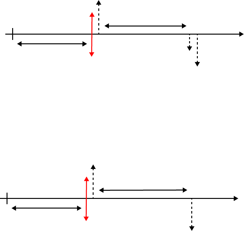
9 Futures
9.1 Forward rate agreement
468 © Wall Street Systems IPH AB - Confidential
BV = rounder (A*D)
where:
D = discount factor
A = nominal amount
rounder depends on instrument rounding parameters
•Cashflows
An FRA is an off-balance sheet instrument, meaning that the principal cashflows never change
hands and are therefore marked as pseudo. When an FRA contract is entered into TRM, the
pseudo cashflows are established in order to calculate market values and interest rate risks.
At the settlement date (when the market interest rate is known and can be compared to the
contractual interest rate), the pseudo cashflows are netted with the settled cashflows, and the
buyer or seller of the FRA either receives or pays the net amount, instead of the full settlement
amount (see 1.8 Processing on page 28 for more information about the netting process).
The figure below illustrates the cashflows which are established in TRM for a purchased FRA
deposit:
where the interest amount is calculated as follows:
rounder (A*(1/D-1))
where:
D = discount factor
A = nominal amount
rounder depends on the instrument’s rounding parameters
The figure below illustrates the cashflows which are established in TRM for a purchased FRA discount
paper:
9.1.1.3 Processing
This section describes the actions that can be done throughout the life of an FRA.
Opening
date Netting
Forward
period
Value
date
Nominal Maturity
period Maturity
date
Interest
Nominal
Opening
date Netting
Forward
period
Value
date
Book
value Maturity
period Maturity
date
Nominal
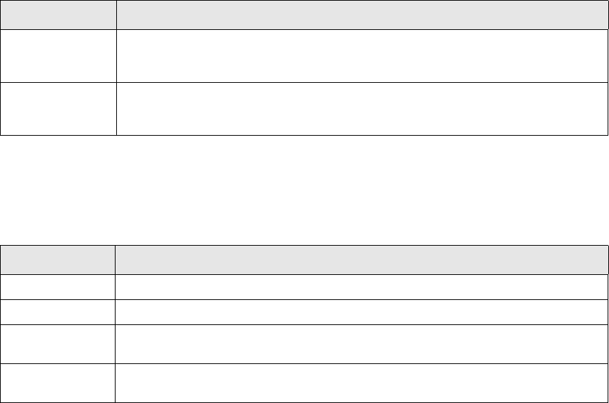
9 Futures
9.1 Forward rate agreement
Transaction & Risk Management Module (TRM) Instruments: Processing and Calculations 469
9.1.1.3.1 Netting
FRAs are not subject to a physical delivery of the underlying at expiry but simply result in the
difference (positive or negative) between the predefined interest rate and the fixing rate of the
underlying at expiry.
At the fixing date, the interest rate of the FRA period is known and the profit or loss for that FRA can
be calculated. For a purchased FRA, if the fixed market rate is higher than the one originally agreed
upon, a settlement amount is received (the profit); but if the fixed interest rate is lower than the
contractual rate, the difference must be paid (the loss).
•Setup
The fixing parameters for FRAs can be defined either at instrument level or at deal entry. Where
the fixing parameters are defined depends on how narrow or open the instrument definition
needs to be:
See A.2.157 Forward Rate Agreement (Deposit) on page 786 and A.2.158 Forward Rate
Agreement (Discount) on page 787.
•Execution
The following information is needed to process the netting:
Retrieving of the Netting Price:
FP = evaluate(expression, date, scenario, ref curve, period)
Calculation of the Netting Amount:
PL = BV-(A + I)*D
where:
BV = book value of the transaction (A for discount and A *D for depo)
A = Nominal Amount
I = Interest Amount (0 for discount and A*(1/D-1) for depo)
D = discount factor for the fixing rate at fixing date
As a result of the Netting action, the netting cashflow’s Not Fixed attribute is unset and the P/L
amount is set.
•Cancellation
Information Description
Closing price
parameters
Yield curve and period, rate scenario, and offset between value date and observation
period for the rate can be defined either at instrument level or when entering the
deal.
Settlement
Parameters
It is possible to define if the netting of the deal is to be paid in a different currency. In
this case, the currency can be defined either at instrument level, or when entering the
deal. If there is a payment offset it must also be defined here.
Information Description
Netting Date Day of netting (Fixing Date of the FRA).
Netting Currency Currency of settlement. (Information only.)
Netting Price Netting (market) interest rate. This is defaulted by the system and can be changed by
the user.
Netting Amount Settlement amount (profit/loss) from the FRA netting. This is calculated automatically
by TRM and can be changed by the user.
9 Futures
9.1 Forward rate agreement
470 © Wall Street Systems IPH AB - Confidential
On a fixed netting cashflow there is an Undo Netting action available. Executing this action
resets the cashflow’s Not Fixed flag and the P/L amount reverts to 0.
9.1.1.3.2 Early expiration
FRAs can be matured earlier than their agreed maturity date by executing the action Early Expiration.
This action is only enabled for transactions that have reached a certain state in the transaction flow.
•Execution
The following information is needed to process the early-expiration:
The execution generates an early expiration transaction with the following attributes:
Transaction sign = opposite of initial transaction
Nominal amount = amount to expire
Rate = early expiration rate
Opening date = date when the early expiration is done
Value date = date when the early expiration is settled
Kind = Early Expiration
The remaining attributes are inherited from the initial transaction.
•Cancellation
You can undo the early expiration by canceling the early expiration transaction.
9.1.1.4 Position monitoring
There are two basic methods for valuation of FRA instruments: Quoted or Theoretical.
9.1.1.4.1 Setup
The valuation approach used for an FRA contract is activated by the presence of the appropriate
feature in the instrument definition: see A.2.160 FRA Valuation on page 789.
•Theoretical valuation method
By default, risk calculation is based on the IR exposure settings defined at the FRA instrument
level, otherwise, it is based on the interpolation settings defined at the yield curve level (IR
Quote and Yield Curve Editor - Interpolation page). See A.2.48 Base IR Exposure Setup on page
732.
For more information about risk calculations, see 2.3 Key-figures on page 112.
Information Description
Opening Date Date when the early expiration is executed. By default, this is today’s date.
Settlement Date Date when the early expiration is settled. This must be earlier than the value date of
the FRA being expired.
Amount to Expire Amount to be early expired. This defaults to the amount still available to be early
expired, taking into account previous partial early expirations.
Expiration Rate Agreed early expiration rate applied over the FRA period to calculate the forward
settlement amount (settlement amount on the original value date).
Discount Rate Rate used to discount the forward settlement amount from FRA value date to the early
expiration settlement date (rate type Interest Rate) to calculate the Net Amount.
Date Basis Date basis used to discount the forward settlement amount from FRA value date to
the early expiration settlement date to calculate the Net Amount.
9 Futures
9.1 Forward rate agreement
Transaction & Risk Management Module (TRM) Instruments: Processing and Calculations 471
•Quoted valuation method
By default, with the Quoted valuation method, the discount factor used to compute the market
value of the Payback flows is calculated as follows:
Equation 9-1 FRA: Quoted valuation method
where
–rq is the market quote of the FRA on the figure valuation date
–D1 is the discount factor computed from the rate type and the data basis of the FRA
–r is the market rate retrieved from the valuation default curve between the valuation date
and the value date of the FRA
–D2 is the discount factor computed from the setup of the valuation default curve.
9.1.1.4.2 Calculations
The numerical examples in this section demonstrate how the different figures are calculated for a
FRA contract.
This example shows a 6M/9M EUR FRA deposit with a 3% Periodic Rate, with the following deal data
•Setup
•Portfolio data
•Transaction data
Data Symbol Example
Instrument Date Basis B Act/360
Instrument Yield Type Periodic
Valuation Method Theoretical
Valuation Date Figure Date
Risk Yield Type Continuous
Risk Date Basis B_r 365
Result IR: AI Method Linear
Result IR: Accrual Method Linear Accrual
Accrual Yield: Interest Type Periodic Rate
Accrual Yield: Date Basis Actual/360
Data Symbol Example
IR Risk Rate e_ir 0.0001
Data Symbol Example
Opening Date dt_o 2002-06-07
Nominal Amount A 1,000,000.00
Book Rate r_b 3%
D1 rqdvdmat
,,()D2 r dvlt dv
,,()×
9 Futures
9.1 Forward rate agreement
472 © Wall Street Systems IPH AB - Confidential
•Calculated transaction data
•Market data on Figure Date
•Market data specific to Short Leg
•Market data specific to Long Leg
•Market data specific to interest flow
•Valuation figures specific to Short Leg
Base Book FX Rate S_b 1.000000
Maturity Date d_m 2003-03-11
Value Date d_p 2002-12-11
Data Symbol Example
Data Symbol Example Formula
Interest Cashflow c_I -7,500 =
-1,000,000*0.03*
0.25
= -A*r_b*t_p
Period t_p 0.25 = (2003-03-11
- 2002-12-11)/360
=(d_m-d_p)/B
Discount Factor D_b 0.992555831 =
1/(1 + 0.25*0.03)
=1/(1+t_p*r_b)
Data Symbol Example Formula
Figure Date d_f 2002-08-15
Data Symbol Example Formula
Value Date dt_vs 2002-12-11
Time to Value Date t_vs 0.323287671 =
(2002-12-11 -
2002-08-15)/365
= (dt_vs-d_f)/B_r
Data Symbol Example Formula
Value Date dt_vl 2003-03-11
Time to Value Date t_vl 0.569863014 =
(2003-03-11 -
2002-08-15)/365
= (dt_vl-d_f)/B_r
Data Symbol Example Formula
Value Date dt_vi 2003-03-11
Time to Value Date t_vi 0.569863014 =
(2003-03-11 -
2002-08-15)/365
= (dt_vi-d_f)/B_r
Data Symbol Example Formula
Amount A_p.s 1,000,000.00 = A
9 Futures
9.1 Forward rate agreement
Transaction & Risk Management Module (TRM) Instruments: Processing and Calculations 473
•Valuation figures specific to Long Leg
Market Value V_s 989,103.63 =
1,000,000.00*
0.989103631365
=A*D_V.s
Clean Market Value V_c.s 0.00 =P_ms
Result Value V_result.s 989,439.34 =
1,000,000.00*
0.989103631365/
0.999660710305
= A*D_V.s/D_s
Market Value Discount Factor D_V.s 0.989103631365
Present Value Discount Factor D_p.s 0.989103631365
Market Value Spot Discount Factor D_s 0.999660710305
Risk Value V_r.s 1,000,000.00 =A
IR Exposure 1bp E_ip -31.98 =
-1,000,000.00*
0.989103631365*
0.323287671*
0.0001
=
-V_r.s*D_p.s*t_vs*0.0001
Effective Duration 0.32328767 =
-(-31.98)/
989,103.63/0.0001
=-E_ip/V_s/0.0001
Modified Duration (total) 0.24560530 =
24.277053/(0.5*
(989,103.63-
(-979,793.24)-
(-7,348.45))
*0.0001)*
0.999660710305
=E_1p.t/(0.5*(V_s-V_l-V_i)
*0.0001)*D_s
Data Symbol Example Formula
Data Symbol Example Formula
Amount A_p.l -990,587.04 =
-979,793.24/
0.989103631365
= V_l/D_V.l
Market Value V_l -979,793.24 =
1,000,000.00*
0.979793242655
= -A*D_V.l
Clean Market Value V_c.l 9,313.55 =P_ml
Result Value V_result.l -989,439.34 =
-1,000,000.00*
0.989103631365/
0.999660710305
= -A*D_V.s/D_s
Market Value Discount Factor D_V.l 0.979793242655
Present Value Discount Factor D_p.l 0.979793242655
Risk Value V_r.l -1,000,000.00 =-A
IR Exposure 1bp E_ipl 55.83 =
-(-1,000,000.00)*
0.979793242655*
0.569863014*
0.0001
= -V_r.l*D_p.l*t_vl*0.0001
9 Futures
9.1 Forward rate agreement
474 © Wall Street Systems IPH AB - Confidential
•Valuation figures specific to interest flow
•Valuation figures specific to transaction
Effective Duration 0.56986301 =
-55.83/-979,793.24
/0.0001
=-E_ipl/V_l/0.0001
Data Symbol Example Formula
Data Symbol Example Formula
Amount A_p.i -7,429.40 =
-7,348.45
/0.989103631365
=V_i/D_V.s
Market Value V_i -7,348.45 =
-7,500.00*
0.9797932427
=c_I*D_V.i
Clean Market Value V_c.i -7,350.94 =P_mi
Result Value V_result.i 0
Market Value Discount Factor D_V.i 0.9797932427
Present Value Discount Factor D_p.i 0.9797932427
Risk Value V_r.i -7,500.00 =c_I
IR Exposure 1bp E_ipi 0.42 = -7,500.00*
0.9797932427*
0.569863014*
0.0001
=-V_r.i*D_p.i*t_vi*0.0001
Effective Duration 0.56986301 =
-0.42/-7,348.45/
0.0001
= -E_ipi/V_i/0.0001
Data Symbol Example Formula
Market Value V 1,961.94 =
989,103.63+
(-979,793.24)+
(-7,348.45)
=V_s+V_l+V_i
Clean Market Value V_c.t 1,962.61 =
0.00+9,313.55+
(-7,350.94)
=V_c.s+V_c.l+V_c.i
IR Exposure 1bp E_1p.t 24.277053 = -31.98
+ 55.83 + 0.42
=E_ip + E_ipl + E_ipi
Effective Duration -123.7400764 =
-(24.277053 /
1,961.91) / 0.0001
=-(E_1p.t/V)/0.0001

9 Futures
9.1 Forward rate agreement
Transaction & Risk Management Module (TRM) Instruments: Processing and Calculations 475
•Result figures specific to Short Leg
Note: The way the result is set for the instrument impacts the way result figures are computed.
In this case, the Book Value Method has been set to None.
•Result figures specific to Long Leg
Note: The way the result is set for the instrument impacts the way result figures are computed.
In this case, the Book Value Method has been set to None.
•Result figures specific to interest flow
Note: The way the result is set for the instrument impacts the way result figures are computed.
In this case, the Book Value Method has been set to None.
Data Symbol Example Formula
Total Profit P_ts -335.71 =
989,103.63 -
989,439.34
= V_s - V_result.s
MtoM Profit P_ms 0.00
Other Profit P_os -335.71 = -335.71 -
0.00
=P_ts - P_ms
Data Symbol Example Formula
Total Profit P_tl 9,646.10 =
-979,793.24 -
(-989,439.34)
= V_l - V_result.l
MtoM Profit P_ml 9,313.55 =
1,000,000.00 *
(0.989103631365 -
0.979793242655)/
0.999660710305
= A * (D_V.s - D_V.l) /D_s
Other Profit P_ol 332.55 = 9,646.10
- 9,313.55
=P_tl - P_ml
Data Symbol Example Formula
Total Profit P_ti -7,348.45 =V_i
MtoM Profit P_mi -7,350.94 = -7,500
*0.9797932427/
0.999660710305
=c_I*D_V.i/D_s
Other Profit P_oi 2.49 = -7,348.45 -
(-7,350.94)
=P_ti-P_mi
9 Futures
9.1 Forward rate agreement
476 © Wall Street Systems IPH AB - Confidential
•Result figures specific to the transaction
Note: The way the result is set for the instrument impacts the way result figures are computed.
In this case, the Book Value Method has been set to None.
9.1.2 Australian FRA
The following section describes the characteristics that are specific to Australian FRA contracts.
9.1.2.1 Instrument setup
•Main characteristics
Note that Australian FRAs must be set up using the FRA (Discount) primary feature.
See A.2.158 Forward Rate Agreement (Discount) on page 787.
9.1.2.2 Deal capture
9.1.2.2.1 Input data
A deal involving an Australian FRA is entered in the same way as a standard FRA: see 9.1.1.2 Deal
capture on page 467.
9.1.2.2.2 Generated data
For a purchased Australian FRA, the principal cashflows are calculated as follows:
•At value date:
where:
rc = contract rate
t = number of days between value date and maturity date
N = nominal amount
•At maturity date:
Principal flow = -N
Data Symbol Example Formula
Total Profit 1,961.94 = -335.71
+ 9,646.10 +
-7,348.45
= P_ts + P_tl + P_ti
MtoM Profit 1,962.61 = 0.00 +
9,313.55 +
-7,350.94
= P_ms + P_ml + P_mi
Other Profit -0.67 = -335.71 +
332.55 + 2.49
= P_os + P_ol + P_oi
Information Description
Currency Currency of the Australian FRA-AUD.
Date Basis Date basis of the Australian FRA-Act/365.
Interest Type Interest rate type of the Australian FRA-Periodic Rate.
NNr
c
×t 365⁄×
1r
ct 365⁄×+
-----------------------------------
–

9 Futures
9.1 Forward rate agreement
Transaction & Risk Management Module (TRM) Instruments: Processing and Calculations 477
Therefore, at value date, the settlement amount (A) is calculated by discounting these cashflows
to the value date:
where:
r = the fixed market interest rate from value date to maturity date
9.1.3 Swedish FRA
In Sweden, FRA and bond forwards are traded on the Nasdaq/OMX exchange. These contracts are
fixed every month-end and settled shortly after, up until the last fixing, which is settled on the third
Wednesday of March, June, September, or December.
Settlement of month-end fixings is three business days after fixing. For the final fixing, i.e. on the
underlying value date, the settlement date equals fixing date.
The underlying value date is the 3rd Wednesday of March, June, September, or December, and the
underlying maturity date is the 3rd Wednesday three months later.
9.1.3.1 Instrument setup
Swedish FRA instruments must be based on an instrument type derived from the class FRA.
•Main characteristics
The setup of Swedish FRA is similar to standard FRAs except for the following:
See A.2.159 Forward Rate Agreement (Swedish) on page 788.
9.1.3.2 Deal capture
9.1.3.2.1 Input data
A deal involving an Swedish FRA is entered in the same way as a standard FRA except that fields
related to fixing rate at the transaction level (Fixing Rate/Period) are not mandatory: see 9.1.1.2.1
Input data on page 467.
9.1.3.2.2 Generated data
The generated data for a Swedish FRA are similar to those of a standard FRA.
For Swedish FRA, netting cashflows that are fixed every end of month until the last fixing date (i.e.
the value date) are created at deal entry and set to Not Fixed.
9.1.3.3 Processing
This section describes the actions that can be done throughout the life of an FRA.
9.1.3.3.1 Netting
•Execution
ANr
cr)t 365⁄×–(×
1r
ct 365 )1 r t 365 )⁄×+(×⁄×+(
------------------------------------------------------------------------------------
=
Information Description
Currency SEK
Date Basis Date basis of the Swedish FRA: Actual/360.
Interest Type Interest rate type of the Swedish FRA: Periodic Rate.
9 Futures
9.1 Forward rate agreement
478 © Wall Street Systems IPH AB - Confidential
Right-click a Not Fixed netting cashflow and select Execute Netting. The following window is
displayed:
As with standard FRAs, the netting cashflow’s Not Fixed attribute is unset and the P/L amount is
set as follows:
Equation 9-2 Swedish FRA: Netting - BookReferenceValue calculation
Equation 9-3 Swedish FRA: Netting - Amount calculation
where PreviousValue is the value of the previous netting flow, if it exists, otherwise the
PreviousValue is the sum of the Payback flow amounts (i.e. book value + contractual interest).
At the first month end fixing of a transaction, the exchange fee cashflow is generated as follows:
Equation 9-4 Swedish FRA: Netting - Exchange fee cashflow
•Cancellation
You can cancel the netting either by using the Undo Netting action, or by using the Netting - Undo
activity.
9.1.3.4 Position monitoring
The valuation of Swedish FRA is similar to the valuation of standard FRAs except that Swedish FRAs
use the Quoted valuation method. See 9.1.1.4 Position monitoring on page 470.
Information Description
Netting Date Day of netting (Fixing Date of the FRA).
Netting Currency Currency of settlement. (Information only.)
Netting Rate Defaults to the quotation of the FRA instrument on the netting date.
Discount Rate Defaults to the rate between netting date and value date of the FRA. This rate
is taken from the discount yield curve specified in the netting setup. If no
curve is specified, the curve defined at the currency level is used.
Netting Amount Settlement amount (profit/loss) from the FRA netting. This is calculated
automatically by TRM and can be changed by the user.
First Time Fee Rate First time fee percentage defaults to the value specified at the instrument
level (Instrument Editor’s Netting page). This is only editable on the first
netting flow.
BookReferenceValue PaybackCFi
1 NettingPrice dmat i,dvi,
–
360
-----------------------------
⎝⎠
⎛⎞
×+
-------------------------------------------------------------------------------------
i
∑
=
Amount Value PreviousValue–
1 DiscountRate dvdpay
–
360
-------------------
⎝⎠
⎛⎞
×+
⎝⎠
⎛⎞
-----------------------------------------------------------------------------------
=
Amount Abs A()– FirstTimeFeePercent×
1 DiscountRate dvdpay
–
360
-------------------
⎝⎠
⎛⎞
×+
⎝⎠
⎛⎞
--------------------------------------------------------------------------------------
=
9 Futures
9.2 Bond forward
Transaction & Risk Management Module (TRM) Instruments: Processing and Calculations 479
9.2 Bond forward
Forward bonds are normally traded over-the-counter and are agreements that fix the yield or price
on a specified bond for a specific date in the future. When the deal is made, the type of bond, the
amount, maturity and the value date are agreed upon.
In some capital markets, forward bonds have become instruments in their own right, so-called
synthetic bonds. Synthetic bonds are usually constructed with special features, but commonly there
are underlying instruments, such as Treasury Bonds. These synthetic bonds are quoted at the
market and they can be traded until a particular date.
When the contract/issue expires, the difference between the contractual price and the market price
is settled and the settlement amount is paid or received.
For more information relating to the setup and structure of specific types of bond forwards, see:
•9.2.1 Bond forward on page 479
•9.2.2 Swedish Bond forward on page 482
9.2.1 Bond forward
Bond forward instruments must be based on an instrument type derived from the class
BOND-FORWARD.
9.2.1.1 Instrument setup
The following basic information may be captured when defining the instrument. This information is
relevant to any kind of bond forward instrument.
•Main characteristics
•Netting information
See A.2.61 Bond Forward on page 739.
Information Description
Issuer Client reflected as the Issuer of the transactions, e.g. the exchange or the clearing
house.
Counterparty Client reflected as the Counterparty of the transactions, e.g. the clearing house or
the broker.
Underlying Underlying bond instrument.
Currency Currency in which the instrument is traded.
Information Description
Fixing Offset Number of days’ offset allowed, that is, the difference in days between the fixing
date and the due date (default = 0).
Fixing Max Offset Maximum number of days’ offset allowed.
Fixing Subscenario Subscenario from which the rate is retrieved.
Calendar Calendar to use when calculating the fixing date.
Payment Offset Number of business days between value date and payment date.
Method
Frequency
Choose when you want the netting to occur. For example, for daily netting, select
Business Days as method and 1 as frequency.
9 Futures
9.2 Bond forward
480 © Wall Street Systems IPH AB - Confidential
•Last fixing and settlement dates
See A.2.63 Bond Forward Dates on page 741
It is also possible to set up
•Trading yield convention (used to convert price/rate at transaction level)
•dates.
9.2.1.2 Deal capture
9.2.1.2.1 Input data
In addition to standard deal parameters, the following information is required to enter a bond future
transaction:
Note: When you enter the deal rate or deal price, the other is computed according to the trading
yield convention defined at the instrument level.
Note: The secondary instrument is defaulted with underlying instrument entered at bond forward
instrument level.
9.2.1.2.2 Generated data
The following cashflows are generated:
•Cashflows (pseudo) of underlying bond (interest + redemption)
•Netting flow according to Netting setup and the value date of the transaction.
•Principal cashflow (pseudo) computed as
Nominal Amount * Deal Rate in %.
Information Description
Last Trading Day Last day the instrument can be traded.
Settlement Date Last day on which the cash settlement can take place.
Information Description
Deal Rate The interest rate at which the deal is made (contract rate).
Deal Price The market price of the underlying bond, expressed as a % of the nominal amount.
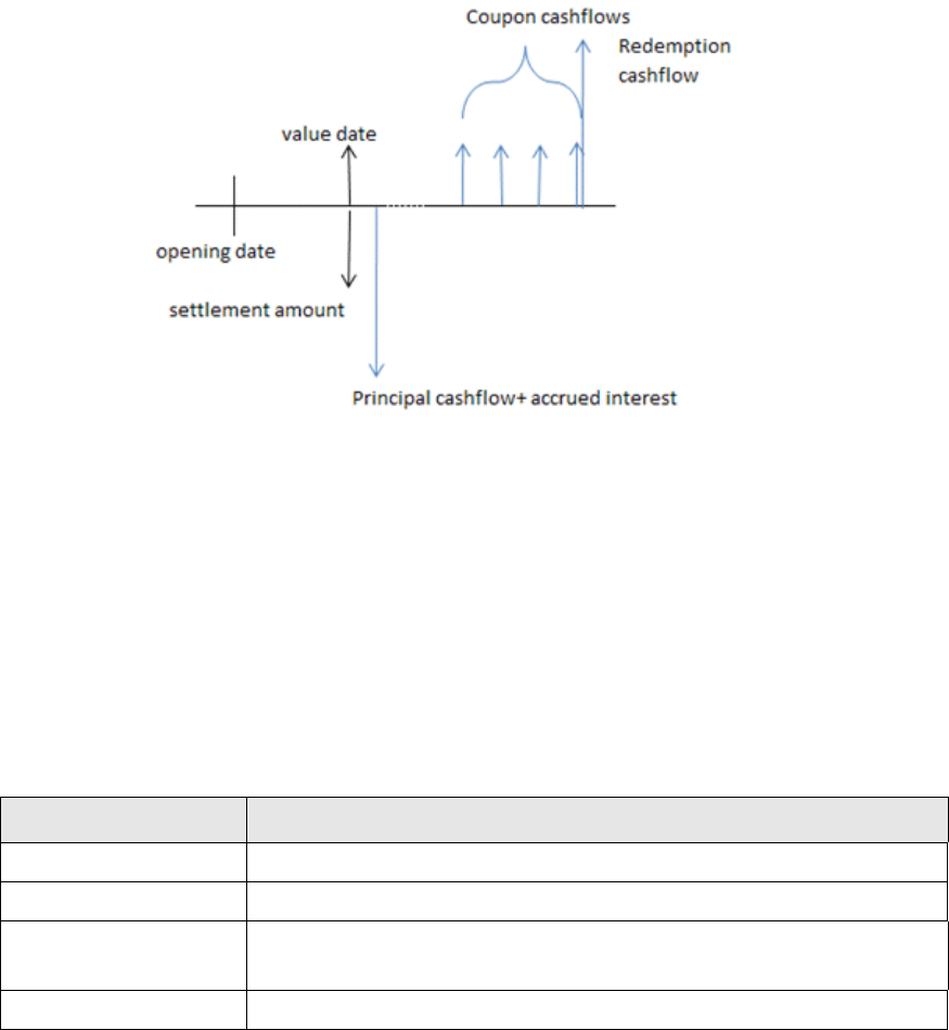
9 Futures
9.2 Bond forward
Transaction & Risk Management Module (TRM) Instruments: Processing and Calculations 481
The following cashflow structure is generated for a bond forward:
9.2.1.3 Processing
This section describes the actions that can be done throughout the life of a bond forward.
9.2.1.3.1 Netting
•Setup
The netting parameters for bond forwards are defined at instrument level.
•Execution
Right-click a Not Fixed netting cashflow and select Execute Netting. The resulting dialog displays the
following information:
Click OK.
The Not Fixed attribute is removed and the netting amount is computed as follows:
NettingAmount = NominalAmount*(Netting Price%-DealPrice%)/100
•Cancellation
On a fixed netting cashflow there is an Undo Netting action available. Executing this action resets
the cashflow’s Not Fixed flag and the P/L amount reverts to 0.
9.2.1.4 Position monitoring
There are two basic methods for the valuation of Bond forward instruments: Quoted or Theoretical.
Information Description
Netting Date Day of netting (Fixing Date of the bond forward).
Netting Currency Currency of settlement. (Information only.)
Netting Rate
Netting Price
When updating one of these fields, the other is computed according to bond
forward trading yield convention.
Netting Amount Settlement amount (profit/loss) from the bond forward netting parameters.
9 Futures
9.2 Bond forward
482 © Wall Street Systems IPH AB - Confidential
9.2.1.4.1 Setup
The valuation approach is activated by attaching the Bond Forward Valuation
(BOND-FORWARD-METHOD) feature to the instrument, see A.2.64 Bond Forward Valuation on page
741.
•Theoretical: Uses the zero coupon approach, i.e. the interest rate corresponding to the
maturity of the cashflow is used to discount from the cashflow date to the figure date and to
compute market value.
–Quoted: If the bond forward is quoted, then the market quote is used to discount the
underlying cashflows from their value date to the bond forward value date (according to the
trading yield convention), then the valuation interest rate is used to discount from the value
date to the figure date. Each cashflow of bond forward is discounted by:
Equation 9-5 Bond forward: Quoted method - Discount factor
Where
–rq is the market quote of the bond forward on figure date
–D1 is the discount factor computed according to the rate type and date basis of the trading
yield convention
–r is the market rate retrieved from the valuation default curve
–D2 is the discount factor computed according to the setup of valuation default curve.
9.2.2 Swedish Bond forward
Swedish Bond forwards are cash settled on a periodic basis. In practice, this means that all future
positions are marked-to-market for monthly cash settlement using a market yield determined on
the final business day of each month. The accumulated profit and loss are settled on the third
business day after.
Swedish bond forward instruments must be based on an instrument type derived from the class
BOND-FORWARD.
9.2.2.1 Instrument setup
The instrument setup is similar to standard bond forwards except that you select the Bond Forward
(Swedish) primary feature and except for the following:
•Main characteristics
•Netting parameters
D1 rqdvdmat
,,()D2 r dvlt dv
,,()×
Information Description
Currency Currency in which the instrument is traded.
Information Description
Fixing Offset Number of days’ offset allowed, that is, the difference in days between the fixing
date and the due date (default = 0).
Fixing Max Offset Maximum number of days’ offset allowed.
Fixing Subscenario Subscenario from which the rate is retrieved.
9 Futures
9.2 Bond forward
Transaction & Risk Management Module (TRM) Instruments: Processing and Calculations 483
See A.2.62 Bond Forward (Swedish) on page 740.
It is also possible to set up
•Trading yield convention (used to convert price/rate at transaction level)
•dates.
9.2.2.2 Deal capture
9.2.2.2.1 Input data
The data required is the same as for a bond forward (see 9.2.1 Bond forward on page 479).
9.2.2.2.2 Generated data
Netting cashflows that are fixed every month-end up until the last fixing date (i.e. the value date)
are created at deal entry and set to Not Fixed.
9.2.2.3 Processing
9.2.2.3.1 Netting
•Setup
The netting parameters for bond forwards are defined at instrument level.
•Execution
Right-click a Not Fixed netting cashflow and select Execute Netting. The resulting dialog displays the
following information:
Calendar Calendar to use when calculating the fixing date.
Switches Activate the switches that apply to the instrument.
•Settlement Currency - switch on if the P/L cashflow is paid in a different currency.
Settlement Currency Currency in which the P/L cashflow is paid (if the switch Settlement Currency is
switched on).
Leave this field blank if you want to specify the settlement currency when you enter
the deal.
Payment Offset Number of business days between the value date and the payment date (should be
3 for a Swedish Bond forward).
Discount Rate Rate used to discount settlements between the value date and the netting date
(used to default the discount rate when performing netting).
Leave this field blank if you want to specify the discount rate when performing
netting.
Method (Read-only.) Defaults to Last of Month.
First Time Fee Rate Fixed percentage of the nominal amount, which will be discounted back from the
underlying value date to the payment date with the discount rate. This fee amount
is settled on the first netting flow.
Leave this field blank if you want to specify the first time fee rate when performing
netting.
Information Description
Information Description
Netting Date Day of netting (Fixing Date of the bond forward).
Netting Currency Currency of settlement. (Information only.)
9 Futures
9.2 Bond forward
484 © Wall Street Systems IPH AB - Confidential
Click OK.
The Not Fixed attribute is removed and the P/L amount is computed as follows:
Equation 9-6 Swedish bond forward: P/L amount calculation
Where
Where discount factor (D) is computed according to the rate type/date basis of the trading yield
convention defined at the underlying instrument level.
Where Previous value is the value of the previous netting flow, if it exists, otherwise, the deal
price of the transaction is used
DealPrice%*NominalAmount/100
The first time you perform the Netting action on a transaction, the exchange fee cashflow is
computed as follows:
Equation 9-7 Swedish bond forward: Exchange Fee calculation
•Cancellation
On a fixed netting cashflow there is an Undo Netting action available. Executing this action resets
the cashflow’s Not Fixed flag and the P/L amount reverts to 0.
9.2.2.4 Position monitoring
The valuation setup for Swedish bond forwards is the same as for standard bond forwards, see
9.2.1.4 Position monitoring on page 481.
Netting Price Defaulted to the quotation of the instrument on the netting date.
Discount Rate Defaulted to the rate between netting date and value date of the transaction.
This rate is taken from the discount yield curve specified in netting setup.
If empty, the default curve from currency editor is used instead.
First Time Fee Expressed as a percentage, and editable for the first netting flow, otherwise it
is not modifiable and defaults to the value specified in the netting setup
(Netting page) at the instrument level.
Information Description
Vbook VPrev
–()Drd
pay dv
,,()×
Vbook PaybackCFiDr
net dvdiv
,,()×
i
∑
Abs A()– FirstTimeFeepercent
×Drd
pay dv
,,()×
9 Futures
9.3 Money market future
Transaction & Risk Management Module (TRM) Instruments: Processing and Calculations 485
9.3 Money market future
A money market (MM) futures contract is an agreement to buy or sell a standard quantity of a
specific financial instrument or deposit, on an Exchange, at a price agreed between two parties, and
with delivery to be executed on a standard future date. The size and direction of the settlement
amount depends on a given short-term interest rate on the settlement date, a few days before the
value date.
An MM futures contract is based on an interbank deposit rate. Its value rises and falls inversely to
changes in interest rates.
The contract amount is expressed in trading units (contract size), where the size of the unit depends
on the type of the contract. For example, the unit size of the three month sterling (Short Sterling)
money market future is £500,000.
Typically there is an initial margin requirement (entered as a payment in TRM) when buying or
selling futures contracts but no principal is paid. The principal amount is notional. The changes in
market value are often settled daily (netted) during the period between the transaction date and the
value date. This means that the market rate underlying the calculation of the settlement amount
must be fixed for the future contracts every day (daily settlement).
Quotations for MM future prices are given as 100-r, where r is the underlying forward interest rate.
There is a minimum price movement (tick size) and the associated value. For example, for Short
Sterling the tick size is 0.01 and the tick value £12.50.
There are several reasons why you would take a position in futures:
•Hedging exposures
A futures contract can be used to fix a price for a transaction to be carried out on a specific
future date, for example to set a price for the purchase of a commodity or the sale of a financial
instrument. If the hedger suffers a loss in the underlying cash market (either pays more than
expected when purchasing or receives less than expected when selling), then the futures
contract will compensate the hedger for the loss suffered in the cash market.
•Speculating on price movements
Commonly referred to as ‘Trading’, traders can use futures contracts to back up their views on
price movements. Futures prices vary with the underlying cash market. If the speculator
correctly predicts the direction and magnitude of price changes, the speculator will make a profit
in the futures market. An incorrect view on price movements will however result in a loss in the
futures market.
•Arbitraging
Traders use futures to exploit price anomalies to make risk-free profits.
9.3.1 Money market future (single contract)
Money market future (single contract) include the following money market future instruments:
•9.3.1.1 MM future on page 485
•9.3.1.2 Australian bank bill future on page 494
•9.3.1.3 Fed fund future on page 496.
9.3.1.1 MM future
MM future instruments must be based on an instrument type derived from the class MM-FUTURE.
9 Futures
9.3 Money market future
486 © Wall Street Systems IPH AB - Confidential
9.3.1.1.1 Instrument setup
•Main characteristics
The following basic information may be captured when defining the instrument. This information
is relevant to any kind of MM future instrument.
•Trading units definition
•Netting information
The daily change in market value (pseudo cashflows) is settled every day (netted) until the
contract is closed or it expires.
See A.2.231 MM Future on page 827.
•Future dates definition
Information Description
Issuer The client reflected as the Issuer of the transactions, e.g. the exchange or the
clearing house.
Counterparty The client reflected as the Counterparty of the transactions, e.g. the clearing house or
the broker.
Currency The currency in which the instrument is traded.
Information Description
Contract Size Standard size of the futures contract (for example, 1,000,000).
Minimum Bid Size Smallest allowed bid size. This is typically 1.0 (meaning 1 contract).
Tick Size
Tick Value
Minimum price movement (tick size and value), for example, 0.005 / 12.50.
Tick Size * Point Value = Tick Value
Rounding Method Rounding method used in the calculations: Up, Down, or Nearest.
Allow Trading in
Half of Tick Size
Allows trading this instrument at a price with a precision of half the tick size (used for
eurodollar Future contracts and options for nearest expiring month).
Information Description
Fixing parameters Leave these fields blank if you want to define the fixing parameters at deal entry.
Calendar Calendar used to calculate the dates.
Switches Switch on Settlement Currency if settlement is made in a different currency.
Settlement
Currency
If the Settlement Currency switch is on, the currency in which settlement is made.
Payment Offset Number of business days between value date and payment date. This must be the
same as the value for Spot Days on the page Spot Date Setup.
Method
Frequency
Choose when you want netting to occur. For example, for daily netting, select Business
Days as method and 1 as frequency.
Information Description
Last Trading Day Last day when the futures contract can be traded.
The final day during which trading may take place in a futures contract, after which it
must be settled.
9 Futures
9.3 Money market future
Transaction & Risk Management Module (TRM) Instruments: Processing and Calculations 487
See A.2.238 MM Future Dates on page 832.
•Quotation information
See A.2.274 Quoted on page 849.
It will then be possible to either enter the quotation manually in Rate Monitor, or get it
automatically in real time.
See the TRM User Guide for information about Rate Monitor.
•Valuation of money market futures
It is possible to specify that another MtoM instrument’s direct market quotation is used to value
the future instrument.
See A.2.246 MtoM Instrument Setup on page 836.
It is also possible to set up
•Spot date calculation
•Cashflow or transaction charge rules
•Manual charges
•Branch codes.
See Appendix A Features on page 713.
9.3.1.1.2 Market information
One future contract corresponds to a given nominal value, known as the contract size (trading unit).
The market quotation is given in terms of percentage, which moves by ticks, the minimum possible
movement.
The tick value is the change in settlement price corresponding to a movement of one tick (assumed
to be one basis point, 0.01%) in the quote. This variable is derived from the length of the period of
the MM future.
For example, Short Sterling has a tick value of £500,000 * 0.25 * 0.0001 = £12.50
The risk and profit/loss valuation of all outstanding futures contracts are recalculated using the most
recent market data. Each instrument is revalued according to its real-time market quote.
These real-time market feeds, from Reuters for example, are set up in the Market Info Source
Editor: see the TRM User Guide.
Settlement Date Last day on which delivery (cash settlement) of the underlying instrument can take
place.
Maturity Date Underlying maturity (last trade date plus contract period length).
Information Description
Active From
Active To
Period within which the quotation information is valid.
Leave these fields blank if you want the quotation information to apply indefinitely.
Price Type Standard method for quoting the price.
For an MM future, usually, the quotation is 100 minus the forward rate.
Quote Handling Select Generic (which means that you will be able to enter the bid and ask quotes for
this instrument).
Currency Currency of the future instrument.
Information Description
9 Futures
9.3 Money market future
488 © Wall Street Systems IPH AB - Confidential
IR quotes are shown as Bid and Ask in Rate Monitor. TRM uses the average of these two quotes; if
the Ask side is empty it is ignored and the Bid rate is used instead, and vice versa.
9.3.1.1.3 Deal capture
Input data
In addition to the standard deal parameters, the following information is required to enter a money
market future contract:
Generated data
Two cashflows are generated:
–One position flow which represents the future position.
–The next netting flow (not fixed) which will be the support for the next daily margin once
fixed (see Daily netting on page 488).
9.3.1.1.4 Processing
This section describes the actions that can be done throughout the life of a money market future.
Daily netting
This section describes the actions that can be done throughout the life of a money market future.
Money market futures are not subject to a physical delivery of the underlying at expiry but are
typically fixed every day. If the market quote for the future has changed from the previous day, the
difference (multiplied by the point value and the number of units) is settled between the parties of
the trade.
•Setup
The netting parameters for money market futures are defined at instrument level.
•Execution
The daily netting of money market futures is carried out using the Execute Netting action. The
following information is needed to process the netting:
The Execute Netting action automatically generates the next cashflow.
Information Description
Trading Units Number of futures bought/sold.
Deal Price Contractual rate of the deal expressed as a percentage (100 – r) where r is the
underlying deal interest rate.
Information Description
Netting Date (Information only)
The value date of the cashflow.
Netting Price Fixing market quote.
This is defaulted by the system and can be changed by the user.
Netting Amount The automatically calculated profit or loss from the future (settlement amount).
Automatically adjusts if you modify the netting price.
This can be changed by the user.
Netting Currency (Information only)
Currency of the settlement cashflow.

9 Futures
9.3 Money market future
Transaction & Risk Management Module (TRM) Instruments: Processing and Calculations 489
Netting of the cashflows can also be performed automatically using the Netting activity: see the
TRM User Guide for more information about activities.
•Cancellation
The netting can be canceled either using the Undo Netting action, or using the Netting - Undo
activity.
Closing the position
Closing out a position means entering a trade that is opposite to the original one. Closing of a
futures position takes place when the holder of a short position buys, or a long position sells, new
contracts, which are matched with old ones. The transactions may not have been fixed before the
matching. If not, matching the trades creates a profit/loss cashflow to account for the price
difference between transactions.
Note: Netting must be done before the end of day on the day of the sale.
Matching
•Setup
–The selling parameters used to automatically match transactions are specified in the result
treatment applied to the instrument definition.
–The portfolio must have the Allow Short Selling switch activated.
See the TRM User Guide for more information.
•Execution
Automatic matching of transactions occurs each night with the End of Day Processing activity.
Manual matching of futures is done in Transaction Manager’s Matching mode. This option is
available if you specified Manual or FIFO as the selling method for the instrument.
•Cancellation
You can also unmatch transactions in Transaction Manager’s Matching mode if the cashflows
resulting from the transactions are not yet paid or booked.
See the TRM User Guide for more information about matching and unmatching transactions.
9.3.1.1.5 Position monitoring
This section describes the valuation and risk calculations of MM futures.
Valuation
The market value of MM Futures is calculated as follows:
V = n * V_tic * (F - p_d) / s_t * D_s
Where
n Trading units
V_tic Tick Value
F Market Quote
p_d Deal Price
s_t Tick Size (%)
D_s Spot Discount Factor
9 Futures
9.3 Money market future
490 © Wall Street Systems IPH AB - Confidential
Risk
There are two methods for the IR Exposure and Modified Duration calculation of Money Market
instruments: Default and Par method.
•Default
The default valuation setup for a Money Market future instrument uses the valuation feature MM
Future Method (A.2.243 Money Market Future Valuation on page 834 on page 593) and the
Quoted valuation method. Using the default valuation setup, the Modified Duration key figure is
based on IR Exposure 1 bp, which in turn is calculated by estimating the sensitivity of a
position's market value to a parallel shift of 1 basis point in the zero curves used for the
valuation of the position. See section Calculations - Quoted valuation method on page 492 for
examples of these calculations.
–Default Method: IR Exposure 1bp
E{i1}= E_ir.s + E_ir.e
where
E_ir.s =IR Exposure 1bp at value Date = dV.dD_s * d_D.s * 0.0001
where
E_ir.e =IR Exposure 1bp at Maturity Date = dV.dD_e * d_D.e * 0.0001
where
dV.dD_s Risk Value at Value
Date
= -n * V_tic * 100 / (t_p * s_t * D_p.e)
where n Trading units
V_tic Tick Value
t_p Period length from Value date until Maturity Date according to
the Date Basis = (d_m - d_v) / B
s_t Tick Size (%)
s_t entered as a real number, for example, if you enter a bp tick
size of 1, it is interpreted as 0.0001
D_p.e PV Discount Factor at Maturity Date.
d_D.s Sensitivity of Discount
Factor at Value Date
= -D_p.s * t_v.s
where D_p.s PV Discount Factor at Value Date
t_v.s Time to Risk Date at Value Date
dV.dD_e Risk Value at Maturity
Date
n * V_tic * 100 * D_p.s /(t_p * s_t * D_p.e * D_p.e)
where n Trading units
V_tic Tick Value
D_p.s PV Discount Factor at Value Date
t_p Period length from Value Date until Maturity Date relative to the
Date Basis = (d_m - d_v) / B
9 Futures
9.3 Money market future
Transaction & Risk Management Module (TRM) Instruments: Processing and Calculations 491
–Default Method: Modified Duration
U_mod = 10000 × E{i1}/ (V_p.s + V_p.e)
where
•Par
It is also possible to use the Par method for the valuation of Money Market future instruments.
You can use this method by attaching the features MM Future Par Method (A.2.242 Money
Market Future Par Valuation on page 834) and Base IR Exposure Setup (A.2.48 Base IR
Exposure Setup on page 732) to the MM future instrument and configuring IR Exposure as
follows:
This method calculates the IR exposure 1bp and Modified Duration figures as follows:
–Par method: IR Exposure 1bp
Equation 9-8 Par method: IR exposure 1bp
where
s_t Tick Size (%)
s_t entered as a real number, for example, if you enter a bp tick
size of 1, it is interpreted as 0.0001
D_p.e PV Discount Factor at Maturity Date
d_D.e Sensitivity of Discount
Factor at Maturity
Date
-D_p.e * t_v.e
where D_p.e PV Discount Factor at Maturity Date
t_v.e Time to Risk Date at Maturity Date
E{i1} IR Exposure 1bp
The average of the present value components: 0.5 or 1 depending on the number of
present value components. In the case of MM Future, = 0.5 as the average is between
the present value at Value Date, and the present value at Maturity Date
V_p.s The present value of the position cashflow at Value Date
V_p.e The present value of the position cashflow at Maturity Date
Information Description
Date Basis Actual/365
Yield Type Continuous Yield
n Trading units
S The FX rate between the currency of the contract and the valuation currency.
ϕ
ϕϕ
ϕ
Ei1{} nS–V
tic
0.0001
st
----------------
×=
9 Futures
9.3 Money market future
492 © Wall Street Systems IPH AB - Confidential
–Par method: Modified Duration
Equation 9-9 Par method: Modified Duration NEW
where
Calculations - Quoted valuation method
The numerical examples in this section demonstrate how the different figures are calculated for an
MM Future using the Quoted valuation method.
This example shows an MM Future, with the following deal data:
•Instrument data
•Transaction data
V_tic Tick Value
s_t Tick Size (%)
s_t entered as a real number, for example, if you enter a bp tick size of 1, it is
interpreted as 0.0001
V_tic Tick Value
s_t Tick Size (%)
A Nominal Amount
Data Symbol Example Formula
Contract Size u 1,000,000.00
Tick Size s_t 0.005
Tick Value V_tic 12.5
Maturity Date d_m 2007-03-15
Value Date d_v 2006-12-15
Period Length t_p 0.246575342 =
(2007-03-15 - 2006-12-15)/365
t_p =
(d_m - d_v) / B_y
Valuation Method Quoted
(Risk) Date Basis B Act/365
Interpolation Date Basis B_y Act/365
(Risk) Yield Type Continuous
Data Symbol Example Formula
Opening Date 2005-07-13
Tradi ng un its n 1.00
Deal Price p_d 94.00
Umod
vtic
stA×
--------------
=
9 Futures
9.3 Money market future
Transaction & Risk Management Module (TRM) Instruments: Processing and Calculations 493
•Calculated transaction data
•Market data
•Valuation figures
•Result figures
The setup of the instrument impacts the way result figures are computed.
•Risk figures
–Start date
Data Symbol Example Formula
Nominal Amount A 1,000,000.00 =
1.00 * 1,000,000.00
A = n * u
Data Symbols Example Formula
Figure Date d_f 2006-06-27
Market Quote F 95.00
Spot Discount Factor D_s 0.9998561266
PV Discount Factor - Start D_p.s 0.9859568019
PV Discount Factor - End D_p.e 0.9777229960
Time to Risk Date - Start t_v.s 0.4684931507 =
(2006-12-15 - 2006-06-27)/365
t_v.s = (d_v -d_f) / B
Time to Risk Date - End t_v.e 0.7150684932 t_v.e = (d_m - d_f) / B
Data Symbol Example Formula
Market Value V 2,499.64 =
1.00 * 12.5 * (95.00 – 94.00) /
0.005 * 0.9998561266
V =
n * V_tic * (F - p_d) /
s_t * D_s
Data Symbol Example Formula
Total Profit Total_Profit = 2,499.64 Total_Profit = V
MtoM Profit MtoM_Profit 2,500.00 =
2,499.64 / 0.9998561266
MtoM_Profit = V / D_s
Other Profit -0.36 = 2,499.64 - 2,500.00 = Total_Profit - MtoM_Profit
Data Symbol Example Formula
Sensitivity of D d_D.s -0.46 =
-0.9859568019 * 0.4684931507
d_D.s = -D_p.s * t_v.s
Risk Value dV.dD_s -1,036,989.92 =
-1.00 * 12.5 * 100 /
(0.246575342 * 0.005 *
0.9777229960)
dV.dD_s =
-n * V_tic * 100 /
(t_p * s_t * D_p.e)
IR Exposure 1bp E_ir.s 47.90 =
-1,036,989.92 *
(-0.46) * 0.0001
E_ir.s =
dV.dD_s *
d_D.s * 0.0001
9 Futures
9.3 Money market future
494 © Wall Street Systems IPH AB - Confidential
–End date
–Total
Calculations - Par method
The default IR exposure calculations follow the theoretical approach described in Calculations -
Quoted valuation method on page 492. An alternative is to choose the feature Money Market Future
Par Valuation, as described in section Valuation on page 489, in which case, market value is
calculated as above, but IR exposure is calculated as follows:
•Instrument data
•Transaction data
•Valuation figures
Note: You can view these figures in Transaction Manager and Treasury Monitor.
9.3.1.2 Australian bank bill future
Australian short futures have 90-day Bank Accepted Bills (bank bills) as the underlying. The market
in these instruments is the biggest short-term interest rate market in Australia.
Quotations for 90-day bank bill futures are given as 100 - yield% per annum. This yield-to-maturity
formula discounts the face value (contract size) to earn the correct interest cost. For example, a
yield of 6.85% equals a futures price of 93.15.
Data Symbol Example Formula
Sensitivity of D d_D.e -0.70 =
-0.9777229960 * 0.7150684932
d_D.e = -D_p.e * t_v.e
Risk Value dV.dD_e 1,045,722.83 =
1.00 * 12.5 * 100 *
0.9859568019 / (0.246575342 *
0.005 * 0.9777229960 *
0.9777229960)
dV.dD_e =
n * V_tic * 100 *
D_P.s /
(t_p * s_t * D_p.e * D_p.e)
IR Exposure 1bp E_ir.e -73.11 =
1,045,722.83 * (-0.70) * 0.0001
E_ir.e =
dV.dD_e * d_D.e * 0.0001
Data Symbol Example Formula
IR Exposure 1bp E_ir.t -25.21 = 47.90 + -73.11 E_ir.t = E_ir.s + E_ir.e
Data Symbol Example Formula
Contract Size A 1,000,000.00
Tick Size (%) s_t 0.005
Tick Value V_tic 12.5
Data Symbol Example Formula
Number of Contracts N 3
Data Symbol Example Formula
IR Exposure 1bp E_i1 = -75.0000 =-N*V_tic*0.0001/s_t
Modified Duration U_mod = 0.250 =V_tic/(s_t*A)
9 Futures
9.3 Money market future
Transaction & Risk Management Module (TRM) Instruments: Processing and Calculations 495
9.3.1.2.1 Instrument setup
Australian bank bill futures must be based on an instrument type derived from the class
MM-FUTURE. They are set up in a similar way to MM futures (see 9.3.1.1 MM future on page 485),
but require a different primary feature.
•Main characteristics
See A.2.232 MM Future - Australian Bank Bill Future on page 828.
•Future dates definition
Note that for the correct management of the instrument (netting amount calculation, valuation,
and so on), it is important you select the dates so that the actual number of days is equal to the
number of days to maturity, that is:
Days to Maturity = Maturity Date - Settlement Date = 90
See A.2.238 MM Future Dates on page 832.
•Quotation information
See A.2.274 Quoted on page 849.
•Netting information
The daily change in market value (pseudo cashflows) is settled every day (netted) until the
contract is closed or it expires.
See A.2.319 Ticks Netting on page 870.
9.3.1.2.2 Market information
For an Australian short future, the method used to convert the market quotation into a future price
is as follows:
First, the corresponding yield is computed as:
Yield = 100 - Q
where Q is the market quote of the future contract.
The future price is then converted using the following formula:
Information Description
Last Trading Day Last day when the futures contract can be traded.
The final day during which trading may take place in a futures contract, after which it
must be settled.
Settlement Date Last day on which delivery (cash settlement) of the underlying instrument can take
place.
Maturity Date Underlying maturity (last trade date plus contract period length).
Information Description
Price Type Method for quoting the price - Ticks.
Quote Handling Select Generic (which means that you will be able to enter the bid and ask quotes for
this instrument).
Currency Currency of the future contract - AUD.
PContractSize 365×
365 Yield DaystoMaturity×
100
---------------------------------------------------------------
+
-------------------------------------------------------------------------------
=

9 Futures
9.3 Money market future
496 © Wall Street Systems IPH AB - Confidential
Once the market quotation has been converted into the future price, the valuation of the contract is
carried out in the same way as for a standard MM future contract.
9.3.1.3 Fed fund future
Fed fund futures are similar to money market futures, except that settlement is carried out against
the average daily Fed funds overnight rate over the future period.
9.3.1.3.1 Instrument setup
Fed fund futures are based on an instrument type derived from the class MM Future. They are set up
in the same way as money market futures (see 9.3.1.1 MM future on page 485), but with the
following differences.
•Fed fund future dates
The delivery period needs to be set up in the instrument definition. This is done in the same way
as future dates for MM futures.
See A.2.144 Fed Fund Future Dates on page 782: note that you use this feature instead of
MM-FUTURE-DATES.
9.3.1.3.2 Market information
If tick size is st, tick value is vt, and the average rate over the period is R, then the settlement
amount is:
where:
F = (1 - R) and Fc is the contract price (or last fixing price)
The average rate is the arithmetic average of overnight rates during the delivery period. For
non-business days (such as, public holidays and weekends), the rate of the last business day is
used.
9.3.1.3.3 Position monitoring
Setup
The Fed Fund Future Method valuation feature (see A.2.146 Fed Fund Future Valuation on page 783)
is used to calculate the valuation and risk figures for Fed fund futures. The behavior of this feature
replicates that of the MM Future valuation method except for some differences in IR exposure
calculations. That is, after the netting for a given date has been executed, the risk calculations are
computed using the next fixing date as the valuation date for risk figures. See section Calculations
on page 497 for examples of these calculations.
As for MM futures, it is also possible to use the Par method for the valuation of Fed Fund future
instruments. You can use this method by attaching the features Fed Fund Future Par Method
Information Description
Last Trading Day Last day when the futures contract can be traded.
The final day during which trading may take place in a futures contract, after which it
must be settled.
Delivery Period
Start
First day of the delivery period.
Delivery Period
End
Last day of the delivery period.
(Maturity Date in Transaction Manager)
As100vt
s
----
tFF
c
–()=
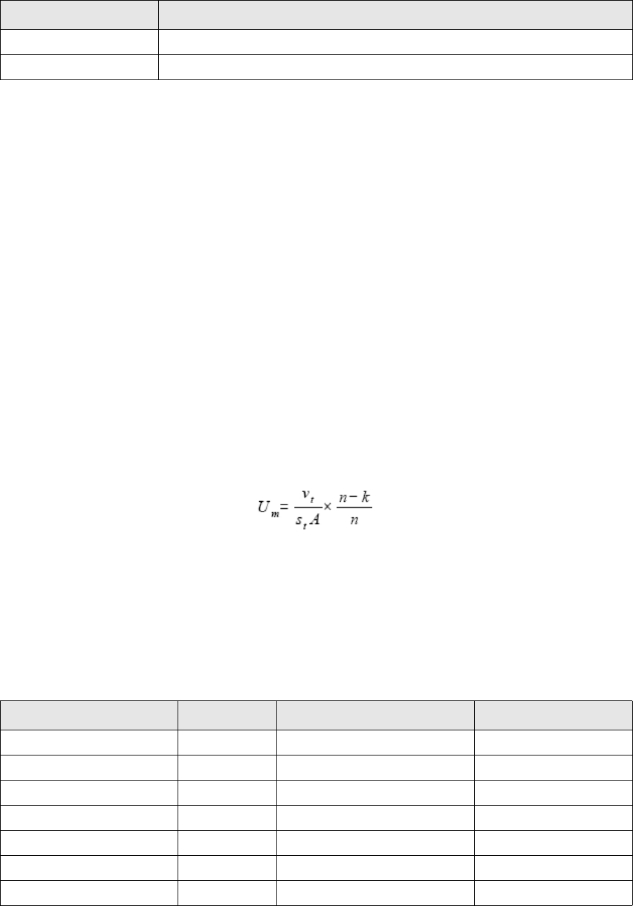
9 Futures
9.3 Money market future
Transaction & Risk Management Module (TRM) Instruments: Processing and Calculations 497
(A.2.145 Fed Fund Future Par Valuation on page 782) and Base IR Exposure Setup (A.2.48 Base IR
Exposure Setup on page 732) to the instrument and configuring IR exposure as follows:
This method calculates IR exposure 1bp and Modified Duration figures as follows:
•IR Exposure 1bp for Fed Fund futures
Before the start of the delivery period of a Fed Fund future, IR exposure 1bp is calculated the
same way as for MM future. During the delivery period, IR exposure will decrease linearly by the
same amount each day.
If the length of the delivery period is n days, then on day k of the delivery period, IR exposure
1bp is:
Equation 9-10 Par method: IR exposure 1bp
•Modified Duration for Fed Fund futures
Modified duration of Fed Fund futures follows the same logic as IR Exposure 1bp. Before the
start of the delivery period of a Fed Fund future, Modified Duration is calculated the same way as
for MM future. During the delivery period, Modified Duration will decrease linearly by the same
amount each day.
If the length of the delivery period is n days, then on day k of the delivery period, Modified
Duration is:
Equation 9-11 Par method: Modified Duration
See section Calculations - Par method on page 502 for examples of these calculations.
Calculations
The numerical examples in this section demonstrate how the different figures are calculated for a
Fed fund future contract both before and during the delivery period.
This example shows a purchase of a Fed fund future contract, with the following deal data:
•Instrument data
Information Description
Date Basis Actual/365
Yield Type Continuous Yield
Data Symbol Example Formula
Contract Size u 5,000,000.00
Tick Size s_t 0.005
Tick Value v_t 20.835
Delivery Period Start d.s 2006-12-01
Delivery Period End d.e 2006-12-31
Interest Period End d.i 2007-01-02
(Risk) Date Basis B 365
Ei1{} N–S
vt0.0001×
st
---------------------------nk–
n
------------
×=
9 Futures
9.3 Money market future
498 © Wall Street Systems IPH AB - Confidential
•Transaction data
•Calculated transaction data
•Before delivery period
Unless otherwise stated, the figure date used in the calculations is 2006-06-27. On this date, the
market data is as follows:
–Market data
–Calculated market data
(Risk) Yield Type Continuous
Delivery Period Length N.d 31 N.d = d.e - d.s +1
Day Length d.l 0.002777778 d.l = 1 / 360
Data Symbol Example
Opening Date 2006-06-27
Trading Units N 7.00
Deal Price F_c 95.00
Data Symbol Example Formula
Nominal Amount A 35,000,000.00 =
7.00 * 5,000,000.00
A =
N * u
Tick Amount A_t 29,169.00 =
35,000,000.00 * 20.835 / 0.005
A_t = N * v_t / s_t
Data Symbol Example
Figure Date d.f 2006-06-27
Market Quote F 96.00
Figure Spot Date ds.f 2006-06-29
Spot Discount Factor D.p 0.9998088047
Data Symbol Example Formula
Time to Spot Date t.s 0.0054794521 =
(2006/06/29 - 2006/06/27) /
365
t.s =
(ds.f - d.f) / B
Unit Market Value 0.9998088047 = 29,163.42 /
29,169.00
= V / A_t
Remaining averaging period k.d = 31 k.d = MIN(N.d, d.e - d.f +
1)
Average discount factor D.a = 0.9999013140 D.a = POWER(D.n / D.1,
1 / k.d)
Data Symbol Example Formula
9 Futures
9.3 Money market future
Transaction & Risk Management Module (TRM) Instruments: Processing and Calculations 499
–Calculated market data - start date
–Calculated market data - end date
–Valuation figures
–Risk figures - start date
–Risk figures - end date
Data Symbol Example Formula
PV Discount Factor D.1 0.9851018295
Time to Risk Date t_v.s 0.4301369863 =
(2006-12-01 - 2006-06-27) /365
t_v.s = (d.s - d.f) / B
Data Symbol Example Formula
PV Discount Factor D.n 0.9820925982
Time to Risk Date t_v.e 0.5178082192 =
(2007-01-02 - 2006-06-27) /365
t_v.e = (d.i - d.f) / B
Data Symbol Example Formula
Market Value V 29,163.42 =
7.00 * 20.835 *
(96.00 - 95.00) /
0.005 * 0.9998088047
V =
N * v_t *
(F - F_c) /
s_t * D.p
Data Symbol Example Formula
Sensitivity of D d_D.s -0.04237 =
-0.9851018295 * 0.4301369863
d_D.s = -D.1 * t_v.s
Sensitivity of D with respect
to Spot
d_Df.1 -0.4184 =
-(0.985101829 / 0.9998088047)
* (0.4301369863 -
0.0054794521)
d_Df.1 = -(D.1 / D.p) *
(t_v.s - t.s)
Risk Value dV.dD.1 -34,382,784.06 = -100 *
0.9998088047 * 29,169.00 /
(0.00277778 * 0.999901314 *
0.9851018295 * 31)
dV.dD.1 = -100 *
D.p * A_t /
(d.l * D.a * D.1 * N.d)
IR Exposure 1bp E_ir.s 1,456.8973 = -0.4237 *
-34,382,784.06 * 0.0001
E_ir.s = d_D.1 *
dV.dD.1 * 0.0001
IR Exposure Spot 1 bp E_ir.s.1 1,438.6132 = -34,382,784.06 *
-0.4184 * 0.0001
E_ir.s.1 = dV.dD.1 *
d_Df.1 * 0.0001
Data Symbol Example Formula
Sensitivity of D d_D.n -0.5085 =
-0.9820925982 * 0.5178082192
d_D.n =
-D.n * t_v.e
Sensitivity of D with respect
to Spot
d_Df.n_1 -0.5033 = -(0.9820925982 /
0.9998088047) *
(0.5178082192 - 0.005479452)
d_Df.n_1 = -(D.n /
D.p) *
(t_v.e - t.s)
9 Futures
9.3 Money market future
500 © Wall Street Systems IPH AB - Confidential
–Risk figures - total
•During delivery period
Unless otherwise stated, the figure date used in the calculations is 2006-12-15. On this date, the
market data is as follows:
–Market data
–Calculated market date
Risk Value dV.dD.n 34,488,136.40 = 100 *
0.9998088047 * 29,169.00 /
(0.002777778 * 0.999901314 *
0.9820925982 * 31)
dV.dD.n = 100 *
D.p * A_t /
(d.l * D.a * D.n * N.d)
IR Exposure 1bp E_ir.e -1,753.8446 =
-0.5085 * 34,488,136.40 *
0.0001
E_ir.e = d_D.n * dV.dD.n
* 0.0001
IR Exposure Spot 1 bp E_ir.s.n_1 -1,735.6172 =
34,488,136.40 * -0.5033 *
0.0001
E_ir.s.n_1 =
dV.dD.n * d_Df.n_1 *
0.0001
Data Symbol Example Formula
IR Exposure 1bp E_ir.t -296.9472305 = 1,456.8973 +
-1,753.8446
E_ir.t = E_ir.s + E_ir.e
IR Exposure Spot 1 bp E_ir.s.t -297.0040163 = 1,438.6132 +
-1,735.6172
E_ir.s.t =
E_ir.s.1 + E_ir.s.n_1
Modified Duration U_m 0.0876712329 =
-297.0040163 / (0.5 *
(ABS(-34382784.06 *
0.9851018295 / 0.9998088047)
+ ABS(34488136.40 *
0.9820925982 /
0.9998088047)) * 0.0001)
U_m = -E_ir.s.t / (0.5 *
(ABS(dV.dD.1 * D.1 / D.p)
+ ABS(dV.dD.n * D.n /
D.p)) * 0.0001)
Data Symbol Example
Figure Date d.f 2006-12-15
Last Fixing Rate F_x 96.00
Market Quote F 93.00
Spot Discount Factor D.p 0.9997870834
Data Symbol Example Formula
Unit Market Value -1.9995741668 =
29,163.42 / 29,169.00
V / A_t
Remaining averaging period k.d = 16 k.d =MIN(N.d, d.e - d.f +
1)
Average discount factor D.a = 0.9999428415 D.a = POWER(D.n / D.1,
1 / k.d)
Data Symbol Example Formula
9 Futures
9.3 Money market future
Transaction & Risk Management Module (TRM) Instruments: Processing and Calculations 501
–Calculated market data - start date
–Calculated market data - end date
–Valuation figures - Position flow
–Valuation figures - Netting flow
–Result figures
–Risk figures - start date
Data Symbol Example Formula
PV Discount Factor D.1 1.000000
Time to Risk Date t_v.s 0.000000 =
(2006-12-15 * 2006-12-15) /
365
t_v.s =
(d.f - d.f)
/ B
Data Symbol Example Formula
PV Discount Factor D.n 0.9990287496
Time to Risk Date t_v.e 0.0493150685 =
(2007-01-02 - 2006-12-15) /
365
t_v.e = (d.i - d.f)
/ B
Data Symbol Example Formula
Market Value V -58,325.58 = 7.00 * 20.835 *
(93.00 - 95.00) / 0.005 *
0.9997870834
V = N * v_t * (F - F_c) /
s_t * D.p
Data Symbol Example Formula
Market Value V_n -29,169.00 = (95.00 - 96.00) *
29,169.00
V_n = (F_c - F_x) * A_t
Data Symbol Example Formula
Total Profit Total_Profit = -58,325.58 Total_Profit = V
MtoM Profit MtoM_Profit -58,338.00 = (93.00 - 95.00) *
29,169.00
MtoM_Profit = (F - F_c) *
A_t
Other Profit 12.42 = -58,325.58 -
(-58,338.00)
= Total_Profit -
MtoM_Profit
Data Symbol Example Formula
Risk Value dV.dD.1 33,875,613.70 = -100 *
29,169.00 / (0.002777778 *
0.9999428415 * 1.000000 * 31
dV.dD.1 = -100 *
A_t / (d.l *
D.a * D.1 * N.d)
Modified Duration U_m 0.03836 = 129.933861 /
(ABS(34488136.4 *
0.9990287496 / 0.9997870834)
* 0.0001)
U_m = -E_ir.s.n /
(ABS(dV.dD.n * D.n / D.p)
* 0.0001)
9 Futures
9.3 Money market future
502 © Wall Street Systems IPH AB - Confidential
–Risk figures - end date
–Risk figures - total
Calculations - Par method
The default IR exposure calculations follow the theoretical approach described in Calculations on
page 497. An alternative is to choose the feature Fed Fund Future Par Valuation, as described in section
Setup on page 496, in which case, market value is calculated as above, but IR exposure is
calculated as follows:
•Instrument data
•Transaction data
Data Symbol Example Formula
Sensitivity of D d_D.n -0.0492672 =
-0.9990287496 * 0.0493150685
d_D.e = -D.n * t_v.e
Sensitivity of D with regards
to Spot
d_Df.n -0.0383271 = -(0.9990287496 *
0.9997870834) *
(0.0493150685 - 4/365)
d_Df.n = -(D.n / D.p) *
(t_v.e - 4/365)
Risk Value dV.dD.n 33,901,327.70 = 100 *
0.9997870834 * 29,169.00 /
(0.002777778 *
0.9999428415 *
0.9990287496 * 31
dV.dD.n = 100 *
D.p * A_t /
(d.l * D.a * D.n * N.d)
IR Exposure 1bp E_ir.e -167.022252 = -0.0492672 *
33,901,327.70 * 0.0001
E_ir.e = d_D.n * dV.dD.n
* 0.0001
IR Exposure Spot 1bp E_ir.s.n -129.933861 = -0.0383271 *
33,901,327.70 * 0.0001
E_ir.s.n = d_Df.n *
dV.dD.n * 0.0001
Data Symbol Example Formula
IR Exposure 1bp E_ir.t -167.02 = 0.00 + -167.022252 E_ir.t = E_ir.s + E_ir.e
Data Symbol Example Formula
Contract Size A.f 1,000,000.00
Tick Size (%) s_t.f 0.005
Tick Value v_t.f 12.5
Delivery Period Start dt.s 2006-12-01
Delivery Period End dt.e 2006-12-29
Delivery Period Length n.p 29 n.p = dt.e - dt.s +1
Data Symbol Example Formula
Number of Contracts N.f 7
9 Futures
9.3 Money market future
Transaction & Risk Management Module (TRM) Instruments: Processing and Calculations 503
•Valuation figures
Note: You can view these figures in Transaction Manager and Treasury Monitor.
9.3.2 Money market future chain
Money Market Future chain allows users to define the whole MM future chain as one instrument,
instead of having to define each contract as a separate instrument (MM-FUTURE class).
Important: MM future chain instruments should only be used in the bootstrapping of zero coupon
yield curves. The 'old-style' MM future instruments (see 9.3.1.1 MM future on page
485) should still be used for trading.
9.3.2.1 Instrument setup
MM future chain must be based on an instrument type derived from the class MM-FUTURE-CHAIN.
•Main characteristics:
The following basic information can be captured when defining the instrument:
•Netting information
The daily change in market value (pseudo cashflows) is settled every day (netted) until the
contract is closed or expires.
Data Symbol Example Formula
Figure Date dt.f 2006-12-15
Remaining Averaging
Period
k14 =dt.f-dt.s
f = 0.517241379 =(n.p-k)/n.p
IR Exposure 1bp E_i1 = -150.87414 =-n.f*f*v_t.f*0.0001/s_t.f
Modified Duration U_mod = 0.0431069 =f*v_t.f/(s_t.f*A.f)
Information Description
Issuer The client reflected as the Issuer of the transactions, e.g. the exchange or the
clearing house.
Counterparty The client reflected as the Counterparty of the transactions, e.g. the clearing house or
the broker.
Currency The currency in which the instrument is traded.
Information Description
Fixing Subscenario Subscenario from which the price is retrieved.
Calendar Calendar used to calculate the dates.
Settlement Offset Number of business days between fixing date and settlement date of the fixing
amount (variation margin).
Also, profit/loss realized from the closing of a position will have their value
date assigned based on this offset. An offset of 0 will realize profits/losses on
the date the position is closed (Opening Date of the closing transaction), and
an offset of 1 will realize profits losses on the next business day (i.e. in line
with the settlement of the fixings).
9 Futures
9.3 Money market future
504 © Wall Street Systems IPH AB - Confidential
See A.2.234 MM Future - Money Market Future Chain on page 830.
•Contract characteristics
•Trading Units definition
These contract characteristics and trading units are specific to the type of the future being
defined, each being selectable via dedicated instrument feature. The system supports the
following:
–One Month Money Market future (with feature Money Market 1M Future Chain)
These are futures on one month deposits, with monthly contracts expiring on or just before
the third Wednesday of the month.
Method
Frequency
Choose when you want netting to occur. For example, for daily netting, select
Business Days as method and 1 as frequency.
Information Description
Information Description
Calendar
Holiday Calendar
The calendars used to determine the business days when calculating the trading,
delivery, and underlying dates.
Root Symbol The root exchange symbol of the chain, for example, enter 'I' for LIFFE Euribor
future chain.
Quarterly Contracts The number of quarterly contracts available for trading with an expiry in March,
June, September and December.
Monthly Contracts The number of monthly contracts (nearest months, excluding the quarterly
months) available for trading.
Trading Offset The number of business days of the last trading day before the third Wednesday of
the month.
Formatter The display formatting for the contracts:
•Default: MMM YY displays as SEP 10.
•Symbol: Root Symbol + Month Code + Single Digit Year
using the same example as above, displays as EDU0 (ED is the root symbol, U
is the month code for September, and 0 is the last digit of the year 2010.)
Month Codes:
Jan = F, Feb = G, Mar = H, Apr = J, May = K, Jun = M, Jul = N, Aug = Q,
Sep = U, Oct = V, Nov = X, Dec = Z
Note: The default formatter is always used in Rate Monitor. In other applications,
the formatting depends on the selected formatter.
Information Description
Contract Size Standard size of the futures contract (for example, 1,000,000).
Minimum Bid Size Smallest allowed bid size. This is typically 1.0 (meaning 1 contract).
Tick Size
Tick Value
Minimum price movement (tick size and value).
Rounding Method Rounding method used in the calculations: Up, Down, or Nearest.
If the nominal amount entered does not correspond to a multiple of the
minimum bid size, the amount is rounded up, down, or to the nearest
corresponding amount.
Allow Trading in Half of
Tick Size
Allows trading this instrument at a price with a precision of half the tick size
(used for eurodollar Future contracts and options for nearest expiring month).
9 Futures
9.3 Money market future
Transaction & Risk Management Module (TRM) Instruments: Processing and Calculations 505
See A.2.235 MM Future - Money Market 1M Future Chain on page 831.
–Three Month Money Market future (with feature Money Market 3M Future Chain)
These are futures on three month deposits, with quarterly contracts expiring in Mar, Jun,
Sep and Dec and monthly (serial) contracts, all expiring on or just before the third
Wednesday of the month.
See A.2.236 MM Future - Money Market 3M Future Chain on page 831.
–Fed Fund future (with feature Fed Fund Future Chain)
These are futures on the average daily Fed Funds overnight rate for a calendar month,
expiring on the last business day of that month.
See A.2.143 Fed Fund Future Chain on page 781.
–Australian 90-Day Bank Bill future (with feature Australian 90-Day Bank Bill Future Chain)
These are Australian futures on (approximately) 90 day bank bills or CDs, with quarterly
contracts expiring in Mar, Jun, Sep and Dec, one business day before the second Friday of
the month. The Australian 90 Day Bank Bills have a variable tick value, thus Tick Size and
Value fields are not available in the trading units definition.
See A.2.233 MM Future - Australian 90-Day Bank Bill Future Chain on page 829.
•Quotation information
Define how these contracts are to be quoted on the market.
See A.2.275 Quoted Chain on page 851.
9.3.2.2 Market information
•Live market feed
To set up market information for MM future chain instruments, open the Market Info Source
Editor, select type as CHAIN and item to the market information provider’s root symbol, for
example, FEI for LIFFE Euribor future chain for the Reuters' feed. For more information about
using this editor, see TRM User Guide.
If you set up the market info at the instrument level, the type CHAIN is defaulted by the system.
Based on this setup, the live market feed is able to ask for prices for all the outstanding
contracts.
Note: Currently, Reuters' is the only live feed that can be used with future chains.
•Displaying quotes
You can view future chain quotes in the Instrument page of the Rate Monitor. You can expand the
chain to display all active contracts by selecting Periods on one of the axes. For more information
about using Rate Monitor, see TRM User Guide.
Information Description
Price Type Select Ticks.
Quote Handling Select MM Future Chain.

9 Futures
9.4 Bond future
506 © Wall Street Systems IPH AB - Confidential
9.4 Bond future
A bond future is an agreement to buy or sell a bond at a future date and with a given price. At the
time when the deal is made, the type of bond, amount, maturity, and value date are agreed upon.
Unlike forward contracts, futures are traded on an exchange and have daily settlement. A bond
future is marked to market and settled daily, instead of once when the contract expires. The
investor’s gain/loss is added to/taken from the margin account daily, essentially bringing the value
of the future to zero. This can be viewed as the future contract being closed out and re-written at a
new price, every day. The daily settlement price is calculated as the average of the prices at which
the contract traded just before the end of trading for the day.
Bond futures are long-term interest rate instruments which allow the buyer to lock into an interest
rate for a future lending period, and the seller to lock into an interest rate for a future borrowing
period.
Bond futures prices represent arbitrage rates implied by the current market rates rather than
individual forecasting or expectations about future yields.
In some capital markets, bond futures have become instruments on their own, so-called synthetic
bonds. Synthetic bonds are usually constructed with special features but they generally have
underlying instruments, Treasury Bonds for example. These synthetic bonds are quoted at the
market and they can be traded until a predefined date.
If the coupon interest earned on the bond is less than the interest cost of funding a long position in
it, then the market is said to have a negative carry; if the coupon interest earned on the bond is
greater than the funding cost, the market has a positive carry.
Under normal circumstances bond markets tend to have a positive carry; the yield curve slopes
upwards.
The implication is that if there is a positive carry, then bond futures should be lower in price than
cash futures. The greater the carry, either as a result of a marked yield differential and/or a lengthy
carry period, the lower the price of the futures contract will be.
9.4.1 Bond future
Bond future instruments must be based on an instrument type derived from the class
BOND-FUTURE.
The following basic information may be captured when defining the instrument. This information is
relevant to any kind of bond future.
For more information relating to the setup and structure of specific types of bond futures, see:
•9.4.2 CTD future on page 509
•9.4.3 Australian bond future on page 518.
9.4.1.1 Instrument setup
•Main characteristics
The following basic information may be captured when defining the instrument. This information
is relevant to any kind of bond future instrument.
Information Description
Issuer The client reflected as the Issuer of the transactions, e.g. the exchange or the
clearing house.
Counterparty The client reflected as the Counterparty of the transactions, e.g. the clearing house or
the broker.
Underlying The underlying bond instrument.
Currency The currency in which the instrument is traded.
9 Futures
9.4 Bond future
Transaction & Risk Management Module (TRM) Instruments: Processing and Calculations 507
•Trading units definition
•Netting information
The daily change in market value (pseudo cashflows) is settled every day (netted) until the
contract is closed or it expires.
See A.2.67 Bond Future on page 742.
•Future dates definition
See A.2.168 Future Dates on page 795.
•Quotation information
Information Description
Contract Size Standard size of the futures contract (for example, 3,000,000).
Minimum Bid Size Smallest allowed bid size (for example, 1.0000).
Tick Size
Tick Value
Minimum price movement (tick size and value), for example, 0.005 / 12.50
Tick Size * Point Value = Tick Value
Rounding Method Rounding method used in the calculations: Up, Down, or Nearest.
Allow Trading in
Half of Tick Size
Allows trading this instrument at a price with a precision of half the tick size (used for
eurodollar Future contracts and options for nearest expiring month).
Information Description
Fixing parameters Leave these fields blank if you want to define the Fixing parameters at deal entry.
Calendar Calendar used to calculate the dates.
Switches Switch on Settlement Currency if settlement is made in a different currency.
Settlement
Currency
If the Settlement Currency switch is on, the Currency in which settlement is made.
Payment Offset Number of business days between value date and payment date.
Method Select Business Days for daily netting.
Frequency For daily netting, enter 1 when Method = Business Days.
Information Description
Last Trading Day Last day when the futures contract can be traded.
The final day during which trading may take place in a futures contract, after which it
must be settled.
Settlement Date Last day on which delivery (cash settlement) of the underlying instrument can take
place.
Information Description
Active From
Active To
Period within which the quotation information is valid.
Leave these fields blank if you want the quotation information to apply indefinitely.
Price Type Standard method for quoting the price: Price/Underlying Unit.
Quote Handling Select Generic.
Currency Currency of the future instrument.
9 Futures
9.4 Bond future
508 © Wall Street Systems IPH AB - Confidential
See A.2.274 Quoted on page 849.
•Valuation of bond futures
It is possible to specify that another MtoM instrument’s direct market quotation is used to value
the future instrument.
See A.2.246 MtoM Instrument Setup on page 836.
It is also possible to set up
•Spot date calculation
•Cashflow or transaction charge rules
•Manual charges
•Branch codes.
See Appendix A Features on page 713.
9.4.1.2 Deal capture
9.4.1.2.1 Input data
In addition to the standard deal parameters, the following information is required to enter a bond
future contract:
9.4.1.2.2 Generated data
Two cashflows are generated:
–One position flow which represents the future position.
–The next netting flow (not fixed) which will be the support for the next daily margin once
fixed (see 9.4.1.3.1 Daily netting on page 508).
9.4.1.3 Processing
This section describes the actions that can be done throughout the life of a bond future.
9.4.1.3.1 Daily netting
Bond futures are fixed (settled) daily at the exchange. If the market quote for the future has
changed from the previous day, the difference (multiplied by the point value and the number of
units) is settled between the parties of the trade.
•Setup
The netting parameters for bond futures are defined at instrument level.
•Execution
The daily netting of bond futures is carried out using the Execute Netting action. The following
information is needed to process the netting:
Information Description
Trading Units Number of futures bought/sold.
Deal Price The market price of the bond future, expressed as a percentage of its nominal value.
Information Description
Netting Date Day the cashflow is fixed.
Netting Price Fixing market quote.
This is defaulted by the system and can be changed by the user.

9 Futures
9.4 Bond future
Transaction & Risk Management Module (TRM) Instruments: Processing and Calculations 509
The Execute Netting action automatically generates the next cashflow.
Netting of the cashflows can also be performed automatically using the Netting activity: see the
TRM User Guide for more information.
•Cancellation
The netting can be canceled either using the Undo Netting action, or using the Netting - Undo
activity.
9.4.1.3.2 Closing the position
Closing out a position means entering into a trade that is opposite to the original one. Closing of a
futures position takes place when the holder of a short position buys, or a long position sells, new
contracts which are matched with old ones. The transactions may not have been fixed before the
matching. If not, matching the trades creates a profit/loss cashflow to account for the price
difference between transactions.
9.4.1.3.3 Matching
•Setup
–The selling parameters used to automatically match transactions are specified in the result
treatment applied to the instrument definition
–The portfolio must have the Allow Short Selling switch activated.
See the TRM User Guide for more information.
•Execution
Automatic matching of transactions occurs each night with the End of Day Processing activity.
Manual matching of futures is done in Transaction Manager’s Matching mode. This option is
available if you specified Manual or FIFO as the selling method for the instrument.
See the TRM User Guide for more information about matching transactions.
•Cancellation
You can also unmatch transactions in Transaction Manager’s Matching mode if the cashflows
resulting from the transactions are not yet paid or booked.
9.4.2 CTD future
Some bond futures (CTD futures) are settled when the contract expires by delivery of an underlying
bond.
The bond to be delivered (Cheapest To Deliver (CTD) bond) is chosen by the party with the short
position from the deliverable basket. The conversion factor defines the price of this bond.
Netting Amount Profit or loss (settlement amount) from the future. This is calculated automatically by
TRM and can be changed by the user.
Netting Currency (Information only)
Currency of the settlement cashflow.
Information Description
9 Futures
9.4 Bond future
510 © Wall Street Systems IPH AB - Confidential
9.4.2.1 Instrument setup
CTD futures are set up in a similar way to bond futures (see 9.4.1 Bond future on page 506), but
require a different primary feature.
•Main characteristics
The following basic information may be captured when defining the instrument. This information
is relevant to any kind of CTD future instrument.
•Delivery basket
•Trading units definition
See A.2.116 CTD Future on page 765.
Information Description
Issuer The client reflected as the Issuer of the transactions, e.g. the exchange or the clearing
house.
Counterparty The client reflected as the Counterparty of the transactions, e.g. the clearing house or
the broker.
Currency The currency in which the instrument is traded.
First and Last
Delivery Date
Delivery period of the future.
Date Basis Date basis used to calculate the implied repo rate used to determine the cheapest to
deliver.
You can see the implied repo rate in the following TRM applications:
• Transaction Manager: In Transaction Figure view, you can see the implied repo rate
(column Implied Repo Rate) for one bond i.e. the cheapest (CTD) bond at the time
of valuation (column Delivery Instrument).
• Rate Monitor: You can display the implied repo rate for each bond in a CTD future's
basket of deliverable bonds, by selecting Period as one of the axes, usually the
vertical one, and figure Implied Repo Rate.
See TRM User Guide for more information.
Information Description
Instrument Bond instrument to include in the basket.
Conversion Factor Conversion factor of the instrument. This is used to determine the exact price of the
underlying bond.
Information Description
Contract Size Nominal value of one future contract.
Minimum Bid Size Minimum number of contracts that can be traded (usually one).
Tick Size
Tick Value
Minimum price movement (tick size and value).
Rounding Method Up, Down or Nearest.
If the nominal amount entered does not correspond to a multiple of the minimum
contract size, the amount is rounded up, down, or to the nearest corresponding
amount.
9 Futures
9.4 Bond future
Transaction & Risk Management Module (TRM) Instruments: Processing and Calculations 511
•Quotation information
See A.2.274 Quoted on page 849.
•Netting information
See A.2.319 Ticks Netting on page 870.
9.4.2.2 Processing
This section describes the actions that can be done throughout the life of a CTD future.
9.4.2.2.1 Delivery
Sometimes bond futures (CTD futures) are settled by delivery of an underlying bond. The delivery
transaction has to be entered as a separate transaction in TRM.
The nominal amount of the bond to be delivered is given by the nominal amount of the future
(contract size * number of contracts), and the delivery price is the last fixing price *
conversion factor.
Information Description
Active From
Active To
Period within which the quotation information is valid.
Leave these fields blank if you want the quotation information to apply indefinitely.
Price Type Standard method for quoting the price: Price %.
Quote Handling Select CTD.
Currency Currency of the future instrument.
Information Description
Fixing parameters Leave these fields blank if you want to define the Fixing parameters at deal entry.
Calendar Calendar used to calculate the dates.
Switches Switch on Settlement Currency if settlement is made in a different currency.
Settlement
Currency
If the Settlement Currency switch is on, the Currency in which settlement is made.
Payment Offset Number of business days between value date and payment date.
Method Select Business Days or Bullet.
Frequency Enter 1 when Method = Business Days, or 0 when Method = Bullet.

9 Futures
9.4 Bond future
512 © Wall Street Systems IPH AB - Confidential
9.4.2.3 Position monitoring
9.4.2.3.1 Setup
The risk calculation is based on the cashflows of the underlying cheapest to deliver bond, and the
setup taken partially from the future and from the underlying bond. For more information about risk
calculations, see 2.3 Key-figures on page 112.
•The risk setup (feature Risk Setup (BOND)) of the future determines which method (Yield to Maturity,
Z-Spread, or Zero-Coupon) is used to discount the underlying bond cashflows to delivery date. See
A.2.288 Risk Setup (BOND) on page 858.
Note: The yield type and date basis used in the risk yield to maturity and Z-Spread calculation
are taken from the underlying bond (Risk Yield or Discount Margin setup, respectively), as
well as from the risk free rate in the Z-Spread calculation. If these are not specified for the
underlying bond, then the following defaults are used:
Yield to Maturity: Continuous Yield, Actual/365 Date Basis
Z-Spread: Annually Continuous Yield, Actual/365 Date Basis, the risk-free curve of the
currency.
Both Risk Yield and Discount Margin are calculated on the delivery date using the invoice
amount. That is, they will differ from the Risk Yield or Discount Margin of the underlying bond,
which is based on the spot date and on the bond's market price.
See A.2.291 Risk Yield on page 859 or A.2.343 Z-DM/Spread Setup on page 882.
•Discounting from the delivery date to the spot date of the future and from the spot date to the
figure date use the valuation curve and discount curve of the future respectively. If either of
these is not defined, the default curve of the currency is used.
Figure Interest Rate shows the interest rate for the period from spot date to risk date of the
cashflow, as usual. When the risk method Yield to Maturity is used, Figure Base Interest Rate
shows the rate for the period from the delivery date to the risk date, i.e. Yield to Maturity.
•The IR exposure setup is taken from the future (feature Base IR Exposure Setup, see A.2.48 Base
IR Exposure Setup on page 732), if defined, except for the Yield Type and Date Basis, which
depend on the risk setup:
–Yield-to-Maturity
Use Yield Type and Date Basis of the risk yield setup of the underlying bond, or
corresponding defaults.
–Z-Spread
Use Yield Type and Date Basis of the Discount Margin setup of the underlying bond, or
corresponding defaults.
–Zero-Coupon
Use Yield Type and Date Basis specified in the IR Exposure setup of the future. If these are
not defined, use the defaults from the valuation curve's interpolation setup.
9.4.2.3.2 Calculations
In this section, numerical examples demonstrate how the different figures are calculated for a CTD
bond future.
If you need more theoretical information about the method used in these calculations, see Chapter 2
Market standards and calculations on page 33.
This example shows a CTD bond future, with the following deal data:
9 Futures
9.4 Bond future
Transaction & Risk Management Module (TRM) Instruments: Processing and Calculations 513
Setup data
Valuation Method Quoted
Risk Date Basis B Act/365
Trading unit u 100
Tick Size 1.00
Tick Value tv 1.00
Delivery Date dt_p.d 2006-10-10
Conversion Factor c_f 1.05
Cashflow data Amount per unit
(A.*)
Value date
(dt_v.*)
Coupon start date
(dt_s.*)
Payment date
(dt_p.*)
Current Coupon (*.c0) 0.02 2006-01-01 2005-07-01 2006-01-02
Next Coupon (*.n) 0.02 2006-07-01 2006-01-01 2006-07-03
Coupon 1 (*.c1) 0.02 2007-01-01 2006-07-01 2007-01-01
Coupon 2 (*.c2) 0.02 2007-07-01 2007-01-01 2007-07-02
Coupon 3 (*.c3) 0.02 2008-01-01 2007-07-01 2008-01-01
Coupon 4 (*.c4) 0.02 2008-07-01 2008-01-01 2008-07-01
Coupon 5 (*.c5) 0.02 2009-01-01 2008-07-01 2009-01-01
Coupon 6 (*.c6) 0.02 2009-07-01 2009-01-01 2009-07-01
Coupon 7 (*.c7) 0.02 2010-01-01 2009-07-04 2010-01-01
Redemption (*.p) 1.00 2010-01-01 2010-01-01
Transaction data
Trading Units N 100,000.00
Trading Price (last fixed price) F_c 95.00
Opening Date dt_o 2005-06-01
9 Futures
9.4 Bond future
514 © Wall Street Systems IPH AB - Confidential
Other important transaction data is calculated by the system as follows:
• Accrued Interest of CTD Bond at delivery
Accrued_Interest = (dt_p.d - dt_s.c1) / (dt_v.c1 - dt_s.c1) * A.c1
0.0109782609 = (2006/10/10 – 2006/07/01) / (2007/01/01 - 2006/07/01) * 0.02
•Nominal Amount
A = N * u
10,000,000.00 = 100,000.00 * 100
• Hedging Amount
Hedging_Amount = A / c_f
9,523,809.52 = 10,000,000.00 / 1.05
•Book Value
V_b.p = 0.00
Unless otherwise stated, the figure date used in the calculations is 2005-07-06. On this date, the
market data is as follows:
Other market data is calculated by the system as follows:
•Time to Payment
Market data on 2005-07-06
Figure Date d_f 2005-07-06
Days to Spot d_fs 2
Figure Spot Date dt_s.f = d_f + d_fs 2005-07-08
Future Price F 90.00
Price of the CTD Bond P_ctd 90.00
Discount Rate r_d 2.0277215%
Yield to Maturity ytm 5.80146169%
Cashflow Time to payment
Fixing t_p.f = (dt_s.f - d_f) / B 0.005479452
Delivery t_p.p = (dt_p.d - d_f) /B 1.26301370
Current Coupon t_p.c0 = (dt_p.c0 - d_f) /B 0.49315068
Next Coupon t_p.n = (dt_p.c0 - d_f) /B 0.49315068
Coupon 1 t_p.c1 = (dt_p.c1 - d_f) /B 1.49041096
Coupon 2 t_p.c2 = (dt_p.c2 - d_f) /B 1.98904110
Coupon 3 t_p.c3 = (dt_p.c3 - d_f) /B 2.49041096
Coupon 4 t_p.c4 = (dt_p.c4 - d_f) /B 2.98904110
Coupon 5 t_p.c5 = (dt_p.c5 - d_f) /B 3.49315068
Coupon 6 t_p.c6 = (dt_p.c6 - d_f) /B 3.98904110
Coupon 7 t_p.c7 = (dt_p.c7 - d_f) /B 4.49315068
Redemption t_p.r = (dt_p.p - d_f) /B 4.49315068

9 Futures
9.4 Bond future
Transaction & Risk Management Module (TRM) Instruments: Processing and Calculations 515
• Accrued Interest of the CTD
I_ctd = (dt_s.f - dt_s.c0) / (dt_v.c0 - dt_s.c0) * A.c0
0.000760870 = (2005/07/08 – 2005/07/01) / (2006/01/01 - 2005/07/01) * 0.02
• Time to Spot (Implied Repo Rate)
t_s = (dt_s.f - d_f) / 365
0.005479452 = (2005/07/08 - 2005/07/06) / 365
• PV Discount Factor
• MV Spot Discount Factor
D_s = EXP(-r_d * t_s)
0.99988890 = EXP(-0.020277215 * 0.005479452)
9.4.2.3.3 Valuation figures
The valuation method used in this example is the Quoted method.
•Market Value
V = N * tv * (F - F_c) * D_s
-499,944.45 = 100,000.00 * 1.00 * (90.00 – 95.00) * 0.99988890
• Implied Repo Rate
irr =
(F/100 * 1.05+ Accrued_Interest - (P_ctd / 100 + I_ctd) + (A.c0 + A.n)) / ((P_ctd / 100 + I_ctd) *
((dt_p.d - dt_s.f) / 365) - (A.c0 * ((dt_p.d - dt_p.c0) / 365) + A.n * ((dt_p.d -dt_p.n) / 365)))
= 8.56336405%
•Risk Value
Cashflow PV discount factor
Fixing D_pv.s = EXP(-r_d * t_s) 0.99988890
Delivery D_pv.f (taken from the valuation curve) 0.90268161
Coupon 1 D_pv.c1 = D_pv.f * EXP(-ytm * (t_p.c1 - t_p.p)) 0.89085131
Coupon 2 D_pv.c2 = D_pv.f * EXP(-ytm * (t_p.c2 - t_p.p)) 0.86545008
Coupon 3 D_pv.c3 = D_pv.f * EXP(-ytm * (t_p.c3 - t_p.p)) 0.84063951
Coupon 4 D_pv.c4 = D_pv.f * EXP(-ytm * (t_p.c4 - t_p.p)) 0.81666999
Coupon 5 D_pv.c5 = D_pv.f * EXP(-ytm * (t_p.c5 - t_p.p)) 0.79313176
Coupon 6 D_pv.c6 = D_pv.f * EXP(-ytm * (t_p.c6 - t_p.p)) 0.77063933
Coupon 7 D_pv.c7 = D_pv.f * EXP(-ytm * (t_p.c7 - t_p.p)) 0.74842780
Redemption D_pv.r = D_pv.f * EXP(-ytm * (t_p.r - t_p.p)) 0.74842780
Cashflow Risk value
Fixing V_r.f
= N * tv * (F - F_c)
= 100,000.00 * 1.00 * (90.00 – 95.00)
-500,000.00
Delivery V_r.d
= -A * (F / 100 + Accrued_Interest / c_f )
= -10,000,000 * (90.00 / 100 + 0.0109782609 / 1.05)
-9,104,554.87
Coupon 1 V_r.c1
= Hedging_Amount * A.c1
= 9,523,809.52 * 0.02
190,476.19
Coupon 2 V_r.c2 = Hedging_Amount * A.c2 190,476.19
Coupon 3 V_r.c3 = Hedging_Amount * A.c3 190,476.19
Coupon 4 V_r.c4 = Hedging_Amount * A.c4 190,476.19
9 Futures
9.4 Bond future
516 © Wall Street Systems IPH AB - Confidential
•Present Value
Coupon 5 V_r.c5 = Hedging_Amount * A.c5 190,476.19
Coupon 6 V_r.c6 = Hedging_Amount * A.c6 190,476.19
Coupon 7 V_r.c7 = Hedging_Amount * A.c7 190,476.19
Redemption V_r.p = Hedging_Amount 9,523,809.52
Cashflow Present value
Fixing V_p.f
= V_r.f * D_pv.s
= -500,000.00 * 0.99988890
-499,944.45
Delivery V_p.d
= V_r.d * D_pv.f
= -9,104,554.87 * 0.90268161
-8,218,514.25
Coupon 1 V_p.c1
= V_r.c1 * D_pv.1
= 190,476.19 * 0.89085131
169,685.96
Coupon 2 V_p.c2
= V_r.c2 * D_pv.2
= 190,476.19 * 0.86545008
164,847.63
Coupon 3 V_p.c3
= V_r.c3 * D_pv.3
= 190,476.19 * 0.84063951
160,121.81
Coupon 4 V_p.c4
= V_r.c4 * D_pv.4
= 190,476.19 * 0.81666999
155,556.19
Coupon 5 V_p.5
= V_r.c5 * D_pv.5
= 190,476.19 * 0.79313176
151,072.72
Coupon 6 V_p.6
= V_r.c6 * D_pv.6
= 190,476.19 * 0.77063933
146,788.44
Coupon 7 V_p.7
= V_r.c7 * D_pv.7
= 190,476.19 * 0.74842780
142,557.68
Redemption V_p.r
= V_r.p * D_pv.7
= 9,523,809.52 * 0.74842780
7,127,883.82
Total V_p.total 499,944.45
Cashflow Risk value

9 Futures
9.4 Bond future
Transaction & Risk Management Module (TRM) Instruments: Processing and Calculations 517
9.4.2.3.4 Result figures
The setup of the instrument impacts the way result figures are computed.
• Total Profit
Tot al_ Prof it = V
= -499,944.45
•MtoM Profit
MtoM_Profit = A * (F - F_c) / 100
-500,000.00 = 10,000,000 * (90.00 - 95.00) / 100
• Accrued Interest
Accrued_Interest = 0.00
• Accrued Profit
Accrued_Profit = 0.00
•Other Profit
Other_Profit = Total_Profit.p - MtoM_Profit.p
55.55 = -499,944.45 - (-500,000.00)>
9.4.2.3.5 Risk figures
•IR Exposure 1bp
Cashflow IR exposure 1bp
Fixing E_i.f
=-V_r.f * D_pv.s * t_p.f * 0.0001
= -(-500,000.00) * 0.99988890 * 0.005479452 * 0.0001
0.27
Delivery E_i.d
= -V_r.d * D_pv.f * t_p.p * 0.0001
= -(-9,104,554.87) * 0.90268161 * 1.26301370 * 0.0001
1,038.01
Coupon 1 E_i.c1
= -V_r.c1 * D_pv.1 * t_p.c1* 0.0001
= -190,476.19 * 0.89085131 * 1.49041096 * 0.0001
-25.29
Coupon 2 E_i.c2
= -V_r.c2 * D_pv.2 * t_p.c2 * 0.0001
= -190,476.19 * 0.86545008 * 1.98904110 * 0.0001
-32.79
Coupon 3 E_i.c3
= -V_r.c3 * D_pv.3 * t_p.c3 * 0.0001
= -190,476.19 * 0.84063951 * 2.49041096 * 0.0001
-39.88
Coupon 4 E_i.c4
= -V_r.c4 * D_pv.4 * t_p.c4 * 0.0001
= -190,476.19 * 0.81666999 * 2.98904110 * 0.0001
-46.50
Coupon 5 E_i.c5
= -V_r.c5 * D_pv.5 * t_p.c5 * 0.0001
= -190,476.19 * 0.79313176 * 3.49315068 * 0.0001
-52.77
Coupon 6 E_i.c6
= -V_r.c6 * D_pv.6 * t_p.c6 * 0.0001
= -190,476.19 * 0.77063933 * 3.98904110 * 0.0001
-58.55
Coupon 7 E_i.c7
= -V_r.c7 * D_pv.7 * t_p.c7 * 0.0001
= -190,476.19 * 0.74842780 * 4.49315068 * 0.0001
-64.05
Redemption E_i.r
= -V_r.p * D_pv.r * t_p.r * 0.0001
= -9,523,809.52 * 0.74842780 * 4.49315068 * 0.0001
-3,202.67
Total E_i.total -2,484.21

9 Futures
9.4 Bond future
518 © Wall Street Systems IPH AB - Confidential
• Effective Duration
U_eff = -E_i.total / V_P.total / 0.0001
-49.69 = -(-2,484.21) / 499,944.45 / 0.0001
9.4.3 Australian bond future
Australian bond futures have 3-year and 10-year Commonwealth Treasury Bonds issued by the
Federal Government as the underlying. These bonds are fixed interest securities that are issued with
a set term to maturity and have a semi-annual coupon rate which is fixed for the life of the bond.
They are considered as the benchmarks of long and medium term interest rates in Australia and are
actively traded by both Australian and international investors and traders.
Australian bond futures are quoted as 100 - yield% per annum in multiples of 0.01%. The Australian
convention quotes Treasury bonds on the basis of their yield-to-maturity, and not by the clean price.
This means that the value of one tick move (0.01%) does not remain constant but moves in line
with changes in the underlying yield.
9.4.3.1 Instrument setup
Australian bond futures are set up in a similar way to standard bond futures (see 9.4.1 Bond future
on page 506), but require a different primary feature.
•Main characteristics
See A.2.68 Bond Future - Australian on page 743.
•Quotation information
See A.2.274 Quoted on page 849.
•Netting information
The daily change in market value (pseudo cashflows) is settled every day (netted) until the
contract is closed or it expires.
See A.2.319 Ticks Netting on page 870.
9.4.3.2 Market information
For an Australian bond future, the Reserve Bank of Australia bond pricing formula is used to convert
the market quotation into a future price.
First, the corresponding yield is computed as:
Yield = 100 - Q
where Q is the market quote of the future contract.
The future price is then converted using the following formula:
Equation 9-12 Australian bond future: future price conversion
where:
–i = yield% p.a. divided by 200
Information Description
Price Type Method for quoting the price - Ticks.
Quote Handling Select Generic (which means that you will be able to enter the bid and ask quotes for
this instrument).
Currency Currency of the future contract - AUD.
P ContractSize c1 v
n)–(
i
-----------------------
⎝
⎛
×vn)+=

9 Futures
9.5 Equity future
Transaction & Risk Management Module (TRM) Instruments: Processing and Calculations 519
–v = 1 / (1 + i)
–n = total number of coupons (20 for 10Y bond, 6 for 3Y bond) as defined at the underlying
instrument level (Bond Future page - underlying instrument)
–c = coupon rate / 2 (expressed as %) as defined at the underlying instrument level (Bond
Future page - underlying instrument)
Once the market quotation has been converted into the future price, the valuation of the contract is
carried out in the same way as for a standard bond future contract.
Note: It is possible to set up 3Y /10Y Treasury Bond future instruments with as underlying a
synthetic bond, which will be defined as follows: Coupon rate = 6%, issue date =
settlement date of the future and a term to maturity of 3Y or 10Y depending on the type of
the future.
9.5 Equity future
A future is an agreement (obligation) to buy or sell a given quantity of a particular asset, at a
specified future date, at a pre-agreed price. Futures contracts have standard delivery dates, trading
units, terms and conditions.
You can "open" a futures position by either buying or selling a future. You can "close" your futures
position by doing the opposite - either selling or buying the same future. In practice, most futures
contract positions are "closed out" before they expire.
If you hold a view that the underlying asset will rise you could buy futures - known as a long futures
position - which commits you to take delivery of the underlying assets, or equivalent cash value, at
a pre-arranged price and by a certain date.
If your view is that the share prices for the underlying asset will fall, you could sell futures - known
as a short futures position - which commits you to deliver the underlying assets, or equivalent cash
value, at a prearranged price and by a certain date.
An equity future is an exchange traded derivative instrument where the underlying is stock. Equity
futures are usually fixed daily.
Typically there is an initial margin requirement (entered as a payment in TRM) when buying or
selling futures contracts but no principal is paid. When the market quote for the future changes, the
variation margin (daily change in market value) is settled every day (netted) until the contract is
closed or it expires. The variation margin is calculated by multiplying the change in the quote by the
point value and the number of contracts.
When the equity future expires, the difference between the last fixing price and the closing price is
settled.
Dividends are taken into account for the market valuation. They can be entered in Rate Monitor and
TRM will then use this information in the calculations.
9.5.1 Instrument setup
Equity future instruments must be based on an instrument type derived from the class
EQUITY-FUTURE.
•Main characteristics

9 Futures
9.5 Equity future
520 © Wall Street Systems IPH AB - Confidential
The following basic information may be captured when defining the instrument. This information
is relevant to any kind of equity future instrument.
•Netting information
The daily change in market value (pseudo cashflows) is settled every day (netted) until the
contract is closed or it expires.
See A.2.131 Equity Future on page 775.
•Future dates definition
See A.2.168 Future Dates on page 795.
•Trading units definition
Information Description
Issuer The client reflected as the Issuer of the transactions, e.g. the exchange or the clearing
house.
Counterparty The client reflected as the Counterparty of the transactions, e.g. the clearing house or
the broker.
Underlying The underlying equity instrument or equity index.
Currency The currency in which the instrument is traded.
Information Description
Fixing parameters Leave these fields blank if you want to define the Fixing parameters at deal entry.
Calendar Calendar used to calculate the dates.
Switches Switch on Settlement Currency if settlement is made in a different currency.
Settlement
Currency
If the Settlement Currency switch is on, the Currency in which settlement is made.
Payment Offset Number of business days between value date and payment date.
Method Select Business Days for daily netting.
Frequency For daily netting, enter 1 when Method = Business Days.
Information Description
Last Trading Day Last day when the futures contract can be traded.
The final day during which trading may take place in a futures contract, after which it
must be settled.
Settlement Date Last day on which delivery (cash settlement) of the underlying instrument can take
place.
Information Description
Point Value Unit of trading of the contract: one future normally represents 100 shares.
Minimum Bid Size Smallest allowed bid size (for example, 100).
Tick Size
Tick Value
Minimum price movement (tick size and value).
Tick Size * Point Value = Tick Value
Note: The tick value needs to be entered in the main currency units (e.g. pounds),
even when the underlying equity is traded in fractional units (e.g. pence).
Rounding Method Rounding method used in the calculations: Up, Down, or Nearest.
9 Futures
9.5 Equity future
Transaction & Risk Management Module (TRM) Instruments: Processing and Calculations 521
See A.2.320 Trading Unit (Derivative) on page 871.
•Quotation information
See A.2.274 Quoted on page 849.
It is also possible to set up
•Spot date calculation
•Cashflow or transaction charge rules
•Manual charges
•Branch codes.
See Appendix A Features on page 713.
9.5.2 Deal capture
9.5.2.1 Input data
In addition to the standard deal parameters, the following information is required to enter an equity
future contract:
9.5.2.2 Generated data
Two cashflows are generated:
–One position flow which represents the future position.
–The next netting flow (not fixed) which will be the support for the next daily margin once
fixed (see 9.5.3.1 Daily netting on page 521).
9.5.3 Processing
This section describes the actions that can be done throughout the life of an equity future.
9.5.3.1 Daily netting
Equity futures are not subject to a physical delivery of the underlying at expiry but are typically fixed
every day. If the market quote for the future has changed from the previous day, the difference
(multiplied by the point value and the number of units) is settled between the parties of the trade.
Allow Trading in
Half of Tick Size
Allows trading this instrument at a price with a precision of half the tick size (used for
eurodollar Future contracts and options for nearest expiring month).
Information Description
Active From
Active To
Period within which the quotation information is valid.
Leave these fields blank if you want the quotation information to apply indefinitely.
Price Type Standard method for quoting the price: Price/Underlying Unit.
Quote Handling Generic
Currency Currency in which the quotation is expressed.
Information Description
Information Description
Trading Units Number of futures bought/sold.
Deal Price Transaction price.

9 Futures
9.5 Equity future
522 © Wall Street Systems IPH AB - Confidential
•Setup
The netting parameters for equity futures are defined at instrument level.
•Execution
The daily netting of equity futures is carried out using the Execute Netting action. The following
information is needed to process the netting:
The Execute Netting action automatically generates the next cashflow.
Netting of the cashflows can also be performed automatically using the Netting activity: see the
TRM User Guide for more information.
•Cancellation
The netting can be canceled either using the Undo Netting action, or using the Netting - Undo
activity.
9.5.3.2 Closing the position
Closing out a position means entering into a trade that is opposite to the original one. Closing of a
futures position takes place when the holder of a short position buys, or a long position sells, new
contracts which are matched with old ones. The transactions may not have been fixed before the
matching. If not, matching the trades creates a profit/loss cashflow to account for the price
difference between transactions.
9.5.3.2.1 Matching
•Setup
–The selling parameters used to automatically match transactions are specified in the result
treatment applied to the instrument definition.
–The portfolio must have the Allow Short Selling switch activated.
See the TRM User Guide for more information.
•Execution
–Automatic matching of transactions occurs each night with the End of Day Processing
activity.
–Manual matching of futures is done in Transaction Manager’s Matching mode. This option is
available if you specified Manual or FIFO as the selling method for the instrument.
See the TRM User Guide for more information about matching transactions.
•Cancellation
You can also unmatch transactions in Transaction Manager’s Matching mode if the cashflows
resulting from the transactions are not yet paid or booked.
Information Description
Netting Date Day the cashflow is fixed.
Netting Price Fixing market quote. This is defaulted by the system and can be changed by the user.
Netting Amount Profit or loss (settlement amount) from the equity future. This is calculated
automatically by TRM and can be changed by the user.
Netting Currency (Information only)
Currency of the settlement cashflow.

9 Futures
9.6 FX future
Transaction & Risk Management Module (TRM) Instruments: Processing and Calculations 523
9.6 FX future
Forex futures serve two primary purposes as financial instruments:
•They can be used by companies or sole proprietors to remove the exchange-rate risk inherent in
cross-border transactions.
•They can be used by investors to speculate and profit from currency exchange-rate fluctuations.
An FX future is an exchange-traded contract to buy or sell a specified amount of a given currency at
a predetermined price on a set date in the future.
With a foreign exchange futures contract, the participants do not actually buy or sell anything: they
simply agree to buy or sell the currencies on the pre-agreed terms if the contract reaches maturity.
However, in reality, the majority of FX future contracts rarely reach maturity: this means that only a
small proportion of FX Futures contracts result in actual delivery of the currencies.
Both FX and traditional futures operate in the same basic manner. There is, however, one key
difference between the two: FX futures are not traded on a centralized exchange; rather, the deal
flow is available through several different exchanges in the U.S. or elsewhere. The vast majority of
FX futures are traded through the Chicago Mercantile Exchange (CME) and its partners.
However, this is not to say that FX futures contracts are OTC; they are still bound to a designated
"size per contract", and they are offered only in whole numbers (unlike forward contracts).
An FX futures contract is conceptually similar to a forward FX contract, in that both are agreements
to buy or sell a certain amount of a certain currency for another at a certain price on a certain date.
However, the fundamental difference between futures and forwards is the fact that futures are
traded on exchanges, whereas forwards trade "over-the-counter". This has three practical
implications:
•Futures are standardized instruments. You can only trade the specific contracts supported by the
exchange. Forwards are entirely flexible. Because they are privately negotiated between parties,
they can be for any conceivable underlying and for any settlement date.
•Forwards entail both market risk and credit risk. A counterparty may fail to perform on a
forward. With futures, there is only market risk. This is because exchanges employ a system
whereby counterparties exchange daily payments of profits or losses on the days they occur.
Through these margin payments, a futures contract's market value is effectively reset to zero at
the end of each trading day. This all but eliminates credit risk.
•The daily cash flows associated with margining can skew futures prices, causing them to diverge
from corresponding forward prices.
9.6.1 Instrument setup
FX future instruments must be based on an instrument type derived from the class FX-FUTURE.
•Main characteristics
The following basic information may be captured when defining the instrument. This information
is relevant to any kind of FX future instrument.
See A.2.176 FX Future on page 798.
Information Description
Issuer The client reflected as the Issuer of the transactions, e.g. the exchange or the clearing
house.
Counterparty The client reflected as the Counterparty of the transactions, e.g. the clearing house or
the broker.
Base Currency
Settlement
Currency
The currency pair: Base Currency/Settlement Currency.

9 Futures
9.6 FX future
524 © Wall Street Systems IPH AB - Confidential
•Future dates definition
Most currency contracts are traded on the March quarterly cycle and go through a physical
delivery process four times a year on the third Wednesday of March, June, September, and
December. However, the Mexican peso and the South African rand are traded on all twelve
calendar months. There are two "cash-settled" contracts — the Brazilian real, traded on all
twelve calendar months; and the Russian ruble, traded on the March quarterly cycle.
See A.2.168 Future Dates on page 795.
•Trading units definition
See A.2.320 Trading Unit (Derivative) on page 871.
•Quotation information
Note that all dollar-based FX futures prices are quoted in direct terms against the US dollar,
unlike the spot forex market.
The price represents the number of US dollars it would take to buy one unit of foreign currency.
See A.2.274 Quoted on page 849.
•Netting information
Information Description
Last Trading Day Last day when the futures contract can be traded after which it must be settled.
After this date, the contract cannot be traded.
Settlement Date Last day on which delivery (or cash settlement) of the underlying instrument can take
place.
The final contract value is determined on this date and settlement is made.
Information Description
Contract Size Amount of base currency.
Minimum Bid Size Smallest allowed bid size: 1.
Tick Size
Tick Value
Minimum fluctuation on the currency contract.
Tick Size * Contract Size = Tick Value
Rounding Method Rounding method used in the calculations: Up, Down, or Nearest.
Allow Trading in
Half of Tick Size
Allows trading this instrument at a price with a precision of half the tick size (used for
eurodollar Future contracts and options for nearest expiring month).
Information Description
Active From
Active To
Period within which the quotation information is valid.
Leave these fields blank if you want the quotation information to apply indefinitely.
Price Type Standard method for quoting the price: Price/Unit.
Quote Handling Generic
Currency Currency in which the quotation is expressed.

9 Futures
9.6 FX future
Transaction & Risk Management Module (TRM) Instruments: Processing and Calculations 525
The daily change in market value (pseudo cashflows) is settled every day (netted) until the
contract is closed or it expires.
See A.2.177 FX Future Netting on page 798.
•Valuation of FX futures
It is possible to specify that another MtoM instrument’s direct market quotation is used to value
the future contract.
See A.2.246 MtoM Instrument Setup on page 836.
It is also possible to set up:
•Spot date calculation
•Cashflow or transaction charge rules
•Manual charges
•Branch codes.
See Appendix A Features on page 713.
9.6.2 Deal capture
9.6.2.1 Input data
In addition to the standard deal parameters, the following information is required to enter an FX
future contract:
9.6.2.2 Generated data
•Cashflows
The following cashflows are generated:
–One position flow which represents the future position
–The netting flow(s).
9.6.3 Processing
This section describes the actions that can be done throughout the life of an FX future.
Information Description
Fixing parameters Leave these fields blank if you want to define the Fixing parameters at deal entry.
Calendar Calendar used to calculate the dates.
Switches Switch on Settlement Currency if settlement is made in a different currency.
Payment Offset Number of business days between value date and payment date.
Method Select Business Days for daily netting.
Frequency For daily netting, enter 1 when Method = Business Days.
Information Description
Trading Units Number of futures bought/sold.
Deal Price Transaction price.
If the quotation information is defined in the instrument setup, the deal price defaults
to the price of the market feed provided by the Price Manager: see A.2.266 Quote
Default on page 845.

9 Futures
9.6 FX future
526 © Wall Street Systems IPH AB - Confidential
9.6.3.1 Daily netting
As for other futures, there are initial and maintenance margins and daily cash settlements.
The initial margin is the minimum amount required to enter into a new futures contract, but the
maintenance margin is the lowest amount an account can reach before needing to be replenished.
If the market quote for the future has changed from the previous day, the daily change in market
value is settled every day (netted) until the contract is closed or expires.
•Setup
The netting parameters for FX futures are defined at instrument level: see A.2.177 FX Future
Netting on page 798.
•Execution
The daily netting of FX futures is carried out using the Execute Netting action. The following
information is needed to process the netting:
The Execute Netting action automatically generates the next cashflow.
Netting of the cashflows can also be performed automatically using the Netting activity: see the
TRM User Guide for more information about activities.
•Cancellation
The netting can be canceled either using the Undo Netting action, or using the Netting - Undo
activity.
9.6.3.2 Closing the position
Closing out a position means entering into a trade that is opposite to the original one. Closing of a
futures position takes place when the holder of a short position buys, or a long position sells, new
contracts which are matched with old ones. The transactions may not have been fixed before the
matching. If not, matching the trades creates a profit/loss cashflow to account for the price
difference between transactions.
9.6.3.2.1 Matching
•Setup
–The selling parameters used to automatically match transactions are specified in the result
treatment applied to the instrument definition.
–The portfolio must have the Allow Short Selling switch switched on.
See the TRM User Guide for more information.
•Execution
–Automatic matching of transactions according to the FIFO method occurs each night with the
End of Day Processing activity.
–Manual matching of futures is done in Transaction Manager’s Matching mode. This option is
available if you specified Manual or FIFO as the selling method for the instrument.
Information Description
Netting Date Day the cashflow is fixed.
Netting Price Fixing market quote. This is defaulted by the system and can be changed by the user.
Netting Amount Profit or loss (settlement amount) from the FX future. This is calculated automatically
by TRM and can be changed by the user.
Netting Currency (Information only)
Currency of the settlement cashflow.
9 Futures
9.6 FX future
Transaction & Risk Management Module (TRM) Instruments: Processing and Calculations 527
•Cancellation
You can also unmatch transactions in Transaction Manager’s Matching mode if the cashflows
resulting from the transactions are not yet paid or booked.
See the TRM User Guide for more information about matching and unmatching transactions.
9.6.4 Position monitoring
The numerical examples in this section demonstrate how the figures are calculated for an FX future
contract.
If you need more theoretical information about the method used in these calculations, see Chapter 2
Market standards and calculations on page 33.
9.6.4.1 Calculations
This example shows an FX Future, with the following deal data:
•Setup data
•Portfolio data
•Transaction data
•Calculated Transaction data
Data Symbol Example
Valuation Method Quoted
Risk Yield Type Continuous
Risk Date Basis B.r 360
Contract Size u 125,000.00
Base CCY EUR
Settlement CCY USD
Data Symbol Example
FX Exposure e_fx 0.01
Figure Currency USD
Data Symbol Example
Opening Date dt_o 2006-10-08
Tradi ng Units N 100
Fixing Rate Before Last F_1 1.260000
Last Fixing Rate F_0 1.275000
Deal Rate F_d 1.270500
Value Date dt_m 2007-03-21
Data Symbol Example
Nominal Amount A = N * u 12,500,000

9 Futures
9.6 FX future
528 © Wall Street Systems IPH AB - Confidential
•Market Data on the Figure Date
•Calculated Data on Figure Date
•Valuation figures - Netting Flow
•Valuation figures - Position Flow
•Valuation figures - Variation Flow
•Valuation figures - Total
•Risk figures - Base CCY
Data Symbol Example
Figure Date dt.f 2006-10-12
Market Quote F 1.280000
FX Convert: Base CCY S 1.270000
Data Symbol Example Formula
Time to Maturity t_m 0.44444444 = (2007/03/21
-2006/10/12) / 360
= (dt.m-dt.f) / B.r
Present Value Discount
Factor: Base CCY
D_P.b 0.994494278
Present Value Discount
Factor: Quote CCY
D_P.q 0.991695620
Data Symbol Example Formula
Amount 187,500 = 12,500,000 * (1.275 - 1.260) = A * (F_0 - F_1)
Market Value V.n 187,500 = 12,500,000 * (1.275 - 1.260) = A * (F_0 - F_1)
Data Symbol Example Formula
Market Value V.p 118,750 = 12,500,000 * (1.28 - 1.2705) = A * (F - F_d)
Data Symbol Example Formula
Market Value V.v -56,250.00 = 12,500,000 * (1.2705 -
1.2750)
= A * (F_d - F_0)
Data Symbol Example Formula
Market Value 250,000 = 187,500 + 118,750 +
-56,250
= V.n + V.p + V.v
Data Symbol Example Formula
Present Value V_P.b 15,787,596.67 = 1.27 * 12,500,000 *
D_P.b
= S * V_r.b * D_P.b
Risk Value V_r.b 12,500,000 = A
IR Exposure 1bp E_ip -701.67 = -1.27 * 12,500,000 *
0.994494278 * 0.44444444 * 0.0001
= -S * V_r.b * D_P.b *
t_m * 0.0001
9 Futures
9.7 Index future
Transaction & Risk Management Module (TRM) Instruments: Processing and Calculations 529
•Risk figures - Quoted CCY
•Risk figures - Total
•Profit
9.7 Index future
A future is an agreement (obligation) to buy or sell a given quantity of a particular asset, at a
specified future date, at a pre-agreed price. Futures contracts have standard delivery dates, trading
units, terms and conditions.
You can open a futures position by either buying or selling a future. You can close your futures
position by doing the opposite, either selling or buying the same future. In practice, most futures
contract positions are closed out before they expire.
If you hold a view that the underlying asset will rise you could buy futures, known as a long futures
position, which commits you to take delivery of the underlying assets, or equivalent cash value, at a
pre-arranged price and by a certain date.
If your view is that the share prices for the underlying asset will fall, you could sell futures, known as
a short futures position, which commits you to deliver the underlying assets, or equivalent cash
value, at a prearranged price and by a certain date.
An index future is an exchange traded derivative instrument where the underlying is an index.
Typically, index futures are fixed daily. As the underlying is an index there is no physical settlement
at the end.
Typically there is an initial margin requirement (entered as a payment in TRM) when buying or
selling futures contracts but no principal is paid. When the market quote for the future changes, the
variation margin (daily change in market value) is settled every day (netted) until the contract is
closed or it expires. The variation margin is calculated by multiplying the change in the quote by the
point value and the number of contracts.
When the index future expires, the difference between the last fixing price and the closing price is
settled.
FX Exposure e_fx 157,875.97 = 0.01 * 15,787,596.67 = e_fx_1 * V_P.b
Data Symbol Example Formula
Data Symbol Example Formula
Present Value V_l.q -15,749,366.06 = 15,881,250 *
0.991695620
= V_r.q * D_P.q
Risk Value V_r.q -15,881,250 = -12,500,000 * 1.2705 = -A * F_d
IR Exposure 1bp E_ipq 699.97 = 15,881,250 * 0.991695620 *
0.44444444 * 0.0001
= -V_r.q * D_P.q * t_m
* 0.0001
Data Symbol Example Formula
Present Value 38,230.61 = 15,787,596.67 +
-15,749,366.06
= V_P.b + V_l.q_1
Data Symbol Example Formula
MtoM 187,500 = V.n
9 Futures
9.7 Index future
530 © Wall Street Systems IPH AB - Confidential
9.7.1 Instrument setup
Index future instruments are based on an instrument type derived from the class INDEX-FUTURE.
•Main characteristics
The following basic information may be captured when defining the instrument. This information
is relevant to any kind of index future contract.
•Netting information
The daily change in market value (pseudo cashflows) is settled every day (netted) until the
contract is closed or it expires.
See A.2.208 Index Future on page 818.
•Future dates definition
See A.2.168 Future Dates on page 795.
•Trading units
Information Description
Issuer The client reflected as the Issuer of the transactions, e.g. the exchange or the clearing
house.
Counterparty The client reflected as the Counterparty of the transactions, e.g. the clearing house or
the broker.
Underlying The underlying index instrument.
Currency The currency in which the instrument is traded.
Information Description
Fixing parameters Leave these fields blank if you want to define the Fixing parameters at deal entry.
Calendar Calendar used to calculate the dates.
Switches Switch on Settlement Currency if settlement is made in a different currency.
Settlement
Currency
If the Settlement Currency switch is on, the Currency in which settlement is made.
Payment Offset Number of business days between value date and payment date.
Method Select Business Days for daily netting.
Frequency For daily netting, enter 1 when Method = Business Days.
Information Description
Last Trading Day Last day when the futures contract can be traded.
The final day during which trading may take place in a futures contract, after which it
must be settled.
Settlement Date Last day on which delivery (cash settlement) of the underlying instrument can take
place.
Information Description
Point Value Unit of trading of the contract: value of 1 point of the index.
Minimum Bid Size Smallest allowed bid size (for example, 1.00000).

9 Futures
9.7 Index future
Transaction & Risk Management Module (TRM) Instruments: Processing and Calculations 531
See A.2.322 Trading Unit (Index) on page 872.
•Quotation information
See A.2.274 Quoted on page 849.
It is also possible to set up:
•Spot date calculation
•Cashflow or transaction charge rules
•Manual charges
•Branch codes.
See Appendix A Features on page 713.
9.7.2 Deal capture
9.7.2.1 Input data
In addition to the standard deal parameters, the following information is required to enter an index
future contract:
9.7.3 Processing
This section describes the actions that can be done throughout the life of an index future.
9.7.3.1 Daily netting
Index futures are not subject to a physical delivery of the underlying at expiry but are typically fixed
every day. If the market quote for the future has changed from the previous day, the difference
(multiplied by the point value and the number of units) is settled between the parties of the trade.
•Setup
Tick Size
Tick Value
Minimum price movement (tick size and value), for example, 0.5 / €5.
Tick Size*Point Value = Tick Value
Rounding Method Rounding method used in the calculations: Up, Down, or Nearest.
Allow Trading in
Half of Tick Size
Allows trading this instrument at a price with a precision of half the tick size (used for
eurodollar Future contracts and options for nearest expiring month).
Information Description
Active From
Active To
Period within which the quotation information is valid.
Leave these fields blank if you want the quotation information to apply indefinitely.
Price Type Standard method for quoting the price: Price/Underlying Unit.
Quote Handling Generic
Currency Currency in which the quotation is expressed.
Information Description
Information Description
Trading Units Number of futures bought/sold.
Deal Price Transaction price.

9 Futures
9.7 Index future
532 © Wall Street Systems IPH AB - Confidential
The netting parameters for index futures are defined at instrument level: see 9.7.1 Instrument
setup on page 530.
•Execution
The daily netting of index futures is carried out using the Execute Netting action. The following
information is needed to process the netting:
The Execute Netting action automatically generates the next cashflow.
Netting of the cashflows can also be performed automatically using the Netting activity: see the
TRM User Guide for more information.
•Cancellation
The netting can be canceled either using the Undo Netting action, or using the Netting - Undo
activity.
9.7.3.2 Closing the position
Closing out a position means entering into a trade that is opposite to the original one. Closing of a
futures position takes place when the holder of a short position buys, or a long position sells, new
contracts which are matched with old ones. The transactions may not have been fixed before the
matching. If not, matching the trades creates a profit/loss cashflow to account for the price
difference between transactions.
9.7.3.3 Matching
•Setup
–The selling parameters used to automatically match transactions are specified in the result
treatment applied to the instrument definition.
–The portfolio must have the Allow Short Selling switch activated.
See the TRM User Guide for more information.
•Execution
Automatic matching of transactions occurs each night with the End of Day Processing activity.
Manual matching of futures is done in Transaction Manager’s Matching mode. This option is
available if you specified Manual or FIFO as the selling method for the instrument.
See the TRM User Guide for more information about matching transactions.
•Cancellation
You can also unmatch transactions in Transaction Manager’s Matching mode if the cashflows
resulting from the transactions are not yet paid or booked.
Information Description
Netting Date Day the cashflow is fixed.
Netting Price Fixing market quote. This is defaulted by the system and can be changed by the user.
Netting Amount Profit or loss (settlement amount) from the index future. This is calculated
automatically by TRM and can be changed by the user.
Netting Currency (Information only)
Currency of the settlement cashflow.
Transaction & Risk Management Module (TRM) Instruments: Processing and Calculations 533
Chapter 10 Options
10.1 Cap/floor/collar
Cap, Floors, and Collars are OTC option instruments that are commonly used to hedge a position.
•Interest Rate Cap: buying a cap protects against a rise in the money market interest rate.
•Interest Rate Floor: buying a floor protects against a fall in the money market interest rate.
•Interest Rate Collar: purchasing a collar consists of buying a cap and selling a floor.
With these option agreements, the buyer has the right to be compensated by the seller for the
difference between the contract interest and the reference interest in exchange for an option
premium.
This comparison of interest takes place periodically according to a number of predetermined data.
The settlement of any difference takes place at the end of the interest period on the fixing date.
For these types of option instrument, the nominal cashflow is pseudo: only the premium is paid at
deal entry.
10.1.1 Vanilla cap/floor/collar
•Cap
A Cap instrument is an option contract which puts an upper limit on a floating exchange rate.
The owner of a cap has an insurance against rising interest rates. At the fixing date, if the
money market interest rate is higher than the contract interest rate, the seller of an interest rate
cap is obliged to compensate the buyer with the difference. In the case of a lower money market
interest rate, no settlement takes place. For this insurance, the buyer must pay a premium.
For example, the issuer of a floating rate debt (such as LIBOR3M) wants to insure against having
to refund more than 4% a year. To do so, the issuer buys a Cap that pays (LIBOR3M - 4%) if
LIBOR3M increases to 4%.
The Cap instrument will have the same period, nominal, and fixing dates as the issue.
•Floor
A Floor instrument is the opposite of a cap: if the money market interest rate is lower than the
contract interest rate, the seller of an interest rate floor is obliged to compensate the difference
to the buyer. In the case of a higher money market interest rate no settlement takes place.
For example, the buyer of a floating rate debt (such as EURIBOR6M) wants to insure against
interest rates falling below 2%. The buyer can purchase a Floor that pays (EURIBOR6M - 2%).
If EURIBOR6M falls below 2%, the holder of the floor will be compensated for the loss with the
floor’s payoff.
•Collar
A Collar instrument is the combination of a bought Cap and a paid Floor. This means that the
premium can be positive/negative if the Cap is worth more/less than the Floor.
For example, the issuer of a floating rate debt wants to ensure a relative stability of interest
flows for a reduced cost. To do so the issuer can buy a Collar.
–If the interest rates go above the Cap, the holder of the collar is paid the difference.
10 Options
10.1 Cap/floor/collar
534 © Wall Street Systems IPH AB - Confidential
–If interest rates go below the Floor, the holder of the collar pays the difference.
This means that in either case, the issuer can ensure that interest rates remain within a narrow
corridor in exchange for a premium. The same strategy can be employed by a lender if a Collar
is sold.
•Cap and Floor
A Cap and Floor instrument consists of buying a cap and a floor at the same time. In exchange
for the premium, the holder of the cap and floor will always be compensated if the interest rates
go outside the interest rate corridor.
A purchased cap and floor instrument hedges against interest rate volatility, whereas a sold cap
and floor is a bet on interest rate stability.
10.1.1.1 Instrument setup
Cap, Floor, Collar, and Cap and Floor instruments must be based on an instrument type derived
from the class CAP-FLOOR-COLLAR.
•Main characteristics
The following basic information may be captured when defining the instrument. This information
is relevant to any kind of Cap/Floor/Collar.
See A.2.87 Cap/Floor/Collar on page 751.
•Maturity definition
It is possible to set up maturity information at instrument level.
Information Description
Currency Currency of the instrument.
Leave this field blank if you want to specify the currency when you enter the
transaction in Transaction Manager.
Transaction Sign Sign to be applied to the transaction: Any (default), Buy/Lend, or Sell/Borrow:
• Select Any or leave this field blank if you want to specify the direction of the
transaction when you enter the deal in Transaction Manager.
• Select either Buy/Lend or Sell/Borrow if you want this to be the default direction of
the transaction, that is, the direction cannot be modified in Transaction Manager.
AI Method Method used to calculate settlement accrued interest.
Amount Rounding Nearest number to which the amount is rounded.
For example, if Amount Rounding = 0.05, an amount of 1.23 would be rounded to
1.20 or 1.25, depending on the Rounding Method chosen.
Rounding Method Up, Down or Nearest. The amount is rounded up, down, or to the nearest figure as
calculated using the specified Amount Rounding number.
Structure Schedule Template to be applied on the instrument. If you specify the schedule in the
instrument setup, this is used as the default in the transaction and cannot be
modified.
Leave this field blank if you want to apply a schedule to the instrument when you
enter the deal in Transaction Manager.
Transaction Type Cap, Floor, Collar, or Cap & Floor.
Information Description
Calendar
parameters
Calendars used to calculate the maturity date of an instrument.
If you enter both a Calendar and a Holiday Calendar, the maturity date calculation
takes both calendars into account.

10 Options
10.1 Cap/floor/collar
Transaction & Risk Management Module (TRM) Instruments: Processing and Calculations 535
See A.2.230 Maturity Date Setup on page 827.
•Premium definition
The main characteristics of a premium are: premium date, premium type, premium currency,
and premium price. The premium amount can then be determined.
For the premium date, it is possible to set up some information at instrument level.
See A.2.263 Premium Date Setup on page 844.
Further information relating to the characteristics of the premium can also be set up at
instrument level.
See A.2.262 Premium on page 844.
For a cap/floor/collar, it is also possible to set up:
•Spot date calculation to define the date when the premium is paid
•Value date calculation
•Quotation information
•Branch codes
•Cashflow and transaction charge rules
•Manual charges.
See Appendix A Features on page 713.
Gap Set Gap set used for supplying the maturity periods for an instrument; these in turn are
used to define exact dates. This is a mandatory field.
Maturity Date
Period
Maturity period used to calculate the maturity date for an instrument in Transaction
Manager, for example, 6M or 1Y.
If you specify the maturity date period in the instrument setup, this is used as the
default in the transaction and cannot be modified.
Information Description
Calendar
parameters
Calendars used to calculate the premium date.
Date Type Type of date on which the settlement of the premium takes place (Premium Date).
This is the spot date by default.
Offset Offset between the date defined previously and the premium date.
Information Description
Type Determines how the premium amount is calculated.
If defined, the premium type is applied to each transaction. Leave this field blank if
you want to specify the premium type when you enter the deal.
Currency Currency of the premium.
If defined, the premium currency is applied to each transaction. Leave this field blank
if you want to specify the premium currency when you enter the deal.
Information Description
10 Options
10.1 Cap/floor/collar
536 © Wall Street Systems IPH AB - Confidential
10.1.1.2 Deal capture
10.1.1.2.1 Input data
In addition to the standard deal parameters, the following information is required to enter a
Cap/Floor contract.
•Transaction view
•Schedule view
If you did not specify the schedule in the instrument setup, you need to apply a schedule to the
instrument when you enter the deal in Transaction Manager.
TRM provides pre-defined primary templates for this instrument class: see B.2.1.1.9 Cap on
page 891, B.2.1.1.10 Cap and Floor on page 891, and B.2.1.1.11 Collar on page 892.
In each template, the principal schedule represents the Nominal Amount and generates pseudo
cashflows as no principal is paid. The interest schedule is used to generate the caplets or
floorlets.
The expression fields contain the formula, and the cap and/or floor value should be entered in
the Cap or Floor fields.
For each set of cashflows, the following information must be supplied at deal entry:
Information Description
Option Type Cap, Floor, Collar, or Cap and Floor.
(Tran sa ctio n Ty pe in Transaction Manager)
Nominal Amount The notional principal of the underlying loan.
Value Date Date when the deal starts, and from which interest starts to accrue. This defaults to
the spot date of the transaction.
Maturity Date Date when the transaction matures. If you enter a maturity code, the date is
calculated automatically; otherwise you can enter the date manually.
Pre mi um Type Type of premium. Select from:
• Price % - the premium amount is calculated as a percentage of the nominal
amount.
•Amount
• Price Points - the premium amount is calculated based on points, where 1 point is
nominal amount/1000.
Premium Price Depends on the premium type: this could be specified in amount, percent, or points.
Premium Amount Amount of the premium. The premium amount can be entered directly.
Premium Currency Currency of the premium amount.
Information Description
Frequency Method
and Period
The frequency method/period for the interest cashflows (for example, Years/4
generates four interest flows per year).
Fixing Rate The yield curve used for the fixing calculations.
Fixing Period The period of the yield curve that is used for the fixing.
Cap/Up
Floor/Down
The cap and/or floor value must be entered in the appropriate field.

10 Options
10.1 Cap/floor/collar
Transaction & Risk Management Module (TRM) Instruments: Processing and Calculations 537
10.1.1.2.2 Generated data
•Cashflows
–One settlement flow for the premium
–The nominal cashflows are pseudo.
For a bought cap, the cashflows generated are as follows:
10.1.1.3 Processing
The processing actions that are typically linked to caps, floors, and collars are fixing and execution
of the trigger. It is also possible to early expire a cap/floor/collar transaction.
10.1.1.3.1 Fixing
For a cap/floor/collar, the amount of each interest flow has to be determined before it is paid. The
buyer has the right to be compensated by the seller for the difference between the contract interest
and the reference interest. The settlement of any difference takes place at the end of the interest
period: this process is known as fixing.
•Execution
The fixing process is performed directly on an individual cashflow in the Cashflow view and
requires the following parameters:
It is possible to modify the fixing values. When the fixing quote is modified, this updates both
the nominal rate and the amount accordingly. Similarly, if the nominal rate is modified, the
amount is affected (but not the fixing quote). It is also possible to modify the amount
independently from the other fixing values. This may be necessary when rounding differences
arise, for example.
Executing the fixing modifies the cashflow as follows:
Marks it as being fixed
Sets the fixing date
Stores the rate of the market reference used for fixing
Stores the effective interest rate (nominal rate) on the cashflow
Sets the amount of the cashflow
Opening
date
Spot days Maturity Maturity
date
Nominal
Nominal
Premium
Interest flows (not fixed)
Information Description
Fixing Date Date of the fixing.
Fixing Quote Fixing quote is the market variable quote taken from Rate Monitor, and is used to
calculate the cashflow fixing price and amount.
Nominal Rate Nominal rate used in the fixing calculations.
Amount Amount of the cashflow.
10 Options
10.1 Cap/floor/collar
538 © Wall Street Systems IPH AB - Confidential
•Cancellation
It is possible to cancel the fixing using the Undo Fixing action.
10.1.1.3.2 Early expiration
Caps, Floors, and Collars can be closed-out earlier than their agreed maturity date. This process is
referred to as early expiration.
•Execution
Early expiration of a the transaction requires the following information:
The execution generates an early expiration transaction with the following attributes:
Sign = Opposite sign of the initial option transaction
Opening date = date when the early expiration is done
Premium = new premium price
Kind = Early Expiration
The remaining attributes are inherited from the initial transaction.
The early expiration transaction generates closing cashflows for the initial transaction.
•Cancellation
You can undo the early expiration by canceling the early expiration transaction.
10.1.1.4 Position monitoring - Caplet
The Theoretical method is the only valuation method used for the valuation of cap/floor/collar and
cap and floor instruments.
10.1.1.4.1 Setup
The valuation approach feature Cap/Floor/Collar Valuation in the instrument definition determines
that the instrument is valuated as a Cap/Floor/Collar.
See A.2.88 Cap/Floor/Collar Valuation on page 751.
Note: Depending on your needs, other approaches can be used such as NumeriX Valuation
(A.2.253 NumeriX Valuation on page 841), External Valuation (A.2.142 External Valuation
on page 781).
10.1.1.4.2 Calculations
The numerical examples in this section demonstrate how the different figures are calculated for a
Caplet using the Theoretical method and the valuation approach Cap/Floor/Collar Valuation.
This example shows a Caplet, with the following deal data:
Information Description
Opening Date Date when the early expiration is done.
Premium Date Date on which the settlement of the premium takes place.
Amount Left Remaining amount of the initial transaction.
Premium Type Determines how the premium amount is calculated (from the initial transaction).
Premium
Currency
Currency of the premium (from the initial transaction).
Premium Price New premium price relative to the early expiration.
Premium Amount Premium amount of the early expiration.
10 Options
10.1 Cap/floor/collar
Transaction & Risk Management Module (TRM) Instruments: Processing and Calculations 539
•Setup
•Transaction data
•Market data on Figure Date
Note: Unless otherwise stated, the figure date used in the calculations is 2006-04-15:
•Market data specific to Caplet Start
Data Symbol Example
Instrument Date Basis (Act/360) B 360
Instrument Yield Type Periodic
Valuation Method Theoretical
Valuation Date Figure Date
Risk Date Figure date
Risk Yield Type Continuous
Risk Date Basis (Act/365) B_r 365
Expiry Date Basis (Act/360) B_e 360
Data Symbol Example
Opening Date dt_o 2006-03-03
Nominal Amount A 100,000,000.00
Cap/Up r_b 3.00%
Fixing To dt_e 2007-11-29
From When dt_s 2007-12-03
Until When dt_l 2008-03-03
Value Date dt_v 2008-03-03
Payment Date dt_p 2008-03-03
Data Symbol Example Formula
Figure Date dt_f 2006-04-15
Sigma sigma 0.180000000000
Days in Period p_d 91.00000 =
2008-03-03 –
2007-12-03
=dt_vl - dt_vs
Period Length p_t 0.25277778 =
91.00000 / 360
= p_d/B
Time to Expiry t_e 1.647222 =
(2007-11-29 –
2006-04-15) / 360
= (dt_e - dt_f) / B_e
Data Symbol Example Formula
Risk Date dt_vs 2007-12-03 = dt_s
10 Options
10.1 Cap/floor/collar
540 © Wall Street Systems IPH AB - Confidential
•Market data specific to Caplet End
•Market data specific to Payment Date
•Option figures
•Transaction figures
Risk Time to Value Date t_vs 1.63561644=
(2007-12-03 –
2006-04-15) / 365
= (dt_vs-dt_f) / B_r
Discount Factor D_s 0.954334399291
Data Symbol Example Formula
Data Symbol Example Formula
Risk Date dt_vl 2008-03-03 = dt_l
Risk Time to Value Date t_ve 1.884931507 =
(2008-03-03 –
2006-04-15) / 365
= (dt_vl - dt_f) / B_r
Discount Factor D_e 0.947737432916
Data Symbol Example Formula
Risk Date 2008-03-03 = dt_p
Risk Time to Value Date t_vp 1.884931507 =
(2008-03-03 –
2006-04-15) / 365
= (dt_p - dt_f) / B_r
Discount Factor D_p 0.947737432916
Data Symbol Example Formula
Forward Price r_f 0.027537046 =(D_s / D_e -1) / p_t
Black D1 d_1 -0.255303877 = (LN(r_f/r_b) + 0.5 *
sigma * sigma * t_e) /
(sigma * SQRT(t_e))
Black D2 d_2 -0.486323357 = d_1 - sigma * SQRT(t_e)
F-factor f_F 0.399244203 =NORMSDIST(d_1)
X-factor f_X -0.313368961 =-NORMSDIST(d_2)
Caplet Price price 0.000381615 = (r_f * f_F + r_b * f_X) *
p_t * D_e
Intrinsic Value v.i 0 = (r_f - r_b) * p_t * D_e *
0.5 * (SIGN(LN(r_f / r_b))
+ 1)
Delta (Caplet Start) delta.s 0.399244203 =f_F
Delta (Caplet End) delta.e -0.313368961 =f_X
Data Symbol Example Formula
Market Value V_m 38,161.51 = A * price
Intrinsic Value V_i.t 0.00 = A * v.i
10 Options
10.1 Cap/floor/collar
Transaction & Risk Management Module (TRM) Instruments: Processing and Calculations 541
•Transaction figures (Caplet Start)
•Transaction figures (Caplet End)
•Transaction figures (Payment Date)
•Transaction figures (Total Caplet)
10.1.1.5 Position monitoring - Floorlet
The Theoretical method is the only valuation method used for the valuation of cap/floor/collar and
cap and floor instruments.
10.1.1.5.1 Setup
The valuation approach feature Cap/Floor/Collar Valuation in the instrument definition determines
that the instrument is valuated as a Cap/Floor/Collar.
Time Value 38,161.51 = V_m - V_i.t
Data Symbol Example Formula
Data Symbol Example Formula
Market Value V.s 38,101,247.64 = A * f_F * D_s
Payment Amount A_P.s 40,202,324.31 = V_r.s * D_s / D_p
Risk Value V_r.s 39,924,420.27 = A * delta.s
IR Exposure 1bp E_1.s -6,231.90 = -V_r.s * D_s * t_vs *
0.0001
Data Symbol Example Formula
Market Value V.e 38,101,247.64 = A * f_F * D_s
Payment Amount A_p.e 40,202,324.31 = V_r.s * D_s / D_p
Risk Value V_r.e 39,924,420.27 = A * delta.s
IR Exposure 1bp E_1.e -6,231.90 = -V_r.s * D_s * t_vs *
0.0001
Data Symbol Example Formula
Market Value V.p -225,218.55 = A * (r_b * p_t * f_X) *
D_p
Payment Amount A_p.p -237,638.13 = V_r.s * D_s / D_p
Risk Value V_r.p -237,638.13 = A * (r_b * p_t * f_X)
IR Exposure 1bp E_1.p 42.45 = -V_r.p * D_e * t_vp *
0.0001
Data Symbol Example Formula
Market Value (Total) V.total 38,161.51 = V.s + V.e + V.p
Payment Amount 40,265.91 = A_P.s + A_p.e + A_p.p
IR Exposure 1bp E_1.t 942.73 = E_1.s + E_1.e + E_1.p
10 Options
10.1 Cap/floor/collar
542 © Wall Street Systems IPH AB - Confidential
See A.2.88 Cap/Floor/Collar Valuation on page 751.
Note: Depending on your needs, other approaches can be used such as NumeriX Valuation
(A.2.253 NumeriX Valuation on page 841), External Valuation (A.2.142 External Valuation
on page 781).
10.1.1.5.2 Calculations
The numerical examples in this section demonstrate how the different figures are calculated for a
Floorlet using the Theoretical method and the valuation approach Cap/Floor/Collar Valuation.
This example shows a Floorlet, with the following deal data:
•Setup
•Transaction data
•Market data on Figure Date
Note: Unless otherwise stated, the figure date used in the calculations is 2006-04-15.
Data Symbol Example
Instrument Date Basis (Act/360) B 360
Instrument Yield Type Periodic
Valuation Method Theoretical
Valuation Date Figure Date
Risk Date Figure date
Risk Yield Type Continuous
Risk Date Basis (Act/365) B_r 365
Expiry Date Basis (Act/360) B_e 360
Data Symbol Example
Opening Date dt_o 2006-03-03
Nominal Amount 100,000,000.00
Cap/Up r_b 3.00%
Fixing To dt_e 2007-11-29
From When dt_s 2007-12-03
Until When dt_l 2008-03-03
Value Date dt_v 2008-03-03
Payment Date dt_p 2008-03-03
Data Symbol Example Formula
Figure Date dt_f 2006-04-15
Sigma sigma 0.180000000000
Days in Period p_d 91.00000000 =
2008-03-03 -
2007-12-03
= dt_vl-dt_vs
10 Options
10.1 Cap/floor/collar
Transaction & Risk Management Module (TRM) Instruments: Processing and Calculations 543
•Market data specific to Floorlet Start
•Market data specific to Floorlet End
•Market data specific to Payment Date
•Option figures
Period Length p_t 0.25277778 =
91.00000000 / 360
= p_d/B
Time to Expiry t_e 1.647222 =
(2007-11-29 -
2006-04-15) / 360
= (dt_e - dt_f) / B_e
Data Symbol Example Formula
Data Symbol Example Formula
Risk Date dt_vs 2007-12-03 =dt_s
Risk Time to Value Date t_vs 1.63561644 =
(2007-12-03 –
2006-04-15) / 365
= (dt_vs-dt_f) / B_r
Discount Factor D_s 0.95457016202929
Data Symbol Example Formula
Risk Date dt_vl 2007-03-03 =dt_l
Risk Time to Value Date t_ve 1.884931507 =
(2008-03-03 –
2006-04-15) / 365
= (dt_vl - dt_f) / B_r
Discount Factor D_e 0.947828995799391
Data Symbol Example Formula
Risk Date 2007-03-03 =dt_p
Risk Time to Value Date t_vp 1.884931507 =
(2008-03-03 –
2006-04-15) / 365
= (dt_p - dt_f) / B_r
Discount Factor D_p 0.947828995799391
Data Symbol Example Formula
Forward Price r_f 0.028136246 =(D_s / D_e -1) / p_t
d_1 d_1 -0.162123724 = (LN(r_f/r_b) + 0.5 *
sigma * sigma * t_e) /
(sigma * SQRT(t_e))
d_2 d_2 -0.393143204 = d_1 - sigma * SQRT(t_e)
F-factor f_F 0.564395788 = NORMSDIST(-d_1)
X-factor f_X 0.652893142 = NORMSDIST(-d_2)
Floorlet Price price 0.000888116 = -(r_f * f_F - r_b * f_X) *
p_t * D_e

10 Options
10.1 Cap/floor/collar
544 © Wall Street Systems IPH AB - Confidential
•Transaction figures
•Transaction figures (Floorlet Start)
•Transaction figures (Floorlet End)
•Transaction figures (Payment Date)
•Transaction figures (Total Floorlet)
10.1.2 Exotic cap/floor/collar
The Cap/Floor/Collar family of instruments can include some exotic features as with any other kind
of option contract.
•Barrier
Intrinsic Value v.i -0.000446537 = (r_f - r_b) * p_t * D_e *
0.5 * (-SIGN(LN(r_f / r_b))
+ 1)
Data Symbol Example Formula
Data Symbol Example Formula
Market Value V_m 88,811.63 = A * price
Intrinsic Value V_i.t -44,653.70 = A * v.i
Time Value 133,465.33 = V_m - V_i.t
Data Symbol Example Formula
Market Value V_f.s -53,875,537.88 = -A * f_F * D_s
Risk Value A_rf.s -56,439,578.80 = -A * f_F
IR Exposure 1bp E_1.s 8,811.97 = -A_rf.s * D_s * t_vs *
0.0001
Data Symbol Example Formula
Market Value V_f.e 53,495,069.30 = A * (f_F) * D_e
Risk Value A_rf.e 56,439,578.80 = A * (f_F)
IR Exposure 1bp E_1.e -10,083.45 = -A_rf.e * D_e * t_ve *
0.0001
Data Symbol Example Formula
Market Value V_f.p 469,280.21 = A * (r_b * p_t * f_X) *
D_p
Risk Value A_rf.p 495,110.63 = A * (r_b * p_t * f_X)
IR Exposure 1bp E_1.p -88.46 = -A_rf.p * D_p * t_vp *
0.0001
Data Symbol Example Formula
Market Value (Total) 88,811.63 = V_f.s+V_f.e+V_f.p
IR Exposure 1bp E_1.t -1,359.94 = E_1.s+E_1.e+E_1.p

10 Options
10.1 Cap/floor/collar
Transaction & Risk Management Module (TRM) Instruments: Processing and Calculations 545
A barrier cap/floor/collar can knock in/out a caplet/floret using a trigger. The execution of the
trigger activates/de-activates the payment.
–Double barrier
A double barrier cap/floor/collar is the association of two barriers below and above the rate
using two triggers.
–Rebate barrier
If the knock-in is not activated (or if the knock-out is activated), the buyer receives
compensation known as the rebate.
•Amortizing cap/floor
The cap/floor or barrier level can change from one period to one other. This can be managed
using the schedule offset, manually at cashflow level, or with the use of several schedules.
•Quanto cap/floor
In a quanto cap/floor, the payment currency of the cashflows is different than the fixing rate
currency.
•Digital cap/floor
The interest amount is fixed if the cap/floor is reached. This is embedded in the expression.
10.1.2.1 Instrument setup
Instrument setup for exotic cap/floor/collar instruments is similar to that of vanilla cap/floor/collar
instruments, see 10.1.1.1 Instrument setup on page 534.
10.1.2.2 Deal capture
Deal capture for exotic cap/floor/collar instruments is similar to that of vanilla cap/floor/collar
instruments (see 10.1.1.2 Deal capture on page 536) with the following additional requirements.
•Schedule view
As with a vanilla cap/floor/collar instrument, if you did not specify the schedule in the instrument
setup, you need to apply a schedule to the instrument when you enter the deal in Transaction
Manager.
For a cap/floor/collar instrument with exotic features, in addition to the primary schedule, a
secondary Trigger schedule must be used to generate triggers and barriers.
TRM provides pre-defined secondary templates for this purpose, See B.2.1.2 Secondary
templates on page 900.
10.1.2.3 Processing
10.1.2.3.1 Execute trigger
A barrier cap/floor/collar can knock in/out a caplet/floret using a trigger. The execution of the
trigger in Transaction Manager’s Event view activates/de-activates the payment.
•Execution
The following table describes the action parameters:
When the trigger is activated from the transaction, it defaults to the transaction’s fixing date and
cannot be modified.
Information Description
Fixing Date Date when the trigger is evaluated.
Fixing Quote Interest rate at fixing date.
10 Options
10.2 Swaption
546 © Wall Street Systems IPH AB - Confidential
When the trigger is activated from the event, it defaults to the Fixing From date of the event but
can be modified as long as it stays within the Fixing From/Fixing To interval.
•Cancellation
It is possible to cancel the generated transaction.
10.1.2.3.2 Rebate barrier
A rebate is a compensation which is paid to the buyer of the cap/floor/collar in one of the following
cases: either when a Knock-In barrier is never activated; or when a Knock-Out barrier is activated.
At deal entry, rebate cashflows are generated as follows (according to the schedule templates):
•A Knock-In barrier generates a cashflow with the following attributes:
Cashflow = Out-Triggerable, P/L, Rebate
Value date = value date of the interest cashflow linked to the barrier
(reference of the rebate = referee of the barrier).
•A Knock-Out barrier generates a cashflow with the following attributes:
Cashflow = Inactive, In-Triggerable, P/L, Rebate c
Value date = value date of the interest cashflow linked to the barrier
(reference of the rebate = referee of the barrier).
10.2 Swaption
A swaption is the option to enter into an interest rate swap. In exchange for an option premium, the
buyer gains the right but not the obligation to enter into a specified IR swap agreement with the
issuer on a specified future date.
The agreement specifies whether the buyer of the swaption will be a fixed-rate receiver (like a Call
option on a bond) or a fixed-rate payer (like a Put option on a bond).
In return for this flexibility, the option holder must pay the option premium up-front to compensate
the other party for the additional risk.
A cash-settled option gives its owner the right to receive a cash payment based on the difference
between a determined value of the underlying swap at the time the option is exercised and the fixed
exercise price of the option. A cash-settled Call conveys the right to receive a cash payment if the
determined value of the underlying swap at exercise exceeds the exercise price of the option.
The style of the option refers to when that option can be exercised: European, American, and
Bermudan.
There are three categories of swaptions: however, note that only the first category is supported in
TRM:
•Category 1 - the dates of the underlying swap are fixed, and the expiry date of the option is
before the start date of the swap.
This is usually a European-style option and is supported in TRM.
•Category 2 - the dates of the underlying swap are fixed and the expiry date of the option is
between the start and end dates of the underlying swap.
This is usually an American or Bermudan-style option and is not supported in TRM.
•Category 3 - the dates of the underlying swap are not fixed: the swap starts when the option is
exercised.
This is usually an American or Bermudan-style option and is not supported in TRM.
Swaption instruments must be based on an instrument type derived from the class SWAPTION.

10 Options
10.2 Swaption
Transaction & Risk Management Module (TRM) Instruments: Processing and Calculations 547
10.2.1 Instrument setup
•Main characteristics
The following basic information may be captured when defining the instrument. This information
is relevant to any kind of swaption instrument.
See A.2.315 Swaption on page 869.
•Expiry definition
You can set up expiry information at instrument level.
See A.2.141 Expiry Date Setup on page 781.
•Premium definition
The main characteristics of a premium are: premium date, premium type, premium currency,
and premium price. The premium amount can then be determined.
For the premium date, it is possible to set up some information at instrument level.
See A.2.263 Premium Date Setup on page 844.
Further information relating to the characteristics of the premium can also be set up at
instrument level.
Information Description
Underlying Underlying swap instrument of the swaption.
Type Type of option: Call or Put
Exercise Type European or American.
Delivery Type Cash-Settlement or Physical Delivery.
Structure Schedule template to be used for the swaption.
If a structure is not defined at instrument level, a schedule needs to be specified for
each transaction.
Information Description
Calendar
parameters
Calendars used to calculate the expiry date.
Gap Set Gap set used for supplying the available expiry periods.
Expiry Date Period If defined, this expiry period is applied to each transaction.
Information Description
Calendar
parameters
Calendars used to calculate the premium date.
Date Type Type of date on which the settlement of the premium takes place (Premium Date).
This is the spot date by default.
Offset Offset between the date defined previously and the premium date.
Information Description
Type Determines how the premium amount is calculated.
If defined, the premium type is applied to each transaction. Leave this field blank if
you want to specify the premium type when you enter the deal.

10 Options
10.2 Swaption
548 © Wall Street Systems IPH AB - Confidential
See A.2.255 Option Premium on page 842.
•IR Pricer (Swaption) definition
To characterize the swaption in terms amortization type (bullet or amortizing), exercise type
(European or American), leg type (fixed or floating) and swap type (single currency or cross
currency). This feature identifies the swaption instrument to be used in the IR Pricing tool. See
A.2.223 IR Pricer (Swaption) on page 824 and see TRM User Guide for more general information
about IR Pricing.
For a swaption, it is also possible to set up:
•Cashflow and transaction charge rules
•Manual charges
•Branch codes
•Spot date calculation.
See Appendix A Features on page 713.
10.2.2 Deal capture
10.2.2.1 Input data
In addition to the standard deal parameters, the following information is required to enter a
swaption.
•Transaction view
Currency Currency of the premium.
If defined, the premium currency is applied to each transaction. Leave this field blank
if you want to specify the premium currency when you enter the deal.
Information Description
Information Description
Option Type Type of option: Call or Put.
(Transaction Type in Transaction Manager)
Note: If Type is defined in the instrument setup, this is used as the default in the
transaction and cannot be changed at deal entry.
Currency Currency of the swaption.
Value Date Date when the swaption starts, and from which interest starts to accrue. This defaults
to the spot date of the transaction.
Maturity Date Date when the transaction matures. If you enter a maturity code, the date is
calculated automatically; otherwise you can enter the date manually.
Expiry Date Final date when the option can be exercised.
Nominal Amount Notional amount of the swaption.
Deal Price Price used for the first leg of the swaption (100 in the case of a vanilla swap).
If you want to have an up-front premium/discount, enter a price <> 100: this will
apply on the first leg. (In this case, Pseudo Settlement should not be activated.)

10 Options
10.2 Swaption
Transaction & Risk Management Module (TRM) Instruments: Processing and Calculations 549
In addition, the following optional information can be captured:
•Leg view
The legs of the underlying IR swap instrument are displayed in this view. If the legs are not
defined on the swap instrument they must be selected here. The relevant instruments for legs
are generic loans. It is also possible to choose a bond as one of the legs.
•Schedule view
The cashflow structure of each leg should also be selected (when the leg is a generic loan
without a predefined cashflow structure).
Schedule information must be provided for each leg, see 3.10 Loan on page 326.
10.2.2.2 Generated data
•Cashflows
The following cashflows are generated:
–One position flow which represents the option
–One settlement flow for the premium
–Plus the cashflows of the underlying IR swap (see 11.1 Interest rate swap on page 629).
10.2.3 Processing
This section describes the actions that can be done throughout the life of a swaption.
10.2.3.1 Interest fixing
When one of the legs of the underlying swap involves a floating-rate instrument, the amount of each
interest flow has to be determined before it is paid. This process is known as fixing.
•Execution
Each interest cashflow of a floating-rate deal contains some parameters that define how its
amount is fixed.
Information Description
Expiry Code If the Expiry Date Setup feature is applied at instrument level, you can enter the
expiry date period you want to use to calculate the expiry date for the transaction, for
example, 3M (3 months).
If you specify an expiry date period in the instrument setup, this is used as the default
in the transaction and cannot be modified: see A.2.141 Expiry Date Setup on page
781.
Secondary
Instrument
Underlying swap instrument.
If this value is specified at instrument setup, it is used as the default in the
transaction and cannot be modified at deal entry.
Currency 2nd Other currency involved in the transaction.
Premium Type
Premium Currency
Type and currency of the premium.
If these values are defined using the Option Premium feature at instrument setup,
these values are used as the default in the transaction and cannot be modified: see
A.2.255 Option Premium on page 842.
Premium Price Depends on the premium type: this could be specified in amount, percent, or points.
Premium Date Settlement date of the premium.
For the premium date, it is possible to set up some information at instrument level:
see A.2.263 Premium Date Setup on page 844.
10 Options
10.2 Swaption
550 © Wall Street Systems IPH AB - Confidential
–The fixing period determined by a from/to date value pair indicates when the amount of the
flow has to be fixed; it can be before the interest starts accruing (in-advance fixing), or
before the payment of the interest (in-arrears fixing).
–The fixing parameters (expression, rate, spread, and so on) that define how the fixing rate is
calculated.
–An "expression value" which is informative and gives the current value of the expression.
Executing the fixing modifies the cashflow as follows:
Marks it as being fixed
Sets the fixing date
Stores the rate of the market reference used for fixing
Stores the effective interest rate (nominal rate) on the cashflow
Sets the amount of the cashflow
•Cancellation/Amendment
It is possible to manually update the fixing quote on a fixed cashflow, which consequently affects
the interest rate and the amount.
10.2.3.2 Exercise/no exercise
The holder of the option has a right to exercise the option at a predetermined date or dates.
•Execution
–If the holder of a swaption with physical delivery exercises an option, an exercise transaction
is created. This transaction closes out the option transaction and buys (or sells) the
appropriate amount of the underlying security at the strike price.
–If the holder of a swaption with cash settlement exercises an option, an exercise transaction
is created. This transaction closes out the option transaction and settles the difference of the
strike price and current market price of the underlying.
•No exercise
If the holder of the option allows the option to expire without exercising it, a "no exercise"
transaction is created. This transaction closes out the option.
•Cancellation
The exercise or no exercise transaction can be canceled. A new exercise/no exercise transaction
can be created as described above.
10.2.4 Position monitoring
In this section, numerical examples demonstrate how the different figures are calculated for a
swaption.
If you need more theoretical information about the method used in these calculations, see Chapter 2
Market standards and calculations on page 33.
Information Description
Exercise Date Date of the exercise. For a European option, this must be the expiry date.
Delivery Type Physical Delivery or Cash Settlement.
Scenario For cash settlement, this is the scenario from which the market price of the underlying
is retrieved.
Price/Spot Rate Market price of the underlying instrument (for cash settlement).
No Exercise If the option is not exercised, select No Exercise.

10 Options
10.2 Swaption
Transaction & Risk Management Module (TRM) Instruments: Processing and Calculations 551
10.2.4.1 Calculations
This example shows a Buy 1,000,000 EUR swaption (Call) European style transaction, with the
following deal data:
•Setup
•Transaction data
Unless otherwise stated, the figure date used in the calculations is 2005-11-25. On this date, the
market data is as follows:
•Market data on 2005-11-25
Data Symbol Example
Instrument Date Basis B Act/360
Instrument Yield Type Periodic
Valuation Method Theoretical
Valuation Date Figure Date
Risk Date Figure Date
Risk Yield Type Continuous
Risk Date Basis B_r Act/365
AI Method Linear
Accrual Method Linear Accrual
Fixed Leg Coupon Rate r_c 2.30%
Floating Leg Risk Profile Simple risk
Data Symbol Example
Opening Date dt_o 2005-11-14
Nominal Amount A -1,000,000.00
Spread r_s 0.05%
Expiry Date d_e 2005-12-14
Maturity Date d_m 2010-12-14
Date Basis B 360
Risk Date Basis B_r 365
Spot Date ds 2005-11-16
Data Symbol Example
Figure Date dt_f 2005-11-25
Days to Spot d_fs 4
Time to Spot t_s 0.011111111 = 4 / 360
Risk Time to Spot t_r 0.010958904 = 4 / 365
Spot Discount Factor D_s 0.999444695
Volatility sg 0.13
10 Options
10.2 Swaption
552 © Wall Street Systems IPH AB - Confidential
•Other market data and figures are calculated by the system as follows:
10.2.4.2 Fixed leg
•Transaction data specific to the opening flow of the fixed leg is as follows:
•Transaction data specific to the coupon flows of the fixed leg is as follows:
Calculated transaction data specific to the coupon flows of the fixed leg is as follows:
•On the figure date, the market data specific to the coupon flows of the fixed leg is as follows:
Data Symbol Example Formula
Time to Expiry t_e 0.052777778 = (2005/12/14 –
2005/11/25) / 360
= (d_e – dt_f) / 360
Data Symbol Example
Value Date dv.p 2005-12-14
Amount A = c_m -1,000,000.00
Data - Coupon 1 Symbol Example
Value Date dv.c1 2006-12-14
Data - Coupon 2 Symbol Example
Value Date dv.c2 2007-12-14
Data - Coupon 1 Symbol Example Formula
Period p.c1 1.0138889 = (2006/12/14 –
2005/12/14) / 360
= (dv.c1 -dv.p) / B
Amount A.c1 = -23,319.44 = ROUND(c_m * p.c1 * r_c, 2)
Data - Coupon 2 Symbol Example Formula
Period p.c2 1.0138889 = (2007/12/14 -
2006/12/14) / 360
= (dv.c2 – dv.c1) / B
Amount A.c2 = -23,319.44 = ROUND(c_m * p.c2 * r_c, 2)
Data - Coupon 1 Symbol Example
MV Discount Factor D_V.c1 0.97770415
Data - Coupon 2 Symbol Example
MV Discount Factor D_V.c2 0.953564819

10 Options
10.2 Swaption
Transaction & Risk Management Module (TRM) Instruments: Processing and Calculations 553
Other market data and figures specific to the coupon flows of the fixed leg are calculated by the
system as follows:
10.2.4.3 Floating leg
•Transaction data specific to the opening flow of the floating leg is as follows:
•Transaction data specific to the coupons of the floating leg is as follows:
Data - Coupon 1 Symbol Example Formula
Time to Value Date tv.c 1.06666667 = (2006/12/14 –
2005/11/25) / 360
= (dv.c1 - dt_f) / B
Risk Time to Value Date tv_r.c 1.05205479 = (2006/12/14 –
2005/11/25) / 365
= (dv.c1 - dt_f) / B_r
Data - Coupon 2 Symbol Example Formula
Time to Value Date tv.c2 2.080555556 = (2007/12/14 –
2005/11/25) / 360
= (dv.c2 - dt_f) / B
Risk Time to Value Date tv_r.c2 2.052054795 = (2007/12/14 –
2005/11/25) / 365
= (dv.c2 - dt_f) / B_r
Data Symbol Example Formula
Value Date dt_v 2005-12-14 = dt_x.f1
Data – Coupon 1 Symbol Example Formula
Value Date dt_v.f1 2006-03-14
Coupon Period p.f1 0.250000000 = (dt_v.f1 - dt_x.f1) / B
Data – Coupon 2 Symbol Example Formula
Value Date dt_v.f2 2006-06-14
Coupon Period p.f2 0.255555556 = (dt_v.f2 - dt_v.f1) / B
Data – Coupon 3 Symbol Example Formula
Value Date dt_v.f3 2006-09-14
Coupon Period p.f3 0.255555556 = (dt_v.f3 - dt_v.f2) / B
Data – Coupon 4 Symbol Example Formula
Value Date dt_v.f4 2006-12-14
Coupon Period p.f4 0.252777778 = (dt_v.f4 - dt_v.f3) / B
Data – Coupon 5 Symbol Example Formula
Value Date dt_v.f5 2007-03-14
Coupon Period p.f5 0.250000000 = (dt_v.f5 - dt_v.f4) / B
10 Options
10.2 Swaption
554 © Wall Street Systems IPH AB - Confidential
On the figure date, the market data specific to the opening flow of the floating leg is as follows:
•Market data on 2005-11-25
•Other market data specific to coupons of the floating leg is calculated by the system as follows:
Data – Coupon 6 Symbol Example Formula
Value Date dt_v.f6 2007-06-14
Coupon Period p.f6 0.255555556 = (dt_v.f6 - dt_v.f5) / B
Data – Coupon 7 Symbol Example Formula
Value Date dt_v.f7 2007-09-14
Coupon Period p.f7 0.255555556 = (dt_v.f7 - dt_v.f6) / B
Data – Coupon 8 Symbol Example Formula
Value Date dt_v.f8 2007-12-14
Coupon Period p.f7 0.252777778 = (dt_v.f8 - dt_v.f7) / B
Data Symbol Example Formula
Time to Value Date tv.vp 0.052054795 = (dt_x.f1 - dt_f) / B_r
MV Discount Factor D_V.fp 0.998911966
Data – Coupon 1 Symbol Example Formula
Time to Value Date tv.f 0.298630137 = (dt_v.f1 - dt_f) / B_r
MV Discount Factor D_V.f 0.993714881
Fixing Rate r_x.f 2.091983% = (D_V.fp / D_V.f1 - 1) / (p.f1)
Data – Coupon 2 Symbol Example Formula
Time to Value Date tv.f2 0.550684932 = (dt_v.f2 - dt_f) / B_r
MV Discount Factor D_V.f2 0.988458384
Fixing Rate r_x.f2 2.080907% = (D_V.f1 / D_V.f2 - 1) / (p.f2)
Data – Coupon 3 Symbol Example Formula
Time to Value Date tv.f3 0.802739726 = (dt_v.f3 - dt_f) / B_r
MV Discount Factor D_V.f3 0.983156734
Fixing Rate r_x.f3 2.110100% = (D_V.f2 / (D_V.f3) - 1) / (p.f3)
Data – Coupon 4 Symbol Example Formula
Time to Value Date tv.f4 1.052054795 = (dt_v.f4 - dt_f) / B_r
MV Discount Factor D_V.f4 0.97770415
Fixing Rate r_x.f4 2.206257% = (D_V.f3 / (D_V.f4) - 1) / (p.f4)
10 Options
10.2 Swaption
Transaction & Risk Management Module (TRM) Instruments: Processing and Calculations 555
10.2.4.4 Key-figures
The key figures on the figure date are calculated as follows:
10.2.4.4.1 Option figures
Data – Coupon 5 Symbol Example Formula
Time to Value Date tv.f5 1.298630137 = (dt_v.f5 - dt_f) / B_r
MV Discount Factor D_V.f5 0.972001731
Fixing Rate r_x.f5 2.346670% = (D_V.f4 / D_V.f5 - 1) / (p.f5)
Data – Coupon 6 Symbol Example Formula
Time to Value Date tv.f6 1.550684932 = (dt_v.f6 - dt_f) / B_r
MV Discount Factor D_V.f6 0.965999527
Fixing Rate r_x.f6 2.431356% = (D_V.f5 / D_V.f6 - 1) / (p.f6)
Data – Coupon 7 Symbol Example Formula
Time to Value Date tv.f7 1.802739726 = (dt_v.f7 - dt_f) / B_r
MV Discount Factor D_V.f7 0.959830039
Fixing Rate r_x.f7 2.515182% = (D_V.f6 / D_V.f7 - 1) / (p.f7)
Data – Coupon 8 Symbol Example Formula
Time to Value Date tv.f8 2.052054795 = (dt_v.f8 - dt_f) / B_r
MV Discount Factor D_V.f8 0.953564819
Fixing Rate r_x.f8 2.599245% = (D_V.f7 / D_V.f8 - 1) / (p.f8)
Data Symbol Example Formula
Figure Forward Rate
(Swap Rate)
r_s = 0.023480493 = (D_V.fp - D_V.f8) / (1 * D_V.c1 + 1 * D_V.c2)
Data Symbol Example Formula
Present Value of
Floating Flows
PVF = 0.0453471475 = - (Total Floating Leg Market Value Underlying) / A
Present Value of
Fixed Flows
PVX = 0.0450361108 = (Total Fixing Leg Market Value Underlying) / A
F F 0.0231588468 = PVF / PVX * r_c
d1 d_1 = 0.2306972587 = (LN(F / r_c) + 0.5 * sg * sg * t_e) / (sg *
SQRT(t_e))
d2 d_2 = 0.1986351837 = d_1 - sg * SQRT(t_e)
Fixed Leg Factor f_x = 0.5787259353 = NORMSDIST(d_2)
Floating Leg Factor f_f = 0.5912249983 = NORMSDIST(d_1)
price p = 0.0007468019 = PVF * NORMSDIST(d_1) - PVX * NORMSDIST(d_2)
10 Options
10.2 Swaption
556 © Wall Street Systems IPH AB - Confidential
10.2.4.4.2 Fixed leg - Valuation figures
10.2.4.4.3 Fixed leg - Risk figures
10.2.4.4.4 Floating leg - Valuation figures
Data - Coupon 1 Symbol Example Formula
Market Value Underlying V_u.c1 -22,799.51 = -23,319.44
* 0.97770415
= A.c1 * D_V.c1
Market Value V.c1 -13,194.67 = Fixed Leg
Factor * -22,799.51
= f_x * V_u.c1
Data - Coupon 2 Symbol Example Formula
Market Value Underlying V_u.c2 -22,236.60 = -23,319.44
* 0.953564819
= A.c2 * D_V.c2
Market Value V.c2 -12,868.90 = Fixed Leg
Factor * -22,236.60
= f_x * V_u.c2
Data - Total Fixed Leg Symbol Example Formula
Market Value V.fixed = -26,063.57
Data - Coupon 1 Symbol Example Formula
IR Exposure Underlying E_u.c1 = -23,980.87 = A.c1 * (D_s * D_V.c1 * (tv_r.c1 - tr.s) +
D_s * D_V.c1 * tr.s)
IR Exposure 1bp E_i.c1 = 1.39 = -E_u.c1 * f_x * 0.0001
Data - Coupon 2 Symbol Example Formula
IR Exposure Underlying E_u.c2 = -45,620.32 = A.c2 * (D_s * D_V.c2 * (tv_r.c2 - tr.s) +
D_s * D_V.c2 * tr.s)
IR Exposure 1bp E_i.c1 = 2.64 = -E_u.c2 * f_x * 0.0001
Data - Total fixed leg Symbol Example Formula
IR Exposure 1bp E_i.fixed = 4.03
Data - Opening flow Symbol Example Formula
Fixed Amount A_x.p = 1,000,000.00 = -A
Data - Coupon 1 Symbol Example Formula
Estimated Amount A_e.f1 5,229.96 = 1,000,000 * 0.02091983 *
0.250000000
= -A * r_x.f1 * p.f1
Market Value Underlying V_u.f1 5,197.09 = 5,229.96 * 0.993714881 = A_e.f1 * D_V.f1
Market Value V.f1 3,072.65 = Floating Leg Factor *
5,197.09
= f_f * V_u.f1
10 Options
10.2 Swaption
Transaction & Risk Management Module (TRM) Instruments: Processing and Calculations 557
Data - Coupon 2 Symbol Example Formula
Estimated Amount A_e.f2 5,317.87 = -1,000,000.00 *
0.02080907 * 0.255555556
= -A * r_x.f2 * p.f2
Market Value Underlying V_u.f2 5,256.50 = 5,317.87 * 0.988458384 =A_e.f2 * D_V.f2
Market Value V.f2 3,107.77 = Floating Leg Factor *
5,256.50
= f_f * V_u.f2
Data - Coupon 3 Symbol Example Formula
Estimated Amount A_e.f3 5,392.48 = 1,000,000 * 0.02110100 *
0.255555556
= -A * r_x.f3 * p.f3
Market Value Underlying V_u.f3 5,301.65 = 5,392.48 * 0.983156734 = A_e.f3 * D_V.f3
Market Value V.f3 3,134.47 = Floating Leg Factor *
5,301.65
= f_f * V_u.f3
Data - Coupon 4 Symbol Example Formula
Estimated Amount A_e.f4 5,576.93 = 1,000,000 * 0.02206257 *
0.252777778
= -A * r_x.f4 * p.f4
Market Value Underlying V_u.f4 5,452.58 = 5,576.93 * 0.97770415 = A_e.f4 * D_V.f4
Market Value V.f4 3,223.70 = Floating Leg Factor *
5,452.58
= f_f * V_u.f4
Data - Coupon 5 Symbol Example Formula
Estimated Amount A_e.f5 5,866.67 = 1,000,000 * 0.02346670 *
0.250000000
= -A * r_x.f5 * p.f5
Market Value Underlying V_u.f5 5,702.42 = 5,866.67 * 0.972001731 = A_e.f5 * D_V.f5
Market Value V.f5 3,371.41 = Floating Leg Factor *
5,702.42
= f_f * V_u.f5
Data - Coupon 6 Symbol Example Formula
Estimated Amount A_e.f6 6,213.47 = 1,000,000 * 0.02431356 *
0.255555556
= -A * r_x.f6 * p.f6
Market Value Underlying V_u.f6 6,002.20 = 6,213.47 * 0.965999527 = A_e.f6 * D_V.f6
Market Value V.f6 3,548.65 = Floating Leg Factor *
6,002.20
= f_f * V_u.f6
Data - Coupon 7 Symbol Example Formula
Estimated Amount A_e.f7 6,427.69 = 1,000,000 * 0.02515182 *
0.255555556
= -A * r_x.f7 * p.f7
Market Value Underlying V_u.f7 6,169.49 = 6,427.69 * 0.959830039 = A_e.f7 * D_V.f7
Market Value V.f7 3,647.56 = Floating Leg Factor *
6,169.49
= f_f * V_u.f7
10 Options
10.2 Swaption
558 © Wall Street Systems IPH AB - Confidential
10.2.4.4.5 Floating leg - Risk figures
Data - Coupon 8 Symbol Example Formula
Estimated Amount A_e.f8 6,570.31 = 1,000,000 * 0.02599245 *
0.252777778
= -A * r_x.f8 * p.f8
Market Value Underlying V_u.f8 6,265.22 = 6,570.31 * 0.953564819 = A_e.f8 * D_V.f8
Market Value V.f8 3,704.15 = Floating Leg Factor *
6,265.22
= f_f * V_u.f8
Data - Total floating leg Symbol Example Formula
Market Value V.floating = 26,810.37
Data - Coupon 1 Symbol Example Formula
IR Exposure Underlying Short E_s.f1 = -51,998.16 = A * (D_V.fp * (tv.fp - tr.s) + D_V.fp * tr.s)
IR Exposure Underlying Long E_l.f1 = 296,753.21 = -A * (D_V.f1 * (tv.f1 - tr.s) + D_V.f1 * tr.s)
IR Exposure 1bp Short E_is.f1 = -3.07 = E_s.f1 * f_f * 0.0001
IR Exposure 1bp Long E_il.f1 = 17.54 = E_l.f1 * f_f * 0.0001
Data - Coupon 2 Symbol Example Formula
IR Exposure Underlying Short E_s.f2 = -296,753.21 = A * (D_V.f1 * (tv.f1 - tr.s) + D_V.f1 * tr.s)
IR Exposure Underlying Long E_l.f2 = 544,329.14 = -A * (D_V.f2 * (tv.f2 - tr.s) + D_V.f2 * tr.s)
IR Exposure 1bp Short E_is.f2 = -17.54 = E_s.f2 * f_f * 0.0001
IR Exposure 1bp Long E_il.f2 = 32.18 = E_l.f2 * f_f * 0.0001
Data - Coupon 3 Symbol Example Formula
IR Exposure Underlying Short E_s.f3 = -544,329.14 = A * (D_V.f2 * (tv.f2 - tr.s) + D_V.f2 * tr.s)
IR Exposure Underlying Long E_l.f3 = 789,218.97 = -A * (D_V.f3 * (tv.f3 - tr.s) + D_V.f3 * tr.s)
IR Exposure 1bp Short E_is.f3 = -32.18 = E_s.f3 * f_f * 0.0001
IR Exposure 1bp Long E_il.f3 = 46.66 = E_l.f3 * f_f * 0.0001
Data - Coupon 4 Symbol Example Formula
IR Exposure Underlying Short E_s.f4 = -789,218.97 A * (D_V.f3 * (tv.f3 - tr.s) + D_V.f3 * tr.s)
IR Exposure Underlying Long E_l.f4 = 1,028,598.34 = -A * (D_V.f4 * (tv.f4 - tr.s) + D_V.f4 * tr.s)
IR Exposure 1bp Short E_is.f4 = -46.66 = E_s.f4 * f_f * 0.0001
IR Exposure 1bp Long E_il.f4 = 60.81 = E_l.f4 * f_f * 0.0001
Data - Coupon 5 Symbol Example Formula
IR Exposure Underlying Short E_s.f5 = -1,028,598.34 = A * (D_V.f4 * (tv.f4 - tr.s) + D_V.f4 * tr.s)
IR Exposure Underlying Long E_l.f5 = 1,262,270.74 = -A * (D_V.f5 * (tv.f5 - tr.s) + D_V.f5 * tr.s)
IR Exposure 1bp Short E_is.f5 = -60.81 = E_s.f5 * f_f * 0.0001
10 Options
10.3 Option on MM future
Transaction & Risk Management Module (TRM) Instruments: Processing and Calculations 559
10.2.4.4.6 Total Valuation figures
10.2.4.4.7 Total Risk Figures
10.3 Option on MM future
Money market future options, for example, options on IMM Eurodollar futures, are standardized,
exchange-traded instruments. At exercise, the owner of the contract will receive the difference
between the strike price and the underlying future’s market price.
IR Exposure 1bp Long E_il.f5 = 74.63 = E_l.f5 * f_f * 0.0001
Data - Coupon 6 Symbol Example Formula
IR Exposure Underlying Short E_s.f6 = -1,262,270.74 = A * (D_V.f5 * (tv.f5 - tr.s) + D_V.f5 * tr.s)
IR Exposure Underlying Long E_l.f6 = 1,497,960.91 = -A * (D_V.f6 * (tv.f6 - tr.s) + D_V.f6 * tr.s)
IR Exposure 1bp Short E_is.f6 = -74.63 = E_s.f6 * f_f * 0.0001
IR Exposure 1bp Long E_il.f6 = 88.56 = E_l.f6 * f_f * 0.0001
Data - Coupon 7 Symbol Example Formula
IR Exposure Underlying Short E_s.f7 = -1,497,960.91 = A * (D_V.f6 * (tv.f6 - tr.s) + D_V.f6 * tr.s)
IR Exposure Underlying Long E_l.f7 = 1,730,323.74 = -A * (D_V.f7 * (tv.f7 - tr.s) + D_V.f7 * tr.s)
IR Exposure 1bp Short E_is.f7 = -88.56 E_s.f7 * f_f * 0.0001
IR Exposure 1bp Long E_il.f7 = 102.3 = E_l.f7 * f_f * 0.0001
Data - Coupon 8 Symbol Example Formula
IR Exposure Underlying Short E_s.f8 = -1,730,323.74 = A * (D_V.f7 * (tv.f7 - tr.s) + D_V.f7 * tr.s)
IR Exposure Underlying Long E_l.f8 = 1,956,767.26 = -A * (D_V.f8 * (tv.f8 - tr.s) + D_V.f8 * tr.s)
IR Exposure 1bp Short E_is.f8 = -102.30 = E_s.f8 * f_f * 0.0001
IR Exposure 1bp Long E_il.f8 = 115.69 = E_l.f8 * f_f * 0.0001
Data - Total floating Leg Symbol Example Formula
IR Exposure 1bp E_i.floating = 112.61
Data - Coupon 5 Symbol Example Formula
Data Symbol Example Formula
Market Value V.transaction = 746.80 = V.fixed + V.floating
Data Symbol Example Formula
IR Exposure 1bp E_i.transaction = 116.64 = E_i.fixed + E_i.floating
Effective Duration = -1,561.90 = -E_i.transaction / V.transaction / 0.0001
10 Options
10.3 Option on MM future
560 © Wall Street Systems IPH AB - Confidential
In addition, each party will receive a future’s position, short or long, which they may liquidate
immediately.
In some markets, the premium is not paid when the deal is made. Instead, there is a futures-style
marking to market process, where cashflows corresponding to daily changes in the option quote
change hands.
10.3.1 Instrument setup
MM future option instruments must be based on an instrument type derived from the class
MM-FUTURE-OPTION.
•Main characteristics
The following basic information may be captured when defining the instrument. This information
is relevant to any kind of MM future option instrument.
See A.2.239 MM Future Option on page 833.
•Option expiry definition
You can set up option date information at instrument level.
See A.2.254 Option Dates on page 841.
•Netting information
In the futures-style marking to market process, the daily change in market value (pseudo
cashflows) is settled every day (netted) until the contract is closed or it expires.
Information Description
Issuer Issuer (writer) of the future option.
Underlying Underlying future contract.
Strike price details Strike price of the option.
Rounding
parameters
Method and precision used to round cashflow amounts.
Currency Currency of the option.
Type Type of option: Call or Put.
Exercise and
Delivery
parameters
Defines when the option can be exercised, and whether there is a physical delivery or
a cash settlement.
Future Style
Premium
Defines type of settlement as Future Style: premium is not paid upfront but netted
daily.
See 10.3.4 Processing on page 563 for more information.
Information Description
Calendar
parameters
Calendars used to calculate the expiry date.
Expiry Date Final date when the option can be exercised.
Delivery Offset Number of days offset allowed in which to deliver the underlying after the option is
exercised.
Information Description
Fixing parameters Leave these fields blank if you want to define the Fixing parameters at deal entry.
10 Options
10.3 Option on MM future
Transaction & Risk Management Module (TRM) Instruments: Processing and Calculations 561
See A.2.319 Ticks Netting on page 870.
•Trading units definition
See A.2.320 Trading Unit (Derivative) on page 871.
•Quotation information
It will then be possible to either enter the quotation manually in Rate Monitor, or get it
automatically in real time: see 10.3.2 Market information on page 562.
See A.2.274 Quoted on page 849.
•Valuation of money market futures
It is possible to specify that another MtoM instrument’s direct market quotation is used to value
the future instrument.
See A.2.246 MtoM Instrument Setup on page 836.
For a MM future options, it is also possible to set up:
•Spot date calculation
•Cashflow or transaction charge rules
•Manual charges
Calendar Calendar used to calculate the dates.
Switches Switch on Settlement Currency if settlement is made in a different currency.
Settlement
Currency
If the Settlement Currency switch is on, the Currency in which settlement is made.
Payment Offset Number of business days between value date and payment date.
Method Select Business Days for daily netting.
Frequency For daily netting, enter 1 when Method = Business Days.
Information Description
Contract Size Number of future contracts for 1 option (usually, this is 1).
Minimum Bid Size Smallest allowed bid size (usually, this is 1).
Tick Size
Tick Value
Minimum price movement (tick size and value), for example, 0.005 / 12.50.
Rounding Method Rounding method used in the calculations: Up, Down, or Nearest.
Information Description
Active From
Active To
Period within which the quotation information is valid.
Leave these fields blank if you want the quotation information to apply indefinitely.
Price Type Standard method for quoting the price.
For an MM future option, select Price %.
Quote Handling Select Generic (which means that you will be able to enter the bid and ask quotes for
this instrument.
Currency Currency of the future instrument.
Information Description
10 Options
10.3 Option on MM future
562 © Wall Street Systems IPH AB - Confidential
•Branch codes.
See Appendix A Features on page 713.
10.3.2 Market information
One future contract corresponds to a given nominal value, known as the contract size (trading unit).
The market quotation is given in terms of percentage, which moves by ticks, the minimum possible
movement. Tick value is defined as the change in the market value of one contract corresponding to
a movement of one tick in the quote.
The point value is the change in settlement price corresponding to a movement of one tick (assumed
to be one basis point, 0.01%) in the quote. This variable is derived from the length of the period of
the IR future.
For example, Short Sterling has a point value of £500,000 * 0.25 * 0.0001 = £12.50.
The risk and profit/loss valuation of all outstanding futures contracts are recalculated using the most
recent market data. Each instrument is revalued according to its real-time market quote.
These real-time market feeds, from Reuters for example, are set up in the Market Info Source
Editor: see the TRM User Guide.
IR quotes are shown as Bid and Ask in Rate Monitor. TRM uses the average of these two quotes; if
the Ask side is empty it is ignored and the Bid rate is used instead, and vice versa.
10.3.3 Deal capture
10.3.3.1 Input data
In addition to the standard deal parameters, the following information is required to enter an MM
future option:
Information Description
Trading Units Number of futures bought/sold.
If the trading units for the instrument are specified at instrument setup using the
Derivative Trading Unit feature, the deal can be input in units and the Nominal Amount
will be computed by the system.
See A.2.320 Trading Unit (Derivative) on page 871.
Deal Price Contractual rate of the deal expressed as a percentage (100 – r) where r is the
underlying deal interest rate.
Premium Amount Amount of the premium if the type of settlement is not defined as Future Style.
Strike Strike value of the option.
If Strike is defined at instrument level, this is used by default and cannot be modified.
(Nominal/Spot Rate in Transaction Manager)
Expiry Date Final date when the option can be exercised.
If the Expiry Date for the instrument is specified at instrument setup using the Option
Dates feature, this is used as the default in the transaction and cannot be modified at
deal entry.
See A.2.254 Option Dates on page 841.
Trans ac ti on Type Type of optio n: Ca ll or Put.
If this is specified at instrument setup, this is used as the default in the transaction
and cannot be modified at deal entry.
Issuer Issuer of the instrument.
If this value is specified at instrument setup, this is used as the default in the
transaction and cannot be modified at deal entry.
10 Options
10.3 Option on MM future
Transaction & Risk Management Module (TRM) Instruments: Processing and Calculations 563
10.3.3.2 Generated data
•Cashflows
The following cashflows are generated:
–One position flow which represents the future position
–One settlement flow for the premium
–For future style, the next netting flow (not fixed) which will be the support for the next daily
margin once it has been fixed (see 10.3.4.2 Daily netting on page 563).
10.3.4 Processing
This section describes the actions that can be done throughout the life of a money market future
option.
10.3.4.1 Exercise/No Exercise
The holder of the option has a right to exercise the option at a predetermined date or dates.
Note: The Exercise action for netted options is not supported.
•Execution
–If the holder of an MM future option with physical delivery exercises an option, an Exercise
transaction is created. This transaction closes out the option transaction and buys (or sells)
the appropriate amount of the underlying future at the strike price.
–If the holder of an MM future option with cash settlement exercises an option, an Exercise
transaction is created. This transaction closes out the option transaction and settles the
difference of the strike price and current market price of the underlying (multiplied by the
appropriate number of units of the underlying).
•No exercise
If the holder of the option allows the option to expire without exercising it, a No Exercise
transaction is created. This transaction closes out the option.
•Cancellation
The Exercise or No Exercise transaction can be canceled. A new Exercise/No Exercise transaction
can be created as described above.
10.3.4.2 Daily netting
Money market future options with a future style settlement are typically fixed every day. If the
market quote for the underlying future has changed from the previous day, the difference is settled
between the parties of the trade.
•Setup
Information Description
Exercise Date Date of exercise. For a European option, this must be the expiry date.
Delivery Type Physical Delivery or Cash Settlement.
Scenario For cash settlement, this is the scenario from which the market price of the underlying
is retrieved.
Price/spot rate Market price of the underlying instrument (for cash settlement).
No Exercise If the option is not exercised, select No Exercise.

10 Options
10.3 Option on MM future
564 © Wall Street Systems IPH AB - Confidential
The netting parameters for money market future options are defined at instrument level: see
10.3.1 Instrument setup on page 560.
•Execution
The daily netting of money market future options is carried out using the Execute Netting action.
The following information is needed to process the netting:
The Execute Netting action automatically generates the next cashflow.
Netting of the cashflows can also be performed automatically using the Netting activity: see the
TRM User Guide for more information.
•Cancellation
The netting can be canceled either by the Undo Netting action, or with the Netting - Undo
activity.
10.3.4.3 Matching
•Setup
The selling parameters used to automatically match transactions are specified in the result
treatment applied to the instrument definition.
–The portfolio must have the Allow Short Selling switch activated.
See the TRM User Guide for more information.
•Execution
–Automatic matching of transactions occurs each night with the End of Day Processing
activity.
–Manual matching of futures is done in Transaction Manager’s Matching mode. This option is
available if you specified Manual or FIFO as the selling method for the instrument.
See the TRM User Guide for more information about matching transactions.
•Cancellation
You can also unmatch transactions in Transaction Manager’s Matching mode if the cashflows
resulting from the transactions are not yet paid or booked.
10.3.5 Position monitoring
10.3.5.1 Calculations
In this section, numerical examples demonstrate how the different figures are calculated for an MM
future option.
If you need more theoretical information about the method used in these calculations, see Chapter 2
Market standards and calculations on page 33.
Information Description
Netting Date Day the cashflow is fixed.
Netting Price Fixing market quote.
This is defaulted by the system and can be changed by the user.
Netting Amount Profit or loss (settlement amount) from the future. This is calculated automatically by
TRM and can be changed by the user.
Netting Currency (Information only)
Currency of the settlement cashflow.
10 Options
10.3 Option on MM future
Transaction & Risk Management Module (TRM) Instruments: Processing and Calculations 565
This example shows an MM future option, with the following deal data:
Other important deal data is calculated (but not displayed) by the system as follows:
• Tick Amount
A_x = 100 * N * (v_t / s_t)
250,000.00 = 100 * 1.00 * (12.5 / 0.005)
Unless otherwise stated, the figure date used in the calculations is 2006-06-15. On this date, the
market data is as follows:
•Market data on 2006-06-15
•Other market data is calculated by the system as follows:
Setup data Symbol Example
Tick Size s_t 0.005
Tick Value v_t 12.5
Next Fixing Date dt_f 2006-12-15
Expiry Date dt_x 2006-12-15
Risk Yield Type Continuous Yield
Risk Date Basis B_r Act/365
Underlying contract data
Start Date dt_s 2006-12-15
End Date dt_e 2007-03-15
Period t_p = (dt_e – dt_s) / B_r 0.246575
Transaction data Symbol Example
Opening Date 2006-06-02
Trading Units N 1.00
Nominal/Spot Rate (strike) F_c 96.50
Deal Price p_c 5.00
Previous fixing price (Nominal Rate) p.xp 6.00
Last fixing price (Nominal Rate) p.xl 7.00
Data Symbol Example
Figure Date dt_f 2006-06-15
Market Quote P 8.00
Underlying Future Quote F 99.00
MV Discount Factor D.s 0.999679
Data Symbol Example Formula
Time to Expiry (Risk) t_e 0.501370 = (2006/12/15 –
2006/06/15) / 365
= (dt_x – dt_f) / B_r

10 Options
10.3 Option on MM future
566 © Wall Street Systems IPH AB - Confidential
•On the figure date, market data specific to the start date of the underlying contract is as follows:
•On the figure date, market data specific to the end date of the underlying contract is as follows:
•On the figure date, market data specific to the fixing date of the underlying contract is as
follows:
10.3.5.1.1 Valuation figures
•Balance flow
•Netting flow
•Variance
Data Symbol Example Formula
PV Discount Factor D_P.s = 0.9855442220
Time to Value Date
(risk)
t_v.s 0.501369863 = (2006/12/15 -
2006/06/15) / 365
= (dt_s – dt_f) / B_r
Data Symbol Example Formula
PV Discount Factor D_P.e = 0.9785870561
Time to Value Date
(risk)
t_v.e 0.747945205 = (2007/03/15 -
2006/06/15) / 365
= (dt_e – dt_f) / B_r
Data Symbol Example Formula
PV Discount Factor D_P.fD_P.f = 1.00
Time to Value Date
(risk)
t_v.i = 0.00
Data Symbol Example Formula
Market Value V 7,497.60 = 1.00 * 12.5 / 0.005 *
(8.00 – 5.00) * 0.999679
= N * v_t / s_t * (P - p_c) * D.s
Unit Option Value V_o 0.08 = 8.00 / 100 = P / 100
Intrinsic Value V.i 6,250.00 = 0.025000 * 250,000 = p_i * A_x
Time Value V.t 13,750.00 = 20,000 – 6,250.00 = V_P – V.i
Present Value V_P 20,000.00 = 0.08 * 250,000 = p_u * A_x
Data Symbol Example Formula
Market Value V.n 2,500.00 = 1.00 * 12.5 / 0.005 *
(7.00 – 6.00)
= N * v_t / s_t * (p.xl - p.xp)
Data Symbol Example Formula
Market Value V.v -5,000.00 = 1.00 * 12.5 / 0.005
(5.00 – 7.00)
= N * v_t / s_t * (p_c - p.xl)
10 Options
10.3 Option on MM future
Transaction & Risk Management Module (TRM) Instruments: Processing and Calculations 567
•Total
10.3.5.1.2 Result figures
•Balance flow
10.3.5.1.3 Risk figures
•Start Date
•Start Date (underlying sensitivities)
•End Date
•End Date (underlying sensitivities)
Data Symbol Example Formula
Market Value V.t = 4,997.60 = V + V.n + V.v
Data Symbol Example Formula
MtoM Profit MtoM_Profit 7,500.00 = 7,497.60 / 0.999679 = V / D.s
Other Profit Other_Profit -2.40 = 7,497.60 – 7,500.00 = V - MtoM_Profit
Data Symbol Example Formula
Risk Value V_r.s -614,252.42 = 250,000.00 *
-2.4570096895
= A_x * d_o.s
IR Exposure 1bp E_ir.s 30.35 = -614,252.42 * -0.49 * 0.0001 = V_r.s * d_D.s * 0.0001
Price Sensitivity Against D d_o.s = -2.4570096895 = delta * dF.dD_s
Data Symbol Example Formula
Sensitivity of D against r d_D.s -0.49 = -0.9855442220 * 0.501369863 = -D_P.s * t_V.s
Sensitivity of Underlying
Price
dF.dD_s -4.14 = -1 / (0.246575 *
0.9785870561)
= - 1 / (t_p * D_P.e)
Data Symbol Example Formula
Risk Value V_r.e 618,619.39 = 250,000 * 2.474478 = A_x * d_o.e
IR Exposure 1bp E_ir.e -45.28 = 618,619.39 * -0.73 *0.0001 = V_r.e * d_D.e * 0.0001
Price Sensitivity Against D d_o.e = 2.474478 = delta * dF.dD_e
Data Symbol Example Formula
Sensitivity of D against r d_D.e -0.73 = -0.9785870561 * 0.747945205 = -D_P.e * t_V.e
Sensitivity of Underlying
Price
dF.dD_e 4.17 = 0.9855442220 / (0.246575 *
0.9785870561 * 0.9785870561)
= D_P.s / (t_p * D_P.e *
D_P.e)

10 Options
10.3 Option on MM future
568 © Wall Street Systems IPH AB - Confidential
10.3.5.1.4 Option pricing – price volatility
•Balance flow
•Netting flow
10.3.6 Australian MM Future option
10.3.6.1 Instrument setup
Australian short future options will be based on an instrument type derived from the class
MM-FUTURE-OPTION.
To take into account characteristics of Australian short futures options, the feature
MM-FUTURE-AU-BB-OPTION embeds the method of computing tick value regarding the level of the
strike. Tick value and tick size are not visible to the user, but will be used as usual in the
management of the instrument.
Australian bank bill futures must be based on an instrument type derived from the class
MM-FUTURE-OPTION. They are set up in a similar way to MM futures (see 9.3 Money market future
on page 485) but require a different primary feature.
•Main characteristics
See A.2.232 MM Future - Australian Bank Bill Future on page 828.
•Quotation information
See A.2.274 Quoted on page 849.
Data Symbol Example Formula
Implied Volatility sigma = 0.242070385
Unit Strike X 0.96500 = 96.50 / 100 = F_c / 100
Unit Underlying Price F.u 0.99000 = 99.00 / 100 = F / 100
d_1 d_1 = 0.234921658 = (LN(F.u/X) + 0.5 * sigma * sigma *
t_e) / (sigma * SQRT(t_e))
d_2 d_2 = 0.063517729= 0.063517729 = d_1 - sigma * SQRT(t_e)
Unit Price p_u = 0.08 = (F.u * NORMSDIST(d_1) - X *
NORMSDIST(d_2)) * D_P.f
Delta delta = 0.59286523 = NORMSDIST(d_1) * D_P.f
Gamma gamma = 0.022870209 = NORMDIST(d_1,0,1,0) * D_P.f / (F *
sigma * SQRT(t_e))
Intrinsic Value p_i = 0.025000000 = 0.5*(1+SIGN(LN(F.u/X)))*(F.u-X)*
D_P.f
Data Symbol Example Formula
Implied Volatility -0.000002 = 10000000 * (p_u - V_o)
Information Description
Price Type Method for quoting the price - Ticks.
Quote Handling Select Generic (which means that you will be able to enter the bid and ask quotes for
this instrument).
Currency Currency of the future contract - AUD.
10 Options
10.4 Bond option
Transaction & Risk Management Module (TRM) Instruments: Processing and Calculations 569
•Netting information
The daily change in market value (pseudo cashflows) is settled every day (netted) until the
contract is closed or it expires.
See A.2.319 Ticks Netting on page 870.
10.3.6.2 Market information
For an Australian short future option, premiums for such instruments are quoted in terms of annual
percentage yield with the value of a single point of premium (i.e. 0.01% p.a.) calculated by
comparing its contract value at the exercise price (expressed as 100 minus annual yield) and its
value at that same exercise price less one point (0.01%). For an option with a particular exercise
price, the value of 0.01% of premium is the tick value.
Tick value for these instruments is computed as follows:
1. Compute the value of the future contract at strike price using the formula in Australian Money
market Futures.
2. Compute the value of the future contract at strike price-0.01%.
3. Compute the difference between these two contracts: this is the tick value.
The premium of an option on 90 Day Bank Bill future with a strike K is computed as follows, where
q% is the quotation of the option: q*Tick_value/Tick_size, where q*Tick_value is rounded to 4
decimals and Tick_value = 0.01.
10.4 Bond option
Bond options allow investors the ability to hedge the risk of their bond portfolios or speculate on the
direction of bond prices with limited risk.
A buyer of a bond call option is expecting a decline in interest rates and an increase in bond prices.
A bond call option gives the holder of the option a right (but not an obligation) to buy the specified
amount of the underlying bond at the specified strike price.
The buyer of a put bond option is expecting an increase in interest rates and a decrease in bond
prices. A bond put option gives the holder of the option a right (but not an obligation) to sell the
specified amount of the underlying bond at the specified strike price.
In return for this flexibility, the option holder must pay a premium up-front to compensate the other
party for the additional risk.
There are two settlement methods when exercising a bond option.
The first method is to deliver the underlying bond (physical delivery). The party receiving the bond
pays the strike plus the accrued interest, unless the strike price refers to the dirty price.
The second method is to pay the difference between the market price of the underlying and the
strike price (cash delivery).
The method used depends on the terms of the contract.
In TRM, the following bond option instruments are supported:
•European type options where the option can be exercised only at the expiry date
•American type options where the option can be exercised any time on or before the expiry date.
10 Options
10.4 Bond option
570 © Wall Street Systems IPH AB - Confidential
10.4.1 Instrument setup
Bond option instruments must be based on an instrument type derived from the class
BOND-OPTION.
•10.4.1.1 Option on bond on page 570
•10.4.1.2 Option on bond future on page 571.
Note: For exchange-traded bond options, the strike price, expiry date, and option type (Call or
Put) must be defined in the instrument setup.
10.4.1.1 Option on bond
•Main characteristics
The following basic information may be captured when defining the instrument. This information
is relevant to any kind of bond option instrument.
See A.2.77 Bond Option on page 745.
•Option expiry definition
You can set up option date information at instrument level.
See A.2.254 Option Dates on page 841
Information Description
Issuer Issuer (writer) of the option.
Underlying Underlying bond instrument.
This is the bond that will be delivered in the case of physical delivery.
Strike price details Strike price of the option.
Rounding
parameters
Method and precision used to round cashflow amounts.
Currency Currency of the bond option.
Type Type of option: Call or Put.
Price Type
information
Price %.
Exercise and
Delivery
parameters
Defines when the option can be exercised, and whether there is a physical delivery or
a cash settlement.
Future Style
Premium
Defines type of settlement as Future Style.
Information Description
Calendar
parameters
Calendars used to calculate the expiry date.
Expiry Date Final date when the option can be exercised.
Delivery Offset Number of days offset allowed in which to deliver the underlying after the option is
exercised.
10 Options
10.4 Bond option
Transaction & Risk Management Module (TRM) Instruments: Processing and Calculations 571
•Trading units definition
See A.2.320 Trading Unit (Derivative) on page 871.
•Netting parameters
If daily netting is required, the netting parameters need to be defined at instrument level.
See A.2.247 Netted Instrument on page 837.
•Valuation of bond options
It is possible to specify that another MtoM instrument’s direct market quotation is used to value
the bond option.
See A.2.246 MtoM Instrument Setup on page 836.
For a bond option, it is also possible to set up:
•Spot date calculation to define the date when the premium is paid
•Quotation information
•Branch codes
•Cashflow and transaction charge rules
•Manual charges.
See Appendix A Features on page 713.
10.4.1.2 Option on bond future
At the exercise of a bond future option, the underlying contract is marked to market, and the
receiving party receives the difference between the strike price and the market price from the
paying party.
Information Description
Point Value Unit of trading of the contract.
Minimum Bid Size Smallest allowed bid size (for example, 100).
Tick Size
Tick Value
Minimum price movement (tick size and value).
Rounding
parameters
Rounding method used in the calculations.
Information Description
Fixing Offset Number of days’ offset allowed, that is, the difference in days between the fixing date
and the due date (default = 0).
Fixing Max Offset Maximum number of days’ offset allowed.
Fixing
Subscenario
Subscenario from which the rate is retrieved.
Calendar Calendar to use when calculating the fixing date.
Settlement
information
Settlement currency if the P/L cashflow is paid in a different currency.
Payment Offset Number of business days between the value date and the payment date.
Method Select Business Days for daily netting.
Frequency For daily netting, enter 1 when Method = Business Days.
10 Options
10.4 Bond option
572 © Wall Street Systems IPH AB - Confidential
In addition, both parties receive a futures position, short or long, which they may liquidate
immediately.
Bond future options are set up in the same way as an option on a bond (see 10.4.1.1 Option on
bond on page 570) except that the underlying instrument is a bond future.
•Main characteristics
10.4.2 Deal capture
10.4.2.1 Input data
In addition to the standard deal parameters, the following information is required to enter a bond
option.
In addition, the following optional information can be captured:
10.4.2.2 Generated data
•Cashflows
The following cashflows are generated:
–One position flow which represents the option
–One settlement flow for the premium
Information Description
Underlying Underlying future contract.
Information Description
Option Type Call or Put (Transaction Type in Transaction Manager).
Note: If you specify Type in the instrument setup, this is used as the default in the
transaction and cannot be modified at deal entry.
Trading Units Number of options bought/sold.
If the trading units for the instrument are specified at instrument setup using the
Derivative Trading Unit feature, the deal can be input in units and the Nominal Amount
will be computed by the system.
See A.2.320 Trading Unit (Derivative) on page 871.
Deal Price Amount of the option premium (per unit).
Strike Strike price of the option.
If Strike is defined at instrument level, this is used by default and cannot be modified.
(Nominal/Spot Rate in Transaction Manager)
Expiry Date Final date when the option can be exercised.
If the Expiry Date for the instrument is specified at instrument setup using the Option
Dates feature, this is used as the default in the transaction and cannot be modified at
deal entry.
See A.2.254 Option Dates on page 841.
Nominal Amount Amount of the transaction.
Information Description
Issuer
Secondary Instrument
Issuer of the instrument and underlying bond instrument.
If these values are specified at instrument setup they are used as the default in the
transaction and cannot be modified at deal entry.
10 Options
10.4 Bond option
Transaction & Risk Management Module (TRM) Instruments: Processing and Calculations 573
–With daily netting, the next netting flow (not fixed) which will be the support for the next
daily margin once fixed (see 10.4.3.2 Daily netting on page 573).
10.4.3 Processing
This section describes the actions that can be done throughout the life of a bond option.
10.4.3.1 Exercise/No Exercise
The holder of the option has a right to exercise the option at a predetermined date or dates.
Note: The Exercise action for netted options is not supported.
•Execution
–If the holder of a bond option with physical delivery exercises an option, an exercise
transaction is created.
This transaction closes out the option transaction and buys (or sells) the appropriate amount
of the underlying bond at the strike price.
–If the holder of a bond option with cash settlement exercises an option, an exercise
transaction is created.
This transaction closes out the option transaction and settles the difference of the strike
price and current market price of the underlying (multiplied by the appropriate number of
units of the underlying).
•No exercise
If the holder of the option allows the option to expire without exercising it, a "no exercise"
transaction is created.
This transaction closes out the option.
•Cancellation
The exercise or no exercise transaction can be canceled. A new exercise/no exercise transaction
can be created as described above.
10.4.3.2 Daily netting
If the market quote for the underlying bond has changed from the previous day, the difference
(multiplied by the point value and the number of units) may be settled between the parties of the
trade.
•Setup
The netting parameters for bond options are defined at instrument level.
Information Description
Exercise Date Date of exercise. For a European option, this must be the expiry date.
Delivery Type Physical Delivery or Cash Settlement.
Scenario For cash settlement, this is the scenario from which the market price of the underlying
is retrieved.
Price/spot rate Market price of the underlying instrument (for cash settlement).
No Exercise If the option is not exercised, select No Exercise.
10 Options
10.5 Bond Future Option
574 © Wall Street Systems IPH AB - Confidential
•Execution
The netting of a bond option is carried out using the Execute Netting action. The following
information is needed to process the netting:
The Execute Netting action automatically generates the next cashflow.
Netting of the cashflows can also be performed automatically using the Netting activity: see the
TRM User Guide for more information.
•Cancellation
The netting can be canceled either using the Undo Netting action, or using the Netting - Undo
activity.
10.5 Bond Future Option
At the exercise of a bond future option, the underlying contract is marked to market, and the
receiving party receives the difference between the strike price and the market price from the
paying party.
In addition, both parties receive a futures position, short or long, which they may liquidate
immediately.
10.5.1 Instrument setup
Bond future options are set up in the same way as an option on a bond (see 10.4.1.1 Option on
bond on page 570) except that the underlying instrument is a bond future.
•Main characteristics
10.5.2 Australian Bond Future Option
10.5.2.1 Instrument setup
Australian bond future options are set up in the same as standard bond future options, but require a
different primary feature.
•Main characteristics
See A.2.28 Australian Bond Future Option on page 724.
Information Description
Netting Date Day the cashflow is fixed.
Netting Price Fixing market quote.
This is defaulted by the system and can be changed by the user.
Netting Amount Profit or loss (settlement amount) from the future.
This is calculated automatically by TRM and can be changed by the user.
Netting Currency (Information only)
Currency of the settlement cashflow.
Information Description
Underlying Underlying future contract.
10 Options
10.6 Equity option
Transaction & Risk Management Module (TRM) Instruments: Processing and Calculations 575
•Quotation information
See A.2.274 Quoted on page 849.
•Netting information
The daily change in market value (pseudo cashflows) is settled every day (netted) until the
contract is closed or it expires.
See A.2.319 Ticks Netting on page 870.
10.5.2.2 Market information
Options on Australian futures are quoted in terms of annual percentage yield with the value of a
single point of premium (0.01% p.a.) calculated by comparing its contract value at the exercise
price (expressed as 100 minus annual yield) and its value at that same exercise price less one point
(0.01%).
As a consequence, for an option with a particular exercise price, the value of 0.01% of premium is
constant, while the tick value of the underlying future is not. Tick value for corresponding
instruments is computed as follows:
1. Compute the value of the future contract at strike price using the Australian Bond Future price
2. Compute the value of the future contract at strike price-0.01%
3. Compute the difference between these two contracts, which is the value of 0.01% of premium
Once the market quotation has been converted into the future option price, the valuation of the
contract is carried out in the same way as for a standard bond option contract.
10.6 Equity option
An equity call option gives the holder of the option a right (but not an obligation) to buy the
specified amount of the underlying security at the specified strike price.
An equity put option gives the holder of the option a right (but not an obligation) to sell the specified
amount of the underlying security at the specified strike price.
There are two different kinds of options: physical delivery options, and cash-settled options.
A physical delivery option gives the holder the right to receive delivery (if it is a call), or the right to
make delivery (if it is a put) of the underlying equity.
A cash-settled option gives the holder the right to receive a cash payment based on the difference
between the value of the underlying at the time the option is exercised and the fixed exercise price
of the option.
In return for this flexibility, the option holder must pay a premium up-front to compensate the other
party for the additional risk.
In TRM, the strike price, expiry date, and option type (call/put) can either be defined at instrument
level, or completed at deal capture.
Information Description
Price Type Method for quoting the price - Ticks.
Quote Handling Select Generic (which means that you will be able to enter the bid and ask quotes for
this instrument).
Currency Currency of the future contract - AUD.
10 Options
10.6 Equity option
576 © Wall Street Systems IPH AB - Confidential
In TRM, the following equity option instruments are supported:
•European type options, where the option can be exercised only at the expiry date
•American type options, where the option can be exercised any time on or before the expiry date.
10.6.1 Instrument setup
Equity option instruments must be based on an instrument type derived from the class
EQUITY-OPTION.
•Main characteristics
The following basic information may be captured when defining the instrument. This information
is relevant to any kind of equity option instrument.
See A.2.133 Equity Option on page 776.
•Option expiry definition
You can set up option date information at instrument level.
See A.2.254 Option Dates on page 841.
For an equity option, it is also possible to set up:
•Spot date calculation to define the date when the premium is paid
Information Description
Issuer details Issuer (writer) of the option.
Underlying Underlying equity instrument.
Strike price details Strike price of the option.
Leave this field blank if you want to specify the strike price details when you enter the
deal in Transaction Manager.
Rounding
parameters
Method and precision used to round cashflow amounts.
Currency Currency of the equity option.
Type Type of option: Call or Put.
Leave this field blank if you want to specify the option type when you enter the deal in
Transaction Manager.
Price Type
information
Amount/Unit.
Exercise and
Delivery
parameters
Defines when the option can be exercised, and whether there is a physical delivery or
a cash settlement.
Further contract
information
Further information concerning the relationship between the option and the
underlying, for example, the equity conversion factor.
Information Description
Calendar
parameters
Calendars used to calculate the expiry date.
Expiry Date Final date when the option can be exercised.
Leave this field blank if you want to specify the expiry date when you enter the deal in
Trans ac ti on Mana ger.
Delivery Offset Number of days offset allowed in which to deliver the underlying after the option is
exercised.
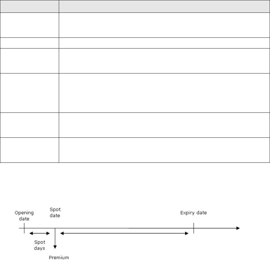
10 Options
10.6 Equity option
Transaction & Risk Management Module (TRM) Instruments: Processing and Calculations 577
•Quotation information
•Netting information
•Branch codes
•Cashflow and transaction charge rules
•Manual charges.
See Appendix A Features on page 713.
10.6.2 Deal capture
10.6.2.1 Input data
In addition to the standard deal parameters, the following information is required to enter an equity
option:
10.6.2.2 Generated data
•Cashflows
For an equity option, the cashflows generated are as follows:
Information Description
Trading Units Number of options bought/sold.
Trading units for the instrument are specified at instrument setup using the Equity
Trading Unit feature. See A.2.321 Trading Unit (Equity) on page 871.
Deal Price Amount of the option premium (per unit).
Strike Strike price of the equity option.
If Strike is defined at instrument level, this is used by default and cannot be modified.
(Nominal/Spot Rate in Transaction Manager)
Expiry Date Final date when the option can be exercised.
If the Expiry Date for the instrument is specified at instrument setup using the Option
Dates feature, this is used as the default in the transaction and cannot be modified at
deal entry.
See A.2.254 Option Dates on page 841.
Option Type Call or Put (Transaction Type in Transaction Manager).
If you specify Type in the instrument setup, this is used as the default in the
transaction and cannot be modified at deal entry.
Issuer Issuer of the instrument.
If this value is specified at instrument setup, it is used as the default in the transaction
and cannot be modified at deal entry.

10 Options
10.6 Equity option
578 © Wall Street Systems IPH AB - Confidential
10.6.3 Processing
This section describes the actions that can be done throughout the life of an equity option.
10.6.3.1 Pricing
Pricing of equity option transactions can be performed using a right-click processing action.
•Setup
The Pricing action is available on the transaction if the Equity Option Pricing feature is associated
with the instrument.
See A.2.134 Equity Option Pricing on page 777.
•Execution
The Pricing action allows you to find the premium price, as well as the theoretical price and the
Greeks, by manually changing the volatility while keeping the other parameters constant.
10.6.3.2 Exercise/no exercise
The holder of the option has a right to exercise the option at a predetermined date or dates.
•Execution
–If the holder of an equity option with physical delivery exercises an option, an exercise
transaction is created. This transaction closes out the option transaction and buys (or sells)
the appropriate amount of the underlying security at the strike price.
–If the holder of an equity option with cash settlement exercises an option, an exercise
transaction is created. This transaction closes out the option transaction and settles the
difference of the strike price and current market price of the underlying (multiplied by the
appropriate number of units of the underlying).
Information Description
Trading Units Trading units of the equity option.
Deal Price By default, this is the Theoretical Price.
Book Value (Information only)
Book Value = Trading Units * Deal Price.
Theoretical Price (Information only)
Theoretical price of the equity option.
Theoretical
Amount
(Information only)
Theoretical price of the equity option weighted by the Book Value.
Intrinsic Value Intrinsic value of the equity option.
Time Value Time value of the equity option.
Volatility Volatility of the equity option.
Delta
Gamma
Theta
Vega
(Information only)
Delta, Gamma, Theta, and Vega of the equity option.

10 Options
10.6 Equity option
Transaction & Risk Management Module (TRM) Instruments: Processing and Calculations 579
•No exercise
If the holder of the option allows the option to expire without exercising it, a “no exercise”
transaction is created. This transaction closes out the option.
•Cancellation
The exercise or no exercise transaction can be canceled. A new exercise/no exercise transaction
can be created as described above.
10.6.4 Position monitoring
10.6.4.1 Calculations
In this section, numerical examples demonstrate how the different figures are calculated for an
Equity Option.
If you need more theoretical information about the method used in these calculations, see Chapter 2
Market standards and calculations on page 33.
This example shows an Equity Option, with the following deal data:
Information Description
Exercise Date Date of the exercise. For a European option, this must be the expiry date.
Delivery Type Physical Delivery or Cash Settlement.
Scenario For cash settlement, this is the scenario from which the market price of the underlying
is retrieved.
Price/spot rate Market price of the underlying instrument (for cash settlement).
No Exercise If the option is not exercised, select No Exercise.
Setup data
Date Basis B 360
Risk Date Basis B_r 365
Tradi ng Unit Size L 100
FX Exposure Offset e_fx 0.01
Underlying instrument data
Price Exposure Offset e_p 5.00%
Annual Dividend (compound) r_y 10.00%
Asset Rate (continuous) r_a = LN(1 +r_y) 0.095310180
Transaction data
Tradi ng Units N 5
Option Type (call = 1, put = -1) type 1
Opening Date 2005-03-17
Spot Date dt_s 2005-03-19
Maturity Date dt_m 2005-06-20
Expiry Date dt_e 2005-06-17
10 Options
10.6 Equity option
580 © Wall Street Systems IPH AB - Confidential
Other important deal data is calculated by the system as follows:
•Nominal Amount
A = type * N * L
500.00 = 1 * 5 * 100
•Book Value (local)
V_bl = pr = 125.00
•Book Value
V_b = V_bl = 125.00
•Period
t_p = (dt_m – dt_s) / B
0.258333333 = (2005/06/20 – 2005/03/19) / 360
Unless otherwise stated, the figure date used in the calculations is 2005-04-15. On this date, the
market data is as follows:
Other market data is calculated by the system as follows:
•Days to Expiry
= dt_m – dt_f = 66
• Time to Maturity
t_m = (dt_m –dt_f) / B = 0.18333333
• Time to Expiry
t_e = (dt_e – dt_f) / B = 0.17500000
• Time to Maturity (risk)
t_m.r = (dt_m –dt_f) / B_r = 0.18082192
• Time to Expiry (risk)
t_e.r = (dt_e – dt_f) / B_r = 0.17260274
•Time to Spot
t_s = d_fs / B = 0.011111111
•Time to Spot (risk)
t_s.r = d_fs / B_r = 0.010958904
• PV Discount Factor
D_Pb = EXP (-r_f * t_m.r) = 0.995705557
• Discount Factor Spot
D_sb = EXP (-r_d * t_s.r) = 0.999780846
Nominal Rate X 35.000000
Premium pr 125.00
Market data on 2005-04-15
Figure Date dt_f 2005-04-15
Interest Rate r_f 2.380071%
Days to Spot d_fs 4
Discount Rate r_d 2.000000%
Asset Spot Price S 35.000000
Quoted Price p_q 0.2500000
Transaction data
10 Options
10.6 Equity option
Transaction & Risk Management Module (TRM) Instruments: Processing and Calculations 581
10.6.4.1.1 Option figures
The option figures on the figure date are as follows:
• Implied Volatility
sg = 7.44225979%
•rc
r_c = LN(D_Pb) / t_m
= 0.023474677
•ds
ds = D_sb * EXP(t_s * r_a)
= 1.000840177
•Asset Today Price
S_t = S * ds
= 35.02940618
•d1
d_1 = (LN(S_t / X) + (r_c - r_a) * t_m + (sg * sg / 2) * t_e) / (sg * SQRT(t_e))
= -0.380474145
•d2
d_2 = d_1 - sg * SQRT(t_e)
= -0.411607351
•price
p = type * ((S_t) * EXP(-r_a * t_m) * NORMSDIST(type * d_1)) - type * ((X) * EXP(-r_c * t_m) *
NORMSDIST(type * d_2))
= 0.249945260
•delta
delta = type * EXP(-r_a * t_m) * NORMSDIST(type * d_1) * ds
= 0.345993457
•Asset Rho
rho.b =-type * t_m * NORMSDIST(type * d_1) * (S_t) * EXP(-r_a * t_m)
= -2.220124682
•Cash Rho
rho.q = type * t_m * NORMSDIST(type * d_2) * (X) * EXP(-r_c * t_m)
= 2.174301384
• Intrinsic Value
v.i=type * ((S_t)*EXP(-r_a*t_m)* 0.5 * (SIGN(type * (LN(ds * S_t / X)+(r_c-r_a)*t_m))+1)) - type *
((X)*EXP(-r_c*t_m)*0.5 * (SIGN(type * (LN(ds * S_t / X)+(r_c-r_a)*t_m))+1))
=0.00
10.6.4.1.2 Valuation figures
•Market Value
V = type * p_q * A * D_sb
=124.97
•Present Value
V_p= type * p * A
= 124.97
• Intrinsic Value
V_i=v.i*A
=0.00
10.6.4.1.3 Risk figures
• Price Exposure
E_p = type * A * delta * S * e_p
= 302.74
•IR Exposure 1bp
E_i = type * A * rho.q * 0.0001
= 0.108715
10 Options
10.7 Index option
582 © Wall Street Systems IPH AB - Confidential
10.7 Index option
An index call option gives the holder of the option a right (but not an obligation) to buy the specified
amount of the underlying index at the specified strike price.
An index put option gives the holder of the option a right (but not an obligation) to sell the specified
amount of the underlying index at the specified strike price.
As it is not practical to buy or sell the index, the index options are settled with cash when they
expire. The holder of the in-the-money option receives the difference between the current index
value and the strike (multiplied by the number of options and the point value).
In return for this potential gain, the option holder must pay a premium up-front to compensate the
other party for the additional risk.
In TRM the index options must be exchange traded, that is, the strike price, expiry date, and option
type (call/put), need to be defined for the instrument.
In TRM the following index option instruments are supported:
•European type options, where the option can be exercised only at the expiry date
•American type options, where the option can be exercised any time on or before the expiry date.
10.7.1 Instrument setup
Index option instruments must be based on an instrument type derived from the class
INDEX-OPTION.
•Main characteristics
The following basic information may be captured when defining the instrument. This information
is relevant to any kind of index option instrument.
See A.2.211 Index Option on page 818.
•Option expiry definition
Information Description
Issuer details Issuer (writer) of the option.
Underlying Underlying index instrument.
Strike price
details
Strike price of the option.
Rounding
parameters
Method and precision used to round cashflow amounts.
Currency Currency of the index option.
Type Type of option: Call or Put.
Price Type
information
Amount/Unit.
Exercise and
Delivery
parameters
Defines when the option can be exercised, and whether there is a physical delivery or
a cash settlement.
For an index option there must always be cash settlement.
Further contract
information
Further information concerning the relationship between the option and the
underlying.

10 Options
10.7 Index option
Transaction & Risk Management Module (TRM) Instruments: Processing and Calculations 583
You can set up option date information at instrument level.
See A.2.254 Option Dates on page 841.
•Trading units
It is possible to specify the point and tick values of the index option instrument.
See A.2.322 Trading Unit (Index) on page 872.
For an index option, it is also possible to set up:
•Spot date calculation to define the date when the premium is paid
•Quotation information
•Netting information
•Branch codes
•Cashflow and transaction charge rules
•Manual charges.
See Appendix A Features on page 713.
10.7.2 Deal capture
10.7.2.1 Input data
In addition to the standard deal parameters, the following information is required to enter an index
option:
Information Description
Calendar
parameters
Calendars used to calculate the expiry date.
Expiry Date Final date when the option can be exercised.
Delivery Offset Number of days offset allowed in which to deliver the underlying after the option is
exercised.
Information Description
Trading Units Number of options bought/sold.
Deal Price Amount of the option premium (per unit).
Issuer Issuer of the option.
If Issuer is defined at instrument level, this is used by default and cannot be modified.
Strike Strike index value of the option.
If Strike is defined at instrument level, this is used by default and cannot be modified.
(Nominal/Spot Rate in Transaction Manager)
Option Type Type of option: Call or Put.
If Type is defined at instrument level, this is used by default and cannot be modified.
(Transaction Type in Transaction Manager)
Expiry Date Final date when the option can be exercised.
If date information is defined at instrument level, this is used by default and cannot be
modified.
Value Date Date when the exercise is settled.

10 Options
10.7 Index option
584 © Wall Street Systems IPH AB - Confidential
10.7.2.2 Generated data
•Cashflows
For an index option, the cashflows generated are as follows:
10.7.3 Processing
This section describes the actions that can be done throughout the life of an index option.
10.7.3.1 Exercise/no exercise
The holder of the option has a right to exercise the option at a predetermined date or dates.
Note: The Exercise action for netted options is not supported.
•Execution
–If the holder of an index option exercises an option, an exercise transaction is created. This
transaction closes out the option transaction and settles the difference of the strike index
value and current underlying index value (multiplied by the number of options and point
value).
•No exercise
–If the holder of the option allows the option to expire without exercising it, a “no exercise”
transaction is created. This transaction closes out the option transaction.
•Cancellation
The exercise or no exercise transaction can be canceled. A new exercise/no exercise transaction
can be created as described above.
Opening
date Spot
date
Spot
days
Premium
Expiry date
Information Description
Exercise Date Date of exercise. For a European option, this must be the expiry date.
Delivery Type Cash Settlement.
Scenario For cash settlement, this is the scenario from which the value of the underlying
index is retrieved.
Price/Spot Rate Value of the underlying index
No Exercise If the option is not exercised, select No Exercise.

10 Options
10.8 FX option
Transaction & Risk Management Module (TRM) Instruments: Processing and Calculations 585
10.8 FX option
This section describes the different types of FX options supported in TRM: plain vanilla, digital,
barrier and compound FX options. It provides instructions for setting up these instruments,
capturing deals, processing and generated data, and calculations. See 10.8.6 Position monitoring on
page 610 for more information about the calculations of FX options.
Additionally, it provides information about valuation settings, for example, to customize the default
valuation settings; and describes the valuation models that are used according to the type of FX
option.
Default valuation settings are determined by the feature FX Option Valuation (See feature A.2.189
FX Option Valuation on page 805). To customize these default settings, use the feature FX Option
Setup (A.2.188 FX Option Setup on page 804). For more information about the valuation models,
see 10.8.6.2.2 Option valuation models on page 611.
10.8.1 Vanilla FX option
An FX Option is the right either to buy or to sell a specified amount of one currency at a price
denominated in another currency. The price of one currency in terms of another currency is known
as an exchange rate. The exercise price (or strike) of a FX Option thus represents an exchange rate.
An option that gives a right to buy is a call option, and an option that gives a right to sell is a put
option.
In addition, there are two different kinds of options: physical delivery options and cash-settled
options.
A physical delivery option gives the owner the right to receive the physical delivery (if it is a call), or
to make physical delivery (if it is a put), of the underlying currencies when the option is exercised.
A cash-settled option gives its owner the right to receive a cash payment based on the difference
between a determined value of the underlying at the time the option is exercised (spot rate from the
market) and the fixed exercise price of the option. A cash-settled Call conveys the right to receive a
cash payment if the determined value of the underlying at exercise exceeds the exercise price of the
option. And a cash-settled Put conveys the right to receive a cash payment if the determined value
of the underlying at exercise is less than the exercise price.
The style of the option refers to when that option is exercisable. With a European exercise style
option, the holder can only exercise the option at expiry. With an American exercise style option,
however, the holder can choose to exercise at any time between the purchase date of the option and
the expiry.
In return for this flexibility, the option holder must pay a premium up-front to compensate the other
party for the additional risk.
10.8.1.1 Instrument setup
FX OTC Options are based on a type derived from the FX-OPTION instrument class.
•Main characteristics
The following basic information may be captured when defining the instrument.
Information Description
Exercise
Instrument
Underlying FX instrument.
If defined, this underlying instrument is applied to each transaction. Leave this field
blank if you want to specify the underlying instrument when you enter the deal.
Type Type of option: Call or Put.
Exercise Type European or American or Templatized (for Bermudan).
Delivery Type Cash Settlement or Physical Delivery.
10 Options
10.8 FX option
586 © Wall Street Systems IPH AB - Confidential
–Dates definition
You can set up expiry and premium date information at instrument level.
See A.2.182 FX Option on page 800.
•Premium definition
Further information relating to the characteristics of the premium can also be set up at
instrument level.
See A.2.186 FX Option Premium on page 803.
•Pricing
The system can provide the theoretical premium (option value) before the actual premium is
captured. This action becomes available on the transaction when the FX-Option-Pricing feature
has been applied to the instrument.
See A.2.187 FX Option Pricing on page 803.
For an FX OTC Option, it is also possible to set up:
•Cashflow and transaction charge rules
•Manual charges
•Branch codes.
Information Description
Gap Set Gap set used for supplying the expiry periods for the option; these in turn are
used to define exact dates. This is a mandatory field.
Expiry Date Period Expiry period used to calculate the expiry date for the option at deal entry, for
example, 6M or 1Y.
If you specify the expiry date period in the instrument setup, this is used as the
default in the transaction and cannot be modified.
Premium Offset Number of days offset between the applied date defined in the Applied On field
and the premium date.
Applied On Date on which the settlement of the premium takes place (Premium Date).
This is the spot date by default.
Calendar
Holiday Calendar
Calendars used to calculate the expiry date and premium date of an option
instrument.
If you enter both a Calendar and a Holiday Calendar, the expiry date and
premium date calculation takes both calendars into account.
Spot Time
Spot Time Zone
Cut-off time for operations.
For global operations, a cut-off time has to be defined: deals before that time
have the number of spot days calculated from that day; deals after that time
have the spot days calculated from the following day. Define a time (Spot
Time) within a selected time zone (Spot Time Zone).
The market convention is 5 p.m. New York time.
Information Description
(Premium) Type Determines how the premium amount is calculated.
If defined, the FX Premium Type is applied to each transaction. Leave this field blank if
you want to specify the premium type when you enter the deal.
(Premium)
Currency
Currency of the premium.
If defined, the premium currency is applied to each transaction. Leave this field blank
if you want to specify the premium currency when you enter the deal.
10 Options
10.8 FX option
Transaction & Risk Management Module (TRM) Instruments: Processing and Calculations 587
See Appendix A Features on page 713.
10.8.1.2 Deal capture
10.8.1.2.1 Input data
In addition to the standard deal parameters, the following information is required to enter an FX
OTC Option:
10.8.1.2.2 Generated data
•Cashflows
When dealing a Vanilla FX option, four cashflows are generated:
–Option position at opening date: this contains all the relevant information of the option
–Option premium settlement at premium date
Information Description
Trans ac ti on Type
(Type)
Call or Put.
Secondary Instrument
(Exercise Instrument)
The underlying instrument of the FX option.
Currency
(Base Currency)
Corresponds to the currency that is bought/sold if the Call/Put FX option is
exercised.
Currency 2nd
(Quote Currency)
Corresponds to the currency that is sold/bought if the Call/Put FX option is
exercised.
Expiry Date Date on which the FX Option expires.
Deal Rate
(Strike)
Fixed exercise price of the FX option.
FX Base Amount
(Base Amount)
Amount that is bought/sold if the Call/Put FX option is exercised.
FX Quote Amount
(Quote Amount)
Amount that is sold/bought if the Call/Put FX option is exercised.
FX Premium Type Determines how the premium amount is calculated.
Premium Price Depends on the premium type: This could be specified in amount, percent, or
points.
Fixing Subscenario Subscenario from which the FX spot rate is retrieved.
10 Options
10.8 FX option
588 © Wall Street Systems IPH AB - Confidential
–Two cashflows for the potential delivered currencies at value date: these cashflows will only
be generated if the option is exercised with physical delivery.
The asset currency is displayed in the transaction column Asset CCY. The cashflow kind Reversed
Asset CCY informs valuation that asset currency is the quote currency, and valuation does the
required reversals. For more information about asset and cash currencies, see 2.3.3.1 Asset and
cash currencies on page 116.
10.8.1.3 Processing
This section describes the actions that can be done throughout the life of an FX option.
10.8.1.3.1 Pricing
Pricing of FX option transactions can be performed using a right-click processing action.
•Setup
The Pricing action is available on the transaction if the FX Option Pricing feature is associated
with the instrument, see A.2.187 FX Option Pricing on page 803.
Note: Before running the Pricing action, you need to set up the pricing configuration in
Transaction Manager, Option - Pricing Configuration. For more information about setting up
pricing at the transaction level, see TRM User Guide.
•Execution
The Pricing action allows you to find the premium price, as well as the theoretical price and the
Greeks, by manually changing the volatility while keeping the other parameters constant.
Option
position
Opening
date Spot
days
Premium
date
Premium Expiry
Expiry
date
Value
date
Quote currency
Base currency
Information Description
Premium
Currency
Currency of the Premium cashflow.
Premium Type Premium type: Percentage or Points.
Premium Amount Premium Amount = Premium Price * Base Amount of the transaction.
Theoretical Price (Information only)
Theoretical price of the FX option.
Theoretical
Amount
(Information only)
Theoretical price of the FX option multiplied by the Base Amount of the transaction.
Intrinsic Value Intrinsic value of the FX option.
Time Value Time value of the FX option.
Volatility Volatility of the FX option.
10 Options
10.8 FX option
Transaction & Risk Management Module (TRM) Instruments: Processing and Calculations 589
10.8.1.3.2 Exercise/no exercise (single option)
The principle is to allow the user to exercise the option:
•If the holder of a physical delivery option wishes to buy (in case of a call) or sell (in the case of a
put) the underlying at the exercise price (strike)
•In the case of a cash-settled option, to receive the cash settlement amount (price of the
underlying at exercise - exercise price of the option).
There are three styles of exercise:
•European: option can be exercised at expiry date
•American: option can be exercised between the opening date and the expiry date.
•Templatized (for Bermudan): option can be exercised at dates specified in the exercise schedule
attached to the transaction. See Appendix C Option schedules on page 911.
If the current spot rate of the exchange rate of the underlying is above the exercise price of the FX
Option, the Call option is considered in-the-money (below for a Put Option).
Then, the user will be able to exercise the FX option.
Conversely, if the current spot rate of the exchange rate of the underlying is below the exercise
price of the FX Option, the Call option is considered out-of-the-money (above for a Put Option). In
this case, a No Exercise is suggested (No Exercise switch selected).
•Execution - Physical Delivery
In the case of exercise with physical delivery, the agreed amount of underlying currencies is
delivered at the agreed exchange rate (strike).
The following table describes the exercise parameters:
Click Next to complete the exercise parameters for a physical delivery:
Delta
Gamma
Theta
Vega
(Information only)
Delta, Gamma, Theta, and Vega of the FX option.
Information Description
Information Description
Exercise Date Date when the exercise is done.
Value Date Shows value date of the delivery transaction. This date can be modified if the
exercise date is before or later than the expiry date of the initial transaction
(American or Bermudan style).
Note: Read-only for a partial exercise.
Delivery Type Physical Delivery.
Information Description
Delivery Instrument (Read-only.) Exercise FX Instrument.
Base Currency (Read-only.) Shows the base currency of the transaction
Base Amount (Read-only except for a partial exercise.)
Shows the base amount of the transaction.
Quote Currency (Read-only.) Shows the quote currency of the transaction.
10 Options
10.8 FX option
590 © Wall Street Systems IPH AB - Confidential
Click Finish.
An Exercise transaction is generated based on each underlying currency with the following
attributes.
Depending on the option type and the sign of the option transaction, the sign of the exercise
transaction is as follows:
where:
Buy/Sell is relative to the Base currency
Instrument = Exercise Instrument (Secondary Instrument) of the option
transaction
FX Base amount = FX Base Amount of the option transaction
FX Quote amount = FX Quote Amount of the option transaction
Exchange Rate (Deal Rate) = strike (deal rate) of the option
Opening date = date when the exercise is done
Value date = date when the exercise is settled
Kind = Exercise
The remaining attributes are inherited from the initial transaction.
With physical delivery, it is also possible to do a partial exercise of the option contract at expiry.
This will close the full original option position. After a partial exercise, it will not be possible to
exercise the amount left of the original option.
•Execution - Cash Settlement
In the case of exercise of a cash-settled option, the underlying currencies are not delivered but a
settlement amount is received (or paid) instead.
The following table describes the exercise parameters:
Quote Amount (Read-only except for a partial exercise.)
Shows the quote amount of the transaction.
Strike (Read-only.)
Shows the deal rate of the option.
Spot Rate Shows the FX spot rate between base and quote currencies.
No Exercise Indicates whether the option should be exercised based on entered Spot Rate.
• Selected if the option is out-of-the-money.
• Not selected if option is in-the-money.
Option Exercise
Buy/Call Buy
Sell/Call Sell
Buy/Put Sell
Sell/Put Buy
Information Description
Exercise Date Date when the exercise is done.
Value Date Date when the exercise is settled. This cannot be later than the maturity date
of the initial transaction.
Information Description
10 Options
10.8 FX option
Transaction & Risk Management Module (TRM) Instruments: Processing and Calculations 591
Click Next to complete the exercise parameters for a cash settlement:
Click Finish.
An Exercise transaction is generated based on each underlying currency with the following
attributes:
Opening date = date when the exercise is done
Value date = date when the exercise is settled
Kind = Exercise
A Net settlement cashflow is generated with Amount = Net settlement Amount
The remaining attributes are inherited from the initial transaction.
In the case where the option is out-of-the-money, the user has to execute a No Exercise.
A No Exercise transaction is generated based on the option with the following attributes:
Opening date = date when the No exercise is done
Kind = No Exercise
The remaining attributes are inherited from the initial transaction.
•Cancellation
It is possible to cancel the generated transaction (Exercise, No Exercise).
Delivery Type Cash Settlement.
Information Description
Base Currency (Read-only.) Shows the base currency of the transaction
Base Amount (Read-only except for a partial exercise.)
Shows the base amount of the transaction.
Quote Currency (Read-only.) Shows the quote currency of the transaction.
Quote Amount (Read-only except for a partial exercise.)
Shows the quote amount of the transaction.
Strike (Read-only.)
Shows the deal rate of the initial transaction.
Fixing Subscenario Subscenario from which the FX spot rate is retrieved. Typically, use the FIXING
scenario.
Read-only when defined at the transaction level, otherwise editable.
Spot Rate Shows FX spot rate between base and quote currencies based on the selected
subscenario. The spot rate is recalculated when the exercise date changes.
Settlement Currency Currency of the net settlement amount.
Defaults to the premium currency.
Settlement Amount Amount to be settled. This amount is recalculated when the spot rate changes.
No Exercise Indicates whether the option should be exercised based on the spot rate.
• Selected if the option is out-of-the-money.
• Not selected if option is in-the-money.
No exercise is recalculated when the spot rate changes.
Information Description

10 Options
10.8 FX option
592 © Wall Street Systems IPH AB - Confidential
10.8.1.3.3 Exercise/no exercise (multiple options)
TRM allows you to exercise multiple options at the same time assuming that certain conditions are
met. In which case, the exercising follows a similar logic to exercising single options though the
action is simplified.
•Execution
To exercise multiple options at the same time, the following conditions must be met:
–All transactions must have the same Fixing/Action Date. If there is no Fixing/Action Date
then the current date is used. For example, as well as other criteria, your query criteria may
include a given Fixing/Action Date. (The Fixing/Action Date column must be visible in the
Query and Transaction views.)
–All transactions must be exercisable, i.e. the Exercise action is available.
Among the resulting transactions, you might have transactions using an instrument set up for
cash settlement or physical delivery. Depending on your needs you can choose the following
options:
–Default: Exercises the options according to the contract setting (cash settlement or physical
delivery) at the instrument level.
–Cash Settlement: Allows you to force all options to be exercised as cash settlement.
–Physical Delivery: Allows you to force all options to be exercised as physical delivery. In this
case only, you can choose to exercise or not exercise the options.
Note: For Default and Cash Settlement, the options are exercised according to whether they are
at-the-money or not.
When you click OK, one exercise (no exercise) transaction is generated for each selected option.
You need to apply these transactions.
10.8.1.3.4 Early expiration (close out)
For an OTC FX Option, early expiration will close out the option contract.
•Execution
The following table describes the early expiration parameters:
The execution generates an early expiration transaction with the following attributes:
Sign = Opposite sign of the initial option transaction
Opening date = date when the early expiration is done
Information Description
Opening Date Date when the early expiration is done.
Premium Date Date on which the settlement of the premium takes place.
Amount to Expire Amount to be early expired. This defaults to the amount still available to be early
expired, taking into account previous partial early expirations.
Amount Left Remaining amount of the initial transaction.
FX Premium Type Determines how the premium amount is calculated (from the initial transaction).
Premium
Currency
Currency of the premium (from the initial transaction).
Premium Price New option premium price relative to the early expiration.
Premium Amount Premium amount of the early expiration.
10 Options
10.8 FX option
Transaction & Risk Management Module (TRM) Instruments: Processing and Calculations 593
Premium = new premium price
Kind = Early Expiration
The remaining attributes are inherited from the initial transaction.
•Cancellation
It is possible to cancel the generated transaction (Early Expiration).
10.8.2 Digital FX option
A Digital Option (also known as a binary option) is designed specifically for traders who believe that
the market will be above or below a certain level at a specified time, and is a good way to profit from
a rally or a correction in the market. The digital option pays a fixed amount if the spot price is above
(call) or below (put) the target level that you have chosen.
As long as the spot price is above or below the barrier level at expiration, you receive the payoff.
The payoff of a digital option is only governed by the spot price prevailing at expiration.
If the spot price is not above (in the case of a Call) or below (in the case of a Put) the specified
barrier at the end of the option period, the option expires worthless.
A One Touch Option is an American style digital option. As long as the spot level hits the barrier level
at least once prior to expiration, the payoff amount is received at expiry. If the barrier is not reached
during the option period, the option expires worthless.
10.8.2.1 Instrument setup
FX digital options are based on a type derived from the FX-OPTION instrument class.
•FX Option Digital main characteristics
The following basic information may be captured when defining the instrument.
–Date definition
You can set up expiry and premium date information at instrument level.
Information Description
Type Type of option: Call or Put.
Exercise Type European or American or Templatized (for Bermudan).
Information Description
Gap Set Gap set used for supplying the expiry periods for the option; these in turn are
used to define exact dates. This is a mandatory field.
Expiry Date Period Expiry period used to calculate the expiry date for the option at deal entry, for
example, 6M or 1Y.
If you specify the expiry date period in the instrument setup, this is used as the
default in the transaction and cannot be modified.
Premium Offset Number of days offset between the applied date defined in the Applied On field
and the premium date.
Applied On Date on which the settlement of the premium takes place (Premium Date).
This is the spot date by default.
Calendar
Holiday Calendar
Calendars used to calculate the expiry date and premium date of an option
instrument.
If you enter both a Calendar and a Holiday Calendar, the expiry date and
premium date calculation takes both calendars into account.
10 Options
10.8 FX option
594 © Wall Street Systems IPH AB - Confidential
See A.2.184 FX Option Digital on page 801.
•Premium definition
For the remaining characteristics of the premium, you can also set up some information at
instrument level.
See A.2.186 FX Option Premium on page 803.
For an FX digital option, it is also possible to set up:
•Cashflow and transaction charge rules
•Manual charges
•Branch codes.
See Appendix A Features on page 713.
10.8.2.2 Deal capture
10.8.2.2.1 Input data
In addition to the standard deal parameters, the following information is required to enter an FX
digital option:
Spot Time
Spot Time Zone
Cut-off time for operations.
For global operations, a cut-off time has to be defined: deals before that time
have the number of spot days calculated from that day; deals after that time
have the spot days calculated from the following day. Define a time (Spot
Time) within a selected time zone (Spot Time Zone).
The market convention is 5 p.m. New York time.
Information Description
Type Premium type: Determines how the premium amount is calculated.
If defined, this is used as the default premium type and cannot be modified when
dealing the instrument.
Currency Currency of the premium.
If defined, this is used as the default premium currency and cannot be modified when
dealing the instrument.
Information Description
Information Description
Trans ac ti on Type
(Type)
Call or Put.
Currency
(Base Currency)
Corresponds to the base currency of the currency pair.
Currency 2nd
(Quote Currency)
Corresponds to the quote currency of the currency pair.
Expiry Date Date on which the FX Option expires.
Deal Rate
(Strike)
Strike of the digital FX option.
FX Base Amount (*)
(Base Amount)
Payoff amount if entered in base currency.

10 Options
10.8 FX option
Transaction & Risk Management Module (TRM) Instruments: Processing and Calculations 595
(*) The payoff is either input in base amount or quote amount depending on the currency.
In addition, the following optional information can be captured:
10.8.2.2.2 Generated data
•Cashflows
The structure of the generated cashflow is as for a FX vanilla standard case (apart from the
pseudo cashflows relative to the underlying):
–Option position at opening date: this contains all the relevant information of the option
(payoff definition in the Expression field).
–Option premium settlement at premium date.
10.8.2.3 Processing
10.8.2.3.1 Exercise/no exercise
For European FX digital options, at expiry, the user is able to exercise the option.
If the current spot rate of the exchange rate of the underlying is above the exercise price of the FX
option, the Call option is considered in-the-money (below for a Put Option).
Then, when exercising the FX digital option, the buyer will receive the payoff (seller/pay).
Conversely, if the current spot rate of the exchange rate of the underlying is below the exercise
price of the FX option, the Call option is considered out-of-the-money (above for a Put Option). In
this case, when exercising the FX digital option, the buyer will not receive anything.
FX Quote Amount (*)
(Quote Amount)
Payoff amount if entered in quote currency.
FX Premium Type Determines how the premium amount is calculated.
Premium Price Depends on the premium type: This could be specified in amount, percent, or
points.
Fixing Subscenario Subscenario from which the Exchange spot rate is retrieved.
Information Description
Premium Date Date on which the payment of the premium occurs.
Note: If you specify the date type in the instrument setup, this is used as the default
in the transaction and cannot be modified: see A.2.184 FX Option Digital on
page 801.
Premium Currency Currency of the premium. The premium currency corresponds to the payoff currency.
Note: If you specify the premium currency in the instrument setup, this is used as the
default in the transaction and cannot be modified: see A.2.186 FX Option
Premium on page 803.
Expiry Code If the Expiry Date Setup feature is applied at instrument level, you can enter the
expiry date period you want to use to calculate the expiry date for the transaction, for
example, 3M (3 months).
Note: If you specify an expiry date period in the instrument setup, this is used as the
default in the transaction and cannot be modified: see A.2.184 FX Option Digital
on page 801.
Information Description
10 Options
10.8 FX option
596 © Wall Street Systems IPH AB - Confidential
•Execution
The following table describes the exercise parameters:
An Exercise transaction is generated based on the option, with the following attributes:
Opening date = date when the exercise is done
Value date = date when the exercise is settled
Kind = Exercise
A Net settlement cashflow is generated with Amount = Payoff
The remaining attributes are inherited from the initial transaction.
The payoff is represented by a Net settlement cashflow.
•Cancellation
It is possible to cancel the generated transaction (Exercise, No Exercise).
10.8.2.3.2 Early expiration (close out)
See 10.8.1.3.4 Early expiration (close out) on page 592.
10.8.3 Barrier FX option
A barrier option is similar to a plain vanilla option but with one exception: the presence of one or two
trigger prices or barriers. If the barrier is touched at any time before maturity, it causes an option
Information Description
Exercise Date Date when the exercise is done.
Value Date Date when the exercise is settled. This cannot be later than the maturity date
of the initial transaction. Editable if the exercise date is before the expiry date
for American and Bermudan options).
Base Currency (Read-only.) Shows the base currency of the transaction
Quote Currency (Read-only.) Shows the quote currency of the transaction.
Strike (Read-only.)
Shows the deal rate of the initial transaction.
Fixing Subscenario Subscenario of the option position flow (exercise event in case of a
Bermudan). Typically, use the fixing scenario.
Read-only when defined at transaction level, otherwise editable.
Spot Rate Shows FX spot rate between base and quote currencies based on the selected
subscenario. The spot rate is recalculated when the exercise date changes.
Settlement Currency Currency of the net settlement amount.
Defaulted to the premium currency.
Settlement Amount Amount to be settled (payoff amount). This amount is recalculated when the
spot rate changes.
If the option is out-of-the-money, a null amount (0) is diplayed, otherwise
either the base amount or quote amount is displayed depending on which one
was entered at transaction level.
No Exercise Indicates whether the option should be exercised based on the spot rate.
• Selected if the option is out-of-the-money.
• Not selected if option is in-the-money.
No exercise is recalculated when the spot rate changes.

10 Options
10.8 FX option
Transaction & Risk Management Module (TRM) Instruments: Processing and Calculations 597
with pre-determined characteristics to come into existence (in the case of a knock-in option) or it
will cause an existing option to cease to exist (in the case of a knock-out option).
If a knock-out option has been knocked out, or if a knock-in option fails to knock in, the option’s
value is zero at expiration date, no matter what the value of the underlying.
There are single barrier options and double barrier options:
•Single barrier options which have one barrier.
•Double barrier options which have barriers on either side of the strike (that is, one trigger price
is greater than the strike, and the other trigger price is less than the strike). Touching either of
them will knock the option.
Intuitively, barrier options should be cheaper than their plain vanilla counterparts because they run
the risk of either not being knocked in or being knocked out.
In total, there are eight types of single barrier options, comprising puts or calls which have barriers.
System schedule templates are provided for each of these types. These are described in C.2.1
System-defined templates on page 913.
•Up-and-in
For an up-and-in call or put, the payout at expiration is zero unless, at some time during the
option’s life time, the underlying breaches the barrier to go above the current spot rate. If this
happens the option becomes a vanilla put option.
•Up-and-out
For an up-and-out call or put, if the underlying breaches the barrier level to go above the current
spot rate, the option ceases to exist.
•Down-and-in
For a down and in call or put, the payout is zero unless the underlying goes below the barrier
level, in which case the option becomes a vanilla call option.
•Down-and-out
For a down and out call or put, if the underlying goes below the barrier level, the option ceases
to exist. Otherwise, the payout is a call option.
•Option with Rebate
Rebates are pre-defined payoffs which are sometimes given when a barrier expires worthless.
With a knock-out option, at the breach of the barrier, the owner of the contract receives the
rebate. With a knock-in option, the rebate is paid at expiry date if the option was not knocked in.
10.8.3.1 Instrument setup
FX barrier options are based on a type derived from the FX-OPTION instrument class.
•FX Option main characteristics
The following basic information may be captured when defining the instrument.
See A.2.182 FX Option on page 800.
Information Description
Exercise
Instrument
Underlying FX instrument.
Option Type Call or Put.
Exercise Style European or American.
Delivery Style Physical Delivery or Cash-Settlement.
10 Options
10.8 FX option
598 © Wall Street Systems IPH AB - Confidential
•Barrier definition
See A.2.140 Exotic Structure (Option) on page 780.
•Expiry definition
You can set up expiry information at instrument level.
See A.2.141 Expiry Date Setup on page 781.
•Premium definition
The main characteristics of a premium are: premium date, premium type, premium currency,
and premium price. The premium amount can then be determined.
For the premium date, it is possible to set up some information at instrument level:
See A.2.263 Premium Date Setup on page 844.
For the remaining characteristics of the premium, you can also set up some information at
instrument level:
See A.2.186 FX Option Premium on page 803.
Information Description
Option Schedule Option Schedule template to be used for the barrier definition. See Appendix C Option
schedules on page 911 for more information about these templates.
If this is not defined at instrument level it must be specified for each transaction.
Note: It is also possible to associate one or several option schedule template groups
to the instrument (see below).
Information Description
Calendar
Holiday Calendar
Calendars used to calculate the expiry date.
Gap Set Gap set used for supplying the available expiry periods.
Expiry Date Period If defined, this expiry period is applied to each transaction and cannot be changed at
deal entry.
Information Description
Calendar
Holiday Calendar
Calendars used to calculate the premium date.
Date Type Type of date on which the payment of the premium occurs (Premium Date).
This is spot date by default.
Offset Offset between the date defined as the premium date type and the premium date.
Information Description
Premium Type Determines how the premium amount is calculated.
If defined, this is used as the default premium type and cannot be modified when
dealing the instrument.
Premium
Currency
Currency of the premium.
If defined, this is used as the default premium currency and cannot be modified when
dealing the instrument.

10 Options
10.8 FX option
Transaction & Risk Management Module (TRM) Instruments: Processing and Calculations 599
•Option schedule groups
You can limit the choice of schedules available to assign to a FX barrier option in Transaction
Manager by associating one or several option schedule template groups to the instrument.
When this feature is selected, it is possible to assign one or several option schedule template
groups to the instrument and, at deal entry, only the templates belonging to these groups will be
available for selection.
Note: If a barrier structure is already defined, this will override the option schedule groups setup.
See A.2.256 Option Template Setup on page 842.
For an FX barrier option, it is also possible to set up:
•Cashflow and transaction charge rules
•Manual charges
•Branch codes.
See Appendix A Features on page 713.
10.8.3.2 Deal capture
10.8.3.2.1 Input data
•General information
An FX barrier option will be dealt using the same standard deal parameters as an FX vanilla
option.
To define the barrier part of the option, you must specify the barrier characteristics. An option
schedule template must be applied on the deal (see Appendix C Option schedules on page 911),
which will generate the barrier structure on the option deal.
•Knock In
An option schedule template needs to be selected that contains a Knock-In schedule (with which
a Knock event is generated with In as Subcategory).
Then, in the Option Schedule view, the following information must be supplied:
–For up-and-in, Expression (fx > cap) and Cap for the barrier
–For down-and-in, Expression (fx < floor) and Floor for the barrier
Many other parameters in an option schedule can be adjusted in order to modify the barrier (for
example, in the case of a discontinuity barrier).
•Knock Out
You need to select an option schedule template that contains a Knock-Out schedule (with which
a Knock event is generated with Out as the Subcategory).
Then, in the Option Schedule view, the following information must be supplied:
–For up-and-out, Expression (fx > cap) and Cap for the barrier
–For down-and-out, Expression (fx < floor) and Floor for the barrier
Many other parameters in an option schedule can be adjusted in order to modify the barrier (for
example, in the case of a discontinuity barrier).
•With Rebate
An option schedule template, which contains a Rebate schedule (with which a Rebate cashflow is
generated), needs to be selected.

10 Options
10.8 FX option
600 © Wall Street Systems IPH AB - Confidential
Then, in the Option Schedule view, the rebate amount needs to be input (as a Rate value).
Many other parameters in an option schedule can be adjusted in order to modify the rebate (for
example, value date).
10.8.3.2.2 Generated data
•Cashflows
The structure of the generated cashflow is identical to the FX vanilla standard case.
Concerning the barrier structure, there is in addition:
•Option Schedule
When an option template is selected, one option schedule is created for each item in the
template. Some of the fields are automatically defaulted from the transaction parameters. See
Appendix C Option schedules on page 911.
•Event
A knock event will be generated from the option schedule.
10.8.3.3 Processing
10.8.3.3.1 Execute Barrier
The Knock-In option consists of a standard option (call or put) and a trigger. It is activated if the
spot rate touches the trigger during the term: if the option is knocked-in, it becomes a standard
option.
The Knock-Out option consists of a standard option (call or put) and a trigger. The option expires if
the spot rate touches the trigger during the term.
For the European style, the term is at expiry date, and for the American style, the standard active
period of the trigger is between the opening date and the expiry date.
This first step is to evaluate the trigger in Transaction Manager’s Event view.
•Execution
If an FX option has a barrier, you must evaluate the barrier each time it is defined in the option
contract to either enable (in case of a knock-in) or disable (in case of a knock-out) the option.
If a barrier exists on the option, you can use the right-click Execute Barrier menu option to
evaluate the barrier.
The following table describes the action parameters:
Information Description
Execution Date Date when the trigger is evaluated.
If today is within the barrier window, the date defaults to the current date
(today) or to the last day of the past barrier window. You can modify the date
as long as the date is still within the barrier window.
Note: If the date of the fixing action was set on the deal prior to barrier
execution, you will not be able to modify the date.
Fixing Subscenario The subscenario used to retrieve spot rate.
Spot Rate The FX spot rate at execution date defaulted from fixing scenario/subscenario.
You can modify this rate.
Touched Barrier Type When available, displays the barrier that has been touched. This is especially
useful for multiple barrier options.
Note: When both an in and an out barrier are touched the out barrier takes
precedence.

10 Options
10.8 FX option
Transaction & Risk Management Module (TRM) Instruments: Processing and Calculations 601
–For touched in barriers, inactive and in-triggerable attributes are removed from the option.
–For touched out barriers or when the option had in barriers that have not been touched and
do not have any in barriers in the future, a no exercise transaction is generated in order to
close the position of the option.
–For all other cases, no action.
•Cancellation
It is possible to cancel the generated transaction.
10.8.3.3.2 Exercise/no exercise
When the barrier option becomes a plain vanilla option, the normal processing is applicable to the
option.
See 10.8.2.3.1 Exercise/no exercise on page 595.
10.8.3.3.3 Early expiration (close out)
Barrier options can be early expired in a similar way to standard FX options.
See 10.8.1.3.4 Early expiration (close out) on page 592.
10.8.4 Compound FX option
A compound option is an option to buy or sell another option: it gives the right to buy or sell (for a
pre-agreed amount at a set future date) a second option of predetermined specification.
This second option is known as the underlying option.
The purchaser of the compound option pays an initial premium (the front premium). If the
purchaser chooses to exercise the right to buy the underlying option, an exercise premium (the back
premium) is paid.
There are four possible types of compound options:
–Call on Call
–Call on Put
–Put on Call
–Put on Put.
An example of a FX compound option would be a call-on-call option giving the owner the right to
buy, in 1 month's time, a 6 month 1.55 US Dollar call/Canadian Dollar call expiring 7 months from
today (or 6 months from the expiry of the compound). The strike price on the compound is the
premium that would be paid in 1 month's time if the compound for the option expiring 6 months
from that point in time is exercised.
Touched Barrier
Expression
Displays which Boolean expression activated the touched barrier.
Rebate Currency
Rebate Amount
When available, displays the rebate information associated with touched
barrier.
No Exercise Shows that the system will automatically perform a no exercise of the deal.
This switch is switched on in the following cases:
• An out barrier is touched, i.e. the spot rate is equal to or higher the rate
defined in the expression.
• None of the in barriers have been touched and there are no more in
barriers to evaluate in the future.
Information Description
10 Options
10.8 FX option
602 © Wall Street Systems IPH AB - Confidential
10.8.4.1 Instrument setup
FX compound options are based on a type derived from the FX-OPTION instrument class.
•FX Compound Option main characteristics
The following basic information may be captured when defining the instrument.
–Date definition
You can set up expiry and premium date information at instrument level.
See A.2.183 FX Option Compound on page 801.
•Premium definition
Further information relating to the characteristics of the premium can also be set up at
instrument level.
Information Description
Exercise
Instrument
Underlying Option.
Type Option type: Call on Call, Call on Put, Put on Call, or Put on Put.
Exercise Type European or American
Option Schedule Option Schedule template to be used for the compound exercise definition.
The selected Option Schedule template should create a Compound Exercise
transaction event.
Information Description
Gap Set Gap set used for supplying the expiry periods for the option; these in turn are
used to define exact dates. This is a mandatory field.
Expiry Date Period Expiry period used to calculate the expiry date for the option at deal entry, for
example, 6M or 1Y.
If you specify the expiry date period in the instrument setup, this is used as the
default in the transaction and cannot be modified.
Premium Offset Number of days offset between the applied date defined in the Applied On field
and the premium date.
Applied On Date on which the settlement of the premium takes place (Premium Date).
This is the spot date by default.
Calendar
Holiday Calendar
Calendars used to calculate the expiry date and premium date of an option
instrument.
If you enter both a Calendar and a Holiday Calendar, the expiry date and
premium date calculation takes both calendars into account.
Spot Time
Spot Time Zone
Cut-off time for operations.
For global operations, a cut-off time has to be defined: deals before that time
have the number of spot days calculated from that day; deals after that time
have the spot days calculated from the following day. Define a time (Spot
Time) within a selected time zone (Spot Time Zone).
The market convention is 5 p.m. New York time.
Information Description
Premium Type Determines how the premium amount is calculated.
If defined, this premium type is applied to each transaction. Leave this field blank if
you want to specify the premium type when you enter the deal.
10 Options
10.8 FX option
Transaction & Risk Management Module (TRM) Instruments: Processing and Calculations 603
See A.2.186 FX Option Premium on page 803.
For an FX compound option, it is also possible to set up:
•Cashflow and transaction charge rules
•Manual charges
•Branch codes.
See Appendix A Features on page 713.
10.8.4.2 Deal capture
10.8.4.2.1 Input data
The capture of an FX compound option deal requires the following input:
–Characteristics of the compound option
–Characteristics of the underlying FX option.
Depending on the type of deal information required, these characteristics can be defined either at
transaction level or at option schedule level.
•Transaction view
In addition to the standard deal parameters, the following information is required to enter an FX
compound option:
Premium
Currency
Currency of the premium.
If defined, the premium currency is applied to each transaction. Leave this field blank
if you want to specify the premium currency when you enter the deal.
Information Description
Information Description
Option Type Call on Call, Call on Put, Put on Call, or Put on Put.
(Transaction Type in Transaction Manager)
Underlying Option Corresponds to the underlying option which is bought/sold if the compound option is
exercised.
(Secondary Instrument in Transaction Manager)
Base Currency Corresponds to the currency that is bought/sold if the Call/Put underlying FX option is
exercised.
(Currency in Transaction Manager)
Quote Currency Corresponds to the currency that is sold/bought if the Call/Put underlying FX option is
exercised.
(Currency 2nd in Transaction Manager)
Expiry Date Date on which the underlying FX option expires.
Strike Fixed exercise price of the underlying FX option.
(Deal Rate in Transaction Manager)
Base Amount Amount that is bought/sold if the Call/Put underlying FX option is exercised.
(FX Base Amount in Transaction Manager)
Quote Amount Amount that is sold/bought if the Call/Put underlying FX option is exercised.
(FX Quote Amount in Transaction Manager)
FX Premium Type Determines how the premium amount of the compound option is calculated.
10 Options
10.8 FX option
604 © Wall Street Systems IPH AB - Confidential
–Option Schedule view
In order to build a compound option, an Option Schedule template that contains a Compound
Exercise schedule (with which a Compound Exercise transaction event is generated) needs to be
selected.
The schedule can be defined either at instrument level when setting up the FX compound option
instrument, or at transaction level by adding an Option Schedule.
Then, in the Option Schedule view, the following information must be supplied:
Many other parameters in an option schedule can be adjusted in order to modify the compound.
See Appendix C Option schedules on page 911.
10.8.4.2.2 Generated data
•Cashflows
The structure of the generated cashflows is composed of:
–Option position at opening date: this contains all the relevant information of the compound
option
–Compound Option premium settlement at premium date
–Pseudo Option position cashflow relative to the underlying option.
•Option Schedule
When the option template relative to the compound exercise is selected, an option schedule is
created. Some of the values are automatically defaulted from the transaction parameters (see
Appendix C Option schedules on page 911), while others can be modified at deal entry (see
above).
•Event
A compound exercise event will be generated from the option schedule.
10.8.4.3 Processing
10.8.4.3.1 Compound exercise/no exercise
The principle is to allow the user to exercise the compound option: only physical delivery is handled.
If the premium price of the underlying option is above the strike price of the FX compound option,
the Call option is considered in-the-money (below for a Put Option).
Then, the user will be able to exercise the FX compound option: the underlying option is
bought/sold.
Conversely, if the premium price of the underlying option is below the strike price of the FX
compound option, the Call option is considered out-of-the-money (above for a Put Option). In this
case, a No Exercise will be suggested.
Premium Price Premium price of the Compound option.
Depends on the premium type: this could be in amount or percent.
Information Description
End date Expiry date of the compound option.
Rate Strike price of compound option (which is equal to the premium of the underlying
option).
Information Description
10 Options
10.8 FX option
Transaction & Risk Management Module (TRM) Instruments: Processing and Calculations 605
•Execution
The following table describes the exercise parameters:
A Compound Exercise transaction is generated based on the underlying option, with the
following attributes:
Opening date = date when the exercise is done
Value date = date when the exercise is settled
Kind = Compound Exercise
The cashflow structure is similar to the buy/sell of the underlying option, plus the closing
cashflows.
•Cancellation
It is possible to cancel the generated transaction (Compound Exercise, No Exercise).
10.8.4.3.2 Early expiration (close out)
The close-out of the compound option can only take place between the opening date of the deal and
the expiry date of the compound.
See 10.8.1.3.4 Early expiration (close out) on page 592.
10.8.5 Average FX rate option
A buyer of an average rate call option buys the right to receive a payment at the option's maturity if
certain conditions are met both during the option's life and at maturity. The value of one currency
for another at various points during the lifetime of an option determines whether a payment is made
and the size of the payment.
This option has a specific expiration date and a series of observation periods (a minimum of two)
during its life, which determine the value of the option at maturity. The option will be in-the-money
and a payment made to the holder only if the spot rate at expiration is less advantageous than the
average of currency exchange rates accumulated during its term. Like vanilla options, the buyer of
the average rate option knows the option strike from day one.
10.8.5.1 Instrument setup
Average FX rate options are based on an instrument type derived from the class FX-OPTION.
•Main characteristics
Information Description
Exercise Date Date when the exercise is done.
Option Underlying option which will be bought/sold.
No Exercise By default, the system suggests the exercise of the option.
For a No Exercise, the switch has to be turned on.
Delivery Type (Used for the future exercise of the underlying option)
Delivery type of the exercise of the underlying option.
In the case of a Physical Delivery, the underlying FX instrument has to be specified in
the Underlying Instrument field.
10 Options
10.8 FX option
606 © Wall Street Systems IPH AB - Confidential
Average FX rate options are set up in a similar way to standard FX options, except that you can
configure the type of average rate option in terms of observation dates and weights:
See A.2.43 Average FX Rate Option on page 729.
10.8.5.2 Deal capture
10.8.5.2.1 Input data
In addition to the standard deal parameters, the following mandatory information is required to
enter an average FX rate option transaction.
•Transaction view
Note: This information defaults to the information defined at the instrument level.
The Fixing Calendar field can be edited at the transaction level to enable the user to specify the
calendar to be used to generate the observation dates. The Fixing Subscenario field can be
edited to specify the subscenario to be used for FX rates observations.
When the observation method is set to Business Days, the observation dates are defined by the
business days (according to the fixing calendar specified at the transaction level) between spot
date and value date – fixing offset (specified at the instrument level in the Netting page)
Information Description
Observation Method Choices are: Irregular and Business Days.
• If you select Business Days, observation dates are defined for all business
days (regarding the fixing currency at transaction level) between the spot
date and the value date - the fixing offset (specified in the Netting page).
• If you select Irregular, you can define the observation dates and weights at
deal entry in the views Observation Date and Observation Schedule in
Transaction Manager.
Weighting Method Choices are: Irregular Weights and Equally Weighted (default).
Note: Only editable when the observation method is Irregular.
Average Rounding Method
Average Rounding
Rounding method and precision to be used for the average.
Information Description
Observation
Method
Choices are: Irregular and Business Days.
• If you select Business Days, observation dates are defined for all business days
(regarding the fixing currency at transaction level) between the spot date and the
value date - the fixing offset (specified in the Netting page).
• If you select Irregular, you can define the observation dates and weights at deal
entry in the views Observation Date and Observation Schedule in Transaction Manager.
Weighting
Method
Choices are: Equally Weighted (default) and Irregular Weights.
If you select Irregular Weights, you will need to enter the weights manually at the
transaction level in the Observation Date view.
Note: Only editable when the observation method is Irregular.
Average
Rounding Method
Average
Rounding
Rounding method and precision to be used for the average.

10 Options
10.8 FX option
Transaction & Risk Management Module (TRM) Instruments: Processing and Calculations 607
If you selected to use the Irregular method, you need to provide the relevant information in order
to generate the observation dates.
•Observation Schedule view
Information Description
Start Date Defaults to the spot date of the transaction.
End Date Defaults to the transaction value value - the fixing offset.
Method Combined with the specified frequency defines how often the cashflows will be
generated. (Used with Frequency.)
•Days, Business Days, Weeks, Months or Years: One flow every specified
frequency days or business days or weeks or months or years. For
example, if you select year and you specify a frequency of 1, you will have
one flow every year; a frequency of 2, one flow every two years, and so
on.
•Times/Year: The specified frequency determines how many times per year.
For example, if you specify a frequency of 1, the cashflows will be
generated once per year; if you specify 2, the cashflows will be generated
twice per year.
•Last of Month: One flow the last day of every specified frequency month.
•Months (sticky): The same as Last of Month, if the end date falls at month
end, otherwise like Months.
•ISDA Dates (Q): 15 March, 15 June, 15 Sept. and 15 Dec.
•IMM Dates (M): One flow every 3rd Wednesday of every specified frequency
month
•Manual: Select if you want to be able to enter the dates directly in the
Observation Date view. When this method is selected, the dates will no
longer be generated from the transaction, and the following fields are
cleared and are no longer editable.
Frequency Number of time units (to be used with Method).
Convention Convention used to adjust the observation dates:
•Backward - previous business day
•Following - next business day
•Modified Backward - previous business day except if not in the same month
(next in this case)
•Modified Following - next business day except if not in the same month
(previous in this case)
•None - no adjustment.
Holiday Calendar Additional calendar to supplement the calendar specified in the Fixing Calendar
column (at the transaction level).
Roll from Start Yes or No:
When set to Yes, dates are calculated from Start Date rather than from the End
Date.
Long Stub Yes or No:
To change the first coupon period to a long first coupon. By default, it is a
short first coupon when the period is broken.
For example, selecting Yes in the Roll from Start field causes a long last coupon.
Fixed Roll Date Specific date to be used in the schedule each year, without reference to the
year: for example, 15 March annually.

10 Options
10.8 FX option
608 © Wall Street Systems IPH AB - Confidential
•Observation Date
10.8.5.2.2 Generated data
The generated cashflows are the same as for average FX rate forwards, i.e. two pseudo FX
settlement flows and one option flow.
10.8.5.3 Processing
This section describes the actions that can be done throughout the life of an average FX rate option
transaction. See 10.8.1.3 Processing on page 588.
10.8.5.3.1 Early expiration
This action is the same as for FX options, see 10.8.5.3.1 Early expiration on page 608.
10.8.5.3.2 Exercise/no exercise
For average FX rate options, only cash settlement options are exercised. This action is similar to the
exercise of a cash settlement FX option, except that the spot rate at exercise date is replaced by the
average value of the observed FX rates, Avg FX rate. See 10.8.1.3.2 Exercise/no exercise (single
option) on page 589.
10.8.5.4 Position monitoring
Average FX rate options are valuated using the Theoretical valuation method.
10.8.5.4.1 Setup
You need to use the specific valuation feature Average FX Rate Option Valuation to support specific
Theoretical valuation of this instrument. See A.2.44 Average FX Rate Option Valuation on page 729.
Information Description
Observation Date If you selected to enter the observation dates manually (Manual method in the
Observation Schedule view), enter the dates, otherwise the dates generated
from the inputs in the observation schedule are displayed.
Weight Enter the weight if you selected the Irregular Weights method.

10 Options
10.8 FX option
Transaction & Risk Management Module (TRM) Instruments: Processing and Calculations 609
10.8.5.4.2 Calculations
With the valuation feature Average FX Rate Option Valuation, the Vorst formula is used, which is initially
an analytic formula for European Asian option with geometric average. Indeed, when the underlying
S is assumed to be log normally distributed, its geometric average is also lognormal.
Equation 10-1 FX options - Average FX rate option
where
–S(t) is the value of the FX rate at the time t
–F(t,Ti) is the t-forward price of S(Ti)
–w1,...,wi the weight of S(t1),...S(ti)
–k is the largest integer such that
–X is the strike of the option
–rrf is the risk free rate
– is the vanilla option volatility strike X for the mth observation day derived from the FX
smile curve.
Call Price:
Equation 10-2 Average FX Rate Option - Call Price
Put Price:
Equation 10-3 Average FX Rate Option - Put Price
tkt≤
σm

10 Options
10.8 FX option
610 © Wall Street Systems IPH AB - Confidential
10.8.6 Position monitoring
There are two basic methods for valuation of FX option instruments: Quoted or Theoretical.
10.8.6.1 Setup
By default, the figures are calculated using the Theoretical valuation method. This method means
that both Market Value and Present Value (and Risk figures) are based on the volatility of the
underlying currency pair, and the interest rates are taken from the valuation yield curves of each
currency. If there is no setup for the valuation approach (FX Option Setup), the default parameters
are applied. See feature A.2.189 FX Option Valuation on page 805.
This default behavior can be overridden by using the Quoted valuation method in the Base Valuation
Setup (see feature A.2.50 Base Valuation Setup on page 734), in which case, the behavior is
different: both Market Value and Present Value (and Risk figures) are based on the volatility of the
underlying currency pair, and the asset currency interest rate derived from the FX forward and spot
rates.
For more information about valuation models, see 10.8.6.2.2 Option valuation models on page 611.
10.8.6.2 Calculations
This section describes the models and calculations of FX options.
10.8.6.2.1 Volatility smile for FX options
Volatility smile is a method of adjusting the Black-Scholes valuation for options that are not
at-the-money. Usually, out-of-the-money and in-the-money options are more expensive than the
Black-Scholes formula would suggest. The market practice is to adjust the price by using the
standard formula, but with a different (higher) volatility.
This means that the volatility will be dependent not only on time to expiry of the option, but also on
its 'moneyness' (extent to which the option is in/out of the money). The moneyness is measured by
the delta (in fact the term of the option).
Note: The Greek symbol is represented by the word delta in numerical examples.
You can view the different values of is given in Rate Monitor.
Note: Delta is calculated using the volatility of the at-the-money option, which is the arithmetic
average of the ask and bid 50% quotes. After the smile adjustment the Black Scholes
formula is recalculated, and in consequence the value of is not the one corresponding to
the that is used in the calculation of the smile adjustment.
If does not fall exactly on one of the grid points given in Rate Monitor, the value of the volatility
will be linearly interpolated from the adjacent grid points. If is between two grid points
with
δNd
1
[]=
δ
δ
δ
σs
δ
δ1
δ2
δ1δ2
<

10 Options
10.8 FX option
Transaction & Risk Management Module (TRM) Instruments: Processing and Calculations 611
the volatility is:
Equation 10-4
where
are the smile volatility corresponding to the grid points
respectively. Before the first and outside the last grid point we use extrapolation:
Equation 10-5
Equation 10-6
The final value of sigma, used in all subsequent calculations, is
Note: The possible time interpolation is carried for each node in the smile curve before the smile
volatility is made.
The volatility is given as a decimal number in the transaction column Figure Sigma.
10.8.6.2.2 Option valuation models
The following sections describe the valuation models currently implemented for FX options.
Vanilla and European digital options (Black-Scholes variants)
This section describes a general Black-Scholes valuation formula, which can be used to valuate
vanilla and European digital options.
Generic payoff function:
Equation 10-7
σ1
σ2
δ1
δ2
σs

10 Options
10.8 FX option
612 © Wall Street Systems IPH AB - Confidential
where
The following market data is needed:
Generic formula:
Equation 10-8 Generic formula
where
Equation 10-9
and N is the cumulative normal distribution with zero mean and unit standard distribution.
This generic formula (Equation 10-8 on page 612) applies to the following special cases:
A Asset currency payoff
Spot FX rate on exercise date
X Strike FX rate
C Cash currency payoff
Sign of the option (Call: = 1, Put: = -1)
S Spot FX rate on valuation date
Asset currency continuous rate
Cash currency continuous rate
Time to expiry date
Time delay between expiry and payment dates
ATM Volatility
Ratio between spot rate and valuation day’s rate
Vanilla option A = S,C = X
Asset-or-nothing A = S,C = 0
Cash-or-nothing A = 0,C < 0
Se
ωωω
ra
rc
te
dp
σ
ds

10 Options
10.8 FX option
Transaction & Risk Management Module (TRM) Instruments: Processing and Calculations 613
American options (Bjerksund-Stensland approximation)
Consider an American call option with strike X and time to expiry te. If the spot rate is S and cash
and asset currency interest rates are rc and ra, respectively, one can approximate the fair value by:
Equation 10-10
where the parameters are given by the following formulas:
Equation 10-11
Note: Parameter I is the trigger price that determines whether it as optimal to exercise the
option immediately.
The function is defined as:
Equation 10-12
where
Equation 10-13
φ
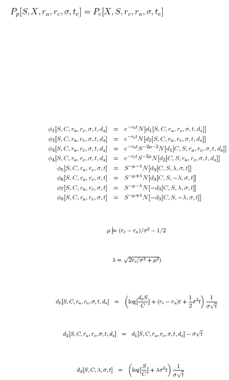
10 Options
10.8 FX option
614 © Wall Street Systems IPH AB - Confidential
The value of a put is calculated by reversing the asset and cash currencies, and considering the
option as a call:
Equation 10-14
Barrier FX Options
If we assume continuous monitoring and zero spot lag, there exists an analytic solution for European
single barrier options (see Haug, E. G. The Complete Guide to Option Pricing Formulas, McGraw-Hill
1997). There is also an infinite series solution for European double barrier options (see Zhang, P.G.
Exotic Options, 2nd Ed, World Scientific).
Basic functions
We start by defining the following functions i, which are solutions to the Black-Scholes partial
differential equation:
Equation 10-15 Black-Scholes partial differential equation
where we use the shorthands
and
and where
φi

10 Options
10.8 FX option
Transaction & Risk Management Module (TRM) Instruments: Processing and Calculations 615
Spot Adjustment
Theoretical formulas are usually given in a framework where the spot rate S is immediate. To make
an adjustment for the real world, the term ds = Dc / Da is used where Dc and Da are discount
factors between the spot date and the valuation date in cash and asset currency, respectively.
The pricing formulas will be linear combinations of the basic functions, such that they will satisfy the
barrier conditions at the barrier(s), and the final condition on the exercise day.
The option with rebates can be valued in parts. That is the fair value of the option is equal to the
value of the option without rebates plus the value of the possible rebates.
Double barrier options
Double barrier option price is given by an infinite sum of terms, which in normal cases converge
fast, so that it is sufficient to use a low number of terms in the approximation of fair value.
Summation terms are included as long as the new term contributes more than a millionth part to the
previous value of the sum.
We define the components that will be used in the summations, first, the components for the asset
and cash parts of the option itself.
•Call Asset
Equation 10-16 Double Barrier component Call Asset
•Call Cash
Equation 10-17 Double Barrier component Call Cash
•Put Asset
Equation 10-18 Double Barrier component Put Asset

10 Options
10.8 FX option
616 © Wall Street Systems IPH AB - Confidential
•Put Cash
Equation 10-19 Double Barrier component Put Cash
Then the components used for rebate valuation:
•Lower Barrier Rebate
Equation 10-20 Lower Barrier Rebate
•Upper Barrier Rebate
Equation 10-21 Upper Barrier Rebate
•No-Knock Rebate
Equation 10-22 No-knock rebate
Finally, we collect the previously defined components to calculate the fair value of a double barrier
option with rebates.
•Knock-Out option
The fair price for the option is given as the sum:
Equation 10-23 Knock-out option fair price

10 Options
10.8 FX option
Transaction & Risk Management Module (TRM) Instruments: Processing and Calculations 617
Where E is the value of the option itself (without rebates), which for a call is:
Equation 10-24 Knock-out option Call
and for a put:
Equation 10-25 Knock-out option Put
is the value of the upper barrier rebate of in asset currency:
Equation 10-26 Knock-out option upper barrier rebate (asset)
is the value of the lower barrier rebate in asset currency:
Equation 10-27 Knock-out option lower barrier rebate (asset)
is the value of the upper barrier rebate in cash currency:
Equation 10-28 Knock-out option upper barrier rebate (cash)
and is the value of the lower barrier rebate in cash currency:
Equation 10-29 Knock-out option lower barrier rebate (cash)
•Knock-In option
Fair price is given as the sum:
Equation 10-30 Knock-in option fair price
where P is the price of the corresponding vanilla option, E is the price of the corresponding
knock-out option (without rebates), and F is the value of the no-knock rebate:
Equation 10-31 Knock-in option No knock rebate
RU
aAU
RL
aAL
RU
cCU
RL
cCL
PE–F+
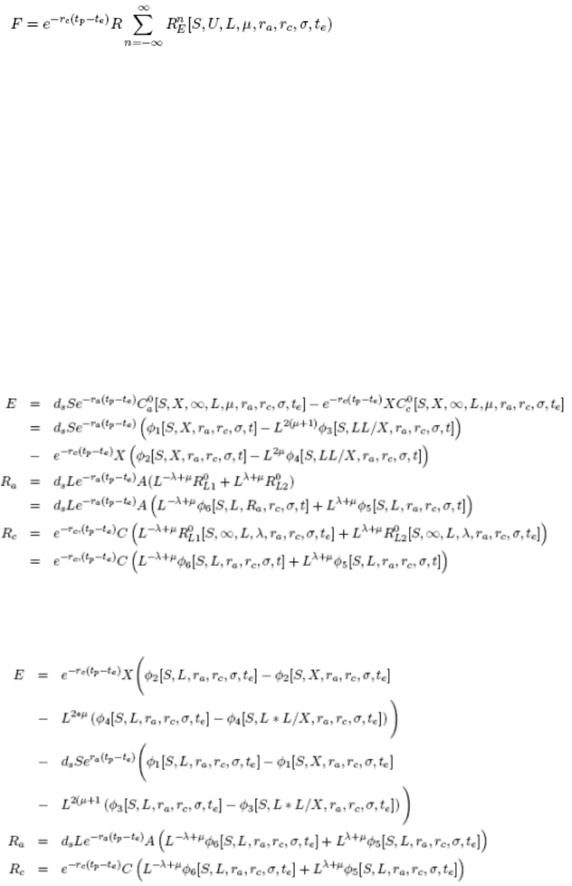
10 Options
10.8 FX option
618 © Wall Street Systems IPH AB - Confidential
if the rebate R is in the asset currency, and
Equation 10-32 Knock-in option rebate
if the rebate is in the cash currency.
Single barrier options
If we assume continuous monitoring, there exists a closed form solution for single barrier options. A
single barrier option is equivalent to a double barrier option where one of the barriers is either zero
or infinity. In these cases, all components with will disappear, and the infinite sums described
in basic and double barrier options are replaced with simple formulas.
•Knock-Out option
The fair value is:
where E is the value of the pay-off, and and are the values of the asset and cash currency
rebates of amounts A and C, respectively, paid in case the option is knocked out. The formulas
for these components are:
Down-and-Out Call
Equation 10-33 Down-and-out call
Down-and-Out Put
Equation 10-34 Down-and-out put
n0≠
ER
aRc
++
RaRc
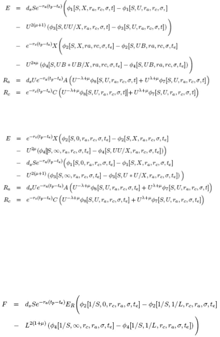
10 Options
10.8 FX option
Transaction & Risk Management Module (TRM) Instruments: Processing and Calculations 619
Up-and-Out Call
Equation 10-35 Up-and-out call
Up-and-Out Put
Equation 10-36 Up-and-out put
•Knock-In option
The fair value is:
Where P is the value of the corresponding vanilla option, E is the value of the corresponding
knock-out option (excluding possible rebates), and F is the value of the rebate of amount ,
given in different cases by:
Down-and-in option, rebate in asset currency:
Equation 10-37 Down-and-in option, rebate in asset currency
PE–F+
ER
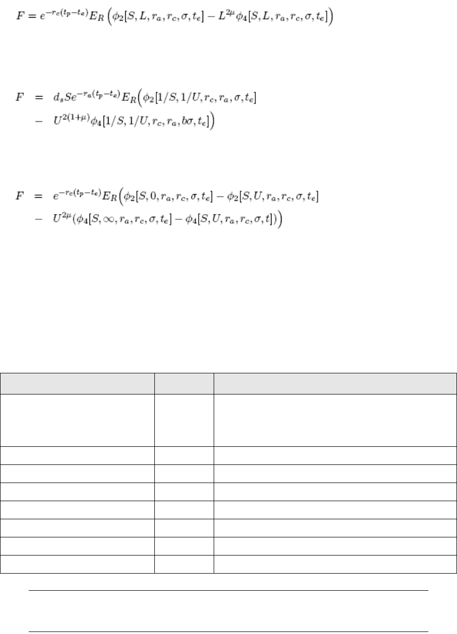
10 Options
10.8 FX option
620 © Wall Street Systems IPH AB - Confidential
Down-and-in option, rebate in cash currency:
Equation 10-38 Down-and-in option, rebate in cash currency
Up-and-in option, rebate in asset currency:
Equation 10-39 Up-and-in option, rebate in asset currency
Up-and-in option, rebate in cash currency:
Equation 10-40 Up-and-in option, rebate in cash currency
10.8.6.2.3 Numerical examples
Example 1 - European Vanilla FX option
In this section, numerical examples demonstrate how the different figures are calculated for a
Vanilla FX option deal.
This example shows a Buy 1,000,000 (strike/deal rate of 1.25) Vanilla FX option (Call) European
style transaction, with the following deal data:
•Setup
Note: For the risk figures, the IR Exposure setup is taken from the underlying instrument of the
option. If the underlying instrument has no IR exposure setup, then the Date Basis and
Yield Type defined for the valuation curve(s) are used.
Data Symbol Example
Date Basis (Act / B) B 360
By default, this is the date basis defined for the currency
of the option position cashflow (in Currency Editor’s
Journals page).
Valuation Method Theoretical
Valuation Date Figure Date
Risk Date Figure Date
Asset Risk Date Basis (Act / B) B.a 360
Cash Risk Date Basis (Act / B) B.c 365
Risk Yield Type Continuous
FX Exposure Offset e_fx 1%
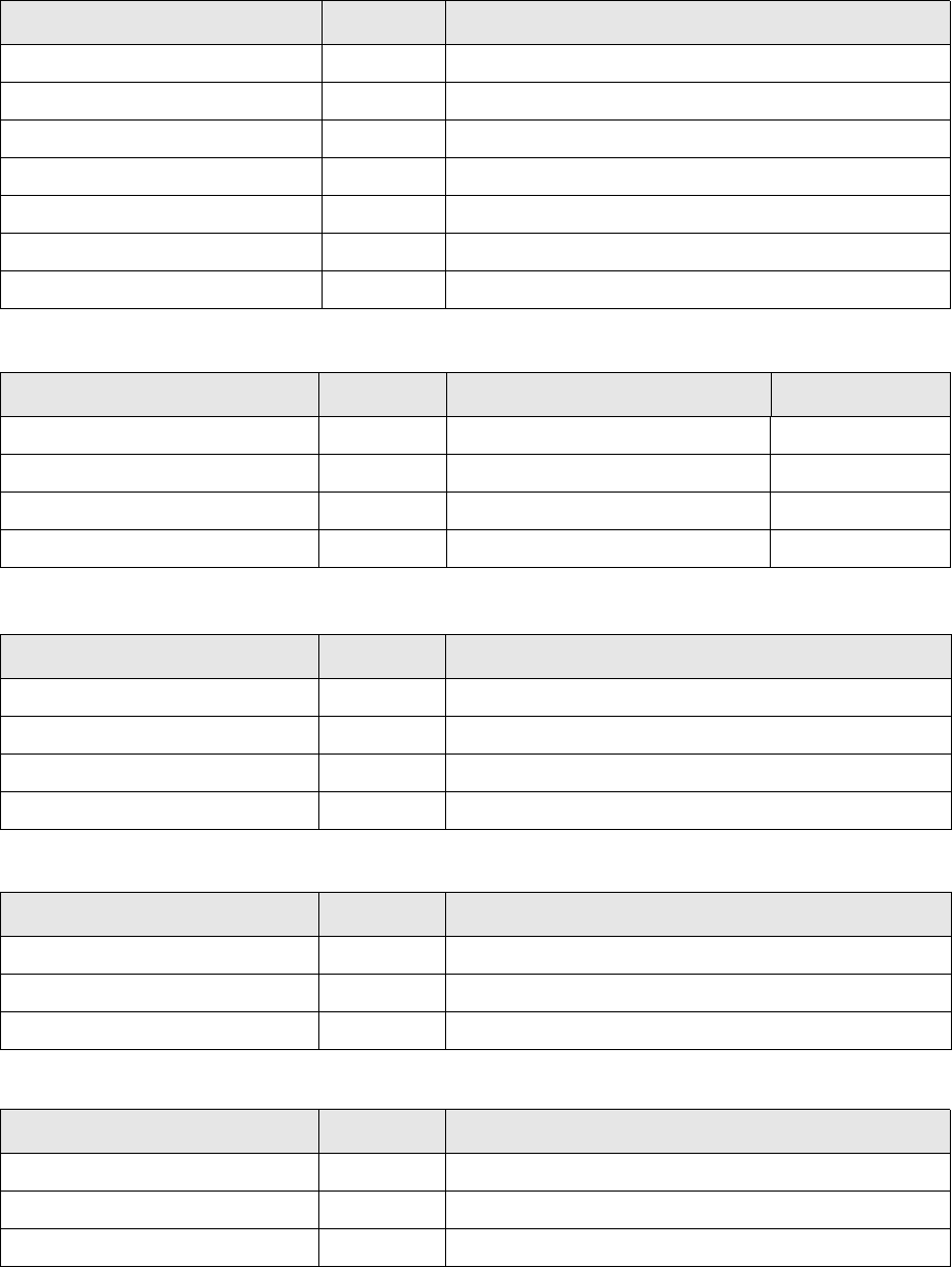
10 Options
10.8 FX option
Transaction & Risk Management Module (TRM) Instruments: Processing and Calculations 621
•Transaction data
•Calculated transaction data
•Market data on Figure Date
•Market data specific to the asset currency
•Market data specific to the cash currency
Data Symbol Example
Opening Date dt_o 2006-05-24
Spot Date dt_s 2006-05-26
Nominal Amount A 1,000,000
Deal Rate F_b 1.250000
Premium Amount premium 47,960
Maturity Date dt_m 2007-05-29
Expiry Date dt_e 2007-05-25
Data Symbol Example Formula
Book Value V_b 47,960.00 V_b=premium
FX Quote Amount A_q -1,000,000 * 1.25 = -1,250,000.00 V_q=-A * F_b
Amount (Asset) A.a -1,250,000.00 A.a=A_q
Amount (Cash) A.c 1,000,000.00 A.c=A
Data Symbol Example
Figure Date dt_f 2006-06-15
Days to Spot d_fs 2
Figure Asset Price S 0.800000000
ATM Volatility sg 13.5%
Data Symbol Example
FX Conversion Rate S.a 1.25
Market Value Discount Factor Spot D_s.a 0.999444695109
Present Value Discount Factor D_P.a 0.953883042421
Data Symbol Example
FX Conversion Rate S.c 1.00
Market Value Discount Factor Spot D_s.c 0.999688530045
Present Value Discount Factor D_P.c 0.973261859544
10 Options
10.8 FX option
622 © Wall Street Systems IPH AB - Confidential
•Calculated data on Figure Date
•Option pricer input on the figure date
Note: Asset Expiry Rate and Cash Expiry Rate are displayed in Transaction Manager as a
percentage (i.e. multiplied by 100).
•Option figures on the figure date
•The Greeks
The Greeks are calculated using numerical differentiation:
Equation 10-41
Since the spot rate is inversed, epsilon is added to (1 / S) rather than S.
Data Symbol Example Formula
Time to Maturity t_m (2006-05-29 - 2006-06-15) /360 =
0.966666667
t_m=(dt_m-dt_f)/B
Time to Expiry t_e (2006-05-25 - 2006-06-15) /360 =
0.955555556
t_e=(dt_e-dt_f)/B
Data Symbol Example Formula
Asset Expiry Rate r.a 0.048842288 r.a=-LN(D_P.a)/Time_to_maturity
Cash Expiry Rate r.c 0.039777543 r.c =-LN(D_P.c)/Time_to_maturity
Sign _sign 1
Spot S 0.8 = S
Strike X 0.8 =1/F_b
Sigma sg 13.50% =sg
Time to Maturity t_m 0.96666667 =Time_to_maturity
Time to Expiry t_e 0.95555556 =Time_to_expiry
Spot Adjustment ds 1.00000002 ds = (D_s.c/D_s.a)
Data Symbol Example Formula
d1 d_1 -0.084572333 =(LN((S*ds)/X)+(r.c-r.a)*t_m+(sg*sg/2)*t_e) /
(sg * sqrt (t_e))
d2 d_2 -0.216538237 =d_1-sg*SQRT(t_e)
price p 0.048675215 =_sign*((S*ds)*EXP(-r.a*t_m)*
Intrinsic Value
(Method zero sigma)
v.i 0.015316878 =_sign *((ds*S)*EXP(-r.a*t_m)*0.5*(_sign *
SIGN(LN(ds*S/X)+(r.c-r.a)*t_m)+1)-((X)*EXP(-r.
c*t_m)*0.5*(_sign
*SIGN(LN(ds*S)+(r.c-r.a)*t_m)+1)))
Data Symbol Example Formula
epsilon eps 0.000000001
dp / dx = (p (x + eps) - p (x - eps)) / (2 eps)
10 Options
10.8 FX option
Transaction & Risk Management Module (TRM) Instruments: Processing and Calculations 623
•IR Risk Conversion figures
•Valuation figures
•Risk figures (Asset)
•Risk figures (Cash)
price (S+/-epsilon) p_up.S 0.0486752143578562
P_dn.S 0.0486752153762781
delta delta.a -0.509210951 = (p_up.S-p_dn.S)/(2*eps)
price (ra+/-epsilon) p_up.ra 0.0486752152608569
p_dn.ra 0.0486752144732773
price (rc+/-epsilon) p_up.rc 0.0486752144262246
p_dn.rc 0.0486752153079095
Asset Rho rho.a 0.393790 = (p_up.ra-p_dn.ra)/(2*eps)
Cash Rho rho.c -0.440842 = (p_up.rc-p_dn.rc)/(2*eps)
price (t +/- epsilon) p_up.t 0.048675215
p_dn.t 0.048675215
Theta theta -0.0280628 = (p_dn.t-p_up.t)/(2*eps)
Data Symbol Example Formula
Risk Value V_r.a 533,829.54 = A /D_P.a * rho.a / t_m * S.a
V_r.c -468,572.68 = A /D_P.c * rho.c / t_m / S.c
Discount factor
sensitivity
dD_dr.a -0.922086941 = -D_P.a * (dt_m - dt_f) / B.a
dD_dr.c -0.927931855 = -D_P.c * (dt_m - dt_f) / B.c
Data Symbol Example Formula
Market Value V 48,675.21 = S.c * p * A
Intrinsic Value V_i 15,316.88 = v.i*A
Time Value V_t 33,358.34 = V-V_i
Data Symbol Example Formula
Present Value V_P.a -407,368.73 = A * _sign * ((S*ds) * EXP (-r.a*t_m) *
NORMSDIST(_sign*d_1)) * S.c
IR Exposure 1bp E_i.a -39.38 = V_r.a * dD_dr.a * 0.0001 / S.a
FX Exposure E_fx -4,073.69 = A.c*delta.a*(e_fx_1/S.a )
Data Symbol Example Formula
Present Value V_P.c 456,043.95 = A* _sign * (-X*EXP (-r.c*t_m) *
NORMSDIST(_sign*d_2)) * S.c
Data Symbol Example Formula

10 Options
10.8 FX option
624 © Wall Street Systems IPH AB - Confidential
Example 2 - American option
This example shows a Buy 1,000,000 (deal rate of 1.25) Vanilla FX option (Call) American style
transaction, with the following deal data:
•Setup
Note: For the risk figures, the IR Exposure setup is taken from the underlying instrument of the
option. If the underlying instrument has no IR exposure setup, then the Date Basis and
Yield Type defined for the valuation curve(s) are used.
•Transaction data
•Calculated transaction data
IR Exposure 1bp E_i.c 43.48 = V_r.c * dD_dr.c * 0.0001 * S.c
FX Exposure E_fx.c 0
Data Symbol Example Formula
Data Symbol Example
Instrument Date Basis (Act / B) B 360
By default, this is the date basis defined for the currency
of the option position cashflow (in Currency Editor’s
Journals page).
Valuation Method Theoretical
Valuation Date Figure Date
Risk Date Figure Date
Intrinsic Method Spot
Asset Risk Date Basis (Act / B) B.a 360
Cash Risk Date Basis (Act / B) B.c 365
Risk Yield Type Continuous
FX Exposure e_fx 1.00%
Data Symbol Example
Opening Date dt_o 2006-05-24
Spot Date dt_s 2006-05-26
Nominal Amount A -1,000,000
Deal Rate F_b 1.250000
Premium Amount premium 47,960
Maturity Date dt_m 2006-05-29
Expiry Date dt_e 2006-05-25
Data Symbol Example Formula
Book Value V_b 47,960.00 V_b=premium
FX Quote Amount A_q -1,000,000 * 1.25 = 1,250,000.00 V_q=-A*F_b

10 Options
10.8 FX option
Transaction & Risk Management Module (TRM) Instruments: Processing and Calculations 625
•Market data on Figure Date
•Market data specific to the Asset Currency
•Market data specific to the Cash Currency
•Calculated data on Figure Date
•Option pricer input on the figure date
Note: Asset Expiry Rate and Cash Expiry Rate are displayed in Transaction Manager as a
percentage (i.e. multiplied by 100).
Amount (Asset) A.a 1,250,000.00 A.a=A_q
Amount (Cash) A.c -1,000,000.00 A.c=A
Data Symbol Example Formula
Data Symbol Example
Figure Date dt_f 2006-06-15
Days to Spot d_fs 2
Figure Asset Price S 0.800000000
ATM Volatility sg 13.50%
Data Symbol Example
FX Convert (Asset) S.a 1.25
Market Value Discount Factor Spot D_s.a 0.9994446951
Present Value Discount Factor D_P.a 0.9538830424
Data Symbol Example
FX Convert (Cash) S.c 1.00
Market Value Discount Factor Spot D_s.c 0.999444714
Present Value Discount Factor D_P.c 0.962278254
Data Symbol Example Formula
Time to Maturity t_m (2006-05-29 - 2006-06-15) /360 =
0.966666667
t_m=(dt_m-dt_f)/B
Time to Expiry t_e (2006-05-25 - 2006-06-15) /360 =
0.955555556
t_e=(dt_e-dt_f)/B
Data Symbol Example Formula
Asset Expiry Rate r.a 0.048842288 r.a=-LN(D_P.a)/Time_to_maturity
Cash Expiry Rate r.c 0.039777543 r.c =-LN(D_P.c)/Time_to_maturity
Sign _sign 1
Spot Rate S 0.8 = Asset_Price
10 Options
10.8 FX option
626 © Wall Street Systems IPH AB - Confidential
•Option figures on the figure date
•The Greeks
The Greeks are calculated using numerical differentiation:
Equation 10-42
Strike X 0.8 =1/F_b
Sigma sg 13.50% =sg
Time to Maturity t_m 0.96666667 =Time_to_maturity
Time to Expiry t_e 0.95555556 =Time_to_expiry
Spot Adjustment ds 1.00000002 ds=(D_s.c/D_s.a)
Data Symbol Example Formula
Data Symbol Example Formula
beta beta 3.312531702 =(0.5-(r.c-r.a)/(sg*sg)+SQRT(POWER(((r.c-r.a)/(s
g*sg)-0.5),2)+2*r.c/(sg*sg)))
b_zero b_zero 0.800000000 =MAX(X,X*r.c/r.a)
b_inf b_inf 1.145941203 =X*Beta/(Beta-1)
ht ht -0.590319833 =-((r.c-r.a)*t_e+2*sg*SQRT(t_e))*B_zero/(B_inf-
B_zero)
I I 0.954237878 =B_zero+(B_inf-B_zero)*(1-EXP(ht))
alpha alpha 0.180127088 =(I-X)*POWER(I,-Beta)
Part_1 0.086012493 =Alpha*POWER(S,Beta)
Part_2 0.063193409 =Alpha *phi(S,t_e,Beta,I,I,r.c,r.c-r.a,sg)
Part_3 0.624830099 =phi(S,t_e,1,I,I,r.c,r.c-r.a,sg)
Part_4 0.378776110 =phi(S,t_e,1,X,I,r.c,r.c-r.a,sg)
Part_5 0.653506387 =X*phi(S,t_e,0,I,I,r.c,r.c-r.a,sg)
Part_6 0.422404879 =X*phi(S,t_e,0,X,I,r.c,r.c-r.a,sg)
price p 0.037771565 =part_1 -part_2+part_3-part_4-part_5+part_6
Intrinsic Value
(method zero sigma)
v.i 0.000000000 =_sign *MAX((_sign * (S - X)), 0)
Data Symbol Example Formula
epsilon eps 0.000000010
price (S+/-epsilon) p_up.S 0.0377715699692693
P_dn.S 0.0377715601162298
delta delta.a 0.492651975 = (p_up.S-p_dn.S)/(2*eps)
dp / dx = (p (x + eps) - p (x - eps)) / (2 eps)

10 Options
10.8 FX option
Transaction & Risk Management Module (TRM) Instruments: Processing and Calculations 627
•IR Risk Conversion figures
•Valuation figures
•Risk figures (Asset)
•Risk figures (Cash)
price (ra+/-epsilon) p_up.ra 0.0377715619439786
p_dn.ra 0.0377715681415203
price (rc+/-epsilon) p_up.rc 0.03777156789416
p_dn.rc 0.0377715621913389
Asset Rho rho.a -0.309877 = (p_up.ra-p_dn.ra)/(2*eps)
Cash Rho rho.c 0.285141 = (p_up.rc-p_dn.rc)/(2*eps)
price (t +/- epsilon) p_up.t 0.0377715652147856
p_dn.t 0.037771564870713
Theta theta -0.0172036 = (p_dn.t-p_up.t)/(2*eps)
Data Symbol Example Formula
Risk Value V_r .a -525,094.68 = A.a /D_P.a * rho.a / t_m *S.a
V_r.c 383,170.75 = A.a /D_P.c * rho.c / t_m / S.c
Discount factor
sensitivity
dD_dr.a -0.922086941 = -D_P.a * (dt_m - dt_f) / B.a
dD_dr.c -0.917459814 = -D_P.c * (dt_m - dt_f) / B.c
Data Symbol Example Formula
Market Value V 47,214.46 =S.c*p*A.a
Intrinsic Value V_i 0.00 =v.i*A
Time Value V_t 47,214.46 =V-V_i
Data Symbol Example Formula
Present Value V_P.a 469,932.36 = A.a * _sign * (EXP (-r.a*t_m) *
delta.a)*S.a
IR Exposure 1bp E_i.a 38.73 = V_r.a * dD_dr.a * 0.0001 / S.a
FX Exposure E_fx 4,926.52 = A.a *delta.a*(e_fx_1/S.a )
Data Symbol Example Formula
Present Value V_P.c -422,717.91 =V - V_P.a
IR Exposure 1bp E_i.c -35.15 = V_r.c * dD_dr.c * 0.0001 * S.c
Data Symbol Example Formula
10 Options
10.9 Exchange traded FX option
628 © Wall Street Systems IPH AB - Confidential
10.9 Exchange traded FX option
TBC

Transaction & Risk Management Module (TRM) Instruments: Processing and Calculations 629
Chapter 11 Swaps
11.1 Interest rate swap
In TRM, a Swap instrument refers to an Interest Rate (IR) Swap.
An IR swap is an agreement between two counterparties to exchange interest rate payments on an
amount over a pre-defined period: the amount is notional for single-currency swaps.
The most common structure is the fixed-for-floating swap in which one counterparty agrees to pay a
fixed rate over the term of the swap in exchange for a floating-rate payment payable by the other
counterparty.
Another structure, usually called Basis Swap, consists of exchanging two floating-rates linked to
different market references. Swaps are also used to create Asset Swaps, where one leg is a bond.
In addition, swaps can be cross-currency, which means that the legs are denominated in different
currencies: see 11.1.3 Cross-currency swap on page 656.
IR swap instruments are based on an instrument type derived from the instrument class SWAP.
11.1.1 Single-currency IR swap
The following information is relevant to any kind of single-currency swap.
For more information relating to the setup and structure of specific types of single-currency swaps,
see:
•11.1.1.1.1 Plain vanilla single-currency on page 631
•11.1.1.1.2 Zero-coupon single-currency on page 631
•11.1.1.1.3 Single-currency with upfront on page 632.
11.1.1.1 Instrument setup
•Main characteristics for single-currency swaps
–Legged
Information Description
Sign Sign of the transaction. If the sign is not defined at instrument level, it needs
to be specified separately for each transaction.
Leg Structure The leg structure for the swap instrument. Select a two leg swap structure.
TRM supports swap structures with multiple legs.
Pseudo Settlement
Pseudo Repayment
Select these options to make the principal notional (no exchange of capital).
11 Swaps
11.1 Interest rate swap
630 © Wall Street Systems IPH AB - Confidential
–Legs
Typically, you need to specify the leg instrument and the sign of the leg versus the
transaction. If this information is not defined at the instrument level, then it must be
specified at deal entry.
See A.2.307 Swap on page 866.
•Maturity definition
It is possible to set up maturity information at instrument level.
See A.2.230 Maturity Date Setup on page 827.
•Upfront cashflow definition
To create a payable upfront cashflow, use the Swap, Upfront trading feature.
See A.2.316 Swap, Upfront on page 869.
•Result treatment setup
The default method is Swap (Book, FX Rate).
See A.2.308 Swap (Book, FX Rate) on page 867.
•IR Pricer definition
To characterize the swap in terms of callable (yes or no), leg type (fix or floating) and swap type
(single currency or cross currency). This feature identifies the swap instrument to be used in the
IR Pricing tool. See A.2.222 IR Pricer (Swap) on page 824 and see TRM User Guide for more
general information about IR Pricing.
Information Description
Instrument The instrument to be used for this leg by default.
Sign versus
Transaction
Choose from: Same, Opposite, or Any.
Information Description
Calendar
parameters
Calendars used to calculate the maturity date.
Gap Set Gap set used for supplying the available maturity periods.
Maturity Date
Period
If defined, this maturity period is applied to each transaction.
11 Swaps
11.1 Interest rate swap
Transaction & Risk Management Module (TRM) Instruments: Processing and Calculations 631
•Valuation
–If the valuation feature Single Swap Valuation or NumeriX Single-Swap Valuation or NumeriX
Valuation is set at the instrument level, the valuation setup is retrieved from the swap.
See A.2.302 Single Swap Valuation on page 863, A.2.251 NumeriX Single-Swap Valuation on
page 840 or A.2.253 NumeriX Valuation on page 841.
–If the valuation feature Swap Valuation or Swap Per Leg Valuation is set at the instrument
level, the valuation setup is retrieved from the leg instrument.
See A.2.310 Swap Valuation on page 867 or A.2.313 Swap Per Leg Valuation on page 868.
–If the valuation feature NumeriX Swap Valuation is set up at the instrument level, the set up
defaults to the first leg instrument.
See A.2.252 NumeriX Swap Valuation on page 841.
For more information about the valuation defaulting see 11.1.1.4 Position monitoring on page
640.
It is also possible to set up:
•Spot day and value date calculations
•Manual charges
•Cashflow and transaction charge rules
•Branch codes.
See Appendix A Features on page 713.
11.1.1.1.1 Plain vanilla single-currency
A swap where value and maturity date principals are notional (that is, not settled), in the same
currency, and their absolute amounts are equal.
For a plain vanilla single-currency swap, the structure can be demonstrated as follows:
•Instrument setup
–Swap characteristics
11.1.1.1.2 Zero-coupon single-currency
A swap where one leg pays no interest. Instead, the redemption amount is split into a notional
component and a payable component. The other leg pays interest on a notional amount that is equal
to the notional component of the zero-coupon leg.
Information Description
Leg Structure SWAP-2-LEGS
Pseudo Settlement
Pseudo Repayment
Both these options should be selected.
Notional
Notional

11 Swaps
11.1 Interest rate swap
632 © Wall Street Systems IPH AB - Confidential
For a zero-coupon single-currency swap, the structure can be demonstrated as follows:
•Instrument setup
–Swap characteristics
–Schedule structure for the leg instrument
TRM provides a pre-defined system template (see B.2.1.1.47 Zero-Coupon Swap Leg on
page 899) designed for this purpose. With this schedule, the redemption flow of the
underlying is split into a pseudo Redemption flow and a payable Redemption Premium flow.
See Appendix B Schedules on page 883.
11.1.1.1.3 Single-currency with upfront
A swap where the value and maturity date principal amounts are notional (that is, not settled), in
the same currency, and their (absolute) amounts are equal.
A separate settled upfront cashflow is created for the value date, for the leg(s) where Deal Price is
more or less than 100, calculated as follows:
(100 - Deal Price) / 100 * Nominal Amount
The upfront cashflow is booked according to the result treatment definition of the swap instrument.
For a single-currency swap with an upfront cashflow, the structure can be demonstrated as follows:
•Instrument setup
–Swap characteristics
–Upfront cashflow definition
Information Description
Leg Structure SWAP-2-LEGS-ZERO
Pseudo Settlement
Pseudo Repayment
Both these options should be selected.
Information Description
Leg Structure SWAP-2-LEGS
Pseudo Settlement
Pseudo Repayment
Both these options should be selected.
Redemption flow =
Pseudo Redemption +
Payable Redemption Premium
Notional
Notional
Upfront
cashflow
11 Swaps
11.1 Interest rate swap
Transaction & Risk Management Module (TRM) Instruments: Processing and Calculations 633
To create a payable upfront cashflow, use the Swap, Upfront trading feature.
See A.2.316 Swap, Upfront on page 869.
11.1.1.2 Deal capture
Note: To perform pricing of swap transactions, you can use the IR Pricing tool. See TRM User
Guide for more information about IR Pricing.
11.1.1.2.1 Input data
In addition to the standard deal parameters, the following information is required to enter a swap.
•Transaction view
You input data for Leg 1 of the swap as this is used as a basis for the calculations on the
remaining legs.
In addition, the following optional information can be captured:
•Leg view
If the legs are not defined on the swap instrument they must be selected here. The relevant
instruments for legs are loans. If you want to create an asset swap it is also possible to choose a
bond as one of the legs.
The cashflow structure of each leg should also be selected (when the leg is a loan without a
predefined cashflow structure).
•Schedule view
Schedule information must be provided for each leg. See A.2.202 Generic Loan on page 812.
Information Description
Currency Currency of the swap.
Value Date Date when the swap starts, and from which interest starts to accrue. This defaults to
the spot date of the transaction.
Maturity Date Date when the transaction matures. If you enter a maturity code, the date is
calculated automatically based on the maturity definition at instrument level;
otherwise you can enter the date manually.
Nominal Amount Amount of the first leg of the swap.
Deal Price Price used for the first leg of the swap (100 in the case of a vanilla swap).
Note: If you want to have an up-front premium/discount, enter a price <> 100: this
will apply on the first leg.
Information Description
Value Date Code If the Value Date Setup feature is applied at instrument level, you can enter the value
date period you want to use to calculate the value date for the transaction, for
example, 3M (3 months).
This can be used to compute the value date for a forward purchase of an IR swap.
Note: If you specify a value date period in the instrument setup, this is used as the
default in the transaction and cannot be modified: see A.2.339 Value Date
Setup on page 879.
Maturity Code If you enter a maturity code at deal entry, the date is calculated automatically;
otherwise you can enter the date manually.
Note: If the maturity definition parameters are defined at instrument level, these are
used by default and cannot be modified.
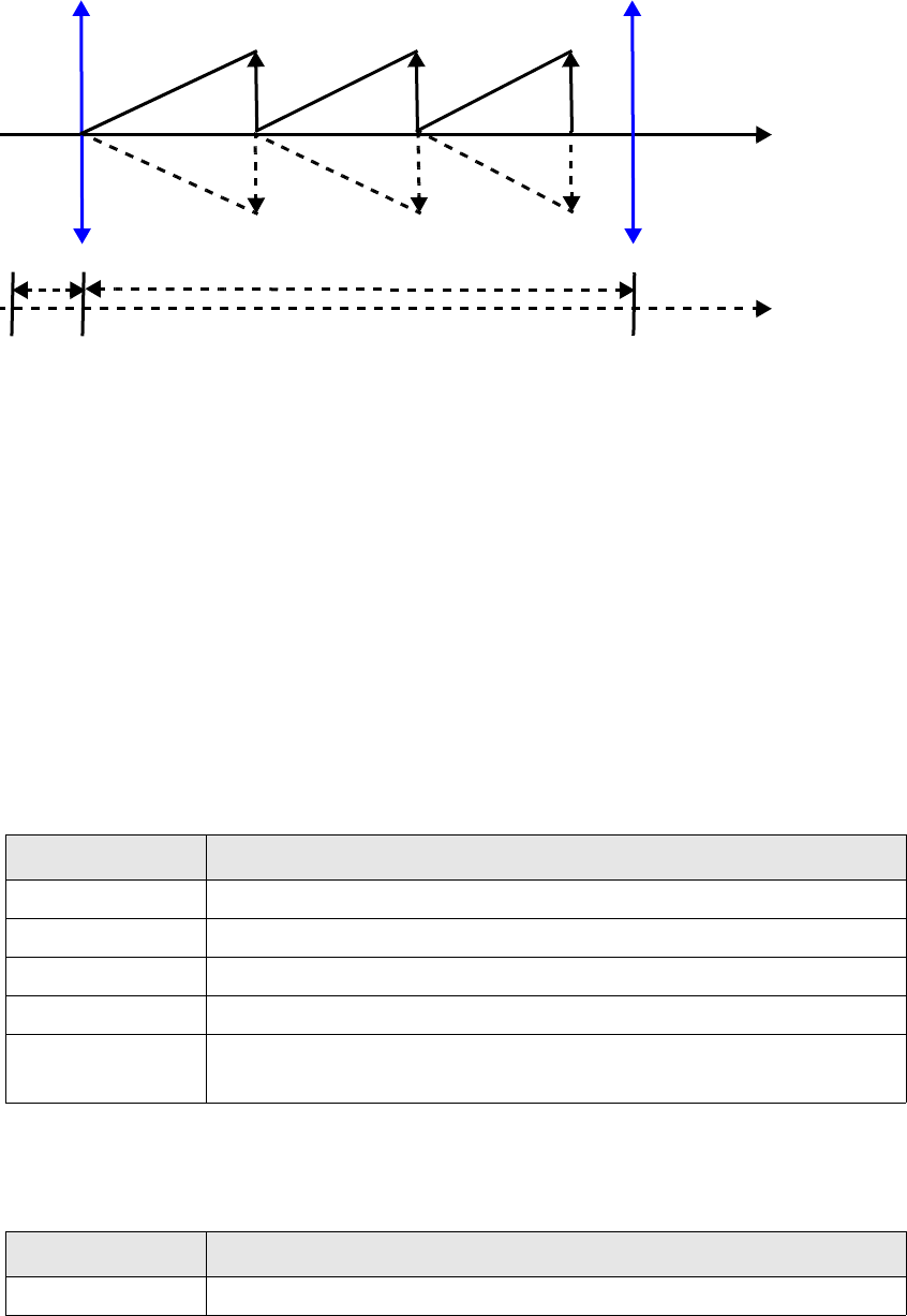
11 Swaps
11.1 Interest rate swap
634 © Wall Street Systems IPH AB - Confidential
11.1.1.2.2 Generated data
•Cashflows
For a vanilla single-currency swap the cashflow structure is as follows:
11.1.1.3 Processing
This section describes the actions that can be done throughout the life of a swap.
11.1.1.3.1 Pricing
Pricing of swap transactions can be performed at transaction level using a right-click processing
action.
•Setup
A choice of three types of Pricing action are available on the transaction if the Swap Pricing
feature is associated with the instrument: Goal Seeker, Annuity, or Spread.
See A.2.314 Swap Pricing on page 868.
•Execution
–Goal Seeker
–Annuity
This Pricing action allows you to convert the Upfront payment into Annuity using the funding
rate.
Opening
date Value
date
Spot Maturity
Floating interest
Maturity
date
Notional
Fixed interest Notional
Information Description
Variable Parameter to use as the variable. Choose from: Spread or Fixed.
Context Entity to which the variable belongs. Choose from: Schedule or Leg.
Target Key-figure that you want to modify: Market Value.
Target Value Value that you want to achieve.
Result (Information only)
Calculated value of the variable after pricing.
Information Description
Funding Rate % Funding rate expressed as a percentage.

11 Swaps
11.1 Interest rate swap
Transaction & Risk Management Module (TRM) Instruments: Processing and Calculations 635
–Spread
The Spread Pricing action is carried out in two steps.
In the first step, the Upfront amount is converted into Annuity using the funding rate.
In the second step, the Annuity amount and the funding rate are both used to calculate the
spread.
11.1.1.3.2 Early expiration
Swaps can be closed-out earlier than their agreed maturity date. This process is referred to as early
expiration.
Note: Early expiration is also available for forward interest rate swaps.
•Execution
Early expiration of a swap requires the following information:
Annuity (Information only)
Calculated Annuity amount after pricing.
Information Description
Funding Rate % Funding rate expressed as a percentage.
Annuity (Information only)
Annuity amount calculated from the Upfront and funding rate.
Information Description
Annuity
Funding Rate
(Information only)
Values taken from the first step in the Pricing action.
Target Market Value Value that you want to reach.
All-In Switch on to take into account any fees which have the All-In attribute.
Re-Offer Switch on to take into account any fees which have the Re-Offer attribute.
Spread % (Information only)
Calculated Spread value expressed as a percentage.
Information Description
Opening Date Date when the early expiration is executed. By default, this is today’s date unless a
Fixing/Action Date is specified at transaction level.
Value Date Date when the early expiration is settled. This must be earlier than the original
maturity date and later than the original value date of the initial transaction.
Settlement Date Date when early-expiration price is paid. Can be different for each leg.
Amount to Expire Amount to be early expired. This defaults to the amount still available to be early
expired, taking into account previous partial early expirations and roll overs.
Settlement
Amount Method
• Clean Price: AI is created as Payable cashflow and P/L flow is the difference
between early-expiration price and original deal price.
• Dirty Price: AI is created as Not Payable cashflow, and P/L flow is reduced by the
AI amount.
Information Description
11 Swaps
11.1 Interest rate swap
636 © Wall Street Systems IPH AB - Confidential
The execution generates an early expiration transaction with the following attributes:
Transaction sign = opposite of initial transaction
Nominal amount = amount to expire
Opening date = date when the early expiration is done
Value date = date when the early expiration is settled
Kind = Early Expiration
The remaining attributes are inherited from the initial transaction.
The early expiration transaction generates closing cashflows for the initial transaction and P/L
cashflows if there is a difference between the early expiration price and the original deal price.
When there is an amortized upfront cashflow, the accrued portion is realized on the early
expiration date.
•Cancellation
You can undo the early expiration by canceling the early expiration transaction.
11.1.1.3.3 Roll over
You can defer the maturity of an a one-leg IR swap acting as a guarantee to a later date. This
process is referred to as a roll-over.
•Setup
This process is available on the transaction if the Allow Roll Over (Guarantee) feature is
associated with the instrument.
See A.2.18 Allow Roll Over (Guarantee) on page 720.
•Execution
The following information is needed to process the roll-over:
Net Amount Net amount to be settled between the two parties.
• If Settlement Amount method is Clean, Net Amount = Sell Profit/Loss).
• If Settlement Amount method is Dirty, Net Amount = Accrued Interest + Sell
Profit/Loss.
Options • Amortize P/L
Switch on Amortize P/L to amortize the P/L from the value date until the original
maturity date. If this switch is off, the Sell P/L flow created by the early expiration
(arising from Net Amount – Accrued Interest) occurs on the early expiration value
date.
•No Fee Realization
Switch on No Fee Realization so that fees keep amortizing to maturity. For
example, this can be used in the case of an asset swap, which mirrors the issue
fees, to keep the fees amortizing even when the asset swap is fully unwound.
If this switch is off, at early expiration, the fees that were amortizing until the
maturity date are closed.
Information Description
Roll Over Date Date when the roll-over is executed.
Roll Over Method Roll-over method: Settle All.
Nominal Amount Amount of the roll-over.
This defaults to the amount left of the initial transaction but you can override this if
you want to perform a partial roll-over.
Information Description
11 Swaps
11.1 Interest rate swap
Transaction & Risk Management Module (TRM) Instruments: Processing and Calculations 637
The initial transaction is paid in its entirety at the initial maturity date. The default nominal
amount of the roll-over transaction equals the sum of the interest and principal cashflows of the
initial transaction.
The execution generates a new transaction with the following attributes:
Nominal amount = amount (can be smaller than the initial transaction)
Opening date = date when the roll-over is done
Value date = maturity date of the initial transaction
Maturity date = maturity of the roll-over
Kind = Roll-over
•Cancellation
You can undo the roll-over by canceling the roll-over transaction.
11.1.1.3.4 Trade assignment
Trade assignments are changes of ownership of transactions.
•Execution
Change of ownership during the life of a transaction can be performed in two steps:
–Right-click the existing transaction and choose Assignment (sale) action. This action closes the
existing transaction, and when required, exchanges settlement amounts between the old
and new owners of the transaction.
–Right-click the generated transaction and choose Assignment (purchase) action. This action
creates the new transaction with the new owner.
Assignment (sale) of a transaction to another client requires the following information:
Gap Gap set used for supplying the maturity date.
This defaults to the maturity period of the initial transaction but can be modified.
Maturity Date New maturity date for the IR swap.
This must be later than the maturity date of the initial transaction. The maturity date
is calculated automatically from the maturity period of the initial transaction.
Information Description
Opening Date Date when the early expiration is executed.
By default, this is today’s date unless a Fixing/Action Date was specified
at transaction level.
Value Date Date when the early expiration is settled. This must be earlier than the
original maturity date and later than the original value date of the initial
transaction.
Settlement Date Date when assign price is paid.
Amount Left Read-only. Remaining amount of the initial transaction.
Assignee New owner of the transaction.
Net Amount Method Clean Amount: AI is created as Payable cashflow.
Dirty Amount: AI is created as Not Payable cashflow, and P/L flow is
reduced by the AI amount.
Net Amount (leg1/leg2) Amount to be settled between old and new owners.
Currency (leg1/leg2) Read-only. Currency of the leg.
Information Description
11 Swaps
11.1 Interest rate swap
638 © Wall Street Systems IPH AB - Confidential
Execution generates an Assignment transaction with following cashflows:
–Cashflows to close the future cashflows of the original transactions (closing of cashflows
where payment date is after the assignment value date)
–Settlement flows between the assignor and the assignee, reflecting the settlement amounts.
The generated transaction has the following attributes:
The original transaction remains unchanged.
On this closing transaction, the assignee can select the Assignment (purchase) action to generate
the future flows of its new transactions. A dialog allows the user to select the portfolio. A new
transaction is generated, reflecting the future cashflows of the original transaction and
settlement flows between assignee and assignor.
Note: The Counterparty field is open, to allow Counterparty change if required.
Assignment can also be done from an external counterparty. You can capture an IRS by
supplying the net amount according to the specified settlement method. In the Action menu,
choose Assignment (purchase), see TRM User Guide.
•Cancellation
You can undo the assignment action by canceling the generated assignment transaction.
11.1.1.3.5 Changing the counterparty of a transaction
You can terminate the existing transaction against one counterparty and reopen it against another
counterparty. The following information is required:
Accrued Interest
(leg1/leg2)
Read-only. Interest accrued on specified date.
Switches • Amortize P/L
Switch on Amortize P/L to amortize the P/L from the value date until
the original maturity date. If this switch is off, the Sell P/L flow created
by the assignment (arising from Net Amount – Accrued Interest)
occurs on the assign value date.
• No Fee Realization
Switch on No Fee Realization so that fees keep amortizing to maturity.
If this switch is off at assignment, the fees that were amortizing until
the maturity date are closed.
Information Description
Transaction Sign Opposite of the original transaction sign.
Nominal Amount Amount to assign.
Opening Date Opening date of action.
Value Date Value date of action.
Kind Assignment.
Information Description
Opening Date Date when the transfer is executed. By default, this is today’s date unless a
Fixing/Action Date was specified at transaction level.
Information Description
11 Swaps
11.1 Interest rate swap
Transaction & Risk Management Module (TRM) Instruments: Processing and Calculations 639
A transaction will be generated whose Kind is Counterparty Conversion. The characteristics of the
new transaction will be the same as the old one, except for Counterparty and opening/value date.
This action generates closing cashflows for the future cashflows from the original transaction, and
futures cashflows between the original owner and the new counterparty.
No settlement/result flows will be affected in the generated transaction, as the assignment is
between the counterparties only.
The generated transaction can be cancelled to undo the action.
11.1.1.3.6 Transferring transactions between portfolios
You can transfer the transaction from one portfolio to another. This is effectively a sale in one
portfolio and a purchase in another. Portfolio transfer of an existing transaction can be performed at
transaction level by right-clicking and choosing Transfer. Transfer of a transaction to another
portfolio requires the following information:
Two Transfer transactions are generated:
1. A sale is created in the source portfolio of the transfer, i.e. closing cashflows of the original
transaction and settlement flows (real or pseudo, depending on inputs).
2. A purchase is then created in the receiving portfolio, with future flows and settlement flows (real
or pseudo, depending on inputs).
The original transaction remains unchanged. The user can undo the portfolio transfer action by
canceling the generated transactions.
Value Date Date when the transfer is settled. This must be earlier than the original maturity date
and later than the original value date of the initial transaction.
Counterparty New counterparty for the transaction.
Information Description
Opening Date Date when the transfer is executed. By default, this is today’s date unless a
Fixing/Action Date was specified at transaction level.
Value Date Date when the transfer is settled. This must be earlier than the original maturity date
and later than the original value date of the initial transaction.
Settlement Date Payment date for settlement flows.
New Portfolio New portfolio for the transaction
No Settlement
switch
If On, the generated settlement amount is marked as pseudo (i.e. not bookable, not
payable).
Net Amount
Method
Clean: AI is created as Payable cashflow.
Dirty: AI is created as Not Payable cashflow, and P/L flow is reduced by the AI
amount.
Net Amount
(leg1/leg2)
Amount to be settled between old and new owners.
Currency
(leg1/leg2)
Read-only. Currency of the leg.
Accrued Interest
(leg1/leg2)
Read-only. Interest accrued on specified date.
Options • Amortize P/L
•No Fee Realization
Information Description
11 Swaps
11.1 Interest rate swap
640 © Wall Street Systems IPH AB - Confidential
11.1.1.3.7 Transaction Conversion
To allow schedule conversion at predefined dates during transaction's life.
•Setup
This process is available on the transaction if the Transaction Conversion feature is associated
with the instrument.
See A.2.325 Transaction Conversion on page 873.
Then, the user is allowed to attach the Conversion schedule to the existing schedule and to
define conversion events and converted schedules.
•Execution
When conversion schedules are defined, the user is allowed to execute generated conversion
events. The conversion inputs are displayed.
See A.2.325 Transaction Conversion on page 873.
The execution generates a conversion transaction with following attributes:
–Kind: Conversion
–Opening Date: Conversion opening date
–Value Date: Conversion value date
The conversion transaction generates closing cashflows for the initial transaction.
If the conversion price is different to the original deal price, then a P/L flow is generated,
showing the differences between the conversion price and the original deal price. On a
non-converted leg, future cashflows are reopened as a new transaction and remain unchanged.
11.1.1.4 Position monitoring
11.1.1.4.1 Setup
Assuming that the relevant valuation features are attached to the instrument (11.1.1.1 Instrument
setup on page 629), the valuation setup is defined by the following features depending on the
Pricing mode.
TRM valuation setup
•The estimation curves default in IR Pricing when these are defined at the instrument level
(feature Estimation Curve Setup).
•The valuation curves default in IR Pricing when these are defined at the instrument level (feature
Valuation Curve Setup).
•The risk profile defaults in IR Pricing when defined at the instrument level (feature Floating
Valuation Setup).
•The values defined for FX method and valuation default in IR Pricing when defined at the
instrument level (feature Base Valuation Setup).
•The volatility surfaces default in IR Pricing when these are defined at the instrument level
(feature Volatility Surface Setup) as follows:
–The volatility curve in IR Pricing defaults to volatility reference set defined at the instrument
level, with the usage Volatility. If not defined, uses the Cap/Floor volatility reference
attached to the currency.
–The adjust volatility curve in IR Pricing defaults to volatility reference set at instrument level
with the usage Adjust Volatility. If not defined, uses the Swaption volatility reference attached
to the currency.
11 Swaps
11.1 Interest rate swap
Transaction & Risk Management Module (TRM) Instruments: Processing and Calculations 641
Numerix valuation setup
•The estimation curves default in IR Pricing when these are defined at the instrument level
(feature Estimation Curve Setup).
•The calibration id, model, quality and analytic quality default in IR Pricing when these are
defined at the instrument level (feature Numerix Setup).
Valuation setup defaulting
•If the TRM valuation setup is not defined, then uses the default valuation defined in the currency
as it does now.
•If the NumeriX valuation (feature Numerix Valuation) is not defined, then it defaults to the Hull
and White model.
Risk calculation setup
The cashflow discounting method (periodic, continuously compounded) used in IR risk calculation
depends on the instrument setup:
•By default, if no IR exposure is set up at leg- or top instrument level, then TRM uses the
valuation curve interpolation settings (IR Quote and Yield Curve Editor - Interpolation page).
•If IR exposure is set up at the leg instrument level, then TRM uses these settings, it uses top
instrument level. For example, If IR exposure is set up with Yield Type Periodic, then risk
calculations use periodic discounting of the cashflows.
See A.2.48 Base IR Exposure Setup on page 732.
For more information about risk calculations, see 2.3 Key-figures on page 112.
11.1.1.4.2 Calculations
In this section, numerical examples demonstrate how the different figures are calculated for a
vanilla IR swap. For information about the method used in these calculations, see Chapter 2 Market
standards and calculations on page 33.
For information about how modified duration is calculated for IR Swaps, see 2.3.4.9.5 Modified
Duration on page 145.
This example shows a 2-leg IR swap in EUR, with the following deal data:
•Setup
Setup data
Instrument Date Basis Act/360
Instrument Yield Type Periodic
Valuation Method Theoretical
Risk Method Theoretical
Valuation Date Figure Date
Risk Date Figure Date
Risk Yield Type Continuous
Fixed Leg Coupon Rate 4.00%
Floating Leg Risk Profile Plain Vanilla (simple risk)
Leg Structure SWAP-2-LEGS

11 Swaps
11.1 Interest rate swap
642 © Wall Street Systems IPH AB - Confidential
•Transaction data
•Market data
Unless otherwise stated, the figure date used in the calculations is 2002-06-15. On this date, the
market data is as follows:
•Other data is calculated by the system as follows:
-Time to Spot
t_s = d_fs / B
0.008333333 = 2002/06/15 / 360
- MV Spot Discount Factor
D_s = EXP (-t_s * r_d) = 0.9997462834
11.1.1.4.3 Fixed leg
Transaction data specific to the principal flow of the fixed leg is as follows:
On the figure date, the market data specific to the principal amount of the fixed leg is as follows:
Other data, specific to the principal amount of the fixed leg is calculated by the system as follows:
• Time to Value Date
tv = (dv.p - dt_f) / B
2.730555556 = (200502/22 – 2002/06/15) / 360
• Market Value Discount Factor
D_V.p = D_s * D.p = 0.8824165107
• Present Value Discount Factor
D_P.p = D_s * D.p = 0.8824165107
• Discount Factor From Spot
D.p = EXP( -(tv.p - t_s) * r.p) = 0.8826404512
Transaction data
Opening Date dt_o 2002-02-22
Nominal Amount c_m 1,000,000
Spread r_s 0.50%
Maturity Date d_m 2005-02-22
Spot Date ds 2002-02-22
Market data on 2005-06-15
Figure date dt_f 2002-06-15
Days to Spot d_fs 3
Discount Rate r_d 3.044986%
Transaction data
Value Date dv.p 2005-02-22
Amount A = c_m 1,000,000
Market data on 2002-06-15
Interest Rate r.p 4.585862%

11 Swaps
11.1 Interest rate swap
Transaction & Risk Management Module (TRM) Instruments: Processing and Calculations 643
Transaction data specific to the coupon flows of the fixed leg is as follows:
Calculated transaction data specific to the coupon flows of the fixed leg is as follows:
•Coupon 1
Period
t_p1 = (dv.c1 - ds) / B
1.01 = (2003/02/22 - 2002-02-22) / 360
Amount
A.c1 = c_m * t_p1 * r_c
40,555.56 = 1,000,000 * 1.01 * 0.04
•Coupon 2
Period
t_p2 = (dv.c2 – dv.c1) / B
1.01 = (2004/02/22 - 2003-02-22) / 360
Amount
A.c2 = c_m * t_p2 * r_c
40,555.56 = 1,000,000 * 1.01 * 0.04
•Coupon 3
Period
t_p3 = (dv.c3 - dv.c2) / B
1.02 = (2005/02/22 – 2004/02/22) / 360
Amount
A.c3 = c_m * t_p3 * r_c
40,666.67 = 1,000,000 * 1.02 * 0.4
On the figure date, the market data specific to the coupons of the fixed leg is as follows:
Other data specific to the coupon flows of the fixed leg is calculated by the system as follows:
•Coupon 1
Time to Value Date
tv.c1 = (dv.c1 - dt_f) / B
0.700000 = (2003/02/22 – 2002/06/15) / 360
Market Value Discount Factor
D_V.c1 = D_s * D.c1 = 0.9752247775
Present Value Discount Factor
D_P.c1 = D_s * D.c1 = 0.9752247775
Discount Factor From Spot
D.c1 = EXP( -(tv.c1 - t_s) * r.c1) = 0.9754722711
•Coupon 2
Time to Value Date
tv.c2 = (dv.c2 - dt_f) / B
1.713888889 = (2004/02/22 – 2002/06/15 / 360
Market Value Discount Factor
D_V.c2 = D_s * D.c2 = 0.9309903649
Present Value Discount Factor
D_P.c2 = = D_s * D.c2 = 0.9309903649
Discount Factor From Spot
D.c2 = EXP( -(tv.c2 - t_s) * r.c2) = 0.9312266326
•Coupon 3
Transaction data Coupon 1 Coupon 2 Coupon 3
Value Date dv.c1 2003-02-22 dv.c2 2004-02-22 dv.c3 2005-02-22
Market data Coupon 1 Coupon 2 Coupon 3
Interest Rate r.c1 3.590392% r.c2 4.177677% r.c3 4.585862%
11 Swaps
11.1 Interest rate swap
644 © Wall Street Systems IPH AB - Confidential
Time to Value Date
tv.c3 = (dv.c3 – dt_f) / B
2.730555556 = (2005/02/22 – 2002/06/15) / 360
Market Value Discount Factor
D_V.c3 = D_s * D.c3 = 0.8824165079
Present Value Discount Factor
D_P.c3 = D_s * D.c3 = 0.8824165079
Discount Factor From Spot
D.c3 = EXP( -(tv.c3 - t_s) * r.c3) = 0.8826404485
Valuation figures – fixed leg
The valuation method commonly used for a vanilla IR swap is the Theoretical method.
• Principal flow
Market Value
V = c_m * D_V.p
882,416.51 = 1,000,000 * 0.8824165107
•Coupon 1
Market Value
V.c1 = A.c1 * D_V.c1
39,550.78 = 40,555.56 * 0.9752247775
•Coupon 2
Market Value
V.c2 = A.c2 * D_V.c2
37,756.83 = 40,555.56 * 0.9309903649
•Coupon 3
Market Value
V.c2 = A.c3 * D_V.c3
35,884.94 = 40,666.67 * 0.8824165079
•Total Fixed
Market Value
= V.p + V.c1 + V.c2 + V.c3
= 995,609.06
Result figures – fixed leg
The setup of the instrument impacts the way result figures are computed.
• Principal flow
Tot al P rof it
Tot al_ Prof it. p = V.p
= 882,416.51
MtoM Profit
MtoM_Profit.p = A * D.p
882,640.45 = 1,000,000 * 0.88264045.12
Other Profit
Other_Profit.p = Total_Profit.p - MtoM_Profit.p
-223.94 = 882,416.51 -882,640.45
•Coupon 1
Tot al P rof it
Tot al_ Prof it. c 1 = V.c 1
= 39,550.78
Accrued Interest
Accrued_Interest.c1 = (dt_f - dt_o) / (dv.c1 - dt_o) * A.c1
12,555.56 = (2002/06/15 – 2002/02/22) / (2003/02/22 – 2002/02/22) * 40,555.56
MtoM Profit
MtoM_Profit.c1 = A.c1 * D.c1 - Accrued_Interest.c1
27,005 = 40,555.56 * 0.9754722711 – 12,555.56
11 Swaps
11.1 Interest rate swap
Transaction & Risk Management Module (TRM) Instruments: Processing and Calculations 645
Other Profit
Other_Profit.c1 = Total_Profit.c1 - Accrued_Interest.c1 - MtoM_Profit.c1
-10.04 = 39,550.78 – 12,555.56 – 27,005.26
•Coupon 2
Tot al P rof it
Tot al_ Prof it. c 2 = V.c 2
= 37,756.83
MtoM Profit
MtoM_Profit.c2 = A.c2 * D.c2
37,766.41 = 40,555.56 * 0.9312266326
Other Profit
Other_Profit.c2 = Total_Profit.c2 - MtoM_Profit.c2
-9.58 = 37,756.83 – 37,766.41
•Coupon 3
Tot al P rof it
Tot al_ Prof it. c 3 = V.c 3
= 35,884.94
MtoM Profit
MtoM_Profit.c3 = A.c3 * D.c3
35,894.04 = 40,666.67 * 0.8826404485
Other Profit
Other_Profit.c3 = Total_Profit.c3 - MtoM_Profit.c3
-9.11 = 35,884.94 – 35,894.04
•Total Fixed
Tot al P rof it
= Total_Profit.p + Total_Profit.c1 + Total_Profit.c2 + Total_Profit.c3
= 995,609.06
Accrued Interest
= Accrued_Interest.c1
= 12,555.56
MtoM Profit
= MtoM_Profit.p + MtoM_Profit.c1 + MtoM_Profit.c2 + MtoM_Profit.c3
= 983,306.17
Other Profit
= Other_Profit.p + Other_Profit.c1 + Other_Profit.c2 + Other_Profit.c3
= -252.67
Risk figures – fixed leg
The risk method commonly used for a vanilla IR swap is the Theoretical method.
• Principal flow
IR Exposure 1bp
E_i.p = (A) * (-(tv.p - t_s) * D.p * D_s - t_s * D.p * D_s) * 0.0001
-240.95 = (1,000,000)*(-(2.730555556-0.008333333)*0.88264045.12*0.9997462834-
t_s*D.p*D_s)*0.0001
Effective Duration
U_eff.p =-E_i.p / V.p / 0.0001
2.730556 = -240.95 / 882,416.51 / 0.0001
•Coupon 1
IR Exposure 1bp
E_i.c1 = = (A.c1) * (-(tv.c1-t_s) * D.c1 * D_s - t_s * D.c1 * D_s) * 0.0001
-2.77 = (40,555.56)*(-(0.70000-0.008333333)*0.9754722711*0.9997462834-t_s*D.c1*D_s)*0.0001
Effective Duration
U_eff.c1 = -E_i.c1 / V.c1 / 0.0001
0.70000 = -2.77 / 39,550.78 / 0.0001
•Coupon 2
IR Exposure 1bp
E_i.c2 = (A.c2) * (-(tv.c2-t_s) * D.c2 * D_s - t_s * D.c2 * D_s) * 0.0001
-6.47 = (40,555.56)*(-(1.713888889-0.008333333)*0.9312266326*0.9997462834-t_s*D.c2*D_s)*0.0001
11 Swaps
11.1 Interest rate swap
646 © Wall Street Systems IPH AB - Confidential
Effective Duration
U_eff.c2 = -E_i.c2 / V.c2 / 0.0001
1.71389 = -6.47 / 37,756.83 / 0.0001
•Coupon 3
IR Exposure 1bp
E_i.c3 = (A.c3) * (-(tv.c3-t_s) * D.c3 * D_s - t_s * D.c3 * D_s) * 0.0001
-9.80 =
(40,666.67)*(-(2.730555556-0.0083333333)*0.8826404485*0.9997462834-t_s*D.c3*D_s)*0.0001
•Total Fixed
IR Exposure 1bp
= E_i.p + E_i.c1 + E_i.c2 + E_i.c3
= 2.611335896
Effective Duration
= -E_i.total / V.total / 0.0001
= 2.611335896
11.1.1.4.4 Floating leg
On the figure date, the market data specific to the principal flow of the floating leg is as follows:
Other figures specific to the principal flow of the floating leg are calculated by the system as follows:
• DF From spot
D_f.fp= EXP (-r.fp * ((dt_v.fp - dt_f )/ B - t_s))
= 0.882640448
• MV Discount Factor
D_V.fp = D_s * D_f.fp
= 0.882416508
Other figures calculated by the system are:
• Spot Discount Factor
D_s.f = EXP (-t_s * r_d)
= 0.999746283
On the figure date, the market data specific to Coupon 1 of the floating leg is as follows:
Other figures are calculated by the system as follows:
• DF From spot
D_f.f1 = EXP(-r.f1 * ((dt_v.f1 - dt_f )/ B - t_s)) = 0.994115334
• MV Discount Factor
D_V.f1 = D_s * D_f.f1 = 0.0.993863111
Market data on 2002-06-15
Value Date dt_v 2005-02-22
Time to Value Date tv.fp= (dt_v.fp - dt_f) / B 2.730555556
Interest Rate r.fp 0.04585862
Market data – Coupon 1
Fixing Date dt_x.f1 2005-05-22
Value Date dt_v.f1 2002-08-22
Coupon Period p_c.1 = dt_v.f1 - dt_x.f1 92
Time to Value Date tv.f1 = (dt_v.f1 - dt_f) / B 0.188888889
Interest Rate r.f1 3.268827%
Fixing Rate r_x.f1 5.0470%

11 Swaps
11.1 Interest rate swap
Transaction & Risk Management Module (TRM) Instruments: Processing and Calculations 647
On the figure date, the market data specific to Coupon 2 of the floating leg is as follows:
Other figures are calculated by the system as follows:
• DF From spot
D_f.f2 = EXP(-r.f2 * ((dt_v.f2 - dt_f )/ B - t_s)) = 0.985196717
• MV Discount Factor
D_V.f2 = D_s * D_f.f2 = 0.984946757
•Fixing Rate
r_x.f2 = (D_V.f1 / D_V.f2 - 1) / (p_c.2 / B) + r_s = 4.042332%
On the figure date, the market data specific to Coupon 3 of the floating leg is as follows:
Other figures are calculated by the system as follows:
• DF From spot
D_f.f3 = EXP(-r.f3 * ((dt_v.f3 - dt_f )/ B - t_s)) = 0.975472271
• MV Discount Factor
D_V.f3 = D_s * D_f.f3 = 0.975224778
•Fixing Rate
r_x.f3 = (D_V.f2 / (D_V.f3) - 1) / (p_c.3 / 360) + r_s = 4.400898%
On the figure date, the market data specific to Coupon 4 of the floating leg is as follows:
Other figures are calculated by the system as follows:
• DF From spot
D_f.f4 = EXP(-r.f4 * ((dt_v.f4 - dt_f )/ B - t_s)) = 0.965601941
• MV Discount Factor
D_V.f4 = D_s * D_f.f4 = 0.965356952
•Fixing Rate
r_x.f4 =(D_V.f3 / D_V.f4 - 1) / (p_c.4 / B) + r_s = 4.634719%
Market data – Coupon 2
Value Date dt_v.f2 2002-11-22
Coupon Period p_c.2 = dt_v.f2 - dt_x.f2 92
Time to Value Date tv.f2 = (dt_v.f2 - dt_f) / B 0.444444444
Interest Rate r.f2 3.419758%
Market data – Coupon 3
Value Date dt_v.f3 2003-02-22
Coupon Period p_c.3 = dt_v.f3 - dt_x.f3 92
Time to Value Date tv.f3 = (dt_v.f3 - dt_f) / B 0.7
Interest Rate r.f3 3.590392%
Market data – Coupon 4
Value Date dt_v.f4 2003-05-22
Coupon Period p_c.4 = dt_v.f4 - dt_x.f4 89
Time to Value Date tv.f4 = (dt_v.f4 - dt_f) / B 0.947222222
Interest Rate r.f4 3.728194

11 Swaps
11.1 Interest rate swap
648 © Wall Street Systems IPH AB - Confidential
On the figure date, the market data specific to Coupon 5 of the floating leg is as follows:
Other figures are calculated by the system as follows:
• DF From spot
D_f.f5 = EXP(-r.f5 * ((dt_v.f5 - dt_f )/ B - t_s)) = 0.954778028
• MV Discount Factor
D_V.f5 = D_s * D_f.f5 0.954535785
•Fixing Rate
r_x.f5 = (D_V.f4 / D_V.f5 - 1) / (p_c.5 / B) + r_s = 4.936051%
On the figure date, the market data specific to Coupon 6 of the floating leg is as follows:
Other figures are calculated by the system as follows:
• DF From spot
D_f.f6 = EXP(-r.f6 * ((dt_v.f6 - dt_f )/ B - t_s)) = 0.943294395
• MV Discount Factor
D_V.f6 = D_s * D_f.f6 = 0.943055066
•Fixing Rate
r_x.f6 = (D_V.f5 / D_V.f6 - 1) / (p_c.6 / B) + r_s = 5.570912%
On the figure date, the market data specific to Coupon 7 of the floating leg is as follows:
Other figures are calculated by the system as follows:
• DF From spot
D_f.f7 = EXP(-r.f7 * ((dt_v.f7 - dt_f )/ B - t_s)) = 0.931226633
• MV Discount Factor
D_V.f7 = D_s * D_f.f7 = 0.930990365
•Fixing Rate
r_x.f7 = (D_V.f6 / D_V.f7 - 1) / (p_c.7 / B) + r_s = 5.570912%
Market data – Coupon 5
Value Date dt_v.f5 2003-08-22
Coupon Period p_c.5 = dt_v.f5 - dt_x.f5 92
Time to Value Date tv.f5 = (dt_v.f5 - dt_f) / B 1.202777778
Interest Rate r.f5 3.874303%
Market data – Coupon 6
Value Date dt_v.f6 2003-11-22
Coupon Period p_c.6 = dt_v.f6 - dt_x.f6 92
Time to Value Date tv.f6 = (dt_v.f6 - dt_f) / B 1.713888889
Interest Rate r.f6 4.177677%
Market data – Coupon 7
Value Date dt_v.f7 2004-02-22
Coupon Period p_c.7 = dt_v.f7 - dt_x.f7 92
Time to Value Date tv.f7 = (dt_v.f7 - dt_f) / B 1.713888889
Interest Rate r.f7 4.177677%

11 Swaps
11.1 Interest rate swap
Transaction & Risk Management Module (TRM) Instruments: Processing and Calculations 649
On the figure date, the market data specific to Coupon 8 of the floating leg is as follows:
Other figures are calculated by the system as follows:
• DF From spot
D_f.f8 = EXP(-r.f8 * ((dt_v.f8 - dt_f )/ B - t_s)) = 0.918881027
• MV Discount Factor
D_V.f8 = D_s * D_f.f8 = 0.918647892
•Fixing Rate
r_x.f8 = (D_V.f7 / D_V.f8 - 1) / (p_c.8 / B) + r_s = 5.874191%
On the figure date, the market data specific to Coupon 9 of the floating leg is as follows:
Other figures are calculated by the system as follows:
• DF From spot
D_f.f9 = EXP(-r.f9 * ((dt_v.f9 - dt_f )/ B - t_s)) = 0.906756779
• MV Discount Factor
D_V.f9 = D_s * D_f.f9 = 0.90652672
•Fixing Rate
r_x.f9 = (D_V.f8 / D_V.f9 - 1) / (p_c.9 / B) + r_s = 5.732132%
On the figure date, the market data specific to Coupon 10 of the floating leg is as follows:
Other figures are calculated by the system as follows:
• DF From spot
D_f.f10 = EXP(-r.f10 * ((dt_v.f10 - dt_f )/ B - t_s)) = 0.894799223
• MV Discount Factor
D_V.f10 = D_s * D_f.f10 = 0.894572197
•Fixing Rate
r_x.f10 = (D_V.f9 / D_V.f10 - 1) / (p_c.10 / B) + r_s = 5.729155%
Market data – Coupon 8
Value Date dt_v.f8 2004-05-22
Coupon Period p_c.8 = dt_v.f8 - dt_x.f8 90
Time to Value Date tv.f8 = (dt_v.f8 - dt_f) / B 1.963888889
Interest Rate r.f8 4.326066%
Market data – Coupon 9
Value Date dt_v.f9 2004-08-22
Coupon Period p_c.9 = dt_v.f9 - dt_x.f9 92
Time to Value Date tv.f9 = (dt_v.f9 - dt_f) / B 2.21944444
Interest Rate r.f9 4.42678%
Market data – Coupon 10
Value Date dt_v.f10 2004-11-22
Coupon Period p_c.10 = dt_v.f10 - dt_x.f10 92
Time to Value Date tv.f10 = (dt_v.f10 - dt_f) / B 2.475
Interest Rate r.f10 4.506321%
11 Swaps
11.1 Interest rate swap
650 © Wall Street Systems IPH AB - Confidential
On the figure date, the market data specific to Coupon 11 of the floating leg is as follows:
Other figures are calculated by the system as follows:
• DF From spot
D_f.f11 = EXP(-r.f11 * ((dt_v.f11 - dt_f )/ B - t_s)) = 0.882640448
• MV Discount Factor
D_V.f11 = D_s * D_f.f11 = 0.882416508
•Fixing Rate
r_x.f11 = (D_V.f10 / D_V.f11 - 1) / (p_c.11 / B) + r_s = 5.890396%
Valuation figures – floating leg
The valuation method commonly used for a vanilla IR swap is the Theoretical method.
• Principal flow
Fixed Amount
A_x.fp = -A
= -1,000,000
Market Value
V.fp = A_x.p * D_V.f1
-993,863.11 = -1,000,000 * 0.993863111
•Coupon 1
Fixed Amount
A_x.1= -A * r_x.f1 * p_c.1 / B
-12,897.89 = -1,000,000 * 0.050470 *92 / 360
Market Value
V. f 1 = A _ x . 1 * D _ V. f 1
-12,818.74 = -12,897.89 * 0.993863111
•Coupon 2
Estimated Amount
A_e.f2= -A * r_x.f2 * p_c.2 / B
-10,330.40 = -1,000,000 * 0.04042332 * 92 / 360
Market Value
V.f2 = A_e.2 * D_V.f2
-1,258.54 = -1,277.78 * 0.984946757
Spread Amount
A_e.2 = -A * r_s * p_c.2 / B
-1,277.78 = -1,000,000 * 0.05 * 92 / B
•Coupon 3
Estimated Amount
A_e.f3 = -A * r_x.f3 * p_c.3 / B
-11,246.74 = -1,000,000 * 0.04400898 * 92 / 360
Market Value
V.f3 = A_e.3 * D_V.f3
-1,246.12 = -1,277.78 * 0.975224778
Spread Amount
A_e.3 = -A * r_s * p_c.3 / B
-1,277.78 = -1,000,000 * 0.05 * 92 / 360
Market data – Coupon 11
Value Date dt_v.f11 2005-02-22
Coupon Period p_c.11 = dt_v.f11 - dt_x.f11 92
Time to Value Date tv.f11 = (dt_v.f11 - dt_f) / B 2.730555556
Interest Rate r.f11 4.585862%
11 Swaps
11.1 Interest rate swap
Transaction & Risk Management Module (TRM) Instruments: Processing and Calculations 651
•Coupon 4
Estimated Amount
A_e.f4= -A * r_x.f4 * p_c.4 / B
-11,458.06 = -1,000,000 * 0.04634719 * 89 / 360
Market Value
V.f4= A_e.4 * D_V.f4
-1,193.29 = -1,236.11 * 0.965356952
Spread Amount
A_e.4 = -A * r_s * p_c.4 / B
-1,236.11 = -1,000,000 * 0.05 * 89 / 360
•Coupon 5
Estimated Amount
A_e.f5= -A * r_x.f5 * p_c.5 / B
-12,614.35 = -1,000,000 * 0.04936051 * 92 / 360
Market Value
V.f5 = A_e.5 * D_V.f5
-1,219.68 = -1,277.78 * 0.954535785
Spread Amount
A_e.5 = -A * r_s * p_c.5 / B
-1,277.78 = -1,000,000 * 0.05 * 92 / 360
•Coupon 6
Estimated Amount
A_e.f6= -A * r_x.f6 * p_c.6 / B
-13,451.74 = -1,000,000 * 0.05263725 * 92 / 360
Market Value
V.f6 = A_e.6 * D_V.f6
-1,205.01 = -1,277.78 * 0.943055066
Spread Amount
A_e.6 = -A * r_s * p_c.6 / B
-1,277.78 = -1,000,000 * 0.05 * 92 / 360
•Coupon 7
Estimated Amount
A_e.f7= -A * r_x.f7 * p_c.7 / B
-14,236.77 = -1,000,000 * 0.05570912 * 92 / 360
Market Value
V.f7 = A_e.7 * D_V.f7
-1,189.60 = -1,277.78 * 0.930990365
Spread Amount
A_e.7 = -A * r_s * p_c.7 / B
-1,277.78 = -1,000,000 * 0.05 * 92 / 360
•Coupon 8
Estimated Amount
A_e.f8= -A * r_x.f8 * p_c.8 / B
-14,685.48 = -1,000,000 * 0.05874191 * 90 / 360
Market Value
V.f8 = A_e.8 * D_V.f8
-1,148.31 = -1,250.00 * 0.918647892
Spread Amount
A_e.8 = -A * r_s * p_c.8 / B
-1,250.00 = -1,000,000 * 0.05 * 90 / 360
•Coupon 9
Estimated Amount
A_e.f9= -A * r_x.f9 * p_c.9 / B
-14,648.78 = -1,000,000 * 0.05732132 * 92 / 360
Market Value
V.f9= A_e.9 * D_V.f9
-1,158.34 = -1,277.78 * 0.90652672
11 Swaps
11.1 Interest rate swap
652 © Wall Street Systems IPH AB - Confidential
Spread Amount
A_e.9 = -A * r_s * p_c.9 / B
-1,277.78 = -1,000,000 * 0.05 * 92 / 360
•Coupon 10
Estimated Amount
A_e.f10 = -A * r_x.f10 * p_c.10 / B
-14,641.17 = -1,000,000 * 0.05729155 * 92 / 360
Market Value
V.f10 = A_e.10 * D_V.f10
-1,143.06 = -1,277.78 * 0.894572197
Spread Amount
A_e.10 = -A * r_s * p_c.10 / B
-1,277.78 = -1,000,000 * 0.05 * 92 / 360
•Coupon 11
Estimated Amount
A_e.f11= -A * r_x.f11 * p_c.11 / B
-15,053.23 = -1,000,000 * 0.05890396 * 92 /360
Market Value
V.f11 = A_e.11 * D_V.f11
-1,127.53 = -1,277.78 * 0.882416508
Spread Amount
A_e.11 = -A * r_s * p_c.11 / B
-1,277.78 = -1,000,000 * 0.05 * 92 / 360
• Total Floating
Market Value
= V.fp + V.f1 + V.f2 + V.f3 +V.f4 + V.f5 + V.f6 + V.f7 + V.f8 + V.f9 + V.f10 + V.f11
= -1,018,571.34
Result figures – floating leg
The setup of the instrument impacts the way result figures are computed.
• Principal flow
Tot al P rof it
Tot al_ Prof it. fp = -A * D_ V.fp
-882,416.51 = -1,000,000 * 0.882416508
MtoM Profit
MtoM_Profit.fp = -A * D_f.fp
-882,640.45 = -1,000,000 * 0.882640448
Other Profit
Other_Profit.fp = Total_Profit.fp - MtoM_Profit.fp
223.94 = -882,416.51 - -882,640.45
•Coupon 1
Tot al P rof it
Tot al P rof it.f 1 = V.f 1
= 12,818.74
Accrued Interest
Accrued_Interest.f1 = (dt_f - dt_x.f1) / (dt_v.f1 - dt_x.f1) * A_x.1
-3,364.67 = (2002/06/15 – 2002/05/22) / (2002/08/22 - dt_x.f1) * -12,897.89
MtoM Profit
MtoM_Profit.f1 = A_x.1 * D_f.f1 - Accrued_Interest.f1
-9,457.32 = -12,897.89 * 0.994115334 – (-3,364.67)
Other Profit
= Total_Profit.f1- Accrued_Interest.f1- MtoM_Profit.f1
= 3.25
•Coupon 2
Tot al P rof it
Total_Profit.f2 = A_e.f2 * D_V.f2
= -12,818.74
11 Swaps
11.1 Interest rate swap
Transaction & Risk Management Module (TRM) Instruments: Processing and Calculations 653
MtoM Profit
= A_e.f2 * D_f.f2
= -10,177.48
Other Profit
= Total_Profit.f2- MtoM_Profit.f2
= 2.58
•Coupon 3
Tot al P rof it
Total_Profit.f3 = A_e.f3 * D_V.f3
= -10,968.10
MtoM Profit
= A_e.f3 * D_f.f3
= -10,970.88
Other Profit
= Total_Profit.f23- MtoM_Profit.f3
= 2.78
•Coupon 4
Tot al P rof it
Total_Profit.f4= A_e.f4 * D_V.f4
= -11,061.11
MtoM Profit
= A_e.f4 * D_f.f4
= -11,063.92
Other Profit
= Total_Profit.f4- MtoM_Profit.f4
= 2.81
•Coupon 5
Tot al P rof it
Total_Profit.f5= A_e.f5 * D_V.f5
= -12,040.85
MtoM Profit
= A_e.f5 * D_f.f5
= -12,043.91
Other Profit
= Total_Profit.f5 - MtoM_Profit.f5
= 3.06
•Coupon 6
Tot al P rof it
Total_Profit.f6 = A_e.f6 * D_V.f6
= -12,685.73
MtoM Profit
= A_e.f6 * D_f.f6
= -12,688.95
Other Profit
= Total_Profit.f6 - MtoM_Profit.f6
= 3.22
•Coupon 7
Tot al P rof it
Total_Profit.f7 = A_e.f7 * D_V.f7
= -13,254.30
MtoM Profit
= A_e.f7 * D_f.f7
= -13,257.66
Other Profit
= Total_Profit.f7- MtoM_Profit.f7
= 3.36
11 Swaps
11.1 Interest rate swap
654 © Wall Street Systems IPH AB - Confidential
•Coupon 8
Tot al P rof it
Total_Profit.f8 = A_e.f8 * D_V.f8
= -13,490.78
MtoM Profit
= A_e.f8 * D_f.f8
= -13,494.21
Other Profit
= Total_Profit.f8- MtoM_Profit.f8
= 3.42
•Coupon 9
Tot al P rof it
Total_Profit.f9 = A_e.f9 * D_V.f9
= -13,279.51
MtoM Profit
= A_e.f9 * D_f.f9
= -13,282.88
Other Profit
= Total_Profit.f9- MtoM_Profit.f9
= 3.37
•Coupon 10
Tot al P rof it
Total_Profit.f10 = A_e.f10 * D_V.f10
= -13,097.59
MtoM Profit
= A_e.f10 * D_f.f10
= -13,100.91
Other Profit
= Total_Profit.f10 - MtoM_Profit.f10
= 3.32
•Coupon 11
Tot al P rof it
Total_Profit.f11 = A_e.f11 * D_V.f11
= -13,283.22
MtoM Profit
= A_e.f11 * D_f.f11
= -13,286.59
Other Profit
= Total_Profit.f11- MtoM_Profit.f11
= 3.37
• Total Floating
Tot al P rof it
= SUM(Total_Profits)
-1,018,571.34
Accrued Interest
= Accrued_Interest.f1
= -3,364.67
MtoM Profit
= SUM(MtoM_Profits)
= -1,015,465.17
Other Profit
= SUM(Other_Profits)
= 258.49
11 Swaps
11.1 Interest rate swap
Transaction & Risk Management Module (TRM) Instruments: Processing and Calculations 655
Risk figures – floating leg
The risk method commonly used for a vanilla IR swap is the Theoretical method.
• Principal flow
IR Exposure 1bp
E_i.fp = (-A) * (-(tv.f1-t_s) * D_s * D_f.f1 - t_s * D_s * D_f.f1) * 0.0001
= 18.77
•Coupon 1
IR Exposure 1bp
E_i.f1 = (A_x.1) * (-(tv.f1-t_s) * D_s * D_f.f1 - t_s * D_s * D_f.f1) * 0.0001
= 0.24
•Coupon 2
IR Exposure 1bp
E_i.f2 = (A_e.2) * (-(tv.f2-t_s) * D_s * D_f.f2 - t_s * D_s * D_f.f2) * 0.0001
= 0.06
•Coupon 3
IR Exposure 1bp
E_i.f3 = (A_e.3) * (-(tv.f3-t_s) * D_s * D_f.f3 - t_s * D_s * D_f.f3) * 0.0001
= 0.09
•Coupon 4
IR Exposure 1bp
E_i.f4 = (A_e.4) * (-(tv.f4-t_s) * D_s * D_f.f4 - t_s * D_s * D_f.f4) * 0.0001
= 0.11
•Coupon 5
IR Exposure 1bp
E_i.f1 = (A_e.5) * (-(tv.f5-t_s) * D_s * D_f.f5 - t_s * D_s * D_f.f5) * 0.0001
= 0.15
•Coupon 6
IR Exposure 1bp
E_i.f6 = (A_e.6) * (-(tv.f6-t_s) * D_s * D_f.f6 - t_s * D_s * D_f.f6) * 0.0001
= 0.18
•Coupon 7
IR Exposure 1bp
E_i.f7 = (A_e.7) * (-(tv.f7-t_s) * D_s * D_f.f7 - t_s * D_s * D_f.f7) * 0.0001
= 0.20
•Coupon 8
IR Exposure 1bp
E_i.f8 = = (A_e.8) * (-(tv.f8-t_s) * D_s * D_f.f8 - t_s * D_s * D_f.f8) * 0.0001
= 0.23
•Coupon 9
IR Exposure 1bp
E_i.f9 = (A_e.9) * (-(tv.f9-t_s) * D_s * D_f.f9 - t_s * D_s * D_f.f9) * 0.0001
= 0.26
•Coupon 10
IR Exposure 1bp
E_i.f10 = (A_e.10) * (-(tv.f10-t_s) * D_s * D_f.f10 - t_s * D_s * D_f.f10) * 0.0001
= 0.28
•Coupon 11
IR Exposure 1bp
E_i.f11 = (A_e.11) * (-(tv.f11-t_s) * D_s * D_f.f11 - t_s * D_s * D_f.f11) * 0.0001
= 0.31
• Total Floating
IR Exposure 1bp
= 20.87
Effective Duration
= -E_i.ftotal / V.ftotal / 0.0001
= 0.204904667

11 Swaps
11.1 Interest rate swap
656 © Wall Street Systems IPH AB - Confidential
11.1.1.4.5 Total transaction figures (fixed and floating)
• Valuation figures
Market Value
= -22,962.28
•Result figures
Tot al P rof it
= -22,962.28
Accrued Interest
= 9,190.89
MtoM Profit
= -32,159.00
Other Profit
= 5.83
• Risk figures
Ir Exposure 1bp
= -239.12
11.1.2 Asset swap
An asset swap is created when the Asset Swap action is performed on a bond: see 3.1.1.3.1 Asset
swap on page 218.
The structure of the asset swap transaction resulting from this action depends on the setup of the
Swap Instrument selected in the Asset Swap dialog.
A swap used in the creation of an asset swap is set up in the same way as a vanilla swap (see 11.1.1
Single-currency IR swap on page 629), with the following exception.
11.1.2.1 Instrument setup
•Legs characteristics
For each leg of the Swap Instrument, it is possible to define the sign of the leg versus the
transaction, and to define the leg instrument.
Schedule structure information must not be provided for the asset leg instrument.
11.1.3 Cross-currency swap
Swaps can be cross-currency, which means that the legs are denominated in different currencies.
IR cross-currency swap instruments are based on an instrument type derived from the instrument
class SWAP.
For more information relating to the setup and structure of specific types of cross-currency swaps,
see:
•11.1.3.1.1 Plain vanilla cross-currency on page 658
•11.1.3.1.2 Notional cross-currency on page 658
Information Description
Instrument • When no instrument is specified for the asset leg: the asset swap’s cashflows are
taken directly from the bond characteristics.
In this case, the schedule information is not visible in Transaction Manager.
• When an instrument is defined for the asset leg, it must not have its own cashflow
structure: the asset instrument is replaced with this generic instrument.
In this case, the schedule information is visible in Transaction Manager. The
schedules and cashflows will be copied from the asset instrument (that is, the
bond) to the asset leg of the swap. The asset instrument will be stored as the swap
transaction's Secondary Instrument.

11 Swaps
11.1 Interest rate swap
Transaction & Risk Management Module (TRM) Instruments: Processing and Calculations 657
•11.1.3.1.3 Notional cross-currency with upfront on page 659
•11.1.3.1.4 Cross-currency with upfront on page 659
•11.1.3.1.5 Non-par cross-currency on page 660
•11.1.3.1.6 Zero-coupon cross-currency on page 660.
11.1.3.1 Instrument setup
A cross-currency swap is set up in a similar way to a single-currency swap.
•Main characteristics for cross-currency swaps
–Legged
–Legs (optional)
For each leg it is possible to define which is the sign of the leg versus the transaction, and
which is the leg instrument. If this information is not provided at instrument setup, it needs
to be specified at deal entry.
See A.2.307 Swap on page 866.
•Maturity definition
It is possible to set up maturity information at instrument level.
See A.2.230 Maturity Date Setup on page 827.
•Upfront cashflow definition
To create a payable upfront cashflow, use the Swap, Upfront trading feature.
See A.2.316 Swap, Upfront on page 869.
Information Description
Sign Sign of the transaction. If the sign is not defined at instrument level, it needs
to be specified separately for each transaction.
Leg Structure The leg structure for the swap instrument.
TRM supports swap structures with multiple legs.
Pseudo Settlement
Pseudo Repayment
The pseudo settlement/repayment options should not be activated if there is
an exchange of capital on the corresponding leg.
It is possible to set or override these options at transaction level.
Information Description
Instrument The instrument to be used for this leg by default.
Sign versus
Transaction
Choose from: Same, Opposite, or Any.
Information Description
Calendar
parameters
Calendars used to calculate the maturity date.
Gap Set Gap set used for supplying the available maturity periods.
Maturity Date
Period
If defined, this maturity period is applied to each transaction.

11 Swaps
11.1 Interest rate swap
658 © Wall Street Systems IPH AB - Confidential
•Result treatment setup
The result treatment of cross-currency swaps needs to be defined in the instrument definition to
define which FX rate is used in the accounting process when there is an exchange of capital on
the corresponding leg.
See A.2.308 Swap (Book, FX Rate) on page 867 (the default method) and A.2.309 Swap (Deal,
FX Rate) on page 867.
It is also possible to set up:
•Spot day and value date calculations
•Manual charges
•Cashflow and transaction charge rules
•Branch codes.
See Appendix A Features on page 713.
11.1.3.1.1 Plain vanilla cross-currency
A swap where the two legs are in different currencies, and the value and maturity date principals are
settled. On each leg, the value and maturity date settlement amounts are equal (but opposite).
For a plain vanilla cross-currency swap, the structure can be demonstrated as follows:
•Instrument setup
–Swap characteristics
11.1.3.1.2 Notional cross-currency
A swap where the two legs are in different currencies, and both the value and maturity date
principal amounts are notional (that is, not settled).
For a notional cross-currency swap, the structure can be demonstrated as follows:
Information Description
Leg Structure Swap 2-Legs
Pseudo Settlement
Pseudo Repayment
Not selected.
Currency 1
Currency 2
Notional
Currency 1
Notional
Currency 2

11 Swaps
11.1 Interest rate swap
Transaction & Risk Management Module (TRM) Instruments: Processing and Calculations 659
•Instrument setup
–Swap characteristics
11.1.3.1.3 Notional cross-currency with upfront
A swap where the two legs are in different currencies, and the value and maturity date principal
amounts are notional (that is, not settled).
A separate settled upfront cashflow is created for the value date, for the leg(s) where Deal Price is
not equal to 100, calculated as follows:
(100 - Deal Price) / 100 * Nominal Amount
For a notional cross-currency swap with an upfront cashflow, the structure can be demonstrated as
follows:
•Instrument setup
–Swap characteristics
–Upfront cashflow setup
See A.2.316 Swap, Upfront on page 869.
11.1.3.1.4 Cross-currency with upfront
A swap where the two legs are in different currencies, and the value and maturity date principal
amounts are settled. On each leg, the value and maturity date settlement amounts are equal (but
opposite).
A separate settled upfront cashflow is created for the value date, for the leg(s) where Deal Price is
not equal to 100, calculated as follows:
(100 - Deal Price) / 100 * Nominal Amount
Information Description
Leg Structure Swap 2-Legs
Pseudo Settlement
Pseudo Repayment
Both these options should be selected.
Information Description
Leg Structure Swap 2-Legs
Pseudo Settlement
Pseudo Repayment
Both these options should be selected.
Notional
Currency 1
Notional
Currency 2
Upfront
cashflow

11 Swaps
11.1 Interest rate swap
660 © Wall Street Systems IPH AB - Confidential
For a cross-currency swap with an upfront cashflow, the structure can be demonstrated as follows:
•Instrument setup
–Swap characteristics
–Upfront cashflow setup
See A.2.316 Swap, Upfront on page 869.
11.1.3.1.5 Non-par cross-currency
A swap where the two legs are in different currencies, and the value and maturity date principal
amounts are settled.
The value date settlement amounts on each leg are calculated as follows:
Nominal Amount * Deal Price
For a non-par cross-currency swap, the structure can be demonstrated as follows:
•Instrument setup
–Swap characteristics
11.1.3.1.6 Zero-coupon cross-currency
A swap where the two legs are in different currencies, and the value and maturity date principal
amounts are settled. One leg pays no interest. On this leg, the value date settlement is calculated as
follows:
Nominal Amount * Deal Price
Information Description
Leg Structure Swap 2-Legs
Pseudo Settlement
Pseudo Repayment
Not selected.
Information Description
Leg Structure Swap-2-Legs-Non-Par
Pseudo Settlement
Pseudo Repayment
Not selected.
Currency 1
Currency 2
Upfront
cashflow
Currency 1
Currency 2
Not equal to 100
Not equal to 100
Currency 2
Currency 1
11 Swaps
11.1 Interest rate swap
Transaction & Risk Management Module (TRM) Instruments: Processing and Calculations 661
The other leg’s value and maturity date settlement amounts are calculated from the value date
settlement amount of the zero-coupon leg.
For a zero-coupon cross-currency swap, the structure can be demonstrated as follows:
•Instrument setup
–Swap characteristics
11.1.3.2 Deal capture
The transaction data for a cross-currency swap is the same way as for a single-currency vanilla swap
(see 11.1.1.2 Deal capture on page 633), with the following exceptions.
11.1.3.2.1 Input data
•Transaction view
•Leg view
The FX rate is automatically populated by the system but can be changed manually: the notional
amount of the second leg is adjusted accordingly.
11.1.3.2.2 Generated data
The generated data for a cross-currency swap is the same way as for a single-currency swap, except
that one leg is in a different currency.
See 11.1.1.2.2 Generated data on page 634.
11.1.3.3 Processing
This section describes the actions that can be done throughout the life of a cross-currency swap.
Information Description
Leg Structure Swap-2-Legs-Zero
Pseudo Settlement
Pseudo Repayment
Not selected.
Currency 1 Currency 2
Currency 2
Currency 1
Zero leg
Information Description
Currency Currency of the first leg.
Nominal Amount Notional amount of the swap in the currency of Leg 1.
Pseudo
Settlement
Pseudo
Repayment
Yes or No to specify whether the exchange of capital is notional.
Information Description
Currency 2nd Currency of the second leg.

11 Swaps
11.1 Interest rate swap
662 © Wall Street Systems IPH AB - Confidential
11.1.3.3.1 Early expiration
Cross-currency swaps can be closed-out earlier than their agreed maturity date. This process is
referred to as early expiration.
•Execution
Early expiration of a cross-currency swap requires the following information:
The execution generates an early expiration transaction with the following attributes:
Transaction sign = opposite of initial transaction
Nominal amount = amount to expire
Opening date = date when the early expiration is done
Value date = date when the early expiration is settled
Kind = Early Expiration
The remaining attributes are inherited from the initial transaction.
The early expiration transaction generates closing cashflows for the initial transaction and P/L
cashflows if there is a difference between the early expiration price and the original deal price.
•Cancellation
You can undo the early expiration by canceling the early expiration transaction.
11.1.3.4 Trade assignment
Trade assignments are done as in single-currency swaps. Refer to 11.1.1.3.4 on page 637.
Information Description
Opening Date Date when the early expiration is executed. By default, this is today’s date unless a
Fixing/Action Date is specified at transaction level.
Value Date Date when the early expiration is settled. This must be earlier than the original
maturity date and later than the original value date of the initial transaction.
Leg Leg to which the early expiration applies.
Currency Currency of the defined leg.
Amount to Expire Amount to be early expired. This defaults to the amount still available on the defined
leg, taking into account previous partial early expirations and roll overs.
Net Amount
(Leg 1)
Net Amount
(Leg 2)
Net amount to be settled between the two parties (Net Amount = Accrued Interest +
Sell Profit/Loss).
Note: For cross-currency IR swaps that have multiple settlements in different
currencies, it is possible to specify the Net Amount (P/L being settled) for each
of the legs.
Options • Amortize P/L
Switch on Amortize P/L to amortize the P/L from the value date until the original
maturity date. If this switch is off, the Sell P/L flow created by the early expiration
(arising from Net Amount – Accrued Interest) occurs on the early expiration value
date.
• No Fee Realization
Switch on No Fee Realization so that fees keep amortizing to maturity. For
example, this can be used in the case of an asset swap, which mirrors the issue
fees, to keep the fees amortizing even when the asset swap is fully unwound.
If this switch is off, at early expiration, the fees that were amortizing until the
maturity date are closed.

11 Swaps
11.1 Interest rate swap
Transaction & Risk Management Module (TRM) Instruments: Processing and Calculations 663
11.1.3.5 Position monitoring
In this section, numerical examples demonstrate how the different figures are calculated for a
cross-currency swap.
If you need more theoretical information about the method used in these calculations, see Chapter 2
Market standards and calculations on page 33.
This example shows a cross-currency swap 5,000,000 EUR / 6,300,000 USD, with the following deal
data:
Unless otherwise stated, the figure date used in the calculations is 2002-08-15. On this date, the
market data is as follows:
Other market data and figures are calculated by the system as follows:
•Time to Spot
t_s = d_fs / B
0.011111111 = 4 / 360
• MV Spot Discount Factor
D_s = EXP (-t_s * r_d) = 0.9996607103
Setup data
Fixed Leg Date Basis Act/360
Floating Leg Date Basis 30E/360
Instrument Yield Type Periodic
Valuation Method Theoretical
Risk Method Theoretical
Valuation Date Figure Date
Risk Date Figure Date
Risk Yield Type Continuous
AI Method Linear
Accrual Method Linear Accrual
Accrual Date Basis (Fixed Leg) 30E/360
Accrual Date Basis (Floating Leg) Actual/360
Coupon Rate (Fixed Leg) r_c 2.71%
Risk Profile (Floating Leg) Plain Vanilla (simple risk)
Transaction data
Opening Date dt_o 2002-06-07
Maturity Date d_m 2004-06-07
Spot Date ds 2002-06-07
Market data on 2002-08-15
Figure date dt_f 2002-08-15
Days to Spot d_fs 4
Discount Rate r_d 3.054125%
FX Conversion Rate S 1.240000

11 Swaps
11.1 Interest rate swap
664 © Wall Street Systems IPH AB - Confidential
11.1.3.5.1 Fixed leg
Transaction data specific to the fixed leg is as follows:
Transaction data specific to the principal flow of the fixed leg is as follows:
Calculated transaction data specific to the principal flow of the fixed leg is as follows:
•Book Value
Book_Value = A * P
5,000,000 = 5,000,000 * 1.00
Transaction data specific to the coupon flows of the fixed leg is as follows:
Calculated transaction data specific to the coupon flows of the fixed leg is as follows:
•Coupon 1
Period
t_p1 = DAYS360 (ds, dv.c1) / B
= 0.50
Amount
A.c1 = c_m * t_p1 * r_c
67,750.00 = 5,000,000 * 0.5 * 0.0271
•Coupon 2
Period
t_p2 = DAYS360 (dv.c1, dv.c2) / B
= 0.50
Amount
A.c2 = c_m * t_p2 * r_c
67,750.00 = 5,000,000 * 0.5 * 0.0271
•Coupon 3
Period
t_p3 = DAYS360 (dv.c2, dv.c3) / B
= 0.50
Amount
A.c3 = c_m * t_p3 * r_c
67,750.00 = 5,000,000 * 0.5 * 0.0271
•Coupon 4
Period
t_p4 = DAYS360 (dv.c3, dv.c4) / B
= 0.50
Transaction data
Nominal Amount A 5,000,000.00
Deal Price P 100.00%
Transaction data
Value Date dv.p 2004-06-07
Amount A = c_m 5,000,000.00
Payment Date dp.p 2004-06-07
Transaction data Coupon 1 Coupon 2 Coupon 3 Coupon 4
Value Date dv.c1 2002-12-07 dv.c2 2003-06-07 dv.c3 2003-12-07 dv.c4 2004-06-07
Payment Date dp.c1 2002-12-09 dp.c2 2003-06-09 dp.c3 2003-12-08 dp.c4 2004-06-07

11 Swaps
11.1 Interest rate swap
Transaction & Risk Management Module (TRM) Instruments: Processing and Calculations 665
Amount
A.c4 = c_m * t_p4 * r_c
67,750.00 = 5,000,000 * 0.5 * 0.0271
On the figure date, the market data specific to the principal amount of the fixed leg is as follows:
Other market data and figures specific to the principal amount of the fixed leg are calculated by the
system as follows:
• Time to Payment Date
tv.p = (dp.p - dt_f) / B
1.838888889 = (2004/06/07 – 2002/08/15) / 360
• MV Discount Factor
D_V.p = D_s * D.p = 0.9249422473
• DF From Spot
D.p = EXP (-(tv.p - t_s) * r.p) = 0.9252561772
On the figure date, the market data specific to the coupon flows of the fixed leg is as follows:
Other market data and figures specific to the coupon flows of the fixed leg are calculated by the
system as follows:
•Coupon 1
Time to Payment Date
tv.c1 = (dp.c1 - dt_f) / B
0.32222222 = (2002/12/09 – 2002/08/15) / 360
MV Discount Factor
D_V.c1 = D_s * D.c1 = 0.9893463479
DF From Spot
D.c1 = EXP (-(tv.c1 - t_s) * r.c1) = 0.9896821368
•Coupon 2
Time to Payment Date
tv.c2 = (dp.c2 - dt_f) / B
0.827777778 = (2003/06/09 – 2002/08/15) / 360
MV Discount Factor
D_V.c2 = D_s * D.c2 = 0.9701854493
DF From Spot
D.c2 = EXP (-(tv.c2 - t_s) * r.c2) = 0.9705147349
•Coupon 3
Time to Payment Date
tv.c3 = (dp.c3 - dt_f) / B
1.333333333 = (2003/12/08– 2002/08/15) / 360
MV Discount Factor
D_V.c3 = D_s * D.c3 = 0.9487887872
DF From Spot
D.c3 = EXP (-(tv.c3 - t_s) * r.c3) = 0.9491108107
•Coupon 4
Time to Payment Date
tv.c4 = (dp.c4 - dt_f) / B
1.838888889 = (2004/06/07 – 2002/08/15) / 360
MV Discount Factor
D_V.c4 = D_s * D.c4 = 0.9249422473
Market data on 2002-08-15
Interest Rate r.p 4.250223%
Market data Coupon 1 Coupon 2 Coupon 3 Coupon 4
Interest Rate r.c1 3.333684% r.c2 3.664738% r.c3 3.950147% r.c4 4.250223%
11 Swaps
11.1 Interest rate swap
666 © Wall Street Systems IPH AB - Confidential
DF From Spot
D.c4 = EXP (-(tv.c4 - t_s) * r.c4) = 0.9252561772
Valuation figures – fixed leg
The valuation method commonly used for a cross-currency IR swap is the Theoretical method.
• Principal flow
Market Value
V. p = c _ m * D _ V. p
4,624,711.25 = 5,000,000 * 0.9249422473
•Coupon 1
Market Value
V.c1 = A.c1 * D_V.c1
67,028.22 = 67,750.00 * 0.9893463479
•Coupon 2
Market Value
V.c2 = A.c2 * D_V.c2
65,730.06 = 67,750.00 * 0.9701854493
•Coupon 3
Market Value
V.c3 = A.c3 * D_V.c3
64,280.44 = 67,750.00 * 0.9487887872
•Coupon 4
Market Value
V.c4 = A.c4 * D_V.c4
62,664.84 = 67,750 * 0.9249422473
•Total Fixed
Market Value
= 4,884,414.79
Result figures – fixed leg
The setup of the instrument impacts the way result figures are computed.
• Principal flow
Tot al P rof it
Tot al_ Prof it. p = V.p – A
-375,288.76 = 4,624,711.25 – 5,000,000
MtoM Profit
MtoM_Profit.p = A * D.p - Book_Value
-373,719.11 = 5,000,000 * 0.9252561772 – (-5,000.000)
Other Profit
Other_Profit.p = Total_Profit.p - MtoM_Profit.p
-1,569.65 = -375,288.76 – (-373,719.11)
•Coupon 1
Tot al P rof it
Total_Profit.c1 = V.c1 = 67,028.22
Accrued Interest
= DAYS360 (dt_o, dt_f) / DAYS360 (dt_o, dv.c1) * A.c1
= 25,594.44
MtoM Profit
MtoM_Profit.c1 = A.c1 * D.c1 - Accrued_Interest.c1
41,456.52 = 67,750.00 * 0.9896821368 – 25,594.44
Other Profit
Other_Profit.c1 = Total_Profit.c1 - Accrued_Interest.c1 - MtoM_Profit.c1
-22.75 = 67,028.22 – 25,594.44 – 41,456.52
•Coupon 2
Tot al P rof it
Total_Profit.c2 = V.c2 = 65,730.06
11 Swaps
11.1 Interest rate swap
Transaction & Risk Management Module (TRM) Instruments: Processing and Calculations 667
MtoM Profit
MtoM_Profit.c2 = A.c2 * D.c2
65,752.37 = 67,750.00 * 0.9705147349
Other Profit
Other_Profit.c2 = Total_Profit.c2 - MtoM_Profit.c2
-22.31 = 65,730.06 – 65,752.37
•Coupon 3
Tot al P rof it
Total_Profit.c3 = V.c3 = 64,280.44
MtoM Profit
MtoM_Profit.c3 = A.c3 * D.c3
64,302.26 = 67,750 * 0.9491108107
Other Profit
Other_Profit.c3 = Total_Profit.c3 - MtoM_Profit.c3
-21.82 = 64,280.44 – 64,302.26
•Coupon 4
Tot al P rof it
Total_Profit.c4 = V.c4 = 62,664.84
MtoM Profit
MtoM_Profit.c4 = A.c4 * D.c4
62,686.11 = 67,750 * 0.9252561772
Other Profit
Other_Profit.c4 = Total_Profit.c4 - MtoM_Profit.c4
-21.27 = 62,664.84 – 62,686.11
•Total Fixed
Tot al P rof it
= Total_Profit.p + Total_Profit.c1 + Total_Profit.c2 + Total_Profit.c3 + Total_Profit.c4
= -115,585.21
MtoM Profit
= MtoM_Profit.p + MtoM_Profit.c1 + MtoM_Profit.c2 + MtoM_Profit.c3 + MtoM_Profit.c4
= -139,521.86
Other Profit
= Other_Profit.p + Other_Profit.c1 + Other_Profit.c2 +Other_Profit.c3 + Other_Profit.c4
= -1,657.79
Risk figures – fixed leg
The risk method commonly used for a vanilla cross-currency IR swap is the Theoretical method.
• Principal flow
IR Exposure 1bp
E_i.p = (A) * (-(tv.p - t_s) * D.p * D_s - t_s * D.p * D_s) * 0.0001
= -850.43
Effective Duration
U_eff.p = -E_i.p / V.p / 0.0001
1.838889 = -(-850.43) / 4,624,711.24 / 0.0001
•Coupon 1
IR Exposure 1bp
E_i.c1 = (A.c1) * (-(tv.c1 - t_s) * D.c1 * D_s - t_s * D.c1 * D_s) * 0.0001
= -2.16
Effective Duration
U_eff.c1 = -E_i.c1 / V.c1 / 0.0001
0.32222 = -(-2.16) / 67,028.22 / 0.0001
•Coupon 2
IR Exposure 1bp
E_i.c2 = (A.c2) * (-(tv.c2 - t_s) * D.c2 * D_s - t_s * D.c2 * D_s) * 0.0001
= -5.44
11 Swaps
11.1 Interest rate swap
668 © Wall Street Systems IPH AB - Confidential
Effective Duration
U_eff.c2 = -E_i.c2 / V.c2 / 0.0001
0.82778 = -(-5.44) / 65,730.06 / 0.0001
•Coupon 3
IR Exposure 1bp
E_i.c3 = (A.c3) * (-(tv.c3 - t_s) * D.c3 * D_s - t_s * D.c3 * D_s) * 0.0001
= -8.57
Effective Duration
U_eff.c3 = -E_i.c3 / V.c3 / 0.0001
1.333333333 = -(-8.57) / 64,280.44 / 0.0001
•Coupon 4
IR Exposure 1bp
E_i.c4 = (A.c4) * (-(tv.c4-t_s) * D.c4 * D_s - t_s * D.c4 * D_s) * 0.0001
= -11.52
Effective Duration
U_eff.c4 = -E_i.c4 / V.c4 / 0.0001
1.838888889 = -(11.52) / 62,664.84 / 0.0001
•Total Fixed
IR Exposure 1bp
= E_i.p + E_i.c1 + E_i.c2 + E_i.c3 + E_i.c4
= -878.13
Effective Duration
= -E_i.fixed / V.fixed / 0.0001
= 1.797815966
11.1.3.5.2 Floating leg
Transaction data specific to the floating leg is as follows:
Calculated transaction data specific to the principal flow of the floating leg is as follows:
•Book Value (Local)
Book_Value_Local.f = A.f * P.f
-6,174,000.00 = -6,300,000 * 0.98
•Book Value
Book_Value = Book_Value_Local.f / S_0
-5,060,655.74 = -6,174,000.00 / 1.22
On the figure date, the market data specific to the floating leg is as follows:
On the figure date, the market data specific to the principal flow of the floating leg is as follows:
Transaction data
Nominal Amount A.f -6,300,000.00
Spread r_s 0.00%
Deal Price P.f 98.00%
Market data on 2002-08-15
Discount Rate r_d.f 1.044962%
Spot Discount Factor D_s.f = EXP(-t_s * r_d.f) 0.999883900
Market data on 2002-08-15
Value Date dt_v.fp 2004-06-07
Time to Value Date tv.fp = (dt_v.fp - dt_f) / B 1.838888889
Interest Rate r.fp 1.850345%

11 Swaps
11.1 Interest rate swap
Transaction & Risk Management Module (TRM) Instruments: Processing and Calculations 669
Other figures specific to the principal flow of the floating leg are calculated by the system as follows:
• DF From Spot
D_f.fp = EXP(-r.fp * ((dt_v.fp - dt_f ) / B - t_s)) = 0.966745315
• MV Discount Factor
D_V.fp = D_s.f * D_f.fp = 0.966633076
On the figure date, the market data specific to Coupon 1 of the floating leg is as follows:
Other figures specific to Coupon 1 of the floating leg are calculated by the system as follows:
• DF From Spot
D_f.f1 = EXP(-r.f1 * ((dt_v.f1 - dt_f ) / B - t_s)) = 0.999383263
• MV Discount Factor
D_V.f1 = D_s.f * D_f.f1 = 0.999267234
On the figure date, the market data specific to Coupon 2 of the floating leg is as follows:
Other figures specific to Coupon 2 of the floating leg are calculated by the system as follows:
• DF From Spot
D_f.f2 = EXP(-r.f2 * ((dt_v.f2 - dt_f ) / B - t_s)) = 0.99655594
• MV Discount Factor
D_V.f2 = D_s.f * D_f.f2 = 0.99644024
On the figure date, the market data specific to Coupon 3 of the floating leg is as follows:
Market data - Coupon 1
Fixing Date dt_x.f1 2002-06-07
Value Date dt_v.f1 2002-09-09
Coupon Period p_c.1 = dt_v.f1 - dt_x.f1 92
Time to Value Date tv.f1 = (dt_v.f1 - dt_f) / B 0.069444444
Interest Rate r.f1 1.057590%
Fixing Rate r_x.f1 2.300000%
Market data - Coupon 2
Value Date dt_v.f2 2002-12-09
Coupon Period p_c.2 = dt_v.f2 - dt_v.f1 91
Time to Value Date tv.f2 = (dt_v.f2 - dt_f) / B 0.3222222222
Interest Rate r.f2 1.108930%
Fixing Rate r_x.f2 1.122367%
Market data - Coupon 3
Value Date dt_v.f3 2003-03-07
Coupon Period p_c.3 = dt_v.f3 - dt_v.f2 88
Time to Value Date tv.f3 = (dt_v.f3 - dt_f) / B 0.566666667
Interest Rate r.f3 1.158815%
Fixing Rate r_x.f3 1.224132%
11 Swaps
11.1 Interest rate swap
670 © Wall Street Systems IPH AB - Confidential
Other figures specific to Coupon 3 of the floating leg are calculated by the system as follows:
• DF From Spot
D_f.f3 = EXP(-r.f3 * ((dt_v.f3 - dt_f ) / B - t_s)) = 0.993582818
• MV Discount Factor
D_V.f3 = D_s.f * D_f.f3 = 0.993467462
On the figure date, the market data specific to Coupon 4 of the floating leg is as follows:
Other figures specific to Coupon 4 of the floating leg are calculated by the system as follows:
• DF From Spot
D_f.f4 = EXP(-r.f4 * ((dt_v.f4 - dt_f ) / B - t_s)) = 0.989934533
• MV Discount Factor
D_V.f4 = D_s.f * D_f.f4 = 0.989819601
On the figure date, the market data specific to Coupon 5 of the floating leg is as follows:
Other figures specific to Coupon 5 of the floating leg are calculated by the system as follows:
• DF From Spot
D_f.f5 = EXP(-r.f5 * ((dt_v.f5 - dt_f ) / B - t_s)) = 0.985589927
• MV Discount Factor
D_V.f5 = D_s.f * D_f.f5 = 0.9854755
On the figure date, the market data specific to Coupon 6 of the floating leg is as follows:
Other figures specific to Coupon 6 of the floating leg are calculated by the system as follows:
• DF From Spot
D_f.f6 = EXP(-r.f6 * ((dt_v.f6 - dt_f ) / B - t_s)) = 0.980082011
• MV Discount Factor
D_V.f6 = D_s.f * D_f.f6 = 0.979968224
Market data - Coupon 4
Value Date dt_v.f4 2003-06-09
Coupon Period p_c.4 = dt_v.f4 - dt_v.f3 94
Time to Value Date tv.f4 = (dt_v.f4 - dt_f) / B 0.827777778
Interest Rate r.f4 1.238751%
Fixing Rate r_x.f4 1.411424%
Market data - Coupon 5
Value Date dt_v.f5 2003-09-08
Coupon Period p_c.5 = dt_v.f5 - dt_v.f4 91
Time to Value Date tv.f5 = (dt_v.f5 - dt_f) / B 1.080555556
Interest Rate r.f5 1.357238%
Fixing Rate r_x.f5 1.743871%
Market data - Coupon 6
Value Date dt_v.f6 2003-12-08
Coupon Period p_c.6 = dt_v.f6 - dt_v.f5 91
Time to Value Date tv.f6 = (dt_v.f6 - dt_f) / B 1.333333333
Interest Rate r.f6 1.521607%
Fixing Rate r_x.f6 2.223238%
11 Swaps
11.1 Interest rate swap
Transaction & Risk Management Module (TRM) Instruments: Processing and Calculations 671
On the figure date, the market data specific to Coupon 7 of the floating leg is as follows:
Other figures specific to Coupon 7 of the floating leg are calculated by the system as follows:
• DF From Spot
D_f.f7 = EXP(-r.f7 * ((dt_v.f7 - dt_f ) / B - t_s)) = 0.973795339
• MV Discount Factor
D_V.f7 = D_s.f * D_f.f7 = 0.973682281
On the figure date, the market data specific to Coupon 8 of the floating leg is as follows:
Other figures specific to Coupon 8 of the floating leg are calculated by the system as follows:
• DF From Spot
D_f.f8 = EXP(-r.f8 * ((dt_v.f8 - dt_f ) / B - t_s)) = 0.966745315
• MV Discount Factor
D_V.f8 = D_s.f * D_f.f8 = 0.966633076
Valuation figures – floating leg
• Principal flow
Fixed/Estimated Amount
A_x/A_e = A.f = -6,300,000.00
Local Market Value
V_lf = A_x.p * D_V.fp
-6,089,788.38 = -6,300,000 * 0.966633076
Market Value
V.fp = V.fl / S
-4,911,119.66 = -6,089,788.38 / 1.240000
Spread Amount
A_s = V.fp / S
-3,960,580.37 = -4,911,119.66 / 1.240000
•Coupon 1
Fixed Amount
A_x.f1 = A.f * r_x.f1 * p_c.1 / B
-37,835.00 = -6,300,000 * 0.02300 * 94 / 360
Local Market Value
V_lf1 = A_x.f1 * D_V.f1
-37,807.28 = -37,835.00 * 0.999267234
Market data - Coupon 7
Value Date dt_v.f7 2004-03-08
Coupon Period p_c.7 = dt_v.f7 - dt_v.f6 91
Time to Value Date tv.f7 = (dt_v.f7 - dt_f) / B 1.586111111
Interest Rate r.f7 1.685976%
Fixing Rate r_x.f7 2.553961%
Market data - Coupon 8
Value Date dt_v.f8 2004-06-07
Coupon Period p_c.8 = dt_v.f8 - dt_v.f7 91
Time to Value Date tv.f8 = (dt_v.f8 - dt_f) / B 1.838888889
Interest Rate r.f8 1.850345%
Fixing Rate r_x.f8 2.884959%
11 Swaps
11.1 Interest rate swap
672 © Wall Street Systems IPH AB - Confidential
Market Value
V. f 1 = V. l f 1 / S
-30,489.74 = -37,807.28 / 1.240000
•Coupon 2
Estimated Amount
A_e.f2 = A.f * r_x.f2 * p_c.2 / B
-17,873.69 = -6,300,000 * 0.01122367 * 91 / 360
Local Market Value
V_fl2 = A_e.f2 * D_V.f2
-17,810.07 = -17,873.69 * 0.99644024
Market Value
V. f 2 = V. l f 2 / S
-14,362.96 = -17,810.07 / 1.240000
•Coupon 3
Estimated Amount
A_e.f3 = A.f * r_x.f3 * p_c.3 / B
-18,851.63 = -6,300,000 * 0.01224132 * 88 / 360
Local Market Value
V_lf3 = A_e.f3 * D_V.f3
-18,728.48 = -18,851.63 * 0.993467462
Market Value
V. f 3 = V. l f 3 / S
-15,103.62 = -18,728.48 / 1.240000
•Coupon 4
Estimated Amount
A_e.f4 = A.f * r_x.f4 * p_c.4 / B
-23,217.92 = -6,300,000 * 0.01411424 * 94 / 360
Local Market Value
V_lf4 = A_e.f4 * D_V.f4
-22,981.56 = -23,217.92 * 0.989819601
Market Value
V. f 4 = V. l f 4 / S
-18,533.51 = -22,981.56 / 1.240000
•Coupon 5
Estimated Amount
A_e.f5 = A.f * r_x.f5 * p_c.5 / B
-27,771.15 = -6,300,000 * 0.01743871 * 91 / 360
Local Market Value
V_lf5 = A_e.f5 * D_V.f5
-27,367.78 = -27,771.15 * 0.9854755
Market Value
V. f 5 = V. l f 5 / S
-22,070.79 = -27,367.78 / 1.240000
•Coupon 6
Estimated Amount
A_e.f6 = A.f * r_x.f6 * p_c.6 / B
-35,405.07 = -6,300,000 * 0.02223238 * 91 / 360
Local Market Value
V_lf6 = A_e.f6 * D_V.f6
-34,695.84 = -35,405.07 * 0.979968224
Market Value
V. f 6 = V. l f 6 / S
-27,980.52 = -34,695.84 / 1.240000
•Coupon 7
Estimated Amount
A_e.f7 = A.f * r_x.f7 * p_c.7 / B
-40,671.83 = -6,300,000 * 0.02553961 * 91 / 360
11 Swaps
11.1 Interest rate swap
Transaction & Risk Management Module (TRM) Instruments: Processing and Calculations 673
Local Market Value
V_lf7 = A_e.f7 * D_V.f7
-39,601.44 = -40,671.83 * 0.973682281
Market Value
V. f 7 = V. l f 7 / S
-31,936.64 = -39,601.44 / 1.240000
•Coupon 8
Estimated Amount
A_e.f8 = A.f * r_x.f8 * p_c.8 / B
-45,942.97 = -6,300,000 * 0.02884959 * 91 / 360
Local Market Value
V_lf8 = A_e.f8 * D_V.f8
-44,410.00 = -45,942.97 * 0.966633076
Market Value
V. f 8 = V. l f 8 / S
-35,814.51 = -44,410.00 / 1.240000
• Total Floating
Market Value
= -5,107,411.95
Result figures – floating leg
• Principal flow
Total Profit (Local)
Total_Profit_Local.fp = V.fl - Book_Value_Local.f
84,211.62 = -6,089,788.38 – (-6,174,000.00)
Accrued Profit (Local)
Accrued_Profit_Local.fp = (dt_f - dt_o) / (dt_v.fp - dt_o) * (A.f - Book_Value_Local.f)
-11,893.30 = (2002/08/15 – 2002/06/07) / (2004/06/07 – 2002/06/07) * (-6,300,000 – (-6,174,000))
MtoM Profit (Local)
MtoM_Profit_Local.fp = A.f * D_f.fp - Book_Value_Local.f - Accrued_Profit_Local.fp
95,397.81 = -6,300,000 * 0.966745315 - (-6,174,000.00) – (-11,893.30)
Other Profit (Local)
Other_Profit_Local.fp = Total_Profit_Local.fp - Accrued_Profit_Local.fp - MtoM_Profit_Local.fp
707.11 = 84,211.62 – (-11,893.30) - 95,397.81
Tot al P rof it
Total_Profit.fp = V.fp - Book_Value.f
149,536.08 = -4,911,119.66 – (-5,060,655.74)
Accrued Profit
Accrued_Profit.fp = Accrued_Profit_Local.fp / S_0
-9,748.60 = -11,893.30 / 1.220000
MtoM Profit
MtoM_Profit.fp = MtoM_Profit_Local.fp / S
76,933.72 = 95,397.81 / 1.240000
FX Profit
FX_Profit.fp = Book_Value_Local.f * (1/S - 1/S_0)
81,623.48 = -6,174,000.00 * (1/1.24 – 1/1.22)
Other Profit
Other_Profit.fp = Total_Profit.fp - Accrued_Profit.fp - MtoM_Profit.fp - FX_Profit.fp
= 727.48
•Coupon 1
Tot al P rof it (L oca l )
Total_Profit_Local.f1 = V.lf1
= -37,807.28
Accrued Interest (Local)
Accrued_Interest_Local.f1 = (dt_f - dt_o) / (dt_v.f1 - dt_o) * A_x.1
-27,772.50 = (2002/08/15 – 2002/06/07) / (2002/06/07 - 2002/06/07) * -37,835.00
MtoM Profit (Local)
MtoM_Profit_Local.f1 = A_x.1 * D_f.f1 - Accrued_Interest_Local.f1
-10,039.17 = -37,835.00 * 0.999383263 – (-27,772.50)
11 Swaps
11.1 Interest rate swap
674 © Wall Street Systems IPH AB - Confidential
Other Profit (Local)
Other_Profit_Local.f1 = Total_Profit_Local.f1 - Accrued_Interest_Local.f1 - MtoM_Profit_Local.f1
4.39 = -37,807.28 – (-27,772.50) – (-10,039.17)
Tot al P rof it
Total_Profit.f1 = V.f1 = -30,489.74
Accrued Interest
Accrued_Interest.f1 = Accrued_Interest_Local.f1 / S
-22,397.18 = -27,772.50 / 1.240000
MtoM Profit
MtoM_Profit.f1 = MtoM_Profit_Local.f1 / S
-8,096.10 = -10,039.17 / 1.240000
Other Profit
Other_Profit.f1 = Total_Profit.f1- Accrued_Interest.f1- MtoM_Profit.f1
= 3.54
•Coupon 2
Tot al P rof it (L oca l )
Total_Profit_Local.f2 = V.lf2
= -17,810.07
MtoM Profit (Local)
MtoM_Profit_Local.f2 = A_e.f2 * D_f.f2
-17,812.14 = -17,873.69 * 0.99655594
Other Profit (Local)
Other_Profit_Local.f2 = Total_Profit_Local.f2 - MtoM_Profit_Local.f2
2.07 = -17,810.07 – (-17,812.14)
Tot al P rof it
Tot al_ Prof it. f2 = V.f2
= -15,103.62
MtoM Profit
MtoM_Profit.f2= MtoM_Profit_Local.f2 / S
-15,105.37 = -17,812.14 / 1.240000
Other Profit
Other_Profit.f2 = Total_Profit.f2- MtoM_Profit.f2
= 1.67
•Coupon 3
Tot al P rof it (L oca l )
Total_Profit_Local.f3 = V.lf3
= -18,728.48
MtoM Profit (Local)
MtoM_Profit_Local.f3 = A_e.f3 * D_f.f3
-18,730.66 = -18,851.63 * 0.993582818
Other Profit (Local)
Other_Profit_Local.f3 = Total_Profit_Local.f3 - MtoM_Profit_Local.f3
2.17 = -18,728.48 – (-18,730.66)
Tot al P rof it
Tot al_ Prof it. f3 = V.f3
= -15,103.62
MtoM Profit
MtoM_Profit.f3= MtoM_Profit_Local.f3 / S
-15,105.37 = -18,730.66 / 1.240000
Other Profit
Other_Profit.f3 = Total_Profit.f3- MtoM_Profit.f3
= 1.75
•Coupon 4
Tot al P rof it (L oca l )
Total_Profit_Local.f4 = V.lf4
= -22,981.56
MtoM Profit (Local)
MtoM_Profit_Local.f4 = A_e.f4 * D_f.f4
-22,984.23 = -23,217.92 * 0.989934533
11 Swaps
11.1 Interest rate swap
Transaction & Risk Management Module (TRM) Instruments: Processing and Calculations 675
Other Profit (Local)
Other_Profit_Local.f4 = Total_Profit_Local.f4 - MtoM_Profit_Local.f4
2.67 = -22,981.56 – (-22,984.23)
Tot al P rof it
Tot al_ Prof it. f4 = V.f4
= -18,533.51
MtoM Profit
MtoM_Profit.f4= MtoM_Profit_Local.f4 / S
-18,535.67 = -22,984.23 / 1.240000
Other Profit
Other_Profit.f4 = Total_Profit.f4- MtoM_Profit.f4
= 2.15
•Coupon 5
Tot al P rof it (L oca l )
Total_Profit_Local.f5 = V.lf5
= -27,367.78
MtoM Profit (Local)
MtoM_Profit_Local.f5 = A_e.f5 * D_f.f5
-27,370.96 = -27,771.15 * 0.985589927
Other Profit (Local)
Other_Profit_Local.f5 = Total_Profit_Local.f5 - MtoM_Profit_Local.f5
3.18 = -27,367.78 – (-27,370.96)
Tot al P rof it
Tot al_ Prof it. f5 = V.f5
= -22,070.79
MtoM Profit
MtoM_Profit.f5= MtoM_Profit_Local.f5 / S
-22,073.36 = -27,370.96 * 1.240000
Other Profit
Other_Profit.f5 = Total_Profit.f5- MtoM_Profit.f5
= 2.56
•Coupon 6
Tot al P rof it (L oca l )
Total_Profit_Local.f6 = V.lf6
= -34,695.84
MtoM Profit (Local)
MtoM_Profit_Local.f6 = A_e.f6 * D_f.f6
-34,699.87 = -35,405.07 * 0.980082011
Other Profit (Local)
Other_Profit_Local.f6 = Total_Profit_Local.f6 - MtoM_Profit_Local.f6
4.03 = -34,695.84 – (-34,699.87))
Tot al P rof it
Tot al_ Prof it. f6 = V.f6
= -27,980.52
MtoM Profit
MtoM_Profit.f6= MtoM_Profit_Local.f6 / S
-27,983.76 = -34,699.87 / 1.240000
Other Profit
Other_Profit.f6 = Total_Profit.f6- MtoM_Profit.f6
= 3.25
•Coupon 7
Tot al P rof it (L oca l )
Total_Profit_Local.f7 = V.lf7
= -39,601.44
MtoM Profit (Local)
MtoM_Profit_Local.f7 = A_e.f7 * D_f.f7
-39,606.04 = -40,671.83 * 0.973795339
11 Swaps
11.1 Interest rate swap
676 © Wall Street Systems IPH AB - Confidential
Other Profit (Local)
Other_Profit_Local.f7 = Total_Profit_Local.f7 - MtoM_Profit_Local.f7
4.60 = -39,601.44 – (-39,606.04)
Tot al P rof it
Tot al_ Prof it. f7 = V.f7
= -31,936.64
MtoM Profit
MtoM_Profit.f7= MtoM_Profit_Local.f7 / S
-31,940.35 = -39,606.04 / 1.240000
Other Profit
Other_Profit.f7 = Total_Profit.f7- MtoM_Profit.f7
= 3.71
•Coupon 8
Tot al P rof it (L oca l )
Total_Profit_Local.f8 = V.lf8
= -44,410.00
MtoM Profit (Local)
MtoM_Profit_Local.f8 = A_e.f8 * D_f.f8
-44,415.15 = -45,942.97 * 0.966745315
Other Profit (Local)
Other_Profit_Local.f8 = Total_Profit_Local.f8 - MtoM_Profit_Local.f8
5.16 = -44,410.00 – (-44,415.15)
Tot al P rof it
Tot al_ Prof it. f8 = V.f8
= -35,814.51
MtoM Profit
MtoM_Profit.f8= MtoM_Profit_Local.f8 / S
-35,818.67 = -44,415.15 / 1.240000
Other Profit
Other_Profit.f8 = Total_Profit.f8- MtoM_Profit.f8
= 4.16
• Total Floating
Accrued Interest (Local)
= -27,772.50
MtoM Profit (Local)
= -120,260.39
Tot al P rof it
= -46,756.21
Accrued Interest
= -22,397.18
MtoM Profit
= -96,984.19
Other Profit
= 750.28
Risk figures – floating leg
• Principal flow
IR Exposure 1bp
E_i.fp = A.f * (-(tv.f1 - t_s) * D_s.f * D_f.f1 - t_s * D_s.f * D_f.f1) * 0.0001 / S
= 35.26
•Coupon 1
IR Exposure 1bp
E_i.f1 = (A_x.1) * (-(tv.f1 -t_s) * D_s.f * D_f.f1 - t_s * D_s.f * D_f.f1) * 0.0001 / S
= 0.21
• Total Floating
IR Exposure 1bp
E_i.floating = 35.47
11 Swaps
11.1 Interest rate swap
Transaction & Risk Management Module (TRM) Instruments: Processing and Calculations 677
Effective Duration
= -E_i.floating / V.floating / 0.0001
= 0.069444445
11.1.3.5.3 Total transaction figures (fixed and floating)
• Valuation figures
Market Value
= -222,997.16
•Result figures
Tot al P rof it
= -162,341.42
Accrued Interest
= 3,197.27
MtoM Profit
= -236,506.04
FX Profit
= 81,623.48
Other Profit
= -907.52
• Risk figures
Ir Exposure 1bp
= -842.66
11.1.4 Brazilian IDxUSD Swap
Brazilian IDxUSD swap instruments are based on an instrument type derived from the class LOAN.
11.1.4.1 Deal entry
The reset dates are set up using method irregular dates. The deal rate is entered in the field
Nominal/Spot rate. The FX rate is entered in the field FX Rate.
11.1.4.2 Resetting
Resetting is carried out as follows:
1. Fix the second referee event using the fixing interest rate.
2. Fix the first referee event using the fixing FX rate.
3. Fix the floating cashflow using the CETIP index rate
To allow optional reset, add the feature ALLOW-DEACTIVATE-FIXING. To deactivate a reset,
right-click on the cashflow and click Deactivate. To reactivate it, click Reactivate.
11.1.4.3 Expressions
It is possible to make reference to previous values of a reference schedule. The syntax is the same
as for ordinary reference to previous values, except the part previous is replaced by
referee_previous. For example, referee_previous refers to the previous nominal rate of the referee
schedule.
The [] operator no longer applies. Instead, a date such as value_date returns the serial number of
the date (1900-01-01 = 0).
11.1.5 Overnight index swap
An overnight index swap is set up with two legs: one with a fixed rate structure, the other with a
floating rate structure. The fixed rate leg is a standard loan and the floating leg is based on a daily
compounded overnight index, such as EONIA. Other characteristics of the floating leg may include
Fixing Rate and Coupon Frequency depending on the swap.
11 Swaps
11.1 Interest rate swap
678 © Wall Street Systems IPH AB - Confidential
Overnight index swap instruments are based on an instrument type derived from the instrument
class SWAP.
The following information is relevant to overnight index swaps.
11.1.5.1 Instrument setup
Instrument setup for an overnight index swap is similar to that of a standard interest rate swap (see
11.1 on page 629), except for the following:
•Main characteristics
–Legged
–Legs
Define which is the sign of the leg versus the transaction, and which instrument to use for
the leg. Usually, this information is defined at instrument level, if this is not case, then you
can define it at deal capture.
See A.2.307 Swap on page 866.
•Base valuation parameters
See A.2.50 Base Valuation Setup on page 734.
•IR valuation parameters
See A.2.49 Base IR Setup on page 733.
Information Description
Leg Structure Select a 2-leg structure for the overnight index swap: SWAP-2-LEG
Information Description
Instrument The instrument to be used for this leg by default. The relevant
instruments for legs are loans.
• For the fixed rate leg, select a loan with fixed rate structure similar to
single currency IR swap.
• For the floating rate leg, select a loan with an overnight compounded
floating rate structure.
Sign versus Transaction Choose from: Same, Opposite, or Any.
Information Description
(Valuation) Method Theoretical
Information Description
AI Method Select Expression to calculate the accrued interest of the compound overnight
swap from the historical values of the fixing quote. For details of this
calculation, see 11.1.5.4 Position monitoring on page 679.
For more generic information about the Expression method, see 2.1.6.1
Accrued interest calculations on page 67.
11 Swaps
11.1 Interest rate swap
Transaction & Risk Management Module (TRM) Instruments: Processing and Calculations 679
•Risk parameters
See A.2.338 Valuation Setup (Floating) on page 879.
11.1.5.2 Deal capture
In addition to the standard deal parameters, the following information is required to enter an
overnight index swap.
11.1.5.2.1 Input data
The data you need to input at deal entry is similar to a standard interest rate swap, except for the
schedule:
•Schedule view
The following schedule information must be provided for each leg.
11.1.5.2.2 Generated data
The generated data are similar to the generated data of a standard interest rate swap.
11.1.5.3 Processing
The actions that can be done throughout the life of an overnight index swap are similar to those that
can be done for a standard single-currency swap.
11.1.5.4 Position monitoring
This section describes the valuation methods used to calculate overnight index swaps. It also
provides a numerical example to illustrate these calculations. The standard valuation method for
overnight index swaps is Theoretical.
11.1.5.4.1 Calculations
The formulas below are for one unit, and results are in transaction currency.
Local market value of the compound O/N leg is calculated as the sum of the discounted values of
estimated coupons:
Equation 11-1 Local market value
where
– The discount factor between the payment date and the valuation date or spot according
to the configuration.
Information Description
Risk Profile Compound (O/N)
For more information about risk profiles, see 2.3.4.8 Risk profiles on page
124.
Information Description
Fixing Rate Select the fixing rate you want to use.
Fixing Period Select the overnight fixing period, O/N.
Expression Compounding expression. See D.4.3.10 Compound on page 928.
Di
p
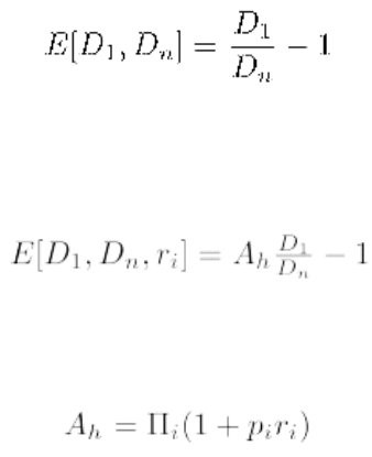
11 Swaps
11.1 Interest rate swap
680 © Wall Street Systems IPH AB - Confidential
– The estimation discount factor between the valuation date and start date of the cashflow
i, or 1, if the valuation date is within the coupon period.
– The estimation discount factor between the valuation date and the end date of cashflow
i.
–E[] The method used to estimate the size of the coupon.
The estimation of a coupon before the start of the coupon period is simply:
Equation 11-2 Coupon estimation: before the start of the coupon period
The estimation of the coupon during the coupon period, historical O/N rates r1, r2.....,rn are
used as part of the estimate:
Equation 11-3 Coupon estimation: during the coupon period
Where the historical compounding factor is calculated from the known O/N rates:
Equation 11-4 Historical compounding factor
Where is the length of the ith overnight period, calculated using the date basis of the fixing
quote. The set of periods includes only business days, and Friday’s period length is calculated
from three days.
The estimation method and risk calculations are described in more detail in 2.3.4.8 Risk profiles on
page 124.
Accrued interest ( ) is based on the historical compounding factor:
Equation 11-5 Accrued Interest
For example, let us consider the valuation of a coupon with the following data:
From When 2009-05-14
Until When 2009-08-14
Fixing To 2009-08-13
Payment Date 2009-08-14
Date Basis Act / 360
Nominal Amount 1000000
Valuation date 2009-05-20
Historical O/N rate (constant) 3.68%
Historical period 3 business days + one weekend
(start date discount factor) 1
Di1
Din
Ah
Pi
Ia
IaAh1–=
Di1
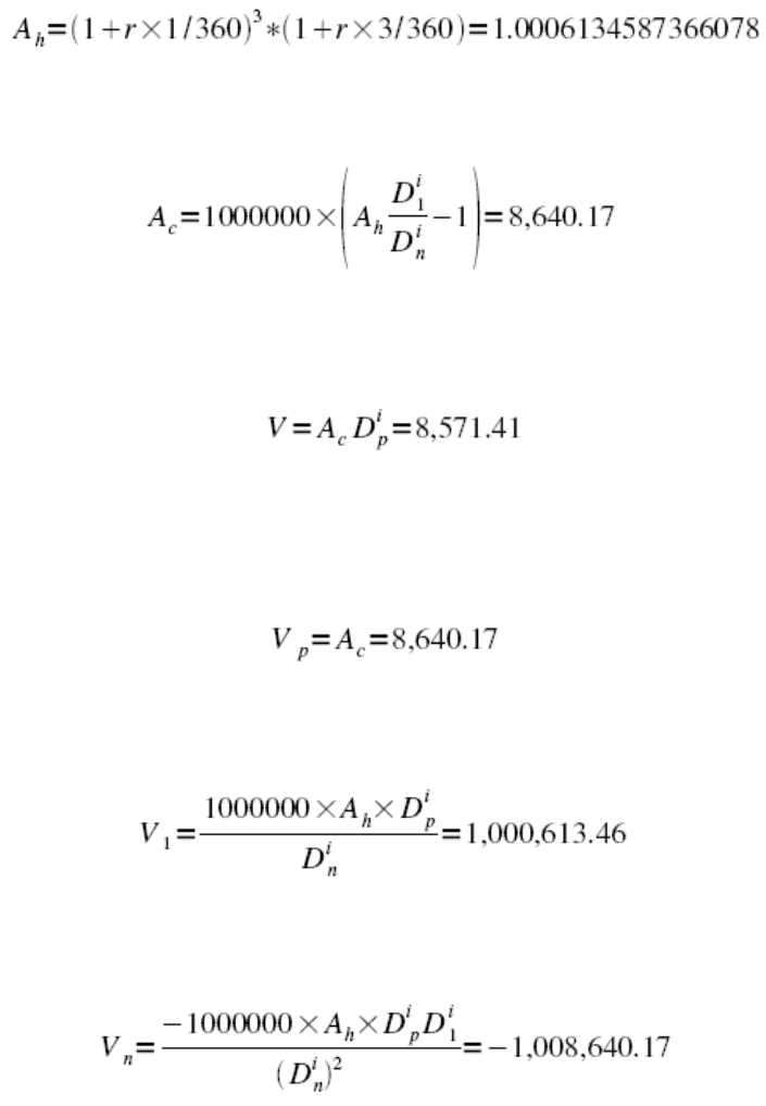
11 Swaps
11.1 Interest rate swap
Transaction & Risk Management Module (TRM) Instruments: Processing and Calculations 681
Valuation figures
•Historical compounding factor ( ) for one weekend, three business days:
Equation 11-6 Example: Historical compounding factor
•Coupon estimate
Equation 11-7 Example: Coupon estimate
•Market value
Equation 11-8 Example: Market Value
Risk values
•Payment Date
Equation 11-9 Example: Payment Date
•Period Start
Equation 11-10 Example: Period Start
•Period End
Equation 11-11 Example: Period End
(end date discount factor) 0.9920420458606090
(payment date discount
factor)
0.9920420458606090
Din
Di
p
Ah

11 Swaps
11.2 Total return swap
682 © Wall Street Systems IPH AB - Confidential
11.1.6 Other swap structures
TRM supports more exotic swap structures. The following sections give a brief description of these
structures.
11.1.6.1 Callable/puttable (cancelable) swap
A callable swap is an interest rate swap where the fixed rate payer has the right to terminate the
contract. The swap is puttable if it is the fixed rate receiver that has the right to terminate the
contract.
Instrument setup for a callable swap is similar to that of a standard IR swap, except that the call or
put events are added to a cashflow structure using a secondary schedule template. The call or put
event should specify the following information:
•Call/put periods or dates
•Call/put price = 0
•Any other characteristics, for example, whether the call/put option gives the right to terminate
the contract to the payer (call: Transaction Sign = "+") or to the receiver (put: Transaction Sign
= "-") of the fixed leg.
Note that the sign means the same no matter to which leg the call events are associated.
A cancelable swap is modeled by adding call or put events to one of the legs of an ordinary swap.
Executing the call will cancel the whole swap transaction.
Note: In an asset swap where the bond leg is callable, the swap automatically inherits the call
schedule of the swap.
11.1.6.2 Basis swap
Basis swaps are floating-to-floating swaps which can be input by selecting floating cashflow
structures for both legs using different market references. Basis swaps are usually cross currency
but can also be single currency.
For more information about how basis swaps are calculated, see 2.2 Yield curves on page 81.
11.1.6.3 Constant maturity swap
Constant maturity swaps are also supported by TRM. In this case, the period used for the floating
leg must be longer than the coupon period.
11.1.6.4 Roller coaster swap
It is possible to schedule periodical principal increases/amortizations on both legs of a swap. If this
option is used, it is possible to set up roller coasters.
11.2 Total return swap
A Total Return Swap (TRS) is a type of derivative that enables the holder of an asset (typically a
fixed-rate bond) to hedge the asset’s exposure by transferring the credit and market risks to a
counterparty without transferring the underlying asset. The total returns from the asset (for
example, the interest flows, dividends, MtoM profit, and so on) are transferred to the counterparty,
while the owner of the asset receives a fixed spread from the counterparty.
TRS transactions can be fully or partially early expired. Partial early maturities are limitless and can
occur at any time until the full value of the TRS has been matured.
11 Swaps
11.2 Total return swap
Transaction & Risk Management Module (TRM) Instruments: Processing and Calculations 683
A DRS (Deferred Rate Settlement) is a special kind of TRS, where the coupons of a swapped bond
are transferred at maturity of the swap, and the swap is made against the daily compounded EONIA.
Note: TRM only supports the swapping of a bond against a fixed or floating rate.
11.2.1 Instrument setup
Total Return Swap instruments are based on an instrument type derived from the instrument class
TRS.
•Main characteristics
The following basic information may be captured when defining the instrument and is relevant to
any kind of total return swap.
–Legged
–Legs
For each leg it is possible to define which is the sign of the leg versus the transaction, and
which is the leg instrument. If this information is not provided at instrument setup, it needs
to be specified at deal entry.
See A.2.327 TRS - Total Return Swap on page 875.
•Maturity definition
It is possible to set up maturity information at instrument level.
Information Description
Transaction Sign Direction of the transaction.
If the sign is not defined at instrument level, it needs to be specified separately
for each transaction.
Leg Structure The leg structure for the swap instrument.
TRM supports swap structures with multiple legs.
Pseudo Settlement
Pseudo Repayment
Select these options to make the principal notional (no exchange of capital).
Information Description
Instrument The instrument to be used for this leg by default (for example, a fixed-rate
bond).
For deferred total return swaps, the floating leg of the swap is a cost-of carry
cashflow of the bond’s notional value. This structure can be obtained in the
instrument by using the schedule for Cost-of-Carry, Compounding, Bullet
Repayment.
Sign versus
Transaction
Choose from: Same, Opposite, or Any.
Information Description
Calendar
parameters
Calendars used to calculate the maturity date.
Gap Set Gap set used for supplying the available maturity periods.
Maturity Date
Period
If defined, this maturity period is applied to each transaction.
11 Swaps
11.2 Total return swap
684 © Wall Street Systems IPH AB - Confidential
See A.2.230 Maturity Date Setup on page 827.
•Roll over
The Roll Over action is available on the transaction if the Allow Roll Over trading feature is
associated with the instrument.
See A.2.9 Allow Roll Over on page 716.
The parameters required are described in 11.2.3.2 Roll over on page 686.
•Deferred parameters
With a deferred TRS, all the cashflows of the deal which occur during its life will be paid at
maturity. This means that they will be reinvested at the same rate between their value date and
payment date.
If the return cashflows in the TRS are to be deferred until the maturity date, use the TRS
Deferred trading feature.
See A.2.328 TRS Deferred on page 875.
It is also possible to set up:
•Branch codes
•Cashflow and transaction charge rules
•Manual charges
•Spot date calculation.
See Appendix A Features on page 713.
11.2.2 Deal capture
11.2.2.1 Input data
In addition to the standard deal parameters, the following information is required to enter a TRS.
•Transaction view
Information Description
Nominal Amount Nominal amount of the swap, which also serves as the nominal (reference) amount of
Leg 1.
Value Date Date when the swap starts, and from which interest starts to accrue. This defaults to
the spot date of the first leg.
Maturity Date Date when the transaction matures.
Fixing Offset Offset, in days, between the maturity date and the fixing of the swap.
Expiry Date Fixing date of the swap. This defaults to Maturity Date - Fixing Offset but can be
modified.
Deal Price Price of the first leg of the deal.

11 Swaps
11.2 Total return swap
Transaction & Risk Management Module (TRM) Instruments: Processing and Calculations 685
In addition, the following optional information can be captured:
•Leg view
If the legs are not defined on the swap instrument they must be selected here.
Note that the different legs of a deferred TRS are always in the same currency.
•Schedule view
Schedule information must be provided for each leg.
For deferred TRS transactions, the floating leg of the swap is a cost-of carry cashflow of the
bond’s notional value. This structure can be obtained in the instrument by using the
Cost-of-Carry, Compounding, Bullet Repayment system-defined schedule.
See B.2.1.1.12 Cost of Carry Compounding, Bullet Repayment on page 892.
11.2.2.2 Generated data
•Cashflows
The cashflows are generated as follows:
–Settlement cashflows are marked as pseudo
–All cashflows with a value date later than the maturity date of the TRS are marked as
pseudo.
For a deferred TRS, the interests are deferred until maturity. Therefore, all the amounts that
would normally be paid during the life of the deal are paid at maturity and reinvested during the
period.
–A cost-of-carry amount is generated for each cashflow to reflect the reinvestment of the
interest until the maturity of the deal.
11.2.3 Processing
This section describes the actions that can be done throughout the life of a total return swap.
11.2.3.1 Early expiration
TRS transactions can be closed-out earlier than their agreed maturity date. This process is referred
to as early expiration.
•Execution
Information Description
Maturity Code If you enter a maturity code at deal entry, the maturity date is calculated
automatically; otherwise you can enter the date manually.
If the maturity definition parameters are defined at instrument level, these are used
by default and cannot be modified.
See A.2.230 Maturity Date Setup on page 827.
Value Date Code If the Value Date Setup feature is applied at instrument level, you can enter the value
date period you want to use to calculate the value date for the transaction, for
example, 3M (3 months).
This can be used to compute the value date for a forward purchase of a TRS.
If you specify a value date period in the instrument setup, this is used as the default in
the transaction and cannot be modified.
See A.2.339 Value Date Setup on page 879.
11 Swaps
11.2 Total return swap
686 © Wall Street Systems IPH AB - Confidential
Early expiration of a swap requires the following information:
The execution generates an early expiration transaction with the following attributes:
Transaction sign = opposite of initial transaction
Nominal amount = amount to expire
Opening date = date when the early expiration is done
Value date = date when the early expiration is settled
Kind = Early Expiration
The remaining attributes are inherited from the initial transaction.
The early expiration transaction generates closing cashflows for the initial transaction.
•Cancellation
You can undo the early expiration by canceling the early expiration transaction.
11.2.3.2 Roll over
You can defer the maturity of a TRS to a later date. This process is referred to as a roll-over.
•Setup
It is possible to restrict the use of the roll over methods at instrument level (see below for a
description of the available methods). It is also possible to specify the default roll over method
for the instrument.
The Roll Over action is available on the transaction if the Allow Roll Over feature is associated
with the instrument.
See A.2.9 Allow Roll Over on page 716.
•Execution
Roll over of TRS deals can be done in four different ways. In all cases, the following information
is needed to process the roll over:
Information Description
Opening Date Date when the early expiration is executed.
By default, this is today’s date unless a Fixing/Action Date is specified at transaction
level.
Value Date Date when the early expiration is settled. This must be earlier than the original
maturity date and later than the original value date of the initial transaction.
Amount to Expire Amount to be early expired. This defaults to the amount still available to be early
expired, taking into account previous partial early expirations and roll overs.
Net Amount Net amount to be settled between the two parties:
(Net Amount = Accrued Interest + Sell Profit/Loss)
Options • Amortize P/L
Switch on to amortize the P/L from the value date until the original maturity date.
If this switch is off, the Sell P/L flow created by the early expiration (arising from
Net Amount – Accrued Interest) occurs on the early expiration value date.
•No Fee Realization
Switch on so that fees keep amortizing to maturity. If this switch is off, at early
expiration, the fees that were amortizing until the maturity date are closed.
Information Description
Roll Over Date Date when the roll over is executed.
11 Swaps
11.2 Total return swap
Transaction & Risk Management Module (TRM) Instruments: Processing and Calculations 687
The outcome of the roll over depends on the method chosen as follows:
The execution generates a new transaction with the following attributes:
Nominal amount = amount (can be smaller than the initial amount)
Rate = roll-over rate
Opening date = date when the roll-over is done
Value date = maturity date of the initial transaction
Maturity date = maturity of the roll-over
Kind = Roll-over
•Cancellation
You can undo the roll over by canceling the roll over transaction.
11.2.3.3 Fixing
The Fixing action needs to be executed at the agreed fixing date to fix the interest rates on the
floating leg of the TRS transaction.
Maturity Date The maturity date for the rollover. The defaulting is defined as follows:
• If the parent transaction was defined with a maturity period, the roll over maturity
date defaults according to that period, otherwise you have to enter the maturity
date.
•If the switch No Maturity Defaulting is selected at the instrument level (Roll Over
page), then the maturity date of the rollover is never defaulted and you must
enter it.
Note: If the specified maturity date does not fall on a business day, you can choose to
keep the non business day or to change it.
Nominal Amount Amount of the roll over. By default, this is the amount left of the initial transaction but
you can override this if you want to perform a partial roll over.
Rate (Mandatory) New interest rate for the roll-over, that is, the rate at which interest is
calculated from the old maturity date until the new maturity date.
By default, the rate is defaulted from the initial transaction, however it is possible to
disable this defaulting by selecting the switch No Rate Defaulting at the instrument level
(Roll Over page).
Roll Over Method Roll over method: Settle All, Settle Interest, Delay Interest, or Compound Interest.
Spread New spread to be used in the roll over transaction.
Method Description
Settle All The initial transaction is paid in its entirety at the initial maturity date. The default
nominal amount of the roll over transaction equals the sum of the interest and
principal cashflows of the initial transaction.
Settle Interest The interest of the initial transaction is paid at the initial maturity date, but the
principal payment is deferred. The part of the principal which is rolled over is paid
back at the end of the roll over transaction.
Delay Interest Nothing is paid at the initial maturity date: both the interest and principal payments
are deferred. The parts of the principal and interest cashflows which are rolled over
are paid back when the first interest payment of the roll over transaction occurs.
Compound
Interest
This method is the same as Delay Interest, but the closed interest of the initial
transaction is reinvested in the roll over. New interest accrues on top of the initial
transaction’s interest.
Information Description
11 Swaps
11.3 Credit default swap
688 © Wall Street Systems IPH AB - Confidential
•Execution
The following information is needed to process the fixing:
The fixing process is performed directly on an individual cashflow in the Cashflow view.
•Cancellation
You can undo the fixing with the Undo Fixing action.
11.3 Credit default swap
A credit default swap (CDS) is a bilateral agreement designed to transfer the credit exposure of a
particular entity (or a group of entities) from the buyer to the seller. The entity whose credit risk is
transferred in a CDS is referred to as a reference entity. The reference entity is not a party to the
contract. The buyer of a CDS pays regular (premium) payments to the seller.
In the case where the reference entity defaults, the buyer will receive compensation from the seller,
usually in the form of a cash payment, but sometimes, for example, as a par value payment for a
bond (issued by the reference entity) against physical delivery. The default is referred to as a credit
event and includes events, such as, the failure to pay a coupon or a redemption on a specific
instrument issued by the reference entity or the bankruptcy of the reference entity.
Following recent changes to the CDS market where previously no specific standard existed, the
market has introduced new conventions to standardize CDSs. In standardized (ISDA-driven) CDSs,
the buyer pays a fixed quarterly (premium) payment (usually 100 or 500 bp) and these payments,
as well as the transaction maturity dates, always fall on the 20th of March, 20th of June, 20th of
September, or 20th of December. The quarterly payments are often referred to as fixed coupons or
fixed spread. A special convention also applies to the calculation of the coupon amounts, as the
calculation period includes the date of the previous coupon (or issue date), and excludes the coupon
payment date, except for the last coupon where both dates are included. As the coupon payment
dates and amounts are fixed, an accrued interest and an upfront payment are often settled when
entering into (or terminating) a CDS transaction.
The CDSs described in this section are based on the standard conventions, but it is possible to define
and capture CDS transactions using other conventions as well. The standardized CDSs are
supported by using the system-defined schedule template Credit Default Swap, ISDA Standard
(CD-SWAP-ISDA). The system-defined schedule template CD-SWAP can be used to capture
'non-standard' CDSs, e.g. with non-fixed dates and different calculation conventions for the regular
payments.
The reference entity of the CDS can be a single entity or a basket of reference entities each with
their own weight. Single entity CDSs are often referred to as a single name CDS, while basket entity
CDSs are known as credit default index swaps (CDISs) or credit default swap index. The main
difference between the two is in the processing of a credit event. In a CDIS, when a credit event
occurs, the CDS is impacted only partially based on the weight of the defaulting reference entity.
CDSs can be terminated before their maturity through early expiration as e.g. loans or IRS.
11.3.1 Instrument setup
Credit default swaps must be based on an instrument type derived from the class CDS.
Information Description
Fixing Date Day the cashflow is fixed.
Fixing Quote Rate of the yield curve
Nominal Rate Rate which is the rate of the yield curve (and optionally * factor + spread).
Amount Amount of the interest flow.
11 Swaps
11.3 Credit default swap
Transaction & Risk Management Module (TRM) Instruments: Processing and Calculations 689
•Main characteristics
The following basic information may be captured when defining the instrument.
•Dates definition
For standardized CDSs, Gap Set and Maturity Date Period do not apply. The Tenor field in
Transaction Manager needs to be used to capture the tenor of the transaction, which is then
translated into a standardized maturity date.
See A.2.110 Credit Default Swap on page 762.
•Credit spread curve setup
It is possible to add a credit spread curve at instrument level: see A.2.114 Credit Default Swap
Curve Setup on page 764.
If no credit spread curve is defined at the instrument level, the system uses the credit spread
curve attached to the reference entity: the linking of spread curves to entities can be done either
in Client Editor or in IR Quote and Yield Curve Editor: see the TRM User Guide.
It is also possible to set up:
•Branch codes
•Cashflow and transaction charge rules
Information Description
AI Method Select ISDA CDS in order to have accrued interest calculated according to the new
conventions (including first day). See ISDA CDS on page 72.
Structure Select the system-defined Credit Default Swap, ISDA Standard (CD-SWAP-ISDA) primary
schedule template: see B.2.1.1.14 Credit Default Swap, ISDA Standard on page 892.
The following parameters are relevant for calculating the fixed coupons:
•CDS Premium schedule:
-Method:
ISDA CDS Dates (Q)
-Rate Type: ISDA CDS
- Adjust Value Date: Yes, Except Last
-Convention: Following
Note: For non-standardized CDSs, select the system-defined Credit Default Swap
(CD-SWAP) primary schedule template: see B.2.1.1.13 Credit Default Swap on
page 892.
Reference Entity • For single name contracts, select the reference entity defined in the Client Editor.
• For CDISs (basket CDSs), select the reference entity with the basket of entities
defined in the Client Editor’s Member Clients page.
See the TRM User Guide for more information.
Settlement Offset The number of business days after the value date that the upfront and accrued
interest are settled. For example, three days for standardized CDSs.
Recovery Rate The default recovery rate, used in calculating CDS Deal Spread (see below), and also
used as the default recovery price in the case of a credit event.
Price Rounding
parameters
Method and precision used to round the deal price when calculated.
Information Description
Spot Days To comply with standard conventions, set this field to 0. This results in the value date
being equal to the opening date. Thus, accrued interest is calculated to the trade date.
Note: The settlement will occur later according to the defined Settlement Offset.
11 Swaps
11.3 Credit default swap
690 © Wall Street Systems IPH AB - Confidential
•Manual charges
See Appendix A Features on page 713.
11.3.2 Market information
11.3.2.1 Credit spread curves
A credit spread curve must be set up to store the credit spread quotes that are taken from the
market feed or via Rate Monitor. This curve is needed for valuating CDSs.
See the TRM User Guide for information about setting up credit spread curves.
11.3.2.2 Rate Monitor
In Rate Monitor, Credit Default Swap page, the credit spread quotes are expressed as basis points and
the recovery rate is expressed as a percentage. The calculated Default Probability (%) and Hazard
Rate (bp) are also displayed. See the TRM User Guide for information about using Rate Monitor.
CDS valuation is based on Par Spreads, and not on quoted upfronts or conventional spreads. Thus, it
is Par Spreads that need to be imported or captured manually.
Note: When importing from Reuters, the Par Spread is found in field 393 (PRIMACT_1). While the
recovery rate is also available in the feed, it is recommended that the recovery rate is
captured manually in Rate Monitor.
11.3.3 Deal capture
11.3.3.1 Input data
In addition to the standard deal parameters, the following information is required to enter a
standardized credit default swap.
•Transaction view
Information Description
Nominal / Spot
Rate
Fixed coupon (CDS premium) in basis points.
Note: If you are using the Enter Board to capture the CDS, this field is displayed as
Fixed Spread.
Deal Price Upfront %, i.e. the percentage of the nominal amount that will be settled between the
transaction parties.
Note: If you are using the Enter Board to capture the CDS, this percentage is
displayed in the Upfront % field.
Deal Rate This field is effectively another representation of the Deal Price, calculated as:
100 - Deal Price
Recovery Rate Recovery rate (defaulted from instrument level) used to calculate the CDS Deal
Spread.
CDS Deal Spread Calculated from the fixed coupon and upfront according to the formula below.
Changes to this field automatically trigger the recalculation of the deal price.
Note: If you are using the Enter Board to capture the CDS, this field is displayed as
Deal Spread.
Nominal Amount Notional amount of the transaction.
Value Date Value date of the transaction, i.e. the date up to which accrued interest is calculated.
For standardized CDSs, this corresponds to the opening date.
11 Swaps
11.3 Credit default swap
Transaction & Risk Management Module (TRM) Instruments: Processing and Calculations 691
In addition, you may define the following information related to the possible credit event:
•Schedule view
If the cashflow structure of the deal is not defined at the instrument level, you need to specify it
at the deal level by applying the system-defined schedule template Credit Default Swap, ISDA
Standard (CD-SWAP-ISDA): see B.2.1.1.14 Credit Default Swap, ISDA Standard on page 892.
Note: In the case of non-standardized CDSs, you can use the system-defined schedule template
Credit Default Swap: see B.2.1.1.13 Credit Default Swap on page 892.
11.3.3.2 Generated data
•Cashflows
–Principal and Accrued Interest
–CDS coupons
–Pseudo Redemption (reflecting the notional amount)
Settlement Date Settlement date of the transaction, i.e. the date when upfront payment and accrued
interest are settled. The settlement date corresponds to the value date plus the
number of business days specified in the Settlement Offset field at the instrument level
(three for the standard convention).
Tenor Term of the transaction (e.g. 1Y, 3Y), which calculates the maturity date according to
the standard convention For example, the maturity date of a 5Y deal is calculated as
the first ISDA date (20th of March, June, September or December) which will be hit
five years or more after the trade date plus one day (calendar unadjusted).
Maturity Date Maturity date of the CDS.
Issuer Reference entity or reference basket entity.
Currency Currency of the transaction.
Information Description
Settlement Type Method of settlement if a credit event occurs: Cash Settlement or Physical Delivery.
Reference
Instrument
Reference instrument of the transaction.
•If
Settlement Method = Physical Delivery, this is the default deliverable
instrument (for information only).
•If
Settlement Method = Cash Settlement, the market price of this instrument is
used by default as the recovery price (which in turn is used to calculate the
settlement amount).
When executing the credit event, it is possible to change the instrument to another
instrument issued by the reference entity.
Note: Normally, the basket of deliverable instruments/obligations is defined in broad
terms, and some deliverables are instruments that are not or cannot be defined
as instruments in the system. In such cases, the details can, for example, be
described in a separate document and linked to the transaction using the
Document Link column.
Reference Price Price at which the underlying bond is exchanged or against which the cash settlement
is calculated when a credit event occurs. The default value is 100.
Settle AI Defines whether the accrued interest of the deliverable bond is to be settled when
there is a physical delivery.
Information Description
11 Swaps
11.3 Credit default swap
692 © Wall Street Systems IPH AB - Confidential
•Cashflow key-figures
11.3.4 Processing
This section describes the actions that can be done throughout the life of a CDS.
11.3.4.1 Early expiration
A CDS can be either fully or partially early expired by executing the Early Expiration action and
supplying the amount you want to expire and the clean price for calculating the (clean) settlement
amount.
•Execution
•Cancellation
You can undo the early expiration by canceling the new transaction.
Figure Description
Figure Default
Probability
Cumulative probability that there will have been a credit event before the coupon
payment.
Figure Premium
Amount
Expected default probability adjusted amount of the coupon payment.
Figure Protection
Amount
Expected protection amount at the coupon payment date:
(Nominal Amount * (1 – Recovery Rate) * Probability of default during
the coupon period)
Figure Amount Expected payment:
Premium Amount + Protection Amount
Figure Market
Value
Discounted value of the expected payment.
Figure Accrued
Interest
Accrued interest (premium).
Information Description
Opening Date Date when the early expiration is executed.
By default, this is today’s date but can be modified to any date falling between the
opening date and maturity date of the transaction.
Value Date Value date of the transaction, i.e. the date up to which accrued interest is calculated.
Settlement Date Settlement date of the transaction. The settlement date corresponds to the value date
plus the number of business days specified in the Settlement Offset field at the
instrument level.
Currency Currency of the transaction. Read-only.
Amount to Expire Amount you want to be early expired. This defaults to the amount still available
(Amount Left) to be early expired, taking into account previous partial early
expirations.
Amount Left Remaining amount of the initial transaction. Read-only.
Clean Price Price used to calculate the Clean Amount.
Deal Spread CDS Deal Spread as calculated for new transactions.
Clean Amount Amount to be settled (excluding accrued interest) calculated as
Amount to Expire * Clean Price / 100
Accrued Interest The accrued interest to be settled.
11 Swaps
11.3 Credit default swap
Transaction & Risk Management Module (TRM) Instruments: Processing and Calculations 693
11.3.4.2 Credit event
With cash settlement, the seller will pay the difference between the recovery price and the reference
price (default 100) on the outstanding notional. The recovery price can be the market price of the
reference instrument, or some other price set by an independent third-party.
Alternatively, there could be physical delivery of some underlying instrument or loan. In the case of
physical delivery, the credit event only terminates the CDS; the physical delivery itself needs to be
captured in a separate transaction.
•Execution
The execution generates a new transaction:
–Closing cashflows against the initial transaction
–Cashflows reflecting the cash settlement (Settlement Amount and Accrued Interest).
•Cancellation
You can undo the credit event by canceling the new transaction.
Information Description
Opening Date Date when the credit event is executed.
By default, this is today’s date but can be modified to any date falling between the
opening date and maturity date of the transaction.
Value Date Value date of the transaction, i.e. the date up to which accrued interest is calculated.
Settlement Date Settlement date of the transaction, i.e. the date when the settlement occurs.
Amount Left Amount left of the initial transaction available for the credit event. Read only.
Amount Amount of the credit event.
Settlement Type Select Cash Settlement or Physical Delivery.
Reference Entity • For a single name CDSs, this field displays the reference entity.
• For a CDISs, you need to select the defaulting reference entity. The Amount field,
i.e. the notional affected by the credit event is calculated based on the weight of
the defaulting entity:
Amount = Amount Left * Weight
Reference
Instrument
The instrument used to default the recovery price.
The list contains all the bonds of the reference entity.
Scenario Scenario from which the recovery price is obtained.
Reference Price Reference price (usually 100) used to calculate the settlement amount.
Recovery Price Price used to calculate the settlement amount.
Settlement
Amount
• For cash settlement, the amount to be settled is calculated as
Amount * (Reference Price - Recovery Price)
• For physical delivery, the credit event is processed without any settlement, and the
physical delivery is handled independently through the capturing of a separate
transaction.
Accrued Interest Accrued Interest to be settled.
11 Swaps
11.3 Credit default swap
694 © Wall Street Systems IPH AB - Confidential
Important: In the case of a CDIS, after executing the credit event, you must set the defaulting
entity to Inactive in Client Editor's Member Clients page of the corresponding basket
entity.
11.3.5 Position monitoring
11.3.5.1 Setup
The result key figures of the cashflows of a credit default swap are calculated based on the
instrument’s valuation method settings: Theoretical or Quoted.
•Theoretical - a default probability curve is constructed from par credit default swap rates. The
market value of the swap is then estimated based on the probability.
•Quoted - the difference between the nominal rate of the transaction and the current market rate
for the corresponding swap is multiplied by the risky point value that is derived from the market
swap rate and recovery rate.
Note: IR exposure is calculated using the Theoretical method even in Quoted mode.
See A.2.50 Base Valuation Setup on page 734.
11.3.5.2 Calculations
In this section, numerical examples demonstrate how the different figures are calculated for a credit
default swap.
If you need more theoretical information about the method used in these calculations, see Chapter 2
Market standards and calculations on page 33.
This example shows a credit default swap, with the following deal data:
Other transaction data specific to the coupon flows is as follows:
Setup data
Maturity Date d_m 2008-03-09
Date Basis B Actual/360
Interpolation Date Basis B_i 365
Transaction data
Opening Date 2006-03-07
Value Date dt_v 2006-03-09
Nominal Amount A 10,000,000.00
Deal Price r_b 18.0000
Maturity Date d_m 2008-03-09
Date Basis B 360
Transaction data Coupon 1 Coupon 2
Value Date dt_v.c1 2007-03-09 dt_v.c2 2008-03-09
11 Swaps
11.3 Credit default swap
Transaction & Risk Management Module (TRM) Instruments: Processing and Calculations 695
Calculated transaction data is as follows:
•Coupon 1
Coupon Period
p.c1 = (dt_v.c1 – dt_v) / B
1.013888889 = (2007/03/09 – 2006/03/09) / 360
Coupon Amount
A.c1 = A * P.c1 * r_b / 10,000
18,250 = 10,000,000.00 * 1.013888889 * 18.0000 / 10,000
•Coupon 2
Coupon Period
p.c2 = (dt_v.c2 – dt_v.c1) / B
1.016666667 = (2008/03/09 – 2007/03/09) / 360
Coupon Amount
A.c2 = A * p.c2 * r_b / 10,000
18,300.00 = 10,000,000.00 * 1.016666667 * 18 / 10,000
Unless otherwise stated, the figure date used in the calculations is 2006-03-09. On this date, the
market data is as follows:
Market data specific to the coupon flows is as follows:
Other market data is calculated by the system as follows:
•Coupon 1
Risk Time
t_r.c1 = (dt_v.c1 - d_f) / 365
1.00000 = (2007/03/09 – 2006/03/09) / 365
•Coupon 2
Risk Time
t_r.c2 = (dt_v.c2 - d_f) / 365
2.002740 = (2008/03/09 – 2006/03/09) / 365
Risk Time from Spot
t_r = (dt_v.c2 – d_s.f) / 365
1.991780822 = (2008/03/09 – 2006/03/13) / 365
Market data on 2006-03-09
Figure Date d_f 2006-03-09
Spot Date d_s.f 2006-03-13
Market Spread S_p 100.00000
Recovery Rate R_c 40.00%
MV Discount Factor Spot D_s 0.9996625908
Market data Coupon 1 Coupon 2
MV Discount Factor D_V.c1 0.9734527645 D_V.c2 0.9446679058
Default Probablility Pr.c1 0.016529 P.c2 0.032828
11 Swaps
11.3 Credit default swap
696 © Wall Street Systems IPH AB - Confidential
11.3.5.2.1 Key-figures
This example uses the Quoted method to calculate market value, and the Theoretical method to
calculate present value and risks.
• Hazard Rate
lambda = S_p / 10,000 / (1 - R_c)
0.0167 = 100.00 / 10,000 / (1 – 0.40)
• Continuous Rate
rate = -LN(D_V.c2 / D_s) / ((dt_v.c2 – d_s.f) / 365)
0.028408934 = LN(0.9446679058 / 0.9996625908) / ((2008/03/09 – 2006/03/13) / 365
•Risk Rate
r_r = (rate + lambda)
0.045076 = 0.028408934 + 0.0167
• Risky Point Value
rpv = ((1 - EXP(-(r_r) * t_r)) / r_r) * A * 0.0001
1904.99 = ((1 – EXP(-(0.045076) * 1.991780822)) / 0.045076 * 10,000,000 * 0.0001
•Market Value
= (S_p - r_b) * rpv * D_s
156,156.14 (100.00 – 18.0000) * 1904.99 * 0.9996625908
•Coupon 1
Premium Amount
A_p.c1 = -A.c1 * (1 – 0.5 * Pr.c1)
-18,099.17 = -18,250 * (1 – 0.5 * 0.016529)
Protection Amount
A_d.c1 = A * (1 – R_p) * Pr.c1
99,173.55 = 10,000,000 * (1 * 0.40) * 0.016529
Amount
A_f.c1 = A_d.c1 + A_p.c1
81,074.38 = 99,173.55 + (-18,099.17)
Market Value
V. c 1 = A _ f. c 1 * D _ V. c 1
78,922.08 = 81,074.38 * 0.9734527645
IR Exposure 1bp
E_pb.c1 = -A_f.c1 * D_V.c1 * t_r.c1 * 0.0001
-7.89 = 81,074.38 * 0.9734527645 * 1.0000 * 0.0001
Effective Duration
U_eff.c1 = -E_pb.c1 / V.c1 / 0.0001
1.00 = -(-7.89) / 78,922.08 / 0.0001
•Coupon 2
Premium Amount
A_p.c2 = -A.c2 * (1 – 0.5 * (p.c2 + P.c1))
-8,846.26 = -18,300 * (1 – 0.5 * (1.016666667 + 0.016529))
Protection Amount
A_d.c2 = A * (1 - R_p) * (p.c2 - P.c1)
6,000,826.45 = 10,000,000 (1 – 0.40) * (0.032828 – 0.016529)
Amount
A_f.c2 = A_d.c2 + A_p.c2
5,991,980.19 = 6,000,826.45 + (-8,846.26)
Market Value
V. c 2 = A _ f. c 2 * D _ V. c 2
5,660,431.37 = 5,991,980.19 * 0.9446679058
IR Exposure 1bp
E_pb.c2 = -A_f.c2 * D_V.c2 * t_r.c2 * 0.0001
-15.13 = 79,948.73 * 0.9446679058 * 2.002740 * 0.0001
Effective Duration
U_eff.c2 = -E_pb.c2 / V.c2 / 0.0001
2.00 = -(-15.13) / 75,525.00 / 0.0001
11 Swaps
11.3 Credit default swap
Transaction & Risk Management Module (TRM) Instruments: Processing and Calculations 697
• Total transaction
Market Value
V. t = V. c 1 + V. c 2
154,447.08 = 78,922.08 + 75,525.00
IR Exposure 1bp
E_pb.t = E_pb.c1 + E_pb.c2
-23.02 = -7.89 + (-15.13)
Effective Duration
U_eff.t = -E_pb.t / V.t / 0.0001
1.49 = -(-23.02) / 154,447.08 / 0.0001
11 Swaps
11.3 Credit default swap
698 © Wall Street Systems IPH AB - Confidential
Transaction & Risk Management Module (TRM) Instruments: Processing and Calculations 699
Chapter 12 Commodities
12.1 Gold
12.1.1 Gold deposit
A gold (XAU) deposit is a short-term deposit, with one interest payment at maturity which is settled
in another currency (normally US Dollars). Gold deposits are set up in a similar way to generic loans
and processed in TRM as dual-currency transactions.
12.1.1.1 Instrument setup
Gold deposits are based on an instrument type derived from the class LOAN.
Instrument setup for gold deposits is similar to that of a standard loan (see 3.10 Loan on page 326),
except for the following:
•Gold main characteristics
•Weight difference instrument
It is possible to manage any difference in the weight of gold that is delivered and issue the
appropriate compensation for the difference between counterparties.
Weight differences are captured at transaction level. You need to define the instrument used to
capture the difference.
See A.2.25 Allow Weight Difference on page 722.
•Sight account transfer instrument
It is possible to manage transfers between the account where the gold is physically held and the
custodian sight account.
Transfers between accounts are captured at transaction level. You need to define the instrument
used for the transfer.
See A.2.20 Allow Sight Account Transfer on page 721.
Information Description
Currency XAU
Structure Select the cashflow structure template you want for the instrument.
One system template is provided for gold deposits. This is a fixed bullet structure: see
B.2.1.1.45 XAU, Unknown FX Rate, Fixed on page 899.
12 Commodities
12.1 Gold
700 © Wall Street Systems IPH AB - Confidential
12.1.1.2 Deal capture
12.1.1.2.1 Input data
Deals on gold instruments are captured in a similar way to those on a standard loan (see 3.10 Loan
on page 326).
To complete the capture of a gold deposit transaction, you need to specify the settlement currency
and the settlement FX rate either at transaction level or at schedule level.
Hint:
At the transaction level, the settlement currency is displayed in the Currency 2 column.
12.1.1.3 Processing
This section describes the actions that can be done throughout the life of a gold deposit transaction.
12.1.1.3.1 Roll over
You can defer the maturity of a gold deposit to a later date. This process is referred to as a roll-over.
See A.2.10 Allow Roll Over (Dual Currency) on page 717.
•Setup
It is possible to restrict the use of the roll-over methods at instrument level.
It is also possible to specify the default roll over method for the instrument.
•Execution
Roll-over of gold transactions can be done in several ways. In all cases, the information needed
to process the roll over is as follows:
Information Description
Roll Over Date Date when the action is executed.
By default, this is today’s date unless a Fixing/Action Date was specified at transaction
level.
Roll Over Method Method used for the roll over.
Nominal Amount Amount of the roll over. This defaults to the amount left of the initial transaction but
you can override this if you want to perform a partial roll over.
Additional Amount Amount to be added to the initial principal amount if you want to increase capital at
roll over.
This field becomes available when one of the Allow Increase roll over methods has
been selected.
New Nominal
Amount
Original nominal amount plus the additional amount.
This field becomes available when one of the Allow Increase roll over methods has
been selected.
Gap Gap used to compute the maturity date.
Maturity Date The maturity date for the rollover. The defaulting is defined as follows:
• If the parent transaction was defined with a maturity period, the roll over maturity
date defaults according to that period, otherwise you have to enter the maturity
date.
•If the switch No Maturity Defaulting is selected at the instrument level (Roll Over
page), then the maturity date of the rollover is never defaulted and you must
enter it.
Note: If the specified maturity date does not fall on a business day, you can choose to
keep the non business day or to change it.
12 Commodities
12.1 Gold
Transaction & Risk Management Module (TRM) Instruments: Processing and Calculations 701
•Cancellation
You can undo the roll over by canceling the roll over transaction.
12.1.1.3.2 Weight differences
It is possible to manage any difference in the weight of gold that is delivered and issue the
appropriate compensation for the difference between counterparties at maturity.
Weight differences in a gold transaction are captured using a processing action on the redemption
flow.
•Setup
In the instrument definition, you need to attach the FX instrument used to capture weight
differences for gold deposit transactions.
See A.2.25 Allow Weight Difference on page 722.
•Execution
At cashflow level, the action is executed on the maturity cashflow. The following information is
needed to process the Weight Difference action:
Deal Rate (Mandatory) New interest rate for the roll-over, that is, the rate at which interest is
calculated from the old maturity date until the new maturity date.
By default, the rate is defaulted from the initial transaction, however it is possible to
disable this defaulting by selecting the switch No Rate Defaulting at the instrument level
(Roll Over page).
Spread Spread to be added to the interest rate.
FX Rate FX rate used to convert the new interest amount into the settlement currency.
Information Description
Opening Date Date when the action is executed.
By default, this is today’s date unless a Fixing/Action Date was specified at transaction
level.
Value Date Value date of the weight difference cashflow. This defaults to the spot date of the
instrument.
Direction Direction of the cashflow. Choose from:
• Over Delivery - when the weight of the gold that is delivered is over the expected
weight
• Under Delivery - when the weight of the gold that is delivered is under the
expected weight.
Currency Currency of the cashflow.
Amount Amount of the weight difference in XAU.
FX Rate Rate used to calculate the settlement amount.
Settlement
Currency
Currency in which the weight difference is settled.
Settlement
Amount
Settlement amount calculated using the Amount and FX Rate values.
Add to Package Switch on to add the new transaction to the same package as the underlying gold
deposit (if it is part of a package).
Information Description

12 Commodities
12.2 Setting up commodities as currencies
702 © Wall Street Systems IPH AB - Confidential
12.1.1.3.3 Sight account transfers
It is possible to manage transfers between the account where the gold is physically held and the
custodian sight account.
•Setup
In the instrument definition, you need to attach the cash transfer instrument that you want to
used to make the transfer.
See A.2.20 Allow Sight Account Transfer on page 721.
•Execution
At cashflow level, the action is executed on the cashflow for which the transfer is made. The
following information is needed to process the Sight Account Transfer action:
12.1.2 Gold IR swap
TBC
12.2 Setting up commodities as currencies
Commodity futures, swaps and forwards are not currently defined as separate instrument classes,
but can now be set up using the existing currency- and instrument-based functionality. They have
financial net settlement, with no physical delivery of the commodity.
You can set up the commodities as currencies in Currency Editor. This also applies to all geographic
or grade-based variations such as electricity in a specific area, or a specific crude oil grade. As in
any currency, the setup identifies the currency in which the commodity is priced in the market, as
well as point factor, etc. The setup must include a default valuation curve even though this curve
may not be actually used in this context.
All Commodity Prices are best managed as FX rates of commodity currencies against their respective
pricing currencies (i.e. Quote Base Currency given in the journal of the commodity currency).
Regardless of the actual quoting structure of the commodity in the marketplace, TRM can only
handle FX quotes as a combination of a spot FX rate and a set of tenor-based forward points, as in
normal currencies.
Consequently, in situations where a forward price curve is required for valuation of commodity
swaps and forwards, forward prices must be first converted into a combination of a single spot rate
and a series of forward points, for the period between spot and the date for which the forward price
is given as defined in Gap Set given in the Journal of the commodity currency, before it is taken into
the system.
Information Description
Opening Date Date when the action is executed.
By default, this is today’s date unless a Fixing/Action Date was specified at transaction
level.
Value Date Value date of the transfer. This is taken from the cashflow.
Currency Currency of the transfer.
Amount Amount of the transfer.
Direction Direction of the transfer. Choose from:
•From Custody
• To Custody.
Add to Package Switch on to add the new transaction to the same package as the underlying gold
deposit (if it is part of a package).
12 Commodities
12.3 Commodity futures
Transaction & Risk Management Module (TRM) Instruments: Processing and Calculations 703
12.3 Commodity futures
12.3.1 Setting up instruments
Commodity futures can be modeled using FX-FUTURE type instruments and commodity currencies.
Commodity futures are settled financially and behave similarly to FX futures, so existing FX futures
functionality in commodity futures instruments and transactions can be used.
12.4 Commodity swaps and forwards
12.4.1 Schedule structure
Commodity swaps and forwards are set up as loan-type instruments, with a specific schedule
structure. The system templates include a COMMODITY-SWAP schedule template which holds
commodity position and settlement schedules.
12.4.1.1 Commodity Position schedule
This principal-type schedule is used to model the commodity amounts purchased or sold at fixed
price in a commodity swap or forward transaction.
•In a forward transaction, the method Bullet is used, so a single commodity position cashflow is
generated at the Maturity Date of the transaction.
•In a swap transaction, method, frequency and calculation method are used to split the
transaction nominal amount in traded commodity to any number of periodic amounts reflecting
the conditions of the swap transaction.
Cashflows generated by this schedule are pseudo-redemption cashflows with no valuation. Their
only purpose is to model the commodity deliveries for which financial settlements can be calculated.
In monitoring, they will produce values in the Nominal Amount key figure, to facilitate analysis of
open positions in terms of the purchased or sold commodity.
12.4.1.2 Commodity Settlement schedule
This interest-type schedule is used to model the financial settlements from commodity position
cashflows. The schedule is a referenced one and automatically creates a settlement cashflow for
each date on which there is a commodity position cashflow. The currency of this schedule is always
the commodity itself (the currency of the transaction). The currency in which the commodity is
priced and in which the financial settlement from the commodity delivery is settled is given in the
Settlement Currency field.
The schedule creates a floating cashflow where the settlement conditions are modeled in an
expression. By default, the following expression is used in the schedule:
abs(reference_amount)*(fx-cap)
where the fixed commodity price at which the commodity has been purchased or sold is given in
field Cap and currency pair referencing commodity market price is given in field Fixing Rate (e.g.
XCU/USD) but this can be modified. This schedule also underlies the market valuation of the
transaction which is based on the figure amount received by evaluating the expression (see 12.3.1
Setting up instruments on page 703).
Schedule is modeled as an interest-type schedule, because commodity swaps are typically settled
against periodic monthly average commodity prices. Sometimes it is possible to use a simple
expression like the default, because periodic average prices are quoted in the market. Otherwise
these averages must be calculated internally using expressions like:
abs(reference_amount)*(average(@,@,@,@,[fx])-cap)
12 Commodities
12.4 Commodity swaps and forwards
704 © Wall Street Systems IPH AB - Confidential
This expression can only be evaluated in an interest-type cashflow identifying a cashflow period
(From When – Until When).
Cashflows generated by this schedule use cashflow type (2, 12, Periodic Netting) which clearly
separates commodity settlement cashflows from true interest cashflows. Also, when realized results
are being analyzed, all results from Periodic Netting cashflows are shown as realized mtom profit
instead of realized interest.
In monitoring, cashflows from this schedule generate values for all relevant valuation, result and
risk figures.
12.4.2 Setting up instruments
Commodity swaps and forwards are set up as loan-type instruments attached to a Schedule
Template derived from the system template. When setting up the instrument, consider the
following:
•GENERIC-IR-METHOD. Valuation is handled by this approach.
•DUAL-CURRENCY. Since valuation is based on Settlement Currency amounts of commodity
settlement cashflows, dual currency valuation is used. This is automatically handled by normal
GENERIC-IR-METHOD but in order for fixings to work properly, feature Dual Currency
(DUAL-CURRENCY) must be attached.
•BASE-IR-SETUP. Since valuation is based on figure amounts received by evaluating expression
used in settlement cashflows, Estimate Method in IR Valuation setup must be set to Estimate
Expression.
•FLOATING-SETUP. Risk Profile in Floating Valuation setup must be explicitly set to None.
•FX-ESTIMATE. If forward prices (forward FX rates of commodity currencies) are to be used in
valuation when evaluating the expressions of cashflows, feature FX-ESTIMATE must be set. If
this feature is not used, figure amounts of commodity settlement cashflows used in valuation are
calculated using spot rate of commodity currency only: all future settlements amounts are
estimated using current spot price. If the feature is used, TRM uses forward prices of respective
Value Dates instead.
Sometimes, as in the case of electricity swaps, standard periods (e.g. year 2008 or Q3 2008) with
irregular delivery amounts (for electricity, monthly hours) are traded in large volumes. In a normal
commodity swap transaction, handling these irregular amounts would require the user to calculate
them outside the system and manually insert them separately into every transaction (either in
Schedule Date / Schedule Data or directly in the cashflow Fixing Quote). This can be very
time-consuming and error-prone.
These swaps can also be set up as separate contract-specific instruments as follows:
•Set up a bond instrument without a fixed issuer. If this is done, the issuer is defaulted during
transaction entry as Owner or Counterparty of the transaction, using the same logic as in
loan-type transactions
•In the expression of a floating schedule it is possible to refer to transaction-level fields in
addition to other cashflow fields by prefixing the field id with "0." (e.g. 0.nominal_rate would
evaluate to a value in the Nominal/Spot Rate field of the transaction).
In the context of standardized commodity swaps, this makes it possible to create instrument
cashflows as part of the instrument setup, with irregular amounts (by updating fixing_quotes
manually in instrument cashflows) using an expression like the following:
reference_amount*(fx-0.nominal_rate)
and identifying a fixed commodity price at which the commodity has been purchased or sold
dynamically for every transaction traded in the instrument by giving it in the transaction field
Nominal/Spot Rate.
Note that if irregular amounts are given in instrument cashflows, the Rate Type of Commodity
Position schedule must be set to Price %, and irregular amounts must be calculated outside the
system and given manually as a percentage of the total contract amount in the Fixing Quote
12 Commodities
12.4 Commodity swaps and forwards
Transaction & Risk Management Module (TRM) Instruments: Processing and Calculations 705
field of the commodity position cashflows. This enables TRM to calculate the respective cashflow
amounts correctly from the transaction Nominal Amount when a transaction is entered.
12.4.3 Deal capture
Commodity swap and forward transactions are captured similarly to any other schedule based
transactions in the system.
12.4.3.1 Input data
You need to consider the following transaction attributes when capturing a commodity swap or
forward transaction:
•Transaction view
•Schedule view
Schedule fields Method, Frequency and Calculation Method of the Commodity Position schedule are used
to define how the Nominal amount of the transaction is split between different delivery periods. In a
commodity forward transaction, Method is set to Bullet as there is only one delivery period underlying
the transaction.
You can enter the following schedule attributes in the Commodity Settlement schedule:
Information Description
Currency Traded commodity.
Nominal Amount Total commodity amount of the deal.
If the swap transaction has several periodic deliveries, this amount is split
between them according to the method, frequency and calculation method of the
commodity position schedule.
Value Date Start date of the first commodity delivery period.
In order for price averaging to work correctly, Value Date must be set to one day
before the first day of the period. For example, if calendar month August 2008 is
the first delivery period, Value Date must be set to July 31st, 2008.
Maturity Date
Maturity Code
End date of the last commodity delivery period.
If you enter a maturity code, the date is calculated automatically; otherwise you
can enter the date manually.
If the maturity definition parameters are defined at instrument level, they are
used by default and cannot be modified.
Deal Rate / Deal Price These fields must not be used.
If values are given in any of these fields for a commodity swap or forward
transaction, the system will incorrectly create a settlement cashflow for the
transaction. The fixed commodity price of the deal is given in the Cap field of the
Commodity Settlement schedule instead.
Information Description
Settlement Currency Currency in which the commodity is priced and the financial settlement is made.
Cap Fixed commodity price of the transactions.
At fixing, this price is compared against the market price of the commodity to
calculate the financial settlement amount.
Fixing Rate The currency pair from which the market price of the commodity is taken.
This is set to Commodity Currency / Settlement Currency.
Payment Offset (Days /
Business Days)
Number of days between end date of the delivery period and payment date of the
financial settlement.
12 Commodities
12.4 Commodity swaps and forwards
706 © Wall Street Systems IPH AB - Confidential
Transaction & Risk Management Module (TRM) Instruments: Processing and Calculations 707
Chapter 13 Funds
In TRM, the term fund is used to cover all types of fund including investment funds, managed funds,
mutual funds and hedge funds. Funds enable investors to invest collectively in a wide range of
investments and to share the related fund management fees (such as shareholder transaction costs,
investment advisory fees, and marketing and distribution expenses).
13.1 Fund shares
In TRM, you can issue and buy back fund shares. Different fund share instruments can be set up so
that you can issue capitalization or distribution shares in different currencies.
13.1.1 Instrument setup
Fund share instruments must be based on an instrument type derived from the class FUND-SHARE.
•Main characteristics:
Fund share instrument setup is the same as for equities. See 4.1 Equity on page 345 for more
information. However, the following setup is specific to fund shares:
Information Description
Relative Spread Switch on/off
If the switch is off, the bid and ask spread% are interpreted as absolute
numbers i.e.:
When you publish a NAV in Rate Monitor, the bid price of the NAV per unit will
be calculated as: Bid Spread% * NAV *Scaling Factor.
For example, if the NAV is 100 and the scaling factor = 1, and you set:
•Switch off
• Bid Spread%: 95
Then the bid NAV is: 0,95*100*1 = 95.
If the switch is on, the bid and ask spread% are interpreted as relative
numbers i.e.:
When you publish a NAV in Rate Monitor, the bid price of the NAV per unit will
be calculated as: (1+ Spread%) * NAV* Scaling Factor CellCode character.
For example, if the NAV is 100 and the scaling factor = 1, and you set:
•Switch on
• Bid Spread%: -5
Then the bid NAV is: (1-0,05)*100*1 = 95.
Bid Spread% Number (0-100).
Note: When you publish a NAV in Rate Monitor, the bid price of the NAV per
unit is calculated using the Bid Spread% (see the field Relative Spread for
more explanation about the calculation).
13 Funds
13.2 Fund fees
708 © Wall Street Systems IPH AB - Confidential
See A.2.165 Fund on page 791.
13.1.2 Deal capture
13.1.2.1 Input data
In addition to the standard deal parameters, the following information is required to enter a
transaction with a fund share instrument:
The following optional information can also be captured:
13.1.2.2 Generated data
Fund share cashflows are the same as for equities. See 4.1.2.2 Generated data on page 347 for
more information.
13.2 Fund fees
Fund fee calculation instruments are assigned to the fund for which you want to calculate and realize
the fee accrual. Fund fee calculation instruments are assigned to a fund in the Fund Fee page of
Portfolio Editor: see the TRM User Guide for more information.
13.2.1 Instrument setup
Fund fee instruments must be based on an instrument type derived from the class FUND-FEE.
•Fund fee accrual main characteristics:
Ask Spread% Number (0-100).
Note: When you publish a NAV in Rate Monitor, the ask price of the NAV per
unit is calculated using the Ask Spread% (see the field Relative Spread for
more explanation about the calculation).
Information Description
Information Description
Deal Price Price of one unit.
Units Number of units bought or sold.
The Fund Trading Unit feature is used to define the minimum bid size of shares or
fund shares.
See A.2.321 Trading Unit (Equity) on page 871.
Value Date Official date when money is transferred. This defaults to the spot date as defined
for the instrument.
Information Description
Value Date Code If the Value Date Setup feature is applied at instrument level, you can enter the
value date period you want to use to calculate the value date for the transaction,
for example, 3M (3 months).
This can be used to compute the value date for a forward purchase of equity.
Note: If you specify a value date period in the instrument setup, this is used as
the default in the transaction and cannot be modified: see A.2.339 Value
Date Setup on page 879.
13 Funds
13.2 Fund fees
Transaction & Risk Management Module (TRM) Instruments: Processing and Calculations 709
The following information may be captured when defining the instrument:
•Fund fee realization:
The following information may also be captured:
See A.2.166 Fund Fee Accrual and Realization on page 792.
Information Description
Date Basis Date basis used to calculate accrued interest for the instrument.
Fee Rate Rate.
Note: If you specify a fee rate, you do not need to specify any ladder values (see
Ladder Rule and Ladder).
Fee IR Reference Underlying yield curve used for fee calculation.
Note: The yield curves are set up in IR Quote and Yield Curve Editor. If you specify
a yield curve (and/or Period, Positive Spread, or Negative Spread), you do not
need to specify any ladder values (see Ladder Rule and Ladder).
Scenario Rates scenario to be used for calculating interest for this instrument.
Information Description
Frequency Frequency of fee realization.
Frequency Unit Unit of time to use for fee realization: Business Days, Days, Months, Weeks, or
Years.
Convention Convention to use for interest realization:
•None – no adjustment is made to the date.
•Backward - fee realization is moved to the first business day before the value
date.
•Following – fee realization is moved to the first business day after the value
date.
•Last of Month – fee realization is moved to the last business day of the
month.
Note: You must select Frequency Unit = Business Days.
•Last of Month Calendar – fee realization is moved to the last calendar day of
the month.
Note: You must select Frequency Unit = Business Days.
•Last of week - fee realization is moved to the last business day of the week.
•Modified Following – fee realization is moved to the first business date after
the value date except where this would cause the payment date to fall into
the month following the value date, in which case the payment date is the
first business date before the value date.
•Not Modified.
Method Method of realizing interest:
•At Withdrawal - not applicable
•Periodically - interest is realized at regular intervals (see Frequency field).
•At Expiration - not applicable.

13 Funds
13.2 Fund fees
710 © Wall Street Systems IPH AB - Confidential
13.2.2 Deal capture
In Fund Fee Manager you can enter fee transactions manually (e.g. one-off custody, broker or
operation fees).
Note: Accrued fund fee transactions are generated by the activity Fund Data
Calculation/Reporting. Fund fee realization is done by the activity Fund Fee Realizing. See
13.2.3 Processing on page 710 for more information.
13.2.2.1 Generated data
•Transaction
Transaction Type = Fund fee
Counterparty = Fund company that manages the fund
•Cashflows
–Cashflow per fund's market value balance (as set in the Charging Basis defined in the Fund Fee
page of Portfolio Editor)
–If the fund fee is unrealized: daily accrued fund fee interest cashflows are generated
–If the fund fee is realized: realized fund fee interest cashflows are generated.
13.2.3 Processing
This section describes the processing that you can perform, either manually in the relevant
application, or automatically, as an activity, using Activity Manager.
13.2.3.1 Accrued fund fee calculation
Accrued fund fee calculation transactions are generated:
•By the activity Fund Data Calculation/Reporting when the NAV report status is set to Published.
You can schedule to run this activity as often as required (for example, nightly). See the TRM
User Guide for more information about the activity Fund Data Calculation/Reporting and how to
set up activities in general.
•In NAV Monitor when you manually set the NAV report to Published. See the TRM User Guide for
more information.
13.2.3.2 Accrued fund fee realization
You can realize accrued fund fees manually, by right-clicking on the transaction in the Transaction
view of the Fund Fee Manager and selecting the Realize Fund Fee action.
•Execution
13 Funds
13.2 Fund fees
Transaction & Risk Management Module (TRM) Instruments: Processing and Calculations 711
The following information is needed to realize the fund fee:
Note: You can realize the accrued fund fee using the activity Fund Fee Realizing. See the TRM
User Guide for information.
•Cancellation
You can cancel the fund fee manually by right-clicking on the transaction in the Transaction view
of the Fund Fee Manager and selecting the Undo Realize Fund Fee action. The following information
is needed to process the cancellation:
Note: You can cancel interest realization using the activity Fund Fee Realizing. See the TRM User
Guide for information.
Information Description
Date Date of the action i.e. the realization date.
Opening Date Transaction date.
Payment Date By default, the Payment Date is the realization date. However, you can change
the default date.
Amount Amount of the realized fund fee cashflow. By default, this is the total amount of
accrued fund fees, but it can be changed to a lesser amount if you do not want
to realize the total.
Update Realization Date Switch on to allow the next interest realization date to be automatically
updated.
Information Description
Date Date of the action i.e. the undo realization date.
By default the date is today's date.
13 Funds
13.2 Fund fees
712 © Wall Street Systems IPH AB - Confidential
Transaction & Risk Management Module (TRM) Instruments: Processing and Calculations 713
Appendix A Features
A.1 Categories of features
A.2 List of features
A.2.1 ABS - Asset Backed Security
Context Description
Primary Each instrument must have one primary feature attached to it. Primary features
enable trade capture in Transaction Manager (or Enter Board). When a primary
feature is added to an instrument, underlying pages are displayed in Instrument
Editor to allow you to complete the instrument definition. Primary features cannot be
deleted.
Trading Trading features affect deal entry at transaction or cashflow level. They can be specific
to one or more instrument classes or be applicable to all instruments
Valuation Approach This type of feature defines the valuation approach to be used for an instrument. If a
valuation setup has been defined for the instrument (see below), these settings are
applied to the valuation approach.
Valuation Setup This type of feature is always optional. If valuation setup is configured for an
instrument, the configuration is taken into account by the valuation approach feature
(see above). If a valuation setup has not been applied for the instrument, the
valuation approach defined for the instrument follows its default behavior.
Action This type of feature enables some actions to be carried out on an instrument.
Function Function features enable the use of specific functions in an expression.
See Appendix D Expressions on page 917.
Accounting This type of feature defines the instrument as requiring specific accounting treatment.
Performance Performance features are used in performance measurement, specifically by the
Performance Monitor application.
Id: ABS
Usage: Defines an Asset/Mortgage Backed Security.
This instrument behaves in the same way as an Amortizing Bond, except that any future
flows are not generated until they are known.
With: ABS
Context: Primary
Setup: As for BOND, Repayment Estimates

A Features
A.2 List of features
714 © Wall Street Systems IPH AB - Confidential
A.2.2 ABS Valuation
A.2.3 Accrual Yield Setup
Information Description
Estimation Date Date from when the estimation is valid.
Outstanding Percentage of the initial nominal amount which is outstanding (the current
repayment included).
WAL Date This date is used when the expected maturity date is different to the coupon date,
i.e. when the method WAL Date is selected during the generation.
Value Date Date on which the repayment may occur.
Percentage Percentage of the principal estimated to be repaid.
Active From
Active To
First and/or last date that the estimation is valid.
Setup: Repayments
Information Description
Date Date from when the estimation is valid.
Value Date Date on which the repayment may occur.
Payment Date Date on which the repayment will be paid.
Percentage Percentage of the principal estimated to be repaid.
WAL (Years) Used to calculate the expected maturity in the next estimate regeneration.
Id: ABS-METHOD
Usage: Determines the instrument is valuated as an Asset-Backed Security.
With: ABS
Context: Valuation Approach
Setup: None
Id: ACCRUAL-YIELD-SETUP
Usage: Used to set up Accrual Yield data.
This feature allows the setup of Accrual Yield data per instrument. The instrument
definition overrides any Accrual Yield setup defined in Result Editor.
With: ABS, BOND
Context: Valuation Approach
Setup: Accrual Yield
A Features
A.2 List of features
Transaction & Risk Management Module (TRM) Instruments: Processing and Calculations 715
A.2.4 Allow Ad-Hoc Instructions
A.2.5 Allow Ad-Hoc Clients/Instructions
A.2.6 Allow Forcing Type to Spot
Information Description
Interest Type The interest type used for yield accrual: Periodic Rate, Compounded Rate, Discount
Rate, and so on.
Date Basis Date basis applied for yield accrual.
Accrued Interest Method applied for interest accrual: for example, Linear or Actual/Actual Accrual.
Id: ALLOW-ADHOC-INSTRUCTIONS
Usage: Allows ad-hoc settlement instructions to be added to a cashflow in Transaction Manager.
With: CASH, COMMERCIAL-LOAN, EQUITY, FX
Context: Action
Setup: None
Details: This feature allows you to attach counterparty settlement instructions ad hoc at
transaction level, even if no standard settlement instructions or even bank accounts have
been defined for the counterparty in Client Editor. When capturing the counterparty's ad
hoc instructions, you can choose banks that have already been defined in the system, and
then enter the bank account numbers required for settlement.
Id: ALLOW-ADHOC-CLIENT-INSTRUCTION
Usage: Allows ad-hoc payment counterparties and settlement instructions to be added to a
cashflow in Transaction Manager.
With: CASH, COMMERCIAL-LOAN, EQUITY, FX
Context: Action
Setup: None
Details: This feature allows you to attach a payment counterparty as well as its banks and account
numbers ad hoc at transaction level, even if the payment counterparty or the banks have
not been previously defined in the system. The payment counterparty and its instructions
can be saved and reused later when entering similar ad hoc instructions.
Id: ALLOW-SPOT-FORCING
Usage: Allows you to change the transaction type Forward into Spot for secondary traded
securities.
If this feature is present in the instrument setup, and the related transaction is a forward
transaction (Transaction Type = Forward), then the Set Transaction Type to Spot action is
enabled at transaction level.
With: DISCOUNT, BOND, CONVERTIBLE-BOND, INDEX-LINKED-BOND, EQUITY, ABS,
CREDIT-STEP-UP
Context: Action
Setup: None

A Features
A.2 List of features
716 © Wall Street Systems IPH AB - Confidential
A.2.7 Allow FX Currency Pair Shift
A.2.8 Allow Manual Classification
A.2.9 Allow Roll Over
Id: ALLOW-FX-PAIR-SHIFT
Usage: Allows an FX Pair shift action to be done on an existing FX deal.
With: FX, FX-SWAP
Context: Action
Setup: None
Details: With this feature, it is possible to split a position from one underlying currency pair into
two new positions, each of which contains one of the currencies with a third currency
(usually, the portfolio currency).
The data that displays in the FX Pair Shift dialog defaults from the initial deal, but can be
modified.
It is also possible to split a position without an existing FX deal. In both cases, the
information required to generate the resulting FX pair shift transactions is the same: see
the TRM User Guide for more information.
Id: ALLOW-MANUAL-CLASSIFICATION
Usage: Enables manual classification of transactions in Transaction Manager.
With: ALL
Context: Action
Setup: None
Id: ALLOW-ROLL-OVER
Usage: Enables roll-over for long-term loans.
With: LOAN, TRS, COMMERCIAL-LOAN
Context: Action
Setup: Roll Over
Information Description
Excluded Methods Roll over methods to exclude from the selection list of the Default Method field and
the Roll Over dialog in Transaction Manager.
Default Method Roll over method to use as default for this loan.
This can be modified in Transaction Manager to any other method that has not been
excluded in the Excluded Methods field.
Switches • Select No Maturity Defaulting to disable the defaulting of the maturity date when
performing the roll over action regardless of whether the parent maturity was
defined with a gap or not.
• Select No Rate Defaulting to disable the defaulting of the rate from the initial
transaction.

A Features
A.2 List of features
Transaction & Risk Management Module (TRM) Instruments: Processing and Calculations 717
A.2.10 Allow Roll Over (Dual Currency)
A.2.11 Allow Roll Over (FX)
Id: ALLOW-ROLL-OVER-DUAL
Usage: Enables roll-over for gold deposit transactions.
With: LOAN, COMMERCIAL-LOAN
Context: Action
Setup: Roll Over
Information Description
Excluded Methods Roll over methods to exclude from the selection list of the Default Method field and
the Roll Over dialog in Transaction Manager.
Default Method Roll over method to use as default for this instrument.
This can be modified in Transaction Manager to any other method that has not been
excluded in the Excluded Methods field.
Switches • Select No Maturity Defaulting to disable the defaulting of the maturity date when
performing the roll over action regardless of whether the parent maturity was
defined with a gap or not.
• Select No Rate Defaulting to disable the defaulting of the rate from the initial
transaction.
Id: ALLOW-FX-ROLL-OVER
Usage: Enables the rollover of FX forwards and FX swaps with the closing of maturing cashflows
without settlement.
With: FX, FX-SWAP
Context: Action
Setup: None
Details: Defers the maturity of FX Forwards and swap transactions to a later date.
Information Description
Roll Over Date Date when the roll over is done
Value Date Value date of the roll over transaction. This corresponds to the maturity date of the
initial transaction.
Maturity Code Gap added to the value date to calculate the maturity date.
This defaults to the maturity code of the initial transaction.
Maturity Date New maturity date of the FX deal. This must be later than the maturity date of the
initial transaction.
Amount Left Remaining amount of the initial transaction. (Read-only)
Amount Amount to roll over defaults to the amount left. You can enter any amount between
0 and the remaining amount of the initial transaction. The amount is expressed in
the same currency (base or quote) as the input amount of the initial transaction.
A Features
A.2 List of features
718 © Wall Street Systems IPH AB - Confidential
A.2.12 Allow Roll Over (FX - Margin Result)
Currency Shows the currency of the roll over. The amount is expressed in either the base or
quote currency depending on the initial transaction. (Read-only.)
Settle Differential By default, this switch is off: the Spot Rate for the roll over is equal to the Original
Deal Rate.
Switch on if the Spot Rate for the roll-over is different from the Original Deal Rate.
If this switch is on: the Spot Rate (see below) defaults to the spot rate of the
market but can be modified. The roll over generates a netting cashflow to handle
the settlement of the difference.
Original Deal Rate This defaults to the deal rate of the initial transaction. (Read-only.)
Spot Rate Exchange spot rate of the roll over. This defaults to the Original Deal Rate.
If Settle Differential is activated (see above), this field becomes available. The Spot
Rate defaults to the spot rate of the market but can be modified.
Note: Roll Over Date, Value Date, Maturity Code, Maturity Date, and Settle
Differential are adjusted automatically.
Base CCY Interest % Interest rate of the base currency for the period from the original settlement date to
the new settlement date.
Quote CCY Interest
%
Interest rate of the quote currency for the period from the original settlement date
to the new settlement date.
Forward Points Forward points of the roll over transaction. This defaults to the number of forward
points from the roll over date to the maturity date.
Note: Roll Over Date, Value Date, Maturity Code, and Maturity Date are adjusted
automatically.
Deal Rate Deal rate for the roll over.
• If the Spot Rate for the roll-over is equal to the Original Deal Rate:
Deal Rate = Original Deal Rate + Forward Points
• If the Spot Rate for the roll-over is different from the Original Deal Rate:
Deal Rate = Spot Rate + Forward Points
Quote Amount The corresponding amount of the roll over transaction. (Read-only.)
Quote Currency Shows the currency of the deal. The currency can be quote or base depending on
default Currency.(Read-only.)
Information Description
Id: ALLOW-FX-ROLL-OVER-MARGIN
Usage: Enables the rollover with margins of FX forwards and FX swaps with the closing of
maturing cashflows without settlement.
With: FX, FX-FORWARD, FX-SWAP
Context: Action
Setup: None
Details: Roll Over Margin
A Features
A.2 List of features
Transaction & Risk Management Module (TRM) Instruments: Processing and Calculations 719
A.2.13 Allow Roll Over (repo)
A.2.14 Allow Roll Over (Short Loan)
A.2.15 Allow Roll Over (Short Loan - Margin Result)
Id: ALLOW-REPO-ROLL-OVER
Usage: Enables roll over of repo transactions.
With: REPO
Context: Action
Setup: Roll Over
Information Description
Excluded Methods Roll over methods to exclude from the selection list of the Default Method field
and the Roll Over dialog in Transaction Manager.
Default Methods Roll over method to use as default for rollovers in this instrument.
This can be modified in Transaction Manager to any other method that has not
been excluded in the Excluded Methods field.
Re-Price Re-price collateral of the repo transaction using the current market price at
the time of rollover.
Id: ALLOW-ROLL-OVER-ONE
Usage: Enables roll-over for short-term deposit/loans and discount papers.
With: SHORT-LOAN
Context: Action
Setup: Roll Over
Information Description
Excluded Methods Roll over methods to exclude from the selection list of the Default Method field and
the Roll Over dialog in Transaction Manager.
Default Method Roll over method to use as default for this loan.
This can be modified in Transaction Manager to any other method that has not been
excluded in the Excluded Methods field.
Switches • Select No Maturity Defaulting to disable the defaulting of the maturity date when
performing the roll over action regardless of whether the parent maturity was
defined with a gap or not.
• Select No Rate Defaulting to disable the defaulting of the rate from the initial
transaction.
Id: ALLOW-ROLL-OVER-ONE-MARGIN
Usage: Allows changing the margin rate when rolling over a short loan transaction.
With: SHORT-LOAN

A Features
A.2 List of features
720 © Wall Street Systems IPH AB - Confidential
A.2.16 Allow Roll Over (FX - Swap Style)
A.2.17 Allow Roll Over (FX - Swap Style - Margin Result)
A.2.18 Allow Roll Over (Guarantee)
Context: Action
Setup: Roll Over
Information Description
Excluded Methods Roll over methods to exclude from the selection list of the Default Method field and
the Roll Over dialog in Transaction Manager.
Default Method Roll over method to use as default for this loan.
This can be modified in Transaction Manager to any other method that has not been
excluded in the Excluded Methods field.
Switches • Select No Maturity Defaulting to disable the defaulting of the maturity date when
performing the roll over action regardless of whether the parent maturity was
defined with a gap or not.
• Select No Rate Defaulting to disable the defaulting of the rate from the initial
transaction.
Id: ALLOW-FX-ROLL-OVER-SWAP-STYLE
Usage: Enables the rollover of FX forwards and FX swaps with normal netted settlement of
maturing and new cashflows on the rollover value date. This feature ensures the correct
split of FX and IR profit.
With: FX, FX-SWAP
Context: Action
Setup: None
Id: ALLOW-FX-ROLL-OVER-SWAP-MARGIN
Usage: Enables the rollover of FX forwards and FX swaps with normal netted settlement of
maturing and new cashflows on the rollover value date. This feature ensures the correct
split of FX and IR profit, as well as the separate calculation of margin results.
With: FX, FX-SWAP
Context: Action
Setup: None
Id: ALLOW-ROLL-OVER-SWAP
Usage: Enables the rollover of one-leg swap instruments acting as guarantees.
With: SWAP
Context: Action
Setup: None

A Features
A.2 List of features
Transaction & Risk Management Module (TRM) Instruments: Processing and Calculations 721
A.2.19 Allow Security Loan
A.2.20 Allow Sight Account Transfer
A.2.21 Allow Signature Date
A.2.22 Allow Spread Curves
Id: ALLOW-SECURITY-LOAN
Usage: Specifies if the instrument can loaned.
With: CREDIT STEP-UP, INDEX-LINKED-BOND, CONVERTIBLE-BOND, EQUITY, ABS, BOND
Context: Trading
Setup: None
Id: ALLOW-SIGHT-ACCOUNT-TRANSFER
Usage: Enables the management of transfers between the account where the gold is physically
held and the custodian sight account.
Using this feature, you can attach the cash payment instrument that is used to make the
gold transfers.
This feature is used instead of the Allow Weight Difference feature: see A.2.25 Allow
Weight Difference on page 722.
With: LOAN, SWAP
Context: Action
Setup: Sight Account Transfer
Information Description
Instrument Cash transfer instrument used to transfer gold between accounts.
Id: ALLOW-SIGNATURE-DATE
Usage: Enables the setting up of a signature date on the instrument and the creation of the
related accounting entries.
With: ABS, BOND, CREDIT-STEP-UP, LOAN, SWAP, TRS
Context: Action
Setup: None
Id: ALLOW-SPREAD-CURVES
Usage: Enables the addition of a spread curve to the transaction.
With: ABS, BOND, CDS, COMMERCIAL-LOAN, CONVERTIBLE-BOND, CREDIT-STEP-UP,
DISCOUNT, LOAN, INDEX-LINKED-BOND, SHORT-LOAN, SWAP, SWAPTION, TRS
Context: Trading
Setup: None

A Features
A.2 List of features
722 © Wall Street Systems IPH AB - Confidential
A.2.23 Allow Swap
A.2.24 Allow Transaction Transfer
A.2.25 Allow Weight Difference
Id: ALLOW-SWAP
Usage: Allows swapping action on bonds to create an asset swap.
With: BOND, CONVERTIBLE-BOND, CREDIT-STEP-UP, INDEX-LINKED-BOND
Context: Action
Setup: None
Id: BOND-TRANSACTION-TRANSFER
Usage: Allows transfer of transactions between portfolios.
If this feature is present in the instrument setup, then the Transaction Transfer action is
enabled at the transaction level. The purpose of the action is to transfer the transaction
from one portfolio to another at a given price. This is effectively a sale in one portfolio and
a purchase in another portfolio. The functionality currently has a limited scope. It is
intended only for outstanding transactions that were not partially sold and that were not
merged into an average balance position. It is also supported only for basic instrument
configurations and does not include dirty priced bonds.
With: BOND
Context: Action
Setup: None
Id: ALLOW-WEIGHT-DIFFERENCE
Usage: Enables the management of any difference in the weight of gold that is delivered.
Using this feature, you can specify the FX instrument that is used to issue the appropriate
compensation transaction for the weight difference.
This feature is used instead of the Allow Sight Account Transfer feature: see A.2.20 Allow
Sight Account Transfer on page 721.
With: LOAN, SWAP
Context: Action
Setup: Weight Difference
Information Description
Instrument FX instrument used to capture weight differences for gold transactions.

A Features
A.2 List of features
Transaction & Risk Management Module (TRM) Instruments: Processing and Calculations 723
A.2.26 Allow Valuation Curves
A.2.27 Alternative Repayment Estimates
Id: ALLOW-VALUATION-CURVES
Usage: Enables the overwriting of curves defined at the instrument level. This feature should be
used with the feature Base Valuation Setup (A.2.50 Base Valuation Setup on page 734).
When used together, the user can define valuation and estimation curves in the Valuation
Curve view in Transaction Manager. See TRM User Guide for more information about
valuation and estimation curves.
Note: Top instrument and leg instruments must be set up with feature Allow Valuation
Curves and no curves must be defined in the Yield Curve page of the leg instruments.
With: SWAP
Context: Trading
Setup: None
Id: ALTERNATIVE-ESTIMATES
Usage: Enables the overriding of the repayment estimation (Repayment Estimates page) of ABS and
MBS deals.
Adds two pages to the instrument: Alternative Repayment Estimate Setup and Alternative
Repayment Estimates to define alternative repayment estimates to overwrite the primary
repayment estimates in the selected valuation modes.
With: ABS
Context: Valuation Setup
Setup: Alternative Repayment Estimate Setup
Information Description
Valuation Modes Default, Benchmark, or Theoretical.
Setup: Alternative Repayment Estimates, same as Repayment Estimates page, see A.2.1 ABS -
Asset Backed Security on page 713.
A Features
A.2 List of features
724 © Wall Street Systems IPH AB - Confidential
A.2.28 Australian Bond Future Option
A.2.29 Australian CIB
A.2.30 Australian FRN
Id: BOND-FUTURE-AU-OPTION
Usage: Enables the setup of Australian Bond Future Options.
With: BOND-OPTION
Context: Primary
Setup: Bond Option, see A.2.77 Bond Option on page 745.
Setup: Trading Unit
Information Description
Contract Size Minimum amount which can be traded.
Minimum Bid Size Smallest allowed bid size. This is typically 1.0 (meaning 1 contract).
Rounding Method Up, Down or Nearest.
If the nominal amount entered does not correspond to a multiple of the minimum
contract size, the amount is rounded up, down, or to the nearest corresponding
amount.
Id: BOND-AU
Usage: Defines an Australian index-linked bond.
With: INDEX-LINKED-BOND
Context: Trading
Setup: As for BOND, Issue Index
Information Description
Index Instrument ID of the underlying index.
Issue Index (Not used for Australian index-linked bonds)
Value must be entered as 100.00 for calculation purposes only.
Id: FRN-AU
Usage: Defines the instrument as an Australian FRN.
With: BOND
Context: Primary
Setup: As for BOND.
A Features
A.2 List of features
Transaction & Risk Management Module (TRM) Instruments: Processing and Calculations 725
A.2.31 Australian FRN Method
A.2.32 Australian IAB
A.2.33 Australian IAB Valuation
A.2.34 Australian IAB (Round to 3)
Id: FRN-AU-METHOD
Usage: Defines the valuation method used for Australian FRN instruments.
With: FRN-AU
Context: Valuation Approach
Setup: None
Id: BOND-AU-ANNUITY
Usage: Determines that in the settlement price calculation, the adjusted annuity is rounded to six
decimal places.
Adds the Issue Index page to the instrument where you define the name of the index and
the value of the index at issue. These values appear respectively in the Fixing Rate and
Divider fields of the Schedule page of the instrument.
With: INDEX-LINKED-BOND
Context: Trading
Setup: As for BOND, Issue Index
Information Description
Index Instrument ID of the underlying index.
Issue Index Value of the underlying index at issue. This value is used to adjust the coupon and
redemption flows of the bond.
Id: BOND-AU-IL-ANNUITY-METHOD
Usage: Determines that the instrument is valuated as a direct quote.
For a valuation using a yield curve, use the feature Australian Index-Linked Annuity Par
Curve Valuation (A.2.36 Australian IAB Par Curve Valuation on page 726).
With: INDEX-LINKED-BOND
Context: Valuation Approach
Setup: None
Id: BOND-AU-ANNUITY-ROUND-3
Usage: Same as feature Australian Index-Linked Annuity, except that in the settlement price
calculation, the adjusted annuity is rounded to three decimal places.
See A.2.32 Australian IAB on page 725.
A Features
A.2 List of features
726 © Wall Street Systems IPH AB - Confidential
A.2.35 Australian IAB Valuation (Round to 3)
A.2.36 Australian IAB Par Curve Valuation
With: INDEX-LINKED-BOND
Context: Trading
Setup: As for BOND, Issue Index
Information Description
Index Instrument ID of the underlying index.
Issue Index Value of the underlying index at issue. This value is used to adjust the coupon and
redemption flows of the bond.
Id: IAB-METHOD-ROUND-3
Usage: Same as Australian Index-Linked Annuity, except that adjusted annuity payments are
rounded to three decimal places.
For a valuation using a yield curve, use the feature Australian Index-Linked Annuity Par
Curve Valuation (A.2.37 Australian IAB Par Curve Valuation (Round to 3) on page 727).
With: INDEX-LINKED-BOND
Context: Valuation Approach
Setup: None
Id: BOND-AU-IL-ANNUITY-PAR-METHOD
Usage: Determines that the instrument is valuated by fetching the yield from the curve defined in
the Yield Curves page of the instrument.
For a direct quote valuation, use the feature Australian Index Linked Annuity Valuation
(A.2.32 Australian IAB on page 725).
With: INDEX-LINKED-BOND
Context: Valuation Approach
Setup: Yield Curves
Information Description
Usage The yield used for valuation is interpolated from the par curve at the maturity
of the bond. Select Par
Yield Curve Select the yield curve you have set up for this valuation.
A Features
A.2 List of features
Transaction & Risk Management Module (TRM) Instruments: Processing and Calculations 727
A.2.37 Australian IAB Par Curve Valuation (Round to 3)
A.2.38 Australian Index-Linked Bond Valuation
A.2.39 Australian MBS
Id: IAB-PAR-METHOD-ROUND-3
Usage: Same as feature Australian Index-Linked Annuity Par Curve Valuation, except that
adjusted annuity payments are rounded to three decimal places. See A.2.36 Australian
IAB Par Curve Valuation on page 726.
For a direct quote valuation, use the feature Australian Index-Linked Annuity Valuation
(A.2.34 Australian IAB (Round to 3) on page 725).
With: INDEX-LINKED-BOND
Context: Valuation Approach
Setup: Yield Curves
Information Description
Usage The yield used for valuation is interpolated from the par curve at the maturity
of the bond. Select Par
Yield Curve Select the yield curve you have set up for this valuation.
Id: BOND-AU-TIB-METHOD
Usage: Determines that the instrument is valuated as an Australian Treasury index-linked bond.
With: BOND-AU
Context: Valuation Approach
Setup: None
Id: MBS-AU
Usage: Defines the instrument as an Australian MBS.
With: ABS
Context: Primary
Setup: Same as for Bonds and the following specific setup in the Bond page:
Information Description
N-Periods’ Rounding Nearest number to which the number of coupon periods ’n’ (as calculated in
Equation 3-9 on page 303) between the next coupon date and the Weighted
Average Life date is rounded.
For example, 0 for none, 1 for an integer, or 0.1 for a rounding to the first
decimal.
N-Periods’ Rounding
Method
Up, Down or Nearest. The amount is rounded up, down, or to the nearest
figure as calculated using the specified N-Periods’ Rounding number.
A Features
A.2 List of features
728 © Wall Street Systems IPH AB - Confidential
A.2.40 Australian MBS Valuation
A.2.41 Average FX Rate Forward
A.2.42 Average FX Rate Valuation
Days Divisor The divisor used in the pricing (valuation) formula:
•365
• 365.25.
Information Description
Id: MBS-AU-METHOD
Usage: Defines the valuation method used for Australian MBS instruments.
With: MBS-AU
Context: Valuation Approach
Setup: None.
Id: FX-AVERAGE-RATE-FORWARD
Usage: Defines an average FX rate forward instrument.
With: FX
Context: Primary
Setup: Same as for a non-deliverable forward FX instrument (see A.2.248 Non Deliverable
Forward FX Instrument on page 837) and Observation page.
Information Description
Observation Method Choices are: Irregular and Business Days.
• If you select Business Days, observation dates are defined for all business
days (regarding the fixing currency at transaction level) between the spot
date and the value date - the fixing offset (specified in the Netting page).
• If you select Irregular, you can define the observation dates and weights at
deal entry in the views Observation Date and Observation Schedule in
Transaction Manager.
Weighting Method Choices are: Irregular Weights and Equally Weighted (default).
Note: Only editable when the observation method is Irregular.
Average Rounding Method
Average Rounding
Rounding method and precision to be used for the average.
Id: FX-AVERAGE-RATE-METHOD
Usage: Allows the valuation of average FX rate forward instruments.
With: FX-AVERAGE-RATE-FORWARD

A Features
A.2 List of features
Transaction & Risk Management Module (TRM) Instruments: Processing and Calculations 729
A.2.43 Average FX Rate Option
A.2.44 Average FX Rate Option Valuation
A.2.45 Bank Account Balance
Context: Valuation Approach
Setup: None
Id: FX-AVERAGE-RATE-OPTION
Usage: Defines an average FX rate option instrument.
With: FX-OPTION
Context: Primary
Setup: Same as for a standard FX option instrument (see A.2.182 FX Option on page 800) and
Observation page.
Information Description
Observation Method Choices are: Irregular and Business Days.
• If you select Business Days, observation dates are defined for all business
days (regarding the fixing currency at transaction level) between the spot
date and the value date - the fixing offset (specified in the Netting page).
• If you select Irregular, you can define the observation dates and weights at
deal entry in the views Observation Date and Observation Schedule in
Transaction Manager.
Weighting Method Choices are: Irregular Weights and Equally Weighted (default).
Note: Only editable when the observation method is Irregular.
Average Rounding Method
Average Rounding
Rounding method and precision to be used for the average.
Id: FX-AVERAGE-RATE-OPTION-METHOD
Usage: Allows the valuation of average FX rate option instruments.
With: FX-OPTION
Context: Valuation Approach
Setup: None
Id: BANK-ACCOUNT-BALANCE
Usage: Defines the instrument used to calculate bank-account balances.
With: BANK-ACCOUNT
Context: Primary
Setup: None
A Features
A.2 List of features
730 © Wall Street Systems IPH AB - Confidential
A.2.46 Bank Account Interest
Id: BANK-ACCOUNT-INTEREST
Usage: Defines the interest-calculation instrument.
With: BANK-ACCOUNT
Context: Trading
Setup: Interest Accrual
Information Description
Date Basis Date basis used to calculate accrued interest for this instrument.
Amount Rounding Nearest number to which the amount is rounded.
For example, if Amount Rounding = 0.05, an amount of 1.23 would be rounded to
1.20 or 1.25, depending on the Rounding Method chosen.
Rounding Method Up, Down or Nearest.
The amount is rounded up, down, or to the nearest figure as calculated using the
specified Amount Rounding number.
Interest Rate Curve Underlying yield curve (set up in IR Quote and Yield Curve Editor) used for interest
calculation.
Note: If you specify a yield curve (and/or Period, Positive Spread, or Negative Spread),
you do not need to specify any Ladder values (see Ladder Rule and Ladder).
Period Period of the underlying yield curve to be used for interest calculation (for example,
O/N).
Positive Spread Spread to be added to the interest rate if the account balance is positive.
Note: This field is static (i.e. not time-dependent). Spread values are applied when
the account balance is created for the first time, and subsequent changes to
the spreads do not impact existing account balances. In the case where
spreads may change over time, ladders should be used instead.
Negative Spread Spread to be added to the interest rate if the account balance is negative.
Note: This field is static (i.e. not time-dependent). Spread values are applied when
the account balance is created for the first time, and subsequent changes to
the spreads do not impact existing account balances. In the case where
spreads may change over time, ladders should be used instead.
Scenario Rate scenario to be used for calculating interest for this instrument.
Ladder Rule
Ladder
Ladder rule (defined in Ladder Rule Editor) or interest rate ladder set (defined in
Ladder Set Editor) that you want applied to this instrument.
You can apply a ladder rule or a ladder, but not both.
Note: If you specify one of the Ladder values, you do not need to specify any
Interest Rate Curve values.

A Features
A.2 List of features
Transaction & Risk Management Module (TRM) Instruments: Processing and Calculations 731
Switches Activate the switches that apply to the instrument.
•Compound Daily AI - switch on to calculate daily compounded interest accrual,
that is, to calculate interest on the sum of the outstanding balance and total
interest accrued to date.
•Fixing Must Match - switch on to create accrued interest cashflows even if there is
no fixed rate. Such cashflows will have the attribute Not Fixed.
•Interest on Value Date - switch on to calculate accrued interest based on today’s
closing balance rather than today’s opening balance (whether interest is
calculated on opening or closing balance depends on market conventions; for
example, in South Africa, it is calculated on the closing balance).
•Round Daily AI - switch on to round daily interest accrual according to the Amount
Precision defined for the currency.
If the switch is off, then daily interest accrual is calculated as an exact number,
and rounding will only occur on the total accumulated accrued interest (for
example, when the interest is realized).
•Split Interest by Sign - switch on to have positive and negative accrued interest
calculated separately.
If this switch is not turned on, the accrued interest will be netted.
Information Description
Setup: Interest Realization
Information Description
Frequency Frequency of interest realization (if Method = Periodically).
Frequency Unit Unit of time to use for interest realization: Business Days, Days, Months, Weeks, or
Years.
Convention Convention to use for interest realization:
•None – no adjustment is made to the date.
•Backward - interest realization is moved to the first business day before the
value date.
•Following – interest realization is moved to the first business day after the value
date.
•Frn Convention – the payment is forwarded to the next business day. However, if
the month changes, the realization goes back to the previous business day.
•Last of Month – interest realization is moved to the last business day of the
month. You must select Frequency Unit = Business Days.
•Last of Month Calendar – interest realization is moved to the last calendar day of
the month. You must select Frequency Unit = Business Days.
•Last of Week - interest realization is moved to the last business day of the week,
even if you want to move the realization to the last calendar day. You must
select Frequency Unit = Business Days.
•Medio/Ultimo – if the interest date falls between the 1st and the 15th of the
month (15th included), the realization takes place on the 15th of the month
(medio). If the interest date falls between the 15th and the end of the month,
the realization takes place at the end of the month (ultimo). If it falls on a
non-business day, the realization is moved back to the previous business day.
•Modified Following – interest realization is moved to the first business date after
the value date except where this would cause the payment date to fall into the
month following the value date, in which case the payment date is the first
business date before the value date.
•Not Modified.
A Features
A.2 List of features
732 © Wall Street Systems IPH AB - Confidential
A.2.47 Bank Account Valuation
A.2.48 Base IR Exposure Setup
Method Method of realizing interest:
•At Withdrawal - not applicable.
•Periodically - interest is realized at regular intervals (see Frequency field).
• At Expiration - not applicable.
Amount Rounding Nearest number to which the amount is rounded.
For example, if Amount Rounding = 0.05, an amount of 1.23 would be rounded to
1.20 or 1.25, depending on the Rounding Method chosen.
Rounding Method Up, Down or Nearest. The amount is rounded up, down, or to the nearest figure as
calculated using the specified Amount Rounding number.
Settlement Method Interest payment method: Capitalize to compound interest or Settle to receive or pay
interest.
Payment Offset Number of days after interest calculation that you want to realize the interest.
Information Description
Id: BANK-ACCOUNT-METHOD
Usage: Determines the instrument is valuated as a bank-account.
With: BANK-ACCOUNT
Context: Valuation Approach
Setup: None
Id: BASE-IR-EXPOSURE-SETUP
Usage: Used to configure IR Exposure calculations: see 2.3.4.1.2 IR Exposure 1 on page 119 for
more information.
Note that the parameters in this feature are also used if a RISK-YIELD feature is present
(see A.2.291 Risk Yield on page 859). However, in this case, Interest Type and Date Basis
are used only for the period between the valuation date and spot date. Between spot
date and risk date, Interest Type and Date Basis defined in Risk Yield setup are used.
With: ALL
Context: Valuation Setup
Setup: IR Exposure
Information Description
Exposure Offset Offset for the revaluation.
If this field is left blank, the offset is taken from the Risk Rate field in Portfolio
Editor.
Sensitivity Scaling Multiplicative factor for IR exposure and duration figures. Effective convexity is
multiplied twice by this factor. This is always a positive number (generally between
0 and 1).

A Features
A.2 List of features
Transaction & Risk Management Module (TRM) Instruments: Processing and Calculations 733
A.2.49 Base IR Setup
Date Basis Date basis used to compute the dates in the calculations.
Note: For Money Market future and Fed Fund future instruments using Par method
calculation, select Actual/365.
Yield Type Price type for the quotation used to determine which FX rate is used in risk
calculations.
Note: For Money Market future and Fed Fund future instruments using Par method
calculation, select Continuous Yield.
Switches Activate the switches that apply to this instrument.
•To Spot determines whether or not discounting is done on instruments valued on
Par from the spot date to valuation date.
Valuation Modes Valuation mode: Default, Benchmark, or Theoretical.
Information Description
Id: BASE-IR-SETUP
Usage: This feature is used to configure the valuation of quoted IR instruments with coupons.
With: ABS, BOND, CDS, COMMERCIAL-LOAN, CONVERTIBLE-BOND, CREDIT-STEP-UP,
DISCOUNT, LOAN, INDEX-LINKED-BOND, SHORT-LOAN, SWAP, TRS
Context: Valuation Setup
Setup: IR Valuation
Information Description
AI Method Method used to calculate accrued interest: for example, Linear, Actual/Actual,
Coupon %, French, Thai, and so on.
The AI method defined here is used in the calculation of the market value, when
the quoted method is used (see A.2.50 Base Valuation Setup on page 734). In this
case, the calculation is as follows:
Price% * Nominal Amount + Accrued Interest
Note: If the AI method is not specified in the instrument’s result definition, the
system defaults to the value defined here for result calculation. For
information about setting up results: see the TRM User Guide.
Estimate Method Method used to determine how floating cashflows are estimated in valuation.
With Estimate Expression, for example, the amount of the coupon is estimated
from the associated expression. This method is used with structured, mostly
fixed-rate deals that may have the occasional non-fixed coupon.
Note: For standard floating rate instruments: the FLOATING-SETUP feature should
be used: see A.2.338 Valuation Setup (Floating) on page 879.
Switches Activate the switches that apply to this instrument.
• Dirty Price - determines whether price used for valuation includes accrued
interest (dirty price) or not. If it is on, the market value for accrued interest is
not calculated, even if the user has configured an AI Method.
Valuation Modes Valuation mode: Default, Benchmark, or Theoretical.
A Features
A.2 List of features
734 © Wall Street Systems IPH AB - Confidential
A.2.50 Base Valuation Setup
A.2.51 Bond
Id: BASE-VALUATION-SETUP
Usage: Use this feature to customize the default settings of any valuation approach.
With: ALL
Context: Valuation Setup
Setup: Base Valuation
Information Description
Active From/To Set active from and to dates if you want the valuation setup to be used only for a
given period.
Method Method used to calculate the result key figures of the cashflows: Quoted or
Theoretical.
If you select Quoted and no market price is found for the instrument, then the deal
price is used to calculate the market value of the transaction.
Switches Activate the switches that apply to this instrument.
•To Spot determines whether or not discounting is done on instruments valued on
Par from the spot date to valuation date.
FX Method Method used to convert a domestic cashflow into a foreign currency when
theoretical valuation is selected: Spot Rate, Today’s Rate (Forward Points), or
Today’s Rate (IR Differential).
For more information about FX method calculations, see 2.1.6.3 FX rate calculation
on page 79.
Valuation Modes Valuation mode: Default, Benchmark, or Theoretical.
Id: BOND
Usage: Defines the instrument as a bond.
With: BOND, CONVERTIBLE-BOND, CREDIT-STEP-UP
Context: Primary
Setup: Bond
Information Description
Issuer Issuer of the instrument.
Issuers are those clients that have been given the role Issuer (in Client Editor’s
Roles page).
Currency Currency of the instrument.
Transaction Sign Sign to be applied to the transaction: Any (default), Buy/Lend, or Sell/Borrow:
• Select Any or leave this field blank if you want to specify the direction of the
transaction when you enter the deal.
• Select either Buy/Lend or Sell/Borrow if you want this to be the default direction
of the transaction, that is, the direction cannot be modified at deal entry.
A Features
A.2 List of features
Transaction & Risk Management Module (TRM) Instruments: Processing and Calculations 735
AI Method Method used to calculate settlement accrued interest, i.e. the interest accrued from
the start date of the current coupon until the value date of the transaction.
• If the bond is traded with clean price, then the settlement accrued interest is
settled between the buyer and seller.
• If the bond is traded with dirty price, the accrued interest is calculated purely
for accounting purposes.
Settlement Switches Activate the switches that apply to the instrument’s settlement flows.
• Dirty Price - switch on to use the dirty price for the instrument, that is, to
include accrued interest in the instrument’s price.
• Round per Unit - switch on to round the settlement principal and accrued
interest amounts per trading unit.
Amount Rounding Nearest number to which the amount is rounded.
For example, if Amount Rounding = 0.05, an amount of 1.23 would be rounded to
1.20 or 1.25, depending on the Rounding Method chosen.
Rounding Method Up, Down or Nearest. The amount is rounded up, down, or to the nearest figure as
calculated using the specified Amount Rounding number.
Default Price Denom. For fractional prices, defines the default denominator. If a default price denominator
is specified, the Deal Price can be entered as a fraction at deal entry.
For example, if you enter 32 in this field, a Deal Price entered as 100-5 is displayed
as 100 5/32. See the TRM User Guide.
Coupon Rate Interest rate of a fixed-rate bond.
Information Description
Setup: Schedule (See B.1 Schedule parameters on page 883)
Cashflow
Details: As the cashflows are an intrinsic characteristic of a bond issue, they must be defined at
instrument level. Generation of the cashflows is automatically done in the instrument
setup and takes into account all the information specified in the schedule. Some fields can
be manually modified at cashflow level if necessary.
The cashflows are saved in the database along with the instrument, and are used directly
to generate the cashflows of the deal when the bond is sold or purchased.
Actions can be performed on the instrument’s cashflows at instrument level, for example,
Fix Price, to fix floating coupons.
Setup: Trading Unit
Information Description
Trading Units If the denomination of a bond instrument is specified at instrument setup, the deal
is input in units and the Nominal Amount is computed by the system. Only available
if Minimum Bid Size is blank.
Minimum Bid Size Minimum face amount that can be traded for the instrument (i.e. the face amount
must be a multiple of the minimum bid size). When a minimum bid size is set for
the instrument, then it cannot be traded in units, and the Units field is not
populated at transaction level.
A Features
A.2 List of features
736 © Wall Street Systems IPH AB - Confidential
Rounding Method Up, Down or Nearest.
If the nominal amount entered does not correspond to a multiple of the minimum
contract size, the amount is rounded up, down, or to the nearest corresponding
amount.
For a bond that has trading units, the amount rounding specified at schedule and
cashflow level is used for calculations of amounts out of one unit, and the rounding
specified at bond level is used to round the final cashflow amounts. Therefore in
order to achieve the expected result it is necessary to use a rounding precision of
four digits at schedule/cashflow level and a precision of two digits at bond level.
Note: For denominated instruments or instruments with trading units, the cashflow
amount is first calculated for one unit, and then multiplied by the number of
units. Two levels of amount rounding take place and are controlled when
setting up the instrument:
- A first rounding is done when calculating the cashflow amount for one unit.
This is controlled at the interest schedule level by using the field 'Amount
Rounding'.
- A second amount rounding is done when multiplying the cashflow amount
per unit by the number of units to get the final cashflow amount. This is
controlled by the 'Amount Rounding' in the Bond feature. This is usually set
to 0.01.
Information Description
Setup: Dates
Information Description
Issue Date Date when the instrument is issued, i.e., the date when securities bought on the
Primary Market are delivered to the buyers.
By default, a deal made spot days before issue (or earlier) is considered as a
primary market deal. That is, both spot and value dates default to the issue date
and the Primary Market value is set to Yes.
On the other hand, a deal made later is considered as a secondary market deal, so
the value and spot dates default according to spot days.
Note: It is possible to manually shift the value date provided the new date is not set
before the issue date.
Maturity Date Date when the instrument matures.
This is used as the default in the transaction and cannot be modified.
Spot Days Number of business days between opening and value dates. Defaults to currency
when left blank.
Calendar Counts the number of business days. Defaults to currency when left blank.
Holiday Calendar Calendar used to determine whether the value date found using calendar is
business or not.
Spot Time
Spot Time Zone
Cut-off time for operations.
For global operations, a cut-off time has to be defined: deals before that time have
the number of spot days calculated from that day; deals after that time have the
spot days calculated from the following day. Define a time (Spot Time) within a
selected time zone (Spot Time Zone).
The market convention is 5 p.m. New York time.
A Features
A.2 List of features
Transaction & Risk Management Module (TRM) Instruments: Processing and Calculations 737
A.2.52 Bond - Brazilian LFT
A.2.53 Bond - Brazilian LFT Valuation
A.2.54 Bond - Brazilian FX-Linked NBC
A.2.55 Bond - Brazilian FX-Linked NBC Valuation
Id: BOND-BR-LFT
Usage: Defines a Brazilian LFT (Letra Financeira do Tesouro) instrument.
With: INDEX-LINKED-BOND
Context: Trading
Setup: As for BOND
Id: BOND-BR-LFT-METHOD
Usage: Determines that the instrument is valuated as a Brazilian LFT (Letra Financeira do
Tesour o ) b o nd.
With: BOND-BR-LFT
Context: Valuation Approach
Setup: None
Id: BOND-BR-NBC-FX
Usage: Defines a Brazilian FX-Linked NBC-E/NTN-D instrument.
With: INDEX-LINKED-BOND
Context: Trading
Setup: As for BOND, Issue Index
Information Description
Index Instrument ID of the PTAX-index (FX rate).
See 7.2.1 Simple Index on page 426.
Issue Index Index ratio used to adjust the coupon and redemption flows of the bond.
Id: BOND-BR-NBC-FX-METHOD
Usage: Determines that the instrument is valuated as a Brazilian FX-Linked NBC bond.
With: BOND-BR-NBC-FX
Context: Valuation Approach
Setup: None
A Features
A.2 List of features
738 © Wall Street Systems IPH AB - Confidential
A.2.56 Bond - Brazilian Inflation-Linked NTN
A.2.57 Bond - Brazilian Inflation-Linked NTN Valuation
A.2.58 Bond - Canadian RRB
A.2.59 Bond - Canadian Index-Linked Bond Valuation
Id: BOND-BR-NTN
Usage: Defines a Brazilian inflation-linked NTN (Nota do Tesouro Nacional) instrument.
With: INDEX-LINKED-BOND
Context: Trading
Setup: As for BOND, Issue Index
Information Description
Index Instrument ID of the IGPM-index (NTN-C) or the ICPA-index (NTN-B).
See 7.2.1 Simple Index on page 426.
Issue Index Index ratio used to adjust the coupon and redemption flows of the bond.
Id: BOND-BR-NTN-METHOD
Usage: Determines that the instrument is valuated as a Brazilian Inflation-Linked NTN bond.
With: BOND-BR-NTN
Context: Valuation Approach
Setup: None
Id: BOND-CA-RRB
Usage: Defines a Canadian Real Return bond instrument.
With: INDEX-LINKED-BOND
Context: Trading
Setup: As for BOND, Issue Index
Information Description
Index Instrument ID of the underlying index.
Issue Index Value of the underlying index at issue. This value is used to adjust the coupon and
redemption flows of the bond.
Id: BOND-CA-RRB-METHOD
Usage: Determines that the instrument is valuated as Canadian Real Return bond.
With: BOND-CA-RRB
A Features
A.2 List of features
Transaction & Risk Management Module (TRM) Instruments: Processing and Calculations 739
A.2.60 Bond Denominations Setup
A.2.61 Bond Forward
Context: Valuation Approach
Setup: None
Id: DENOMINATED-BOND-SETUP
Usage: Allows the setup of denominations for a Denominated Bond (see feature A.2.120
Denominated Bond on page 767).
With: BOND, CREDIT-STEP-UP
Context: Trading
Setup: Denominations
Information Description
Trading Unit Minimum amount which can be traded.
Id: BOND-FORWARD
Usage: Defines the instrument as a Bond Forward.
With: BOND-FORWARD
Context: Primary
Setup: Bond Forward
Information Description
Issuer Client reflected as the Issuer of the transactions, e.g. the exchange or the clearing
house.
Counterparty Client reflected as the Counterparty of the transactions, e.g. the clearing house or
the broker.
Underlying Underlying bond instrument.
Currency Currency in which the instrument is traded.
Setup: Netting
Information Description
Fixing Offset Number of days’ offset allowed, that is, the difference in days between the fixing
date and the due date (default = 0).
Fixing Max Offset Maximum number of days’ offset allowed.
Fixing Subscenario Subscenario from which the rate is retrieved.
Calendar Calendar to use when calculating the fixing date.
Payment Offset Number of business days between value date and payment date.
A Features
A.2 List of features
740 © Wall Street Systems IPH AB - Confidential
A.2.62 Bond Forward (Swedish)
Method
Frequency
Choose when you want the netting to occur. For example, for daily netting, select
Business Days as method and 1 as frequency.
Information Description
Id: BOND-FORWARD-SWEDISH
Usage: Defines the instrument as a Swedish bond forward.
With: BOND-FORWARD
Context: Primary
Setup: Bond Forward
Information Description
Issuer Client reflected as the Issuer of the transactions, e.g. the exchange or the clearing
house.
Counterparty Client reflected as the Counterparty of the transactions, e.g. the clearing house or
the broker.
Underlying Underlying bond instrument.
Currency Currency in which the instrument is traded.
Setup: Netting
Information Description
Fixing Offset Number of days’ offset allowed, that is, the difference in days between the fixing
date and the due date (default = 0).
Fixing Max Offset Maximum number of days’ offset allowed.
Fixing Subscenario Subscenario from which the rate is retrieved.
Calendar Calendar to use when calculating the fixing date.
Switches Activate the switches that apply to the instrument.
•Settlement Currency - switch on if the P/L cashflow is paid in a different currency.
Settlement Currency Currency in which the P/L cashflow is paid (if the switch Settlement Currency is
switched on).
Leave this field blank if you want to specify the settlement currency when you enter
the deal.
Payment Offset Number of business days between the value date and the payment date (should be
3 for a Swedish Bond forward).
Discount Rate Rate used to discount settlements between the value date and the netting date
(used to default the discount rate when performing netting).
Leave this field blank if you want to specify the discount rate when performing
netting.
Method (Read-only.) Defaults to Last of Month.
A Features
A.2 List of features
Transaction & Risk Management Module (TRM) Instruments: Processing and Calculations 741
A.2.63 Bond Forward Dates
A.2.64 Bond Forward Valuation
A.2.65 Bond - French OAT€i
First Time Fee Rate Fixed percentage of the nominal amount, which will be discounted back from the
underlying value date to the payment date with the discount rate. This fee amount
is settled on the first netting flow.
Leave this field blank if you want to specify the first time fee rate when performing
netting.
Information Description
Id BOND-FORWARD-DATE
Usage Used to specify the dates of Bond forward instruments.
With BOND-FORWARD
Context Trading
Setup Bond Forward Dates
Information Description
Last Trading Day Last day the instrument can be traded.
Settlement Date Last day on which the cash settlement can take place.
Id: BOND-FORWARD-METHOD
Usage: Determines that the instrument is valuated as a bond forward.
With: BOND-FORWARD
Context: Valuation Approach
Setup: None
Id: BOND-FR-OAT€I
Usage: Defines the instrument as a French OAT€i instrument.
With: INDEX-LINKED-BOND
Context: Trading
Setup: As for BOND, Issue Index
Information Description
Index Instrument ID of the underlying index.
Issue Index Value of the underlying index at issue. This value is used to adjust the coupon and
redemption flows of the bond.
A Features
A.2 List of features
742 © Wall Street Systems IPH AB - Confidential
A.2.66 Bond - French Index-Linked Bond Valuation
A.2.67 Bond Future
Id: BOND-FR-OAT€I-METHOD
Usage: Determines that the instrument is valuated as a French OAT€i instrument.
With: INDEX-LINKED-BOND
Context: Valuation Approach
Setup: None
Id: BOND-FUTURE
Usage: Defines the instrument as a single Bond Future.
For a CTD Future: see A.2.116 CTD Future on page 765.
With: BOND-FUTURE
Context: Primary
Setup: Bond Future
Information Description
Issuer The client reflected as the Issuer of the transactions, e.g. the exchange or the
clearing house.
Counterparty The client reflected as the Counterparty of the transactions, e.g. the clearing house
or the broker.
Underlying Underlying bond instrument.
Currency Currency in which the instrument is traded.
Default Price
Denom.
For fractional prices, defines the default denominator. If a default price denominator
is specified, the Deal Price can be entered as a fraction at deal entry.
For example, if you enter 32 in this field, a Deal Price entered as 100-5 is displayed
as 100 5/32. See the TRM User Guide.
Setup: Trading Unit
Information Description
Contract Size Minimum amount which can be traded.
Minimum Bid Size Smallest allowed bid size. This is typically 1.0 (meaning 1 contract).
Tick Size
Tick Value
Minimum price movement (tick size and value).
Rounding Method Rounding method used in the calculations: Up, Down, or Nearest.
If the nominal amount entered does not correspond to a multiple of the minimum
bid size, the amount is rounded up, down, or to the nearest corresponding amount.
Setup: Netting, see A.2.319 Ticks Netting on page 870.
A Features
A.2 List of features
Transaction & Risk Management Module (TRM) Instruments: Processing and Calculations 743
A.2.68 Bond Future - Australian
A.2.69 Bond Future Valuation
A.2.70 Bond Future Option Valuation
Id: BOND-FUTURE-AU
Usage: Defines an Australian bond future instrument.
With: BOND-FUTURE
Context: Primary
Setup: Bond Future
Information Description
Issuer The client reflected as the Issuer of the transactions, e.g. the exchange or the
clearing house.
Counterparty The client reflected as the Counterparty of the transactions, e.g. the clearing house
or the broker.
Currency Currency in which the instrument is traded - Australian Dollar (AUD).
Setup: Trading Unit
Information Description
Contract Size Minimum amount which can be traded.
Minimum Bid Size Smallest allowed bid size. This is typically 1.0 (meaning 1 contract).
Price Precision Number of decimal places for the contract price.
Rounding Method Up, Down or Nearest.
If the nominal amount entered does not correspond to a multiple of the minimum
contract size, the amount is rounded up, down, or to the nearest corresponding
amount.
Id: BOND-FUTURE-METHOD
Usage: Determines that the instrument is valuated as a bond future.
With: BOND-FUTURE
Context: Valuation Approach
Setup: None
Id: BOND-FUTURE-OPTION-METHOD
Usage: Determines that the instrument is valuated as a bond future option.
With: BOND-OPTION
A Features
A.2 List of features
744 © Wall Street Systems IPH AB - Confidential
A.2.71 Bond - Greek Index-Linked Bond
A.2.72 Bond - Greek Index-linked Bond Valuation
A.2.73 Bond - Israeli Index-Linked Bond
Context: Valuation Approach
Setup: None
Id: BOND-GR-IX
Usage: Defines a Greek index-linked bond instrument.
With: INDEX-LINKED-BOND
Context: Trading
Setup: As for BOND, Issue Index
Information Description
Index Instrument ID of the underlying index.
Issue Index Value of the underlying index at issue. This value is used to adjust the coupon and
redemption flows of the bond.
Id: BOND-GR-IX-METHOD
Usage: Determines that the instrument is valuated as a Greek index-linked bond.
With: INDEX-LINKED-BOND
Context: Valuation Approach
Setup: None
Id: BOND-IL-IX
Usage: Defines a Israeli Index-Linked bond instrument.
With: INDEX-LINKED-BOND
Context: Trading
Setup: As for BOND, Issue Index
Information Description
Index Instrument ID of the underlying index.
Issue Index Value of the underlying index at issue. This value is used to adjust the coupon and
redemption flows of the bond.

A Features
A.2 List of features
Transaction & Risk Management Module (TRM) Instruments: Processing and Calculations 745
A.2.74 Bond - Israeli Index-Linked Bond Valuation
A.2.75 Bond - Italian BTP€i
A.2.76 Bond - Italian Index-Linked Bond Valuation
A.2.77 Bond Option
Id: BOND-IL-IX-METHOD
Usage: Determines that the instrument is valuated as a Israeli Index-Linked bond.
With: BOND-IL-IX
Context: Valuation Approach
Setup: None
Id: BOND-IT-BTP€I
Usage: Defines an Italian BTP€i instrument.
With: INDEX-LINKED-BOND
Context: Trading
Setup: As for BOND, Issue Index
Information Description
Index Instrument ID of the underlying index.
Issue Index Value of the underlying index at issue. This value is used to adjust the coupon and
redemption flows of the bond.
Id: BOND-IT-BTP€I-METHOD
Usage: Determines that the instrument is valuated as an Italian index-linked instrument.
With: INDEX-LINKED-BOND
Context: Valuation Approach
Setup: None
Id: BOND-OPTION
Usage: Defines the instrument as a bond option.
With: BOND-OPTION
Context: Primary
Setup: Bond Option
A Features
A.2 List of features
746 © Wall Street Systems IPH AB - Confidential
A.2.78 Bond Option Valuation
A.2.79 Bond Pricing
Information Description
Issuer Issuer (writer) of the option.
Issuers are those clients that have been given the role Issuer (in Client Editor’s
Roles page).
Underlying Underlying bond instrument.
This is the bond that will be delivered in the case of physical delivery.
Strike Strike price of the option.
Amount Rounding Nearest number to which the amount is rounded.
For example, if Amount Rounding = 0.05, an amount of 1.23 would be rounded to
1.20 or 1.25, depending on the Rounding Method chosen.
Rounding Method Up, Down or Nearest. The amount is rounded up, down, or to the nearest figure as
calculated using the specified Amount Rounding number.
Currency Currency of the bond option.
Type Type of option: Call or Put.
Price Type Price %.
Exercise Type Defines when the option can be exercised.
Delivery Type Defines whether there is a physical delivery or a cash settlement.
Flags Future Style Premium: Premium is not paid upfront but netted daily.
Id: BOND-OPTION-METHOD
Usage: Determines that the instrument is valuated as a bond option.
With: BOND-OPTION
Context: Valuation Approach
Setup: None
Id: BOND-PRICING
Usage: Use this feature to price bonds.
With: BOND
Context: Action
Setup: None
Details: When the Pricing action is performed on a bond transaction that has this feature, you are
given two pricing options:
- Swap Spread - calculates the spread to be add to the floating leg of an asset swap
generated from a given bond so that the market value of the asset swap is zero.
- Yield/Price - calculates yields using a given price and vice versa. Yield to maturity is
calculated according to the trading convention (set up using TRADING-YIELD feature)
and any other convention (set up using YIELD feature). Yield to next call date is
calculated for callable bonds.
A Features
A.2 List of features
Transaction & Risk Management Module (TRM) Instruments: Processing and Calculations 747
A.2.80 Branch Codes
A.2.81 Bootstrap Instrument
A.2.82 Call Account
Id: BRANCH-CODE
Usage: Enables grouping of instruments in monitors and reports by branch code.
Note: The dates entered in the Active From and Active To fields are used only by Performance
Monitor.
With: ALL
Context: Trading
Setup: Branch Codes
Information Description
Active From The date from when this branch code is active.
The Active From date can be today’s date or an earlier date, but not a future date.
Leave this field blank unless you expect that the branch code assigned to the
instrument will change. In this case, the new branch code cannot be entered in the
system in advance, but only when it comes into effect.
Branch codes that were active prior to the current branch code are available for
historical purposes only (to display historical data in Performance Monitor).
Active To The date until when this branch code is active.
Branch Type Name of the branch code (corresponding to a number between 0 and 19), for
example, Sector.
Branch One of the values within the branch code type, for example, Utilities.
Id: BOOTSTRAP-INSTRUMENT
Usage: Enables a bond or discount paper instrument to be used in the definition of a yield curve.
With: BOND, DISCOUNT
Context: Trading
Setup: None
Id: CALL-ACCOUNT
Usage: Allows the setup of a call account instrument.
With: CALL-ACCOUNT
Context: Primary
Setup: Account
A Features
A.2 List of features
748 © Wall Street Systems IPH AB - Confidential
Information Description
Currency Currency of the call account.
Leave this field blank if you want to specify the currency when you enter the
transaction.
Minimum Balance
Maximum Balance
Balance cannot fall below or go over this amount. If one field is empty, then any
value can be entered in the other field.
Notice Period Positive
Notice Period
Negative
Minimum notice period for calling the money (Notice Period Positive for incoming
money, Notice Period Negative for outgoing money).
Switches Use Last Instructions - select to use the settlement instructions from the last
movement instead of using the default settlement instructions.
Setup: Interest Accrual
Information Description
Date Basis Date basis used to calculate accrued interest for this instrument.
Amount Rounding Nearest number to which the amount is rounded.
For example, if Amount Rounding = 0.05, an amount of 1.23 would be rounded to
1.20 or 1.25, depending on the Rounding Method chosen.
Rounding Method Up, Down or Nearest. The amount is rounded up, down, or to the nearest figure as
calculated using the specified Amount Rounding number.
Interest Rate Curve Underlying yield curve used for interest calculation.
Note: It is not possible to change interest or update accrued interest for call
money/accounts if the instrument has an interest rate curve attached.
Instead, changes to the interest rates must be done in Rate Monitor.
Period Period of underlying yield curve to be used for interest calculation.
Positive Spread Spread to be added to the interest rate if the account balance is positive.
Note: This field is static (i.e. not time-dependent). Spread values are applied when
the account balance is created for the first time, and subsequent changes to
the spreads do not impact existing account balances. In the case where
spreads may change over time, ladders should be used instead.
Negative Spread Spread to be added to the interest rate if the account balance is negative.
Note: This field is static (i.e. not time-dependent). Spread values are applied when
the account balance is created for the first time, and subsequent changes to
the spreads do not impact existing account balances. In the case where
spreads may change over time, ladders should be used instead.
Scenario Rates scenario to be used for calculating interest for this instrument.
Ladder Rule Ladder rule that you want applied to this call instrument.
Ladder rules are defined in Ladder Rule Editor.
Ladder Interest rate ladder that you want applied to this call instrument. Note that you can
apply a ladder rule or a ladder, but not both.
Ladder sets are defined in Ladder Set Editor.
A Features
A.2 List of features
Transaction & Risk Management Module (TRM) Instruments: Processing and Calculations 749
A.2.83 Call Account Valuation
Switches Activate the switches that apply to the instrument.
•Compound Daily AI - switch on to calculate daily compounded interest accrual,
that is, to calculate interest on the sum of the outstanding balance and total
interest accrued to date.
•Fixing Must Match - switch on to create accrued interest cashflows even if there is
no fixed rate. Such cashflows will have the attribute Not Fixed.
•Interest on Value Date - switch on to calculate accrued interest based on today’s
closing balance rather than today’s opening balance (whether interest is
calculated on opening or closing balance depends on market conventions; for
example, in South Africa, it is calculated on the closing balance).
•Round Daily AI - switch on to round daily interest accrual according to the
Amount Precision defined for the currency.
If the switch is off, then daily interest accrual is calculated as an exact number,
and rounding will only occur on the total accumulated accrued interest (for
example, when the interest is realized).
•Split Interest by Sign - switch on to have positive and negative accrued interest
calculated separately. If this switch is not turned on, the accrued interest will be
netted.
Setup: Interest Realization
Information Description
Frequency Frequency of interest realization if Method = Periodically.
Frequency Unit Unit of time to use for interest realization: Business Days, Days, Months, Weeks, or
Years.
Convention Convention to use for interest realization: None, Backward, Following, Modified
Backward, or Modified Following.
Method Method of realizing interest. Choose from:
•At Expiration - interest is realized when the account is closed
•At Withdrawal - interest is realized when there is an absolute reduction in the
balance
•Periodically - interest is realized at regular intervals (see Frequency field).
Amount Rounding Nearest number to which the amount is rounded.
For example, if Amount Rounding = 0.05, an amount of 1.23 would be rounded to
1.20 or 1.25, depending on the Rounding Method chosen.
Rounding Method Up, Down or Nearest. The amount is rounded up, down, or to the nearest figure as
calculated using the specified Amount Rounding number.
Settlement Method Interest payment method. Choose from:
• Capitalize - to compound interest
• Settlement - to receive or pay interest.
Payment Offset Number of days after interest calculation that you want to realize the interest.
Information Description
Id: CALL-ACCOUNT-METHOD
Usage: Determines that the instrument is valuated as a call account.
A Features
A.2 List of features
750 © Wall Street Systems IPH AB - Confidential
A.2.84 Call Money
A.2.85 Call Money Valuation
A.2.86 Cancel Provisional Settlements
With: CALL-ACCOUNT, CALL-MONEY
Context: Valuation Approach
Setup: None
Id: CALL-MONEY
Usage: Allows the setup of a call money instrument.
With: CALL-MONEY
Context: Primary
Setup: Roll Over, and Account, Interest Accrual, and Interest Realization as described for Call
Account: see A.2.82 Call Account on page 747.
Information Description
Frequency Frequency of roll over.
Frequency Unit Unit of time to use for roll over: Business Days, Days, Months, Weeks, or Years.
Convention Convention to use for roll over: None, Backward, Following, Modified Backward, or
Modified Following.
Id: CALL-MONEY-METHOD
Usage: Allows the valuation of call money transactions.
With: CALL-MONEY
Context: Valuation Approach
Setup: None
Id: DELETE-PROVISIONAL-SETTLEMENTS
Usage: Allows the cancellation of provisional settlements and removes the Paid flag from
cashflows at cashflow level in Transaction Manager.
With: COMMERCIAL-LOAN, LOAN, SHORT-LOAN, SWAP
Context: Action
Setup: None
A Features
A.2 List of features
Transaction & Risk Management Module (TRM) Instruments: Processing and Calculations 751
A.2.87 Cap/Floor/Collar
A.2.88 Cap/Floor/Collar Valuation
A.2.89 Cashflow Charges
Id: CAP-FLOOR-COLLAR
Usage: Defines the instrument as a Cap/Floor/Collar.
With: CAP-FLOOR-COLLAR
Context: Primary
Setup: Cap/Floor/Collar
Information Description
Currency Currency of the instrument.
Leave this field blank if you want to specify the currency when you enter the
transaction in Transaction Manager.
Transaction Sign Sign to be applied to the transaction: Any (default), Buy/Lend, or Sell/Borrow:
• Select Any or leave this field blank if you want to specify the direction of the
transaction when you enter the deal.
• Select either Buy/Lend or Sell/Borrow if you want this to be the default direction
of the transaction, that is, the direction cannot be modified at deal entry.
AI Method Method used to calculate settlement accrued interest.
Amount Rounding Nearest number to which the amount is rounded.
For example, if Amount Rounding = 0.05, an amount of 1.23 would be rounded to
1.20 or 1.25, depending on the Rounding Method chosen.
Rounding Method Up, Down or Nearest. The amount is rounded up, down, or to the nearest figure as
calculated using the specified Amount Rounding number.
Structure Schedule Template to be applied on the instrument. If you specify the schedule in
the instrument setup, this is used as the default in the transaction and cannot be
modified.
Leave this field blank if you want to apply a schedule to the instrument when you
enter the deal.
Transaction Type Cap, Floor, Collar, or Cap & Floor.
Id: CAP-FLOOR-COLLAR-METHOD
Usage: Determines that the instrument is valuated as a cap/floor.
With: CAP-FLOOR-COLLAR
Context: Valuation Approach
Setup: None
Id: CASHFLOW-CHARGES
Usage: Allows you to attach a rule to automatically apply charges to individual cashflows, for
example, a coupon cashflow.
A Features
A.2 List of features
752 © Wall Street Systems IPH AB - Confidential
A.2.90 Cash Collateral Account
With: ALL
Context: Trading
Setup: Cashflow Charges
Information Description
Cashflow Charges Cashflow charge rule to apply to the instrument.
Cashflow charge rules are set up Cashflow Charge Editor.
Id: CASH-COLLATERAL-ACCOUNT
Usage: Allows the setup of a cash collateral account instrument.
With: CASH-COLLATERAL-ACCOUNT
Context: Primary
Setup: Account
Information Description
Currency Currency of the cash collateral account.
Leave this field blank if you want to specify the currency when you enter the
transaction.
Minimum Balance
Maximum Balance
Balance cannot fall below or go over this amount. If one field is empty, then
any value can be entered in the other field.
Notice Period Positive
Notice Period Negative
Minimum notice period for movement of cash (Notice Period Positive for
incoming money, Notice Period Negative for outgoing money).
Setup: Interest Accrual
Information Description
Date Basis Date basis used to calculate accrued interest for this instrument.
Amount Rounding Nearest number to which the amount is rounded.
For example, if Amount Rounding = 0.05, an amount of 1.23 would be
rounded to 1.20 or 1.25, depending on the Rounding Method chosen.
Rounding Method Up, Down or Nearest. The amount is rounded up, down, or to the nearest
figure as calculated using the specified Amount Rounding number.
Interest Rate Curve Underlying yield curve used for interest calculation.
Note: It is not possible to change interest or update accrued interest for cash
collateral accounts if the instrument has an interest rate curve attached.
Instead, changes to the interest rates must be done in Rate Monitor.
Period Period of underlying yield curve to be used for interest calculation.
A Features
A.2 List of features
Transaction & Risk Management Module (TRM) Instruments: Processing and Calculations 753
Positive Spread Spread to be added to the interest rate if the account balance is positive.
Note: This field is static (i.e. not time-dependent). Spread values are applied
when the account balance is created for the first time, and subsequent
changes to the spreads do not impact existing account balances. In the
case where spreads may change over time, ladders should be used
instead.
Negative Spread Spread to be added to the interest rate if the account balance is negative.
Note: This field is static (i.e. not time-dependent). Spread values are applied
when the account balance is created for the first time, and subsequent
changes to the spreads do not impact existing account balances. In the
case where spreads may change over time, ladders should be used
instead.
Scenario Rates scenario to be used for calculating interest for this instrument.
Ladder Rule Ladder rule that you want applied to this instrument. Ladder rules are defined
in Ladder Rule Editor.
Ladder Interest rate ladder that you want applied to this instrument. Note that you
can apply a ladder rule or a ladder, but not both. Ladder sets are defined in
Ladder Set Editor.
Switches Activate the switches that apply to the instrument.
•Compound Daily AI - switch on to calculate daily compounded interest
accrual, that is, to calculate interest on the sum of the outstanding balance
and total interest accrued to date.
•Fixing Must Match - switch on to create accrued interest cashflows even if
there is no fixed rate. Such cashflows will have the attribute Not Fixed.
•Interest on Value Date - switch on to calculate accrued interest based on
today’s closing balance rather than today’s opening balance (whether
interest is calculated on opening or closing balance depends on market
conventions; for example, in South Africa, it is calculated on the closing
balance).
•Round Daily AI - switch on to round daily interest accrual according to the
Amount Precision defined for the currency.
If the switch is off, then daily interest accrual is calculated as an exact
number, and rounding will only occur on the total accumulated accrued
interest (for example, when the interest is realized).
•Split Interest by Sign - switch on to have positive and negative accrued
interest calculated separately. If this switch is not turned on, the accrued
interest will be netted.
Setup: Interest Realization
Information Description
Frequency Frequency of interest realization if Method = Periodically.
Frequency Unit Unit of time to use for interest realization: Business Days, Days, Months,
Weeks, or Years.
Convention Convention to use for interest realization: None, Backward, Following,
Modified Backward, or Modified Following.
Method Method of realizing interest. Choose from:
•At Withdrawal - interest is realized when there is an absolute reduction in
the balance
•Periodically - interest is realized at regular intervals (see Frequency field).
Information Description

A Features
A.2 List of features
754 © Wall Street Systems IPH AB - Confidential
A.2.91 Cash Payment
Amount Rounding Nearest number to which the amount is rounded.
For example, if Amount Rounding = 0.05, an amount of 1.23 would be
rounded to 1.20 or 1.25, depending on the Rounding Method chosen.
Rounding Method Up, Down or Nearest. The amount is rounded up, down, or to the nearest
figure as calculated using the specified Amount Rounding number.
Settlement Method Interest payment method. Choose from:
•Capitalize - to compound interest
•Settlement - to receive or pay interest.
Payment Offset Number of days after interest calculation that you want to realize the interest.
Information Description
Id: PAYMENT
Usage: Defines a cash payment instrument.
With: CASH
Context: Primary
Setup: Movement
Information Description
Transaction Sign Sign of the payment.
If the sign is not defined at instrument level, it needs to be specified separately for
each payment transaction.
Currency Currency of the payment.
Leave this field blank if you want to specify the currency when you enter the
payment.
Amount Rounding Precision used to round cashflow amounts.
Rounding Method Method used to round cashflow amounts.
Cashflow Main Type Main type assigned to a cashflow. For example, for a generic payment instrument:
select Payment.
The type defines the purpose or origin of the cashflow.
Cashflow Type Cashflow type of the cashflow.
The cashflow types available for selection depend on the cashflow type selected in
the Cashflow Main Type field.
Attributes Attributes of the cashflow: Nominal Amount, Not Bookable, Not Payable, or Pseudo.
Attributes 2nd Further attributes of the cashflow.
Our Client The portfolio-owner from whose account the payment is made and to whom the
cashflow belongs. This is usually the user organization.
Our Full Chain When this switch is set to on, the settlement instructions chain defaulting stops at
the Our Bank/Account level. This means that the instructions defined in the
instrument are considered to be complete, and the system will not try to
automatically complete the chain from the Client Editor setup.
Our Bank The bank of the user organization (or another portfolio-owner on whose behalf the
payment is made) used for the payment.
A Features
A.2 List of features
Transaction & Risk Management Module (TRM) Instruments: Processing and Calculations 755
A.2.92 Choose Coupon
A.2.93 Collateral
A.2.94 Collateral Delivery
Our Account The bank account of the user organization (or of the portfolio-owner on whose
behalf the payment is made) used for the payment.
Counterparty The counterparty of the payment.
Counterparty Full
Chain
When this switch is set to on, the settlement instructions chain defaulting stops at
the Counterparty Bank/Account level. This means that the instructions defined in
the instrument are considered to be complete, and the system will not try to
automatically complete the chain from the Client Editor setup.
Counterparty Bank The bank of the counterparty.
Counterparty
Account
The bank account of the counterparty.
Information Description
Id: CHOOSE-COUPON
Usage: Allows choice of coupon for rainbow structures.
With: BOND, CREDIT-STEP-UP, LOAN, SWAP
Context: Action
Setup: None
Id: COLLATERAL
Usage: Allows a security to be used as collateral (for example, with a Repo deal).
With: BOND, DISCOUNT, CASH-COLLATERAL-ACCOUNT
Context: Trading
Setup: None
Id: COLLATERAL-DELIVERY
Usage: TBC
With: COLLATERAL-TRANSFER
Context: Trading
Setup: None
A Features
A.2 List of features
756 © Wall Street Systems IPH AB - Confidential
A.2.95 Collateral Setup
A.2.96 Collateral Transfer
A.2.97 Collateral Valuation
A.2.98 Competitive Premiums
Id: COLLATERAL-SETUP
Usage: Allows a collateral agreement to be assigned to the repo instrument.
With: REPO, MARGIN-MOVEMENT, SUBSTITUTION
Context: Trading
Setup: Collateral Agreement
Information Description
Collateral Agreement ID of the collateral agreement defined in Collateral Agreement Editor.
The collateral agreement outlines the details of the master repurchase agreement.
Id: COLLATERAL-TRANSFER
Usage: Defines the instrument as a Collateral Transfer.
With: COLLATERAL-TRANSFER
Context: Primary
Setup: None
Id: COLLATERAL-METHOD
Usage: Determines that the instrument is valuated as a Collateral Transfer.
With: COLLATERAL-TRANSFER
Context: Valuation Approach
Setup: None
Id: COMPETITIVE-PREMIUM
Usage: Allows you to enter details of any competing quotes you receive from your counterparties
in the Competitive Quote view of Transaction Manager.
With: CAP-FLOOR-COLLAR, FRA-OPTION, FX-OPTION, SWAPTION
Context: Trading
Setup: None
Details: When a competitive quote is modified, it is stored in the Premium Price field at
transaction level.
A Features
A.2 List of features
Transaction & Risk Management Module (TRM) Instruments: Processing and Calculations 757
A.2.99 Competitive Prices
A.2.100 Competitive Rates
A.2.101 Competitive Rates (FX Swap)
A.2.102 Complex Payment (cash)
Id: COMPETITIVE-PRICE
Usage: Allows you to enter details of any competing quotes you receive from your counterparties
in the Competitive Quote view of Transaction Manager.
With: BOND, CREDIT-STEP-UP, EQUITY
Context: Trading
Setup: None
Details: When a competitive quote is modified, it is stored in the Deal Price field at transaction
level.
Id: COMPETITIVE-RATE
Usage: Allows you to enter details of any competing quotes you receive from your counterparties
in the Competitive Quote view of Transaction Manager.
With: BOND, CREDIT-STEP-UP, DISCOUNT, FRA, FX, SHORT-LOAN
Context: Trading
Setup: None
Details: When a competitive quote is modified, it is stored in the Deal Rate field at transaction
level.
Id: FX-SWAP-COMPETITIVE-RATE
Usage: Allows you to enter details of any competing quotes for FX swaps that you receive from
your counterparties in the Competitive Quote view of Transaction Manager.
With: FX
Context: Trading
Setup: None
Details: When a competitive quote is modified, it is stored in the transaction as follows:
- Near Quote updates the transaction field Nominal/Spot Rate.
- Quote updates the transaction field Deal Rate.
Id: COMPLEX-PAYMENT
Usage: Defines the instrument as a complex cash payment.
With: CASH
A Features
A.2 List of features
758 © Wall Street Systems IPH AB - Confidential
Context: Primary
Setup: Movement
Information Description
Transaction Sign Sign of the initial payment transaction.
If the sign is not defined at instrument level, it needs to be specified separately for
each payment transaction at deal entry.
The parameters of the initial payment are defined in the Movement Leg page (ID =
0).
Setup: Movement Leg
Information Description
ID Number representing the order in which the payment is made. The ID of the initial
transaction = 0.
The ID is displayed in the Origin column in Transaction Manager’s Cashflow view.
Payment Sign Select from: Any, Negative, or Positive. The payment sign for the cashflow leg is
relative to the transaction sign of the initial payment transaction.
Currency Currency of the payment.
Leave this field blank if you want to specify the currency when you enter the
payment.
Amount Rounding Precision used to round cashflow amounts.
Cashflow Main Type Main type assigned to a cashflow. For example, for a generic payment instrument:
select Payment.
The type defines the purpose or origin of the cashflow.
Cashflow Type Cashflow type of the cashflow.
The cashflow types available for selection depend on the cashflow type selected in
the Cashflow Main Type field.
Attributes Attributes of the cashflow: Nominal Amount, Not Bookable, Not Payable, or Pseudo.
Attributes 2nd Further attributes of the cashflow.
Our Client The portfolio-owner from whose account the payment is made and to whom the
cashflow belongs. This is usually the user organization.
Our Bank The bank of the user organization (or another portfolio-owner on whose behalf the
payment is made) used for the payment.
Our Account The bank account of the user organization (or of the portfolio-owner on whose
behalf the payment is made) used for the payment.
Counterparty The counterparty of the payment.
Counterparty Bank The bank of the counterparty.
Counterparty
Account
The bank account of the counterparty.
A Features
A.2 List of features
Transaction & Risk Management Module (TRM) Instruments: Processing and Calculations 759
A.2.103 Convertible Bond
A.2.104 Convertible Bond Valuation
A.2.105 Convertible Bond Setup
Id: CONVERTIBLE-BOND
Usage: Defines the instrument as a Convertible Bond.
With: CONVERTIBLE-BOND
Context: Trading
Setup: As for BOND, Convertible Bond
Information Description
Active From
Active To
The first/last date when these conversion terms are valid.
Type Defines whether the user can enter conversion price or conversion ratio.
Par Value If the convertible bond is traded using units, enter the par value of one unit.
Conversion Price The price of one unit of the underlying when the convertible is converted to the
underlying.
If Type = Conversion Price, you can enter the conversion ratio.
Otherwise, it is calculated using the conversion price and par value:
Conversion Price = Par Value/Conversion Ratio
Conversion Ratio The ratio of units (units of convertible to units of underlying) when the convertible
is converted to the underlying.
If Type = Conversion Ratio, you can enter the conversion price.
Otherwise it is calculated using the conversion ratio and par value:
Conversion Ratio = Par Value/Conversion Price
Underlying The instrument into which the convertible can be converted.
Comment Any comment you want to add about the instrument.
Id: CONVERTIBLE-BOND-METHOD
Usage: Determines that the instrument is valuated as a Convertible Bond.
With: CONVERTIBLE-BOND
Context: Valuation Approach
Setup: None
Id: CONVERTIBLE-BOND-SETUP
Usage: Allows you to configure the valuation of a Convertible Bond.
With: CONVERTIBLE-BOND
A Features
A.2 List of features
760 © Wall Street Systems IPH AB - Confidential
A.2.106 Cost of Carry Balance
A.2.107 Cost of Carry Interest
Context: Valuation Setup
Setup: Convertible Bond Valuation
Information Description
Quality The quality used for present value calculations.
Analytic Quality The quality used to define how many event/flow level figures are calculated.
Risk Quality The quality used for risk calculations (except convexity).
Convexity Quality The quality used for convexity calculations.
Valuation Modes Valuation modes: Default, Benchmark, or Theoretical.
This setup is valuation mode dependent.
Id: COST-OF-CARRY-BALANCE
Usage: Defines the instrument used to calculate cost-of-carry balances.
With: COST-OF-CARRY
Context: Primary
Setup: None
Id: COST-OF-CARRY-INTEREST
Usage: Defines the interest-calculation parameters for a cost-of-carry instrument.
If this feature is not included in the instrument definition, accrued interest will not be
calculated on the balance.
With: COST-OF-CARRY
Context: Trading
Setup: Interest Accrual
Information Description
Date Basis Date basis used to calculate accrued interest for this instrument.
Amount Rounding Nearest number to which the amount is rounded.
For example, if Amount Rounding = 0.05, an amount of 1.23 would be rounded to
1.20 or 1.25, depending on the Rounding Method chosen.
Rounding Method Up, Down or Nearest.
The amount is rounded up, down, or to the nearest figure as calculated using the
specified Amount Rounding number.
Interest Rate Curve Underlying yield curve used for interest calculation.
Note: If you specify a yield curve, you do not need to specify any Ladder values
(see Ladder Rule and Ladder).
A Features
A.2 List of features
Transaction & Risk Management Module (TRM) Instruments: Processing and Calculations 761
A.2.108 Cost of Carry Valuation
A.2.109 Credit Client Setup
Period Period of the underlying yield curve to be used for interest calculation (for example,
O/N).
Scenario Rate scenario to be used for calculating interest for this instrument.
Ladder Rule
Ladder
Ladder rule (defined in Ladder Rule Editor) or interest rate ladder set (defined in
Ladder Set Editor) that you want applied to this instrument.
You can apply a ladder rule or a ladder, but not both.
Note: If you specify one of the Ladder values, you do not need to specify any
Interest Rate Curve values.
Switches Activate the switches that apply to the instrument.
•Compound Daily AI - switch on to calculate daily compounded interest accrual,
that is, to calculate interest on the sum of the outstanding balance and total
interest accrued to date.
•Fixing Must Match - switch on to create accrued interest cashflows even if there is
no fixed rate. Such cashflows will have the attribute Not Fixed.
•Interest on Value Date - switch on to calculate accrued interest based on today’s
closing balance rather than today’s opening balance (whether interest is
calculated on opening or closing balance depends on market conventions; for
example, in South Africa, it is calculated on the closing balance).
•Round Daily AI - switch on to round daily interest accrual according to the Amount
Precision defined for the currency.
If the switch is off, then daily interest accrual is calculated as an exact number,
and rounding will only occur on the total accumulated accrued interest.
•Split Interest by Sign - switch on to have positive and negative accrued interest
calculated separately.
If this switch is not turned on, the accrued interest will be netted.
Setup: Interest Realization as described for Bank Account Interest: see A.2.46 Bank
Account Interest on page 730. Note that the settlement method Settle does not
apply to cost-of-carry.
Information Description
Id: COST-OF-CARRY-METHOD
Usage: Determines the instrument is valuated as a cost-of-carry balance.
With: COST-OF-CARRY
Context: Valuation Approach
Setup: None
Id: CREDIT-CLIENT-SETUP
Usage: Bond risk can be guaranteed by entities other than the issuer entity. This feature allows
you to define the primary and secondary guarantors of an issue and the proportions of
the issue they are guaranteeing.
It is possible to use limits to expand the credit exposure against these guarantors (see
the TRM User Guide for more information about limit management in TRM).

A Features
A.2 List of features
762 © Wall Street Systems IPH AB - Confidential
A.2.110 Credit Default Swap
With: BOND
Context: Trading
Setup: Guarantors
Information Description
Level Level of the guarantor: primary or secondary.
Client Client ID of the guarantor.
Cover Percent Percentage of the issue the guarantor is covering by the guarantee.
Id: CDS
Usage: Defines the instrument as a Credit Default Swap.
With: CDS
Context: Primary
Setup: CDS
Information Description
Currency Currency of the instrument.
Leave this field blank if you want to specify the currency when you enter the deal.
Transaction Sign Sign of the transaction. Choose from: Any, Buy/Lend, or Sell/Borrow.
If the sign is not defined at instrument level, it can be specified at deal entry.
AI Method Method used to calculate accrued interest (premium), if it starts to accrue before
the value date of the transaction or when a credit event occurs.
Settlement Switches Activate the switches that apply to the instrument’s settlement flows.
•Dirty Price - switch on if you want to use the dirty price for the instrument, that
is, to include accrued interest in the instrument’s price.
Amount Rounding Nearest number to which the amount is rounded.
For example, if Amount Rounding = 0.05, an amount of 1.23 would be rounded to
1.20 or 1.25, depending on the Rounding Method chosen.
Rounding Method Up, Down or Nearest.
The amount is rounded up, down, or to the nearest figure as calculated using the
specified Amount Rounding number.
Structure Select the schedule template to be used to create premium payments for the
transaction, for example, the system-defined Credit Default Swap, ISDA Standard
(CD-SWAP-ISDA) primary schedule.
The schedule is used to generate the fixed premium payments (that is, the cost of
protection): see B.2.1.1.14 Credit Default Swap, ISDA Standard on page 892.
Reference Entity Reference entity of the instrument. Reference entities are defined in Client Editor’s
Member Clients page.
Settlement Offset The number of business days after the trade date that the upfront and accrued
interest are settled.
Recovery Rate Default recovery rate used in the deal price calculation in Transaction Manager.
A Features
A.2 List of features
Transaction & Risk Management Module (TRM) Instruments: Processing and Calculations 763
A.2.111 Credit Default Swap Valuation
Price Rounding
parameters
Method and precision used to round the deal price when calculated.
Setup: Dates
Information Description
Gap Set Gap set used for supplying the maturity periods for an instrument; these in turn
are used to define exact dates. This is a mandatory field.
Maturity Date Period Maturity period used to calculate the maturity date for an instrument at deal entry,
for example, 6M or 1Y.
If you specify the maturity date period in the instrument setup, this is used as the
default in the transaction and cannot be modified.
Spot Days Number of business days between opening and value dates. Defaults to currency
spot days when left blank.
Calendar Counts the number of business days. Defaults to currency calendar when left blank.
Holiday Calendar Calendar used to determine whether the value date found using calendar is
business or not.
Spot Time
Spot Time Zone
Cut-off time for operations.
For global operations, a cut-off time has to be defined: deals before that time have
the number of spot days calculated from that day; deals after that time have the
spot days calculated from the following day. Define a time (Spot Time) within a
selected time zone (Spot Time Zone).
The market convention is 5 p.m. New York time.
Information Description
Id: CDS-METHOD
Usage: Determines that the instrument is valuated as a Credit Default Swap.
With: CDS
Context: Valuation Approach
Setup: None

A Features
A.2 List of features
764 © Wall Street Systems IPH AB - Confidential
A.2.112 CreditManager position template
A.2.113 Credit Rating
A.2.114 Credit Default Swap Curve Setup
Id: CREDITMANAGER-EXPORT
Usage: Used to set up CMI data.
See the TRM User Guide for more information.
With: All
Context: Trading
Setup: CMI
Information Description
Template CM template used to map export data.
CM Debt Issuer Type Type of debt issuer. The possible values are Libor or Government (Govt).
CM Seniority Level Seniority class of the instrument.
CM Spread Curve Spread curve used for future valuations of exposures.
Id: CREDIT-RATING
Usage: Used to define instrument ratings.
With: All traded instruments.
Context: Trading
Setup: Credit Ratings
Information Description
Rating ID Rating ID of the rating agency (for example, Moody’s or Standard & Poors).
Rating Code Rating Code gives the actual rating of the agency (A+, BB, and so on).
Active From
Active To
Period for which the credit rating information is active.
You can leave the Active To field blank: the rating is then assumed to be valid
either indefinitely (if there are no other ratings) or until the next Active From date
(if you specify another rating).
Id: CREDIT-SPREAD-CURVE-SETUP
Usage: Used to add a credit spread curve to an instrument.
Note: It is also possible to link a default credit spread curve to a reference entity (client).
This means that it is not necessary to define a credit spread curve at instrument level
for valuing credit default swaps. If no credit spread curve is defined at instrument
level, the valuation defaults to the credit spread curve defined for the reference entity
(that is, the client stored as the issuer of the transaction).
With: CDS
A Features
A.2 List of features
Transaction & Risk Management Module (TRM) Instruments: Processing and Calculations 765
A.2.115 Credit-Step-Up
A.2.116 CTD Future
Context: Valuation Setup
Setup: Yield Curves
Information Description
Active From
Active To
The first and/or last date that the credit spread curve is valid for the instrument.
Usage Credit Spread
Credit spread curves are used in the valuation of Credit Default Swaps.
Yield Curve ID of the credit spread curve.
Only credit spread curves (defined in Credit Spread Curve Editor) are available for
selection.
If you leave this field blank, TRM defaults to the yield curve defined for the
currency.
Id: CREDIT-STEP-UP
Usage: Defines the instrument as a credit step-up bond.
With: CREDIT-STEP-UP
Context: Primary
Setup: As for BOND, Credit Step-Up
Information Description
Type Select from Downgrade or Upgrade:
• Downgrade when the credit rating deteriorates
• Upgrade when the credit rating improves.
Date Date the step up/down action comes into effect.
Rate Offset Offset that applies to fixed rate flows.
Spread Offset Offset that applies to floating rate flows.
Effective After Date after which the coupons are affected by a change in credit rating.
Id: CTD-FUTURE
Usage: Defines the instrument as a CTD Future.
With: BOND-FUTURE
Context: Primary
Setup: CTD Future
A Features
A.2 List of features
766 © Wall Street Systems IPH AB - Confidential
Information Description
Issuer The client reflected as the Issuer of the transactions, e.g. the exchange or the
clearing house.
Counterparty The client reflected as the Counterparty of the transactions, e.g. the clearing house
or the broker.
Currency Currency of the instrument.
Leave this field blank if you want to specify the currency when you enter the deal.
First Delivery Date
Last Delivery Date
Start and end dates for the delivery period.
Date Basis Date basis used to calculate the implied repo rate used to determine the cheapest
to deliver.
You can see the implied repo rate in the following TRM applications:
• Transaction Manager: In Transaction Figure view, you can see the implied repo
rate (column Implied Repo Rate) for one bond i.e. the 'cheapest' (CTD) bond at
the time of valuation (column Delivery Instrument).
• Rate Monitor: You can display the implied repo rate for each bond in a CTD
future's basket of deliverable bonds, by selecting Period as one of the axes,
usually the vertical one, and figure Implied Repo Rate.
See TRM User Guide for more information.
Default Price Denom. For fractional prices, defines the default denominator. If a default price denominator
is specified, the Deal Price can be entered as a fraction at deal entry.
For example, if you enter 32 in this field, a Deal Price entered as 100-5 is displayed
as 100 5/32. See the TRM User Guide.
Setup: Basket
Information Description
Instrument Bond instrument to include in the basket.
Conversion Factor Conversion factor of the instrument. This is used to determine the exact price of the
underlying bond.
Setup: Trading Unit
Information Description
Contract Size Nominal value of one future contract.
Minimum Bid Size Smallest allowed bid size. This is typically 1.0 (meaning 1 contract).
Tick Size
Tick Value
Minimum price movement (tick size and value).
Rounding Method Up, Down or Nearest.
If the nominal amount entered does not correspond to a multiple of the minimum
contract size, the amount is rounded up, down, or to the nearest corresponding
amount.
A Features
A.2 List of features
Transaction & Risk Management Module (TRM) Instruments: Processing and Calculations 767
A.2.117 Currency Conversion
A.2.118 Debt Flows Valuation (payment amount extraction)
A.2.119 Delivery
A.2.120 Denominated Bond
Id: CURRENCY-CONVERSION
Usage: Allows conversion of a coupon into a different currency.
With: BOND, CREDIT-STEP-UP, LOAN, SWAP
Context: Action
Setup: None
Id: DEBT-FLOWS-METHOD
Usage: Valuation approach used to valuate debt flows.
With: COMMERCIAL-LOAN, EQUITY
Context: Valuation Approach
Setup: None
Id: DELIVERY
Usage: Defines the instrument as deliverable (handled by a Custodian) and enables the
generation of a delivery cashflow.
With: ABS, BOND, COMMERCIAL-LOAN, CONVERTIBLE-BOND, CREDIT-STEP-UP, EQUITY,
INDEX-LINKED-BOND
Context: Trading
Setup: None
Details: When this feature is present in an instrument’s setup, it is possible to transfer deliverable
transactions from one custodian or custody account to another using the Custody Account
Transfer action in Transaction Manager’s Transaction view.
The action creates a Transfer type of transaction which has two delivery flows to
represent the movement of the security from one account to another.
See the TRM User Guide for more information.
Id: DENOMINATED-BOND
Usage: Allows the setup of a Denominated Bond.
With: BOND, CREDIT-STEP-UP
Context: Primary
Setup: As for BOND

A Features
A.2 List of features
768 © Wall Street Systems IPH AB - Confidential
A.2.121 Discount Paper
Id: DISCOUNT
Usage: Allows the setup of a Discount Paper.
With: DISCOUNT
Context: Primary
Setup: Discount Paper
Information Description
Currency Currency of the discount paper (that is, if it is a listed discount paper).
Leave this field blank if you want to specify the currency when you enter the deal or
if you are defining an OTC discount paper.
Date Basis Date basis of the instrument.
Leave this field blank if you want to specify the date basis when you enter the deal.
Amount Rounding Nearest number to which the amount is rounded.
For example, if Amount Rounding = 0.05, an amount of 1.23 would be rounded to
1.20 or 1.25, depending on the Rounding Method chosen.
Amount Rounding
Method
Up, Down or Nearest. The amount is rounded up, down, or to the nearest figure as
calculated using the specified Amount Rounding number.
Price Rounding Nearest number to which the price is rounded.
For example, if Price Rounding = 0.05, an amount of 1.23 would be rounded to
1.20 or 1.25, depending on the Rounding Method chosen.
Price Rounding
Method
Up, Down or Nearest. The price is rounded up, down, or to the nearest figure as
calculated using the specified Price Rounding number.
Rate Rounding Nearest number to which the rate is rounded.
For example, if Rate Rounding = 0.05, an amount of 1.23 would be rounded to 1.20
or 1.25, depending on the Rounding Method chosen.
Rate Rounding
Method
Up, Down or Nearest. The rate is rounded up, down, or to the nearest figure as
calculated using the specified Rate Rounding number.
Interest Type Discount Rate. The yield type of the discount paper.
This is a mandatory field.
Transaction Sign Sign to be applied to the transaction: Any (default), Buy/Lend, or Sell/Borrow:
• Select Any or leave this field blank if you want to specify the direction of the
transaction when you enter the deal.
• Select either Buy/Lend or Sell/Borrow if you want this to be the default direction
of the transaction, that is, the direction cannot be modified at deal entry.
Principal Cashflow
Type
Type of principal cashflows, if you want to override the defaults supplied by the
instrument type.
Issuer Issuer of the instrument.
Setup: Trading Unit

A Features
A.2 List of features
Transaction & Risk Management Module (TRM) Instruments: Processing and Calculations 769
Information Description
Trading Units If the denomination of a bond instrument is specified at instrument setup, the deal
is input in units and the Nominal Amount is computed by the system. Only available
if Minimum Bid Size is blank.
Minimum Bid Size Minimum face amount that can be traded for the instrument (i.e. the face amount
must be a multiple of the minimum bid size). When a minimum bid size is set for
the instrument, then it cannot be traded in units, and the Units field is not
populated at transaction level.
Rounding Method Up, Down or Nearest.
If the nominal amount entered does not correspond to a multiple of the minimum
contract size, the amount is rounded up, down, or to the nearest corresponding
amount.
For a bond that has trading units, the amount rounding specified at schedule and
cashflow level is used for calculations of amounts out of one unit, and the rounding
specified at bond level is used to round the final cashflow amounts. Therefore in
order to achieve the expected result it is necessary to use a rounding precision of
four digits at schedule/cashflow level and a precision of two digits at bond level.
Note: For denominated instruments or instruments with trading units, the cashflow
amount is first calculated for one unit, and then multiplied by the number of
units. Two levels of amount rounding take place and are controlled when
setting up the instrument:
- A first rounding is done when calculating the cashflow amount for one unit.
This is controlled at the interest schedule level by using the field 'Amount
Rounding'.
- A second amount rounding is done when multiplying the cashflow amount
per unit by the number of units to get the final cashflow amount. This is
controlled by the 'Amount Rounding' in the Bond feature. This is usually set
to 0.01.
Setup: Dates
Information Description
Issue Date Date when the instrument is issued, i.e., the date when securities bought on the
Primary Market are delivered to the buyers.
By default, a deal made spot days before issue (or earlier) is considered as a
primary market deal. That is, both spot and value dates default to the issue date
and the Primary Market value is set to Yes.
On the other hand, a deal made later is considered as a secondary market deal, so
the value and spot dates default according to spot days.
Note: It is possible to manually shift the value date provided the new date is not set
before the issue date.
Maturity Date Date when the instrument matures.
This is used as the default in the transaction and cannot be modified.
Spot Days Number of business days between opening and value dates. Defaults to the one
defined at currency level when left blank.
Calendar Counts the number of business days. Defaults to the one defined at currency level
when left blank.
Holiday Calendar Calendar used to determine whether the value date found using calendar is
business or not.
A Features
A.2 List of features
770 © Wall Street Systems IPH AB - Confidential
A.2.122 Discount Paper OTC
A.2.123 Discount Valuation
Spot Time
Spot Time Zone
Cut-off time for operations.
For global operations, a cut-off time has to be defined: deals before that time have
the number of spot days calculated from that day; deals after that time have the
spot days calculated from the following day. Define a time (Spot Time) within a
selected time zone (Spot Time Zone).
The market convention is 5 p.m. New York time.
Information Description
Id: DISCOUNT-OTC
Usage: Embeds the maturity dates setup instead of the fixed dates.
With: DISCOUNT
Context: Primary
Setup: As for Discount Papers, and Dates
Information Description
Spot Days Number of business days between opening and value dates. Defaults to currency
when left blank.
Calendar Counts the number of business days. Defaults to currency when left blank.
Holiday Calendar Calendar used to determine whether the value date found using calendar is
business or not.
Spot Time
Spot Time Zone
Cut-off time for operations.
For global operations, a cut-off time has to be defined: deals before that time have
the number of spot days calculated from that day; deals after that time have the
spot days calculated from the following day. Define a time (Spot Time) within a
selected time zone (Spot Time Zone).
The market convention is 5 p.m. New York time.
Gap Set Gap set used for supplying the maturity periods for an instrument; these in turn
are used to define exact dates. This is a mandatory field.
Maturity Date Period Maturity period used to calculate the maturity date for an instrument at deal entry,
for example, 6M or 1Y.
If you specify the maturity date period in the instrument setup, this is used as the
default in the transaction and cannot be modified.
Id: DISCOUNT-METHOD
Usage: This feature is similar to feature Fixed IR Valuation, except that when the Quoted method
is used, this feature calculates the IR exposure based on the yield calculated using the
market quote of the discount paper. The yield is calculated according to the setup in the
IR Exposure page (A.2.48 Base IR Exposure Setup on page 732).
With: DISCOUNT
Context: Valuation Approach
Setup: None

A Features
A.2 List of features
Transaction & Risk Management Module (TRM) Instruments: Processing and Calculations 771
A.2.124 Dividend Estimate
A.2.125 Dual Currency
Id: DIVIDEND-ESTIMATE
Usage: If specified, this is taken into account by option valuation to estimate the dividend the
underlying equity may pay before expiry.
This feature is used when you need to have an estimate of the yearly dividend expressed
as a compound rate.
This estimate is then converted into continuously compounded yield and used in the
Black-Scholes valuation model.
With: EQUITY, INDEX
Context: Valuation Setup
Setup: Dividend Estimate
Information Description
Active From
Active To
First and/or last date that the dividend estimate is valid.
Annual Dividend Annual dividend yield.
Enter this value as a decimal figure, not a percentage (for example, for 10%, enter
0.1).
Price Type r@compound
Id: DUAL-CURRENCY
Usage: Enables the handling of dual-currency structures.
This feature allows you to define the characteristics of the principal cashflow.
With: BOND, COMMERCIAL-LOAN, CREDIT-STEP-UP, EQUITY, LOAN
Context: Action
Setup: Dual Currency
Information Description
Settlement Currency Currency in which the principal cashflow is settled.
Settlement FX Rate Rate used to calculate the settlement amount of the principal cashflow.
Need Fixing Specify whether the FX rate needs to be fixed:
• Select No when the FX rate is known
• Select Yes, Unmarked when the FX rate is unknown.
Fixing Offset Number of days’ offset allowed, that is, the difference in days between the fixing
date and the due date (default = 0).
Fixing Max. Offset Maximum number of days’ offset allowed.

A Features
A.2 List of features
772 © Wall Street Systems IPH AB - Confidential
A.2.126 Dual Currency Forecast
A.2.127 Equity
Id: DUAL-CURRENCY-FORECAST
Usage: Defines the instrument as a dual-currency forecast exposure instrument.
With: FORECAST
Context: Primary
Setup: Forecast
Information Description
Currency Currency of the cashflow forecast.
Amount Rounding Precision used to round cashflow amounts.
Rounding Method Method used to round cashflow amounts.
Price Type Price type for the quotation used to determine which FX rate is used in risk
calculations.
Id: EQUITY
Usage: Defines the instrument as an equity.
With: EQUITY
Context: Primary
Setup: Equity
Information Description
Issuer Issuer of the equity.
In TRM, issuers are set up as clients with the role Issuer (in Client Editor’s Roles
page).
Price Type Amount (1/100)/Unit and Amount (1/100)/Underlying Unit: Allow trading and quoting
equities in pence.
Cash Dividend and Return of Capital corporate action definitions follow the Price
Type of the instrument, so, for example, for equities traded in pence, the dividend
and return of capital amounts are also entered in pence.
Note: Cash amounts/prices in other corporate actions are to be entered in the main
currency unit, e.g. pounds.
Minimum Price
Denom.
Not in use.
Default Price Denom. Not in use.
Currency Currency in which the equity is traded.
Transaction Sign Sign to be applied to the transaction: Any (default), Buy/Lend, or Sell/Borrow:
• Select Any or leave this field blank if you want to specify the direction of the
transaction when you enter the deal.
• Select either Buy/Lend or Sell/Borrow if you want this to be the direction of the
transactions, that is, the direction cannot be modified at deal entry.

A Features
A.2 List of features
Transaction & Risk Management Module (TRM) Instruments: Processing and Calculations 773
A.2.128 Equity Cash Dividend
A.2.129 Equity Conversion
Amount Rounding Nearest number to which the amount is rounded.
For example, if Amount Rounding = 0.05, an amount of 1.23 would be rounded to
1.20 or 1.25, depending on the Rounding Method chosen.
Rounding Method Up, Down, or Nearest. The amount is rounded up, down or to the nearest figure as
calculated using the specified Amount Rounding number.
Information Description
Id: EQUITY-CASH-DIVIDEND
Usage: Used to calculate the dividend given to shareholders. This information is used by the
activity of type "Dividend" that must be run in the beginning of the ex-dividend date in
order to create the dividend transactions.
With: EQUITY
Context: Trading
Setup: Cash Dividend
Information Description
Description Comment or information you want to enter about the dividend, for example
“Regular dividend 2005”.
Date Date on which the dividend was declared or the information was entered in the
instrument setup.
Ex-Dividend Date First date when the instrument is traded without a dividend.
Record Date Date when the issuer of a security determines the holders who are entitled to
receive this dividend.
Payment Date Date on which the dividend is settled.
Dividend Per Unit Amount of the dividend per one unit of the security.
Currency Currency in which the dividend is settled.
Id: EQUITY-CONVERSION
Usage: Enables you to update the instrument definition with conversion information. This
information is used by the activity of type "Conversion".
With: EQUITY
Context: Trading
Setup: Equity Conversion
Information Description
Description Comment or information you want to enter about the conversion.
Date Date on which the conversion was declared or the information was entered in the
instrument setup.
A Features
A.2 List of features
774 © Wall Street Systems IPH AB - Confidential
A.2.130 Equity Detachment
New Equity ID of the equity that is received as a result of the conversion. This can be the same
as or different from the original equity.
Conversion Date Date on which the new equity position is received.
Record Date Date on which the company considers holders of the security as being entitled to
the corresponding corporate action.
Conversion Payment
Date
Date on which the settlement amount is paid if receipt of the new equity incurs a
cost.
Units to Sell Number of units to be sold with this equity conversion.
Units to Receive Number of units to receive with this equity conversion.
Rounding Precision
New Units
Rounding precision for the new units in the case of fractional units.
Rounding Method
New Units
Up, Down, or Nearest. Method used for rounding precision in the case of fractional
units.
Price to Pay Per Unit Price of one unit if receipt of new equity incurs a cost.
Currency Currency of the new equity.
Odd Lot
Compensation Price
Compensation price per leftover share.
Compensation Price
Currency
Currency in which a resulting odd lot compensation amount is paid.
Information Description
Id: EQUITY-DETACHMENT
Usage: Enables you to update the instrument definition with detachment information. This
information is used by the activity of type "Detachment".
With: EQUITY
Context: Trading
Setup: Equity Detachment
Information Description
Description Comment or information you want to enter about the detachment.
Date Date on which the detachment was declared or the information was entered in the
instrument setup.
New Equity ID of the equity that is received. This can be the same as or different from the
original equity.
Detachment Date Date on which the new equity position is received.
Record Date Date on which the company considers holders of the security as being entitled to
the corresponding corporate action.
Settlement Date Date on which the settlement amount is paid if receipt of the new equity incurs a
cost.

A Features
A.2 List of features
Transaction & Risk Management Module (TRM) Instruments: Processing and Calculations 775
A.2.131 Equity Future
Units to Sell Number of units to be sold with this equity detachment.
The ratio of Units to Sell and Units to Receive determines how many units are
received according to the existing equity position.
Units to Receive Number of units to receive with this equity detachment.
The ratio of Units to Sell and Units to Receive determines how many units are
received according to the existing equity position.
Rounding Precision Rounding precision for the new units in the case of fractional units.
Rounding Method Up, Down, or Nearest. Method used for rounding precision in the case of fractional
units.
Value of the Right Theoretical value of the subscription right that is transferred from the equity.
This is a mandatory field (with Value of the Equity) used to determine how much of
the book value is transferred from the original equity to the new one.
The book value amount to be transferred is calculated as follows:
Book value amount * (Units to receive * Value of right) / (Units to sell * Value of
equity)
Value of the Equity Market value of the subscription right that is transferred from the equity.
This is a mandatory field (with Value of the Right) used to determine how much of
the book value is transferred from the original equity to the new one.
The book value amount to be transferred is calculated as follows:
Book value amount * (Units to receive * Value of right) / (Units to sell * Value of
equity)
Price to Pay Per Unit Price of one unit if receipt of new equity incurs a cost.
Currency Currency of the new equity.
Odd Lot
Compensation Price
Compensation price per leftover share.
Compensation Price
Currency
Currency in which a resulting odd lot compensation amount is paid.
Information Description
Id: EQUITY-FUTURE
Usage: Defines the instrument as an Equity Future.
With: EQUITY-FUTURE
Context: Primary
Setup: Equity Future
Information Description
Issuer The client reflected as the Issuer of the transactions, e.g. the exchange or the
clearing house.
Counterparty The client reflected as the Counterparty of the transactions, e.g. the clearing house
or the broker.
Underlying The underlying equity instrument or equity index.
Currency The currency in which the instrument is traded.

A Features
A.2 List of features
776 © Wall Street Systems IPH AB - Confidential
A.2.132 Equity Info
A.2.133 Equity Option
Setup: Netting, see A.2.319 Ticks Netting on page 870.
Id: EQUITY-INFO
Usage: Allows the definition of the weight of an equity in an index composition.
With: EQUITY
Context: Trading
Setup: Equity Info
Information Description
Active From Start of the active period within which the equity information is valid.
Active To End of the active period within which the equity information is valid.
Outstanding Size Number of shares held by the investors (including insiders and public).
Float Size Total number of shares publicly owned and available for trading. The float is
calculated by subtracting restricted shares from outstanding shares.
Votes per Unit Number of votes entitled per one share.
Total Votes Total number of votes (votes per unit multiplied by the number of shares).
Par Value Par value of the security.
Id: EQUITY-OPTION
Usage: Defines the instrument as an equity option.
With: EQUITY-OPTION
Context: Primary
Setup: Equity Option
Information Description
Issuer Issuer (writer) of the option.
Underlying ID of the underlying equity instrument.
This can be an instrument that belongs to the instrument class EQUITY.
Strike Strike price of the option. If the option is exercised this price is used to buy or sell
the underlying securities.
Amount Rounding Nearest number to which the amount is rounded.
For example, if Amount Rounding = 0.05, an amount of 1.23 would be rounded to
1.20 or 1.25, depending on the Rounding Method chosen.
Rounding Method Up, Down, or Nearest. The amount is rounded up, down or to the nearest figure as
calculated using the specified Amount Rounding number.
Currency Currency in which the equity option is traded.

A Features
A.2 List of features
Transaction & Risk Management Module (TRM) Instruments: Processing and Calculations 777
A.2.134 Equity Option Pricing
A.2.135 Equity Option Setup
Type Option type: Call or Put.
• Select Call if the holder of the option has a right to buy the underlying security
at the strike price.
• Select Put if the holder of the option has a right to sell the underlying security at
the strike price.
Price Type Price type of the equity option: Amount/Unit
Exercise Type American
European
Delivery Type Type of delivery for the option: Cash Settlement or Physical Delivery.
• Select Cash Settlement if the underlying security is not delivered when the
option is exercised, but the difference between market price of the underlying
and the strike price is settled (multiplied by the relevant number of units).
• Select Physical Delivery if the underlying securities are delivered when the
option is exercised.
Contract Multiplier Number of underlying shares or stocks in one option contract.
Option Needed
Underlying Received
Number of options needed (Option Needed) to receive the specified number of
equities (Underlying Received). The ratio between the number of options and the
number or equities is known as the equity conversion factor. You only need to use
these fields if there is not a one-to-one correspondence between the number of
options and the number of underlying equities.
Switches Activate the switches that apply to the instrument.
• Future Style Premium: switch on so that the premium is not paid upfront but
netted daily.
Information Description
Id: EQUITY-OPTION-PRICING
Usage: Use this feature to price Equity Option instruments.
With: EQUITY-OPTION
Context: Action
Setup: None
Details: When the Pricing action is performed on an equity option transaction that has this
feature, you can find the premium price, as well as the theoretical price and the Greeks,
by manually changing the volatility while keeping the other parameters constant.
Id: EQUITY-OPTION-SETUP
Usage: Use this feature to customize the default settings of Equity Option valuation.
With: EQUITY-OPTION
Context: Valuation Setup

A Features
A.2 List of features
778 © Wall Street Systems IPH AB - Confidential
A.2.136 Equity Option Valuation
A.2.137 Equity Return of Capital
Setup: Option Valuation
Details: Note that in order to value a listed option using the price, the Base Valuation Setup must
be used with Method = Quoted, otherwise it is the Theoretical method which is used.
- When Method = Quoted, and if a price quote is given for the option instrument, the
market value of the option is derived form it. Risk figures are based on implied
volatility, which is calculated from the quoted price.
- When Method = Quoted, and if no price quote exists, but a volatility quote is given
for the option instrument, both market value and risks are calculated using this
quote.
- When Method = Theoretical, the (historical) volatility of the underlying equity is used
for both market value and risk calculations.
Information Description
Pricer The pricer you want to use: Default, Analytic, Finite Difference, or Monte Carlo.
Quality
Risk Quality
The quality used for valuation and/or risk calculations.
Intrinsic Method Select from:
• Zero Volatility: the valuation is done by setting the volatility equal to zero. This
is the default method.
• Spot: the valuation is done by setting the volatility to zero, the asset rate to
zero, and the cash rate to zero.
• Forward: the valuation is done by setting the volatility to zero, the cash rate to
zero, the asset rate equal to the asset rate minus the cash rate.
Valuation Modes Default, Benchmark, or Theoretical.
This setup is valuation mode dependent.
Id: EQUITY-OPTION-METHOD
Usage: Determines that the instrument is valuated as an Equity Option.
With: EQUITY-OPTION
Context: Valuation Approach
Setup: None
Details: If there is no setup for the approach (EQUITY-OPTION-SETUP), the default parameters
are:
Pricer = Analytic
Quality and Risk Quality = 1
Note that in order to value a listed option using the price, the Base Valuation Setup must
be used with Method = Quoted, otherwise it is the Theoretical method which is used.
Id: EQUITY-CAPITAL-RETURN
Usage: Enables you to update the instrument definition with return of capital information. This
information is used by the activity of type "Return of Capital".
With: EQUITY
A Features
A.2 List of features
Transaction & Risk Management Module (TRM) Instruments: Processing and Calculations 779
A.2.138 Equity Split
Context: Trading
Setup: Return of Capital
Information Description
Description Comment or information you want to enter about the return of capital.
Date Date on which the return of capital was declared or the information was entered in
the instrument setup.
Position Date Date of the equity position. This date determines how much capital is paid.
Record Date Date on which the company considers holders of the security as being entitled to
the corresponding corporate action.
Payment Date Value date on which the capital is settled.
Amount per Unit Amount of capital to be returned for each unit held.
Note: Amount per Unit may be expressed as a negative value in the event of an
increase in capital.
Currency Currency of the return of capital.
Id: EQUITY-SPLIT
Usage: Used to increase or decrease the number of outstanding shares by splitting the equity
position.
This information is also used by the Split activity in order to create Odd Lot adjustment
transactions.
With: EQUITY
Context: Trading
Setup: Equity Split
Information Description
Description Comment or information you want to enter about the split or reverse split.
Date Date on which the split was declared or the information was entered in the
instrument setup.
Split Date Date on which the position is split.
Record Date Date on which the company considers holders of the security as being entitled to
the corresponding corporate action.
From Units
To U nit s
The split ratio: the number of shares into which the existing unit must be split.
For example, to split 1 unit into 5 units: From Units = 1, and To Units = 5.
To enter a reverse split, inverse the ratio.
Rounding Precision Rounding precision for the new units in case fractional units result from the split.
Rounding Method Rounding method for the new units: up, down, or nearest.
Odd Lot
Compensation Price
Compensation price per leftover share.
A Features
A.2 List of features
780 © Wall Street Systems IPH AB - Confidential
A.2.139 Estimation Curve Setup
A.2.140 Exotic Structure (Option)
Odd Lot
Compensation
Currency
Currency in which a resulting odd lot compensation amount is paid.
Odd Lot
Compensation Value
Date
Value date of a resulting Odd Lot compensation transaction.
Information Description
Id: ESTIMATION-CURVE-SETUP
Usage: Used to add an estimation yield curve to the instrument.
With: ABS, BOND, CDS, COMMERCIAL-LOAN, CREDIT-STEP-UP, LOAN, SWAP, SWAPTION, TRS
Context: Valuation Setup
Setup: Yield Curves
Information Description
Active From
Active To
First and/or last date that the yield curve is valid for the instrument.
Usage Estimation
The yield curve is used to estimate the coupons for a floater. In this case, the
valuation curve is only used for discounting the cashflows.
If no estimation curve is applied to the instrument, the valuation curve is also used
for the estimation of the coupon.
Yield Curve ID of the yield curve.
If you leave this field blank, TRM defaults to the yield curve defined for the
currency.
Valuation Modes Default, Benchmark, or Theoretical.
Id: EXOTIC-STRUCTURE
Usage: Defines an exotic FX option instrument.
With: FX-OPTION
Context: Trading
Setup: Exotic Option
Information Description
Option Schedule Option Schedule Template to be applied on the FX Option.
If you specify the option schedule in the instrument setup, this is used as the
default in the transaction and cannot be modified.
Leave this field blank if you want to apply an option schedule to the FX Option when
you enter the deal.
A Features
A.2 List of features
Transaction & Risk Management Module (TRM) Instruments: Processing and Calculations 781
A.2.141 Expiry Date Setup
A.2.142 External Valuation
A.2.143 Fed Fund Future Chain
Id: EXPIRY-DATE-SETUP
Usage: Used to specify expiry dates of OTC options.
With: FRA-OPTION, FX-OPTION, SWAPTION
Context: Trading
Setup: Expiry Date Setup
Information Description
Calendar
Holiday Calendar
Calendars used to calculate the expiry date of an OTC option.
If you enter both a Calendar and a Holiday Calendar, the expiry date calculation
takes both calendars into account.
Gap Set Gap set used for supplying the expiry periods for an OTC option; these in turn are
used to define exact dates. This is a mandatory field.
Expiry Date Period Expiry period used to calculate the expiry date for an OTC option at deal entry, for
example, 6M or 1Y.
If you specify the expiry date period in the instrument setup, this is used as the
default in the transaction and cannot be modified.
Id: EXTERNAL-METHOD
Usage: Use this approach to override TRM figures with externally computed figures.
With: ALL
Context: Valuation Approach
Setup: None
Id: MM-FUTURE-FF-30
Usage: Used to define a fed fund future on the average daily Fed Funds overnight rate for a
calendar month, expiring on the last business day of that month.
With: MM-FUTURE-CHAIN
Context: Trading
Setup: Contracts
Information Description
Calendar
Holiday Calendar
The calendars used to determine the business days when calculating the trading,
delivery, and underlying dates.
Root Symbol The root exchange symbol of the chain, for example, enter 'I' for LIFFE Euribor
future chain.
A Features
A.2 List of features
782 © Wall Street Systems IPH AB - Confidential
A.2.144 Fed Fund Future Dates
A.2.145 Fed Fund Future Par Valuation
Monthly Contracts The number of monthly contracts available for trading.
Trading Offset The number of business days of the last trading day of the month.
Formatter The display formatting for the contracts:
•Default: MMM YY displays as SEP 10.
•Symbol: Root Symbol + Month Code + Single Digit Year
using the same example as above, displays as EDU0 (ED is the root symbol, U
is the month code for September, and 0 is the last digit of the year 2010.)
Month Codes:
Jan = F, Feb = G, Mar = H, Apr = J, May = K, Jun = M, Jul = N, Aug = Q,
Sep = U, Oct = V, Nov = X, Dec = Z
Note: The default formatter is always used in Rate Monitor. In other applications,
the formatting depends on the selected formatter.
Information Description
Setup: Trading Units, see A.2.231 MM Future on page 827.
Id: FF-FUTURE-DATE
Usage: Used to specify the dates of Fed fund futures.
With: MM-FUTURE
Context: Trading
Setup: Future Dates
Information Description
Last Trading Day Last day when the futures contract can be traded.
This corresponds to the final day during which trading may take place in a futures
contract, after which it must be settled.
Delivery Period Start Last day on which delivery (cash settlement) of the underlying instrument can take
place.
Delivery Period End Last date of the delivery period (last trade date plus contract period length).
Id: FF-FUTURE-PAR-METHOD
Usage: Enables Par method calculation for valuation of Fed Fund futures.
With: MM-FUTURE
Context: Valuation Approach
Setup: IR Exposure, see A.2.48 Base IR Exposure Setup on page 732 for specific Date Basis and
Yield Type settings.
A Features
A.2 List of features
Transaction & Risk Management Module (TRM) Instruments: Processing and Calculations 783
A.2.146 Fed Fund Future Valuation
A.2.147 Filtered Valuation
A.2.148 Fixed Bond Valuation
A.2.149 Fixed IR Quote Valuation
Id: FF-FUTURE-METHOD
Usage: Determines the instrument is valuated as a Fed fund future.
The behavior of this feature replicates that of the MM Future valuation approach except
for some differences in IR exposure calculations (see 9.3.1.3.3 Position monitoring on
page 496 for more information).
With: MM-FUTURE
Context: Valuation Approach
Setup: None
Id: FILTER-METHOD
Usage: Enables the filtering out (i.e. Silence, set to 0) of certain key-figures coming from any
normal valuation feature. To determine which key-figures are filtered out (per cashflow),
you need to use the following cashflow attributes:
- No Position: To filter out position-related key-figures (e.g. Nominal Amount, Units)
- No Valuation: To filter out valuation-related key-figures (e.g. Market Value, Results)
- No Risk: To filter out risk-related key-figures (e.g. IR Exposure, FX Exposure).
With: ALL
Context: Valuation Approach
Setup: None
Id: FIXED-BOND-METHOD
Usage: Valuation approach for Fixed Rate Bonds.
This approach is the same as FIXED-IR-QUOTED-METHOD but adds the concept of Risk
Yield in IR exposure calculations (formerly Yield to Maturity).
With: BOND, CONVERTIBLE-BOND, CREDIT-STEP-UP
Context: Valuation Approach
Setup: None
Id: FIXED-IR-QUOTED-METHOD
Usage: This feature is a combination of IR and QUOTED, which means that this valuation
approach recognizes the IR result settings and defaults to quoted valuation if not
otherwise stated in the Base Valuation Setup.
With: IR quoted instruments.
Context: Valuation Approach
A Features
A.2 List of features
784 © Wall Street Systems IPH AB - Confidential
A.2.150 Fixed IR Valuation
A.2.151 Fixed Quoted Valuation
A.2.152 Force Trade Date Performance
A.2.153 Forecast
Setup: None
Details: This is an "internal" method, that is, it is not directly available in the setup but some
methods are 'internally' defaulting to it for certain cashflows.
Id: FIXED-IR-METHOD
Usage: Defines the valuation approach for Fixed Rate or FX/Index-Linked IR transactions.
This feature estimates future cashflow amounts based on the expression.
With: COMMERCIAL-LOAN, DISCOUNT, FRA, LOAN, CASH
Context: Valuation Approach
Setup: None
Details: This valuation approach also recognizes the Result IR setup, and can therefore calculate
the accrued interest/profit. This is the case for all the %IR% methods.
Id: FIXED-QUOTED-METHOD
Usage: This approach defaults to quoted valuation (which is the case for all the %QUOTED%
methods) if the Base Valuation Setup is not done. Otherwise it works in the same way as
the Fixed Method.
With: Quoted instruments
Context: Valuation Approach
Setup: None
Details: This is an 'internal' approach, that is, it is not directly available in the setup but some
valuation approaches are 'internally' defaulting to it for certain cashflows.
Id: PERFORMANCE-TRADE-DATE
Usage: Used to identify instruments to which trade date performance measurement should
always be applied (that is, never value date).
This feature is used by Performance Monitor.
With: Cash
Context: Performance
Setup: None
Id: FORECAST
Usage: Determines a cashflow forecast instrument.

A Features
A.2 List of features
Transaction & Risk Management Module (TRM) Instruments: Processing and Calculations 785
A.2.154 Forecast Valuation
A.2.155 Forward Price Setup
A.2.156 FRA Dates
With: FORECAST
Context: Primary
Setup: Forecast
Information Description
Currency Currency of the cashflow forecast.
Amount Rounding Precision used to round cashflow amounts.
Rounding Method Method used to round cashflow amounts.
Price Type Price type for the quotation used to determine which FX rate is used in risk
calculations.
Id: FORECAST-METHOD
Usage: Valuation approach used for operational cashflow forecasts.
With: FORECAST
Context: Valuation Approach
Setup: None
Id: FORWARD-PRICE-SETUP
Usage: Allows forward curves to be attached to an index or instrument which are then used by
the expression to estimate the future value or price.
See also A.2.207 Index Estimate on page 817 and A.2.218 Instrument Quote Estimate on
page 822.
With: INDEX, BOND, EQUITY
Context: Valuation Setup
Setup: Forward Price Setup
Information Description
Active From
Active To
First and/or last date that the forward curve is valid for the instrument.
Forward Curve ID of the yield curve.
Id: FRA-DATE
Usage: Used to specify value and maturity dates of listed FRA.
With: FRA
A Features
A.2 List of features
786 © Wall Street Systems IPH AB - Confidential
A.2.157 Forward Rate Agreement (Deposit)
Context: Trading
Setup: FRA Dates
Information Description
Last Fixing Day Day the reference rate is fixed. Settlement arrangements are also made on this
date.
Settlement Date
(Also known as the
Value Date)
First day of the future period agreed by both parties and the date on which the
transfer of funds with regards to profit/loss is made.
Maturity Date Last day of the contract period.
Id: FRA-DEPOSIT
Usage: Defines a forward rate agreement on a deposit.
With: FRA
Context: Primary
Setup: Forward Rate Agreement
Information Description
Currency Currency of the FRA (that is, if it is a listed forward rate agreement).
Leave this field blank if you want to specify the currency when you enter the deal (if
you are defining an OTC forward rate agreement).
Date Basis Date basis of the instrument.
Leave this field blank if you want to specify the date basis when you enter the deal.
Amount Rounding Nearest number to which the amount is rounded.
For example, if Amount Rounding = 0.05, an amount of 1.23 would be rounded to
1.20 or 1.25, depending on the Rounding Method chosen.
Rounding Method Up, Down or Nearest. The amount is rounded up, down, or to the nearest figure as
calculated using the specified Amount Rounding number.
Interest Type Interest rate type of the forward rate agreement.
Principal Cashflow
Type
Type of principal cashflows, if you want to override the defaults supplied by the
instrument type.
Interest Cashflow
Type
Type of interest cashflows, if you want to override the defaults supplied by the
instrument type.
Setup: Netting
Information Description
Fixing Offset Minimum number of days’ offset allowed, that is, the difference in days between
the fixing date and the due date (default = 0).
Leave this field blank if you want to specify the fixing offset when you enter the
deal.
A Features
A.2 List of features
Transaction & Risk Management Module (TRM) Instruments: Processing and Calculations 787
A.2.158 Forward Rate Agreement (Discount)
Fixing Subscenario Prices scenario from which the floating rate is retrieved (for example, EUR/USD
Spot 9:00 London, or EUR/USD Spot 9:00 Tokyo).
Leave this field blank if you want to specify it when you enter the deal.
Calendar Calendar to use when calculating the fixing date.
Switches Activate the switches that apply to the instrument.
•Settlement Currency - switch on if the P/L cashflow is paid in a different currency.
Settlement Currency Currency in which the P/L cashflow is paid (if the switch Settlement Currency is
switched on).
Leave this field blank if you want to specify the settlement currency when you enter
the deal.
Payment Offset Number of business days after which effective payment of the P/L is made
Fixing Rate ID of the yield curve used to calculate the closing price of the forward contract. The
forward contract is fixed with the price and TRM calculates the profit/loss using this
closing price and the deal rate.
Leave this field blank if you want to specify it when you enter the deal.
Fixing Period Length of time for which fixing is to be executed (for example, 3M, 6M, 1Y, and so
on).
Leave this field blank if you want to specify the fixing period when you enter the
deal.
Information Description
Id: FRA-DISCOUNT
Usage: Defines a forward rate agreement on a discount paper.
With: FRA
Context: Primary
Setup: Forward Rate Agreement
Information Description
Currency Currency of the FRA (that is, if it is a listed forward rate agreement).
Leave this field blank if you want to specify the currency when you enter the deal (if
you are defining an OTC forward rate agreement).
Date Basis Date basis of the instrument.
Leave this field blank if you want to specify the date basis when you enter the deal.
Amount Rounding Nearest number to which the amount is rounded.
For example, if Amount Rounding = 0.05, an amount of 1.23 would be rounded to
1.20 or 1.25, depending on the Rounding Method chosen.
Rounding Method Up, Down or Nearest. The amount is rounded up, down, or to the nearest figure as
calculated using the specified Amount Rounding number.
Interest Type Interest rate type of the forward rate agreement.
Principal Cashflow
Type
Type of principal cashflows, if you want to override the defaults supplied by the
instrument type.
Interest Cashflow
Type
Type of interest cashflows, if you want to override the defaults supplied by the
instrument type.
A Features
A.2 List of features
788 © Wall Street Systems IPH AB - Confidential
A.2.159 Forward Rate Agreement (Swedish)
Setup: Netting
Information Description
Fixing Offset Minimum number of days’ offset allowed, that is, the difference in days between
the fixing date and the due date (default = 0).
Leave this field blank if you want to specify the fixing offset when you enter the
deal.
Fixing Subscenario Prices scenario from which the floating rate is retrieved (for example, EUR/USD
Spot 9:00 London, or EUR/USD Spot 9:00 Tokyo).
Leave this field blank if you want to specify it when you enter the deal.
Calendar Calendar to use when calculating the fixing date.
Switches Activate the switches that apply to the instrument.
•Settlement Currency - switch on if the P/L cashflow is paid in a different currency.
Settlement Currency Currency in which the P/L cashflow is paid (if the switch Settlement Currency is
switched on).
Leave this field blank if you want to specify the settlement currency when you enter
the deal.
Payment Offset Number of business days after which effective payment of the P/L is made
Fixing Rate ID of the yield curve used to calculate the closing price of the forward contract. The
forward contract is fixed with the price and TRM calculates the profit/loss using this
closing price and the deal rate.
Leave this field blank if you want to specify it when you enter the deal.
Fixing Period Length of time for which fixing is to be executed (for example, 3M, 6M, 1Y, and so
on).
Leave this field blank if you want to specify the fixing period when you enter the
deal.
Id: FRA-SWEDISH
Usage: Defines a Swedish forward rate agreement.
With: FRA
Context: Primary
Setup: Forward Rate Agreement
Information Description
Currency Currency of the FRA (that is, if it is a listed forward rate agreement).
Leave this field blank if you want to specify the currency when you enter the deal (if
you are defining an OTC forward rate agreement).
Date Basis Date basis of the instrument.
Leave this field blank if you want to specify the date basis when you enter the deal.
Amount Rounding Nearest number to which the amount is rounded.
For example, if Amount Rounding = 0.05, an amount of 1.23 would be rounded to
1.20 or 1.25, depending on the Rounding Method chosen.

A Features
A.2 List of features
Transaction & Risk Management Module (TRM) Instruments: Processing and Calculations 789
A.2.160 FRA Valuation
Rounding Method Up, Down or Nearest. The amount is rounded up, down, or to the nearest figure as
calculated using the specified Amount Rounding number.
Interest Type Interest rate type of the forward rate agreement.
Principal Cashflow
Type
Type of principal cashflows, if you want to override the defaults supplied by the
instrument type.
Interest Cashflow
Type
Type of interest cashflows, if you want to override the defaults supplied by the
instrument type.
Setup: Netting
Information Description
Fixing Offset Number of days’ offset is allowed, that is, the difference in days between the fixing
date and the due date (default is 0).
Fixing Max Offset Maximum number of days’ offset allowed.
Fixing Subscenario Subscenario from which the rate is retrieved.
Calendar Calendar to use when calculating the fixing date.
Switches Switch on Settlement Currency if the P/L cashflow is paid in a different currency.
Settlement Currency Currency in which the P/L cashflow is paid (if the switch Settlement Currency is
switched on).
Leave this field blank if you want to specify the settlement currency when you enter
the deal.
Payment Offset Number of business days between value date and payment date, should be 3 for
Swedish FRA.
Discount Rate Rate used to discount settlements between value date and netting date (used to
default discount rate when performing netting).
Leave this field blank if you want to specify the discount rate when performing
netting.
Method Defaults to Last of Month. (Read-only)
First Time Fee Rate Fixed percentage of the nominal amount, which will be discounted back from the
underlying value date to the payment date with the discount rate. This Fee amount
is settled on the first netting flow).
Leave this field blank if you want to specify the first time fee rate when performing
netting.
Information Description
Id: FRA-METHOD
Usage: Determines that the instrument is valuated as an FRA.
With: FRA
Context: Valuation Approach
Setup: None

A Features
A.2 List of features
790 © Wall Street Systems IPH AB - Confidential
A.2.161 FRA Option
A.2.162 FRA Option Valuation
A.2.163 FRA Periods
Id: FRA-OPTION
Usage: Defines an FRA option instrument.
With: FRA-OPTION
Context: Primary
Setup: FRA Option
Information Description
Issuer Issuer (writer) of the option.
Underlying TBC
Strike TBC
Type Call or Put.
Exercise Type American or European.
Delivery Type Cash Settlement or Physical Delivery.
Id: FRA-OPTION-METHOD
Usage: Determines that the instrument is valuated as an FRA option.
With: FRA-OPTION
Context: Valuation Approach
Setup: None
Id: FRA-PERIODS
Usage: Used to calculate maturity and value dates of OTC FRA contracts.
With: FRA-DEPOSIT, FRA-DISCOUNT
Context: Trading
Setup: Periods
Information Description
Gap Set Gap set used for supplying the FRA periods; these in turn are used to define exact
dates.
Gap Specific gap within the gap set used to calculate the FRA period.
Calendar
Holiday Calendar
Calendar and Holiday Calendar used to calculate the FRA period.
If you enter both a Calendar and a Holiday Calendar, the date calculation takes both
calendars into account.

A Features
A.2 List of features
Transaction & Risk Management Module (TRM) Instruments: Processing and Calculations 791
A.2.164 FRN Valuation
A.2.165 Fund
Id: FRN-METHOD
Usage: Determines that discount margin is used in the valuation. This feature should be used
with the feature Z-DM/Spread Setup (A.2.343 Z-DM/Spread Setup on page 882).
With: BOND
Context: Valuation Approach
Setup: None
Id: FUND-SHARE
Usage: Defines a fund share instrument.
With: FUND-SHARE
Context: Primary
Setup: Fund
Information Description
Issuer Issuer of the fund (the fund management company). In TRM, issuers are set
up as clients with the role Issuer (in the Roles page in Client Editor).
Payment Agent Third party through whom all the payments relative to this instrument are
channelled.
Minimum Price Denom. Not in use.
Default Price Denom. Not in use.
Currency Currency in which the fund is traded.
Transaction Sign Sign to be applied to the transaction: Any (default), Buy, or Sell:
• Select Any or leave this field blank if you want to specify the direction of
the transaction when you enter the deal.
• Select either Buy or Sell if you want this to be the direction of the
transactions, and if you don't want this direction to be modified at deal
entry.
Amount Rounding Amount (nearest number to which the amount is rounded).
Rounding Method Rounding method to be applied: Down, Nearest, Up.
Note: The amount is rounded up, down, or to the nearest figure as calculated
using the specified Amount Rounding number).
Setup: Fund Spread

A Features
A.2 List of features
792 © Wall Street Systems IPH AB - Confidential
A.2.166 Fund Fee Accrual and Realization
Information Description
Relative Spread Switch on/off
If the switch is off, the bid and ask spread% are interpreted as absolute
numbers i.e.
When you publish a NAV in Rate Monitor, the bid price of the NAV per unit will
be calculated as: Bid Spread% * NAV *Scaling Factor.
For example, if the NAV is 100 and the scaling factor = 1, and you set:
•Switch off
• Bid Spread%: 95
Then the bid NAV is: 0,95*100*1 = 95.
If the switch is on, the bid and ask spread% are interpreted as relative
numbers i.e.
When you publish a NAV in Rate Monitor, the bid price of the NAV per unit will
be calculated as: (1+ Spread%) * NAV* Scaling Factor CellCode character
For example, if the NAV is 100 and the scaling factor = 1, and you set:
•Switch on
• Bid Spread%: -5
Then the bid NAV is: (1-0,05)*100*1 = 95.
Bid Spread% Number (0-100).
Note: When you publish a NAV in Rate Monitor, the bid price of the NAV per
unit is calculated using the Bid Spread% (see the field Relative Spread for
more explanation about the calculation).
Ask Spread% Number (0-100).
Note: When you publish a NAV in Rate Monitor, the ask price of the NAV per
unit is calculated using the Ask Spread% (see the field Relative Spread for
more explanation about the calculation).
Id: FUND-FEE
Usage: Defines a fund fee instrument.
With: FUND-FEE
Context: Primary
Setup: Fund Fee Accrual
Information Description
Date Basis Date basis used to calculate accrued interest for this instrument.
Amount Rounding Nearest number to which the amount is rounded.
For example, if Amount Rounding = 0.05, an amount of 1.23 would be rounded to
1.20 or 1.25, depending on the Rounding Method chosen.
Rounding Method Up, Down or Nearest. The amount is rounded up, down, or to the nearest figure as
calculated using the specified Amount Rounding number.
Fee Rate Rate.
Note: If you specify a fee rate, you do not need to specify any ladder values (see
Ladder Rule and Ladder).

A Features
A.2 List of features
Transaction & Risk Management Module (TRM) Instruments: Processing and Calculations 793
Fee IR Reference Underlying yield curve used for fee calculation.
The yield curves are set up in IR Quote and Yield Curve Editor. If you specify a yield
curve (and/or Period, Positive Spread, or Negative Spread), you do not need to specify
any ladder values (see Ladder Rule and Ladder).
Period Period of the underlying yield curve to be used for interest calculation (for example,
O/N).
Positive Spread Spread to be added to the underlying yield curve for interest calculation (lending).
Note: This field is static (i.e. not time-dependent). Spread values are applied when
the account balance is created for the first time, and subsequent changes to
the spreads do not impact existing account balances. In the case where
spreads may change over time, ladders should be used instead.
Negative Spread Spread to be added to the underlying yield curve for interest calculation
(borrowing).
Note: This field is static (i.e. not time-dependent). Spread values are applied when
the account balance is created for the first time, and subsequent changes to
the spreads do not impact existing account balances. In the case where
spreads may change over time, ladders should be used instead.
Scenario Rates scenario to be used for calculating interest for this instrument.
Ladder Rule
Ladder
Ladder rule (defined in Ladder Rule Editor) or interest rate ladder set (defined in
Ladder Set Editor) that you want applied to this instrument.
You can apply a ladder rule or a ladder, but not both.
Note: If you specify one of the Ladder values, you do not need to specify any
Interest Rate Curve values.
Switches Activate the switches that apply to the instrument.
•Compound Daily AI - switch on to calculate daily compounded interest accrual,
that is, to calculate interest on the sum of the outstanding balance and total
interest accrued to date.
•Fixing Must Match - switch on to create accrued interest cashflows even if there is
no fixed rate. Such cashflows will have the attribute Not Fixed.
•Interest on Value Date - switch on to calculate accrued interest based on today’s
closing balance rather than today’s opening balance (whether interest is
calculated on opening or closing balance depends on market conventions; for
example, in South Africa, it is calculated on the closing balance).
•Round Daily AI - switch on to round daily interest accrual according to the Amount
Precision defined for the currency.
If the switch is off, then daily interest accrual is calculated as an exact number,
and rounding will only occur on the total accumulated accrued interest (for
example, when the interest is realized).
•Split Interest by Sign - switch on to have positive and negative accrued interest
calculated separately.
If this switch is not turned on, the accrued interest will be netted.
Setup: Fund Fee Realization
Information Description
Frequency Frequency of fee realization.
Frequency Unit Unit of time to use for fee realization: Business Days, Days, Months, Weeks, or
Years.
Information Description

A Features
A.2 List of features
794 © Wall Street Systems IPH AB - Confidential
A.2.167 Fund Fee Valuation
Convention Convention to use for interest realization:
•None – no adjustment is made to the date.
•Backward - fee realization is moved to the first business day before the value
date.
•Following – fee realization is moved to the first business day after the value
date.
•Last of Month – fee realization is moved to the last business day of the
month.
Note: You must select Frequency Unit = Business Days.
•Last of Month Calendar – fee realization is moved to the last calendar day of
the month.
Note: You must select Frequency Unit = Business Days.
•Last of week - fee realization is moved to the last business day of the week.
•Modified Following – fee realization is moved to the first business date after
the value date except where this would cause the payment date to fall into
the month following the value date, in which case the payment date is the
first business date before the value date.
•Not Modified.
Method Method of realizing interest:
•At Withdrawal - not applicable.
•Periodically - interest is realized at regular intervals (see Frequency field).
• At Expiration - not applicable.
Amount Rounding Nearest number to which the amount is rounded.
For example, if Amount Rounding = 0.05, an amount of 1.23 would be rounded
to 1.20 or 1.25, depending on the Rounding Method chosen.
Rounding Method Up, Down or Nearest.
The amount is rounded up, down, or to the nearest figure as calculated using
the specified Amount Rounding number.
Settlement Method Interest payment method: Capitalize to compound interest or Settle to receive or
pay interest.
Payment Offset Number of days after interest calculation that you want to realize the interest.
Information Description
Id: FUND-FEE-METHOD
Usage: Determines the instrument is valuated as a fund fee.
With: FUND-FEE
Context: Valuation Approach
Setup: None

A Features
A.2 List of features
Transaction & Risk Management Module (TRM) Instruments: Processing and Calculations 795
A.2.168 Future Dates
A.2.169 Future Valuation
A.2.170 FX
Id: FUTURE-DATE
Usage: Used to define dates of future instruments.
With: BOND-FUTURE, EQUITY-FUTURE, FX-FUTURE, INDEX-FUTURE
Context: Trading
Setup: Future Dates
Information Description
Last Trading Day Last day when the futures contract can be traded.
This corresponds to the final day during which trading may take place in a futures
contract, after which it must be settled.
Settlement Date Last day on which delivery (cash settlement) of the underlying instrument can take
place.
Id: FUTURE-METHOD
Usage: Valuation approach used for future contracts.
With: EQUITY-FUTURE, INDEX-FUTURE
Context: Valuation Approach
Setup: None
Id: FX
Usage: Defines an FX instrument (spot or forward).
With: FX
Context: Primary
Setup: Dates
Information Description
Gap Set Gap set used for supplying the value date periods; these in turn are used to define
exact dates.
Value Date Period Value date period used to calculate the value date for the instrument at deal entry.
If this is specified at the instrument level, it is used as default in the transaction
and cannot be modified.
Spot Days Number of business days between opening and value dates. Defaults to currency
spot days when left blank.
A Features
A.2 List of features
796 © Wall Street Systems IPH AB - Confidential
A.2.171 FX Cross Method
Calendar
Holiday Calendar
Calendar and Holiday Calendar used to calculate the value date.
If you enter both a Calendar and a Holiday Calendar, the value date calculation
takes both calendars into account.
Note: When you define the Calendar or Holiday Calendar in one date setup, the
Calendar fields in all date setup pages applied to the instrument default to
the same values.
Spot Time
Spot Time Zone
Cut-off time for operations.
For global operations, a cut-off time has to be defined: deals before that time have
the number of spot days calculated from that day; deals after that time have the
spot days calculated from the following day. Define a time (Spot Time) within a
selected time zone (Spot Time Zone).
The market convention is 5 p.m. New York time.
Information Description
Id: FX-CROSS-METHOD
Usage: Used when you deal a currency pair where neither of the currencies in the deal are the
same as the portfolio base currency.
This feature calculates the Base Spot FX Rate and Base FX Rate at cashflow level. This
will, in turn have an impact on result calculations.
With: FX, FX-SWAP
Context: Trading
Setup: FX Cross Method
Information Description
FX Cross Method Method used to calculate the rates when you deal a currency pair where neither of
the currencies in the deal are the same as the portfolio base currency.
• Default (no value): the basis currency depends on which amount is entered
first. If FX Base Amount is entered first, then Currency 1 will be treated as the
basis currency.
•Prefer Base Currency: the FX rates between the portfolio currency and the basis
currency are fetched from the market, and the FX rates between the portfolio
currency and the other currency in the deal are calculated.
The basis currency is determined based on the quotation of the currency:
- If the quotation is one unit of Currency 1 per Currency 2, then Currency 1 is
the basis currency. For example, whether you deal EUR/USD or USD/EUR,
EUR will be the basis currency.
The definition of the basis currency is configured in Currency Editor’s Cross
Rates page using the Indirect switch: see the TRM User Guide.
•Prefer Sell Currency: the FX rates between the portfolio currency and the sold
currency are fetched from the market, and the FX rates between the portfolio
currency and the purchased currency are calculated.
The Sell currency is treated as the basis currency.
A Features
A.2 List of features
Transaction & Risk Management Module (TRM) Instruments: Processing and Calculations 797
A.2.172 FX Estimate (Forward)
A.2.173 FX Estimate (IR Difference)
A.2.174 FX Fixing
A.2.175 FX Forward
Id: FX-ESTIMATE
Usage: This feature is used to change the way the Estimate Expression estimation method
evaluates the expression, as follows:
Instead of using the spot rate for estimation, the fx function will use the spot rate +
forward points of the currency pair when estimating the future value of the currency pair
quote.
With: LOAN
Context: Function
Setup: None
Id: FX-ESTIMATE-IR-DIFFERENCE
Usage: This feature is used to change the way the Estimate Expression estimation method
evaluates the expression, as follows:
Instead of using the spot rate for estimation, the fx function will use the spot rate + the
IR differential between the two currencies (using the default curves) when estimating the
future value of the currency pair quote.
With: BOND, LOAN
Context: Function
Setup: None
Id: FX-FIXING
Usage: Allows fixing of the FX rate of a dual currency structure.
With: BOND, CREDIT-STEP-UP, LOAN, SWAP
Context: Action
Setup: None
Id: FX-FORWARD
Usage: Used to default/calculate forward figures (forward points) when dealing FX Forwards.
With: FX, FX-SWAP
Context: Trading
Setup: FX Forward
A Features
A.2 List of features
798 © Wall Street Systems IPH AB - Confidential
A.2.176 FX Future
A.2.177 FX Future Netting
Information Description
Switches Activate the switches that apply to the instrument.
• Absolute IR Difference
The way in which FX forward points are calculated from base and quote
currency interest rates depends on this switch. It determines the relationship
between the base currency interest rate, the quote currency interest rate, the
spot FX rate and the forward points.
If On:
Forward Points =
Spot Rate * (Quote Currency Discount Factor - Base Currency Discount Factor)
If Off:
Forward Points =
Spot Rate*(Quote Currency Discount Factor/Base Currency Discount Factor-1)
•Special Spot Value
Decides the selection of the base currency. This selects the currency on which
the interest rate is calculated when the profit method FX Interest is used. For
FX swaps, the interest result is always calculated based on the difference
between spot and forward amounts.
•Truncate Rate
When this switch is used, the deal rate (calculated from FX Spot Rate and
Base/Quote Interest %) is truncated according to the rounding precision
defined for the currency pair. This is mainly needed for capturing gold forwards.
•Use One IR Only
Sets one interest rate to always be zero. By default, the currency for which the
amount has been captured by the user has an interest rate, and the other
currency’s rate is zero. The Forward Points are calculated accordingly.
Id: FX-FUTURE
Usage: Defines an FX Future contract.
With: FX-FUTURE
Context: Primary
Setup: FX Future
Information Description
Issuer The client reflected as the Issuer of the transactions, e.g. the exchange or the
clearing house.
Counterparty The client reflected as the Counterparty of the transactions, e.g. the clearing house
or the broker.
Base Currency
Settlement Currency
The currency pair: Base Currency/Settlement Currency.
Id: FX-FUTURE-NETTING
Usage: Allows netting of FX future contracts.
A Features
A.2 List of features
Transaction & Risk Management Module (TRM) Instruments: Processing and Calculations 799
A.2.178 FX Future Valuation
A.2.179 FX - Lagged FX Function
With: FX-FUTURE
Context: Trading
Setup: Netting
Information Description
Fixing Offset Number of days’ offset allowed, that is, the difference in days between the fixing
date and the due date (default = 0).
Fixing Max Offset Maximum number of days’ offset allowed.
Fixing Subscenario Subscenario from which the exchange rate is retrieved.
Calendar Calendar to use when calculating the fixing date.
Switches Activate the switches that apply to the instrument.
•Settlement Currency - switch on if the P/L cashflow is paid in a different currency.
Payment Offset Number of business days between value date and payment date.
Method Select Business Days for daily netting.
Frequency For daily netting, enter 1 when Method = Business Days.
Details: As for other futures, there are initial and maintenance margins and daily cash
settlements.
If the market quote for the future has changed from the previous day, the daily change in
market value is settled every day (netted) until the contract is closed or expires.
Information Description
Fixing Price Fixing market quote. This is defaulted by the system and can be changed by the
user.
P/L Profit or loss (settlement amount) from the FX future. This is calculated
automatically by TRM and can be changed by the user.
Id: FX-FUTURE-METHOD
Usage: Determines the valuation approach used for FX future contract instruments.
With: FX-FUTURE
Context: Valuation Approach
Setup: None
Id: FX-LAG
Usage: Enables the use of the FX lag function in the expression.
With: BOND, LOAN

A Features
A.2 List of features
800 © Wall Street Systems IPH AB - Confidential
A.2.180 FX Margin Result
A.2.181 FX Valuation
A.2.182 FX Option
Context: Function
Setup: None
Id: FX-MARGIN
Usage: Enables the calculation of margin results for FX spot and FX forward transactions. When
this feature is used, special Margin cashflows are created in the transaction. These
cashflows are then used by the system to calculate Margin Results, for example, visible in
Treasury Monitor and in reports.
See 6.1 FX spot and FX forward on page 383 for information about the calculation of
margin results.
With: FX
Context: Trading
Setup: None
Id: FX-METHOD
Usage: Determines the valuation approach used for FX instruments.
With: CASH, FX, FX-SWAP
Context: Valuation Approach
Setup: None
Id: FX-OPTION
Usage: Defines an FX option instrument.
With: FX-OPTION
Context: Primary
Setup: FX Option
Information Description
Exercise Instrument Underlying FX instrument.
Type Option type: Call or Put.
Exercise Type American, European, or Templatized (should be used for Bermudan option).
Delivery Type Type of delivery for the option: Cash Settlement or Physical Delivery.
Setup: Dates

A Features
A.2 List of features
Transaction & Risk Management Module (TRM) Instruments: Processing and Calculations 801
A.2.183 FX Option Compound
A.2.184 FX Option Digital
Information Description
Gap Set Gap set used for supplying the expiry periods for the option; these in turn are used
to define exact dates. This is a mandatory field.
Expiry Date Period Expiry period used to calculate the expiry date for the option at deal entry, for
example, 6M or 1Y.
If you specify the expiry date period in the instrument setup, this is used as the
default in the transaction and cannot be modified.
Premium Offset Number of days offset between the applied date defined in the Applied On field and
the premium date.
Applied On Date on which the settlement of the premium takes place (Premium Date). This is
the spot date by default.
Calendar
Holiday Calendar
Calendars used to calculate the expiry date and premium date of an option
instrument.
If you enter both a Calendar and a Holiday Calendar, the expiry date and premium
date calculation takes both calendars into account.
Spot Time
Spot Time Zone
Cut-off time for operations.
For global operations, a cut-off time has to be defined: deals before that time have
the number of spot days calculated from that day; deals after that time have the
spot days calculated from the following day. Define a time (Spot Time) within a
selected time zone (Spot Time Zone).
The market convention is 5 p.m. New York time.
Id: FX-OPTION-COMPOUND
Usage: Defines the instrument as an FX compound option.
With: FX-OPTION
Context: Primary
Setup: FX Compound Option, and Dates (same as FX Option)
Information Description
Exercise Instrument Underlying Option.
Type Call on Call, Call on Put, Put on Call, or Put on Put.
Exercise Type European or American or Templatized.
Option Schedule Option Schedule template to be used for the compound exercise definition.
The selected Option Schedule template should create a Compound Exercise
transaction event.
Id: FX-OPTION-DIGITAL
Usage: Defines an FX digital option instrument.
With: FX-OPTION

A Features
A.2 List of features
802 © Wall Street Systems IPH AB - Confidential
A.2.185 FX Option Listed
Context: Primary
Setup: FX Option and Dates (same as FX Option)
Information Description
Type Call or Put.
Exercise Type European (for a Digital option) or American (for a One Touch option) or Templatized.
Id: FX-OPTION-LISTED
Usage: Defines an exchange traded FX option.
With: FX-OPTION-LISTED
Context: Primary
Setup: FX Option Listed
Information Description
Issuer Issuer (writer) of the option.
Exercise Instrument ID of the underlying FX instrument.
This can be an instrument that belongs to the instrument class FX.
Strike Strike price of the option. If the option is exercised this price is used to buy or sell
the underlying currencies.
Amount Rounding Nearest number to which the amount is rounded.
For example, if Amount Rounding = 0.05, an amount of 1.23 would be rounded to
1.20 or 1.25, depending on the Rounding Method chosen.
Rounding Method Up, Down or Nearest. The amount is rounded up, down, or to the nearest figure as
calculated using the specified Amount Rounding number.
Currency Currency of the listed FX option.
Type Option type: Call or Put.
• Select Call if the holder of the option has a right to buy the underlying currency
at the strike price.
• Select Put if the holder of the option has a right to sell the underlying currency
at the strike price.
Price Type Price type of the listed instrument: Amount, Price %, or Price Points.
Underlying Currency Currency of the underlying FX instrument.
Settlement Currency Currency of the settlement flow.
Exercise Type American or European.
Delivery Type Type of delivery for the option: Cash Settlement or Physical Delivery.
• Select Cash Settlement if the underlying currency is not delivered when the
option is exercised, but the difference between exchange spot rate of the
underlying/settlement currencies and the strike price is settled (multiplied by
the relevant amount).
• Select Physical Delivery if the underlying currency is delivered when the option
is exercised.

A Features
A.2 List of features
Transaction & Risk Management Module (TRM) Instruments: Processing and Calculations 803
A.2.186 FX Option Premium
A.2.187 FX Option Pricing
Flags Future Style Premium: Premium is not paid upfront but netted daily.
Information Description
Setup: Dates
Information Description
Expiry Date Last date the option can be exercised before it expires.
Delivery Offset Number of days offset allowed before delivery must take place.
Leave this field blank if you want to specify the delivery offset when you enter the
deal.
Spot Days Number of business days between opening and value dates. Defaults to currency
spot days when left blank.
Note: It is recommended not to specify the spot days in the instrument setup as
these are taken by default from the spot days of the two currencies at deal
entry.
Calendar
Holiday Calendar
Calendars used to calculate the expiry date of the option.
Spot Time
Spot Time Zone
Cut-off time for operations.
For global operations, a cut-off time has to be defined: deals before that time have
the number of spot days calculated from that day; deals after that time have the
spot days calculated from the following day. Define a time (Spot Time) within a
selected time zone (Spot Time Zone).
The market convention is 5 p.m. New York time.
Id: FX-OPTION-PREMIUM
Usage: Used to specify premium characteristics for FX OTC Options.
With: FX-OPTION
Context: Trading
Setup: FX Premium
Information Description
Type Determines how the premium amount is calculated.
If defined, this premium type is applied to each transaction. Leave this field blank
if you want to specify the premium type when you enter the deal.
Currency Currency of the premium.
If defined, the premium currency is applied to each transaction. Leave this field
blank if you want to specify the premium currency when you enter the deal.
Id: FX-OPTION-PRICING
Usage: Use this feature to price FX options.

A Features
A.2 List of features
804 © Wall Street Systems IPH AB - Confidential
A.2.188 FX Option Setup
With: FX-OPTION, FX-OPTION-LISTED
Context: Action
Setup: None
Details: This feature enables the system to provide the theoretical premium (option value) before
the actual premium is captured. In addition, the Volatility, Greeks, Intrinsic Value, and
Time Value are also shown. It is possible to modify the volatility and thereby, update the
other values.
Intrinsic Value is stored as part of the option flow. This means that it is possible to
differentiate which part of the paid premium is Intrinsic Value (IV), and which part is Time
Value (TV). MtoM profit can be split into MtoM Profit (IV) and MtoM Profit (TV), and each
profit component can be booked separately.
Id: FX-OPTION-SETUP
Usage: Use this feature to customize the default settings of FX option valuation (A.2.189 FX
Option Valuation on page 805).
With: FX-OPTION, FX-OPTION-LISTED
Context: Valuation Setup
Setup: Option Valuation
Information Description
Pricer Defines the valuation method to be used:
• Default: Uses the method most relevant to the specific option. Typically,
Analytic where available, Finite difference for others (i.e. Bermudan and
compound).
• Analytic: Uses the exact or approximation formula:
- Black-Scholes (vanilla and European digital options):
- Ikeda-Kunitomo (barrier options):
In the case of an analytic single barrier, this is the equivalent to
Merton-Reiner-Rubinstein.
- Bjerksund-Stensland (American options)
See 10.8.6.2.2 Option valuation models on page 611 for more information
about these methods.
• Finite Difference: used to solve the Black-Scholes partial differential equation
numerically, applying barrier and terminal conditions relevant to the option.
Finite difference method can be used for all option types, including Bermudan
and Compound.
• Monte Carlo (simulation) used to generate time paths for the underlying FX
rate, according to the lognormal distribution, and calculate the expected value
from the simulated outcomes. Monte Carlo simulation may be used for all
option types except American.
Note: European barrier options can use either analytic or Finite Difference
methods. On the other hand, American barrier options must use the Finite
Difference method.
Quality Controls some of the parameters that affect the accuracy of Finite Difference and
Monte Carlo methods. A higher value means increased accuracy though may result
in a higher use of memory and CPU.
Choose a number between 1 and 10.
A Features
A.2 List of features
Transaction & Risk Management Module (TRM) Instruments: Processing and Calculations 805
A.2.189 FX Option Valuation
A.2.190 FX Pricer (Forward)
Risk Quality Controls some of the parameters that affect the accuracy of Finite Difference and
Monte Carlo methods. A higher value means increased accuracy though may result
in a higher use of memory and CPU.
Choose a number between 1 and 10.
Note: If set to zero, risk figures are not calculated at all.
Intrinsic Method Controls how the intrinsic value is calculated. Select from:
• Zero Volatility: The intrinsic value is the value of the option (according to the
chosen valuation method), assuming that the volatility of the underlying rate is
zero. This is the default method.
• Spot: The intrinsic value is the difference between spot rate and strike price.
• Forward: The intrinsic value is the difference between the forward rate and
strike price.
Valuation Modes Default, Benchmark, or Theoretical.
This setup is valuation mode dependent.
Switches Activate the switches that apply to the instrument.
• Use Volatility Smile - switch on so that the valuation is done by taking into
account the out of the money option, that is, those with a delta different from
50%.
Information Description
Id: FX-OPTION-METHOD
Usage: Determines that the instrument is valuated as an FX option.
With: FX-OPTION, FX-OPTION-LISTED
Context: Valuation Approach
Setup: None
Details: If there is no setup for the approach (FX Option Setup), the following default parameters
are applied:
- Pricer: Default, uses the method most relevant to the specific option. Typically,
Analytic where available, Finite difference for others (i.e. Bermudan and compound).
See 10.8.6.2.2 Option valuation models on page 611.
- Quality and Risk Quality: Set to 1 (lowest quality)
- Intrinsic Method: Zero Volatility
Id: FX-PRICER-FORWARD
Usage: Defines the characterization of a standalone Forward instrument to be used in the FX
Pricing tool.
With: FX
Context: Trading
Setup: None

A Features
A.2 List of features
806 © Wall Street Systems IPH AB - Confidential
A.2.191 FX Pricer (Option)
A.2.192 FX Setup
Id: FX-PRICER-OPTION
Usage: Defines the characterization of the option (plain vanilla or digital and vanilla/digital
compound or barrier) to be used in FX Pricing tool.
With: FX-OPTION
Context: Trading
Setup: FX Pricer
Information Description
Property OPTION-TYPE
Value Select the relevant value according to the option instrument you are defining:
• Vanilla
• Vanilla Compound
• Vanilla Barrier
•Digital
•Digital Compound
• Digital Barrier
Id: FX-SETUP
Usage: Used to freeze some basic characteristics of an FX instrument, such as currency pair.
With: FX, FX-SWAP
Context: Primary
Setup: FX Setup
Information Description
Base Currency
Quote Currency
Base and quote currencies for the instrument.
Leave these fields blank if you want to specify the currencies when you enter the
deal.
Transaction Sign Sign to be applied to the transaction: Any (default), Buy/Lend, or Sell/Borrow:
• Select Any or leave this field blank if you want to specify the direction of the
transaction when you enter the deal.
• Select either Buy/Lend or Sell/Borrow if you want this to be the direction of the
transactions, that is, the direction cannot be modified at deal entry.
Issuer Issuer of the instrument.
Issuers are those clients that have been given the role Issuer (in Client Editor’s
Roles page).

A Features
A.2 List of features
Transaction & Risk Management Module (TRM) Instruments: Processing and Calculations 807
A.2.193 FX Swap
A.2.194 FX Swap Cost-of-Funding
Id: FX-SWAP
Usage: Defines an FX swap instrument.
With: FX-SWAP
Context: Primary
Setup: Dates
Information Description
Gap Set Gap set used for supplying the value date periods; these in turn are used to define
exact dates.
Value Date Period Value date period used to calculate the value date for the instrument at deal entry.
If this is specified at the instrument level, it is used as default in the transaction
and cannot be modified.
Maturity Date Period Maturity period used to calculate the maturity date for an instrument at deal entry,
for example, 6M or 1Y.
If you specify the maturity date period in the instrument setup, this is used as the
default in the transaction and cannot be modified.
Spot Days Number of business days between opening and value dates. Defaults to currency
spot days when left blank.
Calendar
Holiday Calendar
Calendar and Holiday Calendar used to calculate the value date.
If you enter both a Calendar and a Holiday Calendar, the value date calculation
takes both calendars into account.
Note: When you define the Calendar or Holiday Calendar in one date setup, the
Calendar fields in all date setup pages applied to the instrument default to
the same values.
Spot Time
Spot Time Zone
Cut-off time for operations.
For global operations, a cut-off time has to be defined: deals before that time have
the number of spot days calculated from that day; deals after that time have the
spot days calculated from the following day. Define a time (Spot Time) within a
selected time zone (Spot Time Zone).
The market convention is 5 p.m. New York time.
Id: FX-SWAP-COST-OF-FUNDING
Usage: Defines a cost of funding FX Swap.
With: FX-SWAP
Context: Trading
Setup: Cost of Fund
Details This feature allows the defaulting of fixing curve/spread curve.
Information Description
Active from/to Set active from and to dates if you want the defaulting to be used only for a given
period.

A Features
A.2 List of features
808 © Wall Street Systems IPH AB - Confidential
A.2.195 FX Swap Margin Result
A.2.196 FX Swap Quote Default
Currency Currency you want to specify.
C-o-F Curve The default curve from which the interest rate will be defaulted.
Note: Only IR quotes (i.e. curve with fixing/interest calculation usage) defined with
the Bootstrap Yield Curve feature are available.
C-o-F Spread Curve The default spread curve from which the spread will be defaulted.
Scenario The default scenario from which the values will be retrieved.
Method Defaulting method: Ask, Bid, Bid/Ask (Spread Against), Bid/Ask (Spread in Favor), or Mid.
•If you select Bid/Ask (Spread Against): if you are buying the base currency of the
quoted currency pair, the Ask price is used; if you are selling the base currency
of the quoted currency pair, the Bid price is used.
•If you select Bid/Ask (Spread in Favor): if you are buying the base currency of the
quoted currency pair, the Bid price is used; if you are selling the base currency
of the quoted currency pair, the Ask price is used.
Information Description
Id: FX-SWAP-MARGIN
Usage: Enables the calculation of margin results for FX swap transactions. When this feature is
used, the transaction margins result in (Not Payable and Not Bookable) Margin cashflows
being created in the transaction.
See 6.4 FX swap on page 416 for information about the calculation of margin results.
With: FX-SWAP
Context: Trading
Setup: None
Id: FX-SWAP-QUOTE-DEFAULT
Usage: Allows defaulting of the FX Spot Rate, Forward Points, and Base Currency Interest Rate at
swap deal entry.
With: FX-SWAP
Context: Action
Setup: Quote Default
Information Description
Scenario Scenario you want to use to price the transactions.
Mode Pricing mode:
• Select Automatic if you want to retrieve the quotes automatically in Transaction
Manager.
• Select Manual if you want to retrieve the quotes manually in Transaction
Manager.
A Features
A.2 List of features
Transaction & Risk Management Module (TRM) Instruments: Processing and Calculations 809
Method Defaulting method: Ask, Bid, Bid/Ask (Spread Against), Bid/Ask (Spread in Favor), or Mid.
•If you select Bid/Ask (Spread Against): if you are buying the base currency of the
quoted currency pair, the Ask price is used; if you are selling the base currency
of the quoted currency pair, the Bid price is used.
•If you select Bid/Ask (Spread in Favor): if you are buying the base currency of the
quoted currency pair, the Bid price is used; if you are selling the base currency
of the quoted currency pair, the Ask price is used.
Values to Default Choose from:
• Forward Points
The FX spot rate and the forward points are taken from the market. The base
currency interest rate is taken from the market from the yield curve defined for
the currency (in Currency Editor’s Journals page) on the spot date and the
maturity date, and the quote currency interest rate is calculated from the FX
forward points and the base currency interest rate. If the FX forward points are
changed manually, the Quote Currency Interest Rate and Deal Rate columns are
updated.
• Interest Rates
The FX spot rate, base currency interest rate, and the quote currency interest
rate are taken from the market. Forward points are calculated from the FX spot
rate of the deal and the discount factors in the base and quote currencies of the
transaction. The forward points are updated if one of the following columns is
changed: Nominal/Spot Rate, Base Currency Interest Rate, and Quote Currency
Interest Rate.
Information Description
A Features
A.2 List of features
810 © Wall Street Systems IPH AB - Confidential
A.2.197 FX Swap Split
A.2.198 FX Time Option
Id: FX-SWAP-SPLIT
Usage: Enables the definition of the near / far leg to be used to split the two legs of an
FX swap into two separate FX transactions.
With: FX-SWAP
Context: Trading
Setup: FX Swap Split
Information Description
Near Leg Instrument
Far Leg Instrument
Select the near / far instrument to be used when you execute an FX swap
order to/from the trading platform.
Id: FX-TIME-OPTION
Usage: Used to define the periods for which the start and end of the exercise window are derived
and to specify time option owner.
With: FX-TIME-OPTION
Context: Primary
Setup: FX Time Option
Information Description
Base Currency
Quote Currency
Base and quote currencies for the instrument.
Leave these fields blank if you want to specify the currencies when you enter the
deal.
Transaction Sign Sign to be applied to the transaction: Any (default), Buy/Lend, or Sell/Borrow:
• Select Any or leave this field blank if you want to specify the direction of the
transaction when you enter the deal.
• Select either Buy/Lend or Sell/Borrow if you want this to be the direction of the
transactions, that is, the direction cannot be modified at deal entry.
Owner Owner of the contract.
Select Counterparty or Portfolio Owner.
Leave this field blank if you want to specify the owner when you enter the deal.
Note: This is used with Optimal maturity method when you are using the valuation
approach FX Time Option Valuation.
Setup: Dates
Information Description
Gap Set Gap set used for supplying the available exercise periods.
Value Date Period Period from which start of exercise window is derived.
A Features
A.2 List of features
Transaction & Risk Management Module (TRM) Instruments: Processing and Calculations 811
A.2.199 FX Time Option Valuation
A.2.200 FX Trading Platform
A.2.201 Generic IR Valuation
Maturity Date Period Period from which end of exercise window is derived.
Calendar
Holiday Calendar
Calendars used to calculate the exercise date.
Spot Time
Spot Time Zone
Cut-off time for operations.
For global operations, a cut-off time has to be defined: deals before that time have
the number of spot days calculated from that day; deals after that time have the
spot days calculated from the following day. Define a time (Spot Time) within a
selected time zone (Spot Time Zone).
The market convention is 5 p.m. New York time.
Information Description
Id: FX-TIME-OPTION-METHOD
Usage: Used to specify the time option valuation method.
With: FX-TIME-OPTION
Context: Valuation Approach
Setup: Time Option Valuation
Information Description
Maturity Method Maturity method for FX Time Option instrument:
•Earliest: Processes open transactions with maturity at the start of the window.
•Latest: Processes open transactions with maturity at the end of the window.
•Optimal: Processes open transactions with maturity at either start (earliest) or
end (latest) of the window, so that the value for the owner is maximized.
Valuation Modes Modes to be used for valuation: Benchmark, Default or Theoretical
Id: TRADING-PLATFORM
Usage: Enables the FX spot, FX forward, FX swap, and NDF instruments to be used in
the order processing to and from the trading platform.
With: FX
Context: Trading
Setup: None
Id: GENERIC-IR-METHOD
Usage: Valuation approach for floating rate transactions.
This approach uses different risk profiles for estimating future interest payments based
on the FLOATING-SETUP: see A.2.338 Valuation Setup (Floating) on page 879.
A Features
A.2 List of features
812 © Wall Street Systems IPH AB - Confidential
A.2.202 Generic Loan
With: BOND, CAP-FLOOR-COLLAR, COMMERCIAL-LOAN, CREDIT-STEP-UP, LOAN
Context: Valuation Approach
Setup: None
Details: The difference between Fixed Method and the Generic IR Method is as follows: in the
Fixed Method, any non-fixed cashflows are estimated using the expression (any
expression, not just an interest rate one), and then valuated as a fixed cashflow; whereas
the Generic IR Method assumes an IR floating risk-wise, that is, two risk flows.
This means that the Generic IR Method can valuate correctly both Fixed and Floating-Rate
IR products.
Id: GENERIC-LOAN
Usage: Used to set up a long-term loan.
With: LOAN
Context: Primary
Setup: Generic Loan
Information Description
Currency Currency of the loan.
Leave this field blank if you want to specify the currency when you enter the deal.
Transaction Sign Sign to be applied to the transaction: Any (default), Buy/Lend, or Sell/Borrow.
• Select Any or leave this field blank if you want to specify the direction of the
transaction when you enter the deal.
• Select either Buy/Lend or Sell/Borrow if you want this to be the default direction
of the transaction, that is, the direction cannot be modified at deal entry.
AI Method Method used to calculate accrued interest, if interest starts to accrue before the
value date of the transaction.
Settlement Switches Activate the switches that apply to the instrument’s settlement flows.
• Dirty Price - switch on to use the dirty price for the instrument, that is, to
include accrued interest in the instrument’s price.
Amount Rounding Nearest number to which the amount is rounded.
For example, if Amount Rounding = 0.05, an amount of 1.23 would be rounded to
1.20 or 1.25, depending on the Rounding Method chosen.
Rounding Method Up, Down or Nearest. The amount is rounded up, down or to the nearest figure as
calculated using the specified Amount Rounding number.
Structure Schedule Template to be applied on the loan. If you specify the schedule in the
instrument setup, this is used as the default in the transaction and cannot be
modified.
Leave this field blank if you want to apply a schedule to the loan when you enter the
deal.
A Features
A.2 List of features
Transaction & Risk Management Module (TRM) Instruments: Processing and Calculations 813
A.2.203 Index
A.2.204 Index Averaging
Id: INDEX
Usage: Defines a simple index instrument.
With: INDEX
Context: Primary
Setup: Quoted and Market Info pages, see A.2.274 Quoted on page 849.
Id: INDEX-AVERAGING
Usage: Allows the definition of a performance averaging index.
With: INDEX
Context: Primary
Setup: As for INDEX COMPOSITION (see A.2.205 Index Composite on page 814)
Index Numerator Dates
Information Description
Date Input Date when the calculation is done.
Observation Date Date when the price is observed.
Calendar Calendar used to compute the dates.
Setup: Index Denominator Dates
Information Description
Date Input Date when the calculation is done.
Observation Date Date when the price is observed.
Calendar Calendar used to compute the dates.
Setup: Index Schedule
Information Description
Start Date Date from when the dates should be generated.
End Date Date until when the dates should be generated.
Method Method used to determine how the dates should be generated (for example,
Months).
Frequency Frequency that should be applied to the method to determine how dates should be
generated (for example, if Frequency = 2 and Method = Months, then one date will
be generated every two months).
Convention Convention used to adjust the observation date when it falls on a non-business day.
A Features
A.2 List of features
814 © Wall Street Systems IPH AB - Confidential
A.2.205 Index Composite
Roll From Start Select Yes if you want generation to begin from the start date.
Schedule Type Schedule type according to the type of performance index.
Information Description
Id: INDEX-COMPOSITE
Usage: Allows the definition of a composite index instrument.
With: INDEX
Context: Primary
Setup: Structure
Information Description
Currency Reference currency for the index, used as the basis of index calculations.
Composition Type Defines the component types used in this index: DEBT-SECURITY (bond, quoted
Discount Paper), EQUITY, and COMPOSITE (other composite index).
Weight Cap The max % of the market value a single component can attain.
Input Method Defines how weightings are input (see also Composition page below). Available
methods are:
• Units/Nominal: the absolute units for the component
• Market value: the market value of the component in index currency
• Weight %: the % of the total market value of the component
• Outstanding: number of times the outstanding units/nominal (typically 1).
Available for Bond and Equity
• Free Float: same as above but with the units available for trading. Available
only for Equity.
Rounding Precision Rounding precision to be applied in calculations.
Rounding Method Rounding method to be applied in calculations.
Setup: Base
Information Description
From Date of the revision
To Read-only. Date up to which this revision is valid.
Index Value • For the initial base, the default is 100.
• For revision bases, this is defaulted to the last known frozen base (from the
previous day). It can be changed (if incorrect in the database for example) but
should normally not be changed: it will be used as the base for index
calculations for every date until the next revision.
Market Value The total market value of the index in the index currency. It is automatically set
with Calculate (see Actions). It can also be forced and then calculate will adjust
composition to match it.
Last Market Value Read-only.
A Features
A.2 List of features
Transaction & Risk Management Module (TRM) Instruments: Processing and Calculations 815
Attributes • Error: calculation of the base is impossible (incorrect base/component
attributes and/or inputs/market value)
• Keep Market Value: affects Calculate button behavior (see below); always on
when method is %.
• Modified: composition has been modified for this base and calculation must be
done before saving
Information Description
Setup: Composition
Information Description
Base Date Reference of the base (corresponds to Base "From").
Component Id of the component; available components are indexes.
Currency Read-only. Currency of the component, retrieved from component characteristics.
Calendar Read-only. Calendar of the component, retrieved from component characteristics.
FX Rate Cross-rate between Component currency and index currency, defaulted from fixing
scenario. Can be changed by the user. It is the base rate used in calculation relative
to this base for this component.
Component Value Price of the component. This is defaulted from the fixing scenario and can be
changed by the user. It is the base price used in calculations relative to this base
for this component.
Input Base weight for this component. The significance of this weight depends on the
input method defined in the index structure (see above).
Units/Nominal Read-only. This is the absolute weight in units which is calculated for the
component depending on the input method.
Amount Read-only. Amount of the component for the base in index currency. The sum of
the amount of all components for a base gives the base market value of the index.
Attributes Keep Input forces the Calculate action to keep the input for this component.
Setup: Rebase
Information Description
Date Date of the market value shift
Old Value Market value of the index before the external event was taken into account
New Value Market value of the index including the impact of the external event.
Setup: Re-Balance
Information Description
Date Input Date of the CA to be balanced.
Component Id of the component.
A Features
A.2 List of features
816 © Wall Street Systems IPH AB - Confidential
A.2.206 Index Derived
Old Units/Nominal Number of units before rebalancing
New Units/Nominal Number of units after rebalancing
Source Where the rebalancing comes from
• Manual: inserted by the user
Information Description
Id: INDEX-DERIVED
Usage: Allows the definition of a derived index instrument.
With: INDEX, QUOTED
Context: Primary
Setup: As for INDEX COMPOSITION (see A.2.205 Index Composite on page 814)
Index Structure
Information Description
Currency Reference currency for the index, used as the basis of index calculations.
Composition Type Index is the only available type.
Weight Cap The max % of the market value a single component can attain.
Input Method Defines how weightings are input (see also Composition page below). Available
methods are:
• Units/Nominal; the absolute units for the component
• Weight %; the % of the total market value of the component
Rounding Precision Rounding precision to be applied in calculations.
Rounding Method Rounding method to be applied in calculations.
Setup: Schedule
Information Description
Start Date Date from when rebalancing starts.
End Date Date when rebalancing stops (if you do not know if it will stop, just use a distant
future date).
Method Specifies how the rebalancing dates are calculated.
Frequency A function of the Method selected. For example, if Method is Months, entering 3
here gives a frequency of 3 months.
Convention Business convention to be followed.
Roll from Start Yes or No.
Date Type Select Re-balance.
Setup: Re-Balance Date
A Features
A.2 List of features
Transaction & Risk Management Module (TRM) Instruments: Processing and Calculations 817
A.2.207 Index Estimate
Information Description
Date Input Date when rebalancing is executed.
Setup: Re-Balance
Information Description
Date Input Date of rebalancing.
Component Id of the component.
Old Units/Nominal Number of units before rebalancing.
New Units/Nominal Number of units after rebalancing.
Source Where the rebalancing comes from
• Manual: inserted by the user
• Rebalance: inserted by the rebalancing action
Id: IX-ESTIMATE
Usage: This feature is used to change the way the Estimate Expression estimation method (see
A.2.150 Fixed IR Valuation on page 784) evaluates the expression, as follows:
Instead of using the spot rate for estimation, the ix function will prolong the current index
value using the forward curve attached to the index (see A.2.155 Forward Price Setup on
page 785) when estimating the future value of the index.
With: BOND, LOAN
Context: Function
Setup: None

A Features
A.2 List of features
818 © Wall Street Systems IPH AB - Confidential
A.2.208 Index Future
A.2.209 Index - Lagged Index Function
A.2.210 Index-Linked Bond
A.2.211 Index Option
Id: INDEX-FUTURE
Usage: Defines the instrument as an index future.
With: INDEX-FUTURE
Context: Primary
Setup: Index Future
Information Description
Issuer The client reflected as the Issuer of the transactions, e.g. the exchange or the
clearing house.
Counterparty The client reflected as the Counterparty of the transactions, e.g. the clearing house
or the broker.
Underlying Underlying index instrument.
Currency Currency in which the instrument is traded.
Setup: Netting, see A.2.319 Ticks Netting on page 870.
Id: INDEX-LAG
Usage: Enables the use of the index lag function in the expression.
With: BOND, CREDIT-STEP-UP, LOAN
Context: Function
Setup: None
Id: INDEX-LINKED-BOND
Usage: This feature is used with any kind of Index-Linked Bond.
With: INDEX-LINKED-BOND, BOND-BR-LFT
Context: Primary
Setup: As for BOND
Id: INDEX-OPTION
Usage: Defines an index option instrument.
With: INDEX-OPTION

A Features
A.2 List of features
Transaction & Risk Management Module (TRM) Instruments: Processing and Calculations 819
A.2.212 Index Option Setup
Context: Primary
Setup: Index Option
Information Description
Issuer Issuer (writer) of the option.
Underlying ID of the underlying index instrument.
This can be an instrument that belongs to the instrument class INDEX.
Strike Strike index value of the option. If the option is exercised, the strike is used to
calculate the cash settlement.
Amount Rounding Nearest number to which the amount is rounded.
For example, if Amount Rounding = 0.05, an amount of 1.23 would be rounded to
1.20 or 1.25, depending on the Rounding Method chosen.
Rounding Method Up, Down, or Nearest. The amount is rounded up, down or to the nearest figure as
calculated using the specified Amount Rounding number.
Currency Currency in which the index option is traded.
Type Option type: Call or Put.
• Select Call if the holder of the option receives cash if the index value at expiry is
higher than strike.
• Select Put if the holder of the option receives cash if the index value at expiry is
lower than strike.
Price Type Price type of the index option: Amount/Unit.
Exercise Type Defines when the option can be exercised: European or American.
Delivery Type Type of delivery for the option: Cash Settlement or Physical Delivery.
Index options must always have Cash Settlement.
Flags Activate the switches that apply to the instrument.
• Future Style Premium - switch on to define the instrument as having a premium
of this type.
Id: INDEX-OPTION-SETUP
Usage: Use this feature to customize the default settings of index option valuation.
With: INDEX-OPTION
Context: Valuation Setup
Setup: Option Valuation
Information Description
Pricer The pricer to use. Choose from: Default, Analytic, Finite Difference, or Monte Carlo.
Quality
Risk Quality
The quality used for valuation and/or risk calculations.
A Features
A.2 List of features
820 © Wall Street Systems IPH AB - Confidential
A.2.213 Index Option Valuation
A.2.214 Index Rebase (Index-Linked Bond)
Intrinsic Method Select from:
• Zero Volatility: the valuation is done by setting the volatility equal to zero. This
is the default method.
• Spot: the valuation is done by setting the volatility to zero, the asset rate to
zero, and the cash rate to zero.
• Forward: the valuation is done by setting the volatility to zero, the cash rate to
zero, the asset rate equal to the asset rate minus the cash rate.
Valuation Modes Default, Benchmark, or Theoretical.
This setup is valuation mode dependent.
Information Description
Id: INDEX-OPTION-METHOD
Usage: Determines the valuation approach used for options on an index.
With: INDEX-OPTION
Context: Valuation Approach
Setup: None
Details: If there is no setup for the valuation approach (INDEX-OPTION-SETUP), the default
parameters are:
Pricer = Analytic
Quality and Risk Quality = 1
Note that in order to value a listed option using the price, the Base Valuation Setup must
be used with Method = Quoted, otherwise the Theoretical method is used.
Id: INDEX-REBASE
Usage: Enables time-dependent index valuation of Israeli index-linked bonds.
With: INDEX
Context: Trading
Setup: Rebase
Information Description
Date Date when rebasing is done.
Type Choices are: Value or Factor
•Value - When you select this option, the New / Old Value fields are available for
editing, the Factor field is no longer available.
•Factor - When you select this option, only the Factor field is available for editing,
the New / Old Value fields are no longer available.
Old Value Index value before the rebase. Defaults to the same value as specified in the Factor
field when type Factor is selected.
New Value Index Value after the rebase. Defaults to 1 when type Factor is selected.

A Features
A.2 List of features
Transaction & Risk Management Module (TRM) Instruments: Processing and Calculations 821
A.2.215 Index Totaling
Factor Rebase factor. When type Value is selected, this field displays Old Value / New
Value, rounded to 9 decimals (i.e. trailing zeros are not displayed).
Information Description
Details: -Example 1: When Type = Value, the Rebase page displays as follows:
Date: January 2010
Type: Value
Old Value: 120
New Value: 100
Factor: 1.2 (= round(120/100),9)
-Example 2: When Type = Factor, the Rebase page displays as follows:
Date: January 2010
Type: Fac tor
Old Value: 1.2
New Value: 1.0
Factor: 1.2
Id: INDEX-TOTALING
Usage: Allows the definition of a performance totaling index.
With: INDEX
Context: Primary
Setup: As for INDEX COMPOSITION (see A.2.205 Index Composite on page 814)
Index Totaling Dates
Information Description
Date Input Date when the calculation is done.
Observation Date Date when the price is observed.
Calendar Calendar used to compute the dates.
Setup: Totaling
Information Description
Floor The floor to use in the totaling formulae.
Cap The cap to use in the totaling formulae.
Setup: Schedule
Information Description
Start Date Date from when generation starts.
End Date Date when generation stops (if you do not know if generation will stop, just use a
distant future date).
Method Defines how the generation dates are calculated.

A Features
A.2 List of features
822 © Wall Street Systems IPH AB - Confidential
A.2.216 Index - UK Index Function
A.2.217 Index Valuation
Frequency A function of the Method selected. For example, if Method is Months, entering 3
here gives a frequency of 3 months.
Convention Business convention to be used.
Roll from Start Yes or No.
Date Type Use average numerator and denominator for date types.
Information Description
Setup: Totaling Date
Information Description
Date Input Date of the calculation.
Observation Date The date when the price will be retrieved for the components following the given
calendar.
Calendar For each Date Input there must be as many records as there are distinct calendars
in the components. The Observation Dates for each calendar can be different.
Id: INDEX-UK
Usage: Enables the use of the UK Index function in the expression to calculate the interest of UK
index-linked bonds.
With: BOND, CREDIT-STEP-UP, LOAN
Context: Function
Setup: None
Id: INDEX-METHOD
Usage: Defines the valuation approach used for indexes.
This feature is only relevant to certain index options where the valuation is done via the
underlying.
With: INDEX
Context: Valuation Approach
Setup: None
A Features
A.2 List of features
Transaction & Risk Management Module (TRM) Instruments: Processing and Calculations 823
A.2.218 Instrument Quote Estimate
A.2.219 Internal Deal Mirroring
A.2.220 IR Derivative Valuation
A.2.221 IR Derivative Valuation Setup
Id: IQ-ESTIMATE
Usage: This feature is used to change the way the Estimate Expression estimation method (see
A.2.150 Fixed IR Valuation on page 784) evaluates the expression, as follows:
Instead of using the spot rate for estimation, the iq function will prolong the current
instrument price using the forward curve attached to the instrument (see A.2.155
Forward Price Setup on page 785) when estimating the future value of the instrument.
With: Quoted instruments
Context: Function
Setup: None
Id: IDM
Usage: Enables the instrument to be used in internal deal mirroring.
With: SHORT-LOAN, LOAN, FX, FX-SWAP, FX-OPTION, FX-OPTION-LISTED, FX-FUTURE,
COMMERCIAL-LOAN
Context: Trading
Setup: None
Id: IR-DERIVATIVE-METHOD
Usage: Determines that the instrument is valuated using the Hull White valuation approach.
The parameters that control the numerical valuation method are specified using the
IR-DERIVATIVE-SETUP feature (see A.2.221 IR Derivative Valuation Setup on page 823).
With: SWAP, BOND
Context: Valuation Approach
Setup: None
Id: IR-DERIVATIVE-SETUP
Usage: Use this feature to specify the parameters for Hull White valuation of IR derivatives.
This valuation approach is activated by the IR-DERIVATIVE-METHOD feature (see A.2.220
IR Derivative Valuation on page 823).
With: SWAP, BOND
Context: Valuation Setup
Setup: IR Derivative Valuation

A Features
A.2 List of features
824 © Wall Street Systems IPH AB - Confidential
A.2.222 IR Pricer (Swap)
A.2.223 IR Pricer (Swaption)
Information Description
Calibration Calibration method as defined in Calibration Single Editor.
See the TRM User Guide for more information about calibration models.
Quality Parameter required in order to control the accuracy of the valuation.
Choose from: 1 to 9. A higher value means more precision but a slower calculation
time.
Analytic Quality Parameter required in order to control how many event/flow level figures are
calculated.
• A value greater than 5 means that present value is distributed among events.
• A value less than 5 means that only total present value is shown.
Risk Quality Quality used for risk calculations (except convexity).
Choose from: 0 to 9. A higher value means more precision in risk calculations. 0
means IR risk is not calculated.
Convexity Quality Quality used for convexity calculations.
Choose from: 0 to 9. A higher value means more precision in convexity
calculations. 0 means convexity is not calculated.
Id: IR-PRICER-SWAP
Usage: Use this feature to define the characterization of the swap to be used in the IR Pricing
tool.
With: IR SWAP, LOAN
Context: Trading
Setup: IR Pricer
Information Description
Property
Value
Select the property and value:
•CALLABLE: Yes or No
•LEG-1-TYPE: Fixed or Floating
•LEG-2-TYPE: Fixed or Floating
•SWAP-TYPE: Single Currency or Cross Currency.
Setup: Base Valuation, see A.2.50 Base Valuation Setup on page 734.
Id: IR-PRICER-SWAPTION
Usage: Use this feature to define the characterization of a swaption instrument to be used in the
IR Pricing tool. Instruments with this feature are available in the IR Pricing tool.
Note: This feature can only be used on swaption instruments that meet the following
conditions: The underlying swap must be IRP eligible (i.e. defined with IR Pricer (swap)
feature), must not callable, and the exercise type of the swaption must be either
European or American.

A Features
A.2 List of features
Transaction & Risk Management Module (TRM) Instruments: Processing and Calculations 825
A.2.224 Issue
A.2.225 Japanese JGBi
With: SWAPTION
Context: Trading
Setup: IR Pricer
Information Description
Property
Value
Select the property and value:
•AMORTIZATION-TYPE (Underlying Amortization Type): Bullet or Amortizing
•EXERCISE-TYPE: European or American
•LEG-1-TYPE: Fixed or Floating
•LEG-2-TYPE: Fixed or Floating
•SWAP-TYPE: Single Currency or Cross Currency.
Note: Except for the AMORTIZATION-TYPE property, all other properties are set
automatically by the system from underlying swap characterization and
swaption instrument definition.
Id: ISSUE
Usage: Defines the IR instrument (Bond) as an instrument issued by a portfolio owner in the
system.
With: BOND, LOAN
Context: Trading
Setup: None
Details: This feature has the effect of setting the transaction type to Own Issue, if the instrument
is traded in a portfolio where the owner is the same as the issuer of the instrument, and if
the portfolio switch Own Issuing is set.
The transaction type can be used, for example, in charges rules (for example, fees), and
also (FIFO) selling with the processing of such transactions taking place in reverse order
(that is, buys (buybacks) are matched against earlier sells (issues)).
Id: BOND-JP-IX
Usage: Defines a Japanese Index-Linked bond instrument.
With: INDEX-LINKED-BOND
Context: Trading
Setup: As for BOND, Issue Index
Information Description
Index Instrument ID of the underlying index.
Issue Index Value of the underlying index at issue. This value is used to adjust the coupon and
redemption flows of the bond.
A Features
A.2 List of features
826 © Wall Street Systems IPH AB - Confidential
A.2.226 Japanese Index-Linked Bond Valuation
A.2.227 Loan Structure
A.2.228 Manual Charges
Id: BOND-JP-IX-METHOD
Usage: Determines that the instrument is valuated as a Japanese Index-Linked bond.
With: BOND-JP-IX
Context: Valuation Approach
Setup: None
Id: LOAN-STRUCTURE
Usage: Used to specify the loan structure (schedule template) at instrument level.
With: LOAN
Context: Trading
Setup: Loan Structure
Information Description
Structure Schedule Template to be applied on the loan. If you specify the schedule in the
instrument setup, this is used as the default in the transaction and cannot be
modified.
Leave this field blank if you want to apply a schedule to the loan when you enter
the deal.
Id: MANUAL-CHARGES
Usage: Enables charges, such as fees and taxes, to be added manually to a transaction at
cashflow level.
With: ALL
Context: Trading
Setup: Manual Charges
Information Description
Currency Currency of the charge.
Date Basis Date basis for the currency specified in the Currency field. The date basis is the
number of days (in months and years) used for calculations denominated in this
currency.

A Features
A.2 List of features
Transaction & Risk Management Module (TRM) Instruments: Processing and Calculations 827
A.2.229 Margin Movement
A.2.230 Maturity Date Setup
A.2.231 MM Future
Id: MARGIN-MOVEMENT
Usage: Allows the setup of a Margin movement (margin call) instrument.
With: MARGIN-MOVEMENT
Context: Primary
Setup: None
Id: MATURITY-DATE-SETUP
Usage: Used to default/compute maturity date of OTC debt instruments or FX swaps.
With: CAP-FLOOR-COLLAR, CDS, COMMERCIAL-LOAN, DISCOUNT, FRA, FX-SWAP, LOAN,
SHORT-LOAN, SWAP, TRS
Context: Trading
Setup: Maturity Date Setup
Information Description
Calendar
Holiday Calendar
Calendars used to calculate the maturity date of an instrument.
If you enter both a Calendar and a Holiday Calendar, the maturity date calculation
takes both calendars into account.
Gap Set Gap set used for supplying the maturity periods for an instrument; these in turn
are used to define exact dates. This is a mandatory field.
Maturity Date Period Maturity period used to calculate the maturity date for an instrument at deal entry,
for example, 6M or 1Y.
If you specify the maturity date period in the instrument setup, this is used as the
default in the transaction and cannot be modified.
Id: MM-FUTURE
Usage: Defines a money market future instrument.
With: MM-FUTURE
Context: Primary
Setup: MM Future
Information Description
Issuer The client reflected as the Issuer of the transactions, e.g. the exchange or the
clearing house.
Counterparty The client reflected as the Counterparty of the transactions, e.g. the clearing house
or the broker.
A Features
A.2 List of features
828 © Wall Street Systems IPH AB - Confidential
A.2.232 MM Future - Australian Bank Bill Future
Currency The currency in which the instrument is traded.
Information Description
Setup: Trading Unit
Information Description
Contract Size Standard size of the futures contract (for example, 1,000,000).
Minimum Bid Size Smallest allowed bid size. This is typically 1.0 (meaning 1 contract).
Tick Size
Tick Value
Minimum price movement (tick size and value).
Rounding Method Rounding method used in the calculations: Up, Down, or Nearest.
If the nominal amount entered does not correspond to a multiple of the minimum
bid size, the amount is rounded up, down, or to the nearest corresponding amount.
Allow Trading in Half
of Tick Size
Allows trading this instrument at a price with a precision of half the tick size (used
for eurodollar Future contracts and options for nearest expiring month).
Setup: Netting
Information Description
Fixing parameters Leave these fields blank if you want to define the fixing parameters at deal entry.
Calendar Calendar used to calculate the dates.
Switches Switch on Settlement Currency if settlement is made in a different currency.
Settlement Currency If the Settlement Currency switch is on, the currency in which settlement is made.
Payment Offset Number of business days between value date and payment date. This must be the
same as the value for Spot Days on the page Spot Date Setup.
Method
Frequency
Choose when you want netting to occur. For example, for daily netting, select
Business Days as method and 1 as frequency.
Id: MM-FUTURE-AU-BB
Usage: Defines an Australian bank bill future instrument.
With: MM-FUTURE
Context: Primary
Setup: MM Future
Information Description
Issuer The client reflected as the Issuer of the transactions, e.g. the exchange or the
clearing house.
Counterparty The client reflected as the Counterparty of the transactions, e.g. the clearing house
or the broker.
A Features
A.2 List of features
Transaction & Risk Management Module (TRM) Instruments: Processing and Calculations 829
A.2.233 MM Future - Australian 90-Day Bank Bill Future Chain
Currency Currency in which the instrument is traded - Australian Dollar (AUD).
Information Description
Setup: Trading Unit
Information Description
Contract Size Minimum amount which can be traded.
Minimum Bid Size Smallest allowed bid size. This is typically 1.0 (meaning 1 contract).
Price Precision Number of decimal places for the contract price.
Rounding Method Up, Down or Nearest.
If the nominal amount entered does not correspond to a multiple of the minimum
contract size, the amount is rounded up, down, or to the nearest corresponding
amount.
Setup: Netting, see A.2.319 Ticks Netting on page 870.
Id: MM-FUTURE-AUD-90
Usage: Defines an Australian 90 day bank bill future instrument.
With: MM-FUTURE-CHAIN
Context: Trading
Setup: Contracts
Information Description
Calendar
Holiday Calendar
The calendars used to determine the business days when calculating the trading,
delivery, and underlying dates.
Root Symbol The root exchange symbol of the chain, for example, enter 'I' for LIFFE Euribor
future chain.
Quarterly Contracts The number of quarterly contracts available for trading with an expiry in March,
June, September and December.
Monthly Contracts The number of monthly contracts (nearest months, excluding the quarterly
months) available for trading.
Trading Offset The number of business days of the last trading day before the third Wednesday of
the month.
A Features
A.2 List of features
830 © Wall Street Systems IPH AB - Confidential
A.2.234 MM Future - Money Market Future Chain
Formatter The display formatting for the contracts:
•Default: MMM YY displays as SEP 10.
•Symbol: Root Symbol + Month Code + Single Digit Year
using the same example as above, displays as EDU0 (ED is the root symbol, U
is the month code for September, and 0 is the last digit of the year 2010.)
Month Codes:
Jan = F, Feb = G, Mar = H, Apr = J, May = K, Jun = M, Jul = N, Aug = Q,
Sep = U, Oct = V, Nov = X, Dec = Z
Note: The default formatter is always used in Rate Monitor. In other applications,
the formatting depends on the selected formatter.
Information Description
Setup: Trading Unit, see A.2.232 MM Future - Australian Bank Bill Future on page 828
Id: MM-FUTURE-CHAIN
Usage: Defines a money market future chain instrument.
Note:
With: MM-FUTURE-CHAIN
Context: Primary
Setup: Future Chain
Information Description
Issuer The client reflected as the Issuer of the transactions, e.g. the exchange or the
clearing house.
Counterparty The client reflected as the Counterparty of the transactions, e.g. the clearing house
or the broker.
Currency The currency in which the instrument is traded.
Setup: Netting
Information Description
Fixing Subscenario Subscenario from which the price is retrieved.
Calendar Calendar used to calculate the dates.
Settlement Offset Number of business days between fixing date and settlement date of the fixing
amount (variation margin).
Also, profit/loss realized from the closing of a position will have their value date
assigned based on this offset. An offset of 0 will realize profits/losses on the date
the position is closed (Opening Date of the closing transaction), and an offset of 1
will realize profits losses on the next business day (i.e. in line with the settlement of
the fixings).
Method
Frequency
Choose when you want netting to occur. For example, for daily netting, select
Business Days as method and 1 as frequency.

A Features
A.2 List of features
Transaction & Risk Management Module (TRM) Instruments: Processing and Calculations 831
A.2.235 MM Future - Money Market 1M Future Chain
A.2.236 MM Future - Money Market 3M Future Chain
Id: MM-FUTURE-1M
Usage: Used to define a money market future with monthly contracts expiring on or just before
the third Wednesday of the month.
With: MM-FUTURE-CHAIN
Context: Trading
Setup: Contracts
Information Description
Calendar
Holiday Calendar
The calendars used to determine the business days when calculating the trading,
delivery, and underlying dates.
Root Symbol The root exchange symbol of the chain, for example, enter 'I' for LIFFE Euribor
future chain.
Monthly Contracts The number of monthly contracts available for trading.
Trading Offset The number of business days of the last trading day before the third Wednesday of
the month.
Formatter The display formatting for the contracts:
•Default: MMM YY displays as SEP 10.
•Symbol: Root Symbol + Month Code + Single Digit Year
using the same example as above, displays as EDU0 (ED is the root symbol, U
is the month code for September, and 0 is the last digit of the year 2010.)
Month Codes:
Jan = F, Feb = G, Mar = H, Apr = J, May = K, Jun = M, Jul = N, Aug = Q,
Sep = U, Oct = V, Nov = X, Dec = Z
Note: The default formatter is always used in Rate Monitor. In other applications,
the formatting depends on the selected formatter.
Setup: Trading Units, see A.2.231 MM Future on page 827.
Id: MM-FUTURE-3M
Usage: Used to define a three month money market future with quarterly contracts expiring in
Mar, Jun, Sep, Dec and monthly (serial) contracts, all expiring on or just before the third
Wednesday of the month.
With: MM-FUTURE-CHAIN
Context: Trading
Setup: Contracts
Information Description
Calendar
Holiday Calendar
The calendars used to determine the business days when calculating the trading,
delivery, and underlying dates.

A Features
A.2 List of features
832 © Wall Street Systems IPH AB - Confidential
A.2.237 MM Future Method - Australian
A.2.238 MM Future Dates
Root Symbol The root exchange symbol of the chain, for example, enter 'I' for LIFFE Euribor
future chain.
Quarterly Contracts The number of quarterly contracts available for trading with an expiry in March,
June, September and December.
Monthly Contracts The number of monthly contracts (nearest months, excluding the quarterly
months) available for trading.
Trading Offset The number of business days of the last trading day before the third Wednesday of
the month.
Formatter The display formatting for the contracts:
•Default: MMM YY displays as SEP 10.
•Symbol: Root Symbol + Month Code + Single Digit Year
using the same example as above, displays as EDU0 (ED is the root symbol, U
is the month code for September, and 0 is the last digit of the year 2010.)
Month Codes:
Jan = F, Feb = G, Mar = H, Apr = J, May = K, Jun = M, Jul = N, Aug = Q,
Sep = U, Oct = V, Nov = X, Dec = Z
Note: The default formatter is always used in Rate Monitor. In other applications,
the formatting depends on the selected formatter.
Information Description
Setup: Trading Units, see A.2.231 MM Future on page 827.
Id: MM-FUTURE-AU-BB-METHOD
Usage: Defines the valuation method used for Australian money market futures.
With: MM-FUTURE-AU-BB
Context: Valuation approach
Setup: None
Id: MM-FUTURE-DATE
Usage: Used to specify the dates of MM Futures.
With: MM-FUTURE
Context: Trading
Setup: Future Dates
Information Description
Last Trading Day Last day when the futures contract can be traded.
This corresponds to the final day during which trading may take place in a futures
contract, after which it must be settled.

A Features
A.2 List of features
Transaction & Risk Management Module (TRM) Instruments: Processing and Calculations 833
A.2.239 MM Future Option
Settlement Date Last day on which delivery (cash settlement) of the underlying instrument can take
place.
Maturity Date Last date of the delivery period (last trade date plus contract period length).
Information Description
Id: MM-FUTURE-OPTION
Usage: Enables the setup of MM future options.
With: MM-FUTURE-OPTION
Context: Primary
Setup: MM Future Option
Information Description
Issuer Issuer (writer) of the future option.
Underlying Underlying future contract.
Strike Strike price of the option.
Amount Rounding Nearest number to which the amount is rounded.
For example, if Amount Rounding = 0.05, an amount of 1.23 would be rounded to
1.20 or 1.25, depending on the Rounding Method chosen.
Rounding Method Up, Down or Nearest. The amount is rounded up, down, or to the nearest figure as
calculated using the specified Amount Rounding number.
Currency Currency of the option.
Type Type of option: Call or Put.
Exercise Type Defines when the option can be exercised: American or European.
Delivery Type Physical delivery or cash settlement.
Flags • Future Style Premium
Defines type of settlement as Future Style: premium is not paid upfront but
netted daily.
A Features
A.2 List of features
834 © Wall Street Systems IPH AB - Confidential
A.2.240 MM Future Option - Australian Bank Bill Future Option
A.2.241 MM Future Option Valuation
A.2.242 Money Market Future Par Valuation
A.2.243 Money Market Future Valuation
Id: MM-FUTURE-AU-BB-OPTION
Usage: Defines and option on an Australian bank bill future instrument.
With: MM-FUTURE-OPTION
Context: Primary
Setup: MM Future Option, see A.2.239 MM Future Option on page 833.
Setup: Trading Unit
Information Description
Contract Size Minimum amount which can be traded.
Minimum Bid Size Smallest allowed bid size. This is typically 1.0 (meaning 1 contract).
Price Precision Number of decimal places for the contract price.
Rounding Method Up, Down or Nearest.
If the nominal amount entered does not correspond to a multiple of the minimum
contract size, the amount is rounded up, down, or to the nearest corresponding
amount.
Id: MM-FUTURE-OPTION-METHOD
Usage: Determines the valuation approach used for money market future options.
With: MM-FUTURE-OPTION
Context: Valuation Approach
Setup: None
Id: MM-FUTURE-PAR-METHOD
Usage: Enables Par method calculation for valuation of MM futures.
With: MM-FUTURE
Context: Valuation Approach
Setup: IR Exposure, see A.2.48 Base IR Exposure Setup on page 732 for specific Date Basis and
Yield Type settings.
Id: MM-FUTURE-METHOD
Usage: Determines the valuation approach used for money market futures.

A Features
A.2 List of features
Transaction & Risk Management Module (TRM) Instruments: Processing and Calculations 835
A.2.244 Mode Specific Method
With: MM-FUTURE
Context: Valuation Approach
Setup: None
Id: TRAMPOLINE-METHOD
Usage: Enables the valuation approach to be Valuation Mode specific to allow simultaneous use of
more than one valuation approach for an instrument.
For example, with this feature it would be possible to specify NUMERIX-METHOD for
ordinary valuation (with mode Default), and PER-LEG-METHOD for Hedge Accounting
purposes (with mode Benchmark), when a different valuation approach is required for
hedge effectiveness calculations.
With: All classes with more than one valuation approach (excluding EXTERNAL-METHOD).
Context: Valuation Approach
Setup: Mode Valuation
Information Description
Active From
Active To
Period for which the valuation approach is valid for the valuation mode.
Valuation Approach Valuation approach to be applied according to the selected mode.
Valuation Mode Valuation mode in which the specified valuation approach is used.
A Features
A.2 List of features
836 © Wall Street Systems IPH AB - Confidential
A.2.245 Mode/Transaction Specific Method
A.2.246 MtoM Instrument Setup
Id: TRANSACTION-METHOD
Usage: Allows you to specify the valuation approach at transaction level (in Transaction
Manager’s Valuation Approach view).
This feature enables the valuation approach to be transaction and valuation mode specific
for a specific time frame: it allows you to change the valuation approach for transactions
without needing to alter the instrument definition (as this might not be possible since
other transactions would also be impacted).
When valuing such a transaction, the system uses the approach that is active on the
valuation date (in the requested mode) and does the valuation accordingly. If no
approach is found at transaction level, the system applies the active approach specified at
instrument level (in the Mode Valuation page).
See the TRM User Guide for more information.
With: All classes with more than one valuation approach.
Context: Valuation Approach
Setup: Mode Valuation
Note: When this valuation approach is used, the setup you define in the Mode Valuation
page is only used if no valuation approach has been specified at transaction level for the
requested valuation mode and date.
Information Description
Active From
Active To
Period for which the valuation approach is valid for the valuation mode(s).
Valuation Approach Valuation approach to be applied according to the selected mode(s).
Valuation Mode Valuation mode(s) in which the specified valuation approach is used.
Id: MTOM-SETUP
Usage: Used to specify an MtoM instrument if different from the instrument itself.
With: ABS, BOND, BOND-FUTURE, BOND-OPTION, CONVERTIBLE-BOND, CREDIT-STEP-UP,
DISCOUNT, EQUITY, EQUITY-FUTURE, EQUITY-OPTION, FRA, FRA-OPTION,
FX-OPTION-LISTED, INDEX-FUTURE, INDEX-LINKED-BOND, INDEX-OPTION,
MM-FUTURE, MM-FUTURE-OPTION
Context: Valuation Setup
Setup: MtoM Instrument
Information Description
Active From
Active To
Period for which the M-to-M instrument is valid.
MtoM Instrument ID of the MtoM instrument.
The direct market quotation of this instrument is used to value the instrument
being defined.
Valuation Modes Valuation mode: Default, Benchmark, or Theoretical.
A Features
A.2 List of features
Transaction & Risk Management Module (TRM) Instruments: Processing and Calculations 837
A.2.247 Netted Instrument
A.2.248 Non Deliverable Forward FX Instrument
Id: NETTING
Usage: Allows netting of futures and options (except FX instruments: see A.2.248 Non
Deliverable Forward FX Instrument on page 837 and FX futures: see A.2.177 FX Future
Netting on page 798).
With: BOND-OPTION, EQUITY-OPTION, FX-OPTION-LISTED, INDEX-OPTION
Context: Trading
Setup: Netting
Information Description
Fixing Offset Number of days’ offset allowed, that is, the difference in days between the fixing
date and the due date (default = 0).
Fixing Max Offset Maximum number of days’ offset allowed.
Fixing Subscenario Subscenario from which the rate is retrieved.
Calendar Calendar to use when calculating the fixing date.
Switches Activate the switches that apply to the instrument.
• Settlement Currency - switch on if the P/L cashflow is paid in a different
currency.
Settlement Currency Currency in which the P/L cashflow is paid (if the switch Settlement Currency is
turned on).
Leave this field blank if you want to specify the settlement currency when you enter
the deal.
Payment Offset Number of business days between value date and payment date.
Method Select Business Days for daily netting.
Frequency For daily netting, enter 1 when Method = Business Days.
Id: FX-NETTED
Usage: Allows the netting of Non-deliverable forwards.
With: FX, FX-FORWARD-NDF
Context: Primary
Setup: Netting
Information Description
Payment Offset Number of business days between value date and payment date.
Calendar Calendar to use when calculating the fixing date.
Fixing Offset Number of days’ offset allowed, that is, the difference in days between the fixing
date and the due date (default = 0).
Fixing Subscenario Subscenario from which the FX spot rate is retrieved (for example, EUR/USD Spot
9:00 London, or EUR/USD Spot 9:00 Tokyo).

A Features
A.2 List of features
838 © Wall Street Systems IPH AB - Confidential
Switches Activate the switches that apply to the instrument.
•Settlement Currency - switch on if the P/L cashflow is paid in a different currency.
Settlement Currency Currency in which the P/L cashflow is paid (if the switch Settlement Currency is on).
Leave this field blank if you want to specify the settlement currency when you enter
the deal.
Netting Method Specifies the currency of the netting cashflow: Base Currency or Quote Currency.
• If you select Base Currency, the net amount is expressed in the base currency of
the transaction.
•If you select Quote Currency, the net amount is expressed in the quote currency
of the transaction.
Information Description
Details: Non-deliverable forwards (NDFs) are FX forward deals that can have a net settlement.
Instead of exchanging principal amounts, the counterparties agree on the value date and
the contractual spot rate. The difference between the actual spot rate and the contractual
rate, multiplied by the nominal amount of the deal, is paid.
Information Description
Fixing Price FX spot rate between the base currency and the quote currency at the fixing date.
P/L Represents the net settlement from the FX transaction. The calculation of the P/L is
based on the difference between the agreed deal rate and the fixing price.
Setup: Dates
Information Description
Gap Set Gap set used for supplying the value date periods; these in turn are used to define
exact dates.
Value Date Period Value date period used to calculate the value date for the instrument at deal entry.
If this is specified at the instrument level, it is used as default in the transaction
and cannot be modified.
Spot Days Number of business days between opening and value dates. Defaults to currency
spot days when left blank.
Calendar
Holiday Calendar
Calendar and Holiday Calendar used to calculate the value date.
If you enter both a Calendar and a Holiday Calendar, the value date calculation
takes both calendars into account.
Note: When you define the Calendar or Holiday Calendar in one date setup, the
Calendar fields in all date setup pages applied to the instrument default to
the same values.
Spot Time
Spot Time Zone
Cut-off time for operations.
For global operations, a cut-off time has to be defined: deals before that time have
the number of spot days calculated from that day; deals after that time have the
spot days calculated from the following day. Define a time (Spot Time) within a
selected time zone (Spot Time Zone).
The market convention is 5 p.m. New York time.

A Features
A.2 List of features
Transaction & Risk Management Module (TRM) Instruments: Processing and Calculations 839
A.2.249 NumeriX Asset Swap Setup
A.2.250 NumeriX Setup
Id: NUMERIX-ASSET-SWAP-SETUP
Usage: Configures the NumeriX valuation package parameters for asset swaps.
See A.2.250 NumeriX Setup on page 839 for more information.
With: BOND
Context: Valuation Setup
Setup: NumeriX Swap
Information Description
Active From
Active To
First and/or last date that the NumeriX valuation model is active.
Valuation Method Numerical or analytical method used to valuate transactions with a given valuation
model.
Calibration Calibration model to apply to this instrument.
Quality Parameter required in order to control the accuracy of the valuation.
Analytics Quality This parameter controls how many event/flow level figures are calculated.
If Analytics Quality is not defined, the default value 10 (= all details) is used.
Valuation Modes Parameter required to control the valuation parameters set up: Default,
Benchmark, or Theoretical.
Calculate Exposure Switch on to inform the system that IR Exposures should be calculated.
Id: NUMERIX-SETUP
Usage: Configures the NumeriX valuation package parameters.
It is also possible to specify these parameters at transaction level: see the TRM User
Guide for more information.
With: ABS, BOND, CREDIT-STEP-UP, LOAN, SWAP, TRS
Context: Valuation Setup
Setup: NumeriX
Information Description
Active From
Active To
First and/or last date that the NumeriX valuation model is active.
Calibration Calibration model to apply to this instrument.
Model Valuation model to apply to this instrument.

A Features
A.2 List of features
840 © Wall Street Systems IPH AB - Confidential
A.2.251 NumeriX Single-Swap Valuation
Valuation Method Choose the numerical or analytical method to valuate transactions according to the
calibration model
• For Hull and White (1 factor), the available methods are Forward Monte Carlo,
Forward/Backward Monte Carlo, Backward Lattice, Backward PDE, and Backward Tree.
• For Hull and White (2 factors and 3 factors), the available methods are Forward
Monte Carlo, Backward Lattice, and Backward PDE.
• For Black-Karasinsky, Spot Skew, and Black-Derman-Toy, the available methods
are Backward PDE and Backward Tree.
• For Brace Gatarek Musiela (BGM), the available methods are Forward Monte Carlo,
Backward Monte Carlo, Backward Analytic, and Backward American Monte Carlo.
• For Deterministic, the available methods are Backward Analytic and Forward
Analytic.
• For Cross Currency Deterministic, the available methods are Backward Analytic,
Forward Analytic, and Backward Tree.
• For Cross Currency (2 currencies 3 factors), the available methods are Backward
Lattice, Backward PDE, Backward Monte Carlo, and Forward Monte Carlo.
• For Cross Currency (3 currencies 5 factors), the available methods are Backward
PDE, Backward Monte Carlo, and Forward Monte Carlo.
Quality Parameter required in order to control the accuracy of the valuation
Analytics Quality This parameter controls how many event/flow level figures are calculated. The used
quality levels are as follows:
• 2 (or more) = calculate present values
• 4 (or more) = calculate fixing rates
• 6 (or more) = calculate cap/floor/base components
• 8 (or more) = calculate local probabilities
• 10 (or more) = calculate global probabilities
If Analytics Quality is not defined, the default value 10 (= all details) is used.
Valuation Mode Parameter required to control the valuation parameters set up: Default,
Benchmark, or Theoretical.
Calculate Exposure Switch on to inform the system that IR Exposures should be calculated.
Information Description
Id: NUMERIX-SINGLE-SWAP-METHOD
Usage: This feature facilitates the calculation of key-figures for structures externalized to the
NumeriX Library.
This valuation approach takes both the result setup and the valuation setup from the
swap instrument itself. The redemption flows of the swap are not valuated if they are
pseudo.
With: SWAP
Context: Valuation Approach
Setup: None

A Features
A.2 List of features
Transaction & Risk Management Module (TRM) Instruments: Processing and Calculations 841
A.2.252 NumeriX Swap Valuation
A.2.253 NumeriX Valuation
A.2.254 Option Dates
Id: NUMERIX-SWAP-METHOD
Usage: This feature facilitates the calculation of key-figures for structures externalized to the
NumeriX Library.
This valuation approach uses the result setup defined for the swap instrument, but values
the whole swap according to the valuation approach of the instrument setup of Leg 1. The
redemption flows of the swap are not valuated if they are pseudo.
Note that in addition to the normal NumeriX valuation of the Leg 1 (bond) instrument, the
bond may have a setup defined by the NUMERIX-ASSET-SWAP-SETUP valuation
approach. In this case, the valuation is taken from this setup rather than from the
instrument’s normal setup.
With: SWAP
Context: Valuation Approach
Setup: None
Id: NUMERIX-METHOD
Usage: Enables the use of the NumeriX package for valuation.
This feature facilitates the calculation of key-figures for structures externalized to the
NumeriX Library (for example, for structured products such as PRDC, Rainbow,
transaction-convertibles, multi-callables, and so on).
With: ABS, BOND, CREDIT-STEP-UP, LOAN, SWAP, TRS
Context: Valuation Approach
Setup: None
Id: OPTION-DATE
Usage: Used to specify the dates (issue, expiry, settlement offset) of listed options.
With: BOND-OPTION, EQUITY-OPTION, FRA-OPTION, FX-OPTION-LISTED, INDEX-OPTION,
MM-FUTURE-OPTION
Context: Trading
Setup: Option Dates
Information Description
Calendar
Holiday Calendar
Calendars used to calculate the expiry date of the option.
Expiry Date Last date the option can be exercised before it expires.
A Features
A.2 List of features
842 © Wall Street Systems IPH AB - Confidential
A.2.255 Option Premium
A.2.256 Option Template Setup
A.2.257 Payment Agent
Delivery Offset Number of days offset allowed before delivery must take place.
Leave this field blank if you want to specify the delivery offset when you enter the
deal.
Information Description
Id: OPTION-PREMIUM
Usage: Used to specify premium characteristics for FRA options and swaptions.
With: FRA-OPTION, SWAPTION
Context: Trading
Setup: Premium
Information Description
Type Determines how the premium amount is calculated.
If defined, the premium type is applied to each transaction. Leave this field blank if
you want to specify the premium type when you enter the deal.
Currency Currency of the premium.
If defined, the premium currency is applied to each transaction. Leave this field
blank if you want to specify the premium currency when you enter the deal.
Id: OPTION-TEMPLATE-SETUP
Usage: Used to limit the choice of option schedules available to assign to an instrument.
With: FX-OPTION
Context: Trading
Setup: Option Groups
Information Description
Group Group of option schedule templates.
If you assign an option schedule group in the instrument setup, you can only apply
schedules from within this group at transaction entry. Option Schedule Groups are
defined in Option Schedule Template Group Editor.
Id: PAYMENT-AGENT
Usage: Used to define a third party to be used as payment client of the cashflows.
It is also possible to define whether the third party is the payment client of all cashflows, or
only payback cashflows (e.g. coupons and redemptions).
Note: If Payment Agent is not used, payment client is either the counterparty or the issuer.
A Features
A.2 List of features
Transaction & Risk Management Module (TRM) Instruments: Processing and Calculations 843
A.2.258 Performance, Cash In/Out
A.2.259 Performance, FX Hedge
A.2.260 Performance, Index
With: ALL (relevant only)
Context: Trading
Setup: Payment Agent
Information Description
Payment Agent Select the third party you want to be used as payment client.
Switches Select Except Settlement Flows for the third party to be used as payment client for
payback cashflows only (e.g. coupons and redemptions).
If you want the third party to be used as payment client for all cashflows, do not
select this switch.
Id: PERFORMANCE-CASH-IN-OUT
Usage: Used to identify payment instruments that should be treated as cash injections or
outflows.
This feature is used by Performance Monitor.
With: CASH
Context: Performance
Setup: None
Id: PERFORMANCE-FX-HEDGE
Usage: Used to identify FX instruments that are to be treated as hedges.
This feature is used by Performance Monitor.
With: FX
Context: Performance
Setup: None
Id: PERFORMANCE-INDEX
Usage: Used to identify an Index instrument as a benchmark index.
If this feature is applied to the instrument, the index is available for selection in
Performance Monitor’s Benchmark selection list.
With: INDEX
Context: Performance
Setup: None
A Features
A.2 List of features
844 © Wall Street Systems IPH AB - Confidential
A.2.261 Per-Leg Cashflow Valuation
A.2.262 Premium
A.2.263 Premium Date Setup
Id: PER-LEG-METHOD
Usage: Defines the valuation approach which can be used for IR swaps: this method valuates the
legs independently.
This feature facilitates the calculation of swap key-figures where each leg is using its own
valuation conventions and approach.
With: SWAP, TRS
Context: Valuation Approach
Setup: None
Id: PREMIUM
Usage: Used to specify premium characteristics for Caps, Floors, and Collars.
With: CAP-FLOOR-COLLAR
Context: Trading
Setup: Premium
Information Description
Type Determines how the premium amount is calculated.
If defined, the premium type is applied to each transaction. Leave this field blank if
you want to specify the premium type when you enter the deal.
Currency Currency of the premium.
If defined, the premium currency is applied to each transaction. Leave this field
blank if you want to specify the premium currency when you enter the deal.
Id: PREMIUM-DATE-SETUP
Usage: Used to calculate the premium date of an option instrument.
With: CAP-FLOOR-COLLAR, FRA-OPTION, FX-OPTION, SWAPTION
Context: Trading
Setup: Premium Date Setup
Information Description
Calendar
Holiday Calendar
Calendars used to calculate the premium date of an option instrument.
If you enter both a Calendar and a Holiday Calendar, the premium date calculation
takes both calendars into account.
Date Type Type of date on which the settlement of the premium takes place (Premium Date).
This is the spot date by default.
A Features
A.2 List of features
Transaction & Risk Management Module (TRM) Instruments: Processing and Calculations 845
A.2.264 Price Exposure Setup
A.2.265 Price Valuation
A.2.266 Quote Default
Offset Number of days offset between the type of date defined in the Date Type field and
the premium date.
Information Description
Id: PRICE-EXPOSURE-SETUP
Usage: TBC
With: EQUITY, EQUITY-FUTURE, EQUITY-OPTION, INDEX-OPTION
Context: Valuation Setup
Setup: Price Exposure
Information Description
Exposure Offset TBC
Index ID of the index instrument.
Valuation Modes Valuation mode: Default, Benchmark, or Theoretical.
Id: PRICE-METHOD
Usage: Valuation approach to be used with non-IR quoted instruments (especially Equities).
With: EQUITY
Context: Valuation Approach
Setup: None
Details: This feature adds the concepts of Price Exposure to the Fixed Quoted Method.
Id: QUOTE-DEFAULT
Usage: Allows the defaulting of the deal price (or the deal rate) for quoted instruments at deal
entry.
With: All quoted instruments.
Context: Action
Setup: Quote Default
Information Description
Scenario Scenario to use to price the transactions.
A Features
A.2 List of features
846 © Wall Street Systems IPH AB - Confidential
A.2.267 Quote Default (Australian FRN)
A.2.268 Quote Default (Australian MBS)
Mode Pricing mode:
• Select Automatic if you want to retrieve the quotes automatically in Transaction
Manager.
• Select Manual if you want to retrieve the quotes manually in Transaction
Manager.
Method Defaulting method: Ask, Bid, Bid/Ask (Spread Against), Bid/Ask (Spread in Favor), or Mid.
•If you select Bid/Ask (Spread Against): when the transaction sign is positive, the
Ask price is used; when the transaction sign is negative, the Bid price is used.
•If you select Bid/Ask (Spread in Favor): when the transaction sign is positive, the
Bid price is used; when the transaction sign is negative, the Ask price is used.
Information Description
Id: FRN-AU-QUOTE-DEFAULT
Usage: Allows the defaulting of the trading margin at deal entry.
With: FRN-AU
Context: Trading
Setup: Same as Quote Default (A.2.266 Quote Default on page 845) and Yield Curve Default page:
Information Description
Currency The currency that you want to specify. Select AUD.
Yield Curve The yield curve to be used instead of the default one defined at currency level
(Currency Editor).
Id: MBS-AU-QUOTE-DEFAULT
Usage: Allows the defaulting of the trading margin at deal entry.
With: MBS-AU
Context: Trading
Setup: Same as Quote Default (A.2.266 Quote Default on page 845) and Yield Curve Default page:
Information Description
Currency The currency that you want to specify. Select AUD.
Yield Curve The yield curve to be used instead of the default one defined at currency level
(Currency Editor).
A Features
A.2 List of features
Transaction & Risk Management Module (TRM) Instruments: Processing and Calculations 847
A.2.269 Quote Default (Chain)
A.2.270 Quote Default (Collateral)
A.2.271 Quote Default (Discount Paper OTC)
Id: CHAIN-QUOTE-DEFAULT
Usage: Allows the definition of market quotes for Money Market Future Chain instruments.
With: MM-FUTURE-CHAIN
Context: Trading
Setup: Quote Default, see A.2.266 Quote Default on page 845.
Id: COLLATERAL-QUOTE-DEFAULT
Usage: Allows the defaulting of the collateral market price for collateral instrument in a Repo
deal.
With: COLLATERAL-TRANSFER, MARGIN-MOVEMENT, REPO, SUBSTITUTION
Context: Action
Setup: Quote Default
Information Description
Scenario Scenario to use to price the transactions.
Mode Pricing mode:
• Select Automatic if you want to retrieve the quotes automatically in Transaction
Manager.
• Select Manual if you want to retrieve the quotes manually in Transaction
Manager.
Method Defaulting method: Ask, Bid, Buy/Sell, or Mid.
If you select Buy/Sell: when the transaction sign is positive the Ask price is used,
and when the transaction sign is negative, the Bid price is used.
Id: DISCOUNT-OTC-QUOTE-DEFAULT
Usage: Allows the defaulting of the nominal rate from the default currency curve in a discount
paper OTC transaction at transaction entry.
With: DISCOUNT-OTC
Context: Trading
Setup: Same as Quote Default, see A.2.266 Quote Default on page 845 and Yield Curve Default
page.
Information Description
Currency The currency that you want to specify.

A Features
A.2 List of features
848 © Wall Street Systems IPH AB - Confidential
A.2.272 Quote Default (FX)
Yield Curve The yield curve to be used instead of the default curve defined at currency level
(Currency Editor).
Information Description
Id: FX-QUOTE-DEFAULT
Usage: Allows the defaulting of the FX Spot Rate, Forward Points, Base Currency Interest Rate
and Quote Currency Interest Rate for foreign exchange instruments at deal entry.
With: FX
Context: Action
Setup: Quote Default
Information Description
Scenario Scenario to use to price the transactions.
Mode Pricing mode:
• Select Automatic if you want to retrieve the quotes automatically in Transaction
Manager.
• Select Manual if you want to retrieve the quotes manually in Transaction
Manager.
Method Defaulting method: Ask, Bid, Bid/Ask (Spread Against), Bid/Ask (Spread in Favor), or Mid.
•If you select Bid/Ask (Spread Against): if you are buying the base currency of the
quoted currency pair, the Ask price is used; if you are selling the base currency
of the quoted currency pair, the Bid price is used.
•If you select Bid/Ask (Spread in Favor): if you are buying the base currency of the
quoted currency pair, the Bid price is used; if you are selling the base currency
of the quoted currency pair, the Ask price is used.
Values to Default Choose from:
• Forward Points
The FX spot rate and the forward points are taken from the market. The base
currency interest rate is taken from the market from the yield curve defined for
the currency (in Currency Editor’s Journals page) on the spot date and the
maturity date, and the quote currency interest rate is calculated from the FX
forward points and the base currency interest rate. If the FX forward points are
changed manually, the Quote Currency Interest Rate and Deal Rate columns are
updated.
• Interest Rates
The FX spot rate, base currency interest rate, and the quote currency interest
rate are taken from the market. Forward points are calculated from the FX spot
rate of the deal and the discount factors in the base and quote currencies of the
transaction. The forward points are updated if one of the following columns is
changed: Nominal/Spot Rate, Base Currency Interest Rate, and Quote Currency
Interest Rate.

A Features
A.2 List of features
Transaction & Risk Management Module (TRM) Instruments: Processing and Calculations 849
A.2.273 Quote Default (Short Loan)
A.2.274 Quoted
Id: SHORT-LOAN-QUOTE-DEFAULT
Usage: Allows the defaulting of the nominal rate from the default currency curve in a short loan
transaction at transaction entry.
With: SHORT-LOAN
Context: Trading
Setup: Same as Quote Default (A.2.266 Quote Default on page 845) and Yield Curve Default page.
Information Description
Currency The currency that you want to specify.
Yield Curve The yield curve to be used instead of the default curve defined at currency level
(Currency Editor).
Id: QUOTED
Usage: Allows the definition of market quotes for a quoted instrument.
The figures displayed in Rate Monitor’s Instrument page correspond to the value of the
instrument’s quotation defined by this feature.
With: All quoted instruments.
Context: Trading
Setup: Quoted
Information Description
Active From
Active To
Period within which the quotation information is valid.
Leave these fields blank if you want the quotation information to apply indefinitely.
Price Type Price type of the quoted instrument, for example, Price, Yield, Index, and so on.
Quote Handling Quote handling: for example, Generic, CTD, Equity, FRN, Bond, Index-Linked Bond,
or Discount Paper.
Currency Currency in which the quotation is made.
Setup: Market Info
Information Description
Period Period to which the quotation applies; for example, 3M for a three-month
quotation, and so on.
For equities and IR instruments, select SPOT.
Source Market information source that is supplying the quotation: for example, Reuters or
Bloomberg.
The actual market sources available to you depend on which ones you use, and
your configuration of TRM.

A Features
A.2 List of features
850 © Wall Street Systems IPH AB - Confidential
Producer The provider of the quotations: for example, Reuters, Bloomberg, and so on.
Item Code identifying the market quotation.
For the actual codes, refer to the documentation supplied by the market
information provider.
MI Group Name of the group to which you want this quotation to belong. You use quotation
groups if you want to freeze quotations in batches rather than all at once.
For more information, see the TRM User Guide.
If the group name does not already exist in the selection list, simply type the name
into the field. When you save the quotation definition, the group name will be
added to the selection list.
Date Tag Field in the market quotation that you want to use to supply a date (for example,
trade date or maturity date) in the quotations.
In particular, this field is used to retrieve the quotations for OTC bonds.
Bid Tag
Ask Tag
Fields in the market quotation that you want to use to supply the bid and ask
quotations.
Usually, you can leave these two fields blank: they are only necessary if you want
to use fields from the market quotation other than the default bid and ask fields.
Underlying Period Underlying maturity of the instrument.
Strike Strike price or strike yield of the instrument.
• For FX Volatilities, the Strike axis is defined by the delta.
The delta points are defined by the corresponding mapping: S01 for 0.05, S02
for 0.10, S03 for 0.15, S04 for 0.25, S05 for 0.3, S06 for 0.4, S07 for 0.5.
In this field, you set the identifier S0.x according to the delta. For ATM, for
example, Strike is set as S07.
• For Cap/Floor Volatilities, see the TRM User Guide.
Note: In Market Info Source Editor, you specify the identifier when defining the
RIC, and not the value of the strike.
Scenario
Subscenario
Name of the scenario and subscenario that is updated by the retrieved quotations.
Rate Type Price type for the quotation.
Divider (Turkish market only)
Number by which the incoming quotation has been divided: for example, if Divider
= 1000, a quotation of 1000 TRL is interpreted by TRM as actually being 1,000,000
TRL.
Enabled Allows the quotation to be retrieved.
Turn off this switch if you want to disable the quotation without deleting its
definition.
Delayed Prices from your market feed to be stored as of yesterday.
Ignore Zero
Zero is Null
These two switches work together, and must both be on for equities and equity
derivatives:
• Ignore Zero forces TRM to ignore all zeros in the quotation.
• Zero is Null changes zeros to nulls (non-defined quotations) which are then
ignored because of the Ignore Zero switch.
You need to ignore zeros in equity quotations, because sometimes a quotation
contains a zero as a delimiter saying "this is the end of the transmission": if this
delimiter is read as an actual quotation value of zero, it distorts the valuation.
The only time these switches should not be on is for FX forward quotations, where
the points can be 0.
Information Description

A Features
A.2 List of features
Transaction & Risk Management Module (TRM) Instruments: Processing and Calculations 851
A.2.275 Quoted Chain
Variable Strike If the switch is off, the strike is constant.
If the switch is on, the strike changes, as in the case of a Cap/Floor volatility.
Information Description
Id: QUOTED-CHAIN
Usage: Allows the definition of market quotes for Money Market Future Chain instruments.
With: MM-FUTURE-CHAIN
Context: Trading
Setup: Quoted
Information Description
Active From
Active To
Period within which the quotation information is valid.
Leave these fields blank if you want the quotation information to apply
indefinitely.
Price Type Price type of the quoted instrument, for example, Ticks.
Quote Handling MM Future Chain.
Currency Currency in which the quotation is made.
Setup: Market Info
Information Description
Period Period to which the quotation applies; for example, 3M for a three-month
quotation, and so on.
For equities and IR instruments, select SPOT.
Source Market information source that is supplying the quotation: for example,
Reuters or Bloomberg.
The actual market sources available to you depend on which ones you use,
and your configuration of TRM.
Producer The provider of the quotations: for example, Reuters, Bloomberg, and so on.
Item Code identifying the market quotation.
For the actual codes, refer to the documentation supplied by the market
information provider.
MI Group Name of the group to which you want this quotation to belong. You use
quotation groups if you want to freeze quotations in batches rather than all at
once.
For more information, see the TRM User Guide.
If the group name does not already exist in the selection list, simply type the
name into the field. When you save the quotation definition, the group name
will be added to the selection list.
Date Tag Field in the market quotation that you want to use to supply a date (for
example, trade date or maturity date) in the quotations.
In particular, this field is used to retrieve the quotations for OTC bonds.

A Features
A.2 List of features
852 © Wall Street Systems IPH AB - Confidential
A.2.276 Range Accrual
Bid Tag
Ask Tag
Fields in the market quotation that you want to use to supply the bid and ask
quotations.
Usually, you can leave these two fields blank: they are only necessary if you
want to use fields from the market quotation other than the default bid and
ask fields.
Underlying Period Underlying maturity of the instrument.
Strike Strike price or strike yield of the instrument.
• For FX Volatilities, the Strike axis is defined by the delta.
The delta points are defined by the corresponding mapping: S01 for 0.05,
S02 for 0.10, S03 for 0.15, S04 for 0.25, S05 for 0.3, S06 for 0.4, S07 for
0.5.
In this field, you set the identifier S0.x according to the delta. For ATM, for
example, Strike is set as S07.
• For Cap/Floor Volatilities, see the TRM User Guide.
In Market Info Source Editor, you specify the identifier when defining the
RIC, and not the value of the strike.
Scenario
Subscenario
Name of the scenario and subscenario that is updated by the retrieved
quotations.
Rate Type Price type for the quotation.
Divider (Turkish market only)
Number by which the incoming quotation has been divided: for example, if
Divider = 1000, a quotation of 1000 TRL is interpreted by TRM as actually
being 1,000,000 TRL.
Enabled Allows the quotation to be retrieved.
Turn off this switch if you want to disable the quotation without deleting its
definition.
Delayed Prices from your market feed to be stored as of yesterday.
Ignore Zero
Zero is Null
These two switches work together, and must both be on for equities and
equity derivatives:
•Ignore Zero forces TRM to ignore all zeros in the quotation. You need to
ignore zeros in equity quotations, because sometimes a quotation contains
a zero as a delimiter saying "this is the end of the transmission": if this
delimiter is read as an actual quotation value of zero, it distorts the
valuation.
•Zero is Null changes zeros to nulls (non-defined quotations) which are then
ignored because of the Ignore Zero switch.
Note: The only time these switches should not be on is for FX forward
quotations, where the points can be 0.
Variable Strike If the switch is off, the strike is constant.
If the switch is on, the strike changes, as in the case of a Cap/Floor volatility.
Information Description
Id: RANGE-ACCRUAL
Usage: Enables the use of the range-accrual function in the expression in order to calculate the
interest of range-accrual bonds or loans.
With: BOND, CREDIT-STEP-UP, LOAN
A Features
A.2 List of features
Transaction & Risk Management Module (TRM) Instruments: Processing and Calculations 853
A.2.277 Repo Cash Delivery
A.2.278 Repo Cash Delivery (Floating)
A.2.279 Repo Cash Delivery (Substitution)
Context: Function
Setup: None
Id: REPO-CASH-DELIVERY
Usage: Makes actual repo cashflows 'Not Payable' and creates a separate Cash Delivery flow for
each collateral instrument. This enables setting of cash settlement instructions correctly
when they are dependent on collateral instruments as well as splitting cash settlement
amount by collateral instrument to allow delivery versus payment settlements from
multi-collateral repos.
You must always use this feature in repo- or substitution instruments when Delivery
versus Payment (DvP) settlements are required.
With: REPO
Context: Trading
Setup: None
Id: REPO-FLOATING-CASH-DELIVERY
Usage: Sets repo cashflows on the value date of the repo to Not Payable and creates a separate
Cash Delivery flow for each collateral instrument when the transaction is created. The same
processing for maturity date takes place when the Fixing action is executed for the
floating repo. This enables the correct setting of cash settlement instructions when they
are dependent on collateral instruments as well as splitting the cash settlement amount
by collateral instrument to allow delivery versus payment settlements from
multi-collateral floating repos.
With: REPO-FLOATING
Context: Trading
Setup: None
Id: SUBSTITUTION-CASH-DELIVERY
Usage: Creates separates Cash Delivery flows for each collateral instrument (both old and new) on
the value date of the substitution when the transaction is created. This enables delivery
versus payment settlements in substitutions as well as setting of cash settlement
instructions correctly when they are dependent on collateral instruments.
With: SUBSTITUTION
Context: Trading
Setup: None

A Features
A.2 List of features
854 © Wall Street Systems IPH AB - Confidential
A.2.280 Repo Rounding
A.2.281 Repo Valuation
A.2.282 Repo Valuation (Floating)
A.2.283 Repurchase Agreement
Id: REPO-ROUNDING
Usage: Used to define the pricing precision of the collateral instrument. The values specified here
override the rounding parameters defined for the collateral instrument with the
Trading-Yield features: see A.2.323 Trading Yield on page 872.
Repo rounding parameters can also be specified at deal entry in the Repo view.
With: BOND, DISCOUNT
Context: Trading
Setup: Repo Rounding
Information Description
Price Rounding Nearest number to which the collateral price is rounded.
Price Rounding
Method
Up, Down or Nearest. The collateral price is rounded up, down, or to the nearest
figure as calculated using the specified Price Rounding number.
Maturity Price
Rounding
Nearest number to which the maturity collateral price is rounded.
Maturity Price
Rounding Method
Up, Down or Nearest. The maturity collateral price is rounded up, down, or to the
nearest figure as calculated using the specified Maturity Price Rounding number.
Id: REPO-METHOD
Usage: Determines that the instrument is valuated as a repo.
With: REPO
Context: Valuation Approach
Setup: None
Id: REPO-FLOATING-METHOD
Usage: Determines that the instrument is valuated as a floating repo.
With: REPO-FLOATING
Context: Valuation Approach
Setup: None
Id: REPO
Usage: Defines the instrument as a Repo.

A Features
A.2 List of features
Transaction & Risk Management Module (TRM) Instruments: Processing and Calculations 855
With: REPO
Context: Primary
Setup: Repo
Information Description
Currency Currency of the repo deal.
Leave this field blank if you want to specify the currency of the repo transaction
when you enter the deal.
Transaction Sign Sign to be applied to the transaction: Reverse Repo (Buy/Lend) or Repo
(Sell/Borrow).
• Select either Repo or Reverse Repo if you want this to be the default direction of
the transaction, that is, the direction cannot be modified at deal entry.
• Leave this field blank if you want to specify the direction of the repo deal at deal
entry.
Interest Type Type of interest rate used to calculate the repo interest amount, for example,
Periodic Rate.
Date Basis Date basis used to calculate the interest of the repo.
If this is not defined at instrument level, date basis of the currency is used unless
another date basis is given by the user at deal entry.
Amount Rounding Nearest number to which the amount is rounded.
For example, if Amount Rounding = 0.05, an amount of 1.23 would be rounded to
1.20 or 1.25, depending on the Amount Rounding Method chosen.
Amount Rounding
Method
Up, Down or Nearest.
The amount is rounded up, down, or to the nearest figure as calculated using the
specified Amount Rounding number.
Principal Cashflow
Type
Type of repayment cashflow (for example, Principal or Expiration).
Interest Cashflow
Type
Type of interest cashflows.
Switches Activate the switches that apply to the repo.
•Reinvest Coupon – switch on for a buy/sell back where the coupon is received by
the buyer of the bond and only paid back at the end of the repo.
This information is displayed in the Reinvest Coupon field in Transaction
Manager’s Transaction view.
•Use Collateral Price Rounding: Switch on to define that Collateral Price and
Maturity Collateral Price are rounded using the rounding parameters of the
underlying collateral instrument. If this switch is not on, collateral prices are
always calculated exactly. If the feature Repo Rounding is used, the rounding
parameters are taken from the rounding setup of the collateral instrument (see
A.2.280 Repo Rounding on page 854). Otherwise, the rounding parameters are
taken from Trading Yield setup of the collateral instrument (see A.2.323 Trading
Yield on page 872).
•Use Dirty Price – switch on if Collateral Price/Maturity Collateral Price should be
expressed as the dirty price.
This information is displayed at the transaction level as Dirty Collateral Price.
A Features
A.2 List of features
856 © Wall Street Systems IPH AB - Confidential
A.2.284 Repurchase Agreement (Floating)
A.2.285 Result
Id: REPO-FLOATING
Usage: Defines the instrument as a floating-rate repo.
With: REPO-FLOATING
Context: Primary
Setup: As for Repo, Repo Floating
Information Description
Interest Method Interest calculation method that controls which expression is used in the floating
interest cashflow of the transaction. The following methods are available:
• Average: The expression 'average' is used to support the calculation of the
interest rate as an average of daily observations during the interest period.
• Average (Business Days): The expression 'average_q' is used to support the
calculation of the interest rate as an average of daily observations during the
interest period using quotations on business days only.
• Compound: The expression 'compound' is used to support the calculation of the
interest rate as a compound rate using daily observations during the interest
period.
In Arrears: The expression 'ir+spread' is used to support the calculation of the
interest rate using a single observation at the end of the interest period.
Fixing Rate IR Quote reference used when fixing the cashflow.
Fixing Period Tenor from which the quotation is retrieved when fixing the interest rate of the
transaction, for example, O/N or 1M.
Fixing Subscenario Rate subscenario from which the interest rate is retrieved.
Fixing Offset Number of business days before the interest date.
Fixing of interest occurs on this date. If the fixing offset is set to anything other
than 0 when average/compound interest methods are used, the quotation of the
fixing date is used for all dates between the fixing date and the interest date.
Fixing Calendar Calendar used for fixing.
Id: RESULT
Usage: This feature is necessary in order to apply result treatments to the instrument.
It must be present in the instrument setup unless rule-based classification of transactions
is used (in which case, the RESULT-CLASSIFICATION feature must be present instead:
see A.2.286 Result with Classification on page 857).
With: ALL
Context: Trading
Setup: None

A Features
A.2 List of features
Transaction & Risk Management Module (TRM) Instruments: Processing and Calculations 857
A.2.286 Result with Classification
A.2.287 RiskManager position template
Id: RESULT-CLASSIFICATION
Usage: Enables classification of transactions according to classification rules and result
treatments.
With: ALL
Context: Trading
Setup: Classification
Information Description
Classification Group Classification group that applies to the instrument.
Classification Specific classification within the classification group that applies to the instrument.
Result Result treatment that applies to the instrument.
Domain Domain in which this classification applies.
Id: RISKMANAGER-EXPORT
Usage: Used to set up RMI data.
See the TRM User Guide for more information.
With: All
Context: Trading
Setup: RMI
Information Description
Template RM template used to map export data.
• For one-to one mapping, select the appropriate RM template.
• For the risk-equivalent cashflow approach, select RiskValueCashflow.
Group By Instrument Switch on to export a position aggregated at instrument level.
RM Discount Curve RM yield curve used as the discount curve.
RM Spread Discount
Curve
RM yield curve used for the spread.
RM Reference Curve RM yield curve used as the reference curve.
No Pending
Cashflows
Switch on if you do not want the Risk Manager Export activity to generate a balance
output if there is a payable cashflow on the day of exporting.
Native Equity Proxy Equity instrument when you want to use internal market data.
If you enter a value in this field, you must also specify the RM TRM Equity Beta.
RM Equity Name Name of the RM equity when you want to map a TRM equity to its counterpart in
RiskManager (same equity, different names).
A Features
A.2 List of features
858 © Wall Street Systems IPH AB - Confidential
A.2.288 Risk Setup (BOND)
A.2.289 Risk Setup (FRN)
RM TRM Equity Beta Value to set a factor between the TRM equity and RM proxy.
If you have specified a Native Equity Proxy to indicate that you want to use internal
market data, you must also enter a value in this field.
RM Equity Beta Beta factor between the equity and the stock index.
RM Fixing Period RM fixing period used to set floating rates.
RM Specific Mapping Yield curve used to discount future coupons (in instrument-specific RMI mapping).
RM Index Name of an inflation index (used in instrument-specific RMI mapping).
RM Index Lag Name of a reference index to read lag time in months (used in instrument-specific
RMI mapping).
Information Description
Id: BOND-RISK-SETUP
Usage: Used to add risk valuation to a fixed rate bond.
With: BOND
Context: Valuation Setup
Setup: Risk Setup
Information Description
Method Choices are:
•Zero-Coupon (Default): IR exposure is calculated by shifting all curves used in
the valuation (discounting, valuation and estimation).
•Yield to Maturity: IR exposure is calculated by shifting the risk yield.
•Z-Spread: IR exposure is calculated by only shifting the valuation and
discounting curves; the estimation curve remains unchanged.
Valuation Modes Predefined valuation modes are Benchmark, Default, Theoretical.
Id: FRN-RISK-SETUP
Usage: Used to add risk valuation to an FRN instrument.
With: BOND
Context: Valuation Setup
Setup: None
Information Description
Method Choices are:
• Zero-Coupon (Default)
• Zero Discount Margin (Z-DM)
Valuation Modes Predefined valuation modes are Benchmark, Default, Theoretical.
A Features
A.2 List of features
Transaction & Risk Management Module (TRM) Instruments: Processing and Calculations 859
A.2.290 Risk Venture Capital
A.2.291 Risk Yield
A.2.292 Schedule Data
A.2.293 Schedule Template Setup
Id: RISK-VENTURE-CAPITAL
Usage: Enables the investment in Equities under a lending facility.
With: EQUITY
Context: Action
Setup: None
Id: RISK-YIELD
Usage: For Bonds when using the FIXED-BOND valuation approach, adding this feature forces the
valuation to use the quoted price to calculate yield with the desired interest type/date
basis and use that for all position cashflows. Interest rate risk calculations are based on
interest type/date basis defined here for the period between spot date and risk date,
while definitions of IR Exposure setup are used between valuation date and spot date.
With: ABS, BOND, CONVERTIBLE-BOND, CREDIT-STEP-UP, INDEX-LINKED-BOND
Context: Trading
Setup: Risk Yield
Information Description
Interest Type Interest rate type of the instrument.
Date Basis Date basis used in the calculations.
Id: SCHEDULE-DATA
Usage: Enables the modification of schedule data in the Irregular Value view of Transaction
Manager.
This feature can be used to provide validity ranges when a given field needs to take
several values into account depending on the date without needing to touch any
cashflows or add additional schedules.
With: CDS, COMMERCIAL-LOAN, LOAN
Context: Trading
Setup: None
Id: SCHEDULE-TEMPLATE-SETUP
Usage: Used to limit the choice of schedules available to assign to an instrument.
With: CAP-FLOOR-COLLAR, CDS, COMMERCIAL-LOAN, LOAN, SWAPTION

A Features
A.2 List of features
860 © Wall Street Systems IPH AB - Confidential
A.2.294 Schuldschein
A.2.295 Security Identifiers
Context: Trading
Setup: Schedule Groups
Information Description
Group Group of schedule templates.
If you assign a schedule group in the instrument setup, you can only apply
schedules from within this group at transaction entry.
Schedule Groups are defined in Schedule Template Group Editor.
Id: SCHULDSCHEIN
Usage: Allows the setting up of a Schuldschein bond.
With: BOND, CREDIT-STEP-UP
Context: Primary
Setup: As for BOND
Id: SECURITY-CODE
Usage: Allows you to assign security identifiers to the instrument.
Note: You can query transactions by their security identifier or security identifier type in
Transaction Manager’s Query view.
With: ABS, BOND, COMMERCIAL-LOAN, CONVERTIBLE-BOND, CREDIT-STEP-UP, EQUITY,
EQUITY-FUTURE, EQUITY-OPTION, INDEX-FUTURE, INDEX-LINKED-BOND,
INDEX-OPTION
Context: Trading
Setup: Security Identifiers
Information Description
Type The security identifier type is defined in the Security Identifier Type Editor. Refer to
TRM User Guide.
Identifier Enter the unique security identification code.
Attributes When multiple identifiers are used, it is possible to use the Default switch to flag the
identifier that you want to appear by default in other TRM applications: Transaction
Manager, Settlement Processing and Treasury Monitor.
Note: You can use the option Security Identifier Type (in Transaction Manager) to
display either the default type or a specific type, regardless of the default
type set at the instrument level.
A Features
A.2 List of features
Transaction & Risk Management Module (TRM) Instruments: Processing and Calculations 861
A.2.296 Security Info
A.2.297 Security Loan
A.2.298 Settlement Setup
Id: SECURITY-INFO
Usage: Allows the definition of issue size and par value for the security. Issue size may then be
used in index composition or limits.
With: BOND, DISCOUNT
Context: Trading
Setup: Security Info
Information Description
Active From Start of the active period.
Active To End of the active period.
Outstanding Size Outstanding nominal.
Par Value (Information only) Par value of the security.
Id: SECURITY-LOAN
Usage: Allows the setup of a security loan.
With: SECURITY-LOAN
Context: Primary
Setup: None
Id: SETTLEMENT-SETUP
Usage: Allows the definition of the level of automatic aggregation during settlement generation
for cashflows related to the instrument.
With: All
Context: Trading
Setup: Settlement Setup
A Features
A.2 List of features
862 © Wall Street Systems IPH AB - Confidential
A.2.299 Short Term Loan
Information Description
Generation Method The generation methods are:
• Transaction Number: (This is the default behavior.) Cashflows belonging to the
same transaction are automatically aggregated together in settlement
generation (provided their terms match).
• Transaction Number, Leg: Same as 'Transaction Number', but aggregation is
done within the leg group of a transaction, i.e. cashflows in different leg groups
are not aggregated (applies to IRSs, i.e. IRS interest payments would be settled
separately).
• Cashflow Type: Cashflows belonging to the same transaction are aggregated
together as long as they share the same cashflow type.
• Continuation Number: Cashflows from transactions sharing the same
continuation number are aggregated together.
• Continuation Number, Leg: Same as 'Continuation Number', but aggregation is
done within leg groups, i.e. cashflows in different leg groups are not aggregated
together.
• Position: Cashflow aggregation is done across all transactions that use the same
instrument within the same portfolio (allowing for example bond coupons to be
aggregated across multiple transactions).
• None: No settlements are generated for this instrument.
Id: SHORT-LOAN
Usage: Allows the setup of a deposit or short-term loan.
With: SHORT-LOAN
Context: Primary
Setup: Short Loan
Information Description
Currency Currency of the deposit or short-term loan.
Leave this field blank if you want to specify the currency when you enter the deal.
Date Basis Date basis of the instrument.
Leave this field blank if you want to specify the date basis when you enter the deal.
Amount Rounding Nearest number to which the amount is rounded.
For example, if Amount Rounding = 0.05, an amount of 1.23 would be rounded to
1.20 or 1.25, depending on the Rounding Method chosen.
Rounding Method Up, Down or Nearest. The amount is rounded up, down or to the nearest figure as
calculated using the specified Amount Rounding number.
Interest Type Interest rate type of the instrument.
This is a mandatory field.
Transaction Sign Sign to be applied to the transaction: Any (default), Buy/Lend, or Sell/Borrow:
• Select Any or leave this field blank if you want to specify the direction of the
transaction when you enter the deal.
• Select either Buy/Lend or Sell/Borrow if you want this to be the default direction
of the transaction, that is, the direction cannot be modified at deal entry.

A Features
A.2 List of features
Transaction & Risk Management Module (TRM) Instruments: Processing and Calculations 863
A.2.300 Short Term Loan Margin Result
A.2.301 Short Term Loan Valuation
A.2.302 Single Swap Valuation
Principal Cashflow
Type
Type of principal cashflows, if you want to override the defaults supplied by the
instrument type.
Interest Cashflow
Type
Type of interest cashflows, if you want to override the defaults supplied by the
instrument type.
Information Description
Id: SHORT-LOAN-MARGIN
Usage: Enables the calculation of margin results for short-term loan transactions. When this
feature is used, the transaction margin results in (Not Payable and Not Bookable) Margin
cashflow being created in the transaction.
See 3.8 Short term loan on page 305 for information about the calculation of margin
results.
With: SHORT-LOAN
Context: Trading
Setup: None
Id: DEPO-METHOD
Usage: Determines that the instrument is valuated as a short term loan.
With: SHORT-LOAN
Context: Valuation Approach
Setup: None
Id: SINGLE-SWAP-METHOD
Usage: Defines a valuation approach which can be used for IR swaps.
This method uses the GENERIC-IR-METHOD (see A.2.201 Generic IR Valuation on page
811) for both legs and does not valuate the pseudo principal amounts. Both the result
setup and the valuation setup are taken from the swap instrument itself.
With: SWAP, TRS
Context: Valuation Approach
Setup: None

A Features
A.2 List of features
864 © Wall Street Systems IPH AB - Confidential
A.2.303 Special Issue
A.2.304 Spot Date Setup
Id: SPECIAL-ISSUE
Usage: Specifies sell transactions as being issues by the portfolio owner (if instrument issuer =
portfolio owner), and results in a book value of par, and linear accrual of transaction fees
(accrued linearly from value date to maturity date).
With: BOND, LOAN
Context: Trading
Setup: None
Details: When used in addition to the ISSUE feature, the discount/premium will be amortized
linearly over the life of the issue, and partial buybacks will not realize any
discount/premium. In other words, discount/premium will be amortized until the original
maturity, or until the final buyback that brings the outstanding amount to 0.
Id: SPOT-DATE-SETUP
Usage: Allows you to define the spot days of an instrument.
With: ALL
Context: Trading
Setup: Spot Date Setup
Information Description
Spot Days Number of business days from the trade date to the settlement date.
The number of days varies according to market conventions for the country and
instrument.
The number of days you select in this field will have an impact on the profit/loss
value date; the spot date of a transaction will be used as the value date of the
profit/loss flow.
Calendar
Holiday Calendar
Calendar and Holiday Calendar used to calculate the spot date.
If you enter both a Calendar and a Holiday Calendar, the spot date calculation takes
both calendars into account.
Note: When you define the Calendar or Holiday Calendar in one date setup, the
Calendar fields in all date setup pages applied to the instrument default to
the same values.
Spot Time
Spot Time Zone
Cut-off time for operations.
For global operations, a cut-off time has to be defined: deals before that time have
the number of spot days calculated from that day; deals after that time have the
spot days calculated from the following day. Define a time (Spot Time) within a
selected time zone (Spot Time Zone).
The market convention is 5 p.m. New York time.

A Features
A.2 List of features
Transaction & Risk Management Module (TRM) Instruments: Processing and Calculations 865
A.2.305 Spread Curve Setup
A.2.306 Substitution
Id: SPREAD-CURVE-SETUP
Usage: Used to add a spread curve to an instrument.
With: ABS, BOND, CDS, COMMERCIAL-LOAN, CONVERTIBLE-BOND, CREDIT-STEP-UP,
DISCOUNT, LOAN, INDEX-LINKED-BOND, SHORT-LOAN, SWAP, SWAPTION, TRS
Context: Valuation Setup
Setup: Yield Curves
Information Description
Active From
Active To
First and/or last date that the yield curve is valid for the instrument.
Usage Spread
The spread curve is added to the valuation curve and the discount curve before
calculating the discount factor(s) applied to the cashflows. The spread rate is added
to each point of the curve after interpolation has been carried out in the calculation
of zero-rates for instruments defined with a spread rate.
Yield Curve ID of the yield curve.
Only yield curves that have been defined as spread curves (in IR Quote and Yield
Curve Editor) are available for selection.
If you leave this field blank, TRM defaults to the yield curve defined for the
currency.
Id: SUBSTITUTION
Usage: Allows the setup of a Substitution instrument.
With: SUBSTITUTION
Context: Primary
Setup: None

A Features
A.2 List of features
866 © Wall Street Systems IPH AB - Confidential
A.2.307 Swap
Id: SWAP
Usage: Allows the setup of a swap instrument.
With: SWAP
Context: Primary
Setup: Legged
Information Description
Transaction Sign Sign to be applied to the transaction: Any (default), Buy/Lend, or Sell/Borrow:
• Select Any or leave this field blank if you want to specify the direction of the
transaction when you enter the deal.
• Select either Buy/Lend or Sell/Borrow if you want this to be the default direction
of the transaction, that is, the direction cannot be modified at deal entry.
Leg Structure Leg structure of the swap instrument. TRM supports swap structures with multiple
legs. Choose from:
• Swap, One Leg (up to Swap, Five Legs)
•Swap, Two Legs, Non-Par
• Swap, Two Legs, Zero Coupon.
Switches Activate the switches that apply to the instrument.
• No Common Maturity
•Pseudo Repayment
• Pseudo Settlement.
Setup: Legs
Information Description
Leg The leg of the transaction to which the information in the following fields applies.
Instrument The instrument to be used for this leg.
Note: If a bond is used as the swap leg instrument, theoretical valuation is used by
default.
Sign vs Transaction Choose from: Same, Opposite, or Any.
A Features
A.2 List of features
Transaction & Risk Management Module (TRM) Instruments: Processing and Calculations 867
A.2.308 Swap (Book, FX Rate)
A.2.309 Swap (Deal, FX Rate)
A.2.310 Swap Valuation
Id: SWAP-BOOK-FX
Usage: Used to drive the result treatment of IR swaps and the setting of the FX rate in the
accounting process for cross-currency swaps. This is the default method.
For a single-currency IR swap, even though there is no actual exchange of capital, a
trading feature that is responsible for driving the result treatment must still be present in
the instrument definition.
For a cross-currency swap, if this feature is used, and if the swap is settled on both value
date and maturity date, the swap is treated in the same way as a deposit and loan, that
is, bookkeeping sets the FX rate on the value date, and FX Profit is calculated at the
maturity date as the difference between the value and maturity dates’ FX rates.
See also A.2.309 Swap (Deal, FX Rate) on page 867.
With: SWAP
Context: Trading
Setup: None
Id: SWAP-DEAL-FX
Usage: Used to drive the result treatment and the setting of the FX rate in the accounting
process for cross-currency swaps.
With this method, a cross-currency swap is treated like an FX spot/forward, that is, on
the value date and maturity date, the difference between the swap's deal FX rate and the
book FX rate of each respective day is realized as FX Profit. This is also the case when
realization occurs on one leg only (as determined by the pseudo settlement or repayment
parameters defined either in the instrument setup or at deal entry).
See also A.2.308 Swap (Book, FX Rate) on page 867.
With: SWAP
Context: Trading
Setup: None
Id: SWAP-METHOD
Usage: Defines the standard valuation approach which can be used for all swap instruments.
This feature works in the same way as SINGLE-SWAP-METHOD except that the result
setup is taken from the swap instrument and the valuation setup is taken from the leg
instruments.
With: SWAP, TRS
Context: Valuation Approach
Setup: None
A Features
A.2 List of features
868 © Wall Street Systems IPH AB - Confidential
A.2.311 Swaption Valuation
A.2.312 Swaption Pricing
A.2.313 Swap Per Leg Valuation
A.2.314 Swap Pricing
Id: SWAP-OPTION-METHOD
Usage: Defines the valuation approach which can be used for swaptions.
With: SWAPTION
Context: Valuation Approach
Setup: None
Id: SWAP-OPTION-PRICING
Usage: Use this feature to price swaptions.
With: SWAPTION
Context: Action
Setup: None
Id: SWAP-PER-LEG-METHOD
Usage: Defines a valuation approach which can be used for IR swaps.
This approach uses the result setup defined for the swap instrument, but values each leg
according to its own valuation approach and setup.
With: SWAP
Context: Valuation Approach
Setup: None
Id: SWAP-PRICING
Usage: Use this feature to price swap transactions at transaction level.
With: SWAP
Context: Action
Setup: None
Details: When the Pricing action is performed on a swap transaction that has this feature, you are
given three pricing options: Goal Seeker, Annuity, or Spread.

A Features
A.2 List of features
Transaction & Risk Management Module (TRM) Instruments: Processing and Calculations 869
A.2.315 Swaption
A.2.316 Swap, Upfront
A.2.317 Swedish Index-Linked Treasury Bond
Id: SWAPTION
Usage: Defines a swaption instrument.
With: SWAPTION
Context: Primary
Setup: Swaption
Information Description
Underlying Underlying swap instrument of the swaption.
Type Type of option: Call or Put
Exercise Type Defines when the option can be exercised: European or American.
Delivery Type Cash-Settlement or Physical Delivery.
Structure Schedule template to be used for the swaption.
If a structure is not defined at instrument level, a schedule needs to be specified for
each transaction.
Id: SWAP-UPFRONT
Usage: This feature is used to handle the creation of an upfront cashflow in a swap instrument
when the leg price is not equal to 100 (the notional and nominal amounts are calculated
based on a price of 100).
With: SWAP
Context: Trading
Setup: None
Details: The upfront cashflow is booked according to the result treatment applied to the
instrument.
Generally the upfront cashflow is included in the transaction’s book value (if one of the
invested capital options is specified in the Book Value setup in Result Editor). The upfront
can be amortized (as Accrued Profit) according to the Accrual Method setup: see the TRM
User Guide for more information about result treatments and how they are defined.
Id: BOND-SE-RO
Usage: Defines a Swedish index-linked treasury bond.
With: INDEX-LINKED-BOND
Context: Trading
Setup: As for BOND, Issue Index

A Features
A.2 List of features
870 © Wall Street Systems IPH AB - Confidential
A.2.318 Swedish Index-Linked Bond Valuation
A.2.319 Ticks Netting
Information Description
Index Instrument ID of the underlying index.
Issue Index Value of the underlying index at issue. This value is used to adjust the coupon and
redemption flows of the bond.
Id: BOND-SE-RO-METHOD
Usage: Determines that the instrument is valuated as a Swedish index-linked bond.
With: BOND-SE-RO
Context: Valuation Approach
Setup: None
Id: TICKS-NETTING
Usage: This feature allows the user to specify the values used to calculate the change in market
value (pseudo cashflows) until the contract is closed or it expires.
With: EQUITY-OPTION, INDEX-OPTION, BOND-OPTION, MM-FUTURE-OPTION,
FX-OPTION-LISTED
Context: Trading
Setup: Netting
Information Description
Fixing Offset Number of days’ offset allowed, that is, the difference in days between the fixing
date and the due date (default = 0).
Fixing Max Offset Maximum number of days’ offset allowed.
Fixing Subscenario Subscenario from which the rate is retrieved.
Calendar Calendar used to calculate the dates.
Switches Activate the switches that apply to the instrument.
•Settlement Currency - switch on if settlement is made in a different currency.
Settlement Currency If the Settlement Currency switch is on, the Currency in which settlement is made.
Payment Offset Number of business days between value date and payment date.
Method Select Business Days for daily netting.
Frequency Enter 1 when Method = Business Days.

A Features
A.2 List of features
Transaction & Risk Management Module (TRM) Instruments: Processing and Calculations 871
A.2.320 Trading Unit (Derivative)
A.2.321 Trading Unit (Equity)
Id: DERIVATIVE-TRADING-UNIT
Usage: Allows you to specify the contract size, tick value, and so on.
With: BOND-OPTION, EQUITY-FUTURE, FRA-OPTION, FX-OPTION-LISTED, FX-FUTURE,
MM-FUTURE-OPTION, SWAPTION
Context: Trading
Setup: Trading Unit
Information Description
Contract Size Unit of trading of the contract.
Minimum Bid Size Smallest allowed bid size.
Tick Size
Tick Value
Minimum price movement (tick size and value).
Rounding Method Rounding method used in the calculations: Up, Down, or Nearest.
If the nominal amount entered does not correspond to a multiple of the minimum
bid size, the amount is rounded up, down, or to the nearest corresponding amount.
Note: For denominated instruments or instruments with trading units, the cashflow
amount is first calculated for one unit, and then multiplied by the number of
units. Two levels of amount rounding take place and are controlled when
setting up the instrument:
- A first rounding is done when calculating the cashflow amount for one unit.
This is controlled at the interest schedule level by using the field 'Amount
Rounding'.
- A second amount rounding is done when multiplying the cashflow amount
per unit by the number of units to get the final cashflow amount. This is
controlled by the 'Amount Rounding' in the Bond feature. This is usually set
to 0.01.
Allow Trading in Half
of Tick Size
Allows trading this instrument at a price with a precision of half the tick size (used
for eurodollar Future contracts and options for nearest expiring month).
Id: EQUITY-TRADING-UNIT
Usage: Used to define the minimum bid size of shares or fund shares.
With: EQUITY, EQUITY-OPTION
Context: Trading
Setup: Trading Unit
Information Description
Minimum Bid Size Smallest allowed bid size.
Price Precision Number of decimal places for the equity price.
Rounding Method Rounding method used in the calculations of amounts: Up, Down, or Nearest.

A Features
A.2 List of features
872 © Wall Street Systems IPH AB - Confidential
A.2.322 Trading Unit (Index)
A.2.323 Trading Yield
Id: INDEX-TRADING-UNIT
Usage: Used to specify point and tick values for Index Options.
With: INDEX-FUTURE, INDEX-OPTION
Context: Trading
Setup: Trading Unit
Information Description
Point Value Unit of trading of the contract: value of 1 point of the index.
When the index option is exercised, the cash settlement amount is the difference
between the strike and current index value multiplied by the point value.
Minimum Bid Size Smallest allowed bid size (for example, 1.00000).
Tick Size
Tick Value
Minimum price movement (tick size and value), for example, 0.5 / €5.
Tick Size * Point Value = Tick Value
Rounding Method Rounding method used in the calculations: Up, Down, or Nearest.
Allow Trading in Half
of Tick Size
Allows trading this instrument at a price with a precision of half the tick size (used
for eurodollar Future contracts and options for nearest expiring month).
Id: TRADING-YIELD
Usage: Allows the specification of the Price/Yield Method and the rounding treatment to be
applied.
If the instrument is used as collateral for a repo, the rounding treatment specified here
can be overridden with the Repo-Rounding feature: see A.2.280 Repo Rounding on page
854.
See also A.2.342 Yield on page 881.
With: ABS, BOND, COMMERCIAL-LOAN, CONVERTIBLE-BOND, CREDIT-STEP-UP, LOAN,
INDEX-LINKED-BOND
Context: Trading
Setup: Trading Yield
Information Description
Yield Convention Yield Convention. Choose from:
•ISMA
• US Street
•US Treasury
• Brazilian
• Government (country specific or Eurozone for governments in the Eurozone)
•Index-UK.

A Features
A.2 List of features
Transaction & Risk Management Module (TRM) Instruments: Processing and Calculations 873
A.2.324 Transaction Charges
A.2.325 Transaction Conversion
Price Rounding Nearest number to which the price is rounded.
For example, if Price Rounding = 0.05, a price of 1.23 would be rounded to 1.20 or
1.25, depending on the Rounding Method chosen.
Price Rounding
Method
Up, Down or Nearest. The price is rounded up, down or to the nearest figure as
calculated using the specified Price Rounding number.
Rate Rounding Nearest number to which the rate is rounded.
For example, if Rate Rounding = 0.05, a rate of 1.23 would be rounded to 1.20 or
1.25, depending on the Rounding Method chosen.
Rate Rounding
Method
Up, Down or Nearest. The rate is rounded up, down or to the nearest figure as
calculated using the specified Rate Rounding number.
Information Description
Id: TRANSACTION-CHARGES
Usage: Allows you to attach a rule to automatically apply charges to transactions, for example, a
broker fee.
With: ALL
Context: Trading
Setup: Transaction Charges
Information Description
Transaction Charges Transaction charge rule you want to apply to the instrument.
Transaction charge rules are set up in Transaction Charge Editor. See TRM User
Guide for more information.
Id: TRANSACTION-CONVERSION
Usage: Allows conversion of a transaction to another type of transaction.
With: BOND, CREDIT-STEP-UP, LOAN, SWAP
Context: Action
Setup: None
Details:
Information Description
Opening Date Opening date of the selected event.
Value Date Value date of the selected event.
Amount Left Read-only. Amount left of the transaction on corresponding date.
Conversion Price 100 by default, used to adjust the nominal amount after conversion.
A Features
A.2 List of features
874 © Wall Street Systems IPH AB - Confidential
A.2.326 Transfer (cash)
Capitalized Accrued
Interest
If selected, the Accrued Interest flow is flagged as Not payable and the
Nominal amount after the conversion is increased with the accrued interest
amount.
Conversion Adjustment
Price
Editable when Capitalized Accrued Interest is selected.
If a price is specified in this field, then same behavior as above, except that
the nominal amount will be adjusted with this price instead of accrued interest
value
Information Description
Id: TRANSFER
Usage: Defines a cash transfer instrument.
With: CASH
Context: Primary
Setup: Movement
Information Description
Transaction Sign Sign of the transfer.
If the sign is not defined at instrument level, it needs to be specified separately for
each transfer transaction.
Currency Currency of the transfer.
Leave this field blank if you want to specify the currency when you enter the
transfer.
Amount Rounding Precision used to round cashflow amounts.
Rounding Method Method used to round cashflow amounts.
Cashflow Main Type Main type assigned to a cashflow. For example, for a generic payment instrument:
select Payment.
The type defines the purpose or origin of the cashflow.
Cashflow Type Cashflow type of the cashflow.
The cashflow types available for selection depend on the cashflow type selected in
the Cashflow Main Type field.
Attributes Attributes of the cashflow: Nominal Amount, Not Bookable, Not Payable, or Pseudo.
Attributes 2nd Further attributes of the cashflow.
Our Client The portfolio-owner from whose account the transfer is made and to whom the
cashflow belongs. This is usually the user organization.
Our Full Chain When this switch is set to on, the settlement instructions chain defaulting stops at
the Our Bank/Account level. This means that the instructions defined in the
instrument are considered to be complete, and the system will not try to
automatically complete the chain from the Client Editor setup.
Our Bank The bank of the user organization (or another portfolio-owner on whose behalf the
transfer is made) used for the transfer.
Our Account The bank account of the user organization (or of the portfolio-owner on whose
behalf the transfer is made) used for the transfer.
A Features
A.2 List of features
Transaction & Risk Management Module (TRM) Instruments: Processing and Calculations 875
A.2.327 TRS - Total Return Swap
A.2.328 TRS Deferred
Counterparty The counterparty of the transfer.
Counterparty Full
Chain
When this switch is set to on, the settlement instructions chain defaulting stops at
the Counterparty Bank/Account level. This means that the instructions defined in
the instrument are considered to be complete, and the system will not try to
automatically complete the chain from the Client Editor setup.
Counterparty Bank The bank of the transfer.
Information Description
Id: TRS
Usage: Defines a Total Return Swap instrument. This feature is also used to define a DRS.
With: TRS
Context: Primary
Setup: Legged
Information Description
Transaction Sign Direction of the transaction.
If the sign is not defined at instrument level, it needs to be specified separately for
each transaction.
Leg Structure Leg structure for the swap instrument.
TRM supports swap structures with multiple legs.
Switches Activate the switches that apply to the instrument.
• Pseudo Settlement and Pseudo Repayment - switch on these options to make
the principal notional (no exchange of capital).
Setup: Legs
Information Description
Leg Leg of the swap.
Instrument Instrument to be used for this leg by default (for example, a fixed-rate bond).
Sign versus
Transaction
Sign of the leg in relation to the sign (direction) of the transaction. Choose from:
Same, Opposite, or Any.
Id: TRS-DEFERRED
Usage: Defines a deferred TRS, where the return cashflows in the TRS are to be deferred until
the maturity date.
With: TRS
A Features
A.2 List of features
876 © Wall Street Systems IPH AB - Confidential
A.2.329 UK ILG (3M)
A.2.330 UK ILG (8M)
A.2.331 UK Index-Linked Bond (3M) Valuation
Context: Trading
Setup: None
Id: BOND-UK-IG3M
Usage: Defines a UK 3 month index-linked gilt.
With: INDEX-LINKED-BOND
Context: Trading
Setup: As for BOND, Issue Index
Information Description
Index Instrument ID of the underlying index.
Issue Index Value of the underlying index at issue. This value is used to adjust the coupon and
redemption flows of the bond.
Id: BOND-UK-IG8M
Usage: Defines a UK 8 month index-linked gilt.
With: INDEX-LINKED-BOND
Context: Trading
Setup: As for BOND, Issue Index
Information Description
Index Instrument ID of the underlying index.
Issue Index Value of the underlying index at issue. This value is used to adjust the coupon and
redemption flows of the bond.
Id: BOND-UK-IG3M-METHOD
Usage: Determines that the instrument is valuated as UK 3 month index-linked gilt.
With: BOND-UK-IG3M
Context: Valuation Approach
Setup: None
A Features
A.2 List of features
Transaction & Risk Management Module (TRM) Instruments: Processing and Calculations 877
A.2.332 UK Index-Linked Bond (8M) Valuation
A.2.333 US Index-Linked Bond Valuation
A.2.334 US TIPS
A.2.335 US TIPS (with Rounding)
Id: BOND-UK-IG8M-METHOD
Usage: Determines that the instrument is valuated as UK 8 month index-linked gilt.
With: BOND-UK-IG8M
Context: Valuation Approach
Setup: None
Id: BOND-US-TIPS-METHOD
Usage: Determines that the instrument is valuated as US Tips bond.
With: BOND-US-TIPS
Context: Valuation Approach
Setup: None
Id: BOND-US-TIPS
Usage: Defines a US Tips instrument.
With: INDEX-LINKED-BOND
Context: Trading
Setup: As for BOND, Issue Index
Information Description
Index Instrument ID of the underlying index.
Issue Index Value of the underlying index at issue. This value is used to adjust the coupon and
redemption flows of the bond.
Id: BOND-US-TIPS-ROUND
Usage: Defines a US Tips instrument with rounding.
With: INDEX-LINKED-BOND
Context: Trading
Setup: As for BOND, Issue Index
Information Description
Index Instrument ID of the underlying index.
A Features
A.2 List of features
878 © Wall Street Systems IPH AB - Confidential
A.2.336 VaR Mapping Type
A.2.337 Valuation Curve Setup
Issue Index Value of the underlying index at issue. This value is used to adjust the coupon and
redemption flows of the bond.
Information Description
Id: VAR-MAPPING-TYPE
Usage: Used to enable multiple VaR mappings per currency for interest rate instruments. The
default mapping consists of one mapping per currency. VaR mappings are defined in VaR
Mapping Editor, see TRM User Guide for more information.
Note: For swaps, VaR mapping follows the swap instrument setup and not the leg instrument
setup.
With: BOND, SWAP
Context: Valuation Setup
Setup: VaR Mapping Type
Information Description
Type Select the VaR mapping type. The standard configuration has two mapping
types, GOVT and SWAP. It is possible to add or modify mapping types during
the implementation of the system, see TRM System Admin Guide.
Id: VALUATION-CURVE-SETUP
Usage: Used to add a valuation or discount yield curve to the instrument.
With: ALL
Context: Valuation Setup
Setup: Yield Curves
Information Description
Active From
Active To
First and/or last date that the yield curve is valid for the instrument.
Usage • Discount
The yield curve is used to discount cashflows between figure date and figure
spot date.
•Valuation
The yield curve is used to discount cashflows from cashflow payment date until
figure spot date. The yield curve calculates the instrument’s current market
value and present value (which is needed for measuring your current risk).
Yield Curve ID of the yield curve.
Only yield curves that have been defined as discount or valuation curves (in IR
Quote and Yield Curve Editor) are available for selection.
If you leave this field blank, TRM defaults to the yield curve defined for the
currency.
A Features
A.2 List of features
Transaction & Risk Management Module (TRM) Instruments: Processing and Calculations 879
A.2.338 Valuation Setup (Floating)
A.2.339 Value Date Setup
Id: FLOATING-SETUP
Usage: Allows you to select the risk profile you want to use for IR risk calculations for Floaters.
With: ABS, BOND, CAP-FLOOR-COLLAR, COMMERCIAL-LOAN, CREDIT-STEP-UP, LOAN
Context: Valuation Setup
Setup: Floating Valuation
Information Description
Risk Profile Risk profile you want to use for IR risk calculations for Floaters.
Choose from: None, Plain Vanilla, Generic, Constant Maturity, Compound (O/N),
Generic Compound (O/N), Compound (Simple), Average (Simple), or Fed Fund
(for federal fund instruments).
For more information about risk profiles, see 2.3.4.8 Risk profiles on page 124.
• If Risk Profile = None, GENERIC-IR-METHOD (see A.2.201 Generic IR Valuation
on page 811) defaults to Estimate Expression (see also A.2.49 Base IR Setup on
page 733).
• If Risk Profile = Plain Vanilla and you are setting up a FRN instrument, set up
the discount margin parameters: see A.2.343 Z-DM/Spread Setup on page 882.
Valuation Modes Valuation Mode: Default, Benchmark, or Theoretical.
This setup is valuation mode dependent.
Id: VALUE-DATE-SETUP
Usage: Allows you to define how the value date is calculated.
With: ALL OTC instruments.
Context: Trading
Setup: Value Date Setup
Information Description
Calendar
Holiday Calendar
Calendar and Holiday Calendar used to calculate the value date.
If you enter both a Calendar and a Holiday Calendar, the value date calculation
takes both calendars into account.
Note: When you define the Calendar or Holiday Calendar in one date setup, the
Calendar fields in all date setup pages applied to the instrument default to
the same values.
Gap Set Gap set used for supplying the value date periods; these in turn are used to define
exact dates.
Value Date Period Value date period used to calculate the value date for the instrument at deal entry.

A Features
A.2 List of features
880 © Wall Street Systems IPH AB - Confidential
A.2.340 Volatility Surface Setup
A.2.341 XAU Loan
Id: VOLATILITY-SETUP
Usage: Allows you to attach a volatility structure to an instrument.
TRM supports usage of the volatility surface by taking into account: the time to expiry,
delta correction, and the underlying maturity, and linking them to real-time price sources
(such as Reuters).
You can price Caps, Floors, and Collars by using a volatility structure with ATM volatility or
skew (flat or forward), Swaptions with ATM straddle volatility or three dimensional
structure, and Bond Options by using a three dimensional structure.
With: BOND-OPTION, CAP-FLOOR-COLLAR, FRA-OPTION, LOAN, SWAPTION
Context: Valuation Setup
Setup: Volatility References
Information Description
Active From
Active To
First and/or last date that the volatility reference is valid for the instrument.
Usage Adjustment Volatility or Volatility.
Volatility Reference ID of the volatility reference you want to use.
Valuation Mode Valuation Mode: Default, Benchmark, or Theoretical.
Id: XAU-LOAN
Usage: Defines a gold deposit instrument.
With: XAU-LOAN
Context: Primary
Setup: XAU Loan
Information Description
Currency Currency of the instrument.
Leave this field blank if you want to specify the currency when you enter the deal.
Transaction Sign Sign of the transaction. Choose from: Any, Buy/Lend, or Sell/Borrow.
If the sign is not defined at instrument level, it can be specified at deal entry.
AI Method Method used to calculate accrued interest (premium), if it starts to accrue before
the value date of the transaction or when a credit event occurs.
Settlement Switches Activate the switches that apply to the instrument’s settlement flows.
• Dirty Price - switch on if you want to use the dirty price for the instrument, that
is, to include accrued interest in the instrument’s price.
Amount Rounding Nearest number to which the amount is rounded.
For example, if Amount Rounding = 0.05, an amount of 1.23 would be rounded to
1.20 or 1.25, depending on the Rounding Method chosen.

A Features
A.2 List of features
Transaction & Risk Management Module (TRM) Instruments: Processing and Calculations 881
A.2.342 Yield
Rounding Method Up, Down or Nearest.
The amount is rounded up, down, or to the nearest figure as calculated using the
specified Amount Rounding number.
Structure Schedule template to be used to create payments for the transaction, for example,
the system-defined XAU Unknown FX Rate, Fixed (XAU-UNKNOWN-FX-FIXED)
primary schedule.
See B.2.1.1.45 XAU, Unknown FX Rate, Fixed on page 899.
Information Description
Setup: Interest Amount
Information Description
No XAU Amount Rounding When switched on interest amount is not calculated from intermediate
rounded USD amount.
Id: YIELD
Usage: Allows you to define multiple, different yield types that can be used, for example, in Rate
Monitor for comparison purposes.
This feature works in a similar way to the Trading-Yield feature (see A.2.323 Trading Yield
on page 872) except that it allows multiple values, and does not have price rounding.
With: ABS, BOND, CONVERTIBLE-BOND, CREDIT-STEP-UP, INDEX-LINKED-BOND
Context: Trading
Setup: Yield
Information Description
Yield Convention Yield Convention. Choose from:
•ISMA
• US Street
•US Treasury
• Brazilian
• Government (country specific or Eurozone for governments in the Eurozone)
•Index-UK.
Rate Rounding Nearest number to which the rate is rounded.
For example, if Rate Rounding = 0.05, a rate of 1.23 would be rounded to 1.20 or
1.25, depending on the Rounding Method chosen.
Rate Rounding
Method
Up, Down or Nearest. The rate is rounded up, down or to the nearest figure as
calculated using the specified Rate Rounding number.
Default Switch on to indicate that the selected Yield Convention is the default convention.

A Features
A.2 List of features
882 © Wall Street Systems IPH AB - Confidential
A.2.343 Z-DM/Spread Setup
Id: DISCOUNT-MARGIN-SETUP
Usage: This feature allows you to take the discount margin into account when calculating the
discount factors used in the estimation of the future coupon and redemption cashflows of
an FRN.
After the calculation of the discount margin, the payment discount factor of each flow is
adjusted. The derived risk structure is achieved by setting the risk parameters: see
A.2.338 Valuation Setup (Floating) on page 879.
See also 2.1.5 Discount Margin on page 66 for more information about the calculation.
With: BOND
Context: Valuation Setup
Setup: Discount Margin
Information Description
Date Basis Date basis used to compute the dates in the discount margin calculation.
Yield Type Type of rate used in the discount margin calculation.
Yield Curve Reference rate used in the discount margin calculation.

Transaction & Risk Management Module (TRM) Instruments: Processing and Calculations 883
Appendix B Schedules
In TRM, a schedule drives the generation of a set of cashflows of the same type (for example,
interest flows).
Schedules are directly used to generate the cashflows for instruments belonging to the following
instrument classes:
•Asset Backed Securities, Bonds, Caps, Floors, and Collars, Loans, and Commercial Loans.
Schedules are also indirectly used for structured products which comprise the above-mentioned
instrument classes, namely:
•Swaps, Total Return Swaps, and Swaptions.
B.1 Schedule parameters
This section describes the information that can be specified at schedule level to determine how a set
of cashflows are generated. Not all parameters are relevant to all types of cashflows.
Information Description
Id Unique identifier of the schedule, it is automatically assigned by the system.
Description Descriptive name for the schedule, provided by the user.
Reference Schedule Id of the reference schedule if this schedule is linked to another one.
Group Logical group the schedule belongs to: if the schedule is deleted, all members of its
group are deleted too.
Cashflow Group Determines if the cashflows are part of the same (sequential) or separate (parallel)
interest calculations.
Category Category of the cashflow: Balance / Payback / Settlement.
Option/Trigger Type Category of the event:
• Call: Call option
• In: Trigger/Knock In
• Out: Trigger/Knock Out
• Put: Put option
Main Type Main type of the cashflows to be generated: Dividend, Event, Principal, Interest, P/L,
Fee/Tax, and so on.
Type Cashflow type belonging to the main type, for example, Accrued Interest, Coupon,
and so on, depending on the Main Type specified above.
Additional cashflow types can be added using Cashflow Type Editor.

B Schedules
B.1 Schedule parameters
884 © Wall Street Systems IPH AB - Confidential
Kind Kind to be set on the generated cashflows; each cashflow can have one or more of the
following kinds attached:
• Annuity Component
• Capitalized
•Cash Settled
•Conditional
• Deferred
• Discount Interest
• Fixed Annuity
•Inactive
• Interest
• In-Triggerable
•Optional
• Out-Triggerable
•Risk Asset
•Up-Front Interest.
Sign For optional events: who has the right to do the action: Asset / Liability.
Start Date Schedule start date: cashflow generation starts from here.
End Date Schedule end date: cashflow generation ends here.
Method Used to define the method of frequency for the generated cashflows (or events) (to be
used with Frequency):
•Bullet: Only one flow at the end of the schedule period
•Business Days: One flow every Frequency business day
•Days: One flow every Frequency day
•IMM Dates (M): One flow every 3rd Wednesday of every Frequency month
•ISDA Dates (Q): 15 March, 15 June, 15 Sept. and 15 Dec.
•ISDA CDS Dates (Q): 20 March, 20June, 20 Sept. and 20 Dec.
•Last of Month: One flow the last day of every Frequency month
•Months: One flow every Frequency month
•Months (sticky): The same as Last of Month if the end date falls at month end,
otherwise like Months.
•Times/Year: Frequency determines how many times per year
•Weeks: One flow every Frequency week
•Years: One flow every Frequency year
•Irregular: This method is used when no other method can be applied as there is no
logical frequency for the generation of the schedule’s cashflow/event dates. It
activates the New Irregular Date processing action in Transaction Manager’s
Schedule level. This enables the user to enter specific dates for the corresponding
schedule in the Irregular Dates level. Note that it is not necessary to specify a
Frequency with this method. See the TRM User Guide for more information.
Frequency Number of time units (to be used with Method).
Calculation Method Method used to compute the amounts of the repayment flows:
None / Annuity / Fixed Annuity / Linear / Percentage
See 2.1.6 Calculation methods on page 67.
Information Description

B Schedules
B.1 Schedule parameters
Transaction & Risk Management Module (TRM) Instruments: Processing and Calculations 885
Exclude Interest
Periods
For Annuity and Fixed Annuity calculation methods, coupons to be excluded from the
calculation:
None / First / First and Last / Last
Roll From Start Yes or No:
When set to Yes, dates are calculated from Start Date rather than End Date.
FRN Yes or No:
Defines how payment dates are modified when the value date is a bank holiday: dates
are calculated from Start Date and the time step is added after calendar adjustments.
Long Stub Yes or No:
To change the first coupon period to a long first coupon. By default, it is a short first
coupon when the period is broken.
Selecting Yes in the field Roll from Start causes a long last coupon.
Min. Stub Length Minimum stub length in calendar days. If a short stub is less than the minimum
length, a time step is added to create a long stub.
Fixed Roll Date Specific date to be used in the schedule each year, without reference to the year: for
example, 15 March annually.
First Date First date generated from a schedule. Required value if it does not follow the standard
rolling dates.
Penultimate Date Last-but-one date for a schedule used for adjusting irregular periods, for example, in
an Annuity situation.
Currency Currency of the instrument.
Interest Type Rate type is used to interpret the value in the Rate field.
Rate Value of the rate (for example: for 5% interest, select 5 in this field, and Interest Rate
in the Rate Type field).
Rate Offset Rate offset added to the previous rate step while rolling from the reference date.
Date Basis Date basis used to calculate the interest cashflows.
Accrual Date Basis Date basis used to calculate accrued amounts: for example, accrual date basis for
Amortization.
Convention Convention to follow to adjust the payment date:
• Backward - previous business day
• Business Days - next business day (same as Following)
• Following - next business day
• Modified Backward - previous business day except if not in the same month (next
in this case)
• Modified Following - next business day except if not in the same month (previous
in this case)
•None - no adjustment.
Note: By default, the last interest payment date is adjusted to the last repayment
date of the transaction (market convention). This behavior can be changed at
transaction level by setting the attribute No Common Interest / Repayment
Maturity in the Attribute field.
Calendar Calendar used for adjustment purposes.
Holiday Calendar Additional calendar to supplement the calendar you specify in the Calendar field.
Information Description

B Schedules
B.1 Schedule parameters
886 © Wall Street Systems IPH AB - Confidential
Payment Offset
Calendar Days /
Business Days /
Months
Number of business days, calendar days, or months after which a convention is to be
applied.
Payment Client Client used to settle all cashflows generated from this schedule.
Adjust Value Date Determines whether a value date falling on a non-business day will be adjusted
according to the selected convention (Backward, Following, Modified Following, and so
on). Adjusting the value date will affect the calculation of the interest amount.
• Select Yes if you want the value date to be adjusted.
• Select Yes, Except First/Last if you want the value date to be adjusted except for the
first and/or last interest periods.
• Select Yes, Except First or Yes, Except Last, if you want the value date to be adjusted
except for the start date of the first or the end date of the last interest period. For
example, if you selected Yes, Except Last then the end date of the last interest
period will not be adjusted.
Payment In Advance Yes or No:
When set to Yes, payment is made at the beginning of the period rather than at the
end.
Min Payment Stub
Length
Minimum payment stub length in calendar days.
If a short stub is less than the minimum length, a time step is added to create a long
stub.
Payment Adjust
Method
Method used to adjust payments: for example, Capitalizing, Up Front, or Value Dates.
Payment Adjust End
Date
Used by the Payment Adjust Method as the date on which payment adjustment
ceases.
Need Fixing Specifies if fixing will be required for the cashflows:
• No: No fixing needed
• Yes: Standard floating cashflow
• Yes, unmarked: Dual-currency FX rate fixing needed
• Yes, by periods: Special cashflow where periods must be re-created from dates
(used mainly in triggers).
Fixing Date Method Impacts the calculation of fixing dates:
• In Arrears: Fixing occurs at the end of the interest/event period, i.e.; fixing
from/to dates are calculated from the period end date
• In Advance: Fixing occurs at the beginning of the interest/event period, i.e.; fixing
from/to dates are calculated from the start date
• Entire Period: Fixing occurs during the interest/event period, i.e.; fixing from is
calculated from start date and fixing to from end date
• Based on Previous: Fixing occurs at/around the previous similar event, i.e.; fixing
from/to calculated as of the date of the previous event (or schedule start date for
the first event).
Fixing(/Notification)
Offset Calendar Days /
Business Days /
Months
Minimum number of days’ offset allowed for fixing or notification (default is 0). The
fixing/notification offset is a positive number, which corresponds to the number of
days (or business days or months) before the calculated value date (e.g. coupon
calculation date) or event-from date (e.g. call date).
With the field Fixing(/Notification) Max Offset, it enables you to define the notification
period. This period is defined from the fixing/notification-from date (calculated from
the event-from date using the max fixing/notification offset) to the
fixing/notification-to date (calculated from the event-to date using the
fixing/notification offset).
Note: You can combine months with calendar days and/or business days.
Information Description

B Schedules
B.1 Schedule parameters
Transaction & Risk Management Module (TRM) Instruments: Processing and Calculations 887
Fixing(/Notification)
Max Offset Calendar
Days / Business Days
/ Months
Maximum number of days’ offset allowed for fixing or notification (default is
Fixing/Notification Offset above). The fixing/notification max offset is a positive
number, which corresponds to the number of days (or business days or months)
before the calculated event-to date.
Note: You can combine months with calendar days and/or business days.
Fixing Convention Convention to be followed if the fixing date is a business holiday:
• Backward - previous business day
• Business Days - next business day (same as Following)
• Following - next business day
• Modified Backward - previous business day except if not in the same month (next
in this case)
• Modified Following - next business day except if not in the same month (previous
in this case)
•None - no adjustment.
Fixing Calendar Calendar used for fixing.
Fixing Holiday
Calendar
Additional calendar to supplement the calendar you specify in the Fixing Calendar
field.
Expression Expression used to compute the cashflow payoff.
Used in floating cashflow and several events (for example, triggers).
Fixing Rate ID of the market variable to be used for fixing.
Fixing Period Length of time for which fixing is to be executed (for example, 3M, 6M, 1Y, and so on).
Fixing Subscenario Rates scenario from which the floating rate is retrieved.
Spread Expression parameter.
Floor Expression parameter.
Cap Expression parameter.
Factor Expression parameter.
Divider Expression parameter.
Offset
Calendar Days /
Business Days /
Months
Mainly used in the context of events (e.g. call):
The offset is a positive number, which corresponds to the number of days (or business
days or months) before the coupon date.
With the field Max Offset, it enables you to define an exercise (event) period. This
period is defined from the event-from date and the event-to date, which are both
calculated from the coupon date.
Note: You can combine months with calendar days and/or business days.
Max Offset
Calendar Days /
Business Days /
Months
The max offset is a positive number, which corresponds to the number of days (or
business days or months) before the coupon date.
Note: You can combine months with calendar days and/or business days.
Settlement Currency Settlement currency for dual-currency structures.
Settlement FX Rate FX rate between currency and settlement currency for dual-currency structures.
Information Description

B Schedules
B.1 Schedule parameters
888 © Wall Street Systems IPH AB - Confidential
Amount Rounding Nearest number to which the cashflow amount is rounded: for example, if Amount
Rounding = 0.05, an amount of 1.23 would be rounded to 1.20 or 1.25, depending on
the Rounding Method chosen.
Note: For denominated instruments or instruments with trading units, the cashflow
amount is first calculated for one unit, and then multiplied by the number of
units. This field controls that level of rounding. The actual cashflow rounding is
done after multiplying by the number of units in the transaction. For Bonds, this
is controlled by the ‘Amount Rounding’ defined in the Bond feature.
Amount Rounding
Method
Up, Down or Nearest. The amount is rounded up, down or to the nearest figure as
calculated using the specified Amount Rounding number.
Calculation Rounding Nearest number to which the calculation is rounded: for example, if Calculation
Rounding = 0.05, a calculation of 1.23 would be rounded to 1.20 or 1.25, depending
on the Rounding Method chosen.
Calculation Rounding
Method
Up, Down or Nearest. The calculation is rounded up, down or to the nearest figure as
calculated using the specified Calculation Rounding number.
Base Rounding Nearest number to which the base amount is rounded.
Base Rounding
Method
Up, Down or Nearest. The base amount is rounded up, down or to the nearest figure
as calculated using the specified Base Rounding number.
Gap Set Defines the set of selectable gaps (see Gap).
Gap Gap into which the cashflows’ value date falls.
Trading Unit When a set amount rounding is applied to a Trading Unit, the final amount is obtained
by multiplying by the number of units.
Not Payable Yes or No:
Used for Subsidy and Subsidy Adjustment schedules. If Yes, Subsidy Call and Subsidy
calculation are enabled.
Post Settlement Yes or No:
Set to Yes for schedules using a value obtained during the settlement calculations (for
example, deal rate or aggregated rate).
Pseudo Yes (Yes, Payback, Yes, Settlement) or No:
To indicate whether cashflows from this schedule are pseudo or genuine cashflows.
This attribute only has an impact on the settlement flow when used with a Principal
Increase type of schedule. For any other type of schedule, this attribute has no
impact.
Attributes Attributes that affect the cashflow generation and amount calculations:
• Flip Flop - enables the nominal amount to change sign (for example, for a Flip-Flop
IR Swap)
•Mark First Stub
•Mark Last Stub
• Mark Stubs Automatically
• Prepayment Base Rate.
Information Description

B Schedules
B.2 Templates
Transaction & Risk Management Module (TRM) Instruments: Processing and Calculations 889
B.2 Templates
Templates are used to default the cashflow structure of a deal or instrument. In addition to the
cashflow structure and some default schedule parameters, templates also contain information about
the availability of the parameters, if the parameters are mandatory, and if any rules default from
these parameters. TRM is delivered with a set of system-defined templates. However, it is possible
for users to define their own templates, but with some constraints:
•User-defined templates must be derived from a system template.
•The default setup for system-defined templates cannot be changed when the user templates are
created.
There are two types of templates, primary and secondary:
•Primary templates can be attached only to the transaction (or leg in case of a swap) or
instrument. Assigning a primary template defines the main cashflow structure of the deal. (Only
one primary template can be attached per transaction.) It is possible to supplement the primary
template using secondary templates.
•Secondary templates can only be attached to a component of a primary template. The criteria
used by the system to identify if it is possible to attach a secondary template to a given schedule
depends on the type of cashflows that are to be generated. Secondary templates can be used for
different purposes, such as, to accompany certain primary templates as a way of adding further
parameters.
B.2.1 System-defined templates
This section describes the pre-packaged templates (primary and secondary) which can be used to
create user-defined templates.
Cashflow Attributes
1st
Specific attributes of the generated cashflow:
• Booked
•No Figures
• Nominal Amount
• Not Bookable
•Not Payable
•Paid
•Pseudo
•Special.
Cashflow Attributes
2nd
Specific attributes of the generated cashflow:
•ABS
•All-in
•Amortized
•External Key-Figures
•Fixed Amount
• Guaranteed
•Late
• No Partial Realization
•No Valuation
• Re-offer
• Split Interest.
Information Description
B Schedules
B.2 Templates
890 © Wall Street Systems IPH AB - Confidential
B.2.1.1 Primary templates
Primary templates are listed hereafter in alphabetical order.
B.2.1.1.1 ABS-MBS, Fixed Rate
B.2.1.1.2 ABS-MBS, Floating Rate
B.2.1.1.3 Australian Capital Indexed Bond
B.2.1.1.4 Australian Indexed Annuity Bond
B.2.1.1.5 Brazilian FX-Linked Bond (NBC)
ID: ABS-FIXED
Type: Primary
Composition: 1 interest, 1 principal
Linked To: Transaction
Description: Use this template for fixed-rate Asset-Backed Securities.
ID: ABS-FLOATING
Type: Primary
Composition: 1 interest, 1 principal
Linked To: Transaction
Description: Use this template for floating-rate Asset-Backed Securities.
ID: BOND-AU-CIB
Type: Primary
Composition: 1 interest, 1 principal, 1 ex dates
Linked To: Transaction
Description: Use this template or any user-defined template derived from it to define Australian
Capital Indexed bonds.
ID: BOND-AU-IAB
Type: Primary
Composition: 1 fixed interest, 1 amortization, 1 interest adjustment, 1 fixing dates, 3 ex dates
Linked To: Instrument
Description: Use this template or any user-defined template derived from it to define Australian
Indexed Annuity bonds.
ID: BOND-BR-NBC
Type: Primary
Composition: 1 interest, 1 principal
Linked To: Transaction
Description: Use this template to define a Brazilian FX-Linked Bond (NBC-E/NTN-D).
B Schedules
B.2 Templates
Transaction & Risk Management Module (TRM) Instruments: Processing and Calculations 891
B.2.1.1.6 Brazilian IDxUSD Swap
B.2.1.1.7 Brazilian LFT Bond
B.2.1.1.8 Canadian Real Return Bond
B.2.1.1.9 Cap
B.2.1.1.10 Cap and Floor
ID: IDxUSD
Type: Primary
Composition: 1 interest, 2 reference, 1 principal
Linked To: Transaction
Description: Use this template for Brazilian IDxUSD Swaps.
ID: BOND-BR-LFT
Type: Primary
Composition: 1 principal
Linked To: Transaction
Description: Use this template to define a Brazilian LFT Bond.
ID: BOND-CA-RRB
Type: Primary
Composition: 1 interest, 1 principal
Linked To: Transaction
Description: Use this template to define a Canadian Real Return Bond.
ID: CAP
Type: Primary
Composition: 1 interest, 1 principal
Linked To: Transaction
Description: Use this template for Caps.
The principal schedule represents the Nominal Amount and generates pseudo
cashflows as no principal is paid in the case of a cap.
Interest schedule is used to generate the caplets. The expression fields contains the
formula, the cap value should be put in the Cap field.
ID: CAP-FLOOR
Type: Primary
Composition: 1 interest, 1 principal
Linked To: Transaction
B Schedules
B.2 Templates
892 © Wall Street Systems IPH AB - Confidential
B.2.1.1.11 Collar
B.2.1.1.12 Cost of Carry Compounding, Bullet Repayment
B.2.1.1.13 Credit Default Swap
B.2.1.1.14 Credit Default Swap, ISDA Standard
Description: Use this template to create a Cap/Floor.
The principal schedule represents the Nominal Amount and generates pseudo
cashflows as no principal is paid in the case of a cap/floor.
Interest schedule is used to generate the caplets. The expression fields contain the
formula, the cap and floor values should be put in the Cap and Floor fields.
ID: COLLAR
Type: Primary
Composition: 1 interest, 1 principal
Linked To: Transaction
Description: Use this template to create Collars.
The principal schedule represents the Nominal Amount and generates pseudo
cashflows as no principal is paid in the case of a cap/floor.
Interest schedule is used to generate the caplets. The expression fields contain the
formula, the collar boundaries should be put in the Cap and Floor fields.
ID: COC-COMPOUNDING-BULLET
Type: Prim ar y
Composition: 1 interest, 1 principal
Linked To: Transaction
Description: Use this template for the floating leg of Deferred Rate Settings agreements.
ID: CD-SWAP
Type: Primary
Composition: 1 premium, 1 notional position
Linked To: Transaction
Description: Use this template to define a Credit Default Swap.
ID: CD-SWAP-ISDA
Type: Primary
Composition: 1 premium, 1 notional position
Linked To: Transaction
Description: Use this template to define a Credit Default Swap with interest dates created on ISDA
dates, i.e. quarterly basis on the 20th of March, June, September, and December.
B Schedules
B.2 Templates
Transaction & Risk Management Module (TRM) Instruments: Processing and Calculations 893
B.2.1.1.15 Dual Currency, Known FX Rate
B.2.1.1.16 Dual Currency, Known FX Rate, Floating
B.2.1.1.17 Dual Currency, Unknown FX Rate
B.2.1.1.18 Exercise
ID: DUAL-CURRENCY-KNOWN-FX
Type: Primary
Composition: 1 interest, 1 principal
Linked To: Transaction
Description: Use this template for dual currency instruments when both interest rate and FX rate
are known when the deal is entered.
For both interest and principal schedules you can choose a different settlement
currency and select the settlement FX rate.
ID: DUAL-CURRENCY-KNOWN-FX-FLOATING
Type: Primary
Composition: 1 interest, 1, principal
Linked To: Transaction
Description: Same as above, but for floaters.
ID: DUAL-CURRENCY-UNKNOWN-FX
Type: Primary
Composition: 1 interest, 1 principal
Linked To: Transaction
Description: Use this template for dual currency instruments when the settlement FX rate is not
known beforehand.
For both interest and principal schedules you can choose a different settlement
currency.
Note that this template covers fixed interest rates only. For floating rates, you also
have to use the fixing dates secondary template (see B.2.1.2 Secondary templates on
page 900).
ID: EXERCISE
Type: Primary
Composition: 1 exercise
Linked To: Transaction
Description: Use this template for Bermuda Swaptions.
Define the exercise periods using dates method and frequency.
This template must be used in conjunction with a Knocks secondary template to deal
swaptions with barriers (see B.2.1.2 Secondary templates on page 900).
B Schedules
B.2 Templates
894 © Wall Street Systems IPH AB - Confidential
B.2.1.1.19 Fixed Expression, Bullet Repayment
B.2.1.1.20 Fixed, Annuity Repayment
B.2.1.1.21 Fixed, Bullet Repayment
B.2.1.1.22 Floating, Bullet Repayment
B.2.1.1.23 Floor
ID: FIXED-EXPRESSION-BULLET
Type: Primary
Composition: 1 interest, 1 principal
Linked To: Transaction
Description: TBC
ID: FIXED-ANNUITY
Type: Primary
Composition: 1 exercise, 1 principal
Linked To: Transaction
Description: Use this template for fixed annuity structures.
The system computes the amortization amounts in order to have even interest and
principal repayment amounts throughout the life of the deal.
ID: FIXED-BULLET
Type: Primary
Composition: 1 interest, 1 principal
Linked To: Transaction
Description: Simple fixed rate structure.
This template is used for both bullet repayment and amortizing structures.
ID: FLOATING-BULLET
Type: Primary
Composition: 1 interest, 1 principal
Linked To: Transaction
Description: Same as above, but for floating rate.
The expression handles the formula used to fix the rate. A classical expression is "ir +
spread%" (see Appendix D Expressions on page 917 for details).
ID: FLOOR
Type: Primary
Composition: 1 interest, 1 principal
B Schedules
B.2 Templates
Transaction & Risk Management Module (TRM) Instruments: Processing and Calculations 895
B.2.1.1.24 French Index-Linked Bond (OAT)
B.2.1.1.25 Greek Index-Linked Bond
B.2.1.1.26 Guarantee, Fixed underlying
B.2.1.1.27 Guarantee, Floating underlying
B.2.1.1.28 Israeli Index-Linked Bond
Linked To: Transaction
Description: Use this template for Floors.
The principal schedule represents the Notional Amount as no principal is paid in the
case of a floor.
Interest schedule is used to generate the floorlets. The expression fields contain the
formula; the cap value should be put in the Cap field.
ID: BOND-FR-OATI
Type: Primary
Composition: 1 interest, 1 principal
Linked To: Transaction
Description: Use this template to define a French Index-Linked Bond (OAT).
ID: BOND-GR-IX
Type: Primary
Composition: 1 interest, 1 principal
Linked To: Transaction
Description: Use this template to define a Greek Index-Linked Bond.
ID: GUARANTEE-ON-FIXED
Type: Primary
Composition: 2 interest, 2 principal
Linked To: Transaction
Description: TBC
ID: GUARANTEE-ON-FLOATING
Type: Primary
Composition: 2 interest, 2 principal
Linked To: Transaction
Description: TBC
ID: BOND-IL-IX
Type: Primary
Composition: 1 interest, 1 principal, 1 ex-dates
B Schedules
B.2 Templates
896 © Wall Street Systems IPH AB - Confidential
B.2.1.1.29 Israeli Index-Linked Bond Galil
B.2.1.1.30 Italian Index-Linked Bond (BTP)
B.2.1.1.31 Japanese Index-Linked Bond
B.2.1.1.32 LPI-Linked Annuity Repayment
B.2.1.1.33 Multi Currency, Bullet Repayment
Linked To: Transaction
Description: Use this template to define an Israeli Index-Linked Bond.
ID: BOND-IL-IX-GALIL
Type: Primary
Composition: 1 interest, 1 principal, 1 ex-dates
Linked To: Transaction
Description: Use this template to define an Israeli GALIL Index-Linked Bond.
ID: BOND-IT-BTPI
Type: Primary
Composition: 1 interest, 1 principal
Linked To: Transaction
Description: Use this template to define an Italian Index-Linked Bond (BTP).
ID: BOND-JP-IX
Type: Primary
Composition: 1 interest, 1 principal
Linked To: Transaction
Description: Use this template to define an Japanese Index-Linked Bond.
ID: LPI-ANNUITY
Type: Primary
Composition: 1 interest, 1 principal, 1 interest premium
Linked To: Transaction
Description: Limited Price Inflation index linked structure, with annuity repayment and no
adjustment of the nominal amount.
ID: MULTI-CCY-BULLET
Type: Primary
Composition: 1 currency choice, 3 interest, 1 principal
B Schedules
B.2 Templates
Transaction & Risk Management Module (TRM) Instruments: Processing and Calculations 897
B.2.1.1.34 Revisable, Bullet Repayment
B.2.1.1.35 Revisable, Open-ended, Bullet Repayment
B.2.1.1.36 RPI-Linked Interest and Capital, Annuity Repayment
B.2.1.1.37 RPI-Linked Interest and Capital, Bullet Repayment
Linked To: Transaction
Description: Use this template for rainbow coupon structures.
At each interest payment, one of up to three coupon flows may be nominated. A
currency choice event is linked to them which allows the user to choose the coupon,
that is, the coupon in the preferred currency.
The principal cashflow is standard.
ID: REVISABLE-BULLET
Type: Primary
Composition: 1 interest, 1 principal, 1 revision
Linked To: Transaction
Description: Revisable cashflow structure.
Generates revision events which allow the interest/repayment structure to be
changed later.
ID: REVISABLE-OPEN-END-BULLET
Type: Primary
Composition: 1 interest, 1 principal, 1 revision
Linked To: Transaction
Description: Same as above, but with open ended maturity.
ID: RPI-FIXED-ANNUITY
Type: Primary
Composition: 1 interest, 1 principal, 1 interest premium, 1 principal premium
Linked To: Transaction
Description: Retail Price Index linked structure, annuity repayment.
Both interest and nominal are linked to the index.
ID: RPI-FIXED-BULLET
Type: Primary
Composition: 1 interest, 1 principal, 1 interest premium, 1 principal premium
Linked To: Transaction
Description: Same as above, but with bullet repayment.
B Schedules
B.2 Templates
898 © Wall Street Systems IPH AB - Confidential
B.2.1.1.38 Swedish Index-Linked Bond
B.2.1.1.39 Swedish Index-Linked ZC Bond
B.2.1.1.40 Target Redemption
B.2.1.1.41 Target Redemption, Fixed Then Floating
B.2.1.1.42 United Kingdom Index-Linked Gilt (3M)
ID: BOND-SE-RO
Type: Primary
Composition: 1 interest, 1 principal
Linked To: Transaction
Description: Use this template to define a Swedish Index-Linked Bond.
ID: BOND-SE-RO-ZERO
Type: Pr imary
Composition: 1 principal
Linked To: Transaction
Description: Use this template to define a Swedish Index-Linked Zero Coupon Bond.
ID: TARGET-REDEMPTION
Type: Primary
Composition: 1 floating interest, 2 redemption, 3 accumulator, 4 triggered redemption, 5 trigger
Linked To: Transaction
Description: Schedule template for standard target redemption transactions, i.e. early
redemption occurs when a certain accumulated coupon amount is reached, and
the accumulated coupon amount is capped.
ID: TARGET-REDEMPTION-FIXED-THEN-FLOATING
Type: Primary
Composition: 1 fixed interest, 1 floating interest, 2 redemption, 3 fixed accumulator, 3 floating
accumulator, 4 triggered redemption, 5 trigger
Linked To: Transaction
Description: Similar to the TARGET-REDEMPTION schedule template, with the exception that
there is an initial fixed interest period before the floating interest period. The
possible early redemptions start at the beginning of the floating interest period.
ID: BOND-UK-IG-3M
Type: Primary
Composition: 1 Coupon, 1 Redemption, 1 Ex Dates
B Schedules
B.2 Templates
Transaction & Risk Management Module (TRM) Instruments: Processing and Calculations 899
B.2.1.1.43 United Kingdom Index-Linked Gilt (8M)
B.2.1.1.44 US Treasury Inflation Protected Security
B.2.1.1.45 XAU, Unknown FX Rate, Fixed
B.2.1.1.46 Zero-Coupon
B.2.1.1.47 Zero-Coupon Swap Leg
Linked To: Transaction
Description: Use this template to define a United Kingdom Index-Linked Gilt (3M). See 3.6.16
UK index-linked gilt on page 287.
Note: These templates correspond to rounding down to 4 decimal places.
ID: BOND-UK-IG-8M
Type: Primary
Composition: 1 Interest, 1 Redemption, 1 Ex Dates
Linked To: Transaction
Description: Use this template to define a United Kingdom Index-Linked Gilt (8M). See 3.6.16
UK index-linked gilt on page 287.
Note: These templates correspond to rounding down to 4 decimal places.
ID: BOND-US-TIPS
Type: Primary
Composition: 1 interest, 1 principal
Linked To: Transaction
Description: Use this template to define a US Treasury Inflation Protected Security.
ID: XAU-UNKNOWN-FX-FIXED
Type: Primary
Composition: 1 interest, 1 principal
Linked To: Transaction
Description: Use this template for gold deposit instruments.
ID: ZERO-COUPON
Type: Primary
Composition: 1 interest, 1 principal
Linked To: Transaction
Description: Use this template to generate a zero coupon cashflow structure.
ID: ZERO-COUPON-SWAP-LEG
Type: Primary
Composition: 1 redemption, 1 redemption premium
B Schedules
B.2 Templates
900 © Wall Street Systems IPH AB - Confidential
B.2.1.2 Secondary templates
Secondary templates are listed hereafter in alphabetical order.
B.2.1.2.1 Accreting Dates
B.2.1.2.2 Amortization
B.2.1.2.3 Amortization, Floating
B.2.1.2.4 Amortization, To Propagate to Other Legs
Linked To: Transaction
Description: Use this template to generate a cashflow structure for the zero-coupon leg of an IR
swap, where the redemption amount is split into pseudo redemption and payable
redemption premium.
ID ACCRETING-DATES
Type: Secondary
Composition: 1 principal
Linked To: TBC
Description: TBC
ID AMORTIZATION
Type: Secondary
Composition: 1 principal
Linked To: Principal, Interest
Description: Use this template to add an additional amortization structure with a fixed amortization
rate.
ID FLOATING-AMORTIZATION
Type: Secondary
Composition: 1 principal
Linked To: Principal, Interest
Description: Same as above, but with a floating amortization rate (linked to a market variable).
ID AMORTIZATION-TO-PROPAGATE
Type: Secondary
Composition: 1 principal
Linked To: Principal
Description: Use this template for swaps.
The amortization structure will automatically be propagated to the other legs of the
swap (avoid duplicating amortization structure on both legs).
B Schedules
B.2 Templates
Transaction & Risk Management Module (TRM) Instruments: Processing and Calculations 901
B.2.1.2.5 Call/Put
B.2.1.2.6 Call/Put, Referenced
B.2.1.2.7 Capitalizing
B.2.1.2.8 Capitalizing, with Amortization
ID CALL-PUT
Type: Secondary
Composition: 1 transaction event
Linked To: Principal, Interest
Description: Use this template to generate a call schedule.
Effective dates are either copied from the coupon dates (call schedule using Reference
method) or generated from the call schedule start date / end date / method (e.g.
times per year) / frequency (e.g. 1)
For each Effective Date (D) when using offset and offset max:
• Event From (EF) = D - Max Offset where Max Offset defaults to Offset if smaller.
• Event To (ET) = D - Offset where Offset defaults to 0 if not provided.
For each Effective Date (D) when using notification offset and notification max offset:
• Notification From = EF - Notification Max Offset where Notification Max Offset
defaults to Notification Offset if smaller.
• Notification To = ET - Notification Offset where Notification Offset defaults to 0 if
not provided.
ID CALL-PUT-REF
Type: Secondary
Composition: 1 transaction event
Linked To: Interest
Description: Same as above, but in this case, the call dates are calculated from the effective dates
which are copied from the coupon dates generated off the interest schedule it is linked
to.
ID CAPITALIZING
Type: Secondary
Composition: 1 principal, 1 interest
Linked To: Interest, Payment Method
Description: Use this as a payment method or as a secondary template in order to capitalize
interest.
ID CAPITALIZING-WITH-AMORT
Type: Secondary
Composition: 2 principal, 1 interest
Linked To: Interest
Description: Same as above, but with amortization.
B Schedules
B.2 Templates
902 © Wall Street Systems IPH AB - Confidential
B.2.1.2.9 Compounding
B.2.1.2.10 Compounding, with special Fixing Offset
B.2.1.2.11 Convertible Conversion
B.2.1.2.12 Currency Conversion
B.2.1.2.13 Delaying
ID COMPOUNDING
Type: Secondary
Composition: 1 interest
Linked To: Interest, Payment Method
Description: Use this template to compound interest.
ID COMPOUNDING-FIXING-OFFSET
Type: Secondary
Composition: 1 interest, 2 Payment Dates
Linked To: Interest, Payment Method
Description: Use this template to compound interest with a different Fixing Offset for floating
cashflows ending on payment dates.
ID: CONVERTIBLE-CONVERSION
Type: Secondary
Composition: 1 transaction conversion
Linked To: Transaction
Description: Use this template to add a transaction conversion option to a convertible bond.
ID CURRENCY-CONVERSION
Type: Secondary
Composition: 1 event
Linked To: Principal, Transaction Event
Description: Use this template to add a currency conversion option on redemption or call events.
ID DELAYING
Type: Secondary
Composition: 1 interest, 1 principal
Linked To: Interest
Description: This template is similar to Capitalizing, except that the interest does not become
capital.
B Schedules
B.2 Templates
Transaction & Risk Management Module (TRM) Instruments: Processing and Calculations 903
B.2.1.2.14 Ex Dates
B.2.1.2.15 Fixing Dates
B.2.1.2.16 Interest, Fixed
B.2.1.2.17 Interest, Fixed Annuity
B.2.1.2.18 Interest, Fixed, In Sequence
ID EX-DATES
Type: Secondary
Composition: 1 dates
Linked To: Principal, Interest
Description: Use this in order to compute ex coupon and/or principal dates.
The Offset field holds the number of calendar days on which the ex date occurs before
the value date.
ID FIXING-DATES
Type: Secondary
Composition: 1 date
Linked To: Interest
Description: Use this to compute additional set of fixing dates for a set of interest flows.
This is useful to model floating rate / unknown FX rate dual currency structures.
ID FIXED-INTEREST
Type: Secondary
Composition: 1 interest
Linked To: Interest
Description: Creates an additional interest schedule.
When several interest schedules are present, they can be in parallel, in sequence,
overlapping, and so on.
ID FIXED-ANNUITY-INTEREST
Type: Secondary
Composition: 1 interest
Linked To: Interest
Description: Creates an additional interest schedule for a fixed annuity.
ID FIXED-INTEREST-SEQ
Type: Secondary
Composition: 1 interest
Linked To: Interest
Description: Creates an additional interest schedule for fixed interest in sequence.
This can be used to move from a floating rate to a fixed rate from a specified date.
B Schedules
B.2 Templates
904 © Wall Street Systems IPH AB - Confidential
B.2.1.2.19 Interest, Fixed, Referenced
B.2.1.2.20 Interest, Fixed, Up-Front
B.2.1.2.21 Interest, Fixed, Up-Front, Referenced
B.2.1.2.22 Interest, Floating
B.2.1.2.23 Interest, Floating, In Sequence
ID FIXED-INTEREST-REF
Type: Secondary
Composition: 1 interest
Linked To: Interest
Description: Same as above, but in this case, the dates are copied from the parent schedule and
cannot be changed.
The two parallel interest schedules have the same dates and periods.
ID FIXED-UP-FRONT-INTEREST
Type: Secondary
Composition: 2 interest
Linked To: Interest
Description: Use this template to create an interest schedule where all the coupons are paid at the
beginning of the deal.
ID FIXED-UP-FRONT-INTEREST-REF
Type: Secondary
Composition: 2 interest
Linked To: Interest
Description: Same as above, but with referenced dates.
ID FLOATING-INTEREST
Type: Secondary
Composition: 1 interest
Linked To: Interest
Description: Same as fixed interest, but for floating rates.
ID FLOATING-INTEREST-SEQ
Type: Secondary
Composition: 1 interest
Linked To: Interest
Description: Same as above, but in sequence with the reference schedule.
This means that the interest flows take effect when the reference schedule stops.
B Schedules
B.2 Templates
Transaction & Risk Management Module (TRM) Instruments: Processing and Calculations 905
B.2.1.2.24 Interest, Floating, Referenced
B.2.1.2.25 Interest, LPI-Linked
B.2.1.2.26 Interest, LPI-Linked Annuity
B.2.1.2.27 Interest, RPI-Linked
B.2.1.2.28 Knock-In
ID FLOATING-INTEREST-REF
Type: Secondary
Composition: 1 interest
Linked To: Interest
Description: Same as above, but in this case, the additional floating schedule is strictly parallel.
ID LPI-INTEREST
Type: Secondary
Composition: 1 interest
Linked To: Interest
Description: Same as interest floating, except that the expression is related to the Limited Price
Inflation Index.
ID LPI-ANNUITY-INTEREST
Type: Secondary
Composition: 1 interest
Linked To: Interest
Description: Same as Interest LPI-Linked, except that it is used for an annuity.
ID RPI-INTEREST
Type: Secondary
Composition: 1 interest
Linked To: Interest
Description: Same as above, except that the expression is related to the Retail Price Index.
ID KNOCK-IN
Type: Secondary
Composition: 1 event
Linked To: Interest, Transaction Event
Description: This template has to be used to model activating barriers.
When it is attached to a schedule, the linked cashflows become inactive and
in-triggerable. Activating barriers can be used with call/puts, swaptions, caps, floors,
and collars, or transaction conversions.
If the expression includes a condition such as "rate > x", this means it is an "up-in". If
the expression includes a condition such as "rate < x", this means it is a "down-in"
barrier.
B Schedules
B.2 Templates
906 © Wall Street Systems IPH AB - Confidential
B.2.1.2.29 Knock-In with Rebate
B.2.1.2.30 Knock-Out
B.2.1.2.31 Knock-Out with Rebate
B.2.1.2.32 Margin
B.2.1.2.33 Payment Dates
ID KNOCK-IN-REBATE
Type: Secondary
Composition: 1 event, 1 rebate
Linked To: Interest, Transaction Event
Description: Same as above, but with a linked rebate.
The rebate will be triggered out if the barrier is activated, otherwise it remains active.
ID KNOCK-OUT
Type: Secondary
Composition: 1 event
Linked To: Interest, Transaction Event
Description: Same as Knock-in, but for a de-activating barrier.
ID KNOCK-OUT-REBATE
Type: Secondary
Composition: 1 event, 1 rebate
Linked To: Interest, Transaction Event
Description: Same as above, but with a rebate.
The rebate becomes active as soon as the barrier condition is met.
ID MARGIN
Type: Secondary
Composition: 1 margin
Linked To: Interest
Description: Enables the calculation of margin results for long term loan transactions. When this
schedule is used, the transaction margin results in a (Not Payable and Not Bookable)
Margin cashflow being created for the transaction.
ID PAYMENT-DATES
Type: Secondary
Composition: 1 interest
Linked To: Principal, Interest, Payment Method
Description: Use this secondary template in order to shift the payment dates for a set of cashflows.
This template can be used, for example, to pay annually or quarterly coupons.
B Schedules
B.2 Templates
Transaction & Risk Management Module (TRM) Instruments: Processing and Calculations 907
B.2.1.2.34 Principal Increase
B.2.1.2.35 Principal Increase, Floating
B.2.1.2.36 Principal Increase, RPI-Linked
B.2.1.2.37 Principal Increase, with Amortization
B.2.1.2.38 Redemption Premium
B.2.1.2.39 Redemption Premium, Floating
ID PRINCIPAL-INCREASE
Type: Secondary
Composition: 1 principal
Linked To: Principal, Interest
Description: Use this template in order to generate principal increase flows with a fixed amount.
ID FLOATING-PRINCIPAL-INCREASE
Type: Secondary
Composition: 1 principal
Linked To: Principal, Interest
Description: Same as above, but the principal increase amount is floating.
ID RPI-PRINCIPAL-INCREASE
Type: Secondary
Composition: 1 principal
Linked To: Principal, Interest
Description: Same as above, but the principal increase amount is floating and linked to the UK
Retail Price Index.
ID PRINCIPAL-INCREASE-WITH-AMORT
Type: Secondary
Composition: 2 principal
Linked To: TBC
Description: This template is the same as Principal Increase, but with amortization.
ID REDEMPTION-PREMIUM
Type: Secondary
Composition: 1 principal
Linked To: Principal, Interest
Description: Generates a redemption premium flow with a known fixed amount.
ID FLOATING-REDEMPTION-PREMIUM
Type: Secondary
B Schedules
B.2 Templates
908 © Wall Street Systems IPH AB - Confidential
B.2.1.2.40 Referee, Floating
B.2.1.2.41 Transaction Conversion, to Fixed Interest
B.2.1.2.42 Transaction Conversion, to Fixed Interest, Referenced
B.2.1.2.43 Transaction Conversion, to Floating Interest
B.2.1.2.44 Transaction Conversion, to Floating Interest, Referenced
Composition: 1 principal
Linked To: Principal, Interest
Description: Same as above, with a floating amount.
ID FLOATING-REFEREE
Type: Secondary
Composition: 1 cashflow event
Linked To: Event
Description: This template allows you to specify a floating market reference which is used in the
expression of the linked cashflow.
If this template is used, it is possible to have several market references taken into
account to fix the effective interest flow.
ID TRANSACTION-CONVERSION-FIXED
Type: Secondary
Composition: 1 transaction event
Linked To: Principal, Interest
Description: This template generates an optional transaction conversion to a fixed interest
structure.
ID TRANSACTION-CONVERSION-FIXED-REF
Type: Secondary
Composition: 1 transaction event
Linked To: Principal, Interest
Description: Same as above, except that the transaction conversion dates are copied from the
original cashflow structure.
ID TRANSACTION-CONVERSION-FLOATING
Type: Secondary
Composition: 1 transaction event
Linked To: Principal, Interest
Description: This template generates an optional transaction conversion to a floating interest
structure.
ID TRANSACTION-CONVERSION-FLOATING-REF
Type: Secondary
B Schedules
B.2 Templates
Transaction & Risk Management Module (TRM) Instruments: Processing and Calculations 909
B.2.1.2.45 Trigger
B.2.1.2.46 Up-Front Discounting
B.2.1.2.47 Value Dates
B.2.2 User-defined templates
TRM is delivered with a set of system-defined templates. However, it is also possible for users to
define their own templates but with some constraints:
•User-defined templates must be derived from a system template
•The default setup for system-defined templates cannot be changed when the user templates are
created.
There are two advantages to creating user templates from system templates:
•Ability to customize templates by pre-defining some parameters
•Possibility of pre-packaging complex structures by combining primary and secondary templates.
(This is necessary for the definition of bonds, as dynamic packaging is not available.)
When a user template is defined, it initially inherits all the values from the system template on
which it is based: cashflow structure, defaulting rules, and frozen parameters. Apart from frozen
values which cannot be modified, the default and optional standard system values within the system
template can be changed by the user, for example, they can be set to frozen or made mandatory.
Composition: 1 transaction event
Linked To: Principal, Interest
Description: Same as above, but the transaction conversion dates are copied from the original
cashflow structure.
ID TRIGGER
Type: Secondary
Composition: 1 Event
Linked To: Interest, Event
Description: Links an event (typically a call event) to a trigger.
If the trigger condition is fulfilled, the linked event is executed automatically.
ID UP-FRONT
Type: Secondary
Composition: 1 interest
Linked To: Interest, Payment Method
Description: TBC
ID VALUE-DATES
Type: Secondary
Composition: 1 interest
Linked To: Interest, Principal
Description: Use this template to shift value dates for a set of cashflows.
B Schedules
B.3 Schedule template groups
910 © Wall Street Systems IPH AB - Confidential
The system template’s parameters are copied to the user template. This means that there is no
dependency between the structures. This is also the case when a template (system-defined or
user-defined) is applied to a deal or an instrument. All the information contained in the template is
copied at instrument or deal level. If a template is changed or deleted at a later date, there is no
impact on any of the instruments or deals that are already in the system.
Note: Setting up user templates is not a mandatory step. It is possible to set up all instruments
using system templates alone.
B.3 Schedule template groups
Schedules can be organized into groups according to their category or function. There are two main
advantages to grouping schedules: schedule groups can be used to restrict availability of the
templates, and also can be used to make the template list easier to navigate.
When a schedule group is defined, it is possible to restrict the availability of the group to instrument
setup only. This ensures that the group (and therefore the schedules within the group) is not
available for selection at transaction level.
At instrument setup, a schedule-related feature can be added to the instrument. This allows the user
to assign one or more schedule groups to the instrument. When this is done, only the schedules that
belong to those groups are accessible at deal entry.
Groups can also aid navigation of the schedule template list, especially at deal entry. When a user
wishes to apply a schedule to a transaction, only the names of the available groups are displayed
initially. This means that instead of needing to search through an extensive list of individual
template names, the user can simply navigate to the appropriate group and then select the required
schedule.
Note: Any schedules that have not been organized into a group are placed into an unclassified
group.
Transaction & Risk Management Module (TRM) Instruments: Processing and Calculations 911
Appendix C Option schedules
In TRM, an option schedule drives the creation of the exotic structure of an FX Option.
Option schedules are directly used to generate the structure cashflows for instruments belonging to
the FX Option/Exotic instrument class.
The option schedule can be associated to the instrument (setup level) or at deal entry.
An option schedule contains a number of values that determine how a set of cashflows are
generated. The information that can be defined in an option schedule is explained in the following
section.
C.1 Option schedule parameters
This section describes the information that can be specified at option schedule level to determine
how a set of cashflows or events are generated. Not all parameters are relevant to all types of
cashflows.
Information Description
Id Unique identifier of the option schedule, it is automatically assigned by the system.
Reference Schedule ID of the parent schedule from which the current option schedule is derived.
Category Category of the cashflow: Payback (for Rebate cashflow).
Description Descriptive name for the option schedule, provided by the user.
Group Logical group the option schedule belongs to: if the option schedule is deleted, all
members of its group are deleted too.
Option/Trigger Type Category of the event:
In: If the trigger level is reached (expression valid), the option is activated.
Out: If the trigger level is reached, the option expires.
Main Type Main type of the cashflows to be generated: Event, Transaction Event, Cashflow (P/L
for Rebate), and so on.
Type Generated cashflow type belonging to the main type, for example, for example:
Knock, Exercise, Rebate.
Additional cashflow types can be added using Cashflow Type Editor.
Kind Kinds to be set on the generated cashflows; each cashflow can have one or more of
the following kinds attached:
• Inactive: Cashflow is not taken into account.
• In-Triggerable: If the Trigger In is activated, the cashflow becomes active.
• Out-Triggerable: If the Trigger Out is activated, the cashflow becomes inactive.

C Option schedules
C.1 Option schedule parameters
912 © Wall Street Systems IPH AB - Confidential
Method Used to define the frequency of the generated cashflows (to be used with Frequency)
• Bullet: Only one flow at the end of the option schedule period
• Business Days: One flow every Frequency business day
• Days: One flow every Frequency day
• Last of Month: One flow the last day of every Frequency month
• Months: One flow every Frequency month
• Times/Year: defined Frequency determines how many times per year
• Weeks: One flow every Frequency week
• Years: One flow every Frequency year
Frequency Number of time units (to be used with Method).
Roll From Start Yes or No.
When set to Yes, dates are calculated from Start Date rather than End Date.
Rate Type Rate type is used to interpret the value in the Rate field.
Convention Convention to follow to adjust payment date:
• Backward: Previous business day
• Business Days: Next business day (same as Following)
• Following: Next business day
• Modified Backward: Previous business day except if not in the same month (next in
this case)
• Modified Following: Next business day except if not in the same month (previous in
this case)
•None: No adjustment
Calendar Calendar used for adjustment purposes.
Holiday Calendar Additional calendar to supplement the calendar you specify in the Calendar field.
Fixing Date Method Impacts the calculation of fixing dates:
• In Arrears: Fixing occurs at the end of the interest/event period, i.e.; fixing
from/to dates are calculated from the period end date
• In Advance: Fixing occurs at the beginning of the interest/event period, i.e.; fixing
from/to dates are calculated from the start date
• Entire Period: Fixing occurs during the interest/event period, i.e.; fixing from is
calculated from start date and fixing to from end date
• Based on Previous: Fixing occurs at/around the previous similar event, i.e.; fixing
from/to calculated as of the date of the previous event (or schedule start date for
the first event).
Fixing Offset Minimum number of days’ offset allowed for fixing (default is 0).
Fixing Max Offset Maximum number of days’ offset allowed (default is Fixing Offset above).
Expression Expression used to specify the barrier.
Fixing Rate Currency pair to be used for fixing.
Fixing Period Length of time for which fixing is to be executed (for example, SPOT).
Fixing Subscenario Subscenario from which the exchange rate is retrieved.
Information Description
C Option schedules
C.2 Templates
Transaction & Risk Management Module (TRM) Instruments: Processing and Calculations 913
C.2 Templates
Option Templates are used to create the exotic structure of a FX Option deal.
These templates can be attached to the transaction or associated to an instrument. Assigning a
template defines an additional cashflow structure of the deal.
In addition to the cashflow structure and some default schedule parameters, templates also contain
information about the availability of the parameters, if the parameters are mandatory, and if any
rules default from these parameters.
TRM is delivered with a set of system-defined templates. However, it is also possible for users to
define their own templates but with some constraints:
•User-defined templates must be derived from a system template
•The default setup for system-defined templates cannot be changed when the user templates are
created.
C.2.1 System-defined templates
TRM provides some pre-packaged templates which need to be used as a basis for creating
user-defined templates.
System-defined templates can be divided into two logical categories:
•Barrier templates are used for defining Barrier on FX Option (Knock)
•Option Exercise templates are used to generate events for exercise of exotic options.
C.2.1.1 Up-In
C.2.1.2 Down-In
C.2.1.3 Up-Out
ID UP-IN
Category: Barrier
Composition: 1 event
Linked To: Transaction
Description: Should be used to define an up and in barrier option.
ID DOWN-IN
Category: Barrier
Composition: 1 event
Linked To: Transaction
Description: Should be used to define a down and in barrier option.
ID UP-OUT
Category: Barrier
Composition: 1 event
Linked To: Transaction
Description: Should be used to define an up and out barrier option.
C Option schedules
C.2 Templates
914 © Wall Street Systems IPH AB - Confidential
C.2.1.4 Down-Out
C.2.1.5 Up-Out with Rebate
C.2.1.6 Down-Out with Rebate
C.2.1.7 Rebate for Knock-In
C.2.1.8 Exercise
ID DOWN-OUT
Category: Barrier
Composition: 1 event
Linked To: Transaction
Description: Should be used to define a down and out barrier option.
ID UP-OUT-REBATE
Category: Barrier
Composition: 1 event
Linked To: Transaction
Description: Should be used to define an up and out barrier option with a rebate.
ID DOWN-OUT-REBATE
Category: Barrier
Composition: 1 event
Linked To: Transaction
Description: Should be used to define a down and out barrier option with a rebate.
ID REBATE-FOR-KNOCK-IN
Category: Barrier
Composition: 1 event
Linked To: Transaction
Description: Should be used when you want to associate a rebate payment to the non realization of
any knock in barrier.
ID: EXERCISE
Category: Option Exercise
Composition: 1 exercise
Linked To: Transaction
Description: Should be used to define a Bermuda FX Option.

C Option schedules
C.3 Option schedule template groups
Transaction & Risk Management Module (TRM) Instruments: Processing and Calculations 915
C.2.1.9 Compound Exercise
C.2.2 User-defined templates
TRM is delivered with a set of system-defined templates. However, it is also possible for users to
define their own templates but with some constraints:
•User-defined templates must be derived from a system template
•The default setup for system-defined templates cannot be changed when the user templates are
created.
Note: Note that setting up user templates is not a mandatory step. It is possible to set up all
instruments/deals using system templates alone.
There are three advantages to creating user templates from system templates:
•Ability to customize templates by pre-defining some parameters
•Possibility of pre-packaging complex structures
•Possibility to create composite template structures like double barriers, in and out barriers
(corridors), with or without rebates, bermuda barrier options and so on.
When a user template is defined, it initially inherits all the values from the system template on
which it is based: cashflow structure, defaulting rules, and frozen parameters. Apart from frozen
values which cannot be modified, the default and optional standard system values within the system
template can be changed by the user, for example, they can be set to frozen or made mandatory.
The system template’s parameters are copied to the user template. This means that there is no
dependency between the structures. This is also the case when a template (system-defined or
user-defined) is applied to a deal. All the information contained in the template is copied at deal
level. If a template is changed or deleted at a later date, there is no impact on any of the deals that
are already in the system.
Note: It is also possible to create these complex structures by combining several simple
templates at deal entry: It is possible to add as many templates as you want to a deal.
C.3 Option schedule template groups
Option Schedules can be organized into groups according to their category or function. There are
two main advantages to grouping option schedules: option schedule groups can be used to restrict
availability of the templates, and also can be used to make the template list easier to navigate.
When an option schedule group is defined, it is possible to restrict the availability of the group to
instrument setup only. This ensures that the group (and therefore the schedules within the group),
are not available for selection at transaction level.
At instrument setup, an option schedule-related feature can be added to the instrument. This allows
the user to assign one or more option schedule groups to the instrument. When this is done, only
the option schedules that belong to those groups are accessible at deal entry.
ID: COMPOUND-EXERCISE
Category: Option Exercise
Composition: 1 exercise
Linked To: Transaction
Description: Should be used to define a Compound FX Option.

C Option schedules
C.3 Option schedule template groups
916 © Wall Street Systems IPH AB - Confidential
Groups can also aid navigation of the option schedule template list, especially at deal entry. When a
user wishes to apply an option schedule to a transaction, only the names of the available groups are
displayed initially. This means that instead of needing to search through an extensive list of
individual template names, the user can simply navigate to the appropriate group and then select
the required option schedule.
Note: Any option schedules that have not been organized into a group are placed into an
unclassified group.
Transaction & Risk Management Module (TRM) Instruments: Processing and Calculations 917
Appendix D Expressions
D.1 Expression syntax
Expressions need to be logically formulated. If the expression syntax is incorrect, an error message
is displayed. The maximum expression length is 256 characters.
D.2 Market references in expressions
Market references can be used in expressions either with or without Fixing Quote. Fixing Quote is
the market variable quote taken from Rate Monitor, and is used to calculate the cashflow fixing price
and amount.
D.2.1 Using Fixing Quote
Only one of the below-mentioned market references can be used, either once or several times, in
the expression. This is because these references share the Fixing Quote value. The Fixing Quote
value is populated on fixing from the rates as they can be seen in Rate Monitor.
D.2.1.1 Interest rate market reference - ir (same as r)
ir (‘Fixing Rate’,’Fixing Period’[,’Subscenario’[, rounding]])
•ir
Uses cashflow Fixing Rate, Fixing Period, Subscenario, no rounding (that is, 0)
•ir (rounding)
As above but using the specified rounding (for example, 0.0001)
D.2.1.2 Constant maturity swap rate market reference - cms
The syntax is the same as ir (see previous).
The difference is on the valuation side only (convexity adjustment).
D.2.1.3 Interest rate market reference interpolation - iri
iri (‘Fixing Rate’,’Fixing Period_1’, ’Fixing Period_2’, [rounding[,’Subscenario’[, factor]]])
•iri
Uses cashflow Fixing Rate, Fixing Period, Fixing Period_2, Subscenario, no rounding (that is, 0)
and calculates the factor
•iri (rounding)

D Expressions
D.2 Market references in expressions
918 © Wall Street Systems IPH AB - Confidential
D.2.1.4 FX spot market reference - fx
fx (‘Currency_1’, ‘Currency_2’ [,’Subscenario’[, rounding]])
•fx
Uses cashflow Fixing Rate, Subscenario, no rounding (that is, 0), Fixing Rate is entered like
EUR/USD
•fx (rounding)
As above but using the specified rounding (for example, 0.0001)
Note: Specifying EUR/USD in Fixing Rate for an expression like fx (or fx(‘EUR’,’USD’)) returns the
inverse of when USD/EUR (or fx(’USD’,‘EUR’)) is specified.
D.2.1.5 Index market reference - ix
ix (‘Fixing Rate’[,’Subscenario’[, rounding]])
•ix
Uses cashflow Fixing Rate, Subscenario, no rounding (that is, 0), Fixing Rate like EURSTOXX50
•ix (rounding)
As above but using the specified rounding (for example, 0.0001)
D.2.2 Not using Fixing Quote
Several of the market references described below can be used in the expression, however, the
Fixing Quote is not used. This is because each reference gets its value on fixing directly from the
rates as seen in Rate Monitor. The rates cannot be modified.
Note: "m"-suffixed market variables should not be combined with non "m"-suffixed ones.
D.2.2.1 Interest rate market reference - irm
irm (‘Fixing Rate’,’Fixing Period’[,’Subscenario’[, rounding]])
For example:
–Libor Spread:
factor*max(0,irm('EUR-EURIBOR','6M')-irm('EUR-EURIBOR','3M'))
D.2.2.2 Constant maturity swap rate market reference - cmsm
The syntax is the same as irm.
The difference is on the valuation side only.
For example:
–CMS Spread:
factor*max(0,irm('EUR-CMS','10Y')-irm('EUR-CMS','2Y'))
D.2.2.3 Interest rate market reference interpolation - irim
irim (‘Fixing Rate’,’Fixing Period_1’, ’Fixing Period_2’, [rounding[,’Subscenario’[, factor]]])
D Expressions
D.3 Constants in expressions
Transaction & Risk Management Module (TRM) Instruments: Processing and Calculations 919
D.2.2.4 FX spot market reference - fxm
fxm (‘Fixing Rate’[,’Subscenario’[, rounding]])
For example:
–FX basket linked:
fxm('EUR','JPY')/110-1+fxm('EUR','USD')/1.2-1+fxm('EUR','GBP')/1.5-1
D.2.2.5 Index market reference - ixm
ixm (‘Fixing Rate’[,’Subscenario’[, rounding]])
D.3 Constants in expressions
Constants can be used in the expression where they are basically replaced by their value given in
the cashflow:
•spread
•factor
•divider
•cap
•floor
•face_value
Units * Trading Unit Size of the transaction (cashflow)
•nominal
The Nominal Amount of the transaction
•origin
The amount that when multiplied by the Nominal Rate gives the amount:
(outstanding_nominal * days/basis for Interest types, nominal for Principal types)
•q (same as quote)
The Fixing Quote, used for an expression-based (but known from the outset) cashflow amount
For example:
–Plain-vanilla floater: ir+spread%
–Reverse floater: max(floor%,spread%-ir)
•years, days
Functions 'years' and 'days' can be used in expressions to provide the time between the From
When and Until When dates of the cashflow, according to the date basis used. For example,
'origin/years' provides the (outstanding) Nominal Amount based on which the amount on an
Interest cashflow is calculated.
D Expressions
D.4 Functions in expressions
920 © Wall Street Systems IPH AB - Confidential
D.4 Functions in expressions
D.4.1 Basic functions
•%
Divides by 100
•mod(i, j) (resp div(i, j))
Provides the result of the integral division (in respect to the quotient)
•round(value, rounding[, rounding_method])
Rounds according to specified rounding: for example, 0.0001, Rounding Method = 0: nearest, 1:
upwards, -1: downwards (default is 0)
For example:
–round(1.234, 0.01) = 1.23 whereas round(1.234, 0.01, 1) = 1.24
•round(value, “amount_rounding”)
Rounds according to the specified cashflow amount rounding. Amount Rounding and Rounding
Method work together.
For example:
–round(1.234, "amount_rounding") = 1.23
where the Amount Rounding column at (Bond) Schedule level is 0.01
•round_by_unit(value, rounding[, rounding_method]) or round_by_unit(value, "amount_rounding")
Returns:
–Value if not denominated, that is, no rounding
–“units” * round(value / “units”, “amount_rounding”) if denominated
For example:
–For an RPI Redemption premium:
-round_by_unit(face_value*(ixuk/divider-1),"amount_rounding")/face_value =
1,000*round(10M*1.234%/1,000, 0.01)/10M = 1,000*round(123.4546)
assuming face_value is 10M, ixuk 101.234, divider 100, amount rouding 0.01 and Trading
Unit 10,000 (so units = 1,000)
•min(value_1, value_2[, value_3, …]), max(value_1, value_2[, value_3, …])
•if(test_condition, value_1[, value_2])
test_condition like ir==2%, ir>2% (can include and, or)
•abs()
Returns the absolute value (without its sign) of the constant or expression.
For example:
–To return the absolute value of the amount in the previous cashflow, use the expression
abs(previous_amount).
•year("value_date") extracts the year from a date.
•month("value_date") extracts the month from a date.
•day("value_date") extracts the day from a date.
D Expressions
D.4 Functions in expressions
Transaction & Risk Management Module (TRM) Instruments: Processing and Calculations 921
D.4.2 Referring functions
D.4.2.1 previous_*
Referring back within the schedule cashflows, for example, to refer to a previously fixed value to
enable a sticky type of comparison (such as, sticky coupons).
When there is no previous value (for example, when it is the first cashflow), a NULL value is
returned. When this expression is added to another, this also results in a NULL value. However, this
does not happen when used as follows: isnull(previous, 0) or max(0, previous).
•previous = Previous Nominal Rate
•previous_q = Previous Fixing Quote
•previous_amount = Previous Amount
•previous_sum = Sum of all previous Nominal Rate(s)
•previous_q_sum = Sum of all previous Fixing Quote(s)
•previous_amount_sum = Sum of all previous Amount(s)
For all of these functions, you can use (nth-back) to go back n steps rather than just 1 (for example,
(previous(1) + previous(2))/2). Note that previous is equivalent to previous(1).
For example:
–Sticky capped and floored reverse floater:
max(previous+floor%, min(previous+cap%, ir+spread%)),
ensuring that each price is not lower than the previous price plus a floor% and not higher
than the previous price plus a cap%.
–Payoff linked to an Index performance:
ix/isnull(previous_q,factor)-1.
As for the first interest, there is no previous_q factor (initial index) used.
D.4.2.2 referee_* and reference_*
Referring to the reference or referee schedule cashflow/event.
•referee_* gets the value of a specific cashflow/event of the referee schedule containing the
expression.
–referee = Nominal Rate (=fixing_price)
–referee_q = Fixing Quote (=fixing_quote)
–referee_amount = Amount (=amount)
–referee_origin = Origin Value (=origin_value, that is, the transaction's Nominal Amount for
principal cashflows, or the average outstanding nominal amount for interest cashflows)
•reference_* same as referee_*, but works in the opposite direction. In other words
reference_* gets the value of a specific cashflow/event of the reference schedule containing the
expression.
–reference
–reference_q
–reference_amount
–reference_origin
Note that in the case of chains of reference schedules or multiple direct referee schedules, it is
possible to use numbers to define the exact reference or referee schedule. For example,
'reference(2)' gets the value of a specific cashflow/event of the reference schedule of the reference
schedule (i.e. the system looks for a cashflow/event two levels up in the chain of reference
D Expressions
D.4 Functions in expressions
922 © Wall Street Systems IPH AB - Confidential
schedules). Note that reference(1) is equivalent to reference. For example, ’referee(2)' gets the
value of a specific cashflow/event of the referee schedule that was created as the second direct
referee schedule. Note that referee(1) is equivalent to referee.
For example:
–Payoff linked to the average of Libor at beginning and end of period:
(ir+referee)/2 where the referee expression is ir and fixed in arrears.
–Payoff linked to a Libor times range accrual on Libor:
referee*range where the referee expression is ir and both the range and the referee ir are
linked to the same Libor reference.
–Propagated amortization to leg 2 in a swap:
reference_amount*origin/reference_origin, reference_amount/reference_origin is the
amortized % and multiplied by origin it gives the leg 2 amount pro-rata the leg notional.
D.4.2.3 “ ” operator
Referring to a field within the cashflow. This function is available for numeric and date types.
The database ID of the field needs to be given, not the column label.
For example:
–“units”, “amount_rounding”, and so on.
D.4.3 Special functions
D.4.3.1 UK RPI index market reference - ixuk
The only difference between ix() and ixuk, is that ixuk implies an eight month time lag between the
cashflow Until When date and the observation date.
•ixuk or ixuk(months lag, ['Fixing Rate'[,'Subscenario'[, rounding]]])
Where months lag defaults to 8.
Uses the cashflow Fixing Rate, Subscenario, no rounding (that is, 0), Fixing Rate such as GBP
RPI.
The observation date is calculated as the first calendar day of the month being "months lag"
months before the Until When date.
For example:
–interest period [15/06/2006, 15/12/2006], Expression ixuk, Fixing Offset 210 calendar days,
the observation date is 01/04/2006.
The Fixing To date here is independent and the date on which the quote will be read,
typically set on 15/05/2006.
•ixuk_f or ixuk_f(months lag, [‘Fixing Rate’[,’Subscenario’[, rounding]]])
Where months lag defaults to 1.
This calculates the time lag back from the Fixing To date.
The observation date is calculated as the first calendar day of the month being “months lag”
months before the Fixing To date.
This is typically used when the index is to be observed once a year, but valid for two
semi-annual interests. In this case, the expression would be ixuk_f. However, one flow would
have 210 days fixing offset, but the next one would have 390 days, so they get fixed on the
same date.
D Expressions
D.4 Functions in expressions
Transaction & Risk Management Module (TRM) Instruments: Processing and Calculations 923
For example:
–interest period [15/06/2006, 15/12/2006], Expression ixuk_f, Fixing Offset 210 calendar
days.
The Fixing To date here is 15/05/2006 so the observation date is 01/04/2006.
•ixukm and ixukm_f for multiple indices
Note:
–The feature INDEX-UK has to be applied to the instrument: see A.2.216 Index - UK Index
Function on page 822).
–In the Trading Yield page, INDEX-UK must be selected as the Yield Convention to obtain the
prevailing price/yield conversion.
–In the Fixed Setup page, Expression Estimate must be selected in the Amount Estimation
Method field in order to obtain the estimated figure amount.
D.4.3.2 Index lag
This function is used to read an index quotation and enables the time lag to be specified.
•ixlag(n)
Identifies an index value with a lag of n months from the until_when date (normally the same as
the value_date) of the cashflow.
•ixlagm(n)
Same as above but allowing multiple index references in a single expression in a similar style to
"irm" versus "ir".
•ixlag_f(n)
Identifies an index value with a lag of n months from the fixing_to date of the cashflow.
•ixlagm_f(n)
Same as above but allowing multiple index references in a single expression in a similar style to
"irm" versus "ir".
•ixlag_d(n)
Identifies an index value with a lag of n days from the until_when date (normally the same as
the value_date) of the cashflow.
For example:
ixlag_d/divider*price
where ixlag_d = lagged index value of one day, divider = index value on the transaction’s
opening date inserted on deal capture, and price = quoted bond price
•ixlagm_d(n)
Same as above but allowing multiple index references in a single expression in a similar style to
"irm" versus "ir".
•ixlag_d_f(n)
Identifies an index value with a lag of n days from the fixing_to date of the cashflow.
•ixlagm_d_f(n)
Same as above but allowing multiple index references in a single expression in a similar style to
"irm" versus "ir".
For example:

D Expressions
D.4 Functions in expressions
924 © Wall Street Systems IPH AB - Confidential
–Using the 1 month backward index from the cashflow value date, where the fixing is in
arrears:
ixlag(1) providing the index in the Fixing Rate column
–Using the delta between the 3M and the 1M backward index (floored at 0) from the cashflow
value date, where the fixing is in arrears:
max(0, ixlagm(3,'IX-US') - ixlagm(1,'IX-US')) providing the index in the Fixing Rate column
Note: ixlag_d is automatically present in the schedule used to define Brazilian FX-Linked (NBC)
instruments (see 3.6.7 Brazilian FX-linked NBC-E/NTN-D on page 271). For other
instruments, the feature INDEX-LAG needs to be applied to the instrument setup: see
A.2.209 Index - Lagged Index Function on page 818).
D.4.3.3 FX lag
This function is used to read an FX quotation and enables the time lag to be specified. It is used in
the same way as the Index lag function (see D.4.3.2 Index lag on page 923).
•fxlag(n)
Identifies an FX value with a lag of n months from the until_when date (normally the same as
the value_date) of the cashflow.
•fxlagm(n)
Same as above but allowing multiple FX references in a single expression in a similar style to
"irm" versus "ir".
•fxlag_f(n)
Identifies an FX value with a lag of n months from the fixing_to date of the cashflow.
•fxlagm_f(n)
Same as above but allowing multiple FX references in a single expression in a similar style to
"irm" versus "ir".
•fxlag_d(n)
Identifies an FX value with a lag of n days from the until_when date (normally the same as the
value_date) of the cashflow.
•fxlagm_d(n)
Same as above but allowing multiple FX references in a single expression in a similar style to
"irm" versus "ir".
•fxlag_d_f(n)
Identifies an FX value with a lag of n days from the fixing_to date of the cashflow.
•fxlagm_d_f(n)
Same as above but allowing multiple FX references in a single expression in a similar style to
"irm" versus "ir".
For example:
–max (0, fxlagm (3, 'EUR', 'USD') - fxlagm (1, 'EUR', 'USD'))
Note:
–The feature FX-LAG has to be applied to the instrument: see A.2.179 FX - Lagged FX
Function on page 799).

D Expressions
D.4 Functions in expressions
Transaction & Risk Management Module (TRM) Instruments: Processing and Calculations 925
D.4.3.4 Index Ratio - ixratio
Function ixratio calculates the ratio between the current CPI value and the instrument's issue index
value.
D.4.3.4.1 Generic calculation
Current CPI value is:
Equation D-1 Current CPI value
where
•v1 is the CPI index value for the month three months before the month where the value date of
the cashflow falls
•dc is the day number of the value date of the cashflow
•m is the number of days in the month that is three months before the value date
•v2 is the CPI index value for the month that is two months before the value date
•[]5 means rounding to 5 decimal places.
The value of ixratio is then:
Equation D-2 ixratio value
where v0 is the value in the divider column of the cashflow.
D.4.3.4.2 Calculation for Australian index-linked bonds
If the instrument has feature Australian Index Linked, Australian Index Linked Annuity, or Australian
Index Linked Annuity (Round to 3), then ixratio is calculated differently.
The formula is:
Equation D-3 ixratio - Australian index-linked bonds
where the product is taken over all quarters starting from the quarter that is two quarters before the
first coupon's value date and ending at the quarter that is two quarters before the value date of the
cashflow, and v2 is the CPI value for the ith quarter.
Note: The rounding (to four decimal places) is carried out on real numbers, not percentage,
corresponding to rounding to two decimal places on percentage.
D.4.3.4.3 Calculation for Israeli index-linked bonds
If the instrument has the feature Index Rebase (Index-Linked Bond), the Index Ratio takes into account
the rebased index at issue and and the latest index value. For Israeli index-linked bond the Index
Ratio is rounded to 7 decimals
vcv1
dc1–
m
--------------v2v1
–()+
5
=
vc
v0
-----
5
Π0.5 vivi2–
⁄1–()[]
41+[]
4
D Expressions
D.4 Functions in expressions
926 © Wall Street Systems IPH AB - Confidential
The index ratio is calculated as the current index value (Index column) divided by the rebased Index
at Issue (Index at Issue column):
Equation D-4 ixratio - Israel index-linked bonds
Where
–V1 is the current value of the reference index on the transaction's value date (Index column).
–ixrb1 is the the rebased Index at Issue.
D.4.3.5 Instrument-specific index - iix
This is used to retrieve the index price from Rate Monitor for a specific instrument. It functions in the
the same way as function ix, except that iix fetches the index value instead of the price.
Note: iix should only be used with Brazilian LFT instruments.
Example
–To use the index value to fix the redemption flow of a Brazilian LFT Bond:
iix/trading_unit
D.4.3.6 Swedish CPI market reference - ixse
Calculates the CPI reference for the end date of the fixing period of the cashflow.
Equation D-5 ixse - Swedish CPI market reference
where
•v1 is the index value for the month that is three months before the given date
•v2 is the index value for the month that is two months before the given date
•d is the day of the month number of the date.
D.4.3.7 Price - price
Returns the fixing price of the cashflow.
D.4.3.8 Instrument quotes - iq
This is used to define expressions that refer to instrument quotes (that is, prices or rates).
For example:
–Using the price of an equity as the reference rate in the definition of a triggered convertible
bond. This can be used when conversion of a bond (to equity) occurs "automatically" if the
price of the equity reaches a certain level:
iq>cap
where the instrument quote (equity) = Reference Rate, and the triggering price = Cap.
vv
1
d1–
30
------------v2v1
–()+=
D Expressions
D.4 Functions in expressions
Transaction & Risk Management Module (TRM) Instruments: Processing and Calculations 927
D.4.3.9 Range accrual - range
This is used to verify that a market reference is within a range over a period of time.
range (
Alternative shorter syntaxes are:
1- range () or range + Fixing Rate, Fixing Period, Fixing Subscenario, Floor, Cap from the
Cashflow fields. The following defaults apply: Offset = 0, Bounds= ii
or
2- range (offset), all the rest as in 1-
or
3- range (offset, bounds), all the rest as in 1-
or
4- range (offset, bounds, floor, cap, expression), nothing taken from the Schedule fields
Bounds = [ii, ie, ei, ee]
Expression, surrounded by "[]", for example, within a range function:
range(0, ii, floor%, cap%, [irm('JNS-ERB','O/N','')])
For example:
–Range on a cms spread 10Y vs 2Y with no observation offset, including boundaries being
[floor%, cap%]:
factor%*range(0,ii,floor%,cap%,[cmsm('EUR ZERO DEPO/SWAP','10Y')-cmsm('EUR ZERO
DEPO/SWAP','2Y')])
Note:
–Cap and Floor are taken as they are in range(), that is, as plain numbers. Therefore, for a
rate of 3% you must enter 0.03, not 3.
–Fixing Subscenario is not yet implemented for range(). It is only available using syntax 4- by
plugging it in the expression within the range.
–The feature RANGE-ACCRUAL must be applied to the instrument (see A.2.276 Range Accrual
on page 852).
–Fixing Date Method must be set to In Arrears.
–Only 1, 2, or 5 parameters are supported: a message is displayed if an incorrect number of
arguments is given.
observation_offset offset used to read the market quote backward from a given date in
the interest period,
defaults: 0,
bounds specifies whether each range boundary is included or excluded,
values: ii (floor incl. and cap incl.), ie, ei, ee,
defaults: ii
floor defines the lower boundary of the range (as a plain number so 1%
is to entered as 0.01),
defaults: cashflow floor value,
cap defines the upper boundary of the range (as a plain number),
defaults: cashflow cap value,
sub_expression expression which output is compared to the range boundaries,
defaults: [ir]
)
D Expressions
D.4 Functions in expressions
928 © Wall Street Systems IPH AB - Confidential
D.4.3.10 Compound
This is used to compound a market reference over a period of time.
compound (
Also using the fields:
fixing_rate, fixing_period, fixing_offset (and fixing_convention, fixing_calendar), spread, and so
on.
Note that Fixing Date Method should be set to In Arrears.
Note:
–Therefore, you can write the following as an expression:
compounding or compounding(1) or compounding(1,‘SEK’,1)
–Period is expressed as a number with a “special” meaning:
[0, 7[ = business days
[7, 30[ = calendar days (that is, 14 = 2 weeks)
[30, …[ = months (that is, 180 = 6 months, 720 = 2 years)
–sub_expression MUST be written with no quotes, within [ ]
–factor is multiplicative:
To calculate the compounding factor for one period: C = 1 + rate * years
To multiply part over 1 by factor: C_with_factor = (C-1) * factor + 1
–If the cashflow's Rate Type is an interest rate (for example, Periodic or Annually
Compounded), the compound function returns the interest rate.
–If the cashflow's Rate Type is not an interest rate (for example, Price %), the compound
function returns the value: compound factor - 1.
D.4.3.11 Average
This function is used to average a market reference over a period of time.
•Averaging using rate periods (for example, Friday’s O/N rate valid from Friday until Monday)
average (
Also using the fields:
observation_offset , defaults: 0,
observation_offset_calendar , defaults: currency calendar,
reset_period = compounding_period , defaults: 1,
compounding_factor_rounding , defaults: 1e-14,
sub_expression , defaults: [ir+spread]
factor , defaults: 1
)
observation_offset , defaults: 0,
observation_offset_calendar , defaults: currency calendar,
reset_period , defaults: 1,
rounding (not used in this context) , defaults: 1e-14,
sub_expression , defaults: [ir+spread]
)

D Expressions
D.4 Functions in expressions
Transaction & Risk Management Module (TRM) Instruments: Processing and Calculations 929
fixing_rate, fixing_period, fixing_offset (and fixing_convention, fixing_calendar), spread, and so
on.
Note: Fixing Date Method should be set to In Arrears.
On fixing action execution, the last quote observed on Fixing To date is used as many times as
needed to have enough observations (typically Period Days - 1).
•Averaging using direct quotes (for example, Friday's O/N rate counts for 1; Saturdays,
Sundays and any bank holiday are ignored).
average_q()
with the same syntax as average().
D.4.3.12 Dual
This function is used when the fixing expression that is to be used for fixing purposes is too complex
to be handled by the valuation engine or library, for which a simplified one is provided.
•dual([sub-expression-fixing], [sub-expression-valuation])
where sub-expression-fixing is replaced by the relevant expression to be used for fixing
purposes (for example, to calculate the Nominal Rate)
and sub-expression-valuation is replaced by the relevant expression to be used for valuation
purposes.
For example:
–dual(ir+isnull(previous_q,0),ir)
which fixes to:
ir+isnull(previous_q,0)
but valuation uses:
ir
D.4.3.13 ixau
This function is used to fetch the index value with the correct lag. It also takes into account the
publication date of the index value.
D.4.4 Special characters
D.4.4.1 @
The special character "@" is used to replace a function parameter that you wish to keep at the
default, in order to be able to provide a parameter further in the parameter list: @.
For example:
–Instead of writing:
compound(2,'SEK', 1, 1e-10, [ir])
where the second and third parameters are as per the default, you can write:
compound(2, @, @, 1e-10, [ir])
D Expressions
D.4 Functions in expressions
930 © Wall Street Systems IPH AB - Confidential
