T SQL Querying Guide
User Manual:
Open the PDF directly: View PDF ![]() .
.
Page Count: 154 [warning: Documents this large are best viewed by clicking the View PDF Link!]

T-SQL Querying Guide
A Comprehensive Guide for Learning T-SQL

T-SQL Querying Guide © The Knowlton Group, LLC 2 | P a g e
Table of Contents
About this Guide ........................................................................................................................................... 5
About the Author .......................................................................................................................................... 6
Online Course Material .................................................................................. Error! Bookmark not defined.
Start Here: Installing SQL Server and Sample Data ....................................................................................... 7
Download and Attach AdventureWorks ................................................................................................... 7
Section 1: General Database Concepts ....................................................................................................... 10
Section 2: Literal SELECT Statements .......................................................................................................... 12
Lab 1: Literal Select Statements: ............................................................................................................. 13
Section 3: Basic SELECT Statements............................................................................................................ 14
Lab 2: Basic SELECT Statements .............................................................................................................. 19
Section 4: Filtering with the WHERE Clause ............................................................................................... 21
Basics of the WHERE Clause – Part 1 ...................................................................................................... 21
Lab 3: Using the WHERE Clause Part 1 .................................................................................................... 23
Symbolic Logic and Truth Tables ............................................................................................................. 23
Lab 4: Symbolic Logic and Truth Table Practice ...................................................................................... 28
Using the WHERE Clause Part 2 .............................................................................................................. 28
Lab 5: Using the WHERE Clause Part 2 .................................................................................................... 35
Section 5: Sorting using the ORDER BY Clause............................................................................................ 36
Lab 6: Sorting using the ORDER BY Clause .............................................................................................. 40
Section 6: Querying Multiple Tables via Joins............................................................................................. 41
Normalization and Basic Database Design: ............................................................................................ 41
Basics of the INNER JOIN ......................................................................................................................... 45
Lab 7: INNER JOIN Practice ..................................................................................................................... 51
LEFT OUTER JOIN and RIGHT OUTER JOIN .............................................................................................. 51
Lab 8: Including LEFT OUTER JOINs and RIGHT OUTER JOINs ................................................................. 55
FULL OUTER JOINs ................................................................................................................................... 56
Section 7: Aggregate Functions .................................................................................................................. 57
Lab 9: Aggregate Functions ..................................................................................................................... 60
Section 8: Grouping with the GROUP BY Clause ......................................................................................... 61
Lab 10: Grouping with the GROUP BY Clause ......................................................................................... 64
Section 9: Filtering Groups with HAVING Clause ........................................................................................ 66
Lab 11: Filtering Groups with the HAVING Clause .................................................................................. 68

T-SQL Querying Guide © The Knowlton Group, LLC 3 | P a g e
Section 10: Built-In SQL Server Functions ................................................................................................... 69
String Built-In Functions .......................................................................................................................... 69
Lab 12: String Functions and Nested Functions ...................................................................................... 73
Date and Time Built-In Functions ............................................................................................................ 73
Lab 13: Date and Time Built In Functions ............................................................................................... 76
NULL Handling Functions ........................................................................................................................ 76
Lab 14: NULL Handling Functions ........................................................................................................... 77
Section 11: SQL Server Data Types & Type Casting .................................................................................... 78
Lab 15: SQL Server Data Types & Type Casting....................................................................................... 80
Section 12: Table Expressions ..................................................................................................................... 81
Derived Tables......................................................................................................................................... 81
Lab 16: Using Derived Tables .................................................................................................................. 85
Using Common Table Expressions .......................................................................................................... 85
Lab 17: Common Table Expressions ....................................................................................................... 88
Section 13: CASE Statements ...................................................................................................................... 89
Lab 18: CASE Statements ........................................................................................................................ 93
Section 14: Ranking Functions .................................................................................................................... 94
Lab 19: Ranking Functions ...................................................................................................................... 99
Section 15: Set Operations........................................................................................................................ 100
Lab 20: Set Operations .......................................................................................................................... 103
Section 16: Subqueries.............................................................................................................................. 105
Inline Subqueries .................................................................................................................................. 105
Lab 21: Inline Subquery Practice ........................................................................................................... 108
Correlated Subqueries .......................................................................................................................... 108
Lab 22: Using Correlated Subqueries .................................................................................................... 110
Section 17: Advanced Aggregations and Pivoting .................................................................................... 111
Lab 23: Advanced Aggregations and Pivoting ....................................................................................... 121
Section 18: SQL Variables .......................................................................................................................... 122
Lab 24: SQL Variables ............................................................................................................................ 124
Section 19: WHILE Loops .......................................................................................................................... 125
Lab 25: WHILE Loops ............................................................................................................................. 128
Appendix A: Solutions for Lab Questions .................................................................................................. 130
Lab 1: Literal SELECT Statements .......................................................................................................... 130

T-SQL Querying Guide © The Knowlton Group, LLC 4 | P a g e
Lab 2: Basic SELECT Statements ............................................................................................................ 130
Lab 3: Using the WHERE Clause Part 1 .................................................................................................. 131
Lab 4: Symbolic Logic and Truth Tables ................................................................................................ 131
Lab 5: Using the WHERE Clause Part 2 .................................................................................................. 133
Lab 6: Sorting Using the ORDER BY Clause ........................................................................................... 134
Lab 7: INNER JOIN Practice ................................................................................................................... 135
Lab 8: LEFT OUTER JOINs and RIGHT OUTER JOINs .............................................................................. 136
Lab 9: Aggregate Functions ................................................................................................................... 137
Lab 10: Grouping with the GROUP BY Clause ....................................................................................... 137
Lab 11: Filtering Groups with the GROUP BY Clause ............................................................................ 138
Lab 12: String Functions and Nested Functions .................................................................................... 139
Lab 13: Date and Time Built-In Functions ............................................................................................. 140
Lab 14: NULL Handling Functions ......................................................................................................... 140
Lab 15: SQL Server Data Types & Type Casting..................................................................................... 141
Lab 16: Using Derived Tables ................................................................................................................ 142
Lab 17: Common Table Expressions ..................................................................................................... 142
Lab 18: CASE Statements ...................................................................................................................... 143
Lab 19: Ranking Functions .................................................................................................................... 145
Lab 20: Set Operations .......................................................................................................................... 146
Lab 21: Inline Subquery Practice ........................................................................................................... 148
Lab 22: Using Correlated Subqueries .................................................................................................... 149
Lab 23: Advanced Aggregations and Pivoting ....................................................................................... 149
Lab 24: SQL Variables ............................................................................................................................ 151
Lab 25: WHILE Loops ............................................................................................................................. 152

T-SQL Querying Guide © The Knowlton Group, LLC 5 | P a g e
About this Guide
This guide is designed to train users that have either no SQL or database background or those who have
some basic experience working with SQL and databases. There are three main parts to the training
guide. Part one consists of sections one through eleven. This part is geared towards those with no or
limited prior SQL background. Certainly, those with some prior background would benefit from the
lessons and practice problems contained in the first part of the guide, however the main emphasis is on
the foundation of SQL querying.
Part two contains sections twelve through seventeen. This can be classified as the “Intermediate SQL
Training” section. It contains lessons and practice problems associated with intermediate concepts such
as: common table expressions, derived tables, subqueries and more advanced aggregations and
pivoting.
The final part of the guide, part three, is the “Advanced SQL Programming and Control Flow” area of the
guide. This guide intentionally only briefly explores some the advanced SQL concepts like variables and
control flow. Sections eighteen and nineteen comprise the advanced component of this guide.
Each section will contain a learning subsection and a set of lab questions based on the
AdventureWorks2012 database (Microsoft’s default training database). This will give you the
opportunity to practice in a test environment without the stress of impacting production servers before
working in a live setting.
If you proceed to the back of the book and look at Appendix A or Appendix B, you will find solutions to
all practice problems contained in the guide. Be sure to use the appendix of solutions as you spend time
practicing on your own!

T-SQL Querying Guide © The Knowlton Group, LLC 6 | P a g e
About the Author
Brewster Knowlton is the Owner and Principal Consultant of
The Knowlton Group. The Knowlton Group is a data and
analytics consulting firm that specializes in helping
organizations of all sizes and industries become data-driven.
Brewster’s entire professional career has been dedicated
towards developing business intelligence programs and
solutions for clients in several industries including healthcare,
banking, government agencies, and retail clients.
Truly passionate about the power of data and analytics, he
brings that passion to help each client overcome their data
challenges and take the necessary steps towards becoming a
data-driven credit union.
A summa cum laude graduate of Western New England University with a degree in Mathematical
Sciences, he was a two-time All-American as a goalie for a nationally ranked lacrosse program. He still
volunteers his time by training youth, high school, and college lacrosse goalies.
T-SQL Querying Guide © The Knowlton Group, LLC 7 | P a g e
Start Here: Installing SQL Server and Sample Data
The first thing you need to get started is a FREE copy of Microsoft® SQL Server® 2012 Express. Navigate
to
https://www.microsoft.com/en-us/download/details.aspx?id=29062 and click the red “Download”
button.
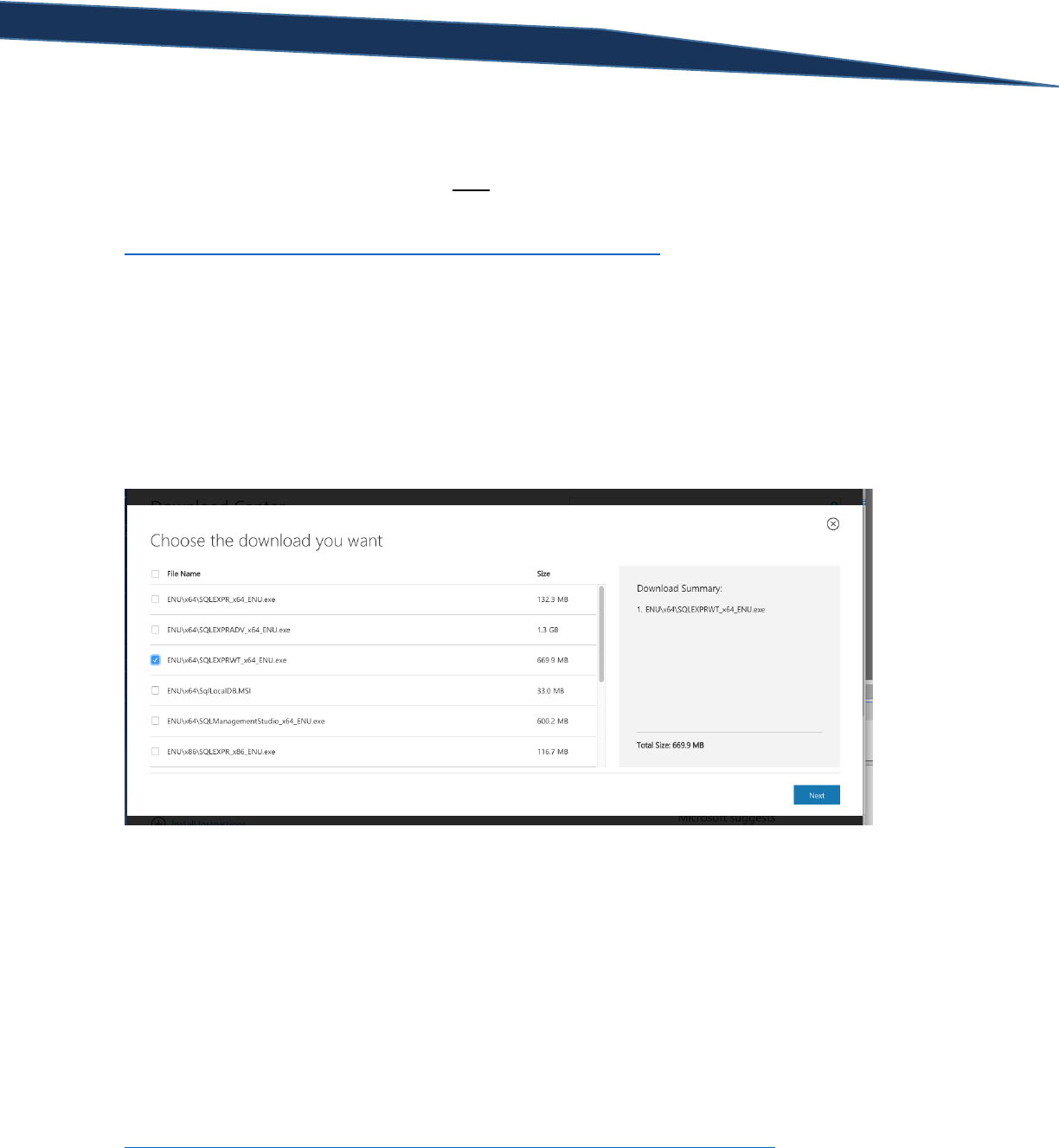
When the “Choose the download you want” window appears, click the check box next to
“ENU\x64\SQLEXPRWT_x64_ENU.ex”e if you have a 64-bit machine. If you have a 32-bit machine,
download the file named “ENU\x86\SQLEXPRWT_x86_ENU.exe”. Then press “Next” and download the
executable file.
Once downloaded, run the executable and follow the on-screen instructions to install Microsoft® SQL
Server® 2012 Express. Be sure to install both the database engine and SQL Server Management Studio
(SSMS). Management Studio is the tool that we will be used to complete our queries.
Download and Attach AdventureWorks
Once you have the Microsoft® SQL Server® 2012 Express successfully installed, you will need to
download the sample AdventureWorks2012 database that the course lectures use. Navigate to
https://www.dropbox.com/s/igulj4m7lv73eap/AdventureWorks2012_Data.zip?dl=0 and download the
file named “AdventureWorks2012_Database.zip”. Once downloaded, extract the files in the zipped
T-SQL Querying Guide © The Knowlton Group, LLC 8 | P a g e
folder. Move the file with the “.mdf” extension to the folder: C:\Program Files\Microsoft SQL
Server\MSSQL11.MSSQLSERVER\MSSQL\DATA.
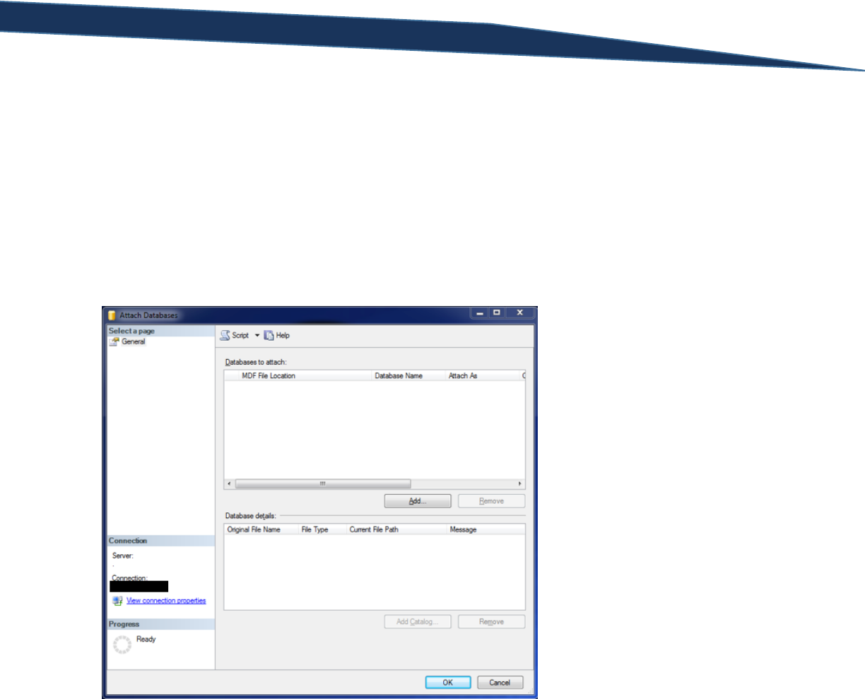
Open SQL Management Studio (SSMS) once the file is finished downloading. Once SSMS is open,
connect to your newly installed SQL Server Express instance. You can type “.\sqlexpress” in the “Server
Name” field when first opening SQL Server Management Studio. Once connected, right click on the
folder named “Databases”, and then select “Attach…”. The “Attach Databases” screen will appear as
shown below:
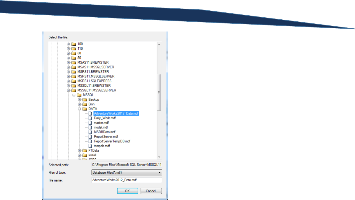
Click the “Add…” button to open the “Locate Database Files” screen where you will select the file named
“AdventureWorks2012_Data.mdf”. This is the AdventureWorks SQL database file that we downloaded
previously.
T-SQL Querying Guide © The Knowlton Group, LLC 9 | P a g e
Press “OK” once you have selected the correct file. Information will populate into the “Attach
Databases” screen based on what .mdf file you selected. Since we downloaded the database file but not
any log file associated with it, click on the row with the word “Log” in the “File Type” column. As an
extra step to make sure you selected the correct file, the log row will contain the text “Not Found” in the
“Message” column. After confirming you have selected the correct row, click Remove and then press
OK.
Right click on the “Databases” folder and select Refresh. Expand the “Databases” folder. The
AdventureWorks2012 database should now appear in the expanded list, and you are ready to start the
lessons!

T-SQL Querying Guide © The Knowlton Group, LLC 10 | P a g e
Section 1: General Database Concepts
Before we dive too deep into this guide, we should cover a few basic concepts that are key to
understanding databases (note: these concepts will be defined in the context of Microsoft SQL Server.
Though the vast majority of these concepts are universal, you should take the time to understand the
differences if you will be using another database engine).
Instance: An instance can be thought of as the installation of SQL Server. The database engine is the
application that stores data and allows you to query against it. Each installation of the database engine
is a separate instance under most circumstances. Multiple instances of SQL Server can exist on the same
Windows server.
Database: A database can be thought of as an organized collection of data. The structure of relational
databases implies that data is stored in tables. Each database belongs to a SQL instance. In fact, there is
a one-to-many mapping between an instance and a database. That is, an instance may contain one to
many databases and a database (or many databases) belong to a single SQL Server instance.
Schema: A schema is a physical grouping of tables in a logical way for the purposes of security and
business understanding. Schemas contain one-to-many tables and are often used in databases to help
create security profiles with more ease. The AdventureWorks sample database that we will be using has
several schemas built into their model.
Table: A table is a collection of data organized in the form of rows and columns. A table is where the
data truly lives at the lowest level. To improve both the performance of queries and the understanding
of the data within the table, primary and foreign keys are often included in tables.
To better understand the hierarchical relationship between the previous concepts, take a look at the
image below:
Primary Key: A primary key is the column(s) that define uniqueness for each row of a table. For
example, a table of customer accounts might use a column named “AccountID” as the primary key. This

T-SQL Querying Guide © The Knowlton Group, LLC 11 | P a g e
forces each AccountID in the table to be unique. Therefore, if the AccountID CID123456 appears in the
table, you will not be able to insert another record with that same AccountID without getting an error.
Foreign Key: A foreign key is a column in one table that identifies with a row (or rows) of another table
based on the primary key in that other table. For example, suppose we have a table called Sales. This
table contains three columns: SalesID (representing an incrementing sales number unique to each sale),
CustomerSSN (representing the customer’s SSN), and SalesAmount. Then suppose we have another
table, called Customers, that contains two columns: CustomerSSN and CustomerName. The
CustomerSSN column in the Customers table is that table’s primary key. This means that, as we
discussed in the primary key definition, that each CustomerSSN appears only once in this table. We
would then want to set the CustomerSSN column in the Sales table to be a foreign key with a
relationship to the CustomerSSN column in the Sales table. This tells users that if you wanted to get
customer details associated with each sale, you could use the foreign key relationship on CustomerSSN
between the two tables to gather the information you are looking for. This concept will become clearer
as we discuss the concept of inner and outer joins.
View: A view is a virtual table whose contents are defined by a query. Like a table, a view consists of a
set of named columns and rows of data. Unless indexed, a view does not exist as a stored set of data
values in a database. The rows and columns of data come from tables referenced in the query defining
the view and are produced dynamically when the view is referenced.

T-SQL Querying Guide © The Knowlton Group, LLC 12 | P a g e
Section 2: Literal SELECT Statements
A literal SELECT statement is a SELECT statement that does not directly query a particular table and
return columns, rather it returns the result of a string or expression. For example, if I wanted to return
the string “This a T-SQL Beginner Guide”, I would execute the query:
SELECT 'This is a T-SQL Beginner Guide'
If you wanted to return a string that said “This is a SQL query”, you would type:
SELECT 'This is a SQL query'
There are two key things to notice at this point. First, all SQL SELECT statements (until we start working
with common table expressions and other advanced SQL programming concepts) will begin with the
word “SELECT”. This tells the database engine that it will completing the operations related to SELECT
statements and will most likely be returning some data as an output result set. The second observation
you should make is that strings in T-SQL are denoted with the single apostrophe and not a quotation
mark like in any other programming languages.
In the “Results” tab at the bottom panel in SQL Server Management Studio (SSMS), you will notice that it
treats the string output as an unnamed column with a single row of data. We can include multiple
different strings or expressions in our literal select statement by placing a comma in between them. For
example, two return two strings in separate columns – one saying “SQL Query” and another saying “The
Knowlton Group” – we would execute the query:
SELECT 'SQL Query', 'The Knowlton Group'
The comma in between the two strings indicates that each string will be returned in a separate column.
Commas are T-SQL’s way of indicating multiple columns will be returned by the SELECT statement.
Mathematical expressions are also commonly embedded in SELECT statements. Below are a few
examples of how we can use mathematical operators in expressions for a simple literal SELECT
statement:
SELECT 1+1
SELECT 5*6
SELECT 5*5-2
Notice how in all of the examples, we are simply returning a scalar value – that is, a single string or
mathematical result per query. Literal SELECT statements by themselves don’t provide a ton of value,
however, embedding expressions and literal strings within larger queries can provide tremendous value
during more advanced processes or when applying mathematical operations to column values.
Mathematical expressions in T-SQL follow the standard order of operations. Properly placing
parentheses can alter the order in which the expression is evaluated. For example, take the two
following examples. Adjusting the parentheses within each expression yields different values:

T-SQL Querying Guide © The Knowlton Group, LLC 13 | P a g e
SELECT (5*5)-3+(2*6)
SELECT 5*(5-3+2)*6
The first expression yields a value of 34. The second returns 120. Order of operations mathematically is
an important concept to adhere to. We will encounter a similar concept when we discuss nested
functions which carry certain similarities to the order of operations that must be keenly observed in
order to return the desired results.
By now, you are aware that we are using the single apostrophe to indicate the presence of a string.
However, you may be asking yourself how you would handle returning a string where an apostrophe is
present in the actual string value. To do this, you will use two apostrophes in a row. For example, to
return “Adam’s Apple”, you would execute the query:
SELECT 'Adam''s Apple'
Or to return “John’s Office”, you would type and execute:
SELECT 'John''s Office'
This is another subtlety that must be carefully observed while typing your SQL code to avoid raising
errors.
Lab 1: Literal Select Statements:
1) Execute a literal select statement that returns your name.
2) Write the literal select statement that evaluates the product of 7 and 4.
3) Write the literal select statement that takes the difference of 7 and 4 then multiplies that
difference by 8.
4) Write a literal select statement that returns the phrase “The Knowlton Group’s SQL Training
Class”. (Hint: note the single apostrophe in the string).
5) Execute a literal SELECT statement that returns the phrase “Day 1 of Training” in one column
and the result of 5*3 in another column.

T-SQL Querying Guide © The Knowlton Group, LLC 14 | P a g e
Section 3: Basic SELECT Statements
For the purposes of this training guide, we will consider a basic SELECT statement as one that returns
one to many columns from a single table with no additional filtering, grouping or sorting clauses. The
basic SELECT statement will have the following form:
SELECT [Column 1], [Column 2], ... , [Column N]
FROM [Database Name].[Schema Name].[Table Name]
Let’s look at some very simply examples of a basic SELECT statement. Ensure that you are connected to
the “AdventureWorks2012” database by navigating to the database selection dropdown menu just
above the Object Explorer and selecting “AdventureWorks2012”.
You may also execute, in the query editor, the statement:
USE AdventureWorks2012
This command will tell the query editor that you are currently using to connect to the
“AdventureWorks2012” database. Typically, by default, you will initially be connected to the “master”
database. As a side note, you should rarely, if ever, use the “master” database, unless you are executing
basic literal select statements.
Once connected the “AdventureWorks2012” database, expand the “AdventureWorks2012” database
folder in the object explorer. When complete, expand the “Tables” folder.
T-SQL Querying Guide © The Knowlton Group, LLC 15 | P a g e
This represents the complete list of tables within the “AdventureWorks2012” database. You will notice
that each table has some leading text, then a period, and then a name. The leading text, before the
period, indicates the schema to which the table belongs. The schema “dbo” is the default schema for
any database and table. The text after the period indicates the table name.
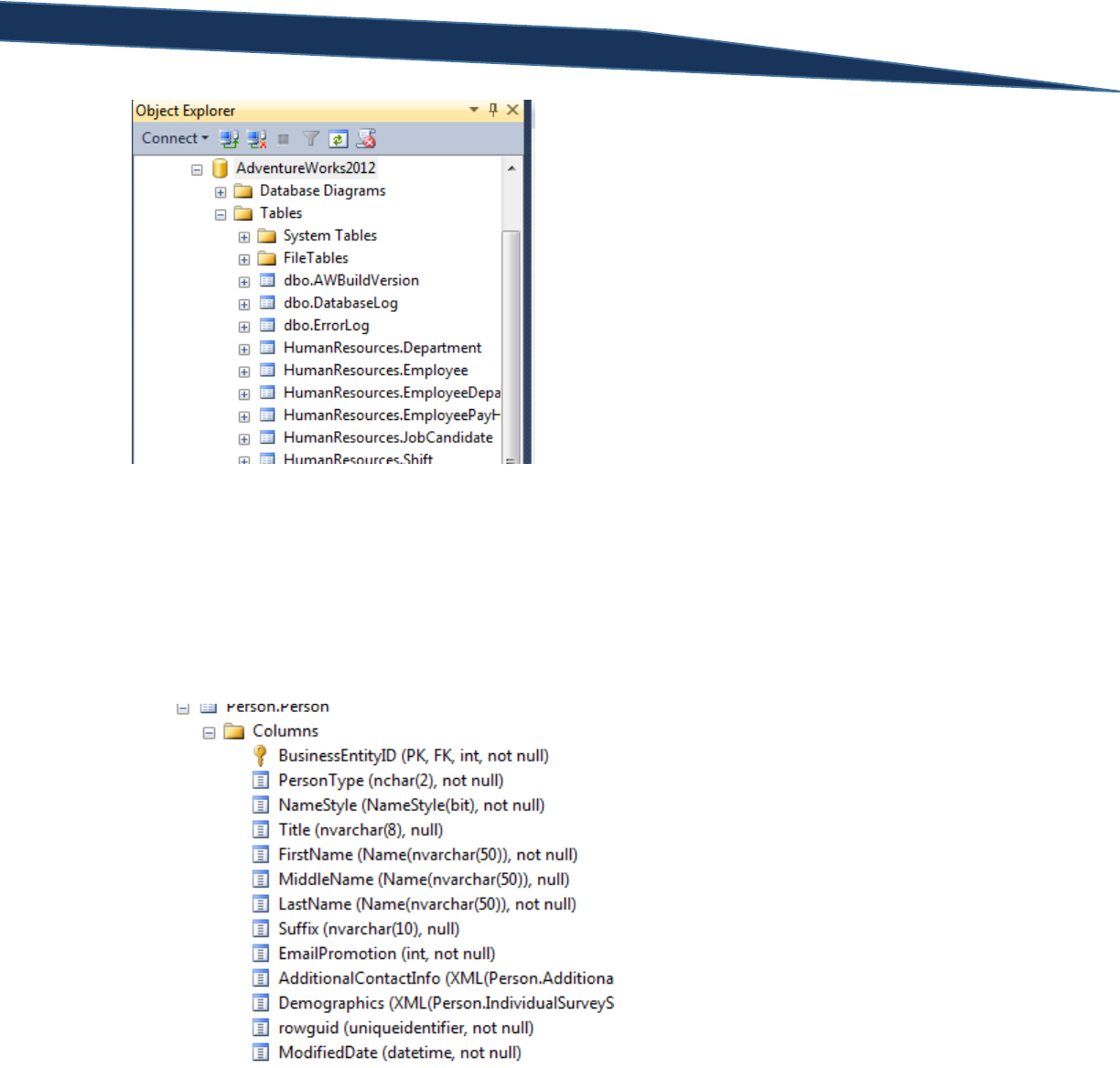
Find the table named “Person.Person”. Click the expand toggle button the left of the table name. Once
expanded, click the toggle button the left of “Columns”.
You are now able to see all of the columns contained within the Person.Person table and some
additional details such as the column data type and whether or not the column allows NULL values. I
will explain more about NULL values and data types in section 12 of this training guide.
Now that we are able to identify the columns in the table Person.Person, we can execute our first basic
SELECT statement. Suppose we want to return the FirstName column for all rows in the Person.Person
table, we would execute the query:

T-SQL Querying Guide © The Knowlton Group, LLC 16 | P a g e
SELECT FirstName
FROM Person.Person
If we wanted to return only the LastName column, we would execute:
SELECT LastName
FROM Person.Person
If you look in the bottom right hand corner of the results panel, you will see that SSMS indicates how
many rows of data were returned by the previous SELECT statement that was executed.
While nearly 20,000 rows is not a particularly large set of returned data, we want to make sure that we
don’t write inefficient queries. As we continue to execute SELECT statements, the database engine will
store more and more data into memory. Eventually, data will need to be dropped from memory (the
data is NOT deleted from the hard drive, merely it is removed from the memory of the PC or server –
this is where your machine’s RAM is necessary) so that new data can be added to memory and returned
in your results. So, we want to do our best to limit the results to only what we need.
Since, we are just exploring the contents of a table, we can employ the TOP operator. The TOP operator
limits the number of rows returned by a SELECT statement.
Let’s write a SELECT statement that returns only the top 500 rows of the FirstName column from the
Person.Person table. To do this, we execute:
SELECT TOP 500 FirstName
FROM Person.Person
To limit the number of rows returned, we simply type TOP after SELECT and then indicate the number of
rows we would like the result set limited to. Instead of limiting the results by a specific number of rows,
we can limit the rows by a percentage of the total number of rows. Suppose we take the same query as
before but the limit the result to ten percent of the total number of rows in the table. To do this, we
execute:
SELECT TOP 10 PERCENT FirstName
FROM Person.Person
Having learned how to limit the number of rows returned by any SELECT statement, let’s return more
than one column. Let’s return the FirstName and LastName column from the Person.Person table
limiting our results to 1000 rows. To complete this, we execute:
SELECT TOP 1000 FirstName, LastName
FROM Person.Person

T-SQL Querying Guide © The Knowlton Group, LLC 17 | P a g e
Suppose we wanted the top 20 percent of all rows for the FirstName, MiddleName and LastName
columns from Person.Person. To do this, we would execute:
SELECT TOP 20 PERCENT FirstName, MiddleName, LastName
FROM Person.Person
Changing the table we are referencing, let’s return all rows from the table Production.Product and limit
the data to just the ProductID, Name and ProductNumber columns.
SELECT ProductID, Name, ProductNumber
FROM Production.Product
Occasionally, we may want to return all columns from a particular table. Fortunately, SQL has a built in
command to do just this. If we wanted to return all columns from the table Production.Product, we
would execute:
SELECT *
FROM Production.Product
This returns every column that is contained in the table. This can be helpful to get an idea of the data
that is stored in a particular table if you are unsure of its contents. Especially with larger tables, it is a
best practice to apply the TOP operator to this type of statement. Let’s use the same query as before,
except we will limit the results to only the top 100 rows:
SELECT TOP 100 *
FROM Production.Product
The asterisk or star (usually someone, when speaking about a query using an asterisk, will say “select
star from production dot product”) is a very useful tool when writing SELECT statements and becoming
more familiar with the data that is contained within a table. The asterisk will also be helpful when we
work with aggregate functions – particularly the COUNT() function.
Now that we have a bearing on how to complete basic SELECT statements, let’s add a few details that
will improve the clarity of your results. We often find that business users tend to not want to see
column names like “ProductNumber” without spaces separating the words. While databases typically
avoid using spaces in table names, business users like to see clean, proper words and spacing.
To modify how the name of the column appears in the results, we can employ column aliases. Below is
an example of a column alias being used:
SELECT Name AS ProductName
FROM Production.Product
If you look in the results panel, you will notice the column name is not “Name” rather it is
“ProductName”. You may be tempted to execute the query:
SELECT Name AS Product Name

T-SQL Querying Guide © The Knowlton Group, LLC 18 | P a g e
FROM Production.Product
If you execute this query, you will be met with an error stating:
Msg 102, Level 15, State 1, Line 1
Incorrect syntax near 'Name'.
This is SQL’s way of telling you that something went wrong near “Name” in the query. The issue is that
spaces have very specific purposes in the SQL language parser. It treats the second “Name” like another
column, and, therefore, is expecting a column between “Product” and “Name”. To resolve this issue, we
can do one a couple things: surround the column alias with quotation marks or surround the column
alias with square brackets.
SELECT Name AS "Product Name"
FROM Production.Product
SELECT Name AS [Product Name]
FROM Production.Product
Using the quotation or square bracket method resolves the SQL parser’s issue with the space separating
the two words of the column alias. Let’s apply these newly learned techniques to another example.
We will be writing a query that returns the top 200 rows from Person.Person. Let’s return only the
FirstName, MiddleName and LastName columns but give them each a column alias – “First Name”,
“Middle Name”, and “Last Name” respectively.
SELECT TOP 200
FirstName AS [First Name],
MiddleName AS [Middle Name],
LastName AS [Last Name]
FROM Person.Person
Upon executing the query, you will notice that each of the columns are properly spaced just as the text
between the brackets indicates. You could have also used quotation marks in place of square brackets
and execute this query:
SELECT TOP 200
FirstName AS "First Name",
MiddleName AS "Middle Name",
LastName AS "Last Name"
FROM Person.Person
If you look back at Section 1 you will notice there was a definition for the term view. This is essentially a
virtual table that is constructed by some SELECT statement in the background. Views are an incredibly
helpful tool to minimize the querying effort needed to retrieve commonly accessed information. This
text will not discuss how views are created and maintained, but it is necessary to address how you
access them. Accessing a view is as simple as querying data in a table. Instead of placing the table name
in the FROM clause, you can place a view’s name.

T-SQL Querying Guide © The Knowlton Group, LLC 19 | P a g e
The views contained within a database can be seen directly in the Object Explorer. If you minimize the
Tables folder, you will notice a folder named “Views”. Expand this folder.
This indicates all views that are accessible within the database. Let’s execute a few queries against a
view so that you may become comfortable with them.
If we wanted to return all rows and columns from the view named HumanResources.vEmployee, you
simply type and execute the query:
SELECT *
FROM HumanResources.vEmployee
Or, if you wanted to return the FirstName, LastName, EmailAddress and PhoneNumber columns from
the view Sales.vIndividualCustomer, you would execute:
SELECT FirstName, LastName, EmailAddress, PhoneNumber
FROM Sales.vIndividualCustomer
As you can see, there is no noticeable difference between how you query a view and how you query
against a table. Views are created to make our lives easier when trying to access information, and it is
comforting that we do not need to learn any new syntax to reference them.
While we will continue to build upon what we learned in this chapter, understanding the concepts
behind the basic SELECT statement is absolutely crucial before advancing to other sections. Complete
the exercises, and, if necessary, spend some additional time reviewing the content in this chapter to
improve your confidence in completing basic SQL SELECT statements.
Lab 2: Basic SELECT Statements
1) Retrieve all rows from the HumanResources.Employee table. Return only the
NationalIDNumber column.
2) Retrieve all rows from the HumanResources.Employee table. Return the NationalIDNumber and
JobTitle columns.

T-SQL Querying Guide © The Knowlton Group, LLC 20 | P a g e
3) Retrieve the top 20 percent of rows from the HumanResources.Employee table. Return the
NationalIDNumber, JobTitle and BirthDate columns.
4) Retrieve the top 500 rows from the HumanResources.Employee table. Return the
NationalIDNumber, JobTitle and BirthDate columns. Give the NationalIDNumber column an
alias, “SSN”, and the JobTitle column an alias, “Job Title”.
5) Return all rows and all columns from the Sales.SalesOrderHeader table.
6) Return the top 50 percent of rows and all columns from the Sales.Customer table.
7) Return the Name column from the Production.vProductAndDescription view. Give this column
an alias “Product’s Name”.
8) Return the top 400 rows from HumanResources.Department
9) Return all rows and columns from the table named Production.BillOfMaterials
10) Return the top 1500 rows and columns from the view named Sales.vPersonDemographics
T-SQL Querying Guide © The Knowlton Group, LLC 21 | P a g e
Section 4: Filtering with the WHERE Clause
Basics of the WHERE Clause – Part 1
Now that we have covered the basics of retrieving columns of data from a table, you may be asking
yourself how you might filter the rows returned by some criteria. For example, perhaps we are asked to
get a list of all products that have a sale price greater than $100. You might be asked to retrieve a list of
all customers who purchased a product within a certain date range. These types of queries are very
commonly requested and can be easily handled with the WHERE clause.
We discussed in Section 3 that the generic form of a basic select statement was:
SELECT [Column 1], [Column 2], ... , [Column N]
FROM [Database Name].[Schema Name].[Table Name]
By adding the WHERE clause to the general form, we now get:
SELECT [Column 1], [Column 2], ... , [Column N]
FROM [Database Name].[Schema Name].[Table Name]
WHERE [Column Name] {Comparison Operator} {Filter Criteria}
The third line of the SELECT statement will begin with WHERE and then be followed by the name of the
column that you will be filtering against. After indicating the column you will be filtering on, we indicate
the comparison operator that will be used (these include =, >, < symbols – see the table of operators
below). From there, we specify the filtering criteria – this may be a wildcard string, string, expression or
numeric value. Below is a basic example of the WHERE clause in use:
SELECT *
FROM Production.Product
WHERE ListPrice > 10
The query above returns all rows and columns from the table Production.Product where the ListPrice
column has a value greater than 10. Notice the form of the WHERE clause: indicate the column to be
filtered on, then indicate the comparison operator to be used, and finally specify the filtering criteria.
There are many comparison operators that can be used in a WHERE clause. The table below contains a
list of them with descriptions and links to Microsoft’s technical documentation for each:
Operator
Meaning
Microsoft Documentation Link
=
Equal to
= (Equals)
>
Greater than
> (Greater than)
<
Less than
< (Less than)
>=
Greater than or equal to
>= (Greater than or equal to)
<=
Less than or equal to
<= (Less than or equal to)
<>
Not equal to
<> (Not equal to)
!=
Not equal to
!= (Not equal to)

T-SQL Querying Guide © The Knowlton Group, LLC 22 | P a g e
!<
Not less than
!< (Not less than)
!>
Not greater than
!> (Not greater than)
Let’s walk through an example of many of these operators in use. First, let’s find all employees in the
HumanResources.vEmployee view whose first name is Chris.
SELECT *
FROM HumanResources.vEmployee
WHERE FirstName = 'Chris'
Notice again the basic form of the WHERE clause: identify the column you will be filtering on, then the
comparison operator you will be used, and lastly the filtering criteria. In this case, we are filtering on the
FirstName column, using the “equal to” comparison operator, and specifying we only want those first
name’s equal to “Chris”.
Let’s modify the previous example’s filter to find all employees whose first name is NOT Chris. To do
this, we simply change the comparison operator from the “=” operator to the “<>” operator:
SELECT *
FROM HumanResources.vEmployee
WHERE FirstName <> 'Chris'
Next, suppose we wish to find all employees from the HumanResources.vEmployee view whose last
name begins with a letter less than “P”. To complete this query, we would execute:
SELECT *
FROM HumanResources.vEmployee
WHERE LastName < 'P'
When using the less than operator with a string value, the database engine will use standard
alphabetical ordering to determine whether or not a string is less than the given filtering criteria. For
example, “Orange” starts with a letter less than “P” therefore “Orange” would be included in the result
set. However, “Pair” starts with “P” which is not less than “P” and therefore would not be included. It
gets a little trickier if we took the same query as above but applied the greater than operator instead of
the less than operator.
SELECT *
FROM HumanResources.vEmployee
WHERE LastName > 'P'
You will notice that one of the last names in the result set is “Pak”. You might be thinking that both start
with the letter “P”, so why is “Pak” included in the results? Think of the filtering criteria of “P” starting
with the letter “P” and then being followed by a large number of blank spaces – “P_ _ _ _ _ _”. So, since
both “Pak” and “P” start with the same letter, the database engine will then go to the next letter and
evaluate the two-letter string to determine which string is larger. So, in the example, “Pa” is the first
two letters of “Pak” and the first two letters of “P” can be thought of as “P” and a blank space, “P_”.
Since the letter “a” – the second letter of “Pak” – is greater than the blank in “P_”, “Pa” is considered to
be greater than “P_”. This is how you would a dictionary would evaluate order, and SQL merely follows

T-SQL Querying Guide © The Knowlton Group, LLC 23 | P a g e
the same evaluation criteria. If this concept is difficult to wrap your head around, spend some time
completing some basic queries trying different combinations of strings and operators to further
comprehend this evaluation criteria. The lab at the end of this section will also contain some questions
to help clarify this concept.
Moving on, let’s take a look at an example of the “greater than or equal to” comparison operator being
used. To write a query that returns all rows in the Production.Product table where the ReorderPoint
column value is greater than or equal to 500, we would execute:
SELECT *
FROM Production.Product
WHERE ReorderPoint >= 500
Using the previous example as a starting point, we can modify the query to return all rows where the
ReorderPoint column value is less than or equal to 500:
SELECT *
FROM Production.Product
WHERE ReorderPoint <= 500
There are three other operators that we haven’t used: the “!=”, “!<”, and “!>” operators. These are
considered non-ISO standard operators in the T-SQL syntax, however their use within SQL queries are
perfectly acceptable. The other comparison operators allow you to complete any query that the use of
these three comparison operators would enable you to do; it is more, at this point, a matter of
preference and being aware that these three non-ISO standard operators exist.
Lab 3: Using the WHERE Clause Part 1
1) Return the FirstName and LastName columns from Person.Person where the FirstName column
is equal to “Mark”
2) Find the top 100 rows from Production.Product where the ListPrice is not equal to 0.00
3) Return all rows and columns from the view HumanResources.vEmployee where the employee’s
last name starts with a letter less than “D”
4) Return all rows and columns from Person.StateProvince where the CountryRegionCode column
is equal to “CA”
5) Return the FirstName and LastName columns from the view Sales.vIndividualCustomer where
the LastName is equal to “Smith”. Give the column alias “Customer First Name” and “Customer
Last Name” to the FirstName and LastName columns respectively.
Symbolic Logic and Truth Tables
We have now seen examples of how to filter on a single column with some filtering criteria. But what
about filtering on multiple columns within the same query? For this we can employ a subset of what
SQL calls logical operators: the AND operator and the OR operator.

T-SQL Querying Guide © The Knowlton Group, LLC 24 | P a g e
The query syntax used when employing these two logical operators is fairly simple. Instead of ending
our query with a single filtering statement after the WHERE clause, we can add one of the logical
operators and include a second filtering criteria. For example, if we wanted to return all rows from the
HumanResources.vEmployee view where the employee’s first name is either Chris or Steve, we would
execute:
SELECT *
FROM HumanResources.vEmployee
WHERE FirstName = 'Chris' OR FirstName = 'Steve'
Notice that the second criteria in the WHERE clause contains all three components of the WHERE clause:
the column name to be filtered on, the comparison operator, and then the filtering criteria. The only
subtle difference is that you do not need to add “WHERE” for a second time.
Let’s now look at an example of the AND logical operator being used. Suppose we wanted to return all
rows from the Production.Product table where the ListPrice value is greater than 100 and the Color
column has a value of “Red”, we would execute the query:
SELECT *
FROM Production.Product
WHERE ListPrice > 100 AND Color = 'Red'
The WHERE clause is similar to the previous example; the only difference is the logical operator that we
have used and the filtering criteria.
As you may have guessed, we can string together more than two logical operators in a single WHERE
clause. For example, let’s suppose we wanted to find all rows in the Production.Product table that have
a ListPrice greater than 100, a color equal to “Red”, SafetyStockLevel equal to 500, and a Size greater
than 50. To complete this query we execute:
SELECT *
FROM Production.Product
WHERE ListPrice > 100 AND Color = 'Red' AND SafetyStockLevel = 500 AND Size > 50
Nothing complicated has happened here; we simply add another logical operator and then another
filtering statement. Complexity increases when we start to mix the two different logical operators we
have been using in the WHERE clause. The SQL parser will evaluate the WHERE clause like the order of
operations – that is AND operations will be evaluated before OR operations. We will look at a few
examples of this and show how we can explicitly ensure we get the results we would like.
Let’s modify the previous example and try to retrieve only those rows from the Production.Product table
where the ListPrice is greater than 100, the color is “Red” OR the StandardCost is greater than 30. To do
this, we would execute the query:
SELECT *
FROM Production.Product

T-SQL Querying Guide © The Knowlton Group, LLC 25 | P a g e
WHERE ListPrice > 100 AND Color = 'Red' OR StandardCost > 30
Examine the results for a brief moment. You might notice that you have many rows returned where the
color is not equal to “Red”. You even find rows with a value in the ListPrice column that is less than 100.
This is not a mistake – in fact this is the 100% correct data set returned by SQL. To explain why this is
the case, we need to take a step back and understand the concept of truth tables and properly
evaluating Boolean expressions.
Determining whether or not a Boolean expression returns a TRUE or FALSE value is an exact activity.
That is, there are very clear rules to be followed – subjectivity is not a factor in determining the truth of
a Boolean expression. In most computer science or mathematics curriculums in college, a course in
symbolic logic is often required for graduation and often a prerequisite for more advanced courses. Set
theory in mathematics and much of programming relies heavily on the concepts learned in a symbolic
logic course. Truth tables are one of the core concepts in this course, and they help new students of the
subject determine whether or not a statement is true or false based on the truth of the individual
components that make up the Boolean expression.
A truth table breaks down a Boolean expression into its simple components. Taking one of the filtering
criteria from one of our earlier examples, let’s look at the query:
SELECT *
FROM Production.Product
WHERE ListPrice > 100 AND Color = 'Red'
There are two filtering components here: ListPrice is greater than 100, and Color is equal to “Red”.
Symbolic logic courses, and truth tables, would give each of these components a letter as a symbol: let’s
use A and B to give it basic. So operator A is the filtering component that the ListPrice is greater than
50, and operator B is the filtering component that the color is equal to “Red”.
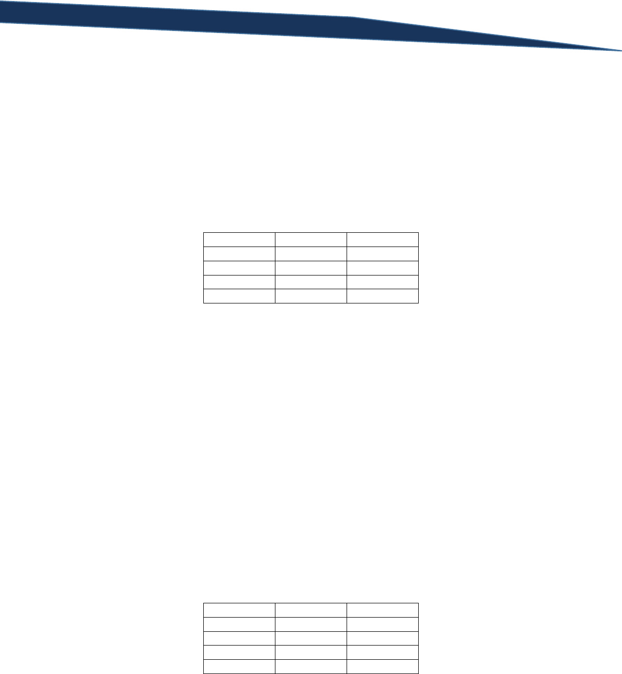
In a truth table, we would take these two components and list all possible combinations that these two
components could be true or false (T implies TRUE and F implies FALSE). A row’s ListPrice column could
be greater than 100 or less than or equal to 100. Therefore the expression “ListPrice > 100” has two
possible outcomes: true or false. The same goes for the second filtering criteria “Color = “Red”. The
Color column’s value could be “Red” or it might not be “Red”, thus returned either a TRUE or FALSE
value for that Boolean expression. The truth table below summarizes the combination of these possible
outcomes:
A
B
T
T
T
F
F
T
F
F
There are four different outcomes for each of these Boolean expressions: A is TRUE and B is TRUE, A is
TRUE and B is FALSE, A is FALSE and B is TRUE, and A is FALSE and B is FALSE. To further clarify this with
T-SQL Querying Guide © The Knowlton Group, LLC 26 | P a g e
examples, if the ListPrice of a row was greater than 100 and the Color was “Red”, both A and B (the two
filtering criteria symbolized) would be TRUE and the first row would represent the evaluation of the two
expressions. If the ListPrice was not greater than 100, but the Color was “Red”, then A would be FALSE
and B would be TRUE, implying the third row symbolizes the truth of each individual component.
Identifying a Boolean value for each component individually is fairly simple: the ListPrice is either greater
than 100 or it is not (i.e. it is either TRUE or FALSE). Where truth tables demonstrate their importance is
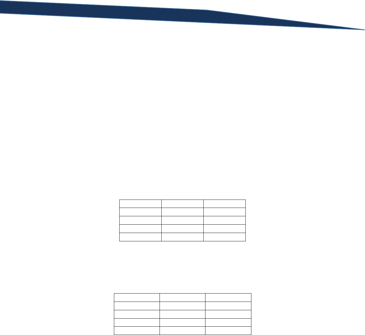
when we apply an operator to the two individual components. In the WHERE clause of the example we
have been using, AND is the logical operator connecting the two filtering criteria. Truth tables will then
utilize a third column (in our example) so determine the truth of the two individual components when
combined together by the logical operator in use:
A
B
A and B
T
T
T
T
F
F
F
T
F
F
F
F
Adding a third column to determine the Boolean evaluation of the expression “component A AND
component B”, symbolic logic defines truth for the expression. When evaluation an expression of two
components joined together by the “AND” operator, the only time “A and B” evaluates as TRUE is if both
individual components evaluate to TRUE. This makes sense if we look at it in the context of the SQL
query. If the ListPrice is greater than 100, but the Color column does not equal to “Red” then both
criteria are not true. It then follows that any row where both criteria are not true, in this example,
would not evaluate as TRUE and be returned by SQL. When we use the “AND” operator, we explicitly
are telling the SQL parser that we only want the rows where BOTH filtering criteria are met. The above
truth table simply visually represents the total possible outcomes for the expression given the
combinations of truth for each individual components.
Let’s take the same query but modify the comparison operator from AND to OR:
SELECT *
FROM Production.Product
WHERE ListPrice > 100 OR Color = 'Red'
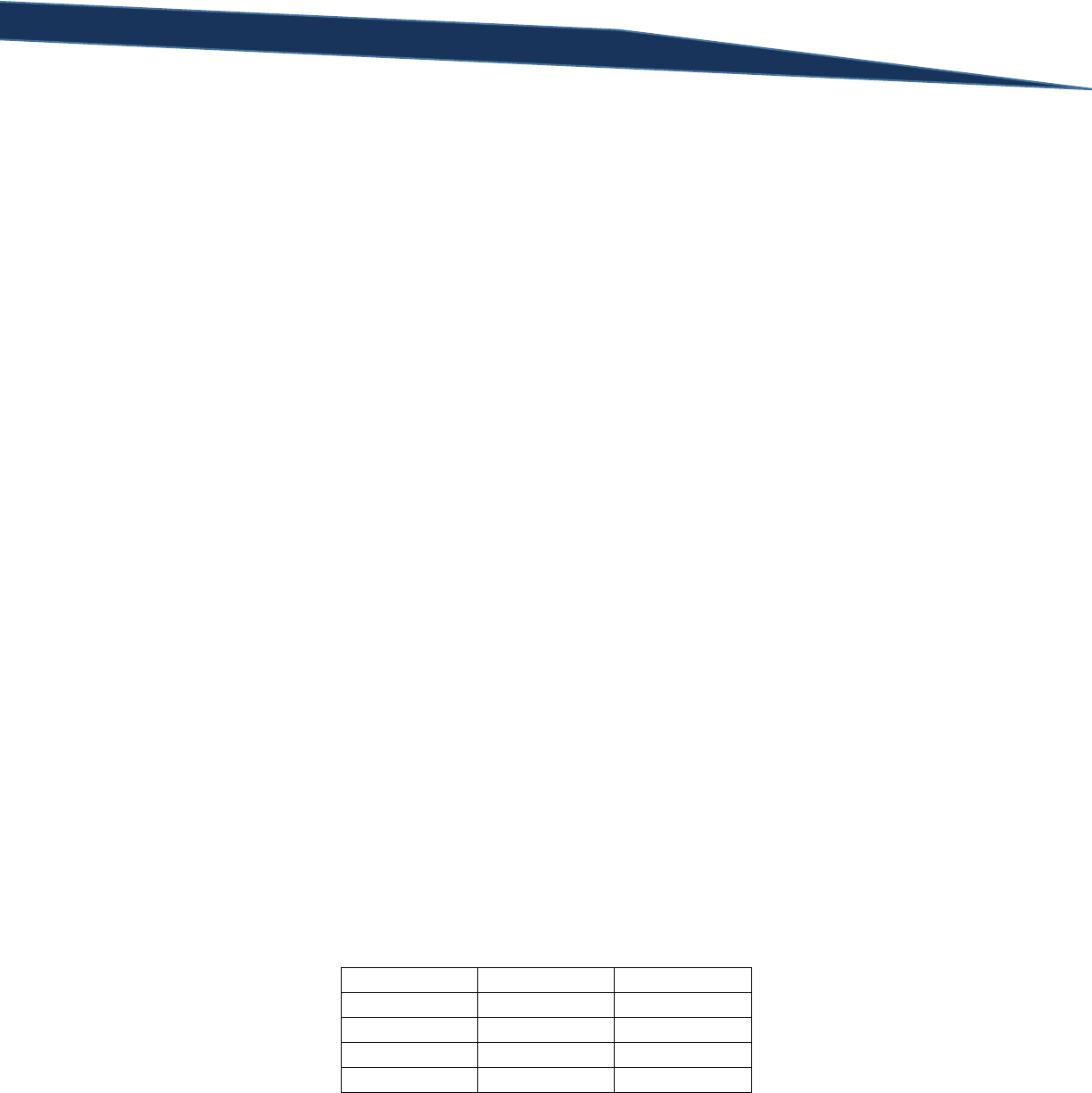
Take a look at some of the results from this query. If either the ListPrice is greater than 100 or the Color
is equal to “Red” then the row is returned to the results panel. Below is the truth table for two
components joined with the “OR” operator:
A
B
A or B
T
T
T
T
F
T
F
T
T
F
F
F
T-SQL Querying Guide © The Knowlton Group, LLC 27 | P a g e
Notice how all rows except the last row in the truth table evaluate to TRUE when evaluating the Boolean
expression “A or B”. With the OR operator, as long as one of the components yields a TRUE value, then
the entire expression returns as TRUE. This is why some rows in the result set for the previous query
appear in the panel when the ListPrice is greater than 100 but the Color is not “Red”.
Now that we have covered the basics of the truth tables for the “OR” and “AND” operators for two
components, what happens when we combine them? If you remember, this discussion began when
evaluating the query:
SELECT *
FROM Production.Product
WHERE ListPrice > 100 AND Color = 'Red' OR StandardCost > 30
So, let’s break this WHERE clause down into the three separate filtering components and create a truth
table. Component A will be “ListPrice > 100”, Component B will be “Color = ‘Red’”, and Component C
will be “Standard Cost > 30”. Keep in mind that the criteria will be evaluating AND operations first and
then OR operations. Because of the way the database engine evaluates this criteria, the first Boolean
expression to be evaluated will be “ListPrice > 100 and Color = ‘Red’” or “A and B”. The truth table for
this is:
A
B
A and B
T
T
T
T
F
F
F
T
F
F
F
F
Once that has been evaluated, then the database engine evaluates the next Boolean expression. This
next expression is the result of “A and B” OR component C. We could visualize this as “(A and B) or C”.
Now, the truth table for this final Boolean expression is:
A and B
C
(A and B) or C
T
T
T
T
F
T
F
T
T
F
F
F
So, regardless of whether or not (A and B) evaluates as FALSE, as long as component C is TRUE, then
entire expression evaluates as TRUE. This is why we had what seemed to be strange results the first
time that we evaluated this query. In fact, as long as one of the components of the OR expression are
true, the entire expression is TRUE. So, if component C is FALSE but component (A and B) evaluates to
TRUE, then (A and B) or C evaluates as TRUE. In terms of our SELECT statement, if the ListPrice was
greater than 100 and the Color was “Red” but the StandardCost was not greater than 30, that particular
row would still appear as part of our results.
T-SQL Querying Guide © The Knowlton Group, LLC 28 | P a g e
This was just a very basic introduction to the concepts of symbolic logic and truth tables. The lab
exercises will help to improve and reinforce the concepts learned.
Lab 4: Symbolic Logic and Truth Table Practice
1) On a scrap piece of paper, complete the truth table for the Boolean expression, A and B.
2) On a scrap piece of paper, complete the truth table for the Boolean expression, A or B.
3) On a scrap piece of paper, complete the truth table for the Boolean expression, (A or B) and C.
4) Suppose we execute the query:
SELECT *
FROM HumanResources.vEmployee
WHERE FirstName < 'K' OR PhoneNumberType = 'Cell' AND EmailPromotion = 1
Could there be a row in the result set where the employee’s PhoneNumberType equals “Work”
and their EmailPromotion column value is 0?
5) Using the same query from question 4, would it be possible for an employee’s FirstName to start
with a letter greater than “K” and have a PhoneNumberType not equal to “Cell”? Why or why
not?
Using the WHERE Clause Part 2
Having covered the basics of truth tables and Boolean logic, let’s jump back into the WHERE clause. We
left off discussing how we can add two logical operators, “AND” and “OR”, to create multiple filters
within the same SELECT statement. One of the concepts we encountered is the order in which SQL
evaluates the Boolean expression in a WHERE clause. We do, however, have ways of altering the order
in which expressions are evaluated with properly placed parentheses.
Using one of the existing queries we have worked with:
SELECT *
FROM Production.Product
WHERE ListPrice > 100 AND Color = 'Red' OR StandardCost > 30
How can we modify the order in which the Boolean expression is evaluated? Currently, it is being
evaluated by the following truth table:
A and B
C
(A and B) or C
T
T
T
T
F
T
F
T
T
F
F
F
Perhaps, we want the order to be the Boolean expression to be “A and (B or C)” as opposed the existing
expression “(A and B) or C”. To make this change in the SQL statement, we placed parentheses before
“Color = ‘Red’” and after “StandardCost > 30”:
SELECT *

T-SQL Querying Guide © The Knowlton Group, LLC 29 | P a g e
FROM Production.Product
WHERE ListPrice > 100 AND (Color = 'Red' OR StandardCost > 30)
Now, SQL is evaluating the Boolean expression differently – instead of treating “ListPrice > 100” and
“Color = ‘Red’” as different components connected together by the “AND” operator, now SQL is
evaluating “Color = ‘Red’” or “StandardCost > 30” together and then applying the AND operator with
“ListPrice > 100”. Looking at the size of the result set is the first indication that this change caused a
difference – the number of rows returned now is 214. Before we added the parentheses, the query
returned 235 rows. These subtle changes to the order in which the Boolean expressions are evaluated
makes a tremendous difference in the data that is returned.
These concepts are being stressed because we often must deal with complicated requests with many
filters. Understanding exactly what is being requested and how to handle these requests
programmatically is critical to your success writing SQL SELECT statements.
Let’s look at a few more examples. Suppose, I wanted to find all employees from the
HumanResources.vEmployeeDepartment view who belong to the “Research and Development”
department and started at their department before 2005, or whose department is “Executive”. To
complete this query, we would execute:
SELECT *
FROM HumanResources.vEmployeeDepartment
WHERE Department = 'Research and Development' AND StartDate < '1/1/2005'
OR Department = 'Executive'
We could also get the same results by adding parentheses. Adding parentheses is sometimes helpful to
improve the readability of the query and to understand which filtering criteria you are expecting to be
evaluated together and in what order:
SELECT *
FROM HumanResources.vEmployeeDepartment
WHERE (Department = 'Research and Development' AND StartDate < '1/1/2005')
OR Department = 'Executive'
With the parentheses now, it seems clearer that we are evaluating the conjunction (“conjunction” is a
term used to describe two filtering criteria joined together by an “AND” operator) of “Department =
‘Research and Development’” and “StartDate < ‘1/1/2005’” together first, and then evaluating the
disjunction (the term used to describe two filtering criteria joined together by an “OR” operator)
between the previous conjunction and “Department = ‘Executive’”.
Suppose we wish to alter this request a bit. Now we wish to find all employees from
HumanResources.vEmployeeDepartment whose department equals “Research and Development” or
their StartDate is before 2005 and their Department equals “Executive”. We would modify the previous
query slightly and execute:
SELECT *
FROM HumanResources.vEmployeeDepartment
T-SQL Querying Guide © The Knowlton Group, LLC 30 | P a g e
WHERE Department = 'Research and Development' OR (StartDate < '1/1/2005'
AND Department = 'Executive')
You might argue that you interpreted the request slightly differently. Your argument to a slightly
different interpretation of the request is completely logical and respectable. This simply stresses the
importance of understanding exactly what is being requested and the order in which filters are applied
together.
For our last example of these complicated Boolean expressions, let’s break down a very complex
sample. Suppose I wish to find all stores from the Sales.vStoreWithDemographics view where the
AnnualSales were greater than 1000000 and BusinessType was equal to “OS”. I also want to see, in the
same result, stores that were opened before 1990 (YearOpened less than 1990), have a value in
SquareFeet greater than 40000 and have more than ten employees. To complete this query, we would
type and execute:
SELECT *
FROM Sales.vStoreWithDemographics
WHERE (AnnualSales > 1000000 AND BusinessType = 'OS') OR
(
YearOpened < 1990 AND SquareFeet > 40000 AND
NumberEmployees > 10
)
Let’s break each filtering component down symbolically. Let “AnnualSales > 1000000” be A,
“BusinessType = ‘OS’” be B, “YearOpened < 1990” be C, “SquareFeet > 40000” be D, and
“NumberEmployees > 10” be E. As a Boolean expression, we could express this query as:
(A and B) or (C and D and E)
Putting together a simplified truth table for this expression (a condensed version for space and
compactness):
A and B
C and D and E
(A and B) or (C and D and E)
T
T
T
T
F
T
F
T
T
F
F
F
So, regardless of whether or not the store had annual sales greater than a million dollars and the
BusinessType column equaled “OS”, as long as the second portion of the disjunction, (C and D and E),
evaluated to TRUE, the row was returned as part of the result set. The row with BusinessEntityID 504 is
a perfect example of those. The annual sales were greater than a million dollars, but the BusinessType
equals “BS” implying that the first part of the conjunction, (A and B), evaluates to FALSE. However, the
YearOpened value is less than 1990, the SquareFeet column is greater than 40000 and the
NumberEmployees column exceeds 10. Because the second part of the disjunction evaluates to TRUE,

T-SQL Querying Guide © The Knowlton Group, LLC 31 | P a g e
then the whole Boolean expression evaluates TRUE. This is represented by the third row of the previous
truth table since (A and B) is FALSE, yet (C and D and E) is TRUE for the row we just examined.
There are two more logical operators that we have at our disposal to use in the WHERE clause: the IN,
BETWEEN, and LIKE operators. The IN operator is used when we want to filter on a list of items for a
particular column. For example, if I wanted to find all employees from the view
HumanResource.vEmployee whose first name was either “Chris”, “Stacy”, “Michael”, or “Li”, I could type
out an inefficient query like:
SELECT *
FROM HumanResources.vEmployee
WHERE FirstName = 'Chris' OR FirstName = 'Stacy'
OR FirstName = 'Michael' OR FirstName = 'Li'
However, the IN operator allows us to make this much simpler:
SELECT *
FROM HumanResources.vEmployee
WHERE FirstName IN ('Chris', 'Stacy', 'Michael', 'Li')
We have been able to greatly condense the WHERE clause and minimize the redundancy in repeating
“FirstName = “ for each name we wish to filter on. We can use multiple IN operators in the same query.
For example, suppose we wanted to find all employees with the first name in the list from the previous
query or whose last name was either “Hill”, “Miller”, “Brown” or “Zhang”. To find these employees, we
would execute:
SELECT *
FROM HumanResources.vEmployee
WHERE FirstName IN ('Chris', 'Stacy', 'Michael', 'Li')
OR LastName IN ('Hill', 'Miller', 'Brown', 'Zhang')
In short, the IN operator allows you to condense a list of multiple filtering components separated by an
OR operator into a simple, concise, and efficient filtering component.
The next operator we have at our disposal is the BETWEEN operator. This allows you to filter a column
based on a range of values. For example, before the BETWEEN operator, if we wanted to find all stores
from the Sales.vStoreWithDemographics view who had annual sales between one million and two
million, you would have to execute:
SELECT *
FROM Sales.vStoreWithDemographics
WHERE AnnualSales >= 1000000 AND AnnualSales <= 2000000
The BETWEEN operator simplifies this a bit for us. With the BETWEEN operator, we could condense the
previous query into:
SELECT *
FROM Sales.vStoreWithDemographics
WHERE AnnualSales BETWEEN 1000000 AND 2000000

T-SQL Querying Guide © The Knowlton Group, LLC 32 | P a g e
This is helpful to improve the readability of your SELECT statements and to reduce unnecessary typing.
Note that the BETWEEN operator uses an inclusive range only; be careful if you are trying to create an
exclusive range filter.
The next logical operator we look at in this section is the LIKE operator. The LIKE operator tells SQL that
you will using a wildcard operator. Wildcard operators allow you to search for values within a column
based off knowing only parts of the string you are looking for. For example, if I wanted to find all
employees from HumanResources.vEmployee whose name starts with “Mi”, we would execute:
SELECT *
FROM HumanResources.vEmployee
WHERE FirstName LIKE 'Mi%'
The “%” symbol after “Mi” tells SQL that it will be looking for any value in the FirstName column that
starts with “Mi” and is followed by zero to many characters after. So, “Michael” appears in the result
set because the name starts with “Mi” and then is followed by some amount of characters after. If
someone’s first name was simply “Mi” they would also be returned by the query.
There are four wildcard characters that the LIKE operator employs:
Wildcard Character
Description
% (percent symbol)
Any string of one or more characters
_ (underscore)
A single character
[ ]
A single character confined to a specified group of allowable characters
[ ^ ]
A single character not contained in the specified range of allowable characters
The underscore character allows you to use the wildcard operator for a single character. For example,
suppose we wanted to find all employees from HumanResources.vEmployee whose name starts with
“Mi” and then ends with some character. We could use the underscore wildcard character to complete
this request:
SELECT *
FROM HumanResources.vEmployee
WHERE FirstName LIKE 'Mi_'
You’ll notice that “Min” is returned in the results. This is the only first name in our table that starts with
“Mi” and is followed by only a single character. The wildcard characters do not have to appear after the
string, but can also appear before the string. So, if we wanted to find all employees whose first name
starts with some letter then ends in “on”, we would execute:
SELECT *
FROM HumanResources.vEmployee
WHERE FirstName LIKE '_on'

T-SQL Querying Guide © The Knowlton Group, LLC 33 | P a g e
The wildcard character can be used anywhere in the string you are searching against, in fact. The square
bracket range wildcard character can be used like a more advanced version of the underscore character.
This allows you to limit the range of possible characters that could appear. Let’s find all employees
whose name starts with a “D”, is followed by either an “a” or an “o”, and ends with an “n”. To complete
this query, we execute:
SELECT *
FROM HumanResources.vEmployee
WHERE FirstName LIKE 'D[a,o]n'
Instead of separating the characters in the square bracket character by commas, we can indicate a range
of letters with a hyphen. So, in the previous example, if we changed the criteria to search for employees
who first name starts with a “D”, is followed by a letter between “a” and “p” in the alphabet, and then
ends with “n”, we could execute the query:
SELECT *
FROM HumanResources.vEmployee
WHERE FirstName LIKE 'D[a-p]n'
The bracket with carat wildcard character acts similarly to the bracket character without the carat
except that the carat indicates you do NOT want to return the characters specified. So, to find all
employees whose first name starts with a “D”, is followed by some character that is not an “o”, and ends
with an “n”, we would type:
SELECT *
FROM HumanResources.vEmployee
WHERE FirstName LIKE 'D[^o]n'
Read the carat as “not” when understanding how the character can be used. Just like with the bracket
character, you can specify that a range of characters be excluded in the search.
There are many things that you can do with wildcard characters that can help you when searching for
portions of strings within a column. Be careful not to use these excessively as the performance of the
query will decrease significantly when you employ too many of them in a single query. Searches with
wildcard characters are not optimized by the database engine compared with basic queries that can
take advantage of indexes. When we work on live systems with larger amounts of data, this will become
immediately apparent.
By this point in the guide, you have written several queries that may have resulted in NULL values
appearing somewhere in the results. The NULL value is a very important concept to understand as we
advance further into the training material. A NULL value in a column implies that there is nothing for a
value in that column. This shouldn’t be thought of as a blank space. A blank space is a value. NULL is
truly nothingness. Handling NULL values also has certain subtleties that need to be observed to
complete successful and error-proof SQL code.

T-SQL Querying Guide © The Knowlton Group, LLC 34 | P a g e
Unlike the previous examples of the WHERE clause, trying to filter on NULL values requires slightly
different comparison operators. For example, to find all rows from the Person.Person table who do not
have a middle name (i.e. the MiddleName column contains a NULL value), we would complete the
query:
SELECT *
FROM Person.Person
WHERE MiddleName IS NULL
Notice that we do not say “WHERE MiddleName = NULL”. Trying to do that will result in no rows
returned:
SELECT *
FROM Person.Person
WHERE MiddleName = NULL
In a SELECT statement, you will never say a column name or value “equals” NULL. The use of the IS
operator is necessary in this instance. Similarly, to find all rows where the middle name is not NULL, we
write:
SELECT *
FROM Person.Person
WHERE MiddleName IS NOT NULL
By adding the NOT after the IS operator, we negate the filtering criteria and return only those rows with
some value in the MiddleName column. It is important to remember that even a blank value in the
MiddleName value will be returned by the above query because a blank value is not equivalent to a
NULL value.
Like any other filtering criteria in the WHERE clause, filtering on NULL values can be combined with
outer filtering criteria using operators like AND and OR. For example, to find all employees from the
view HumanResources.vEmployee who have a listed middle name and a PhoneNumberType value equal
to “Cell”, we would execute the query:
SELECT *
FROM HumanResources.vEmployee
WHERE MiddleName IS NOT NULL AND PhoneNumberType = 'Cell'
There is absolutely no change to how we combine filtering criteria. The only difference between
filtering on NULL values and filtering with standard values is the use of the IS and IS NOT operator in
place of the standard comparison operators (like “=”, “<>”, “>=”, etc.).
The WHERE clause contains many different methodologies with which to filter your data set.
Understand the concepts of Boolean logic and truth tables can assist you in determining how to write
your queries to be successful. Understanding all of the different filtering methods may take time to fully
grasp, however continue to practice and you will eventually become quite comfortable with the

T-SQL Querying Guide © The Knowlton Group, LLC 35 | P a g e
techniques. The many lab questions that follow will help you further grasp the concepts we have
covered in this section.
Lab 5: Using the WHERE Clause Part 2
1) Using the Sales.vIndividualCustomer view, find all customers with a CountryRegionName equal
to “Australia” or all customers who have a PhoneNumberType equal to “Cell” and an
EmailPromotion column value equal to 0. (Hint: the correct query requires the use of
parentheses in your WHERE clause)
2) Find all employees from the view HumanResources.vEmployeeDepartment who have a
Department column value in the list of: “Executive”, “Tool Design”, and “Engineering”.
Complete this query twice – once using the IN operator in the WHERE clause and a second time
using multiple OR operators.
3) Using HumanResources.vEmployeeDepartment, find all employees who have a StartDate
between July 1, 2000 and June 30, 2002. Complete this query twice – once using the BETWEEN
operator and then by using a combination of the “greater than or equal to” and “less than or
equal to” operators.
4) Find all customers from the view Sales.vIndividualCustomer whose LastName starts with the
letter “R”. (Hint: a wildcard character can assist you with this query)
5) Find all customers from the view Sales.vIndividualCustomer whose LastName ends with the
letter “r”. (Hint: a wildcard character can assist you with this query)
6) Find all customers from the view Sales.vIndividualCustomer whose LastName is either “Lopez”,
“Martin”, or “Wood” and whose FirstName starts with any letter between “C” and “L” in the
alphabet. (Hint: multiple wildcard characters will be used in this query)
7) Return all columns from the Sales.SalesOrderHeader table for all sales that are associated with a
sales person. That is, return all rows where the SalesPersonID column does not contain a NULL
value.
8) Return the SalesPersonID and TotalDue columns from Sales.SalesOrderHeader for all sales that
do not have a NULL value in the SalesPersonID column and whose TotalDue value exceeds
$70,000.

T-SQL Querying Guide © The Knowlton Group, LLC 36 | P a g e
Section 5: Sorting using the ORDER BY Clause
By this point of the training guide, we should be able to successfully complete SELECT statements that
allow us to filter our data set based on a specified criteria. Quite a bit of complexity enters when we
discuss filtering – hence, the extended and detailed last section on the WHERE clause. The WHERE
clause, however, is only the third of six standard clauses that a SELECT statement can employ. As you
may have guessed, this section discusses how we can sort our results in any SELECT statement.
The ORDER BY clause will always be the last clause when typed out in a SELECT statement. The two
other clauses that we will discuss in subsequent sections (the GROUP BY and HAVING clauses) will
appear before the ORDER BY clause. Despite the ORDER BY clause appearing last in how we type a
SELECT statement, it makes sense to discuss its usage at this point.
As with each new clause we add to our toolbox, the SQL SELECT statement general form is expanded.
Our general form was:
SELECT [Column 1], [Column 2], ... , [Column N]
FROM [Database Name].[Schema Name].[Table Name]
WHERE [Column Name] {Comparison Operator} {Filter Criteria}
And is now:
SELECT [Column 1], [Column 2], ... , [Column N]
FROM [Database Name].[Schema Name].[Table Name]
WHERE [Column Name] {Comparison Operator} {Filter Criteria}
ORDER BY {[Column Name], [Column Alias], [Column Ordinal]} [ASC/DESC]
You will notice that the ORDER BY clause can use one of three possible options: a column name, a
column alias, or a column ordinal. Then, using the “ASC” or “DESC” option, identify whether or not you
will be ordering the indicated column in an ascending or descending fashion. You may choose not to
place an “ASC” or “DESC” option after the column name, alias or ordinal, however SQL will default to
ascending order in that instance.
Using a column name to order your results is fairly straightforward. Suppose we wish to return the
FirstName and LastName columns from the view Sales.vIndividualCustomer and have our results
ordered by the FirstName column in ascending order. To complete this request, we would execute:
SELECT FirstName, LastName
FROM Sales.vIndividualCustomer
ORDER BY FirstName ASC
Or:
SELECT FirstName, LastName
FROM Sales.vIndividualCustomer
ORDER BY FirstName

T-SQL Querying Guide © The Knowlton Group, LLC 37 | P a g e
Since SQL automatically assumes that you will be ordering in ascending order - unless stated otherwise –
the results will be the same regardless of whether we leave the “ASC” off or include it. To improve
readability, it might be beneficial to include the “ASC” anyway out of habit, but it is certainly not
necessary.
If we wanted to take the same query used in the previous example but order the results by the
FirstName column in descending order, we would execute:
SELECT FirstName, LastName
FROM Sales.vIndividualCustomer
ORDER BY FirstName DESC
The ORDER BY clause also allows you to sort the results by identifying the column alias you wish to sort
by. This is possible because of the way SQL evaluates and executes a query. When we get through the
GROUP BY and HAVING clauses, our SELECT statements will have the complete general form (we will
walk through the GROUP BY and HAVING clauses in later sections):
SELECT [Column 1], [Column 2], ... , [Column N]
FROM [Database Name].[Schema Name].[Table Name]
WHERE [Column Name] {Comparison Operator} {Filter Criteria}
GROUP BY [Column Name]
HAVING {[Aggregate Function]} {Comparison Operator} {Filtering Critera}
ORDER BY {[Column Name], [Column Alias], [Column Ordinal]} [ASC/DESC]
As you can see, the order in which we type the clauses is: SELECT, FROM, WHERE, GROUP BY, HAVING,
and lastly ORDER BY. You may be asking yourself why we can use a column alias in the ORDER BY clause,
but we couldn’t do this when using the WHERE clause. This is because of the order in which the
database engine actually executes the query. Even though we type the query in the order we do, the
database engine actually evaluates the clauses in this order: FROM, WHERE, GROUP BY, HAVING,
SELECT, and ORDER BY. Since the column alias is specified in the SELECT clause, the database engine
doesn’t actually recognize the alias when it evaluating the WHERE clause. This is because the WHERE
clause is evaluated by SQL before the SELECT clause. This is a subtle technical note, yet it is helpful to
remember this when troubleshooting errors and understanding more about SQL Server as a whole.
Using a column alias in the ORDER BY clause is as simple as using a standard column name. Let’s take
the previous example we worked with but give the FirstName and LastName columns two aliases: “First
Name” and “Last Name”. To order by the “Last Name” alias in ascending order, we would execute:
SELECT FirstName AS [First Name], LastName AS "Last Name"
FROM Sales.vIndividualCustomer
ORDER BY [Last Name] ASC
As you can see, ordering by a column alias is an identical process to ordering by a column name; the only
difference is what you are choosing to order by.
Ordering by the column ordinal is also a helpful option. The term “column ordinal”, in this context,
means the numbered position that the column appears in the SELECT clause. For example, in the query
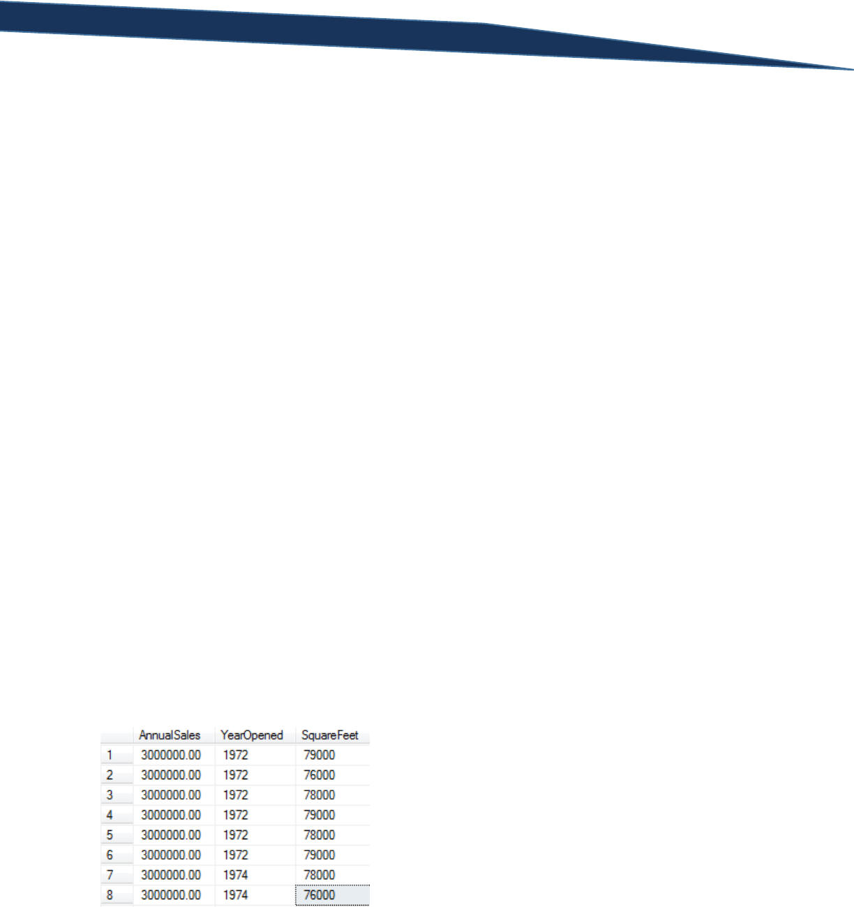
T-SQL Querying Guide © The Knowlton Group, LLC 38 | P a g e
below the FirstName column represents column ordinal 1, and the LastName column represents column
ordinal 2:
SELECT FirstName, LastName
FROM Sales.vIndividualCustomer
So, if we wanted to order by the LastName column using the column ordinal, we would execute:
SELECT FirstName, LastName
FROM Sales.vIndividualCustomer
ORDER BY 2 ASC
And to order the LastName column in descending order:
SELECT FirstName, LastName
FROM Sales.vIndividualCustomer
ORDER BY 2 DESC
The process is completely identical to the other ordering methods, we are simply using the ordinal
instead of the name or alias to explicitly identify how we are ordering our results.
Order by multiple columns is also an option the ORDER BY clause allows. Suppose we wish to return the
AnnualSales, YearOpened and SquareFeet columns from the view Sales.vStoreWithDemographics. Then
suppose we want to order the results by AnnualSales in descending order and then by YearOpened in
ascending order. To complete this task, we execute:
SELECT AnnualSales, YearOpened, SquareFeet
FROM Sales.vStoreWithDemographics
ORDER BY AnnualSales DESC, YearOpened ASC
SQL will order our results by AnnualSales, from largest to smallest, first. Then it orders by the
YearOpened column from oldest to newest. So, in the event of multiple rows having the same
AnnualSales value, the YearOpened column will then be used to determine which rows appear in what
order. You can see this in some of the first few rows returned:
You will notice that the first six rows all have the same AnnualSales and YearOpened value. Then, in the
seventh row, you will see the YearOpened is different – two years later than the YearOpened value in

T-SQL Querying Guide © The Knowlton Group, LLC 39 | P a g e
the previous six rows. This is where the second ordering criteria “YearOpened ASC” assists in
determining the results order.
While we can also order by multiple columns, we can also use different methods in identifying the
sorting criteria. Let’s use the same query as the previous example except let’s give the YearOpened
column the alias “Year Opened”. Let’s also sort by the SquareFeet column in descending order, but only
after having sorted by the AnnualSales and YearOpened columns. Also, we will order using the column
alias for the YearOpened column and the column ordinal when referring to the SquareFeet column.
Putting all of this together, we get:
SELECT AnnualSales, YearOpened AS [Year Opened], SquareFeet
FROM Sales.vStoreWithDemographics
ORDER BY AnnualSales DESC, [Year Opened] ASC, 3 DESC
Just like with the other clauses, we use all four of our SELECT statement clauses together in a single
statement. For example, suppose we wish to return the LastName, FirstName and SalesQuota columns
from the Sales.vSalesPerson views. We only want to return those rows where the SalesQuota column is
greater than or equal to 250,000. Lastly, we want the results ordered by the SalesQuota column (from
largest to smallest) and then by the LastName column in ascending order. We could complete this query
using a few different similar queries:
SELECT LastName, FirstName, SalesQuota
FROM Sales.vSalesPerson
WHERE SalesQuota >= 250000
ORDER BY SalesQuota DESC, LastName ASC
Or:
SELECT LastName, FirstName, SalesQuota
FROM Sales.vSalesPerson
WHERE SalesQuota >= 250000
ORDER BY 3 DESC, 1 ASC
Or:
SELECT LastName, FirstName, SalesQuota
FROM Sales.vSalesPerson
WHERE SalesQuota >= 250000
ORDER BY 3 DESC, LastName ASC
We can use the different sorting methods we have at our disposal to modify the look of the query.
Notice how the WHERE clause has absolutely no effect on what we do in the ORDER BY clause. We
simply add our WHERE clause with the filtering criteria and then define the sorting criteria in the ORDER
BY clause. No complexity or complication is added despite the extra clause included in the statement.
While there certainly are some subtleties to note, the ORDER BY clause has easy to understand rules and
procedures. It also offers some unique flexibilities that other clauses simply do not allow. Complete the
labs at the end of this section to reinforce your knowledge of the ORDER BY clause.

T-SQL Querying Guide © The Knowlton Group, LLC 40 | P a g e
Lab 6: Sorting using the ORDER BY Clause
1) From the HumanResources.vEmployeeDepartment view, return the FirstName, LastName and
JobTitle columns. Sort the results by the FirstName column in ascending order.
2) Modify the query from question 1 to sort the results by the FirstName column in ascending
order and then by the LastName column in descending order.
3) From the Sales.vIndividualCustomer view, return the FirstName, LastName and
CountryRegionName columns. Sort the results by the CountryRegionName column. Use the
column ordinal in the ORDER BY clause.
4) From the Sales.vIndividualCustomer view, return the FirstName, LastName and
CountryRegionName columns for those rows with a CountryRegionName that is either “United
States” or “France”. Sort the results by the CountryRegionName column in ascending order.
5) From the Sales.vStoreWithDemographics view, return the Name, AnnualSales, YearOpened,
SquareFeet, and NumberEmployees columns. Give the SquareFeet column the alias “Store Size”
and the NumberEmployees column the alias “Total Employees”. Return only those rows with
AnnualSales greater than 1,000,000 and with NumberEmployees greater than or equal to 45.
Order your results by the “Store Size” alias in descending order and then by the “Total
Employees” alias in descending order.

T-SQL Querying Guide © The Knowlton Group, LLC 41 | P a g e
Section 6: Querying Multiple Tables via Joins
Normalization and Basic Database Design:
In the majority of the examples throughout this training guide, we have queried against views instead of
database tables. Views are specifically designed to simplify the code required to get commonly
requested information – like consolidated information about employees or customers. Tables in most
transactional databases are not designed with this consolidation in mind, rather they are designed with
a concept of normalization in mind. This normalization, which we will discuss momentarily, reduces the
amount of redundancy and repetition in the data stored within a table. These transactional databases
are typically designed to allow for improved write operations: inserting and modifying data. We are
interested in read operations – returning data – when we write and execute our SELECT statements.
Systems designed for transactions typically require a SQL user to query against multiple tables at once to
return the information they are looking for. Up to this point, we have only focused on how to return
data from a single table or view. Using a concept called joins, we will be able to return columns from
multiple tables in the same SQL SELECT statement.
If you remember back in Section 1, we discussed a few key database concepts. There are two in
particular that will be necessary to understand before talking about joins: primary keys and foreign keys.
Before going any further, re-read the definitions of each.
In the introduction to this section, a concept called normalization was mentioned. Microsoft’s
Developer Network (MSDN) defines normalization as “the process of refining tables, keys, columns, and
relationships to create an efficient database”. Let’s take a look at an example which will best explain
this concept.
Assume we have a table, named Book, that has information about books. Each row contains
information about the authors, publishers and information about the book itself. Below might be an
example of what this table looks like:
Title
ISBN
Publish Date
Publisher
Author 1
Author 2
Author 3
Book 1
123456789
June 1, 2008
Publisher 1
Author A
Author B
Book 2
124356798
September 12, 2009
Publisher 2
Author B
Author C
Book 3
873781927
April 6, 2011
Publisher 3
Author A
Author C
Author D
Book 4
826389163
January 4, 2010
Publisher 1
Author B
Author D
Author E
Book 5
129471352
December 12, 2013
Publisher 2
Author D
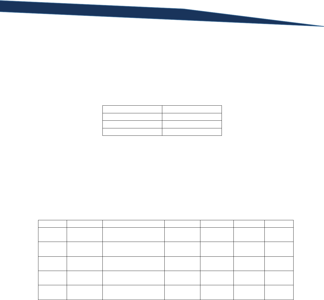
T-SQL Querying Guide © The Knowlton Group, LLC 42 | P a g e
There are a few important details to notice in this table. First, the same publishers and authors are
repeated multiple times throughout this table. Most books have multiple authors and certainly several
authors write multiple books. There exists significant repetition in each row of this table. This table is
known as a denormalized table – that is, repetition and redundancy exist.
If we wanted to normalize this table, we would look at the key areas of redundancy. First, a publisher is
the publisher for multiple books. However, there is no more than one publisher associated with each
book. The first step in normalizing this table would then be to set up a publisher table. The table would
look like:
PublisherID
Publisher Name
1
Publisher 1
2
Publisher 2
3
Publisher 3
The first thing you will most likely notice is the PublisherID column. In a normalized database (most
databases in fact), a key or ID column will be created. This key is usually an integer and, in this example,
the PublisherID represents the primary key of the Publisher table. For many reasons, including query
performance and uniqueness identification, ID columns are almost a near necessity.
Getting back to our normalization example, since we have created a Publisher table with a key assigned
to each publisher, let’s go ahead and replaced “Publisher 1” with the PublisherID of 1, “Publisher 2” with
the PublisherID of 2, and “Publisher 3” with the PublisherID of 3. So, our main table, Book, now looks
like:
Title
ISBN
Publish Date
Publisher
Author 1
Author 2
Author 3
Book 1
123456789
June 1, 2008
1
Author A
Author B
Book 2
124356798
September 12, 2009
2
Author B
Author C
Book 3
873781927
April 6, 2011
3
Author A
Author C
Author D
Book 4
826389163
January 4, 2010
1
Author B
Author D
Author E
Book 5
129471352
December 12, 2013
2
Author D
The value in the publisher column represents a row in the Publisher table. This Publisher column in the
main book table can now be thought of a foreign key. That is, the Publisher column in the Book table
has a foreign key relationship with the PublisherID column of the Publisher table.
Moving on, let’s handle the redundancy relating to the authors. The relationship between authors and
books is what is known as a “many-to-many” relationship. This is because an author can be related to
more than one book, while a book can be related to more than one author. The relationship between
publishers and books, on the other hand, was known as a “one-to-many” relationship. That is because

T-SQL Querying Guide © The Knowlton Group, LLC 43 | P a g e
one publisher can be related with more than one book, but a book can only be related to a single
publisher.
To handle the “many-to-many” relationship that we have between authors and books, we start just like
we did with the publishers. We will create an Author table that contains two columns: AuthorID and
Author Name:
AuthorID
Author Name
1
Author A
2
Author B
3
Author C
4
Author D
5
Author E
We will replace each author with the associated AuthorID from the Author table. We will also create a
BookID column for our Book table to follow proper form. The Book table now looks like:
BookID
Title
ISBN
Publish Date
Publisher
Author 1
Author 2
Author
3
1
Book 1
123456789
June 1, 2008
1
1
2
2
Book 2
124356798
September 12, 2009
2
2
3
3
Book 3
873781927
April 6, 2011
3
1
3
4
4
Book 4
826389163
January 4, 2010
1
2
4
5
5
Book 5
129471352
December 12, 2013
2
4
This still isn’t quite a completely normalized table even though we now have a foreign key relationship
on Author 1, Author 2, and Author 3 to the AuthorID column of the Author table. For “many-to-many”
tables, a bridge table is often need to bridge the gap between the two previous tables. We are going to
create this bridge table by having a table that contains two columns: BookID and AuthorID. Our goal is
to have the complete list of combinations of BookID and AuthorID that we see in our Book table
represented in this new bridge table. This new bridge table, which we will call BookAuthor, will look
like:
BookID
AuthorID
1
1
1
2
2
2
2
3
3
1
3
3
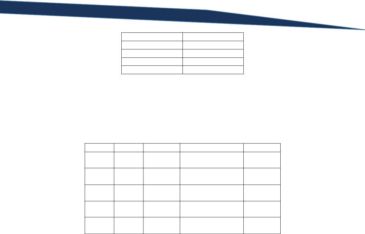
T-SQL Querying Guide © The Knowlton Group, LLC 44 | P a g e
3
4
4
2
4
4
4
5
5
4
The primary key of BookAuthor, the column or columns that define uniqueness for the table, will be the
combination of BookID and AuthorID. Notice how each combination is distinct; this details is important
and will become more apparent when we start practicing joins with SQL statements.
Since we have a bridge between the book and author(s) established, our Book table can be trimmed
down to:
BookID
Title
ISBN
Publish Date
Publisher
1
Book 1
123456789
June 1, 2008
1
2
Book 2
124356798
September 12, 2009
2
3
Book 3
873781927
April 6, 2011
3
4
Book 4
826389163
January 4, 2010
1
5
Book 5
129471352
December 12, 2013
2
Why can this be done? All of the basic author details are stored in the Author table. All of the
information connecting each author to each book is stored in the BookAuthor bridge table. We have
eliminated the necessary redundancy in storing multiple columns of author details in the Book table.
We now have a completely normalized database of tables. A database diagram is an effective way to
visualize each table’s relationship with one another. The database diagram of our example above would
look like:
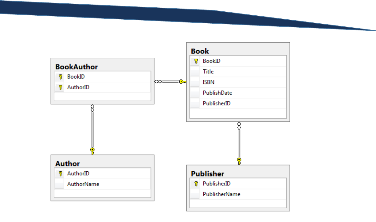
T-SQL Querying Guide © The Knowlton Group, LLC 45 | P a g e
The table adjacent the gold key in the lines connected two tables implies that table contains the primary
key and the table with the infinity symbol contains a foreign key that references the table on the other
end of the connecting line. For example, Book contains a column, PublisherID, that is a foreign key and
references the primary key of Publisher, PublisherID.
We have successfully eliminated all possible redundancy from our original version of the Book table.
Understanding the concepts of normalization and how data is typically organized is essential to
becoming proficient in SQL querying. This small, trivial example has helped us grasp the concepts of
basic database design, primary and foreign keys, and – without you even realizing it – the underlying
principles necessary for joins.
Basics of the INNER JOIN
A join, at the simplest explanation possible, is the process by which you can connect two tables
together. There are four types of joins: INNER JOIN, LEFT OUTER JOIN, RIGHT OUTER JOIN, and FULL
OUTER JOIN. An INNER JOIN can be thought of as the intersection of tables based on some key. In well-
designed databases, an INNER JOIN (all join types, in fact), is defined by the connection of a foreign key
from one table to the primary key in another table. Venn diagrams are often used to visualize what
happens when joins are completed. With that in mind, below is the visual representation of the INNER
JOIN:

T-SQL Querying Guide © The Knowlton Group, LLC 46 | P a g e
Notice how only the space shared by both tables is shaded in the diagram above. Let’s work through an
example of an INNER JOIN through a few queries and further explain the concept as we go.
Execute the query below in SQL Server Management Studio while connected to the
AdventureWorks2012 database:
SELECT P.Name, P.ProductNumber, PS.Name AS ProductSubCategoryName
FROM Production.Product P
INNER JOIN Production.ProductSubcategory PS
ON P.ProductSubcategoryID = PS.ProductSubcategoryID
There are a few new concepts introduced here. First, you will notice the letters “P” and “PS” after the
table names. These are called table aliases. They act similarly to column aliases in that you can use the
alias to reference the table during your SELECT statement. Unlike the column alias, you can use this
table alias in all clauses of the SELECT statement. Using table aliases when joining drastically improves
readability of the code and minimizes unnecessary typing. The second thing you will notice is the form
of the JOIN. After the FROM clause, and before any other clause, we specify the phrase “INNER JOIN”
and then identify which table we would like to join to. In this case, we want to join the
Product.ProductSubcategory table. After giving the Product.ProductSubcategory table the alias “PS”, we
type “ON” and then indicate how we are joining the two tables together. Knowing what column to join
on is critical for success in joining tables together. In this example, the ProductSubcategoryID in the
Production.Product table is a foreign key that references the ProductSubcategoryID column in the
Product.ProductSubcategory table.
A valid question at this point is “how do you know which columns to join?” The object explorer is
helpful in this instance. In the object explorer, expand the “Tables” folder under
“AdventureWorks2012” if it is not already. Find the table named “Production.Product”, and click the
expand button to left of it. Find the toggle button to the left of “Keys” and click it.
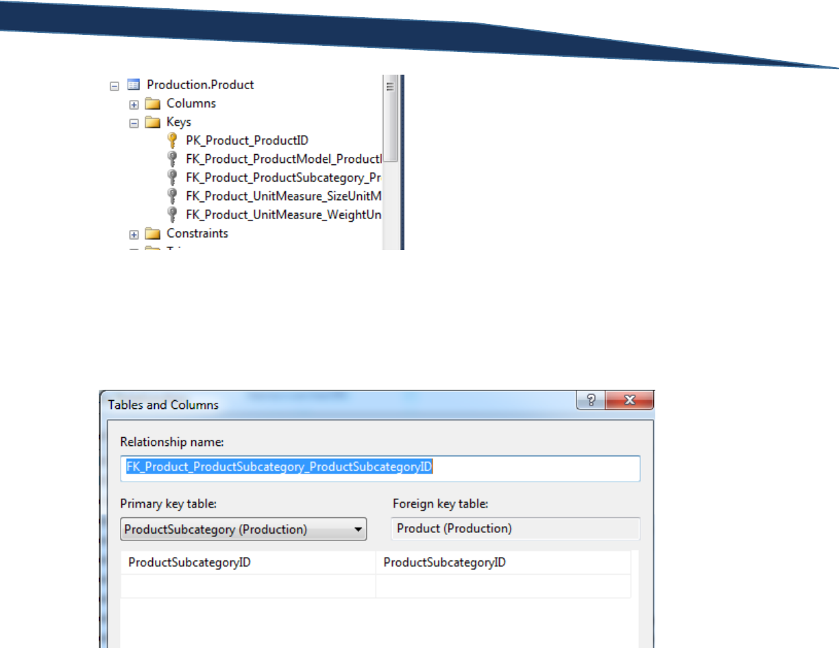
T-SQL Querying Guide © The Knowlton Group, LLC 47 | P a g e
The first key, the gold key, contains information about the primary key of this table. Well named keys
often tell you exactly what columns are contained in the key. Double click on the second key named
“FK_Product_ProductSubcategory_ProductSubcategoryID”. Click the blank space to the right of the
“Table and Column Specifications” option, and click the ellipsis button to the right of that. The “Tables
and Columns” window will appear. This window details how this particular key is defined.
This table tells you that the ProductSubcategoryID in the Production.Product table (see the column on
the right) is a foreign key with a relationship to the ProductSubcategoryID column of the
Production.ProductSubcategory table. Given the foreign key relationship, joining on these columns is
designed for this use.
Let’s take a look at the query in our example. Run the query below and note the number of rows
returned:
SELECT *
FROM Production.Product
The table Production.Product returns 504 rows. Now re-run our original query below and notice the
rows returned:

T-SQL Querying Guide © The Knowlton Group, LLC 48 | P a g e
SELECT P.Name, P.ProductNumber, PS.Name AS ProductSubCategoryName
FROM Production.Product P
INNER JOIN Production.ProductSubcategory PS
ON P.ProductSubcategoryID = PS.ProductSubcategoryID
This query only returns 295 rows. Why is this the case? Since an INNER JOIN is the intersection of two
sets based on a column relationship, a row is returned only if the value in the joining column from one
table matches at least one value of the joining column in another table. That is, a row will only be
returned if the ProductSubcategoryID column’s value in Production.Product appears in the
ProductSubcategoryID column of the table Production.ProductSubcategory. Re-run the query:
SELECT *
FROM Production.Product
Once the results are returned, find the ProductSubcategoryID column and take a look at the values. You
will notice a NULL value in many of the rows for this column. Since the value in those columns is NULL,
that means that there is no value with which to join the row to in the Production.ProductSubcategory
table. Since the INNER JOIN is an intersection of two tables based on the columns defined and there are
many NULL values in our joining column from one table, those rows will not be matches to any row in
the other table (in this case, the Production.ProductSubcategory table).
Let’s go back to our example in the previous sub-section that discussed basic database diagram. After
normalizing the initial Book table, we ended up with four tables: Author, Publisher, BookAuthor, and
Book. If you have not already done so, download the SQL file that will create those tables in your
AdventureWorks2012 database and execute the code http://knowlton-group.com/sql-training-class-
resource/.
Run the query below to view the contents of the Book table:
SELECT *
FROM Book
Notice how the PublisherID is the last column. Expand the Book table item in the object explorer, then
explain the Keys item as well (you may need to refresh the database if the items are not visible after
running the code).
Double click on the second key. Once the “Foreign Key Relationships” window appears, click the ellipses
to the right of the “Tables and Columns Specification” option. The “Tables and Columns” window should
appear and contain the following contents:
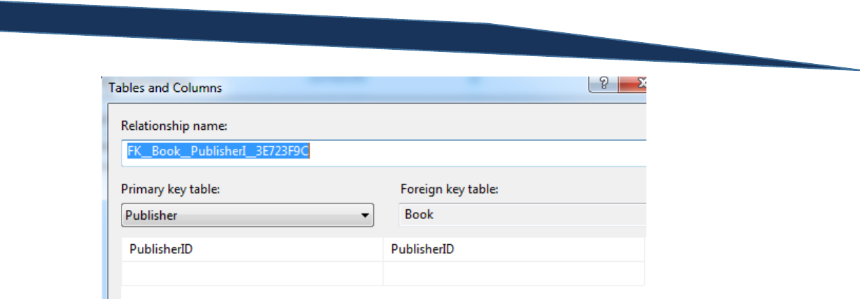
T-SQL Querying Guide © The Knowlton Group, LLC 49 | P a g e
As you can see, the PublisherID column in the Book table is referencing the primary key, PublisherID,
from the Publisher table. If we wanted to join the Book and Publisher tables, we would use the
PublisherID to make that connection.
Let’s do that, in fact. We are going to create a SQL query that joins the Book table with the Publisher
table through the PublisherID column in both tables. We will then be able to return the details of the
book along with the name of the publisher. To do this, execute the query below:
SELECT B.Title, B.ISBN, B.PublishDate, P.PublisherName
FROM Book B
INNER JOIN Publisher P
ON B.PublisherID = P.PublisherID
Notice the use of table aliases “B” and “P” to represent the Book and Publisher tables, respectively. Our
SELECT clause returns only the columns we wish to return. These columns include the details about the
book, contained in the Book table, and then the name of the publisher that is contained in the Publisher
table. We originate our query in the Book table as specified in the FROM clause. Next, we indicate that
we are going to be utilizing an INNER JOIN. Then, we specified the table we wish to join to; in this case,
the Publisher table is the table we are joining to. Next, we type “ON” which tells SQL that we are about
to tell it how we wish to connect our tables. Lastly, we specify that we want to connect these tables
when the PublisherID column from the Book table matches a PublisherID column in the Publisher table.
When viewing the results of the query, none of the IDs appear, only the columns that we have indicated.
For your own benefit, execute these two queries below:
SELECT B.Title, B.ISBN, B.PublishDate, B.PublisherID, P.PublisherName
FROM Book B
INNER JOIN Publisher P
ON P.PublisherID = B.PublisherID
SELECT *
FROM Publisher
Notice how we include the PublisherID column from the Book table in the first query. Manually validate
that the first query returned the proper value for the PublisherName column. Verify that each time a

T-SQL Querying Guide © The Knowlton Group, LLC 50 | P a g e
“1” appears in the PublisherID column of Book that it matches the PublisherName column value
associated with the row in the Publisher table with a “1” in the PublisherID column. Do this for each
book. This is a very simple way to validate that the join you executed is performing as intended.
Let’s look at another example. In the AdventureWorks2012 database, there is table, named
Person.Person, that contains some basic information about individuals in a database. There is another
table, Person.EmailAddress, that contains the email address for each person in the Person.Person table.
Both tables use the column BusinessEntityID as the key identifier for the individual. If we wanted to
return the FirstName and LastName columns from Person.Person and the EmailAddress column from
Person.EmailAddress, we would execute the query:
SELECT P.FirstName, P.LastName, E.EmailAddress
FROM Person.Person P
INNER JOIN Person.EmailAddress E
ON E.BusinessEntityID = P.BusinessEntityID
This query is telling SQL to look at each BusinessEntityID in Person.Person and find the row with the
same BusinessEntityID in the table Person.EmailAddress. When that matching row is found, return the
EmailAddress column. Because this join is an INNER JOIN, rows are only returned if the joining key is
present in both tables; in this case, the joining key is the BusinessEntityID column.
Often times the data we need is spread across more than two tables. How can we use the INNER JOIN
(or any join for that matter) to handle retrieving data from more than two tables in the same query?
The process is nearly identical to joining between two columns. Suppose we wanted to take our
previous example but add the person’s phone number. The phone number is stored in the table
Person.PersonPhone. Person.PersonPhone contains the BusinessEntityID column that we can use to join
each table together. To add the phone number, execute the query:
SELECT P.FirstName, P.LastName, E.EmailAddress, PP.PhoneNumber
FROM Person.Person P
INNER JOIN Person.EmailAddress E
ON E.BusinessEntityID = P.BusinessEntityID
INNER JOIN Person.PersonPhone PP
ON PP.BusinessEntityID = P.BusinessEntityID
Since each BusinessEntityID has a single row in the Person.PersonPhone table, our row count remains
unchanged in the results. Notice that all we needed to do was add another INNER JOIN line, specify the
table we wanted to join to, and then specify which columns we would be joining on. Since there is a
“one-to-one” relationship between each of these tables – that is, each row in a table matches up to only
one row in another one of these tables – we can modify our join slightly. Instead of joining between
Person.PersonPhone and Person.Person on the BusinessEntityID column, we can join between
Person.PersonPhone and Person.EmailAddress:
SELECT P.FirstName, P.LastName, E.EmailAddress, PP.PhoneNumber
FROM Person.Person P
INNER JOIN Person.EmailAddress E
ON E.BusinessEntityID = P.BusinessEntityID
INNER JOIN Person.PersonPhone PP

T-SQL Querying Guide © The Knowlton Group, LLC 51 | P a g e
ON PP.BusinessEntityID = E.BusinessEntityID
The concept of the INNER JOIN will become clearer with more practice. Given that, complete the
following lab questions to further cement your understanding of this very important aspect of SQL
querying.
Lab 7: INNER JOIN Practice
1) Using the Person.Person and Person.Password tables, INNER JOIN the two tables using the
BusinessEntityID column and return the FirstName and LastName columns from Person.Person
and then PasswordHash column from Person.Password
2) Join the HumanResources.Employee and the HumanResources.EmployeeDepartmentHistory
tables together via an INNER JOIN using the BusinessEntityID column. Return the
BusinessEntityID, NationalIDNumber and JobTitle columns from HumanResources.Employee and
the DepartmentID, StartDate, and EndDate columns from
HumanResources.EmployeeDepartmentHistory. Notice the number of rows returned. Why is
the row count what it is?
3) Expand upon the query used in question 1. Using the existing query, add another INNER JOIN to
the Person.EmailAddress table and include the EmailAddress column in your select statement.
4) Using the Book, BookAuthor and Author tables, join them together so that you return the Title
and ISBN columns from Book and the AuthorName column from Author. (Hint: You must start
with the BookAuthor table in your FROM clause even though we will not be returning any
columns from this table)
5) Using the query from example 4, add another INNER JOIN that joins the Publisher table with
your query. Return the PublisherName column from this table. So, you should return the Title
and ISBN columns from Book, the AuthorName column from Author, and the PublisherName
column from Publisher. (Hint: this will require three separate INNER JOINs).
LEFT OUTER JOIN and RIGHT OUTER JOIN
What is the LEFT OUTER JOIN and RIGHT OUTER JOIN? If you remember back to the introduction to
INNER JOINs, it was explained that the INNER JOIN was the intersection of two sets. The LEFT OUTER
JOIN and RIGHT OUTER JOIN can be thought of as “everything from one set and then information from
the intersection of both sets”. Let’s visualize this with a Venn diagram for the LEFT OUTER JOIN:
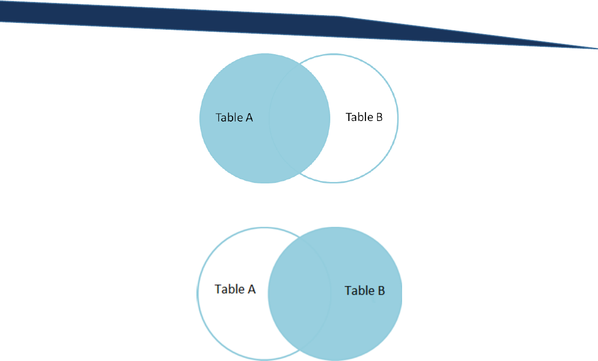
T-SQL Querying Guide © The Knowlton Group, LLC 52 | P a g e
And the Venn diagram for the RIGHT OUTER JOIN:
One thing to note is that the LEFT OUTER JOIN and RIGHT OUTER JOIN are nearly identical – the only
difference is which set is completed shaded.
Looking at some examples will further clarify the LEFT OUTER JOIN and RIGHT OUTER JOIN. If you
remember to the last section, we executed the query:
SELECT P.Name, P.ProductNumber, PS.Name AS ProductSubCategoryName
FROM Production.Product P
INNER JOIN Production.ProductSubcategory PS
ON P.ProductSubcategoryID = PS.ProductSubcategoryID
This query returns only 295 rows, yet the Production.Product table contains 504 rows. We discussed
that since this was an INNER JOIN and since some of the column values in ProductSubcategoryID were
NULL in Production.Product, then no rows could be matched to them from
Production.ProductSubcategory. But suppose we wanted to return EVERY row in Production.Product
and include the product’s subcategory name (contained in the Name column from
Production.ProductSubcategory) if one existed. The LEFT OUTER JOIN would solve this for us:
SELECT P.Name, P.ProductNumber, PS.Name AS ProductSubCategoryName
FROM Production.Product P
LEFT OUTER JOIN Production.ProductSubcategory PS
ON P.ProductSubcategoryID = PS.ProductSubcategoryID

T-SQL Querying Guide © The Knowlton Group, LLC 53 | P a g e
Notice how there are many rows in the result set that have a NULL value in the
ProductSubCategoryName column. This is fine and expected; these rows have a NULL value in the
ProductSubcategoryID column in Production.Product, so it makes sense that they wouldn’t match to
row in Production.ProductSubcategory. If you imagine the LEFT OUTER JOIN Venn diagram while
viewing the results, you can see that all rows are returned from Production.Product (Table A in the
diagram) and only the values that match as part of the intersection defined by the join from
Production.ProductSubcategory.
Now, execute this query:
SELECT P.Name, P.ProductNumber, PS.Name AS ProductSubCategoryName
FROM Production.ProductSubcategory PS
RIGHT OUTER JOIN Production.Product P
ON P.ProductSubcategoryID = PS.ProductSubcategoryID
Notice how we made the Production.ProductSubcategory table in the FROM clause and shifted the
Production.Product table to the RIGHT OUTER JOIN line. Despite the change in code, the results are
identical. Why? This is because the LEFT OUTER JOIN and RIGHT OUTER JOIN only differ in the order in
which they are evaluated. The RIGHT OUTER JOIN returns everything from Table B and those values for
rows that match in Table A. The LEFT OUTER JOIN returns everything from Table A and those values for
rows that match in Table B. That is the ONLY difference between the LEFT OUTER JOIN and RIGHT
OUTER JOIN. The LEFT OUTER JOIN evaluates the table listed first (on the “left”) and then the table
listed second (on the “right”).
Take this generic form query:
SELECT A.[Column 1], A.[Column 2], B.[Column 3]
FROM [Table A] A
LEFT OUTER JOIN [Table B] B
ON A.[Primary Key] = B.[Foreign Key]
This query’s results will contain all rows from Table A and then the [Colum 3] value from Table B where
the primary key value from Table A matches to a foreign key’s value in Table B.
Let’s look at another example: suppose we wanted to identify the first and last name for each sales
person associated with every single sale recorded in the Sales.SalesOrderHeader table. However, we
want to include all sales regardless of whether or not a sales person was listed on the sale (in this
database, sales that were placed online do not have a sales person associated with them). Return the
SalesOrderNumber and TotalDue columns from Sales.SalesOrderHeader and the FirstName and
LastName columns from Person.Person. To complete this query, you would execute:
SELECT SOH.SalesOrderNumber, SOH.TotalDue, P.FirstName, P.LastName
FROM Sales.SalesOrderHeader SOH
LEFT OUTER JOIN Sales.SalesPerson SP
ON SP.BusinessEntityID = SOH.SalesPersonID
LEFT OUTER JOIN Person.Person P
ON P.BusinessEntityID = SP.BusinessEntityID

T-SQL Querying Guide © The Knowlton Group, LLC 54 | P a g e
Notice how we first needed to make a LEFT OUTER JOIN between Sales.SalesOrderHeader and
Sales.SalesPerson. Looking at the keys of Sales.SalesOrderHeader, you will find a foreign key
relationship between the SalesPersonID column of Sales.SalesOrderHeader and the BusinessEntityID for
Sales.SalesPerson. Since we wanted to return all rows from the Sales.SalesOrderHeader regardless of
whether or not a sales person was listed (and you will notice many rows in this table have a NULL value
in the SalesPersonID column), we needed to use a LEFT OUTER JOIN to connect the two sets. Then, we
want to use a LEFT OUTER JOIN to join the Sales.SalesPerson and Person.Person tables. We use the LEFT
OUTER JOIN because not every row in Sales.SalesOrderHeader has a SalesPersonID, therefore not every
row that is returned will have a BusinessEntityID matching. It then follows that since there will be a
NULL value for the BusinessEntityID column value returned by the join of Sales.SalesOrderHeader and
Sales.SalesPerson, we must use a LEFT OUTER JOIN to connect Sales.SalesPerson and Person.Person. If
we used an INNER JOIN, those BusinessEntityID values from Sales.SalesPerson would have no match to
Person.Person and thus greatly reduce our result set.
There are scenarios where a query will require one LEFT or RIGHT OUTER JOIN and an INNER JOIN to
complete a request. For example, suppose we wanted to return all rows from Sales.SalesOrderHeader
that had a sales person listed on the sale. In other words, we only want to return those sales where the
SalesPersonID column in Sales.SalesOrderHeader matches a BusinessEntityID column value in
Sales.SalesPerson. However, we also want to view the sales territory that each sales person is
associated with regardless of whether or not they have a listed sales territory. Since there are rows in
the Sales.SalesPerson table with a NULL value in the TerritoryID column, we need to use a LEFT OUER
JOIN from Sales.SalesPerson to Sales.SalesTerritory in order to complete this request. Putting it all
together, we can complete the aforementioned request with the following query:
SELECT
P.FirstName, P.LastName, T.Name AS TerritoryName,
SOH.SalesOrderNumber, SOH.TotalDue
FROM Sales.SalesOrderHeader SOH
INNER JOIN Sales.SalesPerson SP
ON SP.BusinessEntityID = SOH.SalesPersonID
INNER JOIN Person.Person P
ON P.BusinessEntityID = SP.BusinessEntityID
LEFT OUTER JOIN Sales.SalesTerritory T
ON T.TerritoryID = SP.TerritoryID
Notice the use of the INNER JOINs between Sales.SalesOrderHeader and Sales.SalesPerson. This ensures
that we only returns rows for sales that had a listed sales person. The join between Sales.SalesPerson
and Sales.SalesTerritory is a LEFT OUTER JOIN. Had we used an INNER JOIN here, any sale for a sales
person that wasn’t associated with a sales territory would be excluded from our results. This would
have caused our result set to be less than it should be.
What about using the other clauses while using a join? This is fairly simple; imagine that the joins are all
part of the FROM clause. So, in the previous example, if we wanted to only returns those rows where
the territory’s name was “Northeast”, we would execute:
SELECT
P.FirstName, P.LastName, T.Name AS TerritoryName,

T-SQL Querying Guide © The Knowlton Group, LLC 55 | P a g e
SOH.SalesOrderNumber, SOH.TotalDue
FROM Sales.SalesOrderHeader SOH
INNER JOIN Sales.SalesPerson SP
ON SP.BusinessEntityID = SOH.SalesPersonID
INNER JOIN Person.Person P
ON P.BusinessEntityID = SP.BusinessEntityID
LEFT OUTER JOIN Sales.SalesTerritory T
ON T.TerritoryID = SP.TerritoryID
WHERE T.Name = 'Northeast'
And if we wanted to sort by the TotalDue column in descending order:
SELECT
P.FirstName, P.LastName, T.Name AS TerritoryName,
SOH.SalesOrderNumber, SOH.TotalDue
FROM Sales.SalesOrderHeader SOH
INNER JOIN Sales.SalesPerson SP
ON SP.BusinessEntityID = SOH.SalesPersonID
INNER JOIN Person.Person P
ON P.BusinessEntityID = SP.BusinessEntityID
LEFT OUTER JOIN Sales.SalesTerritory T
ON T.TerritoryID = SP.TerritoryID
WHERE T.Name = 'Northeast'
ORDER BY SOH.TotalDue DESC
The different clauses can easily be employed while using joins. Follow the same order that the general
form requires. The only subtle difference is that the joins “belong” to the FROM clause. Becoming
familiar with the general form of a SELECT statement when using joins and all clauses is critical to your
success in querying.
The LEFT OUTER JOIN and RIGHT OUTER JOIN will become more easily understood with continued
practice. Understanding when to use a LEFT OUTER JOIN or RIGHT OUTER JOIN as opposed to an INNER
JOIN requires complete awareness of the request and the data within the database. Progress may be
slow when querying a new database as you may not understand every single table’s relationships. Be
sure to consult the object explorer and identify the foreign keys. Feel free to write a SELECT statement
that returns all rows from a table so that you know how many rows to expect in your results. Like most
things: practice makes perfect.
Lab 8: Including LEFT OUTER JOINs and RIGHT OUTER JOINs
1) Return the BusinessEntityID and SalesYTD column from Sales.SalesPerson. Join this table to the
Sales.SalesTerritory table in such a way that every in Sales.SalesPerson will be returned
regardless of whether or not they are assigned to a territory. Also, return the Name column
from Sales.SalesTerritory. Give this column the column alias “Territory Name”.
2) Using the previous example as your foundation, join to the Person.Person table to return the
sales person’s first name and last name. Now, only include those rows where the territory’s
name is either “Northeast” or “Central”
3) Return the Name and ListPrice columns from Production.Product. For each product, regardless
of whether or not it has an assigned ProductSubcategoryID, return the Name column from
T-SQL Querying Guide © The Knowlton Group, LLC 56 | P a g e
Product.ProductSubcategory for each product. Then, return the Name column from
Production.ProductCategory for each row. Give the Name column from Production.Product the
alias “ProductName”, the Name column from Production.ProductSubcategory the alias
“ProductSubcategoryName”, and the Name column from Production.ProductCategory the alias
“ProductCategoryName”. Order the results by the “ProductCategoryName” in descending order
and then the “ProductSubcategoryName” in ascending order.
FULL OUTER JOINs
We won’t spend too much time on FULL OUTER JOINs as they are less frequently used than the other
three join types discussed in this section. A FULL OUTER JOIN returns rows from both tables involved in
the join regardless of whether or not a match is identified on the joining key. Visually, the Venn diagram
of a FULL OUTER JOIN looks like:
Regardless of whether a match is found for the joining key, rows will be returned. So as to not
overcomplicate the difficult that joins may initially present, we will not do anything further with a FULL
OUTER JOIN. If an example later on the text presents itself and requires the FULL OUTER JOIN,
additional time will be dedicated to explaining its usage further. For now, simply be aware of its
existence and basic definition.

T-SQL Querying Guide © The Knowlton Group, LLC 57 | P a g e
Section 7: Aggregate Functions
Aggregate functions are functions that perform a calculation on a set of values and return a single result.
Aggregate functions are necessary to understand before moving on to the GROUP BY clause within a
SQL SELECT statement. This section will include examples for each commonly used aggregate function
to further your understanding and ability to apply these functions in a SELECT statement.
The first aggregate function is the MAX() function. This function will take a set of values as its input and
output the largest of the values it receives. For example, to find the largest sale listed in the
Sales.SalesOrderHeader table we would execute:
SELECT MAX(TotalDue)
FROM Sales.SalesOrderHeader
Notice how we type “MAX”, then have an opening parentheses followed by the column name we are
attempting to find the max value for, and then end with a closing parentheses. All functions in T-SQL
will require opening and closing parentheses; be careful to make sure you have properly closed each
function. The previous query, though receiving thousands of values from all the rows that have a value
in the TotalDue column, returns a single value – the max of the TotalDue column. Noting the scalar
value result with be important when we start working with the HAVING clause and with subqueries in
later sections of this guide.
The next aggregate function we will explore is the MIN() function. As you might have guess, this
function takes a set of values as its input and returns the smallest value of input as a result. For
example, to find the smallest sales amount from the Sales.SalesOrderHeader table, we would type:
SELECT MIN(TotalDue)
FROM Sales.SalesOrderHeader
Again, the query follows the same basic pattern that we saw in the MAX() function example. An
important note is that NULL values are ignored. In fact, NULL values are ignored for all aggregate
functions except the COUNT() function. So, you will never see NULL returned as a value for the MAX() or
MIN() function.
Given the discussion about NULL values in the previous paragraph, the COUNT() function will be the next
function we look at. This function provides a count of the number of input values it receives. Instead of
executing a query like:
SELECT *
FROM Sales.SalesOrderHeader
Where this query will return every row and every single column – a query that takes up plenty of
memory and is poorly optimized. We have been doing the “SELECT *” operation to find the number of
rows that a table contains. With the COUNT() function, we can accomplish the same objective but with
a simpler query:

T-SQL Querying Guide © The Knowlton Group, LLC 58 | P a g e
SELECT COUNT(*)
FROM Sales.SalesOrderHeader
Notice the single value that is returned. You might have also noticed how much faster that query
completed compared to the previous example. The asterisk in between the parentheses is telling SQL
that we don’t want to count the number of values for a particular column, but the number of rows that
are contained in the results.
Alternatively, we can use the COUNT() function with a column name between the parentheses.
SELECT COUNT(SalesPersonID)
FROM Sales.SalesOrderHeader
However, you must be aware of the column you choose to place between the parentheses or acutely
aware of what you are trying to accomplish with your query. Notice the significant decrease in the
result of the previous query compared to the one before it. If you remember to an earlier paragraph in
this section, it was stated that the COUNT() function does not ignore NULL values. That is, the result of
the function can be directly affected by the presence of NULL values. In the previous example, the
COUNT(SalesPersonID) was only counting the values in the SalesPersonID column that were NOT NULL.
However, the COUNT(*) query counted all rows regardless of whether or not everything was NULL. This
subtlety within the COUNT() function can significantly vary your results; be sure to understand what you
are trying to return and handle the function accordingly.
Another useful ability the COUNT() function provides us is the distinct count. The distinct count requires
a column name to be specified; the asterisk cannot be used here. For example, if we wanted to find the
number of distinct first names in the Person.Person table, we would execute the query:
SELECT COUNT(DISTINCT FirstName)
FROM Person.Person
This operation counts the distinct number of non-NULL first name values in the table. Suppose that a
table exists that contains sales order details for customers. The customer identifier can be repeated
throughout the table because a customer could have made more than one purchase. If we were asked
to find the distinct number of customers that purchased our products, a COUNT(DISTINCT [Customer
Identifier]) would be a quick way to answer this request. This is but another useful tool to keep in mind
as you begin to resolve requests through SQL statements.
The next aggregate function we will look at is the AVG() function. This function take the average of all
the non-NULL values in a column specified in the query. So, to find the average sale amount for each
sale recorded in the Sales.SalesOrderHeader table we would use the query:
SELECT AVG(TotalDue)
FROM Sales.SalesOrderHeader

T-SQL Querying Guide © The Knowlton Group, LLC 59 | P a g e
The AVG() function has no subtleties like the COUNT() function possesses. It is, like the MAX() and MIN()
functions, fairly straight-forward in its uses and applications.
The SUM() function is another common aggregate function. Like the AVG(), MIN() , and MAX()
functions, the SUM() function takes a column as an input. Sticking with the TotalDue column from
Sales.SalesOrderHeader, let’s find the sum of all sales that exist in our database:
SELECT SUM(TotalDue)
FROM Sales.SalesOrderHeader
A more common request might be to find the total sales for a given year. So, let’s use the SUM()
function to find the total sales that occurred in the year 2006:
SELECT SUM(TotalDue) AS [2006 Sales Total]
FROM Sales.SalesOrderHeader
WHERE OrderDate BETWEEN '1/1/2006' AND '12/31/2006'
We included a column alias on the SUM() function to be clear about what we were summing and what
the returned value represents. The WHERE clause means that the values being totaled up in the SUM()
function are only the values from the rows where the OrderDate value was between 1/1/2006 and
12/31/2006. If you remember the order in which SQL evaluates a SELECT statement, the WHERE clause
is the second clause evaluated. The SELECT clause isn’t evaluated until after the WHERE clause has been
evaluated. Therefore, the SELECT statement, and specifically the aggregate function we are using in the
previous example, will only perform an operation against the rows that have passed the WHERE clause’s
filtering.
The values that the SUM() function receives, just like the AVG() function, must be numeric in nature.
Logically, it does not make sense to sum up the values in a column like FirstName. If you do attempt to
sum a column that it is not an appropriate data type, SQL will provide an error message similar to the
message below:
SELECT SUM(FirstName)
FROM Person.Person
Error Message:
Msg 8117, Level 16, State 1, Line 1
Operand data type nvarchar is invalid for sum operator.
The error message is stating that the FirstName column has the data type “nvarchar” (in Section 11 we
will discuss data types) which is not a data type compatible for a sum operation. We will explore these
concepts in more detail later in the training guide.
There are a few more aggregate functions that you should be aware of, but we will not explore in depth.
The majority of these aggregate functions act similarly, therefore you should be able to use a new
aggregate function based on the information you have already accumulated. The other aggregate
functions can be found on Microsoft’s MSDN documentation here.

T-SQL Querying Guide © The Knowlton Group, LLC 60 | P a g e
Lab 9: Aggregate Functions
1) How many rows are in the Person.Person table? Use an aggregate function NOT “SELECT *”.
2) How many rows in the Person.Person table do not have a NULL value in the MiddleName
column?
3) What is the average StandardCost (located in Production.Product) for each product where the
StandardCost is greater than $0.00?
4) What is the average Freight amount for each sale (found in Sales.SalesOrderHeader) where the
sale took place in TerritoryID 4?
5) How expensive is the most expensive product, by ListPrice, in the table Production.Product?
6) Join the Production.Product table and the Production.ProductInventory table for only the
products that appear in both table. Use the ProductID as the joining column.
Production.ProductInventory contains the quantity of each product (several rows can appear for
each product to indicate the product appears in multiple locations). Your goal is to determine
how much money we would earn if we sold every product for its list price for each product with
a ListPrice greater than $0. That is, if you summed the product of each product’s inventory by
its list price, what would that value be? (Hint: This is intentionally challenging. You must use an
aggregate function with a mathematical expression to accomplish your goal)

T-SQL Querying Guide © The Knowlton Group, LLC 61 | P a g e
Section 8: Grouping with the GROUP BY Clause
Grouping is a common task required to complete effective SQL queries. A request like “show me all
sales in the last year and who the sales person was” is less common than “show me each sales person’s
YTD sales”. The first request wants every sale in its own row, while the second request only wants one
row per sales person. To complete this type of request, the GROUP BY clause is required.
The GROUP BY clause is placed immediately after the WHERE clause in the SELECT statement general
form:
SELECT [Column 1], [Column 2], ... , [Column N]
FROM [Database Name].[Schema Name].[Table Name]
WHERE [Column Name] {Comparison Operator} {Filter Criteria}
GROUP BY [Column Name]
ORDER BY {[Column Name], [Column Alias], [Column Ordinal]} [ASC/DESC]
The GROUP BY clause will take every row that passes the WHERE clause filters and group the result
based on the column that you specify. Typically, the GROUP BY clause is used in conjunction with an
aggregate function in the SELECT clause. Let’s take a look at an example and explain further:
SELECT SalesPersonID, SUM(TotalDue) AS [Total Sales]
FROM Sales.SalesOrderHeader
GROUP BY SalesPersonID
This query takes all rows from the Sales.SalesOrderHeader and then groups them by the unique
SalesPersonID values. Then, it sums the TotalDue column for each group of SalesPersonIDs and returns
the result accordingly. We MUST use an aggregate function or SQL will return an error. If we instead
used this incorrect query:
SELECT SalesPersonID, TotalDue
FROM Sales.SalesOrderHeader
GROUP BY SalesPersonID
We would receive the error:
Msg 8120, Level 16, State 1, Line 1
Column 'Sales.SalesOrderHeader.TotalDue' is invalid in the select list because it is not
contained in either an aggregate function or the GROUP BY clause.
This error message is very clear: if you are going to complete a SELECT statement with a GROUP BY
clause either every column in the SELECT clause needs to appear in the GROUP BY clause, or those
columns not specified in the GROUP BY clause must be aggregate functions. You cannot display a group
without aggregating the values in that group. SQL is confused in the above query because we insist that
we want to group our results by the SalesPersonID column but then want to return an ungrouped or
unaggregated column, TotalDue. If you see the above error message when writing queries with the
GROUP BY clause, immediately look to your SELECT clause and ensure that every column is in the
GROUP BY clause or that those columns not in the GROUP BY clause and part of an aggregate function.

T-SQL Querying Guide © The Knowlton Group, LLC 62 | P a g e
Let’s look at another example. The Production.ProductInventory table contains information about our
product’s current inventory. Each ProductID may have multiple rows due to the design of the table. If
we wanted to find, for each ProductID, the total number of inventory we currently possess, we would
execute the query:
SELECT ProductID, SUM(Quantity) AS [Total Quantity]
FROM Production.ProductInventory
GROUP BY ProductID
If we wanted to use the same query as above but add another column for how many different locations
the product is stored (i.e. the number of rows in the table for each ProductID), we could execute:
SELECT
ProductID,
SUM(Quantity) AS [Total Quantity],
COUNT(*) AS [Locations Product is Stored]
FROM Production.ProductInventory
GROUP BY ProductID
We can also group by multiple columns in the same query to define, in essence, a hierarchy. Using the
Sales.SalesOrderHeader, we will determine total sales from 1/1/2006 to 12/31/2006 by territory and
then by sales person. This would look like:
SELECT TerritoryID, SalesPersonID, SUM(TotalDue)
FROM Sales.SalesOrderHeader
WHERE OrderDate BETWEEN '1/1/2006' AND '12/31/2006'
GROUP BY TerritoryID, SalesPersonID
ORDER BY 1,2
Notice that some sales took place in a specific territory with no sales person assigned to the sale, hence
the NULL value in the SalesPersonID column for some rows. The query has taken the rows from
Sales.SalesOrderHeader that pass the WHERE clause filter and then groups them first by the TerritoryID
and then breaks them down further by SalesPersonID. Finally, after the groups have been established,
SQL sums the TotalDue column based on these groups then sorts and outputs the results.
Using the previous query, let’s make it cleaner. We would rarely want to give a business user results
that had columns like TerritoryID or SalesPersonID. Instead, we would want the name of the territory or
sales person. For the next query, we will be joining to the tables that contains the names for the
aforementioned ID columns. We will be using INNER JOINs to simplify the results – that is, we will find
no NULL values in the results for the territory name or sales person name column.
SELECT
ST.Name AS [Territory Name],
P.FirstName AS [SalesPerson First Name],
P.LastName AS [SalesPerson Last Name],
SUM(TotalDue) AS [Total 2006 Sales]
FROM Sales.SalesOrderHeader SOH
INNER JOIN Sales.SalesPerson SP
ON SP.BusinessEntityID = SOH.SalesPersonID

T-SQL Querying Guide © The Knowlton Group, LLC 63 | P a g e
INNER JOIN Person.Person P
ON P.BusinessEntityID = SP.BusinessEntityID
INNER JOIN Sales.SalesTerritory ST
ON ST.TerritoryID = SOH.TerritoryID
WHERE OrderDate BETWEEN '1/1/2006' AND '12/31/2006'
GROUP BY ST.Name, P.FirstName, P.LastName
ORDER BY 1,2
Though this query looks intimidating, we are not introducing anything new or complicated. We are
using INNER JOINs to get the territory name (via Sales.SalesTerritory) and the sales person’s name (we
must join twice to return this information). Instead of grouping on the ID columns, like in the previous
example, we are grouping on the name columns. This has no effect on the results since each ID
correlates directly with each territory name or sales person name (even though the sales person name is
broken up into two columns). If we tried to group on the ID columns instead of the name columns
using:
SELECT
ST.Name AS [Territory Name],
P.FirstName AS [SalesPerson First Name],
P.LastName AS [SalesPerson Last Name],
SUM(TotalDue) AS [Total 2006 Sales]
FROM Sales.SalesOrderHeader SOH
INNER JOIN Sales.SalesPerson SP
ON SP.BusinessEntityID = SOH.SalesPersonID
INNER JOIN Person.Person P
ON P.BusinessEntityID = SP.BusinessEntityID
INNER JOIN Sales.SalesTerritory ST
ON ST.TerritoryID = SOH.TerritoryID
WHERE OrderDate BETWEEN '1/1/2006' AND '12/31/2006'
GROUP BY SOH.TerritoryID, SOH.SalesPersonID
ORDER BY 1,2
We would receive a similar error message to the error message we have been discussing throughout this
section:
Msg 8120, Level 16, State 1, Line 2
Column 'Sales.SalesTerritory.Name' is invalid in the select list because it is not contained
in either an aggregate function or the GROUP BY clause.
SQL doesn’t necessarily know that the Name column in Sales.SalesTerritory is a direction relation to the
TerritoryID. So, as it evaluates each clause, it identifies an error and outputs it to the screen. Become
familiar with this error message; knowing it well can help reduce the time it takes you to debug each
incorrect query.
Let’s look another example. Suppose we want to know how many products fall into each product
subcategory. This would be a fairly simple query:
SELECT PS.Name AS [Subcategory Name], COUNT(*) AS [Products in Subcategory]
FROM Production.ProductSubcategory PS
INNER JOIN Production.Product P
ON PS.ProductSubcategoryID = P.ProductSubcategoryID
GROUP BY PS.Name

T-SQL Querying Guide © The Knowlton Group, LLC 64 | P a g e
We simply start with Production.ProductSubcategory and INNER JOIN to Production.Product. Making
the assumption that we wish to ignore any product with a NULL ProductSubcategoryID, we could have
placed Production.Product in the FROM clause. Order does not matter in this instance. We then specify
that we wish to group by the name of the subcategory and then count the number of rows in each
group.
Expanding upon the previous example, let’s say now that instead of finding the number of products per
subcategory, we wish to find the number of products per main category. To do this, we simply add an
INNER JOIN and modify a few clauses:
SELECT PC.Name AS [Category Name], COUNT(*) AS [Products in Category]
FROM Production.ProductSubcategory PS
INNER JOIN Production.Product P
ON PS.ProductSubcategoryID = P.ProductSubcategoryID
INNER JOIN Production.ProductCategory PC
ON PC.ProductCategoryID = PS.ProductCategoryID
GROUP BY PC.Name
If we wanted to see the number of products per subcategory but also include the category name in the
code to improve the readability of the results, we would write:
SELECT
PC.Name AS [Category Name],
PS.Name AS [Subcategory Name],
COUNT(*) AS [Products in Category]
FROM Production.ProductSubcategory PS
INNER JOIN Production.Product P
ON PS.ProductSubcategoryID = P.ProductSubcategoryID
INNER JOIN Production.ProductCategory PC
ON PC.ProductCategoryID = PS.ProductCategoryID
GROUP BY PC.Name, PS.Name
ORDER BY 1,2
In the end, SQL is a means to analysis. Analysis typically involves grouping and stratifying results by a
few important concepts or dimensions. This, in fact, is one of the main premises behind data
warehousing. Grouping then is an integral component to writing valuable SQL code. Be sure to
understand how SQL is grouping the data and how to write error-free SELECT statements leveraging the
GROUP BY clause.
Lab 10: Grouping with the GROUP BY Clause
1) In the Person.Person table, how many people are associated with each PersonType?
2) Using only one query, find out how many products in Production.Product are the color “red”
and how many are “black”.
3) Using Sales.SalesOrderHeader, how many sales occurred in each territory between July 1, 2005
and December 31, 2006? Order the results by the sale count in descending order.

T-SQL Querying Guide © The Knowlton Group, LLC 65 | P a g e
4) Expanding on the previous example, group the results not by the TerritoryID but by the name of
the territory (found in the Sales.SalesTerritory table).
5) Using the Book, BookAuthor, Author and/or Publisher tables, identify how many books each
author either wrote or co-authored.

T-SQL Querying Guide © The Knowlton Group, LLC 66 | P a g e
Section 9: Filtering Groups with HAVING Clause
The HAVING clause is the last clause in the SQL SELECT statement. It behaves very similarly to the
WHERE clause, in fact. While a WHERE clause filters out individual rows, the HAVING clause filters out
groups. A HAVING clause can NEVER be employed without the SELECT statement using the GROUP BY
clause. Since the HAVING clause filters groups out of the results, it follows that the GROUP BY clause
must exist to define those groups in advance of them being filtered.
Given the addition of the HAVING clause, our final SELECT statement general form now looks like:
SELECT [Column 1], [Column 2], ... , [Column N]
FROM [Database Name].[Schema Name].[Table Name]
WHERE [Column Name] {Comparison Operator} {Filter Criteria}
GROUP BY [Column Name]
HAVING {[Aggregate Function]} {Comparison Operator} {Filtering Critera}
ORDER BY {[Column Name], [Column Alias], [Column Ordinal]} [ASC/DESC]
It will be helpful to have an example to look at as we describe the HAVING clause:
SELECT ST.Name AS [Territory Name], SUM(TotalDue) AS [Total Sales - 2006]
FROM Sales.SalesOrderHeader SOH
INNER JOIN Sales.SalesTerritory ST
ON ST.TerritoryID = SOH.TerritoryID
WHERE OrderDate BETWEEN '1/1/2006' AND '12/31/2006'
GROUP BY ST.Name
HAVING SUM(TotalDue) > 4000000
In the previous example, we group all of the sales from 2006 by the territory the sale was associated
with. We then filter out each territory based on the total sales amount in 2006. If the territory had less
than or equal to $4 million in sales for 2006, the territory was excluded from the results.
The HAVING clause first requires an aggregate function. Since we are going to eliminate groups based
on their counts, maxes, mins, etc. then it follows we must specify which aggregate function will be using
to filter the groups by. From there, we identify which comparison operator we will be using for this
group filtering (see Section 4 for a review of the comparison operators). Lastly, we specify the criteria
we will be filtering by; in this case, $4 million is the number we have chosen to filter on.
Suppose we wanted to return a list of only those product subcategories that contained at least 15
products. To complete this query we would execute:
SELECT PS.Name AS [Subcategory Name], COUNT(*) AS [Product Count]
FROM Production.Product P
INNER JOIN Production.ProductSubcategory PS
ON PS.ProductSubcategoryID = P.ProductSubcategoryID
GROUP BY PS.Name
HAVING COUNT(*) > 15

T-SQL Querying Guide © The Knowlton Group, LLC 67 | P a g e
Or, if wanted to follow the instructions extremely explicitly and return ONLY the subcategory name, we
could remove the “COUNT(*)” from the SELECT clause and execute:
SELECT PS.Name AS [Subcategory Name]
FROM Production.Product P
INNER JOIN Production.ProductSubcategory PS
ON PS.ProductSubcategoryID = P.ProductSubcategoryID
GROUP BY PS.Name
HAVING COUNT(*) > 15
You do not need to have the aggregate function you are filtering on in the HAVING clause specified in
the SELECT clause.
In another example, suppose you wish to find only those departments within the company that
currently have at least 8 employees. Using the HumanResources.vEmployeeDepartment view, we could
use the query:
SELECT Department AS [Department Name], COUNT(*) AS [Employees in Department]
FROM HumanResources.vEmployeeDepartment
GROUP BY Department
HAVING COUNT(*) > 8
Like the WHERE clause, we can also use the logical operators (AND and OR) to add complexity to the
HAVING clause. We could modify the previous query, for example, to include all departments that had
between 6 and 10 employees:
SELECT Department AS [Department Name], COUNT(*) AS [Employees in Department]
FROM HumanResources.vEmployeeDepartment
GROUP BY Department
HAVING COUNT(*) BETWEEN 6 AND 10
Going back to the Sales.SalesOrderHeader table, let’s write a query that groups all sales during the year
2006 by sales person for each sale that had a sales person assigned to it. We want to see the total
amount that each sales person sold and the number of sales each sales person was responsible for. To
complete this query without any group filtering (yet), we could type:
SELECT
SOH.SalesPersonID,
SUM(TotalDue) AS [Total Sales ($) - 2006],
COUNT(*) AS [Total Sales (#) - 2006]
FROM Sales.SalesOrderHeader SOH
WHERE SOH.SalesPersonID IS NOT NULL
AND OrderDate BETWEEN '1/1/2006' AND '12/31/2006'
GROUP BY SOH.SalesPersonID
Now that we have the groupings complete, we will use the HAVING clause to only return those sales
people who had at least $2 million in sales amount and at least 75 completed sales:
SELECT
SOH.SalesPersonID,

T-SQL Querying Guide © The Knowlton Group, LLC 68 | P a g e
SUM(TotalDue) AS [Total Sales ($) - 2006],
COUNT(*) AS [Total Sales (#) - 2006]
FROM Sales.SalesOrderHeader SOH
WHERE SOH.SalesPersonID IS NOT NULL
AND OrderDate BETWEEN '1/1/2006' AND '12/31/2006'
GROUP BY SOH.SalesPersonID
HAVING SUM(TotalDue) > 2000000
AND COUNT(*) > 75
Notice the AND logical operator separating the two filtering criteria in the HAVING clause. The same
process of using logical operators in the WHERE clause can be applied to the HAVING clause.
If you fully comprehended the WHERE clause, then the HAVING clause should not give you much
trouble. The key difference to note is that the WHERE clause filters out rows based on column values,
while the HAVING clause filters out groups based on aggregate functions. If you can understand this
subtle difference, the HAVING clause will come easy and should give you little trouble.
Lab 11: Filtering Groups with the HAVING Clause
1) Find the total sales by territory for all rows in the Sales.SalesOrderHeader table. Return only
those territories that have exceeded $10 million in historical sales. Return the total sales and
the TerritoryID column.
2) Using the query from the previous question, join to the Sales.SalesTerritory table and replace
the TerritoryID column with the territory’s name.
3) Using the Production.Product table, find how many products are associated with each color.
Ignore all rows where the color has a NULL value. Once grouped, return to the results only
those colors that had at least 20 products with that color.
4) Starting with the Sales.SalesOrderHeader table, join to the Sales.SalesOrderDetail table. This
table contains the line item details associated with each sale. From Sales.SalesOrderDetail, join
to the Production.Product table. Return the Name column from Production.Product and assign
it the column alias “Product Name”. For each product, find out how many of each product was
ordered for all orders that occurred in 2006. Only output those products where at least 200
were ordered.
5) Find the first and last name of each customer who has placed at least 6 orders between July 1,
2005 and December 31, 2006. Order your results by the number of orders placed in descending
order. (Hint: You will need to join to three tables – Sales.SalesOrderHeader, Sales.Customer,
and Person.Person. You will use every clause to complete this query).

T-SQL Querying Guide © The Knowlton Group, LLC 69 | P a g e
Section 10: Built-In SQL Server Functions
SQL Server has many built-in functions that can improve the efficiency of your code and reduce
unnecessary development. An entirely book could be dedicated to the vast number of functions
available to us when developing queries. In this guide, however, we will focus on some of the most
commonly used built-in function. That is not to say that every function you may ever want to use is
contained in this guide; merely that this guide will walk you through the most common functions and
give you the skills to be able to then immediately use any new function you learn of while completing
SELECT statements. For the complete built-in function documentation, navigate to
http://msdn.microsoft.com/en-us/library/ms174318(v=sql.105).aspx.
String Built-In Functions
Due to the sheer number of functions we will be discussing, this section will contain the name and
description of the function, its basic syntax, and then at least one example of the function in use.
Function: LEFT()
Syntax: LEFT(string, integer_value)
Description: Returns the specified number of left most characters, from the integer_value argument,
from the specified string.
Example 1: The first five characters from each LastName from Person.Person
SELECT LEFT(LastName, 5)
FROM Person.Person
Example 2: The first five characters for each FirstName from Person.Person with a column alias:
SELECT LEFT(FirstName, 5) AS [First Five FirstName Characters]
FROM Person.Person
Function: RIGHT()
Syntax: RIGHT(string, integer_value)
Description: Returns the specified number of right most characters, from the integer_value argument,
from the specified string.
Example 1: The last five characters from each product name in Production.Product
SELECT RIGHT(Name, 5) AS [Last Five Characters of Product Name]
FROM Production.Product
Function: SUBSTRING()
Syntax: SUBSTRING(string_value, starting_integer, substring_length)
Description: Takes a substring of a base string starting at the integer index specified by the
starting_integer argument and is substring_length characters in length.
Example 1: From the string “T-SQL Training Guide”, find the string that is between the third and fifth
characters (inclusive):
SELECT SUBSTRING('T-SQL Training Guide', 3, 3)

T-SQL Querying Guide © The Knowlton Group, LLC 70 | P a g e
For those with a programming background, it is important to note that T-SQL treats the first index of the
string “T-SQL Training Guide” as the value 1 NOT 0. In most object-oriented programming languages or
even general scripting languages, the first character of a string or array typically is the index value 0. In
T-SQL, the initial index value is 1. Be aware of this when developing your queries.
Example 2: Find, from each FirstName from Person.Person, the third through seventh characters in each
name. Also display the unmodified FirstName in the query.
SELECT FirstName, SUBSTRING(FirstName, 3, 5)
FROM Person.Person
Notice how the length of the FirstName affects the resulting substring.
Function: CHARINDEX()
Syntax: CHARINDEX(searching_for_string, string [, starting_index])
Description: The CHARINDEX() function looks through the string argument to find the starting index of
the searching_for_string argument somewhere in the string. The starting_index optional argument
allows you to tell the function you wish to start looking for the searching_for_string argument at the
specified index location in string.
Example 1: Find the first instance of the letter “Q” in the string “T-SQL Training Guide”
SELECT CHARINDEX('Q', 'T-SQL Training Guide')
Example 2: In each FirstName of Person.Person, find the location of the first “m” in each name:
SELECT CHARINDEX('m', FirstName, 0), FirstName
FROM Person.Person
By itself this function has minimal usage, however when we discuss nesting functions at the end of this
section, it will be incredibly helpful when combined with other string functions.
Function: LTRIM()
Syntax: LTRIM(string or column)
Description: Returns a string with the leading spaces removed.
Example 1: Remove the leading spaces from the string “ This is a test”
SELECT LTRIM(' This is a test')
The RTRIM() function performs nearly an identical task as the LTRIM() function except the RTRIM()
function removes the trailing spaces (at the end of the string) instead of the leading spaces like the
LTRIM() function handles.
Function: REPLACE()
Syntax: REPLACE(string_expression, string_pattern, string_replacement)

T-SQL Querying Guide © The Knowlton Group, LLC 71 | P a g e
Description: The REPLACE() function searches through the string_expression argument for the
string_pattern string. For each instance that the string_pattern is found in string_expression, the
string_pattern characters are replaced with the string_replacement value.
Example 1: Replace each “T” from the string “T-SQL Training Guide” with the letter “X”
SELECT REPLACE('T-SQL Training Guide', 'T', 'X')
Example 2: Replace every “a” from each FirstName in Person.Person with the phrase “REDACTED”
SELECT FirstName, REPLACE(FirstName, 'a', 'REDACTED')
FROM Person.Person
Function: LOWER()
Syntax: LOWER(string or column)
Description: Converts every character in the string or column to lowercase letters.
Example 1: Make every character in the FirstName column of Person.Person lowercase:
SELECT FirstName, LOWER(FirstName)
FROM Person.Person
Converting strings you are comparing to either all uppercase or all lowercase is a helpful trick to avoiding
the case-sensitivity issues presented.
Function: UPPER()
Syntax: UPPER(string or column)
Description: Converts every character in the string or column to uppercase letters.
Example 1: Make every character in the LastName column of Person.Person uppercase:
SELECT LastName, UPPER(LastName)
FROM Person.Person
Function: LEN()
Syntax: LEN(string or column)
Description: Returns the length (number of characters) of the string or column expression
Example 1: How many characters long is the string “T-SQL Training Guide”
SELECT LEN('T-SQL Training Guide')
Example 2: How many characters is each FirstName in the Person.Person table?
SELECT FirstName, LEN(FirstName)
FROM Person.Person
Earlier in this section, we briefly mentioned the concept of nesting functions. This is where the result of
a function is used as in the input argument for another function – hence the term “nesting”. For
example, if we wanted to trim the leading spaces from the string “ T-SQL Training Guide” and then,
once it has been trimmed, return the length of the resulting string, we would execute:

T-SQL Querying Guide © The Knowlton Group, LLC 72 | P a g e
SELECT LEN(LTRIM(' T-SQL Training Guide'))
If we break this down step-by-step, we can see how the result evolves. Like the order of operations,
function evaluation works “inside out”. That is, the inner most function is evaluated first, then the
second inner most function, and so on until the outer function is finally evaluated. In the previous
example, the first function to be evaluated is “LTRIM(‘ T-SQL Training Guide’)”. Once that result has
been determined, then the LEN() function is applied to the LTRIM() result. We can show the progression
of this nested function in the query below:
SELECT
' T-SQL Training Guide' AS OriginalExpression,
LTRIM(' T-SQL Training Guide') AS TrimmedExpression,
LEN(LTRIM(' T-SQL Training Guide')) AS LengthOfTrimmedExpression
By viewing the results, you can see the step-by-step process unfold of the nested function evaluation.
Let’s look at another, larger nested function. Suppose we wanted to take the substring of “This is a
sample expression we are going to manipulate.” starting at the seventh character and ending with the
twenty-second character (including the twenty-second character). From there, we will make each
character uppercase. After that, we will replace each ‘E’ with the letter ‘x’. So, in all, we are going to
utilize three functions in a single expression.
SELECT
REPLACE(UPPER(SUBSTRING('This is a sample expression we are going to manipulate.',
7, 16)), 'E', 'x')
The result is a pretty lengthy expression. Let’s do as we did with the previous example and break this
nested function down into its individual steps:
SELECT
'This is a sample expression we are going to manipulate.' AS OriginalString,
(SUBSTRING('This is a sample expression we are going to manipulate.', 7, 16)) AS
SubstringValue,
UPPER(SUBSTRING('This is a sample expression we are going to manipulate.', 7, 16))
AS UpperSubstring,
REPLACE(UPPER(SUBSTRING('This is a sample expression we are going to manipulate.',
7, 16)), 'E', 'x') AS FinalString
By reading the results left-to-right, you can see how the nested function evaluation process is taking
place. The substring is first identified, then the substring is capitalized, and lastly each “E” in the
substring is replaced with “x”.
Understanding how nested functions are evaluated is not altogether complicated, rather it is being able
to unravel what the inner-most function is and then working outward from there. Whenever you are
compiling a larger nested function, it may be beneficial to type out each individual step – like in the last
example query – to understand each level of the nested function. Below are several practice problems

T-SQL Querying Guide © The Knowlton Group, LLC 73 | P a g e
for you to complete to reinforce your understanding of string functions and the basics of nested
functions.
Lab 12: String Functions and Nested Functions
1) Return the first eight characters of the string “This is a basic string”.
2) Return the last six characters of the string “This is another string”
3) Find the index (integer location) of the first instance of the letter “e” in each product name from
the Production.Product table.
4) Find the substring of the territory name from Sales.SalesTerritory starting at the third character
and lasting four characters in length.
5) Starting with the string “This is a slightly longer string”, find the last eight characters and then,
from that result, find the first four characters. In other words, find the first four characters of
the last eight characters from the string “This is a slightly longer string”. (Hint: use a nested
function for this query)
6) Find the string that results from finding all characters to left of and including the first “e” in each
FirstName from Person.Person. Only return those results where the resulting string is not blank.
(Hint: this will be challenging. Use a nested function in the SELECT statement and then that
same nested function in the WHERE clause)
Date and Time Built-In Functions
Like the set of built-in string functions, there are many date and time functions. However,
understanding the date and time functions can be incredibly useful. Especially in later levels of SQL
training, using parameters based on date functions can drastically improve the quality of your code.
Below are some of the most commonly used date and time functions and at least one example of each.
Function: GETDATE()
Syntax: GETDATE()
Description: Returns the current date and time of the computer on which SQL Server is running. The
date and time is returned with the form: YYYY-MM-DD HH:MM:SS.nnn. The GETDATE() function is
accurate to within .00333 seconds.
Example:
SELECT GETDATE()
Function: SYSDATETIME()
Syntax: SYSDATETIME()
Description: Returns the current date and time of the computer on which SQL Server is running. This is
a slightly higher precision function than GETDATE(). The form returned is YYYY-MM-DD
HH:MM:SS.nnnnnnn. The SYSDATETIME() function is accurate to 100 nanoseconds.
SELECT SYSDATETIME()
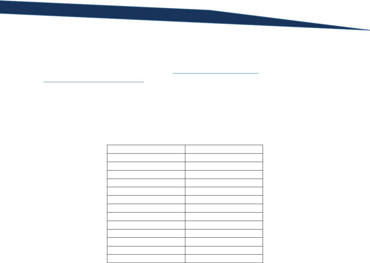
T-SQL Querying Guide © The Knowlton Group, LLC 74 | P a g e
There are several other date and time functions that return slightly different variations of the current
time. These include time zone offsets and UTC date and times. The two most commonly used at this
stage in SQL development will be either the GETDATE() or the SYSDATETIME() function. If you
information on the other functions, navigate to http://msdn.microsoft.com/en-
us/library/ms186724(v=sql.105).aspx.
Function: DATEDIFF()
Syntax: DATEDIFF(datepart, start_date, end_date)
Description: The DATEDIFF() function with find the datepart time gap between the start_date and
end_date values. There are many dateparts that can be used. These dateparts are captured in the table
below:
Datepart
Abbreviation
year
yy, yyyy
quarter
qq, q
month
mm, m
dayofyear
dy, y
day
dd, d
week
wk, ww
weekday
dw, w
hour
hh
minute
mi, n
second
ss, s
millisecond
ms
microsecond
mcs
nanosecond
ns
Example 1: Find the number of years between July 7, 1927 and May 14, 1929.
SELECT DATEDIFF(YEAR, '7/1/1927', '5/14/1929')
Example 2: Find the number of months between July 18, 1990 and May 14, 1991.
SELECT DATEDIFF(mm, '7/18/1990', '5/14/1991')
Example 3: Find the number of hours between 5:14 PM on June 3, 2008 and 12:15 PM on June 5, 2008.
SELECT DATEDIFF(HOUR, '6/3/2008 17:14:00', '6/5/2008 12:15:00')
Function: DATEADD()
Syntax: DATEADD(datepart, number, date_value)
Description: Add to the date_value date or time the number argument value in the specified datepart
intervals.

T-SQL Querying Guide © The Knowlton Group, LLC 75 | P a g e
Example 1: What was the date thirty days after April 7, 2011?
SELECT DATEADD(DAY, 30, '4/7/2011')
Example 2: What date will it be thirty days from today?
SELECT DATEADD(DAY, 30, GETDATE())
Example 3: What date was it three weeks before January 26, 2013?
SELECT DATEADD(WK, -3, '1/26/13')
The DATEADD() function will accept a negative value for the number argument. This allows you to
subtract a given number of dateparts from the time specified in the last argument.
Function: YEAR()
Syntax: YEAR(date)
Description: Returns the year of the date argument.
Example 1: What is the year value for the current date?
SELECT YEAR(SYSDATETIME())
Example 2: What year was it 8,456 days ago?
SELECT YEAR(DATEADD(DAY, -8456, GETDATE()))
In the previous nested function example, we first found what the date was 8,456 days ago. Then, given
the returned date value, we extracted the year datepart from the result.
Function: MONTH()
Syntax: MONTH(date)
Description: Returns the month value of the given date argument.
Example: What is the month value for November 11, 1945?
SELECT MONTH('11/11/1945')
Like MONTH() and YEAR(), there also exists a DAY() function which returns the day datepart from the
date value.
There are not as many date and time functions as there are string functions. However, becoming
familiar with date and time functions is a necessary skill in becoming a proficient developer of SQL
queries. Below are some practice problems that will help you gain experience using date and time
functions.

T-SQL Querying Guide © The Knowlton Group, LLC 76 | P a g e
Lab 13: Date and Time Built In Functions
1) What is the month datepart for June 12, 2011?
2) What is the year datepart for November 20, 1992?
3) What day was it seventy-four days ago?
4) What is the current date? Complete this problem using at least two different date functions.
5) How many days are between April 17, 1996 and September 4, 2001?
6) How many months are between December 25, 1993 and the date that is 2,719 days before
today’s date?
NULL Handling Functions
Though the majority of the functions will explore lie under the concept of “Date and Time” or “String”
functions, there are two other important functions we will look at: COALESCE() and NULLIF(). Both of
these functions are used to handle NULL values in your result set. The following brief section will show
examples of both functions being employed.
Function: COALESCE()
Syntax: COALESCE(expression_1, expression_2, …, expression_n)
Description: The COALESCE() function receives expressions as inputs and, based on the order of these
inputs, returns the first non-NULL value. These expression arguments can be columns, functions,
mathematical expressions, strings or any other type of SQL value.
Example 1: Retrieve the FirstName, MiddleName, and LastName columns from Person.Person.
However, anytime a NULL is present in the MiddleName column, replace it with a blank space.
SELECT FirstName, COALESCE(MiddleName, '') AS MiddleName, LastName
FROM Person.Person
If you look at the results of the previous query, you will notice that the MiddleName no longer contains
any NULL values in the output. Instead, you find many blank spaces. This indicates to us that the
COALESCE() function worked properly. To reiterate again, blank spaces are not equal to NULL values!
Example 2: Return the product name and the product color from Production.Product. If the product
does not have a value in the Color column, return the string “No Color Listed”.
SELECT Name AS ProductName, COALESCE(Color, 'No Color Listed') AS Color
FROM Production.Product
In place of the NULL value, the results now show the string “No Color Listed”. If you were exporting the
results of the query to an Excel file and providing the data to business users, replacing NULL values with
either blanks or some other meaningful text is often more valuable and more easily understood by the
recipient.

T-SQL Querying Guide © The Knowlton Group, LLC 77 | P a g e
Example 3: Using the Person.Person table, return the MiddleName column. If the MiddleName column
is NULL, then return the Title column. If the Title column is NULL then return the Suffix column. If the
Suffix column is NULL return the FirstName column.
SELECT COALESCE(MiddleName, Title, Suffix, FirstName)
FROM Person.Person
This is an unrealistic and trivial example, but it shows the capability of multiple expressions being
evaluated in the COALESCE() function. Since the COALESCE() function returns the first non-NULL value
of inputs, the function can evaluate multiple inputs at once. In the above example, the function looks to
see if the MiddelName value is NULL. If it is non-NULL then the MiddleName value is returned. If the
MiddleName value is NULL, then the function looks at the Title value. If the Title value is non-NULL then
that value is returned, else the function looks at whether or not the Suffix column value is NULL. This
iterative process completes until the function has exhausted all possible arguments.
Function: NULLIF()
Syntax: NULLIF(expression_1, expression_2)
Description: Returns a NULL value if the two expressions are equal.
Example 1: Return a NULL value if the BillToAddressID and ShipToAddressID in the table
Sales.SalesOrderHeader are equal.
SELECT NULLIF(BillToAddressID, ShipToAddressID)
FROM Sales.SalesOrderHeader
The NULLIF() function can, at times, provide a simpler solution to comparing value in a SELECT statement
without requiring CASE statements – a subject we will talk about in later sections.
Lab 14: NULL Handling Functions
1) If the Title column of Person.Person is NULL then return the string “No Title Listed”.
2) If the MiddleName column of Person.Person is NULL then return the string “No Middle Name
Listed”.
3) If the MiddleName column is NULL then return the FirstName and LastName concatenated. If
the MiddleName is non-NULL then return the FirstName, MiddleName and LastName
concatenated.
4) Using the Production.Product table, if the MakeFlag and FinishedGoodsFlag columns are equal
then return a NULL value.

T-SQL Querying Guide © The Knowlton Group, LLC 78 | P a g e
Section 11: SQL Server Data Types & Type Casting
Every column, variable, expression or parameter in SQL Server has an associated data type. This data
type represents the type of data that the value can store: integer data, money data, character data, etc.
We have found in the aggregate function section that certain functions only apply to values with certain
data types. For example, we cannot sum the values of a FirstName column. Logically, this makes sense.
Sometimes, however, we need to modify the data type of a column or value in order to return the value
in a form that we want. For example, the GETDATE() function returns the date in the datetime data type
format. This data type contains both date and time values. Suppose we only wanted to return the date
part of the result and not the timestamp component. To complete this request, we can use one of two
functions to perform a task known as type casting. This is where you alter the data type associated with
an expression or value.
SELECT CAST(GETDATE() AS DATE)
SELECT CONVERT(DATE, GETDATE())
The CONVERT() and CAST() functions complete the same task though CAST() is the more ANSI-standard
version of the casting functions. If you look at the results, you will notice that the timestamp is removed
from the result of GETDATE(). This is because the GETDATE() result, returned as a datetime data type,
has been casted as a date data type. This subtle change in data type removes the timestamp since the
timestamp is not a component of the date data type.
You may not be able to convert one data type to another data type. For example, trying to convert a
column containing non-Unicode strings, the VARCHAR data type, to a DECIMAL data type may not be
possible if the VARCHAR column contains values such as word, phrases or letters. If the VARCHAR
column contains all numeric values (despite the fact that the column is defined as a VARCHAR data
type), then the column could be cast to a numeric data type. If you tried, for example, to convert the
FirstName column of Person.Person to an integer, INT, data type, you would receive the following error:
SELECT CAST(FirstName AS INT)
FROM Person.Person
Error Message:
Msg 245, Level 16, State 1, Line 1
Conversion failed when converting the nvarchar value 'Syed' to data type int.
The database engine is going through each value in the column and trying to convert the value to the
INT data type. It runs into the NVARCHAR value “Syed” – an individual’s name – that clearly cannot be
converted to an integer. This - or a similar - error message is common when you attempt to type cast
from one data type to another data type that SQL will not allow.
One common area where type casting may be required is during the joining process. You may be trying
to join from an NVARCHAR column to a VARCHAR column. It is possible that you will need to cast one of
those data types to the matching data type in order to resolve the join. Observe the error message for

T-SQL Querying Guide © The Knowlton Group, LLC 79 | P a g e
indicating of type mismatches and review your code for potential locations that require type casting
within the SELECT statement.
Below is a table containing the common data types in SQL Server 2008R2. For more information on data
types and type casting, navigate to the following links: http://msdn.microsoft.com/en-
us/library/ms187928(v=sql.105).aspx and http://msdn.microsoft.com/en-
us/library/ms187752(v=sql.105).aspx.
Data Type
Description
bigint
An 8 byte integer ranging from -9,223,372,036,854,775,808 to
9,223,372,036,854,775,807
numeric
A numeric data type with fixed precision and scale
bit
An integer that can be either NULL, 0, or 1.
smallint
A 2 byte integer ranging from
decimal
A numeric data type with fixed precision and scale (functionally equivalent to
numeric)
smallmoney
A 4 byte representation of currency ranging from - 214,748.3648 to
214,748.3647
int
A 4 byte integer ranging from -2,147,483,648 to 2,147,483,647
tinyint
A 1 byte integer ranging from 0 to 255
money
An 8 byte representation of currency ranging from -922,337,203,685,477.5808
to 922,337,203,685,477.5807
float
An approximate numeric data type that falls within the ranges: - 1.79E+308 to -
2.23E-308, 0 and 2.23E-308 to 1.79E+308
real
An approximate numeric data type that falls within the ranges: - 3.40E + 38 to -
1.18E - 38, 0 and 1.18E - 38 to 3.40E + 38. The real data type is equivalent to
float(24).
date
A data type storing date values. They can be stored and viewed in a variety of
formats. The date data type has the range: 0001-01-01 through 9999-12-31
datetimeoffset
Combines the date and time into a time-zone aware value.
datetime2
A data type storing a date and time component with more precision than the
datetime data type.
smalldatetime
A smaller, subset data type of datetime. It allows values ranging from 1900-01-
01 through 2079-06-06.
datetime
Defines a date and time with fractional seconds.
time
Defines the time of data without time zone awareness.
char
A string of a defined fixed length (i.e. char(48) = 48 character, 48 bytes)
varchar
A string that cannot exceed the defined length yet whose storage space is
based on the length of the value + 2 bytes. (i.e. VARCHAR(20) means that no
value in the column can exceed 20 characters. Unless CHAR(20), if a value in
the common is six characters long then the storage for the VARCHAR column
will only use 8 bytes for that value.)
text
Variable length, non-Unicode string that cannot exceed 2,147,483,647
characters.

T-SQL Querying Guide © The Knowlton Group, LLC 80 | P a g e
nchar
Fixed length Unicode string data types between 1 and 4,000 characters.
Storage space is two times the length of the defined data type (i.e. nchar(4)
stores 8 bytes per value).
nvarchar
Variable length, Unicode string data. Similar to VARCHAR but with Unicode
values.
ntext
Variable length, Unicode string data that cannot exceed 1,073,741,823
characters.
Lab 15: SQL Server Data Types & Type Casting
1) Write the SQL SELECT statement that returns the FirstName column of Person.Person casted as
the VARCHAR data type.
2) Write three expressions in a single SELECT statement: one that returns the results of 11 divided
by 4. The second column should return the result of 11 casted as float divided by 4 casted as
float. The final column should divide 11.0 by 4.0 (including the decimal point and trailing zero).
3) Cast the FirstName column of Person.Person as the VARCHAR(3) data type. What happens?
Why?
4) Many of the values in the Size column of the Production.Product table contain numeric values.
Write a SELECT statement that returns the Size column casted as the integer data type. What is
the result? Why?
5) Using the same SELECT statement that you developed in problem 4, add the WHERE clause,
“WHERE ISNUMERIC(Size) = 1”. What is the result of the query now? Why? (Hint: use the MSDN
articles to find how the ISNUMERIC() function is used).

T-SQL Querying Guide © The Knowlton Group, LLC 81 | P a g e
Section 12: Table Expressions
A table expression can be thought of as a virtual table defined by a query. The scope of the results of a
table expression are confined to a single SELECT statement. You can think of a table expression as an
imaginary table that you create with columns and values that can be used in a SELECT statement. We
will discuss two types of table expressions: the derived table and the common table expression (CTE).
Derived Tables
A derived table is a table expression that appears in the FROM clause of a SELECT statement. Instead of
specifying a table or view name in the FROM clause, like we have in past examples, you will define a
simple query whose results will take the place of a table or view name. Let’s look at an example:
SELECT *
FROM (
SELECT BusinessEntityID, FirstName, LastName
FROM Person.Person
) AS PersonName
Notice how we are not placing a table name or view name after the FROM clause. Instead, we define a
derived table using a basic query – in this case, our derived table contains the BusinessEntityID,
FirstName, and LastName columns from Person.Person. We must always give a derived table a table
alias; in this case, we give the derived table the name PersonName. So you are aware of the type of
error message you will receive if no table alias is given, execute the query below and see the error
message that results:
SELECT *
FROM (
SELECT BusinessEntityID, FirstName, LastName
FROM Person.Person
)
Error Message:
Msg 102, Level 15, State 1, Line 5
Incorrect syntax near ')'.
Unfortunately, the error message is vague and, aside from giving us the location of the error, is relatively
unhelpful in specifically identifying the problem.
Derived tables have three other rules that must be met: all columns must have names, all columns must
have unique names, and the ORDER BY clause is not allowed unless TOP is included in the SELECT clause.
The first two should intuitively make sense: a table is not allowed to have a column without a name or
you would have no way of querying that nameless column. A table also cannot have multiple columns
with the same name. The database engine wouldn’t be able to tell which of the identically named
columns you wish to return. This, in a way, presents itself when joining tables. When two tables have

T-SQL Querying Guide © The Knowlton Group, LLC 82 | P a g e
the same column name, we must specify the table alias in front of the column name else we receive
error messages indicating column ambiguity.
There are several reasons as to why we may use a derived table. Remember back to when we discussed
that you could not use a column alias in the WHERE clause of your SELECT statement due to the order in
which SQL clauses are processed by the database. A derived table can help reduce the amount of typing
required to filter on functions that employ column aliases. For example, suppose I want to return how
many orders were placed each year from the Sales.SalesOrderHeader table. However, we only want to
return this information for the year 2006. We could avoid a derived table and complete the query this
way:
SELECT YEAR(OrderDate) AS OrderYear, COUNT(*) AS SalesCount
FROM Sales.SalesOrderHeader
WHERE YEAR(OrderDate) = '2006'
GROUP BY YEAR(OrderDate)
In the query above we are focused to constantly type out “YEAR(OrderDate)” in both the WHERE and
GROUP BY clause. However, with a derived table we could simplify the query slightly:
SELECT OrderYear, COUNT(*) AS SalesCount
FROM (
SELECT YEAR(OrderDate) AS OrderYear, SalesOrderID
FROM Sales.SalesOrderHeader
) SalesDetails
WHERE OrderYear = '2006'
GROUP BY OrderYear
Now the “YEAR(OrderDate)” is only specified once as opposed to three times in the first query. This may
seem trivial with a function as simple as “YEAR(OrderDate)”, but, with larger nested functions, simplicity
and reduced redundancy in your code can save you quite a bit of time and actually improve the query’s
performance.
Some functions, like the ranking functions we will explore in section 15, are not allowed to be used in
the WHERE clause. In these instances, the use of a table expression is necessary if you which to filter
based on the values of the ranking function.
Let’s look at a few more examples of derived tables to build up our comfort. Using a derived table
return the BusinessEntityID, NationalIDNumber, year of the birth date, and year of the hire date for all
rows where the year of the birth date is less than 1960. We can complete this query using:
SELECT *
FROM (
SELECT BusinessEntityID, NationalIDNumber, YEAR(BirthDate) AS BirthYear,
YEAR(HireDate) AS HiredYear
FROM HumanResources.Employee
) HR_Emp
WHERE BirthYear < 1960

T-SQL Querying Guide © The Knowlton Group, LLC 83 | P a g e
As you can see, we are applying a derived table with the YEAR() function for both the BirthDate and
HireDate columns. A column alias is applied to each column with the YEAR() function in the derived
table, and the derived table itself is given the table alias HR_Emp. We can now use the BirthYear alias
from the derived table in the WHERE clause and restrict our result set based on the request.
Using the same techniques, let’s return only those employees who were hired during or after the year
2004.
SELECT *
FROM (
SELECT BusinessEntityID, NationalIDNumber, YEAR(BirthDate) AS BirthYear,
YEAR(HireDate) AS HiredYear
FROM HumanResources.Employee
) HR_Emp
WHERE HiredYear >= 2004
Derived tables, like functions, can be nested within each other. Let’s look at the following example:
SELECT *
FROM (
SELECT BusinessEntityID, NationalIDNumber, BirthYear, YEAR(HireDate) AS HiredYear
FROM (
SELECT BusinessEntityID, NationalIDNumber, YEAR(BirthDate) AS BirthYear, HireDate
FROM HumanResources.Employee
) AS HR_Inner_Nested
) AS HR_Outer
Now, we have used a derived table in the FROM clause of another derived table. This is perfectly
acceptable and is often required for more complex queries. Notice how in the outer derived table we
are able to use the BirthYear column alias from the inner derived table.
We could add WHERE clauses to the derived tables to create a more robust and involved query:
SELECT *
FROM (
SELECT BusinessEntityID, NationalIDNumber, BirthYear, YEAR(HireDate) AS HiredYear
FROM (
SELECT BusinessEntityID, NationalIDNumber, YEAR(BirthDate) AS BirthYear, HireDate
FROM HumanResources.Employee
) AS HR_Inner_Nested
WHERE BirthYear < 1960
) AS HR_Outer
WHERE HiredYear > 2003
Now, we have employed a WHERE clause twice without having to include the YEAR() function. This
simplicity will be incredibly helpful as we add more complexity to our queries in later sections.
Just as we could use a derived table in the FROM clause, we can also use derived tables in joins. Say we
wanted to view, for each year we had sales, the total amount of sales revenue generated and the
number of employees hired for each year. This is a relatively complicated query, but it can be made
easier with the use of derived tables:

T-SQL Querying Guide © The Knowlton Group, LLC 84 | P a g e
SELECT Sales_by_Year.SalesYear, Sales_by_Year.TotalRevenue, Hires_by_Year.NewHireCount
FROM (
SELECT SalesYear, SUM(TotalDue) AS TotalRevenue
FROM (
SELECT YEAR(OrderDate) AS SalesYear, TotalDue
FROM Sales.SalesOrderHeader
) SalesDetails
GROUP BY SalesYear
) Sales_by_Year
LEFT OUTER JOIN (
SELECT HireYear, COUNT(BusinessEntityID) AS NewHireCount
FROM (
SELECT YEAR(HireDate) AS HireYear, BusinessEntityID
FROM HumanResources.Employee
) AS EmployeeDetails
GROUP BY HireYear
) AS Hires_by_Year
ON Hires_by_Year.HireYear = Sales_by_Year.SalesYear
ORDER BY 1
Both the FROM clause and the LEFT OUTER JOIN use nested derived tables. This is to emphasize that we
do not need to specify the YEAR() function in each WHERE clause. Each outer derived table is grouped
by the year and then the two sets of outer derived tables are joined by the year. Since we wanted the
sales and hire information for only the years in which we had sales, we start with the sales information
and then LEFT OUTER JOIN to the hiring information by year.
This query could also be written without a nested derived table in the FROM clause and the LEFT OUTER
JOIN:
SELECT Sales_by_Year.SalesYear, Sales_by_Year.TotalRevenue, Hires_by_Year.NewHireCount
FROM (
SELECT YEAR(OrderDate) AS SalesYear, SUM(TotalDue) AS TotalRevenue
FROM Sales.SalesOrderHeader
GROUP BY YEAR(OrderDate)
) Sales_by_Year
LEFT OUTER JOIN (
SELECT YEAR(HireDate) AS HireYear, COUNT(BusinessEntityID) AS NewHireCount
FROM HumanResources.Employee
GROUP BY YEAR(HireDate)
) AS Hires_by_Year
ON Hires_by_Year.HireYear = Sales_by_Year.SalesYear
ORDER BY 1
This second query is less lines but is more redundant than the first query due the repetition of the
YEAR() function in the GROUP BY clause of each derived table. We could have completed this query
with even less lines in a much more cumbersome and less readable manner with only a single derived
table:
SELECT YEAR(SOH.OrderDate) AS SalesYear, SUM(TotalDue) AS SalesRevenue
FROM Sales.SalesOrderHeader SOH
LEFT OUTER JOIN (
SELECT YEAR(HireDate) AS HiredYear, COUNT(*) AS NewHireCount
FROM HumanResources.Employee

T-SQL Querying Guide © The Knowlton Group, LLC 85 | P a g e
GROUP BY YEAR(HireDate)
) AS EmployeeDetails
ON EmployeeDetails.HiredYear = YEAR(SOH.OrderDate)
GROUP BY YEAR(SOH.OrderDate)
ORDER BY 1
We are forced to group on functions and use many of them in the SELECT clause and even in the ON line
of the LEFT OUTER JOIN. This is by no means wrong. It simply reduces readability and forces you to
modify multiple locations in the query to make even a minor change.
Spend some time going through the practice problems in the following lab section to practice using
derived tables.
Lab 16: Using Derived Tables
1) Will the following query execute properly? Why or why not?
SELECT *
FROM (
SELECT P.BusinessEntityID, P.FirstName, P.LastName, YEAR(E.HireDate)
FROM HumanResources.Employee E
INNER JOIN Person.Person P
ON P.BusinessEntityID = E.BusinessEntityID
) AS EmployeeDetails
2) Will the following query execute properly? Why or why not?
SELECT *
FROM (
SELECT TOP 100 P.BusinessEntityID, P.FirstName, P.LastName
FROM HumanResources.Employee E
INNER JOIN Person.Person P
ON P.BusinessEntityID = E.BusinessEntityID
ORDER BY 1
) AS EmployeeDetails
3) Using a derived table so that no functions will appear in the WHERE clause, find all employees
from the HumanResources.Employee table who were hired in the year 2006 or greater and who
were born in the year 1968 or less.
4) Using a derived table, find the total sales revenue generated for the year 2005 and 2006. The
WHERE and GROUP BY clause of your SELECT statement should have no functions.
Using Common Table Expressions
A common table expression (hereon referred to as a CTE) is another type of table expression in SQL
Server that has certain advantages over a derived table. A CTE is directly queried in the FROM clause
like the derived table; instead it is defined before the SELECT clause. In the subsection on derived
tables, we looked at this example query:

T-SQL Querying Guide © The Knowlton Group, LLC 86 | P a g e
SELECT OrderYear, COUNT(*) AS SalesCount
FROM (
SELECT YEAR(OrderDate) AS OrderYear, SalesOrderID
FROM Sales.SalesOrderHeader
) SalesDetails
WHERE OrderYear = '2006'
GROUP BY OrderYear
We can return the same results using a CTE by executing the query:
WITH SalesDetails
AS (
SELECT YEAR(OrderDate) AS OrderYear, SalesOrderID
FROM Sales.SalesOrderHeader
)
SELECT OrderYear, COUNT(*) AS SalesCount
FROM SalesDetails
WHERE OrderYear = '2006'
GROUP BY OrderYear
Notice that the CTE begins with “WITH” and then the name of the CTE is specified – in this case
“SalesDetails”. Then we type “AS” and open a parenthesis. From there, we type the query that will
define the CTE and close the opening parenthesis. Next, we type our query that uses the CTE simply by
referencing its name. Unlike the derived table, there is a separation of sorts in that the table expression
is not directly defined in the eventual SELECT statement. Let’s look at another example of a query we
completed using a derived table and then how we could return the same results with a CTE.
In the last subsection, we created the following query using a derived table:
SELECT *
FROM (
SELECT BusinessEntityID, NationalIDNumber, YEAR(BirthDate) AS BirthYear,
YEAR(HireDate) AS HiredYear
FROM HumanResources.Employee
) HR_Emp
WHERE HiredYear >= 2004
We could rewrite this query using a CTE with the query:
WITH HR_Emp
AS (
SELECT BusinessEntityID, NationalIDNumber, YEAR(BirthDate) AS BirthYear,
YEAR(HireDate) AS HiredYear
FROM HumanResources.Employee
)
SELECT *
FROM HR_Emp
WHERE HiredYear >= 2004

T-SQL Querying Guide © The Knowlton Group, LLC 87 | P a g e
The query used to define the table expression does not change; the location in which it is defined and
how it is called are just slightly different between CTEs and derived tables.
CTEs possess an advantage over derived tables in that they can be used multiple times during a SELECT
statement. Say, for example, that we wanted to return three columns: the sales year, the total sales
that year and the total sales the year before. To complete this query using derived tables, we would
have to type the same derived table twice:
SELECT
SalesCurrentYear.SalesYear,
SalesCurrentYear.TotalSales AS AnnualSales,
SalesPriorYear.TotalSales AS PriorYearSales
FROM (
SELECT YEAR(OrderDate) AS SalesYear, SUM(TotalDue) AS TotalSales
FROM Sales.SalesOrderHeader
GROUP BY YEAR(OrderDate)
) AS SalesCurrentYear
LEFT OUTER JOIN (
SELECT YEAR(OrderDate) AS SalesYear, SUM(TotalDue) AS TotalSales
FROM Sales.SalesOrderHeader
GROUP BY YEAR(OrderDate)
) AS SalesPriorYear
ON SalesCurrentYear.SalesYear - 1 = SalesPriorYear.SalesYear
ORDER BY 1
However, a CTE can be called multiple times in the same SELECT statement. The above query could be
reduced to:
WITH SalesByYear
AS (
SELECT YEAR(OrderDate) AS SalesYear, SUM(TotalDue) AS TotalSales
FROM Sales.SalesOrderHeader
GROUP BY YEAR(OrderDate)
)
SELECT
CurrentYearSales.SalesYear,
CurrentYearSales.TotalSales AS AnnualSales,
PriorYearSales.TotalSales AS PriorYearSales
FROM SalesByYear AS CurrentYearSales
LEFT OUTER JOIN SalesByYear AS PriorYearSales
ON CurrentYearSales.SalesYear - 1 = PriorYearSales.SalesYear
ORDER BY 1
Notice how the SalesByYear CTE is defined once initially but is used in both the FROM clause and the
LEFT OUTER JOIN. The ability to reuse the CTE in the SELECT statement is an important benefit that the
CTE possesses over the derived table. For many queries, this can reduce the amount of code required to
complete a SQL statement.
Another benefit that CTEs possess over derived tables is that a CTE can be directly nested in other CTEs.
Let’s take a look at an example of this:

T-SQL Querying Guide © The Knowlton Group, LLC 88 | P a g e
WITH S1
AS (
SELECT YEAR(OrderDate) AS SalesYear, SalesOrderID, TotalDue
FROM Sales.SalesOrderHeader
),
S2 AS (
SELECT SalesYear, COUNT(SalesOrderID) AS SalesCount, SUM(TotalDue) AS AnnualSales
FROM S1
GROUP BY SalesYear
)
SELECT SalesYear, SalesCount, AnnualSales
FROM S2
WHERE SalesCount > 5000
ORDER BY 1
Looking carefully at the CTE “S2”, you will see that the table expression is created based on data from
the CTE “S1”. As complexity in your queries expands, the ability to simplify these steps will improve the
readability of your code and allow you to make code modifications much more easily.
CTEs and derived tables are often necessary in order to complete some SQL queries. Becoming familiar
with them is essential in becoming a proficient intermediate SQL developer. Complete the following lab
questions to reinforce your understanding of common table expressions.
Lab 17: Common Table Expressions
1) Will the following code execute properly? Why or why not?
WITH Sales
AS (
SELECT YEAR(OrderDate), TotalDue
FROM Sales.SalesOrderHeader
)
SELECT *
FROM Sales
2) Using CTEs, find out, for each year the company hired new employees, how many employees
the company hired for each year and how many employees they hired the previous year. Use
the HumanResources.Employee table for this lab question. You should have return three
columns: the hire year, the number of employees hired that year, and the number of employees
hired the year before.
3) Using a CTE such that no functions are contained in the GROUP BY clause of the SELECT
statement, find the number of products that began selling per year (using the
Production.Product table and the SellStartDate column).
4) Using a CTE that references the Sales.SalesOrderHeader table, find each month’s total sales for
the year 2006. No functions should be used in either the WHERE or the GROUP BY clause of
your SELECT statement.

T-SQL Querying Guide © The Knowlton Group, LLC 89 | P a g e
Section 13: CASE Statements
CASE statements are an incredibly helpful tool in completing more advanced SELECT statements. A
CASE statement allows you to evaluate multiple conditions and return one possible expression based on
the criteria you define. Let’s take a look at an example:
SELECT ProductID, ListPrice,
CASE
WHEN ListPrice > 100 THEN 'Expensive Product'
ELSE 'Inexpensive Product'
END AS ProductPriceClass
FROM Production.Product
WHERE ListPrice <> 0
The previous query returns the ProductID and ListPrice column from the Production.Product table for all
rows that do not have a ListPrice value equal to zero. The third column in the result, which we call
ProductPriceClass, is a CASE statement that, based on certain conditions, outputs a classification of the
product’s price based on the ListPrice column value. We are telling SQL that if the ListPrice value of the
row exceeds 100, then return the string “Expensive Product”. If that condition is not met, then SQL
returns the string “Inexpensive Product”.
CASE statements are useful when trying to classify row values into ranges. A marketing department
often stratifies their customer information by age ranges to understand their consumer demographics.
Let’s apply the same concept to our AdventureWorks data set and group our customers into age ranges
and output the results:
WITH CustomerAges
AS (
SELECT
P.FirstName, P.LastName, FLOOR(DATEDIFF(DAY, PD.BirthDate,
GETDATE())/365.25) AS Age
FROM Sales.vPersonDemographics PD
INNER JOIN Person.Person P
ON PD.BusinessEntityID = P.BusinessEntityID
)
SELECT *,
CASE
WHEN Age IS NULL THEN 'Unknown Age'
WHEN Age BETWEEN 0 AND 17 THEN 'Under 18'
WHEN Age BETWEEN 18 AND 24 THEN '18 to 24'
WHEN Age BETWEEN 25 AND 34 THEN '25 to 34'
WHEN Age BETWEEN 35 AND 49 THEN '35 to 49'
WHEN Age BETWEEN 50 AND 64 THEN '50 to 64'
ELSE 'Over 65'
END AS AgeRange
FROM CustomerAges
We are first using a CTE to reduce the number of times we have to write our Age function. The age
column uses the DATEDIFF() function to determine the number of days between the customer’s birth
date and the current date. Dividing the result by 365.25 yields a more accurate numeric value of the

T-SQL Querying Guide © The Knowlton Group, LLC 90 | P a g e
customer’s true age. We then use the FLOOR() function, a function we haven’t yet seen, which simply
truncates the decimal and returns only the leading integer. Then, using our CTE in the SELECT
statement, we use a multi-condition CASE statement to define the age values that comprise each range.
Let’s take the previous query a step further and count the number of customers that fit into each age
range. We will again utilize CTEs to reduce the redundancy in our code:
WITH CustomerAges
AS (
SELECT
P.BusinessEntityID,
P.FirstName,
P.LastName,
FLOOR(DATEDIFF(DAY, PD.BirthDate, GETDATE())/365.25) AS Age
FROM Sales.vPersonDemographics PD
INNER JOIN Person.Person P
ON PD.BusinessEntityID = P.BusinessEntityID
),
CustomerAgeRanges AS (
SELECT
CASE
WHEN Age IS NULL THEN 'Unknown Age'
WHEN Age BETWEEN 0 AND 17 THEN 'Under 18'
WHEN Age BETWEEN 18 AND 24 THEN '18 to 24'
WHEN Age BETWEEN 25 AND 34 THEN '25 to 34'
WHEN Age BETWEEN 35 AND 49 THEN '35 to 49'
WHEN Age BETWEEN 50 AND 64 THEN '50 to 64'
ELSE 'Over 65'
END AS AgeRange, BusinessEntityID
FROM CustomerAges
)
SELECT AgeRange, COUNT(*) AS Customer_Count
FROM CustomerAgeRanges
GROUP BY AgeRange
ORDER BY 1
Now, we have been able to use two CTEs so that a large CASE statement or function is not being placed
in our GROUP BY clause. Creating multi-step conditional outputs based on the column values is not an
uncommon practice in more involved SQL queries. Generally, queries are developed to return data for
business users. Business users often want to see their data presented in ways that does not necessarily
match up to how the data exists in the database. Something as simple as the Gender column in the
Sales.vPersonDemographics view may require output modification for a business user’s satisfaction. In
our database, the Gender field is marked by either NULL values or an “M” or “F” value. Our business
users may want to see “Male” and “Female” in place of “M” and “F”. A CASE statement would allow us
to complete their request without issue:
SELECT
PD.BusinessEntityID,
P.FirstName,
P.LastName,
CASE

T-SQL Querying Guide © The Knowlton Group, LLC 91 | P a g e
WHEN PD.Gender = 'M' THEN 'Male'
WHEN PD.Gender = 'F' THEN 'Female'
ELSE 'No Gender Specified'
END AS Gender
FROM Sales.vPersonDemographics PD
INNER JOIN Person.Person P
ON P.BusinessEntityID = PD.BusinessEntityID
In just a few short lines of code, we are able to alter the output of the Gender column to satisfy the
requirements of the business user who requested the data.
If you remember back to our section on NULL Handling Functions, we observed the COALESCE()
function. We can create a CASE statement that is functionally equivalent to the COALESCE() function:
SELECT
MiddleName,
CASE
WHEN MiddleName IS NULL THEN ''
ELSE MiddleName
END AS NULL_Handled_MiddleName
FROM Person.Person
You can think of the COALESCE() function as a CASE statement that simply handles when the value of the
input argument is NULL. There are many of these similarities throughout SQL Server and trying to
understand them will greatly improve your understanding of the querying language.
We can also use CASE statements to cleverly order our results when we wish to use a non-standard
ordering method. For example, let’s say we wanted to find each customer’s historical sales with our
company. Then, we want to use various ranges to see how many customers fall into each historical
sales range. Given the names of our sales ranges, however, ordering in ascending or descending order
does not properly order the results given the combination of numbers, symbols and text. The query
below will accomplish this request:
WITH CustomerSales
AS (
SELECT
P.BusinessEntityID,
SUM(SOH.TotalDue) AS TotalSalesAmount
FROM Sales.SalesOrderHeader SOH
INNER JOIN Sales.Customer SC
ON SC.CustomerID = SOH.CustomerID
INNER JOIN Person.Person P
ON P.BusinessEntityID = SC.PersonID
GROUP BY P.BusinessEntityID
),
CustomerSalesRange AS (
SELECT
P.FirstName + ' ' + P.LastName AS CustomerName,
CASE
WHEN CS.TotalSalesAmount BETWEEN 0 AND 149.99 THEN 'Under $150'

T-SQL Querying Guide © The Knowlton Group, LLC 92 | P a g e
WHEN CS.TotalSalesAmount BETWEEN 150 AND 499.99 THEN '$150 -
$499.99'
WHEN CS.TotalSalesAmount BETWEEN 500 AND 999.99 THEN '$500 -
$999.99'
WHEN CS.TotalSalesAmount BETWEEN 1000 AND 4999.99 THEN '$1,000 -
$4,999.99'
WHEN CS.TotalSalesAmount BETWEEN 5000 AND 14999.99 THEN '$5,000 -
$14,999.99'
WHEN CS.TotalSalesAmount BETWEEN 15000 AND 49999.99 THEN '$15,000 -
$49,999.99'
WHEN CS.TotalSalesAmount BETWEEN 50000 AND 149999.99 THEN '$50,000 -
$149,999.99'
ELSE 'Over $150,000'
END AS SalesRange
FROM CustomerSales CS
INNER JOIN Person.Person P
ON P.BusinessEntityID = CS.BusinessEntityID
)
SELECT SalesRange, COUNT(*) AS [Customers in Range]
FROM CustomerSalesRange
GROUP BY SalesRange
ORDER BY
CASE
WHEN SalesRange = 'Under $150' THEN 1
WHEN SalesRange = '$150 - $499.99' THEN 2
WHEN SalesRange = '$500 - $999.99' THEN 3
WHEN SalesRange = '$1,000 - $4,999.99' THEN 4
WHEN SalesRange = '$5,000 - $14,999.99' THEN 5
WHEN SalesRange = '$15,000 - $49,999.99' THEN 6
WHEN SalesRange = '$50,000 - $149,999.99' THEN 7
WHEN SalesRange = 'Over $150,000' THEN 8
END
This is a rather lengthy query, but it does not utilize any technique we are not already familiar with. We
first define two CTEs so that we do not need to type out the large CASE statement in
CustomerSalesRange an unnecessary amount of times in our code. Then we start our SELECT statement
by grouping our results by the SalesRange column and finding the number of rows that fit into each
range. The unique aspect of this query is the CASE statement in the ORDER BY clause. If you remove the
ORDER BY clause and execute the query, you will notice the improper ordering that we discussed in the
previous paragraph. However, a CASE statement will resolve this ordering issue. In this CASE statement,
we are telling the ORDER BY clause to assign the value 1 to the first SalesRange (“Under $150”), 2 for the
second SalesRange (“$150 - $499.99”), and so on. The ORDER BY clause then orders not by the
SalesRange text but by the number we assign to it in the CASE statement. This forces the ORDER BY
clause to order in the method we desire – the correct ordering method given the ranges.
CASE statements can be an invaluable tool in writing successful SQL queries. The ability to modify
output column values based on several conditions, defining ranges, and even defining atypical ordering
are all benefits that CASE statements offer. Complete the following lab exercises to gain some
additional practice.

T-SQL Querying Guide © The Knowlton Group, LLC 93 | P a g e
Lab 18: CASE Statements
1) Return the FirstName and LastName column from Person.Person. Return a third column that
outputs “Promotion 1” if the EmailPromotion column value is 0, “Promotion 2” if the
EmailPromotion value is 1, and “Promotion 3” if the column value is 2.
2) In a CASE statement you define conditional expressions based on column values. What happens
if a value does not meet any of the conditions expressed in the CASE statement?
3) Using the Person.Person table, complete a CASE statement that returns the string “Long Name”
if the FirstName column is at least ten characters long. If the FirstName column is less than ten
characters, return the string “Short Name”.
4) Find out how many sales in Sales.SalesOrderHeader fell into the following ranges: “$0 to
$149.99”, “$150 – 499.99”, “$500 to $4,999.99”, “$5,000 - $24,999.99”, and “Over $25,000”.
Only analyze sales that had a sales person associated with them.
5) Using the Production.Product table, if the value in Color column is NULL then return the string
“No Color”. If a color exists, then return that color. Complete this request two ways: once with
a CASE statement, and the second with a function we have previously discussed in this guide.

T-SQL Querying Guide © The Knowlton Group, LLC 94 | P a g e
Section 14: Ranking Functions
Ranking functions allow you to rank your results given a certain grouping (referred to as a partition in a
ranking function) and in a specified order. There are four ranking functions: ROW_NUMBER(), RANK(),
DENSE_RANK() and NTILE(). As with each of the prior sections that involve functions, we will provide the
syntax and description of each along with several supporting examples.
Function: ROW_NUMBER()
Syntax: ROW_NUMBER() OVER([PARTITION BY partition_argument] ORDER BY order_by_clause)
Description: The ROW_NUMBER() ranking function returns the sequential number of each row within
the context of each partition and ordered based on the order_by_clause.
Example 1: For each employee in HumanResources.Employee, return the BusinessEntityID, HireDate
and then the numerical order in which each employee was hired such that the first employee hired has
the value 1.
SELECT
BusinessEntityID,
HireDate,
ROW_NUMBER() OVER(ORDER BY HireDate ASC) AS HireOrder
FROM HumanResources.Employee
In this example, we do not need to use the PARTITION BY component of the ROW_NUMBER() function
since we are looking at the entire data set as one partition. You will notice that the row with the
HireOrder value of 1 is the employee that has the oldest HireDate just as we desired.
Example 2: Find the SalesOrderID, CustomerID, OrderDate and a ranking function that tells us what
order number each sale is for each customer. So, for each customer’s oldest order, we wish to see the
value 1 in this ranking column. Order the results by the CustomerID and then the ranking function
column.
SELECT
SalesOrderID,
CustomerID,
OrderDate,
ROW_NUMBER() OVER(PARTITION BY CustomerID ORDER BY OrderDate) AS
CustomerSalesOrder
FROM Sales.SalesOrderHeader
ORDER BY 2, 4
Now you will notice we employ the PARTITION BY clause of the ROW_NUMBER() function to partition
the set into groups based on the CustomerID. Given the ORDER BY component within the
ROW_NUMBER() function, the first order that a customer places is assigned a value of 1, the second a
value of 2, and so on.
Example 3: Using the ROW_NUMBER() function, rank each sales person by their total sales in 2006. The
sales person with the most sales should be given the value of 1.

T-SQL Querying Guide © The Knowlton Group, LLC 95 | P a g e
WITH Sales_2006
AS (
SELECT
P.FirstName + ' ' + P.LastName AS SalesPerson,
SOH.TotalDue
FROM Sales.SalesOrderHeader SOH
INNER JOIN Sales.SalesPerson SP
ON SP.BusinessEntityID = SOH.SalesPersonID
INNER JOIN Person.Person P
ON P.BusinessEntityID = SP.BusinessEntityID
WHERE YEAR(SOH.OrderDate) = 2006
)
SELECT
SalesPerson,
SUM(TotalDue) AS Total_2006_Sales,
ROW_NUMBER() OVER(ORDER BY SUM(TotalDue) DESC) AS SalesPersonRank
FROM Sales_2006
GROUP BY SalesPerson
Instead of ordering by a specific column, we had to order by the SUM(TotalDue) given that we were
grouping our data by the SalesPerson column. This is completed acceptable for the ROW_NUMBER()
function. We could have grouped our data before the ranking function with a query like:
WITH Sales_2006
AS (
SELECT
P.FirstName + ' ' + P.LastName AS SalesPerson,
SUM(SOH.TotalDue) AS Total_2006_Sales
FROM Sales.SalesOrderHeader SOH
INNER JOIN Sales.SalesPerson SP
ON SP.BusinessEntityID = SOH.SalesPersonID
INNER JOIN Person.Person P
ON P.BusinessEntityID = SP.BusinessEntityID
WHERE YEAR(SOH.OrderDate) = 2006
GROUP BY P.FirstName + ' ' + P.LastName
)
SELECT *, ROW_NUMBER() OVER(ORDER BY Total_2006_Sales DESC) AS SalesPersonRank
FROM Sales_2006
It is a matter of personal preference. The only difference is that the grouping occurs in the CTE in the
second version of the query as opposed to occurring in the outer SELECT statement like in the first
query. Whichever method you choose, the ROW_NUMER() function is still properly ranking based on
the sales person’s sales in 2006 as the query requires.
Though it may not initially seem to be important, this query has proven to be tremendously valuable in
my experience. In the section on subqueries, we will see some examples where the ROW_NUMBER()
enables us to retrieve data that might have been incredibly difficult to complete otherwise.
Function: RANK()
Syntax: RANK() OVER([PARTITION BY partition_argument] ORDER BY order_by_clause)

T-SQL Querying Guide © The Knowlton Group, LLC 96 | P a g e
Description: Returns the rank of each row such that the rank equals one plus the number of ranks
preceding it. If you image sports standing with two teams tied for first, the rank for those two teams
would be the number 1. However, the third team would not have the rank of 2 but would have the rank
3.
Example 1: Find the number of products in each order. Then find which order quantity is the most
common and rank them accordingly.
WITH SalesOrderQuantities
AS (
SELECT SOH.SalesOrderID, SUM(SOD.OrderQty) AS QtyPerOrder
FROM Sales.SalesOrderHeader SOH
INNER JOIN Sales.SalesOrderDetail SOD
ON SOH.SalesOrderID = SOD.SalesOrderID
GROUP BY SOH.SalesOrderID
),
SalesOrderQuantitiesGrouped
AS (
SELECT QtyPerOrder, COUNT(*) AS Orders_with_Quantity
FROM SalesOrderQuantities
GROUP BY QtyPerOrder
)
SELECT
QtyPerOrder,
Orders_with_Quantity,
RANK() OVER(ORDER BY Orders_with_Quantity DESC) AS OrderQuantityRank
FROM SalesOrderQuantitiesGrouped
This query first finds out how many products were ordered with each order. Then it finds out how many
orders were associated with each order quantity. Lastly, in the outer SELECT statement, the RANK()
function supplies us with a rank for each order quantity based on how many orders had the specified
order quantity.
Example 2: Open and the SQL file named “NHL_Standings.sql” and execute the code if you have not
already done so. The generated table contains the 2014 point totals for each NHL team at the end of
the regular season. Using the RANK() function, find each team’s rank.
SELECT
TeamName,
RANK() OVER(ORDER BY Points DESC) AS NHL_Rank
FROM NHL_Standings_2014
You will notice that both St. Louis and San Jose were tied for fourth place (we are not taking into
account the tiebreaker rules the NHL has in place for this query). The team after those two, Pittsburgh,
is not the fifth ranked team but rather the sixth ranked team. This is the main subtlety of the RANK()
function.
Function: DENSE_RANK()
Syntax: DENSE_RANK() OVER([PARTITION BY partition_argument] ORDER BY order_by_clause)

T-SQL Querying Guide © The Knowlton Group, LLC 97 | P a g e
Description: Returns the rank of each row in the partition such that the dense rank equals one plus the
number of distinct ranks before the specified row. This is slightly different than the RANK() function and
will become clear in the examples.
Example 1: Rank the NHL teams based on their point totals using the NHL_Standings_2014 table. Unlike
the previous example, use the DENSE_RANK() function instead of the RANK() function.
SELECT
TeamName,
DENSE_RANK() OVER(ORDER BY Points DESC) AS NHL_Rank
FROM NHL_Standings_2014
Unlike when we used the RANK() function, Pittsburgh – the team following the two teams tied for fourth
place – now has a dense rank value of 5 instead of 6. Unlike the rank function which supplies a rank of a
one plus the number of ranked rows prior to the row in question, the dense rank gives a value of one
plus the number of distinct ranks preceding the row. In this case, there were only four distinct dense
ranks before Pittsburgh, hence they receive a dense rank value of 5.
Example 2: View both the dense rank and rank of each NHL team side-by-side.
SELECT
TeamName,
RANK() OVER(ORDER BY Points DESC) AS NHL_Rank,
DENSE_RANK() OVER(ORDER BY Points DESC) AS NHL_Dense_Rank
FROM NHL_Standings_2014
You will see that there are a few instances of these “ties”. Both the DENSE_RANK() and RANK()
functions handle the subsequent values after the tie differently. Keep this difference in mind as you
complete requests that may require a rank similar to those we have seen in the previous three
examples.
Function: NTILE()
Syntax: NTILE() OVER([PARTITION BY partition_argument] ORDER BY order_by_clause)
Description: Partitions the rows into the number of groups specified in the NTILE() argument based on
the ordering method specified with the order_by_clause.
Example 1: Based on each sales person’s sales in 2006, assign them to one of four tiers such that the top
tier, tier 1, contains only the highest performing sales people.
WITH SalesPerson_2006
AS (
SELECT
P.FirstName + ' ' + P.LastName AS SalesPerson,
SUM(SOH.TotalDue) AS TotalSales_2006
FROM Sales.SalesOrderHeader SOH
INNER JOIN Sales.SalesPerson SP
ON SP.BusinessEntityID = SOH.SalesPersonID
INNER JOIN Person.Person P
ON P.BusinessEntityID = SP.BusinessEntityID
WHERE YEAR(SOH.OrderDate) = 2006
GROUP BY P.FirstName + ' ' + P.LastName

T-SQL Querying Guide © The Knowlton Group, LLC 98 | P a g e
)
SELECT
SalesPerson,
NTILE(4) OVER(ORDER BY TotalSales_2006 DESC) AS SalesPersonTier
FROM SalesPerson_2006
Since we specified the number 4 in the NTILE() clause, the function will split the results into four groups.
Unfortunately, since the number of rows (14) is not divisible by four, the remainder of the number of
rows and NTILE() group argument is applied to the first groups. Since 14 divided by 4 has a remainder of
two, the first two groups have one more row than groups three and four.
Example 2: Group our sales force into three groups based on their 2006 sales. Using a CASE statement
and the NTILE() ranking function, label the first group as “Top Tier”, second group as “Middle Tier”, and
third group as “Bottom Tier”.
WITH SalesPerson_2006
AS (
SELECT
P.FirstName + ' ' + P.LastName AS SalesPerson,
SUM(SOH.TotalDue) AS TotalSales_2006
FROM Sales.SalesOrderHeader SOH
INNER JOIN Sales.SalesPerson SP
ON SP.BusinessEntityID = SOH.SalesPersonID
INNER JOIN Person.Person P
ON P.BusinessEntityID = SP.BusinessEntityID
WHERE YEAR(SOH.OrderDate) = 2006
GROUP BY P.FirstName + ' ' + P.LastName
)
SELECT
SalesPerson,
CASE
WHEN NTILE(3) OVER(ORDER BY TotalSales_2006 DESC) = 1 THEN 'Top Tier'
WHEN NTILE(3) OVER(ORDER BY TotalSales_2006 DESC) = 2 THEN 'Middle Tier'
WHEN NTILE(3) OVER(ORDER BY TotalSales_2006 DESC) = 3 THEN 'Bottom Tier'
END AS SalesPersonTier
FROM SalesPerson_2006
In this scenario, we have embedded the NTILE() function directly into our CASE statement. We could
have reduced this redundancy by using a second CTE:
WITH SalesPerson_2006
AS (
SELECT
P.FirstName + ' ' + P.LastName AS SalesPerson,
SUM(SOH.TotalDue) AS TotalSales_2006
FROM Sales.SalesOrderHeader SOH
INNER JOIN Sales.SalesPerson SP
ON SP.BusinessEntityID = SOH.SalesPersonID
INNER JOIN Person.Person P
ON P.BusinessEntityID = SP.BusinessEntityID
WHERE YEAR(SOH.OrderDate) = 2006
GROUP BY P.FirstName + ' ' + P.LastName

T-SQL Querying Guide © The Knowlton Group, LLC 99 | P a g e
),
SalesPerson_NTILE AS (
SELECT
SalesPerson,
NTILE(3) OVER(ORDER BY TotalSales_2006 DESC) AS SalesPersonTierNumber
FROM SalesPerson_2006
)
SELECT
SalesPerson,
CASE
WHEN SalesPersonTierNumber = 1 THEN 'Top Tier'
WHEN SalesPersonTierNumber = 2 THEN 'Middle Tier'
WHEN SalesPersonTierNumber = 3 THEN 'Bottom Tier'
END AS SalesPersonTier
FROM SalesPerson_NTILE
Ranking functions are necessary in many analytic applications. You may be determining which areas
have the most traffic, the most visited branches, the most purchased products or any number of other
analytic questions that leverages ranking functions. Understanding the subtleties of each and where
and when to use them is an essential skill for a SQL developer.
Lab 19: Ranking Functions
1) Using the ROW_NUMBER() function, rank each customer by the amount they purchased in the
year 2005.
2) Using the RANK() function, rank each product by how many times it was ordered in the year
2006.
3) Complete the same query as the previous lab question except use the DENSE_RANK() function
instead of the RANK() function. Find any differences between the two ranking methods.
4) Find the total sales for each territory in the year 2006. Using the NTILE() function, split them
into two groups.
5) Expanding on question four, complete a CASE statement that takes the result of the NTILE()
function and assigns the value “Top Territory Group” when the NTILE() value is 1 and “Bottom
Territory Group” when the NTILE() value is 2.
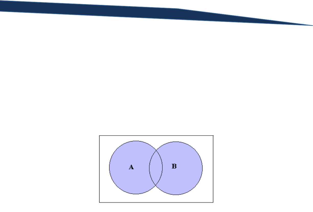
T-SQL Querying Guide © The Knowlton Group, LLC 100 | P a g e
Section 15: Set Operations
Set operations use specific operators to combine multiple queries into a single result set. This is
different from a join operation where columns from both tables are presented into a single
representation. Set operations simply combine results from separate queries into a single result.
There are three major set operations: UNION, EXCEPT, and INTERSECT. However, there are keywords
that can be used for each set operations to alter the result.
Set Operation: UNION
Description: Combines results from multiple queries into one result such that the results contains all
rows from both queries.
Venn Diagram:
As you can see by the Venn diagram, both sets are shaded (equate a set to either a table or query)
indicating that the results of the union of the sets contains all data from both sets.
Example 1: Find all states in which our customers reside. Find all states in which our employees reside.
Union the two queries such that the states where our employees reside and the states where our
customers reside both appear in the results.
SELECT SP.Name AS StateProvinceName
FROM HumanResources.Employee E
INNER JOIN Person.BusinessEntityAddress BEA
ON BEA.BusinessEntityID = E.BusinessEntityID
INNER JOIN Person.[Address] PA
ON PA.AddressID = BEA.AddressID
INNER JOIN Person.StateProvince SP
ON SP.StateProvinceID = PA.StateProvinceID
UNION
SELECT SP.Name AS StateProvinceName
FROM Sales.Customer SC
INNER JOIN Person.Person P
ON P.BusinessEntityID = SC.PersonID
INNER JOIN Person.BusinessEntityAddress BEA

T-SQL Querying Guide © The Knowlton Group, LLC 101 | P a g e
ON BEA.BusinessEntityID = P.BusinessEntityID
INNER JOIN Person.[Address] PA
ON PA.AddressID = BEA.AddressID
INNER JOIN Person.StateProvince SP
ON SP.StateProvinceID = PA.StateProvinceID
The top query identifies all states where our employees reside, while the bottom query identifies all
states where our customers reside. The union of these two sets takes the distinct list of states from
both queries. By default, the UNION set operation only takes the distinct combination of both sets. For
example, Washington appears many times in the top query, but it appears only once in the results.
The keyword ALL can be placed after the UNION operation and the result will be dramatically different:
SELECT SP.Name AS StateProvinceName
FROM HumanResources.Employee E
INNER JOIN Person.BusinessEntityAddress BEA
ON BEA.BusinessEntityID = E.BusinessEntityID
INNER JOIN Person.[Address] PA
ON PA.AddressID = BEA.AddressID
INNER JOIN Person.StateProvince SP
ON SP.StateProvinceID = PA.StateProvinceID
UNION ALL
SELECT SP.Name AS StateProvinceName
FROM Sales.Customer SC
INNER JOIN Person.Person P
ON P.BusinessEntityID = SC.PersonID
INNER JOIN Person.BusinessEntityAddress BEA
ON BEA.BusinessEntityID = P.BusinessEntityID
INNER JOIN Person.[Address] PA
ON PA.AddressID = BEA.AddressID
INNER JOIN Person.StateProvince SP
ON SP.StateProvinceID = PA.StateProvinceID
Unlike a standard UNION set operation that returns the distinct combined list from both SELECT
statement, the UNION ALL set operation returns every row regardless of whether or not it is a duplicate
value.
Set Operation: INTERSECT
Description: Returns the values from two queries that are present in both sets.
Venn Diagram:

T-SQL Querying Guide © The Knowlton Group, LLC 102 | P a g e
The sets A and B represents two tables or queries. The INTERSECT set operation only returns the
intersection of those two sets; that is, only values that are present in both sets.
Example: Find the states in which both customers and employees reside.
SELECT SP.Name AS StateProvinceName
FROM HumanResources.Employee E
INNER JOIN Person.BusinessEntityAddress BEA
ON BEA.BusinessEntityID = E.BusinessEntityID
INNER JOIN Person.[Address] PA
ON PA.AddressID = BEA.AddressID
INNER JOIN Person.StateProvince SP
ON SP.StateProvinceID = PA.StateProvinceID
INTERSECT
SELECT SP.Name AS StateProvinceName
FROM Sales.Customer SC
INNER JOIN Person.Person P
ON P.BusinessEntityID = SC.PersonID
INNER JOIN Person.BusinessEntityAddress BEA
ON BEA.BusinessEntityID = P.BusinessEntityID
INNER JOIN Person.[Address] PA
ON PA.AddressID = BEA.AddressID
INNER JOIN Person.StateProvince SP
ON SP.StateProvinceID = PA.StateProvinceID
The individual queries remain the same as in the previous examples using the UNION and UNION ALL set
operation. However, the result set only contains the distinct list of values present in both queries.
Unlike with the UNION operation, there is no INTERSECT ALL set operation.
Set Operation: EXCEPT
Description: Returns all values from set A except for those values that are also present in set B (see
Venn diagram for visualization).
Venn Diagram:

T-SQL Querying Guide © The Knowlton Group, LLC 103 | P a g e
You may see the EXCEPT set operation expressed as “A minus B” occasionally.
Example: Find the states in which our employees reside and no customers reside.
SELECT SP.Name AS StateProvinceName
FROM HumanResources.Employee E
INNER JOIN Person.BusinessEntityAddress BEA
ON BEA.BusinessEntityID = E.BusinessEntityID
INNER JOIN Person.[Address] PA
ON PA.AddressID = BEA.AddressID
INNER JOIN Person.StateProvince SP
ON SP.StateProvinceID = PA.StateProvinceID
EXCEPT
SELECT SP.Name AS StateProvinceName
FROM Sales.Customer SC
INNER JOIN Person.Person P
ON P.BusinessEntityID = SC.PersonID
INNER JOIN Person.BusinessEntityAddress BEA
ON BEA.BusinessEntityID = P.BusinessEntityID
INNER JOIN Person.[Address] PA
ON PA.AddressID = BEA.AddressID
INNER JOIN Person.StateProvince SP
ON SP.StateProvinceID = PA.StateProvinceID
The three states returned are the only locations where employees reside and customers do not reside.
States like Washington, for example, have a presence of both employees and customers. Therefore,
based on the EXCEPT operation, Washington would not be included in the result set.
The way in which this database was designed does not offer many great real-world examples of using
set operations. However, the real life labs section will contain many practical scenarios in which a set
operation might be an effective solution or the only solution.
Lab 20: Set Operations
1) Union the following queries together: all products from Production.Product with a ProductID
value less than 325 and all products from Production.Product with a ProductID greater than or
equal to 325.

T-SQL Querying Guide © The Knowlton Group, LLC 104 | P a g e
2) Union the following queries together: all products from Production.Product with a ProductID
value less than 425 and all products from Production.Product with a ProductID greater than or
equal to 325.
3) Modify the query from question 2 so that you use a UNION ALL set operation instead of a
UNION set operation. Are the results different? Why or why not?
4) Find the resulting intersection of the following two queries: all products from
Production.Product with a ProductID value less than 425 and all products from
Production.Product with a ProductID greater than or equal to 325.
5) Use the EXCEPT set operation between the following two queries: all products from
Production.Product with a ProductID value less than 425 and all products from
Production.Product with a ProductID greater than or equal to 325. What is the result? Why?
6) Use the EXCEPT set operation between the following two queries: all products from
Production.Product with a ProductID value greater than or equal to 325 and all products from
Production.Product with a ProductID value less than 425. How are the results different from
the results found in question 5? Why?

T-SQL Querying Guide © The Knowlton Group, LLC 105 | P a g e
Section 16: Subqueries
Inline Subqueries
A subquery is a query that is nested inside of another query. You can think of a subquery in a similar
fashion to how you think of nested functions. The only difference is that instead of nesting functions
within other functions, you will be nesting queries inside other queries. Subqueries can be a very useful
technique to employ when completing SQL statements. Suppose, for example, that we wanted to find
the row from Sales.SalesOrderHeader with the largest sale price. Using our existing techniques, the best
we could do would be:
SELECT TOP 1 SalesOrderID, SalesOrderNumber, TotalDue
FROM Sales.SalesOrderHeader
ORDER BY TotalDue DESC
Using a subquery, however, we can complete the request using a scalar inline subquery:
SELECT TOP 1 SalesOrderID, SalesOrderNumber, TotalDue
FROM Sales.SalesOrderHeader
WHERE TotalDue = (SELECT MAX(TotalDue) FROM Sales.SalesOrderHeader)
This is known as a scalar inline subquery because the subquery returns only a single value result and it
has no dependency on any of the other clauses in the SELECT statement. Subqueries that do have
dependencies to the outer query are called correlated subqueries and will be discussed in the second
part of this section.
Breaking down the subquery in the WHERE clause, we first are specifying that we want the TotalDue
column to be equal to the subquery result. In the subquery, we are writing a SELECT statement that
returns the largest TotalDue value. Take a second and execute the subquery by itself. You will see that
only a single value is returned. When SQL is evaluating this query, it first evaluates the subquery and
then uses whatever the resulting value is as part of the evaluation for the outer query. In this instance,
SQL executes the subquery and returns the value 187487.825. After the subquery has been evaluated,
SQL is essentially evaluating the query:
SELECT TOP 1 SalesOrderID, SalesOrderNumber, TotalDue
FROM Sales.SalesOrderHeader
WHERE TotalDue = 187487.825
The only difference is that we are not hard-coding the largest sale price value into the WHERE clause;
instead, we are leaving it dynamic to let SQL find the largest value for us.
Suppose we wanted to find all employees who belonged to the engineering department. We could
complete this request using several joins or we could complete the request using a subquery:
SELECT *
FROM HumanResources.Employee

T-SQL Querying Guide © The Knowlton Group, LLC 106 | P a g e
WHERE BusinessEntityID IN (
SELECT ED.BusinessEntityID
FROM HumanResources.EmployeeDepartmentHistory ED
LEFT OUTER JOIN HumanResources.Department D
ON D.DepartmentID = ED.DepartmentID
LEFT OUTER JOIN HumanResources.Employee E
ON E.BusinessEntityID = ED.BusinessEntityID
WHERE ED.EndDate IS NULL
AND D.Name = 'Engineering'
)
Our subquery identifies all BusinessEntityIDs that are associated with the engineering department.
Once the subquery returns the list of BusinessEntityIDs, the outer query that uses those results as the
values for the WHERE clause with the IN operator. It is important to note the use of the IN operator
instead of the equals operator. Since the result of our subquery contains multiple results (i.e. is
multivalued and non-scalar), an operator that accepts multiple values is required. Had we used an equal
to operator in the previous query, we would have returned an error:
SELECT *
FROM HumanResources.Employee
WHERE BusinessEntityID = (
SELECT ED.BusinessEntityID
FROM HumanResources.EmployeeDepartmentHistory ED
LEFT OUTER JOIN HumanResources.Department D
ON D.DepartmentID = ED.DepartmentID
LEFT OUTER JOIN HumanResources.Employee E
ON E.BusinessEntityID = ED.BusinessEntityID
WHERE ED.EndDate IS NULL
AND D.Name = 'Engineering'
)
Error Message:
Msg 512, Level 16, State 1, Line 1
Subquery returned more than 1 value. This is not permitted when the subquery follows
=, !=, <, <= , >, >= or when the subquery is used as an expression.
This is a pretty explicit error message in that we know exactly where we went wrong. SQL sees the
equals sign and expects a scalar value to compare. However, when SQL sees a list of BusinessEntityIDs
in the result of the subquery, an error is generated since the equal to operator only can compare against
a scalar value. The error message makes it clear that using the equal to operator (or several others) is
not compatible with a multi-valued subquery result.
Suppose we wanted to find the most recently placed orders. In other words, we wish to find all orders
that were placed on the most recent day that orders were placed. To complete this query, we would
execute:
SELECT *
FROM Sales.SalesOrderHeader
WHERE OrderDate = (SELECT MAX(OrderDate) FROM Sales.SalesOrderHeader)

T-SQL Querying Guide © The Knowlton Group, LLC 107 | P a g e
Unlike the first example we looked at, this query returns multiple rows despite using the equal to
operator and returning a scalar value in the subquery. This is completely acceptable. Since the
subquery returns a single value, the WHERE clause evaluates properly. There could be millions of rows
that contained the most recent order date in the OrderDate column, and that still would not be an issue.
Just because we return a single value in the subquery does not mean we return a single row in the outer
query.
Now suppose we wanted to find how many orders had a sales price greater than the average value of all
orders that were placed. A subquery will allow us to complete this request:
SELECT COUNT(*)
FROM Sales.SalesOrderHeader
WHERE TotalDue > (
SELECT AVG(TotalDue)
FROM Sales.SalesOrderHeader
)
In the subquery, we are first identifying what the average sale price is. Then, the outer query counts all
rows where the TotalDue column value exceeds the returned value from the subquery.
There is another subtlety to be aware of when completing inline subqueries. Take the prior example of
trying to find all employees associated with the engineering department. Suppose we modified the
subquery a bit and execute the code:
SELECT *
FROM HumanResources.Employee
WHERE BusinessEntityID IN (
SELECT ED.BusinessEntityID, D.Name AS DepartmentName
FROM HumanResources.EmployeeDepartmentHistory ED
LEFT OUTER JOIN HumanResources.Department D
ON D.DepartmentID = ED.DepartmentID
LEFT OUTER JOIN HumanResources.Employee E
ON E.BusinessEntityID = ED.BusinessEntityID
WHERE ED.EndDate IS NULL
AND D.Name = 'Engineering'
)
Now, the department name is a column included in the subquery along with the BusinessEntityID value.
This returns the error message:
Msg 116, Level 16, State 1, Line 12
Only one expression can be specified in the select list when the subquery is not introduced
with EXISTS.
Since you are using the IN operator in the WHERE clause, SQL is expecting a single column and
potentially multi-value result. However, this subquery returns a table valued result since there are
multiple columns contained in the subquery result set. This can be a frequent mistake that causes
errors to appear in your code. Be cautious not to return multiple columns from your subquery unless
you absolutely must. You may have noticed in the error message that the exception to this rule of
multiple columns in a subquery result set is the EXISTS operator. We will not discuss the EXISTS

T-SQL Querying Guide © The Knowlton Group, LLC 108 | P a g e
operator in this guide, but there is good reference material at http://msdn.microsoft.com/en-
us/library/ms188336(v=sql.105).aspx.
If you consider that you are dynamically identifying what values we wish to filter on as opposed to hard
coding them into your query, then a basic inline subquery is not all that more complex than a standard
WHERE clause filter. To reinforce this concept, complete the lab questions below.
Lab 21: Inline Subquery Practice
1) Using a subquery, find all rows from Sales.SalesOrderDetail where the ProductID value is in the
list of all ProductIDs that have the Color “Black” from Production.Product.
2) Using a subquery, find all employees who have an address based in California. (Hint: your
subquery will require multiple joins).
3) Find all sales for the year 2006 that have a sale price less than the average sale price from our
entire sales history.
4) Using a subquery, find all products from Production.Product whose ProductSubcategoryID falls
in the list of all subcategories whose name ends with “Bikes”. (Hint: you will use the LIKE
operator in the subquery to handle this request).
5) Find all sales from Sales.SalesOrderHeader that were ordered on the most recent OrderDate and
had a TotalDue value less than the average TotalDue for all sales.
Correlated Subqueries
Correlated subqueries, unlike inline subqueries, are dependent on the outer query. Correlated
subqueries reference columns from the outer query and provide some dynamic options for developing
queries.
For our first correlated subquery example, suppose that you wished to find the orders with the most
recent order date but for each employee. To complete this request, execute the following query:
SELECT SalesPersonID, SalesOrderID, OrderDate, TotalDue
FROM Sales.SalesOrderHeader S1
WHERE OrderDate = (
SELECT MAX(OrderDate)
FROM Sales.SalesOrderHeader S2
WHERE S1.SalesPersonID = S2.SalesPersonID
)
The subquery finds the MAX(OrderDate) but does so for each employee. Instead of a GROUP BY clause,
we match the SalesPersonID from the subquery to the SalesPersonID in the outer query (specified by the
“S1.SalesPersonID = S2.SalesPersonID” in the WHERE clause). You could have completed the same
query using a slightly more involved query:

T-SQL Querying Guide © The Knowlton Group, LLC 109 | P a g e
SELECT S1.SalesPersonID, S1.SalesOrderID, S1.OrderDate, S1.TotalDue
FROM Sales.SalesOrderHeader S1
INNER JOIN (
SELECT SalesPersonID, MAX(OrderDate) AS OrderDate
FROM Sales.SalesOrderHeader
GROUP BY SalesPersonID
) S2
ON S2.SalesPersonID = S1.SalesPersonID AND S2.OrderDate = S1.OrderDate
WHERE S1.SalesPersonID IS NOT NULL
In the second method we have to use a self-joining derived table that groups each sales person and
identifies the max order date. Then we join to the initial Sales.SalesOrderHeader table matching on
both the SalesPersonID and the OrderDate columns to return only those orders that had both the
proper SalesPersonID and where the OrderDate matched to the maximum OrderDate found in the
derived table. Additionally, we specify that the SalesPersonID cannot be NULL to ensure that no
returned rows have a NULL SalesPersonID. The correlated subquery allows us to complete the query in
a cleaner fashion than the slightly more convoluted derived table self-joining method.
Suppose we wanted to use a correlated subquery to find all employees who received a bonus of
$5,000.00. To complete this request with a correlated subquery, we could execute:
SELECT P.FirstName, P.LastName
FROM HumanResources.Employee E
INNER JOIN Person.Person P
ON P.BusinessEntityID = E.BusinessEntityID
WHERE 5000 = (
SELECT Bonus
FROM Sales.SalesPerson SP
WHERE SP.BusinessEntityID = E.BusinessEntityID
)
Here, we start with our list of employees and then, matching on the BusinessEntityID, identify all those
employees who had a bonus of $5,000.00. You could have completed the request using:
SELECT P.FirstName, P.LastName
FROM HumanResources.Employee E
INNER JOIN Person.Person P
ON P.BusinessEntityID = E.BusinessEntityID
INNER JOIN Sales.SalesPerson SP
ON SP.BusinessEntityID = E.BusinessEntityID
WHERE SP.Bonus = 5000
The previous example of identifying employees who earned a certain bonus is probably best completed
using joins as the previous query demonstrated. However, for the purposes of understanding correlated
subqueries, it is important to understand how these queries can be used. When completing
complicated UPDATE or DELETE statements (these will not be discussed in this guide), correlated
subqueries offer an effective solution to efficiently targeting rows that you wish to update or delete.
Complete the following few lab questions to gain a little experience in writing correlated subqueries.

T-SQL Querying Guide © The Knowlton Group, LLC 110 | P a g e
Lab 22: Using Correlated Subqueries
1) Find the orders with the greatest TotalDue for each sales person using a correlated subquery.
2) Find all sales people who had a bonus of zero dollars using a correlated subquery.
3) Using a correlated subquery, find all products who had a list price of $539.99.

T-SQL Querying Guide © The Knowlton Group, LLC 111 | P a g e
Section 17: Advanced Aggregations and Pivoting
Suppose we wanted to find out what are total sales revenue was by month throughout our entire sales
history. You might be tempted to write a query like:
SELECT MONTH(OrderDate) AS OrderMonth, SUM(TotalDue) AS TotalSales
FROM Sales.SalesOrderHeader
GROUP BY MONTH(OrderDate)
ORDER BY 1
But the previous query will only give you what you historically sold in each month, but not broken out by
the year in which that month occurred. You could add another column for the order year and group by
that column:
SELECT
MONTH(OrderDate) AS OrderMonth,
YEAR(OrderDate) AS OrderYear,
SUM(TotalDue) AS TotalSales
FROM Sales.SalesOrderHeader
GROUP BY MONTH(OrderDate), YEAR(OrderDate)
ORDER BY 2,1
But this is not exactly the cleanest result either. However, by employing some of the Date and Time
Functions we learned about earlier in this guide, we can cleverly create a nice summary table:
WITH MonthlyOrderTotals
AS (
SELECT DATEDIFF(MONTH, 0, OrderDate) AS OrderMonth, SUM(TotalDue) AS MonthlySales
FROM Sales.SalesOrderHeader
GROUP BY DATEDIFF(MONTH, 0, OrderDate)
)
SELECT
CAST(DATEADD(MONTH, OrderMonth, 0) AS DATE) AS OrderMonth,
MonthlySales
FROM MonthlyOrderTotals
ORDER BY 1
Let’s break this query down step-by-step. First, we define a CTE before our outer SELECT statement. In
this CTE we use the DATEDIFF() function to find the number of months that have passed between the 0
day (January 1, 1900) and the OrderDate column value. This gives us an integer value to define each
month as opposed to having the date stored as a date value. Since there are many days within each
month, identify the month using this method accounts for all possible days within the month in an
integer format. We then take the SUM(TotalDue) and group the result set by the month integer we
determined via the DATEDIFF() function. In the outer SELECT statement, we then convert the integer
date value back to the date format with the DATEADD() function and order the results by this date
value. By using the DATEADD() function with the zero day as the starting date and the OrderMonth
value (which represents the number of months between the zero day and the OrderDate), we return the
first of each month throughout our sales history. Unlike our first two attempts at this request, we have

T-SQL Querying Guide © The Knowlton Group, LLC 112 | P a g e
retrieve each month’s sales information in a clean format. If you would like, we can employ a CASE
statement to alter the output format of the date value:
WITH MonthlyOrderTotals
AS (
SELECT DATEDIFF(MONTH, 0, OrderDate) AS OrderMonth, SUM(TotalDue) AS MonthlySales
FROM Sales.SalesOrderHeader
GROUP BY DATEDIFF(MONTH, 0, OrderDate)
),
MonthlyOrderTotals2 AS (
SELECT
CAST(DATEADD(Month, OrderMonth, 0) AS Date) AS OrderMonth,
MONTH(DATEADD(Month, OrderMonth, 0)) AS OrderMonthInteger,
CAST(YEAR(DATEADD(Month, OrderMonth, 0)) AS VARCHAR) AS OrderYear,
MonthlySales
FROM MonthlyOrderTotals
)
SELECT
CASE
WHEN OrderMonthInteger = 1 THEN 'January - ' + OrderYear
WHEN OrderMonthInteger = 2 THEN 'February - ' + OrderYear
WHEN OrderMonthInteger = 3 THEN 'March - ' + OrderYear
WHEN OrderMonthInteger = 4 THEN 'April - ' + OrderYear
WHEN OrderMonthInteger = 5 THEN 'May - ' + OrderYear
WHEN OrderMonthInteger = 6 THEN 'June - ' + OrderYear
WHEN OrderMonthInteger = 7 THEN 'July - ' + OrderYear
WHEN OrderMonthInteger = 8 THEN 'August - ' + OrderYear
WHEN OrderMonthInteger = 9 THEN 'September - ' + OrderYear
WHEN OrderMonthInteger = 10 THEN 'October - ' + OrderYear
WHEN OrderMonthInteger = 11 THEN 'November - ' + OrderYear
WHEN OrderMonthInteger = 12 THEN 'December - ' + OrderYear
END AS MonthValue,
MonthlySales
FROM MonthlyOrderTotals2
ORDER BY OrderYear, OrderMonthInteger
Unfortunately, this added a little bit of extra code to our query, but we return a much more business-
user friendly output. Reporting out of transactional database systems tend to require some of these
additional modifications to the output. Data warehouses and data marts, on the other hand, are
designed with reporting in mind. Therefore, when you work in a data warehouse environment, there
should be columns that cleanly store the output format that we worked so hard to create on the fly.
Running totals are another type of aggregation method that can be requested occasionally. There is no
easy function that is built-in to SQL Server to handle such a request. However, we have the expertise at
this point to be able to complete such a request. Suppose we want to get a running tally, by month, of
the number of orders that were placed and the total order amount. We could modify some the code in
our previous example to complete this request:
WITH MonthlyOrderTotals
AS (
SELECT
DATEDIFF(MONTH, 0, OrderDate) AS OrderMonth,

T-SQL Querying Guide © The Knowlton Group, LLC 113 | P a g e
SUM(TotalDue) AS MonthlySalesAmount,
COUNT(*) AS MonthlySalesCount
FROM Sales.SalesOrderHeader
GROUP BY DATEDIFF(MONTH, 0, OrderDate)
)
SELECT
CAST(DATEADD(MONTH, M.OrderMonth, 0) AS DATE) AS OrderMonth,
M.MonthlySalesAmount AS CurrentMonthSales,
SUM(M1.MonthlySalesAmount) AS RunningTotalSalesAmount,
M.MonthlySalesCount AS CurrentMonthSalesCount,
SUM(M1.MonthlySalesCount) AS RunningTotalSalesCount
FROM MonthlyOrderTotals M
INNER JOIN MonthlyOrderTotals M1
ON M1.OrderMonth <= M.OrderMonth
GROUP BY
CAST(DATEADD(MONTH, M.OrderMonth, 0) AS DATE),
M.MonthlySalesAmount,
M.MonthlySalesCount
ORDER BY 1
We use our existing CTE (with the addition of the sales count as determined by the COUNT() function),
we modify our outer query to add a self-join. This self-join matches each month to itself and each
month to all months prior to itself. What this does is create an ungrouped result set where each month
has as many rows as it has months less than or equal to itself in the CTE. By then summing the sales
count and amount values for each month and grouping by the already grouped current month values,
we create the running total. If you don’t believe me, use the query earlier in the section to retrieve each
month’s sales amounts, modify it to include the count, and then paste the results into Excel and create
your own running calculations. You will see that the values match up perfectly.
To understand more about what is going on, execute this query:
WITH MonthlyOrderTotals
AS (
SELECT
DATEDIFF(MONTH, 0, OrderDate) AS OrderMonth,
SUM(TotalDue) AS MonthlySalesAmount,
COUNT(*) AS MonthlySalesCount
FROM Sales.SalesOrderHeader
GROUP BY DATEDIFF(MONTH, 0, OrderDate)
)
SELECT
CAST(DATEADD(MONTH, M.OrderMonth, 0) AS DATE) AS OrderMonth,
M.MonthlySalesAmount AS CurrentMonthSales,
M1.MonthlySalesAmount AS M1SalesAmount,
M.MonthlySalesCount AS CurrentMonthSalesCount,
M1.MonthlySalesCount AS M1SalesCount
FROM MonthlyOrderTotals M
INNER JOIN MonthlyOrderTotals M1
ON M1.OrderMonth <= M.OrderMonth
ORDER BY 1

T-SQL Querying Guide © The Knowlton Group, LLC 114 | P a g e
This is the ungrouped version of the query that solved our request. If you notice, each month has as
many rows as there are months equal to or before it. So, September 2005 has three rows in this
ungrouped result set because there are three months less than or equal to it in our MonthlyOrderTotals
CTE: July 2005, August 2005, and September 2005. Each row matches up to one of the corresponding
sales totals from one of the prior months. By grouping and summing, we simply are adding up each of
the prior month and the current month’s sales to return the running value. It is by no means expected
that you would have solved this on your own initially. But understanding how SQL Server evaluates
queries and what tools you have at your disposal allows you to cleverly find solutions to requests that
you may not have thought were possible.
Instead of finding the cumulative running total for our sales amount and quantity, let’s make a little bit
more challenging and find the year-to-date (YTD) totals. Completing this request requires just a slight
change to our previous cumulative running total query:
WITH MonthlyOrderTotals
AS (
SELECT
DATEDIFF(MONTH, 0, OrderDate) AS OrderMonth,
SUM(TotalDue) AS MonthlySalesAmount,
COUNT(*) AS MonthlySalesCount
FROM Sales.SalesOrderHeader
GROUP BY DATEDIFF(MONTH, 0, OrderDate)
)
SELECT
DATEADD(MONTH, M1.OrderMonth, 0) AS OrderMonth_Date,
M1.MonthlySalesAmount,
SUM(M2.MonthlySalesAmount) AS YTD_Sales_Amount,
M1.MonthlySalesCount,
SUM(M2.MonthlySalesCount) AS YTD_Sales_Count
FROM MonthlyOrderTotals M1
INNER JOIN MonthlyOrderTotals M2
ON M2.OrderMonth <= M1.OrderMonth
AND YEAR(DATEADD(MONTH, M2.OrderMonth, 0)) =
YEAR(DATEADD(MONTH, M1.OrderMonth, 0))
GROUP BY
DATEADD(MONTH, M1.OrderMonth, 0),
M1.MonthlySalesAmount,
M1.MonthlySalesCount
ORDER BY 1
For this request, we must add a second filtering criteria to the WHERE clause. In the cumulative running
total example, we needed to add up the values for all months that were either equal to or less than the
current month. For the YTD request, we need to do this but only for the months that are equal to or less
than the current month and are in the same year. A YTD calculation for Feburary 2006 will certainly not
include the sales totals for November 2005. We add an additional filtering criteria that first converts
each OrderMonth – which if you remember is just an integer value for the start of each month – to a
date value and then capture the year value from the date. We do this for each table’s OrderMonth
value and set the comparison operator to the equals sign. Now, we are telling SQL to sum up the sales
values for the current month’s YTD total based on all of the months equal to or less than it and in the

T-SQL Querying Guide © The Knowlton Group, LLC 115 | P a g e
same calendar year. This slight modification to the query gives us exactly what we are looking for. Run
the ungrouped query below to see the result pre-grouping and to test the results in Excel if you would
like:
WITH MonthlyOrderTotals
AS (
SELECT
DATEDIFF(MONTH, 0, OrderDate) AS OrderMonth,
SUM(TotalDue) AS MonthlySalesAmount,
COUNT(*) AS MonthlySalesCount
FROM Sales.SalesOrderHeader
GROUP BY DATEDIFF(MONTH, 0, OrderDate)
)
SELECT
DATEADD(MONTH, M1.OrderMonth, 0) AS OrderMonth_Date,
M1.MonthlySalesAmount,
M2.MonthlySalesAmount AS YTD_Sales_Amount,
M1.MonthlySalesCount,
M2.MonthlySalesCount AS YTD_Sales_Count
FROM MonthlyOrderTotals M1
INNER JOIN MonthlyOrderTotals M2
ON M2.OrderMonth <= M1.OrderMonth
AND YEAR(DATEADD(MONTH, M2.OrderMonth, 0)) =
YEAR(DATEADD(MONTH, M1.OrderMonth, 0))
ORDER BY 1
February of 2006 only has two rows in the ungrouped result set – as it should. The YTD calculation for
that month should only count its sales values and the sales values for January 2006. Quickly looking at
the results, you will see the query is doing exactly that.
If you remember back to the section on aggregate functions, there was no listed function for finding the
median of a set of values. SQL Server does not give provide us with a simple solution, however, we can
determine the median of a set of values through some code. Say, for example, that we wanted to find
the median TotalDue for our entire sales history in Sales.SalesOrderHeader. To complete this request,
we would execute the query:
WITH TopHalf
AS (
SELECT TOP 50 PERCENT TotalDue
FROM Sales.SalesOrderHeader
ORDER BY TotalDue
),
BottomHalf AS (
SELECT TOP 50 PERCENT TotalDue
FROM Sales.SalesOrderHeader
ORDER BY TotalDue DESC
)
SELECT ((SELECT MAX(TotalDue) FROM TopHalf) +
(SELECT MIN(TotalDue) FROM BottomHalf))/2

T-SQL Querying Guide © The Knowlton Group, LLC 116 | P a g e
The first CTE identifies what the top 50 percent of all orders are in ascending order. The second CTE
identifies the top 50 percent of all orders in descending order based on the TotalDue value. Then, the
outer query utilizes two subqueries to return the largest value from the TopHalf CTE and another to
return the smallest value from the BottomHalf CTE. This gives us the smallest value of the largest values
and the largest values from the smallest values. This process identifies the two middle values. Since
these values could be different, we add the two values together and then divide by two – per proper
median calculation. Let’s complete another median request. Let’s use a similar methodology to identify
what the median ListPrice is for all products in the Production.Product table that have a ListPrice value
greater than $0.00.
WITH TopHalf
AS (
SELECT TOP 50 PERCENT ListPrice
FROM Production.Product
WHERE ListPrice <> 0
ORDER BY ListPrice
),
BottomHalf AS (
SELECT TOP 50 PERCENT ListPrice
FROM Production.Product
WHERE ListPrice > 0
ORDER BY ListPrice DESC
)
SELECT ((SELECT MAX(ListPrice) FROM TopHalf) +
(SELECT MIN(ListPrice) FROM BottomHalf))/2
Again, we find the smallest fifty percent and the largest fifty percent of the ListPrice values. Then by
taking the largest of the smallest fifty percent and the smallest of the largest fifty percent, we can
complete a proper median calculation and divide the values by two. This accurately gives us the median
of this list which can be verified by ordering and exporting all ListPrice values into Excel and using the
Excel median function.
Pivoting data is a common request when working with business users. Suppose, for example, that we
wanted to return how many orders were placed by salesperson by month for the year 2007. So, we
want to see a row for each sales person and a column for each month of 2007. Using methods we have
already learned about, we can complete the request with the following query:
WITH SalesDetails
AS (
SELECT
P.FirstName + ' ' + P.LastName AS SalesPerson,
MONTH(OrderDate) AS OrderMonth
FROM Sales.SalesOrderHeader SOH
INNER JOIN Sales.SalesPerson SP
ON SP.BusinessEntityID = SOH.SalesPersonID
INNER JOIN Person.Person P
ON P.BusinessEntityID = SP.BusinessEntityID
WHERE SalesPersonID IS NOT NULL
AND YEAR(OrderDate) = 2007
),

T-SQL Querying Guide © The Knowlton Group, LLC 117 | P a g e
SalesByMonth AS (
SELECT
SalesPerson,
CASE
WHEN OrderMonth = 1 THEN 1
ELSE 0
END AS JanuarySales,
CASE
WHEN OrderMonth = 2 THEN 1
ELSE 0
END AS FebruarySales,
CASE
WHEN OrderMonth = 3 THEN 1
ELSE 0
END AS MarchSales,
CASE
WHEN OrderMonth = 4 THEN 1
ELSE 0
END AS AprilSales,
CASE
WHEN OrderMonth = 5 THEN 1
ELSE 0
END AS MaySales,
CASE
WHEN OrderMonth = 6 THEN 1
ELSE 0
END JuneSales,
CASE
WHEN OrderMonth = 7 THEN 1
ELSE 0
END JulySales,
CASE
WHEN OrderMonth = 8 THEN 1
ELSE 0
END AS AugustSales,
CASE
WHEN OrderMonth = 9 THEN 1
ELSE 0
END AS SeptemberSales,
CASE
WHEN OrderMonth = 10 THEN 1
ELSE 0
END AS OctoberSales,
CASE
WHEN OrderMonth = 11 THEN 1
ELSE 0
END AS NovemberSales,
CASE
WHEN OrderMonth = 12 THEN 1
ELSE 0
END AS DecemberSales
FROM SalesDetails
)
SELECT
SalesPerson,
SUM(JanuarySales) AS JanuarySales,
SUM(FebruarySales) AS FebruarySales,

T-SQL Querying Guide © The Knowlton Group, LLC 118 | P a g e
SUM(MarchSales) AS MarchSales,
SUM(AprilSales) AS AprilSales,
SUM(MaySales) AS MaySales,
SUM(JuneSales) AS JuneSales,
SUM(JulySales) AS JulySales,
SUM(AugustSales) AS AugustSales,
SUM(SeptemberSales) AS SeptemberSales,
SUM(OctoberSales) AS OctoberSales,
SUM(NovemberSales) AS NovemberSales,
SUM(DecemberSales) AS DecemberSales
FROM SalesByMonth SM
GROUP BY SalesPerson
This looks like a more intimidating query than it truly is. The first CTE gathers the full name of each sales
person and then identifies which month of 2007 each order associated with each sales person was
placed. The second CTE then applies a CASE statement for each month. If the OrderMonth integer
value equals the month we are interested in, then we assign the value 1 to it. If the OrderMonth does
not equal the month we are interested in, we set the value to 0. We do this so that in the outer query,
we are able to sum up the values for each month and only count those sales where the order was
actually placed in the month we are interested in. If you look at just the values in the SalesByMonth CTE
without completing any groupings, you will see that each row contains the sales person name and then
a zero in every column except for the column associated with the month that the order was placed.
Once the grouping takes placed in the outer query, the sum functions ignore the zero values in each
column and return the total number of orders placed per employee per month.
We could return the total sales amount by month for each sales person by modifying the query slightly:
WITH SalesDetails
AS (
SELECT
P.FirstName + ' ' + P.LastName AS SalesPerson,
MONTH(OrderDate) AS OrderMonth,
TotalDue
FROM Sales.SalesOrderHeader SOH
INNER JOIN Sales.SalesPerson SP
ON SP.BusinessEntityID = SOH.SalesPersonID
INNER JOIN Person.Person P
ON P.BusinessEntityID = SP.BusinessEntityID
WHERE SalesPersonID IS NOT NULL
AND YEAR(OrderDate) = 2007
),
SalesByMonth AS (
SELECT
SalesPerson,
CASE
WHEN OrderMonth = 1 THEN TotalDue
ELSE 0
END AS JanuarySales,
CASE
WHEN OrderMonth = 2 THEN TotalDue
ELSE 0
END AS FebruarySales,
CASE

T-SQL Querying Guide © The Knowlton Group, LLC 119 | P a g e
WHEN OrderMonth = 3 THEN TotalDue
ELSE 0
END AS MarchSales,
CASE
WHEN OrderMonth = 4 THEN TotalDue
ELSE 0
END AS AprilSales,
CASE
WHEN OrderMonth = 5 THEN TotalDue
ELSE 0
END AS MaySales,
CASE
WHEN OrderMonth = 6 THEN TotalDue
ELSE 0
END JuneSales,
CASE
WHEN OrderMonth = 7 THEN TotalDue
ELSE 0
END JulySales,
CASE
WHEN OrderMonth = 8 THEN TotalDue
ELSE 0
END AS AugustSales,
CASE
WHEN OrderMonth = 9 THEN TotalDue
ELSE 0
END AS SeptemberSales,
CASE
WHEN OrderMonth = 10 THEN TotalDue
ELSE 0
END AS OctoberSales,
CASE
WHEN OrderMonth = 11 THEN TotalDue
ELSE 0
END AS NovemberSales,
CASE
WHEN OrderMonth = 12 THEN TotalDue
ELSE 0
END AS DecemberSales
FROM SalesDetails
)
SELECT
SalesPerson,
SUM(JanuarySales) AS JanuarySales,
SUM(FebruarySales) AS FebruarySales,
SUM(MarchSales) AS MarchSales,
SUM(AprilSales) AS AprilSales,
SUM(MaySales) AS MaySales,
SUM(JuneSales) AS JuneSales,
SUM(JulySales) AS JulySales,
SUM(AugustSales) AS AugustSales,
SUM(SeptemberSales) AS SeptemberSales,
SUM(OctoberSales) AS OctoberSales,
SUM(NovemberSales) AS NovemberSales,
SUM(DecemberSales) AS DecemberSales
FROM SalesByMonth SM
GROUP BY SalesPerson

T-SQL Querying Guide © The Knowlton Group, LLC 120 | P a g e
Instead of returning a 1 when the month of the order matches the month column we are interested in,
we replace the 1 with the sales price. Then, when the grouping occurs in the outer query, we aren’t
summing up ones and zeroes, but are summing up the value of each sale. Once grouped, this returns
each sales person’s sales totals by month.
We could, however, save ourselves from typing quite so much and leverage the PIVOT operator. This
allows us to return the same results as the previous query but with a bit less code:
WITH SalesDetails
AS (
SELECT
P.FirstName + ' ' + P.LastName AS SalesPerson,
MONTH(OrderDate) AS OrderMonth,
TotalDue
FROM Sales.SalesOrderHeader SOH
INNER JOIN Sales.SalesPerson SP
ON SP.BusinessEntityID = SOH.SalesPersonID
INNER JOIN Person.Person P
ON P.BusinessEntityID = SP.BusinessEntityID
WHERE SalesPersonID IS NOT NULL
AND YEAR(OrderDate) = 2007
)
SELECT
SalesPerson,
[1] AS JanuarySales,
[2] AS FebruarySales,
[3] AS MarchSales,
[4] AS AprilSales,
[5] AS MaySales,
[6] AS JuneSales,
[7] AS JulySales,
[8] AS AugustSales,
[9] AS SeptemberSales,
[10] AS OctoberSales,
[11] AS NovemberSales,
[12] AS DecemberSales
FROM SalesDetails
PIVOT(SUM(TotalDue) FOR OrderMonth
IN ([1],[2],[3],[4],[5],[6],[7],[8],[9],[10],[11],[12])) AS P
With the PIVOT operator, we define the aggregation method we wish to employ – in this case, the SUM
function – and then specify on which column we wish to pivot. Since we wish to pivot the data with
respect to the OrderMonth, we specify it accordingly. Then we type IN and define the different
attributes we want to pivot the data by. Since we are pivoting by the OrderMonth, we need to specify
the integer values with which SQL will look to pivot. In this case, the values one through twelve need to
be specified. We need to define an alias for the PIVOT operator just like we do with a derived table.
Assigning column aliases makes the result set easier to interpret, and, in significantly less lines, we are
able to produce nearly an identical output. Instead of seeing zeroes in places where a sales person had
no sales for a given month, we see NULL values. Wrapping each column with a COALESCE function could
handle that scenario if you wished to exactly replicate the output.

T-SQL Querying Guide © The Knowlton Group, LLC 121 | P a g e
There are several other topics relating to advanced aggregations and pivoting. Grouping sets, for
example, are another method with which to develop grouped result outputs. MSDN has several pages
dedicated with descriptions and examples to discussing grouping sets. They can be found here:
http://msdn.microsoft.com/en-us/library/ms178544.aspx.
Using the lessons supplied in this section, do your best to complete the following lab exercises on
advanced aggregations and pivoting.
Lab 23: Advanced Aggregations and Pivoting
1) Using some of the examples from the first part of this section, create a query that returns the
first day of the month for the current month. Can you complete a query that always returns the
first day of the prior month? What about the last day of the current month?
2) Using the Sales.SalesOrderHeader table, which day in our sales history had the most sales
(based on the sales amount and not count)?
3) Using the NHL_Standings_2014 table we generated in a previous section (see the SQL file
contained with the guide to create the table if needed), find the median point total.
4) Using a cumulative running total, find the total number of products that have been ordered
based on the OrderQty column in the Sales.SalesOrderDetail table for the end of each month
since the start of our sales history. (Hint: question 4 and 5 are extensions of the running total
examples we completed in this section)
5) For the end of each month, find the YTD total number of products ordered based on the
Sales.SalesOrderDetail table.

T-SQL Querying Guide © The Knowlton Group, LLC 122 | P a g e
Section 18: SQL Variables
A variable can be thought of as a placeholder for some value to be determined at another time.
Variables can hold scalar values and even table values depending on how the variable is defined. The
classic programming example is to return the string “Hello World”. We can complete this task using a
literal select statement:
SELECT 'Hello World'
Or, we can define a variable, set the variable’s value equal to the “Hello World” string, and then return
the value of the variable using a SELECT statement.
DECLARE @StringVariable VARCHAR(15)
SET @StringVariable = 'Hello World'
SELECT @StringVariable
There are three parts to this variable driven query. First, we use the DECLARE statement to define the
name of the variable and the variable’s data type. All local variables we will work with must begin with
the “@” symbol. Each variable must be assigned a specific data type; this is critical for how SQL Server
will parse and treat the variable as the SELECT statement is evaluated. Next, we use a SET statement to
assign a value to the variable. In this case, we are setting the value of @StringVariable equal to the
string “Hello World”. The final step is to reference that variable in the SELECT statement.
As long as you are using a newer version of SQL Server (SQL 2008 and up), you will be able to complete
an inline variable definition. This allows you to remove the SET statement and embed the value of the
variable directly into the DECLARE statement. So, we could rewrite the previous query and execute:
DECLARE @StringVariable VARCHAR(15) = 'Hello World'
SELECT @StringVariable
Using variables to execute basic string or integer values is relatively meaningless by itself. However,
when embedding the variables in a complete SQL statement, we allow ourselves to create incredibly
dynamic SQL queries. For example, suppose we created a query that we ran every month. This query
would return all sales details for the previous month. However, every time we run the query, we have
to change the hard-coded values of the month. This is an example of what our code might look like
(running this code will return no values since the data in the database does not have orders past the
year 2008):
SELECT SalesOrderID, SalesOrderNumber, OrderDate, TotalDue
FROM Sales.SalesOrderHeader
WHERE OrderDate BETWEEN '1/1/2015' AND '1/31/2015'

T-SQL Querying Guide © The Knowlton Group, LLC 123 | P a g e
This can become annoying; having to modify a simple date just to run a new version of a report is a
redundant task that should be eliminated. Using SQL variables will allow us to remove the redundancy
in modifying the dates each month. By creating two date variables, @StartDate and @EndDate, and
assigning them the values equal to the first and last of the prior month, respectively, we will never have
to modify the SQL code to return the proper data:
DECLARE @StartDate DATE = DATEADD(MONTH, DATEDIFF(MONTH, 0, GETDATE())-1, 0),
@EndDate DATE = DATEADD(DAY, -1, DATEADD(MONTH, DATEDIFF(MONTH, 0,
GETDATE()), 0))
SELECT SalesOrderID, SalesOrderNumber, OrderDate, TotalDue
FROM Sales.SalesOrderHeader
WHERE OrderDate BETWEEN @StartDate AND @EndDate
The @StartDate variable is defined as a DATE data type. It is then set to the first day of the prior month
based on the current date. Similarly, the @EndDate is defined as a DATE variable and is set to
automatically return the last day of the prior month. Replacing the hard-coded date values in the
SELECT statement with the @StartDate and @EndDate variables completes the code rewrite. At no
point will we ever have to change anything in this code to return last month’s sales data.
Variables can also be set to the result of a subquery. Like when we use the equals operator in a WHERE
clause with a subquery, the subquery must return a scalar value. We had previously completed an
example that found which sale had the highest sale price based on the TotalDue column:
SELECT SalesOrderID, SalesOrderNumber, OrderDate, TotalDue
FROM Sales.SalesOrderHeader
WHERE TotalDue = (
SELECT MAX(TotalDue)
FROM Sales.SalesOrderHeader
)
We can rewrite this query to accept a parameter value for the largest sale price and adjust the WHERE
clause accordingly:
DECLARE @LargestSalePrice MONEY = (
SELECT MAX(TotalDue)
FROM Sales.SalesOrderHeader
)
SELECT SalesOrderID, SalesOrderNumber, OrderDate, TotalDue
FROM Sales.SalesOrderHeader
WHERE TotalDue = @LargestSalePrice
Instead of defining the value of the subquery in the WHERE clause, we assign the value of the resulting
subquery to the @LargestSalePrice variable. Then, in the WHERE clause, we replace the subquery with
the variable which already is storing the result of the subquery as defined in the variable declaration.

T-SQL Querying Guide © The Knowlton Group, LLC 124 | P a g e
SQL variables provide a way to parameterize key components of your code without requiring manual
modification before runtime. Having dates automatically generated based on the current date
eliminates the necessity to constantly change code in scheduled processes. If you become more
involved with SQL DBA (database administrator) tasks, having variables involved with T-SQL SQL Agent
job steps can significantly improve the efficiency of automated tasks. In the next few sections we will
explore more ways that variables are employed in SQL code.
Lab 24: SQL Variables
1) Create a variable named “StringExample” that stores the value “This is a sample string”.
Complete a SELECT statement that returns the value of this variable.
2) Create two integer variables “IntegerA” and “IntegerB”. Assign the values 1 and 4 to the
variables. Write a SELECT statement that returns the sum of these two variables.
3) Create a date variable called “MaxOrderDate”. Set the value of “MaxOrderDate” equal to the
most recent date from the OrderDate column in the Sales.SalesOrderHeader table. Write a
SELECT statement that returns all rows from Sales.SalesOrderHeader where the OrderDate
equals the “MaxOrderDate” variable.
4) Create a MONEY variable called “SmallestSalePrice”. Set the “SmallestSalePrice” variable equal
to the smallest TotalDue value from Sales.SalesOrderHeader. Write a SELECT statement that
returns all rows from Sales.SalesOrderHeader where the TotalDue column equals the value of
“SmallestSalePrice”.

T-SQL Querying Guide © The Knowlton Group, LLC 125 | P a g e
Section 19: WHILE Loops
WHILE loops allow you to repeatedly execute a statement based on specified conditions. For example, if
we wanted to execute a SQL statement that returns the string “Hello World” five times, we could write
the code:
DECLARE @Count INT = 1
WHILE @Count <= 5
BEGIN
SELECT 'Hello World'
SET @Count += 1
END
The DECLARE statement defines our iterating variable. We will set this variable to the value of 1 initially.
The WHILE statement defines the criteria by which the code will execute until the condition is no longer
met; in this case, the criteria is that the @Count integer must be less than or equal to five in order for
the SELECT statement to execute. We then define the code we want to execute within the WHILE
statement after specifying the operator BEGIN. After the SELECT statement, we use a SET statement to
add one to the @Count variable after each iteration. This allows for the @Count variable to be one
integer greater each time the SELECT statement is executed. The WHILE loop is then closed off with the
END operator.
The SET statement within the WHILE loop is incredibly important. Without that statement, our code will
never cease. Since the WHILE loop is set to run as long as the @Count variable is less than or equal to
five, then if we never increase the value of @Count, it will always remain at the value of 1. If it always
remains at the value of one, then the condition is always met and the code will run endlessly.
To see this infinite loop, remove the SET statement from within the WHILE loop:
DECLARE @Count INT = 1
WHILE @Count <= 5
BEGIN
SELECT 'Hello World'
END
The code will continue to run until an error was reached within the machine or you manually stop the
code. Click the red square to the right of the “Execute” button within SQL Server Management Studio to
stop the code execution.
Suppose we wanted to create a temporary table that input 50 random integers. This guide does not
spend any time discussing how to update, insert, or delete data, so don’t worry about those parts of the
code.
CREATE TABLE #TempTable(
IntegerValue INT
)

T-SQL Querying Guide © The Knowlton Group, LLC 126 | P a g e
GO
DECLARE @Count INT = 1
WHILE @Count <= 50
BEGIN
INSERT INTO #TempTable(IntegerValue)
SELECT RAND()*25+1
SET @Count += 1
END
SELECT *
FROM #TempTable
DROP TABLE #TempTable
The first portion of the code creates a temporary table. This is a table that exists virtually (it is not
stored to disk) and is only available in that query window. Any other query window will not be able to
use the temporary table, nor would any other use connected to the instance. We declare the @Count
variable and set its value equal to one. Defining the WHILE loop criteria, we then specify that we will
insert a value into the #TempTable temporary table in the IntegerValue column. That value will be a
random integer between 1 and 25 as specified in the SELECT statement. After the value has been
inserted, we increment the value of @Count by one until. Finally, we return all of the newly inserted
data from #TempTable.
We can iterate over multiple variables if we needed to. Suppose we created a table that stored website
traffic for fifty users who accessed one of several sites between one and five times. If we wanted to
generate sample data to be able to test some queries, we could use variables and WHILE loops to
generate the sample table:
CREATE TABLE #WebTraffic(
UserID INT,
UserAccessCountID INT,
WebSiteName VARCHAR(50),
AccessDate DATETIME
)
GO
DECLARE @UserID INT = 1,
@UserAccessCountID INT = 1,
@WebSiteID INT = 1
WHILE @UserID <= 50
BEGIN
WHILE @UserAccessCountID <= RAND()*5+1
BEGIN
SET @WebSiteID = RAND()*3+1
INSERT INTO #WebTraffic
SELECT
@UserID,

T-SQL Querying Guide © The Knowlton Group, LLC 127 | P a g e
@UserAccessCountID,
CASE
WHEN @WebSiteID = 1 THEN 'www.espn.com'
WHEN @WebSiteID = 2 THEN 'www.google.com'
ELSE 'www.yahoo.com'
END,
DATEADD(SECOND, RAND()*86400+1, '1/14/2015')
SET @UserAccessCountID += 1
END
SET @UserAccessCountID = 1
SET @UserID += 1
END
SELECT *
FROM #WebTraffic
DROP TABLE #WebTraffic
After creating the #WebTraffic temporary table, we declare three variables: @UserID,
@UserAccessCountID, and @WebSiteID. The @UserID variable stored the ID value for the one of fifty
users in the sample data we are generating. The @UserAccessCountID variable stores the number that
will iterate the number of sites accessed by each individual user. The @WebSiteID variable stores a
random value that is used in conjunction with a CASE statement to determine the site that each user
visited. The outer WHILE loop is driven by the @UserID. The inner WHILE loop is driven by the
@UserAccessCountID which represents the number of visits each user makes. After our INSERT
statement, we increment the @UserAccessCountID variable by one. The END operator closes out the
inner WHILE loop properly. You will then notice the next statement is “SET @UserAccessCountID = 1”
which seems a little odd compared to what we have done in the past. However, if you think about what
is going on which this variable in the inner WHILE loop it might become clear. We specify that the
INSERT statement will execute as long as “@UserAccessCountID <= RAND()*5+1”. Let’s assume, for the
sake of argument, the RAND()*5+1 function evaluated to five. Then, as long as @UserAccessCountID is
less than or equal to five the INSERT statement will execute. After the fifth INSERT statement execution,
the @UserAccessCountID holds a value of six. Since six is not less than or equal to five, then the inner
WHILE loop does not execute. If we only incremented the @UserID variable by one to create fake data
for a new user, the @UserAccessCountID variable would still be set to six. Since we specified that the
inner WHILE loop will run if the @UserAccessCountID is less than or equal to a random value between
one and five, then the inner WHILE loop will not run again for any of the remaining users. To handle
this, we reset the @UserAccessCountID to one and begin the iteration process again. After each inner
WHILE loop is complete, we increment the @UserID variable by one until we have inserted data for all
fifty users. The subtlety in resetting the inner iterating variable is important whenever you work with
nested WHILE loops.
Those with prior programming background will recognize many of these techniques. In fact, the
techniques involved with other programming languages are very similar; it simply is a matter of learning
the proper syntax involved in writing T-SQL code.

T-SQL Querying Guide © The Knowlton Group, LLC 128 | P a g e
Lab 25: WHILE Loops
1) Create a query that returns the string “This is a T-SQL guide” five times using a WHILE loop.
2) Modify the following code to insert 30 rows with a random integer value between one and
fourty.
CREATE TABLE #TempTable(
IntegerValue INT
)
GO
DECLARE @Count INT = 1
WHILE @Count <= 50
BEGIN
INSERT INTO #TempTable(IntegerValue)
SELECT RAND()*25+1
SET @Count += 1
END
SELECT *
FROM #TempTable
DROP TABLE #TempTable
3) Modify the previous code to insert ten rows with a random integer between one and ten.
4) Modify the following query to insert fake web traffic data for thirty users with each user
accessing a site between one and ten times.
CREATE TABLE #WebTraffic(
UserID INT,
UserAccessCountID INT,
WebSiteName VARCHAR(50),
AccessDate DATETIME
)
GO
DECLARE @UserID INT = 1,
@UserAccessCountID INT = 1,
@WebSiteID INT = 1
WHILE @UserID <= 50
BEGIN
WHILE @UserAccessCountID <= RAND()*5+1
BEGIN
SET @WebSiteID = RAND()*3+1
INSERT INTO #WebTraffic
SELECT
@UserID,
@UserAccessCountID,
CASE
WHEN @WebSiteID = 1 THEN 'www.espn.com'

T-SQL Querying Guide © The Knowlton Group, LLC 129 | P a g e
WHEN @WebSiteID = 2 THEN 'www.google.com'
ELSE 'www.yahoo.com'
END,
DATEADD(SECOND, RAND()*86400+1, '1/14/2015')
SET @UserAccessCountID += 1
END
SET @UserAccessCountID = 1
SET @UserID += 1
END
SELECT *
FROM #WebTraffic
DROP TABLE #WebTraffic

T-SQL Querying Guide © The Knowlton Group, LLC 130 | P a g e
Appendix A: Solutions for Lab Questions
Lab 1: Literal SELECT Statements
Question 1:
SELECT 'FirstName LastName'
Question 2:
SELECT 7*4
Question 3:
SELECT (7-4)*8
Question 4:
SELECT 'The Knowlton Group''s SQL Training Class'
Question 5:
SELECT 'Day 1 of Training', 5*3
Lab 2: Basic SELECT Statements
Question 1:
SELECT NationalIDNumber
FROM HumanResources.Employee
Question 2:
SELECT NationalIDNumber, JobTitle
FROM HumanResources.Employee
Question 3:
SELECT TOP 20 PERCENT
NationalIDNumber, JobTitle, BirthDate
FROM HumanResources.Employee
Question 4:
SELECT TOP 500
NationalIDNumber AS SSN,
JobTitle AS [Job Title],
BirthDate
FROM HumanResources.Employee
Question 5:
SELECT *
FROM Sales.SalesOrderHeader
Question 6:
SELECT TOP 50 PERCENT *
FROM Sales.Customer

T-SQL Querying Guide © The Knowlton Group, LLC 131 | P a g e
Question 7:
SELECT Name AS [Product's Name]
FROM Production.vProductAndDescription
Question 8:
SELECT TOP 400 *
FROM HumanResources.Department
Question 9:
SELECT *
FROM Production.BillOfMaterials
Question 10:
SELECT TOP 1500 *
FROM Sales.vPersonDemographics
Lab 3: Using the WHERE Clause Part 1
Question 1:
SELECT FirstName, LastName
FROM Person.Person
WHERE FirstName = 'Mark'
Question 2:
SELECT TOP 100 *
FROM Production.Product
WHERE ListPrice <> 0.00
Question 3:
SELECT *
FROM HumanResources.vEmployee
WHERE LastName < 'D'
Question 4:
SELECT *
FROM Person.StateProvince
WHERE CountryRegionCode = 'CA'
Question 5:
SELECT
FirstName AS "Customer First Name",
LastName AS "Customer Last Name"
FROM Sales.vIndividualCustomer
WHERE LastName = 'Smith'
Lab 4: Symbolic Logic and Truth Tables
Question 1:
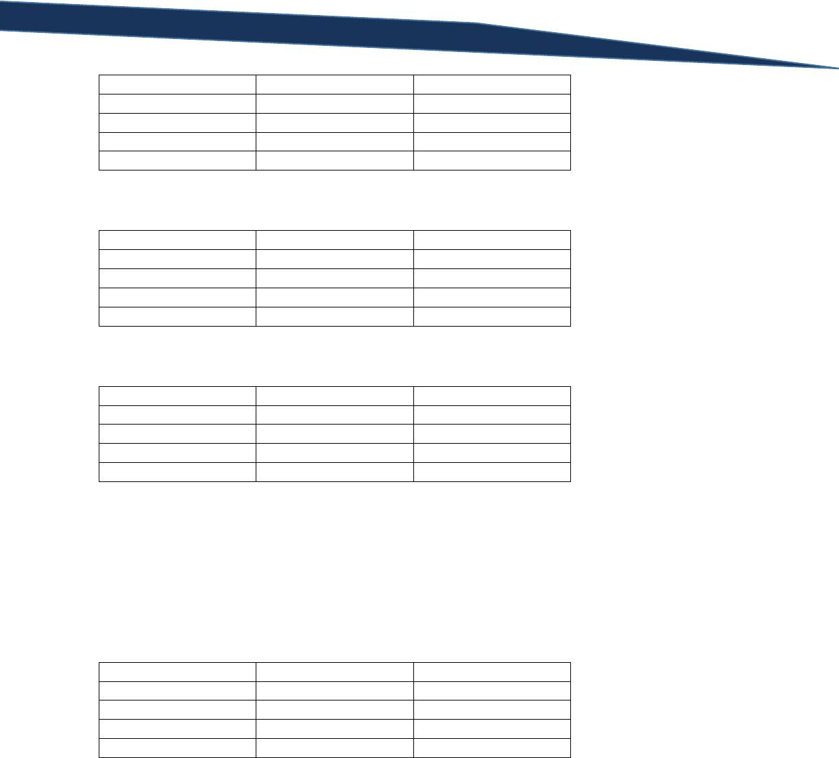
T-SQL Querying Guide © The Knowlton Group, LLC 132 | P a g e
A
B
A and B
T
T
T
T
F
F
F
T
F
F
F
F
Question 2:
A
B
A or B
T
T
T
T
F
T
F
T
T
F
F
F
Question 3:
A or B
C
(A or B) and C
T
T
T
T
F
F
F
T
F
F
F
F
Question 4:
Yes, that is a possibility. The query is evaluated as:
SELECT COUNT(*)
FROM HumanResources.vEmployee
WHERE FirstName < 'K' OR (PhoneNumberType = 'Cell' AND EmailPromotion = 1)
If we were to create a truth table for this query it would look like the following:
A
B and C
A or (B and C)
T
T
T
T
F
F
F
T
F
F
F
F
So, the only time a false row would exist for (B and C) – which represents a scenario like
PhoneNumberType equals “Work” and EmailPromotion equals “0” – is if A was true – in this case, if the
FirstName is less than “K”. If you look at the instances where the EmailPromotion is 0 and the
PhoneNumberType is “Work”, you will find that each FirstName value begins with a letter less than “K”.
This is why that possibility exists in the results as the query is written.
Question 5:
This would not be possible. If you look at the truth table in the solution explanation for question 4, the
only time that a row would exist where the statement (B and C) is false would be if the FirstName

T-SQL Querying Guide © The Knowlton Group, LLC 133 | P a g e
column began with a letter less than “K”. Since the PhoneNumberType being something other than
“Cell” would make the conjunction – (B and C) – false, then the FirstName column must begin with a
letter less than “K” or the row would not be returned in the results.
Lab 5: Using the WHERE Clause Part 2
Question 1:
SELECT *
FROM Sales.vIndividualCustomer
WHERE CountryRegionName = 'Australia' OR
(PhoneNumberType = 'Cell' AND EmailPromotion = 0)
Question 2:
SELECT *
FROM HumanResources.vEmployeeDepartment
WHERE Department IN ('Executive', 'Tool Design', 'Engineering')
SELECT *
FROM HumanResources.vEmployeeDepartment
WHERE Department = 'Executive' OR Department = 'Tool Design'
OR Department = 'Engineering'
Question 3:
SELECT *
FROM HumanResources.vEmployeeDepartment
WHERE StartDate BETWEEN '7/1/2000' AND '6/30/2002'
SELECT *
FROM HumanResources.vEmployeeDepartment
WHERE StartDate >= '7/1/2000' AND StartDate <= '6/30/2002'
Question 4:
SELECT *
FROM Sales.vIndividualCustomer
WHERE LastName LIKE 'R%'
Question 5:
SELECT *
FROM Sales.vIndividualCustomer
WHERE LastName LIKE '%r'
Question 6:
SELECT *
FROM Sales.vIndividualCustomer
WHERE LastName IN ('Lopez', 'Martin', 'Wood') AND
FirstName LIKE '[C-L]%'
Question 7:
SELECT *
FROM Sales.SalesOrderHeader
WHERE SalesPersonID IS NOT NULL

T-SQL Querying Guide © The Knowlton Group, LLC 134 | P a g e
Question 8:
SELECT
SalesPersonID,
TotalDue
FROM Sales.SalesOrderHeader
WHERE SalesPersonID IS NOT NULL
AND TotalDue > 70000
Lab 6: Sorting Using the ORDER BY Clause
Question 1:
SELECT
FirstName,
LastName,
JobTitle
FROM HumanResources.vEmployeeDepartment
ORDER BY FirstName ASC
Question 2:
SELECT
FirstName,
LastName,
JobTitle
FROM HumanResources.vEmployeeDepartment
ORDER BY FirstName, LastName DESC
Question 3:
SELECT
FirstName,
LastName,
CountryRegionName
FROM Sales.vIndividualCustomer
ORDER BY 3
Question 4:
SELECT
FirstName,
LastName,
CountryRegionName
FROM Sales.vIndividualCustomer
WHERE CountryRegionName IN ('United States', 'France')
ORDER BY CountryRegionName
Question 5:
SELECT
Name,
AnnualSales,
YearOpened,
SquareFeet AS [Store Size],
NumberEmployees AS [Total Employees]
FROM Sales.vStoreWithDemographics

T-SQL Querying Guide © The Knowlton Group, LLC 135 | P a g e
WHERE AnnualSales > 1000000
AND NumberEmployees >= 45
ORDER BY [Store Size] DESC, [Total Employees] DESC
Lab 7: INNER JOIN Practice
Question 1:
SELECT
P.FirstName,
P.LastName,
PP.PasswordHash
FROM Person.Person P
INNER JOIN Person.[Password] PP
ON PP.BusinessEntityID = P.BusinessEntityID
Question 2:
SELECT
E.BusinessEntityID,
E.NationalIDNumber,
E.JobTitle,
EDH.DepartmentID,
EDH.StartDate,
EDH.EndDate
FROM HumanResources.Employee E
INNER JOIN HumanResources.EmployeeDepartmentHistory EDH
ON E.BusinessEntityID = EDH.BusinessEntityID
Since the HumanResources.Employee table has 290 rows, you might expect the INNER JOIN of that table
with HumanResources.EmployeeDepartmentHistory would have no more than 290 rows. However,
there are multiple instances of a few BusinessEntityID values in
HumanResources.EmployeeDepartmentHistory. Instead of matching a single row from
HumanResources.Employee to a single row in HumanResources.EmployeeDepartmentHistory, a row in
HumanResources.Employee is matching to potentially two rows. This means that multiple rows are
returned for the duplicate BusinessEntityID values. The lowest level of detail of uniqueness is often
referred to as the grain of a table. Making sure that your joins account for potential grain differences is
critical to produce proper queries.
Question 3:
SELECT
P.FirstName,
P.LastName,
PP.PasswordHash,
E.EmailAddress
FROM Person.Person P
INNER JOIN Person.[Password] PP
ON PP.BusinessEntityID = P.BusinessEntityID
INNER JOIN Person.EmailAddress E
ON E.BusinessEntityID = P.BusinessEntityID
Question 4:
SELECT

T-SQL Querying Guide © The Knowlton Group, LLC 136 | P a g e
B.Title,
B.ISBN,
A.AuthorName
FROM BookAuthor BA
INNER JOIN Book B
ON B.BookID = BA.BookID
INNER JOIN Author A
ON A.AuthorID = BA.AuthorID
Question 5:
SELECT
B.Title,
B.ISBN,
A.AuthorName,
P.PublisherName
FROM BookAuthor BA
INNER JOIN Book B
ON B.BookID = BA.BookID
INNER JOIN Author A
ON A.AuthorID = BA.AuthorID
INNER JOIN Publisher P
ON P.PublisherID = B.PublisherID
Lab 8: LEFT OUTER JOINs and RIGHT OUTER JOINs
Question 1:
SELECT
SP.BusinessEntityID,
SP.SalesYTD,
ST.Name AS [Territory Name]
FROM Sales.SalesPerson SP
LEFT OUTER JOIN Sales.SalesTerritory ST
ON ST.TerritoryID = SP.TerritoryID
Question 2:
SELECT
P.FirstName,
P.LastName,
SP.BusinessEntityID,
SP.SalesYTD,
ST.Name AS [Territory Name]
FROM Sales.SalesPerson SP
LEFT OUTER JOIN Sales.SalesTerritory ST
ON ST.TerritoryID = SP.TerritoryID
INNER JOIN Person.Person P
ON P.BusinessEntityID = SP.BusinessEntityID
WHERE ST.Name IN ('Northeast', 'Central')
Question 3:
SELECT
P.Name,
P.ListPrice,
SC.Name AS ProductSubcategoryName,
C.Name AS ProductCategoryName

T-SQL Querying Guide © The Knowlton Group, LLC 137 | P a g e
FROM Production.Product P
LEFT OUTER JOIN Production.ProductSubcategory SC
ON SC.ProductSubcategoryID = P.ProductSubcategoryID
LEFT OUTER JOIN Production.ProductCategory C
ON C.ProductCategoryID = SC.ProductCategoryID
ORDER BY ProductCategoryName DESC, ProductSubcategoryName ASC
Lab 9: Aggregate Functions
Question 1:
SELECT COUNT(*)
FROM Person.Person
Question 2:
SELECT COUNT(MiddleName)
FROM Person.Person
Question 3:
SELECT AVG(StandardCost)
FROM Production.Product
WHERE StandardCost > 0
Question 4:
SELECT AVG(Freight)
FROM Sales.SalesOrderHeader
WHERE TerritoryID = 4
Question 5:
SELECT MAX(ListPrice)
FROM Production.Product
Question 6:
SELECT SUM(P.ListPrice*I.Quantity)
FROM Production.Product P
INNER JOIN Production.ProductInventory I
ON I.ProductID = P.ProductID
WHERE P.ListPrice > 0
Lab 10: Grouping with the GROUP BY Clause
Question 1:
SELECT
PersonType,
COUNT(*) AS PersonCount
FROM Person.Person
GROUP BY PersonType
Question 2:
SELECT
Color,

T-SQL Querying Guide © The Knowlton Group, LLC 138 | P a g e
COUNT(*) AS ProductCount
FROM Production.Product
WHERE Color IN ('Red', 'Black')
GROUP BY Color
Question 3:
SELECT
TerritoryID,
COUNT(*) AS SalesCount
FROM Sales.SalesOrderHeader
WHERE OrderDate BETWEEN '7/1/2005' AND '12/31/2006'
GROUP BY TerritoryID
Question 4:
SELECT
ST.Name AS TerritoryName,
COUNT(*) AS SalesCount
FROM Sales.SalesOrderHeader SOH
LEFT OUTER JOIN Sales.SalesTerritory ST
ON ST.TerritoryID = SOH.TerritoryID
WHERE OrderDate BETWEEN '7/1/2005' AND '12/31/2006'
GROUP BY ST.Name
Question 5:
SELECT
A.AuthorName,
COUNT(*) AS BookCount
FROM BookAuthor BA
INNER JOIN Author A
ON A.AuthorID = BA.AuthorID
GROUP BY A.AuthorName
Lab 11: Filtering Groups with the GROUP BY Clause
Question 1:
SELECT
TerritoryID,
SUM(TotalDue) AS TotalSales
FROM Sales.SalesOrderHeader
GROUP BY TerritoryID
HAVING SUM(TotalDue) > 10000000
Question 2:
SELECT
ST.Name AS TerritoryName,
SUM(TotalDue) AS TotalSales
FROM Sales.SalesOrderHeader SOH
LEFT OUTER JOIN Sales.SalesTerritory ST
ON ST.TerritoryID = SOH.TerritoryID
GROUP BY ST.Name
HAVING SUM(TotalDue) > 10000000
Question 3:

T-SQL Querying Guide © The Knowlton Group, LLC 139 | P a g e
SELECT
Color,
COUNT(*) AS ProductCount
FROM Production.Product
WHERE Color IS NOT NULL
GROUP BY Color
HAVING COUNT(*) >= 20
Question 4:
SELECT
P.Name AS [Product Name],
SUM(SOD.OrderQty) AS ProductOrderCount
FROM Sales.SalesOrderHeader SOH
INNER JOIN Sales.SalesOrderDetail SOD
ON SOD.SalesOrderID = SOH.SalesOrderID
INNER JOIN Production.Product P
ON P.ProductID = SOD.ProductID
WHERE SOH.OrderDate BETWEEN '1/1/2006' AND '12/31/2006'
GROUP BY P.Name
HAVING SUM(SOD.OrderQty) >= 200
Question 5:
SELECT
P.FirstName,
P.LastName,
COUNT(*) AS OrdersPlaced
FROM Sales.SalesOrderHeader SOH
INNER JOIN Sales.Customer C
ON C.CustomerID = SOH.CustomerID
INNER JOIN Person.Person P
ON P.BusinessEntityID = C.PersonID
WHERE OrderDate BETWEEN '7/1/2005' AND '12/31/2006'
GROUP BY P.FirstName, P.LastName
HAVING COUNT(*) >= 6
ORDER BY OrdersPlaced DESC
Lab 12: String Functions and Nested Functions
Question 1:
SELECT LEFT('This is a basic string', 8)
Question 2:
SELECT RIGHT('This is another string', 6)
Question 3:
SELECT CHARINDEX('e', Name)
FROM Production.Product
Question 4:
SELECT SUBSTRING(Name, 3, 4)
FROM Sales.SalesTerritory
Question 5:

T-SQL Querying Guide © The Knowlton Group, LLC 140 | P a g e
SELECT LEFT(RIGHT('This is a slightly longer string', 8), 4)
Question 6:
SELECT
LEFT(FirstName, CHARINDEX('e', FirstName, 0))
FROM Person.Person
WHERE LEFT(FirstName, CHARINDEX('e', FirstName, 0)) <> ''
Lab 13: Date and Time Built-In Functions
Question 1:
SELECT DATEPART(MONTH, '6/12/2011')
SELECT MONTH('6/12/2011')
Question 2:
SELECT DATEPART(YEAR, '11/20/1992')
SELECT YEAR('11/20/1992')
Question 3:
SELECT DATEADD(DAY, -74, GETDATE())
Question 4:
SELECT GETDATE()
SELECT GETUTCDATE()
SELECT SYSDATETIME()
Question 5:
SELECT DATEDIFF(DAY, '4/17/1996', '9/4/2001')
Question 6:
SELECT DATEDIFF(MONTH, '12/25/1993', DATEADD(DAY, -2719, GETDATE()))
Lab 14: NULL Handling Functions
Question 1:
SELECT
COALESCE(Title, 'No Title Listed') AS Title
FROM Person.Person
Question 2:
SELECT
COALESCE(MiddleName, 'No Middle Name Listed') AS MiddleName
FROM Person.Person

T-SQL Querying Guide © The Knowlton Group, LLC 141 | P a g e
Question 3:
SELECT
COALESCE(FirstName + ' ' + MiddleName + ' ' + LastName,
FirstName + ' ' + LastName) AS FullName
FROM Person.Person
Question 4:
SELECT NULLIF(MakeFlag, FinishedGoodsFlag)
FROM Production.Product
Lab 15: SQL Server Data Types & Type Casting
Question 1:
SELECT
CAST(FirstName AS VARCHAR)
FROM Person.Person
Question 2:
SELECT
11/4,
CAST(11 AS FLOAT)/CAST(4 AS FLOAT),
11.0/4.0
Question 3:
SELECT
CAST(FirstName AS VARCHAR(3))
FROM Person.Person
Question 4:
SELECT
CAST(Size AS INT)
FROM Production.Product
An error is returned stating “conversion failed when converting the nvarchar value ‘M’ to data type int.”.
This is because there are some values of the Size column that contain sizes like “S”, “M”, “L”, etc. These
values are not numeric and cannot be converted to an integer as there is certainly no integer equivalent
for the value of the letter “S” or “M”.
Question 5:
SELECT
CAST(Size AS INT)
FROM Production.Product
WHERE ISNUMERIC(Size) = 1
With the addition of the WHERE clause and the appropriate filtering condition, we do not receive an
error this time. The ISNUMERIC() function looks at a value and outputs a 1 if the value is numeric and a
0 if the value is not numeric. By specifying that we only want to evaluate numeric values, we bypass the
error where we cannot convert non-numeric value to an integer. Since the WHERE clause is evaluated

T-SQL Querying Guide © The Knowlton Group, LLC 142 | P a g e
before the SELECT clause by the database, the CAST() function will not evaluate any values like “S”, “M”,
or “L” which caused the errors in the previous question.
Lab 16: Using Derived Tables
Question 1:
The query will not execute because a required condition of a table expression is that each column must
have a name specified. The “YEAR(HireDate)” column does not have an alias specified, therefore the
table expression cannot be evaluated and the query will fail.
Question 2:
This query will execute without an issue. ORDER BY clauses are not allowed in table expressions unless
the TOP operator is used within the expression. Since the TOP operator is included in this table
expression the ORDER BY clause is allowed.
Question 3:
SELECT *
FROM (
SELECT *, YEAR(HireDate) AS HireYear, YEAR(BirthDate) AS BirthYear
FROM HumanResources.Employee
) AS Emp
WHERE HireYear >= 2006 AND BirthYear <= 1968
Question 4:
SELECT
OrderYear,
SUM(TotalDue) AS TotalSales
FROM (
SELECT *, YEAR(OrderDate) AS OrderYear
FROM Sales.SalesOrderHeader
) AS SalesOrders
WHERE OrderYear IN (2005, 2006)
GROUP BY OrderYear
Lab 17: Common Table Expressions
Question 1:
This query will fail at runtime because the first column of the CTE does not contain a name. Since every
column in a table expression must have a name specified, the lack of a column alias will cause the query
to return an error.
Question 2:
WITH Hires
AS (
SELECT
YEAR(HireDate) AS HireYear,
BusinessEntityID

T-SQL Querying Guide © The Knowlton Group, LLC 143 | P a g e
FROM HumanResources.Employee
), HireByYear AS (
SELECT
HireYear,
COUNT(*) AS HireCount
FROM Hires
GROUP BY HireYear
)
SELECT
H1.HireYear,
H1.HireCount AS CurrentYearHireCount,
H2.HireCount AS PriorYearHireCount
FROM HireByYear H1
LEFT OUTER JOIN HireByYear H2
ON H1.HireYear = H2.HireYear + 1
Question 3:
WITH Products
AS (
SELECT
YEAR(SellStartDate) AS ProductSellStartYear,
ProductID
FROM Production.Product
)
SELECT
ProductSellStartYear,
COUNT(*) AS ProductCount
FROM Products
GROUP BY ProductSellStartYear
Question 4:
WITH SalesMonth
AS (
SELECT
MONTH(OrderDate) AS OrderMonth,
TotalDue
FROM Sales.SalesOrderHeader
WHERE YEAR(OrderDate) = 2006
)
SELECT
OrderMonth,
SUM(TotalDue) AS MonthlySales
FROM SalesMonth
GROUP BY OrderMonth
ORDER BY 1
Lab 18: CASE Statements

T-SQL Querying Guide © The Knowlton Group, LLC 144 | P a g e
Question 1:
SELECT
FirstName,
LastName,
CASE
WHEN EmailPromotion = 0 THEN 'Promotion 1'
WHEN EmailPromotion = 1 THEN 'Promotion 2'
WHEN EmailPromotion = 2 THEN 'Promotion 3'
END AS PromotionName
FROM Person.Person
Question 2:
If a value does not meet any of the conditions in a CASE statement, the output to be returned will be a
NULL value.
Question 3:
SELECT
CASE
WHEN LEN(FirstName) >= 10 THEN 'Long Name'
ELSE 'Short Name'
END
FROM Person.Person
Question 4:
WITH SalesRanges
AS (
SELECT
CASE
WHEN TotalDue BETWEEN 0 AND 149.99
THEN '$0 to $149.99'
WHEN TotalDue BETWEEN 150 AND 499.99
THEN '$150 to $499.99'
WHEN TotalDue BETWEEN 500 AND 4999.99
THEN '$500 to $4,999.99'
WHEN TotalDue BETWEEN 5000 AND 24999.99
THEN '$5,000 to $24,999.99'
ELSE 'Over $25,000'
END AS SalesPriceRange,
SalesOrderID
FROM Sales.SalesOrderHeader
)
SELECT
SalesPriceRange,
COUNT(*)
FROM SalesRanges
GROUP BY SalesPriceRange
Question 5:
SELECT
CASE
WHEN Color IS NULL THEN 'No Color'

T-SQL Querying Guide © The Knowlton Group, LLC 145 | P a g e
ELSE Color
END AS Color
FROM Production.Product
SELECT
COALESCE(Color, 'No Color')
FROM Production.Product
Lab 19: Ranking Functions
Question 1:
WITH SalesDetails
AS (
SELECT
CustomerID,
SUM(TotalDue) AS TotalSales
FROM Sales.SalesOrderHeader
WHERE YEAR(OrderDate) = 2005
GROUP BY CustomerID
)
SELECT
CustomerID,
ROW_NUMBER() OVER(ORDER BY TotalSales DESC) AS CustomerSalesRank,
TotalSales
FROM SalesDetails
Question 2:
SELECT
P.ProductID,
OrderQuantity,
RANK() OVER(ORDER BY OrderQuantity DESC)
FROM Production.Product P
LEFT OUTER JOIN (
SELECT SOD.ProductID, SUM(SOD.OrderQty) AS OrderQuantity
FROM Sales.SalesOrderHeader SOH
INNER JOIN Sales.SalesOrderDetail SOD
ON SOH.SalesOrderID = SOD.SalesOrderID
WHERE YEAR(OrderDate) = 2006
GROUP BY ProductID
) SP
ON SP.ProductID = P.ProductID
Question 3:
SELECT
P.ProductID,
OrderQuantity,
DENSE_RANK() OVER(ORDER BY OrderQuantity DESC)
FROM Production.Product P
LEFT OUTER JOIN (
SELECT SOD.ProductID, SUM(SOD.OrderQty) AS OrderQuantity
FROM Sales.SalesOrderHeader SOH
INNER JOIN Sales.SalesOrderDetail SOD
ON SOH.SalesOrderID = SOD.SalesOrderID
WHERE YEAR(OrderDate) = 2006

T-SQL Querying Guide © The Knowlton Group, LLC 146 | P a g e
GROUP BY ProductID
) SP
ON SP.ProductID = P.ProductID
Question 4:
SELECT
TerritoryID,
NTILE(2) OVER(ORDER BY SUM(TotalDue) DESC) AS TerritoryTier
FROM Sales.SalesOrderHeader
WHERE YEAR(OrderDate) = 2006
GROUP BY TerritoryID
Question 5:
WITH TerritoryRank
AS (
SELECT
TerritoryID,
NTILE(2) OVER(ORDER BY SUM(TotalDue) DESC) AS TerritoryTier
FROM Sales.SalesOrderHeader
WHERE YEAR(OrderDate) = 2006
GROUP BY TerritoryID
)
SELECT
TerritoryID,
CASE
WHEN TerritoryTier = 1 THEN 'Top Territory Group'
ELSE 'Bottom Territory Group'
END AS TerritoryTier
FROM TerritoryRank
Lab 20: Set Operations
Question 1:
SELECT ProductID, Name
FROM Production.Product
WHERE ProductID < 325
UNION
SELECT ProductID, Name
FROM Production.Product
WHERE ProductID >= 325
Question 2:
SELECT ProductID, Name
FROM Production.Product
WHERE ProductID < 425
UNION
SELECT ProductID, Name
FROM Production.Product
WHERE ProductID >= 325

T-SQL Querying Guide © The Knowlton Group, LLC 147 | P a g e
Question 3:
SELECT ProductID, Name
FROM Production.Product
WHERE ProductID < 425
UNION ALL
SELECT ProductID, Name
FROM Production.Product
WHERE ProductID >= 325
The results for question 3 contain more rows than the results in question 2 due to the ALL operator
added to the UNION set operation. This is because the UNION ALL operation no longer returns a distinct
list of values. Since there is overlap between the two queries, any product with a ProductID value
between 325 and 424 (inclusive) contains two rows in the results.
Question 4:
SELECT ProductID, Name
FROM Production.Product
WHERE ProductID < 425
INTERSECT
SELECT ProductID, Name
FROM Production.Product
WHERE ProductID >= 325
Question 5:
SELECT ProductID, Name
FROM Production.Product
WHERE ProductID < 425
EXCEPT
SELECT ProductID, Name
FROM Production.Product
WHERE ProductID >= 325
Based on the order in which the queries appear, the EXCEPT operator finds all rows with a ProductID
less than 425 and then returns only those rows that do not appear in the list of all rows with a ProductID
greater than or equal to 325. The 13 rows of the result set clearly indicate this; the ProductID’s returned
are all between 1 and 324.
Question 6:
SELECT ProductID, Name
FROM Production.Product
WHERE ProductID >= 325
EXCEPT
SELECT ProductID, Name

T-SQL Querying Guide © The Knowlton Group, LLC 148 | P a g e
FROM Production.Product
WHERE ProductID < 425
With the order of the two queries switched, the result is dramatically different. The query is now finding
all products with a ProductID greater than or equal to 325 and then only returning those products where
the ProductID is NOT less than 425. This yields a list of all products with a ProductID greater than or
equal to 425.
Lab 21: Inline Subquery Practice
Question 1:
SELECT *
FROM Sales.SalesOrderDetail
WHERE ProductID IN (
SELECT ProductID
FROM Production.Product
WHERE Color = 'Black'
)
Question 2:
SELECT *
FROM HumanResources.Employee
WHERE BusinessEntityID IN (
SELECT E.BusinessEntityID
FROM HumanResources.Employee E
INNER JOIN Person.BusinessEntityAddress BEA
ON BEA.BusinessEntityID = E.BusinessEntityID
INNER JOIN Person.[Address] A
ON A.AddressID = BEA.AddressID
INNER JOIN Person.StateProvince SP
ON SP.StateProvinceID = A.StateProvinceID
WHERE SP.Name = 'California'
)
Question 3:
SELECT *
FROM Sales.SalesOrderHeader
WHERE TotalDue < (
SELECT AVG(TotalDue)
FROM Sales.SalesOrderHeader
)
AND YEAR(OrderDate) = 2006
Question 4:
SELECT *
FROM Production.Product
WHERE ProductSubcategoryID IN (
SELECT ProductSubcategoryID
FROM Production.ProductSubcategory
WHERE Name LIKE '%Bikes'
)

T-SQL Querying Guide © The Knowlton Group, LLC 149 | P a g e
Question 5:
SELECT *
FROM Sales.SalesOrderHeader
WHERE OrderDate = (
SELECT MAX(OrderDate)
FROM Sales.SalesOrderHeader
)
AND TotalDue < (
SELECT AVG(TotalDue)
FROM Sales.SalesOrderHeader
)
Lab 22: Using Correlated Subqueries
Question 1:
SELECT
SalesPersonID, SalesOrderNumber, TotalDue
FROM Sales.SalesOrderHeader S1
WHERE TotalDue = (
SELECT MAX(TotalDue)
FROM Sales.SalesOrderHeader S2
WHERE S1.SalesPersonID = S2.SalesPersonID
)
Question 2:
SELECT
BusinessEntityID,
Bonus
FROM Sales.SalesPerson S1
WHERE 0 = (
SELECT Bonus
FROM Sales.SalesPerson S2
WHERE S1.BusinessEntityID = S2.BusinessEntityID
)
Question 3:
SELECT *
FROM Production.Product P1
WHERE 539.99 = (
SELECT ListPrice
FROM Production.Product P2
WHERE P1.ProductID = P2.ProductID
)
Lab 23: Advanced Aggregations and Pivoting
Question 1:
SELECT
DATEADD(MONTH, DATEDIFF(MONTH, 0, GETDATE()), 0) AS FirstOfCurrentMonth,
DATEADD(MONTH, DATEDIFF(MONTH, 0, GETDATE())-1, 0) AS FirstOfPriorMonth,

T-SQL Querying Guide © The Knowlton Group, LLC 150 | P a g e
DATEADD(DAY, -1, DATEADD(MONTH, DATEDIFF(MONTH, 0, GETDATE())+1, 0)) AS
LastDayOfCurrentMonth
Question 2:
WITH SalesDay
AS (
SELECT
SalesOrderID,
DATEDIFF(DAY, 0, OrderDate) AS OrderDay,
TotalDue
FROM Sales.SalesOrderHeader
),
SalesTotalByDay AS (
SELECT
OrderDay,
SUM(TotalDue) AS TotalSales
FROM SalesDay
GROUP BY OrderDay
)
SELECT
CAST(DATEADD(DAY, OrderDay, 0) AS DATE) AS OrderDate,
TotalSales
FROM SalesTotalByDay
WHERE TotalSales = (
SELECT MAX(TotalSales)
FROM SalesTotalByDay
)
Question 3:
WITH TopHalf
AS (
SELECT TOP 50 PERCENT Points
FROM NHL_Standings_2014
ORDER BY Points DESC
),
BottomHalf AS (
SELECT TOP 50 PERCENT Points
FROM NHL_Standings_2014
ORDER BY Points
)
SELECT
((SELECT CAST(MAX(Points) AS NUMERIC) FROM BottomHalf) +
(SELECT CAST(MIN(Points) AS NUMERIC) FROM TopHalf)) / 2
Question 4:
WITH Products
AS (
SELECT
DATEDIFF(MONTH, 0, OrderDate) AS OrderMonth,
SOD.OrderQty
FROM Sales.SalesOrderHeader SOH
INNER JOIN Sales.SalesOrderDetail SOD
ON SOD.SalesOrderID = SOH.SalesOrderID
), ProductsByMonth AS (

T-SQL Querying Guide © The Knowlton Group, LLC 151 | P a g e
SELECT
OrderMonth,
SUM(OrderQty) AS ProductsOrdered
FROM Products
GROUP BY OrderMonth
)
SELECT
CAST(DATEADD(MONTH, P1.OrderMonth, 0) AS DATE) AS OrderMonth,
P1.ProductsOrdered AS ProductsOrderedCurrentMonth,
SUM(P2.ProductsOrdered) AS ProductsOrderedToDate
FROM ProductsByMonth P1
LEFT OUTER JOIN ProductsByMonth P2
ON P2.OrderMonth <= P1.OrderMonth
GROUP BY CAST(DATEADD(MONTH, P1.OrderMonth, 0) AS DATE), P1.ProductsOrdered
ORDER BY 1
Question 5:
WITH Products
AS (
SELECT
DATEDIFF(MONTH, 0, OrderDate) AS OrderMonth,
SOD.OrderQty
FROM Sales.SalesOrderHeader SOH
INNER JOIN Sales.SalesOrderDetail SOD
ON SOD.SalesOrderID = SOH.SalesOrderID
), ProductsByMonth AS (
SELECT
OrderMonth,
SUM(OrderQty) AS ProductsOrdered
FROM Products
GROUP BY OrderMonth
)
SELECT
CAST(DATEADD(MONTH, P1.OrderMonth, 0) AS DATE) AS OrderMonth,
P1.ProductsOrdered AS ProductsOrderedCurrentMonth,
SUM(P2.ProductsOrdered) AS ProductsOrderedToDate
FROM ProductsByMonth P1
LEFT OUTER JOIN ProductsByMonth P2
ON P2.OrderMonth <= P1.OrderMonth
AND YEAR(DATEADD(MONTH, P1.OrderMonth, 0)) = YEAR(DATEADD(MONTH, P2.OrderMonth,
0))
GROUP BY CAST(DATEADD(MONTH, P1.OrderMonth, 0) AS DATE), P1.ProductsOrdered
ORDER BY 1
Lab 24: SQL Variables
Question 1:
DECLARE @StringExample VARCHAR(23) = 'This is a sample string'
SELECT @StringExample
Question 2:
DECLARE @IntegerA INT = 1,

T-SQL Querying Guide © The Knowlton Group, LLC 152 | P a g e
@IntegerB INT = 4
SELECT @IntegerA + @IntegerB
Question 3:
DECLARE @MaxOrderDate DATE = (SELECT MAX(OrderDate) FROM Sales.SalesOrderHeader)
SELECT *
FROM Sales.SalesOrderHeader
WHERE OrderDate = @MaxOrderDate
Question 4:
DECLARE @SmallestSalePrice MONEY = (SELECT MIN(TotalDue) FROM Sales.SalesOrderHeader)
SELECT *
FROM Sales.SalesOrderHeader
WHERE TotalDue = @SmallestSalePrice
Lab 25: WHILE Loops
Question 1:
DECLARE @Count INT = 1
WHILE @Count <= 5
BEGIN
SELECT 'This is a T-SQL Guide'
SET @Count += 1
END
Question 2:
CREATE TABLE #TempTable(
IntegerValue INT
)
GO
DECLARE @Count INT = 1
WHILE @Count <= 30
BEGIN
INSERT INTO #TempTable(IntegerValue)
SELECT RAND()*40+1
SET @Count += 1
END
SELECT *
FROM #TempTable
DROP TABLE #TempTable
Question 3:
CREATE TABLE #TempTable(
IntegerValue INT

T-SQL Querying Guide © The Knowlton Group, LLC 153 | P a g e
)
GO
DECLARE @Count INT = 1
WHILE @Count <= 10
BEGIN
INSERT INTO #TempTable(IntegerValue)
SELECT RAND()*10+1
SET @Count += 1
END
SELECT *
FROM #TempTable
DROP TABLE #TempTable
Question 4:
CREATE TABLE #WebTraffic(
UserID INT,
UserAccessCountID INT,
WebSiteName VARCHAR(50),
AccessDate DATETIME
)
GO
DECLARE @UserID INT = 1,
@UserAccessCountID INT = 1,
@WebSiteID INT = 1
WHILE @UserID <= 30
BEGIN
WHILE @UserAccessCountID <= RAND()*10+1
BEGIN
SET @WebSiteID = RAND()*3+1
INSERT INTO #WebTraffic
SELECT
@UserID,
@UserAccessCountID,
CASE
WHEN @WebSiteID = 1 THEN 'www.espn.com'
WHEN @WebSiteID = 2 THEN 'www.google.com'
ELSE 'www.yahoo.com'
END,
DATEADD(SECOND, RAND()*86400+1, '1/14/2015')
SET @UserAccessCountID += 1
END
SET @UserAccessCountID = 1
SET @UserID += 1
END
SELECT *
FROM #WebTraffic

T-SQL Querying Guide © The Knowlton Group, LLC 154 | P a g e
DROP TABLE #WebTraffic
